0 Alternative Transportation Fuel Standards: Welfare Effects and Climate Benefits Xiaoguang Chen Energy Biosciences Institute University of Illinois at Urbana Champaign 1206 West Gregory Dr Urbana, IL 61801 Email: [email protected] Haixiao Huang Energy Biosciences Institute University of Illinois at Urbana Champaign 1206 West Gregory Dr Urbana, IL 61801 Email: [email protected] Madhu Khanna Department of Agricultural and Consumer Economics University of Illinois at Urbana Champaign 326 Mumford Hall 1301 W. Gregory Dr Urbana, IL 61801 Email: [email protected] Address for Correspondence Madhu Khanna Department of Agricultural and Consumer Economics Energy Biosciences Institute University of Illinois, Urbana-Champaign 1301 W. Gregory Drive Urbana, IL 61801 Phone: 217-333-5176 Email: [email protected] ____________________________________________________________________ Authorship is alphabetical. Funding from the Energy Biosciences Institute, University of California, Berkeley, is gratefully acknowledged.

Welcome message from author
This document is posted to help you gain knowledge. Please leave a comment to let me know what you think about it! Share it to your friends and learn new things together.
Transcript

0
Alternative Transportation Fuel Standards: Welfare Effects and Climate Benefits
Xiaoguang Chen Energy Biosciences Institute
University of Illinois at Urbana Champaign 1206 West Gregory Dr
Urbana, IL 61801 Email: [email protected]
Haixiao Huang
Energy Biosciences Institute University of Illinois at Urbana Champaign
1206 West Gregory Dr Urbana, IL 61801
Email: [email protected]
Madhu Khanna Department of Agricultural and Consumer Economics
University of Illinois at Urbana Champaign 326 Mumford Hall
1301 W. Gregory Dr Urbana, IL 61801
Email: [email protected]
Address for Correspondence Madhu Khanna Department of Agricultural and Consumer Economics Energy Biosciences Institute University of Illinois, Urbana-Champaign 1301 W. Gregory Drive Urbana, IL 61801 Phone: 217-333-5176 Email: [email protected] ____________________________________________________________________
Authorship is alphabetical. Funding from the Energy Biosciences Institute, University of California, Berkeley, is gratefully acknowledged.
1
Alternative Transportation Fuel Standards: Welfare Effects and Climate Benefits
Abstract
This paper develops a conceptual framework and a numerical simulation model of the fuel and agricultural sectors in the US to analyze the effects of the existing Renewable Fuels Standard (RFS) that mandates the blending of specific volumes of low carbon biofuels with liquid fossil fuels and a proposed national Low Carbon Fuel Standard (LCFS) that imposes a limit on the GHG intensity of the blended fuel on fuel mix, GHG emissions and social welfare in an open economy and to compare them to those with a carbon price policy. The conceptual framework illustrates that, unlike a carbon price policy, the RFS and LCFS have an ambiguous effect on GHG emissions. The numerical analysis shows that all three policies reduce US GHG emissions and increase domestic social welfare (not including environmental benefits) relative to a no-policy, business-as usual scenario, with the RFS leading to a lower reduction in GHG emissions than the LCFS. However, the RFS leads to higher social welfare among the policies examined here than the LCFS and the carbon tax. Key words: biofuel mandate, low carbon fuel standard, greenhouse gas emissions, social welfare, cellulosic biofuels, dynamic optimization, sectoral model

2
The transportation sector in the US accounted for 29% of total US greenhouse gas (GHG)
emissions in 2006, second only to the electric power sector. These emissions from the
transportation sector have been growing steadily and accounted for almost half of the increase in
total US GHG emissions since 1990. The sector also relies heavily on imported fuel, with over
65% of fossil fuel consumed in the US being imported1. Concerns about GHG emissions and the
desire to promote energy independence have led to support for policy strategies targeted directly
at promoting renewable/low carbon fuels [11].
While renewable fuels for transportation are currently limited to first generation biofuels
produced primarily from corn, these policy strategies seek to incentivize a new generation of
advanced biofuels that have greater potential for reducing GHG emissions relative to corn
ethanol and can be produced from a variety of feedstocks. These feedstocks differ in their GHG
intensity, costs of production, yields per unit land and the type of land they can be grown on.
Advanced biofuels are yet to be produced commercially, but their costs of production are
anticipated to be significantly higher than those of corn ethanol and liquid fossil fuels. Policy
support is, therefore, considered critical to induce the production of these biofuels.
These policies include existing technology (biofuel) mandates and proposed
performance-based standards for transportation fuel. The former has taken the form of the
Renewable Fuel Standard (RFS) in the US established by the Energy Independence and Security
Act (EISA) of 2007, which sets volumetric (quantity-based) targets for the blending of specific
types of biofuels with fossil fuels based on their life-cycle GHG intensity2. Although the RFS is
implemented by the US Environmental Protection Agency (EPA) specifying an annual blend rate
that blenders need to meet, the blend rate is designed to achieve the legally established biofuel
quantities.3 A performance-based standard implemented in California and being considered by

3
several states and at the national level is a Low Carbon Fuel Standard (LCFS) that requires
blenders to meet an increasingly stringent target to reduce GHG intensity of transportation fuel.4
A carbon price policy could also be used to directly target GHG emissions reduction but may not
induce a switch to low carbon fuels to the same extent as the fuel standards above because unlike
them the reduction in GHG emissions could be met simply by reducing total fuel consumption.
These biofuel and climate policies affect GHG emissions through two ways, by using
quantity or price-based incentives to change the mix of various low and high carbon fuels and by
explicitly or implicitly affecting the cost of driving and thus the demand for vehicle kilometers
travelled (VKT). The implementation of both the LCFS and RFS requires determination of the
life-cycle GHG emissions of biofuels, but the two policies are likely to differ, from each other
and from a carbon price policy, in the incentives they create for consuming different types of
biofuels and in their effect on overall demand for transportation fuel and VKT. Rajagopal et al.
[33] show that a blend mandate and a LCFS are equivalent when they both achieve the same
share of biofuel in the fuel mix. In practice, however, with many different types of biofuels that
differ in their carbon intensity and costs of production, the two policies are not likely to achieve
the same blend of each type of biofuel, unless the LCFS becomes as prescriptive as the mandate,
defeating its objective of being a technology neutral standard.
The effect of these policies on total demand for transportation fuel (or VKT) will depend
on their effect on the prices of fossil fuels and biofuels for consumers. Biofuels will need to be
sold at the energy-equivalent prices of fossil fuels since the consumption of the large volumes of
biofuels required for compliance with the RFS or LCFS policies is feasible only if there is a
significant share of flex-fuel vehicles in the fleet structure and the two fuels are priced as energy
equivalent substitutes. However, these policies differ in their impact on the consumer price of

4
transportation fuels and in the extent to which they will generate a “rebound effect” on fossil fuel
consumption which could offset some of the reduction in consumption of liquid fossil fuels that
would have occurred otherwise. While both the RFS and LCFS reduce the demand for fossil fuel
through the displacement by biofuels (and implicitly subsidize biofuels) and thus the prices of
fossil fuels, the LCFS can additionally raise the price of fossil fuel and reduce the demand for
fossil fuel by implicitly taxing them [22].
Our purpose here is to analyze the mechanisms by which the RFS and LCFS affect GHG
emissions from the transportation sector and compare their social welfare implications with those
of a carbon tax policy. Economic theory suggests that the most cost effective way to reduce
GHG emissions in a closed economy is through a carbon tax because it induces the use of the
lowest costs strategies for GHG abatement. Technology mandates and GHG intensity standards
limit the flexibility of abatement options and can, therefore, be expected to result in higher costs
of abatement. However, in a large open economy such as the US, these policies are likely to
increase the world market prices of agricultural exports and lower world prices of fuel imports
Therefore, they can improve the terms-of-trade for the US by shifting a part of the costs of these
policies to trading partners (causing such policies to be referred to as "beggar-thy-neighbor"
policies) [3] and offset the efficiency costs of these policies relative to a no-policy (laissez-
faire) scenario.
We develop an integrated model of the fuel and food sectors to undertake a conceptual
analysis of the effects of these policies on fuel consumption and prices and GHG emissions. We
use this conceptual framework to identify some of the key parameters likely to influence the
impacts of these policies on fuel consumption and GHG emissions. We then develop a numerical
simulation model to quantify the effects of these policies. Specifically, we examine the impact of

5
these policies on the mix of fuels consumed, on food and fuel prices and their benefits in
improving energy security by reducing fuel imports and mitigating GHG emissions from the fuel
and agricultural sectors. The numerical simulation is conducted using the dynamic, multi-market
equilibrium, nonlinear mathematical programming model, Biofuel and Environmental Policy
Analysis Model (BEPAM). The model simulates the transportation and agricultural sectors in the
US and endogenously determines the effects of the LCFS and the RFS and a carbon tax on land
allocation, fuel mix, prices in markets for fuel, biofuel, food/feed crops and livestock and on
GHG emissions in the US at annual time scales over the period 2007-2030. Additionally, we
examine the distributional effects of these policies on domestic consumers and producers in the
transportation and agricultural sectors and compare these to a business-as usual scenario to
determine the welfare costs of these policies (not considering environmental benefits). As
alternative fuels we consider first generation biofuels produced domestically from corn and
soybeans and imported sugarcane ethanol. We also consider various second generation biofuels
from cellulosic feedstocks including crop and forest residues and dedicated energy crops, namely
perennial grasses, such as switchgrass and miscanthus. Sensitivity analysis is conducted to assess
the robustness of our findings to various assumptions about parameters governing the
responsiveness of consumers and producers in these sectors to policy induced price changes.
The rest of the paper is organized as follows. Section II reviews the existing literature
examining the implications of these policies. Section III presents the conceptual framework
underlying our analysis. Section IV describes the numerical model, BEPAM, followed by a
description of the data in Section V. The results of our analysis are presented in Section VI
followed by the conclusions in Section VII.

6
II. Previous Literature
A few studies have developed stylized models to analyze the economic effects of a blend
mandate [10], biofuel quantity mandate [1] and a LCFS [22]. While these studies differ in their
assumptions about the substitutability between gasoline and biofuels in the production of VKT,
they all assume that the consumer is constrained to buy a blended fuel. These papers, therefore,
assume that the consumer price of transportation fuels will be a weighted average of the gasoline
and biofuel prices and higher than that in the absence of the biofuel policies (unless the reduction
in the price of gasoline due to the displacement by biofuels is large enough to offset the increase
in the price of biofuels). Ando et al. [1] and Holland et al. [22] show that the mandate and the
LCFS have an ambiguous effect on GHG emissions, respectively. The above studies analyze
policy effects in a closed economy and show that a biofuel mandate and an LCFS are less
efficient than a carbon tax policy which internalizes GHG externalities by pricing gasoline and
biofuels based on their marginal social cost [1,23].
Unlike the previous studies, Moschini et al. [31] compare the fuel price and welfare
implications of a biofuel quantity mandate and a biofuel subsidy designed to achieve the same
level of biofuel consumption in an open economy. By assuming that the consumer is forced to
buy a blended fuel, they show that a biofuel mandate operates like a tax on gasoline and a
subsidy on biofuel. The mandate lowers gasoline consumption and price more than a biofuel
subsidy alone, leading to improved terms of trade and higher social welfare than the subsidy.
There are several large-scale numerical models that have examined the effects of biofuel
policies, specifically biofuel mandates, on land use and crop prices. Hertel et al. [20] and
Searchinger et al. [34] use the Global Trade Analysis Project (GTAP) and Food and Agricultural
Policy Research Institute (FAPRI) models, respectively, to examine the direct and indirect land

7
use changes due to the mandate for corn ethanol. They estimate the GHG emissions due to the
land use change only and do not examine the aggregate GHG emissions from fuel, biofuel and
other production activities impacted by biofuel production. Beach and McCarl [2] use the Forest
and Agricultural Sector Optimization Model (FASOM) while Chen et al. [6] apply an earlier
version of the BEPAM to analyze the implications of the RFS including the advanced biofuels
mandate for land use, crop prices and GHG emissions. These large-scale numerical models have
focused on biofuel mandates for first generation biofuels with the exception of Beach and
McCarl [2] and Chen et al. [6] who consider a mix of first and second generation biofuel
feedstocks to meet all categories of the RFS. While Hertel et al. [20] and Chen et al. [6] include
demands for agricultural goods, fossil fuels and biofuels, Searchinger et al. [34] and Beach and
McCarl [2] consider the agricultural sector only and focus on the supply-side of biofuel
production. Hertel et al. [21] and Chen et al. [6] examine the welfare costs of biofuel policies.
The former study shows that the terms of trade effects of biofuel mandates in the US and EU
partially offsets a portion of the allocative efficiency costs of these policies. Chen et al. [6] show
that the RFS increases social welfare and reduces GHG emissions in the US relative to a no
policy baseline; when combined with biofuel tax credits, GHG mitigation increases but at high
welfare costs relative to the RFS alone.
Our paper makes several contributions to the existing literature. Our conceptual
framework presents an integrated model of the food and fuel sectors with the demand for fuels
being derived from the demand for VKT. It also incorporates the effects of limited land
availability and the demand for food on the costs of producing biofuels and on the extent to
which these biofuel and climate policies will create incentives for increasing biofuel
consumption and reducing gasoline consumption. It differs from existing studies in that it not

8
only assumes that gasoline and biofuels are perfect substitutes (given their energy content) in the
production of VKT but also in the consumption decision by consumers (assuming the availability
of flex-fuel vehicles).
Our numerical analysis using BEPAM broadens the stylized model by linking the
multiple markets in the agricultural and fuel sectors and endogenously determines the policy
induced supply of different types of biofuels and mixes of feedstocks. It extends the model
structure of BEPAM described in Chen et al.[6] by explicitly modeling the substitutability
between fossil fuels and biofuels based on the projected vehicle fleet structure (as indicated by
estimates from the Energy Information Administration [12]) and by incorporating domestic and
global markets for fossil fuels. We consider several types of first and second generation biofuels
including ligno-cellulosic ethanol and biomass-to-liquids diesel that can be blended with
gasoline and diesel, respectively. These biofuels can be produced from a variety of feedstocks,
whose production levels are endogenously determined given policy, technology and land
availability constraints. Moreover, by including both the agricultural and transportation sectors
and a full-fledged lifecycle GHG accounting for all crops, biofuel feedstocks and fuels, we
examine the implications of alternative policies for GHG emissions from crop production and
fuel consumption in both sectors.
III. Conceptual Framework
We now present a simple conceptual framework to analyze the effects of the three
policies considered here on fuel consumption, food prices, and GHG emissions. This framework
considers an economy with a representative consumer who demands food (f) and vehicle
kilometers travelled (m). The latter are produced by blending gasoline (g) 5 and biofuels (e),
which are perfect substitutes in the production of VKT. The production of VKT can be expressed
9
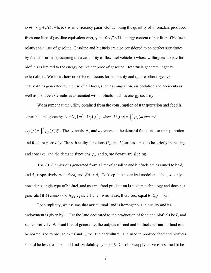
as ( )m r g e , where r is an efficiency parameter denoting the quantity of kilometers produced
from one liter of gasoline equivalent energy and 0 1 is energy content of per liter of biofuels
relative to a liter of gasoline. Gasoline and biofuels are also considered to be perfect substitutes
by fuel consumers (assuming the availability of flex-fuel vehicles) whose willingness to pay for
biofuels is limited to the energy equivalent price of gasoline. Both fuels generate negative
externalities. We focus here on GHG emissions for simplicity and ignore other negative
externalities generated by the use of all fuels, such as congestion, air pollution and accidents as
well as positive externalities associated with biofuels, such as energy security.
We assume that the utility obtained from the consumption of transportation and food is
separable and given by m fU U m U f , where 0
( ) ( )m
m mU m p m dm and
0( ) ( )
f
f fU f p f df . The symbols and m fp p represent the demand functions for transportation
and food, respectively. The sub-utility functions and m fU U are assumed to be strictly increasing
and concave, and the demand functions and m fp p are downward sloping.
The GHG emissions generated from a liter of gasoline and biofuels are assumed to be δg
and δe, respectively, with δg>δe and g e . To keep the theoretical model tractable, we only
consider a single type of biofuel, and assume food production is a clean technology and does not
generate GHG emissions. Aggregate GHG emissions are, therefore, equal to δgg + δee.
For simplicity, we assume that agricultural land is homogenous in quality and its
endowment is given by L . Let the land dedicated to the production of food and biofuels be Lf and
Le, respectively. Without loss of generality, the outputs of food and biofuels per unit of land can
be normalized to one, so Lf = f and Le =e. The agricultural land used to produce food and biofuels
should be less than the total land availability, f e L . Gasoline supply curve is assumed to be
10
upward sloping and convex, denoted by c(g). Processing costs of food and biofuels are assumed
to be constant, represented by cf and ce, respectively. However, the marginal costs of food and
biofuels will be upward-sloping due to the increasing cost of diverting land from alternative uses.
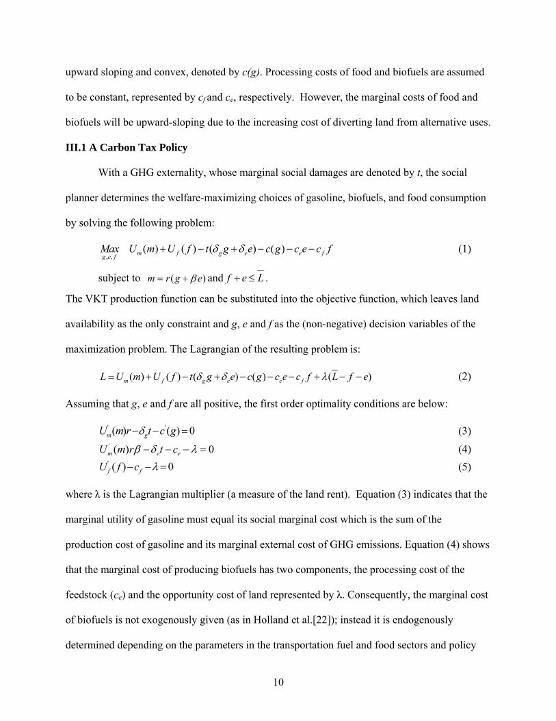
III.1 A Carbon Tax Policy
With a GHG externality, whose marginal social damages are denoted by t, the social
planner determines the welfare-maximizing choices of gasoline, biofuels, and food consumption
by solving the following problem:
, ,( ) ( ) ( ) ( )m f g e e f
g e fMax U m U f t g e c g c e c f (1)
subject to ( )m r g e and f e L .
The VKT production function can be substituted into the objective function, which leaves land
availability as the only constraint and g, e and f as the (non-negative) decision variables of the
maximization problem. The Lagrangian of the resulting problem is:
( ) ( ) ( ) ( ) ( )m f g e e fL U m U f t g e c g c e c f L f e (2)
Assuming that g, e and f are all positive, the first order optimality conditions are below:
' '( ) ( ) 0m gU m r t c g (3) ' ( ) 0m e eU m r t c (4) ' ( ) 0f fU f c (5)
where λ is the Lagrangian multiplier (a measure of the land rent). Equation (3) indicates that the
marginal utility of gasoline must equal its social marginal cost which is the sum of the
production cost of gasoline and its marginal external cost of GHG emissions. Equation (4) shows
that the marginal cost of producing biofuels has two components, the processing cost of the
feedstock (ce) and the opportunity cost of land represented by λ. Consequently, the marginal cost
of biofuels is not exogenously given (as in Holland et al.[22]); instead it is endogenously
determined depending on the parameters in the transportation fuel and food sectors and policy

11
parameters. The carbon tax policy will raise the cost of biofuels such that its marginal social cost
includes the marginal cost of production and land and the marginal external cost of GHG
emissions. Equation (5) implies that at the margin the net returns to land from biofuel production
must equal those from food production. In a market economy, fuel consumers will not consider
externality costs in their consumption decisions. With marginal cost pricing of fuels, they will
consume biofuels and gasoline such that ' '( ) and ( )m g m eU m r p U m r p , where pg and pe are
the consumer prices of gasoline and biofuel, respectively, set equal to their marginal social costs.
Perfect substitutability between gasoline and biofuels implies that pe =βpg. To induce the optimal
levels of consumption suggested by equations (3) and (4), a fuel tax that equals t times the
carbon intensity of the fuel should be levied.
Further insight on the implications of a carbon tax for fuel consumption and GHG
emissions can be gained from the comparative static analysis using the first order conditions (3)-
(5) which lead to our first proposition 6:
Proposition 1 A carbon tax unequivocally lowers the consumption of gasoline and VKT and
reduces GHG emissions. It increases biofuel consumption if the demand elasticity of VKT is
small while the supply elasticity of gasoline and the demand elasticity of food are large.
A carbon tax leads to a reduction in gasoline consumption by raising the consumer price
of gasoline, increasing the marginal cost of VKT, and lowering the demand for VKT. The effects
of the carbon tax on VKT and GHG emissions are shown in (6) and (7).
' ( )[ ] 0g f e
d sf g
p c gdm r
dt H f g
(6)
2 2 ' 22( )1
{ ( ) } 0g f e mg ed s d
f g m
p c g r pdGHG
dt H f g m
(7)
12
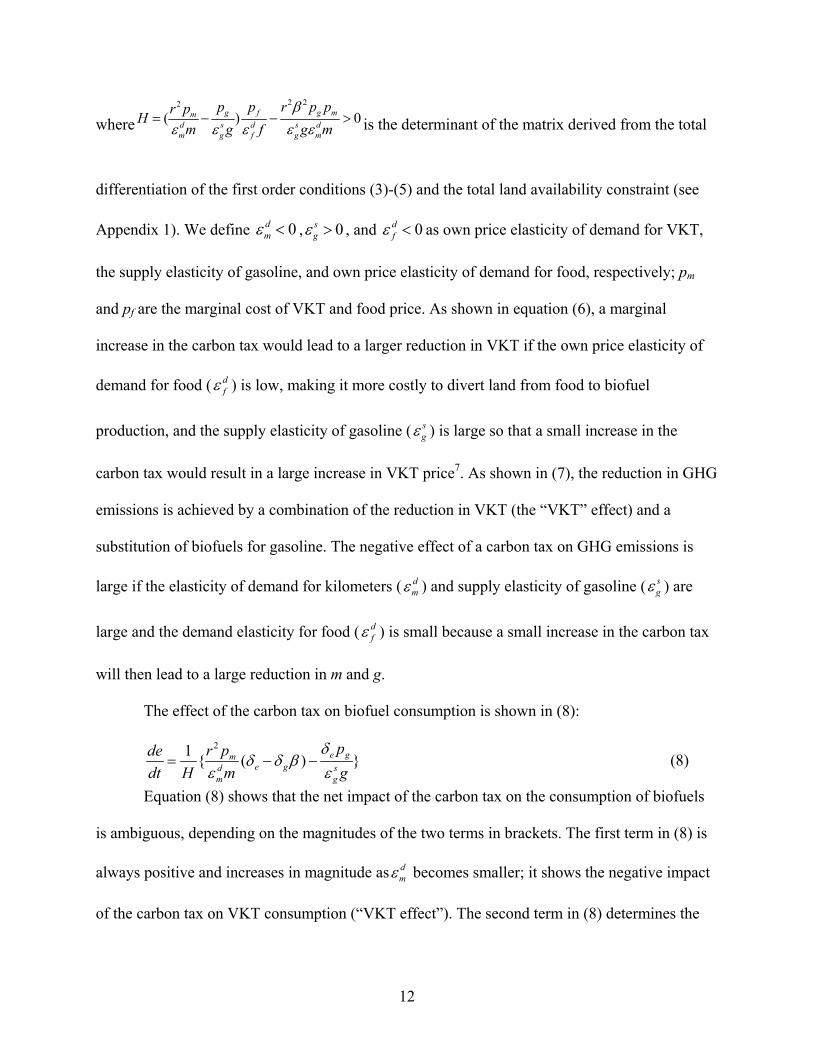
where
2 22
( ) 0g f g mmd s d s dm g f g m
p p r p pr pH
m g f g m
is the determinant of the matrix derived from the total
differentiation of the first order conditions (3)-(5) and the total land availability constraint (see
Appendix 1). We define 0dm , 0s
g , and 0df as own price elasticity of demand for VKT,
the supply elasticity of gasoline, and own price elasticity of demand for food, respectively; pm
and pf are the marginal cost of VKT and food price. As shown in equation (6), a marginal
increase in the carbon tax would lead to a larger reduction in VKT if the own price elasticity of
demand for food ( df ) is low, making it more costly to divert land from food to biofuel
production, and the supply elasticity of gasoline ( sg ) is large so that a small increase in the
carbon tax would result in a large increase in VKT price7. As shown in (7), the reduction in GHG
emissions is achieved by a combination of the reduction in VKT (the “VKT” effect) and a
substitution of biofuels for gasoline. The negative effect of a carbon tax on GHG emissions is
large if the elasticity of demand for kilometers ( dm ) and supply elasticity of gasoline ( s
g ) are
large and the demand elasticity for food ( df ) is small because a small increase in the carbon tax
will then lead to a large reduction in m and g.
The effect of the carbon tax on biofuel consumption is shown in (8):
21{ ( ) }e gm
e gd sm g
pr pde
dt H m g
(8)
Equation (8) shows that the net impact of the carbon tax on the consumption of biofuels
is ambiguous, depending on the magnitudes of the two terms in brackets. The first term in (8) is
always positive and increases in magnitude as dm becomes smaller; it shows the negative impact
of the carbon tax on VKT consumption (“VKT effect”). The second term in (8) determines the

13
substitution effect of the carbon tax, which will increase e, because it changes the relative prices
of gasoline and biofuel. Both terms together show that a marginal increase in the carbon tax is
likely to lead to an increase in biofuel consumption if dm =0 and s
g =∞ because in this case the
first term becomes infinitely positive and the second term in (8) is zero. With an inelastic
demand for VKT and an elastic supply of gasoline, a small change in relative prices of fuels due
to the carbon tax will lead to a relatively large substitution effect in favor of biofuels and a small
VKT effect. Moreover, the magnitude of the carbon tax on biofuels consumption depends on df .
With an elastic demand for food (implying it is not costly to convert cropland for biofuel
production), the determinant H becomes small and a marginal increase in the carbon tax will
induce a large increase in biofuels consumption. Given a limited availability of land, if the
carbon tax increases biofuel consumption, it will raise land rent and reduce food consumption.
III.2 Effects of Alternative Policies
Suppose that alternative biofuel policies, such as a mandate to produce/consume a given
amount of biofuel or a LCFS, are implemented instead of a carbon tax. The quantity mandate and
the LCFS are fixed exogenously.
A. Biofuel Mandate
The biofuel mandate requires a fixed amount of biofuels e e to be produced and consumed.
Substituting this into the objective function leads to the Lagrangian:
( ( , )) ( ) ( ) ( )m f e fL U m g e U f c g c e c f L f e (9)
First order condition (3) is now as follows, while condition (5) is unchanged:
' ' ( ) 0mrU c g (10)
Thus, gasoline consumption will be determined by equating its marginal benefits in producing

14
kilometers with its marginal cost of production. By requiring biofuel consumption beyond the
no-policy level, the mandate will lead to an equilibrium where '( ) e gc e p p with energy
equivalent consumer pricing of biofuel and gasoline. By totally differentiating (5) and (10) and
the constraint on total land availability we obtain the expression (11) and Proposition 2 below:
2
0
1d
g m
sg m
dg
p mde
r gp
(11)
Proposition 2 A biofuel mandate will lead to a reduction in gasoline consumption and an
increase in VKT. It may either increase or decrease GHG emissions. GHG emissions will
decrease if the demand elasticity of VKT is small while the supply elasticity of gasoline is large.
The expression in (11) shows that a biofuel mandate always reduces gasoline
consumption; the extent of this reduction is greater with a smaller dm and a larger s
g . Biofuel
production will displace an energy equivalent amount of gasoline only when sg is infinite (or the
price of gasoline is fixed). With energy equivalent pricing of fuels, the mandate raises the
marginal cost of producing biofuels while lowering (or keeping constant) the consumer price of
fuel. Therefore, the biofuel mandate operates like a subsidy for biofuel consumers, and the
subsidy is paid for by blenders. This is unlike the finding in de Gorter and Just [10]and
Moschini et al.[31] that a biofuel mandate operates like a tax on gasoline consumers and a
subsidy on biofuel consumers. Since the volumetric mandate is imposed on fuel blenders, the
loss in profits due to the difference between consumer price and producer price of biofuels would
be borne by fuel blenders and represent a transfer from gasoline producers (or blenders) to
biofuel producers.
The lowered consumer price of fuels will create incentives for fuel consumers to increase
their VKT consumption above the level in the absence of the mandate, as shown in (12).

15
0g
sg
pdm r
K gde
(12)
where 2 '' '' ( ) 0mmK r U c g is the determinant of the matrix under the consumption mandate and
always negative as shown in Appendix 2. The positive VKT effect of the mandate in (12) works
in the opposite direction than the substitution effect in (11), leading to an ambiguous effect of the
mandate on GHG emissions as shown in equation (13).
'21 ( )
{ ( ) }me g ed s
m g
pdGHG c gr
K m gde
(13)
The effect of the consumption mandate on GHG emissions depends (among other terms)
on dm and s
g . The first term in the square bracket in (13) is positive since g e and 0dm .
The second term is negative. Thus, the overall effect of the mandate on GHG emissions is
negative only if dm is small while s
g is large.
B. Low Carbon Fuel Standard
A LCFS requires the carbon intensity of the blended fuel to be less than a given level
where e g , and the LCFS constraint can be written as:
( )g eg e g e
(14)
The social planner’s optimization problem under the LCFS constraint becomes:
( ) ( ) ( ) ( ) [ ( ) ( )]m f e f g eL U m U f c g c e c f L f e g e g e
where 0 is the shadow value associated with the LCFS constraint. First order conditions with
respect to fuel consumption lead to equations (15) and (16) with the condition (5) unchanged:
' '( ) ( ) ( ) 0m gU m r c g (15) ' ( ) ( ) 0m e eU m r c (16)
The LCFS constraint introduces a wedge between marginal benefits and marginal costs of
fuels. This wedge can be positive or negative depending on the carbon intensities of fuels relative

16
to the LCFS set at . Because e g , the LCFS constraint imposes an implicit tax on
gasoline at a level of ( )g , and provides an implicit subsidy to biofuels at a level of
( )e . The LCFS differs from a carbon tax and a biofuel mandate in the effects on fuel and
VKT consumption and GHG emissions, leading to the following proposition:
Proposition 3 A LCFS always reduces gasoline consumption. It will (i) increase biofuel
consumption if dm and s
g are small and df is large; (2) decrease VKT consumption if f
d is
small and sg is large; and (3) reduce GHG emissions if d
m and fd are small and s
g is large.
The LCFS differs from a carbon tax in that the implicit tax on gasoline is imposed only
on the portion of the carbon intensity of gasoline larger than the LCFS and that biofuels are
subsidized instead of being taxed. A marginal increase in the stringency of the LCFS will always
lead to a reduction in g like a carbon tax but its impact on e is ambiguous, as shown below.
'21 ( )
{[ ( )( )] ( )[ ( (1 ) ( )) ( ) ]}mg e g g e ed s
m g
pde c gg e r
d P m g
(17)
where P >0 is the determinant of the matrix under the LCFS constraint as shown in Appendix 3.
The effect of a small reduction (increase in stringency) in σon biofuel consumption
depends on dm , s
g and df (P is a function of d
f ) as displayed in (17).The first term in (17),
( ( )( )g e g ), is always positive since e g and 0 , and the second term in the
brackets is always negative because 1 and e g . An elastic demand for food (lowers P),
and lowers the impact of an increase in biofuel consumption on food prices. Thus, the LCFS will
increase biofuel consumption more when dm and s
g are smaller and df is larger and a small
increase in the stringency of the LCFS will not reduce VKT and gasoline consumption much,
thereby requiring a large increase in biofuel consumption to comply with the LCFS.
17
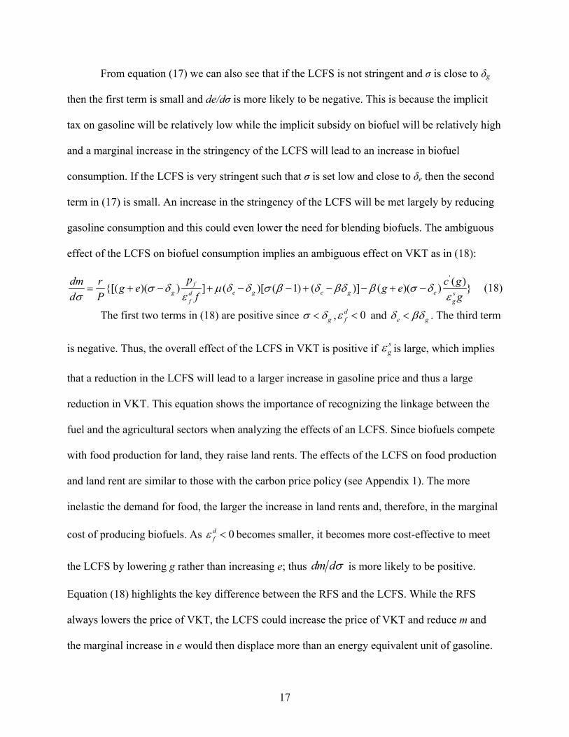
From equation (17) we can also see that if the LCFS is not stringent and σ is close to δg
then the first term is small and de/dσ is more likely to be negative. This is because the implicit
tax on gasoline will be relatively low while the implicit subsidy on biofuel will be relatively high
and a marginal increase in the stringency of the LCFS will lead to an increase in biofuel
consumption. If the LCFS is very stringent such that σ is set low and close to δe then the second
term in (17) is small. An increase in the stringency of the LCFS will be met largely by reducing
gasoline consumption and this could even lower the need for blending biofuels. The ambiguous
effect of the LCFS on biofuel consumption implies an ambiguous effect on VKT as in (18):
' ( ){[( )( ) ] ( )[ ( 1) ( )] ( )( ) }f
g e g e g ed sf g
pdm r c gg e g e
d P f g
(18)
The first two terms in (18) are positive since g , 0df and e g . The third term
is negative. Thus, the overall effect of the LCFS in VKT is positive if sg is large, which implies
that a reduction in the LCFS will lead to a larger increase in gasoline price and thus a large
reduction in VKT. This equation shows the importance of recognizing the linkage between the
fuel and the agricultural sectors when analyzing the effects of an LCFS. Since biofuels compete
with food production for land, they raise land rents. The effects of the LCFS on food production
and land rent are similar to those with the carbon price policy (see Appendix 1). The more
inelastic the demand for food, the larger the increase in land rents and, therefore, in the marginal
cost of producing biofuels. As 0df becomes smaller, it becomes more cost-effective to meet
the LCFS by lowering g rather than increasing e; thus dm d is more likely to be positive.
Equation (18) highlights the key difference between the RFS and the LCFS. While the RFS
always lowers the price of VKT, the LCFS could increase the price of VKT and reduce m and
the marginal increase in e would then displace more than an energy equivalent unit of gasoline.
18
2 2( )( ) ( ) [ (1 ) ( )]( )( )
( )( )
f mg g e g g e e gd d
f m
ge es
g
p pdGHGg e r g e
d f m
pg e
g
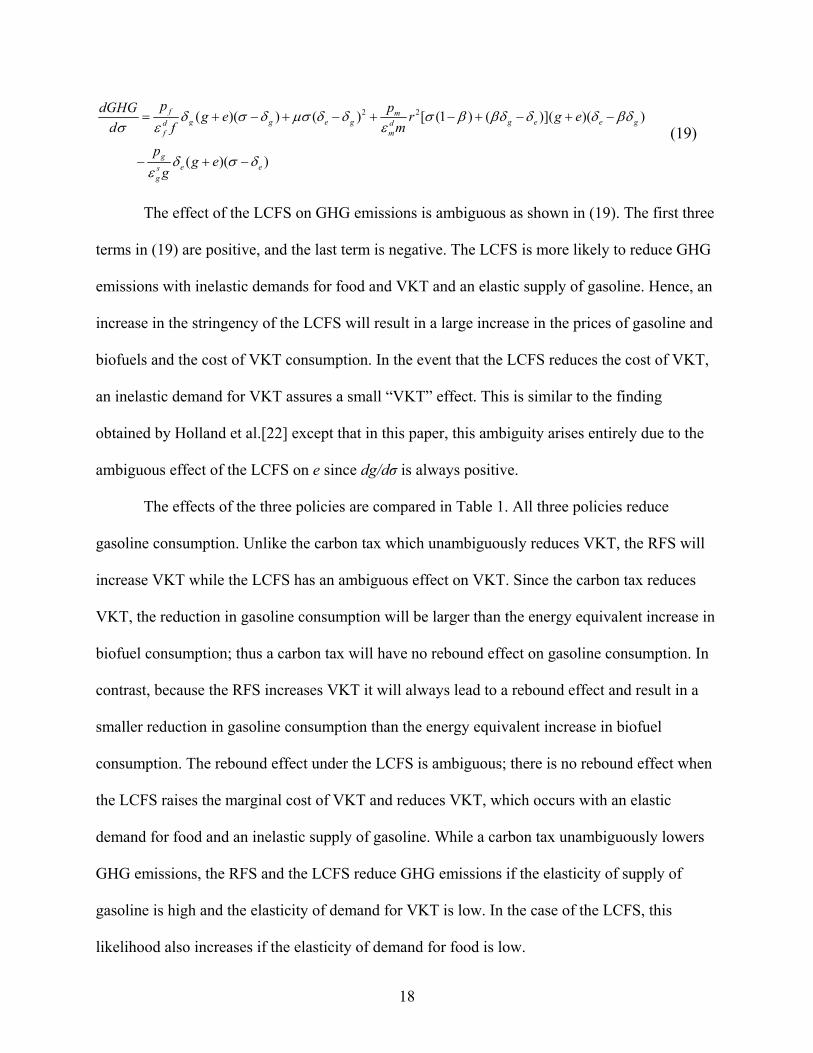
(19)
The effect of the LCFS on GHG emissions is ambiguous as shown in (19). The first three
terms in (19) are positive, and the last term is negative. The LCFS is more likely to reduce GHG
emissions with inelastic demands for food and VKT and an elastic supply of gasoline. Hence, an
increase in the stringency of the LCFS will result in a large increase in the prices of gasoline and
biofuels and the cost of VKT consumption. In the event that the LCFS reduces the cost of VKT,
an inelastic demand for VKT assures a small “VKT” effect. This is similar to the finding
obtained by Holland et al.[22] except that in this paper, this ambiguity arises entirely due to the
ambiguous effect of the LCFS on e since dg/dσ is always positive.
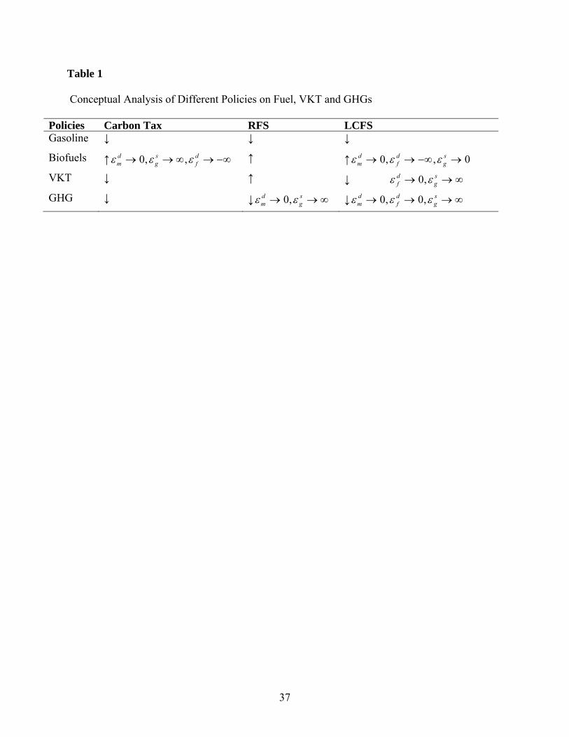
The effects of the three policies are compared in Table 1. All three policies reduce
gasoline consumption. Unlike the carbon tax which unambiguously reduces VKT, the RFS will
increase VKT while the LCFS has an ambiguous effect on VKT. Since the carbon tax reduces
VKT, the reduction in gasoline consumption will be larger than the energy equivalent increase in
biofuel consumption; thus a carbon tax will have no rebound effect on gasoline consumption. In
contrast, because the RFS increases VKT it will always lead to a rebound effect and result in a
smaller reduction in gasoline consumption than the energy equivalent increase in biofuel
consumption. The rebound effect under the LCFS is ambiguous; there is no rebound effect when
the LCFS raises the marginal cost of VKT and reduces VKT, which occurs with an elastic
demand for food and an inelastic supply of gasoline. While a carbon tax unambiguously lowers
GHG emissions, the RFS and the LCFS reduce GHG emissions if the elasticity of supply of
gasoline is high and the elasticity of demand for VKT is low. In the case of the LCFS, this
likelihood also increases if the elasticity of demand for food is low.
19
IV. Numerical Model
BEPAM is a multi-market, multi-period, price-endogenous, nonlinear mathematical
programming model that simulates U.S. agricultural and fuel sectors including international trade
with the rest of the world. This model determines several endogenous variables simultaneously,
including VKT, fuel and biofuel consumption, imports of gasoline and sugarcane ethanol, mix of
biofuels and regional land allocation among different food and fuel crops and livestock over a
given time horizon (2007-2030 in this case). This is achieved by maximizing the sum of
consumers’ and producers’ surpluses in the transportation fuel and agricultural sectors subject to
market clearing conditions and technological and land availability constraints underlying
commodity production and consumption within a dynamic framework.
IV.1Transportation Sector
This sector considers linear demand curves of VKT for five types of vehicles that use
liquid fossil fuels (gasoline or diesel) blended with biofuels, including conventional gasoline,
ethanol flex-fuel, hybrid, electric, and diesel vehicles. In addition to a minimum ethanol blend
for gasoline blend vehicles in order to meet the oxygenate additive requirement, we impose the
blend limits as specified by EIA [12] for each of these five types of vehicles due to their
technological constraints in blending biofuels with gasoline or diesel. With the except of VKT
with electric vehicles that are exogenously fixed, the demands for VKT with other types of
vehicles endogenously generate demands for liquid fossil fuels and biofuels given the energy
contents of alternative fuels, the fuel economy of each type of vehicle and biofuel blending limits.
We include upward sloping supply curves for domestic gasoline production and for
gasoline supply from the rest of the world (ROW). The excess supply of gasoline to the U.S. is
determined by the difference between gasoline demand and gasoline supply in the ROW. In the

20
case of diesel we assume that it is only produced domestically and include an upward sloping
supply curve to represent its marginal cost of production and price responsiveness.
The demand for ethanol from VKT with gasoline blends can be met with four broad types
of biofuels, first generation ethanol, second generation ethanol (cellulosic ethanol), first
generation biodiesel (derived from vegetable oils) and second generation biomass to liquids
(BTL) diesel. First generation ethanol can be produced domestically from corn or imported
sugarcane ethanol from Brazil. Cellulosic ethanol can be produced from crop or forest residues
and dedicated energy crops (miscanthus and switchgrass). These cellulosic feedstocks can also
be used to produce BTL with the Fischer-Tropsch process which can be blended with petroleum
diesel together with biodiesel produced from soybean oil, DDGS-derived corn oil and waste
grease. Life-cycle analysis is used to determine the GHG intensity of all fuels and crop
production processes, including soil carbon sequestration with land use changes. The model
endogenously determines the supply of each type of biofuels and its marginal cost with given
policy, technology and land availability constraints.8 While feedstock costs of producing biofuels
are determined in the agricultural sector, we use the experience curve approach to relate the
decline in processing costs of a biofuel with its cumulative production (experience) at a point in
time [39]. 9
IV.2 Agricultural Sector
The agricultural sector in BEPAM includes all major conventional crops and livestock
animals produced in the US, two bioenergy crops (miscanthus and switchgrass), crop residues
from corn and wheat, forest residues, as well as co-products from the production of corn ethanol
and soybean oil. We specify domestic and export demand/import supply functions for individual
commodities, including crop and livestock products. These are shifted upward over time at
21
exogenously specified rates.
To reflect the spatial heterogeneity in crop productivity and land availability, we model
the regional supply of crop and biofuel feedstocks at Crop Reporting District (CRD) level. The
model considers 295 CRDs in 41 of the contiguous U.S. states in five major regions.10 Yields of
conventional crops are assumed to grow over time based on econometrically estimated trend
rates of growth and price responsiveness of crop yields [see 6]. Yields of energy crops,
miscanthus and switchgrass are obtained at a 56 mx 56 m resolution using a crop productivity
model described in Jain et al. [25] and aggregated to the CRD level. Crop production costs,
yields and resource endowments are specified for each CRD and each crop, based on CRD
specific yields, input application rates, input prices and costs of various field operations, for
conventional crops, energy crops and crop residues. Conventional crops can be produced using
alternative tillage, rotation and irrigation practices. Costs of production of cellulosic biofuels are
estimated by aggregating costs of feedstock, conversion to fuel and transportation and differ
across CRDs.
In the livestock sector, we consider several types of meat (chicken, turkey, lamb, beef,
and pork), wool, dairy, and eggs. The demand for feed for the production of livestock animals is
determined by the number of animals and their nutrition requirements in terms of protein and
calories; these requirements are met by determining the least cost mix of feed including co-
products DDGS from corn ethanol production given its nutrient content, subject to an upper
bounds for the share of DDGS in total feed consumption for each livestock category. The supply
of beef is restricted by the number of cattle which in turn depends on the amount of grazing land
available at regional level. We model the supply of other livestock commodities, at the national
level, and their supply is constrained by their historical numbers.
22
The model includes several types of cropland and land that is idle or marginal for each
CRD. Cropland availability in each CRD is assumed to change in response to crop prices. Idle
land and cropland pasture are assumed to move into cropland and back into idle state; crop yields
are lower on marginal land as compared to average cropland (based on Hertel et al.[20]). This
marginal land can also be converted for the production of energy crops after incurring a
conversion cost. Following the definition of renewable biomass in EISA, we keep other land,
including pasture land and forestland pasture fixed at 2007 levels while land enrolled in the
Conservation Reserve Program is fixed at levels authorized by the Farm Bill of 2008 and cannot
be used to produce energy crops. Based on agronomic evidence , we assume that perennial
grasses have the same productivity on marginal land as on regular cropland [37] but there is a
conversion cost for the use of idle land/cropland pasture for producing perennial grasses; this is
assumed to be equal to the returns the land would obtain from producing the least profitable
annual crop in the CRD to rationalize the land owner’s decision to keep land idle.
V. Data and Assumptions
A detailed description about the data used for the agricultural sector can be found in Chen
et al. [6]. Here we describe the data sources for the transportation fuel sector, which include the
demand for VKT, the supply of alternative fuels, and specification of GHG intensity. We
calibrate the demand curves for VKT for each of five types of vehicles at 2007 level, and shift
the demand curve for VKT at an exogenously fixed rate based on the annual projections for VKT
for the 2007-2030 period [12]. Demands for VKT and fuel economy (kilometers per liter of fuel)
for each of the vehicle types from 2007 to 2030 are obtained from EIA [12]. Gasoline, diesel,
ethanol and biodiesel consumed by on-road vehicles in 2007 are obtained from Davis et al. [9].
Retail fuel prices, markups, taxes and subsidies are obtained from EIA [12]. We assume demand

23
elasticities of -0.2 for VKT with all types of vehicles [32].
We assume a linear short-run supply for US gasoline production with an elasticity of
0.049 at $35 per barrel [18]. This is consistent with the long run elasticity of US supply of 0.46
and adjustment rates of 0.9 reported in Leiby [29], implying a short run elasticity of 0.046. The
domestic gasoline elasticity used here is also similar to the estimate obtained by Gately [15],
Greene and Ahmad [17] and Huntington [24]. Since diesel consumed in the US is primarily
produced domestically, we assume a linear domestic supply curve for diesel with the same price
response as domestic gasoline supply curve. The US gasoline imports from the rest of the world
(ROW) is derived by specifying linear demand and supply functions for gasoline in ROW.
Followed the literature review by Hamilton [19]who suggests that the short run elasticity of
demand for gasoline ranges between -0.25 and -0.34 [4, 8, 14,16],we assume a value of -0.26 for
the elasticity of demand for the ROW (as in Hertel et al. [21]). An elasticity of 0.2 is assumed for
short- run gasoline supply in the ROW, according to the review of literature in Leiby [29]. These
supply and demand curves are calibrated for 2007 using the elasticity parameters and the U.S.
fuel consumption data discussed above as well as data on fuel production and consumption for
the ROW obtained from International Energy Outlook 2010 [12] .
We consider various biofuel pathways in the model as mentioned above.11 Methods used
to determine the costs of producing energy crops and yields are based on Jain et al.[25] and
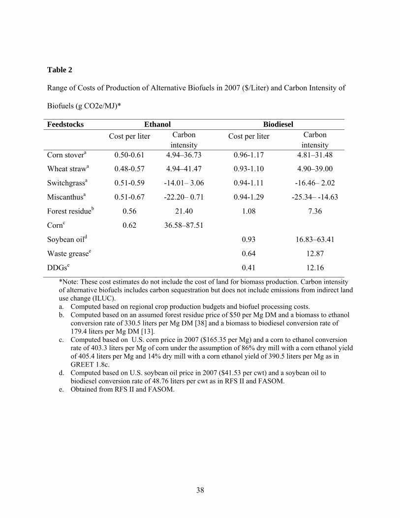
described in greater detail in Chen et al. [6]. The range of the costs of producing alternative
biofuels differs across CRDs as shown in Table 2. These costs do not include the cost of land,
which is determined endogenously and differs across policy scenarios. Costs of production of
biofuels from food crops are based on the market price of the feedstock and are the same across
CRDs. The producer costs of various biofuels in equilibrium under alternative policies are shown

24
in Table 5.
Conversion rates from feedstocks to biofuels (yield of biofuel per metric ton of
feedstock) are exogenously fixed and assembled from several sources. They are based on the
estimates in GREET 1.8c for corn ethanol, FASOM [2] for biodiesel from vegetable oil or waste
grease, Business Wire for biodiesel from DDGS-derived corn oil12, and EPA [13] for BTL and
cellulosic ethanol. For the experience curve approach for determining the reduction in costs of
converting feedstocks to biofuels over time, the initial individual biofuel conversion costs are
obtained from various sources including EPA [13], Swanson et al. [35], and Crago et al.[7] while
the learning rate parameters are obtained from [39].
We use U.S. ethanol retail prices and imports from Brazil and Caribbean countries in
2007 as well as an assumed elasticity of the excess supply of ethanol import of 2.7 to calibrate
the sugarcane ethanol import supply curve for the U.S [28]. The total costs of production
(including feedstock cost) for sugarcane ethanol are assumed to decline at a value of b of -0.32
and an exogenously specified rate of growth of sugarcane ethanol production of 8% [36].
We also specify the life-cycle GHG intensity of alternative transportation fuels. Life-
cycle GHG emissions for conventional gasoline are assumed to be 93.05 g CO2e/ MJ and for
petro diesel fuel to be 91.95 g CO2e/ MJ in 2005. These carbon intensities are assumed to
increase over time due to imports of high carbon intensive fuels, like oil tarsands. We estimate
the life-cycle GHG emissions of the biofuel pathways included in the analysis using data on
feedstock production and biofuel conversion, distribution and consumption. The agricultural
phase GHG emissions include emissions from agricultural input uses such as fertilizer,
chemicals, fuels and machinery, and soil carbon sequestration. These input use data are obtained
from region specific crop budgets while the life-cycle GHG emission factors for these inputs are

25
derived from GREET 1.8c. We also obtain GHG emissions of biofuel conversion, distribution
and use from GREET 1.8c.
We assume the carbon intensity of corn ethanol will decrease over time from 58.4 g
CO2e/MJ in 2007 to 45.5 g CO2e/MJ by 2030 due to the growth in corn yields and
technological innovation in corn ethanol refinery phase [13,30]. The carbon intensity of soybean
oil biodiesel weighted at the national average is estimated to be 35.1gCO2e/MJ in 2007 and
assumed to decline to 31.7gCO2e/MJ in 2030 according to National Biodiesel Board13. For
cellulosic ethanol and biodiesel derived from corn stover, wheat straw, switchgrass, and
miscanthus, their life cycle carbon intensities differ across CRDs, as shown in Table 2. We
assume a carbon intensity of 21.4 g CO2e/MJ for forest residue and pulpwood derived cellulosic
ethanol [5]and 7.36 g CO2e/MJ for forest residue and pulpwood derived biodiesel following the
carbon intensity of stover derived diesel estimated in EPA [13]. We assume a carbon intensity of
25.12 g CO2e/MJ for sugarcane ethanol obtained from Crago et al.[7].
VI. Results
We first validate the simulation model for 2007 assuming existing fuel taxes, the corn
ethanol mandate, corn ethanol tax credit, and import tariffs, and compare the model results on
land allocation, commodity prices, and fuel prices and consumption with the corresponding
observed values in 2007. As shown in Table 3, the differences between model results and the
observed land use allocations and commodity prices for major crops (corn, soybeans, wheat, and
sorghum) are typically less than 10.0%. Fuel prices and consumption are also simulated well,
within 5.0% deviation from the observed values with the exception for corn ethanol price and
ethanol consumption that are 16.0% and -6.0%, respectively.
We then simulate a business-as-usual (BAU) scenario and three policy scenarios: the

26
RFS, a national LCFS and a carbon tax policy. The RFS sets ethanol equivalent volumetric
requirements for four categories of renewable fuels: renewable fuel, advanced biofuels, biomass-
based diesel and cellulosic biofuels for the period 2007-2022. Requirements for cellulosic
biofuels for 2010 and 2011 have been waived due to the lack of commercial production
technology. According to the Annual Energy Outlook [12], the volumes of second generation
biofuels as mandated by EISA are considered unlikely to be achieved by 2022, but to be
exceeded by 2035. For the analysis here, we use the AEO projections for annual volumes of first
and second generation biofuels to set the achievable biofuel quantities for the period 2007-2030.
These projections set corn ethanol production at its upper limit of 57 billion liters in 2015 and
beyond and total renewable fuel production at 143 billion liters in 2030. We assume that
commercial production of cellulosic biofuels will be feasible from 2015 onwards.
We consider a national LCFS that lowers the average fuel carbon intensity of gasoline
blended fuel and of diesel blended fuel by 10% by 2030 relative to the GHG intensity of
conventional gasoline and petro-diesel in 2005. Annual rates of reduction in GHG intensity are
set linearly to meet these targets between 2015 and 2030. The LCFS restricts the ratio of GHG
emissions from all fuels blended/consumed in a given year to the total energy produced by all
those fuels in that year to be below a specified intensity level for that year. The LCFS is only
binding at the aggregate level and not the firm level; it thereby implicitly allows for the
possibility of trading among fuel providers, some of whom might over-achieve the LCFS while
others may under-achieve it, the industry as a whole meets the LCFS cost-effectively. It also
allows trading in carbon intensity reductions across biofuels, gasoline and diesel. Climate change
legislation is yet to be enacted in the U.S. For this analysis we determine a carbon price that
achieves the same cumulative level of GHG emissions (over the study period) as the 10% LCFS

27
and assume it is constant over the study period.
Table 4 shows the results for fuel consumption in 2030 and cumulative GHG emissions
over the 2007-2030. Table 5 presents the results on food and fuel prices in 2030. Implications for
social welfare under different policies are displayed in Table 6. Social welfare is computed as the
sum of discounted domestic consumers’ and producers’ surpluses in the agricultural and
transportation fuel sectors over the period 2007-2030. We report the change in social welfare
relative to the BAU.
VI.1 Business-As-Usual Scenario
Under the BAU scenario, the shift in demand for VKT over time increases the quantity of
VKT demanded with gasoline blends by 40.6% from 4704 billion kilometers in 2007 to 6617
billion kilometers in 2030, and the VKT demanded with diesel blends by 54.6% from 469 billion
kilometers to 725 billion kilometers. Due to the increase in fuel economy of vehicles, gasoline
and diesel consumption increase by much less, 0.7% and 16.7% , respectively, over the 2007-
2030 period. In the absence of any biofuel or climate policies, we find first generation biofuel
production would be 19.3 billion liters in 2030, representing a 6.1% increase over this period. Of
the first generation biofuel consumed, about 14.6 billion liters would be domestically produced
corn ethanol, 3.7 billion liters would be imported sugarcane ethanol and the rest (1 billion liters)
is biodiesel produced from vegetable oils. The ethanol production would essentially meet the
demand for ethanol as an oxygenate to be blended with gasoline and there is no production of
second generation biofuels.
The increase in the consumption of transportation fuels over time leads to higher
consumer prices of gasoline and diesel in 2030 by 30.0% and 26.4%, respectively, relative to the
2007 levels. Despite the increase in the demand for corn for biofuel production, corn price would
28
decrease by 13.6% over the 2007-2030 due to the increase in corn yield.
VI.2 Effects of Biofuel and Climate Policies on the Agricultural and Fuel Sectors
Fuel Mixes and GHG Emissions
The three policies differ in the volume and mix of biofuels consumed and the
consumption of fossil fuels. Under the RFS first generation biofuel production would increase
from 19.3 billion liters under the BAU to 48.3 billion liters in 2030, consisting of 41 billion liters
of corn ethanol, 4 billion liters of sugarcane ethanol, and 3.3 billion liters of biodiesel derived
from vegetable oils. This is somewhat lower than the upper limit on corn ethanol of 57 billion
liters because advanced biofuels would become competitive by 2030 and expand beyond the
minimum levels required by the RFS. About 94.8 billion liters of cellulosic ethanol would be
produced to meet the advanced biofuel mandate. However, the production of BTL would not be
a cost-effective strategy to meet the advanced biofuels mandate by 2030. The expansion in
biofuel production results in a reduction in the consumption of gasoline and diesel by 13.8% and
0.5% in 2030, respectively, relative to the BAU, which reduces the dependence on gasoline
imports by 18.4%. The share of ethanol in gasoline blends increases from 3.5% under the BAU
to 24.3% in 2030 under the RFS, while the share of biodiesel in the diesel blends increases from
0.4% under the BAU to 1.2%. As expected from the conceptual framework, the RFS leads to an
increase in gasoline-based VKT and diesel-based VKT by 2.2% and 0.3% relative to the BAU
level in 2030, respectively, leading to a rebound effect on fossil fuel consumption. Hence, there
is a positive rebound effect and the reduction in domestic gasoline consumption is 13.8% lower
than the energy equivalent increase in ethanol consumption while the reduction in diesel
consumption is 37.0% lower than the increase in energy equivalent biodiesel consumption in
2030. Nevertheless, the substitution of fossil fuels by biofuels lowers cumulative GHG emissions
29
by 3.9% relative to the BAU level over the 2007-2030 period.
As compared to the RFS, the LCFS encourages greater consumption of biofuels with
relatively lower carbon intensity than the fossil fuel it is a substitute for. In particular it induces
greater use of BTL, even though it is a higher cost fuel than cellulosic ethanol, because of its
lower carbon content compared to other biofuels and compared to diesel. As a result, the LCFS
reduces the GHG intensity of diesel blends more than that of gasoline blends. Biofuel
production now includes 100.8 billion liters of cellulosic ethanol and 22.5 billion liters of BTL
while the consumption of first generation biofuels is only 21.7 billion liters. Although total
biofuels consumption under the LCFS is only 2 billion liters higher as compared to the RFS in
2030 (145 billion liters versus 143 billion liters), the production of cellulosic biofuels is 70.0%
(28.5 billion liters) greater as compared to the RFS, while the production of first generation
biofuels would be 155.0% (26.6 billion liters) lower. Gasoline consumption would decrease by
12.6% in 2030 relative to the BAU scenario, leading to a reduction in gasoline imports by 16.7%.
Due to a large amount of BTL production, the LCFS significantly reduces diesel consumption by
6.7% as compared to the BAU and increases the share of biodiesel in the diesel blends to 7.8% in
2030. The consumption of VKT is 1.0% higher under the LCFS as compared to the BAU
scenario in 2030. The rebound effects are 7.2% and 10.0% in the domestic gasoline and diesel
markets respectively and smaller than those under the RFS. The greater consumption of
cellulosic biofuels reduces cumulative GHG emissions by 4.7% compared to the BAU scenario
and 0.9% more than the RFS over the 2007-2030 period.
We find a carbon tax of $60 per metric ton of CO2e would achieve the same cumulative
level of GHG emissions over the 2007-2030 as the LCFS with a 10% target for reduction in
GHG intensity of transportation fuels. Unlike the other two policies, the carbon tax achieves a

30
reduction in GHG emissions primarily by reducing fossil fuel consumption and VKT. The
carbon tax reduces gasoline and diesel consumption by 3.4% while VKT with gasoline and
diesel decrease by 3.0 and 3.2%, respectively in 2030. Consumption of first generation biofuels
increases by 21.8 billion liters in 2030, which is 13.3% (2.6 billion liters) higher relative to the
BAU scenario. The tax is not high enough to make the consumption of cellulosic biofuels a cost-
effective abatement strategy by 2030.
Fuel Prices
The reduction in consumption of gasoline and diesel due to the RFS-induced biofuel
production reduces their prices in 2030 by 10.4% and 0.7%, respectively, relative to the BAU
scenario. Since biofuels and fossil fuels are perfect substitutes, the consumer prices of ethanol
and biodiesel would also fall by the same percentages as gasoline and diesel prices and remain at
the energy equivalent level. The RFS provides an implicit subsidy to biofuel consumers (the
difference between producer price and consumer price of biofuels). Since advanced biofuel
production exceeds the minimum mandated level and reduces corn ethanol consumption to be
below the upper limit on corn ethanol, this implicit subsidy is the same for all types of ethanol, as
shown in Table 5. Specifically, this implicit subsidy is $0.15 per liter for ethanol and $0.21 per
liter for oils-based biodiesel in 2030.
Unlike the RFS, the LCFS implicitly subsidizes biofuels and implicitly taxes fossil fuels
depend on the stringency of the LCFS constraint and the carbon intensity of fuels. We estimates
the subsidies to be $0.12 and $0.16 per liter for corn and sugarcane ethanol in 2030, while the
subsidies for cellulosic ethanol and BTL are significantly larger with $0.22 and $0.38 per liter
due to their lower carbon content. The LCFS also imposes a tax of $0.05 per liter on gasoline and
on diesel of $0.07 per liter in 2030. Despite these taxes, the prices of gasoline and diesel are
31
lower relative to the BAU. The LCFS lowers the consumer price of gasoline and gasoline blends
by less than the RFS (4.1% as compared to 10.4% under the RFS) but it lowers the consumer
price of diesel and diesel blends by more than the RFS (3.0% as compared to 0.7% under the
RFS), because it leads to a larger displacement of diesel than the RFS.
The carbon tax of $60 per metric ton of CO2e implies a tax of $0.18 per liter on gasoline,
$0.21 per liter on diesel, $0.06 per liter on corn ethanol, and $0.03 per liter on sugarcane ethanol.
The corresponding taxes imposed on cellulosic biofuels are fairly small due to their low carbon
intensities. Thus, the carbon tax raises gasoline and diesel consumer prices by 16.7% in 2030 as
compared to the BAU scenario, which results in a 3.0% reduction in VKT.
Food Prices
As expected from the conceptual model, we find all three policies raise food crop prices
because of the increase in biofuel production. However these effects differ because the three
policies differ in the mix of biofuels they induce. Among the three policies, the RFS raises food
prices the most since the production of first generation biofuels is largest in this case. Corn and
soybean prices would be 26.4% and 22.6% higher in 2030 in comparison to the BAU scenario.
Unlike the RFS, more than 85.0% of the biofuels produced under the LCFS are from non-food
based cellulosic feedstocks in the form of high-yielding energy crops and crop and forest
residues. These energy crops do divert some land from food crop production but at the same time
the reduction in demand for first generation biofuels under the LCFS reduces demand for land.
Thus, corn and soybean prices under the LCFS would only be 10.8% and 12.1% greater as
compared to the BAU scenario in 2030. These prices are 12.4% and 8.6%, respectively, lower
than those under the RFS. The carbon tax generates modest impacts on food crop prices with
corn and soybean prices increasing by 8.5% and 2.3%, respectively, relative to the BAU, in part

32
due to some increase in corn ethanol consumption and in part due to higher costs of carbon
inputs in crop production.
VI.3 Welfare Effects of Biofuel and Climate Policies
As a result of the reduction in fuel prices, fuel consumers gain by 1.9% ($408 billion) and
0.6% ($131 billion) under the RFS and the LCFS, respectively, relative to the BAU scenario. In
contrast to this, the carbon tax reduces fuel consumers’ surplus by -7.5% ($1619 billion). Fuel
producers will suffer a significant loss in surplus from the reduction in fuel production and
producer prices of fuels across all scenarios considered here, with the largest surplus loss being
13.8% ($388 billion) under the RFS as compared to the BAU scenario. The LCFS and carbon tax
reduce the surplus of fuel producers by 2.6% ($74 billion) and 6.2% ($176 billion), respectively.
The increase in demand for biofuels raises the opportunity costs of cropland and thereby
raises producer surplus for crop producers. We find that the gain in surplus for agricultural
producers is largest under the RFS, by 19.1% ($285 billion) relative to the BAU while the loss
for agricultural consumers is by 5.0% ($110 billion). The welfare effects of the LCFS and carbon
price policies on the agricultural sector are much more modest. Specifically, agricultural
producers’ surplus increases by 6.2% ($92 billion) and 1.2% ($17 billion) under the LCFS and
the carbon tax, respectively. Both policies have negligible impacts on agricultural consumers.
All of the policies considered here increase overall social welfare relative to the BAU, by
improving the terms of trade for the US. Welfare gains are the highest under the RFS (by 0.8%
of $238 billion) relative to the BAU. The LCFS and the carbon tax increase domestic social
welfare by 0.6% ($173 billion) and 0.4% ($125 billion), respectively, relative to the BAU. While
the LCFS and carbon tax policies lead to additional reduction in carbon emissions than the RFS,
they also lead to lower levels of domestic social welfare than the RFS.

33
VI.4 Sensitivity Analysis
The welfare and GHG impacts of these policies depend on a number of technological and
behavioral assumptions in the model. Here we focus on examining the sensitivity of our results
to wide variations in the parameter assumptions that were analyzed in the conceptual framework.
In scenario (1), we double the demand elasticity of VKT from -0.2 to -0.4 while in scenario (2)
we significantly increase the ROW supply elasticity of gasoline from 0.2 to 30. In scenario (3),
we consider a case with 30 times higher demand elasticities for food in the ROW relative to the
parameters in the benchmark case. We present the mix of cumulative biofuels consumption over
2007-2030 under the three policy scenarios (the RFS, the LCFS and a carbon tax) with the
changes in each of these parameters in Fig. 1. We also compute the percentage changes in
cumulative liquid fossil fuel consumption, GHG emissions, and social welfare under these
policies relative to the corresponding BAU with each of the parameters (Figs. 2 and 3).
We find that despite the large differences in parameters considered here there is a
remarkable similarity in the level and mix of biofuels consumed over 2007-2030 under a
particular policy. An exception is the reduced consumption of biofuels, particularly cellulosic
ethanol and larger consumption of BTL under the LCFS with a high supply elasticity of gasoline;
the reduction in GHG intensity in this case is met largely by reducing fossil fuel consumption.
Across the parameter assumptions considered here, the reduction in fossil fuel
consumption ranges between 3.8 - 6.5% under the carbon tax, between 3.4-3.8% under the LCFS
and between 4.8-6.2% under the RFS relative to the corresponding BAU levels with each of
those parameters. The reduction in fuel consumption is largest under the RFS across the different
parameter assumptions followed by the carbon tax; an exception is when the elasticity of demand
for VKT is high and the reduction in VKT becomes an even more cost-effective strategy for
34
reducing GHG emissions with the carbon tax in this case compared to the benchmark case.
However, the effect of parametric changes on fossil fuel consumption under the RFS and LCFS
is within 1.0% of the effect with the benchmark parameters.
In general, we find that changes in parameters in the agricultural and fuel sectors affect
fuel consumption but do not have significant impacts on GHG emissions and social welfare
relative to those with the benchmark parameters. Across the scenarios considered here we find
the carbon tax always leads to the largest reduction in GHG emissions, ranging from -4.8% in the
benchmark to -7.3% in scenario (1), while the RFS generates the smallest reduction in GHG
emissions fluctuating between -3.1% in scenario (1) to -4.5% in scenario (2). The reduction in
GHG emissions under the LCFS is about 4.5% to 4.8% despite the large changes in parametric
assumptions. The larger reduction in GHG emissions under the LCFS occurs when the elasticity
of supply of gasoline is relatively larger.
All three policies result in higher domestic social welfare as compared to the BAU. A
carbon tax policy generates the lowest gain in social welfare. While this appears counter-
intuitive, it shows that a significant source of these gains is the improvement in terms of trade
due to higher crop prices and lower fuel prices. We find that with an elastic supply curve of
gasoline and elastic export demand curves of food, the gains in the improvement in terms of
trade will be smaller, resulting in a smaller gain in domestic social welfare as compared to the
benchmark results. In these cases the LCFS is a preferred policy relative to the RFS because it
leads to a larger reduction in GHG emissions and higher social welfare. Under other parameter
assumptions there could be a trade-off between the higher GHG reductions achieved by the
LCFS and the larger social welfare benefits provided by the RFS. Gains in social welfare are
however less than 1.5% across all scenarios as compared to the BAU levels.

35
VII. Conclusions
Fuel standards are being promoted by policy makers as a mechanism for reducing the
dependence on fossil fuels and reducing GHG emissions from the transportation sector. We
develop both a conceptual framework and a numerical simulation model to examine the
efficiency of two types of fuel standards, the RFS with quantity mandates on biofuel
consumption, and the LCFS with a restriction on the GHG intensity of transportation fuels. We
compare these to the effects of a carbon tax policy which would be the most direct approach to
internalizing the externalities associated with GHG emissions from the fuel sector.
The conceptual framework shows that the effects of both types of fuel standards on GHG
emissions are ambiguous and that both policies could result in greater consumption of VKT and
a rebound effect that reduces the extent to which biofuels displace fossil fuels. We also examine
the welfare effects of alternative policies. In an open economy, the RFS and the LCFS impose
not only allocative efficiency costs on the economy but also affect the terms of trade by affecting
the prices of exports (agricultural commodities) and imports (fossil fuels). Thus, these policies
may lead to higher domestic social welfare relative to a carbon tax that would be the most cost-
effective approach to achieving a given reduction in GHG emissions in a closed economy.
Our numerical analysis shows that all three policies lead to a reduction in GHG
emissions, but they differ in how this reduction is achieved. Both the RFS and the LCFS reduce
GHG emissions by displacing high-carbon liquid fossil fuels with a large volume of biofuels
consumption, but these two policies differ in the mix of biofuels they promote. While the RFS
encourages more first generation biofuels, the LCFS promotes more second generation biofuels
(particularly BTL). We also show that while these fuel standards promote low carbon fuels, they
are unlikely to achieve an energy equivalent reduction in fossil fuel consumption due to a
36
rebound effect caused by the reduction in fuel prices and increase in VKT. The rebound effect is
larger under the RFS as compared to the LCFS because the latter leads to a higher consumer
price of fossil fuels as compared to the RFS. In contrast, a carbon tax policy leads to a smaller
increase in biofuels production but relatively large reductions in VKT.
All three policies increase domestic social welfare with the gain being the largest under
the RFS and the smallest under a carbon tax policy without considering the benefits from the
GHG mitigation achieved by these policies. A significant source of the gain in social welfare
comes from improved terms of trade due to the increases in exported agricultural commodities
and the decreases in producer prices of imported fossil fuels. In two extreme cases with very
elastic supply curve of gasoline and elastic export demand curves of food, we find the gains in
the improvement in terms of trade and thus in domestic social welfare would be smaller as
compared to the benchmark results. However, the gains in domestic social welfare are still
positive. While the LCFS and carbon tax policies lead to additional reduction in carbon
emissions than the RFS, they lead to lower levels of domestic social welfare in some scenarios.
Our analysis shows the trade-offs that these fuels standards pose between the various
objectives of reducing fossil fuel consumption, GHG mitigation and economic benefits for the
domestic economy. We also find that these standards differ in their impacts on food and fuel
prices and therefore in their impacts on the global economy. Analysis of those effects is beyond
the scope of this paper. However, our findings do suggest that the LCFS analyzed here is likely
to have smaller international leakage effects than the RFS because it lowers fuel prices and raises
food crop prices less than the RFS.
37
Table 1
Conceptual Analysis of Different Policies on Fuel, VKT and GHGs
Policies Carbon Tax RFS LCFSGasoline ↓ ↓ ↓
Biofuels ↑ 0, ,d s dm g f ↑ ↑ 0, , 0d d s
m f g
VKT ↓ ↑ ↓ 0,d sf g
GHG ↓ ↓ 0,d sm g ↓ 0, 0,d d s
m f g
38
Table 2
Range of Costs of Production of Alternative Biofuels in 2007 ($/Liter) and Carbon Intensity of
Biofuels (g CO2e/MJ)*
Feedstocks Ethanol Biodiesel
Cost per liter Carbon intensity
Cost per liter Carbon intensity
Corn stovera 0.50-0.61 4.94–36.73 0.96-1.17 4.81–31.48
Wheat strawa 0.48-0.57 4.94–41.47 0.93-1.10 4.90–39.00
Switchgrassa 0.51-0.59 -14.01– 3.06 0.94-1.11 -16.46– 2.02
Miscanthusa 0.51-0.67 -22.20– 0.71 0.94-1.29 -25.34– -14.63
Forest residueb 0.56 21.40 1.08 7.36
Cornc 0.62 36.58–87.51
Soybean oild 0.93 16.83–63.41
Waste greasee 0.64 12.87
DDGse 0.41 12.16
*Note: These cost estimates do not include the cost of land for biomass production. Carbon intensity of alternative biofuels includes carbon sequestration but does not include emissions from indirect land use change (ILUC). a. Computed based on regional crop production budgets and biofuel processing costs. b. Computed based on an assumed forest residue price of $50 per Mg DM and a biomass to ethanol
conversion rate of 330.5 liters per Mg DM [38] and a biomass to biodiesel conversion rate of 179.4 liters per Mg DM [13].
c. Computed based on U.S. corn price in 2007 ($165.35 per Mg) and a corn to ethanol conversion rate of 403.3 liters per Mg of corn under the assumption of 86% dry mill with a corn ethanol yield of 405.4 liters per Mg and 14% dry mill with a corn ethanol yield of 390.5 liters per Mg as in GREET 1.8c.
d. Computed based on U.S. soybean oil price in 2007 ($41.53 per cwt) and a soybean oil to biodiesel conversion rate of 48.76 liters per cwt as in RFS II and FASOM.
e. Obtained from RFS II and FASOM.

39
Table 3
Model Validation for 2007
Observed Model Difference (%) Land Use (M Ha)
Total land 123.0 122.8 -0.2 Corn 34.3 32.2 -6.1 Soybeans 28.1 29.7 5.5 Wheat 21.5 21.7 0.7 Sorghum 2.7 2.9 8.2
Commodity Prices ($/MT) Corn 142.5 133.2 -6.5 Soybeans 303.7 325.7 7.2 Wheat 197.3 211.3 7.1 Sorghum 145.1 132.0 -9.0
Fuel Sector Gas prices ($/Liter) 0.7 0.7 0.4 Diesel prices ($/Liter) 0.8 0.8 0.9 Gas consumption (Billion liters) 494.8 495.9 0.2 Diesel consumption (Billion liters) 154.1 154.9 0.5 Ethanol consumption (Billion liters) 26.7 25.2 -5.6 VKT (Billion kilometers) 5184.9 5183.1 0.0

40
Table 4
Effects of Biofuel Policies on Fuel Consumption and GHG Emissions1
Scenarios BAU 2007
BAU 2030
Mandate 2030
LCFS 2030
Carbon Tax2030
VKT and Fuel Consumption (Billion kilometers or Billion liters) Gas VKT 4704.6 6616.5 6760.0 6679.3 6416.1 (2.2) (0.9) (-3.0) Diesel VKT 469.1 725.3 727.3 730.6 702.0 (0.3) (0.7) (-3.2) US gas consumption 500.8 504.4 434.6 440.9 487.5 (-13.8) (-12.6) (-3.4) US gasoline imports 336.3 312.1 254.8 260.0 298.5 (-18.4) (-16.7) (-4.4) US petro diesel consumption 154.9 180.7 179.9 168.7 174.5 (-0.5) (-6.7) (-3.4) First generation biofuels2 18.2 19.3 48.3 21.7 21.8 (150.9) (12.7) (13.3) Cellulosic ethanol 94.8 100.8 BTL2 22.5 Ethanol share in gasoline blends (%) 3.5 3.5 24.3 21.5 4.0 Biodiesel share in diesel blends (%) 0.0 0.4 1.2 7.8 0.6
Rebound Effects (%) and GHG Emissions (Billion metric tons) Domestic gasoline rebound effect 13.8 7.2 -1216.9 Diesel rebound effect 37.0 10.0 -1548.2 GHG emissions 52.3 50.2 49.8 49.8 (-3.9) (-4.7) (-4.7)
1. Numbers in the parentheses represent the percentage changes of VKT and fuel consumption under each policy relative to the BAU scenario in 2030.
2. Energy equivalent ethanol liters.

41
Table 5
Effects of Biofuel Policies on Food and Fuel Prices
Scenarios BAU 2007
BAU 2030
Mandate 2030
LCFS 2030
Carbon tax 2030
Food Prices ($/MT) Corn 145.61 125.80 159.05 139.37 136.42 Soybeans 335.10 335.74 411.45 376.24 343.53
Consumer Prices of Fuels ($/Liter) Gasoline 0.73 0.95 0.85 0.91 1.11 Diesel 0.77 0.98 0.97 0.95 1.14 Ethanol 0.49 0.63 0.57 0.61 0.74 BTL 0.93 1.12
Implicit(explicit) taxes ($/Liter)1 Gasoline 0.05 0.18 Diesel 0.07 0.21 Corn Ethanol -0.152 -0.10 0.06 Sugarcane Ethanol -0.152 -0.16 0.03 Cellulosic Ethanol -0.152 -0.26 0.00 BTL -0.39 -0.01
Producer Prices of Fuels ($/Liter) Gasoline 0.73 0.95 0.85 0.86 0.93 Diesel 0.77 0.98 0.97 0.88 0.93 Corn Ethanol 0.49 0.63 0.72 0.71 0.68 Sugarcane Ethanol 0.49 0.63 0.72 0.77 0.71 Cellulosic Ethanol 0.72 0.87 0.74 BTL 1.32 1.13
1 Negative numbers represent subsidies for biofuels. 2 This represents the subsidy to biofuel consumers that is paid by blenders; this is the same for all biofuels due to the nested nature of the mandates for the different types of biofuels

42
Table 6
Effects of Biofuel Policies on Social Welfare Relative to the BAU1
Scenarios Mandate LCFS Carbon Tax Fuel consumers 408.1
(1.9) 131.3 (0.6)
-1618.5 (-7.5)
Fuel producers -388.3 (-13.8)
-74.3 (-2.6)
-175.6 (-6.2)
Agricultural consumers -109.8 (-5.0)
5.7 (0.3)
-12.4 (-0.6)
Agricultural producers 285.2 (19.1)
92.3 (6.2)
17.2 (1.2)
Government 43.0 (3.8)
18.1 (1.6)
1914.1 (167.2)
Total social welfare 238.2 (0.8)
173.2 (0.6)
124.8 (0.4)
1. Numbers in the parentheses represent the percentage changes of social welfare under each policy relative to the BAU scenario.
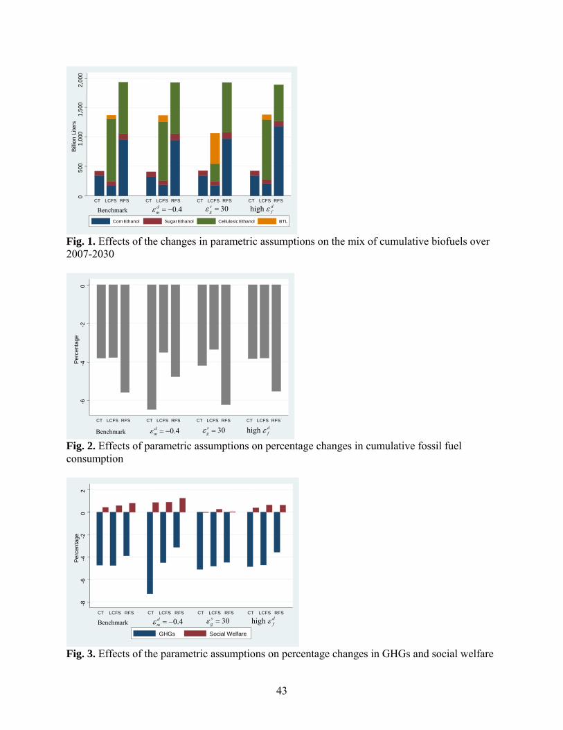
43
Fig. 1. Effects of the changes in parametric assumptions on the mix of cumulative biofuels over 2007-2030
Fig. 2. Effects of parametric assumptions on percentage changes in cumulative fossil fuel consumption
Fig. 3. Effects of the parametric assumptions on percentage changes in GHGs and social welfare
050
01,
000
1,50
02,
000
Bill
ion
Lite
rs
CT LCFS RFS CT LCFS RFS CT LCFS RFS CT LCFS RFS
Corn Ethanol Sugar Ethanol Cellulosic Ethanol BTL
0.4dm 30s
g high dfBenchmark
-6-4
-20
Per
cent
age
CT LCFS RFS CT LCFS RFS CT LCFS RFS CT LCFS RFS
0.4dm 30s
g high dfBenchmark
-8-6
-4-2
02
Per
cent
age
Benchmark
CT LCFS RFS CT LCFS RFS CT LCFS RFS CT LCFS RFS
GHGs Social Welfare
0.4dm 30s
g high df
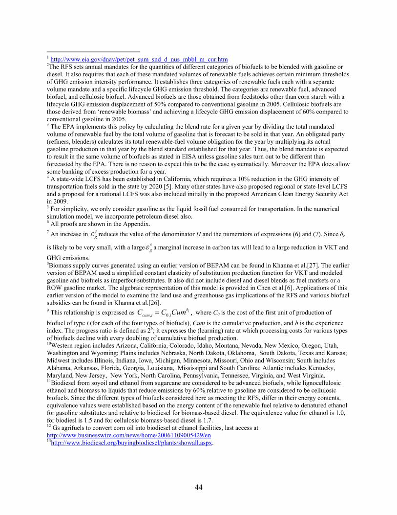
44
1 http://www.eia.gov/dnav/pet/pet_sum_snd_d_nus_mbbl_m_cur.htm 2The RFS sets annual mandates for the quantities of different categories of biofuels to be blended with gasoline or diesel. It also requires that each of these mandated volumes of renewable fuels achieves certain minimum thresholds of GHG emission intensity performance. It establishes three categories of renewable fuels each with a separate volume mandate and a specific lifecycle GHG emission threshold. The categories are renewable fuel, advanced biofuel, and cellulosic biofuel. Advanced biofuels are those obtained from feedstocks other than corn starch with a lifecycle GHG emission displacement of 50% compared to conventional gasoline in 2005. Cellulosic biofuels are those derived from ‘renewable biomass’ and achieving a lifecycle GHG emission displacement of 60% compared to conventional gasoline in 2005. 3 The EPA implements this policy by calculating the blend rate for a given year by dividing the total mandated volume of renewable fuel by the total volume of gasoline that is forecast to be sold in that year. An obligated party (refiners, blenders) calculates its total renewable-fuel volume obligation for the year by multiplying its actual gasoline production in that year by the blend standard established for that year. Thus, the blend mandate is expected to result in the same volume of biofuels as stated in EISA unless gasoline sales turn out to be different than forecasted by the EPA. There is no reason to expect this to be the case systematically. Moreover the EPA does allow some banking of excess production for a year. 4 A state-wide LCFS has been established in California, which requires a 10% reduction in the GHG intensity of transportation fuels sold in the state by 2020 [5]. Many other states have also proposed regional or state-level LCFS and a proposal for a national LCFS was also included initially in the proposed American Clean Energy Security Act in 2009. 5 For simplicity, we only consider gasoline as the liquid fossil fuel consumed for transportation. In the numerical simulation model, we incorporate petroleum diesel also. 6 All proofs are shown in the Appendix. 7 An increase in
sg reduces the value of the denominator H and the numerators of expressions (6) and (7). Since δe
is likely to be very small, with a largesg a marginal increase in carbon tax will lead to a large reduction in VKT and
GHG emissions. 8Biomass supply curves generated using an earlier version of BEPAM can be found in Khanna et al.[27]. The earlier version of BEPAM used a simplified constant elasticity of substitution production function for VKT and modeled gasoline and biofuels as imperfect substitutes. It also did not include diesel and diesel blends as fuel markets or a ROW gasoline market. The algebraic representation of this model is provided in Chen et al.[6]. Applications of this earlier version of the model to examine the land use and greenhouse gas implications of the RFS and various biofuel subsidies can be found in Khanna et al.[26]. 9 This relationship is expressed as , 0, ,ib
cum i iC C Cum where C0 is the cost of the first unit of production of
biofuel of type i (for each of the four types of biofuels), Cum is the cumulative production, and b is the experience index. The progress ratio is defined as 2b; it expresses the (learning) rate at which processing costs for various types of biofuels decline with every doubling of cumulative biofuel production. 10Western region includes Arizona, California, Colorado, Idaho, Montana, Nevada, New Mexico, Oregon, Utah, Washington and Wyoming; Plains includes Nebraska, North Dakota, Oklahoma, South Dakota, Texas and Kansas; Midwest includes Illinois, Indiana, Iowa, Michigan, Minnesota, Missouri, Ohio and Wisconsin; South includes Alabama, Arkansas, Florida, Georgia, Louisiana, Mississippi and South Carolina; Atlantic includes Kentucky, Maryland, New Jersey, New York, North Carolina, Pennsylvania, Tennessee, Virginia, and West Virginia. 11Biodiesel from soyoil and ethanol from sugarcane are considered to be advanced biofuels, while lignocellulosic ethanol and biomass to liquids that reduce emissions by 60% relative to gasoline are considered to be cellulosic biofuels. Since the different types of biofuels considered here as meeting the RFS, differ in their energy contents, equivalence values were established based on the energy content of the renewable fuel relative to denatured ethanol for gasoline substitutes and relative to biodiesel for biomass-based diesel. The equivalence value for ethanol is 1.0, for biodiesl is 1.5 and for cellulosic biomass-based diesel is 1.7. 12 Gs agrifuels to convert corn oil into biodiesel at ethanol facilities, last access at http://www.businesswire.com/news/home/20061109005429/en 13http://www.biodiesel.org/buyingbiodiesel/plants/showall.aspx.

45
References
[1] A.W. Ando, M. Khanna, F. Taheripour, Market and social welfare effect of the renewable fuels standard, in: M. Khanna., J. Scheffran and D. Zilberman (eds.), Handbook of Bioenergy Economics and Policy. Springer Publishers, New York, 2010, pp. 233-250.
[2] R.H. Beach, B.A. McCarl, U.S. Agricultural and forestry impacts of the energy independence and security act: FASOM results and model description, Final Report prepared for U.S. Environmental Protection Agency, RTI International, Research Triangle Park, NC 27709, 2010.
[3] C. Böhringer, T.F. Rutherford, Carbon abatement and international spillovers, Environmental and Resource Economics 22 (2002) 391-417.
[4] M. Brons, P. Nijkamp, E. Pels, P. Rietveld, A meta-analysis of the price elasticity of gasoline demand: a SUR approach, Energy Economics 30 (2008) 2105-2122.
[5] CARB, Proposed regulation to implement the low carbon fuel standard volume I, California Environmental Protection Agency Air Resouces Board : http://www.arb.ca.gov/fuels/lcfs/030409lcfs_isor_vol1.pdf, 2009.
[6] X. Chen, H. Huang, M. Khanna, H. Onal, Meeting the mandate for biofuels: implications for land use and food and fuel prices, Working Paper No. 16697 (http://www.nber.org/papers/w16697), 2011.
[7] C. Crago, M. Khanna, J.B. Barton, W. Amaral, E. Guiliani, Cost competitiveness of sugarcane ethanol in brazil relative to corn ethanol in the US, Energy Policy 38 (2010) 7404-15.
[8] C. Dahl, T. Sterner, Analysing gasoline demand elasticities: a survey, Energy Economics 13 (1991) 203-210.
[9] S.C. Davis, S.W. Diegel, R.G. Boundy, Transportation energy data book: Edition 29, Oak Ridge National Laboratory, Oak Ridge, TN, 2010.
[10] H. de Gorter, D.R. Just, The economics of the U.S. ethanol import tariff with a blend mandate and tax credit, Journal of Agricultural & Food Industrial Organization 6 (2008) 1-21.
[11] DOT, Transportation's role in reducing U.S. greenhouse gas emissions, volume 1: synthesis report, Report to Congress, US Department of Transportation, Center for Climate Change and Environmental Forecasting, Washington, D.C., 2010.
[12] EIA, Annual Energy Outlook 2010: with projections to 2035, U.S. Energy Information Administration, Office of Integrated Analysis and Forecasting, U.S. Department of Energy, Washington, DC, 2010.
[13] EPA, Renewable Fuel Standard program (RFS2) regulatory impact analysis, epa-420-r-10-00, Available on line at http://www.epa.gov/otaq/fuels/renewablefuels/index.htm, US Environmental Protection Agency, Washington, DC, 2010.
[14] M. Espey, Gasoline demand revisited: an international meta-analysis of elasticities, Energy Economics 20 (1998) 273-295.
[15] D. Gately, OPEC’s incentives for faster output growth, Energy Journal 25 (2004) 75-96. [16] D.J. Graham, S. Glaister, Road traffic demand elasticity estimates: a review, Transport Reviews
24 (2004) 261—274. [17] D.L. Greene, S. Ahmad, Costs of U.S. Oil dependence: 2005 update, ornl/tm-2005/45, Oak
Ridge, TN: Oak Ridge National Laboratory 2005. [18] D.L. Greene, N.I. Tishchishyna, Costs of oil dependence: a 2000 update Oak Ridge, TN: Oak
Ridge National Laboratory 2000. [19] J.D. Hamilton, Understanding crude oil prices, The Energy Journal 30 (2009) 179-2006. [20] T.W. Hertel, A.A. Golub, A.D. Jones, M. O’Hare, R.J. Plevin, D.M. Kammen, Effects of US
maize ethanol on global land use and greenhouse gas emissions: estimating market mediated responses, BioScience 60 (3) (2010) 223-231.
[21] T.W. Hertel, W.E. Tyner, D.K. Birur, The global impacts of biofuel mandates, The Energy Journal 31 (2010) 75-100.
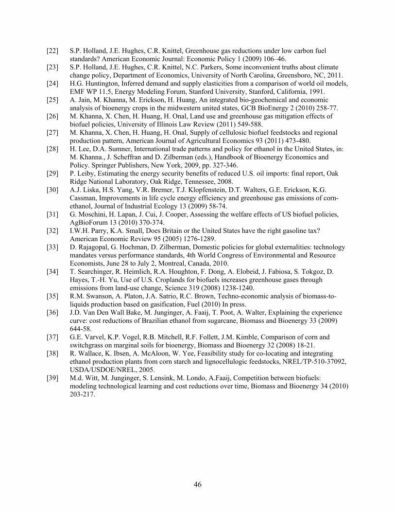
46
[22] S.P. Holland, J.E. Hughes, C.R. Knittel, Greenhouse gas reductions under low carbon fuel standards? American Economic Journal: Economic Policy 1 (2009) 106–46.
[23] S.P. Holland, J.E. Hughes, C.R. Knittel, N.C. Parkers, Some inconvenient truths about climate change policy, Department of Economics, University of North Carolina, Greensboro, NC, 2011.
[24] H.G. Huntington, Inferred demand and supply elasticities from a comparison of world oil models, EMF WP 11.5, Energy Modeling Forum, Stanford University, Stanford, California, 1991.
[25] A. Jain, M. Khanna, M. Erickson, H. Huang, An integrated bio-geochemical and economic analysis of bioenergy crops in the midwestern united states, GCB BioEnergy 2 (2010) 258-77.
[26] M. Khanna, X. Chen, H. Huang, H. Onal, Land use and greenhouse gas mitigation effects of biofuel policies, University of Illinois Law Review (2011) 549-588.
[27] M. Khanna, X. Chen, H. Huang, H. Onal, Supply of cellulosic biofuel feedstocks and regional production pattern, American Journal of Agricultural Economics 93 (2011) 473-480.
[28] H. Lee, D.A. Sumner, International trade patterns and policy for ethanol in the United States, in: M. Khanna., J. Scheffran and D. Zilberman (eds.), Handbook of Bioenergy Economics and Policy. Springer Publishers, New York, 2009, pp. 327-346.
[29] P. Leiby, Estimating the energy security benefits of reduced U.S. oil imports: final report, Oak Ridge National Laboratory, Oak Ridge, Tennessee, 2008.
[30] A.J. Liska, H.S. Yang, V.R. Bremer, T.J. Klopfenstein, D.T. Walters, G.E. Erickson, K.G. Cassman, Improvements in life cycle energy efficiency and greenhouse gas emissions of corn-ethanol, Journal of Industrial Ecology 13 (2009) 58-74.
[31] G. Moschini, H. Lapan, J. Cui, J. Cooper, Assessing the welfare effects of US biofuel policies, AgBioForum 13 (2010) 370-374.
[32] I.W.H. Parry, K.A. Small, Does Britain or the United States have the right gasoline tax? American Economic Review 95 (2005) 1276-1289.
[33] D. Rajagopal, G. Hochman, D. Zilberman, Domestic policies for global externalities: technology mandates versus performance standards, 4th World Congress of Environmental and Resource Economists, June 28 to July 2, Montreal, Canada, 2010.
[34] T. Searchinger, R. Heimlich, R.A. Houghton, F. Dong, A. Elobeid, J. Fabiosa, S. Tokgoz, D. Hayes, T.-H. Yu, Use of U.S. Croplands for biofuels increases greenhouse gases through emissions from land-use change, Science 319 (2008) 1238-1240.
[35] R.M. Swanson, A. Platon, J.A. Satrio, R.C. Brown, Techno-economic analysis of biomass-to-liquids production based on gasification, Fuel (2010) In press.
[36] J.D. Van Den Wall Bake, M. Junginger, A. Faaij, T. Poot, A. Walter, Explaining the experience curve: cost reductions of Brazilian ethanol from sugarcane, Biomass and Bioenergy 33 (2009) 644-58.
[37] G.E. Varvel, K.P. Vogel, R.B. Mitchell, R.F. Follett, J.M. Kimble, Comparison of corn and switchgrass on marginal soils for bioenergy, Biomass and Bioenergy 32 (2008) 18-21.
[38] R. Wallace, K. Ibsen, A. McAloon, W. Yee, Feasibility study for co-locating and integrating ethanol production plants from corn starch and lignocellulogic feedstocks, NREL/TP-510-37092, USDA/USDOE/NREL, 2005.
[39] M.d. Witt, M. Junginger, S. Lensink, M. Londo, A.Faaij, Competition between biofuels: modeling technological learning and cost reductions over time, Biomass and Bioenergy 34 (2010) 203-217.

47
Appendix 1: Comparative Static Analysis of a Carbon Tax
Totally differentiating (2) to (4) and f e L , we get 2 '' '' 2 ''
2 '' 2 2 ''
''
0( ) 0 0
00 1.
00 0 1 0
10 1 1 0 0
gmm mm
emm mm
ff
dgr U c g r Udtder U r U
dfU d L
d
2 '' '' 2 ''
2 '' 2 2 ''2 '' '' '' '' 2 2 ''
''
( ) 0 0
0 1( ( )) ( ) 0
0 0 1
0 1 1 0
mm mm
mm mmmm ff mm
ff
r U c g r U
r U r UH r U c g U c g r U
U
2 ''
2 2 ''2
''
0 0
0 11 1{ ( )}
0 0 1
0 1 1 0
g mm
fe mm mg g ed d
f mff
r U
pr U pdgr
dt H H f mU
(A1.1)
Because we assume g e , we know 0dg
dt .
2 '' ''
2 '' 2 2'
''
( ) 0 0
0 11 1 ( ){ ( ) }
0 0 1
0 0 1 0
mm g
mm e m me gd s d
m g mff
r U c g
r U r p r pde c g
dt H H m g mU
(A1.2)
It is straightforward to showdf de
dt dt (A1.3)
and f
df
pd de
dt f dt
(A1.4)
2 2 ' 2
2( )1{ ( ) } 0g f e m
g e g ed s df g m
p c g r pdGHG dg de
dt dt dt H f g m
(A1.5)
' ( )[ ] 0g f e
d sf g
p c gdm r
dt H f g
(A1.6)
Appendix 2: Comparative Static Analysis of a Biofuel Consumption Mandate
Totally differentiating (5) and (10) and combining 0L f e , we get 2 ''2 '' ''
''
( ) 0 0 0
0 1 . 0 0
0 1 0 1 1
mmmm
ff
r Ur U c g dgde
U dfd Ld
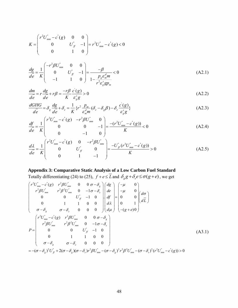
48
2 '' ''
'' 2 '' ''
( ) 0 0
0 1 ( ) 0
0 1 0
mm
ff mm
r U c g
K U r U c g
2 ''
''
2
0 01
0 1 0
1 1 0 1
mm
ff dg m
sg m
r Udg
Up mKde
r gp
(A2.1)
' ( )0
sg
dm dg r c gr r
K gde de
(A2.2)
'21 ( )
{ ( ) }mg e e g ed s
m g
pdGHG dg c gr
K m gde de
(A2.3)
2 '' '' 2 ''
2 '' ''( ) 0
( ( ))10 0 1 0
0 1 0
mm mm
mm
r U c g r Ur U c gdf
K Kde
(A2.4)
2 '' '' 2 '''' 2 '' ''
''
( ) 0( ( ))1
0 0 0
0 1 1
mm mmff mm
ff
r U c g r UU r U c gd
UK Kde
(A2.5)
Appendix 3: Comparative Static Analysis of a Low Carbon Fuel Standard Totally differentiating (24) to (25), f e L and ( )g eg e g e , we get
2 '' '' 2 ''
2 '' 2 2 ''
''
0( ) 0 0
00 1
. 0 00 0 1 0
0 1 0 0 1 1 0
( )000 0
mm mm g
mm mm e
ff
g e
dgr U c g r U
der U r Ud
dfUd L
d
d g e
2 '' '' 2 ''
2 '' 2 2 ''
''
2 '' 2 '' 2 2 2 '' 2 2 '' ''
( ) 0 0
0 1
0 0 1 0
0 0 1 1 0
00 0
( ) 2( )( ) ( ) ( ) ( ( )) 0
mm mm g
mm mm e
ff
g e
g ff g e mm g mm e mm
r U c g r U
r U r U
P U
U r U r U r U c g
(A3.1)
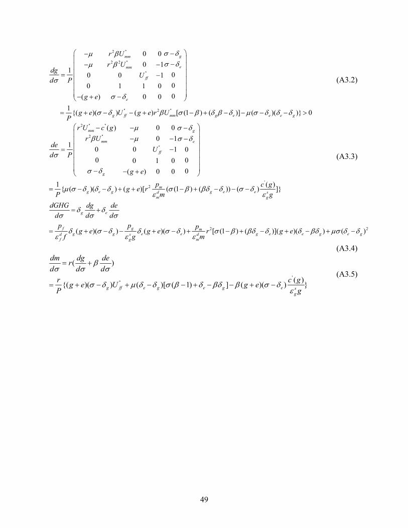
49
2 ''
2 2 ''
''
'' 2 ''
0 0
0 11
00 0 1
0 1 0 1 0
0( ) 0 0
1 {( )( ) ( ) [ (1 ) ( )] ( )( )} 0
gmm
emm
ff
e
g ff mm g e e e g
r U
r Udg
Ud P
g e
g e U g e r UP
(A3.2)
2 '' ''
2 ''
''
'2
( ) 0 0
0 11
0 0 1 0
0 0 0 1 0
0( ) 0 0
1 ( ){ ( )( ) ( )[ ( (1 ) ( )) ( ) ]}
mm g
mm e
ff
g
mg e g g e ed s
m g
r U c g
r Ude
Ud P
g e
p c gg e r
P m g
(A3.3)
2 2( )( ) ( )( ) [ (1 ) ( )]( )( ) ( )
g e
f g mg g e e g e e g e gd s d
f g m
dGHG dg de
d d d
p p pg e g e r g e
f g m
(A3.4)
'''
( )
( ){( )( ) ( )[ ( 1) ] ( )( ) }g ff e g e g e s
g
dm dg der
d d d
r c gg e U g e
P g
(A3.5)
Related Documents