Alignment Introduction Notes courtesy of Funk et al., SIGGRAPH 2004.

Alignment

Introduction

Notes courtesy of Funk et al., SIGGRAPH 2004

Outline:• Challenge

• General Approaches

• Specific Examples

Alignment

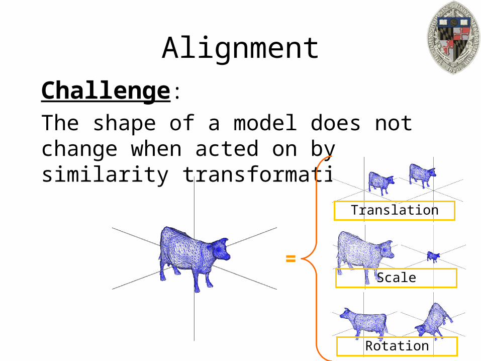
Challenge:

The shape of a model does not change when acted on by similarity transformations:

=Scale

Rotation

Translation

AlignmentChallenge:However, the shape descriptors can change if a the model is:

– Translated

– Scaled

– Rotated

How do we match shape descriptors across transformations that do not change the shape of a model?

Outline:• Challenge

• General Approaches

• Specific Examples

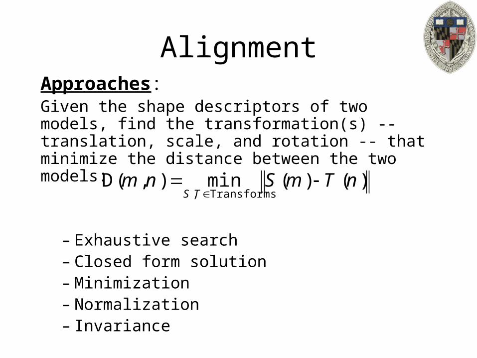
AlignmentApproaches:Given the shape descriptors of two models, find the transformation(s) -- translation, scale, and rotation -- that minimize the distance between the two models:

– Exhaustive search– Closed form solution– Minimization – Normalization– Invariance

)()(min),(DTransforms,

nTmSnmTS

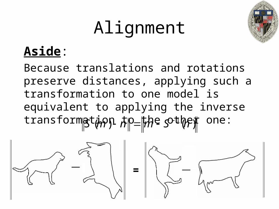
AlignmentAside:Because translations and rotations preserve distances, applying such a transformation to one model is equivalent to applying the inverse transformation to the other one:

)()( 1 nSmnmS

=

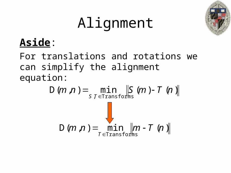
AlignmentAside:For translations and rotations we can simplify the alignment equation:

)()(min),(DTransforms,

nTmSnmTS

)(min),(DTransforms

nTmnmT

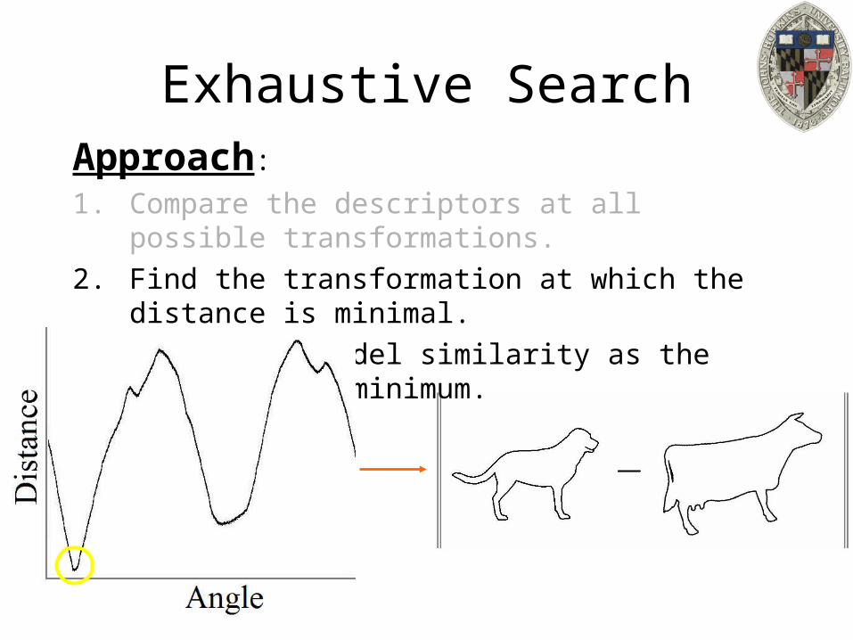
Exhaustive SearchApproach:

1. Compare the descriptors at all possible transformations.

2. Find the transformation at which the distance is minimal.

3. Define the model similarity as the value at the minimum.

Exhaustive SearchApproach:

1. Compare the descriptors at all possible transformations.

2. Find the transformation at which the distance is minimal.

3. Define the model similarity as the value at the minimum.

Exhaustive search for optimal rotation

Exhaustive SearchApproach:

1. Compare the descriptors at all possible transformations.

2. Find the transformation at which the distance is minimal.

3. Define the model similarity as the value at the minimum.

Exhaustive Search

Properties:

Always gives the correct answer Needs to be performed at run-time and can be

very slow to compute:Computes the measure of similarity for every transform. We only need the value at the best one.

Closed Form SolutionApproach:

Explicitly find the transformation(s) that solves the equation:

Properties:

Always gives the correct answer Only compute the measure of similarity for the best

transformation. A closed form solution does not always exist. Often needs to be computed at run-time.

)()(min),(DTransforms,

nTmSnmTS

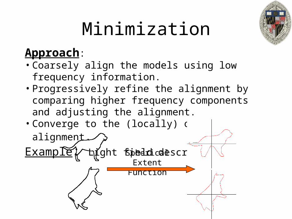
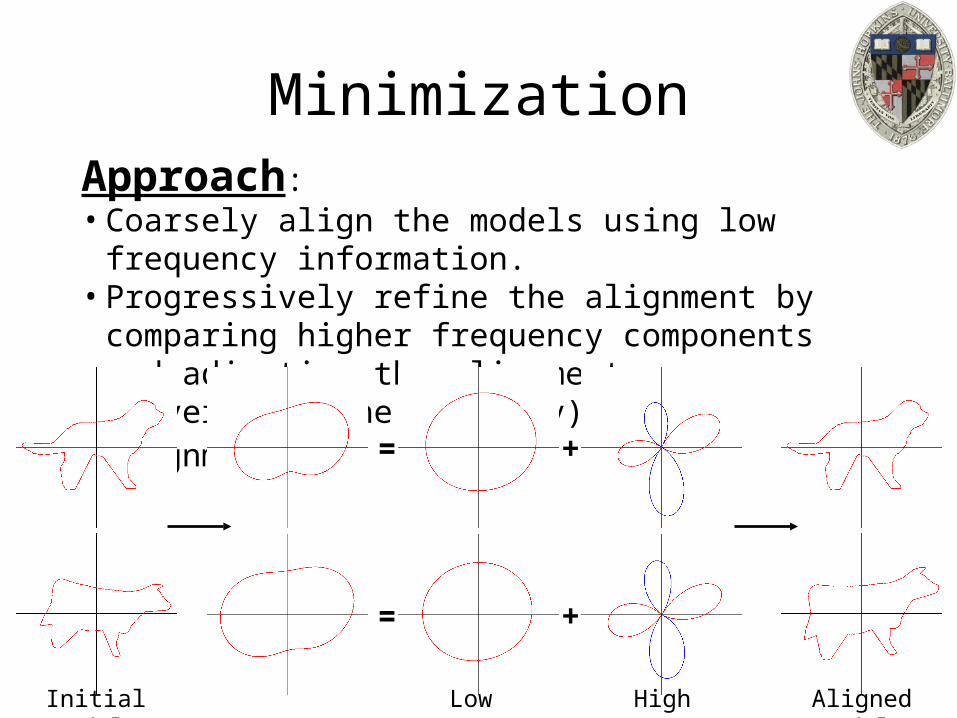
MinimizationApproach:• Coarsely align the models using low frequency information.• Progressively refine the alignment by comparing higher

frequency components and adjusting the alignment.• Converge to the (locally) optimal alignment.Example: Light field descriptors

Spherical Extent Function

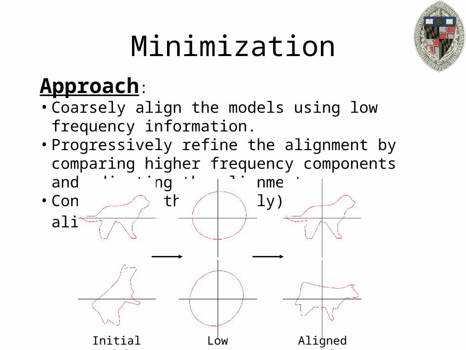
MinimizationApproach:• Coarsely align the models using low frequency information.• Progressively refine the alignment by comparing higher

frequency components and adjusting the alignment.• Converge to the (locally) optimal alignment.

Initial Models Low Frequency Aligned Models

MinimizationApproach:• Coarsely align the models using low frequency information.• Progressively refine the alignment by comparing higher

frequency components and adjusting the alignment.• Converge to the (locally) optimal alignment.

=

= +

+

Initial Models Low Frequency Aligned ModelsHigh Frequency

Minimization

Properties:

Can be applied to any type of transformation Needs to be computed at run-time. Difficult to do robustly:

Given the low frequency alignment and the computed high-frequency alignment, how do you combine the two?

Considerations can include:• Relative size of high and low frequency info

• Distribution of info across the low frequencies

• Speed of oscillation

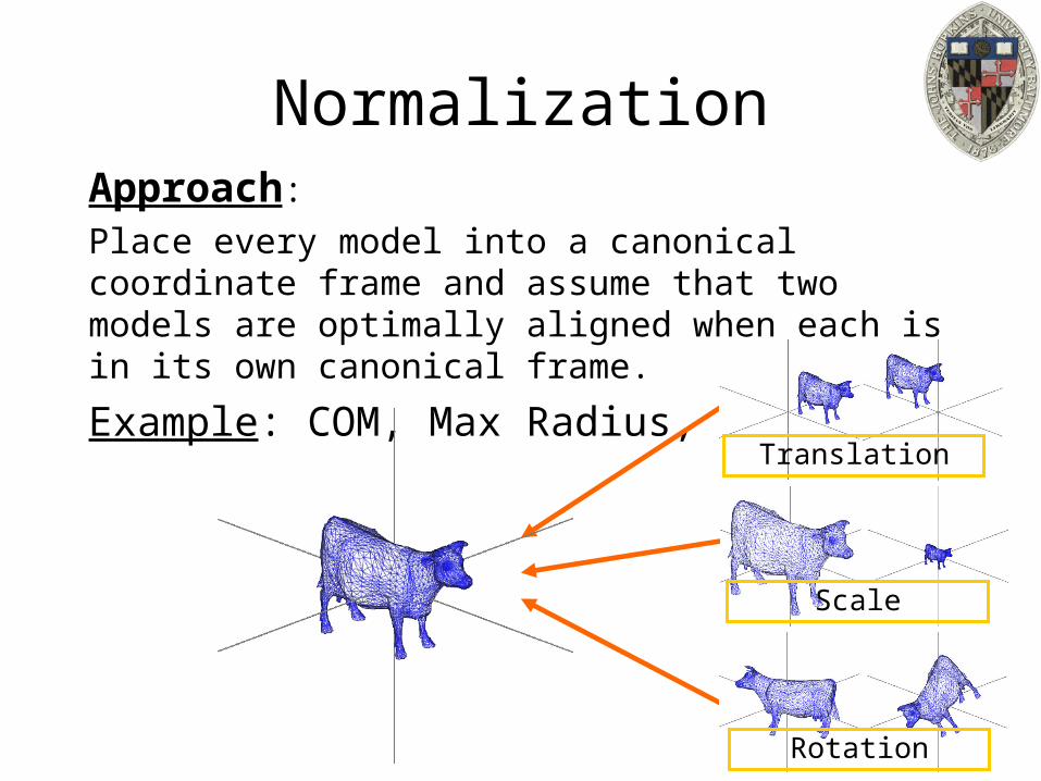
NormalizationApproach:

Place every model into a canonical coordinate frame and assume that two models are optimally aligned when each is in its own canonical frame.

Example: COM, Max Radius, PCA

Scale

Rotation

Translation

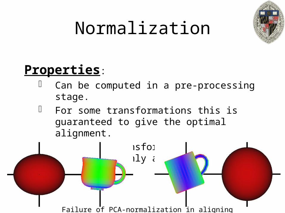
Normalization

Properties: Can be computed in a pre-processing stage. For some transformations this is guaranteed to give

the optimal alignment. For other transformations the approach is only a

heuristic and may fail.

Failure of PCA-normalization in aligning rotations

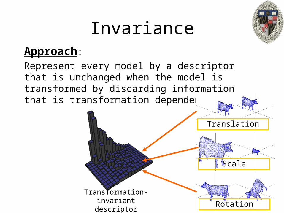
InvarianceApproach:

Represent every model by a descriptor that is unchanged when the model is transformed by discarding information that is transformation dependent.

Scale

Rotation

Translation

Transformation-invariant descriptor

InvarianceReview:

Is there a general method for addressing these basic types of transformations?

Descriptor Translation Scale RotationShape Distributions (D2) + - +Extended Gaussian Images + - -Shape Histograms (Shells) - - +Shape Histograms (Sectors) - + -Spherical Parameterizations + - -

Invariance

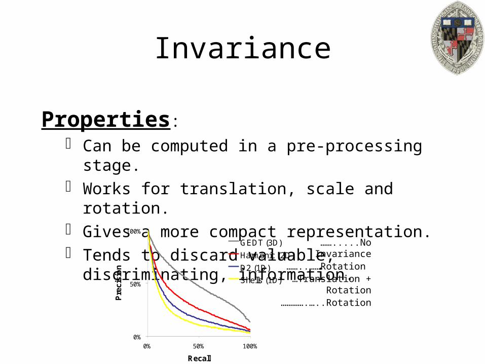
Properties: Can be computed in a pre-processing stage. Works for translation, scale and rotation. Gives a more compact representation.Tends to discard valuable, discriminating, information.

0%

50%

100%

0% 50% 100%

Recall

Precision

GEDT (3D)

Harmonic (2D)

D2 (1D)

Shells (1D)

…….....No Invariance……..……Rotation

…Translation + Rotation………….…..Rotation

Outline:• Challenge

• General Approaches

• Specific Examples– Normalization: PCA– Closed Form Solution: Ordered Point Sets

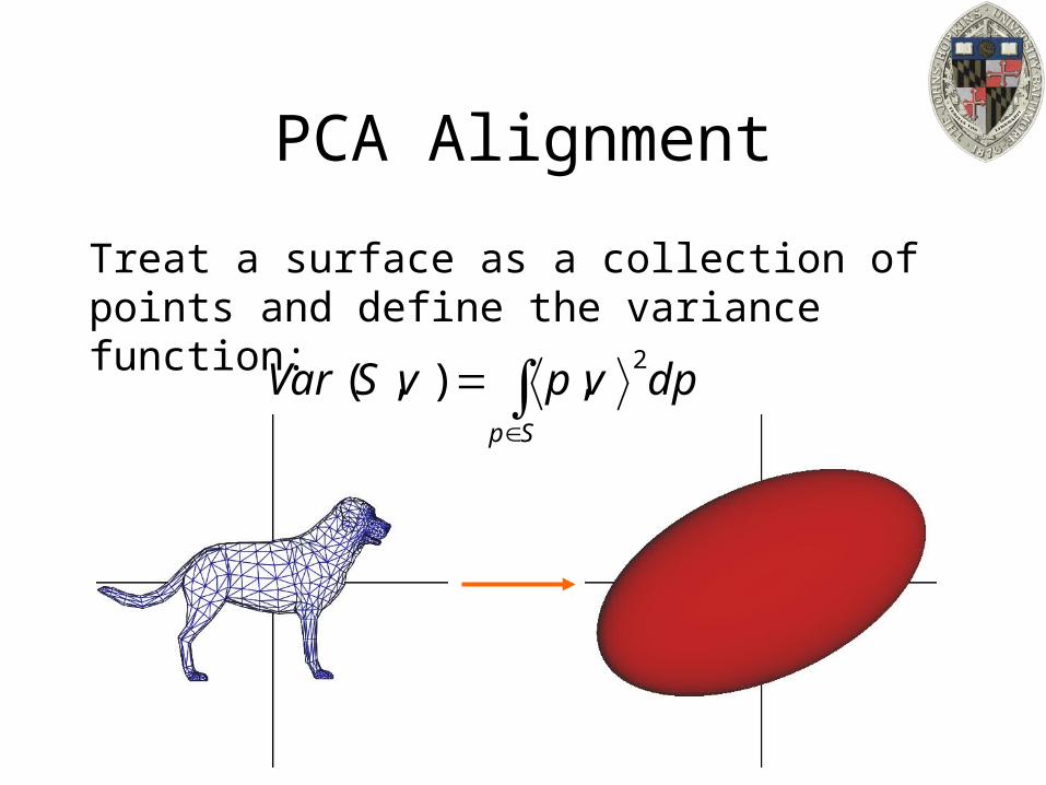
PCA Alignment

Treat a surface as a collection of points and define the variance function:

Sp

dpvpvSVar2

,),(

PCA Alignment

Define the covariance matrix M:

Find the eigen-values and align so that the eigen-values map to the x-, y-, and z-axes

Sp

jiij dpppM

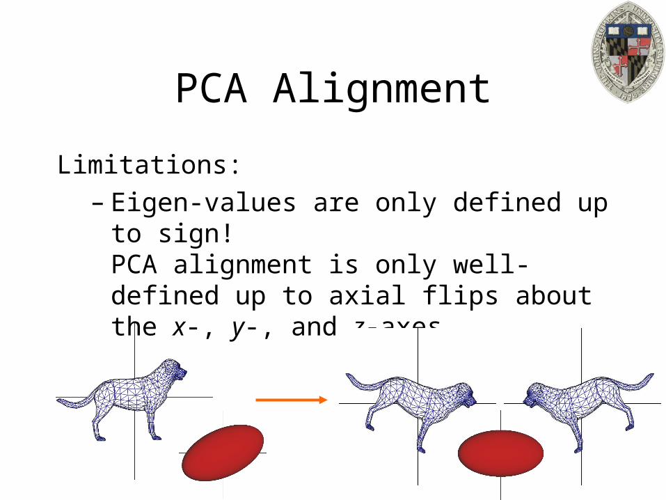
PCA Alignment

Limitations:– Eigen-values are only defined up to sign!

PCA alignment is only well-defined up to axial flips about the x-, y-, and z-axes.

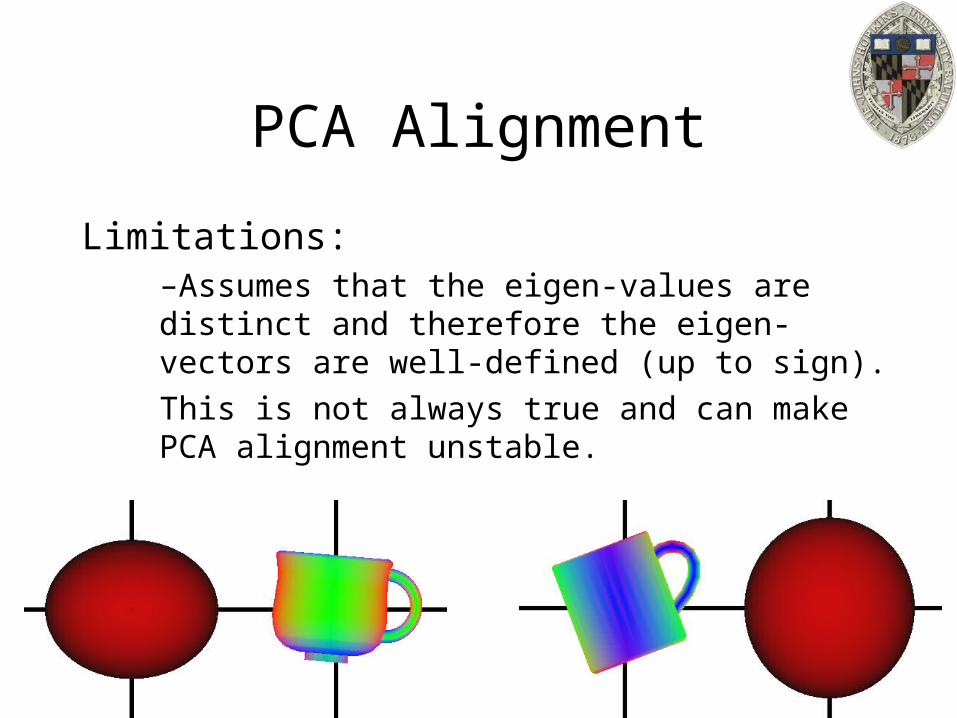
PCA Alignment

Limitations:–Assumes that the eigen-values are distinct and therefore the eigen-vectors are well-defined (up to sign).

This is not always true and can make PCA alignment unstable.

Outline:• Challenge

• General Approaches

• Specific Examples– Normalization: PCA– Closed Form Solution: Ordered Point Sets

Ordered Point Sets

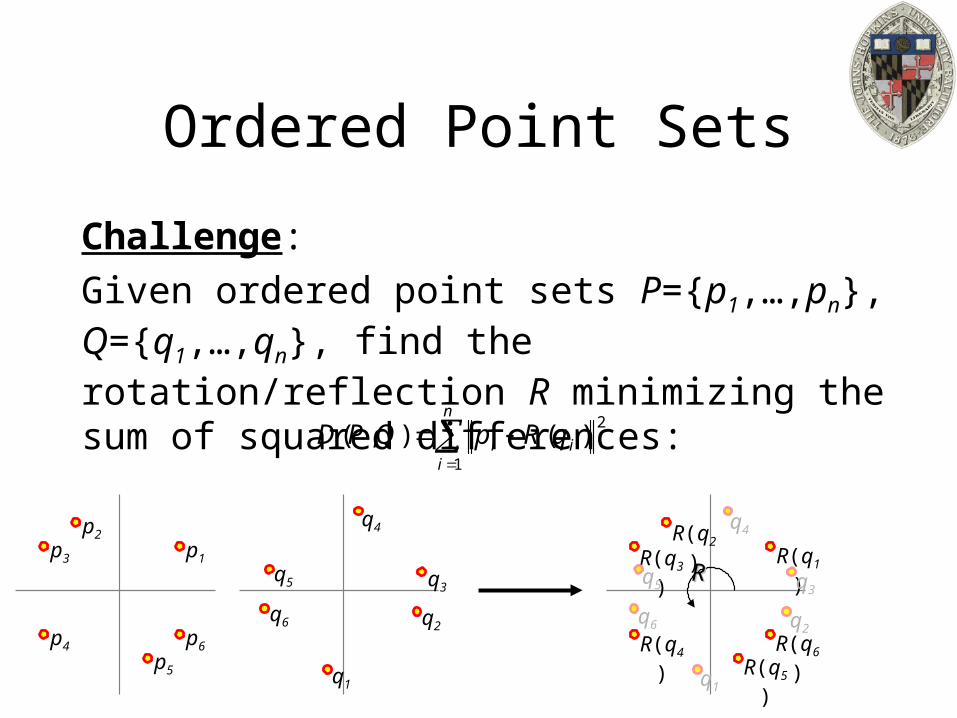
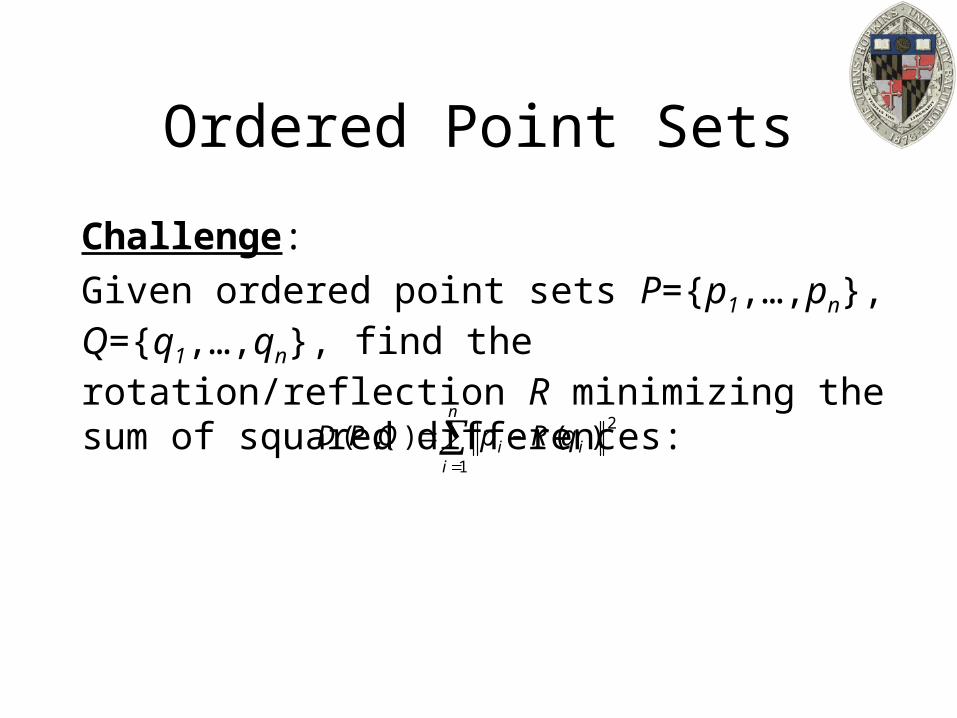
Challenge:

Given ordered point sets P={p1,…,pn}, Q={q1,…,qn}, find the rotation/reflection R minimizing the sum of squared differences:

n

iii qRpQPD

1

2)(),(

p1p2

p3

p4p5

p6

q1

q2

q3

q4

q5

q6

R(q2)R(q1)R(q3)

R(q4)R(q5)

R(q6)

q1

q2

q3

q4

q5

q6

RR

Review

Vector dot-product:

If v =(v1,…,vn) and w=(w1,…,wn) are two n-dimensional vectors the dot-product of v with w is the sum of the product of the coefficients:

n

iiiwvv,w

1

Review

Trace:

The trace of a nxn matrix M is the sum of the diagonal entries of M:

Properties:–

–

n

iiiMM

1,Trace

)(NMMN TraceTrace )( tMM TraceTrace

Review

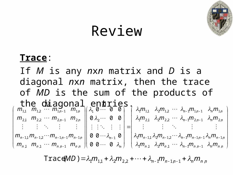
Trace:

If M is any nxn matrix and D is a diagonal nxn matrix, then the trace of MD is the sum of the products of the diagonal entries.

nnnnnnnn

nnnnnnnn

nnnn

nnnn

n

n

nnnnnn

nnnnnn

nn

nn

mmmm

mmmm

mmmm

mmmm

mmmm

mmmm

mmmm

mmmm

,1,11,21,1

,11,112,121,11

,21,212,221,21

,11,112,121,11

1

2

1

,1,1,1,

,11,12,11,1

,21,22,21,2

,11,12,11,1

000

000

000

000

nnnnnn mmmmMD ,1,112,221,11)( Trace

M D

Review

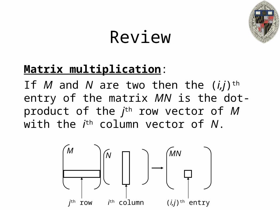
Matrix multiplication:

If M and N are two then the (i,j)th entry of the matrix MN is the dot-product of the jth row vector of M with the ith column vector of N.

MN

jth row ith column

MN

(i,j)th entry

Review

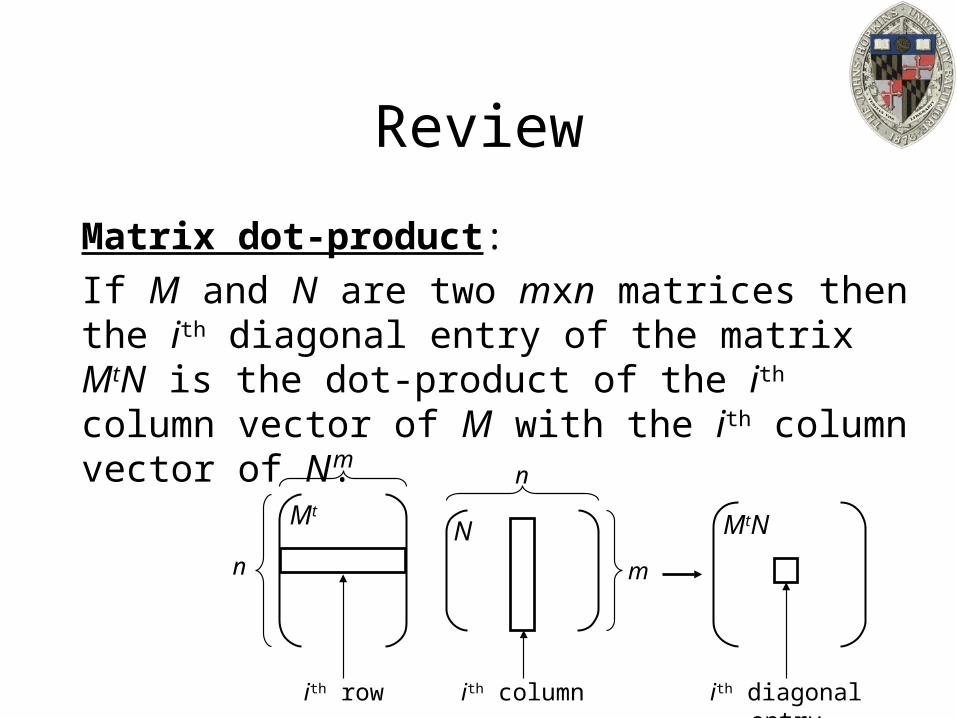
Matrix dot-product:

If M and N are two mxn matrices then the ith diagonal entry of the matrix MtN is the dot-product of the ith column vector of M with the ith column vector of N.

Mt

N

ith row ith column

mn

nm

MtN

ith diagonal entry

Review

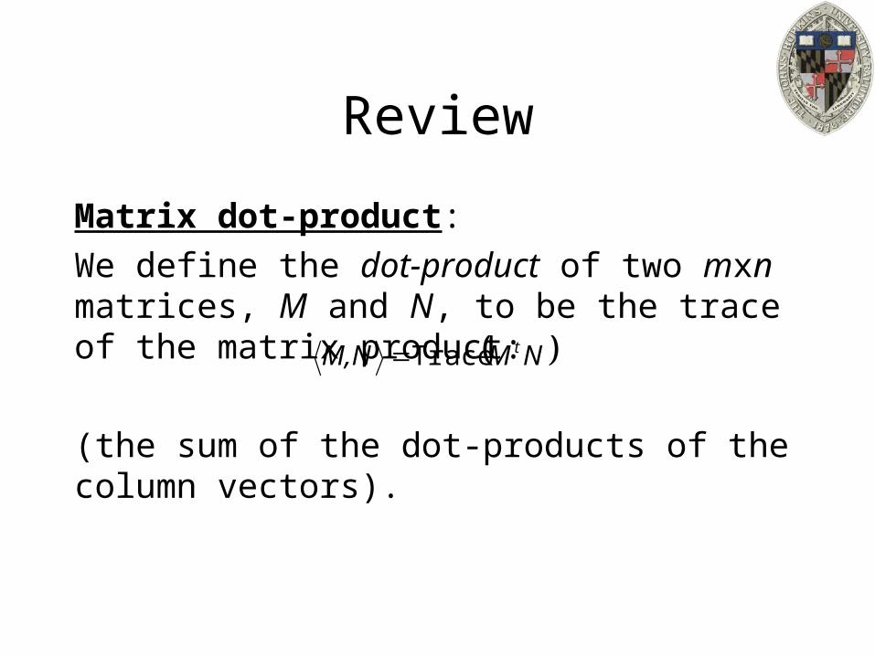
Matrix dot-product:

We define the dot-product of two mxn matrices, M and N, to be the trace of the matrix product:

(the sum of the dot-products of the column vectors).

NMM,N tTrace

Review

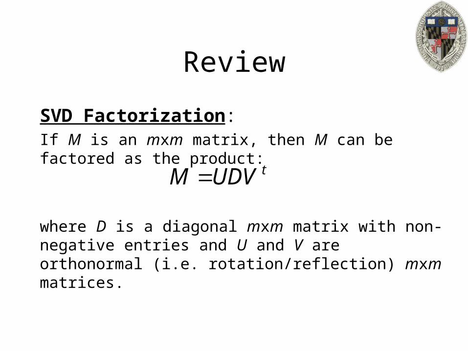
SVD Factorization:If M is an mxm matrix, then M can be factored as the product:

where D is a diagonal mxm matrix with non-negative entries and U and V are orthonormal (i.e. rotation/reflection) mxm matrices.

tUDVM

Trace Maximization

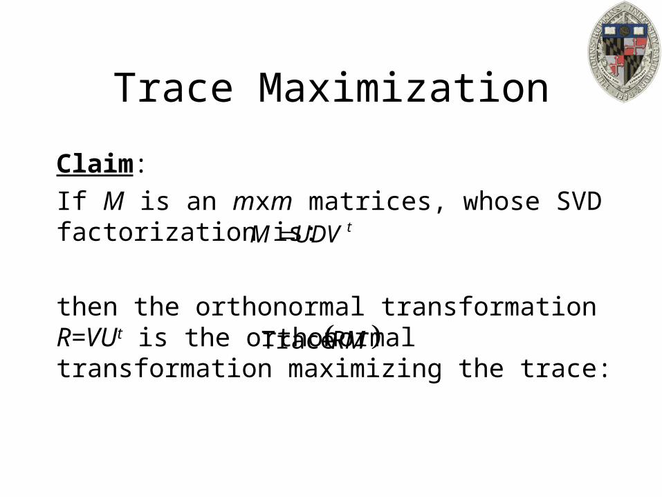
Claim:

If M is an mxm matrices, whose SVD factorization is:

then the orthonormal transformation R=VUt is the orthonormal transformation maximizing the trace:

tUDVM

RMTrace

Trace Maximization

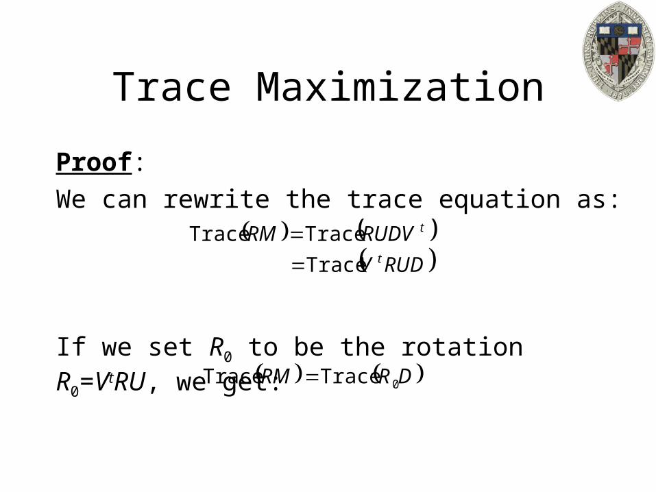
Proof:

We can rewrite the trace equation as:

If we set R0 to be the rotation R0=VtRU, we get:

RUDV

RUDVRMt

t

Trace

TraceTrace

DRRM 0TraceTrace

Trace Maximization

Proof:

Since R0 is a rotation, each of its entries can have value no larger than one.

Since D is diagonal, the value of the trace is the product of the diagonal elements of D and R0.

DRRM 0TraceTrace

Trace Maximization

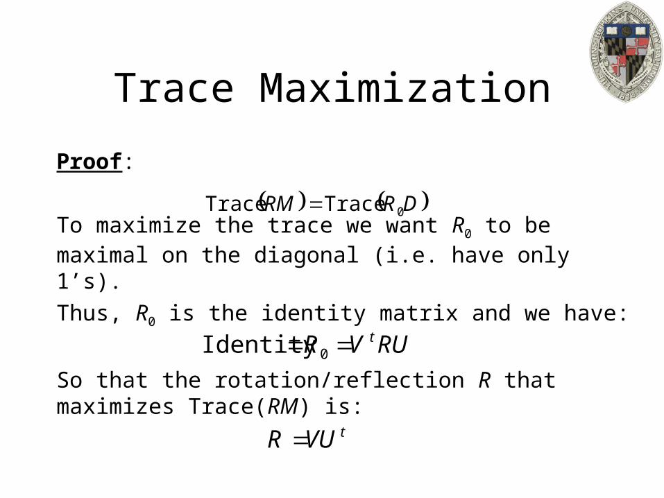
Proof:

To maximize the trace we want R0 to be maximal on the diagonal (i.e. have only 1’s).

Thus, R0 is the identity matrix and we have:

So that the rotation/reflection R that maximizes Trace(RM) is:

DRRM 0TraceTrace

RUVR t 0Identity

tVUR

Ordered Point Sets

Challenge:

Given ordered point sets P={p1,…,pn}, Q={q1,…,qn}, find the rotation/reflection R minimizing the sum of squared differences:

n

iii qRpQPD

1

2)(),(

Ordered Point Sets

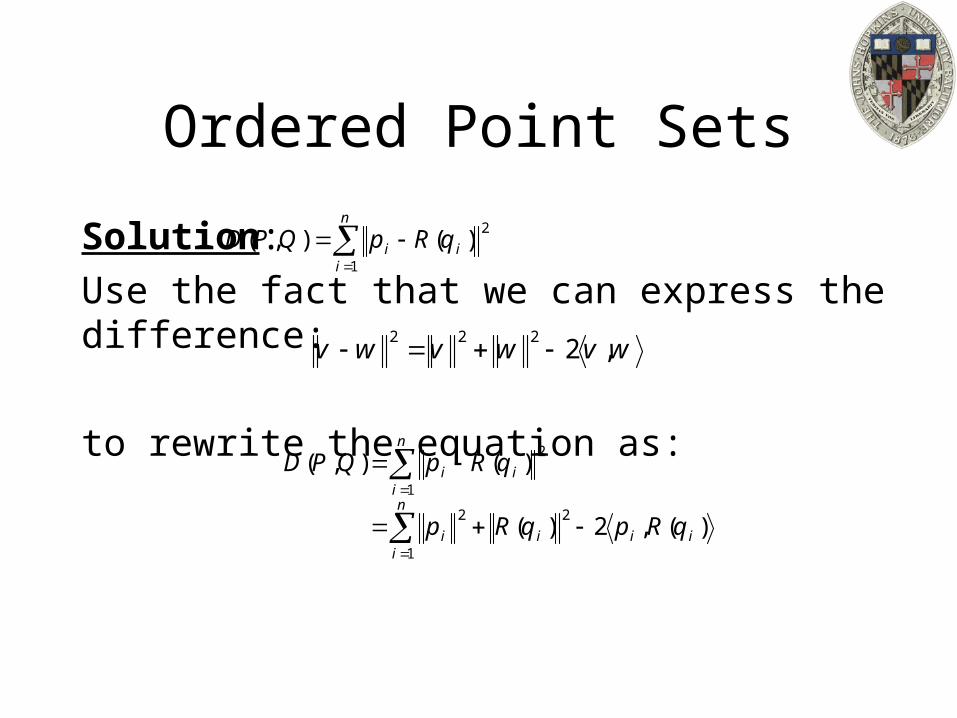
Solution:

Use the fact that we can express the difference:

to rewrite the equation as:

wvwvwv ,2222

n

iiiii

n

iii

qRpqRp

qRpQPD

1

22

1

2

)(,2)(

)(),(

n

iii qRpQPD

1

2)(),(

Ordered Point Sets

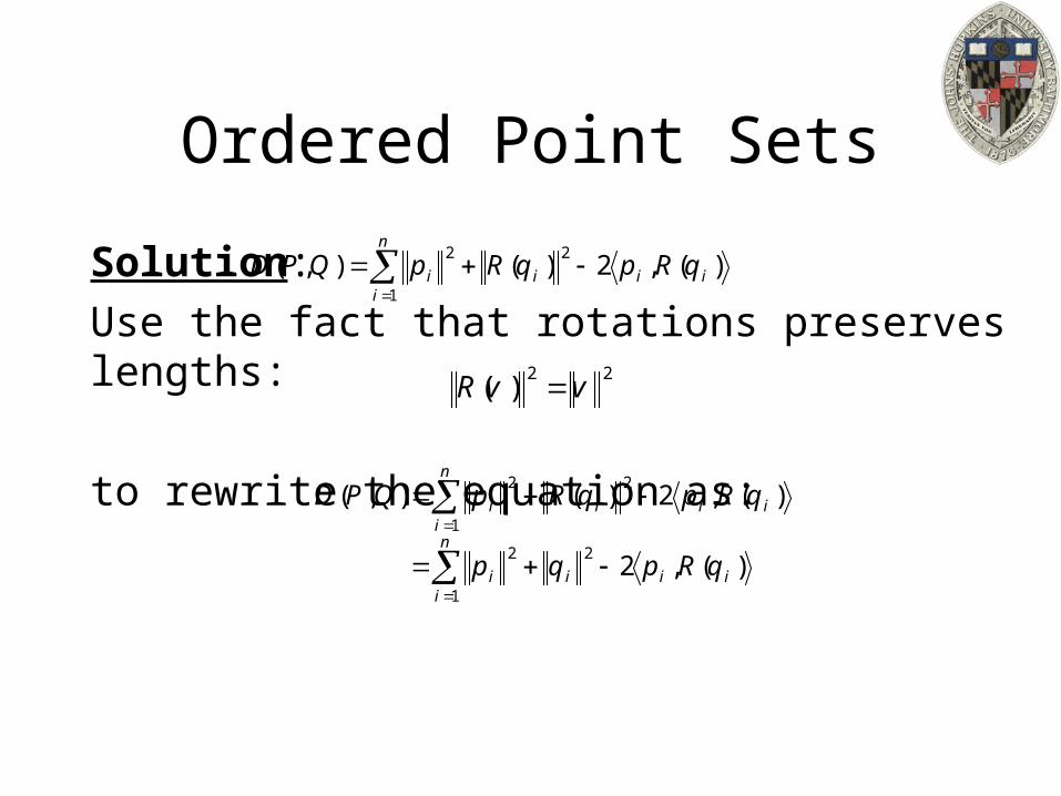
Solution:

Use the fact that rotations preserves lengths:

to rewrite the equation as:

22)( vvR

n

iiiii

n

iiiii

qRpqp

qRpqRpQPD

1

22

1

22

)(,2

)(,2)(),(

n

iiiii qRpqRpQPD

1

22)(,2)(),(

Ordered Point Sets

Solution:

Since the value:

Does not depend on the choice of rotation R, minimizing the sum of squared distances is equivalent to maximizing the sum of dot-products:

n

iii qp

1

22

n

iii qRp

1

)(,

n

iiiii qRpqpQPD

1

22)(,2),(

Ordered Point Sets

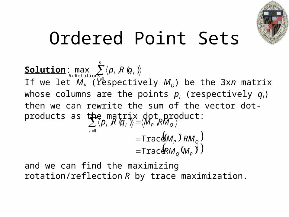
Solution:

If we let MP (respectively MQ) be the 3xn matrix whose columns are the points pi (respectively qi) then we can rewrite the sum of the vector dot-products as the matrix dot product:

and we can find the maximizing rotation/reflection R by trace maximization.

tPQ

Qt

P

QP

n

iii

MRM

RMM

RMMqRp

Trace

Trace

,)(,1

n

iii

RqRp

1

)(,maxRotations