07-058 Copyright © 2007 by Santiago Kraiselburd and Noel Watson, revised May 2007 Working papers are in draft form. This working paper is distributed for purposes of comment and discussion only. It may not be reproduced without permission of the copyright holder. Copies of working papers are available from the author. Alignment in Cross-Functional and Cross-Firm Supply Chain Planning Santiago Kraiselburd* Noel Watson** *Instituto de Empresa, Zaragoza, Spain [email protected] **Harvard Business School, Boston, MA 02163-1010 [email protected]

Welcome message from author
This document is posted to help you gain knowledge. Please leave a comment to let me know what you think about it! Share it to your friends and learn new things together.
Transcript

07-058
Copyright © 2007 by Santiago Kraiselburd and Noel Watson, revised May 2007
Working papers are in draft form. This working paper is distributed for purposes of comment and discussion only. It may not be reproduced without permission of the copyright holder. Copies of working papers are available from the author.
Alignment in Cross-Functional and Cross-Firm Supply Chain Planning
Santiago Kraiselburd* Noel Watson**
*Instituto de Empresa, Zaragoza, Spain [email protected] **Harvard Business School, Boston, MA 02163-1010 [email protected]
Alignment in Cross-Functional and Cross-Firm Supply ChainPlanning
Santiago Kraiselburd • Noel Watson
Instituto de Empresa, and MIT Zaragoza International Logistics Program, Zaragoza LogisticsCenter, Avda Gomez Laguna 25, 1 o Planta, 50009 Zaragoza, Spain
Harvard Business School, Soldiers Field Road, Boston, MA 02163
[email protected] • [email protected]
May 31, 2007
In this paper, we seek to use quantitative models to help appreciate the behavioral processesassociated with successful cross-functional and cross-firm alignment in supply/demand planning.We model the interaction between a sales and a manufacturing function within a firm, or betweenan upstream and downstream firm. We claim that misalignment is costly both to the involvedfunctions/firms and to the rest of the organization or supply chain, and focus the paper on studyingthe circumstances under which alignment will or will not happen. Using game theory, we find that,although misaligned economic incentives can play a role in explaining misalignment of planningbehaviors, there is another important issue to consider: in our setting, the key factor that determineswhether two functions or firms can align their planning is how much each party knows about theother’s beliefs about demand. Thus, in this paper’s setting, improved communication can inducealignment even if no economic incentives are changed. While consistent with the predominantview in organizational behavior (OB), this is a fundamental departure from the extant operationsmanagement (OM) literature.
1 Introduction
Until now, the existence of misalignment in inventory decisions across different firms within a supply
chain has been mostly attributed in the operations management (OM) academic literature to the
presence of misaligned economic incentives (Cachon 2001). A similar reasoning has been applied
in this literature to the study of decentralized but vertically integrated firms (Lee and Whang
1999). One reason why decentralized but vertically integrated firms can suffer alignment problems
similar to the ones observed across firms is that, within many organizations, the administration of
its customer-facing and supplier-facing sides are separated in distinct functional groups. Managing
such groups so as to minimize mismatches and thus create and capture value is a cross-functional
effort requiring integration of the differentiated functions (Lawrence and Lorsch 1986). However,
this specialization or differentiation is notorious for generating conflicts in organizations (Shapiro
1977; Fawcett and Magnan 2002; Kahn and Mentzer 1996). As an example of this intrafirm focus
1
in OM, the coordination of manufacturing (production) and marketing (sales) for forecasting and
inventory decisions by direct incentive design has been given much prominence (Chen 2005).
However, the changing of incentives either within or between organizations can be difficult
and costly to accomplish. Although this fact has not been explicitly considered in most of the
extant OM literature, it has been part of the academic debate in economics for some time. For
example, Coase (1937), Klein, Crawford and Alchian (1978), Williamson (1978), and others have
pointed out that the design and enforcement of contracts and incentives has a cost (which may
differ depending on whether the two parties are within or between firms). In addition to this cost,
a high potential for unintended consequences makes companies cautious, and sometimes reluctant,
to make such incentive changes. Recent case studies and practitioner accounts provide evidence,
however, that some organizations manage to achieve an aligned planning and execution of the
customer- and supplier- facing sides of the organization without wholesale change in incentives
(Lapide 2004a, 2004b, 2005; Oliva and Watson 2007). In fact, gains from supply chain improvement
and performance have been posited and empirically shown to be linked to a much broader but more
difficult degree of integration which goes beyond incentive alignment (Stank et. al. 1999; Stank et.
al. 2001; Shapiro 1998 and Barratt 2004).
Within the quantitative modeling literature, the need for this more elusive, broader-reaching
integration has grown out of recognition that both the customer- and supplier-facing sides of the
organization or supply chain can be simultaneously influenced and planned resulting in improved
performance (Lee 2004). The OM academic literature by and large has reflected practice in studying
the demand and supply sides of the organization independently (Federgruen and Heching 1999).
Although the trend is reversing given the increased focus on modeling integrated production and
pricing decisions (Chen et. al. 2006; Eliashberg and Steinberg 1991; Yano and Gilbert 2004), a
clear understanding of the behavioral processes and systems that are associated with successful
interdepartmental and inter-firm integration has not been established (Griffin and Hauser 1996;
Kahn 1996; Kahn and Mentzer 1998).
We seek, then, to use quantitative models to help appreciate the behavioral processes associ-
ated with successful cross-functional and cross-firm integration in supply/demand planning. As in
Oliva and Watson (2007), we operationalize this integration as “alignment” which we define as a
congruence in the activities or actions taken in anticipation of demand across functions or firms.
By this we mean, for example, that in an organization the sales function and manufacturing group
work towards the same target for the sales of a particular product and respectively create/facilitate
the requisite demand and supply so that the target is met. Note that alignment as defined here
2

is different from what the OM contract theory papers usually call “coordination” or “first-best,”
which would be a global maximum or minimum along some objective for the firm/supply chain.
We do not necessarily define this alignment or operationalize this integration as achieving first-best
performance (Chen; and Porteus and Whang 1991), but rather focus on alignment as an objective
per se, even if it was “suboptimal”. The distinction here is a subtle but important one. We claim
that misalignment can be so costly, that even alignment of plans (and capacities) at a level that is
not optimal with respect to the “true” distribution of demand can be better than a misalignment
of plans (and capacities) centered around the “true” demand distribution. Since this goes against
over 20 years of tradition in research around coordinating systems, we are obligated to make a case
for this alternative objective which we attempt as follows.
Let us start by pointing out that the cross-functional/firm context for planning is a complex
one implying that optimization as a goal may be behaviorally unrealistic. If this is true, then
alignment, even if considered as a “second-best” objective, can still provide powerful benefits to
the organization/supply chain. Recall that, as mentioned earlier, most organizations are primarily
functional and the customer-facing and supplier-facing sides of the supply chain are usually man-
aged separately by different functions or groups of functions. The complexity of administrating
either of these sides, and the specific set of skills required to do so, drives the differentiation into
functional groups within the organization, or into different firms within the supply chain. The very
same motives that drive this differentiation, however, drive difficulties in the communication and
collaboration needed for integrated performance (Lawrence and Lorsch 1986) creating conflicts.
These conflicts generally center around differing expectations about both demand and supply, and
differing functional/organizational preferences and priorities that can result in mismatches between
the capacities invested to meet planned demand and the required planned supply of the organiza-
tion. Now, true optimization requires the appropriate trade-off of valid priorities of the organization
based on appropriate assessment of risks and cost. The extraction and assessment of such valid
and appropriate priorities, risks and costs (if they at all can be extracted and assessed) would be
similarly compromised by the just described cross-functional/firm context.
We therefore propose alignment as an alternative and argue for its appeal mainly because it
can yield two important benefits. First, as action plans become credible and accurate statements
of organizational intentions (which is more likely to happen if actions are aligned), the organi-
zation’s reputation grows in the eyes of customers, suppliers, employees, and investors, affording
powerful leverage through trusted relationships (Kreps 1986). For economist David Kreps (1986),
corporate culture is the means to achieve a set of principles upon which reputations can be built,
3
and reputations are the key to overcoming the problems created either by incomplete contracts
(that, for example, do not foresee all possible contingencies) or by transaction costs (that could
yield enforcing certain contracts uneconomic). However, for reputations to be effectively built, it
is essential that behavior outside the established principles can be identified (and potentially pun-
ished by, for example, withdrawing future business). As Kreps points out, observing such breaches
of principles is only plausible if the organization (or supply chain) is consistently aligned. This
issue can be so important, that Kreps goes as far as stating: “Consistency and simplicity being
virtues, the culture/principle will reign even when it is not first-best”. Second, if the organization
is capable of executing according to stated plans, the door is opened to continuous improvement as
stable and predictable processes are the first requirements for reliably interpreting historical data
and making inferences for learning and improvement (Spear and Bowen 1999, Oliva and Watson
2007). In addition, there are a number of other strategic, operational and tactical decisions that
are influenced and determined by an organization’s lack of a capability for achieving alignment.
This fact increases the value of alignment both within and between organizations as, above and
beyond reducing waste, the existence of alignment allows decision makers to more clearly observe
changes in key variables and take appropriate actions when needed.
To summarize our case for alignment, we have made two claims: (1) that misalignment in
actions or activities taken in preparation for future demand can be costly, and (2) that changing
contracts and incentives can also be costly (as explained earlier in the introduction). Given this,
we model a setting where there is an upstream and a downstream player, each with decision rights
over the capacity put in place to meet respectively planned supply and demand. These players can
be both independent functions within a decentralized vertically integrated firm or separate firms
within a supply chain, and differentiate between (a) players beliefs about demand (which is what
some economists call “priors”, see Van den Steen 2001), (b) players beliefs about each other’s beliefs
about demand or accuracy, (c) economic incentives in the “traditional” OM sense, and (d) actual
actions or activities taken to plan for future demand. The question that we will attempt to answer
in this paper is the following: under what circumstances is alignment expected to (spontaneously)
happen in actions or activities taken to plan for future demand between a customer- facing and
a supplier- facing function (firm) of a firm (supply chain)? Note that, by “spontaneously,” we
mean “without changing economic incentives.” Above and beyond its academic contributions, this
question can be specially relevant for practice if both the costs in claims (1) and (2) above are high.
We find that, even when players have significantly different beliefs about demand and economic
incentives, it is possible for actual actions taken by the parties to be aligned. Moreover, our model
4
indicated that the accuracy of players beliefs about each other is a key ingredient for this alignment
to happen. This becomes specially relevant if the cost of changing incentives is high relative to the
cost of improving the players perceptions about each other through improved communications.
In our model, the capacity put in place to meet planned supply and demand is not only related
to demand potential indicated by the perceived probability distribution of demand (and the cost of
inventory and opportunity cost of lost demand) but also to the cost of investing in capacity to meet
such planned supply and demand. The higher the cost of investing in capacity for such supply and
demand, the lower the planned supply and demand capacities (i.e., the organization/supply chain
may choose to leave more demand unsatisfied through investing in less capacity). Also, if a certain
function in the organization or member of the supply chain plans for a given capacity to meet their
perceived demand, the other party would prefer not to invest in any more capacity, since the total
company capacity is given by the constraining capacity (e.g., sales will not invest in higher capacity
than manufacturing plans to deliver). This set up is similar to Tomlin (2003). Finally, rather than
knowing the true demand distribution, functions have perceptions about demand and, sometimes,
about the other function’s own perceptions (e.g., sales may think demand behaves in a certain way,
while manufacturing may think differently; sales may or may not be aware of such difference in
perceptions; sales may be commonly accepted to be better than manufacturing at forecasting, etc.).
This feature is, as far as we know, unique to this paper.
A relatively recent, related stream of literature within economics/game theory models general
situations when two players have different prior beliefs about certain events (Van den Steen 2001,
Yildiz 2000). While this literature shares with this paper the fact that parties are allowed to differ
in their beliefs even if both parties were exposed to the same information, this paper is different in
two ways: (1) this paper models a specific supply chain/firm problem which is common in OM but
has not been, to the best of our knowledge, treated in the extant literature, (2) we not only allow
for the parties to believe different things about demand, but also about the other party’s belief
about demand.
The intrafirm OM literature has either concentrated on approaches for managing the sales force
(Chen, Gonik 1978; and Lal and Staelin 1986), or considered schemes for coordinating functions
such as manufacturing and marketing so as to achieve the benefits of centralized decision making
(Porteus and Whang, Celikbas et. al. 1999, and Li and Atkins 2002). The related interfirm
OM literature, which considers the interactions between manufacturers and retailers that are not
in the same firm, generally concentrates on finding new incentive schemes to achieve the benefits
of centralized decision making (Cachon 2001; Cachon and Lariviere 2001; Tomlin 2003), or on
5
the value of particular supply chain approaches such as information sharing (Fisher and Cachon
2001) and collaborative forecasting (Aviv 2001). The first and fourth set of articles, that is, the
intrafirm and interfirm OM literature on value creating approaches, recognize the need for vital
information for decision making in the organization or across firms but does not explicitly address
cross-functional/firm alignment. The literature on coordinating recognizes the incentive differences
between functions or firms but usually assumes the context of the different decision makers to be
otherwise congruent (although sometimes acknowledging certain information asymmetries, as in
Cachon and Lariviere 2001, or in Cohen Kulp 2002), and goes on to propose incentive schemes to
achieve some “global optimum” (i.e., first-best). Thus, these articles assume misalignment to be the
result of differences in incentives or knowledge about end-customer demand (and do not explicitly
model the perceptions that each party may have about the other party’s perception). Within the
collaborative forecasting stream of literature, Miyaoka (2003), Lariviere (2002) and Özer and Wei
(2006) argue, among others, that whether the parties reveal truthful information depends on their
incentives, and go on to design truth-revealing incentive mechanisms. In Kurtulus and Toktay
(2007), the parties must decide wether to invest to improve their forecasting before sharing it. In
this paper, we abstract away from the investments that each party may incur to improve their
forecast, although we do consider cases when one party’s forecast is perceived to be better than the
other’s.
Therefore, given 1) the necessity of alignment of planned activities in order to meet the either
strategic, operational or tactical objectives/constraints of an organization within a supply chain
(whatever they may be), 2) the difficulty in achieving this alignment, and 3) the fact that the
processes and systems for achieving this alignment are not clearly understood in the OM literature
(a literature that mostly focuses in changing incentives or information about demand), this paper
provides motivation for studying alignment as a key operational objective.
The rest of the paper is organized as follows: Section 2 describes the model, goes into the
general profit function for a vertically integrated firm/supply chain and finds the global optimum.
The remainder of the paper considers separate objective functions for each function/firm within
the supply chain. In Section 3, functions/firms have perfect knowledge about each other’s demand
perception and cost parameters. In Section 4, some of this is relaxed. In subsection 4.1, no
function/firm knows the demand perceptions of the other function. In subsection 4.2, one function
knows the demand perceptions of the other function/firm but not vice versa. In subsection 4.3, both
functions/firms know that they have different perceptions about demand, but do not know exactly
how these perceptions are different. Section 5 covers cases where one or more functional/firm
6

perceptions contains information of value for forecasting by the other function/firm. This differs
from Section 4 where essentially the assumption is that there is no informational value for forecasting
to be deduced from the perception of the other function/firm, thus the perceptions are unaffected
when shared. We refer to the perceptions in section 4 as static and to the perceptions in Section
5 as dynamic. Sections 6 and 7 concludes the paper with a discussion about the insights revealed
about the behavioral processes required for generating alignment.
2 Model Description
2.1 Setting
While the topic of alignment is extremely rich, in this paper we use a simple model to generate some
insights and to illustrate how the extant OM literature can be expanded. Consider a decentralized
vertically integrated organization or a supply chain which consists of an upstream group or firm
(from now on, “manufacturing”) which administers the supply facing side of the organization or
supply chain and a downstream group or firm (from now on, “sales”) which administers the demand
facing side of the organization. “Manufacturing” supplies “sales” with a product that sales converts
into final sales. In order for demand to be met, the organization/supply chain needs both demand
and supply to be explicitly planned by both groups/firms by investing in capacity to meet potential
end demand.
LetKs andKm be the capacity invested by these groups/firms in anticipation of future demand.
Alignment in planning actions is defined as Ks = Km. The unit cost of Ks, the capacity within
sales (i.e., the downstream group) that is needed to satisfy demand, is represented by γ. It can
be thought of as the cost of sales-persons, infrastructure or demand creating activities such as
promotions, which serve to generate/meet demand. The unit cost of Km, the capacity within
manufacturing (i.e., the upstream group) that is needed, in addition to inventory, in order to make
inventory available to meet existing demand, is α. Both α and γ are costs in addition to the
costs of acquiring inventory or price that is offered to the customers. We make the assumption of
unit capacity costs, because although capacities in aggregate within the upstream and downstream
parties are usually added in batches, these capacities usually are allocatable over multiple products
in smaller quantities. A complete treatment of such a multi-product setting is avoided here for
analytical convenience. Assume also that the manufacturing cost of the product is c, the retail
price is p, and the transfer price of the product from the upstream to the downstream party is w.
We will assume that α, γ, w, p, and c are common knowledge across both parties and that true
7

demand and perceptions of demand can be expressed as probability distributions. The newsvendor-
based critical fractiles for sales and manufacturing are recurring elements for our analysis, therefore
let s∗ = p−w−γp−w and m∗ = w−c−α
w−c .
The timing of events is as follows:
1) The upstream and downstream parties make their planning decisions on capacity for inventory
and demand, i.e. they choose (and incur the cost of) Ks and Km. In the simultaneous version of
the game, both capacity decisions are made simultaneously. In the Stackelberg game, one party
announces its capacity plans before the other. In both cases, there is full commitment (i.e. capacity
announcements are “binding” agreements, or, in other words, there is no “bluffing”). In this section,
the probability distribution of true demand is known, but in the remaining sections there will be
different assumptions about demand perceptions.
2) Demand is realized and is satisfied if it has been planned for by both manufacturing and
sales.
As a result of our assumptions about demand perceptions, the equilibria for our games described
in this paper are slightly non-traditional, in the sense that we are not considering true final payoffs,
but, rather, perceived ex ante payoffs. This is further compounded by the fact that multiple
equilibria exist for most of our games. However, we assume that the players will use the perceived
Pareto dominant equilibrium (PPD) as a focal point see Kreps. By PPD, we mean the equilibrium
that, based on each player’s own perceptions about demand, knowledge of economic parameters,
and perception of the other player’s perceptions about demand, is preferred to other equilibria. It
is reasonable to predict such equilibria as the unique outcome of the games, as in Wang (2007).
However, it is important to note that, in this paper, these equilibria are based on the individual
perceptions of decision makers which may not be identical. Therefore, although more profitable
alternative actions may exist for a more knowledgeable party (such as the reader), our decision
makers are limited by what they know about each other, and what they perceive about demand.
2.2 First-best
In this paper, we model a system without explicit costs of changing incentives and costs of mis-
alignment related to learning or reputation effects, but implicitly assume that both are high. As
mentioned in Section 1, this implies that first-best performance within this model is not necessarily
the global optimum of the supply chain, which is the reason why this paper concentrates on achiev-
ing alignment without changing incentives rather on achieving first-best performance according to
the model stated here. However, we still find first-best to distinguish it where possible from the
8

policies under alignment, and because it can also provide a measure of the performance of the
decentralized system. Let Φ be the true probability distribution for demand D and let Πl (Ks,Km)
be the total expected profit for the system. Then:
Πl (Ks,Km) = −γKs − αKm +E (p− c)min [D,Km,Ks]
Note that, in the above expression for Πl (Ks,Km), inventory is only procured for demand when
it occurs. Such a setting represents most supply chain setting which are hybrids of make-to-stock
(usually as a result of long leadtimes or bottlenecks) and make-to-order systems. This model is,
essentially, the initial set up in Tomlin (2003).
Proposition 2.1 The optimal plan for the system has planned demand and supply satisfying Ks =
Km = Φ−1³p−c−α−γp−c
´.
In the integrated system, the optimal plan requires alignment because it saves waste (i.e. by
not incurring unnecessarily in α or γ). Note that, although not specifically modeled, misalignment
may imply other costs discussed in the introduction. In addition, note that the planned capacity of
supply and demand is not only related to demand potential indicated by the probability distribution
of demand (and the cost of inventory and opportunity cost of lost demand) but also to the cost
of capacities necessary to support supply and demand. The higher the cost of supply and demand
capacity, the lower the planned supply and demand, that is, the organization may choose to leave
more demand unsatisfied, that is, suffer more expected lost sales.
3 Perfect Information in a Decentralized System
For the remainder of this paper, we either assume that the sales and manufacturing groups are in
different firms, or that they are managed in a decentralized way as centers responsible for their own
profit and loss, and seek to understand the conditions under which alignment in planning occurs.
We consider both simultaneous and Stackelberg games. In the next subsection, we assume that Φ
(the true distribution of demand) is common knowledge. Propositions of this subsection also hold if
Φ represents, instead, some firm wide belief about the distribution of demand. In later subsections
and sections we will change what each function perceives about demand and what it knows about
the other party’s perceptions.
3.1 Common Perceptions about Demand
In this subsection, we examine the game results for shared common perception about demand across
both sales and manufacturing functions. Let Πs (Ks) be sales’ expected profit as a function of the
9

planned demand Ks. Under our assumptions, given planned supply of Km from manufacturing, we
have
Πs (Ks) = −γKs +E (p− w)min [D,Ks,Km] .
Assuming sales solves
maxKs
Πs (Ks) ,
its unique reaction functionKs (Km) is given byKs (Km) = min£Φ−1 (s∗) ,Km
¤.A similar expected
profit function Πm (Km) can be defined for manufacturing:
Πm (Km) = −αKm +E (w − c)min [D,Ks,Km] ,
where similarly manufacturing’s unique reaction function Km (Ks) is given by
Km (Ks) = min£Φ−1 (m∗) ,Ks
¤.
Proposition 3.1 There exists a unique PPD Nash Equilibrium to the simultaneous move game
given by£KSim,K
Sis
¤, where KSi
m = KSis = min
£Φ−1 (m∗) ,Φ−1 (s∗)
¤.
Proposition 3.2 The PPD equilibrium is the same in the Stackelberg game irrespective of which
group leads as in the simultaneous game.
The propositions above state that if perceptions about demand are homogeneous across func-
tions, then alignment will happen irrespective of who moves first. Proposition 3.1 is just as the
result in Tomlin (2003). Here, however, is where this paper departs from Tomlin (2003), who does
not consider Stackelberg games or differences in perceptions, and goes on to look for a contract
that would achieve first-best in a perfect information, simultaneous game setting.
The alignment described in Proposition 3.1 and 3.2 surrounds an alignment concerning both the
mean inventory and safety stock held in the system (assuming for convenience that it is appropriate
to consider our capacities in this conventional inventory perspective). The conditions for alignment
in Proposition 3.1 and 3.2 are actually quite strong requirements. Both manufacturing and sales
are quite familiar with the decision-making (approach, cost structure, objective, consistency) and
information structure available to each other, furthermore these perceptions match with reality.
This is clearly not necessarily true across firms, but may also not be true within two groups of the
same firm: in fact, in today’s conventional functionally oriented organizations this type of familiarity
is not easy to find. As a result, the argument can be made that information asymmetries exist
within the organization along with incomplete and sometimes inaccurate perceptions of the decision
making process of and information available to others. Furthermore, even when the information
10
structures and decision-making processes are equally known, the information may not be accurate.
The question is: When does the alignment shown here break down?
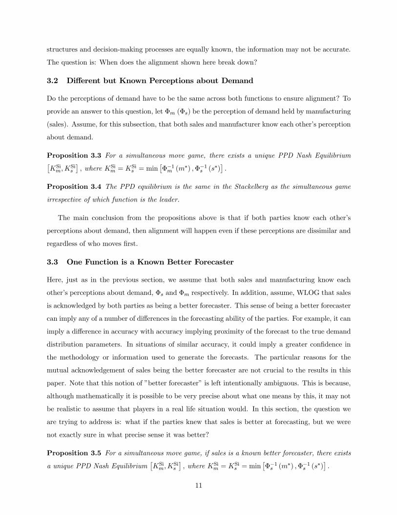
3.2 Different but Known Perceptions about Demand
Do the perceptions of demand have to be the same across both functions to ensure alignment? To
provide an answer to this question, let Φm (Φs) be the perception of demand held by manufacturing
(sales). Assume, for this subsection, that both sales and manufacturer know each other’s perception
about demand.
Proposition 3.3 For a simultaneous move game, there exists a unique PPD Nash Equilibrium£KSim,K
Sis
¤, where KSi
m = KSis = min
£Φ−1m (m∗) ,Φ−1s (s∗)
¤.
Proposition 3.4 The PPD equilibrium is the same in the Stackelberg as the simultaneous game
irrespective of which function is the leader.
The main conclusion from the propositions above is that if both parties know each other’s
perceptions about demand, then alignment will happen even if these perceptions are dissimilar and
regardless of who moves first.
3.3 One Function is a Known Better Forecaster
Here, just as in the previous section, we assume that both sales and manufacturing know each
other’s perceptions about demand, Φs and Φm respectively. In addition, assume, WLOG that sales
is acknowledged by both parties as being a better forecaster. This sense of being a better forecaster
can imply any of a number of differences in the forecasting ability of the parties. For example, it can
imply a difference in accuracy with accuracy implying proximity of the forecast to the true demand
distribution parameters. In situations of similar accuracy, it could imply a greater confidence in
the methodology or information used to generate the forecasts. The particular reasons for the
mutual acknowledgement of sales being the better forecaster are not crucial to the results in this
paper. Note that this notion of ”better forecaster” is left intentionally ambiguous. This is because,
although mathematically it is possible to be very precise about what one means by this, it may not
be realistic to assume that players in a real life situation would. In this section, the question we
are trying to address is: what if the parties knew that sales is better at forecasting, but we were
not exactly sure in what precise sense it was better?
Proposition 3.5 For a simultaneous move game, if sales is a known better forecaster, there exists
a unique PPD Nash Equilibrium£KSim,K
Sis
¤, where KSi
m = KSis = min
£Φ−1s (m∗) ,Φ−1s (s∗)
¤.
11

Proposition 3.6 The PPD equilibrium is the same in the Stackelberg game as in the simultaneous
game irrespective of which function is the leader.
Just as in Proposition 3.3, if both parties know each other’s perceptions about demand, then
alignment will happen regardless of who moves first. The difference with Proposition 3.3 is that,
now, both parties will use the information provided by the better predictor. Essentially, if both
parties agree on and are certain about who is the better predictor, and know each other’s perceptions
perfectly, then they simply choose to use the best perception of demand. This could be interpreted
as a variation of the ideas in section 3.1.
4 Imperfect Information: Static Perceptions with Partial Sharing
How does imperfect information about perceptions affect alignment? In this section we assume
imperfect information surrounding perceptions of demand across functions (firms). Again, let
Φm (Φs) be the perception of demand held by manufacturing (sales). In this section, the other
function’s (firm’s) perception of demand is not assumed to have any informational content for
forecasting for the current function. We thus assume that each function’s (firm’s) beliefs about
demand are unaffected by the sharing of beliefs. We term this case the static case. In the next
section we will relax this assumption, assuming that, after sharing beliefs about demand, functions
(firms) may change their original beliefs.
4.1 Difference in Perceptions Unknown
Assume in this subsection that neither sales nor manufacturing knows that their perceptions are not
shared. For example, it may be that sales and manufacturing have different information on which to
base their predictions, but that they are not aware of this: imagine that sales did not realize that the
product features have changed in a subtle way that would impact demand, but that manufacturing
did know about such changes and their implications, and thought that sales also knew. In this case,
we know from Propositions 3.1 and 3.2 that both manufacturing and sales expect the equilibrium
to happen based on their perceptions. For convenience let m̄ denote min£Φ−1m (m∗) ,Φ−1m (s∗)
¤and
s̄ denote min£Φ−1s (m∗) ,Φ−1s (s∗)
¤. Here m̄ (s̄) is the limiting capacity based on the perception of
manufacturing (sales) of demand and of sales’ (manufacturing’s) capacity decision.
Proposition 4.1 The resulting PPD Nash equilibrium for a simultaneous move game is£KSim,K
Sis
¤where KSi
m = m̄ and KSis = s̄.
12

Proposition 4.2 In the Stackelberg game,
(a) when manufacturing is the leader, the PPD equilibrium is£KStM ,K
Sts
¤where KSt
M = m̄ and
KSts = min
£m̄,Φ−1s (s∗)
¤. In this case, the plans are misaligned if and only if Φ−1s (s∗) < m̄.
(b) when sales is the leader, the PPD equilibrium is£KStm ,K
StS
¤where KSt
m = min£Φ−1m (m∗) , s̄
¤and KSt
S = s̄. In this case, the plans are misaligned if and only if Φ−1m (m∗) < s̄.
From the Propositions above, it is clear that (1) under the simultaneous move game, misalign-
ment is very likely,(2) a Stackelberg game increases the chances of alignment. However, under the
Stackelberg game, because the functions do not know about the other’s demand perceptions, it is
hard to prescribe ex ante who should move first.
4.2 Differences in Perceptions Asymmetrically Known
In this subsection, we assume that only one function knows the perceptions of both functions. The
other function assumes that their perception is common for both functions. Thus, one function
can be considered to be more aware of the functional differences that exist in the organization
or between the firms. For example, imagine that manufacturing gave sales its forecast, but that
sales did not. Imagine also that manufacturing, rather naively, did not think that sales had any
other belief about demand. In this case, if manufacturing’s forecast was different than sales’, then
sales would be aware of this but manufacturing would not. Interestingly such a scenario can be
interpreted as a “leader” communicating demand forecasts to a “follower.” It is the leader, though,
who ends up being the more naive member of the two.
We assume, WLOG, that sales is the function with the greater cross-functional awareness. That
is, assume that sales knows both Φm and Φs but not vice-versa (i.e. that sales knows both its own
and manufacturing’s perception about demand, but manufacturing only knows its own perception
about demand, and assumes that sales has the same perception). The unique sales reaction function
Ks (Km) is given by
Ks (Km) = min£Φ−1s (s∗) ,Km
¤,
while the unique manufacturing function Km (Ks) is given by
Km (Ks) = min£Φ−1m (m∗) ,Ks
¤.
However since sales knows manufacturing’s perception and knows that manufacturing is unaware
of the differences in perception, it knows that manufacturing perceives the sales reaction function
to be K̃s (Km) given by
K̃s (Km) = min£Φ−1m (s∗) ,Km
¤.
13

This gives the following results concerning alignment.
Proposition 4.3 The resulting PPD Nash equilibrium for a simultaneous move game is£KSim,K
Sis
¤,
where KSis = min
£m̄,Φ−1s (s∗)
¤, and KSi
m = m̄.
Proposition 4.4 The Stackelberg game, when the manufacturing is the leader, gives the same PPD
equilibrium as the simultaneous game.
Proposition 4.5 For simultaneous game or Stackelberg game where manufacturing is the leader,
the plans are aligned if and only if Φ−1s (s∗) ≥ m̄.
Proposition 4.6 In the Stackelberg game, when sales is the leader, the PPD equilibrium is£KStm ,K
StS
¤where KSt
m = KStS = min
£Φ−1m (m∗) ,Φ−1s (s∗)
¤.
The main conclusion from the Propositions above is that sales’ better information or greater
awareness can be exploited to achieve alignment by making sales move first. Interestingly, in the
example cited at the beginning of this section, this would imply that if manufacturing (or our
leader) moves first by sharing its forecast with sales (and not vice-versa), then sales (the follower)
should move first in terms of capacity investment.
4.3 One Function is a Known Better Forecaster
In this section, we assume, that each function knows that the other function has different perceptions
about demand, but it does not know what these perceptions are. In addition, WLOG, let sales be
the known better forecaster as discussed in section 3.3. Now the question is: is it possible to exploit
this extra knowledge?
Proposition 4.7 In the simultaneous game, there is no PPD Nash equilibrium.
Proposition 4.8 In the Stackelberg game, if s∗ ≤ m∗, sales moves first, and sales is better at
forecasting, then the PPD Nash equilibrium is£KStm ,K
StS
¤where KSt
m = KStS = Φ−1s (s∗) .
Remark 4.9 In the Stackelberg game, if s∗ > m∗, sales moves first, and sales is better at fore-
casting, then the PPD Nash equilibrium depends on sales’ beliefs about the probability that manu-
facturing will invest in more capacity. For an example of a possible approach the reader can see
Proposition 5.4.
14

In Proposition 4.7 we make no assumptions about what players can try to infer about the other
player’s perceptions and thus the players are unable to find a suitable focal point as for example,
a PPD equilibrium would be. If the players have some defined a priori beliefs about the other
players perceptions about demand, then the logic of subsection 5.2 would apply.
It can be noted from the propositions above that, under this scenario, alignment will happen
if the acknowledged better forecaster has a smaller critical fractile (and is thus, ceteris paribus,
more likely to be a bottleneck), and makes the first move. It is not clear, however, how to induce
alignment without changing incentives if the fractile of the acknowledged better predictor is larger
that the other party’s (the situation of Remark 4.9). The reason why it is not clear, is that, in this
scenario, the acknowledged better predictor may have an incentive to inflate forecasts to attempt
to induce a higher capacity investment by the other party, for example as described by Terwiesch
et. al. (2005), a multi-period empirical paper describing forecast sharing between a semiconductor
manufacturer and its suppliers. Cachon and Lariviere (2001) focusing on this scenario, add more
structure to what they mean by “better” or in their case “accurate” forecasts, and devise an
incentive changing scheme based on the ideas of Spence (1973) about signalling that can, under
certain conditions, achieve first-best. In any case, one conclusion that can be inferred from the
results of this section is that knowing that one party is a better forecaster increases the chances of
alignment.
5 Imperfect Information: Dynamic Perceptions with Perfect Shar-ing
In this section we relax the assumption that the perception of the other function has no informa-
tional content for forecasting for the current function and allow complete sharing. Now the very
act of sharing perceptions adds complexity to the cross-functional setting because perceptions may
change as a result of the sharing, thus we refer to them as dynamic, but we assume that how they
have changed is not explicitly known. Such a setting could in reality be modeled in a number of
different ways. We consider two ways here which we feel represent two extremes along a spectrum
of responses. In the first subsection, we assume that the perceptions as shared serve as the exclusive
options for the function to use for their decision. However, unlike in subsection 3.3, manufacturing
(sales) is not exactly sure what sales (manufacturing) thinks about manufacturing’s (sales’) accu-
racy. In the second subsection, we assume a more general model where after sharing perceptions,
functions infer a probability distribution over the other function’s capacity decision.
15
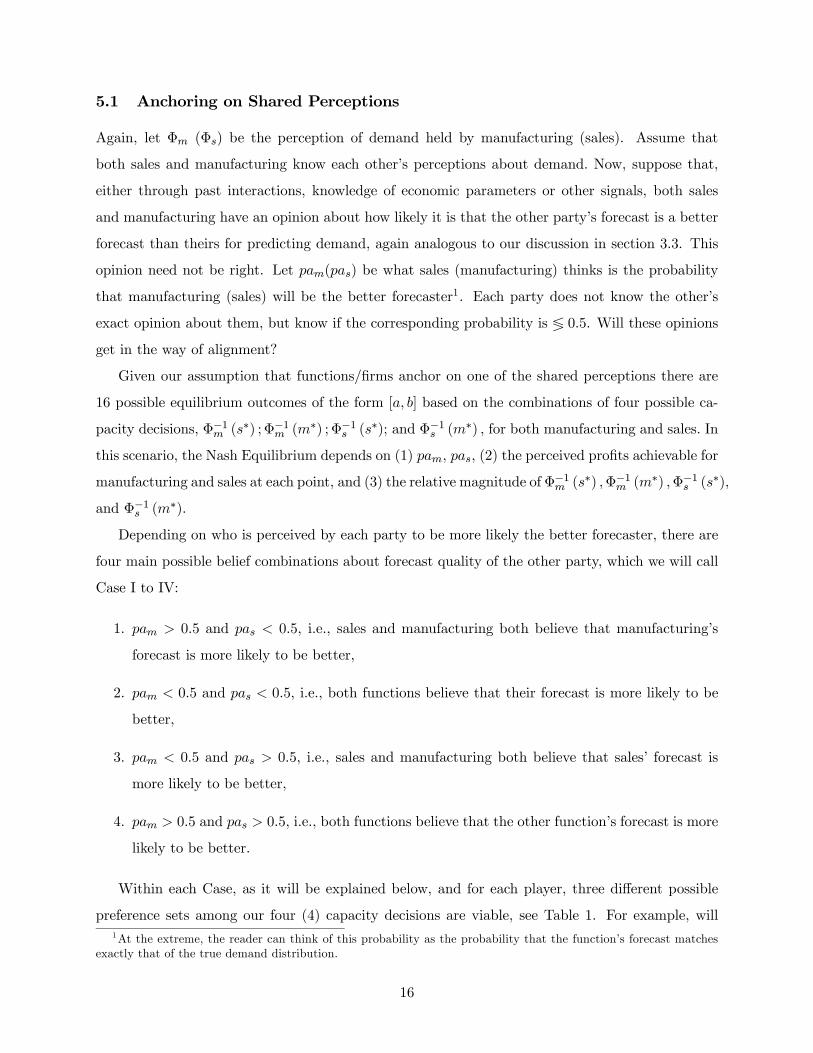
5.1 Anchoring on Shared Perceptions
Again, let Φm (Φs) be the perception of demand held by manufacturing (sales). Assume that
both sales and manufacturing know each other’s perceptions about demand. Now, suppose that,
either through past interactions, knowledge of economic parameters or other signals, both sales
and manufacturing have an opinion about how likely it is that the other party’s forecast is a better
forecast than theirs for predicting demand, again analogous to our discussion in section 3.3. This
opinion need not be right. Let pam(pas) be what sales (manufacturing) thinks is the probability
that manufacturing (sales) will be the better forecaster1. Each party does not know the other’s
exact opinion about them, but know if the corresponding probability is ≶ 0.5. Will these opinionsget in the way of alignment?
Given our assumption that functions/firms anchor on one of the shared perceptions there are
16 possible equilibrium outcomes of the form [a, b] based on the combinations of four possible ca-
pacity decisions, Φ−1m (s∗) ;Φ−1m (m∗) ;Φ−1s (s∗); and Φ−1s (m∗) , for both manufacturing and sales. In
this scenario, the Nash Equilibrium depends on (1) pam, pas, (2) the perceived profits achievable for
manufacturing and sales at each point, and (3) the relative magnitude of Φ−1m (s∗) ,Φ−1m (m∗) ,Φ−1s (s∗),
and Φ−1s (m∗).
Depending on who is perceived by each party to be more likely the better forecaster, there are
four main possible belief combinations about forecast quality of the other party, which we will call
Case I to IV:
1. pam > 0.5 and pas < 0.5, i.e., sales and manufacturing both believe that manufacturing’s
forecast is more likely to be better,
2. pam < 0.5 and pas < 0.5, i.e., both functions believe that their forecast is more likely to be
better,
3. pam < 0.5 and pas > 0.5, i.e., sales and manufacturing both believe that sales’ forecast is
more likely to be better,
4. pam > 0.5 and pas > 0.5, i.e., both functions believe that the other function’s forecast is more
likely to be better.
Within each Case, as it will be explained below, and for each player, three different possible
preference sets among our four (4) capacity decisions are viable, see Table 1. For example, will1At the extreme, the reader can think of this probability as the probability that the function’s forecast matches
exactly that of the true demand distribution.
16

sales prefer a capacity that uses what it thinks to be the more likely worse forecast but that
maximizes profits over sales’ cost parameters to a capacity that uses what it thinks to be the
more likely better forecast although it optimizes profits over manufacturing’s cost parameters?
Given that each player can respond to such questions in different ways depending on what they
believe to be the shape of their expected profit function, and on pai, i ∈ {m, s}, there are nine
possible preference set combinations. The total number of feasible combinations of beliefs about
forecast quality (i.e. cases) and preference sets (i.e. beliefs about the shape of the expected profit
function) is thus 4*9=36. Now, for each of the 36 combinations of beliefs and preferences, there
are 12 possible ordering for the four capacity decisions, from the smallest to the largest (e.g.,
Φ−1m (s∗) < Φ−1s (s∗) < Φ−1m (m∗) < Φ−1s (m∗), etc.)2. The order is relevant because it determines
whether a given capacity can be “undercut” by the other player. Thus, there are a total of 12*36 =
432 possible games. We will show that, in a simultaneous game, for all possible games we can find
a unique Nash equilibrium while in Stackelberg games we find unique PPD equilibria depending
on who plays first.
More formally, define  as a preference relation where º means “is at least as preferable as.”
We define the following preference relations for sales:
S1) Φ−1m (s∗) º Φ−1m (m∗) because s∗optimizes sales’s profits under Φm.
S2) Φ−1s (s∗) º Φ−1s (m∗) because s∗optimizes sales’s profits under Φs.
and for manufacturing:
M1) Φ−1m (m∗) º Φ−1m (s∗) because m∗optimizes manufacturing’s profits under Φm.
M2) Φ−1s (m∗) º Φ−1s (s∗) because m∗optimizes manufacturing’s profits under Φs.
Under different Cases for the perceived probabilities of accuracy pai, i ∈ {m, s}, other preference
relationships can be defined. Consider Case I: where pam > 0.5 and pas < 0.5, i.e., both sales and
manufacturing think that it is likely that manufacturing’s forecast is better.
For sales, unless restricted by the other party’s capacity choices, we know that:
S3) Φ−1m (s∗) º Φ−1s (s∗) because sales thinks Φm is more likely to be a better forecast than Φs.
S4) Φ−1m (s∗) º Φ−1s (m∗) transitivity with S2) and S3)
For manufacturing, unless restricted by the other party’s capacity choices, we know that:
M3) Φ−1m (m∗) º Φ−1s (m∗) because manufacturing thinks Φm is more likely to be a better
forecast than Φs.
M4) Φ−1m (m∗) º Φ−1s (s∗) transitivity with M2) and M3).2Of the 24 (4*3*2) potential orderings exactly half are eliminated since ordering implied by s∗ < (>)m∗ must be
consistent for both perceptions Φm and Φs.
17

Without violating any of the rules above, Table 1 shows the two preference sets which are
possible for sales and for manufacturing individually:Sales ManufacturingΦ−1m (s∗) º Φ−1s (s∗) º Φ−1m (m∗) º Φ−1s (m∗) Φ−1m (m∗) º Φ−1s (m∗) º Φ−1m (s∗) º Φ−1s (s∗)Φ−1m (s∗) º Φ−1s (s∗) º Φ−1s (m∗) º Φ−1m (m∗) Φ−1m (m∗) º Φ−1s (m∗) º Φ−1s (s∗) º Φ−1m (s∗)Φ−1m (s∗) º Φ−1m (m∗) º Φ−1s (s∗) º Φ−1s (m∗) Φ−1m (m∗) º Φ−1m (s∗) º Φ−1s (m∗) º Φ−1s (s∗)Table 1: Preference Sets for Sales and for Manufacturing
Although in all cases sales would prefer optimizing their profit function using the better forecast
over its own economic parameters (for example, in this case, sales would strictly prefer Φ−1m (s∗) to
anything else), the remaining preferences, and thus which set truly represents sales’s total prefer-
ences, will depend on the particular situation. For example, note that in the second set, sales thinks
that optimizing manufacturing’s profit function using the more likely better forecast is preferable
than optimizing their profit function using the more likely worse forecast (i.e. Φ−1m (m∗) º Φ−1s (s∗)),
while for the first and second set, the opposite is true (i.e. Φ−1s (s∗) º Φ−1m (m∗)). Note that,
although sales (manufacturing) will know exactly which set represents its own preferences, manu-
facturing (sales) will not be able to tell. The only thing that manufacturing (sales) can be sure of
is that, as long as pam > 0.5, (pas < 0.5) sales’ most preferred option is Φ−1m (s∗)¡Φ−1m (m∗)
¢. Note
in Table 1 the similarities of manufacturing’s preferences to that of sales.
As mentioned previously, the viable preference sets for sales and manufacturing in this case
can be combined in nine different ways. There are also 12 possible ordering for the four plays,
from the smallest to the largest (e.g., Φ−1m (s∗) < Φ−1s (s∗) < Φ−1m (m∗) < Φ−1s (m∗), etc.). Thus,
there are 9*12=108 possible games where both sales and manufacturing think that it is likely that
manufacturing’s forecast is better. Each game may yield a different PPD Nash Equilibrium. The
possible preference sets for the remaining cases can be similarly enumerated as is done in the proof.
Proposition 5.1 In the simultaneous game, for all feasible combinations of the preference sets for
sales and manufacturing, there exists a unique Nash Equilibrium [KSim,K
Sis ] where K
Sim = KSi
s =
min[m̄, s̄].
From Proposition 5.1 we see that in all cases a unique equilibrium with alignment is always
possible but only on the constraining capacity across both perceptions and function. Note that in
Case I and III, depending on the constraining capacity across both perceptions and function, that
this equilibrium can be at a capacity decision which for both parties, is based on the forecast that
both think is more likely to be the worse of the two forecasts. Similarly, in Case II and IV, as
highlighted by the results for the Stackelberg game below, unperceived Pareto dominant solutions
are ignored.
18

For the results on the Stackelberg games below, we define the following:
- smaxº (a, b) = a if a º b given the preference set for sales, otherwise b.
- smaxº (a, b, c) = smaxº (smaxº (a, b) , smaxº (a, c))
- mmaxº (a, b) = a if a º b given the preference set for manufacturing, otherwise b.
- mmaxº (a, b, c) = mmaxº (mmaxº (a, b) ,mmaxº (a, c))
Here smaxº (·, ·) and mmaxº (·, ·) define “maximum” functions based on the preference set of
sales and manufacturing respectively.
Proposition 5.2 i) In the Stackelberg game, regardless of who moves first, there exists a unique
Nash Equilibrium£KStm ,K
Sts
¤with KSt
m = KSts under the following conditions:
Case Condition EquilibriumI Φ−1m (s∗) = min[m̄, s̄] KSt
m = KSts = Φ−1m (s∗)
I Φ−1m (m∗) = min[m̄, s̄] KStm = KSt
s = Φ−1m (m∗)II Φ−1s (s∗) = min[m̄, s̄] KSt
m = KSts = Φ−1s (s∗)
II Φ−1m (m∗) = min[m̄, s̄] KStm = KSt
s = Φ−1m (m∗)III Φ−1s (s∗) = min[m̄, s̄] KSt
m = KSts = Φ−1s (s∗)
III Φ−1s (m∗) = min[m̄, s̄] KStm = KSt
s = Φ−1s (m∗)IV Φ−1s (m∗) = min[m̄, s̄] KSt
m = KSts = Φ−1s (m∗)
IV Φ−1m (s∗) = min[m̄, s̄] KStm = KSt
s = Φ−1m (s∗)ii) Otherwise, in the Stackelberg game, depending on who moves first, there exists a unique PPD
Nash Equilibrium£KStm ,K
Sts
¤such that KSt
m = KSts under the following conditions:
Case Condition First-Mover EquilibriumI Φ−1s (s∗) = min[m̄, s̄] Manufacturing KSt
m = KSts = mmaxº
¡Φ−1m (s∗) ,Φ−1s (s∗)
¢Sales KSt
m = KSts = smaxº
¡Φ−1m (m∗) ,Φ−1s (s∗)
¢Φ−1s (m∗) = min[m̄, s̄] Manufacturing KSt
m = KSts = mmaxº
¡Φ−1m (s∗) ,Φ−1s (m∗)
¢Sales KSt
m = KSts = smaxº
¡Φ−1m (m∗) ,Φ−1s (m∗)
¢II Φ−1m (s∗) = min[m̄, s̄] Manufacturing KSt
m = KSts = mmaxº
¡Φ−1s (s∗) ,Φ−1m (s∗)
¢Sales KSt
m = KSts = smaxº
¡Φ−1m (m∗) ,Φ−1m (s∗)
¢Φ−1s (m∗) = min[m̄, s̄] Manufacturing KSt
m = KSts = mmaxº
¡Φ−1s (s∗) ,Φ−1s (m∗)
¢Sales KSt
m = KSts = smaxº
¡Φ−1m (m∗) ,Φ−1s (m∗)
¢III Φ−1m (s∗) = min[m̄, s̄] Manufacturing KSt
m = KSts = mmaxº
¡Φ−1s (s∗) ,Φ−1m (s∗)
¢Sales KSt
m = KSts = smaxº
¡Φ−1s (m∗) ,Φ−1m (s∗)
¢Φ−1m (m∗) = min[m̄, s̄] Manufacturing KSt
m = KSts = mmaxº
¡Φ−1s (s∗) ,Φ−1m (m∗)
¢Sales KSt
m = KSts = smaxº
¡Φ−1s (m∗) ,Φ−1m (m∗)
¢IV Φ−1s (s∗) = min[m̄, s̄] Manufacturing KSt
m = KSts = mmaxº
¡Φ−1m (s∗) ,Φ−1s (s∗)
¢Sales KSt
m = KSts = smaxº
¡Φ−1s (m∗) ,Φ−1s (s∗)
¢Φ−1m (m∗) = min[m̄, s̄] Manufacturing KSt
m = KSts = mmaxº
¡Φ−1m (s∗) ,Φ−1m (m∗)
¢Sales KSt
m = KSts = smaxº
¡Φ−1s (m∗) ,Φ−1m (m∗)
¢Proposition 5.2, as expected, provides greater opportunity for alignment at economically more
opportunistic capacity decisions (especially in Cases I and III) than in the simultaneous game
where alignment is always at the minimum capacity over perceptions and functions. In (i) when
19

this minimum capacity is the most preferred capacity decision for one of the functions, it forms the
equilibrium irrespective of who plays first. Otherwise, as shown in (ii), the Stackelberg game allows
the leader to partially reveal their preference set and lead to a perceived Pareto dominant solution
versus the minimum capacity when it can exist. Note that this perceived Pareto dominant solution
can be described as a compromise since when it differs from the minimum capacity, it optimizes the
profit function of the “follower” in Cases I and III and also uses the forecasts that the “follower”
believes is more likely to be better in Cases II and IV.
In summary, the Propositions above indicate that, with partial knowledge of the other party’s
beliefs about demand, and an anchoring on the capacities implied by shared perceptions alignment is
guaranteed. However, the Stackelberg game provides the opportunity for perceived Pareto dominant
solutions as equilibrium.
5.2 Inferring Capacity Decisions
In this section, we assume that after sharing initial perceptions of demand, both sales and manufac-
turing only know that the other function has a different perception about demand, but that neither
function knows how these perceptions have changed as a result of sharing. However, based on
the perceptions, and either through past interactions, knowledge of economic parameters or other
signals, both sales and manufacturing have an opinion about how the other party is likely to now
perceive demand. This opinion need not be right. Each party does not know the other’s opinion
about them. Let pm (Ks) (ps (Km)) be what sales (manufacturing) thinks is the probability that
manufacturing (sales) will choose a capacity above sales’s (manufacturing’s) own chosen capacity,
Ks(Km) (note that these probabilities would be similar to what some economists call “priors”, as
in Van den Steen 2001). Assume that dpmdKs≤ 0 ( dpsdKm
≤ 0) andd2pmd2Ks
≤ 0 ( d2psd2Km
≤ 0), i.e., assume
that sales (manufacturing) believes that the larger its capacity, the less likely it is that the other
party will choose a larger capacity, and that the change in this probability decreases with capacity.
Sales’s expected profit function given planned supply of Km from manufacturing is:
E [Πs (Ks)] = pm (Ks) · (−γKs +E (p− w)min [D,Ks]))
+(1− pm (Ks)) · (−γKs +E (p− w)min [D,Km])) .
20
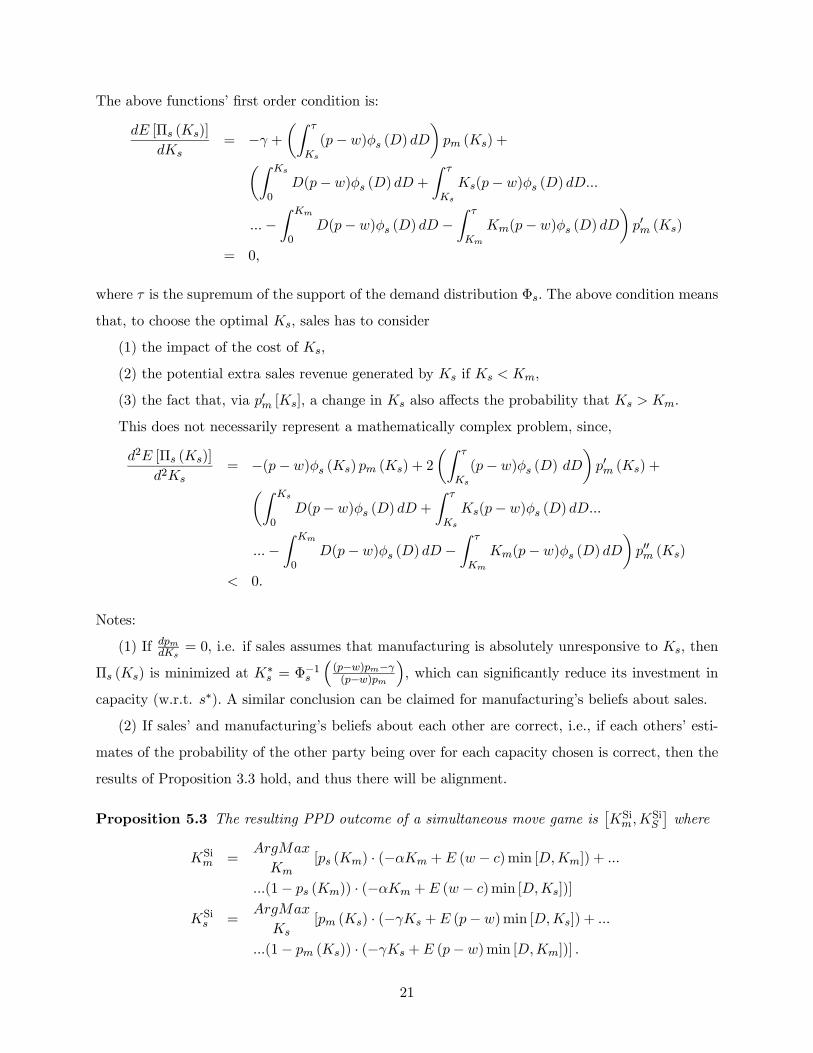
The above functions’ first order condition is:
dE [Πs (Ks)]
dKs= −γ +
µZ τ
Ks
(p− w)φs (D) dD¶pm (Ks) +µZ Ks
0D(p− w)φs (D) dD +
Z τ
Ks
Ks(p− w)φs (D) dD...
...−Z Km
0D(p− w)φs (D) dD −
Z τ
Km
Km(p− w)φs (D) dD¶p0m (Ks)
= 0,
where τ is the supremum of the support of the demand distribution Φs. The above condition means
that, to choose the optimal Ks, sales has to consider
(1) the impact of the cost of Ks,
(2) the potential extra sales revenue generated by Ks if Ks < Km,
(3) the fact that, via p0m [Ks], a change in Ks also affects the probability that Ks > Km.
This does not necessarily represent a mathematically complex problem, since,
d2E [Πs (Ks)]
d2Ks= −(p− w)φs (Ks) pm (Ks) + 2
µZ τ
Ks
(p− w)φs (D) dD¶p0m (Ks) +µZ Ks
0D(p− w)φs (D) dD +
Z τ
Ks
Ks(p− w)φs (D) dD...
...−Z Km
0D(p− w)φs (D) dD −
Z τ
Km
Km(p− w)φs (D) dD¶p00m (Ks)
< 0.
Notes:
(1) If dpmdKs= 0, i.e. if sales assumes that manufacturing is absolutely unresponsive to Ks, then
Πs (Ks) is minimized at K∗s = Φ−1s
³(p−w)pm−γ(p−w)pm
´, which can significantly reduce its investment in
capacity (w.r.t. s∗). A similar conclusion can be claimed for manufacturing’s beliefs about sales.
(2) If sales’ and manufacturing’s beliefs about each other are correct, i.e., if each others’ esti-
mates of the probability of the other party being over for each capacity chosen is correct, then the
results of Proposition 3.3 hold, and thus there will be alignment.
Proposition 5.3 The resulting PPD outcome of a simultaneous move game is£KSim,K
SiS
¤where
KSim =
ArgMax
Km[ps (Km) · (−αKm +E (w − c)min [D,Km]) + ...
...(1− ps (Km)) · (−αKm +E (w − c)min [D,Ks])]
KSis =
ArgMax
Ks[pm (Ks) · (−γKs +E (p− w)min [D,Ks]) + ...
...(1− pm (Ks)) · (−γKs +E (p− w)min [D,Km])] .
21

Proposition 5.4 In the Stackelberg game,
(a) if sales moves first, the PPD Nash equilibrium is£KStm ,K
StS
¤whereKSt
m = min£KSis ,Φ
−1m (m∗)
¤,
and KStS = KSi
s . In this case, plans are misaligned if and only if KSis > Φ
−1m (m∗) .
(b) if manufacturing moves first, the PPD Nash equilibrium is£KStM ,K
Sts
¤where KSt
M = KSim,
and KSts = min
£Φ−1s (s
∗),KSim
¤.In this case, plans are misaligned if and only if KSi
m > Φ−1s (s∗) .
Proposition 5.3 helps shed light on the benefits of sharing perceptions. Namely, it points out
that sharing perceptions may not always lead to alignment, in fact, it shows that perception could
exacerbate misalignment. Recall that the sharing of perceptions creates opinions pm (·) (ps (·))
about the planning choices of the other player which need not be correct. Sharing perceptions
could exacerbate misalignment if the sharing of perception causes a decrease in the accuracy of the
opinions held by functions in such a way that the capacity mismatch is more severe. An example
of such a scenario is sales sharing (and receiving) perceptions but over-estimating the influence of
their perceptions on manufacturing, an over-estimate which may not have happened if sales hadn’t
shared their perception and only received that of manufacturing.
It should be noted from the above propositions that the condition for alignment in the Stack-
elberg game cannot be known a priori by the functions (since, in this scenario, final demand
perceptions about the other function are unknown to each other by definition). Thus, although the
Stackelberg game does result in a higher chance of alignment, it is not easy to prescribe who should
move first without knowing about each function’s perceptions about demand. However, as each
other’s perceptions of the other’s potential moves becomes more accurate, the chance of alignment
will increase, since each party does incorporate part of the cost of misalignment in its objective
function.
6 Discussion
6.1 Managing Communication of Perceptions
Summary 6.1 Figure 1 summarizes the main results from the previous sections:
Sections 3 and 4 make a strong case for the mutual sharing of the perceptions of demand across
functions in order to have alignment assuming static perceptions. This case is strengthened when
we recognize that under this static perceptions assumptions there is no disincentive to sharing
perceptions as functions only benefit from sharing as it reduces their own wasted capacity and
state this as a theorem.
22

Main Section Subsection Recommendation Alignment guaranteed?
3.1 Common preceptions about demand Indifferent Yes
3.2 Different but known perceptions about demand Indifferent Yes
3.3 One Function is a Known Better Forecaster Indifferent Yes
4.1 Difference in perceptions unknownStackelberg, unclear who moves first No
4.2 Differences in Perceptions Asymmetrically known
Stackelberg, knowledgeable party moves first.
Yes
4.3 Difference in Perceptions Partially known
Stackelberg, better forecaster moves first.
No
5.1 Anchoring on Shared PerceptionsStackelberg, indifferent who moves first.
Yes
5.2 Inferring Capacity DecisionsStackelberg, unclear who moves first No.
Section 4. Imperfect Information: Static Perceptions with Partial Sharing
Section 5. Imperfect Information: Dynamic Perceptions with Perfect Sharing
Section 3. Perfect Information in a Decentralized System
Figure 1:
23

Theorem 6.2 Under static perceptions, there is no disincentive to sharing one’s perception with
another function with mutual sharing of perceptions resulting in functional alignment in capacity
planning.
However under dynamic perceptions (Section 5), mutual sharing of perceptions may not always
create alignment. Furthermore, though not explicitly examined in Section 5, incentives can exist
for manipulation by sharing false perceptions, for example, if it affects perceived probabilities of
accuracy (as in Section 5.1) or one’s own opinion of the planning choices likely to be made by the
other player (as in Section 5.2). It is even possible that, as argued in Section 5.2, such sharing, if
left unattended, could even exacerbate misalignment.
Observations for managing alignment in such a setting can still be generated from our results.
For example, when the “right” party takes the initiative (as modeled by Stackelberg games) the
chances of alignment are increased. Alignment is also encouraged by either natural or artificial
limiting of the capacity decisions although leadership may still be required to encourage more
Pareto dominating outcomes. Theorem 6.2 and the observation that it is the lack of knowledge
of how perceptions are affected by sharing which affects alignment provides some guidance for
any communication structure between the players which supports alignment. Such communication
should try to mimic the end-conditions of perception sharing under static perceptions, that is,
that players have a greater sense of the final perceptions of the other player as a result of sharing.
Note that, to achieve alignment, this communication need not align perceptions, but make the final
perceptions better known by one or both parties. Based on Theorem 6.2, it would not be erroneous
to expect that mutual sharing of true perceptions of demand would at least not be discouraged
under such a structure.
6.2 Managing Alignment in Practice
Three dimensions for supporting alignment (integration) have been identified in the academic lit-
erature on coordination within planning contexts: roles/responsibilities, structures and processes
with the literature primarily concentrating on the first two dimensions. These dimensions have been
characterized more explicitly for cross-functional integration (Oliva and Watson 2007), but coordi-
nation efforts across firms can be categorized similarly. By responsibilities, we mean the participants
and the distribution of decision rights among them in the collaborative effort, and by structures we
mean the accompanying formal systematic arrangements, relationships and infrastructure.
The literature on responsibilities for cross-functional coordination primarily draws on the or-
ganizational behavior literature. Lawrence and Lorsch (1986) recommend explicitly the role of
24

integrators for coordinating unity of effort. These integrators act as translators, mediators and
integrative goal setters facilitating the differing cognitive and emotional perspectives of the various
functions and directing collective efforts. Across firms, the role of intermediaries such as Li &
Fung in the apparel supply chain and distributors like Arrow Electronics in the electronic com-
ponent supply chain share some similarities with integrators. The allocation of decision rights or
focus has also been argued to be important for coordination across firms (Anand and Mendelson
1997; Kraiselburd, Narayanan and Raman, 2004; Watson and Zheng 2005). Within firms, struc-
tural recommendations for improving integration have come from analysis of the informational and
organizational infrastructure impeding integration. Such infrastructure includes the level of infor-
mation sharing among functional decision makers (Dougherty 1992; Shapiro 1977; Van Dierdonck
and Miller 1980) including that facilitated by enterprise information systems (Al-Mashari et. al.
2003); evaluation and incentive systems whether for individual functions (Chen 2005; Gonik 1978;
Kouvelis and Lariviere 2000; Porteus and Whang 1991) or collective incentives (Mallik and Harker
2004); support for complex decision making whether from quantitative models (Yano and Gilbert
2004), decision support systems (Crittenden et. al. 1993), outsourcing planning decision-making to
competent third parties (Troyer et. al. 2005); and formal arrangements systematizing the desired
integrative norms (Stonebraker and Afifi 2004) such as standardization of policies, compatible com-
munications formats, and formal hierarchies and departmentalization. An emphasis on incentives
as discussed in the introduction, characterizes the literature on cross-firm coordination.
In terms of general process features for integration, the OB literature posits that interdepartmen-
tal integration is fostered by two types of activities (Barratt 2004): (1) interaction/communication
activities (Dougherty 1992; Griffin and Hauser 1992; Ruekert andWalker 1987), and (2) collaboration-
related activities (Lawrence and Lorsch 1986; Pinto et. al. 1993). Both types of activities are
facilitated by norms and specific responsibilities and goals. Interaction/communication activities,
however, relate to the activities that enable the existing types, quantity, quality, and frequency
of information flows (structure) between functions. Collaboration activities, on the other hand,
relate to the roles (responsibilities) spread across functions that in combination —and usually in
the short term— have shared goals. Whereas integration and communication activities are neces-
sary for collaboration, collaborative activities are generally believed to be a precondition for full
integration (Barratt 2004). One type of internal planning processes examined in the practitioner
literature (Bower 2005; Lapide 2004a; 2004b; 2005a; 2005b) is referred to as a Sales and Operations
planning (S&OP) process. A basic S&OP process facilitates the transfer of information needed
from demand planning to master planning; however both practitioners and academics argue that
25

the S&OP process can move beyond this superficial synchronizing of master planning with demand
planning and begin to approach coordinated joint planning with a certain degree of sophistication
surrounding the quality of plans generated (Lapide 2005a; Van Landeghem and Vanmaele 2002).
Planning processes across firms tend to be less explicitly defined and range from simple call-and-
response processes, (sending of production requests with sometimes an unverifiable commitment
in response,) to more sophisticated interactions, for example, with embedded liaisons in either
customer or supplier operations, or collaborative planning processes like collaborative planning
forecasting and replenishment (CPFR). Interestingly these interfirm processes can be compromised
by lack of intrafirm alignment, Fliedner (2003).
Our analysis suggests an understanding of how the three dimensions of responsibilities, struc-
ture and process can effect alignment as we model it here. Integrators or intermediaries and the
supporting structure can serve as conduits for the sharing of perceptions, helping with elucidation
of perceptions and then their translation, so that other functions can assimilate the information.
Our perceptions of demand, modeled here as probability distributions, greatly simplifies differences
that can exist between how different functions, (firms) think about and represent uncertainty in
demand. Intermediaries familiar with such differences can help in translating and, if necessary,
embellishing or reducing information so as to aid understanding. This translation-related activity
arguably enhances the additional structural recommendations for coordination such as enterprise
resource information systems within firms and EDI protocols across firms by basically ensuring
that the message being sent is the message being received. Finally, if our recommendation for
managing dynamic perceptions has merit, then processes would prove instrumental in allowing or
helping functions to generate or revise “final” (static) perceptions after initial perception sharing
or subsequent updates. Forecasting methods involving the combination of forecasts provide one
such mechanism for generating perceptions, but even the need for these methods imply that, in
general, combining perceptions of demand is not a trivial task. Such an approach is even further
complicated by the observation that black box analytical approaches have diminished persuasive
value in many of the subjective planning approaches which characterize planning in and across
firms.
For one perspective on achieving alignment in practice, we related the findings from a case study
which examined the implementation of an S&OP process in an effort to understand the systems and
behavioral process associated with cross functional integration (Oliva and Watson 2007). Central to
this instance of the S&OP processes was the use of consensus forecasting among the participating
groups in the process. Here, the intention was for participant groups to come to an agreement
26
concerning the forecast that would be used for planning purposes. This agreement also carried
over to the plan that was eventually developed based on the forecasts after being validated for
both financial and external supply chain viability. The authors argue that the quality of demand
and supply planning can be roughly related to the quality of information used, the quality of the
inferences made from available data (e.g., forecasts and plans), and the organization’s conformance
to the plans that are generated, that is, the organizational alignment. A significant fraction of
the reported benefits, however, was not exclusively the result of a logical and efficient information-
processing. It was argued that improvements in forecast accuracy and other operating metrics were
less the result of a better forecasting process than of an aligned organization working with unity of
purpose to realize those forecasts and plans.
7 Conclusions
We used game theory to explore the conditions required for intrafirm and between firm supply
chain coordination. One of our main conclusions, which is consistent with the OB literature, is
that although incentive misalignment in the sense studied in the OM literature may be a factor
in determining alignment, it is not necessarily a central one. For example, in Sections 3 and 4.2,
alignment can be guaranteed even if there are misaligned incentives in the traditional sense. What
we learnt from our models is that it is often the communication structure which ends up determining
whether alignment will happen or not. This would support the emphasis placed in the OB literature
on better communication, rather than incentive alignment, for improved coordination. In our setup,
the key to alignment is not so much how each function is rewarded (i.e. the transfer prices, etc.), it
is more what each function knows about the other function’s beliefs. According to this, any effort
to increase knowledge of each other’s (final) perspective will improve the chances of alignment,
even if no change in incentives is made. This is a fundamental departure from most papers in OM,
where the claim is often that both parties do not align because of each party’s differing economic
incentives, or knowledge about end demand. In many of these papers, misalignment happens
even if both parties knew each other perfectly. While we do not disagree that the right incentives
can induce alignment in actions, we claim, instead, that incentive alignment is not a necessary
condition for alignment in actions, and that the key to alignment in actions lies in the degree of
knowledge about each other’s beliefs. Although this claim is predominant in the OB literature , we
are unaware of any other paper that explicitly models coordination issues and yet reaches similar
conclusions. The use of mathematical modeling and game theory to reach such conclusion matters
because we are able to show that this seemingly behavioral, psychological effects (i.e. alignment
27

happening despite “misaligned” incentives in the traditional sense, etc.) may still happen if both
parties are rational profit maximizers (vs. boundedly rational profit satisfiers, etc.). Although we
do not negate the importance of such behavioral effects on decision making, our contribution pushes
the frontier of what the “rational, profit maximizing agent” assumption can find within the set of
problems covered by the OM literature .
8 Appendix: Proofs
Throughout the proofs, we will follow the convention of making the upstream party (i.e. manufac-
turing) female, and the downstream party (i.e. sales), male.
Proof. Proposition 2.1
By inspection, it can be noted that the optimum involves settingKm = Ks, since any differences
in the capacities would incur the cost of λ,and either γ or α without increasing revenues.
If we set Km = Ks = K, the problem becomes the standard newsvendor problem, whose
solution is as stated.
Proof. Proposition 3.1
Assume, WLOG, that min[Φ−1 (m∗) ,Φ−1 (s∗)] = Φ−1 (m∗) (i.e. manufacturing would prefer to
be the bottleneck).
Then, manufacturing will want to play KSim = Φ
−1 (m∗), because it is her optimum value, and
she knows that sales will not go lower that this because if he sets a capacity lower than this, he
will make less profits. For manufacturing, setting a capacity higher than this will be a waste, since
manufacturing is the bottleneck. Therefore, sales will align with manufacturing.
Similar logic applies if min[Φ−1 (m∗) ,Φ−1 (s∗)] = Φ−1 (s∗) .
Proof. Proposition 3.2
Assume, WLOG, that min[Φ−1 (m∗) ,Φ−1 (s∗)] = Φ−1(m∗).
If manufacturing moves first, she will play Φ−1(m∗), knowing, as in the proof of Proposition
3.1, that sales will not go lower than this. Sales will align, because going lower means less profits
for him, and going higher is a waste of capacity.
If sales moves first, although he would prefer the equilibrium to be Φ−1 (s∗), he is forced to play
Φ−1(m∗) because he knows that if he plays anything higher than this, manufacturing will undercut
him by playing Φ−1(m∗), making any capacity above this a waste.
Similar logic applies if min[Φ−1 (m∗) ,Φ−1 (s∗)] = Φ−1 (s∗) .
Proof. Proposition 3.3
28
The same logic as in the proof of Proposition 3.1. holds if we just replace, at the appropriate
places, Φ−1 with Φ−1i i ∈ {m, s}.
Proof. Proposition 3.4
Again, the same logic as in the proof of Proposition 3.2. holds if we just replace, at the
appropriate places, Φ−1 with Φ−1i i ∈ {m, s}.
Proof. Proposition 3.5
Sales would prefer Φ−1s (s∗) to Φ−1m (s∗) because Φs is more accurate that Φm. Similarly, manu-
facturing would prefer Φ−1s (m∗) to Φ−1m (m∗). So the possible plays are Φ−1s (s∗) and Φ−1s (m∗).
Assume min£Φ−1s (m∗) ,Φ−1s (s∗)
¤= Φ−1s (s∗) . Sales will play Φ−1s (s∗) . Although manufactur-
ing would prefer otherwise, she will match sales because playing her preferred capacity would result
in a waste.
Now, assume min£Φ−1s (m∗) ,Φ−1s (s∗)
¤= Φ−1s (m∗). Although sales would prefer to play the
higher capacity, he will play Φ−1s (m∗) because he knows that manufacturing will play this anyway,
and any capacity above it will be wasted.
Proof. Proposition 3.6
The logic of the proof to Proposition 3.5 still holds if one of the players moves first.
Proof. Proposition 4.1
Since players are unaware of each other’s differences, they will each play as in Proposition 3.3.
Proof. Proposition 4.2
(a) Since manufacturing is unaware of sales having a different perception about demand, she
assume she is in the situation of Proposition 3.4 and plays KStM = m̄.
Sales will simply chose either his optimal value Φ−1s (s∗), or, if this is lower than what manu-
facturing played, simply match manufacturing.
(b) Symmetric to proof of Proposition 4.2 (a)
Proof. Proposition 4.3
Since manufacturing is unaware of sales having a different perception about demand, she will
assume she is in the situation of Proposition 3.4 and play KStM = m̄.
Knowing what manufacturing will play (because he knows manufacturing’s perception), sales
will simply chose either his optimal value Φ−1s (s∗), or, if this is lower than what manufacturing
played, simply match manufacturing.
Proof. Proposition 4.4
29

The logic is almost exactly as in the proof of Proposition 4.3, because manufacturing’s move
will not change.
Proof. Proposition 4.5
This is a direct consequence of Proposition 4.3 and 4.4
Proof. Proposition 4.6
Assume min£Φ−1m (m∗) ,Φ−1s (s∗)
¤= Φ−1s (s∗). Then, since sales knows that manufacturing will
not prefer going lower, he will play Φ−1s (s∗) . Despite preferring a larger capacity, manufacturing
will match sales’ move because playing any larger capacity would be a waste for her.
Now, assume min£Φ−1m (m∗) ,Φ−1s (s∗)
¤= Φ−1m (m∗). Despite preferring a larger capacity, sales
will play Φ−1m (m∗) because he knows that if he plays any larger capacity, he will be undercut by
manufacturing. Since this is manufacturing’s preferred capacity, she will match it.
Proof. Proposition 4.7
Without additional structure on the knowledge of payoffs, for example as in Proposition 5.3, if
the players do not know anything about the other players perceptions, they are unable to select
among different perceived equilibria.
Proof. Proposition 4.8
Sales simply plays Φ−1s (s∗) because it is its global optimum. Since s∗ ≤ m∗, and sales is
supposed to be the best forecaster, manufacturing reasons as follows: ”If I knew sale’s perception
of demand (which is better than mine), I would not want to undercut sales, because his fractile is
smaller than mine”. Thus, manufacturing will not undercut sales.
Proof. Proposition 5.1
Case I
Recall Table 1 the possible set of preferences of sales and manufacturing.
(a) Let Φ−1m (s∗) = min[Φ−1m (s∗) ,Φ−1s (s∗) ,Φ−1m (m∗) ,Φ−1s (m∗)].
Throughout the proof, an underlined play means that this is what sales (manufacturing) would
strictly play if manufacturing (sales) played the capacity stated in the row (column).
(Sales, Manufacturing)(Φ−1m (s∗),Φ−1m (s∗)) (Φ−1s (s∗) ,Φ−1m (s∗)) (Φ−1m (m∗) ,Φ−1m (s∗)) (Φ−1s (m∗) ,Φ−1m (s∗))
(Φ−1m (s∗),Φ−1s (s∗)) (Φ−1s (s∗) ,Φ−1s (s∗)) (Φ−1m (m∗) ,Φ−1s (s∗)) (Φ−1s (m∗) ,Φ−1s (s∗))
(Φ−1m (s∗),Φ−1m (m∗)) (Φ−1s (s∗) ,Φ−1m (m∗)) (Φ−1m (m∗) ,Φ−1m (m∗)) (Φ−1s (m∗) ,Φ−1m (m∗))
(Φ−1m (s∗),Φ−1s (m∗)) (Φ−1s (s∗) ,Φ−1s (m∗)) (Φ−1m (m∗) ,Φ−1s (m∗)) (Φ−1s (m∗) ,Φ−1s (m∗))
Based on our examination of possible outcomes above, the NE is (Φ−1m (s∗),Φ−1m (s∗)) for all
9*3=27 combinations (of preferences and capacities).
30

The NE can be explained the following way: since sales’s most preferred option is also a mini-
mum, he will play it because it cannot be undercut by manufacturing. Manufacturing knows this,
and, thus, matches sales’s play. A similar logic can be applied throughout.
(b) Let Φ−1m (m∗) = min[Φ−1m (s∗) ,Φ−1s (s∗) ,Φ−1m (m∗) ,Φ−1s (m∗)]
(Sales, Manufacturing)(Φ−1m (s∗) ,Φ−1m (s∗)) (Φ−1s (s∗) ,Φ−1m (s∗)) (Φ−1m (m∗) ,Φ−1m (s∗)) (Φ−1s (m∗) ,Φ−1m (s∗))(Φ−1m (s∗) ,Φ−1s (s∗)) (Φ−1s (s∗) ,Φ−1s (s∗)) (Φ−1m (m∗) ,Φ−1s (s∗)) (Φ−1s (m∗) ,Φ−1s (s∗))(Φ−1m (s∗) ,Φ−1m (m∗)) (Φ−1s (s∗) ,Φ−1m (m∗)) (Φ−1m (m∗),Φ−1m (m∗)) (Φ−1s (m∗) ,Φ−1m (m∗))
(Φ−1m (s∗) ,Φ−1s (m∗)) (Φ−1s (s∗) ,Φ−1s (m∗)) (Φ−1m (m∗) ,Φ−1s (m∗)) (Φ−1s (m∗) ,Φ−1s (m∗))
Again based on our examination of possible outcomes above, the NE is (Φ−1m (m∗),Φ−1m (m∗))
for all 9*3=27 combinations (of preferences, and capacities).
(c) Let Φ−1s (s∗) = min[Φ−1m (s∗) ,Φ−1s (s∗) ,Φ−1m (m∗) ,Φ−1s (m∗)].Now since Φ−1s (s∗) ≤ Φ−1s (m∗)
this implies that Φ−1m (s∗) ≤ Φ−1m (m∗) . This is sufficient to imply the following results for equilib-
rium for all 9*3=27 combinations (of preferences, and capacities).
(Sales, Manufacturing)(Φ−1m (s∗),Φ−1m (s∗)) (Φ−1s (s∗) ,Φ−1m (s∗)) (Φ−1m (m∗) ,Φ−1m (s∗)) (Φ−1s (m∗) ,Φ−1m (s∗))
(Φ−1m (s∗) ,Φ−1s (s∗)) (Φ−1s (s∗),Φ−1s (s∗)) (Φ−1m (m∗) ,Φ−1s (s∗)) (Φ−1s (m∗) ,Φ−1s (s∗))
(Φ−1m (s∗),Φ−1m (m∗)) (Φ−1s (s∗) ,Φ−1m (m∗)) (Φ−1m (m∗) ,Φ−1m (m∗)) (Φ−1s (m∗) ,Φ−1m (m∗))
(Φ−1m (s∗) ,Φ−1s (m∗)) (Φ−1s (s∗),Φ−1s (m∗)) (Φ−1m (m∗) ,Φ−1s (m∗)) (Φ−1s (m∗) ,Φ−1s (m∗))Here the equilibrium as far as manufacturing is concerned optimizes the profit function of sales
using the worse forecast of the two. An alternative equilibrium is not allowed because of the exact
preference of each function is unknown.
(d) Let Φ−1s (m∗) = min[Φ−1m (s∗) ,Φ−1s (s∗) ,Φ−1m (m∗) ,Φ−1s (m∗)].Now sinceΦ−1s (m∗) ≤ Φ−1s (s∗)
this implies that Φ−1m (m∗) ≤ Φ−1m (s∗) . This is sufficient to imply the following results for equilib-
rium for all 9*3=27 combinations (of preferences, and capacities).
(Sales, Manufacturing)(Φ−1m (s∗),Φ−1m (s∗)) (Φ−1s (s∗) ,Φ−1m (s∗)) (Φ−1m (m∗) ,Φ−1m (s∗)) (Φ−1s (m∗) ,Φ−1m (s∗))
(Φ−1m (s∗) ,Φ−1s (s∗)) (Φ−1s (s∗) ,Φ−1s (s∗)) (Φ−1m (m∗) ,Φ−1s (s∗)) (Φ−1s (m∗) ,Φ−1s (s∗))(Φ−1m (s∗) ,Φ−1m (m∗)) (Φ−1s (s∗) ,Φ−1m (m∗)) (Φ−1m (m∗) ,Φ−1m (m∗)) (Φ−1s (m∗) ,Φ−1m (m∗))
(Φ−1m (s∗) ,Φ−1s (m∗)) (Φ−1s (s∗) ,Φ−1s (m∗)) (Φ−1m (m∗) ,Φ−1s (m∗)) (Φ−1s (m∗),Φ−1s (m∗))
Similar to (c) here the equilibrium as far as sales is concerned optimizes the profit function of
manufacturing using the worse forecast of the two. Again an alternative equilibrium is not allowed
because the exact preference of each function is unknown.
A similar enumeration provides the results for Case III.
We now consider Case II.
Table 2 provides the possible preferences for sales and manufacturing.
31
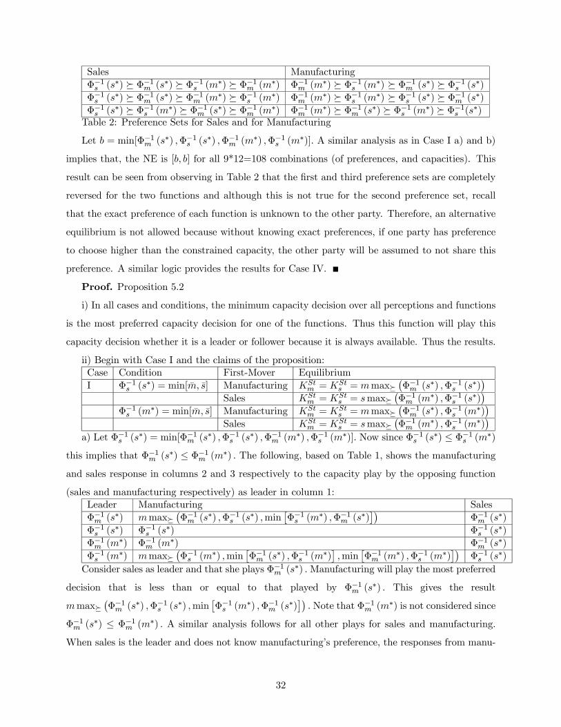
Sales ManufacturingΦ−1s (s∗) º Φ−1m (s∗) º Φ−1s (m∗) º Φ−1m (m∗) Φ−1m (m∗) º Φ−1s (m∗) º Φ−1m (s∗) º Φ−1s (s∗)Φ−1s (s∗) º Φ−1m (s∗) º Φ−1m (m∗) º Φ−1s (m∗) Φ−1m (m∗) º Φ−1s (m∗) º Φ−1s (s∗) º Φ−1m (s∗)Φ−1s (s∗) º Φ−1s (m∗) º Φ−1m (s∗) º Φ−1m (m∗) Φ−1m (m∗) º Φ−1m (s∗) º Φ−1s (m∗) º Φ−1s (s∗)Table 2: Preference Sets for Sales and for Manufacturing
Let b = min[Φ−1m (s∗) ,Φ−1s (s∗) ,Φ−1m (m∗) ,Φ−1s (m∗)]. A similar analysis as in Case I a) and b)
implies that, the NE is [b, b] for all 9*12=108 combinations (of preferences, and capacities). This
result can be seen from observing in Table 2 that the first and third preference sets are completely
reversed for the two functions and although this is not true for the second preference set, recall
that the exact preference of each function is unknown to the other party. Therefore, an alternative
equilibrium is not allowed because without knowing exact preferences, if one party has preference
to choose higher than the constrained capacity, the other party will be assumed to not share this
preference. A similar logic provides the results for Case IV.
Proof. Proposition 5.2
i) In all cases and conditions, the minimum capacity decision over all perceptions and functions
is the most preferred capacity decision for one of the functions. Thus this function will play this
capacity decision whether it is a leader or follower because it is always available. Thus the results.
ii) Begin with Case I and the claims of the proposition:Case Condition First-Mover EquilibriumI Φ−1s (s∗) = min[m̄, s̄] Manufacturing KSt
m = KSts = mmaxº
¡Φ−1m (s∗) ,Φ−1s (s∗)
¢Sales KSt
m = KSts = smaxº
¡Φ−1m (m∗) ,Φ−1s (s∗)
¢Φ−1s (m∗) = min[m̄, s̄] Manufacturing KSt
m = KSts = mmaxº
¡Φ−1m (s∗) ,Φ−1s (m∗)
¢Sales KSt
m = KSts = smaxº
¡Φ−1m (m∗) ,Φ−1s (m∗)
¢a) Let Φ−1s (s∗) = min[Φ−1m (s∗) ,Φ−1s (s∗) ,Φ−1m (m∗) ,Φ−1s (m∗)]. Now since Φ−1s (s∗) ≤ Φ−1s (m∗)
this implies that Φ−1m (s∗) ≤ Φ−1m (m∗) . The following, based on Table 1, shows the manufacturing
and sales response in columns 2 and 3 respectively to the capacity play by the opposing function
(sales and manufacturing respectively) as leader in column 1:Leader Manufacturing SalesΦ−1m (s∗) mmaxº
¡Φ−1m (s∗) ,Φ−1s (s∗) ,min
£Φ−1s (m∗) ,Φ−1m (s∗)
¤¢Φ−1m (s∗)
Φ−1s (s∗) Φ−1s (s∗) Φ−1s (s∗)Φ−1m (m∗) Φ−1m (m∗) Φ−1m (s∗)Φ−1s (m∗) mmaxº
¡Φ−1s (m∗) ,min
£Φ−1m (s∗) ,Φ−1s (m∗)
¤,min
£Φ−1m (m∗) ,Φ−1s (m∗)
¤¢Φ−1s (s∗)
Consider sales as leader and that she plays Φ−1m (s∗) .Manufacturing will play the most preferred
decision that is less than or equal to that played by Φ−1m (s∗) . This gives the result
mmaxº¡Φ−1m (s∗) ,Φ−1s (s∗) ,min
£Φ−1s (m∗) ,Φ−1m (s∗)
¤¢. Note that Φ−1m (m∗) is not considered since
Φ−1m (s∗) ≤ Φ−1m (m∗) . A similar analysis follows for all other plays for sales and manufacturing.
When sales is the leader and does not know manufacturing’s preference, the responses from manu-
32
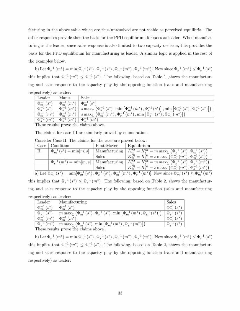
facturing in the above table which are thus unresolved are not viable as perceived equilibria. The
other responses provide then the basis for the PPD equilibrium for sales as leader. When manufac-
turing is the leader, since sales response is also limited to two capacity decision, this provides the
basis for the PPD equilibrium for manufacturing as leader. A similar logic is applied in the rest of
the examples below.
b) Let Φ−1s (m∗) = min[Φ−1m (s∗) ,Φ−1s (s∗) ,Φ−1m (m∗) ,Φ−1s (m∗)].Now since Φ−1s (m∗) ≤ Φ−1s (s∗)
this implies that Φ−1m (m∗) ≤ Φ−1m (s∗) . The following, based on Table 1 ,shows the manufactur-
ing and sales response to the capacity play by the opposing function (sales and manufacturing
respectively) as leader:Leader Manu. SalesΦ−1m (s∗) Φ−1m (m∗) Φ−1m (s∗)Φ−1s (s∗) Φ−1s (m∗) smaxº
¡Φ−1s (s∗) ,min
£Φ−1m (m∗) ,Φ−1s (s∗)
¤,min
£Φ−1m (s∗) ,Φ−1s (s∗)
¤¢Φ−1m (m∗) Φ−1m (m∗) smaxº
¡Φ−1m (m∗) ,Φ−1s (m∗) ,min
£Φ−1s (s∗) ,Φ−1m (m∗)
¤¢Φ−1s (m∗) Φ−1s (m∗) Φ−1s (m∗)These results prove the claims above.
The claims for case III are similarly proved by enumeration.
Consider Case II: The claims for the case are proved below:Case Condition First-Mover EquilibriumII Φ−1m (s∗) = min[m̄, s̄] Manufacturing KSt
m = KSts = mmaxº
¡Φ−1s (s∗) ,Φ−1m (s∗)
¢Sales KSt
m = KSts = smaxº
¡Φ−1m (m∗) ,Φ−1m (s∗)
¢Φ−1s (m∗) = min[m̄, s̄] Manufacturing KSt
m = KSts = mmaxº
¡Φ−1s (s∗) ,Φ−1s (m∗)
¢Sales KSt
m = KSts = smaxº
¡Φ−1m (m∗) ,Φ−1s (m∗)
¢a) Let Φ−1m (s∗) = min[Φ−1m (s∗) ,Φ−1s (s∗) ,Φ−1m (m∗) ,Φ−1s (m∗)]. Now since Φ−1m (s∗) ≤ Φ−1m (m∗)
this implies that Φ−1s (s∗) ≤ Φ−1s (m∗) . The following, based on Table 2, shows the manufactur-
ing and sales response to the capacity play by the opposing function (sales and manufacturing
respectively) as leader:Leader Manufacturing SalesΦ−1m (s∗) Φ−1m (s∗) Φ−1m (s∗)Φ−1s (s∗) mmaxº
¡Φ−1m (s∗) ,Φ−1s (s∗) ,min
£Φ−1m (m∗) ,Φ−1s (s∗)
¤¢Φ−1s (s∗)
Φ−1m (m∗) Φ−1m (m∗) Φ−1m (s∗)Φ−1s (m∗) mmaxº
¡Φ−1m (s∗) ,min
£Φ−1m (m∗) ,Φ−1s (m∗)
¤¢Φ−1s (s∗)
These results prove the claims above.
b) Let Φ−1s (m∗) = min[Φ−1m (s∗) ,Φ−1s (s∗) ,Φ−1m (m∗) ,Φ−1s (m∗)].Now since Φ−1s (m∗) ≤ Φ−1s (s∗)
this implies that Φ−1m (m∗) ≤ Φ−1m (s∗) . The following, based on Table 2, shows the manufactur-
ing and sales response to the capacity play by the opposing function (sales and manufacturing
respectively) as leader:
33
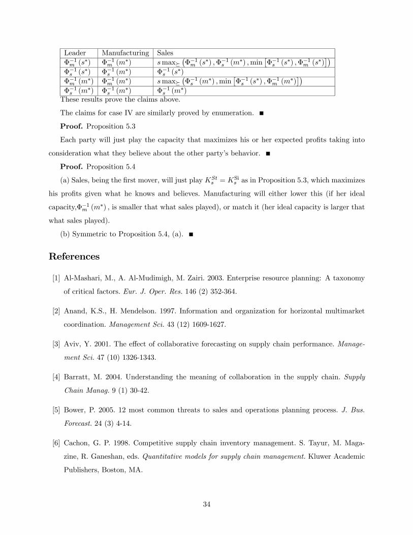
Leader Manufacturing SalesΦ−1m (s∗) Φ−1m (m∗) smaxº
¡Φ−1m (s∗) ,Φ−1s (m∗) ,min
£Φ−1s (s∗) ,Φ−1m (s∗)
¤¢Φ−1s (s∗) Φ−1s (m∗) Φ−1s (s∗)Φ−1m (m∗) Φ−1m (m∗) smaxº
¡Φ−1s (m∗) ,min
£Φ−1s (s∗) ,Φ−1m (m∗)
¤¢Φ−1s (m∗) Φ−1s (m∗) Φ−1s (m∗)These results prove the claims above.
The claims for case IV are similarly proved by enumeration.
Proof. Proposition 5.3
Each party will just play the capacity that maximizes his or her expected profits taking into
consideration what they believe about the other party’s behavior.
Proof. Proposition 5.4
(a) Sales, being the first mover, will just play KSts = KSi
s as in Proposition 5.3, which maximizes
his profits given what he knows and believes. Manufacturing will either lower this (if her ideal
capacity,Φ−1m (m∗) , is smaller that what sales played), or match it (her ideal capacity is larger that
what sales played).
(b) Symmetric to Proposition 5.4, (a).
References
[1] Al-Mashari, M., A. Al-Mudimigh, M. Zairi. 2003. Enterprise resource planning: A taxonomy
of critical factors. Eur. J. Oper. Res. 146 (2) 352-364.
[2] Anand, K.S., H. Mendelson. 1997. Information and organization for horizontal multimarket
coordination. Management Sci. 43 (12) 1609-1627.
[3] Aviv, Y. 2001. The effect of collaborative forecasting on supply chain performance. Manage-
ment Sci. 47 (10) 1326-1343.
[4] Barratt, M. 2004. Understanding the meaning of collaboration in the supply chain. Supply
Chain Manag. 9 (1) 30-42.
[5] Bower, P. 2005. 12 most common threats to sales and operations planning process. J. Bus.
Forecast. 24 (3) 4-14.
[6] Cachon, G. P. 1998. Competitive supply chain inventory management. S. Tayur, M. Maga-
zine, R. Ganeshan, eds. Quantitative models for supply chain management. Kluwer Academic
Publishers, Boston, MA.
34

[7] Cachon, G. P., M. Fisher. 2000. Supply chain inventory management and the value of shared
information. Management Sci. 46 (8) 1032-1048.
[8] Cachon, G. P. 2001. “Supply Chain Coordination with contracts.” Technical report, Whar-
ton School, University of Pennsylvania, Philadelphia, PA. Chapter later published in Steven
Graves’ and Ton de Kok’s Handbooks in Operations Research and Management Science: Supply
Chain Management. North-Holland, Amsterdam, The Netherlands. 2003.
[9] Cachon, G.P., M. Lariviere. 2001. Contracting to assure supply: How to share demand forecasts
in a supply chain. Management Sci. 47 (5) 629-646.
[10] Celikbas, M., J.G. Shanthikumar, J.M. Swaminathan. 1999. Coordinating production quanti-
ties and demand forecasts through penalty schemes. IEE Trans. 31(9) 851-864.
[11] Chen, F. 2005. Salesforce incentives, market information and production/inventory planning.
Management Sci. 51 (1) 60-75.
[12] Chen, J.M., L.T. Chen, J.D. Leu. 2006. Developing optimization models for cross-functional
decision-making: integrating marketing and production planning. OR Spectrum 28(2) 223-240.
[13] Coase, R. H. 1937. The nature of the firm. Economica. 4 (16) 386-405.
[14] Cohen Kulp, S. 2002. The Effect of Information Precision and Reliability on Manufacturer-
Retailer Relationships. The Accounting Review, 77 (3) 653-677.
[15] Crittenden, V.L., L.R. Gardiner, A. Stam. 1993. Reducing conflict between marketing and
manufacturing. Ind. Market. Manag. 22 (4) 299-309.
[16] Dougherty, D. 1992. Interpretive barriers to successful product innovation in large firms. Organ.
Sci. 3 (2) 179-202.
[17] Fawcett, S.E., G.M. Magnan. 2002. The rhetoric and reality of supply chain integration. Int.
J. Phys. Dist. 32 (5) 339-361.
[18] Federgruen, A., A. Heching. 1999. Combined pricing and inventory control under uncertainty.
Operations Research 47 (3) 454-475.
[19] Fliedner, G., 2003. CPFR: an emerging supply chain tool. Industrial Management & Data
Systems 103 (1) 14-21.
35

[20] Gonik, J. 1978. Tie salesmen’s bonuses to their forecasts. Harvard Bus. Rev. 56 (3) 116-123.
[21] Griffin, A., J.R. Hauser. 1992. Patterns of communication among marketing, engineering and
manufacturing: A comparison between two new product teams. Management Sci. 38(3) 360-
373.
[22] Griffin, A., J.R. Hauser. 1996. Integrating R&D and marketing: A review and analysis of the
literature. J. Prod. Innovat. Manag. 13 (3) 191-215.
[23] Jacobs, F.R., E. Bendoly. 2003. Enterprise resource planning: Developments and directions for
operations management research. European Journal of Operational Research 146 (2) 233-240.
[24] Kahn, K.B. 1996. Interdepartmental integration: A definition and implications for product
development performance. J. Prod. Innovat. Manag. 13 (2) 137-151.
[25] Kahn, K.B., J.T. Mentzer. 1996. Logistics and interdepartmental integration. Int. J. Phys.
Dist. 26 (8) 6-14.
[26] Kahn, K.B., J.T. Mentzer. 1998. Marketing’s integration with other departments. J. Bus. Res.
42 (1) 53-62.
[27] Kouvelis, P., M.A. Lariviere. 2000. Decentralizing cross-functional decisions: Coordination
through internal markets. Management Sci. 46 (8) 1049-1058.
[28] Klein, B., R. Crawford and A. Alchian. 1978. Vertical Integration, Appropriable Rents, and
the Competitive Contracting Process. Journal of Law and Economics. 21 (2) 297-326.
[29] Kraiselburd, S., V. G. Narayanan, and A. Raman. 2004. Contracting in a Supply Chain with
Stochastic Demand and Substitute Products. Production and Operations Management. 13 (1)
46-62
[30] Kreps, D. 1986. Corporate Culture and Economic Theory, in Technological Innovation and
Business Strategy, by M. Tsuchiya. Nihom Keizai Shimbun Inc.
[31] Kurtulus, M., and B. Toktay. 2007. Investing in Forecast Collaboration. Working paper. Van-
derbilt University.
[32] Lal, R., R. Staelin. 1986. Salesforce compensation plans in environments with asymmetric
information. Marketing Sci. 5 (3) 179-198.
36

[33] Lapide, L. 2004a. Sales and operations planning Part I: The process. J. Bus. Forecast. 23 (3)
17-19.
[34] Lapide, L. 2004b. Sales and operations planning Part II: Enabling technology. J. Bus. Forecast.
23 (4) 18-20.
[35] Lapide, L. 2005a. An S&OP Maturity Model. J. Bus. Forecast. 24 (3) 15-20.
[36] Lapide, L. 2005b. Sales and operations planning Part III: A diagnostic model. J. Bus. Forecast.
24 (1) 13-16.
[37] Larivivere, M. 2002. Inducing Forecast Revelation Through Restricted Returnds. Working
paper. Northwestern University.
[38] Lawrence, P.R., J.W. Lorsch. 1986. Organization and Environment: Managing Differentiation
and Integration. Harvard Business School Press, Boston.
[39] Lee, H.L. 2004. The Triple-A Supply Chain. Harvard Bus. Rev. 82 (10) 102.
[40] Lee, H. L. and S. Whang, “Decentralized Multi-echelon Supply Chains: Incentives and Infor-
mation”, Management Sci., 45 (1999), 633-640.
[41] Li, Q., D. Atkins. 2002. Coordinating replenishment and pricing in a firm. Manufacturing &
Service Operations Management 4 (4) 241-257.
[42] Mallik, S., P.T. Harker. 2004. Coordinating supply chains with competition: Capacity alloca-
tion in semiconductor manufacturing. Eur. J. Oper. Res. 159 (2) 330-347.
[43] Malone, T.W., K. Crowston. 1994. The interdisciplinary study of coordination. ACM Comput-
ing Surveys 26 (1) 87-119.
[44] Miyaoka, J. 2003. Implementing Collaborative Forecasting Through Buyback Contracts. Work-
ing paper. Stanford University.
[45] Oliva, R., N. Watson. 2007. Cross functional alignment in supply chain planning: A case study
of sales and operations planning. Harvard Business School Working Paper #07-001.
[46] Özer, Ö, and W. Wei. 2006. Strategic Commitment for Optimal Capacity Decision Under
Asymmetric Forecast Information. Management Sci. 52 (8) 1238-1257.
37
[47] Pinto, M.B., J.K. Pinto, J.E. Prescott. 1993. Antecedents and consequences of project team
cross-functional cooperation. Management Sci. 39 (10) 1281-1297.
[48] Porteus, E.L., S. Whang. 1991. On manufacturing marketing incentives. Management Sci. 37
(9) 1166-1181.
[49] Ruekert, R.W., O.C. Walker. 1987. Marketing interaction with other functional units: A con-
ceptual framework and empirical evidence. J. Marketing 51 (1) 1-19.
[50] Shapiro, B.P. 1977. Can marketing and manufacturing co-exist? Harvard Bus. Rev. 55 (5)
104-114.
[51] Shapiro, J. 1998. Bottom-up versus top-down approaches to supply chain modeling. S. Tayur,
M. Magazine, R. Ganeshan, eds. Quantitative models for supply chain management. Kluwer
Academic Publishers, Boston, MA.
[52] Spence, A. 1973. Job Market Signalling. Quart. J. Econom. 87 355-374.
[53] Spear, S. and H. K. Bowen. 1999. Decoding the DNA of the Toyota Production System.
Harvard Bus. Rev. Reprint 99509.
[54] Stank, T.P., P.J. Daugherty, A.E. Ellinger. 1999. Marketing/Logistics interaction and firm
performance. Int. J. Logistics Man. 10 (1) 11-24.
[55] Stank, T.P., S.B. Keller, D.J. Closs. 2001. Performance benefits of supply chain logistical
integration. Transport. J. 41 (2-3) 32-46.
[56] Stonebraker, P.W., R. Afifi. 2004. Towards a contingency theory of supply chains.Management
Decis. 42 (9) 1131-1144.
[57] Terwiesch, C., Z. J. Ren, T. H. Ho, and M. A. Cohen. 2005. An empirical analysis of forecast
sharing in the semiconductor equipment supply chain. Management Sci. 51 (2) 208-220.
[58] Tomlin, B. 2003. Capacity investments in supply chains: Sharing the gain rather than sharing
the pain. Manufacturing & Service Operations Management 5(4) 317-333.
[59] Troyer, L., J. Smith, S. Marshall, E. Yaniv, S. Tayur, M. Barkman, A. Kaya, Y. Liu. 2005.
Improving asset management and order fulfillment at Deere & Company’s C&CE division.
Interfaces 35(1) 76-87.
38

[60] Van den Steen, E.. 2001. Essays on the Managerial Implications of Differing Priors. Phd
Thesis. Stanford Business School.
[61] Van Dierdonck, R., J.G. Miller. 1980. Designing production planning and control systems. J.
Oper. Manag. 1(1) 37-46.
[62] Van Landeghem, H., H. Vanmaele. 2002. Robust planning: A new paradigm for demand chain
planning. J. Oper. Manag. 20(6) 769-783.
[63] Wang, Y. 2007. Joint pricing-production decisions in supply chains of complementary products
with uncertain demand. Operations Research 54(6) 1110-1127.
[64] Watson, N. and Y.S. Zheng. 2005. Decentralized serial supply chains subject to order delays and
information distortion: Exploiting real time Sales data. Manufacturing & Service Operations
Management 7 (2) 152-168.
[65] Williamson, O. 1979. Transaction cost economics: The governance of contractual relations.
Journal of Law and Economics 22 (2) 233-261.
[66] Yano, C.A., S.M. Gilbert. 2004. Coordinated pricing and production/procurement decision: A
review. In Chakravarty, J. E. (ed.), Managing Business Interfaces: Marketing, Engineering,
and Manufacturing Perspectives, Springer, New York, pp. 39-xx.
[67] Yildiz, M. 2000. Essays on Sequential Bargaining, PhD Dissertation, Stanford Business School.
39
Related Documents