ALGORITHMS FOR VERTEX-WEIGHTED MATCHING IN GRAPHS by Mahantesh Halappanavar B.S. August 1996, Karnataka University M.S. December 2003, Old Dominion University A Dissertation Submitted to the Faculty of Old Dominion University in Partial Fulfillment of the Requirement for the Degree of DOCTOR OF PHILOSOPHY COMPUTER SCIENCE OLD DOMINION UNIVERSITY May 2009 Approved by: Alex Pothen (Director) Jessica Crouch Bruce Hendrickson Stephan Olariu Mohammad Zubair

Welcome message from author
This document is posted to help you gain knowledge. Please leave a comment to let me know what you think about it! Share it to your friends and learn new things together.
Transcript

ALGORITHMS FOR
VERTEX-WEIGHTED MATCHING IN GRAPHS
by
Mahantesh HalappanavarB.S. August 1996, Karnataka University
M.S. December 2003, Old Dominion University
A Dissertation Submitted to the Faculty ofOld Dominion University in Partial Fulfillment of the
Requirement for the Degree of
DOCTOR OF PHILOSOPHY
COMPUTER SCIENCE
OLD DOMINION UNIVERSITYMay 2009
Approved by:
Alex Pothen (Director)
Jessica Crouch
Bruce Hendrickson
Stephan Olariu
Mohammad Zubair
ABSTRACT
ALGORITHMS FOR
VERTEX-WEIGHTED MATCHING IN GRAPHS
Mahantesh Halappanavar
Old Dominion University, 2009
Director: Dr. Alex Pothen
A matching M in a graph is a subset of edges such that no two edges in M are inci-
dent on the same vertex. Matching is a fundamental combinatorial problem that has
applications in many contexts: high-performance computing, bioinformatics, net-
work switch design, web technologies, etc. Examples in the first context include
sparse linear systems of equations, where matchings are used to place large matrix
elements on or close to the diagonal, to compute the block triangular decomposition
of sparse matrices, to construct sparse bases for the null space or column space of
under-determined matrices, and to coarsen graphs in multi-level graph partitioning
algorithms. In the first part of this thesis, we develop exact and approximation al-
gorithms for vertex weighted matchings, an under-studied variant of the weighted
matching problem. We propose three exact algorithms, three half approximation
algorithms, and a two-third approximation algorithm. We exploit inherent proper-
ties of this problem such as lexicographical orders, decomposition into sub-problems,
and the reachability property, not only to design efficient algorithms, but also to
provide simple proofs of correctness of the proposed algorithms. In the second part
of this thesis, we describe work on a new parallel half-approximation algorithm for
weighted matching. Algorithms for computing optimal matchings are not amenable
to parallelism, and hence we consider approximation algorithms here. We extend
the existing work on a parallel half approximation algorithm for weighted matching
and provide an analysis of its time complexity. We support the theoretical obser-
vations with experimental results obtained with MatchBoxP, toolkit designed and
implemented in C++ and MPI using modern software engineering techniques. The
work in this thesis has resulted in better understanding of matching theory, a func-
tional public-domain software toolkit, and modeling of the sparsest basis problem as
a vertex-weighted matching problem.

c©Copyright, 2009, by Mahantesh Halappanavar, All Rights Reserved
iii

ACKNOWLEDGEMENTS
“One can pay back the loan of gold, but one dies forever in debt to those
who are kind.” - Malayan Proverb
First and foremost, I would like to thank my advisor Alex Pothen, without him
this work would have been impossible. He not only introduced me to the subject, but
has also been a constant inspiration throughout. His support and encouragement has
been invaluable both personally and professionally, for which I will remain forever
indebted.
This work has evolved in collaboration with Florin Dobrian, a friend, guide and
mentor who has irreversibly changed my thinking. I will also remain indebted to As-
sefaw Gebremedhin for his friendship and generousness in improving my presentation
on numerous occasions.
I remain thankful to my committee members Jessica Crouch, Bruce Hendrickson,
Stephan Olariu and Mohammad Zubair. Their comments have been thought pro-
voking, and their suggestions invaluable. I also want to thank Erik Boman for his
time and efforts in helping my research.
I will remain indebted to my supervisor Mike Sachon and coworkers Amit Kumar
and Ruben Igloria, for providing flexibility, support and a productive work environ-
ment. Special thanks are due to Amit Kumar for his friendship that has only grown
over the years.
I was introduced to academic research in my Masters program by Ravi Mukka-
mala. I will remain forever indebted for his mentorship - academic as well as spiritual.
I would like to thank the following departments at Old Dominion University - the
Office of Graduate Studies for the University Graduate Fellowship during 2005 to
2006; the Office of Research and the Department of Computer Science for teaching
and research assistanceships during 2001 to 2005; and the Office of Study Abroad
for travel assistance in 2005.
With long hours away from home, the last five years have been especially hard on
my wife Savitha and daughter Anika. They have accepted it in stride and I cannot
thank them enough for it. I will remain thankful to my parents who have always
emphasized education above everything else, my sister for being my inspiration, my
in-laws for their support, and my very large extended family where everyone has
made a special impression on me.
iv

This research used resources of the National Energy Research Scientific Comput-
ing Center, which is supported by the Office of Science of the U.S. Department of
Energy under Contract No. DE-AC02-05CH11231.
v

vi
TABLE OF CONTENTS
PageLIST OF TABLES . . . . . . . . . . . . . . . . . . . . . . . . . . . . . . . . . ixLIST OF FIGURES . . . . . . . . . . . . . . . . . . . . . . . . . . . . . . . . xvii
CHAPTERS
I Introduction . . . . . . . . . . . . . . . . . . . . . . . . . . . . . . . . . . 1I.1 Outline . . . . . . . . . . . . . . . . . . . . . . . . . . . . . . . . . . . 3I.2 Combinatorial Scientific Computing . . . . . . . . . . . . . . . . . . . 3I.3 Motivation . . . . . . . . . . . . . . . . . . . . . . . . . . . . . . . . . 4I.4 Contributions . . . . . . . . . . . . . . . . . . . . . . . . . . . . . . . 9I.5 Chapter Summary . . . . . . . . . . . . . . . . . . . . . . . . . . . . 10
II Background and Related Work . . . . . . . . . . . . . . . . . . . . . . . 11II.1 Introduction . . . . . . . . . . . . . . . . . . . . . . . . . . . . . . . . 11II.2 Foundations . . . . . . . . . . . . . . . . . . . . . . . . . . . . . . . . 15II.3 Maximum Cardinality Matching . . . . . . . . . . . . . . . . . . . . . 25II.4 Maximum Edge-Weight Matching . . . . . . . . . . . . . . . . . . . . 28II.5 Approximation Algorithms . . . . . . . . . . . . . . . . . . . . . . . . 33II.6 Chapter Summary . . . . . . . . . . . . . . . . . . . . . . . . . . . . 39
III Exact Algorithms . . . . . . . . . . . . . . . . . . . . . . . . . . . . . . . 40III.1 Introduction and Related Work . . . . . . . . . . . . . . . . . . . . . 40III.2 Foundations . . . . . . . . . . . . . . . . . . . . . . . . . . . . . . . . 44III.3 New Algorithms for Maximum Vertex-weight Matching . . . . . . . . 47
III.3.1 Algorithm GlobalOptimal . . . . . . . . . . . . . . . . . . . . 48III.3.2 Algorithm LocalOptimal . . . . . . . . . . . . . . . . . . . . . 50III.3.3 Algorithm HybridOptimal . . . . . . . . . . . . . . . . . . . . 51III.3.4 Negative Weights . . . . . . . . . . . . . . . . . . . . . . . . . 53
III.4 Proof of Correctness . . . . . . . . . . . . . . . . . . . . . . . . . . . 55III.5 A Reachability-Based Algorithm . . . . . . . . . . . . . . . . . . . . . 61III.6 Chapter Summary . . . . . . . . . . . . . . . . . . . . . . . . . . . . 62
IV Approximation Algorithms . . . . . . . . . . . . . . . . . . . . . . . . . . 64IV.1 Introduction . . . . . . . . . . . . . . . . . . . . . . . . . . . . . . . . 64IV.2 New 1
2-approx Algorithms . . . . . . . . . . . . . . . . . . . . . . . . 64
IV.3 Proof of Correctness . . . . . . . . . . . . . . . . . . . . . . . . . . . 71IV.4 Global 2
3-approx Algorithm . . . . . . . . . . . . . . . . . . . . . . . . 78
IV.4.1 Proof of Correctness . . . . . . . . . . . . . . . . . . . . . . . 78IV.5 Potential Local 2
3-approx Algorithm . . . . . . . . . . . . . . . . . . . 88
IV.5.1 Correctness of Algorithm LocalTwoThird . . . . . . . . . . 89IV.6 Experimental Results . . . . . . . . . . . . . . . . . . . . . . . . . . . 91IV.7 Chapter Summary . . . . . . . . . . . . . . . . . . . . . . . . . . . . 95
V Parallel Approximate Algorithms . . . . . . . . . . . . . . . . . . . . . . 97V.1 Introduction . . . . . . . . . . . . . . . . . . . . . . . . . . . . . . . . 97
vii
V.1.1 Complexity Analysis . . . . . . . . . . . . . . . . . . . . . . . 100V.2 Distributed Algorithm of Hoepman . . . . . . . . . . . . . . . . . . . 104
V.2.1 Complexity Analysis . . . . . . . . . . . . . . . . . . . . . . . 107V.3 Parallel 1
2-approx Algorithm . . . . . . . . . . . . . . . . . . . . . . . 108
V.3.1 Complexity Analysis . . . . . . . . . . . . . . . . . . . . . . . 119V.4 Experimental Results . . . . . . . . . . . . . . . . . . . . . . . . . . . 122
V.4.1 Data Set for Experiments . . . . . . . . . . . . . . . . . . . . 122V.4.2 Performance of Serial Matching Algorithms . . . . . . . . . . 127V.4.3 Performance of Parallel Matching Algorithm: . . . . . . . . . . 130V.4.4 Performance of Parallel Matching on Graphs from Applications 144V.4.5 Analysis of Communication . . . . . . . . . . . . . . . . . . . 147
V.5 Chapter Summary . . . . . . . . . . . . . . . . . . . . . . . . . . . . 150VI Conclusions and Future Work . . . . . . . . . . . . . . . . . . . . . . . . 152
VI.1 Future Work . . . . . . . . . . . . . . . . . . . . . . . . . . . . . . . . 153
viii
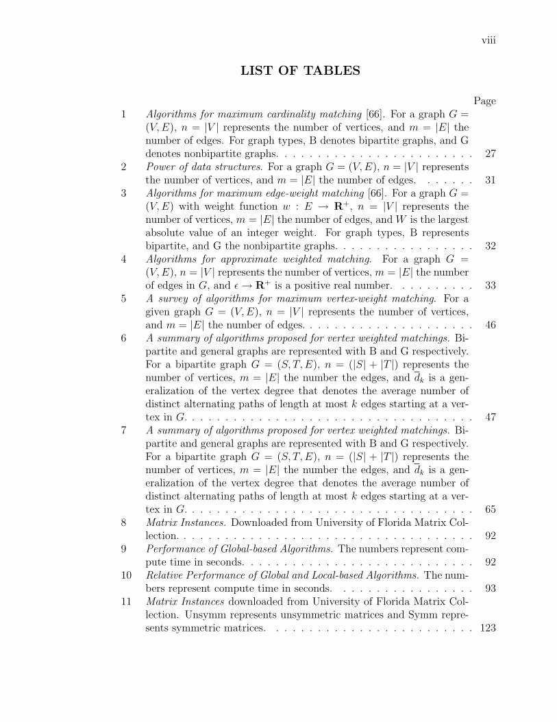
LIST OF TABLES
Page1 Algorithms for maximum cardinality matching [66]. For a graph G =
(V,E), n = |V | represents the number of vertices, and m = |E| thenumber of edges. For graph types, B denotes bipartite graphs, and Gdenotes nonbipartite graphs. . . . . . . . . . . . . . . . . . . . . . . . 27
2 Power of data structures. For a graph G = (V,E), n = |V | representsthe number of vertices, and m = |E| the number of edges. . . . . . . 31
3 Algorithms for maximum edge-weight matching [66]. For a graph G =(V,E) with weight function w : E → R+, n = |V | represents thenumber of vertices, m = |E| the number of edges, and W is the largestabsolute value of an integer weight. For graph types, B representsbipartite, and G the nonbipartite graphs. . . . . . . . . . . . . . . . . 32
4 Algorithms for approximate weighted matching. For a graph G =(V,E), n = |V | represents the number of vertices, m = |E| the numberof edges in G, and ε→ R+ is a positive real number. . . . . . . . . . 33
5 A survey of algorithms for maximum vertex-weight matching. For agiven graph G = (V,E), n = |V | represents the number of vertices,and m = |E| the number of edges. . . . . . . . . . . . . . . . . . . . . 46
6 A summary of algorithms proposed for vertex weighted matchings. Bi-partite and general graphs are represented with B and G respectively.For a bipartite graph G = (S, T,E), n = (|S| + |T |) represents thenumber of vertices, m = |E| the number the edges, and dk is a gen-eralization of the vertex degree that denotes the average number ofdistinct alternating paths of length at most k edges starting at a ver-tex in G. . . . . . . . . . . . . . . . . . . . . . . . . . . . . . . . . . . 47
7 A summary of algorithms proposed for vertex weighted matchings. Bi-partite and general graphs are represented with B and G respectively.For a bipartite graph G = (S, T,E), n = (|S| + |T |) represents thenumber of vertices, m = |E| the number the edges, and dk is a gen-eralization of the vertex degree that denotes the average number ofdistinct alternating paths of length at most k edges starting at a ver-tex in G. . . . . . . . . . . . . . . . . . . . . . . . . . . . . . . . . . . 65
8 Matrix Instances. Downloaded from University of Florida Matrix Col-lection. . . . . . . . . . . . . . . . . . . . . . . . . . . . . . . . . . . . 92
9 Performance of Global-based Algorithms. The numbers represent com-pute time in seconds. . . . . . . . . . . . . . . . . . . . . . . . . . . . 92
10 Relative Performance of Global and Local-based Algorithms. The num-bers represent compute time in seconds. . . . . . . . . . . . . . . . . 93
11 Matrix Instances downloaded from University of Florida Matrix Col-lection. Unsymm represents unsymmetric matrices and Symm repre-sents symmetric matrices. . . . . . . . . . . . . . . . . . . . . . . . . 123
ix
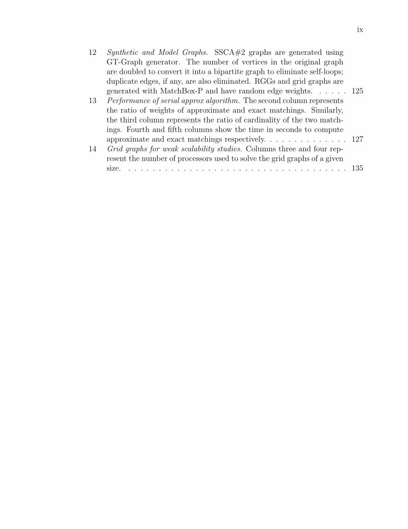
12 Synthetic and Model Graphs. SSCA#2 graphs are generated usingGT-Graph generator. The number of vertices in the original graphare doubled to convert it into a bipartite graph to eliminate self-loops;duplicate edges, if any, are also eliminated. RGGs and grid graphs aregenerated with MatchBox-P and have random edge weights. . . . . . 125
13 Performance of serial approx algorithm. The second column representsthe ratio of weights of approximate and exact matchings. Similarly,the third column represents the ratio of cardinality of the two match-ings. Fourth and fifth columns show the time in seconds to computeapproximate and exact matchings respectively. . . . . . . . . . . . . . 127
14 Grid graphs for weak scalability studies. Columns three and four rep-resent the number of processors used to solve the grid graphs of a givensize. . . . . . . . . . . . . . . . . . . . . . . . . . . . . . . . . . . . . 135
x
LIST OF FIGURES
Page1 Landscape of the matching problems. The vertex-weighted matching
problem can be formulated as an edge-weighted matching problem.The weighted matching algorithms utilize techniques developed for thecardinality matching problem. The arrows indicate these relationships. 2
2 Representation of a sparsest column-space basis problem. A matrix Awith k rows and n columns, and a basis B with k rows and k linearlyindependent columns. . . . . . . . . . . . . . . . . . . . . . . . . . . . 7
3 A greedy algorithm for computing a sparsest column-space basis. (a)State before augmenting a basis Bi with a column of current heaviestweight wmax from C; (b) state after augmenting a basis with a sparsestlinearly independent column from C. . . . . . . . . . . . . . . . . . . 7
4 Computation of a sparsest column-space basis with a maximum vertex-weight matching. (a) A matrix A; (b) A bipartite graph (G) repre-sentation of A. Numbers on the right indicate the weight of each Svertex. Bold lines represent the matched edges, and matched verticesare colored black; (c) A candidate basis as computed by a maximumvertex-weight matching in G. . . . . . . . . . . . . . . . . . . . . . . 9
5 An example of matching. (a) A bipartite graph G, (b) a matching Min G. Bold lines represent matched edges, and matched vertices arecolored black. . . . . . . . . . . . . . . . . . . . . . . . . . . . . . . . 12
6 Types of matchings. Matched edges are represented with bold lines andmatched vertices are filled with black color. (a) A maximal matching,(b) a maximum matching, and (c) a perfect matching. . . . . . . . . . 13
7 Types of paths. Matched edges are represented with bold lines andmatched vertices are colored black. (a) An alternating path startingwith an unmatched vertex, (b) an alternating path starting with amatched vertex, and (c) an augmenting path. . . . . . . . . . . . . . 15
8 Augmentation by symmetric difference. The matched edges are rep-resented with bold lines and matched vertices are colored black. (a)Before augmentation, (b) after augmentation. . . . . . . . . . . . . . 16
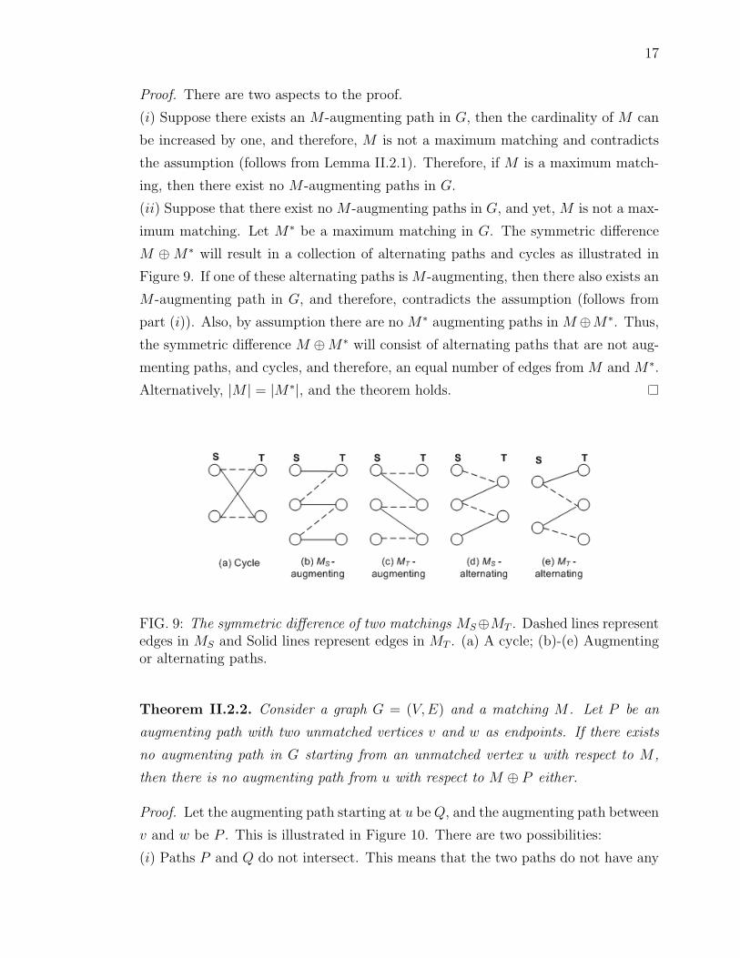
9 The symmetric difference of two matchings MS ⊕MT . Dashed linesrepresent edges in MS and Solid lines represent edges in MT . (a) Acycle; (b)-(e) Augmenting or alternating paths. . . . . . . . . . . . . 17
10 Effect of M ⊕ P . Bold lines represent matched edges and matchedvertices are colored black. (a) Paths P and Q do not intersect; (b)paths P and Q intersect. This figure has been adapted from [57]. . . 18

xi
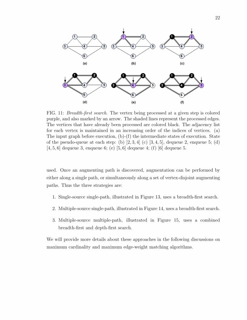
11 Breadth-first search. The vertex being processed at a given step is col-ored purple, and also marked by an arrow. The shaded lines representthe processed edges. The vertices that have already been processedare colored black. The adjacency list for each vertex is maintainedin an increasing order of the indices of vertices. (a) The input graphbefore execution, (b)-(f) the intermediate states of execution. Stateof the pseudo-queue at each step: (b) [2, 3, 4] (c) [3, 4, 5], dequeue 2,enqueue 5; (d) [4, 5, 6] dequeue 3, enqueue 6; (e) [5, 6] dequeue 4; (f)[6] dequeue 5. . . . . . . . . . . . . . . . . . . . . . . . . . . . . . . . 22
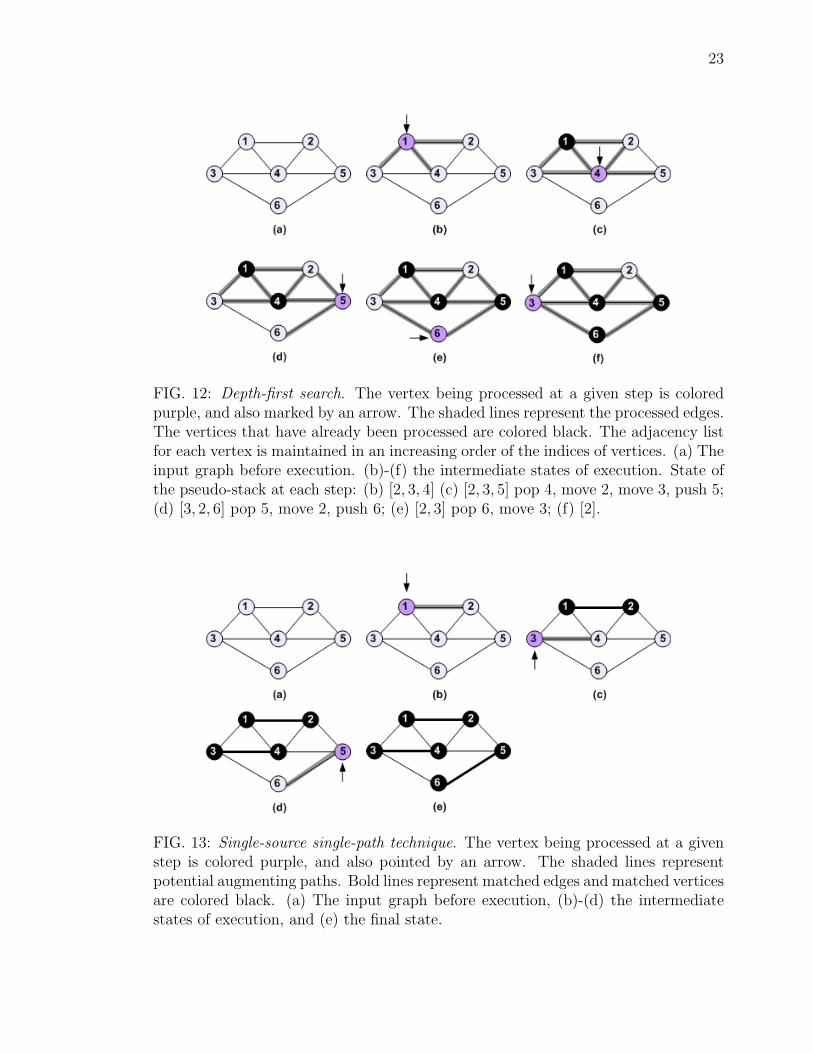
12 Depth-first search. The vertex being processed at a given step is col-ored purple, and also marked by an arrow. The shaded lines representthe processed edges. The vertices that have already been processedare colored black. The adjacency list for each vertex is maintainedin an increasing order of the indices of vertices. (a) The input graphbefore execution. (b)-(f) the intermediate states of execution. Stateof the pseudo-stack at each step: (b) [2, 3, 4] (c) [2, 3, 5] pop 4, move2, move 3, push 5; (d) [3, 2, 6] pop 5, move 2, push 6; (e) [2, 3] pop 6,move 3; (f) [2]. . . . . . . . . . . . . . . . . . . . . . . . . . . . . . . 23
13 Single-source single-path technique. The vertex being processed ata given step is colored purple, and also pointed by an arrow. Theshaded lines represent potential augmenting paths. Bold lines repre-sent matched edges and matched vertices are colored black. (a) Theinput graph before execution, (b)-(d) the intermediate states of exe-cution, and (e) the final state. . . . . . . . . . . . . . . . . . . . . . . 23
14 Multiple-source single-path technique. The vertices being processed ata given step are colored purple. The shaded lines represent potentialaugmenting paths. Bold lines represent matched edges and matchedvertices are colored black. (a) The input graph before execution, (b)-(d) the intermediate states of execution, and (e) the final state. . . . 24
15 Multiple-source multiple-path technique. The vertices processed at agiven step are colored purple. The shaded lines represent potentialaugmenting paths, bold lines represent matched edges and matchedvertices are colored black. (a) The input graph before execution, (b)the intermediate state of execution, and (c) the final state. . . . . . . 24
16 Execution of Algorithm GlobalHeavy. The weights are associatedwith the edges. Bold lines represent matched edges, and matched ver-tices are colored black. Vertices processed at a given step are coloredpurple. Dashed lines represent the edges that are removed from thegraph. (a) The input graph before execution, (b)-(c) the intermediatestates of execution, and (d) the final state. . . . . . . . . . . . . . . . 34

xii
17 Execution of Algorithm LAM. The weights are associated with theedges. Bold lines represent matched edges. Matched vertices are col-ored black, and the vertices being processed at a given step are coloredpurple. The shaded edges represent dominating edges at a currentstep, and dashed lines represent the edges that are removed from thegraph. (a) The input graph before execution, (b)-(e) the intermediatestates of execution, and (f) the final state. . . . . . . . . . . . . . . . 36
18 Execution of Algorithm PathGrow. The weights are associated withthe edges. The solid bold-lines represent edges matched in M1, and thedashed bold-lines represent the edges matched in M2. The matchedvertices are colored black, and the vertices processed at a given stepare colored purple. The shaded edges highlight the edges that arebeing processed for matching at a given step. (a) The input graphbefore execution, (b)-(f) the intermediate states of execution. . . . . . 38
19 Decomposition of the maximum vertex-weight matching problem. . . . 4120 The symmetric difference of two matchings MS ⊕MT . Dashed lines
represent edges in MS and Solid lines represent edges in MT . (a) Acycle; (b)-(e) Augmenting or alternating paths. . . . . . . . . . . . . 42
21 Execution of Algorithm GlobalOptimal. (a) The input graphG = (S, T,E) before execution, weights are associated only with theS vertices. (b)-(e) The intermediate states of execution. Bold linesrepresent matched edges, and matched vertices are colored black. Theshaded edges highlight the shortest augmenting path from a given Svertex. Vertices colored Violet represent the vertex processed at agiven step, and the end-point of an augmenting path if one exists.The arrows indicate the S vertex that is being processed at a given step. 50
22 Execution of Algorithm LocalOptimal. (a) The input graph G =(S, T,E) before execution, weights are associated only with the S ver-tices. (b)-(d) The intermediate states of execution, (e) the final state.Bold lines represent matched edges, and matched vertices are coloredblack. The shaded edges highlight all the augmenting paths that existfrom a given T vertex. The arrows indicate the T vertex that is beingprocessed at a given step. . . . . . . . . . . . . . . . . . . . . . . . . 52
23 Transformation of graphs with negative weights. (a) The input graphG = (S, T,E) with some negative weights associated with the vertices,(b) the new graph G
′(S′, T′, E′) with zero or positive weights. The
new vertices are filled with Black color. . . . . . . . . . . . . . . . . . 5424 Illustration of the reachability property. Bold lines represent the
matched edges and matched vertices are colored black. . . . . . . . . 5625 Illustrates that reachability property holds for Algorithm GlobalOp-
timal. Bold lines represent the matched edges and matched verticesare colored black. (a) State before (k + 1)-th augmentation, (b) stateafter (k + 1)-th augmentation. . . . . . . . . . . . . . . . . . . . . . . 58

xiii
26 Greedy initialization. Bold lines represent matched edges, andmatched vertices are colored black. (a) The input graph G = (S, T,E),weights are associated only with the T vertices, (b) a greedy initial-ization that picks best augmenting paths of length one, and (c) anoptimal matching. . . . . . . . . . . . . . . . . . . . . . . . . . . . . . 63
27 Execution of Algorithm GlobalHalf. (a) The input graph G =(S, T,E) with weights associated only with the S vertices, (b)-(e) theintermediate states of execution. Bold lines represent matched edges,and matched vertices are colored black. The shaded edges mark theaugmenting paths of length one (an unmatched edge) from a given Svertex, (f) the final state. . . . . . . . . . . . . . . . . . . . . . . . . . 67
28 Execution of Algorithm LocalHalf. (a) The input graph G =(S, T,E) with weights associated only with the S vertices, (b)-(d)the intermediate states of execution, (e) the final state. Bold linesrepresent matched edges, and matched vertices are colored black. Theshaded edges mark all the augmenting paths of length one (unmatchededges) that exist from a given T vertex. . . . . . . . . . . . . . . . . . 69
29 Execution of Algorithm GlobalTwoThird. (a) The input graphG = (S, T,E) before the execution, weights are associated only withS vertices, (b)-(e) the intermediate states of execution. Bold linesrepresent matched edges, and matched vertices are colored black. Theshaded edges highlight the shortest augmenting path from a given Svertex, and (f) the final state. . . . . . . . . . . . . . . . . . . . . . . 80
30 Symmetric difference. (a) Input graph, weights are associated onlywith the S vertices such that s1 � s2 � s3 � s4; (b) an optimalmatching M∗ computed by Algorithm GlobalOptimal. Bold linesrepresent matched edges. At step one, edge e(s1, t3) is matched; atstep two, edge e(s2, t2) is matched; at step three, the matching is aug-mented via path [s3, t2, s2, t3, s1, t1]; no path exists at step four; (c) a23-approx matching M3 computed by Algorithm GlobalTwoThird,
Wavy lines represent matched edges; At step one, edge e(s1, t3) ismatched; at step two, edge e(s2, t2) is matched; at step three, noaugmenting path of length three exists; at step four, the matchingis augmented via path [s4, t3, s1, t1]; and (d) the symmetric differenceM∗⊕M3. The bold lines denote edges matched in M∗, and wavy linesdenote edges matched in M3. . . . . . . . . . . . . . . . . . . . . . . . 81
31 Intuition for proof of 23-approx algorithm GlobalTwoThird. For
each failed S vertex, Algorithm GlobalTwoThird will match twoS vertices that are at least as heavy as the failed vertex. Note that theassociation of matched vertices with failed vertices is dynamic. Thefigure is representative of a state at a particular step of execution. . . 82
32 New augmenting paths. Bold lines represent the matched edges andmatched vertices are colored black. The two kinds of paths in LemmaIV.4.1 are shown as P1 and P2. . . . . . . . . . . . . . . . . . . . . . 83

xiv
33 Execution of Algorithm LocalTwoThird. (a) The input graphG = (S, T,E) before the execution, weights are associated only with Svertices, (b)-(d) the intermediate states of execution, and (e) the finalstate. Bold lines represent matched edges, and matched vertices arecolored black. The shaded edges highlight all the augmenting pathsthat exist from a given T vertex. . . . . . . . . . . . . . . . . . . . . 89
34 Performance of Approximation Algorithms. Cardinality of matchingsof the approximation algorithms as a ratio of the cardinality of theexact algorithm. . . . . . . . . . . . . . . . . . . . . . . . . . . . . . . 94
35 Performance of Approximation Algorithms. Weight of matchings ofthe approximation algorithms as a ratio of the weight of the exactalgorithm. . . . . . . . . . . . . . . . . . . . . . . . . . . . . . . . . . 94
36 New augmenting paths. (a) No augmenting path of length less than orequal to five exist starting at vertex s1 in graph G at step k; (b) anaugmenting path of length five is available from s1 at a step after k. . 95
37 Execution of Algorithm 22. (a) The input graph G = (V,E) withweights associated with the edges; (b) an intermediate step of execu-tion where the pointers are set for each vertex in the graph; (c) anintermediate step where vertices that are pointing to each other arematched. Bold lines represent matched edges. Dashed lines representthe edges removed from the graph; (d) reset pointers for vertices 4 and6; (e) edge (4, 5) is matched; (d) the final state. Matched vertices arecolored black. . . . . . . . . . . . . . . . . . . . . . . . . . . . . . . . 102
38 Complexity analysis. A sample graph G with weights associated withthe edges such that (w(e1) > w(e2) > · · · > w(e8)). . . . . . . . . . . 103
39 Execution of Hoepman’s Algorithm. (a) The input graph G = (V,E)with weights associated with the edges, vertices {1, 2, 3} are assignedto processors {P1, P2, P3} respectively; (b) an intermediate step of ex-ecution when REQUEST messages are sent by each processor to theirneighbors of choice; (c) an intermediate step when edge (2, 3) ismatched. (d) A possible intermediate step when processors P2 andP3 send UNAVAILABLE messages to P1 in that order, (d’) an alternativesituation when P1 gets an UNAVAILABLE message from P3, and sendsa REQUEST to P2. Eventually, P1 will also receive an UNAVAILABLE
message from P2. (e) The final state. Matched vertices are coloredblack. . . . . . . . . . . . . . . . . . . . . . . . . . . . . . . . . . . . 106
40 Data distribution among processors. (a) The input graph G = (V,E)with weights associated with the edges; (b) The vertex set V is par-titioned among two processors P0 and P1. Processor P0 owns vertices{0, 3, 4} and Processor P1 owns vertices {1, 2, 6}. (c) Data storageon the processors. Along with internal edges, each processor will alsostore the endpoints of the edges that get cut (cross-edges). Thesevertices are called the ghost vertices and are colored purple in the figure.109

xv
41 Possible communication patterns. Message types are denoted by Rfor REQUEST, U for UNAVAILABLE, and F for FAILURE. (a) When tworequests match, it results in a matched edge. An UNAVAILABLE messagefrom P1 to P0 can be responded by an UNAVAILABLE message (b), ora FAILURE message (c) from P0 to P1. (d) An UNAVAILABLE messagefrom P0 can either be responded with an UNAVAILABLE or a FAILURE
message by P1. . . . . . . . . . . . . . . . . . . . . . . . . . . . . . . 11742 Execution of parallel approximation algorithm. (a) The input graph
G = (V,E) with weights associated with the edges, vertices {0, 3, 4}are assigned to processor {P0}, and vertices {1, 2, 6} are assignedto processor {P1}. (b) an intermediate step of execution when lo-cal computations are done. REQUEST(4, 1) message is sent from P0
to P1; (c) Processor P0 matches edge (0, 3) and sends messages:UNAVAILABLE(0, 6) and REQUEST(4, 6) to P1. Processor P1 matchesedge (1, 2) and sends messages: UNAVAILABLE(1, 4) and REQUEST(6, 4)to P0. (d) Processor P0 matches edge (4, 6) and sends messageUNAVAILABLE(4, 1) to P1. Processor P1 matches edge (6, 4) and sendsmessage UNAVAILABLE(6, 0) to P0. . . . . . . . . . . . . . . . . . . . . 118
43 Illustration of different imbalance factors on Processor Pi. . . . . . . . 11944 Visualization of matrix structures. . . . . . . . . . . . . . . . . . . . . 12345 Random geometric graph. A random geometric graph with 1, 000 ver-
tices as visualized with Pajek. . . . . . . . . . . . . . . . . . . . . . . 12446 SSCA#2 graph. An SSCA#2 graph with 1, 024 vertices as visualized
with Pajek. . . . . . . . . . . . . . . . . . . . . . . . . . . . . . . . . 12547 Five-point grid graph. A 10 X 10 five-point grid graph visualized with
Pajek. . . . . . . . . . . . . . . . . . . . . . . . . . . . . . . . . . . . 12648 Nine-point grid graph. A 10 X 10 nine-point grid graph visualized with
Pajek. . . . . . . . . . . . . . . . . . . . . . . . . . . . . . . . . . . . 12649 Performance of Serial Approximation Algorithms: Weight. The path
growing algorithms are represented by PG1, PG2, and PG3. . . . . . 12850 Performance of Serial Approximation Algorithms: Cardinality. . . . . 12951 Performance of Serial Approximation Algorithms: Compute Time. . . 12952 4k grid graph: Edgecut as a function of number of vertices. Ac-
tual edgecut for different number of partitions using multi-level K-way partitioning algorithm in Metis, and ideal edgecut given by(2√|V |(√P − 1)), where V is the number of vertices and P is the
number of partitions. . . . . . . . . . . . . . . . . . . . . . . . . . . . 13153 4k grid graph: Compute time (maximum). Maximum time is the time
in seconds of the slowest processor in the group of processors used tosolve the problem. . . . . . . . . . . . . . . . . . . . . . . . . . . . . . 132
54 4k grid graph: Compute time (average). Average time is the sum ofcompute time on each processor in the group divided by the numberof processors in that group. . . . . . . . . . . . . . . . . . . . . . . . 133
55 Speedup for 4k x 4k grid graph. . . . . . . . . . . . . . . . . . . . . . 133

xvi
56 4k grid graph: Cardinality after Phase-1. . . . . . . . . . . . . . . . . 13457 Weak scaling for grid graphs: Series-1 uses the graph size and proces-
sor combinations as shown in Table 14. . . . . . . . . . . . . . . . . . 13658 Weak scaling for grid graphs: Series-2 uses the graph size and proces-
sor combinations as shown in Table 14. . . . . . . . . . . . . . . . . . 13659 Edgecut and number of messages for different grid graphs: The graph
size and processor combinations are shown in Table 14. . . . . . . . . 13760 320k RGG: Edgecut as a function of number of vertices. Actual edge-
cut for different number of partitions using multi-level K-way parti-tioning algorithm in Metis. . . . . . . . . . . . . . . . . . . . . . . . . 137
61 320k RGG: Compute time (maximum). Maximum time is the timein seconds of the slowest processor in the group of processors used tosolve the problem. . . . . . . . . . . . . . . . . . . . . . . . . . . . . . 138
62 320k RGG: Compute time (average). Average time is the sum ofcompute time on each processor in the group divided by the numberof processors in that group. . . . . . . . . . . . . . . . . . . . . . . . 138
63 320k RGG: Speedup. . . . . . . . . . . . . . . . . . . . . . . . . . . . 13964 320k RGG: Cardinality after Phase-1. . . . . . . . . . . . . . . . . . . 13965 524k SSCA#2: Edgecut as a function of number of vertices. Actual
edgecut for different number of partitions using K-way partitioningalgorithm in Metis. . . . . . . . . . . . . . . . . . . . . . . . . . . . . 140
66 524k SSCA#2: Compute time (maximum). Maximum time is thetime in seconds of the slowest processor in the group of processorsused to solve the problem. . . . . . . . . . . . . . . . . . . . . . . . . 141
67 524k SSCA#2: Compute time (average). Average time is the sum ofcompute time on each processor in the group divided by the numberof processors in that group. . . . . . . . . . . . . . . . . . . . . . . . 142
68 524k SSCA#2: Speedup. . . . . . . . . . . . . . . . . . . . . . . . . . 14269 524k SSCA#2: Cardinality after Phase-1. . . . . . . . . . . . . . . . 14370 Edgecut for graphs from applications. Percentage of edges cut is a
ratio of edgecut to the number of edges in the graph. . . . . . . . . . 14471 Graphs from Applications: Compute time for different matrices with
different number of processors. Compute time in seconds (log2 scale)is plotted on the Y-axis, and the number of processors is plotted onthe X-axis. Max is the maximum time on any given processor in theset, and Avg is the average time for a given set of processors. . . . . . 145
72 Graphs from Applications: Compute time for different matrices withdifferent number of processors. Compute time in seconds (logarithmicscale with base two) is plotted on the Y-axis, and the number of pro-cessors is plotted on the X-axis. Max is the maximum time on anygiven processor in the set, and Avg is the average time for a givennumber of processors. The Figure also has results for two instances ofSSCA#2 graphs. . . . . . . . . . . . . . . . . . . . . . . . . . . . . . 146
xvii
73 Communication. Total number of messages sent are bounded betweentwice and thrice the edge cut. . . . . . . . . . . . . . . . . . . . . . . 147
74 Communication. Total number of messages sent are bounded betweentwice and thrice the edge cut. . . . . . . . . . . . . . . . . . . . . . . 148
75 Message Bundling. Percentage bundled represents the number of mes-sages that could be bundled in Phase 1, higher the better. Percentagesent represents the actual number of messages that get sent due tobundling, lower the better. . . . . . . . . . . . . . . . . . . . . . . . . 149
76 Message Bundling. Percentage bundled represents the number of mes-sages that could be bundled in Phase 1, higher the better. Percentagesent represents the actual number of messages that get sent due tobundling, lower the better. . . . . . . . . . . . . . . . . . . . . . . . . 149
77 Limitations of the pointer-based approach. (a) The input graph G =(V,E) with weights associated with the edges; (b) an intermediatestep of execution where the pointers are set for each vertex in thegraph; (c) an intermediate step where vertices that are pointing toeach other are matched. Bold lines represent matched edges. Dashedlines represent the edges removed from the graph; (d) the final state.Matched vertices are colored black. . . . . . . . . . . . . . . . . . . . 150

1
CHAPTER I
INTRODUCTION
“Pioneered by the work of Jack Edmonds, polyhedral combinatorics has
proved to be a most powerful, coherent, and unifying tool throughout
combinatorial optimization.” - Alexander Schrijver [66]
Given a graph G = (V,E) with a set of vertices V , and a set of edges E, a matching
M is a subset of edges such that no two edges in M are incident on the same vertex.
A graph can additionally have weights associated with the edges, or the vertices,
or both. The objective of the matching problem can be to maximize the number
of edges in M (a maximum cardinality matching); or to maximize the total weight
of matched edges (a maximum edge-weight matching problem); or to maximize the
total weight of matched vertices (a maximum vertex-weight matching). Thus, we
have three basic variations of the matching problem:
1. Maximum cardinality matching (MCM),
2. Maximum edge-weight matching (MEM), and
3. Maximum vertex-weight matching (MVM).
Figure 1 sketches a landscape of the matching problems. While the three problems
are closely related, they also have unique features that distinguish them from each
other. The cardinality and the edge-weighted matching problems have been studied
extensively. However, the vertex-weighted matching problem has not received as
much attention. The main focus of our work, therefore, is on the vertex-weighted
matching problem.
An underlying combinatorial problem in many scientific computing applications is
finding matchings in graphs. For example, the problem of coarsening a graph without
losing the characteristics of the original graph in multi-level partitioning algorithms
can be solved by computing a matching problem. The matching problem can be
solved in polynomial time, and we will provide a detailed discussion of some of these
algorithms in Chapter II. However, for many of the large-scale scientific computing
applications, polynomial-time solutions are not always sufficient. Thus, there is a
need for faster approximation algorithms for the matching problem. The weighted

2
Vertex Wtd Matching
GeneralBipartite
ApproxExact
Cardinality Matching
GeneralBipartite
ApproxExact
Edge Wtd Matching
GeneralBipartite
ApproxExact
FIG. 1: Landscape of the matching problems. The vertex-weighted matching problemcan be formulated as an edge-weighted matching problem. The weighted matchingalgorithms utilize techniques developed for the cardinality matching problem. Thearrows indicate these relationships.
matching problem in particular has numerous applications and therefore many linear-
time approximation algorithms have been proposed for the same [24, 64]. The best
known approximation for the edge-weighted matching problem is a (23− ε)-approx
algorithm with a run time of O(|E| log 1ε), where |E| represents the number of edges
and ε is a positive real number [59]. In this work we propose a 23-approx algorithm
for vertex-weighted matching with linear-time performance for a class of graphs with
some restrictions.
Along with the development of new algorithms, there is a need for good open
source implementation of the matching algorithms. Driven by these needs, we pro-
pose to accomplish the following with this dissertation:
• development of new exact and approximation MVM-algorithms,
• development of open source implementation of these algorithms, and
• development of use-case models for the vertex weighted matching problem.
We will now provide a brief outline of this thesis.

3
I.1 OUTLINE
The thesis is organized into six chapters. In this chapter we present an overview
and motivation for this work. The second chapter provides an introduction to the
matching theory, and discusses background and related work. Third and fourth
chapters discuss the exact and approximation algorithms for the maximum vertex-
weight matching problem (MVM) respectively. In chapter five we provide details
of a parallel half-approximation algorithm and experimental results on a distributed
memory parallel computer. The sixth chapter provides conclusions and plans for the
future work.
In order to motivate our work, we will now provide a brief introduction to a field
of study known as combinatorial scientific computing (CSC), where this disserta-
tion belongs to. CSC encompasses three broad fields - computer science, applied
mathematics, and operations research.
I.2 COMBINATORIAL SCIENTIFIC COMPUTING
Combinatorial scientific computing is the development, analysis and application of
discrete algorithms for applications in scientific computing [33, 34]. The three com-
ponents that characterize CSC are (i) identifying a scientific computing problem, and
building an appropriate combinatorial model for this problem; (ii) developing an ef-
ficient solution for the combinatorial problem; and (iii) developing required software
tools and evaluating the performance on representative test instances.
Computational simulation of a physical phenomenon is a better alternative to
experiments in many situations, and in some cases the only alternative. However,
realistic simulations of physical phenomena are extremely difficult. Computational
challenges and massive resource requirements for numerous applications in science
and engineering have been extensively documented by hundreds of field experts in
the SCaLeS (A Science-Based Case for Large-Scale Simulation) reports [42]. Com-
binatorial algorithms play a critical role in computational science by enhancing the
efficiency of numerical algorithms, and in many cases enables a computation which
would be infeasible otherwise. The role of combinatorial algorithms in scientific com-
puting have been discussed in detail elsewhere, and we refer the readers to a paper
by Hendrickson and Pothen [34] for one such discussion.
Approximation algorithms are generally developed for intractable problems [35].
4
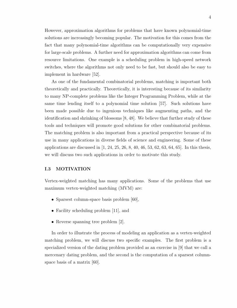
However, approximation algorithms for problems that have known polynomial-time
solutions are increasingly becoming popular. The motivation for this comes from the
fact that many polynomial-time algorithms can be computationally very expensive
for large-scale problems. A further need for approximation algorithms can come from
resource limitations. One example is a scheduling problem in high-speed network
switches, where the algorithms not only need to be fast, but should also be easy to
implement in hardware [52].
As one of the fundamental combinatorial problems, matching is important both
theoretically and practically. Theoretically, it is interesting because of its similarity
to many NP-complete problems like the Integer Programming Problem, while at the
same time lending itself to a polynomial time solution [57]. Such solutions have
been made possible due to ingenious techniques like augmenting paths, and the
identification and shrinking of blossoms [8, 48]. We believe that further study of these
tools and techniques will promote good solutions for other combinatorial problems.
The matching problem is also important from a practical perspective because of its
use in many applications in diverse fields of science and engineering. Some of these
applications are discussed in [1, 24, 25, 26, 8, 40, 46, 53, 62, 63, 64, 65]. In this thesis,
we will discuss two such applications in order to motivate this study.
I.3 MOTIVATION
Vertex-weighted matching has many applications. Some of the problems that use
maximum vertex-weighted matching (MVM) are:
• Sparsest column-space basis problem [60],
• Facility scheduling problem [11], and
• Reverse spanning tree problem [2].
In order to illustrate the process of modeling an application as a vertex-weighted
matching problem, we will discuss two specific examples. The first problem is a
specialized version of the dating problem provided as an exercise in [9] that we call a
mercenary dating problem, and the second is the computation of a sparsest column-
space basis of a matrix [60].
5
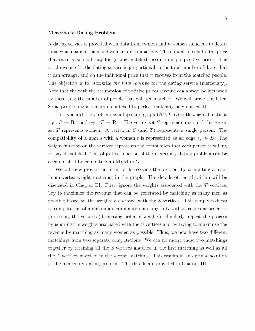
Mercenary Dating Problem
A dating service is provided with data from m men and n women sufficient to deter-
mine which pairs of men and women are compatible. The data also includes the price
that each person will pay for getting matched; assume unique positive prices. The
total revenue for the dating service is proportional to the total number of dates that
it can arrange, and on the individual price that it receives from the matched people.
The objective is to maximize the total revenue for the dating service (mercenary).
Note that the with the assumption of positive prices revenue can always be increased
by increasing the number of people that will get matched. We will prove this later.
Some people might remain unmatched (a perfect matching may not exist).
Let us model the problem as a bipartite graph G(S, T,E) with weight functions
wS : S → R+ and wT : T → R+. The vertex set S represents men and the vertex
set T represents women. A vertex in S (and T ) represents a single person. The
compatibility of a man s with a woman t is represented as an edge est ∈ E. The
weight function on the vertices represents the commission that each person is willing
to pay if matched. The objective function of the mercenary dating problem can be
accomplished by computing an MVM in G.
We will now provide an intuition for solving the problem by computing a max-
imum vertex-weight matching in the graph. The details of the algorithm will be
discussed in Chapter III. First, ignore the weights associated with the T vertices.
Try to maximize the revenue that can be generated by matching as many men as
possible based on the weights associated with the S vertices. This simply reduces
to computation of a maximum cardinality matching in G with a particular order for
processing the vertices (decreasing order of weights). Similarly, repeat the process
by ignoring the weights associated with the S vertices and by trying to maximize the
revenue by matching as many women as possible. Thus, we now have two different
matchings from two separate computations. We can no merge these two matchings
together by retaining all the S vertices matched in the first matching as well as all
the T vertices matched in the second matching. This results in an optimal solution
to the mercenary dating problem. The details are provided in Chapter III.

6
Sparsest column-space Basis Problem
Another application of vertex weighted matching arises in the computation of a
sparsest column-space basis (SCB) of a matrix. The sparsest column-space basis
problem is an instance of the nice-basis problem that has numerous applications in
scientific computing, including models of deforming structures, circuit and device
modeling, equality constrained optimization, etc. We refer the readers to [60] for
details. We will now briefly discuss the role of vertex weighted matching in the
solution of SCB. This is a novel method for computing a SCB and has not been
published elsewhere.
Consider a matrix A with k rows and n columns, n > k, and rank k. A set of
columns C = {c1, c2, · · · cl} is linearly independent if none of the columns in C can
be expressed as a linear combination of the others. The maximal number of linearly
independent columns of A is called the column rank of A. The row rank of A is
defined similarly. Since the row and column ranks are equal, they are called the rank
of A. A generalized diagonal of A is a subset of nonzeros with at most one chosen
from each row and each column. The maximum number of nonzeros in a generalized
diagonal is called the structural rank of A. The numerical rank of a matrix (we
have called this the rank) is less than or equal to the structural rank of A. In the
following discussions we will make a simplifying assumption that the numerical and
the structural ranks of a matrix are equal.
A basis for the column-space of A is a linearly independent set of columns with
maximum rank (by the assumption on A, this is k). A sparsest basis for the column-
space of A is a basis with the fewest nonzeros in it. Formally, the sparsest column-
space basis problem (SCB) can be defined as:
Definition I.3.1. Given a sparse matrix A of rank k, with k rows and n > k columns,
find a sparsest basis B for its column-space.
The sparsest column-space basis selects k out of n sparse columns of A. A graph-
ical representation of SCB is given by Figure 2. For a matrix with k rows and n
columns there could be(nk
)potential column-space bases. However, a simple greedy
algorithm, as follows, works: Start with an empty set (of columns) B. Find the
sparsest column based on the number of non-zeros in the column and represented
with a weight function wi. Add this column to B. Until k columns have been added
to B, add new (sparsest) columns such that they are linearly independent of the

7
FIG. 2: Representation of a sparsest column-space basis problem. A matrix A with krows and n columns, and a basis B with k rows and k linearly independent columns.
current columns in B. The set B now represents the sparsest set over all choices of
sparsest column-space bases. One step of this algorithm is illustrated in Figure 3. A
sparsest column-space basis can be computed in O(k2n) time and a 12-approx solution
in O(nnz(A) + k2) time, where nnz(A) denotes the number of nonzero elements in
A [60].
FIG. 3: A greedy algorithm for computing a sparsest column-space basis. (a) Statebefore augmenting a basis Bi with a column of current heaviest weight wmax from C;(b) state after augmenting a basis with a sparsest linearly independent column fromC.
The proof that such a greedy algorithm will solve the sparsest column-space basis
problem is given by a theory about greedy algorithms: combinatorial structures
known as matroids, as named by Hessler Whitney [19, 45].
Definition I.3.2. A matroid M = (E, I) is defined as a set of elements E, and a
nonempty collection of subsets, I, of E defined to be independent. The three proper-
ties that an independent set I ∈ I needs to satisfy are:
1. The empty set is independent;

8
2. Subsets of an independent set are independent;
3. Given two independent sets with unequal cardinalities, the smaller set can be
augmented with some element from the larger set to form a larger independent
set (this is called the exchange property).
Based on this background, we will now discuss how computing a sparsest column-
space basis can be transformed into a maximum vertex-weight matching problem.
A matrix A with k rows and n columns can be represented as a bipartite graph
G = (S, T,E) with weight function w : S → R+, where set S represents the columns,
set T represents the rows, and each nonzero element in A is represented by an edge
est ∈ E. The weight of a column vertex is given by w(s) = k + 1 − deg(s), where
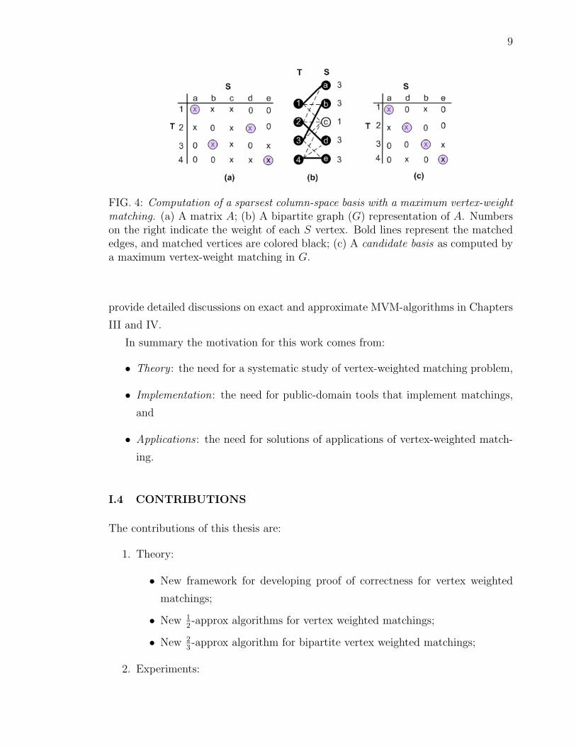
deg(s) represents the number of nonzeros in column s. A matrix and its bipartite
graph representation are shown in Figures 4.(a) and 4.(b).
A matching M in G corresponds to a subset of nonzeros in A, with at most one
from each column and each row (see Figure 4.(a) for an example). By permuting
the rows and columns of A, we can put the nonzeros corresponding to a matching
on the diagonal of A. This is illustrated in Figure 4.(c). As discussed earlier, the
maximum number of nonzeros in a matching is the structural rank of a matrix. If we
make a simplifying assumption that the numerical rank of A is equal to the structural
rank of A, then a maximum matching in G will result in a candidate basis with full
structural rank. While the assumption that the numerical rank of a matrix is equal
to the structural rank is true for many scientific computing applications, it is not
always a correct assumption. However, the correctness of a candidate basis with full
structural rank can be checked by numerical factorization.
Thus, the greedy algorithm for computing a sparsest basis, discussed earlier, can
now be replaced by an algorithm for computing a matching. Specifically, a maximum
vertex-weight matching, since it will compute a maximum matching that is as sparse
as possible. The weights on the S vertices are formulated such that maximizing the
total weight of the matched vertices will minimize the number of nonzeros in the
submatrix induced by this matching (basis B).
Spencer and Mayr provide a O(√nm log n) time algorithm [69] for computing a
maximum vertex-weight matching, where n denotes the number of vertices and m
denotes the number of edges in a graph. Exact algorithms tend to be expensive for
large-scale problems, and therefore, there is a need for approximation algorithms. We
9
FIG. 4: Computation of a sparsest column-space basis with a maximum vertex-weightmatching. (a) A matrix A; (b) A bipartite graph (G) representation of A. Numberson the right indicate the weight of each S vertex. Bold lines represent the matchededges, and matched vertices are colored black; (c) A candidate basis as computed bya maximum vertex-weight matching in G.
provide detailed discussions on exact and approximate MVM-algorithms in Chapters
III and IV.
In summary the motivation for this work comes from:
• Theory : the need for a systematic study of vertex-weighted matching problem,
• Implementation: the need for public-domain tools that implement matchings,
and
• Applications : the need for solutions of applications of vertex-weighted match-
ing.
I.4 CONTRIBUTIONS
The contributions of this thesis are:
1. Theory:
• New framework for developing proof of correctness for vertex weighted
matchings;
• New 12-approx algorithms for vertex weighted matchings;
• New 23-approx algorithm for bipartite vertex weighted matchings;
2. Experiments:

10
• Open-source library of C++ routines to compute various kinds of match-
ings;
• Open-source library of C++ and MPI routines to compute approximate
matchings in parallel.
• Extensive experimental study of various (serial) matching algorithms, and
scalability study of 12-approx parallel algorithm with up to 8, 192 proces-
sors.
3. Applications:
• Study of applicability of vertex weighted matchings in solving the sparsest
basis problem.
• Study of approximation algorithms in sparse matrix computations.
I.5 CHAPTER SUMMARY
In this chapter we provided the motivation and rationale for this dissertation. We
also introduced two specific application of the vertex weighted matching problem.
We show how the sparsest-basis problem can be efficiently solved by modeling it as
a maximum vertex-weight matching problem and concluded the chapter by listing
some of the contributions of this work.
11
CHAPTER II
BACKGROUND AND RELATED WORK
“It (matching) is included in (class) P, thanks to the ingenious
introduction of nontrivial combinatorial tools such as alternating paths
and blossoms.” - Marek Karpinski and Wojciech Rytter [39]
Matching theory has been studied in great detail [8, 45, 48, 57, 66]. In this chapter,
we will provide a brief introduction to matchings in graphs. We will also introduce
the basic tools and techniques to compute a matching. We will discuss both ex-
act and approximation algorithms for the maximum cardinality and the maximum
edge-weight matchings in bipartite graphs. The approximation algorithms are also
applicable to nonbipartite graphs. We will keep the discussion on the exact algo-
rithms brief. Our goal is to provide sufficient background for a better understanding
of the proposed algorithms. Since the approximation algorithms have been more
recently developed, we will discuss them at a relatively greater detail. We refer the
reader to above cited references for a thorough discussion on matching theory and
algorithms.
II.1 INTRODUCTION
A graph G is a pair (V,E), where V is a set of vertices and E is a set of edges
that represent a binary relation on V . A simple instance of a graph is shown in
Figure 5. The vertices are represented with small circles, and the lines that connect
two vertices represent the edges. In a graph, weights can be associated with edges,
vertices, or both. In this proposal, we will only consider weights with real positive
numbers. Graphs with negative weights will have to be considered separately. The
association of weights in a graph G = (V,E) can be represented as w : E → R+ for
a weight function on edges, and w : V → R+ for a weight function on vertices.
A bipartite graph G = (S, T,E) is a graph in which the vertex set V = S ∪ T can
be partitioned into two sets S and T , S ∩ T = φ, such that no two vertices in S, or
in T , are joined by an edge. An example of a bipartite graph is shown in Figure 5.
Since edges in a bipartite graph always join an S vertex to a T vertex, cycles of odd
length cannot exist. Absence of odd-length cycles is a distinguishing characteristic

12
of bipartite graphs, that is important and well exploited in the context of matching
algorithms.
We use the following notations. Given a graph G = (V,E), an edge e belong to
Set E. We can further specify the two endpoints (u, v) of an edge as euv. The weight
assigned with an edge is denoted as w(e), and the weight of a vertex v is denoted as
w(v). Given a vertex v ∈ V , the set of edges incident on it is called the adjacency
set, and denoted as adj(v). We will introduce other symbols and notations where
appropriate.
A matching in a graph can be defined as follows:
Definition II.1.1. Given a graph G = (V,E) with a set of vertices V , and a set of
edges E, a matching M is a subset of edges such that no two edges in M are incident
on the same vertex.
A matching can also be seen as a pairing of two objects in the set. Using the
example of mercenary dating problem that we introduced in Chapter 1, the set of
men is denoted by {S1, S2, S3}, and the set of women is denoted by {T1, T2, T3}. A
matching is pairing of a man with a woman such that no man is paired with more
than one woman, and no woman is paired with more than one man. This is illustrated
in Figure 5.
FIG. 5: An example of matching. (a) A bipartite graph G, (b) a matching M in G.Bold lines represent matched edges, and matched vertices are colored black.
CLASSIFICATION
Based on different criteria the matching problem can be classified as follows:
• Input graph: Bipartite and Nonbipartite,
• Objective function: Cardinality and Weighted,

13
• Placement of weights in the graph: Edge-weighted and Vertex-weighted,
• Optimality : Exact and Approximate.
A given matching problem can thus be specified as an exact maximum edge-
weight matching problem, or as a 12-approx vertex-weighted matching problem. The
landscape of matching algorithms is provided in Figure 1.
The odd-length cycles that exist in nonbipartite graphs need special consideration
and will significantly increase the conceptual complexity of a matching algorithm for
nonbipartite graphs. However, the computational complexity might remain the same
as that for bipartite graphs.
The cardinality of a matching is the number of edges in it and is denoted by
|M |. Based on the cardinality there can be three types of matchings. A maximal
matching is a matching that cannot be augmented by adding a new edge to it.
However, it might be possible to increase the cardinality of a maximal matching by
changing the set of matched edges. A maximum matching in a graph is a matching
of maximum cardinality among all possible matchings. When all the vertices are
matched, the matching is called a perfect matching. While a maximum matching is
also a maximal matching, a maximal matching is not always a maximum matching.
However, a perfect matching necessarily has maximum cardinality. These three types
of matchings are illustrated in Figure 6.
FIG. 6: Types of matchings. Matched edges are represented with bold lines andmatched vertices are filled with black color. (a) A maximal matching, (b) a maximummatching, and (c) a perfect matching.
In a graph G = (V,E) with weight function w : E → R+, the edge-weight of a
matching M is the sum of weights of the matched edges∑
e∈M w(e). For a graph
G = (V,E) with weight function w : V → R+, the vertex-weight of a matching is
the sum of weights of matched vertices∑
v∈V (M) w(v), where V (M) represents the
set of matched vertices. We will denote the edge-weight and the vertex-weight as
weight, and depend on the context for specific reference as to whether the weights
14
are associated with the edges or the vertices. For the current discussion we will
only consider positive weights. We will later show that the same algorithms can be
extended to include negative weights. A maximum edge-weight matching, also known
as a maximum weighted matching, is a matching of maximum edge-weight among
all possible matchings in a graph. A maximum edge-weight matching can be of
maximal, maximum or perfect cardinality. A maximum vertex-weight matching is a
matching of maximum vertex-weight among all possible matchings in a graph. When
the weights are positive, a maximum vertex-weight matching is also a matching of
maximum cardinality, which will proved in Chapter III.
An α-approx algorithm computes a solution that is within a factor of α of the opti-
mal value. For example, a 12-approx algorithm for a maximum edge-weight matching
problem guarantees that the weight of an approximate matching computed by the
algorithm is at least half of the weight of an optimal matching. If M2 denotes a
matching computed by a 12-approx algorithm, and M∗ denotes an optimal matching,
then ∑e∈M2
w(e) ≥ 1
2
∑e∈M∗
w(e) (1)
Approximation algorithms for maximum cardinality matching are relatively easier
than approximation algorithms for weighted matchings. While computing a linear
time 12-approx to maximum cardinality matching (maximal) is trivial, computing the
same for weighted matching is not. We will discuss these approximation algorithms
in Section II.5.

15
II.2 FOUNDATIONS
One of the most fundamental techniques in matching is the technique of augmen-
tation. Given a graph G = (V,E) and a matching M in G, a path is said to be
alternating if it alternates between an edge in M (matched) and an edge not in M
(unmatched). An alternating path that starts and ends with edges that are not in
M (unmatched) is called an augmenting path. Note that an augmenting path will
always have an odd number of edges and an even number of vertices. A few examples
of paths are illustrated in Figure 7.
FIG. 7: Types of paths. Matched edges are represented with bold lines and matchedvertices are colored black. (a) An alternating path starting with an unmatchedvertex, (b) an alternating path starting with a matched vertex, and (c) an augmentingpath.
The symmetric difference of two sets, denoted by the symbol ⊕, is computed
by choosing the elements that are present in either of the sets, but not in both.
Mathematically, the symmetric difference of two setsM and P is shown in Equation 2.
The operator \ represents the set resulting from retaining only those elements in the
set on the left hand side of the operator that do not also exist in the set on the right
hand side of the operator (the set minus operator).
M ⊕ P = (M \ P ) ∪ (P \M) (2)
In the context of matching, the symmetric difference operation is important due
to Lemma II.2.1, which states that the cardinality of a current matching can always
be increased by performing a symmetric difference with an augmenting path. The
process of symmetric difference is illustrated in Figure 8. Note that although the
matched edges change, the matched vertices will always remain matched.
Lemma II.2.1. Consider a graph G = (V,E) and a matching M . Let P be an
augmenting path in G with respect to M . The symmetric difference, M′
= M ⊕ P ,
is a matching of cardinality (|M |+ 1).

16
FIG. 8: Augmentation by symmetric difference. The matched edges are representedwith bold lines and matched vertices are colored black. (a) Before augmentation, (b)after augmentation.
Proof. There are two parts to the proof. First we will prove that the symmetric
difference M⊕P will result in a matching, and then we will prove that the symmetric
difference will result in a matching that increases the cardinality by one.
(i) An augmenting path P is of the form [e1, e2, e3, · · · , en], where all odd-indexed
edges {e1, e3, · · · , en} are unmatched, and all even-indexed edges {e2, e4, · · · , en−1}are matched. Also, edges e1 and en are unmatched, and n is an odd number. The
symmetric difference is given by M ⊕ P = (M \ P ) ∪ (P \M). The edges obtained
by the operation (M \ P ) contain those edges that are in M , but are not part of
the path P , and therefore a set of independent edges (it retains the matched edges
independent of P ). The edges obtained by the operation (P \M) contain those edges
that are on the path P , but are not in M (the unmatched edges in P ). By definition,
an augmenting path P connects two distinct unmatched vertices, and therefore, edges
e1 and en are independent edges. All the intermediate edges in {P \M} are also
independent edges because they share vertices with matched edges. Therefore, the
symmetric difference M ⊕ P results in a matching.
(ii) An augmenting path P starts and ends with an unmatched edge, therefore, the
number of unmatched edges in P is exactly one larger than than the number of
matched edges in P . Thus, symmetric difference M ⊕ P results in a matching of
cardinality of (|M |+ 1).
The concept of symmetric difference immediately gives us a basic technique to
compute a matching: find an augmenting path, and perform the symmetric difference.
The proof of correctness for such an algorithm is given by Theorems II.2.1 and II.2.2.
Theorem II.2.1 (Berge [1957]). A matching M in a graph G is a maximum match-
ing if and only if there is no M-augmenting path in G.
17
Proof. There are two aspects to the proof.
(i) Suppose there exists an M -augmenting path in G, then the cardinality of M can
be increased by one, and therefore, M is not a maximum matching and contradicts
the assumption (follows from Lemma II.2.1). Therefore, if M is a maximum match-
ing, then there exist no M -augmenting paths in G.
(ii) Suppose that there exist no M -augmenting paths in G, and yet, M is not a max-
imum matching. Let M∗ be a maximum matching in G. The symmetric difference
M ⊕M∗ will result in a collection of alternating paths and cycles as illustrated in
Figure 9. If one of these alternating paths is M -augmenting, then there also exists an
M -augmenting path in G, and therefore, contradicts the assumption (follows from
part (i)). Also, by assumption there are no M∗ augmenting paths in M ⊕M∗. Thus,
the symmetric difference M ⊕M∗ will consist of alternating paths that are not aug-
menting paths, and cycles, and therefore, an equal number of edges from M and M∗.
Alternatively, |M | = |M∗|, and the theorem holds.
FIG. 9: The symmetric difference of two matchings MS⊕MT . Dashed lines representedges in MS and Solid lines represent edges in MT . (a) A cycle; (b)-(e) Augmentingor alternating paths.
Theorem II.2.2. Consider a graph G = (V,E) and a matching M . Let P be an
augmenting path with two unmatched vertices v and w as endpoints. If there exists
no augmenting path in G starting from an unmatched vertex u with respect to M ,
then there is no augmenting path from u with respect to M ⊕ P either.
Proof. Let the augmenting path starting at u be Q, and the augmenting path between
v and w be P . This is illustrated in Figure 10. There are two possibilities:
(i) Paths P and Q do not intersect. This means that the two paths do not have any

18
vertices or edges in common. This is illustrated in Figure 10.(a). In such a case P
will not have any effect on the possibility of an augmenting path starting at u. If no
augmenting path exists from u with respect to M , then no augmenting path exists
from u with respect to M ⊕ P either. Therefore, the theorem holds.
(ii) Paths P and Q intersect each other. Path Q is of the form [u, u1, · · · , uj, · · · , u′].
Let uj be the first vertex on Q that is also on P . This is illustrated in Figure 10.(b).
The portion of Q from u up to uj, along with the portion of P that is incident on
uj with a matched edge (Q′
in Figure 10.(b)), forms an augmenting path starting at
u with respect to M . This contradicts the assumption, and therefore, the theorem
holds.
FIG. 10: Effect of M ⊕P . Bold lines represent matched edges and matched verticesare colored black. (a) Paths P and Q do not intersect; (b) paths P and Q intersect.This figure has been adapted from [57].
Corollary II.2.1. If at some stage of an augmentation-based matching algorithm,
there is no augmenting path starting at vertex u, then there will be no augmenting
path from u at any future step in the algorithm.
Proof. Inducting on the number of steps that remain after discovering that no aug-
menting path exists from a vertex u, we can use Theorem II.2.2 to show that there
never will be an augmenting path from u, if none existed when u was processed the
first time.
Thus, from Corollary II.2.1, it is enough if we process a given vertex only once.
We will now discuss techniques to perform the search for augmenting paths in a
graph.

19
GRAPH SEARCH TECHNIQUES FOR MATCHING
Searching for an augmenting path in a graph with respect to a matching is one the
basic steps in the computation of a matching. There are two basic approaches to find
an augmenting path - a breadth-first search, and a depth-first search. The difference
between a breadth-first and a depth-first search comes from the way the elements
are queued during a search. We will define two data structures known as a pseudo-
queue, and a pseudo-stack. A pseudo-queue is different from a regular queue data
structure in that the former excludes duplicate elements. Note, that Algorithm 1 does
not attempt to add duplicates, and therefore, does need this special data structure.
Similarly, there are no duplicates in a pseudo-stack. An additional characteristic of a
pseudo-stack is that if a new element that is being added to the pseudo-stack already
exists, then it is moved to the top of the pseudo-stack. We need vectors to store
information about the parent-child relationships (parent), distance from the source
(depth), and state of processing (color). We initialize color with φ for all vertices,
and update it to Processable or Processed.
A breadth-first search is illustrated in Algorithm 1, and works as follows. Initialize
the data structures by setting the color, parent and depth values to zeros. Start with a
vertex u and add it to the pseudo-queue data structure and mark it as Processable.
Enqueue the vertices adjacent to u and mark them as Processable. Add u as the
parent of all the enqueued vertices and set the depth values for these elements one
greater than the depth value of the parent. Repeat the steps by dequeing the front
of the queue each time, until all the vertices have been processed. A breadth-first
search on a small graph is illustrated in Figure 11.
A depth-first search is illustrated in Algorithm 2. The algorithm functions as
follows. Start with a vertex u and mark it as Processed. Enqueue the vertices
adjacent to u in a pseudo-stack data structure, and mark them as Processable.
Add u as the parent of all the enqueued vertices, and a depth value one greater than
the depth of the parent. Dequeue the top of the pseudo-stack, and repeat the steps
until all the vertices have been processed. A depth-first search on a small graph is
illustrated in Figure 12.
The search for an augmenting path can be breadth-first, depth-first or a com-
bination of these. The search could either start from one vertex (single-source), or
simultaneously from a set of unmatched vertices (multiple-source). The general strat-
egy is to find a shortest-augmenting path. Therefore, breadth-first search is generally

20
Algorithm 1 Input: A graph G and a vertex source u. Output: A breadth-firsttree. Associated data structures: Q is a queue data structure. Effect: performa breadth-first search.1: procedure BreadthFirstSearch(G = (V,E), u)2: for all v ∈ V do . Initialization3: color[v] = φ;4: parent[v] = 0;5: depth[v] = 0;6: end for7: Q← {u};8: color[u]← Processable;9: while Q 6= φ do . Graph search
10: pick v from Q; . Head of the queue11: Q← Q\v; . Dequeue12: color[v]← Processed;13: for all w ∈ adj[v] do14: if color[w] 6= φ then15: continue;16: end if17: parent[w]← v;18: depth[w]← depth[v] + 1;19: Q← Q ∪ {w}; . Enqueue20: color[w]← Processable;21: end for22: end while23: end procedure

21
Algorithm 2 Input: A graph G and a vertex source u. Output: A breadth-first (or depth-first) tree. Associated data structures: S is a pseudo-stack datastructure. Effect: perform a depth-first search.
1: procedure DEPTH-FIRST-SEARCH(G = (V,E), u)2: for all v ∈ V do . Initialization3: color[v] = φ;4: parent[v] = 0;5: depth[v] = 0;6: end for7: S ← {u};8: color[u]← Processable;9: while Q 6= φ do . Graph search
10: pick v from S; . Top of the pseudo-stack11: S ← S\v; . Dequeue12: color[v]← Processed;13: for all w ∈ adj[v] do14: if color[w] 6= φ then15: move w to the top of S;16: continue;17: end if18: parent[w]← v;19: depth[w]← depth[v] + 1;20: S ← S ∪ {w}; . Enqueue21: color[w]← Processable;22: end for23: end while24: end procedure
22
FIG. 11: Breadth-first search. The vertex being processed at a given step is coloredpurple, and also marked by an arrow. The shaded lines represent the processed edges.The vertices that have already been processed are colored black. The adjacency listfor each vertex is maintained in an increasing order of the indices of vertices. (a)The input graph before execution, (b)-(f) the intermediate states of execution. Stateof the pseudo-queue at each step: (b) [2, 3, 4] (c) [3, 4, 5], dequeue 2, enqueue 5; (d)[4, 5, 6] dequeue 3, enqueue 6; (e) [5, 6] dequeue 4; (f) [6] dequeue 5.
used. Once an augmenting path is discovered, augmentation can be performed by
either along a single path, or simultaneously along a set of vertex-disjoint augmenting
paths. Thus the three strategies are:
1. Single-source single-path, illustrated in Figure 13, uses a breadth-first search.
2. Multiple-source single-path, illustrated in Figure 14, uses a breadth-first search.
3. Multiple-source multiple-path, illustrated in Figure 15, uses a combined
breadth-first and depth-first search.
We will provide more details about these approaches in the following discussions on
maximum cardinality and maximum edge-weight matching algorithms.
23
FIG. 12: Depth-first search. The vertex being processed at a given step is coloredpurple, and also marked by an arrow. The shaded lines represent the processed edges.The vertices that have already been processed are colored black. The adjacency listfor each vertex is maintained in an increasing order of the indices of vertices. (a) Theinput graph before execution. (b)-(f) the intermediate states of execution. State ofthe pseudo-stack at each step: (b) [2, 3, 4] (c) [2, 3, 5] pop 4, move 2, move 3, push 5;(d) [3, 2, 6] pop 5, move 2, push 6; (e) [2, 3] pop 6, move 3; (f) [2].
FIG. 13: Single-source single-path technique. The vertex being processed at a givenstep is colored purple, and also pointed by an arrow. The shaded lines representpotential augmenting paths. Bold lines represent matched edges and matched verticesare colored black. (a) The input graph before execution, (b)-(d) the intermediatestates of execution, and (e) the final state.

24
FIG. 14: Multiple-source single-path technique. The vertices being processed at agiven step are colored purple. The shaded lines represent potential augmenting paths.Bold lines represent matched edges and matched vertices are colored black. (a) Theinput graph before execution, (b)-(d) the intermediate states of execution, and (e)the final state.
FIG. 15: Multiple-source multiple-path technique. The vertices processed at a givenstep are colored purple. The shaded lines represent potential augmenting paths, boldlines represent matched edges and matched vertices are colored black. (a) The inputgraph before execution, (b) the intermediate state of execution, and (c) the finalstate.

25
II.3 MAXIMUM CARDINALITY MATCHING
Maximum cardinality matching (MCM) algorithms for bipartite graphs are concep-
tually easier than those for nonbipartite graphs. In this section, we will discuss MCM
algorithms for bipartite graphs, and refer the readers to [28, 29, 8, 45, 48, 57, 66, 73]
for discussions on algorithms for nonbipartite graphs. We will provide two algorithms
for MCM, a simple algorithm based on the single-source single-path approach, and an
advanced algorithm based on the multiple-source multiple-path approach for search-
ing an augmenting path.
The simple version of MCM is given in Algorithm 3. The algorithm functions as
follows. Let G = (S, T,E) be a bipartite graph, and M an empty matching. Find an
M -augmenting path P in G, and perform the symmetric difference M⊕P to increase
the cardinality of the current matching. Repeat the process until no M -augmenting
paths exist in G. A breadth-first or depth-first search, as described in Algorithms 1
and 2, can be used to find an augmenting path starting at a given vertex. However,
the former is preferred because it retrieves the shortest augmenting path from a given
source, if such a path exists. This graph search operation is bounded by O(m), where
m = |E| is the number of edges in G. Since G is a bipartite graph, edges will always
connect an S vertex to a T vertex. Therefore, it is sufficient to loop either over the S
vertices, or the T vertices. A vertex needs to be processed only once, this follows from
Corollary II.2.1. Thus, Algorithm MAX-CARD1 can be computed in O(nm) time,
where n is either the number of S vertices or T vertices, depending on the vertex
set used. Execution of Algorithm MAX-CARD1 based on a single-source single-path
approach is illustrated in Figure 13, and that for a multiple-source multiple-path is
illustrated in Figure 14.
Algorithm 3 Input: A bipartite graph G. Output: a matching M . Effect: com-putes a maximum cardinality matching using a single-source single-path approach.
1: procedure MAX-CARD1(G = (S, T,E),M)2: M ← φ;3: for all s ∈ S do . Can also loop over T vertices4: Find an augmenting path P starting at s;5: if P found then6: M ←M ⊕ P ;7: end if8: end for9: end procedure

26
In the previous section we briefly mentioned about the multiple-source multiple-
path approach for finding augmenting paths in a graph and illustrated it in Figure 15.
Hopcroft and Karp [37] use a similar technique and show that the worst-case bounds
for such an approach in bipartite graphs is O(√nm), where n is the number of
vertices and m the number of edges. From a simple observation of Figure 15, possibly
many vertex-disjoint augmenting paths can be found with each pass, and therefore,
drastically reduces the total number of steps that need to be performed. In fact, the
number of steps is bounded by O(√n). We refer the reader to [37] for a proof.
A multiple-source multiple-path search approach works by finding a set of vertex-
disjoint M -augmenting paths per iteration; specifically, a maximal set of shortest
length vertex-disjoint M -augmenting paths. A breadth-first search is first performed
to compute the length of the shortest augmenting path. Then, depth-first searches
are done simultaneously from each unmatched vertex to find a maximal set of vertex-
disjoint paths. Thus, the cardinality of a matching advances by |M ′ | = |M |+d, where
d is the number of vertex-disjoint augmenting paths, instead of |M ′| = |M | + 1 for
single-path approach. Algorithm 4 sketches a multiple-path technique for computing
a maximum cardinality matching in a bipartite graph.
Algorithm 4 Input: a bipartite graph G. Output: a matching M . Effect:computes a maximum cardinality matching M in G using a mulitple-source multiple-path approach.
1: procedure MAX-CARD2(G = (S, T,E),M)2: M ← φ;3: repeat4: P ← {P1, P2, . . . , Pk}; . a maximal set of vertex-disjoint paths of
shortest length5: M ←M ⊕ P6: until P = φ;7: end procedure
We conclude our discussion on the maximum cardinality matching algorithms
with Table 1 that summarizes the development of MCM algorithms in bipartite and
nonbipartite graphs.

27
Year Authors Graph Type Complexity
1931 Konig B O(nm)1955 Kuhn B O(nm)1965 Edmonds G O(n2m)1972 Gabow G O(n3)1973 Hopcroft and Karp B O(
√nm)
1974 Kameda and Munro G O(nm)1974 Even and Kariv G O(n2.5)1976 Kariv G O(
√nm log log n)
1980 Micali and Vazirani G O(√nm)
1991 Alt, Blum, Melhorn and Paul B O(n1.5√
mlogn
)
1991 Feder and Motwani B O(√nm logn(n
2
m))
1995 Goldberg and Karzanov G O(√nm logn
n2
m)
TABLE 1: Algorithms for maximum cardinality matching [66]. For a graph G =(V,E), n = |V | represents the number of vertices, and m = |E| the number of edges.For graph types, B denotes bipartite graphs, and G denotes nonbipartite graphs.

28
II.4 MAXIMUM EDGE-WEIGHT MATCHING
Given a graph G = (V,E) with weight function w : E → R+, and a matching M , the
weight of a matching is the sum of weight of matched edges∑
e∈M w(e). A matching
M in G is a maximum edge-weight matching (MEM) if it has the largest weight of all
matchings in the graph. Conceptually, an algorithm for computing a MEM is similar
to an algorithm to compute a maximum cardinality matching (MCM). In both the
cases, the general technique is to find augmenting paths and perform symmetric
differences to increase the current size of the matching. However, for a MEM one
also has to consider the weights associated with the edges. This will add complexity
to the MEM algorithms. Traditionally, the MEM problem has been formulated as
a linear programming problem, and is an example of the theory of duality. The
intuition for such a formulation is given by Theorem II.4.1. The theorem highlights
relationships between maximization and minimization, and between the weights on
the edges and the weights on the vertices. We refer the reader to [66] for a proof of
the theorem.
Theorem II.4.1 (Egervary [1931 ]). Consider a bipartite graph G = (S, T,E) with
weight function w : E → R+. Let V = {S ∪ T} represent the set of vertices. The
maximum weight of a matching M in G is equal to the minimum weight of y(V ),
where y : V → R+ is a set of dual weights on V such that, for each edge est ∈ E,
ys + yt ≥ w(est).
Linear programming (LP) problems are optimization (minimization or maximiza-
tion) problems with linear objective function subject to linear inequality constraints.
Linear programming problems are usually formulated as primal problems. Every
primal formulation can also be recast as a dual LP problem (this primal-dual for-
mulation for the MEM problem will be described shortly). The dual of a dual is
the primal problem. The dual of a primal problem can be obtained by changing the
objective function and the constraints. If one is a maximization problem, then other
is a minimization problem. A solution to the objective function that satisfies all
the constraints is known as a feasible solution. By design, every feasible solution to
the dual program gives an upper bound on the optimal value of the primal feasible

29
solution, and vice versa. The solution is optimal when the primal and dual solutions
are equal.
The primal-dual solution for the MEM problem in bipartite graphs is known as
the Hungarian method for the assignment problem as proposed by Harold W. Kuhn
[43]. Consider a bipartite graph G = (S, T,E) with weight function w : E → R+.
Let nS = |S| and nT = |T | represent the number of S and T vertices respectively,
and m = |E| represents the number of edges. Let n denote the total number of S
and T vertices, n = nS + nT . If a vertex pair (si, ti) does not exist in the edge set
E, then the weight wst is set to zero. The primal-dual formulation for the MEM
problem is given by:
Primal problem:
z = maximize
nS∑s=1
nT∑t=1
wstxst,
subject to constraints:
nS∑s=1
xst = 1 for t = 1, ..., nT ,
nT∑t=1
xst = 1 for s = 1, ..., nS,
xst ∈ {0, 1} for s = 1, ..., nS; t = 1, ..., nT .
Dual problem:
w = minimize
nS∑s=1
us +
nT∑t=1
vt,
subject to constraints:
us + vt ≥ wst for s = 1, ..., nS; t = 1, ..., nT ,
us, vt ≥ 0.
The primal variable xst is assigned to the edges, and can take a value of 1 if
matched, and 0 if not. The dual variables us and vt are assigned to the vertices, and
help guide the graph search procedures. The optimality of the primal-dual solution
is given by Lemma II.4.1. We refer the reader to [76] for a proof.
Lemma II.4.1 (Complementary slackness condition). If there exist vectors u, v ∈ Rn
and a matching X ∈ {0, 1}m with the following properties:
1. wst = (w(est)− us − vt) ≤ 0 for all s, t, and

30
2. Xst = 1 only when wst = 0,
then the matching X is optimal and has a value (∑nS
s=1 us +∑nT
t=1 vt).
Based on the complimentary slackness condition, the key idea for the primal-dual
algorithm is to maintain dual feasibility at all times (Condition 1 from Lemma II.4.1),
and form a subgraph of these edges, known as the tight edges, for which wst = 0.
From a vertex, a search for an augmenting path is made in this subgraph. If an
augmenting path exists, then the current matching is augmented with this path and
proceed to the next vertex. If no such path can be found in the tight subgraph, the
duals are adjusted such that an augmenting path might become possible. The process
repeats until the current vertex is matched. The process of updating the duals is
nontrivial and assumes the presence of a perfect matching in the graph. Note that
the required number of edges with zero weights can be trivially added to the initial
bipartite graph in order to facilitate a perfect matching. When the number of S and
T vertices differ (nS 6= nT ), a perfect matching is either an S-perfect or a T -perfect
matching based on the cardinalities. A skeleton for computing an S-perfect matching
is described in Algorithm 5.
The search strategy in Algorithm MAX-WT is based on the single-source single-
path approach, and iterations are made through the S vertices. The complexity
of the graph search procedure is bounded by O(m), where m = |E| denotes the
number of edges in G. However, there is an additional task of updating the dual
variables when a search for an augmenting path fails. From a given source, shortest
augmenting paths to all possible unmatched vertices are built. The typical approach
at this step is to use a Dijkstra-like search [19] to compute the smallest change
in dual variables that is required to create a new augmenting path. This step is
critical in determining the overall complexity of the algorithm. Updating the dual
variables requires manipulation of priority queues, and therefore, the complexity of
the algorithm is influenced by the choice of the priority queue implementation. The
complexities as determined by some of the common data structures is summarized
in Table 2.
We will conclude the discussion on MEM algorithms with a summary of historical
development of MEM algorithms for bipartite and nonbipartite graphs as listed in
Table 3.

31
Algorithm 5 Input: A bipartite graph G. Output: a matching M . Effect:computes a maximum edge-weight S-perfect matching M in G.
1: procedure MAX-WT(G = (S, T,E), w : E → R+, M)2: M ← φ; . Initialization3: ∀s ∈ S, dual[s] = max(w(est)), for t ∈ adj(s);4: ∀t ∈ T , dual[t] = max((w(est)− dual[s])), for s ∈ adj(t);5: for all s ∈ S do . Compute matching6: while (true) do . Repeat until s gets matched.7: w(est) = (w(est)− dual[s]− dual[t]);8: G = (S, T,E), where E ⊂ E such that ∀est ∈ E, w(est) = 0;9: Find an augmenting path Ps t in G with respect to M ;
10: if P found then11: M ←M ⊕ P ;12: break;13: else14: δ ← minimum change required to update duals; . Dijkstra-like
search15: dual[s]← dual[s]− δ;16: dual[t]← dual[t] + δ;17: end if18: end while19: end for20: end procedure
Data structure Time to update duals
Simple vectors O(n2)Binary heaps O(m log n)Fibonacci heaps O(m+ n log n)
TABLE 2: Power of data structures. For a graph G = (V,E), n = |V | represents thenumber of vertices, and m = |E| the number of edges.

32
Year Authors Graph Type Complexity1957 Berge (theoretical) – –1955 Kuhn, Munkres B O(n4)1960 Iri B O(n2m)1965 Edmonds G O(n4)1969 Dinits and Kronrod B O(n3)1973 Gabow G O(n3)1976 Lawler G O(n3)1982 Galil, Micali and Gabow G O(nm log n)1983 Ball and Derigs G O(nm log n)1988 Gabow and Tarjan B O(
√nm log(nW ))
1989 Gabow, Galil, and Spencer G O(n(m log log logmax{mn,2} n+ n log n))
1990 Gabow G O(n(m+ n log n))1991 Gabow and Tarjan B O(m log(nW )
√nα(n,m) log n)
1992 Orlin and Ahuja B O(√nm log(nW ))
2001 Kao, Lam, Sung, and Ting B O(√nmW logn(n2/m))
TABLE 3: Algorithms for maximum edge-weight matching [66]. For a graph G =(V,E) with weight function w : E → R+, n = |V | represents the number of vertices,m = |E| the number of edges, and W is the largest absolute value of an integerweight. For graph types, B represents bipartite, and G the nonbipartite graphs.

33
II.5 APPROXIMATION ALGORITHMS
Approximation algorithms are generally developed for intractable problems [35].
Given that the matching algorithms are polynomial, approximation techniques for
matchings were initially developed for greedy initialization in exact algorithms [25].
However, recent developments in approximation algorithms for matching have been
motivated by scientific computing applications [24, 64]. For some applications match-
ings need to be computed on very large graphs, while for other applications, match-
ings need be computed a large number of times, although for small or medium sized
graphs. The optimality of the matching is not critical for many of these applications,
and therefore, motivate the development of fast approximation algorithms. Yet an-
other motivation for the development of approximation algorithms for matchings is
the simplicity in parallel implementations. In this section we will discuss some of the
recent developments in approximation theory for matching algorithms as summarized
in Table 4.
Year Author(s) Strategy Approx Complexity
1983 Avis Global maximum 12
O(m log n)1999 Preis Local maximum 1
2O(m)
2003 Drake and Hougardy Path-growing (PG) 12
O(m)2003 Drake and Hougardy PG with short augmentations 2
3− ε O(m1
ε)
2004 Pettie and Sanders Randomized, Deterministic 23− ε O(m log 1
ε)
TABLE 4: Algorithms for approximate weighted matching. For a graph G = (V,E),n = |V | represents the number of vertices, m = |E| the number of edges in G, andε→ R+ is a positive real number.
Avis proposed a simple heuristic algorithm for computing approximate matching
[4]. The algorithm is as follows. Given a graph G = (V,E) with weight function
w : E → R+, consider the edges in decreasing order of weights. Pick a heaviest
unmatched edge and add it to the matching M (initially empty). From G, remove
all the edges that are incident on the endpoints of the current matched edge. Repeat
the process until all the edges have been processed. This is illustrated in Algorithm
6.
It is ease to see that Algorithm GlobalHeavy computes a maximal matching in
G. Given the fact the cardinality of a maximal matching is at least half of a maximum
cardinality, the weight of the matching computed by GlobalHeavy guarantees a12-approx to a maximum edge-weight matching in G. Since the edges need to be
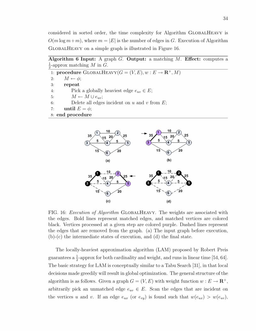
34
considered in sorted order, the time complexity for Algorithm GlobalHeavy is
O(m logm+m), where m = |E| is the number of edges in G. Execution of Algorithm
GlobalHeavy on a simple graph is illustrated in Figure 16.
Algorithm 6 Input: A graph G. Output: a matching M . Effect: computes a12-approx matching M in G.
1: procedure GlobalHeavy(G = (V,E), w : E → R+,M)2: M ← φ;3: repeat4: Pick a globally heaviest edge euv ∈ E;5: M ←M ∪ euv;6: Delete all edges incident on u and v from E;7: until E = φ;8: end procedure
FIG. 16: Execution of Algorithm GlobalHeavy. The weights are associated withthe edges. Bold lines represent matched edges, and matched vertices are coloredblack. Vertices processed at a given step are colored purple. Dashed lines representthe edges that are removed from the graph. (a) The input graph before execution,(b)-(c) the intermediate states of execution, and (d) the final state.
The locally-heaviest approximation algorithm (LAM) proposed by Robert Preis
guarantees a 12-approx for both cardinality and weight, and runs in linear time [54, 64].
The basic strategy for LAM is conceptually similar to a Tabu Search [31], in that local
decisions made greedily will result in global optimization. The general structure of the
algorithm is as follows. Given a graph G = (V,E) with weight function w : E → R+,
arbitrarily pick an unmatched edge euv ∈ E. Scan the edges that are incident on
the vertices u and v. If an edge eux (or evy) is found such that w(eux) > w(euv),
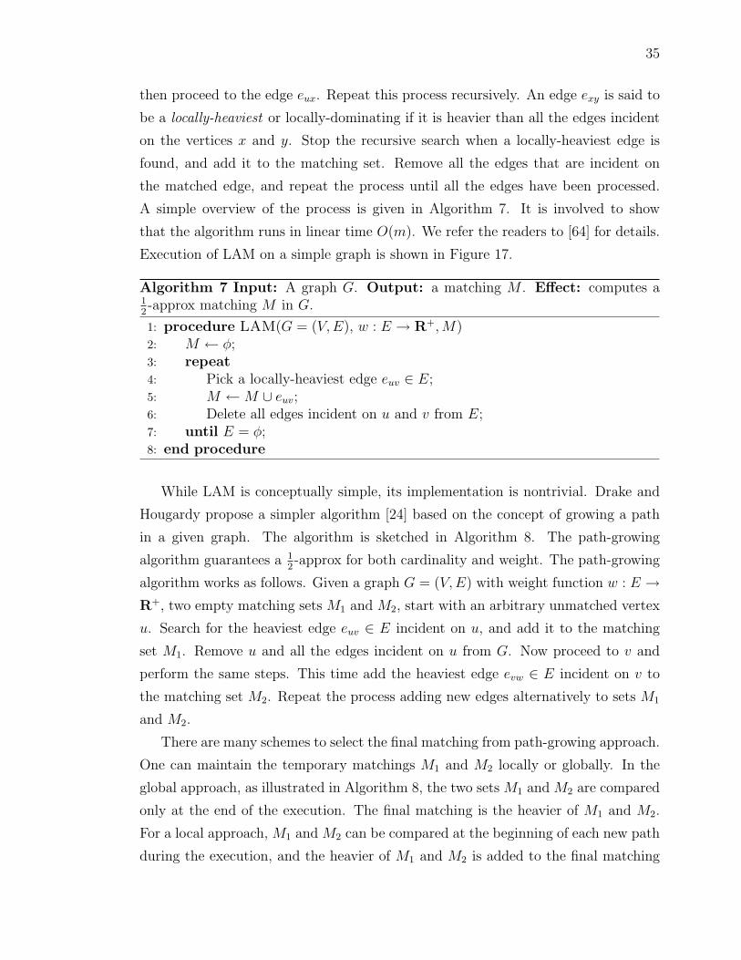
35
then proceed to the edge eux. Repeat this process recursively. An edge exy is said to
be a locally-heaviest or locally-dominating if it is heavier than all the edges incident
on the vertices x and y. Stop the recursive search when a locally-heaviest edge is
found, and add it to the matching set. Remove all the edges that are incident on
the matched edge, and repeat the process until all the edges have been processed.
A simple overview of the process is given in Algorithm 7. It is involved to show
that the algorithm runs in linear time O(m). We refer the readers to [64] for details.
Execution of LAM on a simple graph is shown in Figure 17.
Algorithm 7 Input: A graph G. Output: a matching M . Effect: computes a12-approx matching M in G.
1: procedure LAM(G = (V,E), w : E → R+,M)2: M ← φ;3: repeat4: Pick a locally-heaviest edge euv ∈ E;5: M ←M ∪ euv;6: Delete all edges incident on u and v from E;7: until E = φ;8: end procedure
While LAM is conceptually simple, its implementation is nontrivial. Drake and
Hougardy propose a simpler algorithm [24] based on the concept of growing a path
in a given graph. The algorithm is sketched in Algorithm 8. The path-growing
algorithm guarantees a 12-approx for both cardinality and weight. The path-growing
algorithm works as follows. Given a graph G = (V,E) with weight function w : E →R+, two empty matching sets M1 and M2, start with an arbitrary unmatched vertex
u. Search for the heaviest edge euv ∈ E incident on u, and add it to the matching
set M1. Remove u and all the edges incident on u from G. Now proceed to v and
perform the same steps. This time add the heaviest edge evw ∈ E incident on v to
the matching set M2. Repeat the process adding new edges alternatively to sets M1
and M2.
There are many schemes to select the final matching from path-growing approach.
One can maintain the temporary matchings M1 and M2 locally or globally. In the
global approach, as illustrated in Algorithm 8, the two sets M1 and M2 are compared
only at the end of the execution. The final matching is the heavier of M1 and M2.
For a local approach, M1 and M2 can be compared at the beginning of each new path
during the execution, and the heavier of M1 and M2 is added to the final matching

36
FIG. 17: Execution of Algorithm LAM. The weights are associated with the edges.Bold lines represent matched edges. Matched vertices are colored black, and the ver-tices being processed at a given step are colored purple. The shaded edges representdominating edges at a current step, and dashed lines represent the edges that areremoved from the graph. (a) The input graph before execution, (b)-(e) the interme-diate states of execution, and (f) the final state.
at the end of each step. Alternatively, dynamic programming can also be used to
compute the final matching. Dynamic programming will yield the best matching,
and local selection will yield better results than global selection. For a given graph,
an edge will be processed only once by Algorithm PathGrow, thus resulting in a
linear time algorithm. We refer the reader to [24] for details.
In more recent work [74, 59], advances have been made to improve the approx-
imation ratio from half to (23− ε). The basic technique is to iteratively improve
the weight and the cardinality by performing short-augmentations that meet a cer-
tain threshold for improvement. An augmenting path of certain length, usually of
length three or five edges, is called a short-augmenting path. One such simple scheme
that looks for augmenting paths of length three in a graph with an initial maximal
matching M is shown in Algorithm 9. Augmenting with short paths will not always
increase the weight of the final matching. Therefore, a greedy decision is made based
on a threshold β that represents the ratio of weight of the existing matching, and
the weight of the matching after augmentation. For example, if the value of β is
one, then augmentation will be performed only if the weight of the final matching

37
Algorithm 8 Input: A graph G. Output: a matching M . Effect: computes a12-approx matching M in G.
1: procedure PathGrow(G = (V,E), w : E → R+,M)2: M ← φ; M1 ← φ; M2 ← φ; . Initialization3: i← 1;4: while E 6= φ do . Compute M1 and M2
5: M1 ← φ; M2 ← φ;6: i← 1;7: Arbitrarily pick a vertex u ∈ V of degree ≥ 1;8: while deg(v) ≥ 1 do . deg(v) represents the number of edges incident
on a vertex v9: Pick the heaviest edge euv ∈ E incident on u;
10: Mi ←Mi ∪ {euv};11: i← (3− i); . Alternate between M1 and M2
12: Delete u and all edges incident on u from G;13: u← v;14: end while15: end while16: if w(M1) > w(M2) then . Compute M17: M ←M1;18: else19: M ←M2;20: end if21: end procedure
38
FIG. 18: Execution of Algorithm PathGrow. The weights are associated with theedges. The solid bold-lines represent edges matched in M1, and the dashed bold-linesrepresent the edges matched in M2. The matched vertices are colored black, and thevertices processed at a given step are colored purple. The shaded edges highlight theedges that are being processed for matching at a given step. (a) The input graphbefore execution, (b)-(f) the intermediate states of execution.
at least remains the same (while the cardinality will increase). A 12-approx matching
computed with one of the algorithms discussed before, for example GlobalHeavy,
can be used to compute the initial maximal matching M .

39
Algorithm 9 Input: A graph G, and a maximal matching M . Output: a matchingM′. Effect: improve cardinality and weight of the input matching M .
1: procedure IMPROVE-MATCHING(G = (V,E), w : E → R+,M,M′)
2: M′ ←M ;
3: repeat k times4: for all e ∈M ′
do5: Find β-augmenting path P centered at e; . β is the threshold value6: if P found then7: M
′ ←M′ ⊕ P ;
8: end if9: end for
10: until11: end procedure
II.6 CHAPTER SUMMARY
In this chapter, we gave a brief introduction to matching and discussed exact and
approximation algorithms for matching in graphs. The scope of the exact algorithms
was restricted to bipartite graphs. Some of the recent developments in approximation
techniques for matchings were also discussed. One of the goals for this chapter has
been to build the necessary background for presenting our work in the following
chapters.
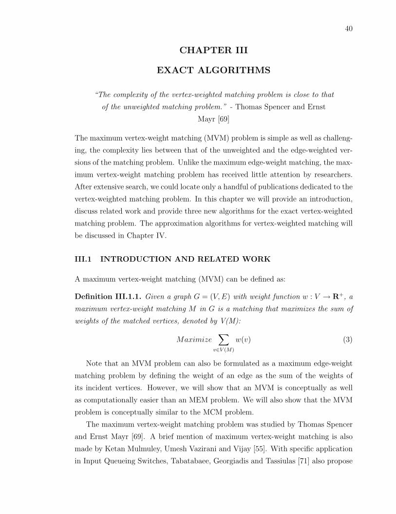
40
CHAPTER III
EXACT ALGORITHMS
“The complexity of the vertex-weighted matching problem is close to that
of the unweighted matching problem.” - Thomas Spencer and Ernst
Mayr [69]
The maximum vertex-weight matching (MVM) problem is simple as well as challeng-
ing, the complexity lies between that of the unweighted and the edge-weighted ver-
sions of the matching problem. Unlike the maximum edge-weight matching, the max-
imum vertex-weight matching problem has received little attention by researchers.
After extensive search, we could locate only a handful of publications dedicated to the
vertex-weighted matching problem. In this chapter we will provide an introduction,
discuss related work and provide three new algorithms for the exact vertex-weighted
matching problem. The approximation algorithms for vertex-weighted matching will
be discussed in Chapter IV.
III.1 INTRODUCTION AND RELATED WORK
A maximum vertex-weight matching (MVM) can be defined as:
Definition III.1.1. Given a graph G = (V,E) with weight function w : V → R+, a
maximum vertex-weight matching M in G is a matching that maximizes the sum of
weights of the matched vertices, denoted by V(M):
Maximize∑
v∈V (M)
w(v) (3)
Note that an MVM problem can also be formulated as a maximum edge-weight
matching problem by defining the weight of an edge as the sum of the weights of
its incident vertices. However, we will show that an MVM is conceptually as well
as computationally easier than an MEM problem. We will also show that the MVM
problem is conceptually similar to the MCM problem.
The maximum vertex-weight matching problem was studied by Thomas Spencer
and Ernst Mayr [69]. A brief mention of maximum vertex-weight matching is also
made by Ketan Mulmuley, Umesh Vazirani and Vijay [55]. With specific application
in Input Queueing Switches, Tabatabaee, Georgiadis and Tassiulas [71] also propose
41
an MVM algorithm. In this chapter we will provide relevant concepts from these
two papers and use them in our subsequent work. Detailed descriptions of the new
algorithms and the proof sketch of correctness will also be provided.
Spencer and Mayr show that the MVM problem in a nonbipartite graph can be
reduced to the MVM problem in a bipartite graph. Further, the bipartite MVM
problem itself can be simplified into two subproblems of computing the MVM in
special bipartite graphs called the restricted bipartite graphs. Spencer and Mayr also
show how to transform the MVM problem in a graph with negative weights to the
MVM problem in a graph with positive weights. Thus, computing the MVM in a
restricted bipartite graph will lead to a solution in general graphs. This relationship
is illustrated in Figure 19.
FIG. 19: Decomposition of the maximum vertex-weight matching problem.
Given a bipartite graph G = (S, T,E) and weight functions wS : S → R+ and
wT : T → R+, the two restricted bipartite graphs can be defined as: (i) G = (S, T,E)
and weight function wS : S → R+, and (ii) G = (S, T,E) and weight function
wT : T → R+. In the first restricted bipartite graph the weights on T vertices are set
to zero and in the second the weights on S vertices are set to zero, while everything
else remains the same. The fact that the matching problem in a bipartite graph can
be simplified into two subproblems of computing matchings in the restricted bipartite
graphs is given by Theorem III.1.1.
Theorem III.1.1 (Mendelsohn-Dulmage). Given two matchings MS and MT in a
bipartite graph G = (S, T,E), a new matching M ⊆ MS ∪MT can be computed in
linear time such that M matches all the S vertices matched by MS and all the T
vertices matched by MT .
Proof. Compute the symmetric difference MS ⊕MT , this will contain a set of cycles
and paths as enumerated in Figure 20. In each case it is possible to pick edges for

42
M such that it covers all the vertices of S matched by MS and all the T vertices
matched by MT . The edges that are matched by both MS and MT should also be
added to M . All the above operations are bounded by O(|E|). All these operations
can be summarized as follows:
(a) A cycle: arbitrarily choose MS or MT edges,
(b) MS-augmenting path: choose MT edges,
(c) MT -augmenting path: choose MS edges,
(d) MS-alternating path: choose MS edges,
(e) MT -alternating path: choose MT edges, and
(f) MS ∩MT : choose MS or MT edges.
FIG. 20: The symmetric difference of two matchings MS ⊕MT . Dashed lines rep-resent edges in MS and Solid lines represent edges in MT . (a) A cycle; (b)-(e)Augmenting or alternating paths.
An implementation of the Mendelsohn-Dulmage technique is illustrated in Algo-
rithm 10. The algorithm has three stages. In Stage 1, Lines 8-17, we will pick the
relevant MS edges shown as Cases (c) and (d) in Figure 20. These edges can be
detected by looking for S vertices that are matched by MS and unmatched by MT .
In Stage 2, Lines 19-29, we pick the relevant MT edges shown as Cases (b) and (e)
in Figure 20). These can be detected by looking for T vertices that are matched by
MT and unmatched by MS. In Stage 3, Lines 30-36, we will pick the edges that will
be matched by both MS and MT , as well as the cycles.

43
Algorithm 10 Input: A bipartite graph G and matchings MS and MT . Output:a matching M . Effect: using Mendelsohn-Dulmage technique, computes a matchingM that matches all the S vertices matched by MS and all the T vertices matched byMT .
1: procedure MendelsohnDulmage(G = (S, T,E), Ms, Mt, M)2: for all s ∈ S do . Initialize M3: M [s]← φ;4: end for5: for all t ∈ T do6: M [t]← φ;7: end for8: for all s ∈ S do . Pick MS edges (Cases (c) and (d))9: if Ms[s] 6= φ and Mt[s] = φ then
10: s′ ← s;
11: repeat12: t
′ ←MS[s′];
13: M [s′]← t
′;
14: M [t′]← s
′;
15: s′ ←MT [t
′];
16: until s′= φ or MS[s
′] = φ
17: end if18: end for19: for all t ∈ T do . Pick MT edges (Cases (b) and (e))20: if Mt[t] 6= φ and Ms[t] = φ then21: t
′ ← t;22: repeat23: s
′ ←MT [t′];
24: M [s′]← t
′;
25: M [t′]← s
′;
26: t′ ←MS[s
′];
27: until t′= φ or MT [t
′] = φ
28: end if29: end for30: for all s ∈ S do . Pick MS edges (Cases (a) and (f))31: if Ms[s] 6= φ and M [s] = φ then32: t←MS[s];33: M [s]← t;34: M [t]← s;35: end if36: end for37: end procedure

44
III.2 FOUNDATIONS
We will now discuss two theorems that provide necessary and sufficient conditions
to prove the optimality of an MVM. An important observation is the fact that any
maximum vertex-weight matching is also a maximum cardinality matching. This
provides the necessary condition and is stated by Theorem III.2.1.
Theorem III.2.1. Given a graph G = (V,E) and weight function w : V → R+, a
maximum vertex-weight matching M in G is also a maximum cardinality matching.
Proof. Let M be a maximum vertex-weight matching that is not of maximum cardi-
nality. Since M is not of maximum cardinality, there is at least one augmenting path
P with respect to M . The symmetric difference M ⊕ P will increase the cardinal-
ity of M by one edge and matches two new vertices while retaining all the vertices
that were already matched by M . Since positive weights are associated with the
vertices, the total weight of M increases when its cardinality is increased. Therefore
a maximum vertex-weight matching is also a maximum cardinality matching.
If a graph has a perfect matching, then all the vertices will be matched by any
maximum cardinality matching in this graph. Therefore any maximum cardinality
matching will also be a maximum vertex-weight matching for this graph. However,
when a maximum cardinality matching in a graph is not a perfect matching, comput-
ing a maximum vertex-weight matching will be conceptually harder than computing
a maximum cardinality matching. Since only a subset of vertices need to be matched,
we will have to explicitly consider the weights associated with the vertices. An im-
portant concept in vertex-weighted matching is the lexicographical ordering of vertex
sets.
We will need the definition of a lexicographical order to differentiate vertices with
duplicate weights. For a graph G = (V,E) with weight function w : V → R+, let
each vertex be assigned a distinct integer label between 1 and |V |. A relationship
between two vertices, and sets of vertices, can be established by using both the
weights and the labels associated with the vertices. A precedence operator ≺ can be
defined as follows: given two vertices v1 and v2, v1 ≺ v2 if and only if w(v1) < w(v2),
or w(v1) = w(v2) and l(v1) < l(v2), where l(v1) and l(v2), the labels of vertices v1
and v2 are considered as integers. Conversely, v2 succeeds v1, denoted as v2 � v1.
The precedence relationship can be used to compare two matchings. Given two
matchings M1 and M2 in a graph G = (V,E), let V1 = V (M1) and V2 = V (M2)
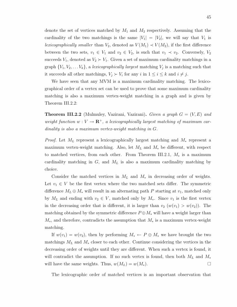
45
denote the set of vertices matched by M1 and M2 respectively. Assuming that the
cardinality of the two matchings is the same |V1| = |V2|, we will say that V1 is
lexicographically smaller than V2, denoted as V (M1) ≺ V (M2), if the first difference
between the two sets, v1 ∈ V1 and v2 ∈ V2, is such that v1 ≺ v2. Conversely, V2
succeeds V1, denoted as V2 � V1. Given a set of maximum cardinality matchings in a
graph {V1, V2, . . . Vk}, a lexicographically largest matching Vj is a matching such that
it succeeds all other matchings, Vj � Vi for any i in 1 ≤ i ≤ k and i 6= j.
We have seen that any MVM is a maximum cardinality matching. The lexico-
graphical order of a vertex set can be used to prove that some maximum cardinality
matching is also a maximum vertex-weight matching in a graph and is given by
Theorem III.2.2:
Theorem III.2.2 (Mulmuley, Vazirani, Vazirani). Given a graph G = (V,E) and
weight function w : V → R+, a lexicographically largest matching of maximum car-
dinality is also a maximum vertex-weight matching in G.
Proof. Let ML represent a lexicographically largest matching and M∗ represent a
maximum vertex-weight matching. Also, let ML and M∗ be different, with respect
to matched vertices, from each other. From Theorem III.2.1, M∗ is a maximum
cardinality matching in G, and ML is also a maximum cardinality matching by
choice.
Consider the matched vertices in ML and M∗ in decreasing order of weights.
Let v1 ∈ V be the first vertex where the two matched sets differ. The symmetric
difference ML⊕M∗ will result in an alternating path P starting at v1, matched only
by ML and ending with v2 ∈ V , matched only by M∗. Since v1 is the first vertex
in the decreasing order that is different, it is larger than v2 (w(v1) > w(v2)). The
matching obtained by the symmetric difference P⊕M∗ will have a weight larger than
M∗, and therefore, contradicts the assumption that M∗ is a maximum vertex-weight
matching.
If w(v1) = w(v2), then by performing M∗ ← P ⊕M∗ we have brought the two
matchings ML and M∗ closer to each other. Continue considering the vertices in the
decreasing order of weights until they are different. When such a vertex is found, it
will contradict the assumption. If no such vertex is found, then both ML and M∗
will have the same weights. Thus, w(ML) = w(M∗).
The lexicographic order of matched vertices is an important observation that

46
assisted in the design of the first proposed algorithm, which sorts the vertices in
decreasing order of their weights and process them in that order. The algorithm
proposed by Spencer and Mayr [69] also uses a sorting-based approach to compute
an MVM. Their divide and conquer strategy is successful because the choice of the
heaviest vertices that should be matched can be determined independently from the
choice of the lightest vertices that should be matched. Given a graph G = (V,E)
with weight function w : V → R+, there can be at most O(log2 n) divisions, where n
is the number of vertices. Computing a maximum cardinality matching at each step
will dominate the run time. Since any given problem can be reduced to computing
an MVM in a bipartite graph, a maximum cardinality can be computed in O(√nm)
time complexity [37], thus providing an overall time complexity of O(√nm log n) to
compute an MVM in a graph. In their algorithm Tabatabaee, Georgiadis and Tas-
siulas, first compute a maximum cardinality matching and then sort the unmatched
vertices in decreasing order of weights. From each unmatched vertex processed in
that order, an attempt to increase the weight of the matching is made. A maxi-
mum cardinality matching, as well as the subsequent computation can be bounded
by O(nm). Related work is summarized in Table 5.
Year Author(s) Complexity
1984 Spencer and Mayr O(√nm log n)
1987 Mulmuley, Vazirani and Vazirani Theoretical2001 Tabatabaee, Georgiadis and Tassiulas O(nm)
TABLE 5: A survey of algorithms for maximum vertex-weight matching. For a givengraph G = (V,E), n = |V | represents the number of vertices, and m = |E| thenumber of edges.

47
III.3 NEW ALGORITHMS FOR MAXIMUM VERTEX-WEIGHT
MATCHING
In this section we provide three algorithms to compute maximum vertex-weight
matchings (MVM). We will build on the work of Spencer and Mayr [69], and Mul-
muley, Vazirani and Vazirani [55] for the exact algorithms. We also propose three
algorithms for 12-approx matchings and a 2
3-approx algorithm. The approximation
algorithms are discussed Chapter 4. The proposed algorithms are summarized in
Table 6.
Name Type Description Complexity
Exact AlgorithmsGlobalOptimal B Sort-based O(n log n+ nm)LocalOptimal B Search-based O(nm)HybridOptimal G Sort and search-based O(n log n+ nm)
Approximation AlgorithmsGlobalHalf B 1
2-approx; Sort-based O(n log n+m)
LocalHalf B 12-approx; Search-based O(m)
HybridHalf G 12-approx; Sort and search-based O(n log n+m)
GlobalTwoThird B 23-approx; Sort-based O(n log n+ nd3)
TABLE 6: A summary of algorithms proposed for vertex weighted matchings. Bipar-tite and general graphs are represented with B and G respectively. For a bipartitegraph G = (S, T,E), n = (|S|+ |T |) represents the number of vertices, m = |E| thenumber the edges, and dk is a generalization of the vertex degree that denotes theaverage number of distinct alternating paths of length at most k edges starting at avertex in G.
The fundamental technique to compute an MVM is to find an augmenting path
and augment the matching via symmetric difference of the augmenting path and the
current matching. The algorithms for MVM are conceptually similar to algorithms
for computing a maximum cardinality matching. The proposed algorithms use the
single-source single-path approach (discussed in Chapter 2). In a single-source single-
path approach, the search for an augmenting path starts from an unmatched vertex,
and if found, augmentation can be performed along only one such path. For the
proposed algorithms we will not be able to use the multiple-path approach proposed
by Hopcroft and Karp [37], as discussed later in this chapter.
For the bipartite graph algorithms, we propose two basic approaches - global and
local. The two approaches differ in the way the vertices are selected for processing.

48
While GlobalOptimal uses a global-order in selecting the vertices as sources for
augmenting paths, LocalOptimal selects the sources arbitrarily (but, considers all
the potential augmenting paths from this source in an order). From the perspective
of computational complexity, both the techniques have similar worst-case bounds.
However, there can be significant differences in performance. The primary motivation
for developing two different approaches is to provide an algorithm for computing
maximum vertex-weight matchings in nonbipartite graphs. This is achieved in the
hybrid approach, HybridOptimal, where the source-vertices are processed in a
global-order, as well as, ordering all the potential augmenting paths like the local
approach. We will now discuss the three proposed algorithms in detail.
III.3.1 Algorithm GlobalOptimal
The first proposed algorithm, shown in Algorithm 11, is based on processing the
vertices according to a global order. We first decompose the given bipartite graph
G = (S, T,E), with weights associated with both S and T vertices, into two sub-
graphs, the restricted bipartite graphs, by ignoring the weights on the T vertices and
then on the S vertices. Construction of the restricted bipartite graphs is represented
in Algorithm 11 by Lines 5 and 6 for S vertices, and Lines 15 and 16 for T vertices.
For the first matching subproblem, we will compute the matching MS by find-
ing shortest augmenting paths starting from unmatched S vertices, considered in
decreasing order of weights. Lines 7− 14 represent the computation of MS. A sim-
ilar approach is used to compute the matching MT where weights are associated
only with the T vertices is represented by Lines 17− 24 in GlobalOptimal. The
final matching will be obtained by merging the two matchings MS and MT using
Mendelsohn-Dulmage technique. Execution of GlobalOptimal on a simple bipar-
tite graph with weights associated with S vertices is shown in Figure 21. For this
discussion, we will only consider positive weights. We will later show how to compute
an MVM in bipartite graphs with negative weights.

49
Algorithm 11 Input: a bipartite graph G. Output: a matching M . AssociatedData Structures: sets S and T are stored as stack data structures. The elementsin the stack follow a precedence order ≺, with the top of the stack being the heaviestelement at any given time. Effect: computes a maximum vertex-weight matchingM in G1: procedure GlobalOptimal(G = (S, T,E), wS : S → R+, wT : T → R+, M)2: M ← φ;3: MS ← φ;4: MT ← φ;5: S ← S in increasing order of weights wS;6: T ← T with weights set wT to zero;7: while S 6= φ do . Compute MS
8: s←top of S;9: S ← S \ s;
10: Find a shortest augmenting path P starting at s;11: if P found then12: MS ←MS ⊕ P ;13: end if14: end while15: T ← T in increasing order of weights wT ;16: S ← S with weights wS set to zero ;17: while T 6= φ do . Compute MT
18: t←top of T ;19: T ← T \ t;20: Find a shortest augmenting path P starting at t;21: if P found then22: MT ←MT ⊕ P ;23: end if24: end while25: M ←MendelsohnDulmage(MS,MT ,M); . Compute M26: end procedure
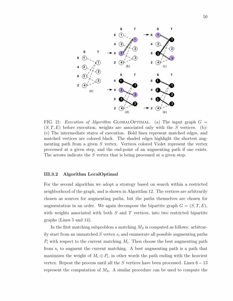
50
FIG. 21: Execution of Algorithm GlobalOptimal. (a) The input graph G =(S, T,E) before execution, weights are associated only with the S vertices. (b)-(e) The intermediate states of execution. Bold lines represent matched edges, andmatched vertices are colored black. The shaded edges highlight the shortest aug-menting path from a given S vertex. Vertices colored Violet represent the vertexprocessed at a given step, and the end-point of an augmenting path if one exists.The arrows indicate the S vertex that is being processed at a given step.
III.3.2 Algorithm LocalOptimal
For the second algorithm we adopt a strategy based on search within a restricted
neighborhood of the graph, and is shown in Algorithm 12. The vertices are arbitrarily
chosen as sources for augmenting paths, but the paths themselves are chosen for
augmentation in an order. We again decompose the bipartite graph G = (S, T,E),
with weights associated with both S and T vertices, into two restricted bipartite
graphs (Lines 5 and 14).
In the first matching subproblem a matching MS is computed as follows: arbitrar-
ily start from an unmatched S vertex si and enumerate all possible augmenting paths
Pi with respect to the current matching Mi. Then choose the best augmenting path
from si to augment the current matching. A best augmenting path is a path that
maximizes the weight of Mi ⊕ Pi, in other words the path ending with the heaviest
vertex. Repeat the process until all the S vertices have been processed. Lines 6− 13
represent the computation of MS. A similar procedure can be used to compute the
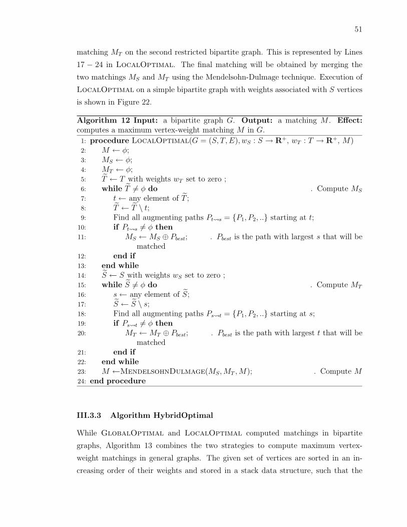
51
matching MT on the second restricted bipartite graph. This is represented by Lines
17 − 24 in LocalOptimal. The final matching will be obtained by merging the
two matchings MS and MT using the Mendelsohn-Dulmage technique. Execution of
LocalOptimal on a simple bipartite graph with weights associated with S vertices
is shown in Figure 22.
Algorithm 12 Input: a bipartite graph G. Output: a matching M . Effect:computes a maximum vertex-weight matching M in G.
1: procedure LocalOptimal(G = (S, T,E), wS : S → R+, wT : T → R+, M)2: M ← φ;3: MS ← φ;4: MT ← φ;5: T ← T with weights wT set to zero ;6: while T 6= φ do . Compute MS
7: t← any element of T ;8: T ← T \ t;9: Find all augmenting paths Pt s = {P1, P2, ..} starting at t;
10: if Pt s 6= φ then11: MS ←MS ⊕ Pbest; . Pbest is the path with largest s that will be
matched12: end if13: end while14: S ← S with weights wS set to zero ;15: while S 6= φ do . Compute MT
16: s← any element of S;17: S ← S \ s;18: Find all augmenting paths Ps t = {P1, P2, ..} starting at s;19: if Ps t 6= φ then20: MT ←MT ⊕ Pbest; . Pbest is the path with largest t that will be
matched21: end if22: end while23: M ←MendelsohnDulmage(MS,MT ,M); . Compute M24: end procedure
III.3.3 Algorithm HybridOptimal
While GlobalOptimal and LocalOptimal computed matchings in bipartite
graphs, Algorithm 13 combines the two strategies to compute maximum vertex-
weight matchings in general graphs. The given set of vertices are sorted in an in-
creasing order of their weights and stored in a stack data structure, such that the

52
FIG. 22: Execution of Algorithm LocalOptimal. (a) The input graph G =(S, T,E) before execution, weights are associated only with the S vertices. (b)-(d) The intermediate states of execution, (e) the final state. Bold lines representmatched edges, and matched vertices are colored black. The shaded edges highlightall the augmenting paths that exist from a given T vertex. The arrows indicate theT vertex that is being processed at a given step.

53
top element is the current heaviest vertex. The vertices are then retrieved from the
stack one at a time. All possible augmenting paths starting from this vertex are
discovered and ordered based on the weight of the last vertex, which is also the only
unmatched vertex in the path. The current matching is augmented with the path
with the heaviest weight of the last vertex. The algorithm processes each vertex
only once and terminates when it processes every vertex in the graph. Note that
the implementation of this algorithm should be capable of processing cycles of odd
length (Blossoms).
Algorithm 13 Input: a graph G. Output: a matching M . Associated DataStructures: set V is a stack data structure. The elements in the stack follow aprecedence order ≺, with the top of the stack being the heaviest element at anygiven time. Effect: computes a maximum vertex-weight matching M in G.
1: procedure HybridOptimal(G = (V,E), w : V → R+)2: M ← φ;3: V ← V in increasing order of weights;4: while V 6= φ do . Compute M5: v ← top of V ;6: V ← V \ v;7: Find all augmenting paths Pv w = {P1, P2, ..} starting at v;8: if Pv w 6= φ then9: M ←M ⊕ Pbest; . Pbest is the path with largest w that will be
matched10: V ← V \ w;11: end if12: end while13: end procedure
III.3.4 Negative Weights
Spencer and Mayr provide a method to handle negative weights. Given a graph
G = (V,E) and weight function w : V → R, for each vertex vi ∈ V that has a
negative weight, add a new vertex v′i and an edge e(vi, v
′i). Also set w(vi) = 0 and
w(v′i) = abs(w(vi)), the absolute value of the original weight. This will result in a
new graph G′(V′, E′) and weight function w :→ (R+ ∪ {0}). An MVM M in G
′will
also be an MVM in G. While M will also be a maximum cardinality matching in G′,
the same is not necessarily true in G.
For the proposed algorithms GlobalOptimal and LocalOptimal, we can
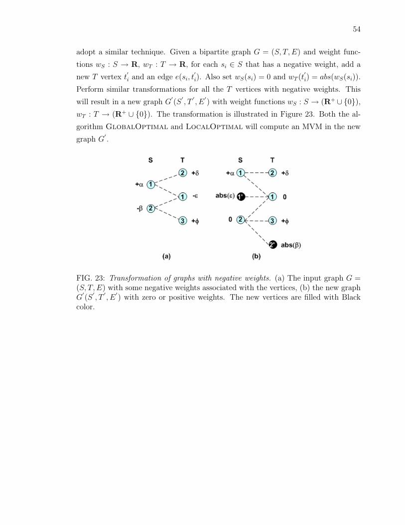
54
adopt a similar technique. Given a bipartite graph G = (S, T,E) and weight func-
tions wS : S → R, wT : T → R, for each si ∈ S that has a negative weight, add a
new T vertex t′i and an edge e(si, t
′i). Also set wS(si) = 0 and wT (t
′i) = abs(wS(si)).
Perform similar transformations for all the T vertices with negative weights. This
will result in a new graph G′(S′, T′, E′) with weight functions wS : S → (R+ ∪ {0}),
wT : T → (R+ ∪ {0}). The transformation is illustrated in Figure 23. Both the al-
gorithm GlobalOptimal and LocalOptimal will compute an MVM in the new
graph G′.
FIG. 23: Transformation of graphs with negative weights. (a) The input graph G =(S, T,E) with some negative weights associated with the vertices, (b) the new graphG′(S′, T′, E′) with zero or positive weights. The new vertices are filled with Black
color.

55
III.4 PROOF OF CORRECTNESS
In this section we provide the proof of correctness for the proposed algorithms. We
will first discuss the proof for the two bipartite graph algorithms and then extend it
to the algorithm for the general graph. In Section III.2 we provided the necessary
and sufficient condition to prove the optimality of an MVM in a graph. In this sec-
tion, we will provide an alternative method to prove the correctness of the proposed
algorithms. The bipartite algorithms decompose the given problem into two match-
ing problems on the restricted bipartite graphs. We will prove the correctness for an
MVM computed in the first restricted bipartite graph, which can then be trivially
extended to the second subgraph. The correctness of an MVM in the original graph
can be proved subsequently using the Mendelsohn-Dulmage technique as stated in
Theorem III.1.1. However, there is no such decomposition in the case of general
graphs.
We will adapt the definitions of the lexicographical sets for the restricted bipartite
cases. We will generally consider the first restricted bipartite case: a bipartite graph
G = (S, T,E) and weight function w : S → R+ (we would have specifically set the
weights on the T vertices to zero). In all lexicographic comparisons, we will consider
only the S vertices. Recall that MS is a matching in this restricted bipartite graph
that has weights only on the S vertices. The S vertices matched by MS, the S-vertex
set of MS, will be represented as S(MS).
The proof for the correctness for GlobalOptimal is straight-forward, however,
the proof for the correctness of Algorithm LocalOptimal is nontrivial. In order
to provide a uniform method of proof for both these algorithms, we introduce the
concept of reachability property, which can be defined as:
Definition III.4.1 (Reachability Property). Consider a graph G = (V,E) with
weight function w : V → R+, and any matching M in G. The matching M satisfies
the reachability property if for any M-unmatched vertex v, and any M-matched vertex
v′
reachable by an M-alternating path from v, the condition that v ≺ v′
holds.
As illustrated in Figure 25, the alternating path for a reachability test starts
with an unmatched vertex and ends with a matched vertex. This path is always of
even length with an equal number of matched and unmatched edges, and has only
one unmatched vertex. We use the concept of reachability to prove of correctness
of all the proposed algorithms. Existence of the reachability property is a sufficient
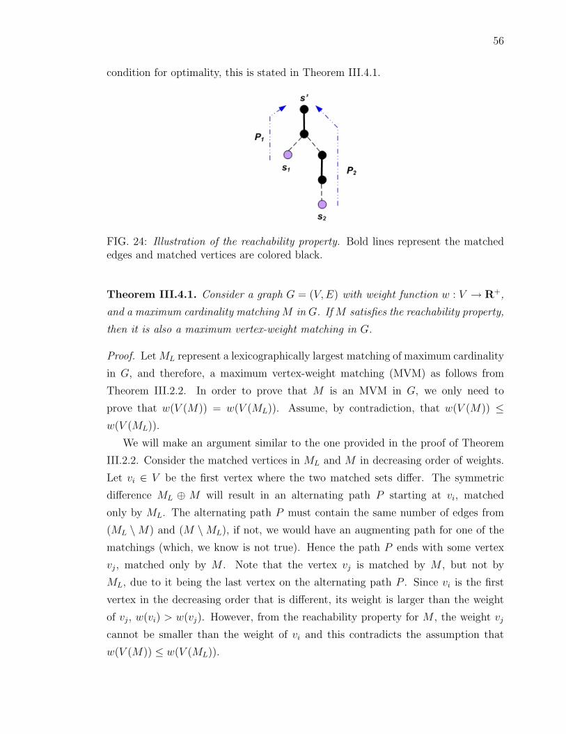
56
condition for optimality, this is stated in Theorem III.4.1.
FIG. 24: Illustration of the reachability property. Bold lines represent the matchededges and matched vertices are colored black.
Theorem III.4.1. Consider a graph G = (V,E) with weight function w : V → R+,
and a maximum cardinality matching M in G. If M satisfies the reachability property,
then it is also a maximum vertex-weight matching in G.
Proof. LetML represent a lexicographically largest matching of maximum cardinality
in G, and therefore, a maximum vertex-weight matching (MVM) as follows from
Theorem III.2.2. In order to prove that M is an MVM in G, we only need to
prove that w(V (M)) = w(V (ML)). Assume, by contradiction, that w(V (M)) ≤w(V (ML)).
We will make an argument similar to the one provided in the proof of Theorem
III.2.2. Consider the matched vertices in ML and M in decreasing order of weights.
Let vi ∈ V be the first vertex where the two matched sets differ. The symmetric
difference ML ⊕ M will result in an alternating path P starting at vi, matched
only by ML. The alternating path P must contain the same number of edges from
(ML \M) and (M \ML), if not, we would have an augmenting path for one of the
matchings (which, we know is not true). Hence the path P ends with some vertex
vj, matched only by M . Note that the vertex vj is matched by M , but not by
ML, due to it being the last vertex on the alternating path P . Since vi is the first
vertex in the decreasing order that is different, its weight is larger than the weight
of vj, w(vi) > w(vj). However, from the reachability property for M , the weight vj
cannot be smaller than the weight of vi and this contradicts the assumption that
w(V (M)) ≤ w(V (ML)).

57
If w(vi) = w(vj), then replace M by M ⊕ P . This will not affect the weight of
matching M . Continue considering the vertices in the decreasing order of weights
until the next differing vertex is found. We can repeat the above argument for such
a vertex. When there are no more vertices to be considered, then both ML and M
have the same weights. Thus w(V (M)) = w(V (ML)).
The reachability property provides a sufficient condition to prove the optimality
of a maximum vertex-weight matching in a graph. We will now prove that the
proposed algorithms will satisfy the reachability property, and thus compute optimal
vertex-weight matchings. These are stated in Theorems III.4.2, III.4.3 and III.4.4.
Theorem III.4.2. Consider a graph G = (S, T,E) with weight function w : S →R+, and a matching MG
S computed by algorithm GlobalOptimal. The matching
MGS satisfies the reachability property.
Proof. We will prove the theorem by using mathematical induction. We will con-
sider those steps when Algorithm GlobalOptimal augments the current matching,
called the augmenting steps. Let M iS correspond to a matching at some intermediate
step in the algorithm. We will prove that the theorem holds true at each augmenting
step, and therefore at the end of the execution of GlobalOptimal.
Base case: Let s1 ∈ S be the first matched vertex. Since GlobalOptimal
considers the S vertices for augmentation in the decreasing order of weights, s1 will
precede all other S vertices from which s1 is reachable through an M iS alternating
path. Thus the base case holds true. For simplicity, assume that there are no isolated
vertices in G.
Step k : Assume that the reachability property holds true after the k-th augmen-
tation.
Step (k+1): Let the (k + 1)-th augmentation be performed along the M iS-
augmenting path Pk+1 from sk+1 ∈ S to tk+1 ∈ T . In order to prove the theorem, we
need to show that for any M iS-unmatched vertex si, and any M i
S-matched vertex s′i
reachable through an M iS-alternating path, the condition that si ≺ s
′i holds after the
(k + 1)-th augmentation. Note that the vertices s′i and sk+1 can be the same.
When the (k + 1)-th augmenting path Pk+1 and any M iS-alternating path be-
tween si and s′i are vertex disjoint, the (k + 1)-th augmentation has no affect on
the reachability of s′i from si. However, if s
′i becomes reachable after the (k + 1)-th
augmentation, then the alternating path between si and s′i, and the augmenting path

58
Pk+1 have at least one vertex (and one edge) in common. This is illustrated in Figure
25. Now, there are only two alternatives: (i) the two vertices s′i and sk+1 are the
same. In such a case, there was at least one augmenting path from si to tk+1, but
sk+1 was preferred, and the condition si ≺ s′i holds; or (ii) the two vertices s
′i and
sk+1 are different. In which case we know that all the matched s ∈ S vertices succeed
sk+1, and the condition si ≺ s′i holds.
FIG. 25: Illustrates that reachability property holds for Algorithm GlobalOptimal.Bold lines represent the matched edges and matched vertices are colored black. (a)State before (k + 1)-th augmentation, (b) state after (k + 1)-th augmentation.
Theorem III.4.3. Given a graph G = (S, T,E) with weight function w : S → R+,
and a matching MLS computed by algorithm LocalOptimal. The matching ML
S
satisfies the reachability property.
Proof. Similar to the proof of Theorem III.4.3, we will induct on the MLS augmenting
steps. We will show that at the end of any given iteration of the algorithm, MLS
will satisfy the reachability property such that for any MLS -matched vertex s
′ ∈ S
reachable via an MLS -alternating path P originating at any ML
S -unmatched vertex
s ∈ S, s ≺ s′.
Base case: LocalOptimal will arbitrarily start from a T vertex, say t1, and
process all S vertices adjacent to t1, S1 = adj(t1). It will then select the largest
s ∈ S1, say s1. After matching s1 to t1, s1 will be reachable via an MLS alternating
path only from the vertices in S1 \ {s1}. Since s1 is heaviest vertex in S1, the
reachability property will hold true for the base case.

59
Step k : Assume that the reachability property holds true after the k-th augmen-
tation.
Step (k+1): Given that the reachability property holds true at step k, we will
prove that it also holds true for step (k + 1). Let the two vertices matched at step
(k + 1) be tk+1 ∈ T and sk+1 ∈ S. LocalOptimal will consider all the unmatched
S vertices reachable via an MLS -augmenting path from tk+1, let this set be Sk+1 ⊂ S.
Vertex sk+1 is selected by Algorithm LocalOptimal because it is the largest among
all the vertices in the set Sk+1.
Again, in order to have an impact any MLS -matched vertex s
′ ∈ S reachable via
an MLS -alternating path P , after the (k + 1)-th augmentation, originating at any
MLS -unmatched vertex s ∈ S, should contain tk+1 in the path (Figure 25). The
two possibilities are: (i) s /∈ Sk+1, in which case nothing changes with respect to
s from the augmentation at step (k + 1). Therefore, from the assumption at step
k, s ≺ s′; or (ii) s ∈ Sk+1 \ {sk+1}: for these S vertices there are two possibilities
- an MLS -matched vertex s
′reachable via an alternating path was reachable either
before the (k+ 1)-th augmentation, and therefore s ≺ s′, or becomes reachable after
the (k + 1)-th augmentation. In the latter case, we know that LocalOptimal will
select the largest vertex, and therefore, s ≺ sk+1. From step k, we also know that
sk+1 ≺ s′
(since sk+1 will also be available for matching until step k + 1 for all s′
vertices reachable via sk+1). Thus, s ≺ s′, and the property holds true for step
(k + 1).
We will now prove that the reachability property holds true for a matching com-
puted by HybridOptimal in Theorem III.4.4.
Theorem III.4.4. Given a graph G = (V,E) with weight function w : V → R+, and
a matching M computed by algorithm HybridOptimal. The matching M satisfies
the reachability property.
Proof. Similar to two earlier proofs, we will again induct on the M -augmenting steps.
Base case: HybridOptimal will start from the heaviest vertex, say v1, and
process all vertices adjacent to v1, V1 = adj(v1). It will then select the largest
vertex in V1, say w1, for matching. After matching the edge v1 to w1, there are two
possibilities: (i) vertex v1 will be reachable via an M -alternating path from vertices
in Vw ∈ adj(w1). But, we already know that v1 is the heaviest vertex, and therefore,
reachability property holds; and (ii) vertex w1 will be reachable via an M -alternating

60
path from vertices in Vv ∈ adj(v1). But, HybridOptimal has already processed
all vertices in Vv and, w1 is the heaviest vertex in this set. Thus, the reachability
property holds for the base case.
Step k : Assume that the reachability property holds true after the k-th augmen-
tation.
Step (k+1): Let the two vertices matched at step (k + 1) be vk+1 and wk+1.
HybridOptimal will start with the current heaviest vertex vk+1, and process all
vertices reachable via an M i-augmenting path from it, let this set be Pk+1 ⊂ V .
Vertex wk+1 is selected by because it is the heaviest among all the vertices in Pk+1.
Again, we are only concerned with the vertices that become reachable via ver-
tices vk+1 and wk+1. (Figure 25). However, we are not worried about vertex vk+1
becoming reachable to any unmatched vertex after (k+ 1)-th augmentation because
we know that it is the current heaviest vertex. Therefore, we are only concerned
about the vertex wk+1, and other matched vertices becoming reachable through it.
Let v represent the unmatched vertices and v′
represent the matched vertices that
are reachable via an M i-alternating path from v.
The two possibilities are: (i) v /∈ Pk+1, in which case nothing changes with respect
to v from the augmentation at step (k + 1). Therefore, from the assumption at step
k, v ≺ v′; or (ii) v ∈ Pk+1 \ {wk+1}: for these vertices there are two possibilities - a
matched vertex v′
reachable via an M i-alternating path was reachable either before
the (k + 1)-th augmentation, and therefore, v ≺ v′, or becomes reachable after the
(k + 1)-th augmentation. In the latter case, we know that HybridOptimal will
select the largest vertex, and therefore, v ≺ wk+1. From step k, we also know that
wk+1 ≺ v′
(since wk+1 will also be available for matching before step k + 1 for all
v′
vertices reachable via wk+1). Thus, v ≺ v′, and the property holds true for step
(k + 1).
From Theorems III.4.1, III.4.2, III.4.3 and III.4.4, the optimality of GlobalOp-
timal, LocalOptimal and HybridOptimal immediately follows, and is stated
in Corollary III.4.1.
Corollary III.4.1. Given a graph G = (S, T,E) with weight function w : S → R+,
Algorithms GlobalOptimal and LocalOptimal will compute maximum vertex-
weight matchings MS in G.
61
III.5 A REACHABILITY-BASED ALGORITHM
A conceptually similar algorithm to compute maximum vertex weighted matching
was proposed by Tabatabaee, Georgiadis and Tassiulas [71]. The authors use the
reachability property not only to provide a proof of correctness, but also to design
their algorithm. Our goal of this discussion is to demonstrate the power of expressing
optimality of a matching using the existence of reachability property in the graph
with respect to a matching. The algorithm is sketched in Algorithm 14.
Algorithm 14 Input: a graph G. Output: a matching M . Effect: computes amaximum vertex-weight matching M in G. Associated Data Structures: set Uis a stack data structure. The elements in the stack follow a precedence order ≺,with the top of the stack being the heaviest element at any given time.
1: procedure ReachabilityBasedAlg(G = (V,E), w : V → R+)2: M ←M∗, a maximum (cardinality) matching;3: U ← V \ V (M) in decreasing order of weights;4: while U 6= φ do5: u← top element of U ;6: U ← U \ {u};7: Find an alternating path Pu w starting at u, such that w ≺ v;8: if Pu w 6= φ then9: M ←M ⊕ Pu w;
10: U ← U ∪ {w};11: end if12: end while13: end procedure
The first step is to compute a maximum (cardinality) matching by ignoring all
the weights on the vertices. Let U ← V \ V (M) represent the unmatched vertices
in decreasing order of weights. Consider the current heaviest vertex v ∈ U . If there
exist an alternating path P between v and any vertex w such that w ≺ v, then switch
(M ←M ⊕ P )the matched edges of this path to match vertex v instead of w. Note
that since M is a maximum matching there cannot exist any augmenting paths in
G with respect to M . Add w to the set U , and repeat. If no such path is found,
then remove vertex v from U and continue with the next heaviest vertex in U . The
algorithm terminates when set U becomes empty. Note that for every unmatched
vertex the algorithm attempts to satisfy the reachability property with respect to the
current matching. The computational cost for satisfying the reachability property for
a vertex can be bounded by O(|E|) (a breadth-first search can be used). The number
62
of unmatched vertices can be bounded by O(|V |), and therefore, the complexity of
Algorithm 14 is O(|V ||E|). It can be noted that the reachability-based algorithm is
a less sophisticated than the algorithm proposed by Spencer and Mayr [69].
The proof of correctness can be easily shown by demonstrating that Algorithm 14
computes a matching that satisfies the reachability property, and therefore, computes
a maximum vertex-weight matching as provided by Theorem III.4.1.
III.6 CHAPTER SUMMARY
In this chapter we introduced three new algorithms, GlobalOptimal, LocalOpti-
mal and HybridOptimal for computing maximum vertex-weight matchings. Proof
of correctness for the proposed algorithms were also discussed. We developed the con-
cept of reachability property as a necessary condition to establish optimality of an
MVM.
The proposed algorithms are easy to understand and simple to implement. How-
ever, there are limitations to the proposed algorithms, in that we can neither perform
greedy initializations nor grow multiple paths. Although the greedy initializations do
not have a bound on the approximation ratio, for practical purposes greedy initial-
ization is very important. In some of our preliminary experiments on matrices from
applications downloaded from the University of Florida Sparse Matrix Collection,
greedy initializations tend to match a substantial percentage of edges. Therefore, we
consider that inability to perform greedy initializations for vertex-weighted matching
algorithms is a limitation. In Figure 26, we show why greedy initialization fails. A
vertex once matched cannot be unmatched in an augmentation-based algorithm. For
example, vertex T3 gets matched in the greedy initialization phase, but should not
be matched in a maximum vertex-weight matching. Note that this does not apply
to Algorithm ReachabilityBasedAlg.
The multiple-path approach discussed in Chapter 2 has the best time complexity
for maximum cardinality matching. However, for the proposed algorithms we will
not be able to implement the multiple-path approach. We will encounter the same
problem illustrated in Figure 26.
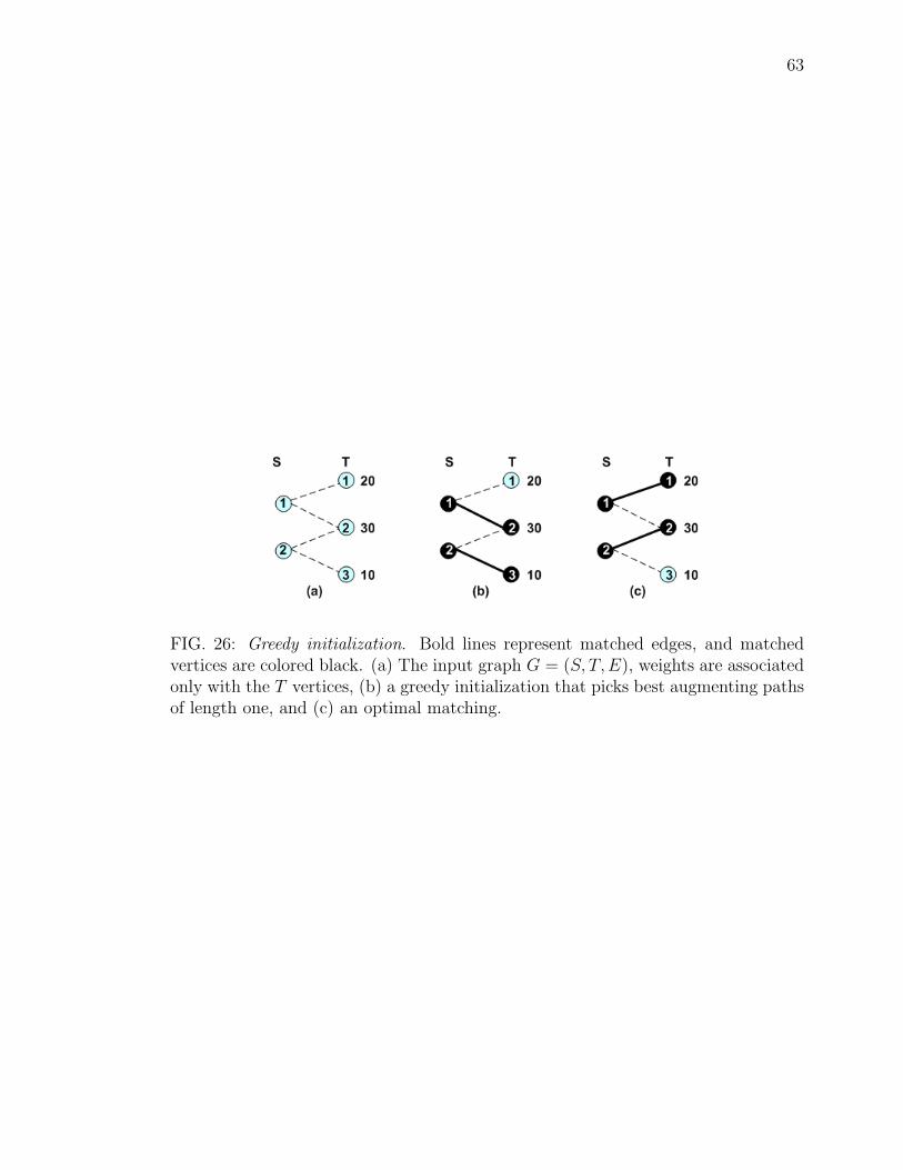
63
FIG. 26: Greedy initialization. Bold lines represent matched edges, and matchedvertices are colored black. (a) The input graph G = (S, T,E), weights are associatedonly with the T vertices, (b) a greedy initialization that picks best augmenting pathsof length one, and (c) an optimal matching.
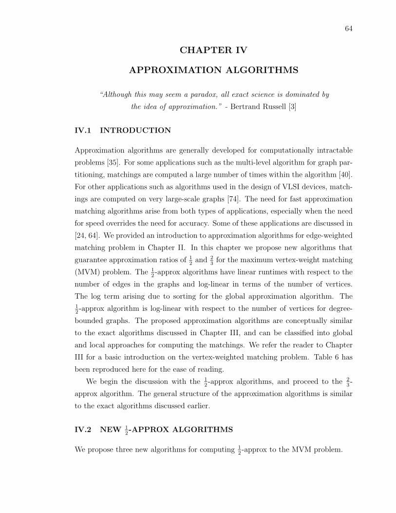
64
CHAPTER IV
APPROXIMATION ALGORITHMS
“Although this may seem a paradox, all exact science is dominated by
the idea of approximation.” - Bertrand Russell [3]
IV.1 INTRODUCTION
Approximation algorithms are generally developed for computationally intractable
problems [35]. For some applications such as the multi-level algorithm for graph par-
titioning, matchings are computed a large number of times within the algorithm [40].
For other applications such as algorithms used in the design of VLSI devices, match-
ings are computed on very large-scale graphs [74]. The need for fast approximation
matching algorithms arise from both types of applications, especially when the need
for speed overrides the need for accuracy. Some of these applications are discussed in
[24, 64]. We provided an introduction to approximation algorithms for edge-weighted
matching problem in Chapter II. In this chapter we propose new algorithms that
guarantee approximation ratios of 12
and 23
for the maximum vertex-weight matching
(MVM) problem. The 12-approx algorithms have linear runtimes with respect to the
number of edges in the graphs and log-linear in terms of the number of vertices.
The log term arising due to sorting for the global approximation algorithm. The12-approx algorithm is log-linear with respect to the number of vertices for degree-
bounded graphs. The proposed approximation algorithms are conceptually similar
to the exact algorithms discussed in Chapter III, and can be classified into global
and local approaches for computing the matchings. We refer the reader to Chapter
III for a basic introduction on the vertex-weighted matching problem. Table 6 has
been reproduced here for the ease of reading.
We begin the discussion with the 12-approx algorithms, and proceed to the 2
3-
approx algorithm. The general structure of the approximation algorithms is similar
to the exact algorithms discussed earlier.
IV.2 NEW 12-APPROX ALGORITHMS
We propose three new algorithms for computing 12-approx to the MVM problem.

65
Name Type Description Complexity
Exact AlgorithmsGlobalOptimal B Sort-based O(n log n+ nm)LocalOptimal B Search-based O(nm)HybridOptimal G Sort and search-based O(n log n+ nm)
Approximation AlgorithmsGlobalHalf B 1
2-approx; Sort-based O(n log n+m)
LocalHalf B 12-approx; Search-based O(m)
HybridHalf G 12-approx; Sort and search-based O(n log n+m)
GlobalTwoThird B 23-approx; Sort-based O(n log n+ nd3)
TABLE 7: A summary of algorithms proposed for vertex weighted matchings. Bipar-tite and general graphs are represented with B and G respectively. For a bipartitegraph G = (S, T,E), n = (|S|+ |T |) represents the number of vertices, m = |E| thenumber the edges, and dk is a generalization of the vertex degree that denotes theaverage number of distinct alternating paths of length at most k edges starting at avertex in G.
The first proposed algorithm, GlobalHalf, is based on processing the vertices
in a global order of decreasing weights. Given a bipartite graph G = (S, T,E) with
weights associated with the S and T vertices, we will decompose it into two restricted
bipartite graphs by first ignoring the weights on T vertices, and then on S vertices.
The problem decomposition is represented in Algorithm 15 by Lines 5 and 6 for the
S vertices, and by Lines 15 and 16 for the T vertices.
Consider the first restricted bipartite graph with weights on only S vertices.
Algorithm 15 processes the S vertices in a succeeding order (s1 � s2 � s3 . . .). From
a given vertex si ∈ S, search for any unmatched vertex ti ∈ T adjacent to si. If
such a vertex is found, then add it to the current matching and proceed with the
next unmatched S vertex in succeeding order. Computation of MS in Algorithm
15 is represented by Lines 7 − 14. A similar approach to compute the matching
MT for the second restricted graph is represented by Lines 17− 24 in Algorithm 15.
The final matching is obtained by merging the two matchings MS and MT using the
Mendelsohn-Dulmage technique. Execution of Algorithm GlobalHalf on a simple
bipartite graph with weights associated only to the S vertices is shown in Figure 27.
For the second 12-approx algorithm, LocalHalf, we adopt a strategy based
on searching for an unmatched edge from the unweighted vertices in arbitrary order;

66
Algorithm 15 Input: A bipartite graph G. Output: a matching M . AssociatedData Structures: sets S and T are stored as stack data structures. The elementsin the stack follow a precedence order ≺, with the top of the stack being the heaviestelement at any given time. Effect: computes a 1
2-approx to maximum vertex-weight
matching.
1: procedure GlobalHalf(G = (S, T,E), wS : S → R+, wT : T → R+, M)2: M ← φ; . Initialization3: MS ← φ;4: MT ← φ;5: S ← S in descending order of weights wS;6: T ← T with weights wT set to zero ;7: while S 6= φ do . Compute MS
8: s←top of S;9: S ← S \ s;
10: Find an unmatched edge est incident on s;11: if est exists then12: MS ←MS ∪ {est};13: end if14: end while15: T ← T in descending order of weights wT ;16: S ← S with weights wS set to zero ;17: while T 6= φ do . Compute MT
18: t←top of T ;19: T ← T \ t;20: Find an unmatched edge ets incident on t;21: if ets exists then22: MT ←MT ∪ {ets};23: end if24: end while25: M ←MendelsohnDulmage(MS,MT ,M); . Compute M26: end procedure

67
FIG. 27: Execution of Algorithm GlobalHalf. (a) The input graph G = (S, T,E)with weights associated only with the S vertices, (b)-(e) the intermediate states ofexecution. Bold lines represent matched edges, and matched vertices are coloredblack. The shaded edges mark the augmenting paths of length one (an unmatchededge) from a given S vertex, (f) the final state.
however, we will need to find an edge that leads to the heaviest vertex on the weighted
side. This approach does not depend on a global order but, on a local search. The
input graph is divided into two restricted bipartite graphs by first ignoring the weights
on the T vertices and then on the S vertices. The decomposition is represented in
Algorithm 16 by Lines 5 and 14.
For the first restricted bipartite graph, a matching MS is computed as follows:
arbitrarily start from an unmatched vertex ti ∈ T , and enumerate all the unmatched
edges incident on the vertex ti. If such edges exist, then choose the best edge from
this set and augment the current matching. We define the best edge as the edge
that leads to a heaviest weighted vertex. Repeat the process until all the T vertices
have been processed. Lines 6 − 13 in Algorithm 16 represent the computation of
MS. A similar procedure can be used to compute the matching MT for the second
restricted bipartite graph. This is represented by Lines 15−22 in Algorithm 16. The
final matching will be obtained by merging the two matchings MS and MT using
the Mendelsohn-Dulmage technique. The execution of Algorithm LocalHalf on a

68
Algorithm 16 Input: a bipartite graph G. Output: a matching M . AssociatedData Structures: sets S and T are stored as stack data structures. The elementsin the stack can be in any arbitrary order. Effect: computes a 1
2-approx MVM.
1: procedure LocalHalf(G = (S, T,E), wS : S → R+, wT : T → R+, M)2: M ← φ; . Initialization3: MS ← φ;4: MT ← φ;5: T ← T with weights wT set to zero ;6: while T 6= φ do . Compute MS
7: t←top of T ;8: T ← T \ t;9: Find all unmatched edges ets incident on t;
10: if unmatched edges exist then11: MT ←MT ∪ {ebest}; . ebest is ets with largest w(s)12: end if13: end while14: S ← S with weights wS set to zero ;15: while S 6= φ do . Compute MT
16: s←top of S;17: S ← S \ s;18: Find all unmatched edges est incident on s;19: if unmatched edges exist then20: MS ←MS ∪ {ebest}; . ebest is est with the largest w(t)21: end if22: end while23: M ←Mendelsohn-Dulmage(MS,MT ,M); . Compute M24: end procedure
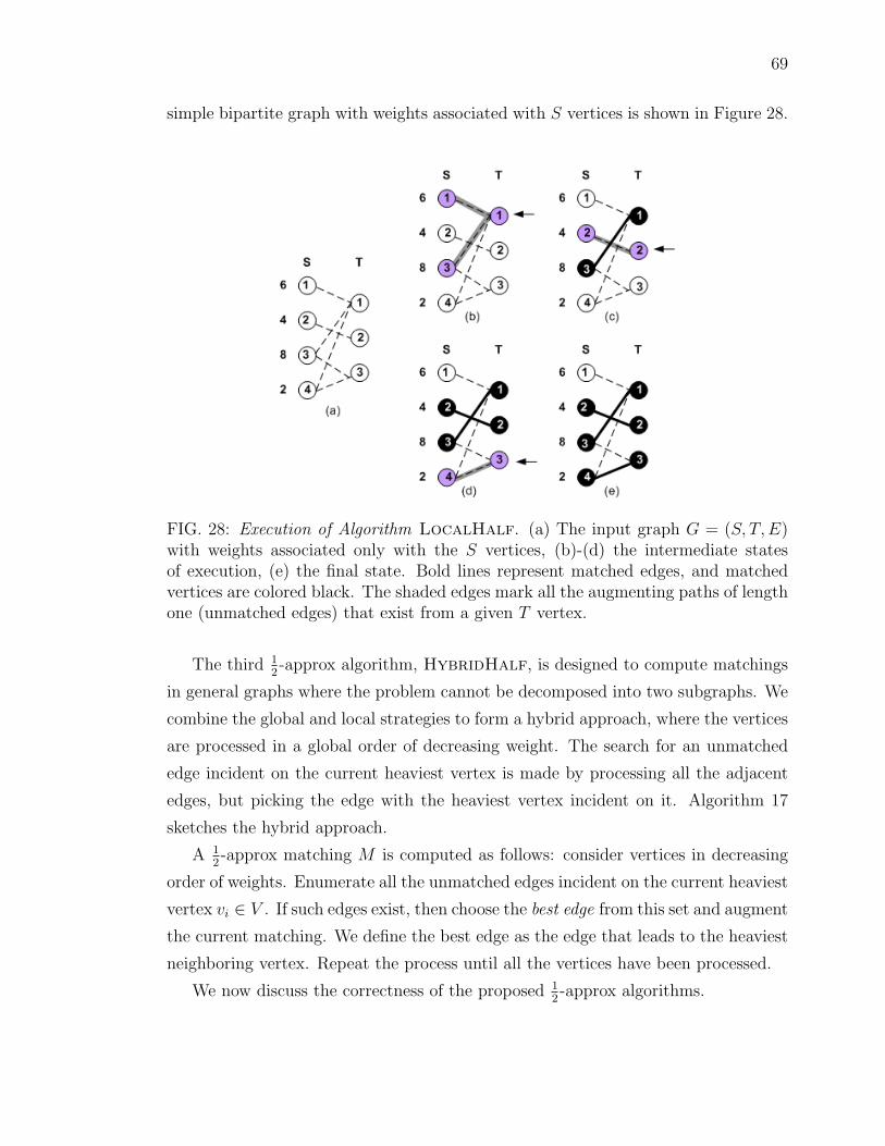
69
simple bipartite graph with weights associated with S vertices is shown in Figure 28.
FIG. 28: Execution of Algorithm LocalHalf. (a) The input graph G = (S, T,E)with weights associated only with the S vertices, (b)-(d) the intermediate statesof execution, (e) the final state. Bold lines represent matched edges, and matchedvertices are colored black. The shaded edges mark all the augmenting paths of lengthone (unmatched edges) that exist from a given T vertex.
The third 12-approx algorithm, HybridHalf, is designed to compute matchings
in general graphs where the problem cannot be decomposed into two subgraphs. We
combine the global and local strategies to form a hybrid approach, where the vertices
are processed in a global order of decreasing weight. The search for an unmatched
edge incident on the current heaviest vertex is made by processing all the adjacent
edges, but picking the edge with the heaviest vertex incident on it. Algorithm 17
sketches the hybrid approach.
A 12-approx matching M is computed as follows: consider vertices in decreasing
order of weights. Enumerate all the unmatched edges incident on the current heaviest
vertex vi ∈ V . If such edges exist, then choose the best edge from this set and augment
the current matching. We define the best edge as the edge that leads to the heaviest
neighboring vertex. Repeat the process until all the vertices have been processed.
We now discuss the correctness of the proposed 12-approx algorithms.

70
Algorithm 17 Input: a graph G. Output: a matching M . Associated DataStructures: set V is a stack data structure. The elements in the stack follow aprecedence order ≺, with the top of the stack being the heaviest element at anygiven time. Effect: computes a 1
2-approx MVM.
1: procedure HybridHalf(G = (V,E), w : V → R+)2: M ← φ;3: V ← V in increasing order of weights;4: while V 6= φ do . Compute M5: v ← top of V ;6: V ← V \ v;7: Find all unmatched edges evx incident on v;8: if unmatched edges exist then9: M ←M ∪ {ebest}; . ebest is evw with largest w(x)
10: V ← V \ w;11: end if12: end while13: end procedure

71
IV.3 PROOF OF CORRECTNESS
The proofs of correctness of the 12-approx algorithms are fairly straightforward. The
main idea is to establish a relationship between the matched and the unmatched
vertices that reveal the correctness of the approximation ratio. In order to estab-
lish this relationship, we will introduce the concept of failed vertices. Consider a
graph G = (S, T,E) with weight function w : S → R+, a matching M∗ computed by
Algorithm GlobalOptimal, and a matching M2 computed by Algorithm Global-
Half A failed S-vertex is a vertex that is matched in M∗, but not in M2. The same
definition is extended to the T vertices for the second restricted bipartite graph, can
also be extended similarly for Algorithms LocalOptimal and LocalHalf, Hy-
bridOptimal and HybridHalf). No distinction between S and T vertices is made
for general graphs.
The intuition for the proof of correctness comes from the fact that for every
failed vertex, there will be at least one distinct vertex, at least as large as the failed
vertex, that will be matched by the 12-approx algorithm. Thus, resulting in half
approximation to the optimal matching. This relationship is characterized by the
restricted reachability property, which can be defined as follows.
Definition IV.3.1 (Restricted Reachability Property). Consider a graph G = (V,E)
with weight function w : V → R+, and any matching M in G. The matching M
satisfies the restricted reachability property if for any M-unmatched vertex v, and
any M-matched vertex v′
reachable from v by an M-alternating path of length two
edges, the condition v ≺ v′
holds.
We show that if a given maximal matching satisfies the restricted reachability
property, then it is also a 12-approx to the optimal matching. This is stated in
Lemma IV.3.1.
Lemma IV.3.1. Consider a graph G = (V,E) with weight function w : V → R+,
and a maximal matching M2 in G. If M2 satisfies the restricted reachability property,
then M2 is a 12-approximation to a maximum vertex-weight matching in G.
Remark : The reader should note the requirement for a maximal matching in this
Lemma.
Proof. Let M∗ represent a maximum vertex-weight matching, and M2 represent any

72
maximal matching in G with the restricted reachability property. Consider the sym-
metric difference M∗ ⊕M2. This will result in a collection of paths and cycles. All
possibilities for bipartite graphs are enumerated in Figure 20. Note that even for
general graphs, there cannot be cycles of odd length, and therefore, Figure 20 also
holds true for general graphs (without the distinction of S and T vertex sets). The
edges that are matched in both the algorithms will not be represented in the symmet-
ric difference, and these edges will not have a negative impact on the approximation
ratio. The vertices in a cycle will be matched by both the matchings, and therefore,
will not affect the approximation ratio. For this lemma, we only need to consider the
paths, augmenting or alternating.
Consider the paths that start at failed vertices (matched in M∗, but not in M2).
Given that M2 is a maximal matching, paths of length one in M∗ ⊕ M2 cannot
exist. Consider an alternating path of length two, of form [v, w, v′], in M∗ ⊕ M2.
Since, M2 satisfies the restricted reachability property, v ≺ v′. Such an alternating
path would contradict the optimality of a maximum vertex-weight matching, and
therefore, cannot exist.
Now let us consider paths of length greater than two in M∗ ⊕ M2. Consider
an M2-augmenting path of length three, of form [v1, v2, v3, v4], where v1 and v4 are
matched only in M∗. From the restricted reachability property in M2, v1 ≺ v3
and v4 ≺ v2. The same arugment will hold for all augmenting paths of length five
or more. Consider an M2-alternating path of length four, of form [v1, v2, v3, v4, v5],
where v1 is matched only in M∗, and v5 is matched only in M2. From the restricted
reachability property in M2, v1 ≺ v3 and all other vertices are matched in M2. Thus,
for alternating paths of any even-length Pi, except the very first vertex, M2 matches
all other vertices in Pi, irrespective of the length of Pi. Let V (M) represent the
vertices matched in M . From the restricted reachability property, on the path Pi,
for a vertex v′i at a distance two edges from vi, the following relation holds vi ≺ v
′i.
Summing over all the failed vertices (N), we obtain:
N∑i=1
w(vi) ≤N∑i=1
w(v′
i). (4)
The weight of the maximum vertex-weight matching can be represented as follows.∑v∈V (M∗)
w(v) =∑
vi∈V (M∗\M2)
w(vi) +∑
vj∈V (M∗∩M2)
w(vj). (5)

73
The set V (M∗ \M2) represents the set of failed vertices. Therefore, we can rewrite
the first term on the right-hand-side of Equation 5 with respect to the failed vertices
as ∑v∈V (M∗)
w(v) =N∑i=1
w(vi) +∑
vj∈V (M∗∩M2)
w(vj). (6)
Substituting from Equation 4 we get
∑v∈V (M∗)
w(v) ≤N∑i=1
w(v′
i) +∑
vj∈V (M∗∩M2)
w(vj). (7)
Each of two sets on the right-hand-side of the equation above are subsets of the
matched vertices in M2, and thus we have∑v∈V (M∗)
w(v) ≤∑
vi∈V (M2)
w(vi) +∑
vj∈V (M2)
w(vj). (8)
Rewriting the equation above, we have∑v∈V (M2)
w(v) ≥ 1
2
∑v∈V (M∗)
w(v). (9)
With the result from Lemma IV.3.1, we only need to show that a given 12-approx
algorithm satisfies the restricted reachability property. We will use mathematical
induction and show that Algorithms GlobalHalf, LocalHalf and HybridHalf
satisfy the restricted reachability property. This is stated in Theorems IV.3.1, IV.3.2
and IV.3.3 respectively.
Theorem IV.3.1. Consider a graph G = (S, T,E) with weight function w : S →R+. A maximal matching M2 in G computed by Algorithm GlobalHalf satisfies
the restricted reachability property.
Proof. A necessary condition for the theorem is that the matching M2 be a maximal
matching. We will first prove that GlobalHalf will compute a maximal matching.
Consider step k during the execution of GlobalHalf when vertex sk ∈ S is pro-
cessed. If at step k no augmenting path of length one, starting at sk exists, then it
means that all the adjacent vertices ti ∈ adj(sk) have already been matched before
step k. In order to create a new augmenting path of length one from sk at a future
step, one of the adjacent T vertices must be unmatched. However, we also know that
74
a vertex (ad edge) once matched will always remain matched during the course of
this algorithm. Thus, if none exist at a given step, no new augmenting path of length
one can become available at a future step. GlobalHalf searches all the S vertices
for augmenting paths of length one. Thus, GlobalHalf will compute a maximal
matching in G.
Let Mk2 represent a matching computed by GlobalHalf at the end of step k.
We will induct on the steps when M2 matches a new S vertex, and show that the
theorem holds true at each augmenting step, and therefore, at the end of execution
of Algorithm GlobalHalf.
Base case: Let s1 ∈ S be the first matched vertex. Since Algorithm Global-
Half will consider the S vertices for augmentation in decreasing order of weights, s1
will succeed all other S vertices from which s1 is reachable through an M12 -alternating
path. Thus, the base case holds true.
Step k : Assume that the restricted reachability property holds true after the k-th
augmentation.
Step (k+1): Let GlobalHalf process vertex sk+1 ∈ S at step (k + 1), and let
sk+1 be matched to tk+1 ∈ T . Consider an Mk+12 -unmatched vertex s ∈ S, and an
Mk+12 -matched vertex s
′ ∈ S reachable via an Mk+12 -alternating path of length two
edges from s. The two possibilities are: (i) s′was reachable from s before the (k+1)-
th augmentation, in which case, s ≺ s′from step k, or (ii) s
′becomes reachable from
s after the (k + 1)-th augmentation, which means that s′
and sk+1 represent the
same vertex. Also, s is one of the unmatched S vertices adjacent to tk+1. However,
we know that sk+1 succeeds all the unmatched S vertices adjacent to tk+1. By the
structure of GlobalHalf, s ≺ sk+1. Thus, the theorem holds true.
Theorem IV.3.2. Consider a graph G = (S, T,E) with weight function w : S →R+. A maximal matching M2 in G computed by Algorithm LocalHalf satisfies
the restricted reachability property.
Proof. This proof is similar to the proof of restricted reachability property for Glob-
alHalf as discussed in Theorem IV.3.1.
A necessary condition for the theorem is that the matching M2 is a maximal
matching. We will first prove that LocalHalf will compute a maximal matching.
Consider step k during the execution of LocalHalf when vertex tk ∈ T is processed.
If at step k no augmenting path of length one starting at vertex tk exists, then all the
adjacent vertices si ∈ adj(tk) have already been matched before this step. In order
75
to create a new augmenting path of length one from tk at a future step, one of the
adjacent S vertices must be unmatched. However, we also know that a vertex (and
edge) once matched will always remain matched during the course of this algorithm.
Thus, no new augmenting path of length one can become available at a future step,
if none exists at a given step. LocalHalf searches all the T vertices for augmenting
paths of length one. Thus, LocalHalf will compute a maximal matching in G.
Let Mk2 represent a matching computed by LocalHalf at the end of step k.
We will induct on the steps when M2 matches a new S vertex, and show that the
theorem holds true at each augmenting step, and therefore, at the end of execution
of Algorithm LocalHalf.
Base case: Let the first edge matched by LocalHalf be (t1, s1) ∈ E. We know
that LocalHalf will consider all the si ∈ S adjacent to t1, before matching it to
s1. Therefore, the restricted reachability property holds true for the base case.
Step k : Assume that the restricted reachability property holds true after the k-th
augmentation.
Step (k+1): Let (tk+1, sk+1) ∈ E be the edge matched by Algorithm LocalHalf
at step (k + 1). Consider an Mk+12 -unmatched vertex s ∈ S, and an Mk+1
2 -matched
vertex s′ ∈ S reachable via an Mk+1
2 -alternating path of length two edges from s. The
two possibilities are: (i) s′
was reachable from s before the (k+ 1)-th augmentation,
in which case, s ≺ s′
from step k, or (ii) s′
becomes reachable from s after the
(k + 1)-th augmentation, which means that both s′
and sk+1 represent the same
vertex. Also, s will have to be one of the unmatched S vertices adjacent to tk+1.
Since LocalHalf processes all the unmatched S vertices adjacent to tk+1 we have
s ≺ sk+1. Thus, the theorem holds.
Theorem IV.3.3. Consider a graph G = (V,E) with weight function w : V → R+.
A maximal matching M2 in G computed by Algorithm HybridHalf satisfies the
restricted reachability property.
Proof. This proof is similar to the proofs of restricted reachability property for the
bipartite graphs.
Again, a necessary condition for the theorem is that the matching M2 is a maximal
matching. From the earlier proofs that argue that no new augmenting paths of length
one can become available at a future step, if none exists at a given step, it can be
easily shown that HybridHalf will compute a maximal matching.
76
Let Mk2 represent a matching computed by HybridHalf at the end of step k.
Again, we will induct on the steps when M2 matches a new vertex and show that the
theorem holds true at each augmenting step, and therefore, at the end of execution.
Base case: Let the first edge matched by HybridHalf be (v1, w1) ∈ E, while
processing vertex v1. For the restricted reachability property to hold, we need to show
that all the v1-adjacent vertices (reachable to w1), and all the w1-adjacent vertices
(reachable to v1) will satisfy the required property. We already know that v1 is the
heaviest vertex, and HybridHalf will consider all the wi ∈ V adjacent to v1, before
matching it to w1. Therefore, the restricted reachability property holds true for the
base case.
Step k : Assume that the restricted reachability property holds true after the k-th
augmentation.
Step (k+1): Let (vk+1, wk+1) ∈ E be the edge matched by HybridHalf at step
(k + 1), while processing vertex vk+1.
Consider an Mk+12 -unmatched vertex v, and an Mk+1
2 -matched vertex v′reachable
via an Mk+12 -alternating path of length two edges from v. The two possibilities are:
(i) v′
was reachable from v before the (k+ 1)-th augmentation, in which case, v ≺ v′
from the assumption at induction-step k, or (ii) v′
becomes reachable from v after
the (k + 1)-th augmentation. This means that both v′
can either be vk+1 or wk+1.
Therefore, we only need to consider the vertices adjacent to vertices vk+1 or wk+1.
We know that vk+1 is the heaviest vertex among all the unmatched vertices at this
stage, and therefore, all the unmatched wk+1-adjacent vertices will be lighter that it.
We also know that HybridHalf considered all the unmatched wi ∈ V adjacent to
vk+1, and wk+1 was the heaviest of all. Thus, the theorem holds.
For the bipartite graphs where the final matching M is computed by merging the
matchings MS and MT using the Mendelsohn-Dulmage technique (Theorem III.1.1).
It is not guaranteed that M be maximal. However, the matching MS is already12-approx with respect to the S vertices and this approximation ratio also holds for
S-vertices matched in M . It can similarly be extended to the T vertices.
From Lemma IV.3.1, and Theorems IV.3.1, IV.3.2 and IV.3.3, the optimality of
Algorithms GlobalHalf and LocalHalf immediately follows, and is stated in
Corollary IV.3.1.
Corollary IV.3.1. Given a graph G = (V,E) with weight function w : V → R+,

77
Algorithm HybridHalf will compute 12-approx to a maximum vertex-weight match-
ing in G. Given a bipartite graph G = (S, T,E) with weight function w : S, T → R+,
Algorithms GlobalHalf and LocalHalf will compute 12-approx to a maximum
vertex-weight matching in G.
The time complexities for the 12-approx algorithms are stated in Theorems IV.3.4
and IV.3.5.
Theorem IV.3.4. Given a graph G = (S, T,E) with weight functions wS : S → R+
and wT : T → R+, let n = (|S|+ |T |) represent the number of vertices and m = |E|represent the number of edges. A 1
2-approx matching M2 in G can be computed in
O(n log n + m) time by Algorithm GlobalHalf and in O(m) time by Algorithm
LocalHalf.
Proof. Algorithm GlobalHalf processes the vertices in a global order. The given
set of vertices can be sorted in decreasing order of vertex weights in time O(n log n).
From each set of vertices S and T , GlobalHalf will consider the adjacent edges
and will therefore compute a matching MS and MT bounded by O(m), resulting in
a total time complexity of O(n log n + m). The two matchings, MS and MT can
be merged using the Mendelsohn-Dulmage technique in linear time, O(m). Since
Algorithm LocalHalf does not need to process the vertices in a global order, it is
bounded by O(m).
Theorem IV.3.5. Given a graph G = (V,E) with weight functions w : V → R+
let n = (|V |) represent the number of vertices and m = |E| represent the number of
edges. A 12-approx matching M2 in G can be computed in O(n log n + m) time by
Algorithm HybridHalf.
Proof. HybridHalf processes the vertices in a global order. The given set of vertices
can be sorted in decreasing order of vertex weights in timeO(n log n). For each vertex,
HybridHalf will process all the adjacent edges and will therefore incur a cost of by
Θ(m) =∑
v∈V δ(v), where δ(v) is the degree of vertex v. Thus, the total complexity
is O(n log n+m).
We will now proceed to the 23-approx algorithms.
78
IV.4 GLOBAL 23-APPROX ALGORITHM
The first proposed algorithm for 23-approx GlobalTwoThird is similar to the half-
approximation Algorithm GlobalHalf. The main idea is to process the vertices
according to a global order of weights associated with the vertices. For Algorithm
GlobalTwoThird, we first decompose the given bipartite graph G = (S, T,E),
with weights associated with both S and T vertices, into two restricted bipartite
graphs by first ignoring the weights on T vertices and then on S vertices. This
process is represented in Algorithm 18 by Lines 5 and 6 for the S vertices, and by
Lines 15 and 16 for the T vertices.
Consider the first restricted bipartite graph G = (S, T,E) with weight function
w : S → R+. A 23-approx matching MS is computed by considering the S vertices
in succeeding order. From a given S vertex si, find a shortest augmenting path P of
length ≤ 3. If such an augmenting path is found, then augment the current matching
with the symmetric difference MS ⊕ P and continue with the next S vertex in suc-
ceeding order. Computation of MS is represented by Lines 7−14. A similar approach
to compute the matching MT , when weights are associated only with the T vertices,
is the second subproblem and is represented by Lines 17−24 in GlobalTwoThird.
The final matching will be obtained by merging the two matchings MS and MT using
the Mendelsohn-Dulmage technique. Execution of Algorithm GlobalTwoThird
on a simple bipartite graph with weights associated with the S vertices is shown in
Figure 29.
IV.4.1 Proof of Correctness
While the proof of correctness for the 12-approx algorithms is straightforward, the
proof of correctness for the 23-approx algorithms is nontrivial. The concept of reach-
ability that was used to build the proofs for exact and 12-approx algorithms will not
be sufficient for the current task. We will now show why the previous arguments
fail for the 23-approx algorithms. Consider the symmetric difference of the match-
ings computed by Algorithms GlobalOptimal and GlobalTwoThird, M∗⊕M3.
The result will be a set a distinct paths and cycles. Note that the paths will always
start and end with vertices that are matched only by one of the algorithms, however,
all the intermediate vertices will be matched by both. Let us consider those paths
that start with an S vertex matched only by Algorithm GlobalOptimal; we call
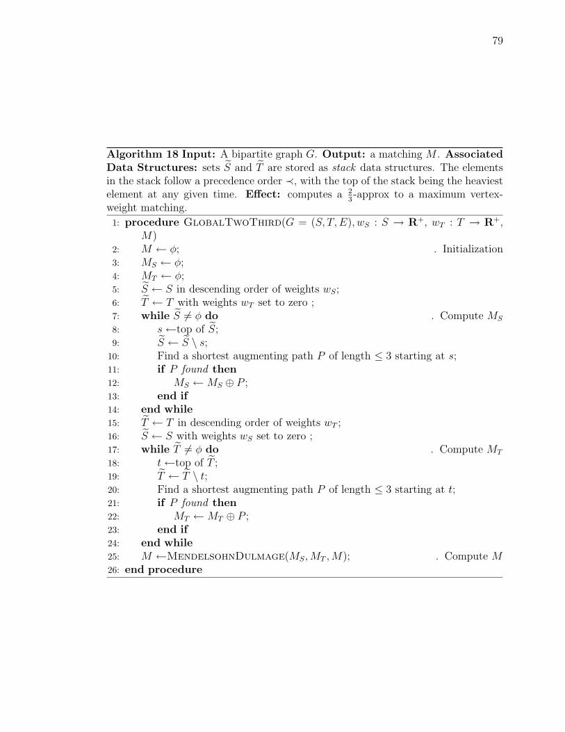
79
Algorithm 18 Input: A bipartite graph G. Output: a matching M . AssociatedData Structures: sets S and T are stored as stack data structures. The elementsin the stack follow a precedence order ≺, with the top of the stack being the heaviestelement at any given time. Effect: computes a 2
3-approx to a maximum vertex-
weight matching.
1: procedure GlobalTwoThird(G = (S, T,E), wS : S → R+, wT : T → R+,M)
2: M ← φ; . Initialization3: MS ← φ;4: MT ← φ;5: S ← S in descending order of weights wS;6: T ← T with weights wT set to zero ;7: while S 6= φ do . Compute MS
8: s←top of S;9: S ← S \ s;
10: Find a shortest augmenting path P of length ≤ 3 starting at s;11: if P found then12: MS ←MS ⊕ P ;13: end if14: end while15: T ← T in descending order of weights wT ;16: S ← S with weights wS set to zero ;17: while T 6= φ do . Compute MT
18: t←top of T ;19: T ← T \ t;20: Find a shortest augmenting path P of length ≤ 3 starting at t;21: if P found then22: MT ←MT ⊕ P ;23: end if24: end while25: M ←MendelsohnDulmage(MS,MT ,M); . Compute M26: end procedure
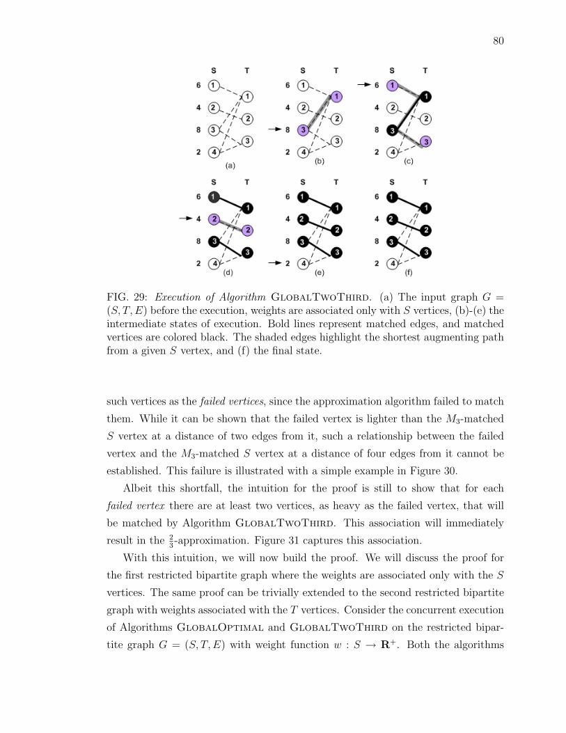
80
FIG. 29: Execution of Algorithm GlobalTwoThird. (a) The input graph G =(S, T,E) before the execution, weights are associated only with S vertices, (b)-(e) theintermediate states of execution. Bold lines represent matched edges, and matchedvertices are colored black. The shaded edges highlight the shortest augmenting pathfrom a given S vertex, and (f) the final state.
such vertices as the failed vertices, since the approximation algorithm failed to match
them. While it can be shown that the failed vertex is lighter than the M3-matched
S vertex at a distance of two edges from it, such a relationship between the failed
vertex and the M3-matched S vertex at a distance of four edges from it cannot be
established. This failure is illustrated with a simple example in Figure 30.
Albeit this shortfall, the intuition for the proof is still to show that for each
failed vertex there are at least two vertices, as heavy as the failed vertex, that will
be matched by Algorithm GlobalTwoThird. This association will immediately
result in the 23-approximation. Figure 31 captures this association.
With this intuition, we will now build the proof. We will discuss the proof for
the first restricted bipartite graph where the weights are associated only with the S
vertices. The same proof can be trivially extended to the second restricted bipartite
graph with weights associated with the T vertices. Consider the concurrent execution
of Algorithms GlobalOptimal and GlobalTwoThird on the restricted bipar-
tite graph G = (S, T,E) with weight function w : S → R+. Both the algorithms

81
FIG. 30: Symmetric difference. (a) Input graph, weights are associated only withthe S vertices such that s1 � s2 � s3 � s4; (b) an optimal matching M∗ computedby Algorithm GlobalOptimal. Bold lines represent matched edges. At step one,edge e(s1, t3) is matched; at step two, edge e(s2, t2) is matched; at step three, thematching is augmented via path [s3, t2, s2, t3, s1, t1]; no path exists at step four; (c)a 2
3-approx matching M3 computed by Algorithm GlobalTwoThird, Wavy lines
represent matched edges; At step one, edge e(s1, t3) is matched; at step two, edgee(s2, t2) is matched; at step three, no augmenting path of length three exists; atstep four, the matching is augmented via path [s4, t3, s1, t1]; and (d) the symmetricdifference M∗ ⊕M3. The bold lines denote edges matched in M∗, and wavy linesdenote edges matched in M3.
will consider the S vertices in succeeding order of weights. While Algorithm Glob-
alOptimal searches for a shortest augmenting path without any restrictions on the
length of the path, the search in Algorithm GlobalTwoThird is restricted to aug-
menting paths of at most three edges. However, at any step k, both the algorithms
will consider the same vertex sk ∈ S for matching.
A failed vertex is a vertex that is matched in the optimal matching, but not in
the approximation matching. For the current discussion, we will consider only the
failed S vertices, since the weights are associated only with them. The time step of
execution is an important parameter for the proof. Therefore, to accommodate the
time step, we will introduce a new notation. The failed vertex at step k is represented
as sk,k ∈ S. The other failed vertices in S at this step are represented as si,k, for
1 ≤ i ≤ k. Our objective is to associate two unique M3-matched S vertices with each
failed vertex si. We will use subscripts to represent such vertices, si,ka and si,kb . The
rationale to use two indices (i, k) to represent the past and current steps is due to the
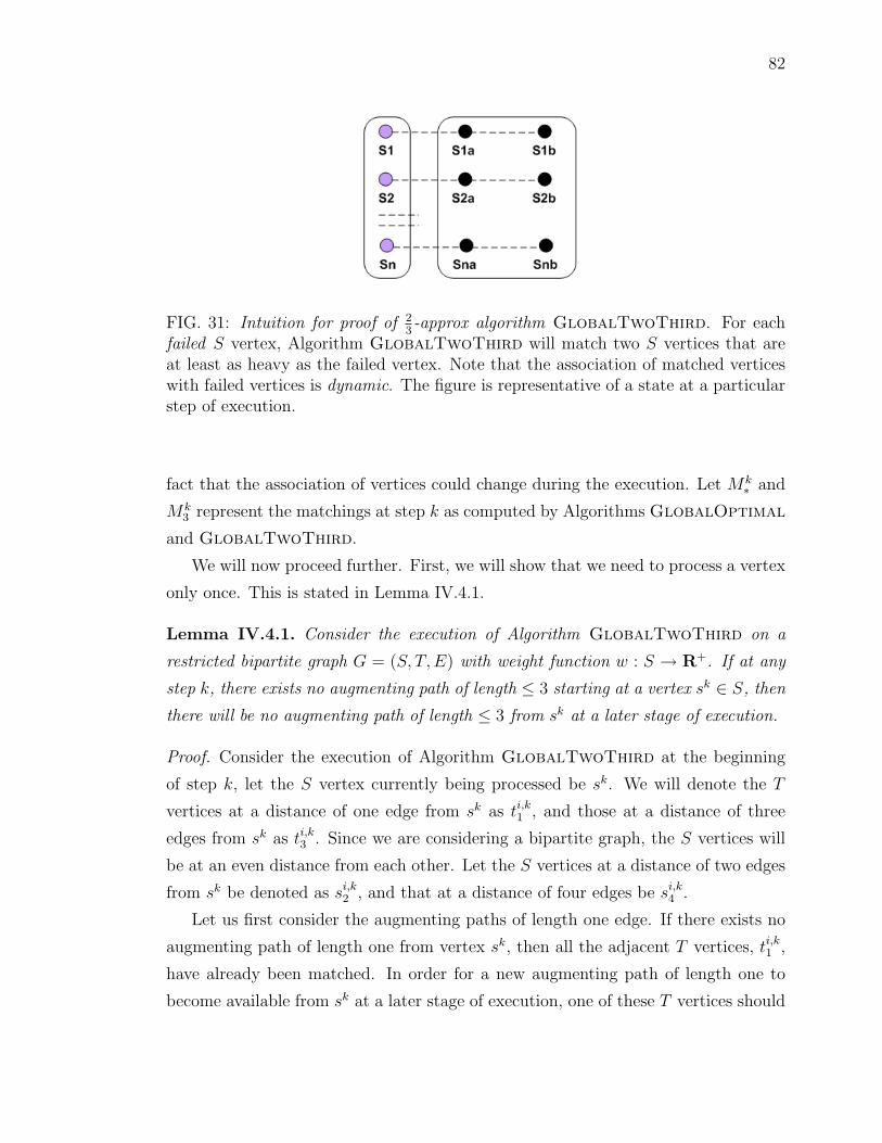
82
FIG. 31: Intuition for proof of 23-approx algorithm GlobalTwoThird. For each
failed S vertex, Algorithm GlobalTwoThird will match two S vertices that areat least as heavy as the failed vertex. Note that the association of matched verticeswith failed vertices is dynamic. The figure is representative of a state at a particularstep of execution.
fact that the association of vertices could change during the execution. Let Mk∗ and
Mk3 represent the matchings at step k as computed by Algorithms GlobalOptimal
and GlobalTwoThird.
We will now proceed further. First, we will show that we need to process a vertex
only once. This is stated in Lemma IV.4.1.
Lemma IV.4.1. Consider the execution of Algorithm GlobalTwoThird on a
restricted bipartite graph G = (S, T,E) with weight function w : S → R+. If at any
step k, there exists no augmenting path of length ≤ 3 starting at a vertex sk ∈ S, then
there will be no augmenting path of length ≤ 3 from sk at a later stage of execution.
Proof. Consider the execution of Algorithm GlobalTwoThird at the beginning
of step k, let the S vertex currently being processed be sk. We will denote the T
vertices at a distance of one edge from sk as ti,k1 , and those at a distance of three
edges from sk as ti,k3 . Since we are considering a bipartite graph, the S vertices will
be at an even distance from each other. Let the S vertices at a distance of two edges
from sk be denoted as si,k2 , and that at a distance of four edges be si,k4 .
Let us first consider the augmenting paths of length one edge. If there exists no
augmenting path of length one from vertex sk, then all the adjacent T vertices, ti,k1 ,
have already been matched. In order for a new augmenting path of length one to
become available from sk at a later stage of execution, one of these T vertices should

83
get unmatched. However, we know that during the execution of Algorithm Glob-
alTwoThird, once a vertex is matched it will always remain matched. Therefore,
the lemma holds true for augmenting paths of length one.
Now we consider paths from the vertex sk. Since there is no augmenting path of
length three from the vertex sk, these paths can be of two different kinds. The first
kind of path has the form [sk, ti,k1 , si,k2 , ti,k3 , si,k4 · · · ], where ti,k1 is matched to si,k2 , and ti,k3
is matched to si,k4 and so on. The second kind of path has the form [sk, ti,k1 , sj,k2 , tj,k3 ],
where the first two vertices are the same as the first two vertices from the path of
the first kind, and the last two vertices, sj,k2 and tj,k3 are unmatched. These two kinds
of paths are illustrated in Figure 32 as P1 and P2 respectively.
An augmenting path of length three beginning at sk can exist at a later step
because either (i) ti,k3 becomes unmatched, or (ii) sj,k2 becomes matched to ti,k1 . The
first case cannot occur since a vertex once matched is always matched in a matching
algorithm based on augmentations. In the second case, sj,k2 becomes matched in
a previous augmentation step (but after the k-th step) involving the augmenting
path [sj,k2 , ti,k1 , si,k2 , t`,k3 ], where the last vertex is an unmatched vertex. But such an
augmenting path would imply an augmenting path at the k-th step from sk consisting
of [sk, ti,k1 , si,k2 , t`,k3 ]. This contradiction completes the proof.
FIG. 32: New augmenting paths. Bold lines represent the matched edges and matchedvertices are colored black. The two kinds of paths in Lemma IV.4.1 are shown as P1
and P2.
We will now argue for the correctness of the claimed approximation ratio of 23.
Consider the concurrent execution of Algorithms GlobalOptimal and GlobalT-
woThird on the first restricted bipartite graph with weights on the S vertices. We
will consider the steps when a vertex sk ∈ S gets matched by Algorithm Glob-
alOptimal, but not by Algorithm GlobalTwoThird. We define these vertices
as the failed vertices. An important relationship between the failed and the matched
vertices is stated in Lemma IV.4.2.

84
Lemma IV.4.2. Consider the restricted bipartite graph G = (S, T,E) with weight
function w : S → R+. Let Mk∗ represent the matching computed by Algorithm
GlobalOptimal at the end of step k, and let Mk3 represent the matching computed
by Algorithm GlobalTwoThird at the end of step k. (i) For each failed vertex
that exists at the end of step k, si,k, 1 ≤ i ≤ k, there are two distinct vertices si,ka and
si,kb that are matched in Mk3 . (ii) At the end of step k, the following relation holds:
sk,k ≺ sk,ka and sk,k ≺ sk,kb .
Proof. We consider the proof of (i). Consider the symmetric difference Mk∗ ⊕Mk
3 .
Each failed vertex si,k is matched in the first, but not in the second of these matchings,
and hence begins an alternating path in the symmetric difference. This alternating
path cannot have length two, of the form si,k, ti,k1 , si,ka . If this is true, then only one
of the vertices si,k and si,ka can be matched to ti,k1 . If si,k ≺ si,ka , then the optimal
algorithm made a wrong choice, and therefore, contradicts. If otherwise, then the
approximate algorithm made a wrong choice and contradicts again.
If the alternating path is of length three, then it is an Mk3 -augmenting path of
length three and the approximation algorithm would have matched along this path.
Therefore, the alternating path must be of length at least four. If the alternating
path has even length (greater than or equal to four), then it ends with a terminal
S-vertex that is matched in Mk3 but not in Mk
∗ . Hence this terminal vertex cannot
be another failed S-vertex. If the alternating path is of odd length, then it termi-
nates with a T -vertex. From these two cases, we conclude that every failed vertex
begins a vertex-disjoint alternating path of length four or more, and has the form
[si,k, ti,k1 , si,ka , ti,k3 , si,kb , · · · ].
Part (ii) follows from three observations:
1. Both the exact and approximation matching algorithms consider S-vertices in
a succeeding order for matching;
2. sk,k is the last failed vertex (which happens at step k); and
3. the vertices sk,ka and sk,kb have been matched in earlier steps.
We provided a conclusive relationship between the failed and the matched ver-
tices in for a given step in Lemma IV.4.2. However, in order to provide an overall
85
approximation ratio of 23, we will induct on the failed steps. Theorem IV.4.1 provides
this argument.
Theorem IV.4.1 (Counting Technique). Consider a bipartite graph G = (S, T,E)
with weight function w : S → (R)+, a matching M∗ computed by Algorithm Glob-
alOptimal, and a matching M3 computed by Algorithm GlobalTwoThird. For
every failed vertex si ∈ S, there are two distinct vertices sia and sib that are matched
by M3, such that si ≺ sia and si ≺ sib.
Proof. The proof is based on induction. Consider the failed S vertices during the
concurrent execution of Algorithms GlobalOptimal and GlobalTwoThird. We
will reuse the notation from proof of Lemma IV.4.2.
Base case: Consider the step when the first failed vertex s1,1 ∈ S is encountered.
We know from Lemma IV.4.2 that at the end of this step, there are two vertices
s1,1a and s1,1
b , matched in M13 , such that s1,1 ≺ s1,1
a and s1,1 ≺ s1b . Let s1
a = s1,1a and
s1b = s1,1
b .
Step k: Assume true for the first k failures, 1 ≤ i ≤ k.
Step k+1: At the end of the step when the (k+1)-th failed vertex is encountered,
from Lemma IV.4.2 we know that there are at least two distinct vertices matched in
Mk+13 such that sk+1,k+1 ≺ sk+1,k+1
a and sk+1,k+1 ≺ sk+1,k+1b .
A potential conflict arises when the Mk+13 -matched vertices sk+1,k+1
a and sk+1,k+1b
had already been associated with a failed vertex si, i < k, in a previous step. They
are now being reused at step (k + 1). We will show how to address such a case.
From the inductive assumption at step k, we know that for every failed vertex
si, 1 ≤ i ≤ k, there are two vertices sia and sib, such that the relations si ≺ sia and
si ≺ sib hold. Now consider two sets S1 = ∪k+1i=1 {si,k+1
a , si,k+1b } and S2 = ∪ki=1{sia, sib}.
The cardinalities are given by |S1| ≥ 2(j + 1) and |S2| ≥ 2(j). This follows from
Lemma IV.4.2. Thus, |S1 \S2| ≥ 2. Therefore, there are at least two distinct vertices
in {S1 \ S2} that can be associated with sk+1 as sk+1a = sk+1,k+1
a and sk+1b = sk+1,k+1
b .
Since we know that sk+1 is the most current vertex processed, all the matched S
vertices will be at least as large as this vertex. Thus the theorem holds.
From Theorem IV.4.1, the approximation follows immediately, and is stated in
Corollary IV.4.1.
Corollary IV.4.1. Given a bipartite graph G = (S, T,E), w : S → R+, algorithm
86
GlobalTwoThird computes a 23-approximation to maximum vertex-weight match-
ing.
Proof. Let M∗ denote the optimal matching, and M3 denote the matching computed
by Algorithm GlobalTwoThird. We will consider the first restricted bipartite
graph with weights associated only to S vertices. Let S(M) denote the S vertices
matched in M , and N the number of failed vertices with respect to M3. From Theo-
rem IV.4.1, it immediately follows that for every failed vertex si GlobalTwoThird
matches at least two heavier vertices, sia and sib. Therefore,
N∑i=1
w(si) ≤ 1
2
N∑i=1
w(sia) + w(sib). (10)
The weight of the optimal matching M∗ can be represented as∑s∈S(M∗)
w(s) =∑
si∈S(M∗\M3)
w(si) +∑
sj∈S(M∗∩M3)
w(sj). (11)
We know that the set S(M∗\M3) represents the set of failed vertices. We can rewrite
the first term of right-hand-side in Equation 11 as
∑s∈S(M∗)
w(s) ≤N∑i=1
w(si) +∑
sj∈S(M∗∩M3)
w(sj). (12)
Using the results from Equation 10, we have
∑s∈S(M∗)
w(s) ≤ 1
2.N∑i=1
w(sia) + w(sib) +∑
sj∈S(M∗∩M3)
w(sj). (13)
We can simplify the first term of R.H.S., in Equation 13 that results in∑s∈S(M∗)
w(s) ≤ 1
2.∑
si∈S(M3)
w(si) +∑
sj∈S(M∗∩M3)
w(sj). (14)
The set S(M∗ ∩M3) in the second term of R.H.S., can be simply replaced with a set
S(M3). Therefore, we have∑s∈S(M∗)
w(s) ≤ 1
2.∑
si∈S(M3)
w(si) +∑
sj∈S(M3)
w(sj). (15)
Therefore, ∑s∈S(M∗)
w(s) ≤ 3
2
∑si∈S(M3)
w(si). (16)
87
Rewriting the equation above, we have∑s∈S(M3)
w(s) ≥ 2
3
∑s∈S(M∗)
w(s).
The time complexity for Algorithm GlobalTwoThird is stated in Theorem
IV.4.2.
Theorem IV.4.2. Given a graph G = (S, T,E) with weight functions wS : S → R+
and wT : T → R+, let n = (|S|+ |T |) represent the number of vertices and m = |E|represent the number of edges. Algorithm GlobalTwoThird computes a matching
M3 in G in O(n log n + nd3), where d3 is the vertex degree that denotes the average
number of distinct alternating paths of length at most three edges starting at a vertex
in G.
Proof. Algorithm GlobalTwoThird processes the vertices in a global order. The
given set of vertices can be sorted in decreasing order of vertex weights in time
O(n log n). From each set of vertices S and T , GlobalTwoThird will search for
shortest augmenting paths of length at most three. In order to find augmenting
paths of length one edge, we only need to process all the edges incident on the
given vertex and is therefore bounded by O(m). An augmenting path of length
three edges is of the form [s1, t1, s2, t2], where vertices t1 and s2 are matched by
an edge (t1, s2). In order to search augmenting paths of length up to three edges,
Algorithm GlobalTwoThird will incur a cost of at most (deg(s1).deg(s2)). Due to
the matched edge, vertex s2 can be directly reached from vertex t1. Let us represent
this search operation as d3, where d3 is the vertex degree that denotes the average
number of distinct paths of length at most three edges starting at a vertex. Thus, the
run time of Algorithm GlobalTwoThird can be bounded by O(n log n+nd3). The
two matchings, MS and MT can be merged using the Mendelsohn-Dulmage technique
in linear time O(m).
We will now proceed to the describe a potential local-approach to compute a23-approx VWM in a bipartite graph.
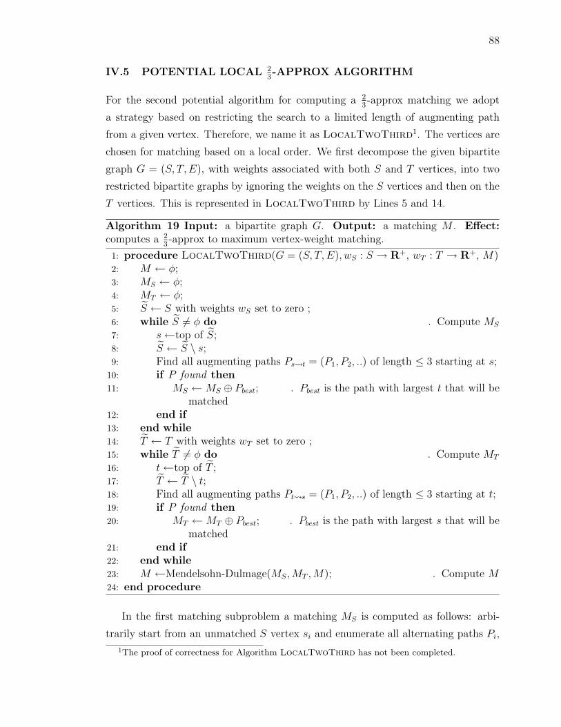
88
IV.5 POTENTIAL LOCAL 23-APPROX ALGORITHM
For the second potential algorithm for computing a 23-approx matching we adopt
a strategy based on restricting the search to a limited length of augmenting path
from a given vertex. Therefore, we name it as LocalTwoThird1. The vertices are
chosen for matching based on a local order. We first decompose the given bipartite
graph G = (S, T,E), with weights associated with both S and T vertices, into two
restricted bipartite graphs by ignoring the weights on the S vertices and then on the
T vertices. This is represented in LocalTwoThird by Lines 5 and 14.
Algorithm 19 Input: a bipartite graph G. Output: a matching M . Effect:computes a 2
3-approx to maximum vertex-weight matching.
1: procedure LocalTwoThird(G = (S, T,E), wS : S → R+, wT : T → R+, M)2: M ← φ;3: MS ← φ;4: MT ← φ;5: S ← S with weights wS set to zero ;6: while S 6= φ do . Compute MS
7: s←top of S;8: S ← S \ s;9: Find all augmenting paths Ps t = (P1, P2, ..) of length ≤ 3 starting at s;
10: if P found then11: MS ←MS ⊕ Pbest; . Pbest is the path with largest t that will be
matched12: end if13: end while14: T ← T with weights wT set to zero ;15: while T 6= φ do . Compute MT
16: t←top of T ;17: T ← T \ t;18: Find all augmenting paths Pt s = (P1, P2, ..) of length ≤ 3 starting at t;19: if P found then20: MT ←MT ⊕ Pbest; . Pbest is the path with largest s that will be
matched21: end if22: end while23: M ←Mendelsohn-Dulmage(MS,MT ,M); . Compute M24: end procedure
In the first matching subproblem a matching MS is computed as follows: arbi-
trarily start from an unmatched S vertex si and enumerate all alternating paths Pi,
1The proof of correctness for Algorithm LocalTwoThird has not been completed.

89
of length at most three, with respect to the current matching Mi. Pick the best aug-
menting path from si and augment the current matching. A best augmenting path
is a path that maximizes Mi ⊕ Pi. Repeat the process until all the S vertices have
been processed. Lines 6−13 represent the computation of MS. Similarly a matching
MT can be computed when weights are associated only with the S vertices. This is
the second subproblem and is represented by Lines 15 − 22 in LocalTwoThird.
The final matching will be obtained by merging the two matchings MS and MT using
the Mendelsohn-Dulmage technique. Execution of LocalTwoThird on a simple
bipartite graph with weights associated with S vertices is shown in Figure 33.
FIG. 33: Execution of Algorithm LocalTwoThird. (a) The input graph G =(S, T,E) before the execution, weights are associated only with S vertices, (b)-(d)the intermediate states of execution, and (e) the final state. Bold lines representmatched edges, and matched vertices are colored black. The shaded edges highlightall the augmenting paths that exist from a given T vertex.
IV.5.1 Correctness of Algorithm LocalTwoThird
We have not been successful to prove the the correctness of LocalTwoThird. A
critical part of the proof for GlobalTwoThird was Theorem IV.4.1, where for the
induction step (k+ 1) we could safely state that all the matched vertices at that step
were heavier than the (k + 1)-th failed vertex. We could state such a fact because
the vertices were considered in a decreasing order of weight. However, we will not

90
be able to state the same for a matching computed by LocalTwoThird where
vertices are processed in an arbitrary order. We will therefore leave the proof of
LocalTwoThird as an open problem.

91
IV.6 EXPERIMENTAL RESULTS
In this section we present experimental results from our implementation of matching
algorithms in a toolkit called MatchBox. The two types of experiments done
are serial and parallel. The goals for serial experiments are to demonstrate the
efficiency of approximation algorithms in terms of execution time, cardinality and
weight of matching as compared to those of the exact algorithms. The experiments
are conducted on a system equipped with four 2.4 GHz Intel quad core processors
and 32 GB RAM at Old Dominion University.
The graphs used for experiments are representations of regular sparse matrices
downloaded from the University of Florida Sparse Matrix Collection. A matrix is
stored as a bipartite graph, where rows and columns of the matrix represent ver-
tices, and the nonzero elements represent edges. The absolute value of a nonzero
element in the matrix is considered as the weight of the edge that connects the ver-
tices representing the row and the column of the nonzero element. In the following
experiments, the degrees of vertices are used as the weights of the vertices. A similar
model is used to represent symmetric matrices. Since the files downloaded from the
University of Florida Sparse Matrix Collection store only the lower triangle of the
matrix, we explicitly add edges to represent both the upper and lower triangles of
the matrix. The matrices used in the experiments are listed in Table 8.
The performance of global algorithms is presented in Table 9. It can be noted
that the 12-approx algorithms are very fast and the 1
2-approx algorithms are relatively
fast. As mentioned earlier, the degree of the vertices are used as weights for both the
S and T vertex sets for a given graph. The two matchings, MS and MT are computed
separately and the final matching is obtained by merging the two matchings using
the Mendelsohn-Dulmage technique.
Comparision between the Global and Local-based algorithms is presented in Ta-
ble 10. For the 12-approx algorithms, it can be noted that Algorithm LocalHalf is
faster than the Algorithm GlobalHalf in many cases, except for largest graph in
the collection. However, for 23-approx algorithms, the Global-based algorithm almost
always beats the Local-based algorithm. Note that we did not prove the correctness
of Algorithm LocalTwoThird, and the data is provided here for comparision. The
Local-based algorithms are forced to enumerate all possible paths of certain length
and are therefore inefficient. For the same reason, we do not provide results for
Algorithm LocalOptimal, which we believe is not a practical algorithm.
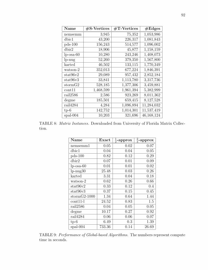
92
Name #S-Vertices #T-Vertices #Edges
nemsemm 3,945 75,352 1,053,986dbic1 43,200 226,317 1,081,843pds-100 156,243 514,577 1,096,002dbir2 18,906 45,877 1,158,159lp-osa-60 10,280 243,246 1,408,073lp-nug 52,260 379,350 1,567,800karted 46,502 133,115 1,770,349watson-2 352,013 677,224 1,846,391stat96v2 29,089 957,432 2,852,184stat96v3 33,841 1,113,780 3,317,736stormG2 528,185 1,377,306 3,459,881cont11 1,468,599 1,961,394 5,382,999rail2586 2,586 923,269 8,011,362degme 185,501 659,415 8,127,528rail4284 4,284 1,096,894 11,284,032tp-6 142,752 1,014,301 11,537,419spal-004 10,203 321,696 46,168,124
TABLE 8: Matrix Instances. Downloaded from University of Florida Matrix Collec-tion.
Name Exact 12-approx 2
3-approx
nemsemm1 0.05 0.02 0.07dbic1 0.04 0.04 0.05pds-100 0.82 0.12 0.29dbir2 0.07 0.01 0.09lp-osa-60 0.01 0.01 0.02lp-nug30 25.48 0.03 0.26karted 3.31 0.04 0.18watson-2 0.62 0.26 0.66stat96v2 0.33 0.12 0.4stat96v3 0.37 0.15 0.45stormG2-1000 1.34 0.64 1.44cont11-l 24.52 0.83 1.5rail2586 0.04 0.05 0.05degme 10.17 0.27 0.92rail4284 0.06 0.06 0.07tp-6 6.49 0.3 1.39spal-004 733.36 0.14 26.69
TABLE 9: Performance of Global-based Algorithms. The numbers represent computetime in seconds.

93
Name Global12
Local12
Global23
Local23
nemsemm1 0.02 0.01 0.07 0.07dbic1 0.04 0.01 0.05 0.16pds-100 0.12 0.03 0.29 0.28dbir2 0.01 0.01 0.09 0.41lp-osa-60 0.01 0.01 0.02 0.1lp-nug30 0.03 0.02 0.26 1.32karted 0.04 0.02 0.18 3.03watson-2 0.26 0.03 0.66 0.69stat96v2 0.12 0.02 0.4 0.91stat96v3 0.15 0.03 0.45 1.08stormG2-1000 0.64 0.06 1.44 23.1cont11-l 0.83 0.07 1.5 1.5rail2586 0.05 0.07 0.05 0.76degme 0.27 0.09 0.92 7.94rail4284 0.06 0.11 0.07 1.14tp-6 0.3 0.12 1.39 9.81spal-004 0.14 0.29 26.69 1495.95
TABLE 10: Relative Performance of Global and Local-based Algorithms. The num-bers represent compute time in seconds.
The quality of a matching can be measured in terms of the cardinality (the number
of edges in the matching) and the weight (sum of weights of the matched edges) of
the matching. We present the cardinality of the matchings computed by the different
algorithms in Figure 34, and the weight of the matchings in Figure 35. The exact
algorithm used in these comparision is Algorithm GlobalOptimal. It can be noted
that the approximation algorithms compute matchings of high quality in terms of
both cardinality and weight of the matchings.
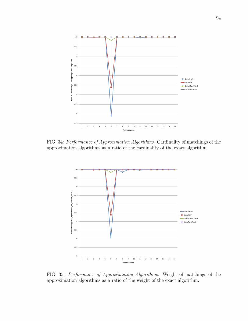
94
95.5
96
96.5
97
97.5
98
98.5
99
99.5
100
1 2 3 4 5 6 7 8 9 10 11 12 13 14 15 16 17
Rat
io o
f C
ard
inal
ity
= (|
Map
pro
x|/|
Me
xact
|)*1
00
Test Instances
GlobalHalf
LocalHalf
GlobalTwoThird
LocalTwoThird
FIG. 34: Performance of Approximation Algorithms. Cardinality of matchings of theapproximation algorithms as a ratio of the cardinality of the exact algorithm.
95
95.5
96
96.5
97
97.5
98
98.5
99
99.5
100
1 2 3 4 5 6 7 8 9 10 11 12 13 14 15 16 17
Rat
io o
f W
eigh
ts =
(W
(Map
pro
x)/W
(Mex
act)
)*1
00
Test Instances
GlobalHalf
LocalHalf
GlobalTwotThird
LocalTwoThird
FIG. 35: Performance of Approximation Algorithms. Weight of matchings of theapproximation algorithms as a ratio of the weight of the exact algorithm.

95
IV.7 CHAPTER SUMMARY
In this chapter we introduced three new 12-approx algorithms and two new 2
3-approx
algorithms to MVM problem. Proof of correctness for all the proposed 12-approx
and one of the 23-approx algorithms were also discussed. We introduced the con-
cept of the restricted reachability property to provide the correctness of 12-approx
Algorithms GlobalHalf, LocalHalf and HybridHalf. We also introduced the
concept of a counting technique in order to provide the correctness of 23-approx Al-
gorithm GlobalTwoThird. While we did not succeed to prove the correctness
of LocalTwoThird algorithm, this approach, if proved correct, will also provide
us an algorithm to compute 23-approx matchings in general graphs. We concluded
the chapter by providing experimental results highlighting the effectiveness of the
approximation algorithms, both in execution time and the quality of the matchings.
There are a few limitations to our current approach. The proposed techniques,
global and local, fail to generalize for a ( kk+1
)-approx, for k > 3. As illustrated in
Figure 36, an augmenting path of length five starting at a vertex s1 ∈ S could appear
at a later stage, while none existed when s1 was processed the first time. Therefore
with the current approaches, we cannot guarantee an approximation ratio better
than (45). However, we cannot say anything conclusively about a 3
4-approx ratio for
the proposed algorithms, and will study this in the follow-up work.
FIG. 36: New augmenting paths. (a) No augmenting path of length less than or equalto five exist starting at vertex s1 in graph G at step k; (b) an augmenting path oflength five is available from s1 at a step after k.

96
Similar to the exact algorithms discussed in Chapter III, the proposed approxima-
tion algorithms also suffer from the same limitations: (i) absence of greedy initializa-
tions, and (ii) inability to grow multiple paths, both for 12
and 23-approx algorithms.
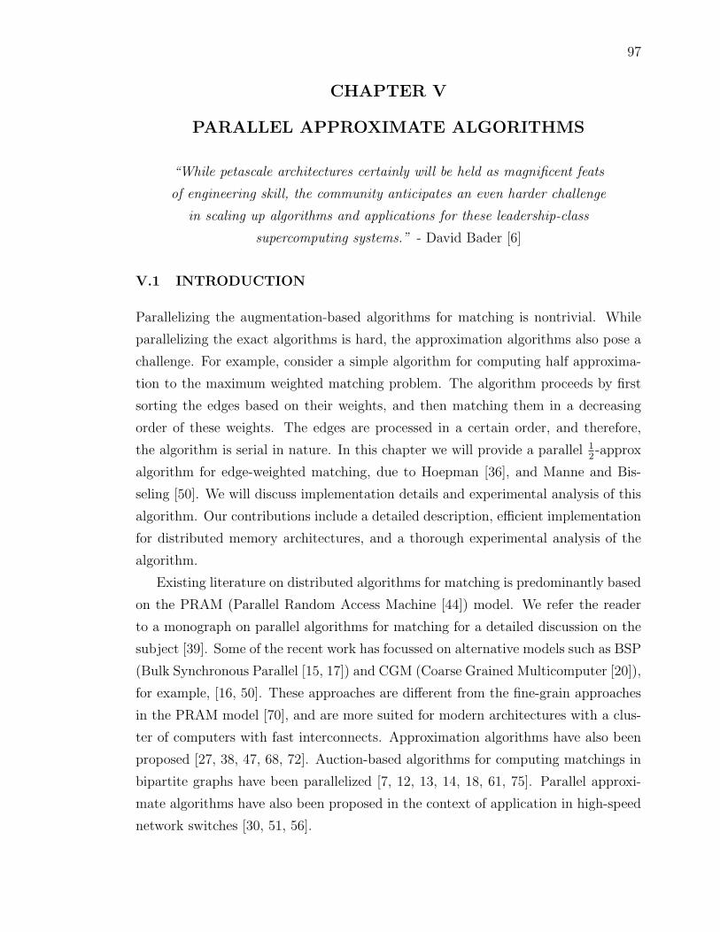
97
CHAPTER V
PARALLEL APPROXIMATE ALGORITHMS
“While petascale architectures certainly will be held as magnificent feats
of engineering skill, the community anticipates an even harder challenge
in scaling up algorithms and applications for these leadership-class
supercomputing systems.” - David Bader [6]
V.1 INTRODUCTION
Parallelizing the augmentation-based algorithms for matching is nontrivial. While
parallelizing the exact algorithms is hard, the approximation algorithms also pose a
challenge. For example, consider a simple algorithm for computing half approxima-
tion to the maximum weighted matching problem. The algorithm proceeds by first
sorting the edges based on their weights, and then matching them in a decreasing
order of these weights. The edges are processed in a certain order, and therefore,
the algorithm is serial in nature. In this chapter we will provide a parallel 12-approx
algorithm for edge-weighted matching, due to Hoepman [36], and Manne and Bis-
seling [50]. We will discuss implementation details and experimental analysis of this
algorithm. Our contributions include a detailed description, efficient implementation
for distributed memory architectures, and a thorough experimental analysis of the
algorithm.
Existing literature on distributed algorithms for matching is predominantly based
on the PRAM (Parallel Random Access Machine [44]) model. We refer the reader
to a monograph on parallel algorithms for matching for a detailed discussion on the
subject [39]. Some of the recent work has focussed on alternative models such as BSP
(Bulk Synchronous Parallel [15, 17]) and CGM (Coarse Grained Multicomputer [20]),
for example, [16, 50]. These approaches are different from the fine-grain approaches
in the PRAM model [70], and are more suited for modern architectures with a clus-
ter of computers with fast interconnects. Approximation algorithms have also been
proposed [27, 38, 47, 68, 72]. Auction-based algorithms for computing matchings in
bipartite graphs have been parallelized [7, 12, 13, 14, 18, 61, 75]. Parallel approxi-
mate algorithms have also been proposed in the context of application in high-speed
network switches [30, 51, 56].

98
In the following discussions we will assume data structures for graph represen-
tations that store vertex-adjacency sets, and that the graphs are distributed among
the processors via vertex partitioning. We will start the discussion by presenting
a modified version of Preis’s algorithm [64] that builds an intuition for the parallel
algorithm. A distributed scheme of Preis’s algorithm was developed by Hoepman.
Manne and Bisseling show that this is a variant of Luby’s parallel algorithm for
computing maximal independent sets in a graph [49].
We introduced Preis’s algorithm, Algorithm LAM, in Chapter II and refer the
reader to [64] for details. The algorithm computes a half-approx matching by finding
locally dominant edges and adding them to the set of matched edges. However, the
search for locally dominant edges involves traversing through the graph. Thus, this
algorithm is sequential in nature. Alternatively, the same matching can be computed
by using a pointer-based technique that was proposed by Manne [50]. The pointer-
based technique works as follows. Let each vertex set a pointer to the vertex that is
the end point of a heaviest edge incident on it. If two vertices point to each other,
then the edge connecting them is a locally dominant edge. Therefore, add this edge
to the set of matched edges. Remove all edges that are incident on the matched
vertices. Reset the pointers of those vertices that are affected by the changes and
match the dominating edges. Repeat the process until all edges have been removed.
A basic step in the pointer-based algorithm is to set a pointer for a given vertex.
A simple way of doing this is to traverse through the adjacency set S(v) of a given
vertex that contains unmatched neighboring vertices, find a heaviest neighbor and
set the pointer to point this vertex. This is described in Algorithm 20. In case of ties,
the indices of vertices are used to break ties (Line 5). The lowest numbered heaviest
end-point of the edge incident on vertex v is chosen. Note that since each vertex sets
its pointer independent of other vertices, breaking the ties in a consistent manner
is an important task. In the absence of a deterministic scheme to break ties, the
algorithm may not function correctly when cycles of equal edge-weights exit. Also,
note that the running time for this procedure can be improved by maintaining a
sorted list of adjacent vertices so that the current heaviest vertex can be determined
in constant time.
Once the pointer for a vertex v, represented by candidateMate(v), has been set,
the next step is to check if the vertex being pointed to by v also points back to v.
If so, we have successfully identified a locally dominant edge, and this edge can be
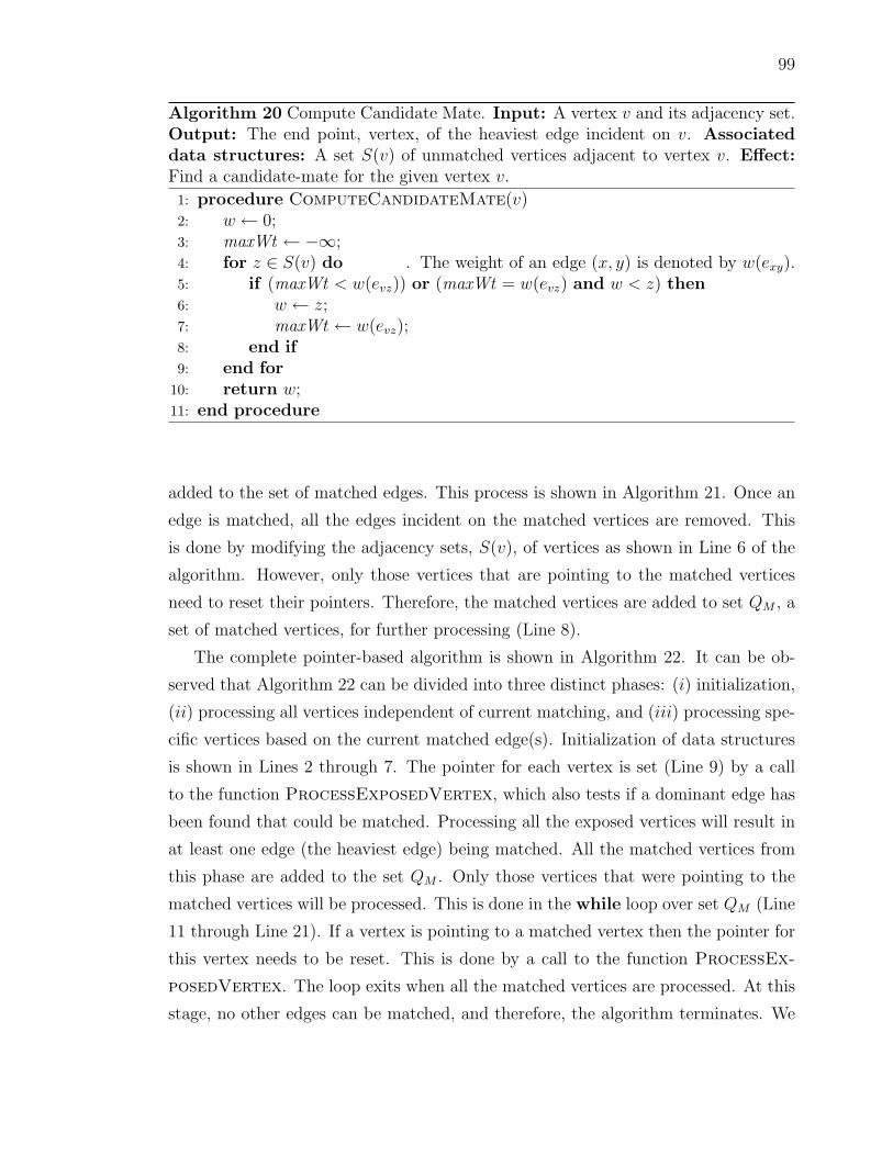
99
Algorithm 20 Compute Candidate Mate. Input: A vertex v and its adjacency set.Output: The end point, vertex, of the heaviest edge incident on v. Associateddata structures: A set S(v) of unmatched vertices adjacent to vertex v. Effect:Find a candidate-mate for the given vertex v.
1: procedure ComputeCandidateMate(v)2: w ← 0;3: maxWt ← −∞;4: for z ∈ S(v) do . The weight of an edge (x, y) is denoted by w(exy).5: if (maxWt < w(evz)) or (maxWt = w(evz) and w < z) then6: w ← z;7: maxWt ← w(evz);8: end if9: end for
10: return w;11: end procedure
added to the set of matched edges. This process is shown in Algorithm 21. Once an
edge is matched, all the edges incident on the matched vertices are removed. This
is done by modifying the adjacency sets, S(v), of vertices as shown in Line 6 of the
algorithm. However, only those vertices that are pointing to the matched vertices
need to reset their pointers. Therefore, the matched vertices are added to set QM , a
set of matched vertices, for further processing (Line 8).
The complete pointer-based algorithm is shown in Algorithm 22. It can be ob-
served that Algorithm 22 can be divided into three distinct phases: (i) initialization,
(ii) processing all vertices independent of current matching, and (iii) processing spe-
cific vertices based on the current matched edge(s). Initialization of data structures
is shown in Lines 2 through 7. The pointer for each vertex is set (Line 9) by a call
to the function ProcessExposedVertex, which also tests if a dominant edge has
been found that could be matched. Processing all the exposed vertices will result in
at least one edge (the heaviest edge) being matched. All the matched vertices from
this phase are added to the set QM . Only those vertices that were pointing to the
matched vertices will be processed. This is done in the while loop over set QM (Line
11 through Line 21). If a vertex is pointing to a matched vertex then the pointer for
this vertex needs to be reset. This is done by a call to the function ProcessEx-
posedVertex. The loop exits when all the matched vertices are processed. At this
stage, no other edges can be matched, and therefore, the algorithm terminates. We

100
Algorithm 21 Process Exposed Vertex. Input: A vertex v and its adjacency set.Associated data structures: A set S(v) of unmatched vertices adjacent to vertexv, a set QM of matched vertices, a vector candidateMate of pointers, and set Mof matched edges. Effect: Processes an exposed vertex - find candidate-mate andmatch if possible.
1: procedure ProcessExposedVertex(v)2: candidateMate(v)← ComputeCandidateMate(v);3: c← candidateMate(v);4: if c 6= 0 and candidateMate(c) = v then5: M ←M ∪ {(v, c)};6: S(v)← S(v) \ {c};7: S(c)← S(c) \ {v};8: QM ← QM ∪ {v, c};9: end if
10: end procedure
will follow a similar three phase distinction to simplify the description and analysis
of the parallel approximation algorithm. We refer the reader to [50] for a proof of
correctness of the pointer-based algorithm.
Execution of Algorithm 22 on a simple graph is shown in Figure 37. It can be ob-
served that in Step (c) of the figure, two edges,(1, 3) and (2, 5), concurrently become
eligible for matching. This provides an intuition for the potential of parallelism in
the pointer-based approach for computing approximate matchings.
V.1.1 Complexity Analysis
We will use the following notation for this analysis. Let the degree of a vertex v be
denoted by d(v), which represents the number of edges incident on a vertex v. The
maximum degree of a graph G is represented by ∆(G), or simply ∆, which is the
maximum number of edges incident on any vertex in G.
The complexity of Algorithm 22 is essentially determined by the complexity of
finding a candidate-mate described in Algorithm 20, and the number of times this
function will be called for a vertex. In a simple implementation, a linear search
is performed to find the heaviest edge incident on a vertex v, and therefore, the
compute time is given by Θ(d(v)). The procedure to find a candidate-mate of a
vertex v can be invoked at most the number of edges incident on v. The total time
can be obtained by the summation of work done for each vertex, O(∑
v∈V d(v)2).

101
Algorithm 22 Pointer-based Matching Algorithm. Input: A graph G(V,E)with weights associated with the edges. Output: A 1
2-approx matching M in G.
Associated data structures: A set S(v) of unmatched vertices adjacent to vertexv, a set QM of matched vertices, a vector candidateMate of pointers, and a set M ofmatched edges.
1: procedure PointerBasedMatching(G = (V,E),M)2: for v ∈ V do3: candidateMate(v)← 0;4: S(v)← adj (v);5: end for6: M ← ∅;7: QM ← ∅;8: for v ∈ V do9: ProcessExposedVertex(v);
10: end for11: while QM 6= ∅ do12: u← pick from QM ;13: QM ← QM \ {u};14: for v ∈ S(u) do15: S(v)← S(v) \ {u};16: if candidateMate(v) = u then17: ProcessExposedVertex(v);18: end if19: end for20: S(u)← ∅;21: end while22: return M ;23: end procedure

102
FIG. 37: Execution of Algorithm 22. (a) The input graph G = (V,E) with weightsassociated with the edges; (b) an intermediate step of execution where the pointersare set for each vertex in the graph; (c) an intermediate step where vertices that arepointing to each other are matched. Bold lines represent matched edges. Dashedlines represent the edges removed from the graph; (d) reset pointers for vertices 4and 6; (e) edge (4, 5) is matched; (d) the final state. Matched vertices are coloredblack.
Since |E| =∑
v∈V d(v), complexity can be expressed as O(|E|∆).
The running time of Algorithm 22 can be improved by maintaining the adjacency
set of each vertex in a decreasing order of weights. The status of a vertex, matched or
not, can also maintained in constant time. With a sorted adjacency set, candidate-
mate of a vertex can be computed in constant time. However, building the sorted
adjacency set for a vertex v will cost O(d(v) log d(v)). The total time can be obtained
by the summation of work done for each vertex, O(∑
v∈V d(v) log d(v)), which can
be expressed as
O(|E| log ∆). (17)
Note that if a vertex v is matched, only those vertices that are at a distance two
from v and pointing to it need to reset their pointers. Therefore, a tighter bound
can be expressed by O(|V |d2), where dk(G) is a generalization of the vertex degree
that denotes the average number of distinct paths of length at most k edges starting
at a vertex in graph G. For example, consider the graph in Figure 38. It can be
observed that there are eight distinct paths from vertex 9, for example, paths {(9, 1)},
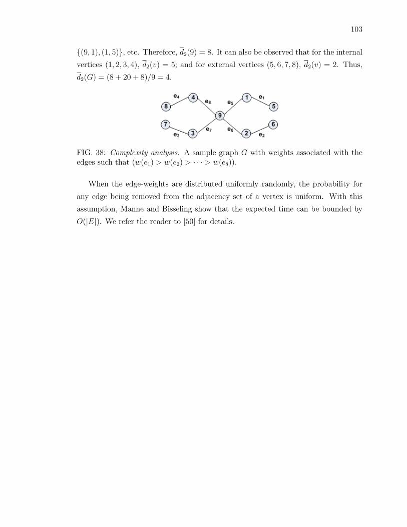
103
{(9, 1), (1, 5)}, etc. Therefore, d2(9) = 8. It can also be observed that for the internal
vertices (1, 2, 3, 4), d2(v) = 5; and for external vertices (5, 6, 7, 8), d2(v) = 2. Thus,
d2(G) = (8 + 20 + 8)/9 = 4.
FIG. 38: Complexity analysis. A sample graph G with weights associated with theedges such that (w(e1) > w(e2) > · · · > w(e8)).
When the edge-weights are distributed uniformly randomly, the probability for
any edge being removed from the adjacency set of a vertex is uniform. With this
assumption, Manne and Bisseling show that the expected time can be bounded by
O(|E|). We refer the reader to [50] for details.

104
V.2 DISTRIBUTED ALGORITHM OF HOEPMAN
The intuition for parallelism using pointers was provided in the previous section. In
this section we will discuss how this scheme can be implemented in a distributed
manner. Hoepman [36] provides a distributed algorithm that assigns one vertex per
processor. A processor is capable of computing as well as communicating with other
processors, and has independent memory that is not accessible by other other pro-
cessors. Hoepman’s algorithm provides the necessary understanding for the parallel
algorithm that we have implemented where each processor is assigned a set of vertices
for processing.
Hoepman’s algorithm is described in Algorithm 23. The algorithm starts by
assigning each processor a unique vertex and its adjacency set. In order to simplify,
we will assign the same index to both the processor and the vertex. Thus, from
the adjacency set, each processor will also know the identities of its neighboring
processors. Each processor will maintain a set S that is initialized with the adjacency
set of the vertex it owns. Every time a processor receives a message from its neighbors,
it removes the identity of that neighbor from set S. Similarly, each processor also
maintains a set QR to store the requests received from its neighbors. We will reuse
Algorithm 20, introduced in Section 1, to compute the candidate-mate of a vertex.
The algorithm loops until set S becomes empty (Lines 9 through 28). There
are two possibilities for this to happen: (i) either a processor receives a message
from all its neighbors, or (ii) it finds a mate. We will use two types of messages -
REQUEST and UNAVAILABLE. A REQUEST message is sent when a processor wants to
match with one of its neighboring processors. When a REQUEST message is matched
with a corresponding REQUEST message, it means that a locally dominant edge has
been identified (similar to two vertices pointing to each other). This will result in an
edge being matched. An UNAVAILABLE message is sent when a processor successfully
matches its vertex and is not interested in the matching process anymore (Lines 23
through 25). Execution of Algorithm 23 on a simple graph with three vertices is
shown in Figure 39.

105
Algorithm 23 Distributed Algorithm of Hoepman. Input: A graph G(V,E) withweights associated with the edges. Output: A 1
2-approx matching M . Data dis-
tribution: Processor Pi owns vertex vi and stores edges incident on vi, adj(vi).Associated data structures: A set S of processor identities that share an edgewith Pi, a set QR of requests received on Pi, a scalar c that identifies the mate.
1: procedure DistributedMatchingAlgorithm(G = (V,E), M)2: loop on each processor Pi, i ∈ I = {1, . . . , |V |} . One vertex per processor.3: S ← adj(vi);4: QR ← ∅;5: c← ComputeCandidateMate(vi);6: if c 6= null then7: send REQUEST to c;8: end if9: while S 6= ∅ do
10: receive message from u ∈ S;11: if message = REQUEST then12: QR ← QR ∪ {u};13: else if message = UNAVAILABLE then14: S ← S \ {u}; . Processor Pu has found a mate elsewhere15: if c = u then16: c← ComputeCandidateMate(vi); . Reset the pointer.17: if c 6= 0 then18: send REQUEST to c;19: end if20: end if21: end if22: if c 6= null and c ∈ QR then23: for all w ∈ S \ {c} do24: send UNAVAILABLE to w;25: end for26: S ← ∅;27: end if28: end while29: return c;30: end loop31: Compute M based on the c values received from all processors;32: return M ;33: end procedure
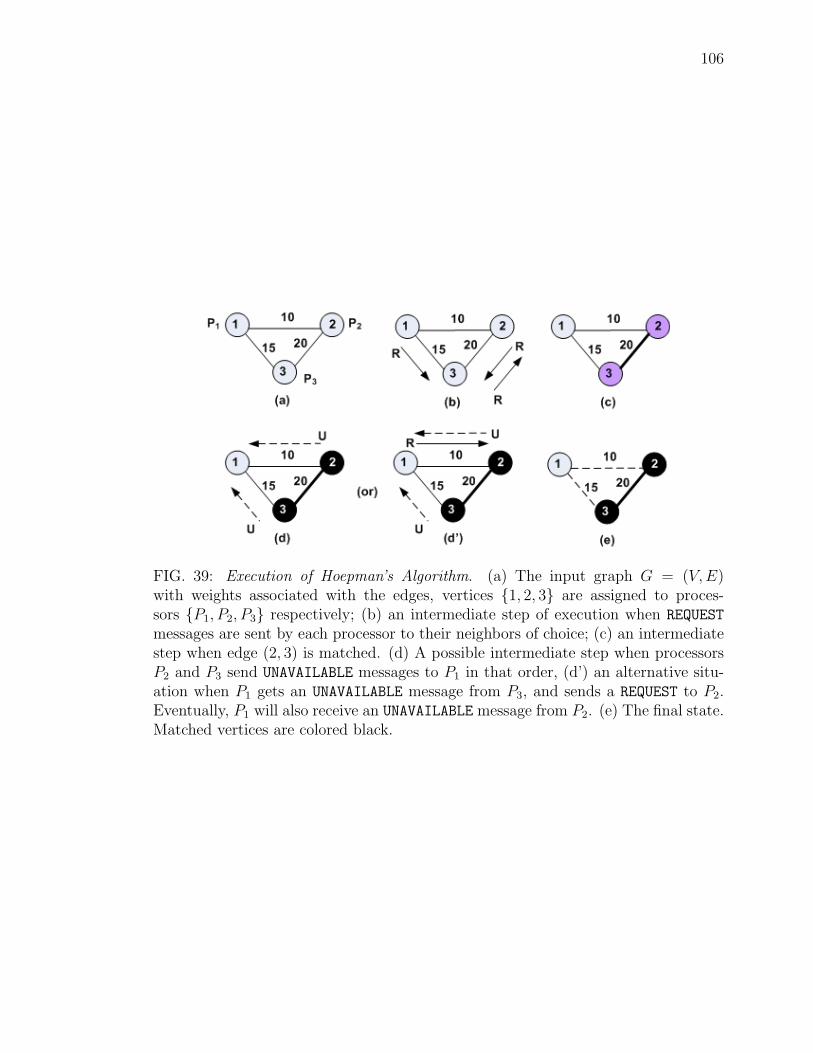
106
FIG. 39: Execution of Hoepman’s Algorithm. (a) The input graph G = (V,E)with weights associated with the edges, vertices {1, 2, 3} are assigned to proces-sors {P1, P2, P3} respectively; (b) an intermediate step of execution when REQUEST
messages are sent by each processor to their neighbors of choice; (c) an intermediatestep when edge (2, 3) is matched. (d) A possible intermediate step when processorsP2 and P3 send UNAVAILABLE messages to P1 in that order, (d’) an alternative situ-ation when P1 gets an UNAVAILABLE message from P3, and sends a REQUEST to P2.Eventually, P1 will also receive an UNAVAILABLE message from P2. (e) The final state.Matched vertices are colored black.

107
V.2.1 Complexity Analysis
The number of messages a processor Pi sends is Θ(d(vi)), where d(vi) is the degree of a
vertex vi that Pi owns. Let us define one time step as the time it takes for a processor
to compute a candidate-mate and send a REQUEST message to the processor that owns
the candidate-mate. If each processor can independently perform this task, then the
computational time of Hoepman’s algorithm will be determined by the number of
time steps it takes before every vertex either has a candidate-mate of its choice or
has processed all the edges incident on the vertex it owns.
Similar to Algorithm 22 the complexity of finding a candidate-mate, as described
in Algorithm 20, is given by Θ(|S(v)|) using a linear search for the heaviest edge,
where S(v) represents the set of unmatched vertices adjacent to vertex v. This can
be bounded by O(∆), where ∆ is the maximum degree of any vertex in the graph.
In each step a processor either sends a REQUEST message to a particular processor
or UNAVAILABLE messages to one or more processors. The number of messages sent by
any given processor is the number of edges incident on the vertex it owns, Θ(|S(v)|).This can again be bounded by O(∆).
Algorithm 23 has (2|E|) messages communicated before completion. Manne and
Bisseling [50] show that Hoepman’s algorithm can complete in O(log |E|) rounds
when the weights of edges are random. Thus, the expected time for Hoepman’s
algorithm with |V | processors can be expressed as
O(∆ log |E|). (18)
We will now present a parallel 12-approx algorithm where each processor gets a
set of vertices and the associated edges. The main idea is to combine Algorithms 22
and 23 to develop an efficient algorithm for the given problem.

108
V.3 PARALLEL 12-APPROX ALGORITHM
We now present a parallel 12-approx algorithm for computing matchings in graphs.
The main idea is to adapt the serial pointer-based algorithm into a distributed al-
gorithm by using communication techniques from Hoepman’s algorithm to match
edges whose end-points are not owned by the same processor. We call these edges as
cross-edges or cut-edges, and edgecut represents the number of cross-edges.
Note that the data structures for graph representation store vertex adjacencies
and the graph is distributed via vertex partitioning. Given a graph G(V,E) and p
processors, the vertex set V is partitioned into p subsets V1, . . . , Vp. Processor Pi
owns the vertex subset Vi. In addition to the vertices that the processor owns, it also
stores some of the vertices that are owned by other processors. We will represent the
subgraph on processor Pi as G′i(V
′i , E
′i). The vertex set V
′i = Vi ∪ V G
i , where the set
V Gi represents the vertices in G
′i that are not owned by Pi - the ghost vertices. The
edge set E′i = Ei∪EG
i , where Ei represents the edges between two vertices in Vi (the
internal edges), and EGi represents the edges with one end-point in Vi and the other
in V Gi (the cross-edges). This is shown in Figure 40. The ghost vertices are colored
purple and the cross-edges are shown with dashed lines. Note that a processor Pi
will not store edges connecting two vertices in V Gi . Processor Pi will also store the
identities of processors that own the ghost vertices. It can be observed that storing
the ghost vertices will have implications on the memory usage and is suitable for
sparse graphs that have partitions with a small number of edges cut.
We now present a framework for computing approximate weighted-matching in
parallel. The framework is sketched in Algorithm 24. This framework can be eas-
ily extended to compute approximation matchings with different objectives such as
maximizing the cardinality or vertex-weight of a matching. The parallel algorithm
has three distinct phases - (i) initialization, (ii) independent computation, and (iii)
shared computation. The algorithm follows the SPMD (Single Program Multiple
Data) model targeted for implementation using MPI standards for distributed mem-
ory architectures.
The given graph is partitioned and distributed among p processors as described
earlier. The associated data structures used in the algorithm are as follows. A set
QG, initialized with ghost vertices V Gi , represents the set of ghost vertices that still
need to be processed in some manner. A set QM , which is initially empty, stores
the matched vertices as the algorithm proceeds. A vector counter , initialized with

109
FIG. 40: Data distribution among processors. (a) The input graph G = (V,E) withweights associated with the edges; (b) The vertex set V is partitioned among twoprocessors P0 and P1. Processor P0 owns vertices {0, 3, 4} and Processor P1 ownsvertices {1, 2, 6}. (c) Data storage on the processors. Along with internal edges, eachprocessor will also store the endpoints of the edges that get cut (cross-edges). Thesevertices are called the ghost vertices and are colored purple in the figure.
the number of edges in E′i incident on each ghost vertex, represents the number
of messages that need to be sent (and received) with respect to a ghost vertex.
A vector candidateMate stores the desired mate (pointer) for each vertex in V′i .
The sets Sl(v) and Sg(v), initialized with the adjacency sets for local and ghost
vertices respectively, represent the unmatched adjacent vertices of vertex v in V′i .
All these data structures are initialized in the initialization phase represented by
Lines 4 through 15 in Algorithm 24.
In Phase-1, each processor attempts to match as many edges as possible with-
out having to depend on information from the neighboring processors. Therefore,
we call this phase independent computation. The computation in Phase-1 is similar
to the serial pointer-based algorithm. The two main tasks in Phase-1 are to pro-
cess all the (unmatched or exposed) vertices once, and process the vertices that get
matched in the first task. Calls to functions ProcessExposedVertexParallel
and ProcessMatchedVerticesParallel are made to complete these tasks. We
will describe these functions soon. The calls to these two functions will initiate some
communication among processors. There are three types of messages - REQUEST,
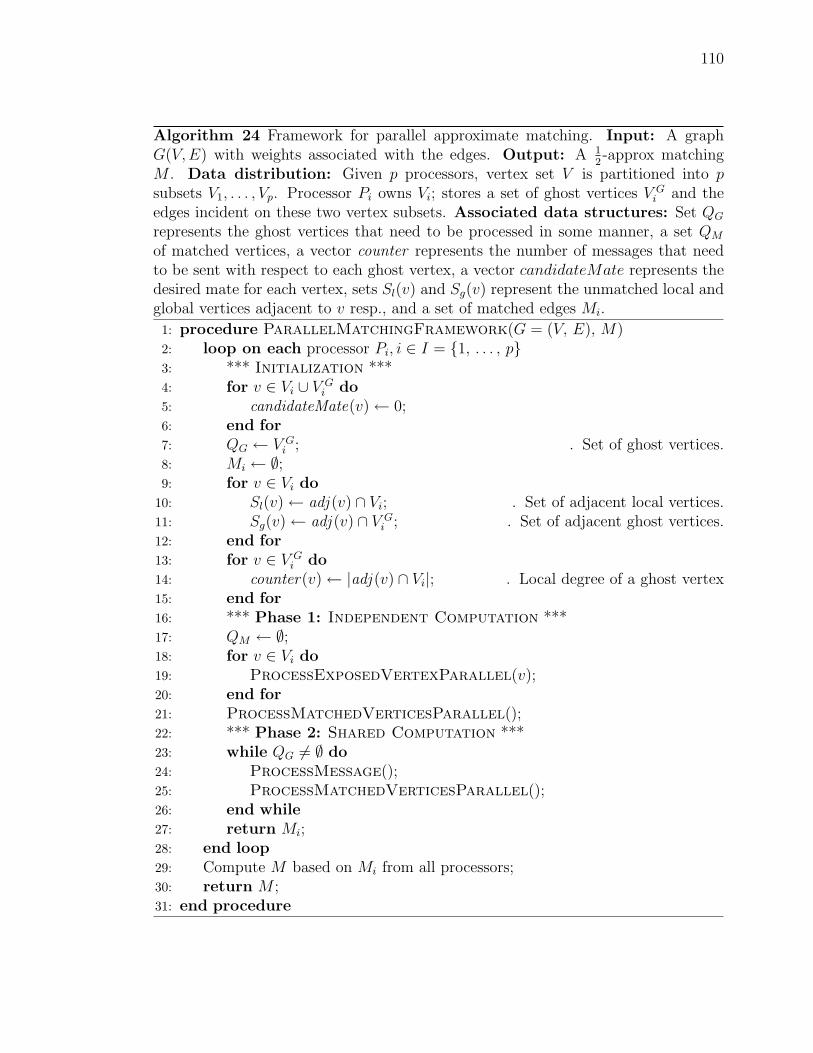
110
Algorithm 24 Framework for parallel approximate matching. Input: A graphG(V,E) with weights associated with the edges. Output: A 1
2-approx matching
M . Data distribution: Given p processors, vertex set V is partitioned into psubsets V1, . . . , Vp. Processor Pi owns Vi; stores a set of ghost vertices V G
i and theedges incident on these two vertex subsets. Associated data structures: Set QG
represents the ghost vertices that need to be processed in some manner, a set QM
of matched vertices, a vector counter represents the number of messages that needto be sent with respect to each ghost vertex, a vector candidateMate represents thedesired mate for each vertex, sets Sl(v) and Sg(v) represent the unmatched local andglobal vertices adjacent to v resp., and a set of matched edges Mi.
1: procedure ParallelMatchingFramework(G = (V, E), M)2: loop on each processor Pi, i ∈ I = {1, . . . , p}3: *** Initialization ***4: for v ∈ Vi ∪ V G
i do5: candidateMate(v)← 0;6: end for7: QG ← V G
i ; . Set of ghost vertices.8: Mi ← ∅;9: for v ∈ Vi do
10: Sl(v)← adj (v) ∩ Vi; . Set of adjacent local vertices.11: Sg(v)← adj (v) ∩ V G
i ; . Set of adjacent ghost vertices.12: end for13: for v ∈ V G
i do14: counter(v)← |adj (v) ∩ Vi|; . Local degree of a ghost vertex15: end for16: *** Phase 1: Independent Computation ***17: QM ← ∅;18: for v ∈ Vi do19: ProcessExposedVertexParallel(v);20: end for21: ProcessMatchedVerticesParallel();22: *** Phase 2: Shared Computation ***23: while QG 6= ∅ do24: ProcessMessage();25: ProcessMatchedVerticesParallel();26: end while27: return Mi;28: end loop29: Compute M based on Mi from all processors;30: return M ;31: end procedure

111
UNAVAILABLE and FAILURE, descriptions of which will soon follow. All the REQUEST
and UNAVAILABLE messages originating in this phase can be queued (bundled or ag-
gregated), and sent at the end of this phase. There cannot be any FAILURE messages
originating in this phase.
In Phase 2, computation can only proceed based on the information received
from the neighboring processors, and therefore, the name - shared computation. The
basic tasks in this phase can be grouped as communication-based and computation-
based. The computation begins when a message from a neighboring processor is
received. Communication is handled in function ProcessMessage, which is called
within a while loop (Line 24). Appropriate action, based on the type of message,
is taken within this function. If the message results in edges being matched, then a
call to function ProcessMatchedVerticesParallel is made (Line 25). Detailed
descriptions of these two functions will soon follow. The tasks are looped until the set
QG becomes empty. As will be described soon, a ghost vertex g is removed from QG
only when its counter(g) becomes zero. This implies that all computations related
to this vertex are complete. Matchings on each processor, Mi, can be gathered on
the master process, or consumed locally, depending on the needs of the applications.
We will now present the details of different functions that are used in Algorithm 24.
All the communication involved in the algorithm is handled by three types of
messages - REQUEST, UNAVAILABLE and FAILURE. Messages are asynchronous point-
to-point messages sent by one processor to another. Each message contains identities
of two vertices that represent a cross-edge. The meaning of a message is determined
by the type of the message, as follows. A REQUEST message conveys a positive intent
of matching a cross-edge sent by the owner-processor of one endpoint to the owner-
processor of the other endpoint. An UNAVAILABLE message sent by a processor means
that the local vertex identified in the message has already been matched, and there-
fore, a request to match this vertex by a neighboring processor cannot be satisfied.
A FAILURE message sent by a processor means that the local vertex identified in the
message could not be matched and that its owner-processor has finished all compu-
tation related to this vertex. Note the minor difference between the UNAVAILABLE
and FAILURE types - the local vertex identified in the message is matched in the
former and unmatched in the latter; although, both types imply a negative response
to match a cross-edge as identified in the message.
We mentioned that computation in Phase-1 is similar to the serial pointer-based
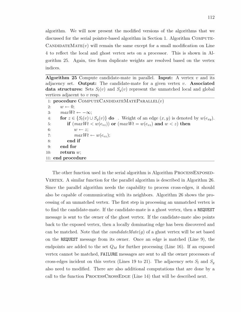
112
algorithm. We will now present the modified versions of the algorithms that we
discussed for the serial pointer-based algorithm in Section 1. Algorithm Compute-
CandidateMate(v) will remain the same except for a small modification on Line
4 to reflect the local and ghost vertex sets on a processor. This is shown in Al-
gorithm 25. Again, ties from duplicate weights are resolved based on the vertex
indices.
Algorithm 25 Compute candidate-mate in parallel. Input: A vertex v and itsadjacency set. Output: The candidate-mate for a given vertex v. Associateddata structures: Sets Sl(v) and Sg(v) represent the unmatched local and globalvertices adjacent to v resp.
1: procedure ComputeCandidateMateParallel(v)2: w ← 0;3: maxWt ← −∞;4: for z ∈ {Sl(v) ∪ Sg(v)} do . Weight of an edge (x, y) is denoted by w(exy).5: if (maxWt < w(evz)) or (maxWt = w(evz) and w < z) then6: w ← z;7: maxWt ← w(evz);8: end if9: end for
10: return w;11: end procedure
The other function used in the serial algorithm is Algorithm ProcessExposed-
Vertex. A similar function for the parallel algorithm is described in Algorithm 26.
Since the parallel algorithm needs the capability to process cross-edges, it should
also be capable of communicating with its neighbors. Algorithm 26 shows the pro-
cessing of an unmatched vertex. The first step in processing an unmatched vertex is
to find the candidate-mate. If the candidate-mate is a ghost vertex, then a REQUEST
message is sent to the owner of the ghost vertex. If the candidate-mate also points
back to the exposed vertex, then a locally dominating edge has been discovered and
can be matched. Note that the candidateMate(g) of a ghost vertex will be set based
on the REQUEST message from its owner. Once an edge is matched (Line 9), the
endpoints are added to the set QM for further processing (Line 16). If an exposed
vertex cannot be matched, FAILURE messages are sent to all the owner processors of
cross-edges incident on this vertex (Lines 19 to 21). The adjacency sets Sl and Sg
also need to modified. There are also additional computations that are done by a
call to the function ProcessCrossEdge (Line 14) that will be described next.
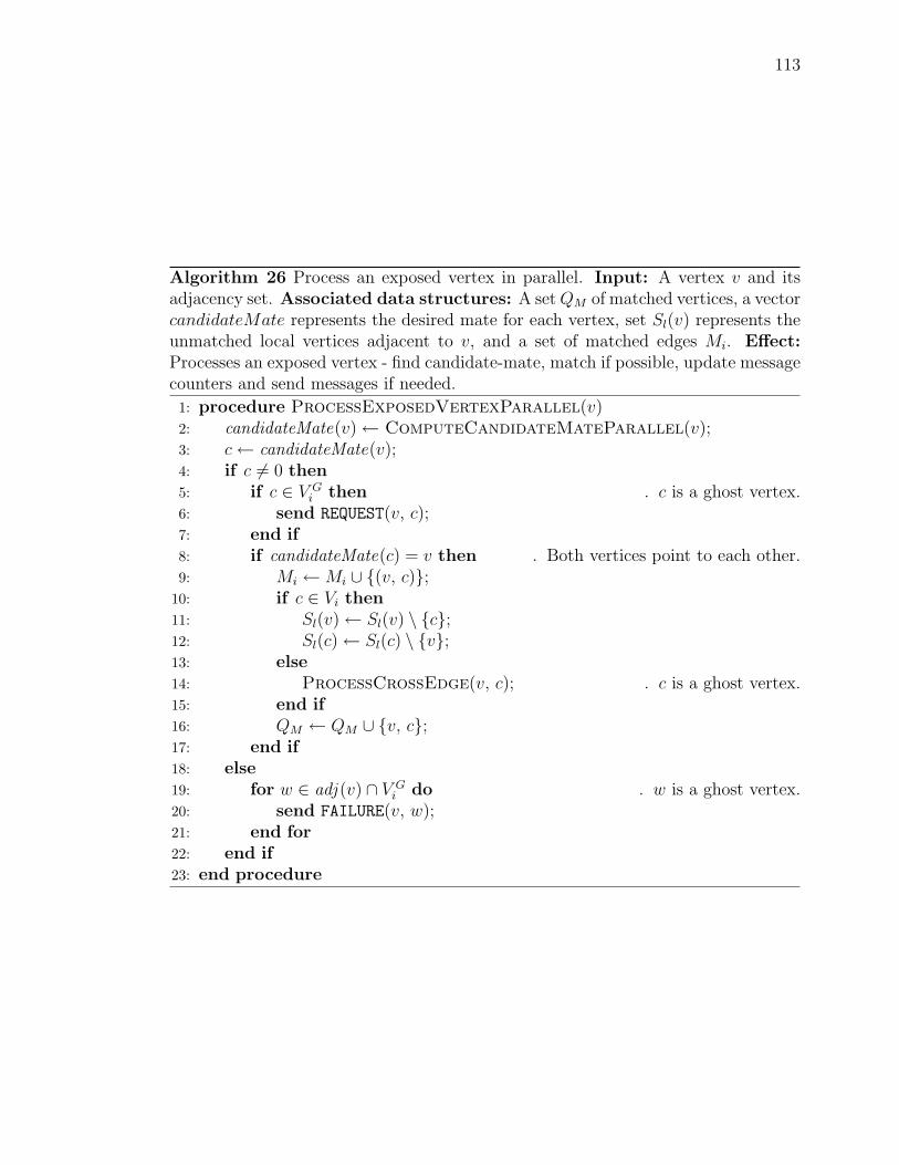
113
Algorithm 26 Process an exposed vertex in parallel. Input: A vertex v and itsadjacency set. Associated data structures: A setQM of matched vertices, a vectorcandidateMate represents the desired mate for each vertex, set Sl(v) represents theunmatched local vertices adjacent to v, and a set of matched edges Mi. Effect:Processes an exposed vertex - find candidate-mate, match if possible, update messagecounters and send messages if needed.
1: procedure ProcessExposedVertexParallel(v)2: candidateMate(v)← ComputeCandidateMateParallel(v);3: c← candidateMate(v);4: if c 6= 0 then5: if c ∈ V G
i then . c is a ghost vertex.6: send REQUEST(v, c);7: end if8: if candidateMate(c) = v then . Both vertices point to each other.9: Mi ←Mi ∪ {(v, c)};
10: if c ∈ Vi then11: Sl(v)← Sl(v) \ {c};12: Sl(c)← Sl(c) \ {v};13: else14: ProcessCrossEdge(v, c); . c is a ghost vertex.15: end if16: QM ← QM ∪ {v, c};17: end if18: else19: for w ∈ adj (v) ∩ V G
i do . w is a ghost vertex.20: send FAILURE(v, w);21: end for22: end if23: end procedure

114
We observe that there is a shortcoming in Hoepman’s algorithm described in Al-
gorithm 23. A processor Pi will ignore all messages that it receives as soon as it
successfully finds a mate and sends UNAVAILABLE messages to its remaining active
neighbors. Once the UNAVAILABLE messages are received by these neighbors they
will not send any message to Pi. However, there can be a situation when a processor
Pk sends a REQUEST message to Pi before it receives an UNAVAILABLE message, but
after Pi has found a mate. This case is illustrated in Figure 39 in step (d’). Thus,
the REQUEST message from Pk will be lost, or not acknowledged, by Processor Pi
(Processor P1 in Figure 39). The message passing interface MPI standard stipulates
that every send be matched with a corresponding receive. Therefore, techniques
that prevent message losses in the algorithm will facilitate implementation, espe-
cially using the MPI standards for distributed memory systems. We address this
unacknowledged-message problem by providing two data structures to keep track of
messages - (i) a set QG of ghost vertices that need to be processed in some manner,
and (ii) a vector counter that stores a number for each ghost vertex. The value for
a ghost vertex in counter is initialized with the number of cross-edges incident on
it (the local degree). The counting of messages can now be done by keeping track
of each cross-edge and modifying the counters each time a communication happens.
When all the cross-edges incident on a given ghost vertex g are processed in some
manner its counter(g) becomes zero, it can then be removed from the set QG. This
is shown in Algorithm 27.
Algorithm 27 Process a cross-edge. Input: Two vertices that represent a cross-edge. Associated data structures: Set QG represents the ghost vertices that needto be processed in some manner, a vector counter represents the number of messagesthat need to be sent with respect to each ghost vertex, and sets Sg(v) representsthe unmatched ghost vertices adjacent to v. Effect: Modifies the adjacency set of aghost vertex, decrements its counter and modifies the set QG if needed.
1: procedure ProcessCrossEdge(l, g) . g is ghost, and l is a local vertex.2: Sg(l)← Sg(l) \ {g};3: counter(g)← counter(g)− 1;4: if counter(g) = 0 then5: QG ← QG \ {g}; . All computation for vertex g is complete.6: end if7: end procedure
The call to function ProcessExposedVertexParallel will result in some
edges (at least the heaviest edge) getting matched. The vertices that point to matched
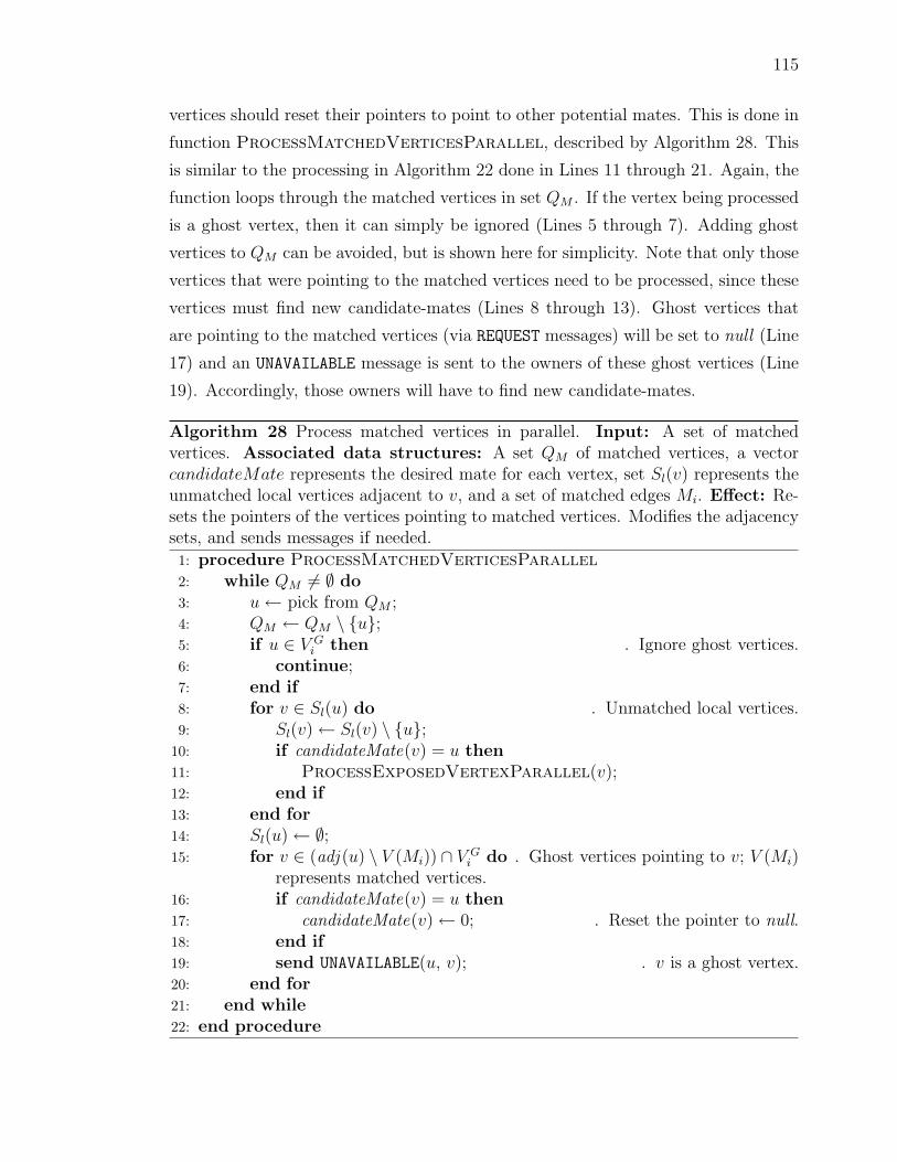
115
vertices should reset their pointers to point to other potential mates. This is done in
function ProcessMatchedVerticesParallel, described by Algorithm 28. This
is similar to the processing in Algorithm 22 done in Lines 11 through 21. Again, the
function loops through the matched vertices in set QM . If the vertex being processed
is a ghost vertex, then it can simply be ignored (Lines 5 through 7). Adding ghost
vertices to QM can be avoided, but is shown here for simplicity. Note that only those
vertices that were pointing to the matched vertices need to be processed, since these
vertices must find new candidate-mates (Lines 8 through 13). Ghost vertices that
are pointing to the matched vertices (via REQUEST messages) will be set to null (Line
17) and an UNAVAILABLE message is sent to the owners of these ghost vertices (Line
19). Accordingly, those owners will have to find new candidate-mates.
Algorithm 28 Process matched vertices in parallel. Input: A set of matchedvertices. Associated data structures: A set QM of matched vertices, a vectorcandidateMate represents the desired mate for each vertex, set Sl(v) represents theunmatched local vertices adjacent to v, and a set of matched edges Mi. Effect: Re-sets the pointers of the vertices pointing to matched vertices. Modifies the adjacencysets, and sends messages if needed.
1: procedure ProcessMatchedVerticesParallel2: while QM 6= ∅ do3: u← pick from QM ;4: QM ← QM \ {u};5: if u ∈ V G
i then . Ignore ghost vertices.6: continue;7: end if8: for v ∈ Sl(u) do . Unmatched local vertices.9: Sl(v)← Sl(v) \ {u};
10: if candidateMate(v) = u then11: ProcessExposedVertexParallel(v);12: end if13: end for14: Sl(u)← ∅;15: for v ∈ (adj (u) \ V (Mi)) ∩ V G
i do . Ghost vertices pointing to v; V (Mi)represents matched vertices.
16: if candidateMate(v) = u then17: candidateMate(v)← 0; . Reset the pointer to null.18: end if19: send UNAVAILABLE(u, v); . v is a ghost vertex.20: end for21: end while22: end procedure
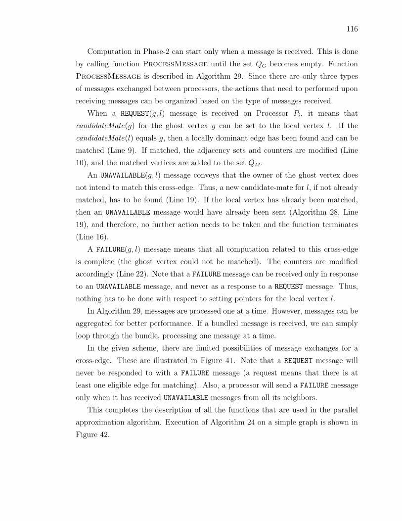
116
Computation in Phase-2 can start only when a message is received. This is done
by calling function ProcessMessage until the set QG becomes empty. Function
ProcessMessage is described in Algorithm 29. Since there are only three types
of messages exchanged between processors, the actions that need to performed upon
receiving messages can be organized based on the type of messages received.
When a REQUEST(g, l) message is received on Processor Pi, it means that
candidateMate(g) for the ghost vertex g can be set to the local vertex l. If the
candidateMate(l) equals g, then a locally dominant edge has been found and can be
matched (Line 9). If matched, the adjacency sets and counters are modified (Line
10), and the matched vertices are added to the set QM .
An UNAVAILABLE(g, l) message conveys that the owner of the ghost vertex does
not intend to match this cross-edge. Thus, a new candidate-mate for l, if not already
matched, has to be found (Line 19). If the local vertex has already been matched,
then an UNAVAILABLE message would have already been sent (Algorithm 28, Line
19), and therefore, no further action needs to be taken and the function terminates
(Line 16).
A FAILURE(g, l) message means that all computation related to this cross-edge
is complete (the ghost vertex could not be matched). The counters are modified
accordingly (Line 22). Note that a FAILURE message can be received only in response
to an UNAVAILABLE message, and never as a response to a REQUEST message. Thus,
nothing has to be done with respect to setting pointers for the local vertex l.
In Algorithm 29, messages are processed one at a time. However, messages can be
aggregated for better performance. If a bundled message is received, we can simply
loop through the bundle, processing one message at a time.
In the given scheme, there are limited possibilities of message exchanges for a
cross-edge. These are illustrated in Figure 41. Note that a REQUEST message will
never be responded to with a FAILURE message (a request means that there is at
least one eligible edge for matching). Also, a processor will send a FAILURE message
only when it has received UNAVAILABLE messages from all its neighbors.
This completes the description of all the functions that are used in the parallel
approximation algorithm. Execution of Algorithm 24 on a simple graph is shown in
Figure 42.
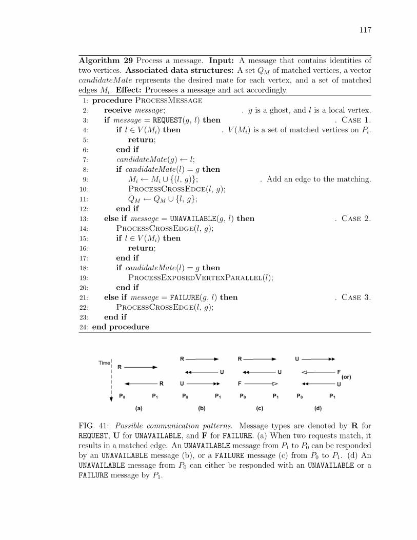
117
Algorithm 29 Process a message. Input: A message that contains identities oftwo vertices. Associated data structures: A set QM of matched vertices, a vectorcandidateMate represents the desired mate for each vertex, and a set of matchededges Mi. Effect: Processes a message and act accordingly.
1: procedure ProcessMessage2: receive message; . g is a ghost, and l is a local vertex.3: if message = REQUEST(g, l) then . Case 1.4: if l ∈ V (Mi) then . V (Mi) is a set of matched vertices on Pi.5: return;6: end if7: candidateMate(g)← l;8: if candidateMate(l) = g then9: Mi ←Mi ∪ {(l, g)}; . Add an edge to the matching.
10: ProcessCrossEdge(l, g);11: QM ← QM ∪ {l, g};12: end if13: else if message = UNAVAILABLE(g, l) then . Case 2.14: ProcessCrossEdge(l, g);15: if l ∈ V (Mi) then16: return;17: end if18: if candidateMate(l) = g then19: ProcessExposedVertexParallel(l);20: end if21: else if message = FAILURE(g, l) then . Case 3.22: ProcessCrossEdge(l, g);23: end if24: end procedure
FIG. 41: Possible communication patterns. Message types are denoted by R forREQUEST, U for UNAVAILABLE, and F for FAILURE. (a) When two requests match, itresults in a matched edge. An UNAVAILABLE message from P1 to P0 can be respondedby an UNAVAILABLE message (b), or a FAILURE message (c) from P0 to P1. (d) AnUNAVAILABLE message from P0 can either be responded with an UNAVAILABLE or aFAILURE message by P1.

118
FIG. 42: Execution of parallel approximation algorithm. (a) The input graphG = (V,E) with weights associated with the edges, vertices {0, 3, 4} are assignedto processor {P0}, and vertices {1, 2, 6} are assigned to processor {P1}. (b) anintermediate step of execution when local computations are done. REQUEST(4, 1)message is sent from P0 to P1; (c) Processor P0 matches edge (0, 3) and sends mes-sages: UNAVAILABLE(0, 6) and REQUEST(4, 6) to P1. Processor P1 matches edge (1, 2)and sends messages: UNAVAILABLE(1, 4) and REQUEST(6, 4) to P0. (d) ProcessorP0 matches edge (4, 6) and sends message UNAVAILABLE(4, 1) to P1. Processor P1
matches edge (6, 4) and sends message UNAVAILABLE(6, 0) to P0.

119
V.3.1 Complexity Analysis
Given a graph G(V,E) with weight function w : E → R+, and p processors, let
n = |V | and m = |E| be the number of vertices and edges respectively. Recall that
G is distributed on p processors as follows. The vertex set V is partitioned into
p subsets V1, . . . , Vp and Processor Pi owns the vertex subset Vi. Let m′
= |Ecut|represent the total edgecut, and m
′Pi
represent the number of cross-edges incident
on the vertices owned by Processor Pi. Let ∆ represent the maximum degree of any
vertex in G, and d(v) represent the degree of a vertex v.
We make the following assumptions in this analysis:
• The adjacency list of a vertex is maintained in a sorted order (we note that
this does not increase the complexity of the algorithm);
• The weights of the edges are distributed uniformly randomly. Therefore, the
expected number of rounds for completion is O(logm) [49, 50]; and
• The input graph has good separators resulting in well balanced partitions. Let
α represent the load imbalance in the (interior) edges incident on the vertices
owned by the same processor (ratio of the maximum number of interior-edges to
the average number of interior-edges over all processors), β represent a similar
imbalance factor in the edges incident on the boundary vertices, and γ represent
the imbalance factor in the cut-edges. The imbalance factors are illustrated in
Figure 43.
FIG. 43: Illustration of different imbalance factors on Processor Pi.
The compute time for Phase-1 on Processor Pi is given by O(∑
v∈Vi d(v) log d(v)),
where the log factor comes from sorting the adjacency sets. This can be relaxed to
O((log ∆)∑
v∈Vi d(v)). This can be generalized to any processor as
O(αm log ∆
p). (19)
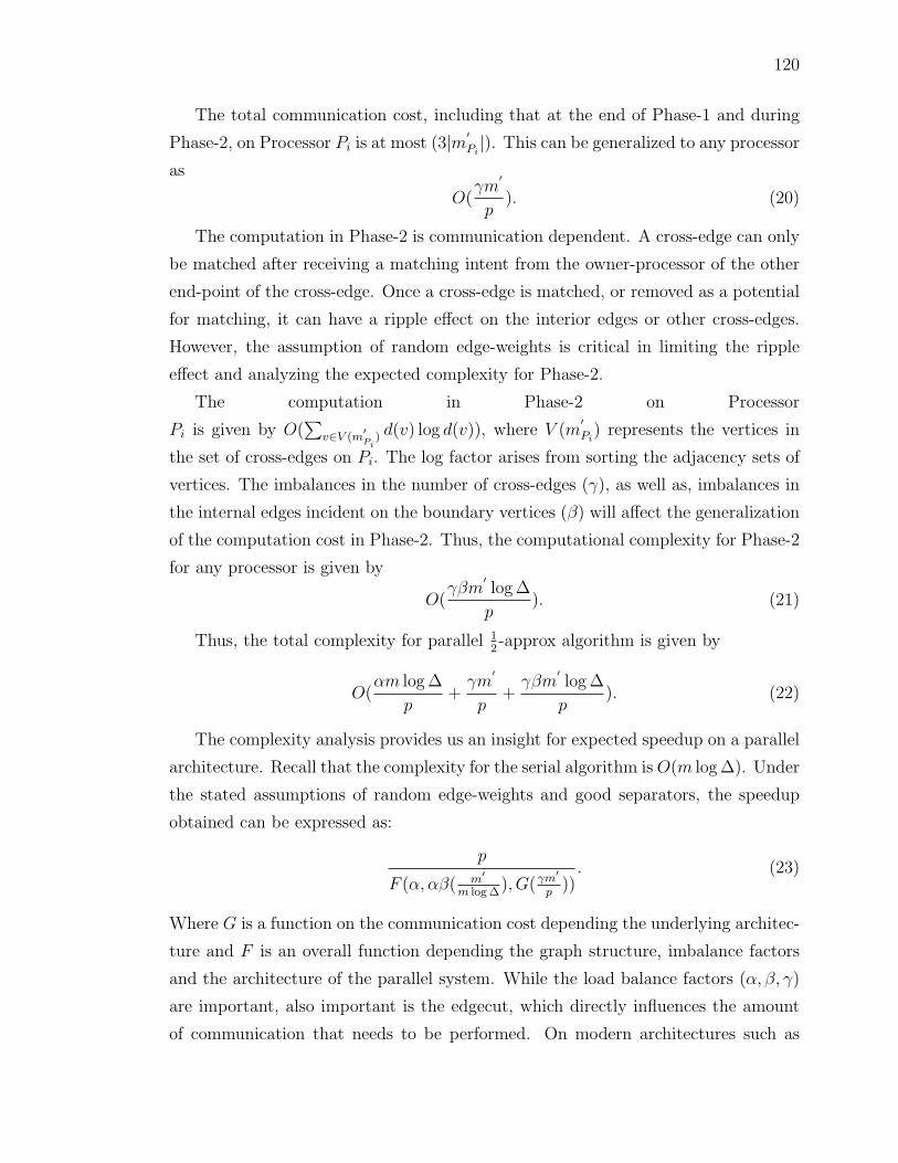
120
The total communication cost, including that at the end of Phase-1 and during
Phase-2, on Processor Pi is at most (3|m′Pi |). This can be generalized to any processor
as
O(γm
′
p). (20)
The computation in Phase-2 is communication dependent. A cross-edge can only
be matched after receiving a matching intent from the owner-processor of the other
end-point of the cross-edge. Once a cross-edge is matched, or removed as a potential
for matching, it can have a ripple effect on the interior edges or other cross-edges.
However, the assumption of random edge-weights is critical in limiting the ripple
effect and analyzing the expected complexity for Phase-2.
The computation in Phase-2 on Processor
Pi is given by O(∑
v∈V (m′Pi
) d(v) log d(v)), where V (m′Pi
) represents the vertices in
the set of cross-edges on Pi. The log factor arises from sorting the adjacency sets of
vertices. The imbalances in the number of cross-edges (γ), as well as, imbalances in
the internal edges incident on the boundary vertices (β) will affect the generalization
of the computation cost in Phase-2. Thus, the computational complexity for Phase-2
for any processor is given by
O(γβm
′log ∆
p). (21)
Thus, the total complexity for parallel 12-approx algorithm is given by
O(αm log ∆
p+γm
′
p+γβm
′log ∆
p). (22)
The complexity analysis provides us an insight for expected speedup on a parallel
architecture. Recall that the complexity for the serial algorithm is O(m log ∆). Under
the stated assumptions of random edge-weights and good separators, the speedup
obtained can be expressed as:
p
F (α, αβ( m′
m log ∆), G(γm
′
p)). (23)
Where G is a function on the communication cost depending the underlying architec-
ture and F is an overall function depending the graph structure, imbalance factors
and the architecture of the parallel system. While the load balance factors (α, β, γ)
are important, also important is the edgecut, which directly influences the amount
of communication that needs to be performed. On modern architectures such as

121
compute clusters with fast processors and relatively slow communication, edgecut is
the most influential factor in determining performance. We also make an important
assumption about the random distribution of edge-weights that directly influences
the number of rounds of execution O(logm) instead of O(m). We will now present
experimental results on the parallel 12-approx algorithm.

122
V.4 EXPERIMENTAL RESULTS
In this section we present experimental results from our implementation of matching
algorithms in a toolkit called MatchBox-P. The two types of experiments done are
serial and parallel. The goals for serial experiments are to demonstrate the efficiency
of approximation algorithms in terms of execution time, cardinality and weight of
matching as compared to those of exact algorithms. We will also demonstrate the
efficiency of the pointer-based algorithm as compared to other approximation algo-
rithms. For the parallel experiments we will try to identify classes of graphs for which
the proposed algorithm, in its current implementation, is effective, and in the process
expose the shortcomings and suggest improvements. The parallel experiments are
conducted on a Cray XT4 system, Franklin, at NERSC with 9, 660 compute nodes.
Each compute node has a 2.3 GHz AMD Opteron quad core processor with 8 GB
RAM. The nodes are interconnected using SeaStar2 router with a 3D torus topol-
ogy. The details can be obtained from www.nersc.gov. The serial experiments are
conducted on a system equipped with four 2.4 GHz Intel quad core processors and
32 GB RAM at Old Dominion University.
V.4.1 Data Set for Experiments
The graphs used for experiments can be broadly classified into two types: (i) graph
representations of regular sparse matrices downloaded from the University of Florida
Sparse Matrix Collection, and (ii) synthetic and model graphs. A matrix is stored
as a general graph, where rows and columns of the matrix represent vertices, and
the nonzero elements represent edges. The absolute value of a nonzero element
in the matrix is considered as the weight of the edge that connects the vertices
representing the row and the column of the nonzero element. A similar model is
used to represent symmetric matrices. Since the files downloaded from the University
of Florida Sparse Matrix Collection store only the lower triangle of the matrix, we
explicitly add edges to represent both the upper and lower triangles of the matrix.
Two types of synthetic graphs are used - random geometric graphs and scalable
synthetic compact application (SSCA#2) graphs. Generation of random geometric
graphs is implemented in MatchBox-P, and SSCA#2 graphs are generated with
GT-Graph generator [5]. In order to eliminate self-loops, the SSCA#2 graphs are
stored as bipartite graphs. Two-dimensional five-point and nine-point grid graphs

123
are used as the model graph problems. The matrices used in the experiments are
listed in Table 11, and the associated structures are illustrated in Figure 44.
Name #Vertices #Edges Type Details
ASIC-680 1, 365, 424 1, 693, 767 Unsymm Circuit simulation matrixHamrle3 2, 894, 720 5, 514, 242 Unsymm Circuit simulation matrixRajat31 9, 380, 004 20, 316, 253 Unsymm Circuit simulation matrixCage14 3, 011, 570 27, 130, 349 Unsymm DNA electrophoresisLdoor 1, 904, 406 84, 035, 431 Symm INDEED Test MatrixAudikw-1 1, 887, 390 154, 359, 999 Symm Crankshaft model
TABLE 11: Matrix Instances downloaded from University of Florida Matrix Col-lection. Unsymm represents unsymmetric matrices and Symm represents symmetricmatrices.
FIG. 44: Visualization of matrix structures.
A d-dimensional random geometric graph (RGG), represented as G(n, r(n)), is a
graph generated by randomly placing n vertices in a d-dimensional space and con-
necting pairs of vertices whose Euclidean distance is less than or equal to r(n). In
our experiments we only consider two-dimensional RGGs contained in a unit square,
[0, 1]2, and the Euclidean distance between two vertices is used as the weight of the
edge connecting them. Our primary objective is to generate RGGs that have good
separators. Therefore, we generate RGGs that are as sparse as possible, but with-
out generating too many isolated vertices or too many disconnected components.
Connectivity, a monotonic property of RGG, in 2d unit-square RGGs has a sharp
threshold at rc =√
lnnπn
[21]. The connectivity threshold is also the longest edge
length of the minimum spanning tree in G [58]. The thermodynamic limit when a
giant component appears with high probability is given by rt =√
λcn
[21, 32]. Em-
pirically, the value of λc is given by 2.0736 for 2d unit-square RGGs. The particular
value of r(n) that we have used in the experiments is rct = (rc + rt)/2. We refer the
reader to [21, 23, 22, 32, 58] for details. A 2d RGG with 1, 000 vertices visualized
with Pajek [10] is shown in Figure 45. Note that along with a few isolated vertices,

124
there are also a few disconnected components. The details of RGGs used in the
experiments are provided in Table 12.
FIG. 45: Random geometric graph. A random geometric graph with 1, 000 verticesas visualized with Pajek.
The SSCA#2 graphs were generated with the GTgraph generator [5]. For conve-
nience, we eliminate self-loops by considering the original graph as a bipartite graph
by simply representing every vertex in the original graph with two vertices (one in
each set) in the bipartite graph. We generated SSCA#2 graphs with the following
properties. For a particular value of λ, the graph has 2λ vertices; the maximum size
of random-sized cliques is 2λ3 ; initial probability of interclique edges is set to 0.5; and
the weights of edges are uniformly randomly assigned with a maximum value of 2λ.
We refer the reader to [5] for details. Visualization of an SSCA#2 graph of 1, 024
vertices with Pajek is shown in Figure 46. The details of SSCA#2 graphs used in
the experiments are provided in Table 12.
Model graphs used in the experiments are five-point and nine-point grid graphs.
The grid graphs are generated within MatchBox-P and the edge weights are assigned
uniformly randomly in the range 0 through RAND MAX. Visualization of sample five-
point and nine-point graphs with Pajek are provided in Figures 47 and 48, and the
details of the grid graphs used in the experiments are provided in Table 12.

125
FIG. 46: SSCA#2 graph. An SSCA#2 graph with 1, 024 vertices as visualized withPajek.
Name #Vertices #Edges
RGG-1 320, 000 63, 148, 387RGG-2 8, 388, 608 404, 249, 646SSCA#2-1 2, 097, 152 63, 148, 387SSCA#2-2 8, 388, 608 404, 249, 646FivePtGrid4k 16, 000, 000 31, 992, 000
TABLE 12: Synthetic and Model Graphs. SSCA#2 graphs are generated using GT-Graph generator. The number of vertices in the original graph are doubled to convertit into a bipartite graph to eliminate self-loops; duplicate edges, if any, are alsoeliminated. RGGs and grid graphs are generated with MatchBox-P and have randomedge weights.

126
FIG. 47: Five-point grid graph. A 10 X 10 five-point grid graph visualized withPajek.
FIG. 48: Nine-point grid graph. A 10 X 10 nine-point grid graph visualized withPajek.

127
V.4.2 Performance of Serial Matching Algorithms
In this section we show experimental results from serial implementation of the match-
ing algorithms. The goal for these experiments is to highlight the performance of
approximation algorithms not only in the execution time but also for computing
matching of good quality. We present the quality as a ratio of cardinality and weight
of approximation matchings to those of exact matchings. Our implementation of ex-
act matching algorithm is based on the primal-dual algorithm [57] using array data
structures. For large graphs, we also observe empirically that the performance of
binary-heap-based implementation is only incrementally better than the array-based
implementation of the exact algorithm. The results are summarized in Table 13.
It can be observed that the approximation algorithms generate matchings of high
quality with huge gains in compute time.
Instance Wgt-Ratio Card-Ratio Time-Approx(s) Time-Exact(s)
ASIC-680 1.00 0.99 0.13 46, 639Hamrle3 0.99 0.81 0.28 170, 059Rajat31 1.00 1.00 0.58 1, 361, 146Cage14 1.00 1.00 0.55 409, 250Ldoor 1.00 1.00 0.46 178, 004Audikw1 1.00 1.00 0.72 242, 591
TABLE 13: Performance of serial approx algorithm. The second column representsthe ratio of weights of approximate and exact matchings. Similarly, the third columnrepresents the ratio of cardinality of the two matchings. Fourth and fifth columnsshow the time in seconds to compute approximate and exact matchings respectively.
We will now present the relative performance of different half approximation algo-
rithms. The two main categories of approximation algorithms are the sorting-based
algorithms of Avis [4] and Preis [64], and path growing algorithms of Vinkemeier
and Hougardy [24, 74]. The path growing algorithm finds simple paths of heaviest
weight in a graph, alternatively adding edges to two sets of potential matchings.
While in PG-1 the two sets of potential matching are compared at the very end, the
two potential sets are compared for each distinct path in PG-2, and therefore, PG-2
is a better algorithm. PG-3 merges the two potential matching sets using Dynamic
Programming techniques, and thus, has the best results, with respect to the weight
of the matching, as compared to PG-1 and PG-2. Since the pointer-based algorithm
is a version of Preis’s algorithm, which in turn is a version of Avis’s algorithm, we
will only present the results for the pointer-based algorithm. Weight and cardinality
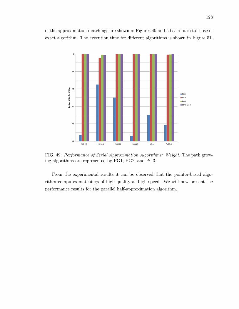
128
of the approximation matchings are shown in Figures 49 and 50 as a ratio to those of
exact algorithm. The execution time for different algorithms is shown in Figure 51.
0.5
0.6
0.7
0.8
0.9
1
ASIC-680 Hamrle3 Rajat31 Cage14 Ldoor Audikw1
Rat
io =
W(M
½)
/ W
(M*)
PG1
PG2
PG3
Ptr-Based
FIG. 49: Performance of Serial Approximation Algorithms: Weight. The path grow-ing algorithms are represented by PG1, PG2, and PG3.
From the experimental results it can be observed that the pointer-based algo-
rithm computes matchings of high quality at high speed. We will now present the
performance results for the parallel half-approximation algorithm.
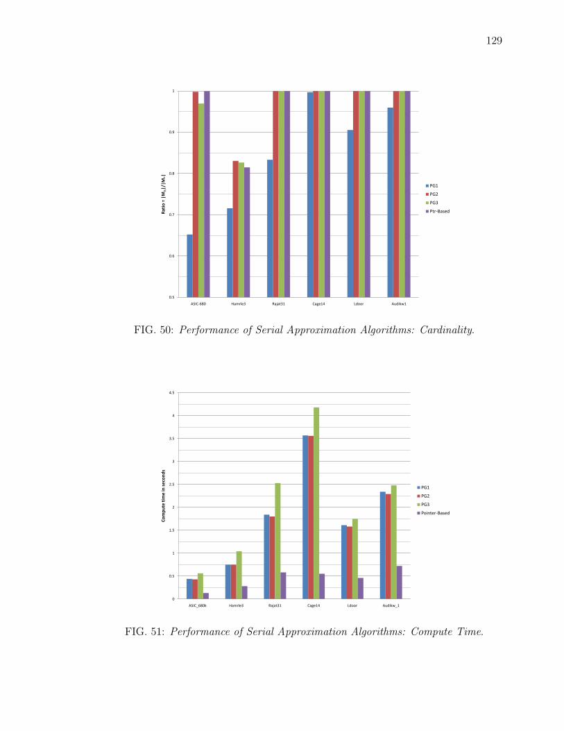
129
0.5
0.6
0.7
0.8
0.9
1
ASIC-680 Hamrle3 Rajat31 Cage14 Ldoor Audikw1
Rat
io =
|M
½|/
|M*|
PG1
PG2
PG3
Ptr-Based
FIG. 50: Performance of Serial Approximation Algorithms: Cardinality.
0
0.5
1
1.5
2
2.5
3
3.5
4
4.5
ASIC_680k Hamrle3 Rajat31 Cage14 Ldoor Audikw_1
Co
mp
ute
tim
e in
se
con
ds
PG1
PG2
PG3
Pointer-Based
FIG. 51: Performance of Serial Approximation Algorithms: Compute Time.
130
V.4.3 Performance of Parallel Matching Algorithm:
The parallel half-approximation algorithm has been implemented in C++ and uses
Message Passing Interface (MPI) libraries for communication between processors.
The implementation also uses the Standard Template Library (STL) data structures
such as Vectors and Maps. We use multi-level K-way partitioning algorithm in Metis
[41] for distributing input data among participating processors. As described in Al-
gorithm ParallelMatchingFramework, the implementation has three distinct
phases:
• Initialization: The actions performed in this phase are initialization of asso-
ciated data structures such as the adjacency structures for the ghost vertices,
mapping of ghost vertex indices to zero-based indices, allocation of memory for
communication (based on the edgecut), etc.
• Phase-1 : In this phase, candidate mates are set for all local vertices, and
an attempt to match is performed. At the end of Phase-1, all the resulting
communication is sent. Individual messages to a processor are aggregated and
sent as one packet of information using MPI constructs for immediate messages
(MPI Isend()) [67].
• Phase-2 : Computation in Phase-2 is communication dependent, and can only
start once a message is received. It can be broadly classified into two super-
steps - computation and communication. In our current implementation, we do
not aggregate individual messages, but send (non-blocking) them immediately
as needed. Given the fact that we have a bound on the number of messages that
will be communicated, we have implemented asynchronous messaging using the
MPI constructs for buffered messages (MPI Bsend()) [67]. We note that the
current implementation can be improved by performing message aggregation in
Phase-2, while acknowledging that there will be a certain amount of overhead
for message aggregation and potentially longer idle times as processors wait for
messages.
We will now present details from parallel experiments for synthetic and model
graphs for up to 8, 192 processors on Franklin.

131
Five-Point Grid Graph of 4k x 4k Size
The graph representing the 4k x 4k grid has 16, 000, 000 vertices and 31, 992, 000
edges. Since the amount of communication is directly dependent on the edgecut,
existence of good separators is important to obtain good performance for the parallel
algorithm. For the following experiments we used multi-level K-way partitioning
algorithm in Metis [41]. In Figure 52, we plot the edgecut as a function of number
of vertices. An ideal partitioning of a square grid (2D block distribution) will be
proportional to (2√|V |(√P − 1)), where |V | is the number of vertices and P is
the number of partitions. We observe a similar pattern in the partitions that were
obtained from Metis giving us an expectation for good performance.
4
8
16
32
64
128
256
512
1024
2 4 8 16 32 64 128 256 512 1024 2048 4096 8192
Tho
usa
nd
s
# of partitions
Actual EdgeCut
2(Sqrt(P)-1)*Sqrt(N)
FIG. 52: 4k grid graph: Edgecut as a function of number of vertices. Actual edgecutfor different number of partitions using multi-level K-way partitioning algorithm inMetis, and ideal edgecut given by (2
√|V |(√P − 1)), where V is the number of
vertices and P is the number of partitions.
The maximum time is the longest time taken by any given processor in the group
of processors used to compute a matching. Alternatively, it is the time taken by
the slowest processor. The difference in the compute time of different processors can
be due to various reasons including load imbalance, heterogeneous capacities, graph
structure, and unusual behavior of different processors that is time dependent. This
become an important factor when the number of processors used for a given job is very

132
large. Therefore, we also provide the average (mean) compute time for computing the
matching. Ideally, the experiments should be repeated for a large number of times,
but given limited resources we have not repeated similar experiments, especially for
experiments with large number of processors. Maximum and average execution times
for the 4k grid graph are shown in Figures 53 and 54 respectively. For each type,
the execution time of different phases of the computation are shown separately. The
speedup obtained is shown in Figure 55.
2.44E-04
4.88E-04
9.77E-04
1.95E-03
3.91E-03
7.81E-03
1.56E-02
3.13E-02
6.25E-02
1.25E-01
2.50E-01
5.00E-01
1.00E+00
2.00E+00
4.00E+00
2 4 8 16 32 64 128 256 512 1024 2048 4096 8192
Co
mp
ute
Tim
e (
Max
imu
m)
in s
eco
nd
s
# of processors
Initztn.
Phase-1
Phase-2
Total
FIG. 53: 4k grid graph: Compute time (maximum). Maximum time is the time inseconds of the slowest processor in the group of processors used to solve the problem.
It can be observed that while the execution time for Initialization and Phase-1
scale with the number of processors, the execution time for Phase-2 does not scale
well, and drastically increases for 4, 096 and 8, 192 processors. It should be noted
that the messages are aggregated only in Phase-1 of our current implementation. It
should also be noted that for larger number of processors the amount of work done
per processor is very small. In order to explore further, we plot the cardinality of the
matching at the end of Phase-1 in Figure 56. It can be observed that close to 100
per cent cardinality is obtained at the end of Phase-1 in most cases. As the number
of partitions are increased, the cardinality of matching at the end of Phase-1 also
decreases resulting in more work during Phase-2. The edgecut as a function of the
number of edges is also plotted in Figure 56. It can be observed that a very small

133
2.44E-04
4.88E-04
9.77E-04
1.95E-03
3.91E-03
7.81E-03
1.56E-02
3.13E-02
6.25E-02
1.25E-01
2.50E-01
5.00E-01
1.00E+00
2.00E+00
2 4 8 16 32 64 128 256 512 1024 2048 4096 8192
Co
mp
ute
tim
e (
Ave
rage
) in
se
con
ds
# of processors
Initztn.
Phase-1
Phase-2
Total
FIG. 54: 4k grid graph: Compute time (average). Average time is the sum of computetime on each processor in the group divided by the number of processors in that group.
1
2
4
8
16
32
64
128
256
512
2 4 8 16 32 64 128 256 512 1024 2048 4096 8192
Spe
ed
up
= T
ime-
2-p
rocs
/ T
ime-
N-p
rocs
# of processors
FIG. 55: Speedup for 4k x 4k grid graph.

134
fraction of edges get cut.
0
10
20
30
40
50
60
70
80
90
100
2 4 8 16 32 64 128 256 512 1024 2048 4096 8192
(1)
% C
ard
-P1
= |
M_P
has
e-1
| /
|M|
* 1
00
(2
) %
Ed
ges
cut
= Ed
gecu
t/
|E|
* 1
00
# of processors
%EdgeCut
%Card-P1
FIG. 56: 4k grid graph: Cardinality after Phase-1.
Weak Scaling for Five Point Grid Graphs
We now present weak scaling studies on the five-point grid graphs. The largest graph
is the graph with 16 million vertices, and we solve it on 2, 048 and 1, 024 processors
as two separate series. For each subsequent data point, we will reduce the number
of vertices and the number of processors by half. The test set is summarized in
Table 14.
If the total compute time remains fairly constant for different graph size and
number of processor combinations, then we demonstrate the weak scalability of the
parallel 12-approx algorithm. We plot the execution times for the two series in Fig-
ures 57 and 58. It can be observed that the total execution time remains fairly
constant. In particular, initialization and Phase-1 show good scalability. However,
Phase-2 does not scale proportionally, especially for smaller graph sizes. We plot
edgecut and number of messages sent for each grid-size and number of processor
combinations in Figure 59. The two curves are edgecut divided by the number of
processors and messages sent divided by the number of processors. From this figure
we can observe that the edgecut increases, and therefore, the total time for Phase-2
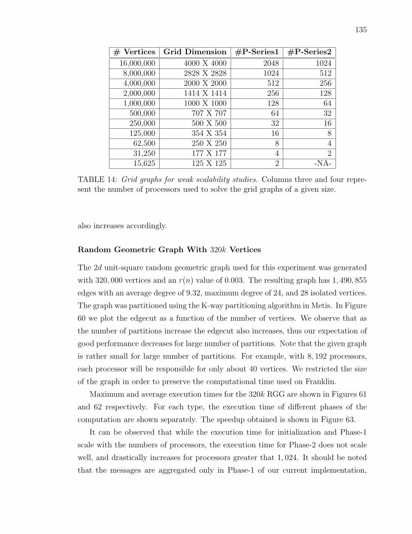
135
# Vertices Grid Dimension #P-Series1 #P-Series2
16,000,000 4000 X 4000 2048 10248,000,000 2828 X 2828 1024 5124,000,000 2000 X 2000 512 2562,000,000 1414 X 1414 256 1281,000,000 1000 X 1000 128 64
500,000 707 X 707 64 32250,000 500 X 500 32 16125,000 354 X 354 16 862,500 250 X 250 8 431,250 177 X 177 4 215,625 125 X 125 2 -NA-
TABLE 14: Grid graphs for weak scalability studies. Columns three and four repre-sent the number of processors used to solve the grid graphs of a given size.
also increases accordingly.
Random Geometric Graph With 320k Vertices
The 2d unit-square random geometric graph used for this experiment was generated
with 320, 000 vertices and an r(n) value of 0.003. The resulting graph has 1, 490, 855
edges with an average degree of 9.32, maximum degree of 24, and 28 isolated vertices.
The graph was partitioned using the K-way partitioning algorithm in Metis. In Figure
60 we plot the edgecut as a function of the number of vertices. We observe that as
the number of partitions increase the edgecut also increases, thus our expectation of
good performance decreases for large number of partitions. Note that the given graph
is rather small for large number of partitions. For example, with 8, 192 processors,
each processor will be responsible for only about 40 vertices. We restricted the size
of the graph in order to preserve the computational time used on Franklin.
Maximum and average execution times for the 320k RGG are shown in Figures 61
and 62 respectively. For each type, the execution time of different phases of the
computation are shown separately. The speedup obtained is shown in Figure 63.
It can be observed that while the execution time for initialization and Phase-1
scale with the numbers of processors, the execution time for Phase-2 does not scale
well, and drastically increases for processors greater that 1, 024. It should be noted
that the messages are aggregated only in Phase-1 of our current implementation,

136
1.22E-04
2.44E-04
4.88E-04
9.77E-04
1.95E-03
3.91E-03
7.81E-03
2 4 8 16 32 64 128 256 512 1024 2048
Co
mp
ute
tim
e (
max
imu
m)
in s
eco
nd
s
# of processors (different graph problems)
Initztn.
Phase-1
Phase-2
Total
FIG. 57: Weak scaling for grid graphs: Series-1 uses the graph size and processorcombinations as shown in Table 14.
1.22E-04
2.44E-04
4.88E-04
9.77E-04
1.95E-03
3.91E-03
7.81E-03
1.56E-02
2 4 8 16 32 64 128 256 512 1024
Co
mp
ute
tim
e (
max
imu
m)
in s
eco
nd
s
# of processors (different graph problems)
Initztn.
Phase-1
Phase-2
Total
FIG. 58: Weak scaling for grid graphs: Series-2 uses the graph size and processorcombinations as shown in Table 14.

137
50.00
100.00
150.00
200.00
250.00
300.00
350.00
400.00
450.00
500.00
550.00
2 4 8 16 32 64 128 256 512 1024 2048
(1)
Edge
cut/
P =
Ed
gecu
t /
# p
rocs
(2
) M
sg/P
= #
Me
ssag
es
/ #
pro
cs
# of processors
EdgeCut/P
Msg/P
FIG. 59: Edgecut and number of messages for different grid graphs: The graph sizeand processor combinations are shown in Table 14.
0.0E+00
2.0E+04
4.0E+04
6.0E+04
8.0E+04
1.0E+05
1.2E+05
1.4E+05
1.6E+05
1.8E+05
2.0E+05
2 4 8 16 32 64 128 256 512 1024 2048 4096 8192
# of partitions
FIG. 60: 320k RGG: Edgecut as a function of number of vertices. Actual edgecutfor different number of partitions using multi-level K-way partitioning algorithm inMetis.

138
2.44E-04
4.88E-04
9.77E-04
1.95E-03
3.91E-03
7.81E-03
1.56E-02
3.13E-02
6.25E-02
1.25E-01
2.50E-01
5.00E-01
2 4 8 16 32 64 128 256 512 1024 2048 4096 8192
Co
mp
ute
Tim
e (
Max
imu
m)
in s
eco
nd
s
# of processors
Initztn.
Phase-1
Phase-2
Total
FIG. 61: 320k RGG: Compute time (maximum). Maximum time is the time inseconds of the slowest processor in the group of processors used to solve the problem.
1.22E-04
2.44E-04
4.88E-04
9.77E-04
1.95E-03
3.91E-03
7.81E-03
1.56E-02
3.13E-02
6.25E-02
1.25E-01
2.50E-01
2 4 8 16 32 64 128 256 512 1024 2048 4096 8192
Co
mp
ute
Tim
e (
Ave
rage
) in
se
con
ds
# of processors
Initztn.
Phase-1
Phase-2
Total
FIG. 62: 320k RGG: Compute time (average). Average time is the sum of computetime on each processor in the group divided by the number of processors in thatgroup.

139
1
2
4
8
16
32
64
2 4 8 16 32 64 128 256 512 1024 2048 4096 8192
Spe
ed
up
= T
ime
-2-p
rocs
/ T
ime
-P-p
rocs
# of processors
FIG. 63: 320k RGG: Speedup.
0
10
20
30
40
50
60
70
80
90
100
2 4 8 16 32 64 128 256 512 1024 2048 4096 8192
(1)
%C
ard
-P1
=(|M
_p1
| /
|M|)
*10
0
(2)
%Ed
geC
ut
= (E
dge
cut
/|E|
)*1
00
# of processors
%Card-P1
%EdgeCut
FIG. 64: 320k RGG: Cardinality after Phase-1.
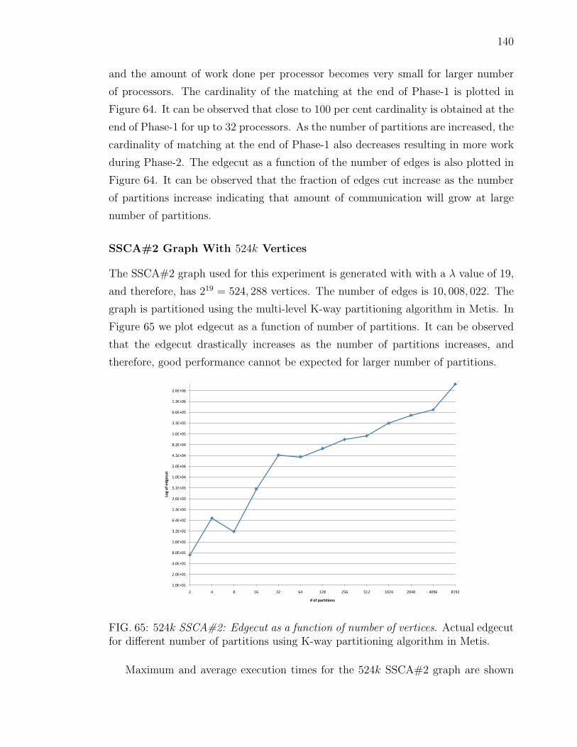
140
and the amount of work done per processor becomes very small for larger number
of processors. The cardinality of the matching at the end of Phase-1 is plotted in
Figure 64. It can be observed that close to 100 per cent cardinality is obtained at the
end of Phase-1 for up to 32 processors. As the number of partitions are increased, the
cardinality of matching at the end of Phase-1 also decreases resulting in more work
during Phase-2. The edgecut as a function of the number of edges is also plotted in
Figure 64. It can be observed that the fraction of edges cut increase as the number
of partitions increase indicating that amount of communication will grow at large
number of partitions.
SSCA#2 Graph With 524k Vertices
The SSCA#2 graph used for this experiment is generated with with a λ value of 19,
and therefore, has 219 = 524, 288 vertices. The number of edges is 10, 008, 022. The
graph is partitioned using the multi-level K-way partitioning algorithm in Metis. In
Figure 65 we plot edgecut as a function of number of partitions. It can be observed
that the edgecut drastically increases as the number of partitions increases, and
therefore, good performance cannot be expected for larger number of partitions.
1.0E+01
2.0E+01
4.0E+01
8.0E+01
1.6E+02
3.2E+02
6.4E+02
1.3E+03
2.6E+03
5.1E+03
1.0E+04
2.0E+04
4.1E+04
8.2E+04
1.6E+05
3.3E+05
6.6E+05
1.3E+06
2.6E+06
2 4 8 16 32 64 128 256 512 1024 2048 4096 8192
Log
of
ed
gecu
t
# of partitions
FIG. 65: 524k SSCA#2: Edgecut as a function of number of vertices. Actual edgecutfor different number of partitions using K-way partitioning algorithm in Metis.
Maximum and average execution times for the 524k SSCA#2 graph are shown

141
in Figures 66 and 67 respectively. For each type, the execution time of different
phases of the computation are shown separately. The speedup obtained is shown in
Figure 68.
4.88E-04
9.77E-04
1.95E-03
3.91E-03
7.81E-03
1.56E-02
3.13E-02
6.25E-02
1.25E-01
2.50E-01
5.00E-01
1.00E+00
2 4 8 16 32 64 128 256 512 1024 2048 4096 8192
Co
mp
ute
tim
e (
Max
imu
m)
in s
eco
nd
s
# of processors
Initztn.
Phase-1
Phase-2
Total
FIG. 66: 524k SSCA#2: Compute time (maximum). Maximum time is the time inseconds of the slowest processor in the group of processors used to solve the problem.
The cardinality of the matching at the end of Phase-1 is plotted in Figure 69.
It can be observed that close to 100 per cent cardinality is obtained at the end of
Phase-1 for up to 512 processors, but it drastically decreases for partitions greater
than 512, especially, for 8, 192 partitions. The edgecut as a function of the number
of edges is also plotted in Figure 69. It can be observed that the fraction of edges
cut increase drastically for 4, 096 and 8, 192 partitions.
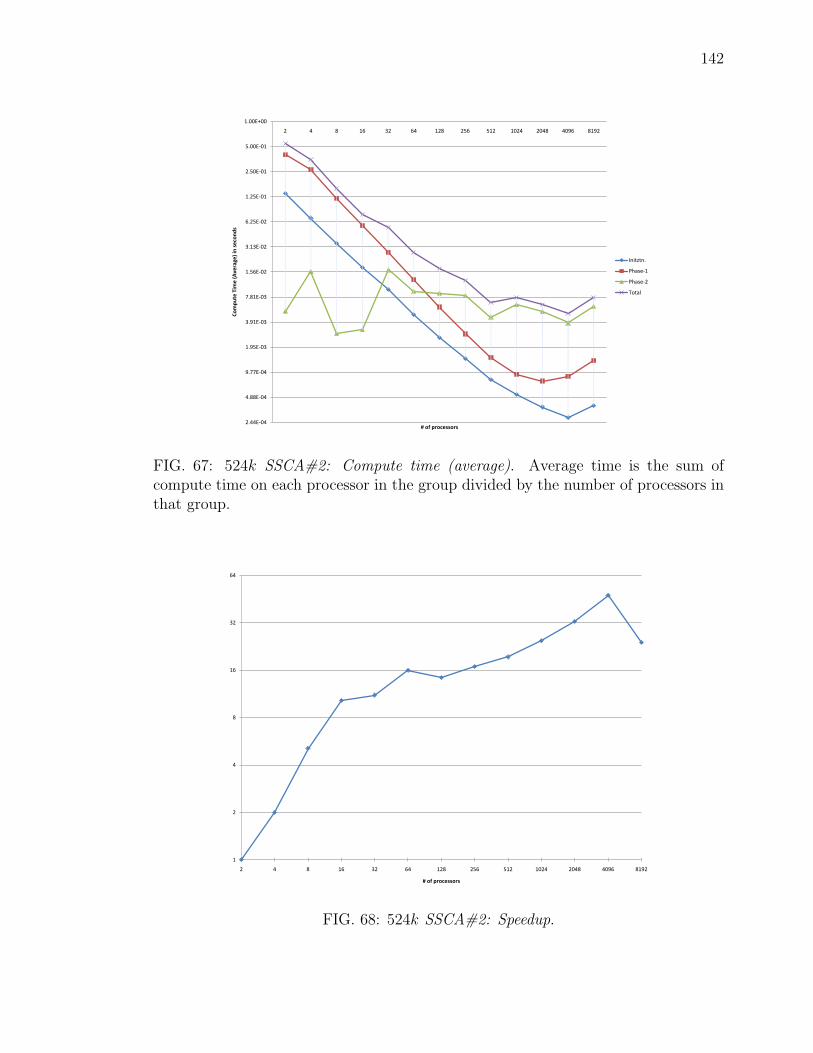
142
2.44E-04
4.88E-04
9.77E-04
1.95E-03
3.91E-03
7.81E-03
1.56E-02
3.13E-02
6.25E-02
1.25E-01
2.50E-01
5.00E-01
1.00E+00
2 4 8 16 32 64 128 256 512 1024 2048 4096 8192
Co
mp
ute
Tim
e (
Ave
rage
) in
se
con
ds
# of processors
Initztn.
Phase-1
Phase-2
Total
FIG. 67: 524k SSCA#2: Compute time (average). Average time is the sum ofcompute time on each processor in the group divided by the number of processors inthat group.
1
2
4
8
16
32
64
2 4 8 16 32 64 128 256 512 1024 2048 4096 8192
# of processors
FIG. 68: 524k SSCA#2: Speedup.

143
0
10
20
30
40
50
60
70
80
90
100
2 4 8 16 32 64 128 256 512 1024 2048 4096 8192
(1)
%Ed
gecu
t=
Edge
cut
/ |E
| *
10
0
(2)
%C
ard
-P1
= |
M_P
has
e1
| /
|M
| *
10
0
# of processors
%EdgeCut
%Card-P1
FIG. 69: 524k SSCA#2: Cardinality after Phase-1.

144
V.4.4 Performance of Parallel Matching on Graphs from Applications
We will now provide experimental results of the parallel approximation algorithm for
the graphs representing matrices selected randomly from the University of Florida
Matrix Collection. Communication in Algorithm ParallelMatchingFrame-
work is directly dependent on the edge-cut for a given number of partitions. There-
fore, in order to predict the performance of the algorithm, we will present the edgecut,
for different numbers of partitions, as a percentage of the total number of edges for
a graph in Figure 70. It can be observed that edgecut for Rajat31 and Hamrle3 are
under ten per cent, but are relatively high for ASIC-680k, Audikw1 and Cage14.
0.00
10.00
20.00
30.00
40.00
50.00
60.00
2 4 8 16 32 64 128 256 512 1024 2048 4096 8192
Perc
enta
ge =
Ed
geC
ut
/ N
um
ber
of
edge
s
# of partitions
ASIC-680k
Audikw1
Cage14
Hamrle3
Ldoor
Rajat31
FIG. 70: Edgecut for graphs from applications. Percentage of edges cut is a ratio ofedgecut to the number of edges in the graph.
We will now present the execution time on Franklin for up to 4, 096 processors
(Figures 71 and 72). There are a few missing data points in the plots when a
particular problem could not be solved for a particular number of processors. For
example, Cage14 could not be solved for 512 processors. A major cause of failure
has the restriction on the number of messages that a processor can send. Another
cause of failure has been the limitation on memory usage, usually during the graph
partitioning phase.
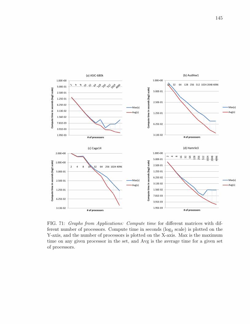
145
1.95E-03
3.91E-03
7.81E-03
1.56E-02
3.13E-02
6.25E-02
1.25E-01
2.50E-01
5.00E-01
1.00E+00
Co
mp
ute
tim
e in
se
con
ds
(lo
g2 s
cale
)
# of processors
(a) ASIC-680k
Max(s)
Avg(s)
3.13E-02
6.25E-02
1.25E-01
2.50E-01
5.00E-01
1.00E+00
16 32 64 128 256 512 1024 2048 4096
Co
mp
ute
tim
e in
se
con
ds
(lo
g2 s
cale
)
# of processors
(b) Audikw1
Max(s)
Avg(s)
3.13E-02
6.25E-02
1.25E-01
2.50E-01
5.00E-01
1.00E+00
2.00E+00
2 4 8 16 32 64 256 1024 4096
Co
mp
ute
tim
e in
se
con
ds
(lo
g2 s
cale
)
# of processors
(c) Cage14
Max(s)
Avg(s)
1.95E-03
3.91E-03
7.81E-03
1.56E-02
3.13E-02
6.25E-02
1.25E-01
2.50E-01
5.00E-01
1.00E+00
2 4 8
16
32
64
12
8
25
6
51
2
10
24
20
48
40
96
Co
mp
ute
tim
e in
se
con
ds
(lo
g2 s
cale
)
# of processors
(d) Hamrle3
Max(s)
Avg(s)
FIG. 71: Graphs from Applications: Compute time for different matrices with dif-ferent number of processors. Compute time in seconds (log2 scale) is plotted on theY-axis, and the number of processors is plotted on the X-axis. Max is the maximumtime on any given processor in the set, and Avg is the average time for a given setof processors.

146
7.81E-03
1.56E-02
3.13E-02
6.25E-02
1.25E-01
2.50E-01
5.00E-01
1.00E+00
2.00E+00
2 4 8
16
32
64
12
8
25
6
51
2
10
24
20
48
40
96
Co
mp
ute
tim
e in
se
con
ds
(lo
g2 s
clae
)
# of processors
(a) Ldoor
Max(s)
Avg(s)
1.95E-03
3.91E-03
7.81E-03
1.56E-02
3.13E-02
6.25E-02
1.25E-01
2.50E-01
5.00E-01
1.00E+00
2.00E+00
2 4 8
16
32
64
12
8
25
6
51
2
10
24
20
48
40
96
Co
mp
ute
tim
e in
se
con
ds
(lo
g2 s
cale
)
# of processors
(b) Rajat31
Max(s)
Avg(s)
3.91E-03
7.81E-03
1.56E-02
3.13E-02
6.25E-02
1.25E-01
2.50E-01
5.00E-01
1.00E+00
2 4 8
16
32
64
12
8
25
6
51
2
10
24
20
48
40
96
Co
mp
ute
tim
e in
se
con
ds
(lo
g2 s
cale
)
# of processors
(c) SSCA#2-1
Max(s)
Avg(s)
1.56E-02
3.13E-02
6.25E-02
1.25E-01
2.50E-01
5.00E-01
1.00E+00
2.00E+00
4.00E+00
8.00E+00
1.60E+01C
om
pu
te t
ime
in s
eco
nd
s (l
og2
sca
le)
# of processors
(d) SSCA#2-2
Max(s)
Avg(s)
FIG. 72: Graphs from Applications: Compute time for different matrices with dif-ferent number of processors. Compute time in seconds (logarithmic scale with basetwo) is plotted on the Y-axis, and the number of processors is plotted on the X-axis.Max is the maximum time on any given processor in the set, and Avg is the averagetime for a given number of processors. The Figure also has results for two instancesof SSCA#2 graphs.

147
V.4.5 Analysis of Communication
In this section we will present details about the communication involved in computing
the approximation matchings. The total number of messages is bounded between
twice and thrice the edgecut. This is plotted in Figures 73 and 74.
0.00E+00
5.00E+04
1.00E+05
1.50E+05
2.00E+05
2.50E+05
3.00E+05
3.50E+05
4.00E+05
4.50E+05
5.00E+05
(a) ASIC-680k
Msg Sent
2 X EdgeCut
3 X Edgecut
0.00E+00
1.00E+07
2.00E+07
3.00E+07
4.00E+07
5.00E+07
6.00E+07
7.00E+07
8.00E+07
9.00E+07
1.00E+08
16 32 64 128 256 512 1024 2048 4096
(b) Audikw1
Msg Sent
2 X EdgeCut
3 X Edgecut
0.00E+00
5.00E+06
1.00E+07
1.50E+07
2.00E+07
2.50E+07
3.00E+07
3.50E+07
Axi
s Ti
tle
(c) Cage14
Msg Sent
2 X EdgeCut
3 X Edgecut
0.00E+00
2.00E+05
4.00E+05
6.00E+05
8.00E+05
1.00E+06
1.20E+06
2 4 8
16
32
64
12
8
25
6
51
2
10
24
20
48
40
96
(d) Hamrle3
Msg Sent
2 X EdgeCut
3 X Edgecut
FIG. 73: Communication. Total number of messages sent are bounded between twiceand thrice the edge cut.
Message Bundling
Message bundling greatly influences performance. Here we show the performance of
the message bundling that we have implemented only for Phase 1 of the algorithm.
It can be observed that the number of messages that can be bundled in Phase 1,
MB can be given by the relation (|Edgecut| ≤ MB ≤ 2|Edgecut|). We also know
that a lower bound on the total number of messages sent is given by (2|EdgeCut|).Thus, in a best possible scenario all the messages can be bundled resulting in at most
O(P 2) messages, where P is the number of processors. The worst case results from
a situation when every processor sends messages to every other processor. However,
for graphs with good partitions the communication can be limited to a few processors
resulting in a O(P ) bound on the number of messages. In Figures 75 and 76, we
show the percentage of messages that could be bundled, and the actual number of
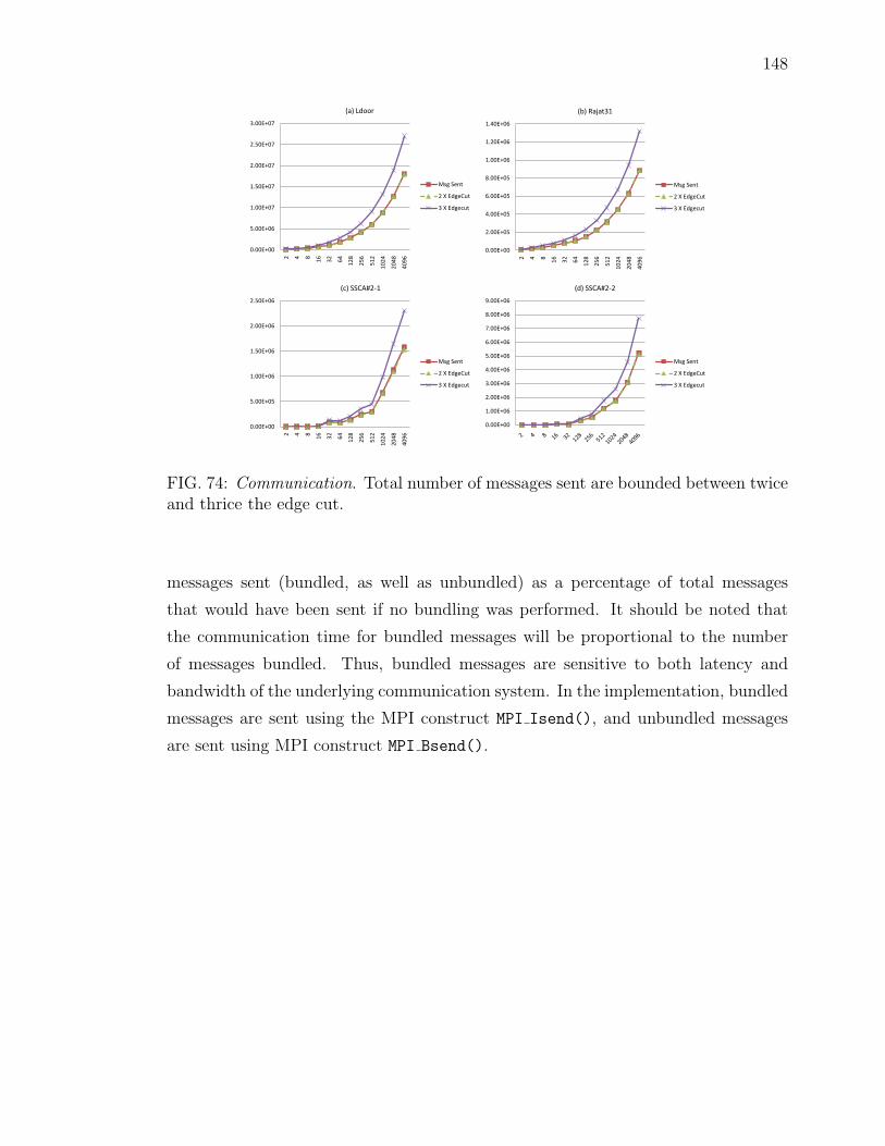
148
0.00E+00
5.00E+06
1.00E+07
1.50E+07
2.00E+07
2.50E+07
3.00E+07
2 4 8
16
32
64
12
8
25
6
51
2
10
24
20
48
40
96
(a) Ldoor
Msg Sent
2 X EdgeCut
3 X Edgecut
0.00E+00
2.00E+05
4.00E+05
6.00E+05
8.00E+05
1.00E+06
1.20E+06
1.40E+06
2 4 8
16
32
64
12
8
25
6
51
2
10
24
20
48
40
96
(b) Rajat31
Msg Sent
2 X EdgeCut
3 X Edgecut
0.00E+00
5.00E+05
1.00E+06
1.50E+06
2.00E+06
2.50E+06
2 4 8
16
32
64
12
8
25
6
51
2
10
24
20
48
40
96
(c) SSCA#2-1
Msg Sent
2 X EdgeCut
3 X Edgecut
0.00E+00
1.00E+06
2.00E+06
3.00E+06
4.00E+06
5.00E+06
6.00E+06
7.00E+06
8.00E+06
9.00E+06
(d) SSCA#2-2
Msg Sent
2 X EdgeCut
3 X Edgecut
FIG. 74: Communication. Total number of messages sent are bounded between twiceand thrice the edge cut.
messages sent (bundled, as well as unbundled) as a percentage of total messages
that would have been sent if no bundling was performed. It should be noted that
the communication time for bundled messages will be proportional to the number
of messages bundled. Thus, bundled messages are sensitive to both latency and
bandwidth of the underlying communication system. In the implementation, bundled
messages are sent using the MPI construct MPI Isend(), and unbundled messages
are sent using MPI construct MPI Bsend().
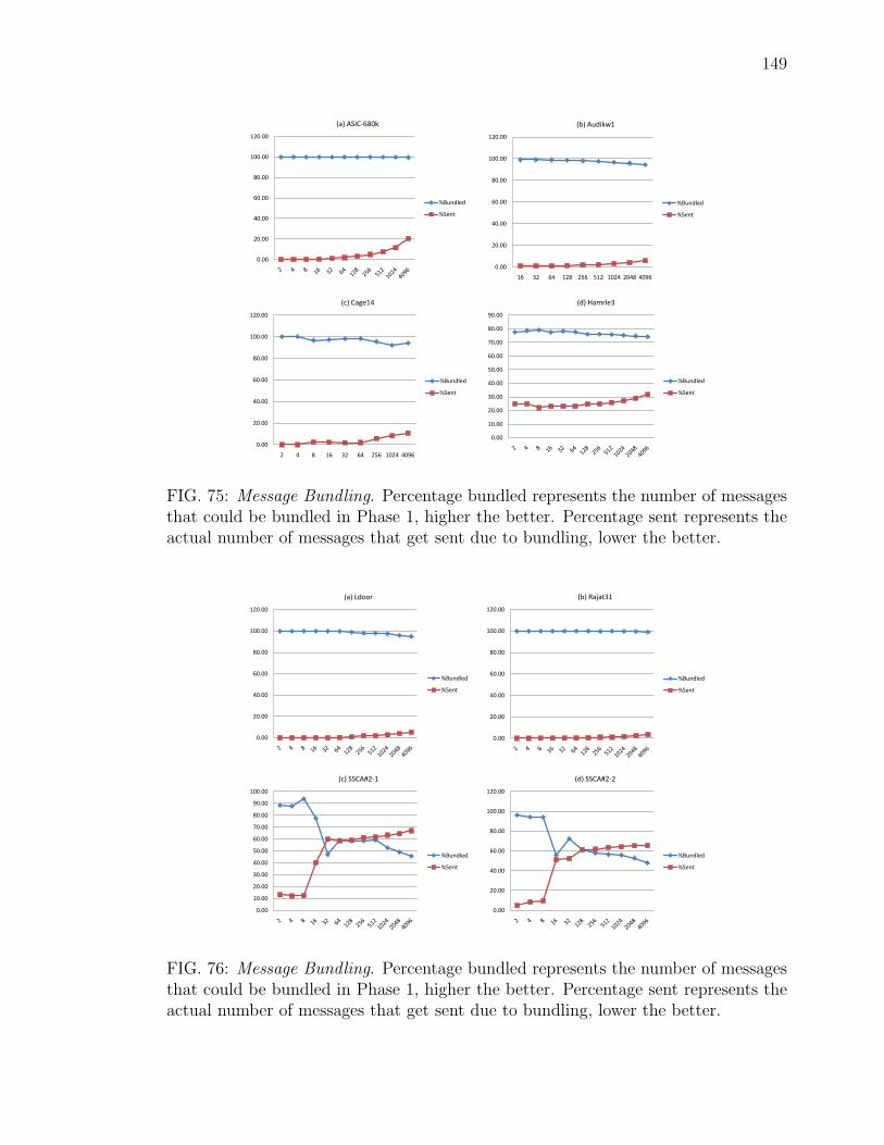
149
0.00
20.00
40.00
60.00
80.00
100.00
120.00
(a) ASIC-680k
%Bundled
%Sent
0.00
20.00
40.00
60.00
80.00
100.00
120.00
16 32 64 128 256 512 1024 2048 4096
(b) Audikw1
%Bundled
%Sent
0.00
20.00
40.00
60.00
80.00
100.00
120.00
2 4 8 16 32 64 256 1024 4096
(c) Cage14
%Bundled
%Sent
0.00
10.00
20.00
30.00
40.00
50.00
60.00
70.00
80.00
90.00
(d) Hamrle3
%Bundled
%Sent
FIG. 75: Message Bundling. Percentage bundled represents the number of messagesthat could be bundled in Phase 1, higher the better. Percentage sent represents theactual number of messages that get sent due to bundling, lower the better.
0.00
20.00
40.00
60.00
80.00
100.00
120.00
(a) Ldoor
%Bundled
%Sent
0.00
20.00
40.00
60.00
80.00
100.00
120.00
(b) Rajat31
%Bundled
%Sent
0.00
10.00
20.00
30.00
40.00
50.00
60.00
70.00
80.00
90.00
100.00
(c) SSCA#2-1
%Bundled
%Sent
0.00
20.00
40.00
60.00
80.00
100.00
120.00
(d) SSCA#2-2
%Bundled
%Sent
FIG. 76: Message Bundling. Percentage bundled represents the number of messagesthat could be bundled in Phase 1, higher the better. Percentage sent represents theactual number of messages that get sent due to bundling, lower the better.
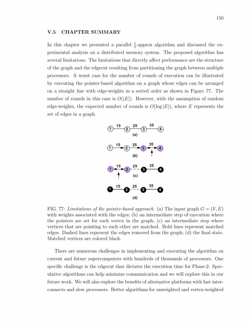
150
V.5 CHAPTER SUMMARY
In this chapter we presented a parallel 12-approx algorithm and discussed the ex-
perimental analysis on a distributed memory system. The proposed algorithm has
several limitations. The limitations that directly affect performance are the structure
of the graph and the edgecut resulting from partitioning the graph between multiple
processors. A worst case for the number of rounds of execution can be illustrated
by executing the pointer-based algorithm on a graph whose edges can be arranged
on a straight line with edge-weights in a sorted order as shown in Figure 77. The
number of rounds in this case is O(|E|). However, with the assumption of random
edge-weights, the expected number of rounds is O(log |E|), where E represents the
set of edges in a graph.
FIG. 77: Limitations of the pointer-based approach. (a) The input graph G = (V,E)with weights associated with the edges; (b) an intermediate step of execution wherethe pointers are set for each vertex in the graph; (c) an intermediate step wherevertices that are pointing to each other are matched. Bold lines represent matchededges. Dashed lines represent the edges removed from the graph; (d) the final state.Matched vertices are colored black.
There are numerous challenges in implementing and executing the algorithm on
current and future supercomputers with hundreds of thousands of processors. One
specific challenge is the edgecut that dictates the execution time for Phase-2. Spec-
ulative algorithms can help minimize communication and we will explore this in our
future work. We will also explore the benefits of alternative platforms with fast inter-
connects and slow processors. Better algorithms for unweighted and vertex-weighted

151
matching problems will also be explored in future work.
Acknowledgements: This research used resources of the National Energy Research
Scientific Computing Center, which is supported by the Office of Science of the U.S.
Department of Energy under Contract No. DE-AC02-05CH11231.
152
CHAPTER VI
CONCLUSIONS AND FUTURE WORK
“Art is never finished, only abandoned.” - Leonardo da Vinci
The work completed in this thesis lays the groundwork for future research. The goals
for this research were broadly organized into theory, implementation and applications.
We were able to accomplish many of the goals we set for ourselves. The following
list provides a summary of the contributions from this work:
1. Theory:
• New framework for developing proof of correctness for vertex weighted
matchings;
• New 12-approx algorithms for vertex weighted matchings;
• New 23-approx algorithm for bipartite vertex weighted matchings;
2. Experiments:
• Open-source library of C++ routines to compute various kinds of match-
ings;
• Open-source library of C++ and MPI routines to compute approximate
matchings in parallel.
• Extensive experimental study of various (serial) matching algorithms, and
scalability study of 12-approx parallel algorithm with up to 8, 192 proces-
sors.
3. Applications:
• Study of applicability of vertex weighted matchings in solving the sparsest
basis problem.
• Study of approximation algorithms in sparse matrix computations.

153
Constrained by time and priorities we have also left many questions unanswered.
Some of the important open problems that will be addressed in the future work
include
• How to provide a proof of correctness for 23-approx algorithm LocalT-
woThird?
• Is a 23-approx algorithm possible for vertex weighted matching in general
graphs?
• Is a 34-approx algorithm possible for vertex weighted matching in bipartite
and/or general graphs?
VI.1 FUTURE WORK
Preliminary work on a parallel approximate matching was completed as part of this
research. The need for efficient parallel implementations has never been greater than
now. As part of our future work we plan to continue to improve the current im-
plementation, develop new algorithms - exact as well as approximate, and conduct
scalability studies on different parallel architectures. Some specific goals for imme-
diate future include:
• Conduct scalability studies on IBM Bluegene/P system at Argonne Leadership
Computing Facility (ALCF), at the Argonne National Laboratory.
• Conduct scalability studies on SiCortex 5832 system Green at Rosen Center
for Advanced Computing, Purdue University.
• Study impact on performance from different partitioning schemes.

154
BIBLIOGRAPHY
[1] Ahuja, R. K., Magnanti, T. L., and Orlin, J. B. Network Flows: Theory,
Algorithms, and Applications. Prentice Hall, 1993.
[2] Ahuja, R. K., and Orlin, J. B. A faster algorithm for the inverse spanning
tree problem. J. Algorithms 34, 1 (2000), 177–193.
[3] Auden, W. H., and Kronenberger, L. The Viking Book of Aphorisms, A
Personal Selection. Dorset Press, 1981.
[4] Avis, D. A survey of heuristics for the weighted matching problem. Network
13 (1983), 475–493.
[5] Bader, D., and Madduri, K. Design and implementation of the hpcs graph
analysis benchmark on symmetric multiprocessors. In Lecture Notes in Com-
puter Science (2005), vol. 3769, pp. 465–476.
[6] Bader, D. A. Petascale Computing: Algorithms and Applications. Chapman
and Hall/CRC, New York, NY, USA, 2007.
[7] Bagherzadeh, N., and Hawk, K. Parallel implementation of the auction
algorithm on the intel hypercube. Parallel Processing Symposium, 1992. Pro-
ceedings., Sixth International (Mar 1992), 443–447.
[8] Ball, M., Magnanti, T., Monma, C., and Nemhauser, G. Network
Models, Handbooks in Operations Research and Management Science, vol. 7.
North Holland Press, Amsterdam, 1995, ch. Matching, pp. 135–224.
[9] Ball, M., Magnanti, T., Monma, C., and Nemhauser, G. Network Mod-
els, Handbooks in Operations Research and Management Science, vol. 7. North
Holland Press, Amsterdam, 1995, ch. Applications of Network Optimization.
[10] Batagelj, V., and Mrvar, A. Pajek - program for large network analysis.
Connections 21 (1998), 47–57.
[11] Bell, C. E. Weighted matching with vertex weights: An application to
scheduling training sessions in nasa space shuttle cockpit simulators. Euro-
pean Journal of Operational Research 73, 3 (March 1994), 443–449. available at
http://ideas.repec.org/a/eee/ejores/v73y1994i3p443-449.html.

155
[12] Bertsekas, D. P., and Castanon, D. A. Parallel synchronous and asyn-
chronous implementations of the auction algorithm. Parallel Computing 17, 6-7
(1991), 707–732.
[13] Bertsekas, D. P., and David A. Casta n. A generic auction algorithm
for the minimum cost network flow problem. Comput. Optim. Appl. 2, 3 (1993),
229–260.
[14] Bertsekas, D. P., and David A. Casta n. Parallel primal-dual methods
for the minimum cost flow problem. Comput. Optim. Appl. 2, 4 (1993), 317–336.
[15] Bisseling, R. H. Parallel Scientific Computation: A Structured Approach
Using BSP and MPI. Oxford University Press, 2004.
[16] Chan, A., Dehne, F., Bose, P., and Latzel, M. Coarse grained parallel
algorithms for graph matching. Parallel Comput. 34, 1 (2008), 47–62.
[17] Cheatham, T., Fahmy, A., Stefanescu, D. C., and Valiant, L. G.
Bulk synchronous parallel computing-a paradigm for transportable software. In
HICSS ’95: Proceedings of the 28th Hawaii International Conference on System
Sciences (HICSS’95) (Washington, DC, USA, 1995), IEEE Computer Society,
p. 268.
[18] Cohen, N., and Brassil, J. A parallel pruning technique for highly asym-
metric assignment problems. IEEE Trans. Parallel Distrib. Syst. 11, 6 (2000),
550–558.
[19] Cormen, T. H., Leiserson, C. E., Rivest, R. L., and Stein, C. Intro-
duction to Algorithms, 2nd ed. The MIT Press, 2001.
[20] Dehne, F., Fabri, A., and Rau-Chaplin, A. Scalable parallel geometric
algorithms for coarse grained multicomputers. In SCG ’93: Proceedings of the
ninth annual symposium on Computational geometry (New York, NY, USA,
1993), ACM, pp. 298–307.
[21] Dıaz, J., Mitsche, D., and Perez-Gimenez, X. On the connectivity of
dynamic random geometric graphs. In SODA ’08: Proceedings of the nineteenth
annual ACM-SIAM symposium on Discrete algorithms (Philadelphia, PA, USA,
2008), Society for Industrial and Applied Mathematics, pp. 601–610.
156
[22] Dıaz, J., Penrose, M. D., Petit, J., and Serna, M. Convergence theo-
rems for some layout measures on random lattice and random geometric graphs.
Comb. Probab. Comput. 9, 6 (2000), 489–511.
[23] Dıaz, J., Penrose, M. D., Petit, J., and Serna, M. Approximating
layout problems on random geometric graphs. J. Algorithms 39, 1 (2001), 78–
116.
[24] Drake, D. E., and Hougardy, S. A simple approximation algorithm for
the weighted matching problem. Inf. Process. Lett. 85, 4 (2003), 211–213.
[25] Duff, I. S., and Koster, J. On algorithms for permuting large entries to the
diagonal of a sparse matrix. SIAM J. Matrix Anal. Appl. 22, 4 (2000), 973–996.
[26] Duff, I. S., and Pralet, S. Strategies for scaling and pivoting for sparse
symmetric indefinite problems. SIAM J. Matrix Anal. Appl. 27, 2 (2005), 313–
340.
[27] Fischer, T., Goldberg, A. V., Haglin, D. J., and Plotkin, S. Approx-
imating matchings in parallel. Inf. Process. Lett. 46, 3 (1993), 115–118.
[28] Gabow, H. N. An efficient implementation of edmonds’ algorithm for maxi-
mum matching on graphs. J. ACM 23, 2 (1976), 221–234.
[29] Galil, Z. Efficient algorithms for finding maximum matching in graphs. ACM
Comput. Surv. 18, 1 (1986), 23–38.
[30] Giaccone, P., Shah, D., and Prabhakar, B. An implementable parallel
scheduler for input-queued switches. In HOTI ’01: Proceedings of the The Ninth
Symposium on High Performance Interconnects (HOTI ’01) (Washington, DC,
USA, 2001), IEEE Computer Society, p. 9.
[31] Glover, F., and Laguna, M. Tabu search. In Modern Heuristic Techniques
for Combinatorial Problems (Oxford, England, 1993), C. Reeves, Ed., Blackwell
Scientific Publishing.
[32] Goel, A., Rai, S., and Krishnamachari, B. Sharp thresholds for monotone
properties in random geometric graphs. In STOC ’04: Proceedings of the thirty-
sixth annual ACM symposium on Theory of computing (New York, NY, USA,
2004), ACM, pp. 580–586.

157
[33] Hendrickson, B. Combinatorial scientific computing: The role of discrete
algorithms in computational science and engineering, 2003.
[34] Hendrickson, B., and Pothen, A. Combinatorial scientific computing:
The enabling power of discrete algorithms in computational science. In Pro-
ceedings of the 7th International Meeting on High Performance Computing for
Computational Science (VECPAR’06) (2006), Springer-Verlag.
[35] Hochbaum, D. S., Ed. Approximation algorithms for NP-hard problems. PWS
Publishing Co., Boston, MA, USA, 1997.
[36] Hoepman, J.-H. Simple distributed weighted matchings. CoRR
cs.DC/0410047 (2004).
[37] Hopcroft, J., and Karp, R. A n52 algorithm for maximum matchings in
bipartite graphs. SIAM J. Comput. 2 (1973), 225–231.
[38] Hougardy, S., and Vinkemeier, D. E. Approximating weighted matchings
in parallel. Inf. Process. Lett. 99, 3 (2006), 119–123.
[39] Karpinski, M., and Rytter, W. Fast parallel algorithms for graph matching
problems. Oxford University Press, Inc., New York, NY, USA, 1998.
[40] Karypis, G., and Kumar, V. Analysis of multilevel graph partitioning. In
Supercomputing ’95: Proceedings of the 1995 ACM/IEEE conference on Super-
computing (CDROM) (New York, NY, USA, 1995), ACM, p. 29.
[41] Karypis, G., and Kumar, V. A fast and high quality multilevel scheme for
partitioning irregular graphs. SIAM J. Sci. Comput. 20, 1 (1998), 359–392.
[42] Keyes, D. A science-based case for large-scale simulation, the scales report,
2003. (http://www.pnl.gov/scales/).
[43] Kuhn, H. W. The Hungarian method for the assignment problem. Naval
Research Logistic Quarterly 2 (1955), 83–97.
[44] Kumar, V., Grama, A., Gupta, A., and Karypis, G. Introduction to
parallel computing: design and analysis of algorithms. Benjamin-Cummings
Publishing Co., Inc., Redwood City, CA, USA, 1994.

158
[45] Lawler, E. Combinatorial Optimization: Networks and Matroids. Dover Pub-
lications, Mineola, New York, 1976.
[46] Li, X. S., and Demmel, J. W. Making sparse gaussian elimination scalable
by static pivoting. In Supercomputing ’98: Proceedings of the 1998 ACM/IEEE
conference on Supercomputing (CDROM) (Washington, DC, USA, 1998), IEEE
Computer Society, pp. 1–17.
[47] Lotker, Z., Patt-Shamir, B., and Rosen, A. Distributed approximate
matching. In PODC ’07: Proceedings of the twenty-sixth annual ACM sympo-
sium on Principles of distributed computing (New York, NY, USA, 2007), ACM,
pp. 167–174.
[48] Lovasz, L. Matching Theory (North-Holland mathematics studies). Elsevier
Science Ltd, 1986.
[49] Luby, M. A simple parallel algorithm for the maximal independent set problem.
In STOC ’85: Proceedings of the seventeenth annual ACM symposium on Theory
of computing (New York, NY, USA, 1985), ACM, pp. 1–10.
[50] Manne, F., and Bisseling, R. H. A parallel approximation algorithm for the
weighted maximum matching problem. In The Seventh International Conference
on Parallel Processing and Applied Mathematics (2007), pp. 708–717.
[51] McKeown, N. The islip scheduling algorithm for input-queued switches.
IEEE/ACM Trans. Netw. 7, 2 (1999), 188–201.
[52] McKeown, N., Anantharam, V., and Walrand, J. C. Achieving 100%
throughput in an input-queued switch. In INFOCOM (1996), pp. 296–302.
[53] Mehta, A., Saberi, A., Vazirani, U., and Vazirani, V. Adwords and
generalized online matching. J. ACM 54, 5 (2007), 22.
[54] Monien, B., Preis, R., and Diekmann, R. Quality matching and local
improvement for multilevel graph-partitioning. Parallel Comput. 26, 12 (2000),
1609–1634.
[55] Mulmuley, K., Vazirani, U. V., and Vazirani, V. V. Matching is as
easy as matrix inversion. In STOC ’87: Proceedings of the nineteenth annual

159
ACM conference on Theory of computing (New York, NY, USA, 1987), ACM,
pp. 345–354.
[56] Nong, G., Muppala, J. K., and Hamdi, M. Performance analysis of input
queueing atm switches with parallel iterative matching scheduling. In Proceed-
ings of the IFIP TC6 WG6.3/WG6.4 Fifth International Workshop on Perfor-
mance Modelling and Evaluation of ATM Networks (Deventer, The Netherlands,
The Netherlands, 2000), Kluwer, B.V., pp. 189–207.
[57] Papadimitriou, C. H., and Steiglitz, K. Combinatorial optimization:
algorithms and complexity. Prentice-Hall, Inc., Upper Saddle River, NJ, USA,
1982.
[58] Penrose, M. Random Geometric Graphs. Oxford University Press, 2003.
[59] Pettie, S., and Sanders, P. A simpler linear time 23− ε approximation for
maximum weight matching. Inf. Process. Lett. 91, 6 (2004), 271–276.
[60] Pinar, A., Chow, E., and Pothen, A. Combinatorial algorithms for com-
puting column space bases that have sparse inverses. Electronic Transactions
on Numerical Analysis 22 (2006), 122–145.
[61] Polymenakos, L. C., and Bertsekas, D. P. Parallel shortest path auction
algorithms. Parallel Comput. 20, 9 (1994), 1221–1247.
[62] Pothen, A. Sparse null bases and marriage theorems. PhD thesis, Cornell
University, Ithaca, NY, USA, 1984.
[63] Pothen, A., and Fan, C.-J. Computing the block triangular form of a sparse
matrix. ACM Trans. Math. Softw. 16, 4 (1990), 303–324.
[64] Preis, R. Linear time 12-approximation algorithm for maximum weighted
matching in general graphs. In 16th Ann. Symp. on Theoretical Aspects of
Computer Science (STACS) (1999), pp. 259–269.
[65] Schenk, O., Wachter, A., and Hagemann, M. Matching-based pre-
processing algorithms to the solution of saddle-point problems in large-scale
nonconvex interior-point optimization. Comput. Optim. Appl. 36, 2-3 (2007),
321–341.

160
[66] Schrijver, A. Combinatorial Optimization - Polyhedra and Efficiency.
Springer, 2003.
[67] Snir, M., and Otto, S. MPI-The Complete Reference: The MPI Core. MIT
Press, Cambridge, MA, USA, 1998.
[68] Spencer, T. Parallel approximate matching. System Sciences, 1993, Pro-
ceeding of the Twenty-Sixth Hawaii International Conference on ii (Jan 1993),
293–297 vol.2.
[69] Spencer, T. H., and Mayr, E. W. Node weighted matching. In Proceedings
of the 11th Colloquium on Automata, Languages and Programming (London,
UK, 1984), Springer-Verlag, pp. 454–464.
[70] Storoy, S., and Sorevik, T. Massively parallel augmenting path algorithms
for the assignment problem. Computing 59, 1 (1997), 1–16.
[71] Tabatabaee, V., Georgiadis, L., and Tassiulas, L. Qos provisioning and
tracking fluid policies in input queueing switches. IEEE/ACM Trans. Netw. 9,
5 (2001), 605–617.
[72] Uehara, R., and Chen, Z.-Z. Parallel approximation algorithms for max-
imum weighted matching in general graphs. Inf. Process. Lett. 76, 1-2 (2000),
13–17.
[73] Vazirani, V. V. A theory of alternating paths and blossoms for proving cor-
rectness of the o(√V E) general graph matching algorithm. Tech. rep., Ithaca,
NY, USA, 1989.
[74] Vinkemeier, D. E. D., and Hougardy, S. A linear-time approximation
algorithm for weighted matchings in graphs. ACM Trans. Algorithms 1, 1 (2005),
107–122.
[75] Wein, J., and Zenios, S. Massively parallel auction algorithms for the assign-
ment problem. Frontiers of Massively Parallel Computation, 1990. Proceedings.,
3rd Symposium on the (Oct 1990), 90–99.
[76] Wolsey, L. Integer Programming. Wiley-Interscience Publication, John Wiley
and Sons, 1998.
Related Documents