Algorithms for separable nonlinear least squares with ...

J Glob Optim (2007) 38:201–213DOI 10.1007/s10898-006-9071-7

O R I G I NA L PA P E R

Algorithms for separable nonlinear least squares withapplication to modelling time-resolved spectra

Katharine M. Mullen · Mikas Vengris ·Ivo H. M. van Stokkum

Received: 15 December 2005 / Accepted: 27 July 2006 / Published online: 29 March 2007© Springer Science+Business Media B.V. 2007

Abstract The multiexponential analysis problem of fitting kinetic models to time-resolved spectra is often solved using gradient-based algorithms that treat the spectralparameters as conditionally linear. We make a comparison of the two most-appliedsuch algorithms, alternating least squares and variable projection. A numerical studyexamines computational efficiency and linear approximation standard error estimates.A new derivation of the Fisher information matrix under the full Golub-Pereyra gra-dient allows a numerical comparison of parameter precision under variable projec-tion variants. Under the criteria of efficiency, quality of standard error estimates andparameter precision, we conclude that the Kaufman variable projection techniqueperforms well, while techniques based on alternating least squares have significantdisadvantages for application in the problem domain.

Keywords Separable nonlinear models · Time-resolved spectra · Variable projec-tion · Alternating least squares · Fisher information

1 Introduction

State-of-the-art dynamical experiments in photophysics result in huge datasets oftime-resolved spectra. Such data represent a spectral property associated with a photo-physical system at m times and n wavelengths by an m × n matrix �. For typical

K. M. Mullen (B) · I. H. M. van StokkumDepartment of Physics and Astronomy, Vrije Universiteit Amsterdam,De Boelelaan 1081, 1081 HV Amsterdam, The Netherlandse-mail: [email protected]

I. H. M. van Stokkume-mail: [email protected]

M. VengrisDepartment of Quantum Electronics, Vilnius University,Sauletekio 10, LT10223 Vilnius, Lithuaniae-mail: [email protected]

202 J Glob Optim (2007) 38:201–213

experiments, m and n are of order 103. With such an overwhelming amount of dataa model-based analysis is mandatory for interactive validation of hypotheses regard-ing physicochemical mechanisms of the underlying system. The basic kinetic modelapplied to � is

� = CET + � =ncomp∑

l=1

cleTl + � =

ncomp∑

l=1

exp(−φlt)eTl + � (1)

where column l of C represents the concentration in time of a spectrally distinctsubsystem contributing a component to �, column l of E describes the spectrum ofthat subsystem, ncomp is the number of contributing components, and � is a residualmatrix with spherical Gaussian distribution. Elements of �, C, and E are in R, butno other constraints are enforced in the general case. Estimation of parameters φ

under least-squares criteria is thus a multiexponential analysis problem, the difficultyof which is well-known [3,28]. Problems in multiexponential analysis are ubiquitous inphysics applications in which data is modelled by the solution of first-order differentialequations, as Istratov and Vyvenko review [18].

The estimation problem associated with estimating φ in Model (1) under least-squares criteria is

Minimize ‖ vec(C(φ)ET − �) ‖2, (2)

which is an instance of the unconstrained optimization problem Minimize γ (x), x ∈ Rn

in which the variables separate into x = (y, z) with y ∈ Rp, z ∈ R

q, p + q = n, and thesubproblem

Minimize γ (y, z), (3)

is easy to solve for fixed z, and, more generally, of the bilinear programming prob-lem [1,9,17]. Separating the parameters reduces the n-dimensional unconstrainedoptimization problem to the q-dimensional unconstrained problem

Minimize γ (y(z), z), (4)

where y(z) denotes a solution of (3). In the considered application y(z) is solved asthe solution of a linear-least squares problem for fixed z, there are hundreds moreconditionally linear parameters y than intrinsically nonlinear parameters z, and lin-ear approximation standard error estimates about estimates for z are desired formodel validation. These structural features of the problem and the requirement forstandard error estimates make gradient-based algorithms that exploit the conditionallinearity of Problem (2) attractive, though a variety of other algorithms, e.g., Branchand Cut methods [2], evolutionary search [35], or Prony-based methods [22] are alsoapplicable. The development of gradient-based methods for the separable Problem(4) is chronicled in, e.g., [13,23,29]. The gradient-based algorithms most commonlyapplied to Problem (2) are based on alternating least squares [6,7,10,19] or variableprojection [14,21,33]. These techniques have been numerically compared in [4] for asingle nonlinear parameter, and in [11] for small datasets (<70 datapoints). Theoret-ical comparisons of gradient-based methods for separable problems have been madein [4,8,20,23,27]. In this paper we extend the literature comparing gradient-basedmethods for separable nonlinear optimization problems to Problem (2), the centralestimation problem in fitting parametric kinetic models to time-resolved spectra.

A comparison of techniques in the photophysical modelling application domainis desirable due to the difficulty of Problem (2), which is not identifiable [34] and

J Glob Optim (2007) 38:201–213 203

sensitive to starting values [24,30]. Convergence issues due to ill-conditioning whentwo or more decay rate parameters φl are close are well-known [22,25], and are par-tially dependent on the choice of gradient. The stochastic noise term contained in mea-sured � introduces a further source of difficulty by complicating the sum-of-squareerror parameter surface of φ with local minima. The performance of alternating leastsquares and variable projection variants is studied here in such a way as to expose thevulnerabilities and strengths of the algorithms in the face of these difficulties as theyoccur in typical photophysical model fitting problems. To the best of our knowledgethis is the first such comparison in the literature.

Alternating least squares and variable projection variants are presented in termsof their gradients in Sect. 2. The ability of the algorithms to deal with degeneracyin the case of similar decay rate parameters φl, φj is studied theoretically in Sect. 3by comparison of Fisher information matrices (FIM) associated with parameter esti-mates under variable projection variants. This Sect. contains a new derivation of theFIM under the full Golub-Pereyra variable projection functional. Sect. 4 discussesthe simulation of realistic datasets of time-resolved spectra to be used in numericalcomparison. A numerical study is made in Sect. 5 to highlight convergence issuesand sensitivity to starting values. Section 5.2 contains a numerical comparison of var-iable projection techniques using FIMs as rate constants vary in such a way to makeProblem (2) more nearly-degenerate.

2 Gradient-based algorithms for separable nonlinear least squares

Gradient-based algorithms for solution of Problem (2) estimate E as ET(φ) = C+�

where + is the Moore-Penrose pseudoinverse, so that Problem (2) may be written as

Minimize ‖ (I − C(φ)C+(φ))� ‖2 . (5)

The gradient-based techniques most often applied to Problem (5) are based on eitherthe alternating least squares (ALS) or variable projection functionals. ALS was intro-duced by Wold [36] as NIPALS and has a simple functional form which neglects thederivative of the pseudoinverse C+. The variable projection gradient (GP) makes useof the derivative of C+ due to Golub and Pereyra [15,16]. The approximation to thefull GP functional (KAUF) introduced by Kaufman [20] is more efficient to computeand for simple models has been shown to return nearly as precise parameter estimatesas the full functional [4,11].

In order to make clear the core differences between algorithms, we present ALS,KAUF and GP and a finite difference approximation of (I − C(φ)C+(φ))� in termsof the gradient in φ-space, using the notation of [4]. The derivative of C with respectto the nonlinear parameters is denoted Cφ = dC

dφT . Applying the QR decomposition,

C = QR = [Q1 Q2][R11 0]T , where Q is m × m and orthogonal and R is m × ncomp.Assuming C is of full column rank, C+ = R−1

11 QT1 . Then, where “convergence” is some

appropriate stopping criterion and the iteration subscript s is suppressed, we have

Algorithms ALS, KAUF, GP, NUM:1. Choose starting φ approximately2. For s := 1, 2 . . . until convergence doDetermine the gradient in φ-space according to:

204 J Glob Optim (2007) 38:201–213

NUM := finite difference approximation of d(I−CC+)dφ

�

GP := −Q2QT2 CφC+� − Q1R−T

11 CTφ Q2QT

2 �

KAUF := −Q2QT2 CφC+�

ALS := −CφC+�

φs+1 := step(φs, gradient, . . .)

In the presentation of the algorithms above, step refers to the method of determin-ing the step-size, which is not further discussed. This allows for a clear description andseparates the question of which step method is optimal from the differences betweenthe gradients.

For a numerical comparison, we consider two varieties of ALS differing in the stepmethod. The first (ALS-GN) makes a Gauss-Newton step given the ALS gradient.The second (ALS-LS) makes a Gauss-Newton step augmented by a line search untilthe sum-square error (SSE) is seen to increase. KAUF, GP, and NUM are consideredunder a Gauss-Newton step. Simulation studies indicate that for the numerical prob-lems considered in Sect. 5, replacement of the Gauss-Newton step with a Levenberg-Marquardt step does not appreciably alter the performance for any of the algorithmsconsidered.

Implementation is straightforward using library subroutines for QR decomposi-tion, finite difference derivatives, and nonlinear least squares. Such subroutines arefound, for instance, in the base and stats packages of the R language and environ-ment for statistical computing [26], where we base the implementation for numericalcomparison. An analytical expression for Cφ is used for models based on a sum-of-exponentials. Under more complicated models for C a finite difference approximationof Cφ is often desirable.

We now summarize some prior results comparing subsets of the algorithms underconsideration. Ruhe and Wedin [27] have shown that for starting φ close to the solu-tion, the asymptotic convergence rates of KAUF and GP are superlinear wheneverapplication of Gauss-Newton to the unseparated parameter set (φ + E) has a super-linear rate of convergence, and that ALS always has only a linear rate of convergence.Bates and Lindstrom [4] demonstrated that for a simple model having a single non-linear parameter the performance of KAUF and GP was similar. Gay and Kaufman[11] also performed a comparison of KAUF and GP on several small datasets, (<70data points), demonstrating that the time to compute KAUF was about 25% less thanthe time to compute GP for the range of problems considered.

3 Parameter precision under variable projection variants

The precision of nonlinear parameter estimates φ is a means of evaluating the perfor-mance of algorithms on Problem (2) of special interest on nearly-degenerate problems,i.e., when optimal estimates for two or more nonlinear parameters are close, so thatthe data are well-approximated by a lower-order sum-of-exponentials. Sect. 4.1 fur-ther elaborates the importance of parameter precision in solving nearly-degenerateproblems.

A means of quantifying the precision of a vector of parameter estimates is foundin the FIM. The structure of the FIM provides insight into contributions to parameterprecision, and FIMs may be numerically compared under different gradients, as in

J Glob Optim (2007) 38:201–213 205

Sect. 5.2. The resolution limit of exponential analysis has been oft-studied in termsof FIMs and other information-theoretic metrics, as discussed in [18]. Badu andBresler [3] have studied the connection between the stochastic stability of nonlin-ear least squares problems and the FIM with attention to separable problems such asProblem (2).

Definition 3.1 Where J is the gradient of the residual function with respect to thenonlinear parameters φ and the model error σ 2 is determined as σ 2 = SSE(φ)/df ,with df the degrees of freedom of the model, and where, as throughout, the noise �

is assumed to have spherical Gaussian distribution, the FIM M may be defined as

M = σ−2vec(J)Tvec(J) = σ−2M. (6)

When M is positive definite the covariance estimate of any unbiased estimator ofparameter vector φ is bounded below by the inverse of M (the Cramér-Rao Bound),so that

Cov[φ] ≥ M−1. (7)

We will now give functions for M under the variable projection algorithms KAUF andGP.

Proposition 3.1MKAUF = vec(Cφ)T(ETE ⊗ P)vec(Cφ). (8)

Proof JKAUF is given as

JKAUF = Q2QT2 CφC+� = PCφET , (9)

where P = Q2QT2 .

Writing JKAUF in vectorized form,

vec(JKAUF) = vec(PCφET) (10)

= (E ⊗ P)vec(Cφ). (11)

Then from [32],

MKAUF = vec(JKAUF)Tvec(JKAUF) (12)

= ((E ⊗ P)vec(Cφ))T((E ⊗ P)vec(Cφ)) (13)

= vec(Cφ)T(ETE ⊗ P)vec(Cφ). (14)

It is often convenient to consider M by entry Mij. This is

(MKAUF)ij = vec(Cφi)TETE ⊗ Pvec(Cφj), (15)

where vec(Cφi) is the vector representation of dCdφi

.

For a two column matrix C in which cl = exp(φl), vec(Cφ1) =(

g10

)and vec(Cφ2) =

(0g2

), where gi = −texp(−φit). For this case the expression for MKAUF simplifies to

(MKAUF)ij = εTi εjgT

i Pgj. (16)

206 J Glob Optim (2007) 38:201–213

Proposition 3.2 Writing MGP per entry,

(MGP)ij = (MKAUF)ij + vec(CTφi

)T(P�)(P�)T ⊗ C+(C+)Tvec(CTφj

). (17)

Proof The gradient JGP of the residuals with respect to the nonlinear parameterscontains the extra term Q1R−T

11 CTφ Q2QT

2 � as compared to JKAUF, so that

JGP = Q2QT2 CφC+� + Q1R−T

11 CTφ Q2QT

2 � (18)

= JKAUF + (C+)TCTφ P�. (19)

Vectorizing JGP,

vec(JGP) = (E ⊗ P)vec(Cφ) + (P�)T ⊗ (C+)Tvec(CTφ ), (20)

and vectorizing JTGP,

vec(JGP)T = vec(Cφ)T(ET ⊗ P) + vec(CTφ )T(P�) ⊗ C+. (21)

Then, writing MGP per entry,

(MGP)ij = (MKAUF)ij + vec(CTφi

)T(P�)(P�)T ⊗ C+(C+)Tvec(CTφj

). (22)

where we have used the orthogonality of JKAUF and (C+)TCφP�.For a two column matrix C in which cl = exp(φl), the expression for MGP simplifies

to(MGP)ij = (MKAUF)ij + gT

i P�(P�)Tgj(RT11R11)

−1ij . (23)

The extra term in MGP as compared to MKAUF is associated with the more accuraterepresentation of the Hessian of Problem (2) under JGP as compared to under JKAUF.The extent to which this extra term is of benefit in solving Problem (2) in practice isevaluated numerically in Sect. 5.2.

4 Data for a simulation study

For a simulation study we used a model giving rise to a multiexponential analysisproblem involving two exponentials with rate constant parameters φ = {k1, k2}. Thegenerative model for the C matrix of concentrations is then cl = exp(−klt), where t isa vector of times and ncomp = 2 (Fig. 1).

The spectra E associated with the exponential decays are modelled as a mixture ofGaussians in the wavenumber ν (reciprocal of wavelength) domain, so that

el(µν , �ν) = alν5 exp(−ln(2)(2(ν − µν)/�ν)

2), (24)

where el is column l of E describing the lth spectrum, with parameters µν , �ν , and al,for the location, full width at half maximum (FWHM), and amplitude, respectively.This underlying model for E is chosen because it is a simple model capable of rep-resenting real spectra in practice [32], and because the use of Gaussians to representspectral shapes is wide-spread, (see, e.g., [33] and references therein). The algorithmspresented in Sect. 2 to solve Problem (2) treat the entries of E as conditionally linearparameters so that the spectral shapes are recoverable without specification of anunderlying parametric model. This is often desirable because the set of parameters

J Glob Optim (2007) 38:201–213 207

time (ns)

wav

elen

gth

(nm

)

0.0 0.5 1.0 1.5 2.0

350

400

450

500

550

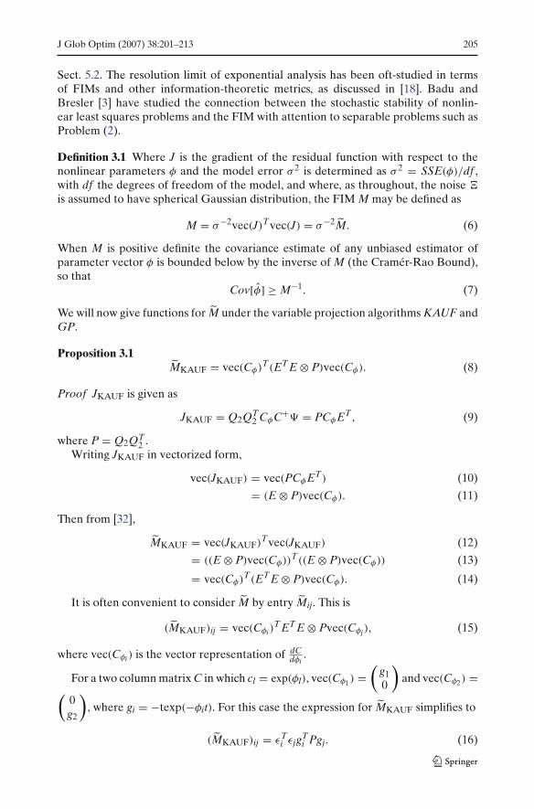
Fig. 1 Contour map of typical simulated data � used in computational study. Model fitting willresolve the two contributing components

Table 1 Rate constants, spectral parameters, and amplitudes for simulated �

component k µν σν a

1 0.5 22 9 12 0.6 18 8 2

necessary to adequately describe the spectra of photophysical systems of interest isoften large and more difficult to determine in comparison to the small and relativelysimple parameterization φ of the concentrations C.

Given these models for C and E, data was generated with the parameter values inTable 1. Values for kinetic parameters k1 and k2 are similar and the spectral param-eters represent overlapping spectral shapes. n = 51 time points equidistant in theinterval 0–2 ns and m = 51 wavelengths equidistant in the interval 350–550 nm. Theseparameter values are inspired by real data ([32] and references cited therein).

4.1 Degeneracy and multimodality due to noise

Measured time-resolved spectra � always contain stochastic noise. The presence ofnoise may introduce stationary points where dJ(φ)

dφ= 0 at φ distinct from those values

underlying the deterministic model, so that the algorithms presented in Sect. 2 aresensitive to starting values. This numerical identifiability problem is well-known inkinetic modeling [12], (as is the problem of structural, i.e., deterministic model-based,lack of identifiability). In the case of convergence to a local minimum introducedby noise, estimates for kinetic parameters and spectra are often implausible fromphysicochemical first principles. Uninterpretable parameter estimates typically allowspurious solutions to be recognized and discarded.

In fitting Model (1) to measured time-resolved spectra the signal-to-noise ratio maybe such that degeneracy is a significant issue. That is, optimal estimates for two or morerate constant parameters in the vector of nonlinear parameters φ may be close enoughthat noise disrupts the SSE surface in such a way that the globally optimal solution

208 J Glob Optim (2007) 38:201–213

k 1

k 2

0.4 0.5 0.6 0.7

0.4

0.5

0.6

0.7

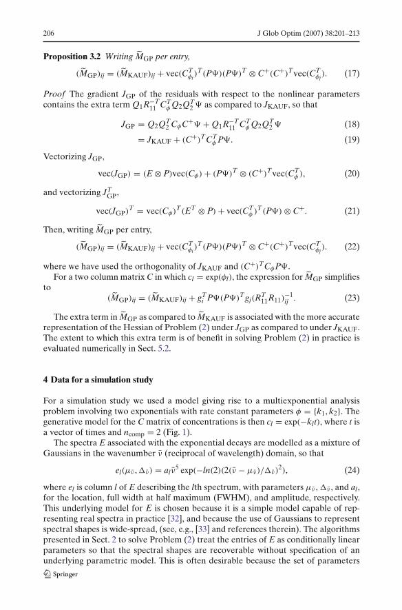
Fig. 2 The dataset described in Sect. 4 with a stochastic noise term with Gaussian distribution and zeromean having width � equal to 7×10−3 the maximum of the data. The parameter values φ = {0.5, 0.6}or symmetrically φ = {0.6, 0.5} (closed circles) underly the deterministic part of the data, and wouldbe the globally optimal parameter estimates save for the effect of noise, which makes the lower ordersolution φ = {0.55, 0.55} (crossed circle) globally optimal

is a sum of less than ncomp exponentials, as reviewed in [31]. Then the least-squaressolution yields estimates with k1 = k2 for {k1, k2} ∈ φ. In nearly-degenerate casesthe least squares solution is with k1 ≈ k2, and the parameters may be resolved if theprecision with which they are estimated is sufficiently high, as is studied numericallyunder the KAUF and GP algorithms in Sect. 5.2. For the simulated dataset describedin Sect. 4 degeneracy is probable for noise with width of about 7 × 10−3 the maximumof the data. The SSE surface of parameters φ for a noise realization that results innear-degeneracy is shown in Fig. 2.

5 Computational results

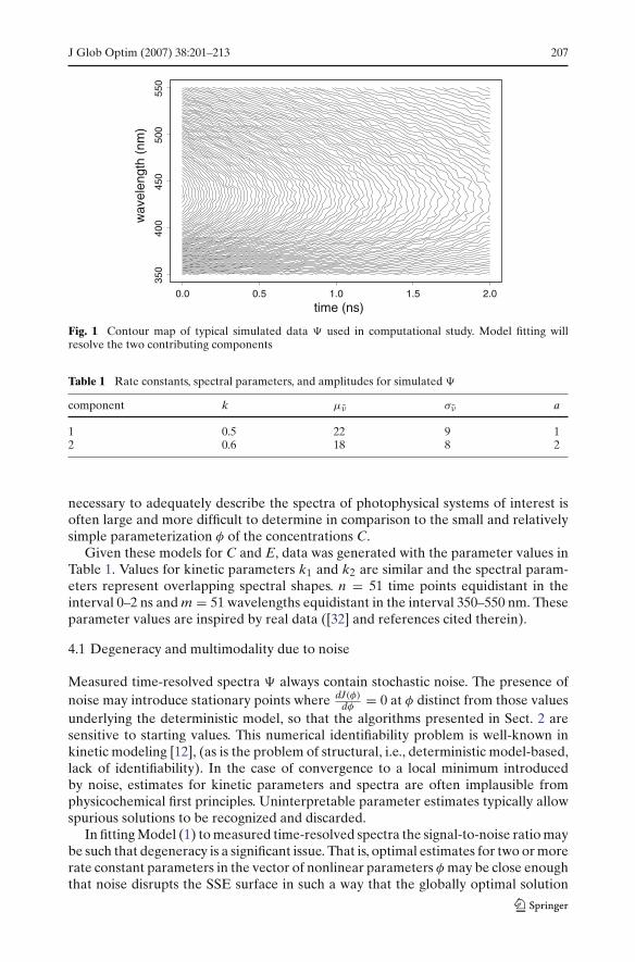
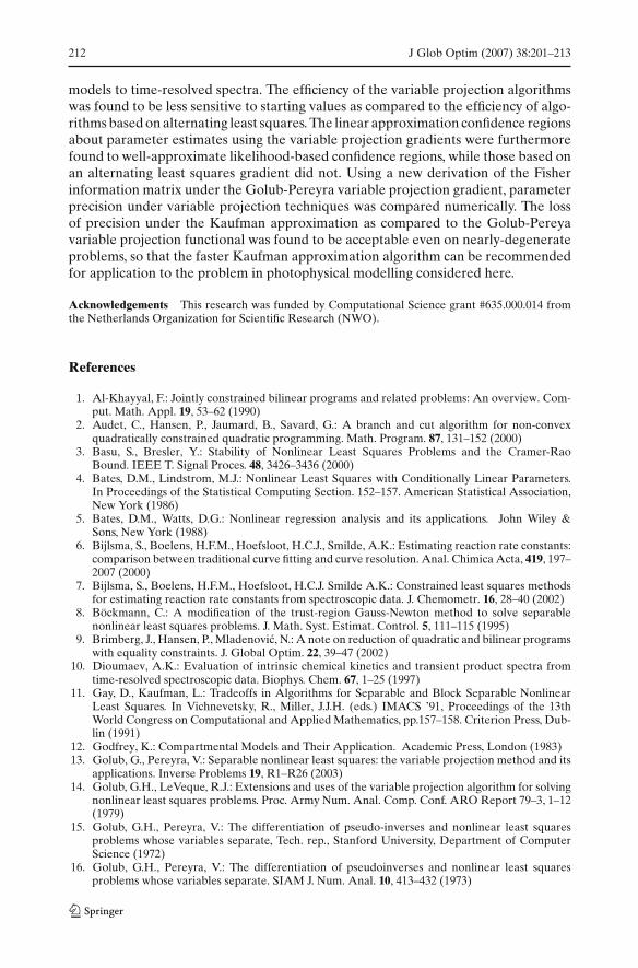
Model (1) was fit to the data described in Sect. 4 with a stochastic noise term withGaussian distribution and zero mean having width � equal to 3 × 10−3 the maximumof the data using each of the algorithms described in Sect. 2. The convergence criterionwas reduction of sum square error (SSE) ||vec(� − CET)||2 by a factor of less than1/210 between iterations. Estimated spectra found as conditionally linear parametersunder KAUF, GP, ALS-LS or NUM well-represent the spectra used in generating thesimulated data, as shown in Fig. 3.

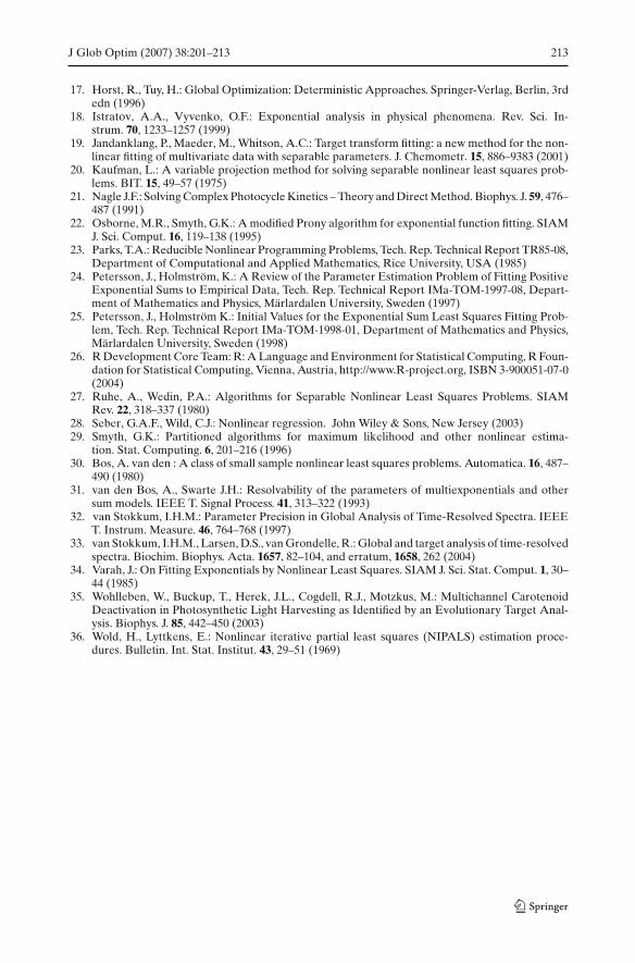
To visualize the progress of the algorithms per iteration, the SSE as rate constantsk1, k2 vary is evaluated, with the result being the surface shown in Fig. 4. Figure 4 also

Fig. 3 Estimated spectra(dashed lines) as found withKAUF, GP or NUM by fittingthe simulated dataset depictedin Fig. 1 with thetwo-component kinetic modeldescribed in Sect. 5. Spectraused to generate thedeterministic part of thedataset (solid lines) are shownfor comparison

350 400 450 500 550

1000

5000

wavelength (nm)

ampl

itude

J Glob Optim (2007) 38:201–213 209

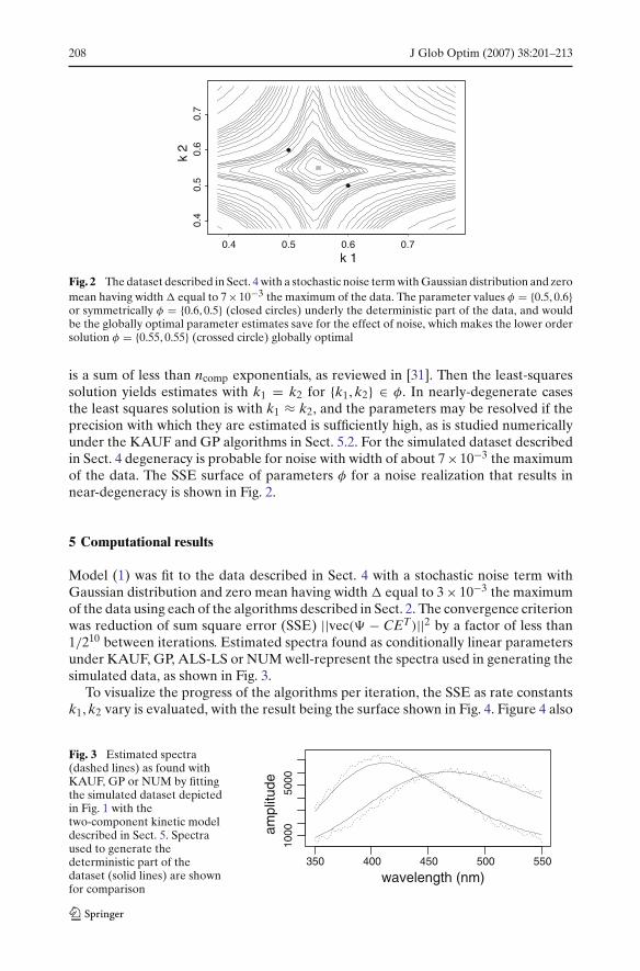
Fig. 4 Contour map of thesum square of residuals||vec(� − CET )||2 as rateconstants k1, k2 vary, at arelatively large (a) andrelatively small (b) scale. Theprogress of ALS-GN (unfilledtriangle), ALS-LS (square),KAUF (filled triangle), andGP/NUM (filled and unfilledcircles) is depicted fromstarting valuesk1 = 0.1, k2 = 1; rate constantestimates are marked with thesymbol associated with eachalgorithm after each iteration.Spacing between contour linesis not uniform

k 1 k

2

0.0 0.2 0.4 0.6 0.8 1.0

0.0

0.2

0.4

0.6

0.8

1.0

k 1

k 2

0.40 0.45 0.50 0.55

0.4

0.5

0.6

0.7

(a)

(b)

shows the values found by each algorithm under consideration for each of 50 iterationsfrom the starting values k1 = 0.1, k2 = 1. KAUF, GP, ALS-LS and NUM converge onthe same (globally optimal) solution in 4 iterations. ALS-GN is not generally conver-gent in many hundreds of iterations, and from this case study and others we concludethat the Gauss-Newton step coupled with the ALS-gradient is not sufficient for thesolution of typical estimation problems in this domain.

Performance from a range of starting values and on variants of the dataset underdifferent noise realizations was examined. For cases in which globally optimal param-eter values are located at the end of a valley with respect to the starting values, theperformance of ALS-LS is very much hampered in terms of iterations required toconvergence in comparison to KAUF, GP, and NUM. A plot of the SSE surface (asin Fig. 4) in this case shows that ALS-LS follows a zig-zagging path between the wallsof the valley toward a globally optimal solution.

We conclude that the ALS gradient coupled with a line search and both variableprojection methods KAUF and GP solve this problem for the considered data real-izations. The KAUF algorithm typically requires the same number of iterations as theGP algorithm. ALS with line search converges in a greater or equal number of itera-tions as compared to KAUF and GP. The iterations required for ALS-LS are greaterthan for KAUF and GP when the globally optimal parameter values are at the endof a valley in SSE with respect to starting parameter estimates. Therefore in termsof iterations to convergence and sensitivity of computational efficiency to startingvalues, the variable projection-based algorithms demonstrate the best performance.

210 J Glob Optim (2007) 38:201–213

5.1 Standard error estimates

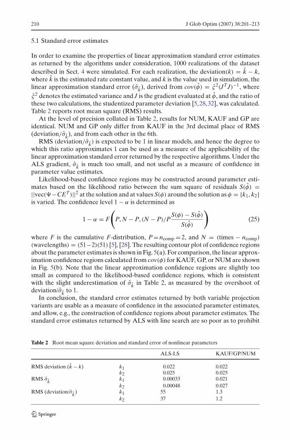
In order to examine the properties of linear approximation standard error estimatesas returned by the algorithms under consideration, 1000 realizations of the datasetdescribed in Sect. 4 were simulated. For each realization, the deviation(k) = k − k,where k is the estimated rate constant value, and k is the value used in simulation, thelinear approximation standard error (σk), derived from cov(φ) = ς2(JTJ)−1, whereς2 denotes the estimated variance and J is the gradient evaluated at φ, and the ratio ofthese two calculations, the studentized parameter deviation [5,28,32], was calculated.Table 2 reports root mean square (RMS) results.

At the level of precision collated in Table 2, results for NUM, KAUF and GP areidentical. NUM and GP only differ from KAUF in the 3rd decimal place of RMS(deviation/σk), and from each other in the 6th.

RMS (deviation/σk) is expected to be 1 in linear models, and hence the degree towhich this ratio approximates 1 can be used as a measure of the applicability of thelinear approximation standard error returned by the respective algorithms. Under theALS gradient, σk is much too small, and not useful as a measure of confidence inparameter value estimates.

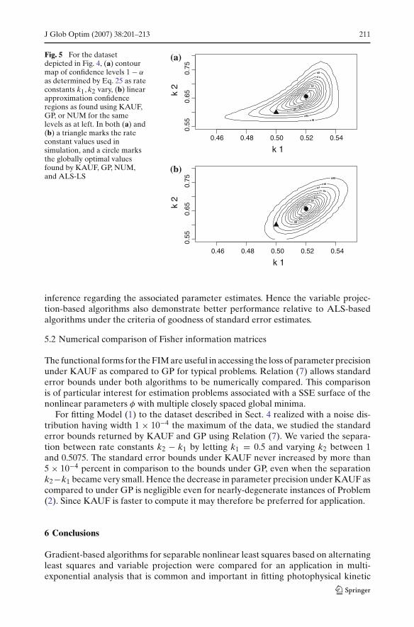
Likelihood-based confidence regions may be constructed around parameter esti-mates based on the likelihood ratio between the sum square of residuals S(φ) =||vec(�−CET)||2 at the solution and at values S(φ) around the solution as φ = {k1, k2}is varied. The confidence level 1 − α is determined as

1 − α = F

(P, N − P, (N − P)/P

S(φ) − S(φ)

S(φ)

)(25)

where F is the cumulative F-distribution, P = ncomp = 2, and N = (times − ncomp)

(wavelengths) = (51−2)(51) [5], [28]. The resulting contour plot of confidence regionsabout the parameter estimates is shown in Fig. 5(a). For comparison, the linear approx-imation confidence regions calculated from cov(φ) for KAUF, GP, or NUM are shownin Fig. 5(b). Note that the linear approximation confidence regions are slightly toosmall as compared to the likelihood-based confidence regions, which is consistentwith the slight underestimation of σk in Table 2, as measured by the overshoot ofdeviation/σk to 1.

In conclusion, the standard error estimates returned by both variable projectionvariants are usable as a measure of confidence in the associated parameter estimates,and allow, e.g., the construction of confidence regions about parameter estimates. Thestandard error estimates returned by ALS with line search are so poor as to prohibit

Table 2 Root mean square deviation and standard error of nonlinear parameters

ALS-LS KAUF/GP/NUM

RMS deviation (k − k) k1 0.022 0.022k2 0.025 0.025

RMS σk k1 0.00033 0.021k2 0.00048 0.027

RMS (deviation/σk) k1 55 1.3k2 37 1.2

J Glob Optim (2007) 38:201–213 211

Fig. 5 For the datasetdepicted in Fig. 4, (a) contourmap of confidence levels 1 − α

as determined by Eq. 25 as rateconstants k1, k2 vary, (b) linearapproximation confidenceregions as found using KAUF,GP, or NUM for the samelevels as at left. In both (a) and(b) a triangle marks the rateconstant values used insimulation, and a circle marksthe globally optimal valuesfound by KAUF, GP, NUM,and ALS-LS

k 1

k 2

0.46 0.48 0.50 0.52 0.54

k 10.46 0.48 0.50 0.52 0.54

0.55

0.65

0.75

k 2

0.55

0.65

0.75

(a)

(b)

inference regarding the associated parameter estimates. Hence the variable projec-tion-based algorithms also demonstrate better performance relative to ALS-basedalgorithms under the criteria of goodness of standard error estimates.

5.2 Numerical comparison of Fisher information matrices

The functional forms for the FIM are useful in accessing the loss of parameter precisionunder KAUF as compared to GP for typical problems. Relation (7) allows standarderror bounds under both algorithms to be numerically compared. This comparisonis of particular interest for estimation problems associated with a SSE surface of thenonlinear parameters φ with multiple closely spaced global minima.

For fitting Model (1) to the dataset described in Sect. 4 realized with a noise dis-tribution having width 1 × 10−4 the maximum of the data, we studied the standarderror bounds returned by KAUF and GP using Relation (7). We varied the separa-tion between rate constants k2 − k1 by letting k1 = 0.5 and varying k2 between 1and 0.5075. The standard error bounds under KAUF never increased by more than5 × 10−4 percent in comparison to the bounds under GP, even when the separationk2−k1 became very small. Hence the decrease in parameter precision under KAUF ascompared to under GP is negligible even for nearly-degenerate instances of Problem(2). Since KAUF is faster to compute it may therefore be preferred for application.

6 Conclusions

Gradient-based algorithms for separable nonlinear least squares based on alternatingleast squares and variable projection were compared for an application in multi-exponential analysis that is common and important in fitting photophysical kinetic

212 J Glob Optim (2007) 38:201–213

models to time-resolved spectra. The efficiency of the variable projection algorithmswas found to be less sensitive to starting values as compared to the efficiency of algo-rithms based on alternating least squares. The linear approximation confidence regionsabout parameter estimates using the variable projection gradients were furthermorefound to well-approximate likelihood-based confidence regions, while those based onan alternating least squares gradient did not. Using a new derivation of the Fisherinformation matrix under the Golub-Pereyra variable projection gradient, parameterprecision under variable projection techniques was compared numerically. The lossof precision under the Kaufman approximation as compared to the Golub-Pereyavariable projection functional was found to be acceptable even on nearly-degenerateproblems, so that the faster Kaufman approximation algorithm can be recommendedfor application to the problem in photophysical modelling considered here.

Acknowledgements This research was funded by Computational Science grant #635.000.014 fromthe Netherlands Organization for Scientific Research (NWO).

References

1. Al-Khayyal, F.: Jointly constrained bilinear programs and related problems: An overview. Com-put. Math. Appl. 19, 53–62 (1990)

2. Audet, C., Hansen, P., Jaumard, B., Savard, G.: A branch and cut algorithm for non-convexquadratically constrained quadratic programming. Math. Program. 87, 131–152 (2000)

3. Basu, S., Bresler, Y.: Stability of Nonlinear Least Squares Problems and the Cramer-RaoBound. IEEE T. Signal Proces. 48, 3426–3436 (2000)

4. Bates, D.M., Lindstrom, M.J.: Nonlinear Least Squares with Conditionally Linear Parameters.In Proceedings of the Statistical Computing Section. 152–157. American Statistical Association,New York (1986)

5. Bates, D.M., Watts, D.G.: Nonlinear regression analysis and its applications. John Wiley &Sons, New York (1988)

6. Bijlsma, S., Boelens, H.F.M., Hoefsloot, H.C.J., Smilde, A.K.: Estimating reaction rate constants:comparison between traditional curve fitting and curve resolution. Anal. Chimica Acta, 419, 197–2007 (2000)

7. Bijlsma, S., Boelens, H.F.M., Hoefsloot, H.C.J. Smilde A.K.: Constrained least squares methodsfor estimating reaction rate constants from spectroscopic data. J. Chemometr. 16, 28–40 (2002)

8. Böckmann, C.: A modification of the trust-region Gauss-Newton method to solve separablenonlinear least squares problems. J. Math. Syst. Estimat. Control. 5, 111–115 (1995)

9. Brimberg, J., Hansen, P., Mladenovic, N.: A note on reduction of quadratic and bilinear programswith equality constraints. J. Global Optim. 22, 39–47 (2002)

10. Dioumaev, A.K.: Evaluation of intrinsic chemical kinetics and transient product spectra fromtime-resolved spectroscopic data. Biophys. Chem. 67, 1–25 (1997)

11. Gay, D., Kaufman, L.: Tradeoffs in Algorithms for Separable and Block Separable NonlinearLeast Squares. In Vichnevetsky, R., Miller, J.J.H. (eds.) IMACS ’91, Proceedings of the 13thWorld Congress on Computational and Applied Mathematics, pp.157–158. Criterion Press, Dub-lin (1991)

12. Godfrey, K.: Compartmental Models and Their Application. Academic Press, London (1983)13. Golub, G., Pereyra, V.: Separable nonlinear least squares: the variable projection method and its

applications. Inverse Problems 19, R1–R26 (2003)14. Golub, G.H., LeVeque, R.J.: Extensions and uses of the variable projection algorithm for solving

nonlinear least squares problems. Proc. Army Num. Anal. Comp. Conf. ARO Report 79–3, 1–12(1979)

15. Golub, G.H., Pereyra, V.: The differentiation of pseudo-inverses and nonlinear least squaresproblems whose variables separate, Tech. rep., Stanford University, Department of ComputerScience (1972)

16. Golub, G.H., Pereyra, V.: The differentiation of pseudoinverses and nonlinear least squaresproblems whose variables separate. SIAM J. Num. Anal. 10, 413–432 (1973)

J Glob Optim (2007) 38:201–213 213

17. Horst, R., Tuy, H.: Global Optimization: Deterministic Approaches. Springer-Verlag, Berlin, 3rdedn (1996)

18. Istratov, A.A., Vyvenko, O.F.: Exponential analysis in physical phenomena. Rev. Sci. In-strum. 70, 1233–1257 (1999)

19. Jandanklang, P., Maeder, M., Whitson, A.C.: Target transform fitting: a new method for the non-linear fitting of multivariate data with separable parameters. J. Chemometr. 15, 886–9383 (2001)

20. Kaufman, L.: A variable projection method for solving separable nonlinear least squares prob-lems. BIT. 15, 49–57 (1975)

21. Nagle J.F.: Solving Complex Photocycle Kinetics – Theory and Direct Method. Biophys. J. 59, 476–487 (1991)

22. Osborne, M.R., Smyth, G.K.: A modified Prony algorithm for exponential function fitting. SIAMJ. Sci. Comput. 16, 119–138 (1995)

23. Parks, T.A.: Reducible Nonlinear Programming Problems, Tech. Rep. Technical Report TR85-08,Department of Computational and Applied Mathematics, Rice University, USA (1985)

24. Petersson, J., Holmström, K.: A Review of the Parameter Estimation Problem of Fitting PositiveExponential Sums to Empirical Data, Tech. Rep. Technical Report IMa-TOM-1997-08, Depart-ment of Mathematics and Physics, Märlardalen University, Sweden (1997)

25. Petersson, J., Holmström K.: Initial Values for the Exponential Sum Least Squares Fitting Prob-lem, Tech. Rep. Technical Report IMa-TOM-1998-01, Department of Mathematics and Physics,Märlardalen University, Sweden (1998)

26. R Development Core Team: R: A Language and Environment for Statistical Computing, R Foun-dation for Statistical Computing, Vienna, Austria, http://www.R-project.org, ISBN 3-900051-07-0(2004)

27. Ruhe, A., Wedin, P.A.: Algorithms for Separable Nonlinear Least Squares Problems. SIAMRev. 22, 318–337 (1980)

28. Seber, G.A.F., Wild, C.J.: Nonlinear regression. John Wiley & Sons, New Jersey (2003)29. Smyth, G.K.: Partitioned algorithms for maximum likelihood and other nonlinear estima-

tion. Stat. Computing. 6, 201–216 (1996)30. Bos, A. van den : A class of small sample nonlinear least squares problems. Automatica. 16, 487–

490 (1980)31. van den Bos, A., Swarte J.H.: Resolvability of the parameters of multiexponentials and other

sum models. IEEE T. Signal Process. 41, 313–322 (1993)32. van Stokkum, I.H.M.: Parameter Precision in Global Analysis of Time-Resolved Spectra. IEEE

T. Instrum. Measure. 46, 764–768 (1997)33. van Stokkum, I.H.M., Larsen, D.S., van Grondelle, R.: Global and target analysis of time-resolved

spectra. Biochim. Biophys. Acta. 1657, 82–104, and erratum, 1658, 262 (2004)34. Varah, J.: On Fitting Exponentials by Nonlinear Least Squares. SIAM J. Sci. Stat. Comput. 1, 30–

44 (1985)35. Wohlleben, W., Buckup, T., Herek, J.L., Cogdell, R.J., Motzkus, M.: Multichannel Carotenoid

Deactivation in Photosynthetic Light Harvesting as Identified by an Evolutionary Target Anal-ysis. Biophys. J. 85, 442–450 (2003)

36. Wold, H., Lyttkens, E.: Nonlinear iterative partial least squares (NIPALS) estimation proce-dures. Bulletin. Int. Stat. Institut. 43, 29–51 (1969)