ALGORITHMS FOR PRESSURE CORRECTION IN THE …platte/vita/publications/Wccm98.pdf · Rodrigo B. Platte, Haroldo F. de Campos Velho, Julio C. Ruiz Claeyssen and Elba O. Bravo 1 Introduction

COMPUTATIONAL MECHANICSNew Trends and Applications

S. Idelsohn, E. Onate and E. Dvorkin (Eds.)

c©CIMNE, Barcelona, Spain 1998

ALGORITHMS FOR PRESSURE CORRECTION IN THEDRIVEN CAVITY PROBLEM

Rodrigo B. Platte ∗, Haroldo F. de Campos Velho ∗∗,Julio C. Ruiz Claeyssen ∗ and Elba O. Bravo ∗

∗ Instituto de Matematica/PROMECUniversidade Federal do Rio Grande do Sul (UFRGS)

Porto Alegre (RS) - BRASILe-mail: [rbplatte, julio]@mat.ufrgs.bf and [email protected]

∗∗ Laboratorio Associado de Computacao e Matematica Aplicada (LAC)Instituto Nacional de Pesquisas Espaciais (INPE), Caixa Postal 515

12201-970 – Sao Jose dos Campos (SP) – BRASILe-mail: [email protected]

Key words: Pressure Poisson equation, incompressible fluid, driven cavity problem.

Abstract. The driven cavity problem has been extensively used as a benchmark problemto evaluate numerical techniques that solve the Navier-Stokes equations. In this work, theincompressible fluid flow is integrated by calculating the velocity fields and computing thepressure field in each time step. In order to avoid approximation errors, that imply a lackof incompressibility, a dilatation term is incorporated to the Poisson equation of the pres-sure. The goal of this paper is twofold. The first purpose is to examinate the performanceof the three different methods for the pressure correction: the Claeyssen-Bravo algorithm,the iterative scheme given in C. Hirsch (1990), and the steady state solution of the non-homogeneous diffusion equation. The second goal is to perform numerical experimentationwith deep and shallow cavities.

1

Rodrigo B. Platte, Haroldo F. de Campos Velho, Julio C. Ruiz Claeyssen and Elba O. Bravo

1 Introduction

The laminar incompressible flow in a cavity, whose upper wall continuosly moves withuniform velocity parallel to its plane, has been extensively used as a test problem toevaluate the numerical techniques. In this work the Navier-Stokes equations are solvedfor a viscous, isothermic and incompressible fluid in a rectangular cavity. The numericalsolution consists on getting the velocity fields by using the Adams-Bashforth methodfor the time integration and by means of the central finite differences for the spatialdiscretization in a staggered grid.

The Poisson equation for the pressure with Neumann boundary conditions is obtainedfollowing Gresho and Sani [7]. In an incompressible flow special attention must be given tothe solution of this equation. The correction terms are inserted in the discretized Poissonequation for avoiding the lack of incompressibility. In order to solve this equation threeschemes are used: the iterative Gauss-Seidel method, the Claeyssen-Bravo algorithm,which updates the pressure in only one step, and the asymptotic solution for the non-homogeneous diffusion equation.

The numerical results are shown for different Reynolds numbers. It is also analysedthe influence of the diffusivity parameter in the final result.

2 The Driven Cavity Problem

The Navier-Stokes equations are considered in its primitive variables in the bi-dimensionalcavity

∂u

∂t+ u.∇u = −∇p + ν∇2u , t > 0 and x ∈ Ω (1)

∇.u = 0 , (x, t) ∈ Ω × [0,∞) (2)

u(x, 0) = u0(x) , x at Ω = Ω ⊕ Γ (3)

u = uΓ(x, t) at Γ = ∂Ω , (4)

with the following Poisson equation for the pressure [3]

∇2p = ∇.(ν∇2u− u.∇u) = ∇.(u.∇u) (5)

associated to the Neumann boundary condition [7]

∂p

∂n= ν∇2un − (

∂n

∂t+ u.∇un) at Γ for t ≥ 0 (6)

where un = u.n is the normal component of the velocity field u = ux i + vy j = u i + v j =(u, v).

2


The goal is to determine the induced flow by shear movement of the upper wall, which ismoving with uniform horizontal velocity uT = 1. The other walls remain fixed. Therefore,the boundary conditions for the tangential velocity are given by

u(x, 0, t) = v(0, y, t) = v(Lx, y, t) = 0 , u(x, Ly, t) = uT = 1 ;

and the boundary conditions for the normal velocity

u(0, y, t) = u(Lx, y, t) = v(x, 0, t) = v(x, Ly, t) = 0

where Lx and Ly are the length and the height of the cavity, respectively.

In addition, it is assumed that, at the initial time, the fluid is in rest

u0(x, y) = v0(x, y) = 0 .

3 Numerical Integration

In order to solve Eq. (1), some numerical schemes were tested and compared in [11].For the time integration it was used the explicit Euler method, the second order Adams-Bashforth method, the upwind method with centered differences of first and second orders,and an Euler-Lagrange (or semi-Lagrangian) method.

For convection dominant flow the Euler-Lagrange scheme presented the lower numer-ical diffusion, being however slower than other methods. The Adams-Bashforth methodfor time integration associated to the central differences for the space derivative showedgood results and smaller restrictions as to the numerical stability than the explicit Eulermethod. Therefore the Adams-Bashforth scheme was chosen for the integration of Eq.(1), that is:

uk+1 = uk +∆t

2[3F(uk) − F(uk−1) + 3∇pk −∇pk−1] (7)

where F(uk) is the discretization of the convective and diffusive terms from (1) by centraldifferences of second order. This scheme is implemented with staggered grid in [8] and∇pk is also approximated by central differences.

4 Solving the Pressure Poisson Equation

The simple discretization of the pressure in Eq. (5) produces a cumulative error due tothe approximation errors, which implies in a leakage of the incompressibility leading toinstabilities in the simulation. These errors can be avoided by adding corrective terms inEq. (5). This is done in [9] where it is obtained the corrective equations for the pressure on

3


0.1 0.2 0.3 0.4 0.5 0.6 0.7 0.8 0.9

0.1

0.2

0.3

0.4

0.5

0.6

0.7

0.8

0.9

0.1 0.2 0.3 0.4 0.5 0.6 0.7 0.8 0.9

0.1

0.2

0.3

0.4

0.5

0.6

0.7

0.8

0.9

0.1 0.2 0.3 0.4 0.5 0.6 0.7 0.8 0.9

0.1

0.2

0.3

0.4

0.5

0.6

0.7

0.8

0.9

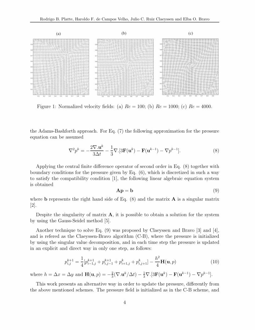
Figure 1: Normalized velocity fields: (a) Re = 100; (b) Re = 1000; (c) Re = 4000.

the Adams-Bashforth approach. For Eq. (7) the following approximation for the pressureequation can be assumed

∇2pk = −2∇.uk

3∆t− 1

3∇.[3F(uk) − F(uk−1) −∇pk−1]. (8)

Applying the central finite difference operator of second order in Eq. (8) together withboundary conditions for the pressure given by Eq. (6), which is discretized in such a wayto satisfy the compatibility condition [1], the following linear algebraic equation systemis obtained

Ap = b (9)

where b represents the right hand side of Eq. (8) and the matrix A is a singular matrix[2].

Despite the singularity of matrix A, it is possible to obtain a solution for the systemby using the Gauss-Seidel method [5].

Another technique to solve Eq. (9) was proposed by Claeyssen and Bravo [3] and [4],and is refered as the Claeyssen-Bravo algorithm (C-B), where the pressure is initializedby using the singular value decomposition, and in each time step the pressure is updatedin an explicit and direct way in only one step, as follows:

pk+1i,j =

1

4[pk+1

i−1,j + pk+1i,j−1 + pk

i+1,j + pki,j+1] −

h2

4H(u, p) (10)

where h = ∆x = ∆y and H(u, p) = −23(∇.uk/∆t) − 1

3∇.[3F(uk) − F(uk−1) −∇pk−1].

This work presents an alternative way in order to update the pressure, differently fromthe above mentioned schemes. The pressure field is initialized as in the C-B scheme, and

4


0.1 0.2 0.3 0.4 0.5 0.6 0.7 0.8 0.9

0.1

0.2

0.3

0.4

0.5

0.6

0.7

0.8

0.9

0.1 0.2 0.3 0.4 0.5 0.6 0.7 0.8 0.9

0.1

0.2

0.3

0.4

0.5

0.6

0.7

0.8

0.9

0.1 0.2 0.3 0.4 0.5 0.6 0.7 0.8 0.9

0.1

0.2

0.3

0.4

0.5

0.6

0.7

0.8

0.9

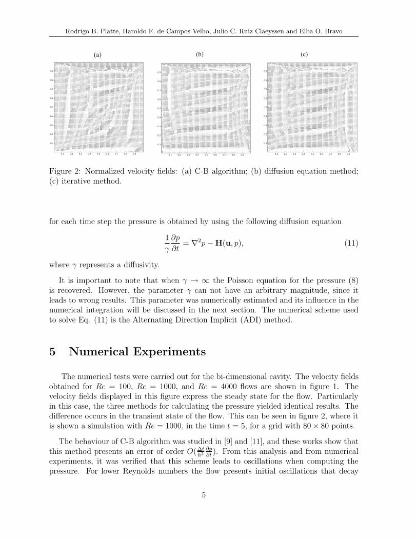
Figure 2: Normalized velocity fields: (a) C-B algorithm; (b) diffusion equation method;(c) iterative method.

for each time step the pressure is obtained by using the following diffusion equation

1

γ

∂p

∂t= ∇2p − H(u, p), (11)

where γ represents a diffusivity.

It is important to note that when γ → ∞ the Poisson equation for the pressure (8)is recovered. However, the parameter γ can not have an arbitrary magnitude, since itleads to wrong results. This parameter was numerically estimated and its influence in thenumerical integration will be discussed in the next section. The numerical scheme usedto solve Eq. (11) is the Alternating Direction Implicit (ADI) method.

5 Numerical Experiments

The numerical tests were carried out for the bi-dimensional cavity. The velocity fieldsobtained for Re = 100, Re = 1000, and Re = 4000 flows are shown in figure 1. Thevelocity fields displayed in this figure express the steady state for the flow. Particularlyin this case, the three methods for calculating the pressure yielded identical results. Thedifference occurs in the transient state of the flow. This can be seen in figure 2, where itis shown a simulation with Re = 1000, in the time t = 5, for a grid with 80 × 80 points.

The behaviour of C-B algorithm was studied in [9] and [11], and these works show thatthis method presents an error of order O(∆t

h2∂p∂t

). From this analysis and from numericalexperiments, it was verified that this scheme leads to oscillations when computing thepressure. For lower Reynolds numbers the flow presents initial oscillations that decay

5


Table 1: Parameters used in the simulations.

Re = 100 Re = 400 Re = 1000no h ∆t γ no h ∆t γ no h ∆t γ1 0.02 0.005 0.08 5 0.02 0.005 0.08 9 0.02 0.01 0.042 0.02 0.005 0.09 6 0.02 0.005 0.09 10 0.02 0.01 0.053 0.0125 0.005 0.03 7 0.0125 0.005 0.03 11 0.01 0.007 0.0144 0.0125 0.005 0.04 8 0.0125 0.005 0.04 12 0.01 0.007 0.02

fastly. For dominant convective flow (high Re) the oscillations present smaller amplitudes,but they decay slowly. A similar behaviour is found when the pressure is computed bythe diffusion equation method, which depends on γ.

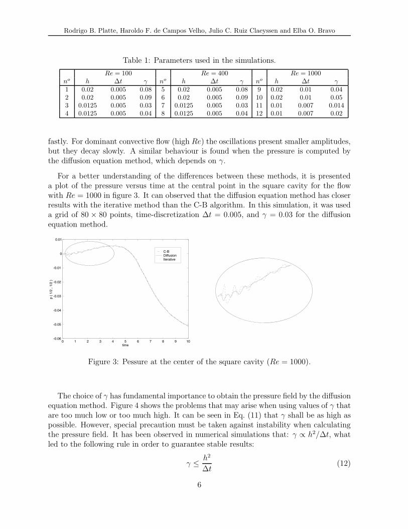
For a better understanding of the differences between these methods, it is presenteda plot of the pressure versus time at the central point in the square cavity for the flowwith Re = 1000 in figure 3. It can observed that the diffusion equation method has closerresults with the iterative method than the C-B algorithm. In this simulation, it was useda grid of 80 × 80 points, time-discretization ∆t = 0.005, and γ = 0.03 for the diffusionequation method.

Figure 3: Pessure at the center of the square cavity (Re = 1000).

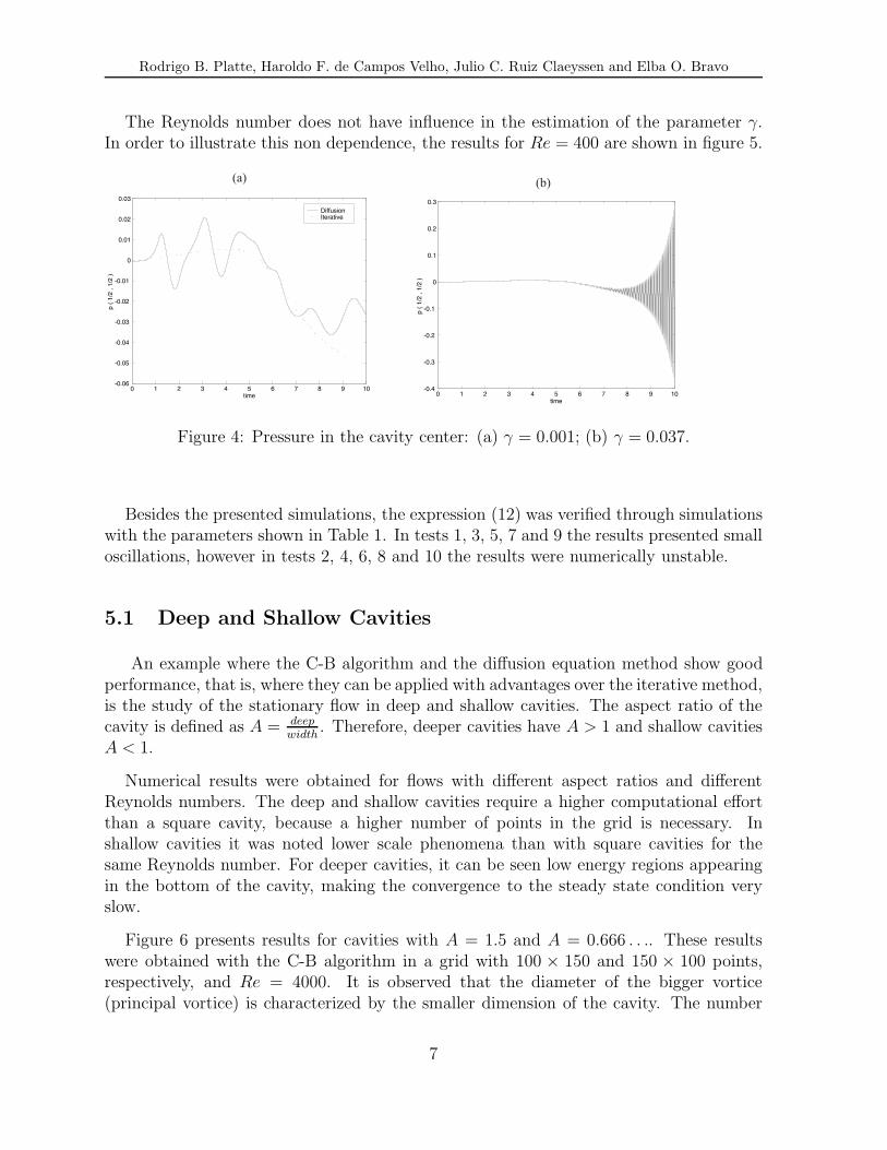
The choice of γ has fundamental importance to obtain the pressure field by the diffusionequation method. Figure 4 shows the problems that may arise when using values of γ thatare too much low or too much high. It can be seen in Eq. (11) that γ shall be as high aspossible. However, special precaution must be taken against instability when calculatingthe pressure field. It has been observed in numerical simulations that: γ ∝ h2/∆t, whatled to the following rule in order to guarantee stable results:

γ ≤ h2

∆t(12)

6


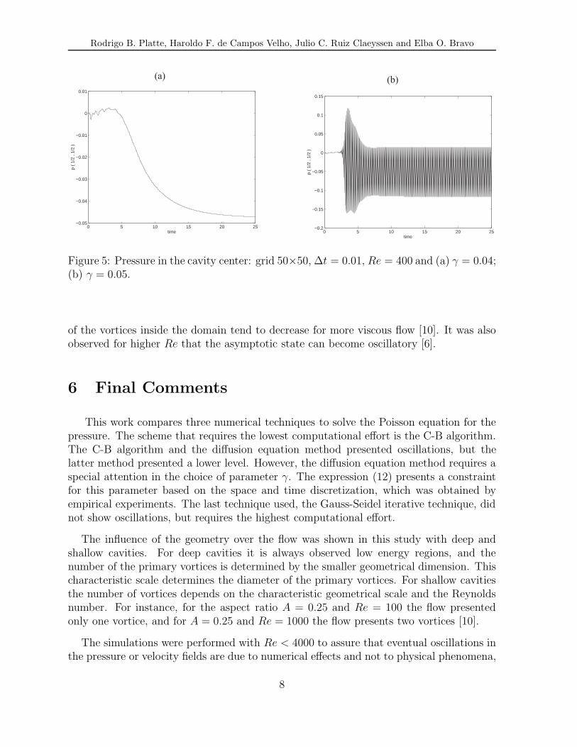
The Reynolds number does not have influence in the estimation of the parameter γ.In order to illustrate this non dependence, the results for Re = 400 are shown in figure 5.

Figure 4: Pressure in the cavity center: (a) γ = 0.001; (b) γ = 0.037.

Besides the presented simulations, the expression (12) was verified through simulationswith the parameters shown in Table 1. In tests 1, 3, 5, 7 and 9 the results presented smalloscillations, however in tests 2, 4, 6, 8 and 10 the results were numerically unstable.

5.1 Deep and Shallow Cavities

An example where the C-B algorithm and the diffusion equation method show goodperformance, that is, where they can be applied with advantages over the iterative method,is the study of the stationary flow in deep and shallow cavities. The aspect ratio of thecavity is defined as A = deep

width. Therefore, deeper cavities have A > 1 and shallow cavities

A < 1.

Numerical results were obtained for flows with different aspect ratios and differentReynolds numbers. The deep and shallow cavities require a higher computational effortthan a square cavity, because a higher number of points in the grid is necessary. Inshallow cavities it was noted lower scale phenomena than with square cavities for thesame Reynolds number. For deeper cavities, it can be seen low energy regions appearingin the bottom of the cavity, making the convergence to the steady state condition veryslow.

Figure 6 presents results for cavities with A = 1.5 and A = 0.666 . . .. These resultswere obtained with the C-B algorithm in a grid with 100 × 150 and 150 × 100 points,respectively, and Re = 4000. It is observed that the diameter of the bigger vortice(principal vortice) is characterized by the smaller dimension of the cavity. The number

7


0 5 10 15 20 25−0.05

−0.04

−0.03

−0.02

−0.01

0

0.01

time

p (

1/2

, 1/2

)

0 5 10 15 20 25−0.2

−0.15

−0.1

−0.05

0

0.05

0.1

0.15

time

p (

1/2

, 1/2

)

Figure 5: Pressure in the cavity center: grid 50×50, ∆t = 0.01, Re = 400 and (a) γ = 0.04;(b) γ = 0.05.

of the vortices inside the domain tend to decrease for more viscous flow [10]. It was alsoobserved for higher Re that the asymptotic state can become oscillatory [6].

6 Final Comments

This work compares three numerical techniques to solve the Poisson equation for thepressure. The scheme that requires the lowest computational effort is the C-B algorithm.The C-B algorithm and the diffusion equation method presented oscillations, but thelatter method presented a lower level. However, the diffusion equation method requires aspecial attention in the choice of parameter γ. The expression (12) presents a constraintfor this parameter based on the space and time discretization, which was obtained byempirical experiments. The last technique used, the Gauss-Seidel iterative technique, didnot show oscillations, but requires the highest computational effort.

The influence of the geometry over the flow was shown in this study with deep andshallow cavities. For deep cavities it is always observed low energy regions, and thenumber of the primary vortices is determined by the smaller geometrical dimension. Thischaracteristic scale determines the diameter of the primary vortices. For shallow cavitiesthe number of vortices depends on the characteristic geometrical scale and the Reynoldsnumber. For instance, for the aspect ratio A = 0.25 and Re = 100 the flow presentedonly one vortice, and for A = 0.25 and Re = 1000 the flow presents two vortices [10].

The simulations were performed with Re < 4000 to assure that eventual oscillations inthe pressure or velocity fields are due to numerical effects and not to physical phenomena,

8


0 0.2 0.4 0.6 0.8 10

0.5

1

1.5

0 0.1 0.2 0.3 0.4 0.5 0.6 0.7 0.8 0.9 10

0.1

0.2

0.3

0.4

0.5

0.6

Figure 6: Normalized velocity fields: (a) A = 1.5; (b) A = 0.666 . . .

which can happen for higher Reynolds [12].

Acknowledgments

The first author acknowledges the CNPq (Brazilian Council for Scientific and Tech-nological Development) for the financial support and the Laboratory for Computing andApplied Mathematics of the Brazilian Institute for Space Research (LAC-INPE) for the4-months technical visit, during which this work was partially done.

References

[1] S. ABDALLAH (1987): “Numerical Solutions for the Pressure Poisson Equationwith Neumann Boundary Conditions Using a Non-staggered Grid, I”, Journal ofComputational Physics, vol. 70, pp. 182–192.

[2] E.O. BRAVO, J.C.R. CLAEYSSEN (1995): “Matrix Methods and Boundary Condi-tions in the Integration of the Incompressible Flow”, XVI Iberian Latin Ameri-

9


can Conference on Computational Methods for Engineering, Curitiba (PR),Brazil, pp. 592-600.

[3] E.O. BRAVO (1997):. “Incompressible Flow with Neumann Pressure Con-dition: Simulation and Matrix Formulation in Primitive Variables”, PhDThesis, PROMEC-UFRGS, Porto Alegre, Brasil.

[4] E.O. BRAVO, J.C.R. CLAEYSSEN, A. CASTRO (1997): “A Modified Velocity-Pressure Algorithm with Neumann Pressure Conditions for Incompressible Flow ona Staggered Grid”, Proceedings II Italian - Latinamerican Conference onApplied and Industrial Mathematics (ITLA’97), Roma, Italy, pp. 31.

[5] V. CASULLI (1988): “Eulerian–Lagrangian Methods for the Navier-Stokes Equa-tions at High Reynolds Number”. International Journal for Numerical Meth-ods in Fluids, New York, vol.8, pp. 1349-1360.

[6] J.W. GOODRICH, K. GUSTAFSON, K. HALASI (1990): “Hopf Bifurcation in theDriven Cavity”, Journal of Computational Physics, vol. 90, pp. 219–261.

[7] P.M. GRESHO, R.L. SANI (1987): “On Pressure Boundary Conditions for the In-compressible Navier-Stokes Equations”, International Journal for NumericalMethods in Fluids, vol. 7, pp. 1111-1145.

[8] C. HIRSCH (1990): “Numerical Computation of Internal and ExternalFlows”, John Wiley & Sons Ltd..

[9] R.B. PLATTE, E.O. BRAVO, J.C.R. CLAEYSSEN, H.F. CAMPOS VELHO, (1997):“The Behaviour of the Velocity-pressure Algoritms in Incompressible Flow with Pres-sure Neumman Condition”, XVI Iberian Latin American Conference on Com-putational Methods for Engineering, Brasılia (DF), Brazil, vol. II, pp. 1005-1012, in portuguese.

[10] R.B. PLATTE, H.F. CAMPOS VELHO, J.C.R. CLAEYSSEN, E.O. BRAVO (1997):“Numerical Experiments in Bidimensional Cavity Flow”, Technical Report,INPE, in portuguese (to be published).

[11] R.B. PLATTE (1998): “The Numerical Study of the Bidimensional Cav-ity Flow”, Master Degree Thesis, Institute of Mathematics, UFRGS, Porto Alegre,Brasil (in portuguese).

[12] M. POLIASHENKO, C.K. AIDUN (1995): “A Direct Method for Computation ofSimple Bifurcation”, Journal of Computational Physics, vol. 121, pp. 246-260.

10

ALGORITHMS FOR PRESSURE CORRECTION IN THE …platte/vita/publications/Wccm98.pdf · Rodrigo B. Platte, Haroldo F. de Campos Velho, Julio C. Ruiz Claeyssen and Elba O. Bravo 1 Introduction

Documents