ALGORITHMS FOR MASSIVE, EXPENSIVE, OR OTHERWISE ...

University of Massachusetts Amherst University of Massachusetts Amherst

ScholarWorks@UMass Amherst ScholarWorks@UMass Amherst

Doctoral Dissertations Dissertations and Theses

12-18-2020

ALGORITHMS FOR MASSIVE, EXPENSIVE, OR OTHERWISE ALGORITHMS FOR MASSIVE, EXPENSIVE, OR OTHERWISE

INCONVENIENT GRAPHS INCONVENIENT GRAPHS

David Tench University of Massachusetts Amherst

Follow this and additional works at: https://scholarworks.umass.edu/dissertations_2

Part of the OS and Networks Commons, and the Theory and Algorithms Commons

Recommended Citation Recommended Citation Tench, David, "ALGORITHMS FOR MASSIVE, EXPENSIVE, OR OTHERWISE INCONVENIENT GRAPHS" (2020). Doctoral Dissertations. 2084. https://doi.org/10.7275/g94z-xg57 https://scholarworks.umass.edu/dissertations_2/2084

This Open Access Dissertation is brought to you for free and open access by the Dissertations and Theses at ScholarWorks@UMass Amherst. It has been accepted for inclusion in Doctoral Dissertations by an authorized administrator of ScholarWorks@UMass Amherst. For more information, please contact [email protected].

ALGORITHMS FOR MASSIVE, EXPENSIVE, OR OTHERWISEINCONVENIENT GRAPHS

A Dissertation Presented

by

DAVID TENCH

Submitted to the Graduate School of theUniversity of Massachusetts Amherst in partial fulfillment

of the requirements for the degree of

DOCTOR OF PHILOSOPHY

September 2020

College of Information and Computer Sciences

© Copyright by David Tench 2020All Rights Reserved

ALGORITHMS FOR MASSIVE, EXPENSIVE, OR OTHERWISEINCONVENIENT GRAPHS

A Dissertation Presented

by

DAVID TENCH

Approved as to style and content by:

Andrew McGregor, Chair

Phillipa Gill, Member

Markos Katsoulakis, Member

Cameron Musco, Member

James Allan, Chair of the FacultyCollege of Information and Computer Sciences

ABSTRACT

ALGORITHMS FOR MASSIVE, EXPENSIVE, OR OTHERWISEINCONVENIENT GRAPHS

SEPTEMBER 2020

DAVID TENCH

B.Sc., LEHIGH UNIVERSITY

M.Sc., UNIVERSITY OF MASSACHUSETTS AMHERST

Ph.D., UNIVERSITY OF MASSACHUSETTS AMHERST

Directed by: Professor Andrew McGregor

A long-standing assumption common in algorithm design is that any part of the input isaccessible at any time for unit cost. However, as we work with increasingly large data sets,or as we build smaller devices, we must revisit this assumption. In this thesis, I present someof my work on graph algorithms designed for circumstances where traditional assumptionsabout inputs do not apply.

1. Classical graph algorithms require direct access to the input graph and this is notfeasible when the graph is too large to fit in memory. For computation on massive graphswe consider the dynamic streaming graph model. Given an input graph defined by as astream of edge insertions and deletions, our goal is to approximate properties of this graphusing space that is sublinear in the size of the stream. In this thesis, I present algorithmsfor approximating vertex connectivity, hypergraph edge connectivity, maximum coverage,unique coverage, and temporal connectivity in graph streams.

2. In certain applications the input graph is not explicitly represented, but its edges maybe discovered via queries which require costly computation or measurement. I present twoopen-source systems which solve real-world problems via graph algorithms which mayaccess their inputs only through costly edge queries. MESH is a memory manager whichcompacts memory efficiently by finding an approximate graph matching subject to stringenttime and edge query restrictions. PathCache is an efficiently scalable network measurementplatform that outperforms the current state of the art.

iv

CONTENTS

Page

ABSTRACT . . . . . . . . . . . . . . . . . . . . . . . . . . . . . . . . . . . . . . . . . . . . . . . . . . . . . . . . . . . . . . iv

LIST OF FIGURES . . . . . . . . . . . . . . . . . . . . . . . . . . . . . . . . . . . . . . . . . . . . . . . . . . . . . . viii

CHAPTER

1. INTRODUCTION . . . . . . . . . . . . . . . . . . . . . . . . . . . . . . . . . . . . . . . . . . . . . . . . . . . . . . 11.1 The Graph Streaming Setting . . . . . . . . . . . . . . . . . . . . . . . . . . . . . . . . . . . . . . . . . . 1

1.1.1 Preliminaries and Notation . . . . . . . . . . . . . . . . . . . . . . . . . . . . . . . . . . . . . 21.1.2 Connectivity Results in Dynamic (Hyper-)Graph Streams . . . . . . . . . . . 31.1.3 Coverage Results in Data Streams . . . . . . . . . . . . . . . . . . . . . . . . . . . . . . . 51.1.4 Temporal Graph Streams . . . . . . . . . . . . . . . . . . . . . . . . . . . . . . . . . . . . . . 6

1.2 Graph Algorithms for Systems Challenges . . . . . . . . . . . . . . . . . . . . . . . . . . . . . . 81.2.1 Memory Compaction Powered by Graph Algorithms . . . . . . . . . . . . . . . 81.2.2 Efficient Network Measurement via Graph Discovery . . . . . . . . . . . . . . 9

2. VERTEX AND HYPEREDGE CONNECTIVITY IN DYNAMIC GRAPHSTREAMS . . . . . . . . . . . . . . . . . . . . . . . . . . . . . . . . . . . . . . . . . . . . . . . . . . . . . . . . . 12

2.1 Vertex Connectivity . . . . . . . . . . . . . . . . . . . . . . . . . . . . . . . . . . . . . . . . . . . . . . . . . 122.1.1 Warm-Up: Vertex Connectivity Queries . . . . . . . . . . . . . . . . . . . . . . . . 132.1.2 Vertex Connectivity . . . . . . . . . . . . . . . . . . . . . . . . . . . . . . . . . . . . . . . . . . 14

2.2 Reconstructing Hypergraphs . . . . . . . . . . . . . . . . . . . . . . . . . . . . . . . . . . . . . . . . . 162.2.1 Skeletons for Hypergraphs . . . . . . . . . . . . . . . . . . . . . . . . . . . . . . . . . . . . 172.2.2 Beyond k-Skeletons . . . . . . . . . . . . . . . . . . . . . . . . . . . . . . . . . . . . . . . . . . 18

2.2.2.1 Finding the light edges . . . . . . . . . . . . . . . . . . . . . . . . . . . . . . . 182.2.2.2 What are the light edges? . . . . . . . . . . . . . . . . . . . . . . . . . . . . 19

2.3 Hypergraph Sparsification . . . . . . . . . . . . . . . . . . . . . . . . . . . . . . . . . . . . . . . . . . . 20

3. MAXIMUM COVERAGE IN THE DATA STREAM MODEL:PARAMETERIZED AND GENERALIZED . . . . . . . . . . . . . . . . . . . . . . . . . . . 22

3.1 Introduction . . . . . . . . . . . . . . . . . . . . . . . . . . . . . . . . . . . . . . . . . . . . . . . . . . . . . . . 223.1.1 Our Results . . . . . . . . . . . . . . . . . . . . . . . . . . . . . . . . . . . . . . . . . . . . . . . . . 233.1.2 Technical Summary . . . . . . . . . . . . . . . . . . . . . . . . . . . . . . . . . . . . . . . . . . 233.1.3 Comparison to related work. . . . . . . . . . . . . . . . . . . . . . . . . . . . . . . . . . . 24

v

3.2 Preliminaries . . . . . . . . . . . . . . . . . . . . . . . . . . . . . . . . . . . . . . . . . . . . . . . . . . . . . . 253.2.1 Notation and Parameters . . . . . . . . . . . . . . . . . . . . . . . . . . . . . . . . . . . . . . 253.2.2 Structural Preliminaries . . . . . . . . . . . . . . . . . . . . . . . . . . . . . . . . . . . . . . . 253.2.3 Sketches and Subsampling . . . . . . . . . . . . . . . . . . . . . . . . . . . . . . . . . . . . 26

3.3 Exact Algorithms . . . . . . . . . . . . . . . . . . . . . . . . . . . . . . . . . . . . . . . . . . . . . . . . . . 283.3.1 Warm-Up Idea . . . . . . . . . . . . . . . . . . . . . . . . . . . . . . . . . . . . . . . . . . . . . . 283.3.2 Algorithm . . . . . . . . . . . . . . . . . . . . . . . . . . . . . . . . . . . . . . . . . . . . . . . . . . 283.3.3 Analysis . . . . . . . . . . . . . . . . . . . . . . . . . . . . . . . . . . . . . . . . . . . . . . . . . . . 283.3.4 Generalization to Sets of Different Size . . . . . . . . . . . . . . . . . . . . . . . . . 313.3.5 An Algorithm for Insert/Delete Streams . . . . . . . . . . . . . . . . . . . . . . . . . 32

3.4 Approximation Algorithms . . . . . . . . . . . . . . . . . . . . . . . . . . . . . . . . . . . . . . . . . . 333.4.1 Unique Coverage: 2 + ε Approximation . . . . . . . . . . . . . . . . . . . . . . . . . 333.4.2 Maximum Coverage and Set Cover . . . . . . . . . . . . . . . . . . . . . . . . . . . . . 363.4.3 Unique Coverage: 1 + ε Approximation . . . . . . . . . . . . . . . . . . . . . . . . . 383.4.4 Unique Coverage: O(log min(k, r)) Approx. . . . . . . . . . . . . . . . . . . . . . 38

3.5 Lower Bounds . . . . . . . . . . . . . . . . . . . . . . . . . . . . . . . . . . . . . . . . . . . . . . . . . . . . . 393.5.1 Lower Bounds for Exact Solutions . . . . . . . . . . . . . . . . . . . . . . . . . . . . . 393.5.2 Lower bound for a e1−1/k approximation . . . . . . . . . . . . . . . . . . . . . . . . 403.5.3 Lower bound for 1 + ε approximation . . . . . . . . . . . . . . . . . . . . . . . . . . . 41

4. TEMPORAL GRAPH STREAMS . . . . . . . . . . . . . . . . . . . . . . . . . . . . . . . . . . . . . . . 424.1 Preliminaries . . . . . . . . . . . . . . . . . . . . . . . . . . . . . . . . . . . . . . . . . . . . . . . . . . . . . . 434.2 Forward Reachability Problems . . . . . . . . . . . . . . . . . . . . . . . . . . . . . . . . . . . . . . . 434.3 Backwards Reachability Problems . . . . . . . . . . . . . . . . . . . . . . . . . . . . . . . . . . . . 464.4 Departure Reachability . . . . . . . . . . . . . . . . . . . . . . . . . . . . . . . . . . . . . . . . . . . . . . 47

5. MESH . . . . . . . . . . . . . . . . . . . . . . . . . . . . . . . . . . . . . . . . . . . . . . . . . . . . . . . . . . . . . . . . 495.1 Introduction . . . . . . . . . . . . . . . . . . . . . . . . . . . . . . . . . . . . . . . . . . . . . . . . . . . . . . . 49

5.1.1 Contributions . . . . . . . . . . . . . . . . . . . . . . . . . . . . . . . . . . . . . . . . . . . . . . . 505.2 Overview . . . . . . . . . . . . . . . . . . . . . . . . . . . . . . . . . . . . . . . . . . . . . . . . . . . . . . . . . 51

5.2.1 Remapping Virtual Pages . . . . . . . . . . . . . . . . . . . . . . . . . . . . . . . . . . . . . 515.2.2 Random Allocation . . . . . . . . . . . . . . . . . . . . . . . . . . . . . . . . . . . . . . . . . . 515.2.3 Finding Spans to Mesh . . . . . . . . . . . . . . . . . . . . . . . . . . . . . . . . . . . . . . . 52

5.3 Algorithms & System Design . . . . . . . . . . . . . . . . . . . . . . . . . . . . . . . . . . . . . . . . 525.3.1 Allocation . . . . . . . . . . . . . . . . . . . . . . . . . . . . . . . . . . . . . . . . . . . . . . . . . . 525.3.2 Deallocation . . . . . . . . . . . . . . . . . . . . . . . . . . . . . . . . . . . . . . . . . . . . . . . . 535.3.3 Meshing . . . . . . . . . . . . . . . . . . . . . . . . . . . . . . . . . . . . . . . . . . . . . . . . . . . 535.3.4 Implementation . . . . . . . . . . . . . . . . . . . . . . . . . . . . . . . . . . . . . . . . . . . . . 53

5.4 Analysis . . . . . . . . . . . . . . . . . . . . . . . . . . . . . . . . . . . . . . . . . . . . . . . . . . . . . . . . . . 545.4.1 Formal Problem Definitions . . . . . . . . . . . . . . . . . . . . . . . . . . . . . . . . . . . 545.4.2 Simplifying the Problem: From MINCLIQUECOVER to

MATCHING . . . . . . . . . . . . . . . . . . . . . . . . . . . . . . . . . . . . . . . . . . . . . . 565.4.2.1 Triangles and Larger Cliques are Uncommon. . . . . . . . . . . . 57

5.4.3 Experimental Confirmation of Maximum Matching/Min CliqueCover Convergence . . . . . . . . . . . . . . . . . . . . . . . . . . . . . . . . . . . . . . . 57

vi

5.4.4 Theoretical Guarantees . . . . . . . . . . . . . . . . . . . . . . . . . . . . . . . . . . . . . . . 585.4.5 New Lower Bound for Maximum Matching Size . . . . . . . . . . . . . . . . . 605.4.6 Summary of Analytical Results . . . . . . . . . . . . . . . . . . . . . . . . . . . . . . . . 62

5.5 Summary of Evaluation . . . . . . . . . . . . . . . . . . . . . . . . . . . . . . . . . . . . . . . . . . . . . 635.6 Related Work . . . . . . . . . . . . . . . . . . . . . . . . . . . . . . . . . . . . . . . . . . . . . . . . . . . . . . 635.7 Conclusion . . . . . . . . . . . . . . . . . . . . . . . . . . . . . . . . . . . . . . . . . . . . . . . . . . . . . . . . 64

6. PATHCACHE . . . . . . . . . . . . . . . . . . . . . . . . . . . . . . . . . . . . . . . . . . . . . . . . . . . . . . . . . 656.1 Contributions . . . . . . . . . . . . . . . . . . . . . . . . . . . . . . . . . . . . . . . . . . . . . . . . . . . . . . 656.2 The PathCache System . . . . . . . . . . . . . . . . . . . . . . . . . . . . . . . . . . . . . . . . . . . . . . 66

6.2.1 Design Choices . . . . . . . . . . . . . . . . . . . . . . . . . . . . . . . . . . . . . . . . . . . . . 676.3 Efficient Topology Discovery . . . . . . . . . . . . . . . . . . . . . . . . . . . . . . . . . . . . . . . . 67

6.3.1 Existing Data Sources . . . . . . . . . . . . . . . . . . . . . . . . . . . . . . . . . . . . . . . . 686.3.2 Maximizing Topology Discovery . . . . . . . . . . . . . . . . . . . . . . . . . . . . . . . 686.3.3 Optimality for Destination-based Routing . . . . . . . . . . . . . . . . . . . . . . . 696.3.4 Prior-hop Violations of Destination-Based Routing. . . . . . . . . . . . . . . . 706.3.5 Other violations of destination-based routing. . . . . . . . . . . . . . . . . . . . . 716.3.6 A Note on Graph Coverage . . . . . . . . . . . . . . . . . . . . . . . . . . . . . . . . . . . 72

6.4 Path Prediction . . . . . . . . . . . . . . . . . . . . . . . . . . . . . . . . . . . . . . . . . . . . . . . . . . . . 726.4.1 Constructing per-prefix DAGs . . . . . . . . . . . . . . . . . . . . . . . . . . . . . . . . . 726.4.2 Path Prediction via Markov Chains . . . . . . . . . . . . . . . . . . . . . . . . . . . . . 736.4.3 Splicing Empirical and Simulated Paths . . . . . . . . . . . . . . . . . . . . . . . . . 75

6.5 Summary of Evaluation . . . . . . . . . . . . . . . . . . . . . . . . . . . . . . . . . . . . . . . . . . . . . 756.6 Case Studies . . . . . . . . . . . . . . . . . . . . . . . . . . . . . . . . . . . . . . . . . . . . . . . . . . . . . . . 766.7 Discussion and Future Work . . . . . . . . . . . . . . . . . . . . . . . . . . . . . . . . . . . . . . . . . 76

7. CONCLUSION . . . . . . . . . . . . . . . . . . . . . . . . . . . . . . . . . . . . . . . . . . . . . . . . . . . . . . . . 787.1 Future Work . . . . . . . . . . . . . . . . . . . . . . . . . . . . . . . . . . . . . . . . . . . . . . . . . . . . . . . 79

BIBLIOGRAPHY . . . . . . . . . . . . . . . . . . . . . . . . . . . . . . . . . . . . . . . . . . . . . . . . . . . . . . . . . 80

vii

LIST OF FIGURES

Figure Page

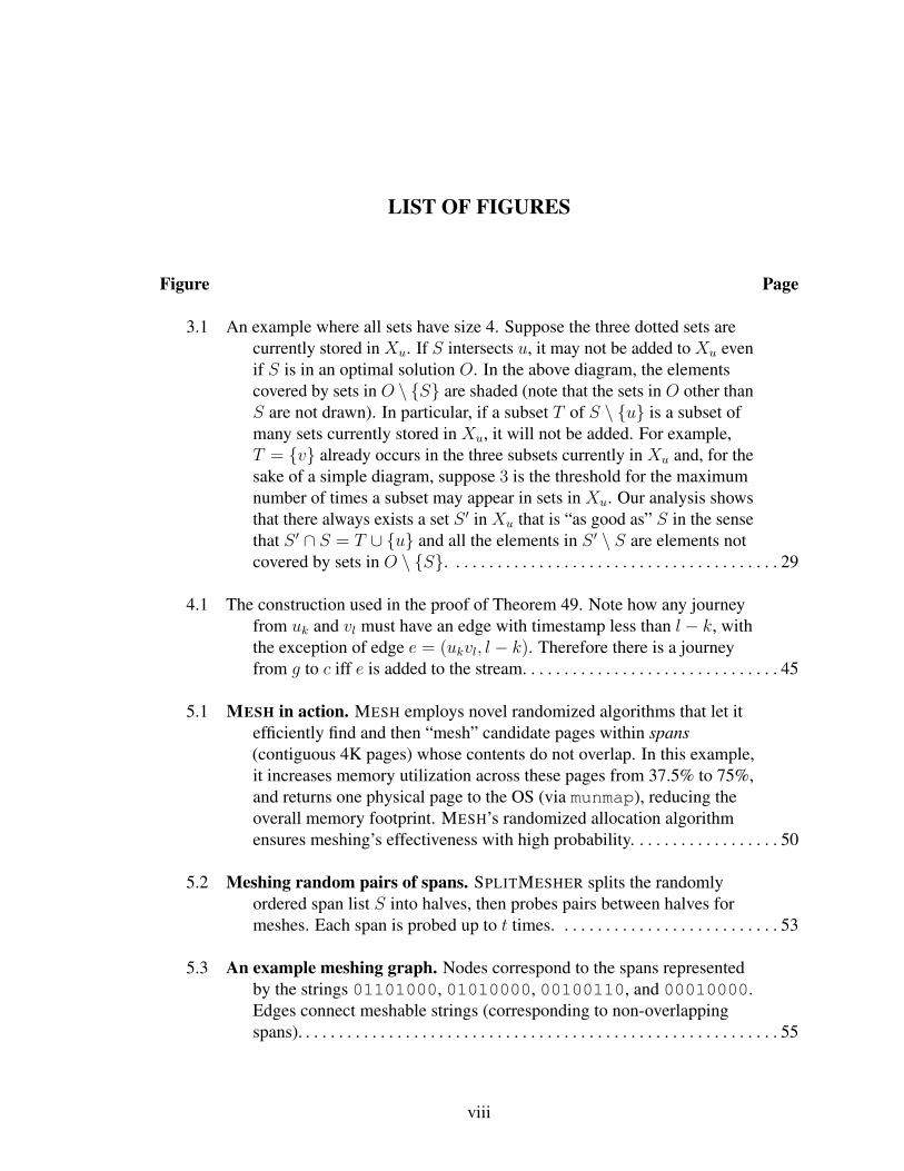
3.1 An example where all sets have size 4. Suppose the three dotted sets arecurrently stored in Xu. If S intersects u, it may not be added to Xu evenif S is in an optimal solution O. In the above diagram, the elementscovered by sets in O \ S are shaded (note that the sets in O other thanS are not drawn). In particular, if a subset T of S \ u is a subset ofmany sets currently stored in Xu, it will not be added. For example,T = v already occurs in the three subsets currently in Xu and, for thesake of a simple diagram, suppose 3 is the threshold for the maximumnumber of times a subset may appear in sets in Xu. Our analysis showsthat there always exists a set S ′ in Xu that is “as good as” S in the sensethat S ′ ∩ S = T ∪ u and all the elements in S ′ \ S are elements notcovered by sets in O \ S. . . . . . . . . . . . . . . . . . . . . . . . . . . . . . . . . . . . . . . . 29

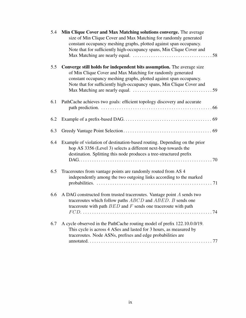
4.1 The construction used in the proof of Theorem 49. Note how any journeyfrom uk and vl must have an edge with timestamp less than l − k, withthe exception of edge e = (ukvl, l − k). Therefore there is a journeyfrom g to c iff e is added to the stream. . . . . . . . . . . . . . . . . . . . . . . . . . . . . . . 45

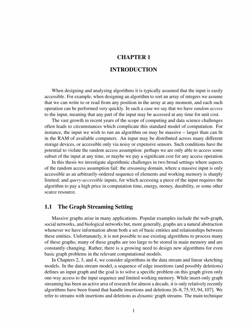
5.1 MESH in action. MESH employs novel randomized algorithms that let itefficiently find and then “mesh” candidate pages within spans(contiguous 4K pages) whose contents do not overlap. In this example,it increases memory utilization across these pages from 37.5% to 75%,and returns one physical page to the OS (via munmap), reducing theoverall memory footprint. MESH’s randomized allocation algorithmensures meshing’s effectiveness with high probability. . . . . . . . . . . . . . . . . . 50

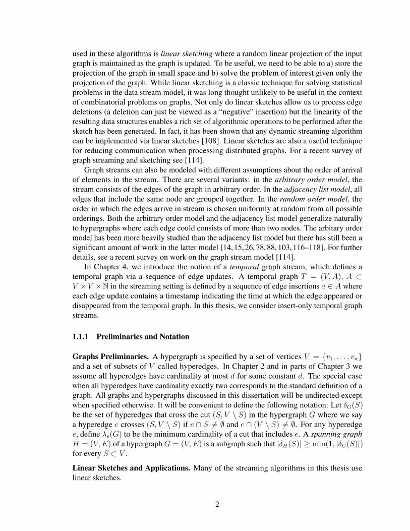
5.2 Meshing random pairs of spans. SPLITMESHER splits the randomlyordered span list S into halves, then probes pairs between halves formeshes. Each span is probed up to t times. . . . . . . . . . . . . . . . . . . . . . . . . . . 53

5.3 An example meshing graph. Nodes correspond to the spans representedby the strings 01101000, 01010000, 00100110, and 00010000.Edges connect meshable strings (corresponding to non-overlappingspans). . . . . . . . . . . . . . . . . . . . . . . . . . . . . . . . . . . . . . . . . . . . . . . . . . . . . . . . . . 55

viii

5.4 Min Clique Cover and Max Matching solutions converge. The averagesize of Min Clique Cover and Max Matching for randomly generatedconstant occupancy meshing graphs, plotted against span occupancy.Note that for sufficiently high-occupancy spans, Min Clique Cover andMax Matching are nearly equal. . . . . . . . . . . . . . . . . . . . . . . . . . . . . . . . . . . . 58

5.5 Converge still holds for independent bits assumption. The average sizeof Min Clique Cover and Max Matching for randomly generatedconstant occupancy meshing graphs, plotted against span occupancy.Note that for sufficiently high-occupancy spans, Min Clique Cover andMax Matching are nearly equal. . . . . . . . . . . . . . . . . . . . . . . . . . . . . . . . . . . . 59

6.1 PathCache achieves two goals: efficient topology discovery and accuratepath prediction. . . . . . . . . . . . . . . . . . . . . . . . . . . . . . . . . . . . . . . . . . . . . . . . . . 66

6.2 Example of a prefix-based DAG. . . . . . . . . . . . . . . . . . . . . . . . . . . . . . . . . . . . . . . 69

6.3 Greedy Vantage Point Selection . . . . . . . . . . . . . . . . . . . . . . . . . . . . . . . . . . . . . . . 69

6.4 Example of violation of destination-based routing. Depending on the priorhop AS 3356 (Level 3) selects a different next-hop towards thedestination. Splitting this node produces a tree-structured prefixDAG. . . . . . . . . . . . . . . . . . . . . . . . . . . . . . . . . . . . . . . . . . . . . . . . . . . . . . . . . . . 70

6.5 Traceroutes from vantage points are randomly routed from AS 4independently among the two outgoing links according to the markedprobabilities. . . . . . . . . . . . . . . . . . . . . . . . . . . . . . . . . . . . . . . . . . . . . . . . . . . . 71

6.6 A DAG constructed from trusted traceroutes. Vantage point A sends twotraceroutes which follow paths ABCD and ABED. B sends onetraceroute with path BED and F sends one traceroute with pathFCD. . . . . . . . . . . . . . . . . . . . . . . . . . . . . . . . . . . . . . . . . . . . . . . . . . . . . . . . . . 74

6.7 A cycle observed in the PathCache routing model of prefix 122.10.0.0/19.This cycle is across 4 ASes and lasted for 3 hours, as measured bytraceroutes. Node ASNs, prefixes and edge probabilities areannotated. . . . . . . . . . . . . . . . . . . . . . . . . . . . . . . . . . . . . . . . . . . . . . . . . . . . . . . 77

ix

CHAPTER 1

INTRODUCTION

When designing and analyzing algorithms it is typically assumed that the input is easilyaccessible. For example, when designing an algorithm to sort an array of integers we assumethat we can write to or read from any position in the array at any moment, and each suchoperation can be performed very quickly. In such a case we say that we have random accessto the input, meaning that any part of the input may be accessed at any time for unit cost.

The vast growth in recent years of the scope of computing and data science challengesoften leads to circumstances which complicate this standard model of computation. Forinstance, the input we wish to run an algorithm on may be massive – larger than can fitin the RAM of available computers. An input may be distributed across many differentstorage devices, or accessible only via noisy or expensive sensors. Such conditions have thepotential to violate the random access assumption: perhaps we are only able to access somesubset of the input at any time, or maybe we pay a significant cost for any access operation.

In this thesis we investigate algorithmic challenges in two broad settings where aspectsof the random access assumption fail: the streaming domain, where a massive input is onlyaccessible as an arbitrarily-ordered sequence of elements and working memory is sharplylimited; and query-accessible inputs, for which accessing a piece of the input requires thealgorithm to pay a high price in computation time, energy, money, durability, or some otherscarce resource.

1.1 The Graph Streaming Setting

Massive graphs arise in many applications. Popular examples include the web-graph,social networks, and biological networks but, more generally, graphs are a natural abstractionwhenever we have information about both a set of basic entities and relationships betweenthese entities. Unfortunately, it is not possible to use existing algorithms to process manyof these graphs; many of these graphs are too large to be stored in main memory and areconstantly changing. Rather, there is a growing need to design new algorithms for evenbasic graph problems in the relevant computational models.

In Chapters 2, 3, and 4, we consider algorithms in the data stream and linear sketchingmodels. In the data stream model, a sequence of edge insertions (and possibly deletions)defines an input graph and the goal is to solve a specific problem on this graph given onlyone-way access to the input sequence and limited working memory. While insert-only graphstreaming has been an active area of research for almost a decade, it is only relatively recentlyalgorithms have been found that handle insertions and deletions [6–8, 75, 93, 94, 107]. Werefer to streams with insertions and deletions as dynamic graph streams. The main technique

1

used in these algorithms is linear sketching where a random linear projection of the inputgraph is maintained as the graph is updated. To be useful, we need to be able to a) store theprojection of the graph in small space and b) solve the problem of interest given only theprojection of the graph. While linear sketching is a classic technique for solving statisticalproblems in the data stream model, it was long thought unlikely to be useful in the contextof combinatorial problems on graphs. Not only do linear sketches allow us to process edgedeletions (a deletion can just be viewed as a “negative” insertion) but the linearity of theresulting data structures enables a rich set of algorithmic operations to be performed after thesketch has been generated. In fact, it has been shown that any dynamic streaming algorithmcan be implemented via linear sketches [108]. Linear sketches are also a useful techniquefor reducing communication when processing distributed graphs. For a recent survey ofgraph streaming and sketching see [114].

Graph streams can also be modeled with different assumptions about the order of arrivalof elements in the stream. There are several variants: in the arbitrary order model, thestream consists of the edges of the graph in arbitrary order. In the adjacency list model, alledges that include the same node are grouped together. In the random order model, theorder in which the edges arrive in stream is chosen uniformly at random from all possibleorderings. Both the arbitrary order model and the adjacency list model generalize naturallyto hypergraphs where each edge could consists of more than two nodes. The arbitary ordermodel has been more heavily studied than the adjacency list model but there has still been asignificant amount of work in the latter model [14, 15, 26, 78, 88, 103, 116–118]. For furtherdetails, see a recent survey on work on the graph stream model [114].

In Chapter 4, we introduce the notion of a temporal graph stream, which defines atemporal graph via a sequence of edge updates. A temporal graph T = (V,A), A ⊂V ×V ×N in the streaming setting is defined by a sequence of edge insertions a ∈ A whereeach edge update contains a timestamp indicating the time at which the edge appeared ordisappeared from the temporal graph. In this thesis, we consider insert-only temporal graphstreams.

1.1.1 Preliminaries and Notation

Graphs Preliminaries. A hypergraph is specified by a set of vertices V = v1, . . . , vnand a set of subsets of V called hyperedges. In Chapter 2 and in parts of Chapter 3 weassume all hyperedges have cardinality at most d for some constant d. The special casewhen all hyperedges have cardinality exactly two corresponds to the standard definition of agraph. All graphs and hypergraphs discussed in this dissertation will be undirected exceptwhen specified otherwise. It will be convenient to define the following notation: Let δG(S)be the set of hyperedges that cross the cut (S, V \ S) in the hypergraph G where we saya hyperedge e crosses (S, V \ S) if e ∩ S 6= ∅ and e ∩ (V \ S) 6= ∅. For any hyperedgee, define λe(G) to be the minimum cardinality of a cut that includes e. A spanning graphH = (V,E) of a hypergraph G = (V,E) is a subgraph such that |δH(S)| ≥ min(1, |δG(S)|)for every S ⊂ V .

Linear Sketches and Applications. Many of the streaming algorithms in this thesis uselinear sketches.

2

Definition 1 (Linear Sketches). A linear measurement of a hypergraph on n vertices isdefined by a set of coefficients ce : e ∈ Pr(V ) where Pr(V ) is the set of all subsets of Vof size at most d. Given a hypergraph G = (V,E), the evaluation of this measurement isdefined as

∑e∈E ce. A sketch is a collection of (non-adaptive) linear measurements. The

cardinality of this collection is referred to as the size of the sketch. We will assume that themagnitude of the coefficients ce is poly(n). We say a linear measurement is local for node vif the measurement only depends on hyper-edges incident to v, i.e., ce = 0 for all hyper-edgesthat do not include v. We say a sketch is vertex-based if every linear measurement is local tosome node.

Linear sketches have long been used in the context of data stream models because it ispossible to maintain a sketch of the stream incrementally. Specifically, if the next streamupdate is an insertion or deletion of an edge, we can update the sketch by simply adding orsubtracting the appropriate set of coefficients. Sketches are also useful in distributed settings.In particular, the model considered by Becker et al. [19] was as follows: suppose there aren + 1 players P1, . . . , Pn and Q. The input for player Pi is the set of (hyper-)edges thatinclude the ith vertex of a graph G. Player Q wants to compute something about this graphsuch as determining whether G connected. To enable this, each of the players P1, . . . , Pnsimultaneously sends a message about their input to Q such that the set of these n messagescontains sufficient information to complete Q’s computation. In the case of randomizedprotocols, we assume that all players have access to public random bits. The goal is tominimize the maximum length of the n messages that are sent to Q. If a vertex-based sketchexists for the problem under consideration, then for each linear measurement, there is asingle player that can evaluate this message and send it to Q.

1.1.2 Connectivity Results in Dynamic (Hyper-)Graph Streams

In Chapter 2, we present sketch-based dynamic graph algorithms for three basic graphproblems: computing vertex connectivity, graph reconstruction, and hypergraph sparsifi-cation. All our algorithms run in (low) polynomial time, typically linear in the number ofedges. However, our primary focus is on space complexity, as is the convention in much ofthe data streams literature.

Vertex Connectivity. To date, the main success story for graph sketching has been aboutedge connectivity, i.e., estimating how many edges need to be removed to disconnectthe graph, and estimating the size of cuts. We present the first dynamic graph streamalgorithms for vertex connectivity, i.e., estimating how many vertices need to be removed todisconnect the graph. While it can be shown that edge connectivity is an upper bound forvertex connectivity, the vertex connectivity of a graph can be much smaller. Furthermore,the combinatorial structure relevant to both quantities is very different. For example,edge-connectivity is transitive1 whereas vertex-connectivity is not. A celebrated result byKarger [95] bounds the number of near minimum cuts whereas no analogous bound is knownfor vertex removal. Feige et al. [60] discuss issues that arise specific to vertex connectivityin the context of approximation algorithms and embeddings.

1If it takes at least k edge deletions to disconnect u and v and it takes at least k edge deletions to disconnectv and w, then it takes at least k edge deletions to disconnect u and w.

3

In Section 2.1, we present two sketch-based algorithms for vertex connectivity. The firstalgorithm uses O(kn polylog n) space and constructs a data structure such that, at the endof the stream, it is possible to test whether the removal of a queried set of at most k verticeswould disconnect the graph. We prove that this algorithm is optimal in terms of its spaceuse. The second algorithm estimates the vertex connectivity up to a (1 + ε) factor usingO(ε−1kn polylog n) space where k is an upper bound on the vertex connectivity.

No stream algorithms were previously known that supported both edge insertions anddeletions. Existing approaches either use Ω(n2) space [140] or only handle insertions [56].With only insertions, Eppstein et al. [56] proved that O(kn polylog n) space was sufficient.Their algorithm drops an inserted edge u, v iff there already exists k vertex-disjoint pathsbetween u and v amongst the edges stored thus far. Such an algorithm fails in the presenceof edge deletions since some of the vertex disjoint paths that existed when an edge wasignored need not exist if edges are subsequently deleted.

Graph Reconstruction. Our next result relates to reconstructing graphs rather than esti-mating properties of the graph. Becker et al. [19] show that is possible to reconstruct aµ-degenerate graph (that is, a graph for which all induced subgraphs have a vertex of degreeat most µ) given an O(µ polylog n) size sketch of each row of the adjacency matrix of thegraph. In Section 2.2, we define the µ-cut-degeneracy and show that the strictly larger classof graphs that satisfy this property can also be reconstructed given an O(µ polylog n)-sizesketch of each row. Moreover, even if the graph is not µ-cut-degenerate we show that wecan find all edges with a certain connectivity property. This will be an integral part of ouralgorithm for hypergraph sparsification. For this purpose, we also prove the first dynamicgraph stream algorithms for hypergraph connectivity in this section. We also extend thevertex connectivity results to hypergraphs.

Hypergraph Sparsification. Hypergraph sparsification is a natural extension of graphsparsification. Given a hypergraph, the goal is to find a sparse weighted subgraph suchthat the weight of every cut in the subgraph is within a (1 + ε) factor of the weight of thecorresponding cut in the original hypergraph. Estimating hypergraph cuts has applicationsin video object segmentation [81], network security analysis [148], load balancing inparallel computing [29], and modelling communication in parallel sparse-martix vectormultiplication [28].

Kogan and Krauthgamer [101] recently presented the first stream algorithm for hyper-graph sparsification in the insert-only model. In Section 2.3, we present the first algo-rithm that supports both edge insertions and deletions. The algorithm uses O(n polylog n)space assuming that size of the hyperedges is bounded by a constant. This result ispart of a growing body of work on processing hypergraphs in the data stream model[54,101,133,138,144]. There are numerous challenges in extending previous work on graphsparsification [7, 8, 75, 93, 94] to hypergraph sparsification and we discuss these in Section2.3. In the process of overcoming these challenges, we also identify a simpler approach forgraph sparsification in the data stream model.

4

1.1.3 Coverage Results in Data Streams

In Chapter 3, we present algorithms for the Max-k-Cover and Max-k-UniqueCoverproblems in the data stream model. The input to both problems are m subsets of a universeof size n and a value k ∈ [m]. In Max-k-Cover, the problem is to find a collection of atmost k sets such that the number of elements covered by at least one set is maximized.In Max-k-UniqueCover, the problem is to find a collection of at most k sets such that thenumber of elements covered by exactly one set is maximized. These problems are closelyrelated to a range of graph problems including matching, partial vertex cover, and capacitatedmaximum cut.

In the stream model, we assume k is given and the sets are revealed online. Our goalis to design single-pass algorithms that use space that is sublinear in the input size. Thefollowing algorithms are for insert-only streams except where specified otherwise. Our mainalgorithmic results are as follows.

• If sets have size at most d, there exist single-pass algorithms using O(dd+1kd) spacethat solve both problems exactly. This is optimal up to logarithmic factors for constantd.

• If each element appears in at most r sets, we present single pass algorithms usingO(k2r/ε3) space that return a 1 + ε approximation in the case of Max-k-Cover and2 + ε approximation in the case of Max-k-UniqueCover. We also present a single-passalgorithm using slightly more memory, i.e., O(k3r/ε4) space, that 1 + ε approximatesMax-k-UniqueCover.

In contrast to the above results, when d and r are arbitrary, any constant pass 1 + ε approxi-mation algorithm for either problem requires Ω(ε−2m) space but a single pass O(mk/ε2)space algorithm exists. In fact any constant-pass algorithm with an approximation betterthan e1−1/k requires Ω(m/k2) space when d and r are unrestricted. En route, we also obtainan algorithm for the parameterized version of the streaming SetCover problem.

Relationship to Graph Streaming.

To explore the relationship between Max-k-Cover and Max-k-UniqueCover and variousgraph stream problems, it makes sense to introduce to additional parameters beyond m (thenumber of sets) and n (the size of the universe). Specifically, throughout the chapter welet d denote the maximum cardinality of a set in the input and let r denote the maximummultiplicity of an element in the universe where the multiplicity is the number of sets theelement appears.2 Then an input to Max-k-Cover and Max-k-UniqueCover can define a(hyper)graph in one of the following two natural ways:

(1) First Interpretation: A sequence of (hyper-)edges on a graph with n nodes of maxi-mum degree r (where the degree of a node v corresponds to how many hyperedgesinclude that node) and m hyperedges where each hyperedge has size at most d. In the

2Note that d and r are dual parameters in the sense that if the input is S1, . . . , Sm and we defineTi = j : i ∈ Sj then d = maxj |Sj | and r = maxi |Ti|.

5

case where every set has size d = 2, the hypergraph is an ordinary graph, i.e., a graphwhere every edge just has two endpoints. With this interpretation, the graph is beingpresented in the arbitrary order model.

(2) Second Interpretation: A sequence of adjacency lists (where the adjacency list fora given node includes all the hyperedges) on a graph with m nodes of maximumdegree d and n hyperedges of maximum size r. In this interpretation, if every elementappears in exactly r = 2 sets, then this corresponds to an ordinary graph where eachelement corresponds to an edge and each element corresponds to an edge. With thisinterpretation, the graph is being presented in the adjacency list model.

Under the first interpretation, the Max-k-Cover problem and the Max-k-UniqueCoverproblem when all sets have exactly size 2 naturally generalize the problem of finding amaximum matching in an ordinary graph in the sense that if there exists a matching withat least k edges, the optimum solution to either Max-k-Cover and Max-k-UniqueCover willbe a matching. There is a large body of work on graph matchings in the data streammodel [5, 27, 47, 48, 57, 63, 74, 76, 89, 90, 102–104, 113, 150] including work specificallyon solving the problem exactly if the matching size is bounded [38, 40]. More precisely,Max-k-Cover corresponds to the partial vertex cover problem [111]: what is the maximumnumber of edges that can be covered by selecting k nodes. For larger sets, the Max-k-Coverand Max-k-UniqueCover are at least as hard as finding partial vertex covers and matching inhypergraphs.

Under the second interpretation, when all elements have multiplicity 2, Max-k-UniqueCovercorresponds to finding the capacitated maximum cut, i.e., a set of at most k vertices suchthat the number of edges with exactly one endpoint in this set is maximized. In the offlinesetting, Ageev and Sviridenko [4] and Gaur et al. [68] presented a 2 approximation forthis problem using linear programming and local search respectively. The (uncapacitated)maximum cut problem was been studied in the data stream model by Kapralov et al. [91,92];a 2-approximation is trivial in logarithmic space3 but improving on this requires space that ispolynomial in the size of the graph. The capacitated problem is a special case of the problemof maximizing a non-monotone sub-modular function subject to a cardinality constraint.This general problem has been considered in the data stream model [16, 32, 35, 80] but inthat line of work it is assumed that there is oracle access to the function being optimized,e.g., given any set of nodes, the oracle will return the number of edges cut. Alaluf et al. [9]presented a 2 + ε approximation in this setting, assuming exponential post-processing time.In contrast, our algorithm does not assume an oracle while obtaining a 1 + ε approximation(and also works for the more general problem Max-k-UniqueCover).

1.1.4 Temporal Graph Streams

Graphs are extremely general and useful structures which can elegantly represent manyaspects of real-world structures such as social networks, disease spreading models, and theInternet. However, one aspect of all of these structures that the traditional view of graphsdoes not accomodate is temporality. For example, consider disease-tracking on a real-time

3It suffices to count the number of edges M since there is always a cut whose size is between M/2 and M .

6

stream of physical contact events between people. Say Alice has the flu. She shakes Bob’shand, and then Bob later shakes Charlie’s hand. We could attempt to model this with a graphG with nodes A,B,C and edges (A,B), (B,C) where Alice is represented by node A,Bob by node B, Charlie by node C, and edges represent infection-spreading handshakes.We can use this graph to conclude that Charlie is susceptible to infection because there isa path from Alice to him. However, this graph representation would also suggest that ifCharlie was the one who started with the flu, Alice is susceptible to infection since thereis a path from Charlie to Alice as well. This is incorrect, since Alice interacts with Bobbefore he can be infected by Charlie. By not taking the time at which these edges occurredinto account, this graph representation fails to adequately represent the spread of disease.We would like some model that allows us to determine who is at risk of infection fromsome patient zero, perhaps through an indirect chain of time-ordered contact events. Tocapture such dynamics, we use temporal graphs whose edges are augmented with set oftimestamps which indicate times at which the edge exists. In our example, we replace Gwith temporal graph T with nodes A,B,C and edges (A,B, 1), (B,C, 2) where edgesare now triples: a pair of endpoints and a timestamp. Note that the path from A to C usesedges with increasing timestamps, suggesting infection can spread along this path, whilethe path from C to A uses edges with decreasing timestamps, ruling out the possibility ofinfection spreading in the reverse direction. We say that there is a time-respecting path fromA to C but not from C to A.

Mertzios et al. [122] give an algorithm that computes short time-respecting paths froma source node s to all other nodes in O(n poly(τ)) time where τ denotes the number ofdistinct timestamps in the temporal graph. Menger’s theorem, which states that the maximumnumber of node-disjoint s to t paths is equal to the minimum number of nodes that mustbe removed in order to separate s from z [121], does not hold for time-respecting paths intemporal graphs [23, 99]. However, Mertzios et. al. [122] recently proved a reformulatedtemporal analogue of Menger’s theorem that holds for temporal graphs.

Researchers have noted that temporal analogues of graph problems tend to have highercomplexity. Bhadra & Ferreira [24] demonstrate that computing strongly connected compo-nents of directed temporal graphs is NP-Complete. Michail & Spirakis [124] show that atemporal analogue of the maximum matching problem, where one must find a maximummatching whose edges have distinct timestamps, is NP-Complete as well. They also provethat a temporal analogue of the Graphic Traveling Salesman Problem cannot be approxi-mated within multiplicative factor cn for some constant c > 0 unless P = NP . For thestandard and more general TSP, its temporal analogue is APX-Hard even if its edge costsare constrained to 1, 2.

The study of temporal graphs is in its infancy [123] and to date no one has consideredalgorithms on temporal graphs in the streaming domain. It will be useful to study thesestructures at scale. For instance, in the spirit of our infection example, we may wish totrack the spread of disease through a large, densely connected population. What can weaccomplish by storing a small summary of the massive stream of connection events?

We begin the study of temporal graph streams by considering variations of reachabilityproblems, which involve determining whether or not there exists a time-respecting pathbetween nodes in the temporal graph. We demonstrate strong lower bounds for manyversions of this problem, but also find several versions that admit space-efficient algorithms.

7

We also present some conjectures about the overall hardness of streaming temporal graphreachability.

1.2 Graph Algorithms for Systems Challenges

A significant portion of the work in this dissertation consists of applications of graphalgorithms to practical systems challenges, resulting in open-source software which weshow both analytically and empirically to be effective and efficient. In this thesis, wepresent two such completed projects: MESH, a memory manager that is capable of memorycompaction in C and C++ (a feat long thought impossible), and PathCache, an efficientlyscalable network measurement platform that outperforms the current state of the art.

1.2.1 Memory Compaction Powered by Graph Algorithms

Memory consumption is a serious concern across the spectrum of modern computingplatforms, from mobile to desktop to datacenters. For example, on low-end Androiddevices, Google reports that more than 99% of Chrome crashes are due to running outof memory when attempting to display a web page [79]. On desktops, the Firefox webbrowser has been the subject of a five-year effort to reduce its memory footprint [142]. Indatacenters, developers implement a range of techniques from custom allocators to other adhoc approaches in an effort to increase memory utilization [135, 139].

A key challenge is that, unlike in garbage-collected environments, automatically reducinga C/C++ application’s memory footprint via compaction is not possible. Because theaddresses of allocated objects are directly exposed to programmers, C/C++ applicationscan freely modify or hide addresses. For example, a program may stash addresses inintegers, store flags in the low bits of aligned addresses, perform arithmetic on addressesand later reference them, or even store addresses to disk and later reload them. This hostileenvironment makes it impossible to safely relocate objects: if an object is relocated, allpointers to its original location must be updated. However, there is no way to safely updateevery reference when they are ambiguous, much less when they are absent.

Existing memory allocators for C/C++ employ a variety of best-effort heuristics aimed atreducing average fragmentation [86]. However, these approaches are inherently limited. Ina classic result, Robson showed that all such allocators can suffer from catastrophic memoryfragmentation [137]. This increase in memory consumption can be as high as the log of theratio between the largest and smallest object sizes allocated. For example, for an applicationthat allocates 16-byte and 128KB objects, it is possible for it to consume 13× more memorythan required.

Chapter 5 introduces MESH, a plug-in replacement for malloc that, for the firsttime, eliminates fragmentation in unmodified C/C++ applications. MESH combines novelrandomized algorithms with widely-supported virtual memory operations to provably reducefragmentation, breaking the classical Robson bounds with high probability. We focus hereon the randomized graphalgorithms which power MESH and proofs of their solution qualityand runtime. Because MESH operates on live memory contents of active programs, itoperates under extreme time pressure and in essence cannot afford to observe every edge

8

in the graph. Instead it must find a solution by making a limited number of edge querieswhich take valuable time to answer. MESH generally matches the runtime performance ofstate-of-the-art memory allocators while reducing memory consumption; in particular, itreduces the memory of consumption of Firefox by 16% and Redis by 39%.

1.2.2 Efficient Network Measurement via Graph Discovery

Despite its engineered nature, the Internet has evolved into a collection of networkswith different–and sometimes conflicting–goals, where understanding its behavior requiresempirical study of topology and network paths. This problem is compounded by networks’desire to keep their routing policies and behaviors opaque to outsiders for commercial orsecurity-related reasons. Researchers have worked for over a decade designing tools andtechniques for inferring AS level connectivity and paths [109, 110]. However, operatorsseeking to leverage information about network paths or researchers requiring Internet pathsto evaluate new Internet-scale systems are often confronted with limited vantage pointsfor direct measurement and myriad data sets, each offering a different lens on AS levelconnectivity and paths.

Predicting network paths is crucial for a variety of problems impacting researchers,network operators and content/cloud providers. Researchers often need knowledge ofInternet routing to evaluate Internet-scale systems (e.g., refraction routing [146], Tor [51],Secure-BGP [71]). For network operators, network paths can aid in diagnosing the root causeof performance problems like high latency or packet loss. Content providers debuggingpoor client-side performance require the knowledge of the set of networks participating indelivering client traffic to root-cause bottleneck links. While large cloud providers, likeAmazon, Google and Microsoft are known to develop in-house telemetry for global networkdiagnostics, small companies, ISPs and academics often lack such visibility and data.

Understanding and predicting Internet routes is confounded by several factors. Internetpaths are dependant on several deterministic but not public phenomena: route advertisementsmade via BGP and best path selection algorithms based on private business relationships.Additionally, factors like load balancing via ECMP, intermittent congestion on networklinks, control plane mis-configurations and BGP hijacks also impact network paths.

Standard diagnostic tools like traceroute provide limited visibility into network pathssince the user can only control the destination of a traceroute query, the source being herown network. Tools like reverse traceroute [97] rely on the support of IP options to shedlight on the reverse path towards one’s network. In addition to requiring the support for IPoptions from Internet routers, these techniques require active probing from the client (ora set of vantage points distributed on the Internet). Active probing is not only expensivein terms of amount of traffic generated (traceroutes, pings etc.) but also provides limitedvisibility into the network state.

In Chapter 6, we design and develop PathCache, which predicts network paths betweenarbitrary sources and destinations on the Internet by developing probabilistic models ofrouting from observed network paths. For this purpose, PathCache, leverages existingdata and control plane measurements (such as stale traceroutes and BGP routing data),optimizing use of existing data plane measurement platforms, and applying routing modelswhen empirical data is absent. Specifically, the challenge is to select a bounded number of

9

path measurement queries to make towards some destination which maximize the amount ofnetwork topology (modeled as a directed graph with the destination as the ”root”) discovered.Using provably efficient algorithms, PathCache consumes millions of traceroutes from publicmeasurement platforms every hour and updates the probabilistic routing model using newlyacquired information. We offer PathCache as a service at https://www.davidtench.com/deeplinks/pathcache. In its present form, the PathCache REST API allowsusers to query network paths between sources and destinations (IP address, BGP routed prefixor autonomous system). In addition to providing the predicted paths, PathCache providesconfidence values associated with each network path based on historical information.

PathCache complements the approach of existing path-prediction systems [98, 109] bydeveloping efficient algorithms for measuring the routing behavior towards all BGP prefixeson the Internet. When measuring paths towards each BGP prefix, PathCache maximizesdiscovery of the network topology with a constrained measurement budget, both globallyand per vantage point. PathCache’s strategy for exploring network paths discovers 4X moreAS-hops than other well known strategies used in practice today.

10

Problems in the Graph Streaming Modeland Extensions

11

CHAPTER 2

VERTEX AND HYPEREDGE CONNECTIVITY IN DYNAMICGRAPH STREAMS

A growing body of work addresses the challenge of processing dynamic graph streams:a graph is defined by a sequence of edge insertions and deletions and the goal is to constructsynopses and compute properties of the graph while using only limited memory. Linearsketches have proved to be a powerful technique in this model and can also be used tominimize communication in distributed graph processing.

We present the first linear sketches for estimating vertex connectivity and constructinghypergraph sparsifiers. Vertex connectivity exhibits markedly different combinatorial struc-ture than edge connectivity and appears to be harder to estimate in the dynamic graph streammodel. Our hypergraph result generalizes the work of Ahn et al. [6] on graph sparsificationand has the added benefit of significantly simplifying the previous results. One of the mainideas is related to the problem of reconstructing subgraphs that satisfy a specific sparsityproperty. We introduce a more general notion of graph degeneracy and extend the graphreconstruction result of Becker et al. [19].

2.1 Vertex Connectivity

A natural approach to determining vertex connectivity could be to try to mimic thealgorithm of Cheriyan et al. [36]. They showed that the union of k disjoint “scan first searchtrees” (a generalization of breadth-first search trees) can be used to determine if a graphis k vertex connected. A similar approach worked in data stream model for the case ofedge-connectivity (which we discuss in further detail in the next section) but in that case thetrees to be constructed could be arbitrary. Unfortunately, we can show that any algorithmfor constructing a scan-first search tree in the data stream model requires Ω(n2) space evenwhen there are no edge deletions.

A scan first search tree (SFST) of a graph [36] is defined as follows: The tree is initiallyempty, all vertices except the root (chosen arbitrarily) are unmarked, and all vertices areunscanned. At each step we scan an marked but unscanned vertex. For each vertex x that isbeing scanned, all edges from x to unmarked neighbors of x are added to the tree and theunmarked neighbors are marked. This continues until no marked but unscanned verticesremain.

Theorem 2. Any data stream algorithm that constructs a SFST with probability at least 3/4requires Ω(n2) space.

12

Proof. The proof is by a reduction from the communication problem of indexing [1].Suppose Alice has a binary string x ∈ 0, 1n2 indexed by [n] × [n] and Bob wants tocompute xi,j for some index (i, j) ∈ [n]× [n] that is unknown to Alice. This requires Ω(n2)bits to be communicated from Alice to Bob if Bob is to learn xi,j with probability at least 3/4.Suppose we have a data stream algorithm for constructing an SFST. Alice creates a graph onnodes T ∪ U ∪ V ∪W where T = t1, . . . , tn, U = u1, . . . , un, V = v1, . . . , vn, andW = w1, . . . , wn. She adds edges tk, u` and v`, tk for each `, k such that x`,k = 1.Alice runs the scan-first search algorithm and sends the contents of her memory to Bob. Bobadds the edge ui, vi. Note that any SFST includes all neighbors of ui or vi. In particular,xi,j = 1 iff at least one of tj, ui or vi, wj is present in the SFST constructed. Hence,the algorithm must have used Ω(n2) space.

To avoid this issue, we take a different approach based on finding arbitrary spanningtrees for the induced graph on a random subset of vertices.1 We will use the following resultfor finding these spanning trees.

Theorem 3 (Ahn et al. [6]). For a graph on n vertices, there exists a vertex-based sketch ofsize O(n polylog n) from which we can construct a spanning forest with high probability.

Note that in this section we restrict our attention to graphs rather than hypergraphs.However, in the next section we will explain how the vertex connectivity results extend tohypergraphs.

2.1.1 Warm-Up: Vertex Connectivity Queries

For i = 1, 2, . . . , R := 16 · k2 lnn, let Gi be a graph formed by deleting each vertexin G with probability 1 − 1/k. Let Ti be an arbitrary spanning forest of Gi and defineH = T1 ∪ T2 ∪ . . . ∪ TR.

Lemma 4. Let S be an arbitrary collection of at most k vertices. With high probability,H \ S is connected iff G \ S is connected.

Proof. First we note that H has the same set of vertices as G with high probability. Thisfollows because the probability a given vertex is not in H is (1− 1/k)R ≤ exp (()− 16 ·k · lnn) = n−16k and hence by an application of the union bound, all vertices in G are alsoin H with probability at least 1− n−(16k−1). Then since H is a subgraph of G, then G \ Sdisconnected implies H \ S disconnected. It remains to prove that G \ S connected impliesH \ S connected.

Assume G \ S is connected. Consider an arbitrary pair of vertices s, t 6∈ S and lets = v0 → v1 → v2 → . . . → v` = t be a path between s and t in G \ S. Then note thatthere is a path between vi and vi+1 in H \ S if there exists Gi such that Gi ∩ S = ∅ and

1We note that the idea of subsampling vertices was recently explored by Censor-Hillel et al. [30, 31]. Theyshowed that if each vertex of a k-vertex-connected graph is subsampled with probability p = Ω(

√log n/k)

then the resulting graph has vertex connectivity Ω(kp2). We do not make use of this result in our work as itdoes not lead to an approximation factor better than

√k.

13

vi, vi+1 ∈ H \ S. This follows because if vi, vi+1 ∈ Gi and Gi ∩ S = ∅ then Ti \ S eithercontains vi, vj or a path between between vi and vj . Hence,

P [vi and vi+1 are connected in Ti \ S] ≥ 1/k2(1− 1/k)k

and therefore

P [vi and vi+1 are disconnected in Ti \ S for all i ∈ [R]] ≤ (1−1/k2(1−1/k)k)R ≤ 1/n4 .

Taking the union bound over all ` < n pairs vi, vi+1, we conclude that s and t areconnected in H \ S with probability at least 1− 1/n3. By applying the union bound again,with probability at least 1− 1/n2, s is connected in H \ S to all other vertices.

Our algorithm constructs a spanning forest for each of G1, . . . , GR using the algorithmreferenced in Theorem 3. Note that since each Gi has O(n/k) vertices with high probability,we can construct these R trees in R · O(n/k polylog n) = O(nk polylog n) space. Thisgives us the following theorem.

Theorem 5. There is a sketch-based dynamic graph algorithm that uses O(kn polylog n)space to test whether a set of vertices S of size at most k disconnects the graph. The queryset S is specified at the end of the stream.

We next prove that the above query algorithm is space-optimal.

Theorem 6. Any dynamic graph algorithm that allows us to test, with probability at least3/4, whether a queried set of at most k vertices disconnects the graph requires Ω(kn) space.

Proof. The proof is by a reduction from the communication problem of indexing [1].Suppose Alice has a binary string x ∈ 0, 1(k+1)·n indexed by [k + 1] · [n] and Bob wantsto compute xi,j for some index (i, j) ∈ [k + 1] · [n] that is unknown to Alice. This requiresΩ(nk) bits to be communicated from Alice to Bob if Bob is to be successful with probabilityat least 3/4. Consider the protocol where the players create a bipartite graph on verticesL ∪ R where L = l1, . . . , lk+1 and R = r1, . . . , rn. Alice adds edges li, rj for allpairs (i, j) such that xi,j = 1. Alice runs the algorithm and sends the state to Bob. Bob addsedges r`, r`′ for all `, `′ 6= j and deletes all vertices in L except li. Now rj is connected tothe rest of the graph iff the xi,j = 1.

2.1.2 Vertex Connectivity

For i = 1, 2, . . . , R := 160 · k2ε−1 lnn, let Gi be a graph formed by deleting each vertexin G with probability 1− 1/k. As before, let Ti be an arbitrary spanning forest of Gi anddefine H = T1 ∪ T2 ∪ . . . ∪ TR.

Theorem 7. Let S be a subset of V of size k. Consider any pair of vertices u, v ∈ V \ Ssuch that there are at least (1 + ε)k vertex-disjoint paths between u and v in G. Then,

P [u and v are connected in GS] ≥ 1− 4/n10k

where GS = ∪i∈U(S)Gi and U(S) = i : Gi ∩ S = ∅ is the set of sampled graphs with novertices in S.

14

Proof. We first argue that |U(S)| is large with high probability. Then E [|U(S)|] = (1 −1/k)kR ≥ R/4. By an application of the Chernoff bound:

P [|U(S)| ≤ 1/2 ·R/4] ≤ e−1/4·R/4·1/3 < 1/n10k .

In the rest of the proof we condition on event |U(S)| ≥ r := R/8.Note that there are t ≥ εk vertex-disjoint paths between u and v in G \ S. Call these

paths P1, . . . , Pt. For each Pi, let ai be the edge incident to u, let ci be the edge incident tov, and let Bi be the remaining edges in Pi. Note that ai and ci need not be distinct and Bi

could be empty.

Claim 1. The followings three probabilities are each larger than 1− 1/n10k:

P [ai ∈ GS for at least 3t/4 values of i]

P [Bi ⊆ GS for at least 3t/4 values of i]

P [ci ∈ GS for at least 3t/4 values of i] .

Proof. Each edge in Bi is not present in GS with probability (1 − 1/k2)r. Hence, by theunion bound, P [Bi 6⊆ GS] ≤ |Bi|(1− 1/k2)r. Also by the union bound,

P [Bi 6⊆ GS for more than t/4 values of i]

<

(t

t/4

)(n(1− 1/k2)r)t/4

< exp(t ln 2 + (lnn− r/k2)t/4

)< 1/n10k .

The proofs for ai and ci are entirely symmetric so we just consider ai. Consider the setU ′(S) = U(S) ∩ j : u ∈ Gj. Note that for j ∈ U ′(S) we have P [ai ∈ Gj] = 1/k and bythe union bound,

P[ai 6∈ ∪j∈U ′(S)Gj for at least t/4 values of i

]≤

(t

t/4

)(1− 1/k)|U

′(S)|t/4

≤ 2texp(−|U ′(S)|t

(4k)

).

Let E be the event that |U ′(S)| ≤ |U(S)|/(2k). Then, by an application of the Chernoffbound:

P [ai 6∈ GS for at least t/4 values of i]≤ P [E]

+P[ai 6∈ ∪j∈U ′(S)Gj for at least t/4 values of i | ¬E

]≤ exp (−1/4 · |U(S)|/k · 1/3)

+P[ai 6∈ ∪j∈U ′(S)Gj for at least t/4 values of i | ¬E

]≤ exp (−1/4 · r/k · 1/3) + 2texp (−r/(2k) · t/(4k))

< 1/n10k .

15

It follows from the claim that there exists i such that Pi ∈ GS (and therefore u and vare connected in GS) with probability at least 1− 3/n10k. The conditioning on |U(S)| ≥ rdecreases this by another 1/n10k.

Corollary 8. If G is (1 + ε)k-vertex-connected then H is k-vertex-connected with highprobability. If H is k-vertex connected then G is k-vertex connected.

Proof. The first part of the corollary follows from Theorem 7 by applying the union boundover all O(nk) subsets of size at most k and O(n2) choices of u and v. Note that u and vconnected in GS implies u and v are connected in H since H includes a spanning forest ofGS . The second part is implied by the fact H is a subgraph of G.

As in the previous section, our algorithm is simply to construct H be using the algorithmreferenced in Theorem 3 to construct T1, . . . , TR. We can then run any vertex connectivityalgorithm onH in post-processing. Since eachGi hasO(n/k) vertices with high probability,we can construct these R trees in R ·O(n/k · polylog n) = O(nkε−1 polylog n) space. Thisgives us the following theorem.

Theorem 9. There is a sketch-based dynamic graph algorithm that usesO(knε−1 polylog n)space to distinguish (1 + ε)k-vertex connected graphs from k-connected graphs.

2.2 Reconstructing Hypergraphs

We next present sketches for reconstructing cut-degenerate hypergraphs. Recall thata hypergraph is µ-degenerate if all induced subgraphs have a vertex of degree at most µ.Cut-degeneracy is defined as follows.

Definition 10. A hypergraph is µ-cut-degenerate if every induced subgraph has a cut of sizeat most µ.

The following lemma establishes that this is a strictly weaker property than µ-degeneracy.

Lemma 11. Any hypergraph that is µ-degenerate is also µ-cut-degenerate. There existsgraphs that are µ-cut-degenerate but not µ-degenerate.

Proof. Since the degree of a vertex v is exactly the size of the cut (v, V \ v) itis immediate that µ-degeneracy implies µ-cut-degeneracy. For an example that µ-cut-degenerate does not imply it is µ-degenerate consider the graph G on eight verticesv1, v2, v3, v4, u1, u2, u3, u4 with edges vi, vj, ui, uj for all i, j except i = 1, j = 4and edges v1, u1 and v4, u4. Then G has minimum degree 3 and is therefore not2-degenerate while it is 2-cut-degenerate.

Becker et al. [19] showed how to reconstruct a µ-degenerate graph in the simultaneouscommunication model if each player sends an O(µ polylog n) bit message. We will showthat it is also possible to reconstruct any µ-cut-degenerate with the same message complexity.Even if the graph is not cut-degenerate, we show that is possible to reconstruct all edgeswith a certain connectivity property. We will subsequently use this fact in Section 2.3.

16

2.2.1 Skeletons for Hypergraphs

We first review the existing results on constructing k-skeletons [6] that we will need forour new results. In doing so, we generalize the previous work to the case of hypergraphs.In particular, this leads to the first dynamic graph algorithm for determining hypergraphconnectivity.

Definition 12 (k-skeleton). Given a hypergraph H = (V,E), a subgraph H ′ = (V,E ′) is ak-skeleton of H if for any S ⊂ V , |δH′(S)| ≥ min(|δH(S)|, k).

In particular, any spanning graph is a 1-skeleton and it can be shown that F1∪F2∪. . .∪Fkis a k-skeleton [6] ofG if Fi is a spanning graph ofG\(∪i−1

j=1Fj). The next lemma establishesthat given an arbitrary k-skeleton of a graph we can exactly determine the set of edges withλe(G) ≤ k − 1.

Lemma 13. Let H be a k-skeleton of G then λe(H) ≤ k − 1 iff λe(G) ≤ k − 1.

Proof. Since H is a subgraph λe(H) ≤ λe(G) and hence λe(G) ≤ k − 1 implies λe(H) ≤k− 1. Using the fact that H is a k-skeleton λe(H) ≥ min(k, λe(G)) and hence, if λe(H) ≤k − 1 it must be that λe(G) ≤ k − 1.

Constructing Spanning Graphs. For each vertex vi ∈ V , define the vector ai ∈ −1, 0, 1, 2,. . . , d− 1α where α =

∑di=2

(ni

)is the number of possible hyperedges of size at most d:

aie =

|e| − 1 if i = min e and e ∈ E−1 if i ∈ e \min e and e ∈ E0 otherwise

where e ranges over all subsets of V of size between 2 and d and min e denotes the smallestID of a node in e. Observe that these vectors have the property that for any subset of verticesvii∈S , the non-zero entries of

∑i∈S a

i correspond exactly to δ(S). This follows becausethe only subsets of

|e| − 1,−1,−1, . . . ,−1︸ ︷︷ ︸|e|−1

that sum to zero are the empty set and the entire set. Hence, the e-th coordinate of∑

i∈S ai

is zero iff either e 6∈ E or e ⊂ S or e ⊂ V \ S.The rest of algorithm proceeds exactly as in the case of (non-hyper) graphs [6] and a

reader that is very familiar with the previous work should feel free to skip the remainder ofSection 2.2.1. We construct the sketches Ma1, . . . ,Man where M is chosen according toa distribution over matrices Rk·α where k = polylog(α). The distribution has the propertythat for any a ∈ Rd, it is possible to determine the index of a non-zero entry of a given Mawith probability 1− 1/ poly(n). Such as distribution is known to exist by a result of Jowhariet al. [87]. Given Ma1, . . . ,Man we can find an edge across an arbitrary cut (S, V \ S).To do this, we compute

∑i∈SMai = M(

∑i∈S a

i). We can then determine the index ofa non-zero entry of

∑i∈S a

i which corresponds to an element of δ(S) as required. It mayappear that to test connectivity we need to test all 2n−1 − 1 possible cuts. Since the failureprobability for each cut is only inverse polynomial in n this would be problematic. However,it is possible to be more efficient and only test O(n) cuts. See Ahn et al. [6] for details.

17

Theorem 14 (Spanning Graph Sketches). There exists a vertex-based sketch A of sizeO(n polylog n) such that we can find a spanning graph of a hypergraph G from A(G) withhigh probability.

Note the above theorem can be substituted for Theorem 3 and the resulting algorithmsfor vertex connectivity go through for hypergraphs unchanged.

Constructing k-skeletons. As mentioned above, it suffices to find F1, . . . , Fk such thatFi is a spanning graph of G \ (∪i−1

j=1Fj). Do to this we use k independent spanning graphsketchesA1(G),A2(G), . . . ,Ak(G) as described in the previous section. We may constructF1 from A1(G) because this is the functionality of a spanning graph sketch. Assuming wehave already constructed F1, . . . , Fi−1 we can construct Fi from:

Ai(G− F1 − F2 . . .− Fi−1) = Ai(G)−i−1∑j=1

Ai(Fj) .

Theorem 15 (k-Skeleton Sketches). There exists a vertex-based sketch B of sizeO(kn polylog n) such that we can find of a k-skeleton a hypergraph G from B(G) with highprobability.

2.2.2 Beyond k-Skeletons

One might be tempted as ask whether it was necessary to use k independent spanninggraph sketches A1, . . . ,Ak rather that reuse a single sketch A. If each application of thesketchA fails to return a spanning graph with probability δ, one might hope to use the unionbound to argue that the probability that A fails on any of the inputs G,G− F1, G− F1 −F2, . . . , G − F1 − . . . − Fk−1 is at most kδ. But this would not be a valid application ofthe union bound! The union bound states that for any fixed set of t events B1, . . . , Bt, wehave P [B1 ∪ . . . ∪Bt] ≤

∑i P [Bi]. The issue is that the events in the above example are

not fixed, i.e., they can not be specified a priori, since spanning graph Fi is determined bythe randomness in the sketch.2 We belabor this point because, while the union bound wasnot applicable in the above case, we will need it to prove our next result in a situation that isonly subtly different and yet the union bound is valid.

2.2.2.1 Finding the light edges

Given a graph G = (V,E) and a postive integer k, recursively define

Ei = e ∈ E : λe(G \i−1⋃j=1

Ei) ≤ k

2Another way to see that using the same sketch cannot work is that if it were possible to repeatedly removeeach spanning graph from the sketch of the original graph, we would be able to reconstruct the entire graphusing only a sketch of size O(npolylog n). Clearly this is not possible because it requires at Ω(n2) bits tospecify an arbitrary graph on n vertices.

18

and denote the union of these sets as:

lightk(G) =⋃i≥1

Ei .

Note that if G is µ cut-degenerate then lightµ(G) = E. Furthermore, there is at most nvalues of i such that Ei is non-empty since removing each non-empty set Ei from the graphincreases the number of connected components.

Suppose B(G) is a sketch that returns an arbitrary (k + 1)-skeleton of G with failureprobability δ = 1/ poly(n). Then, since E1, E2, . . . , En are sets defined solely by the inputgraph (and not any randomness in a sketch) we can specify the fixed events

Bi = “We fail to return a (k + 1)-skeleton sketch ofG− E1 − . . .− Ei given B(G− E1 − . . .− Ei)”

and therefore use the union bound to establish that the probability that we find a (k + 1)-skeleton of each of the relevant graphs with failure probability at most nδ = 1/ poly(n).

We can therefore find the sets E1, E2, . . . , En as follows. Let Si be an arbitrary (k + 1)skeleton of G − E1 − . . . Ei−1. Assuming we have already determined E1, . . . , Ei−1, wecan find Si using:

B(G− E1 − E2 . . .− Ei−1) = B(G)−i−1∑j=1

B(Ej) .

Then, by appealing to Lemma 13, we know that we can then uniquely determine Ei givenSi.

Theorem 16. There exists a vertex-based sketch of size O(kn) from which lightk(G) canbe reconstructed for any hypergraph G. In the case of a k-cut-degenerate graph, this is theentire graph.

2.2.2.2 What are the light edges?

In this section, we restrict our attention to graphs rather than hypergraphs and show thatthe set of edges in lightk(G) can be defined in terms of the notion of strong connectivityintroduced by Benczur and Karger [20].

Lemma 17. lightk(G) = e : ke ≤ k where ku,v is the maximum k such that there is aset S ⊂ V including u and v such that the induced graph on S is k-edge-connected.

Proof. Define te to be the minimum value of k such that e ∈ lightk(G). We prove thatte = ke and the result follows. To show ke ≥ te suppose te = t and then note that esurvives when we recursively remove edges with edge connectivity t− 1. But the remainingcomponents in this graph are at least (t − 1) + 1 = t connected so ke ≥ t. To show thatke ≤ te, suppose ke = k. Then there exists a vertex induced subgraph H containing e that isk-connected. But when we recursively remove edges with edge connectivity at most k − 1then no edge in H can be removed. Hence, te > (k − 1) and so te ≥ k.

19

2.3 Hypergraph Sparsification

In this final section, we present a vertex-based sketch for constructing a sparsifier of ahypergraph. This yields the first dynamic graph stream algorithm for constructing a sparsifierof a hypergraph. As an added bonus, our approach gives an algorithm and analysis that issignificantly simpler than previous work on the specific case of graph sparsification [7, 75].

Definition 18 (Hypergraph Sparsifier). A weighted subgraph H = (V,E ′, w) of a hyper-graph G = (V,E) is a sparsfier if for all S ⊂ V ,

∑e∈δH(S) w(e) = (1± ε)|δG(S)|.

Previous approaches to sparsification in the dynamic stream model relied on work byFung et al. [67]. To construct a graph sparsifier, they showed that it was sufficient toindependently sample every edge in the graph with probability O(ε−2λ−1

e log n). Usingtheir work required coopting their machinery and modifying it appropriately (e.g., replacingChernoff arguments with careful Martingale arguments). Another downside to the previousapproach is that the Fung et al. result does not seem to extend to the case of hypergraphs.3

Using our new-found ability (see the previous section) to find the entire set of edges thatare not k-strong, we present an algorithm that a) has a simpler, and almost self-contained,analysis and b) extends to hypergraphs. Our approach is closer in spirit to Benczur andKarger’s original work on sparsification [20] which in turn is based on the following resultby Karger [96]: if we sample each edge with probability p ≥ p∗ = cε−2λ−1 log n where λis the cardinality of the minimum cut and c ≥ 0 is some constant, and weight the samplededges by 1/p then the resulting graph is a sparsifier with high probability.

The idea behind our algorithm is as follows. For a hypergraph G, if we remove thehyperedges lightk(G) where k = 2cε−2 log n, then every connected component in theremaining hypergraph has minimum cut of size greater than 2cε−2 log n. Hence, for each ofthese components p∗ ≤ 1/2. Therefore, the graph formed by sampling the hyperedges inG \ lightk(G) with probability 1/2 (and doubling the weight of sampled hyperedges) andadding the set of hyperedges in lightk(G) with unit weights is a sparsifier of G. We thenrepeat this process until there are no hyperedges left to sample.

Algorithm.

(1) Generate a series of graphs G0, G1, G2 . . . where Gi is formed by deleting eachhyperedge in Gi−1 independently with probability 1/2 and G0 = G.

(2) For i = 0, 1, 2, . . . , ` = 3 log n:

(a) Let Fi = lightk(Hi) where k = O(ε−2(log n+ r)) where Hi = Gi \ (F0 ∪F1 ∪F2 ∪ . . . ∪ Fi−1)

(3) Return⋃`i=0 2i · Fi where 2i · Fi is the set of hyperedges in Fi where each is given

weight 2i.

Analysis. The following lemma uses an argument due to Karger [95] combined with ahypergraph cut counting result by Kogan and Krauthgamer [101].

3For the reader familiar with Fung et al. [67], the issue is finding a suitable definition of cut-projection forhypergraphs and then proving a bound on the number of distinct cut-projections.

20

Lemma 19. 2Hi+1 ∪ Fi is a (1 + ε)-sparsifier for Hi.

Proof. It suffices to prove that 2Hi+1 is a (1 + ε)-sparsifier for Hi \ Fi. Furthermore, itsuffices to consider each connected component of Hi \ Fi separately.

Let C be an arbitrary connected component of Hi \ Fi and note that C has a minimumcut of size at least k. Let C ′ be the graph formed by deleting each hyperedge in C withprobability 1/2. Consider a cut of size t in C and let X be the number of hyperedges inthis cut that are in C ′. Then E [X] = t/2 and by an application of the Chernoff bound,P [|X − t/2| ≥ εt/2] ≤ 2exp (−ε2t/6).

The number of cuts of size at most t is exp (O(dt/k + t/k · log n)) by appealing toa result by Kogan and Krauthgamer [101]. By an application of the union bound, theprobability that there exists a cut of size t such that the number of hyperedges in thecorresponding cut in C ′ is not (1± ε)t/2 is at most

2exp(−ε2t/6

)· exp (O(dt/k + t/k · log n)) .

This probability is less than 1/n10 if k ≥ cε−2(log n+d) for some sufficiently large constantc. Hence, taking the union bound over all t ≥ k ensures that with probability at least 1/n8,for every cut in C, the fraction of edges in the corresponding cut in C ′ is (1± ε)/2.

Theorem 20.⋃`i=0 2i · Fi is a (1 + ε)`-sparsifier of G where ` = 3 log n.

Proof. The theorem follows by repeatedly applying Lemma 19. Specifically,

(1) F`−1 is a (1 + ε) sparsifier for H`−1 since H` is the empty graph with high probability.

(2) 2H`−1∪F`−2 is a (1+ε)-sparsifier forH`−2 and so 2F`−1∪F`−2 is a (1+ε)2-sparsifierfor H`−2

(3) 2H`−2 ∪ F`−3 is a (1 + ε)-sparsifier for H`−3 and so 4F`−1 ∪ 2F`−2 ∪ F`−3 is a(1 + ε)3-sparsifier for H`−3

We continue in this way until we deduce⋃`i=0 2i ·Fi is a (1+ε)`-sparsifier forH0 = G0.

By re-parameterizing ε← ε/(2`) and using the sketches from Section 2.2, we establishthe next theorem.

Theorem 21. There exists a vertex-based sketch of size O(ε−2n) from which we can con-struct a (1 + ε) hypergraph sparsifier.

21

CHAPTER 3

MAXIMUM COVERAGE IN THE DATA STREAM MODEL:PARAMETERIZED AND GENERALIZED

3.1 Introduction

We consider the Max-k-Cover and Max-k-UniqueCover problems in the data streammodel. The input to both problems are m subsets of a universe of size n and a value k ∈ [m].In Max-k-Cover, the problem is to find a collection of at most k sets such that the number ofelements covered by at least one set is maximized. In Max-k-UniqueCover, the problem is tofind a collection of at most k sets such that the number of elements covered by exactly oneset is maximized. In the stream model, we assume k is provided but that the sets are revealedonline and our goal is to design single-pass algorithms that use space that is sub-linear inthe input size.

Max-k-Cover is a classic NP-Hard problem that has a wide range of applications includ-ing facility and sensor allocation [105], information retrieval [11], influence maximization inmarketing strategy design [100], and the blog monitoring problem where we want to choosea small number of blogs that cover a wide range of topics [138]. It is well-known that thegreedy algorithm, which greedily picks the set that covers the most number of uncoveredelements, is a e/(e− 1) approximation and that unless P = NP , this approximation factoris the best possible [61].

Max-k-UniqueCover was first studied in the offline setting by Demaine et al. [49]. Amotivating application for this problem was in the design of wireless networks where wewant to place base stations that cover mobile clients. Each station could cover multipleclients but unless a client is covered by a unique station the client would experience toomuch interference. Demaine et al. [49] gave a polynomial time O(log k) approximation.Furthermore, they showed that Max-k-UniqueCover is hard to approximate within a factorO(logσ n) for some constant σ under reasonable complexity assumptions. Erlebach and vanLeeuwen [58] and Ito et al. [85] considered a geometric variant of the problem and Misraet al. [126] considered the parameterized complexity of the problem. This problem is alsoclosely related to Minimum Membership Set Cover where one has to cover every elementand minimizes the maximum overlap on any element [52, 106].

In the streaming set model, Max-k-Cover and the related SetCover problem1 have bothreceived a significant amount of attention [15, 34, 55, 78, 82, 83, 120, 138]. The most relevantresult is a single-pass 2 + ε approximation using O(kε−2) space [16, 120] although betterapproximation is possible in a similar amount of space if multiple passes are permitted [120]

1That is, find the minimum number of sets that cover the entire universe.

22

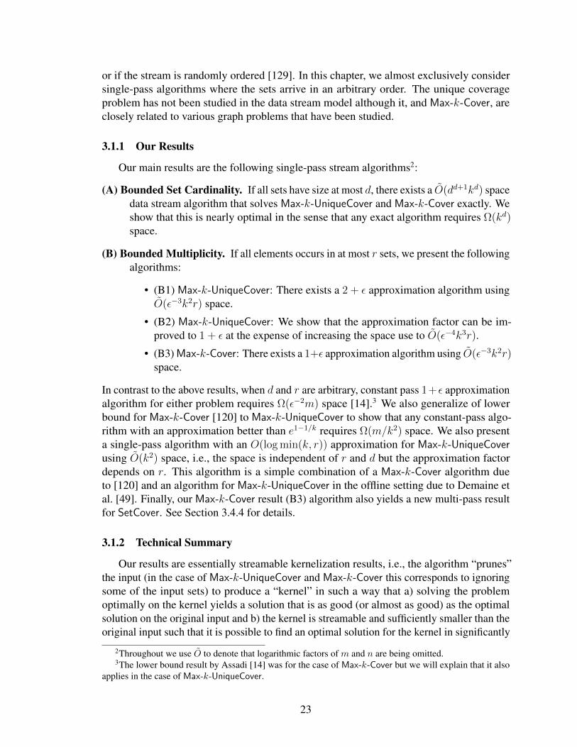
or if the stream is randomly ordered [129]. In this chapter, we almost exclusively considersingle-pass algorithms where the sets arrive in an arbitrary order. The unique coverageproblem has not been studied in the data stream model although it, and Max-k-Cover, areclosely related to various graph problems that have been studied.

3.1.1 Our Results

Our main results are the following single-pass stream algorithms2:

(A) Bounded Set Cardinality. If all sets have size at most d, there exists a O(dd+1kd) spacedata stream algorithm that solves Max-k-UniqueCover and Max-k-Cover exactly. Weshow that this is nearly optimal in the sense that any exact algorithm requires Ω(kd)space.

(B) Bounded Multiplicity. If all elements occurs in at most r sets, we present the followingalgorithms:

• (B1) Max-k-UniqueCover: There exists a 2 + ε approximation algorithm usingO(ε−3k2r) space.

• (B2) Max-k-UniqueCover: We show that the approximation factor can be im-proved to 1 + ε at the expense of increasing the space use to O(ε−4k3r).

• (B3) Max-k-Cover: There exists a 1+ε approximation algorithm using O(ε−3k2r)space.

In contrast to the above results, when d and r are arbitrary, constant pass 1+ε approximationalgorithm for either problem requires Ω(ε−2m) space [14].3 We also generalize of lowerbound for Max-k-Cover [120] to Max-k-UniqueCover to show that any constant-pass algo-rithm with an approximation better than e1−1/k requires Ω(m/k2) space. We also presenta single-pass algorithm with an O(log min(k, r)) approximation for Max-k-UniqueCoverusing O(k2) space, i.e., the space is independent of r and d but the approximation factordepends on r. This algorithm is a simple combination of a Max-k-Cover algorithm dueto [120] and an algorithm for Max-k-UniqueCover in the offline setting due to Demaine etal. [49]. Finally, our Max-k-Cover result (B3) algorithm also yields a new multi-pass resultfor SetCover. See Section 3.4.4 for details.

3.1.2 Technical Summary

Our results are essentially streamable kernelization results, i.e., the algorithm “prunes”the input (in the case of Max-k-UniqueCover and Max-k-Cover this corresponds to ignoringsome of the input sets) to produce a “kernel” in such a way that a) solving the problemoptimally on the kernel yields a solution that is as good (or almost as good) as the optimalsolution on the original input and b) the kernel is streamable and sufficiently smaller than theoriginal input such that it is possible to find an optimal solution for the kernel in significantly

2Throughout we use O to denote that logarithmic factors of m and n are being omitted.3The lower bound result by Assadi [14] was for the case of Max-k-Cover but we will explain that it also

applies in the case of Max-k-UniqueCover.

23

less time than it would take to solve on the original input. In the field of fixed parametertractability, the main requirement is that the kernel can be produced in polynomial time. Inthe growing body of work on streaming kernelization [37–39] the main requirement is thatthe kernel can then be constructed using small space in the data stream model. Our resultsfits in with this line of work and the analysis requires numerous combinatorial insights intothe structure of the optimum solution for Max-k-UniqueCover and Max-k-Cover.

Our technical contributions can be outlined as follows.

• Results (A) and (B3) rely on various structural and combinatorial observations. Ata high level, Result (A) uses the observation that each set of any Max-k-Cover orMax-k-UniqueCover solution intersects any maximal set of disjoint sets. The maintechnical step is to demonstrate that storing a small number of intersecting sets sufficesto preserve the optimal solution.

• The 1 + ε and 2 + ε approximations for Max-k-Cover and Max-k-UniqueCover, i.e.,results (B1) and (B3), are based on a very simple idea of first collecting the largestO(rk/ε) sets and then solving the problem optimally on these sets. This can be donein a space efficient manner using existing sketch for F0 estimation in the case ofMax-k-Cover and a new sketch we present the case of Max-k-UniqueCover. Whilethe approach is simple, showing that it yields the required approximations requiressome work and builds on a recent result by Manurangsi [111]. We also extend thealgorithm to the model where sets can be inserted and deleted in a non-trivial way.

3.1.3 Comparison to related work.

In the context of streaming algorithms, for the Max-k-Cover problem, McGregor andVu [119] showed that any approximation better than 1/(1− 1/e) requires Ω(m/k2) space.For the more general problem of streaming submodular maximization subject to a cardinalityconstraint, Feldman et al. [64] very recently showed a stronger lower bound that anyapproximation better than 2 requires Ω(m) space. Our results provide a route to circumventthese bounds via parameterization on k, r, and d.

Result (B3) leads to a parameterized algorithm for streaming SetCover. This newalgorithm uses O(rk2nδ + n) space which improves upon the algorithm by Har-Peled etal. [78] that uses O(mn1/δ+n) space, where k is an upper bound for the size of the minimumset cover, in the case rk2 m. Both algorithms use O(1/δ) passes and yield an O(1/δ)approximation.

In the context of offline parameterized algorithms, Bonnet et al. [25] showed that Max-k-Cover is fixed-parameter tractable in terms of k and d. However, their branching-searchalgorithm is not streamable. Misra et al. [126] showed that the maximum unique coverageproblem in which the aim is to maximize the number of uniquely covered elements uwithout any restriction on the number of sets in the solution is fixed-parameter tractable.This problem admits a kernel of size 4u. On the other hand, they showed that the budgetedversion of this problem (where each element has a profit and each set has a cost and the goalis maximize the profit subject to a budget constraint) is W [1]-hard when parameterized by

24

the budget 4. In this context, our result shows that a parameterization on both the maximumset size d and the budget k is possible (at least when all costs and profits are unit).

3.2 Preliminaries

3.2.1 Notation and Parameters

Throughout the chapter, m will denote the number of sets, n will denote the size of theuniverse, and k will denote the maximum number of sets that can be used in the solution.Given input sets S1, S2, . . . , Sm ⊂ [n], let

d = maxi|Si|

be the maximum set size and let

r = maxj|i : j ∈ Si|

be the maximum number of sets that contain the same element.

3.2.2 Structural Preliminaries

Given a collection of sets C = S1, S2, . . . , Sm, we say a sub-collection C ′ ⊂ C is amatching if the sets in C ′ are mutually disjoint. C ′ is a maximal matching if there does notexist S ∈ C \ C ′ such that S is disjoint from all sets in C ′. The following simple lemmawill be useful at various points in the chapter.

Lemma 22. For any input C, let O ⊂ C be an optimal solution for either the Max-k-Coveror Max-k-UniqueCover problem. Let Mi be a maximal matching amongst the input set ofsize i. Then every set of size i in O of size intersects some set in Mi.

Proof. Let S ∈ O have size i. If it was disjoint from all sets in Mi then it could be added toMi and the resulting collection would still be a matching. This violates the assumption thatMi is maximal.

The next lemma extends the above result to show that we can potentially remove manysets from each Mi and still argue that there is an optimal solution for the original instanceamongst the sets that intersect a set in some Mi.

Lemma 23. Consider an input of sets of size at most d. For i ∈ [d], let Mi be a maximalmatching amongst the input set of size i and let M ′

i be an arbitrary subset of Mi of sizemin(k + dk, |Mi|). Let Di be the collection of all sets that intersect a set in M ′

i . Then⋃i(Di∪M ′

i) contains an optimal solution to both the Max-k-UniqueCover and Max-k-Coverproblem.

4In the Max-k-UniqueCover problem that we consider, all costs and profits are one and the budget is k.

25

Proof. If |Mi| = |M ′i | for all 1 ≤ i ≤ d then the result follows from Lemma 22. Suppose

that If not, let j = maxi ∈ [d] : |Mi| > |M ′i |. Let O be an optimal solution and let Oi be

all the sets in O of size i. We know that every set in Od ∪Od−1 ∪ . . . ∪Oj+1 is in⋃i≥j+1

(Di ∪M ′i) =

⋃i≥j+1

(Di ∪Mi) .

Hence, the number of elements (uniquely) covered by O is at most the number of elements(uniquely) covered by Od ∪ Od−1 ∪ . . . ∪ Oj+1 plus kj since every set in Oj ∪ . . . ∪ O1

(uniquely) covers at most j additional elements. But we can (uniquely) cover at least thenumber of elements (uniquely) covered by Od ∪Od−1 ∪ . . .∪Oj+1 plus kj. This is becauseMj contains k + dk disjoint sets of size j and at least k + dk − kd = k of these are disjointfrom all sets in Od ∪Od−1 ∪ . . . ∪Oj+1. Hence, there is a solution amongst

⋃i≥j(Di ∪M ′

i)that is at least as good as O and hence is also optimal.

3.2.3 Sketches and Subsampling

Coverage Sketch. Given a vector x ∈ Rn, F0(x) is defined as the number of elementsof x which are non-zero. If given a subset S ⊂ 1, . . . , n, we define xS ∈ 0, 1n to bethe characteristic vector of S (i.e., xi = 1 iff i ∈ S) then given sets S1, S2, . . . note thatF0(xS1 + xS2 + . . .) is exactly the number of elements covered by S1 ∪ S2 ∪ . . .. We willuse the following result for estimating F0.

Theorem 24 ( [17, 45]). There exists an O(ε−2 log δ−1)-space algorithm that, given a setS ⊆ [n], can construct a data structure M(S), called an F0 sketch of S, that has theproperty that the number of distinct elements in a collection of sets S1, S2, . . . , St can beapproximated up to a 1 + ε factor with probability at least 1− δ given the collection of F0

sketchesM(S1),M(S2), . . . ,M(St).

Note that if we set δ 1/(poly(m) ·(tk

)) in the above result we can try collection

of k sets amongst S1, S2, . . . , St and get a 1 + ε approximation for the coverage of eachcollection with high probability.

The Subsampling Framework. Assuming we have v such that OPT /2 ≤ v ≤ OPT.Let h : [n]→ 0, 1 be a hash function that is Ω(ε−2k logm)-wise independent. We run ouralgorithm on the subsampled universe U ′ = u ∈ U : h(u) = 1. Furthermore, let

P [h(u) = 1] = p =ck logm

ε2v

where c is some sufficiently large constant. Let S ′ = S ∩ U ′ and let OPT′ be the optimalunique coverage value in the subsampled set system. The following result is from McGregorand Vuj [120]. We note that the proof is the same except that the indicator variables nowcorrespond to the events that an element being uniquely covered (instead of being covered).

26

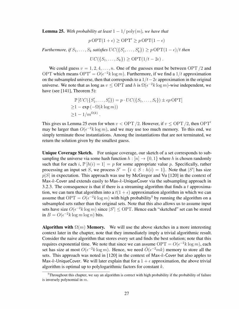
Lemma 25. With probability at least 1− 1/ poly(m), we have that

pOPT(1 + ε) ≥ OPT′ ≥ pOPT(1− ε)

Furthermore, if S1, . . . , Sk satisfies UC(S ′1, . . . , S ′k) ≥ pOPT(1− ε)/t then

UC(S1, . . . , Sk) ≥ OPT(1/t− 2ε) .

We could guess v = 1, 2, 4, . . . , n. One of the guesses must be between OPT /2 andOPT which means OPT′ = O(ε−2k logm). Furthermore, if we find a 1/t approximationon the subsampled universe, then that corresponds to a 1/t−2ε approximation in the originaluniverse. We note that as long as v ≤ OPT and h is Ω(ε−2k logm)-wise independent, wehave (see [141], Theorem 5):

P [UC(S ′1, . . . , S ′`) = p · UC(S1, . . . , S`)± εpOPT]

≥1− exp (−Ω(k logm))

≥1− 1/mΩ(k) .

This gives us Lemma 25 even for when v < OPT /2. However, if v ≤ OPT /2, then OPT′

may be larger than O(ε−2k logm), and we may use too much memory. To this end, wesimply terminate those instantiations. Among the instantiations that are not terminated, wereturn the solution given by the smallest guess.

Unique Coverage Sketch. For unique coverage, our sketch of a set corresponds to sub-sampling the universe via some hash function h : [n]→ 0, 1 where h is chosen randomlysuch that for each i, P [h(i) = 1] = p for some appropriate value p. Specifically, ratherprocessing an input set S, we process S ′ = i ∈ S : h(i) = 1. Note that |S ′| has sizep|S| in expectation. This approach was use by McGregor and Vu [120] in the context ofMax-k-Cover and extends easily to Max-k-UniqueCover via the subsampling approach in3.2.3. The consequence is that if there is a streaming algorithm that finds a t approxima-tion, we can turn that algorithm into a t(1 + ε) approximation algorithm in which we canassume that OPT = O(ε−2k logm) with high probability5 by running the algorithm on asubsampled sets rather than the original sets. Note that this also allows us to assume inputsets have size O(ε−2k logm) since |S ′| ≤ OPT. Hence each “sketched” set can be storedin B = O(ε−2k logm log n) bits.

Algorithm with Ω(m) Memory. We will use the above sketches in a more interestingcontext later in the chapter, note that they immediately imply a trivial algorithmic result.Consider the naive algorithm that stores every set and finds the best solution; note that thisrequires exponential time. We note that since we can assume OPT = O(ε−2k logm), eachset has size at most O(ε−2k logm). Hence, we need O(ε−2mk) memory to store all thesets. This approach was noted in [120] in the context of Max-k-Cover but also apples toMax-k-UniqueCover. We will later explain that for a 1 + ε approximation, the above trivialalgorithm is optimal up to polylogarithmic factors for constant k.

5Throughout this chapter, we say an algorithm is correct with high probability if the probability of failureis inversely polynomial in m.

27

3.3 Exact Algorithms

Let C be the input sets. In this section we will initially assume all input sets havesize exactly d and will show that there exists a single-pass data stream algorithm that usesO(dd+1kd) space and returns a collection of sets C ′ ⊂ C such that the optimal solution foreither the maximum coverage or unique coverage problem when restricted to C ′ is equal tothe optimal solution with no such restriction. We will subsequently generalize this to thecase when sets can have any size at most d. In this section we will assume that r can beunbounded, e.g., an element in the universe could appear in m of the input sets.

3.3.1 Warm-Up Idea

Appealing to Lemma 22, we know that sets in an optimal solution to maximum coverageor maximum unique coverage intersect with a maximal matching. Hence, a natural approachis to construct a maximimal matching A greedily as the sets arrive along with any set thatintersects a set in A. If the maximal matching ever exceeds size k then we have an optimalsolution to Max-k-Cover and Max-k-UniqueCover that covers dk elements and hence wecan ensure |A| ≤ k. However, a set in A could intersect with Ω(m) other sets in the worstcase6 The main technical step in the algorithm in the next section is a way to carefully storeonly some of the sets that intersect A such that we can bound the number of stored sets interms of k and d and yet still assume that stored sets include an optimal solution to eitherMax-k-Cover or Max-k-UniqueCover.

3.3.2 Algorithm

(1) Let A and Xu (for all u ∈ [n]) be empty sets. Each will correspond to a collection ofsets. Let b = d(k − 1).

(2) Process the stream and let S be the next set:

(a) If S is disjoint from all sets in A and |A| < k, add S to A.

(b) If u ∈ S ∩ S ′ for some S ′ ∈ A:

i. Add S to Xu if there does not exist a subset T ⊂ (S \ u) that occurs assubset of (b+ 1)d−1−|T | sets in Xu.

(3) Return the best solution in C ′ = A ∪ (⋃uXu).

3.3.3 Analysis

We start with the following combinatorial lemma7.6It can be bounded in terms of d and r however. Specifically, each set can intersect with at most d(r − 1)

other sets. However, in this section we are assuming r is unbounded so this bound does not help us here.7For the interested reader who is familiar with the relevant combinatorial results, we note that we can prove

a similar lemma to the one here via the Sunflower Lemma [10, 134]. In particular, one can argue that thereexists a sufficiently large sunflower amongst S ∈ X : T ∗ is a subset of S whose core includes T ∗. Withsome small adjustment to the subsequent theorem, this would be sufficient for our purposes. However, weinstead include this version of the lemma because it is simpler and self-contained.

28

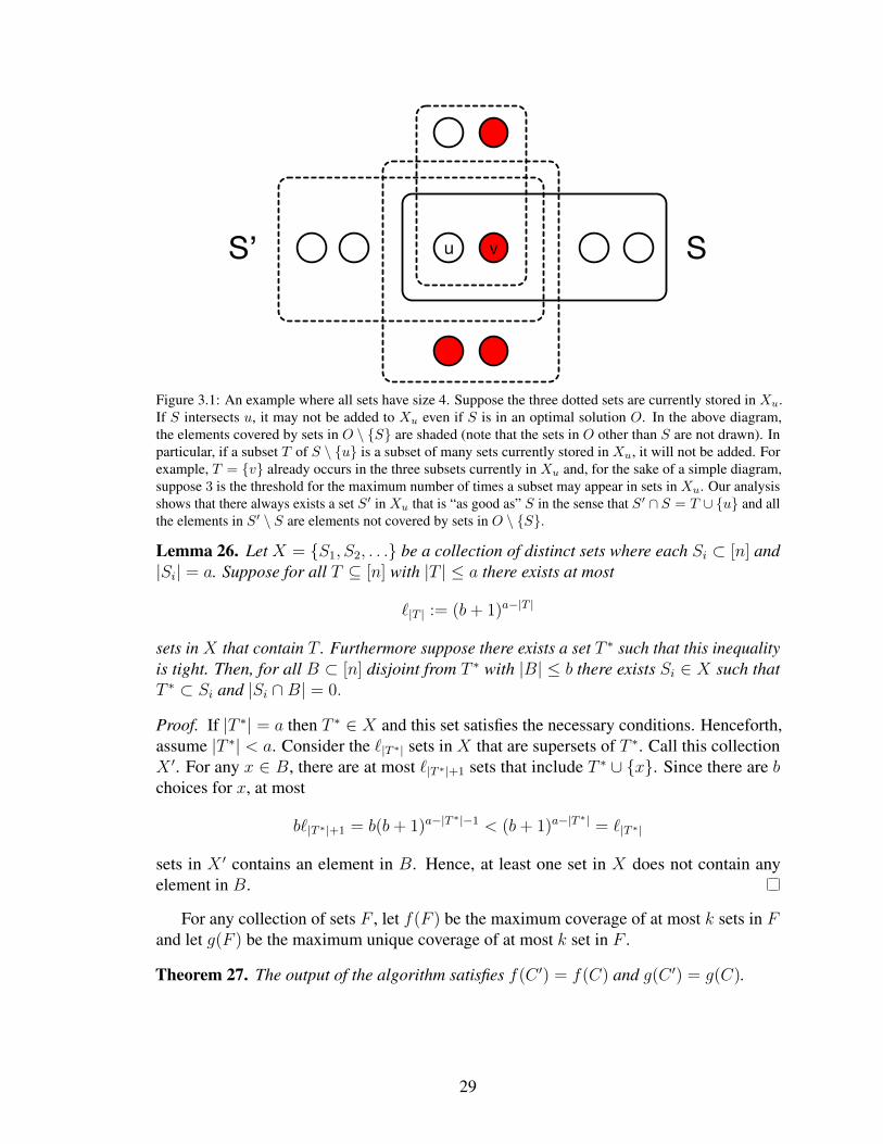
u v SS’

Figure 3.1: An example where all sets have size 4. Suppose the three dotted sets are currently stored in Xu.If S intersects u, it may not be added to Xu even if S is in an optimal solution O. In the above diagram,the elements covered by sets in O \ S are shaded (note that the sets in O other than S are not drawn). Inparticular, if a subset T of S \ u is a subset of many sets currently stored in Xu, it will not be added. Forexample, T = v already occurs in the three subsets currently in Xu and, for the sake of a simple diagram,suppose 3 is the threshold for the maximum number of times a subset may appear in sets in Xu. Our analysisshows that there always exists a set S′ in Xu that is “as good as” S in the sense that S′ ∩ S = T ∪ u and allthe elements in S′ \ S are elements not covered by sets in O \ S.

Lemma 26. Let X = S1, S2, . . . be a collection of distinct sets where each Si ⊂ [n] and|Si| = a. Suppose for all T ⊆ [n] with |T | ≤ a there exists at most

`|T | := (b+ 1)a−|T |

sets in X that contain T . Furthermore suppose there exists a set T ∗ such that this inequalityis tight. Then, for all B ⊂ [n] disjoint from T ∗ with |B| ≤ b there exists Si ∈ X such thatT ∗ ⊂ Si and |Si ∩B| = 0.

Proof. If |T ∗| = a then T ∗ ∈ X and this set satisfies the necessary conditions. Henceforth,assume |T ∗| < a. Consider the `|T ∗| sets in X that are supersets of T ∗. Call this collectionX ′. For any x ∈ B, there are at most `|T ∗|+1 sets that include T ∗ ∪ x. Since there are bchoices for x, at most

b`|T ∗|+1 = b(b+ 1)a−|T∗|−1 < (b+ 1)a−|T

∗| = `|T ∗|

sets in X ′ contains an element in B. Hence, at least one set in X does not contain anyelement in B.

For any collection of sets F , let f(F ) be the maximum coverage of at most k sets in Fand let g(F ) be the maximum unique coverage of at most k set in F .

Theorem 27. The output of the algorithm satisfies f(C ′) = f(C) and g(C ′) = g(C).

29

Proof. Let C0 be the union of A and all sets that intersect a set in A, i.e.,

C0 = S ∈ A ∪ S ∈ C : |S ∩ S ′| > 0 for some S ′ ∈ A .

Note that every set in the optimum solution of maximum coverage intersects with some setin A and hence f(C0) = f(C). For i ≥ 1 consider,

Ci = C0 \ first i sets in stream that are not in output C ′ .

We will next argue that for any i ≥ 0, f(Ci+1) = f(Ci) and the theorem follows.Let O be an optimum solution in Ci and let S = Ci \ Ci+1. If S 6∈ O then clearly

f(Ci+1) = f(Ci) since O ⊆ Ci+1. If S ∈ O but not in Ci+1 then let u ∈ S be the node forwhich we contemplated adding S to Xu but didn’t because of the additional requirements.

Claim 2. There exists S ′ in Xu such that f((O \ S) ∪ S ′) = f(Ci) as required.

Proof of Claim. If S was not added to Xu there exists a subset of T ∗ ⊂ (S \ u) that isa subset of (b + 1)d−1−|T ∗| sets in Xu. Let X be the collection of sets of size a = d − 1formed by removing u from each of the sets in Xu. Note that X satisfies the assumptions ofLemma 26. Let B be the set of at most b = d(k − 1) elements in the set

B = v : v ∈ S ′′ for some S ′′ ∈ O \ S .

By Lemma 26, there exists a set S ′ in X such that T ∗ ⊂ S ′ and |(S ′ \ T ∗) ∩B| = 0. Hence,f((O \ S) ∪ S ′).

The proof for unique coverage, i.e., g(), is identical.

Lemma 28. The space used by the algorithm is O(dd+1kd).

Proof. Recall that one of the requirements for a set S to be added to Xu is that the numberof sets in Xu that are supersets of any subset of S \ u of size t is at most (b + 1)d−1−t.This includes the empty subset and since every set in Xu is a superset of the empty set, wededuce that

|Xu| ≤ (b+ 1)d−1−0 = (b+ 1)d−1.

Since |A| ≤ k, the number of sets that are stored is at most

|A|+∑

u∈∪S∈A

|Xu| ≤ |A|+ d|A| · (b+ 1)d−1

≤ |A|+ d|A| ·O((dk)d−1)

= O((dk)d) .

30

3.3.4 Generalization to Sets of Different Size

In the case where sets may have any size at most d, we run the algorithm described inSection 3.3.2 in parallel for stream sets of each size t ∈ [d]. By appealing to Lemma 23,we know that an optimal maximum overage or maximum unique coverage intersects withthe union of maximal matchings of sets of size t for each t. We again rely on Lemma 26to establish that we can store only some of the sets that intersect these matchings and stillretain an optimal solution to either coverage problem. We describe the algorithm below.

(1) Let At and Xu,t (for all u ∈ [n] and t ∈ [d]) be empty sets. Each will correspond to acollection of sets. Let b = d(k − 1).

(2) Process the stream and let S be the next set and let t = |S|:

(a) If S is disjoint from all sets in At and

|At| <

dk + k if t < d

k if t = d

then add S to At.

(b) If u ∈ S ∩ S ′ for some S ′ ∈ At:i. Add S to Xu,t if there does not exist a subset T ⊂ (S \ u) that occurs as

subset of (b+ 1)t−1−|T | sets in Xu.

(3) Return C ′′ = (⋃tAt) ∪

(⋃u,tXu,t

).

Theorem 29. The output of the algorithm satisfies f(C ′′) = f(C) and g(C ′′) = g(C).

Proof. Let

C0 =⋃t

(S ∈ At ∪ S ∈ C : |S ∩ S ′| > 0 for some S ′ ∈ A) .

Define Ci, O, and S as in the proof of Theorem 27. By Lemma 23, f(C0) = f(C) sincethere is an optimum solution of maximum coverage in which every set intersects with someset At. Let u ∈ S be the node which prevented us from adding S to Xu,t. We now prove ananalog of Claim 2 which implies that for any i ≥ 0, f(Ci+1) = f(Ci).

Claim 3. There exists S ′ in Xu,t such that f((O \ S) ∪ S ′) = f(Ci) as required.

Proof of Claim. If S was not added to Xu,t there exists of a subset of T ∗ ⊂ (S \ u) thatis a subset of (b + 1)t−1−|T ∗| sets in Xu. Let X be the collection of sets of size a = t − 1formed by removing u from each of the sets in Xu. X satisfies the assumptions of Lemma26. Let B be the set of at most b = d(k − 1) elements in the set

B = v : v ∈ S ′′ for some S ′′ ∈ O \ S .

By Lemma 26, there exists a set S ′ in X such that T ∗ ⊂ S ′ and |(S ′ \ T ∗) ∩B| = 0. Hence,f((O \ S) ∪ S ′)

31

Again, the proof is identical for unique coverage.

Lemma 30. The space used by the algorithm is O(dd+1kd).

Proof. For all t, |Xu,t| ≤ (b + 1)t−1. Since |Ad| ≤ k and |At| = O(dk) for t < k, thenumber of sets stored is at most:

d∑t=1

|At|+ ∑u∈

⋃S∈At

|Xu,t|

≤ O(d2k + d2k(1 + (b+ 1) + . . .+ (b+ 1)d−2) + dk(b+ 1)d−1)

= O((dk)d) .

We summarize the result as a theorem.

Theorem 31. There exists a single-pass, O(dd+1kd)-space algorithm that yields an exactsolution to Max-k-Cover and Max-k-UniqueCover.

3.3.5 An Algorithm for Insert/Delete Streams

Chitnis et. al. [38] introduce a sketching primitive Sampleγ,d suitable for insert/deletedata streams which is capable of randomly sampling a diverse selection of sets. Sampleγ,dfirst assigns a color to each element from γ colors uniformly at random using a d-wiseindependent hash function. Each set in C is therefore associated with the multiset of colorsassigned to its elements (a ”color signature”). By maintaining an `0-sampler for all sets ofeach color signature, It is possible to sample one set of each color signature from Sampleγ,dat the end of stream. The following lemma establishes that these sampled sets are likely toinclude optimal solutions for maximum coverage and maximum unique coverage.

Lemma 32. LetC ′ be the collection of sets sampled from Sample4k2d2,d. Then P [f(′C) = f(C)] ≥3/4 and P [g(C ′) = g(C)] ≥ 3/4.

Proof. Let M be an optimal solution to Max-k-Cover and let c : U → [γ] be the coloringof sets defined by Sample4k2d2,d. Order the k sets in M arbitrarily and let mi be the ithset in this ordering. We will argue that with good probability, the ith set’s color signaturehas no colors in common with any earlier set in the ordering, except for those of elementswhich are already covered. More formally, let col(S) := w|c(e) = w|e ∈ S and let Hi

denote the event |col(mi) ∩ col(⋃j<imj)| = |mi ∩ (

⋃j<imj)|. Note that if Hi occurs then

Sample4k2d2,d either returns mi or some other set with the same color signature which canreplace mi in the optimal solution (since its color signature guarantees its intersection with

32

the rest of the optimal solution is not greater than mi’s). Since our hash function is d-wiseindependent:

P [Hi] ≥(

1− i · dγ

)d=

(1− i

4k2d

)d≈ e−i/4k

2

.

The above inequality holds because the earlier i edges have at most i · d unique colors. If Hi

occurs for all 0 ≤ i ≤ k − 1,

k−1∏i=0

P [Hi] ≥k−1∏i=0

e−i/4k2

= exp

(−

k−1∑i=0

(i/4k2)

)

= exp(−(k − 1)(k − 2)

4k2

)≥ e−1/4 ≥ 3/4.

A Sample4k2d2,d sketch maintains an `0 sketch for each of γd color signatures, requiringtO((kd)2d) space. Additionally, the d-wise independent hash function mapping nodes to4k2d2 colors uses O(d log(4k2d2) = O(d) space, so the entire Sample4k2d2,d sketch requirestO((kd)2d) space. Constructing log(k) Sample4k2d2,d sketches in parallel8 guarantees thatf(′C) = f(C) and g(′C) = g(C) with probability 1− 1/ poly(k). This gives the followingtheorem.

Theorem 33. There exist randomized single-pass algorithms using O((kd)2d) space andallowing deletions that yield an exact solution to Max-k-Cover and Max-k-UniqueCover.

3.4 Approximation Algorithms

In this section, we present a variety of different approximation algorithms where thespace used by the algorithm is independent of d but, in some cases, may depend on r.

3.4.1 Unique Coverage: 2 + ε Approximation

In this section, we present a 2 + ε approximation for unique coverage. The algorithmis simple but the analysis is non-trivial. The algorithm stores the ηk largest sets whereη = dr/εe and finds the best unique coverage achievable by selecting at most k of these sets.

We will present an algorithm with a 1 + ε approximation in the next subsection withthe expense of an extra k/ε factor in the space use. However, the algorithm in this sectionis appealing in the sense that it is much simpler and can be extended to insertion-deletionstreams. The analysis of this approach may also be of independent interest.

Let C ′ be the ηk sets of largest size. To find the best solution C ′′ amongst C ′, we usethe unique coverage sketches presented in the Section 3.2. Note that to find the ηk largestsets we just store the sizes of sets sketched so far along with their unique coverage sketches.Finally, we return the best solution C ′′ using most k sets in C ′ based on the unique coveragesketches that we store. Recall that each unique coverage sketch requires O(k/ε2) space. Wehave the following result.

8Note that each Sample4k2d2,d sketch has a different random coloring.

33

Theorem 34. There exists a randomized single-pass algorithm using O(ε−2ηk) = O(ε−3k2r)space algorithm that 2 + ε approximates Max-k-UniqueCover.

Proof. Let the sizes of the ηk largest sets be (with arbitrarily tie-breaking) be d1 ≥ d2 ≥. . . ≥ dηk and let

d∗ :=d1 + . . .+ dk

kand d′ :=

dk+1 + . . .+ dηk(η − 1)k

.

Let O be an optimal collection of sets for Max-k-UniqueCover. First, we observe that foreach set S ∈ O \ C ′, we have that |S| ≤ dηk ≤ d′. Hence,

OPT ≤ f(O ∩ C ′) +∑

S∈O\C′|S| ≤ h(C ′′) + kd′ .

where h() is a function of a collection of sets that returns the number of elements that arecovered by exactly one of these sets. Thus, if kd′ < 0.5 OPT, then it is immediate that thenumber of elements uniquely covered by our solution is h(C ′′) > 0.5 OPT.

Now we consider the case kd′ ≥ 0.5 OPT. For the sake of analysis, consider randomlypartitioning C ′ into a set C ′1 of size k and C ′2 = C ′ \ C ′1. Observe that

E [h(C ′1)]

=∑S∈C′

E [# of elements uniquely covered by S in C ′1]

=∑S∈C′

∑u∈S

P [S ∈ C ′1 and u is uniquely covered in C ′1]

≥∑S∈C′

∑u∈S

P [S ∈ C ′1]−∑

S′∈C\S:u∈S′P [S ∈ C ′1, S ′ ∈ C ′1]

≥∑S∈C′|S|(ε/r − (r − 1)(ε/r)2

)≥ ηk · d′

(ε/r − r(ε/r)2

)≥ kd′ (1− ε) ≥ (1− ε) OPT /2 .

We note that it is possible to improve the result slightly by setting η =√

2/ε for thebound of for E [h(C ′1)] in the proof of Theorem 34 as follows:

34

E [h(C ′1)] =∑S∈C′

E [# of elements uniquely covered by S in C ′1]

≥∑S∈C′

∑i∈S

k

ηk

(η − 1)k

ηk − 1

=1

η·(

(η − 1)k

ηk − 1

)∑S∈C′|S|

>η − 1

η2(kd∗ + (η − 1)kd′)

≥ OPT(1/η − 1/η2 + (1− 1/η)20.5)

= OPT(0.5− 0.5/η2)

= (0.5− ε) OPT .

The space used in resulting algorithm scales with ε−2.5 rather than ε−3 as implied by theanalysis for general r.

Extension to Insert/Delete Streams

We now explain how the above approach can be extended to the case where sets may beinserted and deleted. In this setting, it is not immediately obvious how to select the largestηk sets; the approach used when sets are only inserted does not extend. Note that in thismodel we can set m to be that maximum number of sets that have been inserted and notdeleted at any prefix of the stream rather than the total number of sets inserted/deleted.

However, we can extend the result as follows. Suppose the sketch of a set for ap-proximating maximum unique coverage requires B bits; recall from Section 3.2.3 thatB = kε−2 polylog(n,m) suffices. We can encode such a sketch of a set S as an integeri(S) ∈ [2B]. Suppose we know that exactly ηk sets have size at least some threshold t. Wewill remove this assumption shortly. Consider the vector x ∈ [N ] where N = 2B that isinitially 0 and then is updated by a stream of set insertions/deletions as follows:

(1) When S is inserted, if |S| ≥ t, then xi(S) ← xi(S) + 1.

(2) When S is deleted, if |S| ≥ t, then xi(S) ← xi(S) − 1.

At the end of this process x ∈ 0, 1, . . . , ,m2B , `1(x) = ηk, and reconstruct the sketchesof largest ηk sets given x. Unfortunately, storing x explicitly in small space is not possiblesince, while we are promised that at the end of the stream `1(x) = ηk, during the stream itcould be that x is an arbitrary binary string with m one’s and this requires Ω(m) memory tostore. To get around this, it is sufficient to maintain a linear sketch of x itself that supportsparse recovery. For our purposes, the CountMin Sketch [46] is sufficient although otherapproaches are possible. The CountMin Sketch allows x to reconstructed probability 1− δusing a sketch of size

O(logN + ηk log(ηk/δ) logm) = O(ηkε−2 polylog(n,m)) .

To remove the assumption that we do not know t in advance, we consider values:

t0, t1, . . . , tdlog1+εme where ti = (1 + ε)i .

35

We define vector x0, x1, . . . ∈ 0, 1, . . . , ,m2B where xi is only updated when a set of size≤ ti but > ti−1 is inserted/deleted. Then there exists i such that ≤ ηk sets have size ≤ ti−1

and the sketches of these sets can be reconstructed from x0, . . . , xti−1 . To ensure we haveηk sets, we may need some additional sketches corresponding to sets of size > ti−1 and≤ ti but unfortunately there could be m such sets and we are only guaranteed recover ofxti when it is sparse. However, if this is indeed the case we can still recover enough entriesof xt1 by first subsampling the entries at the appropriate rate (we can guess sampling rate1, 1/2, 1/22, . . . 1/m) in the standard way. Note that we can keep track of `1(xi) exactly foreach i using O(logm) space.

The next section presents algorithms for maximum coverage and set cover using a similarapproach based on keeping a set of the largest elements seen so far.

3.4.2 Maximum Coverage and Set Cover

In this section, we generalize the approach of Manurangsi [111] and combine that withF0-sketch to obtain a 1+ε approximation using O(ε−3k2r) space for the maximum coverageproblem.

Manurangsi [111] showed that for the maximum k-vertex cover problem, the Θ(k/ε)vertices with highest degrees form a 1 + ε approximation kernel. That is, there exist kvertices among those that cover (1− ε) OPT edges. We now consider a set system in whichan element belongs to at most r sets (this can also be viewed as a hypergraph where each setcorresponds to a vertex and each element corresponds to a hyperedge; we then want to findk vertices that touch as many hyperedges as possible).

We begin with the following lemma that generalizes the aforementioned result in [111].We may assune that m Crk/ε for some large constant C; otherwise, we can store all thesets.

Lemma 35. Suppose m > drk/εe. Let K be the collection of drk/εe sets with largest sizes(tie-broken arbitrarily). There exist k sets in K that cover (1− ε) OPT elements.

Proof. Let O denote the collection of k sets in some optimal solution. Let Oin = O ∩Kand Oout = O \K. We consider a random subset Z ⊂ K of size |Oout|. We will show thatthe sets in Z ∪ Oin cover (1− ε) OPT elements in expectation; this implies the claim.

Let χ(Z) denote the set of elements covered by the sets in Z. Let [E ] denote the indicatorvariable for event E . We rewrite

|χ(Z ∪ Oin)| = |χ(Oin)|+ |χ(Z)| − |χ(Oin) ∩ χ(Z)| .Furthermore, the probability that we pick a set S in K to add to Z is

p :=|Oout||K|

≤ k

kr/ε=ε

r.

Next, we upper bound E [|χ(Oin) ∩ χ(Z)|]. We have

E[|χ(Oin) ∩ χ(Z)|

]≤

∑u∈χ(Oin)

∑S∈K:u∈S

P [S ∈ Z]

≤∑

u∈χ(Oin)

rp ≤ |χ(Oin)| · ε .

36

We lower bound E [|χ(Z)|] as follows.

E [|χ(Z)|]

≥ E

∑S∈K

|S|[S ∈ Z]−∑

S′∈K\S

|S ∩ S ′|[S ∈ Z ∧ S ′ ∈ Z]

≥∑S∈K

|S|p− ∑S′∈K\S

|S ∩ S ′|p2

≥∑S∈K

(|S|p− r|S|p2

)≥ p(1− pr)

∑S∈K

|S| ≥ p(1− ε)∑S∈K

|S| .

In the above derivation, the second inequality follows from the observation that P [S ∈ Z ∧ S ′ ∈ Z] ≤p2. The third inequality is because

∑S′∈K\S |S ∩ S ′| ≤ r|S| since each element belongs

to at most r sets.For all S ∈ K, we must have have

|S| ≥∑

Y ∈Oout |Y ||Oout|

≥ |χ(Oout)||Oout|

.

Thus,

E [|χ(Z)|] ≥ p (1− ε) |K| |χ(Oout)||Oout|

= p (1− ε) |χ(Oout)|p

= (1− ε)|χ(Oout)| .

Putting it together,

E[|χ(Z ∪ Oin)|

]≥ |χ(Oin)|+ (1− ε)|χ(Oout)| − |χ(Oin)| · ε≥ (1− ε) OPT .

With the above lemma in mind, the following algorithm’s correctness is immediate.

(1) Store F0-sketches of the kr/ε largest sets, where the failure probability of the sketchesis set to 1

poly(n)(mk).

(2) At the end of the stream, return the k sets with the largest coverage based on theestimates given by the F0-sketches.

We restate our result as a theorem.

Theorem 36. There exists a randomized one-pass, O(k2r/ε3)-space, algorithm that withhigh probability finds a 1 + ε approximation to Max-k-Cover.

37

3.4.3 Unique Coverage: 1 + ε Approximation

The approximation factor in the previous section can be improved to 1 + ε at the expenseof an extra factor of k/ε in the space. Recall in Section 3.3.1 that there exists an algorithmfor solving Max-k-UniqueCover exactly by storing O(kdr) sets, i.e., with O(kd2r) space.Combining this with the Subsampling Framework discussed in Section 3.2.3, we mayassume d ≤ OPT = O(ε−2k logm). This immediately implies the following theorem.

Theorem 37. There exists a randomized one-pass algorithm using O(ε−4k2r) space thatfinds a 1 + ε approximation of Max-k-UniqueCover.

Note that the same approach would work for Max-k-Cover but we present a better resultin Section 3.4.2.

3.4.4 Unique Coverage: O(log min(k, r)) Approx.

We now present an algorithm whose space does not depend on r but the result comes atthe cost of increasing the approximation factor to O(log(min(k, r))). It also has the featurethat the running time is polynomial in k in addition to being polynomial in m and n.

The basic idea is as follows: We consider an existing algorithm that first finds a 2approximation for the Max-k-Cover problem. Let the corresponding solution be C ′. Thealgorithm then finds the best solution of Max-k-UniqueCover among the sets in C ′.

Let z∗ be a guess such that (1 − ε) OPT∗ ≤ z∗ ≤ OPT∗ where OPT∗ is the value ofthe optimal Max-k-Cover.

(1) Initialize T = ∅ which will store sets from the stream.

(2) For each set S in the stream, if |T | < k and

|(∪A∈TA) ∪ S| − |∪A∈TA| ≥ z∗/(2k) ,

then add S to T and store S in the memory.

(3) Return the best solution Q (in terms of unique coverage) among the sets in T .

The following theorem captures the above algorithm.

Theorem 38. There exists a randomized one-pass, O(k2)-space, algorithm that with highprobability finds a O(log min(k, r)) approximation of Max-k-UniqueCover.

Proof. It has been shown in previous work [16, 120] that T is a 2 + ε approximation ofMax-k-Cover. Demaine et al. [49] proved that Q is an O(log min(k, r)) approximation ofMax-k-UniqueCover. In fact, they presented a polynomial time algorithm to find Q from Tsuch that the number of uniquely covered elements is at least

Ω(1/ log k) · |∪A∈TA| ≥ Ω(1/ log k) · 1/2 ·OPT∗ ≥ Ω(1/ log k) ·OPT .

We note that OPT∗ ≤ kOPT. Otherwise, one can find a set that covers more than OPTelements which is a contradiction.

38

The above algorithm needs to keep track of the elements being covered by T at allpoints during the stream. This requires O(OPT∗) = O(kOPT) space. Furthermore,storing the sets in T needs O(kOPT) space. Finally, guessing z∗ entails a O(ε−1 log OPT)factor. Thus, the algorithm uses O(ε−1kOPT) space which could be translated into anotheralgorithm that uses O(ε−3k2) space after using the subsampling framework. For the purposeof the proving the claimed approximation factor we can set ε to a small constant.

Application to Parameterized Set Cover.

We parameterize the set cover problem as follows. Given a set system, either A) outputa set cover of size αk if OPT ≤ k where α the approximation factor or B) correctly declarethat a set cover of size k does not exist.

Theorem 39. There exists a randomized, O(1/δ)-pass, O(rk2n1/δ + n)-space, algorithmthat with high probability finds a O(1/δ) approximation of the parameterized set coverproblem.

Proof. In each pass, we run the algorithm in Theorem 36 with parameters k and ε = 1/nδ/3

on the remaining uncovered elements. The space use is O(rk2n1/δ + n). Here, we needadditional O(n) space to keep track of the remaining uncovered elements.

Note that if OPT ≤ k, after each pass, the number of uncovered elements is reduced bya factor 1/nδ/3. This is because if n′ is the number of uncovered elements at the beginningof a pass, then after that pass, we cover all but at most n′/nδ/3 of those elements. Afteri passes, the number of remaining uncovered elements is O(n1−iδ/3); we therefore use atmost O(1/δ) passes until we are done. At the end, we have a set cover of size O(k/δ).

If after ω(1/δ) passes, there are still remaining uncovered elements, we declare that sucha solution does not exist.

Our algorithm improves upon the algorithm by Har-Peled et al. [78] that uses O(mn1/δ +n) space for when rk2 m and also yields an O(1/δ) approximation.

Extension to Insert/Delete Streams

The result can be extended to the case where sets are inserted and deleted using the sameapproach as that used for unique coverage.

3.5 Lower Bounds

3.5.1 Lower Bounds for Exact Solutions

As observed earlier, any exact algorithm for either the Max-k-Cover or Max-k-UniqueCoverproblem on an input where all sets have size d will return a matching of size k if one exists.However, by a lowerbound due to Chitnis et al. [38] we know that determining if there existsa matching of size k in a single pass requires Ω(kd) space. This immediately implies thefollowing theorem.

Theorem 40. Any single-pass algorithm that solves Max-k-Cover or Max-k-UniqueCoverexactly with probability at least 9/10 requires Ω(kd) space.

39

3.5.2 Lower bound for a e1−1/k approximation

The strategy is similar to previous work on Max-k-Cover [119, 120]. However, we needto argue that the relevant probabilistic construction works for all collections of fewer thank sets since the unique coverage function is not monotone. This extra argument will alsoallow us to show that the lower bound also applies to bi-criteria approximation in which weare allowed to pick more than k sets (this is not the case for Max-k-Cover).

We make a reduction from the communication problem k-player set disjointness, denotedby DISJ(m, k). In this problem, there are k players where the ith player has a set Si ⊆ [m].It is promised that exactly one of the following two cases happens a) NO instance: All thesets are pairwise disjoint and b) YES instance: There is a unique element v ∈ [m] such thatv ∈ Si for all i ∈ [k] and all other elements belong to at most one set. The (randomized)communication complexity, for some large enough constant success probability, of theabove problem in p-round, one-way model is Ω(m/(pk)) even if the players may use publicrandomness [33]. We can assume that |S1 ∪ S2 ∪ . . . ∪ Sk| ≥ m/4 via a padding argument.

Theorem 41. Any constant-pass randomized algorithm with an approximation better thane1−1/k for Max-k-UniqueCover requires Ω(m/k2) space.

Proof. Consider a sufficiently large n where k divides n. For each i ∈ [m], let Pi be arandom partition of [n] into k sets V i

1 , . . . , Vik such that an element in the universe U = [n]

belongs to exactly one of these sets uniformly at random. In particular, for all i ∈ [m] andv ∈ U ,

P[v ∈ V i

j ∧ (∀j′ 6= j, v /∈ V ij′)]

= 1/k .

The partitions are chosen independently using public randomness before receiving theinput. For each player j, if i ∈ Sj , then they put V i

j in the stream. Note that the streamconsists of Θ(m) sets.

If the input is a NO instance, then for each i ∈ [m], there is at most one set V ij in the

stream. Therefore, for each element v ∈ [n] and any collection of ` ≤ k sets V i1j1, . . . , V i`

j`in

the stream,

P[v is uniquely covered by V i1

j1, . . . , V i`

j`

]= `/k · (1− 1/k)`−1

≤ `/k · e−(`−1)/k .

Therefore, in expectation, µ` := E[h(V i1

j1, . . . , V i`

j`)]≤ `/k · e−(`−1)/kn where h() is the

number of elements that are uniquely covered. By an application of Hoeffding’s inequality,

P[h(V i1

j1∪ . . . ∪ V i`

j`) > µ` + εe−(k−1)/k · n

]≤exp

(−2ε2e−2(`−1)/kn

)≤exp

(−Ω(ε2n)

)≤ 1

m10k.

The last inequality follows by letting n = Ω(ε−2k logm). The following claim showsthat for large k, in expectation, picking k sets is optimal in terms of unique coverage.

Lemma 42. The function g(`) = `/k · e−(`−1)/kn is increasing in the interval (−∞, k] anddecreasing in the interval [k,+∞).

40

Proof. We take the partial derivative of g with respect to `

∂g

∂`=e(1−`)/k(k − `)

k2· n

and observe that it is non-negative if and only if ` ≤ k.

By appealing to the union bound over all(m1

)+ . . .+

(mk−1

)+(mk

)≤ O(mk+1) possible

collections ` ≤ k sets, we deduce that with high probability, for all collections of ` ≤ k setsS1, . . . , S`,

h(S1, . . . , S`) ≤ µ` + εe−(k−1)/k · n≤ `/k · e−(`−1)/kn+ εe−(k−1)/k · n≤ (1 + ε)e−1+1/kn .

If the input is a YES instance, then clearly, the maximum k-unique coverage is n. This isbecause there exists i such that i ∈ S1 ∩ . . . ∩ Sk and therefore V i

1 , . . . , Vik are in the stream

and these sets uniquely cover all elements.Therefore, any constant pass algorithm that finds a (1 + 2ε)e1−1/k approximation of

Max-k-UniqueCover for some large enough constant success probability implies a protocolto solve DISJ(m, k). Thus, Ω(m/k2) space is required.

Remark. Since g(`) is decreasing in the interval [k,m], the lower bound also holds forbi-criteria approximation where the algorithm is allows to pick more than k sets.

3.5.3 Lower bound for 1 + ε approximation

Assadi [14] presents a O (m/ε2) lower bound for the space required to compute a1 + ε approximation for Max-k-Cover when k = 2, even when the stream is in a randomorder and is allowed constant passes. This is accomplished via a reduction to multipleinstances of the Gap-Hamming Distance problem on a hard input distribution, where aninput with high maximum coverage corresponds to a YES answer for some Gap-HammingDistance instance, and a low maximum coverage corresponds to a NO answer for all GHDinstances. This hard distribution has the additional property that high maximum coverageinputs also have high maximum unique coverage, and low maximum coverage inputs havelow maximum unique coverage. Therefore, the following corollary holds:

Corollary 43. Any constant-pass randomized algorithm with an approximation factor 1 + εfor Max-k-UniqueCover requires Ω(m/ε2) space.

41

CHAPTER 4

TEMPORAL GRAPH STREAMS

Temporal graphs incorporate the notion of time into the structure of traditional graphsto model time-dependent phenomena in applications such as information sharing, diseasespreading, Internet routing, and more. In a temporal graph, edges are augmented withtimestamps: labels which indicate at which moments in time the edge can be said to exist.Temporal graphs are a recent topic of study and no one has yet considered the problemof designing algorithms to compute properties of temporal graphs at scale. We introducethe notion of a temporal graph stream, where a temporal graph is defined via a sequenceof temporal edge updates, and ask whether various properties of a temporal graph can becomputed given sequential access to the stream and space sublinear in the size of the stream.

The significance and interpretation of edge timestamps may appear to vary with thealgorithmic problem being considered, as well as the intended application. For instance, inthis chapter we concern ourselves with reachability, where timestamps indicate moments atwhich the edge is traversable. In contrast, Mikhail et al. [124] consider the problem of findinga maximum matching where all edges in the matching have distinct timestamps. However,the idea that timestamps represent times at which an edge is traversible is central to existingwork. For instance, the above temporal constraint on maximum matching is motivated asa technique for algorithms computing temporal versions of traveling salesman problems,which require a matching of temporally distinct edges to construct an approximately optimaltraveling salesman tour. From this it is clear that connectivity in temporal graphs is afundamental problem and a natural first topic of study.

We begin our study of temporal reachability in the data stream setting. In the non-temporal graph setting, a graph is connected iff there is a path between any two nodes in thegraph. In temporal graphs, the fact that edges exist at some times and not others complicatesour notion of a path. We consider journeys, paths on a temporal graph whose edges havestrictly increasing timestamps. Given access to a stream defining T and O(n polylog(n))space, can we determine whether T has a journey between arbitrary nodes (s, t) ∈ V ?

We begin investigating this question by considering various simpler versions of it. Inparticular we consider forward reachability where the task is to find all nodes reachablefrom some source node, and backward reachability where the task is to find all nodes fromwhich some destination node is reachable. In Section 4.2, we prove lower space bounds onthe problem of detecting forward journeys. In Section 4.3, we provide sketching algorithmsfor tracing randomly sampled backward journeys and estimating the number of backwardjourneys, and prove lower bounds for some other backwards reachability variants. In Section4.4 we consider a generalization of the above problems where we trace journeys that departbefore a certain timestep, and prove a strong lower bound on this generalized problem.

42

4.1 Preliminaries

We borrow some notation and definitions from [123].

Definition 44. A temporal graph T is an ordered pair of disjoint sets (V,A) such thatA ⊂

(V2

)× N. We refer to A as the set of time-edges of T . For e = (uv, t) ∈ A, we refer to

t as the timestamp of e. Let τ denote the number of distinct timestamps in A. A directedtemporal graph D is an ordered pair of disjoint sets (V,A′) such that A′ ⊂ V × V ×N. Fore = (u, v, t) ∈ A′, we refer to to u as the tail of e and v as the head of e.

Throughout this chapter we refer to classical graphs whose edges do not vary with timeas static graphs.

As in static graphs, the notion of a path and resulting ideas of reachability and connec-tivity are fundamental to the study of temporal graphs. We begin with an investigation ofthese concepts.

Definition 45. A temporal (or time-respecting) walk W on T is an alternating sequenceof nodes and times u1, t1, u2, t2, . . . , tk−1, uk where (uiui+1, ti) ∈ A ∀i ∈ [k − 1] andti < ti+1 ∀i ∈ [k − 2]. We call t1 the departure time of W , tk−1 its arrival time, andtk−1 − t1 + 1 its duration. A journey (or temporal/time-respecting path) J is a temporalwalk with pairwise distinct nodes. We say that a node v is reachable from node u iff there isa journey from u to v.

Note that T can have a journey from u to v but not have a journey from v to u. We definethe reachability matrix R ∈ 0, 1n×n of T such that Ri,j = 1 if there exists a journey fromi to j and 0 otherwise.1

In the streaming temporal graph setting, we assume that T is revealed via a stream oftime-edge updates. A time-respecting stream is one whose time-edges arrive in increasingtimestamp order.

4.2 Forward Reachability Problems

We consider some basic reachability problems in the temporal streaming setting. Typi-cally, this means computing some portion of the reachability matrix, when the portion to becomputed may be revealed before or after the stream. A natural temporal reachability prob-lem to consider is forward reachability, where we must determine the set of nodes reachablefrom node s in T . If time-edges in the temporal graph represent infection-spreading contactevents between people in a disease model, we can think of this forward reachability problemas tracking the spread of infection starting from person s. This forward reachability problemis equivalent to computing Rs,∗, the sth row of the reachability matrix.

Theorem 46. Computing Rs,∗ in a time-respecting stream requires Θ(n) space if s is knownbefore the stream.

1We adopt the convention that there is always a journey from a node to itself, so Ri,i = 1 ∀i.

43

Proof. A very simple algorithm suffices. Initialize matrix M s ∈ 0, 1n×τ such thatM s

s,0 = 1 and 0 everywhere else. When the algorithm finishes, M s∗,i will represent the state

of Rs,∗ during timestep i. Process the stream of edges as follows: When the time-edge(uv, i) arrives in stream, if it is the first time-edge with timestamp i, set M s

∗,i = M s∗,i−1 and

then delete M s∗,i−2. Then set M s

u,i = maxM su,i,M

sv,i−1 and M s

v,i = maxM sv,i,M

su,i−1.

Let t′ be the timestamp of the last time-edge in the stream. At the end of the stream, returnM s∗,t′ .

Proof of correctness follows by a simple induction argument on timesteps. Since wedelete columns as we go, we only ever represent two columns at any time in memory andtherefore use O(n) space.

We now prove the lower bound via a reduction from the communication problem ofindexing. See the proof of Theorem 2 in Chapter 2 for details on the indexing problem.Suppose that we have a streaming algorithm that computes the problem. Alice constructs aninput for the algorithm as follows: First, she creates a graph on nodes g ∪ V ∪ c with|V| = n, and indicates to the algorithm to compute Rg,∗. Then for each j ∈ [n], Alice adds(gvj, 1) to the stream iff aj = 1 where a is her binary string. She then sends the contents ofher memory to Bob who has index b. Bob adds time-edge (vbc, 2) to the stream and has itreturn Rg,c. This solves the index problem since Rg,c = 1 iff time-edge (gvb, 1) appeared inthe stream which occurred iff ab = 1. Since the indexing problem requires space Ω(n), thisstreaming algorithm must also use space Ω(n).

We might next ask whether it is possible to compute Rs,∗ in small space even when s isnot revealed until after the stream. This is essentially equivalent to computing all of R, evenif we are allowed to fail to find Rs,∗ with constant probability (since we can simply repeatsuch a procedure log(n) times in parallel to acheive a failure probability polynomially smallin n).

Conjecture 47. Computing Rs,∗ in a time-respecting stream with probability 3/4 requiresΩ(n2) space if s is not known until after the stream.

We now prove Ω(n2) lower bounds for some generalizations of this problem. It turnsout that for these generalizations, we can prove an Ω(n2) lower bound for an even simplertask: computing Rs,z for s, z ∈ V even if both s and z known before the stream.

Theorem 48. Computing Rs,z of a directed temporal graph D in a time-respecting streamwith success probability 9/10 requires Ω(n2) space even if s and z are known before thestream.

Proof. We prove via a reduction from the index problem. Suppose there exists a streamingalgorithm that computes the problem with probability at least 9/10. Alice, who has binarystring a ∈ 0, 1n2 , constructs an input for the streaming algorithm as follows: First, shecreates a graph on nodes g ∪ U ∪ V ∪ c with |U| = |V| = n, and indicates to thealgorithm to compute Rg,c. Alice maps each index of a to a unique node pair in U × V via aone-to-one function f : [n2]→ [n]× [n]. For convenience, denote the nodes in this uniquepair as fu(i) and fv(i) for each input i. For each i ∈ [n2], Alice adds directed time-edge(g, ui, 1) to the stream. Then for each i ∈ [n], Alice adds directed time-edge (fu(i), fv(i), 2)to the stream iff ai = 1. She then sends the contents of her memory to Bob who has index

44

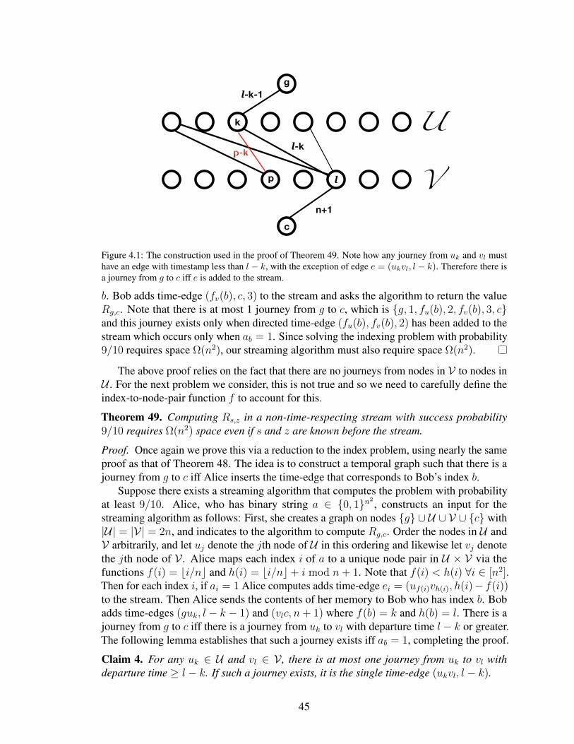
g

c

U

V

k

lp

l-k

l-k-1

p-k

n+1

Figure 4.1: The construction used in the proof of Theorem 49. Note how any journey from uk and vl musthave an edge with timestamp less than l − k, with the exception of edge e = (ukvl, l − k). Therefore there isa journey from g to c iff e is added to the stream.

b. Bob adds time-edge (fv(b), c, 3) to the stream and asks the algorithm to return the valueRg,c. Note that there is at most 1 journey from g to c, which is g, 1, fu(b), 2, fv(b), 3, cand this journey exists only when directed time-edge (fu(b), fv(b), 2) has been added to thestream which occurs only when ab = 1. Since solving the indexing problem with probability9/10 requires space Ω(n2), our streaming algorithm must also require space Ω(n2).

The above proof relies on the fact that there are no journeys from nodes in V to nodes inU . For the next problem we consider, this is not true and so we need to carefully define theindex-to-node-pair function f to account for this.

Theorem 49. Computing Rs,z in a non-time-respecting stream with success probability9/10 requires Ω(n2) space even if s and z are known before the stream.

Proof. Once again we prove this via a reduction to the index problem, using nearly the sameproof as that of Theorem 48. The idea is to construct a temporal graph such that there is ajourney from g to c iff Alice inserts the time-edge that corresponds to Bob’s index b.

Suppose there exists a streaming algorithm that computes the problem with probabilityat least 9/10. Alice, who has binary string a ∈ 0, 1n2 , constructs an input for thestreaming algorithm as follows: First, she creates a graph on nodes g ∪ U ∪ V ∪ c with|U| = |V| = 2n, and indicates to the algorithm to compute Rg,c. Order the nodes in U andV arbitrarily, and let uj denote the jth node of U in this ordering and likewise let vj denotethe jth node of V . Alice maps each index i of a to a unique node pair in U × V via thefunctions f(i) = bi/nc and h(i) = bi/nc+ i mod n+ 1. Note that f(i) < h(i) ∀i ∈ [n2].Then for each index i, if ai = 1 Alice computes adds time-edge ei = (uf(i)vh(i), h(i)− f(i))to the stream. Then Alice sends the contents of her memory to Bob who has index b. Bobadds time-edges (guk, l − k − 1) and (vlc, n+ 1) where f(b) = k and h(b) = l. There is ajourney from g to c iff there is a journey from uk to vl with departure time l − k or greater.The following lemma establishes that such a journey exists iff ab = 1, completing the proof.

Claim 4. For any uk ∈ U and vl ∈ V , there is at most one journey from uk to vl withdeparture time ≥ l − k. If such a journey exists, it is the single time-edge (ukvl, l − k).

45

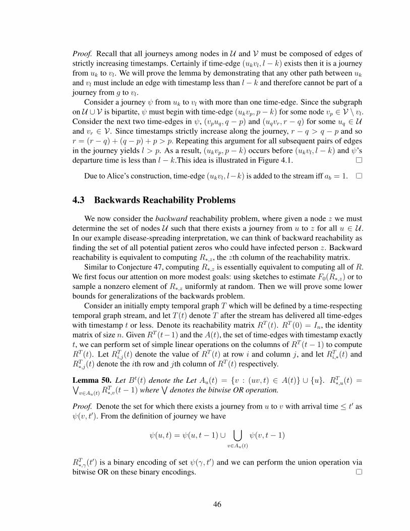
Proof. Recall that all journeys among nodes in U and V must be composed of edges ofstrictly increasing timestamps. Certainly if time-edge (ukvl, l − k) exists then it is a journeyfrom uk to vl. We will prove the lemma by demonstrating that any other path between ukand vl must include an edge with timestamp less than l− k and therefore cannot be part of ajourney from g to vl.

Consider a journey ψ from uk to vl with more than one time-edge. Since the subgraphon U ∪ V is bipartite, ψ must begin with time-edge (ukvp, p− k) for some node vp ∈ V \ vl.Consider the next two time-edges in ψ, (vpuq, q − p) and (uqvr, r − q) for some uq ∈ Uand vr ∈ V . Since timestamps strictly increase along the journey, r − q > q − p and sor = (r − q) + (q − p) + p > p. Repeating this argument for all subsequent pairs of edgesin the journey yields l > p. As a result, (ukvp, p − k) occurs before (ukvl, l − k) and ψ’sdeparture time is less than l − k.This idea is illustrated in Figure 4.1.

Due to Alice’s construction, time-edge (ukvl, l−k) is added to the stream iff ab = 1.

4.3 Backwards Reachability Problems

We now consider the backward reachability problem, where given a node z we mustdetermine the set of nodes U such that there exists a journey from u to z for all u ∈ U .In our example disease-spreading interpretation, we can think of backward reachability asfinding the set of all potential patient zeros who could have infected person z. Backwardreachability is equivalent to computing R∗,z, the zth column of the reachability matrix.

Similar to Conjecture 47, computing R∗,z is essentially equivalent to computing all of R.We first focus our attention on more modest goals: using sketches to estimate F0(R∗,z) or tosample a nonzero element of R∗,z uniformly at random. Then we will prove some lowerbounds for generalizations of the backwards problem.

Consider an initially empty temporal graph T which will be defined by a time-respectingtemporal graph stream, and let T (t) denote T after the stream has delivered all time-edgeswith timestamp t or less. Denote its reachability matrix RT (t). RT (0) = In, the identitymatrix of size n. Given RT (t−1) and the A(t), the set of time-edges with timestamp exactlyt, we can perform set of simple linear operations on the columns of RT (t− 1) to computeRT (t). Let RT

i,j(t) denote the value of RT (t) at row i and column j, and let RTi,∗(t) and

RT∗,j(t) denote the ith row and jth column of RT (t) respectively.

Lemma 50. Let Bt(t) denote the Let Au(t) = v : (uv, t) ∈ A(t) ∪ u. RT∗,u(t) =∨

v∈Au(t) RT∗,v(t− 1) where

∨denotes the bitwise OR operation.

Proof. Denote the set for which there exists a journey from u to v with arrival time ≤ t′ asψ(v, t′). From the definition of journey we have

ψ(u, t) = ψ(u, t− 1) ∪⋃

v∈Au(t)

ψ(v, t− 1)

RT∗,γ(t

′) is a binary encoding of set ψ(γ, t′) and we can perform the union operation viabitwise OR on these binary encodings.

46

We can essentially perform OR operations on the columns by summing them together.Define BT (0) = In and BT

∗,u(i) =∑

v∈Au(i) BT∗,v(i − 1) ∀i ∈ [τ ]. If we treat all nonzero

elements of BT as equal to 1, then we can simply sum the appropriate columns togetherinstead of performing bitwise OR (treating any nonzero entry as equivalent to 1). Thismeans we can sketch the columns of RT of the matrix using any linear sketch and updateby summing different column sketches. Using existing sketches, we can immediatelyperform tasks in small space like estimating F0(R∗,z) or to sample a nonzero element ofR∗,z uniformly at random.

However, this summing approach introduces a complication we must address. Elementsof RT (t) may be as large as 2t. For example, if the stream contains time-edges (u, v, i)for each i ∈ [τ ], then RT

u,v(t) = 2τ . F0 and `0 sketches (which we use below) use spacedependent on log(σ) where σ is the maximum value which elements in the sketched vectorcan take on, so in our example the presence of large values would incur an additional τ spacefactor. However, [115] outlines alternative versions of F0 and `0 sketches which sketch eachvector element mod p for some large random prime p n, eliminating this extra τ spacefactor and leading to the following theorem:

Theorem 51. There is a sketch-based time-respecting temporal graph stream algorithm thatusesO(nε−2 log(1/δ)) space that (1+ε)-approximates F0(R∗,z) with probability 1−δ, and asketch-based time-respecting temporal graph stream algorithm usingO(n polylog(n) log(1/δ))space that samples a nonzero element of R∗,z with probability 1− δ.

4.4 Departure Reachability

So far we have been considering journeys which may depart and arrive at any time. Wemight however want to determine whether a journey with a departure time greater thansome constant k exists between some nodes u and v. To accomodate this, we define thedeparture-reachability matrix D of a temporal graph T to be an n× n× τ matrix whereDu,v,t = 1 iff there is a journey from u to v with departure time t or greater, and 0 otherwise.

Theorem 52. Computing Ds,z,t in a time-respecting stream with success probability 9/10requires Ω(n2) space if t and s are not known before the stream, even if z is known.

Proof. The proof is nearly identical to that of Theorem 49. We assume there exists astreaming algorithm that finds Ds,z,t. Alice follows exactly the same procedure to constructthe temporal graph stream, except that she asks the algorithm to compute Ds′,c,t′ for somenot-yet-known value of t′ and some not-yet-specified node s′. Bob, instead of adding edge(guk, l − k) to the stream, indicates that t′ = l − k and s′ = uk. Then by Claim 4 there is ajourney from uk to c with departure time ≥ l − k iff time-edge (ukvl, l − k) is added to thestream, which by Alice’s construction occurs iff ab = 1.

47

Algorithms in the Field

48

CHAPTER 5

MESH

Programs written in C/C++ can suffer from serious memory fragmentation, leading tolow utilization of memory, degraded performance, and application failure due to memoryexhaustion. This chapter introduces MESH, a plug-in replacement for malloc that, for thefirst time, eliminates fragmentation in unmodified C/C++ applications. MESH combinesnovel randomized algorithms with widely-supported virtual memory operations to provablyreduce fragmentation, breaking the classical Robson bounds with high probability. We focushere on the randomized algorithms which power MESH and proofs of their solution qualityand runtime. MESH generally matches the runtime performance of state-of-the-art memoryallocators while reducing memory consumption; in particular, it reduces the memory ofconsumption of Firefox by 16% and Redis by 39%.

5.1 Introduction

Despite nearly fifty years of conventional wisdom indicating that compaction is impossi-ble in unmanaged languages, this chapter shows that it is not only possible but also practical.It introduces MESH, a memory allocator that effectively and efficiently performs compactingmemory management to reduce memory usage in unmodified C and C++ applications.

Crucially and counterintuitively, MESH performs compaction without relocation; thatis, without changing the addresses of objects. This property is vital for compatibility witharbitrary C/C++ applications. To achieve this, MESH builds on a mechanism which we callmeshing, first introduced by Novark et al.’s Hound memory leak detector [131]. Houndemployed meshing in an effort to avoid catastrophic memory consumption induced by itsmemory-inefficient allocation scheme, which can only reclaim memory when every objecton a page is freed. Hound first searches for pages whose live objects do not overlap. It thencopies the contents of one page onto the other, remaps one of the virtual pages to point tothe single physical page now holding the contents of both pages, and finally relinquishes theother physical page to the OS. Figure 5.1 illustrates meshing in action.

MESH overcomes two key technical challenges of meshing that previously made it bothinefficient and potentially entirely ineffective. First, Hound’s search for pages to meshinvolves a linear scan of pages on calls to free. While this search is more efficient thana naive O(n2) search of all possible pairs of pages, it remains prohibitively expensive foruse in the context of a general-purpose allocator. Second, Hound offers no guarantees thatany pages would ever be meshable. Consider an application that happens to allocate evenone object in the same offset in every page. That layout would preclude meshing altogether,eliminating the possibility of saving any space.

49

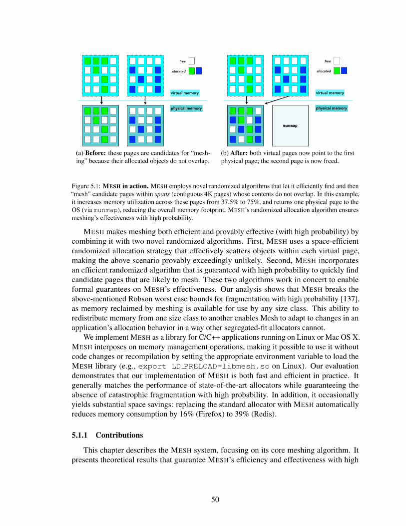
virtual memory

physical memory

free

allocated

(a) Before: these pages are candidates for “mesh-ing” because their allocated objects do not overlap.

munmap

free

allocated

virtual memory

physical memory

(b) After: both virtual pages now point to the firstphysical page; the second page is now freed.

Figure 5.1: MESH in action. MESH employs novel randomized algorithms that let it efficiently find and then“mesh” candidate pages within spans (contiguous 4K pages) whose contents do not overlap. In this example,it increases memory utilization across these pages from 37.5% to 75%, and returns one physical page to theOS (via munmap), reducing the overall memory footprint. MESH’s randomized allocation algorithm ensuresmeshing’s effectiveness with high probability.

MESH makes meshing both efficient and provably effective (with high probability) bycombining it with two novel randomized algorithms. First, MESH uses a space-efficientrandomized allocation strategy that effectively scatters objects within each virtual page,making the above scenario provably exceedingly unlikely. Second, MESH incorporatesan efficient randomized algorithm that is guaranteed with high probability to quickly findcandidate pages that are likely to mesh. These two algorithms work in concert to enableformal guarantees on MESH’s effectiveness. Our analysis shows that MESH breaks theabove-mentioned Robson worst case bounds for fragmentation with high probability [137],as memory reclaimed by meshing is available for use by any size class. This ability toredistribute memory from one size class to another enables Mesh to adapt to changes in anapplication’s allocation behavior in a way other segregated-fit allocators cannot.

We implement MESH as a library for C/C++ applications running on Linux or Mac OS X.MESH interposes on memory management operations, making it possible to use it withoutcode changes or recompilation by setting the appropriate environment variable to load theMESH library (e.g., export LD PRELOAD=libmesh.so on Linux). Our evaluationdemonstrates that our implementation of MESH is both fast and efficient in practice. Itgenerally matches the performance of state-of-the-art allocators while guaranteeing theabsence of catastrophic fragmentation with high probability. In addition, it occasionallyyields substantial space savings: replacing the standard allocator with MESH automaticallyreduces memory consumption by 16% (Firefox) to 39% (Redis).

5.1.1 Contributions

This chapter describes the MESH system, focusing on its core meshing algorithm. Itpresents theoretical results that guarantee MESH’s efficiency and effectiveness with high

50

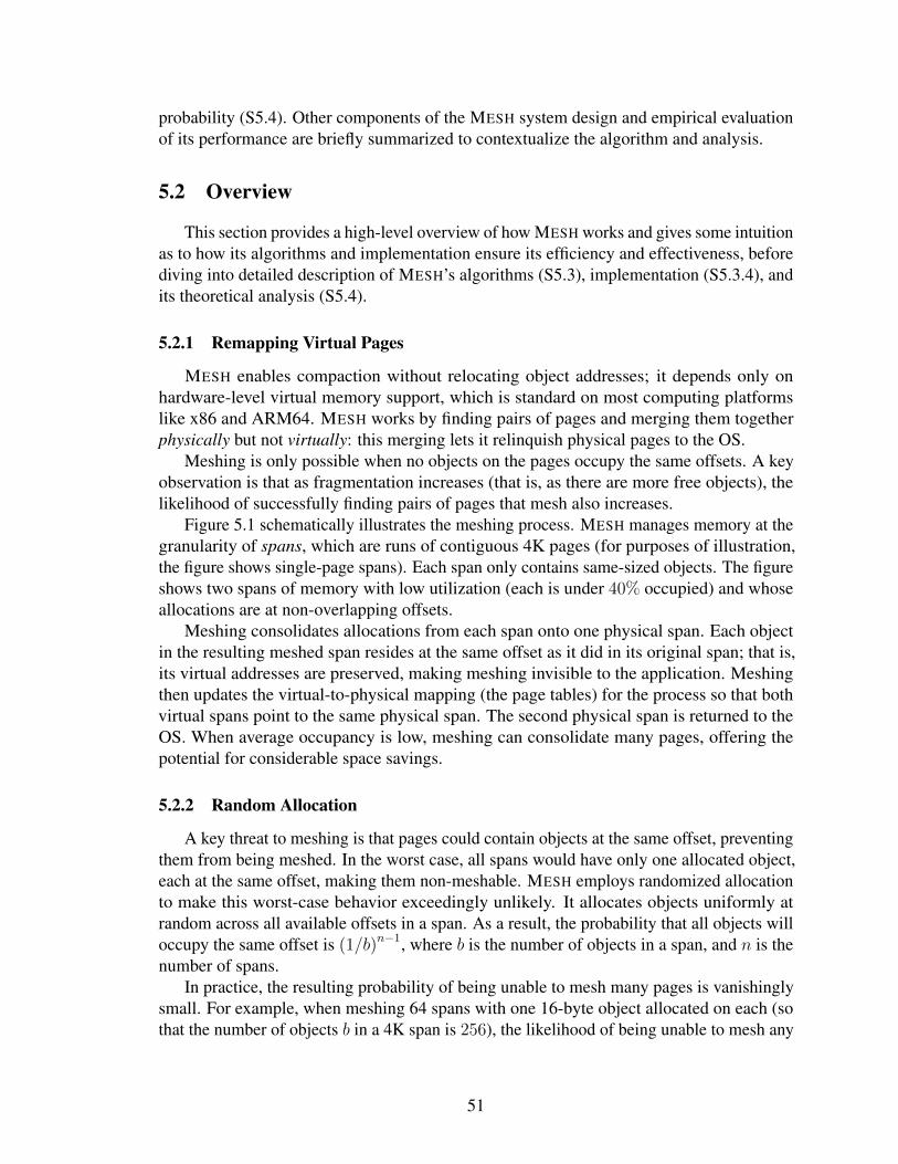
probability (S5.4). Other components of the MESH system design and empirical evaluationof its performance are briefly summarized to contextualize the algorithm and analysis.

5.2 Overview

This section provides a high-level overview of how MESH works and gives some intuitionas to how its algorithms and implementation ensure its efficiency and effectiveness, beforediving into detailed description of MESH’s algorithms (S5.3), implementation (S5.3.4), andits theoretical analysis (S5.4).

5.2.1 Remapping Virtual Pages

MESH enables compaction without relocating object addresses; it depends only onhardware-level virtual memory support, which is standard on most computing platformslike x86 and ARM64. MESH works by finding pairs of pages and merging them togetherphysically but not virtually: this merging lets it relinquish physical pages to the OS.

Meshing is only possible when no objects on the pages occupy the same offsets. A keyobservation is that as fragmentation increases (that is, as there are more free objects), thelikelihood of successfully finding pairs of pages that mesh also increases.

Figure 5.1 schematically illustrates the meshing process. MESH manages memory at thegranularity of spans, which are runs of contiguous 4K pages (for purposes of illustration,the figure shows single-page spans). Each span only contains same-sized objects. The figureshows two spans of memory with low utilization (each is under 40% occupied) and whoseallocations are at non-overlapping offsets.

Meshing consolidates allocations from each span onto one physical span. Each objectin the resulting meshed span resides at the same offset as it did in its original span; that is,its virtual addresses are preserved, making meshing invisible to the application. Meshingthen updates the virtual-to-physical mapping (the page tables) for the process so that bothvirtual spans point to the same physical span. The second physical span is returned to theOS. When average occupancy is low, meshing can consolidate many pages, offering thepotential for considerable space savings.

5.2.2 Random Allocation

A key threat to meshing is that pages could contain objects at the same offset, preventingthem from being meshed. In the worst case, all spans would have only one allocated object,each at the same offset, making them non-meshable. MESH employs randomized allocationto make this worst-case behavior exceedingly unlikely. It allocates objects uniformly atrandom across all available offsets in a span. As a result, the probability that all objects willoccupy the same offset is (1/b)n−1, where b is the number of objects in a span, and n is thenumber of spans.

In practice, the resulting probability of being unable to mesh many pages is vanishinglysmall. For example, when meshing 64 spans with one 16-byte object allocated on each (sothat the number of objects b in a 4K span is 256), the likelihood of being unable to mesh any

51

of these spans is 10−152. To put this into perspective, there are estimated to be roughly 1082

particles in the universe.We use randomness to guide the design of MESH’s algorithms (S5.3) and implementation

(S5.3.4); this randomization lets us prove robust guarantees of its performance (S5.4),showing that MESH breaks the Robson bounds with high probability.

5.2.3 Finding Spans to Mesh

Given a set of spans, our goal is to mesh them in a way that frees as many physical pagesas possible. We can think of this task as that of partitioning the spans into subsets such thatthe spans in each subset mesh. An optimal partition would minimize the number of suchsubsets.

Unfortunately, as we show, optimal meshing is not feasible (S5.4). Instead, the al-gorithms in Section 5.3 present practical methods for finding high-quality meshes underreal-world time constraints. We show that solving a simplified version of the problem (S5.3)is sufficient to achieve reasonable meshes with high probability (S5.4).

5.3 Algorithms & System Design

MESH comprises three main algorithmic components: allocation (S5.3.1), deallocation(S5.3.2), and finding spans to mesh (S5.3.3). Unless otherwise noted and without loss ofgenerality, all algorithms described here are per size class (within spans, all objects are samesize).

5.3.1 Allocation

Allocation in MESH consists of two steps: (1) finding a span to allocate from, and(2) randomly allocating an object from that span. MESH always allocates from a thread-local shuffle vector – a randomized version of a freelist The shuffle vector contains offsetscorresponding to the slots of a single span. We call that span the attached span for a giventhread.

If the shuffle vector is empty, MESH relinquishes the current thread’s attached span (ifone exists) to the global heap (which holds all unattached spans), and asks it to select anew span. If there are no partially full spans, the global heap returns a new, empty span.Otherwise, it selects a partially full span for reuse. To maximize utilization, the globalheap groups spans into bins organized by decreasing occupancy (e.g., 75-99% full in onebin, 50-74% in the next). The global heap scans for the first non-empty bin (by decreasingoccupancy), and randomly selects a span from that bin.

Once a span has been selected, the allocator adds the offsets corresponding to the freeslots in that span to the thread-local shuffle vector (in a random order). MESH pops the firstentry off the shuffle vector and returns it.

52

SPLITMESHER(S, t)

1 n = length(S)2 Sl, Sr = S[1 : n/2], S[n/2 + 1 : n]3 for (i = 0, i < t, i+ +)4 len = |Sl|5 for (j = 0, j < len, j + +)6 if MESHABLE (Sl(j), Sr(j + i % len))7 Sl ← Sl \ Sl(j)8 Sr ← Sr \ Sr(j + i % len)9 MESH(Sl(j), Sr(j + i % len))

Figure 5.2: Meshing random pairs of spans. SPLITMESHER splits the randomly ordered span list S intohalves, then probes pairs between halves for meshes. Each span is probed up to t times.

5.3.2 Deallocation

Deallocation behaves differently depending on whether the free is local (the addressbelongs to the current thread’s attached span), remote (the object belongs to another thread’sattached span), or if it belongs to the global heap.

For local frees, MESH adds the object’s offset onto the span’s shuffle vector in a randomposition and returns. For remote frees, MESH atomically resets the bit in the correspondingindex in a bitmap associated with each span. Finally, for an object belonging to the globalheap, MESH marks the object as free, updates the span’s occupancy bin; this action mayadditionally trigger meshing.

5.3.3 Meshing

When meshing, MESH randomly chooses pairs of spans and attempts to mesh eachpair. The meshing algorithm, which we call SPLITMESHER (Figure 5.2), is designedboth for practical effectiveness and for its theoretical guarantees. The parameter t, whichdetermines the maximum number of times each span is probed (line 3), enables space-timetrade-offs. The parameter t can be increased to improve mesh quality and therefore reducespace, or decreased to improve runtime, at the cost of sacrificed meshing opportunities. Weempirically found that t = 64 balances runtime and meshing effectiveness, and use thisvalue in our implementation.

SPLITMESHER proceeds by iterating through Sl and checking whether it can mesh eachspan with another span chosen from Sr (line 6). If so, it removes these spans from theirrespective lists and meshes them (lines 7–9). SPLITMESHER repeats until it has checkedt ∗ |Sl| pairs of spans.

5.3.4 Implementation

We implement MESH as a drop-in replacement memory allocator that implements mesh-ing for single or multi-threaded applications written in C/C++. Its current implementationwork for 64-bit Linux and Mac OS X binaries. MESH can be explicitly linked against

53

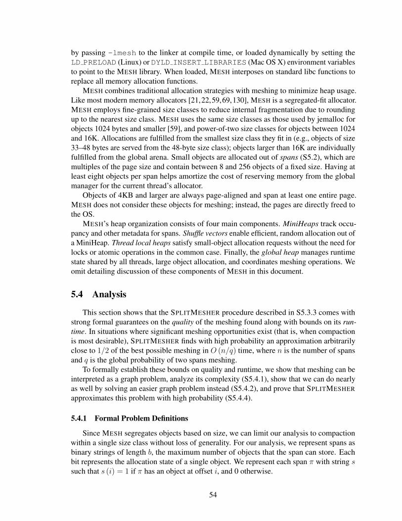
by passing -lmesh to the linker at compile time, or loaded dynamically by setting theLD PRELOAD (Linux) or DYLD INSERT LIBRARIES (Mac OS X) environment variablesto point to the MESH library. When loaded, MESH interposes on standard libc functions toreplace all memory allocation functions.

MESH combines traditional allocation strategies with meshing to minimize heap usage.Like most modern memory allocators [21,22,59,69,130], MESH is a segregated-fit allocator.MESH employs fine-grained size classes to reduce internal fragmentation due to roundingup to the nearest size class. MESH uses the same size classes as those used by jemalloc forobjects 1024 bytes and smaller [59], and power-of-two size classes for objects between 1024and 16K. Allocations are fulfilled from the smallest size class they fit in (e.g., objects of size33–48 bytes are served from the 48-byte size class); objects larger than 16K are individuallyfulfilled from the global arena. Small objects are allocated out of spans (S5.2), which aremultiples of the page size and contain between 8 and 256 objects of a fixed size. Having atleast eight objects per span helps amortize the cost of reserving memory from the globalmanager for the current thread’s allocator.

Objects of 4KB and larger are always page-aligned and span at least one entire page.MESH does not consider these objects for meshing; instead, the pages are directly freed tothe OS.

MESH’s heap organization consists of four main components. MiniHeaps track occu-pancy and other metadata for spans. Shuffle vectors enable efficient, random allocation out ofa MiniHeap. Thread local heaps satisfy small-object allocation requests without the need forlocks or atomic operations in the common case. Finally, the global heap manages runtimestate shared by all threads, large object allocation, and coordinates meshing operations. Weomit detailing discussion of these components of MESH in this document.

5.4 Analysis

This section shows that the SPLITMESHER procedure described in S5.3.3 comes withstrong formal guarantees on the quality of the meshing found along with bounds on its run-time. In situations where significant meshing opportunities exist (that is, when compactionis most desirable), SPLITMESHER finds with high probability an approximation arbitrarilyclose to 1/2 of the best possible meshing in O (n/q) time, where n is the number of spansand q is the global probability of two spans meshing.

To formally establish these bounds on quality and runtime, we show that meshing can beinterpreted as a graph problem, analyze its complexity (S5.4.1), show that we can do nearlyas well by solving an easier graph problem instead (S5.4.2), and prove that SPLITMESHER

approximates this problem with high probability (S5.4.4).

5.4.1 Formal Problem Definitions

Since MESH segregates objects based on size, we can limit our analysis to compactionwithin a single size class without loss of generality. For our analysis, we represent spans asbinary strings of length b, the maximum number of objects that the span can store. Eachbit represents the allocation state of a single object. We represent each span π with string ssuch that s (i) = 1 if π has an object at offset i, and 0 otherwise.

54

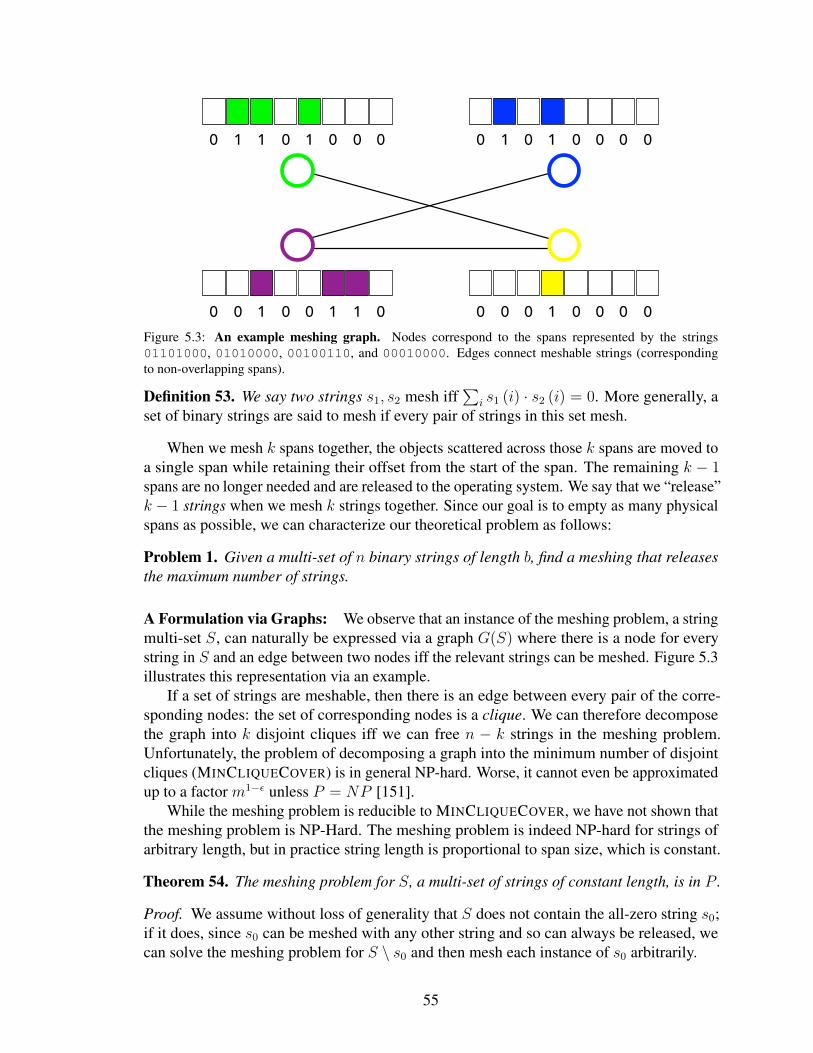
0 1 1 0 1 0 0 0 0 1 0 1 0 0 0 0

0 0 1 0 0 1 1 0 0 0 0 1 0 0 0 0Figure 5.3: An example meshing graph. Nodes correspond to the spans represented by the strings01101000, 01010000, 00100110, and 00010000. Edges connect meshable strings (correspondingto non-overlapping spans).

Definition 53. We say two strings s1, s2 mesh iff∑

i s1 (i) · s2 (i) = 0. More generally, aset of binary strings are said to mesh if every pair of strings in this set mesh.

When we mesh k spans together, the objects scattered across those k spans are moved toa single span while retaining their offset from the start of the span. The remaining k − 1spans are no longer needed and are released to the operating system. We say that we “release”k − 1 strings when we mesh k strings together. Since our goal is to empty as many physicalspans as possible, we can characterize our theoretical problem as follows:

Problem 1. Given a multi-set of n binary strings of length b, find a meshing that releasesthe maximum number of strings.

A Formulation via Graphs: We observe that an instance of the meshing problem, a stringmulti-set S, can naturally be expressed via a graph G(S) where there is a node for everystring in S and an edge between two nodes iff the relevant strings can be meshed. Figure 5.3illustrates this representation via an example.

If a set of strings are meshable, then there is an edge between every pair of the corre-sponding nodes: the set of corresponding nodes is a clique. We can therefore decomposethe graph into k disjoint cliques iff we can free n − k strings in the meshing problem.Unfortunately, the problem of decomposing a graph into the minimum number of disjointcliques (MINCLIQUECOVER) is in general NP-hard. Worse, it cannot even be approximatedup to a factor m1−ε unless P = NP [151].

While the meshing problem is reducible to MINCLIQUECOVER, we have not shown thatthe meshing problem is NP-Hard. The meshing problem is indeed NP-hard for strings ofarbitrary length, but in practice string length is proportional to span size, which is constant.

Theorem 54. The meshing problem for S, a multi-set of strings of constant length, is in P .

Proof. We assume without loss of generality that S does not contain the all-zero string s0;if it does, since s0 can be meshed with any other string and so can always be released, wecan solve the meshing problem for S \ s0 and then mesh each instance of s0 arbitrarily.

55

Rather than reason about MINCLIQUECOVER on a meshing graph G, we consider theequivalent problem of coloring the complement graph G in which there is an edge betweenevery pair of two nodes whose strings do not mesh. The nodes of G can be partitioned intoat most 2b − 1 subsets N1 . . . N2b−1 such that all nodes in each Ni represent the same stringsi. The induced subgraph of Ni in G is a clique since all its nodes have a 1 in the sameposition and so cannot be pairwise meshed. Further, all nodes in Ni have the same set ofneighbors.

Since Ni is a clique, at most one node in Ni may be colored with any color. Fix somecoloring on G. Swapping the colors of two nodes in Ni does not change the validity of thecoloring since these nodes have the same neighbor set. We can therefore unambiguouslyrepresent a valid coloring of G merely by indicating in which cliques each color appears.

With 2b cliques and a maximum of n colors, there are at most (n+ 1)c such coloringson the graph where c = 22b . This follows because each color used can be associated witha subset of 1, . . . , 2b corresponding to which of the cliques have node with this color;we call this subset a signature and note there are c possible signatures. A coloring can betherefore be associated with a multi-set of possible signatures where each signature hasmultiplicity between 0 and n; there are (n + 1)c such multi-sets. This is polynomial in nsince b is constant and hence c is also constant. So we can simply check each coloring forvalidity (a coloring is valid iff no color appears in two cliques whose string representationsmesh). The algorithm returns a valid coloring with the lowest number of colors from allvalid colorings discovered.

Note that the runtime of the above algorithm is at least exponential in the string length.While technically polynomial for constant string length, the running time of the abovealgorithm would obviously be prohibitive in practice and so we never employ it in MESH.Fortunately, as we show next, we can exploit the randomness in the strings to design a muchfaster algorithm.

5.4.2 Simplifying the Problem: From MINCLIQUECOVER to MATCHING

We leverage MESH’s random allocation to simplify meshing; this random allocationimplies a distribution over the graphs that exhibits useful structural properties. We first makethe following important observation:

Observation 1. Conditioned on the occupancies of the strings, edges in the meshing graphare not three-wise independent.

To see that edges are not three-wise independent consider three random strings s1, s2, s3

of length 4, each with exactly 2 ones. It is impossible for these strings to all mesh mutuallysince if we know that s1 and s2 mesh, and that s2 and s3 mesh, we know for certain thats1 and s3 cannot mesh. More generally, conditioning on s1 and s2 meshing and s1 and s3

meshing decreases the probability that s1 and s3 mesh. Below, we quantify this effect toargue that we can mesh near-optimally by solving the much easier MATCHING problemon the meshing graph (i.e., restricting our attention to finding cliques of size 2) instead ofMINCLIQUECOVER. Another consequence of the above observation is that we will not beable to appeal to theoretical results on the standard model of random graphs, ErdHos-Renyi

56

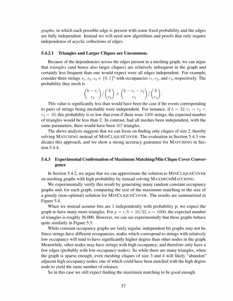
graphs, in which each possible edge is present with some fixed probability and the edgesare fully independent. Instead we will need new algorithms and proofs that only requireindependence of acyclic collections of edges.

5.4.2.1 Triangles and Larger Cliques are Uncommon.

Because of the dependencies across the edges present in a meshing graph, we can arguethat triangles (and hence also larger cliques) are relatively infrequent in the graph andcertainly less frequent than one would expect were all edges independent. For example,consider three strings s1, s2, s3 ∈ 0, 1b with occupancies r1, r2, and r3, respectively. Theprobability they mesh is(

b− r1

r2

)/( br2

)×(b− r1 − r2

r3

)/( br3

).

This value is significantly less than would have been the case if the events correspondingto pairs of strings being meshable were independent. For instance, if b = 32, r1 = r2 =r3 = 10, this probability is so low that even if there were 1000 strings, the expected numberof triangles would be less than 2. In contrast, had all meshes been independent, with thesame parameters, there would have been 167 triangles.

The above analysis suggests that we can focus on finding only cliques of size 2, therebysolving MATCHING instead of MINCLIQUECOVER. The evaluation in Section 5.4.3 vin-dicates this approach, and we show a strong accuracy guarantee for MATCHING in Sec-tion 5.4.4.

5.4.3 Experimental Confirmation of Maximum Matching/Min Clique Cover Conver-gence

In Section 5.4.2, we argue that we can approximate the solution to MINCLIQUECOVER

on meshing graphs with high probability by instead solving MAXIMUMMATCHING.We experimentally verify this result by generating many random constant occupancy

graphs and, for each graph, comparing the size of the maximum matching to the size ofa greedy (non-optimal) solution for MINCLIQUECOVER. The results are summarized inFigure 5.4.

When we instead assume bits are 1 independently with probability p, we expect thegraph to have many more triangles. For p = r/b = 10/32, n = 1000, the expected numberof triangles is roughly 36,000. However, we can see experimentally that these graphs behavequite similarly in Figure 5.5.

While constant occupancy graphs are fairly regular, independent bit graphs may not be.Since strings have different occupancies, nodes which correspond to strings with relativelylow occupancy will tend to have significantly higher degree than other nodes in the graph.Meanwhile, other nodes may have strings with high occupancy, and therefore only have afew edges (probably with low-occupancy nodes). So while there are many triangles, whenthe graph is sparse enough, even meshing cliques of size 3 and 4 will likely ”abandon”adjacent high-occupancy nodes, one of which could have been matched with the high degreenode to yield the same number of releases.

So in this case we still expect finding the maximum matching to be good enough.

57

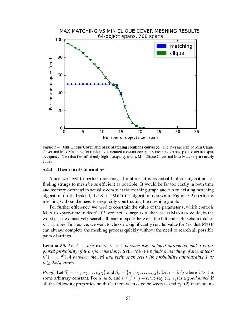
0 5 10 15 20 25 30 35

Number of objects per span

0

20

40

60

80

100

Perc

enta

ge o

f sp

ans

freed

MAX MATCHING VS MIN CLIQUE COVER MESHING RESULTS 64-object spans, 200 spans

matching

clique

Figure 5.4: Min Clique Cover and Max Matching solutions converge. The average size of Min CliqueCover and Max Matching for randomly generated constant occupancy meshing graphs, plotted against spanoccupancy. Note that for sufficiently high-occupancy spans, Min Clique Cover and Max Matching are nearlyequal.

5.4.4 Theoretical Guarantees

Since we need to perform meshing at runtime, it is essential that our algorithm forfinding strings to mesh be as efficient as possible. It would be far too costly in both timeand memory overhead to actually construct the meshing graph and run an existing matchingalgorithm on it. Instead, the SPLITMESHER algorithm (shown in Figure 5.2) performsmeshing without the need for explicitly constructing the meshing graph.

For further efficiency, we need to constrain the value of the parameter t, which controlsMESH’s space-time tradeoff. If t were set as large as n, then SPLITMESHER could, in theworst case, exhaustively search all pairs of spans between the left and right sets: a total ofn2/4 probes. In practice, we want to choose a significantly smaller value for t so that MESH

can always complete the meshing process quickly without the need to search all possiblepairs of strings.

Lemma 55. Let t = k/q where k > 1 is some user defined parameter and q is theglobal probability of two spans meshing. SPLITMESHER finds a matching of size at leastn(1 − e−2k)/4 between the left and right span sets with probability approaching 1 asn ≥ 2k/q grows.

Proof. Let Sl = v1, v2, . . . vn/2 and Sr = u1, u2, . . . un/2. Let t = k/q where k > 1 issome arbitrary constant. For ui ∈ Sl and i ≤ j ≤ j + t, we say (ui, vj) is a good match ifall the following properties hold: (1) there is an edge between ui and vj , (2) there are no

58

0 5 10 15 20 25 30 35

Number of objects per span

0

20

40

60

80

100

Perc

enta

ge o

f sp

ans

freed

MAX MATCHING VS MIN CLIQUE COVER MESHING RESULTS 64-object spans, 200 spans

matching

clique

Figure 5.5: Converge still holds for independent bits assumption. The average size of Min Clique Coverand Max Matching for randomly generated constant occupancy meshing graphs, plotted against span occupancy.Note that for sufficiently high-occupancy spans, Min Clique Cover and Max Matching are nearly equal.

edges between ui and vj′ for i ≤ j′ < j, and (3) there are no edges between ui′ and vj fori < i′ ≤ j.

We observe that SPLITMESHER finds any good match, although it may also find ad-ditional matches. It therefore suffices to consider only the number of good matches. Theprobability (ui, vj) is a good match is q(1−q)2(j−i) by appealing to the fact that the collectionof edges under consideration is acyclic. Hence, Pr(ui has a good match) is

r := q

k/q−1∑i=0

(1− q)2i = q1− (1− q)2k/q

1− (1− q)2>

1− e−2k

2.

To analyze the number of good matches, define Xi = 1 iff ui has a good match. Then,∑iXi is the number of good matches. By linearity of expectation, the expected number of

good matches is rn/2. We decompose∑

iXi into

Z0 + Z1 + . . .+ Zt−1 where Zj =∑

i≡j mod t

Xi .

Since each Zj is a sum of n/(2t) independent variables, by the Chernoff bound,P [Zj < (1− ε)E[Zj]] ≤ exp (−ε2rn/(4t)). By the union bound,

P [X < (1− ε) rn/2] ≤ t · exp(−ε2rn/(4t)

)and this becomes arbitrarily small as n grows.

59

In the worst case, the algorithm checks nk/2q pairs. For our implementation of MESH,we use a static value of t = 64; this value enables the guarantees of Lemma 5.1 in caseswhere significant meshing is possible. As Section 5.5 shows, this value for t results ineffective memory compaction with modest performance overhead.

5.4.5 New Lower Bound for Maximum Matching Size

In this section, we develop a bound for the size of the maximum matching in a graphthat can easily be estimated in the context of meshing graphs. As meshing may be costly toperform, this lower bound is useful as it can be used to predict the magnitude of compactionachievable before committing to the process. In the case where little compaction is possible,it is often better not to try to mesh and instead conserve resources for other tasks. Thequantity we introduce will always lower bound the size of the maximum matching and willtypically be relatively close to the size of the maximum matching. For example, if we wantto release 30% of our active spans through meshing, but the bound suggests a release of lessthan 5% is possible, we can infer that the maximum matching on the graph is small andmeshing is currently not worth attempting.

Our approach is based on extending a result by McGregor and Vorotnikova [116]. Letd(u) be the degree of node u in a graph. They considered the quantity

∑e∈E 1/max(d(u), d(v))

and showed that it is at most a factor 3/2 larger than the maximum matching in the graphand at most a factor 4 smaller in the case of planar graphs. These bounds were tight. Forexample, on a complete graph on three nodes, the quantity is 3/2 while M is 1. Meshinggraphs are very unlikely to be planar but are likely be almost regular, i.e., most degrees areroughly similar. We need to extend the above bound such that we can guarantee that it neverexceeds the size of the maximum matching while also being a good estimate for the graphsthat are likely to arise as meshing graphs.

One simple approach is to scale the above quantity by a factor of 2/3, but this can resultin a poor approximation for the size of the maximum matching for some graphs of interest.Instead, we take a more nuanced approach. Specifically, we prove the following theorem(proof omitted due to space constraints):

Theorem 56.

W =∑e∈E

1

max(d(u), d(v)) + I[min(d(u), d(v)) > 1]≤M .

Proof. We begin by showing that the simpler quantity W is a lower bound of the maximummatching M .

W =∑e∈E

1

max(d (u) , d (v)) + 1.

Let U be an arbitrary set of t nodes in G where t is odd. Define

W (U) =∑u,v∈U

1

max(d (u) , d (v)) + 1.

As a corollary of Edmonds Matching Polytope Theorem, it can be shown that W ≤M ifW (U) ≤ (|U | − 1)/2. We can argue this as follows:

60

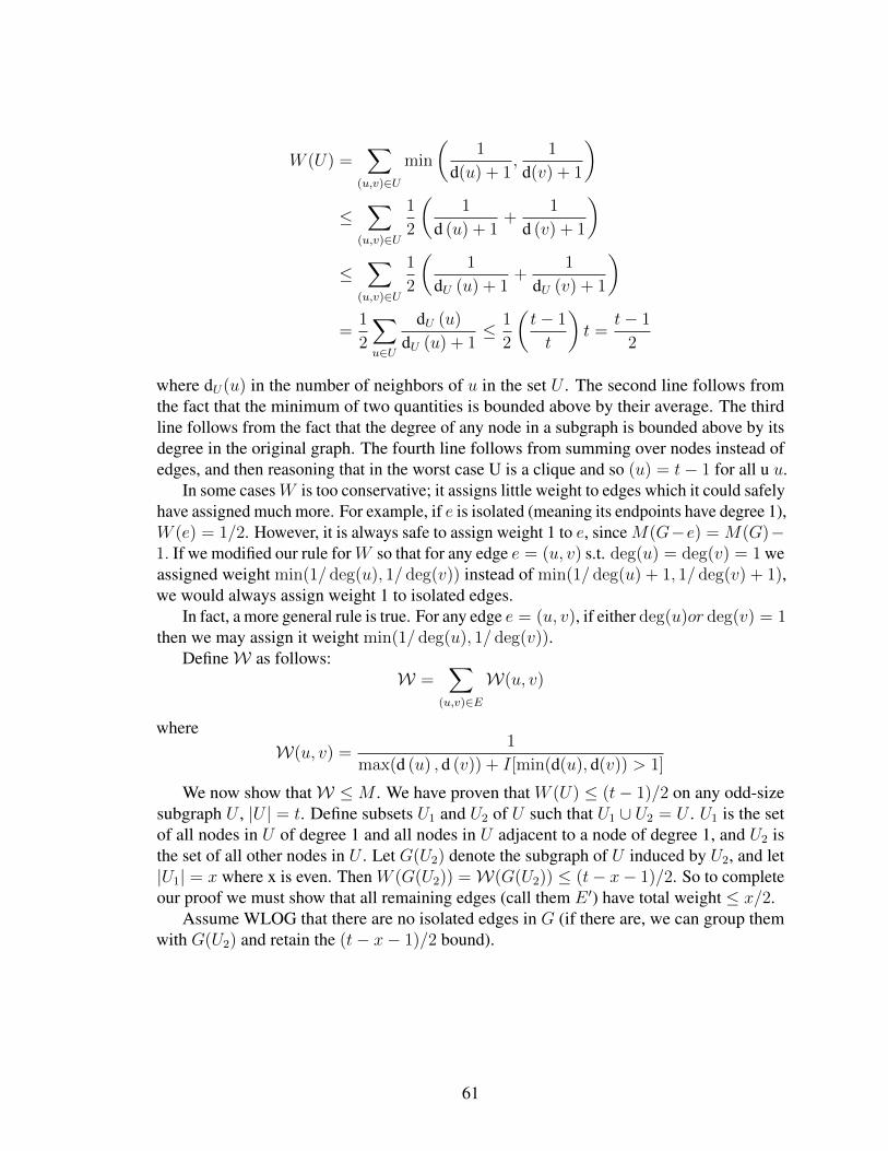
W (U) =∑

(u,v)∈U

min

(1

d(u) + 1,

1

d(v) + 1

)

≤∑

(u,v)∈U

1

2

(1

d (u) + 1+

1

d (v) + 1

)

≤∑

(u,v)∈U

1

2

(1

dU (u) + 1+

1

dU (v) + 1

)

=1

2

∑u∈U

dU (u)

dU (u) + 1≤ 1

2

(t− 1

t

)t =

t− 1

2

where dU(u) in the number of neighbors of u in the set U . The second line follows fromthe fact that the minimum of two quantities is bounded above by their average. The thirdline follows from the fact that the degree of any node in a subgraph is bounded above by itsdegree in the original graph. The fourth line follows from summing over nodes instead ofedges, and then reasoning that in the worst case U is a clique and so (u) = t− 1 for all u u.

In some casesW is too conservative; it assigns little weight to edges which it could safelyhave assigned much more. For example, if e is isolated (meaning its endpoints have degree 1),W (e) = 1/2. However, it is always safe to assign weight 1 to e, sinceM(G−e) = M(G)−1. If we modified our rule forW so that for any edge e = (u, v) s.t. deg(u) = deg(v) = 1 weassigned weight min(1/ deg(u), 1/ deg(v)) instead of min(1/ deg(u) + 1, 1/ deg(v) + 1),we would always assign weight 1 to isolated edges.

In fact, a more general rule is true. For any edge e = (u, v), if either deg(u)or deg(v) = 1then we may assign it weight min(1/ deg(u), 1/ deg(v)).

DefineW as follows:W =

∑(u,v)∈E

W(u, v)

whereW(u, v) =

1

max(d (u) , d (v)) + I[min(d(u), d(v)) > 1]

We now show thatW ≤M . We have proven that W (U) ≤ (t− 1)/2 on any odd-sizesubgraph U , |U | = t. Define subsets U1 and U2 of U such that U1 ∪ U2 = U . U1 is the setof all nodes in U of degree 1 and all nodes in U adjacent to a node of degree 1, and U2 isthe set of all other nodes in U . Let G(U2) denote the subgraph of U induced by U2, and let|U1| = x where x is even. Then W (G(U2)) =W(G(U2)) ≤ (t− x− 1)/2. So to completeour proof we must show that all remaining edges (call them E ′) have total weight ≤ x/2.

Assume WLOG that there are no isolated edges in G (if there are, we can group themwith G(U2) and retain the (t− x− 1)/2 bound).

61

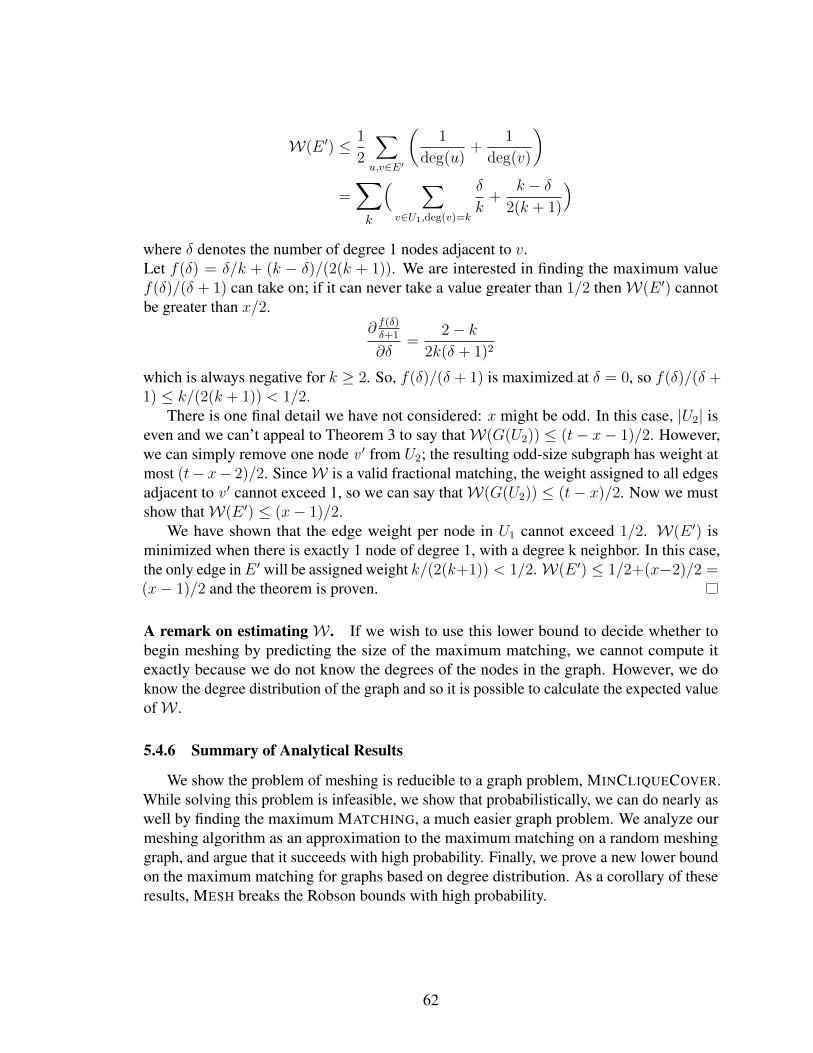
W(E ′) ≤ 1

2

∑u,v∈E′

(1

deg(u)+

1

deg(v)

)=∑k

( ∑v∈U1,deg(v)=k

δ

k+

k − δ2(k + 1)

)where δ denotes the number of degree 1 nodes adjacent to v.Let f(δ) = δ/k + (k − δ)/(2(k + 1)). We are interested in finding the maximum valuef(δ)/(δ + 1) can take on; if it can never take a value greater than 1/2 thenW(E ′) cannotbe greater than x/2.

∂ f(δ)δ+1

∂δ=

2− k2k(δ + 1)2

which is always negative for k ≥ 2. So, f(δ)/(δ + 1) is maximized at δ = 0, so f(δ)/(δ +1) ≤ k/(2(k + 1)) < 1/2.

There is one final detail we have not considered: x might be odd. In this case, |U2| iseven and we can’t appeal to Theorem 3 to say thatW(G(U2)) ≤ (t− x− 1)/2. However,we can simply remove one node v ′ from U2; the resulting odd-size subgraph has weight atmost (t− x− 2)/2. SinceW is a valid fractional matching, the weight assigned to all edgesadjacent to v ′ cannot exceed 1, so we can say thatW(G(U2)) ≤ (t− x)/2. Now we mustshow thatW(E ′) ≤ (x− 1)/2.

We have shown that the edge weight per node in U1 cannot exceed 1/2. W(E ′) isminimized when there is exactly 1 node of degree 1, with a degree k neighbor. In this case,the only edge inE ′ will be assigned weight k/(2(k+1)) < 1/2.W(E ′) ≤ 1/2+(x−2)/2 =(x− 1)/2 and the theorem is proven.

A remark on estimating W . If we wish to use this lower bound to decide whether tobegin meshing by predicting the size of the maximum matching, we cannot compute itexactly because we do not know the degrees of the nodes in the graph. However, we doknow the degree distribution of the graph and so it is possible to calculate the expected valueofW .

5.4.6 Summary of Analytical Results

We show the problem of meshing is reducible to a graph problem, MINCLIQUECOVER.While solving this problem is infeasible, we show that probabilistically, we can do nearly aswell by finding the maximum MATCHING, a much easier graph problem. We analyze ourmeshing algorithm as an approximation to the maximum matching on a random meshinggraph, and argue that it succeeds with high probability. Finally, we prove a new lower boundon the maximum matching for graphs based on degree distribution. As a corollary of theseresults, MESH breaks the Robson bounds with high probability.

62

5.5 Summary of Evaluation

For a number of memory-intensive applications, including aggressively space-optimizedapplications like Firefox, MESH can substantially reduce memory consumption (by 16%to 39%) while imposing a modest impact on runtime performance (e.g., around 1% forFirefox and SPECint 2006). We find that MESH’s randomization can enable substantialspace reduction in the face of a regular allocation pattern.

5.6 Related Work

Hound: Hound is a memory leak detector for C/C++ applications that introduced meshing(a.k.a. “virtual compaction”), a mechanism that MESH leverages [131]. Hound combines anage-segregated heap with data sampling to precisely identify leaks. Because Hound cannotreclaim memory until every object on a page is freed, it relies on a heuristic version ofmeshing to prevent catastrophic memory consumption. Hound is unsuitable as a replacementgeneral-purpose allocator; it lacks both MESH’s theoretical guarantees and space and runtimeefficiency (Hound’s repository is missing files and it does not build, precluding a directempirical comparison here). The Hound paper reports a geometric mean slowdown of≈ 30%for SPECint2006 (compared to MESH’s 0.7%), slowing one benchmark (xalancbmk) byalmost 10×. Hound also generally increases memory consumption, while MESH oftensubstantially decreases it.

Compaction for C/C++: Previous work has described a variety of manual and compiler-based approaches to support compaction for C++. Detlefs shows that if developers useannotations in the form of smart pointers, C++ code can also be managed with a relocatinggarbage collector [50]. Edelson introduced GC support through a combination of automati-cally generated smart pointer classes and compiler transformations that support relocatingGC [53]. Google’s Chrome uses an application-specific compacting GC for C++ objectscalled Oilpan that depends on the presence of a single event loop [2]. Developers must use avariety of smart pointer classes instead of raw pointers to enable GC and relocation. Thiseffort took years. Unlike these approaches, MESH is fully general, works for unmodified Cand C++ binaries, and does not require programmer or compiler support; its compactionapproach is orthogonal to GC.

CouchDB and Redis implement ad hoc best-effort compaction, which they call “de-fragmentation”. These work by iterating through program data structures like hash tables,copying each object’s contents into freshly-allocated blocks (in the hope they will be contigu-ous), updating pointers, and then freeing the old objects [135,139]. This application-specificapproach is not only inefficient (because it may copy objects that are already densely packed)and brittle (because it relies on internal allocator behavior that may change in new releases),but it may also be ineffective, since the allocator cannot ensure that these objects are actuallycontiguous in memory. Unlike these approaches, MESH performs compaction efficientlyand its effectiveness is guaranteed.

63

Compacting garbage collection in managed languages: Compacting garbage collectionhas long been a feature of languages like LISP and Java [65, 77]. Contemporary runtimeslike the Hotspot JVM [125], the .NET VM [112], and the SpiderMonkey JavaScript VM [44]all implement compaction as part of their garbage collection algorithms. MESH brings thebenefits of compaction to C/C++; in principle, it could also be used to automatically enablecompaction for language implementations that rely on non-compacting collectors.

Bounds on Partial Compaction: Cohen and Petrank prove upper and lower bounds ondefragmentation via partial compaction [41, 42]. In their setting, corresponding to managedenvironments, every object may be relocated to any free memory location; they ask whatspace savings can be achieved if the memory manager is only allowed to relocate a boundednumber of objects. By contrast, MESH is designed for unmanaged languages where objectscannot be arbitrarily relocated.

PCM fault mitigation: Ipek et al. use a technique similar to meshing to address thedegradation of phase-change memory (PCM) over the lifetime of a device [84]. The authorsintroduce dynamically replicated memory (DRM), which uses pairs of PCM pages withnon-overlapping bit failures to act as a single page of (non-faulty) storage. When thememory controller reports a page with new bit failures, the OS attempts to pair it with acomplementary page. A random graph analysis is used to justify this greedy algorithm.

DRM operates in a qualitatively different domain than MESH. In DRM, the OS occa-sionally attempts to pair newly faulty pages against a list of pages with static bit failures.This process is incremental and local. In MESH, the occupancy of spans in the heap ismore dynamic and much less local. MESH solves a full, non-incremental version of themeshing problem each cycle. Additionally, in DRM, the random graph describes an errormodel rather than a design decision; additionally, the paper’s analysis is flawed. The papererroneously claims that the resulting graph is a simple random graph; in fact, its edgesare not independent (as we show in S5.4.2). This invalidates the claimed performanceguarantees, which depend on properties of simple random graphs. In contrast, we prove theefficacy of our original SPLITMESHER algorithm for MESH using a careful random graphanalysis.

5.7 Conclusion

This chapter introduces MESH, a memory allocator that efficiently performs compactionwithout relocation to save memory for unmanaged languages. We show analytically thatMESH provably avoids catastrophic memory fragmentation with high probability, andempirically show that MESH can substantially reduce memory fragmentation for memory-intensive applications written in C/C++ with low runtime overhead.

We have released MESH as an open source project; it can be used with arbitrary C andC++ Linux and Mac OS X binaries and can be downloaded at http://libmesh.org.

64

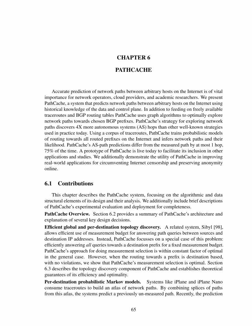
CHAPTER 6

PATHCACHE

Accurate prediction of network paths between arbitrary hosts on the Internet is of vitalimportance for network operators, cloud providers, and academic researchers. We presentPathCache, a system that predicts network paths between arbitrary hosts on the Internet usinghistorical knowledge of the data and control plane. In addition to feeding on freely availabletraceroutes and BGP routing tables PathCache uses graph algorithms to optimally explorenetwork paths towards chosen BGP prefixes. PathCache’s strategy for exploring networkpaths discovers 4X more autonomous systems (AS) hops than other well-known strategiesused in practice today. Using a corpus of traceroutes, PathCache trains probabilistic modelsof routing towards all routed prefixes on the Internet and infers network paths and theirlikelihood. PathCache’s AS-path predictions differ from the measured path by at most 1 hop,75% of the time. A prototype of PathCache is live today to facilitate its inclusion in otherapplications and studies. We additionally demonstrate the utility of PathCache in improvingreal-world applications for circumventing Internet censorship and preserving anonymityonline.

6.1 Contributions

This chapter describes the PathCache system, focusing on the algorithmic and datastructural elements of its design and their analysis. We additionally include brief descriptionsof PathCache’s experimental evaluation and deployment for completeness.PathCache Overview. Section 6.2 provides a summary of PathCache’s architecture andexplanation of several key design decisions.Efficient global and per-destination topology discovery. A related system, Sibyl [98],allows efficient use of measurement budget for answering path queries between sources anddestination IP addresses. Instead, PathCache focusses on a special case of this problem:efficiently answering all queries towards a destination prefix for a fixed measurement budget.PathCache’s approach for doing measurement selection is within constant factor of optimalin the general case. However, when the routing towards a prefix is destination based,with no violations, we show that PathCache’s measurement selection is optimal. Section6.3 describes the topology discovery component of PathCache and establishes theoreticalguarantees of its efficiency and optimality.Per-destination probabilistic Markov models. Systems like iPlane and iPlane Nanoconsume traceroutes to build an atlas of network paths. By combining splices of pathsfrom this atlas, the systems predict a previously un-measured path. Recently, the prediction

65

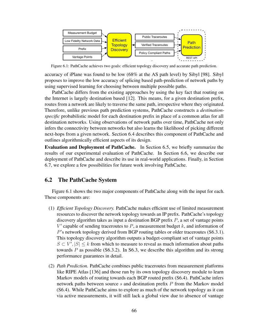
REST API

Path Prediction

Measurement Budget

Low Fidelity Network Data

Prefix

Vantage Points

Public Traceroutes

Verified Traceroutes

Policy Compliant Paths

Efficient Topology Discovery

Figure 6.1: PathCache achieves two goals: efficient topology discovery and accurate path prediction.

accuracy of iPlane was found to be low (68% at the AS path level) by Sibyl [98]. Sibylproposes to improve the low accuracy of splicing based path-prediction of network paths byusing supervised learning for choosing between multiple possible paths.

PathCache differs from the existing approaches by using the key fact that routing onthe Internet is largely destination based [12]. This means, for a given destination prefix,routes from a network are likely to traverse the same path, irrespective where they originated.Therefore, unlike previous path prediction systems, PathCache constructs a destination-specific probabilistic model for each destination prefix in place of a common atlas for alldestination networks. Using observations of network paths over time, PathCache not onlyinfers the connectivity between networks but also learns the likelihood of picking differentnext-hops from a given network. Section 6.4 describes this component of PathCache andoutlines algorithmically efficient aspects of its design.Evaluation and Deployment of PathCache. In Section 6.5, we briefly summarize theresults of our experimental evaluation of PathCache. In Section 6.6, we describe ourdeployment of PathCache and describe its use in real-world applications. Finally, in Section6.7, we explore a few possibilities for future work involving PathCache.

6.2 The PathCache System

Figure 6.1 shows the two major components of PathCache along with the input for each.These components are:

(1) Efficient Topology Discovery. PathCache makes efficient use of limited measurementresources to discover the network topology towards an IP prefix. PathCache’s topologydiscovery algorithm takes as input a destination BGP prefix P , a set of vantage pointsV ′ capable of sending traceroutes to P , a measurement budget k, and information ofP ’s network topology derived from BGP routing tables or older traceroutes (S6.3.1).This topology discovery algorithm outputs a budget-compliant set of vantage pointsS ⊂ V ′, |S| ≤ k from which to measure to reveal as much information about pathstowards P as possible (S6.3.2). In S6.3, we describe this algorithm and its strongperformance guarantees in detail.

(2) Path Prediction. PathCache combines public traceroutes from measurement platformslike RIPE Atlas [136] and those run by its own topology discovery module to learnMarkov models of routing towards each BGP routed prefix (S6.4). PathCache infersnetwork paths between source s and destination prefix P from the Markov model(S6.4). While PathCache aims to explore as much of the network topology as it canvia active measurements, it will still lack a global view due to absence of vantage

66

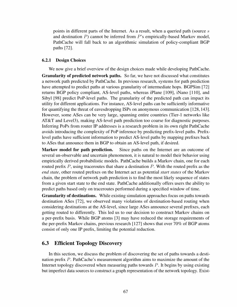
points in different parts of the Internet. As a result, when a queried path (source sand destination P ) cannot be inferred from P ’s empirically-based Markov model,PathCache will fall back to an algorithmic simulation of policy-compliant BGPpaths [72].

6.2.1 Design Choices

We now give a brief overview of the design choices made while developing PathCache.Granularity of predicted network paths. So far, we have not discussed what constitutesa network path predicted by PathCache. In previous research, systems for path predictionhave attempted to predict paths at various granularity of intermediate hops. BGPSim [72]returns BGP policy compliant, AS-level paths, whereas iPlane [109], iNano [110], andSibyl [98] predict PoP-level paths. The granularity of the predicted path can impact itsutility for different applications. For instance, AS-level paths can be sufficiently informativefor quantifying the threat of eavesdropping ISPs on anonymous communication [128, 143].However, some ASes can be very large, spanning entire countries (Tier-1 networks likeAT&T and Level3), making AS-level path prediction too coarse for diagnostic purposes.Inferring PoPs from router IP addresses is a research problem in its own right PathCacheavoids introducing the complexity of PoP inference by predicting prefix-level paths. Prefix-level paths have sufficient information to predict AS-level paths by mapping prefixes backto ASes that announce them in BGP to obtain an AS-level path, if desired.Markov model for path prediction. Since paths on the Internet are an outcome ofseveral un-observable and uncertain phenomenon, it is natural to model their behavior usingempirically derived probabilistic models. PathCache builds a Markov chain, one for eachrouted prefix P , using traceroutes that share a destination P . With the routed prefix as theend state, other routed prefixes on the Internet act as potential start states of the Markovchain, the problem of network path prediction is to find the most likely sequence of statesfrom a given start state to the end state. PathCache additionally offers users the ability topredict paths based only on traceroutes performed during a specified window of time.Granularity of destinations. While existing simulation approaches focus on paths towardsdestination ASes [72], we observed many violations of destination-based routing whenconsidering destinations at the AS-level, since large ASes announce several prefixes, eachgetting routed to differently. This led us to our decision to construct Markov chains ona per-prefix basis. While BGP atoms [3] may have reduced the storage requirements ofthe per-prefix Markov chains, previous research [127] shows that over 70% of BGP atomsconsist of only one IP prefix, limiting the potential reduction.

6.3 Efficient Topology Discovery

In this section, we discuss the problem of discovering the set of paths towards a desti-nation prefix P . PathCache’s measurement algorithm aims to maximize the amount of theInternet topology discovered when measuring paths towards P . It begins by using existingbut imperfect data sources to construct a graph representation of the network topology. Exist-

67

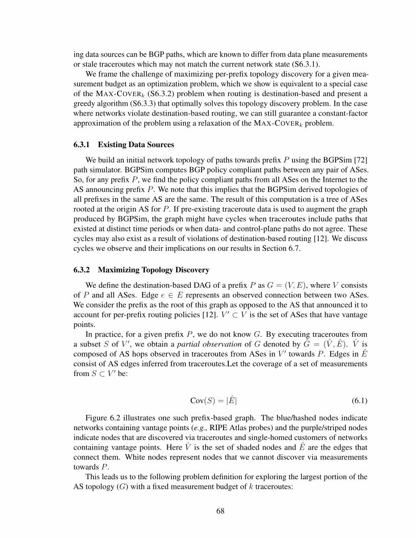
ing data sources can be BGP paths, which are known to differ from data plane measurementsor stale traceroutes which may not match the current network state (S6.3.1).

We frame the challenge of maximizing per-prefix topology discovery for a given mea-surement budget as an optimization problem, which we show is equivalent to a special caseof the MAX-COVERk (S6.3.2) problem when routing is destination-based and present agreedy algorithm (S6.3.3) that optimally solves this topology discovery problem. In the casewhere networks violate destination-based routing, we can still guarantee a constant-factorapproximation of the problem using a relaxation of the MAX-COVERk problem.

6.3.1 Existing Data Sources

We build an initial network topology of paths towards prefix P using the BGPSim [72]path simulator. BGPSim computes BGP policy compliant paths between any pair of ASes.So, for any prefix P , we find the policy compliant paths from all ASes on the Internet to theAS announcing prefix P . We note that this implies that the BGPSim derived topologies ofall prefixes in the same AS are the same. The result of this computation is a tree of ASesrooted at the origin AS for P . If pre-existing traceroute data is used to augment the graphproduced by BGPSim, the graph might have cycles when traceroutes include paths thatexisted at distinct time periods or when data- and control-plane paths do not agree. Thesecycles may also exist as a result of violations of destination-based routing [12]. We discusscycles we observe and their implications on our results in Section 6.7.

6.3.2 Maximizing Topology Discovery

We define the destination-based DAG of a prefix P as G = (V,E), where V consistsof P and all ASes. Edge e ∈ E represents an observed connection between two ASes.We consider the prefix as the root of this graph as opposed to the AS that announced it toaccount for per-prefix routing policies [12]. V ′ ⊂ V is the set of ASes that have vantagepoints.

In practice, for a given prefix P , we do not know G. By executing traceroutes froma subset S of V ′, we obtain a partial observation of G denoted by G = (V , E). V iscomposed of AS hops observed in traceroutes from ASes in V ′ towards P . Edges in Econsist of AS edges inferred from traceroutes.Let the coverage of a set of measurementsfrom S ⊂ V ′ be:

Cov(S) = |E| (6.1)

Figure 6.2 illustrates one such prefix-based graph. The blue/hashed nodes indicatenetworks containing vantage points (e.g., RIPE Atlas probes) and the purple/striped nodesindicate nodes that are discovered via traceroutes and single-homed customers of networkscontaining vantage points. Here V is the set of shaded nodes and E are the edges thatconnect them. White nodes represent nodes that we cannot discover via measurementstowards P .

This leads us to the following problem definition for exploring the largest portion of theAS topology (G) with a fixed measurement budget of k traceroutes:

68

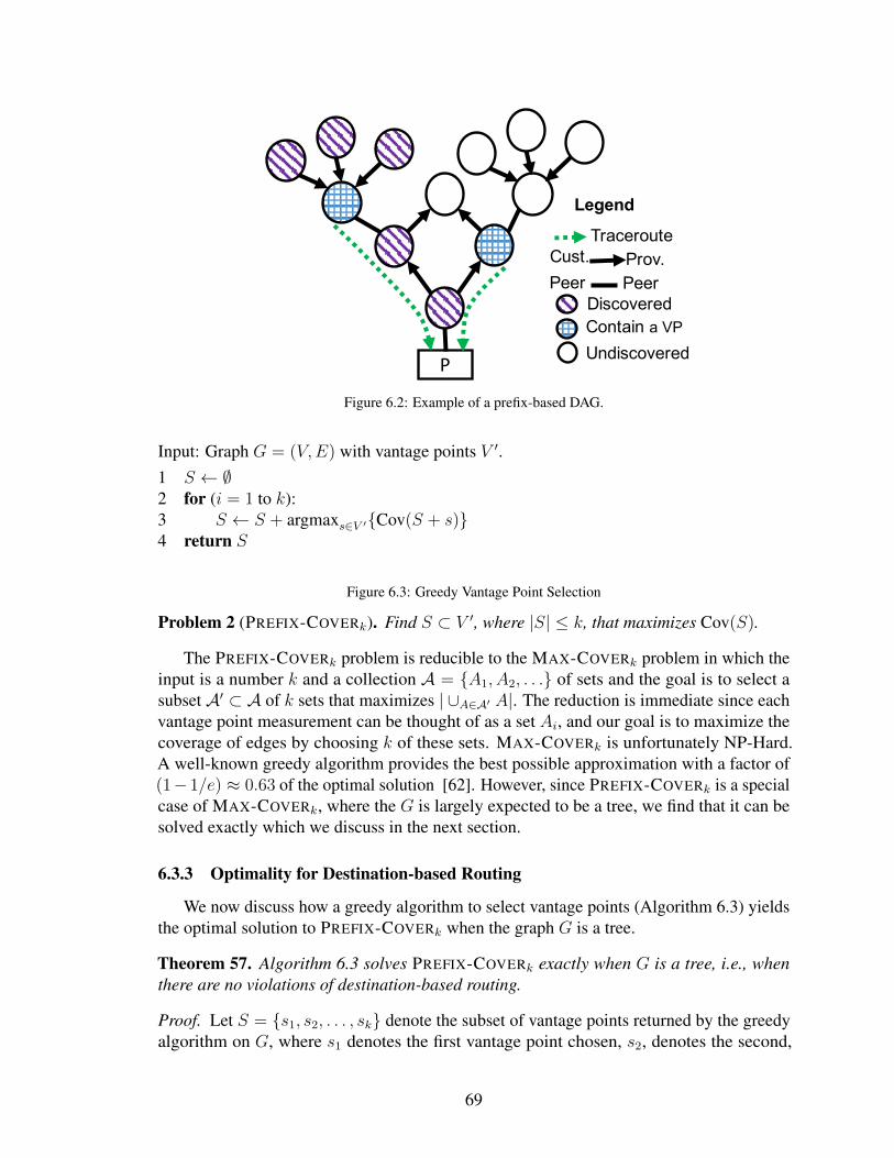
P

Cust. Prov.Peer Peer

Legend

DiscoveredContain a VP

Undiscovered

Traceroute

Figure 6.2: Example of a prefix-based DAG.

Input: Graph G = (V,E) with vantage points V ′.1 S ← ∅2 for (i = 1 to k):3 S ← S + argmaxs∈V ′Cov(S + s)4 return S

Figure 6.3: Greedy Vantage Point Selection

Problem 2 (PREFIX-COVERk). Find S ⊂ V ′, where |S| ≤ k, that maximizes Cov(S).

The PREFIX-COVERk problem is reducible to the MAX-COVERk problem in which theinput is a number k and a collection A = A1, A2, . . . of sets and the goal is to select asubset A′ ⊂ A of k sets that maximizes | ∪A∈A′ A|. The reduction is immediate since eachvantage point measurement can be thought of as a set Ai, and our goal is to maximize thecoverage of edges by choosing k of these sets. MAX-COVERk is unfortunately NP-Hard.A well-known greedy algorithm provides the best possible approximation with a factor of(1− 1/e) ≈ 0.63 of the optimal solution [62]. However, since PREFIX-COVERk is a specialcase of MAX-COVERk, where the G is largely expected to be a tree, we find that it can besolved exactly which we discuss in the next section.

6.3.3 Optimality for Destination-based Routing

We now discuss how a greedy algorithm to select vantage points (Algorithm 6.3) yieldsthe optimal solution to PREFIX-COVERk when the graph G is a tree.

Theorem 57. Algorithm 6.3 solves PREFIX-COVERk exactly when G is a tree, i.e., whenthere are no violations of destination-based routing.

Proof. Let S = s1, s2, . . . , sk denote the subset of vantage points returned by the greedyalgorithm on G, where s1 denotes the first vantage point chosen, s2, denotes the second,

69

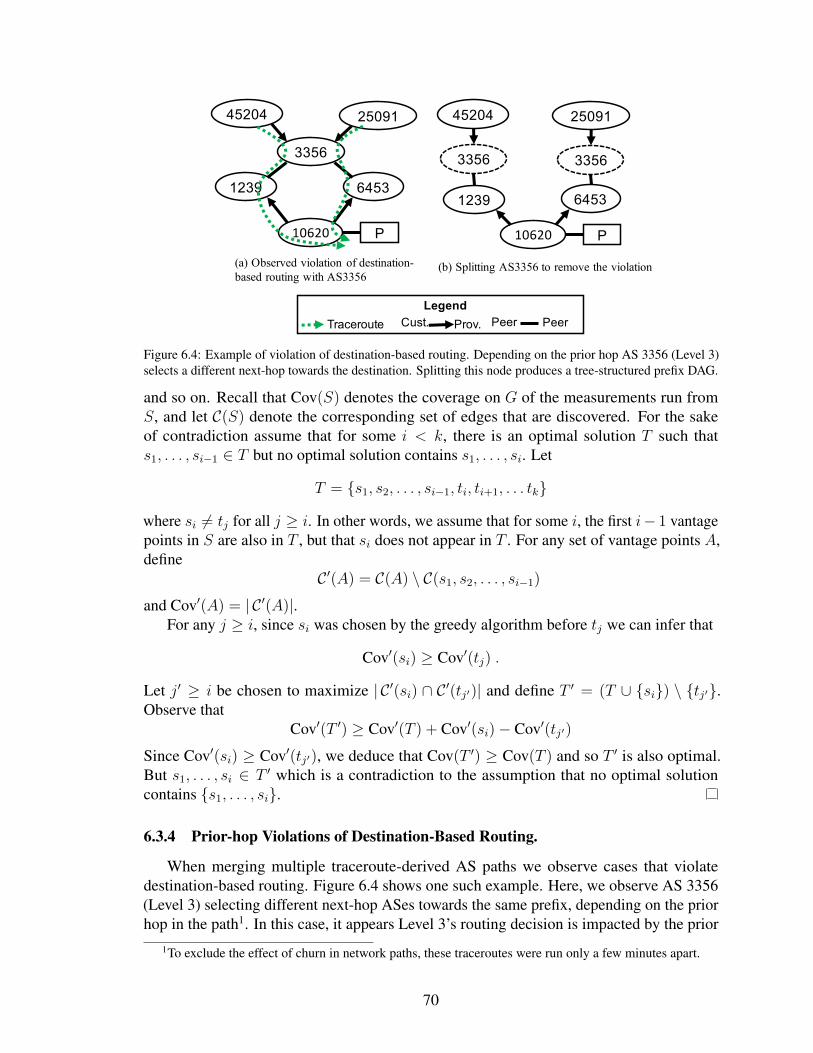
10620

6453

3356

P

1239

45204 25091

Cust. Prov. Peer PeerLegend

Traceroute

10620

6453

3356

P

1239

45204 25091

3356

(a) Observed violation of destination-based routing with AS3356

(b) Splitting AS3356 to remove the violation

Figure 6.4: Example of violation of destination-based routing. Depending on the prior hop AS 3356 (Level 3)selects a different next-hop towards the destination. Splitting this node produces a tree-structured prefix DAG.

and so on. Recall that Cov(S) denotes the coverage on G of the measurements run fromS, and let C(S) denote the corresponding set of edges that are discovered. For the sakeof contradiction assume that for some i < k, there is an optimal solution T such thats1, . . . , si−1 ∈ T but no optimal solution contains s1, . . . , si. Let

T = s1, s2, . . . , si−1, ti, ti+1, . . . tk

where si 6= tj for all j ≥ i. In other words, we assume that for some i, the first i− 1 vantagepoints in S are also in T , but that si does not appear in T . For any set of vantage points A,define

C ′(A) = C(A) \ C(s1, s2, . . . , si−1)

and Cov′(A) = | C ′(A)|.For any j ≥ i, since si was chosen by the greedy algorithm before tj we can infer that

Cov′(si) ≥ Cov′(tj) .

Let j′ ≥ i be chosen to maximize | C ′(si) ∩ C ′(tj′)| and define T ′ = (T ∪ si) \ tj′.Observe that

Cov′(T ′) ≥ Cov′(T ) + Cov′(si)− Cov′(tj′)

Since Cov′(si) ≥ Cov′(tj′), we deduce that Cov(T ′) ≥ Cov(T ) and so T ′ is also optimal.But s1, . . . , si ∈ T ′ which is a contradiction to the assumption that no optimal solutioncontains s1, . . . , si.

6.3.4 Prior-hop Violations of Destination-Based Routing.

When merging multiple traceroute-derived AS paths we observe cases that violatedestination-based routing. Figure 6.4 shows one such example. Here, we observe AS 3356(Level 3) selecting different next-hop ASes towards the same prefix, depending on the priorhop in the path1. In this case, it appears Level 3’s routing decision is impacted by the prior

1To exclude the effect of churn in network paths, these traceroutes were run only a few minutes apart.

70

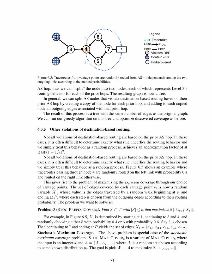
P

Cust. Prov.

Peer Peer

Legend

Violates DBR

Contain a VP

Undiscovered

Traceroute

.4

.6

1

2

3 4

5

6

7

Figure 6.5: Traceroutes from vantage points are randomly routed from AS 4 independently among the twooutgoing links according to the marked probabilities.

AS hop, thus we can “split” the node into two nodes, each of which represents Level 3’srouting behavior for each of the prior hops. The resulting graph is now a tree.

In general, we can split AS nodes that violate destination-based routing based on theirprior AS hop by creating a copy of the node for each prior hop, and adding to each copiednode all outgoing edges associated with that prior hop.

The result of this process is a tree with the same number of edges as the original graph.We can run our greedy algorithm on this tree and optimize discovered coverage as before.

6.3.5 Other violations of destination-based routing.

Not all violations of destination-based routing are based on the prior AS hop. In thesecases, it is often difficult to determine exactly what rule underlies the routing behavior andwe simply treat this behavior as a random process. achieves an approximation factor of atleast (1− 1/e)2.

Not all violations of destination-based routing are based on the prior AS hop. In thesecases, it is often difficult to determine exactly what rule underlies the routing behavior andwe simply treat this behavior as a random process. Figure 6.5 shows an example wheretraceroutes passing through node 4 are randomly routed on the left link with probability 0.4and routed on the right link otherwise.

This gives rise to the problem of maximizing the expected coverage through our choiceof vantage points. The set of edges covered by each vantage point vi is now a randomvariable Xvi whose value is the edges traversed by a random walk beginning at vi andending at P , where each step is chosen from the outgoing edges according to their routingprobability. The problem we want to solve is:

Problem 3 (STOC-PREFIX-COVERk). Find S ⊂ V ′ with |S| ≤ k, that maximizes E [| ∪v∈S Xv|].

For example, in Figure 6.5, X1 is determined by starting at 1, continuing to 3 and 4, andrandomly choosing either 5 with probability 0.4 or 6 with probability 0.6. Say 5 is chosen.Then continuing to 7 and ending at P yields the set of edges X1 = e1,3, e3,4, e4,5, e5,7, e7,P.Stochastic Maximum Coverage. The above problem is special case of the stochasticmaximum coverage problem. STOC-MAX-COVERk is a variant of MAX-COVERk wherethe input is an integer k and A = A1, A2, . . . where Ai is a random set chosen accordingto some known distribution pi. The goal is pick A′ ⊂ A to maximize E [| ∪A∈A′ A|].

71

It can be shown that a natural extension of the greedy algorithm that, at each step, picksthe set with the largest expected increase in the coverage, achieves a 1− 1/e approximation[13]. However, note that using this algorithm in our context requires us to be adaptive,i.e., we select a vantage point, perform a measurement from that vantage point, and see theresult of this measurement before selecting the next vantage point. This is in contrast toa non-adaptive algorithm that must choose the full set of k vantage points before runningany measurements. There is a tradeoff between these two approaches: on the one hand,an adaptive approach may provide a solution of strictly better quality than a nonadaptivealgorithm since it has strictly more information.

On the other hand, the adaptive algorithm is slower since after the adaptive algorithmchooses each measurement, it must wait for the traceroute to finish before computingthe next measurement. This serial computation and measurement requirement preventsparallelization. Contrast this with the nonadaptive algorithm, which can immediatelygenerate a complete schedule of measurements without actually performing any traceroutes.This schedule can be used to perform the actual traceroutes at any time/in parallel. Thisflexibility makes the nonadaptive algorithm desirable in some cases despite its strictly worsesolution quality. For these reasons, we implement both versions and evaluate their solutionquality theoretically and experimentally. As mentioned above, the adaptive greedy algorithmis guaranteed to achieve an approximation factor of at least 1−1/e. The non-adaptive greedyalgorithm is guaranteed an approximation factor of at least (1− 1/e)2; this follows fromwork by Asadpour and Nazerzadeh [13] on the more general STOC-MAX-COVERk problem.

6.3.6 A Note on Graph Coverage

The observant reader will note that the algorithmic focus here on graph coverage isrelated to the streaming coverage problems investigated in Chapter 3. However, the contextsin which graph problems are addressed in these two chapters are very different. PathCachehas costly query access to the graph it is attempting to cover, while in Chapter 3 the inputgraph is only accessible as a stream. As a result, there is little technical overlap between thetwo problems.

6.4 Path Prediction

In this section, we outline how PathCache uses empirical data to predict paths. Sec-tion 6.4.1 explains how PathCache builds destination specific graphs and auxiliary tables tocapture the routing behavior towards a prefix. Section 6.4.2 details how PathCache uses thisinformation to define Markov chains for predicting paths between source and destinationhosts on the Internet. Section 6.4.3 explains how simulations are used to fill in gaps in theMarkov chains derived from traceroutes, enabling PathCache to predict paths for all queriesto a measured prefix.

6.4.1 Constructing per-prefix DAGs

We gather a set of traceroutes publicly available on measurement platforms and thoserun in the topology discovery stage of PathCache. We aggregate traceroute hops into BGP

72

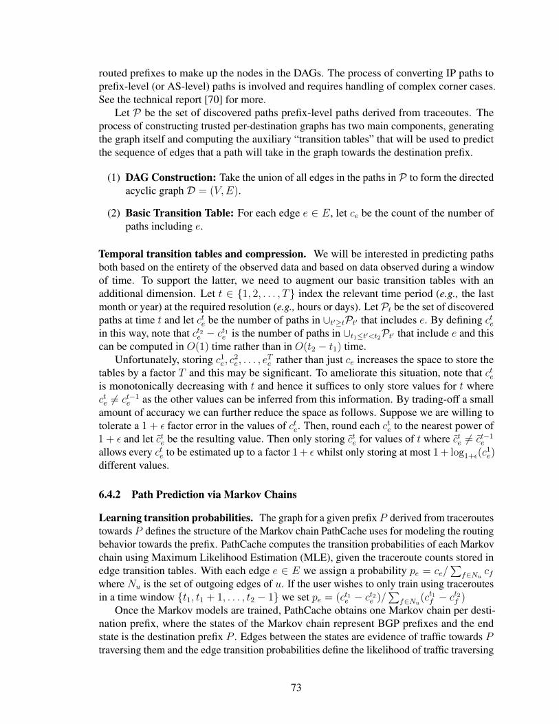
routed prefixes to make up the nodes in the DAGs. The process of converting IP paths toprefix-level (or AS-level) paths is involved and requires handling of complex corner cases.See the technical report [70] for more.

Let P be the set of discovered paths prefix-level paths derived from traceoutes. Theprocess of constructing trusted per-destination graphs has two main components, generatingthe graph itself and computing the auxiliary “transition tables” that will be used to predictthe sequence of edges that a path will take in the graph towards the destination prefix.

(1) DAG Construction: Take the union of all edges in the paths in P to form the directedacyclic graph D = (V,E).

(2) Basic Transition Table: For each edge e ∈ E, let ce be the count of the number ofpaths including e.

Temporal transition tables and compression. We will be interested in predicting pathsboth based on the entirety of the observed data and based on data observed during a windowof time. To support the latter, we need to augment our basic transition tables with anadditional dimension. Let t ∈ 1, 2, . . . , T index the relevant time period (e.g., the lastmonth or year) at the required resolution (e.g., hours or days). Let Pt be the set of discoveredpaths at time t and let cte be the number of paths in ∪t′≥tPt′ that includes e. By defining ctein this way, note that ct2e − ct1e is the number of paths in ∪t1≤t′<t2Pt′ that include e and thiscan be computed in O(1) time rather than in O(t2 − t1) time.

Unfortunately, storing c1e, c

2e, . . . , e

Te rather than just ce increases the space to store the

tables by a factor T and this may be significant. To ameliorate this situation, note that cteis monotonically decreasing with t and hence it suffices to only store values for t wherecte 6= ct−1

e as the other values can be inferred from this information. By trading-off a smallamount of accuracy we can further reduce the space as follows. Suppose we are willing totolerate a 1 + ε factor error in the values of cte. Then, round each cte to the nearest power of1 + ε and let cte be the resulting value. Then only storing cte for values of t where cte 6= ct−1

e

allows every cte to be estimated up to a factor 1 + ε whilst only storing at most 1 + log1+ε(c1e)

different values.

6.4.2 Path Prediction via Markov Chains

Learning transition probabilities. The graph for a given prefix P derived from traceroutestowards P defines the structure of the Markov chain PathCache uses for modeling the routingbehavior towards the prefix. PathCache computes the transition probabilities of each Markovchain using Maximum Likelihood Estimation (MLE), given the traceroute counts stored inedge transition tables. With each edge e ∈ E we assign a probability pe = ce/

∑f∈Nu cf

where Nu is the set of outgoing edges of u. If the user wishes to only train using traceroutesin a time window t1, t1 + 1, . . . , t2 − 1 we set pe = (ct1e − ct2e )/

∑f∈Nu(ct1f − c

t2f )

Once the Markov models are trained, PathCache obtains one Markov chain per desti-nation prefix, where the states of the Markov chain represent BGP prefixes and the endstate is the destination prefix P . Edges between the states are evidence of traffic towards Ptraversing them and the edge transition probabilities define the likelihood of traffic traversing

73

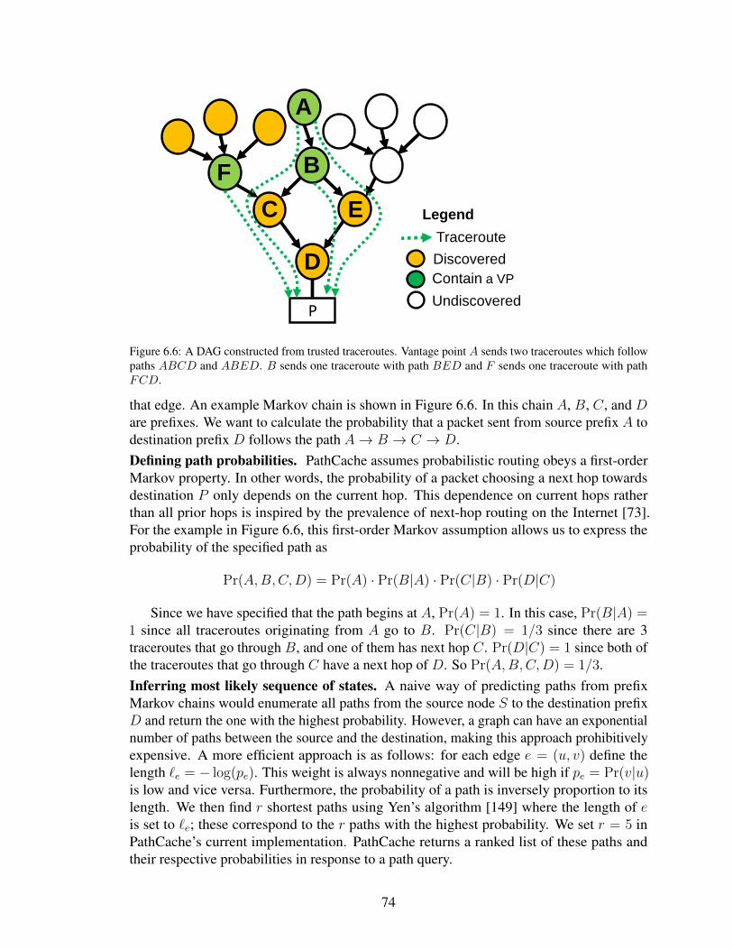
P

Legend

Discovered

Contain a VP

Undiscovered

Traceroute

A

B

C

D

E

F

Figure 6.6: A DAG constructed from trusted traceroutes. Vantage point A sends two traceroutes which followpaths ABCD and ABED. B sends one traceroute with path BED and F sends one traceroute with pathFCD.

that edge. An example Markov chain is shown in Figure 6.6. In this chain A, B, C, and Dare prefixes. We want to calculate the probability that a packet sent from source prefix A todestination prefix D follows the path A→ B → C → D.Defining path probabilities. PathCache assumes probabilistic routing obeys a first-orderMarkov property. In other words, the probability of a packet choosing a next hop towardsdestination P only depends on the current hop. This dependence on current hops ratherthan all prior hops is inspired by the prevalence of next-hop routing on the Internet [73].For the example in Figure 6.6, this first-order Markov assumption allows us to express theprobability of the specified path as

Pr(A,B,C,D) = Pr(A) · Pr(B|A) · Pr(C|B) · Pr(D|C)

Since we have specified that the path begins at A, Pr(A) = 1. In this case, Pr(B|A) =1 since all traceroutes originating from A go to B. Pr(C|B) = 1/3 since there are 3traceroutes that go through B, and one of them has next hop C. Pr(D|C) = 1 since both ofthe traceroutes that go through C have a next hop of D. So Pr(A,B,C,D) = 1/3.Inferring most likely sequence of states. A naive way of predicting paths from prefixMarkov chains would enumerate all paths from the source node S to the destination prefixD and return the one with the highest probability. However, a graph can have an exponentialnumber of paths between the source and the destination, making this approach prohibitivelyexpensive. A more efficient approach is as follows: for each edge e = (u, v) define thelength `e = − log(pe). This weight is always nonnegative and will be high if pe = Pr(v|u)is low and vice versa. Furthermore, the probability of a path is inversely proportion to itslength. We then find r shortest paths using Yen’s algorithm [149] where the length of eis set to `e; these correspond to the r paths with the highest probability. We set r = 5 inPathCache’s current implementation. PathCache returns a ranked list of these paths andtheir respective probabilities in response to a path query.

74

6.4.3 Splicing Empirical and Simulated Paths

If PathCache is faced with a query between a source AS and a destination prefix suchthat the source AS is not a state in the Markov chain of the destination prefix, it cannotpredict the path using the chain alone. In such situations we query BGPSim for a policycompliant path from the source AS to the destination prefix. We keep each hop of thispath, starting from the source ASN, until we reach an ASN that is present in the Markovchain for destination prefix. We predict the path between the ASN at the splice point andthe destination prefix using methods described in the previous subsection. In this manner,PathCache can still return probability-ranked paths for such a query by considering theBGPSim splice of the path as fixed (with transition probabilities of 1).

6.5 Summary of Evaluation

Here we briefly summarize the findings of PathCache’s experimental evaluation. See thetechnical report [70] for more.

• When compared to other strategies such as randomly choosing vantage points, orselecting vantage points from as many countries as possible, our measurement se-lection algorithm discovers 4 times the number of ASes using the same number ofmeasurements (k = 500). These results are robust across different types of destinationprefixes and across measurment platforms.

• To evaluate the accuracy of PathCache’s path prediction algorithm, we trained itsMarkov model on all RIPE Atlas traceroutes from December 25, 2018 until March4, 2019: approximately 4.5 billion traceroutes which allow us to learn the routingbehavior towards all ≈ 500, 000 routable prefixes on the Internet. We then hadPathCache predict paths from a source to a destination prefix, and compared thesepredicted paths with actual measured paths.

• 75% of PathCache’s predicted paths differ from the corresponding measured path byat most 1 hop.

• When PathCache returned the correct path as one of its predictions, 90% of the time itwas the path that PathCache assigned the highest probability to.

• By splicing empirical and simulated paths, PathCache is capable of responding to anypath query, in contrast to iPlane and Sybil which only are able to respond to 70% ofpath queries.

• PathCache outperforms iPlane and Sybil in terms of path accuracy based on 2 metrics:edit distance and Jaccard index. The gap in performance increases with the length ofthe true path.

• We discovered that PathCache’s per-destination directed graphs occasionally containcycles. We discuss the implications of this in Section 6.7.

75

6.6 Case Studies

We are releasing the entire codebase of PathCache2. More importantly, we have de-ployed PathCache in beta version at https://www.davidtench.com/deeplinks/pathcache. PathCache can be queried for paths, either on the website or via the RESTAPI3. The REST API can be incorporated programmatically into other systems.

In this section we demonstrate the impact of PathCache on real-world applications.PathCache for Refraction Networking (RN). Refraction networking [147] is a recenttechnique for Internet censorship circumvention that incorporates the circumvention infras-tructure into routers on the Internet. This technique has been considered more resilientto blocking by censors since it is hard to block individual routers on the Internet, whileblocking source and destination of packets is relatively easy.

A key problem faced by Refraction Routing deployments today [66] is to place refractionrouters in large ISPs such that client traffic gets intercepted by them. If client traffic followsa path without the refraction router on it, it leads to the failure of the refraction routingsession.

We worked with the largest ISP-scale deployment of refraction routing [66] to usePathCache for predicting if a client refraction routing session will be successful. To predicta successful refraction routing connection, we use PathCache to predict the path betweenthe client and refraction router. If the PathCache predicted path crosses specific prefixeswithin the deploying ISP, we conclude that the connection went via a refraction routerand was successful (except for other non-networking failures). We find that in the currentdeployment of clients, PathCache can predict the prefix hop inside the deploying ISP whichclient traffic took when a RN session was successful, 100% of the time. In future, we areworking towards incorporating the PathCache API into RN software for improved clientperformance.PathCache to defend against routing adversaries. Researchers have found that anony-mous communication via Tor [51] is susceptible to network-level adversaries launchingrouting attacks [145]. Several defenses against such attacks have been proposed that aimto avoid Tier-1 providers [18], use simulated BGP paths to avoid network-level adver-saries [143], etc. PathCache’s AS-level path prediction is highly accurate and readilyavailable as a REST API which can be incorporated into Tor client software for defendingagainst network-level adversaries.

6.7 Discussion and Future Work

In addition to their utility for path prediction, PathCache prefix graphs capture routingbehavior in a novel way. We believe they can be used to revisit several classical problems ininter-domain routing. For instance:BGP atoms. The networking research community has long studied the right granularityfor modeling routing behavior on the Internet. One proposal is to find a set of routers that

2Link/reference omitted to preserve anonymity while the associated conference paper is still in submission.3see the documentation on the website for details.

76

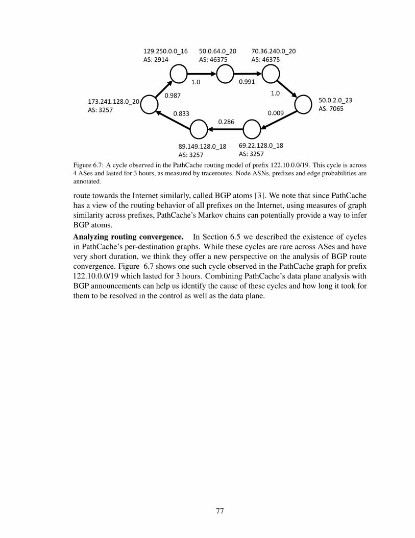
129.250.0.0_16AS: 2914

50.0.64.0_20AS: 46375

70.36.240.0_20AS: 46375

50.0.2.0_23AS: 7065

69.22.128.0_18AS: 3257

89.149.128.0_18AS: 3257

173.241.128.0_20AS: 3257

0.987

1.0 0.991

1.0

0.009

0.2860.833

Figure 6.7: A cycle observed in the PathCache routing model of prefix 122.10.0.0/19. This cycle is across4 ASes and lasted for 3 hours, as measured by traceroutes. Node ASNs, prefixes and edge probabilities areannotated.

route towards the Internet similarly, called BGP atoms [3]. We note that since PathCachehas a view of the routing behavior of all prefixes on the Internet, using measures of graphsimilarity across prefixes, PathCache’s Markov chains can potentially provide a way to inferBGP atoms.Analyzing routing convergence. In Section 6.5 we described the existence of cyclesin PathCache’s per-destination graphs. While these cycles are rare across ASes and havevery short duration, we think they offer a new perspective on the analysis of BGP routeconvergence. Figure 6.7 shows one such cycle observed in the PathCache graph for prefix122.10.0.0/19 which lasted for 3 hours. Combining PathCache’s data plane analysis withBGP announcements can help us identify the cause of these cycles and how long it took forthem to be resolved in the control as well as the data plane.

77

CHAPTER 7

CONCLUSION

We conclude by briefly summarizing the work presented in this thesis, and discussopportunities for future research in these areas.

Connectivity in Dynamic (Hyper-)Graph Streams. Prior to this work the main successstory in dynamic streaming graph connectivity had been in computing edge connectivity.Vertex connectivity exhibits markedly different combinatorial structure than edge connec-tivity and appeared to be more difficult in the dynamic grpah stream model. In Chapter 2,we presented the first linear sketches for estimating vertex connectivity and constructinghypergraph sparsifiers in dynamic graph streams, We also extended a graph reconstructionresult to a larger class of graphs.

Coverage in Data Streams. In Chapter 3, we presented a variety of efficient algorithmsfor computing Max-k-Cover and Max-k-UniqueCover in the data stream model. Theseproblems are closely related to a range of important graph problems including matching,partial vertex cover, and capacitated maximum cut. Our results improve upon the stateof the art for Max-k-Cover streaming algorithms, and are the first of their kind for theMax-k-UniqueCover problem.

Temporal Graph Streaming. In Chapter 4, we initiated the study of temporal graphalgorithms in the streaming setting. We provide sketching algorithms for some notionsof temporal connectivity, and prove a set of strong lower bounds for others. This work isthe first step in a more complete investigation of these rich combinatorial structures in thestreaming setting.

MESH. Chapter 5 introduced MESH, a memory allocator that efficiently performs com-paction without relocation to save memory for unmanaged languages. We show analyticallythat MESH provably avoids catastrophic memory fragmentation with high probability, andempirically show that MESH can substantially reduce memory fragmentation for memory-intensive applications written in C/C++ with low runtime overhead.

PathCache. Chapter 6 introduced PathCache, a system that predicts network paths be-tween arbitrary hosts on the Internet using historical knowledge of the control and dataplane. PathCache’s strategy for exploring network paths discovers 4 times more AS hopsthan the current state of the art methods. The PathCache system is capable of accurately

78

predicting destination-based Internet paths at scale. We investigated the utility of PathCachein improving real-world applications for circumventing Internet censorship and preservinganonymity online.

7.1 Future Work

Temporal graph streams have never before been studied and many fundamental algo-rithmic questions have yet to be answered. Does Conjecture 47 hold, implying that evenrelatively basic temporal reachability problems are difficult to compute in streams? If so, arethere other notions of reachability which are still useful but require less space to compute? Ifinstead these reachability problems are feasible, how might we compute more complicatedconnectivity problems, such as edge or vertex connectivity? What other important temporalgraph properties are computable in the streaming setting? Can we use sketching to createfingerprints of temporal graph streams, such that any two streams which define the sametemporal graph have the same fingerprint, and a different temporal graph has a differentfingerprint with high probability? Is it possible to determine in the streaming setting whetherT contains a journey that visits every node at least once? Can we sparsify a temporal graphwhile maintaining pairwise reachability? Can we perform this sparsification if distance (orjourney duration) must be approximately maintained?

In Chapter 6, we described the existence of cycles in PathCache’s per-destination graphs,a phenomenon which violates the common assumption of that Internet routing is destination-based. Are these apparent violations merely artifacts of vantage point measurement capa-bilities or are they evidence of poorly understood BGP routing dynamics? Answering thisquestion requires characterizing frequency, duration, length, and other properties of thesecycles which is an algorithmic challenge at Internet scale.

Memory systems are described by a hierarchy of transfer block size and latency. Theclassical assumption is that the blocks and latencies grow exponentially as one moves downthe memory hierarchy. Cache is larger and slower than register, RAM is larger and slowerthan cache, and disk is larger and slower than RAM. This size and accessibility gradientmotivates both external memory data structures and streaming algorithms. Recently, thehierarchy has been flattening. For instance, random I/O bandwidth in RAM is roughlycomparable to sequential I/O bandwidth to new NVMe devices [43]. This new storagelandscape has not yet been investigated thoroughly, but early work [132] suggests thattechniques from the data stream model will prove useful in designing data structures that areoptimized for the tradeoffs of modern external memory. The existence of this new externalmemory hardware motivates new models for the streaming domain as well. Which streamingproblems become easier if, for example, the algorithm is allowed a small amount of randomaccess to the input in addition to the stream? What if it has access to its own sequentiallyaccessible writeable memory, which is asymptotically larger than its random access memorybut still asymptotically smaller than the size of the stream?

79

BIBLIOGRAPHY

[1] Ablayev, Farid M. Lower bounds for one-way probabilistic communication com-plexity and their application to space complexity. Theor. Comput. Sci. 157, 2 (1996),139–159.

[2] Adger, Mads. [Blink-dev] Oilpan - experimenting with a garbage collected heap forthe DOM, 2013. http://bit.ly/2pwDhwk.

[3] Afek, Yehuda, Ben-Shalom, Omer, and Bremler-Barr, Anat. On the structure and ap-plication of bgp policy atoms. In Proceedings of the 2Nd ACM SIGCOMM Workshopon Internet Measurment (New York, NY, USA, 2002), IMW ’02, ACM, pp. 209–214.

[4] Ageev, Alexander A., and Sviridenko, Maxim. Pipage rounding: A new method ofconstructing algorithms with proven performance guarantee. J. Comb. Optim. 8, 3(2004), 307–328.

[5] Ahn, Kook Jin, and Guha, Sudipto. Linear programming in the semi-streaming modelwith application to the maximum matching problem. Inf. Comput. 222 (2013), 59–79.

[6] Ahn, Kook Jin, Guha, Sudipto, and McGregor, Andrew. Analyzing graph structurevia linear measurements. In Twenty-Third Annual ACM-SIAM Symposium on DiscreteAlgorithms, SODA 2012 (2012), pp. 459–467.

[7] Ahn, Kook Jin, Guha, Sudipto, and McGregor, Andrew. Graph sketches: sparsifica-tion, spanners, and subgraphs. In 31st ACM SIGMOD-SIGACT-SIGART Symposiumon Principles of Database Systems (2012), pp. 5–14.

[8] Ahn, Kook Jin, Guha, Sudipto, and McGregor, Andrew. Spectral sparsification indynamic graph streams. In APPROX (2013), pp. 1–10.

[9] Alaluf, Naor, Ene, Alina, Feldman, Moran, Nguyen, Huy L., and Suh, Andrew.Optimal streaming algorithms for submodular maximization with cardinality con-straints. In ICALP (2020), vol. 168 of LIPIcs, Schloss Dagstuhl - Leibniz-Zentrumfur Informatik, pp. 6:1–6:19.

[10] Alweiss, Ryan, Lovett, Shachar, Wu, Kewen, and Zhang, Jiapeng. Improved boundsfor the sunflower lemma. In Proceedings of the 52nd Annual ACM SIGACT Sym-posium on Theory of Computing, STOC 2020, Chicago, IL, USA, June 22-26, 2020(2020), pp. 624–630.

80

[11] Anagnostopoulos, Aris, Becchetti, Luca, Bordino, Ilaria, Leonardi, Stefano, Mele,Ida, and Sankowski, Piotr. Stochastic query covering for fast approximate documentretrieval. ACM Trans. Inf. Syst. 33, 3 (2015), 11:1–11:35.

[12] Anwar, R., Niaz, H., Choffnes, D., Cunha, I., Gill, P., and Katz-Bassett, E. Investigat-ing interdomain routing policies in the wild. In ACM IMC (2015).

[13] Asadpour, Arash, and Nazerzadeh, Hamid. Maximizing stochastic monotone sub-modular functions. Management Science 62, 8 (2016), 2374–2391.

[14] Assadi, Sepehr. Tight space-approximation tradeoff for the multi-pass streaming setcover problem. In PODS (2017), ACM, pp. 321–335.

[15] Assadi, Sepehr, Khanna, Sanjeev, and Li, Yang. Tight bounds for single-pass stream-ing complexity of the set cover problem. In STOC (2016), ACM, pp. 698–711.

[16] Badanidiyuru, Ashwinkumar, Mirzasoleiman, Baharan, Karbasi, Amin, and Krause,Andreas. Streaming submodular maximization: massive data summarization on thefly. In KDD (2014), ACM, pp. 671–680.

[17] Bar-Yossef, Ziv, Jayram, T. S., Kumar, Ravi, Sivakumar, D., and Trevisan, Luca.Counting distinct elements in a data stream. In RANDOM (2002), vol. 2483 ofLecture Notes in Computer Science, Springer, pp. 1–10.

[18] Barton, Armon, and Wright, Matthew. Denasa: Destination-naive as-awareness inanonymous communications. Proceedings on Privacy Enhancing Technologies 2016,4 (2016), 356–372.

[19] Becker, Florent, Matamala, Martın, Nisse, Nicolas, Rapaport, Ivan, Suchan, Karol,and Todinca, Ioan. Adding a referee to an interconnection network: What can(not)be computed in one round. In 25th IEEE International Symposium on Parallel andDistributed Processing, IPDPS 2011 (2011), pp. 508–514.

[20] Benczur, Andras A., and Karger, David R. Approximating s-t minimum cuts in O(n2)time. In STOC (1996), pp. 47–55.

[21] Berger, Emery D., McKinley, Kathryn S., Blumofe, Robert D., and Wilson, Paul R.Hoard: a scalable memory allocator for multithreaded applications. In ASPLOS-IX: Proceedings of the ninth international conference on Architectural support forprogramming languages and operating systems (New York, NY, USA, 2000), ACMPress, pp. 117–128.

[22] Berger, Emery D., and Zorn, Benjamin G. DieHard: Probabilistic memory safetyfor unsafe languages. In Proceedings of the 2006 ACM SIGPLAN Conference onProgramming Language Design and Implementation (PLDI 2006) (New York, NY,USA, 2006), ACM Press, pp. 158–168.

[23] Berman, Kenneth A. Vulnerability of scheduled networks and a generalization ofmenger’s theorem. Networks 28, 3 (1996), 125–134.

81

[24] Bhadra, Sandeep, and Ferreira, Afonso. Complexity of connected components inevolving graphs and the computation of multicast trees in dynamic networks. vol. 3,pp. 259–270.

[25] Bonnet, Edouard, Paschos, Vangelis Th., and Sikora, Florian. Parameterized exactand approximation algorithms for maximum k-set cover and related satisfiabilityproblems. RAIRO Theor. Informatics Appl. 50, 3 (2016), 227–240.

[26] Braverman, Vladimir, Ostrovsky, Rafail, and Vilenchik, Dan. How hard is countingtriangles in the streaming model? In ICALP (1) (2013), vol. 7965 of Lecture Notes inComputer Science, Springer, pp. 244–254.

[27] Bury, Marc, and Schwiegelshohn, Chris. Sublinear estimation of weighted matchingsin dynamic data streams. In Algorithms - ESA 2015 - 23rd Annual European Sympo-sium, Patras, Greece, September 14-16, 2015, Proceedings (2015), pp. 263–274.

[28] Catalyurek, Umit V., and Aykanat, Cevdet. Hypergraph-partitioning-based decompo-sition for parallel sparse-matrix vector multiplication. IEEE Trans. Parallel Distrib.Syst. 10, 7 (1999), 673–693.

[29] Catalyurek, Umit V., Boman, Erik G., Devine, Karen D., Bozdag, Doruk, Heaphy,Robert T., and Riesen, Lee Ann. A repartitioning hypergraph model for dynamic loadbalancing. J. Parallel Distrib. Comput. 69, 8 (2009), 711–724.

[30] Censor-Hillel, Keren, Ghaffari, Mohsen, Giakkoupis, George, Haeupler, Bernhard,and Kuhn, Fabian. Tight bounds on vertex connectivity under vertex sampling. InACM-SIAM Symposium on Discrete Algorithms, SODA 2015 (2015).

[31] Censor-Hillel, Keren, Ghaffari, Mohsen, and Kuhn, Fabian. A new perspective onvertex connectivity. In Twenty-Fifth Annual ACM-SIAM Symposium on DiscreteAlgorithms, SODA 2014, Portland, Oregon, USA, January 5-7, 2014 (2014), pp. 546–561.

[32] Chakrabarti, Amit, and Kale, Sagar. Submodular maximization meets streaming:matchings, matroids, and more. Math. Program. 154, 1-2 (2015), 225–247.

[33] Chakrabarti, Amit, Khot, Subhash, and Sun, Xiaodong. Near-optimal lower boundson the multi-party communication complexity of set disjointness. In IEEE Conferenceon Computational Complexity (2003), IEEE Computer Society, pp. 107–117.

[34] Chakrabarti, Amit, and Wirth, Anthony. Incidence geometries and the pass complexityof semi-streaming set cover. In SODA (2016), SIAM, pp. 1365–1373.

[35] Chekuri, Chandra, Gupta, Shalmoli, and Quanrud, Kent. Streaming algorithms forsubmodular function maximization. In ICALP (1) (2015), vol. 9134 of Lecture Notesin Computer Science, Springer, pp. 318–330.

82

[36] Cheriyan, J., Kao, M. Y., and Thurimella, R. Scan-first search and sparse certificates:an improved parallel algorithm for k-vertex connectivity. SIAM Journal on Computing22, 1 (1993), 157–174.

[37] Chitnis, Rajesh, and Cormode, Graham. Towards a theory of parameterized streamingalgorithms. In 14th International Symposium on Parameterized and Exact Computa-tion, IPEC 2019, September 11-13, 2019, Munich, Germany (2019), pp. 7:1–7:15.

[38] Chitnis, Rajesh, Cormode, Graham, Esfandiari, Hossein, Hajiaghayi, Mohammad-Taghi, McGregor, Andrew, Monemizadeh, Morteza, and Vorotnikova, Sofya. Kernel-ization via sampling with applications to finding matchings and related problems indynamic graph streams. In SODA (2016), SIAM, pp. 1326–1344.

[39] Chitnis, Rajesh Hemant, Cormode, Graham, Esfandiari, Hossein, Hajiaghayi, Mo-hammadTaghi, and Monemizadeh, Morteza. Brief announcement: New streamingalgorithms for parameterized maximal matching & beyond. In Proceedings of the27th ACM on Symposium on Parallelism in Algorithms and Architectures, SPAA 2015,Portland, OR, USA, June 13-15, 2015 (2015), pp. 56–58.

[40] Chitnis, Rajesh Hemant, Cormode, Graham, Hajiaghayi, Mohammad Taghi, andMonemizadeh, Morteza. Parameterized streaming: Maximal matching and vertexcover. In SODA (2015), SIAM, pp. 1234–1251.

[41] Cohen, Nachshon, and Petrank, Erez. Limitations of partial compaction: Towardspractical bounds. In Proceedings of the 34th ACM SIGPLAN Conference on Pro-gramming Language Design and Implementation (New York, NY, USA, 2013), PLDI’13, ACM, pp. 309–320.

[42] Cohen, Nachshon, and Petrank, Erez. Limitations of partial compaction: Towardspractical bounds. ACM Trans. Program. Lang. Syst. 39, 1 (Mar. 2017), 2:1–2:44.

[43] Conway, Alex, Gupta, Abhishek, Tai, Amy, Spillane, Richard, Chidabaram, Vijay,Farach-Colton, Martin, and Johnson, Rob. SplinterDB: Closing the bandwidth gapfor NVMe key-value stores. In USENIX ATC 2020 (2020).

[44] Coppeard, Jon. Compacting Garbage Collection in SpiderMonkey, 2015. https://mzl.la/2rntQlY.

[45] Cormode, Graham, Datar, Mayur, Indyk, Piotr, and Muthukrishnan, S. Comparingdata streams using hamming norms (how to zero in). IEEE Trans. Knowl. Data Eng.15, 3 (2003), 529–540.

[46] Cormode, Graham, and Muthukrishnan, S. An improved data stream summary: thecount-min sketch and its applications. J. Algorithms 55, 1 (2005), 58–75.

[47] Crouch, Michael, and Stubbs, Daniel S. Improved streaming algorithms for weightedmatching, via unweighted matching. In Approximation, Randomization, and Combina-torial Optimization. Algorithms and Techniques, APPROX/RANDOM 2014, Septem-ber 4-6, 2014, Barcelona, Spain (2014), pp. 96–104.

83

[48] Crouch, Michael S., McGregor, Andrew, and Stubbs, Daniel. Dynamic graphs in thesliding-window model. In Algorithms - ESA 2013 - 21st Annual European Symposium,Sophia Antipolis, France, September 2-4, 2013. Proceedings (2013), pp. 337–348.

[49] Demaine, Erik D., Feige, Uriel, Hajiaghayi, MohammadTaghi, and Salavatipour,Mohammad R. Combination can be hard: Approximability of the unique coverageproblem. SIAM J. Comput. 38, 4 (2008), 1464–1483.

[50] Detlefs, David. Garbage collection and run-time typing as a C++ library. In Proceed-ings of the 1992 USENIX C++ Conference (1992), USENIX Association, pp. 37–56.

[51] Dingledine, Roger, Mathewson, Nick, and Syverson, Paul. Tor: The second-generation onion router. Tech. rep., Naval Research Lab Washington DC, 2004.

[52] Dom, Michael, Guo, Jiong, Niedermeier, Rolf, and Wernicke, Sebastian. Mini-mum membership set covering and the consecutive ones property. In SWAT (2006),vol. 4059 of Lecture Notes in Computer Science, Springer, pp. 339–350.

[53] Edelson, Daniel R. Precompiling C++ for garbage collection. In Proceedings of theInternational Workshop on Memory Management (London, UK, UK, 1992), IWMM’92, Springer-Verlag, pp. 299–314.

[54] Emek, Yuval, and Rosen, Adi. Semi-streaming set cover - (extended abstract). InICALP (2014), pp. 453–464.

[55] Emek, Yuval, and Rosen, Adi. Semi-streaming set cover. ACM Trans. Algorithms 13,1 (2016), 6:1–6:22.

[56] Eppstein, David, Galil, Zvi, Italiano, Giuseppe F., and Nissenzweig, Amnon. Sparsifi-cation - a technique for speeding up dynamic graph algorithms. J. ACM 44, 5 (1997),669–696.

[57] Epstein, Leah, Levin, Asaf, Mestre, Julian, and Segev, Danny. Improved approx-imation guarantees for weighted matching in the semi-streaming model. SIAM J.Discrete Math. 25, 3 (2011), 1251–1265.

[58] Erlebach, Thomas, and van Leeuwen, Erik Jan. Approximating geometric coverageproblems. In Proceedings of the Nineteenth Annual ACM-SIAM Symposium onDiscrete Algorithms, SODA 2008, San Francisco, California, USA, January 20-22,2008 (2008), pp. 1267–1276.

[59] Evans, Jason. A scalable concurrent malloc (3) implementation for freebsd. In Proc.of the bsdcan conference, ottawa, canada (2006).

[60] Feige, U., Hajiyaghayi, M., and Lee, J. R. Improved approximation algorithms forminimum-weight vertex separators. Proc. of STOC (2005).

[61] Feige, Uriel. A threshold of ln n for approximating set cover. J. ACM 45, 4 (1998),634–652.

84

[62] Feige, Uriel. A threshold of ln n for approximating set cover. J. ACM 45, 4 (July1998), 634–652.

[63] Feigenbaum, Joan, Kannan, Sampath, McGregor, Andrew, Suri, Siddharth, andZhang, Jian. On graph problems in a semi-streaming model. Theor. Comput. Sci. 348,2 (2005), 207–216.

[64] Feldman, Moran, Norouzi-Fard, Ashkan, Svensson, Ola, and Zenklusen, Rico. Theone-way communication complexity of submodular maximization with applicationsto streaming and robustness. In STOC (2020), ACM, pp. 1363–1374.

[65] Fenichel, Robert R., and Yochelson, Jerome C. A lisp garbage-collector for virtual-memory computer systems. Commun. ACM 12, 11 (Nov. 1969), 611–612.

[66] Frolov, Sergey, Douglas, Fred, Scott, Will, McDonald, Allison, VanderSloot, Ben-jamin, Hynes, Rod, Kruger, Adam, Kallitsis, Michalis, Robinson, David G, Schultze,Steve, et al. An isp-scale deployment of tapdance. In 7th USENIXWorkshop onFree and Open Communications on the Internet (FOCI 17) (2017).

[67] Fung, Wai Shing, Hariharan, Ramesh, Harvey, Nicholas J. A., and Panigrahi, Deb-malya. A general framework for graph sparsification. In STOC (2011), pp. 71–80.

[68] Gaur, Daya Ram, Krishnamurti, Ramesh, and Kohli, Rajeev. Erratum to: Thecapacitated max k-cut problem. Math. Program. 126, 1 (2011), 191.

[69] Ghemawat, Sanjay, and Menage, Paul. TCMalloc: Thread-caching malloc, 2007.http://goog-perftools.sourceforge.net/doc/tcmalloc.html.

[70] Gill, Phillipa, McGregor, Andrew, Singh, Rachee, and Tench, David. Path-cache: A network path prediction toolkit. https://www.davidtench.com/deeplinks/pathcache_paper.

[71] Gill, Phillipa, Schapira, Michael, and Goldberg, Sharon. Let the market drive deploy-ment: A strategy for transitioning to bgp security. SIGCOMM Comput. Commun. Rev.41, 4 (Aug. 2011), 14–25.

[72] Gill, Phillipa, Schapira, Michael, and Goldberg, Sharon. Modeling on quicksand:Dealing with the scarcity of ground truth in interdomain routing data. ACM SIG-COMM Computer Communication Review 42, 1 (2012), 40–46.

[73] Gill, Phillipa, Schapira, Michael, and Goldberg, Sharon. A survey of interdomainrouting policies. In ACM Computer Communications Review (CCR). (Jan 2014).

[74] Goel, Ashish, Kapralov, Michael, and Khanna, Sanjeev. On the communicationand streaming complexity of maximum bipartite matching. In Proceedings of theTwenty-Third Annual ACM-SIAM Symposium on Discrete Algorithms, SODA 2012,Kyoto, Japan, January 17-19, 2012 (2012), pp. 468–485.

85

[75] Goel, Ashish, Kapralov, Michael, and Post, Ian. Single pass sparsification in thestreaming model with edge deletions. CoRR abs/1203.4900 (2012).

[76] Guruswami, Venkatesan, and Onak, Krzysztof. Superlinear lower bounds for mul-tipass graph processing. In Proceedings of the 28th Conference on ComputationalComplexity, CCC 2013, Palo Alto, California, USA, 5-7 June, 2013 (2013), pp. 287–298.

[77] Hansen, Wilfred J. Compact list representation: Definition, garbage collection, andsystem implementation. Commun. ACM 12, 9 (Sept. 1969), 499–507.

[78] Har-Peled, Sariel, Indyk, Piotr, Mahabadi, Sepideh, and Vakilian, Ali. Towards tightbounds for the streaming set cover problem. In PODS (2016), ACM, pp. 371–383.

[79] Hara, Kentaro. State of Blink’s Speed, Sept. 2017.https://docs.google.com/presentation/d/1Az-F3CamBq6hZ5QqQt-ynQEMWEhHY1VTvlRwL7b_6TU.

[80] Huang, Chien-Chung, Kakimura, Naonori, and Yoshida, Yuichi. Streaming algorithmsfor maximizing monotone submodular functions under a knapsack constraint. InAPPROX-RANDOM (2017), vol. 81 of LIPIcs, Schloss Dagstuhl - Leibniz-Zentrumfuer Informatik, pp. 11:1–11:14.

[81] Huang, Yuchi, Liu, Qingshan, and Metaxas, Dimitris N. Video object segmentation byhypergraph cut. In 2009 IEEE Computer Society Conference on Computer Vision andPattern Recognition (CVPR 2009), 20-25 June 2009, Miami, Florida, USA (2009),pp. 1738–1745.

[82] Indyk, Piotr, Mahabadi, Sepideh, Rubinfeld, Ronitt, Ullman, Jonathan, Vakilian,Ali, and Yodpinyanee, Anak. Fractional set cover in the streaming model. InAPPROX-RANDOM (2017), vol. 81 of LIPIcs, Schloss Dagstuhl - Leibniz-Zentrumfuer Informatik, pp. 12:1–12:20.

[83] Indyk, Piotr, and Vakilian, Ali. Tight trade-offs for the maximum k-coverage problemin the general streaming model. In Proceedings of the 38th ACM SIGMOD-SIGACT-SIGAI Symposium on Principles of Database Systems, PODS 2019, Amsterdam, TheNetherlands, June 30 - July 5, 2019 (2019), pp. 200–217.

[84] Ipek, Engin, Condit, Jeremy, Nightingale, Edmund B., Burger, Doug, and Moscibroda,Thomas. Dynamically replicated memory: Building reliable systems from nanoscaleresistive memories. SIGPLAN Not. 45, 3 (Mar. 2010), 3–14.

[85] Ito, Takehiro, Nakano, Shin-Ichi, Okamoto, Yoshio, Otachi, Yota, Uehara, Ryuhei,Uno, Takeaki, and Uno, Yushi. A 4.31-approximation for the geometric uniquecoverage problem on unit disks. Theor. Comput. Sci. 544 (2014), 14–31.

[86] Johnstone, Mark S., and Wilson, Paul R. The memory fragmentation problem:Solved? In Proceedings of the 1st International Symposium on Memory Management(New York, NY, USA, 1998), ISMM ’98, ACM, pp. 26–36.

86

[87] Jowhari, Hossein, Saglam, Mert, and Tardos, Gabor. Tight bounds for lp samplers,finding duplicates in streams, and related problems. In PODS (2011), pp. 49–58.

[88] Kallaugher, John, McGregor, Andrew, Price, Eric, and Vorotnikova, Sofya. Thecomplexity of counting cycles in the adjacency list streaming model. In Proceedingsof the 38th ACM SIGMOD-SIGACT-SIGAI Symposium on Principles of DatabaseSystems, PODS 2019, Amsterdam, The Netherlands, June 30 - July 5, 2019 (2019),pp. 119–133.

[89] Kapralov, Michael. Better bounds for matchings in the streaming model. In Proceed-ings of the Twenty-Fourth Annual ACM-SIAM Symposium on Discrete Algorithms,SODA 2013, New Orleans, Louisiana, USA, January 6-8, 2013 (2013), pp. 1679–1697.

[90] Kapralov, Michael, Khanna, Sanjeev, and Sudan, Madhu. Approximating matchingsize from random streams. In Proceedings of the Twenty-Fifth Annual ACM-SIAMSymposium on Discrete Algorithms, SODA 2014, Portland, Oregon, USA, January5-7, 2014 (2014), pp. 734–751.

[91] Kapralov, Michael, Khanna, Sanjeev, and Sudan, Madhu. Streaming lower boundsfor approximating MAX-CUT. In SODA (2015), SIAM, pp. 1263–1282.

[92] Kapralov, Michael, Khanna, Sanjeev, Sudan, Madhu, and Velingker, Ameya. (1 +ω(1))-approximation to MAX-CUT requires linear space. In Proceedings of theTwenty-Eighth Annual ACM-SIAM Symposium on Discrete Algorithms, SODA 2017,Barcelona, Spain, Hotel Porta Fira, January 16-19 (2017), pp. 1703–1722.

[93] Kapralov, Michael, Lee, Yin Tat, Musco, Cameron, Musco, Christopher, and Sidford,Aaron. Single pass spectral sparsification in dynamic streams. In FOCS (2014).

[94] Kapralov, Michael, and Woodruff, David P. Spanners and sparsifiers in dynamicstreams. In ACM Symposium on Principles of Distributed Computing, PODC ’14,Paris, France, July 15-18, 2014 (2014), pp. 272–281.

[95] Karger, David R. Random sampling in cut, flow, and network design problems. InSTOC ’94: Proceedings of the twenty-sixth annual ACM symposium on Theory ofcomputing (New York, NY, USA, 1994), ACM, pp. 648–657.

[96] Karger, David R. Random sampling in cut, flow, and network design problems. InSTOC (1994), pp. 648–657.

[97] Katz-Bassett, E., Madhyastha, H., Adhikari, V., Scott, C., Sherry, J., van Wesep, P.,Krishnamurthy, A., and Anderson, T. Reverse traceroute. In USENIX Symposium onNetworked Systems Design & Implementation (NSDI) (2010).

[98] Katz-Bassett, Ethan, Marchetta, Pietro, Calder, Matt, Chiu, Yi-Ching, Cunha, Italo,Madhyastha, Harsha, and Giotsas, Vasileios. Sibyl: A practical internet route oracle.In USENIX NSDI (2016).

87

[99] Kempe, David, Kleinberg, Jon, and Kumar, Amit. Connectivity and inferenceproblems for temporal networks. Journal of Computer and System Sciences 64, 4(2002), 820 – 842.

[100] Kempe, David, Kleinberg, Jon M., and Tardos, Eva. Maximizing the spread ofinfluence through a social network. Theory of Computing 11 (2015), 105–147.

[101] Kogan, Dmitry, and Krauthgamer, Robert. Sketching cuts in graphs and hypergraphs.In 6th Innovations in Theoretical Computer Science (2015).

[102] Konrad, Christian. Maximum matching in turnstile streams. In Algorithms - ESA2015 - 23rd Annual European Symposium, Patras, Greece, September 14-16, 2015,Proceedings (2015), pp. 840–852.

[103] Konrad, Christian, Magniez, Frederic, and Mathieu, Claire. Maximum matching insemi-streaming with few passes. In APPROX-RANDOM (2012), vol. 7408 of LectureNotes in Computer Science, Springer, pp. 231–242.

[104] Konrad, Christian, and Rosen, Adi. Approximating semi-matchings in streamingand in two-party communication. In Automata, Languages, and Programming - 40thInternational Colloquium, ICALP 2013, Riga, Latvia, July 8-12, 2013, Proceedings,Part I (2013), pp. 637–649.

[105] Krause, Andreas, and Guestrin, Carlos. Near-optimal observation selection usingsubmodular functions. In AAAI (2007), AAAI Press, pp. 1650–1654.

[106] Kuhn, Fabian, von Rickenbach, Pascal, Wattenhofer, Roger, Welzl, Emo, andZollinger, Aaron. Interference in cellular networks: The minimum membershipset cover problem. In COCOON (2005), vol. 3595 of Lecture Notes in ComputerScience, Springer, pp. 188–198.

[107] Kutzkov, Konstantin, and Pagh, Rasmus. Triangle counting in dynamic graph streams.In Algorithm Theory - SWAT 2014 - 14th Scandinavian Symposium and Workshops,Copenhagen, Denmark, July 2-4, 2014. Proceedings (2014), pp. 306–318.

[108] Li, Yi, Nguy˜en, Huy L., and Woodruff, David P. Turnstile streaming algorithmsmight as well be linear sketches.

[109] Madhyastha, Harsha V., Isdal, Tomas, Piatek, Michael, Dixon, Colin, Anderson,Thomas, Krishnamurthy, Arvind, and Venkataramani, Arun. iPlane: An Informa-tion Plane for Distributed Services. In Proc. of Operatings System Design andImplementation (2006).

[110] Madhyastha, Harsha V, Katz-Bassett, Ethan, Anderson, Thomas E, Krishnamurthy,Arvind, and Venkataramani, Arun. iplane nano: Path prediction for peer-to-peerapplications. In NSDI (2009), vol. 9, pp. 137–152.

88

[111] Manurangsi, Pasin. A note on max k-vertex cover: Faster fpt-as, smaller approximatekernel and improved approximation. In 2nd Symposium on Simplicity in Algorithms,SOSA@SODA 2019, January 8-9, 2019 - San Diego, CA, USA (2019), pp. 15:1–15:21.

[112] Mariani, Rico. Garbage Collector Basics and Performance Hints, 2003. https://msdn.microsoft.com/en-us/library/ms973837.aspx.

[113] McGregor, Andrew. Finding graph matchings in data streams. APPROX-RANDOM(2005), 170–181.

[114] McGregor, Andrew. Graph stream algorithms: a survey. SIGMOD Record 43, 1(2014), 9–20.

[115] McGregor, Andrew, Rudra, Atri, and Uurtamo, Steve. Polynomial fitting of datastreams with applications to codeword testing, 2011.

[116] McGregor, Andrew, and Vorotnikova, Sofya. Planar matching in streams revisited. InApproximation, Randomization, and Combinatorial Optimization. Algorithms andTechniques, APPROX/RANDOM 2016, September 7-9, 2016, Paris, France (2016),pp. 17:1–17:12.

[117] McGregor, Andrew, and Vorotnikova, Sofya. Triangle and four cycle counting inthe data stream model. In Proceedings of the 39th ACM SIGMOD-SIGACT-SIGAISymposium on Principles of Database Systems, PODS 2020, Portland, OR, USA,June 14-19, 2020 (2020), pp. 445–456.

[118] McGregor, Andrew, Vorotnikova, Sofya, and Vu, Hoa T. Better algorithms forcounting triangles in data streams. In PODS (2016), ACM, pp. 401–411.

[119] McGregor, Andrew, and Vu, Hoa T. Better streaming algorithms for the maximumcoverage problem. In ICDT (2017), vol. 68 of LIPIcs, Schloss Dagstuhl - Leibniz-Zentrum fuer Informatik, pp. 22:1–22:18.

[120] McGregor, Andrew, and Vu, Hoa T. Better streaming algorithms for the maximumcoverage problem. Theory of Computing Systems (2018), 1–25.

[121] Menger, Karl. Zur allgemeinen kurventheorie. Fundamenta Mathematicae 10, 1(1927), 96–115.

[122] Mertzios, George B., Michail, Othon, Chatzigiannakis, Ioannis, and Spirakis, Paul G.Temporal network optimization subject to connectivity constraints. In Automata,Languages, and Programming (Berlin, Heidelberg, 2013), Fedor V. Fomin, RusinsFreivalds, Marta Kwiatkowska, and David Peleg, Eds., Springer Berlin Heidelberg,pp. 657–668.

[123] Michail, Othon. An introduction to temporal graphs: An algorithmic perspective.Internet Mathematics 12, 4 (2016), 239–280.

89

[124] Michail, Othon, and Spirakis, Paul G. Traveling salesman problems in temporalgraphs. Theoretical Computer Science 634 (2016), 1 – 23.

[125] Microystems, Sun. Memory management in the java hotspot™ virtual machine, 2006.

[126] Misra, Neeldhara, Moser, Hannes, Raman, Venkatesh, Saurabh, Saket, and Sik-dar, Somnath. The parameterized complexity of unique coverage and its variants.Algorithmica 65, 3 (2013), 517–544.

[127] Muhlbauer, Wolfgang, Uhlig, Steve, Fu, Bingjie, Meulle, Mickael, and Maennel,Olaf. In search for an appropriate granularity to model routing policies. SIGCOMMComput. Commun. Rev. 37, 4 (Aug. 2007), 145–156.

[128] Nithyanand, Rishab, Singh, Rachee, Cho, Shinyoung, and Gill, Phillipa. Holdingall the ases: Identifying and circumventing the pitfalls of as-aware tor client design.CoRR abs/1605.03596 (2016).

[129] Norouzi-Fard, Ashkan, Tarnawski, Jakub, Mitrovic, Slobodan, Zandieh, Amir,Mousavifar, Aidasadat, and Svensson, Ola. Beyond 1/2-approximation for submodu-lar maximization on massive data streams. In ICML (2018), vol. 80 of Proceedingsof Machine Learning Research, PMLR, pp. 3826–3835.

[130] Novark, Gene, and Berger, Emery D. DieHarder: securing the heap. In Proceedingsof the 17th ACM conference on Computer and communications security (New York,NY, USA, 2010), CCS ’10, ACM, pp. 573–584.

[131] Novark, Gene, Berger, Emery D., and Zorn, Benjamin G. Efficiently and preciselylocating memory leaks and bloat. In Proceedings of the 2009 ACM SIGPLANconference on Programming language design and implementation (PLDI 2009) (NewYork, NY, USA, 2009), ACM, pp. 397–407.

[132] Pandey, Prashant, Singh, Shikha, Bender, Michael A., Berry, Jonathan W., Farach-Colton, Martın, Johnson, Rob, Kroeger, Thomas M., and Phillips, Cynthia A. Timelyreporting of heavy hitters using external memory. In Proceedings of the 2020 ACMSIGMOD International Conference on Management of Data (New York, NY, USA,2020), SIGMOD ’20, Association for Computing Machinery, p. 1431–1446.

[133] Radhakrishnan, Jaikumar, and Shannigrahi, Saswata. Streaming algorithms for 2-coloring uniform hypergraphs. In Algorithms and Data Structures - 12th InternationalSymposium, WADS 2011, New York, NY, USA, August 15-17, 2011. Proceedings(2011), pp. 667–678.

[134] Rao, Anup. Coding for sunflowers. CoRR abs/1909.04774 (2019).

[135] Rigby, Dave. [jemalloc] expose hints that will allow applications to perform runtimeactive defragmentation Bug 566, 2017. https://github.com/jemalloc/jemalloc/issues/566.

[136] RIPE Atlas. https://atlas.ripe.net/.

90

[137] Robson, J. M. Worst case fragmentation of first fit and best fit storage allocationstrategies. The Computer Journal 20, 3 (1977), 242.

[138] Saha, Barna, and Getoor, Lise. On maximum coverage in the streaming model &application to multi-topic blog-watch. In SIAM International Conference on DataMining, SDM 2009, April 30 - May 2, 2009, Sparks, Nevada, USA (2009), pp. 697–708.

[139] Sanfilippo, Salvatore. Redis 4.0 ga is out!, 2017. https://groups.google.com/forum/#!msg/redis-db/5Kh3viziYGQ/58TKLwX0AAAJ.

[140] Sankowski, Piotr. Faster dynamic matchings and vertex connectivity. In EighteenthAnnual ACM-SIAM Symposium on Discrete Algorithms, SODA 2007, New Orleans,Louisiana, USA, January 7-9, 2007 (2007), pp. 118–126.

[141] Schmidt, Jeanette P., Siegel, Alan, and Srinivasan, Aravind. Chernoff-hoeffdingbounds for applications with limited independence. SIAM J. Discrete Math. 8, 2(1995), 223–250.

[142] Schoenick, John. Are we slim yet?, 2017. https://areweslimyet.com/faq.htm.

[143] Starov, Oleksii, Nithyanand, Rishab, Zair, Adva, Gill, Phillipa, and Schapira, Michael.Measuring and mitigating as-level adversaries against tor. In NDSS (2016).

[144] Sun, He. Counting hypergraphs in data streams. CoRR abs/1304.7456 (2013).

[145] Sun, Yixin, Edmundson, Anne, Vanbever, Laurent, Li, Oscar, Rexford, Jennifer,Chiang, Mung, and Mittal, Prateek. Raptor: Routing attacks on privacy in tor. In24th USENIX Security Symposium (USENIX Security 15) (Washington, D.C., Aug.2015), USENIX Association, pp. 271–286.

[146] Wustrow, Eric, Wolchok, Scott, Goldberg, Ian, and Halderman, J. Alex. Telex:Anticensorship in the network infrastructure. In Proceedings of the 20th USENIXConference on Security (Berkeley, CA, USA, 2011), SEC’11, USENIX Association,pp. 30–30.

[147] Wustrow, Eric, Wolchok, Scott, Goldberg, Ian, and Halderman, J. Alex. Telex:Anticensorship in the network infrastructure. In Proceedings of the 20th USENIXConference on Security (Berkeley, CA, USA, 2011), SEC’11, USENIX Association,pp. 30–30.

[148] Yamaguchi, Y., Ogawa, A., Takeda, A., and Iwata, S. Cyber security analysis of powernetworks by hypergraph cut algorithms. In 2014 IEEE International Conference onSmart Grid Communications (2014).

[149] Yen, Jin Y. Finding the k shortest loopless paths in a network. Management Science17, 11 (1971), 712–716.

91

[150] Zelke, Mariano. Weighted matching in the semi-streaming model. Algorithmica(2010), 1–20. 10.1007/s00453-010-9438-5.

[151] Zuckerman, David. Linear degree extractors and the inapproximability of max cliqueand chromatic number. Theory of Computing 3, 6 (2007), 103–128.

92