ALGORITHMS AND PROTOCOLS FOR EFFICIENT ... - RUcore

ALGORITHMS AND PROTOCOLS FOR EFFICIENTMULTICAST, TRANSPORT, AND CONGESTION

CONTROL IN WIRELESS NETWORKS

BY

KAI SU

A dissertation submitted to the

Graduate School—New Brunswick

Rutgers, The State University of New Jersey

In partial fulfillment of the requirements

For the degree of

Doctor of Philosophy

Graduate Program in Electrical and Computer Engineering

Written under the direction of

Dipankar Raychaudhuri and Narayan B. Mandayam

And approved by

New Brunswick, New Jersey

October, 2016

ABSTRACT OF THE DISSERTATION

Algorithms and Protocols for Efficient Multicast,

Transport, and Congestion Control in Wireless Networks

By KAI SU

Dissertation Directors:

Dipankar Raychaudhuri and Narayan B. Mandayam

Effective and efficient support for wireless data transfer is an essential requirement

for future Internet design, as the number of wireless network users and devices, and

the amount of traffic flowing through these devices have been steadily growing. This

dissertation tackles several problems, and proposes algorithmic and protocol design

solutions to better provide such support. The first problem is regarding the inefficiency

of multicast in wireless networks: a transmission is considered a unicast despite the

fact that multiple nearby nodes can receive the transmitted packet. Random network

coding (RNC) is considered a cure for this problem, but related wireless network radio

resources, such as transmit power, need to be optimally allocated to use RNC to its

full advantage. A dynamic radio resource allocation framework for RNC is proposed to

maximize multicast throughput. Its efficacy is evaluated through both numerical and

event driven simulations.

Next, we present the design of MFTP, a clean-slate transport protocol aimed for

supporting efficient wireless and mobile content delivery. Current transport protocol of

the Internet, TCP, is known to fall short if the end-to-end path involves wireless links

ii

where link quality varies drastically, or if the client is mobile. Building on a mobility-

centric future Internet architecture, MobilityFirst (MF), a set of transport protocol

components are designed to collectively provide robust and efficient data transfer to

wireless, or mobile end hosts. These include en-route storage for disconnection, in-

network transport service, and hop-by-hop delivery of large chunks of data. A research

prototype is built and deployed on ORBIT testbed to evaluate the design. Results from

several wireless network use case evaluations, such as large file transfer, web content

retrieval, and disconnection services, have shown that the proposed mechanisms achieve

significant performance improvement over TCP.

Finally, a scalable, network-assisted congestion control algorithm is proposed for the

MobilityFirst future Internet architecture. In MobilityFirst, various intelligent function-

alities, such as reliability and storage, are placed inside the network to assist with data

delivery. Traditional end-to-end congestion control such as that carried out by TCP

becomes unsuitable as it is unable to take advantage of such in-network functionalities.

We design a congestion control policy that uses explicit congestion notifications from

network routers and rate control at traffic sources. The hop-by-hop reliability pro-

vided in MF simplifies end-to-end reliable delivery of wireless/mobile data, but often

requires routers to keep per-flow queues to carry out congestion control which could

become impractical in the presence of a large number of flows. Our approach builds

on a per-interface queueing scheme, and we show through simulation that it is able to

substantially improve delay, fairness, and scalability with only ≤ 6% link utilization

degradation, compared with a per-flow queueing based scheme.

iii

Acknowledgements

I would like to express my deepest gratitude to my advisors, Prof. Dipankar Raychaud-

huri and Prof. Narayan B. Mandayam, for their continuous support and guidance.

Prof. Ray’s acute technological vision and strong passion for revolutionizing the Inter-

net have greatly enlightened and inspired me. The wisdom in his advice, on research

and life, has guided and will continue to guide me through the challenges ahead. Prof.

Mandayam has cultivated my skill of modeling abstract problems mathematically, and

it has benefitted me tremendously throughout my Ph.D. study. His rigor, accuracy,

and professionalism are something that I strive to attain as a researcher and engineer.

I am deeply indebted to them for being my Ph.D. dissertation advisors.

I am honored to have the opportunity to be mentored by and to work with Prof. K.

K. Ramakrishnan on MFTP design and its congestion control in particular. I admire

him for his expertise, enthusiasm and wholeheartedness. Prof. Ramakrishnan’s sharp

attention to details has motivated me to be meticulous, to be thorough, and to be able

to question and challenge. I can never thank him enough for his mentorship.

I am grateful to Prof. Roy Yates and Prof. Wade Trappe for serving on my disserta-

tion committee and proposal defense committee, respectively. I would also like to thank

Ivan Seskar for his constant support on various aspects of practical experimentation on

the ORBIT testbed.

I enjoyed collaborating with Dr. Dan Zhang, Francesco Bronzino, and Shreyasee

Mukherjee and am grateful to them for their time and efforts. I am lucky to meet and

become friends with many other students at WINLAB.

Last but not the least, I want to thank my parents, Chunxiang Su and Qiong Yu,

and my fiancee, Wenjie Li, for their perpetual faith, encouragement, and love.

iv

Dedication

To Chunxiang Su, Qiong Yu, and Wenjie Li

v

Table of Contents

Abstract . . . . . . . . . . . . . . . . . . . . . . . . . . . . . . . . . . . . . . . . ii

Acknowledgements . . . . . . . . . . . . . . . . . . . . . . . . . . . . . . . . . iv

Dedication . . . . . . . . . . . . . . . . . . . . . . . . . . . . . . . . . . . . . . . v

1. Introduction . . . . . . . . . . . . . . . . . . . . . . . . . . . . . . . . . . . 1

1.1. Motivation for wireless network algorithm and protocol design . . . . . . 1

1.2. Outline of the remainder of the dissertation and key contributions . . . 3

1.2.1. Dynamic Resource Allocation for Random Network Coding

(Chapter 2) . . . . . . . . . . . . . . . . . . . . . . . . . . . . . . 3

1.2.2. MFTP: Transport protocols for MobilityFirst future Internet ar-

chitecture (Chapter 3) . . . . . . . . . . . . . . . . . . . . . . . . 4

1.2.3. Scalable, network-assisted congestion control for the Mobility-

First future Internet architecture (Chapter 4) . . . . . . . . . . . 5

2. Dynamic Resource Allocation for Random Network Coding . . . . . 6

2.1. Introduction . . . . . . . . . . . . . . . . . . . . . . . . . . . . . . . . . . 6

2.2. Preliminaries . . . . . . . . . . . . . . . . . . . . . . . . . . . . . . . . . 10

2.2.1. Differential Equation Framework for RNC . . . . . . . . . . . . . 10

2.3. Resource Allocation Algorithm for Wireless Network Coding . . . . . . 14

2.3.1. Problem Formulation . . . . . . . . . . . . . . . . . . . . . . . . 14

2.3.2. Gradient-based Resource Allocation Algorithm . . . . . . . . . . 15

2.3.3. Relationship to existing literature on resource allocation for RNC 17

2.4. Dynamic Power Control in RNC . . . . . . . . . . . . . . . . . . . . . . 18

2.4.1. Interference Model . . . . . . . . . . . . . . . . . . . . . . . . . . 18

2.4.2. Centralized Power Control . . . . . . . . . . . . . . . . . . . . . . 19

vi

2.4.3. Online Power Control . . . . . . . . . . . . . . . . . . . . . . . . 21

Motivation for online power control algorithm . . . . . . . . . . . 21

Deriving the online algorithm . . . . . . . . . . . . . . . . . . . . 21

Discussion regarding implementation considerations. . . . . . . . 24

2.4.4. Numerical Results . . . . . . . . . . . . . . . . . . . . . . . . . . 26

Centralized algorithm . . . . . . . . . . . . . . . . . . . . . . . . 26

Comparison between DE-based centralized algorithm and flow-

based algorithm . . . . . . . . . . . . . . . . . . . . . . 28

Online algorithm . . . . . . . . . . . . . . . . . . . . . . . . . . . 29

2.5. Dynamic CSMA Mean Backoff Delay Control in RNC . . . . . . . . . . 30

2.5.1. CSMA Model . . . . . . . . . . . . . . . . . . . . . . . . . . . . . 31

2.5.2. Centralized Gradient Algorithm for CSMA Mean Backoff Delay

Control . . . . . . . . . . . . . . . . . . . . . . . . . . . . . . . . 33

2.5.3. Online Gradient Algorithm for CSMA Mean Backoff Delay Control 34

2.5.4. Numerical Results . . . . . . . . . . . . . . . . . . . . . . . . . . 35

Centralized algorithm . . . . . . . . . . . . . . . . . . . . . . . . 36

Online algorithm . . . . . . . . . . . . . . . . . . . . . . . . . . . 36

3. Transport protocols for MobilityFirst future Internet architecture . 39

3.1. Introduction . . . . . . . . . . . . . . . . . . . . . . . . . . . . . . . . . . 39

3.2. Requirements for transport layer service for ICN . . . . . . . . . . . . . 41

3.3. MFTP design . . . . . . . . . . . . . . . . . . . . . . . . . . . . . . . . . 44

3.3.1. Segmentation and re-sequencing . . . . . . . . . . . . . . . . . . 45

3.3.2. Coordinated End-to-end error recovery and hop-by-hop reliable

delivery . . . . . . . . . . . . . . . . . . . . . . . . . . . . . . . . 46

3.3.3. In-network transport proxy . . . . . . . . . . . . . . . . . . . . . 48

3.3.4. Flow control and congestion control . . . . . . . . . . . . . . . . 50

3.3.5. Multicast . . . . . . . . . . . . . . . . . . . . . . . . . . . . . . . 52

3.4. Implementation . . . . . . . . . . . . . . . . . . . . . . . . . . . . . . . . 53

vii

3.5. Case studies and evaluations . . . . . . . . . . . . . . . . . . . . . . . . 55

3.5.1. Large content delivery over wireless . . . . . . . . . . . . . . . . 56

3.5.2. Transport proxy for disconnection . . . . . . . . . . . . . . . . . 58

Comparison between network-proactive and receiver-driven ap-

proaches . . . . . . . . . . . . . . . . . . . . . . . . . . 59

3.5.3. Web content retrieval . . . . . . . . . . . . . . . . . . . . . . . . 60

3.6. Related work . . . . . . . . . . . . . . . . . . . . . . . . . . . . . . . . . 62

4. Scalable, network-assisted congestion control for the MobilityFirst fu-

ture Internet architecture . . . . . . . . . . . . . . . . . . . . . . . . . . . . . 64

4.1. Introduction . . . . . . . . . . . . . . . . . . . . . . . . . . . . . . . . . . 64

4.2. Background on MobilityFirst and data transport in MF . . . . . . . . . 67

4.2.1. MobilityFirst architecture overview . . . . . . . . . . . . . . . . . 67

4.2.2. Data transport in MF . . . . . . . . . . . . . . . . . . . . . . . . 68

4.3. Design Considerations . . . . . . . . . . . . . . . . . . . . . . . . . . . . 68

4.3.1. Back-pressure . . . . . . . . . . . . . . . . . . . . . . . . . . . . . 69

4.3.2. Fair share allocation . . . . . . . . . . . . . . . . . . . . . . . . . 69

4.3.3. Router queue build-up . . . . . . . . . . . . . . . . . . . . . . . . 70

4.4. Design . . . . . . . . . . . . . . . . . . . . . . . . . . . . . . . . . . . . . 70

4.4.1. Overall framework . . . . . . . . . . . . . . . . . . . . . . . . . . 70

4.4.2. Local fair share estimation . . . . . . . . . . . . . . . . . . . . . 71

4.4.3. Rate adjustment . . . . . . . . . . . . . . . . . . . . . . . . . . . 72

Frequency of control . . . . . . . . . . . . . . . . . . . . . . . . . 72

Control logic . . . . . . . . . . . . . . . . . . . . . . . . . . . . . 72

4.4.4. Aggressive bootstrapping . . . . . . . . . . . . . . . . . . . . . . 74

4.5. Evaluation . . . . . . . . . . . . . . . . . . . . . . . . . . . . . . . . . . . 74

4.5.1. Simulator . . . . . . . . . . . . . . . . . . . . . . . . . . . . . . . 74

4.5.2. Single bottleneck scenario . . . . . . . . . . . . . . . . . . . . . . 75

viii

Understanding cause of per-interface queueing throughput im-

pairment . . . . . . . . . . . . . . . . . . . . . . . . . . 76

4.5.3. RocketFuel topologies . . . . . . . . . . . . . . . . . . . . . . . . 76

4.6. Related work . . . . . . . . . . . . . . . . . . . . . . . . . . . . . . . . . 81

5. Concluding remarks . . . . . . . . . . . . . . . . . . . . . . . . . . . . . . . 83

References . . . . . . . . . . . . . . . . . . . . . . . . . . . . . . . . . . . . . . . 85

ix

1

Chapter 1

Introduction

1.1 Motivation for wireless network algorithm and protocol design

The past decade sees several prominent trends of evolution of the Internet. The number

of devices connected to the Internet through wireless technologies has been rapidly

and steadily growing. Not only smart phones, but other handheld devices, such as

tablets, and ebook readers, become the new “norm” of communication with the Internet.

Along with the popularity of wirelessly connected handheld devices, wireless traffic

has been surging during the last couple of years and it is still continuing. Improved

communication capacity and availability of wireless access points are poised to cater to

the end users’ appetite for different kinds of contents, such as web pages, photos, and

even videos.

Multiple layers of the networking stack need to continuously evolve to adapt to

the ubiquity of wireless-based networking, the ever-increasing wireless traffic demand,

and emerging mobile data delivery service patterns. Take PHY and MAC layers from

the networking protocol stack for an example. Novel PHY technologies, and efficient

PHY/MAC resource management algorithms are demanded to sustain high data rate

and wireless channel utilization. Consider also the network and transport layers. In the

current Internet architecture, end points of data transport are statically bound with IP

addresses, which are used both as identity and locator. This results in difficulty and

inefficiency in supporting seamless data transfer to a mobile end point. Because both

the identity and location would change when it moves, and connection to the same end

point needs to be re-established. Thus mobility support should be factored into the

network and transport layer design.

2

This dissertation aims to address several existing problems of wireless networks: i)

we design radio resource allocation algorithms for random network coding, to support

efficient multicast in wireless networks; ii) we design and validate a suite of transport

protocols, on top of the MobilityFirst future Internet architecture, to handle client dis-

connection and mobility in mobile content deliveries; iii) we propose explicit congestion

notification based congestion control algorithms for hop-by-hop data transfers, which

are suitable for wireless connections. The general goal of all these projects is to im-

prove efficiency and scalability of wireless networking, through meticulous algorithmic

and protocol design. We discuss their individual motivations in the following.

The first problem is regarding the intrinsic inefficiency in the wireless broadcast

medium. Consider a WiFi network. In a single collision domain, every node can

hear other nodes’ transmission, and each transmission is effectively a broadcast in

this domain. Therefore such wireless networks can potentially support multicast. Un-

fortunately, due to the lossy nature of wireless links, reliable multicast has to rely

on unicast-based retransmissions, resulting in under-utilized broadcast channel. An

emerging transport paradigm, Random Network Coding (RNC) addresses this prob-

lem. RNC allows transmitting nodes to randomly combine packets, and makes each

transmitted packet potentially useful to multiple other nodes. Of paramount impor-

tance for this kind of system to operate to its full advantage is the optimized allocation

of wireless network resources, such as transmit power and transmission aggressiveness.

To this end, a mathematical framework of radio resource management is developed in

this dissertation, to guide RNC to optimize the raw throughput of the wireless medium.

The second problem concerns about lack of efficient transport protocol support for

mobile content retrieval. Current transport protocol of the Internet, TCP, is known

to perform poorly if the end-to-end path involves wireless links where link quality

varies significantly and randomly over time. In addition, TCP binds a connection

to the two endpoints’ network addresses. When one endpoint moves and changes its

point of attachment, the connection is disrupted and has to be reestablished, resulting

in interrupted transfers and prolonged response times. Building on a mobility-centric

future Internet architecture, a set of transport protocols are designed in this dissertation

3

to provide robust and efficient data transfer to wireless, or mobile end hosts.

The third problem we examine is on congestion management. Hop-by-hop reliable

transfer of large chunks are considered more efficient in wireless networks, and are

adopted in MobilityFirst to provide in-network reliability. Previous works on hop-by-

hop transfer utilize back pressure based congestion control mechanisms, and presume

that each router maintains per-flow queues in its memory. Such a queueing model,

combined with certain fair scheduling policies, such as Round Robin, achieves good

throughput, delay, and fairness simultaneously. Nevertheless, with an enormous num-

ber of concurrent, in-transit flows, such per-flow queueing based schemes incur a non-

negligible amount of cost in terms of memory consumption, and computation complex-

ity. In this dissertation, we attempt to design scalable congestion control mechanisms,

with a much simplified queueing model, i.e. per-interface queueing, to attain similar

performance as per-flow queueing.

1.2 Outline of the remainder of the dissertation and key contributions

1.2.1 Dynamic Resource Allocation for Random Network Coding

(Chapter 2)

By means of a differential equation framework which models RNC throughput in terms

of lower layer parameters, we propose a gradient based approach that can dynamically

allocate MAC and PHY layer resources with the goal of maximizing the minimum

network coding throughput among all the destination nodes in a RNC multicast. We

exemplify this general approach with two resource allocation problems: (i) power control

to improve network coding throughput, and (ii) CSMA mean backoff delay control to

improve network coding throughput. We design both centralized algorithms and online

algorithms for power control and CSMA backoff control. Our evaluations, including

numerically solving the differential equations in the centralized algorithm and an event-

driven simulation for the online algorithm, show that such gradient based dynamic

resource allocation yields significant throughput improvement of the destination nodes

in RNC. Further, our numerical results reveal that network coding aware power control

4

can regain the broadcast advantage of wireless transmissions to improve the throughput.

1.2.2 MFTP: Transport protocols for MobilityFirst future Internet

architecture (Chapter 3)

This chapter presents the design and evaluation of clean-slate transport layer protocols

for the MobilityFirst (MF) future Internet architecture based on the concept of named

objects. The MF architecture is a specific realization of the emerging class of Informa-

tion Centric Networks (ICN) that are designed to support new modes of communication

based on names of information objects rather than their network addresses or locators.

ICN architectures including MF are characterized by the following distinctive features:

(a) use of names to identify sources and sinks of information; (b) storage of information

at routers within the network in order to support content caching and disconnection;

(c) multicasting and anycasting as integral network services; and in the MF case (d)

hop-by-hop reliability protocols between routers in the network. These properties have

significant implications for transport layer protocol design since the current Internet

transports (TCP and UDP) were designed for the end-to-end Internet principle which

uses address based routing with minimal functionality (i.e. no storage or reliability

mechanisms) within the network. Several use cases including web access, large file

transfer, machine-to-machine and multicast services are considered, leading to an iden-

tification of four basic functions needed to constitute a flexible transport protocol for

ICN: (i) fragmentation and end-to-end re-sequencing; (ii) lightweight end-to-end error

recovery with in-network transport proxies; (iii) optional flow and congestion control

mechanisms; and (iv) scalable multicast delivery mechanisms. The design of the Mo-

bilityFirst transport protocol (MFTP) framework realizing these features in a modular

and flexible manner is presented and discussed. The proposed MFTP protocol is then

experimentally evaluated and compared with TCP/IP for a few representative scenar-

ios including mobile data delivery, web content retrieval and disconnected/late binding

service. The results show that significant performance gains can be achieved in each

case.

5

1.2.3 Scalable, network-assisted congestion control for the Mobility-

First future Internet architecture (Chapter 4)

Hop-by-hop transfer calls for specialized congestion control mechanisms. This is be-

cause with bulk data transfer, congestion detection and control operations have to be

carried out on a less granular basis, compared with TCP. This chapter investigates con-

gestion control for hop-by-hop data transfer in MobilityFirst. Theoretically, queuing

and scheduling on a per-flow basis achieves the best throughput and fairness across

concurrent flows, but with an enormous number of flows, the required resources such as

CPU and memory space make such a scheme less attractive. The overall cost of per-flow

queues motivates the pursuit of a different congestion control scheme. In this work, we

develop aggregated, and scalable mechanisms, which use explicit congestion notifica-

tion and source rate control, to accomplish similar performance as per-flow queueing

based schemes. Preliminary simulation results have shown the proposed schemes only

introduce at most 6% degradation of mean link utilization, compared with per-flow

queueing. In the meantime, it greatly simplifies queueing and scheduling operations at

routers, and substantially improves data transfer performance on additional metrics,

such as fairness and delay.

6

Chapter 2

Dynamic Resource Allocation for Random Network

Coding

2.1 Introduction

In wireless networks, resource allocation takes place at multiple layers of the proto-

col stack. Examples of these include transmit power control, channel allocation, and

link scheduling at the PHY/MAC layer and buffer management at the transport layer.

While network protocol layering aims to reduce inter-layer dependency and brings no-

ticeable benefits for interconnection, it is recognized that performance can be optimized

if network resources at different layers are jointly taken into consideration. Specifically,

the PHY and MAC layer resources, which tend to be isolated from upper layer function-

alities, can be designed to support performance requirements at routing and transport

layers [1]. The resource allocation problem has been extensively studied for different

types of wireless networks (see [2–4]), such as cellular networks and wireless ad hoc

networks.

Random network coding (RNC) is a new transport paradigm, different from routing

and forwarding. It allows the nodes in the network to perform coding of packets at the

network layer. It has received a large amount of attention since its inception [5] and

has been demonstrated to yield benefits in achieving the optimal network throughput

[5], improving network security [6], and supporting distributed storage [7] and content

delivery [8]. The topic of resource allocation for RNC has also been visited and existing

works include [9–13]. As is known, resource allocation interacts with the performance

of wireless networks with a routing-based transport pattern. In fact, the cooperative

nature of RNC further complicates this interaction, and varied allocation of resources

7

at different nodes would lead to unpredictable RNC performance. We will elaborate on

this complex interaction using two motivating examples: (i) power control in a wireless

network with RNC, and (ii) CSMA backoff control in a wireless network with RNC.

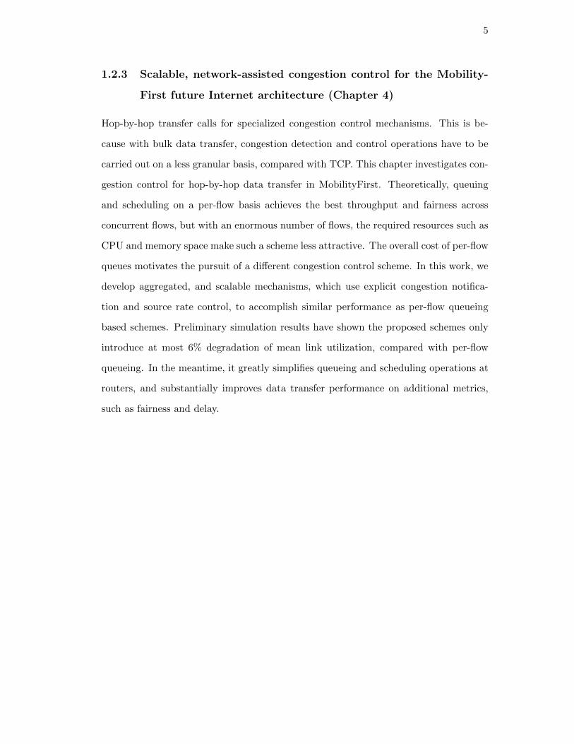
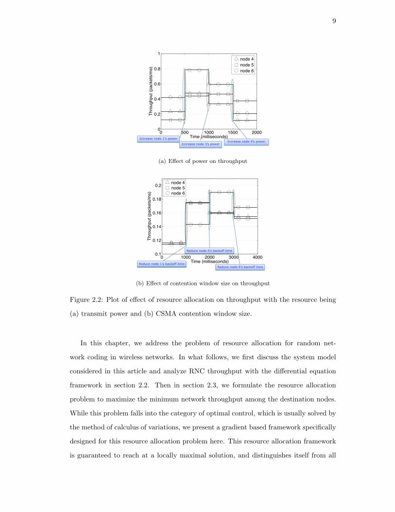
Let us first consider the effects of transmit powers on the performance of random

network coding in the wireless network shown in Figure 2.1. The source node, node 1, is

trying to multicast to a set of sink nodes, node {4, 5, 6}. In this network, every node is

transmitting and is also able to receive from others. We further assume the network is

interference limited, i.e., each transmission is interfered by simultaneous transmissions

from other nodes. Therefore, increasing transmit power at a node improves SINR

value of its own transmission but raises interference to others. The throughput of the

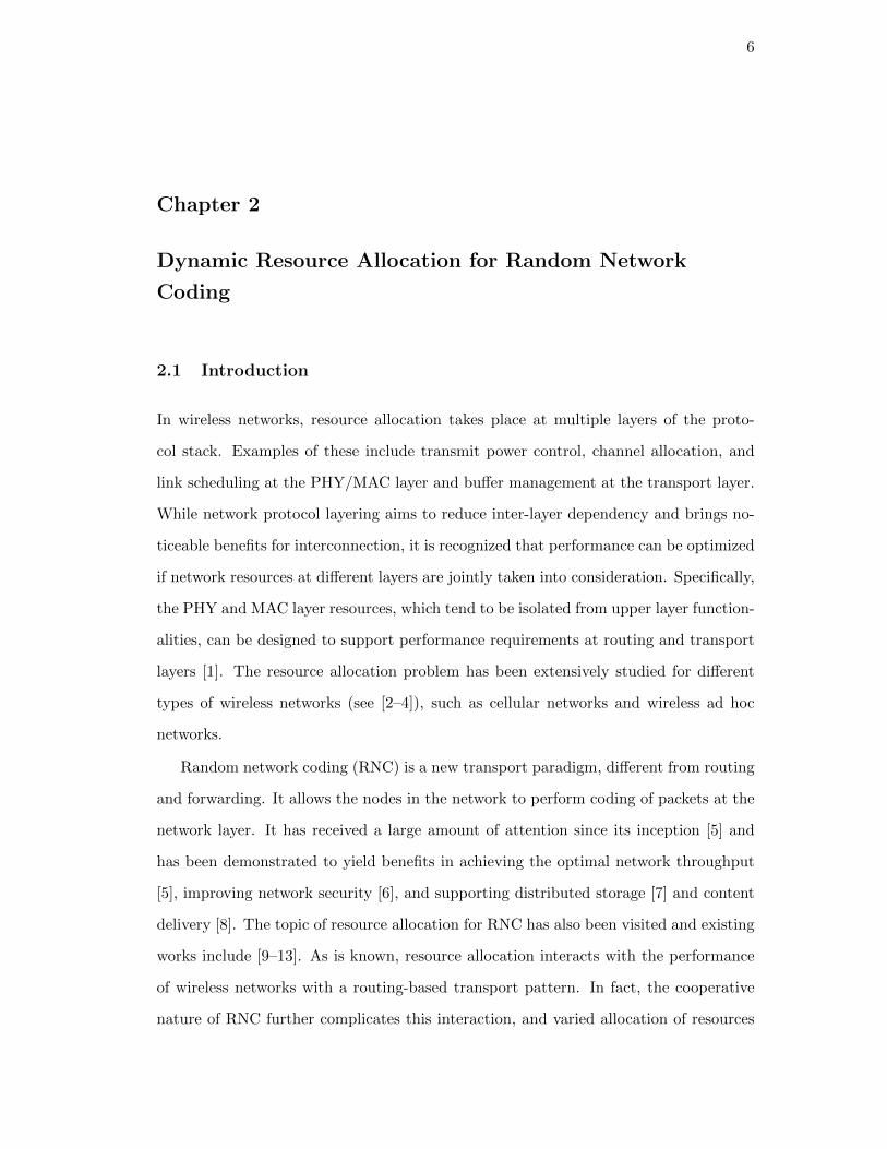
destination nodes thus depend on the power levels at all nodes. To observe this effect,

we set the transmit power PTxi of each node i to 13dBm at t = 0ms. Subsequently,

at t = 500ms, t = 1000ms and t = 1500ms, the transmit powers of node 1, 3, 4, i.e.,

PTx1 , PTx

3 and PTx4 are increased to 14dBm, respectively. As seen in Figure 2.2(a),

the power increment of node 1 at 500ms improves the throughput of all the sink nodes,

whereas node 3’s increment at 1000ms leads to the decrease of throughput of node 4 and

6. Therefore, increasing power at one node does not necessarily improve the throughput

at all the destination nodes; on the contrary, it may possibly hurt the throughput at

some node.

4

2

65

3

1

4

2

65

3

1

Figure 2.1: Hypergraph model of a wireless network of six nodes with s = 1 and

D = {4, 5, 6}.

Now consider the case of adjusting the backoff time in a CSMA network employing

RNC. We consider a network with the same topology as in Figure 2.1 that is utilizing

8

CSMA as the MAC layer protocol. In this network, each node contends for transmission

with an exponentially distributed delay value. We manipulate the mean of the backoff

delay to control the transmission aggressiveness of each node and see its impacts on

RNC throughput. At t = 0ms, the mean backoff delay of each node is set such that all

the destination nodes, node 4, 5, 6, are transmitting at about 0.12pkt/ms. Subsequently,

at t = 1000ms, t = 2000ms and t = 3000ms, the mean backoff delay of nodes 1, 4, 6 are

reduced, i.e., transmission aggressiveness increased, respectively as follows. The mean

backoff delay of node 1 is reduced from 3.70ms to 2.24ms, node 4 from 2.74ms to

1.66ms, and node 6 from 1.66ms to 0.83ms. Figure 2.2(b) shows that, for example,

at t = 2000ms, when node 4 starts to contend more aggressively, it improves the

throughput of node 6. However, this simultaneously leads to the drop of the throughput

of node 4 itself and node 5. An apparent reason is that it leads to reduced channel

availability for these two nodes. Similar effects can also be seen for the subsequent

window size change when node 6 becomes more aggressive.

Both of the above two examples, one at the PHY layer, and the other at the MAC

layer, show that due to the network dynamics and the complexity of the problem,

it would be cumbersome or unsuccessful to employ some static, or heuristic resource

allocation mechanism in a network employing RNC. Rather, a deliberately designed,

and more importantly, dynamic resource allocation algorithm is required to support

the optimal RNC performance. Since RNC is fundamentally different from routing and

forwarding in terms of packet delivery as there are no specific routes being computed and

followed [14], analyzing it with traditional methods designed for uncoded networks will

be problematic, because adopting an inappropriate model will not take full advantage

of the benefits that RNC offers, such as the fact that RNC utilizes wireless network’s

broadcast effect. In light of this, a differential equation based framework in [15] and

[16] is of particular interest for deriving resource allocation algorithms for RNC. This

framework leverages a system of differential equations to elegantly model the rank

evolution process which shapes the RNC performance. The presence of PHY and MAC

layer parameters in this model makes it natural to analyze lower layer resource allocation

for RNC.

9

0 500 1000 1500 20000

0.2

0.4

0.6

0.8

1

Time (milliseconds)

Thro

ughp

ut (p

acke

ts/m

s)

node 4node 5node 6

Increase node 1’s power

Increase node 3’s power Increase node 4’s power

(a) Effect of power on throughput

0 1000 2000 3000 40000.1

0.12

0.14

0.16

0.18

0.2

Time (milliseconds)

Thro

ughp

ut (p

acke

ts/m

s)

node 4node 5node 6

Reduce node 1’s backoff time

Reduce node 4’s backoff time

Reduce node 6’s backoff time

(b) Effect of contention window size on throughput

Figure 2.2: Plot of effect of resource allocation on throughput with the resource being

(a) transmit power and (b) CSMA contention window size.

In this chapter, we address the problem of resource allocation for random net-

work coding in wireless networks. In what follows, we first discuss the system model

considered in this article and analyze RNC throughput with the differential equation

framework in section 2.2. Then in section 2.3, we formulate the resource allocation

problem to maximize the minimum network throughput among the destination nodes.

While this problem falls into the category of optimal control, which is usually solved by

the method of calculus of variations, we present a gradient based framework specifically

designed for this resource allocation problem here. This resource allocation framework

is guaranteed to reach at a locally maximal solution, and distinguishes itself from all

10

the other previous works most of which utilize the flow-based formulation of RNC. We

will compare our algorithm with the related works after it is introduced in section 2.3.

After that, two use cases of this algorithm, i.e., power control and CSMA mean backoff

delay control, are presented to improve network coding throughput in section 2.4 and

2.5, respectively. In these two sections, we derive both centralized and online algo-

rithms for the above two use cases. The main contribution of this work is to present

a novel methodology to analyze cross-layer resource allocation in the context of RNC

from a dynamical system view provided by the differential equation model. The frame-

work utilized in this methodology is sufficiently general such that it can be used to

analyze all kinds of PHY/MAC layer resources and derive effective resource allocation

algorithms.

2.2 Preliminaries

2.2.1 Differential Equation Framework for RNC

We now present a brief review of the differential equation framework for RNC that is

introduced in [15]. A directed hypergraph is adopted in [15] to model a wireless network:

G = (N , E) which has N nodesN = {1, 2, . . . , N} and hyperarcs E = {(i,K)|i ∈ N ,K ⊂

N}. The hyperarc (i,K) captures the fact that in a wireless environment, a packet

transmitted by node i can be received by a subset of nodes from K. To illustrate this,

we note from Figure 2.1 that each node has a point to point link to every other node,

but a transmitted packet can only be received by a subset of these nodes. This subset

could be determined explicitly by the received signal and interference levels (adopted

in section 2.4 for the case of power control), or implicitly by a thresholding distance for

reception (adopted in section 2.5 for the case of CSMA).

Consider that each node in the wireless network G is performing random network

coding [14], i.e., a source node sends out random linear combinations of the original

packets (coded packets), and other nodes merely receive packets from the network and

they in turn send out random linear combinations of the packets received. It is assumed

that each coded packet is a row vector of length l from Flq, where q is the field size. No

11

routing operations are performed in the network and destination nodes can recover the

original packets after collecting sufficient coded packets. Assuming packet loss is only

due to bit errors, the probability that a packet transmitted by node i can be received

by at least one node in K, Pi,K can be defined as:

Pi,K = 1−∏j∈K

(1− Pi,j) , (2.1)

where Pi,j is the reception probability of link (i, j). We can see that Pi,K is a function

of the PHY layer parameters, e.g., transmit powers and interference. Assuming there

exists certain MAC protocol running in its stable state such that node i is sending

out coded packets at the average rate of λi packets per second, then the successful

transmission rate for the hyperarc (i,K) can be defined as:

zi,K = λiPi,K. (2.2)

zi,K can also be regarded as the capacity of hyperarc (i,K). Note that the capacity

of a cut, T for (S,K), S,K ⊂ N where K ⊂ T ⊂ Sc is given as c(T ) =∑

i∈T c zi,T .

Then, the min cut for (S,K) is the cut with the minimum size. The number of linearly

independent coded packets is called the rank, and V{i} is used to denote the rank at

node i. In essence, V{i} is the dimension of the subspace Si spanned by the coded

packets at node i, i.e., V{i} = dimSi. An innovative packet of node i is defined as the

received packet which increases the rank V{i}. For a RNC multicast session, if there are

m original packets to be delivered, each destination node i can decode only if V{i} = m.

The notion of rank can be naturally extended to a set of nodes, K, and thus VK is the

joint rank of all the nodes from K, i.e., VK = dimSK = dim∑

i∈K Si. Note VK serves

as a measure of the amount of information jointly possessed by the set of nodes, K; the

decoding process, however, is carried out independently at each destination. We call

the stochastic process VK(t) that grows from 0 to m the rank evolution process.

In [15], it has been shown that under the fluid approximation, a concentration result

has been established for the rank evolution process, i.e., the stochastic process VK(t)

is well represented by its mean, E[VK(t)]. Then consider a small time interval ∆t in

which the number of packets sent from node i that can be successfully received by K

12

(a)

1 4

2

3

1  2  3  

1  2  

2  3  

2  3  

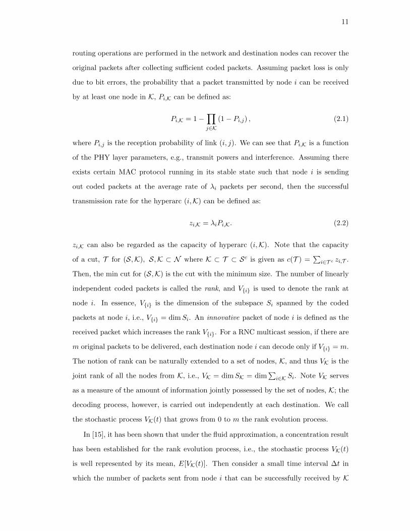
(b)

Figure 2.3: (a) Illustration of the subspace of coded packets that are innovative to K.

(b) An illustrative example where node 1 tries to multicast 3 coded packets to node

1, 2, and 3. The coded packets that each node has are shown next to it. Here, the only

packet from node 2 that is innovative to node 4 is packet 1, which is from S2\(S2∩S4).

is ∆tzi,K. The packets, if received, have to come from the subspace Si\(Si ∩ SK) to

be innovative to the set of nodes, K (see illustration in Figure 2.3). It can be seen the

probability that a coded packet transmitted by node i is actually from Si\(Si ∩ SK) is

given by:

|Si| − |Si ∩ SK||Si|

=qdimSi − qdimSi∩SK

qdimSi=qVi − qVi+VK−V{i}∪K

qVi= 1− qVK−V{i}∪K . (2.3)

Now an equality of the rank increase of K for the interval ∆t can be established:

VK(t+ ∆t)− VK(t) = ∆t∑i/∈K

zi,K(1− qVK−V{i}∪K) (2.4)

Dividing both sides by ∆t and then approximating the left hand side with the derivative,

we reach at the following system of differential equations:

VK =∑i/∈K

zi,K(1− qVK−V{i}∪K), ∀K ⊂ N and K 6= ∅. (2.5)

The derivation of the above differential equations is detailed in [15]. It is worth noting

that VK is the rate at which K is receiving innovative packets, i.e., VK denotes the

throughput of K. Apparently, with zi,K being an abstraction of the outcome of all the

PHY/MAC operations in the system of differential equations (2.5), the throughput of

13

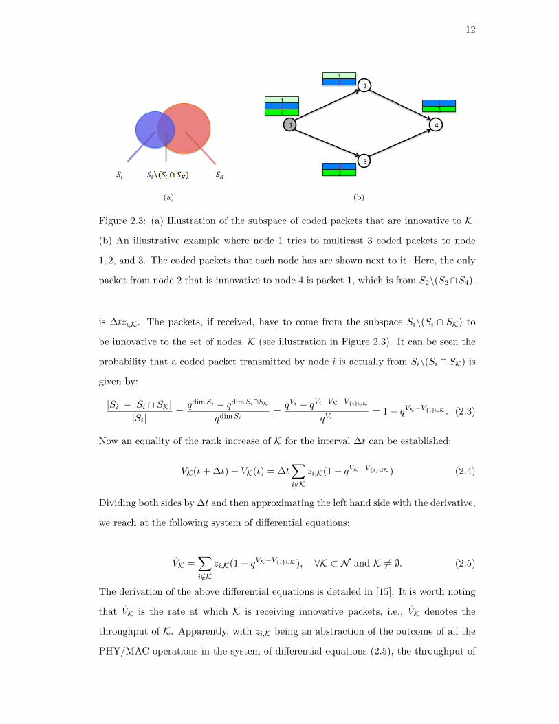
a set of nodes can be elegantly analyzed with respect to PHY/MAC parameters. To

illustrate this, we present two numerical examples. First consider a wireless network

shown in Figure 2.4(a) (also discussed in [15]) where the source node, node 1 intends

to multicast 1000 packets to destination nodes 2, 3, 4. Let each node perform RNC

operations and transmit at 1pkt/ms. Suppose that packets from node 1 can only be

successfully received by node 2 and 3, with probability of 0.2 and 0.4, respectively, and

node 2 and node 3’s packets can only be successfully received by node 4 with probability

of 0.6 and 0.7, respectively. Based on the above parameters, we can compute the

successful transmission rate zi,K for each hyperarc (i,K) for this topology. Then all the

zi,K are plugged in the system of differential equations (2.5) and solving them yields the

result shown in Figure 2.4(b), the plot of rank evolution process for this RNC multicast.

It can be easily verified that the throughputs of the destinations, i.e., the rates at which

ranks increase, match the min cuts of every source and destination pair1. For instance,

it is trivial to see the min cut between node 1 and 2 is 0.2, which is equal to the

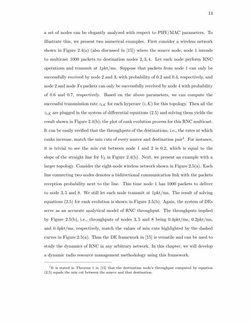
slope of the straight line for V2 in Figure 2.4(b). Next, we present an example with a

larger topology. Consider the eight-node wireless network shown in Figure 2.5(a). Each

line connecting two nodes denotes a bidirectional communication link with the packets

reception probability next to the line. This time node 1 has 1000 packets to deliver

to node 3, 5 and 8. We still let each node transmit at 1pkt/ms. The result of solving

equations (2.5) for rank evolution is shown in Figure 2.5(b). Again, the system of DEs

serve as an accurate analytical model of RNC throughput. The throughputs implied

by Figure 2.5(b), i.e., throughputs of nodes 3, 5 and 8 being 0.4pkt/ms, 0.2pkt/ms,

and 0.4pkt/ms, respectively, match the values of min cuts highlighted by the dashed

curves in Figure 2.5(a). Thus the DE framework in [15] is versatile and can be used to

study the dynamics of RNC in any arbitrary network. In this chapter, we will develop

a dynamic radio resource management methodology using this framework.

1It is stated in Theorem 1 in [15] that the destination node’s throughput computed by equation(2.5) equals the min cut between the source and that destination.

14

2 3

1

4

0.4 0.2

0.7 0.6

(a) 4-node network

topology

0 200 400 600 800 10000

100

200

300

400

500

600

Time (milliseconds)

Ra

nk

V2

V3

V4

(b) Rank evolution

Figure 2.4: Rank evolution modeled by DE, example 1.

7

4

2

6

0.2

0.3

0.2

0.4 0.1

0.2

0.1 0.1 0.1

0.6

0.7

(a) 8-node network topology

0 200 400 600 800 10000

100

200

300

400

Time (milliseconds)

Ra

nk

V3

V5

V8

(b) Rank evolution

Figure 2.5: Rank evolution modeled by DE, example 2.

2.3 Resource Allocation Algorithm for Wireless Network Coding

2.3.1 Problem Formulation

Consider a wireless network G = (N , E) which is performing random network coding.

The source node s tries to multicast m packets to a set of sink nodes. We proceed to

consider some PHY or MAC layer resource at every node i and denote it as ri. Note that

ri can be any PHY/MAC layer parameter which contributes to the transmission rate

λi or the packet reception probability Pi,K. Letting the vector r denote [r1, r2, ..., rN ]>,

15

we have

zi,K = zi,K(r), (2.6)

i.e., the reception rate zi,K for each hyperarc (i,K) is an explicit function of allocated

resource r. To formulate the resource allocation as an optimization problem for improv-

ing the RNC performance, we consider maximizing the minimum throughput among

all the sink nodes as the objective function. We let R be the set of destination nodes

which have not reached full rank, m. With a little abuse of notation, we let Vi denote

V{i}. Then letting k = arg minj∈R Vj , we construct the following optimization problem:

maximize Vk

subject to VK =∑i/∈K

zi,K · (1− qVK−V{i}∪K), ∀K ⊂ N .

zi,K = zi,K(r).

k = arg minj∈R

Vj

variables r.

(2.7)

2.3.2 Gradient-based Resource Allocation Algorithm

Note that in general, the optimization problem given by (2.7) is not convex, and thus

it is difficult to find the globally optimal solution. Additionally, this type of problem

which is constrained by a set of first-order differential equations can be categorized

into an optimal control problem. Existing approaches to optimal control involve cal-

culus of variations, which can be computationally expensive and intractable in wireless

networks. In this chapter, we aim to find a local optimum of this problem which can

provide significant throughput gains with less computational complexity. We take an

approach based on the steepest ascent (its counterpart for minimization problems is

called steepest descent, see [17]), i.e. adjust the resource r towards the direction of the

gradient. Essentially, our optimization objective, Vk is a function of the resource r, i.e.,

Vk = Vk(r). This allows us to establish the gradient of throughput as the direction of

the dynamic adjustment of the resource, i.e.,

r = a′ · ∇Vk, (2.8)

16

where a′ is a positive constant tuning the gain. In this way, the allocation of resource

will be iterative, as well as dynamic. We consider a discrete approximation to compute

the derivative in equation (2.8) as follows. Let ∆v be the step size, and ei be a column

vector with 1 being the ith component and 0 elsewhere. Writing in component-wise

form, we have

ri = a′ · Vk(r + ∆vei)− Vk(r)

∆v. (2.9)

Replacing a′/∆v with a, we have:

ri = a ·(Vk(r + ∆vei)− Vk(r)

). (2.10)

Equation (2.10) serves as the basis of the resource allocation algorithm and works

in an iterative manner to adapt the resource allocation towards the direction of the

approximated gradient of the minimum throughput. Our algorithm stops when, at

certain iteration, r ≤ ε is achieved for a sufficiently small vector ε. In the above, Vk is

given by equation (2.5) and thus the allocation of resources takes into consideration the

latest network throughput information and therefore also works in a dynamic fashion.

It has been proved in [13] that the algorithm given by equation (2.10) converges to a

local maximum. [13] also pointed out that the gain parameter a should be chosen such

that q1/a � 1 and qa � 1.

Note that until now, we have not imposed any specific models for the PHY/MAC

layers. In fact, the resource allocation approach presented here is flexible enough that

it can work with any specific lower layer models/mechanisms. For a better elucida-

tion of this approach, we illustrate its applicability by solving two practical allocation

problems for RNC in following sections: (i) power control for maximizing the minimum

throughput, and (ii) CSMA mean backoff delay control for maximizing the minimum

throughput. Before that, we first discuss the the differences between our framework

and the previous resource allocation frameworks for RNC.

17

2.3.3 Relationship to existing literature on resource allocation for

RNC

The topic of resource allocation for RNC was first visited by Lun et al. in [9] where the

authors considered associating a cost function for each hyperarc and minimizing the

total cost for the whole network. Since [9], a number of works focused on more specific

problems of crosslayer optimization, such as power control and scheduling [10] [11] for

RNC. When lower layers’ parameters are considered, the crosslayer resource optimiza-

tion problems tend to be non-convex. Like the other works, our resource allocation

framework is able to yield locally optimal allocation for such non-convex problems, as

proved in [13]. Apart from this, our resource allocation algorithm distinguishes itself

from most of the previous works of the similar topic owing to the use of the differential

equation model of RNC, which not only augments the algorithmic design space for RNC

resource allocation, but brings many merits over the other algorithms based upon the

network flow model, e.g. the one used in [9]. First of all, our framework is dynamic.

Note the common methodology of most flow based algorithms [10] [11] is to establish

a network utility function as the optimization objective and consider wireless hyperarc

capacities, formulated with network flows, as constraints. One invariable feature of

these works is that the utility function and hyperarc capacities considered are not time-

dependent but static. Therefore, for instance, in [11] which considers fading, fading

has to be studied through its ergodic behavior. Due to the lack of time-dependency

when setting up the optimization framework for resource allocation for RNC, if any

of the underlying dynamic network elements, such as channel, network connection, or

MAC/PHY configuration, alter, the utility maximization based optimization framework

needs to be updated. On the other hand, since our differential equation based resource

allocation framework is built upon the theory of dynamical systems, it is inherently

capable of accommodating the dynamism of the network: the underlying parameters λi

and Pi,j , which capture MAC and PHY characteristics respectively, are in fact modeled

to be time dependent. They evolve together with the rank Vj naturally. Thus our

framework provides an accurate model for such dynamic interaction between network

18

resources and RNC performance whereas the other existing models do not. Second, our

framework is less complex. Note with flow based model, it is known how to solve for

the RNC throughput Vj . However, that is done by i) setting up a network flow based

formulation where flow sizes are bounded by hyperarc capacities, which in turn are

determined by the lower layer resources, and ii) solving this formulated problem for the

min cut between the source and the destination node. In other words, it can be seen

that flow-based models as adopted in [10] [11] do not explicitly model Vj , and thus the

resources to be allocated have to be placed in the constraints when being optimized. The

differential equation model of RNC, on the other hand, explicitly describes Vj in terms

of PHY and MAC parameters, λi and Pi,j . This allows resource allocation for RNC

to be directly the objective of the optimization problem formulated, rather than con-

straints, e.g., in equation (2.7) Vk is actually given by Vk =∑

i 6=k λiPi,k ·(1−qVk−V{i,k}).

Thus it substantially simplifies algorithm design for such resource allocation. Specif-

ically, this allows us to apply a very fundamental line search algorithm based on the

idea of gradient ascent for unconstrained optimization, and effectively solve the RNC

resource allocation, as will be illustrated later.

2.4 Dynamic Power Control in RNC

There exists a rich history of transmit power control for cellular networks (see [18])

where the goal was to minimize the total power levels [19–21], or to maximize network

utilities [22–24]. In this section, however, we consider performing power control in a

coded wireless network to improve RNC throughput and design a centralized power

control algorithm, as well as an online version of it which is more amenable to imple-

mentation.

2.4.1 Interference Model

While the gradient based resource allocation framework in section 2.3 is applicable for

any wireless network with RNC, in this section we will specifically illustrate its use for

power control in a network where we model the interference as Gaussian. Here we also

19

assume the wireless network G to be interference limited, and model each point-to-

point link gain hji for (i, j) with a path loss model. We use PTxi to denote the transmit

power at node i. The received signal level is given by PTxi hji. Each node i is assumed

to implement a certain processing gain gi. Therefore, when node j intends to receive

the signal transmitted by i, the aggregated interference power is

Jji =∑m 6=j,i

(PTxm · hjm/gi). (2.11)

Let σ2 denote the noise power. The signal-to-noise-and-interference ratio (SINR) for

the point-to-point link (i, j) can be written as

SINR(i,j) =PTxi · hjiJji + σ2

. (2.12)

Assuming BPSK signaling and Gaussian interference, the bit error rate for sender-

receiver pair (i, j) is given as

pbiti,j = Q(√

SINR(i,j)

). (2.13)

Further, assuming each packet is of l bits, the probability that node j can receive a

packet without error is

Pi,j = (1− pbiti,j )l. (2.14)

Note that the differential equation framework requires the computation of Pi,K given

in equation (2.1). Under the above interference model, we assume that there is a MAC

protocol running in steady state such that each node i has an average transmission rate

λi. Therefore, zi,K in equation (2.2) can be now written as:

zi,K = λiPi,K

= λi ·

(1−

∏j∈K

(1−

(1−Q

(√PTxi ·hji∑

m 6=j,i(PTxm ·hjm/gi)+σ2

))l)).

(2.15)

2.4.2 Centralized Power Control

Let PTx =[PTx1 , PTx

2 , ..., PTxN

]>be the transmit power vector and the resource ri =

PTxi . The centralized power control algorithm follows directly from equation (2.10) (see

also [25] and [13]):

20

PTxi = a ·

(Vk(P

Tx + ∆vei)− Vk(PTx)), (2.16)

where

Vk =∑i 6=k

λi ·

(1−Q

(√PTxi · hki∑

m 6=k,i(PTxm · hkm/gi) + σ2

))l·(1− qVk−V{i,k}

), (2.17)

based on the interference model above. Further, we consider dividing the time into

equal length intervals, and only computing and applying power update at the end of

each interval. Then we can rewrite the above algorithm in a discretized and iterative

form:

PTx,n = PTx,n−1 + a ·B(PTx,n−1), n = 2, 3, 4, ... (2.18)

where we use a superscript n to denote a parameter evaluated at nth iteration, e.g.

PTx,n is PTx at the nth iteration, and B(PTx) is a vector defined such that its ith

component is given by:

Bi(PTx) = Vk(P

Tx + ∆vei)− Vk(PTx). (2.19)

In fact, B is the direction to which we update PTx such that Vk is improved; thus B is

a gradient ascent direction.

We assume there is a certain power budget at each node i, i.e., 0 ≤ PTxi ≤ Pmax

i .

Considering this, the algorithm can be summarized as:

k = arg minj∈R Vn−1j

Bi(PTx,n−1) = Vk(P

Tx,n−1 + ∆vei)− Vk(PTx,n−1)

PTx,ni =

PTx,n−1i , if PTx,n−1

i + a ·Bi(PTx,n−1) > Pmaxi and

Bi(PTx,n−1) > 0,

or PTx,n−1i + a ·Bi(PTx,n−1) < 0 and

Bi(PTx,n−1) < 0;

PTx,n−1i + a ·Bi(PTx,n−1), otherwise.

(2.20)

It is assumed that there exists a central controller which knows the exact analytical

expression of Vk(PTx), so that based on equation (2.19), Bi(P

Tx) can be evaluated to

obtain the ascent direction. We thus call it a centralized resource allocation algorithm.

21

2.4.3 Online Power Control

Motivation for online power control algorithm

While the algorithm in section 2.4.2 is effective in achieving the objective to improve

network coding throughput [13], it can be further improved for the purpose of imple-

mentation. Specifically, the centralized algorithm, specified in equation (2.20), works

by adjusting powers towards an ascent direction, B(PTx), which is an approximation of

the gradient ∇PTx Vk, i.e., B(PTx) ≈ ∇PTx Vk. Therefore in the centralized algorithm,

Bi(PTx) has to be evaluated. From equation (2.19) we can see that this in turn re-

quires the exact analytical formula for Vk(PTx) be known. If one were to implement

it in a wireless network, obtaining or in some manner accurately estimating such exact

formulas might be an intimidating, or even infeasible task. To circumvent this problem,

we seek another algorithm which produces a better estimation of ∇PTx Vk, denoted by

B′(PTx), in a sense that it has the following desirable properties: i) it would perform

similarly well as the centralized algorithm to improve RNC performance, however with

only a minimal amount of knowledge about the network; ii) this knowledge could be

learnt by every node through a limited amount of message passing such that the algo-

rithm can operate online, i.e., each node exchanges control messages with the network,

computes the power update for itself based on the information obtained and adjusts

its power without any noticeable delay. In the following, we first describe a method

to estimate B′(PTx) with reduced network state knowledge, and then discuss possible

aspects to take into consideration when implementing this algorithm.

Deriving the online algorithm

We seek a better estimation of the gradient ∇nPTx Vk, written as B′(PTx,n), at the end

of interval n based on the network information available. The goal is to use B′(PTx)

when computing the power updates:

PTx,n = PTx,n−1 + a ·B′(PTx,n−1), n = 2, 3, 4, ... (2.21)

Before starting deriving the online algorithm, we first introduce the following nota-

tions:

22

• Let V denote the size-(2N −1) throughput vector, consisting of VK, ∀K ⊂ N ,K 6=

∅. More precisely, V is given by

V =[V{1} V{2} V{1,2} V{3} ... V{1,2,...,N}

](2.22)

• Let z denote the size-(N · (2N − 1)

)packet reception rate vector, consisting of

zi,K, ∀i ∈ N ,K ⊂ N,K 6= ∅. For each i, zi,K,∀K ⊂ N is arranged similarly with

V. Then z is given by concatenating zi,K, ∀K ⊂ N ,K 6= ∅ from i = 1 to i = N :

z =[z1,{1} z1,{2} z1,{1,2} ... z1,{1,2,...,N} ... zN,{1,2,...,N}

](2.23)

• Let z′i,K denote the innovative packet reception rate of hyperarc (i,K).

• Let z′ denote the size-(N · (2N − 1)

)innovative packet reception rate vector, con-

sisting of z′i,K, ∀(i,K) ∈ E . By replacing every zi,K of z with z′i,K, we get z′.

Unlike the way the centralized algorithm works to directly approximate ∇PTx Vk,

here Vk is viewed as a composition of z which is again a composition of PTx. More

precisely, since we have Vk = Vk(z) and z = z(PTx), then based on the chain rule,

∇PTx Vk can be derived as:

∇PTx Vk = ∇zVkJPTxz, (2.24)

where∇zVk and JPTz are the gradient of Vk with respect to z and the Jacobian of z with

respect to PTx, respectively. Note that from the above equation on, we temporarily

drop the superscript n to simplify the notation. Equation (2.24) provides the exact

formula for computing the gradient of Vk. To derive the online algorithm, we shall

investigate both terms on the right hand side one after another.

Referring to equation (2.23), and noting Vk =∑

i/∈k zi,k · (1− qVk−V{i,k}), we have

∇zVk =[0, 1− qVk−V{1,k} , 1− qVk−V{2,k} , 0, ..., 0, 1− qVk−V{k−1,k} , 0, ..., 0, 1− qVk−V{k+1,k} , ...

].

(2.25)

Noting ∇zVk has (N − 1) non-zero components: 1− qVk−V{i,k} , ∀i ∈ N , i 6= k, we would

like to avoid evaluating ∇zVk since it requires the knowledge of V{i,k}, the joint rank of

node i and k. Obtaining such joint rank in a wireless network would be cumbersome

23

because it requires plenty of information to be exchanged. Instead, note that zi,K is

defined as the packet reception rate, and (1 − qVK−V{i}∪K) is the probability that the

received packet is an innovative packet. Then the innovative packet reception rate z′i,K

is given by z′i,K = zi,K · (1 − qVK−V{i}∪K). Therefore, we take an alternative approach

to consider obtaining the gradient with respect to the innovative packet reception rate

z′ instead of z, i.e., ∇z′ Vk. With z′, we can rewrite equation (2.5) in a more compact

form:

VK =∑i/∈K

z′i,K, ∀K ⊂ N , (2.26)

and ∇z′ Vk can be derived accordingly as:

∇z′ Vk = [0, 1, 1, 0, ..., 0, 1, 0, ..., 0, 1, 0, ... 0] . (2.27)

Then the gradient of Vk can be calculated by

∇PTx Vk = ∇z′ VkJPTxz′. (2.28)

Thus the evaluation of ∇PTx Vk in equation (2.28) boils down to the evaluation of

JPTxz′. Note we would avoid the approach of directly evaluating it as this would again

require that the underlying PHY layer specifics of all the nodes be known universally,

such that the analytical formula of z′ is known. Furthermore, computing the Jacobian,

i.e., JPTxz′ can be computationally prohibitive. Rather, we numerically estimate this

Jacobian at each iteration by following a similar approach that is adopted in Broyden’s

method [26]. For that purpose, we recover the superscript n to denote the parameters

evaluated at the nth interval. Each interval is of equal-length (corresponding to the

time between successive power updates) and is assumed to be of τ seconds. Then

according to [26], we have

JnPTxz′ = Jn−1

PTx z′ +∆z′n − Jn−1

PTx z′∆PTx,n

‖∆PTx,n‖2∆PTx,n>, (2.29)

where ∆z′n = z′n − z′n−1, ∆PTx,n = PTx,n −PTx,n−1, and JnPTxz

′ is the estimation of

the Jacobian in the nth interval.

We can estimate the average innovative packets reception rate in each time interval

which is of length τ , i.e.,

z′ni,j = cni,j/τ, (2.30)

24

where cni,j is the number of innovative packets sent by node i that node j has received

in the nth time interval. Note that the granularity of power updates are based on

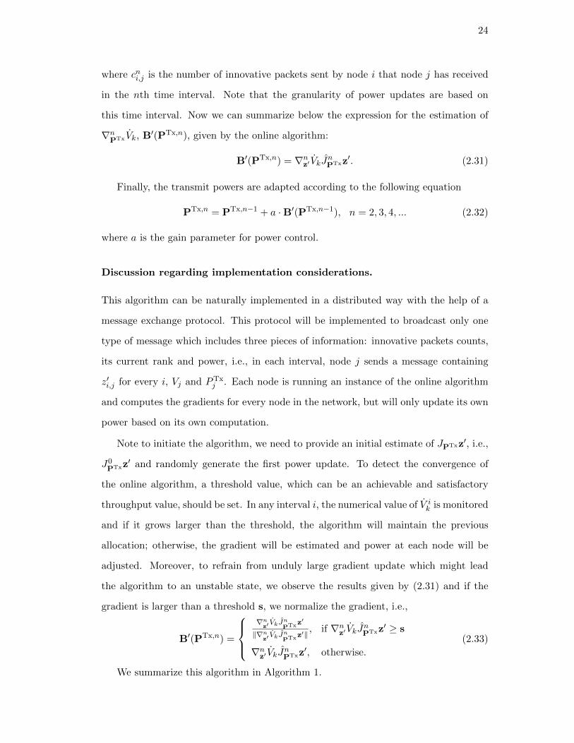
this time interval. Now we can summarize below the expression for the estimation of

∇nPTx Vk, B′(PTx,n), given by the online algorithm:

B′(PTx,n) = ∇nz′ VkJnPTxz′. (2.31)

Finally, the transmit powers are adapted according to the following equation

PTx,n = PTx,n−1 + a ·B′(PTx,n−1), n = 2, 3, 4, ... (2.32)

where a is the gain parameter for power control.

Discussion regarding implementation considerations.

This algorithm can be naturally implemented in a distributed way with the help of a

message exchange protocol. This protocol will be implemented to broadcast only one

type of message which includes three pieces of information: innovative packets counts,

its current rank and power, i.e., in each interval, node j sends a message containing

z′i,j for every i, Vj and PTxj . Each node is running an instance of the online algorithm

and computes the gradients for every node in the network, but will only update its own

power based on its own computation.

Note to initiate the algorithm, we need to provide an initial estimate of JPTxz′, i.e.,

J0PTxz

′ and randomly generate the first power update. To detect the convergence of

the online algorithm, a threshold value, which can be an achievable and satisfactory

throughput value, should be set. In any interval i, the numerical value of V ik is monitored

and if it grows larger than the threshold, the algorithm will maintain the previous

allocation; otherwise, the gradient will be estimated and power at each node will be

adjusted. Moreover, to refrain from unduly large gradient update which might lead

the algorithm to an unstable state, we observe the results given by (2.31) and if the

gradient is larger than a threshold s, we normalize the gradient, i.e.,

B′(PTx,n) =

∇n

z′ VkJnPTxz

′

‖∇nz′ VkJ

nPTxz

′‖, if ∇nz′ VkJnPTxz

′ ≥ s

∇nz′ VkJnPTxz′, otherwise.

(2.33)

We summarize this algorithm in Algorithm 1.

25

Algorithm 1 Online network coding aware power control algorithm

τ ← Power update granularity

τ0 ← Time interval to make gradient computation

rand(N,1) ← length-N random vector with each element larger than −0.5 and less

than 0.5

c0 ← 0: counters for number of innovative packets.

PTx,0 ← Pinit

J0PTxz

′ ← JPTxz′init

while t ≤ τ do

update c0

end while

compute z′0

PTx,1 = PTx,0 + rand(N, 1)

n← 1

while nτ ≤ t ≤ (n+ 1)τ do

update cn

if t > (n+ 1)τ − τ0 then

while B′(PTx,n) has not been computed do

compute z′n

∆PTx,n = PTx,n −PTx,n−1

∆z′n = z′n − z′n−1

Compute JnPTxz

′ as in (2.29)

Compute B′(PTx,n) as in (2.31)

Set power PTx,n = PTx,n−1 + a ·B′(PTx,n−1)

n← n+ 1

end while

end if

end while

26

2.4.4 Numerical Results

We use two ways to evaluate the power control algorithm for random network coding.

First, for the centralized algorithm, we use a numerical differential equation solver to

simultaneously solve the differential equations in equation (2.5) and (2.20). According

to the results of evaluating the gradient ascent direction B(PTx,n−1) given in (2.20),

the power levels are updated at the end of each iteration n in the differential equation

solver. Second, for the online algorithm, we implement the algorithm with an event-

driven simulation in MATLAB.

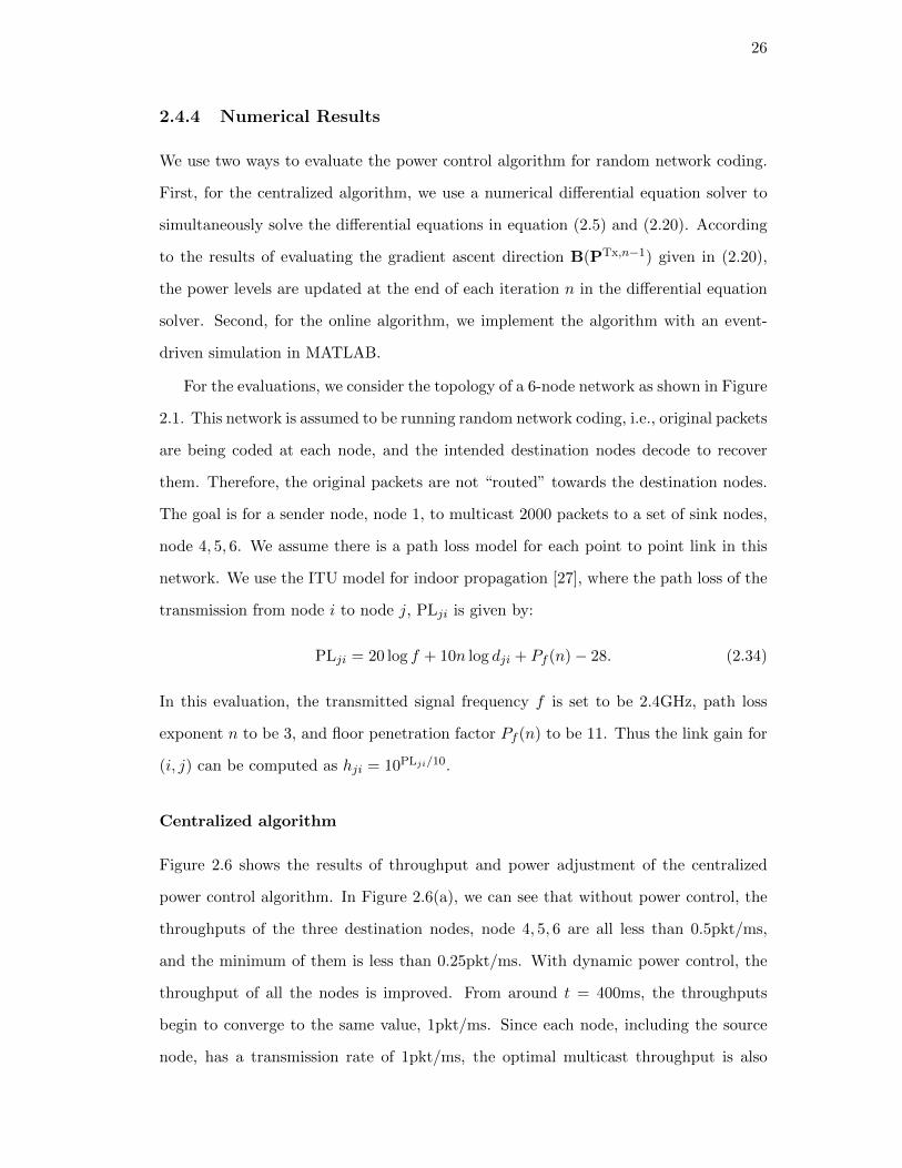
For the evaluations, we consider the topology of a 6-node network as shown in Figure

2.1. This network is assumed to be running random network coding, i.e., original packets

are being coded at each node, and the intended destination nodes decode to recover

them. Therefore, the original packets are not “routed” towards the destination nodes.

The goal is for a sender node, node 1, to multicast 2000 packets to a set of sink nodes,

node 4, 5, 6. We assume there is a path loss model for each point to point link in this

network. We use the ITU model for indoor propagation [27], where the path loss of the

transmission from node i to node j, PLji is given by:

PLji = 20 log f + 10n log dji + Pf (n)− 28. (2.34)

In this evaluation, the transmitted signal frequency f is set to be 2.4GHz, path loss

exponent n to be 3, and floor penetration factor Pf (n) to be 11. Thus the link gain for

(i, j) can be computed as hji = 10PLji/10.

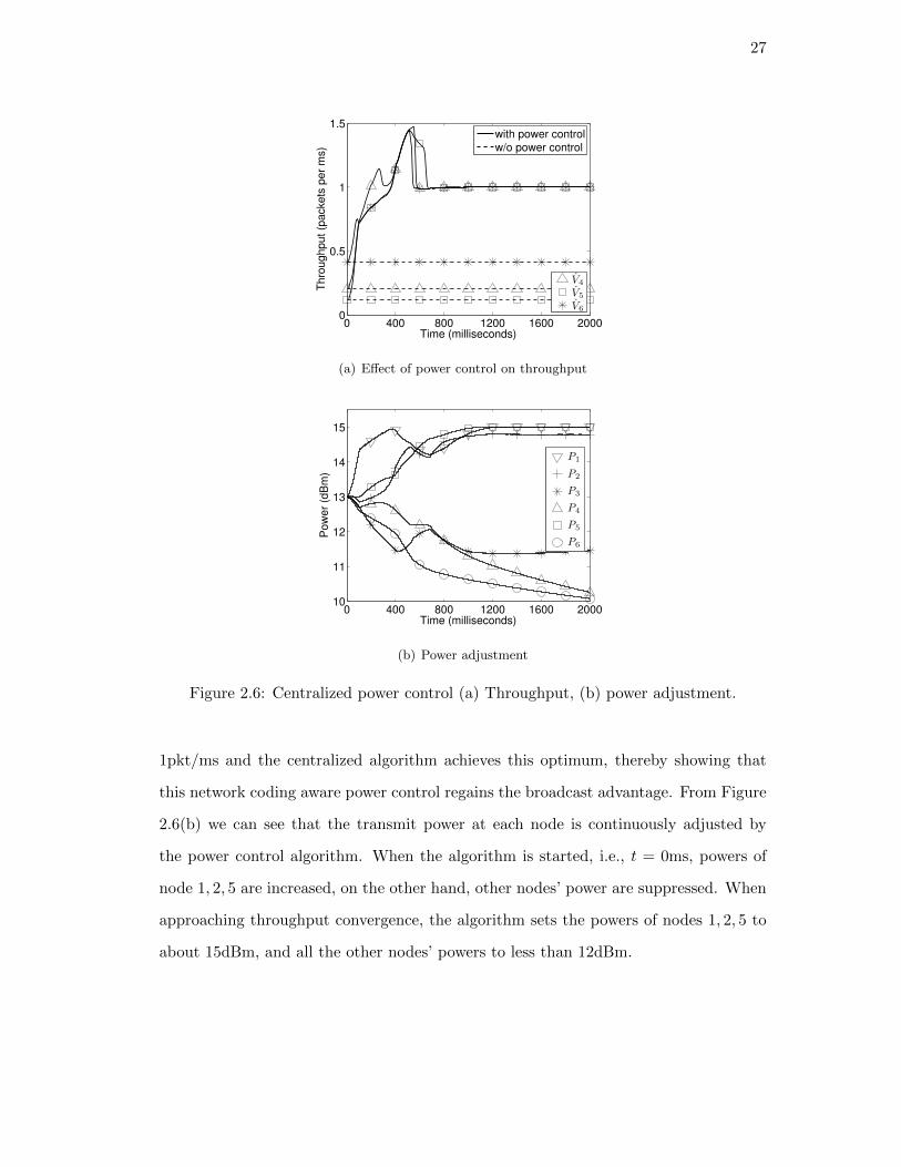
Centralized algorithm

Figure 2.6 shows the results of throughput and power adjustment of the centralized

power control algorithm. In Figure 2.6(a), we can see that without power control, the

throughputs of the three destination nodes, node 4, 5, 6 are all less than 0.5pkt/ms,

and the minimum of them is less than 0.25pkt/ms. With dynamic power control, the

throughput of all the nodes is improved. From around t = 400ms, the throughputs

begin to converge to the same value, 1pkt/ms. Since each node, including the source

node, has a transmission rate of 1pkt/ms, the optimal multicast throughput is also

27

0 400 800 1200 1600 20000

0.5

1

1.5

Time (milliseconds)

Thro

ughput (p

ackets

per

ms)

V4

V5

V6

with power control

w/o power control

(a) Effect of power control on throughput

0 400 800 1200 1600 200010

11

12

13

14

15

Time (milliseconds)

Pow

er

(dB

m)

P1

P2

P3

P4

P5

P6

(b) Power adjustment

Figure 2.6: Centralized power control (a) Throughput, (b) power adjustment.

1pkt/ms and the centralized algorithm achieves this optimum, thereby showing that

this network coding aware power control regains the broadcast advantage. From Figure

2.6(b) we can see that the transmit power at each node is continuously adjusted by

the power control algorithm. When the algorithm is started, i.e., t = 0ms, powers of

node 1, 2, 5 are increased, on the other hand, other nodes’ power are suppressed. When

approaching throughput convergence, the algorithm sets the powers of nodes 1, 2, 5 to

about 15dBm, and all the other nodes’ powers to less than 12dBm.

28

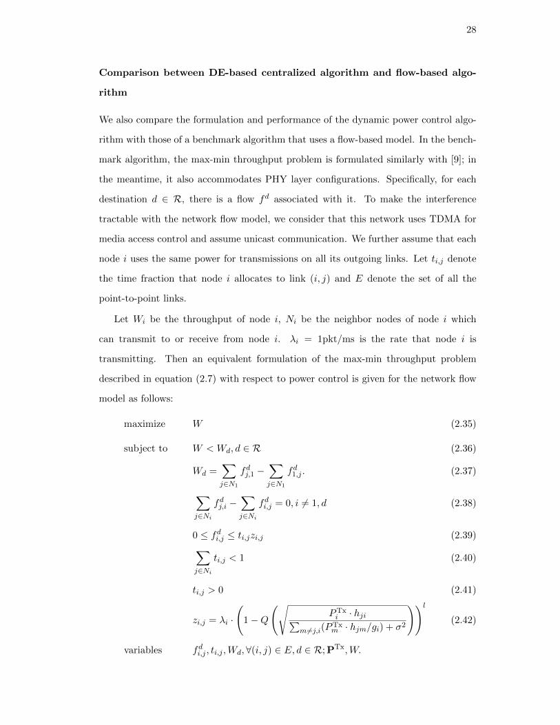
Comparison between DE-based centralized algorithm and flow-based algo-

rithm

We also compare the formulation and performance of the dynamic power control algo-

rithm with those of a benchmark algorithm that uses a flow-based model. In the bench-

mark algorithm, the max-min throughput problem is formulated similarly with [9]; in

the meantime, it also accommodates PHY layer configurations. Specifically, for each

destination d ∈ R, there is a flow fd associated with it. To make the interference

tractable with the network flow model, we consider that this network uses TDMA for

media access control and assume unicast communication. We further assume that each

node i uses the same power for transmissions on all its outgoing links. Let ti,j denote

the time fraction that node i allocates to link (i, j) and E denote the set of all the

point-to-point links.

Let Wi be the throughput of node i, Ni be the neighbor nodes of node i which

can transmit to or receive from node i. λi = 1pkt/ms is the rate that node i is

transmitting. Then an equivalent formulation of the max-min throughput problem

described in equation (2.7) with respect to power control is given for the network flow

model as follows:

maximize W (2.35)

subject to W < Wd, d ∈ R (2.36)

Wd =∑j∈N1

fdj,1 −∑j∈N1

fd1,j . (2.37)

∑j∈Ni

fdj,i −∑j∈Ni

fdi,j = 0, i 6= 1, d (2.38)

0 ≤ fdi,j ≤ ti,jzi,j (2.39)∑j∈Ni

ti,j < 1 (2.40)

ti,j > 0 (2.41)

zi,j = λi ·

(1−Q

(√PTxi · hji∑

m 6=j,i(PTxm · hjm/gi) + σ2

))l(2.42)

variables fdi,j , ti,j ,Wd, ∀(i, j) ∈ E, d ∈ R; PTx,W.

29

In equation (2.42), hji is the link gain and gi is the processing gain. Feeding this for-

mulation with the same topology and initial conditions as that are used in the dynamic

power control simulation, a numerical nonlinear program solver yields the optimal value

of 1pkt/ms with Sequential Quadratic Programming (SQP) method [28]. However, note

that this algorithm can only be applied in a static fashion, i.e., it does not retain the

dynamic characteristics of the power control in equation (2.16). Without taking into

account the dynamic growth of ranks in RNC, any changes in the network would render

a previously optimal allocation unsatisfactory and to make it work, a new allocation

has to be computed.

Online algorithm

In the simulation for online power control, the power is adjusted in every discrete time

interval. Here, the interval is set to 150ms. The power levels of all the nodes are set

to 13dBm in the first interval, and a random update is applied in the second interval.

After this initialization, in any interval n, we attempt to maintain a fixed step size γ

with the following rule:

PTx,ni =

PTx,n−1i + γ, if a ·B′i(PTx,n−1) ≥ γ

PTx,n−1i − γ, if a ·B′i(PTx,n−1) ≤ −γ

PTx,n−1i , otherwise.

(2.43)

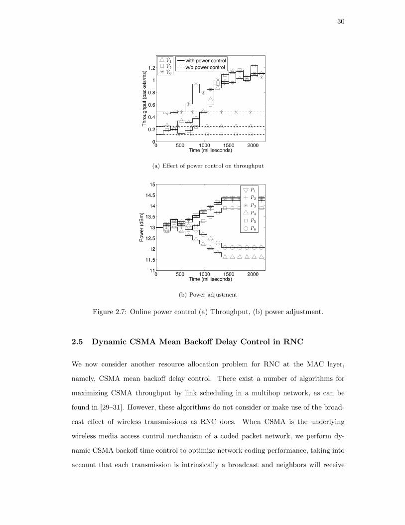
In this simulation, we set γ as 0.2dBm. From Figure 2.7(a), we can see in the first inter-

val of this experiment, the destination nodes’ largest throughput is about 0.5pkt/ms,

and the throughputs of node 4 and 5 are both less than 0.3pkt/ms. As the algo-

rithm progresses, the minimum throughput increases from about 0.1pkt/ms to about

1pkt/ms, and approaches convergence of about 1pkt/ms around t = 1500ms. Figure

2.7(b) shows how the transmit powers at each node are adjusted by the online power

control algorithm.

30

0 500 1000 1500 20000

0.2

0.4

0.6

0.8

1

1.2

Time (milliseconds)

Thro

ughput (p

ackets

/ms)

V4

V5

V6

with power control

w/o power control

(a) Effect of power control on throughput

0 500 1000 1500 200011

11.5

12

12.5

13

13.5

14

14.5

15

Time (milliseconds)

Pow

er

(dB

m)

P1

P2

P3

P4

P5

P6

(b) Power adjustment

Figure 2.7: Online power control (a) Throughput, (b) power adjustment.

2.5 Dynamic CSMA Mean Backoff Delay Control in RNC

We now consider another resource allocation problem for RNC at the MAC layer,

namely, CSMA mean backoff delay control. There exist a number of algorithms for

maximizing CSMA throughput by link scheduling in a multihop network, as can be

found in [29–31]. However, these algorithms do not consider or make use of the broad-

cast effect of wireless transmissions as RNC does. When CSMA is the underlying

wireless media access control mechanism of a coded packet network, we perform dy-

namic CSMA backoff time control to optimize network coding performance, taking into

account that each transmission is intrinsically a broadcast and neighbors will receive

31

the transmitted packet. Although the general algorithm presented in section 2.3 is

sufficiently flexible such that it does not need to assume any particular model for λi,

we now introduce a CSMA model for the purpose of illustration. We then apply the

resource allocation algorithm in this setting to dynamically adjust the mean of backoff

delay at each node to maximize the minimum throughput among the sink nodes. Note

that the differential equation framework in equation (2.5) described earlier requires the

knowledge of zi,K, the rate at which the packets from i are successfully received by at

least one node in K. We will now derive zi,K for this CSMA model.

2.5.1 CSMA Model

The CSMA model considered here was first introduced in [32] and is illustrative of a

multihop network as is the case for RNC. We consider the wireless network G = (N , E)

and let Ni denote the neighbors of node i, i.e., all the nodes that are within the range

to be able to communicate with node i and N∗i = Ni ∪ {i}. It should be noted that

we assume here that the layer of network coding operation sits above the MAC layer

on the protocol stack, and in this section, we refer to packet as the coded packet with

the MAC header attached. We describe next the assumptions for the CSMA model

from [32]:

• When a packet is scheduled to be transmitted at node i, the node senses the

channel first. If the channel is idle, i.e., no ongoing transmissions from Ni, node i

transmits the packet immediately. We assume that the packet length is exponen-

tially distributed with instantaneous transmission (zero propagation delay). We

use 1/µi to denote the mean of node i’s packet length.

• After sensing the channel, if the channel is busy, node i defers its transmission

according to a random delay. The scheduling of packets, including the deferred

ones, together with the newly scheduled after a successful transmission, is a Pois-

son process with rate αi.

• Any node from Ni, which are not currently receiving, can receive the packet from

32

node i without error immediately after the transmission. Subsequent transmis-

sions heard by node i while it is receiving will fail.

Let xi, i = 0, 1, ...,M be a length-N vector denoting the valid transmission status of

the whole network where the jth component of xi, xij , is 1 if node j is transmitting, and

0 otherwise. For instance, [1 0 0 1 0 0] implies node 1 and node 4 are transmitting and

other nodes are idle, and it is only valid when node 1 and 4 are not neighbors of each

other. Let G(xi) denote the set of transmitting nodes in state xi and H(xi) denote the

set of nodes that are not neighbors of any node in G(xi). The state transitions among

all the states xi constitute a finite-state continuous Markov chain. Let Q(xi) be the

stationary probability of state xi, we have the following global balance equations:

∑j∈G(xi)Q(xi)µj +

∑j∈H(xi)Q(xi)αj

=∑

j∈G(xi)Q(xi − ej)αj +∑

j∈H(xi)Q(xi + ej)µj , i = 1, ...,M,(2.44)

where ej is a length-N vector where the jth component is 1 and 0’s elsewhere. It can

be verified that the following detailed balance equations hold:

Q(xi + ej)µj = Q(xi)αj , i = 0, 1, ...,M, j ∈ H(xi). (2.45)

Let x0 denote the state that no nodes are transmitting, and define vj = αj/µj .

Then

Q(xi) = Q(x0)∏

j∈G(xi)

vj , i = 1, ...,M, (2.46)

and

Q(x0) = 1/(∑i

∏j∈G(xi)

vj). (2.47)

Note that for a packet scheduled by node i to be received by one of its neighbor

nodes, j, the following requirements must be satisfied:

• i must be idle.

• All the neighbors of i, including j, must be idle.

• All the neighbors of j must be idle.

33

Based on the above results from [32], we can now proceed to derive the probability that

a packet scheduled by node i can be received by a neighbor node j and let P ′i,j denote

this probability. One should distinguish P ′i,j from Pi,j , since Pi,j is the conditional

probability that a packet transmitted by node i can be received by node j. Let I(X)

denote the event that all the nodes from the set X are idle. Then

P ′i,j = Prob[I(N∗i ∪N∗j )] =∑

G(xm)⊂N\(N∗i ∪N∗j )

Q(xm). (2.48)

Further, we continue to derive P ′i,K, the probability that a scheduled packet from i can

be received by at least one node in K. Let K′ = K ∩Ni, then

P ′i,K = P ′i,K′ =∑

∃A⊂K′, s.t. G(xm)⊂N\(N∗i ∪N∗A)

Q(xm), (2.49)

where N∗A = ∪i∈AN∗i . Then, the rate at which node i’s packets are successfully received

by at least one node from set K is given by:

zi,K = αiP′i,K. (2.50)

While the above developments assumed that packet length is exponentially dis-

tributed, it turns out that this assumption can be relaxed. For instance, it has been

shown in [33] that the results derived using the above model are more sensitive to

the mean µi, rather than the distribution itself. Therefore, the expressions in equations

(2.49) and (2.50) are suitable for analyzing CSMA in a RNC network where transmitted

data packets at the network layer are assumed to be of the same length.

2.5.2 Centralized Gradient Algorithm for CSMA Mean Backoff Delay

Control

In a CSMA network, we consider the network resource r to be the rate of the Poisson

scheduling process, α, i.e., r = α. Since a Poisson process has exponentially distributed

arrival times, the backoff delay of node i will be exponential with mean 1/αi. Our goal

is to adjust α to maximize the minimum throughput. Thus, as long as we have the

formulation of the CSMA model above, we know that the reception rate zi,K is a function

of α, i.e.,

zi,K = zi,K(α). (2.51)

34

Let node k be the node with the minimum throughput among all the destination nodes,

i.e., k = arg minj∈R Vj . Then based on the system of equations (2.5), we have:

Vk =∑

i∈Nkzi,k(1− qVk−V{i,k})

=∑

i∈Nkαi ·

(∑G(xm)⊂N\(N∗i ∪N∗k )

Q(xm))· (1− qVk−V{i,k})

=∑

i∈Nkαi ·

(∑G(xm)⊂N\(N∗i ∪N∗k )

Q(x0)∏j∈G(xm) αj/µj

)· (1− qVk−V{i,k}).

(2.52)

The versatility of the aforementioned dynamic resource allocation algorithm allows us

to derive an algorithm customized for the CSMA backoff delay control problem. To

this end, we follow equation (2.10) and get

αi = a ·(Vk(α + ∆vei)− Vk(α)

), (2.53)

where a is the control gain value, ∆v is the step size, and ei is a vector whose ith

component is 1 with 0 elsewhere. We define an ascent direction vector B(α) such that

its ith component is given by:

Bi(α) = Vk(α + ∆vei)− Vk(α). (2.54)

Then the centralized backoff delay control algorithm can be written in the following

iterative form:

αn = αn−1 + a ·B(αn−1). (2.55)

2.5.3 Online Gradient Algorithm for CSMA Mean Backoff Delay Con-

trol

We can also derive an online version of the resource allocation algorithm for CSMA

mean backoff delay control based on the centralized gradient algorithm. As in the case

of dynamic power control, the online algorithm for CSMA backoff control at each node

makes the estimation of the gradient, denoted by B′(α), i.e., B′(α) ≈ ∇z′ Vk without the

demand of knowing the underlying PHY/MAC layer specifics at other nodes; rather,

the estimation is based on a limited amount of network state information, obtained

through message exchanges. Specifically, during each interval n, we seek an estimation

of the gradient given as follows:

B′(αn) = ∇nz′ VkJnαz′. (2.56)

35

where αn is α at the nth time interval and Jnαz′ is an estimation of the Jacobian of z′

with respect to α during the nth interval. In the above equation, ∇nz′ Vk could be readily

obtained in a similar way as for online power control (see equations (2.26) and (2.27)).

Further, the estimation of Jacobian, Jnαz′ for the nth interval, could be obtained by

following Broyden’s method [26]:

Jnαz′ = Jn−1α z′ +∆z′n − Jn−1α z′∆αn

‖∆αn‖2∆αn>. (2.57)

where ∆αn = αn−αn−1. With the estimated ascent direction B′(α) being established,

we can write the following iterative method to adjust the value of the mean backoff

delay:

αn = αn−1 + a ·B′(αn−1), (2.58)

2.5.4 Numerical Results

We perform two kinds of evaluations: (i) a differential equation solver based evaluation

for centralized CSMA mean backoff delay control and (ii) an event-driven simulation

for the online algorithm. We use the 6-node network shown in Figure 2.1 and consider

that each node has a set of neighbor nodes, as summarized in Table 2.1. The neighbors

are determined based on a thresholding distance between nodes.

Node Neighbors

1 {3, 5}

2 {5, 6}

3 {1, 4, 5}

4 {3, 5, 6}

5 {1, 2, 3, 4, 6}

6 {2, 4, 5}

Table 2.1: Nodes and their neighbors.

Recall that αi is the scheduling rate of node i. We measure this rate in packets per

millisecond (pkt/ms). In both evaluations, we introduce a scalar parameter βi taking

the value of log 1000αi. We call βi the transmission aggressiveness of node i and set

36

3 ≤ βi ≤ 6.5, i = 1, 2, ..., N . Initially, βi of every node i is set to 4 and therefore the

average scheduling rate αi is about 0.06pkt/ms. We assume the packets are of fixed

length and set 1/µi of any node i to be 1/1000ms.

Centralized algorithm

The results of DE solver based evaluation for centralized CSMA mean backoff delay

control is shown in Figure 2.8. The dashed lines in Figure 2.8(a) indicate that without

dynamic backoff control, the throughput of nodes 4, 5, 6 remain at about 0.06pkt/ms.

The resource allocation algorithm increases all the three destination nodes’ performance

and their throughputs converge to about 0.22pkt/ms, making it a gain of greater than

200% from the initial throughputs. Figure 2.8(b) shows how the transmission aggres-

siveness β is continuously adjusted at each node.

Online algorithm

From Figure 2.9(a), we can see that all the three destinations’ original throughputs

are less than 0.075pkt/ms at t = 0ms. Starting from t = 1ms, the online resource

allocation algorithm gradually improves the throughputs of all the destination nodes.

Around t = 7000ms, the throughputs begin to converge around 0.20pkt/ms. Figure

2.9(b) shows how the transmission aggressiveness is adjusted by the online algorithm.

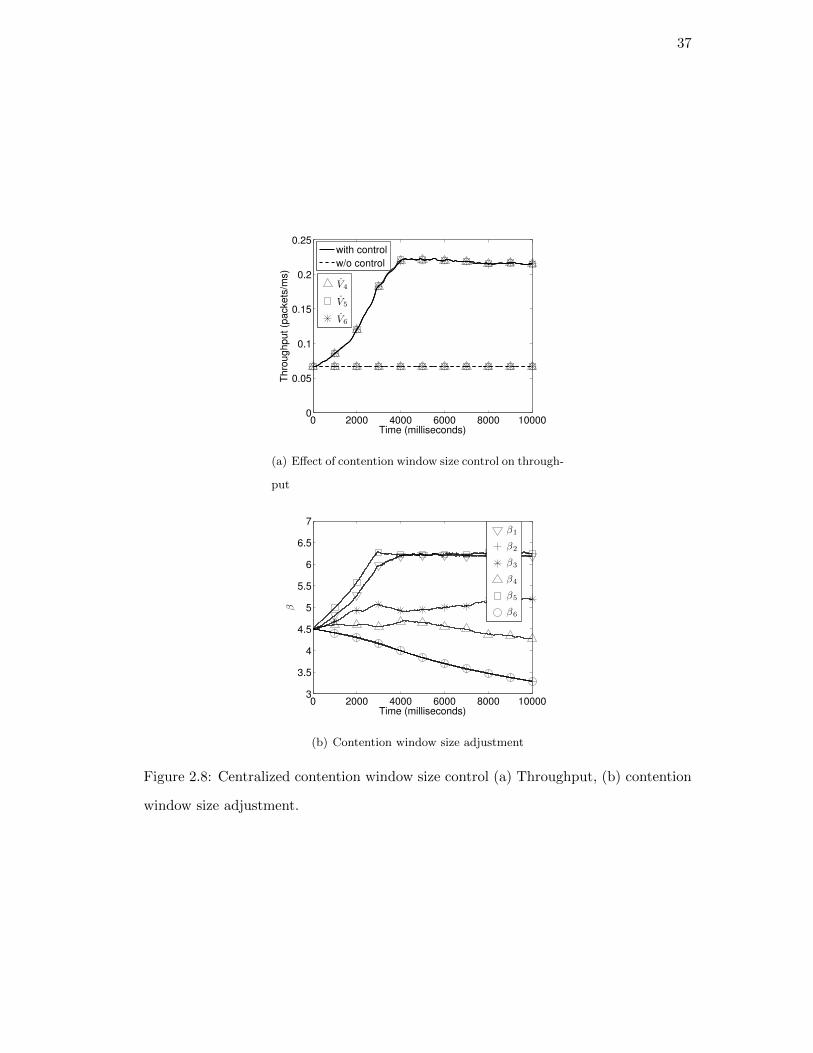
37

0 2000 4000 6000 8000 100000

0.05

0.1

0.15

0.2

0.25

Time (milliseconds)

Thro

ughput (p

ackets

/ms)

V4

V5

V6

with control

w/o control

(a) Effect of contention window size control on through-

put

0 2000 4000 6000 8000 100003

3.5

4

4.5

5

5.5

6

6.5

7

Time (milliseconds)

β

β1

β2

β3

β4

β5

β6

(b) Contention window size adjustment

Figure 2.8: Centralized contention window size control (a) Throughput, (b) contention

window size adjustment.

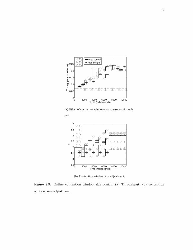
38

0 2000 4000 6000 8000 100000

0.05

0.1

0.15

0.2

0.25

Time (milliseconds)

Thro

ughput (p

ackets

/ms)

V4

V5

V6

with control

w/o control

(a) Effect of contention window size control on through-

put

0 2000 4000 6000 8000 100003.5

4

4.5

5

5.5

6

6.5

7

Time (milliseconds)

β

β1

β2

β3

β4

β5

β6

(b) Contention window size adjustment

Figure 2.9: Online contention window size control (a) Throughput, (b) contention

window size adjustment.

39

Chapter 3

Transport protocols for MobilityFirst future Internet

architecture

3.1 Introduction

The TCP/IP architecture underpinning the current Internet is based on the end-to-

end principle [34] of minimizing functionality in the network while handling service-

specific requirements such as error and flow control at the end-points. In addition,

the current Internet architecture is based on the concept of routing between IP ad-

dresses requiring a static one-to-one association between hosts and network locators.

While the Internet works well for traditional kinds of communication, emerging mobile

content and Internet-of-Things (IoT) services have motivated consideration of clean-

slate Information-Centric Network (ICN) architectures [35,36] which operate on names

rather than addresses. Several distinct architectures for ICN have recently been pro-

posed including MobilityFirst (MF) [37, 38], Named Data Network (NDN) [39], and

XIA [40]. While there are differences in detail, all the proposed ICN protocols share

some common design elements that need to be considered in the design of transport

protocols to be used for end-to-end services. Specific characteristics of ICN include: (a)

use of names to identify sources and sinks of information; (b) storage of information

at routers within the network in order to support content caching and disconnection;

(c) multicasting and anycasting as integral network services; and in the MF case (d)

hop-by-hop reliability protocols between routers in the network. These properties have

significant implications for transport protocol design since the current protocols, TCP

and UDP, were designed based on the end-to-end Internet principle, which typically

assumes end-to-end connectivity during a transfer and uses address based routing with

40

minimal functionality (i.e., no storage or reliability mechanisms) within the network.

Consider first the implications of name-based routing on transport protocol design.

Communication with named objects, whether content files, devices, groups of devices or

more complex context-based groups is different from conventional TCP connections in

the sense that an object may have multiple end-points because the object may be multi-

homed (i.e., multiple network interfaces to the same device) or multicast (to multiple

devices, each with a different network interface) or multi-copy (i.e., multiple instances

of the same information object can be found at different places in the network). This

indicates that transport protocols need to be designed to provide appropriate service

semantics for retrieving or delivering such named objects, for example, in multicast

where the information object reaches all the named destinations or anycast where the

object is fetched from the “nearest location”. A second important property of ICN

protocols is the fact that routers may store information objects such as content either

for caching or for delay tolerant delivery. This implies the existence of in-network

transport proxies which are in between the source and the destination, and the transport

protocol should be designed to take advantage of the in-network copy to provide the

desired service efficiently. For example, reliable delivery with an ICN transport would

be able to utilize a copy of the information object stored at an intermediate router

and avoid the need for end-to-end retransmission used in TCP. The third feature of

ICN architectures is the fact that in-network storage can be associated with reliable

hop-by-hop transmission of information objects between routers, thus alleviating the

need for strong reliability mechanisms at the transport layer depending on the type of

service desired.

In Section 3.2, we consider the requirements for ICN transport in further detail

and identify a set of core transport protocol functions needed to address an anticipated

range of service requirements. These core transport protocol components are developed

in further detail for a specific ICN architecture, MobilityFirst, and several examples of

how these functions are integrated with the named-object network layer are given in

Section 3.3. The prototype of MFTP is discussed in Section 3.4. Then we provide a

set of experimental results based on the prototype and compare its performance with

41

conventional TCP/IP to the extent possible.

Our contributions in designing and implementing transport protocols for an ICN

architecture with explicit locators, such as MF, are twofold: (i) we examine a repre-

sentative set of delivery service scenarios, and based on them, define the requirement

space for transport protocols for any Information Centric architecture; (ii) with explicit

locators in an ICN architecture, much richer end-to-end semantics, such as reliabil-

ity delegation, and in-network retransmission, are enabled by integrating in-network

transport services. We show that such features are conducive to supporting mobility,

and flexibly and robustly supporting different delivery patterns. The proposed de-

sign is validated using an experimental prototype, with bulk (e.g., video) content and

latency-sensitive web (text, image and video) content delivered over wireless networks

to mobile clients. The general principles of our design for end-to-end transport, re-

gardless of whether MF-like locators are used, can also be customized to work with

and bring benefits to NDN as well, e.g., to apply per-hop error and congestion control

to improve transmission efficiency, and employ router-proactive mechanisms to provide

better and richer mobility support.

3.2 Requirements for transport layer service for ICN

We analyze four common service scenarios, and identify the set of transport layer fea-

tures for an ICN environment (see the summary of requirements in Table 3.1).

Large file retrieval. A large file retrieval is abstracted as a get(content name) socket

call [41] in an ICN context. Clients inject a content request, independent of the content

location, with a get() call, and the network will route the request to the location of

a copy of the content. Then a flow with a large volume which carries the content is

transferred reliably from the server to the requesting client. This is often referred as

anycast.

Key TP functions required: Because of the large amount of data to be delivered, file

transfer requires: (i) fragmentation and sequencing at the source, and reassembly at

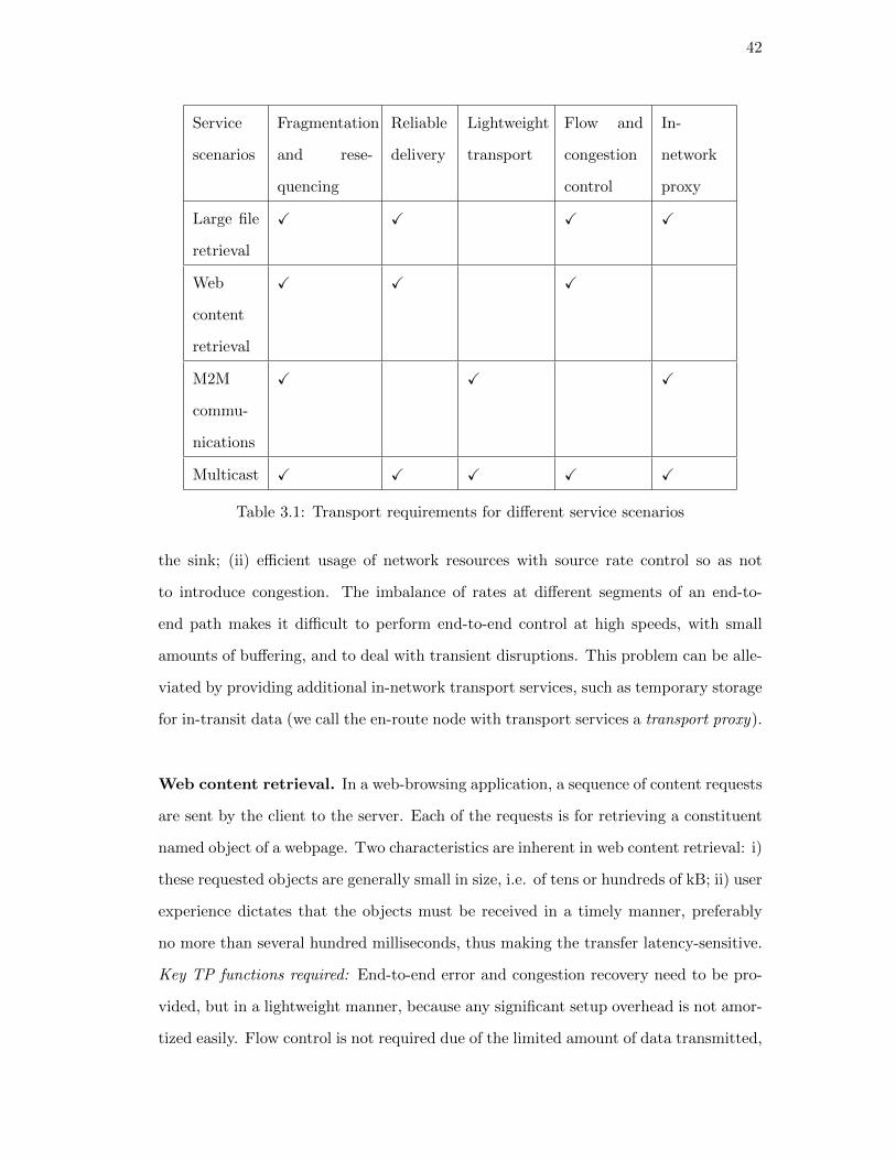
42

Service

scenarios

Fragmentation

and rese-

quencing

Reliable

delivery

Lightweight

transport

Flow and

congestion

control

In-

network

proxy

Large file

retrieval

X X X X

Web

content

retrieval

X X X

M2M

commu-

nications

X X X

Multicast X X X X X

Table 3.1: Transport requirements for different service scenarios

the sink; (ii) efficient usage of network resources with source rate control so as not

to introduce congestion. The imbalance of rates at different segments of an end-to-

end path makes it difficult to perform end-to-end control at high speeds, with small

amounts of buffering, and to deal with transient disruptions. This problem can be alle-

viated by providing additional in-network transport services, such as temporary storage

for in-transit data (we call the en-route node with transport services a transport proxy).

Web content retrieval. In a web-browsing application, a sequence of content requests

are sent by the client to the server. Each of the requests is for retrieving a constituent

named object of a webpage. Two characteristics are inherent in web content retrieval: i)

these requested objects are generally small in size, i.e. of tens or hundreds of kB; ii) user

experience dictates that the objects must be received in a timely manner, preferably

no more than several hundred milliseconds, thus making the transfer latency-sensitive.

Key TP functions required: End-to-end error and congestion recovery need to be pro-

vided, but in a lightweight manner, because any significant setup overhead is not amor-

tized easily. Flow control is not required due of the limited amount of data transmitted,

43

in order to avoid unnecessary overhead contributing to increased latency.

M2M communications. In Machine-to-machine (M2M) communications, sensor data

by nature is idempotent. That is, if the PDU is lost (due to bit errors or congestion)

or it is delayed beyond the limits of latency for the data, the transport layer need

not attempt to reliably deliver that PDU. This transfer paradigm is captured in a

send(dst name, content name) API with no explicit reliability preference.

Key TP functions required: In such cases, the transport layer could simply resort

to stateless communication (e.g., lightweight transport with no error recovery and no

flow/congestion control) to minimize overheads. Moreover, due to power constraints in

devices, a sensor node may not be on all the time. End-to-end control is not always

possible in this case and delegation of transport service guarantees, such as reliability,

need to be made to other en-route nodes. Thus in-network proxy support is desired.

Multicast. A number of popular applications are based on multicast, such as group-

based subscriptions (RSS), teleconferencing, online gaming, etc. In a name-based ar-

chitecture, multicast can be realized with a send (dst name, content name) API with

the dst name referring to a group of individual endpoints names.

Key TP functions required: Guaranteeing 100% reliability in a multicast session is a

well-known hard problem. To achieve reliable transport, the source relies on negative

acknowledgement (NACK) from clients to initiate retransmissions. With the number

of subscribers increasing, retransmission has to be implemented in an efficient manner

such that the ACK-implosion (see [42]) is avoided. This may require aggregation of

retransmission requests in the network, and retransmission from within the network.

Thus in-network proxies are desired to handle such aggregation and storage of pieces

of contents for retransmission.

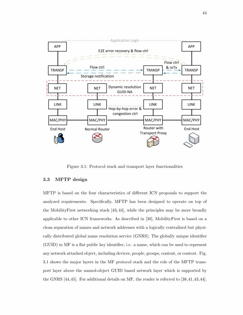
44

LINK LINK

MAC/PHY MAC/PHY MAC/PHY MAC/PHY

NET NET NET NET

TRANSP TRANSP TRANSP

APP APP

Application Logic

Hop-by-hop error & congestion ctrl

E2E error recovery & flow ctrl

Router with Transport Proxy

End Host End HostNormal Router

LINK LINK

Storage notification

Flow ctrl & reTx

Dynamic resolution GUID-NA

Flow ctrl

Figure 3.1: Protocol stack and transport layer functionalities

3.3 MFTP design

MFTP is based on the four characteristics of different ICN proposals to support the

analyzed requirements. Specifically, MFTP has been designed to operate on top of

the MobilityFirst networking stack [43, 44], while the principles may be more broadly

applicable to other ICN frameworks. As described in [38], MobilityFirst is based on a

clean separation of names and network addresses with a logically centralized but physi-

cally distributed global name resolution service (GNRS). The globally unique identifier

(GUID) in MF is a flat public key identifier, i.e. a name, which can be used to represent

any network attached object, including devices, people, groups, content, or context. Fig.

3.1 shows the major layers in the MF protocol stack and the role of the MFTP trans-

port layer above the named-object GUID based network layer which is supported by

the GNRS [44,45]. For additional details on MF, the reader is referred to [38,41,43,44].

45

Transport

Application/Socket

File A File B

a1 a2 aN b1 b2 bN... ...

a4a3

b4b3

Strict reordering Strict reordering

Loose Relationship

Different files uniquely named &

separated.

Figure 3.2: Illustration of named object’s implication to fragmentation and sequencing.

Transport layer fragments a content into large chunks. Sequential delivery is guaranteed

for each content, but no strict ordering maintained for chunks of different contents.

3.3.1 Segmentation and re-sequencing

Typically in ICN, a data request is abstracted by an API, get(content name). In NDN,

such a request, called an Interest, with an associated relative sequence number, solicits

one segment of a content. In MF, the requestor only sends one request for a piece

of content; the server that handles the request then segments the content and assigns

the segments a relative sequence number. In any case, sequence numbers are bound

to the named content, rather than the two endpoints. This has significant implication

for the hop-by-hop transfer and storage capability in ICN, as we shall see later. With

content-centricity, such a sequencing scheme works naturally for anycast, multicast and

multipath transfers. For example, in an anycast scenario, the forwarding plane decides

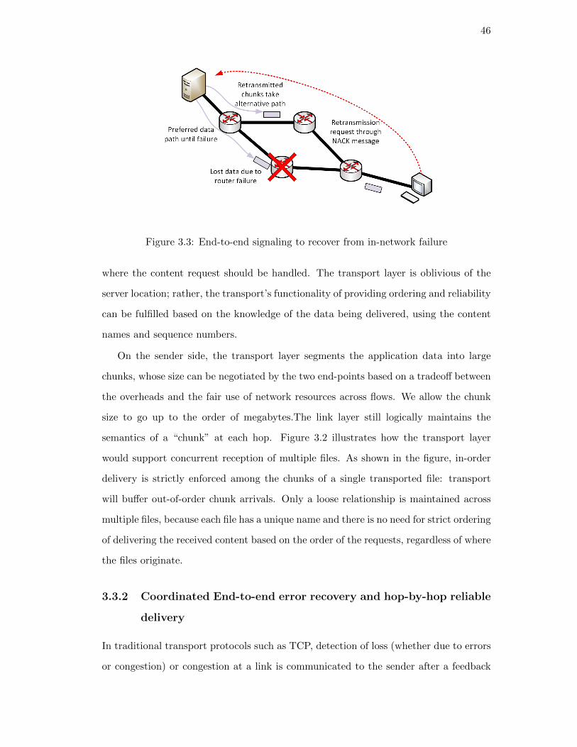
46

Figure 3.3: End-to-end signaling to recover from in-network failure

where the content request should be handled. The transport layer is oblivious of the

server location; rather, the transport’s functionality of providing ordering and reliability

can be fulfilled based on the knowledge of the data being delivered, using the content

names and sequence numbers.

On the sender side, the transport layer segments the application data into large

chunks, whose size can be negotiated by the two end-points based on a tradeoff between

the overheads and the fair use of network resources across flows. We allow the chunk

size to go up to the order of megabytes.The link layer still logically maintains the

semantics of a “chunk” at each hop. Figure 3.2 illustrates how the transport layer

would support concurrent reception of multiple files. As shown in the figure, in-order

delivery is strictly enforced among the chunks of a single transported file: transport

will buffer out-of-order chunk arrivals. Only a loose relationship is maintained across

multiple files, because each file has a unique name and there is no need for strict ordering

of delivering the received content based on the order of the requests, regardless of where

the files originate.

3.3.2 Coordinated End-to-end error recovery and hop-by-hop reliable

delivery

In traditional transport protocols such as TCP, detection of loss (whether due to errors

or congestion) or congestion at a link is communicated to the sender after a feedback

47

delay, possibly quite a few end-to-end RTT’s. After the detection, recovery mechanisms,

such as congestion recovery or retransmission, can incur an unduly large penalty to the

flow. Also, due to queuing at routers, and heterogeneous transmission technologies

employed along the route to destination, spurious, or premature, retransmissions are

not uncommon [46]. Link level mechanisms alleviate these problems as errors can be

detected and reacted upon more quickly. Hop-by-hop transfer is suitable in ICN due

in part to the fact that the segment of data being transferred is named; moreover, ICN

routers can have storage capability, and can temporarily store the in-transit copy to

provide delay-tolerant delivery, and also cache a copy to serve future requests. In NDN,

each named data item is indeed transferred in a hop-by-hop manner: upon receiving

such a data item, the router examines whether an Interest for the data has been received

earlier, and whether it needs to cache the data.

MFTP integrates per-hop error recovery and congestion control whenever the prob-

lem can be resolved locally, and only invokes end-to-end mechanisms when it is ab-

solutely necessary, e.g., a router fails and loses all the buffered data. On each hop,

after every chunk that is transmitted, a corresponding control message called CSYN

is used to explicitly request acknowledgement from downstream, which then replies

with a bitmap of reception status for every packet in that chunk. The transmission

for this chunk finishes if there is no loss, otherwise the lost packets of that chunk are

retransmitted locally following the same procedure until all packets are received.

Taking advantage of the hop-by-hop reliability of the network, we seek to have a

parsimonious end-to-end mechanism that has minimal overhead. The end-to-end error

recovery mechanism is built to be flexible to accommodate application and sender needs

(including don’t care, NACK, ACK ). With a Negative-ACK, i.e. NACK, the transport

reduces end-to-end message overhead, and the receiver provides notification only when

a chunk is not delivered over a conservatively long period of time (as a result of a

failure that causes the reliable hop-by-hop mechanism to lose an acknowledged chunk

as shown in Figure 3.3). It is only for short-sessions (e.g., single PDU delivery) and

for latency-sensitive interactions that the sender would enable the use of an end-to-end

ACK option. With idempotent data transmissions (e.g, sensor data which the transport

48

Figure 3.4: Procedures involved to use in-network transport proxy to handle destina-

tion disconnection and retransmission: the proxy temporarily stores chunks when the

destination disconnects, and transmits to the client when connectivity is restored as

indicated by the name resolution service.

layer sends and forgets), the sender may choose to use the don’t care option.

3.3.3 In-network transport proxy

One of the challenges for conventional transport protocols is in dealing with the content

delivery to mobile devices, where mobility results in intermittent connectivity and the

end-to-end connection experiences frequent disruptions. If the transport protocol has

to re-establish the connection, then the transfer has to re-start and any data already in

transit in the network will have to be discarded. ICN’s architecture inherently supports

mobility and resolves connection disruptions in multiple ways. For instance, in NDN,

each data is solicited by an Interest packet; in case a client moves before obtaining

the requested data, it can re-issue an Interest packet for the same data, which will be

delivered to the new location. In the MF architecture, the network can take on a more

proactive role in re-initiating data transfers when connectivity is re-established.

To this end, we postulate having routers (or at least a subset of them) which provide

49

in-network transport service such that the original source can delegate part of the end-

to-end data transfer responsibility. The router, which we call an in-network transport

proxy, would have substantial amounts of memory, e.g., several GB, to temporarily hold

in-transit chunks when the destination is unreachable. This disruption may be due to:

lack of connectivity to a mobile destination node, until connectivity is subsequently re-

established; alternatively, in M2M communication, when a sensor node is only powered

on intermittently, it may choose to deliver information chunks to the next hop and then

power down.

The mechanisms implemented by such a node are shown in Figure 3.4: when faced

with the impossibility of forwarding chunks with the information available at the net-

work layer (i.e. the router detects that connectivity towards the destination of a chunk

is disrupted), the router pushes up to the transport proxy layer the relative data chunks.

Two reasons might generate this impossibility of forwarding chunks: (i) the destina-

tion does not have an active network address (NA) binding corresponding to its GUID

entry in the GNRS; (ii) the chunk reaches the destination network given by its most

recent binding, but either the destination has changed its point of attachment or it

has disconnected from the network before the previous NA entry expires in the GNRS

server. As a consequence, the link layer is not able to deliver the chunk despite several

attempts, and corresponding CSYN timeouts. In these cases, the chunk is pushed up

to the proxy layer to be temporarily stored. While this is similar to Delay-Tolerant

Network protocols, the innovation here is the integration of these mechanisms with the

support of dynamic mobility and ICN style named object services.

We limit the amount of content that can be stored for a flow. Each (source GUID,

destination GUID) pair is limited to have buffered content up to size S. When a chunk

for a new flow arrives, the chunk will be stored directly if sufficient space is available

for the new flow; otherwise, a chunk for the oldest flow is replaced from the storage

by the new chunk. When the chunk is stored, a timer is created to schedule future

transmission. Further, a transport layer message, either Store or Drop, is transmitted

back to the original source to notify it of the intermediate proxy storing or dropping the

chunk. A stored chunk will be scheduled to retry a GNRS lookup to bind an updated

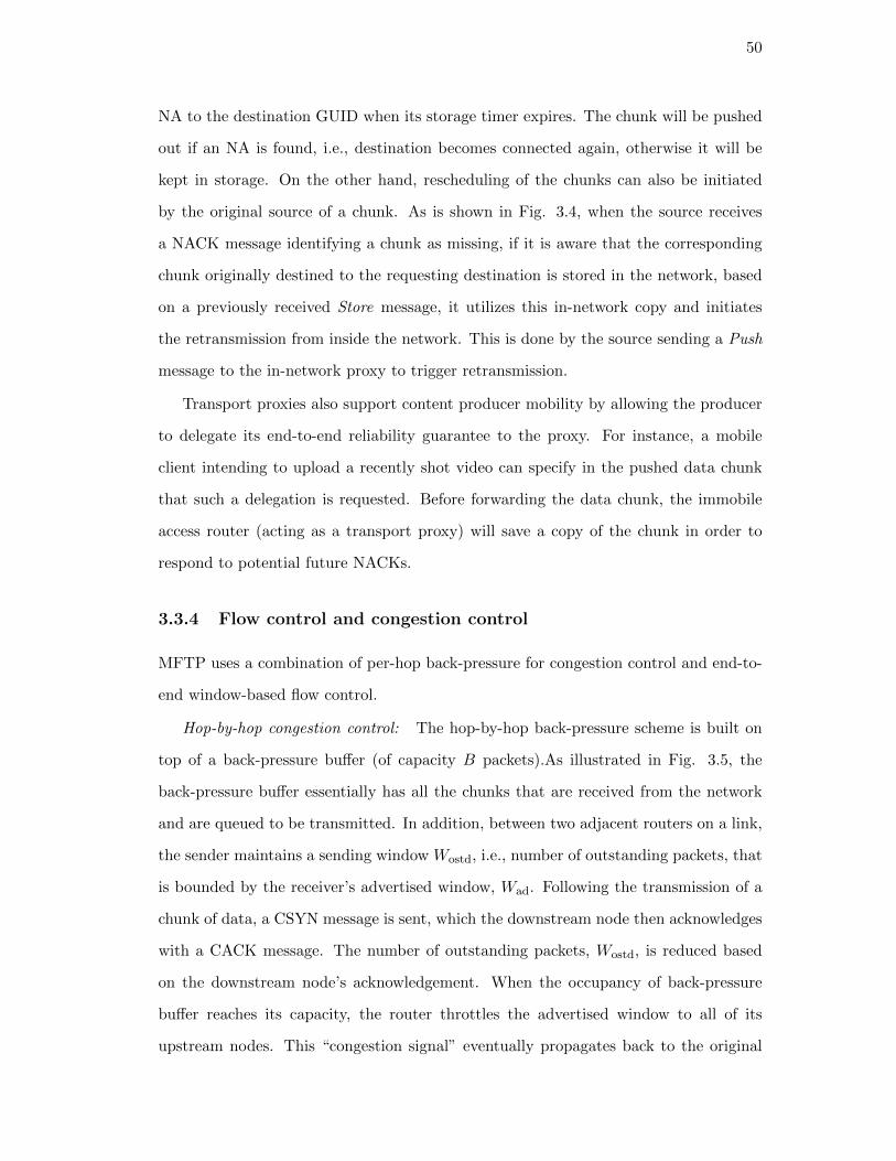
50

NA to the destination GUID when its storage timer expires. The chunk will be pushed

out if an NA is found, i.e., destination becomes connected again, otherwise it will be

kept in storage. On the other hand, rescheduling of the chunks can also be initiated

by the original source of a chunk. As is shown in Fig. 3.4, when the source receives

a NACK message identifying a chunk as missing, if it is aware that the corresponding

chunk originally destined to the requesting destination is stored in the network, based

on a previously received Store message, it utilizes this in-network copy and initiates

the retransmission from inside the network. This is done by the source sending a Push

message to the in-network proxy to trigger retransmission.

Transport proxies also support content producer mobility by allowing the producer

to delegate its end-to-end reliability guarantee to the proxy. For instance, a mobile

client intending to upload a recently shot video can specify in the pushed data chunk

that such a delegation is requested. Before forwarding the data chunk, the immobile

access router (acting as a transport proxy) will save a copy of the chunk in order to

respond to potential future NACKs.

3.3.4 Flow control and congestion control

MFTP uses a combination of per-hop back-pressure for congestion control and end-to-

end window-based flow control.

Hop-by-hop congestion control: The hop-by-hop back-pressure scheme is built on

top of a back-pressure buffer (of capacity B packets).As illustrated in Fig. 3.5, the

back-pressure buffer essentially has all the chunks that are received from the network

and are queued to be transmitted. In addition, between two adjacent routers on a link,

the sender maintains a sending window Wostd, i.e., number of outstanding packets, that

is bounded by the receiver’s advertised window, Wad. Following the transmission of a

chunk of data, a CSYN message is sent, which the downstream node then acknowledges

with a CACK message. The number of outstanding packets, Wostd, is reduced based

on the downstream node’s acknowledgement. When the occupancy of back-pressure

buffer reaches its capacity, the router throttles the advertised window to all of its

upstream nodes. This “congestion signal” eventually propagates back to the original

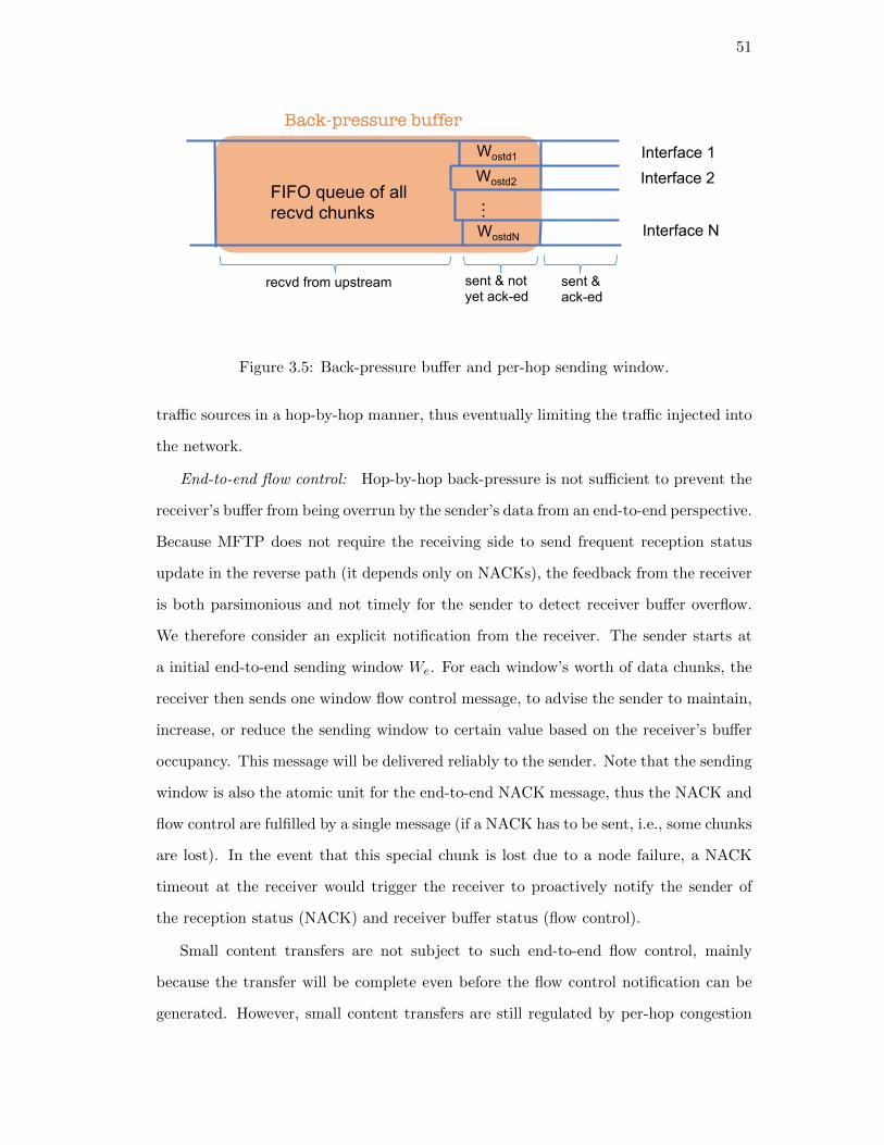
51

Wostd1 Wostd2

WostdN

FIFO queue of all recvd chunks

…

Interface 1

Interface N

Back-pressure buffer

sent & ack-ed

sent & not yet ack-ed

recvd from upstream

Interface 2

Figure 3.5: Back-pressure buffer and per-hop sending window.

traffic sources in a hop-by-hop manner, thus eventually limiting the traffic injected into

the network.

End-to-end flow control: Hop-by-hop back-pressure is not sufficient to prevent the

receiver’s buffer from being overrun by the sender’s data from an end-to-end perspective.

Because MFTP does not require the receiving side to send frequent reception status

update in the reverse path (it depends only on NACKs), the feedback from the receiver

is both parsimonious and not timely for the sender to detect receiver buffer overflow.

We therefore consider an explicit notification from the receiver. The sender starts at

a initial end-to-end sending window We. For each window’s worth of data chunks, the

receiver then sends one window flow control message, to advise the sender to maintain,

increase, or reduce the sending window to certain value based on the receiver’s buffer

occupancy. This message will be delivered reliably to the sender. Note that the sending

window is also the atomic unit for the end-to-end NACK message, thus the NACK and

flow control are fulfilled by a single message (if a NACK has to be sent, i.e., some chunks

are lost). In the event that this special chunk is lost due to a node failure, a NACK

timeout at the receiver would trigger the receiver to proactively notify the sender of

the reception status (NACK) and receiver buffer status (flow control).

Small content transfers are not subject to such end-to-end flow control, mainly

because the transfer will be complete even before the flow control notification can be

generated. However, small content transfers are still regulated by per-hop congestion

52

Figure 3.6: Multicast data delivery, small scale (left), large scale (right).

control.

Alleviating head-of-line blocking due to hop-by-hop transfer: A drawback inherent

with hop-by-hop back pressure is the unfairness caused by head-of-line (HOL) blocking

with FIFO queueing [47]. Theoretically, per-flow queuing solves this problem, but

scheduling with per-flow queues is difficult to scale and is impractical with large numbers

of flows. However, the in-network transport proxy provides some relief to this situation

and alleviates the short-term unfairness. If a back-pressure signal is received for the

chunk at the head of the sending queue, the transfers of chunks destined to other nodes

will thus not be blocked because chunk at the head of the queue will be removed and

pushed up to the transport proxy layer for temporary storage. The transport proxy

will then attempt to transmit that chunk when the storage timer expires (or is dropped

if the chunk is replaced in the storage buffer because of the replacement policy we

described above).

3.3.5 Multicast

Multicast is naturally supported by name based architectures. For instance, in NDN,

data is forwarded to the requestor based on the receipt of the corresponding request:

each router forwards the data on the interface(s) the request for the data was received

on. Multicast is thus fulfilled by the stateful forwarding plane [39]. In MobilityFirst, a

53

dynamically formed multicast group is explicitly identified by a globally unique identifier

(GUID), which can be mapped into a set of individual clients’ GUIDs or network

addresses.

A small scale scenario is depicted on the left side of Figure 3.6. During the transmis-

sion the source of the multicast data marks outgoing chunks with a multicast service

identifier and selects as destination GUID the one identifying the multicast group.

Multicast clients send NACK messages over a unicast channel and the multicast source

can identify which multicast group a specific client belongs to. Further, the source

aggregates retransmission requests for the transmitted chunks; it can, either employ

multicast again for retransmission when the number of requestors exceeds a threshold;

otherwise retransmitted data chunks can be sent using unicast destination GUIDs that

identify the specific nodes that need the retransmitted data.

As the number of participants increases we can exploit in-network transport proxies

to build multiple levels of multicast group GUID to a set of GUIDs mappings recursively.

This scenario is shown on the right side of Figure 3.6. In order to limit potential

explosion of unfulfilled requests reaching the original source, transport proxies can

be instructed through proper chunk marking, to discard retransmission requests that

exceed a number of traversed proxies without encountering the missing chunks. In a

scenario where reliability is not demanded, the source just use the don’t care option of

the reliability preference.

3.4 Implementation

Our implementation of MFTP consists of two parts: end-system transport operations

that are implemented on the MobilityFirst client stack [41], and an in-network transport

proxy implemented as a pluggable module inside a MobilityFirst Click router imple-

mentation.

Host Stack and API. The client host stack has been implemented on Linux as a

user-level process built as an event-based data pipeline. Apart from the MF transport

54

protocol, the stack contains a name-based network layer and a reliable link layer with

large chunk transfer. Applications interface with the host stack through socket APIs

that are available as a linkable library and include the primitives send, recv, and get,

and a set of meta-operations. Examples of meta-operations include those to bind or

attach a GUID to one or more NAs. By specifying the options field in the API call,

an application is able to configure transport parameters such as the i) desired chunk

size; ii) end-to-end reliability preference; iii) NACK timeout; iv) willingness to use in-

network proxy.

Router. The MobilityFirst software router is implemented as a set of routing and

forwarding elements using Click [48]. The router implements MFTP transport proxy

layer, MF network layer including intra-domain routing and dynamic binding using

GNRS, and hop-by-hop reliable transfer. The transport layer (proxy) interacts with

the intra-domain route look up component: if a lookup does not yield a valid next hop,

the chunk is pushed up to the transport proxy. The transport proxy at the router will

hold the data chunk for some time and attempt to rebind the name with one or more

network addresses. When rebinding is successful, the chunk is pushed back down to

the routing layer for forwarding.

Timers. There are three types of timers used in our implementation: one for trig-

gering the transmission of an end-to-end NACK message, one for storage, and another

one for link layer retransmission. For guaranteeing end-to-end reliability, timers are

indispensable because a node has to learn about a remote node’s failure impacting the

end-end path. Previous experience with TCP end-to-end timers have taught us that

timers need to be set loosely so as to reduce number of false alarms [49, 50], and not

have a strict dependence of the transport protocol on timers for normal operations. In

MFTP’s design, this goal is achievable because: (i) different end-to-end service guar-

antees are dissected and each timer only handles a specific job; (ii) NACK timers and

per-hop timers are associated with a chunk of data, rather than a single packet; (ii)

the storage timer is only concerned about disconnection, and is thus decoupled from

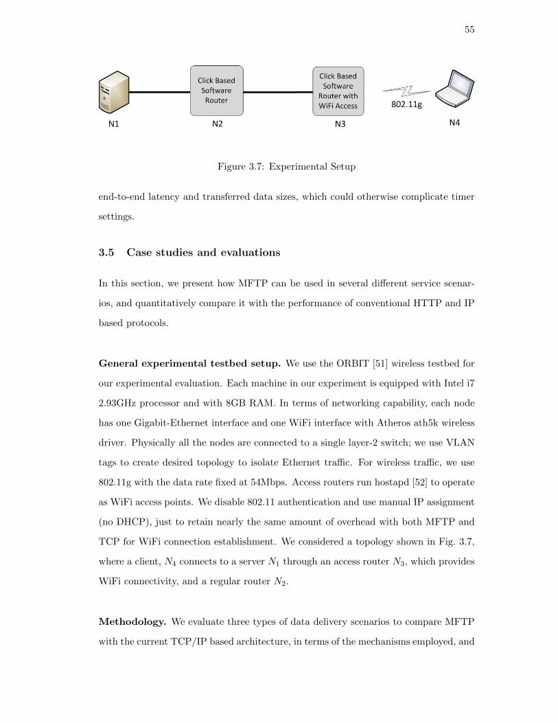
55

Figure 3.7: Experimental Setup

end-to-end latency and transferred data sizes, which could otherwise complicate timer

settings.

3.5 Case studies and evaluations

In this section, we present how MFTP can be used in several different service scenar-

ios, and quantitatively compare it with the performance of conventional HTTP and IP

based protocols.

General experimental testbed setup. We use the ORBIT [51] wireless testbed for

our experimental evaluation. Each machine in our experiment is equipped with Intel i7

2.93GHz processor and with 8GB RAM. In terms of networking capability, each node

has one Gigabit-Ethernet interface and one WiFi interface with Atheros ath5k wireless

driver. Physically all the nodes are connected to a single layer-2 switch; we use VLAN

tags to create desired topology to isolate Ethernet traffic. For wireless traffic, we use

802.11g with the data rate fixed at 54Mbps. Access routers run hostapd [52] to operate

as WiFi access points. We disable 802.11 authentication and use manual IP assignment

(no DHCP), just to retain nearly the same amount of overhead with both MFTP and

TCP for WiFi connection establishment. We considered a topology shown in Fig. 3.7,

where a client, N4 connects to a server N1 through an access router N3, which provides

WiFi connectivity, and a regular router N2.

Methodology. We evaluate three types of data delivery scenarios to compare MFTP

with the current TCP/IP based architecture, in terms of the mechanisms employed, and

56

their performance. We emulate the end-to-end RTT’s of local, coast-to-coast and inter-

continental communications, use the emulation tool netem [53] to add 10ms, 50ms,

100ms RTT between the two routers, respectively. To emulate loss in a controlled

manner, we again use netem to introduce 1% loss. With MF, we run the MF Click

router prototype (mentioned in section 3.4), and a local GNRS server on both N2

and N3. The MF client stack runs on N1 and N4. For specific use cases, we run

corresponding applications that interface with the client stack through the MF API. In

the case of TCP-based experiments, we run Click IP routers on node N2 and N3. TCP

segmentation offloading is turned off as the basic Click IP router drops TCP packets

with size larger than 1500 bytes. We enabled manual Ethernet header encapsulation

on the Click IP router so no ARP message is triggered during routing. On the two

end nodes, the default version of TCP, TCP Cubic, is used. We configured both nodes’

TCP receiver buffer to be 2MB, so that it is not a bottleneck in a high delay-bandwidth

path in any of the experiments.

3.5.1 Large content delivery over wireless

We first look into a large volume data transfer experiment. A 400MB file is requested

and transferred. A simple file retrieval application in MF is running on the two end

nodes. In the case of TCP, we used iperf to generate a flow of equal size with the

maximum packet payload size of 1400 bytes. We repeated this experiment for a num-

ber of network conditions: RTT being 10ms, 50ms, or 100ms, and loss on WiFi link

being 0 or 1%, to explore their effect on both architectures’ goodput (i.e., application

throughput).

Fig. 3.8(a) shows the average throughput comparisons for the six different network

settings. Both MFTP and TCP’ throughputs are consistently high when there is no

loss, despite varying the end-to-end latency. MFTP is slightly higher in throughput

in the lossless cases. MFTP is significantly more robust in the presence of loss, e.g.,

the throughput degrades by only 10% when there is 1% residual loss, with all 3 RTT

profiles. On the other hand, TCP throughput drops significantly when there is loss.

For instance, with 50ms RTT, TCP throughput with loss drops to only a quarter of its

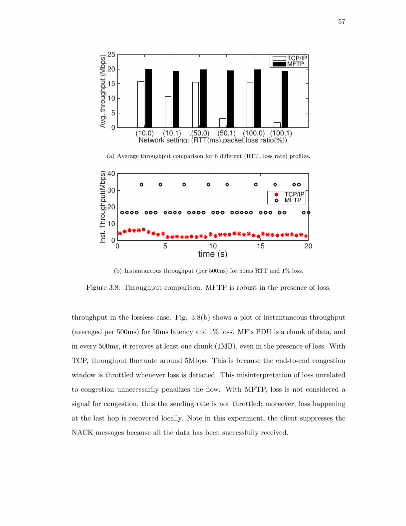
57

Network setting: (RTT(ms),packet loss ratio(%))(10,0) (10,1) ,(50,0) (50,1) (100,0) (100,1)

Avg

. th

rou

gh

pu

t (M

bp

s)

0

5

10

15

20

25TCP/IPMFTP

(a) Average throughput comparison for 6 different (RTT, loss rate) profiles.

time (s)0 5 10 15 20

Inst.

Th

rou

gh

pu

t(M

bp

s)

0

10

20

30

40

TCP/IPMFTP

(b) Instantaneous throughput (per 500ms) for 50ms RTT and 1% loss.

Figure 3.8: Throughput comparison. MFTP is robust in the presence of loss.

throughput in the lossless case. Fig. 3.8(b) shows a plot of instantaneous throughput

(averaged per 500ms) for 50ms latency and 1% loss. MF’s PDU is a chunk of data, and

in every 500ms, it receives at least one chunk (1MB), even in the presence of loss. With

TCP, throughput fluctuate around 5Mbps. This is because the end-to-end congestion

window is throttled whenever loss is detected. This misinterpretation of loss unrelated

to congestion unnecessarily penalizes the flow. With MFTP, loss is not considered a

signal for congestion, thus the sending rate is not throttled; moreover, loss happening

at the last hop is recovered locally. Note in this experiment, the client suppresses the

NACK messages because all the data has been successfully received.

58

3.5.2 Transport proxy for disconnection

We evaluate the benefits of using in-network transport proxies for handling client discon-

nections in content retrieval. We consider the same topology as above. The end-to-end

RTT is set to be 50ms, and no loss is added so that difference in performance would

not be incurred by having different mechanisms for error recovery. We use netem to

introduce 100% loss intermittently, so as to emulate client disconnections. In the ex-

periment, WiFi connectivity is on for 10 seconds; then is turned off for d seconds; then

the connection is restored. During the first 10 seconds of connection, the client requests

a 10MB file at a random time. The experiment is repeated 30 times for both MF and

TCP. We compare the distribution of file retrieval response times between MFTP and

TCP.

In Fig. 3.9(a), all the transfers having a response time of less than 10 seconds are

completed before the disconnection. For the transfers that experience the disconnec-

tion, MFTP has at least 3 seconds lower response time (at 60th percentile). With 30

seconds disconnection, as shown in Fig. 3.9(b), the difference in response time is about

15 seconds at 70th percentile. It is worthwhile to understand the difference in the

approaches taken by TCP and MFTP to dealing with disconnection. With TCP, the

sender retransmits, based on a timer whose timeout value increases exponentially when

the disconnection persists. In MFTP, the chunk in-transit is stored at the in-network

proxy. A network address and next-hop lookup, rather than retransmission, is triggered

when the storage timer for that chunk expires. Thus the transport proxy takes advan-

tages of the global name resolution service in MF to learn whether there is a network

address binding update for a client, and retransmits only when client is connected.

This results in fewer retransmission attempts and more accuracy in the knowledge of

end-to-end connectivity. Fig. 3.9(a) and Fig. 3.9(b) together suggest that MFTP’s

reduction in response time is nearly proportional to the length of the disconnection.

59

Response time (seconds)0 5 10 15 20 25 30

Cu

mu

lative

Pro

ba

bili

ty

0

0.2

0.4

0.6

0.8

1

MFTPTCP/IP

(a) With 10s disconnection

Response time (seconds)0 10 20 30 40 50 60 70

Cu

mu

lative

Pro

ba

bili

ty

0

0.2

0.4

0.6

0.8

1

MFTPTCP/IP

(b) With 30s disconnection

Figure 3.9: CDF of response times.

Comparison between network-proactive and receiver-driven approaches

We perform another set of experiments, with two different settings of proxy’s storage

and client’s NACK timers. The network-proactive approach was used in the previous

experiment, where the NACK timers are set conservatively, and thus clients rely on the

network to re-deliver the data once a new connection is available. In the receiver-driven

approach, the proxy does not re-initiate the delivery; the clients set the NACK timer

aggressively and explicitly request retransmission, and the original server will request

the retransmission from the transport proxy where the data is stored. As shown in

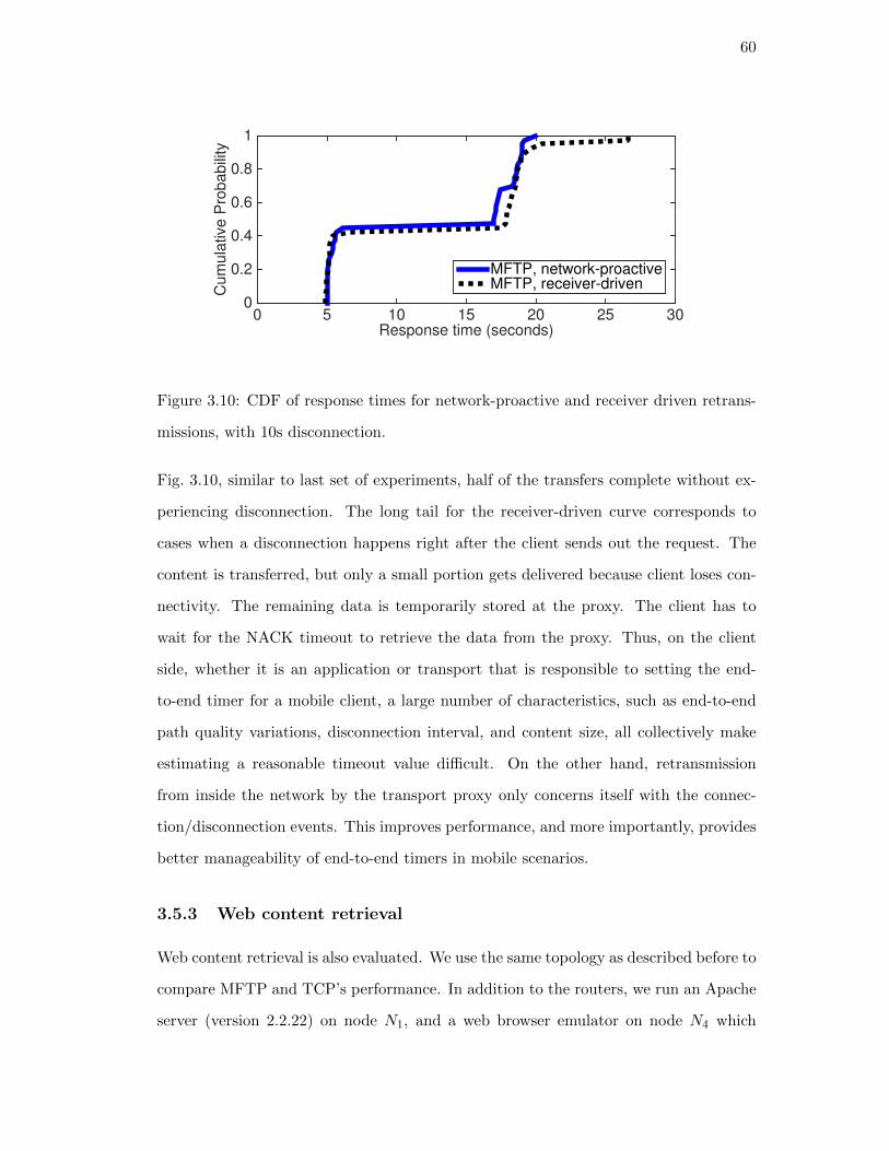
60

Response time (seconds)0 5 10 15 20 25 30

Cu

mu

lative

Pro

ba

bili

ty

0

0.2

0.4

0.6

0.8

1

MFTP, network-proactiveMFTP, receiver-driven

Figure 3.10: CDF of response times for network-proactive and receiver driven retrans-

missions, with 10s disconnection.

Fig. 3.10, similar to last set of experiments, half of the transfers complete without ex-

periencing disconnection. The long tail for the receiver-driven curve corresponds to

cases when a disconnection happens right after the client sends out the request. The

content is transferred, but only a small portion gets delivered because client loses con-

nectivity. The remaining data is temporarily stored at the proxy. The client has to

wait for the NACK timeout to retrieve the data from the proxy. Thus, on the client

side, whether it is an application or transport that is responsible to setting the end-

to-end timer for a mobile client, a large number of characteristics, such as end-to-end

path quality variations, disconnection interval, and content size, all collectively make

estimating a reasonable timeout value difficult. On the other hand, retransmission

from inside the network by the transport proxy only concerns itself with the connec-

tion/disconnection events. This improves performance, and more importantly, provides

better manageability of end-to-end timers in mobile scenarios.

3.5.3 Web content retrieval

Web content retrieval is also evaluated. We use the same topology as described before to

compare MFTP and TCP’s performance. In addition to the routers, we run an Apache

server (version 2.2.22) on node N1, and a web browser emulator on node N4 which

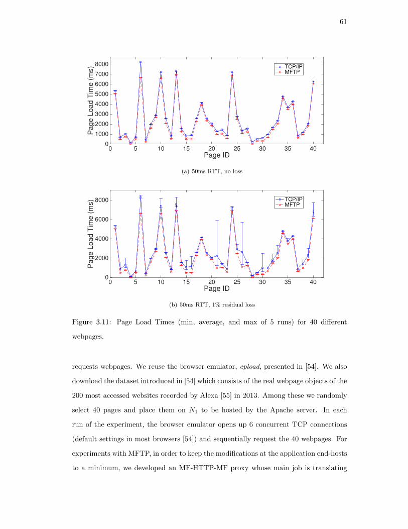
61

Page ID0 5 10 15 20 25 30 35 40

Page L

oad T

ime (

ms)

0

1000

2000

3000

4000

5000

6000

7000

8000 TCP/IPMFTP

(a) 50ms RTT, no loss

Page ID0 5 10 15 20 25 30 35 40

Page L

oad T

ime (

ms)

0

2000

4000

6000

8000 TCP/IPMFTP

(b) 50ms RTT, 1% residual loss

Figure 3.11: Page Load Times (min, average, and max of 5 runs) for 40 different

webpages.

requests webpages. We reuse the browser emulator, epload, presented in [54]. We also

download the dataset introduced in [54] which consists of the real webpage objects of the

200 most accessed websites recorded by Alexa [55] in 2013. Among these we randomly

select 40 pages and place them on N1 to be hosted by the Apache server. In each

run of the experiment, the browser emulator opens up 6 concurrent TCP connections

(default settings in most browsers [54]) and sequentially request the 40 webpages. For

experiments with MFTP, in order to keep the modifications at the application end-hosts

to a minimum, we developed an MF-HTTP-MF proxy whose main job is translating

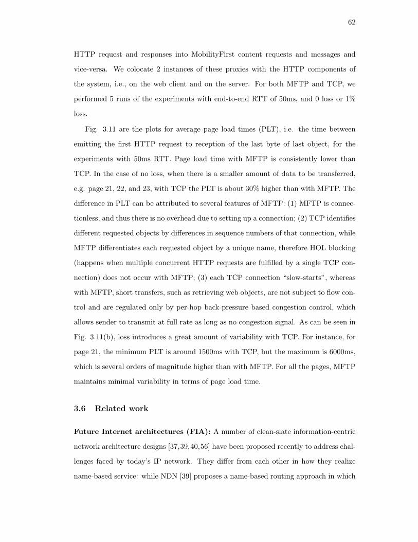
62

HTTP request and responses into MobilityFirst content requests and messages and

vice-versa. We colocate 2 instances of these proxies with the HTTP components of

the system, i.e., on the web client and on the server. For both MFTP and TCP, we

performed 5 runs of the experiments with end-to-end RTT of 50ms, and 0 loss or 1%

loss.

Fig. 3.11 are the plots for average page load times (PLT), i.e. the time between

emitting the first HTTP request to reception of the last byte of last object, for the

experiments with 50ms RTT. Page load time with MFTP is consistently lower than

TCP. In the case of no loss, when there is a smaller amount of data to be transferred,

e.g. page 21, 22, and 23, with TCP the PLT is about 30% higher than with MFTP. The

difference in PLT can be attributed to several features of MFTP: (1) MFTP is connec-

tionless, and thus there is no overhead due to setting up a connection; (2) TCP identifies

different requested objects by differences in sequence numbers of that connection, while

MFTP differentiates each requested object by a unique name, therefore HOL blocking

(happens when multiple concurrent HTTP requests are fulfilled by a single TCP con-

nection) does not occur with MFTP; (3) each TCP connection “slow-starts”, whereas

with MFTP, short transfers, such as retrieving web objects, are not subject to flow con-

trol and are regulated only by per-hop back-pressure based congestion control, which

allows sender to transmit at full rate as long as no congestion signal. As can be seen in

Fig. 3.11(b), loss introduces a great amount of variability with TCP. For instance, for

page 21, the minimum PLT is around 1500ms with TCP, but the maximum is 6000ms,

which is several orders of magnitude higher than with MFTP. For all the pages, MFTP

maintains minimal variability in terms of page load time.

3.6 Related work

Future Internet architectures (FIA): A number of clean-slate information-centric

network architecture designs [37,39,40,56] have been proposed recently to address chal-

lenges faced by today’s IP network. They differ from each other in how they realize

name-based service: while NDN [39] proposes a name-based routing approach in which

63

packets are forwarded directly based on name; some other architectures (like Mobility-

First [37], XIA [40] and HIP [56]) place object names outside of the routing plane and

uses a name resolution service to translate names to addresses.

Transport protocols for FIA: There have been a number of works on transport

protocols for FIA, e.g. NDN [39], and XIA [40]. In NDN, a receiver asks for content

by issuing a group of interest packets, i.e. requests; the corresponding data chunk

is returned by the network in response to each interest. The NDN community has

looked at how the transport layer can be adapted to such a interest-data interactive

and multi-source/multi-path content-transfer pattern. Most of these works propose that

the receiver maintains a Interest window and controls the issuing rate of interest packets

(i.e., ICTP [57]), while others proposes a hop-by-hop Interest shaping scheme at each

router (i.e., HR-ICP [58]). To support multi-source/multi-path transfer, CHoPCoP [59]

proposes to utilize explicit congestion signaling from network to effectively notify the

receiver about network conditions. In [60], a transport protocol, Tapa, for XIA ar-

chitecture [40] is introduced which proposes to manage end-to-end delivery through

segment-by-segment control. We share some of the techniques with these schemes here

for the MFTP design. In addition, we investigate a broader set of ICN transport re-

quirements which are derived from a collection of data delivery service scenarios. This

allows MFTP to flexibly support different applications ranging from receiver-initiated

retrieval, to sender-initiated publish, and from throughput-sensitive large file transfer,

to latency-constrained short transfers of web objects.

64

Chapter 4

Scalable, network-assisted congestion control for the

MobilityFirst future Internet architecture

4.1 Introduction

In this chapter, we present the design of a network-assisted congestion control frame-

work for an Information Centric Network (ICN) architecture, MobilityFirst. Informa-

tion Centric Network architectures place various intelligent functionalities inside the

network to assist with efficient, and reliable data delivery. Unlike traditional conges-

tion control in which only endpoints of the communication participate actively, the

congestion control scheme to be presented involves active interaction between traffic

sources and network routers, and depends heavily on various network functionalities

offered by ICN.

Information/Content Centric Networks have been an area of significant research ef-

forts in the recent past, with multiple proposed architectures ( [38, 40, 61]) seeking to

deliver information efficiently, based on a network layer that identifies content, indepen-

dent of location. The network’s ability to find better (and all) sources of content fully

takes advantage of in-network caching, potentially reducing data retrieval latency by

serving the data request from the cache which is closer to users compared with original

servers. Several distinct features of ICN make traditional end-to-end congestion control

such as TCP unsuitable. First, data transferred in ICN is often in large chunks, which

means congestion detection and control has to operate on coarser granularity. Second,

network may provide segment-wise or hop-by-hop reliability, to facilitate caching, or

delay tolerant delivery, and to efficiently recover from loss locally. This results in infre-

quent end-to-end acknowledgements, which present challenges if congestion detection is

65

based upon such acknowledgements. In addition, as the network provides reliability at

the protocol data unit (PDU) level, congestion control and reliability can be unbundled

(as compared to TCP), potentially opening up to simpler congestion control schemes.

In this chapter, we present the design and evaluation of congestion control for one

of the Information Centric Network architectures, MobilityFirst (MF) [38]. In MF,

several of the intelligent network assistance mechanisms discussed above are considered

core network functionality. MF routers are able to store content for caching as well

as for delay tolerant delivery [62]. MF routers also provide reliability guarantees so

that data can be transferred reliably along each hop, and efficiently over lossy links.

These features make MF desirable for a variety of applications, one of which that is

seeing growing interest is Internet-of-Things (IoT) networking. Under a very resource-

constrained environment, endpoints in IoT systems, such as sensors, have limited power

budget. Taking advantage of the network functionality we consider, such sensor nodes

can implement a “send & forget” primitive to transfer data while conserving energy.

Even though individual sensor traffic tends to be small and infrequent, for the the net-

work to scale to tens of thousands of sensors, a flow and congestion control mechanism

is highly desirable. Thus, being easy to scale is a major design goal for congestion man-

agement mechanisms in such IoT environments. In this chapter, we explore the role

of network layer congestion control schemes for Information Centric Networks while

also supporting the capability of end-systems to effectively use the “send & forget”

primitive.

Network-layer congestion control mechanisms are not new. Previous work, which

considers congestion control in networks with reliable links have proposed the use of

“back pressure” to resolve congestion: when a queue is building up because of a higher

arrival rate than the departure rate, a router seeks to stop incoming data from upstream

nodes. Later when the queue occupancy drops, the upstream nodes are allowed to

continue transmission to the router in question. Analysis showed that by allocating

per-flow queues, such a back pressure based congestion control can achieve superior

throughput and response times. For instance, [63] achieved this goal by limiting the

per-flow queue length to be a single message. Nevertheless, maintaining per-flow state at

66

a router is costly. Modern routers can see millions of flows. Allocating and maintaining

such a large number of queues requires multi-GB of high-speed memory, and scheduling

with these queues introduces additional computational complexity and stringent latency

requirements. The overall cost of per-flow queueing motivates us to pursue a different

approach to congestion control than a simple back-pressure approach (see Fig. 4.1 for

illustration of per-flow and per-interface queueing models).

d2

d3

d4

s1

d1

r1

r2

r3Data flow

Back pressure

(a) Per-flow queueing: at node r1, each of the two flows which go through the same

outgoing interface has its own queue, and r1 uses Round-Robin to schedule transfers

from these queues.

d2

d3

d4

s1

d1

r1

r2

r3Data flow

Back pressure

(b) Per-interface queueing: at r1, the data from two different flows residing in the

same queue, based on the order they arrive. Note with back pressure, if the “blue”

chunk experience congestion and blocks the transmission at r1, it delays the trans-

mission of the subsequent “yellow” chunk.

Figure 4.1: Illustration of per-flow and per-if queueing

67

In this chapter, we design congestion control policies for the MobilityFirst archi-

tecture, with per-interface queues. We consider using rate control at traffic sources,

in conjunction with router initiated explicit congestion notification. We show through

simulation that our proposed scheme attains similar average link utilization to that of

per-flow queueing based approaches. More importantly, our approach provides better

fairness to competing flows, and can scale much more easily. The key contribution of

this work lies in the lightweight, router-feedback based congestion control design which

successfully manages congestion in a network with bulk data transfer. Even though

the control loop feedback has less quantity and frequency, it is still able to sustain the

network with high utilization and low queueing delay. Another important contribution

is the demonstration of the feasibility of the per-interface queueing based approach.

Per-interface queueing model aggregates multiple flows with the same outgoing inter-

face into a single queue, and thus yields less computation and storage overhead. The

improved efficiency and scalability are advantageous in practice.

In what follows, we first discuss several considerations for designing a congestion

control algorithm for better performance. The detailed design, including the rate control

algorithm and the explicit notification scheme, is presented in section 4.4. The proposed

congestion control algorithms are evaluated using an event-driven simulator, and we

present a broad range of simulation results in section 4.5. Section 4.6 discusses related

works.

4.2 Background on MobilityFirst and data transport in MF

4.2.1 MobilityFirst architecture overview

MobilityFirst project [37, 38] presents a clean-slate Internet architecture that supports

large-scale, efficient and robust network services with mobility as the norm. The Mo-

bilityFirst architecture is built upon a name-based service layer that serves as the

“narrow-waist” of the protocol stack. The flat globally unique identifiers (GUIDs) are

used at this layer to name all network-attached objects including hosts, content, ser-

vices and even abstract context. The GUID works as the long-lasting identifier of an

68

object, and is decoupled from its network address(es). The Global Name Resolution

Service (GNRS) exists to maintain GUIDs to network addresses mappings.

4.2.2 Data transport in MF

The design of data transport in MF contains three features:

Large chunk transfer The transport layer fragments the application data into large

chunks, whose size can be negotiated by the two end-points based on a tradeoff be-

tween the overhead and the fair use of network resources across flows1. The chunk size

is allowed to go up to the order of megabytes, to take advantage of high-bandwidth

communication channels.

Hop-by-hop reliable transfer Each chunk is only forwarded once it has been re-

ceived reliably in its entirety from the previous node. This reliability model is suitable

for ICN, and MF in particular, due in part to the fact that the segment of data being

transferred is named; moreover, ICN routers can have storage capability, and can tem-

porarily store the in-transit copy to provide delay-tolerant delivery, and also cache a

copy to serve future requests.

Lightweight end-to-end recovery Taking advantage of the hop-by-hop reliability

of the network, the end-to-end mechanism is designed to be parsimonious and to have

minimal overhead (important in mobile wireless environments) while primarily aiming

to recover from node and link failures.

4.3 Design Considerations

In essence, congestion control aims to simultaneously optimize network performance

along a number of frontiers: throughput, flow completion times, and fairness. The

design of congestion control algorithms must take these aspects into consideration. We

1here a “flow” is identified by a (source GUID, destination GUID) pair.

69

discuss below three specific considerations on which our design of congestion control

for achieving the above goal is based.

4.3.1 Back-pressure

There is an inherent problem when combining per-interface queuing with back-pressure:

head-of-line blocking. An example is when a chunk at the head of the queue is blocked,

all the subsequently queued chunks, possibly with different destinations, or even dif-

ferent next hop nodes (e. g. in a wireless ad hoc network) which are not experiencing

congestion, will not be able to be transferred until the first chunk is pushed out. As

a consequence, router utilization drops and overall network throughput could be im-

paired.

Admittedly, back-pressure cuts off traffic injection to the congested point, and stops

the congestion from deteriorating. However, it only delays traffic injection, and does

not change composition of traffic. It works to its full advantage with per-flow queue-

ing, because fairness is acquired through scheduling, which is decoupled from queueing.

With FIFO per-interface queueing, one needs to seek to use more proactive mechanisms

to collectively and fairly injects traffic to the queue, and more proactively avoid con-

gestion. Thus back pressure should only be used as a “fail safe” mechanism, so as to

reduce incurred unfairness.

4.3.2 Fair share allocation

An important metric for evaluating congestion control mechanisms is fairness. A very

common definition of fairness for flows sharing a single link is max-min fairness [64].

Max-min fairness is achieved if either all the requested rates are satisfied, or all the

concurrent flows equally share the bandwidth. Lack of fairness can lead to conservative

flows being penalized, or even starved.

Fairness across flows becomes even more important when network is reliable and

flows are waiting at a single outgoing interface queue. Because in this case, congested

flow can slow down the transmission or even block the interface, therefore hurt utiliza-

tion. Fairness has to be built into the congestion control scheme to prevent this from

70

happening.

4.3.3 Router queue build-up

Queue occupancy is often an indication of congestion level. Queue buildup is a conse-

quence of mismatch in input and output rate of the corresponding communication link,

which leads to congestion. Fair rates allocation can resolve such mismatch. After that,

however, even if the queue maintains a relatively stable occupancy, as a consequence

of congestion, the queue may already be rather deep. Excessive queueing inside the

network leads to higher end-to-end delay [65], even though flows may be fairly sharing

the links. Congestion control should strive to regulate the input flows also to maintain

a queue that is not overly deep.

Over-control can happen when the congestion control mechanisms overshoot, leading

to queue being temporarily empty (queue underflow). Queue underflow results in the

link sitting idle temporarily, and hurts utilization and throughput. Therefore over

control is to be avoided.

4.4 Design

4.4.1 Overall framework

We consider each node has one or more outgoing network interfaces. Each interface

connects the router to a neighboring node through certain communication medium,

e.g. a fiber optical link, or a wireless channel. All traffic that need to be channeled

through the same next hop will wait in the same outgoing interface FIFO queue. The

unit of data that gets processed, i.e. queued, scheduled, etc, is chunk. A chunk is a

fragmented portion of application data, and essentially a collection of packets that meet

link layer PDU requirement. The traffic sources implement the Token Bucket algorithm

to enforce any sending rate.

The general approaches considered here are source rate control with explicit notifi-

cation from routers. The overall framework involves the following two major pieces (as

illustrated in Fig. 4.2):

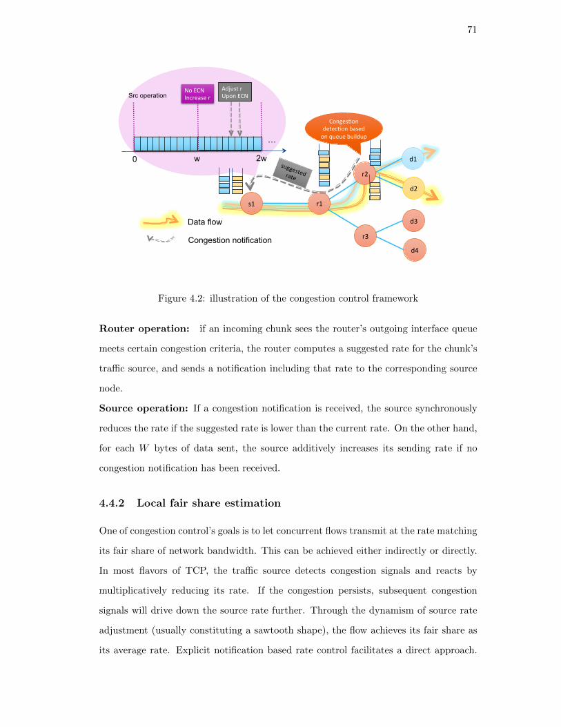
71

d2

d3

d4

s1

d1

r1

r2

r3

Conges.ondetec.onbasedonqueuebuildup

0 w 2w

…

NoECNIncreaser

AdjustrUponECN

Data flow

Congestion notification

Src operation

suggestedrate

Figure 4.2: illustration of the congestion control framework

Router operation: if an incoming chunk sees the router’s outgoing interface queue

meets certain congestion criteria, the router computes a suggested rate for the chunk’s

traffic source, and sends a notification including that rate to the corresponding source

node.

Source operation: If a congestion notification is received, the source synchronously

reduces the rate if the suggested rate is lower than the current rate. On the other hand,

for each W bytes of data sent, the source additively increases its sending rate if no

congestion notification has been received.

4.4.2 Local fair share estimation

One of congestion control’s goals is to let concurrent flows transmit at the rate matching

its fair share of network bandwidth. This can be achieved either indirectly or directly.

In most flavors of TCP, the traffic source detects congestion signals and reacts by

multiplicatively reducing its rate. If the congestion persists, subsequent congestion

signals will drive down the source rate further. Through the dynamism of source rate

adjustment (usually constituting a sawtooth shape), the flow achieves its fair share as

its average rate. Explicit notification based rate control facilitates a direct approach.

72

The routers can periodically estimate current fair share and notify each flow. Traffic

sources cooperate by sending at the lowest rate reported among all en-route routers.

Indeed, this approach has be applied, for instance, in ATM networks [64], and more

recently in data center networks [66].

In our work, we also aim to achieve fair bandwidth allocation to concurrent flows,

and we adjust the explicit notification based rate control framework to the specific

challenges faced with a reliable network and bulk data transfer. We trade short-term

allocation accuracy for feasibility of control over large units of data, and of less frequent

feedbacks from routers.

On each link, the locally fair share of a flow is calculated as if this link is the

bottleneck of the flow. Consider an outgoing interface with corresponding outgoing

link of capacity C. We consider C to be max possible data rate the link can sustain.

Letting n by the estimated number of concurrent flows, then we have the estimated

fair share rate C/n. How do we estimate n? Currently we use transport layer sequence

numbers to determine the start and end of a flow. Thus at any given time, the router

is able to estimate how many flows are currently ongoing.

4.4.3 Rate adjustment

Frequency of control

Traffic sources need to reevaluate its sending rate periodically. We base the periodicity

on a fixed number of bytes, W , so that the requirement on traffic destination feedback

is relaxed (this can be done potentially with windowing). If there is no congestion noti-

fications received during the transmission of W bytes of data, then the rate is increased

by a fixed step size. On the other hand, the source reduces its rate synchronously upon

receiving congestion notification.

Control logic

It may appear that if all the traffic sources adjust their rates based on the rate fair share

computed by the routers, the router’s input rate would converge to match the output

73

rate. However, in practice, a few factors introduce inaccuracies in applying this scheme.

First, it takes time for the notification message to propagate to the corresponding traffic

source. Depending on the latency from the router to the source, the traffic source

essentially sends data at the “wrong” rate during the delivery of congestion notification

message. The excessive amount of data contributes to further queue growth at the

router. In addition, traffic dynamism happens at varied time scales, which leads to

inaccuracy in the estimation of fair share rates. Apart from matching input rate to

the output rate, router’s queue length should be controlled so that queueing delay is

reduced.

Thus the algorithm to be developed need to simultaneously accomplish several ob-

jectives: the sources are driven towards their fair share of bandwidth; meanwhile, queue

length should be constrained to reduce queueing delay. Before describing the control

logic, we need to first introduce a few notations. Consider an arbitrary traffic source,

and an arbitrary router queue along the source’s end-to-end path. Let Rinc be the addi-

tive rate increment of the source, and Qcap be the queue capacity. The router generates

a congestion notification if the observed queue length is greater than Qthresh. We use

Rm0 to denote the rate the source chooses to send at for the m-th block of W bytes of

data, at the beginning of the m-th block. If no congestion notification is received during

this transmission, the source maintains this rate for the entire block, and increases its

rate additively at the beginning of the next block as following:

Rm+10 = Rm0 +Rinc (4.1)

The router computes a suggested rate for the incoming chunk, if current queue

occupancy exceeds a threshold:

Rmk′ = Rfair − f(Q−Qthresh

Qcap) ·Rfair (4.2)

where Rfair is the estimated local fair share at the router. We currently use a quadratic

function to represent f(). The idea here is to reduce the rate more, if queue length is

far beyond the desired queue occupancy. Upon obtaining this suggested rate through

the notification message, the source evaluates and updates its rate if it is less than its

74

current rate:

Rmk+1 = min{Rmk , Rmk′} (4.3)

4.4.4 Aggressive bootstrapping

One way to bootstrap a rate control policy is to start at a low rate, and gradually

increase the rate till the point when some router’s queue overflows. The process of

“polling” the appropriate sending rate can be shortened by using exponential growth,

e. g. slow start in TCP. Nevertheless, it still takes several RTTs to reach at the

equilibrium. Such a scheme i) renders lower utilization when the network is lightly

loaded; ii) incurs extra latency that cannot be amortized easily.

Note that “slow start” mechanism is built on the premise that routers frequently

and deliberately drops packets. Traffic sources take dropped packets as signals for

congestion. However, there is no information or even a hint about the severity of

congestion when a packet is dropped. In our scheme, such “hint” on the severity

of congestion is passed to the traffic sources explicitly, based on which the sources

can react more effectively. Furthermore, link layer back pressure strives to prevent

congestion from worsening by stopping upstream routers from injecting more packets

into downstream. As a consequence, packets drop is rare. The mechanics of explicit

congestion notification and back pressure obviates the need for slow start; rather, the

sources start “fast”, and respond to congestion quickly and effectively.

4.5 Evaluation

4.5.1 Simulator

We built a chunk-level simulator for evaluating the proposed congestion control mech-

anisms. Links and nodes are modeled. All operations performed on the data, such as

transmitting and receiving, are done on chunks, not packets. We implement both per-

flow and per-interface queueing mechanisms, and their respective scheduling policies:

Round Robin and FCFS, respectively. We also implement a module to perform conges-

tion notification, and call it the Explicit Congestion Notification (ECN) module. Our

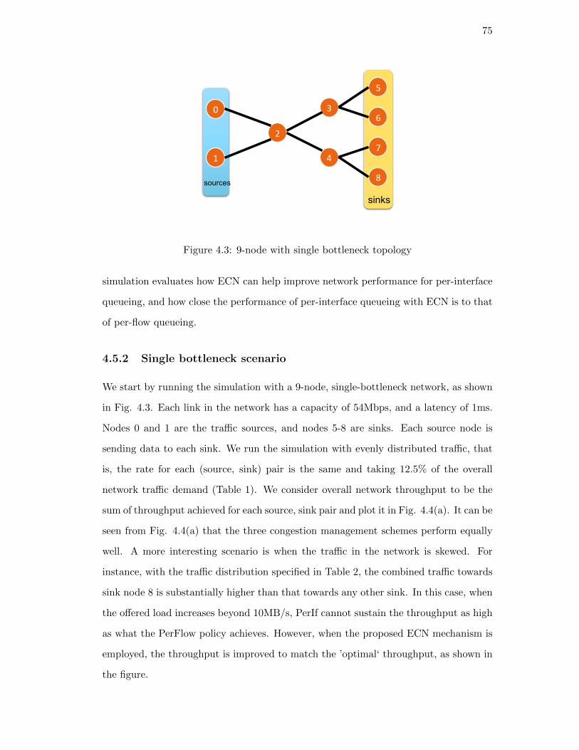
75

3

4

6

8

7

5

2

1

0

sources

sinks

Figure 4.3: 9-node with single bottleneck topology

simulation evaluates how ECN can help improve network performance for per-interface

queueing, and how close the performance of per-interface queueing with ECN is to that

of per-flow queueing.

4.5.2 Single bottleneck scenario

We start by running the simulation with a 9-node, single-bottleneck network, as shown

in Fig. 4.3. Each link in the network has a capacity of 54Mbps, and a latency of 1ms.

Nodes 0 and 1 are the traffic sources, and nodes 5-8 are sinks. Each source node is

sending data to each sink. We run the simulation with evenly distributed traffic, that

is, the rate for each (source, sink) pair is the same and taking 12.5% of the overall

network traffic demand (Table 1). We consider overall network throughput to be the

sum of throughput achieved for each source, sink pair and plot it in Fig. 4.4(a). It can be

seen from Fig. 4.4(a) that the three congestion management schemes perform equally

well. A more interesting scenario is when the traffic in the network is skewed. For

instance, with the traffic distribution specified in Table 2, the combined traffic towards

sink node 8 is substantially higher than that towards any other sink. In this case, when

the offered load increases beyond 10MB/s, PerIf cannot sustain the throughput as high

as what the PerFlow policy achieves. However, when the proposed ECN mechanism is

employed, the throughput is improved to match the ’optimal‘ throughput, as shown in

the figure.

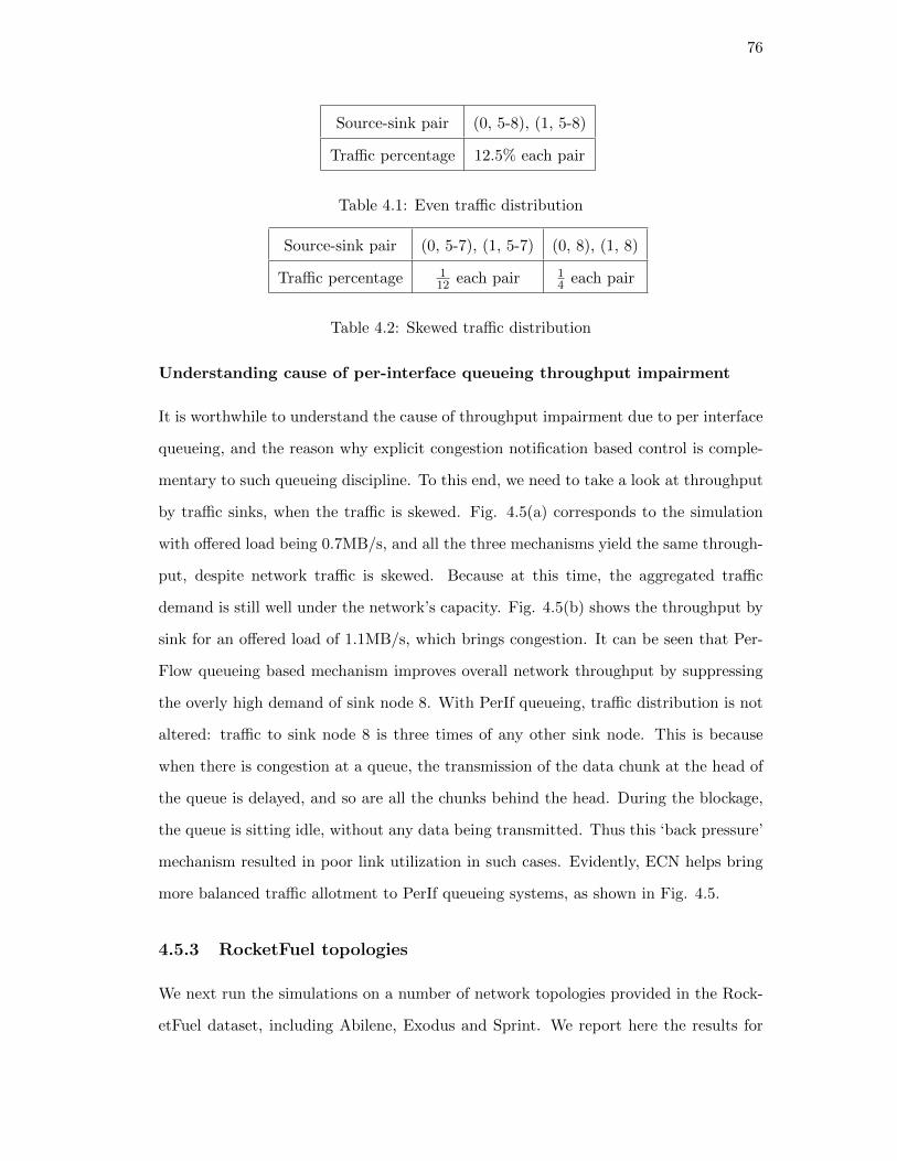
76

Source-sink pair (0, 5-8), (1, 5-8)

Traffic percentage 12.5% each pair

Table 4.1: Even traffic distribution

Source-sink pair (0, 5-7), (1, 5-7) (0, 8), (1, 8)

Traffic percentage 112 each pair 1

4 each pair

Table 4.2: Skewed traffic distribution

Understanding cause of per-interface queueing throughput impairment

It is worthwhile to understand the cause of throughput impairment due to per interface

queueing, and the reason why explicit congestion notification based control is comple-

mentary to such queueing discipline. To this end, we need to take a look at throughput

by traffic sinks, when the traffic is skewed. Fig. 4.5(a) corresponds to the simulation

with offered load being 0.7MB/s, and all the three mechanisms yield the same through-

put, despite network traffic is skewed. Because at this time, the aggregated traffic

demand is still well under the network’s capacity. Fig. 4.5(b) shows the throughput by

sink for an offered load of 1.1MB/s, which brings congestion. It can be seen that Per-

Flow queueing based mechanism improves overall network throughput by suppressing

the overly high demand of sink node 8. With PerIf queueing, traffic distribution is not

altered: traffic to sink node 8 is three times of any other sink node. This is because

when there is congestion at a queue, the transmission of the data chunk at the head of

the queue is delayed, and so are all the chunks behind the head. During the blockage,

the queue is sitting idle, without any data being transmitted. Thus this ‘back pressure’

mechanism resulted in poor link utilization in such cases. Evidently, ECN helps bring

more balanced traffic allotment to PerIf queueing systems, as shown in Fig. 4.5.

4.5.3 RocketFuel topologies

We next run the simulations on a number of network topologies provided in the Rock-

etFuel dataset, including Abilene, Exodus and Sprint. We report here the results for

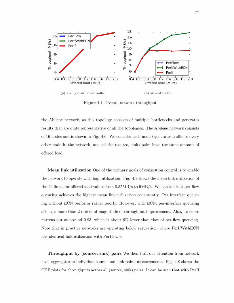
77

0.4 0.6 0.8 1.0 1.2 1.4 1.6 1.8 2.0Offered load (MB/s)

4

6

8

10

12

Thro

ughput (M

B/s

)

PerFlow

PerIfWithECN

PerIf

(a) evenly distributed traffic

0.4 0.6 0.8 1.0 1.2 1.4 1.6 1.8 2.0Offered load (MB/s)

5

6

7

8

9

10

11

12

13

Th

rou

gh

pu

t (M

B/s

)

PerFlow

PerIfWithECN

PerIf

(b) skewed traffic

Figure 4.4: Overall network throughput

the Abilene network, as this topology consists of multiple bottlenecks and generates

results that are quite representative of all the topologies. The Abilene network consists

of 16 nodes and is shown in Fig. 4.6. We consider each node i generates traffic to every

other node in the network, and all the (source, sink) pairs have the same amount of

offered load.

Mean link utilization One of the primary goals of congestion control is to enable

the network to operate with high utilization. Fig. 4.7 shows the mean link utilization of

the 22 links, for offered load values from 0.35MB/s to 9MB/s. We can see that per-flow

queueing achieves the highest mean link utilization consistently. Per interface queue-

ing without ECN performs rather poorly. However, with ECN, per-interface queueing

achieves more than 2 orders of magnitude of throughput improvement. Also, its curve

flattens out at around 0.93, which is about 6% lower than that of per-flow queueing.

Note that in practice networks are operating below saturation, where PerIfWithECN

has identical link utilization with PerFlow’s.

Throughput by (source, sink) pairs We then turn our attention from network

level aggregates to individual source and sink pairs’ measurements. Fig. 4.8 shows the

CDF plots for throughputs across all (source, sink) pairs. It can be seen that with PerIf

78

dst: 5 dst: 6 dst: 7 dst: 80.0

0.5

1.0

1.5

2.0

2.5

3.0

3.5

4.0

4.5

Throughput (M

B/s)

PerFlow

PerIf

PerIfWithECN

(a) offered load 0.7MB/s

dst: 5 dst: 6 dst: 7 dst: 80

1

2

3

4

5

Throughput (MB/s)

PerFlow

PerIf

PerIfWithECN

(b) offered load 1.1MB/s

dst: 5 dst: 6 dst: 7 dst: 80

1

2

3

4

5

Throughput (MB/s)

PerFlow

PerIf

PerIfWithECN

(c) offered load 2.0MB/s

Figure 4.5: Throughput by traffic sink, with skewed traffic

45

11

12

13 15

1 0

8

9

2

7

14

3

610

Figure 4.6: Abilene network topology

queueing, nearly 80% of the source-sink have a throughput of under 0.05. From the plot,

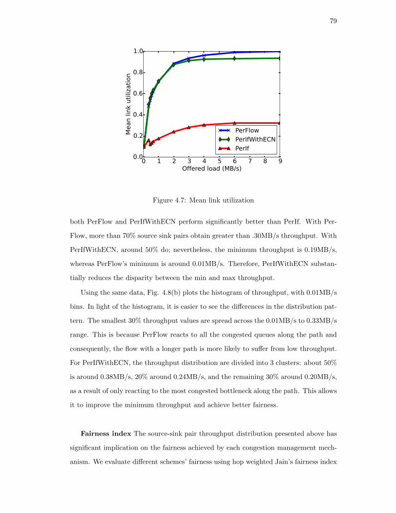
79

0 1 2 3 4 5 6 7 8 9Offered load (MB/s)

0.0

0.2

0.4

0.6

0.8

1.0

Me

an

lin

k u

tiliz

ati

on

PerFlow

PerIfWithECN

PerIf

Figure 4.7: Mean link utilization

both PerFlow and PerIfWithECN perform significantly better than PerIf. With Per-

Flow, more than 70% source sink pairs obtain greater than .30MB/s throughput. With

PerIfWithECN, around 50% do; nevertheless, the minimum throughput is 0.19MB/s,

whereas PerFlow’s minimum is around 0.01MB/s. Therefore, PerIfWithECN substan-

tially reduces the disparity between the min and max throughput.

Using the same data, Fig. 4.8(b) plots the histogram of throughput, with 0.01MB/s

bins. In light of the histogram, it is easier to see the differences in the distribution pat-

tern. The smallest 30% throughput values are spread across the 0.01MB/s to 0.33MB/s

range. This is because PerFlow reacts to all the congested queues along the path and

consequently, the flow with a longer path is more likely to suffer from low throughput.

For PerIfWithECN, the throughput distribution are divided into 3 clusters: about 50%

is around 0.38MB/s, 20% around 0.24MB/s, and the remaining 30% around 0.20MB/s,

as a result of only reacting to the most congested bottleneck along the path. This allows

it to improve the minimum throughput and achieve better fairness.

Fairness index The source-sink pair throughput distribution presented above has

significant implication on the fairness achieved by each congestion management mech-

anism. We evaluate different schemes’ fairness using hop weighted Jain’s fairness index

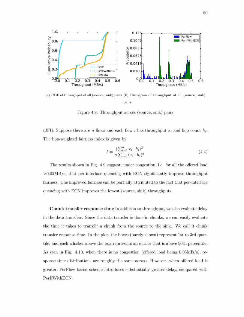
80

0.0 0.1 0.2 0.3 0.4 0.5 0.6Throughput (MB/s)

0.0

0.2

0.4

0.6

0.8

1.0

Cumulative Probability

PerIf

PerIfWithECN

PerFlow

(a) CDF of throughput of all (source, sink) pairs

0.0 0.1 0.2 0.3 0.4 0.5 0.6Throughput (MB/s)

0.0

0.0208

0.0417

0.0625

0.0833

0.1042

0.125

Probability

PerFlow

PerIfWithECN

(b) Histogram of throughput of all (source, sink)

pairs

Figure 4.8: Throughput across (source, sink) pairs

(JFI). Suppose there are n flows and each flow i has throughput xi and hop count hi.

The hop-weighted fairness index is given by:

I =(∑n

i=1 xi · hi)2

n∑n

i=1(xi · hi)2(4.4)

The results shown in Fig. 4.9 suggest, under congestion, i.e. for all the offered load

>0.05MB/s, that per-interface queueing with ECN significantly improve throughput

fairness. The improved fairness can be partially attributed to the fact that per-interface

queueing with ECN improves the lowest (source, sink) throughputs.

Chunk transfer response time In addition to throughput, we also evaluate delay

in the data transfers. Since the data transfer is done in chunks, we can easily evaluate

the time it takes to transfer a chunk from the source to the sink. We call it chunk

transfer response time. In the plot, the boxes (barely shown) represent 1st to 3rd quar-

tile, and each whisker above the box represents an outlier that is above 90th percentile.

As seen in Fig. 4.10, when there is no congestion (offered load being 0.05MB/s), re-

sponse time distributions are roughly the same across. However, when offered load is

greater, PerFlow based scheme introduces substantially greater delay, compared with

PerIfWithECN.

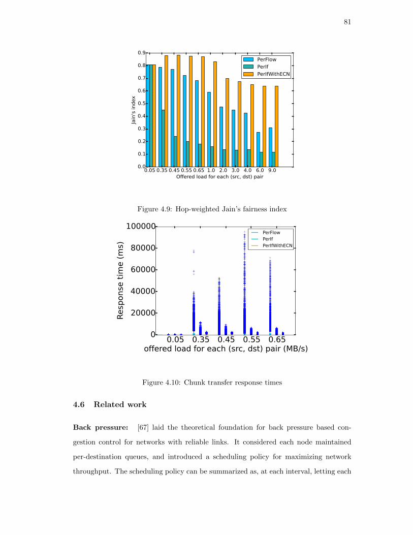
81

0.05 0.35 0.45 0.55 0.65 1.0 2.0 3.0 4.0 6.0 9.0Offered load for each (src, dst) pair

0.0

0.1

0.2

0.3

0.4

0.5

0.6

0.7

0.8

0.9

Jain

's i

nd

ex

PerFlow

PerIf

PerIfWithECN

Figure 4.9: Hop-weighted Jain’s fairness index

0.05 0.35 0.45 0.55 0.65offered load for each (src, dst) pair (MB/s)

0

20000

40000

60000

80000

100000

Response time (ms)

PerFlowPerIfPerIfWithECN

Figure 4.10: Chunk transfer response times

4.6 Related work

Back pressure: [67] laid the theoretical foundation for back pressure based con-

gestion control for networks with reliable links. It considered each node maintained

per-destination queues, and introduced a scheduling policy for maximizing network

throughput. The scheduling policy can be summarized as, at each interval, letting each

82

node schedule to transfer the data in one queue whose length has the max difference

against its next hop’s queue. [63] followed the same idea, and considered each node

maintaining per flow queues. In [63], each per-flow queue has certain capacity. Once

the capacity is reached, that flow is considered to generate back pressure, i.e. the node

will not be able to accept more data for that flow. When scheduling, the flow to be

transferred is selected in a Round Robin fashion among all flows that are not expe-

riencing back pressure. [63] showed through experimental validation that it achieved

substantially better throughput and fairness compared with TCP. Nevertheless, the

scalability concern arising from keeping per-flow queues was not addressed.

Explicit congestion notification based congestion control: The idea of using

explicit congestion notification dates back to several decades ago, for instance, [68]

considered using a single bit to indicate congestion. In [69], a source to destination

flow explicitly requests certain rate with which the flow deadline can be met. Then if

the requested rate can be satisfied, each on-path router exposes its allocated rate for

the next interval. Otherwise the source has to wait and re-request rate in the future.

Therefore the source relies on constant rate share updates from routers. Our work is

different from existing ones mainly in the frequency the notification is sent.

83

Chapter 5

Concluding remarks

As wireless Internet usage gradually becomes the most popular way of accessing the

Internet, it is crucial to engineer new solutions to overcome the challenges presented

by wireless/mobile data delivery. This dissertation proposes algorithmic and protocol

designs to address three problems: multicast, reliable data transport, and congestion

control.

We first investigated integrated resource allocation for wireless networks which em-

ploy random network coding as the transport scheme. We used a differential equation

based framework that models RNC throughput, thereby enabling the analysis of RNC

performance in terms of PHY and MAC layer parameters. Using this framework, we

designed dynamic power control and CSMA mean backoff delay control algorithms to

improve the performance of RNC. Specifically, we used gradient based resource alloca-

tion algorithms and evaluated both centralized and online versions of them, via the use

of differential equation solvers and event driven simulations. Our results revealed that

such network coding aware resource allocation significantly improves the throughput

of destination nodes in RNC. We also observed that such integrated power control can

regain the broadcast advantage. Beyond the use cases of power control and CSMA

backoff control, the framework and approach presented in this dissertation can be gen-

erally applied to joint power and CSMA backoff control as well as a variety of resource

allocation problems for RNC.

We then presented the design of a clean-slate transport layer protocol for the Mo-

bilityFirst future Internet architecture. The proposed transport layer protocol, called

MFTP, is based on an understanding of the key requirements of name-based Infor-

mation Centric Networks. These requirements include the use of names rather than

84

addresses for routing, in-network storage, hop-by-hop reliability and multicasting as

a basic service. Several core transport protocol components responsive to the above

requirements were identified and discussed in the context of the MobilityFirst proto-

col stack. A proof-of-concept experimental validation has been developed and used to

demonstrate feasibility and significantly improved performance relative to conventional

TCP/IP for several use cases including large file transfer, web access and late bind-

ing/delay tolerant services. The reported results represent an initial design of MFTP

to enable services on the MobilityFirst network. The protocol is expected to evolve

with ongoing experimental evaluations and prototype GENI deployment.

Finally, we designed a network-layer congestion control scheme to support efficient

data delivery at scale in the information-centric MobilityFirst network architecture. The

proposed scheme utilizes router’s explicit congestion notifications as feedback for source

rate control, operating on bulk data transfer and with less frequent control looping.

Along with its simple per-interface queueing mechanism which is easy to scale, the

scheme is distinct from per-flow queueing based scheme. Compared with existing per-

flow based network-layer congestion control scheme, the proposed congestion control

is shown through simulation to be able to improve bulk data transfer delay, fairness

across flows and better scalability, at an acceptable cost of only less than 6% average

link utilization degradation under link saturation. This design fills a critical missing

piece in the MF architecture to efficiently support IoT networking at scale.

85

References

[1] J. Tang, G. Xue, C. Chandler, and W. Zhang, “Link scheduling with power controlfor throughput enhancement in multihop wireless networks,” in IEEE Transactionson Vehicular Technology, vol. 55, no. 3, pp. 733 – 742, May 2012.

[2] L. Georgiadis, M. Neely, and L. Tassiulas, “Resource allocation and cross-layercontrol in wireless networks,” Foundations and Trends R© in Networking, vol. 1,no. 1, 2006.

[3] X. Lin, N. Shroff, and R. Srikant, “A tutorial on cross-layer optimization in wirelessnetworks,” Selected Areas in Communications, IEEE Journal on, vol. 24, no. 8,pp. 1452 –1463, aug. 2006.

[4] M. Chiang, S. Low, A. Calderbank, and J. Doyle, “Layering as optimization de-composition: A mathematical theory of network architectures,” Proceedings of theIEEE, vol. 95, no. 1, pp. 255 –312, jan. 2007.

[5] R. Ahlswede, N. Cai, S.-Y. Li, and R. Yeung, “Network information flow,” IEEETransactions on Information Theory, vol. 46, no. 4, pp. 1204 –1216, July 2000.

[6] K. Han, T. Ho, R. Koetter, M. Medard, and F. Zhao, “On network coding forsecurity,” IEEE Military Communications Conference (MILCOM), pp. 1 – 6, Oct.2007.

[7] A. Dimakis, P. Godfrey, Y. Wu, M. Wainwright, and K. Ramchandran, “Networkcoding for distributed storage systems,” Information Theory, IEEE Transactionson, vol. 56, no. 9, pp. 4539 –4551, sept. 2010.

[8] C. Gkantsidis and P. Rodriguez, “Network coding for large scale content distribu-tion,” in INFOCOM 2005. 24th Annual Joint Conference of the IEEE Computerand Communications Societies. Proceedings IEEE, vol. 4, march 2005, pp. 2235 –2245 vol. 4.

[9] D. Lun, N. Ratnakar, M. Medard, R. Koetter, D. Karger, T. Ho, E. Ahmed,and F. Zhao, “Minimum-cost multicast over coded packet networks,” InformationTheory, IEEE Transactions on, vol. 52, no. 6, pp. 2608–2623, 2006.

[10] Y. Xi and E. Yeh, “Distributed algorithms for minimum cost multicast with net-work coding,” Networking, IEEE/ACM Transactions on, vol. 18, no. 2, pp. 379–392, 2010.

[11] K. Rajawat, N. Gatsis, and G. Giannakis, “Cross-layer designs in coded wire-less fading networks with multicast,” Networking, IEEE/ACM Transactions on,vol. 19, no. 5, pp. 1276–1289, 2011.

86

[12] D. Traskov, D. S. Lun, R. Koetter, and M. Medard, “Network coding in wirelessnetworks with random access,” in Information Theory, 2007. ISIT 2007. IEEEInternational Symposium on, june 2007, pp. 2726 –2730.

[13] D. Zhang, K. Su, and N. B. Mandayam, “Network coding aware resource allocationto improve throughput,” IEEE International Symposium on Information Theory(ISIT), 2012.

[14] T. Ho, R. Koetter, M. Medard, D. Karger, and M. Effros, “The benefits of cod-ing over routing in a randomized setting,” in IEEE International Symposium onInformation Theory, p. 442, Jul. 2003.

[15] D. Zhang and N. B. Mandayam, “Analyzing random network coding with differ-ential equations and differential inclusions,” IEEE Transactions on InformationTheory, vol. 57, no. 12, pp. 7932–7949, Dec. 2011.

[16] D. Zhang, N. Mandayam, and S. Parekh, “DEDI: A framework for analyzing rankevolution of random network coding in a wireless network,” in Information TheoryProceedings (ISIT), 2010 IEEE International Symposium on, june 2010, pp. 1883–1887.

[17] A. Ruszczynski, Nonlinear Optimization. Princeton University Press, 2006.

[18] M. Chiang, P. Hande, T. Lan, and C. Tan, “Power control in wireless cellularnetworks,” Foundations and Trends R© in Networking, vol. 2, no. 4, April 2008.

[19] G. Foschini and Z. Miljanic, “A simple distributed autonomous power control algo-rithm and its convergence,” Vehicular Technology, IEEE Transactions on, vol. 42,no. 4, pp. 641 –646, nov 1993.

[20] R. Yates, “A framework for uplink power control in cellular radio systems,” SelectedAreas in Communications, IEEE Journal on, vol. 13, no. 7, pp. 1341 –1347, sep1995.

[21] J. Zander, “Distributed cochannel interference control in cellular radio systems,”Vehicular Technology, IEEE Transactions on, vol. 41, no. 3, pp. 305 –311, aug1992.

[22] M. Chiang and J. Bell, “Balancing supply and demand of bandwidth in wireless cel-lular networks: utility maximization over powers and rates,” in INFOCOM 2004.Twenty-third AnnualJoint Conference of the IEEE Computer and CommunicationsSocieties, vol. 4, march 2004, pp. 2800 – 2811 vol.4.

[23] P. Hande, S. Rangan, M. Chiang, and X. Wu, “Distributed uplink power controlfor optimal sir assignment in cellular data networks,” Networking, IEEE/ACMTransactions on, vol. 16, no. 6, pp. 1420 –1433, dec. 2008.

[24] C. Saraydar, N. Mandayam, and D. Goodman, “Efficient power control via pricingin wireless data networks,” Communications, IEEE Transactions on, vol. 50, no. 2,pp. 291 –303, feb 2002.

87

[25] K. Su, D. Zhang, and N. B. Mandayam, “Network coding aware power controlin wireless netoworks,” in 46th Annual Conference on Information Sciences andSystems (CISS), 2012.

[26] C. G. Broyden, “A class of methods for solving nonlinear simultaneous equations,”Mathematics of Computation (American Mathematical Society), Oct. 1965.

[27] “Propagation data and prediction methods for the planning of indoor radio com-munication systems and the radio local area networks in the frequency range 900mhz to 100 ghz,” ITU-R Recommendations, 2001.

[28] J. Nocedal and S. J. Wright, Numerical Optimization. Springer., 2006.

[29] L. Jiang and J. Walrand, “A distributed csma algorithm for throughput and utilitymaximization in wireless networks,” Networking, IEEE/ACM Transactions on,vol. 18, no. 3, pp. 960 –972, june 2010.

[30] ——, “Approaching throughput-optimality in distributed csma scheduling algo-rithms with collisions,” Networking, IEEE/ACM Transactions on, vol. 19, no. 3,pp. 816 –829, june 2011.

[31] J. Ni and R. Srikant, “Distributed csma/ca algorithms for achieving maximumthroughput in wireless networks,” in Information Theory and Applications Work-shop, 2009, feb. 2009, p. 250.

[32] R. Boorstyn, A. Kershenbaum, B. Maglaris, and V. Sahin, “Throughput analysisin multihop csma packet radio networks,” Communications, IEEE Transactionson, vol. 35, no. 3, pp. 267 – 274, mar 1987.

[33] S. C. Liew, C. H. Kai, H. C. Leung, and P. Wong, “Back-of-the-envelope compu-tation of throughput distributions in csma wireless networks,” Mobile Computing,IEEE Transactions on, vol. 9, no. 9, pp. 1319 –1331, sept. 2010.

[34] J. H. Saltzer, D. P. Reed, and D. D. Clark, “End-to-end arguments in systemdesign,” ACM TOCS, 1984.

[35] B. Ahlgren and et Al, “Design considerations for a network of information,” inACM CoNEXT, 2008.

[36] A. Ghodsi, S. Shenker, T. Koponen, A. Singla, B. Raghavan, and J. Wilcox,“Information-centric networking: Seeing the forest for the trees,” in ACM Hot-Nets. ACM, 2011.

[37] MobilityFirst Project, http://mobilityfirst.winlab.rutgers.edu/.

[38] D. Raychaudhuri, K. Nagaraja, and A. Venkataramani, “Mobilityfirst: a robustand trustworthy mobility-centric architecture for the future internet,” ACM SIG-MOBILE Mobile Computing and Communications Review, 2012.

[39] V. Jacobson et al., “Networking named content,” in ACM CoNEXT. ACM, 2009.

[40] D. Han, A. Anand, F. R. Dogar, and Others, “Xia: Efficient support for evolvableinternetworking.” in USENIX NSDI, 2012.

88

[41] F. Bronzino, K. Nagaraja, I. Seskar, and D. Raychaudhuri, “Network service ab-stractions for a mobility-centric future internet architecture,” in ACM MobiArch.ACM, 2013.

[42] A. Erramilli and R. P. Singh, “A reliable and efficient multicast for broadbandbroadcast networks,” in ACM Workshop on Frontiers in Computer Communica-tions Technology, 1988.

[43] S. C. Nelson, G. Bhanage, and D. Raychaudhuri, “Gstar: Generalized storage-aware routing for mobilityfirst in the future mobile internet,” in ACM MobiArch.ACM, 2011.

[44] T. Vu and Others, “Dmap: A shared hosting scheme for dynamic identifier tolocator mappings in the global internet,” in IEEE ICDCS, June 2012.

[45] A. Sharma, X. Tie, H. Uppal, A. Venkataramani, D. Westbrook, and A. Yadav,“A global name service for a highly mobile internetwork,” in ACM SIGCOMM,2014.

[46] S. Mukherjee, K. Su, N. B. Mandayam, K. Ramakrishnan, D. Raychaudhuri, andI. Seskar, “Evaluating opportunistic delivery of large content with tcp over wifi ini2v communication,” IEEE LANMAN, 2014.

[47] M. Gerla and L. Kleinrock, “Flow control: A comparative survey,” IEEE Trans-actions on Communications, 1980.

[48] E. Kohler and et al, “The click modular router,” ACM Transactions on ComputerSystems, 2000.

[49] L. Zhang, “Why tcp timers don’t work well,” in ACM SIGCOMM, 1986.

[50] I. Psaras and V. Tsaoussidis, “Why tcp timers (still) don’t work well,” ComputerNetworks, 2007.

[51] ORBIT testbed, http://www.orbit-lab.org/.

[52] hostapd, http://wireless.kernel.org/en/users/Documentation/hostapd.

[53] netem: network emulation tool, http://www.linuxfoundation.org/collaborate/workgroups/networking/netem.

[54] X. S. Wang, A. Balasubramanian, A. Krishnamurthy, and D. Wetherall, “Howspeedy is spdy,” in USENIX NSDI, 2014.

[55] Alexa: the top 500 sites on the web, http://www.alexa.com/topsites.

[56] R. Moskowitz, P. Nikander, P. Jokela, and T. Henderson, “Host identity protocol,”RFC 5201, April, 2008.

[57] S. Salsano and et Al, “Transport-layer issues in information centric networks,” inACM ICN, 2012.

[58] G. Carofiglio, M. Gallo, and L. Muscariello, “Joint hop-by-hop and receiver-friveninterest control protocol for content-centric networks,” in ACM ICN, 2012.

89

[59] F. Zhang, Y. Zhang, A. Reznik, H. Liu, C. Qian, and C. Xu, “A transport protocolfor content-centric networking with explicit congestion control,” in IEEE ICCCN,2014.

[60] F. R. Dogar and P. Steenkiste, “Architecting for edge diversity: Supporting richservices over an unbundled transport,” in CoNEXT, 2012.

[61] L. Zhang et al., “Named data networking,” SIGCOMM CCR, 2014.

[62] K. Su et al., “Mftp: A clean-slate transport protocol for the information centricmobilityfirst network,” in ACM ICN, 2015.

[63] M. Li, D. Agrawal, D. Ganesan, and A. Venkataramani, “Block-switched networks:A new paradigm for wireless transport,” in USENIX NSDI, 2009.

[64] L. Kalampoukas, A. Varma, and K. K. Ramakrishnan, “An efficient rate allocationalgorithm for atm networks providing max-min fairness,” in Proceedings of the IFIPSixth International Conference on High Performance Networking VI, 1995.

[65] J. Gettys, “Bufferbloat: Dark buffers in the internet,” IEEE Internet Computing,vol. 15, no. 3, pp. 96, 95, 2011.

[66] M. Alizadeh, A. Greenberg, D. A. Maltz, J. Padhye, P. Patel, B. Prabhakar, S. Sen-gupta, and M. Sridharan, “Data center tcp (dctcp),” in SIGCOMM ’10, 2010.

[67] L. Tassiulas and A. Ephremides, “Stability properties of constrained queueingsystems and scheduling policies for maximum throughput in multihop radio net-works,” Automatic Control, IEEE Transactions on, vol. 37, no. 12, pp. 1936–1948,Dec 1992.

[68] K. K. Ramakrishnan and R. Jain, “A binary feedback scheme for congestion avoid-ance in computer networks with a connectionless network layer,” SIGCOMM Com-put. Commun. Rev., vol. 18, no. 4, Aug. 1988.

[69] C. Wilson, H. Ballani, T. Karagiannis, and A. Rowtron, “Better never than late:Meeting deadlines in datacenter networks,” SIGCOMM Comput. Commun. Rev.