Algorithms and Frameworks for Accelerating Security Applications on HPC Platforms Xiaodong Yu Dissertation submitted to the Faculty of the Virginia Polytechnic Institute and State University in partial fulfillment of the requirements for the degree of Doctor of Philosophy in Computer Science & Applications Danfeng (Daphne) Yao, Chair Michela Becchi Ali R. Butt Matthew Hicks Xinming (Simon) Ou August 1, 2019 Blacksburg, Virginia Keywords: Cybersecurity, HPC, GPU, Intrusion Detection, Automata Processor, Android Program Analysis, Cache Side-Channel Attack Copyright 2019, Xiaodong Yu

Welcome message from author
This document is posted to help you gain knowledge. Please leave a comment to let me know what you think about it! Share it to your friends and learn new things together.
Transcript
Algorithms and Frameworks for Accelerating Security Applicationson HPC Platforms
Xiaodong Yu
Dissertation submitted to the Faculty of the
Virginia Polytechnic Institute and State University
in partial fulfillment of the requirements for the degree of
Doctor of Philosophy
in
Computer Science & Applications
Danfeng (Daphne) Yao, Chair
Michela Becchi
Ali R. Butt
Matthew Hicks
Xinming (Simon) Ou
August 1, 2019
Blacksburg, Virginia
Keywords: Cybersecurity, HPC, GPU, Intrusion Detection, Automata Processor, Android
Program Analysis, Cache Side-Channel Attack
Copyright 2019, Xiaodong Yu

Algorithms and Frameworks for Accelerating Security Applications on HPCPlatforms
Xiaodong Yu
(ABSTRACT)
Typical cybersecurity solutions emphasize on achieving defense functionalities. However, ex-
ecution efficiency and scalability are equally important, especially for real-world deployment.
Straightforward mappings of cybersecurity applications onto HPC platforms may significantly un-
derutilize the HPC devices’ capacities. On the other hand, the sophisticated implementations are
quite difficult: they require both in-depth understandings of cybersecurity domain-specific charac-
teristics and HPC architecture and system model.
In our work, we investigate three sub-areas in cybersecurity, including mobile software security,
network security, and system security. They have the following performance issues, respectively:
1) The flow- and context-sensitive static analysis for the large and complex Android APKs are
incredibly time-consuming. Existing CPU-only frameworks/tools have to set a timeout threshold to
cease the program analysis to trade the precision for performance. 2) Network intrusion detection
systems (NIDS) use automata processing as its searching core and requires line-speed processing.
However, achieving high-speed automata processing is exceptionally difficult in both algorithm
and implementation aspects. 3) It is unclear how the cache configurations impact time-driven
cache side-channel attacks’ performance. This question remains open because it is difficult to
conduct comparative measurement to study the impacts.
In this dissertation, we demonstrate how application-specific characteristics can be leveraged to
optimize implementations on various types of HPC for faster and more scalable cybersecurity exe-
cutions. For example, we present a new GPU-assisted framework and a collection of optimization
strategies for fast Android static data-flow analysis that achieve up to 128X speedups against the
plain GPU implementation. For network intrusion detection systems (IDS), we design and im-

plement an algorithm capable of eliminating the state explosion in out-of-order packet situations,
which reduces up to 400X of the memory overhead. We also present tools for improving the us-
ability of Micron’s Automata Processor. To study the cache configurations’ impact on time-driven
cache side-channel attacks’ performance, we design an approach to conducting comparative mea-
surement. We propose a quantifiable success rate metric to measure the performance of time-driven
cache attacks and utilize the GEM5 platform to emulate the configurable cache.

Algorithms and Frameworks for Accelerating Security Applications on HPCPlatforms
Xiaodong Yu
(GENERAL AUDIENCE ABSTRACT)
Typical cybersecurity solutions emphasize on achieving defense functionalities. However, exe-
cution efficiency and scalability are equally important, especially for the real-world deployment.
Straightforward mappings of applications onto High-Performance Computing (HPC) platforms
may significantly underutilize the HPC devices’ capacities. In this dissertation, we demonstrate
how application-specific characteristics can be leveraged to optimize various types of HPC exe-
cutions for cybersecurity. We investigate several sub-areas, including mobile software security,
network security, and system security. For example, we present a new GPU-assisted framework
and a collection of optimization strategies for fast Android static data-flow analysis that achieve up
to 128X speedups against the unoptimized GPU implementation. For network intrusion detection
systems (IDS), we design and implement an algorithm capable of eliminating the state explosion in
out-of-order packet situations, which reduces up to 400X of the memory overhead. We also present
tools for improving the usability of HPC programming. To study the cache configurations’ impact
on time-driven cache side-channel attacks’ performance, we design an approach to conducting
comparative measurement. We propose a quantifiable success rate metric to measure the perfor-
mance of time-driven cache attacks and utilize the GEM5 platform to emulate the configurable
cache.

Acknowledgments
First and foremost, I would like to express my deepest gratitude to my advisor, Prof. Danfeng
(Daphne) Yao. She helps me overcome the huge difficulties during my Ph.D. study, introduces me
to the field of cybersecurity, and shares with me her invaluable knowledge and experience. I have
learned so much from Prof. Yao, such as the research methodologies, presentation and commu-
nication skills, paper reviewing approaches, and scientific writing ability. Without her guidance,
support, and encouragement, it would not be possible for me to complete my Ph.D.
I would like to especially thank Prof. Michela Becchi, who was my Master’s advisor at the Uni-
versity of Missouri and serves as my Ph.D. thesis committee member. She introduces me into the
world of HPC and continuously supports me throughout my Ph.D. study. She not only inspires
and guides me to conduct research but also provides me plenty of great suggestions regarding my
academic and personal lives, and future career.
I also would like to express my sincere gratitude to the committee members, Prof. Ali R. Butt,
Prof. Matthew Hicks, and Prof. Xinming (Simon) Ou, for their insightful comments and valuable
suggestions for my dissertation. I am also very grateful to many other researchers, including my
AMD internship mentor Daniel Lowell, Prof. Kirk W. Cameron, Prof. Wu-chun Feng, and Dr.
Hao Wang, for their guidance on my HPC research.
I have been fortunate to work with and be a friend of my labmates and fellow collaborators:
Sharmin Afrose, Md Salman Ahmed, Dr. Long Cheng, Myles Frantz, Yuan Luo, Sazzadur Ra-
haman, Dr. Ke Tian, Ya Xiao, Xuewen Cui, Dr. Kaixi Hou, Dr. Konstantinos Krommydas, Da
Zhang, Dr. Jing Zhang, Dr. Hao Gong, Dr. Fengguo Wei, Jon Bernard, Tyler Chang, Chandler
Jearls, Dr. Bo Li, Thomas Lux, and Li Xu. It has been a pleasure to get to know many other
friends in our CS department: Dr. Zheng Song, Tong Zhang, Xinwei Fu, Yin Liu, Run Yu, Hang
Hu, Gagandeep Panwar, Yufeng Ma, Xuan Zhang, Shuo Niu/Yanshen Yang couple, Yali Bian/Siyu
Mi couple, Ziqian Song/Mu Xu couple, and so forth. I also would like to thank my friends from
many other areas: Dr. Yumin Dai and Dr. Hao Li/Gehui Liu couple from Dept. of Chemistry, Wei
Cui and Dr. Chuanhui Chen/Zuoping Zhang couple from Dept. of Physics, Xu Dong from Dept.
v

of Biomedical Engineering, Qianzhou Du from Dept. of Business Information Technology, etc. I
appreciate all these friends making my life in Blacksburg rich and colorful. You are my treasures.
My best wishes to all of you for future endeavors.
Finally, I am immensely grateful to my family. My parents, Sanmao Yu and Junhui Song, provide
me unconditional loves and endless supports. Their loves always save me when I was very down
during my Ph.D. study. My love, Wei Xu, is my resource of courage and enthusiasm. Her company
makes it possible for me to go through the tough period of my life.
vi

Contents
1 Introduction 1
1.1 Automata-based Algorithms for Security Applications . . . . . . . . . . . . . . . 2
1.1.1 Regular Expressions & Finite Automata . . . . . . . . . . . . . . . . . . . 2
1.1.2 Deep Packet Inspection (DPI) . . . . . . . . . . . . . . . . . . . . . . . . 3
1.1.2.1 Automata-based Matching Core . . . . . . . . . . . . . . . . . . 4
1.1.2.2 Out-of-order Packets Issue . . . . . . . . . . . . . . . . . . . . 4
1.2 Security Application Accelerations on HPC Devices . . . . . . . . . . . . . . . . . 6
1.2.1 General-purpose Devices . . . . . . . . . . . . . . . . . . . . . . . . . . . 7
1.2.2 Automata Processor . . . . . . . . . . . . . . . . . . . . . . . . . . . . . 8
1.3 Android Program Analysis for Security Vetting . . . . . . . . . . . . . . . . . . . 10
1.3.1 Android Program Analysis Tools . . . . . . . . . . . . . . . . . . . . . . . 10
1.3.2 High-Performance Android Program Analysis . . . . . . . . . . . . . . . . 11
1.4 Cache Side-Channel Attacks . . . . . . . . . . . . . . . . . . . . . . . . . . . . . 13
1.4.1 Categories of Cache Side-Channel Attacks . . . . . . . . . . . . . . . . . 13
1.4.2 Cache Configurations’ Impact . . . . . . . . . . . . . . . . . . . . . . . . 14
vii

1.5 Dissertation Contributions . . . . . . . . . . . . . . . . . . . . . . . . . . . . . . 15
1.6 Dissertation Organization . . . . . . . . . . . . . . . . . . . . . . . . . . . . . . . 17
2 Literature Review 18
2.1 Algorithm Optimizations . . . . . . . . . . . . . . . . . . . . . . . . . . . . . . . 18
2.1.1 Finite Automata Optimizations . . . . . . . . . . . . . . . . . . . . . . . . 18
2.1.2 Algorithms for Out-of-Order Packets in DPI . . . . . . . . . . . . . . . . . 19
2.2 HPC devices Based Accelerations . . . . . . . . . . . . . . . . . . . . . . . . . . 20
2.2.1 GPU . . . . . . . . . . . . . . . . . . . . . . . . . . . . . . . . . . . . . 20
2.2.2 Automata Processor . . . . . . . . . . . . . . . . . . . . . . . . . . . . . 21
2.3 Security Vettings for Android . . . . . . . . . . . . . . . . . . . . . . . . . . . . . 23
2.3.1 Android Static Analysis Tools . . . . . . . . . . . . . . . . . . . . . . . . 23
2.3.2 Andorid Data-Flow Graph Constructions . . . . . . . . . . . . . . . . . . 24
2.4 Cache Side-Channel Attacks & Countermeasures . . . . . . . . . . . . . . . . . . 25
2.4.1 Time-Driven Attacks . . . . . . . . . . . . . . . . . . . . . . . . . . . . . 25
2.4.2 Access-Driven Attacks . . . . . . . . . . . . . . . . . . . . . . . . . . . . 26
2.4.3 Implementations’ and Systems’ Impacts . . . . . . . . . . . . . . . . . . . 26
3 Scalable Automata-based Pattern-Matching Algorithm for Out-of-Order DPI 27
3.1 Introduction . . . . . . . . . . . . . . . . . . . . . . . . . . . . . . . . . . . . . . 27
3.2 O3FA Design . . . . . . . . . . . . . . . . . . . . . . . . . . . . . . . . . . . . . 30
3.2.1 O3FA Data Structure . . . . . . . . . . . . . . . . . . . . . . . . . . . . . 32
viii

3.3 Optimizations . . . . . . . . . . . . . . . . . . . . . . . . . . . . . . . . . . . . . 34
3.3.1 Index Tags . . . . . . . . . . . . . . . . . . . . . . . . . . . . . . . . . . 35
3.3.2 Compressed Suffix-NFA . . . . . . . . . . . . . . . . . . . . . . . . . . . 36
3.3.3 Prefix- and Suffix-DFA with State Map . . . . . . . . . . . . . . . . . . . 38
3.3.4 Quick Retrieval Table . . . . . . . . . . . . . . . . . . . . . . . . . . . . 40
3.3.5 Functionally Equivalent Packets . . . . . . . . . . . . . . . . . . . . . . . 41
3.4 O3FA-based System . . . . . . . . . . . . . . . . . . . . . . . . . . . . . . . . . . 43
3.4.1 O3FA Engine Architecture . . . . . . . . . . . . . . . . . . . . . . . . . . 43
3.4.2 O3FA Engine Work Flow . . . . . . . . . . . . . . . . . . . . . . . . . . . 45
3.4.3 Worst-case Analysis . . . . . . . . . . . . . . . . . . . . . . . . . . . . . 46
3.5 Evaluation . . . . . . . . . . . . . . . . . . . . . . . . . . . . . . . . . . . . . . . 47
3.5.1 Datasets & Streams . . . . . . . . . . . . . . . . . . . . . . . . . . . . . . 48
3.5.2 Packet Reordering . . . . . . . . . . . . . . . . . . . . . . . . . . . . . . 48
3.5.3 Experiment Results . . . . . . . . . . . . . . . . . . . . . . . . . . . . . . 49
3.5.3.1 O3FA Memory Footprint . . . . . . . . . . . . . . . . . . . . . 49
3.5.3.2 Buffer Size Savings . . . . . . . . . . . . . . . . . . . . . . . . 50
3.5.3.3 Memory Bandwidth Overhead . . . . . . . . . . . . . . . . . . 53
3.5.3.4 Traversal Overhead . . . . . . . . . . . . . . . . . . . . . . . . 53
3.6 Conclusions and Future Work . . . . . . . . . . . . . . . . . . . . . . . . . . . . . 54
4 Framework for Approximate Pattern Matching on the Automata Processor 56
4.1 Introduction . . . . . . . . . . . . . . . . . . . . . . . . . . . . . . . . . . . . . . 56
ix

4.2 Background and Motivations . . . . . . . . . . . . . . . . . . . . . . . . . . . . . 59
4.2.1 Automata Processors . . . . . . . . . . . . . . . . . . . . . . . . . . . . . 59
4.2.2 Motivations . . . . . . . . . . . . . . . . . . . . . . . . . . . . . . . . . . 60
4.3 Paradigms and Building Blocks in APM . . . . . . . . . . . . . . . . . . . . . . . 62
4.3.1 Approximate Pattern Matching on AP . . . . . . . . . . . . . . . . . . . . 62
4.3.2 Paradigms in Approximate Pattern Matching . . . . . . . . . . . . . . . . 64
4.3.3 Inter-Block Transition Connecting Mechanism . . . . . . . . . . . . . . . 66
4.4 Framework Design . . . . . . . . . . . . . . . . . . . . . . . . . . . . . . . . . . 69
4.4.1 From Building Blocks to Automata . . . . . . . . . . . . . . . . . . . . . 69
4.4.2 Design Cascadable Macros . . . . . . . . . . . . . . . . . . . . . . . . . . 70
4.4.3 Cascadable Macro based Automata Construction Algorithm . . . . . . . . 75
4.5 Evaluation . . . . . . . . . . . . . . . . . . . . . . . . . . . . . . . . . . . . . . . 77
4.5.1 Synthetic Patterns . . . . . . . . . . . . . . . . . . . . . . . . . . . . . . . 77
4.5.2 Real-world Dataset . . . . . . . . . . . . . . . . . . . . . . . . . . . . . . 80
4.6 Conclusions . . . . . . . . . . . . . . . . . . . . . . . . . . . . . . . . . . . . . . 85
5 GPU-based Android Program Analysis Framework for Security Vetting 86
5.1 Introduction . . . . . . . . . . . . . . . . . . . . . . . . . . . . . . . . . . . . . . 86
5.2 Background Knowledge . . . . . . . . . . . . . . . . . . . . . . . . . . . . . . . 90
5.2.1 Static Analysis for Android Apps . . . . . . . . . . . . . . . . . . . . . . 90
5.2.2 Worklist-based DFG Building Algorithm . . . . . . . . . . . . . . . . . . 91
5.3 Our Plain GPU Implementation . . . . . . . . . . . . . . . . . . . . . . . . . . . . 92
x

5.3.1 Basic Design . . . . . . . . . . . . . . . . . . . . . . . . . . . . . . . . . 93
5.3.1.1 Using Summary-based Analysis . . . . . . . . . . . . . . . . . . 93
5.3.1.2 Two-level Parallelization . . . . . . . . . . . . . . . . . . . . . 94
5.3.1.3 Dual-Buffering Data Transfer . . . . . . . . . . . . . . . . . . . 94
5.3.2 Performance Analysis . . . . . . . . . . . . . . . . . . . . . . . . . . . . 96
5.3.2.1 Comparison with CPU Counterpart . . . . . . . . . . . . . . . . 96
5.3.2.2 Performance Bottlenecks . . . . . . . . . . . . . . . . . . . . . 97
5.4 The Optimization Designs . . . . . . . . . . . . . . . . . . . . . . . . . . . . . . 98
5.4.1 Optimization 1: Matrix-based Data Structure for Data-Facts . . . . . . . . 99
5.4.2 Optimization 2: Memory Access Pattern Based Node Grouping . . . . . . 100
5.4.3 Optimization 3: Worklist Merging . . . . . . . . . . . . . . . . . . . . . . 101
5.5 Framework Evaluation . . . . . . . . . . . . . . . . . . . . . . . . . . . . . . . . 102
5.5.1 Overview of GPU Implementation’s Performance . . . . . . . . . . . . . . 103
5.5.2 Evaluation of Matrix Data Structure Optimization . . . . . . . . . . . . . . 104
5.5.3 Evaluation of Memory Access Pattern Based Node Grouping Optimization 107
5.5.4 Evaluation of Worklist Merging Optimization . . . . . . . . . . . . . . . . 108
5.6 Conclusion . . . . . . . . . . . . . . . . . . . . . . . . . . . . . . . . . . . . . . 109
6 Comparative Measurement of Cache Configurations’ Impacts on the Performance of
Cache Timing Side-Channel Attacks 111
6.1 Introduction . . . . . . . . . . . . . . . . . . . . . . . . . . . . . . . . . . . . . . 111
6.2 Background . . . . . . . . . . . . . . . . . . . . . . . . . . . . . . . . . . . . . . 113
xi

6.2.1 CPU Cache Hierarchy . . . . . . . . . . . . . . . . . . . . . . . . . . . . 114
6.2.2 Bernstein’s Cache Timing Attack . . . . . . . . . . . . . . . . . . . . . . 115
6.2.3 GEM5 Platform . . . . . . . . . . . . . . . . . . . . . . . . . . . . . . . . 116
6.3 Measurement Design . . . . . . . . . . . . . . . . . . . . . . . . . . . . . . . . . 116
6.3.1 Cache Parameters for Configuration . . . . . . . . . . . . . . . . . . . . . 117
6.3.1.1 Private and Shared Cache Size . . . . . . . . . . . . . . . . . . 118
6.3.1.2 Private and Shared Cache Associativity and Cacheline Size . . . 119
6.3.1.3 Replacement Policies . . . . . . . . . . . . . . . . . . . . . . . 119
6.3.1.4 Cache Clusivity . . . . . . . . . . . . . . . . . . . . . . . . . . 120
6.3.2 Metric Definition: the Success Rate of an Attack . . . . . . . . . . . . . . 120
6.4 Measurement Results . . . . . . . . . . . . . . . . . . . . . . . . . . . . . . . . . 121
6.4.1 Private Caches’ Impacts . . . . . . . . . . . . . . . . . . . . . . . . . . . 122
6.4.2 Shared Caches’ Impacts . . . . . . . . . . . . . . . . . . . . . . . . . . . 124
6.4.3 CLS, RPs, and CCs’s Impacts . . . . . . . . . . . . . . . . . . . . . . . . 125
6.5 Discussion . . . . . . . . . . . . . . . . . . . . . . . . . . . . . . . . . . . . . . . 126
6.6 Limitations . . . . . . . . . . . . . . . . . . . . . . . . . . . . . . . . . . . . . . 127
6.7 Conclusion . . . . . . . . . . . . . . . . . . . . . . . . . . . . . . . . . . . . . . 128
7 Conclusion and Future Work 129
7.1 Summaries . . . . . . . . . . . . . . . . . . . . . . . . . . . . . . . . . . . . . . 129
7.2 Future Work . . . . . . . . . . . . . . . . . . . . . . . . . . . . . . . . . . . . . . 132
7.2.1 High-Performance Network Security . . . . . . . . . . . . . . . . . . . . 132
xii

7.2.2 High-Performance Program Security . . . . . . . . . . . . . . . . . . . . . 132
7.2.3 High-Performance System Security . . . . . . . . . . . . . . . . . . . . . 133
Bibliography 135
xiii

List of Figures
1.1 (a) NFA and (b) DFA accepting regular expressions a.*bc and bcd. . . . . . . . . 3
3.1 (a) DFA accepting pattern set {abc.*def , ghk}, (b) prefix-FA, (c) anchored suffix-
FA and (d) unanchored suffix-FA built upon corresponding prefix set, anchored
suffix set and unanchored suffix set. Accepting states are colored gray. . . . . . . 35
3.2 (a) asNFA and (b) csNFA built upon anchored suffix set {bcdca, cdca, dca, ca, a}.
Accepting states are colored gray. . . . . . . . . . . . . . . . . . . . . . . . . . . 37
3.3 (a) NFA format and (b) sDFA with states map for unanchored suffix set {.*abc,
.*bcd}. Accepting states are colored gray. . . . . . . . . . . . . . . . . . . . . . . 39
3.4 (a) original NFA format, (b) optimized NFA, (c) pDFA with states map for prefix
set {.*abc.*, .*ab, .*a, .*bc, .*b}. Accepting states are colored gray. . . . . . . . . 40
3.5 (a) csNFA and (b) quick retrieval table for anchored suffix set {bcdca, cdca, dca,
ca, a}. Accepting states are colored gray. Each char. position is a pair of index tag
and offset, i.e., <tag, offset> . . . . . . . . . . . . . . . . . . . . . . . . . . . . . 41
3.6 (a) NFA format and (b) pDFA with states map built upon prefix set {.*ab.*, .*a,
.*bc, .*b}. (c) Construction of functionally equivalent packet to packet P2=eabc. . 42
3.7 Overview of the O3FA engine. The blue parts are dataset processing components;
the yellow parts are input packet processing components. . . . . . . . . . . . . . . 44
xiv

3.8 Packet processing flow chart. Dotted arrows indicate alternative paths if there are
no arrived successor/predecessor packets. . . . . . . . . . . . . . . . . . . . . . . 46
3.9 Minimum buffer size requirements for optimized reassembly scheme and O3FA
engine on eight datasets. Note that the vertical coordinate is in logarithmic scale. . 51
4.1 ANML codes for a simple APM AP automaton . . . . . . . . . . . . . . . . . . . 61
4.2 AP automaton . . . . . . . . . . . . . . . . . . . . . . . . . . . . . . . . . . . . . 61
4.3 Levenshtein automaton for pattern “object”, allowing up to two errors. A gray
colored state indicates a match with various numbers of errors. . . . . . . . . . . . 63
4.4 Optimized STE and transition layout for Levenshtein automata for the pattern “ob-
ject” allowing up to two errors. . . . . . . . . . . . . . . . . . . . . . . . . . . . . 65
4.5 (a) Four paradigms in APM applications. (b) A building block for Levenshtein
automata having all four paradigms. . . . . . . . . . . . . . . . . . . . . . . . . . 65
4.6 Inter-block transition connection mechanism for two-consecutive errors: The right
part shows five cases we consider. The left part shows a part of Levenshtein au-
tomata having six blocks and how the inter-block connections are applied on it. . . 67
4.7 There are four instances that from a three layers four columns cascadable macro.
They are vertically and horizontally cascaded to form a larger AP automaton that
have six layers and eight columns. . . . . . . . . . . . . . . . . . . . . . . . . . . 74
4.8 Port design layout for a three layers four columns macro. . . . . . . . . . . . . . . 74
4.9 Construction and compilation time vs. pattern lengths. The highest speedups of
our framework over FU, ANML APIs, SM APIs are highlighted. . . . . . . . . . . 79
4.10 Computational time comparison between AP (with three different construction ap-
proaches) and the CPU counterpart. Notice that FU approach can’t support more
than three errors. . . . . . . . . . . . . . . . . . . . . . . . . . . . . . . . . . . . 83
xv

4.11 Overall time comparison between AP (with three different construction ap-
proaches) and CPU implementation. Notice that FU approach cant support more
than three errors. . . . . . . . . . . . . . . . . . . . . . . . . . . . . . . . . . . . 84
5.1 The execution time of Amandroid. We analyze 1000 Android APKs. The x-axis
represents APK indices. The APKs are sorted according to the descending order of
Amandroid run time. The y-axis shows the execution time. The blue line indicates
overall run time while the orange line indicates the IDFG construction time. . . . . 87
5.2 A sample DFG. Each box is a ICFG node. Blue arrow-lines indicate the ICFG
paths. Each node has a fact set colored in red. . . . . . . . . . . . . . . . . . . . . 92
5.3 The two-level parallelization. Different methods are processed on different SM.
Each core processes one ICFG node in the current corresponding worklist. . . . . 94
5.4 The performance comparison between the plain GPU implementation and the CPU
counterpart. The x-axis represents the APK indices, y-axis indicates the speedups
compared to the CPU performances. the APKs are sorted according to the de-
scending order of GPU implementation’s speedups. . . . . . . . . . . . . . . . . . 96
5.5 (a) is the straightforward data structure of point-to fact set. (b) is the unified com-
pact point-to fact matrix. . . . . . . . . . . . . . . . . . . . . . . . . . . . . . . . 99
5.6 The scheme of node grouping. Three colors indicate three different types of nodes. 100
5.7 An example shows a case that the worklist merging can eliminate redundant pro-
cessing. . . . . . . . . . . . . . . . . . . . . . . . . . . . . . . . . . . . . . . . . 101
5.8 The GPU implementation’s performance overview. The x-axis indicates the app
APK IDs while the y-axis indicates performance speedups against the plain GPU
implementation. . . . . . . . . . . . . . . . . . . . . . . . . . . . . . . . . . . . . 104
xvi

5.9 Performance comparisons between the GPU implementation with and without (a)
matrix data structure (mat) optimization; (b) memory access pattern based node
grouping (grp) optimization; (c) worklist merging (mer) optimization. The x-axis
indicates the app APK IDs while the y-axis indicates the speedups against the GPU
implementation without (a) mat, (b) grp, and (c) mer respectively. . . . . . . . . . 105
5.10 Memory footprint comparison between the matrix-based and set-based data struc-
ture for storing the data-facts. The x-axis indicates the app APK IDs while the
y-axis indicates the memory footprint. . . . . . . . . . . . . . . . . . . . . . . . . 107
6.1 A generic cache model. It is a two-level hierarchy: each CPU core has its own
private cache; all cores could access a shared cache through the private cache. . . . 114
6.2 The workflow of Bernstein’s time-driven attack. It consists of two online phases:
(a) profiling phase and (b) attacking phase, and two offline phases: (c) correlating
phase and (d) searching phase. . . . . . . . . . . . . . . . . . . . . . . . . . . . . 115
6.3 The success rates of time-driven attacks impacted by different cache parameters.
NP stands for the neighbor processes running on the neighbor CPU core. The x-
axis represents the numbers of encryptions conducted during the attacking phase
(Fig. 6.2(b)). The y-axis indicates the equivalent key lengths (Section 6.3.2). . . . . 123
xvii

List of Tables
3.1 Memory footprint of FA kernels (MB) . . . . . . . . . . . . . . . . . . . . . . . . 50
3.2 Ratio between the number of csNFA states traversed and the number of input char-
acters processed (%) . . . . . . . . . . . . . . . . . . . . . . . . . . . . . . . . . 53
3.3 O3FA traversal overhead compared to conventional stream reassembly methods (%) 54
4.1 Paradigm sets for common distances . . . . . . . . . . . . . . . . . . . . . . . . . 66
4.2 Inter-block transitions connecting rules for two-consecutive errors . . . . . . . . . 69
4.3 Port design rules according to paradigm . . . . . . . . . . . . . . . . . . . . . . . 72
4.4 Dataset Characteristics . . . . . . . . . . . . . . . . . . . . . . . . . . . . . . . . 80
4.5 Compilation Profile . . . . . . . . . . . . . . . . . . . . . . . . . . . . . . . . . . 81
5.1 Dataset Characteristics . . . . . . . . . . . . . . . . . . . . . . . . . . . . . . . . 103
5.2 Worklist Profiling . . . . . . . . . . . . . . . . . . . . . . . . . . . . . . . . . . . 108
6.1 Measurement Environment . . . . . . . . . . . . . . . . . . . . . . . . . . . . . . 122
xviii

Chapter 1
Introduction
Most traditional cybersecurity solutions emphasize on achieving defense functionalities. The cy-
bersecurity community largely overlooks the importance of execution efficiency and scalability,
especially for real-world deployment. On the other hand, High-Performance Computing (HPC)
devices have been widely used to accelerate a variety of scientific applications. However, straight-
forwardly mapping the cybersecurity applications onto HPC platforms usually may significantly
underutilize the HPC devices’ capacities. Unfortunately, security applications have not drawn
enough attention in HPC community, and sophisticatedly implementing them are quite tricky: they
require both in-depth understandings of cybersecurity domain-specific characteristics and HPC ar-
chitecture and system model.
In this dissertation, we bridge the gap between the cybersecurity and HPC communities from both
algorithm and implementation aspects. We investigate three sub-areas in cybersecurity, including
mobile software security, network security, and system security. We demonstrate how application-
specific characteristics can be leveraged to optimize various types of HPC executions for cyber-
security. For example, For network intrusion detection systems (IDS), we design and implement
an algorithm capable of eliminating the state explosion in out-of-order packet situations, which
reduces up to 400X of the memory overhead. We also present tools for improving the usability of
HPC programming. We present a new GPU-assisted framework and a collection of optimization
1

2
strategies for fast Android static data-flow analysis. To study the cache configurations’ impact
on time-driven cache side-channel attacks’ performance, we design an approach to conducting
comparative measurement.
1.1 Automata-based Algorithms for Security Applications
In this section, we will introduce the regular expressions and their finite automata based repre-
sentation first, and then explain how they can be used as the computational core of deep packet
inspection.
1.1.1 Regular Expressions & Finite Automata
A regular expression, usually abbreviated as regex, is a string of characters that can be used to
create a search pattern. Regex is a powerful tool to parse and compactly store a large amount
of data; it is also essential for efficiently searching given patterns against the input text. Regex’s
syntax complies with the formal language theory. There are two de facto syntax set standards: The
POSIX and the Perl. Each regular expression must consist of literal characters and meta characters.
The meta characters have special meanings and are the keys of regex’s strong expressive power.
Although meta characters are syntax standard specific, most common meta characters are actually
universal. For example, the well-known metacharacter dot-star ”.*”, representing a random text
with arbitrary length, is shared by all syntax standards.
To allow multi-regex search, current approaches implement the regex-set through finite automata
(FA), either in their deterministic or in their non-deterministic form (DFA and NFA, respectively).
In automata-based approaches, the matching operation is equivalent to a FA traversal guided by
the content of the input stream. Worst-case guarantees on the input processing time can be met by
bounding the amount of per character processing.
Being the basic data structure in the regular expression matching engine, the finite automaton must

3
1 2ab c
5 6b
c0
3remaining transitions
(b)
d 4
d 7
a: from 1-7 ¬a¬b: from 1-4 b: from 2-4
b: from 5-7 1 2a
b c
4 5b
c0
3
(a)
d 6
*
*
Figure 1.1: (a) NFA and (b) DFA accepting regular expressions a.*bc and bcd.
be deployable on a reasonably provisioned hardware platform. As the size of pattern-sets and the
expressiveness of individual patterns increase, limiting the size of the automaton becomes chal-
lenging. The exploration space is characterized by a trade-off between the size of the automaton
and the worst-case bound on the amount of per-character processing. NFA and DFAs are at the
two extremes in this exploration space. NFAs have a limited size but can require expensive per-
character processing, whereas DFAs offer limited per-character processing at the cost of a possibly
large automaton. As an example, in Figure 1.1 we show the NFA and DFA accepting regular ex-
pressions a.*bc and bcd (notice that the dot-star metacharacter ”.*” represents any segment with
any length). In the figure, Accepting states are colored gray. The states active after processing
input stream acbc are highlighted using diagonal filling. In the NFA, states 0 and 1 have a self-
loop on any characters of the alphabet. In the DFA, state 1 has incoming transitions on character
b from states 1 to 7, and incoming transitions from states 1 to 4 on any characters other than a
and b (incoming transitions to states 0, 2 and 5 can be read in the same way). As can be seen, the
NFA consists of fewer states (7 against 8), while the DFA leads to less per-character processing (1
versus 4 concurrently active states).
1.1.2 Deep Packet Inspection (DPI)
Deep packet inspection (DPI) is a one of the fundamental networking operations. It inspects and
manages the network traffics. A traditional form of DPI comprises searching the packet payload
against a set of patterns. It then filters the packets by blocking, re-routing, or logging them ac-
cording to the searching results. Compared to the conventional packet filtering examining only

4
packet headers, DPI is an advanced method that can detect the malicious or abnormal contents in
the payloads.
1.1.2.1 Automata-based Matching Core
DPI is most notably known as the core of network intrusion detection systems (NIDS). NIDS is an
essential part of network security device. A NIDS receives and processes packets, and then reports
the possible intrusions. In the signature-based NIDS, every pattern represents a signature of ma-
licious traffic; the payload of incoming packets is inspected against all available signatures, then
a match triggers pre-defined actions on the interested packets. A regular expression can cover a
wide variety of pattern signatures [1, 2, 3]. Because of their expressive power, regular expressions
have been increasingly adopted to express pattern sets in both industry and academia. Accord-
ingly, many well-known open-source NIDS – such as Snort1 and Bro2 – employ automata-based
matching engine as their core; moreover, most major networking companies offer their own NIDS
solutions (e.g., security appliances from Cisco3 and Juniper Networks4) and also use automata-
based matching cores.
In addition to NIDS, emerging applications like content-based networking [4, 5] require inspect-
ing packets at line rate. Their tasks involve regular expression matching hence also demand the
automata-based matching cores.
1.1.2.2 Out-of-order Packets Issue
In real-world scenarios, a network data stream can span multiple packets. Those packets can arrive
at network security devices out of order due to multiple routes, packet retransmission, or NIDS
evasion. This is referred to as packet reordering. Previous work analyzing Internet traffic has
reported that about 2%-5% of packets are affected by reordering [6, 7, 8]. However, these studies1http://www.snort.org2http://www.bro-ids.org3http://www.cisco.com/en/US/products/ps6120/index.html4http://www.juniper.net/us/en/products-services/security/idp-series

5
have focused on benign traffic; while attackers may intentionally mis-order legitimate traffic to
trigger denial-of-service (DoS) attacks [8]. NIDS face challenges [9] when processing data streams
that span across out-of-order packets, especially when performing regular-expression matching
against traffic containing malicious content located across packets boundaries. In such cases, the
malicious patterns are split and carried by multiple packets; and NIDS cannot detect them by
processing those packets individually.
Several solutions have been proposed to address the problem of processing out-of-order packets
in NIDS. One approach that is widely adopted in current network devices is packet buffering and
stream reassembling [8, 10, 11, 12]. In this case, incoming packets are buffered and packet streams
are reassembled based on the information in the header fields. Regular expression matching is
then performed on the reassembled data stream. This approach is intuitive and easy to implement,
but can be very resource intensive and vulnerable to DoS attacks whereby attackers exhaust the
packet buffer capacity by sending long sequences of out-of-order packets. Recently, researchers
have proposed several new solutions [13, 14, 15] aimed to relieve packet-buffer pressure or even
avoid packet buffering and reassembling. This is done by tracking all possible traversal paths or
leveraging data structures such as suffix trees. While they alleviate the burden of handing out-of-
order packets to some extent, these methods are either applicable only to simple patterns (exact-
match strings or fixed-length patterns), or suffer from bad worst-case properties (and are therefore
still vulnerable to DoS attacks).
In this thesis, we aim to provide a solution that (1) can process out-of-order packets without re-
quiring packet buffering and stream reassembling, (2) relies only on finite automata, and (3) can
handle regular expressions with complex sub-patterns [16]. One of the main challenges in this
design comes from handling regular expressions that include unbounded repetitions of wildcards
and large character sets. This is because these sub-patterns can represent unbounded sets of exact-
match sub-strings which cannot be exhaustively enumerated. Our solution leverages the following
observation: all exact-match strings that match a repetition sub-pattern are functionally equivalent
from the point of view of the regular expression matching engine and interchanging them will not
affect the final matching result. Our proposed solution consists of regular DFAs coupled with a

6
set of supporting FAs either in NFA or DFA form. The supporting FAs are used to detect and
record – using only a few states (typically no more than five) – segments of packets that can poten-
tially be part of a match across packet boundaries. While processing packets out-of-order, those
segments can be dynamically retrieved from the recorded states, and can be then used to resolve
matches across packet boundaries. To be efficient, any automata-based solution requires minimiz-
ing the number of automata, their size, and the number of states that can be active in parallel. Our
proposal includes optimizations aimed to achieve these goals.
1.2 Security Application Accelerations on HPC Devices
Many security applications require the efficient implementations on the hardware in order to satisfy
the scalability and timeliness requests in the real-life scenarios. Given the broad utilization of regex
matching, there is a high demand of high-speed automata processing.
From an implementation perspective, automata-based regex matching engines can be classified into
two categories: memory-based [17, 18, 19, 20, 21, 22, 23, 24, 25, 26, 27] and logic-based [28, 29,
30, 31]. For the former, the FA is stored in memory; for the latter, it is stored in (combinatorial and
sequential) logic. Memory-based implementations can be (and have been) deployed on various
parallel platforms: general purpose multi-core processors, network processors, ASICs, FPGAs,
and GPUs; logic-based implementations typically target FPGAs. Of course, for the logic-based
approaches, updates in the pattern-set require the underlying platform to be reprogrammed. In
a memory-based implementation, design goals are the minimization of the memory size needed
to store the automaton and of the memory bandwidth needed to operate it. Similarly, in a logic-
based implementation the design should aim at minimizing the logic utilization while allowing fast
operation (that is, a high clock frequency).

7
1.2.1 General-purpose Devices
Modern general-purpose HPCs, including CPUs [32, 33, 34, 35, 36, 37], GPUs [38, 39, 40, 41,
42, 43] and Intel’s Xeon Phi [44, 45, 46, 47, 48], have been widely used to accelerate a variety
of scientific applications. In recent years, GPUs gain the popularity due to their massive paral-
lelisms [49, 50, 51, 52, 53, 54, 44, 55, ?]. Most proposals have target NVIDIA GPUs, whose
programmability has greatly improved since the advent of CUDA [56]. The main architectural
traits of these devices can be summarized as follows. NVIDIA GPUs comprise a set of Streaming
Multiprocessors (SMs), each of them containing a set of simple in-order cores. These in-order
cores execute the instructions in a SIMD manner. GPUs have a heterogeneous memory organi-
zation consisting of high latency global memory, low latency read-only constant memory, low-
latency read-write shared memory, and texture memory. GPUs adopting the Fermi architecture,
such as those used in this work, are also equipped with a two-level cache hierarchy. Judicious
use of the memory hierarchy and of the available memory bandwidth is essential to achieve good
performance. With CUDA, the computation is organized in a hierarchical fashion, wherein threads
are grouped into thread blocks. Each thread-block is mapped onto a different SM, while differ-
ent threads in that block are mapped to simple cores and executed in SIMD units, called warps.
Threads within the same block can communicate using shared memory, whereas threads from dif-
ferent thread blocks are fully independent. Therefore, CUDA exposes to the programmer two
degrees of parallelism: fine-grained parallelism within a thread block and coarse-grained paral-
lelism across multiple thread blocks. Branches are allowed on GPU through the use of hardware
masking. In the presence of branch divergence within a warp, both paths of the control flow oper-
ation are in principle executed by all CUDA cores. Therefore, the presence of branch divergence
within a warps leads to core under-utilization and must be minimized to achieve good performance.

8
1.2.2 Automata Processor
Recently, Automata Processor (AP) [57] is introduced by Micron for the non-deterministic FA
(NFA) simulations. Micron AP can perform parallel automata processing within memory arrays
on SDRAM dies by leveraging memory cells to store trigger symbols and simulate NFA state
transitions. The AP includes three kinds of programmable elements : State Transition Elements
(STE), Counter Elements (CE) and Boolean Elements (BE), which implement states/transitions,
counters and logical operators between states, respectively. Each STE includes a 256-bit mask
(one bit per ASCII symbol), and symbols triggering state transitions are associated to states (and
encoded into STEs) rather than to transitions. Transitions between states are then implemented
through a routing matrix consisting of programmable switches, buffers, routing lines, and cross-
point connections. Micron’s current generation of AP board (AP-D480) includes 16 or 32 chips
organized into two to four ranks (8 chips per rank), and its design can scale up to 48 chips. Each AP
chip consists of two half-cores. There are no routes either between half-cores or inter-chips, which
implies that NFA transitions across half-cores and chips are not possible. Programmable elements
are organized in blocks: each block consists of 16 rows, where a row includes eight groups of two
STEs and one special purpose element (CE or BE). Each chip contains a total of 49,152 STEs, 768
CE and 2,304 BE, organized in 192 blocks and equally residing in both half-cores. Current boards
allow up to 6,144 elements per chip to be set as report elements.
AP automata can be described in Automata Network Markup Language (ANML) – an XML-
based language. The ANML is low-level that requires programmers to manipulate STEs and inter-
connections between them. AP SDK provides some high-level APIs e.g., regular expression [58]
and string matching [59] to ease the programming for some applications; however, the lack of
flexibility and customization ability of them would force users to resort to ANML for their own
applications. Programming on AP is still a cumbersome task, requiring considerable developer
expertise on both automata theory and AP architecture.
A more severe problem is the scalability. For reconfigurable devices like AP, a series of costly
processes are needed to generate load-ready binary images. These processes include synthesis,

9
map, place-&-route, post-route physical optimizations, etc., leading to non-negligible configura-
tion time. For a large-scale problem, the situation becomes worse because multi-round reconfigu-
ration might be involved. Most previous research on AP [60, 61, 62, 63, 64, 65, 66, 67] excludes the
configuration cost and only focuses on the computation. Although these studies reported hundreds
or even thousands of fold speedups against the CPU counterparts, the end-to-end time comparison,
including configuration and computation, is not well understood.
We believe a fair comparison has to involve the configuration time, especially when the problem
size is extremely large to exceed the capacity of a single AP board. For example, the claimed
speedups of AP-based DNA string search [68] and motif search [61] can reach up to 3978x and
201x speedup over their CPU counterparts, respectively. In contrast, if their pattern sets are scaling
out and the reconfiguration overhead is included, the speedups will plummet to only 3.8x and
24.7x [69]. In these cases, the configuration time could be very high for three reasons: (1) The
large-scale problem size needs multiple rounds of binary image load and flush. (2) In each round,
once a new binary image is generated, it will use a full compilation process, which time is as high
as several hours. (3) During these processes, the AP device is forced to stall and wait for new
images in an idle status.
In this thesis, we highlight the importance of counting the reconfiguration time towards the overall
AP performance, which would provide a better angle for researchers and developers to identify
essential hardware architecture features. To this end, we propose a framework allowing users
to fully and easily explore AP device capacity and conduct fair comparison to counterpart hard-
ware [70, 71]. It includes a hierarchical approach to automatically generate AP automata and
cascadeable macros to ultimately minimize the reconfiguration cost. Though this framework is
general, in this thesis we focus on Approximate Pattern Matching (APM) for a better demonstra-
tion. Specifically, it takes the types of paradigms, pattern length, and allowed errors as input, and
quickly and automatically generates corresponding optimized ANML APM automata for users to
test the AP performance. During the generation, enabling our cascadeable macros can maximize
the reuse of pre-compiled information and significantly reduce the time on reconfiguration, hence
allows users to conduct performance comparison that is fair to both sides. We evaluate this frame-

10
work using both synthesis and real-world datasets, and conduct end-to-end performance compar-
ison between AP and CPU. We show, even including the multi-round reconfiguration costs, AP
with our framework can achieve up to 461x speedup against CPU counterpart. We also show using
our cascadeable macros can save 39.6x and 17.5x configuration time compared to using non-macro
and conventional macros respectively.
1.3 Android Program Analysis for Security Vetting
In this section, we first introduce how existing tools use the static program analysis to realize the
Android security vetting, and then explain why it is difficult to achieve fast and scalable Android
static analysis on HPC platforms.
1.3.1 Android Program Analysis Tools
Android operating system so far holds 86% smartphone OS market share [72]. End users fre-
quently install and utilize the Android apps for their daily life including many security critical activ-
ities like online bank login, email communication and so on. It has been widely reported the secu-
rity problems, for example, the data leaks, the intent injections, and the API misconfigurations, ex-
ist in the Android devices due to malicious and vulnerable apps [73, 74, 75, 76, 77, 78, 79, 80, 81].
An efficient vetting system for the new and updated Android apps is desired to keep the app store
clean and safe. On the other hand, the Google play store currently has more than 3.5 million5
Android apps available, and around 7K6 new apps are released through play store each day. More-
over, most popular existing apps provide updates weekly or even daily. These huge scales and high
frequencies make the prior entering market app vetting extremely challenging. Bosu et al. [82] ex-
perimentally show that analyzing 110K real-world APPs costs more than 6340 hours, even using
the optimized analysis approaches. Apparently, a fast and scalable implementation is the key to
5https://www.statista.com/statistics/266210/number-of-available-applications-in-the-google-play-store/6https://www.statista.com/statistics/276703/android-app-releases-worldwide/

11
make app vetting practical.
In recent years, plenty of Android program analysis tools including FlowDroid [83], IccTA [84],
DialDroid [82], and AmanDroid [85] have been proposed. Most of them conduct static analysis
on the Dalvik bytecodes to discover the security problems of Android apps. Static analysis can
provide a comprehensive picture of the APP’s possible behaviors, whereas the dynamic analysis
can only screen the behaviors during the dry run. However, static analysis suffers from the inherent
undecidability of code behaviors; any static analysis method must make a trade-off between the
run-time and the analysis precision. Typically, a 10MB app could take around 30 minutes to be
statically analyzed and is defined as a large-size app. We use one of the state-of-art Android
Static Analysis tools – Amandroid [85] to analyze 1000 random chosen Android APKs. The
blue line in Fig. 5.1 shows the execution time: Amandroid takes up to 38min to analyze a single
APK. Accordingly, many existing analysis tools set the cut-off threshold at 30min for a single app.
However, Google raised the app size limit in the play store to 100MB in 2015, and a majority
of modern commodity apps has dozens of MegaBytes. It is manifest that current Android static
analysis implementations must be accelerated to accommodate the app size growth.
1.3.2 High-Performance Android Program Analysis
Over the past decade, parallel devices become very popular computing platforms and successfully
accelerate a verity of domain applications. More recently, due to the massive parallelism and com-
putational power, Graphic Processing Unit (GPU) stands out and is trendy hardware in general-
purpose parallel computing. It has been broadly adopted in Bioinformatics [49], Biomedical [52],
Natural Language Processing [86] and so on. However, this trend doesn’t draw enough attention
in security community. Only a handful of previous work [87, 88, 89, 90, 91, 92, 93, 94, 95, 96]
implement the program analysis on modern parallel hardware; only three work [87, 90, 95] out
of them leverage the GPU, and all discuss the acceleration of the common pointer analysis algo-
rithm; none of them consider the Android program analysis. On the other hand, straightforward
mapping of an application onto GPU usually is sub-optimal or even under-performs its serial coun-

12
terpart. The additional application-specific tuning is required to achieve optimal performance. For
example, the industrial standard generic GPU sparse matrix-vector multiplication (SpMV) library
cuSPARSE [97] can achieve up to 15X speedups against the CPU version. The CT image re-
construction uses SpMV as its computational core. However, mapping the reconstruction to GPU
by directly calling cuSPARSE achieves only 3X speedups. On the contrary, a fine-grained design
leveraging this application’s domain characteristics can increase the performance to 21-fold against
CPU [52].
In this thesis, we propose a GPU-assisted Android static analysis framework. To our best knowl-
edge, this is the first work attempting to accelerate the Android program analysis on HPC platform.
We find that implementing the IDFG construction on GPU using the generic approaches (i.e., lever-
aging no application-specific characteristics) can largely underutilize the GPU computation capac-
ity. We identify four performance bottlenecks existing in the plain GPU implementations: frequent
dynamic memory allocations, a large number of branch divergences, workload imbalance, and ir-
regular memory access patterns. Accordingly, we exploit the application-specific characteristics
to propose three optimizations that refactor the algorithm to fit the GPU architecture and execu-
tion model. (i) Matrix-based data structure for data-facts. It uses the fixed-size matrix-based
data structure to substitute the dynamic-size set-based data structure to store the data-facts. This
optimization can efficiently avoid dynamic memory allocations. It also can reduce the memory
consumption since it removes the copies of repetitive data-facts. (ii) Memory access based node
grouping. It groups the ICFG nodes based on their memory access patterns. Compared to the
original statement type based node grouping, this optimization can significantly reduce the branch
divergences since it leads to only three groups (while the original grouping yields 17 groups). It can
also maximize memory bandwidth usage. (iii) Worklist merging. This optimization postpones the
processing of worklist’s tail subset to significantly mitigate the workload imbalance issue. It also
can avoid the redundant processings by merging the repetitive nodes in the worklist. We evaluate
the three proposed optimizations using 1000 Android APKs. We find the first and third optimiza-
tions can significantly improve the performance compared to the plain GPU implementation, while
the second optimization can slightly improve the performance. The GPU implementation with all

13
three optimizations can achieve optimal performance; it can achieve up to 128X speedups com-
pared to the optimal performance.
1.4 Cache Side-Channel Attacks
In this section, we will first introduce different types of cache side-channel attacks, and then explain
why it remains unclear about the impact of cache configurations on the performance of time-driven
cache side-channel attacks.
1.4.1 Categories of Cache Side-Channel Attacks
Timing-based cache side-channel attacks have been comprehensively studied since its debut in
1996 [98]. The time information of cache access leaks secret contents, specifically through the
time difference of cache hits and misses. These attacks can be broadly categorized into three types
based on the leakage observation method [99, 100]: (1) access-driven attacks, (2) trace-driven
attacks, (3) and time-driven attacks. The access-driven attacks manipulate specific cache-lines and
observe the access behaviors of cryptographic operations on these cache-lines. The trace-driven
attacks observe the cache hit-miss traces during the encryption/decryption. Different from the
former two, the time-driven attacks simply observe the total execution time of the cryptographic
operations. All types derive the secret contents by analyzing the observation.
Time-driven attacks are the primary type in the early age of side-channel attacks. In the last
decade, access-driven attacks, for example, the notorious meltdown attack [101], gain popu-
larity.They have a higher resolution and lower noises, hence require fewer measurements than
time-driven attacks. Fine-grained variants of access-driven attack have been proposed, includ-
ing PRIME+PROBE [102], FLUSH+RELOAD [103], and FLUSH+FLUSH [104]. However, all
access-driven attacks require that the attacker’s process have access to specific cache addresses that
shared by the victim’s process.
14
Recently, some proposals leverage new hardware technologies to defend the access-driven attacks.
For example, the CATalyst [105] exploits Intel’s Cache Allocation Technology (CAT) (CAT iso-
lates shared cache space for victim’s process) to physically revoke the accessibility of attacker’s
process. Given the attackers’ access privilege is not an assurance, studying time-driven attacks are
still worthwhile since they demand no adversary’s intervention during the observations.
1.4.2 Cache Configurations’ Impact
Researchers have been speculating that cache configurations can impact the performances of time-
driven side-channel attacks [106, 107, 108]. For example, intuitively, a bigger cache size would
make the attacks on AES more difficult, as it can hold a larger portion of the precomputed S-box
lookup table in the cache. However, we are not aware of any previous work that provides exper-
imental data to demonstrate how cache configuration parameters influence time-driven attacks. It
is extremely challenging to conduct performance comparisons under the same system with differ-
ent cache configurations, as none of the existing CPU products provide configurable caches. This
challenge prevents the experimental study about the impact of cache parameters on time-driven
attacks.
In this dissertation, we overcome the aforementioned difficulty and conduct a comprehensive study
on how cache configurations impact the success rates of time-driven attacks [109]. We leverage a
modular platform – GEM5 [110] to measure the performances of time-driven attacks under various
cache configurations. GEM5 is one of the most popular cycle-accurate full-system emulators in the
computer-system architecture community [111, 112]. We leverage GEM5 to emulate the X86 64
system with a configurable cache.
In our work, we measure the performance of Bernstein’s cache timing attack on AES [106]. Bern-
stein’s attack is one of the most classic time-driven attacks and still feasible on model proces-
sors [113, 114]. To make its performance comparable, we propose a new metric to quantify the
its success rate. In the measurement, we run Bernstein’s attacks on GEM5 instances with different

15
cache configurations and provide systematic experimental data to describe the correlation of cache
parameters and the attack’s performance.
1.5 Dissertation Contributions
In this thesis, our scientific contributions can be summarized as the follows:
• We present O3FA, a new finite automata-based DPI engine to perform regular-expression
matching on out-of-order packets in real-time, i.e., without requiring flow reassembly.
• We propose several optimizations to improve the average and worst-case behavior of the
O3FA engine, and we analyze how the packet ordering affects the buffer size.
• We evaluate our O3FA engine on various real-world and synthetic datasets. Our results show
that our design is very efficient in practice. The O3FA engine requires 20x-4000x less buffer
space than conventional buffering & reassembling-based solutions, with only 0.0007%-5%
traversal overhead.
• We highlight the importance of counting the reconfiguration time towards the overall AP
performance, especially the for large-scale and/or frequently updated datasets.
• We provide a framework for users to easily and fairly conduct performance comparison
between AP and its counterparts. It uses a hierarchical approach to automatically generate
AP automata and cascadeable macros to ultimately minimize reconfiguration costs.
• We evaluate our framework with AP using both synthesis and real-world datasets, and
conduct end-to-end performance comparison (configuration+computation) between AP and
CPU. Even including the configuration cost, AP can still achieves hundreds of times speedup
against its counterparts.

16
• We propose a GPU-assisted framework for static program analysis based Android security
vetting. It constructs Data-Flow Graphs using GPU and can support multiple vetting tasks
by adding lightweight plugins onto the DFGs.
• We identify four performance bottlenecks in the plain GPU implementation: frequent
dynamic memory allocations, large number of branch divergences, workload imbalance,
and irregular memory access patterns. To breakthrough the bottlenecks, we leverage the
application-specific characteristics to propose three fine-grained optimizations, including
matrix-based data structure for data-facts, memory access based node grouping, and worklist
merging.
• We evaluate the efficacy of proposed optimizations using 1000 Android APKs. The first and
third optimizations can significantly improve the performance compared to the plain GPU
implementation while the second one can slightly improve the performance. The optimal
GPU implementation can achieve up to 128X speedups against the plain GPU implementa-
tion.
• We use the GEM5 platform to investigate the cache configurations’ impacts on time-driven
cache side-channel attacks. We configure the GEM5’s cache through seven parameters:
Private Cache Sizes, Private Cache Associativity, Shared Cache Sizes, Shared Cache Asso-
ciativity, Cacheline Sizes, Replacement Policy, and Clusivity.
• We extend the traditional success-fail binary metric to make the cache timing side-channel
attacks’ performances comparable. We define the equivalent key length (EKL) to describe
the success rates of the attacks under a certain cache configuration.
• We systematically measure and analyze each cache parameter’s influence on the attacks’
success rate. Based on the measurement results, we find the private cache is the key to
the success rates; the 8KB, 16-way private cache can achieve the optimal balance between
the security and the cost. Although the shared cache’s impacts are trivial, running neighbor
processes can significantly increase the success rates of the attacks. The replacement policies

17
and cache clusivity also have impacts on the attacks’ performances: Random replacement
leads to the highest success rates while the LFU/LSU leads to the lowest; the exclusive
policy makes the attacks harder to succeed compared to the inclusive policy. We then use
these findings to enhance both the cache side-channel attacks and defenses and strengthen
future systems.
1.6 Dissertation Organization
The rest of this dissertation is organized as follows. In Chapter 2, we present state-of-the-art
existing works that relate to our targeted problems and some background knowledge required
to understand the proposals in this dissertation. In Chapter 3 and 4, we present our work for
high-performance network security. In Chapter 3, we introduce the O3FA engine, a new regular
expression-based DPI architecture that can handle out-of-order packets on the fly without requir-
ing packet buffering and stream reassembly. In Chapter 4, we address the programmability and
scalability issues in the emerging Micron’s Automata Processors, and accordingly propose the
ROBOTOMATA framework that contains a hierarchical code auto-generating approach and the
cascadeable macros. In Chapter 5, we present our contribution to high-performance mobile soft-
ware security. We propose an Android security vetting framework that uses the highly optimized
GPU-based DFG construction as the core. In Chapter 6, we present the work for high-performance
system security. We design a comparative measurement to systematically study how cache con-
figurations impact the success rates of time-driven cache attacks. Finally, Chapter 7 conclude my
dissertation work.

Chapter 2
Literature Review
2.1 Algorithm Optimizations
In this section, we will present the existing work related to finite automata optimization and the
out-of-order packet DPI respectively.
2.1.1 Finite Automata Optimizations
NFAs have a limited size but can require expensive per-character processing, whereas DFAs offer
limited per-character processing but suffer from the well-known state explosion problem. Each
DFA state corresponds to a set of NFA states that can be simultaneously active [115]. Therefore,
given an N-state NFA, the functionally equivalent DFA may potentially have up to 2N states. This
state explosion problem may limit the DFAs ability to handle large and complex sets of regular
expressions (typically those that include bounded and unbounded repetitions of wildcards or large
character sets). Existing proposals targeting DFA-based solutions have focused on two aspects: (i)
designing compression schemes aimed at minimizing the DFA memory footprint; and (ii) devising
new automata to alternate DFAs in case of state explosion. Alphabet reduction [116, 21, 117, 118],
run-length encoding [116], default transition compression [21, 17], state merging [20] and delta-
18
19
FAs [119] fall in the first category, while multiple-DFAs [116, 120], hybrid-FAs [20], history-
based-FAs [19], XFAs [23], counting-FAs [22], and JFAs [26] fall in the second one. All these
solutions, however, have been designed to operate on reassembled packet streams.
2.1.2 Algorithms for Out-of-Order Packets in DPI
The classic approach to tackle the packet reordering problem is to buffer the received data packets,
reorder them, and finally reassemble the packet stream (or packet flow). Dharmapurikar et al., [8]
proposed a system to buffer and reorder packets. Their system consists of a packet analyzer, an
out-of-order packet processing unit and a buffer manager, and mitigates the risk of denial of service
attacks by forcing attackers to use multiple attacking hosts. However, the system is still vulnerable
to attacks exhausting the buffer capacity. Similar packet buffering and stream reassembly solutions
have also been proposed and adopted in the industry (e.g. Cisco [10], Nortel Networks [11], and
Netrake [12]).
Despite its widespread adoption, this buffering and reassembling approach is vulnerable to De-
nial of Service attacks whereby attackers exhaust the buffer capacity by sending long sequences
of out-of-order packets. There have been a handful of proposals attempting to reduce these risks
by avoiding packet buffering and stream reassembly. Varghese et al., [121] proposed Split-Detect.
This system splits the signatures of malicious traffic into pieces, performs deep packet inspec-
tion on these sub-signatures, and diverts the TCP packets for reassembly from the fast path to the
slow path upon detection of any of these sub-signatures. Split-Detect can achieve up to 90% stor-
age requirement reduction compared to conventional NIDS. However, rather than avoiding stream
reassembly, it offloads it to the slow path. In addition, Split-Detect is restricted to exact-match
signatures and patterns with a fixed length. Our proposal works also on arbitrarily sized patterns.
Johnson et al., [15] proposed a DFA-based solution that, for each packet, performs parallel traver-
sals from each and all DFA states. This proposal is based on the observation that, since the initial
DFA state is unknown when processing an out-of-order packet, any DFA state must be considered
a potential initial state. A post-processing step will then be performed to reconstruct valid traver-
20
sals at packet boundaries. Although this scheme may be effective in the presence of non-malicious
traffic (where the traversal is limited to a few DFA states), it does not provide a good worst-case
bound, and it may involve a large amount of post-processing. More recently, Chen et al., [14]
proposed AC-Suffix-Tree. This scheme avoids packet buffering and stream reassembly by com-
bining an Aho-Corasick DFA with a suffix tree. Zhang et al., [13] proposed On-Line Reassembly
(OLR), a scheme that stores patterns in a DAWG. Both these solutions, however, apply only to
exact-match patterns and are unable to handle regular expressions, which are more common in
real-world applications. Our scheme does not suffer from this limitation.
2.2 HPC devices Based Accelerations
Previous work has focused on accelerating regular expression matching on a variety of parallel
architectures: general purpose multi-core processors [20, 21, 29, 19, 18, 120, 23, 26], network
processors [122, 123, 124], FPGAs [28, 125, 126, 30], ASIC- [116, 17, 127] and TCAM- [128, 129,
130] based systems. In all these proposals, particular attention has been paid to providing efficient
logic- and memory-based representations of the underlying automata (namely, DFAs, NFAs and
equivalent abstractions).
2.2.1 GPU
Recent work [131] has considered exploiting the GPUs massive hardware parallelism and high-
bandwidth memory system in order to implement high-throughput networking operations. In par-
ticular, a handful of proposals [132, 133, 134, 27, 25, 50, 51] have looked at accelerating regular
expression matching on GPU platforms. Most of these proposals use the coarse-grained block-
level parallelism offered by these devices to support packet- (or flow-) level parallelism intrinsic in
networking applications.
Gnort [132, 133], proposed by Vasiliadis et al, represents an effort to port Snort IDS to GPUs.

21
To avoid dealing with the state explosion problem, the authors process on GPU only a portion of
the dataset consisting of regular expressions that can be compiled into a DFA, leaving the rest in
NFA form on CPU for separate processing. As a result, this proposal speeds up the average case,
but does not address malicious and worst case traffic. Gnort represents the DFA on GPU memory
uncompressed, and exploits parallelism only at the packet level (i.e., it does not leverage any kind
of data structure parallelism to further speed up the operation).
Smith et al [134] ported their XFA proposed data structure [23] to GPUs, and compared the per-
formance achieved by an XFA and a DFA-based solution on datasets consisting of 31-96 regular
expressions. They showed that a G80 GPU can achieve a 10-11X speedup over a Pentium 4, and
that, because of the more regular nature of the underlying computation, on GPU platforms DFAs
are slightly preferable to XFAs. It must be noted that the XFA solution is suited to specific classes
of regular expressions: those that can be broken into non-overlapping sub-patterns separated by
.* terms. However, these automata cannot be directly applied to regular expressions containing
overlapping sub-patterns or [ˆc1..ck]⇤ terms followed by sub-pattern containing any of the c1, ..., ck
characters.
More recently, Cascarano et al [27] proposed iNFAnt, a NFA-based regex matching engine on
GPUs. Since state explosion occurs only when converting NFAs to DFAs, iNFAnt is the first
solution that can be easily applied to rule-sets of arbitrary size and complexity. In fact, this work
is, to our knowledge, the only GPU-oriented proposal which presents an evaluation on large, real-
world datasets (from 120 to 543 regular expressions). The main disadvantage of iNFAnt is its
unpredictable performance and its poor worst-case behavior.
2.2.2 Automata Processor
Recent studies have revealed Micron AP can improve performance for many applications from
data mining [135, 60], machine learning [62], bioinformatics [61], intrusion detection [63, 136],
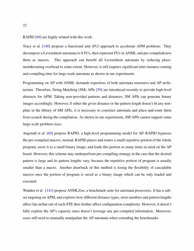
graph analysis [64], and so on[137, 65, 138, 139, 67]. Among them, FU [140], SM APIs [59], and
22
RAPID [69] are highly related with this work.
Tracy et al. [140] propose a functional unit (FU) approach to accelerate APM problems. They
decompose a Levenshtein automata to 8 FUs, then represent FUs in ANML and pre-compile&save
them as macros. This approach can benefit all Levenshtein automata by reducing place-
ment&routing overhead to some extent. However, it still requires significant inter-instance routing
and compiling time for large-scale automata as shown in our experiments.
Programming on AP with ANML demands expertises of both automata structures and AP archi-
tecture. Therefore, String Matching (SM) APIs [59] are introduced recently to provide high-level
abstracts for APM. Taking user-provided patterns and distances, SM APIs can generate binary
images accordingly. However, if either the given distance or the pattern length doesn’t fit any tem-
plate in the library of SM APIs, it is necessary to construct automata and place-and-route them
from scratch during the compilation. As shown in our experiments, SM APIs cannot support some
large-scale problem sizes.
Angstadt et al. [69] propose RAPID, a high-level programming model for AP. RAPID bypasses
the pre-compiled macros; instead, RAPID places and routes a small repetitive portion of the whole
program, saves it as a small binary image, and loads this portion as many times as need on the AP
board. However, this scheme may underperform pre-compiling strategy in the case that the desired
pattern is large and its pattern lengths vary, because the repetitive portion of program is usually
smaller than a macro. Another drawback of this method is losing the flexibility of cascadable
macros once the portion of program is saved as a binary image which can be only loaded and
executed.
Wadden et al . [141] propose ANMLZoo, a benchmark suite for automata processors. It has a sub-
set targeting on APM, and explores how different distance types, error numbers and pattern lengths
affect fan-in/fan-out of each STE then further affect configuration complexity. However, it doesn’t
fully explore the AP’s capacity since doesn’t leverage any pre-compiled information. Moreover,
users still need to manually manipulate the AP automata when extending the benchmarks.

23
2.3 Security Vettings for Android
In this section, we will introduce the existing Android static program analysis tools first, and then
describe how the current solutions construct the Android programs’ data-flow graphs.
2.3.1 Android Static Analysis Tools
Android security nowadays is one of the most crucial and popular subareas in software secu-
rity [142, 143, 144, 145, 146, 147]. A bunch of tools has been proposed for applying the static
analysis on Android security problems. FlowDroid [83] first builds a call graph based on Spark/-
Soot [148] by performing a flow-insensitive points-to analysis. It then uses IFDS [149] to conducts
the taint and on-demand alias analysis based on the call graph. IFDS is flow- and context-sensitive;
however, the call graph building is flow-insensitive hence could degrade the precision of IFDS
analysis. Moreover, FlowDroid does not text- and flow-sensitively calculate all objects’ alias or
points-to information due to computational cost concerns [150]. Epicc [151] adopts IDE frame-
work to compute Android Intent call parameters. It models the intent data structure explicitly in
the flow functions. Epicc only uses the results of Intent parameter analysis to resolve some spe-
cific cases of Intent call and does not perform the inter-component data-flow analysis. IccTA [84]
extends FlowDroid by adopting IC3 [152] Intent resolution engine. IccTA can track data flows
through regular Intent calls and returns but cannot through remote procedure call (RPC). On the
contrary, DroidSafe [153] tracks both Intent and RPC calls but cannot track data flows through
stateful ICC nor inter-app analysis. DialDroid [82] is a scalable and accurate tool designed for
inter-app Inter-Component Communication (ICC) analyses. It makes a balance of the data-flow
analysis accuracy and run-time cost.
Each of the above tools is built to perform one or several specific kinds of static analysis and is not
flexible to extend the capability. On the other hand, Amandroid [85] provides generic support to
multiple Android static analyses. It builds the DFG and DDG then adds low-cost plugins to realize
various specific analyses. Amandroid calculates all objects’ points-to information in a context-
24
and flow-sensitive way. Although this boosts the precision, it drastically increases the computation
burdens [154].
2.3.2 Andorid Data-Flow Graph Constructions
The DFG is constructed through Inter-procedural Data-flow Analysis. Data-flow analysis is con-
ducted using iterative algorithms. The conventional iterative search algorithm visits each ICFG
node once in one iteration and keeps iterating until no further changes occur to the data-flow
sets [155]. This approach has a regular computation pattern hence can leverage the well-studied
depth-first and breadth-first search (BFS/DFS) [156, 157, 158, 159, 160, 161, 162] to efficiently
visit the CFG in each iteration. However, it has large redundancy and slow convergence due
to the fixed full workload in each iteration. Worklist algorithm is an alternative that dynami-
cally updates the worklist after each node visiting. Inter-procedural, finite, distributive subset
(IFDS) [149] and its extension inter-procedural distributed environment transformers (IDE) [163]
are two well-known conceptual frameworks using the worklist algorithm as the core. Some op-
timizations [164, 165, 166] have been proposed to algorithmically improve the IFDS efficiency.
Recently, two mature IFDS/IDE implementations gain massive popularity. IBM releases T.J. Wat-
son Libraries for Analysis (WALA) implementing the IFDS [167]. Heros [168] provides IFDS/IDE
solver on top of Soot [169]. Although the worklist algorithm algorithmically outperforms the con-
ventional algorithm, it still potentially requires high computational cost due to a large number
of iterations. Even worse, the dynamic update of worklist makes the computation pattern pretty
irregular and extremely hard to be parallelized.
All works mentioned above target only on executing the analyses on sequential platforms. The
literature on executing static analyses on modern parallel platforms is sparse. Among them, only
several works use GPUs. Prabhu et al. [87] accelerate the 0-CFA, a higher-order control-flow
analysis algorithm, with GPU. They leverage the sparse-matrix to optimize CFG data structures
and achieves 72X speedups over CPU version. Mendez-Lojo et al. [90] accelerate the Andersen-
style inclusion-based point-to analysis on GPU. They treat the analysis as a graph modification and

25
traversal problem and focus on providing general insights about implementing graph algorithms on
GPU. Su et al. [95] also implement the Andersen’s inclusion-based pointer analysis. Their design
has the similar idea to [90] and proposes several techniques to further optimize the implementation.
They claim their work can achieve 46% speedup against [90]. Each of above three work targets
only on one specific type of analysis and the design is generally not applicable to other static
analyses. Moreover, none of them associates the algorithm with specific language or file type;
significant application-specific tuning may be required when applying their algorithms to analyze
real-world cases.
2.4 Cache Side-Channel Attacks & Countermeasures
In this section, we will introduce the related work with the time-driven and access-driven cache
attacks respectively, and then present the work studying the implementations’ and system’s impacts
on the cache attacks.
2.4.1 Time-Driven Attacks
Bernstein’s attack [106] is one of the most classical practical implementations of time-driven at-
tacks. It is elaborated in Section 6.2.2. Bonneau and Mironov [107] proposed a finer-grained
time attack. They observed the time variations caused by cache-collisions happened during table
lookups of encryption. This attack requires less computational cost but is more difficult to measure.
Tiri et al. [100] proposed an analytic model for time-driven attacks that can estimate the strengths
of the symmetric key cryptosystems. Brumley and Hakala [108] proposed a timing template attack.
They combined vector quantization and the hidden Markov model to build a tool to automatically
analyze the cache-timing data. Brumley and Tuveri [113] described the timing attack vulnerability
in OpenSSL implementation and approved that the time-driven attack on a remote server is feasi-
ble. Wang et al. [170] proposed CacheD, a software examining technique that leverages symbolic
execution to identify potential cache time differences at each program point.

26
2.4.2 Access-Driven Attacks
Yarom et al. [103] presented FLUSH + RELOAD attack. This attack targets LLC and can recover
the keys even if the processes are not co-located in the same core. Liu et al. [102] implemented the
PRIME + PROBE attack also targeting on the LLC. This attack is cross-core, cross-VM, and works
on multiple versions of GnuPG without relying on weaknesses of OS or VM. Irazoqui et al. [171]
introduced another variation of PRIME+PROBE attack. Their attack is a fine-grain cross-core
LLC attack. It needs no deduplication and OS configuration changes hence is quite viable. Gruss
et al. [172] proposed the access-driven template attack on shared inclusive LLC. It automatically
profiles and exploits cache leakage of any programs without requiring prior knowledge of specific
software and system information. Gras et al. [173] proposed TLBleed that attacks the page-table
caches (TLB) to bypass the hardware cache side-channel protections.
2.4.3 Implementations’ and Systems’ Impacts
To our best knowledge, our work is the first systematic and experimental study of the cache con-
figurations’ impacts on the cache attacks’ performances. The most relevant existing work we are
aware of was done by Mantel et al [174]. Although the crypto algorithms are strong, careless
implementations and misuses can make the ciphers vulnerable [175, 176]. Mantel et al. systemati-
cally studied how different AES implementations influence the vulnerability to cache side-channel
attacks. They leveraged the CacheAudit static analyzer [177] to check the leakage bounds of differ-
ent AES implementations. In [174], only one cache parameter (PCS) was considered. Moreover,
its results are still counted as the theoretical expectations since CacheAudit is a program-analysis-
based tool that calculates the leakage bounds without any actual executions.

Chapter 3
Scalable Automata-based Pattern-Matching
Algorithm for Out-of-Order DPI
3.1 Introduction
Regular expression matching is a core task in deep packet inspection (DPI), which is a fundamental
networking operation. A traditional form of DPI comprises searching the packet payload against
a set of patterns. Network intrusion detection systems (NIDS) are an essential part of network
security devices. A NIDS receives and processes packets, and then reports the possible intrusions.
Some well-known open-source NIDS - such as Snort1 and Bro2 - employ DPI as their core; most
major networking companies offer their own NIDS solutions (e.g., security appliances from Cisco3
and Juniper Networks4). In NIDS, every pattern represents a signature of malicious traffic; thus,
the DPI engine of a NIDS inspects the incoming packets payloads against all available signatures,
and triggers pre-defined actions if a match is detected. A regular expression can cover a wide
variety of pattern signatures [1, 2, 3]. Because of their expressive power, regular expressions have
1http://www.snort.org2http://www.bro-ids.org3http://www.cisco.com/en/US/products/ps6120/index.html4http://www.juniper.net/us/en/products-services/security/idp-series
27

28
been increasingly adopted to express pattern sets in both industry and academia. To allow multi-
pattern search, current NIDS mostly represent the pattern-set through finite automata (FA)[115],
either in their deterministic or in their non-deterministic form (DFA and NFA, respectively).
A large body of research has focused on developing efficient regular expression matching engines.
For memory-centric solutions, where the automaton is stored in memory, DFA-based approaches
are more popular than NFA-based ones, because of their predictable memory bandwidth require-
ments. This is due to a simple fact: processing an input character involves only one DFA state
traversal, which can be translated into a deterministic number of memory accesses. However, this
attractive property comes at the cost of potentially large memory space requirements. As a matter
of fact, DFAs constructed from large and complex sets of regular expressions may suffer from the
state explosion problem, making the storage requirements prohibitively large. State explosion can
take place during DFA generation when the corresponding regular expressions have repetitions of
wildcards and/or large character sets. Several variants of DFA [116, 120, 20, 19, 23, 22, 26] have
been proposed to address this problem, and limit the effects of state explosion with varying degree.
In real-world scenarios, a network data stream can span multiple packets. Those packets can arrive
at network security devices out of order due to multiple routes, packet retransmission, or NIDS
evasion. This is referred to as packet reordering. Previous work analyzing Internet traffic has
reported that about 2%-5% of packets are affected by reordering [6, 7, 8]. However, these studies
have focused on benign traffic; while attackers may intentionally mis-order legitimate traffic to
trigger denial-of-service (DoS) attacks [8]. NIDS face challenges [9] when processing data streams
that span across out-of-order packets, especially when performing regular-expression matching
against traffic containing malicious content located across packets boundaries. In such cases, the
malicious patterns are split and carried by multiple packets; and NIDS cannot detect them by
processing those packets individually.
Several solutions have been proposed to address the problem of processing out-of-order packets
in NIDS. One approach that is widely adopted in current network devices is packet buffering and
stream reassembling [8, 10, 11, 12]. In this case, incoming packets are buffered and packet streams
29
are reassembled based on the information in the header fields. Regular expression matching is
then performed on the reassembled data stream. This approach is intuitive and easy to implement,
but can be very resource intensive and vulnerable to DoS attacks whereby attackers exhaust the
packet buffer capacity by sending long sequences of out-of-order packets. Recently, researchers
have proposed several new solutions [13, 14, 15] aimed to relieve packet-buffer pressure or even
avoid packet buffering and reassembling. This is done by tracking all possible traversal paths or
leveraging data structures such as suffix trees. While they alleviate the burden of handing out-of-
order packets to some extent, these methods are either applicable only to simple patterns (exact-
match strings or fixed-length patterns), or suffer from bad worst-case properties (and are therefore
still vulnerable to DoS attacks).
In this work, we aim to provide a solution that (1) can process out-of-order packets without re-
quiring packet buffering and stream reassembling, (2) relies only on finite automata, and (3) can
handle regular expressions with complex sub-patterns. One of the main challenges in this de-
sign comes from handling regular expressions that include unbounded repetitions of wildcards and
large character sets. This is because these sub-patterns can represent unbounded sets of exact-
match sub-strings which cannot be exhaustively enumerated. Our solution leverages the following
observation: all exact-match strings that match a repetition sub-pattern are functionally equivalent
from the point of view of the regular expression matching engine and interchanging them will not
affect the final matching result. Our proposed solution consists of regular DFAs coupled with a set
of supporting FAs either in NFA or DFA form. The supporting FAs are used to detect and record –
using only a few states (typically no more than five) – segments of packets that can potentially be
part of a match across packet boundaries. While processing packets out-of-order, those segments
can be dynamically retrieved from the recorded states, and can be then used to resolve matches
across packet boundaries. To be efficient, any automata-based solution requires minimizing the
number of automata, their size, and the number of states that can be active in parallel. Our pro-
posal includes optimizations aimed to achieve these goals. Our contributions can be summarized
as follows:

30
• We present O3FA, a new finite automata-based DPI engine to perform regular-expression
matching on out-of-order packets in real-time, i.e., without requiring flow reassembly.
• We propose several optimizations to improve the average and worst-case behavior of the
O3FA engine, and we analyze how the packet ordering affects the buffer size.
• We evaluate our O3FA engine on various real-world and synthetic datasets. Our results show
that our design is very efficient in practice. The O3FA engine requires 20x-4000x less buffer
space than conventional buffering & reassembling-based solutions, with only 0.0007%-5%
traversal overhead.
3.2 O3FA Design
In this section, we present our solution for performing regular expression matching on out-of-
order packets without requiring prior stream reassembly. The main challenge in this problem is the
handling of matches across packet boundaries. At the high level, our proposed solution couples
one or more DFAs with supporting-FAs. The DFAs allow us to find matches within a packet. The
supporting-FAs are used to detect and record segments of packets that can potentially be part of
a match across packet boundaries. While processing packets out-of-order, these segments can be
dynamically retrieved from the state information collected on the supporting-FAs, and they can
subsequently be concatenated to the incoming packet in order to handle cross-packet matches.
To have an intuition of this idea, consider matching input stream cabcdeab against pattern b.*cde.
Let us assume that this input stream spans across two packets: P1=cabc and P2=deab. We can
observe that pattern b.*cde is matched across packet boundaries (the match starts in P1 and ends in
P2; the segments of P1 and P2 involved in the match are underlined). If we use a DFA, this match
will be detected only if packets P1 and P2 are processed in order. If the packets are processed out-of-
order, we will need a way to detect that segment de of P2 and segment bc of P1 are partial matches
(specifically, they match the suffix and the prefix of the considered patterns, respectively). We will
then use this information to reconstruct the match. Our proposed supporting-FA will serve this

31
purpose. We note that, because b.*cde is neither an exact-match string nor a fixed-length pattern,
it cannot be handled by previous approaches such as SplitDetect [121], AC-Suffix-Tree [14] and
ORL [13].
Because we are concerned about patterns with variable length, we focus on regular expressions
containing repetitions of characters (e.g., c+ and c*), character sets (e.g, [ci-cj]*) and wildcards
(.*). We note that regular expressions without these features can be handled by traditional meth-
ods. For example, a regular expression containing a non-repeated character set [ci-cj] can be
transformed by exhaustive enumeration into a set of exact-match patterns. For readability and in
the interest of space, the remaining description focuses on the more general case (wildcard repeti-
tions); however, our solution is applicable to all kinds of repetitions.
A central question in the O3FA design is the following: how can we identify the minimal packet
segments that must be recorded in order to handle cross-packet matches? We note that excessively
long segments would pose pressure on the required packet buffer and on the amount of process-
ing involved in the matching operation, thus leading to inefficiencies. Our design leverages the
following observations.
Observation 1: If a regular expression R is matched across a set of packets P1, .., PN, then the
suffix of P1 must match a prefix of R and the prefix of PN must match a suffix of R.
Observation 2: Given a regular expression R in the form sp1.*sp2 and an input stream I contain-
ing a matching segment of the form M1M*M2, where M1 matches sp1 and M2 matches sp2, any
modifications to I that substitutes M* with a shorter segment will not affect the match outcome.
According to Observation 1, O3FA must detect segments of incoming packets that match any
suffixes/prefixes of the considered regular expressions. These segments are recorded by storing the
corresponding matching states information, and they can be dynamically retrieved and properly
concatenated with later-arrival packets to detect cross-boundary matching. For example, while
matching regular expression b.*cde on packets P1=caba, P2=dcac and P3=dead that arrive in order
P3!P1!P2, we first detect that segment de in P3 matches suffix de, and then that segment ba in
P1 matches prefix b.*. When P2 arrives, we retrieve those segments and concatenate them with P2,

32
then conduct regular expression matching on badcacde and detect the cross-boundary matching of
b.*cde. In general, prefix b.* can match arbitrarily long strings, which may span across any number
of intermediate packets. However, according to Observation 2, in order to reconstruct the match it
is sufficient to record the shortest segment of the input stream that matches the regular expression
with the wildcard repetition. In the considered example, rather than recording segment ba of packet
P1, we can simply record segment b. In addition, if a regular expression p.*s is matched across a set
of packets P1, .., PN such that the suffix of P1 matches p and the prefix of PN matches s, recording
the intermediate packets P2, .., PN-1 will not be necessary for matching purposes.
The design is complicated by the fact that multiple regular expressions would require recording
multiple segments, possibly leading to inefficiencies. In section 3.3 we propose a mechanism
(that we call Functionally Equivalent Packets) to combine segments related to different regular
expressions. As we will discuss, this method leverages the overlap between different segments.
3.2.1 O3FA Data Structure
We now discuss the design of O3FA, a composite automata-based solution that implements the
scheme described above. As mentioned, O3FA consists of two components:
• One or more regular DFAs used to perform regular expression matching and constructed
based on the given regular expression set. Any automata optimization techniques [116, 120,
20, 19, 23, 22, 26, 21, 17, 119, 178] can be applied to these DFAs.
• Supporting-FAs used to detect and record significant segments of incoming packets. Ac-
cording to the above discussion, supporting-FAs should be constructed to detect segments
matching regular expressions prefixes and suffixes, and can therefore be of two kinds: prefix-
FAs and suffix-FAs. These automata can be in either NFA or in DFA form.
In order to build the prefix- and suffix-FAs, we split the regular expressions at the positions of the
repetition sub-patterns. For example, regular expression abc.*def .*ghk will be broken down into

33
three sub-patterns: .*abc.*, .*def .* and .*ghk.* (the .* before abc is due to the fact that the original
regular expression is unanchored, that is, it can be matched at any position of the input stream).
This breakdown is possible because the supporting-FAs are used to record packet segments, and
not to perform pattern matching; the short packet segments recorded by breaking down the regular
expressions into sub-patterns will be concatenated into larger segments during processing. This
breakdown allows significantly simplifying the supporting automata: by allowing dot-star terms
to appear only at the beginning or at the end of each pattern, it will avoid state explosion when
representing the supporting-FAs in DFA form. The full prefix and suffix sets corresponding to the
given sub-patterns are: {.*abc.*, .*abc, .*ab, .*a, .*def .*, .*def , .*de, .*d, .*ghk, .*gh, .*g} and
{.*abc.*, abc.*, bc.*, c.*, .*def .*, def .*, ef .*, f .*, .*ghk, ghk, hk, k}, respectively. However,
some simplifications are possible. First, since the suffixes must be matched at the beginning of
packets (Observation 1) and can end anywhere within a packet, the ”.*” at the end of each suffix is
redundant. Second, patterns that are common to prefix and suffix sets (e.g. .*abc, .*def , .*ghk) can
be removed from the prefix set (these patterns would lead to the detection of the same segments5).
Third, sub-patterns that are covered by more general patterns belonging to the same set (e.g. abc
is a special case of .*abc) can also be eliminated. After these simplifications, the prefix and suffix
sets used to build the prefix- and suffix-FA will be {.*abc.*, .*ab, .*a, .*def .*, .*de, .*d, .*gh,
.*g} and {.*abc, bc, c, .*def , ef , f , .*ghk, hk, k}, respectively. Note that the suffix set contains
both anchored and unanchored patterns (the latter start by ”.*”). These two groups of patterns can
be compiled in two different suffix-FAs (i.e., an anchored and an unanchored suffix-FA) to allow
space optimizations when representing the automata in DFA form.
During processing, upon a match within a supporting-FA, the corresponding accepting state must
be recorded, and it will then be used to retrieve the packet segments to be concatenated to the
current input packet. This ”extended” input packet will then be processed by the ”regular” DFA.
However, some matches that occur within the supporting-FAs can be discarded, thus diminishing
the amount of information that must be recorded to reconstruct relevant packet segments. First,
5The reason why these patterns are removed by the prefix set will become apparent later. Specifically, since allprefix matches in the middle of packets can be discarded, keeping these patterns in the suffix set ensures that they willbe detected by the suffix-FA.

34
since prefixes need to be matched only at the end of packets (Observation 1), all prefix matches
occurring in the middle of any packets can be discarded. Second, if multiple anchored suffixes of
a regular expression are matched, only the longest one must be recorded (shorter suffixes will be
subsumed by it).
Figure 3.1 shows an example on regular expression set {abc.*def , ghk}, both patterns are unan-
chored (that is, they can be matched at any position of the input stream). The prefix set, anchored
suffix set and unanchored suffix set are {.*abc.*, .*ab, .*a, .*de, .*d, .*gh, .*g}, {bc, c, ef , f ,
hk, k} and {.*abc, .*def , .*ghk}, respectively. Figure 3.1 (a)-(d) show the resulting regular DFA,
prefix-FA, anchored suffix-FA and unanchored suffix-FA; all supporting-FAs are left in NFA form.
We assume three input packets: P1=bhab, P2=cegh and P3=adef , with the arriving order being
P3!P1!P2. After P3 is processed, the matching state sets of regular DFA and anchored suffix-FA
are empty; the unanchored suffix-FA matching states is 6; the prefix-FA matching states are {8, 9};
since those matches do not happen at the tail of P3, they will be discarded. Then, we process P1; the
matching state sets of regular DFA, anchored suffix-FA and unanchored suffix-FA are empty; the
prefix-FA matching states are {5, 6}; since only matching state 5 is active at the end of P1 process-
ing, this sole prefix-FA state will be recorded. When P2 arrives, we should first check the recorded
information of its previously processed neighbor packets (i.e., predecessor P1 and successor P3):
P1 has a recorded prefix-FA state 5; the retrieved segment is ab and should be concatenated to P2 as
a prefix. P3 has a recorded unanchored suffix-FA state 6; the retrieved segment is def and should
be concatenated to P2 as a suffix. Then, the modified P2 is abceghdef ; after it is processed with
the regular DFA, the matching of the pattern abc.*def will be reported.
3.3 Optimizations
Our basic O3FA design has two limitations: it can lead to false positives (that is, it may report
invalid matches) and it can suffer from inefficiencies during processing. In this section, we describe
a mechanism - called Index Tags - to avoid false positives, and a suitable format for the supporting-

35
(a)
1 2a
b c
12 13g h
0
3remaining transitionsfrom 1,2,12-14 d 6 e 7
f8
k 14
g
9 h k 11
b 5a 4
a: from 1,2,12-14
a: from 4-11
remaining transitionsfrom 4-11
10
c
g: from 1,2,12-14g: from 4-11
d: from 4-11
1 2
a
b c
0
3
*
4ab 5
a 6
7d e 8
10
gh 11
d9g
12
*
0
1bc 2
c 3
4e f 5
7
hk 8
f6k
9
1 2ab c
0
3*
4 5d e f 6
7 8g
h k 9
(b)
(c) (d)
Figure 3.1: (a) DFA accepting pattern set {abc.*def , ghk}, (b) prefix-FA, (c) anchored suffix-FA and (d)unanchored suffix-FA built upon corresponding prefix set, anchored suffix set and unanchored suffix set.Accepting states are colored gray.
FAs and two auxiliary data structures to improve the matching speed.
3.3.1 Index Tags
Our initial O3FA engine design may report false positives in the presence of multiple regular ex-
pressions. For example, consider a dataset with two regular expressions: {bc.*d, acd}. Two input
packets P1:caaba and P2:cabdc are received out of order (P2!P1). Obviously, no matches should
be reported on the corresponding input stream caabacabdc. However, in our basic O3FA design,
the anchored suffix-FA will detect the segment cabd of P2 that matches suffix c.*d of the first pat-
tern; when P1 arrives, segment cd will be retrieved and concatenated to P1 as a suffix, leading to
the extended packet caabacd. Processing this packet with the regular DFA will lead to the false
match acd to be reported.
To understand the root cause of this problem, we make the following observation.
Observation 3: Let R be a set of regular expressions, R’ a proper subset of R, and r a regular
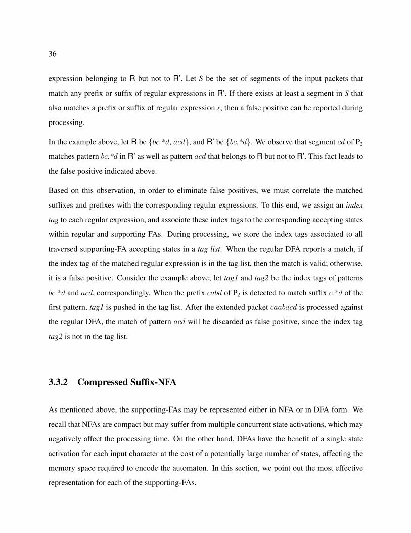
36
expression belonging to R but not to R’. Let S be the set of segments of the input packets that
match any prefix or suffix of regular expressions in R’. If there exists at least a segment in S that
also matches a prefix or suffix of regular expression r, then a false positive can be reported during
processing.
In the example above, let R be {bc.*d, acd}, and R’ be {bc.*d}. We observe that segment cd of P2
matches pattern bc.*d in R’ as well as pattern acd that belongs to R but not to R’. This fact leads to
the false positive indicated above.
Based on this observation, in order to eliminate false positives, we must correlate the matched
suffixes and prefixes with the corresponding regular expressions. To this end, we assign an index
tag to each regular expression, and associate these index tags to the corresponding accepting states
within regular and supporting FAs. During processing, we store the index tags associated to all
traversed supporting-FA accepting states in a tag list. When the regular DFA reports a match, if
the index tag of the matched regular expression is in the tag list, then the match is valid; otherwise,
it is a false positive. Consider the example above; let tag1 and tag2 be the index tags of patterns
bc.*d and acd, correspondingly. When the prefix cabd of P2 is detected to match suffix c.*d of the
first pattern, tag1 is pushed in the tag list. After the extended packet caabacd is processed against
the regular DFA, the match of pattern acd will be discarded as false positive, since the index tag
tag2 is not in the tag list.
3.3.2 Compressed Suffix-NFA
As mentioned above, the supporting-FAs may be represented either in NFA or in DFA form. We
recall that NFAs are compact but may suffer from multiple concurrent state activations, which may
negatively affect the processing time. On the other hand, DFAs have the benefit of a single state
activation for each input character at the cost of a potentially large number of states, affecting the
memory space required to encode the automaton. In this section, we point out the most effective
representation for each of the supporting-FAs.

37
We recall that, in our O3FA design, the anchored suffix set contains only exact-match patterns.
An NFA containing only anchored exact-match patterns can have only one active state. Thus, the
anchored suffix-FA can be left in NFA form without loss in processing efficiency. We denote this
automaton as anchored suffix-NFA (asNFA).
The anchored suffix set can have a large amount of redundancy due to the nature of suffixes. An
n-character pattern can lead to n-1 suffixes, with every two adjacent suffixes differing in only one
character. This creates compression opportunities for asNFA. We propose a compressed suffix-
NFA (csNFA) representation, which reduces both the asNFA size and bandwidth requirements.
Specifically, given the nature of the suffixes of any given pattern, we merge the asNFA states and
transitions starting from the tail states. Figure 3.2 shows an example. Figure 3.2(a) is the asNFA
built upon anchor suffix set {bcdca, cdca, dca, ca, a}; Figure 3.2(b) is the corresponding csNFA. In
this example, the compression reduces the number of NFA states from sixteen to six and removes
six transitions.
0
1 2 3 4bc d c a
6 7 8cd c a
13c
aa
10 11d c a
5
9
12
14
15
0 1 2 3 4b c d c ac
ca
d
5
(a) (b)
Figure 3.2: (a) asNFA and (b) csNFA built upon anchored suffix set {bcdca, cdca, dca, ca, a}. Acceptingstates are colored gray.
While more compact, csNFA requires a more elaborate segments retrieval procedure. In an asNFA,
segments retrieval can be done by simply tracking back from the recorded matching states to the
entry state. However, in the optimized csNFA, this straightforward approach does not work since
the backtracking may lead to ambiguity at some states. To address this problem, during csNFA
traversal we identify all states that are active after the processing of the first input character and
assign state pair <start state, end state> to each active state, where start states are these active

38
states and end states are last states of the traversed paths originating from them. Only state pairs
<start state, end state> such that end states are accepting states are significant; moreover, as
we discussed in Section 3.2, only the state pair representing the longest matching path needs to
be recorded. The matched segment can then be retrieved by tracing the csNFA matching path
using the recorded state pair. Since the anchored suffix set includes only exact-match patterns, the
start states set has a limited size and the active paths are expected to go dead after the processing
of a small number of input characters, reducing the amount of processing. Our experiments in
Section 3.5 confirm the efficiency of this proposed compression scheme.
As an example, we consider the csNFA of Figure 3.2(b) and input cadc. csNFA processes the
first input as {0}�c!{2,4}; we assign state pairs to both active states and track the traversal:
{2}�a!{?}, {4}�a!{5}. Since the first path goes dead and the second path reaches the tail
state of the csNFA, the traversal leads to two state pairs: <2,2> and <4,5>. Since only state 5
is an accepting state and <4,5> matches the longest segment, only state pair <4,5> needs to be
recorded. State pair <4,5> should then be back-traced as 5�a!4�c!0, leading to the retrieval
of segment ca.
3.3.3 Prefix- and Suffix-DFA with State Map
We recall that all patterns in the prefix set and unanchored suffix set are unanchored (that is, they
may be matched at any position of the input stream). Since their entry state is always active (poten-
tially leading to the concurrent activation of multiple NFA branches), NFAs accepting unanchored
patterns tend to have multiple concurrent active states, which negatively affect the processing time.
By requiring a single state activation for each input character processed, a DFA representation
guarantees minimal processing time, potentially at the cost of a larger memory requirement. How-
ever, we recall that patterns in the prefix and suffix sets do not have wildcard repetitions, and thus
do not lead to significant state explosion. Thus, the DFA format is suitable for both prefix- and
unanchored suffix-FAs; we denote these automata as prefix-DFA (pDFA) and suffix-DFA (sDFA).

39
1 2a b c
4 5b c d0
3
6
*
1 2ab c
5 6b
c
d
0
3 4
d
a: from 1-6
b: from 2-6
remaining transitions
(a) (b)
DFA state 1 2 3 4 5 6
NFA states 1 2 3 6 4 5
Figure 3.3: (a) NFA format and (b) sDFA with states map for unanchored suffix set {.*abc, .*bcd}. Accept-ing states are colored gray.
The number of states in a DFA can be minimized through a well-known procedure [115]. In
addition, as discussed in Section 3.2, all prefix matches occurring in the middle of packets can
be ignored. This allows further optimizations to the prefix-DFA. Specifically, all accepting states
that do not present a self-loop can be made non-accepting, and all self-loops can be removed from
the remaining accepting states. This simplification can both reduce the size of the prefix-DFA and
simplify the processing (by making a filtering step to remove non-terminal matches unnecessary).
The use of a DFA representation for these automata, however, has a drawback: it complicates
the retrieval of the matching input segments. Since there may be multiple paths leading to the
same DFA state, it is not possible to retrieve the input segment solely based on the recorded DFA
state. To tackle this problem, we propose using a state map, which maps the pDFA/sDFA states
to the corresponding NFA states; segment retrieval can then be done by back-tracing NFA paths.
Since pDFA and sDFA do not suffer from state explosion, the size of this state map is contained.
One DFA state may map to multiple NFA states; in those cases, however, only the NFA state that
leads to the longest retrieved segment needs to be included in the state map, allowing a one-to-one
mapping.
We illustrate this design through an example. Let us consider pattern .*abc.*bcd. The cor-
responding unanchored suffix and prefix sets are {.*abc, .*bcd} and {.*abc.*, .*ab, .*a, .*bc,
.*b}, respectively. The corresponding automata are shown in Figure 3.3 and 3.4. Specifi-
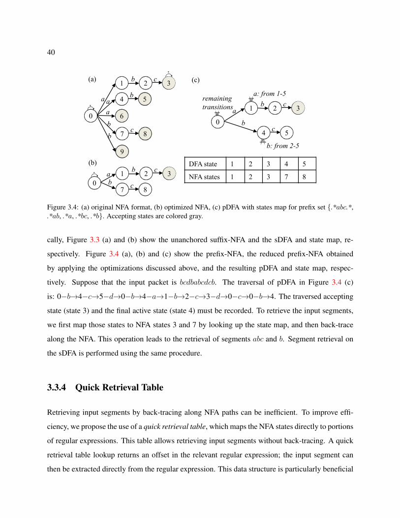
40
DFA state 1 2 3 4 5
NFA states 1 2 3 7 8
1 2
a
b c
4 5
b
b
a0
3
*
6
7 8
9
a
bc
1 2a b c
7 8b c0
3*
1 2ab c
4 5b
c0
3
a: from 1-5
b: from 2-5
remaining transitions
(a) (c)
(b)
*
Figure 3.4: (a) original NFA format, (b) optimized NFA, (c) pDFA with states map for prefix set {.*abc.*,.*ab, .*a, .*bc, .*b}. Accepting states are colored gray.
cally, Figure 3.3 (a) and (b) show the unanchored suffix-NFA and the sDFA and state map, re-
spectively. Figure 3.4 (a), (b) and (c) show the prefix-NFA, the reduced prefix-NFA obtained
by applying the optimizations discussed above, and the resulting pDFA and state map, respec-
tively. Suppose that the input packet is bcdbabcdcb. The traversal of pDFA in Figure 3.4 (c)
is: 0�b!4�c!5�d!0�b!4�a!1�b!2�c!3�d!0�c!0�b!4. The traversed accepting
state (state 3) and the final active state (state 4) must be recorded. To retrieve the input segments,
we first map those states to NFA states 3 and 7 by looking up the state map, and then back-trace
along the NFA. This operation leads to the retrieval of segments abc and b. Segment retrieval on
the sDFA is performed using the same procedure.
3.3.4 Quick Retrieval Table
Retrieving input segments by back-tracing along NFA paths can be inefficient. To improve effi-
ciency, we propose the use of a quick retrieval table, which maps the NFA states directly to portions
of regular expressions. This table allows retrieving input segments without back-tracing. A quick
retrieval table lookup returns an offset in the relevant regular expression; the input segment can
then be extracted directly from the regular expression. This data structure is particularly beneficial

41
NFA state
1 2 3 4 5
char. position
<1,2> <1,3> <1,4> <1,5> <1,6>
0 1 2 3 4b c d c ac
ca
d
5
Index Tag:1 RegEx: abcdca(a) (b)
Figure 3.5: (a) csNFA and (b) quick retrieval table for anchored suffix set {bcdca, cdca, dca, ca, a}.Accepting states are colored gray. Each char. position is a pair of index tag and offset, i.e., <tag, offset>
in the case of long segments.
As an example, consider regular expression abcdca. The anchored suffix set and corresponding
csNFA are the same as for the example in Section 3.3.2. Figure 3.5 (a) shows the csNFA and
Figure 3.5 (b) shows the quick retrieval table, which stores <index˙tag, offset> pairs. We recall
that index tags point to regular expressions. If the recorded state pair is <4, 5>, for example, a
lookup in the quick retrieval table will return index tag tag1 corresponding to pattern abcdca, and
start- and end- offsets 5 and 6, respectively. This will result in retrieving segment ca.
3.3.5 Functionally Equivalent Packets
Any incoming packet may contain multiple segments that match a prefix or a suffix. For exam-
ple, the sample packet in Section 3.3.3 contains two segments that match two different prefixes.
All these segments should be recorded and retrieved properly, and all retrieved segments should
be processed with the current input packet. A simple approach is to sequentially concatenate the
segments retrieved to the current packet and process all modified current packets. For example,
supposing the current packet is efgh, using the same example of Section 3.3.3, then two retrieved
segments are abc and b, and the two corresponding concatenated current packets abcefgh and
befgh should be processed serially. This solution can be highly inefficient. However, concurrently
concatenating all retrieved segments to the current packet is not straightforward, since many seg-
ments may have overlaps. Our proposed solution is the Functionally Equivalent Packet (FEP),
which has the main idea that we construct an alternate packet based on all retrieved segments then

42
DFA state 1 2 3 4
NFA state 1 2 3 4
1 2ab
3 4b c0
a: from 1-4
b: from 2-4
remaining transitions
(b)
1 2a b
3 4b c0
*(a) <2, 3>States map
NFA states 2retrieving
<4, 4>
prefix ab
States mapNFA states 4
retrievingprefix bc
empty string
filled string
FEP:
a b c
offset 3 offset 4
abc
filling filling
shrinking
(c)
Figure 3.6: (a) NFA format and (b) pDFA with states map built upon prefix set {.*ab.*, .*a, .*bc, .*b}. (c)Construction of functionally equivalent packet to packet P2=eabc.
deal with the alternate packet instead of segments. Such an alternate packet contains all effective
information (i.e., all detected segments) of the original packet and thus is functionally equivalent
to the original one.
Consider the example RegEx ab.*bcd; the prefix set is {.*ab.*, .*a, .*bc, .*b}. Figure 3.6 (a) and
(b) are the NFA format and pDFA with a states map for this prefix set. Supposing the input packets
are P1=afab, P2=eabc and P3=defg, there is obviously only one matching of ab.*bcd across all
three packets. Two pDFA states 2 and 4 are recorded after packet P2 is processed, representing
two detected segments that match prefixes .*ab.* and .*bc. The retrieved alternate segments are
ab and bc. Directly concatenating both segments to P3 as abbcdefg can cause a false-positive
matching. Our FEP design needs only one change that recording <state, offset> pairs instead of
only matched states; the offset is the offset of matched segments last character in the packet. When
retrieving segments, all retrieved alternate segments will be filled into an empty string, filling
positions accord to their offsets; then, the filled string will be shrunken to get FEP. Figure 3.6 (c)
shows the construction of FEP to P2. <2, 3> and <4, 4> are two recorded <state, offset> pairs.
The alternate FEP of P2 is abc; substituting P2 by FEP in the data stream as afababcdefg will not
affect the matching results.

43
3.4 O3FA-based System
In this Section, we provide the O3FA engine, which is a completed system based upon the O3FA
design and can perform regular expression matching on out-of-order packets. We also provide
worst-case analysis in this section.
3.4.1 O3FA Engine Architecture
Our O3FA engine consists of four major components:
• Regular Expression Parser
• Finite-automata Kernel
• States Buffer
• Functionally Equivalent Packet Constructor
Regular Expression Parser (RegEx Parser) is for preprocessing the regular expression set as well
as building the corresponding prefix set and anchored/unanchored suffix set. Finite-automata Ker-
nel (FA Kernel) is the operational core of the O3FA engine consisting of both regular DFA and
supporting-FAs. States Buffer is the buffer to store automata states generated by FA Kernel. Func-
tionally Equivalent Packet Constructor (FEP Constructor) is the component for constructing FEPs
by properly querying stored information in States Buffer.
Figure 3.7 is the schematic diagram of the O3FA engine architecture. The blue-colored compo-
nents are components involved in the regular expression dataset processing; the yellow-colored
components are components involved in the input packet processing. Notice that FA Kernel is
involved in both processing, since it is built in dataset processing and should be used for packet
processing. The blue arrows show the dataset processing flow, while the yellow dotted-line arrows
show the packet processing flow.

44
RegEx dataset input packets
RegEx Parser
FA Kernel
States Buffer
FEPConstructor
Figure 3.7: Overview of the O3FA engine. The blue parts are dataset processing components; the yellowparts are input packet processing components.
RegEx Parser: This component works offline. It breaks regular expressions as described in
Section 3.2, and it generates a corresponding prefix set and anchored/unanchored suffix set for
supporting-FA construction.
FA Kernel: FA Kernel is the operational core of the O3FA engine. It takes outputs from RegEx
Parser and builds regular DFA and supporting-FAs following the O3FA design. According to
discussions in Sections 3.2 and 3.3, FA Kernel specifically consists of regular DFA (rDFA),
compressed suffix-NFA (csNFA), prefix-DFA (pDFA) and suffix-DFA (sDFA). This O3FA con-
struction works offline.
Once the O3FA is built, FA Kernel keeps processing packets online. It interacts with States Buffer
and FEP Constructor by getting FEPs from FEP Constructor and storing proper matching informa-
tion to States Buffer. The matching procedures are discussed in previous sections.
States Buffer: The States Buffer is an auxiliary component to assist both FA Kernel and FEP
Constructor. It stores the matching state information generated by FA Kernel and can be queried
by FEP Constructor to provide information for FEP construction.
As discussed in Section 3.3, States Buffer will store final states of regular DFAs and state pairs
<start state, end state> generated by csNFA as well as <state, offset> pairs generated by pDFA
and sDFA. Specifically, States Buffer will create an entry with packet ID for each arriving packet;
if the current packet has neither an arrived predecessor nor successor, it will be directly processed
in FA Kernel, and its entry will store the generated matching state information; if the current packet
has an arrived predecessor/successor, then FEP Constructor will query the predecessor/successors

45
entry in States Buffer, and it will construct FEPs of arrived predecessor/successor packets based
upon stored information in the entry. The FEP will be concatenated with the current packet, and the
modified packet will be processed in FA Kernel; then, the matching state information will be stored
in the current packets entry, and the corresponding predecessor/successor entry can be empty since
all of the predecessor/successors information is already contained in the current packets entry.
Intuitively, the States Buffer will have a much smaller size than the packet buffer in general, since
several state pairs can represent a whole packet, and States Buffer entries may be dynamically
clear during matching. Experimental data in the evaluation section will support this inference.
Worst-case discussion will also be provided in a later section.
FEP Constructor: The FEP constructor uses state information provided by the State Buffer to
reconstruct functionally equivalent packets, as described in Section 3.3.5.
3.4.2 O3FA Engine Work Flow
The O3FA engine can keep processing the incoming packets once the O3FA in FA Kernel is built.
For each current packet, the processing procedure should follow the below steps:
1) For any current packet, first check States Buffer to look up its arrived predecessor/successor.
If you find it, go to step 2; otherwise, go to step 3.
2) FEP Constructor queries States Buffer and constructs FEP based upon the predecessor/-
successor buffer entry; then, it concatenates FEP with the current packet and outputs the
concatenated packet to FA Kernel.
3) FA Kernel processes the current packet (concatenated packet), generates <start˙state,
end˙state>/<state, offset> state pairs and writes them to States Buffer.
4) States Buffer creates an entry for the current packet and stores state pairs generated by FA
Kernel in it. If the current packet has an arrived predecessor/successor, then predecessor/-
successors entries can be empty, and pointers can be added from those empty entries to the

46
current packets entry for lookup purposes.
Figure 3.8 shows the flow chart of packet processing, following the same rule of the above steps.
check pre/suc
Current packet
arrived predecessor/ successor?
query pre/suc buffer entry
concatenated packet
YN
Yif N
functionally equivalent packet
matching? report intrusion
if Y
FA Kernel
States Buffer
Functionally Equivalent Packet (FEP) Constructor
matching states info
Figure 3.8: Packet processing flow chart. Dotted arrows indicate alternative paths if there are no arrivedsuccessor/predecessor packets.
3.4.3 Worst-case Analysis
Two aspects can affect the capacity of our proposed O3FA engine. One is States Buffers size: A
larger buffer size means more vulnerability to a denial of service attack; the other is the traversal
overhead, which is caused by FEP. A longer FEP means more overhead, since the concatenated
packets will be longer than the actual current packet. In this section, we will provide worst-case
analysis for these two aspects.
Each non-empty States Buffer entry will store one packet ID, several rDFA final states (equal to
47
rDFA number in multi-DFA case), one <start˙state, end˙state> pair and multiple <state, offset>
pairs. The first three have firm and tiny sizes, while the last one has an indefinite size, since we
cannot bind the numbers of segments in a packet that matches the prefix and unanchored suffix.
Our evaluation shows, in practice, these two numbers are also very small. However, in theory, they
could be large enough. To provide an upper-boundary, we set a threshold of buffer entry size: If
the actual entry size is less than the threshold, then states will still be stored in the entry; otherwise,
the whole data packet will be stored instead. This ensures our O3FA engine will never be worse
than the regular packet buffering scheme in the memory requirement. Later, our evaluation shows,
in practice, the numbers of <state, offset> pairs are very small; thus, the entry sizes are always far
less than the threshold.
Similarly, the FEP length is indefinite; however, it will not exceed the length of a regular packet.
Thus, the upper-boundary of the traversal overhead for each current packet should be the length of
the packet payload. The evaluation section will also show that the FEPs are very small compared
to the current packets, in practice.
3.5 Evaluation
In this section, we provide experimental data to show the feasibility of our O3FA engine design.
Specifically, our experiments are designed to analyze the following aspects: (i) O3FAmemory foot-
print on reasonably large and complex regular expression sets; (ii) savings in buffer size require-
ments of O3FA engine compared to traditional flow reassembly schemes; (iii) memory bandwidth
overhead of supporting-FAs; and (iv) O3FA traversal efficiency.
48
3.5.1 Datasets & Streams
In our experiments, we use two real world and six synthetic datasets. The real world datasets
contain backdoor and spyware rules from the widely used Snort NIDS6 (snapshot from December
2011), and they include 176 and 304 regular expressions, respectively. The synthetic datasets have
been generated through the synthetic regular expression generator7 [179] using tokens extracted
from the backdoor rules. Each synthetic dataset contains 500 regular expressions. The synthetic
dot-star* datasets contain a varying fraction of dot-star sub-patterns (5%, 10% and 20%); in the
synthetic range* datasets 50% and 100% of the patterns include character sets; finally, the synthetic
exact-match dataset contains only exact-matching strings.
For each dataset, we generate 16 synthetic traces using the traffic trace generator7 [179]. This tool
allows for generating traces that simulate various amount of malicious activity. This can be realized
by tuning parameter pM , which indicates the probability of malicious traffic. In addition, to allow
randomization, a probabilistic seed parameter can be used to configure the trace generation. In our
experiments, we use four probabilistic seeds and four pM values: 0.35, 0.55, 0.75 and 0.95, i.e., 16
traces in total for each dataset. All traces have a 1 MB size. Each of the data points below has been
obtained by averaging the results reported on four simulations, each using a different probabilistic
seed.
3.5.2 Packet Reordering
To simulate out-of-order packet arrival, we break each synthetic stream down into multiple packets
and reorder these packets. Packet reordering is driven by two parameters: the out-of-order degree k
and the stride s. Parameter k indicates the minimum number of arrived packets that are needed for
partial stream reconstruction; parameter s indicates the maximum stride between two consecutive
packets within each group of k packets.
6https://www.snort.org/7http://regex.wustl.edu/
49
For example, let us assume a stream consisting of eight packets: P1 to P8. If we set k=2 and
s=1, then packets are reordered as P2!P1! P4!P3! P6!P5! P8!P7; if we set k=4 and s=1,
then packets are reordered as P4!P3! P2!P1!P8! P7!P6!P5; if we set k=4 and s=2, the
packets order will be P4!P2! P3!P1! P8!P6! P7!P5. Obviously, k=1 and s=1 implies
natural ordering, while k=(number of packets) and s=1 leads to reverse ordering (in the example,
from P8 down to P1).
This packets reordering scheme allows us to characterize how the packet order affects the per-
formance of the O3FA engine, and to compare the O3FA engine with the traditional input stream
reassembly method. In our experiments, we break each 1MB stream into 16 packets, each having
the 64KB standard TCP packet size. We reorder packets of each stream using three parameter
settings: k=2/s=1, k=4/s=1 and k=4/s=2.
3.5.3 Experiment Results
We first present the experiment results regarding the finite automata kernel’s and the state buffer’s
memory consumptions respectively, and then show the evaluation results about the overhead of
memory bandwidth and state traversal in last two subsections.
3.5.3.1 O3FA Memory Footprint
First, we evaluate the memory footprint of the O3FA supporting each of the considered datasets.
The backdoor, spyware and dotstar* datasets include sub-patterns (e.g. dot-stars) leading to state
explosion. To limit state explosion, for these datasets we break the regular DFA into multiple
DFAs [120] (the number of DFA ranges from 8 to 15). Due to their simplicity, the exact-match
and range* datasets can be supported by a single regular DFA. The total number of regular DFA
states ranges from 9k to 254k across the considered datasets. We recall that the supporting-FAs are
of three kinds: compressed suffix-NFA (csNFA), prefix-DFA (pDFA) and suffix-DFA (sDFA). As
discussed in Section 4, none of the supporting-FAs suffers from state explosion, leading to rela-

50
Table 3.1: Memory footprint of FA kernels (MB)
Dataset FA KernelRegular multi-DFAs Supporting-FAs
Backdoor 60 0.62Spyware 56 1.35Dotstar.05 26 3.58Dotstar.1 60 3.12Dotstar.2 100 2.76Range.5 5.6 2.43Range1 5.8 2.05Exact-match 4.7 1.92
tively small automata. The number of csNFA, sDFA and pDFA states ranges from 2k to 13k, from
1k to 13k and from 1k to 9k, respectively. Range* datasets have larger supporting-FA sizes. This
is because all character sets must be exhaustively enumerated before constructing the supporting-
FAs, resulting in large prefix and suffix sets. The number of transitions of the csNFA ranges from
5k to 27k. To achieve memory space efficiency, we apply defaulttransition compression [21] to
DFAs. Table 3.1 shows the estimated memory footprint of the resulting O3FA (we assume 32-
bit transitions). As can be seen, O3FA requires about 100MB memory space in the worst case,
which does not put pressure to commodity systems. In addition, because supporting-FAs do not
suffer from state explosion, their size is in all cases limited, and their memory space overhead is
negligible in case of complex datasets including dot-star terms.
3.5.3.2 Buffer Size Savings
Figure 3.9 shows the maximum buffer size requirement comparison between the O3FA engine
and a traditional flow reassembly scheme [12]. The O3FA engine uses the state buffer described in
Section 3.4, while the flow reassembly scheme uses a packet buffer. The optimized flow reassembly
scheme reassembles a partial stream once the buffered packets allow it and then processes that
partial stream and flushes the corresponding packet buffer entries. For each value of pM , we
average the results reported using four probabilistic seeds. In the charts, the six bars represent

51
opt. reassembly scheme k=2,s=1 O3FA engine k=2, s=1
opt. reassembly scheme k=4,s=1 O3FA engine k=4, s=1
opt. reassembly scheme k=4,s=2 O3FA engine k=4, s=2
0
1
2
3
4
5
6
Pm=0.35 Pm=0.55 Pm=0.75 Pm=0.95
log
valu
e of
min
buf
fer
size(
Byte
s)
Backdoor
0
1
2
3
4
5
6
Pm=0.35 Pm=0.55 Pm=0.75 Pm=0.95
log
valu
e of
min
buf
fer
size(
Byte
s)
Spyware
0
1
2
3
4
5
6
Pm=0.35 Pm=0.55 Pm=0.75 Pm=0.95
log
valu
e of
min
buf
fer
size(
Byte
s)
Dotstar0.05
0
1
2
3
4
5
6
Pm=0.35 Pm=0.55 Pm=0.75 Pm=0.95
log
valu
e of
min
buf
fer
size(
Byte
s)
Dotstar0.1
0
1
2
3
4
5
6
Pm=0.35 Pm=0.55 Pm=0.75 Pm=0.95
log
valu
e of
min
buf
fer
size(
Byte
s)
Dotstar0.2
0
1
2
3
4
5
6
Pm=0.35 Pm=0.55 Pm=0.75 Pm=0.95
log
valu
e of
min
buf
fer
size(
Byte
s)
Range0.5
0
1
2
3
4
5
6
Pm=0.35 Pm=0.55 Pm=0.75 Pm=0.95
log
valu
e of
min
buf
fer
size(
Byte
s)
Range1
0
1
2
3
4
5
6
Pm=0.35 Pm=0.55 Pm=0.75 Pm=0.95
log
valu
e of
min
buf
fer
size(
Byte
s)
Exact-Match
Figure 3.9: Minimum buffer size requirements for optimized reassembly scheme and O3FA engine on eightdatasets. Note that the vertical coordinate is in logarithmic scale.

52
combinations of the two considered packet processing schemes and the three reordered packet
sequences (k=2/s=1, k=4/s=1, and k=4/s=2). In all cases, we report the logarithmic value of the
buffer size.
Overall, the O3FA engine with state buffer achieves 20x-4000x less buffer size requirement than
does the optimized flow reassembly scheme with packet buffer. We can also see how the packet
order and malicious traffic probability affect the buffer size: (i) as could be expected, the degree
of packet reordering k affects the packet buffer size, while s does not, and the buffer size has a
linear relationship with k ; (ii) k has a minor effect on the state buffer size, while s has a major
effect on it; (iii) pM has a major effect on the state buffer size: a higher pM leads to a larger buffer
requirement.
These effects can be explained as follow. First, since the considered flow reassembly scheme
flushes the packet buffer entries after partial stream reconstruction, the packet buffer size is affected
only by the minimum number of packets required for partial reassembly, which is controlled by
parameter k ; on the other hand, the size of the state buffer is affected by the number and size of
non-empty buffer entries, which are related to the detected segments and the arrived predecessors/-
successors. The former is affected by pM , while the latter is affected by the stride parameter s.
Specifically, k=2 and k=4 lead to two and four packets being buffered before partial reassembly,
while s does not affect this number; thus, k=4/s=1 and k=4/s=2 lead to the same packet buffer
size, and to twice the packet buffer size than the k=2/s=1 case. However, s affects the arrival
order of the predecessor/successor of the current packet, thus affecting the size of the state buffer.
s=1 and s=2 lead to two and three entries required (one for previous groups of k packets, the
others for packets out of current k packets having neither a predecessor nor a successor), respec-
tively; thus, k=2/s=1 and k=4/s=1 lead approximately to the same state buffer size requirement,
while k=4/s=2 leads approximately to a 1.5x larger state buffer. Because a higher probability of
malicious traffic leads to the possible detection of more packet segments by supporting-FAs, re-
sulting in more matching state information being stored in buffer entries, a larger pM can lead to
an increased state buffer size requirement.
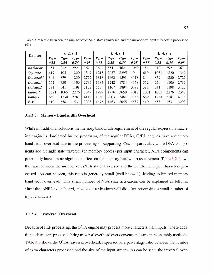
53
Table 3.2: Ratio between the number of csNFA states traversed and the number of input characters processed(%)
Dataset k=2, s=1 k=4, s=1 k=4, s=2P
M
=
0.35
P
M
=
0.55
P
M
=
0.75
P
M
=
0.95
P
M
=
0.35
P
M
=
0.55
P
M
=
0.75
P
M
=
0.95
P
M
=
0.35
P
M
=
0.55
P
M
=
0.75
P
M
=
0.95
Backdoor 151 212 292 367 364 354 462 1060 151 212 292 367Spyware 619 1051 1220 1349 1215 2037 2295 1944 619 1051 1220 1349Dotstar.05 844 879 1230 2722 1818 1462 1591 4118 844 879 1230 2722Dotstar.1 552 750 1106 2737 1184 1242 1784 4168 552 750 1106 2737Dotstar.2 381 641 1198 3122 557 1167 1894 3798 381 641 1198 3122Range.5 1021 1065 2276 2347 1929 1956 3658 4018 1021 1065 2276 2347Range1 669 1238 2287 4118 1780 2003 3481 7266 669 1238 2287 4118E-M 410 658 1531 3293 1476 1463 2055 4587 410 658 1531 3293
3.5.3.3 Memory Bandwidth Overhead
While in traditional solutions the memory bandwidth requirement of the regular expression match-
ing engine is dominated by the processing of the regular DFAs, O3FA engines have a memory
bandwidth overhead due to the processing of supporting-FAs. In particular, while DFA compo-
nents add a single state traversal (or memory access) per input character, NFA components can
potentially have a more significant effect on the memory bandwidth requirement. Table 3.2 shows
the ratio between the number of csNFA states traversed and the number of input characters pro-
cessed. As can be seen, this ratio is generally small (well below 1), leading to limited memory
bandwidth overhead. This small number of NFA state activations can be explained as follows:
since the csNFA is anchored, most state activations will die after processing a small number of
input characters.
3.5.3.4 Traversal Overhead
Because of FEP processing, the O3FA engine may process more characters than inputs. These addi-
tional characters processed bring traversal overhead over conventional stream reassembly methods.
Table 3.3 shows the O3FA traversal overhead, expressed as a percentage ratio between the number
of extra characters processed and the size of the input stream. As can be seen, the traversal over-

54
Table 3.3: O3FA traversal overhead compared to conventional stream reassembly methods (%)
Dataset k=2, s=1 k=4, s=1 k=4, s=2P
M
=
0.35
P
M
=
0.55
P
M
=
0.75
P
M
=
0.95
P
M
=
0.35
P
M
=
0.55
P
M
=
0.75
P
M
=
0.95
P
M
=
0.35
P
M
=
0.55
P
M
=
0.75
P
M
=
0.95
Backdoor 120 107 363 3437 222 146 768 5390 125 80 302 3540Spyware 62 61 1398 25546 106 95 2764 38484 60 52 790 25614Dotstar.05 109 80 2774 10625 231 408 4711 15958 141 232 2810 10628Dotstar.1 43 136 122 23773 126 319 192 35512 77 143 117 23556Dotstar.2 88 97 168 36339 173 182 236 54807 103 106 118 36531Range.5 8 12 34 144 18 21 57 225 10 13 35 135Range1 7 12 35 129 15 21 54 161 9 13 35 107E-M 7 12 35 177 15 24 57 225 9 13 35 167
head (0.0006%-5%) is small enough to be negligible in practice. In other words, O3FA traversal
efficiency is comparable to that of conventional stream reassembly methods.
This traversal overhead is affected by both pM and the number of packets with a previously pro-
cessed predecessor/successor. In our experiments, k=4/s=1 packet sequences have longer FEP
lengths than do k=2/s=1 and k=4/s=2 sequences. In addition, a larger pM leads to longer FEPs,
since it results in more packet segments being detected by supporting-FAs.
In summary, our experiments have shown that: (i) on datasets consisting of a few hundreds regular
expressions with varying complexity, the O3FA memory footprint is typically less than 100MB,
and the supporting-FAs size is limited (3.5MB in the worst case); (ii) O3FA state buffers can be up
to 20x-4000x smaller than conventional packet buffers; (iii) the O3FA bandwidth is linear in the
number of incoming characters and not significantly affected by the NFA components of O3FA; and
(iv) the O3FA traversal efficiency is comparable to that of conventional flow reassembly methods.
3.6 Conclusions and Future Work
In this chapter we have introduced the O3FA engine, a new regular expression-based DPI architec-
ture that can handle out-of-order packets on the fly without requiring packet buffering and stream
reassembly. The O3FA at the core of the proposal consists of regular DFA(s) and supporting-FAs,

55
the latter allowing the detection of matches across packet boundaries. We have proposed several
optimizations aimed to improve both the matching accuracy and speed of the O3FA engine. Our
experimental evaluation shows the feasibility and efficiency of our proposed O3FA engine.

Chapter 4
Framework for Approximate Pattern
Matching on the Automata Processor
4.1 Introduction
Finite Automata (FA) is the core of automata-based searching algorithms of many domain applica-
tions in intrusion detection, data mining, bioinformatics, etc. [180]. Compared to the deterministic
FA (DFA), the non-deterministic FA (NFA) becomes a more practical and affordable technique due
to its much less memory requirement. Recently, Automata Processor (AP) [57] is introduced by
Micron for NFA simulations. Micron AP can perform parallel automata processing within mem-
ory arrays on SDRAM dies by leveraging memory cells to store trigger symbols and simulate NFA
state transitions.
A batch of previous researches investigate accelerating various applications on AP devices [135,
61, 62, 63, 64, 66, 181] and report hundreds or even thousands of fold speedups against the CPU
counterparts. These remarkable achievements are based on limited size datasets within single
AP board capacity, hence treat the compilation and configuration overhead as a one-time cost and
exclude it from performance comparison. However, we believe such computation-only comparison
56

57
becomes unfair when the datasets scale out of single AP board capacity and demand multi-round
reconfigurations.
Similar to other reconfigurable devices, AP needs a series of costly processes to generate load-
ready binary images. These processes include synthesis, map, place-&-route, post-route physi-
cal optimizations, etc., leading to non-negligible configuration time. For small and infrequently
changed datasets, it is relatively reasonable to treat the configuration time as one-time preprocess-
ing cost. However, it becomes non-excludeable and very high for the extremely large datasets
especially those frequently updated ones, due to three reasons: (1) The large-scale problem size
needs multiple rounds of binary image load and flush. (2) In each round, once a new binary image
is generated, it will use a full compilation process, which time is as high as several hours. (3)
During these processes, the AP device is forced to stall and wait for new images in an idle status.
For example, the claimed speedups of AP-based DNA string search [68] and motif search [61]
can reach up to 3978x and 201x speedup over their CPU counterparts, respectively. In contrast,
if their pattern sets are scaling out and the reconfiguration overhead is included, the speedups will
plummet to only 3.8x and 24.7x [69].
AP SDK provides pre-compiled macros to reduce the reconfiguration cost. However, each macro
only works for a fixed shape automaton; any automaton structural change forces the construc-
tion starting from scratch. Moreover, constructing AP automata from scratch is a cumbersome
task requiring considerable expertise on both automata theory and AP architecture, since program-
mers have to manipulate computational elements, called State Transition Elements (STEs), and
inter-connections between them with a low-level Automata Network Markup Language (ANML).
Although Software Development Kit (SDK) provides some high-level APIs for a set of but limited
applications, e.g., regular expression [58] and string matching [59], users have to switch back to
ANML for many specific applications due to their lacking of flexibility and customizability.
In this chapter, we highlight the importance of counting the reconfiguration time towards the over-
all AP performance, which would provide a better angle for researchers and developers to identify
essential hardware architecture features. To this end, we propose a framework allowing users to
58
fully and easily explore AP device capacity and conduct fair comparison to counterpart hardware.
It includes a hierarchical approach to automatically generate AP automata and cascadeable macros
to ultimately minimize the reconfiguration cost. Though this framework is general, in this paper we
focus on Approximate Pattern Matching (APM) for a better demonstration. Specifically, it takes
the types of paradigms, pattern length, and allowed errors as input, and quickly and automatically
generates corresponding optimized ANML APM automata for users to test the AP performance.
During the generation, enabling our cascadeable macros can maximize the reuse of pre-compiled
information and significantly reduce the time on reconfiguration, hence allows users to conduct
performance comparison that is fair to both sides. We evaluate this framework using both syn-
thesis and real-world datasets, and conduct end-to-end performance comparison between AP and
CPU. We show, even including the multi-round reconfiguration costs, AP with our framework
can achieve up to 461x speedup against CPU counterpart. We also show using our cascadeable
macros can save 39.6x and 17.5x configuration time compared to using non-macro and conven-
tional macros respectively. The major contributions of this paper include:
• We highlight the importance of counting the reconfiguration time towards the overall AP
performance, especially the for large-scale and/or frequently updated datasets.
• We provide a framework for users to easily and fairly conduct performance comparison
between AP and its counterparts. It uses a hierarchical approach to automatically generate
AP automata and cascadeable macros to ultimately minimize reconfiguration costs.
• We evaluate our framework with AP using both synthesis and real-world datasets, and
conduct end-to-end performance comparison (configuration+computation) between AP and
CPU. Even including the configuration cost, AP can still achieves hundreds of times speedup
against its counterparts.
59
4.2 Background and Motivations
In this section, we will provide the knowledge about the Automata Processors’ architecture, exe-
cution model, and programming model first, and then describe the programmability and scalability
issues existing in the current AP SDK.
4.2.1 Automata Processors
AP Architecture Overview: Micron’s AP is a DRAM-based reconfigurable device dedicated
for NFA traversal simulations. Its computational resources consist of three major programmable
components: STEs, Counters, and Boolean gates. The STEs are the cores of AP architecture
to provide massive parallelism. Each STE includes a memory cell and a next-state decoder to
simulate a NFA state with trigger symbols, i.e., 256-bit masks for ASCII characters. Connections
between STEs simulate NFA state transitions, implemented by a programmable routing matrix. In
a cycle, all active STEs simultaneously compare their trigger symbols to the input character, and
then those hit STEs activate all their destination STEs via activation signals emitted by next-state
decoders. Counters and Boolean gated are special-purpose elements to extend the capacity of AP
chips beyond classical NFAs.
The current generation of AP board (AP-D480) contains 32 chips organized into 4 ranks. Two
half-cores reside in an AP chip, which includes a total 49,152 STEs, 768 Counters, and 2,304
Boolean gates. The organization of these programmable elements on each AP chip is organized as
following: two STEs and one special-purpose element (a counter or Boolean gate) form a group;
8 groups form a row; 16 rows form a block; and eventually, 192 blocks are evenly distributed into
the two half-cores.
AP Programming and Pre-compiling: Programming AP relies on ANML, which is a XML-
based language. Developers can define their AP automata in ANML by describing the layout of
programmable elements (STEs and transitions). Then, an AP toolchain can parse such an ANML
automata design and compile it to binary images. At runtime, after the AP board loads a binary

60
image, it starts to search given patterns against input streams of 8-bit characters by nominally
processing one character per clock cycle at 133 MHz frequency. AP reports the events to the host,
e.g., CPU, if matches are detected.
Analogous to other reconfigurable devices, AP compilation is a time-consuming process due to
the complex place-&-route calculations. To mitigate the overhead of compilation, the AP SDK
supports the pre-compile of automata to be macros and reuse macros to build larger automata in
the future. That way, any subsequent automata having existing macros can be built directly on
them with a lightweight relabeling, i.e., changing trigger symbols as demand. This can avoid the
recompilation from the ground up.
4.2.2 Motivations
Performance Issues in Reconfiguration: Although the pre-compiling technique becomes avail-
able to alleviate the overhead of reconfiguration, it is strictly restricted to handle an exactly same
structure with a pre-compiled macro, including all STEs and transitions between them. If the
structure changes, a full and time-consuming compilation process must be invoked, leaving the
computing resources in a wait state. For a large-scale problem size, which exceeds the capacity
of a single AP board, more costly reconfiguration and soaring execution time may occur. For
example, the alua dataset from a real-world database used in Bioinformatics sequence search ap-
plications demands around 20-fold of STEs supported by a AP board to perform pattern matching
against input streams, even if only one error, e.g., insertion or substitution, is allowed. It will lead
to 20 rounds of reconfiguration. As shown in our evaluation in Sec. 4.5, a single-round configu-
ration takes as high as 130 seconds, and around 2600 seconds are spent on the reconfiguration in
such a case. The conventional pre-compiled macros unfortunately would fall short from reducing
this cost, because the change of pattern lengths leads to variable structures of automata in each
round. A full recompilation has to be performed each time. Hence, a new approach is of great
necessity to extend the scope of pre-compiling by maximizing the reuse of existing macros, even
if the structure of automata differs.
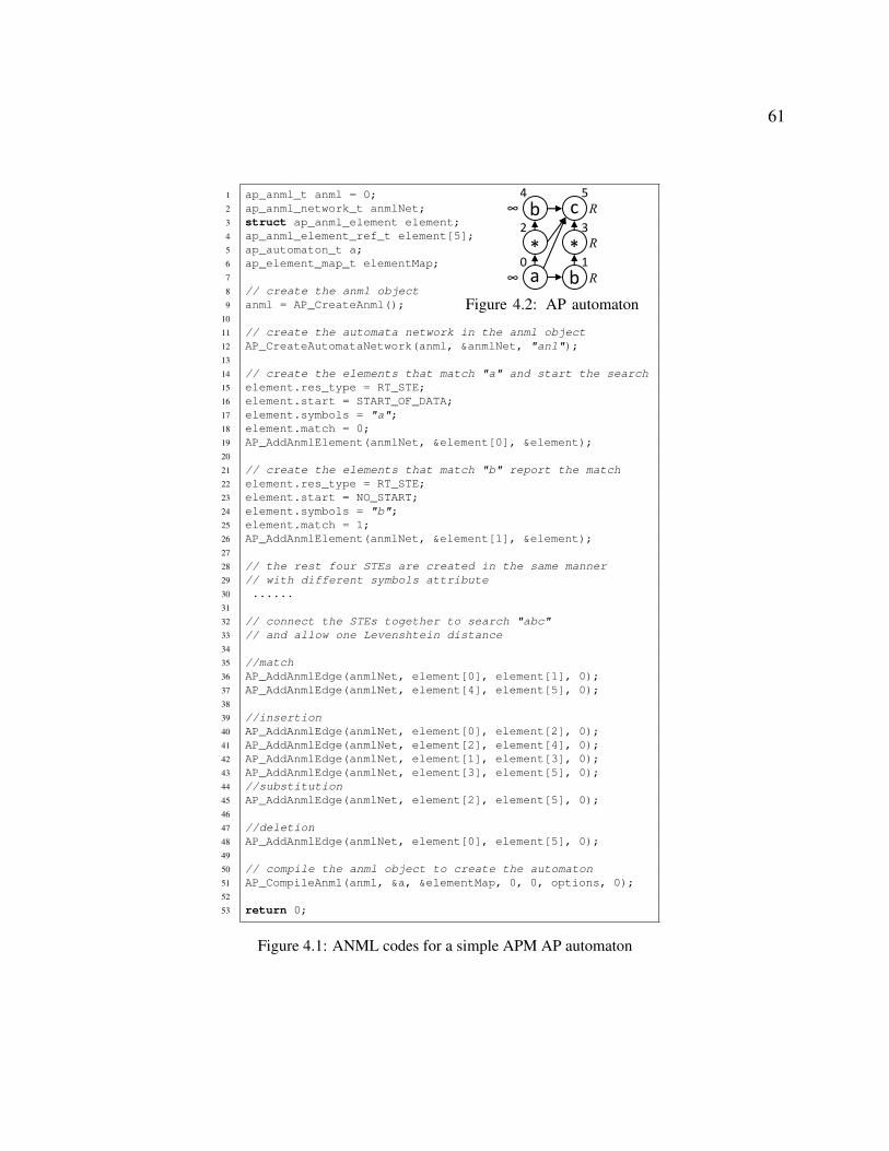
61
1 ap_anml_t anml = 0;2 ap_anml_network_t anmlNet;3 struct ap_anml_element element;4 ap_anml_element_ref_t element[5];5 ap_automaton_t a;6 ap_element_map_t elementMap;78 // create the anml object
9 anml = AP_CreateAnml();1011 // create the automata network in the anml object
12 AP_CreateAutomataNetwork(anml, &anmlNet, "an1");1314 // create the elements that match "a" and start the search
15 element.res_type = RT_STE;16 element.start = START_OF_DATA;17 element.symbols = "a";18 element.match = 0;19 AP_AddAnmlElement(anmlNet, &element[0], &element);2021 // create the elements that match "b" report the match
22 element.res_type = RT_STE;23 element.start = NO_START;24 element.symbols = "b";25 element.match = 1;26 AP_AddAnmlElement(anmlNet, &element[1], &element);2728 // the rest four STEs are created in the same manner
29 // with different symbols attribute
30 ......3132 // connect the STEs together to search "abc"
33 // and allow one Levenshtein distance
3435 //match
36 AP_AddAnmlEdge(anmlNet, element[0], element[1], 0);37 AP_AddAnmlEdge(anmlNet, element[4], element[5], 0);3839 //insertion
40 AP_AddAnmlEdge(anmlNet, element[0], element[2], 0);41 AP_AddAnmlEdge(anmlNet, element[2], element[4], 0);42 AP_AddAnmlEdge(anmlNet, element[1], element[3], 0);43 AP_AddAnmlEdge(anmlNet, element[3], element[5], 0);44 //substitution
45 AP_AddAnmlEdge(anmlNet, element[2], element[5], 0);4647 //deletion
48 AP_AddAnmlEdge(anmlNet, element[0], element[5], 0);4950 // compile the anml object to create the automaton
51 AP_CompileAnml(anml, &a, &elementMap, 0, 0, options, 0);5253 return 0;
Figure 4.1: ANML codes for a simple APM AP automaton
R
*
b
a
c
b R
∞
∞
* R0 1
2 3
4 5
Figure 4.2: AP automaton

62
Programmability Issues: Fig. 4.2 shows an example of Approximate Pattern Matching, which
searches the pattern “abc” and allows one error at most. The STEs take characters “a”, “b”, “c”,
and “*” as input symbols. The symbol infinity means the STE is the starting STE, and the symbol
R means the STE can report the result. We also label STEs with numbers as the STE IDs on AP.
The code snippet in Fig. 4.1 shows how to configure this automata on AP with ANML. Devel-
opers need to create an element for each STE and define its attributes. An error of Approximate
Pattern Matching can be transformed to an insertion, deletion, or substitution, which needs to be
programmed as an edge between STEs. For example, there is an edge from the starting STE 0
(with the symbol “a”) to the reporting STE 5 (with the symbol “c”), meaning that the string “ac”
will be reported as a valid string for the required pattern “abc” with a deletion. As shown in the
example, developers have to carefully connect all possible STEs. The expertise of Approximate
Pattern Matching and ANML programming model of AP is required. Furthermore, if the pre-
compiling technique is used to optimize the configuration, the case will become more complicated
and error-prone.
4.3 Paradigms and Building Blocks in APM
In this section, we start from the manual implementation and optimization of mapping APM on
AP to further illustrate the complexity of using ANML. Then, we identify the paradigms in APM
applications, organize paradigms to a building block, and then discuss the inter-block transition
connecting mechanism to construct automata from blocks.
4.3.1 Approximate Pattern Matching on AP
APM is to find strings that match a pattern approximately. Different with the exact matching, APM
has a more general goal: it searches given patterns in a text, allowing a limited number of various
errors. Errors are usually in three types: insertion, deletion, and substitution. The number of errors
between text and pattern is referred to as distance. There are four most common distances allowing

63
15
8
1
16
9
2
17
10
3
18
11
4
19
12
5
20
13
6
21
14
7
o
o
o
b
b
b
e
e
e
j
j
j
c
c
c
t
t
tƐ Ɛ
Ɛ*
Ɛ*
Ɛ*
Ɛ*
Ɛ*
Ɛ*
Ɛ*
Ɛ*
Ɛ*
*
*
*
*
**
*Ɛ
*
*
*
*
*
*
*
*
*
*
*
no error
one error
two errors
B
A
Figure 4.3: Levenshtein automaton for pattern “object”, allowing up to two errors. A gray colored stateindicates a match with various numbers of errors.
various subsets of error types, including Levenshtein, Hamming, Episode, and Longest Common
Subsequence [180]. Because the Levenshtein Distance allows all three kinds of APM errors, we
use it to discuss the design and optimization of APM on AP.
Fig. 4.3 shows an automata of Levenshtein Distance that detects the pattern “object” allowing up
to two errors between the pattern and the input text. The traverse starts from the starting state at
bottom-left and goes horizontally if no error occurs. Once an error occurs, the traverse goes up
or along a diagonal to an adjacent layer. Once an accepting state (tagged with the gray color) is
reached, a match will be reported. The epsilon-transitions allow the traverse reaching destination
states immediately without consuming any input character once a source state is activated. In an
APM automata, an epsilon-transition represents an error of deletion. The asterisk-transitions allow
the traverse to be triggered by any input characters. In this case, an asterisk-transition represents
an insertion or substitution when the traverse goes vertically or diagonally.
We apply two optimizations [182] on the Levenshtein automata to reduce the usage of STEs. They
are important for the implementation of mapping the Levenshtein automata on AP, considering
the limited numbers of STEs in the hardware. First, we cut down the states above the first full
diagonal.1 The states within the dotted triangle A will be skipped. The reason why we can apply
this optimization is that these states are used to deal with errors before the first character of pattern
1A full diagonal is a diagonal that connects all rows.

64
and not necessary to be counted. Second, we cut down the states below the last full diagonal. That
is because when the APM automata reports a found position in the text for the pattern, it doesn’t
need to report the number of errors. For example, in this case, no matter a position corresponds
to 0 error (of an exact match), 1 error (of insertion, deletion, or substitution), and 2 error (of
combinations of three types of errors), it will be reported. Therefore, the states within the dotted
triangle B will be also skipped.
After truncating the original automata, we manually map it on AP. The Levenshtein automata
shown in Fig. 4.3 will be transformed to the AP recognizable format shown in Fig. 4.4. Two major
problems have to be resolved in the mapping. First, the ANML programming model requires
to move a NFA trigger character associated with a transition to a state, because it can’t support
multiple outgoing transitions with different character sets from a single state, e.g. the transitions
s2 !s3, s2!s9, and s2!s10 in Fig. 4.3. The solution is to split a state to multiple STEs. For
example, the state s2 in Fig. 4.3 is split to STE1 with the trigger character o, and the auxiliary
STE2 with an asterisk. The second problem is that AP hardware can’t reach destination states
within the current clock cycle, leading to the lack of support to ✏-transitions. The alternative is
to add a transition from a source STE to its upper-diagonal adjacent STE. For example, the ✏-
transition from s2 to s10 in Fig. 4.3 is transformed to the transition from STE1 to STE8 in Fig. 4.4.
With these two transformations, the Levenshtein automata shown in Fig. 4.4 can be described in
ANML and mapped on AP.
4.3.2 Paradigms in Approximate Pattern Matching
The transformation of Levenshtein automata on AP illustrates programming with ANML requires
advanced knowledge of both automata and AP architecture. Any parameter change, e.g., the pat-
tern length, error type, max error number, etc., may lead to the code adjustment with tedious
programming efforts. In our hierarchical approach, our first goal is to exploit the paradigms of
applications to be a building block.
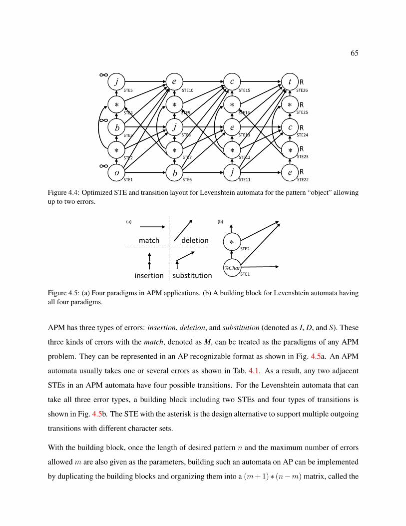
65
o
*
b
*
e
*
*
*
*
*
*
b
j e
j e
j
c
c t∞
∞
∞
R
R
R
STE1
STE2
STE3
STE4
STE5
STE6
STE7
STE8
STE9
STE10
STE11
STE12
STE13
STE14
STE15
STE22
STE23
STE24
STE25
STE26
R
R
Figure 4.4: Optimized STE and transition layout for Levenshtein automata for the pattern “object” allowingup to two errors.
match deletion
insertion substitution
*
STE1
STE2
%Char
(a) (b)
Figure 4.5: (a) Four paradigms in APM applications. (b) A building block for Levenshtein automata havingall four paradigms.
APM has three types of errors: insertion, deletion, and substitution (denoted as I, D, and S). These
three kinds of errors with the match, denoted as M, can be treated as the paradigms of any APM
problem. They can be represented in an AP recognizable format as shown in Fig. 4.5a. An APM
automata usually takes one or several errors as shown in Tab. 4.1. As a result, any two adjacent
STEs in an APM automata have four possible transitions. For the Levenshtein automata that can
take all three error types, a building block including two STEs and four types of transitions is
shown in Fig. 4.5b. The STE with the asterisk is the design alternative to support multiple outgoing
transitions with different character sets.
With the building block, once the length of desired pattern n and the maximum number of errors
allowedm are also given as the parameters, building such an automata on AP can be implemented
by duplicating the building blocks and organizing them into a (m+1) ⇤ (n�m) matrix, called the
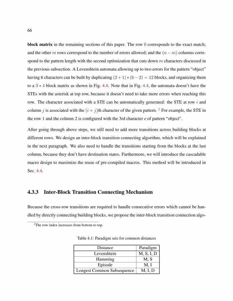
66
block matrix in the remaining sections of this paper. The row 0 corresponds to the exact match;
and the otherm rows correspond to the number of errors allowed; and the (n�m) columns corre-
spond to the pattern length with the second optimization that cuts down m characters discussed in
the previous subsection. A Levenshtein automata allowing up to two errors for the pattern “object”
having 6 characters can be built by duplicating (2+ 1) ⇤ (6� 2) = 12 blocks, and organizing them
to a 3 ⇤ 4 block matrix as shown in Fig. 4.4. Note that in Fig. 4.4, the automata doesn’t have the
STEs with the asterisk at top row, because it doesn’t need to take more errors when reaching this
row. The character associated with a STE can be automatically generated: the STE at row i and
column j is associated with the (i+ j)th character of the given pattern. 2 For example, the STE in
the row 1 and the column 2 is configured with the 3rd character e of pattern “object”.
After going through above steps, we still need to add more transitions across building blocks at
different rows. We design an inter-block transition connecting algorithm, which will be explained
in the next paragraph. We also need to handle the transitions starting from the blocks at the last
column, because they don’t have destination states. Furthermore, we will introduce the cascadable
macro design to maximize the reuse of pre-compiled macros. This method will be introduced in
Sec. 4.4.
4.3.3 Inter-Block Transition Connecting Mechanism
Because the cross-row transitions are required to handle consecutive errors which cannot be han-
dled by directly connecting building blocks, we propose the inter-block transition connection algo-
2The row index increases from bottom to top.
Table 4.1: Paradigm sets for common distances
Distance ParadigmLevenshtein M, S, I, DHamming M, SEpisode M, I
Longest Common Subsequence M, I, D
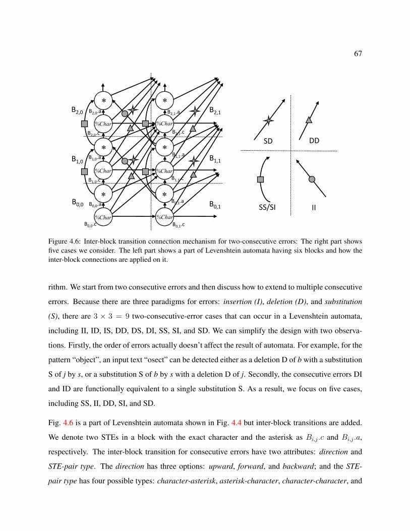
67
*
*
*
*
B0,0.c
%Char
%Char
%Char
%Char
SD DD
SS/SI II
* *
%Char %Char
B0,0.a
B0,1.c
B0,1.a
B1,1.c
B1,1.a
B1,0.c
B1,0.a
B2,0.c
B2,0.a
B2,1.c
B2,1.a
B0,0
B1,0
B2,0
B0,1
B1,1
B2,1
Figure 4.6: Inter-block transition connection mechanism for two-consecutive errors: The right part showsfive cases we consider. The left part shows a part of Levenshtein automata having six blocks and how theinter-block connections are applied on it.
rithm. We start from two consecutive errors and then discuss how to extend to multiple consecutive
errors. Because there are three paradigms for errors: insertion (I), deletion (D), and substitution
(S), there are 3 ⇥ 3 = 9 two-consecutive-error cases that can occur in a Levenshtein automata,
including II, ID, IS, DD, DS, DI, SS, SI, and SD. We can simplify the design with two observa-
tions. Firstly, the order of errors actually doesn’t affect the result of automata. For example, for the
pattern “object”, an input text “osect” can be detected either as a deletion D of b with a substitution
S of j by s, or a substitution S of b by s with a deletion D of j. Secondly, the consecutive errors DI
and ID are functionally equivalent to a single substitution S. As a result, we focus on five cases,
including SS, II, DD, SI, and SD.
Fig. 4.6 is a part of Levenshtein automata shown in Fig. 4.4 but inter-block transitions are added.
We denote two STEs in a block with the exact character and the asterisk as Bi,j.c and Bi,j.a,
respectively. The inter-block transition for consecutive errors have two attributes: direction and
STE-pair type. The direction has three options: upward, forward, and backward; and the STE-
pair type has four possible types: character-asterisk, asterisk-character, character-character, and

68
asterisk-asterisk. Some combinations of these two attributes are invalid or functionally dupli-
cated. For example, forward character-asterisk, e.g., B0,0.c to B1,1.a, can handle SD, e.g., path
B0,0.c!B1,1.a!B2,1.c, but it is duplicated of forward asterisk-character, e.g. B0,0.a to B2,1.c,
which can also handle SD, e.g., pathB0,0.c!B0,0.a!B2,1.c. Hence, as shown in Fig. 4.6, only four
types of inter-connections need to be considered: forward asterisk-character, forward character-
character, upward asterisk-asterisk, and backward asterisk-asterisk; and they can cover all five
cases of two-consecutive errors. Note that the inter-block transitions with asterisks as the destina-
tion STEs are always for two different cases, because the traverse cannot stop at an asterisk. For
example, the transition B0,0.a!B1,0.a is for the path B0,0.a!B1,0.a!B2,0.c of case SI and path
B0,0.a!B1,0.a!B2,1.c of case SS. Tab. 4.2 summarizes the rules of adding inter-block transitions
for two-consecutive errors.
Any case having more than two consecutive errors can be produced as a combination of two-
consecutive errors. Assume we add one more row B3,0 and B3,1 to Fig. 4.6 to allow three errors.
A three-consecutive error SSI can be produced as a combination of SS and SI with the overlapped
middle S. The existing inter-block transition connecting mechanism can handle more errors and
no extra inter-block transition is needed. For the SSI case, SS and SI can naturally generate the
path B0,0.c!B0,0.a!B1,0.a!B2,0.a!B3,0.c for SSI. If the multi-consecutive errors contain a D,
additional forward character/asterisk-character transitions have to be added, because only the
deletion can bypass the current row. For example, DDD requires a transition from B0,0.c to B3,1.c,
with the existing B0,0.c to B1,1.c (added in a building block by default) and B0,0.c to B2,1.c (added
by inter-block transition connection mechanism for a two-consecutive error). The rule for the
deletion in a multi-consecutive error, e.g., SD and DD, can be stated as: a batch of the forward
inter-block transitions with a character STE as the destination is needed from a row i to a row j,
where j is from i+1 to m (the allowed maxim number of errors). Note that in Tab. 4.2 we discuss
the additional transitions are added for the case of two-consecutive errors. For DD and SD, the
case k = 1 has been covered by the direct connection of two building blocks and k starts from 2.
69
Table 4.2: Inter-block transitions connecting rules for two-consecutive errors
Paradigm Transition Attributes STE ConnectionM NoneSS/SI upward a!a Bi,j.a!Bi+1,j.aII backward a!a Bi,j.a!Bi+1,j�1.aDD forward c!c for k=2 tom:Bi,j.c!Bi+k,j+1.cSD forward a!c for k=2 tom:Bi,j.a!Bi+k,j+1.c
4.4 Framework Design
In this section, we first introduce how to build automata from building blocks in our framework,
and then introduce how to extend building blocks to a macro that can be pre-compiled and reused.
Finally, we present our optimized framework that can build automata from reusable macros to
reduce the time on recompilation.
4.4.1 From Building Blocks to Automata
Alg. 1 presents how to build automata on AP from building blocks. This algorithm accepts the
types of paradigms, desired pattern length, and maximum number of errors allowed. Then, this
algorithm can automatically fabricate complex AP automata. Note that this process is independent
with specific APM applications, in the sense that it can work for any given paradigms shown in
Fig. 4.5a and types of distances shown in Tab. 4.1.
In Alg. 1, we use classes of BuildingBlock (ln. 4) and Automation (ln. 3) to represent
building blocks and AP automata, respectively. First, we create the building blocks via ln. 5-6,
where the member function add() in BuildingBlock places and connects STEs following the
rules depicted in Fig. 4.5b. Second, we build up the automaton with the block matrix determined
by maximum error (m) and target pattern length (n) (ln. 7-8). After duplicating the blocks to fill
the dimensions in ln. 9, we weave them together through the ADD TRANSITIONS() to add inter-
block transitions defined in Tab. 4.2. Third, the starting and reporting STEs are set in ln. 13 and
all STEs are labels in ln. 22-24. To this point, an AP automaton can be constructed and ready to

70
be compiled to a binary image. Note that the macro-based optimization in ln. 14-21 is an optional
process, which will be discussed in Sec. 4.4.2 and Sec. 4.4.3.
Algorithm 1: Paradigm-based AP Automata Construction/* Alg 1 constructs the automaton from basic building blocks, based on the
user-defined paradigm sets, target pattern, and max error number. */1 CasMacroLib lib ; // Cascadable macro library2 Procedure PRDM Atma Con (ParadigmSet ps, Pattern pat, int err num)3 Automaton atma;4 BuildingBlock block;5 for Paradigm p in ps do6 block.add(p);7 int m = err num, n = pat.length;8 atma.row num = m + 1; atma.col num = n - m;9 atma � block.duplicate(m⇥n);
10 for int i 0 to m + 1 do11 for int j 0 to n - m do12 ADD TRANSITIONS(atma, i,j, ps);13 atma.set start(); atma.set report();14 #ifdef ENABLE MACRO /* Cascadable macro constr. */15 CasMacro cmacro;16 for Paradigm p in ps do17 ADD PORTS(atma, p);18 MERGE PORTS(atma);19 cmacro � AP CompileMacros(atma);20 lib.add(cmacro);21 #endif22 for int i 0 to m + 1 do23 for int j 0 to n - m do24 atma.re label(i, j, pat.c(j+i));25 return atma;
4.4.2 Design Cascadable Macros
The most time consuming parts of an application on AP include the execution time and the recom-
pilation time which has the place-&-route process [69]. Although the pre-compiling technique can
build macros to reduce the recompilation time, the restriction of using this technique hinders it
widely used in manual programing. For example, we can assume the AP automaton in Fig. 4.4 (for
the pattern “object”, allowing up to 2 errors) is pre-compiled as a macro M1 with all characters of
STEs parameterized. We can reuse it for patterns with any 6 characters and up to two errors. If a

71
new pattern, e.g., “gadget” for two errors, is also needed to check, we can reuse it by relabeling
STEs to “gadget”. However, this macro can only be reused for exactly same numbers of STEs
and connections between them. Failing to comply with any of these requirements will cause an
indispensable recompilation from scratch. Thus, the pattern “gadgets” and the pattern“gadget” but
allowing up to three errors cannot directly take advantage of the macro M1.
In our framework, we propose cascadable macros to support reuse of macros for larger-scale AP
automata. In particular, we connect one or more macro instances to compose a larger and differ-
ent AP automata through our carefully-designed interconnection algorithm. With the cascadable
macros, the overhead of reconfiguration can be significantly reduced, since only the connections
between instances need to be placed-&-routed. Our method is to generate the desired automata by
connecting multiple macros if the result block matrix can be constructed by multiple building block
matrices. For example, the AP automata in Fig. 4.4 is stored as a cascadable macro M2 having a
(3 ⇤ 4) block matrix. Assume we will build an automata for a larger pattern “international” having
13 characters and allowing up to 5 errors. The result block matrix is a (5 + 1) ⇤ (13 � 5) = 6 ⇤ 8
matrix. As a consequence, the AP automata can be built by connecting 4 M2 macro instances.
To create cascadable macros, we need to extend current macros, e.g., M2, by adding input/output
ports and connecting these ports with appropriate STEs.
Builidng Cascadable Macros: The first step is to add input/output ports. The optimal design of
adding ports should minimize (1) the number of total ports, and (2) the in-degree of each input
port, because both the number of ports and the number of signals that go into an input port are
limited in AP hardware [183]. We define the port struct that has three attributes:
• Port role identifies the port is used to either input or output signals (in=input, out=output).
• Cascade direction indicates the direction of allowed cascade, and the side of two paired
macros (h=horizontal, v=vertical, d=diagonal, ad=anti-diagonal).
• Transition scope represents whether connections can cross edges of neighboring macro to
link non-adjacent STEs (e=edge of neighbors, ce=cross-edge of neighbors, e/ce=both).
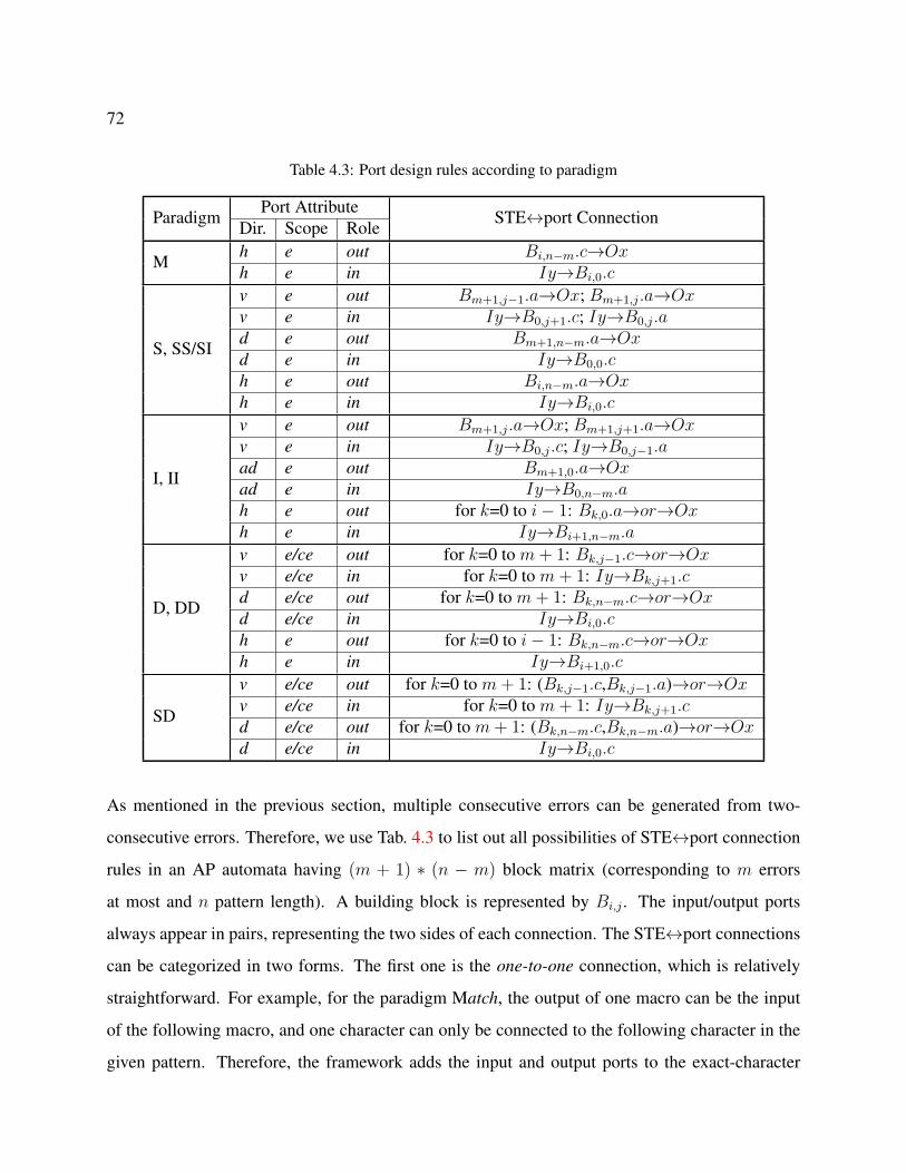
72
Table 4.3: Port design rules according to paradigm
Paradigm Port Attribute STE$port ConnectionDir. Scope Role
M h e out Bi,n�m.c!Oxh e in Iy!Bi,0.c
S, SS/SI
v e out Bm+1,j�1.a!Ox; Bm+1,j.a!Oxv e in Iy!B0,j+1.c; Iy!B0,j.ad e out Bm+1,n�m.a!Oxd e in Iy!B0,0.ch e out Bi,n�m.a!Oxh e in Iy!Bi,0.c
I, II
v e out Bm+1,j.a!Ox; Bm+1,j+1.a!Oxv e in Iy!B0,j.c; Iy!B0,j�1.aad e out Bm+1,0.a!Oxad e in Iy!B0,n�m.ah e out for k=0 to i� 1: Bk,0.a!or!Oxh e in Iy!Bi+1,n�m.a
D, DD
v e/ce out for k=0 tom+ 1: Bk,j�1.c!or!Oxv e/ce in for k=0 tom+ 1: Iy!Bk,j+1.cd e/ce out for k=0 tom+ 1: Bk,n�m.c!or!Oxd e/ce in Iy!Bi,0.ch e out for k=0 to i� 1: Bk,n�m.c!or!Oxh e in Iy!Bi+1,0.c
SD
v e/ce out for k=0 tom+ 1: (Bk,j�1.c,Bk,j�1.a)!or!Oxv e/ce in for k=0 tom+ 1: Iy!Bk,j+1.cd e/ce out for k=0 tom+ 1: (Bk,n�m.c,Bk,n�m.a)!or!Oxd e/ce in Iy!Bi,0.c
As mentioned in the previous section, multiple consecutive errors can be generated from two-
consecutive errors. Therefore, we use Tab. 4.3 to list out all possibilities of STE$port connection
rules in an AP automata having (m + 1) ⇤ (n � m) block matrix (corresponding to m errors
at most and n pattern length). A building block is represented by Bi,j . The input/output ports
always appear in pairs, representing the two sides of each connection. The STE$port connections
can be categorized in two forms. The first one is the one-to-one connection, which is relatively
straightforward. For example, for the paradigm Match, the output of one macro can be the input
of the following macro, and one character can only be connected to the following character in the
given pattern. Therefore, the framework adds the input and output ports to the exact-character

73
STEs of blocks in the first column (Bi,0.c) and last column (Bi,n�1.c), respectively. The rule is
shown in the table as Iy ! Bi,0.c and Bi,n�1.c! Ox.
The second one is the N-to-one connection, whose design needs to meet the requirements of build-
ing ANML macros and optimize the usage of ports. Here, we introduce or Boolean gates to our
design. For example, in the case of the fifth port design of paradigm Insert, rather than adding a
new port as Bk,0.a ! Ox for each row k, we use an or Boolean gate to allow a combination of
connections as Bk,0.a ! or ! Ox, so as to reduce the number of used port to be only one. This
design also bypasses a restriction of AP routing, i.e., no more than one transition is allowed to
directly go to a single output port [183].
In the final step of completing the port design of a macro, we search and merge the ports with inclu-
sive STE$port connections. Then, the attribute sets of merged port equal to the union of all partici-
pant ports. This can help further optimize the port usage. The procedure of constructing cascadable
macros is integrated into Alg. 1 from ln. 14 to ln. 21. Two predefined functions are implemented:
(1) ADD PORTS() adds input/output ports to given automata based on each paradigm (ln. 16-17),
followed by STE$port connections as described in Tab. 4.3; and (2) MERGE PORTS() optimizes
the ports layout by merging equivalent and inclusive ports (ln. 18).
Fig. 4.8 exhibits the completed ports layout for the cascadable macro M2. 3 Fig. 4.7, on the other
hand, shows the connections of four cascadable macros. Because the macro instances I and II are
vertically aligned and adjacent to each other, we simply link the input-output port pairs that have
port attributes of v and e. Note that with these fourM2 macros, we can construct more complicated
automata other than the case for the pattern “international” having a (6 ⇤ 8) block matrix: once the
block matrix of a given pattern is times of the (3⇤4)matrix, we can construct it by duplicating and
connecting these four M2 macros vertically, horizontally, diagonally, and anti-diagonally.
3Transitions between STEs inside a macro are skipped to highlight the port connections.

74
C4L3_S1R0II
I I I I I I I I II I
O O O O O O O
O11
O10O9
I8
I7
O1
O2
O7
O6
O8
O4
O0
I0 I14
I1 I5 I5I3
I11
I10
I9
O5
O3
C4L3_S1R0I
I12
I4 I13
I2 I6
O12
C4L3_S0R1IV
C4L3_S0R1III
I I I I I I I I II I I I I I I I I I II I
I I I I I I I I II I
OO O O O O OO
O O O O O OO
O O O O O OOO OO
O
I
I
O
O
O
I
I
O
O
O
I
I
O
O
O
I
I
O
O
I
I
I
O
O
I
I
I
O
O
I
I
I
O
O
I
I
I
O
OO11
O10O9
I8
I7
O1
O2
O7
O6
O8
O4
O0
I0 I14
I1 I5 I5I3I11
I10
I9
O5
O3
I12
I4 I13
I2 I6
O12
O11
O10O9
I8
I7
O1
O2
O7O6
O8
O4
O0
I0 I14
I1 I5 I5I3
I11
I10
I9
O5
O3
I12
I4 I13
I2 I6
O12
O11
O10O9
I8
I7
O1
O2
O7
O6
O8
O4
O0
I0 I14
I1 I5 I5I3
I11
I10
I9
O5
O3
I12
I4 I13
I2 I6
O12
Figure 4.7: There are four instances that from a three layers four columns cascadable macro. They arevertically and horizontally cascaded to form a larger AP automaton that have six layers and eight columns.
*
*
*
*
*
*
*
*
*
*
*
*or
or
or
or
or
or
or
or
or
or
O
O
OO
O
O
O O
O
O
O
I
I
I
I
I
I
I
I
II
I
I
I
%Char
%Char
%Char
%Char
%Char
%Char
%Char
%Char
%Char
%Char
%Char
%Char
O11
O16
O15
O14
O4 O5 O6 O7
O8 O9 O10
I16
I15
I14
I0 I1 I2 I3
I8 I9 I10
I11 I12 I13
I
I
I17
I18
B0,0.c
or
O
O
O12
O13
O O O O
O1 O2 O3
I III4 I5 I6
O0
B0,0.a
B1,0.c
B1,0.a
B2,0.c
B2,0.a
B0,1.c
B0,1.a
B1,1.c
B1,1.a
B2,1.c
B2,1.a
B0,2.c
B0,2.a
B1,2.c
B1,2.a
B2,2.c
B2,2.a
B0,3.c
B0,3.a
B1,3.c
B1,3.a
B2,3.c
B2,3.a
I7I
Figure 4.8: Port design layout for a three layers four columns macro.

75
4.4.3 Cascadable Macro based Automata Construction Algorithm
After the pre-compilation, the cascadable macros are inserted into a macro library for reuse (ln. 19-
20). In our current design, the library contains macros whose pattern lengths (column numbers)
are in three groups of {1,2, ..., 9} {10, 20, ..., 90} {100, 200, ..., 900} with each one allowing up
to 3 errors (layers). The reasons of choosing these 27⇥ 3 = 81 macros in the library are two-fold:
(1) It is inefficient and even impractical to save all possible situations for different combinations of
pattern sizes and errors. (2) Many real-world cases focus on pattern sizes < 1000 characters and
errors 6 3 (in Sec. 4.5). Therefore, this scheme can efficiently find the appropriate instances from
the three pattern groups to handle any pattern of 6 1000 characters. For the rare cases with longer
patterns (e.g., ¿1000 characters) or larger error allowance, we can handle them by using more
macro instances. Although a dynamic macro management mechanism is promising to optimize
which macros should be put into the macro library, we leave it to our future work.
Based on the cascadable macro library, we can effectively reduce the construction and compilation
overhead and efficiently build AP automata. Alg. 2 shows our macro-based AP automata con-
struction. In this algorithm, we search the library for a hit macro, which has the same structure
with the desired automaton. If found, the macro can be directly instantiated (ln. 5-6). Otherwise,
we use multiple macros to form the desired automaton. First, we select and instantiate proper
macros according to the dimensions of the desired automaton (ln. 8-11). Second, these macro
instances are organized to a lattice (ln. 12-16). Third, we link these instances to generate the
complete AP automaton (ln. 17-27). The function CONN INST(ParadigmSet, src, dst,
dir, scope) is predefined to make cascade links of input-output port pairs from the source
instance src to the destination instance dst. The arguments of dir and scope are used as a
filter, meaning only the ports with provided attribute values are qualified for linking. Finally, the
AP automaton can be constructed after the relabeling process (ln. 29-31).

76
Algorithm 2: Cascadable Macro-based AP Automata Construction/* Alg. 2 constructs automata based on our cascadable macro library, whose
macros are built by ln. 14-21 in Alg. 1. */1 MacroLib lib;2 Procedure CASM Atma Con(ParadigmSet ps, Pattern pat, int err num)3 Automaton atma;4 int m = err num, n = pat.length;5 if lib.search(ps, m+1, n�m) = true then6 Instantiate(ps, atma, m+1, n�m, true, true);7 else8 int digits[] = {(n�m) /100, (n�m) %100/10, (n�m) %10};9 int quo = (m+1) / lib.max err, rem = (m+1) % lib.max err;
10 int ins col = (bool)digits[0] + (bool)digits[1] + (bool)digits[2];11 Automaton inst[quo+(bool)rem][ins col ];12 if quo then13 for int i 0 to (quo�1) do14 Gen inst row(ps, inst[i ], lib.max err, digits);15 if rem then16 Gen ins row(ps, inst[quo], rem, digits);17 for int i 0 to (quo+(bool)rem�1) do18 for int j 0 to (ins col�1) do19 if j then CONN INST(ps, inst[i ][j�1], inst[i ][j ], h, e);20 for int k 0 to (i�1) do21 TransitionRange scope;22 if k=(i�1) then scope=e else scope=ce;23 CONN INST(ps, inst[k ][j ], inst[i ][j ], v, scope);24 if j 6=(ins col�1) then25 CONN INST(ps, inst[k ][j ], inst[i ][j+1], d, scope);26 if j 6=0 then27 CONN INST(ps, inst[k ][j�1], inst[i ][j ], ad, scope);28 atma � inst;29 for int i 0 to m+1 do30 for int j 0 to n�m do31 atma.re label(i, j, pat.c(j+i�1));32 return atma;33 Function Instantiate(ParadigmSet ps, Automaton am, int row, int col, bool start, bool report)34 CasMacro cmacro;35 cmacro � lib.pick(ps, row, col, start, report);36 am � cmacro.instantiate();37 Function Gen inst row(ParadigmSet ps, Automaton ams[], int err, int digits[])38 int j = 0;39 for int i 0 to (ams.size-1) do40 while j<digits.size do41 if digits[j ] then42 Instantiate(ps, ams[i ], err, digits[j ], !i, !(digits.size�1�j));43 j++; break;44 j++;

77
4.5 Evaluation
We evaluate our APM framework by using the Levenshtein automata construction, since it includes
a full paradigm set of M, S, I, D in Tab. 4.1. In contrast, the other APM distances (e.g., Hamming
and Episode) only need to use a subset of the paradigms and simpler routing, so that the com-
pilation overhead will be less accordingly. Thus, we focus on the Levenshtein distance to better
serve our purpose for evaluating the construction of complex automata. We run our experiments
on a platform equipped with Intel Xeon E5-2637 CPU@ 3.5 GHz and 256 GB main host memory.
The installed AP SDK is in version 1.6.5. Currently, the Micron AP is not ready for production;
thus, we use an emulator4 to estimate the runtime performance. We enable the cascadable macro
library in our framework and generate AP automata using Alg. 2. The size of the library follows
the scheme in Sec. 4.4.3. We also set the macros in library to accept up to three errors. That way,
the higher error number (e.g., ¿3) will need not only horizontal instance cascading but also vertical
cascading.
4.5.1 Synthetic Patterns
To evaluate our framework on processing different patterns and error allowances, we use a set of
six synthetic patterns of lengths from 25 to 155 in steps of 25. The error allowances range from
one to four. In Fig. 4.9, the construction and compilation time of our framework is compared with
other three AP automata construction approaches: Functional Units (FU) [140], String Matching
APIs (SM API) [59], and basic ANMLAPIs (ANML). These three use partially optimized macros,
conventional macros and non-macros respectively. We choose up to 155 characters for the synthetic
patterns to fit into the AP board and avoid reconfiguration. The AP runtime performance is not
considered in this section, because all these approaches present similar performance in processing
patterns with the same length. This is due to AP’s lock-step execution mode, which makes the
performance linear to the length of input stream and independent of what automata construction is
4http://www.micronautomata.com

78
applied.
The compilation data of FU is not available when four errors are allowed, due to the in-degree
limitation in the FU approach [140]. In Fig. 4.9, we first observe that the compilation costs of all
approaches increase exponentially as the error number rises. This explains that even with small
growth rates of error number, the AP construction and compilation will have a larger impact on total
performance. The reason for this error-cost relationship is because more errors require higher STE
usage and more complicated placement-&-routing. SM API is a “black-box” approach provided
byMicron and its performance is insensitive to the pattern length, meaning high compilation time is
needed even for small patterns. The FU and ANML approaches show positively correlated pattern
length and compilation cost, for the similar reason with aforementioned error-cost relationship. In
contrast, the compilation cost of our framework is more determined by the instance number than
the pattern length. For example, if only one error is allowed, a 100-char pattern uses 1 instance,
while a 75-char pattern needs 2 instances (One has 70 columns and another has 5 columns). Since
additional cascade compilation is required for the 75-char pattern, we observe its cost is higher
than that for the 100-char pattern. On the other hand, we can also notice that the instantiation of a
larger pre-compiled macro usually causes higher cost, e.g., the 100-char pattern needs more time
for compiling than the 50-char pattern, despite only one macro used in both cases.
Overall, the SM API approach provides higher abstraction and is easier for developers to use.
However, it usually requires more expensive construction and compilation than the other ap-
proaches. FU approach can achieve up to 3.7x speedups against the ANML approach. As a con-
trast, our framework can achieve up to 33.9x, 34.2x, and 46.5x speedups over the ANML for the
case of one, two, and three errors respectively. Note, the speedups are obtained in the scenario of
only cascading horizontal instances, because the error numbers are less than our predefined max-
imum error allowance for the library macros. When the error number exceeds this threshold, the
scenario changes to use both vertical and horizontal instance cascades, where our framework can
still provide up to 16.3x speedups over the ANML baseline.
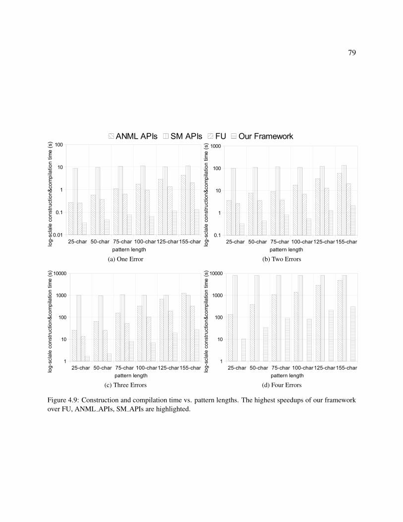
79
ANML APIs SM APIs FU Our Framework
25-char 50-char 75-char 100-char125-char155-char
0.01
0.1
1
10
100
pattern length
log
-scla
le c
on
str
uctio
n&
co
mp
ilatio
n t
ime
(s)
(a) One Error
25-char 50-char 75-char 100-char125-char155-char
0.1
1
10
100
1000
pattern length
log
-scla
le c
on
str
uctio
n&
co
mp
ilatio
n t
ime
(s)
(b) Two Errors
25-char 50-char 75-char 100-char125-char155-char
1
10
100
1000
10000
pattern length
log
-scla
le c
on
str
uctio
n&
co
mp
ilatio
n t
ime
(s)
(c) Three Errors
25-char 50-char 75-char 100-char125-char155-char
1
10
100
1000
10000
pattern length
log
-scla
le c
on
str
uctio
n&
co
mp
ilatio
n t
ime
(s)
(d) Four Errors
Figure 4.9: Construction and compilation time vs. pattern lengths. The highest speedups of our frameworkover FU, ANML APIs, SM APIs are highlighted.

80
Table 4.4: Dataset Characteristics
Pattern Sets Pattern# Length (min.) Length (max.) Diff lengths#Bio 85389 32 686 375
IR 100K 10 959 846
4.5.2 Real-world Dataset
We evaluate the framework with two real-world datasets “Bio” and “IR” from bioinformatics and
information retrieval domains respectively. The “Bio” is the BLAST igseqprot dataset5, and “IR”
is the NHTSA Complaints dataset6. Tab. 4.4 describes the characteristics of the two datasets.
The “Bio” contains ˜85K patterns ranging from 32 to 686 characters, while the “IR” has ˜100K
patterns from 10 to 959 characters. Apparently, the overall demand for STEs in processing either
dataset exceeds the capacity of a single AP board. For example, the “Bio” dataset with one error
allowance requires over 4M STEs; however, the AP board can supply only 1.5M STEs (=49,152
STEs⇥32 chips in Sec. 4.2.1). This supply-demand imbalance forces us to use multiple flush/load
reconfigurations to completely process the dataset. Since the AP automata can be stored as a
macro in a library, we can reuse it for all the patterns with the same length and errors by simply
instantiating the macro and relabeling parameters. Therefore, we only need to cascade and compile
the patterns with different lengths. The two datasets have 375 and 846 such patterns respectively.
Compilation Profiling: We compare our framework to two other AP construction approaches:
FU and ANML-APIs. The SM APIs method is not used because it hides the compiling profile
(e.g., STE usage) so that the rounds of reconfiguration are uncomputable. Tab. 4.5 shows the
profiles of the three approaches. We test the two datasets “Bio” and “IR” with up to 4 maximum
error allowances. Since the FU supports up to three errors, the corresponding data is not available
for 4 errors. In the table, the “STE usage” (in percentages) is used to estimate the number of
reconfiguration rounds. Generally, in the case of same datasets and errors, higher STE usage
indicates less reconfiguration rounds are needed. On the other hand, the STE usage is negatively
5https://www-odi.nhtsa.dot.gov/downloads/flatfiles.cfm6ftp://ftp.ncbi.nlm.nih.gov/blast/db/FASTA/

81
correlated to the placement-&-routing complexity, which is represented by “BR allocation” (in
percentages). Obviously, longer patterns (e.g., “IR”) and more errors will result in more larger
single automata, thereby giving rise to higher BR allocation and lower STE usage.
For reconfiguration rounds, we distinguish the “recompile” rounds from the light-weight “relabel”
rounds, based on that the patterns with the same length and error number require at most one
cascading and placement-&-routing processing. Relabeling the entire AP board costs 45 ms [60],
while the recompiling time depends on AP automata complexity. The “total compile time” columns
include the cost from both recompile and relabel rounds. ANML-APIs show the best STE usage
and thus use the least reconfiguration rounds. This is because the ANML-APIs use the low-level
interfaces to accurately manipulate AP computational resources, which can provide efficient STE
usages. However, the ANML approach takes the longest overall compile time, since there are no
optimizations applied onto its recompile rounds.
In contrast, the FU approach oftentimes presents the lowest STE usage with the highest recon-
figuration rounds, due to its large number of functional unit copies and associated complex inter-
connections. Nevertheless, the functional units can also reduce the placement-&-routing costs and
thus optimize recompile rounds. As a result, the total compile time of FU approach can be still
shorter than ANML-APIs. On the other hand, our APM framework shows slightly lower STE
usage with more reconfiguration rounds than ANML-APIs. However, our framework can achieve
Table 4.5: Compilation Profile
#Err Approach Bioinformatics (Bio) Information Retrieval (IR)Reco-mpileround
Relabelround
MeanSTEusage(%)
MeanBRalloc(%)
Totalcompiletime (s)
Reco-mpileround
Relabelround
MeanSTEusage(%)
MeanBRalloc(%)
Totalcompiletime (s)
1 errANML 1 34 71.2 73.5 103 2 79 70.3 75.8 329FU 1 56 44.7 80.1 53.8 3 131 42.4 80.7 162Ours 1 36 68.3 79.2 5.83 2 89 62.6 80.4 12.8
2 errsANML 1 61 61.2 80.9 665 3 148 56.3 81.4 3763FU 2 95 39.6 89.3 335 4 228 36.8 92.2 996Ours 1 71 52.8 82.7 48.1 3 174 48.3 86.4 110
3 errsANML 2 105 47.5 81.7 7585 4 242 46.2 84.2 42340FU 3 149 33.5 91.4 3634 6 323 34.6 95.1 18780Ours 2 119 42.2 85.9 381 5 281 39.5 89.4 1070
4 errsANML 3 141 44.2 86.3 43201 6 353 39.6 87.9 135437FU Beyond the capacityOurs 3 168 37.4 88.6 3607 8 460 30.4 90.5 12760

82
the fastest total compile time, thanks to our cascadable macro design. In particular, our framework
can achieve up to 39.6x and 17.5x speedups against ANML-APIs and FU approaches respectively.
Performance Comparison: In Fig. 4.10 and Fig. 4.11, we compare the performance of AP ap-
proaches to an automata-based CPU implementation PatMaN [184] over the two datasets. Differ-
ent from other CPU-based APM tools (e.g., BLAST [185]), PatMaN allows both gaps (insertion
and deletion) and mismatches (substitution) with no upper-bound error number. We first compare
the pure computational time between AP and CPU. After loading the binary image to AP board,
it executes in a lock-step style; thus, the runtime performance is linear to input stream length
and rounds of reconfiguration. This process is independent of automata construction approach.
Fig. 4.10 shows our APM codes on AP can achieve up to 4370x speedups, which are within the
same order of magnitude with the other AP-related work [60, 63].
In Fig. 4.11, we conduct a more fair comparison using the overall execution time (i.e., runtime
and compiling time) for AP. We can observe that these AP approaches can generally outperform
the CPU implementation in the cases of large error number (e.g., in sub-figures of “Four Errors
Bio” and “Four Error IR”). However, ANML-APIs based approach may be slower than its CPU
counterpart for small error number (in “One Error Bio”). This performance deterioration becomes
more salient in processing the larger pattern set of “IR” (in “One Error IR”). The FU approach can
provide better performance than ANML-APIs, but still fails to outperform the PatMaN in some
cases (e.g., in “One Error IR”). This overall view shows the significance of the reconfiguration
overhead of processing large-scale datasets.In contrast to these AP approaches, our APM solution
can outperform all AP approaches and CPU implementations. Specifically, our APM is able to
give an improvement of 2x to 461x speedups over CPU PatMaN for the two datasets. In addition,
the optimal speedups over ANML-APIs and FU are 33.1x and 14.8x respectively.

83
CPU ANML_APIs FU Our Framework
100M 200M 300M 400M 500M
0
50
100
150
200
250
300One Error Bio
input length
tota
l tim
e (
se
co
nd
)
100M 200M 300M 400M 500M
0
100
200
300
400
500
600
700One Error IR
input length
tota
l tim
e (
se
co
nd
)
100M 200M 300M 400M 500M
0
50000
100000
150000
200000
250000Three Errors IR
input length
tota
l tim
e (
se
co
nd
)
100M 200M 300M 400M 500M
0
1000
2000
3000
4000
5000
6000
7000
8000Two Errors Bio
input length
tota
l tim
e (
se
co
nd
)
100M 200M 300M 400M 500M
0
50000
100000
150000
200000
250000Three Errors IR
input length
tota
l tim
e (
se
co
nd
)
100M 200M 300M 400M 500M
0
2000
4000
6000
8000
10000
12000
14000
16000Two Errors IR
input length
tota
l tim
e (
se
co
nd
)
100M 200M 300M 400M 500M
0
20000
40000
60000
80000
100000
120000Three Errors Bio
input length
tota
l tim
e (
se
co
nd
)
100M 200M 300M 400M 500M
0
50000
100000
150000
200000
250000Three Errors IR
input length
tota
l tim
e (
se
co
nd
)
100M 200M 300M 400M 500M
0
500000
1000000
1500000
2000000
2500000Four Errors Bio
input length
tota
l tim
e (
se
co
nd
)
100M 200M 300M 400M 500M
0
1000000
2000000
3000000
4000000
5000000Four Errors IR
input length
tota
l tim
e (
se
co
nd
)
Figure 4.10: Computational time comparison between AP (with three different construction approaches)and the CPU counterpart. Notice that FU approach can’t support more than three errors.

84
CPU ANML_APIs FU Our Framework
100M 200M 300M 400M 500M
0
50
100
150
200
250
300One Error Bio
input length
tota
l tim
e (
se
co
nd
)
100M 200M 300M 400M 500M
0
100
200
300
400
500
600
700One Error IR
input length
tota
l tim
e (
se
co
nd
)
100M 200M 300M 400M 500M
0
1000
2000
3000
4000
5000
6000
7000
8000Two Errors Bio
input length
tota
l tim
e (
se
co
nd
)
100M 200M 300M 400M 500M
0
50000
100000
150000
200000
250000Three Errors IR
input length
tota
l tim
e (
se
co
nd
)
100M 200M 300M 400M 500M
0
2000
4000
6000
8000
10000
12000
14000
16000Two Errors IR
input length
tota
l tim
e (
se
co
nd
)
100M 200M 300M 400M 500M
0
20000
40000
60000
80000
100000
120000Three Errors Bio
input length
tota
l tim
e (
se
co
nd
)
100M 200M 300M 400M 500M
0
50000
100000
150000
200000
250000Three Errors IR
input length
tota
l tim
e (
se
co
nd
)
100M 200M 300M 400M 500M
0
50000
100000
150000
200000
250000Three Errors IR
input length
tota
l tim
e (
se
co
nd
)
100M 200M 300M 400M 500M
0
500000
1000000
1500000
2000000
2500000Four Errors Bio
input length
tota
l tim
e (
se
co
nd
)
100M 200M 300M 400M 500M
0
1000000
2000000
3000000
4000000
5000000Four Errors IR
input length
tota
l tim
e (
se
co
nd
)
Figure 4.11: Overall time comparison between AP (with three different construction approaches) and CPUimplementation. Notice that FU approach cant support more than three errors.
85
4.6 Conclusions
In this chapter, we provide a framework allowing users to easily conduct fair end-to-end perfor-
mance comparison between Micron AP and its counterpart platforms, especially for large-scale
problem sizes leading to high reconfiguration costs. In this framework, we use a hierarchical ap-
proach to automatically generate optimized low-level codes for Approximate Pattern Matching
applications on AP, and we propose the cascadeable macros to ultimately minimize the reconfigu-
ration overhead. We evaluate our framework by comparing to state-of-the-art research using non-
macros or conventional macros. The experimental results illustrate the improved programming
productivity and significantly reduced configuration time, hence fully explore the AP capacity.

Chapter 5
GPU-based Android Program Analysis
Framework for Security Vetting
5.1 Introduction
The Android operating system so far holds 86% smartphone OS market share [72]. End-users
frequently install and utilize Android apps for their daily life, including many security-critical
activities like online bank login and email communication. It has been widely reported the security
problems, for example, the data leaks, the intent injections, and the API misconfigurations, exist in
the Android devices due to malicious and vulnerable apps [73, 74, 75, 76, 77, 78, 79, 80, 81]. An
efficient vetting system for the new and updated Android apps is desired to keep the app store clean
and safe. On the other hand, the Google play store currently has more than 3.5 million1 Android
apps available, and around 7K2 new apps are released through play store each day. Moreover,
most popular existing apps provide updates weekly or even daily. These huge scales and high
frequencies make the prior entering market app vetting extremely challenging. Bosu et al. [82]
experimentally show that analyzing 110K real-world apps costs more than 6340 hours, even using
1https://www.statista.com/statistics/266210/number-of-available-applications-in-the-google-play-store/2https://www.statista.com/statistics/276703/android-app-releases-worldwide/
86

87
Figure 5.1: The execution time of Amandroid. We analyze 1000 Android APKs. The x-axis representsAPK indices. The APKs are sorted according to the descending order of Amandroid run time. The y-axisshows the execution time. The blue line indicates overall run time while the orange line indicates the IDFGconstruction time.
the optimized analysis approaches. Apparently, a fast and scalable implementation is the key to
make app vetting practical.
In recent years, plenty of Android program analysis tools including FlowDroid [83], IccTA [84],
DialDroid [82], and AmanDroid [85] have been proposed. Most of them conduct static analysis
on the Dalvik bytecodes to discover the security problems of Android apps. Static analysis can
provide a comprehensive picture of the app’s possible behaviors, whereas the dynamic analysis can
only screen the behaviors during the dry run. However, static analysis suffers from the inherent
undecidability of code behaviors; any static analysis method must make a trade-off between the
run-time and the analysis precision. Typically, a 10MB app could take around 30 minutes to be
statically analyzed and is defined as a large-size app. We use one of the state-of-art Android
Static Analysis tools – Amandroid [85] to analyze 1000 random chosen Android APKs. The
blue line in Fig. 5.1 shows the execution time: Amandroid takes up to 38min to analyze a single
APK. Accordingly, many existing analysis tools set the cut-off threshold at 30min for a single app.
However, Google raised the app size limit in the play store to 100MB in 2015, and a majority
of modern commodity apps has dozens of MegaBytes. It is manifest that current Android static
analysis implementations must be accelerated to accommodate the app size growth.
88
Over the past decade, parallel devices become very popular computing platforms and successfully
accelerate a verity of domain applications. More recently, due to the massive parallelism and com-
putational power, Graphic Processing Unit (GPU) stands out and is trendy hardware in general-
purpose parallel computing. It has been broadly adopted in Bioinformatics [49], Biomedical [52],
Natural Language Processing [86] and so on. However, this trend does not draw enough attention
in security community. Only a handful of previous work [87, 88, 89, 90, 91, 92, 93, 94, 95, 96]
implement the program analysis on modern parallel hardware; only three work [87, 90, 95] out
of them leverage the GPU, and all discuss the acceleration of the common pointer analysis algo-
rithm; none of them consider the Android program analysis. On the other hand, straightforward
mapping of an application onto GPU usually is sub-optimal or even under-performs its serial coun-
terpart. The additional application-specific tuning is required to achieve optimal performance. For
example, the industrial standard generic GPU sparse matrix-vector multiplication (SpMV) library
cuSPARSE [97] can achieve up to 15X speedups against the CPU version. The CT image re-
construction uses SpMV as its computational core. However, mapping the reconstruction to GPU
by directly calling cuSPARSE achieves only 3X speedups. On the contrary, a fine-grained design
leveraging this application’s domain characteristics can increase the performance to 21-fold against
CPU [52].
In this chapter, we propose a GPU-assisted Android static analysis framework. To our best knowl-
edge, this is the first work attempting to accelerate the Android program analysis on HPC platform.
We find that implementing the IDFG construction on GPU using the generic approaches (i.e., lever-
aging no application-specific characteristics) can largely underutilize the GPU computation capac-
ity. We identify four performance bottlenecks existing in the plain GPU implementations: frequent
dynamic memory allocations, a large number of branch divergences, workload imbalance, and ir-
regular memory access patterns. Accordingly, we exploit the application-specific characteristics
to propose three optimizations that refactor the algorithm to fit the GPU architecture and execu-
tion model. (i) Matrix-based data structure for data-facts. It uses the fixed-size matrix-based data
structure to substitute the dynamic-size set-based data structure to store the data-facts. This opti-
mization can efficiently avoid dynamic memory allocations. It also can reduce memory consump-

89
tion since it removes the copies of repetitive data-facts. (ii) Memory access based node grouping.
It groups the ICFG nodes based on their memory access patterns. Compared to the original state-
ment type based node grouping, this optimization can significantly reduce the branch divergences
since it leads to only three groups (while the original grouping yields 17 groups). It can also maxi-
mize memory bandwidth usage. (iii)Worklist merging. This optimization postpones the processing
of worklist’s tail subset to significantly mitigate the workload imbalance issue. It also can avoid
the redundant processings by merging the repetitive nodes in the worklist. We evaluate the three
proposed optimizations using 1000 Android APKs. We find the first and third optimizations can
significantly improve the performance compared to the plain GPU implementation, while the sec-
ond optimization can slightly improve the performance. The GPU implementation with all three
optimizations can achieve the optimal performance; it can achieve up to 128X speedups compared
to optimal performance. Our contribution can be summarized as follows:
• We propose a GPU-assisted framework for static program analysis based Android security
vetting. It constructs Data-Flow Graphs using GPU and can support multiple vetting tasks
by adding lightweight plugins onto the DFGs.
• We identify four performance bottlenecks in the plain GPU implementation: frequent dy-
namic memory allocations, a large number of branch divergences, workload imbalance,
and irregular memory access patterns. To break through the bottlenecks, we leverage the
application-specific characteristics to propose three fine-grained optimizations, including
matrix-based data structure for data-facts, memory access based node grouping, and worklist
merging.
• We evaluate the efficacy of proposed optimizations using 1000 Android APKs. The first and
third optimizations can significantly improve the performance compared to the plain GPU
implementation while the second one can slightly improve the performance. The optimal
GPU implementation can achieve up to 128X speedups against the plain GPU implementa-
tion.
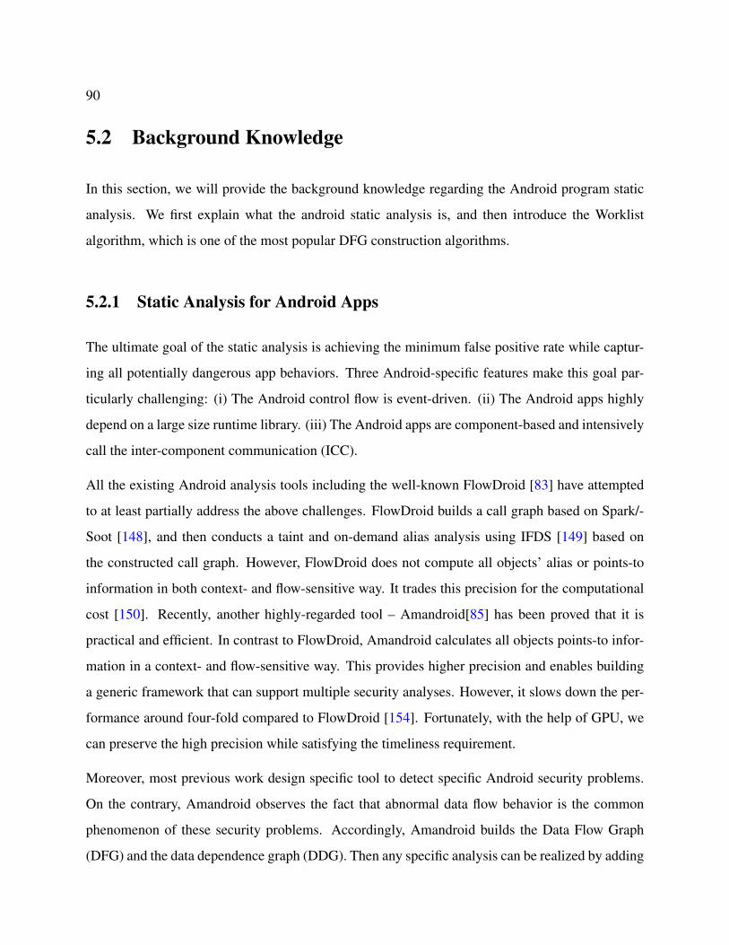
90
5.2 Background Knowledge
In this section, we will provide the background knowledge regarding the Android program static
analysis. We first explain what the android static analysis is, and then introduce the Worklist
algorithm, which is one of the most popular DFG construction algorithms.
5.2.1 Static Analysis for Android Apps
The ultimate goal of the static analysis is achieving the minimum false positive rate while captur-
ing all potentially dangerous app behaviors. Three Android-specific features make this goal par-
ticularly challenging: (i) The Android control flow is event-driven. (ii) The Android apps highly
depend on a large size runtime library. (iii) The Android apps are component-based and intensively
call the inter-component communication (ICC).
All the existing Android analysis tools including the well-known FlowDroid [83] have attempted
to at least partially address the above challenges. FlowDroid builds a call graph based on Spark/-
Soot [148], and then conducts a taint and on-demand alias analysis using IFDS [149] based on
the constructed call graph. However, FlowDroid does not compute all objects’ alias or points-to
information in both context- and flow-sensitive way. It trades this precision for the computational
cost [150]. Recently, another highly-regarded tool – Amandroid[85] has been proved that it is
practical and efficient. In contrast to FlowDroid, Amandroid calculates all objects points-to infor-
mation in a context- and flow-sensitive way. This provides higher precision and enables building
a generic framework that can support multiple security analyses. However, it slows down the per-
formance around four-fold compared to FlowDroid [154]. Fortunately, with the help of GPU, we
can preserve the high precision while satisfying the timeliness requirement.
Moreover, most previous work design specific tool to detect specific Android security problems.
On the contrary, Amandroid observes the fact that abnormal data flow behavior is the common
phenomenon of these security problems. Accordingly, Amandroid builds the Data Flow Graph
(DFG) and the data dependence graph (DDG). Then any specific analysis can be realized by adding

91
a plugin on top of the DFG and DDG. It substantially improves the design and running efficiency
due to the reuse of DFG. We leverage this Amandroid’s observation and design the GPU-based
framework for different Android analyses. Fig 5.1 shows the breakdown of Amandroid execution
time. The DFG construction consumes the majority of running time. It takes at least 58% and up
to 96% of the total execution time. Plugins for any specific analyses bring in negligible overhead
(usually in the order of tens of milliseconds). Hence the GPU-assist framework design is specified
to efficiently mapping of DFG building to the GPU.
5.2.2 Worklist-based DFG Building Algorithm
ADFG consists of an Inter-procedural Control-Flow Graph (ICFG) and the point-to fact sets. Each
ICFG node has one set, and the DFG is built by flowing the point-to facts along the ICFG paths
into the corresponding node’s set. Formally, let C be a component, the DFG can be defined as the
following:
DFG(EC) ⌘ ((N,E), {fact(n)|n 2 N}) (5.1)
where EC is the environment method of C, N and E are the nodes and edges of the ICFG starting
from EC , and fact(n) is the fact set of the statement associated with node n.
Fig. 5.2 shows a sample DFG. Each ICFG node is accompanied by a point-to fact set fact(i){}.
During the DFG building, the facts are generated after each node processing and propagated along
the ICFG paths. Unlike the graph traversal, visiting all nodes is not the end of the process. For
example, in Fig. 5.2, after visiting node L7, one flow goes back to L1 and the fact set fact(i) is
updated to fact(i)0. Due to this update, its visited successor nodes L2 and L4 must be revisited,
and fact sets fact(2) and fact(4) must be updated accordingly. Amandroid constructs the DFG
using a fixed-point worklist-based algorithm. Alg. 3 reproduce this algorithm. The while loop
(ln. 10-ln. 14) is the core that iteratively processes the nodes and propagates the point-to facts.
In each iteration, the analyzer pops out a node from the worklist and processes it through the
function ProcessNode() (ln. 11-ln. 13). ProcessNode() processes a node to generate the facts and

92
foo().Entry
L2: v2:= new A1
L1: if(x=0) goto 5
L3: v2.f1:= new B
L6: v3:= “abc”
L7: if(y=1) goto 1
L5: v9:= new B
L4: v2:= new A2
.…
Fact(0){}
Fact(1){}
Fact(2){} Fact(4){}
Fact(3){<v2,2>} Fact(5){<v2,4>}
Fact(6){<v2,2>, <v2,4>, <v9,5>, <(v2.f1),3>}
Fact(7){<v2,2>, <v2,4>, <v9,5>, <(v2.f1),3>}
Fact(1)’{<v2,2>, <v2,4>, <v9,5>, <(v2.f1),3>}
Figure 5.2: A sample DFG. Each box is a ICFG node. Blue arrow-lines indicate the ICFG paths. Each nodehas a fact set colored in red.
propagates the facts to current node’s successors. If any of the successors’ fact set gets a new fact,
that successor will be collected into a set nodes (ln. 13). Then the nodes will be inserted into
the worklist (ln. 14). The while loop keeps active until it converges to a fixed point that all fact
sets are steady (i.e., worklist goes to empty). Apparently, the while loop could be significantly
time-consuming due to the potentially huge number of iterations.
5.3 Our Plain GPU Implementation
In this section, we will present our plain GPU implementation. This implementation uses only
generic approaches without leveraging any application-specific characteristics. We first introduce
the basic implementation designs, and then analyze the performance bottlenecks.

93
Algorithm 3: Worklist-based Iterative DFG Building1 Require: entry point procedure EP;2 Ensure: DFG;3 Procedure DFGBuilding(EP)4 icfg ⌘ (N,E);5 for ni 2 N do6 new empty Set fact(i){};7 ni fact(i){};8 new empty List worklist ;9 worklist EntryNodeEP ;
10 while worklist 6= ? do11 n worklist.front();12 worklist.pop front();13 nodes ProcessNode(icfg,n);14 worklist nodes;15 return (icfg, fact{})
5.3.1 Basic Design
In this section, we implement the worklist algorithm on GPU using the generic approaches. We
call it the plain GPU implementation because it neither uses application-specific characteristics nor
considers fine-grained GPU architectural features.
5.3.1.1 Using Summary-based Analysis
In order to parallelize the Android method processing, we employ the Summary-based Bottom-
up Data-flow Analysis (SBDA) algorithm introduced in [186]. SBDA generates a unified heap
manipulation summary for each method. With SBDA, the interprocedural DFG construction can
utilize the summaries instead of re-analyzing the visited methods. It makes the methods at the
same layer independent hence makes the worklist algorithm more parallel-friendly. Though the
SBDA is a more conservative approach, it still can preserve flow and context-sensitive data-flow
analysis result [187].
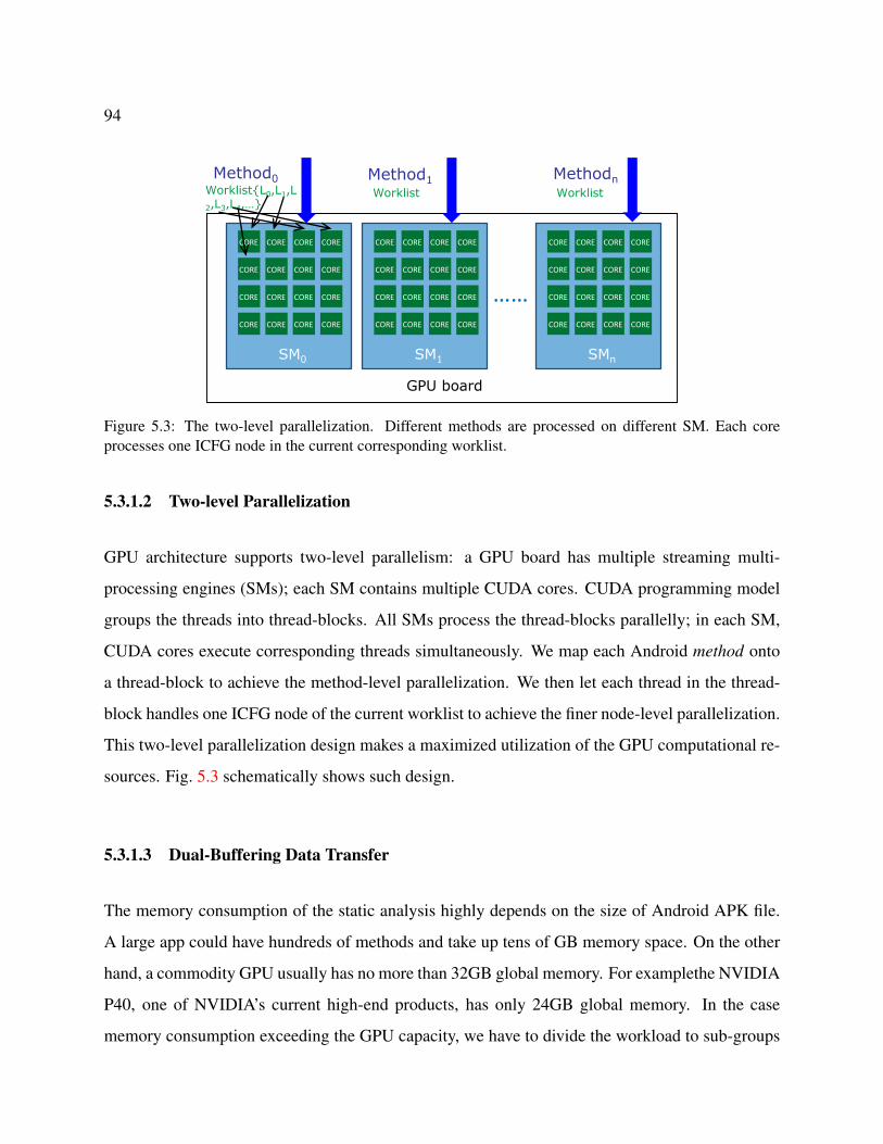
94
CORE
CORE
CORE
CORE
CORE
CORE
CORE
CORE
CORE
CORE
CORE
CORE
CORE
CORE
CORE
CORE
SM0
CORE
CORE
CORE
CORE
CORE
CORE
CORE
CORE
CORE
CORE
CORE
CORE
CORE
CORE
CORE
CORE
SM1
CORE
CORE
CORE
CORE
CORE
CORE
CORE
CORE
CORE
CORE
CORE
CORE
CORE
CORE
CORE
CORE
SMn
……
GPU board
Method0Worklist{L0,L1,L2,L3,L4,…}
Method1Worklist
MethodnWorklist
Figure 5.3: The two-level parallelization. Different methods are processed on different SM. Each coreprocesses one ICFG node in the current corresponding worklist.
5.3.1.2 Two-level Parallelization
GPU architecture supports two-level parallelism: a GPU board has multiple streaming multi-
processing engines (SMs); each SM contains multiple CUDA cores. CUDA programming model
groups the threads into thread-blocks. All SMs process the thread-blocks parallelly; in each SM,
CUDA cores execute corresponding threads simultaneously. We map each Android method onto
a thread-block to achieve the method-level parallelization. We then let each thread in the thread-
block handles one ICFG node of the current worklist to achieve the finer node-level parallelization.
This two-level parallelization design makes a maximized utilization of the GPU computational re-
sources. Fig. 5.3 schematically shows such design.
5.3.1.3 Dual-Buffering Data Transfer
The memory consumption of the static analysis highly depends on the size of Android APK file.
A large app could have hundreds of methods and take up tens of GB memory space. On the other
hand, a commodity GPU usually has no more than 32GB global memory. For examplethe NVIDIA
P40, one of NVIDIA’s current high-end products, has only 24GB global memory. In the case
memory consumption exceeding the GPU capacity, we have to divide the workload to sub-groups

95
Algorithm 4: GPU Worklit Kernel1 int *h cfg, *h nodeValue, *h facts;2 d cfg h cfg; d nodeValue h nodeValue; d facts h facts; . copy data from host to device;3 Procedure WORKLIST(d cfg, d nodeValue, d facts)4 local int worklist; . allocate shared memory space for worklist;5 int tid � threadIdx.x;6 int methodid � blockIdx.x ⇤ blockDim.x;7 worklist � init nodes[methodid ];8 while !worklist.empty() do9 if tid < worklist.size() then
10 src node � worklist[tid ]; . each thread handles one node in current worklist;11 new facts � Gen Kill(d nodeValue(methodid, src node));12 . each thread processes corresponding node statement and generate facts; different blocks
handle different methods;13 dest nodes � search CFG(d cfg(methodid, src node));14 . each thread collects destination nodes of its current source node;15 for n 2 dest nodes do16 d facts(methodid, n).union(new facts);17 if d facts(methodid, n).update() then18 worklist � n;19 . update facts and worklist;20 syncthread;21 h facts d facts;22 . copy the result back to host;
and transfer the data in and out of the GPU multiple rounds. Even the latest hardware technologies
– NVLink and unified memory provide faster transfer speed, the CPU-GPU data communication
is still considered as one of the major overhead and can significantly degrade the performance.
In order to hide the CPU-GPU data transfer overhead, we propose a double buffering scheme.
This scheme is a software solution based on the asynchronous execution of the CUDA kernel and
data-transfer engine. Specifically, we create two buffer spaces in the GPU global memory and two
CUDA execution streams. Buffer 1 stores the current data, and Stream 1 launches kernel execution
accessing Buffer 1. Simultaneously, Stream 2 transfers next bulk of the workload to Buffer 2 for
next round of kernel executions. The function of the two streams and two buffers is swapped from
iteration to iteration. The CPU-GPU data communication overhead of (i+1)th round is hidden by
overlapping the kernel execution of ith round.

96
Figure 5.4: The performance comparison between the plain GPU implementation and the CPU counterpart.The x-axis represents the APK indices, y-axis indicates the speedups compared to the CPU performances.the APKs are sorted according to the descending order of GPU implementation’s speedups.
5.3.2 Performance Analysis
To evaluate the efficiency of the plain GPU implementation, we examine the designs mentioned
above with a dataset containing 1K Android APKs. We then analyze the experiment results to
discover the performance bottlenecks.
5.3.2.1 Comparison with CPU Counterpart
We test our plain GPU implementation on a NVIDIA TESLA P40 GPU using 1000 Android APKs.
Fig. 5.4 shows the performance comparison between the GPU implementation and the CPU coun-
terpart. We re-implement the worklist algorithm in Amandroid using C language with multithread-
ing to make the CPU version fairly comparable to the GPU implementation. The figure shows that
GPU can only achieve 1.81X speedups on average against the CPU counterpart. It at most can
achieve 3.39X speedups against CPU; for the majority (65.9%) of the APKs, GPU only achieve
less than 2X speedups (the skyblue area); for 7.3% of the APKs, GPU even runs slower than the
CPU (the red area). Apparently, the plain implementation largely underutilizes the GPU computa-
tion capacity.

97
5.3.2.2 Performance Bottlenecks
As Fig. 5.4 indicated, worklist algorithm is an irregular application; straightforwardly mapping
the algorithm onto GPU largely underutilizes GPU’s computation capacity. There are four perfor-
mance bottlenecks in the plain implementation:
Dynamic Memory Allocation Although very recently, researchers notice and try to break through
the GPU memory allocation bottleneck [188], dynamic memory allocation in GPU is still a sig-
nificant challenge due to the hardware limitation. Worklist algorithm associates an data fact set
with each node; the data fact sets keep updating during the node traversals. Hence the sizes of the
data fact sets cannot be foreknown, and the GPU implementation requires frequent dynamic GPU
allocations and reallocations.
Branch Divergence The GPU execution model is single instruction multiple threads (SIMT),
means that to maximize the GPU resource usage, all threads in a thread-block should execute
the same instructions with different data. In the occurrence of branches, GPU has to handle them
one by one. When the threads with branch 1 are executing, all other threads get stuck until the
branch 1 execution complete. Then GPU will execute branch 2 and all succeeding branches in the
same manner. In the worst case that all threads execute different branches, it will deteriorate to
sequential execution.
The worklist algorithm groups the ICFG nodes based on the types of their corresponding state-
ments. There are nine categories of statements in Android apps: AssignmentStatement, Emp-
tyStatement, MonitorStatement, ThrowStatement, CallStatement, GoToStatement, Ifstatement, Re-
turnStatement, SwitchStatement. Furthermore, AssignmentStatement consists of expressions com-
ing from 17 different groups: AccessExpr, BinaryExpr, CallRhs, CastExpr, CmpExpr, ConstClas-
sExpr, ExceptionExpr, IndexingExpr, InstanceOfExpr, LengthExpr, LiteralExpr, VariableName-
Expr, StaticFieldAccessExpr, NewExpr, NullExpr, TupleExpr, UnaryExpr. Apprently, this group-
ing scheme in original worklist algorithm could result in dozes of branches. It could be a disaster
to the GPU execution.

98
Load Imbalance An ideal balanced workload should be that the number of ICFG nodes in a work-
list matches or is an integral multiple of the number of CUDA cores in a SM. The balanced work-
load can ultimately utilize the resources since no cores will be idle during execution. However,
the size of worklist on each iteration highly depends on the ICFG structure. Any two consecutive
worklists’ size could be quite different and unpredictable. It is pretty hard to make every worklist
to be a balanced load.
Irregular Memory Access Pattern GPU has enormous memory bandwidth. Each memory access
of a warp (32 threads) can read or write a 128B memory block. If this 128B block contains
the requested data of all 32 threads, it is a full utilization of the bandwidth. However, if the
block contains only the data requested by some of the threads, then multiple memory accesses are
needed to feed the whole warp, and a proportion of the bandwidth is wasted. In the worst case, the
request data of 32 threads reside at 32 random memory location, then 32 memory accesses should
be performed and 31⁄32 bandwidth is wasted. Unfortunately, like other graph traversal problems,
the accesses to the destination nodes are unstructured; hence it’s extremely difficult to guarantee
the efficient bandwidth utilization. Moreover, different statements and expressions have different
memory access patterns, and the data-fact set of each node is dynamically changing; these make
the memory access pattern of the worklist algorithm even more irregular.
5.4 The Optimization Designs
Aiming to break through the performance bottlenecks described above, in the section, we propose
three optimizations. These optimizations leverage fine-grained application-specific characteristics
to refactor the worklist algorithm to make it fit the GPU’s architecture and execution model.
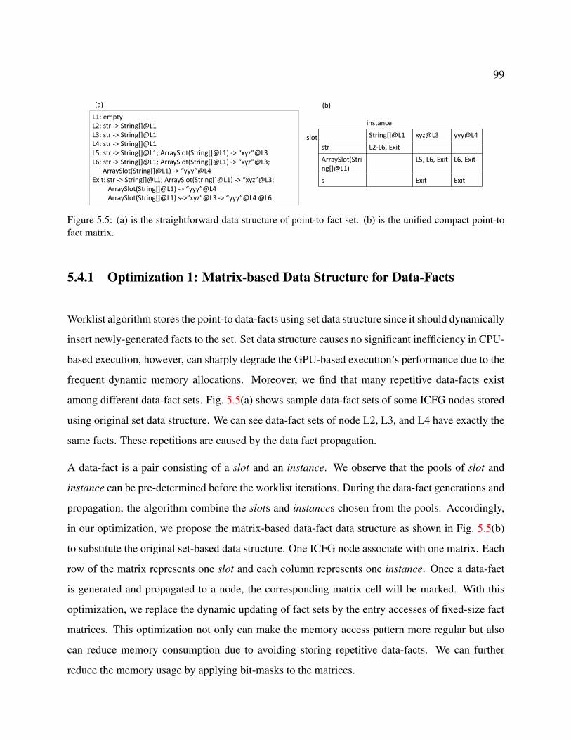
99
String[]@L1 xyz@L3 yyy@L4str L2-L6, ExitArraySlot(String[]@L1)
L5, L6, Exit L6, Exit
s Exit Exit
slot
instanceL1: emptyL2: str -> String[]@L1L3: str -> String[]@L1L4: str -> String[]@L1L5: str -> String[]@L1; ArraySlot(String[]@L1) -> “xyz”@L3L6: str -> String[]@L1; ArraySlot(String[]@L1) -> “xyz”@L3;
ArraySlot(String[]@L1) -> “yyy”@L4Exit: str -> String[]@L1; ArraySlot(String[]@L1) -> “xyz”@L3;
ArraySlot(String[]@L1) -> “yyy”@L4ArraySlot(String[]@L1) s->”xyz”@L3 -> “yyy”@L4 @L6
(a) (b)
Figure 5.5: (a) is the straightforward data structure of point-to fact set. (b) is the unified compact point-tofact matrix.
5.4.1 Optimization 1: Matrix-based Data Structure for Data-Facts
Worklist algorithm stores the point-to data-facts using set data structure since it should dynamically
insert newly-generated facts to the set. Set data structure causes no significant inefficiency in CPU-
based execution, however, can sharply degrade the GPU-based execution’s performance due to the
frequent dynamic memory allocations. Moreover, we find that many repetitive data-facts exist
among different data-fact sets. Fig. 5.5(a) shows sample data-fact sets of some ICFG nodes stored
using original set data structure. We can see data-fact sets of node L2, L3, and L4 have exactly the
same facts. These repetitions are caused by the data fact propagation.
A data-fact is a pair consisting of a slot and an instance. We observe that the pools of slot and
instance can be pre-determined before the worklist iterations. During the data-fact generations and
propagation, the algorithm combine the slots and instances chosen from the pools. Accordingly,
in our optimization, we propose the matrix-based data-fact data structure as shown in Fig. 5.5(b)
to substitute the original set-based data structure. One ICFG node associate with one matrix. Each
row of the matrix represents one slot and each column represents one instance. Once a data-fact
is generated and propagated to a node, the corresponding matrix cell will be marked. With this
optimization, we replace the dynamic updating of fact sets by the entry accesses of fixed-size fact
matrices. This optimization not only can make the memory access pattern more regular but also
can reduce memory consumption due to avoiding storing repetitive data-facts. We can further
reduce the memory usage by applying bit-masks to the matrices.
100
T0 T1 T2 T31……
Thread-block
One warp (32 threads)
…… …… ……
memory layout
Current
worklist
……
(node IDs only)
Suppose there are 96 total, and each type has 32 nodes
……
32 nodes
…… ……
32 nodes 32 nodes
Re-group the worklist
Each thread
read one ID
Read 32 actual node
data from memory
Figure 5.6: The scheme of node grouping. Three colors indicate three different types of nodes.
5.4.2 Optimization 2: Memory Access Pattern Based Node Grouping
The original worklist algorithm classifies the ICFG nodes based on the statement and expression
types. This classifying scheme is insufficient for the GPU implementation due to the large number
of divergences. We observe that if we pre-determine the pools of slot and instance, generating
and propagating data-facts for every ICFG node are converted to looking up and combining entries
from two pools. Hence, grouping the nodes based on the types of statements is no longer neces-
sary. Instead, we propose a memory access pattern based grouping scheme for ICFG nodes. We
identify that there are only three ICFG node memory access patterns existing: (i) The one-time
fact-generation statements, e.g., ConstClassExpression, NullExpression, LiteralExpression. Each
of them only generates new facts at the first time they are visited; then it will only propagates the
facts when they are inserted to the worklist again. (ii) The single-layer statements, e.g., Variable-
NameExpression, StaticFieldAccessExpression. They may produce new facts every time they are
visited; each visit only requires single de-reference. (iii) The double-layer statements, e.g., Acces-
sExpression, IndexingExpression. They may produce new facts every time they are visited; each
visit requires a double de-reference.
The nodes in the same group are stored consecutively in the global memory. We sort each current
worklist based on the node group before we process it. This new grouping scheme apparently

101
Worklist algorithm
{L1}
{L2, L3}
{L6, L4}
{L5}
{L6}
Processing this L6 is redundant
Figure 5.7: An example shows a case that the worklist merging can eliminate redundant processing.
can significantly reduce the number of branches given that it has only three groups. Moreover,
the new grouping scheme can maximize memory coalescing. For example, in Fig. 5.6’s case, a
warp will always process the nodes with the same memory access pattern, so it eliminates the
branch divergence. Moreover, storing the nodes of the same group consecutively in the memory
can maximize bandwidth utilization.
5.4.3 Optimization 3: Worklist Merging
We assume the current worklist has 36 ICFG nodes. Given a warp has only 32 threads, GPU needs
two warps to handle the current worklist. The second warp processes only four nodes leads to a
waste of 28 threads. Hence this 32-node worklist is an imbalanced load.
Aiming to solve the load imbalance issue, we propose the worklist merging optimization. In this
optimization, we divide each current worklist to a head list and a tail list. The head list contains
the subset of current worklist in which the number of nodes is the integral multiple of 32 while the
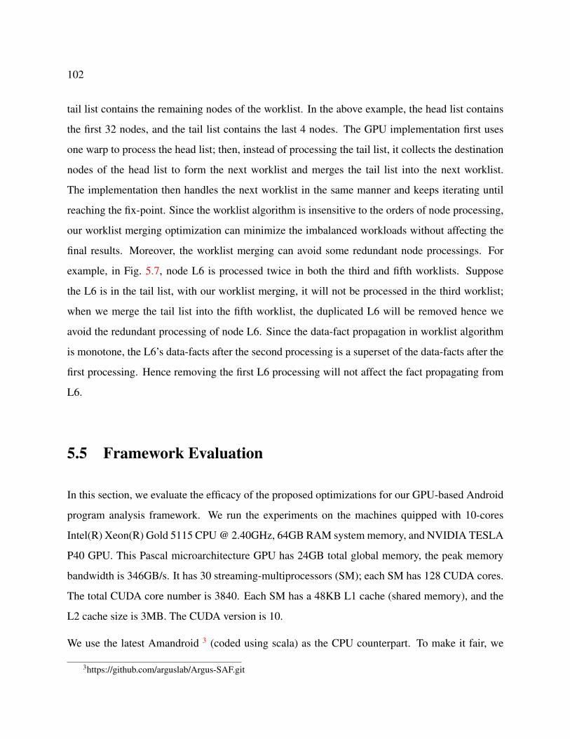
102
tail list contains the remaining nodes of the worklist. In the above example, the head list contains
the first 32 nodes, and the tail list contains the last 4 nodes. The GPU implementation first uses
one warp to process the head list; then, instead of processing the tail list, it collects the destination
nodes of the head list to form the next worklist and merges the tail list into the next worklist.
The implementation then handles the next worklist in the same manner and keeps iterating until
reaching the fix-point. Since the worklist algorithm is insensitive to the orders of node processing,
our worklist merging optimization can minimize the imbalanced workloads without affecting the
final results. Moreover, the worklist merging can avoid some redundant node processings. For
example, in Fig. 5.7, node L6 is processed twice in both the third and fifth worklists. Suppose
the L6 is in the tail list, with our worklist merging, it will not be processed in the third worklist;
when we merge the tail list into the fifth worklist, the duplicated L6 will be removed hence we
avoid the redundant processing of node L6. Since the data-fact propagation in worklist algorithm
is monotone, the L6’s data-facts after the second processing is a superset of the data-facts after the
first processing. Hence removing the first L6 processing will not affect the fact propagating from
L6.
5.5 Framework Evaluation
In this section, we evaluate the efficacy of the proposed optimizations for our GPU-based Android
program analysis framework. We run the experiments on the machines quipped with 10-cores
Intel(R) Xeon(R) Gold 5115 CPU@ 2.40GHz, 64GB RAM systemmemory, and NVIDIA TESLA
P40 GPU. This Pascal microarchitecture GPU has 24GB total global memory, the peak memory
bandwidth is 346GB/s. It has 30 streaming-multiprocessors (SM); each SM has 128 CUDA cores.
The total CUDA core number is 3840. Each SM has a 48KB L1 cache (shared memory), and the
L2 cache size is 3MB. The CUDA version is 10.
We use the latest Amandroid 3 (coded using scala) as the CPU counterpart. To make it fair, we
3https://github.com/arguslab/Argus-SAF.git

103
Table 5.1: Dataset Characteristics
no. of CFG Nodes no. of Methods no. of Variable max Worklist length6217 268 116 74
re-implement the worklist algorithm in Amandroid using multithreading C. We evaluate our GPU
implementation using a dataset containing 1000 APKs. The characteristics of these APKs are listed
in the table 5.1.
We verify the output results of GPU implementations by comparing them to the DFG constructed
by the original CPU implementation. The plain GPU implementation, as well as every opti-
mizations, do not affect the correctness of DFG. In the following subsections, we first provide
an overview of our GPU implementation. We then zoom in the performance and evaluate three
optimizations: matrix-based data structure, node grouping, and worklist merging, respectively.
5.5.1 Overview of GPU Implementation’s Performance
Section 5.3.2.1 indicates our plain GPU implementation mostly can only achieve less than 2X
speedups against the CPU counterpart. In order to evaluate our optimizations, we use the perfor-
mance of plain GPU implementation as the baseline, then accumulate the optimizations to the GPU
implementation and compare their performances with the baseline.
Fig. 5.8 shows the performance comparison of GPU implementations with different optimizations.
The x-axis shows the app APK indices. Notice that we sort the APKs according to the descending
order of the optimal performance. The y-axis shows the performance speedups against the base-
line. The figure indicates that applying all three optimizations to the GPU implementation can
achieve the optimal performance: it can achieve 128X peak speedups and 71.3X average speedups
against the plain GPU implementation. The figure also shows that the matrix-based data struc-
ture (mat) and the worklist merging (mer) optimizations can largely improve the performance of
GPU implementation. Though the memory access pattern based node grouping (grp) optimization
can also improve the performance, it is not significant. We will provide detailed evaluations and
discussions of each optimization in the following sections.

104
Figure 5.8: The GPU implementation’s performance overview. The x-axis indicates the app APK IDs whilethe y-axis indicates performance speedups against the plain GPU implementation.
5.5.2 Evaluation of Matrix Data Structure Optimization
In this subsection, we apply the first optimization – matrix-based data structure (mat) of the data-
facts to the general GPU implementation. The optimization design is described in subsection 5.4.1.
Fig. 5.9a shows the performance comparison between the GPU implementation with and without
the first optimization. The x-axis shows the APK IDs while the y-axis shows the performance
speedups compared to GPU implementation without mat. Notice that we sort the data pairs based
on the running time of CPU version in descending order.
The figure indicates that the matrix-based data structure optimization can significantly improve
the GPU version’s performance. It can achieve at least 7.6X speedups and up to 92.4X speedups
against the plain GPU implementation. For 59.4% of APKs, the mat optimization can improve
20X-40X performance (the skyblue area in Fig. 5.9a), and in average, it can achieve 26.7X
speedups. The performance improvement is significant because the mat optimization can elim-
inate dynamic memory allocation, which is one of the major GPU performance bottlenecks.

105
(a) Matrix-based Data Structure (mat) optimization
(b) Memory Access Pattern based Node Grouping (grp) optimization
Figure 5.9: Performance comparisons between the GPU implementation with and without (a) matrix datastructure (mat) optimization; (b) memory access pattern based node grouping (grp) optimization; (c) work-list merging (mer) optimization. The x-axis indicates the app APK IDs while the y-axis indicates thespeedups against the GPU implementation without (a) mat, (b) grp, and (c) mer respectively.

106
(c) Worklist Merging (mer) optimization
Figure 5.9: (cont.) Performance comparisons between the GPU implementation with and without (a) matrixdata structure (mat) optimization; (b) memory access pattern based node grouping (grp) optimization; (c)worklist merging (mer) optimization. The x-axis indicates the app APK IDs while the y-axis indicates thespeedups against the GPU implementation without (a) mat, (b) grp, and (c) mer respectively.

107
Figure 5.10: Memory footprint comparison between the matrix-based and set-based data structure for storingthe data-facts. The x-axis indicates the app APK IDs while the y-axis indicates the memory footprint.
Since the matrix-based data structure is also designed to reduce the memory space consumption,
we also compare its memory footprints to the memory footprint of the set-based data structure.
Fig. 5.10 shows the memory footprint comparisons between the matrix-based and set-based data
structure. It indicates the matrix-based data structure optimization can reduce 75% memory con-
sumption on average. It at most needs 34%memory space compared to the set-based data structure.
The matrix-based data structure can significantly reduce the memory footprint because it avoids
storing the copies of repetitive data-facts.
5.5.3 Evaluation of Memory Access Pattern Based Node Grouping Opti-
mization
In this subsection, we apply the second optimization – the memory access pattern based node
grouping (grp) in addition to the GPU implementation with mat. The optimization design is de-
scribed in subsection 5.4.2.

108
Table 5.2: Worklist Profiling
Worklist sizes32 >32 & 64 >64
before mer 87.6% 4.3% 8.1%after mer 74.4% 11.9% 13.7%
no. of Worklist iterationaverage max min
before mer 5.6K 6.8K 4.3Kafter mer 4.5K 5.8K 3.6K
Fig. 5.9b shows the performance comparison between the GPU implementation with and without
the second optimization. The x-axis shows the APK IDs while the y-axis shows the performance
speedups compared to GPU implementation without grp. Notice that we sort the data pairs based
on the running time of CPU version in descending order.
The figure indicates that grp optimization can only slightly improve the performance. For 76.3%
APKs, the grp can only achieve less than 1.5X speedups (the skyblue area in Fig. 5.9b) against
the baseline; for 15.5% APKs, it even degrades the performance (the red area in Fig. 5.9b). The
performance degradation is caused by that most worklists are small. Table 5.2 shows the results of
worklist profiling. The third line of the Table indicates that on average, 87.6% of the worklists in
a worklist algorithm instance have less than 32 ICFG nodes. It means that most of the worklists
can fit into a single warp hence cannot take the merits of grp but will suffer the sorting overhead.
However, since the grp can maximize the coalesced memory accesses, in some cases, it can still
achieve slightly overall performance improvement.
5.5.4 Evaluation of Worklist Merging Optimization
In this subsection, we apply the third optimization – the worklist merging (mer) in addition to the
GPU implementation with both mat and grp optimizations. The optimization design is described
in subsection 5.4.3.
Fig. 5.9c shows the performance comparison between the GPU implementation with and without

109
the third optimization. The x-axis shows the APK IDs while the y-axis shows the performance
speedups compared to GPU implementation without mer. Notice that we sort the data pairs based
on the running time of CPU version in descending order.
The figure indicates that mer optimization can significantly improve performance. For 67.4%
APKs, the mer can achieve at least 1.5X speedups and up to 3X speedups against the baseline (the
skyblue area in Fig. 5.9c). In average, it can achieve 1.94X speedups. The improvement is signif-
icant because mer can efficiently reduce the number of worklist algorithm iterations and enlarge
the worklist sizes. The eighth line of Table 5.2 indicates that in average, the mer optimization can
reduce 1.1K iterations in a worklist algorithm instance. This reduction apparently can improve
performance. Moreover, merging the tail list with the predecessor worklists can enlarge the sizes
of the worklists. The fourth line of the Table 5.2 indicates that 25.6% worklists require more than
one warp to process. Hence the mer can boost the benefits of grp optimization.
5.6 Conclusion
In this chapter, we propose a GPU-based Android program analysis framework for the security
vetting. Based on the profiling results, we find that the IDFG constructions take the most of the
overall analyzing time (up to 96%); hence we accelerate the IDFG constructions on the GPUs.
In the GPU design, we first implement the IDFG construction algorithm on GPU using general ap-
proaches, including summary-based analysis, two-level parallelization, and optimized data trans-
fer. However, we find this plain GPU implementation has four major performance bottlenecks:
frequent dynamic memory allocation, the branch divergences, load imbalance, and the irregu-
lar memory access pattern. These issues can sharply degrade GPU implementation’s efficiency.
Accordingly, we leverage application-specific characteristics and propose three advanced opti-
mizations, including matrix-based data structure for data-facts, memory access pattern based node
grouping, and worklist merging. The matrix-based data structure is also designed to reduce mem-
ory consumption.
110
In our experiments, we evaluate the three proposed optimizations respectively on Intel(R) Xeon(R)
Gold 5115 CPU and NVIDIA TESLA P40 GPU using 1000 Android APKs. The experiment re-
sults show that the matrix-based data structure for data-facts and worklist merging optimizations
can significantly improve the performance compared to the plain GPU implementation, while the
memory access pattern based node grouping optimization can slightly improve the performance.
The optimal GPU implementation can achieve up to 128X speedups against plain GPU optimiza-
tion. The matrix-based data structure optimization also can save 75% memory space on average
compared to the original set-based data structure.

Chapter 6
Comparative Measurement of Cache
Configurations’ Impacts on the
Performance of Cache Timing Side-Channel
Attacks
6.1 Introduction
Timing-based cache side-channel attacks have been comprehensively studied since its debut in
1996 [98]. The time side-channel of cache leaks secret information, specifically through the time
differences of cache hits and misses. Time-driven attacks are the primary type in the early age of
the timing-based side-channel attacks. They observe the total execution time of the cryptographic
operations and crack the keys by analyzing the observations.
In the last decade, access-driven attacks, for example, the notorious meltdown attack [101], have
gained popularity. They manipulate specific cache-lines and observe the access behaviors of
cryptographic operations on these cache-lines. They require fewer observations than the time-
111

112
driven attacks due to the higher resolutions and lower noises. Fine-grained variants of the access-
driven attacks have been proposed, including PRIME+PROBE [102], FLUSH+RELOAD [103],
and FLUSH+FLUSH [104]. However, all access-driven attacks require that the attacker’s process
have access to specific cache addresses that shared by the victim’s process.
Recently, some proposals leverage new hardware technologies to defend the access-driven attacks.
For example, the CATalyst [105] exploits Intel’s Cache Allocation Technology (CAT) (CAT iso-
lates shared cache space for victim’s process) to physically revoke the accessibility of attacker’s
process. Given the attackers’ access privilege is not an assurance, studying time-driven attacks are
still worthwhile since they demand no adversary’s intervention during the observations.
Researchers have been speculating that cache configurations can impact the performances of time-
driven side-channel attacks [106, 107, 108]. For example, intuitively, a bigger cache size would
make the attacks on AES more difficult, as it can hold a larger portion of the precomputed S-box
lookup table in the cache. However, we are not aware of any previous work that provides exper-
imental data to demonstrate how cache configuration parameters influence time-driven attacks. It
is extremely challenging to conduct performance comparisons under the same system with differ-
ent cache configurations, as none of the existing CPU products provide configurable caches. This
challenge prevents the experimental study about the impact of cache parameters on time-driven
attacks.
In this work, we overcome the aforementioned difficulty and conduct a comprehensive study on
how cache configurations impact the success rates of time-driven attacks. We leverage a modular
platform – GEM5 [110] to measure the performances of time-driven attacks under various cache
configurations. GEM5 is one of the most popular cycle-accurate full-system emulators in the
computer-system architecture community [111, 112]. We leverage GEM5 to emulate the X86 64
system with a configurable cache.
In our work, we measure the performance of Bernstein’s cache timing attack on AES [106]. Bern-
stein’s attack is one of the most classic time-driven attacks and still feasible on model proces-
sors [113, 114]. To make its performance comparable, we propose a new metric to quantify the

113
its success rate. In the measurement, we run Bernstein’s attacks on GEM5 instances with different
cache configurations and provide systematic experimental data to describe the correlation of cache
parameters and the attack’s performance. Our contribution can be summarized as follows:
• We use the GEM5 platform to investigate the cache configurations’ impacts on time-driven
cache side-channel attacks. We configure the GEM5’s cache through seven parameters:
Private Cache Sizes, Private Cache Associativity, Shared Cache Sizes, Shared Cache Asso-
ciativity, Cacheline Sizes, Replacement Policy, and Clusivity.
• We extend the traditional success-fail binary metric to make the cache timing side-channel
attacks’ performances comparable. We define the equivalent key length (EKL) to describe
the success rates of the attacks under a certain cache configuration.
• We systematically measure and analyze each cache parameter’s influence on the attacks’
success rate. Based on the measurement results, we find the private cache is the key to
the success rates; the 8KB, 16-way private cache can achieve the optimal balance between
the security and the cost. Although the shared cache’s impacts are trivial, running neighbor
processes can significantly increase the success rates of the attacks. The replacement policies
and cache clusivity also have impacts on the attacks’ performances: Random replacement
leads to the highest success rates while the LFU/LSU leads to the lowest; the exclusive
policy makes the attacks harder to succeed compared to the inclusive policy. We then use
these findings to enhance both the cache side-channel attacks and defenses and strengthen
future systems.
6.2 Background
In this section, we provide the knowledge about modern cache model and the GEM5 platform, and
explain how the Bernstein’s time-driven attack works.

114
CPU Core
register
On-board Main Memory
Shared Cache (LLC)
Private Cache
CPU Core
register
Private Cache
Two-level cache hierarchy
size
large
small
spee
d
slow
fast
Figure 6.1: A generic cache model. It is a two-level hierarchy: each CPU core has its own private cache; allcores could access a shared cache through the private cache.
6.2.1 CPU Cache Hierarchy
The CPU cache is in between of the CPU cores and the main memory. It stores copies of the
frequently used data in main memory, aiming to reduce the average latency of data access from
the main memory. Compared to the main memory, the cache is faster but smaller. Modern multi-
core CPUs usually organize the cache as a hierarchy of multiple cache levels. Fig. 6.1 indicates a
generic cache hierarchy model. Each CPU core is bound with a private cache and has this private
cache’s exclusive access permission. The whole CPU chip has one shared cache (a.k.a Last Level
Cache (LLC)) that shared by all the CPU cores. The shared cache usually is larger but slower
than the private cache. Commodity Intel CPUs follow this cache model and usually implement the
private cache as two levels (L1 and L2) and split L1 cache into instruction and data caches. Private
cache size typically is in KB scale while shared cache size is in MB scale.

115
2N encryptions on victim server
2N encryptions on victim server
Reference time model
Attacking time data
Correlating the reference and attacking data
Reduced key search space
Brute-force search
Known Key Secret Key
Recovered Key
(a) Profiling phase (b) Attacking phase
(c) correlating phase
(d) searching phaseO
nline phases on victim server
Offline phases on local system
Figure 6.2: The workflow of Bernstein’s time-driven attack. It consists of two online phases: (a) profilingphase and (b) attacking phase, and two offline phases: (c) correlating phase and (d) searching phase.
6.2.2 Bernstein’s Cache Timing Attack
The Bernstein’s cache timing attack on AES [106] is one of the most classical time-driven cache
attacks. It cracks the AES keys by measuring and analyzing the encryption time data.
Fig. 6.2 shows the workflow of Bernstein’s attack. On the victim server, the attacker performs two
online phases. During the profiling phase (Fig. 6.2 (a)), she or he encrypts millions of different
plaintexts with a known key, then collects and profiles each execution time to build the reference
time model. During the attacking phase (Fig. 6.2 (b)), she or he collects attacking time data
by measuring the execution time of millions of encryptions with an unknown key. Then two
116
offline phases postprocess the attacking data to guess the unknown key. Specifically, during the
correlating phase(Fig. 6.2 (c)), the attacker mathematically correlates the time model and attacking
data to shrink the key search space by generating value candidates for each key byte. Finally, in
the searching phase(Fig. 6.2 (d)), the attacker brute-force searches the reduce key space to recover
the secret key.
Only the two online phases need to be performed on the victim server. Although the Bernstein’s
attack is computationally expensive (typically needs 222-223 encryptions for profiling and attacking
phases respectively [106]), it does not require attacker’s intervention during the attack. Thus, con-
ducting this attack does not need much computer architecture knowledge and the victim system’s
access privilege.
6.2.3 GEM5 Platform
GEM5 is a modular platform for computer-system architecture research [110]. GEM5 is the combi-
nation of two influential projects: M5 [189] and Gems [190]. The former is renowned for CPU sim-
ulation while the latter is for memory system simulation. Therefore, GEM5 can cycle-accurately
emulate the full X86 system encompassing system-level architecture and processor microarchitec-
ture. It provides the interfaces to manipulate the configuration of almost all system components,
including processing units, cache, and main memory. In the full-system mode, GEM5 runs a real
operating system on it and allows users to interact with the OS. Hence, users can run any applica-
tions on GEM5 as running on real-world hardware. The downside of GEM5 is that its execution is
1000X slower than real hardware.
6.3 Measurement Design
We measure the performances of Bernstein’s attacks running on different GEM5 instances. We
configure these instances’ caches using seven cache parameters, including Private Cache Size, Pri-

117
vate Cache Associativity, Shared Cache Size, Shared Cache Associativity, Cacheline Size, Replace-
ment Policy, and Cache Clusivity. We elaborate all the cache parameters in Section 6.3.1. GEM5
instances play the role of victim servers; hence we only need to run two online phases (Fig. 6.2 (a)
and (b)) on it. Under each cache configuration, in accordance with the references [106, 113, 114],
we conduct 222 encryptions for profiling and attacking phases respectively. To quantify the perfor-
mances of the attacks, we define the success rate of the time-driven attack in Section 6.3.2.
6.3.1 Cache Parameters for Configuration
GEM5 platform gives us the full privilege to configure the cache. Without loss of generality, we
configure the cache in our measurements to a two-level hierarchy as shown in Fig. 6.1. Under such
implementation, there are seven controllable cache parameters listed below:
1. Private Cache Size (PCS) The total amount of private cache space. It generally falls in the
range from 2KB to 32KB. Intuitively, smaller PCS makes the attacks easier.
2. Private Cache Associativity (PCA) The number of cache blocks in a private cache set.
Its range typically is between 2-way and 32-way. Intuitively, larger PCA results in lower
success rates of the attacks.
3. Shared Cache Size (SCS) The total amount of shared cache space. It usually is a value in
between 2MB and 32MB. Intuitively, the smaller SCS the easier attacks.
4. Shared Cache Associativity (SCA) The number of cache blocks in a shared cache set. It
commonly is consistent with the PCA and intuitively has similar impacts.
5. Cacheline Size (CLS) The size of the basic unit of cache storage. The common CLSs are
32Bytes, 64Bytes, and 128Bytes. Intuitively, larger CLS leads to lower success rates of the
attacks.
6. Replacement Policy (RP) The algorithms to manage the contents stored in the cache. The
RP’s impacts are highly-depend on the application’s memory locality.
118
7. Cache Clusivity (CC) Clusivity describes whether the data in one level of cache present
also in other levels. It is either inclusive or exclusive. Intuitively, the exclusive policy makes
the attacks easier.
We reconfigure the cache of GEM5 platform through changing the above parameters. In the sub-
sequent sections, we elaborate these cache parameters and their possible theoretical impacts on the
time-driven attacks.
6.3.1.1 Private and Shared Cache Size
Both private and shared cache copy a portion of the main memory that possibly contains the next
data that CPU will use. Apparently, larger PCS and SCS provide broader coverage and lower
cache-miss rate; However, taking into account the production cost factor, commodity systems
usually limit their PCS in KB scale and SCS in MB scale.
Theoretical expectation of PCS’s impacts. We attack the AES implemented in OpenSSL library.
OpenSSL precomputes the results of each AES step and stores them as a 4KB lookup table [174].
Given the time-driven attacks rely on the time differences of overall cache hits and misses, theoret-
ically, a PCS less than 4KB renders higher miss rates and consequently causes higher success rates
of the attacks. After 4KB, the attacks are impossible since the private cache can hold the entire
lookup table.
Theoretical expectation of SCS’s impacts. We discuss the impacts of SCS in two different scenar-
ios. Theoretically, given the SCS is in MB scale that is much larger than the 4KB table, if there
are no other processes running on the neighbor CPU cores, the SCS impacts to the attacks’ success
rates could be negligible. On the other hand, if there are random neighbor processes running, the
SCS’s impacts can be non-trivial. In the next section, we will experimentally examine whether the
facts align with these theoretical expectations.

119
6.3.1.2 Private and Shared Cache Associativity and Cacheline Size
The basic data copying unit between caches and main memory is referred to as cacheline. A
cacheline contains multiple bytes. The commodity CPUs usually divide the caches into multiple
sets that each of them contains N cachelines (referred to as N-way associativity). Each cacheline
of the main memory must go to a particular cache set but can choose one of the N positions in the
set to reside. Either PCA or SCA (i.e., the N) is a trade-off between miss-rate and the searching
cost.
Theoretical expectation of CLS, PCA, and SCA’s impacts. The larger CLS leverages more spatial
locality hence has lower miss-rates. The larger PCA leads to lower miss-rates as well. Lower
cache miss-rates result in lower success rates of the attacks. Similar to SCS, if there are no running
neighbor processes, SCA’s impacts will be trivial. Otherwise, SCA’s impacts are analogous to
PCA’s.
6.3.1.3 Replacement Policies
When a cache-miss occurs and the cache is full, the cache should make room for the new entry.
Replacement policies are sophisticated algorithms to choose the existing cache entries to evict.
Since the mission of the cache is storing the data that CPU is most likely to use next, the RPs
speculate about which existing entries have the least chances to be used in the future. Given this
heuristic is difficult, there is no universal optimal choice among available RPs.
In our measurement design, we examine four most common RPs: (i) Least recently used (LRU). It
keeps tracking what cache entries are used and discards the least recently used entry first. (ii) Least-
-frequently used (LFU). It counts how many times each cache entry is used and discards the least
often used entry first. (iii) First in first out (FIFO). Cache with the FIFO works in the same way
as FIFO queue. It always discards the entry loaded first. (iv) Random replacement (RANDOM). It
randomly chooses the candidate entries and evicts them when necessary. It doesn’t require tracking
any cache access history.

120
Theoretical expectation of RP’s impacts. The relations of the RPs and the miss-rates highly depend
on the memory access patterns of the crypto algorithms. Therefore, without the measurement data,
it is difficult to predict the impacts of RPs on the time-driven attacks’ success rates. We will use
the measurement results in the next section to illustrate it.
6.3.1.4 Cache Clusivity
Cache Clusivity describes the data consistency policy between the private and shared cache. We
consider two CCs: inclusive and exclusive. With the inclusive policy, all entries in the private cache
will also present in the shared cache. Evicting a shared cache entry results in the eviction of the
corresponding private cache entry. Whereas with the exclusive policy, the shared cache contains
only the entries that do not present in the private cache. A hit entry in shared cache will be moved
to private cache while an evicted entries from the private cache will be stored in the shared cache.
Theoretical expectation of CC’s impacts. The inclusive policy implies less cache-miss penalties but
smaller unique memory capacity. The exclusive policy is the opposite. Given the AES lookup table
is small, cache-miss penalties will dominate the influences on the attacks’ success rates. Hence we
expect the inclusive policy leads to lower success rates compared to the exclusive policy.
6.3.2 Metric Definition: the Success Rate of an Attack
Conventionally, the metric for cache side-channel attack performance is a dualism: either success
or failure. For any attack, no matter the difficulty, if it can crack the unknown key using reasonable
computational resources and time, we label it with success; otherwise, we label it as a failure.
However, this binary metric does not have sufficient granularity to support performance compar-
ison of the attacks labeled with success. To compare two successful attacks or evaluate a single
successful attack running under different hardware environments, we need to measure the attack-
ing difficulty i.e., the amount of demanded computational resources and time. Accordingly, we
leverage the classical cryptanalysis concept [191] and propose the equivalent key length (EKL) to

121
indicate the success rate of the time-driven cache side-channel attack. The EKL is formally defined
as the following:
Definition 6.3.1. The equivalent key length (EKL) is a normalized metric to represent the key
search space. The EKL value 2 [0, 1] is computed as in Equation 6.1, where n is the length of the
target key, vk denotes the number of candidate values for the k-th key byte after the correlating
phase and k 2 [0, n� 1].
EKL = 1�Pn
k=0 log2 vk8n
(6.1)
In our measurement, we use 16-byte keys, i.e. n is 16. EKL being 0 represents the original search
space, i.e. the correlating phase (Fig. 6.2 (c)) fails to reduce the number of candidate values of any
key byte. On the other extreme, EKL being 1 represents the single element search space, i.e. the
correlating phase fully reveals the unknown key.
We indicate the success rate of time-driven attacks using the ratio of EKL to the number of en-
cryptions in attacking phase. Apparently, with the same amount of attacking encryptions, larger
EKL implies a higher success rate. Increasing the number of encryptions could boost the EKL,
however, will demand more measurement cost. One does not need to make the EKL achieve 1 at
the correlating phase. We only need to reduce the search space to a reasonable size before entering
the brute-force search phase (Fig. 6.2 (d)). Practically, an EKL at 0.8 achieves a good balance of
the measurement cost and the brute-force search cost.
6.4 Measurement Results
We perform our measurements on a 10-node cluster. Each node is equipped with a 24-core Intel(R)
Xeon(R) E5-2620 2.4GHz CPU and a 192GB RDIMM main memory. We launch multiple GEM5
instances. Each instance emulates the system with two 3GHz CPU cores, 4GB main memory,
and a two-level cache. Different instances have different cache configuration; each configuration
is one combination of seven cache parameters’ candidate values described in Section 6.3.1. In

122
Table 6.1: Measurement Environment
Host SystemCPU Intel(R) Xeon(R) E5-2620main memory 192 GB RDIMM
GEM5 PlatformCPU core # 2 cores (3 GHz)main memory 4 GBCPU cache two-level configurableoperating system Ubuntu 16.04.1 LTSOpenSSL version 1.0.2 LTS
each GEM5 instance, we run a Bernstein’s time-driven attack to attack the AES implemented in
OpenSSL 1.0.2. This OpenSSL version uses the lookup table and is vulnerable to cache timing
side-channel attacks. The measurement environment is summarized in Table 6.1.
We measure the attack’s success rates under every instance and show them in Fig. 6.3, then analyze
the impacts of each cache parameter respectively. In a nutshell, the private cache has a significant
effect on the attacks’ success rates; larger private cache size and associativity could make the
attacks more difficult. The shared cache parameters have minor impacts on the attacks without
regard to the neighbor processes. The replacement policies can significantly affect the success
rate of attacks while the cacheline size’s effect is insignificant. The clusivity also influences the
success rates; using the exclusive policy makes the attack harder than using the inclusive policy.
We elaborate on the impacts of each cache parameter in the following sections.
6.4.1 Private Caches’ Impacts
PCS Fig. 6.3a shows how the Private Cache Size impacts the success rates of the attacks. We
can observe that the overall trend of the impact is that the larger PCS leads to a lower success rate.
Moreover, we can see a cliff-like drop in the success rate when the PCS increases from 4KB to
8KB.
The observed fact, by and large, matches the theoretical expectation stated in Section 6.3.1.1. The
larger PCS results in fewer cache-misses (i.e., fewer time differences) and makes the time-driven

123
(a) Private Cache Size (b) Private Cache Associativity (c) Shared Cache Sizes (w/o NP)
(d) Shared Cache Sizes (w/ NP) (e) Shared Cache Associativity (w/oNP)
(f) Shared Cache Associativity (w/NP)
(g) Cacheline Sizes (h) Replacement Policies (i) Cache Clusivity
Figure 6.3: The success rates of time-driven attacks impacted by different cache parameters. NP stands forthe neighbor processes running on the neighbor CPU core. The x-axis represents the numbers of encryp-tions conducted during the attacking phase (Fig. 6.2(b)). The y-axis indicates the equivalent key lengths(Section 6.3.2).
attacks more difficult. The cliff drop between 4KB and 8KB is caused by the AES lookup table size
(4KB). When the private cache is larger than 4KB, since there are no other processes co-located
on the same core, the entire lookup table theoretically can reside in the private cache. It means the
cache-misses will not happen; hence, the time-driven attacks will not succeed. However, disagreed
with the expectation, the measurement result shows that, although it is much harder, the attacks
still have the chance to succeed with a PCS larger than 4KB. It implies that the AES computation
itself and the system operations can kick some lookup table entries out of the private cache.

124
PCA Fig. 6.3b indicates the attacks’ success rates influenced by the Private Cache Associativity.
We observe that the success rates and the PCA are negatively correlated: larger PCA leads to lower
success rates. We also find that there is a sharp success-rate decrease from 8-way to 16-way. The
16-way and 32-way associativities make the attacks have nearly the same success rates.
For the most part, the impact of PCA matches the expectation discussed in Section 6.3.1.2. A
larger PCA results in less cache misses hence makes the attacks harder to succeed. The experi-
mental results imply that if a cache set has 16 entries or more, the loaded entry mostly can find
an appropriate place in the set without flushing the data needed by next cache reads. Accordingly,
from 8-way to 16-way, the cache-misses become very occasional. It causes that the success rates
fall quickly from 8-way to 16-way, and 16-way and 32-way make similar success rates.
Above findings suggest that the private cache parameters have significant influences on the success
rates of the time-driven attacks. The influences mostly comply with the theoretical expectations
with a few unexpected singular points.
6.4.2 Shared Caches’ Impacts
SCS We use the stress tool to generate random memory-intensive workloads and run these work-
loads as the neighbor processes. Fig. 6.3c and 6.3d show the attacks’ success rates impacted by
Shared Cache Size without and with the neighbor processes (NP) respectively. As anticipated,
without NP, the SCS has negligible impacts on the success rates. Differing from the expectation,
although running the NP can make the attacks easier, changing SCS still has no significant impact
on the success rates. The reason is likely to be that the MB-level shared cache is huge compared
to 4KB AES lookup table; so the table entries always have similar chances to be found in shared
cache no matter it is 4MB or 32MB.
SCA Fig. 6.3e and 6.3f are the success rates of attacks impacted by various Shared Cache As-
sociativity without and with the NP respectively. SCA without the NP matches the expectation: it
barely affects the success rates. On the contrary, similar to SCS, despite the NP can increase the
125
attacks’ success rates, the SCA’s impacts are still trivial.
Our findings in this suction suggest that shared cache parameters have no significant impact on
the attacks’ success rates with no regards of the NP. As distinct from the theoretical expectation,
although running a memory-intensive NP can make the attacks easier to succeed, it cannot boost
either SCS or SCA’s impacts on the attacks’ success rates.
6.4.3 CLS, RPs, and CCs’s Impacts
CLS We measure the attacks’ success rates affected by different CacheLine Sizes. Disagreeing
with the expectation in Section 6.3.1.2, Fig. 6.3g indicates that the impacts of CLS are subtle and
random. There are two possible explanations. One reason is that the AES computation has good
spatial locality that many next cache-reads are within 32B. The other is that the AES has bad
locality that many next reads are out of the 128B range. Later we will indicate that the former
explanation matches the fact. So changing the CLS will not significantly change the cache-miss
rates.
RPs We also measure the attacks’ success rates under a variety of Replacement Policies de-
scribed in Section 6.3.1.3. Fig. 6.3h indicates the RPs have significant impacts on the success
rates. The attacks under RANDOM have the highest success rates while under FIFO have the
runner-up ones. The LFU and LRU lead to similar success rates that are lower than the other two
RPs.
The measurement results imply that AES computation has good temporal and spatial localities. It
is consistent with the findings regarding CLS. So the LFU and LRU result in the least miss-rates,
i.e. lowest success rates of the attacks. Since the RANDOM does not leverage any localities, many
cache misses can occur, makes the attacks easy to succeed. The FIFO leverages the localities to
some extent, makes its success rates lie between the RANDOM and the LFU/LRU.

126
CCs We finally measure the Clusivity’s impacts. In contrast to the expectation described in
Section 6.3.1.4, Fig. 6.3i shows the exclusive policy makes the attacks more difficult to succeed.
The reason is that private cache’s cache-misses dominate the AES computation time. Since the
exclusive policy stores all private cache evicted entries into the shared cache, the private cache
miss rates are low. Conversely, the inclusive policy removes the private cache entries whenever
their copies in the shared cache are evicted, hence increases the private cache miss rates and makes
the attacks easier.
6.5 Discussion
1) Takeaways Private cache configuration is the key to the success rates of the time-driven cache
attacks. Although larger PCS and PCA cannot completely prevent the time-driven attacks, they can
make the attacks much harder to succeed.
Shared cache configuration is trivial to the attacks’ success rates, but the neighbor processes can
have significant impacts on the success rates. A memory-intensive neighbor process can make the
attacks one order of magnitude easier.
Replacement policies and cache clusivity also can influence the attacks’ success rates. In this
Bernstein’s AES attack case, the random replacement leads to the easiest attack; the exclusive
policy makes the attack easier compared to the inclusive policy.
2) Suggestions for the attackers Increasing the eviction rate of the AES lookup table entries
from the private cache can make the time-driven attacks easier to succeed. A feasible way is
binding a noise process with the same CPU core running the AES encryptions. It leads to a higher
possibility of kicking the table entries out of the private cache.
3) Suggestions for the defenders A luxury private cache definitely can reduce the vulnerability
to time-driven cache attacks. However, in order to achieve the optimal cost-efficiency balance, it
127
is better to set the private cache parameters at some inflection points, for example, 8KB PCS and
32-way PCA for this AES attack case.
If AES lookup table size can fit into private cache, using lock-into-cache instruction to ensure the
entire table in the private cache can sharply reduce the attacks’ success rates. Besides, assigning a
CPU core exclusive and reserving a shared cache space for the AES encryptions can also make the
cache less vulnerable to the time-driven attacks.
It is not necessary to keep the replacement policy and clusivity consistent between the private
caches and shared cache. One can use Random replacement and exclusive policy for one private
cache used by AES encryptions, then apply other replacement policies and clusivity to remaining
private caches and shared cache, to balance the cache-attack resistances and the system perfor-
mance efficiency.
6.6 Limitations
There are a few limitations in our measurement design from both the attacks and the systems
aspects.
It is unclear whether our measurement design is compatible with other cache side-channel attacks.
The targeted Bernstein’s attack relies on the statistical patterns of the encryption time rather than
any cache-behavior based analytic attack models. Its advantages include that it is portable between
different systems with rare adaptations, and its performance is easy to be measured. However,
some other time-driven attacks use the attack models based on particular cache effects, for ex-
ample, the cache-collision effect [107]. The current measurement design may need case-by-case
modifications for investigating these specific time-driven attacks. The current design also may be
not compatible with other crypto algorithms, e.g. DES, RSA and with the access-driven attacks.
Our measurement design does not count the effects of some modern hardware technologies. The
GEM5 platform accurately emulates the cache latency and behaviors, but it does not implement

128
some advanced hardware techniques, e.g. the prefetcher. The prefetcher predicts the future cache
accesses and loads the data to the cache before any possible cache-misses happen. It may signif-
icantly change the impacts of some cache parameters, including cacheline sizes and replacement
policies, on the attacks’ success rates. It is difficult to theoretically model the prefetcher’s effects
since it depends on the prediction accuracy for specific encryption algorithms.
6.7 Conclusion
In this chapter, we systematically studied how cache configurations impact the success rates of
time-driven cache attacks. We addressed the difficulty of conducting apples-to-apples experimen-
tal comparisons and proposed the methodology to measure the attacks’ performances under dif-
ferent cache configurations. In our measurement design, we made the cache-attack performances
comparable by extending the traditional success-fail binary metric to the quantifiable success rate
metric. We leveraged the GEM5 platform to emulate the X86 system with the configurable cache.
We configured the cache through seven cache parameters, including Private and Shared Caches’
Size and Associativity, Cacheline Size, Replacement Policy, and Clusivity. From the measurement
results, we found that the private caches’ impacts on the attacks’ success rates are significant while
the shared caches’ are trivial; the replacement policies and cache clusivity also have clear influ-
ences on the attacks’ performances. We provided suggestions to the attackers and defenders and
implications for the future system designs according to our measurement findings.
Our measurement work is focused on cache timing based side channels. It remains an interesting
open question of whether one can similarly characterize other types of more complex side channels
in a systematic fashion.

Chapter 7
Conclusion and Future Work
In this dissertation, we have tried to improve the execution efficiency and scalability of cybersecu-
rity applications. We demonstrated how to leverage application-specific characteristics to achieve
fast and scalable implementations of cybersecurity applications on the HPC platforms. We in-
vestigated three sub-areas in cybersecurity, including mobile software security, network security,
and system security. We targeted various HPC platforms, including multi-core CPUs, many-core
GPUs, and reconfigurable Micron’s Automata Processors.
7.1 Summaries
In Chapter 3, we have presented the O3FA, a new finite automata-based, deep packet inspection
engine to perform regular-expression matching on out-of-order packets without requiring flow re-
assembly. Our proposed approach leveraged the insight that various segments matching the same
repetitive sub-pattern are logically equivalent to the regular-expression matching engine, and thus,
interchanging them would not affect the final result. The O3FA at the core of the proposal consisted
of the regular deterministic finite automaton (DFAs) coupled with supporting-FAs (a set of prefix-
/suffix-FA), which allows processing out-of-order packets on the fly. It is faster and more scalable
129

130
compared to the conventional approaches because it requires no packet buffering and stream re-
assembly. We have proposed several optimizations aimed to improve both the matching accuracy
and speed of the O3FA engine. Our experiments showed that our design requires 20-4000 less
buffer space than conventional buffering-and-reassembling schemes on various datasets and that it
can process packets in real-time, i.e., without reassembly.
In Chapter 4, we provided a framework – ROBOTOMATA allowing users to easily and efficiently
deploy their domain-specific applications on the emergingMicron’s Automata Processors (AP), es-
pecially for large-scale problem sizes leading to high reconfiguration costs. We observed that AP
suffered from two major problems: the programmability and the scalability issues. Firstly, the cur-
rent APIs of AP required manual manipulations of all computational elements. Secondly, multiple
rounds of time-consuming compilation were needed for large datasets. Both problems hindered
programmers’ productivity and end-to-end performance. Accordingly, in ROBOTOMATA, we
used a paradigm-based hierarchical approach to automatically generate optimized low-level codes
for Approximate Pattern Matching applications on AP, and we proposed the cascadeable macros
to ultimately minimize the reconfiguration overhead. By taking in the following inputs - the types
of APM paradigms, the desired pattern length, and the allowed number of errors as input - our
framework can generate the optimized APM-automata codes on AP, so as to improve program-
mer productivity. The generated codes can also maximize the reuse of pre-compiled macros and
significantly reduce the time for reconfiguration. We evaluated our framework by comparing to
state-of-the-art research using non-macros or conventional macros with real-world datasets. The
experimental results showed that our generated codes can achieve up to 30.5x and 12.8x speedup
with respect to configuration while maintaining the computational performance. Compared to the
counterparts on CPU, our codes achieved up to 393x overall speedup, even when including the re-
configuration costs. We highlighted the importance of counting the configuration time towards the
overall performance on AP, which would provide better insight in identifying essential hardware
features, specifically for large-scale problem sizes.
In Chapter 5, we presented a GPU-based static Android program analysis framework for the se-
curity vetting. We focused on the IDFG constructions since it is the core of Android program

131
analysis and takes most part of the overall analyzing time (up to 96%). We found our plain GPU
implementation largely underutilized the GPU’s capacity due to the following four major perfor-
mance bottlenecks: frequent dynamic memory allocation, the branch divergences, load imbalance,
and the irregular memory access pattern. Accordingly, we leveraged the application-specific char-
acteristics and proposed three advanced optimizations, including matrix-based data structure for
data-facts, memory access pattern based node grouping, and worklist merging. The matrix-based
data structure was also designed to reduce memory consumption. Our experiment results showed
that the matrix-based data structure for data-facts and worklist merging optimizations can signif-
icantly improve the performance compared to the plain GPU implementation, while the memory
access pattern based node grouping optimization can slightly improve the performance. The opti-
mal GPU implementation can achieve up to 128X speedups against plain GPU optimization. The
matrix-based data structure optimization also can save 75% memory space on average compared
to the original set-based data structure.
In Chapter 6, we found that it is unclear how different cache parameters influence the attacks suc-
cess rates. This question remained open because it was extremely difficult to conduct comparative
measurements. The difficulty came from the unavailability of the configurable caches in existing
CPU products. Accordingly, we proposed the methodology to fairly measure the attacks’ perfor-
mances under different cache configurations. In our measurement design, we defined the equiva-
lent key length (EKL) to describe the attacks success rates and proposed the quantifiable success
rate metric to make the cache-attack performances comparable. We utilize the GEM5 platform to
measure the impacts of different cache parameters, including Private and Shared Caches’ Size and
Associativity, Cacheline Size, Replacement Policy, and Clusivity. Key findings from the measure-
ment results included (i) private cache has a key effect on the attacks success rates; (ii) changing
shared cache has a trivial effect on the success rates, but adding neighbor processes can make the
effect significant; (iii) the Random replacement policy leads to the highest success rates while the
LRU/LFU are the other way around; (iv) the exclusive policy makes the attacks harder to succeed
compared to the inclusive policy. We finally leveraged these findings to provide suggestions to the
attackers and defenders as well as the future system designers.
132
7.2 Future Work
There still is plenty of research spaces at the intersection of high-performance computing and cy-
bersecurity. In the following, we explore the potential research opportunities in the three subareas
of security, including network security, program security, and system security, then discuss the
future research directions, respectively.
7.2.1 High-Performance Network Security
The main goal of Chapter 3 is to demonstrate the O3FA idea and engine design; in the future, we
aim to deploy this engine on real hardware. In particular, because the automata in O3FA can operate
concurrently, the O3FA engine can be implemented on parallel architectures such as FPGAs [125]
and GPGPUs [25], potentially leading to higher traversal efficiency. Moreover, since the size of
the O3FA state buffer is typically at the KB level, better performance can be achieved by storing
this buffer in SRAM (rather than in DRAM).
We also can implement the O3FA on Automata processor using our ROBOTOMATA framework.
Since O3FA uses automata processing as its computational core, AP is a suitable platform to ac-
celerate O3FA implementation. Moreover, since O3FA contains a regular DFA which can be large
and complicated, using hierarchical construction and cascadeable macro in our ROBOTOMATA
framework can ultimately optimize the O3FA implementation.
7.2.2 High-Performance Program Security
Currently, our GPU-based framework focuses on accelerating the construction of Android program
IDFG on GPU.We leave the plugins for various vetting tasks in CPU. In the future, we can consider
moving the plugins into GPU as well to minimize the slow data transfers between CPU and GPU.
The plugin and the IDFG construction should be implemented as two GPU kernels, and the plu-
gin kernel should launch the IDFG construction kernel. Such realization should involve dynamic

133
parallelism (DP) technique. Using DP requires fine-grained application-specific optimizations to
minimize the kernel launching overhead.
IDFG construction is also the core of program analyses for many other languages. In the future, we
can consider generalizing our GPU implementation to support the static security checks for other
languages. Moreover, we can extend the generic GPU IDFG construction framework to make it
portable to other parallel platforms including FPGAs, Intel Xeon Phis, and GPU clusters.
7.2.3 High-Performance System Security
We can extend our comparative measurement for cache side-channel attacks to answer some other
interesting in-depth questions.
Are this measurement’s approach, findings, and conclusions transferable to other cache side-
channel attacks? To answer this question, we should extend our experiment to measure the per-
formances of other side-channel attacks. However, as mentioned in Section 6.6, we might need
to modify the current measurement design to fit other attacks. For example, with the purpose of
measuring the performance of the access-driven attacks on GEM5, one needs to run malicious
processes concurrently with the victim crypto process on the GEM5 platform.
Do the RISC-based embedded systems’ cache configurations have the same impacts? In order to
answer it, we plan to measure the attacks’ performance on the Rocket emulator [192] whose cache
also can be configured. Different from the GEM5 that implements the CISC ISA, the Rocket im-
plements the RISC-V specification and can emulate the SoC embedded platforms. This extension
will complete our measurement by covering all scale systems from embedded to server systems.
How accurate is this emulation-based measurement? Can we apply the conclusions to predict
the cache timing attack vulnerability of unseen systems? Though the GEM5-based measurement
results can largely reflect the real hardware’s impacts, according to the limitation stated in Sec-
tion 6.6, they might not exactly match the actual performances on modern commodity CPUs. In
the future, we can run the attacks on real CPUs with corresponding cache configurations to exam-

134
ine the deviations, and then try to use the statistic approaches to model these deviations. Moreover,
inspired by the works that model and predict the system performance variability [193, 194, 195],
we can build the vulnerability prediction model based on the measurement and deviation analysis
results. The possible linear and nonlinear statistic tools that we can leverage to build the model
include linear Shepard and Delaunay triangulation. This model will be useful to predict the success
rates of cache attacks on the unseen systems. The predictions can provide implications for future
system designs to reduce the cache-attack vulnerability.

Bibliography
[1] J. Newsome, B. Karp, and D. Song. Polygraph: automatically generating signatures for
polymorphic worms. In 2005 IEEE Symposium on Security and Privacy (S&P’05), pages
226–241, May 2005.
[2] Robin Sommer and Vern Paxson. Enhancing byte-level network intrusion detection signa-
tures with context. In Proceedings of the 10th ACM Conference on Computer and Commu-
nications Security, CCS ’03, pages 262–271, New York, NY, USA, 2003. ACM.
[3] Yinglian Xie, Fang Yu, Kannan Achan, Rina Panigrahy, Geoff Hulten, and Ivan Osipkov.
Spamming botnets: Signatures and characteristics. In Proceedings of the ACM SIGCOMM
2008 Conference on Data Communication, SIGCOMM ’08, pages 171–182, New York, NY,
USA, 2008. ACM.
[4] Antonio Carzaniga, Matthew J Rutherford, and Alexander L Wolf. A routing scheme for
content-based networking. In INFOCOM 2004. Twenty-third AnnualJoint Conference of the
IEEE Computer and Communications Societies, volume 2, pages 918–928. IEEE, 2004.
[5] Yaxuan Qi, Kai Wang, Jeffrey Fong, Yibo Xue, Jun Li, Weirong Jiang, and Viktor Prasanna.
Feacan: Front-end acceleration for content-aware network processing. In INFOCOM, 2011
Proceedings IEEE, pages 2114–2122. IEEE, 2011.
135

136
[6] Vern Paxson. End-to-end internet packet dynamics. In Proceedings of the ACM SIGCOMM
’97 Conference on Applications, Technologies, Architectures, and Protocols for Computer
Communication, SIGCOMM ’97, pages 139–152, New York, NY, USA, 1997. ACM.
[7] Sharad Jaiswal, Gianluca Iannaccone, Christophe Diot, Jim Kurose, and Don Towsley. Mea-
surement and classification of out-of-sequence packets in a tier-1 ip backbone. IEEE/ACM
Trans. Netw., 15(1):54–66, February 2007.
[8] Sarang Dharmapurikar and Vern Paxson. Robust tcp stream reassembly in the presence
of adversaries. In Proceedings of the 14th Conference on USENIX Security Symposium -
Volume 14, SSYM’05, pages 5–5, Berkeley, CA, USA, 2005. USENIX Association.
[9] Thomas H Ptacek and Timothy N Newsham. Insertion, evasion, and denial of service: Elud-
ing network intrusion detection. Technical report, SECURE NETWORKS INC CALGARY
ALBERTA, 1998.
[10] Alan E Saldinger, James Ding, and Shirish K Sathe. Method and apparatus for ensuring
atm cell order in multiple cell transmission lane switching system, July 20 1999. US Patent
5,926,475.
[11] Alan Stanley John Chapman and Hsiang-Tsung Kung. Method and apparatus for re-ordering
data packets in a network environment, June 12 2001. US Patent 6,246,684.
[12] Aswinkumar Vishanji Rana and Corey Alan Garrow. Queue engine for reassembling and
reordering data packets in a network, August 24 2004. US Patent 6,781,992.
[13] Meng Zhang and Jiu-bin Ju. Space-economical reassembly for intrusion detection system.
In International Conference on Information and Communications Security, pages 393–404.
Springer, 2003.
[14] Xinming Chen, Kailin Ge, Zhen Chen, and Jun Li. Ac-suffix-tree: Buffer free string match-
ing on out-of-sequence packets. In Architectures for Networking and Communications Sys-
tems (ANCS), 2011 Seventh ACM/IEEE Symposium on, pages 36–44. IEEE, 2011.

137
[15] Theodore Johnson, SMuthukrishnan, and Irina Rozenbaum. Monitoring regular expressions
on out-of-order streams. In Data Engineering, 2007. ICDE 2007. IEEE 23rd International
Conference on, pages 1315–1319. IEEE, 2007.
[16] Xiaodong Yu, Wu-chun Feng, Danfeng (Daphne) Yao, and Michela Becchi. O3FA: A Scal-
able Finite Automata-based Pattern-Matching Engine for Out-of-Order Deep Packet Inspec-
tion. In Proceedings of the 2016 Symposium on Architectures for Networking and Commu-
nications Systems, ANCS ’16, pages 1–11, New York, NY, USA, 2016. ACM.
[17] Sailesh Kumar, Sarang Dharmapurikar, Fang Yu, Patrick Crowley, and Jonathan Turner.
Algorithms to accelerate multiple regular expressions matching for deep packet inspection.
In ACM SIGCOMM Computer Communication Review, volume 36, pages 339–350. ACM,
2006.
[18] Sailesh Kumar, Jonathan Turner, and John Williams. Advanced algorithms for fast and scal-
able deep packet inspection. In Architecture for Networking and Communications systems,
2006. ANCS 2006. ACM/IEEE Symposium on, pages 81–92. IEEE, 2006.
[19] Sailesh Kumar, Balakrishnan Chandrasekaran, Jonathan Turner, and George Varghese. Cur-
ing regular expressions matching algorithms from insomnia, amnesia, and acalculia. In
Proceedings of the 3rd ACM/IEEE Symposium on Architecture for Networking and Com-
munications Systems, ANCS ’07, pages 155–164, New York, NY, USA, 2007. ACM.
[20] Michela Becchi and Patrick Crowley. A hybrid finite automaton for practical deep packet
inspection. In Proceedings of the 2007 ACM CoNEXT Conference, CoNEXT ’07, pages
1:1–1:12, New York, NY, USA, 2007. ACM.
[21] Michela Becchi and Patrick Crowley. An improved algorithm to accelerate regular expres-
sion evaluation. In Proceedings of the 3rd ACM/IEEE Symposium on Architecture for Net-
working and Communications Systems, ANCS ’07, pages 145–154, New York, NY, USA,
2007. ACM.
138
[22] Michela Becchi and Patrick Crowley. Extending finite automata to efficiently match perl-
compatible regular expressions. In Proceedings of the 2008 ACM CoNEXT Conference,
page 25. ACM, 2008.
[23] Randy Smith, Cristian Estan, Somesh Jha, and Shijin Kong. Deflating the big bang: Fast and
scalable deep packet inspection with extended finite automata. In Proceedings of the ACM
SIGCOMM 2008 Conference on Data Communication, SIGCOMM ’08, pages 207–218,
New York, NY, USA, 2008. ACM.
[24] Alex X Liu and Eric Torng. An overlay automata approach to regular expression matching.
In INFOCOM, 2014 Proceedings IEEE, pages 952–960. IEEE, 2014.
[25] Xiaodong Yu and Michela Becchi. GPU Acceleration of Regular Expression Matching for
Large Datasets: Exploring the Implementation Space. In Proceedings of the ACM Inter-
national Conference on Computing Frontiers, CF ’13, pages 18:1–18:10, New York, NY,
USA, 2013. ACM.
[26] X. Yu, B. Lin, and M. Becchi. Revisiting state blow-up: Automatically building augmented-
fa while preserving functional equivalence. IEEE Journal on Selected Areas in Communi-
cations, 32(10):1822–1833, Oct 2014.
[27] Niccolo’ Cascarano, Pierluigi Rolando, Fulvio Risso, and Riccardo Sisto. infant: Nfa pat-
tern matching on gpGPU devices. SIGCOMM Comput. Commun. Rev., 40(5):20–26, Octo-
ber 2010.
[28] Reetinder Sidhu and Viktor K. Prasanna. Fast regular expression matching using FPGAs. In
Proceedings of the the 9th Annual IEEE Symposium on Field-Programmable Custom Com-
puting Machines, FCCM ’01, pages 227–238, Washington, DC, USA, 2001. IEEE Com-
puter Society.
[29] Michela Becchi and Patrick Crowley. Efficient regular expression evaluation: Theory to
practice. In Proceedings of the 4th ACM/IEEE Symposium on Architectures for Networking
and Communications Systems, ANCS ’08, pages 50–59, New York, NY, USA, 2008. ACM.

139
[30] AbhishekMitra, Walid Najjar, and Laxmi Bhuyan. Compiling pcre to FPGA for accelerating
snort ids. In Proceedings of the 3rd ACM/IEEE Symposium on Architecture for Networking
and Communications Systems, ANCS ’07, pages 127–136, New York, NY, USA, 2007.
ACM.
[31] Yi-Hua E Yang, Weirong Jiang, and Viktor K Prasanna. Compact architecture for high-
throughput regular expression matching on FPGA. In Proceedings of the 4th ACM/IEEE
Symposium on Architectures for Networking and Communications Systems, pages 30–39.
ACM, 2008.
[32] Jing Zhang, Heshan Lin, Pavan Balaji, and Wu-chun Feng. Optimizing burrows-wheeler
transform-based sequence alignment on multicore architectures. In 2013 13th IEEE/ACM
International Symposium on Cluster, Cloud, and Grid Computing, pages 377–384. IEEE,
2013.
[33] Da Zhang, Hao Wang, Kaixi Hou, Jing Zhang, and Wu chun Feng. pDindel: Accelerating
InDel Detection on a Multicore CPU Architecture with SIMD. In 2015 IEEE 5th Inter-
national Conference on Computational Advances in Bio and Medical Sciences (ICCABS),
pages 1–6, Oct 2015.
[34] Jing Zhang, Sanchit Misra, Hao Wang, and Wu-chun Feng. mublastp: database-indexed
protein sequence search on multicore cpus. BMC bioinformatics, 17(1):443, 2016.
[35] Xuewen Cui, Thomas RW Scogland, Bronis R de Supinski, and Wu-Chun Feng. Directive-
based pipelining extension for openmp. In 2016 IEEE International Conference on Cluster
Computing (CLUSTER), pages 481–484. IEEE, 2016.
[36] K. Hou, W. c. Feng, and S. Che. Auto-tuning strategies for parallelizing sparse matrix-vector
(spmv) multiplication on multi- and many-core processors. In 2017 IEEE International
Parallel and Distributed Processing Symposium Workshops (IPDPSW), May 2017.

140
[37] Jing Zhang, Sanchit Misra, Hao Wang, and Wu-chun Feng. Eliminating irregularities of
protein sequence search on multicore architectures. In 2017 IEEE International Parallel
and Distributed Processing Symposium (IPDPS), pages 62–71. IEEE, 2017.
[38] Wenqiang Li, Guanghao Jin, Xuewen Cui, and Simon See. An evaluation of unified memory
technology on nvidia GPUs. In 2015 15th IEEE/ACM International Symposium on Cluster,
Cloud and Grid Computing, pages 1092–1098. IEEE, 2015.
[39] X. Yu, H. Wang, W. C. Feng, H. Gong, and G. Cao. cuART: Fine-Grained Algebraic Recon-
struction Technique for Computed Tomography Images on GPUs. In 2016 16th IEEE/ACM
International Symposium on Cluster, Cloud and Grid Computing (CCGrid), 2016.
[40] K. Hou, H. Wang, W. Feng, J. Vetter, and S. Lee. Highly Efcient Compensation-based
Parallelism for Wavefront Loops on GPUs. In IEEE Int. Parallel and Distrib. Process.
Symp. (IPDPS), 2018.
[41] Jing Zhang, HaoWang, andWu-chun Feng. cublastp: Fine-grained parallelization of protein
sequence search on cpu+ GPU. IEEE/ACM Transactions on Computational Biology and
Bioinformatics (TCBB), 14(4):830–843, 2017.
[42] Kaixi Hou, Weifeng Liu, Hao Wang, and Wu-chun Feng. Fast Segmented Sort on GPUs.
In Proceedings of the 2017 International Conference on Supercomputing, ICS ’17. ACM,
2017.
[43] Xuewen Cui and Wu-chun Feng. Iterative machine learning (iterml) for effective parameter
pruning and tuning in accelerators. In Proceedings of the 16th ACM International Confer-
ence on Computing Frontiers, pages 16–23. ACM, 2019.
[44] K. Hou, H. Wang, and W. c. Feng. Delivering Parallel Programmability to the Masses via
the Intel MIC Ecosystem: A Case Study. In 2014 43rd International Conference on Parallel
Processing Workshops, pages 273–282, Sept 2014.

141
[45] Kaixi Hou, Hao Wang, and Wu-chun Feng. ASPaS: A Framework for Automatic SIMDiza-
tion of Parallel Sorting on x86-based Many-core Processors. In Proceedings of the 29th
ACM on International Conference on Supercomputing, ICS ’15, pages 383–392, New York,
NY, USA, 2015. ACM.
[46] K. Hou, H. Wang, and W. C. Feng. AAlign: A SIMD Framework for Pairwise Sequence
Alignment on x86-Based Multi-and Many-Core Processors. In 2016 IEEE International
Parallel and Distributed Processing Symposium (IPDPS), pages 780–789, May 2016.
[47] Kaixi Hou, Hao Wang, and Wu-chun Feng. A Framework for the Automatic Vectorization
of Parallel Sort on x86-based Processors. IEEE Trans. Parallel Distrib. Syst. (TPDS), 2018.
[48] Kaixi Hou. Exploring Performance Portability for Accelerators via High-level Parallel
Patterns. PhD thesis, Virginia Tech, 2018.
[49] Jing Zhang, Hao Wang, Heshan Lin, and Wu-chun Feng. cuBLASTP: Fine-Grained Par-
allelization of Protein Sequence Search on a GPU. In IEEE International Parallel and
Distributed Processing Symposium, Phoenix, Arizona, USA, 2014.
[50] Xiaodong Yu and Michela Becchi. Exploring Different Automata Representations for Effi-
cient Regular Expression Matching on GPUs. SIGPLAN Not., 2013.
[51] Xiaodong Yu. Deep packet inspection on large datasets: algorithmic and parallelization
techniques for accelerating regular expression matching on many-core processors. Univer-
sity of Missouri-Columbia, 2013.
[52] Xiaodong Yu, Hao Wang, Wu-chun Feng, Hao Gong, and Guohua Cao. An enhanced image
reconstruction tool for computed tomography on GPUs. In Proceedings of the Computing
Frontiers Conference, CF’17. ACM, 2017.
[53] Kaixi Hou, Hao Wang, and Wu-chun Feng. GPU-unicache: Automatic code generation of
spatial blocking for stencils on GPUs. In Proceedings of the ACMConference on Computing
Frontiers, CF ’17. ACM, 2017.
142
[54] Xuewen Cui, Thomas RW Scogland, Bronis R de Supinski, and Wu-chun Feng. Directive-
based partitioning and pipelining for graphics processing units. In 2017 IEEE International
Parallel and Distributed Processing Symposium (IPDPS), pages 575–584. IEEE, 2017.
[55] Jing Zhang, Ashwin M Aji, Michael L Chu, Hao Wang, and Wu-chun Feng. Taming irreg-
ular applications via advanced dynamic parallelism on GPUs. In Proceedings of the 15th
ACM International Conference on Computing Frontiers, pages 146–154. ACM, 2018.
[56] John Nickolls, Ian Buck, Michael Garland, and Kevin Skadron. Scalable parallel program-
ming with CUDA. In ACM SIGGRAPH 2008 classes, page 16. ACM, 2008.
[57] P. Dlugosch, D. Brown, P. Glendenning, M. Leventhal, and H. Noyes. An efficient and
scalable semiconductor architecture for parallel automata processing. IEEE Transactions
on Parallel and Distributed Systems, 25(12):3088–3098, Dec 2014.
[58] Micron Technology. PCRE Programmers Reference.
http://www.micronautomata.com/apsdk˙documentation/latest/h1˙pcre.html.
[59] Micron Technology. String Matching Programmers Reference.
http://www.micronautomata.com/apsdk˙documentation/latest/h1˙string.html.
[60] Ke Wang, Elaheh Sadredini, and Kevin Skadron. Sequential pattern mining with the micron
automata processor. In Proceedings of the ACM International Conference on Computing
Frontiers, CF ’16, pages 135–144, New York, NY, USA, 2016. ACM.
[61] Indranil Roy and Srinivas Aluru. Finding motifs in biological sequences using the micron
automata processor. In Proceedings of the 2014 IEEE 28th International Parallel and Dis-
tributed Processing Symposium, IPDPS ’14, pages 415–424, Washington, DC, USA, 2014.
IEEE Computer Society.
[62] Tommy Tracy, Yao Fu, Indranil Roy, Eric Jonas, and Paul Glendenning. Towards Machine
Learning on the Automata Processor, pages 200–218. Springer International Publishing,
Cham, 2016.

143
[63] I. Roy, A. Srivastava, M. Nourian, M. Becchi, and S. Aluru. High performance pattern
matching using the automata processor. In 2016 IEEE International Parallel and Distributed
Processing Symposium (IPDPS), pages 1123–1132, May 2016.
[64] I. Roy, N. Jammula, and S. Aluru. Algorithmic techniques for solving graph problems on
the automata processor. In 2016 IEEE International Parallel and Distributed Processing
Symposium (IPDPS), pages 283–292, May 2016.
[65] Fast track pattern recognition in high energy physics experiments with the automata proces-
sor. arXiv preprint arXiv:1602.08524, 2016.
[66] J. Wadden, N. Brunelle, K. Wang, M. El-Hadedy, G. Robins, M. Stan, and K. Skadron.
Generating efficient and high-quality pseudo-random behavior on automata processors. In
2016 IEEE 34th International Conference on Computer Design (ICCD), pages 622–629,
Oct 2016.
[67] C. Bo, K. Wang, J. J. Fox, and K. Skadron. Entity resolution acceleration using the automata
processor. In 2016 IEEE International Conference on Big Data (Big Data), pages 311–318,
Dec 2016.
[68] C. Bo, K. Wang, Y. Qi, and K. Skadron. String kernel testing acceleration using the mi-
cron automata processor. In the 1st International Workshop on Computer Architecture for
Machine Learning (CAMEL), in conjunction with the 42nd International Symposium on
Computer Architecture (ISCA 2015), 2015.
[69] Kevin Angstadt, Westley Weimer, and Kevin Skadron. Rapid programming of pattern-
recognition processors. In Proceedings of the Twenty-First International Conference on
Architectural Support for Programming Languages and Operating Systems, ASPLOS ’16,
pages 593–605, New York, NY, USA, 2016. ACM.
[70] X. Yu, K. Hou, H. Wang, and W. c. Feng. A framework for fast and fair evaluation of
automata processing hardware. In 2017 IEEE International Symposium on Workload Char-
acterization (IISWC), pages 120–121, Oct 2017.

144
[71] X. Yu, K. Hou, H. Wang, and W. c. Feng. Robotomata: A framework for approximate pat-
tern matching of big data on an automata processor. In 2017 IEEE International Conference
on Big Data (Big Data), 2017.
[72] Gartner. Gartner says worldwide sales of smartphones returned to growth in first quarter of
2018, 2018. https://www.gartner.com/newsroom/id/3876865.
[73] Erika Chin, Adrienne Porter Felt, Kate Greenwood, and David Wagner. Analyzing inter-
application communication in android. In Proceedings of the 9th international conference
on Mobile systems, applications, and services, pages 239–252. ACM, 2011.
[74] William Enck, Peter Gilbert, Seungyeop Han, Vasant Tendulkar, Byung-Gon Chun, Lan-
don P Cox, Jaeyeon Jung, Patrick McDaniel, and Anmol N Sheth. Taintdroid: an
information-flow tracking system for realtime privacy monitoring on smartphones. ACM
Transactions on Computer Systems (TOCS), 32(2):5, 2014.
[75] Clint Gibler, Jonathan Crussell, Jeremy Erickson, and Hao Chen. Androidleaks: automati-
cally detecting potential privacy leaks in android applications on a large scale. In Interna-
tional Conference on Trust and Trustworthy Computing, pages 291–307. Springer, 2012.
[76] William Klieber, Lori Flynn, Amar Bhosale, Limin Jia, and Lujo Bauer. Android taint flow
analysis for app sets. In Proceedings of the 3rd ACM SIGPLAN International Workshop on
the State of the Art in Java Program Analysis, pages 1–6. ACM, 2014.
[77] Menghao Li, Wei Wang, Pei Wang, Shuai Wang, Dinghao Wu, Jian Liu, Rui Xue, and
Wei Huo. Libd: scalable and precise third-party library detection in android markets. In
Software Engineering (ICSE), 2017 IEEE/ACM 39th International Conference on, pages
335–346. IEEE, 2017.
[78] Damien Octeau, Patrick McDaniel, Somesh Jha, Alexandre Bartel, Eric Bodden, Jacques
Klein, and Yves Le Traon. Effective inter-component communication mapping in android:
An essential step towards holistic security analysis. In Presented as part of the 22nd

145
USENIX Security Symposium (USENIX Security 13), pages 543–558, Washington, D.C.,
2013. USENIX.
[79] Damien Octeau, Somesh Jha, Matthew Dering, Patrick McDaniel, Alexandre Bartel, Li Li,
Jacques Klein, and Yves Le Traon. Combining static analysis with probabilistic models
to enable market-scale android inter-component analysis. In ACM SIGPLAN Notices, vol-
ume 51, pages 469–484. ACM, 2016.
[80] TrendMicro. In review: 2016s mobile threat landscape brings diversity, scale, and
scope, 2017. https://blog.trendmicro.com/trendlabs-security-intelligence/2016-mobile-
threat-landscape/.
[81] Yutaka Tsutano, Shakthi Bachala, Witawas Srisa-An, Gregg Rothermel, and Jackson Dinh.
An efficient, robust, and scalable approach for analyzing interacting android apps. In Pro-
ceedings of the 39th International Conference on Software Engineering, pages 324–334.
IEEE Press, 2017.
[82] Amiangshu Bosu, Fang Liu, Danfeng Daphne Yao, and Gang Wang. Collusive data leak
and more: Large-scale threat analysis of inter-app communications. In Proceedings of the
2017 ACM on Asia Conference on Computer and Communications Security, pages 71–85.
ACM, 2017.
[83] Steven Arzt, Siegfried Rasthofer, Christian Fritz, Eric Bodden, Alexandre Bartel, Jacques
Klein, Yves Le Traon, Damien Octeau, and Patrick McDaniel. Flowdroid: Precise context,
flow, field, object-sensitive and lifecycle-aware taint analysis for android apps. Acm Sigplan
Notices, 49(6):259–269, 2014.
[84] Li Li, Alexandre Bartel, Tegawende F. Bissyande, Jacques Klein, Yves Le Traon, Steven
Arzt, Siegfried Rasthofer, Eric Bodden, Damien Octeau, and Patrick McDaniel. IccTA:
Detecting Inter-component Privacy Leaks in Android Apps. In Proceedings of the 37th
International Conference on Software Engineering - Volume 1, ICSE ’15, pages 280–291.
IEEE Press, 2015.

146
[85] Fengguo Wei, Sankardas Roy, Xinming Ou, and Robby. Amandroid: A precise and general
inter-component data flow analysis framework for security vetting of android apps. In Pro-
ceedings of the 2014 ACM SIGSAC Conference on Computer and Communications Security,
pages 1329–1341. ACM, 2014.
[86] Rajat Raina, Anand Madhavan, and Andrew Y Ng. Large-scale deep unsupervised learning
using graphics processors. In Proceedings of the 26th annual international conference on
machine learning, pages 873–880. ACM, 2009.
[87] Tarun Prabhu, Shreyas Ramalingam, Matthew Might, and Mary Hall. Eigencfa: Accelerat-
ing flow analysis with GPUs. In Proceedings of the 38th Annual ACM SIGPLAN-SIGACT
Symposium on Principles of Programming Languages, POPL ’11, pages 511–522, New
York, NY, USA, 2011. ACM.
[88] Francesco Banterle and Roberto Giacobazzi. A fast implementation of the octagon abstract
domain on graphics hardware. In International Static Analysis Symposium, pages 315–332.
Springer, 2007.
[89] Mario Mendez-Lojo, Augustine Mathew, and Keshav Pingali. Parallel inclusion-based
points-to analysis. In Proceedings of the ACM International Conference on Object Ori-
ented Programming Systems Languages and Applications, OOPSLA ’10, pages 428–443,
New York, NY, USA, 2010. ACM.
[90] Mario Mendez-Lojo, Martin Burtscher, and Keshav Pingali. A GPU implementation of
inclusion-based points-to analysis. In Proceedings of the 17th ACM SIGPLAN Symposium
on Principles and Practice of Parallel Programming, PPoPP ’12, pages 107–116, NewYork,
NY, USA, 2012. ACM.
[91] Aws Albarghouthi, Rahul Kumar, Aditya V. Nori, and Sriram K. Rajamani. Parallelizing
top-down interprocedural analyses. In Proceedings of the 33rd ACM SIGPLAN Conference
on Programming Language Design and Implementation, PLDI ’12, pages 217–228, New
York, NY, USA, 2012. ACM.
147
[92] Sandeep Putta and Rupesh Nasre. Parallel replication-based points-to analysis. In Interna-
tional Conference on Compiler Construction, pages 61–80. Springer, 2012.
[93] Yu Su, Ding Ye, and Jingling Xue. Parallel pointer analysis with cfl-reachability. In 2014
43nd International Conference on Parallel Processing (ICPP), pages 451–460. IEEE, 2014.
[94] Yu Su, Ding Ye, and Jingling Xue. Accelerating inclusion-based pointer analysis on hetero-
geneous CPU-GPU systems. In High Performance Computing (HiPC), 2013 20th Interna-
tional Conference on, pages 149–158. IEEE, 2013.
[95] Yu Su, Ding Ye, Jingling Xue, and Xiang-Ke Liao. An efficient GPU implementation of
inclusion-based pointer analysis. IEEE Transactions on Parallel and Distributed Systems,
27(2):353–366, 2016.
[96] Vaivaswatha Nagaraj and R Govindarajan. Parallel flow-sensitive pointer analysis by graph-
rewriting. In Proceedings of the 22nd international conference on Parallel architectures and
compilation techniques, pages 19–28. IEEE Press, 2013.
[97] Nvidia. Cusparse library. NVIDIA Corporation, Santa Clara, California, 2014.
[98] Paul C. Kocher. Timing Attacks on Implementations of Diffie-Hellman, RSA, DSS, and
Other Systems. In Advances in Cryptology — CRYPTO ’96, pages 104–113. Springer,
1996.
[99] Dan Page. Theoretical Use of Cache Memory as a Cryptanalytic Side-Channel. IACR
Cryptology ePrint Archive, 2002(169), 2002.
[100] Kris Tiri, Onur Acıicmez, Michael Neve, and Flemming Andersen. An Analytical Model
for Time-Driven Cache Attacks. In Fast Software Encryption, pages 399–413. Springer,
2007.
[101] Moritz Lipp, Michael Schwarz, Daniel Gruss, Thomas Prescher, Werner Haas, Anders Fogh,
Jann Horn, StefanMangard, Paul Kocher, Daniel Genkin, Yuval Yarom, andMike Hamburg.

148
Meltdown: Reading Kernel Memory fromUser Space. In 27th USENIX Security Symposium
(USENIX Security 18), pages 973–990. USENIX Association, 2018.
[102] Fangfei Liu, Yuval Yarom, Qian Ge, Gernot Heiser, and Ruby B Lee. Last-Level Cache
Side-Channel Attacks are Practical. In 2015 IEEE Symposium on Security and Privacy,
pages 605–622, 2015.
[103] Yuval Yarom and Katrina Falkner. FLUSH+ RELOAD: a High Resolution, Low Noise, L3
Cache Side-Channel Attack. In USENIX Security Symposium, pages 719–732, 2014.
[104] Daniel Gruss, Clementine Maurice, Klaus Wagner, and Stefan Mangard. Flush+Flush: A
Fast and Stealthy Cache Attack. In Detection of Intrusions and Malware, and Vulnerability
Assessment, pages 279–299. Springer, 2016.
[105] Fangfei Liu, Qian Ge, Yuval Yarom, Frank Mckeen, Carlos Rozas, Gernot Heiser, and
Ruby B Lee. Catalyst: Defeating Last-Level Cache Side Channel Attacks in Cloud Com-
puting. In 2016 IEEE international symposium on high performance computer architecture
(HPCA), pages 406–418. IEEE, 2016.
[106] Daniel J Bernstein. Cache-Timing Attacks on AES. 2005.
[107] Joseph Bonneau and Ilya Mironov. Cache-Collision Timing Attacks Against AES. In Cryp-
tographic Hardware and Embedded Systems - CHES 2006, pages 201–215. Springer, 2006.
[108] Billy Bob Brumley and Risto M. Hakala. Cache-Timing Template Attacks. In Advances in
Cryptology – ASIACRYPT 2009, pages 667–684. Springer, 2009.
[109] Xiaodong Yu, Ya Xiao, Kirk Cameron, and Danfeng Daphne Yao. Comparative mea-
surement of cache configurations impacts on cache timing side-channel attacks. In 12th
{USENIX} Workshop on Cyber Security Experimentation and Test ({CSET} 19), 2019.
[110] Nathan Binkert, Bradford Beckmann, Gabriel Black, Steven K. Reinhardt, Ali Saidi,
Arkaprava Basu, Joel Hestness, Derek R. Hower, Tushar Krishna, Somayeh Sardashti,

149
Rathijit Sen, Korey Sewell, Muhammad Shoaib, Nilay Vaish, Mark D. Hill, and David A.
Wood. The Gem5 Simulator. SIGARCH Comput. Archit. News, 39(2):1–7, August 2011.
[111] Mohammad Alian, Ahmed HMO Abulila, Lokesh Jindal, Daehoon Kim, and Nam Sung
Kim. Ncap: Network-driven, Packet Context-aware Power Management for Client-Server
Architecture. In 2017 IEEE International Symposium on High Performance Computer Ar-
chitecture (HPCA), pages 25–36. IEEE, 2017.
[112] D. Zhang, V. Sridharan, and X. Jian. Exploring and Optimizing Chipkill-Correct for Persis-
tent Memory Based on High-Density NVRAMs. In 2018 51st Annual IEEE/ACM Interna-
tional Symposium on Microarchitecture (MICRO), pages 710–723, 2018.
[113] Billy Bob Brumley and Nicola Tuveri. Remote Timing Attacks Are Still Practical. In
Computer Security – ESORICS 2011, pages 355–371. Springer, 2011.
[114] Hassan Aly andMohammed ElGayyar. Attacking AES Using Bernstein’s Attack onModern
Processors. In Progress in Cryptology – AFRICACRYPT 2013, pages 127–139. Springer,
2013.
[115] John E. Hopcroft, Rajeev Motwani, and Jeffrey D. Ullman. Introduction to automata theory,
languages, and computation, 2nd edition. SIGACT News, 32(1):60–65, March 2001.
[116] Benjamin C. Brodie, David E. Taylor, and Ron K. Cytron. A scalable architecture for high-
throughput regular-expression pattern matching. In Proceedings of the 33rd Annual Interna-
tional Symposium on Computer Architecture, ISCA ’06, pages 191–202, Washington, DC,
USA, 2006. IEEE Computer Society.
[117] Shijin Kong, Randy Smith, and Cristian Estan. Efficient signature matching with multiple
alphabet compression tables. In Proceedings of the 4th international conference on Security
and privacy in communication netowrks, page 1. ACM, 2008.

150
[118] Jignesh Patel, Alex X Liu, and Eric Torng. Bypassing space explosion in high-speed regular
expression matching. IEEE/ACM Transactions on Networking (TON), 22(6):1701–1714,
2014.
[119] Domenico Ficara, Stefano Giordano, Gregorio Procissi, Fabio Vitucci, Gianni Antichi, and
Andrea Di Pietro. An improved dfa for fast regular expression matching. ACM SIGCOMM
Computer Communication Review, 38(5):29–40, 2008.
[120] Fang Yu, Zhifeng Chen, Yanlei Diao, T. V. Lakshman, and Randy H. Katz. Fast and
memory-efficient regular expression matching for deep packet inspection. In Proceedings
of the 2006 ACM/IEEE Symposium on Architecture for Networking and Communications
Systems, ANCS ’06, pages 93–102, New York, NY, USA, 2006. ACM.
[121] George Varghese, J Andrew Fingerhut, and Flavio Bonomi. Detecting evasion attacks at
high speeds without reassembly. In ACM SIGCOMM Computer Communication Review,
volume 36, pages 327–338. ACM, 2006.
[122] Michela Becchi, Charlie Wiseman, and Patrick Crowley. Evaluating regular expression
matching engines on network and general purpose processors. In Proceedings of the 5th
ACM/IEEE Symposium on Architectures for Networking and Communications Systems,
ANCS ’09, pages 30–39, New York, NY, USA, 2009. ACM.
[123] Piti Piyachon and Yan Luo. Efficient memory utilization on network processors for deep
packet inspection. In Proceedings of the 2006 ACM/IEEE symposium on Architecture for
networking and communications systems, pages 71–80. ACM, 2006.
[124] Subramanian Shiva Shankar, Lin PinXing, and Andreas Herkersdorf. Deep packet inspec-
tion in residential gateways and routers: Issues and challenges. In Integrated Circuits (ISIC),
2014 14th International Symposium on, pages 560–563. IEEE, 2014.
[125] Christopher R Clark and David E Schimmel. Efficient reconfigurable logic circuits for
matching complex network intrusion detection patterns. In International Conference on
Field Programmable Logic and Applications, pages 956–959. Springer, 2003.

151
[126] Ioannis Sourdis, Joao Bispo, Joao MP Cardoso, and Stamatis Vassiliadis. Regular expres-
sion matching in reconfigurable hardware. Journal of Signal Processing Systems, 51(1):99–
121, 2008.
[127] Yuanwei Fang, Tung T. Hoang, Michela Becchi, and Andrew A. Chien. Fast support for
unstructured data processing: The unified automata processor. In Proceedings of the 48th
International Symposium on Microarchitecture, MICRO-48, pages 533–545, New York,
NY, USA, 2015. ACM.
[128] Chad R Meiners, Jignesh Patel, Eric Norige, Eric Torng, and Alex X Liu. Fast regular
expression matching using small tcams for network intrusion detection and prevention sys-
tems. In Proceedings of the 19th USENIX conference on Security, pages 8–8. USENIX
Association, 2010.
[129] Chad R Meiners, Alex X Liu, and Eric Torng. Bit weaving: A non-prefix approach to
compressing packet classifiers in tcams. IEEE/ACM Transactions on Networking (ToN),
20(2):488–500, 2012.
[130] Kunyang Peng, Siyuan Tang, Min Chen, and Qunfeng Dong. Chain-based dfa deflation
for fast and scalable regular expression matching using tcam. In Proceedings of the 2011
ACM/IEEE Seventh Symposium on Architectures for Networking and Communications Sys-
tems, pages 24–35. IEEE Computer Society, 2011.
[131] Sangjin Han, Keon Jang, KyoungSoo Park, and Sue Moon. Packetshader: a GPU-
accelerated software router. ACM SIGCOMM Computer Communication Review,
41(4):195–206, 2011.
[132] Giorgos Vasiliadis, Spiros Antonatos, Michalis Polychronakis, Evangelos P Markatos, and
Sotiris Ioannidis. Gnort: High performance network intrusion detection using graphics
processors. In International Workshop on Recent Advances in Intrusion Detection, pages
116–134. Springer, 2008.

152
[133] Giorgos Vasiliadis, Michalis Polychronakis, Spiros Antonatos, Evangelos P Markatos, and
Sotiris Ioannidis. Regular expression matching on graphics hardware for intrusion detec-
tion. In International Workshop on Recent Advances in Intrusion Detection, pages 265–283.
Springer, 2009.
[134] Randy Smith, Neelam Goyal, Justin Ormont, Karthikeyan Sankaralingam, and Cristian Es-
tan. Evaluating GPUs for network packet signature matching. In Performance Analysis of
Systems and Software, 2009. ISPASS 2009. IEEE International Symposium on, pages 175–
184. IEEE, 2009.
[135] K. Wang, Y. Qi, J. J. Fox, M. R. Stan, and K. Skadron. Association rule mining with the
micron automata processor. In Parallel and Distributed Processing Symposium (IPDPS),
2015 IEEE International, pages 689–699, May 2015.
[136] Marziyeh Nourian, Xiang Wang, Xiaodong Yu, Wu-chun Feng, and Michela Becchi. De-
mystifying automata processing: GPUs, FPGAs or micron’s AP? In Proceedings of the
International Conference on Supercomputing, ICS ’17. ACM, 2017.
[137] Tiffany Ly, Rituparna Sarkar, Kevin Skadron, and Scott T Acton. Feature extraction and
image retrieval on an automata structure. In Signals, Systems and Computers, 2016 50th
Asilomar Conference on, pages 566–570. IEEE, 2016.
[138] I. Roy, A. Srivastava, and S. Aluru. Programming techniques for the automata processor.
In 2016 45th International Conference on Parallel Processing (ICPP), pages 205–210, Aug
2016.
[139] K. Zhou, J. J. Fox, K. Wang, D. E. Brown, and K. Skadron. Brill tagging on the micron
automata processor. In Proceedings of the 2015 IEEE 9th International Conference on
Semantic Computing (IEEE ICSC 2015), pages 236–239, Feb 2015.
[140] T. Tracy, M. Stan, N. Brunelle, J. Wadden, K. Wang, K. Skadron, and G. Robins. Non-
deterministic finite automata in hardware : the case of the levenshtein automaton. In 5th
153
International Workshop on Architectures and Systems for Big Data (ASBD), in conjunction
with the 42nd International Symposium on Computer Architecture (ISCA 2015), 2015.
[141] J. Wadden, V. Dang, N. Brunelle, T. T. II, D. Guo, E. Sadredini, K. Wang, C. Bo, G. Robins,
M. Stan, and K. Skadron. Anmlzoo: a benchmark suite for exploring bottlenecks in au-
tomata processing engines and architectures. In 2016 IEEE International Symposium on
Workload Characterization (IISWC), pages 1–12, Sept 2016.
[142] Ke Tian, Danfeng Yao, Barbara G Ryder, and Gang Tan. Analysis of code heterogeneity for
high-precision classification of repackaged malware. In 2016 IEEE Security and Privacy
Workshops (SPW), pages 262–271. IEEE, 2016.
[143] Ke Tian, Danfeng Daphne Yao, Barbara G Ryder, Gang Tan, and Guojun Peng. Detection
of repackaged android malware with code-heterogeneity features. IEEE Transactions on
Dependable and Secure Computing, 2017.
[144] Ke Tian, Gang Tan, Danfeng Daphne Yao, and Barbara G Ryder. Redroid: Prioritizing data
flows and sinks for app security transformation. In Proceedings of the 2017 Workshop on
Forming an Ecosystem Around Software Transformation, pages 35–41. ACM, 2017.
[145] Ke Tian, Zhou Li, Kevin D Bowers, and Danfeng Daphne Yao. Framehanger: Evaluating
and classifying iframe injection at large scale. In International Conference on Security and
Privacy in Communication Systems, pages 311–331. Springer, 2018.
[146] Ke Tian, Steve TK Jan, Hang Hu, Danfeng Yao, and Gang Wang. Needle in a haystack:
tracking down elite phishing domains in the wild. In Proceedings of the Internet Measure-
ment Conference 2018, pages 429–442. ACM, 2018.
[147] Ke Tian. Learning-based Cyber Security Analysis and Binary Customization for Security.
PhD thesis, Virginia Tech, 2018.

154
[148] Raja Vallee-Rai, Etienne Gagnon, Laurie Hendren, Patrick Lam, Patrice Pominville, and
Vijay Sundaresan. Optimizing java bytecode using the soot framework: Is it feasible? In
International conference on compiler construction, pages 18–34. Springer, 2000.
[149] Thomas Reps, Susan Horwitz, and Mooly Sagiv. Precise interprocedural dataflow analysis
via graph reachability. In Proceedings of the 22nd ACM SIGPLAN-SIGACT symposium on
Principles of programming languages, pages 49–61. ACM, 1995.
[150] Christian Fritz, Steven Arzt, Siegfried Rasthofer, Eric Bodden, Alexandre Bartel, Jacques
Klein, Yves Le Traon, Damien Octeau, and Patrick McDaniel. Highly precise taint analysis
for android applications. , EC SPRIDE, 2013.
[151] Damien Octeau, Patrick McDaniel, Somesh Jha, Alexandre Bartel, Eric Bodden, Jacques
Klein, and Yves Le Traon. Effective inter-component communication mapping in android:
An essential step towards holistic security analysis. In the 22nd USENIX Security Sympo-
sium (USENIX Security 13), pages 543–558, Washington, D.C., 2013. USENIX.
[152] Damien Octeau, Daniel Luchaup, Matthew Dering, Somesh Jha, and Patrick McDaniel.
Composite constant propagation: Application to android inter-component communication
analysis. In Proceedings of the 37th International Conference on Software Engineering-
Volume 1, pages 77–88. IEEE Press, 2015.
[153] Michael I. Gordon, Deokhwan Kim, Jeff H. Perkins, Limei Gilham, Nguyen Nguyen, and
Martin C. Rinard. Information flow analysis of android applications in droidsafe. In NDSS,
2015.
[154] Felix Pauck, Eric Bodden, and Heike Wehrheim. Do android taint analysis tools keep their
promises? arXiv preprint arXiv:1804.02903, 2018.
[155] Darren C Atkinson and William G Griswold. Implementation techniques for efficient data-
flow analysis of large programs. In Proceedings of the IEEE International Conference on
Software Maintenance (ICSM’01), page 52. IEEE Computer Society, 2001.

155
[156] Pawan Harish and PJ Narayanan. Accelerating large graph algorithms on the GPU us-
ing cuda. In International conference on high-performance computing, pages 197–208.
Springer, 2007.
[157] Sungpack Hong, Sang Kyun Kim, Tayo Oguntebi, and Kunle Olukotun. Accelerating cuda
graph algorithms at maximum warp. In Proceedings of the 16th ACM Symposium on Prin-
ciples and Practice of Parallel Programming, PPoPP ’11, pages 267–276, 2011.
[158] Duane Merrill, Michael Garland, and Andrew Grimshaw. Scalable GPU graph traversal. In
Proceedings of the 17th ACM SIGPLAN Symposium on Principles and Practice of Parallel
Programming, PPoPP ’12, pages 117–128, 2012.
[159] Jatin Chhugani, Nadathur Satish, Changkyu Kim, Jason Sewall, and Pradeep Dubey. Fast
and efficient graph traversal algorithm for cpus: Maximizing single-node efficiency. In Par-
allel & Distributed Processing Symposium (IPDPS), 2012 IEEE 26th International, pages
378–389. IEEE, 2012.
[160] Hang Liu and H Howie Huang. Enterprise: Breadth-first graph traversal on GPUs. In
High Performance Computing, Networking, Storage and Analysis, 2015 SC-International
Conference for, pages 1–12. IEEE, 2015.
[161] Federico Busato and Nicola Bombieri. An efficient implementation of the bellman-ford
algorithm for kepler GPU architectures. IEEE Transactions on Parallel and Distributed
Systems, 27(8):2222–2233, 2016.
[162] Yangzihao Wang, Andrew Davidson, Yuechao Pan, Yuduo Wu, Andy Riffel, and John D.
Owens. Gunrock: A high-performance graph processing library on the GPU. In Proceedings
of the 21st ACM SIGPLAN Symposium on Principles and Practice of Parallel Programming,
PPoPP ’16, pages 11:1–11:12, 2016.
[163] Mooly Sagiv, Thomas Reps, and Susan Horwitz. Precise interprocedural dataflow analysis
with applications to constant propagation. Theoretical Computer Science, 167(1-2):131–
170, 1996.

156
[164] Derek Rayside and Kostas Kontogiannis. A generic worklist algorithm for graph reacha-
bility problems in program analysis. In Software Maintenance and Reengineering, 2002.
Proceedings. Sixth European Conference on, pages 67–76. IEEE, 2002.
[165] Hakjoo Oh. Large spurious cycle in global static analyses and its algorithmic mitigation. In
Asian Symposium on Programming Languages and Systems, pages 14–29. Springer, 2009.
[166] Nomair A Naeem, Ondrej Lhotak, and Jonathan Rodriguez. Practical extensions to the
ifds algorithm. In International Conference on Compiler Construction, pages 124–144.
Springer, 2010.
[167] IBM. T.J. Watson Libraries for Analysis (WALA).
http://wala.sourceforge.net/wiki/index.php/Main˙Page.
[168] Eric Bodden. Inter-procedural data-flow analysis with ifds/ide and soot. In Proceedings of
the ACM SIGPLAN International Workshop on State of the Art in Java Program analysis,
pages 3–8. ACM, 2012.
[169] Raja Vallee-Rai, Phong Co, Etienne Gagnon, Laurie Hendren, Patrick Lam, and Vijay Sun-
daresan. Soot: A java bytecode optimization framework. In CASCON First Decade High
Impact Papers, pages 214–224. IBM Corp., 2010.
[170] Shuai Wang, Pei Wang, Xiao Liu, Danfeng Zhang, and Dinghao Wu. CacheD: Identifying
Cache-based Timing Channels in Production Software. In 26th USENIX Security Sympo-
sium (USENIX Security 17), pages 235–252, 2017.
[171] Gorka Irazoqui, Thomas Eisenbarth, and Berk Sunar. S$A: A Shared Cache Attack that
Works Across Cores and Defies VM Sandboxing–and its Application to AES. In 2015
IEEE Symposium on Security and Privacy, pages 591–604. IEEE, 2015.
[172] Daniel Gruss, Raphael Spreitzer, and Stefan Mangard. Cache Template Attacks: Automat-
ing Attacks on Inclusive Last-Level Caches. In 24th USENIX Security Symposium (USENIX
Security 15), pages 897–912. USENIX Association, 2015.

157
[173] Ben Gras, Kaveh Razavi, Herbert Bos, and Cristiano Giuffrida. Translation Leak-aside
Buffer: Defeating Cache Side-channel Protections with TLB Attacks. In 27th USENIX
Security Symposium (USENIX Security 18), pages 955–972. USENIX Association, 2018.
[174] Heiko Mantel, Alexandra Weber, and Boris Kopf. A Systematic Study of Cache Side Chan-
nels Across AES Implementations. In Engineering Secure Software and Systems, pages
213–230. Springer, 2017.
[175] Sazzadur Rahaman and Danfeng Yao. Program Analysis of Cryptographic Implementations
for Security. In 2017 IEEE Cybersecurity Development (SecDev), pages 61–68. IEEE, 2017.
[176] Sazzadur Rahaman, Ya Xiao, Sharmin Afrose, Fahad Shaon, Ke Tian, Miles Frantz, Dan-
feng (Daphne) Yao, and Murat Kantarcioglu. CryptoGuard: High Precision Detection of
Cryptographic Vulnerabilities in Massive-sized Java Projects. In Proceedings of the 2019
ACM SIGSAC Conference on Computer and Communications Security (CCS). ACM, 2019.
[177] Goran Doychev, Dominik Feld, Boris Kopf, Laurent Mauborgne, and Jan Reineke.
CacheAudit: A Tool for the Static Analysis of Cache Side Channels. In 22nd USENIX
Security Symposium (USENIX Security 13), pages 431–446. USENIX, 2013.
[178] Randy Smith, Cristian Estan, and Somesh Jha. Xfa: Faster signature matching with extended
automata. In 2008 IEEE Symposium on Security and Privacy, pages 187–201. IEEE, 2008.
[179] Michela Becchi, Mark Franklin, and Patrick Crowley. A workload for evaluating deep
packet inspection architectures. In Workload Characterization, 2008. IISWC 2008. IEEE
International Symposium on, pages 79–89. IEEE, 2008.
[180] Gonzalo Navarro. A guided tour to approximate string matching. ACM Comput. Surv.,
33(1):31–88, March 2001.
[181] Indranil Roy, Ankit Srivastava, Matt Grimm, and Srinivas Aluru. Parallel interval stabbing
on the automata processor. In Proceedings of the Sixth Workshop on Irregular Applications:
Architectures and Algorithms, pages 10–17, Piscataway, NJ, USA, 2016. IEEE Press.

158
[182] Baeza-Yates and R. G. Navarro. Faster approximate string matching. Algorithmica,
23(2):127–158, 1999.
[183] Micron Technology. Guidelines for Building a Macro.
http://www.micronautomata.com/documentation/anml˙documentation/c˙macros.html.
[184] Kay Prfer, Udo Stenzel, Michael Dannemann, Richard E. Green, Michael Lachmann, and
Janet Kelso. Patman: rapid alignment of short sequences to large databases. Bioinformatics,
24(13):1530, 2008.
[185] Stephen F. Altschul, Warren Gish, Webb Miller, Eugene W. Myers, and David J. Lipman.
Basic local alignment search tool. Journal of Molecular Biology, 215(3):403 – 410, 1990.
[186] Isil Dillig, Thomas Dillig, Alex Aiken, and Mooly Sagiv. Precise and compact modular pro-
cedure summaries for heap manipulating programs. In ACM SIGPLAN Notices, volume 46,
pages 567–577. ACM, 2011.
[187] Fengguo Wei, Xingwei Lin, Xinming Ou, Ting Chen, and Xiaosong Zhang. Jn-saf: Precise
and efficient ndk/jni-aware inter-language static analysis framework for security vetting of
android applications with native code. In Proceedings of the 2018 ACM SIGSAC Conference
on Computer and Communications Security, pages 1137–1150. ACM, 2018.
[188] Isaac Gelado and Michael Garland. Throughput-oriented GPU memory allocation. In
Proceedings of the 24th Symposium on Principles and Practice of Parallel Programming
(PPoPP ’19), pages 27–37. ACM, 2019.
[189] Nathan L Binkert, Ronald G Dreslinski, Lisa R Hsu, Kevin T Lim, Ali G Saidi, and Steven K
Reinhardt. The M5 Simulator: Modeling Networked Systems. IEEE Micro, (4):52–60,
2006.
[190] Milo MKMartin, Daniel J Sorin, Bradford M Beckmann, Michael RMarty, Min Xu, Alaa R
Alameldeen, Kevin E Moore, Mark D Hill, and David A Wood. Multifacet’s General

159
Execution-driven Multiprocessor Simulator (GEMS) Toolset. ACM SIGARCH Computer
Architecture News, 33(4):92–99, 2005.
[191] Eli Biham and Adi Shamir. Differential Cryptanalysis of the Full 16-round DES. In Ad-
vances in Cryptology — CRYPTO’ 92, pages 487–496. Springer, 1993.
[192] Krste Asanovi, Rimas Avizienis, Jonathan Bachrach, Scott Beamer, David Biancolin,
Christopher Celio, Henry Cook, Daniel Dabbelt, John Hauser, Adam Izraelevitz, Sagar
Karandikar, Ben Keller, Donggyu Kim, John Koenig, Yunsup Lee, Eric Love, Martin
Maas, Albert Magyar, Howard Mao, Miquel Moreto, Albert Ou, David A. Patterson, Brian
Richards, Colin Schmidt, Stephen Twigg, Huy Vo, and Andrew Waterman. The Rocket
Chip Generator. Number UCB/EECS-2016-17, Apr 2016.
[193] Thomas C. H. Lux, Layne T. Watson, Tyler H. Chang, Jon Bernard, Bo Li, Xiaodong Yu,
Li Xu, Godmar Back, Ali R. Butt, Kirk W. Cameron, Danfeng Yao, and Yili Hong. Novel
Meshes for Multivariate Interpolation and Approximation. In Proceedings of the ACMSE
2018 Conference, ACMSE ’18, pages 13:1–13:7. ACM, 2018.
[194] Thomas CH Lux, Layne TWatson, Tyler H Chang, Jon Bernard, Bo Li, Xiaodong Yu, Li Xu,
Godmar Back, Ali R Butt, Kirk W Cameron, Danfeng Yao, and Yili Hong. Nonparametric
Distribution Models for Predicting and Managing Computational Performance Variability.
In SoutheastCon 2018, pages 1–7. IEEE, 2018.
[195] Kirk W Cameron, Ali Anwar, Yue Cheng, Li Xu, Bo Li, Uday Ananth, Jon Bernard, Chan-
dler Jearls, Thomas Lux, Yili Hong, Layne T Watson, and Ali R Butt. Moana: Modeling
and Analyzing I/O Variability in Parallel System Experimental Design. IEEE Transactions
on Parallel and Distributed Systems, 2019.
Related Documents