Algorithms analysis and design

64

Algorithms analysis and design

BY

Lecturer: Aisha Dawood

64

Interval Trees

● The problem: maintain a set of intervals■ E.g., time intervals for a scheduling program:

107

115

84 1815 2321

17 19

i = [7,10]; i low = 7; ihigh = 10

64

Review: Interval Trees

● The problem: maintain a set of intervals■ E.g., time intervals for a scheduling program:

■ Query: find an interval in the set that overlaps a given query interval

○ [14,16] [15,18]○ [16,19] [15,18] or [17,19]○ [12,14] NULL

107

115

84 1815 2321

17 19

i = [7,10]; i low = 7; ihigh = 10

64


● Following the methodology:■ Pick underlying data structure

○ Red-black trees will store intervals, keyed on ilow

■ Decide what additional information to store○ Store the maximum endpoint in the subtree rooted at i

■ Figure out how to maintain the information○ Update max as traverse down during insert○ Recalculate max after delete with a traversal up the tree

■ Develop the desired new operations

64

max

maxmaxmax

rightx

leftx

highx

x


[17,19]23

[5,11]18

[21,23]23

[4,8]8

[15,18]18

[7,10]10

intmax

Note that:

64

Review: Searching Interval Trees

IntervalSearch(T, i){ x = T->root; while (x != NULL && !overlap(i, x->interval)) if (x->left != NULL && x->left->max i->low) x = x->left; else x = x->right; return x}

● What will be the running time?

64

Review: Correctness of IntervalSearch()

● Key idea: need to check only 1 of node’s 2 children■ Case 1: search goes right

○ Show that overlap in right subtree, or no overlap at all

■ Case 2: search goes left○ Show that overlap in left subtree, or no overlap at all

64

Correctness of IntervalSearch()

● Case 1: if search goes right, overlap in the right subtree or no overlap in either subtree■ If overlap in right subtree, we’re done■ Otherwise:

○ xleft = NULL, or x left max < i low (Why?)○ Thus, no overlap in left subtree!

while (x != NULL && !overlap(i, x->interval))

if (x->left != NULL && x->left->max i->low) x = x->left;

else

x = x->right;

return x;

64

Review: Correctness of IntervalSearch()

● Case 2: if search goes left, overlap in the left subtree or no overlap in either subtree■ If overlap in left subtree, we’re done■ Otherwise:

○ i low x left max, by branch condition○ x left max = y high for some y in left subtree○ Since i and y don’t overlap and i low y high,

i high < y low○ Since tree is sorted by low’s, i high < any low in right subtree○ Thus, no overlap in right subtree

while (x != NULL && !overlap(i, x->interval)) if (x->left != NULL && x->left->max i->low) x = x->left; else x = x->right; return x;

64

Graphs

● A graph G = (V, E)■ V = set of vertices■ E = set of edges = subset of V V■ Thus |E| = O(|V|2)

64

Graph Variations

● Variations:■ A connected graph has a path from every vertex to

every other■ In an undirected graph:

○ Edge (u,v) = edge (v,u)○ No self-loops

■ In a directed graph:○ Edge (u,v) goes from vertex u to vertex v, notated uv

64

Graph Variations

● More variations:■ A weighted graph associates weights with either

the edges or the vertices○ E.g., a road map: edges might be weighted w/ distance

■ A multigraph allows multiple edges between the same vertices

○ E.g., the call graph in a program (a function can get called from multiple points in another function)

64

Graphs

● We will typically express running times in terms of |E| and |V| (often dropping the |’s)■ If |E| |V|2 the graph is dense■ If |E| |V| the graph is sparse

● If you know you are dealing with dense or sparse graphs, different data structures may make sense

64

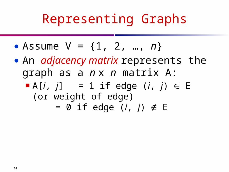
Representing Graphs

● Assume V = {1, 2, …, n}● An adjacency matrix represents the graph as a

n x n matrix A:■ A[i, j] = 1 if edge (i, j) E (or weight of

edge)= 0 if edge (i, j) E

64

Graphs: Adjacency Matrix

● Example:

1

2 4

3

a

d

b c

A 1 2 3 4

1

2

3 ??4

64


● Example:

1

2 4

3

a

d

b c

A 1 2 3 4

1 0 1 1 0

2 0 0 1 0

3 0 0 0 0

4 0 0 1 0

64


● How much storage does the adjacency matrix require?

● A: O(V2)● What is the minimum amount of storage

needed by an adjacency matrix representation of an undirected graph with 4 vertices?

● A: 6 bits■ Undirected graph matrix is symmetric■ No self-loops don’t need diagonal

64

Graphs: Adjacency List

● Adjacency list: for each vertex v V, store a list of vertices adjacent to v

● Example:■ Adj[1] = {2,3}■ Adj[2] = {3}■ Adj[3] = {}■ Adj[4] = {3}

● Variation: can also keep a list of edges coming into vertex

1

2 4

3

64

Graphs: Adjacency List

● How much storage is required?■ The degree of a vertex v = # incident edges

○ Directed graphs have in-degree, out-degree

■ For directed graphs, # of items in adjacency lists is out-degree(v) = |E|For undirected graphs, # items in adj lists is

degree(v) = 2 |E| (handshaking lemma)

64

Graph Searching

● Given: a graph G = (V, E), directed or undirected

● Goal: methodically explore every vertex and every edge

● Ultimately: build a tree on the graph■ Pick a vertex as the root■ Choose certain edges to produce a tree■ Note: might also build a forest if graph is not

connected

64

Breadth-First Search

● “Explore” a graph, turning it into a tree■ One vertex at a time■ Expand frontier of explored vertices across the

breadth of the frontier

● Builds a tree over the graph■ Pick a source vertex to be the root■ Find (“discover”) its children, then their children,

etc.

64


● Again will associate vertex “colors” to guide the algorithm■ White vertices have not been discovered

○ All vertices start out white

■ Grey vertices are discovered but not fully explored○ They may be adjacent to white vertices

■ Black vertices are discovered and fully explored○ They are adjacent only to black and gray vertices

● Explore vertices by scanning adjacency list of grey vertices

64


BFS(G, s) { initialize vertices; Q = {s}; // Q is a queue (duh); initialize to

s while (Q not empty) { u = RemoveTop(Q); for each v u->adj { if (v->color == WHITE) v->color = GREY; v->d = u->d + 1; v->p = u; Enqueue(Q, v); } u->color = BLACK; }}

v->p is the parent v->d is the discovered

64

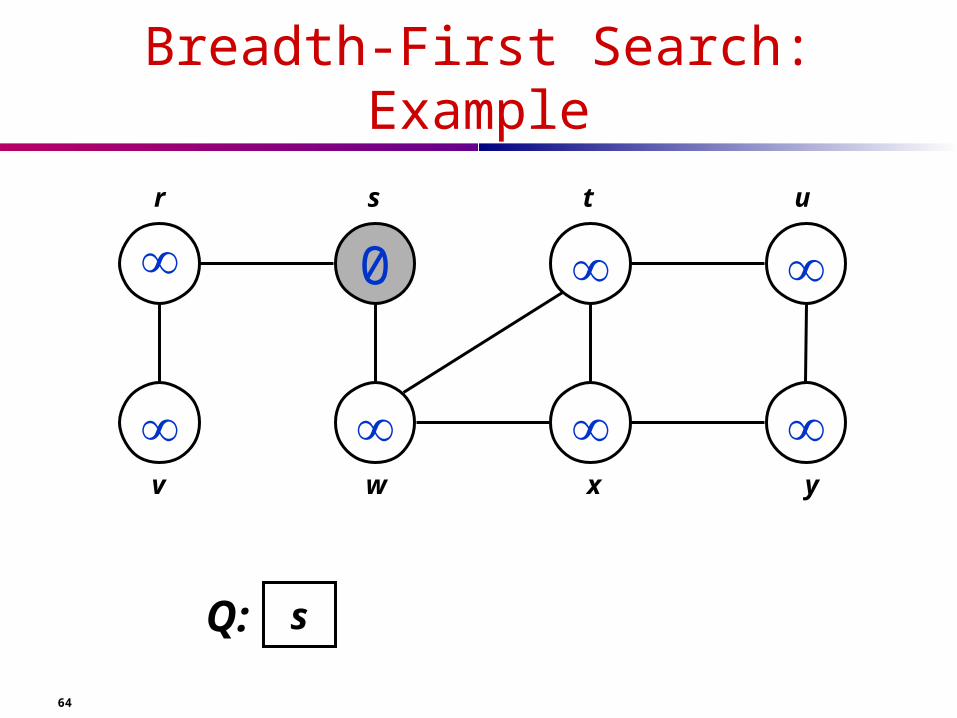
Breadth-First Search: Example

r s t u

v w x y

64


0

r s t u

v w x y

sQ:

64


1

0

1

r s t u

v w x y

wQ: r

64


1

0

1

2

2

r s t u

v w x y

rQ: t x

64


1

2

0

1

2

2

r s t u

v w x y

Q: t x v

64


1

2

0

1

2

2

3

r s t u

v w x y

Q: x v u

64


1

2

0

1

2

2

3

3

r s t u

v w x y

Q: v u y

64


1

2

0

1

2

2

3

3

r s t u

v w x y

Q: u y

64


1

2

0

1

2

2

3

3

r s t u

v w x y

Q: y

64


1

2

0

1

2

2

3

3

r s t u

v w x y

Q: Ø

64

BFS: The Code Again

BFS(G, s) { initialize vertices; Q = {s}; while (Q not empty) { u = RemoveTop(Q); for each v u->adj { if (v->color == WHITE) v->color = GREY; v->d = u->d + 1; v->p = u; Enqueue(Q, v); } u->color = BLACK; }}

What will be the running time?

Touch every vertex: O(V)

u = every vertex, but only once : O(V)

So v = every vertex that appears in some other vert’s adjacency list: O(E)

Total running time: O(2V+E)

64

Breadth-First Search: Properties

● BFS calculates the shortest-path distance to the source node■ Shortest-path distance (s,v) = minimum number

of edges from s to v.

● BFS builds breadth-first tree, in which paths to root represent shortest paths in G■ Thus can use BFS to calculate shortest path from

one vertex to another in O(2V+E) time

64

Depth-First Search

● Depth-first search is another strategy for exploring a graph■ Explore “deeper” in the graph whenever possible■ Edges are explored out of the most recently

discovered vertex v that still has unexplored edges■ When all of v’s edges have been explored,

backtrack to the vertex from which v was discovered

64

Depth-First Search

● Vertices initially colored white● Then colored gray when discovered● Then black when finished

64

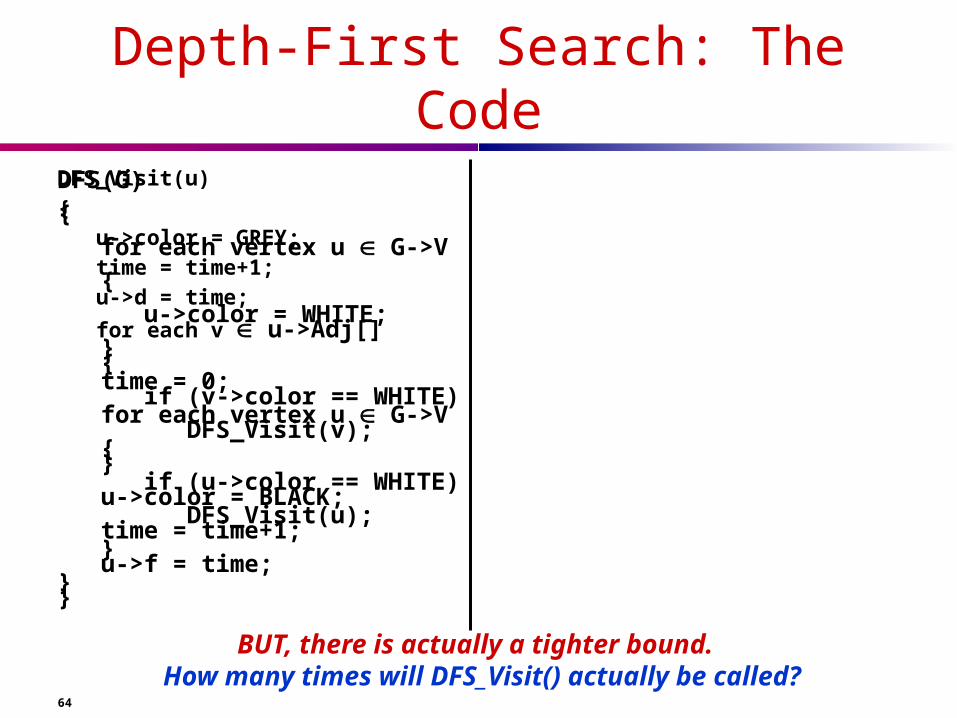
Depth-First Search: The Code

DFS(G){ for each vertex u G->V { u->color = WHITE; } time = 0; for each vertex u G->V { if (u->color == WHITE) DFS_Visit(u); }}

DFS_Visit(u){ u->color = GREY; time = time+1; u->d = time;

for each v u->Adj[] { if (v->color == WHITE) DFS_Visit(v); } u->color = BLACK; time = time+1; u->f = time;}

u->d : discovered , u -> f : finished

64





Running time: O(n2) because call DFS_Visit on each vertex, and the loop over Adj[] can run as many as |V| times

64





BUT, there is actually a tighter bound. How many times will DFS_Visit() actually be called?

64





So, running time of DFS = O(V+E)

64

Depth-First Sort Analysis

● This running time argument is an example of amortized analysis■ “Charge” the exploration of edge to the edge:

○ Each loop in DFS_Visit can be attributed to an edge in the graph

○ Runs once/edge if directed graph, twice if undirected○ Thus loop will run in O(E) time, algorithm O(V+E)

64

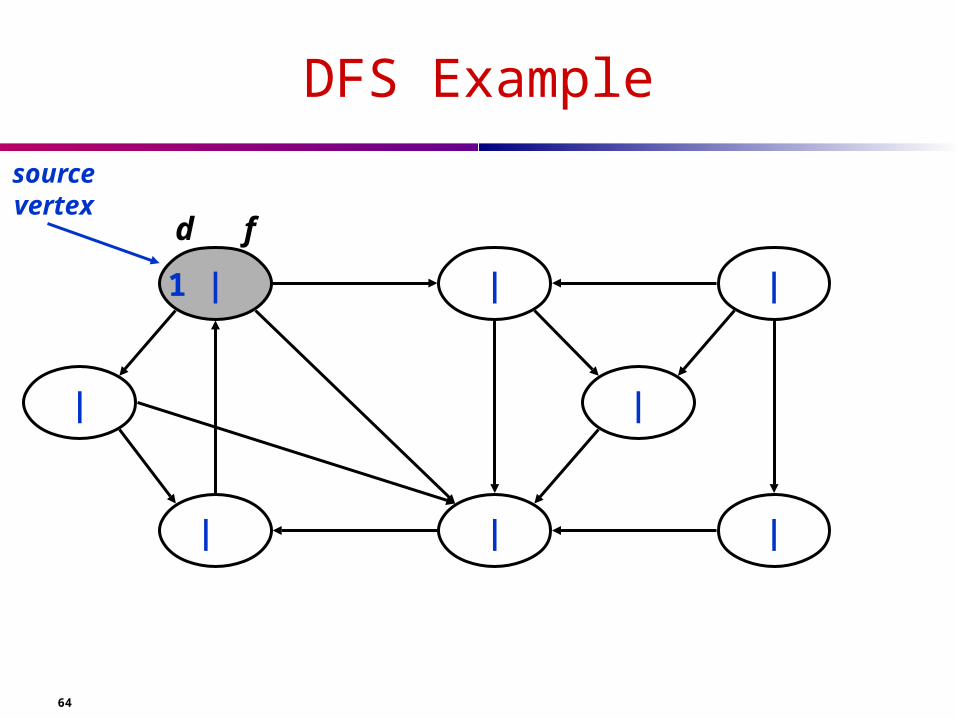
DFS Example

sourcevertex

64

DFS Example

1 | | |

| | |

| |

sourcevertex

d f

64

DFS Example

1 | | |

| | |

2 | |

sourcevertex

d f

64

DFS Example

1 | | |

| | 3 |

2 | |

sourcevertex

d f

64

DFS Example

1 | | |

| | 3 | 4

2 | |

sourcevertex

d f

64

DFS Example

1 | | |

| 5 | 3 | 4

2 | |

sourcevertex

d f

64

DFS Example

1 | | |

| 5 | 63 | 4

2 | |

sourcevertex

d f

64

DFS Example

1 | 8 | |

| 5 | 63 | 4

2 | 7 |

sourcevertex

d f

64

DFS Example

1 | 8 | |

| 5 | 63 | 4

2 | 7 |

sourcevertex

d f

64

DFS Example

1 | 8 | |

| 5 | 63 | 4

2 | 7 9 |

sourcevertex

d f

What is the structure of the grey vertices? What do they represent?

64

DFS Example

1 | 8 | |

| 5 | 63 | 4

2 | 7 9 |10

sourcevertex

d f

64

DFS Example

1 | 8 |11 |

| 5 | 63 | 4

2 | 7 9 |10

sourcevertex

d f

64

DFS Example

1 |12 8 |11 |

| 5 | 63 | 4

2 | 7 9 |10

sourcevertex

d f

64

DFS Example

1 |12 8 |11 13|

| 5 | 63 | 4

2 | 7 9 |10

sourcevertex

d f

64

DFS Example

1 |12 8 |11 13|

14| 5 | 63 | 4

2 | 7 9 |10

sourcevertex

d f

64

DFS Example

1 |12 8 |11 13|

14|155 | 63 | 4

2 | 7 9 |10

sourcevertex

d f

64

DFS Example

1 |12 8 |11 13|16

14|155 | 63 | 4

2 | 7 9 |10

sourcevertex

d f

64

DFS: Kinds of edges

● DFS introduces an important distinction among edges in the original graph:■ Tree edge: encounter new (white) vertex ■ Back edge: from descendent to ancestor■ Forward edge: from ancestor to descendent■ Cross edge: between a tree or subtrees

○ From a grey node to a black node

64

DFS Example

1 |12 8 |11 13|16

14|155 | 63 | 4

2 | 7 9 |10

sourcevertex

d f

Tree edges Back edges Forward edges Cross edges

64

DFS And Graph Cycles

● An undirected graph is acyclic iff a DFS yields no back edges■ If acyclic, no back edges (because a back edge

implies a cycle■ If no back edges, acyclic

○ No back edges implies only tree edges○ Only tree edges implies we have a tree or a forest○ Which by definition is acyclic

● Thus, can run DFS to find whether a graph has a cycle

64

DFS

● What will be the running time?DFS(G){ for each vertex u G->V { u->color = WHITE; } time = 0; for each vertex u G->V { if (u->color == WHITE) DFS_Visit(u); }}



64

DFS And Cycles

● What will be the running time?● O(V+E)● We can actually determine if cycles exist in

O(V) time:■ In an undirected acyclic forest, |E| |V| ■ So count the edges: if ever see |V| distinct edges,

must have seen a back edge along the way

Algorithms analysis and design

Documents