Algorithmics 12 Search - utcourses.cs.ut.ee/.../uploads/Main/Algorithmics_12_Search.pdf · Search • for what? – the solution – the best possible (approximate?) solution •

Advanced Algorithmics (4AP)Search

Jaak ViloJaak Vilo

2009 Spring

1MTAT.03.190 Text Algorithms Jaak Vilo

SearchSearch

• for what?– the solution

– the best possible (approximate?) solution

f h ?• from where? – search space (all valid solutions or paths)

• under which conditions?compute time space– compute time, space, …

– constraints, …

Objective functionObjective function

• An optimal solution– what is the measure that we optimise?p

• Any solution (satisfiability /SAT/ problem)– does the task have a solution?

– is there a solution with objective measure better than X?

• Minimal/maximal cost solution

• A winning move in a game

• A (feasible) solution with smallest nr of constraintviolations (e.g. course time scheduling)

Search spaceSearch space

• Linear (list, binary search, …)

• Trees, Graphs

• Real nr in [x y)Real nr in [x,y) – Integers

• A point in high‐dimensional space

ConstraintsConstraints

• Time, space…– if optimal cannot be found, approximatep , pp

All ki d f d h t i ti• All kinds of secondary characteristics

• Constraintssometimes finding even a point in the valid search– sometimes finding even a point in the valid searchspace is hard

OutlineOutline

B fi h• Best‐first search• Greedy best‐first search• A* search• Heuristics• Local search algorithms• Hill‐climbing searchc b g sea c• Simulated annealing search• Local beam searchLocal beam search• Genetic algorithms

Classes of Search TechniquesClasses of Search Techniques

Calculus based techniques Guided random search techniques Enumerative techniques

Search techniques

Direct methods Indirect methods

Calculus-based techniques

Evolutionary algorithms Simulated annealing

Guided random search techniques

Dynamic programming

Enumerative techniques

Finonacci Newton Evolutionary strategies

Parallel Sequential

Genetic algorithms

Centralized Distributed Steady-state Generational

11Wendy WilliamsMetaheuristic Algorithms

Genetic Algorithms: A Tutorial

Local SearchLocal Search

Local search algorithmsLocal search algorithms

I ti i ti bl th th t th l• In many optimization problems, the path to the goal is irrelevant; the goal state itself is the solution

• State space = set of "complete" configurations• Find configuration satisfying constraints e g n‐• Find configuration satisfying constraints, e.g., n‐queens

• In such cases, we can use local search algorithms• keep a single "current" state, try to improve itkeep a single current state, try to improve it

Example: n queensExample: n‐queens

• Put n queens on an n × n board with no two queens on the same row, column, or diagonalq g

• may get stuck…may get stuck…

ProblemsProblems

• Cycles– Memorize; Tabu search;

• How to transfer valleys with bad choicesonly…

Tree/Graph searchTree/Graph search

• order defined by picking a node for expansionorder defined by picking a node for expansion

• BFS, DFS

• Random, Best First, …– Best – an evaluation function

Id l i f i f( ) f h d• Idea: use an evaluation function f(n) for each node– estimate of "desirability"– Expand most desirable unexpanded nodeExpand most desirable unexpanded node

• Implementation:Order the nodes in fringe in decreasing order of desirabilityPriority queue

• Special cases:greedy best first search f(n) h(n) heuristic e g estimate to goal– greedy best‐first search f(n) = h(n) heuristic, e.g. estimate to goal

– A* search

A*A

• f(n) = g(n) + h(n)

– g(n) – path covered so far in graph

h( ) i d di f l– h(n) – estimated distance from n to goal

F

A C20

20 10

A CB

15

D25

Admissible heuristicsAdmissible heuristics

• A heuristic h(n) is admissible if for every node n,

h(n) ≤ h*(n), where h*(n) is the true cost to reach the goal state from n.

• An admissible heuristic never overestimates the cost to reach the goal, i.e., it is optimistic

• Example: hSLD(n) (never overestimates the actual road d ) ( h l d )distance) (SLD – shortest linear distance)

( ) *• Theorem: If h(n) is admissible, A* using TREE-SEARCH is optimal

Optimality of A* (proof)Optimality of A (proof)

b l l h b d d h f• Suppose some suboptimal goal G2 has been generated and is in the fringe. Let n be an unexpanded node in the fringe such that n is on a shortest path to an optimal goal G.

• f(G2) = g(G2) since h(G2) = 0

• g(G2) > g(G) since G2 is suboptimal

• f(G) = g(G) since h(G) = 0

• f(G ) > f(G) from above• f(G2) > f(G) from above

Optimality of A* (proof)Optimality of A (proof)

b l l h b d d h f• Suppose some suboptimal goal G2 has been generated and is in the fringe. Let n be an unexpanded node in the fringe such that n is on a shortest path to an optimal goal G.

• f(G2) = g(G2) since h(G2) = 0

• g(G2) > g(G) since G2 is suboptimal

• f(G) = g(G) since h(G) = 0

• f(G ) > f(G) from above• f(G2) > f(G) from above

• Hence f(G2) > f(n), and A* will never select G2 for expansion

GraphGraph

• A Virtual graph/search space– valid states of Fifteen‐gameg

– Rubik’s cube

1 2 3 4

5 6 7 85 6 7 8

9 10 11 12

13 14 15

SolveSolve

• Which move takes us closer to the solution?

• Estimate the goodness of the stateEstimate the goodness of the state

34 1314

5 6 7 8

9 10 12

1 2

9 10

11

12

15

• How many are misplaced? (7) 34

5 6 7 8

1314

• How far have they beeni l d? S f h i l

1 2

9 10

11

12

15

misplaced? Sum of theoreticalshortest paths to the correct place Search

A* h t d fi l l

space

• A* search towards a final goal

The Traveling Salesperson Problem (TSP)(TSP)

i i i i• TSP – optimization variant:• For a given weighted graph G = (V,E,w), find a g g g p ( ) fHamiltonian cycle in G with minimal weight,

• i e find the shortest round‐trip visiting eachi.e., find the shortest round trip visiting each vertex exactly once.

• TSP decision variant:• TSP – decision variant:• For a given weighted graph G = (V,E,w), decide whether a Hamiltonian cycle with minimal weight ≤ b exists in G.

TSP instance: shortest round trip through 532 US citiesthrough 532 US cities

Search Methods

• Types of search methods:

• systematic←→ local searchsystematic ←→ local search

• deterministic ←→ stochastic

• sequential ←→ parallel

Local Search (LS) Algorithms

• search space S

(SAT: set of all complete truth assignments to propositional variables)

• solution set SS '(SAT: models of given formula)

• neighborhood relation SxSN (SAT: neighboring variable assignments differ in the

truth value of exactly one variable)

• evaluation function g : S → R+

(SAT: number of clauses unsatisfied under given

assignment)

Local Search:Local Search:

• start from initial position

• iteratively move from current position toiteratively move from current position to neighboring position

l i f i f id• use evaluation function for guidance

Two main classes:

• local search on partial solutions

• local search on complete solutions

local search on partial solutions

Local search for partial solutionsLocal search for partial solutions

• Order the variables in some order.

• Span a tree such that at each level a givenSpan a tree such that at each level a given value is assigned a value.

P f d h fi h• Perform a depth‐first search.

• But, use heuristics to guide the search. Choose , gthe best child according to some heuristics. (DFS with node ordering)(DFS with node ordering)

Construction Heuristics for partial solutions

• search space: space of partial solutions

• search steps: extend partial solutions with assignment for the next elementass g e t o t e e t e e e t

• solution elements are often ranked according t d l ti f tito a greedy evaluation function

Nearest Neighbor heuristic for the TSP:TSP:

Nearest neighbor tour through 532 US citiescities

DFSDFS

• Once a solution has been found (with the first dive into the tree) we can continue search the )tree with DFS and backtracking.

• In fact this is what we did with DFBnB• In fact, this is what we did with DFBnB.

• DFBnB with node ordering.

local search on complete solutionscomplete solutions

Iterative Improvement p(Greedy Search):

• initialize search at some point of search space• initialize search at some point of search space

• in each step, move from the current search position to a neighboring position with better evaluation function valueevaluation function value

Iterative Improvement for SAT

i i i li i d l h l• initialization: randomly chosen, complete truth assignment

• neighborhood: variable assignments are neighbors iff they differ in truth value of one g yvariable

• neighborhood size: O(n) where n = number ofneighborhood size: O(n) where n = number of variables

l ti f ti b f l• evaluation function: number of clauses unsatisfied under given assignment

Hill climbingHill climbing

Choose the nieghbor with the largest

improvment as the next state

f lf-value

f-value = evaluation(state

statesstates

while f value(state) > f value(next best(state))while f-value(state) > f-value(next-best(state)) state := next-best(state)

Hill climbingHill climbing

function Hill-Climbing(problem) returns a solution stateg(p )

current Make-Node(Initial-State[problem])( S [p ])loop do

next a highest-valued successor of currentnext a highest valued successor of currentif Value[next] < Value[current] then return currentcurrent nextcurrent next

end

Problems with local searchProblems with local searchTypical problems with local search (with hill climbing in particular)

• getting stuck in local optima• getting stuck in local optima

• being misguided by evaluation/objective function

Stochastic Local SearchStochastic Local Search

• randomize initialization step

• randomize search steps such thatrandomize search steps such that suboptimal/worsening steps are allowed

i d f & b• improved performance & robustness

• typically, degree of randomization controlled yp y, gby noise parameter

Stochastic Local SearchStochastic Local Search

PPros:• for many combinatorial problems more efficient than systematic searchsystematic search

• easy to implement• easy to parallelize• easy to parallelizeCons:• often incomplete (no guarantees for finding existing• often incomplete (no guarantees for finding existing solutions)

• highly stochastic behaviorhighly stochastic behavior• often difficult to analyze theoretically/empirically

Simple SLS methods

• Random Search (Blind Guessing):

• In each step, randomly select one element ofIn each step, randomly select one element of the search space.

(U i f d) R d W lk• (Uninformed) RandomWalk:

• In each step, randomly select one of the p, y fneighbouring positions of the search space and move thereand move there.

Random restart hill climbingRandom restart hill climbing

f-value

f-value = evaluation(state)

states

Randomized Iterative Improvement:

i i i li h i f h h• initialize search at some point of search space search steps:• with probability p, move from current search position to a

randomly selected neighboring positionrandomly selected neighboring position• otherwise, move from current search position to neighboring

position with better evaluation function value.• Has many variations of how to choose the randomly neighbor,

and how many of theml k d ( k• Example: Take 100 steps in one direction (Army mistake

correction) – to escape from local optima.

Search spaceSearch space

• Problem: depending on initial state, can get stuck in local maxima

•

General iterative AlgorithmsGeneral iterative Algorithms

eneral and “eas ” to implement– general and “easy” to implement

– approximation algorithms

–must be told when to stop

hill li bi–hill‐climbing

– convergenceg

spie98‐48

General iterative searchGeneral iterative search

• Algorithm• Algorithm– Initialize parameters and data structures

– construct initial solution(s)

– Repeatp• Repeat

– Generate new solution(s)( )

– Select solution(s)

• Until time to adapt parameters

• Update parameters

– Until time to stop

spie98‐49

p

• End

Iterative searchIterative search

• Most popular algorithms of this class– Genetic Algorithmsg

• Probabilistic algorithm inspired by evolutionary mechanisms

– Simulated Annealing• Probabilistic algorithm inspired by the annealing ofProbabilistic algorithm inspired by the annealing of metals

– Tabu SearchTabu Search• Meta‐heuristic which is a generalization of local search

spie98‐50

Hill climbing searchHill‐climbing search

• Problem: depending on initial state, can get stuck in local maxima

•

Simulated annealing

Combinatorial search technique inspired by the physical process of annealingphysical process of annealing [Kirkpatrick et al. 1983, Cerny 1985]

O tliOutline Select a neighbor at random.

If better than current state go there.

Otherwise, go there with some probability.

Probability goes down with time (similar to

temperature cooling)temperature cooling)

Simulated annealingg

eE/Te

delta = -10 T= 0 1 10 000T 0.1 .. 10,000

Generic choices for annealing schedule

Simulated AnnealingKirkpatrick, S., C. D. Gelatt Jr., M. P. Vecchi, "Optimization by Simulated

Annealing",Science, 220, 4598, 671‐680, 1983.

g

Pseudo codePseudo code

f ti Si l t d A li ( bl h d l ) tfunction Simulated-Annealing(problem, schedule) returns solution state

current Make Node(Initial State[problem])current Make-Node(Initial-State[problem])for t 1 to infinity

T h d l [ ] // T d dT schedule[t] // T goes downwards.if T = 0 then return currentnext Random-Successor(current) E f-Value[next] - f-Value[current]if E > 0 then current nextelse current next with probability eE/T

end

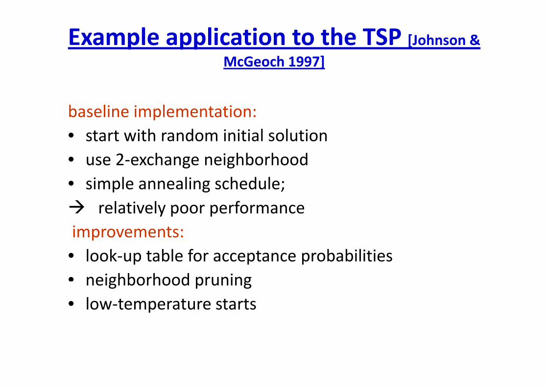
Example application to the TSP [Johnson & McGeoch 1997]McGeoch 1997]

b li i l ibaseline implementation:• start with random initial solution• use 2‐exchange neighborhood• simple annealing schedule; relatively poor performanceimprovements:p o e e s• look‐up table for acceptance probabilities• neighborhood pruningneighborhood pruning• low‐temperature starts

Summary‐Simulated Annealing

Simulated Annealing . . .

• is historically importantis historically important

• is easy to implement

• has interesting theoretical properties (convergence), but these are of very limited ( g ), ypractical relevance

hi d f ft t th t• achieves good performance often at the cost of substantial run‐times

Examples for combinatorial problems:

• finding shortest/cheapest round trips (TSP)

• finding models of propositional formulaefinding models of propositional formulae (SAT)

l i h d li i bli• planning, scheduling, time‐tabling

• resource allocation

• protein structure prediction

• genome sequence assembly

SATSAT

The Propositional Satisfiability Problem (SAT)Problem (SAT)

Tabu SearchTabu Search

C bi i l h h i hi h h il li• Combinatorial search technique which heavily relies on the use of an explicit memory of the search process [Glover 1989 1990] to guide search processprocess [Glover 1989, 1990] to guide search process

• memory typically contains only specific attributes of previously seen solutionspreviously seen solutions

• simple tabu search strategies exploit only short term memorymemory

• more complex tabu search strategies exploit long term memoryterm memory

Tabu search – exploiting short term memorymemory

i h t t b t i hb i l ti• in each step, move to best neighboring solution although it may be worse than current one

• to avoid cycles tabu search tries to avoid revisiting• to avoid cycles, tabu search tries to avoid revisiting previously seen solutions by basing the memory on attributes of recently seen solutions

• tabu list stores attributes of the tlmost recently visited

• solutions; parameter tl is called tabu list length or tabu tenurel ti hi h t i t b tt ib t• solutions which contain tabu attributes are

forbidden

Example: Tabu Search for SAT / MAX‐SATSAT

i hb h d i hi h diff i• Neighborhood: assignments which differ in exactly one variable instantiation

• Tabu attributes: variables• Tabu criterion: flipping a variable is forbiddenTabu criterion: flipping a variable is forbidden for a given number of iterations

• Aspiration criterion: if flipping a tabu variable• Aspiration criterion: if flipping a tabu variable leads to a better solution, the variable’s tabu t t i iddstatus is overridden

[Hansen & Jaumard 1990; Selman & Kautz 1994]

• Bart Selman, Cornellwww‐verimag.imag.fr/~maler/TCC/selman‐tcc.pptg g f / / / pp

Ideas from physics statistics combinatoricsIdeas from physics, statistics, combinatorics, algorithmics …

Fundamental challenge: Combinatorial Search Spacesg p

• Significant progress in the last decade.

• How much?

• For propositional reasoning:• ‐‐We went from 100 variables, 200 clauses (early 90’s)• to 1,000,000 vars. and 5,000,000 constraints in• 10 years. Search space: from 10^30 to 10^300,000.y p ,

• ‐‐ Applications: Hardware and Software Verification,• Test pattern generation Planning Protocol DesignTest pattern generation, Planning, Protocol Design, • Routers, Timetabling, E‐Commerce (combinatorial• auctions), etc.•••

• How can deal with such large combinatorial spaces and• still do a decent job?

• I’ll discuss recent formal insights into• combinatorial search spaces and their• practical implications that makes searching• such ultra‐large spaces possible.

• Brings together ideas from physics of disordered systems • (spin glasses), combinatorics of random structures, and• algorithms• algorithms.

• But first, what is BIG?

What is BIG?

Consider a real-world Boolean Satisfiability (SAT) problem

I.e., ((not x_1) or x_7)((not x_1) or x_6)

etc.

x_1, x_2, x_3, etc. our Boolean variables(set to True or False)

Set x_1 to False ??

10 pages later:p g

I.e., (x_177 or x_169 or x_161 or x_153 …x_33 or x_25 or x_17 or x_9 or x_1 or (not x_185))

…

_ _ _ _ _ ( _ ))

clauses / constraints are getting more interesting…

Note x_1 …

4000 pages later:

…

Finally 15 000 pages later:Finally, 15,000 pages later:

C bi t i l h f t th i t HOW?Combinatorial search space of truth assignments: HOW?

Current SAT solvers solve this instance in approx. 1 minute!

Progress SAT SolversProgress SAT Solvers

Instance Posit' 94

2670 136 40 66

Grasp' 96

1 2

Sato' 98

0 95

Chaff' 01

0 02ssa2670-136 40,66s

bf1355-638 1805,21s

1,2s

0,11s

0,95s

0,04s

0,02s

0,01s

pret150_25 >3000s

d b i 100 3000

0,21s

11 85

0,09s

0 08

0,01s

0 01dubois100 >3000s

aim200-2_0-no-1 >3000s

11,85s

0,01s

0,08s

0s

0,01s

0s

2dlx_..._bug005 >3000s

6288 3000

>3000s

3000

>3000s

3000

2,9s

300073

c6288 >3000s >3000s >3000s >3000sSource: Marques Silva 2002

• From academically interesting to practicallyFrom academically interesting to practically relevant.

• We now have regular SAT solver competitionscompetitions.

• Germany ’89, Dimacs ’93, China ’96, SAT‐02, SAT‐03, SAT‐04, SAT05.

• E.g. at SAT‐2004 (Vancouver, May 04):• ‐‐‐ 35+ solvers submitted

500 i d t i l b h k• ‐‐‐ 500+ industrial benchmarks• ‐‐‐ 50,000+ instances available on the WWW.

•

Real‐World ReasoningTackling inherent computational complexity

DARPA ResearchProgram

Tackling inherent computational complexity

1M5M10301,020

mpl

exity

Multi-AgentSystems

0.5M 1M10150,500

Cas

e co Hardware/Software

Verification

50K1015,050W

orst

Chess

200K600K

Military Logistics

10K 50K

50K 200K

103010Deep space mission control

Chess

No. of atomson earth 1047

Hi h P f R iTechnology Targets

100200

50K

1030 Car repair diagnosis

mission controlSeconds until heat death of sun

Protein foldingcalculation

• High-Performance Reasoning• Temporal/ uncertainty reasoning• Strategic reasoning/Multi-player

75

Variablescalculation (petaflop-year) 100 10K 20K 100K 1M

Rules (Constraints)Example domains cast in propositional reasoning system (variables, rules).

A Journey from Random to Structured InstancesInstances

•• I ‐‐‐ Random InstancesI Random Instances• ‐‐‐ phase transitions and algorithms• ‐‐‐ from physics to computer science

• II ‐‐‐ Capturing Problem Structure• ‐‐‐ problem mixtures (tractable / intractable)

b kd i bl d h il• ‐‐‐ backdoor variables, restarts, and heavy tails

• III ‐‐‐ Beyond Satisfactiony• ‐‐‐ sampling, counting, and probabilities• ‐‐‐ quantification

Genetic Algorithms:Genetic Algorithms:ggA TutorialA Tutorial

“Genetic Algorithms are good at taking large,good at taking large,

potentially huge search spaces and navigating

them looking for optimalthem, looking for optimal combinations of things, solutions you might not

th i fi d iotherwise find in a lifetime.”

S l t M- Salvatore ManganoComputer Design, May 1995



The Genetic AlgorithmThe Genetic Algorithm Directed search algorithms based on

the mechanics of biological evolutiong Developed by John Holland, University

of Michigan (1970’s)of Michigan (1970 s) To understand the adaptive processes of

natural systems To design artificial systems software that

retains the robustness of natural systems



The Genetic Algorithm (cont )The Genetic Algorithm (cont.) Provide efficient, effective techniques

for optimization and machine learning p gapplicationsWidely used today in business Widely-used today in business, scientific and engineering circles



Components of a GAComponents of a GAA problem to solve, and ... Encoding technique (gene chromosome) Encoding technique (gene, chromosome)

Initialization procedure (creation)

Evaluation function (environment)

Selection of parents (reproduction) Selection of parents (reproduction)

Genetic operators (mutation, recombination)

Parameter settings (practice and art)



Simple Genetic AlgorithmSimple Genetic Algorithm{{

initialize population;evaluate population;evaluate population;while TerminationCriteriaNotSatisfied{{

select parents for reproduction;perform recombination and mutation;evaluate population;p p

}}



The GA Cycle of ReproductionThe GA Cycle of Reproduction

reproduction modificationchildren

parentsmodifiedchildren

population evaluation

d l t devaluated children

deleted members

discard



Genetic algorithmsGenetic algorithms

• How to generate the next generation.

• 1) Selection: we select a number of states1) Selection: we select a number of states from the current generation. (we can use the fitness function in any reasonable way)fitness function in any reasonable way)

• 2) crossover : select 2 states and reproduce a child.

• 3) mutation: change some of the genues• 3) mutation: change some of the genues.

ExampleExample

8 queen example8‐queen example

Summary: Genetic AlgorithmsSummary: Genetic Algorithms

i l i hGenetic Algorithms• use populations, which leads to increased p psearch space exploration

• allow for a large number of differentallow for a large number of different implementation choices

• typically reach best performance when using• typically reach best performance when using operators that are based on problem h t i ticharacteristics

• achieve good performance on a wide range of problems

Classes of Search TechniquesClasses of Search Techniques

Calculus based techniques Guided random search techniques Enumerative techniques

Search techniques

Direct methods Indirect methods

Calculus-based techniques

Evolutionary algorithms Simulated annealing

Guided random search techniques

Dynamic programming

Enumerative techniques

Finonacci Newton Evolutionary strategies

Parallel Sequential

Genetic algorithms

Centralized Distributed Steady-state Generational



The GA Cycle of ReproductionThe GA Cycle of Reproduction

reproduction modificationchildren

parentsmodifiedchildren

population evaluation

d l t devaluated children

deleted members

discard



PopulationPopulationl tipopulation

Chromosomes could be: Bit strings (0101 ... 1100) Real numbers (43.2 -33.1 ... 0.0 89.2) Permutations of element (E11 E3 E7 ... E1 E15)( ) Lists of rules (R1 R2 R3 ... R22 R23) Program elements (genetic programming)g (g p g g) ... any data structure ...



ReproductionReproductionhild

reproductionchildren

population

parents

population

P t l t d t d ithParents are selected at random with selection chances biased in relation to chromosome evaluations.



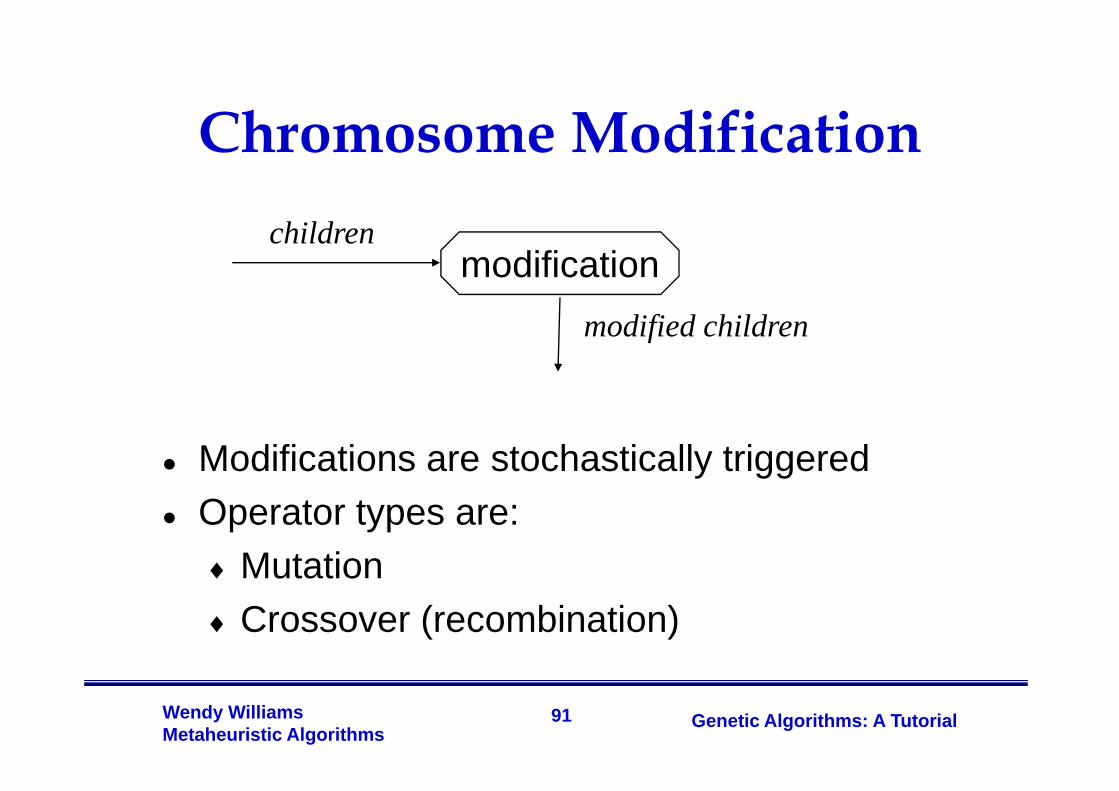
Chromosome ModificationChromosome Modification

modificationchildren

modified children

Modifications are stochastically triggered Operator types are:

Mutation Mutation Crossover (recombination)



Mutation: Local ModificationMutation: Local ModificationBefore: (1 0 1 1 0 1 1 0)Before: (1 0 1 1 0 1 1 0)

After: (0 1 1 0 0 1 1 0)

Before: (1 38 -69 4 326 44 0 1)Before: (1.38 69.4 326.44 0.1)

After: (1.38 -67.5 326.44 0.1)

Causes movement in the search space(local or global)

Restores lost information to the population



Crossover: RecombinationCrossover: Recombination*

P1 (0 1 1 0 1 0 0 0) (0 1 0 0 1 0 0 0) C1

P2 (1 1 0 1 1 0 1 0) (1 1 1 1 1 0 1 0) C2( ) ( )

Crossover is a critical feature of geneticalgorithms:

It greatly accelerates search early in g y yevolution of a population

It leads to effective combination of It leads to effective combination of schemata (subsolutions on different chromosomes)



chromosomes)

EvaluationEvaluation

evaluatedmodifiedchildren

evaluationchildren

Th l t d d h d The evaluator decodes a chromosome and assigns it a fitness measure

The evaluator is the only link between a classical GA and the problem it is solving



DeletionDeletionl ipopulation

discarded members

discard

discarded members

Generational GA: Generational GA:entire populations replaced with each iterationiteration

Steady-state GA:a few members replaced each generation



a few members replaced each generation

An Abstract ExampleAn Abstract Example

Distribution of Individuals in Generation 0f

Distribution of Individuals in Generation N



A Simple ExampleA Simple Example

“The Gene is by far the most sophisticated program around.”

- Bill Gates, Business Week, June 27, 1994



A Simple ExampleA Simple Example

The Traveling Salesman Problem:The Traveling Salesman Problem:

Find a tour of a given set of cities so thatFind a tour of a given set of cities so that each city is visited only once the total distance traveled is minimized



RepresentationRepresentationRepresentation is an ordered list of citynumbers known as an order-based GAnumbers known as an order based GA.

1) London 3) Dunedin 5) Beijing 7) Tokyo) ) ) j g ) y2) Venice 4) Singapore 6) Phoenix 8) Victoria

CityList1 (3 5 7 2 1 6 4 8)CityList2 (2 5 7 6 8 1 3 4)



CrossoverCrossoverCrossover combines inversion andrecombination:

* *Parent1 (3 5 7 2 1 6 4 8)Parent1 (3 5 7 2 1 6 4 8)Parent2 (2 5 7 6 8 1 3 4)

Child (5 8 7 2 1 6 3 4)

This operator is called the Order1 crossover.



MutationMutationMutation involves reordering of the list:

* *B f (5 8 7 2 1 6 3 4)Before: (5 8 7 2 1 6 3 4)

After: (5 8 6 2 1 7 3 4)



TSP Example: 30 CitiesTSP Example: 30 Cities

120

80

100

40

60y

0

20

00 10 20 30 40 50 60 70 80 90 100

x



Solution (Distance = 941)Solution i (Distance = 941)TSP30 (Performance = 941)

100

120

TSP30 (Performance = 941)

80

100

40

60y

0

20

0 10 20 30 40 50 60 70 80 90 100x



Solution (Distance = 800)Solution j(Distance = 800)4462 TSP30(Performance = 800)6269677864 100

120


6462544250

80

100

5040403821

40

60y

2135676060 0

20

40425099

0 10 20 30 40 50 60 70 80 90 100x



Solution (Distance = 652)Solution k(Distance = 652)TSP30 (Performance = 652)

100

120


80

100

40

60y

0

20

00 10 20 30 40 50 60 70 80 90 100

x



Best Solution (Distance = 420)Best Solution (Distance = 420)4238 TSP30Solution (Performance = 420)3835262135 100

120

TSP30 Solution (Performance = 420)

35327

3846

80

100

4644586069

40

60y

6976787169 0

20

67628494

0 10 20 30 40 50 60 70 80 90 100x



Overview of PerformanceOverview of PerformanceT S P 30 - O verview o f P erfo rm an ce

1600

1800

T S P 30 - O verview o f P erfo rm an ce

1000

1200

1400

nce

400

600

800Distan

0

200

1 3 5 7 9 11 13 15 17 19 21 23 25 27 29 31B e st

W tG en erat io n s (1000)

W o rst

A ve ra g e



Considering the GA TechnologyConsidering the GA Technology“Almost eight years ago ... lmost eight yea s ago ...people at Microsoft wrote

a program [that] uses some genetic things for

finding short code sequences Windows 2 0sequences. Windows 2.0

and 3.2, NT, and almost all Microsoft applications f ppproducts have shipped

with pieces of code created by that system.”

- Nathan Myhrvold, Microsoft Advanced Technology Group, Wired, September 1995



Technology Group, Wired, September 1995

Issues for GA PractitionersIssues for GA Practitioners Choosing basic implementation issues:

representation population size, mutation rate, ... selection, deletion policies crossover, mutation operators

Termination Criteria Performance, scalability

Solution is only as good as the evaluation Solution is only as good as the evaluation function (often hardest part)



Benefits of Genetic AlgorithmsBenefits of Genetic Algorithms Concept is easy to understand Modular separate from application Modular, separate from application Supports multi-objective optimization Good for “noisy” environments Always an answer; answer gets better Always an answer; answer gets better

with time Inherently parallel; easily distributed



B fit f G ti Al ith ( t )Benefits of Genetic Algorithms (cont.)

Many ways to speed up and improve a GA-based application as knowledge pp gabout problem domain is gainedEasy to exploit previous or alternate Easy to exploit previous or alternate solutions

Flexible building blocks for hybrid applicationsapplications

Substantial history and range of use



When to Use a GAWhen to Use a GA Alternate solutions are too slow or overly

complicated Need an exploratory tool to examine new

approaches Problem is similar to one that has already been

successfully solved by using a GA Want to hybridize with an existing solution Benefits of the GA technology meet key problem

requirements



Some GA Application TypesSome GA Application TypesDomain Application TypesControl gas pipeline, pole balancing, missile evasion, pursuit

Design semiconductor layout, aircraft design, keyboardDesign semiconductor layout, aircraft design, keyboardconfiguration, communication networks

Scheduling manufacturing, facility scheduling, resource allocation

Robotics trajectory planning

Machine Learning designing neural networks, improving classificationalgorithms classifier systemsalgorithms, classifier systems

Signal Processing filter design

Game Playing poker, checkers, prisoner’s dilemmaGame Playing p , , p

CombinatorialOptimization

set covering, travelling salesman, routing, bin packing,graph colouring and partitioning



p

ConclusionsConclusions

Question: ‘If GAs are so smart, why ain’t they rich?’

Answer: ‘Genetic algorithms are rich - rich in application across a large and growing number of disciplines.’- David E. Goldberg, Genetic Algorithms in Search, Optimization and Machine Learning



Algorithmics 12 Search - utcourses.cs.ut.ee/.../uploads/Main/Algorithmics_12_Search.pdf · Search • for what? – the solution – the best possible (approximate?) solution •

Documents