Algorithmic Trading in CDS and Equity Indices Using Machine Learning and Statistical Arbitrage Lund Institute of Technology Tobias Ek, Melker Samuelsson 2017-05-20

Welcome message from author
This document is posted to help you gain knowledge. Please leave a comment to let me know what you think about it! Share it to your friends and learn new things together.
Transcript

Algorithmic Trading in CDS and Equity Indices Using
Machine Learning and Statistical Arbitrage
Lund Institute of Technology
Tobias Ek, Melker Samuelsson
2017-05-20

Abstract
Historical data shows a strong relationship between hourly changes in CDS index iTraxx
Main and equity futures EURO STOXX 50. We hypothesize that the relatively stable
relationship should allow us to trade the two markets. A Markov regime switching model
is introduced, distinguishing cointegrated regimes that allows the cointegration relation-
ship to be switched on and off. A pairs trade between the two securities is carried out in
the cointegrated regimes. We show that trading exclusively in these regimes produces a
significantly better performance compared to static pairs trading over the whole data set.
Keywords: Algorithmic Trading, CDS indices, Equity futures, Markov Regime Switch-
ing Models, Cointegration

Acknowledgements
Firstly, we would like to express our sincere gratitude to our supervisors, Prof. Erik Lind-
strom at the Centre for Mathematical Sciences at Lund University and Senior Portfolio
Manager Dr. Ulf Erlandsson at AP4 for their continuous support of this thesis sharing
their immense knowledge.
Besides our supervisors, we would also like to thank the rest of the employees at AP4,
who provided insight and expertise that greatly assisted the research, especially Ludvig
Vikstrom and Victor Tingstrom for sharing lots of programming advice.
Contents
1 Introduction 31.1 A brief history of the CDS market . . . . . . . . . . . . . . . . . . . . . 31.2 CDS Indices . . . . . . . . . . . . . . . . . . . . . . . . . . . . . . . . . . 41.3 Credit Default Swaps . . . . . . . . . . . . . . . . . . . . . . . . . . . . . 5
1.3.1 Defintion . . . . . . . . . . . . . . . . . . . . . . . . . . . . . . . 51.3.2 Pricing of CDS Contracts . . . . . . . . . . . . . . . . . . . . . . 6
1.4 Equity market contracts . . . . . . . . . . . . . . . . . . . . . . . . . . . 111.4.1 Equities and Equity indices . . . . . . . . . . . . . . . . . . . . . 111.4.2 EURO STOXX 50 . . . . . . . . . . . . . . . . . . . . . . . . . . 11
1.5 Our Contribution . . . . . . . . . . . . . . . . . . . . . . . . . . . . . . . 121.6 Outline of the thesis . . . . . . . . . . . . . . . . . . . . . . . . . . . . . 12
2 Theory 132.1 Linear Regression . . . . . . . . . . . . . . . . . . . . . . . . . . . . . . . 13
2.1.1 OLS Assumptions . . . . . . . . . . . . . . . . . . . . . . . . . . 142.2 Robust Regression . . . . . . . . . . . . . . . . . . . . . . . . . . . . . . 14
2.2.1 Bisquare weight function . . . . . . . . . . . . . . . . . . . . . . . 142.3 Markov Chains . . . . . . . . . . . . . . . . . . . . . . . . . . . . . . . . 152.4 Time series models . . . . . . . . . . . . . . . . . . . . . . . . . . . . . . 15
2.4.1 Stationarity . . . . . . . . . . . . . . . . . . . . . . . . . . . . . . 152.4.2 Order of integration . . . . . . . . . . . . . . . . . . . . . . . . . 162.4.3 Model evaluation . . . . . . . . . . . . . . . . . . . . . . . . . . . 16
2.5 Dickey-Fuller tests . . . . . . . . . . . . . . . . . . . . . . . . . . . . . . 172.5.1 Cointegration of financial time series . . . . . . . . . . . . . . . . 19
2.6 Markov Regime Switching Models . . . . . . . . . . . . . . . . . . . . . 202.6.1 A Simple Example . . . . . . . . . . . . . . . . . . . . . . . . . . 212.6.2 Hidden Markov Models . . . . . . . . . . . . . . . . . . . . . . . 212.6.3 Distinguish Regimes of Cointegration . . . . . . . . . . . . . . . 222.6.4 Implementation of the Markov Regime Switching Model . . . . . 23
2.7 Trading Strategies on Regime Shifts . . . . . . . . . . . . . . . . . . . . 262.7.1 Algorithmic Trading . . . . . . . . . . . . . . . . . . . . . . . . . 262.7.2 Pairs trading . . . . . . . . . . . . . . . . . . . . . . . . . . . . . 262.7.3 The trading setup . . . . . . . . . . . . . . . . . . . . . . . . . . 27
3 Data 293.1 The data sets . . . . . . . . . . . . . . . . . . . . . . . . . . . . . . . . . 293.2 Properties of the CDS data . . . . . . . . . . . . . . . . . . . . . . . . . 30
3.2.1 Price recording of OTC CDS prices . . . . . . . . . . . . . . . . . 30
1
3.2.2 Rolling of CDS series . . . . . . . . . . . . . . . . . . . . . . . . . 303.3 Properties of the EURO STOXX data . . . . . . . . . . . . . . . . . . . 31
3.3.1 Rolling of EURO STOXX series . . . . . . . . . . . . . . . . . . 313.4 Order of integration . . . . . . . . . . . . . . . . . . . . . . . . . . . . . 31
3.4.1 Heavy tails and leptokurtosis of return data . . . . . . . . . . . . 323.5 Regression analysis of the the data . . . . . . . . . . . . . . . . . . . . . 33
3.5.1 Optimal memory length for regression parameters . . . . . . . . 333.5.2 Stability to outliers . . . . . . . . . . . . . . . . . . . . . . . . . . 34
3.6 Residual analysis of the data . . . . . . . . . . . . . . . . . . . . . . . . 35
4 Results 374.1 The Regime Switching Model . . . . . . . . . . . . . . . . . . . . . . . . 37
4.1.1 200 hour Regression Window . . . . . . . . . . . . . . . . . . . . 374.1.2 400 hour Regression Window . . . . . . . . . . . . . . . . . . . . 394.1.3 Transition Probabilities . . . . . . . . . . . . . . . . . . . . . . . 404.1.4 Model Parameters . . . . . . . . . . . . . . . . . . . . . . . . . . 404.1.5 Model Evaluation . . . . . . . . . . . . . . . . . . . . . . . . . . . 41
4.2 Comparison with naive pairs trading strategy . . . . . . . . . . . . . . . 414.3 The Trading Strategies . . . . . . . . . . . . . . . . . . . . . . . . . . . . 42
5 Conclusions 455.1 Establishing efficient memory length . . . . . . . . . . . . . . . . . . . . 455.2 Considering transaction costs . . . . . . . . . . . . . . . . . . . . . . . . 465.3 Further Research Areas . . . . . . . . . . . . . . . . . . . . . . . . . . . 46
2

Chapter 1
Introduction
This thesis explores the relationship between the european CDS index iTraxx Main
and European equity futures index EURO STOXX 50. The idea to the thesis was
given to us by Senior Portfolio Manager Ulf Erlandsson at the Fourth National Swedish
Pension Fund (AP4). It is well known that these indices are correlated in some way
enabling a cross asset pairs trade. To further strengthen this statement, we formulated a
hypothesis that the correlated indices experience regimes of cointegration. We introduce
a regime switching Markov model distinguishing cointegrated regimes and allows the
cointegration relationship to be switched on and off, which builds the base of the decision
making process of when to enable the pairs trade.
1.1 A brief history of the CDS market
In the early summer of 1994 a team of about 80 bankers from JP Morgan assembled
for a ”weekend offsite” at the posh holiday resort of Boca Raton, just off the Florida
coastline [Lanchester, 2009]. The get-away was designed to let the derivatives and swaps
people at JP get together to blow off some steam and to come up with new interesting
business opportunities for the bank. There, squeezed into a conference room just by
the the Boca Raton marina, someone came up with the idea of mixing derivatives with
traditional credit risk.
A few months later, Robert Reoch, a young British banker at JP Morgan’s London
branch brokered a ”first-to-default” swap, which is a basket-like product based on a
3
credit default swap (CDS), to an investor [Tett, 2006]. The contract ensured JP Mor-
gan was covered against credit losses if anyone of a number of European government
bonds would default. This innovative way to manage credit exposure would open the
gates to the novel world of credit derivatives.
1.2 CDS Indices
As the scope of credit markets and trading in credit derivatives became profitable busi-
ness, other banks were quick to open their own operations and embark on this new area
of financial innovation. As the market increased, a natural demand to track performance
on these products emerged and soon indices on CDS’s began to surface. Some of the
first synthetic credit indices that appeared was in 2001 when JPMorgan launched the
JECI and Hydi credit indices, as well as rival Morgan Stanley’s presenting its TRAC-
ERS counterpart [markit, 2008].
In 2003 JP and Morgan Stanley joined their respective indices to create the Trac-x.
However, only a year later in 2004 the Trac-x was again merged with the newly created
iBoxx, in order to form two new synthetic credit indices. These were CDX for the North
American credit market and iTraxx for Europe and Asia. These indices are still to this
day the most closely followed references for credit traders and investors.
Following its early years, the CDS market grew exponentially. From totalling around
$300 billion in 1998, with JP Morgan representing one sixth of total global volume, to
over $2 trillion by 2002 (with the market share of any one player fully eroded) [Gillian,
2009]. The overly exuberant CDS-market inflows continued until 2007 when notional
volumes peaked at $62.2 trillion [ISDA, 2010].
Credit Default Swaps then come to play a major role in the credit crisis of 2008, which
led to heavy scrutiny of these markets with new regulation and requirements coming into
effect. Since its peak level the CDS market today stands at just over $10 trillion [ISDA,
2017b]. Moreover the fraction of these contracts being cleared centrally have gone from
about one tenth only three years ago to over 75% of CDS contracts being centrally
cleared as of 2016 [ISDA, 2017a].
4
The creation of official CDS indices led to trading in contracts on CDX and iTraxx
to begin. Since then many sub indices such as iTraxx Europe Senior Financials, iTraxx
Asia ex-Japan High Volatility and CDX have also been added to the offering.
1.3 Credit Default Swaps
The purpose of a credit default swap is to let credit risk be valued and traded in a similar
manner to other forms of financial risk [Hull and White, 2000]. In 1998 the International
Swaps and Derivatives Association (ISDA) published standardised documentation for
credit default swaps in order to facilitate trading and liquidity for these contracts.
1.3.1 Defintion
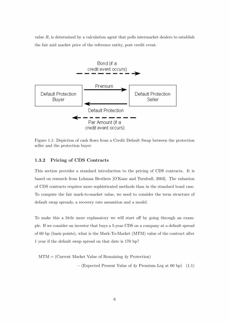
A Credit Default Swap (CDS) is a financial contract whereby the buyer (premium leg)
buys protection in case of a credit event on the underlying credit asset (reference en-
tity). The CDS contract more specifically allows the premium leg to sell the defaulted
entity for its par value. Hereafter, we will make this equivalent to receiving (100−R)%
(recovery) on the defaulted asset, where 100 denotes the par value and recovery is the
residual value of the defaulted asset.
In exchange for this insurance the protection buyer compensates the protection seller
by paying periodic coupons until maturity of the CDS or until the refereance entity
experience a credit event (as determined by an ISDA Credit Derivatives Determina-
tions Committee) [ISDA, 2016]. Membership in a Determinations Committee (DCs)
includes both sell- and buy-side representatives. In order to declare a credit event a
super-majority of 80% of the committee is required to vote for the occurrence of a credit
event.
In case a credit event is determined to have occurred, the CDS contract can be set-
tled either in cash or by physical delivery. If the contract specify physical delivery the
premium leg transfers the defaulted paper and in exchange receive par notional amount.
If the contract is cash settled the protection seller pays the protection buyer par minus
recovery value (100−R)%, without any exchange of the reference entity. The recovery
5
value R, is determined by a calculation agent that polls intermarket dealers to establish
the fair mid market price of the reference entity, post credit event.
Figure 1.1: Depiction of cash flows from a Credit Default Swap between the protectionseller and the protection buyer
1.3.2 Pricing of CDS Contracts
This section provides a standard introduction to the pricing of CDS contracts. It is
based on research from Lehman Brothers [O’Kane and Turnbull, 2003]. The valuation
of CDS contracts requires more sophisticated methods than in the standard bond case.
To compute the fair mark-to-market value, we need to consider the term structure of
default swap spreads, a recovery rate assumtion and a model.
To make this a little more explanatory we will start off by going through an exam-
ple. If we consider an investor that buys a 5-year CDS on a company at a default spread
of 60 bp (basis points), what is the Mark-To-Market (MTM) value of the contract after
1 year if the default swap spread on that date is 170 bp?
MTM = (Current Market Value of Remaining 4y Protection)
− (Expected Present Value of 4y Premium Leg at 60 bp) (1.1)
6
Since the value of the CDS increased and the market value of a new default swap is
zero, we have that
(Current Market Value of Remaining 4y Protection) =
(Expected Present Value of 4y Premium Leg at 170 bp) (1.2)
Hence, the MTM for the protection buyer is
MTM = (Expected Present Value of 4y Premium Leg at 170 bp)
− (Expected Present Value of 4y Premium Leg at 60 bp) (1.3)
For simplicity we define the expected present value of 1 bp on the premium leg until
maturity (or default) as Risky PV01 we can simplify the expression as
MTM(tv, tN ) = ±(S(tv, tn)− S(t0, tN ))RPV 01(tv, tN ) (1.4)
Where t0 is the time of the initial trade, S(t0, tN ) is the contractual spread, tv is the
offset valuation time and tN is the maturity. The RPV01 is risky in the sense that the
stream of premia is uncertain if any credit event would occur. To realize the gain or loss,
the investor can either unwind the contract with the initial counterparty or enter into
an offsetting position (by selling protection during the next 4 years). By no-arbitrage
assumptions both choices have same value today.
Pricing Models
To calculate RPV01 we need to use a model that includes the probability of the refer-
ence entity surviving each premium payment. There are two main approaches to credit
modelling - the structural approach and the reduced form approach. We will shortly
adress both below.
Structural Approach
In the structural apporach a potential default is seen as a consequence of a credit event,
i.e. resulting in that the company does not have enough assets to repay a debt. It is
called a structural approach since, according to the model, corporate bonds should trade
7

based on the internal structure of the firm. Hence it requires balance sheet information
to link pricing in the equity and debt markets. There are several limitations with this
model. The most obvious one is that it is hard to calibrate since company data cannot
be observed continously.
Reduced Form Approach
In the Reduced Form approach the probability of a credit event is modelled from market
prices. Jarrow and Turnbull (1995) developed a reduced form approach that is widely
used. It models the credit events as the first event of a Poisson process at time τ with
probability
P (τ < t+ dt|τ ≥ t) = λ(t)dt (1.5)
where λ(t) is known as the hazard rate. It can be shown that the continuous survival
probability (dt→ 0) is given by
Q(tv, T ) = exp(−∫ T
tv
λ(s)ds) (1.6)
This can be used to value both the premium and protection legs, and therefore also the
breakeven spead of a CDS.
Valuation of the Premium Leg
The premium leg is the regular stream of payments the protection buyer pays to the
seller until maturity or credit event. If assuming N payments on times t1...tN and the
contractural default swap spread S(t0, tN ), then the present value of the premium leg
of an existing contract is
PV (tv, tN ) = S(t0, tn)
N∑n=1
∆(tn−1, tn, B)Z(tv, tn)Q(tv, tn) (1.7)
where ∆(tn−1, tn, B) is the day count fraction between tn−1 and tn in the basis conven-
tion B. Q(tv, tn) is the arbitrage free survival probability of the reference entity. Z(tv, tn)
is the Libor discount factor.
If we want to include the premium accrued, i.e. the premium from the last payment to
the credit event (before the next payment), we have to calculate the expected accrued
8
premium by considering probability of default between two payments. The premium
accrued is given by
S(t0, tN )N∑n=1
∫ tN
tn−1
∆(tn−1, s, B)Z(tv, s)Q(tv, s)λ(s)ds (1.8)
As shown in O’Kane and Turnbull (2003) this expression can be approximated as
S(t0, tN )
2
N∑n=1
∆(tn−1, tn, B)Z(tv, tn)(Q(tv, tn−1)−Q(tv, tn)) (1.9)
The full value of the premium leg is
Value of Premium Leg = S(t0, tn)RPV 01 (1.10)
where
RPV 01 =N∑n=1
∆(tn−1, tn, B)Z(tv, tn)
[Q(tv, Tn) +
1PA2
(Q(tv, tn−1)−Q(tv, tn))
](1.11)
1PA = 1 if contract says that premium should be accrued and 0 otherwise.
Valuation of the Protection Leg
The protection leg pays (1-Recovery Rate) on the face value of the protection if the CDS
triggers. When pricing the protection leg timing of the credit event is important to find
the correct present value. Therefore we condition on small time intervals [s, s + ds]
between tv and tN when calculating the expected present value of the recovery payment
as
(1−R)
∫ tN
tv
Z(tv, s)Q(tv, s)λ(s)ds (1.12)
To simplify the calculations we assume that a credit even only can occur a finite number
of times and we get
(1−R)
MtN∑m=1
Z(tv, tm)(Q(tv, tm−1)−Q(tv, tm)) (1.13)
Calculating the breakeven default swap spread
Having priced the protection and premium leg we can now extract the survival prob-
9
abilities from the quoted default swap spread in the market. This breakeven spread is
given by
PV of Premium Leg = PV of Protection Leg (1.14)
Since tv = t0 for a new contract we can substitute in equation (1.11) and (1.13) and get
S(tv, tN ) =(1−R)
∑MtNm=1 Z(tv, tm)(Q(tv, tm−1)−Q(tv, tm))
RPV 01(1.15)
Trading in CDSs
An investor can trade a CDS contract either for hedging or for speculative purposes.
If the investor owns the underlying reference entity, say a corporate bond, but wishes
to protect himself from the credit risk associated with this investment he could then
purchase a CDS with this bond as underlying, thereby hedging out the credit risk.
However, if an investor does not own the underlying paper (or something correlated
with the underlying) a CDS can still be bought as a pure bet on the credit quality of
the reference entity. If the belief is that the market is underpricing the financial risk in
a bond, the investor could buy protection on this name in order to make a financial gain
when this risk is identified by the broader market. Another advantage is that a CDS do
not require much margin or capital to take a position and furthermore synthetic credit
markets generally have much better liquidity then cash bonds [Oehmke and Zawadowski,
2016].
CDS contracts can reference either single bonds (single names) or a basket of bonds.
There are also many variations such as first-to-default and nth-to-default products, which
covers a basket of assets and whose mechanics is like a normal single name CDS when
any (either the first or the nth) asset in that basket experience a credit event.
As mentioned previously one can also trade in CDS indices. Trading in a CDS in-
dex, such as the iTraxx Europe Main, is equivalent to trading each constituent in the
index equivalent to its weighting (in the case of iTraxx Main this translates to 1/125th on
each index member) [Markit, 2017]. A portfolio manager that wishes to gain exposure
to the broader corporate credit market could sell protection on the iTraxx Main, which
10

would essentially give long exposure in corporate debt. This way, the portfolio manager
does not need to form a view on certain individual names or buy many different bonds.
In CDS index trading the offered contracts normally are of 3, 5, 7 and 10-year ma-
turities, with the 5-year contract being by far the most liquid and actively traded.
Furthermore these contracts are rolled (updated) every sixth months in order to extend
the maturity of the index traded and to potentially update the list of constituents in
the index.
CDS contracts are by historical conventions quoted in spread (basis points of notional)
but traded at upfront with standardized fixed coupons (for iTraxx Europe Main the fixed
rate is 100 bp’s) and is being paid quarterly throughout maturity of the contract. The
upfront amount being exchanged in the trade is equivalent to the difference in quoted
and fixed spread, adjusted for any coupons accrued.
1.4 Equity market contracts
1.4.1 Equities and Equity indices
Equity markets are what people generally think of when financial markets and trading
are referenced. The history of stock markets dates several hundred years back and
have played a major role in the development of the modern world and its economic
systems. Equivalently to the evolution of the synthetic credit market described in Section
1.2 equity indices have also emerged. Some of the most well known and dominating
equity indices are the American S&P 500 and the Dow Jones index. In Europe the
English FTSE 100 and the pan-European EURO STOXX 50 are the most prominent
counterparts.
1.4.2 EURO STOXX 50
The EURO STOXX 50 Index, introduced in February 1998, is a leading blue-chip in-
dex representing supersector leaders in the Eurozone. It serves as underlying for many
investment products such as Exchange Traded Funds (ETF), Futures and Options, and
structured products. The index includes 50 stocks from 11 Eurozone countries: Aus-
11

tria, Belgium, Finland, France, Germany, Ireland, Italy, Luxembourg, the Netherlands,
Portugal and Spain [stoxx, 2017]. EURO STOXX 50 is provided by STOXX, which is
an index provider owned by Deutsche Borse Group. Its futures contract is amongst the
most liquid of such instruments globally and is to a greatly used gain European equity
market exposure.
1.5 Our Contribution
Several previous papers have looked into the applications of Hidden Markov Models on
financial time series data as a foundation for trading strategies or portfolio allocation,
for example [Erlandsson, 2005], [Nystrup et al., 2016] and [Idvall and Jonsson, 2008].
These papers have however, mainly looked into Hidden Markov Models applied on data
from exchange traded markets. Based on the papers authored by [Bhattacharyya and
Erlandsson, 2007], [Alavei and Olsson, 2015] and in discussions with AP4 we concluded
that there could exists interesting opportunities in applying this very promising area
of mathematics (HMMs) to the algorithmically less exploited markets of CDS index
contracts (see Section 3.2.1 for a description of the features related to trading in Over-
the-Counter (OTC) markets). Hence we have dedicated this thesis to extend on the
work by [Alavei and Olsson, 2015] to investigate whether this cointegration pairs trade
can be further improved by introducing a Markov regime switching model.
1.6 Outline of the thesis
The next Chapter will briefly go through the most vital theory needed to understand
the concepts of the regime switching Markov model. At the end of the Chapter, the
model will be introduced, as well as some trading strategies based on the model. In
Chapter 3, the details of the indices data that we used will be discussed, i.e. origin and
different properties. In Chapter 4 the results from both the regime switching model
and the trading strategies will be presented. The final conclusions will be discussed in
Chapter 5.
12
Chapter 2
Theory
This section will provide the probabilistic background necessary in order to understand
the theoretical foundations behind the modeling approach chosen for this thesis.
2.1 Linear Regression
In linear regression, the dependent variable yi is a linear combination of the parameters.
Simple linear regression has only one independent variable x and can be described as
yi = β0 + β1xi + εi (2.1)
The residual, εi = yi − yi, is the distance between the observation data point and
the regression line. One way of estimating the parameters is through a method called
ordinary least squares (OLS). This method minimizes the sum of squared errors
minβ0,β1
n∑i=1
= ε2i (2.2)
which makes it possible to solve for the parameters as
β1 =
∑xiyi − 1
n
∑xi∑yi∑
x2i −1n(∑xi)2
and β0 = y − β1x (2.3)
This ordinary least squares estimator can be shown to be BLUE (Best Linear Unbiased
Estimator) given that the following assumptions are satisfied.
13
2.1.1 OLS Assumptions
i. Linearity in Parameters
ii. Independent and Identically Distributed Error Terms
iii. No Perfect Collinearity
iv. Homoscedasticity
If these assumptions are not perfectly fulfilled the ordinary least squares estimator may
not be the best linear unbiased estimator.
2.2 Robust Regression
Results from an OLS regression can be misleading if the assumptions in Section 2.1.1
are not true, thus ordinary least squares is unstable to violations of its assumptions.
Robust regression methods are designed to reduce the bias effect of estimators overly
affected by violations of assumptions by the underlying data-generating process. It is
particularly effective in the presence of outliers in the data. In order to calculate a more
robust estimation the least squares deviations are multiplied by a weight function that
assigns a given weight to each observation.
2.2.1 Bisquare weight function
One popular method of preforming robust regression is by using the bisquare weight
function to generate the vector of weights, which is specified by:
weights(r) = (abs(r) < 1)(1− r2)2 (2.4)
with
r =εi
4.685s√
1− h(2.5)
where εi is the vector of residuals from the previous iteration, h is the vector of leverage
values from a least-squares fit, and s is an estimate of the standard deviation of the
error term given by:
s =MAD
0.6745(2.6)
14
Here MAD is the median absolute deviation of the residuals from their median. The
constant 0.6745 makes the estimate unbiased for the normal distribution [Mathworks,
2016].
2.3 Markov Chains
A probability space can be represented by the triplet (Ω,F ,P). Here, Ω refers to the
sample space of all possible outcomes, F is a set of events where each event is a set
containing zero or more outcomes, and P is the probability measure function. If we let S
be a measure space (S,S), then an S-valued stochastic process X = (Xt, t ∈ T ) adapted
to the filtration (Ft, t ∈ T ) is said to posses the Markov property with respect to Ft
if, for each A ∈ S and each s, t ∈ T with s < t,
P(Xt ∈ A|Fs) = P(Xt ∈ A|Xs) (2.7)
A discrete-time Markov chain is a sequence of random variables Xi, i = 1, ..., n, with
the Markov property, i.e. that the probability of changing state only depends on the
current state and not the previous [Durrett, 2011].
P(Xn+1 = x|X1 = x1, ..., Xn = xn) = P(Xn+1 = x|Xn = xn) (2.8)
2.4 Time series models
A time series is a collection of observations Xt made sequentially through time.
2.4.1 Stationarity
Broadly speaking, a time series is said to be stationary if there is no substantial and
systematic change in mean and variance, i.e. the time series is not trending in any
direction. Below, a mathematical definition of stationarity is given.
Strict Stationarity
A time series is said to be strictly stationary if the joint distribution of X(t1), ..., X(tn)
is the same as the joint distribution of X(t1 + τ), ..., X(tn + τ) for all t1, ..., tn, τ . Hence,
15
shifting the time series window by τ does not affect the joint distributions [Chatfield,
2004].
Weak Stationarity
Normally it is more practical to define stationarity in a less restricted manner than
what was described above. A second-order stationary process (weakly stationary) has a
constant mean and an autocovariance function only depending on the lag so that:
E[X(t)] = u (2.9)
and
Cov[X(t), X(t+ τ)] = γ(τ) (2.10)
If we let τ = 0 it implies that the variance and the mean is constant. Also, we note that
both mean and variance must be finite [Chatfield, 2004].
2.4.2 Order of integration
A time series is integrated of order d if
(1− L)dXt (2.11)
is a stationary process, where L is the lag operator, i.e.
(1− L)dXt = Xt −Xt−1 = ∆X (2.12)
Hence, a process is integrated to order d if taking differences d times gives a stationary
process [Hamilton, 1994].
2.4.3 Model evaluation
The Akaike Information Criterion
Assume that there is a statistical model M based on some data x. We set k to the
number of parameters in the parameter set θ corresponding to the model and L as the
16

maximized likelihood, i.e.
L = maxθ
P(x|θ,M) (2.13)
Then, the AIC (Akaike Information Criterion) of the model is calculated as
AIC = 2k − ln L (2.14)
Given a number of models for the data, the model with the minimum AIC value is
preferred [Akaike, 1974].
The Bayesian Information Criterion
A closely related concept to the AIC within model selection is the Bayesian Information
Criterion (BIC). It fulfills the same purpose as the AIC but takes overfitting into con-
sideration, punishing the model evaluation score when adding more parameters. The
BIC is defined as
BIC = ln(n)k − 2 ln L (2.15)
where n is the sample size [Schwarz, 1978].
2.5 Dickey-Fuller tests
The procedures described so far neither provide a formal test of stationarity nor do they
allow to distinguish between trend stationarity and difference stationarity. In a Dickey-
Fuller tests, developed by David Dickey and Wayne Fuller in 1979, the null hypothesis
whether a unit root is present is tested in an autoregressive model. The alternative
hypothesis depends on if the model is tested for stationarity or trend-stationarity [Dickey
and Fuller, 1979].
The standard Dickey-Fuller test
In an AR(1) process we have
yt = ρyt−1 + εt (2.16)
17

where εt is the error term and ρ is a coefficient. The process has a unit root if ρ = 1
and is non-stationary in that case. Rewrite the equation as
∆yt = (ρ− 1)yt−1 + εt = δyt−1 + εt (2.17)
We can now estimate the model and testing the hypothesis that δ = 0. Since we test
the residual term rather than the raw data, we test the t-statistics against a specific
distribution simply known as the Dickey-Fuller table. The three most common versions
of the test are as follows:
1. Testing for a unit root:
∆yt = δyt−1 + εt
2. Testing for a unit root with drift:
∆yt = α0 + δyt−1 + εt
3. Testing for a unit root with drift and deterministic time trend:
∆yt = α0 + α1t+ δyt−1 + εt
The Augmented Dickey-Fuller test
The approach for conducting the Augmented Dickey-Fuller test (ADF-test) is the same
as in the standard DF-case, but it is applied to the model
∆yt = α+ βt+ γyt−1 + δ1∆yt−1 + ...+ δp−1∆yt−p+1 + εt (2.18)
where p is the order of the autoregressive model. Hence, the order of lags must be
determined before applying the test. A way to do this is using an information criterion
such as the Akaike information criterion (AIC), Bayesian information criterion (BIC) or
the Hannan–Quinn information criterion.
The null hypothesis γ = 0 is tested against γ < 0 when comparing the test statistics
DFτ =γ
SE(γ)(2.19)
is compared to the relevant critical value for the Dickey–Fuller Test. We reject the
null hypothesis if the test statistics is smaller than the critical value [Kirchgassner and
18
Wolters, 2007].
2.5.1 Cointegration of financial time series
Udne Yule was the first to introduce the concept of spurious correlations between time
series in 1926. A spurious relation exists when two independent variables may be wrongly
interpreted as dependent of each other due to coincidence (e.g. presence of a unit root in
both variables) or due to a third unseen factor (common response variable). Before the
80s, linear regression was commonly used on de-trended ”non-stationary” data. In 1974,
Clive Granger and Paul Newbold showed that this could indeed produce spurious corre-
lations, since standard detrending techniques can produce non-stationary data [Granger
and Newbold, 1974]. In a simulation study they regressed two independently generated
random walks on each other. They observed that the least-squares regression parame-
ters do not converge towards zero but towards random variables with a non-degenerated
distribution. Later on, Clive Granger and Robert Engle formally described the cointe-
grating vector approach and introduced the concept of cointegrating time series [Engle
and Granger, 1987].
Cointegration is characterised by two or more I(1) variables indicating a common long-
run development except for transitory fluctuations. This is a statistical equilibrium
which can often be interpreted as a long-term economic relation. According to Granger
and Engle, the elements of a k-dimensional vector Y are cointegrated of order (d,c),
Y ∼ CI(d, c), if all elements of Y are integrated of order d, and if there exists at least
one non-trivial linear combination z of these variables, which is I(d-c), where d ≥ c > 0
holds, if and only if
β′Yt = zt ∼ I(d− c) (2.20)
Here, β is what is called the cointegration vector. The number of linearly independent
cointegration vector makes up the cointegration rank r. The cointegration vectors are
the columns of the coitegration matrix B in
B′Yt = Zt (2.21)
19
The Bivariate Case
Let x and y be I(1) processes. If there exists a parameter b such that:
yt − btx = zt + a (2.22)
is stationary, then we say that x and y are cointagrated. The process z is I(0) and has
expectation 0. The parameter a defines the level of corresponding equilibrium relation
which is given by
y = a+ bx (2.23)
The cointegrated variables x and y follows the same stochastic trend, which can be
modelled as a random walk. Hence, we can represent the relation as follows
yt = bwt + yt where yt ∼ I(0) (2.24)
xt = wt + xt where xt ∼ I(0) (2.25)
and
wt = wt−1 + εt (where εt is white noise) (2.26)
According to the Granger representation theorem, there exists an error correction rep-
resentation for any cointegrating relation. In this bivariate case it can be written as
∆yt = a0 − γy(yt−1 − bxt−1) +
ny∑j=1
ayj∆yt−j + uy,t (2.27)
∆xt = b0 − γx(yt−1 − bxt−1) +
kx∑j=1
byj∆yt−j + ux,t (2.28)
where u is a pure random process. If x and y are cointegrated, at least one γi, i = x, y,
has to be different from 0 [Kirchgassner and Wolters, 2007].
2.6 Markov Regime Switching Models
Markov Regime Switching models are very flexible as they can handle processes driven by
heterogeneous states of the world, which can often be the case when modelling financial
time series. The Markov switching model was popularized by Hamilton in 1988 and
20

is one of the most popular nonlinear time series models in literature. It is structured
by several regimes represented by equations that characterize the different states of
the world. The model switches between these states with a mechanism controlled an
unobservable state variable that follows a first-order Markov chain.
2.6.1 A Simple Example
Let st represent two unobservable states (1 and 2). A simple switching model for the
variable zt is letting it switch between two autoregressive states.
zt =
α0 + βzt−1 + εt, if st = 1,
α0 + α1 + βzt−1 + εt, if st = 2.
(2.29)
where |β| < 1 and εt ∈ i.i.d.. This is a stationary AR(1) process with mean α0/(1− β)
in state 1 and (α0 +α1)/(1−β) in state 2. The state specification st follows a first order
Markov chain with a transition matrix
P =
P(st = 1|st−1 = 1) P(st = 2|st−1 = 1)
P(st = 1|st−1 = 2) P(st = 2|st−1 = 2)
=
p11 p12
p21 p22
(2.30)
2.6.2 Hidden Markov Models
Efficient parameter estimation of the dynamics of financial time series is of great im-
portance when it comes to valuation of derivatives, risk management and asset allo-
cation. The first major results HMM-filtering was made during the 60s. Since then,
much has been done, including results as the forward-backward method [Baum et al.,
1970], the Baum-Welch filter [Baum et al., 1970], the Viterbi algorithm [Viterbi, 2006],
the Expectation Maximisation algorithm [Dempster et al., 1977], the Markov-switching
model [Hamilton, 1988] and much more. In this section we will introduce the theory
and all the underlying assumptions behind Hidden Markov Models based on [Tenyakov,
2014].
Let Xk, k ≥ 0 be a Markov chain where k is a non-negative integer. As in the case
with financial time series, we let Xk be embedded in noisy signals. Hence, we say that
Xk is hidden since the process that we can observe is corrupted by noise. However, the
21

process that we can observe, Yk, k ≥ 0, is a distorted version (and a function) of Xk.
If we follow the formulation of Hidden Markov Models described in [Cappe et al., 2005],
the HMM is formulated as a bivariate discrete process Xk, Yk, where Xk is a Markov
chain and Yk is random variables conditional on Xk [Cappe et al., 2005]. This can
be formulated as
Xk+1 = f(Xk, Uk) (2.31)
Yk = g(Xk, Vk) (2.32)
where f, g are measurable functions and Uk, Vk are sequences of random variables
belonging to the same underlying distributions. This is visualized in Figure 2.1.
Figure 2.1: A simple Hidden Markov Model where Xt is the hidden states and Yt is theobservation process.
2.6.3 Distinguish Regimes of Cointegration
Since Engle and Granger developed the concept of cointegration in 1987 it has been used
widely in research and in applications in real data analysis. A Markov regime switching
model is now introduced that allows the cointegration relationship between two time
series to be switched on or off over time via a discrete-time Markov process.
Suppose that we have two non-stationary I(1) series Ut and Vt, and Yt = Ut − δVt − α.
Here, α and δ are parameters from a (rolling) regression between the two time series.
If Yt is stationary, then we say that time series Ut and Vt are cointegrated. To test for
stationarity, we use the Engle-Granger method which tests the γ = 0 null hypothesis
22
using the ADF unit root test based on the error correction model with lag order K [Cui
and Cui, 2012].
∆Yt = u(Xt) + γ1Xt=0Yt−1 +K∑k=1
β(Xt)i ∆Yt−k + ε
(Xt)t (2.33)
PXt =
p00 p01
p10 p11
(2.34)
where u is a constant, βi are autoregression coefficients, εt is the error term and P is
the Markov transition matrix. When Xt = 0 there exists a cointegration relationship
and Xt = 1 specifies a unit root process for Yt and hence no cointegration exists.
2.6.4 Implementation of the Markov Regime Switching Model
In this section the algorithms used in our computational implementation will be de-
scribed formally. Our model was implemented using the Matlab package MS Regress
[Perlin, 2015].
Maximum Likelihood Estimation
The general Markov Switching model can be estimated with either maximum likelihood
methods or Gibbs-Sampling (Bayesian inference). In the Matlab package that we used,
all models are estimated using maximum likelihood. A general overview of the theory
will be described below.
Consider a regime switching model
yt = uSt + εt (2.35)
εt ∈ N(0, σ2St) (2.36)
St = 0, 1 (2.37)
The log likelihood of this model is
lnL =
T∑t=1
ln
1√2πσ2St
exp(−yt − uSt
2σ2St
)
(2.38)
23

If all the states would have been known, the maximum likelihood estimation is straight-
forward, with a simple maximization of the expression with respect to the parameters.
In the regime switching setting we change the notation for the likelihood function. Con-
sider f(yt|St = j,Θ) as the likelihood function for state j conditional on the parameter
set (Θ). In this case, the full likelihood function of the model is given by
lnL =
T∑t=1
ln
2∑j=1
(f(yt|St = j,Θ)P(St = j)) (2.39)
This the weighted average of the likelihood function in each state, where the weights
equals the state probabilities. However, when the state probabilities are not observed,
this weighted likelihood function is not enough, but Hamilton’s filter can be used to
calculate the filtered probabilities of each state.
Hamilton’s filter
Let ψt−1 be the matrix of available information at time t− 1 and the following iterative
algorithm can be used to estimate P(St = j).
1. Set a guess for the initial probabilities at t = 0, P(S0 = j) for j = 0, 1, e.g.
[0.5; 0.5].
2. From t = 1 calculate the probabilities of each state given information in previous
state
P(St = j|ψt−1) =2∑i=1
pijP(St−1 = i|ψt−1) (2.40)
where pij are the Markov transition probabilities.
3. Then update the probability of each state given the new information according to
P(St = j|ψt) =f(yt|St = j, ψt−1)P(St = j|ψt−1)∑2j=1 f(yt|St = j, ψt−1)P(St = j|ψt−1)
(2.41)
4. Set t = t+ 1 and iterate step 2 and 3 until t = T .
See Hamilton (1994) and Kim and Nelson (1999) for a more thorough discussion on the
topic.
24
Viterbi Algorithm
Given a sequence of observations Yi, i = 1...T , we want to compute the most likely
sequence of states Xi, i = 1...T , conditional on our observations.
arg maxX
P (X|Y ) (2.42)
Then, we define for arbitrary t and i the maximum probability of ending up in state Si
at time t
δt(i) = maxX1...Xt−1
P (X1...Xt, Xt = Si ∩ Y1...Yt) (2.43)
Since
maxX
P (X|Y ) = maxP (X ∩ Y )
P (Y )(2.44)
we have that
arg maxX
P (X|Y ) = arg maxX
P (X ∩ Y )
P (Y )= arg max
XP (X ∩ Y ) (2.45)
To summarize, we end up in an algorithm as follows
• Initialization step: δ1(i) = πibi(Y1) for 1 ≤ i ≤ N
• Induction step: δt(j) = max1≤i≤N δt−1(i)aijbj(Yt), 2 ≤ t ≤ T , 1 ≤ j ≤ N
To recover the most likely sequence of states, we define
ψT = arg max1≤i≤N
δT (i) (2.46)
and use XT = SψT. The remaining states are found recursively through
ψt = arg max1≤i≤N
δt(i)aiψt+1 (2.47)
and then letting
Xt = Sψt (2.48)
Forward Backward Smoothing Algorithm
The whole idea of the Forward Backward Algorithm is to answer the question of how
to efficiently calculate the probability of a specific sequence of observations given a
25
parameter set λ = (A,B, π). We define the joint probability of this observation and
being in state Si at time t as
α(t, i) = P (Y1, ..., Yt, Xt = Si) (2.49)
The Forward Algorithm is then carried out as
• Initialization: α(1, i) = πibi(Y1)
• Induction: α(t+ 1, i) =∑N
j=1 α(t, j)ajibi(Yt+1)
• Termination: P (0) =∑N
i=1 α(T, i)
The Backward Algorithm calculates the probability β(t, i) given by
β(t, i) = P (Yt+1, ..., YT |Xt = Si),where 1 ≤ t ≤ T − 1 (2.50)
We set β(T, j) = 1 ∀j and calculate the above equation backwards from t = T − 1 as
β(t− 1, i) =
N∑j=1
aijbj(Yt)β(t, j) (2.51)
2.7 Trading Strategies on Regime Shifts
The natural motivation for finding cointegrated regimes is to develop efficient and prof-
itable trading strategies. In this section we suggest a couple of trading strategies based
on the results of our statistical modelling of the iTraxx and EURO STOXX indices.
2.7.1 Algorithmic Trading
Algorithmic trading represents the computerized executions of financial instruments
[Kissell, 2013]. Trading via algorithms requires investors to first specify their trading
rules through mathematical instructions. It can be used to maximizing profits but also
minimize the cost, market impact and risk in execution of an order.
2.7.2 Pairs trading
Pairs trading is a trading or investment strategy used to exploit financial markets that
are out of equilibrium [Elliott et al., 2005]. In the 1980s, the Wall Street quant Nunzio
26
Tartaglia at Morgan Stanley together with his team of mathematicians and computer
scientists tried to find arbitrage opportunities in the equities market. The group devel-
oped highly technical trading schemes that were executed through automated trading
systems. One phenomenon that they exploited with great success was to trade securities
that tended to move together - in 1987 the group made an astonishing $50 million profit
to the firm. Even though the group ended their operations in 1989 after some bad years,
pairs trading has since then become a popular ”market neutral” investment strategy for
hedge funds, institutional and individual traders [Gatev et al., 1999].
The standard pairs trade looks at the magnitude of the spread of the pairs, i.e. the
residuals of the rolling regression. A long position is put on the relatively undervalued
security and a short position is put on the relatively overvalued security. We tried dif-
ferent thresholds to initiate and exit the trades described in Section 2.7.2. The model
was specified as
∆Yt = γ1Xt=0Yt−1 + β(Xt)∆Yt−1 + ε(Xt)t (2.52)
PXt =
p00 p01
p10 p11
(2.53)
where compared to Section 3.5.2 we have set u = 0 and k = 1, since the original series
are I(1) and ∆Yt has no drift. The Viterbi path described in Section 3.6.4 assumed to
have the initial state probability vector [0.5; 0.5].
2.7.3 The trading setup
Our trading strategies are based on looking at the magnitude of the regression residuals,
during the cointegrated regimes. This section will go through and motivate the trading
rules that we will be using. Their performance will be disclosed in Chapter 4.
• When in a cointegrated regime, if residuals > k1σ short the spread, i.e. sell equities
and sell protection. Exit the trade when residuals < k2σ.
• When in a cointegrated regime, if residuals < k3σ go long the spread, i.e. buy
equities and buy protection. Exit the trade when residuals > k4σ.
Here, σ is the standard deviation of the residuals, and k is just a scaling factor to the
threshold of when to enter and exit the trade. Figure 2.2 visualizes the trading strategy,
27

showing the residuals next to the regimes and trading thresholds.
0 500 1000 1500 2000 2500 3000 3500
Time (Hours)
-0.1
-0.05
0
0.05
0.1
0.15Trading Strategy
No Cointegration
Cointegration
Figure 2.2: Illustration of the trading strategy, showing the regimes, residuals and trad-ing thresholds k1 − k4 as horizontal lines.
28

Chapter 3
Data
3.1 The data sets
The data set that we are working with consists of three series of iTraxx Europe Main
(Series 20-22) ranging from 2013-09-20 to 2015-03-11, as well as EURO STOXX 50
futures from the corresponding time period (Figure 3.1). All prices for both of the
indicies are roll adjusted.
Jul-2013 Oct-2013 Jan-2014 Apr-2014 Jul-2014 Oct-2014 Jan-2015 Apr-201550
60
70
80
90
100
110
120
130
140
2500
2600
2700
2800
2900
3000
3100
3200
3300
3400
3500
iTraxx
Eurostoxx
Figure 3.1: iTraxx (blue line, left axis (basis points)) plotted with EURO STOXX 50(red line, right axis (index level)).
29

3.2 Properties of the CDS data
When working with historical CDS prices, like most financial time series data, there
are some special features that must be taken into consideration, such as: stationarity,
autocorrelation and so forth. In a later section of this chapter we will therefore dedicate
some effort into the statistical properties and stylized facts of our data.
3.2.1 Price recording of OTC CDS prices
The CDS data provided for this thesis is historical price data on the iTraxx Europe
index. Unlike equity futures that are traded on organized and electronic exchanges CDS
index contracts are OTC products. OTC stands for Over-the-Counter and means that
these contracts are traded on inter-dealer broker markets. When an order is placed on
an exchange the order information is easily available to all members of the exchange.
Moreover, this data is recorded by many agents and easily accessible afterwards (e.g.
through a Bloomberg Terminal). However when a trade occurs in an OTC market it is
a bilateral transaction that only the two parties in the trade are aware of. Orders and
transactions are thus not publicly available. Therefore, there is nothing in the structure
of the market that prevents two trades to occur simultaneously, but at different prices,
in contrast to an order on a public exchange. The index provider (Markit Group Lim-
ited) only publishes daily data points, which is based on an average of daily transactions.
The data provided to us for this thesis from AP4 is therefore quite unique. As a portfolio
manager, AP4 have the privilege of being approached by sell-side representatives that
quotes them on the levels were they can offer to trade. Ulf Erlandsson at AP4 have set
up a system to scrape and store the levels quoted to him. Thus he has a very time dense
data set of where the biggest CDS index brokers, such as the big investment banks, are
offering to trade these contracts.
3.2.2 Rolling of CDS series
The price data we were given from Erlandsson was raw price data. In actual trading
these contracts are rolled every sixth month. This is done in order to sustain the
maturity of the contract, so that there are always available contracts with standardized
maturities. By convention, traders and portfolio managers roll to a new on-the-run
30

series semiannually, around March 20 and September 20 [ISDA, 2016]. Rolling over to
a new on-the-run series also allows changes to the single name constituents of the index
(e.g. in case of a credit event in any of the index members). The roll down the curve,
implied by the extended maturity, is manifested in an abrupt price change when a series
is rolled. In the data employed for analysis in this paper, adjustments have been taken
to account for this roll effect on all series. Information on impact from the roll was given
to us by Erlandsson in the data file, who has observed the price effect from the set of
days then both the subsequent series were trading with good liquidity.
3.3 Properties of the EURO STOXX data
Unlike the CDS index contracts, EURO STOXX futures are an exchange traded product
and does not have the same opacity issues, since trading takes place on public exchanges
where all trades are centrally recorded. Because of this, algorithmic trading strategies
for equity futures is more straightforward and requires less infrastructure. Contracts are
priced directly on the index with a fixed euro amount per index tick level.
3.3.1 Rolling of EURO STOXX series
EURO STOXX futures contracts are rolled in a similar fashion to iTraxx Europe Main,
however, with a quarterly frequency. EURO STOXX futures contracts are rolled on
specified end dates for each of the months: March, June, September and December.
Also for the EURO STOXX price time series data, the raw price has been adjusted for
the roll effect in accordance with the discrepancy when both series were liquidly trading.
3.4 Order of integration
The aim is to identify the regimes in which the original I(1) iTraxx and EURO STOXX
series are co-integrated, hence making the residuals of a linear combination stationary,
so that a trading algorithm can be developed based on a divergence/convergence be-
haviour under the periods identified as co-integrated. A first step is to examine establish
that the original series are indeed I(1).
In order to test the iTraxx and EURO STOXX time series being integrated of order
31

one an ADF-test (described in Section 2.5) is conducted using MATLAB’s built in
adftest. Both time series were tested with the default significance level of α = 0.05.
Results from these statistical tests clearly indicates failure to reject the null hypothesis
of no unit-root being present in the data. Figure 3.2 depicts the return series of the
EURO STOXX 50 and the iTraxx Europe Main indices (first differences of logarithms
of the index, 4221 observations).
Oct 2013 Jan 2014 Apr 2014 Jul 2014 Oct 2014 Jan 2015 Apr 2015-0.1
-0.05
0
0.05
0.1
iTraxx Europe Main
Oct 2013 Jan 2014 Apr 2014 Jul 2014 Oct 2014 Jan 2015 Apr 2015-0.04
-0.02
0
0.02
0.04
EURO STOXX 50
Figure 3.2: iTraxx Europe Main log returns (blue line, top graph) plotted with EUROSTOXX 50 log returns(red line, bottom graph).
3.4.1 Heavy tails and leptokurtosis of return data
A stochastic random variable is described to have fat tails if it exhibits larger deviation
outcomes than a normally distributed random variable with equal mean and variance.
Furthermore, fat tails can be defined by the existance of excess kurtosis in a distribution.
The kurtosis of a distribution is its fourth standardized moment, defined as:
Kurtosis[X] =µ4σ4
=E[(X − µ)4]
(E[(X − µ)2])2(3.1)
Excess kurtosis is kurtosis surpassing that of what is displayed from a normal distri-
bution. High kurtosis displayed in financial time series is due to asynchronous larger
deviations than what is predicted by the standard normal distribution (which has kur-
tosis equal to 3), often with a more peaked density of the mean, often referred to as
32
leptokurtosis. The table below presents the sample kurtosis for both iTraxx and EURO
STOXX data.
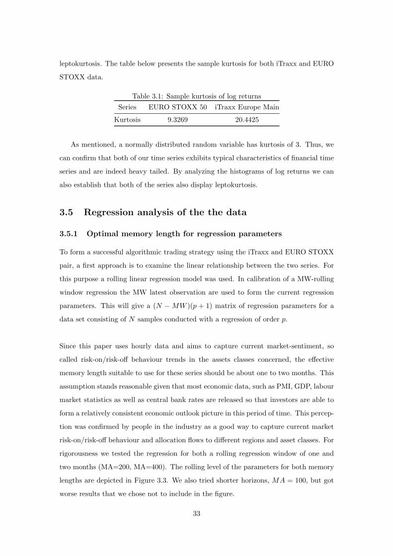
Table 3.1: Sample kurtosis of log returns
Series EURO STOXX 50 iTraxx Europe Main
Kurtosis 9.3269 20.4425
As mentioned, a normally distributed random variable has kurtosis of 3. Thus, we
can confirm that both of our time series exhibits typical characteristics of financial time
series and are indeed heavy tailed. By analyzing the histograms of log returns we can
also establish that both of the series also display leptokurtosis.
3.5 Regression analysis of the the data
3.5.1 Optimal memory length for regression parameters
To form a successful algorithmic trading strategy using the iTraxx and EURO STOXX
pair, a first approach is to examine the linear relationship between the two series. For
this purpose a rolling linear regression model was used. In calibration of a MW-rolling
window regression the MW latest observation are used to form the current regression
parameters. This will give a (N −MW )(p + 1) matrix of regression parameters for a
data set consisting of N samples conducted with a regression of order p.
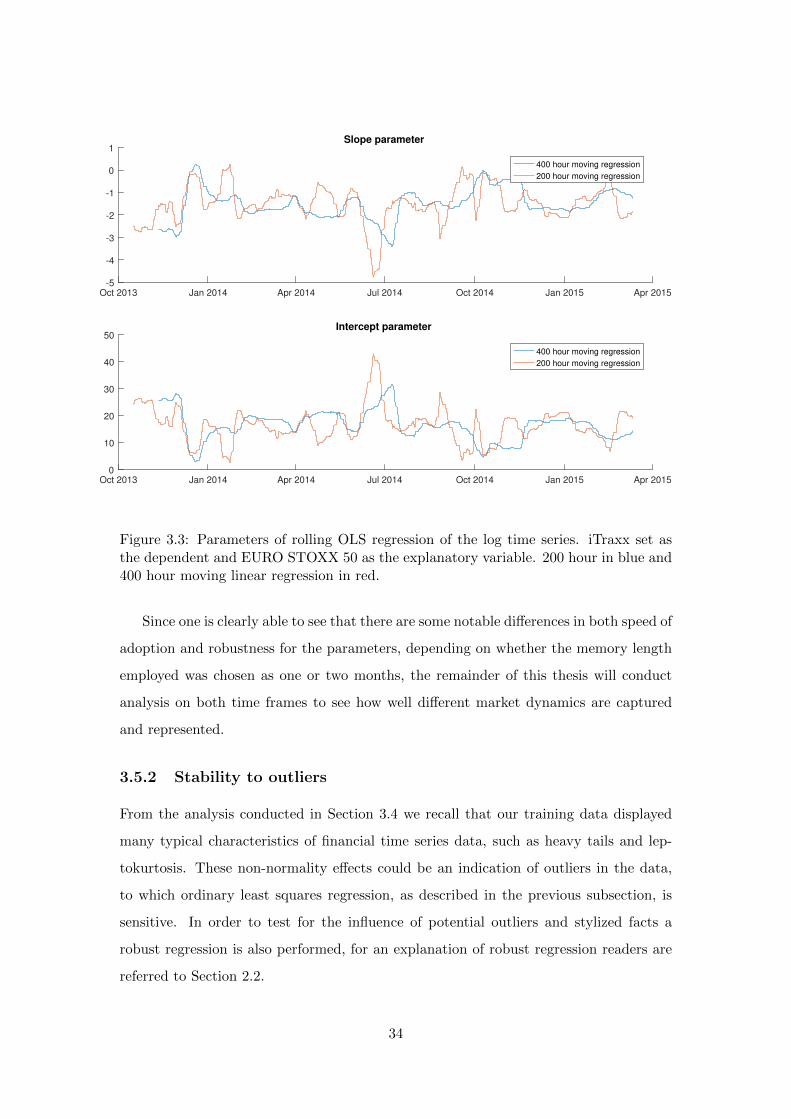
Since this paper uses hourly data and aims to capture current market-sentiment, so
called risk-on/risk-off behaviour trends in the assets classes concerned, the effective
memory length suitable to use for these series should be about one to two months. This
assumption stands reasonable given that most economic data, such as PMI, GDP, labour
market statistics as well as central bank rates are released so that investors are able to
form a relatively consistent economic outlook picture in this period of time. This percep-
tion was confirmed by people in the industry as a good way to capture current market
risk-on/risk-off behaviour and allocation flows to different regions and asset classes. For
rigorousness we tested the regression for both a rolling regression window of one and
two months (MA=200, MA=400). The rolling level of the parameters for both memory
lengths are depicted in Figure 3.3. We also tried shorter horizons, MA = 100, but got
worse results that we chose not to include in the figure.
33
Oct 2013 Jan 2014 Apr 2014 Jul 2014 Oct 2014 Jan 2015 Apr 2015-5
-4
-3
-2
-1
0
1Slope parameter
400 hour moving regression
200 hour moving regression
Oct 2013 Jan 2014 Apr 2014 Jul 2014 Oct 2014 Jan 2015 Apr 20150
10
20
30
40
50Intercept parameter
400 hour moving regression
200 hour moving regression
Figure 3.3: Parameters of rolling OLS regression of the log time series. iTraxx set asthe dependent and EURO STOXX 50 as the explanatory variable. 200 hour in blue and400 hour moving linear regression in red.
Since one is clearly able to see that there are some notable differences in both speed of
adoption and robustness for the parameters, depending on whether the memory length
employed was chosen as one or two months, the remainder of this thesis will conduct
analysis on both time frames to see how well different market dynamics are captured
and represented.
3.5.2 Stability to outliers
From the analysis conducted in Section 3.4 we recall that our training data displayed
many typical characteristics of financial time series data, such as heavy tails and lep-
tokurtosis. These non-normality effects could be an indication of outliers in the data,
to which ordinary least squares regression, as described in the previous subsection, is
sensitive. In order to test for the influence of potential outliers and stylized facts a
robust regression is also performed, for an explanation of robust regression readers are
referred to Section 2.2.
34
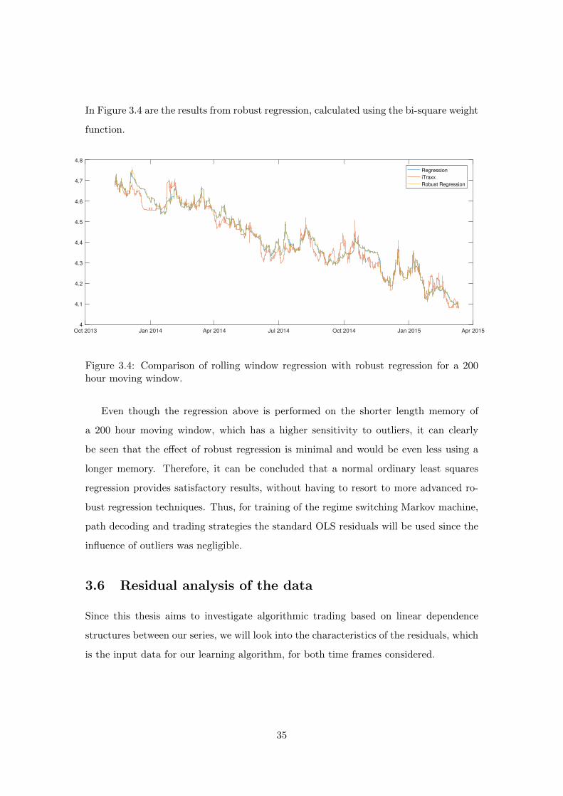
In Figure 3.4 are the results from robust regression, calculated using the bi-square weight
function.
Oct 2013 Jan 2014 Apr 2014 Jul 2014 Oct 2014 Jan 2015 Apr 20154
4.1
4.2
4.3
4.4
4.5
4.6
4.7
4.8
Regression
iTraxx
Robust Regression
Figure 3.4: Comparison of rolling window regression with robust regression for a 200hour moving window.
Even though the regression above is performed on the shorter length memory of
a 200 hour moving window, which has a higher sensitivity to outliers, it can clearly
be seen that the effect of robust regression is minimal and would be even less using a
longer memory. Therefore, it can be concluded that a normal ordinary least squares
regression provides satisfactory results, without having to resort to more advanced ro-
bust regression techniques. Thus, for training of the regime switching Markov machine,
path decoding and trading strategies the standard OLS residuals will be used since the
influence of outliers was negligible.
3.6 Residual analysis of the data
Since this thesis aims to investigate algorithmic trading based on linear dependence
structures between our series, we will look into the characteristics of the residuals, which
is the input data for our learning algorithm, for both time frames considered.
35
Oct 2013 Jan 2014 Apr 2014 Jul 2014 Oct 2014 Jan 2015 Apr 2015-0.1
-0.05
0
0.05
0.1
0.15
Residuals 200 hour moving window
Oct 2013 Jan 2014 Apr 2014 Jul 2014 Oct 2014 Jan 2015 Apr 2015-0.1
-0.05
0
0.05
0.1
0.15
Residuals 400 hour moving window
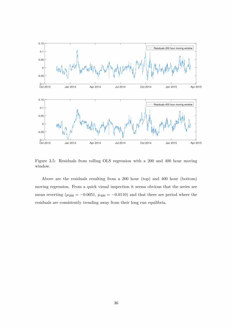
Figure 3.5: Residuals from rolling OLS regression with a 200 and 400 hour movingwindow.
Above are the residuals resulting from a 200 hour (top) and 400 hour (bottom)
moving regression. From a quick visual inspection it seems obvious that the series are
mean reverting (µ200 = −0.0051, µ400 = −0.0110) and that there are period where the
residuals are consistently trending away from their long run equilibria.
36
Chapter 4
Results
This chapter will present the results of the Markov machine modelling and trading
strategies.
4.1 The Regime Switching Model
First, the raw data was down-sampled to hourly business time data (daily 08:00-18:00)
through simple linear interpolation. Then a rolling OLS regression was used to calculate
the residual vector. As describer earlier, we used a rolling window size of 200 and 400
hours when performing the regression. The model was specified as
∆Yt = γ1Xt=0Yt−1 + β(Xt)∆Yt−1 + ε(Xt)t (4.1)
PXt =
p00 p01
p10 p11
(4.2)
where compared to Section 2.6.3 we have set u = 0 and k = 1, since the original series
are I(1) and ∆Yt has no drift. The Viterbi path described in Section 2.6.4 assumed
to have the initial state probability vector [0.5; 0.5]. We will go through the results in
detail for a regression window of 200 and 400 hours.
4.1.1 200 hour Regression Window
In Figure 4.1 we have plotted the explained variable ∆Yt against the conditional stan-
dard deviation of equation (4.1) in state 1 and the smoothed state probabilities with a
regression window of 200 hours.
37
0 500 1000 1500 2000 2500 3000 3500 4000 4500-0.1
0
0.1
Explained Variable #1
0 500 1000 1500 2000 2500 3000 3500 4000 45002
4
6
810
-3
Conditional Std of Equation #1
0 500 1000 1500 2000 2500 3000 3500 4000 4500
Time
0
0.5
1
Sm
oo
the
d S
tate
s P
rob
ab
ilitie
s
State 1
State 2
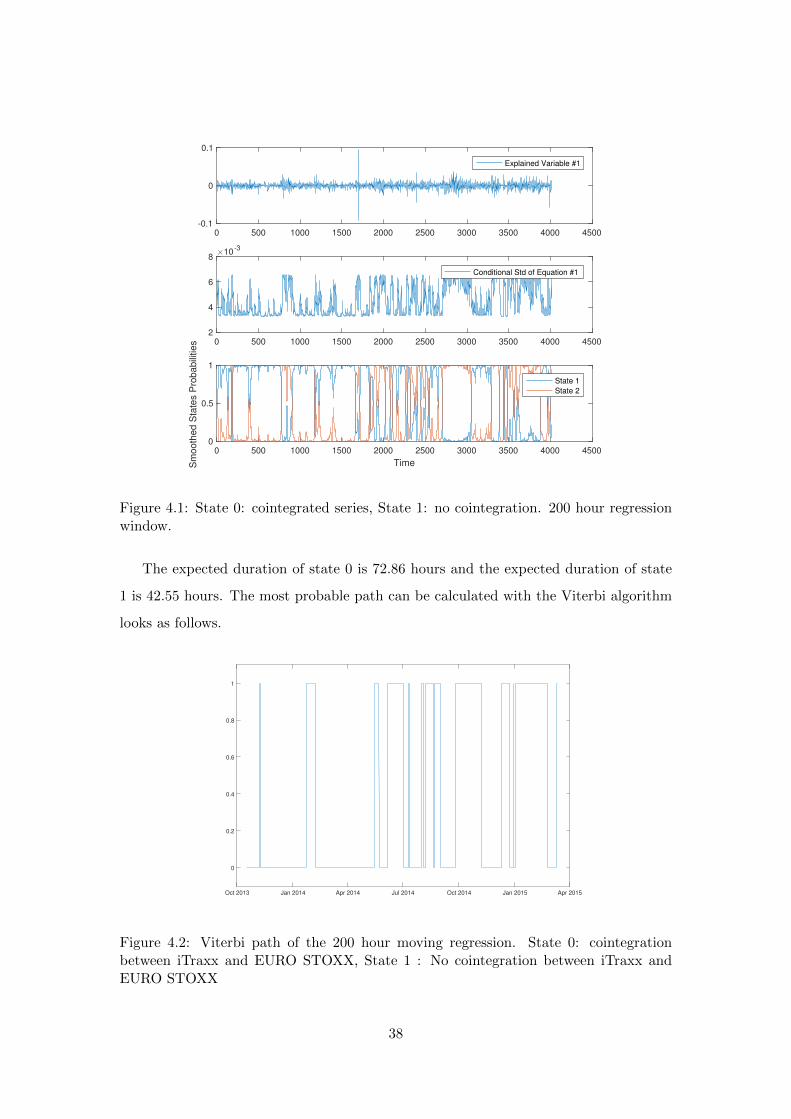
Figure 4.1: State 0: cointegrated series, State 1: no cointegration. 200 hour regressionwindow.
The expected duration of state 0 is 72.86 hours and the expected duration of state
1 is 42.55 hours. The most probable path can be calculated with the Viterbi algorithm
looks as follows.
Oct 2013 Jan 2014 Apr 2014 Jul 2014 Oct 2014 Jan 2015 Apr 2015
0
0.2
0.4
0.6
0.8
1
Figure 4.2: Viterbi path of the 200 hour moving regression. State 0: cointegrationbetween iTraxx and EURO STOXX, State 1 : No cointegration between iTraxx andEURO STOXX
38
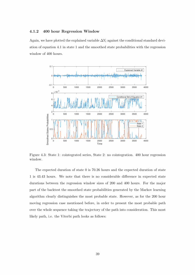
4.1.2 400 hour Regression Window
Again, we have plotted the explained variable ∆Yt against the conditional standard devi-
ation of equation 4.1 in state 1 and the smoothed state probabilities with the regression
window of 400 hours.
0 500 1000 1500 2000 2500 3000 3500 4000-0.1
0
0.1
Explained Variable #1
0 500 1000 1500 2000 2500 3000 3500 40002
4
6
810
-3
Conditional Std of Equation #1
0 500 1000 1500 2000 2500 3000 3500 4000
Time
0
0.5
1
Sm
oo
the
d S
tate
s P
rob
ab
ilitie
s
State 1
State 2
Figure 4.3: State 1: cointegrated series, State 2: no cointegration. 400 hour regressionwindow.
The expected duration of state 0 is 70.26 hours and the expected duration of state
1 is 43.43 hours. We note that there is no considerable difference in expected state
durations between the regression window sizes of 200 and 400 hours. For the major
part of the backtest the smoothed state probabilities generated by the Markov learning
algorithm clearly distinguishes the most probable state. However, as for the 200 hour
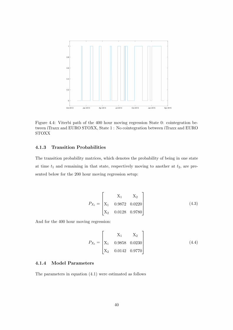
moving regression case mentioned before, in order to present the most probable path
over the whole sequence taking the trajectory of the path into consideration. This most
likely path, i.e. the Viterbi path looks as follows:
39
Oct 2013 Jan 2014 Apr 2014 Jul 2014 Oct 2014 Jan 2015 Apr 2015
0
0.2
0.4
0.6
0.8
1
Figure 4.4: Viterbi path of the 400 hour moving regression State 0: cointegration be-tween iTraxx and EURO STOXX, State 1 : No cointegration between iTraxx and EUROSTOXX
4.1.3 Transition Probabilities
The transition probability matrices, which denotes the probability of being in one state
at time t1 and remaining in that state, respectively moving to another at t2, are pre-
sented below for the 200 hour moving regression setup:
PXt =
X1 X2
X1 0.9872 0.0220
X2 0.0128 0.9780
(4.3)
And for the 400 hour moving regression:
PXt =
X1 X2
X1 0.9858 0.0230
X2 0.0142 0.9770
(4.4)
4.1.4 Model Parameters
The parameters in equation (4.1) were estimated as follows
40
Table 4.1: Model Parameter Estimation Results
State γ β
Window 200 1 -0.0215 -0.0753Window 200 2 0 -0.0844Window 400 1 -0.0111 -0.0665Window 400 2 0 -0.0756
4.1.5 Model Evaluation
In Table 4.1 the two different Markov regime setups are compared and evaluated ac-
cording to a number of information criteria and stability tests. The results are fairly
stable over both regression window lengths. Therefore, for consistency and rigorousness
reasons we carried out the trading strategies with a window of 200 and 400 hours.
Table 4.2: Statistical properties with different regression windows
AIC BIC LL E[dur|St = 1] E[dur|St = 2]
200 hour window -3.0442e04 -3.0366e04 1.5233e04 72.86 42.55400 hour window -2.8949e04 -2.8874e04 1.4487e04 70.26 43.43
Here AIC is the Akaike information criterion, BIC is the Bayesian information cri-
terion, LL is the log-likelihood and E[dur|St = i], i = 1, 2, is the expected duration
(hours) of each state.
4.2 Comparison with naive pairs trading strategy
To get an initial perspective on the trading strategies, we compare them to the perfor-
mance of letting trades be initiated in both states.
Table 4.3: Trading Strategy Performance (Without considering the regimes)
Regression Window k1/− k4 k2/− k3 yield (%) Number of trades
Strategy 1 200 0.75 0 13 268Strategy 2 200 0.5 0 14 360Strategy 3 400 0.75 0 -3 160Strategy 4 400 0.5 0 -4 244
Interestingly, the performance of the same strategies are much worse. As expected
the number of trades increase significantly, but since transaction costs are overlooked,
41

the bad performance is simply due to trading in unprofitable regimes. In Figure 5.1 the
percentage cumulative return for strategy 4 is visualized. As seen, when comparing to
the next Section, the volatility is much higher and in the latter part of the data set when
state 2 is more present, the performance is lousy. These negative returns are obviously
avoided when applying the trading rules based on the Markov regime switching model.
Oct 2013 Jan 2014 Apr 2014 Jul 2014 Oct 2014 Jan 2015 Apr 2015
Time
-10
-5
0
5
10
15
20
25
30
Perc
enta
ge c
ulm
ula
tive r
etu
rn
Figure 4.5: Percentage cumulative return for strategy 4.
4.3 The Trading Strategies
Simulated trading was conducted on the data set according to the setup in Section
2.7.2. However, the trading environment has been significantly simplified. We assume
no transaction costs and the pricing of the CDS contracts is also substantially simplified.
A constant RPV01 of 4.6 is used. In reality the RPV01 would depend on several factors
described in Section 1.3.2. For the EURO STOXX futures contracts the contract tick
value was set to 10 euro, and for the CDS index contract it was set to the fixed RPV01
(4.6). In Table 4.4 performance of different strategies are summarized.
42
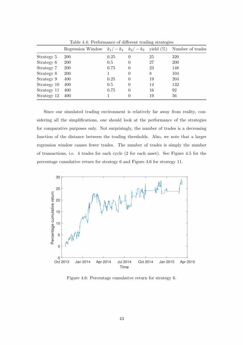
Table 4.4: Performance of different trading strategies
Regression Window k1/− k4 k2/− k3 yield (%) Number of trades
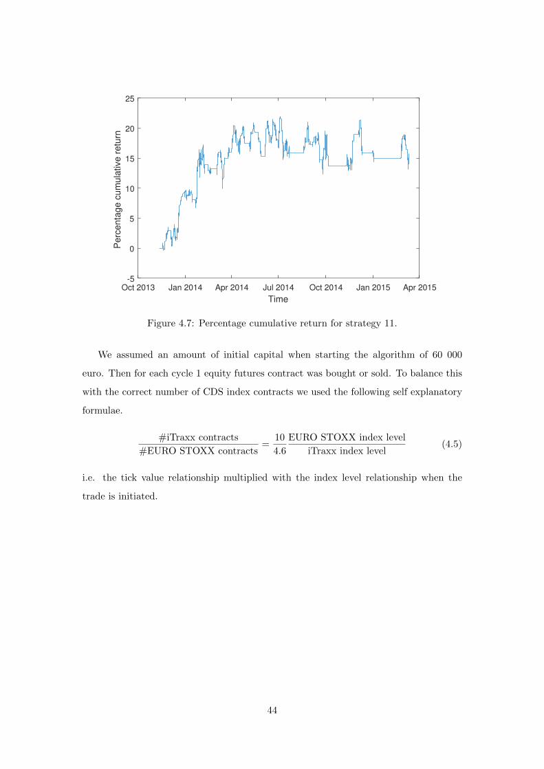
Strategy 5 200 0.25 0 25 320Strategy 6 200 0.5 0 27 200Strategy 7 200 0.75 0 23 148Strategy 8 200 1 0 8 104Strategy 9 400 0.25 0 19 204Strategy 10 400 0.5 0 14 132Strategy 11 400 0.75 0 16 92Strategy 12 400 1 0 19 56
Since our simulated trading environment is relatively far away from reality, con-
sidering all the simplifications, one should look at the performance of the strategies
for comparative purposes only. Not surprisingly, the number of trades is a decreasing
function of the distance between the trading thresholds. Also, we note that a larger
regression window causes fewer trades. The number of trades is simply the number
of transactions, i.e. 4 trades for each cycle (2 for each asset). See Figure 4.5 for the
percentage cumulative return for strategy 6 and Figure 4.6 for strategy 11.
Oct 2013 Jan 2014 Apr 2014 Jul 2014 Oct 2014 Jan 2015 Apr 2015
Time
-5
0
5
10
15
20
25
30
Perc
enta
ge c
um
ula
tive r
etu
rn
Figure 4.6: Percentage cumulative return for strategy 6.
43
Oct 2013 Jan 2014 Apr 2014 Jul 2014 Oct 2014 Jan 2015 Apr 2015
Time
-5
0
5
10
15
20
25
Perc
enta
ge c
um
ula
tive r
etu
rn
Figure 4.7: Percentage cumulative return for strategy 11.
We assumed an amount of initial capital when starting the algorithm of 60 000
euro. Then for each cycle 1 equity futures contract was bought or sold. To balance this
with the correct number of CDS index contracts we used the following self explanatory
formulae.
#iTraxx contracts
#EURO STOXX contracts=
10
4.6
EURO STOXX index level
iTraxx index level(4.5)
i.e. the tick value relationship multiplied with the index level relationship when the
trade is initiated.
44

Chapter 5
Conclusions
This thesis has successfully proposed a novel approach of distinguishing regimes in which
the cross asset pair consisting of EURO STOXX 50 futures and iTraxx Europe Main
CDS contracts statistically indicates cointegration. A regime switching Markov model
is introduced allowing us to determine when the cointegration state is deemed to be
statistically significant.
5.1 Establishing efficient memory length
In chapter 4 we have conducted statistical analysis and presented the results for both
200 and 400 hour moving regressions, as motivated in Section 3.6. It seems that gener-
ally, the 200 hour strategies preform better than its 400 hour counterparts. One purely
mathematical explanation behind this characteristic could relate to the average duration
of the different co-integrated states. The average duration of the the respective states
are about 70 and 50 hours (cointegrated vs. non-cointegrated) so by setting the memory
length to 400 hours means that there is a clear risk of running over several regimes when
calculating the residuals, thereby smoothing out current trends all too much.
Therefore, for reasons of completeness we also conducted a quick test using a 100 hour
moving window. The results here where however dissatisfying as none of the strategies
we tested could generate a double digit return. Thus indicating setting the memory
length close to levels of average state duration risks making the behaviour of the regres-
sion parameters too erratic.
45

5.2 Considering transaction costs
In all of the above investigated trading strategies of this theses, the effect of transactions
costs have been neglected. In real trading, one both faces the effect of brokerage fees as
well as the bid-offer spread.
The brokerage fee is fixed and payed to the exchange-connected broker for executing
the transition on behalf of the client whereas the spread is a function of current market
liquidity. After discussions with AP4 we established that a reasonable range for the
total transaction costs would be about 0.1-0.25 bp for iTraxx and 1 tick in spread with
negligible broker fee for EURO STOXX futures.
Thus we can easily conclude that the totalt impact of transations cost of these strategies
is well below 1 percent of capital yearly. As a result, including the effect of transactions
cost into the strategies would only have a minor impact for the most promising of our
listed strategies. For the more transaction intensive ones (with lower trading thresholds)
the impact would of course be larger. Although, these strategies are less profitable even
when transaciton costs are excluded.
5.3 Further Research Areas
For future research on this topic it is of course very important to have a good and stable
model. Therefore it would be very interesting to test the model over a much larger
data set and making several out of sample tests. Throughout our dataset equities are
constantly strengthening and hence protection is declining. How does the model react
in a state of the world where the inverse is true or equities are fairly constant?
Other natural suggestions for further research is complementing with other cross as-
set pairs, such as an American pair (S&P 500 futures and CDX). The extension of
possible trading strategies on pairs is infinite. In this thesis, the main focus has been
the implementation of the Markov regime switching model. Naturally, it would be of
great interest to simulate a more realistic trading environment with a proper CDS index
pricing technique and real transaction costs.
46
Bibliography
[Akaike, 1974] Akaike, H. (1974). A new look at the statistical model identification.
IEEE Transactions on Automatic Control, 19(6):716 – 723.
[Alavei and Olsson, 2015] Alavei, D. and Olsson, T. (2015). Trading cds indices vs.
equity index futures – a pairs trade. Master’s thesis, Lund University.
[Baum et al., 1970] Baum, L. E., Petrie, T., Soules, G., and Weiss, N. (1970). A max-
imization technique occurring in the statistical analysis of probabilistic functions of
markov chains. Ann. Math. Statist., 41(1):164–171.
[Bhattacharyya and Erlandsson, 2007] Bhattacharyya, A. and Erlandsson, U. (2007).
High-frequency cds index trading. Technical report, Structured Credit Investor.
[Cappe et al., 2005] Cappe, O., Moulines, E., and Ryden, T. (2005). Inference in Hidden
Markov Models (Springer Series in Statistics). Springer-Verlag New York, Inc.
[Chatfield, 2004] Chatfield, C. (2004). The analysis of time series: an introduction.
CRC Press, Florida, US, 6th edition.
[Cui and Cui, 2012] Cui, K. and Cui, W. (2012). Bayesian markov regime-switching
models for cointegration. Scientific Research Applied Mathematics, 3(12).
[Dempster et al., 1977] Dempster, A. P., Laird, N. M., and Rubin, D. B. (1977). Max-
imum likelihood from incomplete data via the em algorithm. Journal of the Royal
Statistical Society, Series B, 39(1):1–38.
[Dickey and Fuller, 1979] Dickey, D. A. and Fuller, W. A. (1979). Distribution of the
estimators for autoregressive time series with a unit root. Journal of the American
Statistical Association, 74(366):427–431.
47
[Durrett, 2011] Durrett, R. (2011). Probability: Theory and examples.
[Elliott et al., 2005] Elliott, R., Van Der Hoek, J., and Malcolm, W. (2005). Pairs
trading. Quantitative Finance, 5(3):271–276.
[Engle and Granger, 1987] Engle, R. F. and Granger, C. W. J. (1987). Co-integration
and error correction: Representation, estimation, and testing. Econometrica,
55(2):251–276.
[Erlandsson, 2005] Erlandsson, U. (2005). Markov Regime Switching in Economic Time
Series. Lund economic studies. Department of Economics, University of Lund.
[Gatev et al., 1999] Gatev, E. G., Goetzmann, W. N., and Rouwenhorst, K. G. (1999).
Pairs trading: Performance of a relative value arbitrage rule. Working Paper 7032,
National Bureau of Economic Research.
[Gillian, 2009] Gillian, T. (2009). Fool’s Gold: How Unrestrained Greed Corrupted a
Dream, Shattered Global Markets and Unleashed a Catastrophe. Little Brown.
[Granger and Newbold, 1974] Granger, C. and Newbold, P. (1974). Spurious regressions
in econometrics. Journal of Econometrics, 2(2):111 – 120.
[Hamilton, 1988] Hamilton, J. (1988). Rational-expectations econometric analysis of
changes in regime: An investigation of the term structure of interest rates. Journal
of Economic Dynamics and Control, 12(2-3):385–423.
[Hamilton, 1994] Hamilton, J. (1994). Time series analysis. Princeton Univ. Press,
Princeton, NJ.
[Hull and White, 2000] Hull, J. C. and White, A. (2000). Valuing credit default swaps
i: No counterparty default risk. Journal of Derivatives, 8(1):29–40.
[Idvall and Jonsson, 2008] Idvall, P. and Jonsson, C. (2008). Algorithmic trading - hid-
den markov models on foreign exchange data. Master’s thesis, LiTh.
[ISDA, 2010] ISDA (2010). Isda market survey.
[ISDA, 2016] ISDA (2016). Credit derivatives determinations committees rules.
[ISDA, 2017a] ISDA (2017a). Swaps info - clearing.
48
[ISDA, 2017b] ISDA (2017b). Swaps info - notional outstanding.
[Kirchgassner and Wolters, 2007] Kirchgassner, G. and Wolters, J. (2007). Introduction
to Modern Time Series Analysis. Springer-Verlag Berlin Heidelberg, Berlin, Heidel-
berg.
[Kissell, 2013] Kissell, R. (2013). The Science of Algorithmic Trading and Portfolio
Management. Elsevier, 1 edition.
[Lanchester, 2009] Lanchester, J. (2009). Outsmarted: High finance vs. human nature.
[markit, 2008] markit (2008). Markit credit indices - a primer.
[Markit, 2017] Markit (2017). itraxx.
[Mathworks, 2016] Mathworks (2016). robustfit, robust regression documentation.
[Nystrup et al., 2016] Nystrup, P., Madsen, H., and Lindstrom, E. (2016). Dynamic
portfolio optimization across hidden market regimes.
[Oehmke and Zawadowski, 2016] Oehmke, M. and Zawadowski, A. (2016). The
anatomy of the cds market. Technical report, Columbia University.
[O’Kane and Turnbull, 2003] O’Kane, D. and Turnbull, S. (2003). Valuation of credit
default swaps. Lehman Brothers quantitative credit research quarterly, 2003:Q1–Q2.
[Perlin, 2015] Perlin, M. (2015). Ms regress - the matlab package for markov regime
switching models.
[Schwarz, 1978] Schwarz, G. (1978). Estimating the dimension of a model. Ann. Statist.,
6(2):461–464.
[stoxx, 2017] stoxx (2017). Euro stoxx 50.
[Tenyakov, 2014] Tenyakov, A. (2014). Estimation of Hidden Markov Models and their
Applications in Finance. PhD thesis, University of Western Ontario.
[Tett, 2006] Tett, G. (2006). The dream machine: invention of credit derivatives.
[Viterbi, 2006] Viterbi, A. (2006). Error bounds for convolutional codes and an
asymptotically optimum decoding algorithm. IEEE Trans. on Information Theory,
13(2):260–269.
49
Related Documents