Algorithmic Graph Theory and Sage David Joyner, Minh Van Nguyen, David Phillips Version 0.8-r1991 2013 May 10

Welcome message from author
This document is posted to help you gain knowledge. Please leave a comment to let me know what you think about it! Share it to your friends and learn new things together.
Transcript
Algorithmic Graph Theory and Sage
David Joyner, Minh Van Nguyen, David Phillips
Version 0.8-r19912013 May 10

Copyright © 2010–2013 David Joyner 〈[email protected]〉Copyright © 2009–2013 Minh Van Nguyen 〈[email protected]〉Copyright © 2013 David Phillips 〈[email protected]〉
Permission is granted to copy, distribute and/or modify this document under the termsof the GNU Free Documentation License, Version 1.3 or any later version published bythe Free Software Foundation; with no Invariant Sections, no Front-Cover Texts, and noBack-Cover Texts. A copy of the license is included in the section entitled “GNU FreeDocumentation License”.
The latest version of the book is available from its website at
http://code.google.com/p/graphbook/
EditionVersion 0.8-r19912013 May 10
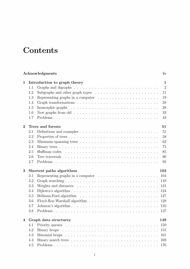
Contents
Acknowledgments iv
1 Introduction to graph theory 1
1.1 Graphs and digraphs . . . . . . . . . . . . . . . . . . . . . . . . . . . . . 2
1.2 Subgraphs and other graph types . . . . . . . . . . . . . . . . . . . . . . 11
1.3 Representing graphs in a computer . . . . . . . . . . . . . . . . . . . . . 19
1.4 Graph transformations . . . . . . . . . . . . . . . . . . . . . . . . . . . . 28
1.5 Isomorphic graphs . . . . . . . . . . . . . . . . . . . . . . . . . . . . . . 28
1.6 New graphs from old . . . . . . . . . . . . . . . . . . . . . . . . . . . . . 33
1.7 Problems . . . . . . . . . . . . . . . . . . . . . . . . . . . . . . . . . . . . 43
2 Trees and forests 51
2.1 Definitions and examples . . . . . . . . . . . . . . . . . . . . . . . . . . . 51
2.2 Properties of trees . . . . . . . . . . . . . . . . . . . . . . . . . . . . . . . 58
2.3 Minimum spanning trees . . . . . . . . . . . . . . . . . . . . . . . . . . . 62
2.4 Binary trees . . . . . . . . . . . . . . . . . . . . . . . . . . . . . . . . . . 75
2.5 Huffman codes . . . . . . . . . . . . . . . . . . . . . . . . . . . . . . . . 85
2.6 Tree traversals . . . . . . . . . . . . . . . . . . . . . . . . . . . . . . . . . 90
2.7 Problems . . . . . . . . . . . . . . . . . . . . . . . . . . . . . . . . . . . . 95
3 Shortest paths algorithms 103
3.1 Representing graphs in a computer . . . . . . . . . . . . . . . . . . . . . 104
3.2 Graph searching . . . . . . . . . . . . . . . . . . . . . . . . . . . . . . . . 110
3.3 Weights and distances . . . . . . . . . . . . . . . . . . . . . . . . . . . . 121
3.4 Dijkstra’s algorithm . . . . . . . . . . . . . . . . . . . . . . . . . . . . . . 124
3.5 Bellman-Ford algorithm . . . . . . . . . . . . . . . . . . . . . . . . . . . 127
3.6 Floyd-Roy-Warshall algorithm . . . . . . . . . . . . . . . . . . . . . . . . 128
3.7 Johnson’s algorithm . . . . . . . . . . . . . . . . . . . . . . . . . . . . . . 135
3.8 Problems . . . . . . . . . . . . . . . . . . . . . . . . . . . . . . . . . . . . 137
4 Graph data structures 149
4.1 Priority queues . . . . . . . . . . . . . . . . . . . . . . . . . . . . . . . . 150
4.2 Binary heaps . . . . . . . . . . . . . . . . . . . . . . . . . . . . . . . . . 151
4.3 Binomial heaps . . . . . . . . . . . . . . . . . . . . . . . . . . . . . . . . 161
4.4 Binary search trees . . . . . . . . . . . . . . . . . . . . . . . . . . . . . . 169
4.5 Problems . . . . . . . . . . . . . . . . . . . . . . . . . . . . . . . . . . . . 176
i

ii Contents
5 Distance and connectivity 1825.1 Paths and distance . . . . . . . . . . . . . . . . . . . . . . . . . . . . . . 1825.2 Vertex and edge connectivity . . . . . . . . . . . . . . . . . . . . . . . . . 1875.3 Menger’s theorem . . . . . . . . . . . . . . . . . . . . . . . . . . . . . . . 1925.4 Whitney’s Theorem . . . . . . . . . . . . . . . . . . . . . . . . . . . . . . 1955.5 Centrality of a vertex . . . . . . . . . . . . . . . . . . . . . . . . . . . . . 1965.6 Network reliability . . . . . . . . . . . . . . . . . . . . . . . . . . . . . . 1985.7 The spectrum of a graph . . . . . . . . . . . . . . . . . . . . . . . . . . . 1985.8 Expander graphs and Ramanujan graphs . . . . . . . . . . . . . . . . . . 2035.9 Problems . . . . . . . . . . . . . . . . . . . . . . . . . . . . . . . . . . . . 205
6 Centrality and prestige 2096.1 Vertex centrality . . . . . . . . . . . . . . . . . . . . . . . . . . . . . . . 2096.2 Edge centrality . . . . . . . . . . . . . . . . . . . . . . . . . . . . . . . . 2096.3 Ranking web pages . . . . . . . . . . . . . . . . . . . . . . . . . . . . . . 2096.4 Hub and authority . . . . . . . . . . . . . . . . . . . . . . . . . . . . . . 2096.5 Problems . . . . . . . . . . . . . . . . . . . . . . . . . . . . . . . . . . . . 209
7 Optimal graph traversals 2107.1 Eulerian graphs . . . . . . . . . . . . . . . . . . . . . . . . . . . . . . . . 2107.2 Hamiltonian graphs . . . . . . . . . . . . . . . . . . . . . . . . . . . . . . 2107.3 The Chinese Postman Problem . . . . . . . . . . . . . . . . . . . . . . . 2117.4 The Traveling Salesman Problem . . . . . . . . . . . . . . . . . . . . . . 211
8 Graph coloring 2128.1 Vertex coloring . . . . . . . . . . . . . . . . . . . . . . . . . . . . . . . . 2128.2 Edge coloring . . . . . . . . . . . . . . . . . . . . . . . . . . . . . . . . . 2158.3 The chromatic polynomial . . . . . . . . . . . . . . . . . . . . . . . . . . 2198.4 Applications of graph coloring . . . . . . . . . . . . . . . . . . . . . . . . 221
9 Network flows 2239.1 Flows and cuts . . . . . . . . . . . . . . . . . . . . . . . . . . . . . . . . 2239.2 Chip firing games . . . . . . . . . . . . . . . . . . . . . . . . . . . . . . . 2289.3 Ford-Fulkerson theorem . . . . . . . . . . . . . . . . . . . . . . . . . . . 2359.4 Edmonds and Karp’s algorithm . . . . . . . . . . . . . . . . . . . . . . . 2409.5 Goldberg and Tarjan’s algorithm . . . . . . . . . . . . . . . . . . . . . . 240
10 Algebraic graph theory 24110.1 Laplacian and adjacency matrices . . . . . . . . . . . . . . . . . . . . . . 24110.2 Eigenvalues and eigenvectors . . . . . . . . . . . . . . . . . . . . . . . . . 24110.3 Algebraic connectivity . . . . . . . . . . . . . . . . . . . . . . . . . . . . 24110.4 Graph invariants . . . . . . . . . . . . . . . . . . . . . . . . . . . . . . . 24110.5 Cycle and cut spaces . . . . . . . . . . . . . . . . . . . . . . . . . . . . . 24110.6 Problems . . . . . . . . . . . . . . . . . . . . . . . . . . . . . . . . . . . . 241
11 Random graphs 24211.1 Network statistics . . . . . . . . . . . . . . . . . . . . . . . . . . . . . . . 24211.2 Binomial random graph model . . . . . . . . . . . . . . . . . . . . . . . . 24611.3 Erdos-Renyi model . . . . . . . . . . . . . . . . . . . . . . . . . . . . . . 253

Contents iii
11.4 Small-world networks . . . . . . . . . . . . . . . . . . . . . . . . . . . . . 25511.5 Scale-free networks . . . . . . . . . . . . . . . . . . . . . . . . . . . . . . 26011.6 Problems . . . . . . . . . . . . . . . . . . . . . . . . . . . . . . . . . . . . 265
A Asymptotic growth 271
B GNU Free Documentation License 2721. APPLICABILITY AND DEFINITIONS . . . . . . . . . . . . . . . . . . . . 2722. VERBATIM COPYING . . . . . . . . . . . . . . . . . . . . . . . . . . . . 2743. COPYING IN QUANTITY . . . . . . . . . . . . . . . . . . . . . . . . . . . 2744. MODIFICATIONS . . . . . . . . . . . . . . . . . . . . . . . . . . . . . . . 2755. COMBINING DOCUMENTS . . . . . . . . . . . . . . . . . . . . . . . . . 2766. COLLECTIONS OF DOCUMENTS . . . . . . . . . . . . . . . . . . . . . . 2777. AGGREGATION WITH INDEPENDENT WORKS . . . . . . . . . . . . . 2778. TRANSLATION . . . . . . . . . . . . . . . . . . . . . . . . . . . . . . . . . 2779. TERMINATION . . . . . . . . . . . . . . . . . . . . . . . . . . . . . . . . . 27810. FUTURE REVISIONS OF THIS LICENSE . . . . . . . . . . . . . . . . . 27811. RELICENSING . . . . . . . . . . . . . . . . . . . . . . . . . . . . . . . . . 278ADDENDUM: How to use this License for your documents . . . . . . . . . . . 279
Bibliography 280
Index 288
Acknowledgments
Fidel Barrera-Cruz: reported typos in Chapter 2. See changeset 101. Suggestedmaking a note about disregarding the direction of edges in undirected graphs. Seechangeset 277.
Daniel Black: reported a typo in Chapter 1. See changeset 61.
Kevin Brintnall: reported typos in the definition of iadj(v) ∩ oadj(v); see change-sets 240 and 242. Solution to Example 1.14(2); see changeset 246.
John Costella: helped to clarify the idea that the adjacency matrix of a bipar-tite graph can be permuted to obtain a block diagonal matrix. See page 22 andrevisions 1865 and 1869.
Aaron Dutle: reported a typo in Figure 1.18. See changeset 125.
Peter L. Erdos (http://www.renyi.hu/∼elp) for informing us of the reference [74] onthe Havel-Hakimi theorem for directed graphs.
Noel Markham: reported a typo in Algorithm 3.5. See changeset 131 and Issue 2.
Caroline Melles: clarify definitions of various graph types (weighted graphs, multi-graphs, and weighted multigraphs); clarify definitions of degree, isolated vertices,and pendant and using the butterfly graph with 5 vertices (see Figure 1.10) toillustrate these definitions; clarify definitions of trails, closed paths, and cycles;see changeset 448. Some rearrangements of materials in Chapter 1 to make thereading flow better and a few additions of missing definitions; see changeset 584.Clarifications about unweighted and weighted degree of a vertex in a multigraph;notational convention about a graph being simple unless otherwise stated; an exam-ple on graph minor; see changeset 617. Reported a missing edge in Figure 1.5(b);see changeset 1945.
Pravin Paratey: simplify the sentence formation in the definition of digraphs; seechangeset 714 and Issue 7.
Henrique Renno: pointed out the ambiguity in the definition of weighted multi-graphs; see changeset 1936. Reported typos; see changeset 1938.
The world map in Figure ?? was adapted from an SVG image file from Wikipedia.The original SVG file was accessed on 2010-10-01 at http://en.wikipedia.org/wiki/File:WorldmapwlocationwNEDw50m.svg.
iv

Chapter 1
Introduction to graph theory
— Spiked Math, http://spikedmath.com/120.html
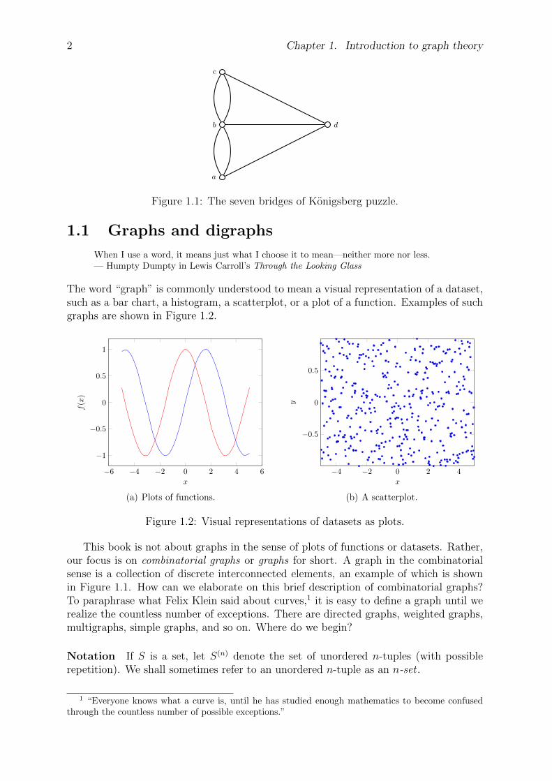
Our journey into graph theory starts with a puzzle that was solved over 250 years ago byLeonhard Euler (1707–1783). The Pregel River flowed through the town of Konigsberg,which is present day Kaliningrad in Russia. Two islands protruded from the river.On either side of the mainland, two bridges joined one side of the mainland with oneisland and a third bridge joined the same side of the mainland with the other island. Abridge connected the two islands. In total, seven bridges connected the two islands withboth sides of the mainland. A popular exercise among the citizens of Konigsberg wasdetermining if it was possible to cross each bridge exactly once during a single walk. Forhistorical perspectives on this puzzle and Euler’s solution, see Gribkovskaia et al. [90]and Hopkins and Wilson [102].
To visualize this puzzle in a slightly different way, consider Figure 1.1. Imagine thatpoints a and c are either sides of the mainland, with points b and d being the two islands.Place the tip of your pencil on any of the points a, b, c, d. Can you trace all the linesin the figure exactly once, without lifting your pencil? Known as the seven bridges ofKonigsberg puzzle, Euler solved this problem in 1735 and with his solution he laid thefoundation of what is now known as graph theory.
1
2 Chapter 1. Introduction to graph theory
a
b
c
d
Figure 1.1: The seven bridges of Konigsberg puzzle.
1.1 Graphs and digraphs
When I use a word, it means just what I choose it to mean—neither more nor less.— Humpty Dumpty in Lewis Carroll’s Through the Looking Glass
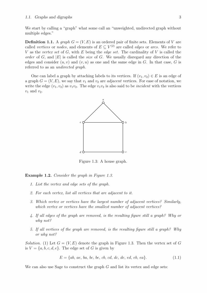
The word “graph” is commonly understood to mean a visual representation of a dataset,such as a bar chart, a histogram, a scatterplot, or a plot of a function. Examples of suchgraphs are shown in Figure 1.2.
−6 −4 −2 0 2 4 6
−1
−0.5
0
0.5
1
x
f(x
)
(a) Plots of functions.
−4 −2 0 2 4
−0.5
0
0.5
x
y
(b) A scatterplot.
Figure 1.2: Visual representations of datasets as plots.
This book is not about graphs in the sense of plots of functions or datasets. Rather,our focus is on combinatorial graphs or graphs for short. A graph in the combinatorialsense is a collection of discrete interconnected elements, an example of which is shownin Figure 1.1. How can we elaborate on this brief description of combinatorial graphs?To paraphrase what Felix Klein said about curves,1 it is easy to define a graph until werealize the countless number of exceptions. There are directed graphs, weighted graphs,multigraphs, simple graphs, and so on. Where do we begin?
Notation If S is a set, let S(n) denote the set of unordered n-tuples (with possiblerepetition). We shall sometimes refer to an unordered n-tuple as an n-set .
1 “Everyone knows what a curve is, until he has studied enough mathematics to become confusedthrough the countless number of possible exceptions.”
1.1. Graphs and digraphs 3
We start by calling a “graph” what some call an “unweighted, undirected graph withoutmultiple edges.”
Definition 1.1. A graph G = (V,E) is an ordered pair of finite sets. Elements of V arecalled vertices or nodes , and elements of E ⊆ V (2) are called edges or arcs . We refer toV as the vertex set of G, with E being the edge set . The cardinality of V is called theorder of G, and |E| is called the size of G. We usually disregard any direction of theedges and consider (u, v) and (v, u) as one and the same edge in G. In that case, G isreferred to as an undirected graph.
One can label a graph by attaching labels to its vertices. If (v1, v2) ∈ E is an edge ofa graph G = (V,E), we say that v1 and v2 are adjacent vertices. For ease of notation, wewrite the edge (v1, v2) as v1v2. The edge v1v2 is also said to be incident with the verticesv1 and v2.
a
be
cd
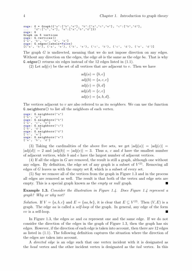
Figure 1.3: A house graph.
Example 1.2. Consider the graph in Figure 1.3.
1. List the vertex and edge sets of the graph.
2. For each vertex, list all vertices that are adjacent to it.
3. Which vertex or vertices have the largest number of adjacent vertices? Similarly,which vertex or vertices have the smallest number of adjacent vertices?
4. If all edges of the graph are removed, is the resulting figure still a graph? Why orwhy not?
5. If all vertices of the graph are removed, is the resulting figure still a graph? Whyor why not?
Solution. (1) Let G = (V,E) denote the graph in Figure 1.3. Then the vertex set of Gis V = a, b, c, d, e. The edge set of G is given by
E = ab, ae, ba, bc, be, cb, cd, dc, de, ed, eb, ea. (1.1)
We can also use Sage to construct the graph G and list its vertex and edge sets:
4 Chapter 1. Introduction to graph theory
sage: G = Graph ("a":["b","e"], "b":["a","c","e"], "c":["b","d"],... "d":["c","e"], "e":["a","b","d"])sage: GGraph on 5 verticessage: G.vertices ()[’a’, ’b’, ’c’, ’d’, ’e’]sage: G.edges(labels=False)[(’a’, ’b’), (’a’, ’e’), (’b’, ’e’), (’c’, ’b’), (’c’, ’d’), (’e’, ’d’)]
The graph G is undirected, meaning that we do not impose direction on any edges.Without any direction on the edges, the edge ab is the same as the edge ba. That is whyG.edges() returns six edges instead of the 12 edges listed in (1.1).
(2) Let adj(v) be the set of all vertices that are adjacent to v. Then we have
adj(a) = b, eadj(b) = a, c, eadj(c) = b, dadj(d) = c, eadj(e) = a, b, d.
The vertices adjacent to v are also referred to as its neighbors. We can use the functionG.neighbors() to list all the neighbors of each vertex.sage: G.neighbors("a")[’b’, ’e’]sage: G.neighbors("b")[’a’, ’c’, ’e’]sage: G.neighbors("c")[’b’, ’d’]sage: G.neighbors("d")[’c’, ’e’]sage: G.neighbors("e")[’a’, ’b’, ’d’]
(3) Taking the cardinalities of the above five sets, we get |adj(a)| = |adj(c)| =|adj(d)| = 2 and |adj(b)| = |adj(e)| = 3. Thus a, c and d have the smallest numberof adjacent vertices, while b and e have the largest number of adjacent vertices.
(4) If all the edges in G are removed, the result is still a graph, although one withoutany edges. By definition, the edge set of any graph is a subset of V (2). Removing alledges of G leaves us with the empty set ∅, which is a subset of every set.
(5) Say we remove all of the vertices from the graph in Figure 1.3 and in the processall edges are removed as well. The result is that both of the vertex and edge sets areempty. This is a special graph known as the empty or null graph.
Example 1.3. Consider the illustration in Figure 1.4. Does Figure 1.4 represent agraph? Why or why not?
Solution. If V = a, b, c and E = aa, bc, it is clear that E ⊆ V (2). Then (V,E) is agraph. The edge aa is called a self-loop of the graph. In general, any edge of the formvv is a self-loop.
In Figure 1.3, the edges ae and ea represent one and the same edge. If we do notconsider the direction of the edges in the graph of Figure 1.3, then the graph has sixedges. However, if the direction of each edge is taken into account, then there are 12 edgesas listed in (1.1). The following definition captures the situation where the direction ofthe edges are taken into account.
A directed edge is an edge such that one vertex incident with it is designated asthe head vertex and the other incident vertex is designated as the tail vertex. In this

1.1. Graphs and digraphs 5
c b
a
Figure 1.4: A figure with a self-loop.
situation, we may assume that the set of edges is a subset of the ordered pairs V × V .A directed edge uv is said to be directed from its tail u to its head v. A directed graphor digraph G is a graph each of whose edges is directed. The indegree id(v) of a vertexv ∈ V (G) counts the number of edges such that v is the head of those edges. Theoutdegree od(v) of a vertex v ∈ V (G) is the number of edges such that v is the tail ofthose edges. The degree deg(v) of a vertex v of a digraph is the sum of the indegree andthe outdegree of v.
Let G be a graph without self-loops and multiple edges. It is important to distinguisha graph G as being directed or undirected. If G is undirected and uv ∈ E(G), then uvand vu represent the same edge. In case G is a digraph, then uv and vu are differentdirected edges. For a digraph G = (V,E) and a vertex v ∈ V , all the neighbors of vin G are contained in adj(v), i.e. the set of all neighbors of v. Just as we distinguishbetween indegree and outdegree for a vertex in a digraph, we also distinguish between in-neighbors and out-neighbors. The set of in-neighbors iadj(v) ⊆ adj(v) of v ∈ V consistsof all those vertices that contribute to the indegree of v. Similarly, the set of out-neighborsoadj(v) ⊆ adj(v) of v ∈ V are those vertices that contribute to the outdegree of v. Then
iadj(v) ∩ oadj(v) = u | uv ∈ E and vu ∈ E
and adj(v) = iadj(v) ∪ oadj(v).
1.1.1 Multigraphs
This subsection presents a larger class of graphs. For simplicity of presentation, in thisbook we shall assume usually that a graph is not a multigraph. In other words, when youread a property of graphs later in the book, it will be assumed (unless stated explicitlyotherwise) that the graph is not a multigraph. However, as multigraphs and weightedgraphs are very important in many applications, we will try to keep them in the backof our mind. When appropriate, we will add as a remark how an interesting property of“ordinary” graphs extends to the multigraph or weighted graph case.
An important class of graphs consist of those graphs having multiple edges betweenpairs of vertices. A multigraph is a graph in which there are multiple edges between apair of vertices. A multi-undirected graph is a multigraph that is undirected. Similarly,a multidigraph is a directed multigraph.
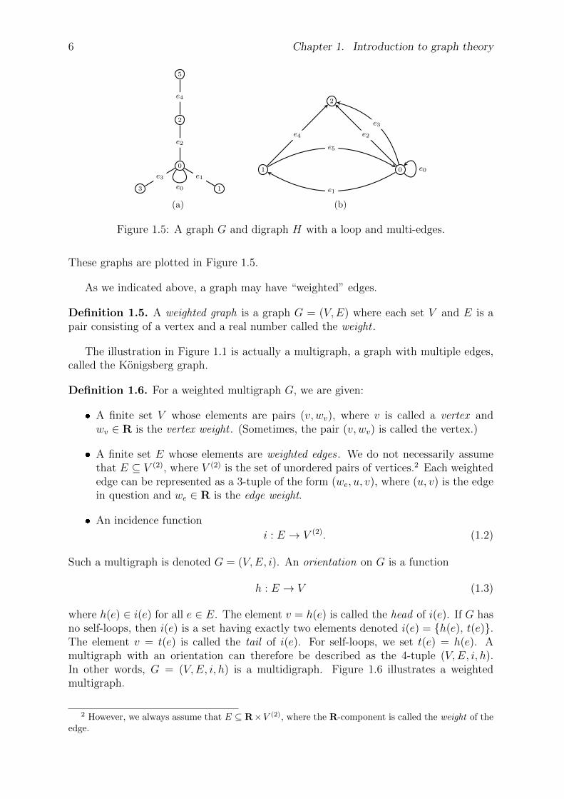
Example 1.4. Sage can compute with and plot multigraphs, or multidigraphs, havingloops.sage: G = Graph (0:0: ’e0’ ,1:’e1’ ,2:’e2’ ,3:’e3’, 2:5: ’e4’)sage: G.show(vertex_labels=True , edge_labels=True , graph_border=True)sage: H = DiGraph (0:0:"e0", Loops=True)sage: H.add_edges ([(0,1,’e1’), (0,2,’e2’), (0,2,’e3’), (1,2,’e4’), (1,0,’e5’)])sage: H.show(vertex_labels=True , edge_labels=True , graph_border=True)
6 Chapter 1. Introduction to graph theory
0
1
2
3
5
e1
e2
e3
e4
e0
(a)
01
2
e4 e2
e3
e1
e5
e0
(b)
Figure 1.5: A graph G and digraph H with a loop and multi-edges.
These graphs are plotted in Figure 1.5.
As we indicated above, a graph may have “weighted” edges.
Definition 1.5. A weighted graph is a graph G = (V,E) where each set V and E is apair consisting of a vertex and a real number called the weight .
The illustration in Figure 1.1 is actually a multigraph, a graph with multiple edges,called the Konigsberg graph.
Definition 1.6. For a weighted multigraph G, we are given:
A finite set V whose elements are pairs (v, wv), where v is called a vertex andwv ∈ R is the vertex weight . (Sometimes, the pair (v, wv) is called the vertex.)
A finite set E whose elements are weighted edges . We do not necessarily assumethat E ⊆ V (2), where V (2) is the set of unordered pairs of vertices.2 Each weightededge can be represented as a 3-tuple of the form (we, u, v), where (u, v) is the edgein question and we ∈ R is the edge weight.
An incidence function
i : E → V (2). (1.2)
Such a multigraph is denoted G = (V,E, i). An orientation on G is a function
h : E → V (1.3)
where h(e) ∈ i(e) for all e ∈ E. The element v = h(e) is called the head of i(e). If G hasno self-loops, then i(e) is a set having exactly two elements denoted i(e) = h(e), t(e).The element v = t(e) is called the tail of i(e). For self-loops, we set t(e) = h(e). Amultigraph with an orientation can therefore be described as the 4-tuple (V,E, i, h).In other words, G = (V,E, i, h) is a multidigraph. Figure 1.6 illustrates a weightedmultigraph.
2 However, we always assume that E ⊆ R×V (2), where the R-component is called the weight of theedge.

1.1. Graphs and digraphs 7
v1v2
v3 v4
v5
1
3
1
3 1
2
1
3
2
3
6
1
Figure 1.6: An example of a weighted multigraph.
The vertex degree of a weighted multigraph must be defined. There is a weighteddegree and an unweighted degree. Let G be a graph as in Definition 1.6. The unweightedindegree of a vertex v ∈ V counts the edges going into v:
deg+(v) =∑
e∈Eh(e)=v
1.
The unweighted outdegree of a vertex v ∈ V counts the edges going out of v:
deg−(v) =∑
e∈Ev∈i(e)=v,v′
h(e)=v′
1.
The unweighted degree deg(v) of a vertex v of a weighted multigraph is the sum of theunweighted indegree and the unweighted outdegree of v:
deg(v) = deg+(v) + deg−(v). (1.4)
Loops are counted twice.Similarly, there is the set of in-neighbors
iadj(v) = w ∈ V | for some e ∈ E, i(e) = v, w, h(e) = v
and the set of out-neighbors
oadj(v) = w ∈ V | for some e ∈ E, i(e) = v, w, h(e) = w.
Define the adjacency of v to be the union of these:
adj(v) = iadj(v) ∪ oadj(v). (1.5)
It is clear that deg+(v) = | iadj(v)| and deg−(v) = | oadj(v)|.The weighted indegree of a vertex v ∈ V counts the weights of edges going into v:
wdeg +(v) =∑
e∈Eh(e)=v
wv.

8 Chapter 1. Introduction to graph theory
The weighted outdegree of a vertex v ∈ V counts the weights of edges going out of v:
wdeg −(v) =∑
e∈Ev∈i(e)=v,v′
h(e)=v′
wv.
The weighted degree of a vertex of a weighted multigraph is the sum of the weightedindegree and the weighted outdegree of that vertex,
wdeg(v) = wdeg +(v) + wdeg −(v).
In other words, it is the sum of the weights of the edges incident to that vertex, regardingthe graph as an undirected weighted graph. Unweighted degrees are a special case ofweighted degrees. For unweighted degrees, we merely set each edge weight to unity.
Definition 1.7. Let G = (V,E, h) be an unweighted multidigraph. The line graph of G,denoted L(G), is the multidigraph whose vertices are the edges of G and whose edges are(e, e′) where h(e) = t(e′) (for e, e′ ∈ E). A similar definition holds if G is undirected.
For example, the line graph of the cyclic graph is itself.
1.1.2 Simple graphs
Our life is frittered away by detail. . . . Simplify, simplify. Instead of three meals a day, ifit be necessary eat but one; instead of a hundred dishes, five; and reduce other things inproportion.— Henry David Thoreau, Walden, 1854, Chapter 2: Where I Lived, and What I Lived For
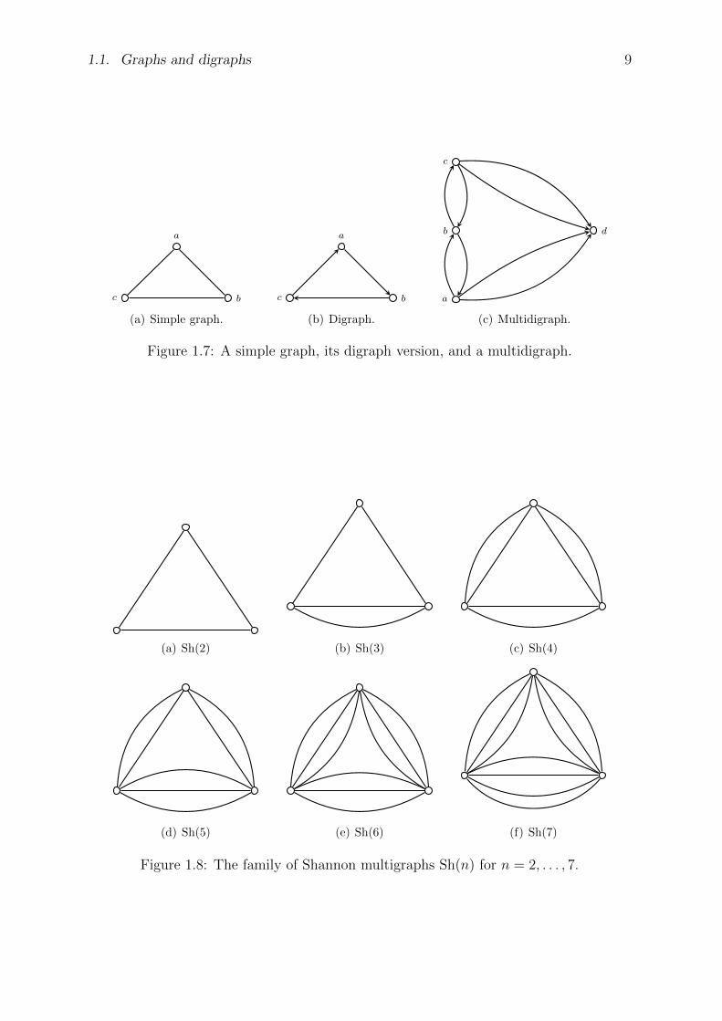
A simple graph is a graph with no self-loops and no multiple edges. Figure 1.7 illustratesa simple graph and its digraph version, together with a multidigraph version of theKonigsberg graph. The edges of a digraph can be visually represented as directed arrows,similar to the digraph in Figure 1.7(b) and the multidigraph in Figure 1.7(c). The digraphin Figure 1.7(b) has the vertex set a, b, c and the edge set ab, bc, ca. There is an arrowfrom vertex a to vertex b, hence ab is in the edge set. However, there is no arrow fromb to a, so ba is not in the edge set of the graph in Figure 1.7(b). The family Sh(n) ofShannon multigraphs is illustrated in Figure 1.8 for integers 2 ≤ n ≤ 7. These graphsare named after Claude E. Shannon (1916–2001) and are sometimes used when studyingedge colorings. Each Shannon multigraph consists of three vertices, giving rise to a totalof three distinct unordered pairs. Two of these pairs are connected by bn/2c edges andthe third pair of vertices is connected by b(n+ 1)/2c edges.
Notational convention Unless stated otherwise, all graphs are simple graphs in theremainder of this book.
Definition 1.8. For any vertex v in a graph G = (V,E), the cardinality of adj(v) (asin 1.5) is called the degree of v and written as deg(v) = | adj(v)|. The degree of v countsthe number of vertices in G that are adjacent to v. If deg(v) = 0, then v is not incidentto any edge and we say that v is an isolated vertex. If G has no loops and deg(v) = 1,then v is called a pendant.
1.1. Graphs and digraphs 9
c b
a
(a) Simple graph.
c b
a
(b) Digraph.
a
b
c
d
(c) Multidigraph.
Figure 1.7: A simple graph, its digraph version, and a multidigraph.
(a) Sh(2) (b) Sh(3) (c) Sh(4)
(d) Sh(5) (e) Sh(6) (f) Sh(7)
Figure 1.8: The family of Shannon multigraphs Sh(n) for n = 2, . . . , 7.
10 Chapter 1. Introduction to graph theory
Some examples would put the above definition in concrete terms. Consider againthe graph in Figure 1.4. Note that no vertices are isolated. Even though vertex a isnot incident to any vertex other than a itself, note that deg(a) = 2 and so by definitiona is not isolated. Furthermore, each of b and c is a pendant. For the house graph inFigure 1.3, we have deg(b) = 3. For the graph in Figure 1.7(b), we have deg(b) = 2.If V 6= ∅ and E = ∅, then G is a graph consisting entirely of isolated vertices. FromExample 1.2 we know that the vertices a, c, d in Figure 1.3 have the smallest degree inthe graph of that figure, while b, e have the largest degree.
The minimum degree among all vertices in G is denoted δ(G), whereas the maximumdegree is written as ∆(G). Thus, if G denotes the graph in Figure 1.3 then we haveδ(G) = 2 and ∆(G) = 3. In the following Sage session, we construct the digraph inFigure 1.7(b) and compute its maximum and minimum number of degrees.
sage: G = DiGraph ("a":"b", "b":"c", "c":"a")sage: GDigraph on 3 verticessage: G.degree("a")2sage: G.degree("b")2sage: G.degree("c")2
So for the graph G in Figure 1.7, we have δ(G) = ∆(G) = 2.The graph G in Figure 1.7 has the special property that its minimum degree is the
same as its maximum degree, i.e. δ(G) = ∆(G). Graphs with this property are referredto as regular . An r-regular graph is a regular graph each of whose vertices has degree r.For instance, G is a 2-regular graph. The following result, due to Euler, counts the totalnumber of degrees in any graph.
Theorem 1.9. Euler 1736. If G = (V,E) is a graph, then∑
v∈V deg(v) = 2|E|.
Proof. Each edge e = v1v2 ∈ E is incident with two vertices, so e is counted twicetowards the total sum of degrees. The first time, we count e towards the degree of vertexv1 and the second time we count e towards the degree of v2.
Theorem 1.9 is sometimes called the “handshaking lemma,” due to its interpretationas in the following story. Suppose you go into a room. Suppose there are n people in theroom (including yourself) and some people shake hands with others and some do not.Create the graph with n vertices, where each vertex is associated with a different person.Draw an edge between two people if they shook hands. The degree of a vertex is thenumber of times that person has shaken hands (we assume that there are no multipleedges, i.e. that no two people shake hands twice). The theorem above simply says thatthe total number of handshakes is even. This is “obvious” when you look at it this waysince each handshake is counted twice (A shaking B’s hand is counted, and B shaking A’shand is counted as well, since the sum in the theorem is over all vertices). To interpretTheorem 1.9 in a slightly different way within the context of the same room of people,there is an even number of people who shook hands with an odd number of other people.This consequence of Theorem 1.9 is recorded in the following corollary.
Corollary 1.10. A graph G = (V,E) contains an even number of vertices with odddegrees.
Proof. Partition V into two disjoint subsets: Ve is the subset of V that contains onlyvertices with even degrees; and Vo is the subset of V with only vertices of odd degrees.

1.2. Subgraphs and other graph types 11
That is, V = Ve ∪ Vo and Ve ∩ Vo = ∅. From Theorem 1.9, we have
∑
v∈V
deg(v) =∑
v∈Ve
deg(v) +∑
v∈Vo
deg(v) = 2|E|
which can be re-arranged as
∑
v∈Vo
deg(v) =∑
v∈V
deg(v)−∑
v∈Ve
deg(v).
As∑
v∈V deg(v) and∑
v∈Ve deg(v) are both even, their difference is also even.
As E ⊆ V (2), then E can be the empty set, in which case the total degree of G =(V,E) is zero. Where E 6= ∅, then the total degree of G is greater than zero. ByTheorem 1.9, the total degree of G is nonnegative and even. This result is an immediateconsequence of Theorem 1.9 and is captured in the following corollary.
Corollary 1.11. If G is a graph, then the sum of its vertex degrees is nonnegative andeven.
If G = (V,E) is an r-regular graph with n vertices and m edges, it is clear by definitionof r-regular graphs that the total degree of G is rn. By Theorem 1.9 we have 2m = rnand therefore m = rn/2. This result is captured in the following corollary.
Corollary 1.12. If G = (V,E) is an r-regular graph having n vertices and m edges,then m = rn/2.
1.2 Subgraphs and other graph types
We now consider several common types of graphs. Along the way, we also present basicproperties of graphs that could be used to distinguish different types of graphs.
Let G be a multigraph as in Definition 1.6, with vertex set V (G) and edge set E(G).Consider a graph H such that V (H) ⊆ V (G) and E(H) ⊆ E(G). Furthermore, ife ∈ E(H) and i(e) = u, v, then u, v ∈ V (H). Under these conditions, H is called asubgraph of G.
1.2.1 Walks, trails, and paths
I like long walks, especially when they are taken by people who annoy me.— Noel Coward
If u and v are two vertices in a graph G, a u-v walk is an alternating sequence of verticesand edges starting with u and ending at v. Consecutive vertices and edges are incident.Formally, a walk W of length n ≥ 0 can be defined as
W : v0, e1, v1, e2, v2, . . . , vn−1, en, vn
where each edge ei = vi−1vi and the length n refers to the number of (not necessarilydistinct) edges in the walk. The vertex v0 is the starting vertex of the walk and vn isthe end vertex, so we refer to W as a v0-vn walk. The trivial walk is the walk of lengthn = 0 in which the start and end vertices are one and the same vertex. If the graph has

12 Chapter 1. Introduction to graph theory
no multiple edges then, for brevity, we omit the edges in a walk and usually write thewalk as the following sequence of vertices:
W : v0, v1, v2, . . . , vn−1, vn.
For the graph in Figure 1.9, an example of a walk is an a-e walk: a, b, c, b, e. In otherwords, we start at vertex a and travel to vertex b. From b, we go to c and then back tob again. Then we end our journey at e. Notice that consecutive vertices in a walk areadjacent to each other. One can think of vertices as destinations and edges as footpaths,say. We are allowed to have repeated vertices and edges in a walk. The number of edgesin a walk is called its length. For instance, the walk a, b, c, b, e has length 4.
ba
c
d
e
g
f
Figure 1.9: Walking along a graph.
A trail is a walk with no repeating edges. For example, the a-b walk a, b, c, d, f, g, b inFigure 1.9 is a trail. It does not contain any repeated edges, but it contains one repeatedvertex, i.e. b. Nothing in the definition of a trail restricts a trail from having repeatedvertices. A walk with no repeating vertices, except possibly the first and last, is called apath. Without any repeating vertices, a path cannot have repeating edges, hence a pathis also a trail.
Proposition 1.13. Let G = (V,E) be a simple (di)graph of order n = |V |. Any path inG has length at most n− 1.
Proof. Let V = v1, v2, . . . , vn be the vertex set of G. Without loss of generality, we canassume that each pair of vertices in the digraph G is connected by an edge, giving a totalof n2 possible edges for E = V × V . We can remove self-loops from E, which now leavesus with an edge set E1 that consists of n2 − n edges. Start our path from any vertex,say, v1. To construct a path of length 1, choose an edge v1vj1 ∈ E1 such that vj1 /∈ v1.Remove from E1 all v1vk such that vj1 6= vk. This results in a reduced edge set E2 ofn2 − n− (n− 2) elements and we now have the path P1 : v1, vj1 of length 1. Repeat thesame process for vj1vj2 ∈ E2 to obtain a reduced edge set E3 of n2−n−2(n−2) elementsand a path P2 : v1, vj1 , vj2 of length 2. In general, let Pr : v1, vj1 , vj2 , . . . , vjr be a path oflength r < n and let Er+1 be our reduced edge set of n2−n− r(n− 2) elements. Repeatthe above process until we have constructed a path Pn−1 : v1, vj1 , vj2 , . . . , vjn−1 of lengthn − 1 with reduced edge set En of n2 − n − (n − 1)(n − 2) elements. Adding anothervertex to Pn−1 means going back to a vertex that was previously visited, because Pn−1
already contains all vertices of V .

1.2. Subgraphs and other graph types 13
A walk of length n ≥ 3 whose start and end vertices are the same is called a closedwalk . A trail of length n ≥ 3 whose start and end vertices are the same is called a closedtrail . A path of length n ≥ 3 whose start and end vertices are the same is called a closedpath or a cycle (with apologies for slightly abusing terminology).3 For example, thewalk a, b, c, e, a in Figure 1.9 is a closed path. A path whose length is odd is called odd ,otherwise it is referred to as even. Thus the walk a, b, e, a in Figure 1.9 is a cycle. It iseasy to see that if you remove any edge from a cycle, then the resulting walk contains noclosed walks. An Euler subgraph of a graph G is either a cycle or an edge-disjoint unionof cycles in G. An example of a closed walk which is not a cycle is given in Figure 1.10.
0
1
2
3
4
Figure 1.10: Butterfly graph with 5 vertices.
The length of the shortest cycle in a graph is called the girth of the graph. Byconvention, an acyclic graph is said to have infinite girth.
Example 1.14. Consider the graph in Figure 1.9.
1. Find two distinct walks that are not trails and determine their lengths.
2. Find two distinct trails that are not paths and determine their lengths.
3. Find two distinct paths and determine their lengths.
4. Find a closed trail that is not a cycle.
5. Find a closed walk C which has an edge e such that C − e contains a cycle.
Solution. (1) Here are two distinct walks that are not trails: w1 : g, b, e, a, b, e andw2 : f, d, c, e, f, d. The length of walk w1 is 5 and the length of walk w2 is also 5.
(2) Here are two distinct trails that are not paths: t1 : a, b, c, e, b and t2 : b, e, f, d, c, e.The length of trail t1 is 4 and the length of trail t2 is 5.
(3) Here are two distinct paths: p1 : a, b, c, d, f, e and p2 : g, b, a, e, f, d. The length ofpath p1 is 5 and the length of path p2 is also 5.
(4) Here is a closed trail that is not a cycle: d, c, e, b, a, e, f, d.(5) Left as an exercise.
Theorem 1.15. Every u-v walk in a graph contains a u-v path.
Proof. A walk of length n = 0 is the trivial path. So assume that W is a u-v walk oflength n > 0 in a graph G:
W : u = v0, v1, . . . , vn = v.
It is possible that a vertex in W is assigned two different labels. If W has no repeatedvertices, then W is already a path. Otherwise W has at least one repeated vertex. Let
3 A cycle in a graph is sometimes also called a “circuit”. Since that terminology unfortunatelyconflicts with the closely related notion of a circuit of a matroid, we do not use it here.

14 Chapter 1. Introduction to graph theory
0 ≤ i, j ≤ n be two distinct integers with i < j such that vi = vj. Deleting the verticesvi, vi+1, . . . , vj−1 from W results in a u-v walk W1 whose length is less than n. If W1 isa path, then we are done. Otherwise we repeat the above process to obtain a u-v walkshorter than W1. As W is a finite sequence, we only need to apply the above process afinite number of times to arrive at a u-v path.
A graph is said to be connected if for every pair of distinct vertices u, v there is au-v path joining them. A graph that is not connected is referred to as disconnected .The empty graph is disconnected and so is any nonempty graph with an isolated vertex.However, the graph in Figure 1.7 is connected. A geodesic path or shortest path betweentwo distinct vertices u, v of a graph is a u-v path of minimum length. A nonempty graphmay have several shortest paths between some distinct pair of vertices. For the graphin Figure 1.9, both a, b, c and a, e, c are geodesic paths between a and c. Let H be aconnected subgraph of a graph G such that H is not a proper subgraph of any connectedsubgraph of G. Then H is said to be a component of G. We also say that H is a maximalconnected subgraph of G. Any connected graph is its own component. The number ofconnected components of a graph G will be denoted ω(G).
The following is an immediate consequence of Corollary 1.10.
Proposition 1.16. Suppose that exactly two vertices of a graph have odd degree. Thenthose two vertices are connected by a path.
Proof. Let G be a graph all of whose vertices are of even degree, except for u and v. LetC be a component of G containing u. By Corollary 1.10, C also contains v, the onlyremaining vertex of odd degree. As u and v belong to the same component, they areconnected by a path.
Example 1.17. Determine whether or not the graph in Figure 1.9 is connected. Find ashortest path from g to d.
Solution. In the following Sage session, we first construct the graph in Figure 1.9 anduse the method is_connected() to determine whether or not the graph is connected.Finally, we use the method shortest_path() to find a geodesic path between g and d.sage: g = Graph ("a":["b","e"], "b":["a","g","e","c"], \... "c":["b","e","d"], "d":["c","f"], "e":["f","a","b","c"], \... "f":["g","d","e"], "g":["b","f"])sage: g.is_connected ()Truesage: g.shortest_path("g", "d")[’g’, ’f’, ’d’]
This shows that g, f, d is a shortest path from g to d. In fact, any other g-d path haslength greater than 2, so we can say that g, f, d is the shortest path between g and d.
Remark 1.18. We will explain Dijkstra’s algorithm in Chapter 3. Dijkstra’s algorithmgives one of the best algorithms for finding shortest paths between two vertices in aconnected graph. What is very remarkable is that, at the present state of knowledge,finding the shortest path from a vertex v to a particular (but arbitrarily given) vertex wappears to be as hard as finding the shortest path from a vertex v to all other verticesin the graph!
Trees are a special type of graphs that are used in modelling structures that havesome form of hierarchy. For example, the hierarchy within an organization can be drawnas a tree structure, similar to the family tree in Figure 1.11. Formally, a tree is an

1.2. Subgraphs and other graph types 15
undirected graph that is connected and has no cycles. If one vertex of a tree is speciallydesignated as the root vertex , then the tree is called a rooted tree. Chapter 2 covers treesin more details.
me sister brother
mum
cousin1 cousin2
uncle aunt
grandma
Figure 1.11: A family tree.
1.2.2 Subgraphs, complete and bipartite graphs
Let G be a graph with vertex set V (G) and edge set E(G). Suppose we have a graphH such that V (H) ⊆ V (G) and E(H) ⊆ E(G). Furthermore, suppose the incidencefunction i of G, when restricted to E(H), has image in V (H)(2). Then H is a subgraphof G. In this situation, G is referred to as a supergraph of H.
Starting from G, one can obtain its subgraph H by deleting edges and/or verticesfrom G. Note that when a vertex v is removed from G, then all edges incident withv are also removed. If V (H) = V (G), then H is called a spanning subgraph of G. InFigure 1.12, let G be the left-hand side graph and let H be the right-hand side graph.Then it is clear that H is a spanning subgraph of G. To obtain a spanning subgraphfrom a given graph, we delete edges from the given graph.
(a) (b)
Figure 1.12: A graph and one of its subgraphs.
We now consider several standard classes of graphs. The complete graph Kn on nvertices is a graph such that any two distinct vertices are adjacent. As |V (Kn)| = n,then |E(Kn)| is equivalent to the total number of 2-combinations from a set of n objects:
|E(Kn)| =(n
2
)=n(n− 1)
2. (1.6)
Thus for any simple graph G with n vertices, its total number of edges |E(G)| is boundedabove by
|E(G)| ≤ n(n− 1)
2. (1.7)

16 Chapter 1. Introduction to graph theory
Figure 1.13 shows complete graphs each of whose total number of vertices is bounded by1 ≤ n ≤ 5. The complete graph K1 has one vertex with no edges. It is also called thetrivial graph.
(a) K5 (b) K4 (c) K3 (d) K2 (e) K1
Figure 1.13: Complete graphs Kn for 1 ≤ n ≤ 5.
The following result is an application of inequality (1.7).
Theorem 1.19. Let G be a simple graph with n vertices and k components. Then Ghas at most 1
2(n− k)(n− k + 1) edges.
Proof. If ni is the number of vertices in component i, then ni > 0 and it can be shown (seethe proof of Lemma 2.1 in [80, pp.21–22]) that
∑n2i ≤
(∑ni
)2
− (k − 1)(
2∑
ni − k). (1.8)
(This result holds true for any nonempty but finite set of positive integers.) Note that∑ni = n and by (1.7) each component i has at most 1
2ni(ni − 1) edges. Apply (1.8) to
get
∑ ni(ni − 1)
2=
1
2
∑n2i −
1
2
∑ni
≤ 1
2(n2 − 2nk + k2 + 2n− k)− 1
2n
=(n− k)(n− k + 1)
2
as required.
The cycle graph on n ≥ 3 vertices, denoted Cn, is the connected 2-regular graph on nvertices. Each vertex in Cn has degree exactly 2 and Cn is connected. Figure 1.14 showscycles graphs Cn where 3 ≤ n ≤ 6. The path graph on n ≥ 1 vertices is denoted Pn. Forn = 1, 2 we have P1 = K1 and P2 = K2. Where n ≥ 3, then Pn is a spanning subgraphof Cn obtained by deleting one edge.
A bipartite graph G is a graph with at least two vertices such that V (G) can be splitinto two disjoint subsets V1 and V2, both nonempty. Every edge uv ∈ E(G) is such thatu ∈ V1 and v ∈ V2, or v ∈ V1 and u ∈ V2. See Kalman [116] for an application of bipartitegraphs to the problem of allocating satellites to radio stations.
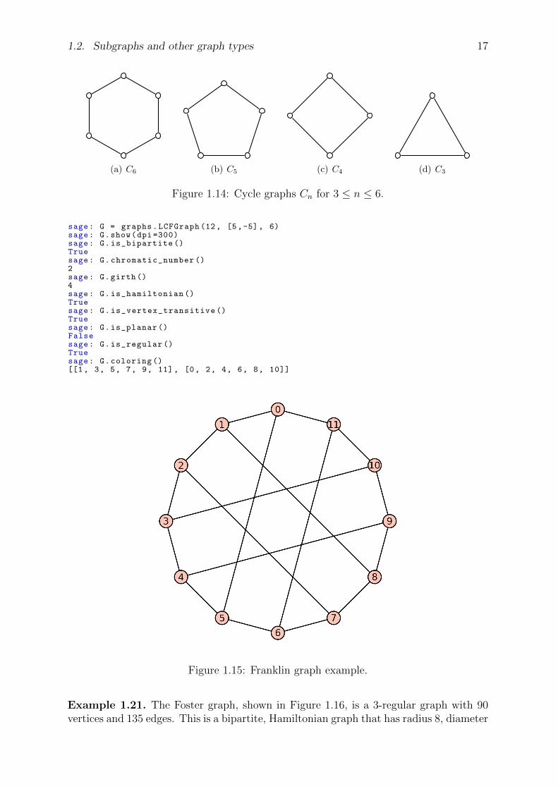
Example 1.20. The Franklin graph, shown in Figure 1.15, is named after Philip Franklin.It is a 3-regular graph with 12 vertices and 18 edges. It is bipartite, Hamiltonian and hasradius 3, diameter 3 and girth 4. It is also a 3-vertex-connected and 3-edge-connectedperfect graph.
1.2. Subgraphs and other graph types 17
(a) C6 (b) C5 (c) C4 (d) C3
Figure 1.14: Cycle graphs Cn for 3 ≤ n ≤ 6.
sage: G = graphs.LCFGraph (12, [5,-5], 6)sage: G.show(dpi =300)sage: G.is_bipartite ()Truesage: G.chromatic_number ()2sage: G.girth ()4sage: G.is_hamiltonian ()Truesage: G.is_vertex_transitive ()Truesage: G.is_planar ()Falsesage: G.is_regular ()Truesage: G.coloring ()[[1, 3, 5, 7, 9, 11], [0, 2, 4, 6, 8, 10]]
Figure 1.15: Franklin graph example.
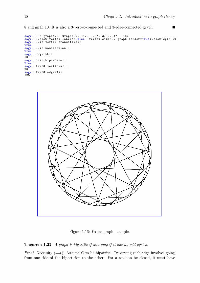
Example 1.21. The Foster graph, shown in Figure 1.16, is a 3-regular graph with 90vertices and 135 edges. This is a bipartite, Hamiltonian graph that has radius 8, diameter
18 Chapter 1. Introduction to graph theory
8 and girth 10. It is also a 3-vertex-connected and 3-edge-connected graph.
sage: G = graphs.LCFGraph (90, [17,-9,37,-37,9,-17], 15)sage: G.plot(vertex_labels=False , vertex_size =0, graph_border=True).show(dpi =300)sage: G.is_vertex_transitive ()Truesage: G.is_hamiltonian ()Truesage: G.girth ()10sage: G.is_bipartite ()Truesage: len(G.vertices ())90sage: len(G.edges ())135
Figure 1.16: Foster graph example.
Theorem 1.22. A graph is bipartite if and only if it has no odd cycles.
Proof. Necessity (=⇒): Assume G to be bipartite. Traversing each edge involves goingfrom one side of the bipartition to the other. For a walk to be closed, it must have

1.3. Representing graphs in a computer 19
even length in order to return to the side of the bipartition from which the walk started.Thus, any cycle in G must have even length.
Sufficiency (⇐=): Assume G = (V,E) has order n ≥ 2 and no odd cycles. If G isconnected, choose any vertex u ∈ V and define a partition of V thus:
X = x ∈ V | d(u, x) is even,Y = y ∈ V | d(u, y) is odd
where d(u, v) denotes the distance (or length of the shortest path) from u to v. If (X, Y )is a bipartition of G, then we are done. Otherwise, (X, Y ) is not a bipartition of G.Then one of X and Y has two vertices v, w joined by an edge e. Let P1 be a shortestu-v path and P2 be a shortest u-w path. By definition of X and Y , both P1 and P2 haveeven lengths or both have odd lengths. From u, let x be the last vertex common to bothP1 and P2. The subpath u-x of P1 and u-x of P2 have equal length. That is, the subpathx-v of P1 and x-w of P2 both have even or odd lengths. Construct a cycle C from thepaths x-v and x-w, and the edge e joining v and w. Since x-v and x-w both have evenor odd lengths, the cycle C has odd length, contradicting our hypothesis that G has noodd cycles. Hence, (X, Y ) is a bipartition of G.
Finally, if G is disconnected, each of its components has no odd cycles. Repeat theabove argument for each component to conclude that G is bipartite.
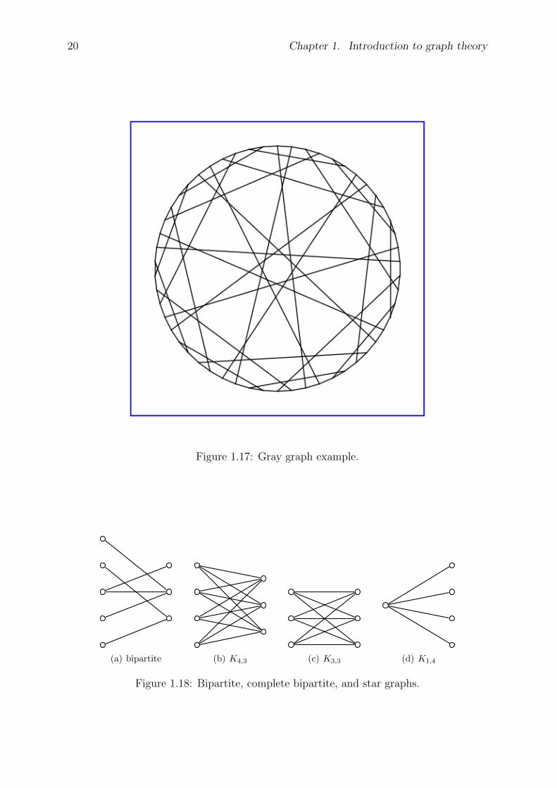
Example 1.23. The Gray graph, shown in Figure 1.17, is an undirected bipartite graphwith 54 vertices and 81 edges. It is a 3-regular graph discovered by Marion C. Grayin 1932. The Gray graph has chromatic number 2, chromatic index 3, radius 6, anddiameter 6. It is also a 3-vertex-connected and 3-edge-connected non-planar graph. TheGray graph is an example of a graph which is edge-transitive but not vertex-transitive.
sage: G = graphs.LCFGraph (54, [-25,7,-7,13,-13,25], 9)sage: G.plot(vertex_labels=False , vertex_size =0, graph_border=True)sage: G.is_bipartite ()Truesage: G.is_vertex_transitive ()Falsesage: G.is_hamiltonian ()Truesage: G.diameter ()6
The complete bipartite graph Km,n is the bipartite graph whose vertex set is parti-tioned into two nonempty disjoint sets V1 and V2 with |V1| = m and |V2| = n. Anyvertex in V1 is adjacent to each vertex in V2, and any two distinct vertices in Vi are notadjacent to each other. If m = n, then Kn,n is n-regular. Where m = 1 then K1,n iscalled the star graph. Figure 1.18 shows a bipartite graph together with the completebipartite graphs K4,3 and K3,3, and the star graph K1,4.
As an example of K3,3, suppose that there are 3 boys and 3 girls dancing in a room.The boys and girls naturally partition the set of all people in the room. Construct agraph having 6 vertices, each vertex corresponding to a person in the room, and drawan edge form one vertex to another if the two people dance together. If each girl dancesthree times, once with with each of the three boys, then the resulting graph is K3,3.
1.3 Representing graphs in a computer
Neo: What is the Matrix?Morpheus: Unfortunately, no one can be told what the Matrix is. You have to see it for
20 Chapter 1. Introduction to graph theory
Figure 1.17: Gray graph example.
(a) bipartite (b) K4,3 (c) K3,3 (d) K1,4
Figure 1.18: Bipartite, complete bipartite, and star graphs.
1.3. Representing graphs in a computer 21
yourself.— From the movie The Matrix, 1999
An m× n matrix A can be represented as
A =
a11 a12 · · · a1n
a21 a22 · · · a2n
. . . . . . . . . . . . . . . . . . .am1 am2 · · · amn
.
The positive integers m and n are the row and column dimensions of A, respectively.The entry in row i column j is denoted aij. Where the dimensions of A are clear fromcontext, A is also written as A = [aij].
Representing a graph as a matrix is very inefficient in some cases and not so inother cases. Imagine you walk into a large room full of people and you consider the“handshaking graph” discussed in connection with Theorem 1.9. If not many peopleshake hands in the room, it is a waste of time recording all the handshakes and also allthe “non-handshakes.” This is basically what the adjacency matrix does. In this kindof “sparse graph” situation, it would be much easier to simply record the handshakes asa Python dictionary.4 This section requires some concepts and techniques from linearalgebra, especially matrix theory. See introductory texts on linear algebra and matrixtheory [19] for coverage of such concepts and techniques.
1.3.1 Adjacency matrix
Let G be an undirected graph with vertices V = v1, . . . , vn and edge set E. Theadjacency matrix of G is the n× n matrix A = [aij] defined by
aij =
1, if vivj ∈ E,0, otherwise.
The adjacency matrix of G is also written as A(G). As G is an undirected graph, thenA is a symmetric matrix. That is, A is a square matrix such that aij = aji.
Now let G be a directed graph with vertices V = v1, . . . , vn and edge set E. The(0,−1, 1)-adjacency matrix of G is the n× n matrix A = [aij] defined by
aij =
1, if vivj ∈ E,−1, if vjvi ∈ E,0, otherwise.
Example 1.24. Compute the adjacency matrices of the graphs in Figure 1.19.
Solution. Define the graphs in Figure 1.19 using DiGraph and Graph. Then call themethod adjacency_matrix().
4 A Python dictionary is basically an indexed set. See the reference manual at http://www.python.orgfor further details.

22 Chapter 1. Introduction to graph theory
1
2
3
4
5
6
(a)
c
e
f
a
b
d
(b)
Figure 1.19: What are the adjacency matrices of these graphs?
sage: G1 = DiGraph (1:[2] , 2:[1], 3:[2,6], 4:[1,5], 5:[6], 6:[5])sage: G2 = Graph ("a":["b","c"], "b":["a","d"], "c":["a","e"], \... "d":["b","f"], "e":["c","f"], "f":["d","e"])sage: m1 = G1.adjacency_matrix (); m1[0 1 0 0 0 0][1 0 0 0 0 0][0 1 0 0 0 1][1 0 0 0 1 0][0 0 0 0 0 1][0 0 0 0 1 0]sage: m2 = G2.adjacency_matrix (); m2[0 1 1 0 0 0][1 0 0 1 0 0][1 0 0 0 1 0][0 1 0 0 0 1][0 0 1 0 0 1][0 0 0 1 1 0]sage: m1.is_symmetric ()Falsesage: m2.is_symmetric ()True
In general, the adjacency matrix of a digraph is not symmetric, while that of an undi-rected graph is symmetric.
More generally, if G is an undirected multigraph with edge eij = vivj having mul-tiplicity wij, or a weighted graph with edge eij = vivj having weight wij, then we candefine the (weighted) adjacency matrix A = [aij] by
aij =
wij, if vivj ∈ E,0, otherwise.
For example, Sage allows you to easily compute a weighted adjacency matrix.sage: G = Graph(sparse=True , weighted=True)sage: G.add_edges ([(0,1,1), (1,2,2), (0,2,3), (0 ,3,4)])sage: M = G.weighted_adjacency_matrix (); M[0 1 3 4][1 0 2 0][3 2 0 0][4 0 0 0]
Bipartite case
Suppose G = (V,E) is an undirected bipartite graph with n = |V | vertices. Any ad-jacency matrix A of G is symmetric and we assume that it is indexed from zero up to

1.3. Representing graphs in a computer 23
n−1, inclusive. Then there exists a permutation π of the index set 0, 1, . . . , n−1 suchthat the matrix A′ = [aπ(i)π(j)] is also an adjacency matrix for G and has the form
A′ =
[0 BBT 0
](1.9)
where 0 is a zero matrix. The matrix B is called a reduced adjacency matrix or a bi-adjacency matrix (the literature also uses the terms “transfer matrix” or the ambiguousterm “adjacency matrix”). In fact, it is known [9, p.16] that any undirected graph isbipartite if and only if there is a permutation π on 0, 1, . . . , n − 1 such that A′(G) =[aπ(i)π(j)] can be written as in (1.9).
Tanner graphs
If H is an m × n (0, 1)-matrix, then the Tanner graph of H is the bipartite graphG = (V,E) whose set of vertices V = V1∪V2 is partitioned into two sets: V1 correspondingto the m rows of H and V2 corresponding to the n columns of H. For any i, j with1 ≤ i ≤ m and 1 ≤ j ≤ n, there is an edge ij ∈ E if and only if the (i, j)-th entry ofH is 1. This matrix H is sometimes called the reduced adjacency matrix or the checkmatrix of the Tanner graph. Tanner graphs are used in the theory of error-correctingcodes. For example, Sage allows you to easily compute such a bipartite graph from itsmatrix.sage: H = Matrix ([(1,1,1,0,0), (0,0,1,0,1), (1,0,0,1,1)])sage: B = BipartiteGraph(H)sage: B.reduced_adjacency_matrix ()[1 1 1 0 0][0 0 1 0 1][1 0 0 1 1]sage: B.plot(graph_border=True)
The corresponding graph is similar to that in Figure 1.20.
1
2
3
4
5
1
2
3
Figure 1.20: A Tanner graph.
Theorem 1.25. Let A be the adjacency matrix of a graph G with vertex set V =v1, v2, . . . , vp. For each positive integer n, the ij-th entry of An counts the numberof vi-vj walks of length n in G.
Proof. We shall prove by induction on n. For the base case n = 1, the ij-th entry ofA1 counts the number of walks of length 1 from vi to vj. This is obvious because A1 ismerely the adjacency matrix A.
Suppose for induction that for some positive integer k ≥ 1, the ij-th entry of Ak
counts the number of walks of length k from vi to vj. We need to show that the ij-th

24 Chapter 1. Introduction to graph theory
entry of Ak+1 counts the number of vi-vj walks of length k+ 1. Let A = [aij], Ak = [bij],
and Ak+1 = [cij]. Since Ak+1 = AAk, then
cij =
p∑
r=1
airbrj
for i, j = 1, 2, . . . , p. Note that air is the number of edges from vi to vr, and brj is thenumber of vr-vj walks of length k. Any edge from vi to vr can be joined with any vr-vjwalk to create a walk vi, vr, . . . , vj of length k + 1. Then for each r = 1, 2, . . . , p, thevalue airbrj counts the number of vi-vj walks of length k + 1 with vr being the secondvertex in the walk. Thus cij counts the total number of vi-vj walks of length k + 1.
1.3.2 Incidence matrix
The relationship between edges and vertices provides a very strong constraint on thedata structure, much like the relationship between points and blocks in a combinatorialdesign or points and lines in a finite plane geometry. This incidence structure gives riseto another way to describe a graph using a matrix.
Let G be a digraph with edge set E = e1, . . . , em and vertex set V = v1, . . . , vn.The incidence matrix of G is the n×m matrix B = [bij] defined by
bij =
−1, if vi is the tail of ej,
1, if vi is the head of ej,
2, if ej is a self-loop at vi,
0, otherwise.
(1.10)
Each column of B corresponds to an edge and each row corresponds to a vertex. Thedefinition of incidence matrix of a digraph as contained in expression (1.10) is applicableto digraphs with self-loops as well as multidigraphs.
For the undirected case, let G be an undirected graph with edge set E = e1, . . . , emand vertex set V = v1, . . . , vn. The unoriented incidence matrix of G is the n × mmatrix B = [bij] defined by
bij =
1, if vi is incident to ej,
2, if ej is a self-loop at vi,
0, otherwise.
An orientation of an undirected graph G is an assignment of direction to each edge ofG. In other words, each edge has a distinguished vertex called a head. In this case, theletter D = D(G) is sometimes used instead of B for the incidence matrix of a digraphor an oriented graph. The oriented incidence matrix D of G is defined similarly to thecase where G is a digraph: it is the incidence matrix of any orientation of G. For eachcolumn of D, we have 1 as an entry in the row corresponding to one vertex of the edgeunder consideration and −1 as an entry in the row corresponding to the other vertex.Similarly, dij = 2 if ej is a self-loop at vi.
Sage allows you to compute the incidence matrix of a graph:

1.3. Representing graphs in a computer 25
sage: G = Graph (1: [2, 4], 2: [1, 3], 3: [2, 6], 4: [1, 5], 5: [4, 6], 6: [3, 5])sage: G.incidence_matrix ()[-1 -1 0 0 0 0][ 0 1 -1 0 0 0][ 0 0 1 -1 0 0][ 1 0 0 0 -1 0][ 0 0 0 0 1 -1][ 0 0 0 1 0 1]
The integral cycle space of a graph is equal to the kernel of an oriented incidencematrix, viewed as a matrix over Q. The binary cycle space is the kernel of its orientedor unoriented incidence matrix, viewed as a matrix over GF (2).
Theorem 1.26. The incidence matrix of an undirected graph G is related to the adja-cency matrix of its line graph L(G) by the following theorem:
A(L(G)) = D(G)TD(G)− 2In ,
where A(L(G)) is the adjacency matrix of the line graph of G.
Proof. Let Di denote the ith column of D.Consider the dot product of Di and Dj, i 6= j. The terms contributing to this
expression are associated to the vertices which are incident to the ith edge and also tothe jth edge. In other words, there is such a vertex (and only one such vertex) if andonly if this dot product is equal to 1 if and only if ith edge is incident to the jth edgein G if and only if the vertex in L(G) associated to the ith edge in G is adjacent to thevertex in L(G) associated to the jth edge in G. But this is exactly the condition thatthe corresponding entry of A(L(G)) is equal to 1.
Consider the dot product of Di with itself. The terms contributing to this expressionare associated to the vertices which are incident to the ith edge. There are 2 such verticesso this dot product is equal to 2. Subtracting, the 2 in 2In, gives 0, as expect for thediagonal entries of A(L(G)).
For a directed graph, the result in the above theorem does not hold in general (exceptin characteristic 2), as the following example shows.
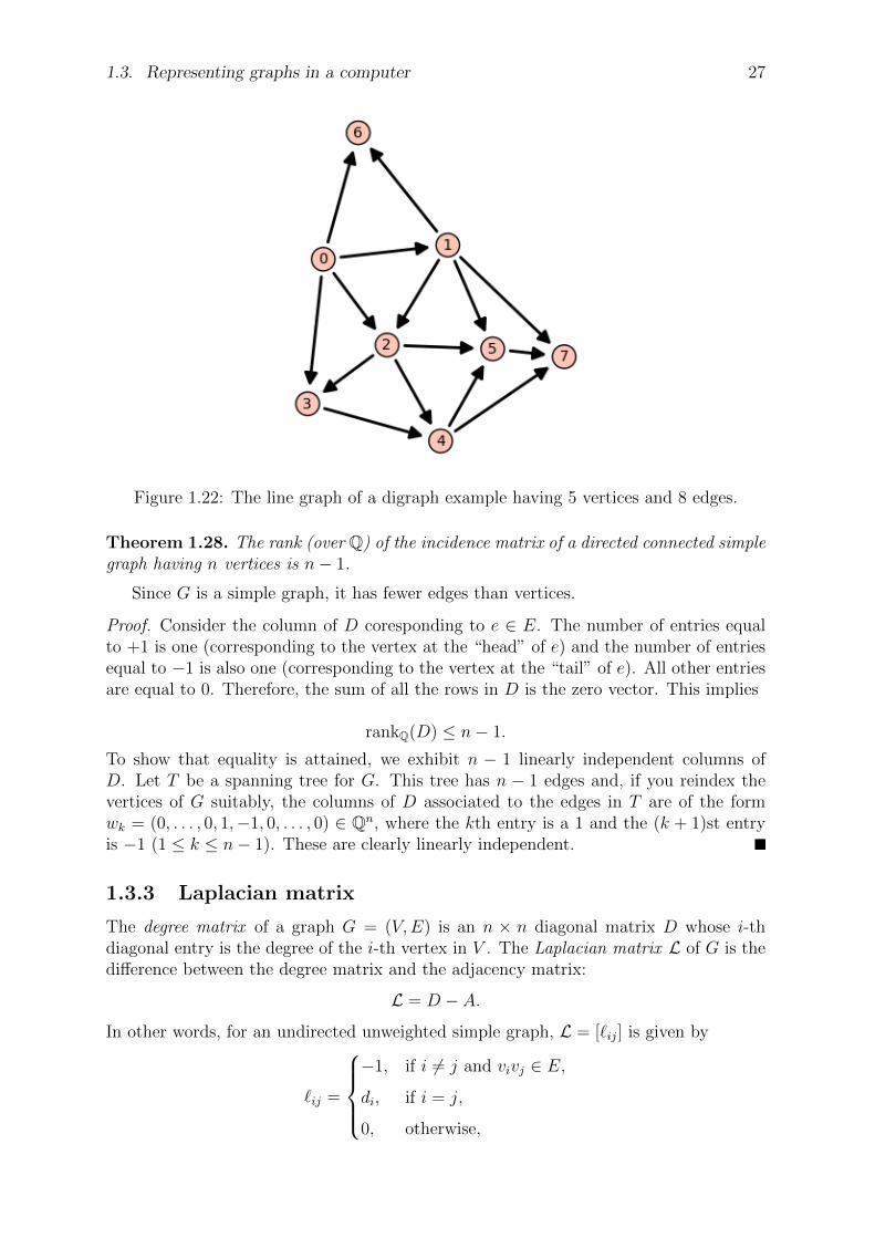
Example 1.27. Consider the graph shown in Figure 1.21, whose line graph is shown inFigure 1.22.
sage: G1 = DiGraph (0:[1 ,2,4], 1:[2,3,4], 2:[3 ,4])sage: G1.show()sage: D1 = G1.incidence_matrix (); D1[-1 -1 -1 0 0 0 0 0][ 0 0 1 -1 -1 -1 0 0][ 0 1 0 0 0 1 -1 -1][ 0 0 0 0 1 0 0 1][ 1 0 0 1 0 0 1 0]sage: A1 = G1.adjacency_matrix ()sage: A1[0 1 1 0 1][0 0 1 1 1][0 0 0 1 1][0 0 0 0 0][0 0 0 0 0]
sage: G = Graph (0:[1 ,2,4], 1:[2,3,4], 2:[3 ,4])sage: D = G.incidence_matrix (); D[-1 -1 -1 0 0 0 0 0][ 0 0 1 -1 -1 -1 0 0][ 0 1 0 0 0 1 -1 -1][ 0 0 0 0 1 0 0 1][ 1 0 0 1 0 0 1 0]

26 Chapter 1. Introduction to graph theory
sage: D.transpose ()*D[ 2 1 1 1 0 0 1 0][ 1 2 1 0 0 1 -1 -1][ 1 1 2 -1 -1 -1 0 0][ 1 0 -1 2 1 1 1 0][ 0 0 -1 1 2 1 0 1][ 0 1 -1 1 1 2 -1 -1][ 1 -1 0 1 0 -1 2 1][ 0 -1 0 0 1 -1 1 2]sage: D*D.transpose ()[ 3 -1 -1 0 -1][-1 4 -1 -1 -1][-1 -1 4 -1 -1][ 0 -1 -1 2 0][-1 -1 -1 0 3]sage: (-1)*G.adjacency_matrix ()[ 0 -1 -1 0 -1][-1 0 -1 -1 -1][-1 -1 0 -1 -1][ 0 -1 -1 0 0][-1 -1 -1 0 0]sage: V = G.vertices ()sage: [G.degree(v) for v in V][3, 4, 4, 2, 3]sage: MS8 = MatrixSpace(QQ, 8,8)sage: I8 = MS8 (1)sage: D.transpose ()*D - 2*I8[ 0 1 1 1 0 0 1 0][ 1 0 1 0 0 1 -1 -1][ 1 1 0 -1 -1 -1 0 0][ 1 0 -1 0 1 1 1 0][ 0 0 -1 1 0 1 0 1][ 0 1 -1 1 1 0 -1 -1][ 1 -1 0 1 0 -1 0 1][ 0 -1 0 0 1 -1 1 0]sage: LG = G.line_graph ()sage: ALG = LG.adjacency_matrix ()sage: ALG[0 1 1 1 1 1 0 0][1 0 1 1 0 0 1 1][1 1 0 0 0 1 0 1][1 1 0 0 1 1 1 1][1 0 0 1 0 1 1 0][1 0 1 1 1 0 0 1][0 1 0 1 1 0 0 1][0 1 1 1 0 1 1 0]
sage: G3 = Graph (0:[1,2,3,6], 1:[2,5,6,7], 2:[3 ,4 ,5] ,3:[4] ,4:[5 ,7] ,5:[7]) ## line graphsage: G3.adjacency_matrix ()[0 1 1 1 0 0 1 0][1 0 1 0 0 1 1 1][1 1 0 1 1 1 0 0][1 0 1 0 1 0 0 0][0 0 1 1 0 1 0 1][0 1 1 0 1 0 0 1][1 1 0 0 0 0 0 0][0 1 0 0 1 1 0 0]
Figure 1.21: A digraph example having 5 vertices and 8 edges.
1.3. Representing graphs in a computer 27
Figure 1.22: The line graph of a digraph example having 5 vertices and 8 edges.
Theorem 1.28. The rank (over Q) of the incidence matrix of a directed connected simplegraph having n vertices is n− 1.
Since G is a simple graph, it has fewer edges than vertices.
Proof. Consider the column of D coresponding to e ∈ E. The number of entries equalto +1 is one (corresponding to the vertex at the “head” of e) and the number of entriesequal to −1 is also one (corresponding to the vertex at the “tail” of e). All other entriesare equal to 0. Therefore, the sum of all the rows in D is the zero vector. This implies
rankQ(D) ≤ n− 1.
To show that equality is attained, we exhibit n − 1 linearly independent columns ofD. Let T be a spanning tree for G. This tree has n − 1 edges and, if you reindex thevertices of G suitably, the columns of D associated to the edges in T are of the formwk = (0, . . . , 0, 1,−1, 0, . . . , 0) ∈ Qn, where the kth entry is a 1 and the (k + 1)st entryis −1 (1 ≤ k ≤ n− 1). These are clearly linearly independent.
1.3.3 Laplacian matrix
The degree matrix of a graph G = (V,E) is an n × n diagonal matrix D whose i-thdiagonal entry is the degree of the i-th vertex in V . The Laplacian matrix L of G is thedifference between the degree matrix and the adjacency matrix:
L = D − A.In other words, for an undirected unweighted simple graph, L = [`ij] is given by
`ij =
−1, if i 6= j and vivj ∈ E,di, if i = j,
0, otherwise,
28 Chapter 1. Introduction to graph theory
where di = deg(vi) is the degree of vertex vi.Sage allows you to compute the Laplacian matrix of a graph:
sage: G = Graph (1:[2 ,4] , 2:[1,4], 3:[2,6], 4:[1,3], 5:[4,2], 6:[3 ,1])sage: G.laplacian_matrix ()[ 3 -1 0 -1 0 -1][-1 4 -1 -1 -1 0][ 0 -1 3 -1 0 -1][-1 -1 -1 4 -1 0][ 0 -1 0 -1 2 0][-1 0 -1 0 0 2]
There are many remarkable properties of the Laplacian matrix. It shall be discussedfurther in Chapter 5.
1.3.4 Distance matrix
Recall that the distance (or geodesic distance) d(v, w) between two vertices v, w ∈ V in aconnected graph G = (V,E) is the number of edges in a shortest path connecting them.The n× n matrix [d(vi, vj)] is the distance matrix of G. Sage helps you to compute thedistance matrix of a graph:sage: G = Graph (1:[2 ,4] , 2:[1,4], 3:[2,6], 4:[1,3], 5:[4,2], 6:[3 ,1])sage: d = [[G.distance(i,j) for i in range (1 ,7)] for j in range (1 ,7)]sage: matrix(d)[0 1 2 1 2 1][1 0 1 1 1 2][2 1 0 1 2 1][1 1 1 0 1 2][2 1 2 1 0 3][1 2 1 2 3 0]
The distance matrix is an important quantity which allows one to better understandthe “connectivity” of a graph. Distance and connectivity will be discussed in more detailin Chapters 5 and 11.
1.4 Graph transformations
1.5 Isomorphic graphs
Determining whether or not two graphs are, in some sense, the “same” is a hard butimportant problem. Two graphs G and H are isomorphic if there is a bijection f :V (G) → V (H) such that whenever uv ∈ E(G) then f(u)f(v) ∈ E(H). The function fis an isomorphism between G and H. Otherwise, G and H are non-isomorphic. If Gand H are isomorphic, we write G ∼= H.
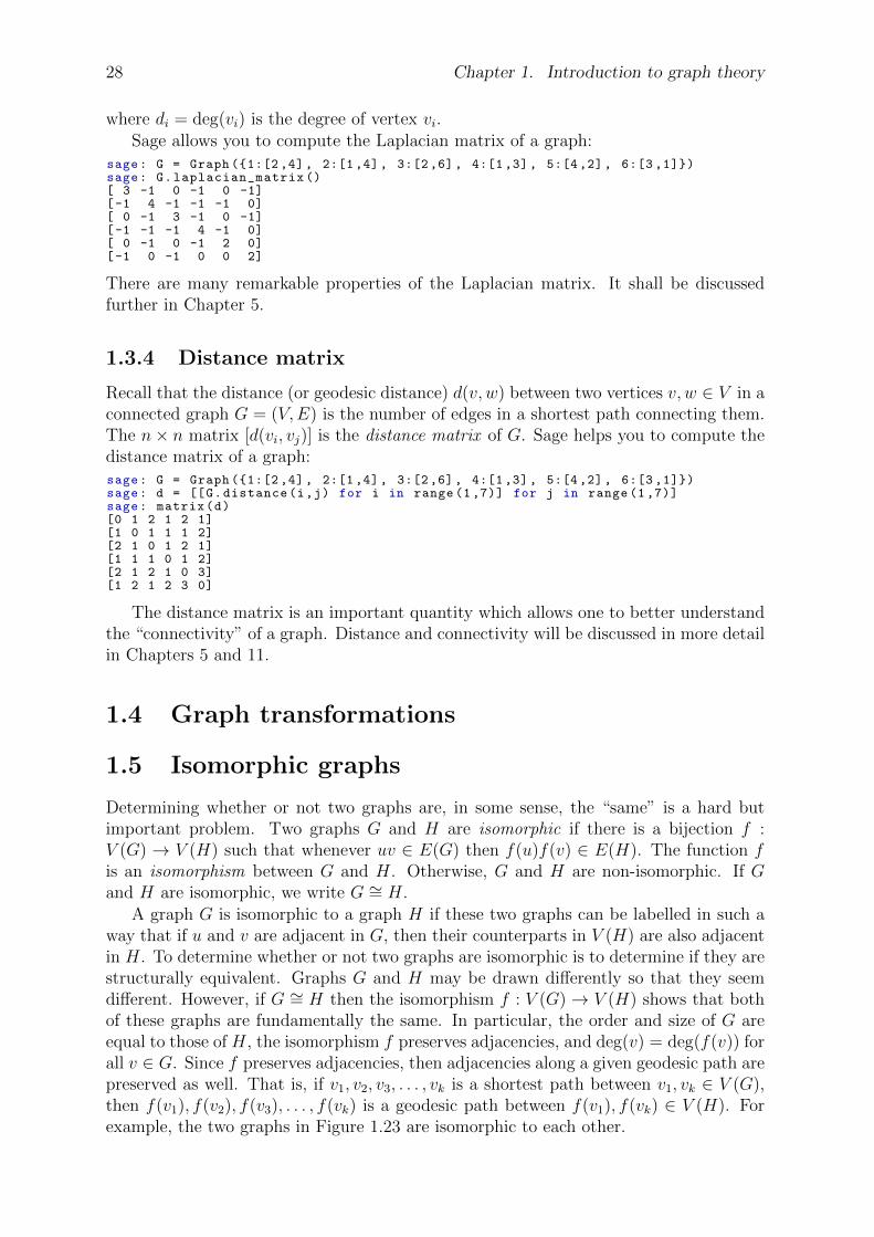
A graph G is isomorphic to a graph H if these two graphs can be labelled in such away that if u and v are adjacent in G, then their counterparts in V (H) are also adjacentin H. To determine whether or not two graphs are isomorphic is to determine if they arestructurally equivalent. Graphs G and H may be drawn differently so that they seemdifferent. However, if G ∼= H then the isomorphism f : V (G)→ V (H) shows that bothof these graphs are fundamentally the same. In particular, the order and size of G areequal to those of H, the isomorphism f preserves adjacencies, and deg(v) = deg(f(v)) forall v ∈ G. Since f preserves adjacencies, then adjacencies along a given geodesic path arepreserved as well. That is, if v1, v2, v3, . . . , vk is a shortest path between v1, vk ∈ V (G),then f(v1), f(v2), f(v3), . . . , f(vk) is a geodesic path between f(v1), f(vk) ∈ V (H). Forexample, the two graphs in Figure 1.23 are isomorphic to each other.
1.5. Isomorphic graphs 29
(a) (b)
Figure 1.23: Two representations of the Franklin graph.
a b
c d
e f
(a) C6
1 2
3 4
5 6
(b) G1
a b
c d
e f
(c) G2
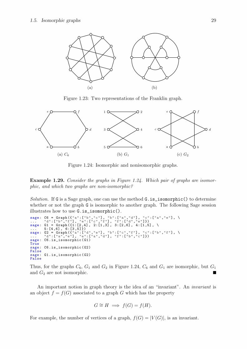
Figure 1.24: Isomorphic and nonisomorphic graphs.
Example 1.29. Consider the graphs in Figure 1.24. Which pair of graphs are isomor-phic, and which two graphs are non-isomorphic?
Solution. If G is a Sage graph, one can use the method G.is_isomorphic() to determinewhether or not the graph G is isomorphic to another graph. The following Sage sessionillustrates how to use G.is_isomorphic().sage: C6 = Graph ("a":["b","c"], "b":["a","d"], "c":["a","e"], \... "d":["b","f"], "e":["c","f"], "f":["d","e"])sage: G1 = Graph (1:[2 ,4] , 2:[1,3], 3:[2,6], 4:[1,5], \... 5:[4,6], 6:[3 ,5])sage: G2 = Graph ("a":["d","e"], "b":["c","f"], "c":["b","f"], \... "d":["a","e"], "e":["a","d"], "f":["b","c"])sage: C6.is_isomorphic(G1)Truesage: C6.is_isomorphic(G2)Falsesage: G1.is_isomorphic(G2)False
Thus, for the graphs C6, G1 and G2 in Figure 1.24, C6 and G1 are isomorphic, but G1
and G2 are not isomorphic.
An important notion in graph theory is the idea of an “invariant”. An invariant isan object f = f(G) associated to a graph G which has the property
G ∼= H =⇒ f(G) = f(H).
For example, the number of vertices of a graph, f(G) = |V (G)|, is an invariant.

30 Chapter 1. Introduction to graph theory
1.5.1 Adjacency matrices
Two n × n matrices A1 and A2 are permutation equivalent if there is a permutationmatrix P such that A1 = PA2P
−1. In other words, A1 is the same as A2 after a suitablere-ordering of the rows and a corresponding re-ordering of the columns. This notion ofpermutation equivalence is an equivalence relation.
To show that two undirected graphs are isomorphic depends on the following result.
Theorem 1.30. Consider two directed or undirected graphs G1 and G2 with respectiveadjacency matrices A1 and A2. Then G1 and G2 are isomorphic if and only if A1 ispermutation equivalent to A2.
This says that the permutation equivalence class of the adjacency matrix is an in-variant.
Define an ordering on the set of n×n (0, 1)-matrices as follows: we say A1 < A2 if thelist of entries of A1 is less than or equal to the list of entries of A2 in the lexicographicalordering. Here, the list of entries of a (0, 1)-matrix is obtained by concatenating theentries of the matrix, row-by-row. For example,
[1 10 1
]<
[1 11 1
].
Algorithm 1.1 is an immediate consequence of Theorem 1.30. The lexicographicallymaximal element of the permutation equivalence class of the adjacency matrix of G iscalled the canonical label of G. Thus, to check if two undirected graphs are isomorphic,we simply check if their canonical labels are equal. This idea for graph isomorphismchecking is presented in Algorithm 1.1.
Algorithm 1.1 Computing graph isomorphism using canonical labels.
Input Two undirected simple graphs G1 and G2, each having n vertices.Output true if G1
∼= G2; false otherwise.1: for i← 1, 2 do2: Ai ← adjacency matrix of Gi
3: pi ← permutation equivalence class of Ai4: A′i ← lexicographically maximal element of pi
5: if A′1 = A′2 then6: return true
7: return false
1.5.2 Degree sequence
Let G be a graph with n vertices. The degree sequence of G is the ordered n-tuple of thevertex degrees of G arranged in non-increasing order.
The degree sequence of G may contain the same degrees, repeated as often as theyoccur. For example, the degree sequence of C6 is 2, 2, 2, 2, 2, 2 and the degree sequenceof the house graph in Figure 1.3 is 3, 3, 2, 2, 2. If n ≥ 3 then the cycle graph Cn has thedegree sequence
2, 2, 2, . . . , 2︸ ︷︷ ︸n copies of 2
.
1.5. Isomorphic graphs 31
The path Pn, for n ≥ 3, has the degree sequence
2, 2, 2, . . . , 2, 1, 1︸ ︷︷ ︸n−2 copies of 2
.
For positive integer values of n and m, the complete graph Kn has the degree sequence
n− 1, n− 1, n− 1, . . . , n− 1︸ ︷︷ ︸n copies of n−1
and the complete bipartite graph Km,n has the degree sequence
n, n, n, . . . , n,︸ ︷︷ ︸m copies of n
m,m,m, . . . ,m︸ ︷︷ ︸n copies of m
.
Let S be a non-increasing sequence of non-negative integers. Then S is said to begraphical if it is the degree sequence of some graph. If G is a graph with degree sequenceS, we say that G realizes S.
Let S = (d1, d2, . . . , dn) be a graphical sequence, i.e. di ≥ dj for all i ≤ j such that1 ≤ i, j ≤ n. From Corollary 1.11 we see that
∑di∈S di = 2k for some integer k ≥ 0. In
other words, the sum of a graphical sequence is nonnegative and even. In 1961, Erdosand Gallai [71] used this observation as part of a theorem that provides necessary andsufficient conditions for a sequence to be realized by a simple graph. The result is statedin Theorem 1.31, but the original paper of Erdos and Gallai [71] does not provide analgorithm to construct a simple graph with a given degree sequence. For a simple graphthat has a degree sequence with repeated elements, e.g. the degree sequences of Cn,Pn, Kn, and Km,n, it is redundant to verify inequality (1.11) for repeated elements ofthat sequence. In 2003, Tripathi and Vijay [184] showed that one only needs to verifyinequality (1.11) for as many times as there are distinct terms in S.
Theorem 1.31. Erdos & Gallai 1961 [71]. Let d = (d1, d2, . . . , dn) be a sequenceof positive integers such that di ≥ di+1. Then d is realized by a simple graph if and onlyif∑
i di is even andk∑
i=1
di ≤ k(k + 1) +n∑
j=k+1
mink, di (1.11)
for all 1 ≤ k ≤ n− 1.
As noted above, Theorem 1.31 is an existence result showing that something ex-ists without providing a construction of the object under consideration. Havel [98] andHakimi [95,96] independently provided an algorithmic approach that allows for construct-ing a simple graph with a given degree sequence. See Sierksma and Hoogeveen [175] fora coverage of seven criteria for a sequence of integers to be graphic. See Erdos et al. [74]for an extension of the Havel-Hakimi theorem to digraphs.
Theorem 1.32. Havel 1955 [98] & Hakimi 1962–3 [95, 96]. Consider the non-increasing sequence S1 = (d1, d2, . . . , dn) of nonnegative integers, where n ≥ 2 and d1 ≥ 1.Then S1 is graphical if and only if the sequence
S2 = (d2 − 1, d3 − 1, . . . , dd1+1 − 1, dd1+2, . . . , dn)
is graphical.
32 Chapter 1. Introduction to graph theory
Proof. Suppose S2 is graphical. Let G2 = (V2, E2) be a graph of order n− 1 with vertexset V2 = v2, v3, . . . , vn such that
deg(vi) =
di − 1, if 2 ≤ i ≤ d1 + 1,
di, if d1 + 2 ≤ i ≤ n.
Construct a new graph G1 with degree sequence S1 as follows. Add another vertex v1
to V2 and add to E2 the edges v1vi for 2 ≤ i ≤ d1 + 1. It is clear that deg(v1) = d1 anddeg(vi) = di for 2 ≤ i ≤ n. Thus G1 has the degree sequence S1.
On the other hand, suppose S1 is graphical and let G1 be a graph with degree sequenceS1 such that
(i) The graph G1 has the vertex set V (G1) = v1, v2, . . . , vn and deg(vi) = di fori = 1, . . . , n.
(ii) The degree sum of all vertices adjacent to v1 is a maximum.
To obtain a contradiction, suppose v1 is not adjacent to vertices having degrees
d2, d3, . . . , dd1+1.
Then there exist vertices vi and vj with dj > di such that v1vi ∈ E(G1) but v1vj 6∈ E(G1).As dj > di, there is a vertex vk such that vjvk ∈ E(G1) but vivk 6∈ E(G1). Replacing theedges v1vi and vjvk with v1vj and vivk, respectively, results in a new graphH whose degreesequence is S1. However, the graph H is such that the degree sum of vertices adjacent tov1 is greater than the corresponding degree sum in G1, contradicting property (ii) in ourchoice of G1. Consequently, v1 is adjacent to d1 other vertices of largest degree. ThenS2 is graphical because G1 − v1 has degree sequence S2.
The proof of Theorem 1.32 can be adapted into an algorithm to determine whetheror not a sequence of nonnegative integers can be realized by a simple graph. If G isa simple graph, the degree of any vertex in V (G) cannot exceed the order of G. Bythe handshaking lemma (Theorem 1.9), the sum of all terms in the sequence cannot beodd. Once the sequence passes these two preliminary tests, we then adapt the proof ofTheorem 1.32 to successively reduce the original sequence to a smaller sequence. Theseideas are summarized in Algorithm 1.2.
We now show that Algorithm 1.2 determines whether or not a sequence of integersis realizable by a simple graph. Our input is a sequence S = (d1, d2, . . . , dn) arrangedin non-increasing order, where each di ≥ 0. The first test as contained in the if block,otherwise known as a conditional, on line 1 uses the handshaking lemma (Theorem 1.9).During the first run of the while loop, the conditional on line 4 ensures that the sequenceS only consists of nonnegative integers. At the conditional on line 6, we know that Sis arranged in non-increasing order and has nonnegative integers. If this conditionalholds true, then S is a sequence of zeros and it is realizable by a graph with only isolatedvertices. Such a graph is simple by definition. The conditional on line 8 uses the followingproperty of simple graphs: If G is a simple graph, then the degree of each vertex of Gis less than the order of G. By the time we reach line 10, we know that S has n terms,max(S) > 0, and 0 ≤ di ≤ n− 1 for all i = 1, 2, . . . , n. After applying line 10, S is now asequence of n−1 terms with max(S) > 0 and 0 ≤ di ≤ n−2 for all i = 1, 2, . . . , n−1. Ingeneral, after k rounds of the while loop, S is a sequence of n−k terms with max(S) > 0

1.6. New graphs from old 33
Algorithm 1.2 Havel-Hakimi test for sequences realizable by simple graphs.
Input A nonincreasing sequence S = (d1, d2, . . . , dn) of nonnegative integers, wheren ≥ 2.
Output true if S is realizable by a simple graph; false otherwise.1: if
∑i di is odd then
2: return false
3: while true do4: if min(S) < 0 then5: return false
6: if max(S) = 0 then7: return true
8: if max(S) > length(S)− 1 then9: return false
10: S ← (d2 − 1, d3 − 1, . . . , dd1+1 − 1, dd1+2, . . . , dlength(S))11: sort S in nonincreasing order
and 0 ≤ di ≤ n − k − 1 for all i = 1, 2, . . . , n − k. And after n − 1 rounds of the whileloop, the resulting sequence has one term whose value is zero. In other words, eventuallyAlgorithm 1.2 produces a sequence with a negative term or a sequence of zeros.
1.5.3 Invariants revisited
In some cases, one can distinguish non-isomorphic graphs by considering graph invariants.For instance, the graphs C6 and G1 in Figure 1.24 are isomorphic so they have the samenumber of vertices and edges. Also, G1 and G2 in Figure 1.24 are non-isomorphic becausethe former is connected, while the latter is not connected. To prove that two graphsare non-isomorphic, one could show that they have different values for a given graphinvariant. The following list contains some items to check off when showing that twographs are non-isomorphic:
1. the number of vertices,
2. the number of edges,
3. the degree sequence,
4. the length of a geodesic path,
5. the length of the longest path,
6. the number of connected components of a graph.
1.6 New graphs from old
This section provides a brief survey of operations on graphs to obtain new graphs fromold graphs. Such graph operations include unions, products, edge addition, edge deletion,vertex addition, and vertex deletion. Several of these are briefly described below.
34 Chapter 1. Introduction to graph theory
1.6.1 Union, intersection, and join
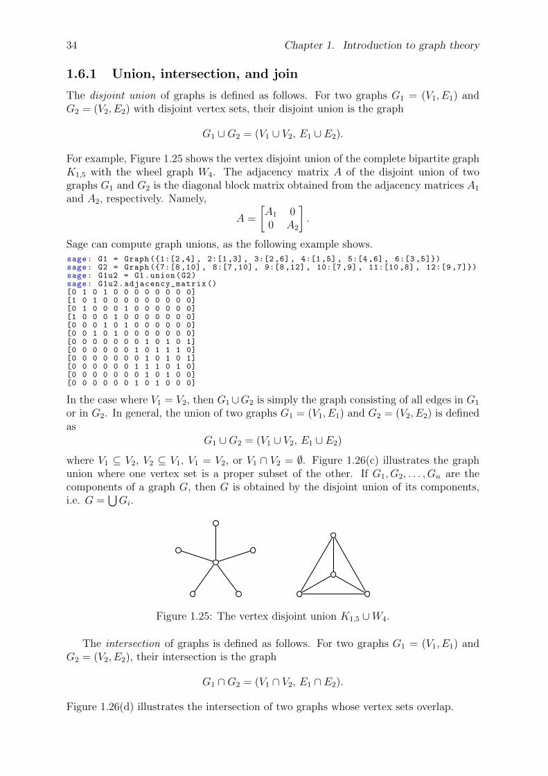
The disjoint union of graphs is defined as follows. For two graphs G1 = (V1, E1) andG2 = (V2, E2) with disjoint vertex sets, their disjoint union is the graph
G1 ∪G2 = (V1 ∪ V2, E1 ∪ E2).
For example, Figure 1.25 shows the vertex disjoint union of the complete bipartite graphK1,5 with the wheel graph W4. The adjacency matrix A of the disjoint union of twographs G1 and G2 is the diagonal block matrix obtained from the adjacency matrices A1
and A2, respectively. Namely,
A =
[A1 00 A2
].
Sage can compute graph unions, as the following example shows.sage: G1 = Graph (1:[2 ,4] , 2:[1,3], 3:[2,6], 4:[1,5], 5:[4,6], 6:[3 ,5])sage: G2 = Graph (7:[8 ,10] , 8:[7,10], 9:[8,12], 10:[7,9], 11:[10 ,8] , 12:[9 ,7])sage: G1u2 = G1.union(G2)sage: G1u2.adjacency_matrix ()[0 1 0 1 0 0 0 0 0 0 0 0][1 0 1 0 0 0 0 0 0 0 0 0][0 1 0 0 0 1 0 0 0 0 0 0][1 0 0 0 1 0 0 0 0 0 0 0][0 0 0 1 0 1 0 0 0 0 0 0][0 0 1 0 1 0 0 0 0 0 0 0][0 0 0 0 0 0 0 1 0 1 0 1][0 0 0 0 0 0 1 0 1 1 1 0][0 0 0 0 0 0 0 1 0 1 0 1][0 0 0 0 0 0 1 1 1 0 1 0][0 0 0 0 0 0 0 1 0 1 0 0][0 0 0 0 0 0 1 0 1 0 0 0]
In the case where V1 = V2, then G1∪G2 is simply the graph consisting of all edges in G1
or in G2. In general, the union of two graphs G1 = (V1, E1) and G2 = (V2, E2) is definedas
G1 ∪G2 = (V1 ∪ V2, E1 ∪ E2)
where V1 ⊆ V2, V2 ⊆ V1, V1 = V2, or V1 ∩ V2 = ∅. Figure 1.26(c) illustrates the graphunion where one vertex set is a proper subset of the other. If G1, G2, . . . , Gn are thecomponents of a graph G, then G is obtained by the disjoint union of its components,i.e. G =
⋃Gi.
Figure 1.25: The vertex disjoint union K1,5 ∪W4.
The intersection of graphs is defined as follows. For two graphs G1 = (V1, E1) andG2 = (V2, E2), their intersection is the graph
G1 ∩G2 = (V1 ∩ V2, E1 ∩ E2).
Figure 1.26(d) illustrates the intersection of two graphs whose vertex sets overlap.
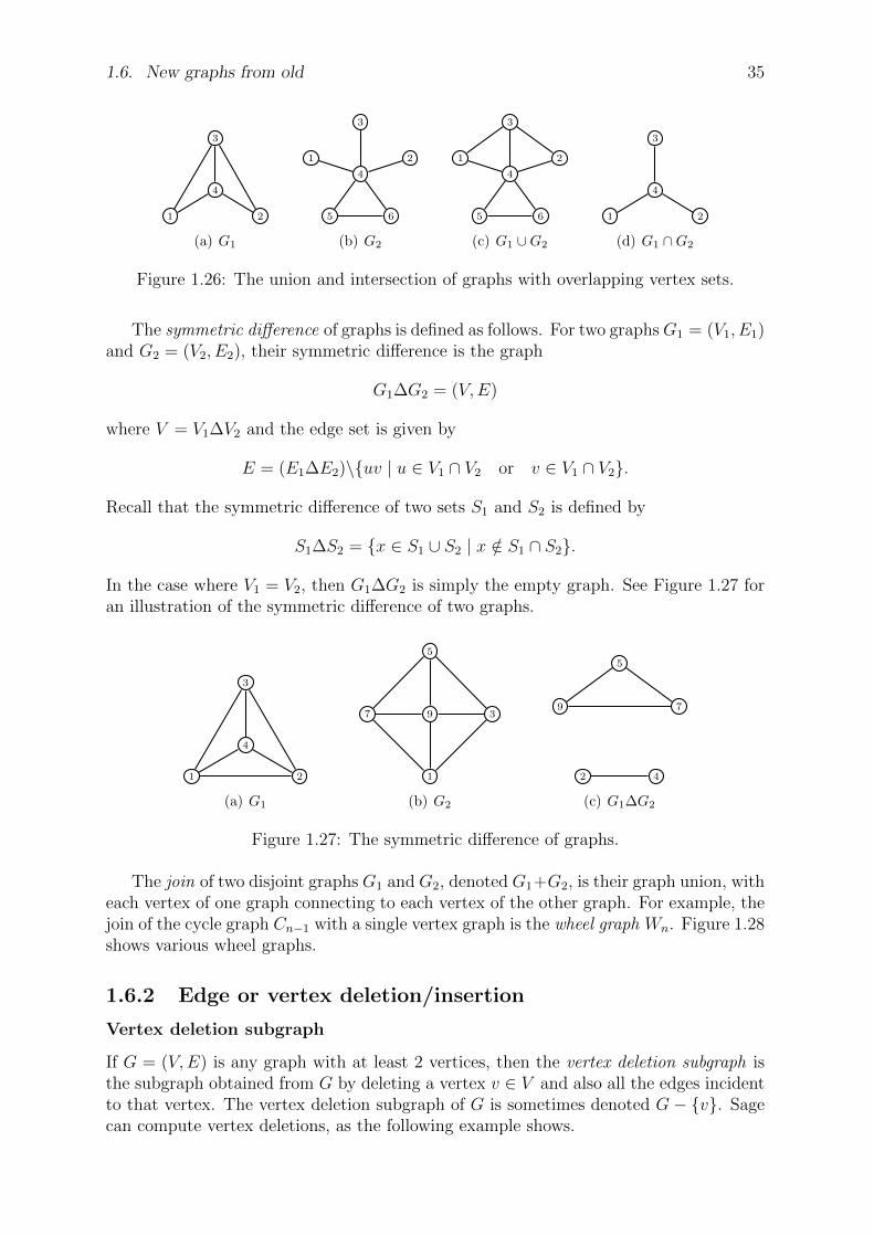
1.6. New graphs from old 35
1 2
3
4
(a) G1
1 2
3
4
5 6
(b) G2
1 2
3
4
5 6
(c) G1 ∪G2
1 2
3
4
(d) G1 ∩G2
Figure 1.26: The union and intersection of graphs with overlapping vertex sets.
The symmetric difference of graphs is defined as follows. For two graphsG1 = (V1, E1)and G2 = (V2, E2), their symmetric difference is the graph
G1∆G2 = (V,E)
where V = V1∆V2 and the edge set is given by
E = (E1∆E2)\uv | u ∈ V1 ∩ V2 or v ∈ V1 ∩ V2.
Recall that the symmetric difference of two sets S1 and S2 is defined by
S1∆S2 = x ∈ S1 ∪ S2 | x /∈ S1 ∩ S2.
In the case where V1 = V2, then G1∆G2 is simply the empty graph. See Figure 1.27 foran illustration of the symmetric difference of two graphs.
1 2
3
4
(a) G1
1
3
5
7 9
(b) G2
2 4
5
79
(c) G1∆G2
Figure 1.27: The symmetric difference of graphs.
The join of two disjoint graphs G1 and G2, denoted G1+G2, is their graph union, witheach vertex of one graph connecting to each vertex of the other graph. For example, thejoin of the cycle graph Cn−1 with a single vertex graph is the wheel graph Wn. Figure 1.28shows various wheel graphs.
1.6.2 Edge or vertex deletion/insertion
Vertex deletion subgraph
If G = (V,E) is any graph with at least 2 vertices, then the vertex deletion subgraph isthe subgraph obtained from G by deleting a vertex v ∈ V and also all the edges incidentto that vertex. The vertex deletion subgraph of G is sometimes denoted G− v. Sagecan compute vertex deletions, as the following example shows.
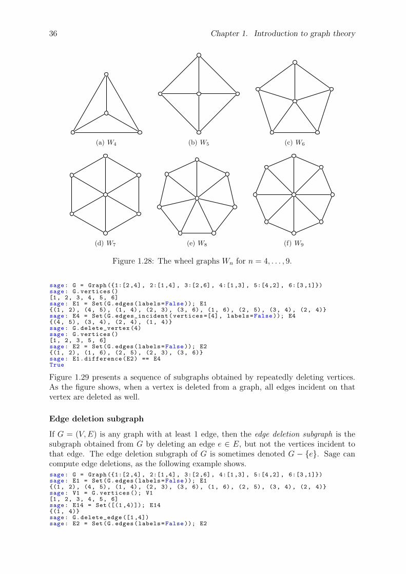
36 Chapter 1. Introduction to graph theory
(a) W4 (b) W5 (c) W6
(d) W7 (e) W8 (f) W9
Figure 1.28: The wheel graphs Wn for n = 4, . . . , 9.
sage: G = Graph (1:[2 ,4] , 2:[1,4], 3:[2,6], 4:[1,3], 5:[4,2], 6:[3 ,1])sage: G.vertices ()[1, 2, 3, 4, 5, 6]sage: E1 = Set(G.edges(labels=False )); E1(1, 2), (4, 5), (1, 4), (2, 3), (3, 6), (1, 6), (2, 5), (3, 4), (2, 4)sage: E4 = Set(G.edges_incident(vertices =[4], labels=False )); E4(4, 5), (3, 4), (2, 4), (1, 4)sage: G.delete_vertex (4)sage: G.vertices ()[1, 2, 3, 5, 6]sage: E2 = Set(G.edges(labels=False )); E2(1, 2), (1, 6), (2, 5), (2, 3), (3, 6)sage: E1.difference(E2) == E4True
Figure 1.29 presents a sequence of subgraphs obtained by repeatedly deleting vertices.As the figure shows, when a vertex is deleted from a graph, all edges incident on thatvertex are deleted as well.
Edge deletion subgraph
If G = (V,E) is any graph with at least 1 edge, then the edge deletion subgraph is thesubgraph obtained from G by deleting an edge e ∈ E, but not the vertices incident tothat edge. The edge deletion subgraph of G is sometimes denoted G − e. Sage cancompute edge deletions, as the following example shows.sage: G = Graph (1:[2 ,4] , 2:[1,4], 3:[2,6], 4:[1,3], 5:[4,2], 6:[3 ,1])sage: E1 = Set(G.edges(labels=False )); E1(1, 2), (4, 5), (1, 4), (2, 3), (3, 6), (1, 6), (2, 5), (3, 4), (2, 4)sage: V1 = G.vertices (); V1[1, 2, 3, 4, 5, 6]sage: E14 = Set ([(1 ,4)]); E14(1, 4)sage: G.delete_edge ([1 ,4])sage: E2 = Set(G.edges(labels=False )); E2
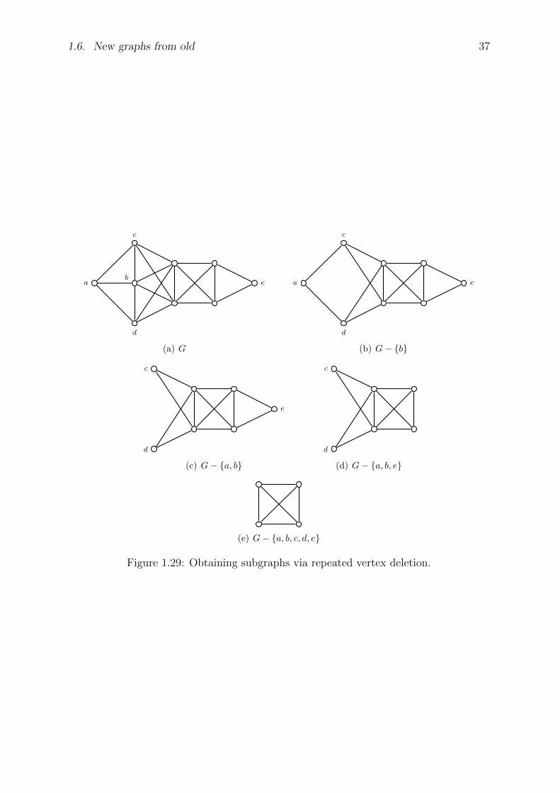
1.6. New graphs from old 37
ab
c
d
e
(a) G
a
c
d
e
(b) G− b
c
d
e
(c) G− a, b
c
d
(d) G− a, b, e
(e) G− a, b, c, d, e
Figure 1.29: Obtaining subgraphs via repeated vertex deletion.

38 Chapter 1. Introduction to graph theory
(1, 2), (4, 5), (2, 3), (3, 6), (1, 6), (2, 5), (3, 4), (2, 4)sage: E1.difference(E2) == E14True
Figure 1.30 shows a sequence of graphs resulting from edge deletion. Unlike vertexdeletion, when an edge is deleted the vertices incident on that edge are left intact.
a
b
c
(a) G
a
b
c
(b) G− aca
b
c
(c) G− ab, ac, bc
Figure 1.30: Obtaining subgraphs via repeated edge deletion.
Vertex cut, cut vertex, or cutpoint
A vertex cut (or separating set) of a connected graph G = (V,E) is a subset W ⊆ Vsuch that the vertex deletion subgraph G−W is disconnected. In fact, if v1, v2 ∈ V aretwo non-adjacent vertices, then you can ask for a vertex cut W for which v1, v2 belongto different components of G−W . Sage’s vertex_cut method allows you to compute aminimal cut having this property. For many connected graphs, the removal of a singlevertex is sufficient for the graph to be disconnected (see Figure 1.30(c)).
Edge cut, cut edge, or bridge
If deleting a single, specific edge would disconnect a graph G, that edge is called abridge. More generally, the edge cut (or disconnecting set or seg) of a connected graphG = (V,E) is a set of edges F ⊆ E whose removal yields an edge deletion subgraphG− F that is disconnected. A minimal edge cut is called a cut set or a bond . In fact, ifv1, v2 ∈ V are two vertices, then you can ask for an edge cut F for which v1, v2 belongto different components of G − F . Sage’s edge_cut method allows you to compute aminimal cut having this property. For example, any of the three edges in Figure 1.30(c)qualifies as a bridge and those three edges form an edge cut for the graph in question.
Theorem 1.33. Let G be a connected graph. An edge e ∈ E(G) is a bridge of G if andonly if e does not lie on a cycle of G.
Proof. First, assume that e = uv is a bridge of G. Suppose for contradiction that e lieson a cycle
C : u, v, w1, w2, . . . , wk, u.
Then G − e contains a u-v path u,wk, . . . , w2, w1, v. Let u1, v1 be any two vertices inG− e. By hypothesis, G is connected so there is a u1-v1 path P in G. If e does not lieon P , then P is also a path in G− e so that u1, v1 are connected, which contradicts ourassumption of e being a bridge. On the other hand, if e lies on P , then express P as
u1, . . . , u, v, . . . , v1 or u1, . . . , v, u, . . . , v1.
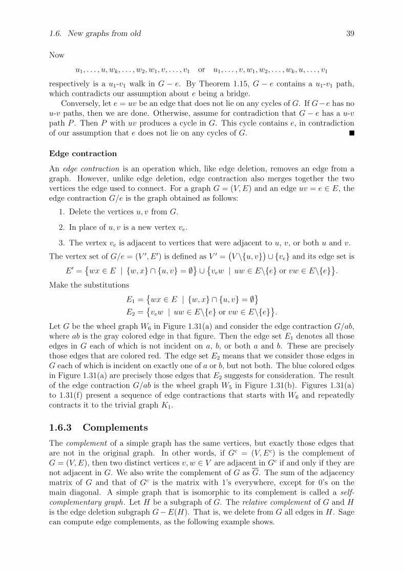
1.6. New graphs from old 39
Now
u1, . . . , u, wk, . . . , w2, w1, v, . . . , v1 or u1, . . . , v, w1, w2, . . . , wk, u, . . . , v1
respectively is a u1-v1 walk in G − e. By Theorem 1.15, G − e contains a u1-v1 path,which contradicts our assumption about e being a bridge.
Conversely, let e = uv be an edge that does not lie on any cycles of G. If G−e has nou-v paths, then we are done. Otherwise, assume for contradiction that G− e has a u-vpath P . Then P with uv produces a cycle in G. This cycle contains e, in contradictionof our assumption that e does not lie on any cycles of G.
Edge contraction
An edge contraction is an operation which, like edge deletion, removes an edge from agraph. However, unlike edge deletion, edge contraction also merges together the twovertices the edge used to connect. For a graph G = (V,E) and an edge uv = e ∈ E, theedge contraction G/e is the graph obtained as follows:
1. Delete the vertices u, v from G.
2. In place of u, v is a new vertex ve.
3. The vertex ve is adjacent to vertices that were adjacent to u, v, or both u and v.
The vertex set of G/e = (V ′, E ′) is defined as V ′ =(V \u, v
)∪ ve and its edge set is
E ′ =wx ∈ E | w, x ∩ u, v = ∅
∪vew | uw ∈ E\e or vw ∈ E\e
.
Make the substitutions
E1 =wx ∈ E | w, x ∩ u, v = ∅
E2 =vew | uw ∈ E\e or vw ∈ E\e
.
Let G be the wheel graph W6 in Figure 1.31(a) and consider the edge contraction G/ab,where ab is the gray colored edge in that figure. Then the edge set E1 denotes all thoseedges in G each of which is not incident on a, b, or both a and b. These are preciselythose edges that are colored red. The edge set E2 means that we consider those edges inG each of which is incident on exactly one of a or b, but not both. The blue colored edgesin Figure 1.31(a) are precisely those edges that E2 suggests for consideration. The resultof the edge contraction G/ab is the wheel graph W5 in Figure 1.31(b). Figures 1.31(a)to 1.31(f) present a sequence of edge contractions that starts with W6 and repeatedlycontracts it to the trivial graph K1.
1.6.3 Complements
The complement of a simple graph has the same vertices, but exactly those edges thatare not in the original graph. In other words, if Gc = (V,Ec) is the complement ofG = (V,E), then two distinct vertices v, w ∈ V are adjacent in Gc if and only if they arenot adjacent in G. We also write the complement of G as G. The sum of the adjacencymatrix of G and that of Gc is the matrix with 1’s everywhere, except for 0’s on themain diagonal. A simple graph that is isomorphic to its complement is called a self-complementary graph. Let H be a subgraph of G. The relative complement of G and His the edge deletion subgraph G−E(H). That is, we delete from G all edges in H. Sagecan compute edge complements, as the following example shows.
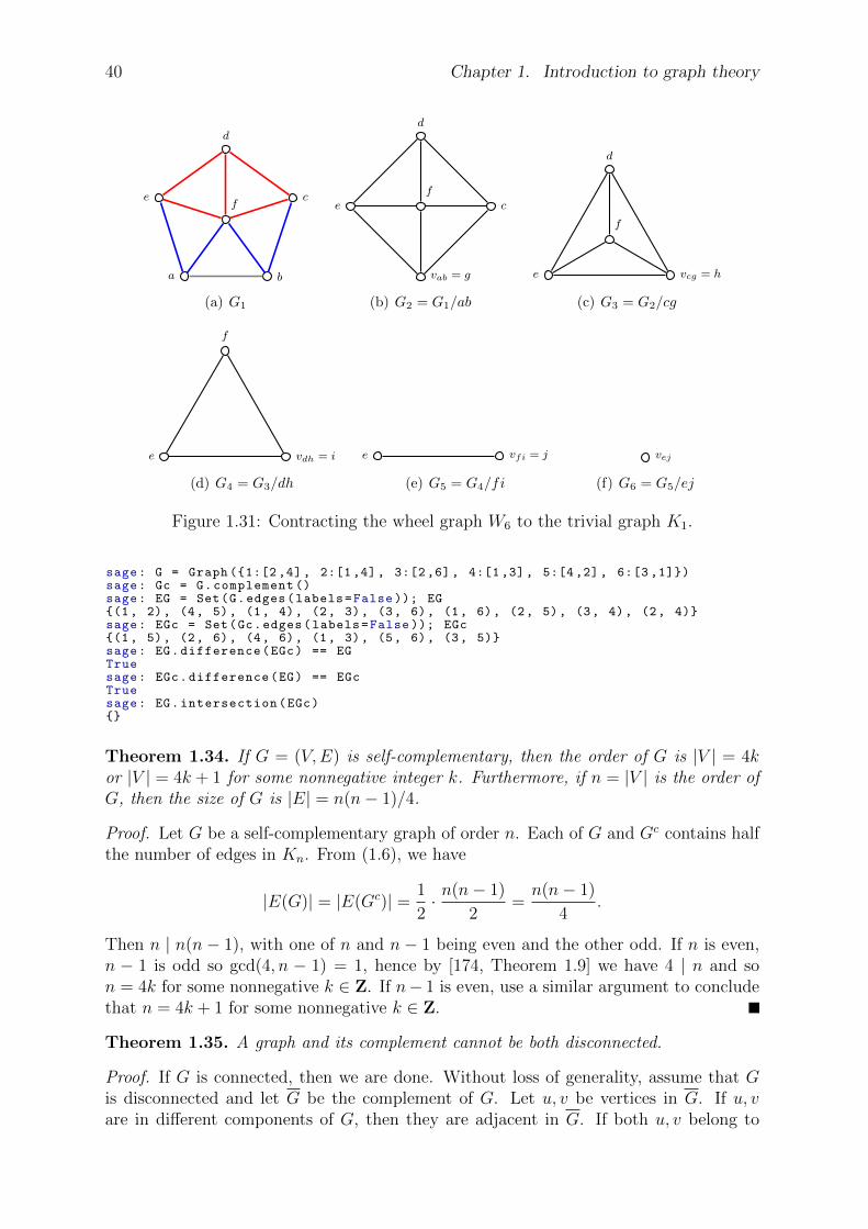
40 Chapter 1. Introduction to graph theory
a b
c
d
ef
(a) G1
c
d
e
f
vab = g
(b) G2 = G1/ab
d
e
f
vcg = h
(c) G3 = G2/cg
f
e vdh = i
(d) G4 = G3/dh
e vfi = j
(e) G5 = G4/fi
vej
(f) G6 = G5/ej
Figure 1.31: Contracting the wheel graph W6 to the trivial graph K1.
sage: G = Graph (1:[2 ,4] , 2:[1,4], 3:[2,6], 4:[1,3], 5:[4,2], 6:[3 ,1])sage: Gc = G.complement ()sage: EG = Set(G.edges(labels=False )); EG(1, 2), (4, 5), (1, 4), (2, 3), (3, 6), (1, 6), (2, 5), (3, 4), (2, 4)sage: EGc = Set(Gc.edges(labels=False )); EGc(1, 5), (2, 6), (4, 6), (1, 3), (5, 6), (3, 5)sage: EG.difference(EGc) == EGTruesage: EGc.difference(EG) == EGcTruesage: EG.intersection(EGc)
Theorem 1.34. If G = (V,E) is self-complementary, then the order of G is |V | = 4kor |V | = 4k + 1 for some nonnegative integer k. Furthermore, if n = |V | is the order ofG, then the size of G is |E| = n(n− 1)/4.
Proof. Let G be a self-complementary graph of order n. Each of G and Gc contains halfthe number of edges in Kn. From (1.6), we have
|E(G)| = |E(Gc)| = 1
2· n(n− 1)
2=n(n− 1)
4.
Then n | n(n− 1), with one of n and n− 1 being even and the other odd. If n is even,n − 1 is odd so gcd(4, n − 1) = 1, hence by [174, Theorem 1.9] we have 4 | n and son = 4k for some nonnegative k ∈ Z. If n− 1 is even, use a similar argument to concludethat n = 4k + 1 for some nonnegative k ∈ Z.
Theorem 1.35. A graph and its complement cannot be both disconnected.
Proof. If G is connected, then we are done. Without loss of generality, assume that Gis disconnected and let G be the complement of G. Let u, v be vertices in G. If u, vare in different components of G, then they are adjacent in G. If both u, v belong to

1.6. New graphs from old 41
some component Ci of G, let w be a vertex in a different component Cj of G. Then u,ware adjacent in G, and similarly for v and w. That is, u and v are connected in G andtherefore G is connected.
1.6.4 Cartesian product
The Cartesian product GH of graphs G and H is a graph such that the vertex set ofGH is the Cartesian product
V (GH) = V (G)× V (H).
Any two vertices (u, u′) and (v, v′) are adjacent in GH if and only if either
1. u = v and u′ is adjacent with v′ in H; or
2. u′ = v′ and u is adjacent with v in G.
The vertex set of GH is V (GH) and the edge set of GH is
E(GH) =(V (G)× E(H)
)∪(E(G)× V (H)
).
Sage can compute Cartesian products, as the following example shows.sage: Z = graphs.CompleteGraph (2); len(Z.vertices ()); len(Z.edges ())21sage: C = graphs.CycleGraph (5); len(C.vertices ()); len(C.edges ())55sage: P = C.cartesian_product(Z); len(P.vertices ()); len(P.edges ())1015
The path graph Pn is a tree with n vertices V = v1, v2, . . . , vn and edges E =(vi, vi+1) | 1 ≤ i ≤ n − 1. In this case, deg(v1) = deg(vn) = 1 and deg(vi) = 2 for1 < i < n. The path graph Pn can be obtained from the cycle graph Cn by deletingone edge of Cn. The ladder graph Ln is the Cartesian product of path graphs, i.e.Ln = PnP1.
The Cartesian product of two graphs G1 and G2 can be visualized as follows. Let V1 =u1, u2, . . . , um and V2 = v1, v2, . . . , vn be the vertex sets of G1 and G2, respectively.Let H1, H2, . . . , Hn be n copies of G1. Place each Hi at the location of vi in G2. Thenui ∈ V (Hj) is adjacent to ui ∈ V (Hk) if and only if vjk ∈ E(G2). See Figure 1.32 for anillustration of obtaining the Cartesian product of K3 and P3.
(a) K3 (b) P3 (c) K3P3
Figure 1.32: The Cartesian product of K3 and P3.
42 Chapter 1. Introduction to graph theory
The hypercube graph Qn is the n-regular graph having vertex set
V =
(ε1, . . . , εn) | εi ∈ 0, 1
of cardinality 2n. That is, each vertex of Qn is a bit string of length n. Two verticesv, w ∈ V are connected by an edge if and only if v and w differ in exactly one coordinate.5
The Cartesian product of n edge graphs K2 is a hypercube:
(K2)n = Qn.
Figure 1.33 illustrates the hypercube graphs Qn for n = 1, . . . , 4.
(a) Q1 (b) Q2 (c) Q3 (d) Q4
Figure 1.33: Hypercube graphs Qn for n = 1, . . . , 4.
Example 1.36. The Cartesian product of two hypercube graphs is another hypercube,i.e. QiQj = Qi+j.
Another family of graphs that can be constructed via Cartesian product is the mesh.Such a graph is also referred to as grid or lattice. The 2-mesh is denoted M(m,n) andis defined as the Cartesian product M(m,n) = PmPn. Similarly, the 3-mesh is definedas M(k,m, n) = PkPmPn. In general, for a sequence a1, a2, . . . , an of n > 0 positiveintegers, the n-mesh is given by
M(a1, a2, . . . , an) = Pa1Pa2 · · ·Pan
where the 1-mesh is simply the path graph M(k) = Pk for some positive integer k.Figure 1.34(a) illustrates the 2-mesh M(3, 4) = P3P4, while the 3-mesh M(3, 2, 3) =P3P2P3 is presented in Figure 1.34(b).
5 In other words, the Hamming distance between v and w is equal to 1.

1.7. Problems 43
(a) M(3, 4) (b) M(3, 2, 3)
Figure 1.34: The 2-mesh M(3, 4) and the 3-mesh M(3, 2, 3).
1.6.5 Graph minors
A graph H is called a minor of a graph G if H is isomorphic to a graph obtained by asequence of edge contractions on a subgraph of G. The order in which a sequence of suchcontractions is performed on G does not affect the resulting graph H. A graph minor isnot in general a subgraph. However, if G1 is a minor of G2 and G2 is a minor of G3, thenG1 is a minor of G3. Therefore, the relation “being a minor of” is a partial ordering onthe set of graphs. For example, the graph in Figure 1.31(c) is a minor of the graph inFigure 1.31(a).
The following non-intuitive fact about graph minors was proven by Neil Robertsonand Paul Seymour in a series of 20 papers spanning 1983 to 2004. This result is knownby various names including the Robertson-Seymour theorem, the graph minor theorem,or Wagner’s conjecture (named after Klaus Wagner).
Theorem 1.37. Robertson & Seymour 1983–2004. If an infinite list G1, G2, . . .of finite graphs is given, then there always exist two indices i < j such that Gi is a minorof Gj.
Many classes of graphs can be characterized by forbidden minors : a graph belongsto the class if and only if it does not have a minor from a certain specified list. We shallsee examples of this in Chapter ??.
1.7 Problems
A problem left to itself dries up or goes rotten. But fertilize a problem with a solution—you’ll hatch out dozens.— N. F. Simpson, A Resounding Tinkle, 1958
1.1. For each graph in Figure 1.7, do the following:
(a) Construct the graph using Sage.
(b) Find its adjacency matrix.
(c) Find its node and edge sets.
(d) How many nodes and edges are in the graph?
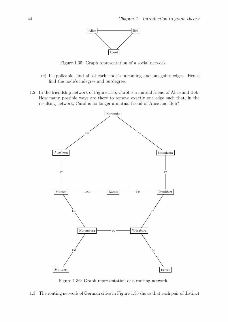
44 Chapter 1. Introduction to graph theory
Alice Bob
Carol
Figure 1.35: Graph representation of a social network.
(e) If applicable, find all of each node’s in-coming and out-going edges. Hencefind the node’s indegree and outdegree.
1.2. In the friendship network of Figure 1.35, Carol is a mutual friend of Alice and Bob.How many possible ways are there to remove exactly one edge such that, in theresulting network, Carol is no longer a mutual friend of Alice and Bob?
Stuttgart Erfurt
Nuremberg
Munich FrankfurtKassel
Augsburg Mannheim
Karlsruhe
Wurzburg
157 154
90
149 97
383 145
57 72
197 54
Figure 1.36: Graph representation of a routing network.
1.3. The routing network of German cities in Figure 1.36 shows that each pair of distinct

1.7. Problems 45
cities are connected by a flight path. The weight of each edge is the flight distancein kilometers between the two corresponding cities. In particular, there is a flightpath connecting Karlsruhe and Stuttgart. What is the shortest route betweenKarlsruhe and Stuttgart? Suppose we can remove at least one edge from thisnetwork. How many possible ways are there to remove edges such that, in theresulting network, Karlsruhe is no longer connected to Stuttgart via a flight path?
1.4. Let D = (V,E) be a digraph of size q. Show that
∑
v∈V
id(v) =∑
v∈V
od(v) = q.
1.5. If G is a simple graph of order n > 0, show that deg(v) < n for all v ∈ V (G).
1.6. Let G be a graph of order n and size m. Then G is called an overfull graph ifm > ∆(G) · bn/2c. If m = ∆(G) · bn/2c + 1, then G is said to be just overfull.It can be shown that overfull graphs have odd order. Equivalently, let G be ofodd order. We can define G to be overfull if m > ∆(G) · (n − 1)/2, and G is justoverfull if m = ∆(G) · (n − 1)/2 + 1. Find an overfull graph and a graph that isjust overfull. Some basic results on overfull graphs are presented in [52].
1.7. Fix a positive integer n and denote by Γ(n) the number of simple graphs on nvertices. Show that
Γ(n) = 2(n2) = 2n(n−1)/2.
1.8. Let G be an undirected graph whose unoriented incidence matrix is Mu and whoseoriented incidence matrix is Mo.
(a) Show that the sum of the entries in any row of Mu is the degree of thecorresponding vertex.
(b) Show that the sum of the entries in any column of Mu is equal to 2.
(c) If G has no self-loops, show that each column of Mo sums to zero.
1.9. Let G be a loopless digraph and let M be its incidence matrix.
(a) If r is a row of M , show that the number of occurrences of −1 in r countsthe outdegree of the vertex corresponding to r. Show that the number ofoccurrences of 1 in r counts the indegree of the vertex corresponding to r.
(b) Show that each column of M sums to 0.
1.10. Let G be a digraph and let M be its incidence matrix. For any row r of M , let mbe the frequency of −1 in r, let p be the frequency of 1 in r, and let t be twice thefrequency of 2 in r. If v is the vertex corresponding to r, show that the degree ofv is deg(v) = m+ p+ t.
1.11. Let G be an undirected graph without self-loops and let M and its oriented in-cidence matrix. Show that the Laplacian matrix L of G satisfies L = M ×MT ,where MT is the transpose of M .
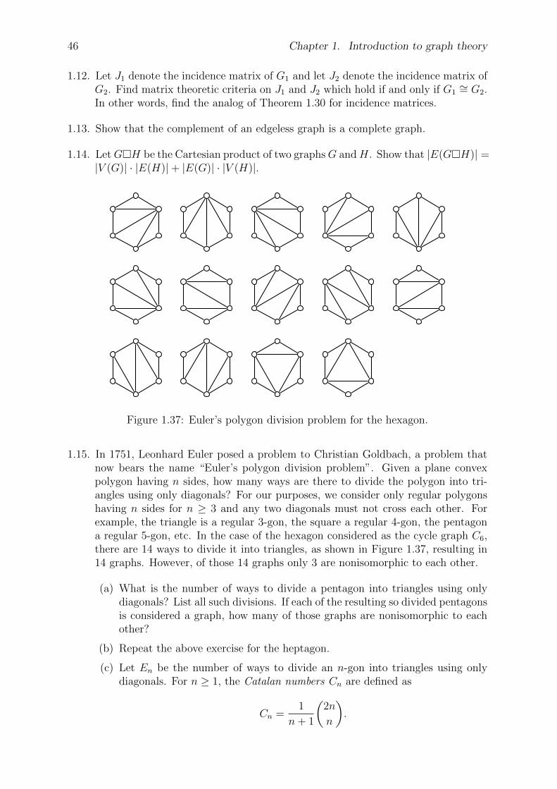
46 Chapter 1. Introduction to graph theory
1.12. Let J1 denote the incidence matrix of G1 and let J2 denote the incidence matrix ofG2. Find matrix theoretic criteria on J1 and J2 which hold if and only if G1
∼= G2.In other words, find the analog of Theorem 1.30 for incidence matrices.
1.13. Show that the complement of an edgeless graph is a complete graph.
1.14. LetGH be the Cartesian product of two graphsG andH. Show that |E(GH)| =|V (G)| · |E(H)|+ |E(G)| · |V (H)|.
Figure 1.37: Euler’s polygon division problem for the hexagon.
1.15. In 1751, Leonhard Euler posed a problem to Christian Goldbach, a problem thatnow bears the name “Euler’s polygon division problem”. Given a plane convexpolygon having n sides, how many ways are there to divide the polygon into tri-angles using only diagonals? For our purposes, we consider only regular polygonshaving n sides for n ≥ 3 and any two diagonals must not cross each other. Forexample, the triangle is a regular 3-gon, the square a regular 4-gon, the pentagona regular 5-gon, etc. In the case of the hexagon considered as the cycle graph C6,there are 14 ways to divide it into triangles, as shown in Figure 1.37, resulting in14 graphs. However, of those 14 graphs only 3 are nonisomorphic to each other.
(a) What is the number of ways to divide a pentagon into triangles using onlydiagonals? List all such divisions. If each of the resulting so divided pentagonsis considered a graph, how many of those graphs are nonisomorphic to eachother?
(b) Repeat the above exercise for the heptagon.
(c) Let En be the number of ways to divide an n-gon into triangles using onlydiagonals. For n ≥ 1, the Catalan numbers Cn are defined as
Cn =1
n+ 1
(2n
n
).
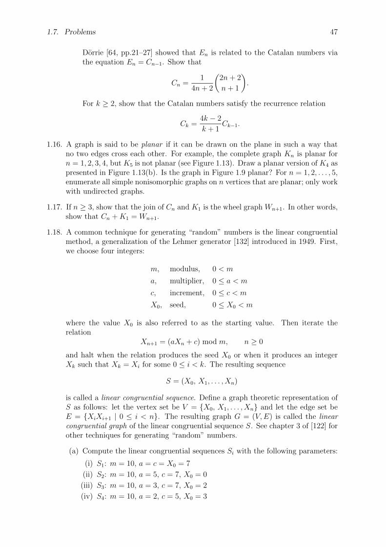
1.7. Problems 47
Dorrie [64, pp.21–27] showed that En is related to the Catalan numbers viathe equation En = Cn−1. Show that
Cn =1
4n+ 2
(2n+ 2
n+ 1
).
For k ≥ 2, show that the Catalan numbers satisfy the recurrence relation
Ck =4k − 2
k + 1Ck−1.
1.16. A graph is said to be planar if it can be drawn on the plane in such a way thatno two edges cross each other. For example, the complete graph Kn is planar forn = 1, 2, 3, 4, but K5 is not planar (see Figure 1.13). Draw a planar version of K4 aspresented in Figure 1.13(b). Is the graph in Figure 1.9 planar? For n = 1, 2, . . . , 5,enumerate all simple nonisomorphic graphs on n vertices that are planar; only workwith undirected graphs.
1.17. If n ≥ 3, show that the join of Cn and K1 is the wheel graph Wn+1. In other words,show that Cn +K1 = Wn+1.
1.18. A common technique for generating “random” numbers is the linear congruentialmethod, a generalization of the Lehmer generator [132] introduced in 1949. First,we choose four integers:
m, modulus, 0 < m
a, multiplier, 0 ≤ a < m
c, increment, 0 ≤ c < m
X0, seed, 0 ≤ X0 < m
where the value X0 is also referred to as the starting value. Then iterate therelation
Xn+1 = (aXn + c) mod m, n ≥ 0
and halt when the relation produces the seed X0 or when it produces an integerXk such that Xk = Xi for some 0 ≤ i < k. The resulting sequence
S = (X0, X1, . . . , Xn)
is called a linear congruential sequence. Define a graph theoretic representation ofS as follows: let the vertex set be V = X0, X1, . . . , Xn and let the edge set beE = XiXi+1 | 0 ≤ i < n. The resulting graph G = (V,E) is called the linearcongruential graph of the linear congruential sequence S. See chapter 3 of [122] forother techniques for generating “random” numbers.
(a) Compute the linear congruential sequences Si with the following parameters:
(i) S1: m = 10, a = c = X0 = 7
(ii) S2: m = 10, a = 5, c = 7, X0 = 0
(iii) S3: m = 10, a = 3, c = 7, X0 = 2
(iv) S4: m = 10, a = 2, c = 5, X0 = 3
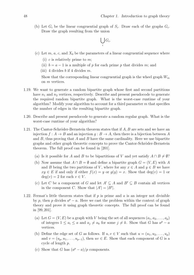
48 Chapter 1. Introduction to graph theory
(b) Let Gi be the linear congruential graph of Si. Draw each of the graphs Gi.Draw the graph resulting from the union
⋃
i
Gi.
(c) Let m, a, c, and X0 be the parameters of a linear congruential sequence where
(i) c is relatively prime to m;
(ii) b = a− 1 is a multiple of p for each prime p that divides m; and
(iii) 4 divides b if 4 divides m.
Show that the corresponding linear congruential graph is the wheel graph Wm
on m vertices.
1.19. We want to generate a random bipartite graph whose first and second partitionshave n1 and n2 vertices, respectively. Describe and present pseudocode to generatethe required random bipartite graph. What is the worst-case runtime of youralgorithm? Modify your algorithm to account for a third parameter m that specifiesthe number of edges in the resulting bipartite graph.
1.20. Describe and present pseudocode to generate a random regular graph. What is theworst-case runtime of your algorithm?
1.21. The Cantor-Schroder-Bernstein theorem states that if A,B are sets and we have aninjection f : A→ B and an injection g : B → A, then there is a bijection between Aand B, thus proving that A and B have the same cardinality. Here we use bipartitegraphs and other graph theoretic concepts to prove the Cantor-Schroder-Bernsteintheorem. The full proof can be found in [201].
(a) Is it possible for A and B to be bipartitions of V and yet satisfy A ∩B 6= ∅?(b) Now assume that A ∩ B = ∅ and define a bipartite graph G = (V,E) with A
and B being the two partitions of V , where for any x ∈ A and y ∈ B we havexy ∈ E if and only if either f(x) = y or g(y) = x. Show that deg(v) = 1 ordeg(v) = 2 for each v ∈ V .
(c) Let C be a component of G and let A′ ⊆ A and B′ ⊆ B contain all verticesin the component C. Show that |A′| = |B′|.
1.22. Fermat’s little theorem states that if p is prime and a is an integer not divisibleby p, then p divides ap − a. Here we cast the problem within the context of graphtheory and prove it using graph theoretic concepts. The full proof can be foundin [99,201].
(a) Let G = (V,E) be a graph with V being the set of all sequences (a1, a2, . . . , ap)of integers 1 ≤ ai ≤ a and aj 6= ak for some j 6= k. Show that G has ap − avertices.
(b) Define the edge set of G as follows. If u, v ∈ V such that u = (u1, u2, . . . , up)and v = (up, u1, . . . , up−1), then uv ∈ E. Show that each component of G is acycle of length p.
(c) Show that G has (ap − a)/p components.
1.7. Problems 49
1.23. For the finite automaton in Figure ??, identify the following:
(a) The states set Q.
(b) The alphabet set Σ.
(c) The transition function δ : Q× Σ→ Q.
(d) The initial state q0 ∈ Q.
(e) The set of final states F ⊆ Q.
0
1
23
4
5
6
7 8
9
(a)
0
1
23
4
5
6
7 8
9
(b)
0
1
23
4
5
6
7 8
9
(c)
Figure 1.38: Various 3-regular graphs on 10 vertices.
(a) k = 4 (b) k = 6 (c) k = 8
Figure 1.39: Various k-circulant graphs for k = 4, 6, 8.
1.24. The cycle graph Cn is a 2-regular graph. If 2 < r < n/2, unlike the cycle graphthere are various realizations of an r-regular graph; see Figure 1.38 for the case ofr = 3 and n = 10. The k-circulant graph on n vertices can be considered as anintermediate graph between Cn and a k-regular graph. Let k and n be positiveintegers satisfying k < n/2 with k being even. Suppose G = (V,E) is a simpleundirected graph with vertex set V = 0, 1, . . . , n − 1. Define the edge set of Gas follows. Each i ∈ V is incident with each of i + j mod n and i − j mod n forj ∈ 1, 2, . . . , k/2. With the latter edge set, G is said to be a k-circulant graph, atype of graphs used in constructing small-world networks (see section 11.4). Referto Figure 1.39 for examples of k-circulant graphs.
(a) Describe and provide pseudocode of an algorithm to construct a k-circulantgraph on n vertices.
(b) Show that the cycle graph Cn is 2-circulant.
50 Chapter 1. Introduction to graph theory
(c) Show that the sum of all degrees of a k-circulant graph on n vertices is nk.
(d) Show that a k-circulant graph is k-regular.
(e) Let C be the collection of all k-regular graphs on n vertices. If each k-regulargraph from C is equally likely to be chosen, what is the probability that ak-circulant graph be chosen from C?

Chapter 2
Trees and forests
— Randall Munroe, xkcd, http://xkcd.com/71/
In section 1.2.1, we briefly touched upon trees and provided examples of how trees couldbe used to model hierarchical structures. This chapter provides an in-depth study oftrees, their properties, and various applications. After defining trees and related con-cepts in section 2.1, we then present various basic properties of trees in section 2.2.Each connected graph G has an underlying subgraph called a spanning tree that con-tains all the vertices of G. Spanning trees are discussed in section 2.3 together withvarious common algorithms for finding spanning trees. We then discuss binary trees insection 2.4, followed by an application of binary trees to coding theory in section 2.5.Whereas breadth- and depth-first searches are general methods for traversing a graph,trees require specialized techniques in order to visit their vertices, a topic that is takenup in section 2.6.
2.1 Definitions and examples
I think that I shall never seeA poem lovely as a tree.— Joyce Kilmer, Trees and Other Poems, 1914, “Trees”
Recall that a path in a graph G = (V,E) whose start and end vertices are the same iscalled a cycle. We say G is acyclic, or a forest , if it has no cycles. In a forest, a vertexof degree one is called an endpoint or a leaf . Any vertex that is not a leaf is called an
51
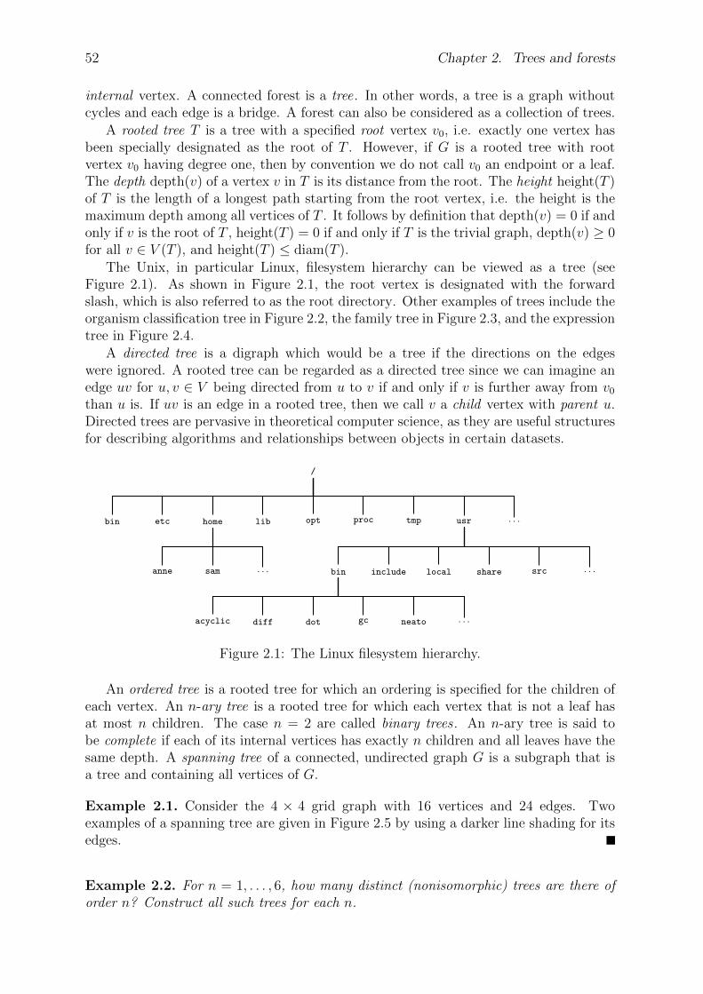
52 Chapter 2. Trees and forests
internal vertex. A connected forest is a tree. In other words, a tree is a graph withoutcycles and each edge is a bridge. A forest can also be considered as a collection of trees.
A rooted tree T is a tree with a specified root vertex v0, i.e. exactly one vertex hasbeen specially designated as the root of T . However, if G is a rooted tree with rootvertex v0 having degree one, then by convention we do not call v0 an endpoint or a leaf.The depth depth(v) of a vertex v in T is its distance from the root. The height height(T )of T is the length of a longest path starting from the root vertex, i.e. the height is themaximum depth among all vertices of T . It follows by definition that depth(v) = 0 if andonly if v is the root of T , height(T ) = 0 if and only if T is the trivial graph, depth(v) ≥ 0for all v ∈ V (T ), and height(T ) ≤ diam(T ).
The Unix, in particular Linux, filesystem hierarchy can be viewed as a tree (seeFigure 2.1). As shown in Figure 2.1, the root vertex is designated with the forwardslash, which is also referred to as the root directory. Other examples of trees include theorganism classification tree in Figure 2.2, the family tree in Figure 2.3, and the expressiontree in Figure 2.4.
A directed tree is a digraph which would be a tree if the directions on the edgeswere ignored. A rooted tree can be regarded as a directed tree since we can imagine anedge uv for u, v ∈ V being directed from u to v if and only if v is further away from v0
than u is. If uv is an edge in a rooted tree, then we call v a child vertex with parent u.Directed trees are pervasive in theoretical computer science, as they are useful structuresfor describing algorithms and relationships between objects in certain datasets.
/
bin etc home
anne sam . . .
lib opt proc tmp usr
bin
acyclic diff dot gc neato . . .
include local share src . . .
. . .
Figure 2.1: The Linux filesystem hierarchy.
An ordered tree is a rooted tree for which an ordering is specified for the children ofeach vertex. An n-ary tree is a rooted tree for which each vertex that is not a leaf hasat most n children. The case n = 2 are called binary trees . An n-ary tree is said tobe complete if each of its internal vertices has exactly n children and all leaves have thesame depth. A spanning tree of a connected, undirected graph G is a subgraph that isa tree and containing all vertices of G.
Example 2.1. Consider the 4 × 4 grid graph with 16 vertices and 24 edges. Twoexamples of a spanning tree are given in Figure 2.5 by using a darker line shading for itsedges.
Example 2.2. For n = 1, . . . , 6, how many distinct (nonisomorphic) trees are there oforder n? Construct all such trees for each n.

2.1. Definitions and examples 53
organism
plant
tree
deciduous evergreen
flower
animal
invertebrate vetebrate
bird
finch rosella sparrow
mammal
dolphin human whale
Figure 2.2: Classification tree of organisms.
Nikolaus senior
Jacob Nicolaus
Nicolaus I
Johann
Nicolaus II Daniel Johann II
Johann III Daniel II Jakob II
Figure 2.3: Bernoulli family tree of mathematicians.
+
×
a a
×
2 a b
×
b b
Figure 2.4: Expression tree for the perfect square a2 + 2ab+ b2.
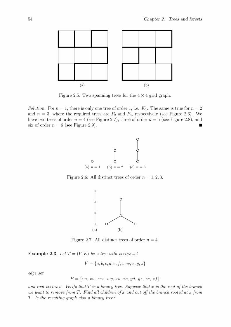
54 Chapter 2. Trees and forests
(a) (b)
Figure 2.5: Two spanning trees for the 4× 4 grid graph.
Solution. For n = 1, there is only one tree of order 1, i.e. K1. The same is true for n = 2and n = 3, where the required trees are P2 and P3, respectively (see Figure 2.6). Wehave two trees of order n = 4 (see Figure 2.7), three of order n = 5 (see Figure 2.8), andsix of order n = 6 (see Figure 2.9).
(a) n = 1 (b) n = 2 (c) n = 3
Figure 2.6: All distinct trees of order n = 1, 2, 3.
(a) (b)
Figure 2.7: All distinct trees of order n = 4.
Example 2.3. Let T = (V,E) be a tree with vertex set
V = a, b, c, d, e, f, v, w, x, y, z
edge setE = va, vw, wx, wy, xb, xc, yd, yz, ze, zf
and root vertex v. Verify that T is a binary tree. Suppose that x is the root of the branchwe want to remove from T . Find all children of x and cut off the branch rooted at x fromT . Is the resulting graph also a binary tree?
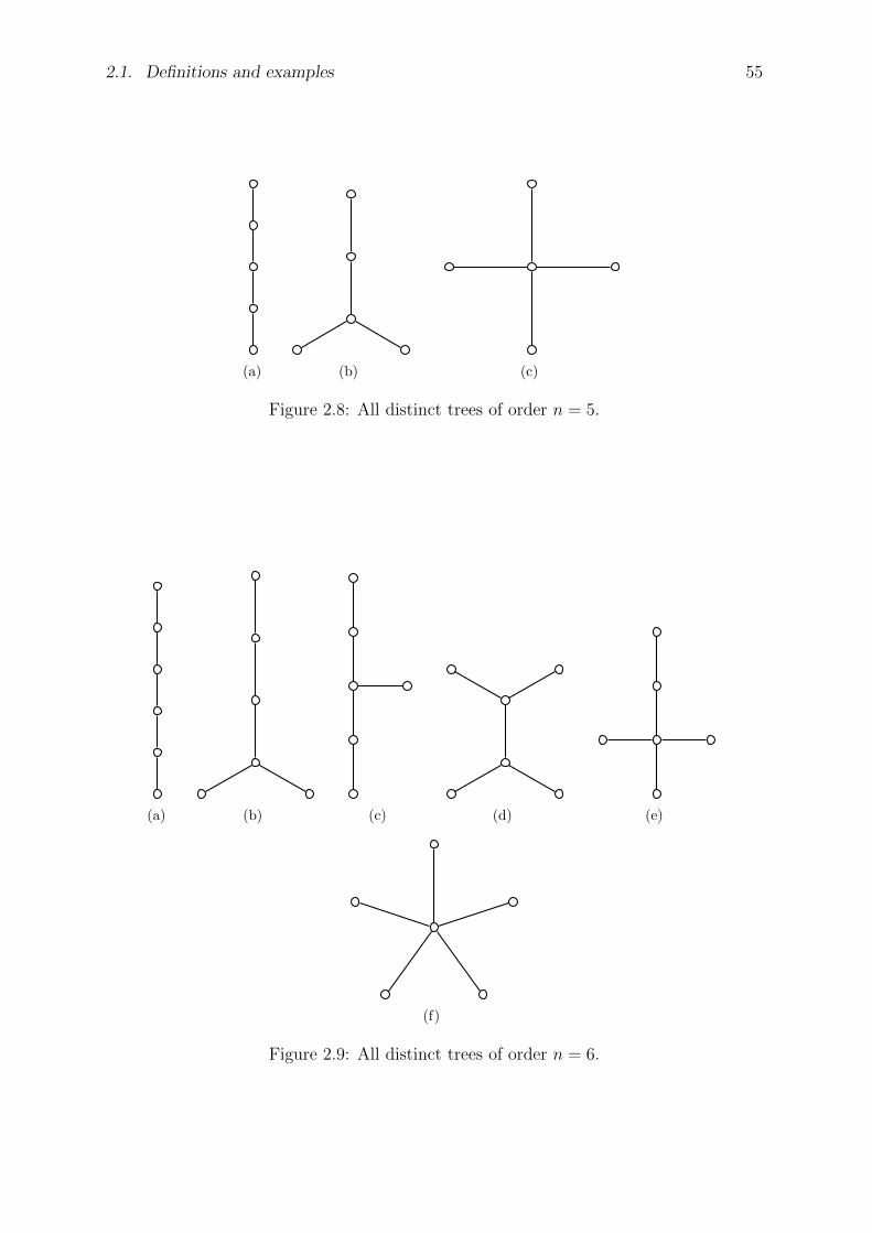
2.1. Definitions and examples 55
(a) (b) (c)
Figure 2.8: All distinct trees of order n = 5.
(a) (b) (c) (d) (e)
(f)
Figure 2.9: All distinct trees of order n = 6.
56 Chapter 2. Trees and forests
Solution. We construct the tree T in Sage as follows:sage: T = DiGraph (... "v":["a","w"], "w":["x","y"],... "x":["c","b"], "y":["z","d"],... "z":["f","e"])sage: for v in T.vertex_iterator ():... print(v),a c b e d f w v y x zsage: for e in T.edge_iterator ():... print("%s%s" % (e[0], e[1])),wy wx va vw yd yz xc xb ze zf
Each vertex in a binary tree has at most 2 children. Use this definition to test whetheror not a graph is a binary tree.sage: T.is_tree ()Truesage: def is_bintree1(G):... for v in G.vertex_iterator ():... if len(G.neighbors_out(v)) > 2:... return False... return Truesage: is_bintree1(T)True
Here’s another way to test for binary trees. Let T be an undirected rooted tree. Eachvertex in a binary tree has a maximum degree of 3. If the root vertex is the only vertexwith degree 2, then T is a binary tree. (Problem 2.5 asks you to prove this result.) Wecan use this test because the root vertex v of T is the only vertex with two children.sage: def is_bintree2(G):... if G.is_tree () and max(G.degree ()) == 3 and G.degree (). count (2) == 1:... return True... return Falsesage: is_bintree2(T.to_undirected ())True
As x is the root vertex of the branch we want to cut off from T , we could use breadth-or depth-first search to determine all the children of x. We then delete x and its childrenfrom T .sage: T2 = copy(T)sage: # using breadth -first searchsage: V = list(T.breadth_first_search("x")); V[’x’, ’c’, ’b’]sage: T.delete_vertices(V)sage: for v in T.vertex_iterator ():... print(v),a e d f w v y zsage: for e in T.edge_iterator ():... print("%s%s" % (e[0], e[1])),wy va vw yd yz ze zfsage: # using depth -first searchsage: V = list(T2.depth_first_search("x")); V[’x’, ’b’, ’c’]sage: T2.delete_vertices(V)sage: for v in T2.vertex_iterator ():... print(v),a e d f w v y zsage: for e in T2.edge_iterator ():... print("%s%s" % (e[0], e[1])),wy va vw yd yz ze zf
The resulting graph T is a binary tree because each vertex has at most two children.sage: TDigraph on 8 verticessage: is_bintree1(T)True
Notice that the test defined in the function is_bintree2 can no longer be used to testwhether or not T is a binary tree, because T now has two vertices, i.e. v and w, each of
2.1. Definitions and examples 57
which has degree 2.
Consider again the organism classification tree in Figure 2.2. We can view the vertex“organism” as the root of the tree and having two children. The first branch of “or-ganism” is the subtree rooted at “plant” and its second branch is the subtree rootedat “animal”. We form the complete tree by joining an edge between “organism” and“plant”, and an edge between “organism” and “animal”. The subtree rooted at “plant”can be constructed in the same manner. The first branch of this subtree is the subtreerooted at “tree” and the second branch is the subtree rooted at “flower”. To constructthe subtree rooted at “plant”, we join an edge between “plant” and “tree”, and anedge between “plant” and “flower”. The other subtrees of the tree in Figure 2.2 can beconstructed using the above recursive procedure.
In general, the recursive construction in Theorem 2.4 provides an alternative wayto define trees. We say construction because it provides an algorithm to construct atree, as opposed to the nonconstructive definition presented earlier in this section, wherewe defined the conditions under which a graph qualifies as a tree without presenting aprocedure to construct a tree. Furthermore, we say recursive since a larger tree can beviewed as being constructed from smaller trees, i.e. join up existing trees to obtain anew tree. The recursive construction of trees as presented in Theorem 2.4 is illustratedin Figure 2.10.
Theorem 2.4. Recursive construction of trees. An isolated vertex is a tree. Thatsingle vertex is the root of the tree. Given a collection T1, T2, . . . , Tn of n > 0 trees,construct a new tree as follows:
1. Let T be a tree having exactly the one vertex v, which is the root of T .
2. Let vi be the root of the tree Ti.
3. For i = 1, 2, . . . , n, add the edge vvi to T and add Ti to T . That is, each vi is nowa child of v.
The result is the tree T rooted at v with vertex set
V (T ) = v ∪(⋃
i
V (Ti)
)
and edge set
E(T ) =⋃
i
(vvi ∪ E(Ti)
).
The following game is a variant of the Shannon switching game, due to Edmonds andLehman. We follow the description in Oxley’s survey [158]. Recall that a minimal edgecut of a graph is also called a bond of the graph. The following two-person game is playedon a connected graph G = (V,E). Two players Alice and Bob alternately tag elementsof E. Alice’s goal is to tag the edges of a spanning tree, while Bob’s goal is to tag theedges of a bond. If we think of this game in terms of a communication network, thenBob’s goal is to separate the network into pieces that are no longer connected to eachother, while Alice is aiming to reinforce edges of the network to prevent their destruction.Each move for Bob consists of destroying one edge, while each move for Alice involvessecuring an edge against destruction. The next result characterizes winning strategieson G. The full proof can be found in Oxley [158]. See Rasmussen [164] for optimizationalgorithms for solving similar games.
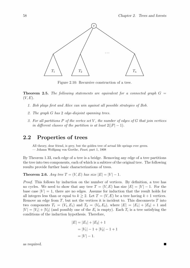
58 Chapter 2. Trees and forests
T1 T2 Tn
v
. . .
Figure 2.10: Recursive construction of a tree.
Theorem 2.5. The following statements are equivalent for a connected graph G =(V,E).
1. Bob plays first and Alice can win against all possible strategies of Bob.
2. The graph G has 2 edge-disjoint spanning trees.
3. For all partitions P of the vertex set V , the number of edges of G that join verticesin different classes of the partition is at least 2(|P | − 1).
2.2 Properties of trees
All theory, dear friend, is grey, but the golden tree of actual life springs ever green.— Johann Wolfgang von Goethe, Faust, part 1, 1808
By Theorem 1.33, each edge of a tree is a bridge. Removing any edge of a tree partitionsthe tree into two components, each of which is a subtree of the original tree. The followingresults provide further basic characterizations of trees.
Theorem 2.6. Any tree T = (V,E) has size |E| = |V | − 1.
Proof. This follows by induction on the number of vertices. By definition, a tree hasno cycles. We need to show that any tree T = (V,E) has size |E| = |V | − 1. For thebase case |V | = 1, there are no edges. Assume for induction that the result holds forall integers less than or equal to k ≥ 2. Let T = (V,E) be a tree having k + 1 vertices.Remove an edge from T , but not the vertices it is incident to. This disconnects T intotwo components T1 = (V1, E1) and T2 = (V2, E2), where |E| = |E1| + |E2| + 1 and|V | = |V1| + |V2| (and possibly one of the Ei is empty). Each Ti is a tree satisfying theconditions of the induction hypothesis. Therefore,
|E| = |E1|+ |E2|+ 1
= |V1| − 1 + |V2| − 1 + 1
= |V | − 1.
as required.

2.2. Properties of trees 59
Corollary 2.7. If T = (V,E) is a graph of order |V | = n, then the following areequivalent:
1. T is a tree.
2. T contains no cycles and has n− 1 edges.
3. T is connected and has n− 1 edges.
4. Every edge of T is a cut set.
Proof. (1) =⇒ (2): This holds by definition of trees and Theorem 2.6.(2) =⇒ (3): If T = (V,E) has k connected components then it is a disjoint union
of trees Ti = (Vi, Ei), i = 1, 2, . . . , k, for some k. By part (2), each of these satisfy
|Ei| = |Vi| − 1
so
|E| =k∑
i=1
|Ei|
=k∑
i=1
|Vi| − k
= |V | − k.
This contradicts part (2) unless k = 1. Therefore, T is connected.(3) =⇒ (4): If removing an edge e ∈ E leaves T = (V,E) connected then T ′ =
(V,E ′) is a tree, where E ′ = E−e. However, this means that |E ′| = |E|−1 = |V |−1−1 =|V | − 2, which contradicts part (3). Therefore e is a cut set.
(4) =⇒ (1): From part (2) we know that T has no cycles and from part (3) weknow that T is connected. Conclude by the definition of trees that T is a tree.
Theorem 2.8. Let T = (V,E) be a tree and let u, v ∈ V be distinct vertices. Then Thas exactly one u-v path.
Proof. Suppose for contradiction that
P : v0 = u, v1, v2, . . . , vk = v
andQ : w0 = u, w1, w2, . . . , w` = v
are two distinct u-v paths. Then P and Q has a common vertex x, which is possiblyx = u. For some i ≥ 0 and some j ≥ 0 we have vi = x = wj, but vi+1 6= wj+1. Lety be the first vertex after x such that y belongs to both P and Q. (It is possible thaty = v.) We now have two distinct x-y paths that have only x and y in common. Takentogether, these two x-y paths result in a cycle, contradicting our hypothesis that T is atree. Therefore T has only one u-v path.
Theorem 2.9. If T = (V,E) is a graph then the following are equivalent:
60 Chapter 2. Trees and forests
1. T is a tree.
2. For any new edge e, the join T + e has exactly one cycle.
Proof. (1) =⇒ (2): Let e = uv be a new edge connecting u, v ∈ V . Suppose that
P : v0 = w, v1, v2, . . . , vk = w
andP ′ : v′0 = w, v′1, v
′2, . . . , v
′` = w
are two cycles in T + e. If either P or P ′ does not contain e, say P does not contain e,then P is a cycle in T . Let u = v0 and let v = v1. The edge (v0 = w, v1) is a u-v pathand the sequence v = v1, v2, . . . , vk = w = u taken in reverse order is another u-v path.This contradicts Theorem 2.8.
We may now suppose that P and P ′ both contain e. Then P contains a subpathP0 = P − e (which is not closed) that is the same as P except it lacks the edge from uto v. Likewise, P ′ contains a subpath P ′0 = P ′− e (which is not closed) that is the sameas P ′ except it lacks the edge from u to v. By Theorem 2.8, these u-v paths P0 and P ′0must be the same. This forces P and P ′ to be the same, which proves part (2).
(2) =⇒ (1): Part (2) implies that T is acyclic. (Otherwise, it is trivial to maketwo cycles by adding an extra edge.) We must show T is connected. Suppose T isdisconnected. Let u be a vertex in one component, T1 say, of T and v a vertex in anothercomponent, T2 say, of T . Adding the edge e = uv does not create a cycle (if it did thenT1 and T2 would not be disjoint), which contradicts part (2).
Taking together the results in this section, we have the following characterizations oftrees.
Theorem 2.10. Basic characterizations of trees. If T = (V,E) is a graph with nvertices, then the following statements are equivalent:
1. T is a tree.
2. T contains no cycles and has n− 1 edges.
3. T is connected and has n− 1 edges.
4. Every edge of T is a cut set.
5. For any pair of distinct vertices u, v ∈ V , there is exactly one u-v path.
6. For any new edge e, the join T + e has exactly one cycle.
Let G = (V1, E1) be a graph and T = (V2, E2) a subgraph of G that is a tree. As inpart (6) of Theorem 2.10, we see that adding just one edge in E1 − E2 to T will createa unique cycle in G. Such a cycle is called a fundamental cycle of G. The set of suchfundamental cycles of G depends on T .
The following result essentially says that if a tree has at least one edge, then the treehas at least two vertices each of which has degree one. In other words, each tree of order≥ 2 has at least two pendants.
Theorem 2.11. Every nontrivial tree has at least two leaves.
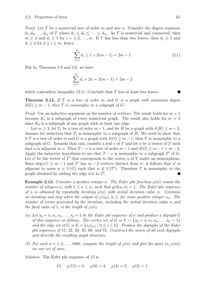
2.2. Properties of trees 61
Proof. Let T be a nontrivial tree of order m and size n. Consider the degree sequenced1, d2, . . . , dm of T where d1 ≤ d2 ≤ · · · ≤ dm. As T is nontrivial and connected, thenm ≥ 2 and di ≥ 1 for i = 1, 2, . . . ,m. If T has less than two leaves, then d1 ≥ 1 anddi ≥ 2 for 2 ≤ i ≤ m, hence
m∑
i=1
di ≥ 1 + 2(m− 1) = 2m− 1. (2.1)
But by Theorems 1.9 and 2.6, we have
m∑
i=1
di = 2n = 2(m− 1) = 2m− 2
which contradicts inequality (2.1). Conclude that T has at least two leaves.
Theorem 2.12. If T is a tree of order m and G is a graph with minimum degreeδ(G) ≥ m− 1, then T is isomorphic to a subgraph of G.
Proof. Use an inductive argument on the number of vertices. The result holds for m = 1because K1 is a subgraph of every nontrivial graph. The result also holds for m = 2since K2 is a subgraph of any graph with at least one edge.
Let m ≥ 3, let T1 be a tree of order m− 1, and let H be a graph with δ(H) ≥ m− 2.Assume for induction that T1 is isomorphic to a subgraph of H. We need to show thatif T is a tree of order m and G is a graph with δ(G) ≥ m− 1, then T is isomorphic to asubgraph of G. Towards that end, consider a leaf v of T and let u be a vertex of T suchthat u is adjacent to v. Then T − v is a tree of order m− 1 and δ(G) ≥ m− 1 > m− 2.Apply the inductive hypothesis to see that T − v is isomorphic to a subgraph T ′ of G.Let u′ be the vertex of T ′ that corresponds to the vertex u of T under an isomorphism.Since deg(u′) ≥ m − 1 and T ′ has m − 2 vertices distinct from u′, it follows that u′ isadjacent to some w ∈ V (G) such that w /∈ V (T ′). Therefore T is isomorphic to thegraph obtained by adding the edge u′w to T ′.
Example 2.13. Consider a positive integer n. The Euler phi function ϕ(n) counts thenumber of integers a, with 1 ≤ a ≤ n, such that gcd(a, n) = 1. The Euler phi sequenceof n is obtained by repeatedly iterating ϕ(n) with initial iteration value n. Continueon iterating and stop when the output of ϕ(αk) is 1, for some positive integer αk. Thenumber of terms generated by the iteration, including the initial iteration value n andthe final value of 1, is the length of ϕ(n).
(a) Let s0 = n, s1, s2, . . . , sk = 1 be the Euler phi sequence of n and produce a digraph Gof this sequence as follows. The vertex set of G is V = s0 = n, s1, s2, . . . , sk = 1and the edge set of G is E = sisi+1 | 0 ≤ i < k. Produce the digraphs of the Eulerphi sequences of 15, 22, 33, 35, 69, and 72. Construct the union of all such digraphsand describe the resulting graph structure.
(b) For each n = 1, 2, . . . , 1000, compute the length of ϕ(n) and plot the pairs (n, ϕ(n))on one set of axes.
Solution. The Euler phi sequence of 15 is
15, ϕ(15) = 8, ϕ(8) = 4, ϕ(4) = 2, ϕ(2) = 1.
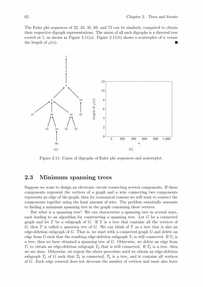
62 Chapter 2. Trees and forests
The Euler phi sequences of 22, 33, 35, 69, and 72 can be similarly computed to obtaintheir respective digraph representations. The union of all such digraphs is a directed treerooted at 1, as shown in Figure 2.11(a). Figure 2.11(b) shows a scatterplot of n versusthe length of ϕ(n).
1
2
4
8
15 20
33 44
69
24
35 72
10
22
(a)
0 200 400 600 800 1,0000
2
4
6
8
10
12
n
len
gth
ofϕ
(n)
(b)
Figure 2.11: Union of digraphs of Euler phi sequences and scatterplot.
2.3 Minimum spanning trees
Suppose we want to design an electronic circuit connecting several components. If thesecomponents represent the vertices of a graph and a wire connecting two componentsrepresents an edge of the graph, then for economical reasons we will want to connect thecomponents together using the least amount of wire. The problem essentially amountsto finding a minimum spanning tree in the graph containing these vertices.
But what is a spanning tree? We can characterize a spanning tree in several ways,each leading to an algorithm for constructing a spanning tree. Let G be a connectedgraph and let T be a subgraph of G. If T is a tree that contains all the vertices ofG, then T is called a spanning tree of G. We can think of T as a tree that is also anedge-deletion subgraph of G. That is, we start with a connected graph G and delete anedge from G such that the resulting edge-deletion subgraph T1 is still connected. If T1 isa tree, then we have obtained a spanning tree of G. Otherwise, we delete an edge fromT1 to obtain an edge-deletion subgraph T2 that is still connected. If T2 is a tree, thenwe are done. Otherwise, we repeat the above procedure until we obtain an edge-deletionsubgraph Tk of G such that Tk is connected, Tk is a tree, and it contains all verticesof G. Each edge removal does not decrease the number of vertices and must also leave

2.3. Minimum spanning trees 63
the resulting edge-deletion subgraph connected. Thus eventually the above procedureresults in a spanning tree of G. Our discussion is summarized in Algorithm 2.1.
Algorithm 2.1 Randomized spanning tree construction.
Input A connected graph G.Output A spanning tree of G.
1: T ← G2: while T is not a tree do3: e← random edge of T4: if T − e is connected then5: T ← T − e6: return T
Another characterization of a spanning tree T of a connected graph G is that T is amaximal set of edges of G that contains no cycle. Kruskal’s algorithm (see section 2.3.1)exploits this condition to construct a minimum spanning tree (MST). A minimum span-ning tree is a spanning tree of a weighted graph having lowest total weight among allpossible spanning trees of the graph. A third characterization of a spanning tree is thatit is a minimal set of edges that connect all vertices, a characterization that results inyet another algorithm called Prim’s algorithm (see section 2.3.2) for constructing mini-mum spanning trees. The task of determining a minimum spanning tree in a connectedweighted graph is called the minimum spanning tree problem. As early as 1926, OtakarBoruvka stated [34, 35] this problem and offered a solution now known as Boruvka’salgorithm (see section 2.3.3). See [88, 139] for a history of the minimum spanning treeproblem.
2.3.1 Kruskal’s algorithm
In 1956, Joseph B. Kruskal published [125] a procedure for constructing a minimum span-ning tree of a connected weighted graph G = (V,E). Now known as Kruskal’s algorithm,with a suitable implementation the procedure runs in O
(|E| · log |E|
)time. Variants
of Kruskal’s algorithm include the algorithm by Prim [163] and that by Loberman andWeinberger [137].
Kruskal’s algorithm belongs to the class of greedy algorithms. As will be explainedbelow, when constructing a minimum spanning tree Kruskal’s algorithm considers onlythe edge having minimum weight among all available edges. Given a weighted nontrivialgraph G = (V,E) that is connected, let w : E → R be the weight function of G. Thefirst stage is creating a “skeleton” of the tree T that is initially set to be a graph withoutedges, i.e. T = (V, ∅). The next stage involves sorting the edges of G by weights innondecreasing order. In other words, we label the edges of G as follows:
E = e1, e2, . . . , en
where n = |E| and w(e1) ≤ w(e2) ≤ · · · ≤ w(en). Now consider each edge ei fori = 1, 2, . . . , n. We add ei to the edge set of T provided that ei does not result in Thaving a cycle. The only way adding ei = uivi to T would create a cycle is if both ui andvi were endpoints of edges (not necessarily distinct) in the same connected componentof T . As long as the acyclic condition holds with the addition of a new edge to T , weadd that new edge. Following the acyclic test, we also test that the (updated) graph

64 Chapter 2. Trees and forests
T is a tree of G. As G is a graph of order |V |, apply Theorem 2.10 to see that if Thas size |V | − 1, then it is a spanning tree of G. Algorithm 2.2 provides pseudocode ofour discussion of Kruskal’s algorithm. When the algorithm halts, it returns a minimumspanning tree of G. The correctness of Algorithm 2.2 is proven in Theorem 2.14.
Algorithm 2.2 Kruskal’s algorithm.
Input A connected weighted graph G = (V,E) with weight function w.Output A minimum spanning tree of G.
1: m← |V |2: T ← ∅3: sort E = e1, e2, . . . , en by weights so that w(e1) ≤ w(w2) ≤ · · · ≤ w(en)4: for i← 1, 2, . . . , n do5: if ei /∈ E(T ) and T ∪ ei is acyclic then6: T ← T ∪ ei7: if |T | = m− 1 then8: return T
Theorem 2.14. Correctness of Algorithm 2.2. If G is a nontrivial connectedweighted graph, then Algorithm 2.2 outputs a minimum spanning tree of G.
Proof. Let G be a nontrivial connected graph of order m and having weight function w.Let T be a subgraph of G produced by Kruskal’s algorithm 2.2. By construction, T is aspanning tree of G with
E(T ) = e1, e2, . . . , em−1where w(e1) ≤ w(e2) ≤ · · · ≤ w(em−1) so that the total weight of T is
w(T ) =m−1∑
i=1
w(ei).
Suppose for contradiction that T is not a minimum spanning tree of G. Among all theminimum spanning trees of G, let H be a minimum spanning tree of G such that H hasthe most number of edges in common with T . As T and H are distinct subgraphs of G,then T has at least an edge not belonging to H. Let ei ∈ E(T ) be the first edge not inH. Construct the graph G0 = H + ei obtained by adding the edge ei to H. Note thatG0 has exactly one cycle C. Since T is acyclic, there exists an edge e0 ∈ E(C) such thate0 is not in T . Construct the graph T0 = G0 − e0 obtained by deleting the edge e0 fromG0. Then T0 is a spanning tree of G with
w(T0) = w(H) + w(ei)− w(e0)
and w(H) ≤ w(T0) and hence w(e0) ≤ w(ei). By Kruskal’s algorithm 2.2, ei is an edge ofminimum weight such that e1, e2, . . . , ei−1∪ei is acyclic. Furthermore, the subgraphe1, e2, . . . , ei−1, e0 of H is acyclic. Thus we have w(ei) = w(e0) and w(T0) = w(H) andso T is a minimum spanning tree of G. By construction, T0 has more edges in commonwith T than H has with T , in contradiction of our hypothesis.
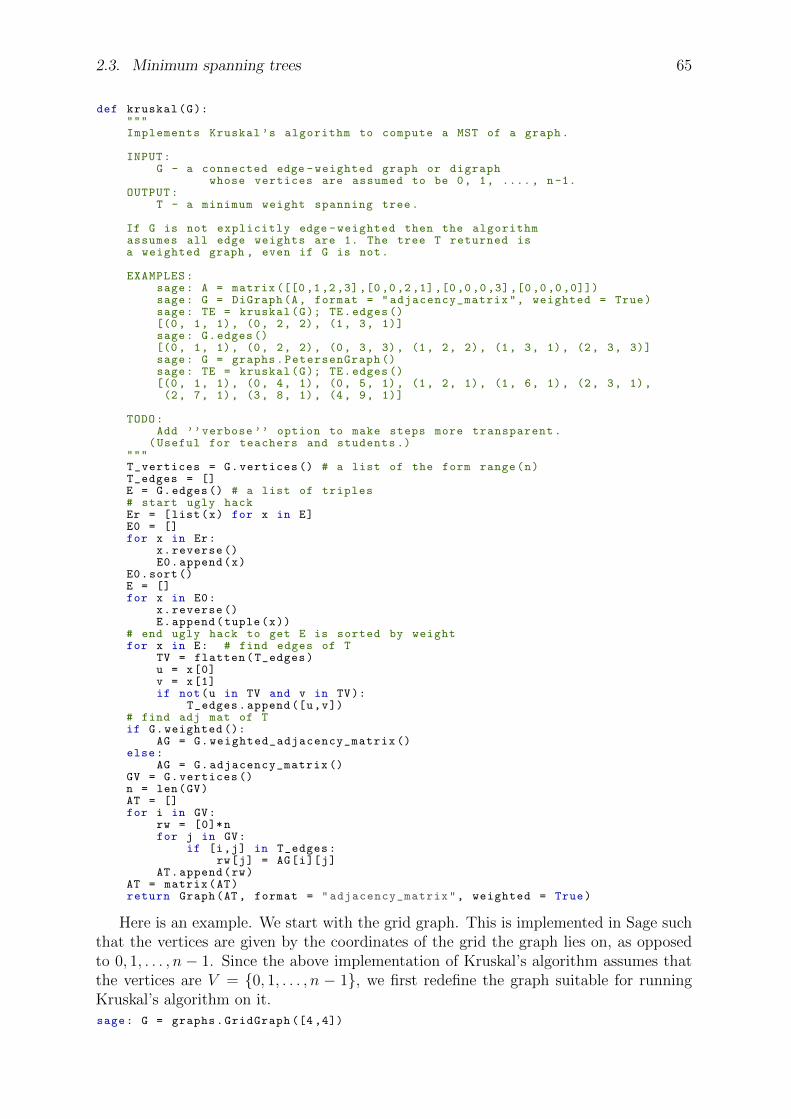
2.3. Minimum spanning trees 65
def kruskal(G):"""Implements Kruskal ’s algorithm to compute a MST of a graph.
INPUT:G - a connected edge -weighted graph or digraph
whose vertices are assumed to be 0, 1, ...., n-1.OUTPUT:
T - a minimum weight spanning tree.
If G is not explicitly edge -weighted then the algorithmassumes all edge weights are 1. The tree T returned isa weighted graph , even if G is not.
EXAMPLES:sage: A = matrix ([[0,1,2,3],[0,0,2,1],[0,0,0,3],[0,0,0,0]])sage: G = DiGraph(A, format = "adjacency_matrix", weighted = True)sage: TE = kruskal(G); TE.edges ()[(0, 1, 1), (0, 2, 2), (1, 3, 1)]sage: G.edges ()[(0, 1, 1), (0, 2, 2), (0, 3, 3), (1, 2, 2), (1, 3, 1), (2, 3, 3)]sage: G = graphs.PetersenGraph ()sage: TE = kruskal(G); TE.edges ()[(0, 1, 1), (0, 4, 1), (0, 5, 1), (1, 2, 1), (1, 6, 1), (2, 3, 1),(2, 7, 1), (3, 8, 1), (4, 9, 1)]
TODO:Add ’’verbose ’’ option to make steps more transparent.
(Useful for teachers and students .)"""T_vertices = G.vertices () # a list of the form range(n)T_edges = []E = G.edges() # a list of triples# start ugly hackEr = [list(x) for x in E]E0 = []for x in Er:
x.reverse ()E0.append(x)
E0.sort()E = []for x in E0:
x.reverse ()E.append(tuple(x))
# end ugly hack to get E is sorted by weightfor x in E: # find edges of T
TV = flatten(T_edges)u = x[0]v = x[1]if not(u in TV and v in TV):
T_edges.append ([u,v])# find adj mat of Tif G.weighted ():
AG = G.weighted_adjacency_matrix ()else:
AG = G.adjacency_matrix ()GV = G.vertices ()n = len(GV)AT = []for i in GV:
rw = [0]*nfor j in GV:
if [i,j] in T_edges:rw[j] = AG[i][j]
AT.append(rw)AT = matrix(AT)return Graph(AT, format = "adjacency_matrix", weighted = True)
Here is an example. We start with the grid graph. This is implemented in Sage suchthat the vertices are given by the coordinates of the grid the graph lies on, as opposedto 0, 1, . . . , n − 1. Since the above implementation of Kruskal’s algorithm assumes thatthe vertices are V = 0, 1, . . . , n − 1, we first redefine the graph suitable for runningKruskal’s algorithm on it.sage: G = graphs.GridGraph ([4 ,4])
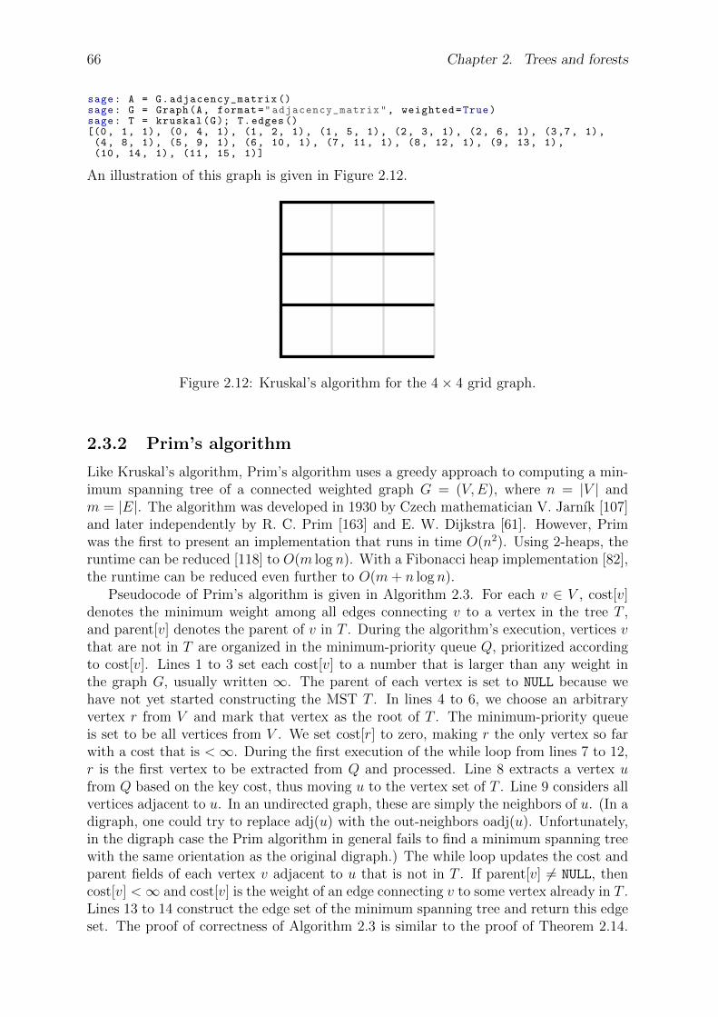
66 Chapter 2. Trees and forests
sage: A = G.adjacency_matrix ()sage: G = Graph(A, format="adjacency_matrix", weighted=True)sage: T = kruskal(G); T.edges ()[(0, 1, 1), (0, 4, 1), (1, 2, 1), (1, 5, 1), (2, 3, 1), (2, 6, 1), (3,7, 1),(4, 8, 1), (5, 9, 1), (6, 10, 1), (7, 11, 1), (8, 12, 1), (9, 13, 1),(10, 14, 1), (11, 15, 1)]
An illustration of this graph is given in Figure 2.12.
Figure 2.12: Kruskal’s algorithm for the 4× 4 grid graph.
2.3.2 Prim’s algorithm
Like Kruskal’s algorithm, Prim’s algorithm uses a greedy approach to computing a min-imum spanning tree of a connected weighted graph G = (V,E), where n = |V | andm = |E|. The algorithm was developed in 1930 by Czech mathematician V. Jarnık [107]and later independently by R. C. Prim [163] and E. W. Dijkstra [61]. However, Primwas the first to present an implementation that runs in time O(n2). Using 2-heaps, theruntime can be reduced [118] to O(m log n). With a Fibonacci heap implementation [82],the runtime can be reduced even further to O(m+ n log n).
Pseudocode of Prim’s algorithm is given in Algorithm 2.3. For each v ∈ V , cost[v]denotes the minimum weight among all edges connecting v to a vertex in the tree T ,and parent[v] denotes the parent of v in T . During the algorithm’s execution, vertices vthat are not in T are organized in the minimum-priority queue Q, prioritized accordingto cost[v]. Lines 1 to 3 set each cost[v] to a number that is larger than any weight inthe graph G, usually written ∞. The parent of each vertex is set to NULL because wehave not yet started constructing the MST T . In lines 4 to 6, we choose an arbitraryvertex r from V and mark that vertex as the root of T . The minimum-priority queueis set to be all vertices from V . We set cost[r] to zero, making r the only vertex so farwith a cost that is <∞. During the first execution of the while loop from lines 7 to 12,r is the first vertex to be extracted from Q and processed. Line 8 extracts a vertex ufrom Q based on the key cost, thus moving u to the vertex set of T . Line 9 considers allvertices adjacent to u. In an undirected graph, these are simply the neighbors of u. (In adigraph, one could try to replace adj(u) with the out-neighbors oadj(u). Unfortunately,in the digraph case the Prim algorithm in general fails to find a minimum spanning treewith the same orientation as the original digraph.) The while loop updates the cost andparent fields of each vertex v adjacent to u that is not in T . If parent[v] 6= NULL, thencost[v] <∞ and cost[v] is the weight of an edge connecting v to some vertex already in T .Lines 13 to 14 construct the edge set of the minimum spanning tree and return this edgeset. The proof of correctness of Algorithm 2.3 is similar to the proof of Theorem 2.14.

2.3. Minimum spanning trees 67
Figure 2.13 shows the minimum spanning tree rooted at vertex 1 as a result of runningPrim’s algorithm over a digraph; Figure 2.14 shows the corresponding tree rooted atvertex 5 of an undirected graph.
Algorithm 2.3 Prim’s algorithm.
Input A weighted connected graph G = (V,E) with weight function w.Output A minimum spanning tree T of G.
1: for each v ∈ V do2: cost[v]←∞3: parent[v]← Null
4: r ← arbitrary vertex of V5: cost[r]← 06: Q← V7: while Q 6= ∅ do8: u← extractMin(Q)9: for each v ∈ adj(u) do
10: if v ∈ Q and w(u, v) < cost[v] then11: parent[v]← u12: cost[v]← w(u, v)
13: T ←
(v, parent[v]) | v ∈ V − r
14: return T
def prim(G):"""Implements Prim’s algorithm to compute a MST of a graph.
INPUT:G - a connected graph.
OUTPUT:T - a minimum weight spanning tree.
REFERENCES:http ://en.wikipedia.org/wiki/Prim’s_algorithm
"""T_vertices = [0] # assumes G.vertices = range(n)T_edges = []E = G.edges() # a list of triplesV = G.vertices ()# start ugly hack to sort EEr = [list(x) for x in E]E0 = []for x in Er:
x.reverse ()E0.append(x)
E0.sort()E = []for x in E0:
x.reverse ()E.append(tuple(x))
# end ugly hack to get E is sorted by weightfor x in E:
u = x[0]v = x[1]if u in T_vertices and not(v in T_vertices ):
T_edges.append ([u,v])T_vertices.append(v)
# found T_vertices , T_edges# find adj mat of Tif G.weighted ():
AG = G.weighted_adjacency_matrix ()else:
AG = G.adjacency_matrix ()GV = G.vertices ()
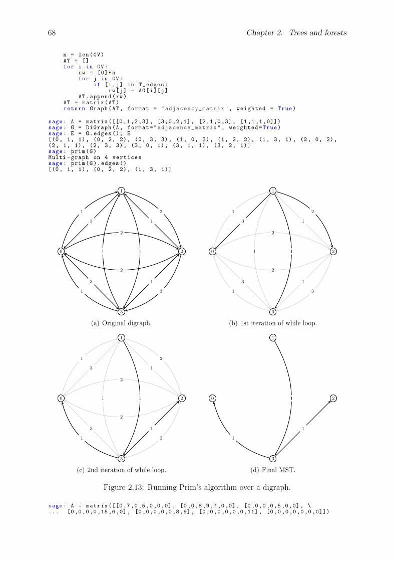
68 Chapter 2. Trees and forests
n = len(GV)AT = []for i in GV:
rw = [0]*nfor j in GV:
if [i,j] in T_edges:rw[j] = AG[i][j]
AT.append(rw)AT = matrix(AT)return Graph(AT, format = "adjacency_matrix", weighted = True)
sage: A = matrix ([[0,1,2,3], [3,0,2,1], [2,1,0,3], [1,1,1,0]])sage: G = DiGraph(A, format="adjacency_matrix", weighted=True)sage: E = G.edges (); E[(0, 1, 1), (0, 2, 2), (0, 3, 3), (1, 0, 3), (1, 2, 2), (1, 3, 1), (2, 0, 2),(2, 1, 1), (2, 3, 3), (3, 0, 1), (3, 1, 1), (3, 2, 1)]sage: prim(G)Multi -graph on 4 verticessage: prim(G).edges ()[(0, 1, 1), (0, 2, 2), (1, 3, 1)]
0
1
2
3
1
2
3
3
2
1
2
1
31
1
1
(a) Original digraph.
0
1
2
3
1
2
3
2
1
31
1
1
3
2
1
(b) 1st iteration of while loop.
0
1
2
3
1
2
3
3
2
2
1
3
1 1
1
1
(c) 2nd iteration of while loop.
0
1
2
3
1
1
1
(d) Final MST.
Figure 2.13: Running Prim’s algorithm over a digraph.
sage: A = matrix ([[0,7,0,5,0,0,0], [0,0,8,9,7,0,0], [0,0,0,0,5,0,0], \... [0,0,0,0,15,6,0], [0,0,0,0,0,8,9], [0,0,0,0,0,0,11], [0,0,0,0,0,0,0]])
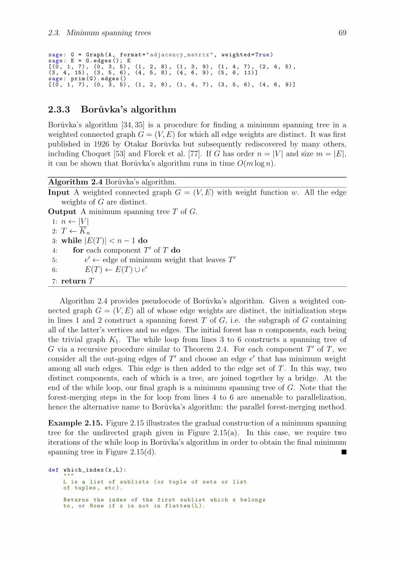
2.3. Minimum spanning trees 69
sage: G = Graph(A, format="adjacency_matrix", weighted=True)sage: E = G.edges (); E[(0, 1, 7), (0, 3, 5), (1, 2, 8), (1, 3, 9), (1, 4, 7), (2, 4, 5),(3, 4, 15), (3, 5, 6), (4, 5, 8), (4, 6, 9), (5, 6, 11)]sage: prim(G).edges ()[(0, 1, 7), (0, 3, 5), (1, 2, 8), (1, 4, 7), (3, 5, 6), (4, 6, 9)]
2.3.3 Boruvka’s algorithm
Boruvka’s algorithm [34, 35] is a procedure for finding a minimum spanning tree in aweighted connected graph G = (V,E) for which all edge weights are distinct. It was firstpublished in 1926 by Otakar Boruvka but subsequently rediscovered by many others,including Choquet [53] and Florek et al. [77]. If G has order n = |V | and size m = |E|,it can be shown that Boruvka’s algorithm runs in time O(m log n).
Algorithm 2.4 Boruvka’s algorithm.
Input A weighted connected graph G = (V,E) with weight function w. All the edgeweights of G are distinct.
Output A minimum spanning tree T of G.1: n← |V |2: T ← Kn
3: while |E(T )| < n− 1 do4: for each component T ′ of T do5: e′ ← edge of minimum weight that leaves T ′
6: E(T )← E(T ) ∪ e′7: return T
Algorithm 2.4 provides pseudocode of Boruvka’s algorithm. Given a weighted con-nected graph G = (V,E) all of whose edge weights are distinct, the initialization stepsin lines 1 and 2 construct a spanning forest T of G, i.e. the subgraph of G containingall of the latter’s vertices and no edges. The initial forest has n components, each beingthe trivial graph K1. The while loop from lines 3 to 6 constructs a spanning tree ofG via a recursive procedure similar to Theorem 2.4. For each component T ′ of T , weconsider all the out-going edges of T ′ and choose an edge e′ that has minimum weightamong all such edges. This edge is then added to the edge set of T . In this way, twodistinct components, each of which is a tree, are joined together by a bridge. At theend of the while loop, our final graph is a minimum spanning tree of G. Note that theforest-merging steps in the for loop from lines 4 to 6 are amenable to parallelization,hence the alternative name to Boruvka’s algorithm: the parallel forest-merging method.
Example 2.15. Figure 2.15 illustrates the gradual construction of a minimum spanningtree for the undirected graph given in Figure 2.15(a). In this case, we require twoiterations of the while loop in Boruvka’s algorithm in order to obtain the final minimumspanning tree in Figure 2.15(d).
def which_index(x,L):"""L is a list of sublists (or tuple of sets or listof tuples , etc).
Returns the index of the first sublist which x belongsto , or None if x is not in flatten(L).
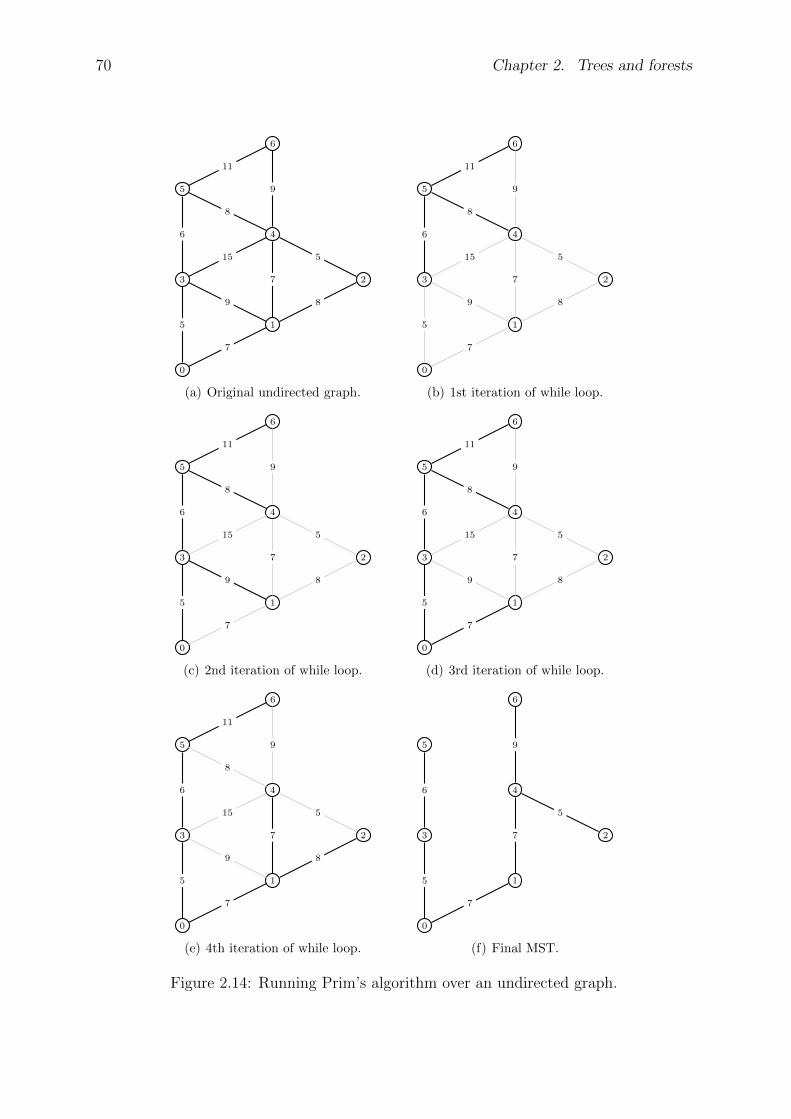
70 Chapter 2. Trees and forests
0
1
23
4
5
6
7
5
89
7
515
6
8
9
11
(a) Original undirected graph.
0
1
23
4
5
6
7
5
89
7
515
9
6
8
11
(b) 1st iteration of while loop.
0
1
23
4
5
6
7
89
7
515
9
5
9
6
8
11
(c) 2nd iteration of while loop.
0
1
23
4
5
6
89
7
515
9
7
5
6
8
11
(d) 3rd iteration of while loop.
0
1
23
4
5
6
9
515
8
9
7
5
8
7
6
11
(e) 4th iteration of while loop.
0
1
23
4
5
6
7
7
5
5
9
6
(f) Final MST.
Figure 2.14: Running Prim’s algorithm over an undirected graph.
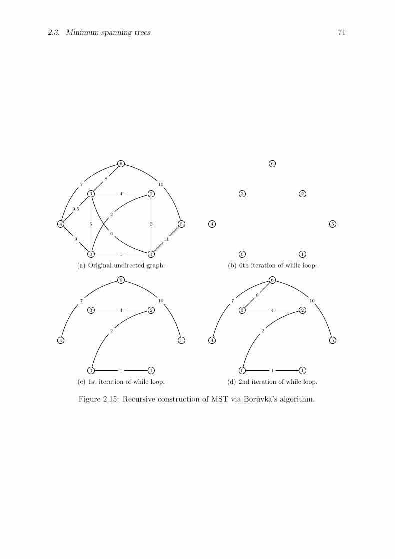
2.3. Minimum spanning trees 71
0 1
23
4 5
6
1
2
5
9
3
611
4
9.5
87 10
(a) Original undirected graph.
0 1
23
4 5
6
(b) 0th iteration of while loop.
0 1
23
4 5
6
1
2
4
7 10
(c) 1st iteration of while loop.
0 1
23
4 5
6
1
2
4
87 10
(d) 2nd iteration of while loop.
Figure 2.15: Recursive construction of MST via Boruvka’s algorithm.
72 Chapter 2. Trees and forests
The 0-th element inLx = [L.index(S) for S in L if x in S]almost works , but if the list is empty then Lx[0]throws an exception.
EXAMPLES:sage: L = [[1,2,3],[4,5],[6,7,8]]sage: which_index (3,L)0sage: which_index (4,L)1sage: which_index (7,L)2sage: which_index (9,L)sage: which_index (9,L) == NoneTrue
"""for S in L:
if x in S:return L.index(S)
return None
def boruvka(G):"""Implements Boruvka ’s algorithm to compute a MST of a graph.
INPUT:G - a connected edge -weighted graph with distinct weights.
OUTPUT:T - a minimum weight spanning tree.
REFERENCES:http ://en.wikipedia.org/wiki/Boruvka ’s_algorithm
"""T_vertices = [] # assumes G.vertices = range(n)T_edges = []T = Graph()E = G.edges() # a list of triplesV = G.vertices ()# start ugly hack to sort EEr = [list(x) for x in E]E0 = []for x in Er:
x.reverse ()E0.append(x)
E0.sort()E = []for x in E0:
x.reverse ()E.append(tuple(x))
# end ugly hack to get E is sorted by weightfor e in E:
# create about |V|/2 edges of T "cheaply"TV = T.vertices ()if not(e[0] in TV) or not(e[1] in TV):
T.add_edge(e)for e in E:
# connect the "cheapest" components to get TC = T.connected_components_subgraphs ()VC = [S.vertices () for S in C]if not(e in T.edges ()) and (which_index(e[0],VC) != which_index(e[1],VC)):
if T.is_connected ():break
T.add_edge(e)return T
Some examples using Sage:sage: A = matrix ([[0,1,2,3], [4,0,5,6], [7,8,0,9], [10 ,11 ,12 ,0]])sage: G = DiGraph(A, format="adjacency_matrix", weighted=True)sage: boruvka(G)Multi -graph on 4 verticessage: boruvka(G).edges ()[(0, 1, 1), (0, 2, 2), (0, 3, 3)]sage: A = matrix ([[0,2,0,5,0,0,0], [0,0,8,9,7,0,0], [0,0,0,0,1,0,0],\... [0,0,0,0,15,6,0], [0,0,0,0,0,3,4], [0,0,0,0,0,0,11], [0,0,0,0,0,0,0]])sage: G = Graph(A, format="adjacency_matrix", weighted=True)

2.3. Minimum spanning trees 73
sage: E = G.edges (); E[(0, 1, 2), (0, 3, 5), (1, 2, 8), (1, 3, 9), (1, 4, 7),(2, 4, 1), (3, 4, 15), (3, 5, 6), (4, 5, 3), (4,6, 4), (5, 6, 11)]sage: boruvka(G)Multi -graph on 7 verticessage: boruvka(G).edges ()[(0, 1, 2), (0, 3, 5), (2, 4, 1), (3, 5, 6), (4, 5, 3), (4, 6, 4)]sage: A = matrix ([[0,1,2,5], [0,0,3,6], [0,0,0,4], [0,0,0,0]])sage: G = Graph(A, format="adjacency_matrix", weighted=True)sage: boruvka(G).edges ()[(0, 1, 1), (0, 2, 2), (2, 3, 4)]sage: A = matrix ([[0,1,5,0,4], [0,0,0,0,3], [0,0,0,2,0], [0,0,0,0,0], [0,0,0,0,0]])sage: G = Graph(A, format="adjacency_matrix", weighted=True)sage: boruvka(G).edges ()[(0, 1, 1), (0, 2, 5), (1, 4, 3), (2, 3, 2)]
2.3.4 Circuit matrix
Recall, the term cycle refers to a closed path. If G is a digraph then a cycle refers toa sequence of edges which form a path in the associated undirected graph. If repeatedvertices are allowed, it is more often called a closed walk. If the path is a simple path,with no repeated vertices or edges other than the starting and ending vertices, it mayalso be called a simple cycle or circuit. A cycle in a directed graph is called a directedcycle.
Let Z1, . . . , ZM denote an enumeration of the cycles (simple closed paths) of G. Thecycle matrix or circuit matrix is a M×m matrix C = (cij) whose rows are parameterizedby the cycles and whose columns are parameterized by the edges E = e1, . . . , em, where
cij =
1, ei ∈ Zi,0, otherwise.
Recall the incidence matrix was defined in §1.3.2.
Theorem 2.16. If G is a directed graph then the rows of the incidence matrix D(G) areorthogonal to the rows of C(G).
Proof. We first show that C ·Dt = 0. Consider the ith row of C and jth column of Dt.There are non-zero entries in the corresponding entries of these vectors if and only if thejth vertex of G is incident to an edge which occurs in the ith cycle of G. Assume thisentry is non-zero. Since G is a directed graph, there is another vertex (the other vertexdefining this edge) for which the associated entry is the same but with opposite sign.Therefore the dot product of the ith row of Q and jth column of Dt is zero.
The theorem above implies that the column space of the matrix Ct (namely, theimage of the associated linear transformation) is contained in the kernel of the incidencematrix D.
Let F be a field. There is a general result called Sylvester’s Law of Nullity which saysthat if K is an r × s matrix over F and L is an s× t matrix over F (so KL is defined),and if
KL = 0,
then
rankF (K) + rankF (L) ≤ s.

74 Chapter 2. Trees and forests
(This is an immediate corollary of the rank plus nullity theorem from linear algebra.) Itfollows from this fact that
rankQ(D) + rankQ(C) ≤ m.
As a corollary to Theorem 1.28, we see that
rankQ(D) ≤ m− n+ 1.
Theorem 2.17. If G is a directed graph then
rankQ(C) = m− n+ 1.
Proof. To show that equality is attained, we exhibit m−n+1 linearly independent rowsof C. Let T = (V (T ), E(T )) be a spanning tree for G. This tree has n − 1 edges andso G has m− n+ 1 edges not in T . Let e /∈ E(T ) be such an edge. The graph T + e isa cycle. Recall such a cycle is called a fundamental cycle (associated to T ). There areexactly m − n + 1 such cycles. Note that no other fundamental cycle “supports” edgee. Suppose that e is the ith edge in E(G). The row of C associated to the cycle T + ehas a 1 in the ith coordinate. Every other row of C associated to a fundamental cyclehas a 0 in the ith coordinate. Therefore, the rows of C associated to these m − n + 1fundamental cycles are linearly independent.
2.3.5 Cutset matrix
The term cutset (or edge cutset) refers to a sequence of edges in a connected graphG = (V,E) which, when removed from G, creates a disconnected graph and, furthermore,that no proper subset of these edges has this property. When a graph can be disconnectedby removing only one edge, that edge is called a bridge.
A cutset can be associated to each vertex v ∈ V as follows.
Lemma 2.18. The subset Sv ⊂ E of all the edges incident to v forms forms a cutset.
This uses only the definitions and is left to the interested reader as an exercise.Let S1, . . . , SN denote the cutsets of G. The cutset matrix N ×m matrix Q = (qij)
whose rows are parameterized by the cutsets and whose columns are parameterized bythe edges E = e1, . . . , em, where
qij =
1, ei ∈ Si,0, otherwise.
Theorem 2.19. If G is a connected digraph then
rankQ(Q) = n− 1.
The analog of this theorem for undirected graphs is false (as the examples belowshow). However, the undirected analog does work if you use the rank over GF (2).
Proof. Let G be any connected graph (directed or not). By Lemma 2.18 above, for eachv ∈ V there is a cut-set Sv consisting of all edges incident to v. The characteristic vectorqv = (q1, . . . , qm) of this set (qi = 1 if ei ∈ Sv and qi = 0 otherwise) gives us a row
2.3. Minimum spanning trees 75
vector in the incidence matrix and in the cut-set matrix. Moreover, all such rows in theincidence matrix are of this form, so
rankQ(Q) ≥ rankQ(C) = n− 1.
Suppose now G is a directed graph. We show equality must hold. Let S be anyedge cutset in G and, for each v ∈ V , let Sv denote the associated cutset as above. If Sdefined a partitioning
V = V1 ∪ V2
then
S =∑
v∈V1
Sv =∑
v∈V2
Sv,
where the sum of two cutsets is simply the formal sum as oriented edges in the freeabelian group Z[E]. From this it is clear that the dimension of the row-span of Q isequal to the dimension of the row-span of the submatrix of Q given by the Sv’s.
Example 2.20. To construct the example, we will make use of the following Pythonfunction.def edge_cutset_matrix(G):
"""Returns the edge cutset matrix of the connected graph $G$."""V = G.vertices ()E = G.edges()rows = []for v1 in V:
for v2 in V:if v1 != v2:
S = G.edge_cut(v1 , v2 , value_only=False )[1]char_S = lambda e: int(bool(e in S))rows.append ([ char_S(e) for e in E])
Q = matrix(rows)return Q
We use the function above in the examples below.For the cube graph in three dimensions (see Figure 2.16) and for the Desargues
graph (see Figure 2.17), the undirected analog of Theorem 2.19 does hold.
sage: G = graphs.CubeGraph (3)sage: G3-Cube: Graph on 8 verticessage: Q = edge_cutset_matrix(G)sage: rank(Q)7sage: G = graphs.DesarguesGraph ()sage: GDesargues Graph: Graph on 20 verticessage: edge_cutset_matrix(G).rank()19
On the other hand, for the Frucht graph (see Figure 2.18):
sage: G = graphs.FruchtGraph ()sage: GFrucht graph: Graph on 12 verticessage: edge_cutset_matrix(G).rank()12
These shall be discussed further in §9.1.
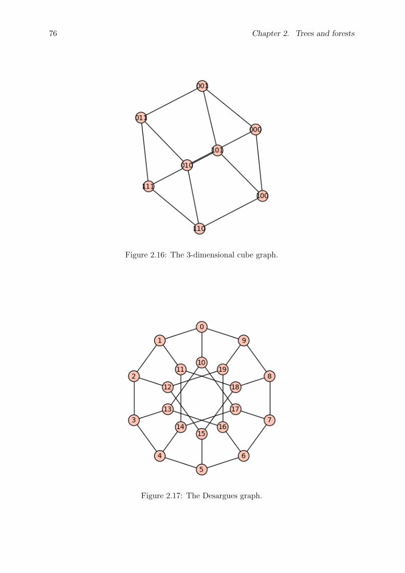
76 Chapter 2. Trees and forests
Figure 2.16: The 3-dimensional cube graph.
Figure 2.17: The Desargues graph.

2.4. Binary trees 77
Figure 2.18: The Frucht graph.
2.4 Binary trees
A binary tree is a rooted tree with at most two children per parent. Each child isdesignated as either a left-child or a right-child . Thus binary trees are also 2-ary trees.Some examples of binary trees are illustrated in Figure 2.19. Given a vertex v in abinary tree T of height h, the left subtree of v is comprised of the subtree that spansthe left-child of v and all of this child’s descendants. The notion of a right-subtree of abinary tree is similarly defined. Each of the left and right subtrees of v is itself a binarytree with height ≤ h− 1. If v is the root vertex, then each of its left and right subtreeshas height ≤ h− 1, and at least one of these subtrees has height equal to h− 1.
(a) (b) (c) (d)
Figure 2.19: Examples of binary trees.
Theorem 2.21. If T is a complete binary tree of height h, then T has 2h+1− 1 vertices.

78 Chapter 2. Trees and forests
Proof. Argue by induction on h. The assertion of the theorem is trivially true in thebase case h = 0. Let k ≥ 0 and assume for induction that any complete binary tree ofheight k has order 2k+1 − 1. Suppose T is a complete binary tree of height k + 1 anddenote the left and right subtrees of T by T1 and T2, respectively. Each Ti (for i = 1, 2)is a complete binary tree of height k and by our induction hypothesis Ti has 2k+1 − 1vertices. Thus T has order
1 + (2k+1 − 1) + (2k+1 − 1) = 2k+2 − 1
as required.
Theorem 2.21 provides a useful upper bound on the order of a binary tree of a givenheight. This upper bound is stated in the following corollary.
Corollary 2.22. A binary tree of height h has at most 2h+1 − 1 vertices.
We now count the number of possible binary trees on n vertices. Let bn be the numberof binary trees of order n. For n = 0, we set b0 = 1. The trivial graph is the only binarytree with one vertex, hence b1 = 1. Suppose n > 1 and let T be a binary tree on nvertices. Then the left subtree of T has order 0 ≤ i ≤ n − 1 and the right subtree hasn−1− i vertices. As there are bi possible left subtrees and bn−1−i possible right subtrees,T has a total of bibn−1−i different combinations of left and right subtrees. Summing fromi = 0 to i = n− 1 and we have
bn =n−1∑
i=0
bibn−1−i. (2.2)
Expression (2.2) is known as the Catalan recursion and the number bn is the n-th Catalannumber, which we know from problem 1.15 can be expressed in the closed form
bn =1
n+ 1
(2n
n
). (2.3)
Figures 2.20 to 2.22 enumerate all the different binary trees on 2, 3, and 4 vertices,respectively.
(a) (b)
Figure 2.20: The b2 = 2 binary trees on 2 vertices.
The first few values of (2.3) are
b0 = 1, b1 = 1, b2 = 2, b3 = 5, b4 = 14
which are rather small and of manageable size if we want to explicitly enumerate alldifferent binary trees with the above orders. However, from n = 4 onwards the valueof bn increases very fast. Instead of enumerating all the bn different binary trees of aspecified order n, a related problem is generating a random binary tree of order n. Thatis, we consider the set B as a sample space of bn different binary trees on n vertices,and choose a random element from B. Such a random element can be generated usingAlgorithm 2.5. The list parent holds all vertices with less than two children, each vertexcan be considered as a candidate parent to which we can add a child. An element ofparent is a two-tuple (v, k) where the vertex v currently has k children.

2.4. Binary trees 79
(a) (b) (c) (d) (e)
Figure 2.21: The b3 = 5 binary trees on 3 vertices.
(a) (b) (c) (d) (e)
(f) (g) (h) (i) (j)
(k) (l) (m) (n)
Figure 2.22: The b4 = 14 binary trees on 4 vertices.
Algorithm 2.5 Random binary tree.Input Positive integer n.Output A random binary tree on n vertices.
1: if n = 1 then2: return K1
3: v ← 04: T ← null graph5: add v to T6: parent← [(v, 0)]7: for i← 1, 2, . . . , n− 1 do8: (v, k)← remove random element from parent
9: if k < 1 then10: add (v, k + 1) to parent
11: add edge (v, i) to T12: add (i, 0) to parent
13: return T
80 Chapter 2. Trees and forests
2.4.1 Binary codes
What is a code?
A code is a rule for converting data in one format, or well-defined tangible representation,into sequences of symbols in another format. The finite set of symbols used is called thealphabet . We shall identify a code as a finite set of symbols which are the image of thealphabet under this conversion rule. The elements of this set are referred to as codewords .For example, using the ASCII code, the letters in the English alphabet get convertedinto numbers in the set 0, 1, . . . , 255. If these numbers are written in binary, theneach codeword of a letter has length 8, i.e. eight bits. In this way, we can reformat orencode a “string” into a sequence of binary symbols, i.e. 0’s and 1’s. Encoding is theconversion process one way. Decoding is the reverse process, converting these sequencesof code-symbols back into information in the original format.
Codes are used for:
Economy . Sometimes this is called entropy encoding since there is an entropyfunction which describes how much information a channel (with a given error rate)can carry and such codes are designed to maximize entropy as best as possible. Inthis case, in addition to simply being given an alphabet A, one might be given aweighted alphabet , i.e. an alphabet for which each symbol a ∈ A is associated witha nonnegative number wa ≥ 0 (in practice, this number represents the probabilitythat the symbol a occurs in a typical word).
Reliability . Such codes are called error-correcting codes , since such codes are de-signed to communicate information over a noisy channel in such a way that theerrors in transmission are likely to be correctable.
Security . Such codes are called cryptosystems . In this case, the inverse of thecoding function c : A → B∗ is designed to be computationally infeasible. In otherwords, the coding function c is designed to be a trapdoor function.
Other codes are merely simpler ways to communicate information (e.g. flag semaphores,color codes, genetic codes, braille codes, musical scores, chess notation, football diagrams,and so on) and have little or no mathematical structure. We shall not study them.
Basic definitions
If every word in the code has the same length, the code is called a block code. If acode is not a block code, then it is called a variable-length code. A prefix-free code is acode (typically one of variable-length) with the property that there is no valid codewordin the code that is a prefix or start of any other codeword.1 This is the prefix-freecondition.
One example of a prefix-free code is the ASCII code. Another example is
00, 01, 100.
On the other hand, a non-example is the code
00, 01, 010, 100
1 In other words, a codeword s = s1 · · · sm is a prefix of a codeword t = t1 · · · tn if and only if m ≤ nand s1 = t1, . . . , sm = tm. Codes that are prefix-free are easier to decode than codes that are notprefix-free.
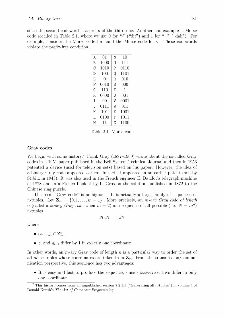
2.4. Binary trees 81
since the second codeword is a prefix of the third one. Another non-example is Morsecode recalled in Table 2.1, where we use 0 for “·” (“dit”) and 1 for “−” (“dah”). Forexample, consider the Morse code for aand the Morse code for w. These codewordsviolate the prefix-free condition.
A 01 N 10B 1000 O 111C 1010 P 0110D 100 Q 1101E 0 R 010F 0010 S 000G 110 T 1H 0000 U 001I 00 V 0001J 0111 W 011K 101 X 1001L 0100 Y 1011M 11 Z 1100
Table 2.1: Morse code
Gray codes
We begin with some history.2 Frank Gray (1887–1969) wrote about the so-called Graycodes in a 1951 paper published in the Bell System Technical Journal and then in 1953patented a device (used for television sets) based on his paper. However, the idea ofa binary Gray code appeared earlier. In fact, it appeared in an earlier patent (one byStibitz in 1943). It was also used in the French engineer E. Baudot’s telegraph machineof 1878 and in a French booklet by L. Gros on the solution published in 1872 to theChinese ring puzzle.
The term “Gray code” is ambiguous. It is actually a large family of sequences ofn-tuples. Let Zm = 0, 1, . . . ,m − 1. More precisely, an m-ary Gray code of lengthn (called a binary Gray code when m = 2) is a sequence of all possible (i.e. N = mn)n-tuples
g1, g2, . . . , gN
where
each gi ∈ Znm,
gi and gi+1 differ by 1 in exactly one coordinate.
In other words, an m-ary Gray code of length n is a particular way to order the set ofall mn n-tuples whose coordinates are taken from Zm. From the transmission/commu-nication perspective, this sequence has two advantages:
It is easy and fast to produce the sequence, since successive entries differ in onlyone coordinate.
2 This history comes from an unpublished section 7.2.1.1 (“Generating all n-tuples”) in volume 4 ofDonald Knuth’s The Art of Computer Programming.

82 Chapter 2. Trees and forests
An error is relatively easy to detect, since we can compare an n-tuple with theprevious one. If they differ in more than one coordinate, we conclude that an errorwas made.
Example 2.23. Here is a 3-ary Gray code of length 2:
[0, 0], [1, 0], [2, 0], [2, 1], [1, 1], [0, 1], [0, 2], [1, 2], [2, 2]
and the sequence
[0, 0, 0], [1, 0, 0], [1, 1, 0], [0, 1, 0], [0, 1, 1], [1, 1, 1], [1, 0, 1], [0, 0, 1]
is a binary Gray code of length 3.
Gray codes have applications to engineering, recreational mathematics (solving theTower of Hanoi puzzle, The Brain puzzle, the Chinese ring puzzle, etc.), and to math-ematics (e.g. aspects of combinatorics, computational group theory, and the computa-tional aspects of linear codes).
Binary Gray codes
Consider the so-called n-hypercube graph Qn, whose first few instances are illustratedin Figure 1.33. This can be envisioned as the graph whose vertices are the vertices of acube in n-space
(x1, . . . , xn) | 0 ≤ xi ≤ 1and whose edges are those line segments in Rn connecting two neighboring vertices, i.e.two vertices that differ in exactly one coordinate. A binary Gray code of length n canbe regarded as a path on the hypercube graph Qn that visits each vertex of the cubeexactly once. In other words, a binary Gray code of length n may be identified with aHamiltonian path on the graph Qn. For example, Figure 2.23 illustrates a Hamiltonianpath on Q3.
Figure 2.23: Viewing Γ3 as a Hamiltonian path on Q3.
How do we efficiently compute a Gray code? Perhaps the simplest way to state theidea of quickly constructing the reflected binary Gray code Γn of length n is as follows:
Γ0 = [ ],
Γn =[[0,Γn−1], [1,Γrev
n−1]]

2.4. Binary trees 83
where Γrevm means the Gray code in reverse order. For instance, we have
Γ0 = [ ],
Γ1 =[[0], [1]
],
Γ2 =[[0, 0], [0, 1], [1, 1], [1, 0]
]
and so on. This is a nice procedure for creating the entire list at once, which gets verylong very fast. An implementation of the reflected Gray code using Python is givenbelow.def graycode(length ,modulus ):
"""Returns the n-tuple reflected Gray code mod m.
EXAMPLES:sage: graycode (2,4)
[[0, 0],[1, 0],[2, 0],[3, 0],[3, 1],[2, 1],[1, 1],[0, 1],[0, 2],[1, 2],[2, 2],[3, 2],[3, 3],[2, 3],[1, 3],[0, 3]]
"""n,m = length ,modulusF = range(m)if n == 1:
return [[i] for i in F]L = graycode(n-1, m)M = []for j in F:
M = M+[ll+[j] for ll in L]k = len(M)Mr = [0]*mfor i in range(m-1):
i1 = i*int(k/m) # this requires Python 3.0 or Sagei2 = (i+1)* int(k/m)Mr[i] = M[i1:i2]
Mr[m-1] = M[(m-1)* int(k/m):]for i in range(m):
if is_odd(i):Mr[i]. reverse ()
M0 = []for i in range(m):
M0 = M0+Mr[i]return M0
Consider the reflected binary code of length 8, i.e. Γ8. This has 28 = 256 codewords.Sage can easily create the list plot of the coordinates (x, y), where x is an integer j ∈ Z256
that indexes the codewords in Γ8 and the corresponding y is the j-th codeword in Γ8
converted to decimal. This will give us some idea of how the Gray code “looks” in somesense. The plot is given in Figure 2.24.
What if we only want to compute the i-th Gray codeword in the Gray code of lengthn? Can it be computed quickly without computing the entire list? At least in the case ofthe reflected binary Gray code, there is a very simple way to do this. The k-th element in
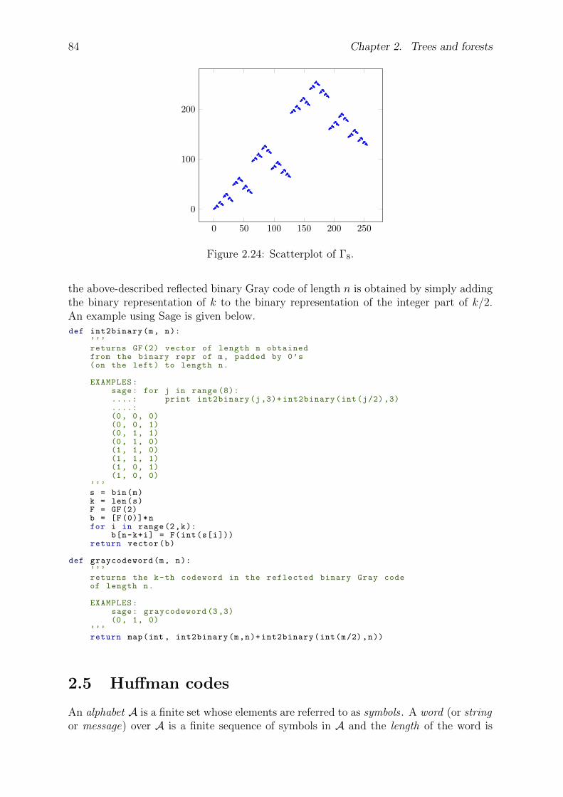
84 Chapter 2. Trees and forests
0 50 100 150 200 250
0
100
200
Figure 2.24: Scatterplot of Γ8.
the above-described reflected binary Gray code of length n is obtained by simply addingthe binary representation of k to the binary representation of the integer part of k/2.An example using Sage is given below.def int2binary(m, n):
’’’returns GF(2) vector of length n obtainedfrom the binary repr of m, padded by 0’s(on the left) to length n.
EXAMPLES:sage: for j in range (8):....: print int2binary(j,3)+ int2binary(int(j/2),3)....:(0, 0, 0)(0, 0, 1)(0, 1, 1)(0, 1, 0)(1, 1, 0)(1, 1, 1)(1, 0, 1)(1, 0, 0)
’’’s = bin(m)k = len(s)F = GF(2)b = [F(0)]*nfor i in range(2,k):
b[n-k+i] = F(int(s[i]))return vector(b)
def graycodeword(m, n):’’’returns the k-th codeword in the reflected binary Gray codeof length n.
EXAMPLES:sage: graycodeword (3,3)(0, 1, 0)
’’’return map(int , int2binary(m,n)+ int2binary(int(m/2),n))
2.5 Huffman codes
An alphabet A is a finite set whose elements are referred to as symbols . A word (or stringor message) over A is a finite sequence of symbols in A and the length of the word is
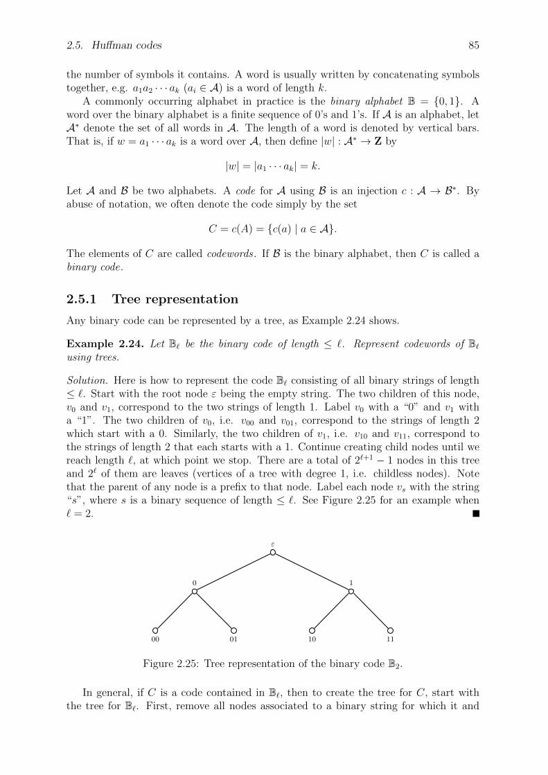
2.5. Huffman codes 85
the number of symbols it contains. A word is usually written by concatenating symbolstogether, e.g. a1a2 · · · ak (ai ∈ A) is a word of length k.
A commonly occurring alphabet in practice is the binary alphabet B = 0, 1. Aword over the binary alphabet is a finite sequence of 0’s and 1’s. If A is an alphabet, letA∗ denote the set of all words in A. The length of a word is denoted by vertical bars.That is, if w = a1 · · · ak is a word over A, then define |w| : A∗ → Z by
|w| = |a1 · · · ak| = k.
Let A and B be two alphabets. A code for A using B is an injection c : A → B∗. Byabuse of notation, we often denote the code simply by the set
C = c(A) = c(a) | a ∈ A.
The elements of C are called codewords . If B is the binary alphabet, then C is called abinary code.
2.5.1 Tree representation
Any binary code can be represented by a tree, as Example 2.24 shows.
Example 2.24. Let B` be the binary code of length ≤ `. Represent codewords of B`using trees.
Solution. Here is how to represent the code B` consisting of all binary strings of length≤ `. Start with the root node ε being the empty string. The two children of this node,v0 and v1, correspond to the two strings of length 1. Label v0 with a “0” and v1 witha “1”. The two children of v0, i.e. v00 and v01, correspond to the strings of length 2which start with a 0. Similarly, the two children of v1, i.e. v10 and v11, correspond tothe strings of length 2 that each starts with a 1. Continue creating child nodes until wereach length `, at which point we stop. There are a total of 2`+1 − 1 nodes in this treeand 2` of them are leaves (vertices of a tree with degree 1, i.e. childless nodes). Notethat the parent of any node is a prefix to that node. Label each node vs with the string“s”, where s is a binary sequence of length ≤ `. See Figure 2.25 for an example when` = 2.
00 01 10 11
0 1
ε
Figure 2.25: Tree representation of the binary code B2.
In general, if C is a code contained in B`, then to create the tree for C, start withthe tree for B`. First, remove all nodes associated to a binary string for which it and

86 Chapter 2. Trees and forests
all of its descendants are not in C. Next, remove all labels which do not correspond tocodewords in C. The resulting labeled graph is the tree associated to the binary code C.
For visualizing the construction of Huffman codes later, it is important to see thatwe can reverse this construction to start from such a binary tree and recover a binarycode from it. The codewords are determined by the following rules:
The root node gets the empty codeword.
Each left-ward branch gets a 0 appended to the end of its parent. Each right-wardbranch gets a 1 appended to the end.
2.5.2 Uniquely decodable codes
If c : A → B∗ is a code, then we can extend c to A∗ by concatenation:
c(a1a2 · · · ak) = c(a1)c(a2) · · · c(ak).
If the extension c : A∗ → T ∗ is also an injection, then c is called uniquely decodable.The property of unique decodability or decipherability informally means that any givensequence of symbols has at most one interpretation as a sequence of codewords.
Example 2.25. Is the Morse code in Table 2.1 uniquely decodable? Why or why not?
Solution. Note that these Morse codewords all have lengths less than or equal to 4.Other commonly occurring symbols used (the digits 0 through 9, punctuation symbols,and some others) are also encodable in Morse code, but they use longer codewords.
Let A denote the English alphabet, B = 0, 1 the binary alphabet, and c : A → B∗the Morse code. Since c(ET ) = 01 = c(A), it is clear that the Morse code is not uniquelydecodable.
In fact, prefix-free implies uniquely decodable.
Theorem 2.26. If a code c : A → B∗ is prefix-free, then it is uniquely decodable.
Proof. We use induction on the length of a message. We want to show that if x1 · · ·xkand y1 · · · y` are messages with c(x1) · · · c(xk) = c(y1) · · · c(y`), then x1 · · · xk = y1 · · · y`.This in turn implies k = ` and xi = yi for all i.
The case of length 1 follows from the fact that c : A → B∗ is injective (by thedefinition of code).
Suppose that the statement of the theorem holds for all codes of length < m. Wemust show that the length m case is true. Suppose c(x1) · · · c(xk) = c(y1) · · · c(y`), wherem = max(k, `). These strings are equal, so the substring c(x1) of the left-hand sideand the substring c(y1) of the right-hand side are either equal or one is contained in theother. If, say, c(x1) is properly contained in c(y1), then c is not prefix-free. Likewise ifc(y1) is properly contained in c(x1). Therefore, c(x1) = c(y1), which implies x1 = y1.Now remove this codeword from both sides, so c(x2) · · · c(xk) = c(y2) · · · c(y`). By theinduction hypothesis, x2 · · · xk = y2 · · · y`. These facts together imply k = ` and xi = yifor all i.
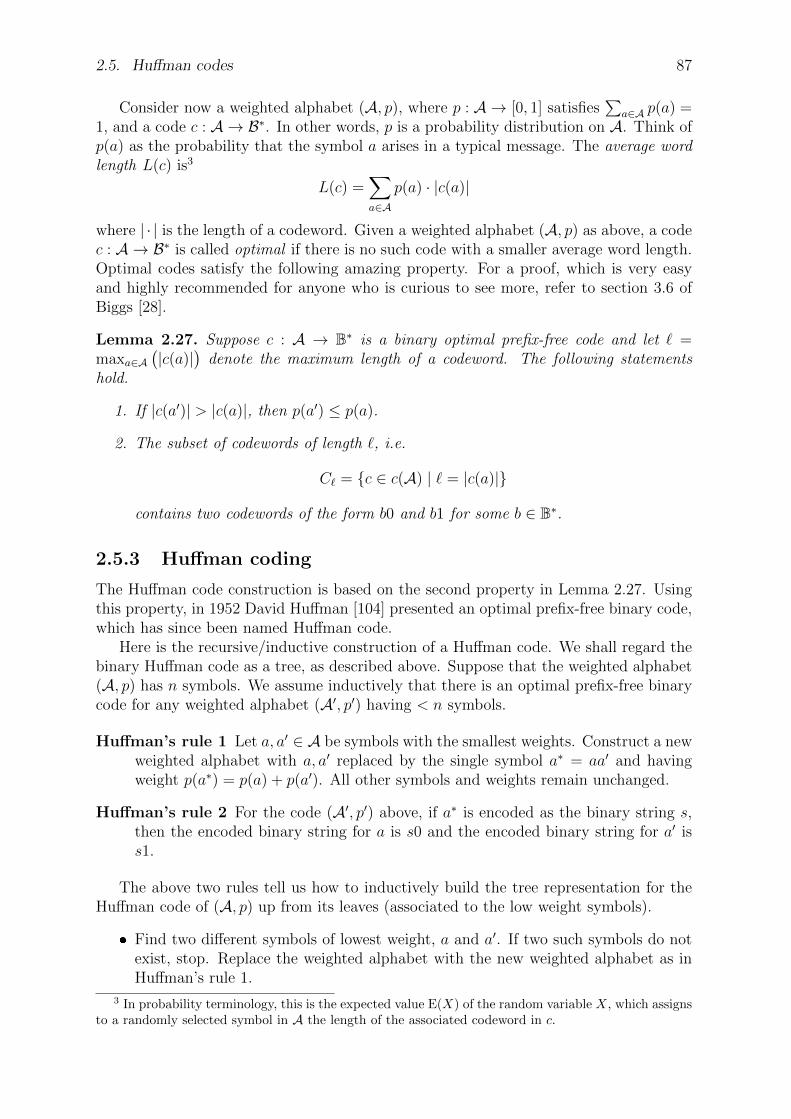
2.5. Huffman codes 87
Consider now a weighted alphabet (A, p), where p : A → [0, 1] satisfies∑
a∈A p(a) =1, and a code c : A → B∗. In other words, p is a probability distribution on A. Think ofp(a) as the probability that the symbol a arises in a typical message. The average wordlength L(c) is3
L(c) =∑
a∈A
p(a) · |c(a)|
where | · | is the length of a codeword. Given a weighted alphabet (A, p) as above, a codec : A → B∗ is called optimal if there is no such code with a smaller average word length.Optimal codes satisfy the following amazing property. For a proof, which is very easyand highly recommended for anyone who is curious to see more, refer to section 3.6 ofBiggs [28].
Lemma 2.27. Suppose c : A → B∗ is a binary optimal prefix-free code and let ` =maxa∈A
(|c(a)|
)denote the maximum length of a codeword. The following statements
hold.
1. If |c(a′)| > |c(a)|, then p(a′) ≤ p(a).
2. The subset of codewords of length `, i.e.
C` = c ∈ c(A) | ` = |c(a)|
contains two codewords of the form b0 and b1 for some b ∈ B∗.
2.5.3 Huffman coding
The Huffman code construction is based on the second property in Lemma 2.27. Usingthis property, in 1952 David Huffman [104] presented an optimal prefix-free binary code,which has since been named Huffman code.
Here is the recursive/inductive construction of a Huffman code. We shall regard thebinary Huffman code as a tree, as described above. Suppose that the weighted alphabet(A, p) has n symbols. We assume inductively that there is an optimal prefix-free binarycode for any weighted alphabet (A′, p′) having < n symbols.
Huffman’s rule 1 Let a, a′ ∈ A be symbols with the smallest weights. Construct a newweighted alphabet with a, a′ replaced by the single symbol a∗ = aa′ and havingweight p(a∗) = p(a) + p(a′). All other symbols and weights remain unchanged.
Huffman’s rule 2 For the code (A′, p′) above, if a∗ is encoded as the binary string s,then the encoded binary string for a is s0 and the encoded binary string for a′ iss1.
The above two rules tell us how to inductively build the tree representation for theHuffman code of (A, p) up from its leaves (associated to the low weight symbols).
Find two different symbols of lowest weight, a and a′. If two such symbols do notexist, stop. Replace the weighted alphabet with the new weighted alphabet as inHuffman’s rule 1.
3 In probability terminology, this is the expected value E(X) of the random variable X, which assignsto a randomly selected symbol in A the length of the associated codeword in c.
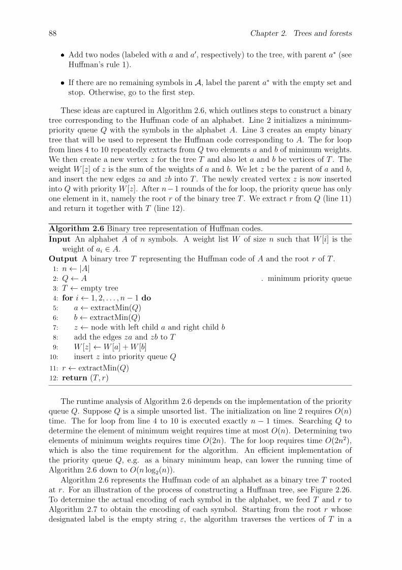
88 Chapter 2. Trees and forests
Add two nodes (labeled with a and a′, respectively) to the tree, with parent a∗ (seeHuffman’s rule 1).
If there are no remaining symbols in A, label the parent a∗ with the empty set andstop. Otherwise, go to the first step.
These ideas are captured in Algorithm 2.6, which outlines steps to construct a binarytree corresponding to the Huffman code of an alphabet. Line 2 initializes a minimum-priority queue Q with the symbols in the alphabet A. Line 3 creates an empty binarytree that will be used to represent the Huffman code corresponding to A. The for loopfrom lines 4 to 10 repeatedly extracts from Q two elements a and b of minimum weights.We then create a new vertex z for the tree T and also let a and b be vertices of T . Theweight W [z] of z is the sum of the weights of a and b. We let z be the parent of a and b,and insert the new edges za and zb into T . The newly created vertex z is now insertedinto Q with priority W [z]. After n−1 rounds of the for loop, the priority queue has onlyone element in it, namely the root r of the binary tree T . We extract r from Q (line 11)and return it together with T (line 12).
Algorithm 2.6 Binary tree representation of Huffman codes.
Input An alphabet A of n symbols. A weight list W of size n such that W [i] is theweight of ai ∈ A.
Output A binary tree T representing the Huffman code of A and the root r of T .1: n← |A|2: Q← A . minimum priority queue3: T ← empty tree4: for i← 1, 2, . . . , n− 1 do5: a← extractMin(Q)6: b← extractMin(Q)7: z ← node with left child a and right child b8: add the edges za and zb to T9: W [z]← W [a] +W [b]
10: insert z into priority queue Q
11: r ← extractMin(Q)12: return (T, r)
The runtime analysis of Algorithm 2.6 depends on the implementation of the priorityqueue Q. Suppose Q is a simple unsorted list. The initialization on line 2 requires O(n)time. The for loop from line 4 to 10 is executed exactly n − 1 times. Searching Q todetermine the element of minimum weight requires time at most O(n). Determining twoelements of minimum weights requires time O(2n). The for loop requires time O(2n2),which is also the time requirement for the algorithm. An efficient implementation ofthe priority queue Q, e.g. as a binary minimum heap, can lower the running time ofAlgorithm 2.6 down to O(n log2(n)).
Algorithm 2.6 represents the Huffman code of an alphabet as a binary tree T rootedat r. For an illustration of the process of constructing a Huffman tree, see Figure 2.26.To determine the actual encoding of each symbol in the alphabet, we feed T and r toAlgorithm 2.7 to obtain the encoding of each symbol. Starting from the root r whosedesignated label is the empty string ε, the algorithm traverses the vertices of T in a
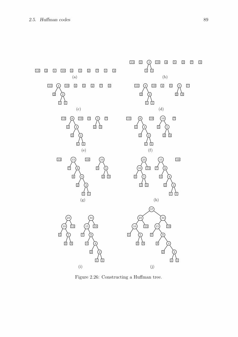
2.5. Huffman codes 89
13 2 1 19 4 5 2 7 1 3
(a)
13 2 2
1 1
19 4 5 2 7 3
(b)
13 4
2 2
1 1
19 4 5 2 7 3
(c)
13 4
2 2
1 1
19 4 5 5
2 3
7
(d)
13 8
4 4
2 2
1 1
19 5 5
2 3
7
(e)
13 8
4 4
2 2
1 1
19 10
5 5
2 3
7
(f)
13 15
7 8
4 4
2 2
1 1
19 10
5 5
2 3
(g)
23
10
5 5
2 3
13
15
7 8
4 4
2 2
1 1
19
(h)
23
10
5 5
2 3
13
34
15
7 8
4 4
2 2
1 1
19
(i)
57
23
10
5 5
2 3
13
34
15
7 8
4 4
2 2
1 1
19
(j)
Figure 2.26: Constructing a Huffman tree.

90 Chapter 2. Trees and forests
breadth-first search fashion. If v is an internal vertex with label e, the label of its left-child is the concatenation e0 and for the right-child of v we assign the label e1. If vhappens to be a leaf vertex, we take its label to be its Huffman encoding. Any Huffmanencoding assigned to a symbol of an alphabet is not unique. Either of the two children ofan internal vertex can be designated as the left- (respectively, right-) child. The runtimeof Algorithm 2.7 is O(|V |), where V is the vertex set of T .
Algorithm 2.7 Huffman encoding of an alphabet.
Input A binary tree T representing the Huffman code of an alphabet A. The root r ofT .
Output A list H representing a Huffman code of A, where H[ai] corresponds to aHuffman encoding of ai ∈ A.
1: H ← [ ] . list of Huffman encodings2: Q← [r] . queue of vertices3: while length(Q) > 0 do4: root← dequeue(Q)5: if root is a leaf then6: H[root]← label of root7: else8: a← left child of root9: b← right child of root
10: enqueue(Q, a)11: enqueue(Q, b)12: label of a← label of root + 0
13: label of b← label of root + 1
14: return H
Example 2.28. Consider the alphabet A = a, b, c, d, e, f with corresponding weightsw(a) = 19, w(b) = 2, w(c) = 40, w(d) = 25, w(e) = 31, and w(f) = 3. Construct abinary tree representation of the Huffman code of A and determine the encoding of eachsymbol of A.
Solution. Use Algorithm 2.6 to construct a binary tree representation of the weightedalphabet A. The resulting binary tree T is shown in Figure 2.27(a), where ai : wi is anabbreviation for “vertex ai has weight wi”. The binary tree is rooted at k. To encodeeach alphabetic symbol, input T and k into Algorithm 2.7 to get the encodings shownin Figure 2.27(b).
2.6 Tree traversals
In computer science, tree traversal refers to the process of examining each vertex in a treedata structure. Starting at the root of an ordered tree T , we can traverse the vertices ofT in one of various ways.
A level-order traversal of an ordered tree T examines the vertices in increasing orderof depth, with vertices of equal depth being examined according to their prescribedorder. One way to think about level-order traversal is to consider vertices of T havingthe same depth as being ordered from left to right in decreasing order of importance.

2.6. Tree traversals 91
b : 2 f : 3
g : 5 a : 19
h : 24 d : 25 e : 31 c : 40
i : 49 j : 71
k : 120
(a)
0000 0001
000 001
00 01 10 11
0 1
ε
(b)
Figure 2.27: Binary tree representation of an alphabet and its Huffman encodings.
If [v1, v2, . . . , vn] lists the vertices from left to right at depth k, a decreasing order ofimportance can be realized by assigning each vertex a numeric label using a labellingfunction L : V (T ) → R such that L(v1) < L(v2) < · · · < L(vn). In this way, a vertexwith a lower numeric label is examined prior to a vertex with a higher numeric label. Alevel-order traversal of T , whose vertices of equal depth are prioritized according to L,is an examination of the vertices of T from top to bottom, left to right. As an example,the level-order traversal of the tree in Figure 2.28 is
42, 4, 15, 2, 3, 5, 7, 10, 11, 12, 13, 14.
Our discussion is formalized in Algorithm 2.8, whose general structure mimics that ofbreadth-first search. For this reason, level-order traversal is also known as breadth-firsttraversal. Each vertex is enqueued and dequeued exactly once. The while loop is executedn times, hence we have a runtime of O(n). Another name for level-order traversal is top-down traversal because we first visit the root node and then work our way down thetree, increasing the depth as we move downward.
Algorithm 2.8 Level-order traversal.
Input An ordered tree T on n > 0 vertices.Output A list of the vertices of T in level-order.
1: L← [ ]2: Q← empty queue3: r ← root of T4: enqueue(Q, r)5: while length(Q) > 0 do6: v ← dequeue(Q)7: append(L, v)8: [u1, u2, . . . , uk]← ordering of children of v9: for i← 1, 2, . . . , k do
10: enqueue(Q, ui)
11: return L
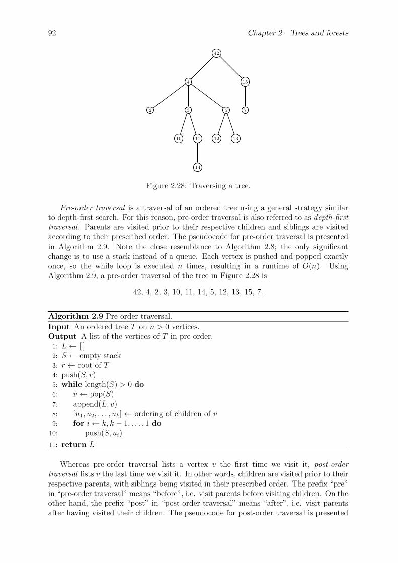
92 Chapter 2. Trees and forests
42
4
2 3
10 11
14
5
12 13
15
7
Figure 2.28: Traversing a tree.
Pre-order traversal is a traversal of an ordered tree using a general strategy similarto depth-first search. For this reason, pre-order traversal is also referred to as depth-firsttraversal. Parents are visited prior to their respective children and siblings are visitedaccording to their prescribed order. The pseudocode for pre-order traversal is presentedin Algorithm 2.9. Note the close resemblance to Algorithm 2.8; the only significantchange is to use a stack instead of a queue. Each vertex is pushed and popped exactlyonce, so the while loop is executed n times, resulting in a runtime of O(n). UsingAlgorithm 2.9, a pre-order traversal of the tree in Figure 2.28 is
42, 4, 2, 3, 10, 11, 14, 5, 12, 13, 15, 7.
Algorithm 2.9 Pre-order traversal.
Input An ordered tree T on n > 0 vertices.Output A list of the vertices of T in pre-order.
1: L← [ ]2: S ← empty stack3: r ← root of T4: push(S, r)5: while length(S) > 0 do6: v ← pop(S)7: append(L, v)8: [u1, u2, . . . , uk]← ordering of children of v9: for i← k, k − 1, . . . , 1 do
10: push(S, ui)
11: return L
Whereas pre-order traversal lists a vertex v the first time we visit it, post-ordertraversal lists v the last time we visit it. In other words, children are visited prior to theirrespective parents, with siblings being visited in their prescribed order. The prefix “pre”in “pre-order traversal” means “before”, i.e. visit parents before visiting children. On theother hand, the prefix “post” in “post-order traversal” means “after”, i.e. visit parentsafter having visited their children. The pseudocode for post-order traversal is presented
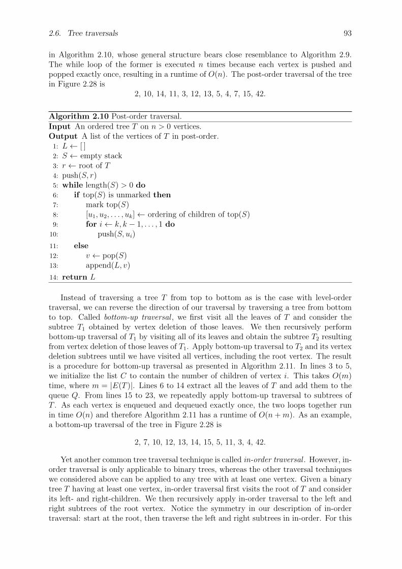
2.6. Tree traversals 93
in Algorithm 2.10, whose general structure bears close resemblance to Algorithm 2.9.The while loop of the former is executed n times because each vertex is pushed andpopped exactly once, resulting in a runtime of O(n). The post-order traversal of the treein Figure 2.28 is
2, 10, 14, 11, 3, 12, 13, 5, 4, 7, 15, 42.
Algorithm 2.10 Post-order traversal.
Input An ordered tree T on n > 0 vertices.Output A list of the vertices of T in post-order.
1: L← [ ]2: S ← empty stack3: r ← root of T4: push(S, r)5: while length(S) > 0 do6: if top(S) is unmarked then7: mark top(S)8: [u1, u2, . . . , uk]← ordering of children of top(S)9: for i← k, k − 1, . . . , 1 do
10: push(S, ui)
11: else12: v ← pop(S)13: append(L, v)
14: return L
Instead of traversing a tree T from top to bottom as is the case with level-ordertraversal, we can reverse the direction of our traversal by traversing a tree from bottomto top. Called bottom-up traversal , we first visit all the leaves of T and consider thesubtree T1 obtained by vertex deletion of those leaves. We then recursively performbottom-up traversal of T1 by visiting all of its leaves and obtain the subtree T2 resultingfrom vertex deletion of those leaves of T1. Apply bottom-up traversal to T2 and its vertexdeletion subtrees until we have visited all vertices, including the root vertex. The resultis a procedure for bottom-up traversal as presented in Algorithm 2.11. In lines 3 to 5,we initialize the list C to contain the number of children of vertex i. This takes O(m)time, where m = |E(T )|. Lines 6 to 14 extract all the leaves of T and add them to thequeue Q. From lines 15 to 23, we repeatedly apply bottom-up traversal to subtrees ofT . As each vertex is enqueued and dequeued exactly once, the two loops together runin time O(n) and therefore Algorithm 2.11 has a runtime of O(n+m). As an example,a bottom-up traversal of the tree in Figure 2.28 is
2, 7, 10, 12, 13, 14, 15, 5, 11, 3, 4, 42.
Yet another common tree traversal technique is called in-order traversal . However, in-order traversal is only applicable to binary trees, whereas the other traversal techniqueswe considered above can be applied to any tree with at least one vertex. Given a binarytree T having at least one vertex, in-order traversal first visits the root of T and considerits left- and right-children. We then recursively apply in-order traversal to the left andright subtrees of the root vertex. Notice the symmetry in our description of in-ordertraversal: start at the root, then traverse the left and right subtrees in in-order. For this
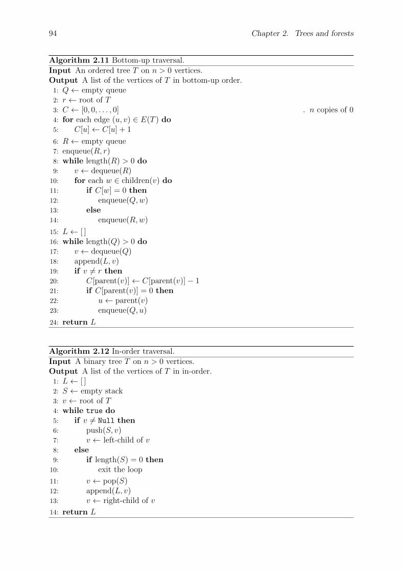
94 Chapter 2. Trees and forests
Algorithm 2.11 Bottom-up traversal.
Input An ordered tree T on n > 0 vertices.Output A list of the vertices of T in bottom-up order.
1: Q← empty queue2: r ← root of T3: C ← [0, 0, . . . , 0] . n copies of 04: for each edge (u, v) ∈ E(T ) do5: C[u]← C[u] + 1
6: R← empty queue7: enqueue(R, r)8: while length(R) > 0 do9: v ← dequeue(R)
10: for each w ∈ children(v) do11: if C[w] = 0 then12: enqueue(Q,w)13: else14: enqueue(R,w)
15: L← [ ]16: while length(Q) > 0 do17: v ← dequeue(Q)18: append(L, v)19: if v 6= r then20: C[parent(v)]← C[parent(v)]− 121: if C[parent(v)] = 0 then22: u← parent(v)23: enqueue(Q, u)
24: return L
Algorithm 2.12 In-order traversal.
Input A binary tree T on n > 0 vertices.Output A list of the vertices of T in in-order.
1: L← [ ]2: S ← empty stack3: v ← root of T4: while true do5: if v 6= Null then6: push(S, v)7: v ← left-child of v8: else9: if length(S) = 0 then
10: exit the loop
11: v ← pop(S)12: append(L, v)13: v ← right-child of v
14: return L

2.7. Problems 95
reason, in-order traversal is sometimes referred to as symmetric traversal. Our discussionis summarized in Algorithm 2.12. In the latter algorithm, if a vertex does not have aleft-child, then the operation of finding its left-child returns NULL. The same holds whenthe vertex does not have a right-child. Since each vertex is pushed and popped exactlyonce, it follows that in-order traversal runs in time O(n). Using Algorithm 2.12, anin-order traversal of the tree in Figure 2.27(b) is
0000, 000, 0001, 00, 001, 0, 01, ε, 10, 1, 11.
2.7 Problems
When solving problems, dig at the roots instead of just hacking at the leaves.— Anthony J. D’Angelo, The College Blue Book
2.1. Construct all nonisomorphic trees of order 7.
2.2. Let G be a weighted connected graph and let T be a subgraph of G. Then T is amaximum spanning tree of G provided that the following conditions are satisfied:
(a) T is a spanning tree of G.
(b) The total weight of T is maximum among all spanning trees of G.
Modify Kruskal’s, Prim’s, and Boruvka’s algorithms to return a maximum spanningtree of G.
2.3. Describe and present pseudocode of an algorithm to construct all spanning treesof a connected graph. What is the worst-case runtime of your algorithm? Howmany of the constructed spanning trees are nonisomorphic to each other? Repeatthe exercise for minimum and maximum spanning trees.
2.4. Consider an undirected, connected simple graph G = (V,E) of order n and size mand having an integer weight function w : E → Z given by w(e) > 0 for all e ∈ E.Suppose that G has N minimum spanning trees. Yamada et al. [198] providean O(Nm lnn) algorithm to construct all the N minimum spanning trees of G.Describe and provide pseudocode of the Yamada-Kataoka-Watanabe algorithm.Provide runtime analysis and prove the correctness of this algorithm.
2.5. The solution of Example 2.3 relied on the following result: Let T = (V,E) be a treerooted at v0 and suppose v0 has exactly two children. If maxv∈V deg(v) = 3 andv0 is the only vertex with degree 2, then T is a binary tree. Prove this statement.Give examples of graphs that are binary trees but do not satisfy the conditionsof the result. Under which conditions would the above test return an incorrectanswer?
2.6. What is the worst-case runtime of Algorithm 2.1?
2.7. Figure 2.5 shows two nonisomorphic spanning trees of the 4× 4 grid graph.
(a) For each n = 1, 2, . . . , 7, construct all nonisomorphic spanning trees of then× n grid graph.

96 Chapter 2. Trees and forests
(b) Explain and provide pseudocode of an algorithm for constructing all spanningtrees of the n× n grid graph, where n > 0.
(c) In general, if n is a positive integer, how many nonisomorphic spanning treesare there in the n× n grid graph?
(d) Describe and provide pseudocode of an algorithm to generate a random span-ning tree of the n × n grid graph. What is the worst-case runtime of youralgorithm?
2.8. Theorem 2.4 shows how to recursively construct a new tree from a given collectionof trees, hence it can be considered as a recursive definition of trees. To prove the-orems based upon recursive definitions, we use a proof technique called structuralinduction. Let S(C) be a statement about the collection of structures C, each ofwhich is defined by a recursive definition. In the base case, prove S(C) for thebasis structure(s) C. For the inductive case, let X be a structure formed usingthe recursive definition from the structures Y1, Y2, . . . , Yk. Assume for inductionthat the statements S(Y1), S(Y2), . . . , S(Yk) hold and use the inductive hypothesesS(Yi) to prove S(X). Hence conclude that S(X) is true for all X. Apply structuralinduction to show that any graph constructed using Theorem 2.4 is indeed a tree.
2.9. In Kruskal’s Algorithm 2.2, line 5 requires that the addition of a new edge to Tdoes not result in T having a cycle. A tree by definition has no cycles. Supposeline 5 is changed to:
if ei /∈ E(T ) and T ∪ ei is a tree then
With this change, explain why Algorithm 2.2 would return a minimum spanningtree or why the algorithm would fail to do so.
2.10. This problem is concerned with improving the runtime of Kruskal’s Algorithm 2.2.Explain how to use a priority queue to obviate the need for sorting the edges byweight. Investigate the union-find data structure. Explain how to use union-findto ensure that the addition of each edge results in an acyclic graph.
2.11. Figure 2.29 shows a weighted version of the Chvatal graph, which has 12 ver-tices and 24 edges. Use this graph as input to Kruskal’s, Prim’s, and Boruvka’salgorithms and compare the resulting minimum spanning trees.
2.12. Algorithm 2.1 presents a randomized procedure to construct a spanning tree of agiven connected graph via repeated edge deletion.
(a) Describe and present pseudocode of a randomized algorithm to grow a span-ning tree via edge addition.
(b) Would Algorithm 2.1 still work if the input graph G has self-loops or multipleedges? Explain why or why not. If not, modify Algorithm 2.1 to handle thecase where G has self-loops and multiple edges.
(c) Repeat the previous exercise for Kruskal’s, Prim’s, and Boruvka’s algorithms.
2.13. Algorithm 2.13 constructs a random spanning tree of the complete graph Kn onn > 0 vertices. Its runtime is dependent on efficient algorithms for obtaining arandom permutation of a set of objects, and choosing a random element from agiven set.
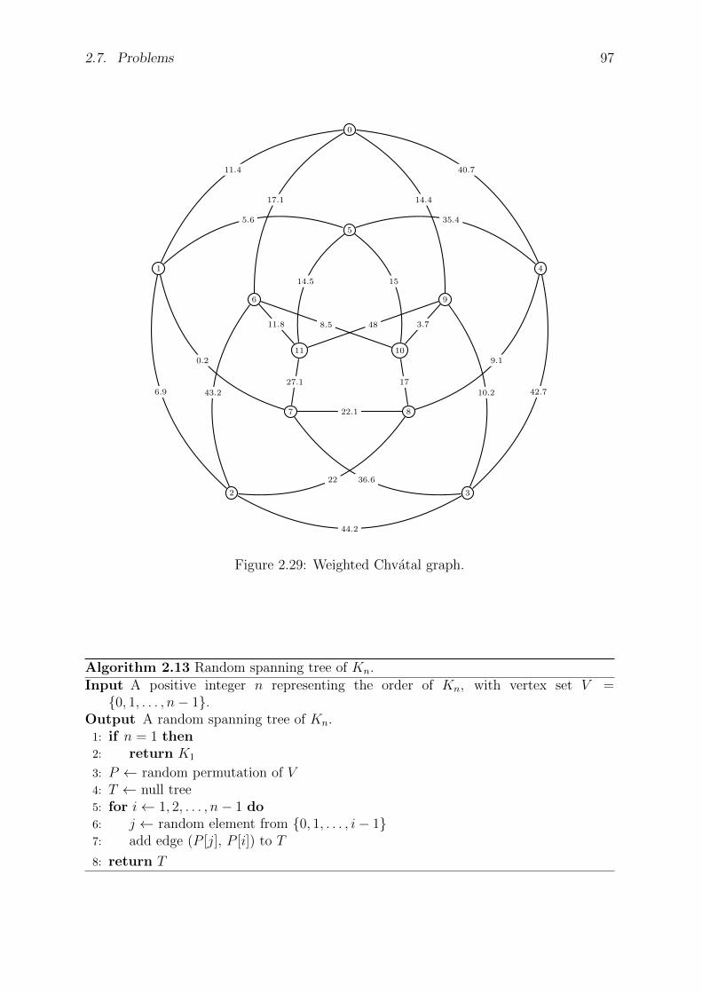
2.7. Problems 97
5
9
87
6
0
4
32
1
1011
11.4 40.7
17.1 14.4
6.9
5.6
0.2
44.2
43.2
22
42.7
36.6
10.2
35.4
9.1
1514.5
8.511.8
22.1
27.1 17
3.748
Figure 2.29: Weighted Chvatal graph.
Algorithm 2.13 Random spanning tree of Kn.
Input A positive integer n representing the order of Kn, with vertex set V =0, 1, . . . , n− 1.
Output A random spanning tree of Kn.1: if n = 1 then2: return K1
3: P ← random permutation of V4: T ← null tree5: for i← 1, 2, . . . , n− 1 do6: j ← random element from 0, 1, . . . , i− 17: add edge (P [j], P [i]) to T
8: return T
98 Chapter 2. Trees and forests
(a) Describe and analyze the runtime of a procedure to construct a random per-mutation of a set of nonnegative integers.
(b) Describe an algorithm for randomly choosing an element of a set of nonnega-tive integers. Analyze the runtime of this algorithm.
(c) Taking into consideration the previous two algorithms, what is the runtime ofAlgorithm 2.13?
2.14. We want to generate a random undirected, connected simple graph on n verticesand having m edges. Start by generating a random spanning tree T of Kn. Thenadd random edges to T until the requirements are satisfied.
(a) Present pseudocode to realize the above procedure. What is the worst-caseruntime of your algorithm?
(b) Modify your algorithm to handle the case where m < n − 1. Why mustm ≥ n− 1?
(c) Modify your algorithm to handle the case where each edge has a weight withinthe closed interval [α, β].
2.15. Enumerate all the different binary trees on 5 vertices.
2.16. Algorithm 2.5 generates a random binary tree on n > 0 vertices. Modify thisalgorithm so that it generates a random k-ary tree of order n > 0, where k ≥ 3.
2.17. Show by giving an example that the Morse code is not prefix-free.
2.18. Consider the alphabet A = a, b, c with corresponding probabilities (or weights)p(a) = 0.5, p(b) = 0.3, and p(c) = 0.2. Generate two different Huffman codes forA and illustrate the tree representations of those codes.
2.19. Find the Huffman code for the letters of the English alphabet weighted by thefrequency of common American usage.4
2.20. Let G = (V1, E2) be a graph and T = (V2, E2) a spanning tree of G. Show thatthere is a one-to-one correspondence between fundamental cycles in G and edgesnot in T .
2.21. Let G = (V,E) be the 3 × 3 grid graph and T1 = (V1, E1), T2 = (V2, E2) bespanning trees of G in Example 2.1. Find a fundamental cycle in G for T1 that isnot a fundamental cycle in G for T2.
2.22. Usually there exist many spanning trees of a graph. Classify those graphs forwhich there is only one spanning tree. In other words, find necessary and sufficientconditions for a graph G such that if T is a spanning tree of G then T is unique.
2.23. Convert the function graycodeword into a pure Python function.
2.24. Example 2.13 verifies that for any positive integer n > 1, repeated iteration ofthe Euler phi function ϕ(n) eventually produces 1. Show that this is the case orprovide an explanation why it is in general false.
4 You can find this on the Internet or in the literature. Part of this exercise is finding this frequencydistribution yourself.

2.7. Problems 99
2.25. The Collatz conjecture [126] asserts that for any integer n > 0, repeated iterationof the function
T (n) =
3n+1
2, if n is odd,
n2, if n is even
eventually produces the value 1. For example, repeated iteration of T (n) startingfrom n = 22 results in the sequence
22, 11, 17, 26, 13, 20, 10, 5, 8, 4, 2, 1. (2.4)
One way to think about the Collatz conjecture is to consider the digraph Gproduced by considering (ai, T (ai)) as a directed edge of G. Then the Collatzconjecture can be rephrased to say that there is some integer k > 0 such that(ak, T (ak)) = (2, 1) is a directed edge of G. The graph obtained in this man-ner is called the Collatz graph of T (n). Given a collection of positive integersα1, α2, . . . , αk, let Gαi
be the Collatz graph of the function T (αi) with initial iter-ation value αi. Then the union of the Gαi
is the directed tree
⋃
i
Gαi
rooted at 1, called the Collatz tree of (α1, α2, . . . , αk). Figure 2.30 shows such atree for the collection of initial iteration values 1024, 336, 340, 320, 106, 104, and96. See Lagarias [127,128] for a comprehensive survey of the Collatz conjecture.
(a) The Collatz sequence of a positive integer n > 1 is the integer sequence pro-duced by repeated iteration of T (n) with initial iteration value n. For example,the Collatz sequence of n = 22 is the sequence (2.4). Write a Sage functionto produce the Collatz sequence of an integer n > 1.
(b) The Collatz length of n > 1 is the number of terms in the Collatz sequence ofn, inclusive of the starting iteration value and the final integer 1. For instance,the Collatz length of 22 is 12, that of 106 is 11, and that of 51 is 18. Writea Sage function to compute the Collatz length of a positive integer n > 1. Ifn > 1 is a vertex in a Collatz tree, verify that the Collatz length of n is thedistance d(n, 1).
(c) Describe the Collatz graph produced by the function T (n) with initial iterationvalue n = 1.
(d) Fix a positive integer n > 1 and let Li be the Collatz length of the integer1 ≤ i ≤ n. Plot the pairs (i, Li) on one set of axes.
2.26. The following result was first published in Wiener [196]. Let T = (V,E) be a treeof order n > 0. For each edge e ∈ E, let n1(e) and n2(e) = n− n1(e) be the ordersof the two components of the edge-deletion subgraph T − e. Show that the Wienernumber of T is
W (T ) =∑
e∈E
n1(e) · n2(e).
2.27. The following result [147] was independently discovered in the late 1980s by Merrisand McKay, and is known as the Merris-McKay theorem. Let T be a tree of order
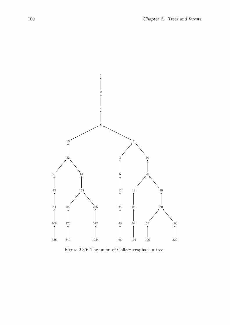
100 Chapter 2. Trees and forests
1
2
4
8
16
32
21
42
84
168
336
64
128
85
170
340
256
512
1024
5
3
6
12
24
48
96
10
20
13
26
52
104
40
80
53
106
160
320
Figure 2.30: The union of Collatz graphs is a tree.
2.7. Problems 101
n and let L be its Laplacian matrix having eigenvalues λ1, λ2, . . . , λn. Show thatthe Wiener number of T is
W (T ) = nn−1∑
i=1
1
λi.
2.28. For each of the algorithms below: (i) justify whether or not it can be appliedto multigraphs or multidigraphs; (ii) if not, modify the algorithm so that it isapplicable to multigraphs or multidigraphs.
(a) Randomized spanning tree construction Algorithm 2.1.
(b) Kruskal’s Algorithm 2.2.
(c) Prim’s Algorithm 2.3.
(d) Boruvka’s Algorithm 2.4.
2.29. Section 2.6 provides iterative algorithms for the following tree traversal techniques:
(a) Level-order traversal: Algorithm 2.8.
(b) Pre-order traversal: Algorithm 2.9.
(c) Post-order traversal: Algorithm 2.10.
(d) Bottom-up traversal: Algorithm 2.11.
(e) In-order traversal: Algorithm 2.12.
Rewrite each of the above as recursive algorithms.
2.30. In cryptography, the Merkle signature scheme [145] was introduced in 1987 as analternative to traditional digital signature schemes such as the Digital SignatureAlgorithm or RSA. Buchmann et al. [43] and Szydlo [178] provide efficient algo-rithms for speeding up the Merkle signature scheme. Investigate this scheme andhow it uses binary trees to generate digital signatures.
2.31. Consider the finite alphabetA = a1, a2, . . . , ar. If C is a subset ofA∗, then we saythat C is an r-ary code and call r the radix of the code. McMillan’s theorem [143],first published in 1956, relates codeword lengths to unique decipherability. Inparticular, let C = c1, c2, . . . , cn be an r-ary code where each ci has length `i. IfC is uniquely decipherable, McMillan’s theorem states that the codeword lengths`i must satisfy Kraft’s inequality
n∑
i=1
1
r`i≤ 1.
Prove McMillan’s theorem.
2.32. A code C = c1, c2, . . . , cn is said to be instantaneous if each codeword ci can beinterpreted as soon as it is received. For example, given the the code 01, 010 andthe string 01010, upon receiving the first 0 we are unable to decide whether thatelement belong to 01 or 010. However, the code 1, 01 is instantaneous becausegiven the string 1101 and the first 1, we can interpret the latter as the codeword1. Prove that a code is instantaneous if and only if it is prefix-free.
102 Chapter 2. Trees and forests
2.33. Kraft’s inequality and the accompanying Kraft’s theorem were first published [124]in 1949 in the Master’s thesis of Leon Gordon Kraft. Kraft’s theorem relates theinequality to instantaneous codes. Let C = c1, c2, . . . , cn be an r-ary code whereeach codeword ci has length `i. Kraft’s theorem states that C is an instantaneouscode if and only if the codeword lengths satisfy
n∑
i=1
1
r`i≤ 1.
Prove Kraft’s theorem.
2.34. Let T be a nontrivial tree and let ni count the number of vertices of T that havedegree i. Show that T has 2 +
∑∞i=3(i− 2)ni leaves.
2.35. If a forest F has k trees totalling n vertices altogether, how many edges does Fcontain?
2.36. The Lucas number Ln, named after Edouard Lucas, has the following recursivedefinition:
Ln =
2, if n = 0,
1, if n = 1,
Ln−1 + Ln−2, if n > 1.
(a) If ϕ = (1 +√
5)/2 is the golden ratio, show that
Ln = ϕn + (−ϕ)−n.
(b) Let τ(Wn) be the number of spanning trees of the wheel graph. Benjaminand Yerger [22] provide a combinatorial proof that τ(Wn) = L2n− 2. Presentthe Benjamin-Yerger combinatorial proof.
(c) LetG be the Dodecahedral graph, implemented in Sage as G = graphs.DodecahedralGraph().Does its cutset matrix satisfy the undirected analog of Theorem 2.19?
Chapter 3
Shortest paths algorithms
— Randall Munroe, xkcd, http://xkcd.com/518/
Graph algorithms have many applications. Suppose you are a salesman with a productyou would like to sell in several cities. To determine the cheapest travel route from city-to-city, you must effectively search a graph having weighted edges for the “cheapest”route visiting each city once. Each vertex denotes a city you must visit and each edgehas a weight indicating either the distance from one city to another or the cost to travelfrom one city to another.
Shortest path algorithms are some of the most important algorithms in algorithmicgraph theory. In this chapter, we first examine several common graph traversal algo-rithms and some basic data structures underlying these algorithms. A data structure isa combination of methods for structuring a collection of data (e.g. vertices and edges)and protocols for accessing the data. We then consider a number of common shortestpath algorithms, which rely in one way or another on graph traversal techniques andbasic data structures for organizing and managing vertices and edges.
103
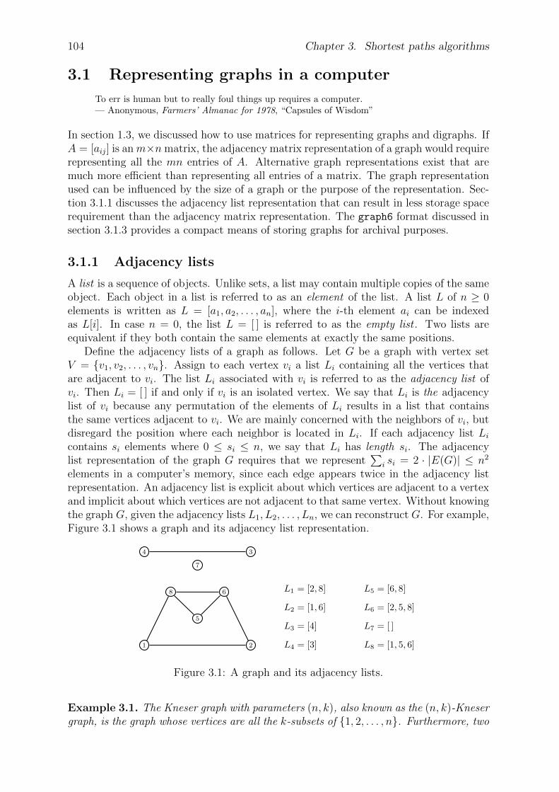
104 Chapter 3. Shortest paths algorithms
3.1 Representing graphs in a computer
To err is human but to really foul things up requires a computer.— Anonymous, Farmers’ Almanac for 1978, “Capsules of Wisdom”
In section 1.3, we discussed how to use matrices for representing graphs and digraphs. IfA = [aij] is an m×n matrix, the adjacency matrix representation of a graph would requirerepresenting all the mn entries of A. Alternative graph representations exist that aremuch more efficient than representing all entries of a matrix. The graph representationused can be influenced by the size of a graph or the purpose of the representation. Sec-tion 3.1.1 discusses the adjacency list representation that can result in less storage spacerequirement than the adjacency matrix representation. The graph6 format discussed insection 3.1.3 provides a compact means of storing graphs for archival purposes.
3.1.1 Adjacency lists
A list is a sequence of objects. Unlike sets, a list may contain multiple copies of the sameobject. Each object in a list is referred to as an element of the list. A list L of n ≥ 0elements is written as L = [a1, a2, . . . , an], where the i-th element ai can be indexedas L[i]. In case n = 0, the list L = [ ] is referred to as the empty list . Two lists areequivalent if they both contain the same elements at exactly the same positions.
Define the adjacency lists of a graph as follows. Let G be a graph with vertex setV = v1, v2, . . . , vn. Assign to each vertex vi a list Li containing all the vertices thatare adjacent to vi. The list Li associated with vi is referred to as the adjacency list ofvi. Then Li = [ ] if and only if vi is an isolated vertex. We say that Li is the adjacencylist of vi because any permutation of the elements of Li results in a list that containsthe same vertices adjacent to vi. We are mainly concerned with the neighbors of vi, butdisregard the position where each neighbor is located in Li. If each adjacency list Licontains si elements where 0 ≤ si ≤ n, we say that Li has length si. The adjacencylist representation of the graph G requires that we represent
∑i si = 2 · |E(G)| ≤ n2
elements in a computer’s memory, since each edge appears twice in the adjacency listrepresentation. An adjacency list is explicit about which vertices are adjacent to a vertexand implicit about which vertices are not adjacent to that same vertex. Without knowingthe graph G, given the adjacency lists L1, L2, . . . , Ln, we can reconstruct G. For example,Figure 3.1 shows a graph and its adjacency list representation.
1 2
34
5
6
7
8 L1 = [2, 8]
L2 = [1, 6]
L3 = [4]
L4 = [3]
L5 = [6, 8]
L6 = [2, 5, 8]
L7 = [ ]
L8 = [1, 5, 6]
Figure 3.1: A graph and its adjacency lists.
Example 3.1. The Kneser graph with parameters (n, k), also known as the (n, k)-Knesergraph, is the graph whose vertices are all the k-subsets of 1, 2, . . . , n. Furthermore, two
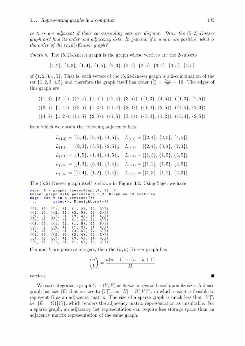
3.1. Representing graphs in a computer 105
vertices are adjacent if their corresponding sets are disjoint. Draw the (5, 2)-Knesergraph and find its order and adjacency lists. In general, if n and k are positive, what isthe order of the (n, k)-Kneser graph?
Solution. The (5, 2)-Kneser graph is the graph whose vertices are the 2-subsets
1, 2, 1, 3, 1, 4, 1, 5, 2, 3, 2, 4, 2, 5, 3, 4, 3, 5, 4, 5
of 1, 2, 3, 4, 5. That is, each vertex of the (5, 2)-Kneser graph is a 2-combination of theset 1, 2, 3, 4, 5 and therefore the graph itself has order
(52
)= 5×4
2!= 10. The edges of
this graph are
(1, 3, 2, 4), (2, 4, 1, 5), (2, 4, 3, 5), (1, 3, 4, 5), (1, 3, 2, 5)(3, 5, 1, 4), (3, 5, 1, 2), (1, 4, 2, 3), (1, 4, 2, 5), (4, 5, 2, 3)(4, 5, 1, 2), (1, 5, 2, 3), (1, 5, 3, 4), (3, 4, 1, 2), (3, 4, 2, 5)
from which we obtain the following adjacency lists:
L1,2 = [3, 4, 3, 5, 4, 5], L1,3 = [2, 4, 2, 5, 4, 5],L1,4 = [2, 3, 3, 5, 2, 5], L1,5 = [2, 4, 3, 4, 2, 3],L2,3 = [1, 5, 1, 4, 4, 5], L2,4 = [1, 3, 1, 5, 3, 5],L2,5 = [1, 3, 3, 4, 1, 4], L3,4 = [1, 2, 1, 5, 2, 5],L3,5 = [2, 4, 1, 2, 1, 4], L4,5 = [1, 3, 1, 2, 2, 3].
The (5, 2)-Kneser graph itself is shown in Figure 3.2. Using Sage, we have
sage: K = graphs.KneserGraph (5, 2); KKneser graph with parameters 5,2: Graph on 10 verticessage: for v in K.vertices ():... print(v, K.neighbors(v))...(4, 5, [1, 3, 1, 2, 2, 3])(1, 3, [2, 4, 2, 5, 4, 5])(2, 5, [1, 3, 3, 4, 1, 4])(2, 3, [1, 5, 1, 4, 4, 5])(3, 4, [1, 2, 1, 5, 2, 5])(3, 5, [2, 4, 1, 2, 1, 4])(1, 4, [2, 3, 3, 5, 2, 5])(1, 5, [2, 4, 3, 4, 2, 3])(1, 2, [3, 4, 3, 5, 4, 5])(2, 4, [1, 3, 1, 5, 3, 5])
If n and k are positive integers, then the (n, k)-Kneser graph has
(n
k
)=n(n− 1) · · · (n− k + 1)
k!
vertices.
We can categorize a graph G = (V,E) as dense or sparse based upon its size. A densegraph has size |E| that is close to |V |2, i.e. |E| = Ω
(|V |2
), in which case it is feasible to
represent G as an adjacency matrix. The size of a sparse graph is much less than |V |2,i.e. |E| = Ω
(|V |), which renders the adjacency matrix representation as unsuitable. For
a sparse graph, an adjacency list representation can require less storage space than anadjacency matrix representation of the same graph.
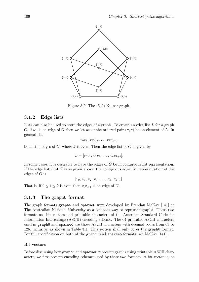
106 Chapter 3. Shortest paths algorithms
2, 4 1, 3
1, 4
3, 5 4, 5
2, 3
1, 5 2, 5
1, 2
3, 4
Figure 3.2: The (5, 2)-Kneser graph.
3.1.2 Edge lists
Lists can also be used to store the edges of a graph. To create an edge list L for a graphG, if uv is an edge of G then we let uv or the ordered pair (u, v) be an element of L. Ingeneral, let
v0v1, v2v3, . . . , vkvk+1
be all the edges of G, where k is even. Then the edge list of G is given by
L = [v0v1, v2v3, . . . , vkvk+1].
In some cases, it is desirable to have the edges of G be in contiguous list representation.If the edge list L of G is as given above, the contiguous edge list representation of theedges of G is
[v0, v1, v2, v3, . . . , vk, vk+1].
That is, if 0 ≤ i ≤ k is even then vivi+1 is an edge of G.
3.1.3 The graph6 format
The graph formats graph6 and sparse6 were developed by Brendan McKay [141] atThe Australian National University as a compact way to represent graphs. These twoformats use bit vectors and printable characters of the American Standard Code forInformation Interchange (ASCII) encoding scheme. The 64 printable ASCII charactersused in graph6 and sparse6 are those ASCII characters with decimal codes from 63 to126, inclusive, as shown in Table 3.1. This section shall only cover the graph6 format.For full specification on both of the graph6 and sparse6 formats, see McKay [141].
Bit vectors
Before discussing how graph6 and sparse6 represent graphs using printable ASCII char-acters, we first present encoding schemes used by these two formats. A bit vector is, as

3.1. Representing graphs in a computer 107
binary decimal glyph binary decimal glyph0111111 63 ? 1011111 95 _
1000000 64 @ 1100000 96 ‘
1000001 65 A 1100001 97 a
1000010 66 B 1100010 98 b
1000011 67 C 1100011 99 c
1000100 68 D 1100100 100 d
1000101 69 E 1100101 101 e
1000110 70 F 1100110 102 f
1000111 71 G 1100111 103 g
1001000 72 H 1101000 104 h
1001001 73 I 1101001 105 i
1001010 74 J 1101010 106 j
1001011 75 K 1101011 107 k
1001100 76 L 1101100 108 l
1001101 77 M 1101101 109 m
1001110 78 N 1101110 110 n
1001111 79 O 1101111 111 o
1010000 80 P 1110000 112 p
1010001 81 Q 1110001 113 q
1010010 82 R 1110010 114 r
1010011 83 S 1110011 115 s
1010100 84 T 1110100 116 t
1010101 85 U 1110101 117 u
1010110 86 V 1110110 118 v
1010111 87 W 1110111 119 w
1011000 88 X 1111000 120 x
1011001 89 Y 1111001 121 y
1011010 90 Z 1111010 122 z
1011011 91 [ 1111011 123
1011100 92 \ 1111100 124 |
1011101 93 ] 1111101 125
1011110 94 ^ 1111110 126 ~
Table 3.1: ASCII printable characters used by graph6 and sparse6.
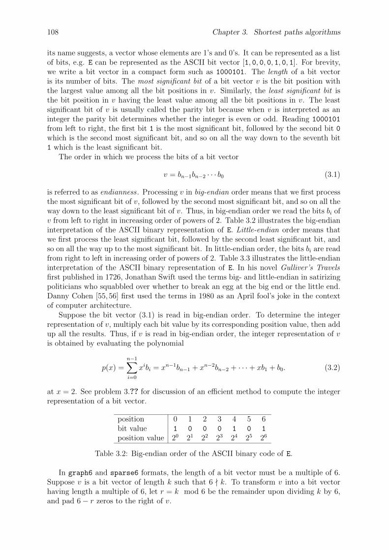
108 Chapter 3. Shortest paths algorithms
its name suggests, a vector whose elements are 1’s and 0’s. It can be represented as a listof bits, e.g. E can be represented as the ASCII bit vector [1, 0, 0, 0, 1, 0, 1]. For brevity,we write a bit vector in a compact form such as 1000101. The length of a bit vectoris its number of bits. The most significant bit of a bit vector v is the bit position withthe largest value among all the bit positions in v. Similarly, the least significant bit isthe bit position in v having the least value among all the bit positions in v. The leastsignificant bit of v is usually called the parity bit because when v is interpreted as aninteger the parity bit determines whether the integer is even or odd. Reading 1000101
from left to right, the first bit 1 is the most significant bit, followed by the second bit 0which is the second most significant bit, and so on all the way down to the seventh bit1 which is the least significant bit.
The order in which we process the bits of a bit vector
v = bn−1bn−2 · · · b0 (3.1)
is referred to as endianness . Processing v in big-endian order means that we first processthe most significant bit of v, followed by the second most significant bit, and so on all theway down to the least significant bit of v. Thus, in big-endian order we read the bits bi ofv from left to right in increasing order of powers of 2. Table 3.2 illustrates the big-endianinterpretation of the ASCII binary representation of E. Little-endian order means thatwe first process the least significant bit, followed by the second least significant bit, andso on all the way up to the most significant bit. In little-endian order, the bits bi are readfrom right to left in increasing order of powers of 2. Table 3.3 illustrates the little-endianinterpretation of the ASCII binary representation of E. In his novel Gulliver’s Travelsfirst published in 1726, Jonathan Swift used the terms big- and little-endian in satirizingpoliticians who squabbled over whether to break an egg at the big end or the little end.Danny Cohen [55, 56] first used the terms in 1980 as an April fool’s joke in the contextof computer architecture.
Suppose the bit vector (3.1) is read in big-endian order. To determine the integerrepresentation of v, multiply each bit value by its corresponding position value, then addup all the results. Thus, if v is read in big-endian order, the integer representation of vis obtained by evaluating the polynomial
p(x) =n−1∑
i=0
xibi = xn−1bn−1 + xn−2bn−2 + · · ·+ xb1 + b0. (3.2)
at x = 2. See problem 3.?? for discussion of an efficient method to compute the integerrepresentation of a bit vector.
position 0 1 2 3 4 5 6bit value 1 0 0 0 1 0 1
position value 20 21 22 23 24 25 26
Table 3.2: Big-endian order of the ASCII binary code of E.
In graph6 and sparse6 formats, the length of a bit vector must be a multiple of 6.Suppose v is a bit vector of length k such that 6 - k. To transform v into a bit vectorhaving length a multiple of 6, let r = k mod 6 be the remainder upon dividing k by 6,and pad 6− r zeros to the right of v.
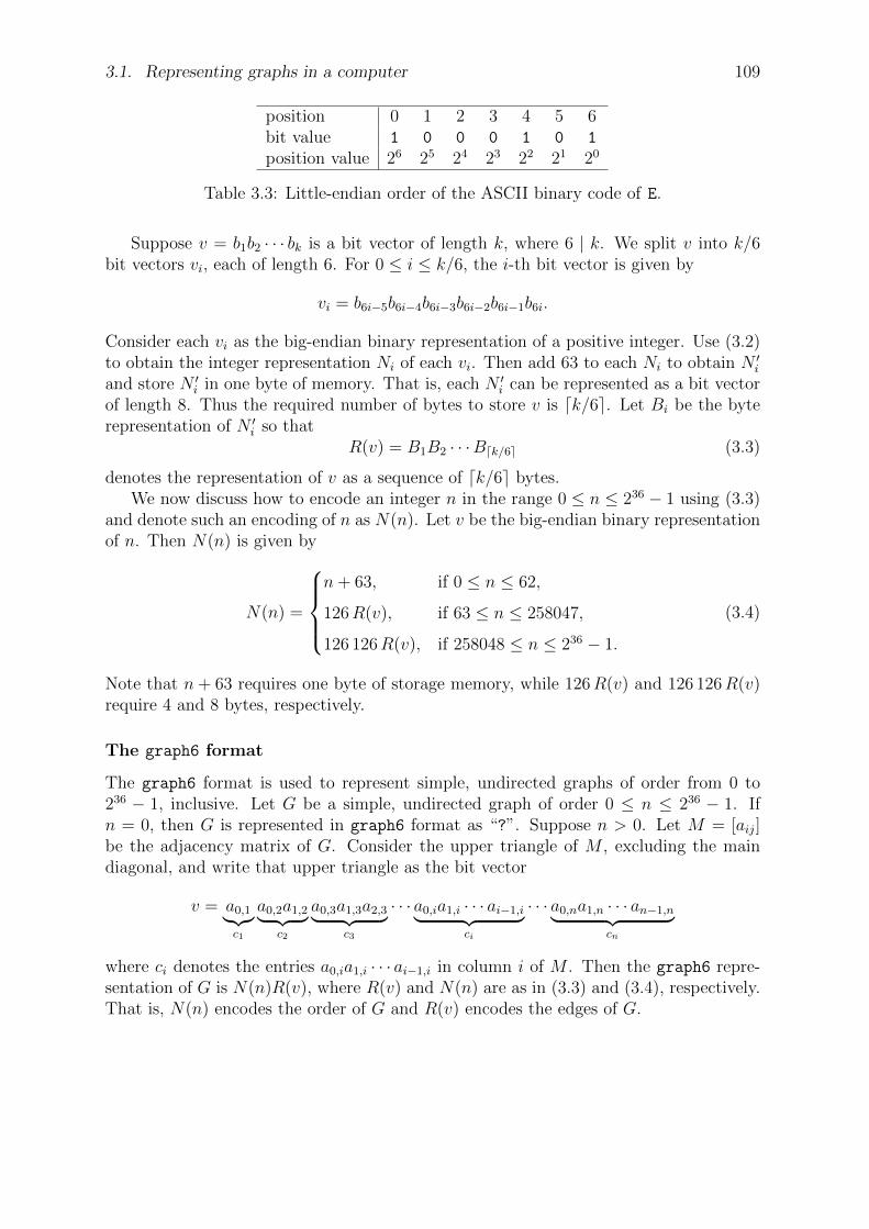
3.1. Representing graphs in a computer 109
position 0 1 2 3 4 5 6bit value 1 0 0 0 1 0 1
position value 26 25 24 23 22 21 20
Table 3.3: Little-endian order of the ASCII binary code of E.
Suppose v = b1b2 · · · bk is a bit vector of length k, where 6 | k. We split v into k/6bit vectors vi, each of length 6. For 0 ≤ i ≤ k/6, the i-th bit vector is given by
vi = b6i−5b6i−4b6i−3b6i−2b6i−1b6i.
Consider each vi as the big-endian binary representation of a positive integer. Use (3.2)to obtain the integer representation Ni of each vi. Then add 63 to each Ni to obtain N ′iand store N ′i in one byte of memory. That is, each N ′i can be represented as a bit vectorof length 8. Thus the required number of bytes to store v is dk/6e. Let Bi be the byterepresentation of N ′i so that
R(v) = B1B2 · · ·Bdk/6e (3.3)
denotes the representation of v as a sequence of dk/6e bytes.We now discuss how to encode an integer n in the range 0 ≤ n ≤ 236 − 1 using (3.3)
and denote such an encoding of n as N(n). Let v be the big-endian binary representationof n. Then N(n) is given by
N(n) =
n+ 63, if 0 ≤ n ≤ 62,
126R(v), if 63 ≤ n ≤ 258047,
126 126R(v), if 258048 ≤ n ≤ 236 − 1.
(3.4)
Note that n+ 63 requires one byte of storage memory, while 126R(v) and 126 126R(v)require 4 and 8 bytes, respectively.
The graph6 format
The graph6 format is used to represent simple, undirected graphs of order from 0 to236 − 1, inclusive. Let G be a simple, undirected graph of order 0 ≤ n ≤ 236 − 1. Ifn = 0, then G is represented in graph6 format as “?”. Suppose n > 0. Let M = [aij]be the adjacency matrix of G. Consider the upper triangle of M , excluding the maindiagonal, and write that upper triangle as the bit vector
v = a0,1︸︷︷︸c1
a0,2a1,2︸ ︷︷ ︸c2
a0,3a1,3a2,3︸ ︷︷ ︸c3
· · · a0,ia1,i · · · ai−1,i︸ ︷︷ ︸ci
· · · a0,na1,n · · · an−1,n︸ ︷︷ ︸cn
where ci denotes the entries a0,ia1,i · · · ai−1,i in column i of M . Then the graph6 repre-sentation of G is N(n)R(v), where R(v) and N(n) are as in (3.3) and (3.4), respectively.That is, N(n) encodes the order of G and R(v) encodes the edges of G.
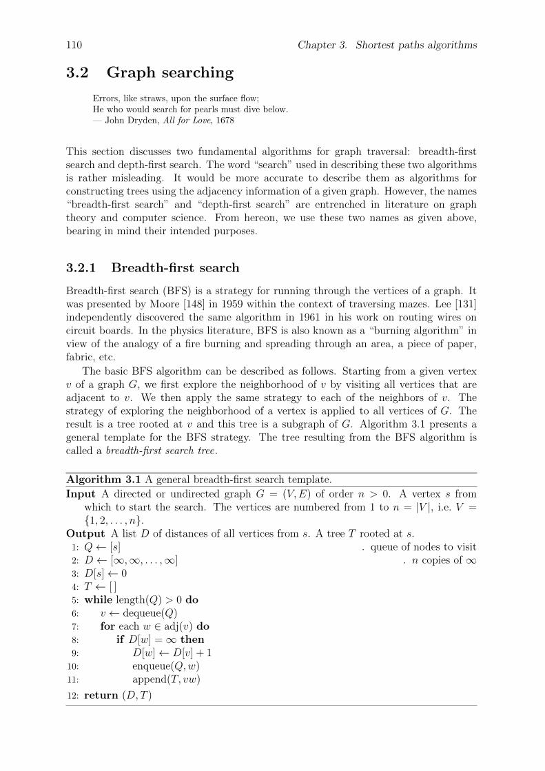
110 Chapter 3. Shortest paths algorithms
3.2 Graph searching
Errors, like straws, upon the surface flow;He who would search for pearls must dive below.— John Dryden, All for Love, 1678
This section discusses two fundamental algorithms for graph traversal: breadth-firstsearch and depth-first search. The word “search” used in describing these two algorithmsis rather misleading. It would be more accurate to describe them as algorithms forconstructing trees using the adjacency information of a given graph. However, the names“breadth-first search” and “depth-first search” are entrenched in literature on graphtheory and computer science. From hereon, we use these two names as given above,bearing in mind their intended purposes.
3.2.1 Breadth-first search
Breadth-first search (BFS) is a strategy for running through the vertices of a graph. Itwas presented by Moore [148] in 1959 within the context of traversing mazes. Lee [131]independently discovered the same algorithm in 1961 in his work on routing wires oncircuit boards. In the physics literature, BFS is also known as a “burning algorithm” inview of the analogy of a fire burning and spreading through an area, a piece of paper,fabric, etc.
The basic BFS algorithm can be described as follows. Starting from a given vertexv of a graph G, we first explore the neighborhood of v by visiting all vertices that areadjacent to v. We then apply the same strategy to each of the neighbors of v. Thestrategy of exploring the neighborhood of a vertex is applied to all vertices of G. Theresult is a tree rooted at v and this tree is a subgraph of G. Algorithm 3.1 presents ageneral template for the BFS strategy. The tree resulting from the BFS algorithm iscalled a breadth-first search tree.
Algorithm 3.1 A general breadth-first search template.
Input A directed or undirected graph G = (V,E) of order n > 0. A vertex s fromwhich to start the search. The vertices are numbered from 1 to n = |V |, i.e. V =1, 2, . . . , n.
Output A list D of distances of all vertices from s. A tree T rooted at s.1: Q← [s] . queue of nodes to visit2: D ← [∞,∞, . . . ,∞] . n copies of ∞3: D[s]← 04: T ← [ ]5: while length(Q) > 0 do6: v ← dequeue(Q)7: for each w ∈ adj(v) do8: if D[w] =∞ then9: D[w]← D[v] + 1
10: enqueue(Q,w)11: append(T, vw)
12: return (D,T )

3.2. Graph searching 111
The breadth-first search algorithm makes use of a special type of list called a queue.This is analogous to a queue of people waiting in line to be served. A person may enterthe queue by joining the rear of the queue. The person who is in the queue the longestamount of time is served first, followed by the person who has waited the second longesttime, and so on. Formally, a queue Q is a list of elements. At any time, we only haveaccess to the first element of Q, known as the front or start of the queue. We inserta new element into Q by appending the new element to the rear or end of the queue.The operation of removing the front of Q is referred to as dequeue, while the operationof appending to the rear of Q is called enqueue. That is, a queue implements a first-infirst-out (FIFO) protocol for adding and removing elements. As with lists, the length ofa queue is its total number of elements.
21
3
4
5
7
6
(a) Original undirected graph.
21
3
4
5
7
6
(b) First iteration of while loop.
21
3
4
5
7
6
(c) Second iteration of while loop.
21
3
4
5
7
6
(d) Third iteration of while loop.
21
3
4
5
7
6
(e) Fourth iteration of while loop.
4
3 7 6
2 5
1
(f) Final BFS tree.
Figure 3.3: Breadth-first search tree for an undirected graph.
Note that the BFS Algorithm 3.1 works on both undirected and directed graphs. Foran undirected graph, line 7 means that we explore all the neighbors of vertex v, i.e. theset adj(v) of vertices adjacent to v. In the case of a digraph, we replace “w ∈ adj(v)”on line 7 with “w ∈ oadj(v)” because we only want to explore all vertices that are out-neighbors of v. The algorithm returns two lists D and T . The list T contains a subset
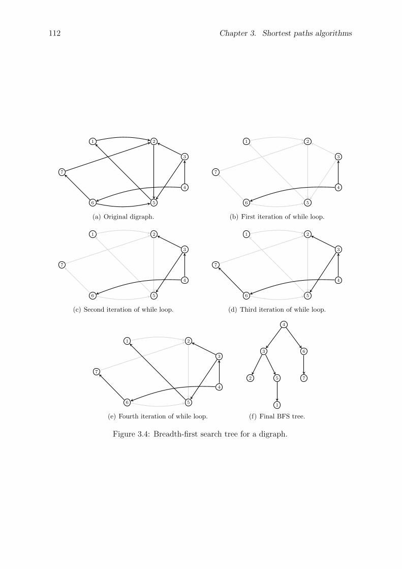
112 Chapter 3. Shortest paths algorithms
21
3
4
5
7
6
(a) Original digraph.
21
3
4
5
7
6
(b) First iteration of while loop.
21
3
4
5
7
6
(c) Second iteration of while loop.
21
3
4
5
7
6
(d) Third iteration of while loop.
21
3
4
5
7
6
(e) Fourth iteration of while loop.
2
1
5 7
63
4
(f) Final BFS tree.
Figure 3.4: Breadth-first search tree for a digraph.
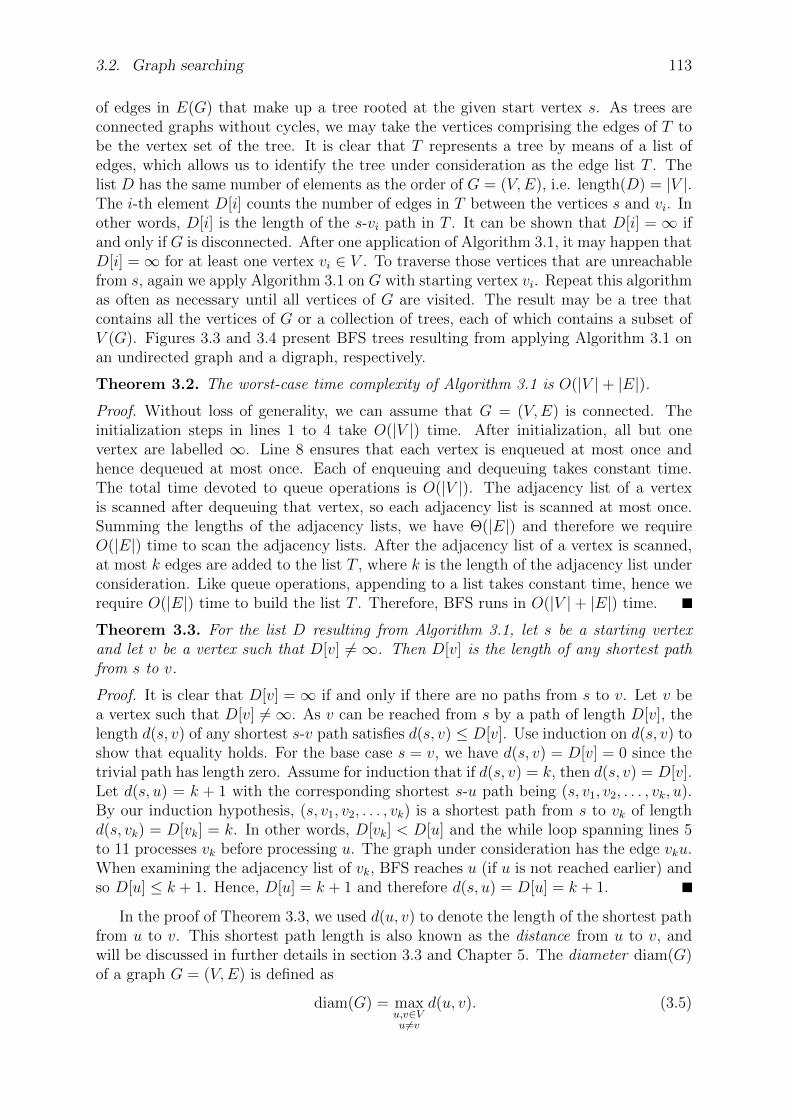
3.2. Graph searching 113
of edges in E(G) that make up a tree rooted at the given start vertex s. As trees areconnected graphs without cycles, we may take the vertices comprising the edges of T tobe the vertex set of the tree. It is clear that T represents a tree by means of a list ofedges, which allows us to identify the tree under consideration as the edge list T . Thelist D has the same number of elements as the order of G = (V,E), i.e. length(D) = |V |.The i-th element D[i] counts the number of edges in T between the vertices s and vi. Inother words, D[i] is the length of the s-vi path in T . It can be shown that D[i] = ∞ ifand only if G is disconnected. After one application of Algorithm 3.1, it may happen thatD[i] =∞ for at least one vertex vi ∈ V . To traverse those vertices that are unreachablefrom s, again we apply Algorithm 3.1 on G with starting vertex vi. Repeat this algorithmas often as necessary until all vertices of G are visited. The result may be a tree thatcontains all the vertices of G or a collection of trees, each of which contains a subset ofV (G). Figures 3.3 and 3.4 present BFS trees resulting from applying Algorithm 3.1 onan undirected graph and a digraph, respectively.
Theorem 3.2. The worst-case time complexity of Algorithm 3.1 is O(|V |+ |E|).
Proof. Without loss of generality, we can assume that G = (V,E) is connected. Theinitialization steps in lines 1 to 4 take O(|V |) time. After initialization, all but onevertex are labelled ∞. Line 8 ensures that each vertex is enqueued at most once andhence dequeued at most once. Each of enqueuing and dequeuing takes constant time.The total time devoted to queue operations is O(|V |). The adjacency list of a vertexis scanned after dequeuing that vertex, so each adjacency list is scanned at most once.Summing the lengths of the adjacency lists, we have Θ(|E|) and therefore we requireO(|E|) time to scan the adjacency lists. After the adjacency list of a vertex is scanned,at most k edges are added to the list T , where k is the length of the adjacency list underconsideration. Like queue operations, appending to a list takes constant time, hence werequire O(|E|) time to build the list T . Therefore, BFS runs in O(|V |+ |E|) time.
Theorem 3.3. For the list D resulting from Algorithm 3.1, let s be a starting vertexand let v be a vertex such that D[v] 6= ∞. Then D[v] is the length of any shortest pathfrom s to v.
Proof. It is clear that D[v] =∞ if and only if there are no paths from s to v. Let v bea vertex such that D[v] 6=∞. As v can be reached from s by a path of length D[v], thelength d(s, v) of any shortest s-v path satisfies d(s, v) ≤ D[v]. Use induction on d(s, v) toshow that equality holds. For the base case s = v, we have d(s, v) = D[v] = 0 since thetrivial path has length zero. Assume for induction that if d(s, v) = k, then d(s, v) = D[v].Let d(s, u) = k + 1 with the corresponding shortest s-u path being (s, v1, v2, . . . , vk, u).By our induction hypothesis, (s, v1, v2, . . . , vk) is a shortest path from s to vk of lengthd(s, vk) = D[vk] = k. In other words, D[vk] < D[u] and the while loop spanning lines 5to 11 processes vk before processing u. The graph under consideration has the edge vku.When examining the adjacency list of vk, BFS reaches u (if u is not reached earlier) andso D[u] ≤ k + 1. Hence, D[u] = k + 1 and therefore d(s, u) = D[u] = k + 1.
In the proof of Theorem 3.3, we used d(u, v) to denote the length of the shortest pathfrom u to v. This shortest path length is also known as the distance from u to v, andwill be discussed in further details in section 3.3 and Chapter 5. The diameter diam(G)of a graph G = (V,E) is defined as
diam(G) = maxu,v∈Vu6=v
d(u, v). (3.5)

114 Chapter 3. Shortest paths algorithms
Using the above definition, to find the diameter we first determine the distance betweeneach pair of distinct vertices, then we compute the maximum of all such distances.Breadth-first search is a useful technique for finding the diameter: we simply run breadth-first search from each vertex. An interesting application of the diameter appears in thesmall-world phenomenon [120, 146, 193], which contends that a certain special class ofsparse graphs have low diameter.
3.2.2 Depth-first search
— Randall Munroe, xkcd, http://xkcd.com/761/
A depth-first search (DFS) is a graph traversal strategy similar to breadth-first search.Both BFS and DFS differ in how they explore each vertex. Whereas BFS exploresthe neighborhood of a vertex v before moving on to explore the neighborhoods of theneighbors, DFS explores as deep as possible a path starting at v. One can think of BFSas exploring the immediate surrounding, while DFS prefers to see what is on the otherside of the hill. In the 19th century, Lucas [138] and Tarry [182] investigated DFS asa strategy for traversing mazes. Fundamental properties of DFS were discovered in theearly 1970s by Hopcroft and Tarjan [101,181].
To get an intuitive appreciation for DFS, suppose we have an 8 × 8 chessboard infront of us. We place a single knight piece on a fixed square of the board, as shown inFigure 3.5(a). Our objective is to find a sequence of knight moves that visits each andevery square exactly once, while obeying the rules of chess that govern the movementof the knight piece. Such a sequence of moves, if one exists, is called a knight’s tour .How do we find such a tour? We could make one knight move after another, recordingeach move to ensure that we do not step on a square that is already visited, until wecould not make any more moves. Acknowledging defeat when encountering a dead end,

3.2. Graph searching 115
0Z0Z0Z0ZZ0Z0Z0Z00Z0Z0Z0ZZ0Z0m0Z00Z0Z0Z0ZZ0Z0Z0Z00Z0Z0Z0ZZ0Z0Z0Z0
(a) The knight’s initial position.
0Z0Z0Z0ZZ0Z0Z0Z00Z0Z0Z0ZZ0Z0Z0Z00Z0Z0Z0ZZ0Z0Z0Z00Z0Z0Z0ZZ0Z0Z0Z0
(b) A knight’s tour.
(c) Graph representation of the tour.
Figure 3.5: The knight’s tour from a given starting position.

116 Chapter 3. Shortest paths algorithms
it might make sense to backtrack a few moves and try again, hoping we would not getstuck. If we fail again, we try backtracking a few more moves and traverse yet anotherpath, hoping to make further progress. Repeat this strategy until a tour is found or untilwe have exhausted all possible moves. The above strategy for finding a knight’s touris an example of depth-first search, sometimes called backtracking. Figure 3.5(b) showsa knight’s tour with the starting position as shown in Figure 3.5(a); and Figure 3.5(c)is a graph representation of this tour. The black-filled nodes indicate the endpointsof the tour. A more interesting question is: What is the number of knight’s tourson an 8 × 8 chessboard? Loebbing and Wegener [136] announced in 1996 that thisnumber is 33,439,123,484,294. The answer was later corrected by McKay [142] to be13,267,364,410,532. See [69] for a discussion of the knight’s tour and its relationship tomathematics.
Algorithm 3.2 A general depth-first search template.
Input A directed or undirected graph G = (V,E) of order n > 0. A vertex s fromwhich to start the search. The vertices are numbered from 1 to n = |V |, i.e. V =1, 2, . . . , n.
Output A list D of distances of all vertices from s. A tree T rooted at s.1: S ← [s] . stack of nodes to visit2: D ← [∞,∞, . . . ,∞] . n copies of ∞3: D[s]← 04: T ← [ ]5: while length(S) > 0 do6: v ← pop(S)7: for each w ∈ adj(v) do8: if D[w] =∞ then9: D[w]← D[v] + 1
10: push(S,w)11: append(T, vw)
12: return (D,T )
Algorithm 3.2 formalizes the above description of depth-first search. The tree re-sulting from applying DFS on a graph is called a depth-first search tree. The generalstructure of this algorithm bears close resemblance to Algorithm 3.1. A significant dif-ference is that instead of using a queue to structure and organize vertices to be visited,DFS uses another special type of list called a stack . To understand how elements of astack are organized, we use the analogy of a stack of cards. A new card is added tothe stack by placing it on top of the stack. Any time we want to remove a card, weare only allowed to remove the top-most card that is on the top of the stack. A listL = [a1, a2, . . . , ak] of k elements is a stack when we impose the same rules for elementinsertion and removal. The top and bottom of the stack are L[k] and L[1], respectively.The operation of removing the top element of the stack is referred to as popping theelement off the stack. Inserting an element into the stack is called pushing the elementonto the stack. In other words, a stack implements a last-in first-out (LIFO) protocolfor element insertion and removal, in contrast to the FIFO policy of a queue. We alsouse the term length to refer to the number of elements in the stack.
The depth-first search Algorithm 3.2 can be analyzed similar to how we analyzedAlgorithm 3.3. Just as BFS is applicable to both directed and undirected graphs, we

3.2. Graph searching 117
21
3
4
5
7
6
(a) Original undirected graph.
21
3
4
5
7
6
(b) First iteration of while loop.
21
3
4
5
7
6
(c) Second iteration of while loop.
21
3
4
5
7
6
(d) Third iteration of while loop.
1
2 5
3 6
7 4
(e) Final DFS tree.
Figure 3.6: Depth-first search tree for an undirected graph.
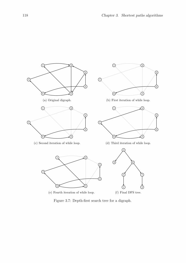
118 Chapter 3. Shortest paths algorithms
21
3
4
5
7
6
(a) Original digraph.
21
3
4
5
7
6
(b) First iteration of while loop.
21
3
4
5
7
6
(c) Second iteration of while loop.
21
3
4
5
7
6
(d) Third iteration of while loop.
21
3
4
5
7
6
(e) Fourth iteration of while loop.
4
3 6
5 7
1 2
(f) Final DFS tree.
Figure 3.7: Depth-first search tree for a digraph.
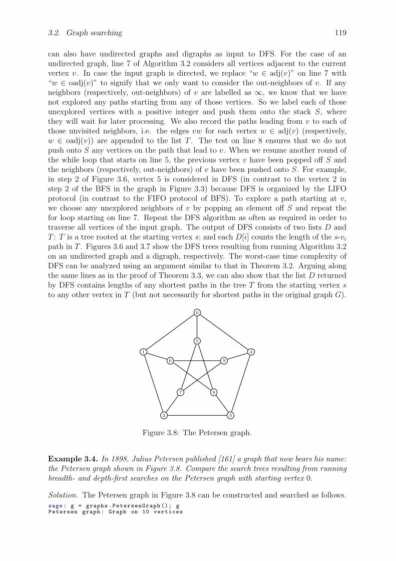
3.2. Graph searching 119
can also have undirected graphs and digraphs as input to DFS. For the case of anundirected graph, line 7 of Algorithm 3.2 considers all vertices adjacent to the currentvertex v. In case the input graph is directed, we replace “w ∈ adj(v)” on line 7 with“w ∈ oadj(v)” to signify that we only want to consider the out-neighbors of v. If anyneighbors (respectively, out-neighbors) of v are labelled as ∞, we know that we havenot explored any paths starting from any of those vertices. So we label each of thoseunexplored vertices with a positive integer and push them onto the stack S, wherethey will wait for later processing. We also record the paths leading from v to each ofthose unvisited neighbors, i.e. the edges vw for each vertex w ∈ adj(v) (respectively,w ∈ oadj(v)) are appended to the list T . The test on line 8 ensures that we do notpush onto S any vertices on the path that lead to v. When we resume another round ofthe while loop that starts on line 5, the previous vertex v have been popped off S andthe neighbors (respectively, out-neighbors) of v have been pushed onto S. For example,in step 2 of Figure 3.6, vertex 5 is considered in DFS (in contrast to the vertex 2 instep 2 of the BFS in the graph in Figure 3.3) because DFS is organized by the LIFOprotocol (in contrast to the FIFO protocol of BFS). To explore a path starting at v,we choose any unexplored neighbors of v by popping an element off S and repeat thefor loop starting on line 7. Repeat the DFS algorithm as often as required in order totraverse all vertices of the input graph. The output of DFS consists of two lists D andT : T is a tree rooted at the starting vertex s; and each D[i] counts the length of the s-vipath in T . Figures 3.6 and 3.7 show the DFS trees resulting from running Algorithm 3.2on an undirected graph and a digraph, respectively. The worst-case time complexity ofDFS can be analyzed using an argument similar to that in Theorem 3.2. Arguing alongthe same lines as in the proof of Theorem 3.3, we can also show that the list D returnedby DFS contains lengths of any shortest paths in the tree T from the starting vertex sto any other vertex in T (but not necessarily for shortest paths in the original graph G).
5
9
87
6
0
4
32
1
Figure 3.8: The Petersen graph.
Example 3.4. In 1898, Julius Petersen published [161] a graph that now bears his name:the Petersen graph shown in Figure 3.8. Compare the search trees resulting from runningbreadth- and depth-first searches on the Petersen graph with starting vertex 0.
Solution. The Petersen graph in Figure 3.8 can be constructed and searched as follows.sage: g = graphs.PetersenGraph (); gPetersen graph: Graph on 10 vertices
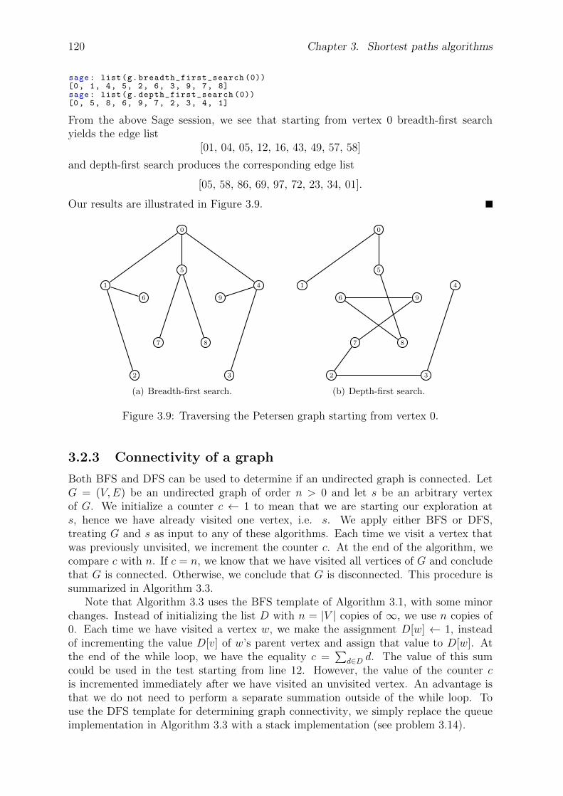
120 Chapter 3. Shortest paths algorithms
sage: list(g.breadth_first_search (0))[0, 1, 4, 5, 2, 6, 3, 9, 7, 8]sage: list(g.depth_first_search (0))[0, 5, 8, 6, 9, 7, 2, 3, 4, 1]
From the above Sage session, we see that starting from vertex 0 breadth-first searchyields the edge list
[01, 04, 05, 12, 16, 43, 49, 57, 58]
and depth-first search produces the corresponding edge list
[05, 58, 86, 69, 97, 72, 23, 34, 01].
Our results are illustrated in Figure 3.9.
5
9
87
6
0
4
32
1
(a) Breadth-first search.
5
9
87
6
0
4
32
1
(b) Depth-first search.
Figure 3.9: Traversing the Petersen graph starting from vertex 0.
3.2.3 Connectivity of a graph
Both BFS and DFS can be used to determine if an undirected graph is connected. LetG = (V,E) be an undirected graph of order n > 0 and let s be an arbitrary vertexof G. We initialize a counter c ← 1 to mean that we are starting our exploration ats, hence we have already visited one vertex, i.e. s. We apply either BFS or DFS,treating G and s as input to any of these algorithms. Each time we visit a vertex thatwas previously unvisited, we increment the counter c. At the end of the algorithm, wecompare c with n. If c = n, we know that we have visited all vertices of G and concludethat G is connected. Otherwise, we conclude that G is disconnected. This procedure issummarized in Algorithm 3.3.
Note that Algorithm 3.3 uses the BFS template of Algorithm 3.1, with some minorchanges. Instead of initializing the list D with n = |V | copies of ∞, we use n copies of0. Each time we have visited a vertex w, we make the assignment D[w] ← 1, insteadof incrementing the value D[v] of w’s parent vertex and assign that value to D[w]. Atthe end of the while loop, we have the equality c =
∑d∈D d. The value of this sum
could be used in the test starting from line 12. However, the value of the counter cis incremented immediately after we have visited an unvisited vertex. An advantage isthat we do not need to perform a separate summation outside of the while loop. Touse the DFS template for determining graph connectivity, we simply replace the queueimplementation in Algorithm 3.3 with a stack implementation (see problem 3.14).

3.3. Weights and distances 121
Algorithm 3.3 Determining whether an undirected graph is connected.
Input An undirected graph G = (V,E) of order n > 0. A vertex s from which to startthe search. The vertices are numbered from 1 to n = |V |, i.e. V = 1, 2, . . . , n.
Output true if G is connected; false otherwise.1: Q← [s] . queue of nodes to visit2: D ← [0, 0, . . . , 0] . n copies of 03: D[s]← 14: c← 15: while length(Q) > 0 do6: v ← dequeue(Q)7: for each w ∈ adj(v) do8: if D[w] = 0 then9: D[w]← 1
10: c← c+ 111: enqueue(Q,w)
12: if c = |V | then13: return true
14: return false
3.3 Weights and distances
In Chapter 1, we briefly mentioned some applications of weighted graphs, but we didnot define the concept of weighted graphs. A graph is said to be weighted when weassign a numeric label or weight to each of its edges. Depending on the application,we can let the vertices represent physical locations and interpret the weight of an edgeas the distance separating two adjacent vertices. There might be a cost involved intraveling from a vertex to one of its neighbors, in which case the weight assigned to thecorresponding edge can represent such a cost. The concept of weighted digraphs can besimilarly defined. When no explicit weights are assigned to the edges of an undirectedgraph or digraph, it is usually convenient to consider each edge as having a weight ofone or unit weight.
Based on the concept of weighted graphs, we now define what it means for a pathto be a shortest path. Let G = (V,E) be a (di)graph with nonnegative edge weightsw(e) ∈ R for each edge e ∈ E. The length or distance d(P ) of a u-v path P from u ∈ Vto v ∈ V is the sum of the edge weights for edges in P . Denote by d(u, v) the smallestvalue of d(P ) for all paths P from u to v. When we regard edge weights as physicaldistances, a u-v path that realizes d(u, v) is sometimes called a shortest path from u to v.The above definitions of distance and shortest path also apply to graphs with negativeedge weights. Unless otherwise specified, where the weight of an edge is not explicitlygiven, we usually consider the edge to have unit weight.
The distance function d on a graph with nonnegative edge weights is known as ametric function. Intuitively, the distance between two physical locations is greater thanzero. When these two locations coincide, i.e. they are one and the same location, thedistance separating them is zero. Regardless of whether we are measuring the distancefrom location a to b or from b to a, we would obtain the same distance. Imagine nowa third location c. The distance from a to b plus the distance from b to c is greaterthan or equal to the distance from a to c. The latter principle is known as the triangle

122 Chapter 3. Shortest paths algorithms
inequality . In summary, given three vertices u, v, w in a graph G, the distance functiond on G satisfies the following property.
Lemma 3.5. Path distance as metric function. Let G = (V,E) be a graph withweight function w : E → R. Define a distance function d : V × V → R given by
d(u, v) =
∞, if there are no paths from u to v,
minw(W ) | W is a u-v walk, otherwise.
Then d is a metric on V if it satisfies the following properties:
1. Nonnegativity: d(u, v) ≥ 0 with d(u, v) = 0 if and only if u = v.
2. Symmetry: d(u, v) = d(v, u).
3. Triangle inequality: d(u, v) + d(v, w) ≥ d(u,w).
The pair (V, d) is called a metric space, where the word “metric” refers to the distancefunction d. Any graphs we consider are assumed to have finite sets of vertices. For thisreason, (V, d) is also known as a finite metric space. The distance matrix D = [d(vi, vj)]of a connected graph is the distance matrix of its finite metric space. The topic of metricspace is covered in further details in topology texts such as Runde [168] and Shirali andVasudeva [173]. See Buckley and Harary [44] for an in-depth coverage of the distanceconcept in graph theory.
Many different algorithms exist for computing a shortest path in a weighted graph.Some only work if the graph has no negative weight cycles. Some assume that there is asingle start or source vertex. Some compute the shortest paths from any vertex to anyother and also detect if the graph has a negative weight cycle. No matter what algorithmis used for the special case of nonnegative weights, the length of the shortest path canneither equal nor exceed the order of the graph.
Lemma 3.6. Fix a vertex v in a connected graph G = (V,E) of order n = |V |. If thereare no negative weight cycles in G, then there exists a shortest path from v to any othervertex w ∈ V that uses at most n− 1 edges.
Proof. Suppose that G contains no negative weight cycles. Observe that at most n− 1edges are required to construct a path from v to any vertex w (Proposition 1.13). Let Pdenote such a path:
P : v0 = v, v1, v2, . . . , vk = w.
Since G has no negative weight cycles, the weight of P is no less than the weight ofP ′, where P ′ is the same as P except that all cycles have been removed. Thus, we canremove all cycles from P and obtain a v-w path P ′ of lower weight. Since the final pathis acyclic, it must have no more than n− 1 edges.
Having defined weights and distances, we are now ready to discuss shortest pathalgorithms for weighted graphs. The breadth-first search Algorithm 3.1 can be appliedwhere each edge has unit weight. Moving on to the general case of graphs with positiveedge weights, algorithms for determining shortest paths in such graphs can be classifiedas weight-setting or weight-correcting [83]. A weight-setting method traverses a graphand assigns weights that, once assigned, remain unchanged for the duration of the al-gorithm. Weight-setting algorithms cannot deal with negative weights. On the other
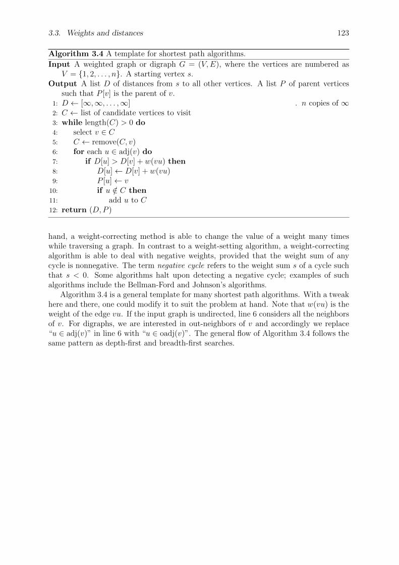
3.3. Weights and distances 123
Algorithm 3.4 A template for shortest path algorithms.
Input A weighted graph or digraph G = (V,E), where the vertices are numbered asV = 1, 2, . . . , n. A starting vertex s.
Output A list D of distances from s to all other vertices. A list P of parent verticessuch that P [v] is the parent of v.
1: D ← [∞,∞, . . . ,∞] . n copies of ∞2: C ← list of candidate vertices to visit3: while length(C) > 0 do4: select v ∈ C5: C ← remove(C, v)6: for each u ∈ adj(v) do7: if D[u] > D[v] + w(vu) then8: D[u]← D[v] + w(vu)9: P [u]← v
10: if u /∈ C then11: add u to C12: return (D,P )
hand, a weight-correcting method is able to change the value of a weight many timeswhile traversing a graph. In contrast to a weight-setting algorithm, a weight-correctingalgorithm is able to deal with negative weights, provided that the weight sum of anycycle is nonnegative. The term negative cycle refers to the weight sum s of a cycle suchthat s < 0. Some algorithms halt upon detecting a negative cycle; examples of suchalgorithms include the Bellman-Ford and Johnson’s algorithms.
Algorithm 3.4 is a general template for many shortest path algorithms. With a tweakhere and there, one could modify it to suit the problem at hand. Note that w(vu) is theweight of the edge vu. If the input graph is undirected, line 6 considers all the neighborsof v. For digraphs, we are interested in out-neighbors of v and accordingly we replace“u ∈ adj(v)” in line 6 with “u ∈ oadj(v)”. The general flow of Algorithm 3.4 follows thesame pattern as depth-first and breadth-first searches.
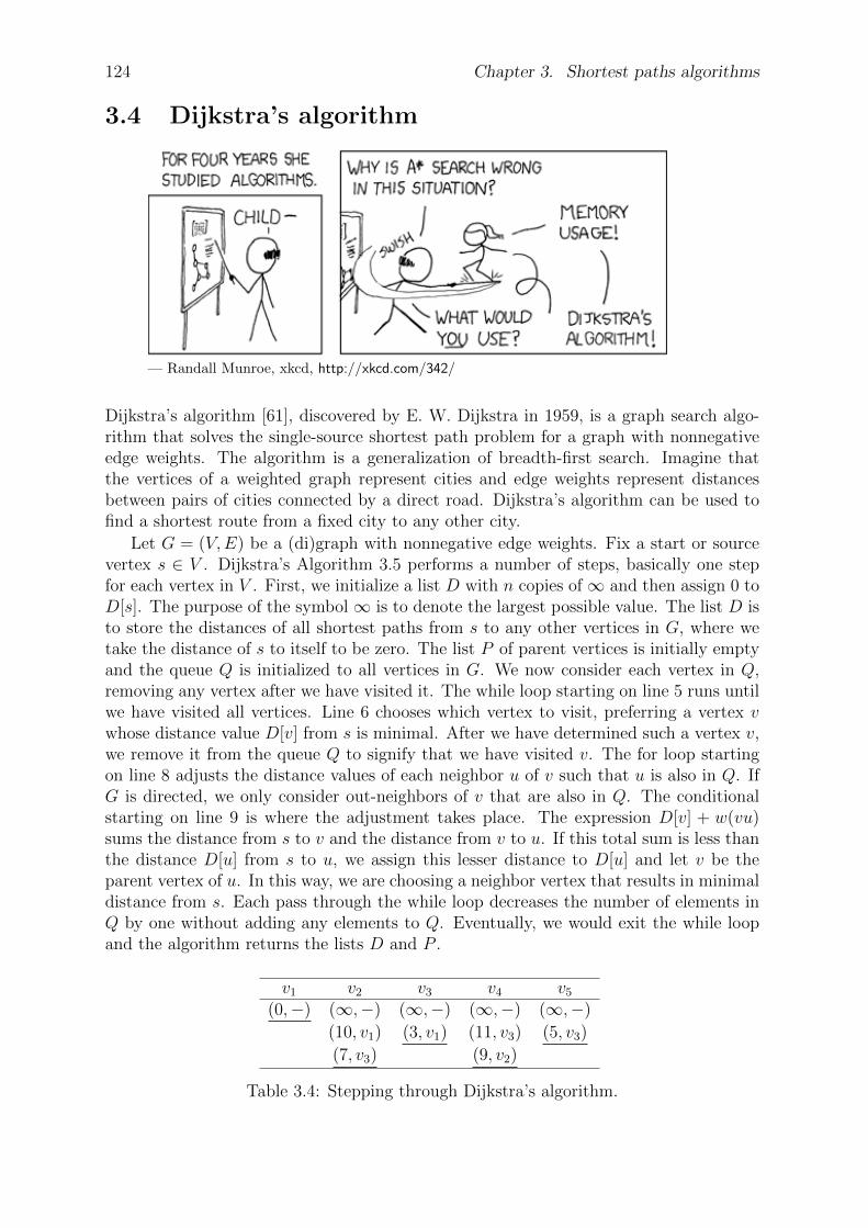
124 Chapter 3. Shortest paths algorithms
3.4 Dijkstra’s algorithm
— Randall Munroe, xkcd, http://xkcd.com/342/
Dijkstra’s algorithm [61], discovered by E. W. Dijkstra in 1959, is a graph search algo-rithm that solves the single-source shortest path problem for a graph with nonnegativeedge weights. The algorithm is a generalization of breadth-first search. Imagine thatthe vertices of a weighted graph represent cities and edge weights represent distancesbetween pairs of cities connected by a direct road. Dijkstra’s algorithm can be used tofind a shortest route from a fixed city to any other city.
Let G = (V,E) be a (di)graph with nonnegative edge weights. Fix a start or sourcevertex s ∈ V . Dijkstra’s Algorithm 3.5 performs a number of steps, basically one stepfor each vertex in V . First, we initialize a list D with n copies of∞ and then assign 0 toD[s]. The purpose of the symbol∞ is to denote the largest possible value. The list D isto store the distances of all shortest paths from s to any other vertices in G, where wetake the distance of s to itself to be zero. The list P of parent vertices is initially emptyand the queue Q is initialized to all vertices in G. We now consider each vertex in Q,removing any vertex after we have visited it. The while loop starting on line 5 runs untilwe have visited all vertices. Line 6 chooses which vertex to visit, preferring a vertex vwhose distance value D[v] from s is minimal. After we have determined such a vertex v,we remove it from the queue Q to signify that we have visited v. The for loop startingon line 8 adjusts the distance values of each neighbor u of v such that u is also in Q. IfG is directed, we only consider out-neighbors of v that are also in Q. The conditionalstarting on line 9 is where the adjustment takes place. The expression D[v] + w(vu)sums the distance from s to v and the distance from v to u. If this total sum is less thanthe distance D[u] from s to u, we assign this lesser distance to D[u] and let v be theparent vertex of u. In this way, we are choosing a neighbor vertex that results in minimaldistance from s. Each pass through the while loop decreases the number of elements inQ by one without adding any elements to Q. Eventually, we would exit the while loopand the algorithm returns the lists D and P .
v1 v2 v3 v4 v5
(0,−) (∞,−) (∞,−) (∞,−) (∞,−)
(10, v1) (3, v1) (11, v3) (5, v3)
(7, v3) (9, v2)
Table 3.4: Stepping through Dijkstra’s algorithm.
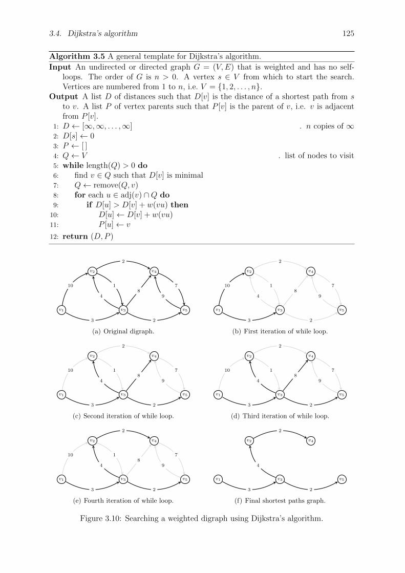
3.4. Dijkstra’s algorithm 125
Algorithm 3.5 A general template for Dijkstra’s algorithm.
Input An undirected or directed graph G = (V,E) that is weighted and has no self-loops. The order of G is n > 0. A vertex s ∈ V from which to start the search.Vertices are numbered from 1 to n, i.e. V = 1, 2, . . . , n.
Output A list D of distances such that D[v] is the distance of a shortest path from sto v. A list P of vertex parents such that P [v] is the parent of v, i.e. v is adjacentfrom P [v].
1: D ← [∞,∞, . . . ,∞] . n copies of ∞2: D[s]← 03: P ← [ ]4: Q← V . list of nodes to visit5: while length(Q) > 0 do6: find v ∈ Q such that D[v] is minimal7: Q← remove(Q, v)8: for each u ∈ adj(v) ∩Q do9: if D[u] > D[v] + w(vu) then
10: D[u]← D[v] + w(vu)11: P [u]← v
12: return (D,P )
v1
v2
v3
v4
v5
10
3
1
2
48
2
7
9
(a) Original digraph.
v1
v2
v3
v4
v5
1
2
48
2
7
9
10
3
(b) First iteration of while loop.
v1
v2
v3
v4
v5
10 1
2
7
9
3
48
2
(c) Second iteration of while loop.
v1
v2
v3
v4
v5
10 1
2
7
9
3
48
2
(d) Third iteration of while loop.
v1
v2
v3
v4
v5
10 18
7
9
3
2
4
2
(e) Fourth iteration of while loop.
v1
v2
v3
v4
v5
3
2
4
2
(f) Final shortest paths graph.
Figure 3.10: Searching a weighted digraph using Dijkstra’s algorithm.

126 Chapter 3. Shortest paths algorithms
Example 3.7. Apply Dijkstra’s algorithm to the graph in Figure 3.10(a), with startingvertex v1.
Solution. Dijkstra’s Algorithm 3.5 applied to the graph in Figure 3.10(a) yields thesequence of intermediary graphs shown in Figure 3.10, culminating in the final shortestpaths graph of Figure 3.10(f) and Table 3.4. For any column vi in the table, each 2-tuplerepresents the distance and parent vertex of vi. As we move along the graph, processingvertices according to Dijkstra’s algorithm, the distance and parent vertex of a columnare updated. The underlined 2-tuple represents the final distance and parent vertexproduced by Dijkstra’s algorithm. From Table 3.4, we have the following shortest pathsand distances:
v1-v2 : v1, v3, v2 d(v1, v2) = 7
v1-v3 : v1, v3 d(v1, v3) = 3
v1-v4 : v1, v3, v2, v4 d(v1, v4) = 9
v1-v5 : v1, v3, v5 d(v1, v5) = 5
Intermediary vertices for a u-v path are obtained by starting from v and work backwardusing the parent of v, then the parent of the parent, and so on.
Dijkstra’s algorithm is an example of a greedy algorithm. Whenever it tries to find thenext vertex, it chooses only that vertex that minimizes the total weight so far. Greedyalgorithms may not produce the best possible result. However, as the following theoremshows, Dijkstra’s algorithm does indeed produce shortest paths.
Theorem 3.8. Correctness of Algorithm 3.5. Let G = (V,E) be a weighted(di)graph with a nonnegative weight function w. When Dijkstra’s algorithm is applied toG with source vertex s ∈ V , the algorithm terminates with D[u] = d(s, u) for all u ∈ V .Furthermore, if D[v] 6= ∞ and v 6= s, then s = u1, u2, . . . , uk = v is a shortest s-v pathsuch that ui−1 = P [ui] for i = 2, 3, . . . , k.
Proof. If G is disconnected, then any v ∈ V that cannot be reached from s has distanceD[v] = ∞ upon algorithm termination. Hence, it suffices to consider the case where Gis connected. Let V = s = v1, v2, . . . , vn and use induction on i to show that aftervisiting vi we have
D[v] = d(s, v) for all v ∈ Vi = v1, v2, . . . , vi. (3.6)
For i = 1, equality holds. Assume for induction that (3.6) holds for some 1 ≤ i ≤ n− 1,so that now our task is to show that (3.6) holds for i+ 1. To verify D[vi+1] = d(s, vi+1),note that by our inductive hypothesis,
D[vi+1] = min d(s, v) + w(vu) | v ∈ Vi and u ∈ adj(v) ∩ (Q\Vi)and respectively
D[vi+1] = min d(s, v) + w(vu) | v ∈ Vi and u ∈ oadj(v) ∩ (Q\Vi)if G is directed. Therefore, D[vi+1] = d(s, vi+1).
Let v ∈ V such that D[v] 6= ∞ and v 6= s. We now construct an s-v path. WhenAlgorithm 3.5 terminates, we have D[v] = D[v1] +w(v1v), where P [v] = v1 and d(s, v) =d(s, v1) +w(v1v). This means that v1 is the second-to-last vertex in a shortest s-v path.Repeated application of this process using the parent list P , we eventually produce ashortest s-v path s = vm, vm−1, . . . , v1, v, where P [vi] = vi+1 for i = 1, 2, . . . ,m− 1.
3.5. Bellman-Ford algorithm 127
To analyze the worst case time complexity of Algorithm 3.5, note that initializing Dtakes O(n+1) and initializing Q takes O(n), for a total of O(n) devoted to initialization.Each extraction of a vertex v with minimal D[v] requires O(n) since we search throughthe entire list Q to determine the minimum value, for a total of O(n2). Each insertioninto D requires constant time and the same holds for insertion into P . Thus, insertioninto D and P takes O(|E| + |E|) = O(|E|), which require at most O(n) time. In theworst case, Dijkstra’s Algorithm 3.5 has running time O(n2 + n) = O(n2).
Can we improve the run time of Dijkstra’s algorithm? The time complexity of Dijk-stra’s algorithm depends on its implementation. With a simple list implementation aspresented in Algorithm 3.5, we have a worst case time complexity of O(n2), where n isthe order of the graph under consideration. Let m be the size of the graph. Table 3.5presents time complexities of Dijkstra’s algorithm for various implementations. Out ofall the four implementations in this table, the heap implementations are much moreefficient than the list implementation presented in Algorithm 3.5. A heap is a type oftree, a topic which will be covered in Chapter 2. Of all the heap implementations inTable 3.5, the Fibonacci heap implementation [82] yields the best runtime. Chapter 4discusses how to use trees for efficient implementations of priority queues via heaps.
Implementation Time complexitylist O(n2)
binary heap O((n+m) lnn
)
k-ary heap O((kn+m) lnn
ln k
)
Fibonacci heap O(n lnn+m)
Table 3.5: Implementation specific worst-case time complexity of Dijkstra’s algorithm.
3.5 Bellman-Ford algorithm
— Randall Munroe, xkcd, http://xkcd.com/69/
A disadvantage of Dijkstra’s Algorithm 3.5 is that it cannot handle graphs with negativeedge weights. The Bellman-Ford algorithm computes single-source shortest paths ina weighted graph or digraph, where some of the edge weights may be negative. Thisalgorithm is a modification of the one published in 1957 by Richard E. Bellman [21] andthat by Lester Randolph Ford, Jr. [79] in 1956. Shimbel [172] independently discoveredthe same method in 1955, and Moore [148] in 1959. In contrast to the “greedy” approachthat Dijkstra’s algorithm takes, i.e. searching for the “cheapest” path, the Bellman-Fordalgorithm searches over all edges and keeps track of the shortest one found as it searches.
The Bellman-Ford Algorithm 3.6 runs in time O(mn), where m and n are the sizeand order of an input graph, respectively. To see this, note that the initialization on
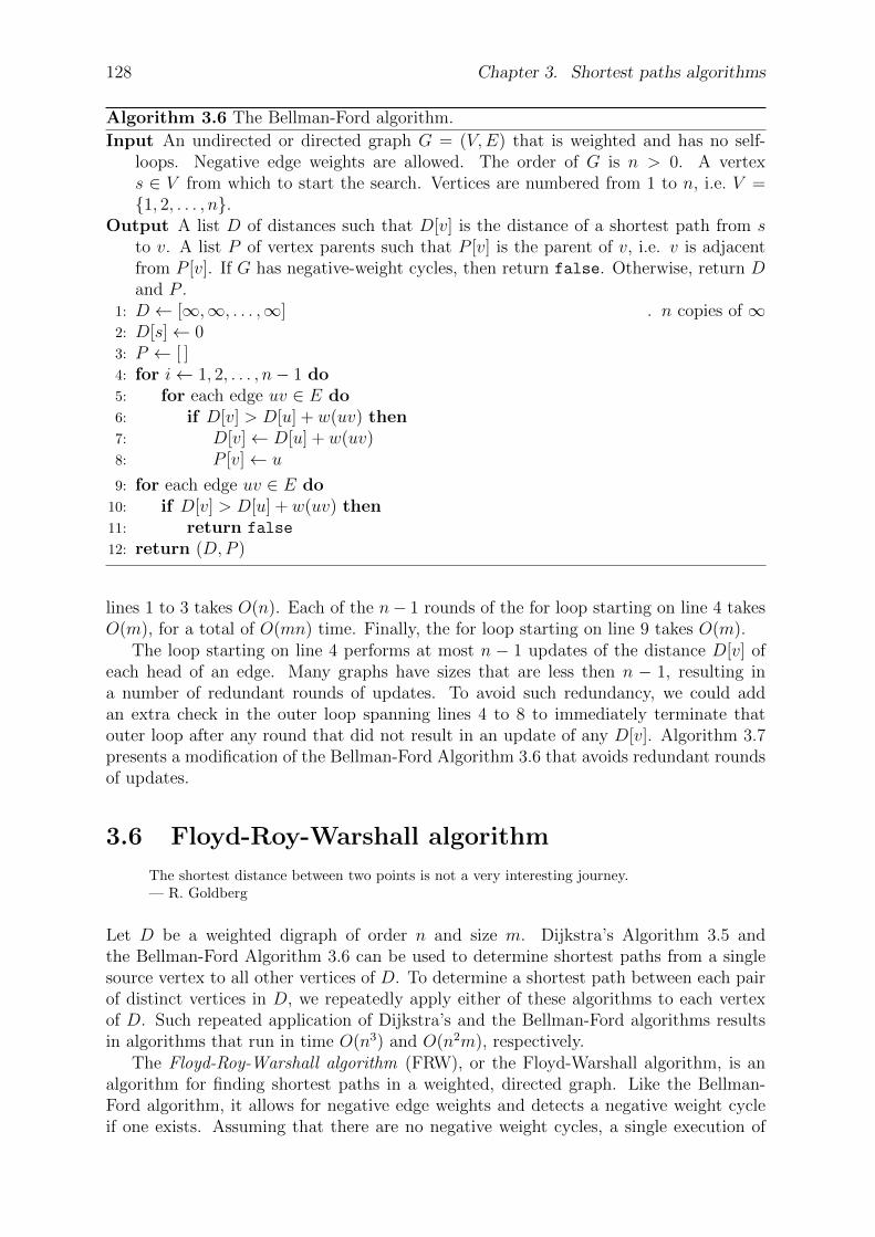
128 Chapter 3. Shortest paths algorithms
Algorithm 3.6 The Bellman-Ford algorithm.
Input An undirected or directed graph G = (V,E) that is weighted and has no self-loops. Negative edge weights are allowed. The order of G is n > 0. A vertexs ∈ V from which to start the search. Vertices are numbered from 1 to n, i.e. V =1, 2, . . . , n.
Output A list D of distances such that D[v] is the distance of a shortest path from sto v. A list P of vertex parents such that P [v] is the parent of v, i.e. v is adjacentfrom P [v]. If G has negative-weight cycles, then return false. Otherwise, return Dand P .
1: D ← [∞,∞, . . . ,∞] . n copies of ∞2: D[s]← 03: P ← [ ]4: for i← 1, 2, . . . , n− 1 do5: for each edge uv ∈ E do6: if D[v] > D[u] + w(uv) then7: D[v]← D[u] + w(uv)8: P [v]← u
9: for each edge uv ∈ E do10: if D[v] > D[u] + w(uv) then11: return false
12: return (D,P )
lines 1 to 3 takes O(n). Each of the n− 1 rounds of the for loop starting on line 4 takesO(m), for a total of O(mn) time. Finally, the for loop starting on line 9 takes O(m).
The loop starting on line 4 performs at most n − 1 updates of the distance D[v] ofeach head of an edge. Many graphs have sizes that are less then n − 1, resulting ina number of redundant rounds of updates. To avoid such redundancy, we could addan extra check in the outer loop spanning lines 4 to 8 to immediately terminate thatouter loop after any round that did not result in an update of any D[v]. Algorithm 3.7presents a modification of the Bellman-Ford Algorithm 3.6 that avoids redundant roundsof updates.
3.6 Floyd-Roy-Warshall algorithm
The shortest distance between two points is not a very interesting journey.— R. Goldberg
Let D be a weighted digraph of order n and size m. Dijkstra’s Algorithm 3.5 andthe Bellman-Ford Algorithm 3.6 can be used to determine shortest paths from a singlesource vertex to all other vertices of D. To determine a shortest path between each pairof distinct vertices in D, we repeatedly apply either of these algorithms to each vertexof D. Such repeated application of Dijkstra’s and the Bellman-Ford algorithms resultsin algorithms that run in time O(n3) and O(n2m), respectively.
The Floyd-Roy-Warshall algorithm (FRW), or the Floyd-Warshall algorithm, is analgorithm for finding shortest paths in a weighted, directed graph. Like the Bellman-Ford algorithm, it allows for negative edge weights and detects a negative weight cycleif one exists. Assuming that there are no negative weight cycles, a single execution of
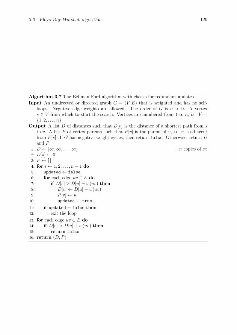
3.6. Floyd-Roy-Warshall algorithm 129
Algorithm 3.7 The Bellman-Ford algorithm with checks for redundant updates.
Input An undirected or directed graph G = (V,E) that is weighted and has no self-loops. Negative edge weights are allowed. The order of G is n > 0. A vertexs ∈ V from which to start the search. Vertices are numbered from 1 to n, i.e. V =1, 2, . . . , n.
Output A list D of distances such that D[v] is the distance of a shortest path from sto v. A list P of vertex parents such that P [v] is the parent of v, i.e. v is adjacentfrom P [v]. If G has negative-weight cycles, then return false. Otherwise, return Dand P .
1: D ← [∞,∞, . . . ,∞] . n copies of ∞2: D[s]← 03: P ← [ ]4: for i← 1, 2, . . . , n− 1 do5: updated← false
6: for each edge uv ∈ E do7: if D[v] > D[u] + w(uv) then8: D[v]← D[u] + w(uv)9: P [v]← u
10: updated← true
11: if updated = false then12: exit the loop
13: for each edge uv ∈ E do14: if D[v] > D[u] + w(uv) then15: return false
16: return (D,P )

130 Chapter 3. Shortest paths algorithms
the FRW algorithm will find the shortest paths between all pairs of vertices. It wasdiscovered independently by Bernard Roy [167] in 1959, Robert Floyd [78] in 1962, andby Stephen Warshall [189] in 1962.
In some sense, the FRW algorithm is an example of dynamic programming , whichallows one to break the computation into simpler steps using some sort of recursiveprocedure. The rough idea is as follows. Temporarily label the vertices of a weighteddigraph G as V = 1, 2, . . . , n with n = |V (G)|. Let W = [w(i, j)] be the weight matrixof G where
w(i, j) =
w(ij), if ij ∈ E(G),
0, if i = j,
∞, otherwise.
(3.7)
Let Pk(i, j) be a shortest path from i to j such that its intermediate vertices are in1, 2, . . . , k. Let Dk(i, j) be the weight (or distance) of Pk(i, j). If no shortest i-jpaths exist, define Pk(i, j) = ∞ and Dk(i, j) = ∞ for all k ∈ 1, 2, . . . , n. If k = 0,then P0(i, j) : i, j since no intermediate vertices are allowed in the path and henceD0(i, j) = w(i, j). In other words, if i and j are adjacent, a shortest i-j path is theedge ij itself and the weight of this path is simply the weight of ij. Now considerPk(i, j) for k > 0. Either Pk(i, j) passes through k or it does not. If k is not on thepath Pk(i, j), then the intermediate vertices of Pk(i, j) are in 1, 2, . . . , k − 1, as arethe vertices of Pk−1(i, j). In case Pk(i, j) contains the vertex k, then Pk(i, j) traversesk exactly once by the definition of path. The i-k subpath in Pk(i, j) is a shortest i-kpath whose intermediate vertices are drawn from 1, 2, . . . , k − 1, which is also the setof intermediate vertices for the k-j subpath in Pk(i, j). That is, to obtain Pk(i, j), wetake the union of the paths Pk−1(i, k) and Pk−1(k, j). We compute the weight Dk(i, j)of Pk(i, j) using the expression
Dk(i, j) =
w(i, j), if k = 0,
minDk−1(i, j), Dk−1(i, k) +Dk−1(k, j), if k > 0.(3.8)
The key to the Floyd-Roy-Warshall algorithm lies in exploiting expression (3.8). Ifn = |V |, then this is a O(n3) time algorithm. For comparison, the Bellman-Ford al-gorithm has complexity O(|V | · |E|), which is O(n3) time for dense graphs. However,Bellman-Ford only yields the shortest paths emanating from a single vertex. To achievecomparable output, we would need to iterate Bellman-Ford over all vertices, which wouldbe an O(n4) time algorithm for dense graphs. Except possibly for sparse graphs, Floyd-Roy-Warshall is better than an iterated implementation of Bellman-Ford. Note thatPk(i, k) = Pk−1(i, k) and Pk(k, i) = Pk−1(k, i), consequently Dk(i, k) = Dk−1(i, k) andDk(k, i) = Dk−1(k, i). This observation allows us to replace Pk(i, j) with P (i, j) fork = 1, 2, . . . , n. The final results of P (i, j) and D(i, k) are the same as Pn(i, j) andDn(i, j), respectively. Algorithm 3.8 summarizes the above discussion into an algorith-mic presentation.
Like the Bellman-Ford algorithm, the Floyd-Roy-Warshall algorithm can also detectthe presence of negative weight cycles. If G is a weighted digraph without self-loops,by (3.7) we have D(i, i) = 0 for i = 1, 2, . . . , n. Any path p starting and ending at icould only improve upon the initial weight of 0 if the weight sum of p is less than zero, i.e.a negative weight cycle. Upon termination of Algorithm 3.8, if D(i, i) < 0, we concludethat there is a path starting and ending at i whose weight sum is negative.

3.6. Floyd-Roy-Warshall algorithm 131
Algorithm 3.8 The Floyd-Roy-Warshall algorithm for all-pairs shortest paths.
Input A weighted digraph G = (V,E) that has no self-loops. Negative edge weightsare allowed. The order of G is n > 0. Vertices are numbered from 1 to n, i.e. V =1, 2, . . . , n. The weight matrix W = [w(i, j)] of G as defined in (3.7).
Output A matrix P = [aij] of shortest paths in G. A matrix D = [aij] of distanceswhere D[i, j] is the weight (or distance) of a shortest i-j path in G.
1: n← |V |2: P [aij]← an n× n zero matrix3: D[aij]← W [w(i, j)]4: for k ← 1, 2, . . . , n do5: for i← 1, 2, . . . , n do6: for j ← 1, 2, . . . , n do7: if D[i, j] > D[i, k] +D[k, j] then8: P [i, j]← k9: D[i, j]← D[i, k] +D[k, j]
10: return (P,D)
Here is an implementation in Sage.def floyd_roy_warshall(A):
"""Shortest paths
INPUT:
- A -- weighted adjacency matrix
OUTPUT:
- dist -- a matrix of distances of shortest paths.- paths -- a matrix of shortest paths."""G = Graph(A, format="weighted_adjacency_matrix")V = G.vertices ()E = [(e[0],e[1]) for e in G.edges ()]n = len(V)dist = [[0]*n for i in range(n)]paths = [[-1]*n for i in range(n)]# initialization stepfor i in range(n):
for j in range(n):if (i,j) in E:
paths[i][j] = jif i == j:
dist[i][j] = 0elif A[i][j]<>0:
dist[i][j] = A[i][j]else:
dist[i][j] = infinity# iteratively finding the shortest pathfor j in range(n):
for i in range(n):if i <> j:
for k in range(n):if k <> j:
if dist[i][k]>dist[i][j]+dist[j][k]:paths[i][k] = V[j]
dist[i][k] = min(dist[i][k], dist[i][j] +dist[j][k])for i in range(n):
if dist[i][i] < 0:raise ValueError , "A negative edge weight cycle exists."
return dist , matrix(paths)
Here are some examples.sage: A = matrix ([[0,1,2,3], [0,0,2,1], [-5,0,0,3], [1 ,0,1,0]]); A

132 Chapter 3. Shortest paths algorithms
sage: floyd_roy_warshall(A)Traceback (click to the left of this block for traceback)...ValueError: A negative edge weight cycle exists.
The plot of this weighted digraph with four vertices appears in Figure 3.11.
0 1
23
1
2
3 2
1 5
3
1
1
Figure 3.11: Demonstrating the Floyd-Roy-Warshall algorithm.
sage: A = matrix ([[0,1,2,3], [0,0,2,1], [-1/2,0,0,3], [1 ,0,1,0]]); Asage: floyd_roy_warshall(A)([[0, 1, 2, 2], [3/2, 0, 2, 1], [-1/2, 1/2, 0, 3/2], [1/2, 3/2, 1, 0]],
[-1 1 2 1][ 2 -1 2 3][-1 0 -1 1][ 2 2 -1 -1])
The plot of this weighted digraph with four vertices appears in Figure 3.12.
0
1
23 1
23
21
−0.5
3
1
1
Figure 3.12: Another demonstration of the Floyd-Roy-Warshall algorithm.
Example 3.9. Section ?? briefly presented the concept of molecular graphs in chem-istry. The Wiener number of a molecular graph was first published in 1947 by Harold

3.6. Floyd-Roy-Warshall algorithm 133
Figure 3.13: Molecular graph of 1,1,3-trimethylcyclobutane.
Wiener [196] who used it in chemistry to study properties of alkanes. Other applica-tions [94] of the Wiener number to chemistry are now known. If G = (V,E) is aconnected graph with vertex set V = v1, v2, . . . , vn, then the Wiener number W of G isdefined by
W (G) =∑
i<j
d(vi, vj) (3.9)
where d(vi, vj) is the distance from vi to vj. What is the Wiener number of the moleculargraph in Figure 3.13?
Solution. Consider the molecular graph in Figure 3.13 as directed with unit weight.To compute the Wiener number of this graph, use the Floyd-Roy-Warshall algorithm toobtain a distance matrix D = [di,j], where di,j is the distance from vi to vj, and apply thedefinition (3.9). The distance matrix resulting from the Floyd-Roy-Warshall algorithmis
M =
0 2 1 2 3 2 42 0 1 2 3 2 41 1 0 1 2 1 32 2 1 0 1 2 23 3 2 1 0 1 12 2 1 2 1 0 24 4 3 2 1 2 0
.
Sum all entries in the upper (or lower) triangular of M to obtain the Wiener numberW = 42. Using Sage, we havesage: G = Graph (1:[3] , 2:[3], 3:[4,6], 4:[5], 6:[5], 5:[7])sage: D = G.shortest_path_all_pairs ()[0]sage: M = [D[i][j] for i in D for j in D[i]]sage: M = matrix(M, nrows=7, ncols =7)sage: W = 0sage: for i in range(M.nrows () - 1):... for j in range(i+1, M.ncols ()):... W += M[i,j]sage: W42
which verifies our computation above. See [94] for a survey of some results concerningthe Wiener number.
3.6.1 Transitive closure
Consider a digraph G = (V,E) of order n = |V |. The transitive closure of G is definedas the digraph G∗ = (V,E∗) having the same vertex set as G. However, the edge set
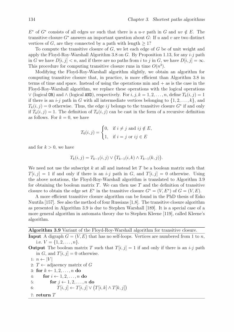
134 Chapter 3. Shortest paths algorithms
E∗ of G∗ consists of all edges uv such that there is a u-v path in G and uv /∈ E. Thetransitive closure G∗ answers an important question about G: If u and v are two distinctvertices of G, are they connected by a path with length ≥ 1?
To compute the transitive closure of G, we let each edge of G be of unit weight andapply the Floyd-Roy-Warshall Algorithm 3.8 on G. By Proposition 1.13, for any i-j pathin G we have D[i, j] < n, and if there are no paths from i to j in G, we have D[i, j] =∞.This procedure for computing transitive closure runs in time O(n3).
Modifying the Floyd-Roy-Warshall algorithm slightly, we obtain an algorithm forcomputing transitive closure that, in practice, is more efficient than Algorithm 3.8 interms of time and space. Instead of using the operations min and + as is the case in theFloyd-Roy-Warshall algorithm, we replace these operations with the logical operations∨ (logical OR) and ∧ (logical AND), respectively. For i, j, k = 1, 2, . . . , n, define Tk(i, j) = 1if there is an i-j path in G with all intermediate vertices belonging to 1, 2, . . . , k, andTk(i, j) = 0 otherwise. Thus, the edge ij belongs to the transitive closure G∗ if and onlyif Tk(i, j) = 1. The definition of Tk(i, j) can be cast in the form of a recursive definitionas follows. For k = 0, we have
T0(i, j) =
0, if i 6= j and ij /∈ E,1, if i = j or ij ∈ E
and for k > 0, we have
Tk(i, j) = Tk−1(i, j) ∨(Tk−1(i, k) ∧ Tk−1(k, j)
).
We need not use the subscript k at all and instead let T be a boolean matrix such thatT [i, j] = 1 if and only if there is an i-j path in G, and T [i, j] = 0 otherwise. Usingthe above notations, the Floyd-Roy-Warshall algorithm is translated to Algorithm 3.9for obtaining the boolean matrix T . We can then use T and the definition of transitiveclosure to obtain the edge set E∗ in the transitive closure G∗ = (V,E∗) of G = (V,E).
A more efficient transitive closure algorithm can be found in the PhD thesis of EskoNuutila [157]. See also the method of four Russians [1,8]. The transitive closure algorithmas presented in Algorithm 3.9 is due to Stephen Warshall [189]. It is a special case of amore general algorithm in automata theory due to Stephen Kleene [119], called Kleene’salgorithm.
Algorithm 3.9 Variant of the Floyd-Roy-Warshall algorithm for transitive closure.
Input A digraph G = (V,E) that has no self-loops. Vertices are numbered from 1 to n,i.e. V = 1, 2, . . . , n.
Output The boolean matrix T such that T [i, j] = 1 if and only if there is an i-j pathin G, and T [i, j] = 0 otherwise.
1: n← |V |2: T ← adjacency matrix of G3: for k ← 1, 2, . . . , n do4: for i← 1, 2, . . . , n do5: for j ← 1, 2, . . . , n do6: T [i, j]← T [i, j] ∨
(T [i, k] ∧ T [k, j]
)
7: return T
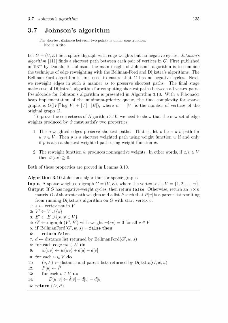
3.7. Johnson’s algorithm 135
3.7 Johnson’s algorithm
The shortest distance between two points is under construction.— Noelie Altito
Let G = (V,E) be a sparse digraph with edge weights but no negative cycles. Johnson’salgorithm [111] finds a shortest path between each pair of vertices in G. First publishedin 1977 by Donald B. Johnson, the main insight of Johnson’s algorithm is to combinethe technique of edge reweighting with the Bellman-Ford and Dijkstra’s algorithms. TheBellman-Ford algorithm is first used to ensure that G has no negative cycles. Next,we reweight edges in such a manner as to preserve shortest paths. The final stagemakes use of Dijkstra’s algorithm for computing shortest paths between all vertex pairs.Pseudocode for Johnson’s algorithm is presented in Algorithm 3.10. With a Fibonacciheap implementation of the minimum-priority queue, the time complexity for sparsegraphs is O(|V |2 log |V | + |V | · |E|), where n = |V | is the number of vertices of theoriginal graph G.
To prove the correctness of Algorithm 3.10, we need to show that the new set of edgeweights produced by w must satisfy two properties:
1. The reweighted edges preserve shortest paths. That is, let p be a u-v path foru, v ∈ V . Then p is a shortest weighted path using weight function w if and onlyif p is also a shortest weighted path using weight function w.
2. The reweight function w produces nonnegative weights. In other words, if u, v ∈ Vthen w(uv) ≥ 0.
Both of these properties are proved in Lemma 3.10.
Algorithm 3.10 Johnson’s algorithm for sparse graphs.
Input A sparse weighted digraph G = (V,E), where the vertex set is V = 1, 2, . . . , n.Output If G has negative-weight cycles, then return false. Otherwise, return an n×n
matrix D of shortest-path weights and a list P such that P [v] is a parent list resultingfrom running Dijkstra’s algorithm on G with start vertex v.
1: s← vertex not in V2: V ′ ← V ∪ s3: E ′ ← E ∪ sv|v ∈ V 4: G′ ← digraph (V ′, E ′) with weight w(sv) = 0 for all v ∈ V5: if BellmanFord(G′, w, s) = false then6: return false
7: d← distance list returned by BellmanFord(G′, w, s)8: for each edge uv ∈ E ′ do9: w(uv)← w(uv) + d[u]− d[v]
10: for each u ∈ V do11: (δ, P )← distance and parent lists returned by Dijkstra(G, w, u)12: P [u]← P13: for each v ∈ V do14: D[u, v]← δ[v] + d[v]− d[u]
15: return (D,P )

136 Chapter 3. Shortest paths algorithms
Lemma 3.10. Reweighting preserves shortest paths. Let G = (V,E) be a weighteddigraph having weight function w : E → R and let h : V → R be a mapping of verticesto real numbers. Let w be another weight function for G such that
w(uv) = w(uv) + h(u)− h(v)
for all uv ∈ E. Suppose p : v0, v1, . . . , vk is any path in G. Then we have the followingresults.
1. The path p is a shortest v0-vk path with weight function w if and only if it is ashortest v0-vk path with weight function w.
2. The graph G has a negative cycle using weight function w if and only if G has anegative cycle using w.
3. If G has no negative cycles, then w(uv) ≥ 0 for all uv ∈ E.
Proof. Write δ and δ for the shortest path weights derived from w and w, respectively.To prove part 1, we need to show that w(p) = δ(v0, vk) if and only if w(p) = δ(v0, vk).First, note that any v0-vk path p satisfies w(p) = w(p) + h(v0)− h(vk) because
w(p) =k∑
i=1
w(vi−1vi)
=k∑
i=1
(w(vi−1vi) + h(vi−1)− h(vi)
)
=k∑
i=1
w(vi−1vi) +k∑
i=1
(h(vi−1)− h(vi)
)
=k∑
i=1
w(vi−1vi) + h(v0)− h(vk)
= w(p) + h(v0)− h(vk).
Any v0-vk path shorter than p and using weight function w is also shorter using w.Therefore, w(p) = δ(v0, vk) if and only if w(p) = δ(v0, vk).
To prove part 2, consider any cycle c : v0, v1, . . . , vk where v0 = vk. Using the proofof part 1, we have
w(c) = w(c) + h(v0)− h(vk)
= w(c)
thus showing that c is a negative cycle using w if and only if it is a negative cycle usingw.
To prove part 3, we construct a new graph G′ = (V ′, E ′) as follows. Consider a vertexs /∈ V and let V ′ = V ∪ s and E ′ = E ∪ sv | v ∈ V . Extend the weight function wto include w(sv) = 0 for all v ∈ V . By construction, s has no incoming edges and anypath in G′ that contains s has s as the source vertex. Thus G′ has no negative cycles ifand only if G has no negative cycles. Define the function h : V → R by v 7→ δ(s, v) withdomain V ′. By the triangle inequality (see Lemma 3.5),
δ(s, u) + w(uv) ≥ δ(s, v) ⇐⇒ h(u) + w(uv) ≥ h(v)
thereby showing that w(uv) = w(uv) + h(u)− h(v) ≥ 0.
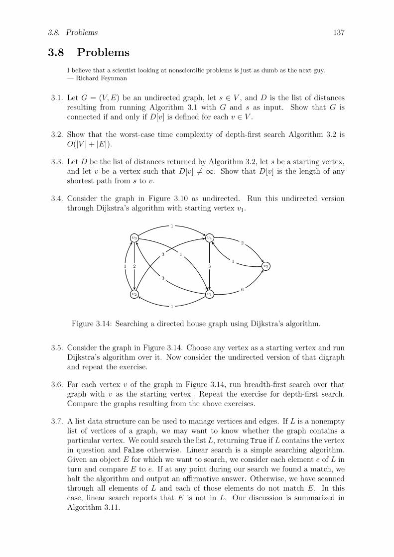
3.8. Problems 137
3.8 Problems
I believe that a scientist looking at nonscientific problems is just as dumb as the next guy.— Richard Feynman
3.1. Let G = (V,E) be an undirected graph, let s ∈ V , and D is the list of distancesresulting from running Algorithm 3.1 with G and s as input. Show that G isconnected if and only if D[v] is defined for each v ∈ V .
3.2. Show that the worst-case time complexity of depth-first search Algorithm 3.2 isO(|V |+ |E|).
3.3. Let D be the list of distances returned by Algorithm 3.2, let s be a starting vertex,and let v be a vertex such that D[v] 6= ∞. Show that D[v] is the length of anyshortest path from s to v.
3.4. Consider the graph in Figure 3.10 as undirected. Run this undirected versionthrough Dijkstra’s algorithm with starting vertex v1.
v1v2
v3 v4
v5
1
3
6
1
3 1
2
1
3
2
1
Figure 3.14: Searching a directed house graph using Dijkstra’s algorithm.
3.5. Consider the graph in Figure 3.14. Choose any vertex as a starting vertex and runDijkstra’s algorithm over it. Now consider the undirected version of that digraphand repeat the exercise.
3.6. For each vertex v of the graph in Figure 3.14, run breadth-first search over thatgraph with v as the starting vertex. Repeat the exercise for depth-first search.Compare the graphs resulting from the above exercises.
3.7. A list data structure can be used to manage vertices and edges. If L is a nonemptylist of vertices of a graph, we may want to know whether the graph contains aparticular vertex. We could search the list L, returning True if L contains the vertexin question and False otherwise. Linear search is a simple searching algorithm.Given an object E for which we want to search, we consider each element e of L inturn and compare E to e. If at any point during our search we found a match, wehalt the algorithm and output an affirmative answer. Otherwise, we have scannedthrough all elements of L and each of those elements do not match E. In thiscase, linear search reports that E is not in L. Our discussion is summarized inAlgorithm 3.11.
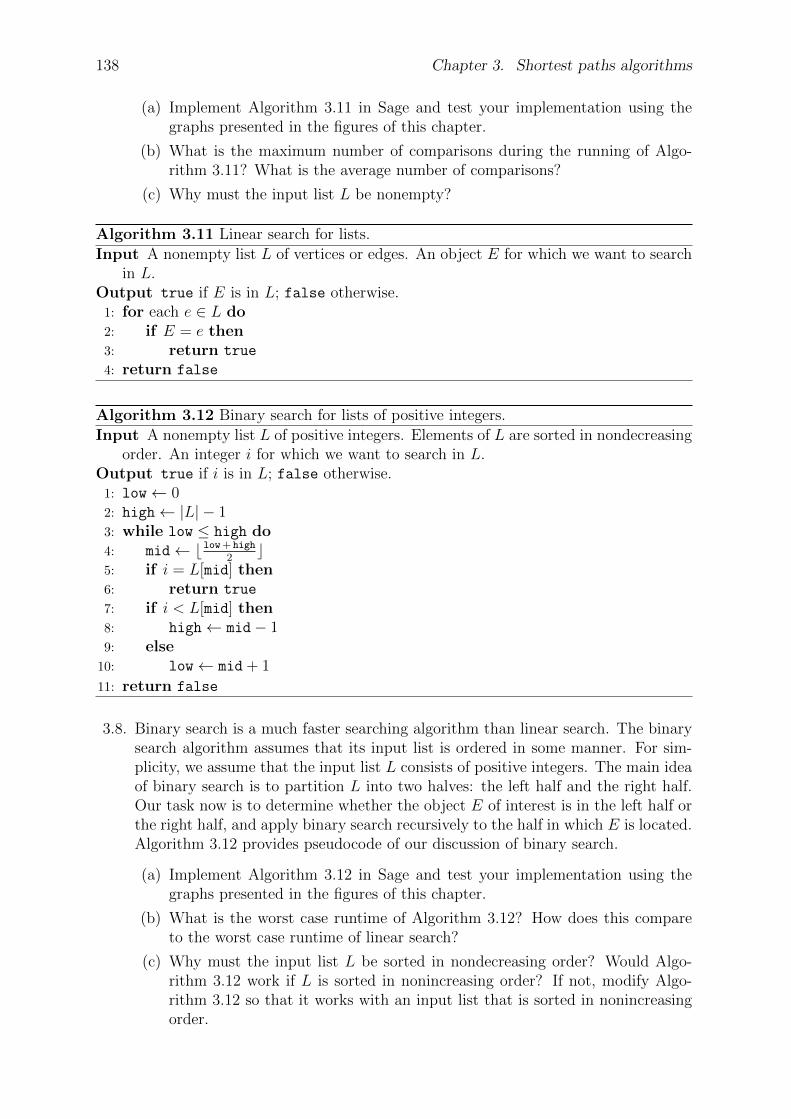
138 Chapter 3. Shortest paths algorithms
(a) Implement Algorithm 3.11 in Sage and test your implementation using thegraphs presented in the figures of this chapter.
(b) What is the maximum number of comparisons during the running of Algo-rithm 3.11? What is the average number of comparisons?
(c) Why must the input list L be nonempty?
Algorithm 3.11 Linear search for lists.
Input A nonempty list L of vertices or edges. An object E for which we want to searchin L.
Output true if E is in L; false otherwise.1: for each e ∈ L do2: if E = e then3: return true
4: return false
Algorithm 3.12 Binary search for lists of positive integers.
Input A nonempty list L of positive integers. Elements of L are sorted in nondecreasingorder. An integer i for which we want to search in L.
Output true if i is in L; false otherwise.1: low← 02: high← |L| − 13: while low ≤ high do4: mid← blow+ high
2c
5: if i = L[mid] then6: return true
7: if i < L[mid] then8: high← mid− 19: else
10: low← mid + 1
11: return false
3.8. Binary search is a much faster searching algorithm than linear search. The binarysearch algorithm assumes that its input list is ordered in some manner. For sim-plicity, we assume that the input list L consists of positive integers. The main ideaof binary search is to partition L into two halves: the left half and the right half.Our task now is to determine whether the object E of interest is in the left half orthe right half, and apply binary search recursively to the half in which E is located.Algorithm 3.12 provides pseudocode of our discussion of binary search.
(a) Implement Algorithm 3.12 in Sage and test your implementation using thegraphs presented in the figures of this chapter.
(b) What is the worst case runtime of Algorithm 3.12? How does this compareto the worst case runtime of linear search?
(c) Why must the input list L be sorted in nondecreasing order? Would Algo-rithm 3.12 work if L is sorted in nonincreasing order? If not, modify Algo-rithm 3.12 so that it works with an input list that is sorted in nonincreasingorder.
3.8. Problems 139
(d) Line 4 of Algorithm 3.12 uses the floor function to compute the index of themiddle value. Would binary search still work if we use the ceiling functioninstead of the floor function?
3.9. Let G be a simple undirected graph having distance matrix D = [d(vi, vj)], whered(vi, vj) ∈ R denotes the shortest distance from vi ∈ V (G) to vj ∈ V (G). Ifvi = vj, we set d(vi, vj) = 0. For each pair of distinct vertices (vi, vj), we haved(vi, vj) = d(vj, vi). The i-j entry of D is also written as di,j and denotes the entryin row i and column j.
(a) The total distance td(u) of a fixed vertex u ∈ V (G) is the sum of distancesfrom u to each vertex in G:
td(u) =∑
v∈V (G)
d(u, v).
If G is connected, i is the row index of vertex u in the distance matrix D, andj is the column index of u in D, show that the total distance of u is
td(u) =∑
k
di,k =∑
k
dk,j. (3.10)
(b) Let the vertices of G be labeled V = v1, v2, . . . , vn, where n = |V (G)| isthe order of G. The total distance td(G) of G is obtained by summing all thed(vi, vj) for i < j. If G is connected, show that the total distance of G is equalto the sum of all entries in the upper (or lower) triangular of D:
td(G) =∑
i<j
di,j =∑
i>j
di,j =1
2
(∑
u∈V
∑
v∈V
d(u, v)
). (3.11)
Hence show that the total distance of G is equal to its Wiener number:
td(G) = W (G).
(c) Would equations (3.10) and (3.11) hold if G is not connected or directed?
3.10. The following result is from [202]. Let G1 and G2 be graphs with orders ni =|V (Gi)| and sizes mi = |E(Gi)|, respectively.
(a) If each of G1 and G2 is connected, show that the Wiener number of theCartesian product G1G2 is
W (G1G2) = n22 ·W (G1) + n2
1 ·W (G2).
(b) If G1 and G2 are arbitrary graphs, show that the Wiener number of the joinG1 +G2 is
W (G1 +G2) = n21 − n1 + n2
2 − n2 + n1n2 −m1 −m2.
3.11. The following results originally appeared in [70] and independently rediscoveredmany times since.
140 Chapter 3. Shortest paths algorithms
(a) If Pn is the path graph on n ≥ 0 vertices, show that the Wiener number ofPn is W (Pn) = 1
6n(n2 − 1).
(b) If Cn is the cycle graph on n ≥ 0 vertices, show that the Wiener number ofCn is
W (Cn) =
18n(n2 − 1), if n is odd,
18n3, if n is even.
(c) If Kn is the complete graph on n vertices, show that its Wiener number isW (Kn) = 1
2n(n− 1).
(d) Show that the Wiener number of the complete bipartite graph Km,n is
W (Km,n) = mn+m(m− 1) + n(n− 1).
3.12. In addition to searching, there is the related problem of sorting a list according toan ordering relation. If the given list L = [e1, e2, . . . , en] consists of real numbers,we want to order elements in nondecreasing order. Bubble sort is a basic sortingalgorithm that can be used to sort a list of real numbers, indeed any collection ofobjects that can be ordered according to an ordering relation. During each passthrough the list L from left to right, we consider ei and its right neighbor ei+1. Ifei ≤ ei+1, then we move on to consider ei+1 and its right neighbor ei+2. If ei > ei+1,then we swap these two values around in the list and then move on to consider ei+1
and its right neighbor ei+2. Each successive pass pushes to the right end an elementthat is the next largest in comparison to the previous largest element pushed tothe right end. Hence the name bubble sort for the algorithm. Algorithm 3.13summarizes our discussion.
Algorithm 3.13 Bubble sort.
Input A list L of n > 1 elements that can be ordered using the “less than or equal to”relation “≤”.
Output The same list as L, but sorted in nondecreasing order.1: for i← n, n− 1, . . . , 2 do2: for j ← 2, 3, . . . , i do3: if L[j − 1] > L[j] then4: swap the values of L[j − 1] and L[j]
5: return L
(a) Analyze the worst-case runtime of Algorithm 3.13.
(b) Modify Algorithm 3.13 so that it sorts elements in nonincreasing order.
3.13. Selection sort is another simple sorting algorithm that works as follows. Let L =[e1, e2, . . . , en] be a list of elements that can be ordered according to the relation“≤”, e.g. the ei can all be real numbers or integers. On the first scan of Lfrom left to right, among the elements L[2], . . . , L[n] we find the smallest elementand exchange it with L[1]. On the second scan, we find the smallest elementamong L[3], . . . , L[n] and exchange that smallest element with L[2]. In general,during the i-th scan we find the smallest element among L[i + 1], . . . , L[n] andexchange that with L[i]. At the end of the i-th scan, the element L[i] is in its final
3.8. Problems 141
position and would not be processed again. When the index reaches i = n, the listwould have been sorted in nondecreasing order. The procedure is summarized inAlgorithm 3.14.
(a) Analyze the worst-case runtime of Algorithm 3.14 and compare your result tothe worst-case runtime of the bubble sort Algorithm 3.13.
(b) Modify Algorithm 3.14 to sort elements in nonincreasing order.
(c) Line 6 of Algorithm 3.14 assumes that among L[i+1], L[i+2], . . . , L[n] there isa smallest element L[k] such that L[i] > L[k], hence we perform the swap. It ispossible that L[i] < L[k], obviating the need to carry out the value swapping.Modify Algorithm 3.14 to take account of our discussion.
Algorithm 3.14 Selection sort.
Input A list L of n > 1 elements that can be ordered using the relation “≤”.Output The same list as L, but sorted in nondecreasing order.
1: for i← 1, 2, . . . , n− 1 do2: min← i3: for j ← i+ 1, i+ 2, . . . , n do4: if L[j] < L[min] then5: min← j
6: swap the values of L[min] and L[i]
7: return L
3.14. Algorithm 3.3 uses breadth-first search to determine the connectivity of an undi-rected graph. Modify this algorithm to use depth-first search. How can Algo-rithm 3.3 be used or modified to test the connectivity of a digraph?
3.15. The following problem is known as the river crossing problem. A man, a goat,a wolf, and a basket of cabbage are all on one side of a river. They have a boatthat could be used to cross to the other side of the river. The boat can only holdat most two passengers, one of whom must be able to row the boat. One of thetwo passengers must be the man and the other passenger can be either the goat,the wolf, or the basket of cabbage. When crossing the river, if the man leaves thewolf with the goat, the wolf would prey on the goat. If he leaves the goat with thebasket of cabbage, the goat would eat the cabbage. The objective is to cross theriver in such a way that the wolf has no chance of preying on the goat, nor thatthe goat eat the cabbage.
(a) Let M , G, W , and C denote the man, the goat, the wolf, and the basket ofcabbage, respectively. Initially all four are on the left side of the river and noneof them are on the right side. Denote this by the ordered pair (MGWC, w),which is called the initial state of the problem. When they have all crossed tothe right side of the river, the final state of the problem is (w, MGWC). Theunderscore “w” means that neither M , G, W , nor C are on the correspondingside of the river. List a finite sequence of moves to get from (MGWC, w) to(w, MGWC). Draw your result as a digraph.
(b) In the digraph Γ obtained from the previous exercise, let each edge of Γ be ofunit weight. Find a shortest path from (MGWC, w) to (w, MGWC).
142 Chapter 3. Shortest paths algorithms
(c) Rowing from one side of the river to the other side is called a crossing. Whatis the minimum number of crossings needed to get from (MGWC, w) to(w, MGWC)?
3.16. Symbolic computation systems such as Magma, Maple, Mathematica, Maxima,and Sage are able to read in a symbolic expression such as
(a + b)^2 - (a - b)^2
and determine whether or not the brackets match. A bracket is any of the followingcharacters:
( ) [ ]
A string S of characters is said to be balanced if any left bracket in S has a corre-sponding right bracket that is also in S. Furthermore, if there are k occurrencesof one type of left bracket, then there must be k occurrences of the correspondingright bracket. The balanced bracket problem is concerned with determining whetheror not the brackets in S are balanced. Algorithm 3.15 contains a procedure to de-termine if the brackets in S are balanced, and if so return a list of positive integersto indicate how the brackets match.
(a) Implement Algorithm 3.15 in Sage and test your implementation on variousstrings containing brackets. Test your implementation on nonempty stringswithout any brackets.
(b) Modify Algorithm 3.15 so that it returns True if the brackets of an inputstring are balanced, and returns False otherwise.
(c) What is the worst-case runtime of Algorithm 3.15?
3.17. An arithmetic expression written in the form a + b is said to be in infix notationbecause the operator is in between the operands. The same expression can also bewritten in reverse Polish notation (or postfix notation) as
a b +
with the operator following its two operands. Given an arithmetic expression A =e0e1 · · · en written in reverse Polish notation, we can use the stack data structureto evaluate the expression. Let P = [e0, e1, . . . , en] be the stack representation ofA, where traversing P from left to right we are moving from the top of the stackto the bottom of the stack. We call P the Polish stack and the stack E containingintermediate results the evaluation stack. While P is not empty, pop the Polishstack and assign the extracted result to x. If x is an operator, we pop the evaluationstack twice: the result of the first pop is assigned to b and the result of the secondpop is assigned to a. Compute the infix expression a x b and push the result ontoE. However, if x is an operand, we push x onto E. Iterate the above process untilP is empty, at which point the top of E contains the evaluation of A. Refer toAlgorithm 3.16 for pseudocode of the above discussion.
(a) Prove the correctness of Algorithm 3.16.
(b) What is the worst-case runtime of Algorithm 3.16?

3.8. Problems 143
Algorithm 3.15 A brackets parser.
Input A nonempty string S of characters.Output A list L of positive integers indicating how the brackets match. If the brackets
are not balanced, return the empty string ε.1: L← [ ]2: T ← empty stack3: c← 14: n← |S|5: for i← 0, 1, . . . , n do6: if S[i+ 1] is a left bracket then7: append(L, c)8: push (S[i+ 1], c) onto T9: c← c+ 1
10: if S[i+ 1] is a right bracket then11: if T is empty then12: return ε13: (left, d)← pop(T )14: if left matches S[i+ 1] then15: append(L, d)16: else17: return ε18: if T is empty then19: return L20: return ε

144 Chapter 3. Shortest paths algorithms
Algorithm 3.16 Evaluate arithmetic expressions in reverse Polish notation.
Input A Polish stack P containing an arithmetic expression in reverse Polish notation.Output An evaluation of the arithmetic expression represented by P .
1: E ← empty stack2: v ← Null
3: while P is not empty do4: x← pop(P )5: if x is an operator then6: b← pop(E)7: a← pop(E)8: if x is addition operator then9: v ← a+ b
10: else if x is subtraction operator then11: v ← a− b12: else if x is multiplication operator then13: v ← a× b14: else if x is division operator then15: v ← a/b16: else17: exit algorithm with error
18: push(E, v)19: else20: push(E, x)
21: v ← pop(E)22: return v
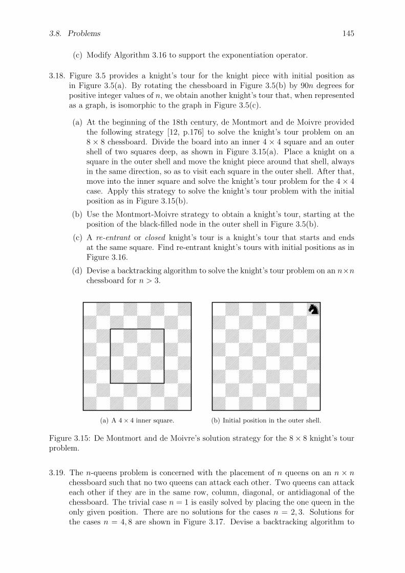
3.8. Problems 145
(c) Modify Algorithm 3.16 to support the exponentiation operator.
3.18. Figure 3.5 provides a knight’s tour for the knight piece with initial position asin Figure 3.5(a). By rotating the chessboard in Figure 3.5(b) by 90n degrees forpositive integer values of n, we obtain another knight’s tour that, when representedas a graph, is isomorphic to the graph in Figure 3.5(c).
(a) At the beginning of the 18th century, de Montmort and de Moivre providedthe following strategy [12, p.176] to solve the knight’s tour problem on an8 × 8 chessboard. Divide the board into an inner 4 × 4 square and an outershell of two squares deep, as shown in Figure 3.15(a). Place a knight on asquare in the outer shell and move the knight piece around that shell, alwaysin the same direction, so as to visit each square in the outer shell. After that,move into the inner square and solve the knight’s tour problem for the 4× 4case. Apply this strategy to solve the knight’s tour problem with the initialposition as in Figure 3.15(b).
(b) Use the Montmort-Moivre strategy to obtain a knight’s tour, starting at theposition of the black-filled node in the outer shell in Figure 3.5(b).
(c) A re-entrant or closed knight’s tour is a knight’s tour that starts and endsat the same square. Find re-entrant knight’s tours with initial positions as inFigure 3.16.
(d) Devise a backtracking algorithm to solve the knight’s tour problem on an n×nchessboard for n > 3.
0Z0Z0Z0ZZ0Z0Z0Z00Z0Z0Z0ZZ0Z0Z0Z00Z0Z0Z0ZZ0Z0Z0Z00Z0Z0Z0ZZ0Z0Z0Z0
(a) A 4× 4 inner square.
0Z0Z0Z0mZ0Z0Z0Z00Z0Z0Z0ZZ0Z0Z0Z00Z0Z0Z0ZZ0Z0Z0Z00Z0Z0Z0ZZ0Z0Z0Z0(b) Initial position in the outer shell.
Figure 3.15: De Montmort and de Moivre’s solution strategy for the 8× 8 knight’s tourproblem.
3.19. The n-queens problem is concerned with the placement of n queens on an n × nchessboard such that no two queens can attack each other. Two queens can attackeach other if they are in the same row, column, diagonal, or antidiagonal of thechessboard. The trivial case n = 1 is easily solved by placing the one queen in theonly given position. There are no solutions for the cases n = 2, 3. Solutions forthe cases n = 4, 8 are shown in Figure 3.17. Devise a backtracking algorithm to
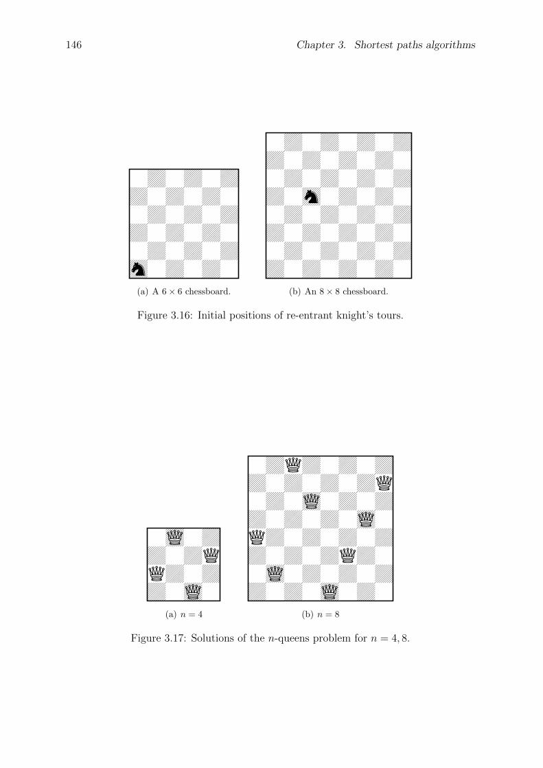
146 Chapter 3. Shortest paths algorithms
0Z0Z0ZZ0Z0Z00Z0Z0ZZ0Z0Z00Z0Z0Zm0Z0Z0
(a) A 6× 6 chessboard.
0Z0Z0Z0ZZ0Z0Z0Z00Z0Z0Z0ZZ0m0Z0Z00Z0Z0Z0ZZ0Z0Z0Z00Z0Z0Z0ZZ0Z0Z0Z0
(b) An 8× 8 chessboard.
Figure 3.16: Initial positions of re-entrant knight’s tours.
0L0ZZ0ZQQZ0ZZ0L0
(a) n = 4
0ZQZ0Z0ZZ0Z0Z0ZQ0Z0L0Z0ZZ0Z0Z0L0QZ0Z0Z0ZZ0Z0ZQZ00L0Z0Z0ZZ0Z0L0Z0
(b) n = 8
Figure 3.17: Solutions of the n-queens problem for n = 4, 8.
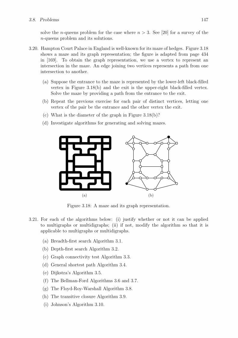
3.8. Problems 147
solve the n-queens problem for the case where n > 3. See [20] for a survey of then-queens problem and its solutions.
3.20. Hampton Court Palace in England is well-known for its maze of hedges. Figure 3.18shows a maze and its graph representation; the figure is adapted from page 434in [169]. To obtain the graph representation, we use a vertex to represent anintersection in the maze. An edge joining two vertices represents a path from oneintersection to another.
(a) Suppose the entrance to the maze is represented by the lower-left black-filledvertex in Figure 3.18(b) and the exit is the upper-right black-filled vertex.Solve the maze by providing a path from the entrance to the exit.
(b) Repeat the previous exercise for each pair of distinct vertices, letting onevertex of the pair be the entrance and the other vertex the exit.
(c) What is the diameter of the graph in Figure 3.18(b)?
(d) Investigate algorithms for generating and solving mazes.
(a) (b)
Figure 3.18: A maze and its graph representation.
3.21. For each of the algorithms below: (i) justify whether or not it can be appliedto multigraphs or multidigraphs; (ii) if not, modify the algorithm so that it isapplicable to multigraphs or multidigraphs.
(a) Breadth-first search Algorithm 3.1.
(b) Depth-first search Algorithm 3.2.
(c) Graph connectivity test Algorithm 3.3.
(d) General shortest path Algorithm 3.4.
(e) Dijkstra’s Algorithm 3.5.
(f) The Bellman-Ford Algorithms 3.6 and 3.7.
(g) The Floyd-Roy-Warshall Algorithm 3.8.
(h) The transitive closure Algorithm 3.9.
(i) Johnson’s Algorithm 3.10.
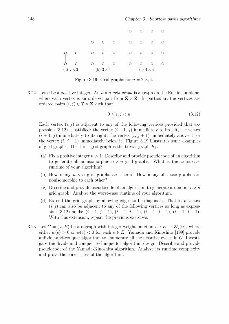
148 Chapter 3. Shortest paths algorithms
(a) 2× 2 (b) 3× 3 (c) 4× 4
Figure 3.19: Grid graphs for n = 2, 3, 4.
3.22. Let n be a positive integer. An n×n grid graph is a graph on the Euclidean plane,where each vertex is an ordered pair from Z × Z. In particular, the vertices areordered pairs (i, j) ∈ Z× Z such that
0 ≤ i, j < n. (3.12)
Each vertex (i, j) is adjacent to any of the following vertices provided that ex-pression (3.12) is satisfied: the vertex (i− 1, j) immediately to its left, the vertex(i + 1, j) immediately to its right, the vertex (i, j + 1) immediately above it, orthe vertex (i, j − 1) immediately below it. Figure 3.19 illustrates some examplesof grid graphs. The 1× 1 grid graph is the trivial graph K1.
(a) Fix a positive integer n > 1. Describe and provide pseudocode of an algorithmto generate all nonisomorphic n × n grid graphs. What is the worst-caseruntime of your algorithm?
(b) How many n × n grid graphs are there? How many of those graphs arenonisomorphic to each other?
(c) Describe and provide pseudocode of an algorithm to generate a random n×ngrid graph. Analyze the worst-case runtime of your algorithm.
(d) Extend the grid graph by allowing edges to be diagonals. That is, a vertex(i, j) can also be adjacent to any of the following vertices so long as expres-sion (3.12) holds: (i − 1, j − 1), (i − 1, j + 1), (i + 1, j + 1), (i + 1, j − 1).With this extension, repeat the previous exercises.
3.23. Let G = (V,E) be a digraph with integer weight function w : E → Z\0, whereeither w(e) > 0 or w(e) < 0 for each e ∈ E. Yamada and Kinoshita [199] providea divide-and-conquer algorithm to enumerate all the negative cycles in G. Investi-gate the divide and conquer technique for algorithm design. Describe and providepseudocode of the Yamada-Kinoshita algorithm. Analyze its runtime complexityand prove the correctness of the algorithm.
Chapter 4
Graph data structures
— Randall Munroe, xkcd, http://xkcd.com/835/
What is the next task to be completed? Our daily lives are littered with priorities. Thereare tasks that take higher priorities than everything else and should be completed as soonas possible. Other tasks are of lower priorities and can be done whenever we have time.If we assign a nonnegative whole number to each task that needs to be completed, thetask with the highest priority has the lowest whole number assigned to it. As each newtask comes along, it is assigned a numerical priority. At any point in time, we want tochoose and complete the task with the highest priority. This chapter will show how astructure called a priority queue can be used to efficiently choose the next task of highestpriority. The structure can efficiently handle from a few tasks up to millions of tasks.
In Chapters 3 and 2, we discussed various algorithms that rely on priority queues asone of their fundamental data structures. Such algorithms include Dijkstra’s algorithm,Prim’s algorithm, and the algorithm for constructing Huffman trees. The runtime ofany algorithm that uses priority queues crucially depends on an efficient implementationof the priority queue data structure. This chapter discusses the general priority queuedata structure and various efficient implementations based on trees. Section 4.1 providessome theoretical underpinning of priority queues and considers a simple implementation
149

150 Chapter 4. Graph data structures
of priority queues as sorted lists. Section 4.2 discusses how to use binary trees to realizean efficient implementation of priority queues called a binary heap. Although very usefulin practice, binary heaps do not lend themselves to being merged in an efficient manner,a setback rectified in section 4.3 by a priority queue implementation called binomialheaps. As a further application of binary trees, section 4.4 discusses binary search treesas a general data structure for managing data in a sorted order.
4.1 Priority queues
A priority queue is a queue data structure with various rules on how to access andmanage elements of the queue. Recall from section 3.2.1 that an ordinary queue Q hasthe following basic functions for accessing and managing its elements:
dequeue(Q) — Remove the front of Q.
enqueue(Q, e) — Append the element e to the end of Q.
If Q is now a priority queue, each element is associated with a key or priority p ∈ Xfrom a totally ordered set X. A binary relation denoted by an infix operator, say “≤”,is defined on all elements of X such that the following properties hold for all a, b, c ∈ X:
Totality: We have a ≤ b or b ≤ a.
Antisymmetry: If a ≤ b and b ≤ a, then a = b.
Transitivity: If a ≤ b and b ≤ c, then a ≤ c.
If the above three properties hold for the relation “≤”, then we say that “≤” is a totalorder on X and that X is a totally ordered set . In all, if the key of each element ofQ belongs to the same totally ordered set X, we use the total order defined on X tocompare the keys of the queue elements. For example, the set Z of integers is totallyordered by the “less than or equal to” relation. If the key of each e ∈ Q is an elementof Z, we use the latter relation to compare the keys of elements of Q. In the case of anordinary queue, the key of each queue element is its position index.
To extract from a priority queue Q an element of lowest priority, we need to definethe notion of smallest priority or key. Let pi be the priority or key assigned to elementei of Q. Then pmin is the lowest key if pmin ≤ p for any element key p. The element withcorresponding key pmin is the minimum priority element. Based upon the notion of keycomparison, we define two operations on a priority queue:
insert(Q, e, p) — Insert into Q the element e with key p.
extractMin(Q) — Extract from Q an element having the smallest priority.
An immediate application of priority queues is sorting a finite sequence of items.Suppose L is a finite list of n > 0 items on which a total order is defined. Let Q bean empty priority queue. In the first phase of the priority queue sorting algorithm,we extract each element e ∈ L from L and insert e into Q with key e itself. In otherwords, each element e is its own key. This first phase of the sorting algorithm requiresn element extractions from L and n element insertions into Q. The second phase ofthe algorithm involves extracting elements from Q via the extractMin operation. Queueelements are extracted via extractMin and inserted back into L in the order in whichthey are extracted from Q. Algorithm 4.1 presents pseudocode of our discussion. Theruntime of Algorithm 4.1 depends on how the priority queue Q is implemented.
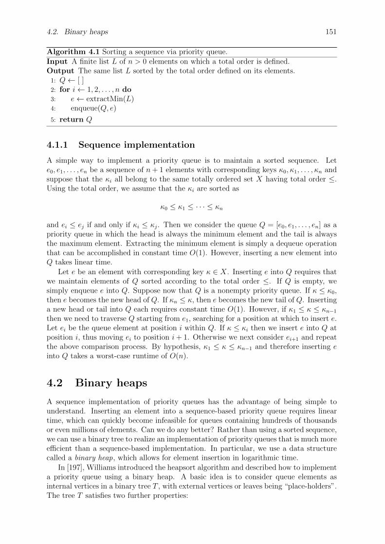
4.2. Binary heaps 151
Algorithm 4.1 Sorting a sequence via priority queue.
Input A finite list L of n > 0 elements on which a total order is defined.Output The same list L sorted by the total order defined on its elements.
1: Q← [ ]2: for i← 1, 2, . . . , n do3: e← extractMin(L)4: enqueue(Q, e)
5: return Q
4.1.1 Sequence implementation
A simple way to implement a priority queue is to maintain a sorted sequence. Lete0, e1, . . . , en be a sequence of n+ 1 elements with corresponding keys κ0, κ1, . . . , κn andsuppose that the κi all belong to the same totally ordered set X having total order ≤.Using the total order, we assume that the κi are sorted as
κ0 ≤ κ1 ≤ · · · ≤ κn
and ei ≤ ej if and only if κi ≤ κj. Then we consider the queue Q = [e0, e1, . . . , en] as apriority queue in which the head is always the minimum element and the tail is alwaysthe maximum element. Extracting the minimum element is simply a dequeue operationthat can be accomplished in constant time O(1). However, inserting a new element intoQ takes linear time.
Let e be an element with corresponding key κ ∈ X. Inserting e into Q requires thatwe maintain elements of Q sorted according to the total order ≤. If Q is empty, wesimply enqueue e into Q. Suppose now that Q is a nonempty priority queue. If κ ≤ κ0,then e becomes the new head of Q. If κn ≤ κ, then e becomes the new tail of Q. Insertinga new head or tail into Q each requires constant time O(1). However, if κ1 ≤ κ ≤ κn−1
then we need to traverse Q starting from e1, searching for a position at which to insert e.Let ei be the queue element at position i within Q. If κ ≤ κi then we insert e into Q atposition i, thus moving ei to position i+ 1. Otherwise we next consider ei+1 and repeatthe above comparison process. By hypothesis, κ1 ≤ κ ≤ κn−1 and therefore inserting einto Q takes a worst-case runtime of O(n).
4.2 Binary heaps
A sequence implementation of priority queues has the advantage of being simple tounderstand. Inserting an element into a sequence-based priority queue requires lineartime, which can quickly become infeasible for queues containing hundreds of thousandsor even millions of elements. Can we do any better? Rather than using a sorted sequence,we can use a binary tree to realize an implementation of priority queues that is much moreefficient than a sequence-based implementation. In particular, we use a data structurecalled a binary heap, which allows for element insertion in logarithmic time.
In [197], Williams introduced the heapsort algorithm and described how to implementa priority queue using a binary heap. A basic idea is to consider queue elements asinternal vertices in a binary tree T , with external vertices or leaves being “place-holders”.The tree T satisfies two further properties:

152 Chapter 4. Graph data structures
1. A relational property specifying the relative ordering and placement of queue ele-ments.
2. A structural property that specifies the structure of T .
The relational property of T can be expressed as follows:
Definition 4.1. Heap-order property. Let T be a binary tree and let v be a vertex ofT other than the root. If p is the parent of v and these vertices have corresponding keysκp and κv, respectively, then κp ≤ κv.
The heap-order property is defined in terms of the total order used to compare thekeys of the internal vertices. Taking the total order to be the ordinary “less than orequal to” relation, it follows from the heap-order property that the root of T is alwaysthe vertex with a minimum key. Similarly, if the total order is the usual “greater thanor equal to” relation, then the root of T is always the vertex with a maximum key. Ingeneral, if ≤ is a total order defined on the keys of T and u and v are vertices of T , wesay that u is less than or equal to v if and only if u ≤ v. Furthermore, u is said to bea minimum vertex of T if and only if u ≤ v for all vertices of T . From our discussionabove, the root is always a minimum vertex of T and is said to be “at the top of theheap”, from which we derive the name “heap” for this data structure.
Another consequence of the heap-order property becomes apparent when we traceout a path from the root of T to any internal vertex. Let r be the root of T and let v beany internal vertex of T . If r, v0, v1, . . . , vn, v is an r-v path with corresponding keys
κr, κv0 , κv1 , . . . , κvn , κv
then we haveκr ≤ κv0 ≤ κv1 ≤ · · · ≤ κvn ≤ κv.
In other words, the keys encountered on the path from r to v are arranged in nonde-creasing order.
The structural property of T is used to enforce that T be of as small a height aspossible. Before stating the structural property, we first define the level of a binary tree.Recall that the depth of a vertex in T is its distance from the root. Level i of a binarytree T refers to all vertices of T that have the same depth i. We are now ready to statethe heap-structure property.
Definition 4.2. Heap-structure property. Let T be a binary tree with height h.Then T satisfies the heap-structure property if T is nearly a complete binary tree. Thatis, level 0 ≤ i ≤ h− 1 has 2i vertices, whereas level h has ≤ 2h vertices. The vertices atlevel h are filled from left to right.
If a binary tree T satisfies both the heap-order and heap-structure properties, thenT is referred to as a binary heap. By insisting that T satisfy the heap-order property,we are able to determine the minimum vertex of T in constant time O(1). Requiringthat T also satisfy the heap-structure property allows us to determine the last vertexof T . The last vertex of T is identified as the right-most internal vertex of T havingthe greatest depth. Figure 4.1 illustrates various examples of binary heaps. The heap-structure property together with Theorem 2.21 result in the following corollary on theheight of a binary heap.
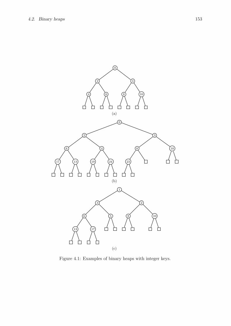
4.2. Binary heaps 153
0
2
4 6
3
8 10
(a)
0
2
6
17 13
4
19 24
3
8
23
10
(b)
1
3
6
13 17
5
2
8 10
(c)
Figure 4.1: Examples of binary heaps with integer keys.
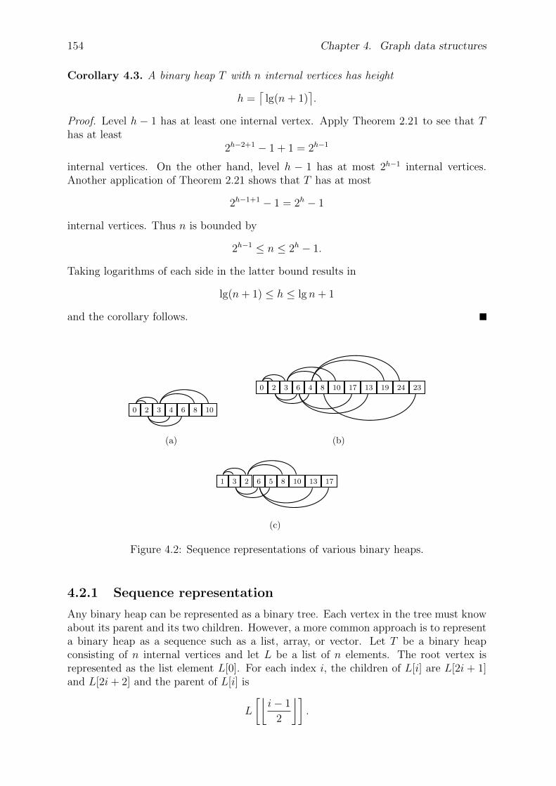
154 Chapter 4. Graph data structures
Corollary 4.3. A binary heap T with n internal vertices has height
h =⌈
lg(n+ 1)⌉.
Proof. Level h − 1 has at least one internal vertex. Apply Theorem 2.21 to see that Thas at least
2h−2+1 − 1 + 1 = 2h−1
internal vertices. On the other hand, level h − 1 has at most 2h−1 internal vertices.Another application of Theorem 2.21 shows that T has at most
2h−1+1 − 1 = 2h − 1
internal vertices. Thus n is bounded by
2h−1 ≤ n ≤ 2h − 1.
Taking logarithms of each side in the latter bound results in
lg(n+ 1) ≤ h ≤ lg n+ 1
and the corollary follows.
0 2 3 4 6 8 10
(a)
0 2 3 6 4 8 10 17 13 19 24 23
(b)
1 3 2 6 5 8 10 13 17
(c)
Figure 4.2: Sequence representations of various binary heaps.
4.2.1 Sequence representation
Any binary heap can be represented as a binary tree. Each vertex in the tree must knowabout its parent and its two children. However, a more common approach is to representa binary heap as a sequence such as a list, array, or vector. Let T be a binary heapconsisting of n internal vertices and let L be a list of n elements. The root vertex isrepresented as the list element L[0]. For each index i, the children of L[i] are L[2i + 1]and L[2i+ 2] and the parent of L[i] is
L
[⌊i− 1
2
⌋].

4.2. Binary heaps 155
With a sequence representation of a binary heap, each vertex needs not know aboutits parent and children. Such information can be obtained via simple arithmetic onsequence indices. For example, the binary heaps in Figure 4.1 can be represented as thecorresponding lists in Figure 4.2. Note that it is not necessary to store the leaves of Tin the sequence representation.
4.2.2 Insertion and sift-up
We now consider the problem of inserting a vertex v into a binary heap T . If T is empty,inserting a vertex simply involves the creation of a new internal vertex. We let thatnew internal vertex be v and let its two children be leaves. The resulting binary heapaugmented with v has exactly one internal vertex and satisfies both the heap-order andheap-structure properties, as shown in Figure 4.3. In other words, any binary heap withone internal vertex trivially satisfies the heap-order property.
(a)
v
(b)
Figure 4.3: Inserting a vertex into an empty binary heap.
Let T now be a nonempty binary heap, i.e. T has at least one internal vertex, andsuppose we want to insert into T an internal vertex v. We must identify the correct leafof T at which to insert v. If the n internal vertices of T are r = v0, v1, . . . , vn−1, then bythe sequence representation of T we can identify the last internal vertex vn−1 in constanttime. The correct leaf at which to insert v is the sequence element immediately followingvn−1, i.e. the element at position n in the sequence representation of T . We replace withv the leaf at position n in the sequence so that v now becomes the last vertex of T .
The binary heap T augmented with the new last vertex v satisfies the heap-structureproperty, but may violate the heap-order property. To ensure that T satisfies the heap-order property, we perform an operation on T called sift-up that involves possibly movingv up through various levels of T . Let κv be the key of v and let κp(v) be the key ofv’s parent. If the relation κp(v) ≤ κv holds, then T satisfies the heap-order property.Otherwise we swap v with its parent, effectively moving v up one level to be at theposition previously occupied by its parent. The parent of v is moved down one leveland now occupies the position where v was previously. With v in its new position, weperform the same key comparison process with v’s new parent. The key comparison andswapping continue until the heap-order property holds for T . In the worst case, v wouldbecome the new root of T after undergoing a number of swaps that is proportional to theheight of T . Therefore, inserting a new internal vertex into T can be achieved in timeO(lg n). Figure 4.4 illustrates the insertion of a new internal vertex into a nonemptybinary heap and the resulting sift-up operation to maintain the heap-order property.Algorithm 4.2 presents pseudocode of our discussion for inserting a new internal vertexinto a nonempty binary heap. The pseudocode is adapted from Howard [103], whichprovides a C implementation of binary heaps.
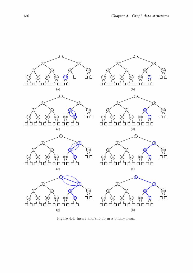
156 Chapter 4. Graph data structures
1
2
6
17 13
4
19 24
3
8
23
10
(a)
1
2
6
17 13
4
19 24
3
8
23 0
10
(b)
1
2
6
17 13
4
19 24
3
8
23 0
10
(c)
1
2
6
17 13
4
19 24
3
0
23 8
10
(d)
1
2
6
17 13
4
19 24
3
0
23 8
10
(e)
1
2
6
17 13
4
19 24
0
3
23 8
10
(f)
1
2
6
17 13
4
19 24
0
3
23 8
10
(g)
0
2
6
17 13
4
19 24
1
3
23 8
10
(h)
Figure 4.4: Insert and sift-up in a binary heap.
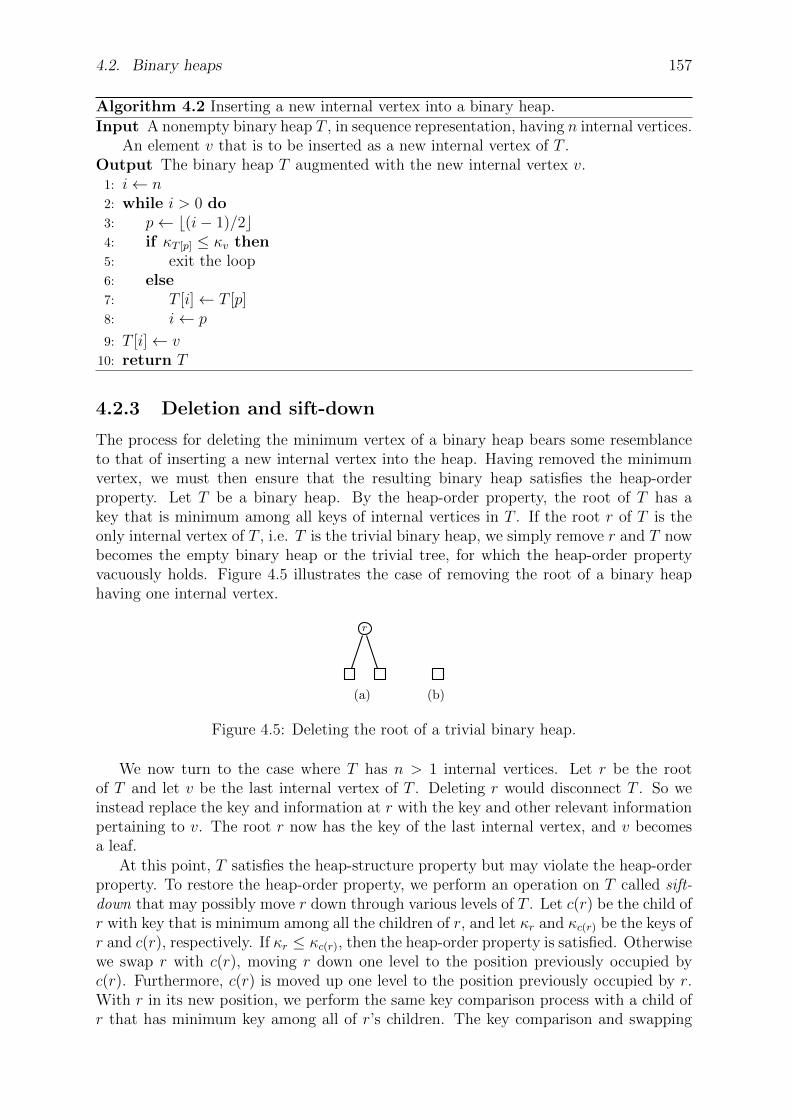
4.2. Binary heaps 157
Algorithm 4.2 Inserting a new internal vertex into a binary heap.
Input A nonempty binary heap T , in sequence representation, having n internal vertices.An element v that is to be inserted as a new internal vertex of T .
Output The binary heap T augmented with the new internal vertex v.1: i← n2: while i > 0 do3: p← b(i− 1)/2c4: if κT [p] ≤ κv then5: exit the loop6: else7: T [i]← T [p]8: i← p
9: T [i]← v10: return T
4.2.3 Deletion and sift-down
The process for deleting the minimum vertex of a binary heap bears some resemblanceto that of inserting a new internal vertex into the heap. Having removed the minimumvertex, we must then ensure that the resulting binary heap satisfies the heap-orderproperty. Let T be a binary heap. By the heap-order property, the root of T has akey that is minimum among all keys of internal vertices in T . If the root r of T is theonly internal vertex of T , i.e. T is the trivial binary heap, we simply remove r and T nowbecomes the empty binary heap or the trivial tree, for which the heap-order propertyvacuously holds. Figure 4.5 illustrates the case of removing the root of a binary heaphaving one internal vertex.
r
(a) (b)
Figure 4.5: Deleting the root of a trivial binary heap.
We now turn to the case where T has n > 1 internal vertices. Let r be the rootof T and let v be the last internal vertex of T . Deleting r would disconnect T . So weinstead replace the key and information at r with the key and other relevant informationpertaining to v. The root r now has the key of the last internal vertex, and v becomesa leaf.
At this point, T satisfies the heap-structure property but may violate the heap-orderproperty. To restore the heap-order property, we perform an operation on T called sift-down that may possibly move r down through various levels of T . Let c(r) be the child ofr with key that is minimum among all the children of r, and let κr and κc(r) be the keys ofr and c(r), respectively. If κr ≤ κc(r), then the heap-order property is satisfied. Otherwisewe swap r with c(r), moving r down one level to the position previously occupied byc(r). Furthermore, c(r) is moved up one level to the position previously occupied by r.With r in its new position, we perform the same key comparison process with a child ofr that has minimum key among all of r’s children. The key comparison and swapping
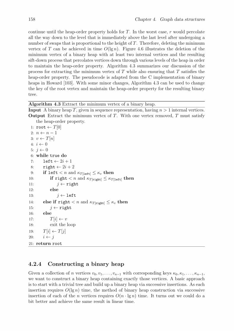
158 Chapter 4. Graph data structures
continue until the heap-order property holds for T . In the worst case, r would percolateall the way down to the level that is immediately above the last level after undergoing anumber of swaps that is proportional to the height of T . Therefore, deleting the minimumvertex of T can be achieved in time O(lg n). Figure 4.6 illustrates the deletion of theminimum vertex of a binary heap with at least two internal vertices and the resultingsift-down process that percolates vertices down through various levels of the heap in orderto maintain the heap-order property. Algorithm 4.3 summarizes our discussion of theprocess for extracting the minimum vertex of T while also ensuring that T satisfies theheap-order property. The pseudocode is adapted from the C implementation of binaryheaps in Howard [103]. With some minor changes, Algorithm 4.3 can be used to changethe key of the root vertex and maintain the heap-order property for the resulting binarytree.
Algorithm 4.3 Extract the minimum vertex of a binary heap.
Input A binary heap T , given in sequence representation, having n > 1 internal vertices.Output Extract the minimum vertex of T . With one vertex removed, T must satisfy
the heap-order property.1: root← T [0]2: n← n− 13: v ← T [n]4: i← 05: j ← 06: while true do7: left← 2i+ 18: right← 2i+ 29: if left < n and κT [left] ≤ κv then
10: if right < n and κT [right] ≤ κT [left] then11: j ← right
12: else13: j ← left
14: else if right < n and κT [right] ≤ κv then15: j ← right
16: else17: T [i]← v18: exit the loop
19: T [i]← T [j]20: i← j
21: return root
4.2.4 Constructing a binary heap
Given a collection of n vertices v0, v1, . . . , vn−1 with corresponding keys κ0, κ1, . . . , κn−1,we want to construct a binary heap containing exactly those vertices. A basic approachis to start with a trivial tree and build up a binary heap via successive insertions. As eachinsertion requires O(lg n) time, the method of binary heap construction via successiveinsertion of each of the n vertices requires O(n · lg n) time. It turns out we could do abit better and achieve the same result in linear time.
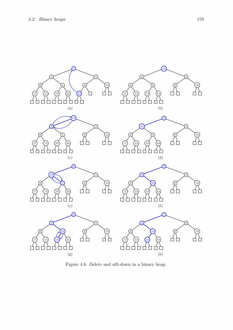
4.2. Binary heaps 159
1
2
6
17 13
4
19 24
3
8
23
10
(a)
23
2
6
17 13
4
19 24
3
8 10
(b)
23
2
6
17 13
4
19 24
3
8 10
(c)
2
23
6
17 13
4
19 24
3
8 10
(d)
2
23
6
17 13
4
19 24
3
8 10
(e)
2
4
6
17 13
23
19 24
3
8 10
(f)
2
4
6
17 13
23
19 24
3
8 10
(g)
2
4
6
17 13
19
23 24
3
8 10
(h)
Figure 4.6: Delete and sift-down in a binary heap.
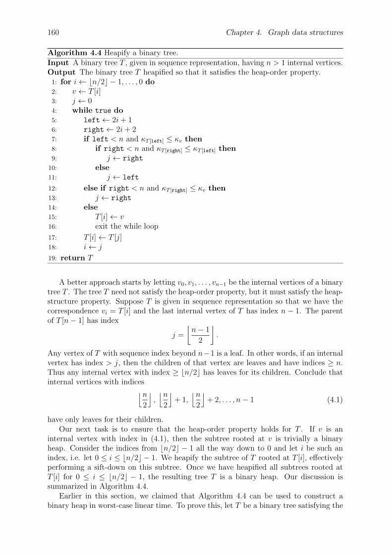
160 Chapter 4. Graph data structures
Algorithm 4.4 Heapify a binary tree.
Input A binary tree T , given in sequence representation, having n > 1 internal vertices.Output The binary tree T heapified so that it satisfies the heap-order property.
1: for i← bn/2c − 1, . . . , 0 do2: v ← T [i]3: j ← 04: while true do5: left← 2i+ 16: right← 2i+ 27: if left < n and κT [left] ≤ κv then8: if right < n and κT [right] ≤ κT [left] then9: j ← right
10: else11: j ← left
12: else if right < n and κT [right] ≤ κv then13: j ← right
14: else15: T [i]← v16: exit the while loop
17: T [i]← T [j]18: i← j
19: return T
A better approach starts by letting v0, v1, . . . , vn−1 be the internal vertices of a binarytree T . The tree T need not satisfy the heap-order property, but it must satisfy the heap-structure property. Suppose T is given in sequence representation so that we have thecorrespondence vi = T [i] and the last internal vertex of T has index n − 1. The parentof T [n− 1] has index
j =
⌊n− 1
2
⌋.
Any vertex of T with sequence index beyond n−1 is a leaf. In other words, if an internalvertex has index > j, then the children of that vertex are leaves and have indices ≥ n.Thus any internal vertex with index ≥ bn/2c has leaves for its children. Conclude thatinternal vertices with indices
⌊n2
⌋,⌊n
2
⌋+ 1,
⌊n2
⌋+ 2, . . . , n− 1 (4.1)
have only leaves for their children.Our next task is to ensure that the heap-order property holds for T . If v is an
internal vertex with index in (4.1), then the subtree rooted at v is trivially a binaryheap. Consider the indices from bn/2c − 1 all the way down to 0 and let i be such anindex, i.e. let 0 ≤ i ≤ bn/2c − 1. We heapify the subtree of T rooted at T [i], effectivelyperforming a sift-down on this subtree. Once we have heapified all subtrees rooted atT [i] for 0 ≤ i ≤ bn/2c − 1, the resulting tree T is a binary heap. Our discussion issummarized in Algorithm 4.4.
Earlier in this section, we claimed that Algorithm 4.4 can be used to construct abinary heap in worst-case linear time. To prove this, let T be a binary tree satisfying the
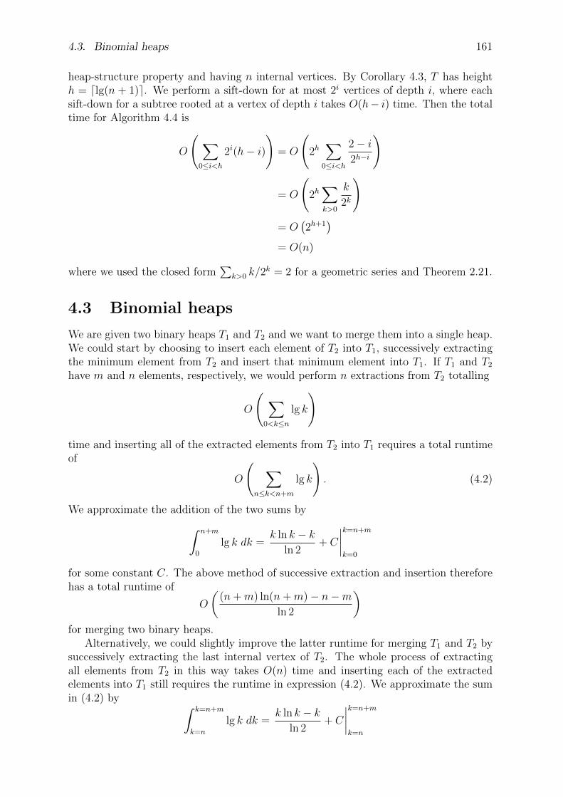
4.3. Binomial heaps 161
heap-structure property and having n internal vertices. By Corollary 4.3, T has heighth = dlg(n + 1)e. We perform a sift-down for at most 2i vertices of depth i, where eachsift-down for a subtree rooted at a vertex of depth i takes O(h− i) time. Then the totaltime for Algorithm 4.4 is
O
(∑
0≤i<h
2i(h− i))
= O
(2h∑
0≤i<h
2− i2h−i
)
= O
(2h∑
k>0
k
2k
)
= O(2h+1
)
= O(n)
where we used the closed form∑
k>0 k/2k = 2 for a geometric series and Theorem 2.21.
4.3 Binomial heaps
We are given two binary heaps T1 and T2 and we want to merge them into a single heap.We could start by choosing to insert each element of T2 into T1, successively extractingthe minimum element from T2 and insert that minimum element into T1. If T1 and T2
have m and n elements, respectively, we would perform n extractions from T2 totalling
O
( ∑
0<k≤n
lg k
)
time and inserting all of the extracted elements from T2 into T1 requires a total runtimeof
O
( ∑
n≤k<n+m
lg k
). (4.2)
We approximate the addition of the two sums by
∫ n+m
0
lg k dk =k ln k − k
ln 2+ C
∣∣∣∣k=n+m
k=0
for some constant C. The above method of successive extraction and insertion thereforehas a total runtime of
O
((n+m) ln(n+m)− n−m
ln 2
)
for merging two binary heaps.Alternatively, we could slightly improve the latter runtime for merging T1 and T2 by
successively extracting the last internal vertex of T2. The whole process of extractingall elements from T2 in this way takes O(n) time and inserting each of the extractedelements into T1 still requires the runtime in expression (4.2). We approximate the sumin (4.2) by ∫ k=n+m
k=n
lg k dk =k ln k − k
ln 2+ C
∣∣∣∣k=n+m
k=n

162 Chapter 4. Graph data structures
for some constant C. Therefore the improved extraction and insertion method requires
O
((n+m) ln(n+m)− n lnn−m
ln 2− n
)
time in order to merge T1 and T2.Can we improve on the latter runtime for merging two binary heaps? It turns out we
can by using a type of mergeable heap called binomial heap that supports merging twoheaps in logarithmic time.
4.3.1 Binomial trees
A binomial heap can be considered as a collection of binomial trees. The binomial treeof order k is denoted Bk and defined recursively as follows:
1. The binomial tree of order 0 is the trivial tree.
2. The binomial tree of order k > 0 is a rooted tree, where from left to right thechildren of the root of Bk are roots of Bk−1, Bk−2, . . . , B0.
Various examples of binomial trees are shown in Figure 4.7. The binomial tree Bk canalso be defined as follows. Let T1 and T2 be two copies of Bk−1 with root vertices r1
and r2, respectively. Then Bk is obtained by letting, say, r1 be the left-most child of r2.Lemma 4.4 lists various basic properties of binomial trees. Property (3) of Lemma 4.4uses the binomial coefficient, from whence Bk derives its name.
Lemma 4.4. Basic properties of binomial trees. Let Bk be a binomial tree oforder k ≥ 0. Then the following properties hold:
1. The order of Bk is 2k.
2. The height of Bk is k.
3. For 0 ≤ i ≤ k, we have(ki
)vertices at depth i.
4. The root of Bk is the only vertex with maximum degree ∆(Bk) = k. If the childrenof the root are numbered k − 1, k − 2, . . . , 0 from left to right, then child i is theroot of the subtree Bi.
Proof. We use induction on k. The base case for each of the above properties is B0,which trivially holds.
(1) By our inductive hypothesis, Bk−1 has order 2k−1. Since Bk is comprised of twocopies of Bk−1, conclude that Bk has order
2k−1 + 2k−1 = 2k.
(2) The binomial tree Bk is comprised of two copies of Bk−1, the root of one copybeing the left-most child of the root of the other copy. Then the height of Bk is onegreater than the height of Bk−1. By our inductive hypothesis, Bk−1 has height k− 1 andtherefore Bk has height (k − 1) + 1 = k.

4.3. Binomial heaps 163
(a) B0 (b) B1 (c) B2 (d) B3
(e) B4
(f) B5
Figure 4.7: Binomial trees Bk for k = 0, 1, 2, 3, 4, 5.

164 Chapter 4. Graph data structures
(3) Denote by D(k, i) the number of vertices of depth i in Bk. As Bk is comprisedof two copies of Bk−1, a vertex at depth i in Bk−1 appears once in Bk at depth i and asecond time at depth i+ 1. By our inductive hypothesis,
D(k, i) = D(k − 1, i) +D(k − 1, i− 1)
=
(k − 1
i
)+
(k − 1
i− 1
)
=
(k
i
)
where we used Pascal’s formula which states that(n+ 1
r
)=
(n
r − 1
)+
(n
r
)
for any positive integers n and r with r ≤ n.(4) This property follows from the definition of Bk.
Corollary 4.5. If a binomial tree has order n ≥ 0, then the degree of any vertex i isbounded by deg(i) ≤ lg n.
Proof. Apply properties (1) and (4) of Lemma 4.4.
4.3.2 Binomial heaps
In 1978, Jean Vuillemin [188] introduced binomial heaps as a data structure for im-plementing priority queues. Mark R. Brown [41, 42] subsequently extended Vuillemin’swork, providing detailed analysis of binomial heaps and introducing an efficient imple-mentation.
A binomial heap H can be considered as a collection of binomial trees. Each vertexin H has a corresponding key and all vertex keys of H belong to a totally ordered sethaving total order ≤. The heap also satisfies the following binomial heap properties :
Heap-order property. Let Bk be a binomial tree in H. If v is a vertex of Bk
other than the root and p is the parent of v and having corresponding keys κv andκp, respectively, then κp ≤ κv.
Root-degree property. For any integer k ≥ 0, H contains at most one binomialtree whose root has degree k.
If H is comprised of the binomial trees Bk0 , Bk1 , . . . , Bkn for nonnegative integers ki,we can consider H as a forest made up of the trees Bki . We can also represent H as a treein the following way. List the binomial trees of H as Bk0 , Bk1 , . . . , Bkn in nondecreasingorder of root degrees, i.e. the root of Bki has order less than or equal to the root of Bkj
if and only if ki ≤ kj. The root of H is the root of Bk0 and the root of each Bki hasfor its child the root of Bki+1
. Both the forest and tree representations are illustrated inFigure 4.8 for the binomial heap comprised of the binomial trees B0, B1, B3.
The heap-order property for binomial heaps is analogous to the heap-order propertyfor binary heaps. In the case of binomial heaps, the heap-order property implies thatthe root of a binomial tree has a key that is minimum among all vertices in that tree.
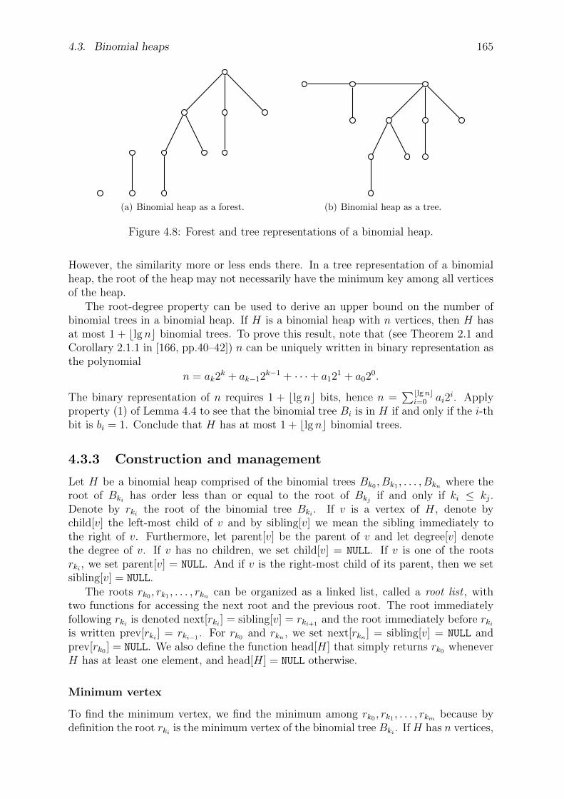
4.3. Binomial heaps 165
(a) Binomial heap as a forest. (b) Binomial heap as a tree.
Figure 4.8: Forest and tree representations of a binomial heap.
However, the similarity more or less ends there. In a tree representation of a binomialheap, the root of the heap may not necessarily have the minimum key among all verticesof the heap.
The root-degree property can be used to derive an upper bound on the number ofbinomial trees in a binomial heap. If H is a binomial heap with n vertices, then H hasat most 1 + blg nc binomial trees. To prove this result, note that (see Theorem 2.1 andCorollary 2.1.1 in [166, pp.40–42]) n can be uniquely written in binary representation asthe polynomial
n = ak2k + ak−12k−1 + · · ·+ a121 + a020.
The binary representation of n requires 1 + blg nc bits, hence n =∑blgnc
i=0 ai2i. Apply
property (1) of Lemma 4.4 to see that the binomial tree Bi is in H if and only if the i-thbit is bi = 1. Conclude that H has at most 1 + blg nc binomial trees.
4.3.3 Construction and management
Let H be a binomial heap comprised of the binomial trees Bk0 , Bk1 , . . . , Bkn where theroot of Bki has order less than or equal to the root of Bkj if and only if ki ≤ kj.Denote by rki the root of the binomial tree Bki . If v is a vertex of H, denote bychild[v] the left-most child of v and by sibling[v] we mean the sibling immediately tothe right of v. Furthermore, let parent[v] be the parent of v and let degree[v] denotethe degree of v. If v has no children, we set child[v] = NULL. If v is one of the rootsrki , we set parent[v] = NULL. And if v is the right-most child of its parent, then we setsibling[v] = NULL.
The roots rk0 , rk1 , . . . , rkn can be organized as a linked list, called a root list , withtwo functions for accessing the next root and the previous root. The root immediatelyfollowing rki is denoted next[rki ] = sibling[v] = rki+1
and the root immediately before rkiis written prev[rki ] = rki−1
. For rk0 and rkn , we set next[rkn ] = sibling[v] = NULL andprev[rk0 ] = NULL. We also define the function head[H] that simply returns rk0 wheneverH has at least one element, and head[H] = NULL otherwise.
Minimum vertex
To find the minimum vertex, we find the minimum among rk0 , rk1 , . . . , rkm because bydefinition the root rki is the minimum vertex of the binomial tree Bki . If H has n vertices,
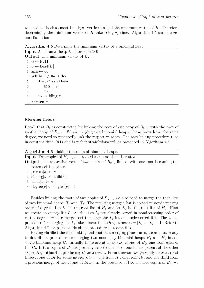
166 Chapter 4. Graph data structures
we need to check at most 1 + blg nc vertices to find the minimum vertex of H. Thereforedetermining the minimum vertex of H takes O(lg n) time. Algorithm 4.5 summarizesour discussion.
Algorithm 4.5 Determine the minimum vertex of a binomial heap.
Input A binomial heap H of order n > 0.Output The minimum vertex of H.
1: u← Null
2: v ← head[H]3: min←∞4: while v 6= Null do5: if κv < min then6: min← κv7: u← v8: v ← sibling[v]
9: return u
Merging heaps
Recall that Bk is constructed by linking the root of one copy of Bk−1 with the root ofanother copy of Bk−1. When merging two binomial heaps whose roots have the samedegree, we need to repeatedly link the respective roots. The root linking procedure runsin constant time O(1) and is rather straightforward, as presented in Algorithm 4.6.
Algorithm 4.6 Linking the roots of binomial heaps.
Input Two copies of Bk−1, one rooted at u and the other at v.Output The respective roots of two copies of Bk−1 linked, with one root becoming the
parent of the other.1: parent[u]← v2: sibling[u]← child[v]3: child[v]← u4: degree[v]← degree[v] + 1
Besides linking the roots of two copies of Bk−1, we also need to merge the root listsof two binomial heaps H1 and H2. The resulting merged list is sorted in nondecreasingorder of degree. Let L1 be the root list of H1 and let L2 be the root list of H2. Firstwe create an empty list L. As the lists Li are already sorted in nondecreasing order ofvertex degree, we use merge sort to merge the Li into a single sorted list. The wholeprocedure for merging the Li takes linear time O(n), where n = |L1|+ |L2| − 1. Refer toAlgorithm 4.7 for pseudocode of the procedure just described.
Having clarified the root linking and root lists merging procedures, we are now readyto describe a procedure for merging two nonempty binomial heaps H1 and H2 into asingle binomial heap H. Initially there are at most two copies of B0, one from each ofthe Hi. If two copies of B0 are present, we let the root of one be the parent of the otheras per Algorithm 4.6, producing B1 as a result. From thereon, we generally have at mostthree copies of Bk for some integer k > 0: one from H1, one from H2, and the third froma previous merge of two copies of Bk−1. In the presence of two or more copies of Bk, we

4.3. Binomial heaps 167
Algorithm 4.7 Merging two root lists.
Input Two root lists L1 and L2, each containing the roots of binomial trees in thebinomial heaps H1 and H2, respectively. Each root list Li is sorted in increasingorder of vertex degree.
Output A single list L that merges the root lists Li and sorted in nondecreasing orderof degree.
1: i← 12: j ← 13: L← [ ]4: n← |L1|+ |L2| − 15: append(L1, ∞)6: append(L2, ∞)7: for k ← 0, 1, . . . , n do8: if deg(L1[i]) ≤ deg(L2[j]) then9: append(L, L1[i])
10: i← i+ 111: else12: append(L, L2[j])13: j ← j + 1
14: return L
merge two copies as per Algorithm 4.6 to produce Bk+1. If Hi has ni vertices, then Hi
has at most 1 + blg nic binomial trees, from which it is clear that merging H1 and H2
requiresmax(1 + blg n1c, 1 + blg n2c)
steps. Letting N = max(n1, n2), we see that merging H1 and H2 takes logarithmic timeO(lgN). The operation of merging two binomial heaps is presented in pseudocode asAlgorithm 4.8, which is adapted from Cormen et al. [57, p.463] and the C implementationof binomial queues in [103]. A word of warning is order here. Algorithm 4.8 is destructivein the sense that it modifies the input heaps Hi in-place without making copies of thoseheaps.
Vertex insertion
Let v be a vertex with corresponding key κv and let H1 be a binomial heap of n vertices.The single vertex v can be considered as a binomial heap H2 comprised of exactly thebinomial tree B0. Then inserting v into H1 is equivalent to merging the heaps Hi andcan be accomplished in O(lg n) time. Refer to Algorithm 4.9 for pseudocode of thisstraightforward procedure.
Delete minimum vertex
Extracting the minimum vertex from a binomial heap H consists of several phases.Let H be comprised of the binomial trees Bk0 , Bk1 , . . . , Bkm with corresponding rootsrk0 , rk1 , . . . , rkm and let n be the number of vertices in H. In the first phase, from amongthe rki we identify the root v with minimum key and remove v from H, an operationthat runs in O(lg n) time because we need to process at most 1 + blg nc roots. With thebinomial tree Bk rooted at v thus severed from H, we now have a forest consisting of the

168 Chapter 4. Graph data structures
Algorithm 4.8 Merging two binomial heaps.
Input Two binomial heaps H1 and H2.Output A binomial heap H that results from merging the Hi.
1: H ← empty binomial heap2: head[H]← merge sort the root lists of H1 and H2
3: if head[H] = Null then4: return H5: prevv← Null
6: v ← head[H]7: nextv← sibling[v]8: while nextv 6= Null do9: if degree[v] 6= degree[nextv] or (sibling[nextv] 6= Null and
degree[sibling[nextv]] = degree[v]) then10: prevv← v11: v ← nextv
12: else if κv ≤ κnextv then13: sibling[v]← sibling[nextv]14: link the roots nextv and v as per Algorithm ??15: else16: if prevv = Null then17: head[H]← nextv
18: else19: sibling[prevv]← nextv
20: link the roots v and nextv as per Algorithm ??21: v ← nextv
22: nextv← sibling[v]
23: return H
Algorithm 4.9 Insert a vertex into a binomial heap.
Input A binomial heap H and a vertex v.Output The heap H with v inserted into it.
1: H1 ← empty binomial heap2: head[H1]← v3: parent[v]← Null
4: child[v]← Null
5: sibling[v]← Null
6: degree[v]← 07: H ← merge H and H1 as per Algorithm ??
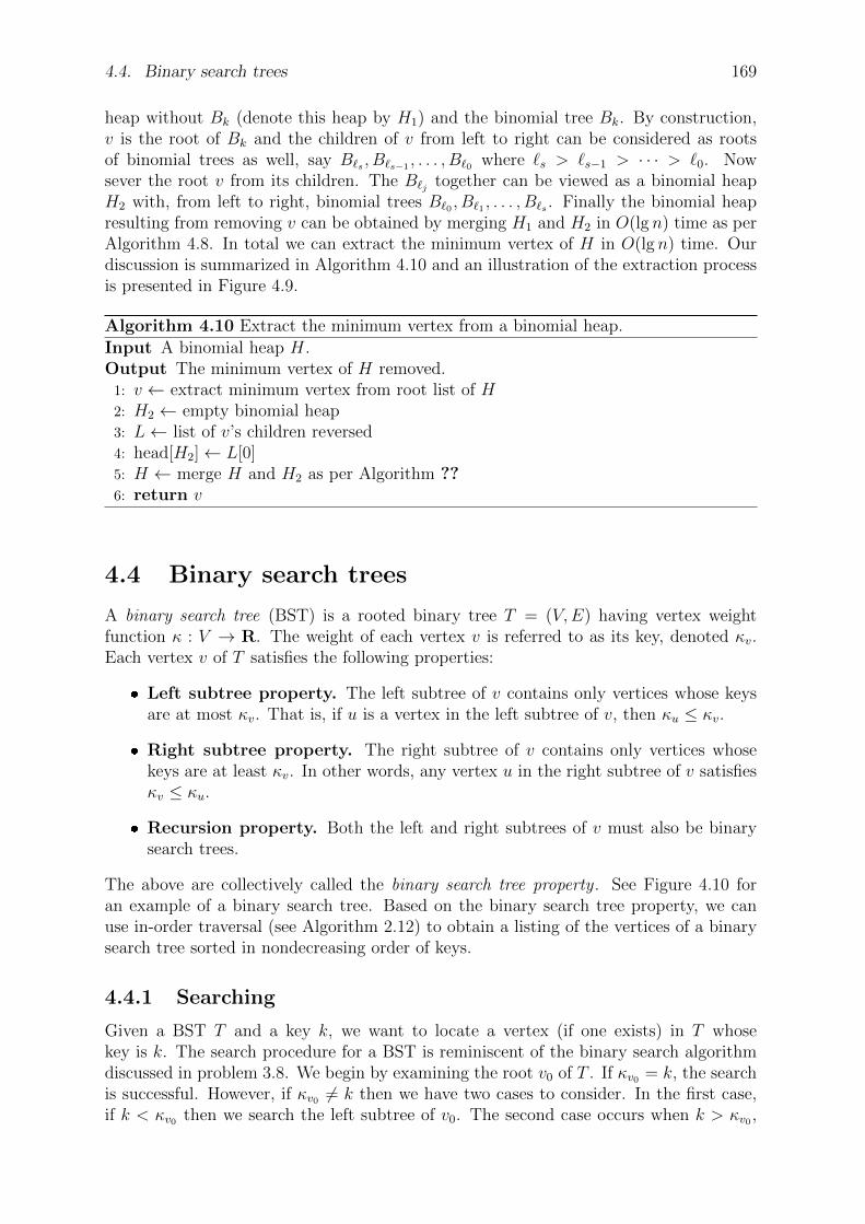
4.4. Binary search trees 169
heap without Bk (denote this heap by H1) and the binomial tree Bk. By construction,v is the root of Bk and the children of v from left to right can be considered as rootsof binomial trees as well, say B`s , B`s−1 , . . . , B`0 where `s > `s−1 > · · · > `0. Nowsever the root v from its children. The B`j together can be viewed as a binomial heapH2 with, from left to right, binomial trees B`0 , B`1 , . . . , B`s . Finally the binomial heapresulting from removing v can be obtained by merging H1 and H2 in O(lg n) time as perAlgorithm 4.8. In total we can extract the minimum vertex of H in O(lg n) time. Ourdiscussion is summarized in Algorithm 4.10 and an illustration of the extraction processis presented in Figure 4.9.
Algorithm 4.10 Extract the minimum vertex from a binomial heap.
Input A binomial heap H.Output The minimum vertex of H removed.
1: v ← extract minimum vertex from root list of H2: H2 ← empty binomial heap3: L← list of v’s children reversed4: head[H2]← L[0]5: H ← merge H and H2 as per Algorithm ??6: return v
4.4 Binary search trees
A binary search tree (BST) is a rooted binary tree T = (V,E) having vertex weightfunction κ : V → R. The weight of each vertex v is referred to as its key, denoted κv.Each vertex v of T satisfies the following properties:
Left subtree property. The left subtree of v contains only vertices whose keysare at most κv. That is, if u is a vertex in the left subtree of v, then κu ≤ κv.
Right subtree property. The right subtree of v contains only vertices whosekeys are at least κv. In other words, any vertex u in the right subtree of v satisfiesκv ≤ κu.
Recursion property. Both the left and right subtrees of v must also be binarysearch trees.
The above are collectively called the binary search tree property . See Figure 4.10 foran example of a binary search tree. Based on the binary search tree property, we canuse in-order traversal (see Algorithm 2.12) to obtain a listing of the vertices of a binarysearch tree sorted in nondecreasing order of keys.
4.4.1 Searching
Given a BST T and a key k, we want to locate a vertex (if one exists) in T whosekey is k. The search procedure for a BST is reminiscent of the binary search algorithmdiscussed in problem 3.8. We begin by examining the root v0 of T . If κv0 = k, the searchis successful. However, if κv0 6= k then we have two cases to consider. In the first case,if k < κv0 then we search the left subtree of v0. The second case occurs when k > κv0 ,
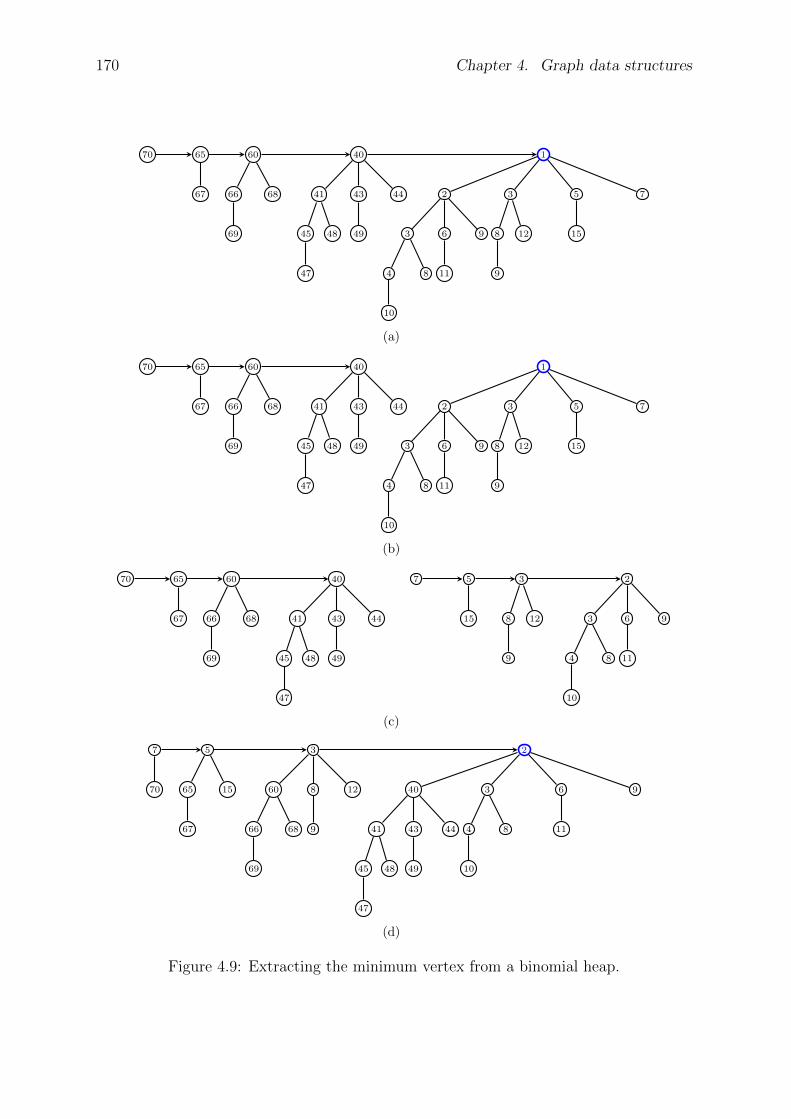
170 Chapter 4. Graph data structures
70 65
67
60
66
69
68
40
41
45
47
48
43
49
44
1
2
3
4
10
8
6
11
9
3
8
9
12
5
15
7
(a)
70 65
67
60
66
69
68
40
41
45
47
48
43
49
44
1
2
3
4
10
8
6
11
9
3
8
9
12
5
15
7
(b)
70 65
67
60
66
69
68
40
41
45
47
48
43
49
44
7 5
15
3
8
9
12
2
3
4
10
8
6
11
9
(c)
7
70
5
65
67
15
3
60
66
69
68
8
9
12
2
40
41
45
47
48
43
49
44
3
4
10
8
6
11
9
(d)
Figure 4.9: Extracting the minimum vertex from a binomial heap.

4.4. Binary search trees 171
10
5
4
3 5
7
5 8
15
13
11
20
Figure 4.10: A binary search tree.
in which case we search the right subtree of v0. Repeat the process until a vertex v inT is found for which k = κv or the indicated subtree is empty. Whenever the target keyis different from the key of the vertex we are currently considering, we move down onelevel of T . Thus if h is the height of T , it follows that searching T takes a worst-caseruntime of O(h). The above procedure is presented in pseudocode as Algorithm 4.11.Note that if a vertex v does not have a left subtree, the operation of locating the rootof v’s left subtree should return NULL. A similar comment applies when v does not havea right subtree. Furthermore, from the structure of Algorithm 4.11, if the input BST isempty then NULL is returned. See Figure 4.11 for an illustration of locating vertices withgiven keys in a BST.
Algorithm 4.11 Locate a key in a binary search tree.
Input A binary search tree T and a target key k.Output A vertex in T with key k. If no such vertex exists, return Null.
1: v ← root[T ]2: while v 6= Null and k 6= κv do3: if k < κv then4: v ← leftchild[v]5: else6: v ← rightchild[v]
7: return v
10
5
4
3
2 3
5
7
5 8
9
15
13
11
20
19 23
22 26
(a) Vertex with key 6: search fail.
10
5
4
3
2 3
5
7
5 8
9
15
13
11
20
19 23
22 26
(b) Vertex with key 22: search success.
Figure 4.11: Finding vertices with given keys in a BST.
From the binary search tree property, deduce that a vertex of a BST T with minimumkey can be found by starting from the root of T and repeatedly traversing left subtrees.
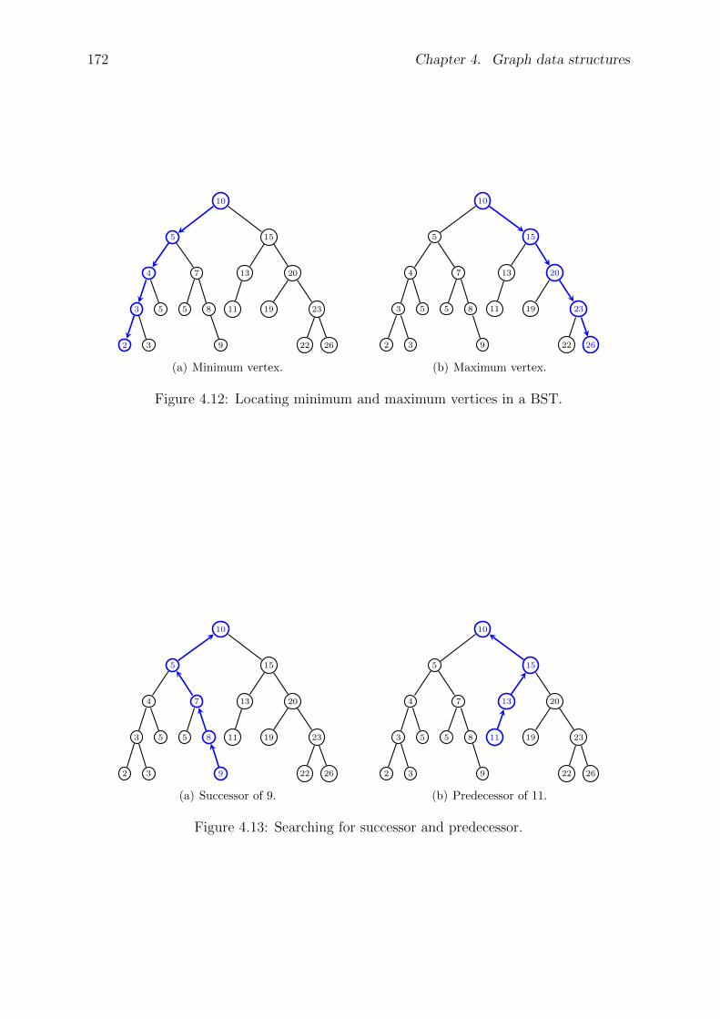
172 Chapter 4. Graph data structures
10
5
4
3
2 3
5
7
5 8
9
15
13
11
20
19 23
22 26
(a) Minimum vertex.
10
5
4
3
2 3
5
7
5 8
9
15
13
11
20
19 23
22 26
(b) Maximum vertex.
Figure 4.12: Locating minimum and maximum vertices in a BST.
10
5
4
3
2 3
5
7
5 8
9
15
13
11
20
19 23
22 26
(a) Successor of 9.
10
5
4
3
2 3
5
7
5 8
9
15
13
11
20
19 23
22 26
(b) Predecessor of 11.
Figure 4.13: Searching for successor and predecessor.
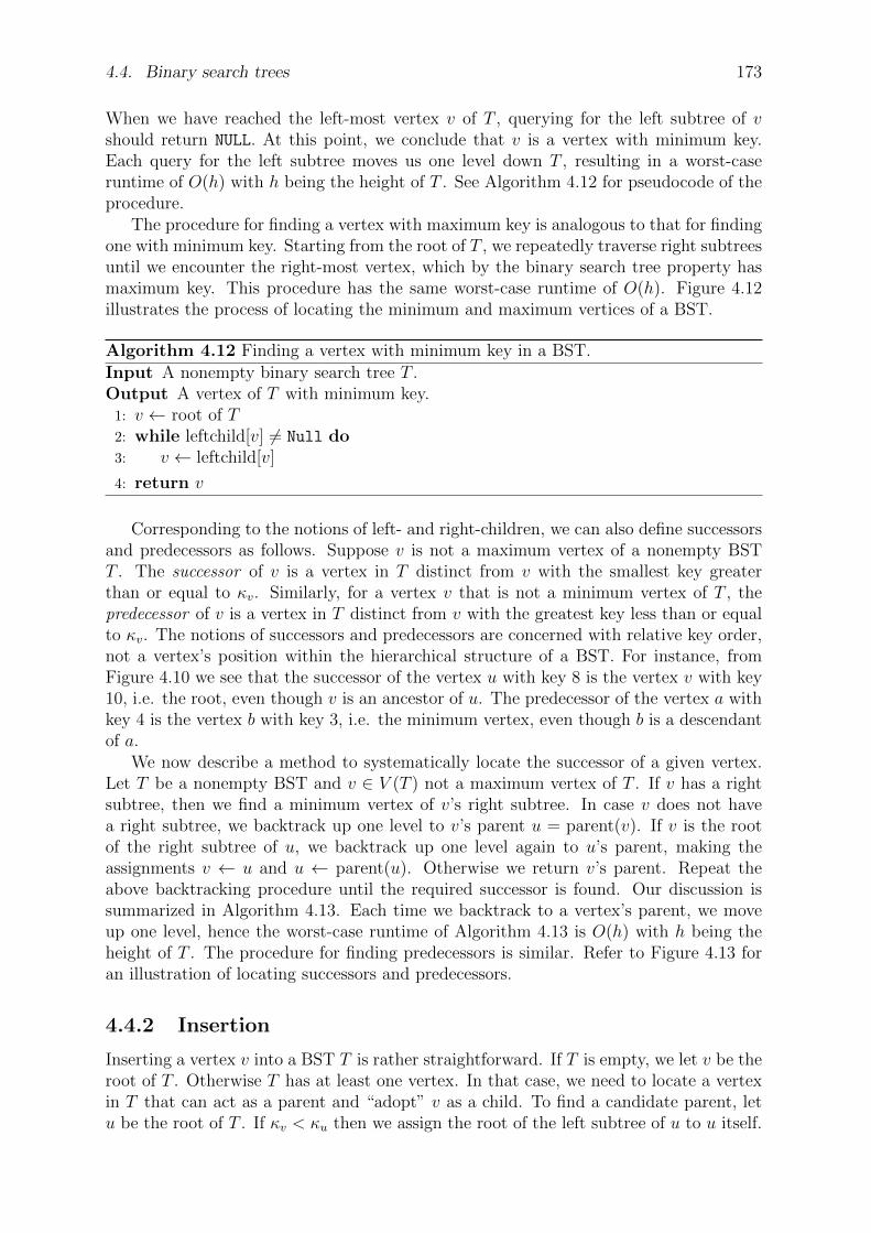
4.4. Binary search trees 173
When we have reached the left-most vertex v of T , querying for the left subtree of vshould return NULL. At this point, we conclude that v is a vertex with minimum key.Each query for the left subtree moves us one level down T , resulting in a worst-caseruntime of O(h) with h being the height of T . See Algorithm 4.12 for pseudocode of theprocedure.
The procedure for finding a vertex with maximum key is analogous to that for findingone with minimum key. Starting from the root of T , we repeatedly traverse right subtreesuntil we encounter the right-most vertex, which by the binary search tree property hasmaximum key. This procedure has the same worst-case runtime of O(h). Figure 4.12illustrates the process of locating the minimum and maximum vertices of a BST.
Algorithm 4.12 Finding a vertex with minimum key in a BST.
Input A nonempty binary search tree T .Output A vertex of T with minimum key.
1: v ← root of T2: while leftchild[v] 6= Null do3: v ← leftchild[v]
4: return v
Corresponding to the notions of left- and right-children, we can also define successorsand predecessors as follows. Suppose v is not a maximum vertex of a nonempty BSTT . The successor of v is a vertex in T distinct from v with the smallest key greaterthan or equal to κv. Similarly, for a vertex v that is not a minimum vertex of T , thepredecessor of v is a vertex in T distinct from v with the greatest key less than or equalto κv. The notions of successors and predecessors are concerned with relative key order,not a vertex’s position within the hierarchical structure of a BST. For instance, fromFigure 4.10 we see that the successor of the vertex u with key 8 is the vertex v with key10, i.e. the root, even though v is an ancestor of u. The predecessor of the vertex a withkey 4 is the vertex b with key 3, i.e. the minimum vertex, even though b is a descendantof a.
We now describe a method to systematically locate the successor of a given vertex.Let T be a nonempty BST and v ∈ V (T ) not a maximum vertex of T . If v has a rightsubtree, then we find a minimum vertex of v’s right subtree. In case v does not havea right subtree, we backtrack up one level to v’s parent u = parent(v). If v is the rootof the right subtree of u, we backtrack up one level again to u’s parent, making theassignments v ← u and u ← parent(u). Otherwise we return v’s parent. Repeat theabove backtracking procedure until the required successor is found. Our discussion issummarized in Algorithm 4.13. Each time we backtrack to a vertex’s parent, we moveup one level, hence the worst-case runtime of Algorithm 4.13 is O(h) with h being theheight of T . The procedure for finding predecessors is similar. Refer to Figure 4.13 foran illustration of locating successors and predecessors.
4.4.2 Insertion
Inserting a vertex v into a BST T is rather straightforward. If T is empty, we let v be theroot of T . Otherwise T has at least one vertex. In that case, we need to locate a vertexin T that can act as a parent and “adopt” v as a child. To find a candidate parent, letu be the root of T . If κv < κu then we assign the root of the left subtree of u to u itself.

174 Chapter 4. Graph data structures
Algorithm 4.13 Finding successors in a binary search tree.
Input A nonempty binary search tree T and a vertex v that is not a maximum of T .Output The successor of v.
1: if rightchild[v] 6= Null then2: return minimum vertex of v’s right subtree as per Algorithm ??
3: u← parent(v)4: while u 6= Null and v = rightchild[u] do5: v ← u6: u← parent(u)
7: return u
Otherwise we assign the root of the right subtree of u to u. We then carry on the abovekey comparison process until the operation of locating the root of a left or right subtreereturns NULL. At this point, a candidate parent for v is the last non-NULL value of u. Ifκv < κu then we let v be u’s left-child. Otherwise v is the right-child of u. After each keycomparison, we move down at most one level so that in the worst-case inserting a vertexinto T takes O(h) time, where h is the height of T . Algorithm 4.14 presents pseudocodeof our discussion and Figure 4.14 illustrates how to insert a vertex into a BST.
Algorithm 4.14 Inserting a vertex into a binary search tree.
Input A binary search tree T and a vertex x to be inserted into T .Output The same BST T but augmeneted with x.
1: u← Null
2: v ← root of T3: while v 6= Null do4: u← v5: if κx < κv then6: v ← leftchild[v]7: else8: v ← rightchild[v]
9: parent[x]← u10: if u = Null then11: root[T ]← x12: else13: if κx < κu then14: leftchild[u]← x15: else16: rightchild[u]← x
4.4.3 Deletion
Whereas insertion into a BST is straightforward, removing a vertex requires much morework. Let T be a nonempty binary search tree and suppose we want to remove v ∈ V (T )from T . Having located the position that v occupies within T , we need to consider threeseparate cases: (1) v is a leaf; (2) v has one child; (3) v has two children.
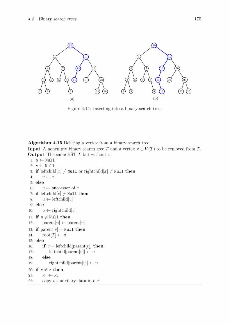
4.4. Binary search trees 175
10
5
4
3
2 3
5
7
5 8
9
15
13
11
20
19 23
22 26
(a)
10
5
4
3
2 3
5
7
5 8
9
15
13
11
12
20
19 23
22 26
(b)
Figure 4.14: Inserting into a binary search tree.
Algorithm 4.15 Deleting a vertex from a binary search tree.
Input A nonempty binary search tree T and a vertex x ∈ V (T ) to be removed from T .Output The same BST T but without x.
1: u← Null
2: v ← Null
3: if leftchild[x] 6= Null or rightchild[x] 6= Null then4: v ← x5: else6: v ← successor of x7: if leftchild[v] 6= Null then8: u← leftchild[v]9: else
10: u← rightchild[v]
11: if u 6= Null then12: parent[u]← parent[v]
13: if parent[v] = Null then14: root[T ]← u15: else16: if v = leftchild[parent[v]] then17: leftchild[parent[v]]← u18: else19: rightchild[parent[v]]← u
20: if v 6= x then21: κx ← κv22: copy v’s auxilary data into x

176 Chapter 4. Graph data structures
1. If v is a leaf, we simply remove v from T and the procedure is complete. Theresulting tree without v satisfies the binary search tree property.
2. Suppose v has the single child u. Removing v would disconnect T , a situation thatcan be prevented by splicing out u and letting u occupy the position previouslyheld by v. The resulting tree with v removed as described satisfies the binarysearch tree property.
3. Finally suppose v has two children and let s and p be the successor and predecessorof v, respectively. It can be shown that s has no left-child and p has no right-child.We can choose to either splice out s or p. Say we choose to splice out s. Then weremove v and let s hold the position previously occupied by v. The resulting treewith v thus removed satisfies the binary search tree property.
The above procedure is summarized in Algorithm 4.15, which is adapted from [57, p.262].Figure 4.15 illustrates the various cases to be considered when removing a vertex froma BST. Note that in Algorithm 4.15, the process of finding the successor dominates theruntime of the entire algorithm. Other operations in the algorithm take at most constanttime. Therefore deleting a vertex from a binary search tree can be accomplished in worst-case O(h) time, where h is the height of the BST under consideration.
4.5 Problems
No problem is so formidable that you can’t walk away from it.— Charles M. Schulz
4.1. Let Q be a priority queue of n > 1 elements, given in sequence representation.From section 4.1.1, we know that inserting an element into Q takes O(n) time anddeleting an element from Q takes O(1) time.
(a) Suppose Q is an empty priority queue and let e0, e1, . . . , en be n+ 1 elementswe want to insert into Q. What is the total runtime required to insert all theei into Q while also ensuring that the resulting queue is a priority queue?
(b) Let Q = [e0, e1, . . . , en] be a priority queue of n + 1 elements. What is thetotal time required to remove all the elements of Q?
4.2. Prove the correctness of Algorithms 4.2 and 4.3.
4.3. Describe a variant of Algorithm 4.3 for modifying the key of the root of a binaryheap, without extracting any vertex from the heap.
4.4. Section 4.2.2 describes how to insert an element into a binary heap T . The generalstrategy is to choose the first leaf following the last internal vertex of T , replacethat leaf with the new element so that it becomes an internal vertex, and perform asift-up operation from there. If instead we choose any leaf of T and replace that leafwith the new element, explain why we cannot do any better than Algorithm 4.2.
4.5. Section 4.2.3 shows how to extract the minimum vertex from a binary heap T .Instead of replacing the root with the last internal vertex of T , we could replacethe root with any other vertex of T that is not a leaf and then proceed to maintainthe heap-structure and heap-order properties. Explain why the latter strategy isnot better than Algorithm 4.3.
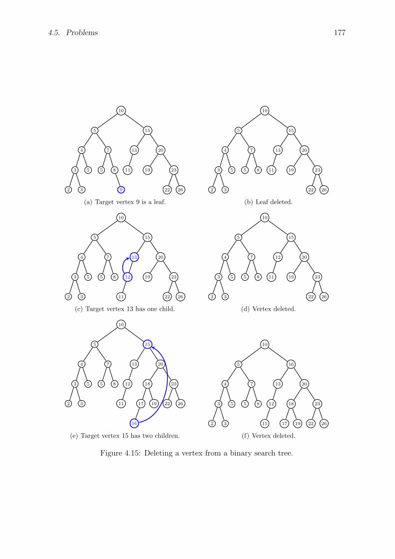
4.5. Problems 177
10
5
4
3
2 3
5
7
5 8
9
15
13
11
20
19 23
22 26
(a) Target vertex 9 is a leaf.
10
5
4
3
2 3
5
7
5 8
15
13
11
20
19 23
22 26
(b) Leaf deleted.
10
5
4
3
2 3
5
7
5 8
15
13
12
11
20
19 23
22 26
(c) Target vertex 13 has one child.
10
5
4
3
2 3
5
7
5 8
15
12
11
20
19 23
22 26
(d) Vertex deleted.
10
5
4
3
2 3
5
7
5 8
15
13
12
11
20
18
17
16
19
23
22 26
(e) Target vertex 15 has two children.
10
5
4
3
2 3
5
7
5 8
16
13
12
11
20
18
17 19
23
22 26
(f) Vertex deleted.
Figure 4.15: Deleting a vertex from a binary search tree.
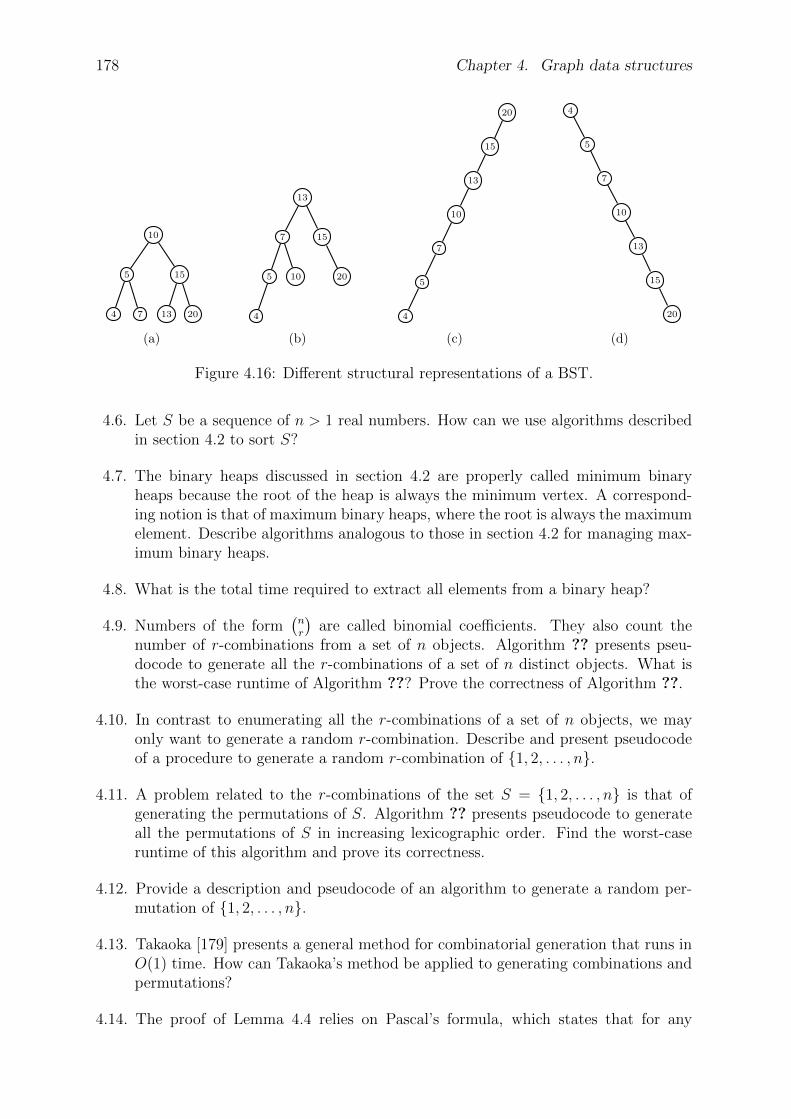
178 Chapter 4. Graph data structures
10
5
4 7
15
13 20
(a)
13
7
5
4
10
15
20
(b)
20
15
13
10
7
5
4
(c)
4
5
7
10
13
15
20
(d)
Figure 4.16: Different structural representations of a BST.
4.6. Let S be a sequence of n > 1 real numbers. How can we use algorithms describedin section 4.2 to sort S?
4.7. The binary heaps discussed in section 4.2 are properly called minimum binaryheaps because the root of the heap is always the minimum vertex. A correspond-ing notion is that of maximum binary heaps, where the root is always the maximumelement. Describe algorithms analogous to those in section 4.2 for managing max-imum binary heaps.
4.8. What is the total time required to extract all elements from a binary heap?
4.9. Numbers of the form(nr
)are called binomial coefficients. They also count the
number of r-combinations from a set of n objects. Algorithm ?? presents pseu-docode to generate all the r-combinations of a set of n distinct objects. What isthe worst-case runtime of Algorithm ??? Prove the correctness of Algorithm ??.
4.10. In contrast to enumerating all the r-combinations of a set of n objects, we mayonly want to generate a random r-combination. Describe and present pseudocodeof a procedure to generate a random r-combination of 1, 2, . . . , n.
4.11. A problem related to the r-combinations of the set S = 1, 2, . . . , n is that ofgenerating the permutations of S. Algorithm ?? presents pseudocode to generateall the permutations of S in increasing lexicographic order. Find the worst-caseruntime of this algorithm and prove its correctness.
4.12. Provide a description and pseudocode of an algorithm to generate a random per-mutation of 1, 2, . . . , n.
4.13. Takaoka [179] presents a general method for combinatorial generation that runs inO(1) time. How can Takaoka’s method be applied to generating combinations andpermutations?
4.14. The proof of Lemma 4.4 relies on Pascal’s formula, which states that for any

4.5. Problems 179
positive integers n and r such that r ≤ n, the following identity holds:(n+ 1
r
)=
(n
r − 1
)+
(n
r
).
Prove Pascal’s formula.
4.15. Let m,n, r be nonnegative integers such that r ≤ n. Prove the Vandermondeconvolution (
m+ n
r
)=
r∑
k=0
(m
k
)(n
r − k
).
The latter equation, also known as Vandermonde’s identity, was already knownas early as 1303 in China by Chu Shi-Chieh. Alexandre-Theophile Vandermondeindependently discovered it and his result was published in 1772.
4.16. If m and n are nonnegative integers, prove that
(m+ n+ 1
n
)=
n∑
k=0
(m+ k
k
).
4.17. Let n be a positive integer. How many distinct binomial heaps having n verticesare there?
4.18. The algorithms described in section 4.3 are formally for minimum binomial heapsbecause the vertex at the top of the heap is always the minimum vertex. Describeanalogous algorithms for maximum binomial heaps.
4.19. If H is a binomial heap, what is the total time required to extract all elementsfrom H?
4.20. Frederickson [81] describes an O(k) time algorithm for finding the k-th smallestelement in a binary heap. Provide a description and pseudocode of Frederickson’salgorithm and prove its correctness.
4.21. Fibonacci heaps [82] allow for amortized O(1) time with respect to finding theminimum element, inserting an element, and merging two Fibonacci heaps. Delet-ing the minimum element takes amortized time O(lg n), where n is the numberof vertices in the heap. Describe and provide pseudocode of the above Fibonacciheap operations and prove the correctness of the procedures.
4.22. Takaoka [180] introduces another type of heap called a 2-3 heap. Deleting theminimum element takes amortized O(lg n) time with n being the number of verticesin the 2-3 heap. Inserting an element into the heap takes amortized O(1) time.Describe and provide pseudocode of the above 2-3 heap operations. Under whichconditions would 2-3 heaps be more efficient than Fibonacci heaps?
4.23. In 2000, Chazelle [50] introduced the soft heap, which can perform common heapoperations in amortized O(1) time. He then applied [49] the soft heap to realize avery efficient implementation of an algorithm for finding minimum spanning trees.In 2009, Kaplan and Zwick [117] provided a simple implementation and analysis ofChazelle’s soft heap. Describe soft heaps and provide pseudocode of common heap
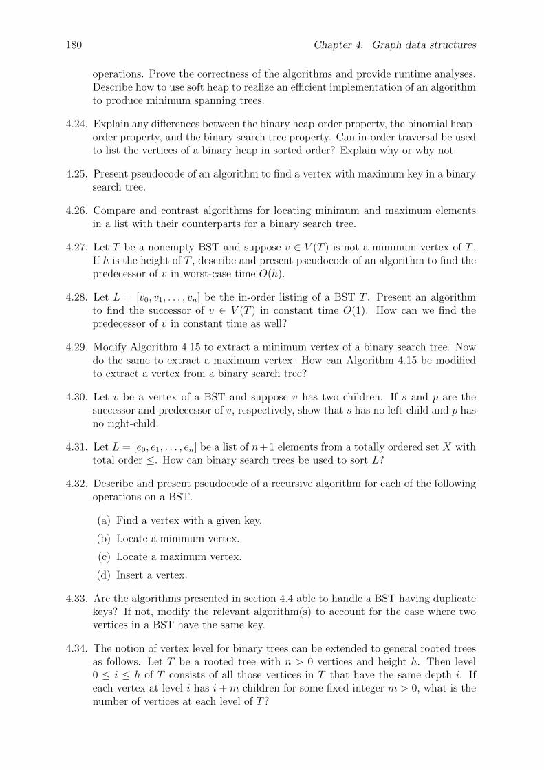
180 Chapter 4. Graph data structures
operations. Prove the correctness of the algorithms and provide runtime analyses.Describe how to use soft heap to realize an efficient implementation of an algorithmto produce minimum spanning trees.
4.24. Explain any differences between the binary heap-order property, the binomial heap-order property, and the binary search tree property. Can in-order traversal be usedto list the vertices of a binary heap in sorted order? Explain why or why not.
4.25. Present pseudocode of an algorithm to find a vertex with maximum key in a binarysearch tree.
4.26. Compare and contrast algorithms for locating minimum and maximum elementsin a list with their counterparts for a binary search tree.
4.27. Let T be a nonempty BST and suppose v ∈ V (T ) is not a minimum vertex of T .If h is the height of T , describe and present pseudocode of an algorithm to find thepredecessor of v in worst-case time O(h).
4.28. Let L = [v0, v1, . . . , vn] be the in-order listing of a BST T . Present an algorithmto find the successor of v ∈ V (T ) in constant time O(1). How can we find thepredecessor of v in constant time as well?
4.29. Modify Algorithm 4.15 to extract a minimum vertex of a binary search tree. Nowdo the same to extract a maximum vertex. How can Algorithm 4.15 be modifiedto extract a vertex from a binary search tree?
4.30. Let v be a vertex of a BST and suppose v has two children. If s and p are thesuccessor and predecessor of v, respectively, show that s has no left-child and p hasno right-child.
4.31. Let L = [e0, e1, . . . , en] be a list of n+1 elements from a totally ordered set X withtotal order ≤. How can binary search trees be used to sort L?
4.32. Describe and present pseudocode of a recursive algorithm for each of the followingoperations on a BST.
(a) Find a vertex with a given key.
(b) Locate a minimum vertex.
(c) Locate a maximum vertex.
(d) Insert a vertex.
4.33. Are the algorithms presented in section 4.4 able to handle a BST having duplicatekeys? If not, modify the relevant algorithm(s) to account for the case where twovertices in a BST have the same key.
4.34. The notion of vertex level for binary trees can be extended to general rooted treesas follows. Let T be a rooted tree with n > 0 vertices and height h. Then level0 ≤ i ≤ h of T consists of all those vertices in T that have the same depth i. Ifeach vertex at level i has i+m children for some fixed integer m > 0, what is thenumber of vertices at each level of T?
4.5. Problems 181
4.35. Compare the search, insertion, and deletion times of AVL trees and random binarysearch trees. Provide empirical results of your comparative study.
4.36. Describe and present pseudocode of an algorithm to construct a Fibonacci tree ofheight n for some integer n ≥ 0. Analyze the worst-case runtime of your algorithm.
4.37. The upper bound in Theorem ?? can be improved as follows. From the proof ofthe theorem, we have the recurrence relation N(h) > N(h− 1) +N(h− 2).
(a) If h ≤ 2, show that there exists some c > 0 such that N(h) ≥ ch.
(b) Assume for induction that
N(h) > N(h− 1) +N(h− 2) ≥ ch−1 + ch−2
for some h > 2. If c > 0, show that c2 − c − 1 = 0 is a solution to therecurrence relation ch−1 + ch−2 and that
N(h) >
(1 +√
5
2
)h
.
(c) Use the previous two parts to show that
h <1
lgϕ· lg n
where ϕ = (1 +√
5)/2 is the golden ratio and n counts the number of internalvertices of an AVL tree of height h.
4.38. The Fibonacci sequence Fn is defined as follows. We have initial values F0 = 0and F1 = 1. For n > 1, the n-th term in the sequence can be obtained via therecurrence relation Fn = Fn−1 + Fn−2. Show that
Fn =ϕn − (−1/ϕ)n√
5(4.3)
where ϕ is the golden ratio. The closed form solution (4.3) to the Fibonacci se-quence is known as Binet’s formula, named after Jacques Philippe Marie Binet,even though Abraham de Moivre knew about this formula long before Binet did.
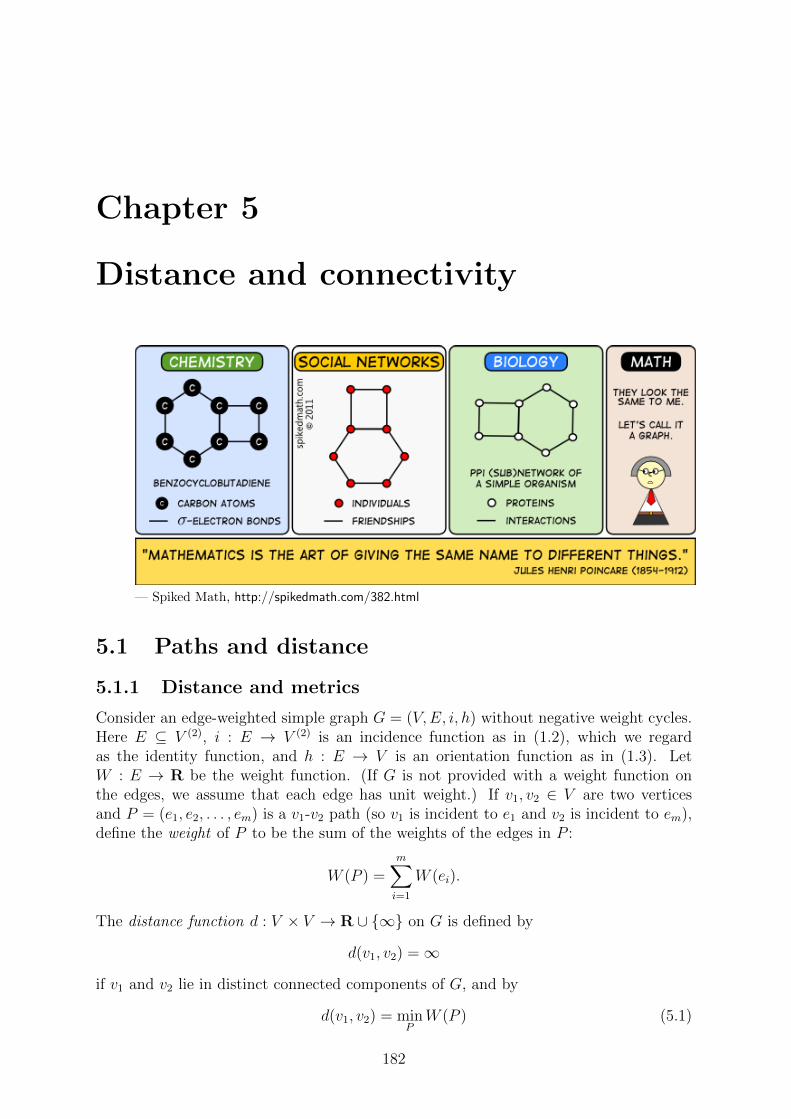
Chapter 5
Distance and connectivity
— Spiked Math, http://spikedmath.com/382.html
5.1 Paths and distance
5.1.1 Distance and metrics
Consider an edge-weighted simple graph G = (V,E, i, h) without negative weight cycles.Here E ⊆ V (2), i : E → V (2) is an incidence function as in (1.2), which we regardas the identity function, and h : E → V is an orientation function as in (1.3). LetW : E → R be the weight function. (If G is not provided with a weight function onthe edges, we assume that each edge has unit weight.) If v1, v2 ∈ V are two verticesand P = (e1, e2, . . . , em) is a v1-v2 path (so v1 is incident to e1 and v2 is incident to em),define the weight of P to be the sum of the weights of the edges in P :
W (P ) =m∑
i=1
W (ei).
The distance function d : V × V → R ∪ ∞ on G is defined by
d(v1, v2) =∞
if v1 and v2 lie in distinct connected components of G, and by
d(v1, v2) = minPW (P ) (5.1)
182
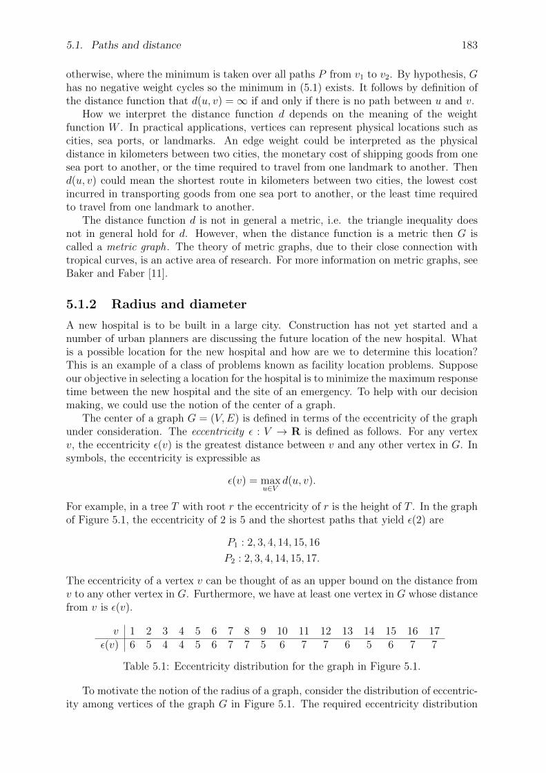
5.1. Paths and distance 183
otherwise, where the minimum is taken over all paths P from v1 to v2. By hypothesis, Ghas no negative weight cycles so the minimum in (5.1) exists. It follows by definition ofthe distance function that d(u, v) =∞ if and only if there is no path between u and v.
How we interpret the distance function d depends on the meaning of the weightfunction W . In practical applications, vertices can represent physical locations such ascities, sea ports, or landmarks. An edge weight could be interpreted as the physicaldistance in kilometers between two cities, the monetary cost of shipping goods from onesea port to another, or the time required to travel from one landmark to another. Thend(u, v) could mean the shortest route in kilometers between two cities, the lowest costincurred in transporting goods from one sea port to another, or the least time requiredto travel from one landmark to another.
The distance function d is not in general a metric, i.e. the triangle inequality doesnot in general hold for d. However, when the distance function is a metric then G iscalled a metric graph. The theory of metric graphs, due to their close connection withtropical curves, is an active area of research. For more information on metric graphs, seeBaker and Faber [11].
5.1.2 Radius and diameter
A new hospital is to be built in a large city. Construction has not yet started and anumber of urban planners are discussing the future location of the new hospital. Whatis a possible location for the new hospital and how are we to determine this location?This is an example of a class of problems known as facility location problems. Supposeour objective in selecting a location for the hospital is to minimize the maximum responsetime between the new hospital and the site of an emergency. To help with our decisionmaking, we could use the notion of the center of a graph.
The center of a graph G = (V,E) is defined in terms of the eccentricity of the graphunder consideration. The eccentricity ε : V → R is defined as follows. For any vertexv, the eccentricity ε(v) is the greatest distance between v and any other vertex in G. Insymbols, the eccentricity is expressible as
ε(v) = maxu∈V
d(u, v).
For example, in a tree T with root r the eccentricity of r is the height of T . In the graphof Figure 5.1, the eccentricity of 2 is 5 and the shortest paths that yield ε(2) are
P1 : 2, 3, 4, 14, 15, 16
P2 : 2, 3, 4, 14, 15, 17.
The eccentricity of a vertex v can be thought of as an upper bound on the distance fromv to any other vertex in G. Furthermore, we have at least one vertex in G whose distancefrom v is ε(v).
v 1 2 3 4 5 6 7 8 9 10 11 12 13 14 15 16 17ε(v) 6 5 4 4 5 6 7 7 5 6 7 7 6 5 6 7 7
Table 5.1: Eccentricity distribution for the graph in Figure 5.1.
To motivate the notion of the radius of a graph, consider the distribution of eccentric-ity among vertices of the graph G in Figure 5.1. The required eccentricity distribution
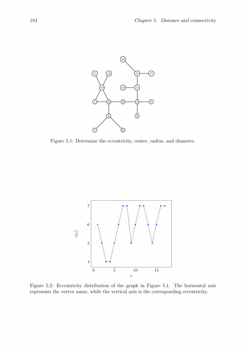
184 Chapter 5. Distance and connectivity
1 2 3 4 5
6
7 8
9
10
11 12
13 14
15
16
17
Figure 5.1: Determine the eccentricity, center, radius, and diameter.
0 5 10 15
4
5
6
7
v
ε(v)
Figure 5.2: Eccentricity distribution of the graph in Figure 5.1. The horizontal axisrepresents the vertex name, while the vertical axis is the corresponding eccentricity.
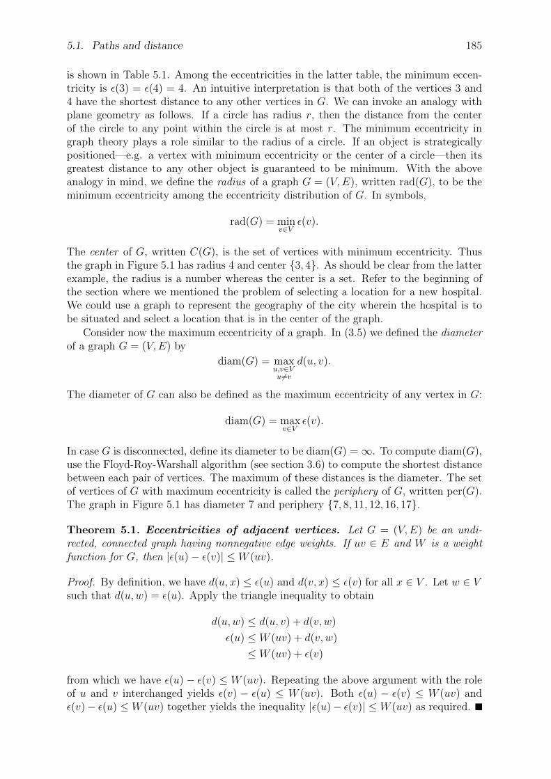
5.1. Paths and distance 185
is shown in Table 5.1. Among the eccentricities in the latter table, the minimum eccen-tricity is ε(3) = ε(4) = 4. An intuitive interpretation is that both of the vertices 3 and4 have the shortest distance to any other vertices in G. We can invoke an analogy withplane geometry as follows. If a circle has radius r, then the distance from the centerof the circle to any point within the circle is at most r. The minimum eccentricity ingraph theory plays a role similar to the radius of a circle. If an object is strategicallypositioned—e.g. a vertex with minimum eccentricity or the center of a circle—then itsgreatest distance to any other object is guaranteed to be minimum. With the aboveanalogy in mind, we define the radius of a graph G = (V,E), written rad(G), to be theminimum eccentricity among the eccentricity distribution of G. In symbols,
rad(G) = minv∈V
ε(v).
The center of G, written C(G), is the set of vertices with minimum eccentricity. Thusthe graph in Figure 5.1 has radius 4 and center 3, 4. As should be clear from the latterexample, the radius is a number whereas the center is a set. Refer to the beginning ofthe section where we mentioned the problem of selecting a location for a new hospital.We could use a graph to represent the geography of the city wherein the hospital is tobe situated and select a location that is in the center of the graph.
Consider now the maximum eccentricity of a graph. In (3.5) we defined the diameterof a graph G = (V,E) by
diam(G) = maxu,v∈Vu6=v
d(u, v).
The diameter of G can also be defined as the maximum eccentricity of any vertex in G:
diam(G) = maxv∈V
ε(v).
In case G is disconnected, define its diameter to be diam(G) =∞. To compute diam(G),use the Floyd-Roy-Warshall algorithm (see section 3.6) to compute the shortest distancebetween each pair of vertices. The maximum of these distances is the diameter. The setof vertices of G with maximum eccentricity is called the periphery of G, written per(G).The graph in Figure 5.1 has diameter 7 and periphery 7, 8, 11, 12, 16, 17.
Theorem 5.1. Eccentricities of adjacent vertices. Let G = (V,E) be an undi-rected, connected graph having nonnegative edge weights. If uv ∈ E and W is a weightfunction for G, then |ε(u)− ε(v)| ≤ W (uv).
Proof. By definition, we have d(u, x) ≤ ε(u) and d(v, x) ≤ ε(v) for all x ∈ V . Let w ∈ Vsuch that d(u,w) = ε(u). Apply the triangle inequality to obtain
d(u,w) ≤ d(u, v) + d(v, w)
ε(u) ≤ W (uv) + d(v, w)
≤ W (uv) + ε(v)
from which we have ε(u)− ε(v) ≤ W (uv). Repeating the above argument with the roleof u and v interchanged yields ε(v) − ε(u) ≤ W (uv). Both ε(u) − ε(v) ≤ W (uv) andε(v)− ε(u) ≤ W (uv) together yields the inequality |ε(u)− ε(v)| ≤ W (uv) as required.
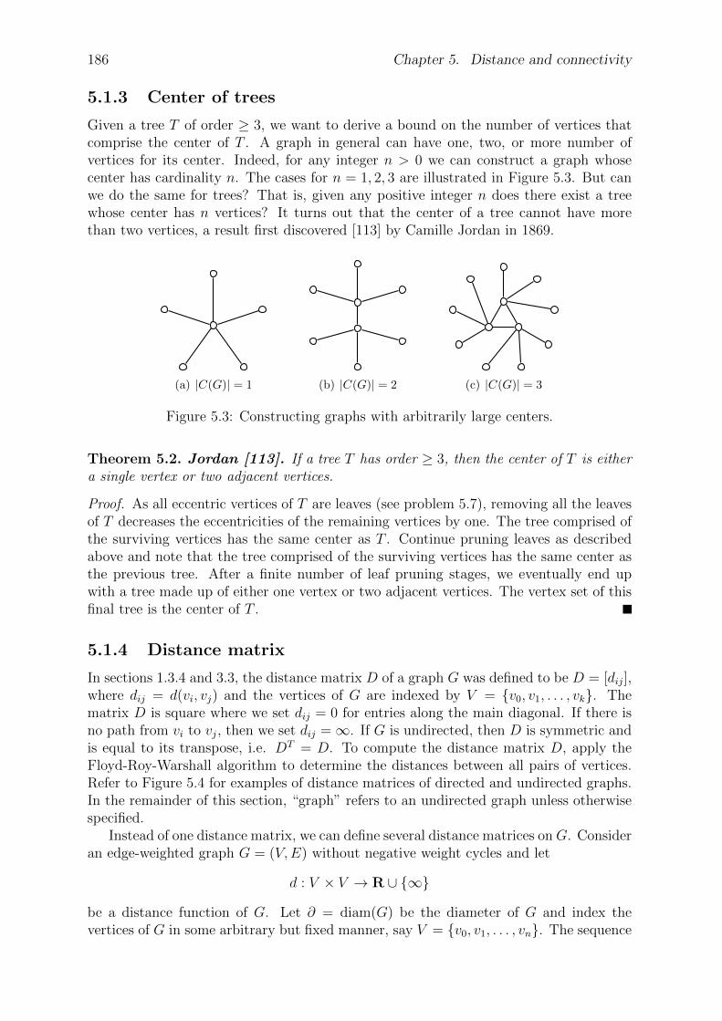
186 Chapter 5. Distance and connectivity
5.1.3 Center of trees
Given a tree T of order ≥ 3, we want to derive a bound on the number of vertices thatcomprise the center of T . A graph in general can have one, two, or more number ofvertices for its center. Indeed, for any integer n > 0 we can construct a graph whosecenter has cardinality n. The cases for n = 1, 2, 3 are illustrated in Figure 5.3. But canwe do the same for trees? That is, given any positive integer n does there exist a treewhose center has n vertices? It turns out that the center of a tree cannot have morethan two vertices, a result first discovered [113] by Camille Jordan in 1869.
(a) |C(G)| = 1 (b) |C(G)| = 2 (c) |C(G)| = 3
Figure 5.3: Constructing graphs with arbitrarily large centers.
Theorem 5.2. Jordan [113]. If a tree T has order ≥ 3, then the center of T is eithera single vertex or two adjacent vertices.
Proof. As all eccentric vertices of T are leaves (see problem 5.7), removing all the leavesof T decreases the eccentricities of the remaining vertices by one. The tree comprised ofthe surviving vertices has the same center as T . Continue pruning leaves as describedabove and note that the tree comprised of the surviving vertices has the same center asthe previous tree. After a finite number of leaf pruning stages, we eventually end upwith a tree made up of either one vertex or two adjacent vertices. The vertex set of thisfinal tree is the center of T .
5.1.4 Distance matrix
In sections 1.3.4 and 3.3, the distance matrix D of a graph G was defined to be D = [dij],where dij = d(vi, vj) and the vertices of G are indexed by V = v0, v1, . . . , vk. Thematrix D is square where we set dij = 0 for entries along the main diagonal. If there isno path from vi to vj, then we set dij =∞. If G is undirected, then D is symmetric andis equal to its transpose, i.e. DT = D. To compute the distance matrix D, apply theFloyd-Roy-Warshall algorithm to determine the distances between all pairs of vertices.Refer to Figure 5.4 for examples of distance matrices of directed and undirected graphs.In the remainder of this section, “graph” refers to an undirected graph unless otherwisespecified.
Instead of one distance matrix, we can define several distance matrices onG. Consideran edge-weighted graph G = (V,E) without negative weight cycles and let
d : V × V → R ∪ ∞
be a distance function of G. Let ∂ = diam(G) be the diameter of G and index thevertices of G in some arbitrary but fixed manner, say V = v0, v1, . . . , vn. The sequence
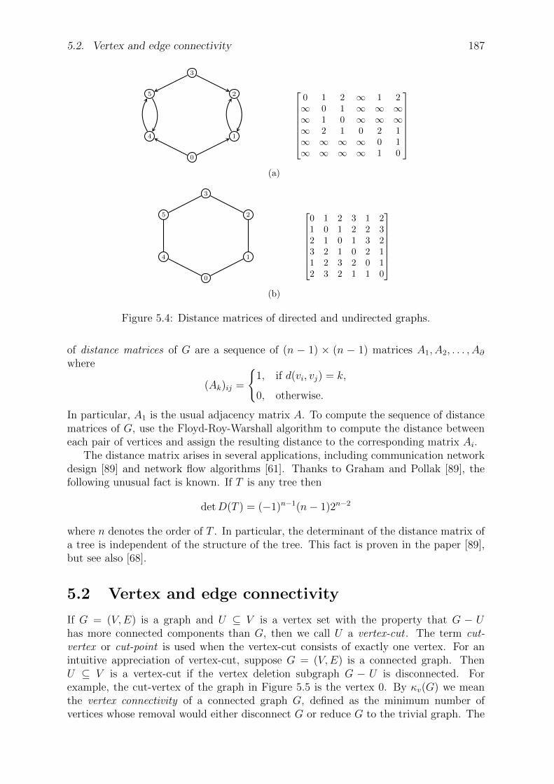
5.2. Vertex and edge connectivity 187
1
2
3
0
4
5
0 1 2 ∞ 1 2∞ 0 1 ∞ ∞ ∞∞ 1 0 ∞ ∞ ∞∞ 2 1 0 2 1∞ ∞ ∞ ∞ 0 1∞ ∞ ∞ ∞ 1 0
(a)
1
2
3
0
4
5
0 1 2 3 1 21 0 1 2 2 32 1 0 1 3 23 2 1 0 2 11 2 3 2 0 12 3 2 1 1 0
(b)
Figure 5.4: Distance matrices of directed and undirected graphs.
of distance matrices of G are a sequence of (n − 1) × (n − 1) matrices A1, A2, . . . , A∂where
(Ak)ij =
1, if d(vi, vj) = k,
0, otherwise.
In particular, A1 is the usual adjacency matrix A. To compute the sequence of distancematrices of G, use the Floyd-Roy-Warshall algorithm to compute the distance betweeneach pair of vertices and assign the resulting distance to the corresponding matrix Ai.
The distance matrix arises in several applications, including communication networkdesign [89] and network flow algorithms [61]. Thanks to Graham and Pollak [89], thefollowing unusual fact is known. If T is any tree then
detD(T ) = (−1)n−1(n− 1)2n−2
where n denotes the order of T . In particular, the determinant of the distance matrix ofa tree is independent of the structure of the tree. This fact is proven in the paper [89],but see also [68].
5.2 Vertex and edge connectivity
If G = (V,E) is a graph and U ⊆ V is a vertex set with the property that G − Uhas more connected components than G, then we call U a vertex-cut . The term cut-vertex or cut-point is used when the vertex-cut consists of exactly one vertex. For anintuitive appreciation of vertex-cut, suppose G = (V,E) is a connected graph. ThenU ⊆ V is a vertex-cut if the vertex deletion subgraph G − U is disconnected. Forexample, the cut-vertex of the graph in Figure 5.5 is the vertex 0. By κv(G) we meanthe vertex connectivity of a connected graph G, defined as the minimum number ofvertices whose removal would either disconnect G or reduce G to the trivial graph. The
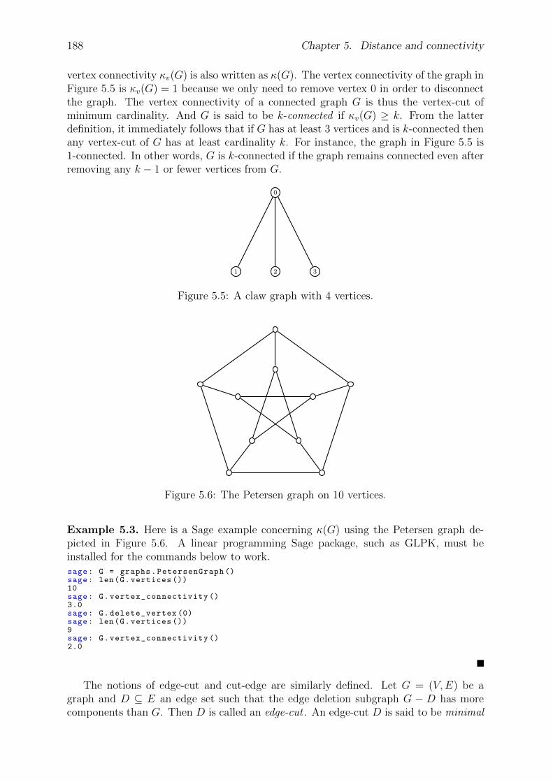
188 Chapter 5. Distance and connectivity
vertex connectivity κv(G) is also written as κ(G). The vertex connectivity of the graph inFigure 5.5 is κv(G) = 1 because we only need to remove vertex 0 in order to disconnectthe graph. The vertex connectivity of a connected graph G is thus the vertex-cut ofminimum cardinality. And G is said to be k-connected if κv(G) ≥ k. From the latterdefinition, it immediately follows that if G has at least 3 vertices and is k-connected thenany vertex-cut of G has at least cardinality k. For instance, the graph in Figure 5.5 is1-connected. In other words, G is k-connected if the graph remains connected even afterremoving any k − 1 or fewer vertices from G.
1 2 3
0
Figure 5.5: A claw graph with 4 vertices.
Figure 5.6: The Petersen graph on 10 vertices.
Example 5.3. Here is a Sage example concerning κ(G) using the Petersen graph de-picted in Figure 5.6. A linear programming Sage package, such as GLPK, must beinstalled for the commands below to work.sage: G = graphs.PetersenGraph ()sage: len(G.vertices ())10sage: G.vertex_connectivity ()3.0sage: G.delete_vertex (0)sage: len(G.vertices ())9sage: G.vertex_connectivity ()2.0
The notions of edge-cut and cut-edge are similarly defined. Let G = (V,E) be agraph and D ⊆ E an edge set such that the edge deletion subgraph G − D has morecomponents than G. Then D is called an edge-cut . An edge-cut D is said to be minimal

5.2. Vertex and edge connectivity 189
if no proper subset of D is an edge-cut. The term cut-edge or bridge is reserved forthe case where the set D is a singleton. Think of a cut-edge as an edge whose removalfrom a connected graph would result in that graph being disconnected. Going backto the case of the graph in Figure 5.5, each edge of the graph is a cut-edge. A graphhaving no cut-edge is called bridgeless . An open question as of 2010 involving bridgesis the cycle double cover conjecture, due to Paul Seymour and G. Szekeres, which statesthat every bridgeless graph admits a set of cycles that contains each edge exactly twice.The edge connectivity of a connected graph G, written κe(G) and sometimes denotedby λ(G), is the minimum number of edges whose removal would disconnect G. In otherwords, κe(G) is the minimum cardinality among all edge-cuts of G. Furthermore, G issaid to be k-edge-connected if κe(G) ≥ k. A connected graph that is k-edge-connectedis guaranteed to be connected after removing ≤ k − 1 edges from it. When we haveremoved k or more edges, then the graph would become disconnected. By convention, a1-edge-connected graph is simply a connected graph. The graph in Figure 5.5 has edgeconnectivity κe(G) = 1 and is 1-edge-connected.
Example 5.4. Here is a Sage example concerning λ(G) using the Petersen graph shownin Figure 5.6. You must install an optional linear programming Sage package such asGLPK for the commands below to work.sage: G = graphs.PetersenGraph ()sage: len(G.vertices ())10sage: E = G.edges (); len(E)15sage: G.edge_connectivity ()3.0sage: G.delete_edge(E[0])sage: len(G.edges ())14sage: G.edge_connectivity ()2.0
Vertex and edge connectivity are intimately related to the reliability and survivabilityof computer networks. If a computer network G (which is a connected graph) is k-connected, then it would remain connected despite the failure of at most k − 1 networknodes. Similarly, G is k-edge-connected if the network remains connected after the failureof at most k − 1 network links. In practical terms, a network with redundant nodesand/or links can afford to endure the failure of a number of nodes and/or links andstill be connected, whereas a network with very few redundant nodes and/or links (e.g.something close to a spanning tree) is more prone to be disconnected. A k-connected ork-edge-connected network is more robust (i.e. can withstand) against node and/or linkfailures than is a j-connected or j-edge-connected network, where j < k.
Proposition 5.5. If δ(G) is the minimum degree of an undirected connected graph G =(V,E), then the edge connectivity of G satisfies λ(G) ≤ δ(G).
Proof. Choose a vertex v ∈ V whose degree is deg(v) = δ(G). Deleting the δ(G) edgesincident on v suffices to disconnect G as v is now an isolated vertex. It is possible thatG has an edge-cut whose cardinality is smaller than δ(G). Hence the result follows.
Let G = (V,E) be a graph and suppose X1 and X2 comprise a partition of V . Apartition-cut of G, denoted 〈X1, X2〉, is the set of all edges of G with one endpoint inX1 and the other endpoint in X2. If G is a bipartite graph with bipartition X1 and X2,then 〈X1, X2〉 is a partition-cut of G. It follows that a partition-cut is also an edge-cut.

190 Chapter 5. Distance and connectivity
Proposition 5.6. An undirected connected graph G is k-edge-connected if and only ifany partition-cut of G has at least k edges.
Proof. Assume that G is k-edge-connected. Then each edge-cut has at least k edges. Asa partition-cut is an edge-cut, then any partition-cut of G has at least k edges.
On the other hand, suppose each partition-cut has at least k edges. If D is a minimaledge-cut of G and X1 and X2 are the vertex sets of the two components of G−D, thenD = 〈X1, X2〉. To see this, note that D ⊆ 〈X1, X2〉. If 〈X1, X2〉 − D 6= ∅ then choosesome e ∈ 〈X1, X2〉 such that e /∈ D. The endpoints of e belong to the same componentof G−D, in contradiction of the definition of X1 and X2. Thus any minimal edge-cut isa partition-cut and conclude that any edge-cut has at least k edges.
Proposition 5.7. If G = (V,E) is an undirected connected graph with vertex connectivityκ(G) and edge connectivity λ(G), then we have κ(G) ≤ λ(G).
Proof. Let S be an edge-cut of G with cardinality k = |S| = λ(G). Removing k suitablychosen vertices of G suffice to delete the edges of S and hence disconnect G. It is alsopossible to have a smaller vertex-cut elsewhere in G. Hence the inequality follows.
Taking together Propositions 5.5 and 5.7, we have Whitney’s inequality.
Theorem 5.8. Whitney’s inequality [195]. Let G be an undirected connected graphwith vertex connectivity κ(G), edge connectivity λ(G), and minimum degree δ(G). Thenwe have the following inequality:
κ(G) ≤ λ(G) ≤ δ(G).
Proposition 5.9. Let G be an undirected connected graph that is k-connected for somek ≥ 3. If e is an edge of G, then the edge-deletion subgraph G− e is (k − 1)-connected.
Proof. Let V = v1, v2, . . . , vk−2 be a set of k − 2 vertices in G − e. It suffice to showthe existence of a u-v walk in (G−e)−V for any distinct vertices u and v in (G−e)−V .We need to consider two cases: (i) at least one of the endpoints of e is in V ; and (ii)neither endpoints of e is in V .
(i) Assume that V has at least one endpoint of e. As G − V is 2-connected, anydistinct pair of vertices u and v in G − V is connected by a u-v path that excludes e.Hence the u-v path is also in (G− e)− V .
(ii) Assume that neither endpoints of e is in V . If u and v are distinct vertices in(G − e) − V , then either: (1) both u and v are endpoints of e; or (2) at least one of uand v is an endpoint of e.
(1) Suppose u and v are both endpoints of e. As G is k-connected, then G has atleast k + 1 vertices so that the vertex set of G− v1, v2, . . . , vk−2, u, v is nonempty.Let w be a vertex of G − v1, v2, . . . , vk−2, u, v. Then there is a u-w path in G −v1, v2, . . . , vk−2, v and a w-v path in G− v1, v2, . . . , vk−2, u. Neither the u-w northe w-v paths contain e. The concatenation of these two paths is a u-v walk in(G− e)− V .
(2) Now suppose at least one of u and v, say u, is an endpoint of e. Let w be the otherendpoint of e. As G is k-connected, then G− v1, v2, . . . , vk−2, w is connected andwe can find a u-v path P in G− v1, v2, . . . , vk−2, w. Furthermore P is a u-v pathin G − v1, v2, . . . , vk−2 that neither contain w nor e. Hence P is a u-v path in(G− e)− V .
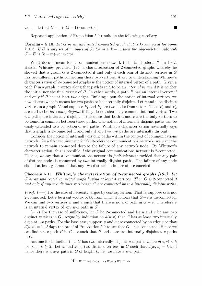
5.2. Vertex and edge connectivity 191
Conclude that G− e is (k − 1)-connected.
Repeated application of Proposition 5.9 results in the following corollary.
Corollary 5.10. Let G be an undirected connected graph that is k-connected for somek ≥ 3. If E is any set of m edges of G, for m ≤ k − 1, then the edge-deletion subgraphG− E is (k −m)-connected.
What does it mean for a communications network to be fault-tolerant? In 1932,Hassler Whitney provided [195] a characterization of 2-connected graphs whereby heshowed that a graph G is 2-connected if and only if each pair of distinct vertices in Ghas two different paths connecting those two vertices. A key to understanding Whitney’scharacterization of 2-connected graphs is the notion of internal vertex of a path. Given apath P in a graph, a vertex along that path is said to be an internal vertex if it is neitherthe initial nor the final vertex of P . In other words, a path P has an internal vertex ifand only if P has at least two edges. Building upon the notion of internal vertices, wenow discuss what it means for two paths to be internally disjoint. Let u and v be distinctvertices in a graph G and suppose P1 and P2 are two paths from u to v. Then P1 and P2
are said to be internally disjoint if they do not share any common internal vertex. Twou-v paths are internally disjoint in the sense that both u and v are the only vertices tobe found in common between those paths. The notion of internally disjoint paths can beeasily extended to a collection of u-v paths. Whitney’s characterization essentially saysthat a graph is 2-connected if and only if any two u-v paths are internally disjoint.
Consider the notion of internally disjoint paths within the context of communicationsnetwork. As a first requirement for fault-tolerant communications network, we want thenetwork to remain connected despite the failure of any network node. By Whitney’scharacterization, this is possible if the original communications network is 2-connected.That is, we say that a communications network is fault-tolerant provided that any pairof distinct nodes is connected by two internally disjoint paths. The failure of any nodeshould at least guarantee that any two distinct nodes are still connected.
Theorem 5.11. Whitney’s characterization of 2-connected graphs [195]. LetG be an undirected connected graph having at least 3 vertices. Then G is 2-connected ifand only if any two distinct vertices in G are connected by two internally disjoint paths.
Proof. (⇐=) For the case of necessity, argue by contraposition. That is, suppose G is not2-connected. Let v be a cut-vertex of G, from which it follows that G−v is disconnected.We can find two vertices w and x such that there is no w-x path in G− v. Therefore vis an internal vertex of any w-x path in G.
(=⇒) For the case of sufficiency, let G be 2-connected and let u and v be any twodistinct vertices in G. Argue by induction on d(u, v) that G has at least two internallydisjoint u-v paths. For the base case, suppose u and v are connected by an edge e so thatd(u, v) = 1. Adapt the proof of Proposition 5.9 to see that G− e is connected. Hence wecan find a u-v path P in G − e such that P and e are two internally disjoint u-v pathsin G.
Assume for induction that G has two internally disjoint u-v paths where d(u, v) < kfor some k ≥ 2. Let w and x be two distinct vertices in G such that d(w, x) = k andhence there is a w-x path in G of length k, i.e. we have a w-x path
W : w = w1, w2, . . . , wk−1, wk = x.
192 Chapter 5. Distance and connectivity
Note that d(w,wk−1) < k and apply the induction hypothesis to see that we have twointernally disjoint w-wk−1 paths in G; call these paths P and Q. As G is 2-connected,we have a w-x path R in G − wk−1 and hence R is also a w-x path in G. Let z be thevertex on R that immediately precedes x and assume without loss of generality that zis on P . We claim that G has two internally disjoint w-x paths. One of these paths isthe concatenation of the subpath of P from w to z with the subpath of R from z to x.If x is not on Q, then construct a second w-x path, internally disjoint from the first one,as follows: concatenate the path Q with the edge wk−1w. In case x is on Q, take thesubpath of Q from w to x as the required second path.
From Theorem 5.11, an undirected connected graphG is 2-connected if and only if anytwo distinct vertices of G are connected by two internally disjoint paths. In particular,let u and v be any two distinct vertices of G and let P and Q be two internally disjointu-v paths as guaranteed by Theorem 5.11. Starting from u, travel along the path Pto arrive at v. Then start from v and travel along the path Q to arrive at u. Theconcatenation of the internally disjoint paths P and Q is hence a cycle passing throughu and v. We have proved the following corollary to Theorem 5.11.
Corollary 5.12. Let G be an undirected connected graph having at least 3 vertices. ThenG is 2-connected if and only if any two distinct vertices of G lie on a common cycle.
The following theorem provides further characterizations of 2-connected graphs, inaddition to Whitney’s characterization.
Theorem 5.13. Characterizations of 2-connected graphs. Let G = (V,E) be anundirected connected graph having at least 3 vertices. Then the following are equivalent.
1. G is 2-connected.
2. If u, v ∈ V are distinct vertices of G, then u and v lie on a common cycle.
3. If v ∈ V and e ∈ E, then v and e lie on a common cycle.
4. If e1, e2 ∈ E are distinct edges of G, then e1 and e2 lie on a common cycle.
5. If u, v ∈ V are distinct vertices and e ∈ E, then they lie on a common path.
6. If u, v, w ∈ V are distinct vertices, then they lie on a common path.
7. If u, v, w ∈ V are distinct vertices, then there is a path containing any two of thesevertices but excluding the third.
5.3 Menger’s theorem
Menger’s theorem has a number of different versions: an undirected, vertex-connectivityversion; a directed, vertex-connectivity version; an undirected, edge-connectivity version;and a directed, edge-connectivity version. In this section, we will prove the undirected,vertex-connectivity version. But first, let’s consider a few technical results that will beof use for the purpose of this section.
Let u and v be distinct vertices in a connected graph G = (V,E) and let S ⊆ V .Then S is said to be u-v separating if u and v lie in different components of the vertex
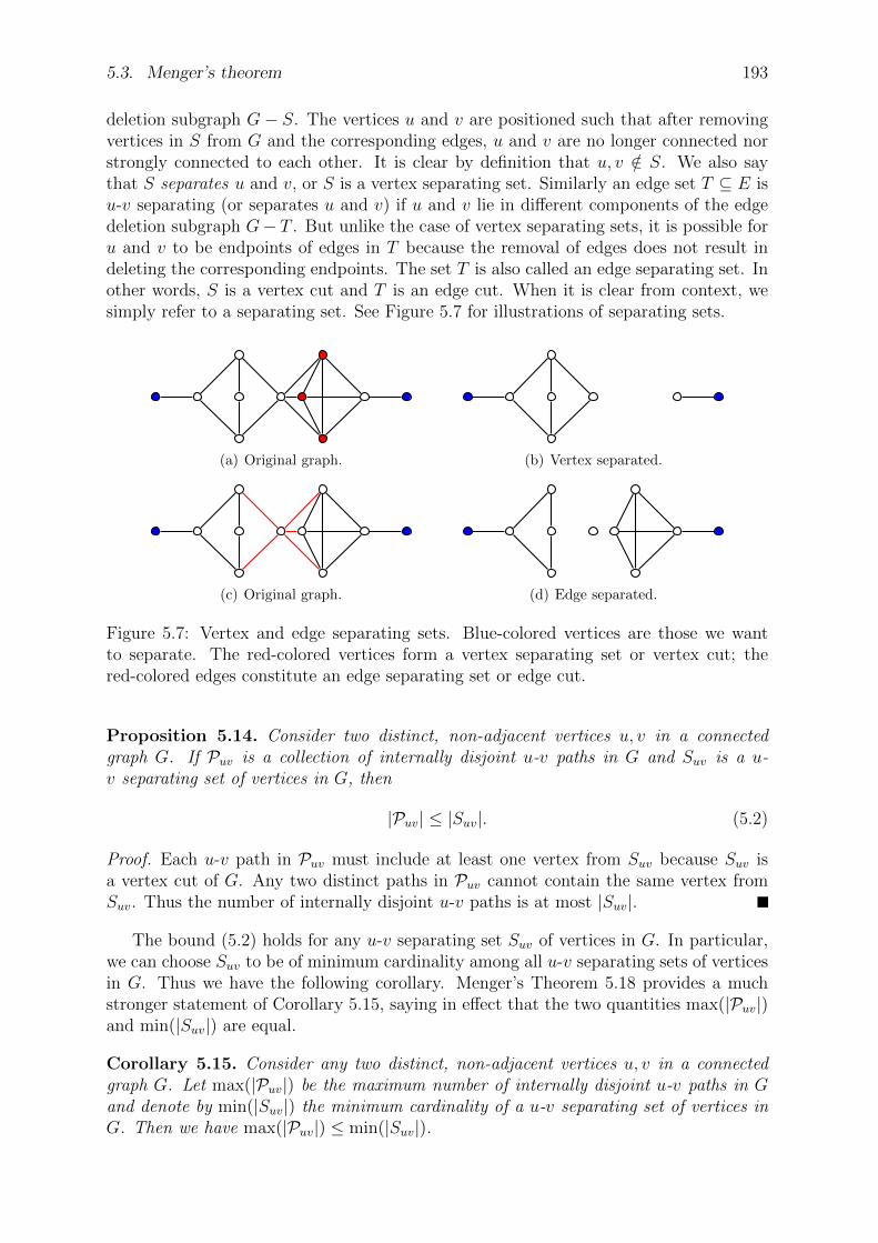
5.3. Menger’s theorem 193
deletion subgraph G− S. The vertices u and v are positioned such that after removingvertices in S from G and the corresponding edges, u and v are no longer connected norstrongly connected to each other. It is clear by definition that u, v /∈ S. We also saythat S separates u and v, or S is a vertex separating set. Similarly an edge set T ⊆ E isu-v separating (or separates u and v) if u and v lie in different components of the edgedeletion subgraph G− T . But unlike the case of vertex separating sets, it is possible foru and v to be endpoints of edges in T because the removal of edges does not result indeleting the corresponding endpoints. The set T is also called an edge separating set. Inother words, S is a vertex cut and T is an edge cut. When it is clear from context, wesimply refer to a separating set. See Figure 5.7 for illustrations of separating sets.
(a) Original graph. (b) Vertex separated.
(c) Original graph. (d) Edge separated.
Figure 5.7: Vertex and edge separating sets. Blue-colored vertices are those we wantto separate. The red-colored vertices form a vertex separating set or vertex cut; thered-colored edges constitute an edge separating set or edge cut.
Proposition 5.14. Consider two distinct, non-adjacent vertices u, v in a connectedgraph G. If Puv is a collection of internally disjoint u-v paths in G and Suv is a u-v separating set of vertices in G, then
|Puv| ≤ |Suv|. (5.2)
Proof. Each u-v path in Puv must include at least one vertex from Suv because Suv isa vertex cut of G. Any two distinct paths in Puv cannot contain the same vertex fromSuv. Thus the number of internally disjoint u-v paths is at most |Suv|.
The bound (5.2) holds for any u-v separating set Suv of vertices in G. In particular,we can choose Suv to be of minimum cardinality among all u-v separating sets of verticesin G. Thus we have the following corollary. Menger’s Theorem 5.18 provides a muchstronger statement of Corollary 5.15, saying in effect that the two quantities max(|Puv|)and min(|Suv|) are equal.
Corollary 5.15. Consider any two distinct, non-adjacent vertices u, v in a connectedgraph G. Let max(|Puv|) be the maximum number of internally disjoint u-v paths in Gand denote by min(|Suv|) the minimum cardinality of a u-v separating set of vertices inG. Then we have max(|Puv|) ≤ min(|Suv|).
194 Chapter 5. Distance and connectivity
Corollary 5.16. Consider any two distinct, non-adjacent vertices u, v in a connectedgraph G. Let Puv be a collection of internally disjoint u-v paths in G and let Suv be a u-vseparating set of vertices in G. If |Puv| = |Suv|, then Puv has maximum cardinality amongall collections of internally disjoint u-v paths in G and Suv has minimum cardinalityamong all u-v separating sets of vertices in G.
Proof. Argue by contradiction. Let Quv be another collection of internally disjoint u-vpaths in G such that |Quv| ≥ |Puv|. Then |Puv| ≤ |Quv| ≤ |Suv| by Proposition 5.14.We cannot have |Quv| > |Puv|, which would be contradictory to our hypothesis thatPuv = |Suv|. Thus |Quv| = |Puv|. Let Tuv be another u-v separating set of vertices inG such that |Tuv| ≤ |Suv|. Then we have |Puv| ≤ |Tuv| ≤ |Suv| by Proposition 5.14.We cannot have |Tuv| < |Suv| because we would then end up with |Puv| ≤ |Tuv| andPuv = |Suv|, a contradiction. Therefore |Tuv| = |Suv|.Lemma 5.17. Consider two distinct, non-adjacent vertices u, v in a connected graph Gand let k be the minimum number of vertices required to separate u and v. If G has au-v path of length 2, then G has k internally disjoint u-v paths.
Proof. Argue by induction on k. For the base case, assume k = 1. Hence G has a cutvertex x such that u and v are disconnected in G− x. Any u-v path must contain x. Inparticular, there can be only one internally disjoint u-v path.
Assume for induction that k ≥ 2. Let P : u, x, v be a path in G having length 2 andsuppose S is a smallest u-v separating set for G − x. Then S ∪ x is a u-v separatingset for G. By the minimality of k, we have |S| ≥ k − 1. By the induction hypothesis,we have at least k − 1 internally disjoint u-v paths in G− x. As P is internally disjointfrom any of the latter paths, conclude that G has k internally disjoint u-v paths.
Theorem 5.18. Menger’s theorem. Let G be an undirected connected graph and letu and v be distinct, non-adjacent vertices of G. Then the maximum number of internallydisjoint u-v paths in G equals the minimum number of vertices needed to separate u andv.
Proof. Suppose that the maximum number of independent u-v paths in G is attained byu-v paths P1, . . . , Pk. To obtain a separating set W ⊂ V , we must at least remove onepoint in each path Pi. This implies the minimum number of vertices needed to separateu and v is at least k. Therefore, we have an upper bound:
#indep. u− v paths ≤ #min. number of vertices needed to separate u and v.
We show that equality holds. Let n denote the number of edges of G. The proof is byinduction on n. By hypothesis, n ≥ 2. If n = 2 the statement holds by inspection, sincein that case G is a line graph with 3 vertices V = u, v, w and 2 edges, E = uw.wv.In that situation, there is only 1 u-v path (namely, uwv) and only one vertex separatingu and v (namely, w).
Suppose now n > 3 and assume the statement holds for each graph with < n edges.Let
k = #independent u− v pathsand let
` = #min. number of vertices needed to separate u and v,
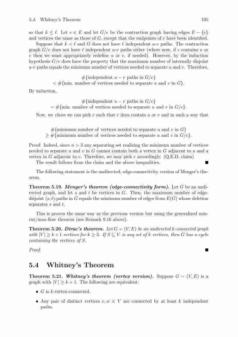
5.4. Whitney’s Theorem 195
so that k ≤ `. Let e ∈ E and let G/e be the contraction graph having edges E − eand vertices the same as those of G, except that the endpoints of e have been identified.
Suppose that k < ` and G does not have ` independent u-v paths. The contractiongraph G/e does not have ` independent u-v paths either (where now, if e contains u orv then we must appropriately redefine u or v, if needed). However, by the inductionhypothesis G/e does have the property that the maximum number of internally disjointu-v paths equals the minimum number of vertices needed to separate u and v. Therefore,
#independent u− v paths in G/e< #min. number of vertices needed to separate u and v in G.
By induction,
#independent u− v paths in G/e= #min. number of vertices needed to separate u and v in G/e.
Now, we claim we can pick e such that e does contain u or v and in such a way that
#minimum number of vertices needed to separate u and v in G≥ #minimum number of vertices needed to separate u and v in G/e.
Proof: Indeed, since n > 3 any separating set realizing the minimum number of verticesneeded to separate u and v in G cannot contain both a vertex in G adjacent to u and avertex in G adjacent to v. Therefore, we may pick e accordingly. (Q.E.D. claim)
The result follows from the claim and the above inequalities.
The following statement is the undirected, edge-connectivity version of Menger’s the-orem.
Theorem 5.19. Menger’s theorem (edge-connectivity form). Let G be an undi-rected graph, and let s and t be vertices in G. Then, the maximum number of edge-disjoint (s, t)-paths in G equals the minimum number of edges from E(G) whose deletionseparates s and t.
This is proven the same way as the previous version but using the generalized min-cut/max-flow theorem (see Remark 9.16 above).
Theorem 5.20. Dirac’s theorem. Let G = (V,E) be an undirected k-connected graphwith |V | ≥ k+ 1 vertices for k ≥ 3. If S ⊆ V is any set of k vertices, then G has a cyclecontaining the vertices of S.
Proof.
5.4 Whitney’s Theorem
Theorem 5.21. Whitney’s theorem (vertex version). Suppose G = (V,E) is agraph with |V | ≥ k + 1. The following are equivalent:
G is k-vertex-connected,
Any pair of distinct vertices v, w ∈ V are connected by at least k independentpaths.
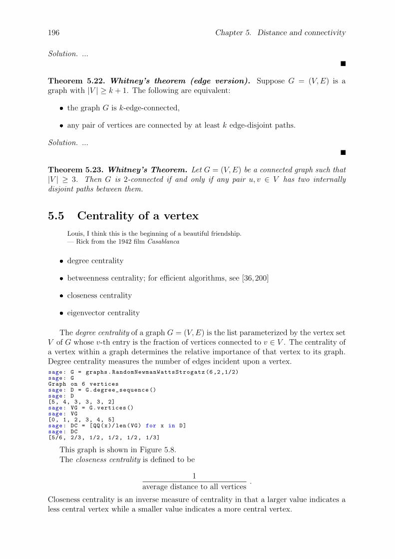
196 Chapter 5. Distance and connectivity
Solution. ...
Theorem 5.22. Whitney’s theorem (edge version). Suppose G = (V,E) is agraph with |V | ≥ k + 1. The following are equivalent:
the graph G is k-edge-connected,
any pair of vertices are connected by at least k edge-disjoint paths.
Solution. ...
Theorem 5.23. Whitney’s Theorem. Let G = (V,E) be a connected graph such that|V | ≥ 3. Then G is 2-connected if and only if any pair u, v ∈ V has two internallydisjoint paths between them.
5.5 Centrality of a vertex
Louis, I think this is the beginning of a beautiful friendship.— Rick from the 1942 film Casablanca
degree centrality
betweenness centrality; for efficient algorithms, see [36,200]
closeness centrality
eigenvector centrality
The degree centrality of a graph G = (V,E) is the list parameterized by the vertex setV of G whose v-th entry is the fraction of vertices connected to v ∈ V . The centrality ofa vertex within a graph determines the relative importance of that vertex to its graph.Degree centrality measures the number of edges incident upon a vertex.sage: G = graphs.RandomNewmanWattsStrogatz (6 ,2,1/2)sage: GGraph on 6 verticessage: D = G.degree_sequence ()sage: D[5, 4, 3, 3, 3, 2]sage: VG = G.vertices ()sage: VG[0, 1, 2, 3, 4, 5]sage: DC = [QQ(x)/len(VG) for x in D]sage: DC[5/6, 2/3, 1/2, 1/2, 1/2, 1/3]
This graph is shown in Figure 5.8.The closeness centrality is defined to be
1
average distance to all vertices.
Closeness centrality is an inverse measure of centrality in that a larger value indicates aless central vertex while a smaller value indicates a more central vertex.
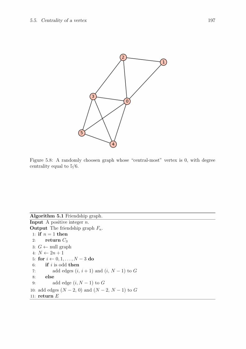
5.5. Centrality of a vertex 197
Figure 5.8: A randomly choosen graph whose “central-most” vertex is 0, with degreecentrality equal to 5/6.
Algorithm 5.1 Friendship graph.Input A positive integer n.Output The friendship graph Fn.
1: if n = 1 then2: return C3
3: G← null graph4: N ← 2n+ 15: for i← 0, 1, . . . , N − 3 do6: if i is odd then7: add edges (i, i+ 1) and (i, N − 1) to G8: else9: add edge (i, N − 1) to G
10: add edges (N − 2, 0) and (N − 2, N − 1) to G11: return E
198 Chapter 5. Distance and connectivity
5.6 Network reliability
Whitney synthesis
Tutte’s synthesis of 3-connected graphs
Harary graphs
constructing an optimal k-connected n-vertex graph
5.7 The spectrum of a graph
We use the notes “The spectrum of a graph” by Andries Brouwer [40] as a basic reference.
Spectrum of a graph
Laplacian spectrum of a graph
Applications
Examples from Boolean functions
Let G = (V,E) be a (possibly directed) finite graph on n = |V | vertices. Theadjacency matrix of G is the n × n matrix A = A(G) = (av,w)v,w∈V with rows andcolumns indexed by V and entries av,w denoting the number of edges from v to w.
The spectrum of G, spec(G), is by definition the spectrum of A, that is, its multi-setof eigenvalues together with their multiplicities. The characteristic polynomial of G isthat of A, that is, the polynomial pA defined by pA(x) = det(A− xI).
5.7.1 The Laplacian spectrum
Recall from section 1.3.3 that, given a simple graph G with n vertices V = v1, . . . , vn,its (vertex) Laplacian matrix L = (`i,j)n×n is defined as:
`i,j =
deg(vi), if i = j,
−1, if i 6= j and vi is adjacent to vj,
0, otherwise.
The Laplacian spectrum is by definition the spectrum of the vertex Laplacian of G, thatis, its multi-set of eigenvalues together with their multiplicities.
For a graph G and its Laplacian matrix L with eigenvalues λn ≤ λn−1 ≤ · · · ≤ λ1:
For all i, λi ≥ 0 and λn = 0.
The number of times 0 appears as an eigenvalue in the Laplacian is the number ofconnected components in the graph.
λn = 0 because every Laplacian matrix has an eigenvector of [1, 1, . . . , 1],
5.7. The spectrum of a graph 199
If we define a signed edge adjacency matrix M with element me,v for edge e ∈ E(connecting vertex vi and vj, with i < j) and vertex v ∈ V given by
Mev =
1, if v = vi,
−1, if v = vj,
0, otherwise
then the Laplacian matrix L satisifies L = MTM , where MT is the matrix trans-pose of M .
These are left as an exercise.
5.7.2 Applications of the (ordinary) spectrum
The following is a basic fact about the largest eigenvalue of a graph.
Theorem 5.24. Each graph G has a real eigenvalue λ1 > 0 with nonnegative real cor-responding eigenvector, and such that for each eigenvalue λ we have |λ| ≤ λ1.
We shall mostly be interested in the case where G is undirected, without loops ormultiple edges. This means that A is symmetric, has zero diagonal (av,v = 0), and is a0-1 matrix ( av,w ∈ 0, 1).
A number λ is eigenvalue of A if and only if it is a zero of the polynomial pA.Since A is real and symmetric, all its eigenvalues are real and A is diagonalizable. Inparticular, for each eigenvalue, its algebraic multiplicity (that is, its multiplicity as aroot of the characteristic polynomial) coincides with its geometric multiplicity (that is,the dimension of the corresponding eigenspace).
Theorem 5.25. Let G be a connected graph of diameter d. Then G has at least d + 1distinct eigenvalues.
Proof. Let the distinct eigenvalues of the adjacency matrix A of G be λ1, ..., λr. Then(A − λ1I)...(A − λrI) = 0, so that Ar is a linear combination of I, A, ..., Ar−1. But ifthe distance from the vertex v ∈ V to the vertex w ∈ V is r, then (Ai)v,w = 0 for0 ≤ i ≤ r − 1 and (Ar)v,w > 0, contradiction. Hence d > r.
5.7.3 Examples from Boolean functions
Let f be a Boolean function on GF (2)n. The Cayley graph of f is defined to be thegraph
Γf = (GF (2)n, Ef ),
whose vertex set is GF (2)n and the set of edges is defined by
Ef = (u, v) ∈ GF (2)n ×GF (2)n | f(u+ v) = 1.The adjacency matrix Af of this graph is the matrix whose entries are
Ai,j = f(b(i) + b(j)),
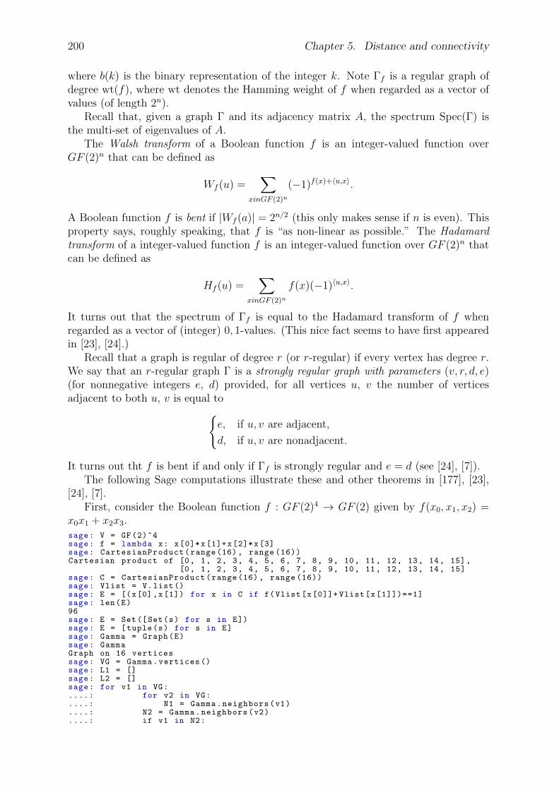
200 Chapter 5. Distance and connectivity
where b(k) is the binary representation of the integer k. Note Γf is a regular graph ofdegree wt(f), where wt denotes the Hamming weight of f when regarded as a vector ofvalues (of length 2n).
Recall that, given a graph Γ and its adjacency matrix A, the spectrum Spec(Γ) isthe multi-set of eigenvalues of A.
The Walsh transform of a Boolean function f is an integer-valued function overGF (2)n that can be defined as
Wf (u) =∑
xinGF (2)n
(−1)f(x)+〈u,x〉.
A Boolean function f is bent if |Wf (a)| = 2n/2 (this only makes sense if n is even). Thisproperty says, roughly speaking, that f is “as non-linear as possible.” The Hadamardtransform of a integer-valued function f is an integer-valued function over GF (2)n thatcan be defined as
Hf (u) =∑
xinGF (2)n
f(x)(−1)〈u,x〉.
It turns out that the spectrum of Γf is equal to the Hadamard transform of f whenregarded as a vector of (integer) 0, 1-values. (This nice fact seems to have first appearedin [23], [24].)
Recall that a graph is regular of degree r (or r-regular) if every vertex has degree r.We say that an r-regular graph Γ is a strongly regular graph with parameters (v, r, d, e)(for nonnegative integers e, d) provided, for all vertices u, v the number of verticesadjacent to both u, v is equal to
e, if u, v are adjacent,
d, if u, v are nonadjacent.
It turns out tht f is bent if and only if Γf is strongly regular and e = d (see [24], [7]).The following Sage computations illustrate these and other theorems in [177], [23],
[24], [7].First, consider the Boolean function f : GF (2)4 → GF (2) given by f(x0, x1, x2) =
x0x1 + x2x3.sage: V = GF(2)^4sage: f = lambda x: x[0]*x[1]+x[2]*x[3]sage: CartesianProduct(range (16), range (16))Cartesian product of [0, 1, 2, 3, 4, 5, 6, 7, 8, 9, 10, 11, 12, 13, 14, 15],
[0, 1, 2, 3, 4, 5, 6, 7, 8, 9, 10, 11, 12, 13, 14, 15]sage: C = CartesianProduct(range (16), range (16))sage: Vlist = V.list()sage: E = [(x[0],x[1]) for x in C if f(Vlist[x[0]]+ Vlist[x[1]])==1]sage: len(E)96sage: E = Set([Set(s) for s in E])sage: E = [tuple(s) for s in E]sage: Gamma = Graph(E)sage: GammaGraph on 16 verticessage: VG = Gamma.vertices ()sage: L1 = []sage: L2 = []sage: for v1 in VG:....: for v2 in VG:....: N1 = Gamma.neighbors(v1)....: N2 = Gamma.neighbors(v2)....: if v1 in N2:
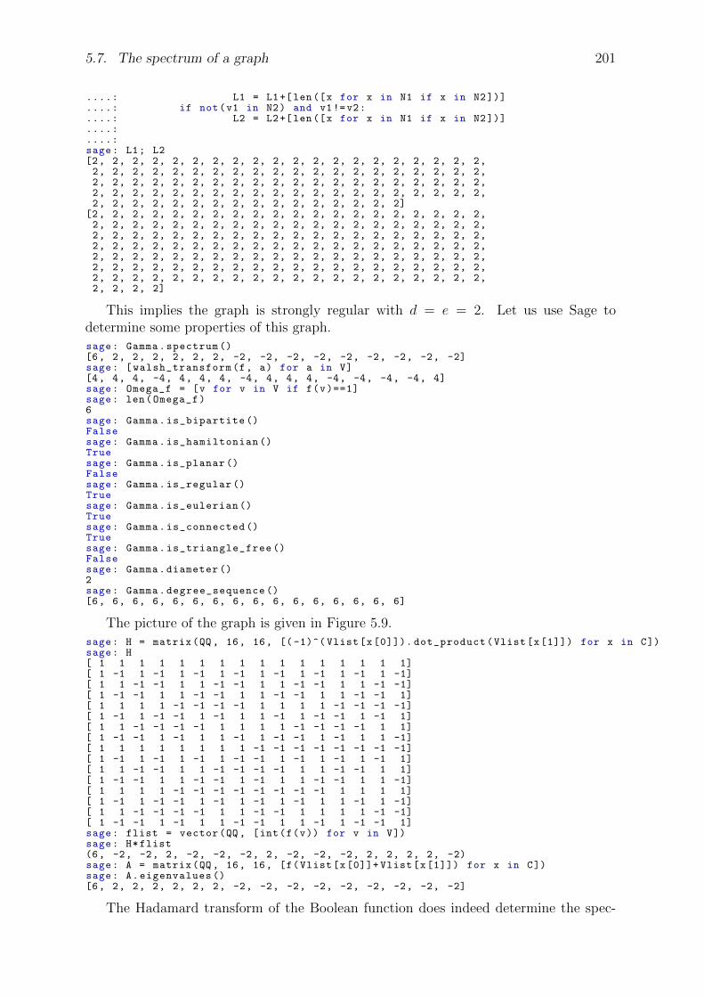
5.7. The spectrum of a graph 201
....: L1 = L1+[len([x for x in N1 if x in N2])]
....: if not(v1 in N2) and v1!=v2:
....: L2 = L2+[len([x for x in N1 if x in N2])]
....:
....:sage: L1; L2[2, 2, 2, 2, 2, 2, 2, 2, 2, 2, 2, 2, 2, 2, 2, 2, 2, 2, 2, 2,2, 2, 2, 2, 2, 2, 2, 2, 2, 2, 2, 2, 2, 2, 2, 2, 2, 2, 2, 2,2, 2, 2, 2, 2, 2, 2, 2, 2, 2, 2, 2, 2, 2, 2, 2, 2, 2, 2, 2,2, 2, 2, 2, 2, 2, 2, 2, 2, 2, 2, 2, 2, 2, 2, 2, 2, 2, 2, 2,2, 2, 2, 2, 2, 2, 2, 2, 2, 2, 2, 2, 2, 2, 2, 2]
[2, 2, 2, 2, 2, 2, 2, 2, 2, 2, 2, 2, 2, 2, 2, 2, 2, 2, 2, 2,2, 2, 2, 2, 2, 2, 2, 2, 2, 2, 2, 2, 2, 2, 2, 2, 2, 2, 2, 2,2, 2, 2, 2, 2, 2, 2, 2, 2, 2, 2, 2, 2, 2, 2, 2, 2, 2, 2, 2,2, 2, 2, 2, 2, 2, 2, 2, 2, 2, 2, 2, 2, 2, 2, 2, 2, 2, 2, 2,2, 2, 2, 2, 2, 2, 2, 2, 2, 2, 2, 2, 2, 2, 2, 2, 2, 2, 2, 2,2, 2, 2, 2, 2, 2, 2, 2, 2, 2, 2, 2, 2, 2, 2, 2, 2, 2, 2, 2,2, 2, 2, 2, 2, 2, 2, 2, 2, 2, 2, 2, 2, 2, 2, 2, 2, 2, 2, 2,2, 2, 2, 2]
This implies the graph is strongly regular with d = e = 2. Let us use Sage todetermine some properties of this graph.sage: Gamma.spectrum ()[6, 2, 2, 2, 2, 2, 2, -2, -2, -2, -2, -2, -2, -2, -2, -2]sage: [walsh_transform(f, a) for a in V][4, 4, 4, -4, 4, 4, 4, -4, 4, 4, 4, -4, -4, -4, -4, 4]sage: Omega_f = [v for v in V if f(v)==1]sage: len(Omega_f)6sage: Gamma.is_bipartite ()Falsesage: Gamma.is_hamiltonian ()Truesage: Gamma.is_planar ()Falsesage: Gamma.is_regular ()Truesage: Gamma.is_eulerian ()Truesage: Gamma.is_connected ()Truesage: Gamma.is_triangle_free ()Falsesage: Gamma.diameter ()2sage: Gamma.degree_sequence ()[6, 6, 6, 6, 6, 6, 6, 6, 6, 6, 6, 6, 6, 6, 6, 6]
The picture of the graph is given in Figure 5.9.sage: H = matrix(QQ, 16, 16, [( -1)^( Vlist[x[0]]). dot_product(Vlist[x[1]]) for x in C])sage: H[ 1 1 1 1 1 1 1 1 1 1 1 1 1 1 1 1][ 1 -1 1 -1 1 -1 1 -1 1 -1 1 -1 1 -1 1 -1][ 1 1 -1 -1 1 1 -1 -1 1 1 -1 -1 1 1 -1 -1][ 1 -1 -1 1 1 -1 -1 1 1 -1 -1 1 1 -1 -1 1][ 1 1 1 1 -1 -1 -1 -1 1 1 1 1 -1 -1 -1 -1][ 1 -1 1 -1 -1 1 -1 1 1 -1 1 -1 -1 1 -1 1][ 1 1 -1 -1 -1 -1 1 1 1 1 -1 -1 -1 -1 1 1][ 1 -1 -1 1 -1 1 1 -1 1 -1 -1 1 -1 1 1 -1][ 1 1 1 1 1 1 1 1 -1 -1 -1 -1 -1 -1 -1 -1][ 1 -1 1 -1 1 -1 1 -1 -1 1 -1 1 -1 1 -1 1][ 1 1 -1 -1 1 1 -1 -1 -1 -1 1 1 -1 -1 1 1][ 1 -1 -1 1 1 -1 -1 1 -1 1 1 -1 -1 1 1 -1][ 1 1 1 1 -1 -1 -1 -1 -1 -1 -1 -1 1 1 1 1][ 1 -1 1 -1 -1 1 -1 1 -1 1 -1 1 1 -1 1 -1][ 1 1 -1 -1 -1 -1 1 1 -1 -1 1 1 1 1 -1 -1][ 1 -1 -1 1 -1 1 1 -1 -1 1 1 -1 1 -1 -1 1]sage: flist = vector(QQ, [int(f(v)) for v in V])sage: H*flist(6, -2, -2, 2, -2, -2, -2, 2, -2, -2, -2, 2, 2, 2, 2, -2)sage: A = matrix(QQ, 16, 16, [f(Vlist[x[0]]+ Vlist[x[1]]) for x in C])sage: A.eigenvalues ()[6, 2, 2, 2, 2, 2, 2, -2, -2, -2, -2, -2, -2, -2, -2, -2]
The Hadamard transform of the Boolean function does indeed determine the spec-
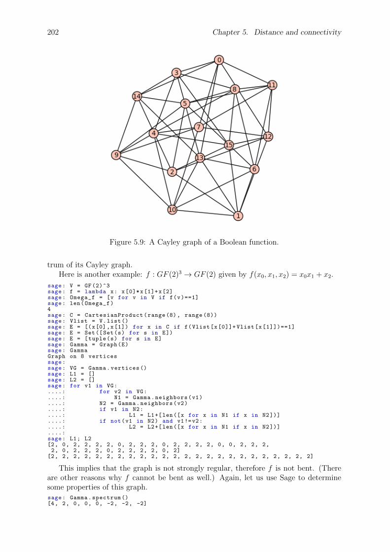
202 Chapter 5. Distance and connectivity
Figure 5.9: A Cayley graph of a Boolean function.
trum of its Cayley graph.Here is another example: f : GF (2)3 → GF (2) given by f(x0, x1, x2) = x0x1 + x2.
sage: V = GF(2)^3sage: f = lambda x: x[0]*x[1]+x[2]sage: Omega_f = [v for v in V if f(v)==1]sage: len(Omega_f)4sage: C = CartesianProduct(range (8), range (8))sage: Vlist = V.list()sage: E = [(x[0],x[1]) for x in C if f(Vlist[x[0]]+ Vlist[x[1]])==1]sage: E = Set([Set(s) for s in E])sage: E = [tuple(s) for s in E]sage: Gamma = Graph(E)sage: GammaGraph on 8 verticessage:sage: VG = Gamma.vertices ()sage: L1 = []sage: L2 = []sage: for v1 in VG:....: for v2 in VG:....: N1 = Gamma.neighbors(v1)....: N2 = Gamma.neighbors(v2)....: if v1 in N2:....: L1 = L1+[len([x for x in N1 if x in N2])]....: if not(v1 in N2) and v1!=v2:....: L2 = L2+[len([x for x in N1 if x in N2])]....:sage: L1; L2[2, 0, 2, 2, 2, 2, 0, 2, 2, 2, 0, 2, 2, 2, 2, 0, 0, 2, 2, 2,2, 0, 2, 2, 2, 0, 2, 2, 2, 2, 0, 2]
[2, 2, 2, 2, 2, 2, 2, 2, 2, 2, 2, 2, 2, 2, 2, 2, 2, 2, 2, 2, 2, 2, 2, 2]
This implies that the graph is not strongly regular, therefore f is not bent. (Thereare other reasons why f cannot be bent as well.) Again, let us use Sage to determinesome properties of this graph.sage: Gamma.spectrum ()[4, 2, 0, 0, 0, -2, -2, -2]

5.8. Expander graphs and Ramanujan graphs 203
sage:sage: Gamma.is_bipartite ()Falsesage: Gamma.is_hamiltonian ()Truesage: Gamma.is_planar ()Falsesage: Gamma.is_regular ()Truesage: Gamma.is_eulerian ()Truesage: Gamma.is_connected ()Truesage: Gamma.is_triangle_free ()Falsesage: Gamma.diameter ()2sage: Gamma.degree_sequence ()[4, 4, 4, 4, 4, 4, 4, 4]sage: H = matrix(QQ, 8, 8, [( -1)^( Vlist[x[0]]). dot_product(Vlist[x[1]]) for x in C])sage: H[ 1 1 1 1 1 1 1 1][ 1 -1 1 -1 1 -1 1 -1][ 1 1 -1 -1 1 1 -1 -1][ 1 -1 -1 1 1 -1 -1 1][ 1 1 1 1 -1 -1 -1 -1][ 1 -1 1 -1 -1 1 -1 1][ 1 1 -1 -1 -1 -1 1 1][ 1 -1 -1 1 -1 1 1 -1]sage: flist = vector(QQ, [int(f(v)) for v in V])sage: H*flist(4, 0, 0, 0, -2, -2, -2, 2)sage: Gamma.spectrum ()[4, 2, 0, 0, 0, -2, -2, -2]sage: A = matrix(QQ, 8, 8, [f(Vlist[x[0]]+ Vlist[x[1]]) for x in C])sage: A.eigenvalues ()[4, 2, 0, 0, 0, -2, -2, -2]
Again, we see the Hadamard transform does indeed determine the graph spectrum.The picture of the graph is given in Figure 5.10.
Figure 5.10: Another Cayley graph of a Boolean function.
5.8 Expander graphs and Ramanujan graphs
In combinatorics, an expander graph is a sparse graph that has strong connectivityproperties. Expander graphs have many applications - for example, to cryptography,

204 Chapter 5. Distance and connectivity
and the theory of error-correcting codes.The edge expansion h(G) of a graph G = (V,E) is defined as
h(G) = min0<|S|≤ |V |
2
|∂(S)||S| ,
where the minimum is over all nonempty sets S of at most |V |/2 vertices and ∂(S) isthe edge boundary of S, i.e., the set of edges with exactly one endpoint in S.
The vertex expansion (or vertex isoperimetric number) hout(G) of a graph G is definedas
hout(G) = min0<|S|≤ |V |
2
|∂out(S)||S| ,
where ∂out(S) is the outer boundary of S, i.e., the set of vertices in V (G) \ S with atleast one neighbor in S.sage: G = PSL(2, 5)sage: X = G.cayley_graph ()sage: V = X.vertices ()sage: S = [V[1], V[3], V[7], V[10], V[13], V[ 14], V[23]]sage: delS = X.edge_boundary(S)sage: edge_expan_XS = len(delS)/len(S); RR(edge_expan_XS)1.00000000000000sage: S = [V[1], V[3], V[7], V[12], V[24], V[37]]sage: delS = X.edge_boundary(S)sage: edge_expan_XS = len(delS)/len(S); RR(edge_expan_XS)1.50000000000000sage: S = [V[2], V[8], V[13], V[27], V[32], V[44], V[57]]sage: delS = X.edge_boundary(S)sage: edge_expan_XS = len(delS)/len(S); RR(edge_expan_XS)1.42857142857143sage: S = [V[0], V[6], V[11], V[16], V[21], V[29], V[35], V[45],V[53]]sage: delS = X.edge_boundary(S)sage: edge_expan_XS = len(delS)/len(S); RR(edge_expan_XS)1.77777777777778sage: n = len(X.vertices ())sage: J = range(n)sage: J30 = Subsets(J, int(n/2))sage: K = J30.random_element ()sage: K0, 2, 3, 4, 5, 6, 8, 9, 11, 13, 16, 18, 19, 21, 24, 25, 26, 28, 29,30, 36, 37, 38, 40, 42, 45, 46, 49, 53, 57
sage: S = [V[i] for i in K] # 30 vertices , randomly selectedsage: delS = [v for v in V if min([X.distance(a,v) for a in S]) == 1]sage: RR(len(delS ))/RR(len(S))0.800000000000000
A family G = G1, G2, . . . of d-regular graphs is an edge expander family if there is aconstant c > 0 such that h(G) ≥ c for each G ∈ G. A vertex expander family is definedsimilarly, using hout(G) instead.
5.8.1 Ramanujan graphs
Let G be a connected d-regular graph with n vertices, and let λ0 ≥ λ1 ≥ . . . ≥ λn−1
be the eigenvalues of the adjacency matrix of G. Because G is connected and d-regular,its eigenvalues satisfy d = λ0 > λ1 ≥ . . . ≥ λn−1 ≥ −d. Whenever there exists λi with|λi| < d, define
λ(G) = max|λi|<d
|λi|.
A d-regular graph G is a Ramanujan graph if λ(G) is defined and λ(G) ≤ 2√d− 1.
5.9. Problems 205
Let q be a prime power such that q ≡ 1 (mod 4). Note that this implies that thefinite field GF (q) contains a square root of −1.
Now let V = GF (q) and E = a, b ∈ GF (q)×GF (q) | (a− b) ∈ GF (q)×)2. Thisset is well defined since a − b = (−1) · (b − a), and since −1 is a square, it follows thata−b is a square if and only if b− a is a square.
By definition G = (V, E) is the Paley graph of order q.The following facts are known about Paley graphs.
The eigenvalues of Paley graphs are q−12
(with multiplicity 1) and−1±√q
2(both with
multiplicity q−12
).
It is known that a Paley graph is a Ramanujan graph.
It is known that the family of Paley graphs of prime order is a vertex expandergraph family.
If q = pr, where p is prime, then Aut(G) has order q(q − 1)/2.
Here is Sage code for the Paley graph1:def Paley(q):
K.<a> = GF(q)return Graph ([K, lambda i,j: i != j and (i-j). is_square ()])
Below is an example.sage: X = Paley (13)sage: X.vertices ()[0, 1, 2, 3, 4, 5, 6, 7, 8, 9, 10, 11, 12]sage: X.is_vertex_transitive ()Truesage: X.degree_sequence ()[6, 6, 6, 6, 6, 6, 6, 6, 6, 6, 6, 6, 6]sage: X.spectrum ()[6, 1.302775637731995? , 1.302775637731995? , 1.302775637731995? ,1.302775637731995? , 1.302775637731995? , 1.302775637731995? ,-2.302775637731995? , -2.302775637731995? , -2.302775637731995? ,-2.302775637731995? , -2.302775637731995? , -2.302775637731995?]sage: G = X.automorphism_group ()sage: G.cardinality ()78sage: 13*12/278
5.9 Problems
When you don’t share your problems, you resent hearing the problems of other people.— Chuck Palahniuk, Invisible Monsters, 1999
5.1. Let G = (V,E) be an undirected, unweighted simple graph. Show that V and thedistance function on G form a metric space if and only if G is connected.
5.2. Let u and v be two distinct vertices in the same connected component of G. If Pis a u-v path such that d(u, v) = ε(u), we say that P is an eccentricity path for u.
(a) If r is the root of a tree, show that the end-vertex of an eccentricity path forr is a leaf.
1Thanks to Chris Godsil; see [86].
206 Chapter 5. Distance and connectivity
(b) If v is a vertex of a tree distinct from the root r, show that any eccentricitypath for v must contain r or provide an example to the contrary.
(c) A vertex w is said to be an eccentric vertex of v if d(v, w) = ε(v). Intuitively,an eccentric vertex of v can be considered as being as far away from v aspossible. If w is an eccentric vertex of v and vice versa, then v and w are saidto be mutually eccentric. See Buckley and Lau [45] for detailed discussions ofmutual eccentricity. If w is an eccentric vertex of v, explain why v is also aneccentric vertex of w or show that this does not in general hold.
5.3. If u and v are vertices of a connected graph G such that d(u, v) = diam(G), showthat u and v are mutually eccentric.
5.4. If uv is an edge of a tree T and w is a vertex of T distinct from u and v, show that|d(u,w)− d(w, v)| = W (uv) with W (uv) being the weight of uv.
5.5. If u and v are vertices of a tree T such that d(u, v) = diam(T ), show that u and vare leaves.
5.6. Let v1, v2, . . . , vk be the leaves of a tree T . Show that per(T ) = v1, v2, . . . , vk.
5.7. Show that all the eccentric vertices of a tree are leaves.
5.8. If G is a connected graph, show that rad(G) ≤ diam(G) ≤ 2 · rad(G).
5.9. Let T be a tree of order ≥ 3. If the center of T has one vertex, show that diam(T ) =2 · rad(T ). If the center of T has two vertices, show that diam(T ) = 2 · rad(T )− 1.
5.10. Let G = (V,E) be a simple undirected, connected graph. Define the distance of avertex v ∈ V by
d(v) =∑
x∈V
d(v, x)
and define the distance of the graph G itself by
d(G) =1
2
∑
v∈V
d(v).
For any vertex v ∈ V , show that d(G) ≤ d(v) +d(G− v) with G− v being a vertexdeletion subgraph of G. This result appeared in Entringer et al. [70, p.284].
5.11. Determine the sequence of distance matrices for the graphs in Figure 5.4.
5.12. If G = (V,E) is an undirected connected graph and v ∈ V , prove the followingvertex connectivity inequality:
κ(G)− 1 ≤ κ(G− v) ≤ κ(G).
5.13. If G = (V,E) is an undirected connected graph and e ∈ E, prove the followingedge connectivity inequality:
λ(G)− 1 ≤ λ(G− e) ≤ λ(G).

5.9. Problems 207
0
1
2
3
4
5
6
78
9
10
11
12
13
14 15
16
17
18
19
20
21
22
23
24
25
26
27
2829
30
31
32
33
34
35
36
37
38
39
40
41
42
43
44
45
46
47
48
49
50
51
52
53
Figure 5.11: Network of common grape cultivars.
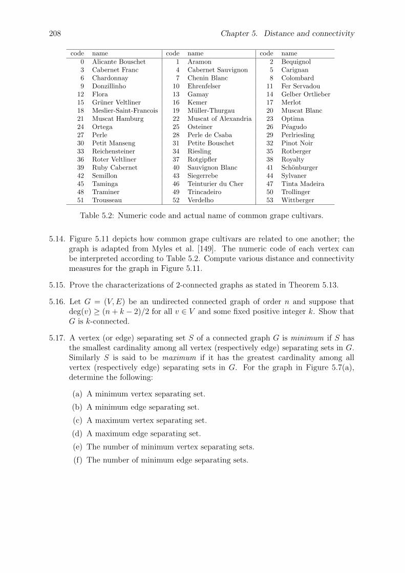
208 Chapter 5. Distance and connectivity
code name code name code name0 Alicante Bouschet 1 Aramon 2 Bequignol3 Cabernet Franc 4 Cabernet Sauvignon 5 Carignan6 Chardonnay 7 Chenin Blanc 8 Colombard9 Donzillinho 10 Ehrenfelser 11 Fer Servadou
12 Flora 13 Gamay 14 Gelber Ortlieber15 Gruner Veltliner 16 Kemer 17 Merlot18 Meslier-Saint-Francois 19 Muller-Thurgau 20 Muscat Blanc21 Muscat Hamburg 22 Muscat of Alexandria 23 Optima24 Ortega 25 Osteiner 26 Peagudo27 Perle 28 Perle de Csaba 29 Perlriesling30 Petit Manseng 31 Petite Bouschet 32 Pinot Noir33 Reichensteiner 34 Riesling 35 Rotberger36 Roter Veltliner 37 Rotgipfler 38 Royalty39 Ruby Cabernet 40 Sauvignon Blanc 41 Schonburger42 Semillon 43 Siegerrebe 44 Sylvaner45 Taminga 46 Teinturier du Cher 47 Tinta Madeira48 Traminer 49 Trincadeiro 50 Trollinger51 Trousseau 52 Verdelho 53 Wittberger
Table 5.2: Numeric code and actual name of common grape cultivars.
5.14. Figure 5.11 depicts how common grape cultivars are related to one another; thegraph is adapted from Myles et al. [149]. The numeric code of each vertex canbe interpreted according to Table 5.2. Compute various distance and connectivitymeasures for the graph in Figure 5.11.
5.15. Prove the characterizations of 2-connected graphs as stated in Theorem 5.13.
5.16. Let G = (V,E) be an undirected connected graph of order n and suppose thatdeg(v) ≥ (n+ k − 2)/2 for all v ∈ V and some fixed positive integer k. Show thatG is k-connected.
5.17. A vertex (or edge) separating set S of a connected graph G is minimum if S hasthe smallest cardinality among all vertex (respectively edge) separating sets in G.Similarly S is said to be maximum if it has the greatest cardinality among allvertex (respectively edge) separating sets in G. For the graph in Figure 5.7(a),determine the following:
(a) A minimum vertex separating set.
(b) A minimum edge separating set.
(c) A maximum vertex separating set.
(d) A maximum edge separating set.
(e) The number of minimum vertex separating sets.
(f) The number of minimum edge separating sets.

Chapter 6
Centrality and prestige
6.1 Vertex centrality
6.2 Edge centrality
6.3 Ranking web pages
6.4 Hub and authority
6.5 Problems
6.1. A.
209

Chapter 7
Optimal graph traversals
7.1 Eulerian graphs
Motivation: tracing out all the edges of a graph without lifting your pencil.
multigraphs and simple graphs
Eulerian tours
Eulerian trails
7.2 Hamiltonian graphs
— Randall Munroe, xkcd, http://xkcd.com/230/
Motivation: the eager tourist problem: visiting all major sites of a city in the leasttime/distance.
Hamiltonian paths (or cycles)
Hamiltonian graphs
Theorem 7.1. Ore 1960. Let G be a simple graph with n ≥ 3 vertices. If deg(u) +deg(v) ≥ n for each pair of non-adjacent vertices u, v ∈ V (G), then G is Hamiltonian.
Corollary 7.2. Dirac 1952. Let G be a simple graph with n ≥ 3 vertices. If deg(v) ≥n/2 for all v ∈ V (G), then G is Hamiltonian.
210
7.3. The Chinese Postman Problem 211
7.3 The Chinese Postman Problem
See section 6.2 of Gross and Yellen [91].
de Bruijn sequences
de Bruijn digraphs
constructing a (2, n)-de Bruijn sequence
postman tours and optimal postman tours
constructing an optimal postman tour
7.4 The Traveling Salesman Problem
— Randall Munroe, xkcd, http://xkcd.com/399/
See section 6.4 of Gross and Yellen [91], and section 35.2 of Cormen et al. [57].
Gray codes and n-dimensional hypercubes
the Traveling Salesman Problem (TSP)
nearest neighbor heuristic for TSP
some other heuristics for solving TSP

Chapter 8
Graph coloring
— Spiked Math, http://spikedmath.com/210.html
See Jensen and Toft [108] for a survey of graph coloring problems.
See Dyer and Frieze [66] for an algorithm on randomly colouring random graphs.
Graph coloring problems originated with the coloring of maps. For example, regardeach state in the United States as a vertex, and connect two vertices by an edge if andonly if they share a boundary, i.e., are neighbors. If you can color the United Statesmap using k colors in such a way that no two neighboring states have the same colorthen we say the map has a k-coloring. While a student in London in the mid-1800’s, theSouth African mathematician Francis Guthrie conjectured to his mathematics professorAugustus de Morgan that four colors suffice to color any map. It was an open problemfor over 100 years (only proven by Appel and Haken in 1976).
8.1 Vertex coloring
When used without any qualification, a coloring of an undirected graph G = (V,E) isintended to mean a vertex coloring, namely a labelling of the graph’s vertices with colorssuch that no two vertices sharing an edge have the same color.
A coloring using at most k colors is called a (proper) k-coloring. For example, the2-colorable graphs are exactly the bipartite graphs.
212

8.1. Vertex coloring 213
Remark 8.1. For each k = 3, 4, . . . , the corresponding decision problem of deciding if agiven graph can be k-colored is NP-hard (see [106]).
The smallest number of colors needed to color a graph G is called its (vertex) chro-matic number, and is here denoted χv(G). A subset of V assigned to the same color iscalled a color-class. A subset S of V is called an independent set if no two vertices in Sare adjacent in G. By definition, every color-class forms an independent set. The set oft-colorings is in one-to-one correspondence with the partitions of V into t independentsets.
Example 8.2. The Dyck graph, shown in Figure 8.1, is named after Walther von Dyck.It is a 3-regular graph with 32 vertices and 48 edges. The graph is Hamiltonian with 120distinct Hamiltonian cycles. It has chromatic number 2 (in other words, is bipartite),chromatic index 3, radius 5, diameter 5 and girth 6. It is also a 3-vertex-connected anda 3-edge-connected graph.
sage: G = graphs.LCFGraph (32, [5,-5,13,-13], 8)sage: G.is_bipartite ()Truesage: G.coloring ()[[1, 3, 5, 7, 9, 11, 13, 15, 17, 19, 21, 23, 25, 27, 29, 31],[0, 2, 4, 6, 8, 10, 12, 14, 16, 18, 20, 22, 24, 26, 28, 30]]
sage: G.is_vertex_transitive ()True
Figure 8.1: A Dyck graph example.
A clique in G is a subset of the vertex set S ⊂ V , such that for every two vertices inS, there exists an edge connecting the two. The clique number ω(G) of a graph G is thenumber of vertices in a maximal clique (a clique which cannot be extended to a cliqueof larger size by adding a vertex to it) in G. From the definitions, we see that thechromatic number is at least the clique number:
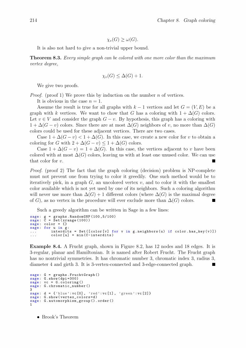
214 Chapter 8. Graph coloring
χv(G) ≥ ω(G).
It is also not hard to give a non-trivial upper bound.
Theorem 8.3. Every simple graph can be colored with one more color than the maximumvertex degree,
χv(G) ≤ ∆(G) + 1.
We give two proofs.
Proof. (proof 1) We prove this by induction on the number n of vertices.It is obvious in the case n = 1.Assume the result is true for all graphs with k − 1 vertices and let G = (V,E) be a
graph with k vertices. We want to chow that G has a coloring with 1 + ∆(G) colors.Let v ∈ V and consider the graph G− v. By hypothesis, this graph has a coloring with1 + ∆(G− v) colors. Since there are at most ∆(G) neighbors of v, no more than ∆(G)colors could be used for these adjacent vertices. There are two cases.
Case 1 + ∆(G− v) < 1 + ∆(G). In this case, we create a new color for v to obtain acoloring for G with 2 + ∆(G− v) ≤ 1 + ∆(G) colors.
Case 1 + ∆(G − v) = 1 + ∆(G). In this case, the vertices adjacent to v have beencolored with at most ∆(G) colors, leaving us with at least one unused color. We can usethat color for v.
Proof. (proof 2) The fact that the graph coloring (decision) problem is NP-completemust not prevent one from trying to color it greedily. One such method would be toiteratively pick, in a graph G, an uncolored vertex v, and to color it with the smallestcolor available which is not yet used by one of its neighbors. Such a coloring algorithmwill never use more than ∆(G) + 1 different colors (where ∆(G) is the maximal degreeof G), as no vertex in the procedure will ever exclude more than ∆(G) colors.
Such a greedy algorithm can be written in Sage in a few lines:sage: g = graphs.RandomGNP (100 ,5/100)sage: C = Set(xrange (100))sage: color = sage: for u in g:... interdits = Set([ color[v] for v in g.neighbors(u) if color.has_key(v)])... color[u] = min(C-interdits)
Example 8.4. A Frucht graph, shown in Figure 8.2, has 12 nodes and 18 edges. It is3-regular, planar and Hamiltonian. It is named after Robert Frucht. The Frucht graphhas no nontrivial symmetries. It has chromatic number 3, chromatic index 3, radius 3,diameter 4 and girth 3. It is 3-vertex-connected and 3-edge-connected graph.
sage: G = graphs.FruchtGraph ()sage: G.show(dpi =300)sage: vc = G.coloring ()sage: G.chromatic_number ()3sage: d = ’blue’:vc[0], ’red’:vc[1], ’green ’:vc[2]sage: G.show(vertex_colors=d)sage: G.automorphism_group (). order ()1
Brook’s Theorem
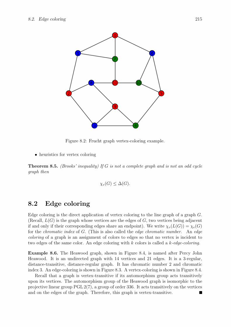
8.2. Edge coloring 215
Figure 8.2: Frucht graph vertex-coloring example.
heuristics for vertex coloring
Theorem 8.5. (Brooks’ inequality) If G is not a complete graph and is not an odd cyclegraph then
χv(G) ≤ ∆(G).
8.2 Edge coloring
Edge coloring is the direct application of vertex coloring to the line graph of a graph G.(Recall, L(G) is the graph whose vertices are the edges of G, two vertices being adjacentif and only if their corresponding edges share an endpoint). We write χv(L(G)) = χe(G)for the chromatic index of G. (This is also called the edge chromatic number. An edgecoloring of a graph is an assignment of colors to edges so that no vertex is incident totwo edges of the same color. An edge coloring with k colors is called a k-edge-coloring.
Example 8.6. The Heawood graph, shown in Figure 8.4, is named after Percy JohnHeawood. It is an undirected graph with 14 vertices and 21 edges. It is a 3-regular,distance-transitive, distance-regular graph. It has chromatic number 2 and chromaticindex 3. An edge-coloring is shown in Figure 8.3. A vertex-coloring is shown in Figure 8.4.
Recall that a graph is vertex-transitive if its automorphism group acts transitivelyupon its vertices. The automorphism group of the Heawood graph is isomorphic to theprojective linear group PGL 2(7), a group of order 336. It acts transitively on the verticesand on the edges of the graph. Therefore, this graph is vertex-transitive.
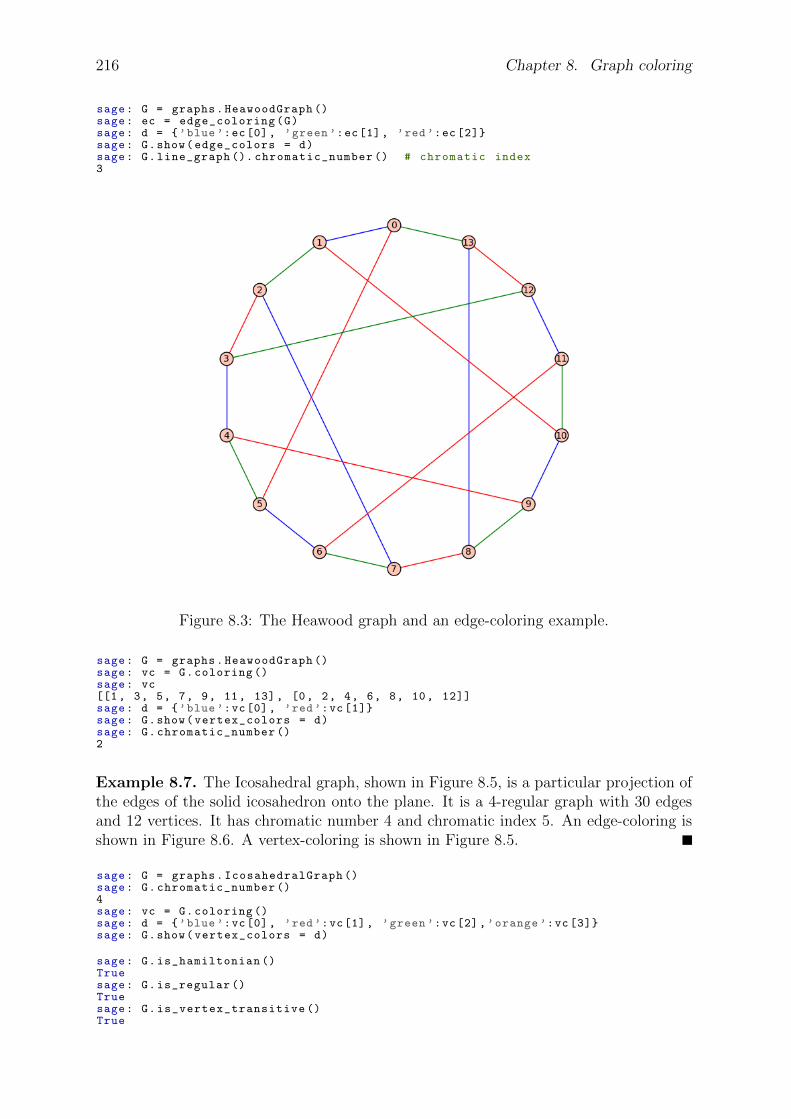
216 Chapter 8. Graph coloring
sage: G = graphs.HeawoodGraph ()sage: ec = edge_coloring(G)sage: d = ’blue’:ec[0], ’green ’:ec[1], ’red’:ec[2]sage: G.show(edge_colors = d)sage: G.line_graph (). chromatic_number () # chromatic index3
Figure 8.3: The Heawood graph and an edge-coloring example.
sage: G = graphs.HeawoodGraph ()sage: vc = G.coloring ()sage: vc[[1, 3, 5, 7, 9, 11, 13], [0, 2, 4, 6, 8, 10, 12]]sage: d = ’blue’:vc[0], ’red’:vc[1]sage: G.show(vertex_colors = d)sage: G.chromatic_number ()2
Example 8.7. The Icosahedral graph, shown in Figure 8.5, is a particular projection ofthe edges of the solid icosahedron onto the plane. It is a 4-regular graph with 30 edgesand 12 vertices. It has chromatic number 4 and chromatic index 5. An edge-coloring isshown in Figure 8.6. A vertex-coloring is shown in Figure 8.5.
sage: G = graphs.IcosahedralGraph ()sage: G.chromatic_number ()4sage: vc = G.coloring ()sage: d = ’blue’:vc[0], ’red’:vc[1], ’green ’:vc[2],’orange ’:vc[3]sage: G.show(vertex_colors = d)
sage: G.is_hamiltonian ()Truesage: G.is_regular ()Truesage: G.is_vertex_transitive ()True
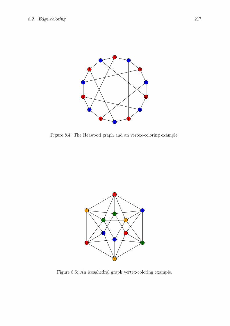
8.2. Edge coloring 217
Figure 8.4: The Heawood graph and an vertex-coloring example.
Figure 8.5: An icosahedral graph vertex-coloring example.
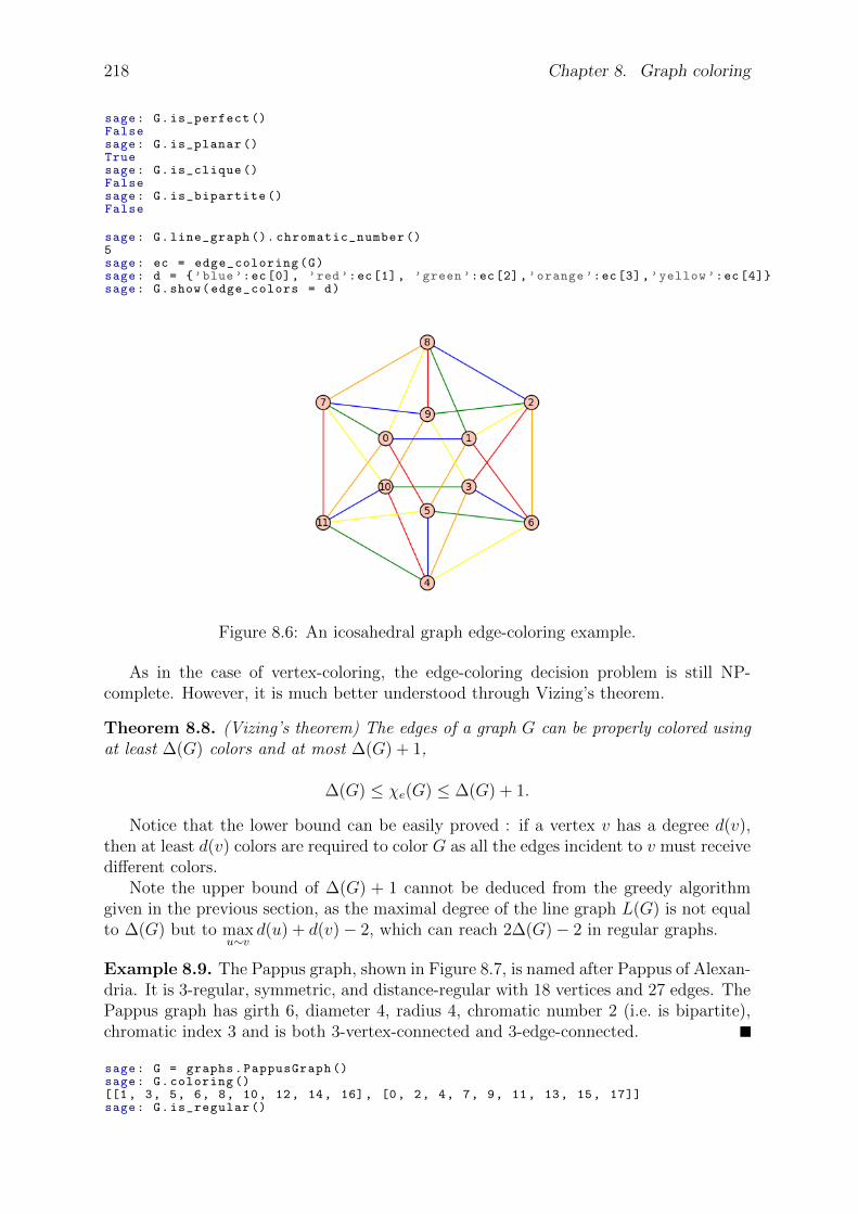
218 Chapter 8. Graph coloring
sage: G.is_perfect ()Falsesage: G.is_planar ()Truesage: G.is_clique ()Falsesage: G.is_bipartite ()False
sage: G.line_graph (). chromatic_number ()5sage: ec = edge_coloring(G)sage: d = ’blue’:ec[0], ’red’:ec[1], ’green ’:ec[2],’orange ’:ec[3],’yellow ’:ec[4]sage: G.show(edge_colors = d)
Figure 8.6: An icosahedral graph edge-coloring example.
As in the case of vertex-coloring, the edge-coloring decision problem is still NP-complete. However, it is much better understood through Vizing’s theorem.
Theorem 8.8. (Vizing’s theorem) The edges of a graph G can be properly colored usingat least ∆(G) colors and at most ∆(G) + 1,
∆(G) ≤ χe(G) ≤ ∆(G) + 1.
Notice that the lower bound can be easily proved : if a vertex v has a degree d(v),then at least d(v) colors are required to color G as all the edges incident to v must receivedifferent colors.
Note the upper bound of ∆(G) + 1 cannot be deduced from the greedy algorithmgiven in the previous section, as the maximal degree of the line graph L(G) is not equalto ∆(G) but to max
u∼vd(u) + d(v)− 2, which can reach 2∆(G)− 2 in regular graphs.
Example 8.9. The Pappus graph, shown in Figure 8.7, is named after Pappus of Alexan-dria. It is 3-regular, symmetric, and distance-regular with 18 vertices and 27 edges. ThePappus graph has girth 6, diameter 4, radius 4, chromatic number 2 (i.e. is bipartite),chromatic index 3 and is both 3-vertex-connected and 3-edge-connected.
sage: G = graphs.PappusGraph ()sage: G.coloring ()[[1, 3, 5, 6, 8, 10, 12, 14, 16], [0, 2, 4, 7, 9, 11, 13, 15, 17]]sage: G.is_regular ()
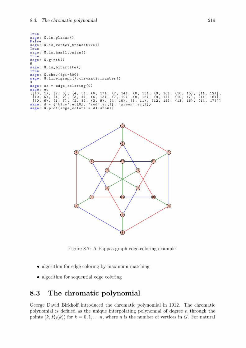
8.3. The chromatic polynomial 219
Truesage: G.is_planar ()Falsesage: G.is_vertex_transitive ()Truesage: G.is_hamiltonian ()Truesage: G.girth ()6sage: G.is_bipartite ()Truesage: G.show(dpi =300)sage: G.line_graph (). chromatic_number ()3sage: ec = edge_coloring(G)sage: ec[[(0, 1), (2, 3), (4, 5), (6, 17), (7, 14), (8, 13), (9, 16), (10, 15), (11, 12)],[(0, 5), (1, 2), (3, 4), (6, 13), (7, 12), (8, 15), (9, 14), (10, 17), (11, 16)],[(0, 6), (1, 7), (2, 8), (3, 9), (4, 10), (5, 11), (12, 15), (13, 16), (14, 17)]]
sage: d = ’blue’:ec[0], ’red’:ec[1], ’green ’:ec[2]sage: G.plot(edge_colors = d).show()
Figure 8.7: A Pappas graph edge-coloring example.
algorithm for edge coloring by maximum matching
algorithm for sequential edge coloring
8.3 The chromatic polynomial
George David Birkhoff introduced the chromatic polynomial in 1912. The chromaticpolynomial is defined as the unique interpolating polynomial of degree n through thepoints (k, PG(k)) for k = 0, 1, . . . n, where n is the number of vertices in G. For natural
220 Chapter 8. Graph coloring
numbers t, the chromatic polynomial is the function that counts the number of t-coloringsof G.
As the name indicates, for a given G the function is indeed a polynomial in t.For a complex number x, let x(k) =
∏k−1i=0 (x− i).
Lemma 8.10. If mk(G) denotes the number of distinct partitions of V into k differentcolor-classes then
PG(t) =n∑
k=1
mk(G)t(k).
Proof. Given a partition of V into k color-classes, we can assign t colors to the color-classes in t(t− 1) . . . (t− k+ 1) = t(k) ways. For each k with 1 ≤ k ≤ n, there are mk(G)distinct partitions of V into k such color-classes. Therefore, the number of colorings witht colors is
∑nk=1 mk(G)t(k), as desired.
Theorem 8.11. A graph G with n vertices is a tree if and only if P (G, t) = t(t− 1)n−1.
Proof. We prove this by induction on n. The statement is clearly true when n = 1.Assume the statement holds for any tree of n− 1 vertices and let G be a tree with n
vertices. There is a vertex v of G having degree 1. The graph G−v is a tree having n−1vertices, so has t(t− 1)n−2 t-colorings. The number of t-colorings of G is the number oft-colorings of G − v times the number of ways to color v. Since we may color v usingany color not used for its one neighbor, there are t− 1 colorings of v. Therefore, G hast(t− 1)n−1 t-colorings.
The theorem above gives examples of non-isomorphic graphs which have the samechromatic polynomial.
Two graphs are said to be chromatically equivalent if they have the same chromaticpolynomial. For example, two trees having the same number of vertices are chromaticallyequivalent.
It is also an open problem to find necessary and sufficient conditions for two arbitrarygraphs to be chromatically equivalent.
Theorem 8.12. If G has n vertices, m edges, and k components G1, G2,. . . ,Gk, then
P (G, t) = P (G1, t)P (G2, t) · · ·P (Gk, t).
This is proven by induction on k and the proof is left to the interested reader.Fix a pair of vertices u, v ∈ V . Recall that the (edge contraction) graph G/uv is
obtained by merging the two vertices and removing any edges between them. Recallthat the (edge deletion) graph G − uv is obtained by merging the the edge uv but notthe two vertices u, v.
Theorem 8.13. (Fundamental Reduction Theorem) The chromatic polynomial satisfiesthe recurrence relation
P (G, t) = P (G− uv, t)− P (G/uv, t).
8.4. Applications of graph coloring 221
For example, if G is a tree then G/uv is another tree but G− uv is a non-connectedgraph.
A root (or zero) of a chromatic polynomial, called a chromatic root is a value x wherePG(x) = 0.
Theorem 8.14. χv(C) is the smallest positive integer that is not a chromatic root:
χv(G) = mink | P (G, k) > 0.
Birkhoff noted that one could establish the four color theorem by showing P (G, 4) > 0for all planar graphs G. This lead to the following statement, which is still an openproblem today.
Conjecture 8.15. (Birkhoff-Lewis Conjecture) As a function of a real variable t, P (g, t)is zero-free in the interval t ≥ 4.
8.4 Applications of graph coloring
assignment problems
scheduling problems
matching problems
map coloring and the Four Color Problem
8.4.1 Application to scheduling
Assume that we have a finite set of different people (for example, students) and a finiteset of distinct one-hour meetings they could attend (for example, classes). Construct thegraph G as follows. The vertices V of G are given by the set of meetings. We connecttwo meetings with an edge if some person needs to attend both meetings.
Example 8.16. Suppose the × in the table below indicated that the student in thatcolumn is attending the class in that row.
Bob Carol Ted ZoeCalculus × ×
Chemistry × × × ×English × × × ×History × ×Physics × ×
Let 0 = Calculus, 1 = Chemistry, 2 = English, 3 = History, and 4 = Physics. Thenthe corresponding graph can be constructed and drawn in Sage using the following com-mands (see Figure 8.8).
sage: G = Graph (0:[1 ,2,4], 1:[2,3,4], 2:[3 ,4])sage: G.show()sage: G.coloring ()[[2], [4], [0, 3], [1]]
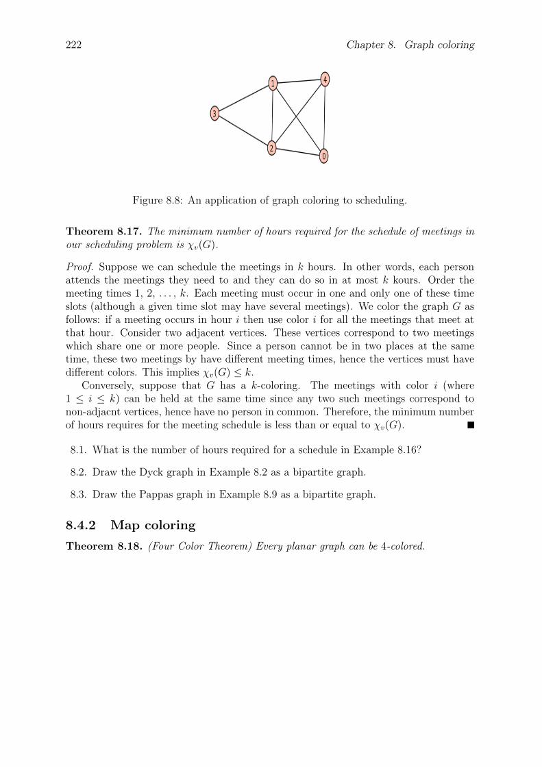
222 Chapter 8. Graph coloring
Figure 8.8: An application of graph coloring to scheduling.
Theorem 8.17. The minimum number of hours required for the schedule of meetings inour scheduling problem is χv(G).
Proof. Suppose we can schedule the meetings in k hours. In other words, each personattends the meetings they need to and they can do so in at most k kours. Order themeeting times 1, 2, . . . , k. Each meeting must occur in one and only one of these timeslots (although a given time slot may have several meetings). We color the graph G asfollows: if a meeting occurs in hour i then use color i for all the meetings that meet atthat hour. Consider two adjacent vertices. These vertices correspond to two meetingswhich share one or more people. Since a person cannot be in two places at the sametime, these two meetings by have different meeting times, hence the vertices must havedifferent colors. This implies χv(G) ≤ k.
Conversely, suppose that G has a k-coloring. The meetings with color i (where1 ≤ i ≤ k) can be held at the same time since any two such meetings correspond tonon-adjacnt vertices, hence have no person in common. Therefore, the minimum numberof hours requires for the meeting schedule is less than or equal to χv(G).
8.1. What is the number of hours required for a schedule in Example 8.16?
8.2. Draw the Dyck graph in Example 8.2 as a bipartite graph.
8.3. Draw the Pappas graph in Example 8.9 as a bipartite graph.
8.4.2 Map coloring
Theorem 8.18. (Four Color Theorem) Every planar graph can be 4-colored.

Chapter 9
Network flows
See Jungnickel [114], and chapter 12 of Gross and Yellen [91].
9.1 Flows and cuts
single source-single sink networks
feasible networks
maximum flow and minimum cut
Let G = (V,E, i, h) be an unweighted multidigraph, as in Definition 1.6.If F is a field such as R or GF (q) or a ring such as Z, let
C0(G,F ) = f : V → F, C1(G,F ) = f : E → F,be the sets of F -valued functions defined on V and E, respectively. If F is a field thenthese are F -inner product spaces with inner product
(f, g) =∑
x∈X
f(x)g(x), (X = V, resp. X = E), (9.1)
and
dimC0(G,F ) = |V |, dimC1(G,F ) = |E|.If you index the sets V and E in some arbitrary but fixed way and define, for 1 ≤ i ≤ |V |and 1 ≤ j ≤ |E|,
fi(v) =
1, v = vi,0, otherwise,
gj(e) =
1, e = ej,0, otherwise,
then F = fi ⊂ C0(G,F ) is a basis of C0(G,F ) and G = gj ⊂ C1(G,F ) is a basis ofC1(G,F ).
We order the edges
E = e1, e2, . . . , e|E|,in some arbitrary but fixed way. A vector representation (or characteristic vector orincidence vector) of a subgraph G′ = (V,E ′) of G = (V,E), E ′ ⊂ E, is a binary |E|-tuple
223
224 Chapter 9. Network flows
vec(G′) = (a1, a2, . . . , a|E|) ∈ GF (2)|E|,
where
ai = ai(E′) =
1, if ei ∈ E ′,0, if ei /∈ E ′.
In particular, this defines a mapping
vec : subgraphs of G = (V,E) → GF (2)|E|.
For any non-trivial partition
V = V1 ∪ V2, Vi 6= ∅, V1 ∩ V2 = ∅,the set of all edges e = (v1, v2) ∈ E, with vi ∈ Vi (i = 1, 2), is called a cocycle1 of G.A cocycle with a minimal set of edges is a bond (or cut set) of G. An Euler subgraph iseither a cycle or a union of edge-disjoint cycles.
The set of cycles of G is denoted Z(G) and the set of cocycles is denoted Z∗(G).The F -vector space spanned by the vector representations of all the cycles is called
the cycle space of G, denoted Z(G) = Z(G,F ). This is the kernel of the incidence matrixof G (§14.2 in Godsil and Royle [87]). Define
D : C1(G,F )→ C0(G,F ),(Df)(v) =
∑h(e)=v f(e)−∑t(e)=v f(e).
With respect to these bases F and G, the matrix representing the linear transformationD : C1(G,F ) → C0(G,F ) is the incidence matrix. An element of the kernel of D issometimes called a flow (see Biggs [25]) or circulation (see below). Therefore, this issometimes also referred to as the space of flows or the circulation space.
It may be regarded as a subspace of C1(G,F ) of dimension n(G). When F is a finitefield, sometimes2 the cycle space is called the cycle code of G.
Let F be a field such as R or GF (q), for some prime power q. Let G be a digraph.Some define a circulation (or flow) on G = (V,E) to be a function
f : E → F,
satisfying3
∑
u∈V, (u,v)∈E f(u, v) =∑
w∈V, (v,w)∈E f(v, w).
(Note: this is simply the condition that f belongs to the kernel of D.)Suppose G has a subgraph H and f is a circulation of G such that f is a constant
function on H and 0 elsewhere. We call such a circulation a characteristic function ofH. For example, if G has a cycle C and if f is the characteristic function on C, then fis a circulation.
The circulation space C is the F -vector space of circulation functions. The cycle space“clearly” may be identified with a subspace of the circulation space, since the F -vector
1Also called an edge cut subgraph or disconnecting set or seg or edge cutset.2Jungnickel and Vanstone in [115] call this the even graphical code of G.3Note: In addition, some authors add the condition f(e) ≥ 0 - see e.g., Chung [54].

9.1. Flows and cuts 225
space spanned by the characteristic functions of cycles may be identified with the cyclespace of G. In fact, these spaces are isomorphic. Under the inner product (9.1), i.e.,
(f, g) =∑
e∈E
f(e)g(e), (9.2)
this vector space is an inner product space.
Example 9.1. This example is not needed but is presented for its independent inter-est. Assume G = (V,E) is a strongly connected directed graph. Define the transitionprobability matrix P for a digraph G by
P (x, y) =
dx, if (x, y) ∈ E,0, otherwise,
where dx denotes the out-degree. The Perron-Frobenius Theorem states that there existsa unique left eigenvector φ such that (when regarded as a function φ : V → R) φ(v) > 0,for all v ∈ V and φP = ρφ, where ρ is the spectral radius of G. We scale φ so that∑
v∈V φ(v) = 1. (This vector is sometimes called the Perron vector.) Let Fφ(u, v) =φ(v)P (u, v). Fact: Fφ is a circulation. For a proof, see F. Chung [54].
If the edges of E are indexed in some arbitrary but fixed way then a circulationfunction restricted to a subgraph H of G may be identified with a vector representationof H, as described above. Thefore, the circulation functions gives a coordinate-freeversion of the cycle space.
The F -vector space spanned by the vector representations of all the segs is called thecocycle space (or the cut space) of G, denoted Z∗(G) = Z∗(G,F ). This is the columnspace of the transpose of the incidence matrix of G (§14.1 in Godsil and Royle [87]). Itmay be regarded as a subspace of C1(G,F ) of dimension the rank of G, r(G). When Fis a finite field, sometimes the cocycle space is called the cocycle code of G.
Lemma 9.2. Under the inner product (9.1) on C1(G,F ), the cycle space is orthogonalto the cocycle space.
Solution. One proof follows from Theorem 8.3.1 in Godsil and Royle [87].Here is another proof. By Theorem 2.3 in Bondy and Murty [33, p.27], an edge of G is
an edge cut if and only if it is contained in no cycle. Therefore, the vector representationof any cocycle is supported on a set of indices which is disjoint from the support of thevector representation of any cycle. Therefore, there is a basis of the cycle space which isorthogonal to a basis of the cocycle space.
Proposition 9.3. Let F = GF (2). The cycle code of a graph G = (V,E) is a linearbinary block code of length |E|, dimension equal to the nullity of the graph, n(G),and minimum distance equal to the girth of G. If C ⊂ GF (2)|E| is the cycle codeassociated to G and C∗ is the cocycle code associated to G then C∗ is the dual code ofC. In particular, the cocycle code of G is a linear binary block code of length |E|, anddimension r(G) = |E| − n(G).
This follows from Hakimi-Bredeson [97] (see also Jungnickel-Vanstone [115]) in thebinary case4.
4It is likely true in the non-binary case as well, but no proof seems to be in the literature.

226 Chapter 9. Network flows
Solution. Let d denote the minimum distance of the code C. Let γ denote the girth ofG, i.e., the smallest cardinality of a cycle in G. If K is a cycle in G then the vectorvec(K) ∈ GF (2)|E| is an element of the cycle code C ⊂ GF (2)|E|. This implies d ≤ γ.
In the other direction, suppose K1 and K2 are cycles in G with associated supportvectors v1 = vec(K1), v2 = vec(K2). Assume that at least one of these cycles is a cycleof minimum length, say K1, so the weight of its corresponding support vector is equal tothe girth γ. The only way that wt(v1 + v2) < minwt(v1),wt(v2) can occur is if K1 andK2 have some edges in common. In this case, the vector v1 + v2 represents a subgraphwhich is either a cycle or it is a union of disjoint cycles. In either case, by minimality ofK1, these new cycles must be at least as long. Therefore, d ≥ γ, as desired.
Consider a spanning tree T of a graph G and its complementary subgraph T . Foreach edge e of T the graph T ∪ e contains a unique cycle. The cycles which arise in thisway are called the fundamental cycles of G, denoted cyc(T, e).
Example 9.4. Consider the graph below, with edges labeled as indicated, together witha spanning tree, depicted to its right, in Figure 9.4.
0
1
2
3
4
5
7
6 8
9
10
Figure 9.1: A graph and a spanning tree for it.
You can see from Figure 9.4 that:
by adding edge 2 to the tree, you get a cycle 0, 1, 2 with vector representation
g1 = (1, 1, 1, 0, 0, 0, 0, 0, 0, 0, 0),
by adding edge 6 to the tree, you get a cycle 4, 5, 6 with vector representation
g2 = (0, 0, 0, 0, 1, 1, 1, 0, 0, 0, 0),
by adding edge 10 to the tree, you get a cycle 8, 9, 10 with vector representation
g3 = (0, 0, 0, 0, 0, 0, 0, 0, 1, 1, 1).
The vectors g1, g2, g3 form a basis of the cycle space of G over GF (2).
The cocycle space of a graph G (also known as the bond space of G or the cut-setspace of G) is the F -vector space spanned by the characteristic functions of bonds.
Example 9.5. Consider the graph below, with edges labeled as indicated, together withan example of a bond, depicted to its right, in Figure 9.5.
You can see from Figure 9.5 that:

9.1. Flows and cuts 227
0
1
2
3
4
5
7
6 8
9
10
Figure 9.2: A graph and a bond of it.
by removing edge 3 from the graph, you get a bond with vector representation
b1 = (0, 0, 0, 1, 0, 0, 0, 0, 0, 0, 0),
by removing edge 7 from the graph, you get a bond with vector representation
b2 = (0, 0, 0, 0, 0, 0, 0, 1, 0, 0, 0),
by removing edges 0, 1 from the graph, you get a bond with vector representation
b3 = (1, 1, 0, 0, 0, 0, 0, 0, 0, 0, 0),
by removing edges 1, 2 from the graph, you get a bond with vector representation
b4 = (0, 1, 1, 0, 0, 0, 0, 0, 0, 0, 0),
by removing edges 4, 5 from the graph, you get a bond with vector representation
b5 = (0, 0, 0, 0, 1, 1, 0, 0, 0, 0, 0),
by removing edges 4, 6 from the graph, you get a bond with vector representation
b6 = (0, 0, 0, 0, 1, 0, 1, 0, 0, 0, 0),
by removing edges 8, 9 from the graph, you get a bond with vector representation
b7 = (0, 0, 0, 0, 0, 0, 0, 0, 1, 1, 0),
by removing edges 9, 10 from the graph, you get a bond with vector representation
b8 = (0, 0, 0, 0, 0, 0, 0, 0, 0, 1, 1).
The vectors b1, b2, b3, b4, b5, b6, b7, b8 form a basis of the cocycle space of G over GF (2).Note that these vectors are orthogonal to the basis vectors of the cycle space in
Example 9.4. Note also that the xor sum of two cuts is not a cut.For example, if you xorthe bond 4, 5 with the bond 4, 6 then you get the subgraph foormed by the edges 5, 6and that is not a disconnecting cut of G.
228 Chapter 9. Network flows
9.1.1 Electrical networks
We present, as an application of circuit matrices and incidence matrices, and abstractdefinition of an electrical network.
We define an electrical network abstractly as follows. Let G = (V,E) be a simpleconnected directed graph having n vertices and m edges. We have a current function
i : E → R,
and a voltage function
v : E → R,
subject to three conditions. If we index the edges, say as E = e1, . . . , em, then thesefunctions may (and sometimes will) be regarded as column vectors in Rm.
The conditions satisfied by the current function are the following.
Kirchhoff’s current law,
Ai = ~0, (9.3)
where A is the incidence matrix and i is regarded as a column vector. This equationcomes from the fact that the algebraic sum of the currents going into a node iszero.
Kirchhoff’s voltage law,
Cv = ~0, (9.4)
where C is the circuit matrix and v is regarded as a column vector. This equationcomes from the fact that the algebraic sum of the voltage drops around a closedloop is zero.
In a network with resistors but no inductors or capacitors, there is a relationshipbetween i and v given by
Ri = v + b,
where b is a vector of external “battery” sources and R is a “resistor matrix.”
9.2 Chip firing games
Chip firing games on graphs (which are just pure fun) relate to “abelian sandpile models”from physics to “rotor-routing models” from theoretical computer scientists (designingefficient computer multiprocessor circuits) to “self-organized criticality” (a subdisciplineof dynamical systems) to “algebraic potential theory” on a graph [25] to cryptography(via the Biggs cryptosystem). Moreover, it relates the concepts of the Laplacian of thegraph to the tree number to the circulation space of the graph to the incidence matrix,as well as many other ideas. Some good references are [65], [159], [160], [100] and [26].
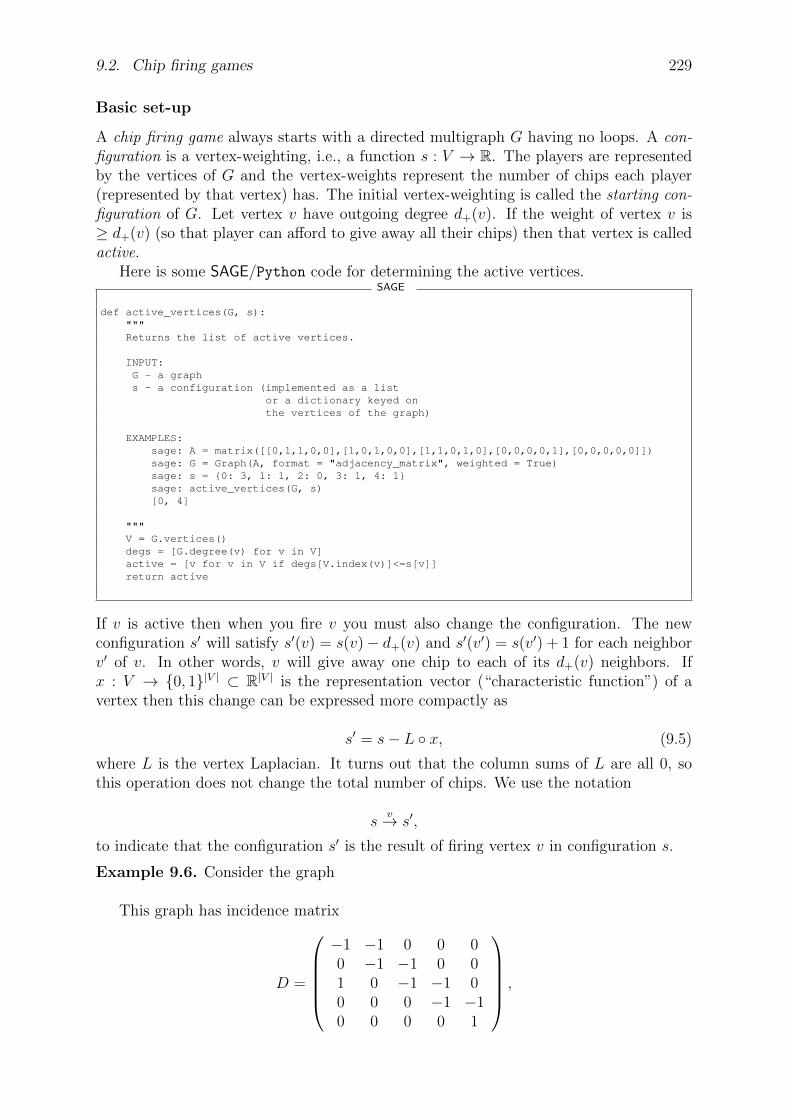
9.2. Chip firing games 229
Basic set-up
A chip firing game always starts with a directed multigraph G having no loops. A con-figuration is a vertex-weighting, i.e., a function s : V → R. The players are representedby the vertices of G and the vertex-weights represent the number of chips each player(represented by that vertex) has. The initial vertex-weighting is called the starting con-figuration of G. Let vertex v have outgoing degree d+(v). If the weight of vertex v is≥ d+(v) (so that player can afford to give away all their chips) then that vertex is calledactive.
Here is some SAGE/Python code for determining the active vertices.SAGE
def active_vertices(G, s):"""Returns the list of active vertices.
INPUT:G - a graphs - a configuration (implemented as a list
or a dictionary keyed onthe vertices of the graph)
EXAMPLES:sage: A = matrix([[0,1,1,0,0],[1,0,1,0,0],[1,1,0,1,0],[0,0,0,0,1],[0,0,0,0,0]])sage: G = Graph(A, format = "adjacency_matrix", weighted = True)sage: s = 0: 3, 1: 1, 2: 0, 3: 1, 4: 1sage: active_vertices(G, s)[0, 4]
"""V = G.vertices()degs = [G.degree(v) for v in V]active = [v for v in V if degs[V.index(v)]<=s[v]]return active
If v is active then when you fire v you must also change the configuration. The newconfiguration s′ will satisfy s′(v) = s(v)− d+(v) and s′(v′) = s(v′) + 1 for each neighborv′ of v. In other words, v will give away one chip to each of its d+(v) neighbors. Ifx : V → 0, 1|V | ⊂ R|V | is the representation vector (“characteristic function”) of avertex then this change can be expressed more compactly as
s′ = s− L x, (9.5)
where L is the vertex Laplacian. It turns out that the column sums of L are all 0, sothis operation does not change the total number of chips. We use the notation
sv→ s′,
to indicate that the configuration s′ is the result of firing vertex v in configuration s.
Example 9.6. Consider the graph
This graph has incidence matrix
D =
−1 −1 0 0 00 −1 −1 0 01 0 −1 −1 00 0 0 −1 −10 0 0 0 1
,

230 Chapter 9. Network flows
•0
1•
@@@@
2•
3•4•Figure 9.3: A graph with 5 vertices.
and Laplacian
L = D · tD =
2 −1 0− 1 0 0−1 2 −1 0 0−1 −1 3 −1 00 0 −1 2 −10 0 0 −1 1
.
Suppose the initial configuration is s = (3, 1, 0, 1, 1), i.e.,
player 0 has 3 dollars,
player 1 has 1 dollar,
player 2 has nothing,
player 3 has 1 dollar,
player 4 has 1 dollar.
Notice player 0 is active. If we fire 0 then we get the new configuration s′ = (1, 2, 1, 1, 1).Indeed, if we compute s′ = s− Lx(0), we get:
s′ =
31011
−
2 −1 −1 0 0−1 2 −1 0 0−1 −1 3 −1 00 0 −1 2 −10 0 0 −1 1
10000
=
31011
−
2−1−100
=
12111
.
This can be written more concisely as
(3, 1, 0, 1, 1)0→ (1, 2, 1, 1, 1).
We have the cycle
(1, 2, 1, 1, 1)1→ (2, 0, 2, 1, 1)
0→ (0, 1, 3, 1, 1)2→ (1, 2, 0, 2, 1)
3→ (1, 2, 1, 0, 2)4→ (1, 2, 1, 1, 1).

9.2. Chip firing games 231
Chip-firing game variants
For simplicity, let G = (V,E) be an undirected graph with an indexed set of verticesV = v1, . . . , vm and an indexed set of vertices E = e1, . . . , en.
One variant (the “sandpile model”) has a special vertex, called “the sink,” which hasspecial firing properties. In the sandpile variant, the sink is never fired. Another variant(the “dollar game”) has a special vertex, called “the source,” which has special firingproperties. In the dollar game variant, the source is only fired when not other vertex isactive. We shall consider the dollar game variant here, following Biggs [27].
We select a distinguished vertex q ∈ V , called the “source5,” which has a specialproperty to be described below. For the dollar game, a configuration is a functions : V → R for which
∑
v∈V
s(v) = 0,
and s(v) ≥ 0 for all v ∈ V with v 6= q. A vertex v 6= q can be fired if and onlyif deg(v) ≤ s(v) (i.e., it “has enough chips”). The equation (9.5) describes the newconfiguration after firing a vertex.
Here is some SAGE/Python code for determining the configuration after firing anactive vertex.
SAGE
def fire(G, s, v0):"""Returns the configuration after firing the active vertex v.
INPUT:G - a graphs - a configuration (implemented as a list
or a dictionary keyed onthe vertices of the graph)
v - a vertex of the graph
EXAMPLES:sage: A = matrix([[0,1,1,0,0],[1,0,1,0,0],[1,1,0,1,0],[0,0,0,0,1],[0,0,0,0,0]])sage: G = Graph(A, format = "adjacency_matrix", weighted = True)sage: s = 0: 3, 1: 1, 2: 0, 3: 1, 4: 1sage: fire(G, s, 0)0: 1, 1: 2, 2: 1, 3: 1, 4: 1
"""V = G.vertices()j = V.index(v0)s1 = copy(s)if not(v0 in V):
raise ValueError, "the last argument must be a vertex of the graph."if not(v0 in active_vertices(G, s)):
raise ValueError, "the last argument must be an active vertex of the graph."degs = [G.degree(w) for w in V]for w in V:
if w == v0:s1[v0] = s[v0] - degs[j]
if w in G.neighbors(v0):s1[w] = s[w]+1
return s1
We say s : V → R is a stable configuration if 0 ≤ s(v) < deg(v), for all v 6= q. Thesource vertex q can only be fired when no other vertex can be fired, that is only in thecase when a stable configuration has been reached.
5Biggs humorously calls q “the government.”

232 Chapter 9. Network flows
Here is some SAGE/Python code for determining the stable vertices.
SAGE
def stable_vertices(G, s, source = None):"""Returns the list of stable vertices.
INPUT:G - a graphs - a configuration (implemented as a list
or a dictionary keyed onthe vertices of the graph)
EXAMPLES:sage: A = matrix([[0,1,1,0,0],[1,0,1,0,0],[1,1,0,1,0],[0,0,0,0,1],[0,0,0,0,0]])sage: G = Graph(A, format = "adjacency_matrix", weighted = True)sage: s = 0: 3, 1: 1, 2: 0, 3: 1, 4: 1sage: stable_vertices(G, s)
"""V = G.vertices()degs = [G.degree(v) for v in V]if source==None:
stable = [v for v in V if degs[V.index(v)]>s[v]]else:
stable = [v for v in V if degs[V.index(v)]>s[v] and v!=source]return stable
Suppose we are in a configuration s1. We say a sequence vertices S = (w1, w2, . . . , wk),wi ∈ V not necessarily distinct, is legal if,
w1 is active in configuration s1,
for each i with 1 ≤ i < k, si+1 is obtained from si by firing wi in configuration si,
for each i with 1 ≤ i < k, wi+1 is active in the configuration si+1 defined in theprevious step,
the source vertex q occurs in S only if it immediately follows a stable configuration.
We call s1 or w1 the start of S. A configuration s is recurrent if there is a legal sequencestarting at s which leads back to s. A configuration is critical if it recurrent and stable.
Here is some SAGE/Python code for determining a stable vertex resulting from alegal sequence of firings of a given configuration s. I think it returns the unique criticalconfiguration associated to s but have not proven this.
SAGE
def stabilize(G, s, source, legal_sequence = False):"""Returns the stable configuration of the graph originating fromthe given configuration s. If legal_sequence = True then thesequence of firings is also returned. By van den Heuvel [1],the number of firings needed to compute a critical configurationis < 3(S+2|E|)|V|ˆ2, where S is the sum of the positiveweights in the configuration.
EXAMPLES:sage: A = matrix([[0,1,1,0,0],[1,0,1,0,0],[1,1,0,1,0],[0,0,1,0,1],[0,0,0,1,0]])sage: G = Graph(A, format="weighted_adjacency_matrix")sage: s = 0: 3, 1: 1, 2: 0, 3: 1, 4: -5sage: stabilize(G, s, 4)0: 0, 1: 1, 2: 2, 3: 1, 4: -4
REFERENCES:
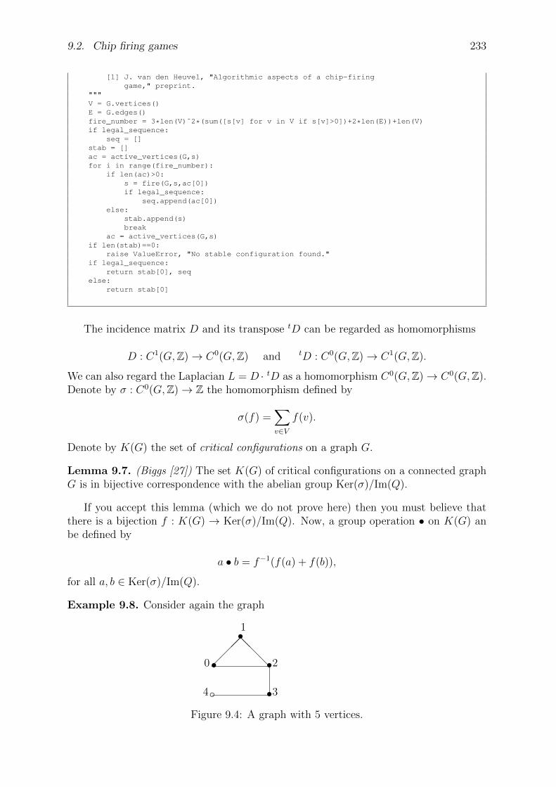
9.2. Chip firing games 233
[1] J. van den Heuvel, "Algorithmic aspects of a chip-firinggame," preprint.
"""V = G.vertices()E = G.edges()fire_number = 3*len(V)ˆ2*(sum([s[v] for v in V if s[v]>0])+2*len(E))+len(V)if legal_sequence:
seq = []stab = []ac = active_vertices(G,s)for i in range(fire_number):
if len(ac)>0:s = fire(G,s,ac[0])if legal_sequence:
seq.append(ac[0])else:
stab.append(s)break
ac = active_vertices(G,s)if len(stab)==0:
raise ValueError, "No stable configuration found."if legal_sequence:
return stab[0], seqelse:
return stab[0]
The incidence matrix D and its transpose tD can be regarded as homomorphisms
D : C1(G,Z)→ C0(G,Z) and tD : C0(G,Z)→ C1(G,Z).
We can also regard the Laplacian L = D · tD as a homomorphism C0(G,Z)→ C0(G,Z).Denote by σ : C0(G,Z)→ Z the homomorphism defined by
σ(f) =∑
v∈V
f(v).
Denote by K(G) the set of critical configurations on a graph G.
Lemma 9.7. (Biggs [27]) The set K(G) of critical configurations on a connected graphG is in bijective correspondence with the abelian group Ker(σ)/Im(Q).
If you accept this lemma (which we do not prove here) then you must believe thatthere is a bijection f : K(G) → Ker(σ)/Im(Q). Now, a group operation • on K(G) anbe defined by
a • b = f−1(f(a) + f(b)),
for all a, b ∈ Ker(σ)/Im(Q).
Example 9.8. Consider again the graph
•0
1•
@@@@
2•
3•4Figure 9.4: A graph with 5 vertices.
234 Chapter 9. Network flows
This graph has incidence matrix
D =
−1 −1 0 0 00 −1 −1 0 01 0 −1 −1 00 0 0 −1 −10 0 0 0 1
,
and Laplacian
L = D · tD =
2 −1 0− 1 0 0−1 2 −1 0 0−1 −1 3 −1 00 0 −1 2 −10 0 0 −1 1
.
Suppose the initial configuration is s = (3, 1, 0, 1,−5), i.e.,
player 0 has 3 dollars,
player 1 has 1 dollar,
player 2 has nothing,
player 3 has 1 dollar,
player 4 is the source vertex q.
The legal sequence (0, 1, 0, 2, 1, 0, 3, 2, 1, 0) leads to the stable configuration (0, 1, 2, 1,−4).If q is fired then the configuration (0, 1, 2, 2,−5) is achieved. This is recurrent since it iscontained in the cyclic legal sequence
(0, 1, 2, 2,−5)3→ (0, 1, 3, 0,−4)
2→ (1, 2, 0, 1,−4)1→ (2, 0, 1, 1,−4)
0→ (0, 1, 2, 1,−4)q→ (0, 1, 2, 2,−5).
In particular, the configuration (0, 1, 2, 1,−4) is also recurrent. Since it is both stableand recurrent, it is critical.
The following result is of basic importance but I’m not sure who proved it first. It isquoted in many of the papers on this topic in one form or another.
Theorem 9.9. (Biggs [26], Theorem 3.8) If s is an configuration and G is connectedthen there is a unique critical configuration s′ which can be obtained by a sequence oflegal firings for starting at s.
The map defined by the above theorem is denoted
γ : C0(G,R)→ K(G).
Another way to define multiplication • on on K(G) is
γ(s1) • γ(s2) = γ(s1 + s2),

9.3. Ford-Fulkerson theorem 235
where s1 + s2 is computed using addition on C0(G,R). According to Perkinson [159],Theorem 2.16, the critical group satisfies the following isomorphism:
K(G) ∼= Zm−1/L,where L is the integer lattice generated by the columns of the reduced Laplacian matrix6.
If s is a configuration then we define
wt(s) =∑
v∈V,v 6=q
s(q)
to be the weight of the configuration. The level of the configuration is defined by
level(s) = wt(s)− |E|+ deg(q).
Lemma 9.10. (Merino [144]) If s is a critical configuration then
0 ≤ level(s) ≤ |E| − |V |+ 1.
This is proven in Theorem 3.4.5 in [144]. What is also proven in [144] is a statementwhcih computes the number of critical configurations of a given level in terms of theTutte polynomial of the associated graph.
9.3 Ford-Fulkerson theorem
The Ford-Fulkerson Theorem, or “Max-flow/Min-cut Theorem,” was proven by P. Elias,A. Feinstein, and C.E. Shannon in 1956, and, independently, by L.R. Ford, Jr. and D.R.Fulkerson in the same year. So it should be called the “Elias-Feinstein-Ford-Fulkerson-Shannon Theorem,” to be precise about the authorship.
To explain the meaning of this theorem, we need to introduce some notation andterminology.
Consider an edge-weighted simple digraph G = (V,E, i, h) without negative weightcycles. Here E ⊂ V (2), i is an incidence function as in (??), which we regard as theidentity function, and h is an orientation function as in (??). Let G be a network, withtwo distinguished vertices, the “source” and the “sink.” Let s and t denote the source andthe sink of G, respectively. The capacity (or edge capacity) ) is a mapping c : E → R,denoted by cuv or c(u, v), for (u, v) ∈ E and h(e) = u. If (u, v) ∈ E and h(e) = vthen we set, by convention, c(v, u) = −c(u, v). Thinking of a graph as a network ofpipes (representing the edges) transporting water with various junctions (representingvertices), the capacity function represents the maximum amount of “flow” that can passthrough an edge.
A flow is a mapping f : E → R, denoted by fuv or f(u, v), subject to the followingtwo constraints:
f(u, v) ≤ c(u, v), for each (u, v) ∈ V (the “capacity constraint”),
∑
u∈V, (u,v)∈E f(u, v) =∑
u∈V, (v,u)∈E f(v, u) , for each v ∈ V (conservation of flows).
6The reduced Laplacian matrix is obtained from the Laplacian matrix by removing the row andcolumn associated to the source vertex.

236 Chapter 9. Network flows
An edge (u, v) ∈ E is f -saturated if f(u, v) = c(u, v). An edge (u, v) ∈ E is f -zeroif f(u, v) = 0. A path with available capacity is called an “augmenting path.” Moreprecisely, a directed path form s to t is f -augmenting, or f -unsaturated, if no forwardedge is f -saturated and no backward edge is f -zero.
The value of the flow is defined by
|f | =∑
v∈V
f(s, v)−∑
v∈V
f(v, s),
where s is the source. It represents the amount of flow passing from the source to thesink. The maximum flow problem is to maximize |f |, that is, to route as much flow aspossible from s to t.
Example 9.11. Consider the digraph having adjacency matrix
0 1 1 0 0 0−1 0 −1 1 0 1−1 1 0 0 1 00 −1 0 0 0 10 0 −1 0 0 10 −1 0 −1 −1 0
,
depicted in Figure 9.5.
0
1
2
3
4
5
Figure 9.5: A digraph with 6 vertices.
Suppose that each edge has capacity 1. A maximum flow f is obtained by taking aflow value of 1 along each edge of the path
p1 : (0, 1), (1, 5),
and a flow value of 1 along each edge of the path
p2 : (0, 2), (2, 4), (4, 5).
The maximum value of the flow in this case is |f | = 2.This graph can be created in Sage using the commands
sage: B = matrix ([[0,1,1,0,0,0],[0,0,0,1,0,1],[0,1,0,0,1,0],[0,0,0,0,0,1],[0,0,0,0,0,1],[0,0,0,0,0,0]])sage: H = DiGraph(B, format = "adjacency_matrix", weighted=True)
Type H.show(edgewlabels=True) if you want to see the graph with the capacities la-beling the edges.
9.3. Ford-Fulkerson theorem 237
Given a capacitated digraph with capacity c and flow f , we define the residual digraphGf = (V,E) to be the digraph with capacity cf (u, v) = c(u, v)− f(u, v) and no flow. Inother words, Gf is the same graph but it has a different capacity cf and flow 0. This isalso called a residual network.
Define an s − t cut in our capacitated digraph G to be a partition C = (S, T ) of Vsuch that s ∈ S and t ∈ T . Recall the cut-set of C is the set
(u, v) ∈ E | u ∈ S, v ∈ T.
Lemma 9.12. Let G = (V,E) be a capacitated digraph with capacity c : E → R, andlet s and t denote the source and the sink of G, respectively. If C is an s− t cut and ifthe edges in the cut-set of C are removed, then |f | = 0.
Exercise 9.13. Prove Lemma 9.12.
The capacity of an s− t cut C = (S, T ) is defined by
c(S, T ) =∑
(s,t)∈(S,T )
c(u, v).
The minimum cut problem is to minimize the amount of capacity of an s− t cut.The following theorem is due to P. Elias, A. Feinstein, L.R. Ford, Jr., D.R. Fulkerson,
C.E. Shannon.
Theorem 9.14. (max-flow min-cut theorem) The maximum value of an s-t flow is equalto the minimum capacity of an s-t cut.
See [155] for a simple proof of the max-flow min-cut theorem. The intuitive explana-tion of this result is as follows.
Suppose that G = (V,E) is a graph where each edge has capacity 1. Let s ∈ V be thesource and t ∈ V be the sink. The maximum flow from s to t is the maximum numberof independent paths from s to t. Denote this maximum flow by m. Each s-t cut mustintersect each s-t path at least once. In fact, if S is a minimal s-t cut then for each edgee in S there is an s-t path containing e. Therefore, |S| ≤ e.
On the other hand, since each edge has unit capacity, the maximum flow value can’texceed the number of edges separating s from t, so m ≤ |S|.
Remark 9.15. Although the notion of an independent path is important for the network-theoretic proof of Menger’s theorem (which we view as a corollary to the Ford-Fulkersontheorem on network flows on networks having capacity 1 on all edges), its significanceis less important for networks having arbitrary capacities. One must use caution ingeneralizing the above intuitive argument to establish a rigorous proof of the generalversion of the MFMC theorem.
Remark 9.16. This theorem can be generalized as follows. In addition to edge capacity,suppose there is capacity at each vertex, that is, a mapping c : V → R, denoted byv 7→ c(v), such that the flow f has to satisfy not only the capacity constraint and theconservation of flows, but also the vertex capacity constraint
∑
w∈V
f(w, v) ≤ c(v),

238 Chapter 9. Network flows
for each v ∈ V − s, t. Define an s − t cut to be the set of vertices and edges suchthat for any path from s to t, the path contains a member of the cut. In this case, thecapacity of the cut is the sum the capacity of each edge and vertex in it. In this newdefinition, the generalized max-flow min-cut theorem states that the maximum value ofan s− t flow is equal to the minimum capacity of an s− t cut..
The idea behind the Ford-Fulkerson algorithm is very simple: As long as there is apath from the source to the sink, with available capacity on all edges in the path, wesend as much flow as we can alone along each of these paths. This is done inductively,one path at a time.
Algorithm 9.1 Ford-Fulkerson algorithm.
Input Graph G = (V,E) with flow capacity c, source s, and sink t.Output A flow f from s to t which is a maximum for all edges in E.
1: f(u, v)← 0 for each edge uv ∈ E2: while there is an s-t path p in Gf such that cf (e) > 0 for each edge e ∈ E do3: find cf (p) = mincf (u, v) | (u, v) ∈ p4: for each edge uv ∈ do5: f(u, v) = f(u, v) + cf (p)6: f(v, u) = f(v, u)− cf (p)
To prove the max-flow/min-cut theorem we will use the following lemma.
Lemma 9.17. Let G = (V,E) be a directed graph with edge capacity c : E → Z, asource s ∈ V , and a sink t ∈ V . A flow f : E → Z is a maximum flow if and only ifthere is no f -augmenting path in the graph.
In other words, a flow f in a capacitated network is a maximum flow if and only ifthere is no f -augmenting path in the network.
Solution. One direction is easy. Suppose that the flow is a maximum. If there is anf -augmenting path then the current flow can be increased using that path, so the flowwould not be a maximum. This contradiction proves the “only if” direction.
Now, suppose there is no f -augmenting path in the network. Let S be the set ofvertices v such that there is an f -unsaturated path from the source s to v. We knows ∈ S and (by hypothesis) t /∈ S. Thus there is a cut of the form (S, T ) in the network.Let e = (v, w) be any edge in this cut, v ∈ S and w ∈ T . Since there is no f -unsaturatedpath from s to w, e is f -saturated. Likewise, any edge in the cut (T, S) is f -zero.Therefore, the current flow value is equal to the capacity of the cut (S, T ). Therefore,the current flow is a maximum.
We can now prove the max-flow/min-cut theorem.
Solution. Let f be a maximum flow. If
S = v ∈ V | there exists an f − saturated path from s to v,then by the previous lemma, S 6= V . Since T = V − S is non-empty, there is a cutC = (S, T ). Each edge of this cut C in the capacitated network G is f -saturated.

9.3. Ford-Fulkerson theorem 239
Here is some Python code7 which implements this. The class FlowNetwork is basicallya Sage Graph class with edge weights and an extra data structure representing the flowon the graph.class Edge:
def __init__(self ,U,V,w):self.source = Uself.to = Vself.capacity = w
def __repr__(self):return str(self.source) + "->" + str(self.to) + " : " + str(self.capacity)
class FlowNetwork(object ):"""This is a graph structure with edge capacities.
EXAMPLES:g=FlowNetwork ()map(g.add_vertex , [’s’,’o’,’p’,’q’,’r’,’t ’])g.add_edge(’s’,’o ’,3)g.add_edge(’s’,’p ’,3)g.add_edge(’o’,’p ’,2)g.add_edge(’o’,’q ’,3)g.add_edge(’p’,’r ’,2)g.add_edge(’r’,’t ’,3)g.add_edge(’q’,’r ’,4)g.add_edge(’q’,’t ’,2)print g.max_flow(’s’,’t’)
"""def __init__(self):
self.adj , self.flow , = ,
def add_vertex(self , vertex ):self.adj[vertex] = []
def get_edges(self , v):return self.adj[v]
def add_edge(self , u,v,w=0):assert(u != v)edge = Edge(u,v,w)redge = Edge(v,u,0)edge.redge = redgeredge.redge = edgeself.adj[u]. append(edge)self.adj[v]. append(redge)self.flow[edge] = self.flow[redge] = 0
def find_path(self , source , sink , path):if source == sink:
return pathfor edge in self.get_edges(source ):
residual = edge.capacity - self.flow[edge]if residual > 0 and not (edge ,residual) in path:
result = self.find_path(edge.to, sink , path + [ (edge ,residual) ])if result != None:
return result
def max_flow(self , source , sink):path = self.find_path(source , sink , [])while path != None:
flow = min(res for edge ,res in path)for edge ,res in path:
self.flow[edge] += flowself.flow[edge.redge] -= flow
path = self.find_path(source , sink , [])return sum(self.flow[edge] for edge in self.get_edges(source ))
7Please see http://en.wikipedia.org/wiki/Ford-Fulkersonwalgorithm.
240 Chapter 9. Network flows
9.4 Edmonds and Karp’s algorithm
The objective of this section is to prove Edmond and Karp’s algorithm for the maximumflow-minimum cut problem with polynomial complexity.
9.5 Goldberg and Tarjan’s algorithm
The objective of this section is to prove Goldberg and Tarjan’s algorithm for findingmaximal flows with polynomial complexity.

Chapter 10
Algebraic graph theory
10.1 Laplacian and adjacency matrices
10.2 Eigenvalues and eigenvectors
10.3 Algebraic connectivity
10.4 Graph invariants
10.5 Cycle and cut spaces
10.6 Problems
10.1. A.
241

Chapter 11
Random graphs
A random graph can be thought of as being a member from a collection of graphs havingsome common properties. Recall that Algorithm 2.5 allows for generating a randombinary tree having at least one vertex. Fix a positive integer n and let T be a collectionof all binary trees on n vertices. It can be infeasible to generate all members of T , so formost purposes we are only interested in randomly generating a member of T . A binarytree of order n generated in this manner is said to be a random graph.
This chapter is a digression into the world of random graphs and various modelsfor generating different types of random graphs. Unlike other chapters in this book, ourapproach is rather informal and not as rigorous as in other chapters. We will discuss somecommon models of random graphs and a number of their properties without being boggeddown in details of proofs. Along the way, we will demonstrate that random graphs canbe used to model diverse real-world networks such as social, biological, technological,and information networks. The edited volume [150] provides some historical contextfor the “new” science of networks. Bollobas [30] and Kolchin [123] provide standardreferences on the theory of random graphs with rigorous proofs. For comprehensivesurveys of random graphs and networks that do not go into too much technical details,see [13, 67, 191, 192]. On the other hand, surveys that cover diverse applications ofrandom graphs and networks and are geared toward the technical aspects of the subjectinclude [4, 29, 47,58,59,63,154].
11.1 Network statistics
Numerous real-world networks are large, having from thousands up to millions of verticesand edges. Network statistics provide a way to describe properties of networks withoutconcerning ourselves with individual vertices and edges. A network statistic shoulddescribe essential properties of the network under consideration, provide a means todifferentiate between different classes of networks, and be useful in network algorithmsand applications [38]. In this section, we discuss various common network statistics thatcan be used to describe graphs underlying large networks.
11.1.1 Degree distribution
The degree distribution of a graph G = (V,E) quantifies the fraction of vertices in Ghaving a specific degree k. If v is any vertex of G, we denote this fraction by
p = Pr[deg(v) = k] (11.1)
242

11.1. Network statistics 243
As indicated by the notation, we can think of (11.1) as the probability that a vertex v ∈ Vchosen uniformly at random has degree k. The degree distribution of G is consequently ahistogram of the degrees of vertices in G. Figure 11.1 illustrates the degree distributionof the Zachary [203] karate club network. The degree distributions of many real-worldnetworks have the same general curve as depicted in Figure 11.1(b), i.e. a peak at lowdegrees followed by a tail at higher degrees. See for example the degree distribution ofthe neural network in Figure 11.2, that of a power grid network in Figure 11.3, and thedegree distribution of a scientific co-authorship network in Figure 11.4.
(a) Zachary karate club network.
2 4 6 8 10 12 14 16
5 · 10−2
0.1
0.15
0.2
0.25
0.3
(b) Linear scaling.
100 100.2 100.4 100.6 100.8 101 101.2
10−1.4
10−1.2
10−1
10−0.8
10−0.6
(c) Log-log scaling.
Figure 11.1: The friendship network within a 34-person karate club. This is more com-monly known as the Zachary [203] karate club network. The network is an undirected,connected, unweighted graph having 34 vertices and 78 edges. The horizontal axis repre-sents degree; the vertical axis represents the probability that a vertex from the networkhas the corresponding degree.
11.1.2 Distance statistics
In chapter 5 we discussed various distance metrics such as radius, diameter, and eccen-tricity. To that distance statistics collection we add the average or characteristic distanced, defined as the arithmetic mean of all distances in a graph. Let G = (V,E) be a simplegraph with n = |V | and m = |E|, where G can be either directed or undirected. Then
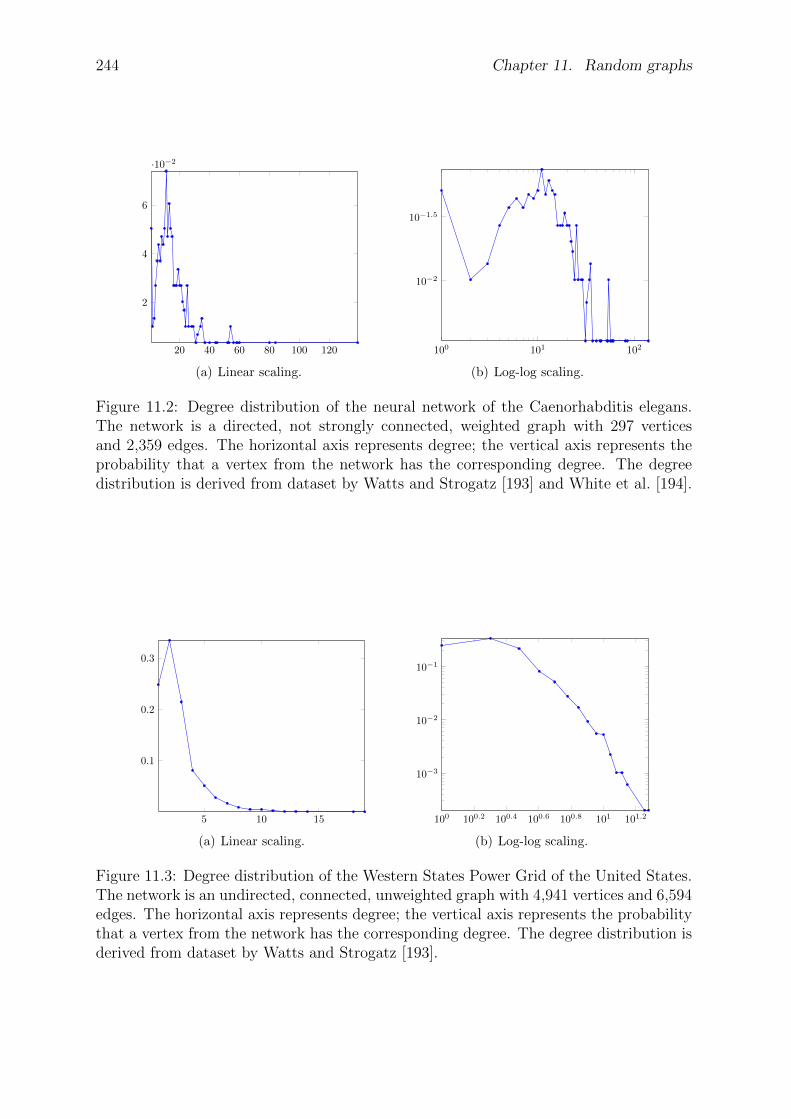
244 Chapter 11. Random graphs
20 40 60 80 100 120
2
4
6
·10−2
(a) Linear scaling.
100 101 102
10−2
10−1.5
(b) Log-log scaling.
Figure 11.2: Degree distribution of the neural network of the Caenorhabditis elegans.The network is a directed, not strongly connected, weighted graph with 297 verticesand 2,359 edges. The horizontal axis represents degree; the vertical axis represents theprobability that a vertex from the network has the corresponding degree. The degreedistribution is derived from dataset by Watts and Strogatz [193] and White et al. [194].
5 10 15
0.1
0.2
0.3
(a) Linear scaling.
100 100.2 100.4 100.6 100.8 101 101.2
10−3
10−2
10−1
(b) Log-log scaling.
Figure 11.3: Degree distribution of the Western States Power Grid of the United States.The network is an undirected, connected, unweighted graph with 4,941 vertices and 6,594edges. The horizontal axis represents degree; the vertical axis represents the probabilitythat a vertex from the network has the corresponding degree. The degree distribution isderived from dataset by Watts and Strogatz [193].
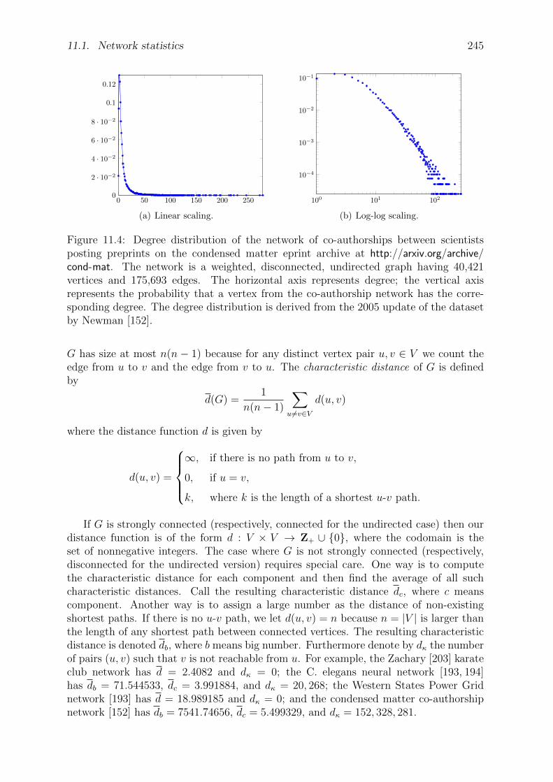
11.1. Network statistics 245
0 50 100 150 200 2500
2 · 10−2
4 · 10−2
6 · 10−2
8 · 10−2
0.1
0.12
(a) Linear scaling.
100 101 102
10−4
10−3
10−2
10−1
(b) Log-log scaling.
Figure 11.4: Degree distribution of the network of co-authorships between scientistsposting preprints on the condensed matter eprint archive at http://arxiv.org/archive/cond-mat. The network is a weighted, disconnected, undirected graph having 40,421vertices and 175,693 edges. The horizontal axis represents degree; the vertical axisrepresents the probability that a vertex from the co-authorship network has the corre-sponding degree. The degree distribution is derived from the 2005 update of the datasetby Newman [152].
G has size at most n(n − 1) because for any distinct vertex pair u, v ∈ V we count theedge from u to v and the edge from v to u. The characteristic distance of G is definedby
d(G) =1
n(n− 1)
∑
u6=v∈V
d(u, v)
where the distance function d is given by
d(u, v) =
∞, if there is no path from u to v,
0, if u = v,
k, where k is the length of a shortest u-v path.
If G is strongly connected (respectively, connected for the undirected case) then ourdistance function is of the form d : V × V → Z+ ∪ 0, where the codomain is theset of nonnegative integers. The case where G is not strongly connected (respectively,disconnected for the undirected version) requires special care. One way is to computethe characteristic distance for each component and then find the average of all suchcharacteristic distances. Call the resulting characteristic distance dc, where c meanscomponent. Another way is to assign a large number as the distance of non-existingshortest paths. If there is no u-v path, we let d(u, v) = n because n = |V | is larger thanthe length of any shortest path between connected vertices. The resulting characteristicdistance is denoted db, where b means big number. Furthermore denote by dκ the numberof pairs (u, v) such that v is not reachable from u. For example, the Zachary [203] karateclub network has d = 2.4082 and dκ = 0; the C. elegans neural network [193, 194]has db = 71.544533, dc = 3.991884, and dκ = 20, 268; the Western States Power Gridnetwork [193] has d = 18.989185 and dκ = 0; and the condensed matter co-authorshipnetwork [152] has db = 7541.74656, dc = 5.499329, and dκ = 152, 328, 281.

246 Chapter 11. Random graphs
We can also define the concept of distance distribution similar to how the degreedistribution was defined in section 11.1.1. If ` is a positive integer with u and v beingconnected vertices in a graph G = (V,E), denote by
p = Pr[d(u, v) = `] (11.2)
the fraction of ordered pairs of connected vertices in V × V having distance ` betweenthem. As is evident from the above notation, we can think of (11.2) as the probabilitythat a uniformly chosen connected pair (u, v) of vertices in G has distance `. The distancedistribution of G is hence a histogram of the distances between pairs of vertices in G.Figure 11.5 illustrates distance distributions of various real-world networks.
1 2 3 4 5
0.1
0.2
0.3
0.4
(a) Zachary karate club network [203].
2 4 6 8 10 12 140
0.1
0.2
0.3
(b) C. elegans neural network [193,194].
10 20 30 400
1
2
3
4
5
·10−2
(c) Power grid network [193].
2 4 6 8 10 12 14 16 180
0.1
0.2
0.3
(d) Condensed matter co-authorship net-work [152].
Figure 11.5: Distance distributions for various real-world networks. The horizontal axisrepresents distance and the vertical axis represents the probability that a uniformlychosen pair of distinct vertices from the network has the corresponding distance betweenthem.
11.2 Binomial random graph model
In 1959, Gilbert [85] introduced a random graph model that now bears the name bino-mial (or Bernoulli) random graph model. First, we fix a positive integer n, a probability
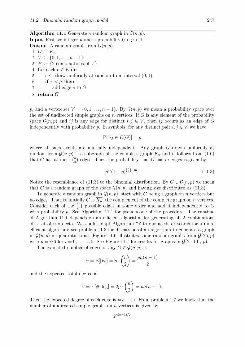
11.2. Binomial random graph model 247
Algorithm 11.1 Generate a random graph in G(n, p).
Input Positive integer n and a probability 0 < p < 1.Output A random graph from G(n, p).
1: G← Kn
2: V ← 0, 1, . . . , n− 13: E ← 2-combinations of V 4: for each e ∈ E do5: r ← draw uniformly at random from interval (0, 1)6: if r < p then7: add edge e to G
8: return G
p, and a vertex set V = 0, 1, . . . , n − 1. By G(n, p) we mean a probability space overthe set of undirected simple graphs on n vertices. If G is any element of the probabilityspace G(n, p) and ij is any edge for distinct i, j ∈ V , then ij occurs as an edge of Gindependently with probability p. In symbols, for any distinct pair i, j ∈ V we have
Pr[ij ∈ E(G)] = p
where all such events are mutually independent. Any graph G drawn uniformly atrandom from G(n, p) is a subgraph of the complete graph Kn and it follows from (1.6)that G has at most
(n2
)edges. Then the probability that G has m edges is given by
pm(1− p)(n2)−m. (11.3)
Notice the resemblance of (11.3) to the binomial distribution. By G ∈ G(n, p) we meanthat G is a random graph of the space G(n, p) and having size distributed as (11.3).
To generate a random graph in G(n, p), start with G being a graph on n vertices butno edges. That is, initially G is Kn, the complement of the complete graph on n vertices.Consider each of the
(n2
)possible edges in some order and add it independently to G
with probability p. See Algorithm 11.1 for pseudocode of the procedure. The runtimeof Algorithm 11.1 depends on an efficient algorithm for generating all 2-combinationsof a set of n objects. We could adapt Algorithm ?? to our needs or search for a moreefficient algorithm; see problem 11.3 for discussion of an algorithm to generate a graphin G(n, p) in quadratic time. Figure 11.6 illustrates some random graphs from G(25, p)with p = i/6 for i = 0, 1, . . . , 5. See Figure 11.7 for results for graphs in G(2 · 104, p).
The expected number of edges of any G ∈ G(n, p) is
α = E[|E|] = p ·(n
2
)=pn(n− 1)
2
and the expected total degree is
β = E[# deg] = 2p ·(n
2
)= pn(n− 1).
Then the expected degree of each edge is p(n− 1). From problem 1.7 we know that thenumber of undirected simple graphs on n vertices is given by
2n(n−1)/2
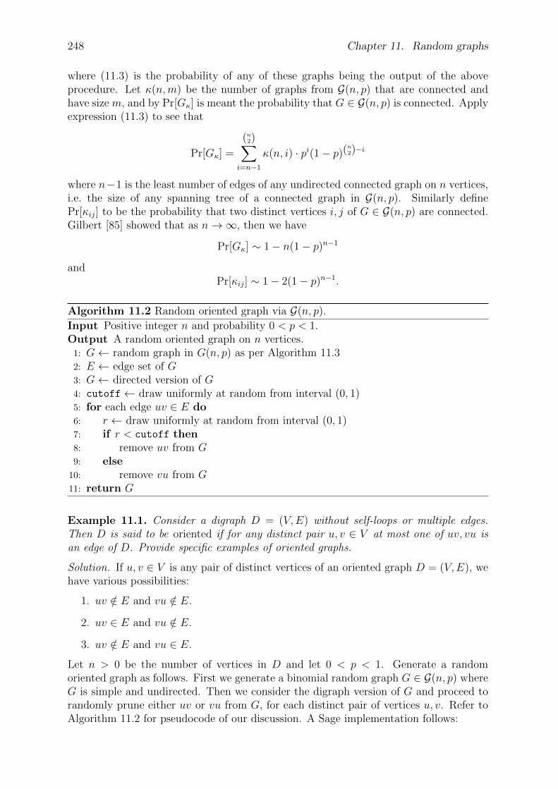
248 Chapter 11. Random graphs
where (11.3) is the probability of any of these graphs being the output of the aboveprocedure. Let κ(n,m) be the number of graphs from G(n, p) that are connected andhave size m, and by Pr[Gκ] is meant the probability that G ∈ G(n, p) is connected. Applyexpression (11.3) to see that
Pr[Gκ] =
(n2)∑
i=n−1
κ(n, i) · pi(1− p)(n2)−i
where n−1 is the least number of edges of any undirected connected graph on n vertices,i.e. the size of any spanning tree of a connected graph in G(n, p). Similarly definePr[κij] to be the probability that two distinct vertices i, j of G ∈ G(n, p) are connected.Gilbert [85] showed that as n→∞, then we have
Pr[Gκ] ∼ 1− n(1− p)n−1
andPr[κij] ∼ 1− 2(1− p)n−1.
Algorithm 11.2 Random oriented graph via G(n, p).
Input Positive integer n and probability 0 < p < 1.Output A random oriented graph on n vertices.
1: G← random graph in G(n, p) as per Algorithm 11.32: E ← edge set of G3: G← directed version of G4: cutoff← draw uniformly at random from interval (0, 1)5: for each edge uv ∈ E do6: r ← draw uniformly at random from interval (0, 1)7: if r < cutoff then8: remove uv from G9: else
10: remove vu from G11: return G
Example 11.1. Consider a digraph D = (V,E) without self-loops or multiple edges.Then D is said to be oriented if for any distinct pair u, v ∈ V at most one of uv, vu isan edge of D. Provide specific examples of oriented graphs.
Solution. If u, v ∈ V is any pair of distinct vertices of an oriented graph D = (V,E), wehave various possibilities:
1. uv /∈ E and vu /∈ E.
2. uv ∈ E and vu /∈ E.
3. uv /∈ E and vu ∈ E.
Let n > 0 be the number of vertices in D and let 0 < p < 1. Generate a randomoriented graph as follows. First we generate a binomial random graph G ∈ G(n, p) whereG is simple and undirected. Then we consider the digraph version of G and proceed torandomly prune either uv or vu from G, for each distinct pair of vertices u, v. Refer toAlgorithm 11.2 for pseudocode of our discussion. A Sage implementation follows:
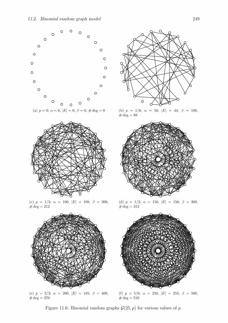
11.2. Binomial random graph model 249
(a) p = 0; α = 0, |E| = 0; β = 0, # deg = 0 (b) p = 1/6; α = 50, |E| = 44; β = 100,# deg = 88
(c) p = 1/3; α = 100, |E| = 108; β = 200,# deg = 212
(d) p = 1/2; α = 150, |E| = 156; β = 300,# deg = 312
(e) p = 2/3; α = 200, |E| = 185; β = 400,# deg = 370
(f) p = 5/6; α = 250, |E| = 255; β = 500,# deg = 510
Figure 11.6: Binomial random graphs G(25, p) for various values of p.
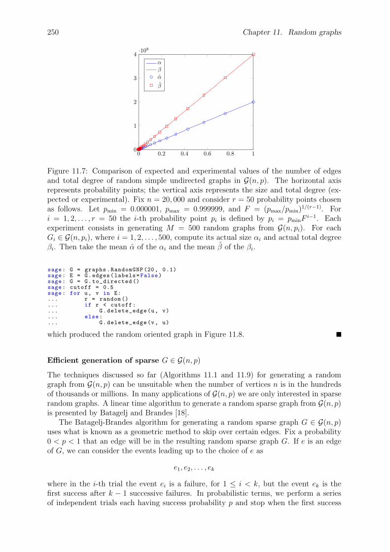
250 Chapter 11. Random graphs
0 0.2 0.4 0.6 0.8 10
1
2
3
4·108
αβα
β
Figure 11.7: Comparison of expected and experimental values of the number of edgesand total degree of random simple undirected graphs in G(n, p). The horizontal axisrepresents probability points; the vertical axis represents the size and total degree (ex-pected or experimental). Fix n = 20, 000 and consider r = 50 probability points chosenas follows. Let pmin = 0.000001, pmax = 0.999999, and F = (pmax/pmin)1/(r−1). Fori = 1, 2, . . . , r = 50 the i-th probability point pi is defined by pi = pminF
i−1. Eachexperiment consists in generating M = 500 random graphs from G(n, pi). For eachGi ∈ G(n, pi), where i = 1, 2, . . . , 500, compute its actual size αi and actual total degreeβi. Then take the mean α of the αi and the mean β of the βi.
sage: G = graphs.RandomGNP (20, 0.1)sage: E = G.edges(labels=False)sage: G = G.to_directed ()sage: cutoff = 0.5sage: for u, v in E:... r = random ()... if r < cutoff:... G.delete_edge(u, v)... else:... G.delete_edge(v, u)
which produced the random oriented graph in Figure 11.8.
Efficient generation of sparse G ∈ G(n, p)
The techniques discussed so far (Algorithms 11.1 and 11.9) for generating a randomgraph from G(n, p) can be unsuitable when the number of vertices n is in the hundredsof thousands or millions. In many applications of G(n, p) we are only interested in sparserandom graphs. A linear time algorithm to generate a random sparse graph from G(n, p)is presented by Batagelj and Brandes [18].
The Batagelj-Brandes algorithm for generating a random sparse graph G ∈ G(n, p)uses what is known as a geometric method to skip over certain edges. Fix a probability0 < p < 1 that an edge will be in the resulting random sparse graph G. If e is an edgeof G, we can consider the events leading up to the choice of e as
e1, e2, . . . , ek
where in the i-th trial the event ei is a failure, for 1 ≤ i < k, but the event ek is thefirst success after k − 1 successive failures. In probabilistic terms, we perform a seriesof independent trials each having success probability p and stop when the first success
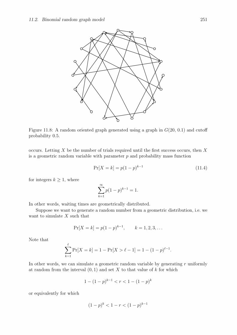
11.2. Binomial random graph model 251
Figure 11.8: A random oriented graph generated using a graph in G(20, 0.1) and cutoffprobability 0.5.
occurs. Letting X be the number of trials required until the first success occurs, then Xis a geometric random variable with parameter p and probability mass function
Pr[X = k] = p(1− p)k−1 (11.4)
for integers k ≥ 1, where∞∑
k=1
p(1− p)k−1 = 1.
In other words, waiting times are geometrically distributed.
Suppose we want to generate a random number from a geometric distribution, i.e. wewant to simulate X such that
Pr[X = k] = p(1− p)k−1, k = 1, 2, 3, . . .
Note that∑
k=1
Pr[X = k] = 1− Pr[X > `− 1] = 1− (1− p)`−1.
In other words, we can simulate a geometric random variable by generating r uniformlyat random from the interval (0, 1) and set X to that value of k for which
1− (1− p)k−1 < r < 1− (1− p)k
or equivalently for which
(1− p)k < 1− r < (1− p)k−1

252 Chapter 11. Random graphs
where 1− r and r are both uniformly distributed. Thus we can define X by
X = mink | (1− p)k < 1− r
= min
k
∣∣∣∣ k >ln(1− r)ln(1− p)
= 1 +
⌊ln(1− r)ln(1− p)
⌋.
That is, we can choose k to be
k = 1 +
⌊ln(1− r)ln(1− p)
⌋
which is used as a basis of Algorithm 11.3. In the latter algorithm, note that the vertexset is V = 0, 1, . . . , n − 1 and candidate edges are generated in lexicographic order.The Batagelj-Brandes Algorithm 11.3 has worst-case runtime O(n+m), where n and mare the order and size, respectively, of the resulting graph.
Algorithm 11.3 Linear generation of a random sparse graph in G(n, p).
Input Positive integer n and a probability 0 < p < 1.Output A random sparse graph from G(n, p).
1: G← Kn
2: u← 13: v ← −14: while u < n do5: r ← draw uniformly at random from interval (0, 1)6: v ← v + 1 + bln(1− r)/ ln(1− p)c7: while v ≥ u and u < n do8: v ← v − u9: u← u+ 1
10: if u < n then11: add edge uv to G
12: return G
Degree distribution
Consider a random graph G ∈ G(n, p) and let v be a vertex of G. With probability p, thevertex v is incident with each of the remaining n− 1 vertices in G. Then the probabilitythat v has degree k is given by the binomial distribution
Pr[deg(v) = k] =
(n− 1
k
)pk(1− p)n−1−k (11.5)
and the expected degree of v is E[deg(v)] = p(n − 1). Setting z = p(n − 1), we canexpress (11.5) as
Pr[deg(v) = k] =
(n− 1
k
)(z
n− 1− z
)k (1− z
n− 1
)n−1
11.3. Erdos-Renyi model 253
and thus
Pr[deg(v) = k]→ zk
k!exp(−z)
as n→∞. In the limit of large n, the probability that vertex v has degree k approachesthe Poisson distribution. That is, as n gets larger and larger any random graph in G(n, p)has a Poisson degree distribution.
11.3 Erdos-Renyi model
Let N be a fixed nonnegative integer. The Erdos-Renyi [72, 73] (or uniform) randomgraph model, denoted G(n,N), is a probability space over the set of undirected simplegraphs on n vertices and exactlyN edges. Hence G(n,N) can be considered as a collection
of((n
2)N
)undirected simple graphs on exactly N edges, each such graph being selected with
equal probability. A note of caution is in order here. Numerous papers on random graphsrefer to G(n, p) as the Erdos-Renyi random graph model, where in fact this binomialrandom graph model should be called the Gilbert model in honor of E. N. Gilbert whointroduced [85] it in 1959. Whenever a paper makes a reference to the Erdos-Renyimodel, one should question whether the paper is referring to G(n, p) or G(n,N).
To generate a graph in G(n,N), start with G being a graph on n vertices but noedges. Then choose N of the possible
(n2
)edges independently and uniformly at random
and let the chosen edges be the edge set of G. Each graph G ∈ G(n,N) is associatedwith a probability
1
/((n2
)
N
)
of being the graph resulting from the above procedure. Furthermore each of the(n2
)
edges has a probability
1
/(n
2
)
of being chosen. Algorithm 11.4 presents a straightforward translation of the aboveprocedure into pseudocode.
Algorithm 11.4 Generation of random graph in G(n,N).
Input Positive integer n and integer N with 0 ≤ N ≤(n2
).
Output A random graph from G(n,N).1: G← Kn
2: E ←e0, e1, . . . , e(n
2)−1
3: for i← 0, 1, . . . , N − 1 do4: r ← draw uniformly at random from
0, 1, . . . ,
(n2
)− 1
5: while er is an edge of G do6: r ← draw uniformly at random from
0, 1, . . . ,
(n2
)− 1
7: add edge er to G
8: return G
The runtime of Algorithm 11.4 is probabilistic and can be analyzed via the geometricdistribution. If i is the number of edges chosen so far, then the probability of choosing
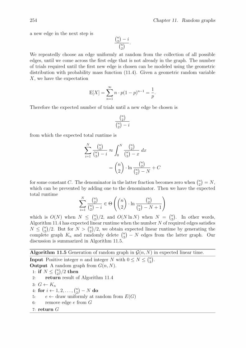
254 Chapter 11. Random graphs
a new edge in the next step is (n2
)− i(n2
) .
We repeatedly choose an edge uniformly at random from the collection of all possibleedges, until we come across the first edge that is not already in the graph. The numberof trials required until the first new edge is chosen can be modeled using the geometricdistribution with probability mass function (11.4). Given a geometric random variableX, we have the expectation
E[X] =∞∑
n=1
n · p(1− p)n−1 =1
p.
Therefore the expected number of trials until a new edge be chosen is
(n2
)(n2
)− i
from which the expected total runtime is
N∑
i=1
(n2
)(n2
)− i ≈
∫ N
0
(n2
)(n2
)− x dx
=
(n
2
)· ln
(n2
)(n2
)−N + C
for some constant C. The denominator in the latter fraction becomes zero when(n2
)= N ,
which can be prevented by adding one to the denominator. Then we have the expectedtotal runtime
N∑
i=1
(n2
)(n2
)− i ∈ Θ
((n
2
)· ln
(n2
)(n2
)−N + 1
)
which is O(N) when N ≤(n2
)/2, and O(N lnN) when N =
(n2
). In other words,
Algorithm 11.4 has expected linear runtime when the numberN of required edges satisfiesN ≤
(n2
)/2. But for N >
(n2
)/2, we obtain expected linear runtime by generating the
complete graph Kn and randomly delete(n2
)− N edges from the latter graph. Our
discussion is summarized in Algorithm 11.5.
Algorithm 11.5 Generation of random graph in G(n,N) in expected linear time.
Input Positive integer n and integer N with 0 ≤ N ≤(n2
).
Output A random graph from G(n,N).1: if N ≤
(n2
)/2 then
2: return result of Algorithm 11.4
3: G← Kn
4: for i← 1, 2, . . . ,(n2
)−N do
5: e← draw uniformly at random from E(G)6: remove edge e from G
7: return G
11.4. Small-world networks 255
11.4 Small-world networks
Vicky: Hi, Janice.
Janice: Hi, Vicky.
Vicky: How are you?
Janice: Good.
Harry: You two know each other?
Janice: Yeah, I met Vicky at the mall today.
Harry: Well, what a small world! You know, I wonder who else I know knows someone Iknow that I don’t know knows that person I know.
— from the TV series Third Rock from the Sun, season 5, episode 22, 2000.
Many real-world networks exhibit the small-world effect : that most pairs of distinctvertices in the network are connected by relatively short path lengths. The small-worldeffect was empirically demonstrated [146] in a famous 1960s experiment by Stanley Mil-gram, who distributed a number of letters to a random selection of people. Recipientswere instructed to deliver the letters to the addressees on condition that letters must bepassed to people whom the recipients knew on a first-name basis. Milgram found thaton average six steps were required for a letter to reach its target recipient, a number nowimmortalized in the phrase “six degrees of separation” [93]. Figure 11.9 plots results ofan experimental study of the small-world problem as reported in [183]. The small-worldeffect has been studied and verified for many real-world networks including
social: collaboration network of actors in feature films [6,193], scientific publicationauthorship [48,92,151,152];
information: citation network [165], Roget’s Thesaurus [121], word co-occurrence [62,76];
technological: internet [51, 75], power grid [193], train routes [171], software [153,185];
biological: metabolic network [110], protein interactions [109], food web [105,140],neural network [193,194].
Watts and Strogatz [190, 191, 193] proposed a network model that produces graphsexhibiting the small-world effect. We will use the notation “” to mean “much greaterthan”. Let n and k be positive integers such that n k lnn 1 (in particular,0 < k < n/2) with k being even. Consider a probability 0 < p < 1. Starting froman undirected k-circulant graph G = (V,E) on n vertices, the Watts-Strogatz modelproceeds to rewire each edge with probability p. The rewiring procedure, also callededge swapping, works as follows. Let V be uniformly distributed. For each v ∈ V , lete ∈ E be an edge having v as an endpoint. Choose another u ∈ V different from v. Withprobability p, delete the edge e and add the edge vu. The rewiring must produce a simplegraph with the same order and size as G. As p→ 1, the graph G goes from k-circulantto exhibiting properties of graphs drawn uniformly from G(n, p). Small-world networksare intermediate between k-circulant and binomial random graphs (see Figure 11.10).The Watts-Strogatz model is said to provide a procedure for interpolating between thelatter two types of graphs.
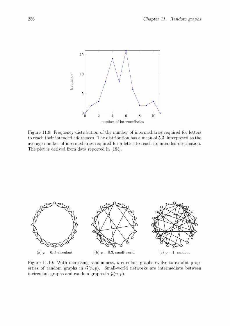
256 Chapter 11. Random graphs
0 2 4 6 8 100
5
10
15
number of intermediaries
freq
uen
cy
Figure 11.9: Frequency distribution of the number of intermediaries required for lettersto reach their intended addressees. The distribution has a mean of 5.3, interpreted as theaverage number of intermediaries required for a letter to reach its intended destination.The plot is derived from data reported in [183].
(a) p = 0, k-circulant (b) p = 0.3, small-world (c) p = 1, random
Figure 11.10: With increasing randomness, k-circulant graphs evolve to exhibit prop-erties of random graphs in G(n, p). Small-world networks are intermediate betweenk-circulant graphs and random graphs in G(n, p).

11.4. Small-world networks 257
The last paragraph contains an algorithm for rewiring edges of a graph. While thealgorithm is simple, in practice it potentially skips over a number of vertices to beconsidered for rewiring. If G = (V,E) is a k-circulant graph on n vertices and p is therewiring probability, the candidate vertices to be rewired follow a geometric distributionwith parameter p. This geometric trick, essentially the same speed-up technique used bythe Batagelj-Brandes Algorithm 11.3, can be used to speed up the rewiring algorithm.To elaborate, suppose G has vertex set V = 0, 1, . . . , n− 1. If r is chosen uniformly atrandom from the interval (0, 1), the index of the vertex to be rewired can be obtainedfrom
1 +
⌊ln(1− r)ln(1− p)
⌋.
The above geometric method is incorporated into Algorithm 11.6 to generate a Watts-Strogatz network in worst-case runtime O(nk+m), where n and k are as per the input ofthe algorithm and m is the size of the k-circulant graph on n vertices. Note that lines 7to 12 are where we avoid self-loops and multiple edges.
Algorithm 11.6 Watts-Strogatz network model.
Input Positive integer n denoting the number of vertices. Positive even integer k forthe degree of each vertex, where n k lnn 1. In particular, k should satisfy0 < k < n/2. Rewiring probability 0 < p ≤ 1.
Output A Watts-Strogatz network on n vertices.1: M ← nk . sum of all vertex degrees = twice number of edges2: r ← draw uniformly at random from interval (0, 1)3: v ← 1 + bln(1− r)/ ln(1− p)c4: E ← contiguous edge list of k-circulant graph on n vertices5: while v ≤M do6: u← draw uniformly at random from [0, 1, . . . , n− 1]7: if v − 1 is even then8: while E[v] = u or (u,E[v]) ∈ E do9: u← draw uniformly at random from [0, 1, . . . , n− 1]
10: else11: while E[v − 2] = u or (E[v − 2], u) ∈ E do12: u← draw uniformly at random from [0, 1, . . . , n− 1]
13: E[v − 1]← u14: r ← draw uniformly at random from interval (0, 1)15: v ← v + 1 + bln(1− r)/ ln(1− p)c16: G← Kn
17: add edges in E to G18: return G
Characteristic path length
Watts and Strogatz [193] analyzed the structure of networks generated by Algorithm 11.6via two quantities: the characteristic path length ` and the clustering coefficient C. Thecharacteristic path length quantifies the average distance between any distinct pair ofvertices in a Watts-Strogatz network. The quantity `(G) is thus said to be a global
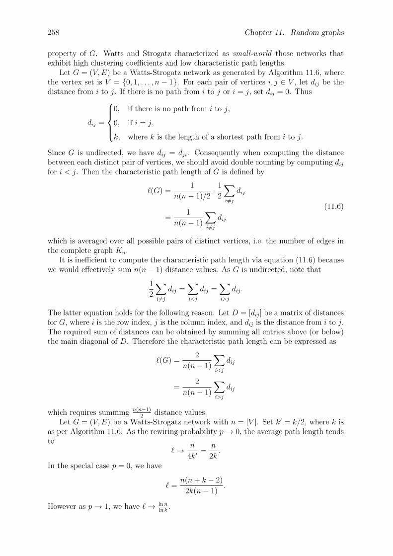
258 Chapter 11. Random graphs
property of G. Watts and Strogatz characterized as small-world those networks thatexhibit high clustering coefficients and low characteristic path lengths.
Let G = (V,E) be a Watts-Strogatz network as generated by Algorithm 11.6, wherethe vertex set is V = 0, 1, . . . , n − 1. For each pair of vertices i, j ∈ V , let dij be thedistance from i to j. If there is no path from i to j or i = j, set dij = 0. Thus
dij =
0, if there is no path from i to j,
0, if i = j,
k, where k is the length of a shortest path from i to j.
Since G is undirected, we have dij = dji. Consequently when computing the distancebetween each distinct pair of vertices, we should avoid double counting by computing dijfor i < j. Then the characteristic path length of G is defined by
`(G) =1
n(n− 1)/2· 1
2
∑
i 6=j
dij
=1
n(n− 1)
∑
i 6=j
dij
(11.6)
which is averaged over all possible pairs of distinct vertices, i.e. the number of edges inthe complete graph Kn.
It is inefficient to compute the characteristic path length via equation (11.6) becausewe would effectively sum n(n− 1) distance values. As G is undirected, note that
1
2
∑
i 6=j
dij =∑
i<j
dij =∑
i>j
dij.
The latter equation holds for the following reason. Let D = [dij] be a matrix of distancesfor G, where i is the row index, j is the column index, and dij is the distance from i to j.The required sum of distances can be obtained by summing all entries above (or below)the main diagonal of D. Therefore the characteristic path length can be expressed as
`(G) =2
n(n− 1)
∑
i<j
dij
=2
n(n− 1)
∑
i>j
dij
which requires summing n(n−1)2
distance values.Let G = (V,E) be a Watts-Strogatz network with n = |V |. Set k′ = k/2, where k is
as per Algorithm 11.6. As the rewiring probability p→ 0, the average path length tendsto
`→ n
4k′=
n
2k.
In the special case p = 0, we have
` =n(n+ k − 2)
2k(n− 1).
However as p→ 1, we have `→ lnnln k
.

11.4. Small-world networks 259
Clustering coefficient
The clustering coefficient of a simple graph G quantifies the “cliquishness” of verticesin G = (V,E). This quantity is thus said to be a local property of G. Watts andStrogatz [193] defined the clustering coefficient as follows. Suppose n = |V | > 0 and let nicount the number of neighbors of vertex i ∈ V , a quantity that is equivalent to the degreeof i, i.e. deg(i) = ni. The complete graph Kni
on the ni neighbors of i has ni(ni − 1)/2edges. The neighbor graph Ni of i is a subgraph of G, consisting of all vertices (6= i) thatare adjacent to i and preserving the adjacency relation among those vertices as found inthe supergraph G. For example, given the graph in Figure 11.11(a) the neighbor graphof vertex 10 is shown in Figure 11.11(b). The local clustering coefficient Ci of i is theratio
Ci =Ni
ni(ni − 1)/2
where Ni counts the number of edges in Ni. In case i has degree deg(i) < 2, we set thelocal clustering coefficient of i to be zero. Then the clustering coefficient of G is definedby
C(G) =1
n
∑
i∈V
Ci =1
n
∑
i∈V
Ni
ni(ni − 1)/2.
0
1
23
4
5
6
7 8
9
10
(a) Graph on 11 vertices.
1
3
6
7 8
(b) N10
Figure 11.11: The neighbor graph of a vertex.
Consider the case where we have a k-circulant graph G = (V,E) on n vertices and arewiring probability p = 0. That is, we do not rewire any edge of G. Each vertex of G hasdegree k. Let k′ = k/2. Then the k neighbors of each vertex in G has 3k′(k′−1)/2 edgesbetween them, i.e. each neighbor graph Ni has size 3k′(k′ − 1)/2. Then the clusteringcoefficient of G is
3(k′ − 1)
2(2k′ − 1).
When the rewiring probability is p > 0, Barrat and Weigt [17] showed that the clusteringcoefficient of any graph G′ in the Watts-Strogatz network model (see Algorithm 11.6)can be approximated by
C(G′) ≈ 3(k′ − 1)
2(2k′ − 1)(1− p)3.

260 Chapter 11. Random graphs
Degree distribution
For a Watts-Strogatz network without rewiring, each vertex has the same degree k. Iteasily follows that for each vertex v, we have the degree distribution
Pr[deg(v) = i] =
1, if i = k,
0, otherwise.
A rewiring probability p > 0 introduces disorder in the network and broadens thedegree distribution, while the expected degree is k. A k-circulant graph on n verticeshas nk/2 edges. With the rewiring probability p > 0, a total of pnk/2 edges wouldbe rewired. However note that only one endpoint of an edge is rewired, thus after therewiring process the degree of any vertex v is deg(v) ≥ k/2. Therefore with k > 2, aWatts-Strogatz network has no isolated vertices.
For p > 0, Barrat and Weigt [17] showed that the degree of a vertex v can be writtenas deg(v) = k/2 + ni with ni ≥ 0, where ni can be divided into two parts α and β asfollows. First α ≤ k/2 edges are left intact after the rewiring process, the probability ofthis occurring is 1−p for each edge. Second β = ni−α edges have been rewired towardsi, each with probability 1/n. The probability distribution of α is
P1(α) =
(k/2
α
)(1− p)αpk/2−α
and the probability distribution of β is
P2(β) =
(pnk/2
β
)(1
n
)β (1− 1
n
)pnk/2−β
where
P2(β)→ (pk/2)β
β!exp(−pk/2)
for large n. Combine the above two factors to obtain the degree distribution
Pr[deg(v) = κ] =
minκ−k/2, k/2∑
i=0
(k/2
i
)(1− p)ipk/2−i (pk/2)κ−k/2−i
(κ− k/2− i)! exp(−pk/2)
for κ ≥ k/2.
11.5 Scale-free networks
The networks covered so far—Gilbert G(n, p) model, Erdos-Renyi G(n,N) model, Watts-Strogatz small-world model—are static. Once a network is generated from any of thesemodels, the corresponding model does not specify any means for the network to evolveover time. Barabasi and Albert [14] proposed a network model based on two ingredients:
1. Growth: at each time step, a new vertex is added to the network and connectedto a pre-determined number of existing vertices.
2. Preferential attachment: the newly added vertex is connected to an existing vertexin proportion to the latter’s existing degree.

11.5. Scale-free networks 261
Preferential attachment also goes by the colloquial name of the “rich-get-richer” effectdue to the work of Herbert Simon [176]. In sociology, preferential attachment is knownas the Matthew effect due to the following verse from the Book of Matthew, chapter 25verse 29, in the Bible: “For to every one that hath shall be given but from him thathath not, that also which he seemeth to have shall be taken away.” Barabasi and Albertobserved that many real-world networks exhibit statistical properties of their proposedmodel. One particularly significant property is that of power-law scaling, hence theBarabasi-Albert model is also called a model of scale-free networks. Note that it is onlythe degree distributions of scale-free networks that are scale-free. In their empirical studyof the World Wide Web (WWW) and other real-world networks, Barabasi and Albertnoted that the probability that a web page increases in popularity is directly proportionalto the page’s current popularity. Thinking of a web page as a vertex and the degree of apage as the number of other pages that the current page links to, the degree distributionof the WWW follows a power law function. Power-law scaling has been confirmed formany real-world networks:
actor collaboration network [14]
citation [60,165,170] and co-authorship networks [152]
human sexual contacts network [112,135]
the Internet [51, 75,186] and the WWW [5,16,39]
metabolic networks [109,110]
telephone call graphs [2, 3]
Figure 11.12 illustrates the degree distributions of various real-world networks, plottedon log-log scales. Corresponding distributions for various simulated Barabasi-Albertnetworks are illustrated in Figure 11.13.
But how do we generate a scale-free graph as per the description in Barabasi andAlbert [14]? The original description of the Barabasi-Albert model as contained in [14]is rather ambiguous with respect to certain details. First, the whole process is supposedto begin with a small number of vertices. But as the degree of each of these verticesis zero, it is unclear how the network is to grow via preferential attachment from theinitial pool of vertices. Second, Barabasi and Albert neglected to clearly specify how toselect the neighbors for the newly added vertex. The above ambiguities are resolved byBollobas et al. [32], who gave a precise statement of a random graph process that realizesthe Barabasi-Albert model. Fix a sequence of vertices v1, v2, . . . and consider the casewhere each newly added vertex is to be connected to m = 1 vertex already in a graph.Inductively define a random graph process (Gt
1)t≥0 as follows, where Gt1 is a digraph on
vi | 1 ≤ i ≤ t. Start with the null graph G01 or the graph G1
1 with one vertex and oneself-loop. Denote by degG(v) the total (in and out) degree of vertex v in the graph G.For t > 1 construct Gt
1 from Gt−11 by adding the vertex vt and a directed edge from vt to
vi, where i is randomly chosen with probability
Pr[i = s] =
degGt−1
1(vs)/(2t− 1), if 1 ≤ s ≤ t− 1,
1/(2t− 1), if s = t.
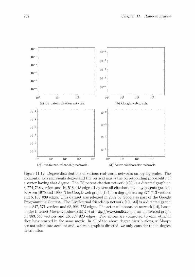
262 Chapter 11. Random graphs
100 101 102
10−6
10−5
10−4
10−3
10−2
10−1
(a) US patent citation network.
100 101 102 103
10−5
10−4
10−3
10−2
10−1
(b) Google web graph.
100 101 102 103 104
10−6
10−5
10−4
10−3
10−2
10−1
(c) LiveJournal friendship network.
100 101 102 103
10−5
10−4
10−3
10−2
(d) Actor collaboration network.
Figure 11.12: Degree distributions of various real-world networks on log-log scales. Thehorizontal axis represents degree and the vertical axis is the corresponding probability ofa vertex having that degree. The US patent citation network [133] is a directed graph on3, 774, 768 vertices and 16, 518, 948 edges. It covers all citations made by patents grantedbetween 1975 and 1999. The Google web graph [134] is a digraph having 875, 713 verticesand 5, 105, 039 edges. This dataset was released in 2002 by Google as part of the GoogleProgramming Contest. The LiveJournal friendship network [10,134] is a directed graphon 4, 847, 571 vertices and 68, 993, 773 edges. The actor collaboration network [14], basedon the Internet Movie Database (IMDb) at http://www.imdb.com, is an undirected graphon 383, 640 vertices and 16, 557, 920 edges. Two actors are connected to each other ifthey have starred in the same movie. In all of the above degree distributions, self-loopsare not taken into account and, where a graph is directed, we only consider the in-degreedistribution.
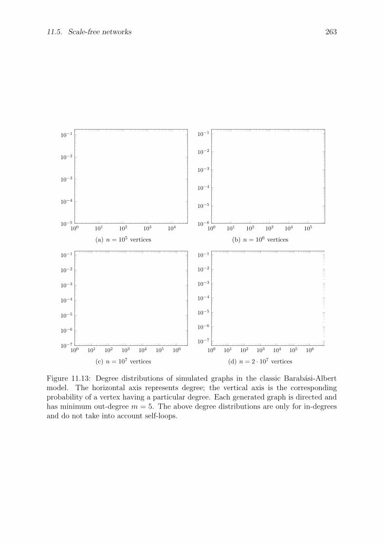
11.5. Scale-free networks 263
100 101 102 103 10410−5
10−4
10−3
10−2
10−1
(a) n = 105 vertices
100 101 102 103 104 10510−6
10−5
10−4
10−3
10−2
10−1
(b) n = 106 vertices
100 101 102 103 104 105 10610−7
10−6
10−5
10−4
10−3
10−2
10−1
(c) n = 107 vertices
100 101 102 103 104 105 10610−7
10−6
10−5
10−4
10−3
10−2
10−1
(d) n = 2 · 107 vertices
Figure 11.13: Degree distributions of simulated graphs in the classic Barabasi-Albertmodel. The horizontal axis represents degree; the vertical axis is the correspondingprobability of a vertex having a particular degree. Each generated graph is directed andhas minimum out-degree m = 5. The above degree distributions are only for in-degreesand do not take into account self-loops.
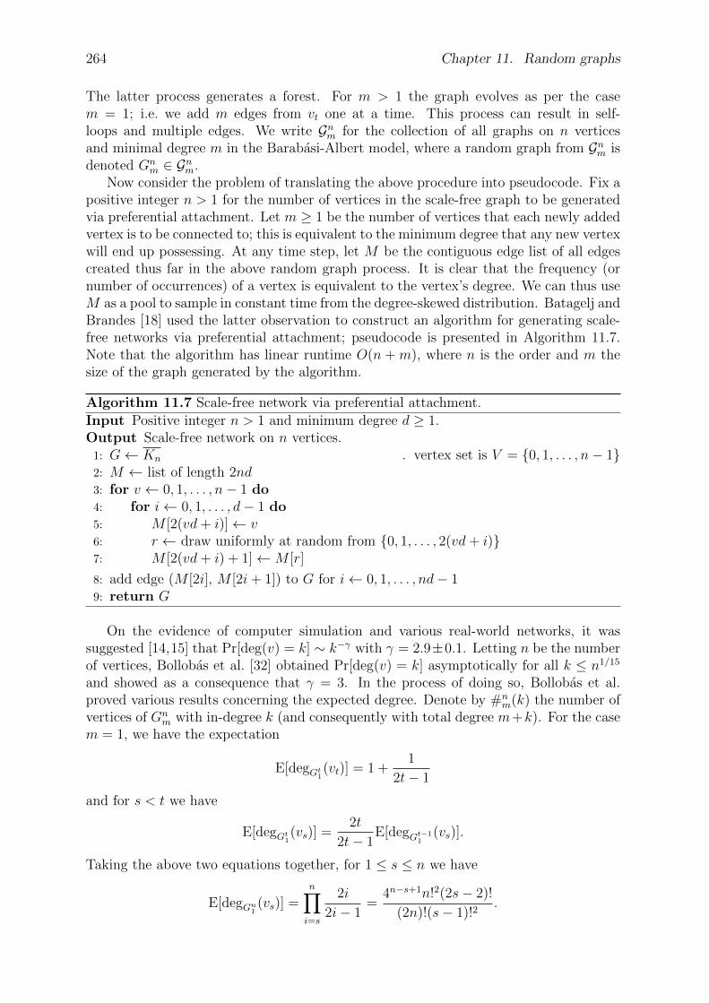
264 Chapter 11. Random graphs
The latter process generates a forest. For m > 1 the graph evolves as per the casem = 1; i.e. we add m edges from vt one at a time. This process can result in self-loops and multiple edges. We write Gnm for the collection of all graphs on n verticesand minimal degree m in the Barabasi-Albert model, where a random graph from Gnm isdenoted Gn
m ∈ Gnm.Now consider the problem of translating the above procedure into pseudocode. Fix a
positive integer n > 1 for the number of vertices in the scale-free graph to be generatedvia preferential attachment. Let m ≥ 1 be the number of vertices that each newly addedvertex is to be connected to; this is equivalent to the minimum degree that any new vertexwill end up possessing. At any time step, let M be the contiguous edge list of all edgescreated thus far in the above random graph process. It is clear that the frequency (ornumber of occurrences) of a vertex is equivalent to the vertex’s degree. We can thus useM as a pool to sample in constant time from the degree-skewed distribution. Batagelj andBrandes [18] used the latter observation to construct an algorithm for generating scale-free networks via preferential attachment; pseudocode is presented in Algorithm 11.7.Note that the algorithm has linear runtime O(n + m), where n is the order and m thesize of the graph generated by the algorithm.
Algorithm 11.7 Scale-free network via preferential attachment.
Input Positive integer n > 1 and minimum degree d ≥ 1.Output Scale-free network on n vertices.
1: G← Kn . vertex set is V = 0, 1, . . . , n− 12: M ← list of length 2nd3: for v ← 0, 1, . . . , n− 1 do4: for i← 0, 1, . . . , d− 1 do5: M [2(vd+ i)]← v6: r ← draw uniformly at random from 0, 1, . . . , 2(vd+ i)7: M [2(vd+ i) + 1]←M [r]
8: add edge (M [2i], M [2i+ 1]) to G for i← 0, 1, . . . , nd− 19: return G
On the evidence of computer simulation and various real-world networks, it wassuggested [14,15] that Pr[deg(v) = k] ∼ k−γ with γ = 2.9±0.1. Letting n be the numberof vertices, Bollobas et al. [32] obtained Pr[deg(v) = k] asymptotically for all k ≤ n1/15
and showed as a consequence that γ = 3. In the process of doing so, Bollobas et al.proved various results concerning the expected degree. Denote by #n
m(k) the number ofvertices of Gn
m with in-degree k (and consequently with total degree m+k). For the casem = 1, we have the expectation
E[degGt1(vt)] = 1 +
1
2t− 1
and for s < t we have
E[degGt1(vs)] =
2t
2t− 1E[degGt−1
1(vs)].
Taking the above two equations together, for 1 ≤ s ≤ n we have
E[degGn1(vs)] =
n∏
i=s
2i
2i− 1=
4n−s+1n!2(2s− 2)!
(2n)!(s− 1)!2.

11.6. Problems 265
Furthermore for 0 ≤ k ≤ n1/15 we have
E[#nm(k)] ∼ 2m(m+ 1)n
(k +m)(k +m+ 1)(k +m+ 2)
uniformly in k.As regards the diameter, with n as per Algorithm 11.7, computer simulation by
Barabasi, Albert, and Jeong [5, 16] and heuristic arguments by Newman et al. [156]suggest that a graph generated by the Barabasi-Albert model has diameter approximatelylnn. As noted by Bollobas and Riordan [31], the approximation diam(Gn
m) ≈ lnn holdsfor the case m = 1, but for m ≥ 2 they showed that as n → ∞ then diam(Gn
m) →ln / ln lnn.
11.6 Problems
Where should I start? Start from the statement of the problem. What can I do? Visualizethe problem as a whole as clearly and as vividly as you can.— G. Polya, from page 33 of [162]
11.1. Algorithm 11.8 presents a procedure to construct a random graph that is simpleand undirected; the procedure is adapted from pages 4–7 of Lau [130]. Analyze thetime complexity of Algorithm 11.8. Compare and contrast your results with thatfor Algorithm 11.5.
11.2. Modify Algorithm 11.8 to generate the following random graphs.
(a) Simple weighted, undirected graph.
(b) Simple digraph.
(c) Simple weighted digraph.
11.3. Algorithm 11.1 can be considered as a template for generating random graphs inG(n, p). The procedure does not specify how to generate all the 2-combinations ofa set of n > 1 objects. Here we discuss how to construct all such 2-combinationsand derive a quadratic time algorithm for generating random graphs in G(n, p).
(a) Consider a vertex set V = 0, 1, . . . , n− 1 with at least two elements and letE be the set of all 2-combinations of V , where each 2-combination is writtenij. Show that ij ∈ E if and only if i < j.
(b) From the previous exercise, we know that if 0 ≤ i < n − 1 then there aren− (i+ 1) pairs jk where either i = j or i = k. Show that
n−2∑
i=0
(n− i− 1) =n2 − n
2
and conclude that Algorithm 11.9 has worst-case runtime O((n2 − n)/2).
11.4. Modify the Batagelj-Brandes Algorithm 11.3 to generate the following types ofgraphs.
(a) Directed simple graphs.
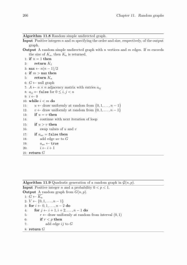
266 Chapter 11. Random graphs
Algorithm 11.8 Random simple undirected graph.
Input Positive integers n and m specifying the order and size, respectively, of the outputgraph.
Output A random simple undirected graph with n vertices and m edges. If m exceedsthe size of Kn, then Kn is returned.
1: if n = 1 then2: return K1
3: max← n(n− 1)/24: if m > max then5: return Kn
6: G← null graph7: A← n× n adjacency matrix with entries aij8: aij ← false for 0 ≤ i, j < n9: i← 0
10: while i < m do11: u← draw uniformly at random from 0, 1, . . . , n− 112: v ← draw uniformly at random from 0, 1, . . . , n− 113: if u = v then14: continue with next iteration of loop
15: if u > v then16: swap values of u and v
17: if auv = false then18: add edge uv to G19: auv ← true
20: i← i+ 1
21: return G
Algorithm 11.9 Quadratic generation of a random graph in G(n, p).
Input Positive integer n and a probability 0 < p < 1.Output A random graph from G(n, p).
1: G← Kn
2: V ← 0, 1, . . . , n− 13: for i← 0, 1, . . . , n− 2 do4: for j ← i+ 1, i+ 2, . . . , n− 1 do5: r ← draw uniformly at random from interval (0, 1)6: if r < p then7: add edge ij to G
8: return G
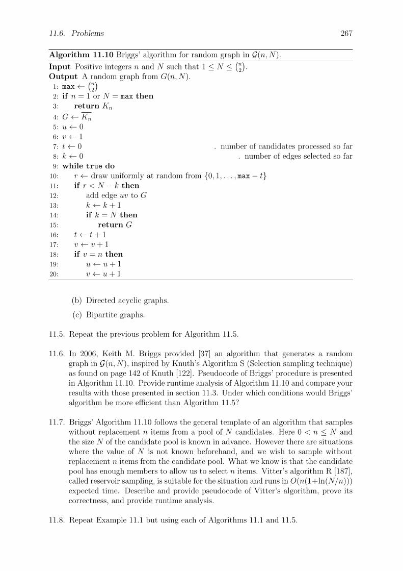
11.6. Problems 267
Algorithm 11.10 Briggs’ algorithm for random graph in G(n,N).
Input Positive integers n and N such that 1 ≤ N ≤(n2
).
Output A random graph from G(n,N).1: max←
(n2
)
2: if n = 1 or N = max then3: return Kn
4: G← Kn
5: u← 06: v ← 17: t← 0 . number of candidates processed so far8: k ← 0 . number of edges selected so far9: while true do
10: r ← draw uniformly at random from 0, 1, . . . , max− t11: if r < N − k then12: add edge uv to G13: k ← k + 114: if k = N then15: return G16: t← t+ 117: v ← v + 118: if v = n then19: u← u+ 120: v ← u+ 1
(b) Directed acyclic graphs.
(c) Bipartite graphs.
11.5. Repeat the previous problem for Algorithm 11.5.
11.6. In 2006, Keith M. Briggs provided [37] an algorithm that generates a randomgraph in G(n,N), inspired by Knuth’s Algorithm S (Selection sampling technique)as found on page 142 of Knuth [122]. Pseudocode of Briggs’ procedure is presentedin Algorithm 11.10. Provide runtime analysis of Algorithm 11.10 and compare yourresults with those presented in section 11.3. Under which conditions would Briggs’algorithm be more efficient than Algorithm 11.5?
11.7. Briggs’ Algorithm 11.10 follows the general template of an algorithm that sampleswithout replacement n items from a pool of N candidates. Here 0 < n ≤ N andthe size N of the candidate pool is known in advance. However there are situationswhere the value of N is not known beforehand, and we wish to sample withoutreplacement n items from the candidate pool. What we know is that the candidatepool has enough members to allow us to select n items. Vitter’s algorithm R [187],called reservoir sampling, is suitable for the situation and runs in O(n(1+ln(N/n)))expected time. Describe and provide pseudocode of Vitter’s algorithm, prove itscorrectness, and provide runtime analysis.
11.8. Repeat Example 11.1 but using each of Algorithms 11.1 and 11.5.
268 Chapter 11. Random graphs
11.9. Diego Garlaschelli introduced [84] in 2009 a weighted version of the G(n, p) model,called the weighted random graph model. Denote by GW (n, p) the weighted randomgraph model. Provide a description and pseudocode of a procedure to generate agraph in GW (n, p) and analyze the runtime complexity of the algorithm. Describevarious statistical physics properties of GW (n, p).
11.10. Latora and Marchiori [129] extended the Watts-Strogatz model to take into ac-count weighted edges. A crucial idea in the Latora-Marchiori model is the conceptof network efficiency. Describe the Latora-Marchiori model and provide pseudocodeof an algorithm to construct Latora-Marchiori networks. Explain the conceptsof local and global efficiencies and how these relate to clustering coefficient andcharacteristic path length. Compare and contrast the Watts-Strogatz and Latora-Marchiori models.
11.11. The following model for “growing” graphs is known as the CHKNS model [46],1
named for its original proponents. Start with the trivial graph G at time stept = 1. For each subsequent time step t > 1, add a new vertex to G. Furthermorechoose two vertices uniformly at random and with probability δ join them by anundirected edge. The newly added edge does not necessarily have the newly addedvertex as an endpoint. Denote by dk(t) the expected number of vertices with degreek at time t. Assuming that no self-loops are allowed, show that
d0(t+ 1) = d0(t) + 1− 2δd0(t)
t
and
dk(t+ 1) = dk(t) + 2δdk−1(t)
t− 2δ
dk(t)
t.
As t → ∞, show that the probability that a vertex be chosen twice decreases ast−2. If v is a vertex chosen uniformly at random, show that
Pr[deg(v) = k] =(2δ)k
(1 + 2δ)k+1
and conclude that the CHKNS model has an exponential degree distribution. Thesize of a component counts the number of vertices in the component itself. LetNk(t) be the expected number of components of size k at time t. Show that
N1(t+ 1) = N1(t) + 1− 2δN1(t)
t
and for k > 1 show that
Nk(t+ 1) = Nk(t) + δ
(k−1∑
i=1
iNi(t)
t· (k − i)Nk−i(t)
t
)− 2δ
kNk(t)
t.
11.12. Algorithm 11.7 can easily be modified to generate other types of scale-free net-works. Based upon the latter algorithm, Batagelj and Brandes [18] presenteda procedure for generating bipartite scale-free networks; see Algorithm 11.11 for
1 Or the “chickens” model, depending on how you pronounce “CHKNS”.
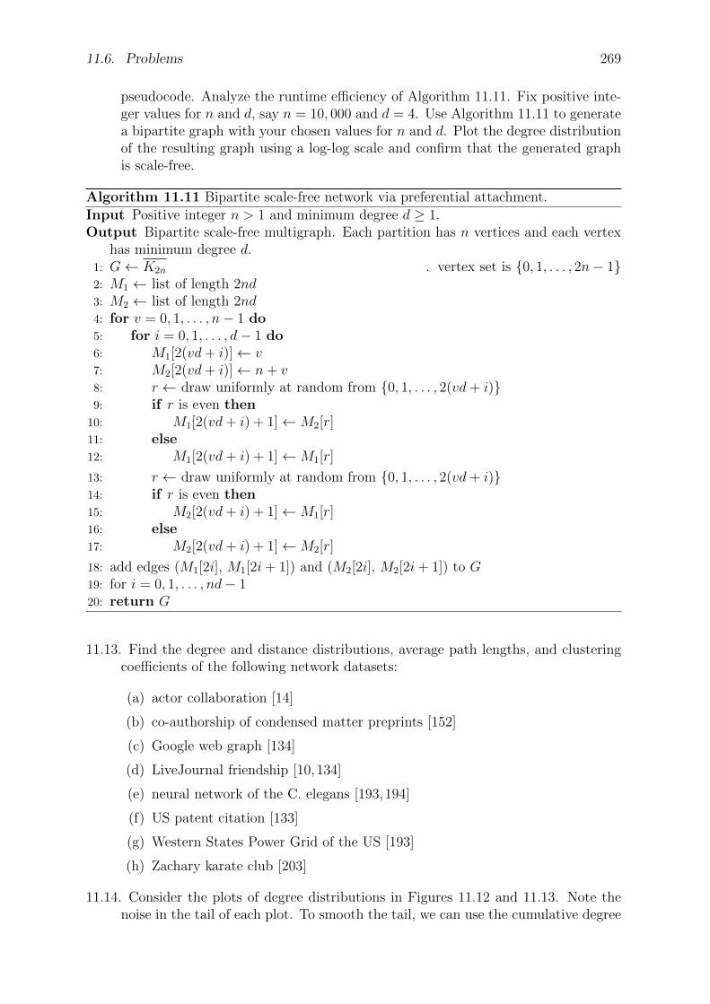
11.6. Problems 269
pseudocode. Analyze the runtime efficiency of Algorithm 11.11. Fix positive inte-ger values for n and d, say n = 10, 000 and d = 4. Use Algorithm 11.11 to generatea bipartite graph with your chosen values for n and d. Plot the degree distributionof the resulting graph using a log-log scale and confirm that the generated graphis scale-free.
Algorithm 11.11 Bipartite scale-free network via preferential attachment.
Input Positive integer n > 1 and minimum degree d ≥ 1.Output Bipartite scale-free multigraph. Each partition has n vertices and each vertex
has minimum degree d.1: G← K2n . vertex set is 0, 1, . . . , 2n− 12: M1 ← list of length 2nd3: M2 ← list of length 2nd4: for v = 0, 1, . . . , n− 1 do5: for i = 0, 1, . . . , d− 1 do6: M1[2(vd+ i)]← v7: M2[2(vd+ i)]← n+ v8: r ← draw uniformly at random from 0, 1, . . . , 2(vd+ i)9: if r is even then
10: M1[2(vd+ i) + 1]←M2[r]11: else12: M1[2(vd+ i) + 1]←M1[r]
13: r ← draw uniformly at random from 0, 1, . . . , 2(vd+ i)14: if r is even then15: M2[2(vd+ i) + 1]←M1[r]16: else17: M2[2(vd+ i) + 1]←M2[r]
18: add edges (M1[2i], M1[2i+ 1]) and (M2[2i], M2[2i+ 1]) to G19: for i = 0, 1, . . . , nd− 120: return G
11.13. Find the degree and distance distributions, average path lengths, and clusteringcoefficients of the following network datasets:
(a) actor collaboration [14]
(b) co-authorship of condensed matter preprints [152]
(c) Google web graph [134]
(d) LiveJournal friendship [10,134]
(e) neural network of the C. elegans [193,194]
(f) US patent citation [133]
(g) Western States Power Grid of the US [193]
(h) Zachary karate club [203]
11.14. Consider the plots of degree distributions in Figures 11.12 and 11.13. Note thenoise in the tail of each plot. To smooth the tail, we can use the cumulative degree

270 Chapter 11. Random graphs
distribution
P c(k) =∞∑
i=k
Pr[deg(v) = i].
Given a graph with scale-free degree distribution P (k) ∼ k−α and α > 1, thecumulative degree distribution follows P c(k) ∼ k1−α. Plot the cumulative degreedistribution of each network dataset in Problem 11.13.
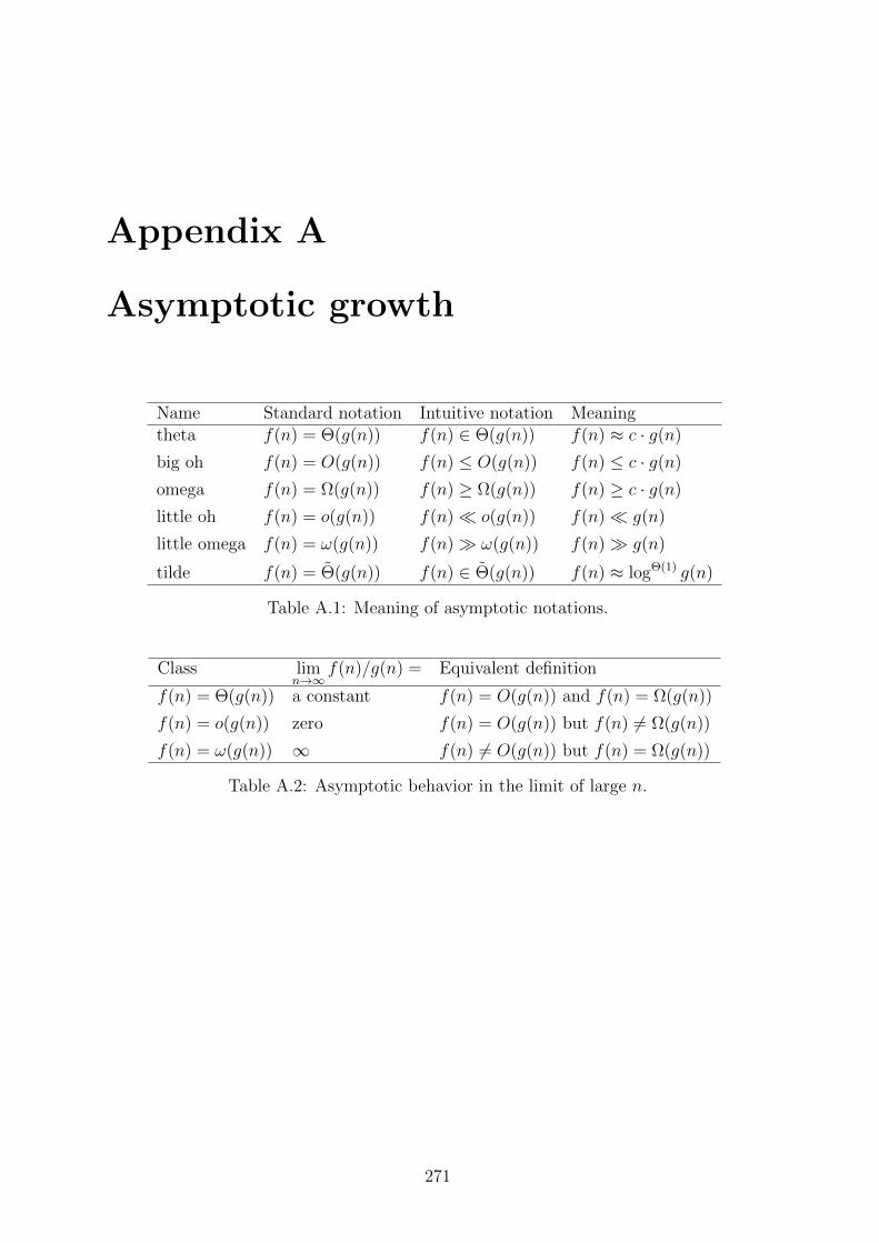
Appendix A
Asymptotic growth
Name Standard notation Intuitive notation Meaningtheta f(n) = Θ(g(n)) f(n) ∈ Θ(g(n)) f(n) ≈ c · g(n)
big oh f(n) = O(g(n)) f(n) ≤ O(g(n)) f(n) ≤ c · g(n)
omega f(n) = Ω(g(n)) f(n) ≥ Ω(g(n)) f(n) ≥ c · g(n)
little oh f(n) = o(g(n)) f(n) o(g(n)) f(n) g(n)
little omega f(n) = ω(g(n)) f(n) ω(g(n)) f(n) g(n)
tilde f(n) = Θ(g(n)) f(n) ∈ Θ(g(n)) f(n) ≈ logΘ(1) g(n)
Table A.1: Meaning of asymptotic notations.
Class limn→∞
f(n)/g(n) = Equivalent definition
f(n) = Θ(g(n)) a constant f(n) = O(g(n)) and f(n) = Ω(g(n))
f(n) = o(g(n)) zero f(n) = O(g(n)) but f(n) 6= Ω(g(n))
f(n) = ω(g(n)) ∞ f(n) 6= O(g(n)) but f(n) = Ω(g(n))
Table A.2: Asymptotic behavior in the limit of large n.
271
Appendix B
GNU Free Documentation License
Version 1.3, 3 November 2008Copyright © 2000, 2001, 2002, 2007, 2008 Free Software Foundation, Inc.
http://www.fsf.org
Everyone is permitted to copy and distribute verbatim copies of this license document,but changing it is not allowed.
Preamble
The purpose of this License is to make a manual, textbook, or other functionaland useful document “free” in the sense of freedom: to assure everyone the effectivefreedom to copy and redistribute it, with or without modifying it, either commerciallyor noncommercially. Secondarily, this License preserves for the author and publisher away to get credit for their work, while not being considered responsible for modificationsmade by others.
This License is a kind of “copyleft”, which means that derivative works of the doc-ument must themselves be free in the same sense. It complements the GNU GeneralPublic License, which is a copyleft license designed for free software.
We have designed this License in order to use it for manuals for free software, be-cause free software needs free documentation: a free program should come with manualsproviding the same freedoms that the software does. But this License is not limited tosoftware manuals; it can be used for any textual work, regardless of subject matter orwhether it is published as a printed book. We recommend this License principally forworks whose purpose is instruction or reference.
1. APPLICABILITY AND DEFINITIONS
This License applies to any manual or other work, in any medium, that contains anotice placed by the copyright holder saying it can be distributed under the terms of thisLicense. Such a notice grants a world-wide, royalty-free license, unlimited in duration,to use that work under the conditions stated herein. The “Document”, below, refersto any such manual or work. Any member of the public is a licensee, and is addressedas “you”. You accept the license if you copy, modify or distribute the work in a wayrequiring permission under copyright law.
272
273
A “Modified Version” of the Document means any work containing the Documentor a portion of it, either copied verbatim, or with modifications and/or translated intoanother language.
A “Secondary Section” is a named appendix or a front-matter section of the Doc-ument that deals exclusively with the relationship of the publishers or authors of theDocument to the Document’s overall subject (or to related matters) and contains noth-ing that could fall directly within that overall subject. (Thus, if the Document is in parta textbook of mathematics, a Secondary Section may not explain any mathematics.) Therelationship could be a matter of historical connection with the subject or with relatedmatters, or of legal, commercial, philosophical, ethical or political position regardingthem.
The “Invariant Sections” are certain Secondary Sections whose titles are desig-nated, as being those of Invariant Sections, in the notice that says that the Document isreleased under this License. If a section does not fit the above definition of Secondarythen it is not allowed to be designated as Invariant. The Document may contain zeroInvariant Sections. If the Document does not identify any Invariant Sections then thereare none.
The “Cover Texts” are certain short passages of text that are listed, as Front-CoverTexts or Back-Cover Texts, in the notice that says that the Document is released underthis License. A Front-Cover Text may be at most 5 words, and a Back-Cover Text maybe at most 25 words.
A “Transparent” copy of the Document means a machine-readable copy, repre-sented in a format whose specification is available to the general public, that is suitablefor revising the document straightforwardly with generic text editors or (for images com-posed of pixels) generic paint programs or (for drawings) some widely available drawingeditor, and that is suitable for input to text formatters or for automatic translation toa variety of formats suitable for input to text formatters. A copy made in an other-wise Transparent file format whose markup, or absence of markup, has been arranged tothwart or discourage subsequent modification by readers is not Transparent. An imageformat is not Transparent if used for any substantial amount of text. A copy that is not“Transparent” is called “Opaque”.
Examples of suitable formats for Transparent copies include plain ASCII withoutmarkup, Texinfo input format, LaTeX input format, SGML or XML using a publiclyavailable DTD, and standard-conforming simple HTML, PostScript or PDF designedfor human modification. Examples of transparent image formats include PNG, XCFand JPG. Opaque formats include proprietary formats that can be read and edited onlyby proprietary word processors, SGML or XML for which the DTD and/or processingtools are not generally available, and the machine-generated HTML, PostScript or PDFproduced by some word processors for output purposes only.
The “Title Page” means, for a printed book, the title page itself, plus such followingpages as are needed to hold, legibly, the material this License requires to appear in thetitle page. For works in formats which do not have any title page as such, “Title Page”means the text near the most prominent appearance of the work’s title, preceding thebeginning of the body of the text.
The “publisher” means any person or entity that distributes copies of the Documentto the public.
A section “Entitled XYZ” means a named subunit of the Document whose titleeither is precisely XYZ or contains XYZ in parentheses following text that translates XYZ
274 Appendix B. GNU Free Documentation License
in another language. (Here XYZ stands for a specific section name mentioned below,such as “Acknowledgements”, “Dedications”, “Endorsements”, or “History”.)To “Preserve the Title” of such a section when you modify the Document means thatit remains a section “Entitled XYZ” according to this definition.
The Document may include Warranty Disclaimers next to the notice which statesthat this License applies to the Document. These Warranty Disclaimers are consideredto be included by reference in this License, but only as regards disclaiming warranties:any other implication that these Warranty Disclaimers may have is void and has no effecton the meaning of this License.
2. VERBATIM COPYING
You may copy and distribute the Document in any medium, either commerciallyor noncommercially, provided that this License, the copyright notices, and the licensenotice saying this License applies to the Document are reproduced in all copies, andthat you add no other conditions whatsoever to those of this License. You may not usetechnical measures to obstruct or control the reading or further copying of the copiesyou make or distribute. However, you may accept compensation in exchange for copies.If you distribute a large enough number of copies you must also follow the conditions insection 3.
You may also lend copies, under the same conditions stated above, and you maypublicly display copies.
3. COPYING IN QUANTITY
If you publish printed copies (or copies in media that commonly have printed covers)of the Document, numbering more than 100, and the Document’s license notice requiresCover Texts, you must enclose the copies in covers that carry, clearly and legibly, allthese Cover Texts: Front-Cover Texts on the front cover, and Back-Cover Texts on theback cover. Both covers must also clearly and legibly identify you as the publisher ofthese copies. The front cover must present the full title with all words of the title equallyprominent and visible. You may add other material on the covers in addition. Copyingwith changes limited to the covers, as long as they preserve the title of the Documentand satisfy these conditions, can be treated as verbatim copying in other respects.
If the required texts for either cover are too voluminous to fit legibly, you should putthe first ones listed (as many as fit reasonably) on the actual cover, and continue therest onto adjacent pages.
If you publish or distribute Opaque copies of the Document numbering more than 100,you must either include a machine-readable Transparent copy along with each Opaquecopy, or state in or with each Opaque copy a computer-network location from whichthe general network-using public has access to download using public-standard networkprotocols a complete Transparent copy of the Document, free of added material. Ifyou use the latter option, you must take reasonably prudent steps, when you begindistribution of Opaque copies in quantity, to ensure that this Transparent copy willremain thus accessible at the stated location until at least one year after the last timeyou distribute an Opaque copy (directly or through your agents or retailers) of thatedition to the public.
275
It is requested, but not required, that you contact the authors of the Document wellbefore redistributing any large number of copies, to give them a chance to provide youwith an updated version of the Document.
4. MODIFICATIONS
You may copy and distribute a Modified Version of the Document under the condi-tions of sections 2 and 3 above, provided that you release the Modified Version underprecisely this License, with the Modified Version filling the role of the Document, thuslicensing distribution and modification of the Modified Version to whoever possesses acopy of it. In addition, you must do these things in the Modified Version:
A. Use in the Title Page (and on the covers, if any) a title distinct from that of theDocument, and from those of previous versions (which should, if there were any,be listed in the History section of the Document). You may use the same title asa previous version if the original publisher of that version gives permission.
B. List on the Title Page, as authors, one or more persons or entities responsible forauthorship of the modifications in the Modified Version, together with at least fiveof the principal authors of the Document (all of its principal authors, if it has fewerthan five), unless they release you from this requirement.
C. State on the Title page the name of the publisher of the Modified Version, as thepublisher.
D. Preserve all the copyright notices of the Document.
E. Add an appropriate copyright notice for your modifications adjacent to the othercopyright notices.
F. Include, immediately after the copyright notices, a license notice giving the publicpermission to use the Modified Version under the terms of this License, in the formshown in the Addendum below.
G. Preserve in that license notice the full lists of Invariant Sections and required CoverTexts given in the Document’s license notice.
H. Include an unaltered copy of this License.
I. Preserve the section Entitled “History”, Preserve its Title, and add to it an itemstating at least the title, year, new authors, and publisher of the Modified Version asgiven on the Title Page. If there is no section Entitled “History” in the Document,create one stating the title, year, authors, and publisher of the Document as givenon its Title Page, then add an item describing the Modified Version as stated inthe previous sentence.
J. Preserve the network location, if any, given in the Document for public access toa Transparent copy of the Document, and likewise the network locations given inthe Document for previous versions it was based on. These may be placed in the“History” section. You may omit a network location for a work that was publishedat least four years before the Document itself, or if the original publisher of theversion it refers to gives permission.
276 Appendix B. GNU Free Documentation License
K. For any section Entitled “Acknowledgements” or “Dedications”, Preserve the Titleof the section, and preserve in the section all the substance and tone of each of thecontributor acknowledgements and/or dedications given therein.
L. Preserve all the Invariant Sections of the Document, unaltered in their text andin their titles. Section numbers or the equivalent are not considered part of thesection titles.
M. Delete any section Entitled “Endorsements”. Such a section may not be includedin the Modified Version.
N. Do not retitle any existing section to be Entitled “Endorsements” or to conflict intitle with any Invariant Section.
O. Preserve any Warranty Disclaimers.
If the Modified Version includes new front-matter sections or appendices that qualifyas Secondary Sections and contain no material copied from the Document, you may atyour option designate some or all of these sections as invariant. To do this, add theirtitles to the list of Invariant Sections in the Modified Version’s license notice. Thesetitles must be distinct from any other section titles.
You may add a section Entitled “Endorsements”, provided it contains nothing butendorsements of your Modified Version by various parties—for example, statements ofpeer review or that the text has been approved by an organization as the authoritativedefinition of a standard.
You may add a passage of up to five words as a Front-Cover Text, and a passage of upto 25 words as a Back-Cover Text, to the end of the list of Cover Texts in the ModifiedVersion. Only one passage of Front-Cover Text and one of Back-Cover Text may beadded by (or through arrangements made by) any one entity. If the Document alreadyincludes a cover text for the same cover, previously added by you or by arrangementmade by the same entity you are acting on behalf of, you may not add another; but youmay replace the old one, on explicit permission from the previous publisher that addedthe old one.
The author(s) and publisher(s) of the Document do not by this License give per-mission to use their names for publicity for or to assert or imply endorsement of anyModified Version.
5. COMBINING DOCUMENTS
You may combine the Document with other documents released under this License,under the terms defined in section 4 above for modified versions, provided that youinclude in the combination all of the Invariant Sections of all of the original documents,unmodified, and list them all as Invariant Sections of your combined work in its licensenotice, and that you preserve all their Warranty Disclaimers.
The combined work need only contain one copy of this License, and multiple identicalInvariant Sections may be replaced with a single copy. If there are multiple InvariantSections with the same name but different contents, make the title of each such sectionunique by adding at the end of it, in parentheses, the name of the original author orpublisher of that section if known, or else a unique number. Make the same adjustment
277
to the section titles in the list of Invariant Sections in the license notice of the combinedwork.
In the combination, you must combine any sections Entitled “History” in the variousoriginal documents, forming one section Entitled “History”; likewise combine any sec-tions Entitled “Acknowledgements”, and any sections Entitled “Dedications”. You mustdelete all sections Entitled “Endorsements”.
6. COLLECTIONS OF DOCUMENTS
You may make a collection consisting of the Document and other documents releasedunder this License, and replace the individual copies of this License in the various docu-ments with a single copy that is included in the collection, provided that you follow therules of this License for verbatim copying of each of the documents in all other respects.
You may extract a single document from such a collection, and distribute it individ-ually under this License, provided you insert a copy of this License into the extracteddocument, and follow this License in all other respects regarding verbatim copying ofthat document.
7. AGGREGATION WITH INDEPENDENT
WORKS
A compilation of the Document or its derivatives with other separate and independentdocuments or works, in or on a volume of a storage or distribution medium, is called an“aggregate” if the copyright resulting from the compilation is not used to limit the legalrights of the compilation’s users beyond what the individual works permit. When theDocument is included in an aggregate, this License does not apply to the other works inthe aggregate which are not themselves derivative works of the Document.
If the Cover Text requirement of section 3 is applicable to these copies of the Docu-ment, then if the Document is less than one half of the entire aggregate, the Document’sCover Texts may be placed on covers that bracket the Document within the aggregate,or the electronic equivalent of covers if the Document is in electronic form. Otherwisethey must appear on printed covers that bracket the whole aggregate.
8. TRANSLATION
Translation is considered a kind of modification, so you may distribute translationsof the Document under the terms of section 4. Replacing Invariant Sections with trans-lations requires special permission from their copyright holders, but you may includetranslations of some or all Invariant Sections in addition to the original versions of theseInvariant Sections. You may include a translation of this License, and all the licensenotices in the Document, and any Warranty Disclaimers, provided that you also includethe original English version of this License and the original versions of those notices anddisclaimers. In case of a disagreement between the translation and the original versionof this License or a notice or disclaimer, the original version will prevail.
If a section in the Document is Entitled “Acknowledgements”, “Dedications”, or“History”, the requirement (section 4) to Preserve its Title (section 1) will typicallyrequire changing the actual title.
278 Appendix B. GNU Free Documentation License
9. TERMINATION
You may not copy, modify, sublicense, or distribute the Document except as expresslyprovided under this License. Any attempt otherwise to copy, modify, sublicense, ordistribute it is void, and will automatically terminate your rights under this License.
However, if you cease all violation of this License, then your license from a particularcopyright holder is reinstated (a) provisionally, unless and until the copyright holderexplicitly and finally terminates your license, and (b) permanently, if the copyright holderfails to notify you of the violation by some reasonable means prior to 60 days after thecessation.
Moreover, your license from a particular copyright holder is reinstated permanentlyif the copyright holder notifies you of the violation by some reasonable means, this is thefirst time you have received notice of violation of this License (for any work) from thatcopyright holder, and you cure the violation prior to 30 days after your receipt of thenotice.
Termination of your rights under this section does not terminate the licenses of partieswho have received copies or rights from you under this License. If your rights have beenterminated and not permanently reinstated, receipt of a copy of some or all of the samematerial does not give you any rights to use it.
10. FUTURE REVISIONS OF THIS LICENSE
The Free Software Foundation may publish new, revised versions of the GNU FreeDocumentation License from time to time. Such new versions will be similar in spirit tothe present version, but may differ in detail to address new problems or concerns. Seehttp://www.gnu.org/copyleft/.
Each version of the License is given a distinguishing version number. If the Docu-ment specifies that a particular numbered version of this License “or any later version”applies to it, you have the option of following the terms and conditions either of thatspecified version or of any later version that has been published (not as a draft) by theFree Software Foundation. If the Document does not specify a version number of thisLicense, you may choose any version ever published (not as a draft) by the Free SoftwareFoundation. If the Document specifies that a proxy can decide which future versionsof this License can be used, that proxy’s public statement of acceptance of a versionpermanently authorizes you to choose that version for the Document.
11. RELICENSING
“Massive Multiauthor Collaboration Site” (or “MMC Site”) means any World WideWeb server that publishes copyrightable works and also provides prominent facilities foranybody to edit those works. A public wiki that anybody can edit is an example ofsuch a server. A “Massive Multiauthor Collaboration” (or “MMC”) contained in thesite means any set of copyrightable works thus published on the MMC site.
“CC-BY-SA” means the Creative Commons Attribution-Share Alike 3.0 license pub-lished by Creative Commons Corporation, a not-for-profit corporation with a principalplace of business in San Francisco, California, as well as future copyleft versions of thatlicense published by that same organization.
279
“Incorporate” means to publish or republish a Document, in whole or in part, as partof another Document.
An MMC is “eligible for relicensing” if it is licensed under this License, and if allworks that were first published under this License somewhere other than this MMC, andsubsequently incorporated in whole or in part into the MMC, (1) had no cover texts orinvariant sections, and (2) were thus incorporated prior to November 1, 2008.
The operator of an MMC Site may republish an MMC contained in the site underCC-BY-SA on the same site at any time before August 1, 2009, provided the MMC iseligible for relicensing.
ADDENDUM: How to use this License for your
documents
To use this License in a document you have written, include a copy of the Licensein the document and put the following copyright and license notices just after the titlepage:
Copyright © YEAR YOUR NAME. Permission is granted to copy, distributeand/or modify this document under the terms of the GNU Free Documenta-tion License, Version 1.3 or any later version published by the Free SoftwareFoundation; with no Invariant Sections, no Front-Cover Texts, and no Back-Cover Texts. A copy of the license is included in the section entitled “GNUFree Documentation License”.
If you have Invariant Sections, Front-Cover Texts and Back-Cover Texts, replace the“with . . . Texts.” line with this:
with the Invariant Sections being LIST THEIR TITLES, with the Front-Cover Texts being LIST, and with the Back-Cover Texts being LIST.
If you have Invariant Sections without Cover Texts, or some other combination ofthe three, merge those two alternatives to suit the situation.
If your document contains nontrivial examples of program code, we recommend re-leasing these examples in parallel under your choice of free software license, such as theGNU General Public License, to permit their use in free software.
Bibliography
[1] A. V. Aho, J. E. Hopcroft, and J. D. Ullman. The Design and Analysis of ComputerAlgorithms. Addison-Wesley Publishing Company, 1974.
[2] W. Aiello, F. Chung, and L. Lu. A random graph model for massive graphs. In TOC,pages 171–180. ACM, 2000.
[3] W. Aiello, F. Chung, and L. Lu. Handbook of Massive Data Sets, chapter Randomevolution of massive graphs, pages 97–122. Kluwer Academic Publishers, 2002.
[4] R. Albert and A.-L. Barabasi. Statistical mechanics of complex networks. Rev. Mod.Phys., 74:47–97, 2002.
[5] R. Albert, H. Jeong, and A.-L. Barabasi. Diameter of the World-Wide Web. Nature,401:130–131, 1999.
[6] L. A. N. Amaral, A. Scala, M. Barthelemy, and H. E. Stanley. Classes of small-worldnetworks. PNAS, 97:11149–11152, 2000.
[7] J. V. Anna Bernasconi, Bruno Codenotti. A characterization of bent functions in termsof strongly regular graphs. IEEE Trans. Comp., 50:984–985, 2001.
[8] V. Arlazarov, E. Dinic, M. Kronrod, and I. Faradzev. On economical construction of thetransitive closure of a directed graph. Soviet Math. Doklady, 11:1209–1210, 1970.
[9] A. S. Asratian, T. M. J. Denley, and R. Haggkvist. Bipartite Graphs and their Applica-tions. Cambridge University Press, 1998.
[10] L. Backstrom, D. P. Huttenlocher, J. M. Kleinberg, and X. Lan. Group formation in largesocial networks: membership, growth, and evolution. In T. Eliassi-Rad, L. H. Ungar,M. Craven, and D. Gunopulos, editors, KDD, pages 44–54. ACM, 2006.
[11] M. Baker and X. Faber. Quantum Graphs and Their Applications, chapter MetrizedGraphs, Laplacian Operators, and Electrical Networks, pages 15–33. AMS, 2006.
[12] W. W. R. Ball and H. S. M. Coxeter. Mathematical Recreations and Essays. DoverPublications, 13th edition, 1987.
[13] A.-L. Barabasi. Linked: The New Science of Networks. Basic Books, 2002.
[14] A.-L. Barabasi and R. Albert. Emergence of scaling in random networks. Science,286:509–512, 1999.
[15] A.-L. Barabasi, R. Albert, and H. Jeong. Mean-field theory for scale-free random net-works. Phys. A, 272:173–187, 1999.
[16] A.-L. Barabasi, R. Albert, and H. Jeong. Scale-free characteristics of random networks:The topology of the world wide web. Phys. A, 281:69–77, 2000.
[17] A. Barrat and M. Weigt. On the properties of small-world network models. Eur. Phys.J. B, 13:547–560, 2000.
[18] V. Batagelj and U. Brandes. Efficient generation of large random networks. Phys. Rev.E, 71:036113, 2005.
[19] R. A. Beezer. A First Course in Linear Algebra. Robert A. Beezer, University of PugetSound, USA, 2009. http://linear.ups.edu.
[20] J. Bell and B. Stevens. A survey of known results and research areas for n-queens. Disc.Math., 309:1–31, 2009.
[21] R. Bellman. Dynamic Programming. Princeton University Press, 1957.
280
Bibliography 281
[22] A. T. Benjamin and C. R. Yerger. Combinatorial interpretations of spanning tree iden-tities. Bull. Inst. Comb. App., 47:37–42, 2006.
[23] A. Bernasconi. Mathematical techniques for the analysis of Boolean functions. PhDthesis, Universit di Pisa-Udine, Pisa, Italy, 1998.
[24] A. Bernasconi and B. Codenotti. Spectral analysis of boolean functions as a grapheigenvalue problem. IEEE Trans. Comp., 48:345–351, 1999.
[25] N. L. Biggs. Algebraic potential theory on graphs. Bull. London Math. Soc., 29:641–682,1997.
[26] N. L. Biggs. Chip firing and the critical groups of graphs. J. Alg. Combin., 9:25–45,1999.
[27] N. L. Biggs. The critical group from a cryptographic perspective. Bull. London Math.Soc., 39:829–836, 2007.
[28] N. L. Biggs. Codes: An Introduction to Information, Communication, and Cryptography.Springer, 2009.
[29] S. Boccaletti, V. Latora, Y. Moreno, M. Chavez, and D.-U. Hwang. Complex networks:Structure and dynamics. Phys. Rep., 424:175–308, 2006.
[30] B. Bollobas. Random Graphs. Cambridge University Press, 2nd edition, 2001.
[31] B. Bollobas and O. Riordan. The diameter of a scale-free random graph. Combinatorica,24:5–34, 2004.
[32] B. Bollobas, O. Riordan, J. Spencer, and G. E. Tusnady. The degree sequence of ascale-free random graph process. Rand. Struc. Alg., 18:279–290, 2001.
[33] J. A. Bondy and U. S. R. Murty. Graph Theory with Applications. North-Holland, 1976.
[34] O. Boruvka. O jistem problemu minimalnım. Prace Mor. Prırodoved. Spol. v Brne III,3:37–58, 1926.
[35] O. Boruvka. Prıspevek k resenı otazky ekonomicke stavby elektrovodnıch sıtı. Elektron-icky Obzor, 15:153–154, 1926.
[36] U. Brandes. A faster algorithm for betweenness centrality. J. Math. Soc., 25:163–177,2001.
[37] K. M. Briggs. The verywnauty graph library (version 1.1), accessed 28th January 2011.http://keithbriggs.info/verywnauty.html.
[38] M. Brinkmeier and T. Schank. Network Analysis: Methodological Foundations, chapterNetwork Statistics, pages 293–317. Springer, 2005.
[39] A. Broder, R. Kumar, F. Maghoul, P. Raghavan, S. Rajagopalan, R. Stata, A. Tomkins,and J. Wiener. Graph structure in the web. Comp. Net., 33:309–320, 2000.
[40] A. Brouwer. The spectrum of a graph, 2003. http://www.win.tue.nl/∼aeb/srgbk/srg1only.html.
[41] M. R. Brown. The Analysis of a Practical and Nearly Optimal Priority Queue. PhDthesis, Stanford University, USA, 1977.
[42] M. R. Brown. Implementation and analysis of binomial queue algorithms. SIAM J.Comp., 7:298–319, 1978.
[43] J. Buchmann, E. Dahmen, and M. Schneider. Merkle tree traversal revisited. In J. Buch-mann and J. Ding, editors, PQCrypto, pages 63–78. Springer, 2008.
[44] F. Buckley and F. Harary. Distance in Graphs. Perseus Books, 1990.
[45] F. Buckley and W. Y. Lau. Mutually eccentric vertices in graphs. Ars Combinatoria,67, 2003.
[46] D. S. Callaway, J. E. Hopcroft, J. M. Kleinberg, M. E. J. Newman, and S. H. Strogatz.Are randomly grown graphs really random? Phys. Rev. E, 64:041902, 2001.
[47] C. Castellano, S. Fortunato, and V. Loreto. Statistical physics of social dynamics. Rev.Mod. Phys., 81:591–646, 2009.
[48] R. D. Castro and J. W. Grossman. Famous trails to Paul Erdos. Math. Intel., 21:51–53,1999.
282 Bibliography
[49] B. Chazelle. A minimum spanning tree algorithm with inverse-Ackermann type com-plexity. J. ACM, 47:1028–1047, 2000.
[50] B. Chazelle. The soft heap: An approximate priority queue with optimal error rate. J.ACM, 47:1012–1027, 2000.
[51] Q. Chen, H. Chang, R. Govindan, S. Jamin, S. Shenker, and W. Willinger. The origin ofpower-laws in internet topologies revisited. In INFOCOM, pages 608–617. IEEE, 2002.
[52] A. G. Chetwynd and A. J. W. Hilton. Star multigraphs with three vertices of maximumdegree. Math. Proc. Camb. Phil. Soc., 100:303–317, 1986.
[53] G. Choquet. Etude de certains reseaux de routes. Comptes Rendus Hebdomadaires desSeances de l’Academie des Sciences, 206:310–313, 1938.
[54] F. Chung. Laplacians and the Cheeger inequality for directed graphs. Ann. Comb.,9:1–19, 2005.
[55] D. Cohen. On holy wars and a plea for peace, 01st April 1980. http://www.ietf.org/rfc/ien/ien137.txt.
[56] D. Cohen. On holy wars and a plea for peace. IEEE Comp. Mag., 14:48–54, 1981.
[57] T. H. Cormen, C. E. Leiserson, R. L. Rivest, and C. Stein. Introduction to Algorithms.MIT Press and McGraw-Hill, 2nd edition, 2001.
[58] L. da F. Costa, F. A. Rodrigues, G. Travieso, and P. R. Villas Boas. Characterizationof complex networks: A survey of measurements. Adv. Phys., 56:167–242, 2007.
[59] L. da Fontoura Costa, O. N. Oliveira Jr., G. Travieso, F. A. Rodrigues, P. R. Villas Boas,L. Antiqueira, M. P. Viana, and L. E. C. Rocha. Analyzing and modeling real-worldphenomena with complex networks: a survey of applications. Adv. Phys., 60:329–412,2011.
[60] D. J. de Solla Price. Networks of scientific papers. Science, 149:510–515, 1965.
[61] E. W. Dijkstra. A note on two problems in connexion with graphs. Numerische Mathe-matik, 1:269–271, 1959.
[62] S. N. Dorogovtsev and J. F. F. Mendes. Language as an evolving word web. Proc. R.Soc. Lond. B, 268:2603–2606, 2001.
[63] S. N. Dorogovtsev and J. F. F. Mendes. Evolution of networks. Adv. Phys., 51:1079–1187,2002.
[64] H. Dorrie. 100 Great Problems of Elementary Mathematics: Their History and Solution.Translated by David Antin. Dover Publications, 1965.
[65] N. J. Durgin. Abelian sandpile model on symmetric graphs. 2009. Thesis, HarveyMudd, 2009. Available: http://www.math.hmc.edu/seniorthesis/archives/2009/ndurgin/ndurgin-2009-thesis.pdf.
[66] M. Dyer and A. Frieze. Randomly coloring random graphs. Rand. Struc. Alg., 36:251–272, 2010.
[67] D. Easley and J. Kleinberg. Networks, Crowds, and Markets: Reasoning about a HighlyConnected World. Cambridge University Press, 2010.
[68] M. Edelberg, M. R. Garey, and R. L. Graham. On the distance matrix of a tree. Disc.Math., 14:23–39, 1976.
[69] N. D. Elkies and R. P. Stanley. The mathematical knight. Math. Intel., 25:22–34, 2003.
[70] R. C. Entringer, D. E. Jackson, and D. A. Snyder. Distance in graphs. Czech. Math. J.,26:283–296, 1976.
[71] P. Erdos and T. Gallai. Graphs with prescribed degrees of vertices (in Hungarian).Matematikai Lopak, 11:264–274, 1960.
[72] P. Erdos and A. Renyi. On random graphs. Pub. Math., 6:290–297, 1959.
[73] P. Erdos and A. Renyi. On the evolution of random graphs. Magyar Tud. Akad. Mat.Kutato Int. Kozl., 5:17–61, 1960.
[74] P. L. Erdos, I. Miklos, and Z. Toroczkai. A simple Havel-Hakimi type algorithm to realizegraphical degree sequences of directed graphs. Elec. J. Comb., 17:R66, 2010.
Bibliography 283
[75] M. Faloutsos, P. Faloutsos, and C. Faloutsos. On power-law relationships of the Internettopology. Comp. Comm. Rev., 29:251–262, 1999.
[76] R. Ferrer i Cancho and R. V. Sole. The small world of human language. Proc. R. Soc.Lond. B, 268:2261–2265, 2001.
[77] K. Florek, J. Lukaszewicz, J. Perkal, H. Steinhaus, and S. Zubrzycki. Sur la liaison et ladivision des points d’un ensemble fini. Colloquium Mathematicum, 2:282–285, 1951.
[78] R. W. Floyd. Algorithm 97: Shortest path. Comm. ACM, 5:345, 1962.[79] L. R. Ford Jr. Network flow theory. Technical Report P-923, The Rand Corporation,
USA, 1956.[80] L. R. Foulds. Graph Theory Applications. Springer, 1992.[81] G. N. Frederickson. An optimal algorithm for selection in a min-heap. Inf. Comp.,
104:197–214, 1993.[82] M. L. Fredman and R. E. Tarjan. Fibonacci heaps and their uses in improved network
optimization algorithms. J. ACM, 34:596–615, 1987.[83] G. Gallo and S. Pallottino. Netflow at Pisa, chapter Shortest path methods: A unifying
approach, pages 38–64. Springer, 1986.[84] D. Garlaschelli. The weighted random graph model. New J. Phys., 11:073005, 2009.[85] E. N. Gilbert. Random graphs. Ann. Math. Stat., 30:1141–1144, 1959.[86] C. Godsil and R. Beezer. Explorations in algebraic graph theory with Sage, 2012. in
preparation.[87] C. Godsil and G. Royle. Algebraic Graph Theory. Springer, 2004.[88] R. L. Graham and P. Hell. On the history of the minimum spanning tree problem. Ann.
Hist. Comp., 7:43–57, 1985.[89] R. L. Graham and H. O. Pollak. On the addressing problem for loop switching. Bell
Sys. Tech. J., 50:2495–2519, 1971.[90] I. Gribkovskaia, Ø. Halskau Sr., and G. Laporte. The bridges of Konigsberg—a historical
perspective. Networks, 49:199–203, 2007.[91] J. Gross and J. Yellen. Graph Theory and Its Applications. CRC Press, 1999.[92] J. W. Grossman and P. D. F. Ion. On a portion of the well-known collaboration graph.
Congressus Numerantium, 108:129–131, 1995.[93] J. Guare. Six Degrees of Separation: A Play. Vintage, 1990.[94] I. Gutman, Y.-N. Yeh, S.-L. Lee, and Y.-L. Luo. Some recent results in the theory of
the Wiener number. Indian J. Chem., 32A:651–661, 1993.[95] S. L. Hakimi. On realizability of a set of integers as degrees of the vertices of a linear
graph I. SIAM J. App. Math., 10:496–506, 1962.[96] S. L. Hakimi. On realizability of a set of integers as degrees of the vertices of a linear
graph II: Uniqueness. SIAM J. App. Math., 11:135–147, 1963.[97] S. L. Hakimi and J. Bredeson. Graph theoretic error-correcting codes. IEEE Trans. Inf.
Theory, 14:584–591, 1968.[98] V. Havel. Poznamka o existenci konecnych grafu. Casopis pro Pestovanı Matematiky,
80:477–480, 1955.[99] K. Heinrich and P. Horak. Euler’s theorem. Am. Math. Mont., 101:260–261, 1994.
[100] A. E. Holroyd, L. Levine, K. Meszaros, Y. Peres, J. Propp, and D. B. Wilson. Chip-firingand rotor-routing on directed graphs. 2008. http://arxiv.org/abs/0801.3306.
[101] J. E. Hopcroft and R. E. Tarjan. Algorithm 447: Efficient algorithms for graph manip-ulation. Comm. ACM, 16:372–378, 1973.
[102] B. Hopkins and R. Wilson. The truth about Konigsberg. College Math. J., 35:198–207,2004.
[103] S. Howard. C algorithms (version 1.2.0), accessed 20th December 2010. http://c-algorithms.sourceforge.net.
[104] D. A. Huffman. A method for the construction of minimum-redundancy codes. InProceedings of the I.R.E, volume 40, pages 1098–1102, 1952.

284 Bibliography
[105] M. Huxham, S. Beaney, and D. Raffaelli. Do parasites reduce the chances of triangulationin a real food web? Oikos, 76:284–300, 1996.
[106] F. Jaeger, D. L. Vertigan, and D. J. A. Welsh. On the computational complexity of theJones and Tutte polynomials. Mathematical Proceedings of the Cambridge PhilosophicalSociety, 108:35–53, 1990.
[107] V. Jarnık. O jistem problemu minimalnım (Z dopisu panu O. Boruvkovi) (Czech). PraceMoravske Prırodovedecke Spolecnosti Brno, 6:57–63, 1930.
[108] T. R. Jensen and B. Toft. Graph Coloring Problems. John Wiley & Sons, 1995.[109] H. Jeong, S. Mason, A.-L. Barabasi, and Z. N. Oltvai. Lethality and centrality in protein
networks. Nature, 411:41–42, 2001.[110] H. Jeong, B. Tombor, R. Albert, Z. N. Oltvai, and A.-L. Barabasi. The large-scale
organization of metabolic networks. Nature, 407:651–654, 2000.[111] D. B. Johnson. Efficient algorithms for shortest paths in sparse networks. J. ACM,
24:1–13, 1977.[112] J. H. Jones and M. S. Handcock. An assessment of preferential attachment as a mecha-
nism for human sexual network formation. Proc. R. Soc. Lond. B, 270:1123–1128, 2003.[113] C. Jordan. Sur les assemblages de lignes. Journal fur die reine und angewandte Mathe-
matik, 70:185–190, 1869.[114] D. Jungnickel. Graphs, Networks and Algorithms. Springer, 3rd edition, 2008.[115] D. Jungnickel and S. A. Vanstone. Graphical codes revisited. IEEE Trans. Inf. Theory,
43:136–146, 1997.[116] D. Kalman. Marriages made in the heavens: A practical application of existence. Math.
Mag., 72:94–103, 1999.[117] H. Kaplan and U. Zwick. A simpler implementation and analysis of Chazelle’s soft heaps.
In C. Mathieu, editor, SODA, pages 477–485. SIAM, 2009.[118] A. Kershenbaum and R. Van Slyke. Computing minimum spanning trees efficiently. In
Proceedings of the ACM Annual Conference 25, pages 518–527. ACM, 1972.[119] S. C. Kleene. Automata Studies, chapter Representation of Events in Nerve Nets and
Finite Automata, pages 3–41. Princeton University Press, 1956.[120] J. Kleinberg. The small-world phenomenon: An algorithmic perspective. In STOC, pages
163–170. ACM, 2000.[121] D. E. Knuth. The Stanford GraphBase: A Platform for Combinatorial Computing.
Addison-Wesley, 1993.[122] D. E. Knuth. Seminumerical Algorithms, volume 2 of The Art of Computer Programming.
Addison-Wesley, 3rd edition, 1998.[123] V. F. Kolchin. Random Graphs. Cambridge University Press, 1999.[124] L. G. Kraft. A device for quantizing, grouping, and coding amplitude-modulated pulses.
Master’s thesis, Massachusetts Institute of Technology, USA, 1949.[125] J. B. Kruskal. On the shortest spanning subtree of a graph and the traveling salesman
problem. Proc. AMS, 7:48–50, 1956.[126] J. C. Lagarias. The 3x+ 1 problem and its generalizations. Am. Math. Mont., 92:3–23,
1985.[127] J. C. Lagarias. The 3x+1 problem: An annotated bibliography (1963–1999), 03rd August
2009. arXiv:math/0309224, http://arxiv.org/abs/math.NT/0309224.[128] J. C. Lagarias. The 3x+1 problem: An annotated bibliography, II (2000-2009), 27th Au-
gust 2009. arXiv:math/0608208, http://arxiv.org/abs/math.NT/0608208.[129] V. Latora and M. Marchiori. Economic small-world behavior in weighted networks. Eur.
Phys. J. B, 32:249–263, 2003.[130] H. T. Lau. A Java Library of Graph Algorithms and Optimization. Chapman & Hal-
l/CRC, 2007.[131] C. Y. Lee. An algorithm for path connections and its applications. IRE Transactions on
Electronic Computers, EC-10:346–365, 1961.
Bibliography 285
[132] D. H. Lehmer. Mathematical methods in large-scale computing units. In Proceedings ofthe Second Symposium on Large-Scale Digital Calculating Machinery, 1949.
[133] J. Leskovec, J. M. Kleinberg, and C. Faloutsos. Graphs over time: Densification laws,shrinking diameters and possible explanations. In R. Grossman, R. J. Bayardo, and K. P.Bennett, editors, KDD, pages 177–187. ACM, 2005.
[134] J. Leskovec, K. J. Lang, A. Dasgupta, and M. W. Mahoney. Statistical properties ofcommunity structure in large social and information networks. In J. Huai, R. Chen, H.-W. Hon, Y. Liu, W.-Y. Ma, A. Tomkins, and X. Zhang, editors, WWW, pages 695–704.ACM, 2008.
[135] F. Liljeros, C. R. Edling, L. A. N. Amaral, H. E. Stanley, and Y. Aberg. The web ofhuman sexual contacts. Nature, 411:907–908, 2001.
[136] M. Lobbing and I. Wegener. The number of knight’s tours equals 33,439,123,484,294 —counting with binary decision diagrams. Elec. J. Comb., 3:R5, 1996.
[137] H. Loberman and A. Weinberger. Formal procedures for connecting terminals with aminimum total wire length. J. ACM, 4:428–437, 1957.
[138] M. E. Lucas. Recreations Mathematiques. 4 volumes, Gauthier-Villars, Paris, 1882–94.[139] M. Mares. The saga of minimum spanning trees. Comp. Sci. Rev., 2:165–221, 2008.[140] N. D. Martinez. Artifacts or attributes? Effects of resolution on the Little Rock Lake
food web. Ecological Monographs, 61:367–392, 1991.[141] B. McKay. Description of graph6 and sparse6 encodings, accessed 05th April 2010.
http://cs.anu.edu.au/∼bdm/data/formats.txt.[142] B. D. McKay. Knight’s tours of an 8 × 8 chessboard. Technical Report TR-CS-97-03,
Department of Computer Science, Australian National University, Australia, February1997.
[143] B. McMillan. Two inequalities implied by unique decipherability. IRE Transactions onInformation Theory, 2:115–116, 1956.
[144] C. Merino. Matroids, the tuttle polynomial, and the chip firing game. 1999. http://calli.matem.unam.mx/∼merino/ewpublications.html#2, http://www.dmtcs.org/dmtcs-ojs/index.php/proceedings/article/viewArticle/dmAA0118, (The first link is for the thesis (inps format); the second is to a paper.).
[145] R. C. Merkle. A digital signature based on a conventional encryption function. InC. Pomerance, editor, CRYPTO, pages 369–378. Springer, 1988.
[146] S. Milgram. The small world problem. Psychology Today, 1:60–67, 1967.[147] B. Mohar, D. Babic, and N. Trinajstic. A novel definition of the Wiener index for trees.
J. Chem. Inf. Comp. Sci., 33:153–154, 1993.[148] E. F. Moore. The shortest path through a maze. In Proceedings of the International
Symposium on the Theory of Switching, pages 285–292, 1959.[149] S. Myles, A. R. Boyko, C. L. Owens, P. J. Brown, F. Grassi, M. K. Aradhya, B. Prins,
A. Reynolds, J.-M. Chia, D. Ware, C. D. Bustamante, and E. S. Buckler. Geneticstructure and domestication history of the grape. PNAS, 108:3530–3535, 2011.
[150] M. Newman, A.-L. Barabasi, and D. J. Watts, editors. The Structure and Dynamics ofNetworks. Princeton University Press, 2006.
[151] M. E. J. Newman. Scientific collaboration networks: I. Network construction and fun-damental results. Phys. Rev. E, 64:016131, 2001.
[152] M. E. J. Newman. The structure of scientific collaboration networks. PNAS, 98:404–409,2001.
[153] M. E. J. Newman. Mixing patterns in networks. Phys. Rev. E, 67:026126, 2003.[154] M. E. J. Newman. The structure and function of complex networks. SIAM Rev., 45:167–
256, 2003.[155] M. E. J. Newman. Analysis of weighted networks. Phys. Rev. E, 70:056131, 2004.[156] M. E. J. Newman, S. H. Strogatz, and D. J. Watts. Random graphs with arbitrary degree
distribution and their applications. Phys. Rev. E, 64:026118, 2001.

286 Bibliography
[157] E. Nuutila. Efficient Transitive Closure Computation in Large Digraphs. FinnishAcademy of Technology, 1995. http://www.cs.hut.fi/∼enu/thesis.html.
[158] J. Oxley. What is a matroid? Cubo Matematica Educacional, 5:179–218, 2003.
[159] D. Perkinson, J. Perlman, and J. Wilmes. Primer on the algebraic geometry of sandpiles.2009. http://people.reed.edu/∼davidp/412/handouts/primer091810.pdf.
[160] J. G. Perlman. Sandpiles: a bridge between graphs and toric ideals. 2009. Thesis, ReedCollege, http://people.reed.edu/∼davidp/homepage/seniors/perlman.pdf.
[161] J. Petersen. Sur le theoreme de tait. L’Intermediaire des Mathematiciens, 5:225–227,1898.
[162] G. Polya. How To Solve It: A New Aspect of Mathematical Method. Princeton UniversityPress, 2nd edition, 1957.
[163] R. C. Prim. Shortest connection networks and some generalizations. Bell Sys. Tech. J.,36:1389–1401, 1957.
[164] R. Rasmussen. Algorithmic Approaches for Playing and Solving Shannon Games. PhDthesis, Queensland University of Technology, Australia, 2007. http://eprints.qut.edu.au/18616/.
[165] S. Redner. How popular is your paper? An empirical study of the citation distribution.Eur. Phys. J. B, 4:131–134, 1998.
[166] K. H. Rosen. Elementary Number Theory and Its Applications. Addison Wesley Long-man, 4th edition, 2000.
[167] B. Roy. Transitivite et connexite. Comptes Rendus des Seances de l’Academie desSciences, 249:216–218, 1959.
[168] V. Runde. A Taste of Topology. Springer, 2005.
[169] R. Sedgewick. Algorithms in C. Addison-Wesley Publishing Company, 1990.
[170] P. O. Seglen. The skewness of science. J. Am. Soc. Inf. Sci., 43:628–638, 1992.
[171] P. Sen, S. Dasgupta, A. Chatterjee, P. A. Sreeram, G. Mukherjee, and S. S. Manna.Small-world properties of the Indian railway network. Phys. Rev. E, 67:036106, 2003.
[172] A. Shimbel. Structure in communications nets. In Proceedings of the Symposium onInformation Networks, pages 199–203, 1955.
[173] S. Shirali and H. L. Vasudeva. Metric Spaces. Springer, 2006.
[174] V. Shoup. A Computational Introduction to Number Theory and Algebra. CambridgeUniversity Press, 2nd edition, 2008. http://www.shoup.net/ntb.
[175] G. Sierksma and H. Hoogeveen. Seven criteria for integer sequences being graphic. J.Graph Theory, 15:223–231, 1991.
[176] H. A. Simon. On a class of skew distribution functions. Biometrika, 42:425–440, 1955.
[177] P. Stanica. Graph eigenvalues and Walsh spectrum of boolean functions. Integers, 7,2007.
[178] M. Szydlo. Merkle tree traversal in log space and time. In C. Cachin and J. Camenisch,editors, EUROCRYPT, pages 541–554. Springer, 2004.
[179] T. Takaoka. O(1) time algorithms for combinatorial generation by tree traversal. Comp.J., 42:400–408, 1999.
[180] T. Takaoka. Theory of 2-3 heaps. In T. Asano, H. Imai, D. T. Lee, S.-I. Nakano, andT. Tokuyama, editors, COCOON. Springer, 1999.
[181] R. E. Tarjan. Depth-first search and linear graph algorithms. SIAM J. Comp., 1:146–160,1972.
[182] G. Tarry. Le probleme des labyrinthes. Nouvelles Annales de Mathematique, 14:187–190,1895.
[183] J. Travers and S. Milgram. An experimental study of the small world problem. Sociom-etry, 32:425–443, 1969.
[184] A. Tripathi and S. Vijay. A note on a theorem of Erdos & Gallai. Disc. Math., 265:417–420, 2003.

Bibliography 287
[185] S. Valverde, R. F. Cancho, and R. V. Sole. Scale-free networks from optimal design.Euro. Lett., 60:512–517, 2002.
[186] A. Vazquez, R. Pastor-Satorras, and A. Vespignani. Large-scale topological and dynam-ical properties of the Internet. Phys. Rev. E, 65:066130, 2002.
[187] J. S. Vitter. Random sampling with a reservoir. ACM Tran. Math. Soft., 11:37–57, 1985.[188] J. Vuillemin. A data structure for manipulating priority queues. Comm. ACM, 21:309–
315, 1978.[189] S. Warshall. A theorem on boolean matrices. J. ACM, 9:11–12, 1962.[190] D. J. Watts. Networks, dynamics, and the small-world phenomenon. Am. J. Soc.,
105:493–527, 1999.[191] D. J. Watts. Small Worlds. Princeton University Press, 1999.[192] D. J. Watts. Six Degrees: The Science of a Connected Age. W. W. Norton & Company,
2004.[193] D. J. Watts and S. H. Strogatz. Collective dynamics of ‘small-world’ networks. Nature,
393:440–442, 1998.[194] J. G. White, E. Southgate, J. N. Thompson, and S. Brenner. The structure of the
nervous system of the nematode Caenorhabditis elegans. Phil. Trans. R. Soc. Lond. B,314:1–340, 1986.
[195] H. Whitney. Congruent graphs and the connectivity of graphs. Am. J. Math., 54:150–168,1932.
[196] H. Wiener. Structural determination of paraffin boiling points. J. Am. Chem. Soc.,69:17–20, 1947.
[197] J. W. J. Williams. Algorithm 232: Heapsort. Comm. ACM, 7:347–348, 1964.[198] T. Yamada, S. Kataoka, and K. Watanabe. Listing all the minimum spanning trees in
an undirected graph. Int. J. Comp. Math., 87:3175–3185, 2010.[199] T. Yamada and H. Kinoshita. Finding all the negative cycles in a directed graph. Disc.
App. Math., 118:279–291, 2002.[200] J. Yang and Y. Chen. Fast computing betweenness centrality with virtual nodes on large
sparse networks. PLoS ONE, 6:e22557, 2011.[201] V. Yegnanarayanan. Graph theory to pure mathematics: Some illustrative examples.
Resonance, 10:50–59, 2005.[202] Y.-N. Yeh and I. Gutman. On the sum of all distances in composite graphs. Disc. Math.,
135:359–365, 1994.[203] W. W. Zachary. An information flow model for conflict and fission in small groups. J.
Anth. Res., 33:452–473, 1977.
Index
A(G), 21C0(G,F ), 223C1(G,F ), 223Cn, 16En, 46Gc, 39Kn, 15Km,n, 19Ln, 41Pn, 16, 41Qn, 42Wn, 35∆, 35∆(G), 10adj, 4L, 27L(G), 8Ni, 259χv(G), 213∼=, 28deg, 5, 8deg+, 7deg−, 7δ(G), 10depth(v), 52diam(G), 185ε, 183, 255height(T ), 52iadj, 5id, 5κ(G), 188κe(G), 189κv(G), 187λ(G), 189lg, 154oadj, 5od, 5ω, 14ω(G), 213G, 39
per(G), 185rad(G), 185, 41td, 139ε, 85, 88ϕ(n), 61f -augmenting, 236f -saturated, 236f -unsaturated, 236f -zero, 236k-coloring, 212k-connected, 188k-edge-connected, 189n-queens problem, 145n-space, 82graph6, 104, 106, 108, 109sparse6, 106, 108 Lukaszewicz, J., 70
edge expander family, 204
active vertex, 229acyclic, 51, 63, 96adjacency matrix, 21
reduced, 23signed edge, 199
algorithmgreedy, 63, 66, 126, 127optimization, 57random, 48, 96–98, 148, 247, 248, 252–
254, 257, 264, 266, 267, 269recursive, 101
alphabet, 79, 80, 85binary, 85, 86English, 79, 98weighted, 80, 87
Altito, Noelie, 135arcs, 3ASCII, 79, 81, 106, 108augmenting path, 236Australian National University, 106
288
Index 289
automata theory, 134AVL tree, 181
backtrack, 116algorithm, 145
Baker, Matthew, 183balanced bracket problem, 142, 143Barabasi-Albert model, 261Batagelj, Vladimir, 250, 268Batagelj-Brandes algorithm, 250, 252Baudot, E., 81Bellman, Richard E., 127Bellman-Ford algorithm, 123, 127–130, 135Benjamin, Arthur T., 102bent, 200Bernoulli family, 53BFS, 110–114, 116, 120big-endian, 108, 109Biggs, Norman, 87binary heap, 150, 151
maximum, 178minimum, 178order property, 152, 180sift-down, 157sift-up, 155structure property, 152
binary search, 138, 169binary search tree, 150, 169, 171, 178
left subtree property, 169property, 169, 180recursion property, 169right subtree property, 169
binary tree, 54, 56, 75, 77–79, 98, 150complete, 77, 78nearly complete, 152random, 80, 98
Binetformula, 181Jacques Philippe Marie, 181
binomialcoefficient, 162, 178distribution, 247random graph, 249tree, 162
binomial heap, 150, 161, 162, 164, 179maximum, 179minimum, 179order property, 164, 180
properties, 164root-degree property, 164, 165
biology, 182bipartite graph, 16, 20, 48, 268, 269
complete, 19, 20Birkhoff-Lewis Conjecture, 221bit, 79, 85, 108
least significant, 108most significant, 108parity, 108
bit vector, 106, 108, 109length, 108
bond, 38, 57, 224Boruvka
algorithm, 63, 70, 71, 95, 96, 101Otakar, 63, 70
bowtie graph, 13braille, 80branch cut, 54, 56Brandes, Ulrik, 250, 268breadth-first search, 56, 90, 91, 110–114,
119, 120, 122–124, 137, 141tree, 110, 113
bridge, 38, 52, 58, 70, 74, 189bridgeless, 189Briggs
algorithm, 267Keith M., 267
Brooks’ inequality, 215BST, 169bubble sort, 140, 141butterfly graph, 13
Caenorhabditis elegans, 244canonical label, 30Cantor-Schroder-Bernstein theorem, 48capacity, 235
cut, 237card, 116cardinality, 8Carroll, Lewis, 2Cartesian product, 41Catalan
number, 46, 47, 78recursion, 78
Cayley graph of Boolean function, 199characteristic polynomial, 198Chazelle, Bernard, 179
290 Index
check matrix, 23chemistry, 133, 182chess, 80, 114, 145
chessboard, 114knight, 114knight piece, 114knight’s tour, 114–116, 145, 146queen, 145, 146
childleft, 75, 77, 90, 93right, 75, 90, 93
Chinese ring puzzle, 81, 82chip firing game, 229chip-firing game, 229chip-firing games, 228CHKNS model, 268Choquet, G., 70chromatic
index, 215number, 213polynomial, 220root, 221
chromatically equivalent, 220Chu Shi-Chieh, 179Chvatal graph, 96, 97circuit, 13
board, 110electronic, 62
circuit matrix, 73circulation, 224circulation space, 224, 225classification tree, 52, 53, 57claw graph, 188clique, 213
maximal, 213number, 213
closed form, 78closeness centrality, 196cocycle code, 225cocycle space, 225cocyle, 224code, 79, 85
r-ary, 101binary, 79, 85block, 80economy, 80error-correcting, 23, 80linear, 82
optimal, 87prefix, 80prefix-free, 80, 81, 86, 98radix, 101reliability, 80security, 80tree representation, 85, 86uniquely decodable, 86variable-length, 80
codeword, 79, 85length, 87
coding function, 80Cohen, Danny, 108Collatz
conjecture, 99graph, 99, 100length, 99sequence, 99tree, 99, 100
color code, 80color-class, 213combinatorial generation, 178combinatorial graphs, 2combinatorics, 82communications network, 191complement, 39complete graph, 15, 16, 97, 98, 247, 252,
254, 257, 258, 266, 267component, 14, 34, 58
connected, 63computer science, 90condensed matter, 245configuration, 229, 231
critical, 232level, 235recurrent, 232stable, 231starting, 229weight, 235
connected graph, 14, 57connectivity, 141cost, 121Coward, Noel, 11critical configurations, 233critical group, 233, 235cryptosystem, 80current, 228cut
Index 291
set, 38, 59cut set, 224cut space, 225cut-edge, 188, 189cut-point, 187cut-vertex, 187, 188cutset, 74
matrix, 74cycle, 13, 51, 52, 58, 60, 122, 123, 136
fundamental, 60, 98negative, 122, 123, 128, 130, 135, 136,
148cycle code, 224cycle double cover conjecture, 189cycle graph, 16, 17, 49cycle matrix, 73cycle space, 25, 224
binary, 25
D’Angelo, Anthony J., 95Dorrie, Heinrich, 47data structure, 103, 149de Moivre, Abraham, 181de Montmort, Pierre Remond, 145decode, 79degree, 5, 8
matrix, 27maximum, 10, 56minimum, 10, 61sequence, 30, 61weighted, 8
degree centrality, 196degree distribution, 242–245, 252, 262, 263depth-first search, 56, 92, 110, 114, 116–
120, 123, 137, 141tree, 116, 119
de Moivre, Abraham, 145DFS, 114, 116–120diameter, 113, 114Digital Signature Algorithm, 101digraph, 5, 52
weighted, 121Dijkstra
algorithm, 14, 124–128, 135, 149E. W., 66, 124
Dirac’s theorem, 195disconnected graph, 14disconnecting set, 38
distance, 52, 103, 113, 114, 121, 122, 124,126, 128, 130
characteristic, 245function, 121, 122, 182, 183, 205matrix, 28, 122minimum, 124total, 139
distance distribution, 246distribution
binomial, 252geometric, 251, 253Poisson, 253uniform, 252
divide and conquer, 148dollar game, 231Dryden, John, 110dynamic programming, 130
eccentricity, 183, 184mutual, 206path, 205vertex, 206
edge, 3boundary, 204capacity, 235contraction, 39cut, 38, 57, 193deletion, 38deletion subgraph, 36directed, 4endpoint, 63expansion, 204head, 6incident, 3multigraph, 6multiple, 3tagging game, 57tail, 6weight, 6
edge chromatic number, 215edge coloring, 215edge cut subgraph, 224edge cutset, 224edge-cut, 188Edmonds, Jack, 57eigenvalue, 101electrical network, 228element

292 Index
random, 79Elkies, Noam D., 116encode, 79endianness, 108England, 147entropy
encoding, 80function, 80
Erdos, Paul, 31error rate, 80Euler
Leonhard, 1, 10, 46, 61phi function, 61, 98phi sequence, 61, 62polygon division problem, 46subgraph, 13
Euler subgraph, 224Eulerian trail, 1expander graph, 204
Faber, Xander, 183family tree, 14, 15, 52, 53fault-tolerant, 191Fermat’s little theorem, 48Fibonacci
sequence, 181tree, 181
FIFO, 111, 116filesystem, 52
hierarchy, 52finite automaton, 49first in, first out, 111flag semaphore, 80Florek, K., 70flow, 224, 235
value, 236flow chart, 103flow space, 224Floyd, Robert, 130Floyd-Roy-Warshall algorithm, 128, 130–
132, 134, 186, 187football, 80forbidden minor, 43Ford, Lester Randolph, Jr., 127forest, 51, 52Franklin graph, 29Frederickson, Greg N., 179FreeBSD, 103
frequency distribution, 256friendship graph, 197FRW, 128, 130function plot, 2fundamental cycles, 226
Gallai, Tibor, 31Garlaschelli, Diego, 268genetic code, 80Gilbert, E. N., 253girth, 13Goldbach, Christian, 46Goldberg, R., 128golden ratio, 102, 181Graham, Ronald L., 187graph, 3
connected, 14, 120, 121cube, 76dense, 105, 130Desargues, 76, 77directed, 5disconnected, 14Dyck, 213Foster, 18Franklin, 17Frucht, 215Gray, 20Heawood, 217icosahedral, 218intersection, 34, 35join, 35line, 8nonisomorphic, 46Pappas, 219simple, 8sparse, 21, 105, 130, 135traversal, 110trivial, 61, 70undirected, 3union, 34, 35unweighted, 3weighted, 6, 63, 66, 121
graph isomorphism, 28, 30graph minor, 43graphical sequence, 31, 33Gray code, 81, 82
m-ary, 81binary, 81, 82
Index 293
reflected, 82, 84Gray, Frank, 81Gribkovskaia, Irina, 1grid, 42
graph, 52, 54, 65, 66, 96, 98, 148Gros, L., 81group theory
computational, 82Gulliver’s Travels, 108
Hadamard transform, 200Hakimi, S. L., 31Halskau Sr., Øyvind, 1Hamming distance, 42Hampton Court Palace, 147handshaking lemma, 10Havel, Vaclav, 31Havel-Hakimi
test, 33theorem, 31
heap2-heap, 66k-ary, 127binary, 127binary minimum, 88Fibonacci, 66, 127, 135
heapsort, 151Heawood graph, 215hierarchical structure, 14, 51, 52Hopcroft, John E., 114Hopkins, Brian, 1house graph, 3Huffman
David, 87tree, 149
Huffman code, 85, 87–89, 91, 98binary, 87encoding, 90tree construction, 87tree representation, 88, 89, 91
Humpty Dumpty, 2hypercube graph, 42, 82, 83
in-neighbor, 5incidence
function, 6matrix, 24
incidence matrixoriented, 24
unoriented, 24indegree, 5
unweighted, 7independent set, 213induction, 58, 61, 77, 86, 87, 96
structural, 96infix notation, 142information channel, 80Internet, 261
topology, 262invariant, 29, 33isomorphism, 61isoperimetric number, 204
Jarnık, V., 66Johnson
algorithm, 123, 135Donald B., 135
join, 60Jordan, Camille, 186
Konigsberg, 1graph, 2, 6seven bridges puzzle, 1, 10
Kaliningrad, 1Kaplan, Haim, 179Kataoka, Seiji, 95Kinoshita, Harunobu, 148Kirchhoff’s current law, 228Kirchhoff’s voltage law, 228Kleene
algorithm, 134Stephen, 134
Klein, Felix, 2Kneser graph, 104–106Knuth
Algorithm S, 267Donald E., 81, 267
Kraftinequality, 101, 102Leon Gordon, 102theorem, 102
Kruskalalgorithm, 63–66, 95, 96, 101Joseph B., 63
ladder graph, 41Lagarias, Jeffrey C., 99Laplacian, 233

294 Index
reduced, 235Laplacian matrix, 27, 101, 198Laporte, Gilbert, 1last in, first out, 116Latora, V., 268Latora-Marchiori model, 268lattice, 42Lee, C. Y., 110legal firing sequence, 232Lehman, A., 57Lehmer, D. H., 47level
binary tree, 152tree, 180
LIFO, 116line graph, 8linear search, 138Linux, 52list, 88, 104, 111, 113, 116, 127
adjacency, 27, 104, 105, 113contiguous edge, 106, 257edge, 106element, 104empty, 104length, 104
little-endian, 108Loberman, H., 63Loebbing, Martin, 116Lucas
M. Edouard, 102, 114number, 102
Marchiori, M., 268matrix, 21
adjacency, 22, 104, 105, 109bi-adjacency, 23cutset, 76distance, 187incidence, 26main diagonal, 109transpose, 45upper triangle, 109
Matthew effect, 261max-flow min-cut theorem, 237
generalized, 238maximum flow problem, 236maze, 110, 114, 147McKay, Brendan D., 106, 116
McMillanBrockway, 101theorem, 101
Menger’s theorem, 192–194merge sort, 166Merkle, Ralph C., 101Merris-McKay theorem, 99mesh, 42, 43message, 85metabolic network, 261metric, 122, 183
function, 121metric graph, 183metric space, 122
finite, 122Milgram, Stanley, 255minimum cut problem, 237minimum spanning tree problem, 63molecular graph, 132Montmort-Moivre strategy, 145Moore, Edward F., 110, 127Morse code, 81, 86, 98MST, 63multi-undirected graph, 5multidigraph, 5multigraph, 5
adjacency, 7in-neighbor, 7out-neighbor, 7
Munroe, Randall, 51, 103, 114, 124, 127,149, 210, 211
musical score, 80
neighbor graph, 259network, 235
biological, 244, 255citation, 262collaboration, 262communication, 57information, 255social, 245, 255, 262technological, 244, 255Zachary karate club, 243
node, 3noisy channel, 80null graph, 4, 261Nuutila, Esko, 134
order, 3

Index 295
organism, 53, 57orientation, 6, 24oriented graph, 248
random, 248, 251out-neighbor, 5, 111, 119, 123, 124outdegree, 5
unweighted, 7, 8outer boundary, 204overfull graph, 45Oxley, James, 57
Paley graph, 205parallel forest-merging, 70parallelization, 70partition, 48Pascal
formula, 164, 178path, 12, 13, 51, 52
closed, 13distance, 121even, 13geodesic, 14graph, 41Hamiltonian, 82, 83internally disjoint, 191length, 52, 121, 122odd, 13shortest, 103, 121–124, 126, 128, 130,
135tree, 59, 60weighted, 135
path graph, 16pendant, 8, 60perfect square, 53Perkal, J., 70permutation
equivalent, 30random, 98
Petersengraph, 119, 120, 188, 189Julius, 119
planar graph, 47plane, 148Pollak, O., 187postfix notation, 142power grid, 244preferential attachment, 260, 261, 264prefix-free condition, 80
Pregel River, 1Prim
algorithm, 63, 66–69, 95, 96, 101, 149R. C., 63, 66
priority queue, 149, 150probability, 87
expectation, 87sample space, 79space, 247
pseudorandom number, 47, 251Python, 21
queue, 92, 111, 113, 116, 120, 124dequeue, 91, 93, 111, 113end, 111enqueue, 91, 93, 111, 113front, 111length, 111minimum-priority, 66, 88, 135priority, 88rear, 111start, 111
Ramanujan graph, 204random graph, 242
Bernoulli, 246binomial, 246, 255Erdos-Renyi, 253uniform, 253weighted, 268
random variablegeometric, 251
Rasmussen, Rune, 57recurrence relation, 181recursion, 57, 58, 70, 71, 87, 93, 96, 130reduced Laplacian, 235regular graph, 10, 48
k-circulant, 49, 255, 257r-regular, 10, 49
relative complement, 39remainder, 108reservoir sampling, 267residual digraph, 237residual network, 237reverse Polish notation, 142rich-get-richer effect, 261river crossing problem, 141Robertson, Neil, 43Robertson-Seymour theorem, 43
296 Index
Roget’s Thesaurus, 255root directory, 52root list, 165rotor-routing model, 228Roy, Bernard, 130RSA, 101Runde, Volker, 122Russia, 1
sandpile model, 231saturated edge, 236scale-free network, 264, 268, 269scatterplot, 2, 62, 84Schulz, Charles M., 176scientific collaboration, 245seg, 224selection sort, 140, 141self-complementary graph, 39self-loop, 4separating set, 38, 193set, 104
n-set, 2totally ordered, 150
SeymourPaul, 43, 189
ShannonClaude E., 8, 57multigraphs, 8, 9switching game, 57, 58
Shimbel, A., 127Shirali, Satish, 122shortest path, 14Simon, Herbert, 261simple graph, 8, 98, 255
random, 247, 252–254, 266, 267single-source shortest path, 124, 127six degrees of separation, 255size, 3
component, 268tree, 58–60
small-world, 49, 114, 257algorithm, 257characteristic path length, 257clustering coefficient, 257, 259effect, 255experimental results, 256network, 257
social network, 182
spanning forest, 70spanning subgraph, 15spanning tree, 52, 54, 57, 62–64, 96, 98, 102
maximum, 95minimum, 62–64, 66–71, 96randomized construction, 96, 97, 101
sparse graph, 250spectrum, 198
Laplacian, 198stack, 92, 116, 119, 120
length, 116pop, 92, 93, 95, 116, 119push, 92, 93, 95, 116, 119
Stanley, Richard P., 116star graph, 19, 20state
final, 141initial, 141
Steinhaus, H., 70string, 79, 85
empty, 88Strogatz, Steven H., 255strongly regular graph, 200subgraph, 11, 15
edge-deletion, 62, 63, 99subtree, 57, 93
left, 77, 93right, 77, 93
supergraph, 15Swift, Jonathan, 108Sylvester’s Law of Nullity, 73symbol, 85symbolic computation, 142symmetric difference, 35Szekeres, G., 189
Takaoka, Tadao, 178, 179Tanner graph, 23Tarjan, Robert Endre, 114Tarry, Gaston, 114telegraph, 81The Brain puzzle, 82Thoreau, Henry David, 8Through the Looking Glass, 2topology, 122total order, 150Tower of Hanoi puzzle, 82trail, 12, 13

Index 297
closed, 13transition probability matrix, 225transitive closure, 133, 134trapdoor function, 80traveling salesman problem, 103traversal
bottom-up, 93, 94, 101in-order, 93, 94, 101, 169level-order, 90, 91, 93, 101post-order, 92, 93, 101pre-order, 92, 101
treasure map, 1tree, 14, 51, 52, 60, 110
2-ary, 75n-ary, 52binary, 52, 85, 88, 93complete, 52, 57depth, 52directed, 52expression, 52, 53height, 52nonisomorphic, 52, 54, 55ordered, 52, 90recursive definition, 57, 58, 96rooted, 15, 52, 56, 75, 110, 119subtree, 58traversal, 90, 92
triangle inequality, 122, 136, 183Tripathi, Amitabha, 31trivial graph, 16, 52, 268tuple, 2
uniondigraph, 61, 62
union-find, 96Unix, 52unweighted degree, 7USA, 244, 262
value of flow, 236Vandermonde
Alexandre-Theophile, 179convolution, 179
Vasudeva, Harkrishan L., 122vertex, 3
adjacent, 3child, 52, 56cut, 38, 193degree, 10
deletion, 37, 93deletion subgraph, 35, 187endpoint, 51, 52expansion, 204head, 4internal, 52, 191isolated, 8, 57, 104isoperimetric number, 204leaf, 51, 52, 85, 93multigraph, 6parent, 52root, 15, 52, 54, 56, 85set, 3source, 124, 136tail, 4union, 34
vertex connectivity, 187vertex-cut, 187Vijay, Sujith, 31Vitter
algorithm, 267Jeffrey Scott, 267
Vizing’s theorem, 218voltage, 228Vuillemin, Jean, 164
Wagnerconjecture, 43Klaus, 43
walk, 11, 13closed, 13length, 11, 12trivial, 11
Walsh transform, 200Warshall, Stephen, 130, 134Watanabe, Kohtaro, 95Watts, Duncan J., 255Watts-Strogatz model, 255, 257, 268Wegener, Ingo, 116weight, 63, 121, 122, 130
correcting, 122, 123function, 63, 122, 136graph, 6minimum, 63, 66, 70, 126multigraph, 6negative, 122, 123, 127, 128nonnegative, 121–124, 126, 135path, 182

298 Index
positive, 122reweight, 135, 136setting, 122, 123unit, 121, 122
Weinberger, A., 63wheel graph, 35, 102Whitney
Hassler, 191inequality, 190theorem, 195
WienerHarold, 99, 132number, 99, 101, 132
Williams, J. W. J., 151Wilson, Robin, 1wine, 197, 202, 203, 207, 208word, 85World Wide Web, 261
Yamada, Takeo, 95, 148Yerger, Carl R., 102
Zachary, Wayne W., 243zero padding, 108Zubrzycki, S., 70Zwick, Uri, 179
Related Documents