Algorithmic construction of the Postnikov tower for diagrams of ...

Masaryk UniversityFaculty of Science

Algorithmic construction of thePostnikov tower for diagrams of

simplicial sets

Doctoral Thesis

Marek Filakovský

Brno, 2015

Declaration

Hereby I declare, that this paper is my original authorial work, which I have worked out bymy own. All sources, references and literature used or excerpted during elaboration of thiswork are properly cited and listed in complete reference to the due source.

Marek Filakovský

Advisor: doc. RNDr. Martin Čadek, CSc.

iii

Acknowledgement

I would like to thank my supervisor M. Čadek for his support and many useful discussions,suggestions and comments. The course in algebraic topology he taught inspired me to con-tinue in this field. I can hardly imagine a teacher that could be more generous with his timeand knowledge.

I am also indebted to L. Vokřínek, who took the unpaid job of being my unofficial sec-ondary supervisor. Many of the results of this thesis follow from ideas originally developedby him. Trying to keep up with his thoughts encouraged me to learn more about model cat-egories, homotopy theory and simplicial sets.

This work also benefited from results achieved by M. Krčál, J. Matoušek, F. Sergeraert andU. Wagner.

Finally, I would like to thank my family for their endless material and emotional support.I dedicate this thesis to my wife, Martina.

v

Abstract

The aim of the thesis is to provide an algorithm that given a nonnegative integer n and afinite diagram of simplicial sets Y : ℐ → sSet, where Y(i) is simply connected for all i ∈ ℐ ,constructs the n-stage Postnikov tower for Y .

Given a finite simplicial set Y with an action of a finite group G, the Elmendorf’s theoremprovides a finite diagram of simplicial sets Y : 𝒪op

G → sSet, where the spaces are fixed pointsYH for subgroups H ≤ G. The diagram Y further reflects the homotopy properties of space Y.Therefore, in the case the set of fixed points YH is simply connected for every subgroup H ≤G, the algorithm constructs the n-stage Postnikov tower for Y , which, informally speaking,represents the n-stage Postnikov tower for Y as a G-simplicial set.

Further, we present an algorithm that decides if a simplicial map f : X → Y betweenfinite simplicial sets X, Y is homotopic to a trivial map under the assumption that Y is simplyconnected.

Keywords

simplicial set, Postnikov tower, chain complex, effective homology, equivariant algebraic to-pology, model category

Abstrakt

Hlavním cílem této práce je popis algoritmu, který pro konečný diagram simpliciálních mno-žin Y : ℐ → sSet, kde Y(i) je jednoduše souvislý prostor pro každé i ∈ ℐ , a pro libovolnénezáporné n ∈ Z, zkonstruuje n-patrovou Postnikovovu věž pro diagram Y .

Podle Elmendorfovy věty, lze každé konečné simpliciální množině Y s akcí grupy G při-řadit diagram simpliciálních množin Y : 𝒪op

G → sSet. Prvky v tomto diagramu jsou prostorypevných bodů YH pro podgrupy H ≤ G. Diagram Y dále zachovává homotopické vlastnostiprostoru Y. Proto v případě kdy je každý prostor YH, H ≤ G jednoduše souvislý, algoritmuskonstruuje n-patrovou Postnikovovu věž pro diagram Y , která, neformálně řečeno, zodpo-vídá n-patrové Postnikovově věži pro G-simpliciální množinu Y.

Dále uvádíme algoritmus, který pro dané simpliciální zobrazení f : X → Y mezi ko-nečnými simpliciálními prostory, kde Y je jednoduše souvislý prostor, rozhoduje, zda je fhomotopické s triviálním zobrazením.

Klíčová slova

simpliciální množina, Postnikovova věž, řetězcový komplex, efektivní homologie, ekvivari-antní algebraická topologie, modelová kategorie

vii

Contents

Foreword . . . . . . . . . . . . . . . . . . . . . . . . . . . . . . . . . . . . . . . . . . . xi1 Motivation . . . . . . . . . . . . . . . . . . . . . . . . . . . . . . . . . . . . . . . . . . 1

1.1 Representing simplicial sets and simplicial maps in a computer . . . . . . . . 3Finite simplicial sets . . . . . . . . . . . . . . . . . . . . . . . . . . . . . . . . 3Locally effective simplicial sets . . . . . . . . . . . . . . . . . . . . . . . . . . 4

1.2 Postnikov tower for simplicial sets . . . . . . . . . . . . . . . . . . . . . . . . . 41.3 Effective homology . . . . . . . . . . . . . . . . . . . . . . . . . . . . . . . . . . 51.4 Our motivation . . . . . . . . . . . . . . . . . . . . . . . . . . . . . . . . . . . . 61.5 Category of orbits . . . . . . . . . . . . . . . . . . . . . . . . . . . . . . . . . . . 7

Simplicial sets with a group action . . . . . . . . . . . . . . . . . . . . . . . . 7Effective homology for diagrams . . . . . . . . . . . . . . . . . . . . . . . . . 8

1.6 Postnikov tower for diagrams . . . . . . . . . . . . . . . . . . . . . . . . . . . . 92 Tools . . . . . . . . . . . . . . . . . . . . . . . . . . . . . . . . . . . . . . . . . . . . . 11

2.1 Simplicial sets . . . . . . . . . . . . . . . . . . . . . . . . . . . . . . . . . . . . . 11Fibrations, cofibrations and weak equivalences . . . . . . . . . . . . . . . . . 11Twisted products . . . . . . . . . . . . . . . . . . . . . . . . . . . . . . . . . . 12

2.2 Diagrams of simplicial sets . . . . . . . . . . . . . . . . . . . . . . . . . . . . . . 13Homotopy and homology . . . . . . . . . . . . . . . . . . . . . . . . . . . . . 13Model structure . . . . . . . . . . . . . . . . . . . . . . . . . . . . . . . . . . . 14Homotopy left Kan extension . . . . . . . . . . . . . . . . . . . . . . . . . . . 15

2.3 Effective homology of chain complexes . . . . . . . . . . . . . . . . . . . . . . . 17Effective chain complexes, reductions and strong equivalences . . . . . . . . 17Perturbation Lemmas . . . . . . . . . . . . . . . . . . . . . . . . . . . . . . . 18

2.4 Effective homology of twisted products . . . . . . . . . . . . . . . . . . . . . . 19Effective chain complex for twisted product . . . . . . . . . . . . . . . . . . 21Vector fields . . . . . . . . . . . . . . . . . . . . . . . . . . . . . . . . . . . . . 23Twisted division . . . . . . . . . . . . . . . . . . . . . . . . . . . . . . . . . . 24

2.5 Effective homology for diagrams . . . . . . . . . . . . . . . . . . . . . . . . . . 25Constructions with effective homology . . . . . . . . . . . . . . . . . . . . . 28Perturbation lemmas for diagrams . . . . . . . . . . . . . . . . . . . . . . . . 29Filtrations . . . . . . . . . . . . . . . . . . . . . . . . . . . . . . . . . . . . . . 31

2.6 Homotopy colimit and cofibrant replacement have effective homology . . . . 31Functorial cofibrant replacement . . . . . . . . . . . . . . . . . . . . . . . . . 32

2.7 Effective abelian groups . . . . . . . . . . . . . . . . . . . . . . . . . . . . . . . 332.8 Polycyclic groups . . . . . . . . . . . . . . . . . . . . . . . . . . . . . . . . . . . 35

Computations with fully effective polycyclic groups . . . . . . . . . . . . . . 362.9 Eilenberg–MacLane spaces and diagrams . . . . . . . . . . . . . . . . . . . . . 38

Evaluation maps . . . . . . . . . . . . . . . . . . . . . . . . . . . . . . . . . . 39Simplicial maps to E(π, k) and K(π, k) . . . . . . . . . . . . . . . . . . . . . . 40Representing a map of diagrams by an effective cocycle . . . . . . . . . . . . 43A pullback from a fibration of Eilenberg–MacLane diagrams . . . . . . . . . 43Effective homology for E(π, n) and K(π, n) . . . . . . . . . . . . . . . . . . . 44

3 Postnikov tower for diagrams . . . . . . . . . . . . . . . . . . . . . . . . . . . . . . . 473.1 Reformulation of Theorem A . . . . . . . . . . . . . . . . . . . . . . . . . . . . 473.2 Description of the algorithm . . . . . . . . . . . . . . . . . . . . . . . . . . . . . 483.3 Correctness of the algorithm . . . . . . . . . . . . . . . . . . . . . . . . . . . . . 49

The cochain κefk−1 is a cocycle. . . . . . . . . . . . . . . . . . . . . . . . . . . . 50

The map ϕ′k takes values in P′k . . . . . . . . . . . . . . . . . . . . . . . . . . . 50

ix

Pk and ϕk satisfy the properties of the Postnikov system . . . . . . . . . . . 513.4 Computing equivariant cohomology operations . . . . . . . . . . . . . . . . . 52

4 How to decide if a map is homotopically trivial . . . . . . . . . . . . . . . . . . . . 55Relative statement . . . . . . . . . . . . . . . . . . . . . . . . . . . . . . . . . 55

4.1 Computations with Postnikov towers . . . . . . . . . . . . . . . . . . . . . . . . 564.2 Maps out of suspensions . . . . . . . . . . . . . . . . . . . . . . . . . . . . . . . 57

Homotopy concatenation . . . . . . . . . . . . . . . . . . . . . . . . . . . . . 574.3 Deciding the existence of a homotopy . . . . . . . . . . . . . . . . . . . . . . . 57

An exact sequence associated with a fibration . . . . . . . . . . . . . . . . . 57Proof of Theorem D . . . . . . . . . . . . . . . . . . . . . . . . . . . . . . . . 58Proof of (poly)n−1 + (null)n−1 → (poly)n . . . . . . . . . . . . . . . . . . . . 59

x

Foreword

This thesis contains the results of my research during my PhD studies.My initial assignment was to deal with the effective homology of twisted cartesian pro-

ducts, namely to generalize F Seregraert’s previous results [39]. The generalization was nee-ded for the paper [8].

The work on this issue turned to be relatively straightforward and after a year, I publishedmy results in [16]. In this thesis these results are contained in Section 2.4 and the main resultis stated as Corollary 2.21.

Together with L. Vokřínek, we used the methods introduced in [8] to give an algorithmthat decides whether two simplicial maps are homotopic. Our result can be found in [15] andis contained here in a simplified version as Chapter 4.

Afterwards, my advisor and L. Vokřínek suggested a particular road map that would leadus to generalize one of the main results of [8] - an algorithm that for given finite simplicialsets X, Y with an action of a finite group G computes the set [X, Y]G of equivariant homotopyclasses of maps, whereas [8] deals with the situation where the group G acts only freely.Our general aim was to use Elmendorf’s theorem on an equivalence of the category of G-simplicial sets with a certain category of diagrams of simplicial sets. Hence our attentionturned to working with diagrams of simplicial sets.

Following an idea of L. Vokřínek, I summed up some introductory technical results inarticle [17]. These are also utilized here in Section 2.5 and Section 3.4.

The main result of this thesis describes an algorithm that given a finite diagram of 1-connected simplicial sets Y and a positive integer n, constructs the n-stage Postnikov systemfor Y. This serves as a generalization of [7] and is proved in Chapter 3.

xi

1 Motivation

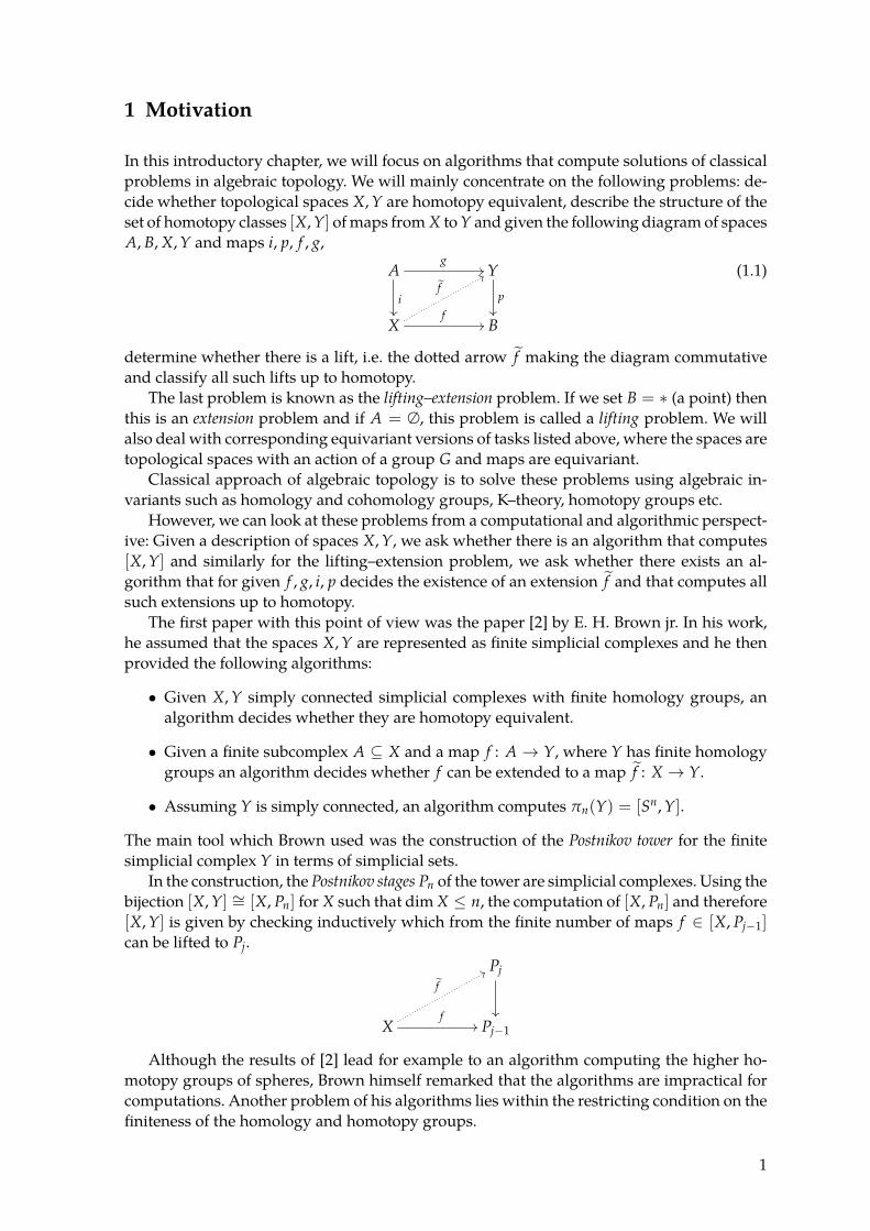
In this introductory chapter, we will focus on algorithms that compute solutions of classicalproblems in algebraic topology. We will mainly concentrate on the following problems: de-cide whether topological spaces X, Y are homotopy equivalent, describe the structure of theset of homotopy classes [X, Y] of maps from X to Y and given the following diagram of spacesA, B, X, Y and maps i, p, f , g,

Ag

//

i��

Yp��

Xf

//

f88

B

(1.1)

determine whether there is a lift, i.e. the dotted arrow f making the diagram commutativeand classify all such lifts up to homotopy.

The last problem is known as the lifting–extension problem. If we set B = * (a point) thenthis is an extension problem and if A = ∅, this problem is called a lifting problem. We willalso deal with corresponding equivariant versions of tasks listed above, where the spaces aretopological spaces with an action of a group G and maps are equivariant.

Classical approach of algebraic topology is to solve these problems using algebraic in-variants such as homology and cohomology groups, K–theory, homotopy groups etc.

However, we can look at these problems from a computational and algorithmic perspect-ive: Given a description of spaces X, Y, we ask whether there is an algorithm that computes[X, Y] and similarly for the lifting–extension problem, we ask whether there exists an al-gorithm that for given f , g, i, p decides the existence of an extension f and that computes allsuch extensions up to homotopy.

The first paper with this point of view was the paper [2] by E. H. Brown jr. In his work,he assumed that the spaces X, Y are represented as finite simplicial complexes and he thenprovided the following algorithms:

∙ Given X, Y simply connected simplicial complexes with finite homology groups, analgorithm decides whether they are homotopy equivalent.

∙ Given a finite subcomplex A ⊆ X and a map f : A → Y, where Y has finite homologygroups an algorithm decides whether f can be extended to a map f : X → Y.

∙ Assuming Y is simply connected, an algorithm computes πn(Y) = [Sn, Y].

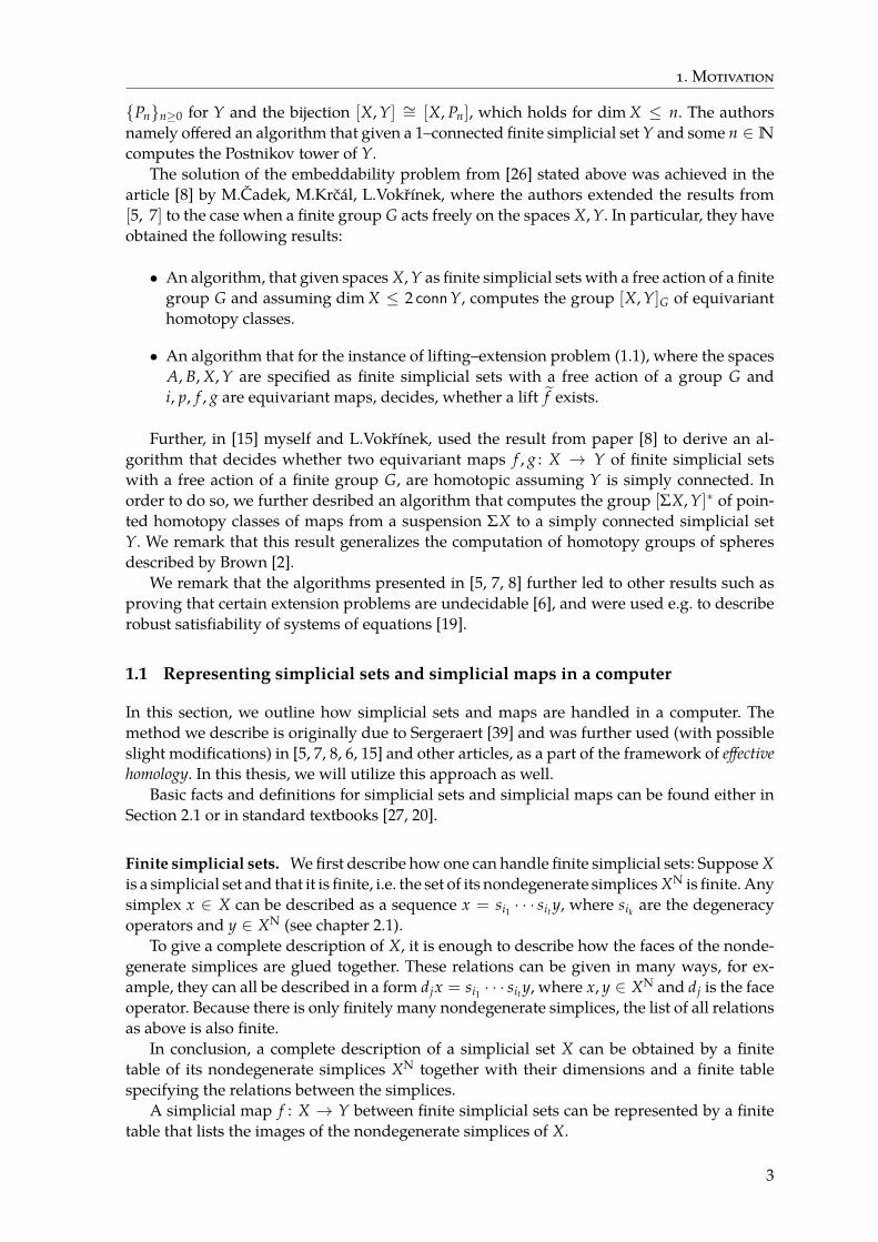
The main tool which Brown used was the construction of the Postnikov tower for the finitesimplicial complex Y in terms of simplicial sets.

In the construction, the Postnikov stages Pn of the tower are simplicial complexes. Using thebijection [X, Y] ∼= [X, Pn] for X such that dim X ≤ n, the computation of [X, Pn] and therefore[X, Y] is given by checking inductively which from the finite number of maps f ∈ [X, Pj−1]can be lifted to Pj.

Pj

��

Xf

//

f88

Pj−1

Although the results of [2] lead for example to an algorithm computing the higher ho-motopy groups of spheres, Brown himself remarked that the algorithms are impractical forcomputations. Another problem of his algorithms lies within the restricting condition on thefiniteness of the homology and homotopy groups.

1

1. Motivation

Francis Sergeraert [39] introduced the notion of objects with effective homology. We willelaborate on the precise definition later, for now we only remark that it is a collection ofalgorithms that allow us to compute the homology groups of the space even if the space ise.g. an infinite simplicial complex.

Together with his students and collaborators P. Real, A. Romero and J. Rubio, [33, 34,36, 38, 39, 37], they further presented a wide range of algorithmic constructions with suchobjects. Using these methods, one can for example compute data from some instances of Serreor Eilenberg–Moore spectral sequences and recently also Bousfield-Kan spectral sequences.Many of the above–mentioned algorithms were implemented in a package for Common Lispcalled Kenzo.

In a series of articles [41], R. Schön presented a different approach to algorithmic calcula-tions and introduced his own method of computing the algebraic data from certain spectralsequences using calculable sequences of groups. A connection and comparison between hismethods and the methods of effective homology as e.g. in [39] is not entirely clear and, to thebest of our knowledge, the algorithms he presented in [41] were not implemented.

A. Nabutovsky and S. Weinberger in the article [31] sketched an algorithm that for pie-cewise–linear or smooth simply connected manifolds Mn and Nk, decides whether they arehomeomorphic, diffeomorphic or piecewise–linear homeomorphic provided that the dimen-sion of one of the manifolds is at least five. In [30, 31] they further provided examples ofproblems that are not algorithmically solvable. Their result uses argument from surgery the-ory and rational homotopy theory and is mainly based on an algorithm that decides whethertwo 1–connected simplicial complexes have the same homotopy type. However details of thisalgorithm are not entirely clear.

Subsequent interest in the algorithmic computations was sparked by the group of authorsJ. Matoušek, M. Tancer and U. Wagner in their study [26] of the embeddability problem:

Given a finite k–dimensional simplicial complex K, decide algorithmically whether it canbe embedded in Rn.

It can be deduced, that if K embeds, then there exists a Z2-equivariant map (K × K) ∖∆K → Sn−1, where ∆K is the diagonal and Sn−1 is equipped with an antipodal action of Z2. Inthe metastable range, i.e. in the case k ≤ 2

3 n− 1, the converse also holds. The authors were ableto present an algorithmic solution or prove undecidability in many ranges of dimensions, butthe metastable range remained an open question.

We state the problem coming from the above embeddability problem as follows: We wantto algorithmically decide whether the set of equivariant homotopy classes of maps

[K× K ∖ ∆K, Sn−1]Z2

is nonempty. Further, in the metastable range, there exists an abelian group structure on thisset and we aim to describe this structure.

It is thus a special case of computing [X, Y]G, i.e. the set of G-equivariant homotopy classesof maps X → Y for a finite group G. This served as a motivation to introduce algorithmicmethods of computation in algebraic topology and homotopy theory in bigger generalitythan the algorithms described by Brown.

A progress in this direction was achieved by a group of authors M. Čadek, M. Krčál,J. Matoušek, F. Sergeraert, L. Vokřínek and U. Wagner. In paper [5] they presented an al-gorithm that computes [X, Y] for spaces X, Y given as finite simplicial sets satisfying dim X ≤2 connY and 1 ≤ connY, where dim X denotes the dimension of X and connY the connectiv-ity of Y.

The construction of their algorithm was further detailed in [7], where the computationalcomplexity of the algorithms was discussed.

Similar to the Brown’s result, the computation of [X, Y] was done using Postnikov tower

2

1. Motivation

{Pn}n≥0 for Y and the bijection [X, Y] ∼= [X, Pn], which holds for dim X ≤ n. The authorsnamely offered an algorithm that given a 1–connected finite simplicial set Y and some n ∈N

computes the Postnikov tower of Y.The solution of the embeddability problem from [26] stated above was achieved in the

article [8] by M.Čadek, M.Krčál, L.Vokřínek, where the authors extended the results from[5, 7] to the case when a finite group G acts freely on the spaces X, Y. In particular, they haveobtained the following results:

∙ An algorithm, that given spaces X, Y as finite simplicial sets with a free action of a finitegroup G and assuming dim X ≤ 2 connY, computes the group [X, Y]G of equivarianthomotopy classes.

∙ An algorithm that for the instance of lifting–extension problem (1.1), where the spacesA, B, X, Y are specified as finite simplicial sets with a free action of a group G andi, p, f , g are equivariant maps, decides, whether a lift f exists.

Further, in [15] myself and L.Vokřínek, used the result from paper [8] to derive an al-gorithm that decides whether two equivariant maps f , g : X → Y of finite simplicial setswith a free action of a finite group G, are homotopic assuming Y is simply connected. Inorder to do so, we further desribed an algorithm that computes the group [ΣX, Y]* of poin-ted homotopy classes of maps from a suspension ΣX to a simply connected simplicial setY. We remark that this result generalizes the computation of homotopy groups of spheresdescribed by Brown [2].

We remark that the algorithms presented in [5, 7, 8] further led to other results such asproving that certain extension problems are undecidable [6], and were used e.g. to describerobust satisfiability of systems of equations [19].

1.1 Representing simplicial sets and simplicial maps in a computer

In this section, we outline how simplicial sets and maps are handled in a computer. Themethod we describe is originally due to Sergeraert [39] and was further used (with possibleslight modifications) in [5, 7, 8, 6, 15] and other articles, as a part of the framework of effectivehomology. In this thesis, we will utilize this approach as well.

Basic facts and definitions for simplicial sets and simplicial maps can be found either inSection 2.1 or in standard textbooks [27, 20].

Finite simplicial sets. We first describe how one can handle finite simplicial sets: Suppose Xis a simplicial set and that it is finite, i.e. the set of its nondegenerate simplices XN is finite. Anysimplex x ∈ X can be described as a sequence x = si1 · · · sit y, where sik are the degeneracyoperators and y ∈ XN (see chapter 2.1).

To give a complete description of X, it is enough to describe how the faces of the nonde-generate simplices are glued together. These relations can be given in many ways, for ex-ample, they can all be described in a form djx = si1 · · · sit y, where x, y ∈ XN and dj is the faceoperator. Because there is only finitely many nondegenerate simplices, the list of all relationsas above is also finite.

In conclusion, a complete description of a simplicial set X can be obtained by a finitetable of its nondegenerate simplices XN together with their dimensions and a finite tablespecifying the relations between the simplices.

A simplicial map f : X → Y between finite simplicial sets can be represented by a finitetable that lists the images of the nondegenerate simplices of X.

3

1. Motivation

Locally effective simplicial sets. In the calculations, we often encounter a situation, whenwe have to work with infinite simplicial sets such as the Eilenberg–MacLane spaces or e.g.any Kan complexes. In these cases, the simplicial sets are assumed to be locally effectivesimplicial sets.

The main idea of this concept is to focus on a local description of a simplicial set only: LetX be a simplicial set. We say that X is locally effective if we are given a specified encoding of thesimplices of X and a collection of algorithms computing the face and degeneracy operationson any simplex of X. We remark that we have no global information here, for example ingeneral we are not able to output a full list of nondegenerate simplices of a given dimension.

For maps of locally effective simplicial sets, we say that a map f : X → Y is computable ifthere is an algorithm that for any simplex x ∈ X computes the encoding of f (x).

As a special case, we remark that any finite simplicial set represented by a finite tableas described above can be seen as a locally effective simplicial set. Any simplex x of X isencoded by a list of degeneracies applied to one nondegenerate simplex x = si1 · · · sit y ↦→(i1, · · · , it, enc(y)).

1.2 Postnikov tower for simplicial sets

In this section, we give a definition of the Postnikov tower of a simplicial set and we discusshow this construction is used in the papers [5, 7].

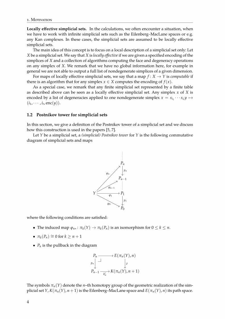
Let Y be a simplicial set, a (simplicial) Postnikov tower for Y is the following commutativediagram of simplicial sets and maps

Pn

pn

��

Pn−1

Y

ϕn

@@

ϕn−1

88

ϕ1//

ϕ0''

P1

p1

��

P0

where the following conditions are satisfied:

∙ The induced map ϕn* : πk(Y)→ πk(Pn) is an isomorphism for 0 ≤ k ≤ n.

∙ πk(Pn) ∼= 0 for k ≥ n + 1

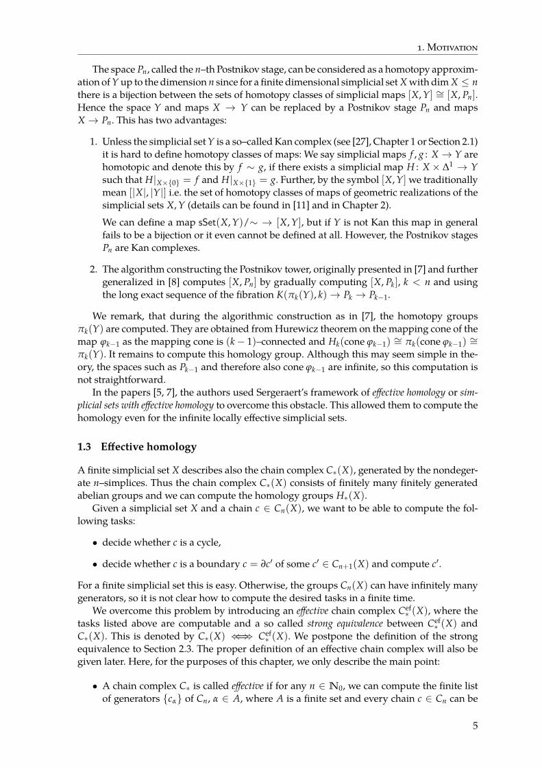
∙ Pn is the pullback in the diagram

Pn //

pn

��

E(πn(Y), n)

�

Pn−1 k′n// K(πn(Y), n + 1)

The symbols πn(Y) denote the n–th homotopy group of the geometric realization of the sim-plicial set Y, K(πn(Y), n+ 1) is the Eilenberg–MacLane space and E(πn(Y), n) its path space.

4

1. Motivation

The space Pn, called the n–th Postnikov stage, can be considered as a homotopy approxim-ation of Y up to the dimension n since for a finite dimensional simplicial set X with dim X ≤ nthere is a bijection between the sets of homotopy classes of simplicial maps [X, Y] ∼= [X, Pn].Hence the space Y and maps X → Y can be replaced by a Postnikov stage Pn and mapsX → Pn. This has two advantages:

1. Unless the simplicial set Y is a so–called Kan complex (see [27], Chapter 1 or Section 2.1)it is hard to define homotopy classes of maps: We say simplicial maps f , g : X → Y arehomotopic and denote this by f ∼ g, if there exists a simplicial map H : X × ∆1 → Ysuch that H|X×{0} = f and H|X×{1} = g. Further, by the symbol [X, Y] we traditionallymean [|X|, |Y|] i.e. the set of homotopy classes of maps of geometric realizations of thesimplicial sets X, Y (details can be found in [11] and in Chapter 2).

We can define a map sSet(X, Y)/∼ → [X, Y], but if Y is not Kan this map in generalfails to be a bijection or it even cannot be defined at all. However, the Postnikov stagesPn are Kan complexes.

2. The algorithm constructing the Postnikov tower, originally presented in [7] and furthergeneralized in [8] computes [X, Pn] by gradually computing [X, Pk], k < n and usingthe long exact sequence of the fibration K(πk(Y), k)→ Pk → Pk−1.

We remark, that during the algorithmic construction as in [7], the homotopy groupsπk(Y) are computed. They are obtained from Hurewicz theorem on the mapping cone of themap ϕk−1 as the mapping cone is (k− 1)–connected and Hk(cone ϕk−1) ∼= πk(cone ϕk−1) ∼=πk(Y). It remains to compute this homology group. Although this may seem simple in the-ory, the spaces such as Pk−1 and therefore also cone ϕk−1 are infinite, so this computation isnot straightforward.

In the papers [5, 7], the authors used Sergeraert’s framework of effective homology or sim-plicial sets with effective homology to overcome this obstacle. This allowed them to compute thehomology even for the infinite locally effective simplicial sets.

1.3 Effective homology

A finite simplicial set X describes also the chain complex C*(X), generated by the nondeger-ate n–simplices. Thus the chain complex C*(X) consists of finitely many finitely generatedabelian groups and we can compute the homology groups H*(X).

Given a simplicial set X and a chain c ∈ Cn(X), we want to be able to compute the fol-lowing tasks:

∙ decide whether c is a cycle,

∙ decide whether c is a boundary c = ∂c′ of some c′ ∈ Cn+1(X) and compute c′.

For a finite simplicial set this is easy. Otherwise, the groups Cn(X) can have infinitely manygenerators, so it is not clear how to compute the desired tasks in a finite time.

We overcome this problem by introducing an effective chain complex Cef* (X), where the

tasks listed above are computable and a so called strong equivalence between Cef* (X) and

C*(X). This is denoted by C*(X) ⇐⇐⇒⇒ Cef* (X). We postpone the definition of the strong

equivalence to Section 2.3. The proper definition of an effective chain complex will also begiven later. Here, for the purposes of this chapter, we only describe the main point:

∙ A chain complex C* is called effective if for any n ∈ N0, we can compute the finite listof generators {cα} of Cn, α ∈ A, where A is a finite set and every chain c ∈ Cn can be

5

1. Motivation

expressed uniquely as a combination

c = ∑ kαcα

with integer coefficients kα in Z.

We say that a locally effective simplicial set X has effective homology if C*(X)⇐⇐⇒⇒ Cef* (X) and

Cef* (X) is an effective chain complex.

We remark that in order to solve the cycle and boundary problems algorithmically, itsuffices to find a (computable) chain homotopy equivalence C*(X) ≃ Cef

* (X). We use strongequivalence, because it enables us to utilize so called perturbation lemmas (see chapter 2.3).This allows us to introduce algorithmic constructions that given simplicial sets with effectivehomology as inputs, produce simplicial sets with effective homology on the outputs. Themapping cone or the mapping cylinder are computed this way.

1.4 Our motivation

We are interested in extending the results from [8, 15] to the case where the action of a finitegroup G on spaces X, Y is not free.

This could potentially be applied to provide a solution of the generalization of the em-beddability problem: To decide if a k-dimensional simplicial complex K can be embeddedinto Rn, where the image of K may intersect itself at most k times.

Again, in some ranges of dimensions, this corresponds to a problem of the existence of aΣk equivariant map K′ → Sn, where the action of the symmetric group Σk is not free on thespace K′, a version of the deleted product for K.

As the algorithmic construction of the Postnikov tower for finite simplicial sets and thecorresponding version for finite simplicial sets with free action of a finite group is one ofthe main tools used in [8, 15], the algorithmic construction of the Postnikov tower for finitesimplicial sets with a non–free action is the obvious way to generalize results in [8, 15] to theequivariant setting.

The main aim of this thesis is therefore to obtain a statement (theorem) that can be in-formally written as follows:

Informal statement. Let Y be a simplicial set with an action of a finite group G. Then there is analgorithm that computes the equivariant Postnikov tower for Y.

However, instead of the Informal statement we will prove a result involving finite dia-grams of simplicial sets, which will enable us to approach the equivariant Postnikov towersfrom a different perspective.

In the rest of the text, by a finite diagram X in a category 𝒞 (or a finite diagram of objectsin that category), we mean a functor X : ℐ → 𝒞, where ℐ is a finite category, i.e. a categorywith finitely many objects and arrows.

For the sake of better readability of the remainder of this thesis, we will stress the factthat an object is a diagram by using the boldface hyphenation. This notation allows certaininconsistencies which we hope won’t be very confusing: Suppose X : ℐ → Top is a diagram ofspaces, then X(i), where i ∈ ℐ is a topological space, but it is (partly) highlighted in boldface.

A pedantic reader might also remark that the category of simplicial sets is a category ofdiagrams of sets but the notation is not emphasized. We are aware of this, as is documentedby this paragraph.

The main effort in this thesis will be concentrated to prove the following theorem

Theorem A. Let ℐ be a finite category and let Y : ℐ → sSet be a diagram of 1–connected simplicialsets. Given n ∈N, there is an algorithm that computes the n-stage Postnikov tower for Y .

6

1. Motivation

In the next section, we will demonstrate that the equivariant Postnikov tower for a G–simplicial set Y can be replaced by a tower of diagrams for a special diagram ℐ . The reasonwhy this is true follows from the fact that problems in the homotopy category of simplicialsets with an action of G can be restated as problems in the homotopy category of certainfinite diagrams of simplicial sets.

1.5 Category of orbits

In this section we will be using some language of model categories. Some details on modelcategories can be found in Sections 2.1 and 2.2. For the full description, we refer to [11]. Forthe purposes of this chapter it is enough to say that a model structure on a category 𝒞 allowsus to define the set [X, X′]𝒞 of homotopy classes of maps from X to X′ in the category 𝒞,where X, X′ ∈ 𝒞.

Further, for model categories 𝒞,𝒟 one can define special adjunctions, called Quillen ad-

junctions. Roughly speaking, these are adjuctions (L ⊣ R) : 𝒞R←→L𝒟 respecting the model

category structure. Quillen adjunctions further induce functors L : 𝒞 → 𝒟 and R : 𝒟 → 𝒞.These constitute a Quillen equivalence if for any objects X, X′ ∈ 𝒞 and Y, Y′ ∈ 𝒟 we have[X, X′]𝒞 ∼= [L(X), L(X′)]𝒟 and in the opposite direction [Y, Y′]𝒟 ∼= [R(d), R(Y′)]𝒞 .

Simplicial sets with a group action. Given a finite group G, simplicial sets with a G–actionand G–equivariant simplicial maps between them form the category sSetG, which is some-times called category of G-simplicial sets. It is a model category, we can define a notion ofhomotopy and we denote the set of homotopy classes of maps in this category by [X, Y]G. Fordetails, see Chapter 1 in [28].

Further, there is a category of orbits 𝒪G, where the objects are orbit sets G/H, whereH ≤ G and the morphisms are equivariant maps G/H1 → G/H2. As G is assumed to befinite, the category 𝒪G is finite and so is the category 𝒪G

op. An object X in the categorysSet𝒪

opG of functors 𝒪G

op → sSet is thus a finite diagram of simplicial sets. Any category ofdiagrams of simplicial sets sSetℐ admits a model structure called the projective model structure,which we are going to use. We can define homotopy and denote the set of homotopy classesof maps in the category sSetℐ by [−,−]ℐ .

We define a functor Φ : sSetG → sSet𝒪opG called the fixed–point functor by Φ(X)(G/H) =

XH = {x ∈ X | hx = x, ∀h ∈ H}. The functor Φ assigns a finite diagram of simplicial sets toevery X ∈ sSetG.

We illustrate this in the following example

Example 1.1. Assume G = C2 = {1,−1} i.e. a two–element group. The category 𝒪G looksas follows:

C2/C2

id

��

C2/{1}ιoo

id

��

−1

VV

and given X ∈ sSetG, Φ(X) ∈ sSet𝒪opG is the following diagram. Notice that arrows are re-

versed.

XC2

id

�� Φ(ι)// X

id

��

−1

EE

7

1. Motivation

By Elemendorf’s theorem [14] the categories sSetG and sSet𝒪opG are Quillen equivalent,

which in particular implies that [X, Y]G ∼= [ΦX, ΦY]𝒪G . For details see e.g. chapter V in [28]or [14, 43].

To sum up, many computational problems in G–simplicial sets can be restated as compu-tational problems in the category sSet𝒪

opG . Instead of computing the Postnikov tower for Y in

the category sSetG as suggested by the Informal statement, we compute the Postnikov towerfor Φ(Y) using Theorem A.

In the following section, we will outline how the construction of the Postnikov tower fordiagrams of simplicial sets differs from the algorithmic construction described in [7].

Effective homology for diagrams. The algorithm that constructs the Postnikov tower asseen in [7, 8] uses the simplicial sets with effective homology. In the next section, we willpresent the main idea of the proof of Theorem A. Because we want to build a Postnikovtower for diagrams, we will define effective homology of diagrams of simplicial sets.

In fact we introduce two notions of effective homology that generalize the effective homo-logy from [39] namely a diagram with pointwise effective homology and a diagram with effectivehomology. As with the effective homology, we postpone the proper definitions and describejust the main ideas:

∙ We say that a diagram of chain complexes C : ℐ → Ch+ has pointwise effective homology iffor every i ∈ ℐ there is given an effective chain complex Cef(i) and a strong equivalenceof chain complexes C(i)⇐⇐⇒⇒ Cef(i).

∙ A diagram of simplicial sets X : ℐ → sSet has pointwise effective homology if for everyi ∈ ℐ there is given an effective chain complex Cef(i) and a strong equivalence of chaincomplexes C(X(i))⇐⇐⇒⇒ Cef(i)

∙ A diagram of chain complexes C : ℐ → Ch+ is effective if for any n ∈N0 we can computea finite list of generators {cα | α ∈ A}, where cα ∈ C(iα) and A is a finite set. Further,given an element c ∈ C(i), there is an algorithm that outputs a unique description of cas

c = ∑α, fα : iα→i

k fαfα*(cα)

where fα* : C(iα)→ C(i) and k fα∈ Z.

∙ A diagram of chain complexes C : ℐ → Ch+ has effective homology if there is given astrong equivalence of diagrams C ⇐⇐⇒⇒ Cef where Cef is an effective diagram.

∙ A diagram of simplicial sets X : ℐ → sSet has effective homology if there is given a strongequivalence C*(X)⇐⇐⇒⇒ Cef

* between the diagram of chain complexes for X and someeffective chain complex Cef

* .

The pointwise effective homology is a weaker notion, because we do not need any in-formation regarding the maps between the chain complexes Cef(i). In fact, any diagram thathas effective homology has pointwise effective homology.

From a historical standpoint, the effective homology of a diagram was first introduced in[8] for two particular diagrams and this served as a motivation for our general definition. Wepresent these diagrams in the following examples.

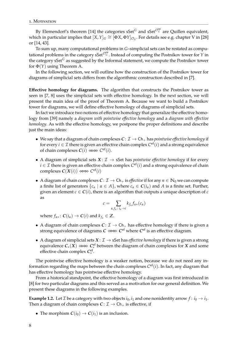
Example 1.2. Let ℐ be a category with two objects i0, i1 and one nonidentity arrow f : i0 → i1.Then a diagram of chain complexes C : ℐ → Ch+ is effective, if

∙ The morphism C(i0)→ C(i1) is an inclusion.

8

1. Motivation

∙ Chain complexes C(i1), C(i0) are effective and generators of C(i0) are generators inC(i1).

Example 1.3. It is a classical example from the category theory that a chain complex C withan action of a finite group G is nothing else than a diagram C : G → Ch+, where the groupG is interpreted as a category with one object * and arrows labelled by the elements of G.Assuming C is effective, C can be seen as a ZG-module with a finite ZG-basis.

In other words, for each n ≥ 0 there is a finite list of distinguished elements {cα} of Cnsuch that they are all distinct and each c ∈ Cn has a unique description

c = ∑ kαgαcα

where the coefficients kα lie in Z and gα ∈ G.

1.6 Postnikov tower for diagrams

In this section, we summarize the gist of our construction of the Postnikov tower for diagramsof simplicial sets and therefore also the essence of the proof of Theorem A.

First, we remark that the algorithm that constructs the Postnikov tower for simplicial setY as seen in [7, 8] is based on repeating one construction step iteratively:

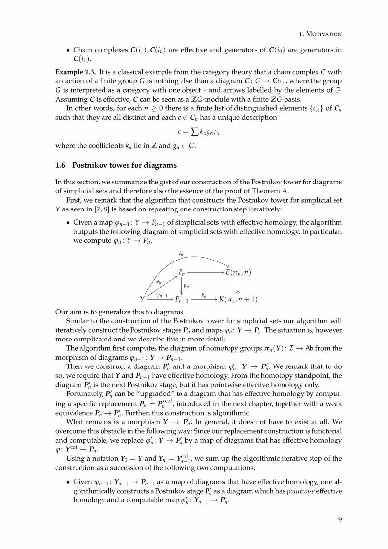
∙ Given a map ϕn−1 : Y → Pn−1 of simplicial sets with effective homology, the algorithmoutputs the following diagram of simplicial sets with effective homology. In particular,we compute ϕn : Y → Pn.

Pn

pn����

// E(πn, n)

����

Yϕn−1

//

ϕn

::

`n

&&

Pn−1kn // K(πn, n + 1)

Our aim is to generalize this to diagrams.Similar to the construction of the Postnikov tower for simplicial sets our algorithm will

iteratively construct the Postnikov stages Pn and maps ϕn : Y → Pn. The situation is, howevermore complicated and we describe this in more detail:

The algorithm first computes the diagram of homotopy groups πn(Y) : ℐ → Ab from themorphism of diagrams ϕn−1 : Y → Pn−1.

Then we construct a diagram P′n and a morphism ϕ′n : Y → P′n. We remark that to doso, we require that Y and Pn−1 have effective homology. From the homotopy standpoint, thediagram P′n is the next Postnikov stage, but it has pointwise effective homology only.

Fortunately, P′n can be “upgraded” to a diagram that has effective homology by comput-ing a specific replacement Pn = P′n

cof, introduced in the next chapter, together with a weakequivalence Pn → P′n. Further, this construction is algorithmic.

What remains is a morphism Y → Pn. In general, it does not have to exist at all. Weovercome this obstacle in the following way: Since our replacement construction is functorialand computable, we replace ϕ′n : Y → P′n by a map of diagrams that has effective homologyϕ : Ycof → Pn.

Using a notation Y0 = Y and Yn = Ycofn−1, we sum up the algorithmic iterative step of the

construction as a succession of the following two computations:

∙ Given ϕn−1 : Yn−1 → Pn−1 as a map of diagrams that have effective homology, one al-gorithmically constructs a Postnikov stage P′n as a diagram which has pointwise effectivehomology and a computable map ϕ′n : Yn−1 → P′n.

9

1. Motivation

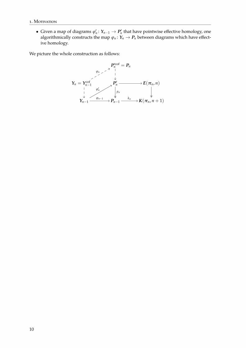
∙ Given a map of diagrams ϕ′n : Yn−1 → P′n that have pointwise effective homology, onealgorithmically constructs the map ϕn : Yn → Pn between diagrams which have effect-ive homology.

We picture the whole construction as follows:

P′cofn = Pn

��

Yn = Ycofn−1

ϕn

88

��

P′npn

����

// E(πn, n)

����

Yn−1ϕn−1

//

ϕ′n

88

Pn−1kn // K(πn, n + 1)

10

2 Tools

2.1 Simplicial sets

In this section, we give a brief introduction to simplicial sets and their homotopy theory. Weomit many details and refer the reader to standard textbooks [27, 20].

A simplicial set X can be seen as a graded set X indexed by the non-negative integerstogether with a collection of mappings di : Xn → Xn−1 and si : Xn → Xn+1, 0 ≤ i ≤ n calledthe face and degeneracy operators. They satisfy the following identities:

disi = di+1si = id; disj = sjdi−1 i > j + 1;didj = dj−1di; disj = sj−1di i < j;sisj = sj+1si; i ≤ j.

Simplicial maps i. e. morphisms of simplicial sets are then defined as maps of graded setswhich commute with the face and degeneracy mappings. The simplicial sets and simplicialmaps form a category that we denote sSet.

The elements of Xn are called n-simplices. We say that a simplex x ∈ Xn is nondegenerate ifit cannot be expressed as x = siy for some y ∈ Xn−1. We will denote the set of nondegeneratesimplices of X by XN.

Using the relations between the face and degeneracy operators, one can deduce that anyn-simplex x can be described uniquely as si1 · · · sit y, where y is a nondegenerate (n− t) sim-plex, 0 ≤ i1 ≤ i2 ≤ · · · < it.

A typical example of a simplicial set is the standard n–simplex, denoted ∆n, which can beseen as a simplicial set freely generated by a single nondegenerate element en ∈ ∆n

n.Erasing the unique n-simplex en of ∆n together with its face dken and all their degen-

eracies, produces a new simplicial set, commonly called the k-th horn of ∆n. We denote thissimplicial set by n

k .Given a simplicial set X, we define the n-skeleton sknX as the simplicial set generated by

the nondegenerate simplices of X of dimension ≤ n. Alternatively, one can picture this asremoving all nondegenerate simplices of dimension greater than n together with all theirdegeneracies. As an example for the standard n-simplex ∆n, where n ≥ 0, we can define itsboundary ∂∆n = skn−1X. We remark that sk−1X = ∅.

A (simplicial) nerve of a small category 𝒞 is a simplicial set N(𝒞) defined in the followingway: N(𝒞)0 consists of the objects of 𝒞 and N(𝒞)k, k ≥ 1 is a collection of the k-tuples ofcomposable morphisms C0 → C1 → · · · → Ck in 𝒞. The degeneracy morphisms si are definedby inserting the identity morphism at the i-th object. The face operator di, 0 < i < k is givenby composing the i-th morphism with the (i + 1)-st and the outer face maps d0, dk are givenby erasing the first and the last morphism, respectively. We will encounter the nerve of acategory later.

For a simplicial set X, we can define chain complexes Cfull* (X) and CN

* (X). The main dif-ference between these chain complexes is that the group Cfull

n (X) is a free abelian group gen-erated by the elements of Xn, whereas CN

* (X), called normalized chain complex, is definedby CN

* (X) = Cfull* (X)/CD

* (X), where CD* (X) is chain subcomplex generated by the degen-

erate elements). The boundary operator ∂ on both chain complexes, is defined by ∂(c) =

∑ni=0(−1)idi(c). We remark that chain complexes Cfull

* (X) and CN* (X) are chain homotopy

equivalent. In the rest of the text, if not stated otherwise, the symbol C*(X) denotes CN* (X).

11

2. Tools

Fibrations, cofibrations and weak equivalences. We call a simplicial map g : X → Y fibra-tion or Kan fibration if for any commutative diagram

nk

//

�

X

g��

∆n //

88

Y

there is a lift ∆n → X. Here ι denotes the inclusion of the horn into the standard simplex.To every simplicial set X, there is an associated topological space (in fact a CW–complex)

|X| called the geometric realization of X. The space |X| is constructed by appointing a standardtopological n–simplex to every nondegenerate n–simplex of X and gluing the faces accordingto the face and degeneracy relations specified by X. The geometric realization is a functor| − | : sSet→ Top.

The homotopy groups π*(X) of a simplicial set X are defined as the homotopy groups ofthe geometric realization π*(|X|). We remark that for Kan complexes there is an alternativedefinition that does not involve the geometric realization, see Chapter 1 in [27].

We call a simplicial map g : X → Y a weak equivalence if the induced homomorphismsgn : πn(|X|)→ πn(|Y|), n ≥ 0 are isomorphisms.

We finally say that a simplicial map f : A → B is a cofibration if it has the so–called leftlifting property (LLP) with respect to maps that are both weak equivalences and fibrations:For every commutative diagram in sSet

A //

f��

Xg��

B //

88

Y

such that g is a weak equivalence and a fibration, there exists a lift in the diagram.We remark without a proof that in this model category structure, the cofibrations corres-

pond to injective maps and thus for any X ∈ sSet the unique inclusion ∅→ X is a cofibration(see [20], p.122).

A simplicial set X is called a Kan complex or fibrant if the unique simplicial map X →∆0 = {*} is a fibration. Not every simplicial set is fibrant, but the theory of model categoriestells us that for any X ∈ sSet there exists some X′ that is fibrant and a weak equivalenceX → X′. Such X′ is called a fibrant replacement of X and denoted Xfib.

We remark that weak equivalence, fibration, cofibration and the fibrant replacement arestandard notions from the theory of model categories (see [11]) and in our context they de-scribe the Kan model structure on the category sSet. The homotopy category Ho(sSet) inducedby the model structure on sSet then corresponds (is Quillen equivalent) to the classical ho-motopy category for topological spaces Ho(Top).

Twisted products. We first remind the reader of the Cartesian product X × Y of simplicialsets X, Y: The set of n-simplices (X × Y)n consists of tuples (x, y), where x ∈ Xn, y ∈ Yn.Further the face and degeneracy operators on X × Y are defined by di(x, y) = (dix, diy),si(x, y) = (six, siy).

A simplicial group G is a simplicial set such that each Gn is a group and di, si are grouphomomorphisms.

We will deal with certain fiber bundles where F, B, and E are simplicial sets, and a sim-plicial group G acts on F. The action i.e. a simplicial map φ : F × G → F satisfies the usualconditions for a (right) action of a group on a set; that is, φ(γγ′) = (φγ)γ′ and φen = φ

(φ ∈ Fn, γ, γ′ ∈ Gn, en the unit element of Gn).We can now define a twisted Cartesian product.

12

2. Tools

Definition 2.1 (Twisted Cartesian product). Let B and F be simplicial sets and G a simplicialgroup acting on F. Let τ be a mapping of graded sets B→ G of degree −1, such that

(i) d0τ(β) = τ(d1β)τ(d0β)−1;(ii) diτ(β) = τ(di+1β) for i ≥ 1;

(iii) siτ(β) = τ(si+1β) for all i; and(iv) τ(s0β) = en for all β ∈ Bn, where en is the unit element of Gn.

Then τ is called a twisting operator and the twisted Cartesian product F×τ B is a simplicial set Ewith En = Fn× Bn, i.e., the n-simplices are the same as in the Cartesian product F× B, and theface and degeneracy operators are also as in the Cartesian product, i.e. di( f , b) = (di f , dib) ,with the sole exception of d0, which is given by

d0(φ, β) B (d0(φ)τ(β), d0β), (φ, β) ∈ Fn × Bn.

A twisted Cartesian product F×τ B is called principal if F = G and the considered rightaction of G on itself is by (right) multiplication.

Thus, the only way in which F×τ B differs from the ordinary Cartesian product F× B is inthe 0-th face operator. It is not trivial to see why this should be the right way of representingfiber bundles simplicially, but for us, it is only important that it works, and we will haveexplicit formulas available for the twisting operator for all the specific applications.

2.2 Diagrams of simplicial sets

In this section, we define homotopy, homology and cohomology groups in the category sSetℐ ,i.e. a category of functors (or diagrams) ℐ → sSet for some fixed category ℐ , which we assumeto be finite. Then we describe in more details the model category structure on sSetℐ andfinally we present Bousfield–Kan model of a homotopy left Kan extension, which as a specialcase gives us models for a cofibrant replacement and a homotopy colimit.

Homotopy and homology. We aim to define homotopy groups of diagrams X : ℐ → sSet

in such a way they can be seen as functors πk(−) : sSetℐ → Grpℐ . To do so, we will assumethat X(i) are simply connected and thus πk(X(i)) do not depend on basepoints.

To define homotopy groups for diagrams of simplicial sets that are not simply connected,basepoints have to be introduced, possibly as a subdiagram pt of X. However in this situation,πk in general does not appear as a functor sSetℐ → Grpℐ .

Definition 2.2. Let X : ℐ → sSet be a diagram of simply connected simplicial sets. We definethe k-th homotopy group πk(X) of X as a diagram ℐ → Set satisfying

πk(X)(i) = πk(X(i)), i ∈ ℐ

and the maps in the diagram π*(X) are given as follows: for any f : i→ j, i, j ∈ ℐ we have

π*(X)( f ) = X( f )* : π*(X(i))→ π*(X(j)).

Later in the text, we will work with relative homotopy groups for a pair (X, A). Here A isa subdiagram of X, i.e for any i ∈ ℐ we have A(i) ⊆ X(i) and for arbitrary f : i→ j we haveA( f ) = X( f )|A. Given that both X and A are 1-connected, the homotopy group π(X, A)appears as a functor Pair(sSetℐ )→ Grpℐ .

Definition 2.3. For a diagram X, we define a diagram of chain complexes C*(X) by settingC*(X)(i) = C*(X(i)). Similarly, we define the homology groups H*(X) of C*(X) as dia-grams of abelian groups.

13

2. Tools

There is another version of homology (and cohomology), namely the Bredon cohomologyand homology. It was originally defined for G–simplicial sets (or, in effect for sSet𝒪

opG , see [1]),

but it can be easily generalized to any diagrams of simplicial sets:

Definition 2.4. Let X : ℐ → sSet be a diagram of simplicial sets and let ρ : ℐ → Ab be adiagram of abelian groups.

We define the cochain complex C*ℐ (X; ρ) B Hom(C*(X), ρ). Its n-th cohomology groupHnℐ (X; ρ) is called the n-th cohomology group of X with coefficients in ρ.

As our notation suggests, C*ℐ (X; ρ) is not a diagram, but a chain complex only. In theliterature [28, 1] the diagrams ρ are sometimes called coefficient systems.

To give the Bredon homology with coefficients, we need the coefficient system to be acontravariant functor, so we assume ρ : ℐop → Ab. We define chain complex Cℐ* (X; ρ) as atensor product Ck(X)⊗ℐ ρ. For details see [28], Chapter 1 or (2.11) in Section 2.7.

It follows, that Cℐk (X; ρ) is an abelian group. The homology group Hℐk (X; ρ) is definedas the k-th homology of the chain complex Cℐ* (X; ρ) where the differential ∂ is given by∂ = d⊗ 1.

Model structure. We now describe the model category structure, known as the projectivemodel structure, first introduced in [4], on a category sSetℐ . Analogously to the situationin simplicial sets, we will do so by listing the classes of weak equivalences, fibrations andcofibrations:

We say that the map of diagrams f : X → Y is a weak equivalence if it is a weak equivalencepointwise, i.e. we assume f (i) : X(i)→ Y(i) induces isomorphism on the homotopy groupsfor all i. If f is a weak equivalence, then it induces an isomorphism of diagrams π*(X), π*(Y).

Similarly, f : X → Y is a fibration if it is a (Kan) fibration pointwise. A diagram Y is calledfibrant if the unique map to ∆0 = * is a fibration. Here, we interpret ∆0 as trivial diagram (allmaps are identity). As in simplicial sets, for any diagram Y , there exists a fibrant diagramYfib ∈ sSetℐ and weak equivalence Y → Yfib. Such Yfib is called a fibrant replacement of Y .

The only remaining type of morphism in the model category is the cofibration, which wedefine as for the simplicial sets. It is a map of diagrams which has the left lifting propertywith respect to all maps that are at the same time weak equivalences and fibrations.

For any diagram X, there exists a unique map ∅ → X from the trivial diagram ∅. Inthe case of simplicial sets, this map is always a cofibration. However, for general sSetℐ thisdoes not hold. We thus call a diagram X cofibrant, if the unique map ∅→ X is a cofibration.We remark that for any X, there exists a cofibrant diagram Xcof and a weak equivalenceXcof → X. This follows from the model category structure on sSetℐ .

To define the notion of homotopy for maps between diagrams, we use the standard ap-proach as in [11], section 4. We will introduce cylinder objects and left homotopy and we omitsimilar definitions of path objects and right homotopy.

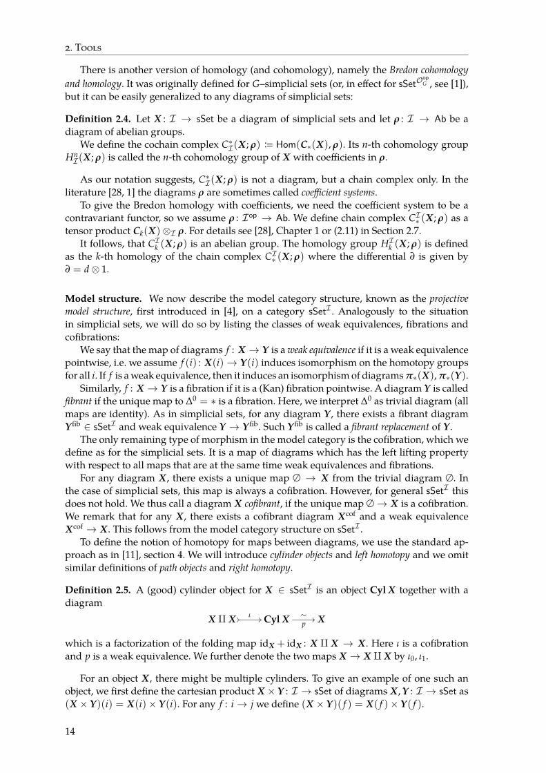
Definition 2.5. A (good) cylinder object for X ∈ sSetℐ is an object Cyl X together with adiagram

X ⨿ X // ι // Cyl X ∼p// X

which is a factorization of the folding map idX + idX : X ⨿ X → X. Here ι is a cofibrationand p is a weak equivalence. We further denote the two maps X → X ⨿ X by ι0, ι1.

For an object X, there might be multiple cylinders. To give an example of one such anobject, we first define the cartesian product X × Y : ℐ → sSet of diagrams X, Y : ℐ → sSet as(X × Y)(i) = X(i)× Y(i). For any f : i→ j we define (X × Y)( f ) = X( f )× Y( f ).

14

2. Tools

We can now state (without proof) that in the case X is cofibrant, the diagram ∆1 × X ∈sSetℐ , where ∆1 is seen as a constant diagram, is a cylinder object for X. We will, however,only use the fact that one such cylinder exists as in [11].

If we assume that X is cofibrant, then according to [11], Lemma 4.4, the maps ι0, ι1 areweak equivalences and cofibrations (such maps are usually called trivial cofibrations or acycliccofibrations).

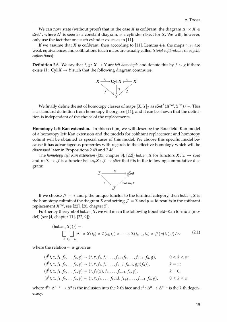
Definition 2.6. We say that f , g : X → Y are left homotopic and denote this by f ∼ g if thereexists H : Cyl X → Y such that the following diagram commutes:

Xι0 //

f""

Cyl X

H��

Xι1oo

g||

Y

We finally define the set of homotopy classes of maps [X, Y ]ℐ as sSetℐ (Xcof, Yfib)/∼. Thisis a standard definition from homotopy theory, see [11], and it can be shown that the defini-tion is independent of the choice of the replacements.

Homotopy left Kan extension. In this section, we will describe the Bousfield–Kan modelof a homotopy left Kan extension and the models for cofibrant replacement and homotopycolimit will be obtained as special cases of this model. We choose this specific model be-cause it has advantageous properties with regards to the effective homology which will bediscussed later in Propositions 2.49 and 2.48.

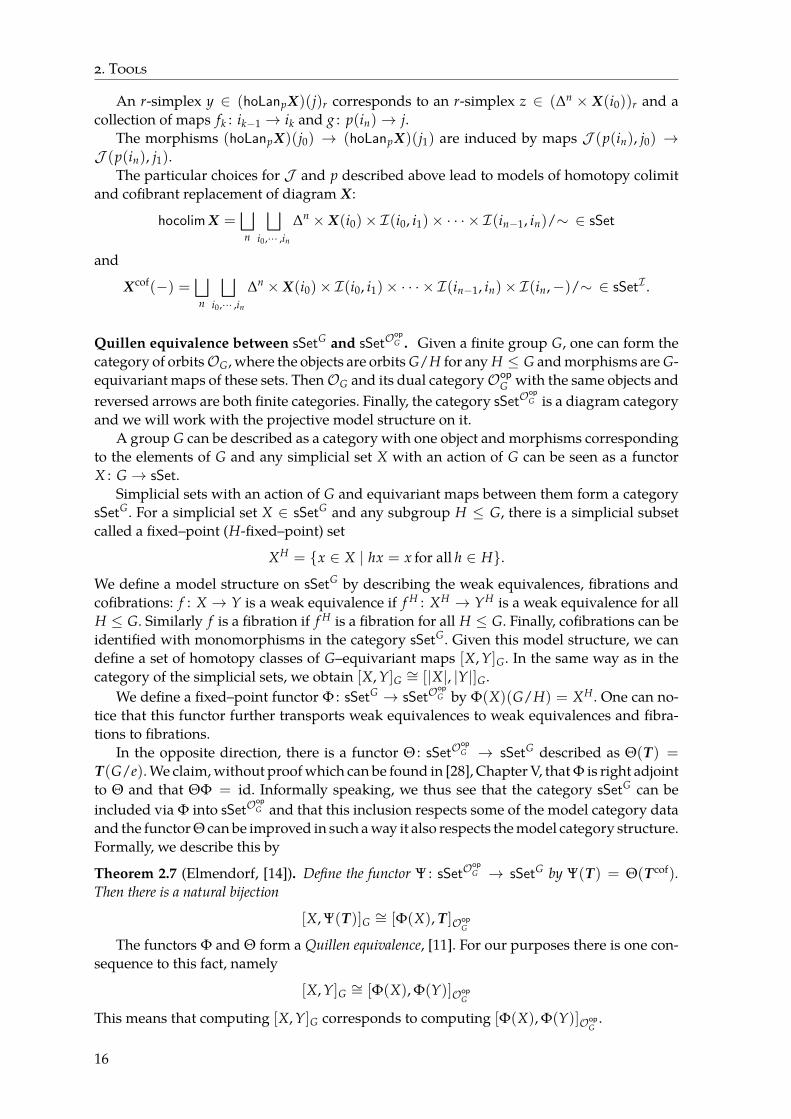
The homotopy left Kan extension ([35, chapter 8], [22]) hoLanpX for functors X : ℐ → sSet

and p : ℐ → 𝒥 is a functor hoLanpX : 𝒥 → sSet that fits in the following commutative dia-gram:

ℐ X //

p��

sSet

𝒥hoLanpX

==

If we choose 𝒥 = * and p the unique functor to the terminal category, then hoLanpX isthe homotopy colimit of the diagram X and setting 𝒥 = ℐ and p = id results in the cofibrantreplacement Xcof, see [22], [28, chapter 5].

Further by the symbol hoLanpX, we will mean the following Bousfield–Kan formula (mo-del) (see [4, chapter 11], [22, 9]):

(hoLanpX)(j) =⊔n

⊔i0,··· ,in

∆n × X(i0)× ℐ(i0, i1)× · · · × ℐ(in−1, in)×𝒥 (p(in), j)/∼ (2.1)

where the relation ∼ is given as

(dkt, x, f1, f2, . . . fn, g) ∼ (t, x, f1, f2, . . . , fk+1 fk, . . . , fn−1, fn, g), 0 < k < n;

(dkt, x, f1, f2, . . . fn, g) ∼ (t, x, f1, f2, . . . , fn−2, fn−1, gp( fn)), k = n;

(dkt, x, f1, f2, . . . fn, g) ∼ (t, f1(x), f2, . . . , fn−1, fn, g), k = 0;

(skt, x, f1, f2, . . . fn, g) ∼ (t, x, f1, . . . , fk, id, fk+1, . . . , fn−1, fn, g), 0 ≤ k ≤ n.

where dk : ∆n−1 → ∆n is the inclusion into the k-th face and sk : ∆n → ∆n−1 is the k-th degen-eracy.

15

2. Tools

An r-simplex y ∈ (hoLanpX)(j)r corresponds to an r-simplex z ∈ (∆n × X(i0))r and acollection of maps fk : ik−1 → ik and g : p(in)→ j.

The morphisms (hoLanpX)(j0) → (hoLanpX)(j1) are induced by maps 𝒥 (p(in), j0) →𝒥 (p(in), j1).

The particular choices for 𝒥 and p described above lead to models of homotopy colimitand cofibrant replacement of diagram X:

hocolim X =⊔n

⊔i0,··· ,in

∆n × X(i0)× ℐ(i0, i1)× · · · × ℐ(in−1, in)/∼ ∈ sSet

and

Xcof(−) =⊔n

⊔i0,··· ,in

∆n × X(i0)× ℐ(i0, i1)× · · · × ℐ(in−1, in)× ℐ(in,−)/∼ ∈ sSetℐ .

Quillen equivalence between sSetG and sSet𝒪opG . Given a finite group G, one can form the

category of orbits𝒪G, where the objects are orbits G/H for any H ≤ G and morphisms are G-equivariant maps of these sets. Then𝒪G and its dual category𝒪op

G with the same objects andreversed arrows are both finite categories. Finally, the category sSet𝒪

opG is a diagram category

and we will work with the projective model structure on it.A group G can be described as a category with one object and morphisms corresponding

to the elements of G and any simplicial set X with an action of G can be seen as a functorX : G → sSet.

Simplicial sets with an action of G and equivariant maps between them form a categorysSetG. For a simplicial set X ∈ sSetG and any subgroup H ≤ G, there is a simplicial subsetcalled a fixed–point (H-fixed–point) set

XH = {x ∈ X | hx = x for all h ∈ H}.

We define a model structure on sSetG by describing the weak equivalences, fibrations andcofibrations: f : X → Y is a weak equivalence if f H : XH → YH is a weak equivalence for allH ≤ G. Similarly f is a fibration if f H is a fibration for all H ≤ G. Finally, cofibrations can beidentified with monomorphisms in the category sSetG. Given this model structure, we candefine a set of homotopy classes of G–equivariant maps [X, Y]G. In the same way as in thecategory of the simplicial sets, we obtain [X, Y]G ∼= [|X|, |Y|]G.

We define a fixed–point functor Φ : sSetG → sSet𝒪opG by Φ(X)(G/H) = XH. One can no-

tice that this functor further transports weak equivalences to weak equivalences and fibra-tions to fibrations.

In the opposite direction, there is a functor Θ : sSet𝒪opG → sSetG described as Θ(T) =

T(G/e). We claim, without proof which can be found in [28], Chapter V, that Φ is right adjointto Θ and that ΘΦ = id. Informally speaking, we thus see that the category sSetG can beincluded via Φ into sSet𝒪

opG and that this inclusion respects some of the model category data

and the functor Θ can be improved in such a way it also respects the model category structure.Formally, we describe this by

Theorem 2.7 (Elmendorf, [14]). Define the functor Ψ : sSet𝒪opG → sSetG by Ψ(T) = Θ(Tcof).

Then there is a natural bijection

[X, Ψ(T)]G ∼= [Φ(X), T ]𝒪opG

The functors Φ and Θ form a Quillen equivalence, [11]. For our purposes there is one con-sequence to this fact, namely

[X, Y]G ∼= [Φ(X), Φ(Y)]𝒪opG

This means that computing [X, Y]G corresponds to computing [Φ(X), Φ(Y)]𝒪opG

.

16

2. Tools

2.3 Effective homology of chain complexes

We give a definition of simplicial sets with effective homology and our generalizations todiagrams of simplicial sets.

We remark that there is a collection of algorithms which for simplicial sets with effectivehomology as inputs give again simplicial sets with effective homology as outputs.

These algorithms usually describe commonly used constructions from algebraic topologysuch as Cartesian product, loop space, bar construction, mapping cylinder, total space of afibration i.e. the twisted Cartesian product (see [39, 5, 7, 16]) and homotopy pushout [8].

Given a finite diagram of simplicial sets X ∈ sSetℐ such that X has pointwise effectivehomology and a (computable) morphism p : ℐ → 𝒥 , where ℐ ,𝒥 are finite, we will presentan algorithm that outputs the Bousfield-Kan model of hoLanpX ∈ sSet𝒥 as diagram that haseffective homology.

In special cases, our algorithm computes the homotopy colimit hocolim X as a simplicialset with effective homology and cofibrant replacement Xcof of X as a diagram of simplicialsets that has effective homology.

There are, however, constructions such as colimits over finite diagrams of simplicial setswith effective homology that do not result in a simplicial set with effective homology and wewill demonstrate this later in Example 2.37.

Effective chain complexes, reductions and strong equivalences. In this section, we give acomplete definition of a simplicial set with effective homology by defining the strong equi-valences. We first define the reduction, which is in literature sometimes referred to as a strongdeformation retraction or a strong contraction.

Definition 2.8. Let C*, C′* be chain complexes. A reduction C* ⇒⇒ C′* is a triple (α, β, η) calledreduction data and pictured as below, where α, β are chain maps and η : C* → C*+1 is a morph-ism of graded groups

(α, β, η) : C* ⇒⇒ C′* ≡ C*η55

α** C′*

β

jj

satisfyingηβ = 0 αη = 0 ηη = 0αβ = id ∂η + η∂ = id−βα

(2.2)

One of the most important and well known examples of a reduction is the following ex-ample, first given in [12, 13]:

Proposition 2.9 (Eilenberg–Zilber reduction). Let X, Y be simplicial sets. Then there is a reduction

(AW, EML, SH) : C*(X×Y)⇒⇒ C*(X)⊗ C*(Y)

The operators in the reduction data are called Alexander–Whitney, Eilenberg–MacLaneand Shih respectively. They can be computed using the acyclic models theorem as e.g. in [27],§ 28 and they are not unique. However, in this thesis, we use the reduction data presentedin Theorem 2.1a, [12]. An important observation is that the operators of the reduction dataare based on the face and degeneracy maps which means that the reduction is functorial (insimplicial sets).

Definition 2.10. A strong equivalence between chain complexes C* ⇐⇐⇒⇒ C′* consists of a spanof reductions C* ⇐⇐ C* ⇒⇒ C′*.

17

2. Tools

Strong equivalences can be composed, as seen in [39], Proposition 125, producing anotherstrong equivalence.

We now give a proper definition of chain complex (and simplicial set) with effective ho-mology, that were discussed in chapter 1.

Definition 2.11 (Effective chain complex). Let C* be a chain complex and let A be a set suchthat for every α ∈ A we are given cα ∈ C*. We call C* free with basis {cα} if every chain c ∈ C*can be expressed uniquely as a combination

c = ∑ kαcα (2.3)

with integer coefficients kα in Z.We call a chain complex C* locally effective if the elements c ∈ C* have finite (agreed upon)

encoding and there are algorithms computing the addition, zero, inverse and differential forthe elements of C*.

Finally, a locally effective chain complex C* is called effective if there is an algorithm thatfor given n ∈ N generates a finite basis cα ∈ Cn and an algorithm that for every c ∈ C*outputs the unique description (2.3).

The chain complex C* has effective homology (C* is a chain complex with effective homology)if there is a strong equivalence C* ⇐⇐⇒⇒ Cef

* where Cef* is an effective chain complex. We say

that a (locally effective) simplicial set X has effective homology (X is a simplicial set with effectivehomology) if C*(X) has.

Objects with effective homology have nice properties:

Lemma 2.12. Let C*, C′* be chain complexes with effective homology and let X, Y be simplicial setswith effective homology. Then the following holds:

1. C* ⊕ C′*, C* ⊗ C′* have effective homology.

2. The space X×Y has effective homology.

Proof. Let ρC = ( fC, gC, hC) : C* ⇒⇒ Cef* and ρC′ = ( fC′ , gv, hC′) : C′* ⇒⇒ C′ef

* be reductions.The proof that C* ⊕ C′* have effective homology is easy – we define the new reduction by

ρC⊕C′ = ( fC ⊕ fC′ , gC ⊕ gC′ , hC ⊕ hC′) : C* ⊕ C′* ⇒⇒ Cef* ⊕ C′ef

* .

For the tensor product, there is a reduction

ρC⊗C′ = ( fC⊗C′ , gC⊗C′ , hC⊗C′) : C* ⊗ C′* ⇒⇒ Cef* ⊗ C′ef

* .

The new reduction is defined by fC⊗C′ = fC ⊗ fC′ , gC⊗C′ = gC ⊗ gC′ , hC⊗C′ = hC ⊗ idC′ +gC fC ⊗ hC′ , or hC⊗C′ = hC ⊗ gC′ fC′ + idC ⊗ hC′ .

For the second part, we use the Eilenberg–Zilber reduction from Proposition 2.9. Theproof is then finished using the first part of the statement, because reductions (as strongequivalences) are composable.

Perturbation Lemmas. Consider a reduction C* ⇒⇒ D*. Assume we change the differentialof one of the complexes, i.e. we replace either C* with some C′* or D* with D′*. Then thePerturbation Lemmas provide us with new reductions C′* ⇒⇒ D* and C* ⇒⇒ D′* where theC*, D* are again the original chain complexes with changed (perturbed) differential.

Definition 2.13. Let (C*, ∂) be a chain complex. We call a collection of maps δ : C* → C*−1perturbation if the sum ∂ + δ is also a differential on C*.

18

2. Tools

The following perturbation lemmas are well–known, they constitute one of the basic toolsin homological perturbation theory. Their genesis can be traced back to [12, 3, 40] and theirfull proofs can be found e.g. in [39].

Lemma 2.14 (Easy Perturbation Lemma). Let (α, β, η) : (C*, ∂)⇒⇒ (C′*, ∂′) be a reduction. Let δ′

be a perturbation of differential ∂′. Then there is a reduction (α, β, η) : (C, ∂+ βδ′α)⇒⇒ (C′, ∂′+ δ).

Proof. Check the formulas for the new reduction given in the statement.

Lemma 2.15 (Basic Perturbation Lemma). Let (α, β, η) : (C*, ∂)⇒⇒ (C*, ∂′) be a reduction. Let δ

be a perturbation of differential ∂ such that for every c ∈ C* there is some i ∈N satisfying (ηδ)i(c) =0. Then there is a perturbation δ′of the differential ∂′ and a reduction (α′, β′, η′) : (C, ∂ + δ) ⇒⇒(C, ∂′ + δ′).

Proof. We describe the formulas for maps in the new reduction and the rest is left for thereader. We set

ϕ =∞

∑i=0

(−1)i(ηδ)i; ψ =∞

∑i=0

(−1)i(δη)i

By the condition in the statement, both sums are finite. The maps in the reduction are givenas follows:

δ′ = αψδβ = αδϕβ; α′ = αψ; β′ = ϕβ; η′ = ϕη = ηψ. (2.4)

2.4 Effective homology of twisted products

In this Section we describe in detail an application of the Basic Perturbation Lemma on theEilenberg–Zilber reduction which will be used to obtain a reduction from a chain complexof a twisted cartesian product C*(F×τ B) to a chain complex which we will denote C*(F)⊗τ

C*(B).We will then describe the differential on C*(F) ⊗τ C*(B) and we give conditions un-

der which the twisted cartesian product has effective homology. The content of this Sectioncomes mostly from the paper [16].

We now introduce the following notation: If X is a simplicial set and x ∈ Xn we putdn−ix = di+1 · · · dnx and d0x = x. Given (x, y) ∈ (X×Y)n we define the Alexander-Whitneyoperator:

AW(x, y) =n

∑i=0

dn−ix⊗ d0iy.

For a non–twisted product F× B, we have the Eilenberg–Zilber reduction

(AW, EML, SH) : (C(F× B), ∂)⇒⇒ (C*(F)⊗ C*(B), ∂F⊗B).

The full description of the reduction can be found in [12].The only difference between the chain complexes (C*(F×τ B), ∂τ) and (C*(F× B), ∂) is

in their differentials (to be precise in the face map d0) and it is easy to see that

∂τ = ∂ + (d0(y) · τ(b), d0(b))− (d0(y), d0(b)).

So the differential ∂τ of C*(E) is just ∂ with the added perturbation

δτ = (d0(y) · τ(b), d0(b))− (d0(y), d0(b)).

Definition 2.16. Let B and F be simplicial sets and let E = F × B. Let (y, b) ∈ E. We mayassume b = s*b′ ∈ B, where s* is a composition of degeneracy operators and b′ is nondegen-erate. The filtration degree of (y, b) is the dimension of b′. The filtration degree of an nonzeroelement y⊗ b ∈ C*(F)⊗ C*(B) is the dimension of b.

19

2. Tools

Proposition 2.17 ([39], Theorem 131). Let F×τ B be a twisted product of simplicial sets and let Gbe the simplicial group acting on F. Then the Basic Perturbation Lemma can be applied to the reductiondata (AW, EML, SH) : C*(F× B, ∂)⇒⇒ (C*(F)⊗ C*(B), ∂F⊗B) to obtain the reduction

( f , g, h) : (C*(F×τ B), ∂τ)⇒⇒ (C*(F)⊗τ C*(B), ∂F⊗Bτ ),

where C*(F)⊗τ C*(B) is just C*(F)⊗ C*(B) with a new differential ∂F⊗Bτ .

According to [40], the perturbation ∂F⊗Bτ − ∂F⊗B can be seen as a cap product with so

called twisting cochain, which is induced by τ. We will now give definitions of these notions.Let t : C*(B) → C*−1(G) be a sequence of abelian group homomorphisms tn : C(B)n →

C(G)n−1. We define a few operators that will be used within the construction:

D = AW ∘ C*(∆) : C*(B)→ C*(B)⊗ C*(B),

where C*(∆) is induced by the diagonal map ∆ : B → B× B. Denoting the right action ofthe simplicial group G on the fibre F by ·, we obtain an operator

σ = C(·) ∘ EML : C*(F)⊗ C*(G)→ C*(F).

Finally, we define the cap product (t∩ ) : C*(F)⊗ C*(B)→ C*(F)⊗ C*(B) as a composition

(σ⊗ 1)(1⊗ t⊗ 1)(1⊗ D).

Observe, that the cap product is a homomorphism of graded abelian groups and not of chaincomplexes. We say that t is a twisting cochain if the following holds:

(∂F⊗B + (t∩))2 = ∂F⊗B(t∩) + (t∩)∂F⊗B + (t∩)(t∩) = 0.

Proposition 2.17 implies that the twisting operator τ induces a new differential ∂F⊗Bτ on

the chain complex C*(F)⊗C*(B) via the Basic Perturbation Lemma. Then the same twistingoperator τ (this time seen as a part of the twisted cartesian product G ×τ B) also induces adifferential ∂G⊗B

τ on the chain complex C*(G)⊗ C*(B).According to [40], the twisting operator τ can further be used to define a special twisting

cochain which we will again denote by t as follows:

tn : Cn(B)e0⊗1−−→ C0(G)⊗ Cn(B)

λ0(∂G⊗Bτ −∂G⊗B)−−−−−−−−→ Cn−1(G)⊗ C0(B)

p−→ Cn−1(G),

here e0 is the unit element of G0, λ0 is a projection on the summand Cn−1(G)⊗ C0(B) of thesum

(C*(G)⊗ C*(B))n−1 =n−1

∑i=0

Cn−1−i(G)⊗ Ci(B)

and p(x⊗ b) = (εb)x where the map ε : C0(B)→ Z is the augmentation.The following proposition was formulated and proved by Shih in [40] and describes the

relation between the differerential ∂F⊗Bτ and twisting cochain t derived from τ and ∂G⊗B

τ asabove:

Proposition 2.18 ([40], Theorem 2). Let F ×τ B be a twisted cartesian product and let t be thetwisting cochain induced by the differential ∂G⊗B

τ of the chain complex C*(G)⊗τ C*(B). Then ∂F⊗Bτ −

∂F⊗B = t ∩ .

Let E = F×τ B be a twisted product of simplicial sets, t be a twisting cochain induced bythe differential ∂G⊗B

τ on the chain complex C*(G)⊗τ C*(B) and b ∈ Bn, y ∈ Fk. Then using

20

2. Tools

the definition of AW and t∩ together with the fact that t(dnb) = 0 we obtain the followingformula:

t ∩ (y⊗ b) = (−1)kσ(y⊗ t(dn−1b))⊗ d0b +n

∑i=2

(−1)kσ(y⊗ t(dn−ib))⊗ d0ib. (2.5)

Using this formula we can summarize some properties of t∩.

Corollary 2.19 ([25], Lemma 3.4). Let E = F×τ B be a twisted product of simplicial sets and let tbe a twisting cochain induced by the differential ∂G⊗B

τ on the chain complex C*(G)⊗τ C*(B). Thenthe following holds:

1. The perturbation (t∩) : C*(F)⊗ C*(B) → C*(F)⊗ C*(B) lowers the filtration degree by atleast one.

2. If for all b ∈ B1, t(b) = 0, then the perturbation (t∩) lowers the filtration degree by at leasttwo.

Proof. The first part is clear by the formula (2.5). If t(dn−1b) = 0 for all b ∈ Bn, then

t ∩ (y⊗ b) =n

∑i=2

(−1)kσ(y⊗ t(dn−ib))⊗ d0ib

which proves the second part.

Effective chain complex for twisted product. We would like to find an answer to the fol-lowing problem: Let B and F be simplicial sets, G a simplicial group, E = F×τ B a twistedcartesian product, and ρB : C*(B)⇒⇒ Cef

* (B), ρF : C*(F)⇒⇒ Cef* (F) be reductions to effective

chain complexes. Is there a reduction of the chain complex C*(E) to an effective chain com-plex which can be obtained from ρB, ρF and τ by the application of the Basic PerturbationLemma?

Our aim is to find an answer using the composition of given reductions. According toLemma 2.12, having reductions ρB, ρF we can construct the reduction

ρF⊗B : C*(F)⊗ C*(B)⇒⇒ Cef* (F)⊗ Cef

* (B).

We know that the chain homotopy hF⊗B from the reduction ρF⊗B raises the filtration degreeby at most 1. This follows from the fact that hB raises the filtration degree by at most 1 andthe proof of Lemma 2.12. We can use the basic perturbation lemma to construct a reduction

ρE = ( f , g, h) : C*(E)⇒⇒ C*(F)⊗τ C*(B).

From Corollary 2.19, the perturbation operator ∂F⊗Bτ − ∂F⊗B = t∩ lowers the filtration degree

by at least one. If the composition hF⊗B ∘ (∂F⊗Bτ − ∂F⊗B) decreased the filtration, it would be

nilpotent and hence we could use the basic perturbation lemma on the reduction data ρF⊗Band the perturbation ∂F⊗B

τ − ∂F⊗B to get a reduction

ρt : C*(F)⊗τ C*(B)⇒⇒ Cef* (F)⊗τ Cef

* (B)

to an effective chain complex Cef* (F)⊗τ Cef

* (B) which is Cef* (F)⊗Cef

* (B) with a new differen-tial obtained from the Basic Perturbation Lemma. However, in full generality hF⊗B ∘ (∂F⊗B

τ −∂F⊗B) = hF⊗B ∘ (t∩) preserves the filtration degree.

From (2.5) we see that in the composition hF⊗B ∘ (t∩)(y⊗ b), where b ∈ Bn, there is onlyone element with the filtration degree n, namely

gF fFσ(y⊗ t(dn−1b))⊗ hBd0b (2.6)

21

2. Tools

and the degree n element in (hF⊗B ∘ (t∩))i(y⊗ b) is yi ⊗ bi where

b0 = b, bi+1 = hBd0bi = (hBd0)ib,

y0 = y, yi+1 = gF fFσ(yi ⊗ t(dn−1bi)).(2.7)

Now we can establish conditions for (hF⊗B ∘ (t∩))i to decrease the filtration and thus we geta proof of the following theorem:

Theorem 2.20. Let B and F be simplicial sets, G a simplicial group with an action on F, E = F×τ Ba twisted cartesian product, and ρB : C*(B) ⇒⇒ Cef

* (B), ρF : C*(F) ⇒⇒ Cef* (F) be reductions to

effective chain complexes.If for all n ∈ N, b ∈ Bn, y⊗ b ∈ C*(F)⊗ C*(B), there exists i ∈ N such that (hBd0)ib = 0

(thus hBd0 is nilpotent) or yi defined by (2.7) is zero, then there is a reduction from the chain complexC*(E) to an effective chain complex Cef

* (F)⊗τ Cef* (B) which can be obtained from ρB, ρF and τ by

the application of the Basic Perturbation Lemma.

Corollary 2.21. If G is 0–reduced or ρB is trivial (i.e. fB = gB = id, hB = 0), C*(E) can be reducedto an effective chain complex using the basic perturbation lemma.

Proof. If the reduction ρB is trivial, then the chain homotopy hB is trivial, so hB = 0 andhence b1 = hBd0 = 0. To prove the case when G is 0–reduced we compute t(b) where b ∈ B1.According to the definition we get

t(b) = t1(b) = pλ0(∂G⊗Bτ − ∂G⊗B)(e0 ⊗ b).

From the Basic Perturbation Lemma we get

(∂G⊗Bτ − ∂G⊗B)(e0 ⊗ b) = AW(1 + δτSH + (δτSH)2 + (δτSH)3 + . . .)δτEML(e0 ⊗ b)

= AW(1 + δτSH + (δτSH)2 + (δτSH)3 + . . .)δτ(s0(e0), b)= AW(1 + δτSH + (δτSH)2 + (δτSH)3 + . . .)(d0s0(e0) · τ(b), d0(b))− (d0s0(e0), d0(b))= AW(1 + δτSH + (δτSH)2 + (δτSH)3 + . . .)(τ(b), d0(b))− (e0, d0(b)).

As the operator SH = 0 on (F× B)0 the only nonzero term of (∂G⊗Bτ − ∂G⊗B)(e0 ⊗ b) is

AW(τ(b), d0(b))− (e0, d0(b)) = (τ(b)⊗ d0(b))− (e0 ⊗ d0(b)),

so we havet(b) = t1(b) = pλ0(τ(b)⊗ d0(b))− (e0 ⊗ d0(b)) = τ(b)− e0.

If the group G is 0–reduced, τ(b) = e0 as e0 is the only element in G0 and we have t(b) = 0 forb ∈ B1. That is why y1 = gF fFσ(y⊗ t(dn−1b)) = 0 and we can apply the previous theorem.

Now we turn to strong equivalences.

Corollary 2.22. Let B and F be simplicial sets, G a simplicial group, E = F×τ B a twisted cartesianproduct, and C*(B)⇐⇐⇒⇒ Cef

* (B), C*(F)⇐⇐⇒⇒ Cef* (F) strong equivalences with effective chain com-

plexes. If G is 0-reduced or ρB is trivial (i.e. Cef* (B) = C*(B) and all reductions are trivial) then

C*(F×τ B) is strongly equivalent to an effective chain complex Cef* (F)⊗τ Cef

* (B) which can be ob-tained from the strong equivalences for C*(B) and C*(F) representing C*(E) and an effective chaincomplex using the Basic and Easy Perturbation Lemmas.

Proof. By Proposition 2.17 we have a reduction C*(F×τ B)⇒⇒ C*(F)⊗τ C*(B). Since strongequivalences are composable, it remains to show that there is a strong equivalence C*(F)⊗τ

C*(B)⇐⇐⇒⇒ Cef* (F)⊗τ Cef

* (B).

22

2. Tools

Having strong equivalences C*(B)⇐⇐ C*(B)⇒⇒ Cef* (B) and C*(F)⇐⇐ C*(F)⇒⇒ Cef

* (F)then by Lemma 2.12 there is a strong equivalence

C*(F)⊗ C*(B)⇐⇐ C*(F)⊗ C*(B)⇒⇒ Cef* (F)⊗ Cef

* (B)

consisting of two reductions:

ρ1 = ( f1, g1, h1) : C*(F)⊗ C*(B)⇐⇐ C*(F)⊗ C*(B),ρ2 = ( f2, g2, h2) : C*(F)⊗ C*(B)⇒⇒ Cef

* (F)⊗ Cef* (B).

Given the perturbation (t∩) on the chain complex C*(F)⊗ C*(B), we can use the Easy Per-turbation Lemma on the reduction ρ1 = ( f1, g1, h1) : C*(F)⊗ C*(B) ⇐⇐ C*(F)⊗ C*(B) toget a new reduction

ρ′1 = ( f1, g1, h1) : C*(F)⊗τ C*(B)⇐⇐ C*(F)⊗τ C*(B),

where we introduce a perturbation g1(t∩) f1 to the differential of the chain complex C*(F)⊗C*(B) and the reduction data remains unchanged. If the nilpotency condition of the com-position (g1(t∩) f1) ∘ h2 was satisfied, we could apply the Basic Perturbation Lemma on thereduction data

ρ2 = ( f2, g2, h2) : C*(F)⊗ C*(B)⇒⇒ Cef* (F)⊗ Cef

* (B)

to obtain a reduction

ρ′2 : C*(F)⊗τ C*(B)⇒⇒ Cef* (F)⊗τ Cef

* (B).

If G is 0–reduced, then the filtration degree of the perturbation g1(t∩) f1 is −2 by Corol-laries 2.19 and 2.21 and as the the filtration degree of h2 is +1, the nilpotency condition issatisfied. For ρB trivial, h2 is 0 and the nilpotency condition is trivially satisfied.

The reductions ρ′1, ρ′2 therefore establish a strong equivalence

C*(F)⊗τ C*(B)⇐⇐⇒⇒ Cef* (F)⊗τ Cef

* (B)

and, as the strong equivalences are composable, we get C*(F×τ B) ⇐⇐⇒⇒ Cef* (F)⊗τ Cef

* (B).

Vector fields. We will now deal with the case in which we have more information about thereduction ρB : C*(B)⇒⇒ Cef

* (B). In particular, ρB is obtained via a discrete vector field, see [37]or [18]. A discrete vector field V on a simplicial set X is a set of ordered pairs (σ, τ), whereσ, τ are nondegenerate simplices of X, σ = diτ for exactly one index i and for every twodistinct pairs (σ, τ), (σ′, τ′) we have σ′ = σ, τ′ = τ, σ′ = τ and τ′ = σ. By writing V(σ) = τ,we mean (σ, τ) ∈ V. Given a discrete vector field V, the nondegenerate simplices of X aredivided into three subsets 𝒮 , 𝒯 , 𝒞 as follows:

∙ 𝒮 is the set of source simplices i.e. the simplices σ such that (σ, τ) ∈ V,

∙ 𝒯 is the set of target simplices i.e. the simplices τ such that (σ, τ) ∈ V,

∙ 𝒞 is the set of critical simplices i.e the remaining ones, not occurring in any edge of V.

Proposition 2.23. Let V be a discrete vector field on a simplicial set X. Then there exists an inducedreduction

ρX = (hX, fX, gX) : C*(X)⇒⇒ C*(𝒞)

23

2. Tools

We will not give the proof of the previous Proposition (it can be found e.g. in [37] or [24])and the way the reduction data are obtained, but we remark that the induced chain homo-topy operator hX has the following property: for any σ ∈ X, we get hX(σ) ∈ Z𝒯 and moreimportantly hX(σ) = 0 whenever σ ∈ 𝒞 ∪ 𝒯 .

Definition 2.24. Let X be a simplicial set. For any nondegenerate simplex σ ∈ Xn we willconsider the following condition:

d0σ ∈ 𝒮 implies σ ∈ 𝒮 (2.8)

We say that a discrete vector field V on a simplicial set satisfies (2.8) if all nondegeneratesimplices of X satisfy (2.8).

Corollary 2.25. Let B and F be simplicial sets, G a simplicial group, E = F×τ B a twisted cartesianproduct and ρB : C*(B) ⇒⇒ Cef

* (B), ρF : C*(F) ⇒⇒ Cef* (F) be reductions to effective chain com-

plexes. If the reduction ρB is induced by a vector field satisfying (2.8), then there exists a reductionfrom the chain complex C*(E) to an effective chain complex which can be obtained from ρB, ρF and τ.

Proof. We show that (hBd0)2 = 0 and apply Theorem 2.20. Because ρB is induced by a discretevector field, for any b ∈ Bn we have b1 = hB(d0b) ∈ Z𝒯 . If d0b1 ∈ Z𝒮 , then the condition(2.8) would give us b1 = hB(d0b) ∈ Z𝒮 . Therefore d0b1 ∈ Z(𝒞 ∪ 𝒯 ).

Finally, from the fact that the homotopy operator hB : C*(B) → C*+1(B) was induced bythe vector field, we see that b2 = hBd0b1 = 0.

Example 2.26. An example of a vector field satisfying (2.8) is so called Eilenberg–MacLanevector field on a space X = K(Z, 1).

The space K(Z, 1) is an Eilenberg-MacLane space. These spaces and their standard mod-els will be introduced and discussed later in Section 2.9.

Here, we will use the fact that a simplex σ ∈ Xn can be represented as an n–tuple[a1| . . . |an], where a1, . . . , an ∈ Z (see [24], page 5). The face operators are d0σ = [a2| . . . |an],dnσ = [a1| . . . |an−1], diσ = [a1| . . . |ai−1|ai + ai+1|ai+2| . . . |an], where 1 < i < n.

For any σ = [a1| . . . |an] ∈ Xn, where an = 1, we define the Eilenberg-MacLane vectorfield VEML in the following way:

VEML(σ) =

{[a1| . . . |an−1|an − 1|1] for an > 1,[a1| . . . |an−1|1] for an < 0.

Now we can classify the simplices:

∙ σ ∈ 𝒮 has the form [a1| . . . |an], where an = 1 and n > 0.

∙ σ ∈ 𝒯 has the form [a1| . . . |an−1|1], where n > 1.

∙ σ ∈ 𝒞 is [ ] and [1].

It is easy to check that the vector field VEML satisfies (2.8) and that it gives us a reductionC*(K(Z, 1)) ⇒⇒ C*([ ], [1]). Note that Corollary 2.25 implies that for any E = F ×τ K(Z, 1)there is a reduction C*(E) ⇒⇒ Cef

* (E) to an effective chain complex if there is a reductionC*(F)⇒⇒ Cef

* (F) to an effective chain complex.

Twisted division. In this section we present a construction, which can be seen as an op-posite construction to the twisted cartesian product: We would like to show that if a twistedcartesian product G×τ B and the simplicial group G have effective homology and some spe-cific conditions are satisfied then the base space B has effective homology. To sum up, insteadof doing a twisted multiplication, we are computing a twisted division.

24

2. Tools

The main result is summarized in the following Proposition that was described e.g. in[7]. We will not give any details about this construction, we only remark that it is based onthe so-called bar construction and applications of the perturbation lemmas.

Proposition 2.27 ([7], Proposition 3.13 ). Let G be a 0-reduced abelian simplicial group, let B bea simplicial set, and let τ be a computable twisting operator. If both G and G×τ B are equipped witheffective homology, then B can also be equipped with effective homology.

2.5 Effective homology for diagrams

In this section, we make a formal definition of a diagram of simplicial sets that has effectivehomology and describe some constructions with such diagrams. We begin by introducingreduction and strong equivalence of diagrams:

Definition 2.28. Let C, C′ : ℐ → Ch+ be diagrams of chain complexes. A reduction C ⇒⇒ C′

is a triple of natural transformations (α, β, η)

(α, β, η) : C ⇒⇒ C′ ≡ Cη88

α** C′

β

ii

which again satisfy the conditions (2.2). The strong equivalence C ⇐⇐⇒⇒ C′ of diagrams ofchain complexes is defined as a span of reductions C ⇐⇐ C ⇒⇒ C′.

The strong equivalences can be composed as in the case of strong equivalences of chaincomplexes. We now define effective diagrams and introduce diagrams that have effectivehomology.

Definition 2.29. We call a diagram C : ℐ → Ch+ of nonnegatively graded chain complexeslocally effective if C(i) is locally effective for every i ∈ ℐ and if C( f ) is a computable morphismfor every morphism f in the category ℐ .

We call a diagram of simplicial sets X : ℐ → sSet locally effective if X(i) is locally effectivesimplicial set for every i ∈ ℐ and if X( f ) is a computable morphism for every morphism fin the category ℐ .

We say that a locally effective diagram of chain complexes C has pointwise effective homo-logy (or C is a diagram with pointwise effective homology) if for every i ∈ ℐ there exists aneffective chain complex Cef(i) and a strong equivalence of chain complexes C(i)⇐⇐⇒⇒ Cef(i).

A locally effective diagram of simplicial sets X : ℐ → sSet is pointwise effective (or haspointwise effective homology) if C(X) has pointwise effective homology.

Definition 2.30. Let C : ℐ → Ch+. We say C is cellular if there exists an indexing set A andfor every α ∈ A there is

iα ∈ ℐ and a chain cα ∈ C(iα) such that the set

{ fα*cα | α ∈ A, fα ∈ ℐ(iα, i)}

forms a basis for each C(i).

We can formulate the cellularity also in a different way: given an element c ∈ C(i) thereis a unique description of c as

c = ∑α, fα : iα→i

k fαfα*(cα) (2.9)

where k fα∈ Z.

25

2. Tools

Example 2.31. Let X be a simplicial set with an action of a finite group G. Then C*(X) is achain complex with an action of G induced by the action of G on X. Further, C*(X) can beinterpreted as a diagram of C : 𝒪op

G → Ch+, where C(G/H) = C*(X)H = C*(XH). We willshow, that C is a cellular diagram. To do so, we will describe a process that obtains the set Aof generators of C. We remark that the idea is to choose the appropriate generators in everychain complex C*(X)H.

Let 𝒮 = {H | H ≤ G} and let ≺ be a total order on 𝒮 that satisfies the condition H ≺ Kif |H| < |K|. We use ≺ to label the elements of 𝒮 by nonnegative integers and we obtain asequence {e} = H0 ≺ H1 ≺ · · · ≺ Hn−1 ≺ Hn = G.

Let Bj be the set of generators (the basis) of C(G/Hj). We now construct the set A usingthe following iterative process:

First set A B Bn. Next, if an element cβ in Bn−1 cannot be expressed as

cβ = ∑α, fα : G/Hn→G/Hn−1

k fαfα*(cα)

where cα ∈ A, j ≥ n− 1 and k fα∈ Z, we add cβ to A by setting A B A ∪ {cβ}. We repeat

the process until we exhaust all elements in Bn−1 and then we continue on with elements inBn−2, Bn−3, . . . , B0.

It remains to give a definition of effective diagram of chain complexes:

Definition 2.32. We call a locally effective diagram C effective if it is cellular and there is analgorithm that generates for given n a finite list of all basis elements cα ∈ C(iα)n and analgorithm computing (2.9) for every input c ∈ C(i).

Example 2.33. Let X be a finite simplicial set with an action of a finite group G. We can viewC*(X) as a diagram of C : 𝒪op

G → Ch+ as in Example 2.31. Then the finiteness of X impliesthat C is effective.

The following effective chain complex will be utilized later:

Example 2.34. Let ℐ be a finite category. Then for any i ∈ ℐ there is a functor Zℐ(i,−) : ℐ →Ab, the free abelian group on the set ℐ(i,−). We think of this abelian group as a chain com-plex concentrated in degree 0 and thus obtain a functor Zℐ(i,−) : ℐ → Ch+. This diagramof chain complexes is effective.

We first show that it is cellular: The basis consists of one element only, namely idi. Givensome j ∈ ℐ , the elements x ∈ ℐ(i, j) form the basis Zℐ(i,−) and we can describe them asx = x*(idi). The finiteness of ℐ now implies that Zℐ(i,−) is effective.

The definition of a diagram of simplicial sets that has effective homology is similar to thedefinition for simplicial sets:

Definition 2.35. We say that a locally effective diagram of simplicial sets X : ℐ → sSet haseffective homology if there is a strong equivalence C(X)* ⇐⇐⇒⇒ Cef

* between the diagram ofchain complexes for X and some effective diagram of chain complexes Cef

* .

To illustrate the fact that in general a construction with diagrams that have effective ho-mology does not result in a diagram that has effective homology, we present two examplesof diagrams that have pointwise effective homology, but their finite colimits do not have ef-fective homology.

The first example shows that given a diagram C : ℐ → Ch+ with pointwise effective ho-mology, the colimit colimℐC ∈ Ch+ does not have effective homology in general. We will thenuse the idea of the first example to give a finite diagram of simplicial sets that has pointwiseeffective homology with a colimit that does not have effective homology.

26

2. Tools

Example 2.36. Let ℐ = C2, where C2 = {1, t} is the two element group. As a category,it has one object and two arrows. Any diagram of chain complexes D : ℐ → Ch+ can beseen as a chain complex of ZC2 modules. We take the following diagram of chain complexesC : ℐ → Ch+, which is a free augmented ZC2 resolution of the module Z with trivial groupaction:

· · · ∂3 // ZC2∂2 // ZC2

∂1 // ZC2∂0 // Z // 0

The differentials ∂i : Ci → Ci−1 are ∂0(1) = ∂0(t) = 1 and for i ≥ 1, we have

∂2i−1(c) = (1 + t) · c; ∂2i(c) = (1− t) · c.

This chain complex is clearly contractible over Z as there is a reduction (0, 0, h) : C ⇒⇒ 0 toa trivial chain complex 0 : ℐ → Ch+. The only nontrivial part of the reduction data is thehomotopy hi : Ci → Ci+1 which is given by

h2i−1(t) = t, h2i−1(1) = 0, h2i(t) = 0, h2i(1) = 1, h0(1) = 1

and it follows that C has pointwise effective homology.The colimit colimℐC is the following chain complex which we obtain by factoring out the

group action:

· · · 2 // Z0 // Z

2 // Z0 // Z

1 // Z // 0

where the differentials 0, 2 alternate. Notice that colimℐC has nontrivial homology groups.Let us now take (

⊕N C) : ℐ → Ch+, the countable sum of copies of C. It is still contract-

ible and has effective homology (we use the reduction above on all factors).On the other hand, colimℐ (

⊕N C) =

⊕N colimℐC has infinitely generated homology

groups and therefore cannot have effective homology.

Example 2.37. We describe the main steps of the construction and omit most of the details.The main idea is similar to the idea of the previous example. We take the space EC2, which isa contractible space with a free action of the group C2. It can be seen as a diagram EC2 : C2 →sSet. Using a specified simplicial model of EC2 described e.g. in [27, p. 101] given by

(EC2)n = C0(∆n,C2)

one can deduce that EC2 has effective homology [24].The unreduced suspension SEC2 of EC2 has two distinct points which we denote +1,−1

where the action of C2 is fixed and the action is free everywhere else. Further SEC2 has ef-fective homology and we can construct a contraction to one of the points, say +1. We takea countable wedge sum of copies of SEC2 with basepoints +1. The resulting space

∨N SEC2

again has effective homology.On the other hand, the space colimC2 SEC2 has different homology. By factoring the action

ofC2, we get colimC2 SEC2 = SBC2 an unreduced suspension of the space BC2. As BC2 = RP∞

has nontrivial homology, the space SBC2 has nontrivial homology, namely for any even n ∈N, we have

Hn(colimC2 SEC2) ∼= Z/2Z.

It follows that Hn(colimC2

∨N SEC2) =

⊕N Hn(colimC2 SEC2) is an infinitely generated gro-

up, so it cannot have effective homology.

27

2. Tools

Constructions with effective homology. Here, we describe some basic constructions withdiagrams that have effective homology.

Lemma 2.38.

(1) Let X, Y : ℐ → sSet be diagrams that have pointwise effective homology. Then the diagram(X × Y) : ℐ → sSet has pointwise effective homology.

(2) Let X : ℐ → sSet, Y : 𝒥 → sSet be diagrams that have pointwise effective homology. ThenX × Y : ℐ × 𝒥 → sSet, X × Y(i, j) = X(i)× Y(j), has effective homology.

(3) Let C : ℐ → Ch+, C′ : ℐ → Ch+ be diagrams of chain complexes that have effective homology.Then C⊕ C′ has effective homology.

Proof. (1) It is enough to show that for each i ∈ ℐ , C((X ×Y)(i)) has effective homology andthis is proven by the second part of Lemma 2.12.

(2) We use the functoriality of Eilenberg–Zilber reduction (see [13], Theorem 2.1a). The dia-gram C(X × Y) is strongly equivalent to diagram Cef(X)⊗ Cef(Y) and it remains to showthe latter to be effective.

Let xα be the finite basis for Cef(X) and yβ be the basis of Cef(Y). It is well-known thatthe basis of tensor product is formed by tensor products of basis elements, so the basis ofCef(X)⊗ Cef(Y) is generated by the set

{ f*xα ⊗ g*yβ | f ∈ ℐ(iα, i), g ∈ 𝒥 (jβ,i)} == {( f , g)*xα ⊗ yβ | ( f , g) ∈ ℐ × 𝒥 ((iα, jβ), (i, j))}.

The last part is trivial.

Corollary 2.39. Let C : ℐ → Ch+ be a diagram that has effective homology and let C′ be a chaincomplex with effective homology. Then the diagram C′ ⊗ C : ℐ → Ch+ has effective homology.

Proof. We can see C′ as a diagram C′ : * → Ch+. Lemma 2.38 (2) then gives the result.

The first statement in Lemma 2.38 is an example of a fact that holds true more generallyand which we informally explain as follows:

Suppose that A is a functorial construction that takes as an input a collection of sim-plicial sets with effective homology (X1, . . . , Xk) and outputs a simplicial set with effectivehomology A(X1, . . . , Xk). Let A be a construction that given diagrams that have pointwiseeffective homology (X1, . . . , Xk), Xj ∈ sSetℐ , 1 ≤ j ≤ k on the input produces a diagramA(X1, . . . , Xk) ∈ sSetℐ such that A(X1, . . . , Xk)(i) = A(X1(i), . . . , Xk(i)). Then A(X1, . . . , Xk)has pointwise effective homology.

To sum up, if a construction on simplicial sets with effective homology results in a simpli-cial set with effective homology then the pointwise version on a pointwise effective diagramresults in a pointwise effective diagram.

The following Proposition will be used in the proof of our main result to compute thehomotopy groups of a diagram Y . Before the statement itself, we define the diagram of cyclesZ: Given an effective diagram of chain complexes C : ℐ → Ch+, there is a diagram of cyclesZk : ℐ → Ch+ such that Zk(i) is the subgroup of cycles in Ck(i).

Proposition 2.40. Let C : ℐ → Ch+ be an effective diagram of chain complexes such that Hk(C) = 0for k ≤ n, i ∈ ℐ . Then there is a (computable) retraction r : Ck+1 → Zk+1 i.e. a homomorphism thatrestricts to the identity on Zk+1.

28

2. Tools

Proof. The proof is a straightforward generalization of the proof of Proposition 2.12 in [8].We define a contraction σ : Ck → Ck+1 i.e. a map satisfying ∂σ + σ∂ = id and we use it tosplit off the cycles. We proceed by induction with respect to the dimension.

Basic step of induction: For every chain x ∈ C(i)0, we have ∂x = 0 and becauseH0(C)(i) = 0, we conclude that x is a boundary and hence there exists y ∈ C1 such that∂y = x. We want to compute such y and set σ(x) = y.

Diagram C is effective, so we have a finite set of generators xα ∈ C(iα)α∈A and it sufficesto compute σ(xα) = yα as any x ∈ C0 can be expressed using the formula

x = ∑α, fα : iα→i

k fαfα*(xα)

and it follows that

σ(x) = ∑α, fα : iα→i

k fαfα*(σ(xα)) = ∑

α, fα : iα→ik fα

fα*(yα)

It remains to show how to compute yα for some xα ∈ C(iα)0. Because C is effective, onecan compute the finite basis {yβ}β∈B of C1(iα). We can interpret ∂ : C(iα)1 → C(iα)0 as a Z-linear map and use Smith normal form algorithm to compute yα as a linear combination ofbasis elements yβ.

Inductive step is similar: Suppose we have successfully constructed σk−1 and we want toconstruct σk: Let again xα be a basis element, α ∈ Ak. Then xα − σk−1∂(xα) is a cycle. BecauseHk(C) = 0, we can compute yα such that ∂(yα) = xα − σk−1∂(xα) and we set σk(xα) = yα.Similarly as above we compute σk(x) for x ∈ Zk(i). Finally, we set r = id−σ∂. This completesthe proof.

Perturbation lemmas for diagrams. In this section, we define perturbation and give per-turbation lemmas for diagrams of chain complexes.

Further on, we will use the following notation: For any diagram of chain complexes,C : ℐ → Ch+, the diagram C[k], k ∈ N is diagram of chain complexes C with all the chaincomplexes moved up by dimension k, i.e. C[k]n = Cn−k.

Definition 2.41. Let C, C′ : ℐ → Ch+. Notice that the differential ∂ on C can be seen as anatural transformation C → C[1] satisfying ∂∂ = 0. We call homomorphism δ : C → C[1]perturbation of ∂ if the sum ∂ + δ is also a differential.

We now formulate the lemmas.

Lemma 2.42 (Easy Perturbation Lemma). Let (α, β, η) : (C, ∂) ⇒⇒ (C′, ∂′) be a reduction ofdiagrams of chain complexes. Let δ′ be a perturbation of the differential ∂′. Then there is a reduction(α, β, η) : (C, ∂ + βδ′α)⇒⇒ (C′, ∂′ + δ).

Lemma 2.43 (Basic Perturbation Lemma). Let (α, β, η) : (C, ∂) ⇒⇒ (C, ∂′) be a reduction ofdiagrams of chain complexes. Let δ be a perturbation of the differential ∂ such that for every i ∈ ℐ andevery c ∈ C(i) there is some k ∈ N satisfying (ηδ)k(c) = 0. Then there is a perturbation δ′ of thedifferential ∂′ and a reduction of diagrams of chain complexes (α′, β′, η′) : (C, ∂+ δ)⇒⇒ (C′, ∂′+ δ′).

We omit the proofs as they can be seen as simple consequences of the proofs of the originalperturbation Lemmas: For the Easy Perturbation Lemma the reduction data are given in thestatement and for the Basic Perturbation Lemma they are described by the formulas (2.4). Thenew reduction data are therefore given as sums of compositions of the operators α, β, η, ∂, δ.As all the operators are natural, the proofs of the original Perturbation Lemmas imply thediagrammatic versions.

As a first application, we will utilize the Perturbation Lemmas to give an effective homo-logy to the algebraic mapping cone. We first define the object itself:

29

2. Tools

Definition 2.44. Suppose that we have diagrams of chain complexes C, D : ℐ → Ch+ and anatural transformation ϕ : C → D. As a graded abelian group, the algebraic mapping coneConeϕ is identical to the direct sum C[1]⊕D and these two diagrams differ in the differentialonly:

∂C[1]⊕D =

(−∂C 0

0 ∂D

)∂Coneϕ

=

(−∂C 0

ϕ ∂D

)We remark that choosing ℐ = *, we get a standard algebraic mapping cone.

Lemma 2.45. Let C, D : ℐ → Ch+ be diagrams that have effective homology and let ϕ : C → D be ahomomorphism. Then the mapping cone Coneϕ : ℐ → Ch+ is a diagram that has effective homology.

Proof. This is obtained using perturbation Lemmas 2.42 and 2.43 on the strong equivalenceof diagrams

C[1]⊕ D ⇐⇐⇒⇒ Cef[1]⊕ Def.

In more detail, there is a span of reductions C[1]⊕ D ⇐⇐ C[1]⊕ D ⇒⇒ Cef[1]⊕ Def.From the definition of the mapping cone, we can see that Coneϕ differs from C[1]⊕D by

the perturbation of the differential ∂C ⊕ ∂D which can described as

δ =

(0 0ϕ 0

).

We now use the Easy Perturbation Lemma 2.42 on the reduction C[1] ⊕ D ⇐⇐ C[1] ⊕D : ( f , g, h) and we end up with a new differential which can de described as the differentialof the direct product plus the perturbation

δ =

(0 0

g ∘ ϕ ∘ f 0

).

It remains to use the Basic Perturbation Lemma for δ on the reduction ( f ef, gef, hef) : C[1]⊕D ⇒⇒ Cef[1]⊕ Def so we need to check the nilpotency condition, but this easily holds as thehomotopy operator hef is given by

hef =

(hef

C[1] 00 hef

D

)

and we obtain δhefδ = 0.

If we restrict the resulting strong equivalence Coneϕ ⇐⇐⇒⇒ Coneefϕ to the second sum-

mand, we get the original strong equivalence D ⇐⇐⇒⇒ Def. We will utilize this fact and thefollowing remark in the proof of Theorem A.

Remark 2.46 (Topological and algebraic mapping cylinders). Given a map ϕ : X → Y ofdiagrams, we can construct a diagram

Cylϕ = (∆1 × X ∪ Y)/ ∼,

where ∼ is the equivalence identifying (1, x) with ϕ(x), x ∈ X. One can see Cylϕ as a par-ticular case of homotopy colimit. We call the resulting diagram a topological mapping cylinder.In this construction, we can identify X with {0} × X, the “top copy” of X in Cylϕ and if wecontract this copy of X, we obtain the topological mapping cone Coneϕ.

Using the Eilenberg–Zilber reduction, one can check that the diagram of chain complexesof the pair (Cyl ϕ, X) has a reduction to Coneϕ*. Details can be found in [45], p. 20–22.

30

2. Tools

Filtrations. We are now going to formulate a general lemma about filtered diagrams of chaincomplexes and effective homology. This result will then be used in the following section toproduce further constructions with effective homology. First, we introduce some notation.Let C : ℐ → Ch+. We consider a filtration F on diagram C of chain complexes:

0 = F−1C ⊆ F0C ⊆ F1C ⊆ · · ·

such that C =⋃

k FkC. We further assume that each FkC is a cellular subcomplex i.e. it isgenerated by a subset of the given basis of C and that the filtration is locally finite i.e. foreach n we have FkCn = Cn for k≫ 0.

Lemma 2.47 ([8], Lemma 7.3). Let C be a diagram of chain complexes with filtration F satisfyingthe properties as above. If each filtration quotient GkC = FkC/Fk−1C is a diagram that has effectivehomology then C has effective homology.

Proof. We define G =⊕k≥0

GkC. The sum is not finite, but it is locally finite: By the properties

of F, we get that GkCn = 0 for k≫ 0. Thus for each n, we get a finite direct sum of diagramsGkCn : ℐ → Ch+ that have effective homology and it follows that G has effective homology.

If we take the direct sum of the given strong equivalences Gk ⇐⇐ Gk ⇒⇒ Gefk , we obtain

a strong equivalence G ⇐⇐ G ⇒⇒ Gef. The chain complex Gef is equipped with a filtrationdegree (coming from F) and the filtration degree can be extended via the reductions to Gand G.

The diagram G differs from C only by a perturbation of its differential. Since this perturb-ation on G decreases the filtration degree, while the homotopy operator preserves it, we canapply the perturbation lemmas 2.42, 2.43 to obtain a strong equivalence C ⇐⇐ C ⇒⇒ Cef.

2.6 Homotopy colimit and cofibrant replacement have effective homology

In this section, we present results regarding homotopy colimits and cofibrant replacements:

Proposition 2.48. Let ℐ be a finite category and let X : ℐ → sSet have pointwise effective homology.Then the space hocolim X has effective homology.

Proposition 2.49. Let ℐ be a finite category and let X : ℐ → sSet have pointwise effective homology.Then there is an algorithm which provides a diagram Xcof which is a cofibrant replacement of X andhas effective homology as a diagram.

We now formulate a theorem regarding effective homology of the Bousfield–Kan modelof hoLanpX and we obtain both Proposition 2.48 and 2.49 as straightforward corollaries.

Theorem 2.50. Let X : ℐ → sSet be diagram that has pointwise effective homology, p : ℐ → 𝒥 afunctor between finite categories. Then hoLanpX : 𝒥 → sSet is a diagram that has effective homology.

We remind that by choosing 𝒥 = ℐ and p = id we get hoLanpX = Xcof and if weset 𝒥 = * we get hoLanpX = hocolim X. The following proof of Theorem 2.50 thereforeestablishes proofs of Proposition 2.48 and 2.49.

Proof. For any category ℐ there is a simplicial set Nℐ , the nerve of ℐ . The simplicial set Nℐ canbe seen as a homotopy colimit of the diagram consisting of points. Then there is a projectionq : hoLanpX → Nℐ given as a projection onto⊔

n

⊔i0,··· ,in

∆n × ℐ(i0, i1)× · · · × ℐ(in−1, in)/∼

31

2. Tools

and we define the skeleton of hoLanpX:

skkhoLanpX = q−1(skkNℐ).

We want to use Lemma 2.47 to prove that the diagram C(hoLanpX) : ℐ → Ch+ has ef-fective homology. Therefore, we first have to introduce a filtration F on the diagram of chaincomplexes C(hoLanpX). We define F as follows:

FkC(hoLanpX) = C(skkhoLanpX)

Denoting Gk = Fk/Fk−1, we get

Gk(C(hoLanpX)) =⊕i0→···→ik

nondeg.

C(∆k×X(i0)×𝒥 (p(ik),−), ∂∆k × X(i0)×𝒥 (p(ik),−)).

The sum is taken over chains of morphisms in ℐ that do not contain identity as those arefactored out when computing Gk = Fk/Fk−1. By the finiteness of ℐ , the number of nonde-generate chains of morphisms of length k is finite, so the sum is finite.

Using the Eilenberg–Zilber reduction we get that Gk(C(hoLanpX)) is strongly equivalentto ⊕

i0→···→iknondeg.

C(∆k, ∂∆k)⊗ C(X(i0))⊗Z𝒥 (p(ik),−) ∼=

∼=⊕

i0→···→iknondeg.

C(X(i0))[k]⊗Z𝒥 (p(ik),−)(2.10)

To finish the proof, it remains to show that under the assumptions of Theorem 2.50 the dia-grams Gk have effective homology.

The diagram Z𝒥 (p(ik),−) is an effective diagram of chain complexes, which was demon-strated in Example 2.34. Therefore it has effective homology. Further C(X(i0))[k] is a chaincomplex with effective homology. Using Corollary 2.39 we get that the diagram of chain com-plexes C(X(i0))[k]⊗Z𝒥 (p(ik),−) has effective homology. As Gk(C(hoLanpX)) is stronglyequivalent to a finite direct sum of chain complexes that has effective homology, it has effect-ive homology. Now we can apply Lemma 2.47 to complete the proof.

Functorial cofibrant replacement. In this section, we present an algorithm that computes acofibrant replacement of a map between two diagrams. We formally describe this result asthe following Lemma:

Lemma 2.51. Let ϕ : Y → P be a computable map of diagrams that have pointwise effective homology.Then there is an algorithm that computes Ycof, Pcof as diagrams that have effective homology togetherwith maps repl(ϕ), replP and replY in the commutative diagram

Ycof repl(ϕ)//

replY

��

Pcof

replP

��

Yϕ

// P

32

2. Tools

Proof. We remind, that the diagram Ycof can be computed by Proposition 2.49 as a diagramthat has effective homology and we have the following model for it:

Ycof(−) =⊔n

⊔i0,··· ,in

∆n × Y(i0)× ℐ(i0, i1)× · · · × ℐ(in−1, in)× ℐ(in,−)/∼.

The description of the model can be further simplified (see [9]), which gives us

Ycof(i) =⊔n

⊔f : i0→···→in→i

∆n × Y(i0)/≈.

We will not specify the relation ≈ here. However, we remark that each Ycof(i) is glued fromsimplicial sets of the form ∆n × Y(i0), for some i0 ∈ ℐ and n ≥ 0. Therefore it is enough todescribe the mapping replY : Ycof → Y on such cells, which will further be indexed by (n, f ),where f : i0 → · · · → in → i. Let f : i0 → i denote the composition of maps in the chain f .

For any standard n-simplex ∆n, there is a unique simplicial map 0 : ∆n → ∆0 given bymapping the unique n-cell en of ∆n to n-fold degeneracy (s0)ne0. Further, one can see thatsimplicial sets Y(i) and ∆0 × Y(i) are isomorphic. We then define

replY(n, f )(en, x) = (0(en), f (x)).

It remains to give repl(ϕ) : Ycof → Pcof:

repl(ϕ)(n, f )(en, x) = (n, f )(en, ϕ(x)).

By comparing the formulas, one can see that the diagram commutes.

2.7 Effective abelian groups

We have previously defined simplicial sets with effective homology in an abstract way es-sentially as a black box with which we can perform certain computations. We further statedthat given a simpicial set that has effective homology X, one can algorithmically computethe homology groups Hk(X).

We will now describe the abstract computational (effective) model for finitely generatedabelian groups first introduced in [5]. The model enables us to compute kernels, cokernelsand extensions in an algorithmic way. The main object of interest in this section is a notionof fully effective abelian group.

Definition 2.52. A semi-effective group A consists of

∙ a set of representatives 𝒜. The element of A represented by an α ∈ 𝒜 is denoted [α],

∙ algorithms that provide us with a representative for neutral element, sum of two ele-ments and inverse. In more detail we can compute 0 ∈ 𝒜 such that [0] = e, given anyα, β ∈ 𝒜 we compute γ ∈ 𝒜 such that [γ] = [α] + [β] and for any α ∈ 𝒜 we cancompute β ∈ 𝒜 such that [β] = −[α],

A semi-effective abelian group A is fully effective if we are further given

∙ a (computable) list of generators a1, . . . , ar of A (given by the representatives) and num-bers q1, . . . , qr ∈ {2, 3, . . .} ∪ {0}, denoting the orders of the generators, i.e. ai is seen asa generator of Z/qi where Z/0 ∼= Z,

∙ an algorithm that given α ∈ 𝒜 computes integers z1, . . . , zr such that [α] = ∑ri=1 ziai.

33

2. Tools

We call a homomorphism f : A → B of fully effective abelian groups computable homo-morphism if there is a computable mapping of sets φ : 𝒜 → ℬ such that f ([α] = [φ(α)]).

The structure of fully effective abelian group A gives us a computable isomorphism (to-gether with its inverse) A ∼= Z/q1 ⊕ · · · ⊕Z/qr.

There are several algorithmic constructions for effective abelian groups. The proof of thefollowing two lemmas can be found in [5].

Lemma 2.53. Let f : A→ B be a computable homomorphism of fully effective abelian groups. Thenboth Ker( f ) and Coker( f ) can be represented as fully effective abelian groups.

Lemma 2.54 (Lemma 3.7 in [5]). Let there be a short exact sequence of semi-effective abelian groups

0 // Af// B g

//

rtt

C //

σtt

0

where

(1) Groups A and C are fully effective, f , g are computable homomorphisms;

(2) r : Ker g → A is a computable map (in general not a homomorphism) satisfying f (r(b)) = bfor every b ∈ B with g(b) = 0;

(3) σ is defined on the level of representatives, i.e. σ : 𝒞 → ℬ and behaves as a section for g, so wehave g([σ(γ)]) = [γ] for all γ ∈ 𝒞.

Then the structure of fully effective abelian group can be obtained on B.

The next result will be utilized in further proofs:

Lemma 2.55. Let A, B be fully effective abelian groups. ThenHom(A, B) and A⊗ B are fully effectiveabelian groups.

Proof. Suppose that a1, . . . , ak are the generators of A and b1, . . . , bn are the generators of B.Let q1, . . . , qk, p1, . . . , pn be the numbers denoting the orders as in the Definition 2.52. Thenwe can identify Hom(A, B) with an abelian group, with generators xi,j, 1 ≤ i ≤ k, 1 ≤ j ≤ nand numbers ri,j ∈N∪ {0} when we identify Z/1 with the trivial group such that

ri,j =

gcd(qi, pj) if qi, pj > 0,pj if qi = 01 if qi > 0, pj = 0.

By removing the trivial groups (generators xi,j where ri,j = 1) from our description ofHom(A, B), we obtain a structure of a fully effective abelian group on Hom(A, B).

For the tensor product, we remark that the generators are

{ai ⊗ bj|1 ≤ i ≤ k, 1 ≤ j ≤ n}

and order of the generator is gcd(qi, pj).

Let ℐ be a finite category and let π : ℐ → Ab be a diagram such that every π(i) is fullyeffective abelian and every morphism is a computable homomorphism. We then call π adiagram of fully effective abelian groups. As a consequence of the previous lemma, we get

Lemma 2.56. Let ℐ be a finite category and let π, ρ : ℐ → Ab be diagrams of fully effective abeliangroups. Then Hom(π, ρ) is a fully effective abelian group.

34

2. Tools

Proof. Notice that each Hom(π(i), ρ(i′)) is a fully effective abelian group by Lemma 2.55 andthat Hom(π, ρ) ≤ ∏i∈ℐ Hom(π(i), ρ(i)). We define a homomorphism

F : ∏i∈ℐ

Hom(π(i), ρ(i))→ ∏f : i→i′

Hom(π(i), ρ(i′))

for any g ∈ ∏i∈ℐ Hom(π(i), ρ(i)) as follows:

F(g) = (ρ( f )g(i)− g(i′)π( f )) f : i→i′ .

Then the desired Hom(π, ρ) is equal to Ker F. As ℐ is a finite category, both∏i∈ℐ Hom(π(i), ρ(i)) and ∏ f : i→i′ Hom(π(i), ρ(i′)) are fully effective abelian groups. Becau-se F is computable, Lemma 2.53 gives us that Ker F is fully effective.

From the perspective of category theory, the previous lemma can be seen as a special caseof a computation of the end of functor G : ℐop × ℐ → Ab, where G(i, j) B Hom(π(i), ρ(j)).Formally, one writes

∫i∈ℐ G(i, i) =

∫i∈ℐ Hom(π(i), ρ(i)) = Hom(π, ρ), see e.g. chapter V in

[28].Dually, to the end (or Hom) there is a construction known as a coend (or tensor product):

This time one of the diagrams of groups, say ρ is contravariant, so ρ : ℐop → Ab. We define∫ i∈ℐπ(i)⊗ ρ(i) = π ⊗ℐ ρ = ∑

i∈ℐ ,i′∈ℐπ(i)⊗ ρ(i′)/ ∼ (2.11)

where∼ is given by ( f*a, b) ∼ (a, f *b), where f : i→ i′ is any arrow in ℐ , a ∈ π(i), b ∈ ρ(i′).We deduce the following result:

Lemma 2.57. Let ℐ be a finite category and let π : ℐ → Ab and ρ : ℐop → Ab be diagrams of fullyeffective abelian groups. Then π ⊗ℐ ρ is a fully effective abelian group.

Proof. The proof is similar to the proof of Lemma 2.56. We first need to show that tensorproduct of two fully effective abelian group is fully effective, but that is due to Lemma 2.55.We define morphism

F : ∑f : i→i′

π(i)⊗ ρ(i′)→ ∑i∈ℐ

π(i)⊗ ρ(i)

by F((a⊗ b) f ) = f*a⊗ b− a⊗ f *b for some a ∈ π(i), b ∈ ρ(i′). Because Coker F = π ⊗ℐ ρ

we can use Lemma 2.53 to obtain the result.

We remark that given a diagram X that has effective homology, these computations canbe utilized to compute the chain complexes Cℐ* (X, π), C*ℐ (X, π) and further the Bredon ho-mology and cohomology groups.

2.8 Polycyclic groups

In Chapter 4, we will encounter computations with nonabelian groups and we will thusneed to extend some of the machinery from abelian groups to a wider class of groups, calledpolycyclic. Results presented here appeared first in [15].

Definition 2.58. A group G is called polycyclic, if it has a subnormal series with cyclic factors.In detail, there exists a sequence of subgroups

G = Gr ≥ Gr−1 ≥ · · · ≥ G1 ≥ G0 = 0 (2.12)

such that:

35

2. Tools

∙ Gi−1 is a normal subgroup of Gi for i = 1, . . . , r,∙ Gi/Gi−1 is a cyclic group for i = 1, . . . , r.

Example 2.59. Every finitely generated abelian group is polycyclic: when G ∼= Z/q1 ⊕ · · · ⊕Z/qr with the corresponding generators g1, . . . , gr, the filtration is given by Gi = [g1, . . . , gi],i.e. the subgroup generated by g1, . . . , gi.

Suppose that elements gi ∈ Gi have been chosen in such a way that their images inGi/Gi−1 are the generators of these cyclic groups (clearly, such a choice is possible). Denotingby qi the order of Gi/Gi−1, the following map

Z/q1 × · · · ×Z/qr −→ G(z1, . . . , zr) ↦−→ z1g1 + · · ·+ zrgr zi ∈ {0, . . . qi−1}

is easily seen to be bijective: given g ∈ G, consider its image zr ∈ Gr/Gr−1∼= Z/qr. Then

g− zrgr ∈ Gr−1 and we continue in the same manner to show that g− zrgr − · · · − z1g1 ∈G0 = 0, i.e. g = z1g1 + · · ·+ zrgr in a unique way. In particular, G is generated by g1, . . . , gr. Atthe same time, the word problem in G, i.e. the problem of deciding whether two given wordsin the generators gi are equal, can be translated to Z/q1× · · · ×Z/qr and easily solved there.This leads to our notion of a fully effective polycyclic group.

Definition 2.60. We say that a semi-effective group G, represented by a set 𝒢, is fully effectivepolycyclic if it is polycyclic with subnormal series (2.12) and a bijection Z/q1× · · ·×Z/qr ∼= Gas above is computable together with its inverse. In detail, this consists of∙ a finite list of elements g1 ∈ G1, . . . , gr ∈ Gr (given by representatives) and the orders

q1, . . . , qr ∈ {2, 3, . . .} ∪ {0} of Gk/Gk−1 (where qk = 0 gives Z/qk = Z),∙ an algorithm that, given γ ∈ 𝒢, computes integers z1, . . . , zr so that [γ] = z1g1 + · · ·+ zrgr;

each coefficient zi is unique within Z/qi, i.e. zi ∈ {0, . . . qi−1}.

As explained just prior to the definition, the algorithm in the second point is equivalentto the computability of the projections pi : Gi → Gi/Gi−1

∼= Z/qi.

Computations with fully effective polycyclic groups. Here, we show that similar to fullyeffective abelian groups, fully effective polycyclic groups are closed under kernels and ex-tensions.

Proposition 2.61. Let G be a fully effective polycyclic group, H a fully effective abelian group andf : G → H a computable homomorphism. Then it is possible to compute K = Ker f as a fully effectivepolycyclic group.

Proof. We will proceed by induction with respect to the length r of the subnormal series for G.For r = 1 we can apply Lemma 2.53. For r > 1, we denote Ki = Ker f |Gi = Gi ∩K. Obviously,K = Kr ≥ Kr−1 ≥ · · · ≥ K1 is the subnormal series for the group K. In the following diagram,

36

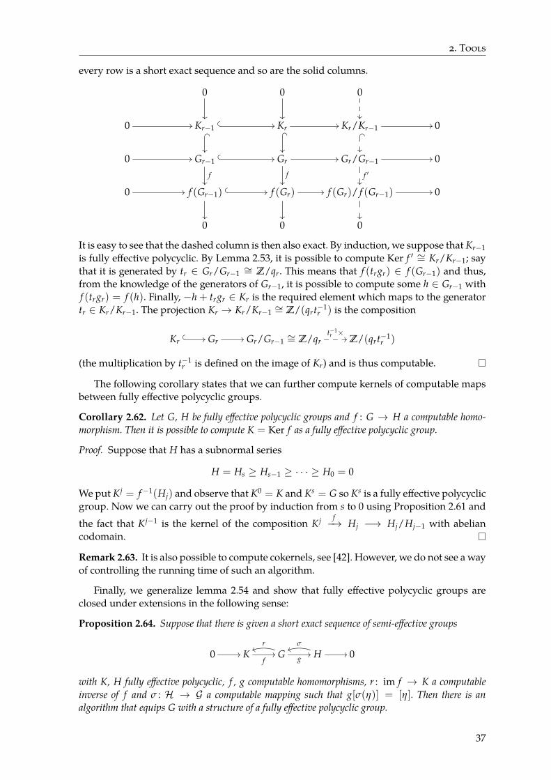
2. Tools

every row is a short exact sequence and so are the solid columns.

0

��

0

��

0

��

0 // Kr−1� _

��

� � // Kr� _

��

// Kr/Kr−1 //� _

��

0

0 // Gr−1� � //

f��

Gr //

f��

Gr/Gr−1 //

f ′��

0

0 // f (Gr−1)� � //

��

f (Gr) //

��

f (Gr)/ f (Gr−1) //

��

0

0 0 0

It is easy to see that the dashed column is then also exact. By induction, we suppose that Kr−1is fully effective polycyclic. By Lemma 2.53, it is possible to compute Ker f ′ ∼= Kr/Kr−1; saythat it is generated by tr ∈ Gr/Gr−1

∼= Z/qr. This means that f (trgr) ∈ f (Gr−1) and thus,from the knowledge of the generators of Gr−1, it is possible to compute some h ∈ Gr−1 withf (trgr) = f (h). Finally, −h + trgr ∈ Kr is the required element which maps to the generatortr ∈ Kr/Kr−1. The projection Kr → Kr/Kr−1

∼= Z/(qrt−1r ) is the composition

Kr� � // Gr // Gr/Gr−1

∼= Z/qrt−1r × // Z/(qrt−1

r )

(the multiplication by t−1r is defined on the image of Kr) and is thus computable.

The following corollary states that we can further compute kernels of computable mapsbetween fully effective polycyclic groups.

Corollary 2.62. Let G, H be fully effective polycyclic groups and f : G → H a computable homo-morphism. Then it is possible to compute K = Ker f as a fully effective polycyclic group.

Proof. Suppose that H has a subnormal series

H = Hs ≥ Hs−1 ≥ · · · ≥ H0 = 0

We put K j = f−1(Hj) and observe that K0 = K and Ks = G so Ks is a fully effective polycyclicgroup. Now we can carry out the proof by induction from s to 0 using Proposition 2.61 and

the fact that K j−1 is the kernel of the composition K j f−→ Hj −→ Hj/Hj−1 with abeliancodomain.

Remark 2.63. It is also possible to compute cokernels, see [42]. However, we do not see a wayof controlling the running time of such an algorithm.

Finally, we generalize lemma 2.54 and show that fully effective polycyclic groups areclosed under extensions in the following sense:

Proposition 2.64. Suppose that there is given a short exact sequence of semi-effective groups

0 // Kf// G g

//

rtt

H //

σtt

0

with K, H fully effective polycyclic, f , g computable homomorphisms, r : im f → K a computableinverse of f and σ : ℋ → 𝒢 a computable mapping such that g[σ(η)] = [η]. Then there is analgorithm that equips G with a structure of a fully effective polycyclic group.

37

2. Tools

Proof. Let Hs ≥ Hs−1 ≥ · · · ≥ H0 and Kt ≥ Kt−1 ≥ · · · ≥ K0 = 0 be the subnormal series forH and K, respectively. Then we have the following filtration

G = g−1(Hs) ≥ g−1(Hs−1) ≥ · · · ≥ g−1(H0) = f (Kt) ≥ f (Kt−1) ≥ · · · ≥ f (K0) = 0

with the filtration quotients either Hi/Hi−1 or Kj/Kj−1, the corresponding projections

g−1(Hi)g−→ Hi −→ Hi/Hi−1,

f (Kj)r−→ Kj −→ Kj/Kj−1,

and the generators either [σ(ηi)] when ηi represents the generator hi ∈ Hi or f (k j) whenk j ∈ Kj is the generator.

2.9 Eilenberg–MacLane spaces and diagrams

Given a group π and an integer k ≥ 0 an Eilenberg–MacLane space K(π, k) is a space satis-fying

πi(K(π, k)) ={

π for i = k,0 else.

In the rest of the thesis, by K(π, k) we will always mean the simplicial model which is definedin [27, page 101]:

K(π, k)q = Zk(∆q; π),

where ∆q ∈ sSet is the standard q–simplex and Zk denotes the cocycles. This means thateach q–simplex is regarded as a labelling of the k–dimensional faces of ∆q by elements of π

such that they add up to 0 on the boundary of every (k+ 1)-simplex in ∆q. The boundary anddegeneracy operators in K(π, k) are given as follows: For any σ ∈ K(π, k)q, di(σ) ∈ K(π, k)q−1is given by a restriction of σ of K(π, k) on the i-th face of ∆q. To define the degeneracy we firstintroduce mapping ηi : {0, 1, . . . , q + 1} → {0, 1, . . . , q} given by

ηi(j) ={

j for j ≤ ij− 1 for j > i

Every mapping ηi defines a map C*(ηi) : C*(∆q+1) → C*(∆q). The degeneracy siσ is now alabelling of the k–faces of ∆q+1 induced by C*(ηi) (see [27], p.101).

In the same way as the Eilenberg–MacLane space, we define the path space E(π, k) bythe formula

E(π, k)q = Ck(∆q; π).

Given a q–simplex σ ∈ E(π, k)q, the coboundary operator δ : Ck(∆q; π) → Ck+1(∆q; π) pro-duces a q–simplex δσ of K(π, k+ 1). Abusing the notation, the coboundary operator describesa simplicial map δ : E(π, k) → K(π, k + 1). In fact, δ is a Kan fibration. Further, according to[27, Theorem 23.10],

δ : E(π, k)→ K(π, k + 1)

is a fibration with fibre K(π, k) and we have a simplicial description of E(π, k) as a twistedproduct

K(π, k)×τ K(π, k + 1),

where we remark, that a k-simplex of ∆q can be represented by an increasing (k + 1)-tuple(i0, i1, . . . , ik) and the twisting operator τ : K(π, k + 1)→ K(π, k) is defined by

τ(z)((i0, i1, . . . , ik)) = z(0, i0 + 1, i1 + 1, . . . , ik + 1)− z(1, i0 + 1, i1 + 1, . . . , ik + 1). (2.13)

38

2. Tools

This description of E(π, k) as a twisted product can be used to show that E(π, k) haseffective homology.

Using these models, we define diagrams of Eilenberg–MacLane spaces K(π, k) : ℐ → sSet

for π : ℐ → Ab by setting K(π, k)(i) = K(π(i), k). The maps in the diagram K(π, k) areinduced by the homomorphisms in π. Analogously, we define the diagram E(π, k) of spacesE(π(i), k).

The simplicial sets K(π, k), E(π, k) defined above have the property that simplicial mapsX → K(π, k) correspond to cocycles Zk(X; π) and simplicial maps X → E(π, k) corres-pond to cochains Ck(X; π). This enables us to represent simplicial maps by cochains andcocycles. We further remark that given a simplicial set X the set of homotopy classes of maps[X, K(π, k)] corresponds to the elements of the group Hk(X; π).

For Bredon cohomology (see Definition 2.4), a similar thing holds as well: MorphismsX → E(π, k) correspond to cochains Ck

ℐ (X; π), morphisms X → K(π, n) correspond tococycles Zk

ℐ (X; π). If the diagram X is further cofibrant (and K(π, k) is fibrant but this isalways true for our model), the set of homotopy classes of maps of diagrams [X, K(π, k)]ℐcorresponds to the elements in Hk

ℐ (X; π).This correspondence will be described in more detail in further sections.

Evaluation maps. Assume that k ≥ 1 and π ∈ Ab. As E(π, k)k = Ck(∆k; π), the k-simplicesof E(π, k) can be seen as labellings of the unique k–simplex ∆k by an element of π. Using thedefinition of the model of E(π, k), we have

Ck(∆k; π) ∼= Hom(Ck(∆k; Z), π) ∼= Hom(Z, π) ∼= π.

This gives us a bijection ev : E(π, k)k = Ck(∆k; π) ∼= π. The map ev is defined by readingthe value on the unique k–simplex. This is why we will call this map evaluation. We remarkthat in this situation we further have E(π, k)k = K(π, k)k, because Ck(∆k; π) = Zk(∆k; π).

Next, we define a map Ck(E(π, k))→ π as the unique extension of ev to the free abeliangroup generated by E(π, k)k.

Abusing the notation, we will call this homomorphism ev. Similarly, we get homomorph-ism Ck(K(π, k))→ π and we again denote this homomorphism by ev.

Homomorphism ev is functorial, hence we can extend its definition to diagrams. To em-phasise the difference, we denote the resulting homomorphisms of diagrams ev, i.e.ev : Ck(E(π, k))→ π and ev : Ck(K(π, k))→ π.

In the proof of Theorem A, the following two lemmas will be used.

Lemma 2.65. The homomorphism ev : Ck(K(π, k))→ π induces an isomorphism of diagrams

Hk(K(π, k))→ π.

Proof. According to [7], Lemma 4.3, the statement of the Lemma holds pointwise and hencethe mapping of diagrams Hk(K(π, k))→ π induced by ev is an isomorphism of diagrams.

Given ev : Ck(E(π, k)) → π and ev : Ck+1(K(π, k + 1)) → π, we define a homomorph-ism

h B ev+ ev : Ck(E(π, k))⊕ Ck+1(K(π, k + 1))→ π ⊕π → π

where the last arrow is the standard addition. Using the map δ : E(π, k) → K(π, k + 1),which is a fibration pointwise, we can construct the algebraic mapping cone

Conek+1(δ*) = Ck(E(π, k))⊕ Ck+1(K(π, k + 1)),

and we in fact have a homomorphism h : Conek+1(δ*)→ π. This homomorphism has a niceproperty:

39

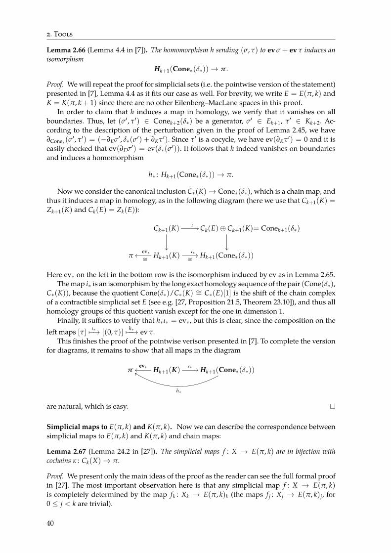
2. Tools

Lemma 2.66 (Lemma 4.4 in [7]). The homomorphism h sending (σ, τ) to ev σ + ev τ induces anisomorphism

Hk+1(Cone*(δ*))→ π.

Proof. We will repeat the proof for simplicial sets (i.e. the pointwise version of the statement)presented in [7], Lemma 4.4 as it fits our case as well. For brevity, we write E = E(π, k) andK = K(π, k + 1) since there are no other Eilenberg–MacLane spaces in this proof.

In order to claim that h induces a map in homology, we verify that it vanishes on allboundaries. Thus, let (σ′, τ′) ∈ Conek+2(δ*) be a generator, σ′ ∈ Ek+1, τ′ ∈ Kk+2. Ac-cording to the description of the perturbation given in the proof of Lemma 2.45, we have∂Cone*(σ

′, τ′) = (−∂Eσ′, δ*(σ′) + ∂Kτ′). Since τ′ is a cocycle, we have ev(∂Kτ′) = 0 and it iseasily checked that ev(∂Eσ′) = ev(δ*(σ′)). It follows that h indeed vanishes on boundariesand induces a homomorphism

h* : Hk+1(Cone*(δ*))→ π.

Now we consider the canonical inclusion C*(K)→ Cone*(δ*), which is a chain map, andthus it induces a map in homology, as in the following diagram (here we use that Ck+1(K) =Zk+1(K) and Ck(E) = Zk(E)):

Ck+1(K)ι //

��

Ck(E)⊕ Ck+1(K)= Conek+1(δ*)

��

π Hk+1(K)∼=ev*oo

∼=ι* // Hk+1(Cone*(δ*))

Here ev* on the left in the bottom row is the isomorphism induced by ev as in Lemma 2.65.The map i* is an isomorphism by the long exact homology sequence of the pair (Cone(δ*),

C*(K)), because the quotient Cone(δ*)/C*(K) ∼= C*(E)[1] is the shift of the chain complexof a contractible simplicial set E (see e.g. [27, Proposition 21.5, Theorem 23.10]), and thus allhomology groups of this quotient vanish except for the one in dimension 1.

Finally, it suffices to verify that h*ι* = ev*, but this is clear, since the composition on theleft maps [τ] ι*↦−→ [(0, τ)]

h*↦−−→ ev τ.This finishes the proof of the pointwise verison presented in [7]. To complete the version

for diagrams, it remains to show that all maps in the diagram

π Hk+1(K)ev*oo

ι* // Hk+1(Cone*(δ*))

h*

ee

are natural, which is easy.

Simplicial maps to E(π, k) and K(π, k). Now we can describe the correspondence betweensimplicial maps to E(π, k) and K(π, k) and chain maps:

Lemma 2.67 (Lemma 24.2 in [27]). The simplicial maps f : X → E(π, k) are in bijection withcochains κ : Ck(X)→ π.

Proof. We present only the main ideas of the proof as the reader can see the full formal proofin [27]. The most important observation here is that any simplicial map f : X → E(π, k)is completely determined by the map fk : Xk → E(π, k)k (the maps f j : Xj → E(π, k)j, for0 ≤ j < k are trivial).

40

2. Tools

This is based on the fact that for any n > k, E(π, k)n corresponds to labellings of k-faces ofa standard n-simplex ∆n by elements of the group π. It follows that for x ∈ Xn, where n > k,the image f (x) ∈ E(π, k) is determined by the images of di0 di1 . . . di(n−k−1)

x ∈ Xk, i.e. the k-faces of the n-simplex x. The induced map of chain complexes f* : C*(X) → C*(E(π, k)) isthen given by

fk* : Ck(X)→ Ck(E(π, k)).

The corresponding cochain κ f is then obtained as the composition

ev ∘ fk* : Ck(X)→ π.

In the opposite direction, take κ : Ck(X) → π. Using π ∼= Ck(∆k; π) ∼= E(π, k)k, we haveκ : Ck(X) → E(π, k)k. For any σ ∈ Xk, we define fk : Xk → E(π, k)k by fk(σ) = κ(σ). Ourprevious observation implies that fk describes f .

For Eilenberg-MacLane spaces, the same reasoning gives us

Lemma 2.68 (Lemma 24.3 in [27]). The simplicial maps f : X → K(π, k) are in bijection withcocycles κ ∈ Zk(X; π).

We omit the proof (it can be found in [27]) and remark that the correspondence betweensimplicial maps f : X → K(π, k) and cochains κ ∈ Zk(X; π) is the same as described in theproof of Lemma 2.67. Here, one has to prove that for a given f : X → K(π, k) the correspond-ing cochain κ is a cocycle and, in the opposite direction, to show that for a given cocycle κ theimage of the map f : X → E(π, k) lies in K(π, k).

When we generalize the previous results to diagrams, we obtain.

Lemma 2.69. Let X : ℐ → sSet and let π : ℐ → Ab. The maps f : X → E(π, k) of diagrams ofsimplicial sets are in bijection with cochains κ ∈ Ck

ℐ (X; π).

Proof. By Lemma 2.67, the collection of maps

fk(i) : (X(i))k → E(π(i), k)k, i ∈ ℐ

is in a one-to-one correspondence with cochains

κ(i) : Ck(X(i))→ π(i), i ∈ ℐ .

Let ι : i→ j for any i, j ∈ ℐ . The following diagrams commute

X(i)f (i)//

X(ι)��

E(π(i), k)

E(π(ι),k)��

X(j)f (j)// E(π(j), k)

Ck(X(i))κ(i)//

Ck(X(ι))��

π(i)

π(ι)��

Ck(X(j))κ(j)// π(j)

which meansE(π(ι), k) ∘ fk(i) = fk(j) ∘ X(ι).

Using Lemma 2.67, this gives us π(ι) ∘ κ(i) = κ(j) ∘ C*(X)(ι). Therefore the collections ofcochains κ(i)i∈ℐ describes a cochain κ ∈ Ck

ℐ (X; π).The other direction is similar: We take a cochain κ ∈ Ck

ℐ (X; π), which is a collectionof individual cochains κ(i)i∈ℐ : Ck(X(i)) → π(i), each of these cochains corresponds to asimplicial map f (i) : X(i)→ E(π(i), k) as in Lemma 2.67.

As above, we have a version for Eilenberg–MacLane spaces.

41

2. Tools

Lemma 2.70. Let X : ℐ → sSet and let π : ℐ → Ab. The maps f : X → K(π, k) of diagrams ofsimplicial sets are in bijection with cocycles κ ∈ Zk

ℐ (X; π).

The proof is omitted as it is just a variation of the proof of Lemma 2.68 using Lemma 2.69.Finally, we have the following result that can be seen as a generalization of Theorem 24.4

in [27].

Proposition 2.71. Let X : ℐ → sSet be cofibrant and let π : ℐ → Ab. Then homotopy classes ofmaps of diagrams [X, K(π, k)]ℐ are in bijection with Bredon cohomology groups Hk

ℐ (X; π).

Proof. Our proof utilizes some basic facts from model categories about the existence of cer-tain maps and uses cylinder objects Cyl X introduced in Definition 2.5. The reader can finddetails in [11]. For a map f from X to E(π, k) or K(π, k), the corresponding cochain (cocycle)will be denoted by κ f .

Suppose we have f , g : X → K(π, k) and that they are (left) homotopic, i.e. there exists ahomotopy H : Cyl X → K(π, k).

X //ι0∼//

f ##

Cyl X

H��

Xooι1∼

oo

g{{

K(π, k)

We aim to find some κa ∈ Ck−1ℐ (X; π) such that δ(κa) = κg − κ f . From the projection

p : Cyl X → X, we have a left homotopy F = f ∘ p : Cyl X → K(π, k) between f and f .

X //ι0∼//

id##

f

""

Cyl X

p∼��

Xooι1∼

oo

id{{

f

||

X

f��

K(π, k)

“Subtracting” the first diagram from the second we get the diagram

X //ι0∼

//

f− f --

Cyl X

H−F=N��

Xooι1∼

oo

g− fqqX

which says that N : Cyl X → K(π, k) is a homotopy between trivial map 0 and g− f . So thefollowing diagram commutes:

X��ι0∼��

0 // E(π, k− 1)

���

Cyl X N //

b77

K(π, k)

Because X is assumed to be cofibrant, the definition of a cylider object tells us that ι0 is acofibration and a weak equivalence. Further δ is a fibration and using the model categorystructure on sSetℐ , a lift (dotted arrow) b has to exist.

We now set a = b ∘ ι1 : X → E(π, k− 1). It remains to show that δ(κa) = κg − κ f , but onecan see that

κδ(a) = κ(δbι1) = κ(Nι1) = κ(H−F)ι1 = κHι1 − κFι1 = κg − κ f .

42

2. Tools

In the opposite direction, the proof essentially follows the lines of proof of Theorem 24.4in [27]:

We assume that f , g are cohomologous i.e. there exists a : X → E(π, k − 1) such thatδ(κa) = κg − κ f .

We use that fact that E(π, k − 1) is both fibrant and weakly equivalent to a point - thisfollows from the fact that any E(π(i), k− 1) has this property. Further, ι is a cofibration, seeDefinition 2.5. Due to the model category structure, there exists a lift b : Cyl X → E(π, k− 1)in the diagram

X ⨿ X��

ι

��

0⨿a // E(π, k− 1)

∼����

Cyl X 0 //

b77

∆0

b ∘ ι0 = 0 and b ∘ ι1 = a.Again, we take the homotopy F = f ∘ p : Cyl X → K(π, k) between f and f and we set

H = F + δ(b). Thus we have κHι0 = κ f and

κHι1 = κ f + κδ(a) = κ f + κg − κ f = κg.

Therefore H is the desired homotopy between f and g.

In case X is not cofibrant, we get the bijection between [X, K(π, k)]ℐ and the cohomologygroup Hk

ℐ (Xcof; π).

Representing a map of diagrams by an effective cocycle. In the Postnikov system algori-thm, we will encounter the following situation: We consider a finite diagram X : ℐ → sSet

that has effective homology and an effective diagram Cef* (X) of chain complexes such that

C*(X)⇐⇐⇒⇒ Cef* (X). Let f : C*(X)→ Cef

* (X) be the composite (natural) map from the strongequivalence.

Let us also consider a (k + 1)-cocycle

ψef ∈ Zk+1(Hom(Cef* (X), π)) = Zk+1

ℐ ,ef (X; π)

for some diagram of fully effective Abelian groups π. The superscript “ef” emphasise thatthe cocycle belongs to the “effective” cochain complex C*ℐ ,ef(X; π) obtained from the effectivediagram Cef

* (X) associated to X. Then ψef can be represented by a system of finite matrices,since it can be seen as a collection of maps from chain groups Cef

k+1(X) of finite rank into π(i),i ∈ ℐ , as was described in Lemma 2.69.

Lemma 2.72. The cocycle ψef defines a simplicial map X → K(π, k + 1).

Proof. Take the chain map f : C(X) → Cef(X). We define a cocycle ψ ∈ Zk+1ℐ (X; π) as ψ =

f ψef. We have seen in Lemma 2.70 that such a ψ canonically defines a simplicial map ψ : X →K(π, k + 1).

A pullback from a fibration of Eilenberg–MacLane diagrams. For our construction of Post-nikov systems, we will need an operation that is essentially a twisted Cartesian product, butin a somewhat different representation. We will have the following situation. We are given adiagram of simplicial sets P ∈ sSetℐ , plus a mapping f : P→ K(π, n + 1), for some diagramof abelian groups π ∈ sSetℐ and a fixed n ≥ 1.

43

2. Tools

Now we define a diagram Q ∈ sSetℐ as the pullback according to the following commut-ative diagram:

Q //

��

E(π, n)

�

Pf// K(π, n + 1)

This means that each Q(i) is the simplicial subset of the Cartesian product P(i)× E(π(i), n)consisting of the pairs (α, β) of simplices α ∈ P(i)`, β ∈ E(π(i), n)` with f (α) = δ(β).

Because the twisted products can be given effective homology, we get

Corollary 2.73. Given π, n, P, f as above, where π is a fully effective diagram of abelian groups,the diagram P has pointwise effective homology, and f is computable, the pullback diagram Q haspointwise effective homology.

Proof. Let τ : K(π, n + 1) → K(π, n) be the twisting operator (2.13) in the twisted productE(π, n) ∼= K(π, n)(i) ×τ K(π, n + 1)(i) and let τ* : K(π, n + 1) → P, where τ*(α) Bτ( f (α)). Then Corollary 2.22 yields effective homology for each twisted productK(π, n)(i) ×τ* P(i). According to [27, Prop. 18.7] (which is formulated in a more generalsetting), there is a simplicial isomorphism ϕ : K(π, n)(i)×τ* P(i)→ Q(i), given by

ϕ(α, β) B (ψ( f (α)) + β, α),

where ψ : K(π, n + 1)→ E(π, n) is the pseudo-section given by

ψ(z)(i0, . . . , in) B z(0, i0 + 1, . . . , in + 1),

with the same notation as in the definition of τ. Since both ϕ and its inverse are computablemaps, we obtain effective homology for every Q(i) as needed. The functoriality of τ* andmaps in diagrams P, K(π, n + 1) further gives us maps in the diagram Q.

Effective homology for E(π, n) and K(π, n). In this subsection, we show that E(π, n) andK(π, n) have effective homology when n ≥ 0 and π is a finitely generated abelian group.

These results were mainly developed by Sergeraert, his students and coworkers, see e.gP. Real’s thesis [33]. A strenghtening of these results was provided in [7], where the authorspresent constructions that are polynomial.

We will use the obvious implication of these results: given π : ℐ → Ab a finite diagramof finitely generated abelian groups and n ≥ 1, the Eilenberg–MacLane space K(π, n) andthe classifying space E(π, n) have pointwise effective homology.

We really only need to concern ourselves with the effective homology for Eilenberg–MacLane spaces as there exists an explicit reduction C*(E(π, n))⇒⇒ Z (this is not surprisingsince E(π, n) is weakly equivalent to a point). Otherwise, one can see E(π, n) as the twis-ted product K(π, n)×τ K(π, n + 1) and it follows that the effective homology of Eilenberg–MacLane spaces implies effective homology of E(π, n)

There is a (polynomial-time) reduction C*(K(Z, 1)) ⇒⇒ Cef* (K(Z, 1)) described in [24]

and we remark that in the section regarding the discrete vector fields, we have shown a vectorfield producing a reduction C*(K(Z, 1))⇒⇒ Cef

* (K(Z, 1)), so K(Z, 1) has effective homology,this reduction, however is not polynomial time.

What remains is to show that K(π, n) has effective homology for other dimensions andgroups. The entire discussion why this is true was given in [7], so we will omit many detailsand describe just the main ideas of how this result is achieved as a succession of steps:

44

2. Tools

∙ One proves that K(Z/m, 1) has effective homology for m ≥ 1 using effective homologyfor K(Z, 1), because there exists a (specific) twisted cartesian product P = K(Z, 1)×τ

K(Z/m, 1) and one can show that P is simplicially isomorphic to K(Z, 1). We will notgive a description of this as it is described in detail by Lemma 3.17 in [7], but we remarkthat conceptually, the isomorphism ϕ : P → K(Z, 1) can be obtained from the shortexact sequence of abelian groups

0 // Z×m

// Zmod m // Z/m // 0

by passing to classifying spaces. The effective homology K(Z/m, 1) now follows fromeffective homology for K(Z, 1) using Proposition 2.27.

∙ For π arbitrary finitely generated abelian, we have a decomposition π = π1⊕ · · · ⊕πs,where πi is cyclic, 1 ≤ i ≤ s. We obtain effective homology for K(π, 1) using

K(π1 ⊕ · · · ⊕ πs, 1) ∼= K(π1, 1)× · · · × K(πs, 1),

which is easy to see from the definition of K(π, 1), and a repeated use of Lemma 2.12(product).

∙ An effective homology for K(π, n), n ≥ 2 is constructed by induction using the pre-vious results and the so–called W construction: Given an Eilenberg–MacLane spaceK(π, n), there is a simplicial isomorphism K(π, n + 1) → WK(π, n). Further, one usesa reduction

( f , g, h) : C*(K(π, n)×τ WK(π, n)) = C*(E(π, n))⇒⇒ Z

where the twisting operator τ is computable (for full description of this operator, see[7], Lemma 3.15). Using Proposition 2.27 and the induction assumption, we obtain thatWK(π, n) ∼= K(π, n + 1) has effective homology.

45

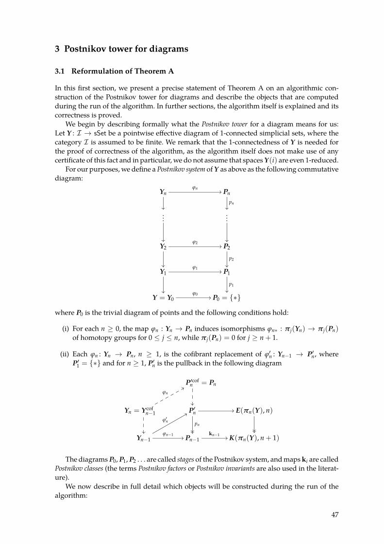
3 Postnikov tower for diagrams

3.1 Reformulation of Theorem A

In this first section, we present a precise statement of Theorem A on an algorithmic con-struction of the Postnikov tower for diagrams and describe the objects that are computedduring the run of the algorithm. In further sections, the algorithm itself is explained and itscorrectness is proved.

We begin by describing formally what the Postnikov tower for a diagram means for us:Let Y : ℐ → sSet be a pointwise effective diagram of 1-connected simplicial sets, where thecategory ℐ is assumed to be finite. We remark that the 1-connectedness of Y is needed forthe proof of correctness of the algorithm, as the algorithm itself does not make use of anycertificate of this fact and in particular, we do not assume that spaces Y(i) are even 1-reduced.

For our purposes, we define a Postnikov system of Y as above as the following commutativediagram:

Ynϕn

//

��

Pn

pn��

...

��

...

��

Y2ϕ2

//

��

P2

p2

��

Y1ϕ1

//

��

P1

p1��

Y = Y0ϕ0

// P0 = {*}

where P0 is the trivial diagram of points and the following conditions hold:

(i) For each n ≥ 0, the map ϕn : Yn → Pn induces isomorphisms ϕn* : πj(Yn) → πj(Pn)of homotopy groups for 0 ≤ j ≤ n, while πj(Pn) = 0 for j ≥ n + 1.

(ii) Each ϕn : Yn → Pn, n ≥ 1, is the cofibrant replacement of ϕ′n : Yn−1 → P′n, whereP′1 = {*} and for n ≥ 1, P′n is the pullback in the following diagram

P′cofn = Pn

��

Yn = Ycofn−1

ϕn

88

��

P′npn

����

// E(πn(Y), n)

����

Yn−1ϕn−1

//

ϕ′n

88

Pn−1kn−1

// K(πn(Y), n + 1)

The diagrams P0, P1, P2 . . . are called stages of the Postnikov system, and maps ki are calledPostnikov classes (the terms Postnikov factors or Postnikov invariants are also used in the literat-ure).

We now describe in full detail which objects will be constructed during the run of thealgorithm:

47

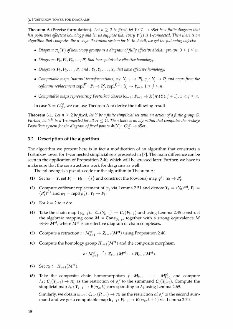
3. Postnikov tower for diagrams

Theorem A (Precise formulation). Let n ≥ 2 be fixed, let Y : ℐ → sSet be a finite diagram thathas pointwise effective homology and let us suppose that every Y(i) is 1-connected. Then there is analgorithm that computes the n-stage Postnikov system for Y . In detail, we get the following objects:

∙ Diagram πj(Y) of homotopy groups as a diagram of fully effective abelian groups, 0 ≤ j ≤ n.

∙ Diagrams P0, P′1, P′2, . . . , P′n that have pointwise effective homology.

∙ Diagrams P1, P2, . . . , Pn and : Y1, Y2, . . . , Yn that have effective homology.

∙ Computable maps (natural transformations) ϕ′j : Yj−1 → P′j , ϕj : Yj → Pj and maps from thecofibrant replacement replP′j : Pj → P′j , replYj−1 : Yj → Yj−1, 1 ≤ j ≤ n.

∙ Computable maps representing Postnikov classes kj−1 : Pj−1 → K(πj(Y), j + 1), 1 < j ≤ n.

In case ℐ = 𝒪opG , we can use Theorem A to derive the following result

Theorem 3.1. Let n ≥ 2 be fixed, let Y be a finite simplicial set with an action of a finite group G.Further, let YH be a 1-connected for all H ≤ G. Then there is an algorithm that computes the n-stagePostnikov system for the diagram of fixed points Φ(Y) : 𝒪op

G → sSet.

3.2 Description of the algorithm

The algorithm we present here is in fact a modification of an algorithm that constructs aPostnikov tower for 1–connected simplicial sets presented in [7]. The main difference can beseen in the application of Proposition 2.40, which will be stressed later. Further, we have tomake sure that the constructions work for diagrams as well.

The following is a pseudo-code for the algorithm in Theorem A:

(1) Set Y0 = Y , set P′1 = P0 = {*} and construct the (obvious) map ϕ′1 : Y0 → P′1.

(2) Compute cofibrant replacement of ϕ′1 via Lemma 2.51 and denote Y1 = (Y0)cof, P1 =(P′1)

cof and ϕ1 = repl(ϕ′1) : Y1 → P1.

(3) For k = 2 to n do:

(4) Take the chain map (ϕk−1)* : C*(Yk−1) → C*(Pk−1) and using Lemma 2.45 constructthe algebraic mapping cone M B Coneϕk−1* together with a strong equivalence M⇐⇐⇒⇒ Mef, where Mef is an effective diagram of chain complexes.

(5) Compute a retraction r : Mefk+1 → Zk+1(Mef) using Proposition 2.40.

(6) Compute the homology group Hk+1(Mef) and the composite morphism

ρ : Mefk+1

r−→ Zk+1(Mef)→ Hk+1(Mef).

(7) Set πk B Hk+1(Mef).

(8) Take the composite chain homomorphism f : Mk+1 −→ Mefk+1 and compute

λk : Ck(Yk−1)→ πk as the restriction of ρ f to the summand Ck(Yk−1). Compute thesimplicial map `k : Yk−1 → E(πk, k) corresponding to λk using Lemma 2.69.

Similarly, we obtain κk−1 : Ck+1(Pk−1)→ πk as the restriction of ρ f to the second sum-mand and we get a computable map kk−1 : Pk−1 → K(πk, k + 1) via Lemma 2.70.

48

3. Postnikov tower for diagrams

(9) Apply Corollary 2.73 to obtain P′k as a pullback in the diagram

P′k

����

// E(πk, k)

���

Yk−1ϕk−1

//

`k−1

&&

ϕ′k

99

Pk−1kk−1

// K(πk, k + 1)

(3.1)

and set ϕ′k = (ϕk−1, `k) as the map to the pullback P′k.

(10) Compute ϕk : Yk → Pk using Lemma 2.51 as the cofibrant replacement of ϕ′k.

3.3 Correctness of the algorithm

In this section, we prove the correctness of the algorithm presented above. The proof is byinduction with respect to k.

The basic step of the induction is in the pseudocode covered by (1) and (2). In these stepswe compute the map ϕ1 : Y1 → P1 between diagrams that have effective homology. BecauseY is 1-connected, ϕ1 and P1 satisfy the properties in the Postnikov tower.

In the induction step, we assume that we have a (computable) map of diagrams that haveeffective homology ϕk−1 : Yk−1 → Pk−1. To produce a map of diagrams that have effectivehomology ϕk : Yk → Pk we need to verify the following claims:

∙ In step (5) we have to make sure that Hefj (M) = 0 for j ≤ k in order to use Proposi-

tion 2.40.

∙ There is an isomorphism πk∼= πk(Yk−1) ∼= πk(Y).

∙ The cochain κk−1 is a cocycle, thus we can define the Postnikov classes kk−1 : Pk−1 →K(πk, k + 1) using Lemma 2.70.

∙ The image of the induced map ϕ′k = (ϕk−1, `k) : Yk−1 × E(πk, k) lies in P′k.

∙ The diagram Pk is a Postnikov stage, has effective homology and ϕk satisfies the prop-erties in the definition of the Postnikov system.

The proof of most of these claims follows from proof of Theorem 4.1 in [7], the maindifference is that we make sure that all statements are true for diagrams, because they areclearly true pointwise.

We will further frequently use the simple observation already mentioned in the defini-tion of a weak equivalence in the projective model structure: given two diagrams of groupsA, B : ℐ → Grp and a morphism f : A → B, to verify that f : A → B is an isomorphism, it isenough to show that it is an isomorphism pointwise.

For brevity we further write K = K(πk, k + 1) and E = E(πk, k).

Homology of the mapping cone M. Let Cyl ϕk−1 be the mapping cylinder of ϕk−1 : Yk−1 →Pk−1. Clearly π*(Cyl ϕk−1) = π*(Pk−1) because these diagrams are pointwise homotopyequivalent. Further Yk−1 is a subdiagram of Cyl ϕk−1. The chain complex of the pair(Cyl ϕk−1, Yk−1) has a reduction to M = Coneϕk−1* , see Remark 2.46. Hence

H*(Cyl ϕk−1, Yk−1) ∼= H*(M) ∼= H*(Mef).

49

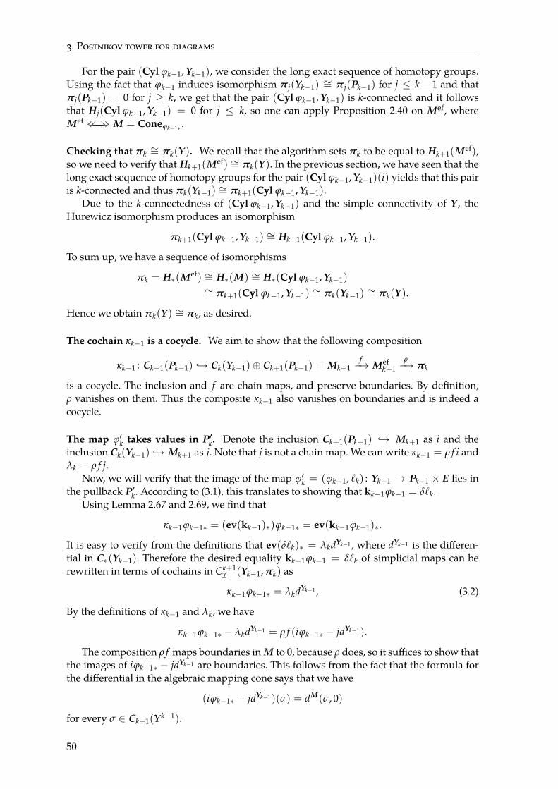
3. Postnikov tower for diagrams

For the pair (Cyl ϕk−1, Yk−1), we consider the long exact sequence of homotopy groups.Using the fact that ϕk−1 induces isomorphism πj(Yk−1) ∼= πj(Pk−1) for j ≤ k− 1 and thatπj(Pk−1) = 0 for j ≥ k, we get that the pair (Cyl ϕk−1, Yk−1) is k-connected and it followsthat Hj(Cyl ϕk−1, Yk−1) = 0 for j ≤ k, so one can apply Proposition 2.40 on Mef, whereMef ⇐⇐⇒⇒ M = Coneϕk−1* .

Checking that πk∼= πk(Y). We recall that the algorithm sets πk to be equal to Hk+1(Mef),

so we need to verify that Hk+1(Mef) ∼= πk(Y). In the previous section, we have seen that thelong exact sequence of homotopy groups for the pair (Cyl ϕk−1, Yk−1)(i) yields that this pairis k-connected and thus πk(Yk−1) ∼= πk+1(Cyl ϕk−1, Yk−1).

Due to the k-connectedness of (Cyl ϕk−1, Yk−1) and the simple connectivity of Y , theHurewicz isomorphism produces an isomorphism

πk+1(Cyl ϕk−1, Yk−1) ∼= Hk+1(Cyl ϕk−1, Yk−1).

To sum up, we have a sequence of isomorphisms

πk = H*(Mef) ∼= H*(M) ∼= H*(Cyl ϕk−1, Yk−1)∼= πk+1(Cyl ϕk−1, Yk−1) ∼= πk(Yk−1) ∼= πk(Y).

Hence we obtain πk(Y) ∼= πk, as desired.

The cochain κk−1 is a cocycle. We aim to show that the following composition

κk−1 : Ck+1(Pk−1) ↪→ Ck(Yk−1)⊕ Ck+1(Pk−1) = Mk+1f−→ Mef

k+1ρ−→ πk

is a cocycle. The inclusion and f are chain maps, and preserve boundaries. By definition,ρ vanishes on them. Thus the composite κk−1 also vanishes on boundaries and is indeed acocycle.

The map ϕ′k takes values in P′k. Denote the inclusion Ck+1(Pk−1) ↪→ Mk+1 as i and theinclusion Ck(Yk−1) ↪→ Mk+1 as j. Note that j is not a chain map. We can write κk−1 = ρ f i andλk = ρ f j.

Now, we will verify that the image of the map ϕ′k = (ϕk−1, `k) : Yk−1 → Pk−1 × E lies inthe pullback P′k. According to (3.1), this translates to showing that kk−1ϕk−1 = δ`k.

Using Lemma 2.67 and 2.69, we find that

κk−1ϕk−1* = (ev(kk−1)*)ϕk−1* = ev(kk−1ϕk−1)*.

It is easy to verify from the definitions that ev(δ`k)* = λkdYk−1 , where dYk−1 is the differen-tial in C*(Yk−1). Therefore the desired equality kk−1ϕk−1 = δ`k of simplicial maps can berewritten in terms of cochains in Ck+1

ℐ (Yk−1, πk) as

κk−1ϕk−1* = λkdYk−1 , (3.2)

By the definitions of κk−1 and λk, we have

κk−1ϕk−1* − λkdYk−1 = ρ f (iϕk−1* − jdYk−1).

The composition ρ f maps boundaries in M to 0, because ρ does, so it suffices to show thatthe images of iϕk−1* − jdYk−1 are boundaries. This follows from the fact that the formula forthe differential in the algebraic mapping cone says that we have

(iϕk−1* − jdYk−1)(σ) = dM(σ, 0)

for every σ ∈ Ck+1(Yk−1).

50

3. Postnikov tower for diagrams

Pk and ϕk satisfy properties of the Postnikov system. Since ϕk is a cofibrant replacementof ϕ′k and Pk is a cofibrant replacement of P′k, we prove that Pk and ϕk satisfy properties of thePostnikov system by showing that ϕ′k* : πj(Yk−1) → πj(P′k) induces isomorphism for j ≤ kand that πj(P′k) = 0 for j > k.

We remark that that P′k has pointwise effective homology because it is a pullback (twistedproduct) of diagrams that have pointwise effective homology as in Corollary 2.73.

Because δ : E → K is a pointwise (principal and minimal) fibration with fibre K(πk, k),the definition of P′k as a pullback, gives us a pointwise fibration

K(πk, k)→ P′k → Pk−1.

By the induction assumption, πj(Pk−1) = 0 for j ≥ k, it is straightforward to check thatπj(P′k) = 0 for j ≥ k + 1, and that the maps πj(Yk−1)→ πj(P′k) induced by ϕ′k are isomorph-isms for j ≤ k− 1. To show that P′k is up to homotopy the k-th Postnikov stage, it remains toverify that (ϕ′k)* : πk(Yk−1)→ πk(P′k) is an isomorphism as well.

We will do this using the diagram

Yk−1

ϕk−1

��

ϕ′k // P′k //

pk

��

E

δ

��

Pk−1 Pk−1 // K

where the right square is the pullback diagram defining P′k.We will now make all the vertical maps into inclusions by replacing the spaces in the

bottom row with the mapping cylinder of the respective vertical map. This construction alsoinduces the horizontal maps between cylinders. We obtain the diagram.

Yk−1

��

ϕ′k // P′k //

��

E

��

Cyl ϕk−1 // Cyl pk // Cyl δ

(3.3)

Now we consider the long exact sequences for pairs (Cyl ϕk−1, Yk−1) and (Cyl pk, P′k):

0 = πk+1(Cyl ϕk−1) //

∼=��

πk+1(Cyl ϕk−1, Yk−1)

∼=��

// πk(Yk−1)

ϕ′k*��

// πk(Cyl ϕk−1) = 0

∼=��

0 = πk+1(Cyl pk) // πk+1(Cyl pk, P′k) // πk(P′k) // πk(Cyl pk) = 0

The first and the last vertical arrows are isomorphisms due to the fact that πj(Pk−1) = 0 forj ≥ k and that both of the mapping cylinders deform onto the base space Pk−1, i.e.

πj(Cyl ϕk−1) ∼= πj(Pk−1) ∼= πj(Cyl pk).

The exactness of the rows further implies isomorphisms πk+1(Cyl ϕk−1, Yk−1) ∼= πk(Yk−1)and πk+1(Cyl pk, P′k)

∼= πk(P′k). If we prove that the second vertical homomorphism is anisomorphism, then ϕ′k* has to be an isomorphism on πk. We formulate the required claim as

Lemma 3.2 (Lemma 4.5 in [7]). The map

πk+1(Cyl ϕk−1, Yk−1)→ πk+1(Cyl pk, P′k)

induced by the left square of diagram (3.3) is an isomorphism.

51

3. Postnikov tower for diagrams

Proof. The proof of the pointwise version of the Lemma is technical and can be found in [7].We thus have a homomorphism of diagrams of groups

πk+1(Cyl ϕk−1, Yk−1)→ πk+1(Cyl pk, P′k)

which is an isomorphism pointwise. It follows that this is an isomorphism of diagrams. Thisfinishes the proof of the correctness of the algorithm and thus of Theorem A.

3.4 Computing equivariant cohomology operations

In the nonequivariant setting, one standardly computes cohomology operations as

[K(π, n), K(ρ, k)].

Here, we will focus on the computation of G-invariant cohomology operations. Before doingthat, we prove the following general statement:

Proposition 3.3. Let ℐ be a finite category and X : ℐ → sSet a diagram with pointwise effectivehomology. Let π : ℐ → Ab be a diagram of fully effective abelian groups. Then there is an algorithmwhich computes [X, K(π, n)]ℐ .

Proof. We will utilize the following sequence of isomorphisms

[X, K(π, n)]ℐ ∼= [Xcof, K(π, n)]ℐ ∼= Hnℐ (Xcof; π),

where the first (left) isomorphism is a standard result of homotopy theory and the second iso-morphism follows from Proposition 2.71. Further C*(Xcof) has effective homology and thisin particular implies that there is a chain complex Cef

* (Xcof) such that Cefn (Xcof) is a diagram

of fully effective abelian groups.By Lemma 2.56 each Hom(Cef

k (Xcof), π) is a fully effective abelian group, so we constructan effective chain complex C*ℐ (Xcof; π). Using Lemma 2.53, we finally compute Hn

ℐ (Xcof; π),which is an effective abelian group.

Let π : 𝒪opG → Ab. We call a G-simplicial set X Eilenberg–MacLane G-simplicial set for

the diagram π in the dimension n if

πj(XH) =

{π(G/H) for j = n,0 otherwise.

Similarly, we call a diagram X : 𝒪opG → sSet Eilenberg-MacLane diagram for the diagram

π in the dimension n if

πj(X) =

{π for j = n,0 otherwise.

As an example, we remark that the diagram K(π, n) introduced in Section 2.9 is an Eilenberg-MacLane diagram for diagram π in the dimension n.

We now formulate the following corollary of Proposition 3.3 that describes the computa-tion of G-invariant cohomology operations.

Corollary 3.4. Let G be a finite group and let X, Y be Eilenberg-MacLane G-simplicial sets for thediagrams of groups π and ρ in dimensions n and k, respectively. Then there exists an algorithmcomputing [X, Y]G.

52

3. Postnikov tower for diagrams

Proof. We use Elmendorf’s theorem [14, 43, 28] to transform our computation to computationwith diagrams of simplicial sets:

[X, Y]G ∼= [ΦX, ΦY]𝒪opG

.

If we suppose that there exists an isomorphism

[ΦX, ΦY]𝒪opG∼= [K(π, n), K(ρ, k)]𝒪op

G, (3.4)

the proof can be finished using Proposition 3.3.It thus remains to prove the isomorphism (3.4): The model category structure on sSet𝒪

opG

induces a homotopy category Ho(sSet𝒪opG ), where maps Ho(sSet𝒪

opG )(A, B) correspond to

homotopy classes of maps [A, B]𝒪opG

(see [11]). Further, any weak equivalence in the categorysSet𝒪

opG turns into an isomorphism in Ho(sSet𝒪

opG ). It is thus enough to construct a zigzag of

weak equivalencesΦX →←←→ · · · ←→→ K(π, n).

We take (ΦX)cof and compute

[(ΦX)cof, K(π, n)]𝒪opG∼= Hn

𝒪opG((ΦX)cof; π).

As (ΦX)cof is an Eilenberg-MacLane diagram, we get that Hi(ΦX) = 0 for i < n andHn(ΦX) = π and thus Hn

𝒪opG(ΦX; π) = Hom(π, π). Using Proposition 2.71, there exists a

map id* : (ΦX)cof → K(π, n) corresponding to id ∈ Hom(π, π). Clearly, id* is a weak equi-valence. This, together with weak equivalence (ΦX)cof → ΦX gives us the required zigzag.Similarly, we get a zigzag connecting ΦY and K(ρ, k). This tells us that

Ho(sSet𝒪opG )(Φ(X, ΦY) ∼= Ho(sSet𝒪

opG )(K(π, n), K(ρ, k))

and we have obtained (3.4).

53

4 How to decide if a map is homotopically trivial

In this chapter, we present a simplified version of the result achieved by L. Vokrinek andmyself in the article [15].

The original article presents decision algorithm for the existence of a homotopy betweengiven maps f , g : X → Y where X and Y are finite simplicial complexes or more generallyfinite simplicial sets, f and g are simplicial maps and Y is assumed to be 1-connected.

Here, we will present a simplified version which decides whether given f : X → Y ishomotopic to a constant (trivial) map to a chosen basepoint in Y. If a homotopy exists, wewill call f nullhomotopic. The original, more general version relies heavily on the fiberwiseapproach of the paper [8]. We feel that introducing further notions to this work would bringmany unnecessary complications.

It is well known that no homotopy decision algorithm may exist if Y is allowed to benon-simply connected; this follows at once from Novikov’s result [32] on the unsolvability ofthe word problem in groups. Here, we will thus restrict our attention to the case of a simplyconnected Y.

Theorem B. Let X, Y be finite simplicial sets where Y is simply connected, and let f : X → Y be asimplicial map. Then there is an algorithm that decides whether f is homotopically trivial.

In the paper [5], the authors gave an algorithmic solution to the following problem: giventwo simplicial sets X, Y, compute [X, Y], i.e. the set of homotopy classes of continuous mapsfrom X to Y. Their algorithm works under a certain connectivity restriction on Y. This re-striction can be removed when the domain is replaced by a suspension – this is our nextresult which, at the same time, generalizes the computation of homotopy groups of spacesdescribed by Brown in [2].

We remark that in the case Y is simply connected, there is a bijection between sets of un-pointed homotopy classes of maps [X, Y] and pointed homotopy classes of maps[(X, *X), (Y, *Y)]. Further on, by [X, Y] we will always mean pointed classes.

Theorem C. There is an algorithm that computes the group [ΣX, Y] of pointed homotopy classes ofmaps from a suspension ΣX to a simply connected simplicial set Y.

The group is presented on the output as a so-called fully-effective polycyclic group – thisstructure is introduced in Section 2.8 and allows one to compute a finite set of generatorsand relations and solve the word problem.

The results described above are connected in the following way: In both cases, we re-place the space Y by a Postnikov tower and the proof is by induction. Further, the inductionassumption obtained used in Theorem B is utilized to give a proof of Theorem C and viceversa.

Relative statement. In order to prove Theorem B and Theorem C we will work in the commacategory A/sSet i.e. the category of pointed simplicial sets under A, where A contains thebasepoint. Here the objects are simplicial sets X equipped with a maps A→ X. Morphismsin this category are maps f : X → Y for which the following diagram

A α //

ι

��

Y

X

??

f (4.1)

commutes. There is also an obvious notion of homotopy (preserving the basepoint and relat-ive to A). In the case that ι is an inclusion, α is fixed and Y is a Kan complex, the resulting set

55

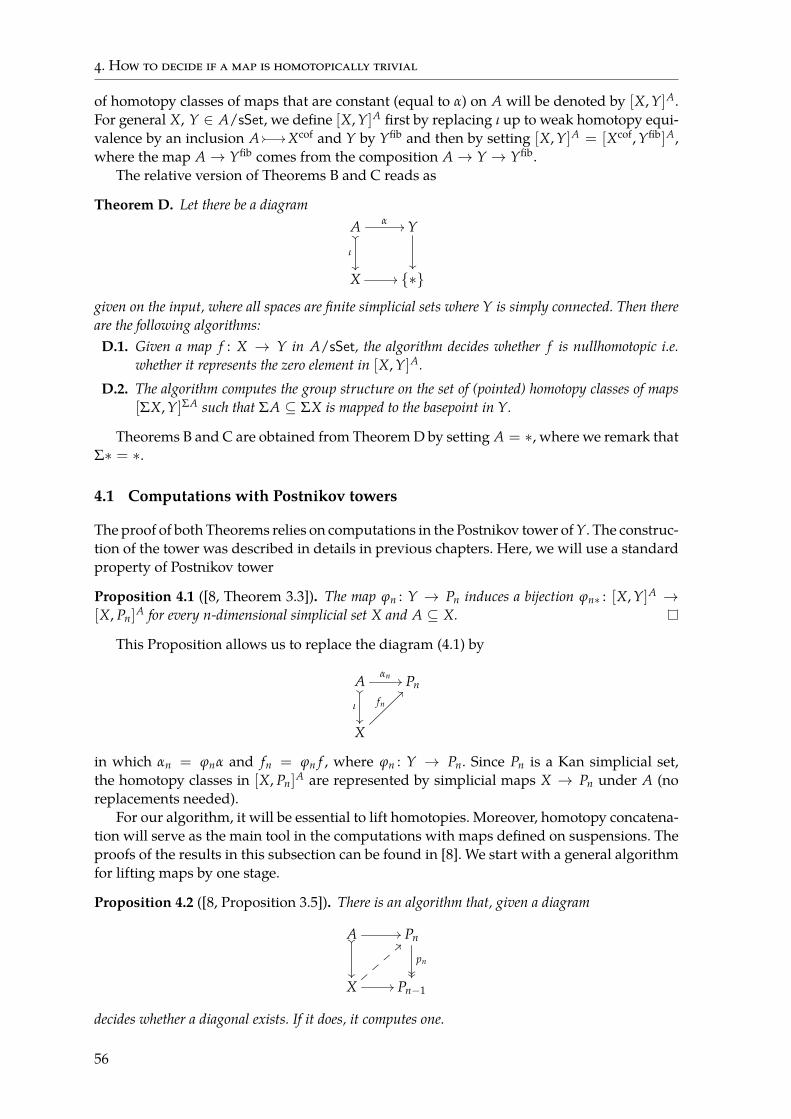
4. How to decide if a map is homotopically trivial

of homotopy classes of maps that are constant (equal to α) on A will be denoted by [X, Y]A.For general X, Y ∈ A/sSet, we define [X, Y]A first by replacing ι up to weak homotopy equi-valence by an inclusion A // //Xcof and Y by Yfib and then by setting [X, Y]A = [Xcof, Yfib]A,where the map A→ Yfib comes from the composition A→ Y → Yfib.

The relative version of Theorems B and C reads as

Theorem D. Let there be a diagramA α //��

ι

��

Y

��

X // {*}

given on the input, where all spaces are finite simplicial sets where Y is simply connected. Then thereare the following algorithms:D.1. Given a map f : X → Y in A/sSet, the algorithm decides whether f is nullhomotopic i.e.

whether it represents the zero element in [X, Y]A.D.2. The algorithm computes the group structure on the set of (pointed) homotopy classes of maps

[ΣX, Y]ΣA such that ΣA ⊆ ΣX is mapped to the basepoint in Y.

Theorems B and C are obtained from Theorem D by setting A = *, where we remark thatΣ* = *.

4.1 Computations with Postnikov towers

The proof of both Theorems relies on computations in the Postnikov tower of Y. The construc-tion of the tower was described in details in previous chapters. Here, we will use a standardproperty of Postnikov tower

Proposition 4.1 ([8, Theorem 3.3]). The map ϕn : Y → Pn induces a bijection ϕn* : [X, Y]A →[X, Pn]A for every n-dimensional simplicial set X and A ⊆ X.

This Proposition allows us to replace the diagram (4.1) by

Aαn //

��

ι

��

Pn

X

>>

fn

in which αn = ϕnα and fn = ϕn f , where ϕn : Y → Pn. Since Pn is a Kan simplicial set,the homotopy classes in [X, Pn]A are represented by simplicial maps X → Pn under A (noreplacements needed).

For our algorithm, it will be essential to lift homotopies. Moreover, homotopy concatena-tion will serve as the main tool in the computations with maps defined on suspensions. Theproofs of the results in this subsection can be found in [8]. We start with a general algorithmfor lifting maps by one stage.

Proposition 4.2 ([8, Proposition 3.5]). There is an algorithm that, given a diagram

A //��

��

Pn

pn����

X //

==

Pn−1

decides whether a diagonal exists. If it does, it computes one.

56

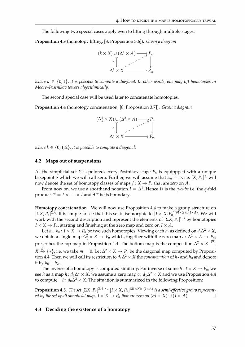
4. How to decide if a map is homotopically trivial

The following two special cases apply even to lifting through multiple stages.

Proposition 4.3 (homotopy lifting, [8, Proposition 3.6]). Given a diagram

(k× X) ∪ (∆1 × A) //

��

∼��

Pn

����

∆1 × X //

77

Pm

where k ∈ {0, 1}, it is possible to compute a diagonal. In other words, one may lift homotopies inMoore–Postnikov towers algorithmically.

The second special case will be used later to concatenate homotopies.

Proposition 4.4 (homotopy concatenation, [8, Proposition 3.7]). Given a diagram

( 2k × X) ∪ (∆2 × A) //

��

∼��

Pn

����

∆2 × X //

77

Pm

where k ∈ {0, 1, 2}, it is possible to compute a diagonal.

4.2 Maps out of suspensions

As the simplicial set Y is pointed, every Postnikov stage Pn is equippped with a uniquebasepoint o which we will call zero. Further, we will assume that αn = o, i.e. [X, Pn]A willnow denote the set of homotopy classes of maps f : X → Pn that are zero on A.

From now on, we use a shorthand notation I = ∆1. Hence Iq is the q-cube i.e. the q-foldproduct Iq = I × · · · × I and ∂Iq is its boundary.

Homotopy concatenation. We will now use Proposition 4.4 to make a group structure on[ΣX, Pn]ΣA. It is simple to see that this set is isomorphic to [I × X, Pn](∂I×X)∪(I×A). We willwork with the second description and represent the elements of [ΣX, Pn]ΣA by homotopiesI × X → Pn, starting and finishing at the zero map and zero on I × A.

Let h2, h0 : I × X → Pn be two such homotopies. Viewing each hi as defined on di∆2× X,we obtain a single map 2

1 × X → Pn which, together with the zero map o : ∆2 × A → Pn,prescribes the top map in Proposition 4.4. The bottom map is the composition ∆2 × X

pr−→X

β−→ {*}, i.e. we take m = 0. Let ∆2 × X → Pn be the diagonal map computed by Proposi-tion 4.4. Then we will call its restriction to d1∆2×X the concatenation of h2 and h0 and denoteit by h0 + h2.

The inverse of a homotopy is computed similarly: For inverse of some h : I × X → Pn, wesee h as a map h : d2∆2 × X, we assume a zero map o : d1∆2 × X and we use Proposition 4.4to compute −h : d0∆2 × X. The situation is summarized in the following Proposition:

Proposition 4.5. The set [ΣX, Pn]ΣA ∼= [I×X, Pn](∂I×X)∪(I×A) is a semi-effective group represent-ed by the set of all simplicial maps I × X → Pn that are zero on (∂I × X) ∪ (I × A).

4.3 Deciding the existence of a homotopy

57

4. How to decide if a map is homotopically trivial

An exact sequence associated with a fibration. We start with the following notation:πn = πn(Y), Kn+1 = K(πn, n + 1) and Ln = K(πn, n). There are maps

Lnj−→ Pn

pn−−→ Pn−1kn−−→ Kn+1,

where kn is the Postnikov invariant Pn−1 −→ K(πn, n + 1) and j is the inclusion such that theimage of j consists precisely of those simplices of Pn that map to zero in Pn−1. The followingsequence of pointed sets is exact by [8, Theorem 4.8] (the relevant parts of the proof do notuse the stability assumption n ≤ 2d):

[ΣX, Pn−1]ΣA ∂−→ [X, Ln]

A j*−→ [X, Pn]A pn*−−→ [X, Pn−1]

A kn*−−→ [X, Kn+1]A. (4.2)

The isomorphisms [X, Ln]A ∼= Hn(X, A; πn) and [X, Kn+1]A ∼= Hn+1(X, A; πn) show that

these sets are abelian groups that can be computed easily. The group homomorphism ∂ isdefined in the following way. Given a homotopy h : I×X → Pn−1, lift it to a homotopy h : I×X → Pn in such a way that (0×X)∪ (I× A) maps to the zero section, using Proposition 4.3.Since the restriction of h to 1× X takes values in the image of j, it could be interpreted as amap X → Ln. This map is then a representative of ∂[h].

Proof of Theorem D. The proof is by induction. First, we list a series of claims:

(gen)n It is possible to compute a finite set of generators of the group[I × X, Pn](∂I×X)∪(I×A).

(null)n It is possible to decide whether a given map f : X → Pn under A is nullhomotopic;when this is the case, it is possible to compute a nullhomotopy, i.e. a homotopy fromthe zero map to f .

We remark that if we perceive the claims above as algorithms, then the pair (X, A) of simpli-cial sets is seen as the input of these algorithms.

Proof of Theorem D.1 from (null)n We use the fact that [X, Y]A ∼= [X, Pn]A, therefore The-orem D.1 follows from (null)n.

Proofs of (null)0 and (gen)0 The basic steps are trivial, because Y is 1-connected and P0 ={*}. Thus the group is trivial and any given map is always nullhomotopic.

The algorithm (null)n is given by induction using (gen)n−1. This is essentially contained in[8, Section 4.9]; we reproduce the algorithm here for reader’s convenience but omit the proofof correctness.

(null)n−1 + (gen)n−1→ (null)n on (X, A)

∙ We take f : X → Pn. By (null)n−1, we decide whether the composition pn f : X → Pn−1is nullhomotopic and compute the nullhomotopy h′ : I × X → Pn−1. If pn f fails to benullhomotopic, then then f cannot be nullhomotopic and the algorithm stops.∙ We lift nullhomotopy h′ using Proposition 4.3 to a homotopy h′ : I × X → Pn such that

h′ : f ′ ∼ f . Since pn f ′ = o (as pnh′ = h′), we interpret f ′ : X → Pn as a map f ′ : X → Ln.∙ We use (gen)n−1 to decide whether [ f ′] ∈ im ∂ and to further compute h′′ : I × X → Pn−1

with ∂[h′′] = [ f ′]. Using Proposition 4.2, it is possible to compute a lift h′′ : I × X → Pnthat starts at the zero map and finishes at f ′

∙ Finally, the concatenation h = h′ + h′′, computed by Proposition 4.4, is a homotopy fromthe zero map to f . If either of h′, h′′ fails to exist, the map f is not nullhomotopic.

58

4. How to decide if a map is homotopically trivial

Thus, it remains to prove (gen)n. To make the induction possible, we will have to strength-en the claim and compute more than just generators, namely the structure of a fully effectivepolycyclic group as the group [I × X, Pn](∂I×X)∪(I×A) is polycyclic.

From now on, we denote

Gn,q = [Iq × X, Pn](∂Iq×X)∪(Iq×A)

and we formulate the new claim as(poly)n There is an algorithm which equips Gn,q with a structure of a fully effective poly-

cyclic group.As fully effective polycyclic group enables us to compute the generators, we get(poly)n → (gen)n.

Since Gn,q for (X, A) is a Gn,1 for (Iq−1, (∂Iq−1 × X) ∪ (Iq−1 × A)), it would be enoughto restrict to the case q = 1. This special case is just Theorem D.2 as for n = dim(I × X) =1 + dim X we have

[ΣX, Y]ΣA ∼= [I × X, Y](∂I×X)∪(I×A) ∼= [I × X, Pn](∂I×X)∪(I×A) = Gn,1

and the last term is computable by (poly)n. Hence (poly)n implies Theorem D.2.

(poly)n−1 + (null)n−1 → (poly)n. We remind that

[Iq × X, Ln](∂Iq×X)∪(Iq×A) ∼= Hn(Iq × X, (∂Iq × X) ∪ (Iq × A); πn) ∼= Hn−q(X, A; πn)

and similarly [Iq × X, Kn+1](∂Iq×X)∪(Iq×A) ∼= Hn+1−q(X, A; πn). The shifts in the degree of

cohomology groups follows from the properties of suspension.

Proof. The group Gn,q is semi-effective by Proposition 4.5. The exact sequence (4.2) appliedto (Iq × X, (∂Iq × X) ∪ (Iq × A)) instead of (X, A) reads

Gn−1,q+1∂−→ Hn−q(X, A; πn)

j*−→ Gn,qpn*−−→ Gn−1,q

kn*−−→ Hn+1−q(X, A; πn)

and induces a short exact sequence

0 // Coker ∂j*// Gn,q pn*

//

rtt

Ker kn* //

σtt

0.

Group Hn−q(X, A; πn) is a fully effective abelian group and by (poly)n−1, groups Gn−1,q+1and Gn−1,q are fully effective polycyclic. The images of generators of Gn−1,q+1 under ∂ gener-ate a subgroup in Hn−q(X, A; πn), so we can use Lemma 2.53 and find that the group Coker ∂

is fully effective abelian. Proposition 2.61 then gives us Ker kn* as a fully effective polycyclicgroup.

For the application of Proposition 2.64, we need to provide algorithms for the two indic-ated sections r, σ. The section σ is defined on the level of representatives (on which it de-pends) by mapping a diagonal f : Iq × X → Pn−1 to an arbitrary lift f : Iq × X → Pn of f thatis zero on (∂Iq × X) ∪ (Iq × A). The computation of f can be performed by Proposition 4.2.

For the construction of the partial inverse r on im j* = Ker pn*, let f : Iq × X → Pn be adiagonal such that its composition with pn : Pn → Pn−1 is homotopic to zero. Then we cancompute such a nullhomotopy h : Iq × X → Pn−1 by (null)n−1 on (Iq × X, (∂Iq × X) ∪ (Iq ×A)). Using Proposition 4.3, we lift h along pn to a homotopy from some f ′ : Iq × X → Pn tof . Since pn f ′ = o, the image of f ′ lies in Ln and we may set r([ f ]) = [ f ′].

59

4. How to decide if a map is homotopically trivial

Remark 4.6. The computation of Coker ∂ in the above proof requires generators of Gn−1,q+1– these are provided by an application of (poly)n−1 which in turn requires generators ofGn−2,q+2, etc. Thus, in principle, we need to compute Gm,p for all m < n and p ≤ n + q.

However, this is not necessary: for q ≥ 2, Gn,q is an abelian group and one may computeits generators from those of Ker kn* and Coker ∂ via Lemma 2.54. Now, Coker ∂ is generatedby the images of generators of Hn−q(X, A; πn). Further, Ker kn* can be computed from a setof generators of Gn−1,q.

Thus, for q ≥ 2, the computation of generators of Gn,q can be executed by inductionon n while q is fixed. To summarize, it is thus possible to organize the computation of Gn,1in Theorem D.2 in such a way that in its course, we only need a fully effective polycyclicstructure on Gm,1, m ≤ n, and generators of Gm,2, m < n.

60

Bibliography

[1] G. Bredon: Equivariant cohomology theories, Springer Lecture Notes in Mathematics, 34(1967).

[2] E. H. Brown: Finite computability of Postnikov complexes, Ann. of Math. 65 1–20, 1957

[3] R. Brown: The twisted Eilenberg-Zilber theorem, Celebrazioni Archimedee del Secolo XX,Simposio di topologia, 1964, (1965).

[4] A. K. Bousfield, D. M. Kan: Homotopy Limits, Completions and Localizations, Springer Lec-ture Notes in Mathematics, 304 (1972).

[5] M. Čadek, M. Krčál, J. Matoušek, F. Sergeraert, L. Vokřínek, U. Wagner: Computing allmaps into a sphere, J. ACM, 61 (2014), article no. 17.

[6] M. Čadek, M. Krčál, J. Matoušek, L. Vokřínek, U. Wagner: Extendabililty of continuousmaps in undecidable, Discrete Comput. Geom., 51 (1), (2014), 24–66.

[7] M. Čadek, M. Krčál, J. Matoušek, L. Vokřínek, U. Wagner: Polynomial time computation ofhomotopy groups and Postnikov systems in fixed dimensions, SIAM J. Comput. 43-5 (2014),1728–1780.

[8] M. Čadek, M. Krčál, L. Vokřínek: Algorithmic solvability of lifting extension problem,arXiv:1307.6444, (2013).

[9] D. Dugger: A primer on homotopy colimits, http://math.uoregon.edu/~ddugger/hocolim.pdf, (2008).

[10] W. G. Dwyer, D. M. Kan: An obstruction theory for diagrams of simplicial sets, Proc. Kon.Akad. van Wetensch, A87 (1984), 139–146.

[11] W. Dwyer, J. Spaliński: Homotopy Theories and Model Categories, in Handbook of Algebraictopology, Elsevier (1995), 73–126.

[12] S. Eilenberg, S. MacLane: On the groups H(π, n) I, Ann. of Math., 58 (1953), 55–106.

[13] S. Eilenberg, S. MacLane: On the groups H(π, n) II, Ann. of Math., 60 (1954), 49–139.

[14] A. D. Elmendorf: Systems of fixed points sets, Trans. Amer. Math. Soc., 277 (1983), 275–284.

[15] M. Filakovský, L. Vokřínek: Are two maps homotopic? An algorithmic viewpoint,arXiv:1312.2337, (2013).

[16] M. Filakovský: Effective homology for twisted products, Arch. Math (Brno), 48 (2012), 313–322.

[17] M. Filakovský: Effective homology for homotopy colimit and cofibrant replacement, Arch. Math(Brno), 50 (2014), 273–286.

[18] R. Forman: Morse theory for cell complexes, Adv. Math., 134 (1998), 90–145.

[19] P. Franek, M. Krčál: Robust satisfiability of systems of equations, Proceedings of the Twenty-Fifth Annual ACM-SIAM Symposium on Discrete Algorithms. SIAM, (2014). p. 193-203.

[20] P. G. Goerss, J. F. Jardine: Simplicial homotopy theory, Boston-Basel-Berlin: Birkhauser,(1999).

61

BIBLIOGRAPHY

[21] P. S. Hirschhorn: Model Categories and Their Localizations, Mathematical Surveys andMonographs, 99 (2009).

[22] S. B. Isaacson: Exercises on homotopy colimits, http://math.mit.edu/~mbehrens/TAGS/Isaacson_exer.pdf.

[23] R. Kannan, A. Bachem: Polynomial algorithms for computing the Smith and Hermite normalforms of an integer matrix, SIAM J. Comput. 8 (1981), 499–507.

[24] M. Krčál, J. Matoušek, l, F. Sergeraert: Polynomial-time homology for simplicial Eilenberg-MacLane spaces, Found. Comput. Math., 13.6, (2013), 935–963.

[25] L. Lambe, J. Stasheff: Applications of Perturbation Theory to Iterated Fibrations, ManuscriptaMath. 58 (1987), 363-376

[26] J. Matouš, M. Tancer, U. Wagner: Hardness of embedding simplicial complexes in Rd, J. Eur.Math. Soc. 13(2), (2011), 259—295.

[27] J. P. May: Simplicial Objects in Algebraic Topology, Chicago Lectures in Mathematics. 1992reprint of 1967 original, (1992).

[28] J. P. May, R. J. Piacenza, M. Cole: Equivariant homotopy and cohomology theory : dedicated tothe memory of Robert J. Piacenza, Providence, R.I.: Published for the Conference Board ofthe Mathematical Sciences by the American Mathematical Society, (1996).

[29] J. R. Munkres: Elements of Algebraic Topology, Addison-Wesley, Reading, MA, (1984).

[30] A. Nabutovsky, S. Weinberger: Algorithmic unsolvability of the triviality problem for multi-dimensional knots, Comment. Math. Helv., 71(3), (1996), 426–434.

[31] A. Nabutovsky, S. Weinberger: Algorithmic aspects of homeomorphism problems, In Tel AvivTopology Conference: Rothenberg Festschrift (1998), volume 231 of Contemp. Math.,pages 245–250. Amer. Math. Soc., Providence, RI, (1999).

[32] P. S. Novikov: On the algorithmic unsolvability of the word problem in group theory (in Rus-sian), Trudy Mat. Inst. im. Steklova 44 (1955), 1–143.

[33] P. Real: Algorithms for computing effective homology of classifying spaces (in Spanish), PhD.Thesis, Facultad de Mathemáticas, Univ. de Sevilla, 1993. Available online at http://fondosdigitales.us.es/media/thesis/1426/C_043-139.pdf.

[34] P. Real: An algorithm computing homotopy groups, Mathematics and Computers in Simu-lation, 42, (1996), 461–465.

[35] E. Riehl: Categorical Homotopy Theory, Cambridge University Press, (2014).

[36] A. Romero, J. Rubio and F. Sergeraert: Computing spectral sequences, J. Symbol. Comput.,41(10), (2006), 1059–1079.

[37] A. Romero, F. Sergeraert: Discrete Vector Fields and Fundamental Algebraic Topology,arXiv:1005.5685v1, (2010).

[38] J. Rubio, F. Sergeraert: Constructive algebraic topology, Bull. Sci. Math., 126(5), (2012), 389–412.

[39] J. Rubio, F. Sergeraert: Constructive Homological Algebra and Applications, Written in 2006for a MAP Summer School at the University of Genova, arXiv:1208.3816v2, (2012).

62

BIBLIOGRAPHY

[40] W. Shih: Homologie des espaces fibrés, Publications Mathematiques del’ I.H.E.S., 13 (1962),293–312.

[41] R. Schön: Effective algebraic topology, Memoirs of the American Mathematical Society, 451,1991.

[42] C. C. Sims: Computation with Finitely Presented Groups, Cambridge University Press, Cam-bridge, 1994.

[43] M. Stephan: On equivariant homotopy theory for model categories, arXiv:1308.0856, (2013).

[44] A. Storjohann: Near optimal algorithms for computing Smith normal forms of integer matrices,International Symposium on Symbolic and Algebraic Computation, (1996), 267–274.

[45] C. A. Weibel: An Introduction to Homological Algebra, Cambridge University Press, Cam-bridge, 1994.

63