Algorithm Efficiency & Sorting • Algorithm efficiency • Big-O notation • Searching algorithms • Sorting algorithms

Welcome message from author
This document is posted to help you gain knowledge. Please leave a comment to let me know what you think about it! Share it to your friends and learn new things together.
Transcript

Algorithm Efficiency & Sorting
• Algorithm efficiency
• Big-O notation
• Searching algorithms
• Sorting algorithms
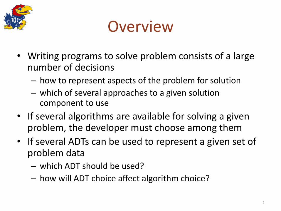
Overview
• Writing programs to solve problem consists of a large number of decisions – how to represent aspects of the problem for solution
– which of several approaches to a given solution component to use
• If several algorithms are available for solving a given problem, the developer must choose among them
• If several ADTs can be used to represent a given set of problem data – which ADT should be used?
– how will ADT choice affect algorithm choice?
2

Overview – 2
• If a given ADT (i.e. stack or queue) is attractive as part of a solution
• How will the ADT implement affect the program's: – correctness and performance?
• Several goals must be balanced by a developer in producing a solution to a problem – correctness, clarity, and efficient use of computer
resources to produce the best performance
• How is solution performance best measured? – time and space
3

Overview – 3
• The order of importance is, generally, – correctness
– efficiency
– clarity
• Clarity of expression is qualitative and somewhat dependent on perception by the reader – developer salary costs dominate many software projects
– time efficiency of understanding code written by others can thus have a significant monetary implication
• Focus of this chapter is execution efficiency – mostly, run-time (some times, memory space)
4

Measuring Algorithmic Efficiency
• Analysis of algorithms – provides tools for contrasting the efficiency of different
methods of solution
• Comparison of algorithms – should focus on significant differences in efficiency
– should not consider reductions in computing costs due to clever coding tricks
• Difficult to compare programs instead of algorithms – how are the algorithms coded?
– what computer should you use?
– what data should the programs use?
5

Analyzing Algorithmic Cost
• Viewed abstractly, an algorithm is a sequence of steps – Algorithm A { S1; S2; .... Sm1; Sm }
• The total cost of the algorithm will thus, obviously, be the total cost of the algorithm's m steps – assume we have a function giving cost of each statement
Cost (Si) = execution cost of Si, for-all i, 1 ≤ i ≤ m
• Total cost of the algorithm's m steps would thus be:
Cost (A) = 𝐶𝑜𝑠𝑡 (𝑆𝑖)𝑚𝑖=1
6

Analyzing Algorithmic Cost – 2
• However, an algorithm can be applied to a wide variety of problems and data sizes – so we want a cost function for the algorithm A that
takes the data set size n into account
Cost 𝐴, 𝑛 = 𝐶𝑜𝑠𝑡 (𝑆𝑖)𝑚1
𝑛1
• Several factors complicate things – conditional statements: cost of evaluating condition
and branch taken
– loops: cost is sum of each of its iterations
– recursion: may require solving a recurrence equation
7

Analyzing Algorithmic Cost – 3
• Do not attempt to accumulate a precise prediction for program execution time, because – far too many complicating factors: compiler
instructions output, variation with specific data sets, target hardware speed
• Provides an approximation, an order of magnitude estimate, that permits fair comparison of one algorithm's behavior against that of another
8

Analyzing Algorithmic Cost – 4
• Various behavior bounds are of interest – best case, average case, worst case
• Worst-case analysis – A determination of the maximum amount of time that
an algorithm requires to solve problems of size n
• Average-case analysis – A determination of the average amount of time that
an algorithm requires to solve problems of size n
• Best-case analysis – A determination of the minimum amount of time that
an algorithm requires to solve problems of size n
9
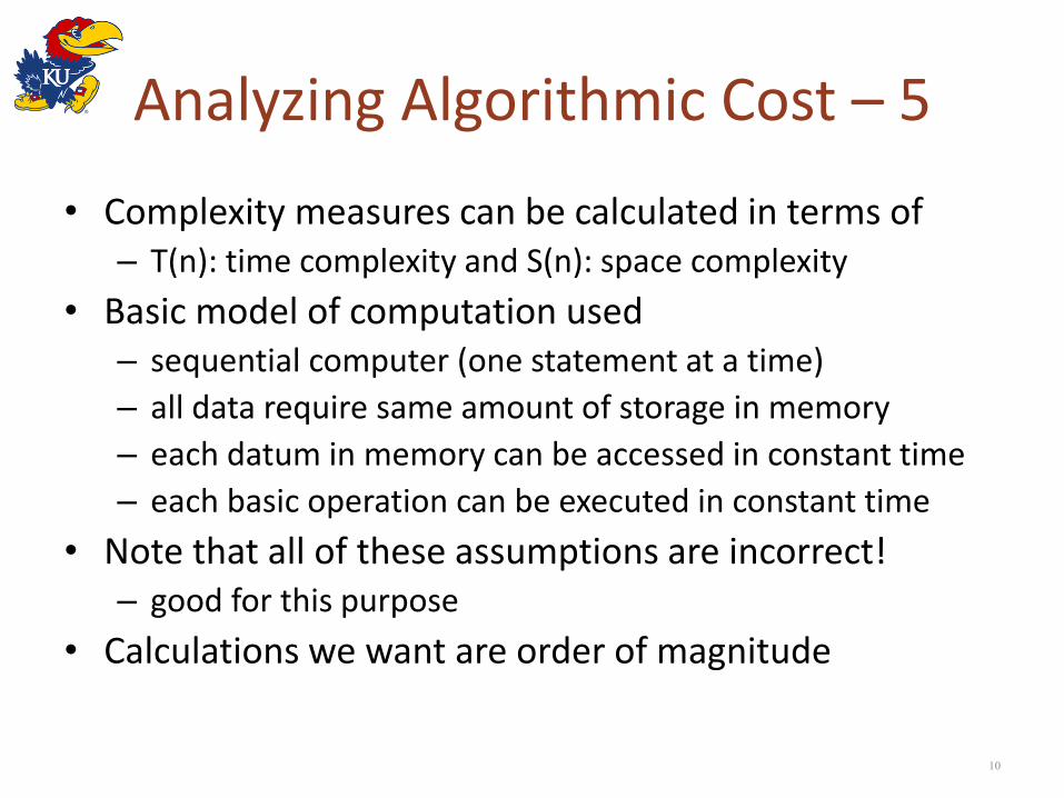
Analyzing Algorithmic Cost – 5
• Complexity measures can be calculated in terms of – T(n): time complexity and S(n): space complexity
• Basic model of computation used – sequential computer (one statement at a time)
– all data require same amount of storage in memory
– each datum in memory can be accessed in constant time
– each basic operation can be executed in constant time
• Note that all of these assumptions are incorrect! – good for this purpose
• Calculations we want are order of magnitude
10
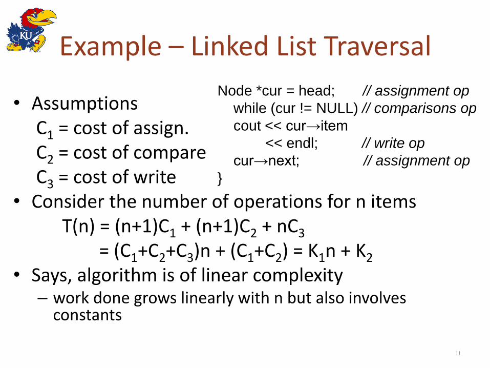
Example – Linked List Traversal
• Assumptions C1 = cost of assign. C2 = cost of compare C3 = cost of write • Consider the number of operations for n items T(n) = (n+1)C1 + (n+1)C2 + nC3
= (C1+C2+C3)n + (C1+C2) = K1n + K2
• Says, algorithm is of linear complexity – work done grows linearly with n but also involves
constants
11
Node *cur = head; // assignment op
while (cur != NULL) // comparisons op
cout << cur→item
<< endl; // write op
cur→next; // assignment op
}

Example – Sequential Search
• Number of comparisons
TB(n) = 1 (or 3?)
Tw(n) = n
TA(n) = (n+1)/2
• In general, what developers worry about the most is that this is O(n) algorithm – more precise analysis is
nice but rarely influences algorithmic decision
12
Seq_Search(A: array, key: integer);
i = 1;
while i ≤ n and A[i] ≠ key do
i = i + 1
endwhile;
if i ≤ n
then return(i)
else return(0)
endif;
end Sequential_Search;

Bounding Functions
• To provide a guaranteed bound on how much work is involved in applying an algorithm A to n items – we find a bounding function f(n) such that
𝑇 𝑛 ≤ 𝑓 𝑛 , ∀ 𝑛
• It is often easier to satisfy a less stringent constraint by finding an elementary function f(n) such that
𝑇 𝑛 ≤ 𝑘 ∗ 𝑓 𝑛 , 𝑓𝑜𝑟 𝑠𝑢𝑓𝑓𝑖𝑐𝑖𝑒𝑛𝑡𝑙𝑦 𝑙𝑎𝑟𝑔𝑒 𝑛
• This is denoted by the asymptotic big-O notation
• Algorithm A is O(n) says – that complexity of A is no worse than k*n as n grows
sufficiently large
13

Asymptotic Upper Bound
• Defn: A function f is positive if 𝑓 𝑛 > 0, ∀ 𝑛 > 0
• Defn: Given a positive function f(n), then
𝑓 𝑛 = 𝑂 𝑔 𝑛
iff there exist constants k > 0 and n0 > 0 such that
𝑓 𝑛 ≤ 𝑘 ∗ 𝑔 𝑛 , ∀ 𝑛 > 𝑛0
• Thus, g(n) is an asymptotic bounding function for the work done by the algorithm
• k and n0 can be any constants – can lead to unsatisfactory conclusions if they are very large
and a developer's data set is relatively small
14

Asymptotic Upper Bound – 2
• Example: show that: 2𝑛2 − 3𝑛 + 10 = 𝑂(𝑛2) • Observe that 2𝑛2 − 3𝑛 + 10 ≤ 2𝑛2+ 10, 𝑛 > 1 2𝑛2 − 3𝑛 + 10 ≤ 2𝑛2+ 10, 𝑛2 𝑛 > 1 2𝑛2 − 3𝑛 + 10 ≤ 12𝑛2, 𝑛 > 1 • Thus, expression is O(n2) for k = 12 and n0 > 1 (also k =
3 and n0 > 1, BTW) – algorithm efficiency is typically a concern for large
problems only
• Then, O(f(n)) information helps choose a set of final candidates and direct measurement helps final choice
15
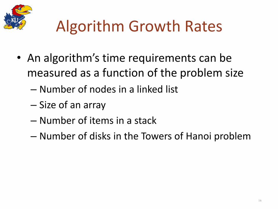
Algorithm Growth Rates
• An algorithm’s time requirements can be measured as a function of the problem size
– Number of nodes in a linked list
– Size of an array
– Number of items in a stack
– Number of disks in the Towers of Hanoi problem
16
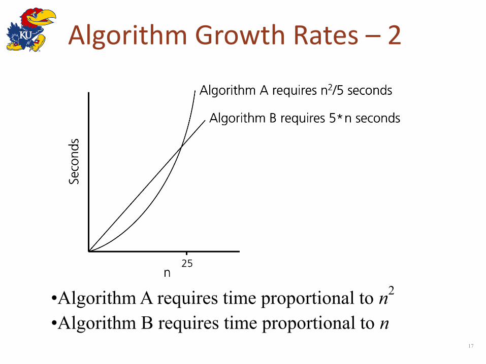
Algorithm Growth Rates – 2
17
•Algorithm A requires time proportional to n2
•Algorithm B requires time proportional to n

Algorithm Growth Rates – 3
• An algorithm’s growth rate enables comparison of one algorithm with another
• Example – if, algorithm A requires time proportional to n2, and
algorithm B requires time proportional to n
– algorithm B is faster than algorithm A – n2 and n are growth-rate functions – Algorithm A is O(n2) - order n2 – Algorithm B is O(n) - order n
• Growth-rate function f(n) – mathematical function used to specify an algorithm’s
order in terms of the size of the problem
18
Order-of-Magnitude Analysis and Big O Notation
19
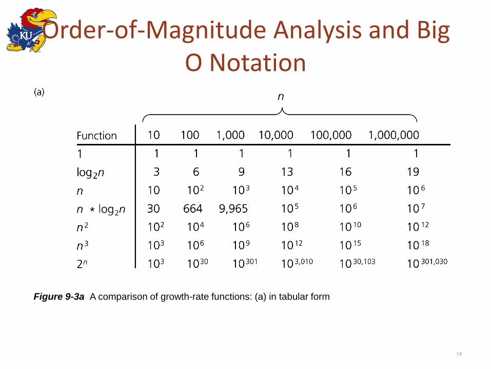
Figure 9-3a A comparison of growth-rate functions: (a) in tabular form
Order-of-Magnitude Analysis and Big O Notation
20
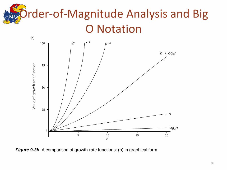
Figure 9-3b A comparison of growth-rate functions: (b) in graphical form

Order-of-Magnitude Analysis and Big O Notation
• Order of growth of some common functions
– O(C) < O(log(n)) < O(n) < O(n * log(n)) < O(n2) < O(n3) < O(2n) < O(3n) < O(n!) < O(nn)
• Properties of growth-rate functions
– O(n3 + 3n) is O(n3): ignore low-order terms
– O(5 f(n)) = O(f(n)): ignore multiplicative constant in the high-order term
– O(f(n)) + O(g(n)) = O(f(n) + g(n))
21

Keeping Your Perspective
• Only significant differences in efficiency are interesting
• Frequency of operations
– when choosing an ADT’s implementation, consider how frequently particular ADT operations occur in a given application
– however, some seldom-used but critical operations must be efficient
22

Keeping Your Perspective
• If the problem size is always small, you can probably ignore an algorithm’s efficiency – order-of-magnitude analysis focuses on large
problems
• Weigh the trade-offs between an algorithm’s time requirements and its memory requirements
• Compare algorithms for both style and efficiency
23
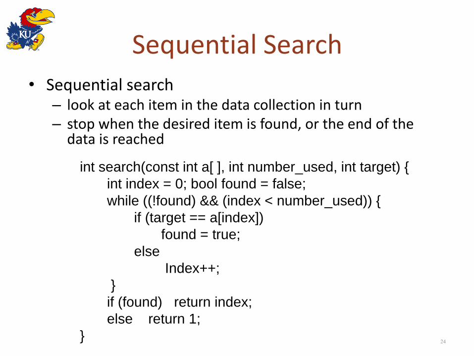
Sequential Search
• Sequential search – look at each item in the data collection in turn – stop when the desired item is found, or the end of the
data is reached
24
int search(const int a[ ], int number_used, int target) {
int index = 0; bool found = false;
while ((!found) && (index < number_used)) {
if (target == a[index])
found = true;
else
Index++;
}
if (found) return index;
else return 1;
}

Efficiency of Sequential Search
• Worst case: O(n)
– key value not present, we search the entire list to prove failure
• Average case: O(n)
– all positions for the key being equally likely
• Best case: O(1)
– key value happens to be first
25
The Efficiency of Searching Algorithms
• Binary search of a sorted array – Strategy
• Repeatedly divide the array in half
• Determine which half could contain the item, and discard the other half
– Efficiency • Worst case: O(log2n)
• For large arrays, the binary search has an enormous advantage over a sequential search
– At most 20 comparisons to search an array of one million items
26

Sorting Algorithms and Their Efficiency
• Sorting – A process that organizes a collection of data into
either ascending or descending order
– The sort key is the data item that we consider when sorting a data collection
• Sorting algorithm types – comparison based
• bubble sort, insertion sort, quick sort, etc.
– address calculation • radix sort
27

Sorting Algorithms and Their Efficiency
• Categories of sorting algorithms
– An internal sort
• Requires that the collection of data fit entirely in the computer’s main memory
– An external sort
• The collection of data will not fit in the computer’s main memory all at once, but must reside in secondary storage
28

for index=0 to size-2 {
select min/max element from among A[index], …, A[size-1];
swap(A[index], min);
}
Selection Sort
• Strategy – Place the largest (or smallest) item in its correct place – Place the next largest (or next smallest) item in its correct
place, and so on
• Algorithm • Analysis
– worst case: O(n2), average case: O(n2) – does not depend on the initial arrangement of the data
29

Selection Sort
30
Figure 9-4 A selection sort of an array of five integers

Bubble Sort
• Strategy
– compare adjacent elements and exchange them if they are out of order
• moves the largest (or smallest) elements to the end of the array
– repeat this process
• eventually sorts the array into ascending (or descending) order
• Analysis: worst case: O(n2), best case: O(n)
31

Bubble Sort – algorithm
for i = 1 to size -- 1 do
for index = 1 to size -- i do
if A[index] < A[index1]
swap(A[index], A[index1]);
endfor;
endfor;
32
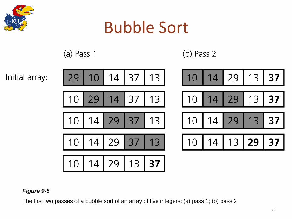
Bubble Sort
33
Figure 9-5
The first two passes of a bubble sort of an array of five integers: (a) pass 1; (b) pass 2

Insertion Sort
• Strategy – Partition array in two regions: sorted and unsorted
• initially, entire array is in unsorted region
• take each item from the unsorted region and insert it into its correct position in the sorted region
• each pass shrinks unsorted region by 1 and grows sorted region by 1
• Analysis – Worst case: O(n2)
• Appropriate for small arrays due to its simplicity
• Prohibitively inefficient for large arrays
34

Insertion Sort
35
Figure 9-7 An insertion sort of an array of five integers.

Mergesort
• A recursive sorting algorithm
• Performance is independent of the initial order of the array items
• Strategy
– divide an array into halves
– sort each half
– merge the sorted halves into one sorted array
– divide-and-conquer approach
36

Mergesort – Algorithm
mergeSort(A,first,last) {
if (first < last) {
mid = (first + last)/2;
mergeSort(A, first, mid);
mergeSort(A, mid+1, last);
merge(A, first, mid, last)
}
}
37

Mergesort
38

Mergesort
39

Mergesort – Properties
• Needs a temporary array into which to copy elements during merging – doubles space requirement
• Mergesort is stable – items with equal key values appear in the same
order in the output array as in the input
• Advantage – mergesort is an extremely fast algorithm
• Analysis: worst / average case: O(n * log2n)
40

Quicksort
• A recursive divide-and-conquer algorithm – given a linear data structure A with n records
– divide A into sub-structures S1 and S2
– sort S1 and S2 recursively
• Algorithm – Base case: if |S|==1, S is already sorted
– Recursive case: • divide A around a pivot value P into S1 and S2 , such that
all elements of S1<=P and all elements of S2>=P
• recursively sort S1 and S2 in place
41

Quicksort
• Partition() – (a) scans array, (b) chooses a pivot, (c) divides A
around pivot, (d) returns pivot index – Invariant: items in S1 are all less than pivot, and items
in S2 are all greater than or equal to pivot
• Quicksort() – partitions A, sorts S1 and S2 recursively
42
Quicksort – Pivot Partitioning
• Pivot selection and array partition are fundamental work of algorithm
• Pivot selection
– perfect value: median of A[ ]
• sort required to determine median (oops!)
• approximation: If |A| > N, N==3 or N==5, use median of N
– Heuristic approaches used instead
• Choose A[first] OR A[last] OR A[mid] (mid = (first+last)/2) OR Random element
• heuristics equivalent if contents of A[ ] randomly arranged
43

Quicksort – Pivot Partitioning Example
A= [5,8,3,7,4,2,1,6], first =0, last =7 • 1. A[first]: pivot = 5 • 2. A[last]: pivot = 6 • 3. A[mid]: mid =(0+7)/2=3, pivot = 7 • 4. A[random()]: any key might be chosen • 5. A[medianof3]: median(A[first], A[mid], A[last]) is • median(5,7,6) = 6 • ● Note that the median determination is itself a sort, • but only of a fixed number of items, which is thus • still O(1) • ● Good pivot selection • ● Computed in O(1) time and partitions A into • roughly equal parts S1 and S2
44

Quicksort
45
Figure 9-19 A worst-case partitioning with quicksort

Quicksort
• Analysis
– Average case: O(n * log2n)
– Worst case: O(n2)
• When the array is already sorted and the smallest item is chosen as the pivot
– Quicksort is usually extremely fast in practice
– Even if the worst case occurs, quicksort’s performance is acceptable for moderately large arrays
46

Radix Sort
• Strategy
– Treats each data element as a character string
– Repeatedly organizes the data into groups according to the ith character in each element
• Analysis
– Radix sort is O(n)
47

Radix Sort
48
Figure 9-21 A radix sort of eight integers

A Comparison of Sorting Algorithms
49
Figure 9-22 Approximate growth rates of time required for eight sorting algorithms

The STL Sorting Algorithms
• Some sort functions in the STL library header <algorithm>
– sort
• Sorts a range of elements in ascending order by default
– stable_sort
• Sorts as above, but preserves original ordering of equivalent elements
50

The STL Sorting Algorithms
– partial_sort
• Sorts a range of elements and places them at the beginning of the range
– nth_element
• Partitions the elements of a range about the nth element
• The two subranges are not sorted
– partition
• Partitions the elements of a range according to a given predicate
51
Summary
• Order-of-magnitude analysis and Big O notation measure an algorithm’s time requirement as a function of the problem size by using a growth-rate function
• To compare the efficiency of algorithms
– Examine growth-rate functions when problems are large
– Consider only significant differences in growth-rate functions
52

Summary
• Worst-case and average-case analyses
– Worst-case analysis considers the maximum amount of work an algorithm will require on a problem of a given size
– Average-case analysis considers the expected amount of work that an algorithm will require on a problem of a given size
53

Summary
• Order-of-magnitude analysis can be the basis of your choice of an ADT implementation
• Selection sort, bubble sort, and insertion sort are all O(n2) algorithms
• Quicksort and mergesort are two very fast recursive sorting algorithms
54
Related Documents


![Improving SAR Automatic Target Recognition Models with ... · ATR data [1]. Despite this, MSTAR is interesting since it can show an algorithm’s robustness to the statistical properties](https://static.cupdf.com/doc/110x72/600020049a112846090dcd34/improving-sar-automatic-target-recognition-models-with-atr-data-1-despite.jpg)


