Algebraically Solvable Problems: Describing Polynomials as Equivalent to Explicit Solutions Uwe Schauz Department of Mathematics University of Tbingen, Germany [email protected] Submitted: Nov 14, 2006; Accepted: Dec 28, 2007; Published: Jan 7, 2008 Mathematics Subject Classifications: 41A05, 13P10, 05E99, 11C08, 11D79, 05C15, 15A15 Abstract The main result of this paper is a coefficient formula that sharpens and general- izes Alon and Tarsi’s Combinatorial Nullstellensatz. On its own, it is a result about polynomials, providing some information about the polynomial map P | X 1 ×···×Xn when only incomplete information about the polynomial P (X 1 ,...,X n ) is given. In a very general working frame, the grid points x ∈ X 1 × ··· × X n which do not vanish under an algebraic solution – a certain describing polyno- mial P (X 1 ,...,X n ) – correspond to the explicit solutions of a problem. As a consequence of the coefficient formula, we prove that the existence of an algebraic solution is equivalent to the existence of a nontrivial solution to a problem. By a problem, we mean everything that “owns” both, a set S , which may be called the set of solutions ; and a subset S triv ⊆S , the set of trivial solutions. We give several examples of how to find algebraic solutions, and how to apply our coefficient formula. These examples are mainly from graph theory and combina- torial number theory, but we also prove several versions of Chevalley and Warning’s Theorem, including a generalization of Olson’s Theorem, as examples and useful corollaries. We obtain a permanent formula by applying our coefficient formula to the matrix polynomial, which is a generalization of the graph polynomial. This formula is an integrative generalization and sharpening of: 1. Ryser’s permanent formula. 2. Alon’s Permanent Lemma. 3. Alon and Tarsi’s Theorem about orientations and colorings of graphs. Furthermore, in combination with the Vigneron-Ellingham-Goddyn property of pla- nar n-regular graphs, the formula contains as very special cases: 4. Scheim’s formula for the number of edge n-colorings of such graphs. 5. Ellingham and Goddyn’s partial answer to the list coloring conjecture. the electronic journal of combinatorics 15 (2008), #R10 1

Welcome message from author
This document is posted to help you gain knowledge. Please leave a comment to let me know what you think about it! Share it to your friends and learn new things together.
Transcript

Algebraically Solvable Problems: Describing
Polynomials as Equivalent to Explicit Solutions
Uwe Schauz
Department of Mathematics
University of Tbingen, Germany
Submitted: Nov 14, 2006; Accepted: Dec 28, 2007; Published: Jan 7, 2008
Mathematics Subject Classifications: 41A05, 13P10, 05E99, 11C08, 11D79, 05C15, 15A15
Abstract
The main result of this paper is a coefficient formula that sharpens and general-
izes Alon and Tarsi’s Combinatorial Nullstellensatz. On its own, it is a result about
polynomials, providing some information about the polynomial map P |X1×···×Xn
when only incomplete information about the polynomial P (X1, . . . , Xn) is given.
In a very general working frame, the grid points x ∈ X1 × · · · × Xn
which do not vanish under an algebraic solution – a certain describing polyno-
mial P (X1, . . . , Xn) – correspond to the explicit solutions of a problem. As a
consequence of the coefficient formula, we prove that the existence of an algebraic
solution is equivalent to the existence of a nontrivial solution to a problem. By a
problem, we mean everything that “owns” both, a set S , which may be called the
set of solutions; and a subset Striv ⊆ S , the set of trivial solutions.
We give several examples of how to find algebraic solutions, and how to apply
our coefficient formula. These examples are mainly from graph theory and combina-
torial number theory, but we also prove several versions of Chevalley and Warning’s
Theorem, including a generalization of Olson’s Theorem, as examples and useful
corollaries.
We obtain a permanent formula by applying our coefficient formula to the matrix
polynomial, which is a generalization of the graph polynomial. This formula is an
integrative generalization and sharpening of:
1. Ryser’s permanent formula.
2. Alon’s Permanent Lemma.
3. Alon and Tarsi’s Theorem about orientations and colorings of graphs.
Furthermore, in combination with the Vigneron-Ellingham-Goddyn property of pla-
nar n-regular graphs, the formula contains as very special cases:
4. Scheim’s formula for the number of edge n-colorings of such graphs.
5. Ellingham and Goddyn’s partial answer to the list coloring conjecture.
the electronic journal of combinatorics 15 (2008), #R10 1

Introduction
Interpolation polynomials P =∑
δ∈Nn PδXδ on finite “grids” X := X1 × · · · × Xn ⊆ F
nX
are not uniquely determined by the interpolated maps P |X : x 7→ P (x) . One could re- P |Xstrict the partial degrees to force the uniqueness. If we only restrict the total degree to
deg(P ) ≤ d1 + · · ·+ dn , where dj := |Xj| − 1 , the interpolation polynomials P are still dj
not uniquely determined, but they are partially unique. That is to say, there is one (and
in general only one) coefficient in P =∑
δ∈Nn PδXδ that is uniquely determined, namely
Pd with d := (d1, . . . , dn) . We prove this in Theorem3.3 by giving a formula for this Pd
coefficient. Our coefficient formula contains Alon and Tarsi’s Combinatorial Nullstellen-
satz [Al2, Th. 1.2], [Al3]:
Pd 6= 0 =⇒ P |X 6≡ 0 . (1)
This insignificant-looking result, along with Theorem3.3 and its corollaries 3.4, 3.5
and 8.4, are astonishingly flexible in application. In most applications, we want to prove
the existence of a point x ∈ X such that P (x) 6= 0 . Such a point x then may represent
a coloring, a graph or a geometric or number-theoretic object with special properties. In
the simplest case we will have the following correspondence:
X ←→ Class of Objects
x ←→ Object
P (x) 6= 0 ←→ “Object is interesting (a solution).”
P |X 6≡ 0 ←→ “There exists an interesting object (a solution).”
(2)
This explains why we are interested in the connection between P and P |X : In general, we
try to retrieve information about the polynomial map P |X using incomplete information
about P . One important possibility is if there is (exactly) one trivial solution x0 to a
problem, so that we have the information that P (x0) 6= 0 . If, in this situation, we further
know that deg(P ) < d1 + . . . + dn , then Corollary 3.4 already assures us that there is a
second (nontrivial ) solution x , i.e., an x 6= x0 in X such that P (x) 6= 0 . The other
important possibility is that we do not have any trivial solutions at all, but we know that
Pd 6= 0 and deg(P ) ≤ d1 + . . . + dn . In this case, P |X 6≡ 0 follows from (1) above or
from our main result, Theorem3.3 . In other cases, we may instead apply Theorem3.2 ,
which is based on the more general concept from Definition 3.1 of d-leading coefficients.
In Section 4, we demonstrate how most examples from [Al2] follow easily from our
coefficient formula and its corollaries. The new, quantitative version 3.3 (i) of the Combi-
natorial Nullstellensatz is, for example, used in Section 5, where we apply it to the matrix
polynomial – a generalization of the graph polynomial – to obtain a permanent formula.
This formula is a generalization and sharpening of several known results about perma-
nents and graph colorings (see the five points in the abstract). We briefly describe how
these results are derived from our permanent formula.
the electronic journal of combinatorics 15 (2008), #R10 2

We show in Theorem6.5 that it is theoretically always possible, both, to represent the
solutions of a given problem P (see Definition 6.1) through some elements x in some
grid X, and to find a polynomial P , with certain properties (e.g., Pd 6= 0 as in (1)
above), that describes the problem:
P (x) 6= 0 ⇐⇒ “ x represents a solution of P .” (3)
We call such a polynomial P an algebraic solution of P , as its existence guarantees the
existence of a nontrivial solution to the problem P .
Sections 4 and 5 contain several examples of algebraic solutions. Algebraic solu-
tions are particularly easy to find if the problems possess exactly one trivial solution:
due to Corollary 3.4, we just have to find a describing polynomial P with degree
deg(P ) < d1 + . . . + dn in this case. Loosely speaking, Corollary 3.4 guarantees that
every problem which is not too complex, in the sense that it does not require too many
multiplications in the construction of P , does not possess exactly one (the trivial)
solution.
In Section 7 we give a slight generalization of the (first) Combinatorial Nullstellensatz
– a sharpened specialization of Hilbert’s Nullstellensatz – and a discussion of Alon’s origi-
nal proving techniques. Note that, in Section 3 we used an approach different from Alon’s
to verify our main result. However, we will show that Alon and Tarsi’s so-called polyno-
mial method can easily be combined with interpolation formulas, such as our inversion
formula 2.9, to reach this goal.
Section 8 contains further generalizations and results over the integers Z and over
Z/mZ . Corollary 8.2 is a surprising relative to the important Corollary 3.4, one which
works without any degree restrictions. Theorem8.4, a version of Corollary 3.5, is a gen-
eralization of Olson’s Theorem.
Most of our results hold over integral domains, though this condition has been weak-
ened in this paper for the sake of generality (see 2.8 for the definition of integral grids).
In the important case of the Boolean grid X = {0, 1}n, our results hold over arbitrary
commutative rings R . Our coefficient formulas are based on the interpolation formulas
in Section 2 , where we generalize known expressions for interpolation polynomials over
fields to commutative rings R . We frequently use the constants and definitions from
Section 1 .
For newcomers to this field, it might be a good idea to start with Section 4 to get a
first impression.
We will publish two further articles: One about a sharpening of Warning’s classical
result about the number of simultaneous zeros of systems of polynomial equations over
finite fields [Scha2], the other about the numerical aspects of using algebraic solutions
to find explicit solutions, where we present two polynomial-time algorithms that find
nonzeros of polynomials [Scha3].
the electronic journal of combinatorics 15 (2008), #R10 3
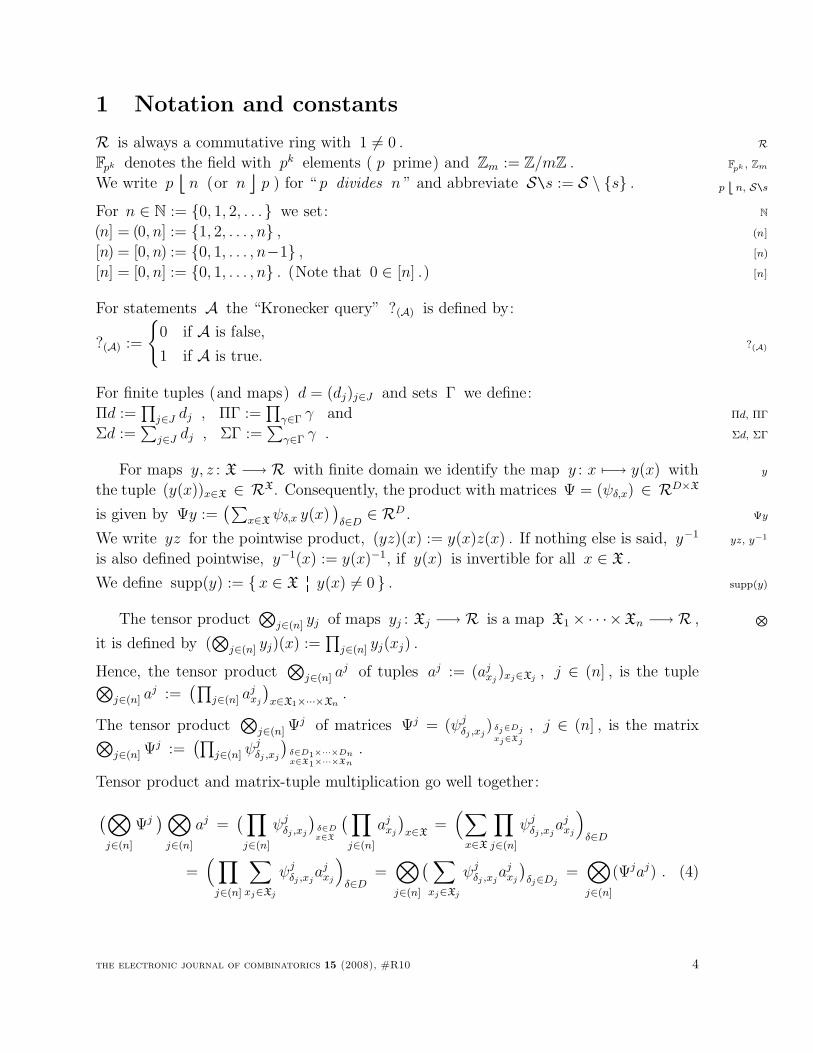
1 Notation and constants
R is always a commutative ring with 1 6= 0 . R
Fpk denotes the field with pk elements ( p prime) and Zm := Z/mZ . Fpk , Zm
We write p⌊⌊
n (or n⌋⌋
p ) for “ p divides n ” and abbreviate S\s := S \ {s} . p¨
n, S\s
For n ∈ N := {0, 1, 2, . . .} we set: N
(n] = (0, n] := {1, 2, . . . , n} , (n]
[n) = [0, n) := {0, 1, . . . , n−1} , [n)
[n] = [0, n] := {0, 1, . . . , n} . (Note that 0 ∈ [n] .) [n]
For statements A the “Kronecker query” ?(A) is defined by:
?(A) :=
{
0 if A is false,
1 if A is true.?(A)
For finite tuples (and maps) d = (dj)j∈J and sets Γ we define:
Πd :=∏
j∈J dj , ΠΓ :=∏
γ∈Γ γ and Πd, ΠΓ
Σd :=∑
j∈J dj , ΣΓ :=∑
γ∈Γ γ . Σd, ΣΓ
For maps y, z : X −→ R with finite domain we identify the map y : x 7−→ y(x) with y
the tuple (y(x))x∈X ∈ RX. Consequently, the product with matrices Ψ = (ψδ,x) ∈ R
D×X
is given by Ψy :=(∑
x∈Xψδ,x y(x)
)
δ∈D∈ RD . Ψy
We write yz for the pointwise product, (yz)(x) := y(x)z(x) . If nothing else is said, y−1yz, y−1
is also defined pointwise, y−1(x) := y(x)−1, if y(x) is invertible for all x ∈ X .
We define supp(y) := { x ∈ X�y(x) 6= 0 } . supp(y)
The tensor product⊗
j∈(n] yj of maps yj : Xj −→ R is a map X1× · · ·×Xn −→ R ,N
it is defined by (⊗
j∈(n] yj)(x) :=∏
j∈(n] yj(xj) .
Hence, the tensor product⊗
j∈(n] aj of tuples aj := (aj
xj)xj∈Xj
, j ∈ (n] , is the tuple⊗
j∈(n] aj :=
(∏
j∈(n] ajxj
)
x∈X1×···×Xn.
The tensor product⊗
j∈(n] Ψj of matrices Ψj = (ψj
δj ,xj) δj∈Dj
xj∈Xj
, j ∈ (n] , is the matrix⊗
j∈(n] Ψj :=
(∏
j∈(n] ψjδj ,xj
)
δ∈D1×···×Dnx∈X1×···×Xn
.
Tensor product and matrix-tuple multiplication go well together:
(
⊗
j∈(n]
Ψj)
⊗
j∈(n]
aj =(
∏
j∈(n]
ψjδj ,xj
)
δ∈Dx∈X
(
∏
j∈(n]
ajxj
)
x∈X=
(
∑
x∈X
∏
j∈(n]
ψjδj ,xj
ajxj
)
δ∈D
=(
∏
j∈(n]
∑
xj∈Xj
ψjδj ,xj
ajxj
)
δ∈D=
⊗
j∈(n]
(
∑
xj∈Xj
ψjδj ,xj
ajxj
)
δj∈Dj=
⊗
j∈(n]
(Ψjaj) . (4)
the electronic journal of combinatorics 15 (2008), #R10 4

In the whole paper we work over Cartesian products X := X1 × · · · × Xn of subsets
Xj ⊆ R of size dj + 1 := |Xj| <∞ . We define:
Definition 1.1 (d-grids X ).
X, [d]
d = d(X)
For all j ∈ (n] we define: In n dimensions we define:
Xj ⊆ R is always a finite set 6= ∅. X := X1 × · · · × Xn ⊆ Rn is a d-grid for
dj = dj(Xj) := |Xj| − 1 and d = d(X) := (d1, . . . , dn) .
[dj] := {0, 1, . . . , dj} . [d] := [d1]×· · ·× [dn] is a d-grid in Zn.
The following function N : X −→ R will be used throughout the whole paper. The
ψδ,x are the coefficients of the Lagrange polynomials LX,x , as we will see in Lemma1.3 .
We define:
Definition 1.2 (NX , ΨX , LX,x and ex ).
Let X := X1 × · · · × Xn ⊆ Rn be a d-grid, i.e., dj = |Xj| − 1 for all j ∈ (n] .
ex , LX,x
N, Ψ
For x ∈ Xj and δ ∈ [dj] we set: For x ∈ X and δ ∈ [d] we set:
ejx : Xj →R , ej
x(x) := ?(x=x) . ex :=⊗
j∈(n] ejxj
= (x 7→ ?(x=x) ) .
LXj\x(X) :=∏
x∈Xj\x(X − x) . LX,x(X1, . . . , Xn) :=
∏
j LXj\xj(Xj) .
Nj = NXj: Xj −→ R is defined by: N = NX : X −→ R is defined by:
Nj(x) := LXj\x(x) . N :=⊗
j∈(n]Nj =(
x 7→ LX,x(x))
.
Ψj := (ψjδ,x) δ∈[dj ]
x∈Xj
with
ψjδ,x :=
∑
Γ⊆Xj\x
|Γ|=dj−δ
Π(−Γ)
and in particular ψjdj ,x = 1 .
(5)
Ψ = (ψδ,x) δ∈[d]x∈X
:=⊗
j∈(n]
Ψj , i.e.,
ψδ,x :=∏
j∈(n]
ψjδj ,xj
and in particular ψd,x = 1 .
(6)
We use multiindex notation for polynomials, i.e., X (δ1,...,δn) := Xδ11 · · ·X
δnn and we X(δ1,...,δn)
define Pδ = (P )δ to be the coefficient of Xδ in the standard expansion of P ∈ R[X] := Pδ = (P )δ
R[X]R[X1, . . . , Xn] . That means P = P (X) =∑
δ∈Nn PδXδ and (Xε)δ = ?(δ=ε) .
the electronic journal of combinatorics 15 (2008), #R10 5

Conversely, for tuples P = (Pδ)δ∈D ∈ RD , we set P (X) :=
∑
δ∈D PδXδ . In this way P (X)
we identify the set of tuples R[d] = R[d1]×···×[dn] with R[X≤d] , the set of polynomials R[d]
R[X≤d]P =∑
δ≤d PδXδ with restricted partial degrees degj(P ) ≤ dj . It will be clear from the
context whether we view P as a tuple (Pδ) in R[d] , a map [d] −→ R or a polynomial
P (X) in R[X≤d] . P (X)|X stands for the map X −→ R , x 7−→ P (x) . P (X)|X
We have introduced the following four related or identified objects:
Maps: Tuples: Polynomials: Polynomial Maps:
δ 7→ Pδ , P = (Pδ) P (X) =∑
PδXδ P (X)|X : x 7→ P (x) ,
[d]→ R ∈ R[d] ∈ R[X≤d] X→ R (7)
With these definitions we get the following important formula:
Lemma 1.3 (Lagrange polynomials).
(Ψex)(X) :=∑
δ∈[d]
ψδ,xXδ =
∏
j∈(n]
∏
xj∈Xj\xj
(Xj − xj) =: LX,x .
Proof. We start with the one-dimensional case. Assume x ∈ Xj , then
(Ψjejx)(Xj) =(
∑
δ∈[dj ]
ψjδ,xX
δj
)
=∑
δ∈[dj ]
∑
Γ⊆Xj\x
|Γ|=dj−δ
Xδj Π(−Γ)
=∑
Γ⊆Xj\x
X|(Xj\x)\Γ|j Π(−Γ)
=∏
x∈Xj\x
(Xj − x) .
(8)
In n dimensions and for x ∈ X we conclude:
(Ψex)(X) =(
(
⊗
jΨj
)
⊗
jejxj
)
(X)
(4)=
(
⊗
j
(
Ψjejxj
)
)
(X)
=∏
j
(
(Ψjejxj)(Xj)
)
(8)=
∏
j∈(n]
∏
xj∈Xj\xj
(Xj − xj) .
(9)
We further provide the following specializations of the ubiquitous function N ∈ RX,
N(x) =∏
j∈(n]Nj(xj) :
the electronic journal of combinatorics 15 (2008), #R10 6

Lemma 1.4. Let El := { c ∈ R�cl = 1 } denote the set of the lth roots of unity in R .
For x ∈ Xj ⊆ R hold:
(i) If Xj = Edj+1 ( |Edj+1| = dj + 1 ) and
if R is an integral domain: Nj(x) = (dj + 1) x−1 .
(ii) If Xj ] {0} is a finite subfield of R : Nj(x) = −x−1 .
(iii) If Xj = Edj] {0} ( |Edj
| = dj ) and
if R is an integral domain: Nj(x) =
{
dj1 for x 6= 0 ,
−1 for x = 0 .
(iv) If Xj is a finite subfield of R : Nj(x) = −1 .
(v) If Xj = {0, 1, . . . , dj} ⊆ Z : Nj(x) = (−1)dj+x dj!(
dj
x
)−1.
(vi) For α ∈ R we have: NXj+α(x+ α) = NXj(x) .
Proof. For finite subsets D ⊆ R we define
LD(X) :=∏
x∈D(X − x) . (10)
It is well-known that, if El contains l elements and lies in an integral domain,
LEl(X) =
∏
x∈El
(X − x) = X l − 1 = (X − 1)(X l−1 + · · ·+X0) . (11)
Thus
LEl\1(1) =
∏
x∈El(X − x)
X − 1
∣
∣
X=1=
X l − 1
X − 1
∣
∣
X=1= X l−1 + · · ·+X0
∣
∣
X=1= l1 . (12)
Using this, we get for x ∈ El
LEl\x(x) = Lx(El\1)(x) =∏
x∈El\1
(x− xx) = xl−1LEl\1(1) = lx−1 . (13)
This gives (i) with l = |Xj| = dj + 1 .
Part (ii) is a special case of part (i), where Xj = Fpk\0 = Epk−1 and where conse-
quently dj + 1 = |Xj| = (pk − 1) ≡ −1 (mod p) .
To get Nj(x) = L{0}]El\x(x) with x 6= 0 in part (iii) and part (iv) we multiply
Equation (13) with x− 0 and use l = |Xj| − 1 = pk − 1 ≡ −1 (mod p) for part (iv) and
l = |Xj| − 1 = dj for part (iii). For x = 0 we obtain in part (iii) and part (iv)
Nj(0) = LEl(0) =
∏
x∈El
(−x) = −∏
x∈El\{1,−1}(−x) = −1 , (14)
the electronic journal of combinatorics 15 (2008), #R10 7
since each subset {x, x−1} ⊆ El\ {1,−1} contributes (−x) (−x−1) = 1 to the product
– as x 6= x−1, since x2− 1 = 0 holds only for x = ±1 – and El\ {1,−1} is partitioned
by such subsets. This completes the proofs of parts (iii) and (iv).
We now turn to part (v):
Nj(x) =(
∏
0≤x<x
(x− x))
∏
x<x≤dj
(x− x) = x! (dj − x)! (−1)dj−x = (−1)dj+x dj !
(
dj
x
)−1
. (15)
Part (vi) is trivial.
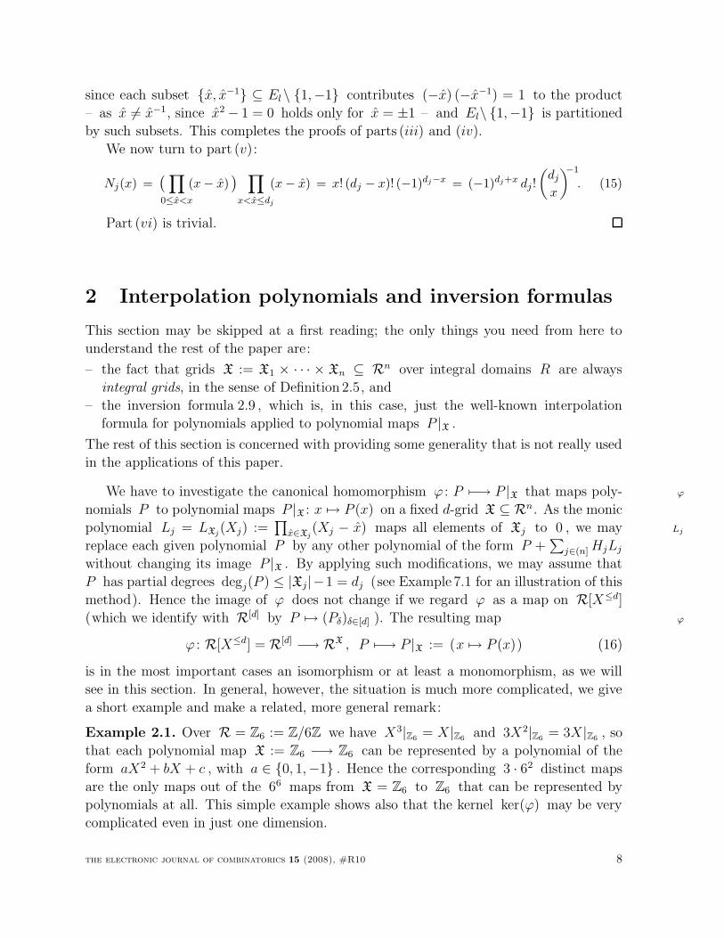
2 Interpolation polynomials and inversion formulas
This section may be skipped at a first reading; the only things you need from here to
understand the rest of the paper are:
– the fact that grids X := X1 × · · · × Xn ⊆ Rn over integral domains R are always
integral grids, in the sense of Definition 2.5, and
– the inversion formula 2.9 , which is, in this case, just the well-known interpolation
formula for polynomials applied to polynomial maps P |X .
The rest of this section is concerned with providing some generality that is not really used
in the applications of this paper.
We have to investigate the canonical homomorphism ϕ : P 7−→ P |X that maps poly- ϕ
nomials P to polynomial maps P |X : x 7→ P (x) on a fixed d-grid X ⊆ Rn. As the monic
polynomial Lj = LXj(Xj) :=
∏
x∈Xj(Xj − x) maps all elements of Xj to 0 , we may Lj
replace each given polynomial P by any other polynomial of the form P +∑
j∈(n]HjLj
without changing its image P |X . By applying such modifications, we may assume that
P has partial degrees degj(P ) ≤ |Xj|−1 = dj (see Example 7.1 for an illustration of this
method). Hence the image of ϕ does not change if we regard ϕ as a map on R[X≤d]
(which we identify with R[d] by P 7→ (Pδ)δ∈[d] ). The resulting map ϕ
ϕ : R[X≤d] = R[d] −→ RX , P 7−→ P |X := (x 7→ P (x)) (16)
is in the most important cases an isomorphism or at least a monomorphism, as we will
see in this section. In general, however, the situation is much more complicated, we give
a short example and make a related, more general remark:
Example 2.1. Over R = Z6 := Z/6Z we have X3|Z6 = X|Z6 and 3X2|Z6 = 3X|Z6 , so
that each polynomial map X := Z6 −→ Z6 can be represented by a polynomial of the
form aX2 + bX + c , with a ∈ {0, 1,−1} . Hence the corresponding 3 · 62 distinct maps
are the only maps out of the 66 maps from X = Z6 to Z6 that can be represented by
polynomials at all. This simple example shows also that the kernel ker(ϕ) may be very
complicated even in just one dimension.
the electronic journal of combinatorics 15 (2008), #R10 8

Remark 2.2. There are some general results for the rings R = Zm of integers mod m :
– In [MuSt] a system of polynomials in Zm[X1, . . . , Xn] is given that represent all poly-
nomial maps Zmn−→ Zm and the number of all such maps is determined.
– In [Sp] it is shown that the Newton algorithm can be used to determine interpolation
polynomials, if they exist. The “divided differences” in this algorithm are, like the
interpolation polynomials themselves, not uniquely determined over arbitrary commu-
tative rings, and exist if and only if interpolation polynomials exist.
But back to the main subject. In which situations does ϕ : P 7−→ P |X become an
isomorphism, or equivalently, when does its representing matrix Φ possess an inverse?
Over commutative rings R , square matrices Φ ∈ Rm×m with nonvanishing determinant
do not have an inverse, in general. However, there is the matrix Adj(Φ) – the adjoint or Adj(Φ)
cofactor matrix – that comes close to being an inverse:
Φ Adj(Φ) = Adj(Φ)Φ = det(Φ)1 . (17)
In our concrete situation, where Φ ∈ RX×[d] is the matrix of ϕ (a tensor product of Φ
Vandermonde matrices), we work with Ψ (from Definition 1.2) instead of the adjoint Ψ
matrix Adj(Φ) . Ψ comes closer than Adj(Φ) to being a right inverse of Φ . The
following theorem shows that
ΦΨ =(
N(x) ?(x=x)
)
x,x∈X, (18)
and the entries N(x) of this diagonal matrix divide the entries det(Φ) of Φ Adj(Φ) ,
so that ΦΨ is actually closer than Φ Adj(Φ) to the unity matrix (provided we identify
the column indices x ∈ X and row indices δ ∈ [d] in some way with the numbers
1, 2, . . . , |X| = |[d]| , in order to make det(Φ) and Adj(Φ) defined).
However, we used the matrix Φ ∈ RX×[d] of ϕ : P 7−→ P |X here just to explain the Φ, ϕ
role of Ψ . In what follows, we do not use it any more; rather, we prefer notations with
“ϕ ” or “ |X .” For maps/tuples y ∈ RX, we write (Ψy)(X) ∈ R[X≤d] , as already defined, (Ψy)(X)
for the polynomial whose coefficients form the tuple Ψy ∈ R[d], i.e., (Ψy)(X) = Ψy by
identification. We have:
Theorem 2.3 (Interpolation). For maps y : X −→ R ,
(Ψy)(X)|X = Ny .
Proof. As both sides of the equation are linear in y , it suffices to prove the equation for
the maps y = ex , where x ranges over X . Now we see that, at each point x ∈ X , we
actually have
(Ψex)(X)|X(x)1.3= LX,x(x) = N(x) ?(x=x) = (Nex)(x) . (19)
the electronic journal of combinatorics 15 (2008), #R10 9

With this theorem, we are able to characterize the situations in which ϕ : P 7−→ P |Xis an isomorphism:
Equivalence and Definition 2.4 (Division grids). We call a d-grid X ⊆ Rn a divi-
sion grid (over R ) if it has the following equivalent properties:
(i) For all j ∈ (n] and all x, x ∈ Xj with x 6= x the difference x− x is invertible.
(ii) N = NX is pointwise invertible, i.e., for all x ∈ X, N(x) is invertible.
(iii) ΠN is invertible.
(iv) ϕ : R[X≤d] = R[d] −→ RX is bijective.
Proof. The equivalence of (i),(ii) and (iii) follows from the Definition 1.2 of N , the defi-
nition ΠN =∏
x∈XN(x) and the associativity and commutativity of R .
Assuming (ii), it follows from Theorem2.3 that y 7−→ (Ψ(N−1y))(X) is a right inverse
of ϕ : P 7−→ P |X :y 7−→ (Ψ(N−1y))(X)
ϕ7−→ N(N−1y) = y . (20)
It is even a two-sided inverse, since square matrices Φ over a commutative ring R are
invertible from both sides if they are invertible at all (since Φ Adj(Φ) = det(Φ)1 ). This
gives (iv).
Now assume (iv) holds; then for all x ∈ X ,
(
ψδ,x
)
δ∈[d]= Ψex
2.3= ϕ−1(Nex) = N(x)ϕ−1(ex) , (21)
and in particular,1
(6)= ψd,x = N(x)
(
ϕ−1(ex))
d. (22)
Thus the N(x) are invertible and that is (ii).
If ϕ : R[X≤d] −→ RX is an isomorphism, then ϕ−1(y) is the unique polynomial in ϕ−1
R[X≤d] that interpolates a given map y ∈ RX, so that, by Theorem2.3 , it has to be the
polynomial Ψ(N−1y) ∈ R[d] = R[X≤d] . This yields the following result:
Theorem 2.5 (Interpolation formula). Let X be a division grid (e.g., if R is a field
or if X is the Boolean grid {0, 1}n ). For y ∈ RX,
ϕ−1(y) = Ψ(N−1y) .
This theorem can be found in [Da, Theorem2.5.2], but just for fields R and in a different
representation (with ϕ−1(y) as a determinant).
the electronic journal of combinatorics 15 (2008), #R10 10

Additionally, if X is not a division grid, we may apply the canonical localization
homomorphism π
S , RN
π : R −→ RN := S−1R , r 7−→ rπ := r1
with S := { (ΠN)m�m ∈ N } , (23)
and exert our theorems in this situation. As π and RN have the universal property with
respect to the invertibility of (ΠN)π in RN (as required in 2.4(iii)), π and RN are
the best choices. This means specifically that if (ΠN)π is not invertible in the codomain
RN of π , then no other homomorphism π′ has this property, either. In general, π does
not have this property itself: By definition,
r1s1
=r2s2
:⇐⇒ ∃ s ∈ S : s r1s2 = s r2s1 , (24)
and hence ker(π)
ker(π) = { r ∈ R�∃m ∈ N : (ΠN)m r = 0 } , (25)
so that (ΠN)π = 0 is possible. Localization works in the following situation:
Equivalence and Definition 2.6 (Affine grids). We call a d-grid X ⊆ Rn affine
(over R ) if it has the following equivalent properties:
(i) ΠN is not nilpotent.
(ii) π 6= 0 .
(iii) (ΠN)π is invertible in RN .
(iv) π 6= 0 is injective on the Xj
and hence induces a bijection X −→ Xπ := X1
π × · · · × Xnπ . Xπ
Proof. Part (ii) is equivalent to 1π 6= 0 , and this means that s1 6= 0 for all s in the
multiplicative system S = { (ΠN)m�m ∈ N } ; thus (i)⇐⇒ (ii) .
Of cause (ΠN)π 1ΠN
= 11
is the unity in RN , provided 11
= 1π 6= 0 ; thus (ii) =⇒ (iii) .
If (iii) holds then (ΠN)π and its factors (xj−xj)π do not vanish; thus (iii) =⇒ (iv) .
Finally, the implication (iv) =⇒ (ii) is trivial.
If X ⊆ Rn is affine, then Xπ := X1
π × · · · × Xnπ ⊆ RN
n is a division d-grid over Xπ
RN by 2.6 (iv), 2.6 (iii) and 2.4 (iii). Now, Theorem2.5 applied to y := P π|Xπ with P π
P π =∑
δ∈[d] PδπXδ yields
P π = ΨXπ
(
(NXπ)−1(P π|Xπ))
, (26)
along with the associated constants NXπ ∈ RNXπ
and ΨXπ ∈ R[d]×Xπ
N of Xπ.
the electronic journal of combinatorics 15 (2008), #R10 11
With componentwise application of π : r 7→ r1
to P |X, N ∈ RX and to Ψ ∈ R[d]×X
so that (P |X)π, Nπ ∈ RNX and Ψπ ∈ R
[d]×X
N , we obtain: Nπ , Ψπ
Theorem 2.7 (Inversion formula). Let X be affine (e.g., if R does not possess nilpo-
tent elements). For P ∈ R[X≤d] = R[d],
P π = Ψπ(
(Nπ)−1(P |X)π)
.
If π is injective on its whole domain R then R is a subring of RN and we may
omit π in formula 2.7 . In fact, we will see that this is precisely when ϕ is injective, as
seen in the following characterization:
Equivalence and Definition 2.8 (Integral grids). We call a d-grid X ⊆ Rn integral
(over R ) if it has the following, equivalent properties:
(i) For all j ∈ (n] and all x, x ∈ Xj with x 6= x, x− x is not a zero divisor.
(ii) For all x ∈ X, N(x) is not a zero divisor.
(iii) ΠN is not a zero divisor.
(iv) π is injective (R ⊆ RN ).
(v) ϕ : R[X≤d] = R[d] −→ RX is injective.
Proof. The equivalence of (i),(ii) and (iii) follows from the Definition 1.2 of N , the
definition ΠN =∏
x∈XN(x) and the associativity and commutativity of R .
As already mentioned ker(π) = { r ∈ R�∃m ∈ N : (ΠN)mr = 0 } , so (iii) =⇒ (iv) .
If (iv) holds, then ΠN is invertible in RN . By Equivalence 2.4 , it follows that
ϕ : RN [X≤d] −→ RNX is bijective, so that (iv) =⇒ (v) .
Now suppose that (ii) does not hold, so that there are a point x ∈ X and a constant
M ∈ R\0 withMN(x) = 0 . (27)
ThenP := Ψ(Mex) 6= 0 , (28)
asPd = M(Ψ(ex))d = Mψd,x
(6)= M 6= 0 . (29)
However,ϕ(P )
2.3= NMex = MN(x)ex ≡ 0 , (30)
so that (v) does not hold, either. Thus (v) =⇒ (ii) .
the electronic journal of combinatorics 15 (2008), #R10 12
Any integral grid X over R is, in fact, a division grid over RN ⊇ R , since ΠN
becomes invertible in RN . Formula 2.5 applied to y := P |X yields the following special-
ization of Theorem2.7:
Theorem 2.9 (Inversion formula). Let X be integral (e.g., if R is an integral do-
main). For P ∈ R[X≤d] = R[d],
P = Ψ(N−1P |X) .
From the case P = 1 , we see that N−1P |X inside this formula does not lie in RX
in general (of course N−1P |X ∈ RNX ). This also shows that, in general, the maps of the
form Ny , with y ∈ RX, in Theorem2.3 are not the only maps that can be represented
by polynomials over R , i.e., {Ny�y ∈ RX } Im(ϕ) . However, the maps of the form
Ny are exactly the linear combinations of Lagrange’s polynomial maps Nex = LX,x|Xover the grid X ; and if we view, a bit more generally, Lagrange polynomials L
X,x over
subgrids X = X1× · · · × Xn ⊆ X , then the maps of the form LX,x|X span Im(ϕ) , as one
can easily show.
On the other hand, in general, Im(ϕ) RX, so that not every map y ∈ RX can
be interpolated over R . If X is integral, then interpolation polynomials exist over
the bigger ring RN . The univariate polynomials(
Xk
)
:= X(X−1)···(X−k+1)k!
, for example,
describe integer-valued maps (on the whole domain Z ), but do not lie in Z[X] . More
information about such “overall” integer-valued polynomials over quotient fields can be
found, for example, in [CCF] and [CCS], and in the literature cited there.
The reader might find it interesting that the principle of inclusion and exclusion follows
from Theorem2.9 as a special case:
Proposition 2.10 (Principle of inclusion and exclusion).
Let X := {0, 1}n = [d] and x ∈ X ; then xδ = ?(δ≤x) for all δ ∈ [d] . Thus, for arbitrary
P = (Pδ) ∈ R[d] = R[X≤d] ,
P (x) =∑
δ≤xPδ . (31)
Formula 2.9 is the Mobius inversion to Equation (31):
Pδ2.9=
∑
x∈[d]
ψδ,xN−1(x)P (x)
1.2=
∑
x∈[d]
[∏
j∈(n]
?(xj≤δj) (−1)1−δj][
∏
j∈(n]
(−1)1−xj]
P (x)
=∑
x≤δ(−1)Σ(δ−x)P (x) .
(32)
the electronic journal of combinatorics 15 (2008), #R10 13

3 Coefficient formulas – the main results
The applications in this paper do not start with a map y ∈ RX that has to be interpolated
by a polynomial P . Rather, we start with a polynomial P , or with some information
about a polynomial P ∈ R[X] , which describes the very map y := P |X that we would
like to understand. Normally, we will not have complete information about P , so that
we do not usually know all coefficients Pδ of P . However, there may be a coefficient Pδ
in P =∑
δ∈Nn PδXδ that, on its own, allows conclusions about the map P |X . We define
(see also figure 1 below):
Definition 3.1. Let P =∑
δ∈Nn PδXδ ∈ R[X] be a polynomial. We call a multiindex
ε ≤ d ∈ Nn d-leading in P if for each monomial Xδ in P , i.e., each δ with Pδ 6= 0 ,
holds either
– (case 1) δ = ε ; or
– (case 2) there is a j ∈ (n] such that δj 6= εj but δj ≤ dj .
Note that the multiindex d is d-leading in polynomials P with deg(P ) ≤ Σd . In
this situation, case 2 reduces to “there is a j ∈ (n] such that δj < dj ,” and, as Σδ ≤ Σd
for all Xδ in P , we can conclude:
“not case 2” =⇒ δ ≥ d =⇒ δ = d =⇒ “case 1” . (33)
Thus d really is d-leading in P (see also figure 2 on page 28). Of course, if all partial
degrees are restricted by degj(P ) ≤ dj then all multiindices δ ≤ d are d-leading. Figure 1
(below) shows a nontrivial example P ∈ R[X1, X2] . The monomials Xδ of P ( Pδ 6= 0 ),
and the 2n− 1 = 3 “forbidden areas” of each of the two d-leading multiindices, are
marked.
In what follows, we examine how the preconditions of the inversion formula 2.9 may be
weakened. It turns out that formula 2.9 holds without further degree restrictions for the
d-leading coefficients Pε of P . The following theorem is a generalization and a sharpening
of Alon and Tarsi’s (second) Combinatorial Nullstellensatz [Al2, Theorem1.2]:
Theorem 3.2 (Coefficient formula). Let X be an integral d-grid. For each polynomial
P =∑
δ∈Nn PδXδ ∈ R[X] with d-leading multiindex ε ≤ d ∈ Nn,
(i) Pε = (Ψ(N−1P |X))ε ( =∑
x∈Xψε,xN(x)−1P (x) ), and
(ii) Pε 6= 0 =⇒ P |X 6≡ 0 .
the electronic journal of combinatorics 15 (2008), #R10 14

Figure 1: Monomials of a polynomial P with
(4, 2)-leading multiindices (0, 1) and (2, 1) .
deg2
4
3
2
1
0
deg16543210
Proof. In our first proof we use the tensor product property (4) and the linearity of the
map P 7→ (Ψ(N−1P |X))ε to reduce the problem to the one-dimensional case. The one-
dimensional case is covered by the inversion formula 2.9 . Another proof, following Alon
and Tarsi’s polynomial method, is described in Section 7.
Since both sides of the Equation (i) are linear in the argument P it suffices to prove
(Xδ)ε = (Ψ(N−1Xδ|X))ε in the two cases of Definition 3.1 . In each case,
(
Ψ(N−1Xδ |X))
ε=
(
Ψ(
(
⊗
jN−1
j
)
⊗
j(X
δj
j |Xj))
)
ε
=
(
(
⊗
jΨj
)
⊗
j(N−1
j Xδj
j |Xj)
)
ε
(4)=
(
⊗
j
(
Ψj(N−1j X
δj
j |Xj))
)
ε
=∏
j∈(n]
(
Ψj(N−1j X
δj
j |Xj))
εj
.
(34)
Using the one-dimensional case of the inversion formula 2.9 we also derive(
Ψj(N−1j X
δj
j |Xj))
εj= (X
δj
j )εj= ?(δj=εj) for all j ∈ (n] with δj ≤ dj . (35)
Thus in case 1 ( ∀ j ∈ (n] : δj = εj ≤ dj ) ,(
Ψ(N−1Xδ|X))
ε= 1 = (Xδ)ε . (36)
And in case 2 ( ∃ j ∈ (n] : εj 6= δj ≤ dj ) ,(
Ψ(N−1Xδ|X))
ε= 0 = (Xδ)ε . (37)
Note that the one-dimensional case of Theorem3.2 (ii) is nothing more then the well-
known fact that polynomials P (X1) 6= 0 of degree at most d1 have at most d1 roots.
With the remark after Definition 3.1, and the knowledge that ψd,x(6)= 1 for all x ∈ X ,
we get our main result as an immediate consequence of Theorem3.2:
the electronic journal of combinatorics 15 (2008), #R10 15

Theorem 3.3 (Coefficient formula). Let X be an integral d-grid. For each polynomial
P =∑
δ∈Nn PδXδ ∈ R[X] of total degree deg(P ) ≤ Σd ,
(i) Pd = Σ(N−1P |X) ( =∑
x∈XN(x)−1P (x) ), and
(ii) Pd 6= 0 =⇒ P |X 6≡ 0 .
This main theorem looks simpler then the more general Theorem3.2, and you do not
have to know the concept of d-leading multiindices to understand it. Furthermore, the
applications in this paper do not really make use of the generality in Theorem3.2 . How-
ever, we tried to provide as much generality as possible, and it is of course interesting to
understand the role of the degree restriction in Theorem3.3 .
The most important part of this results, the implication in Theorem3.3 (ii), which
is known as Combinatorial Nullstellensatz was already proven in [Al2, Theorem1.2], for
integral domains. Note that Pd = 0 whenever deg(P ) < Σd , so that the implication
seems to become useless in this situation. However, one may modify P , or use smaller
sets Xj (and hence smaller dj ), and apply the implication then. So, if Pδ 6= 0 for a
δ ≤ d with Σδ = deg(P ) then it still follows that P |X 6≡ 0 . De facto, such δ are
d-leading.
If, on the other hand, deg(P ) = Σd , then Pd is, in general, the only coefficient that
allows conclusions on P |X as in Theorem3.3 (ii). This follows from the modification
methods of Section 7 . More precisely, if we do not have further information about the
d-grid X , then the d-leading coefficients are the only coefficients that allow such conclu-
sions. For special grids X , however, there may be some other coefficients Pδ with this
property, e.g., P0 in the case 0 = (0, . . . , 0) ∈ X .
Note further that for special grids X , the degree restriction in Theorem3.3 may be
weakened slightly. If, for example, X = Fqn , then the restriction deg(P ) ≤ Σd + q − 2
suffices; see the footnote on page 28 for an explanation.
The following corollary is a consequence of the simple fact that vanishing sums – the
case Pd = 0 in Theorem3.3 (i) – do not have exactly one nonvanishing summand. It is
very useful if a problem possesses exactly one trivial solution: if we are able to describe
the problem by a polynomial of low degree, we just have to check the degree, and Corol-
lary 3.4 guarantees a second (in this case, nontrivial) solution. There are many elegant
applications of this; for some examples see Section 4 . We will work out a general working
frame in Section 6 . We have:
Corollary 3.4. Let X be an integral d-grid. For polynomials P of degree deg(P ) < Σd
(or, more generally, for polynomials with vanishing d-leading coefficient Pd = 0 ),
∣
∣{ x ∈ X�P (x) 6= 0 }
∣
∣ 6= 1 .
the electronic journal of combinatorics 15 (2008), #R10 16

If the grid X has a special structure – for example, if X ⊆ R>0n
– this corollary may also
hold for polynomials P with vanishing d-leading coefficient Pε = 0 for some ε 6= d . The
simple idea for the proof of this, which uses Theorem3.2 instead of Theorem3.3, leads to
the modified conclusion that
∣
∣{ x ∈ X�ψε,xP (x) 6= 0 }
∣
∣ 6= 1 . (38)
Note further that the one-dimensional case of Corollary 3.4 is just a reformulation of the
well-known fact that polynomials P (X1) of degree less than d1 do not have d1 = |X1|−1
roots, except if P = 0 .
The example P = 2X1 + 2 ∈ Z4[X1] , X = {0, 1,−1} shows that Corollary 3.4 does
not hold over arbitrary grids. However, if X = Zmn =: Rn with m not prime, the grid
X is not integral; yet assertion 3.4 holds anyway. Astonishingly, in this case the degree
condition can be dropped, too. We will see this in Corollary 8.2 .
We also present another proof of Corollary 3.4 that uses only the weaker part (ii)
of Theorem3.2 , to demonstrate that the well-known Combinatorial Nullstellensatz, our
Theorem3.3 (ii), would suffice for the proof of the main part of the corollary:
Proof. Suppose P has exactly one nonzero x0 ∈ X . Then
Q := P − P (x0)N−1(x0)LX,x0 ∈ R[X] (39)
vanishes on the whole grid X , but possesses the nonvanishing and d-leading coefficient
Qd = −P (x0)N−1(x0) 6= 0 , (40)
in contradiction to Theorem3.2 (ii).
A further useful corollary, and a version of Chevalley and Warning’s classical result
– Theorem4.3 in this paper – is the following result (see also [Scha2] for a sharpening of
Warning’s Theorem, and Theorem8.4 for a similar result over Zpk ):
Corollary 3.5. Let X ⊆ Fpkn be a d-grid and P1, . . . , Pm ∈ Fpk [X1, . . . , Xn] .
If (pk − 1)∑
i∈(m] deg(Pi) < Σd , then
∣
∣
{
x ∈ X�P1(x) = · · · = Pm(x) = 0
}∣
∣ 6= 1 .
Proof. Define
P :=∏
i∈(m]
(1− P pk−1i ) ; (41)
then for points x = (x1, . . . , xn) ,
P (x) 6= 0 ⇐⇒ ∀ i ∈ (m] : Pi(x) = 0 , (42)
the electronic journal of combinatorics 15 (2008), #R10 17
and hence∣
∣
{
x ∈ X � P1(x) = · · · = Pm(x) = 0}∣
∣ =∣
∣
{
x ∈ X � P (x) 6= 0}∣
∣
3.46= 1 , (43)
sincedeg(P ) ≤
∑
i∈(m]
(pk − 1) deg(Pi) < Σd . (44)
4 First applications and the application principles
In this section we present some short and elegant examples of how our theorems may
be applied. They are all well-known, but we wanted to have some examples to demon-
strate the flexibility of these methods. This flexibility will also be emphasized through the
general working frame described in Section 6, for which the applications of this section
may serve as examples. Alon used them already in [Al2] to demonstrate the usage of
implication 3.3 (ii) ; whereas we prove them by application of Theorem3.3 (i), and corol-
laries 3.4 and 3.5, an approach which is – in most cases – more straightforward and more
elegant. The main advantage of the coefficient formula 3.3 (i) can be seen in the proof
of Theorem4.3 , where the implication 3.3 (ii) does not suffice to give a proof of the full
theorem. Section 5 will contain another application that puts the new quantitative aspect
of coefficient formula 3.3 into the spotlight.
Our first example was originally proven in [AFK]:
Theorem 4.1. Every loopless 4-regular multigraph plus one edge G = (V,E ] {e0})
contains a nontrivial 3-regular subgraph.
See [AFK2] and [MoZi] for further similar results. The additional edge e0 in our
version is necessary as the example of a triangle with doubled edges shows.
We give a comprehensive proof in order to outline the principles:
Proof. Of course, the empty graph (∅,∅) is a (trivial) 3-regular subgraph. So there
is one “solution,” and we just have to show that there is not exactly one “solution.”
This is where Corollary 3.5 comes in. Systems of polynomials of low degree do not have
exactly one common zero. Thus, if the 3-regular subgraphs correspond to the common
zeros of such a system of polynomials we know that there has to be a second (nontrivial)
“solution.”
The subgraphs without isolated vertices can be identified with the subsets S of the
set of all edges E := E ] {e0} . Now, an edge e ∈ E may or may not lie in a subgraph
S ⊆ E . We represent these two possibilities by the numbers 1 and 0 in Xe := {0, 1}
(the first step in the algebraization), we define
χ(S) :=(
?(e∈S)
)
e∈E∈ X := {0, 1}E ⊆ FE
3 . (45)
the electronic journal of combinatorics 15 (2008), #R10 18

With this representation, the subgraphs S correspond to the points x = (xe) of the
Boolean grid X := {0, 1}E ⊆ FE3 ; and it is easy to see that the polynomials
Pv :=∑
e3v
Xe ∈ F3[Xe � e∈ E ] for all v ∈ V (46)
do the job, i.e., they have sufficient low degrees and the common zeros x ∈ X correspond
to the 3-regular subgraphs. To see this, we have to check for each vertex v ∈ V the
number∣
∣{ e 3 v�xe = 1 }
∣
∣ ≤ 5 of edges e connected to v that are “selected” by a
common zero x ∈ X = {0, 1}E :
Pv(x) = 0 ⇐⇒∑
e3v
xe = 0 ⇐⇒∣
∣{ e 3 v � xe = 1 }∣
∣ ∈ {0, 3} . (47)
Furthermore, we have to check the degree condition of Corollary 3.5, and that is where
we need the additional edge e0 :
(31 − 1)∑
v∈V
deg(Pv) = 2|V | = |E| < |E| = Σd(X) . (48)
By Corollary 3.5, the trivial graph ∅ ⊆ E ( x = 0 ) cannot be the only 3-regular subgraph.
The following simple, geometric result was proven by Alon and Furedi in [AlFu], and
answers a question by Komjath. Our proof uses Corollary 3.4:
Theorem 4.2. Let H1, H2, . . . , Hm be affine hyperplanes in Fn ( F a field) that cover
all vertices of the unit cube X := {0, 1}n except one, then m ≥ n .
Proof. Let∑
j∈(n] ai,jXj = bi be an equation defining Hi , and set
P :=∏
i∈(m]
∑
j∈(n]
(ai,jXj − bi) ∈ F[X1, . . . , Xn] ; (49)
then for points x = (x1, . . . , xn) ;
P (x) 6= 0 ⇐⇒(
∀ i ∈ (m] :∑
j∈(n]
ai,jxj 6= bi)
⇐⇒ x /∈⋃
j∈(m]
Hj . (50)
If we now suppose m < n , then it follows that
deg(P ) ≤ m < n = Σd(X) , (51)
and hence,∣
∣X \⋃
j∈(m]Hj
∣
∣ =∣
∣{x ∈ X � P (x) 6= 0 }∣
∣
3.46= 1 . (52)
This means that there is not one unique uncovered point x in X = {0, 1}n – m < n
hyperplanes are not enough to achieve that.
the electronic journal of combinatorics 15 (2008), #R10 19

Our next example is a classical result of Chevalley and Warning that goes back to
a conjecture of Dickson and Artin. There are a lot of different sharpenings to it; see
[MSCK], [Scha2], Corollary 3.5 and Theorem8.4 . In the proof of the classical version,
presented below, we do not use the Boolean grid {0, 1}n, as in the last two examples.
We also have to use Theorem3.3 (i) instead of its corollaries. What remains the same as
in the proof of the closely related Corollary 3.5 is that we have to translate a system of
equations into a single inequality:
Theorem 4.3. Let p be a prime and P1, P2, . . . , Pm ∈ Fpk [X1, . . . , Xn] .
If∑
i∈(m] deg(Pi) < n , then
p⌊⌊
∣
∣{ x ∈ Fpkn �
P1(x) = · · · = Pm(x) = 0 }∣
∣ ,
and hence the Pi do not have one unique common zero x .
Proof. Define
P :=∏
i∈(m]
(1− P pk−1i ) ; (53)
then
P (x) =
{
1 if P1(x) = · · · = Pm(x) = 0 ,
0 otherwisefor all x ∈ Fpk
n , (54)
thus, with X := Fpkn ,
∣
∣
{
x ∈ Fpkn � P1(x) = · · · = Pm(x) = 0
}∣
∣ · 1 =∑
x∈X
P (x)
3.31.4= (−1)n (P )d(X)
(56)= 0 , (55)
where the last two equalities hold as
deg(P ) ≤ (pk − 1)∑
i∈(m]
deg(Pi) < (pk − 1)n = Σd(X) . (56)
The Cauchy-Davenport Theorem is another classical result. It was first proven by
Cauchy in 1813, and has many applications in additive number theory. The proof of
this result is as simple as the last ones, but here we use the coefficient formula 3.3 (i) in
the other direction – we know the polynomial map P |X , and use it to determine the
coefficient Pd :
Theorem 4.4. If p is a prime, and A and B are two nonempty subsets of Zp := Z/pZ ,
then
|A+B| ≥ min{ p , |A|+ |B| − 1 } .
the electronic journal of combinatorics 15 (2008), #R10 20

Proof. We assume |A+B| ≤ |A|+ |B| − 2 , and must prove |A+B| ≥ p .
DefineP :=
∏
c∈A+B
(X1 +X2 − c) ∈ Zp[X1, X2] , (57)
setX1 := A , (58)
and choose a subset∅ 6= X2 ⊆ B (59)
of size|X2| = |A+B| − |A|+ 2 ( ≤ |B| ) . (60)
NowP |X1×X2 ≡ 0 , (61)
anddeg(P ) = |A+B| = |X1|+ |X2| − 2 = d1(X1) + d2(X2) , (62)
so that(|A+B|
d1
)
· 1 = P(d1 ,|A+B|−d1) = Pd3.3=
∑
x∈X1×X2
0 = 0 ∈ Zp . (63)
Hencep
⌊⌊(|A+B|
d1
)
, (64)
and it follows that|A+B| ≥ p . (65)
There are some further number-theoretic applications, for example, Erdos, Ginzburg
and Ziv’s Theorem, which also can be found in [Al2].
5 The matrix polynomial – another application
In this section we apply our results to the matrix polynomial Π(AX) , a generalization
of the graph polynomial (see also [AlTa2] or [Ya]).
We always assume A = (ai,j) ∈ Rm×n, and the product of this matrix with the tuple A, X
X := (X1, . . . , Xn) ∈ R[X]n is AX := (∑
j∈(n] aijXj)i∈(m] . Now, Π(AX) is defined in AX
accordance with the definition of Π in Section 1, as follows:
Definition 5.1 (Matrix polynomial). The matrix polynomial of A = (ai,j) ∈ Rm×n
is given by Π(AX)
Π(AX) :=∏
i∈(m]
∑
j∈(n]
aijXj ∈ R[X] .
the electronic journal of combinatorics 15 (2008), #R10 21

It turns out that the coefficients of the matrix polynomial are some kind of permanents:
Definition 5.2 (δ-permanent). For δ ∈ Nn we define the δ-permanent of A = (ai,j) ∈
Rm×n through perδ(A)
perδ(A) :=∑
σ : (m]→(n]
|σ−1|=δ
πA(σ) ,
where πA(σ)
|σ−1|πA(σ) :=∏
i∈(m]
ai,σ(i) and |σ−1| :=(
|σ−1(j)|)
j∈(n].
Obviously, perδ(A) = 0 if Σδ 6= m . If m = n then per := per(1,1,...,1) is the usual per
permanent; and, if Σδ = m , it is easy to see that
(∏
j∈(n] δj!)
perδ(A) = per(A〈|δ〉), (66)
where A〈|δ〉 is a matrix that contains the jth column of A exactly δj times. But A〈|δ〉
note that perδ(A) is, in general, not determined by per(A〈|δ〉) . If, for example,
(∏
j∈(n] δj!) 1 = 0 in R , the δ-permanent perδ(A) may take arbitrary values, while
per(A〈|δ〉) = 0 .
As an immediate consequence of the definitions, we have
Lemma 5.3.
Π(AX) =∑
δ∈Nnperδ(A)Xδ .
The next theorem now easily follows from our main result, Theorem3.3 . It is an
integrative generalization of Alon’s Permanent Lemma [Al2, Section 8], and of Ryser’s
permanent formula [BrRy, p.200], which follow as the special cases:
– m = n , d = (1, 1, . . . , 1) of the following 5.4 (ii) over fields,
– m = n , d = (1, 1, . . . , 1) , X = {0, 1}n , b = (0, 0, . . . , 0) of 5.4 (i) over fields.
We already proved a slightly weaker version for X ⊆ Nn ⊆ Rn in [Scha, 1.14 & 1.15].
This proof was based on Ryser’s formula, and is a little more technical. [Scha, 1.10] is the
special case X = [d] ⊆ Nn ⊆ Rn, but you will have to use 1.4 (v) to see this. For some
additional tricks over fields of characteristic p > 0 , see [DeV]. We have:
Theorem 5.4 (Permanent formula). Suppose A = (aij) ∈ Rm×n and b = (bi) ∈ R
mA
are given, and let X ⊆ Rn be an integral d-grid. If m ≤ Σd , then
(i) perd(A) =∑
x∈XN(x)−1 Π(Ax− b) , and
(ii) perd(A) 6= 0 =⇒ ∃ x ∈ X : (Ax)1 6= b1 , . . . , (Ax)m 6= bm .
the electronic journal of combinatorics 15 (2008), #R10 22
Proof. Part (i) follows from Theorem3.3, as deg(
Π(AX − b))
= m ≤ Σd , and since(
Π(AX− b))
d=
(
Π(AX))
d
5.3= perd(A) . Part (ii) is a simple consequence of part (i).
We call an element x ∈ Rm with (Ax)1 6= 0 , . . . , (Ax)m 6= 0 a (correct) coloring
of A , and a map σ : (m] −→ (n] with πA(σ) 6= 0 and |σ−1| = δ is a δ-orientation of σ
A . With this terminology, Theorem5.4 describes a connection between the orientations
and the colorings of A , and it is not too difficult to see that this is a sharpening and
a generalization of Alon and Tarsi’s Theorem about colorings and orientations of graphs
in [AlTa]. That is because, in virtue of the embedding�����
G 7−→ A(�����
G) described in (67)
below, oriented graphs form a subset of the set of matrices, if −1 6= 1 in R . The resulting
sharpening 5.5 of the Alon-Tarsi Theorem contains Scheim’s formula for the number of
edge r-colorings of a planar r-regular graph as a permanent and Ellingham and Goddyn’s
partial solution of the list coloring conjecture. We briefly elaborate on this; for even more
detail, see [Scha], where we described this for grids X ⊆ Nn ⊆ Rn, and where we pointed
out that many other graph-theoretic theorems may be formulated for matrices, too.
Let�����
G = (V,E,�����,�����) be a oriented multigraph with vertex set V , edge set E and �����
G, e�����
defining orientations ����� : E −→ V , e 7−→ e����� and ����� : e 7−→ e�����.�����
G shall be loopless, so ��, ��
that e����� 6= e����� for all e ∈ E . We write v ∈ e instead of v ∈ {e�����, e�����} and define the v ∈ e
incidence matrix A(�����
G) of�����
G by A(�����
G)
A(�����
G) := (ae,v) ∈ RE×V, where ae,v := ?(e�����=v) − ?(e�����=v) ∈ {−1, 0, 1} . (67)
With this definition, the orientations σ : E 3 e 7−→ eσ ∈ e and the colorings x : V −→ R
of�����
G are exactly the orientations and the colorings of A(�����
G) as defined above. The
orientations σ of A(�����
G) have the special property πA(�����
G)(σ) = ±1 . According to this, we
say that an orientation σ of�����
G is even/odd if eσ 6= e����� ( i.e., eσ = e����� ) holds for even/odd
many edges e ∈ E . We write DEδ /DOδ for the set of even/odd orientations σ of�����
G DEδ
DOδwith |σ−1| = δ ∈ NV . With this notation we have:
Corollary 5.5. Let�����
G = (V,E,�����,�����) be a loopless, directed multigraph and X ⊆ RV be
an integral d-grid; where d = (dv) ∈ NV, and dv = |Xv| − 1 for all v ∈ V .
If |E| ≤ Σd , then
(i) |DEd| − |DOd| = perd(A(�����
G)) =∑
x∈XN(x)−1∏
e∈E
(
xe����� − xe�����)
,
(ii) |DEd| 6= |DOd| =⇒ ∃ x ∈ X : ∀ e ∈ E : xe����� 6= xe����� ( x is a coloring).
Furthermore, it is not so hard to see that, if EE /EO is the set of even/odd Eulerian EE, EO
subgraphs of�����
G , and δ := |�����−1| , we have |DEδ| = |EE| and |DOδ| = |EO| ; see also
[Scha, 2.6].
Note that even though Corollary 5.5 looks a little simpler than [Scha, 1.14 & 2.4], there
is some complexity hidden in the symbol N(x) . If the “lists” Xv ( X =∏
v∈V Xv ) are all
the electronic journal of combinatorics 15 (2008), #R10 23
equal, this becomes less complex. Further, if the graph�����
G is the line graph of a r-regular
graph, so that its vertex colorings are the edge colorings of the r-regular graph, then
the whole right side becomes very simple. The summands are then – up to a constant
factor – equal to ±1 ; or to 0 , if x = (xv)v∈V is not a correct coloring. The corresponding
specialization of equation 5.5 (i) was already obtained in [ElGo] and [Sch].
If in addition�����
G is planar this formula becomes even simpler, so that the whole
right side is – up to a constant factor – the number of edge r-colorings of the r-regular
graph. Scheim [Sch] proved this specialization in his approach to the four color problem for
3-regular graphs using a result of Vigneron [Vig]. However, with Ellingham and Goddyn’s
generalization [ElGo, Theorem3.1] of Vigneron’s result, this specialization also follows in
the r-regular case.
As the left side of our equation does not depend on the choice of the d-grid X , the
right side does not depend on it, either. In our special case, where the right side is the
number of r-colorings of the line graph of a planar r-regular graph, this means that if there
are colorings to equal lists Xv of size r (e.g., X = [r)V ), then there are also colorings to
arbitrary lists Xv of size |Xv| = r – which is just Ellingham and Goddyn’s confirmation
of the list coloring conjecture for planar r-regular edge r-colorable multigraphs [ElGo].
6 Algebraically solvable existence problems:
Describing polynomials as equivalent to explicit
solutions
In this section we describe a general working frame to Theorem3.3 (ii) and Corollary 3.4,
as it may be used in existence proofs, such as those of 3.5, 4.2 or 5.4 (ii) . We call the
polynomials defined in the equations (41) and (49) or the matrix polynomial Π(AX) in
our last example, algebraic solutions, and show that such algebraic solutions may be seen
as equivalent to explicit solutions. We show that the existence of algebraic solutions, and of
nontrivial explicit solutions are equivalent. To make this more exact, we have to introduce
some definitions. Our definition of problems should not merely reflect common usage.
In fact, the generality gained through an exaggerated extension of the term “problem”
through abstraction is desirable.
Definition 6.1 (Problem). A problem P is a pair (S,Striv) consisting of a set S , P(S,Striv)which we call its set of solutions; and a subset Striv ⊆ S , which we call its set of trivial
solutions.
In example 4.1, the set of solutions S consists of the 3-regular subgraphs and Striv =
{(∅,∅)} . These are exact definitions, but it does not mean that we know if there are
nontrivial solutions, i.e., if S 6= Striv . The set S is well defined, but we do not know
what it looks like; indeed, that is the actual problem.
the electronic journal of combinatorics 15 (2008), #R10 24
To apply our theory about polynomials in such general situations, we have to bring in
grids X in some way. For that, we define impressions:
Definition 6.2 (Impression). A triple (R,X, χ) is an impression of P if R is a (R, X, χ)
commutative ring with 1 6= 0 , if X = X1 × · · · × Xn ⊆ Rn is a finite integral grid (for
some n ∈ N ) and if χ : S −→ X is a map.
As the set S of solutions is usually unknown, one may ask how the map χ : S −→ X
can be defined. The answer is that we usually, define χ on a bigger domain at first, as
in Equation (45) in example 4.1 . Then the unknown set of solutions S (more precisely,
its image χ(S) ) is indirectly described:
Definition 6.3 (Describing polynomial). A polynomial P ∈ R[X1, . . . , Xn] is a de-
scribing polynomial of P over (R,X, χ) if
χ(S) = supp(P |X) .
The diagram (2) in the introduction shows a schematic illustration of our concept in the
case Striv = ∅ . The next question is how it might be possible to reveal the existence of
nontrivial solutions using some knowledge about a describing polynomial P , and how to
find such an appropriate P . In view of our results from Section 3, we give the following
definition:
Definition 6.4 (Algebraic solutions). A describing polynomial P is an algebraic so-
lution (over (R,X, χ) ) of a problem of the form P = (S,∅) if it fulfills
deg(P ) ≤ Σd(X) and Pd(X) 6= 0 .
It is an algebraic solution of a problem P = (S,Striv) with Striv 6= ∅ if it fulfills
deg(P ) < Σd(X) and∑
x∈χ(Striv)
N(x)−1P (x) 6= 0 (e.g., if |χ(Striv)| = 1 ).
The bad news is that now, we do not have a general recipe for finding algebraic
solutions that indicate the solvability of problems. However, we have seen that there are
several combinatorial problems that are algebraically solvable in an obvious way. The
construction of algebraic solutions in these examples follows more or less the same simple
pattern, and that constructive approach is the big advantage. Algebraic solutions are easy
to construct if the problem is not too complex in the sense that the construction does not
require too many multiplications. In many cases algebraic solutions can be formulated
for whole classes of problems, e.g., for all extended 4-regular graphs in example 4.1, where
the final algebraic solution was hidden in Corollary 3.5. In these cases a maybe infinite
number of algebraic solutions fit into one single general form, which can be presented on a
finite blackboard or sheet of paper. The concept of algebraic solutions provides a method
of resolution to what we call the “finite blackboard problem”, a fundamental problem
whenever we view general situations with infinitely many concrete instances.
the electronic journal of combinatorics 15 (2008), #R10 25
If an algebraic solution is found, we can apply Theorem3.3 , Corollary 3.4 or the fol-
lowing theorem, which also shows that algebraic solutions always exist, provided there
are nontrivial solutions in the first place.
Theorem 6.5. Let P = (S,Striv) be a problem. The following properties are equivalent:
(i) There exists a nontrivial solution of P ; i.e., S 6= Striv .
(ii) There exists an algebraic solution of P over an impression (R,X, χ) .
(iii) There exist algebraic solutions of P over each impression (R,X, χ) that fulfills
either
– |R| > 2 and S 6= Striv ⇒ χ(S) 6= χ(Striv)
(e.g., if χ is injective or if Striv = ∅ ); or
– |R| = 2 and |χ(S)|+ 1 ≡ |χ(Striv)| ≡ ?(Striv 6=∅) (mod 2) .
Proof. First, assume (ii), and let P be an algebraic solution. We want to show that (i)
holds. For Striv = ∅ , this follows from Theorem3.3 (ii). For Striv 6= ∅ , we have
0 = Pd3.3= Σ(N−1P |X) =
∑
x∈χ(Striv)
N(x)−1P (x) +∑
x∈χ(S)\χ(Striv)
N(x)−1P (x) , (68)
where the first sum over χ(Striv) does not vanish. Hence, the second sum over the set
χ(S) \χ(Striv) does not vanish, either. Thus χ(S) \χ(Striv) 6= ∅ , and S 6= Striv follows.
To prove (i) =⇒ (iii) for Striv = ∅ , assume (i), and define a map y : X −→ R such
that supp(y) = χ(S) and Σy 6= 0 . (In the case |R| = 2 , we need |χ(S)| ≡ 1 (mod 2)
to make this possible.) The interpolation polynomial P := (Ψy)(X) to the map Ny
described in Theorem2.3 now has degree deg(P ) ≤ Σd , and fulfills
supp(P |X)2.3= supp(y) = χ(S) (69)
andPd
3.3= Σ(N−1P |X)
2.3= Σy 6= 0 . (70)
To prove (i) =⇒ (iii) for Striv 6= ∅ , assume (i), and define a map y : X −→ R such
that supp(y) = χ(S) ,∑
x∈χ(Striv) y(x) 6= 0 and Σy = 0 . (In the case |R| = 2 , we
need |χ(S)| + 1 ≡ |χ(Striv)| ≡ 1 (mod 2) to make this possible.) Now, the polynomial
P := (Ψy)(X) has partial degrees degj(P ) ≤ dj , and total degree deg(P ) < Σd , as
Pd3.3= Σ(N−1P |X)
2.3= Σy = 0 . (71)
It satisfiessupp(P |X)
2.3= supp(y) = χ(S) (72)
and∑
x∈χ(Striv)
N(x)−1P (x)2.3=
∑
x∈χ(Striv)
y 6= 0 . (73)
the electronic journal of combinatorics 15 (2008), #R10 26

Finally, to show (iii) =⇒ (ii) , we only have to prove that there exists an impression
(R,X, χ) as described in (iii). This is clear, as we may define χ by setting
χ(s) :=
{
xtriv for s ∈ Striv ,
xgood for s ∈ S \ Striv ,(74)
where xtriv and xgood are two distinct, arbitrary elements in some suitable grid X .
The arguments in this proof also show that the restrictions to the impression (R,X, χ)
in part (iii) are really necessary. If, for example, we had |R| = 2 , Striv = ∅ and
|χ(S)| ≡ 0 (mod 2) , then Pd = 0 , and the problem would not be algebraically solvable
with respect to the impression (R,X, χ) .
7 The combinatorial nullstellensatz
or how to modify polynomials
In this section, we describe a sharpening of a specialization of Hilbert’s Nullstellensatz (see
e.g. [DuFo]), the so-called (first) Combinatorial Nullstellensatz. This theorem, and the
modification methods behind it, can be used in another proof of the coefficient formulas
in Section 3 .
We start with an example that illustrates the underlying modification method of this
section. It also shows that the coefficient Pd in Theorem3.3 is, in general, the only
coefficient that is uniquely determined by P |X :
Example 7.1. Let P ∈ C[X1, X2] (i.e., R := C and n := 2 ), and define for j = 1, 2 :
Lj :=X5
j − 1
Xj − 1= X4
j +X3j +X2
j +X1j +X0
j and (75)
Xj := {x ∈ C�Lj(x) = 0} = {x1, x2, x3, x4} , where xk := e
k52π
√−1 . (76)
Then d = d(X) = (3, 3) . Now, for ε ∈ N2, the polynomial XεL1 (and XεL2 ) vanishes
on X . Therefore, the modified polynomial
P ′ := P + cXεL1 , where c ∈ R\0 , (77)
fulfills
P ′|X = P |X ; (78)
but the coefficients Pε+(0,0) , Pε+(1,0) , Pε+(2,0) , Pε+(3,0) and Pε+(4,0) have changed:
P ′ε+(i,0) = Pε+(i,0) + c 6= Pε+(i,0) for i = 0, 1, 2, 3, 4 . (79)
In this way we may modify P without changing the map P |X .
the electronic journal of combinatorics 15 (2008), #R10 27

Figure 2: Monomials of degree ≤ 3 + 3 .
X(2,0)L2
X(0,1)L2
X(1,1)L1
X(3,3)
deg2
6
5
4
3
2
1
0
deg16543210
Now, suppose deg(P ) ≤ Σd = 3 + 3 . Figure 2 illustrates that all coefficients Pδ with
δ ≤ Σd – except Pd – can be modified without losing the condition degP ≤ Σd , so that
they are not uniquely determined by P |X . If we try to modify Pd = P(3,3) – for example,
by adding cX (0,3)L1 (or cX (3,0)L2 ) – we realize that
deg(X (0,3)L1) = deg(X (0,7)) = 7 > 3 + 3 = Σd , (80)
and deg(P ′) > Σd would follow. The coefficient Pd cannot be modified in this way.
This example can also be used to illustrate a second proof of Theorem3.3 (and Theo-
rem3.2):
By successive modifications, as above, with Lj
Lj = LXj(Xj) :=
∏
x∈Xj
(Xj − x) (81)
in the general case, it is possible to modify P into a trimmed polynomial P/X with the P/X
properties
P/X|X = P |X and degj(P/X) ≤ dj for j = 1, . . . , n . (82)
By 2.8(v), P/X is uniquely determined if X is an integral d-grid (e.g., P/{x} = P (x) ). If
deg(P ) ≤ Σd , then it is obviously possible to leave the coefficient Pd unchanged during
the modification1. Therefore we get
1At this point the degree restriction deg(P ) ≤ Σd may be weakened slightly if the grid X – and
hence the Lj – have a special structure. If, e.g., Lj = Xk+1
j − 1 (or Lj = Xk+1
j −Xj ) for all j ∈ (n] ,
then deg(P ) ≤ Σd+ k [ = (n+ 1)k ] (respectively deg(P ) ≤ Σd+ k − 1 ) suffices.
the electronic journal of combinatorics 15 (2008), #R10 28
Pd = (P/X)d2.9= (Ψ(N−1P/X|X))d = (Ψ(N−1P |X))d
(6)= Σ(N−1P |X) ; (83)
and Theorem3.3 follows immediately.
Theorem3.2 can also be proven the same way by using the following obvious gener-
alization (Lemma7.2) of the first equation in (83). Furthermore, we want to mention
at this point that the proof above (and the following lemma) may work for some other
coefficients Pδ as well if the Lj = LXj(Xj) have a special structure, e.g., Lj = Xdj − 1 .
Of course it works for P0 if 0 = (0, . . . , 0) ∈ X , since all Lj lack a constant term in
this case. Without further information about the grid X , we “carry through” only the
d-leading coefficients:
Lemma 7.2. Let X be a d-grid. For each polynomial P =∑
δ∈Nn PδXδ ∈ R[X] with
d-leading multiindex ε ≤ d ∈ Nn (e.g., if Σε = deg(P ) ),
(P/X)ε = Pε .
If we take a closer look at the modification methods above, we see that the difference
P − P/X can be written as
P − P/X =∑
j∈(n]
HjLj , (84)
with some Hj ∈ R[X] of degree deg(Hj) ≤ deg(P )− deg(Lj) .
If P |X ≡ 0 , then P/X = 0 by the uniqueness of the trimmed polynomial, and (84)
yields P =∑
j∈(n]HjLj . This was proven for integral rings in [Al2, Theorem1.1]. More
formally, we have:
Theorem 7.3 (Combinatorial Nullstellensatz). Let X = X1× · · ·×Xn ⊆ Rn be an
integral grid with associated polynomials Lj :=∏
x∈Xj(Xj − x) .
For any polynomial P =∑
δ∈Nn PδXδ ∈ R[X] , the following are equivalent:
(i) P |X ≡ 0 .
(ii) P/X = 0 .
(iii) P =∑
j∈(n]
HjLj ∈ R[X] for some polynomials Hj over a ring extension of R .
(iv) P =∑
j∈(n]
HjLj for some Hj ∈ R[X] of degree deg(Hj) ≤ deg(P )− |Xj| .
Proof. We already have seen that the implications (i) =⇒ (ii) =⇒ (iv) hold; and the
implications (iv) =⇒ (iii) =⇒ (i) are trivial.
the electronic journal of combinatorics 15 (2008), #R10 29

The implication “ (i) =⇒ (iv) ” states that polynomials P with P |X ≡ 0 may be
written as∑
j∈(n]HjLj . In other words, P lies in the ideal spanned by the polynomials
Lj . As we do not know a priori that this ideal is a radical ideal, Hilbert’s Nullstellensatz
would only provide P k =∑
j∈(n]HjLj for some k ≥ 1 , and without degree restrictions for
the Hj (provided R is an algebraically closed field). Alon suggested calling the stronger
(with respect to the special polynomials Lj ) result “Combinatorial Nullstellensatz.” He
used it to prove the implication (ii) in the coefficient formula 3.3 [Al2, Theorem1.2] and
recycled the phrase “Combinatorial Nullstellensatz” for the implication 3.3 (ii).
8 Results over Z , Zm and other generalizations
There are several ways to generalize the coefficient formulas 3.3 and 3.2. This section will
address some of those.
If a grid X is just affine but we want to use Theorem3.3, we may apply the homo-
morphism π : r 7→ r1
from R to the localization RN , exactly as in Theorem2.7. In π
particular, this leads to the implications:
Pd = 1 =⇒ Pdπ 6= 0 =⇒ P |X 6≡ 0 . (85)
It may also be that there is an integral grid X over a ring R , and a homomorphism
R −→ R that induces a map from X into X . Our results may then be applied to a
preimage P ∈ R[X] of P ∈ R[X] . This leads to results about P on not necessarily
integral or affine grids X . If, for example, R = Zm := Z/mZ and R = Z , we may read Zm
the following formula 8.1 modulo m (note that it contains only integer coefficients).
Theorem 8.1. Assume P ∈ Z[X] and X = [d] := [d1]× · · · × [dn] .
If deg(P ) ≤ Σd , then
(−1)Σd[∏
j∈(n](dj!)]
Pd =∑
x∈X
[∏
j∈(n](−1)xj(
dj
xj
)]
P (x) .
Proof. This follows from Theorem3.3 and Lemma1.4 (v).
With this theorem we get the following special version of Corollary 3.4, which works
perfectly well without a degree condition. (See [MuSt] and [Sp] for more information
about polynomial maps Zmn → Zm .)
the electronic journal of combinatorics 15 (2008), #R10 30

Corollary 8.2. Let P ∈ Zm[X] , and set X := Zmn , which we identify with [m)n ⊆ Zn.
If m is not prime, and (m,n) 6= (4, 1) , then:
(i)∣
∣{ x ∈ X�P (x) 6= 0 }
∣
∣ 6= 1 .
(ii) P0 6= 0 =⇒ ∃ x ∈ X\0 :[∏
j∈(n]
(
m−1xj
)]
P (x) 6= 0 =⇒ P |X\0 6≡ 0 .
(iii) 0 =∑
x∈X
[∏
j∈(n](−1)xj(
m−1xj
)]
P (x) .
Proof. Suppose there is an x ∈ X = Zmn with P (x) 6= 0 . By applying the substitutions
Xj = Xj + xj , we may assume 0 6= P (0) = P0 ; and part (i) follows from the compounded
implication (ii).
Part (ii) follows from part (iii), as the summand [∏
j∈(n](−1)0(
m−10
)
]P (0) = P0 cannot
be the only nonvanishing summand in the vanishing sum.
To prove part (iii), we may assume that P has partial degrees degj(P ) ≤ dj = dj(X) .
This is so, as the monic polynomial Lj :=∏
x∈Xj(Xj − x) maps Xj to 0 , so that we
may replace P with any polynomial of the form P +∑
j∈(n]HjLj without changing its
image P |X (see the Example 7.1 and (82) for an illustration of this method). Now let
P ∈ Z[X] be such that
P = P +mZ[X] ∈ Z[X]/mZ[X] = Zm[X] and degj(P ) ≤ dj . (86)
We only have to show that m⌊⌊
(m − 1)!n, so that the left side of Equation 8.1, applied
to P , vanishes modulo m , in the relevant case d1, . . . , dn = m− 1 :
If m 6= 4 and m = m1m2 , with m1 < m2 < m , then m⌊⌊
(m− 1)! .
If m 6= 4 and m = p2 with p > 2 , then p < 2p < m and so m⌊⌊
p (2p)⌊⌊
(m− 1)! .
If m = 4 and n ≥ 2 , then m = 22⌊⌊
3! 2⌊⌊
(m− 1)!n .
The examples X3 +X+2 and X3−2X2−X+2 ∈ Z4[X] show that the very special
case (m,n) = (4, 1) in 8.2 is really an exception. As one can show, these two examples
are the only exceptions to assertion (i) that fulfill the additional normalization conditions
deg(P ) ≤ 3 , P3 6= −1 and that the nonvanishing point is the zero ( P (x) 6= 0 ⇔ x = 0 ).
We also present another version of Corollary 3.5 . For this, we will need the following
specialization of [AFK2, LemmaA.2]:
the electronic journal of combinatorics 15 (2008), #R10 31
Lemma 8.3. Let p ∈ N be prime, k > 0 and c = c(pk) :=∑
i∈[k)(pi − 1) . For y ∈ Z ,
(i) pc⌊⌊
∏
0<y<pk
(y − y) , and
(ii) pc+1⌊⌊
�∏
0<y<pk
(y − y) ⇐⇒ pk⌊⌊
y .
For completeness, we present the relatively short proof:
Proof. For each j ∈ (k] there are exactly pk−j numbers among the pk consecutive
integers y , y − 1 , . . . , y − (pk − 1) that are dividable by pj . Thus:
If pk⌊⌊
y , then exactly pk−j − 1 of the factors y− y in the product∏
0<y<pk
(y− y) are
dividable by pj .
If pk⌊⌊
� y , then at least pk−j − 1 of these factors are dividable by pj ; and in the case
j = k , strictly more than pk−j − 1 = 0 are multiples of pj = pk .
It follows:
If pk⌊⌊
y , then pc⌊⌊
∏
0<y<pk(y − y) , but pc+1⌊⌊
�∏
0<y<pk(y − y) .
If pk⌊⌊
� y , then pc+1⌊⌊
∏
0<y<pk(y − y) .
The following version of Corollary 3.5 (see also Theorem4.3 and [Scha2]) reduces to
Olson’s Theorem [AFK2, Theorem2.1], if deg(P1) = · · · = deg(Pm) = 1 and if we set
X := {0, 1}n. Olson’s Theorem can be used, for example, to prove generalizations of
Theorem4.1 about regular subgraphs, such as those in [AFK2]. Here we view, more
generally, arbitrary polynomials and arbitrary p-integral grids – i.e., grids X ⊆ Zn with
the property:
For all j ∈ (n] and all x, x ∈ Xj with x 6= x, p⌊⌊
� x− x . (87)
We have:
Theorem 8.4. Let p ∈ N be a prime and X ⊆ Zn a p-integral d-grid.
For polynomials P1, . . . , Pm ∈ Z[X1, . . . , Xn] , and numbers k1, . . . , km > 0 small enough
so that∑
i∈(m](pki − 1) deg(Pi) < Σd ,
∣
∣
{
x ∈ X�∀ i ∈ (m] : pki
⌊⌊
Pi(x)}∣
∣ 6= 1 .
the electronic journal of combinatorics 15 (2008), #R10 32

Proof. Setc :=
∑
i∈(m]
ci where ci = c(pki) :=∑
j∈[ki)
(pj − 1) , (88)
defineP :=
∏
i∈(m]
∏
0<y<pki
(Pi − y) ∈ Z[X] (89)
and letP := P + pc+1Z[X] ∈ Z[X]/pc+1Z[X] = Zpc+1[X] . (90)
For points x = (x1, . . . , xn) ∈ Zn, set
x := (x1 + pc+1Z , . . . , xn + pc+1Z) ∈ (Zpc+1)n ; (91)
thenX := { x � x ∈ X } ⊆ (Zpc+1)n (92)
is an integral d-grid, and x 7−→ x induces a bijection from X to X .
Now it follows that
P (x) 6=0 ⇐⇒ pc+1⌊⌊
� P (x)
8.3(i)⇐⇒ ∀ i : pci+1
⌊⌊
�∏
0<y<pki
(Pi(x)− y)
8.3(ii)⇐⇒ ∀ i : pki
⌊⌊
Pi(x) ,
(93)
and sincedeg(P ) ≤ deg(P ) ≤
∑
i∈(m]
(pki − 1) deg(Pi) < Σd , (94)
we obtain
∣
∣
{
x ∈ X � ∀ i ∈ (m] : pki⌊⌊
Pi(x)}∣
∣ =∣
∣
{
x ∈ X � P (x) 6= 0}∣
∣
3.46= 1 . (95)
Our result can be generalized further, in the obvious way, by using [AFK2, LemmaA.2],
instead of our Lemma8.3. However, the result would look a bit more technical. In [AFK2]
Alon, Friedland and Kalai also made the following conjecture:
Conjecture 8.5. Set X := {0, 1}n and let P1, . . . , Pm ∈ Z[X1, . . . , Xn] be homogenous
polynomials of degree 1 . If k ∈ N is small enough so that (k − 1)m < n , then
∣
∣
{
x ∈ X�∀ i ∈ (m] : k
⌊⌊
Pi(x)}∣
∣ 6= 1 .
the electronic journal of combinatorics 15 (2008), #R10 33
Acknowledgement:
We are grateful for interesting and useful comments by the referee. He also helped,
together with Alexandra Kallia and Michael Harrison, to improve my English. Many
thanks to all.
References
[Al] N.Alon: Restricted colorings of graphs.
In “Surveys in combinatorics, 1993”, London Math. Soc. Lecture Notes Ser. 187,
Cambridge Univ. Press, Cambridge 1993, 1-33.
[Al2] N.Alon: Combinatorial Nullstellensatz.
Combin. Probab. Comput. 8, No. 1-2 (1999), 7-29.
[Al3] N.Alon: Discrete Mathematics: Methods and Challenges.
Proc. of the International Congress of Mathematicians (ICM), Beijing 2002, China,
Higher Education Press (2003), 119-135.
[AFK] N.Alon, S. Friedland, G.Kalai: Every 4-regular graph plus an edge contains a
3-regular subgraph. J. Combin. Theory Ser. B 37 (1984), 92-93.
[AFK2] N.Alon, S. Friedland, G.Kalai: Regular subgraphs of almost regular graphs.
J. Combin. Theory Ser. B 37 (1984), 79-91.
[AlFu] N.Alon, Z. Furedi: Covering the cube by affine hyperplans.
European J. Combinatorics 14 (1993), 79-83.
[AlTa] N.Alon, M.Tarsi: Colorings and orientations of graphs.
Combinatorica 12 (1992), 125-134.
[AlTa2] N.Alon, M.Tarsi: A nowhere-zero point in linear mappings.
Combinatorica 9 (1989), 393-395.
[ApHa] K. I. Appel, W.Haken, J.Koch: Every planar map is four colorable.
Illinois J. Math. 21 (1977), 429-567.
[BrRy] R.A.Brualdi, H. J.Ryser: Combinatorial matrix theory.
Cambridge University Press, Cambridge 1991.
[CCF] P. J. Cahen, J. L.Chabert, S. Frisch: Interpolation domains.
J. Algebra 225 (2000), 794–803.
[CCS] J. L.Chabert, S. T.Chapman, W.W. Smith:
The Skolem Property in rings of integer-valued polynomials.
Proceedings of the American Mathematical Society, Vol. 126 No. 11 (1998), 3151-3159.
[Da] P. J.Davis: Interpolation and approximation.
Dover Books on Advanced Mathematics. New York 1975.
[DeV] M.DeVos: Matrix choosability. J. Combin. Theory Ser. A 90 (2000), 197-209.
the electronic journal of combinatorics 15 (2008), #R10 34
[Di] R.Diestel: Graph theory. Springer, Berlin 2000.
[DuFo] D. S.Dummit, R.M.Foote: Abstract Algebra.
John Wiley and Sons, Inc. 2004.
[ElGo] M.N.Ellingham, L.Goddyn: List edge colourings of some 1-factorable multi-
graphs. Combinatorica 16 (1996), 343-352.
[JeTo] T.R. Jensen,B.Toft: Graph coloring problems. Wiley, New York 1995.
[Minc] H.Minc: Permanents. Addison-Wesley, London 1978.
[MSCK] O.Moreno, K.W. Shum, F.N.Castro, P.V.Kumar:
Tight bounds for Chevalley-Warning-Ax-Katz type estimates, with improved applica-
tions. Proc. London Math. Soc. (3) 88 (2004), 545-564.
[MoZi] O.Moreno, V.A. Zinoviev: Tree-regular subgraphs of four-regular graphs.
European J. Combinatorics 19, No. 3, (1998), 369-373.
[MuSt] G.Mullen, H. Stevens: Polynomial functions (mod m).
Acta Math. Hung. 44 (1984), 237-241.
[Scha] U. Schauz: Colorings and orientations of matrices and graphs.
The Electronic Journal of Combinatorics 13 (2006), #R61.
[Scha2] U. Schauz: On the Dispersions of the Polynomial Maps over Finite Fields,
and a Sharpening of Warning’s Theorem.
Submitted to the Electronic Journal of Combinatorics.
[Scha3] U. Schauz: Mr. Paint and Mrs. Rubber: How To Find Nonzeros and Colorings of
Polynomials. In preparation.
[Sch] D.E. Scheim: The number of edge 3-colorings of a planar cubic graph as a perma-
nent. Discrete Math. 8 (1974), 377-382.
[Sp] R. Spira: Polynomial interpolation over commutative rings.
Amer. Math. Monthly 75 (1968), 638–640.
[Vig] L.Vigneron: Remarques sur les reseaux cubiques de classe 3 associes au probleme
des quatre couleurs. C. R. Acad. Sci. Paris T. 223 (1946), 770-772.
[Ya] YuYang: The permanent rank of a matrix.
J. Combin. Theory Ser. A 85(2) (1999), 237-242.
the electronic journal of combinatorics 15 (2008), #R10 35
Related Documents