Algebraic geometry over semi-structures and hyper-structures of characteristic … · 2020-05-20 · Algebraic geometry over semi-structures and hyper-structures of characteristic

Algebraic geometry over semi-structures and hyper-structures ofcharacteristic one

byJaiung Jun

A dissertation submitted to Johns Hopkins University in conformity with the requirements for thedegree of Doctor of Philosophy

Baltimore, MarylandMay, 2015

c⃝Jaiung JunAll Rights Reserved

Abstract

In this thesis, we study algebraic geometry in characteristic one from the perspective of semirings

and hyperrings. The thesis largely consists of three parts:

(1) We develop the basic notions and several methods of algebraic geometry over semirings. We first

construct a semi-scheme by directly generalizing the classical construction of a scheme, and prove

that any semiring can be canonically realized as a semiring of global functions on an affine semi-

scheme. We then develop Cech cohomology theory for semi-schemes, and show that the classical

isomorphism Pic(X) ≃ H1(X,O∗

X) is still valid for a semi-scheme (X,OX). In particular, we derive

Pic(X) ≃ H1(X,O∗

X) ≃ Z when X = P1Qmax

. Finally, we introduce the notion of a valuation on a

semiring, and prove that an analogue of an abstract curve by using the (suitably defined) function

field Qmax(T ) is homeomorphic to P1F1.

(2) We develop algebraic geometry over hyperrings. The first motivation for this study arises from

the following problem posed in [9]: if one follows the classical construction to define the hyper-scheme

(X = SpecR,OX), where R is a hyperring, then a canonical isomorphism R ≃ OX(X) does not hold

in general. By investigating algebraic properties of hyperrings (which include a construction of a

quotient hyperring and Hilbert Nullstellensatz), we give a partial answer for their problem as follows:

when R does not have a (multiplicative) zero-divisor, the canonical isomorphism R ≃ OX(X) holds

for a hyper-scheme (X = SpecR,OX). In other words, R can be realized as a hyperring of global

functions on an affine hyper-scheme.

We also give a (partial) affirmative answer to the following speculation posed by Connes and Consani

in [7]: let A = k[T ] or k[T, 1T ], where k = Q or Fp. When k = Fp, the topological space SpecA

is a hypergroup with a canonical hyper-operation ∗ induced from a coproduct of A. The similar

statement holds with k = Q and SpecA\δ, where δ is the generic point (cf. [7, Theorems 7.1

and 7.13]). Connes and Consani expected that the similar result would be true for Chevalley group

schemes. We prove that when X = SpecA is an affine algebraic group scheme over arbitrary field,

then, together with a canonical hyper-operation ∗ on X introduced in [7], (X, ∗) becomes a slightly

ii

general (in a precise sense) object than a hypergroup.

(3) We give a (partial) converse of S.Henry’s symmetrization procedure which produces a hyper-

group from a semigroup in a canonical way (cf. [21]). Furthermore, via the symmetrization process,

we connect the notions of (1) and (2), and prove that such a link is closely related with the notion

of real prime ideals.

Readers: Dr. Caterina Consani (advisor), Dr. Jack Morava

iii

Acknowledgments

I would first like to express my deep gratitude to my advisor, Dr. Caterina Consani who has intro-

duced me the beautiful subject and patiently guided me every step of the way. This thesis could

not have been written without her help.

A special thank you should go to Dr. Steven Zucker for being my first friend and teacher at Hopkins.

It is also my great pleasure to thank Dr. Jeffrey Giansiracusa and Dr. Masoud Khalkhali on various

things, in particular, on accepting to read this very long thesis.

I also would like to express my gratitude to Dr. Brian Smithling and Dr. Jesus Martinez Garcia for

their friendship and advice.

A huge thank you goes to Dr. Sujin Shin and Dr. Sijong Kwak of KAIST who helped and encour-

aged me to pursue mathematics at the first place.

I also thank to my friends whom I could make along the way here; Po-Yao Chang, Jonathan Beard-

sley, Jong Jae Lee, Dr. Jaehoon Kim, Ringi Kim, Dr. Se Kwon Kim, Dr. Youngsu Kim, Kalina

Mincheva, John Ross, Jeffrey Tolliver.

A distinguished thank you goes to Jeungeun Park for her support through my years at Hopkins.

Finally, my heartfelt gratitude goes to my parents Jin Se Jeon and Deoksun Hwang, as well as my

brother Jae Kwen Jeon who have supported me all along from the very beginning.

iv

The introduction of the cipher 0 or the group concept was general nonsense too, and

mathematics was more or less stagnating for thousands of years because nobody was

around to take such childish steps ... Alexander Grothendieck

This thesis is dedicated to my family with respect and love.

v

vi

Contents

Abstract ii

Acknowledgments iv

0 Introduction 1

1 Background and historical note 10

1.1 Background on semi-structures and hyper-structures . . . . . . . . . . 10

1.1.1 Basic notions: Semi-structures . . . . . . . . . . . . . . . . . . 10

1.1.2 Basic notions: Hyper-structures . . . . . . . . . . . . . . . . . 13

1.2 Historical note on hyperrings . . . . . . . . . . . . . . . . . . . . . . . 18

2 Algebraic geometry over semi-structures 20

2.1 Solutions of polynomial equations over semi-structures . . . . . . . . 20

2.1.1 Solutions of polynomial equations over Zmax . . . . . . . . . . 20

2.1.2 Counting rational points . . . . . . . . . . . . . . . . . . . . . 26

2.1.3 A zeta function of a tropical variety . . . . . . . . . . . . . . . 41

2.2 Construction of semi-schemes . . . . . . . . . . . . . . . . . . . . . . 44

2.3 Cohomology theories of semi-schemes . . . . . . . . . . . . . . . . . . 59

2.3.1 An injective resolution of idempotent semimodules . . . . . . 60

2.3.2 Cech cohomology . . . . . . . . . . . . . . . . . . . . . . . . . 71

2.4 Valuation theory over semi-structures . . . . . . . . . . . . . . . . . . 82

2.4.1 The first example, Qmax . . . . . . . . . . . . . . . . . . . . . 86

vii

2.4.2 The second example, Qmax(T ) . . . . . . . . . . . . . . . . . . 89

3 From semi-structures to hyper-structures 103

3.1 The symmetrization functor −⊗B S . . . . . . . . . . . . . . . . . . . 103

4 Algebraic geometry over hyper-structures 118

4.1 Quotients of hyperrings . . . . . . . . . . . . . . . . . . . . . . . . . . 119

4.1.1 Construction of quotients . . . . . . . . . . . . . . . . . . . . 120

4.1.2 Congruence relations . . . . . . . . . . . . . . . . . . . . . . . 125

4.2 Solutions of polynomial equations over hyper-structures . . . . . . . . 131

4.2.1 Solutions of polynomial equations over quotient hyperrings . . 132

4.2.2 A tropical variety over hyper-structures . . . . . . . . . . . . . 142

4.2.3 Analytification of affine algebraic varieties in characteristic one 153

4.3 Construction of hyper-schemes . . . . . . . . . . . . . . . . . . . . . . 160

4.3.1 Analogues of classical lemmas . . . . . . . . . . . . . . . . . . 161

4.3.2 Construction of an integral hyper-scheme . . . . . . . . . . . . 166

4.3.3 The Hasse-Weil zeta function revisited . . . . . . . . . . . . . 187

4.3.4 Connections with semi-structures . . . . . . . . . . . . . . . . 211

5 Connections and Applications 218

5.1 Algebraic structure of affine algebraic group schemes . . . . . . . . . 218

Curriculum Vitae 235

viii

0

Introduction

The study of algebraic geometry in characteristic one was initiated from two com-

pletely separated motivations; (1) an interaction between algebraic geometry and

combinatorics, and (2) an analogy between functions fields and number fields. In

what follows, all semirings and hyperrings are assumed to be commutative.

The combinatorial approach to algebraic geometry often makes computations simpler.

For example, a toric variety can be fully understood from the combinatorial structure

of an associated fan, which is a more tractable object than a variety itself. More

recently, it was noticed that one could build (combinatorial) geometry from algebraic

geometry by means of a valuation of a ground field, which is known as tropical ge-

ometry. One of the main motivations of F1-geometry stems from such interaction.

The notion of ‘the field F1 of characteristic one’ first appeared in Jacques Tits’ pa-

per [45]. His goal was to give a geometric interpretation of a (split and semisimple)

algebraic groupG(K) over an arbitrary fieldK, which was constructed by C.Chevalley

in an algebraic way (cf. [5]). Tits’ idea was to associate a projective geometry ΓK (over

K) to G(K) so that G(K) can be realized as a group of automorphisms of ΓK . In his

construction of a projective geometry ΓK for a finite field K = Fq, Tits observed that

even though the algebraic structure of the field K vanishes as q → 1, the projective

geometry ΓK associated to G(K) does not degenerate completely. Thus, he thought

that this limiting geometry should be built on the degenerate (mysterious) algebraic

1

structure and referred it to ‘the field of characteristic one’, which is now known as F1.

This indicates that an algebraic group G(K) contains a (combinatorial) core, and the

study of this limiting geometry is closely related to combinatorial geometry via the

notion of F1.

Another (but entirely different) motivation for F1-geometry arises from the follow-

ing observation (first appeared in [31]): by finding a proper notion of the geometry

over F1 and by developing relevant tools, one looks for a way to interpret the affine

scheme SpecZ as ‘the curve’ over F1. Then, for example, the surface C ×Fq C, where

C is a (smooth, projective) algebraic curve over a finite field Fq, used in the geo-

metric proof of Weil’s conjecture for a curve C could be replaced with ‘the surface’

SpecZ ×F1 SpecZ over F1 and apply a similar argument to approach the Riemann

Hypothesis.

In [41], C.Soule gave the first mathematical definition of an algebraic variety over F1

by noticing that in order to realize SpecZ as ‘a curve’ over F1, one has to develop

algebraic geometry over various algebraic objects rather than commutative rings. His

idea was to replace the category of commutative rings with the category of finite

abelian groups by considering a scheme as a functor of points. He then introduced a

zeta function of an algebraic variety over F1 when a counting function is given by a

polynomial with integral coefficients. However, in [6], Connes and Consani pointed

out that Soule’s definition is not compatible with the geometry of Chevalley groups

as defined by Tits. They gave a more refined definition by imposing a graduation

on Soule’s definition. This construction is compatible with Tits’ geometry. More

generally, Connes and Consani showed that Chevalley group schemes can be realized

as algebraic varieties over (suitably defined) F12 . Note that, in their subsequent pa-

per [8], Connes and Consani merged their previous work [6], A. Deitmar’s [16], and the

functorial approach of B.Toen and M.Vaquie [46] (cf. [8]). The main idea is to replace

the category of (graded) finite abelian groups with the category of pointed monoids.

They also proved that there exists the real counting function N(q) (q ∈ [1,∞)) (as a

2

distribution) for the completed ‘curve’ SpecZ over F1, whose corresponding (Hasse-

Weil type) zeta function is the complete Riemann zeta function. What makes the

story more interesting is the recent result [12] of the same authors; they construct the

algebro-geometric space whose counting function (as a distribution) of points fixed by

the (suitably defined) Frobenius action provides the complete Riemann zeta function.

As we have seen, algebraic geometry over monoids has been initially the main inter-

est (cf. [6], [8], [16], [17], [41], [46]). Another approach to the notion of F1-geometry,

discovered later, is to consider algebraic structures which maintain an addition rather

than loosing it completely. From this point of view, recently algebraic geometry over

semirings has been studied in [11], [25], and in [18] in connection with tropical ge-

ometry. Also note that, in [29], Oliver Lorscheid unified monoids and semirings by

means of his newly introduced structures, blueprints.

Our main goal in this thesis is to develop algebraic geometry over semirings and over

somewhat exotic objects called ‘hyperrings’ (cf. §1.2 for the historical note on hyper-

rings). The main body of the thesis consists of five chapters. In the first chapter, we

give a brief overview of the basic definitions and properties of semirings and hyper-

rings which will be used in the sequel.

Algebraic geometry over semirings

We investigate the basic notions of algebraic geometry over semirings. First, we

define a (Hasse-Weil type) zeta function of a tropical variety. It has been known that

all roots of a counting function (of lattice-points) of a special polytope have real part

−12and a counting fuction itself satisfies some functional equations (cf. [2, §2 and §4]).

Since a tropical variety is a support of a polyhedron complex (moreover, sometimes it

is a polytope), one is led to consider a possible link between a counting function of a

polytope and a tropical variety. In [11], the authors initiated the study of semifields

extension of the semifield Zmax. In subsequent work [47], Jeffrey Tolliver proved that

any semifield extension of Zmax is of the form F(n) := q ∈ Qmax | nq ∈ Z. These

3

results suggest that a classical counting function (of lattice-points) can be understood

as a (Hasse-Weil type) zeta function of a tropical variety. In this view point, we define

a two variable zeta function Z(X, t, v) of a tropical variety X and prove the following:

Theorem 1. (cf. Proposition 2.1.27) Let X be a tropical variety. Suppose that X is

a rational polytope. Then the zeta function Z(X, t, v) of X is a rational function of t

and v.

Moreover, in Example 2.1.29, we provide evidence that an analogue of functional

equation in characteristic one is valid for Pn.

Next, we introduce the notion of a semi-scheme and a Picard group of a semi-scheme

by directly generalizing the classical construction. We then generalize Cech cohomol-

ogy to semi-schemes by using the result of [37]. We prove the following:

Theorem 2. (cf. Proposition 2.2.4, Remark after Proposition 2.2.16, Proposition

2.3.22, Theorem 2.3.34, Example 2.3.35)

1. Let (X = SpecM,OX) be an affine semi-scheme, where M is a semiring. Then

we have the following canonical isomorphism:

M ≃ OX(X). (0.0.1)

In particular, the category of semirings and the category of affine semi-schemes

are equivalent via the functors Spec and Γ.

2. For a semi-scheme (X,OX), the set Pic(X) of invertible sheaves of OX-semimodules

on X is a group.

3. For a semi-scheme (X,OX), we have Γ(X,OX) ≃ H0(X,OX).

4. Let X be the projective line P1Qmax

over the semifield Qmax. Then we have,

H0(X,OX) ≃ Qmax, H

n(X,OX) = 0 for n ≥ 2, Pic(X) ≃ H

1(X,O∗

X) ≃ Z.

4

In particular, an invertible sheaf L of OX-semimodules on X is isomorphic to

OX(n) for some n ∈ Z.

Finally, we define the notion of a valuation of a semiring and ‘the function semifield’

Qmax(T ). Then we construct an abstract curve associated to a pair (Qmax(T ),Qmax)

and prove the following:

Theorem 3. (cf. Remark 2.4.25) Let k = Qmax and K = Qmax(T ). Then the set

CK of valuations on K which are trivial on k is homeomorphic (with suitably defined

topology) to the projective line P1F1

over F1 introduced in [16].

From semi-structures to hyper-structures

In [21], Simon Henry constructed a procedure which produces a hypergroup MS

from a semigroup M in a canonical way via a map s :M −→MS which is called the

symmetrization. We generalize Henry’s construction to semirings (cf. Lemma 3.1.6,

Proposition 3.1.10). Moreover, by implementing the notion of a good ordering (cf.

Definition 3.1.2), we prove that a partial converse of Henry’ construction holds as

follows:

Theorem 4. (cf. Proposition 3.1.8) Let R be a hyperring such that

x+ x = x ∀x ∈ R; x+ y ∈ x, y ∀x = −y ∈ R. (0.0.2)

Let P be a good ordering on R. Then

1. P is a totally ordered semiring (with a canonical order).

2. Under the symmetrization process, PS is a hyperring with a multiplication given

component-wise and PS is isomorphic to R as hyperrings.

We also investigate several properties of a symmetrization process. In particular, a

symmetrization commutes with a localization (cf. Proposition 3.1.14).

Algebraic geometry over hyperrings

5

We first study algebraic properties of hyperrings. A construction of a quotient

hyperring has been known only for a special class of (hyper) ideals of a hyperring

(cf. [15]). We prove that, in fact, such construction works for any (hyper) ideal (cf.

Proposition 4.1.6). Furthermore, we define the notion of a congruence relation on a

hyperring and prove the following:

Theorem 5. (cf. Propositions 4.1.15 and 4.1.17) There exists a one-to-one corre-

spondence between the set of (hyper) ideals of a hyperring R and the set of congruence

relations on R.

We note that such a one-to-one correspondence is valid in the case of commutative

rings; however, it is not in the case of semirings (cf. Example 4.1.10).

In [50], Oleg Viro tried to recast a tropical variety in the framework of hyper-

structures. To realize his goal, we define an algebraic variety over a hyperring in

the classical sense; a set of solutions of polynomial equations. As a byproduct, we

obtain the following description of a tropical variety in terms of hyper-structures.

Theorem 6. (cf. Proposition 4.2.31) Let R := (Rmax)S be the hyperring sym-

metrized by the tropical semifield Rmax. Let us define the map, sn : (Rmax)n −→

(R)n, (a1, ..., an) →→ (s(a1), ..., s(an)). Let X be an n-dimensional tropical variety

over Rmax. Then there exist a (suitably defined) algebraic variety XS over the hyper-

ring R, and the following set bijection:

ϕ : X ≃ (Img(sn) ∩XS).

Next, we take the scheme-theoretic point view. The main obstacle is that, as Connes

and Consani pointed out in [9], a canonical isomorphism as in (0.0.1) is no longer

true for hyperrings (cf. Example 4.3.12). In fact, a priori if one follows the classical

construction of a structure sheaf, such sheaf does not even have to be a sheaf of hy-

perrings (cf. Remark 4.3.8). However, we prove that when a hyperring does not have

a (multiplicative) zero-divisor, the classical construction and results can be directly

6

generalized to hyperrings. More precisely, we prove the following:

Theorem 7. (cf. Theorem 4.3.11) Let R be a hyperring without a zero-divisor,

K = Frac(R), and X = SpecR. Let OX be the sheaf of multiplicative monoids on X

as in (4.3.6), equipped with the hyper-addition (4.3.9). Then, the following holds

1. OX(D(f)) is a hyperring isomorphic to Rf . In particular, if f = 1, we have

R ≃ OX(X).

2. For each open subset U of X, OX(U) is a hyperring. More precisely, OX(U) is

isomorphic to the following hyperring:

OX(U) ≃ Y (U) := u ∈ K | ∀p ∈ U, u =a

bfor some b /∈ p.

Moreover, by considering the canonical map Rf → K, we have

OX(U) ≃

D(f)⊆U

OX(D(f)).

3. For each p ∈ X, the stalk OX,p exists and is isomorphic to Rp.

Note that (co)limits do not exist in the category of hyperrings in general, therefore

one can not presume the existence of stalks in Theorem 7.

Next, we define a zeta function of an affine hyper-scheme (cf. Definition 4.3.39) and

prove that a zeta function is invariant under ‘the scalar extension’ −⊗Z K, where K

is the Krasner’s hyperfield. More precisely, we show the following:

Theorem 8. (cf. Theorem 4.3.44) Let k be a field, G = k×, and A be a reduced

finitely generated (commutative) k-algebra. Let R := A/G be the quotient hyperring.

Then, R is a finitely generated hyper K-algebra. Furthermore, if X := SpecA and

Y := SpecR, then we have the following:

Z(Y, t) :=y∈|Y |

(1− tdeg(y))−1 =x∈|X|

(1− tdeg(x))−1, (0.0.3)

7

where |X| and |Y | are the sets of closed points of X and Y respectively. In particular,

when k is a finite field of odd characteristic, we have Z(Y, t) = Z(X, t), where Z(X, t)

is the classical Hasse-Weil zeta function attached to the algebraic variety X = SpecA.

To link algebraic geometry over semirings and hyperrings, we first generalize the

notion of real prime ideals in real algebraic geometry (cf. Definition 4.3.67). Then,

an affine hyper-scheme is linked to an affine semi-scheme in the following sense:

Theorem 9. (cf. Propositions 4.3.66, 4.3.68, and 4.3.69) Let M be a semiring and

assume that M produces the hyperring MS via the symmetrization process. Then

SpecMS is homeomorphic to the subspace of SpecM which consists of real prime

ideals. Moreover, any (hyper) prime ideal of MS is real.

Finally, we give a (partial) affirmative answer to the speculation posed in [7]. For an

affine group scheme X = SpecA over a field k, the set Hom(A,K) of homomorphisms

has the canonical group structure induced from a coporudct of A for any field exten-

sion K of k. However, the underlying space SpecA itself does not carry any algebraic

structure in general. In [7], the authors found the following identification (of sets):

Hom(A,K) = SpecA, (0.0.4)

where K is the Krasner’s hyperfield. In other words, one can realize the underlying

space SpecA as the set of ‘K-rational points’ of X. A natural question which arises

from this perspective is whether SpecA is a hypergroup or not. Connes and Consani

proved that the answer is affirmative when A = k[T ] or k[T, 1T] and k = Q or Fp,

and expected that the similar development would hold when X is a Chevalley group

scheme. We answer their expectation; to an affine algebraic group scheme, a similar

argument can be applied. More precisely, we prove the following:

Theorem 10. (cf. Theorem 5.1.12) Any affine algebraic group scheme X = SpecA

over a field k has a canonical hyper-structure ∗ induced from the coproduct of A which

satisfies the following conditions:

8

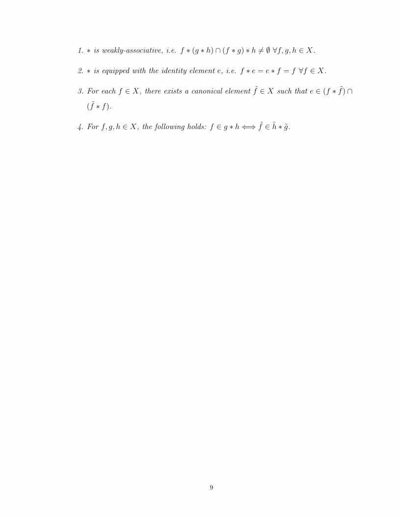
1. ∗ is weakly-associative, i.e. f ∗ (g ∗ h) ∩ (f ∗ g) ∗ h = ∅ ∀f, g, h ∈ X.

2. ∗ is equipped with the identity element e, i.e. f ∗ e = e ∗ f = f ∀f ∈ X.

3. For each f ∈ X, there exists a canonical element f ∈ X such that e ∈ (f ∗ f) ∩

(f ∗ f).

4. For f, g, h ∈ X, the following holds: f ∈ g ∗ h⇐⇒ f ∈ h ∗ g.

9

1

Background and historical note

In the first subsection, we provide the basic definitions and properties of semirings

and hyperrings, which are to be used in the subsequent chapters. Then we give a

historical overview on theory of hyperrings.

1.1 Background on semi-structures and hyper-structures

1.1.1 Basic notions: Semi-structures

We introduce the basic notions and properties in semiring theory.

Definition 1.1.1. A set M equipped with a binary operation · is called a semigroup

if for a, b, c ∈ M , we have (a · b) · c = a · (b · c) and there exists 1 ∈ M such that

1 · a = a · 1 = a. When a · b = b · a ∀a, b ∈ M , we say that M is a commutative

semigroup.

Definition 1.1.2. A semiring (M,+, ·) is a non-empty set M endowed with an ad-

dition + and a multiplication · such that

1. (M,+) is a commutative semigroup with the neutral element 0.

2. (M, ·) is a semigroup with the identity 1.

3. r(s+ t) = rs+ rt and (s+ t)r = sr + tr ∀r, s, t ∈M.

10

4. r · 0 = 0 · r = 0 ∀r ∈M.

5. 0 = 1.

If (M, ·) is a commutative semigroup, then we call M a commutative semiring. If

(M\0, ·) is a group, then a semiring M is called a semifield.

Definition 1.1.3. (cf. [19]) Let M1, M2 be semirings. A map f : M1 −→ M2 is a

homomorphism of semirings if f satisfies the following conditions: ∀a, b ∈M1,

f(a+ b) = f(a) + f(b), f(ab) = f(a)f(b), f(0) = 0, f(1) = 1.

Definition 1.1.4. Let R be a semiring and T be a semigroup. We say that T is a

R-semimodule if there exists a map ϕ : R ×M −→ M which satisfies the following

properties: ∀r, r1, r2 ∈ R, ∀t, t1, t2 ∈ T ,

1. ϕ(1, r) = r.

2. If t = 0 or r = 0, then ϕ(t, r) = 0.

3. ϕ(t1 + t2, r) = ϕ(t1, r) + ϕ(t2, r), ϕ(t, r1 + r2) = ϕ(t, r1) + ϕ(t, r2).

4. ϕ(t1t2, r) = ϕ(t1, ϕ(t2, r)), ϕ(t, r1r2) = ϕ(t, r2)r2.

In what follows, we always assume that all semirings are commutative. We review

the notion of (prime) ideals of a semiring M .

Definition 1.1.5. (cf. [19]) Let M be a semiring.

1. A non-empty subset I of M is an ideal if (I,+) is a sub-semigroup of (M,+)

and for a ∈ I, r ∈M , we have r · a ∈ I.

2. An ideal I ( M is prime if I satisfies the following property: if xy ∈ I, then

x ∈ I or y ∈ I ∀x, y ∈ I.

3. An ideal I (M is maximal if I satisfies the following property: if J (M is an

ideal and I ⊆ J , then I = J .

11

Proposition 1.1.6. (cf. [19, §6]) Let M be a semiring.

1. Any maximal ideal m of M is prime.

2. Any proper ideal I of M (i.e. I =M) is contained in a maximal ideal of M .

LetM be a semiring and X = SpecM be the set of prime ideals ofM . Then, as in the

classical case, one can impose the Zariski topology on X as follows: a subset A of X is

closed if and only if A = V (I) for some ideal I of M , where V (I) := p ∈ X | I ⊆ p

(cf. [19, §6]). Moreover, the following Hilbert’s Nullstellensatz holds: for an ideal I

of M , we have p∈V (I)

p = a ∈M | an ∈ I for some n ∈ N. (1.1.1)

The notion of localization can be directly generalized to a semiring. Let M be a

semiring and S be a multiplicative subset of M , equivalently, S is a (multiplicative)

submonoid. Then, as a set, S−1M is (M × S/ ∼), where ∼ is a congruence relation

on M × S such that

(m1, r1) ∼ (m2, r2) ⇐⇒ ∃s ∈ S such that sm1s2 = sm2s1. (1.1.2)

Note that by a congruence relation∼ on a semiringM we mean an equivalence relation

which satisfies the following condition: if x ∼ y and x′ ∼ y′, then x + x′ ∼ y + y′

and xx′ ∼ yy′ ∀x, x′, y, y′ ∈M . We denote by msthe equivalence class of (m, s) under

the congruence relation (1.1.2). Then, S−1M is a semiring and a localization map

S−1 : M −→ S−1M sending m to m1

is a homomorphism of semirings. Moreover,

as in the classical case, for a (prime) ideal I of M such that I ∩ S = ∅, the set

S−1I := is| i ∈ I, s ∈ S is a (prime) ideal of S−1M . Finally, when S = M\p for

some prime ideal p of M , the semiring S−1M has the unique maximal ideal, namely

S−1p (cf. [19, §10]).

By an idempotent semiring, we mean a semiring M such that x+ x = x ∀x ∈M .

Example 1.1.7. Let B := 0, 1. We define an addition as: 1 + 1 = 1, 1 + 0 =

12

0 + 1 = 1, and 0 + 0 = 0. A multiplication is defined by 1 · 1 = 1, 1 · 0 = 0, and

0 · 0 = 0. Then, B becomes the initial object in the category of idempotent semirings.

Example 1.1.8. The tropical semifield Rmax is R ∪ −∞ as a set. An addition

⊕ is given by: a ⊕ b := maxa, b ∀a, b ∈ Rmax, where −∞ ≤ a ∀a ∈ Rmax. A

multiplication ⊙ is defined as the usual addition of R as follows: a ⊙ b := a + b,

where + is the usual addition of real numbers and (−∞) ⊙ a = a ⊙ (−∞) = (−∞)

∀a ∈ Rmax. We denote by Qmax, Zmax the sub-semifields of Rmax with the underlying

sets Q ∪ −∞, Z ∪ −∞ respectively.

When M is an idempotent semiring, one can impose the following canonical partial

order on M :

a ≤ b ⇐⇒ a+ b = b ∀a, b ∈M. (1.1.3)

Note that by a partial order on M we mean a binary relation ≤ on M which is

reflexive, transitive, and antisymmetric.

1.1.2 Basic notions: Hyper-structures

In this subsection, we introduce the basic definitions and properties of hyperrings.

Definition 1.1.9. (cf. [9]) A hyper-operation on a non-empty set H is a map

+ : H ×H → P(H)∗,

where P(H)∗ is the set of non-empty subsets of H. In particular, ∀A,B ⊆ H, we

also denote

A+B :=

a∈A,b∈B

(a+ b).

Definition 1.1.10. (cf. [9]) A canonical hypergroup (H,+) is a non-empty pointed

set with a hyper-operation + which satisfies the following properties:

1. x+ y = y + x ∀x, y ∈ H. (commutativity)

13

2. (x+ y) + z = x+ (y + z) ∀x, y, z ∈ H. (associativity)

3. 0 + x = x = x+ 0 ∀x ∈ H. (neutral element)

4. ∀x ∈ H ∃!y(:= −x) ∈ H s.t. 0 ∈ x+ y. (unique inverse)

5. x ∈ y + z =⇒ z ∈ x− y. (reversibility)

Remark 1.1.11. The uniqueness of (4) rules out the trivial choice of the inverse,

e.g. the full set H as an inverse of any element. The reversibility property is meant

to be the ‘hyper’-subtraction.

Note that a hypergroup is, in fact, more general object than a canonical hypergroup.

However, throughout the thesis, by a hypergroup we will always mean a canonical

hypergroup.

Definition 1.1.12. (cf. [9]) A hyperring (R,+, ·) is a non-empty set R with a hyper-

addition + and a usual multiplication · which satisfy the following conditions:

1. (R,+) is a canonical hypergroup.

2. (R, ·) is a monoid with 1R (not necessarily commutative).

3. A hyperaddition and a multiplication are compatible, i.e. ∀x, y, z ∈ R, x(y+z) =

xy + xz, (x+ y)z = xz + yz.

4. 0 is an absorbing element, i.e. ∀x ∈ R, x · 0 = 0 = 0 · x.

5. 0 = 1.

When (R \ 0, ·) is a group, we call (R,+, ·) a hyperfield.

Definition 1.1.13. (cf. [9]) For hyperrings (R1,+1, ·1), (R2,+2, ·2) a map f : R1 −→

R2 is called a homomorphism of hyperrings if

1. f(a+1 b) ⊆ f(a) +2 f(b) ∀a, b ∈ R1.

2. f(a ·1 b) = f(a) ·2 f(b) ∀a, b ∈ R1.

14

3. We call f strict if f(a+1 b) = f(a) +2 f(b) ∀a, b ∈ R1.

4. We call f an epimorphism if

x+2 y =

f(a+1 b) | f(a) = x, f(b) = y ∀x, y ∈ R2.

Example 1.1.14. (cf. [9]) Let K := 0, 1. A (commutative) multiplication of K is

given by

1 · 1 = 1, 0 · 1 = 1 · 0 = 0,

and a (commutative) hyperaddition is given by

0 + 1 = 1, 0 + 0 = 0, 1 + 1 = 0, 1.

Then (K,+, ·) is a hyperfield called the Krasner’s hyperfield.

Let R be a hyperring. For x, y ∈ R, if x + y consists of a single element z, we let

x + y = z rather than x + y = z. Another interesting example is the hyperfield of

signs.

Example 1.1.15. (cf. [9]) Let S = −1, 0, 1. A multiplication is commutative and

given by

1 · 1 = (−1) · (−1) = 1, (−1) · 1 = (−1), a · 0 = 0 ∀a ∈ S.

A hyperaddition + is commutative and given by

0+0 = 0, 1+0 = 1+1 = 1, (−1)+0 = (−1)+(−1) = (−1), 1+(−1) = −1, 0, 1.

In other words, a hyperaddition is given by the rule of signs and hence we call S the

hyperfield of signs.

We review the notion of (prime) ideals for hyperrings. In the sequel, all hyperrings

are assumed to be commutative.

15

Definition 1.1.16. (cf. [9]) Let R be a hyperring.

1. A non-empty subset I of R is a hyperideal if: ∀a, b ∈ I =⇒ a − b ⊆ I and

∀a ∈ I,∀r ∈ R =⇒ r · a ∈ I.

2. A hyperideal I ( R is prime if I satisfies the following property: if xy ∈ I, then

x ∈ I or y ∈ I ∀x, y ∈ I.

3. A hyperideal I ( R is maximal if I satisfies the following property: if J ( R is

a hyperideal of R which contains I, then I = J .

Proposition 1.1.17. (cf. [15]) Let R be hyperring.

1. Let I be a proper hyperideal of R (i.e. I = R). Then there exists a maximal

hyperideal m such that I ⊆ m.

2. Any maximal hyperideal m is prime.

Definition 1.1.18. (cf. [39]) Let R be a hyperring. We denote by SpecR the set

of prime hyperideals of R. One can impose the Zariski topology on SpecR as in the

classical case. In other words,

a subset A ⊆ SpecR is closed ⇐⇒ A = V (I) for some hyperideal I of R, (1.1.4)

where V (I) := p ∈ SpecR | I ⊆ p.

Proposition 1.1.19. (cf. [39]) Let R be a hyperring and X = SpecR.

1. Let Ijj∈J be a family of hyperideals of R. Then we have

j∈J

V (Ij) = V (<j∈J

Ij >), (1.1.5)

where <j∈J Ij > is the smallest hyperideal containing

j∈J Ij. Note that such

hyperideal exists since an arbitrary intersection of hyperideals is a hyperideal.

16

2. Let I and I ′ be hyperideals of R, then we have

V (I)

V (I ′) = V (I ∩ I ′). (1.1.6)

Next, we review the notion of a localization of a hyperring. This construction has

been promoted by R.Procesi-Ciampi and R.Rota (cf. [39]).

For a (multiplicative) submonoid S of a hyperring R, one defines the localization

S−1R as follows: as a set, S−1R is the set (R× S/ ∼) of equivalence classes, where

(r1, s1) ∼ (r2, s2) ⇐⇒ ∃x ∈ S s.t. xr1s2 = xr2s1. (1.1.7)

Let [(r, s)] be the equivalence class of (r, s) ∈ R × S under the equivalence relation

(1.1.7). A hyperaddition of S−1R is given by

[(r1, s1)] + [(r2, s2)] = [(r1s2 + s1r2), s1s2] = [(y, s1s2)] | y ∈ r1s2 + s1r2.

A multiplication is naturally given as follows:

[(r1, s1)] · [(r2, s2)] = [(r1r2, s1s2)].

We denote by rsa element [(r, s)]. Note that as in the classical case, the localization

map, S−1 : R −→ S−1R sending r to r1, is a homomorphism of hyperrings.

Proposition 1.1.20. (cf. [15]) Let R be a hyperring and S be a multiplicative subset

of R.

1. For a hyperideal I of R, the following set:

S−1I := is| i ∈ I, s ∈ S

is a hyperideal of S−1R.

2. If p is a prime hyperideal of R such that S ∩ p = ∅, then S−1p is a prime

17

hyperideal of S−1R.

3. If S = R\p for some prime hyperideal p of R, then S−1R has the unique maximal

hyperideal given by S−1p.

The following theorems provide a useful way to construct hyperrings from classical

commutative algebras.

Theorem 1.1.21. (cf. [9, Proposition 2.6]) Let A be a commutative ring and G ⊆ A×

be a subgroup of the multiplicative group A×. Then, the set A/G is a hyperring with

the following operations:

1. xG · yG := xyG ∀x, y ∈ A. (multiplication)

2. xG+ yG := zG | z = xa+ yb for some a, b ∈ G ∀x, y ∈ A. (hyperaddition)

A hyperring which arises in this way is called a quotient hyperring.

Note that, for a field k with |k| ≥ 3, we can identify the Krasner’s hyperfield K with

the quotient hyperring k/k×. We recall the following interesting fact.

Theorem 1.1.22. (cf. [9, Proposition 2.7]) Let A be a commutative ring, and let

G ⊆ A× be a subgroup of the multiplicative group A×. Assume further that |G| ≥ 2.

Then, the quotient hyperring A/G is an extension of the Krasner’s hyperfield K if

and only if 0 ∪G is a subfield of A.

1.2 Historical note on hyperrings

The notion of a hypergroup was first introduced by F.Marty in [34] and subsequently,

in 1956, M.Krasner introduced the notion of hyperrings as a technical tool in his paper

[24] on the approximation of valued fields. However, for decades, hyper-structure has

been better known to computer scientists or applied mathematicians than those who

work in pure mathematics; this is due to uses of hyper-structures in connection with

fuzzy logic (a form of multi-valued logic), automata, cryptography, coding theory via

18

associations schemes, and hypergraphs (cf. [13], [52]).

In [50], Oleg Viro wrote: “Probably, the main obstacle for hyperfields to become a

mainstream notion is that a multivalued operation does not fit to the tradition of set-

theoretic terminology, which forces to avoid multivalued maps at any cost. I believe

the taboo on multivalued maps has no real ground, and eventually will be removed.”

In recent years, hyper-structure theory has been revitalized in connection with various

fields. For example, in connection with number theory, A.Connes’ adele class space

HK = AK/K× of a global field K is a hyperring extension of the Krasner’s hyperfield

K (cf. [9]). Moreover, the use of hyper-structures is essential in the archimedean

(isotypical) Witt construction introduced in [10]. Also, in [50], the author found

a link between hyper-structures and tropical geometry via dequantization. Finally,

in [32], M.Marshall generalizes the Artin-Schreier theory for fields to hyperfields.

Note that the weakness of semirings is that they do not posses additive inverses. This

problem can be fixed by considering hyper-structures via Henry’s symmetrization

process (cf. [21]). Therefore, one might benefit by using both semi-structures and

hyper-structures.

19

2

Algebraic geometry over

semi-structures

We develop algebraic geometry over semi-structures in this chapter. In the first sec-

tion, we take an elementary approach to investigate an algebraic variety over various

sub-semifields of Rmax considered as a set of solutions of polynomial equations. In

the second section, we introduce the notion of a semi-scheme generalizing a scheme

in such a way that a underlying algebra is that of semirings and develop Cech co-

homology theory of semi-schemes. As a byproduct, we confirm that any invertible

sheaf on P1Qmax

is isomorphic to OX(n) for some n ∈ Z. Finally, in the last section,

we introduce the notion of valuations over semirings and prove that the analogue of

an abstract curve by using (suitably defined) Qmax(T ) is provided by the projective

line P1F1.

2.1 Solutions of polynomial equations over semi-structures

2.1.1 Solutions of polynomial equations over Zmax

In recent years, tropical geometry has become a young and popular subject of math-

ematics. Tropical geometry is, briefly speaking, the study of a tropical variety which

is a set of ‘solutions’ of polynomial equations over the semifield Rmax (cf. Example

20

1.1.8).

In the recent paper [11], A.Connes and C.Consani studied arithmetics of the sub-

semifield Zmax of Rmax. This suggests that one might study arithmetics of tropical

varieties based on Zmax. In this section we will briefly introduce the basic theorems

and definitions of tropical geometry and explain how one can naturally replace Rmax

with Zmax. We will follow notations and definitions in [30]. The only difference be-

tween this section and [30] is that we use the maximum convention instead of the

minimum convention, but such choice makes no difference in developing the theory.

Recall that the semifield Zmax is a subsemifield of Rmax with the underlying set

Zmax = Z ∪ −∞. We also note that the set Rmax[x1, ..., xn] of polynomials with

coefficients in Rmax is also a semiring with the operations induced from Rmax. To

be specific, an element F of Rmax[x1, ..., xn] is a finite formal sum of monomials us-

ing ⊕ and ⊙. Furthermore, one defines xi ⊕ −∞ = xi, xi ⊙ 0 = xi. Then, for

F ∈ Rmax[x1, ..., xn], one defines the following set:

V (F ) := w ∈ Rn | the maximum in F is achieved at least twice. (2.1.1)

In what follows, we fix an algebraically closed field K with a nontrivial valuation ν.

For f =

u∈Zn Cuxu ∈ K[x±1 , ..., x

±n ], one defines the tropicalization trop(f) of f as

follows:

trop(f) := ⊕u∈Znν(Cu)⊙ x⊙u = maxu

ν(Cu) + u · x ∈ Rmax[x1, ...xn]. (2.1.2)

With the above notations, one has trop(V (f)) = V (trop(f)).

Example 2.1.1. Let us compute an easy example. Let F := 0 ⊕ x ⊕ y ∈ Rmax[x, y]

be a tropical linear polynomial. It follows from the definition that V (F ) is the subset

of R2 where the maximum in F = 0⊕ x⊕ y is achieved at least twice. Thus one can

observe that V (F ) is the union of the sets X1, X2, X3 by choosing each two of terms

x, y, and 0 to be a maximum as follows:

21

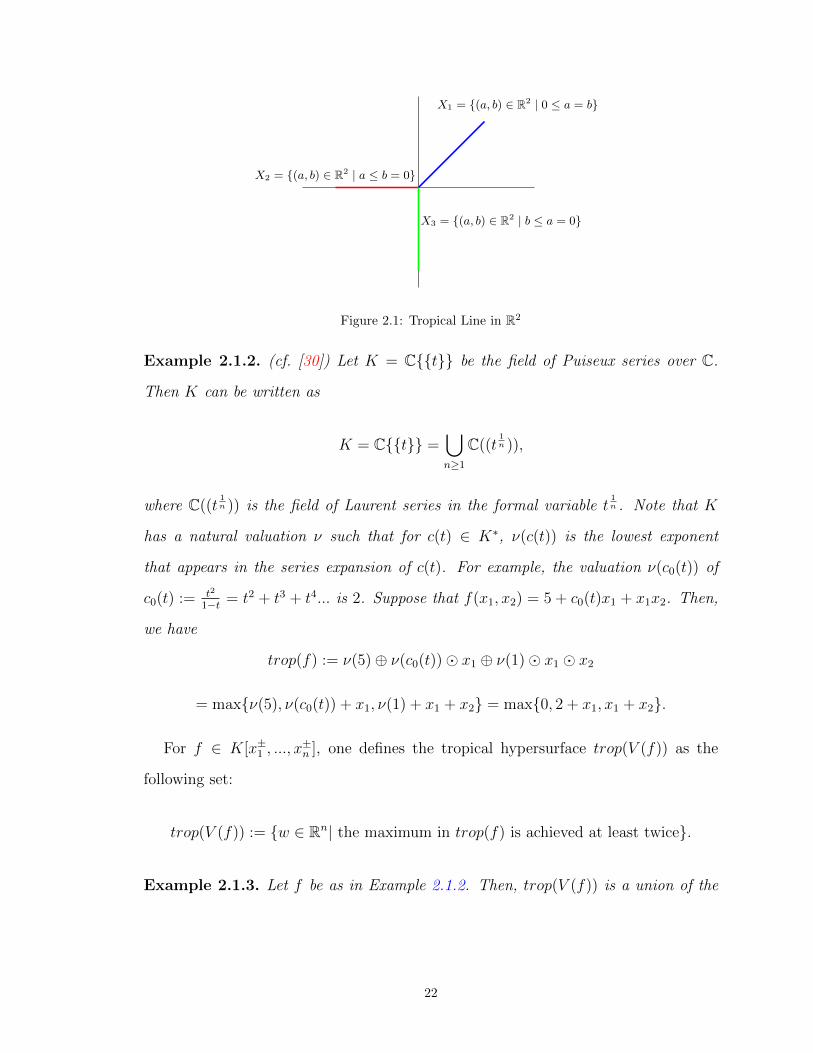
X1 = (a, b) ∈ R2 | 0 ≤ a = b

X2 = (a, b) ∈ R2 | a ≤ b = 0

X3 = (a, b) ∈ R2 | b ≤ a = 0

Figure 2.1: Tropical Line in R2

Example 2.1.2. (cf. [30]) Let K = Ct be the field of Puiseux series over C.

Then K can be written as

K = Ct =n≥1

C((t1n )),

where C((t 1n )) is the field of Laurent series in the formal variable t

1n . Note that K

has a natural valuation ν such that for c(t) ∈ K∗, ν(c(t)) is the lowest exponent

that appears in the series expansion of c(t). For example, the valuation ν(c0(t)) of

c0(t) :=t2

1−t = t2 + t3 + t4... is 2. Suppose that f(x1, x2) = 5 + c0(t)x1 + x1x2. Then,

we have

trop(f) := ν(5)⊕ ν(c0(t))⊙ x1 ⊕ ν(1)⊙ x1 ⊙ x2

= maxν(5), ν(c0(t)) + x1, ν(1) + x1 + x2 = max0, 2 + x1, x1 + x2.

For f ∈ K[x±1 , ..., x±n ], one defines the tropical hypersurface trop(V (f)) as the

following set:

trop(V (f)) := w ∈ Rn| the maximum in trop(f) is achieved at least twice.

Example 2.1.3. Let f be as in Example 2.1.2. Then, trop(V (f)) is a union of the

22

sets X1, X2, X3, where

X1 := (x, y) ∈ R2 | 0 ≤ 2+x1 = x1+x2, X2 := (x, y) ∈ R2 | 2+x1 ≤ 0 = x1+x2,

and X3 := (x, y) ∈ R2 | x1 + x2 ≤ 2 + x1 = 0.

For a subset X ⊆ Rn, let X be the (topological) closure of X in Rn. One of the

main theorems in tropical geometry is the following:

Theorem 2.1.4. (Kapranov’s theorem) Let K an algebraically closed field with a

valuation ν. Suppose that f =

u∈Zn Cuxu ∈ K[x±1 , ..., x

±n ]. Then,

trop(V (f)) = (ν(y1), ..., ν(yn)) ∈ Rn | y = (y1, ..., yn) ∈ V (f).

Example 2.1.5. ( [30, Example 3.1.4]) Let K be an algebraically closed field with a

valuation ν. Let 1 + x+ y ∈ K[x±1, y±1]. Then,

V (f) = (z,−1− z) ∈ K2 | z = 0,−1.

Moreover, we have

(ν(z), ν(−1− z)) =

(ν(z), 0) if ν(z) > 0

(ν(z), ν(z)) if ν(z) < 0

(0, ν(−1− z)) if ν(z) = 0, ν(−1− z) > 0

(0, 0) otherwise.

(2.1.3)

Since K is algebraically closed, the value group of ν is dense in R. It follows from

(2.1.3) that the closure of the set (ν(z), ν(−1 − z) | z = 0,−1 is same as the set

V (F ) in Example 2.1.1.

Remark 2.1.6. The set trop(V (f)) is also same as a support of some Grobner com-

plex, however, we will not use that result in this chapter. For details we refer the

readers to Chapter 3 of [30].

23

Let X be the algebraic variety defined by an ideal I ⊆ K[x±1 , ..., x±n ]. One defines

the tropicalization trop(X) of X as follows:

trop(X) :=f∈I

trop(V (f)) ⊆ Rn.

There are two main theorems in tropical geometry.

Theorem 2.1.7. (Fundamental theorem of tropical algebraic geometry) Let I be an

ideal of K[x±1 , ..., x±n ] and X := V (I). Then,

trop(X) = (ν(y1), ..., ν(yn)) ∈ Rn | y = (y1, ..., yn) ∈ X. (2.1.4)

Theorem 2.1.8. (Structure theorem for tropical varieties) Let X be an irreducible d-

dimensional subvariety of a torus T n over K. Let Γ be the value group of a valuation

ν on K. Then, trop(X) is the support of a balanced, weighted Γ-rational polyhedral

complex which is pure of dimension d. Moreover, the polyhedral complex is connected

through codimension one.

Example 2.1.9. From Example 2.1.1, one observes that trop(X) is the support of a

polyhedral complex pure of dimension 1 connected through codimension 1, i.e. trop(X)

is a connected finite graph.

When we replace Rmax with a subsemifield M of Rmax, the most naive definition

of a tropical variety over M is the following:

Definition 2.1.10. Let M be a subsemifield of Rmax and M1 :=M\−∞(=M∗).

1. For F ∈ M [x1, ..., xn], we define the set VM(F ) of solutions of F over M as

follows: VM(F ) := w ∈Mn1 | the maximum in F is achieved at least twice.

2. For an ideal I ∈M [x1, ..., xn], we define the set VM(I) as follows:

VM(I) :=F∈I

VM(F ).

24

Example 2.1.11. Let M = Zmax and F := 0 ⊕ x ⊕ y ∈ Zmax[x, y]. Then, the set

VM(F ) is the intersection of V (F ) in Example 2.1.1 with Z2.

In fact, for a subsemifield M of Rmax and an ideal I ∈M [x1, ..., xn], we obtain

VM(I) = V (I) ∩Mn1 , (2.1.5)

where V (I) is a tropical variety defined by I. In the sequel, by the set of M -rational

points of V (I) or a tropical variety defined by I over M , we mean VM(I) in (2.1.5).

In [18], Jeffrey Giansiracusa and Noah Giansiracusa proved that there is a (semi)

scheme structure which one can associate to a tropical variety, and the set VM(F )

can be understood as the set of M -rational points of that (semi) scheme. We explain

their result succinctly here.

Fix a subsemifieldM of Rmax and let SM =M [x±1 , ..., x±n ]. For F = maxu(au+x ·u) ∈

SM , one defines the set supp(F ) := u ∈ Zn | au = −∞. For v ∈ supp(F ), one

defines

Fv := maxu=v

(au + x · u).

The bend relation of F is defined by: B(F ) := F ∼ Fv : v ∈ supp(F ). For example,

if F := 1⊕ x⊕ y = max1, x, y, then we have

B(F ) = F ∼ 1⊕ x, F ∼ 1⊕ y, F ∼ x⊕ y.

For an ideal I of SM , the scheme-theoretic tropicalization of I is the congruence on

SM generated by B(trop(f)) : f ∈ I which they denote by T rop(I). Then, the

quotient SM/T rop(I) is a semiring and we have

VM(I) = Hom(SM/T rop(I),M), (2.1.6)

25

where homomorphisms are semiring homomorphisms. In other words,

VM(I) = V (I)∩(M\−∞)n = w ∈ (M\−∞)n | F (w) = Fv(w) ∀F ∈ I, v ∈ supp(F ).

Thus, VM(I) can be considered as the set ofM -rational points of Spec(SM/T rop(I)).

This justifies our notation.

Remark 2.1.12. When the value group Γ is a subgroup of Q, a polynomial F in

Γ[x1, ..., xn] always has a solution over Qmax since tropical polynomials are piecewise

linear functions. Hence, the semifield Qmax can be considered as ‘algebraically closed’.

We close this subsection by claiming that the naive generalization of Galois theory

does not behave well in this setting.

Proposition 2.1.13. The only automorphism of Rmax fixing Zmax is the identity

map.

Proof. Let ϕ be an automorphism of Rmax fixing Zmax. Then, ϕ also has to fix Qmax.

Indeed, for ab∈ Qmax, we have a = ϕ(a) = ϕ(b · a

b) = ϕ(a

b+ a

b+ ...+ a

b) = b · ϕ(a

b). It

follows that ϕ(ab) = a

b. Furthermore, since ϕ and ϕ−1 are order-preserving functions,

they should be continuous with respect to Euclidean topology. Hence, ϕ also has to

fix Rmax.

Remark 2.1.14. Proposition 2.1.13 suggests that if one wants to understand the set

of ‘rational points’ as the set of elements which are fixed by the action of a ‘Galois

group’, then one needs to develop Galois theory which is not as naive as the above.

2.1.2 Counting rational points

In the view of Theorem 2.1.8 (the structure theorem) and (2.1.6), algebraic geometry

over Rmax is the geometry of polyhedral complexes and algebraic geometry over Zmax

is the geometry of lattice points (or integral points) of such polyhedral complexes.

In [11], the authors showed that for each n > 1, there is a Frobenius map Frn :

26

Zmax −→ Zmax such that the image of Frn is isomorphic to the semifield extension

F(n) ≃ q ∈ Qmax | nq ∈ Zmax of Zmax of (suitable defined) degree n. Moreover,

in [47], Jeffrey Tolliver showed that any finite semifield extension of Zmax of degree n

is isomorphic to F(n). In the sequel, we denote F := Zmax.

In the sense that F and F(n) are characteristic one analogues of finite fields Fq and

Fqn , one might be interested in counting the number of ‘F(n)-rational’ points of a

given tropical variety X over Zmax. However, in general, a cardinality of a set of

‘F(n)-rational’ points is not finite. In this subsection, we pose two different counting

problems to overcome such obstruction.

Throughout this section, let K be an algebraically closed, complete non-archimedean

field with a non-trivial valuation ν such that the value group ΓK is a subgroup of Q.

Let X be an irreducible algebraic variety over K of dimension d defined by an ideal

I ⊆ K[X±1 , ..., X

±m]. Let trop(I) := trop(f) | f ∈ I ⊆ ΓK [X

±1 , ..., X

±m] and Trop(X)

be a tropical variety over ΓK defined by trop(I). Note that we consider ΓK ∪ −∞

as the subsemifield of Qmax by imposing the idempotent operation induced from

Rmax. From the structure theorem of tropical geometry (cf. Theorem 2.1.8 or [30,

Theorem 3.3.6] for details), Trop(X) is the support of a polyhedral complex of pure

dimension d. Since X is a subvariety of a torus, counting F-points or F(n)-points is

indeed equivalent to counting Z-points or 1nZ-points of Trop(X). By introducing such

notions, our goal is to find a proper definition of a (Hasse-Weil type) zeta function of

a tropical variety.

The first counting problem

Let X and K be as above. For l ∈ R>0, we define the following number:

Nn(X, l) := #(x1, ..., xm) ∈ Trop(X) ∩ (F(n))m | max(|x1|, ..., |xm|) ≤ l.

In other words, Nn(X, l) is the number of F(n)-rational points x = (x1, ..., xm) of

Trop(X) such that |xi| is bounded by l. In particular, N1(X, l) is the number of

27

F-points of Trop(X) which are bounded by l. In general, Nn(X, l) goes to infinity as

l goes to infinity. Therefore, we will focus on the asymptotic behavior of the following

(suitably normalized) number:

R(X,n) := liml→∞

Nn(X, l)

N1(X, l).

When Nn(X, l) = N1(X, l) = 0 ∀l ∈ R>0, we define R(X,n) := 0. The main result

in this subsection is Proposition 2.1.19: for an irreducible curve X in a torus over a

suitable field, we have R(X,n) = n for infinitely many n ∈ Z.

As an example, consider X = Tm = (K∗)m, an m-dimensional torus. We then have

Trop(X) = Rm. In fact, let Y := (ν(x1), ..., ν(xn) | xi ∈ K∗ = ΓmK , where ΓK is the

value group of K. Since K is algebraically closed, ΓK is dense in R. It follows from

Theorem 2.1.7 that Y = Rm = Trop(X). Then, for l ∈ Z>0, N1(X, l) = (2l + 1)m

and Nn(X, l) = (2nl + 1)m. Thus, if we follow the sequence of natural numbers, the

limit R(X,n) will be nm. What is interesting is that if we consider an m-dimensional

torus over a finite field Fq, then the number of Fq-rational points is (q − 1)m and the

number of Fqn-rational points is (qn− 1)m. Then, we observe that the following limit

limq→1

(qn − 1)m

(q − 1)m= lim

q→1(qn − 1

q − 1)m = nm

gives the same number. In the above example, we computed R(Tm, n) only with

l ∈ Z>0. In fact, we have the following:

Proposition 2.1.15. Let X = Tm be an m-dimensional torus over K. Then the

limit R(X,n) exists and is equal to nm.

Proof. For l ∈ R>0, let ⌊l⌋ be the greatest integer which is less than or equal to l and

let Bl := x = (x1, ..., xm) ∈ Rm | |xi| ≤ ⌊l⌋. Consider the following sets:

M1(n) := #x = (x1, ..., xm) ∈ (F(n))m | max(|x1|, ..., |xn|) ≤ ⌊l⌋,

28

M2(n) := #x = (x1, ..., xm) ∈ (F(n))m | ⌊l⌋ < |xi| ≤ l for some i.

Then, M1(n) = (2n ⌊l⌋+1)m and Nn(X, l) =M1(n)+M2(n). Since (l−⌊l⌋) ≤ 1, the

number of F(n)-points in the closed interval [⌊l⌋ , l] is less than or equal to n. Because

the number of facets of Bl is 2m, we have the following bound:

0 ≤M2(n) ≤ 2mn(2nl + 1)m−1.

In particular, for n = 1, we have

N1(X, l) =M1(1) +M2(1), M1(1) = (2 ⌊l⌋+ 1)m, 0 ≤M2(1) ≤ 2m(2l + 1)m−1.

It follows from the definition that

R(X,n) := liml→∞

Nn(X, l)

N1(X, l)= lim

l→∞

M1(n) +M2(n)

M1(1) +M2(1).

Sincem is a fixed number andM2 is bounded by the polynomial in l of degree (m−1),

we have

liml→∞

M2(n)

M1(n)= lim

l→∞

M2(1)

M1(n)= 0, lim

l→∞

M1(1)

M1(n)= lim

l→∞

(2 ⌊l⌋+ 1)m

(2n ⌊l⌋+ 1)m=

1

nm.

Hence we have

R(X,n) := liml→∞

Nn(X, l)

N1(X, l)= lim

l→∞

1M1(1)M1(n)

= nm.

Next, we consider the case of a plane tropical curve V . In fact, V is a finite (planar)

graph in this case; the following is known.

Remark 2.1.16. ( [30, Proposition 1.3.1]) A plane tropical curve V is a finite graph

which is embedded in the plane R2. It has both bounded and unbounded edges, all edge

slopes are rational, and this graph satisfies a balancing condition around each node.

Unlike the torus case, when we deal with plane curves, a choice of n should be

29

general enough as the following example illustrates.

Example 2.1.17. Let V be the plane tropical curve defined by X⊙t⊕ Y ⊙t⊕ 1, where

t > 1. Then V is the graph with the three unbounded edges in R2; X = (x, 1t) | x ≤

1t, Y = (1

t, y) | y ≤ 1

t, and Z = (z, z) | 1

t≤ z. Suppose that n = t. Then,

on the edge X, we have infinitely many F(n)-points, but no F-point. Thus, we have

R(V, n) = ∞ in this case. On the other hand, if we choose n so that t - n, then on

edges X and Y , there is no F or F(n)-point. On the edge Z, the similar computation as

in the torus case shows that R(V, n) = n. Thus, as long as t - n, we have R(V, n) = n.

In fact, this is true for any plane tropical curve.

Proposition 2.1.18. Let V be a plane tropical curve. Then, for infinitely many

integers n, R(V, n) exists. Furthermore, we have R(V, n) = n if at least one of the

following conditions is satisfied:

1. V has an unbounded edge which is not parallel to a coordinate axis.

2. Each vertex of V is an element of Z2.

Proof. This is actually an easy consequence of Remark 2.1.16. We examine each

case of edges. Let Y = r be a horizontal edge (i.e. parallel to the first coordinate

axis) with a vertex (a, r) in Q2. If r is an integer, then we have R(Y = r, n) = n

∀n ∈ N as in the case of torus. If r ∈ F(t)\F, for an integer n such that gcd(n, t) = 1,

we have no F-point and F(n)-point. Therefore, in this case, R(Y = r, n) = 0. For

the case of a vertical edge X = r, the exact same argument works. Finally, for an

unbounded edge Z with a rational slope which is not parallel to a coordinate axis,

we have infinitely many F-points (hence, F(n)-points). Moreover, since Z has a slope

which is not zero nor infinity, Z passes an integral point in finite length. However, the

finite line segment of Z does not change the limit R(Z, n) since Z has infinitely many

F and F(n)-points. It follows that we may assume that the vertex (a, b) of the edge Z

is in Z2 for computing the limit R(Z, n). We may further assume that (a, b) = (0, 0)

30

since this will not change the number of F or F(n)-points. Therefore, we assume that

Z = (x, kmx) | 0 ≤ x, where m, k ∈ Z\0. If m | k, then the counting argument is

same as the torus case. Hence, we assume that gcd(m, k) = 1. Suppose that |k| < |m|.

Then, for l ∈ R>0, the F-points on the ray Z are (0, 0), (m, k), (2m, 2k), (3m, 3k).....

Since |k| < |m|, we have (N1(Z, l) − 1)|m| ≤ l. Hence, N1(Z, l) ≤ ( l|m| + 1) := l + 1

and N1(Z, l) =l+ 1. Similarly, we can find F(n)-points. In fact, since k

m(αn) =

(βn) ⇐⇒ m | α, one observes that F(n)-points are given by (0, 0), (m

n, kn), (2m

n, 2kn)...

Since |k| < |m|, we have (Nn(Z, l) − 1) |m||n| ≤ l and Nn(Z, l) ≤ ( l

|m|)n + 1 = ln + 1.

This implies that

Nn(Z, l) =ln+ 1 =

ln+ C, |C| < n+ 1.

Thus, we have

R(Z, l) := liml→∞

Nn(Z, l)

N1(Z, l)= n.

Now, let

V = P1 ∪ ... ∪ Ps ∪ f1 ∪ ... ∪ ft,

where Pi are unbounded edges and fi are bounded edges. Assume that for each

i = 1, ..., s, the limit R(Pi, n) exists and R(Pi, n) = n for at least one i. Then, since

fi are all bounded edges, there exists 0 < δ such that ∀x ∈ fi, |x| < δ ∀i = 1, ..., t.

Let G1 := f1 ∪ ... ∪ ft and G2 := P1 ∪ ... ∪ Ps. Then, we have Nn(V, l) = Nn(G1, l) +

Nn(G2, l)− C, where C is a finite number which is less than or equal to the number

of vertices of V . Since G1 is a union of bounded edges, for a large l, we have some

finite numbers A and B such that

R(V, n) = liml→∞

Nn(G1, l) +Nn(G2, l)− C

N1(G1, l) +N1(G2, l)− C= lim

l→∞

A+Nn(G2, l)

B +N1(G2, l).

31

If R(Pi, n) exists, then

|Nn(Pi, l)− nN1(Pi, l)| < 2 · n ∀i = 1, ..., s. (2.1.7)

In fact, suppose that R(Pi, n) exists. Then, the numbers Nn(Pi, l) and N1(Pi, l) are

either both zero or both non-zero for l >> 0. Therefore, the only difference between

Nn(Pi, l) and nN1(Pi, l) happens at each side of the edge. Thus, we obtain (2.1.7).

However, we proved that, in any case, R(Pi, n) exists and is equal to either 0 or n.

Thus, for l >> 0, we have

|A+s

i=1Nn(Pi, l)

B +s

i=1N1(Pi, l)− n| = |(A− nB) +

si=1(Nn(Pi, l)− nN1(Pi, l))

B +s

i=1N1(Pi, l)|

≤ | (A− nB) + 2ns

B +s

i=1N1(Pi, l)|. (2.1.8)

Since we assumed that R(Pi, n) = n for some i, RHS of (2.1.8) goes to zero when l

goes to infinity. It follows that R(V, n) = n.

To sum up, when V has only unbounded edges which are parallel to coordinate axises,

there are two possible sub-cases. The first is when at least one edge is emanated from

an integral point. In this case, the above computations show that R(V, n) = n. The

second case is when all edges are emanated from non-integral points. In this case,

for infinitely many integer n, we have R(V, n) = 0. The last case is when V has an

unbounded edge which is not parallel to a coordinate axis. In this case, the above

computation shows that R(V, n) = n for infinitely many integer n. This proves our

proposition.

In fact, Proposition 2.1.18 can be generalized as follows:

Proposition 2.1.19. Let K be an algebraically closed field with a complete, nontriv-

ial, non-archimedean valuation with a value group ΓK ⊆ Q. Let X be an irreducible

curve over K in Tm and V := Trop(X). Then, for infinitely many integer n, the limit

R(V, n) exists. In particular, R(V, n) = n if V satisfies at least one of the following

32

conditions:

1. V has an unbounded edge which is not parallel to a coordinate axis.

2. Each vertex of V is an element of Zm.

Proof. The proof is similar to the proof of Proposition 2.1.18. From Theorem 2.1.8

(the structure theorem), V is a finite graph in Rm. We investigate the possible cases

of the edges of V . Let P be an unbounded edge which is not parallel to a coordinate

axis. Then, P will both have infinitely many F and F(n)-points ∀n ∈ N since P is

emanated from a point in Qm and has a rational slope. Fix l ∈ R>0 and consider the

following box B with the side length 2l:

B := x = (x1, ..., xm) ∈ Rm | |xi| ≤ l.

Let ψ := B ∩ P be a line segment in B. Suppose that l is large enough so that ψ

has more than two of F and F(n)-points. This is possible since ψ contains infinitely

many F and F(n)-points. Let Z,W be the integral points of ψ such that the distance

between them is the largest among all pairs of integral points of ψ. We label the

integral points on the line segment ψ as Z = A0, A1, ..., Ad−1 = W so that there is no

integral point between Ai and Ai+1. In particular, N1(P, l) = d. We claim that for

each sub-segment AiAi+1, we have (n+1) of F(n)-points including both ends. For the

notational convenience, let Ai = R and Ai+1 = T . Then, we have

S := RT = (1− t)R + tT | t ∈ [0, 1].

Since R and T are F-points, it follows that S contains at least (n+ 1) of F(n)-points

given by t = kn, where k ∈ 0, 1, ..., n. Suppose that S contains more than (n+1) of

F(n)-points. Then, there exist F(n)-points u = (1− t1)R+ t1T and v = (1− t2)R+ t2T

such that |t2 − t1| < 1n. Let t3 := n(t2 − t1). It follows that

(1− t3)R + t3T = R + t3(T −R) = R + n(t2 − t1)(T −R).

33

We observe that

u− v = (1− t1)R+ t1T − (1− t2)R− t2T = R(t2− t1)+T (t1− t2) = (t2− t1)(R−T ).

Since u and v are F(n)-points, the point v − u = (t2 − t1)(T − R) is also an F(n)-

point and hence n(v − u) = n(t2 − t1)(T − R) is an F-point. This implies that

(1− t3)R+ t3T is an F-point between R and T , and this gives a contradiction. Thus,

there are exactly (n + 1) of F(n)-points on RT . Therefore, if N1(P, l) = d, then

Nn(P, l) = n(d− 1) + 1 + C(l), where C(l) is a constant such that |C(l)| ≤ 2(n+ 1)

∀l ∈ R>0. It follows that

R(P, n) := liml→∞

Nn(P, l)

N1(P, 1)= lim

d→∞

n(d− 1) + C(l)

d= n.

The second case is when P is parallel to some coordinate axises. There are three

sub-cases. The first case is when all coordinates xi which are parallel to coordinate

axises are of the form xi = mi ∈ Z. In this case, the same argument as above gives us

the number R(P, n) = n. The second case is when xi = mi ∈ F(ei)\F for some ei ∈ N.

Then, by a choice of n such that gcd(n, ei) = 1, we have R(P, n) = n or R(P, n) = 0.

The case of R(P, n) = 0 happens when all such xi are in mi ∈ F(ei)\F. The final case

is when none of xi is in F(ei). Then, we have R(P, n) = 0. For the general case of V ,

we can compute in the exact same way as in the plane curve case.

To sum up, if V has no unbounded edge, then R(V, n) exists ∀n ∈ N. If V has an

unbounded edge which is not parallel to a coordinate axis, then for infinitely many

(positive) integer n, we have R(V, n) = n. If V has unbounded edges and all of such

edges are parallel to some coordinate axises with xi = mi, then as we analyzed above,

for infinitely many n ∈ N, the limit R(P, n) exists and equal to 0 or n depending on

values mi. This completes our proof.

If a dimension of an algebraic variety X is greater than 1, in general, it seems hard

to compute above numberR(X,n). Also, as we computed above, computingR(V, n) is

34

closely related to computing F-points or, in general, F(n)-points of polytopes. Thus, in

the next subsection, we pose the second counting problem which measures asymptotic

behavior of the numbers of rational points by using a filtration of polytopes.

The second counting problem

For a bounded subset X of Rm, we define the following number:

Nn(X) = #(X ∩ (F(n))m).

In particular, N1(X) is the number of integral points of X. In this subsection, we

investigate a sequence Xi of subsets of a tropical variety V which satisfies the

following properties:

1.

Xi ⊆ Xi+1,i≥1

Xi = V. (2.1.9)

2. The limit

R(V, Xi, n) := limi→∞

Nn(Xi)

N1(Xi)(2.1.10)

makes sense.

The main result of this subsection is Corollary 2.1.22; if V = Trop(X) is a support

of a polyhedral fan which is pure of dimension d, then there exists a sequence Xi

of subsets of V which satisfies (2.1.9) and (2.1.10). In particular, R(V, Xi, n) = nd.

In the case when X is a rational polytope, a counting of lattice (i.e. integral) points

has been studied and named Ehrhart theory (cf. [2], [44]). We briefly review the

classical results of Ehrhart theory. Recall that by a quasi-polynomial f of degree d

we mean a function f : Z −→ C of the following form:

f(n) = cd(n)nd + cd−1(n)n

d−1 + ...+ c0(n),

35

where ci(n) is a periodic function with an integer period and cd(n) is not identically

zero. Equivalently, f is a quasi-polynomial if there exists N > 0 (namely, a common

period of c0, ..., cd) and polynomials f0, ..., fN−1 such that f(n) = fi(n) if n ≡ i(mod

N). An integer N (which is not unique) is called a quasi-period of f . Let P be a

convex rational polytope in Rm. For M ∈ N, we define the following nonnegative

integer:

i(P,M) = #(MP ∩ Zm),

whereMP := Mx | x ∈ P. Then, for each convex rational polytope P , there exists

a quasi-polynomial f such that f(M) = i(P,M). Furthermore, the leading coefficient

cd is known to be the (suitably normalized) volume of P . In particular, cd is indeed

a constant. Let us further recall some definitions. By a polyhedral cone P in Rm we

mean a set of the following form:

P = ki=1

λivi | 0 ≤ λi for some fixed v1, ..., vk ∈ Rm.

A polyhedral cone P is called a rational polyhedral cone if v1, ...vk ∈ Qm. The

following result can be easily derived.

Lemma 2.1.20. For a d-dimensional rational polyhedral cone P in Rm, there exists

a sequence Pi of convex rational polytopes in P such that Pj ⊆ Pj+1,j≥1 Pj = P ,

and

R(P, Pj, n) := limj→∞

Nn(Pj)

N1(Pj)= nd.

Proof. By the definition, there exist v1, ..., vk ∈ Qm such that P = k

i=1 λivi | 0 ≤

λi. Consider the following subset of P :

P1 := ki=1

λivi | 0 ≤ λi ≤ 1.

We then have P1 ⊆ P . One can further clearly observe that P1 is a convex rational

36

polytope. Fix an integer N > 1 and for each j ∈ N, we define the following set:

Pj := N j−1P1 = N j−1α | α ∈ P1.

Since Pj is a rescaling of P1 by a natural number, we know that Pj is a convex rational

polytope ∀j ∈ N. We claim that Pj ⊆ Pj+1. In fact, it is enough to show that P1 ⊆ P2.

We have α ∈ P1 ⇐⇒ α =k

i=1 λivi for some 0 ≤ λi ≤ 1. Let β := 1Nα =

ki=1

λiNvi.

Since λi ≤ 1 < N , we have λiN< 1 and β ∈ P1. Therefore, Nβ = α ∈ P2 and hence

P1 ⊆ P2. For the second assertion, for α =k

i=1 λivi ∈ P , there exists j such that

λi ≤ N j−1 ∀i = 1, ..., k. It follows that α ∈ Pj and hencej≥1 Pj = P . For the last

assertion, we first observe that for a bounded set Q of Rm, there is a set bijection ϕ

as follows:

ϕ : X := (Q ∩ (Z[1

n])m) −→ Y := (nQ ∩ Zm), α →→ nα.

In fact, ϕ is well-defined since for α ∈ X, we have nα ∈ Y . Clearly, ϕ is an injection,

and the inverse map ϕ−1 is given by sending β to 1nβ. From this bijection, we obtain

i(Pj, n) = Nn(Pj).

It follows from Ehrhart’s theory that there exists a quasi-polynomial f(x) = adxd +

ad−1xd−1 + ... + a0 such that f(M) = i(P1,M) = NM(P1). Since Pj = N j−1P1, we

have

i(Pj, n) = i(N j−1P1, n) = i(P1, nNj−1).

Thus,

Nn(Pj)

N1(Pj)=i(Pj, n)

i(Pj, 1)=i(P1, N

j−1n)

i(P1, N j−1)=ad(N

j−1n)d + ad−1(Nj−1n)d−1 + ...+ a0

ad(N j−1)d + ad−1(N j−1)d−1 + ...+ a0.

37

Since ad and n are fixed, ai are bounded, and N > 1, we have

limj→∞

Nn(Pj)

N1(Pj)=ad(N

j−1n)d + ad−1(Nj−1n)d−1 + ...+ a0

ad(N j−1)d + ad−1(N j−1)d−1 + ...+ a0= nd.

This proves our lemma.

Recall that by a finite polyhedral fan Σ we mean a finite collection of polyhedral

cones such that the intersection of any two is a face of each. The support |Σ| of Σ is

the set, α ∈ Rm | α ∈ P for some P ∈ Σ. A polyhedral fan Σ is said to be pure of

dimension d if every polyhedral cone in Σ that is not the face of other cones in Σ has

dimension d.

Theorem 2.1.21. Let Σ be a finite rational polyhedral fan which is pure of dimension

d in Rm. Then, there exists a sequence of subsets Xi ⊆ |Σ| such that Xj ⊆ Xj+1,j≥1Xj = |Σ|, and

limj→∞

Nn(Xj)

N1(Xj)= nd.

Proof. Let P1, ..., Pr be all of d-dimensional rational cones in Σ. Fix an integer N > 1.

For each Pi = k

i=1 λivi | 0 ≤ λi, we define a sequence of polytopes Qi,j ⊂ Pi as

follows:

Qi,1 := ki=1

λivi | 0 ≤ λi ≤ 1, Qi,j := N j−1Qi,1 for j ≥ 2.

We then define the following set:

Xj :=ri=1

Qi,j.

Clearly, we have Xj = N j−1X1. By the exact same argument as in Lemma 2.1.20, we

have Xj ⊆ Xj+1 andj≥1Xj = |Σ|. Thus, all we have to prove is the last assertion.

Let fi(x) be the quasi-polynomial of degree d associated to Qi,1 as in Lemma 2.1.20.

Then, we have

i(X1,M) = (ri=1

fi(M)) + g(M),

38

where g(x) is a quasi-polynomial of degree less than or equal to (d − 1) which we

obtain from an inclusion-exclusion computation by using Lemma 2.1.20 since a face

of a cone is a cone. It follows that

i(Xj, n) = i(N j−1X1, n) = i(X1, Nj−1n) = (

ri=1

fi(Nj−1n)) + g(N j−1n).

Since the degree of g(x) is less than or equal to (d− 1) and N > 1, we have

limj→∞

Nn(Xj)

N1(Xj)= lim

j→∞

i(X1, Nj−1n)

i(X1, N j−1)= lim

j→∞

(r

i=1 fi(Nj−1n)) + g(N j−1n)

(r

i=1 fi(Nj−1)) + g(N j−1)

= nd.

Corollary 2.1.22. Let X be an irreducible algebraic variety contained in a torus Tm

over K. Suppose that Trop(X) is a support of polyhedral fan Σ. Then, there exists a

sequence of subsets Xi ⊆ Trop(X) such that Xj ⊆ Xj+1,j≥1Xj = Trop(X), and

limj→∞

Nn(Xj)

N1(Xj)= nd.

Proof. This is straightforward.

Example 2.1.23. Let SL2 be the algebraic variety defined by a polynomial xy−zw−

1 ∈ K[x, y, z, w]. Consider X := SL2 ∩ T 4, where T 4 is a torus. Then, Trop(X)

consists of the following three cones:

X1 := (x, y, z, w) ∈ R4 | 0 ≤ x+ y = z + w,

X2 := (x, y, z, w) ∈ R4 | z + w ≤ x+ y = 0,

X3 := (x, y, z, w) ∈ R4 | x+ y ≤ z + w = 0.

Each Xi is indeed a cone since we can write them in the matrix form. For example,

39

X1 can be written as follows:

X1 = α = (x, y, z, w) ∈ R4 | Aα ≤ 0,where A =

−1 −1 0 0

1 1 −1 −1

−1 −1 1 1

.

It follows that Trop(X) is a support of polyhedral fan and hence we can apply our

corollary to X.

Example 2.1.24. The tropicalization Trop(X) of an irreducible curve X in Tm over

K is a finite connected graph, and this is a special case of a polyhedral fan. Therefore,

we can apply our corollary to Trop(X).

Example 2.1.25. Consider the Grassmannian X := G(d,m)∩T (md) (in a torus) as an

algebraic variety defined by the Plucker ideal Id,m. Let Trop(X) be the tropicalization

of X. Then, for d = 2, Trop(X) is a polyhedral fan in R(m2 ) (cf. [42, Corollary 3.1]).

Remark 2.1.26. 1. Let X be a hypersurface defined by f =

α∈Zm cαXα ∈ K[X±1

1 , ..., X±1m ].

If the values ν(cα) of cα occurring in f are all same, then Trop(V (f)) is a poly-

hedral fan. Furthermore, if a valuation of a field K is trivial, then for any

irreducible (algebraic) subvariety X of Tm, Trop(X) is a finite polyhedral fan

(cf. [30]).

2. In some cases, a collection of convex rational polytopes P1, ..., Pr totally deter-

mines Trop(X). Since the number of F(n)-points in a convex rational polytope Pi

is finite, one is induced to consider a generating function of the following type:

F (λ) = 1 +rj=1

n≥1

Nn(Pj)λn.

Since Pj is a convex rational polytope, we have i(Pj, n) = Nn(Pj), hence

F (λ) = 1 +rj=1

n≥1

i(Pj, n)λn.

40

In fact, the function of the type g(λ) = 1 +

n≥1 i(P, n)λn is known to be a

rational function for any polytope P (cf. Theorem 4.6.25, [44]). For example, if

Trop(X) is defined by x⊕ y⊕ 1, this is a union of three rays; Q1 = (x, 0) | x ≤

0, Q2 := (0, y) | y ≤ 0, Q3 := (x, x) | 0 ≤ x. Thus, three integral vectors

v1 = (−1, 0), v2 = (0,−1), v3 = (1, 1) contain all information about Trop(X).

Let Pi be a line segment connecting the origin and vi and P = P1 ∪ P2 ∪ P3.

Then, i(P, n) = (3n+ 1) and

F (λ) = 1 +n≥1

(3n+ 1)λn = 1 +3λ

1− λ+

λ

(1− λ)2.

We will explain more about this idea in the next subsection.

2.1.3 A zeta function of a tropical variety

Recall that all finite semifield extensions of F = Zmax are of the forms F(n) := 1nZ ∪

−∞ for some positive integer n (cf. [47]). Intuitively, the relation between F and

F(n) is the characteristic one analogue of the relation between a finite field Fq and its

finite extension Fqn . Therefore, one might consider a zeta function, in characteristic

one, of a tropical variety V as a generating function of numbers of F(n)-points of

V . However, a tropical variety is a support of a polyhedral complex; hence it has

infinitely many F(n)-points in general.

In this section, we define a two variable (Hasse-Weil type) zeta function which encodes

all information about F(n)-points of a tropical variety. Then we compute toy examples.

Fix an integer d ∈ N. For m ∈ N, we define Bm := [−m,m]d ⊆ Rd. For a subset S of

Rd, we let Sm := (SBm) and define the following number:

i(Sm, n) := #Sm

(F(n))d = #nSm

(F)d).

41

Furthermore, we define the following function ΦS:

ΦS : Z>0 −→ Q[[t]], m →→ 1 +n≥1

i(Sm, n)tn.

Finally, for a subset S ⊆ Rd, we define a two variable zeta function Z(S, v, t) as a

formal series as follows:

Z(S, v, t) :=m≥1

ΦS(m)vm =m≥1

(n≥0

i(Sm, n)tn)vm, i(Sm, 0) := 1.

Proposition 2.1.27. Let P be a convex rational polytope in Rd. Then, Z(P, t, v) is

a rational function of t and v.

Proof. Since P is a polytope, there exists m0 ∈ N such that Pm = P ∀m ≥ m0. Then,

for m ≥ m0, we have

Φ(m) = 1 +n≥1

i(P, n)tn.

However, Φ(m) is named the Ehrhart series of P and known to be a rational function

(cf. [44]). Let us denote this function by EhrP (t). Then, we have

Z(P, v, t) =

m0−1m=1

Φ(m)vm +m≥m0

EhrP (t)vm.

Since EhrP (t) is a rational function and

m≥m0

EhrP (t)vm = EhrP (t)

m≥m0

vm = EhrP (t)(vm0

1− v),

we observe that Z(P, v, t) is a rational function if and only ifm0−1

m=1 Φ(m)vm is a

rational function. However, we have

m0−1m=1

Φ(m)vm =

m0−1m=1

EhrPm(t)vm. (2.1.11)

It follows from Ehrhart theory that each EhrPm(t) is a rational function. Since only

42

finitely many m are involved, (2.1.11) is a rational function.

The next example shows that not only for polytopes but also for some polyhedra

P , a zeta function Z(P, t, v) is a rational function.

Example 2.1.28. A d-dimensional tropical torus is Rd. Let P = Rd. Then, the zeta

function Z(P, t, v) is a rational function. Indeed, for each m ∈ N, we have Pm = Bm

and i(Pm, n) = (2nm + 1)d. Since (

n≥1 nktn)′ =

n≥1 n

k+1tn−1 = 1t

n≥1 n

k+1tn,

from the induction argument, we can see that, for each k ∈ N, the series

n≥1 nktn

is a rational function. We denote this function by fk(t). We then have

Φ(m) = 1 +n≥1

(2nm+ 1)dtn = 1 +n≥1

(d

k=0

2knkmk)tn = 1 +d

k=0

2kmkn≥1

nktn.

(2.1.12)

The last term of (2.1.12) is equal tod

k=0 2kmkfk(t). Hence, we have

Z(P, t, v) =m≥1

(1 +d

k=0

2kmkfk(t))vm =

m≥1

vm +m≥1

dk=0

2kmkfk(t)vm

=v

1− v+

dk=0

2kfk(t)m≥1

mkvm =v

1− v+

dk=0

2kfk(t)fk(v).

Thus, in this case, Z(P, t, v) is a rational function.

Example 2.1.29. The tropicalization of the projective space Pn can be thought as

the standard simplex ∆ in dimension n (cf. [40]). In this case, it is known that

Ehr∆(t) =1

(1−t)d+1 . Therefore, one obtains that

Z(∆, v, t) =m≥1

Φ∆(m)vm =m≥1

1

(1− t)n+1vm =

1

(1− t)n+1

1

(1− v). (2.1.13)

Let X be smooth, geometrically connected, projective variety of dimension n over a

finite field Fq. Let Z(X, t) = Z(t) be the classical Hasse-Weil zeta function of X.

43

Then one has the following functional equation:

Z(1

qnt) = ±q

qE2 tEZ(t), (2.1.14)

where E is the Euler characteristic of X.

From (2.1.13), one also obtains the following functional equations:

Z(∆,1

v, t) = −vZ(∆, v, t), Z(∆, v,

1

t) = (−1)n+1td+1Z(∆, v, t). (2.1.15)

In characteristic one, we would have ‘q = 1’. Since n+1 is the Euler characteristic of

Pn, (2.1.15) can be thought as a characteristic one analogue of (2.1.14) for X = Pn.

2.2 Construction of semi-schemes

In this section, we show that the classical construction of schemes can be directly

generalized to the category of commutative semirings. Throughout this section, all

semirings are assumed to be commutative. Also, by a semiring of characteristic one

we mean a semiring M such that x+ y ∈ x, y ∀x, y ∈M .

Recall that for a semiring M , by a prime ideal p of M we mean an ideal p of a

semiring M such that if xy ∈ p, then x ∈ p or y ∈ p. The set X = SpecM is a

topological space equipped with Zariski topology. Then, as in the classical case, we

can implement the structure sheaf OX of X. For more details, see §1.1.1.

The first main result in this section is Proposition 2.2.4 stating that OX(X) ≃M for

an affine semi-scheme (X = SpecM,OX).

Recall that a (multiplicatively) cancellative semiring M is a semiring such that:

∀x, y, z ∈ M , xy = xz implies y = z if x = 0M . Note that this is different from

that M has no (multiplicative) zero-divisor due to the lack of additive inverses.

The second main result is that, when M is a multiplicatively cancellative semiring of

characteristic one, the structure sheaf OX of the semi-scheme (X = SpecM,OX) is

a sheaf of semirings of characteristic one.

44

Finally, we show that several notions of OX-modules can be generalized to OX-

semimodules. In particular, we show that the classical construction of a Picard group

can be generalized to semi-structures.

Lemma 2.2.1. Let M be a semiring and S be a multiplicative subset of M . Let

N := S−1M and S−1 : M −→ N be a localization map (cf. §1 for the definitions).

Then, we have the following universal property: let L be a semiring and ϕ :M −→ L

be a homomorphism of semirings such that each element of ϕ(S) is multiplicatively

invertible in L. Then, there exists a unique homomorphism h : N −→ L of semirings

such that ϕ = h S−1. Furthermore, if M is of characteristic one, then so is N .

Proof. The proof of the universal property is well known in the theory of semirings.

For example, see page 116 of [19]. For the last statement, if M is of characteristic

one, then we have x+ y ∈ x, y ∀x, y ∈M . Therefore, for xa, yb∈ N , we have

x

a+y

b=bx+ ay

ab∈ bx

ab,ay

ab = x

a,y

b.

Lemma 2.2.2. Let M be a semiring and p be a prime ideal of M . Let S := M\p.

Then, the semiring S−1M(:=Mp) has a unique maximal ideal, namely S−1p.

Proof. This is well known in the theory of semirings. For example, see [19, §10].

Lemma 2.2.3. If ϕ : N −→ M is a homomorphism of semirings, then for a prime

ideal p of M , ϕ induces a homomorphism of semirings ϕp as follows:

ϕp : Nq −→Mp,a

b→→ ϕ(a)

ϕ(b), where q = ϕ−1(p).

Furthermore, if m2 is the maximal ideal of Mp and m1 is the maximal ideal of Nq,

then ϕ−1p (m2) = m1.

Proof. First, ϕp is well defined. In fact, if ab= c

d, then we have sad = sbc in N for

some s ∈ N\q. It follows that ϕ(s)ϕ(a)ϕ(d) = ϕ(s)ϕ(b)ϕ(c), and ϕ(s) ∈ p. Thus, we

45

have ϕ(a)ϕ(b)

= ϕ(c)ϕ(d)

. Furthermore, ϕp is clearly a homomorphism of semirings. For the

last assertion, we know that ϕ−1p (m2) ⊆ m1. However, from Lemma 2.2.2, m1 = S−1q,

where S = N\q. Suppose that ab∈ m1, where a ∈ q and b ∈ S = N\q. Then, we can

write a = ϕ−1(c) for some c ∈ p and b = ϕ−1(d) for some d ∈M\p since q = ϕ−1(p).

It follows that ab∈ ϕ−1

p (m2) and hence ϕ−1p (m2) = m1.

Let M be a semiring and X = SpecM . We follow the classical construction of a

structure sheaf. For an open subset U of X, we define

OX(U) := s : U →p∈U

Mp, (2.2.1)

where s ∈ OX(U) are sections such that s(p) ∈ Mp which also satisfies the following

condition: for each p ∈ U , there exists an open neighborhood Vp ⊆ U of p and

a, f ∈M such that

∀q ∈ Vp, f ∈ q and s(q) =a

fin Mq. (2.2.2)

Clearly, OX is a sheaf of sets. In fact, OX(U) is a semiring under the following

operations: for s, t ∈ OX(U),

s · t : U →

Mp, p →→ s(p)t(p), s+ t : U →

Mp, p →→ s(p) + t(p). (2.2.3)

By an affine semi-scheme we mean a pair (X = SpecM,OX) for a semiring M . Note

that for a non-zero element f ∈ M , we let Mf := S−1M , where S = 1, f, f 2, ..., .

Recall that, for an ideal I of M , we denote V (I) := p ∈ SpecM | I ⊆ p and

D(f) := p ∈ SpecM | f ∈ p. In the sequel, by an affine semi-scheme X = SpecM

we always mean a pair (X = SpecM,OX) of a topological space SpecM and a

structure sheaf OX unless otherwise stated.

Proposition 2.2.4. Let M be a semiring and X = SpecM be an affine semi-scheme.

Then, for a non-zero element f ∈ M , we have Mf ≃ OX(D(f)). In particular,

46

M ≃ OX(X). Furthermore, if M is (additively) idempotent, then so is OX(U) for

an open subset U of X.

Proof. The proof is similar to the classical case. For example, as in the classical case,

if we take f = 1 then M ≃Mf . Indeed, consider the following map:

ϕ :M −→Mf , a →→ a

f.

Then, ϕ is clearly a homomorphism of semirings and injective since af= b

fif and only

if there exits some n ∈ N such that fn+1a = fn+1b. This implies that a = b since

f = 1. Furthermore, ϕ is surjective; afn

= af= ϕ(a) since f = 1. It follows that once

we prove that Mf ≃ OX(D(f)), then the isomorphism M ≃ OX(X) follows.

We first define the following map ψ from Mf to OX(D(f)):

ψ :Mf −→ OX(D(f)),a

fn→→ s, (2.2.4)

where s(p) = afn

in Mp. Then, ψ is well defined. Indeed, from the definition, we

have s(p) ∈ Mp for each p ∈ D(f) and s as in (2.2.4) clearly satisfies the local

representability condition (2.2.2). Furthermore, ψ is a homomorphism of semirings.

Next, we claim that ψ is injective. Suppose that ψ( afn) = ψ( b

fm). Then, a

fn= b

fm

in Mp ∀p ∈ D(f). This implies that ∃ h /∈ p such that hfma = hfnb in M for each

p ∈ D(f). Let J = α ∈ M | αfma = αfnb. Then J is an ideal of M , and for

p ∈ D(f), we have J ⊆ p. It follows that V (J) ∩ D(f) = ∅. However, for an ideal

I of M , we haveI⊆p p =

√I (cf. [19, Proposition 6.19]). Thus, V (J)

D(f) = ∅

implies that V (J) ⊆ (D(f))c = V (f). In particular, f ∈√J and hence f l ∈ J

for some l ∈ N by Hilbert’s Nullstellensatz for semirings (cf. Equation (1.1.1)). It

follows that f l+ma = f l+nb and afn

= bfm

in Mf . This shows that ψ is injective. The

proof of surjectivity is also similar to the classical case since basic algebras of ideals

of semirings are same as those of commutative rings (cf. [19]). The last assertion

follows from the fact that if M is (additively) idempotent, then so is any localization

47

of M .

Recall that as in the category of commutative rings, direct limits and inverse limits

exist in the category of semirings. For details, we refer the readers to [19]. It follows

that the notion of stalks can be directly generalized to semi-structures.

Proposition 2.2.5. Let M be a semiring. Then, for p ∈ X = SpecM , the stalk

OX,p of the sheaf OX is isomorphic to the local semiring Mp. Furthermore, if M is

of characteristic one, then so is OX,p.

Proof. The proof is exactly same as the classical case, but we include the proof here

for the completeness. For an open neighborhood U of p, we define the map ψU :

OX(U) −→ Mp sending s to s(p). Clearly, ψU is a homomorphism of semirings

which is compatible with restriction maps. Since OX,p is the direct limit of the

directed system OX(U)U∋p, there exists a unique homomorphism ϕ : OX,p −→ Mp

of semirings. We observe that ϕ is surjective. Indeed, from Proposition 2.2.4, each

element afof Mp for which f ∈ p can be understood as an element of OX(D(f)).

Thus, all we have to prove is that ϕ is an injection. For an open neighborhood U of p

and s, t ∈ OX(U), suppose that s(p) = t(p) at p. Then, by shrinking U if necessary,

we may assume that s = afand t = b

gon U , where a, b, f, g ∈ M and f, g ∈ p. Since

af= b

gin Mp, there exists h ∈ M\p such that hag = hbf in M . Hence, s and t are

equal on U ∩D(f) ∩D(g) ∩D(h) which contains p. This implies that s = t on some

neighborhood of p and hence they have the same stalk at p. The last assertion follows

from the isomorphism ϕ and Lemma 2.2.1.

Let M be a semiring. An affine semi-scheme (X = SpecM,OX) is a locally

semiringed space in the sense that it is a pair of a topological space X and the

structure sheaf OX of semirings such that OX,p is a local semiring ∀ p ∈ X. A semi-

scheme is a locally semiringed space covered by affine semi-schemes. A morphism

from a semi-scheme (Y,OY ) to a semi-scheme (X,OX) is a pair (f, f#); a continuous

map f : Y −→ X and a map f# : OX −→ f∗OY of sheaves of semirings such that

48

the induced map of local semirings is local as in the classical case. Then one obtains

the following:

Proposition 2.2.6. LetM,N be semirings and let X = (SpecM,OX), Y = (SpecN,OY )

be affine semi-schemes. Then, we have the following set identification:

Hom(M,N) = Hom(Y,X), (2.2.5)

where Hom(M,N) is the set of homomorphisms of semirings and Hom(Y,X) is the

set of morphisms of semi-schemes.

Proof. Let ϕ : M −→ N be a homomorphism of semirings. From Lemma 2.2.3, ϕ

induces a local homomorphism ϕp : Mϕ−1(p) −→ Np for each p ∈ SpecN . Moreover,

ϕ induces a continuous map f : SpecN −→ SpecM such that p →→ ϕ−1(p). Then f

induces a morphism f# : OX −→ f∗OY of sheaves. Indeed, for an open subset V of

SpecM , we have OX(V ) = s | s : V −→

p∈V Mp and f∗OY (V ) := OY (f−1(V )) =

t | t : f−1(V ) −→

q∈f−1(V )Nq such that s and t satisfy the local condition (2.2.2).

Consider the following maps:

ψ :=p∈V

ϕp :

p∈f−1(V )

Mϕ−1(p) −→

p∈f−1(V )

Np,

f#(V ) : OX(V ) −→ OY (f−1(V )), s →→ t := ψ s f.

We first claim that f#(V ) is well defined. We have t(p) = ψs(f(p)) = ψs(ϕ−1(p)).

However, s(ϕ−1(p)) ∈ Mϕ−1(p) and ψ(Mϕ−1(p)) ⊆ Np, thus t(p) ∈ Np. Moreover, t

satisfies the condition (2.2.2). In fact, let p ∈ f−1(V ) such that f(p) = q ∈ V .

Since s ∈ OX(V ), there exists a neighborhood V1 ⊆ V of q and elements a, f ∈ M

which satisfy the following: ∀ r ∈ V1 with f ∈ r, we have s(r) = afin Mr. We de-

fine V2 := f−1(V1) ⊆ f−1(V ) which is a neighborhood of p. Then ∀ u ∈ V2 such that

ϕ(f) ∈ u, we have t(u) = ψs(f(u)) = ψs(ϕ−1(u)). However, since f ∈ ϕ−1(u) ∈ V1,

we have t(u) = ψ s(ϕ−1(u)) = ψ( af) = ϕ(a)

ϕ(f)in Mu by Lemma 2.2.3. It follows that t

49

is in OY (f−1(V )) and hence f#(V ) is well defined.

Secondly, we show that f#(V ) is compatible with an inclusion V → U of open sets

of SpecM ; this is clear from the construction.

Thirdly, we show that f#(V ) is indeed a homomorphism of semirings. Let si →→ ti for

i = 1, 2. Suppose that s1s2 →→ t. Then, since ψ is a homomorphism, we have t(p) = ψ

s f(p) = ψ(s1s2(ϕ−1(p))) = ψ(s1(ϕ

−1(p))s2(ϕ−1(p)) = ψ(s1(ϕ

−1(p))ψ(s2(ϕ−1(p)) =

t1(p)t2(p). The addition can be similarly checked.

Finally, we show that f#(V ) is local; this directly follows from Lemma 2.2.3 since

f#p = ϕp. This shows that an element of Hom(M,N) induces an element of Hom(Y,X).

Conversely, let (f, f#) : Y −→ X be a morphism of affine semi-schemes. By Propo-

sition 2.2.4, we have the homomorphism f#(X) : OX(X) = M −→ OY (f−1(X)) =

OY (Y ) = N of semirings. Let ϕ := f#(X). We only have to show that the map

(g, g#) induced from ϕ is equal to (f, f#). Since ϕ = f#(X), ϕ is compatible with

local homomorphisms of stalks. In other words, we have

Mϕ //

N

Mf(p)

f#p // Np

(2.2.6)

In particular, we have ϕ−1(p) = f(p). But, our previous construction of (g, g#) from

ϕ also gives g(p) = ϕ−1(p). It follows that g and f agree and g#p = f#p ∀ p ∈ SpecN .

This means that g# and f# locally agree and hence g# = f#.

The condition x + x = x on a semiring M is transfered to a structure sheaf

OX as we have observed in Proposition 2.2.4. On the other hand, the condition

x+ y ∈ x+ y on M does not have to be transfered to OX . In the next proposition,

we prove that if M is a multiplicatively cancellative semiring of characteristic one,

then for X = SpecM , the structure sheaf OX is a sheaf of semirings of characteristic

one. In other words, the condition x + y ∈ x, y on M can be transfered if M is

multiplicatively cancellative.

50

Lemma 2.2.7. If M is a multiplicatively cancellative semiring, then SpecM is irre-

ducible.

Proof. Let X = SpecM and H =

p∈X p. Then H is a prime ideal. Indeed, clearly

H is an ideal. As in the classical case, we have H = a ∈ M | an = 0 for some

n ∈ N (cf. [19, Proposition 6.21]). Suppose that anbn = (ab)n = 0. Since M is

multiplicatively cancellative, we have an = 0 or bn = 0. This shows that H is a prime

ideal. Next, suppose that X = V (I)V (J) for some ideals I, J of M . Since H is a

prime ideal, we have H ∈ V (J) or H ∈ V (I). This implies that J ⊆ H or I ⊆ H.

Therefore, X = V (I) or X = V (J).

Proposition 2.2.8. LetM be a multiplicatively cancellative semiring of characteristic

one. Let X = (SpecM,OX), an affine semi-scheme. Then, for an open subset U of

X, OX(U) is a semiring of characteristic one.

Proof. Since OX(U) is a semiring, all we have to show is that OX(U) is of character-

istic one. Since M is multiplicatively cancellative, K := Frac(M) is a semifield and

for an non-zero element f ∈ M , Mf can be considered as a subsemiring of Frac(M).

Under this identification, we claim that

OX(U) ≃

D(f)⊆U

Mf ⊆ Frac(M). (2.2.7)

Once we prove (2.2.7), since K is of characteristic one, the conclusion follows. In fact,

for s ∈ OX(U), we can find a cover U =D(hi) such that s = ai

hion D(hi). Since M

is multiplicatively cancellative, X = SpecM is irreducible from Lemma 2.2.7. Hence,

U is also irreducible and D(hi)D(hj) = ∅ ∀i, j. This implies that ai

hi=

ajhj

on

D(hi)D(hj), therefore, sijaihj = sijajhi for some non-zero elements sij ∈ M . It

follows that aihi

=ajhj

as elements of K and each s ∈ OX(U) uniquely determines an

element of K. Consider the following map:

ϕ : OX(U) −→ X(U) := u ∈ K | ∀p ∈ U, we can write u =a

bfor some b ∈ p ⊆ K,

51

where ϕ(s) is a unique element abof K determined by s as we discussed above. Then

ϕ is well defined; for each p ∈ U , p is in some D(hi) andab= ai

hi, thus u = a

b∈ X(U).

Moreover, ϕ is a bijection. Indeed, each element xyof X(U) can be considered as an

element s of OX(U) by letting s(p) = xyin Mp. Therefore, ϕ is surjective. Also, ϕ is

clearly injective since OX is a sheaf. From the definition of ϕ, it follows that ϕ(st) =

ϕ(s)ϕ(t), ϕ(s + t) = ϕ(s) + ϕ(t). This shows that OX(U) ≃ X(U). Furthermore,

for D(f) ⊆ U , we have X(U) ⊆ X(D(f)) ⊆ K. Thus X(U) ⊆D(f)⊆U X(D(f)).

Conversely, suppose that u = ab∈

D(f)⊆U X(D(f)) and p ∈ U . Then p is in some

D(f). Thus, u ∈ X(D(f)) implies that u ∈ X(U). This completes our proof.

Remark 2.2.9. In the papers, [25], [26], [27], Paul Lescot considered a topological

space of prime congruences instead of prime ideals. Let M be a semiring. A con-

gruence on M is an equivalence relation preserving operations of M . More precisely,

if x ∼ y and a ∼ b, then xa ∼ yb and x + a ∼ y + b ∀x, y, a, b ∈ M . A prime

congruence is a congruence ∼ which satisfies the following condition: if xy ∼ 0, then

x ∼ 0 or y ∼ 0. In the theory of commutative rings, there is a one to one correspon-

dence between congruences on a commutative ring A and ideals of A. However, such

correspondence no longer holds for semirings (cf. Example 4.1.10). In general, one

only obtains an ideal from a congruence as follows:

I∼ := a ∈M | a ∼ 0. (2.2.8)

The main advantage of a congruence over an ideal is that in the theory of semirings a

quotient by an ideal does not behave well, however, a quotient by a congruence behaves

well.

Similar to the construction of a prime spectrum SpecM , one can define the set X of

prime congruences and impose Zariski topology on X. Each ideal I∼ arises from a

congruence ∼ as in (2.2.8) is called a saturated ideal. In his papers, Paul Lescot had

not considered a structure sheaf on the topological space X. However, one can mimic

52

the construction of a structure sheaf on semi-schemes by using saturated prime ideals.

This gives the notion of a congruence semi-scheme (X,OX). It seems, however, that

a semiring OX(X) of global sections of an ‘affine congruence semi-scheme (X,OX)’

might not be isomorphic to a semiring M since Hilbert’s Nullstellensatz which is the

main ingredient in the proof of the classical case does not hold in the case of congru-

ences. If every ideal of a semiringM is saturated, then an affine semi-scheme induced

from M and an affine congruence semi-scheme induced from M are isomorphic as

locally semiringed spaces. For example, this is the case when M is a commutative

ring.

For a given semi-scheme X, one defines a sheaf of OX-semimodules to be a sheaf F

of sets onX such that F(U) is anOX(U)-semimodule, and restriction maps F(U) −→

F(V ) and OX(U) −→ OX(V ) are compatible for open sets V ⊆ U of X. A morphism

of sheaves of OX-semimodules is also defined in the same way as in the classical case.

Example 2.2.10. Clearly, a structure sheaf OX is a sheaf of OX-semimodules. Fur-

thermore, let F ,G be sheaves of OX-semimodules. Then, as in the classical case, the

sheaf Hom(F ,G) becomes a sheaf of OX-semimodules.

For a semimoduleM over a semiringA, one can associate a sheaf ofOX-semimodulesM as in the classical theory as follows:

M(U) := s : U −→p∈U

Mp,

where s(p) ∈ Mp and s is locally representable by fractions as in (2.2.2). Then,

clearly M is a sheaf of OX-semimodules. Furthermore, by the exact same arguments

in the classical case, one obtains (M)p = Mp and M(D(f)) = Mf . In particular,

Γ(X,M) =M when X is an affine semi-scheme.

Definition 2.2.11. Let (X,OX) be a semi-scheme. A sheaf F of OX-semimodules is

called quasi-coherent if each x ∈ X has an affine neighborhood U ≃ SpecA such that

F|U ≃ M for some OX(U)-semimodule M .

53

Next, we construct the tensor product F ⊗OXG of sheaves of OX-semimodules.

Note that when we define a tenor product of semimodules, we need to be careful.

There are several ways one can generalize the classical construction of a tensor product

to semimodules, and some generalizations might not work well. For example, the

generalization as in the Golan’s book [19] is not a proper generalization. In fact, if

we follow the generalization in [19], for a semiring A and an A-semimodule M , we

have

A⊗AM ≃ (M/ ∼), (2.2.9)

where ∼ is a congruence relation on M such that a ∼ b if and only if ∃ c ∈ M

such that a + c = b + c. When A is an idempotent semiring in which our main

interest lies, the tensor product of [19] does not behave well. For example, we have

Zmax ⊗Zmax Rmax ≃ 0. Furthermore, we have

0 = Hom(Zmax ⊗Zmax Zmax,Zmax) = Hom(Zmax,Hom(Zmax,Zmax)) = Zmax.

This implies that we can not have the Hom-Tensor duality at the level of sheaves of

OX-semimodules with the Golan’s notion. Therefore, one can not generalize directly

the construction of Picard groups. To this end, we use the definition of a tensor

product which is proposed in [36]. Then we recover usual isomorphisms which one

can expect from a tensor product. More precisely, we have R⊗RM ≃M ⊗R R ≃M

and Hom(M ⊗RN,P ) ≃ Hom(M,Hom(N,P )) for a semiring R and R-semimodules,

M,N,P . By appealing to such results, we can define the Picard group Pic(X) of a

semi-scheme X. The construction is exactly same as the classical case, but we include

the proof here for the completeness.

Lemma 2.2.12. Let X be a semi-scheme. Let F ,G be sheaves of OX-semimodules.

Then, for each p ∈ X, we have

(F ⊗OXG)p ≃ Fp ⊗OX,p

Gp. (2.2.10)

54

Proof. This follows from the corresponding fact of semimodules. Let U be an open

neighborhood of p. Since Fp ⊗OX,pGp is an OX,p-semimodule, via the homomorphism

OX(U) −→ OX,p, we know that Fp⊗OX,pGp carries the OX(U)-semimodule structure.

One can observe that the following map

ϕU : F(U)× G(U) −→ Fp ⊗OX,pGp, (s, t) →→ sp ⊗ tp

is OX(U)-bilinear. Thus, from the universal property of a tensor product (cf. [36, §6]),

we have the following induced homomorphism (also, denoted by ϕU):

ϕU : F(U)⊗OX(U) G(U) −→ Fp ⊗OX,pGp, s⊗ t →→ sp ⊗ tp.

Let H be the presheaf such that U →→ F(U)⊗OX(U) G(U). Then, by the definition of

stalks, ϕU induces the following homomorphism:

h : Hp −→ Fp ⊗OX,pGp.

Consider the following map:

ψ : Fp × Gp −→ Hp, (sp, tp) →→ (s|U∩V ⊗ t|U∩V )p,

where s ∈ F(U), t ∈ G(V ), and p ∈ U ∩ V . Then, clearly ψ is OX,p-bilinear and

hence ψ induces the following homomorphism (also, denoted by ψ):

ψ : Fp ⊗OX,pGp −→ Hp, sp ⊗ tp →→ (s|U∩V ⊗ t|U∩V )p.

It is clear that h and ψ are inverses to each other. Moreover, (F ⊗OXG)p ≃ Hp as in

the classical case. This completes the proof.

By an invertible sheaf L of OX-semimodules we mean a sheaf of OX-semimodules

which is locally isomorphic to OX .

55

Lemma 2.2.13. Let X be a semi-scheme. Let L be an invertible sheaf of OX-

semimodules on X. Then, we have

HomOX(L,OX)⊗OX

L ≃ HomOX(L,L). (2.2.11)

Proof. Let G be a presheaf of OX-semimodules defined by

G(U) := HomOX |U (L|U ,OX |U)⊗OX(U) L(U) for an open subset U ⊆ X.

For an open subset U of X, we define

ϕU : G(U) −→ HomOX |U (L|U ,L|U), β ⊗ a →→ β,

where β(V ) : L(V ) −→ L(V ), t →→ a|V · β(V )(t) for an open subset V of U . One

can easily check that β ∈ HomOX |U (L|U ,L|U) and hence ϕU is well defined. Since the

construction is functorial, ϕU and ϕV agree on U ∩ V . Thus, we can glue ϕUU⊆X

to construct a morphism, ϕ : G −→ HomOX(L,L). Let G+ be the sheafification

of G together with a morphism α : G −→ G+. In fact, by the definition, we have

G+ = HomOX(L,OX) ⊗OX

L. Then, there exists a unique morphism ϕ+ : G+ −→

HomOX(L,L) which satisfies the following diagram:

G α //

ϕ

G+

ϕ+xx

HomOX(L,L)

However, ϕ+ induces a homomorphism on stalks. It follows from Lemma 2.2.12 that,

for each p ∈ X, we obtain

ϕ+p : (HomOX

(L,OX)⊗OXL)p ≃ (HomOX

(L,OX)p ⊗OX,pLp) −→ (HomOX

(L,L))p.

56

Since L is an invertible sheaf, equivalently, we have

ϕ+p : (HomOX

(OX ,OX)p ⊗OX,pOX,p) −→ (HomOX

(OX ,OX))p, fp ⊗ ap →→ fp · ap.

From [36, Theorem 7.6], ϕ+p is an isomorphism. In other words, we have the morphism

ϕ+ : HomOX(L,OX)⊗OX

L −→ HomOX(L,L) such that the induced map ϕ+

p on stalks

is an isomorphism ∀p ∈ X. Hence, ϕ+ is an isomorphism.

Proposition 2.2.14. Let X be a semi-scheme. Then we have an isomorphism

ϕ : HomOX(OX ,OX) ≃ OX .

Proof. Let U be an open subset of X. For a morphism f : OX |U −→ OX |U , we have

f(U) : OX(U) −→ OX(U). In particular, each f determines an element f(U)(1) ∈

OX(U). Consider the following map:

ϕU : HomOX |U (OX |U ,OX |U) −→ OX(U), ϕU(f) = f(U)(1).

We claim that ϕU is injective. In fact, suppose that f(U)(1) = g(U)(1). Then,

for an open subset V ⊆ U , we have f(V )(1) = g(V )(1). Since f(V ) and g(V ) are

homomorphisms ofOX(V )-semimodules, we have f(V ) = g(V ). This implies that f =

g. Furthermore, for t ∈ OX(U), we define a homomorphism t : OX(U) −→ OX(U)

of OX(U)-semimodules by sending 1 to t. Let f : OX |U −→ OX |U be a morphism

of OX-semimodules such that for an open subset V ⊆ U , f(V ) : OX(V ) −→ OX(V )

defined by 1 →→ t|V . Then, clearly ϕU(f) = t. This proves that ϕU is a surjection

and hence an isomorphism. Moreover, one can observe that for open sets U, V of X,

isomorphisms ϕU and ϕV agree on W := U ∩ V . Hence, we can define a morphism

ϕ : HomOX(OX ,OX) −→ OX such that ϕ(U) := ϕU and ϕ becomes our desired

isomorphism.

Proposition 2.2.15. Let X be a semi-scheme. Let L be an invertible sheaf of OX-

57

semimodules on X. Then we have an isomorphism

HomOX(L,L) ≃ OX .

Proof. Let ϕ : OX −→ HomOX(L,L) be a morphism of sheaves such that for an open

subset U of X, we have ϕ(U) : OX(U) −→ HomOX |U (L|U ,L|U), α →→ α, where for

an open subset V ⊆ U ,

α(V ) : L(V ) −→ L(V ), t →→ α|V · t.

Then, clearly α ∈ HomOX |U (L|U ,L|U) and ϕ is compatible with the restriction maps.

Hence, ϕ is well defined. For p ∈ X, there exists an open neighborhood Up of p such

that L|Up ≃ OX |Up . We can further assume that Up = SpecM for some semiring M .

Then, we have

ϕ|Up : OX |Up −→ HomOX(OX ,OX)|Up .

It follows from Proposition 2.2.14 that

ϕ(Up) :M −→ HomM(M,M) ≃M, m →→ m.

Therefore ϕp :Mp ≃Mp and hence ϕ is an isomorphism.

Proposition 2.2.16. Let X be a semi-scheme. Let L be an invertible sheaf of OX-

semimodules on X. Then the sheaf HomOX(L,OX) is also an invertible sheaf of

OX-semimodules. Furthermore, we have the following isomorphism:

HomOX(L,OX)⊗OX

L ≃ OX .

Proof. We first claim that HomOX(L,OX) is an invertible sheaf of OX-semimodules.

In fact, we can find an open cover U = Ui of X such that for each i, L|Ui≃ OX |Ui

58

and Ui = SpecRi for some semiring Ri. It follows from Proposition 2.2.14 that

HomOX(L,OX)|Ui

≃ HomOX(OX ,OX)|Ui

≃ OX |Ui.

For the second assertion, from Lemma 2.2.13, we have

HomOX(L,OX)⊗OX

L ≃ HomOX(L,L).

Then, the conclusion follows from Proposition 2.2.15.

The set Pic(X) of isomorphism classes of invertible sheaves (of OX-semimodules)

on a semi-scheme X is indeed a group with a group operation ⊗OX. In fact, the

isomorphism class of OX is the identity. The inverse of the isomorphism class of L

is the isomorphism class of HomOX(L,OX). The associativity of the group operation

follows from the associativity of the tensor product (cf. [36, Theorem 7.6]). In the

next subsection, we will construct Cech cohomology theory for a semi-scheme X, and

derive the following classical result:

Pic(X) ≃ H1(X,O∗

X).

2.3 Cohomology theories of semi-schemes

In this section, we investigate the notion of cohomology theories of semimodules. In

the first subsection, we construct an injective resolution of an idempotent semimodule.

When we work over semi-structures, one of the main flaws is that a kernel being zero

does not give the full insight of a map being injective. For example, consider the

following sequence:

0 Zmax B,i fwhere f(x) = 0 ⇐⇒ x = 0. (2.3.1)

59

Then, we have Img(i) = 0 = Ker(f), but clearly f is not one-to one. Furthermore,

for a semimodule homomorphism f : A −→ B, the semimodule Img(f) does not have

to be the kernel of the projection B −→ B/ Img(f) as one can see in Lemma 2.3.3.

Therefore, to define the notion of exactness over semi-structures, one might not want

to simply impose the condition Img = Ker. To this end, we introduce three possible

definitions.

In the second subsection, we generalize Cech cohomology to semi-structures. We

will make use of the idea in [37] which interprets an alternating sum as the sum of

two sums such that one represents the positive sums and the other represents the

negative sums. Then, we compute the Cech cohomology of the projective line P1Qmax

over Qmax. Furthermore, we show that the classical cohomological interpretation of

a Picard group holds, i.e. for a semi-scheme X, we have Pic(X) =H1(X,O∗X).

2.3.1 An injective resolution of idempotent semimodules

In the first subsection, we test several possible definitions of exactness over semimod-

ules. Then, in the second subsection, we construct an injective resolution of an idem-

potent semimodule and sheafify the construction. Finally, we explain the difficulty of

the derived functors approach toward a cohomology theory over semi-structures.

Exactness of semimodules

To correct the problems we explained (for example, (2.3.1)), we introduce the follow-

ing definition from the paper [1].

Definition 2.3.1. (cf. [1]) Let R be a semiring. Let A, B be R-semimodules, and

f : A −→ B be a homomorphism of semimodules.

1. f is k-uniform if for x, y ∈ A such that f(x) = f(y), there exists t1, t2 ∈ Ker(f)

such that x+ t1 = y + t2.

2. Img(f) := y ∈ B | ∃t1, t2 ∈ A such that y + f(t1) = f(t2).

60

Remark 2.3.2. The first part of Definition 2.3.1 is designed to fix the injectivity

issue and the second part is to fix the surjectivity issue.

Lemma 2.3.3. Let R be a semiring. Let A, B be R-semimodules, and f : A −→ B be

a homomorphism of semimodules. Then B/ Img(f) ≃ B/Img(f) as R-semimodules.

Proof. It is enough to show that the congruence relations induced by Img(f) and

Img(f) are same. Let ∼f and ∼f be the congruence relations induced by Img(f)

and Img(f) respectively. Suppose that x ∼f y. Then x + f(t1) = y + f(t2) for some

t1, t2 ∈ A. Since Img(f) ⊆ Img(f), this implies that x ∼f y. Conversely, suppose that

x ∼f y. Then, x+ r1 = y+ r2 for some r1, r2 ∈ Img(f). However, by the definition of

Img(f), we have r1+ f(d1) = f(d2) and r2+ f(g1) = f(g2) for some d1, d2, g1, g2 ∈ A.

Hence, x + r1 + f(d1 + g1) = x + f(d2 + g1) = y + r2 + f(d1 + g1) = y + f(d1 + g2).

Therefore, x ∼f y.

Lemma 2.3.4. Let R be a semiring. Let A, B be R-semimodules and f : A −→ B be

a semimodule homomorphism. Then the canonical projection π : B −→ B/ Img(f) is

k-uniform.

Proof. Suppose that π(x) = π(y). Then we have x ∼f y. This means that there exists

t1, t2 ∈ A such that x+ f(t1) = y + f(t2). However, clearly f(t1), f(t2) ∈ Ker(π) and

hence π is k-uniform.

Definition 2.3.5. Let R be a semiring. Let A, B, C be R-semimodules. Consider

the following sequence of R-semimodules.

A B Cf g

(2.3.2)

1. We say that (2.3.2) is weak exact at B if Img(f) = Ker(g).

2. We say that (2.3.2) is half exact at B if Img(f) = Ker(g).

3. We say that (2.3.2) is strong exact at B if it is weak exact at B and g is k-

uniform.

61

If Img(f) = Ker(g), then we have Img(f) = Ker(g). Indeed, for y ∈ Img(f), we

have y + f(t1) = f(t2), thus g(y) = 0 and y ∈ Ker(g). Hence, half exactness implies

weak exactness. This implies that if g is k-uniform, then half exactness implies strong

exactness. However, strong exactness does not imply half exactness in general. For

example, consider the following sequence:

Nmax Zmax 0,i g(2.3.3)

where i is an injection and g is the zero map. Clearly, g is k-uniform. We can see

that Img(i) is a proper subset of Zmax and Ker(g) = Zmax, thus (2.3.3) is not half

exact at Zmax. On the other hand, we have

Img(i) = y ∈ Zmax | ∃t1, t2 ∈ Nmax such that y + i(t1) = i(t2) = Zmax.

Therefore, (2.3.3) is strong exact at Zmax.

Proposition 2.3.6. Let R be a semiring. Let A, B, C be R-semimodules. Consider

the following sequence:

A B Cf g

(2.3.4)

Then (2.3.4) is strong exact at B if and only if the homomorphism g induces the

(well-defined) injection g : B/ Img(f) −→ C defined by g(x) = g(x), where x is the

equivalence class of x ∈ B in B/ Img(f).

Proof. Suppose that (2.3.4) is strong exact at B. We first show that the map g is well

defined. Indeed, if α = β, then α+ t1 = β + t2 for some t1, t2 ∈ Img(f). Since (2.3.4)

is strong exact at B, we have Img(f) ⊆ Ker(g). It follows that g(α) = g(β) and hence

g is well defined. Clearly, g is an R-semimodule homomorphism. Moreover, suppose

that g(α) = g(β). Then we have g(α) = g(β). Since g is k-uniform, this implies that

α+ t1 = β+ t2 for some t1, t2 ∈ Ker(g). However, since Ker(g) = Img(f), there exists

r1, r2, s1, s2 ∈ A such that t1 + f(r1) = f(r2) and t2 + f(s1) = f(s2). It follows that

62

α + t1 + f(r1 + s1) = β + t2 + f(r1 + s1) and α + f(s1 + r2) = β + f(r1 + s2). This

implies that α = β and hence g is one-to-one.

Conversely, assume that (2.3.4) satisfies the given condition. We first show that

(2.3.4) is weak exact at B. If y ∈ Img(f), then y + f(t1) = f(t2) for some t1, t2 ∈ A.

It follows that y = 0 in B/ Img(f). We also have that g(y) = g(y) = g(0) = g(0) = 0.

Hence, Img(f) ⊆ Ker(g). On the other hand, if y ∈ Ker(g), then g(y) = g(y) = 0.

Since g is one-to-one, we have y = 0 in B/ Img(f). This implies that y+f(t1) = f(t2)

for some t1, t2 ∈ A, hence y ∈ Img(f). This proves that (2.3.4) is weak exact at B. We

next claim that g is k-uniform. Indeed, if g(α) = g(β), then g(α) = g(β). Since g is

one-to-one, we have α = β and hence α+t1 = β+t2 for some t1, t2 ∈ Img(f) ⊆ Ker(g).

This proves that (2.3.4) is strong exact at B.

Definition 2.3.7. Let R be a semiring.

1. A cochain complex A· of R-semimodules is a family Aii∈Z of R-semimodules,

together with R-semimodule maps ∂i : Ai −→ Ai+1 such that each composition

∂i+1 ∂i is the zero map.

2. The semimodule of i-cocycles of A·, denoted by Zi = Zi(C ·), is the kernel of

∂i. The semimodule of i-coboundaries of A· is Img(∂i−1) and denoted by Bi =

Bi(A·). Furthermore, we define the n-th cohomology semimodule as Hn(A·) :=

Ker(∂n)/Img(∂n−1).

3. A morphism between two cochain complexes A = (Ai, ∂i), B = (Bi, di) is a family

of R-semimodule homomorphisms f i : Ai −→ Bi such that di f i = f i+1 ∂i.

We similarly defines chain complexes of semimodules and a map between them.

Remark 2.3.8. In Definition 2.3.7, i-coboundaries Bi(A·) is not Img(∂i−1), but

Img(∂i−1). Hence, one might wonder whether the condition ∂i+1 ∂i = 0 is enough to

force Bi(A·) to be a sub-semimodule of Zi(A·). However, the condition ∂i+1 ∂i = 0

implies that Img(∂i−1) ⊆ Zi(A·). Then, for y ∈ Img(∂i−1), we have t1, t2 ∈ Ai−1 such

that y + ∂i−1(t1) = ∂i−1(t2). Hence, ∂i(y) = 0 and Img(∂i−1) ⊆ Zi(A·).

63

As in the classical case, we say that a sequence of (co)chain complexes,

0 A· B· C · 0f g

is weak, half, strong exact if and only if the corresponding sequence, for each n,

0 An Bn Cn 0fn gn

is weak, half, strong exact respectively.

Definition 2.3.9. Let R be a semiring. Let (A·, ∂·), (B·, d·) be cochain complexes of

R-semimodules. Let f = (f i), g = (gi) be morphisms from (A·, ∂·) to (B·, d·). We

say that f and g are homotopic, denoted by f ≃ g, if there exist two collections of

homomorphisms h = (hi : Ai −→ Bi−1), s = (si : Ai −→ Bi−1) such that

hi+1 ∂i + di−1 hi + f i = si+1 ∂i + di−1 si + gi. (2.3.5)

Remark 2.3.10. It is clear that Definition 2.3.9 generalizes the classical notion by

considering h− s or s− h as a homotopy.

Proposition 2.3.11. Let R be a semiring. Let (A·, ∂·), (B·, d·) be cochain complexes

of R-semimodules. Let f = (f i) : (A·, ∂·) −→ (B·, d·) be a morphism. Then, f

induces the following homomorphism for each n:

Hn(f) : Hn(A·) −→ Hn(B·), x →→ fn(x),

where x is the equivalence class of x ∈ Zn(A·) in Hn(A·). Moreover, if f ≃ g, then

Hn(f) = Hn(g).

Proof. First, we show that Hn(f) is well defined. In fact, we have a = b ⇐⇒ a +

∂n−1(t1) = b+ ∂n−1(t2). It follows that fn(a) + fn ∂n−1(t1) = fn(b) + fn ∂n−1(t2)

for some t1, t2 ∈ An−1. Since f is a chain map, we have fn ∂n−1 = dn−1 fn−1 and

therefore fn(a) = fn(b). It is clear that Hn(f) is a homomorphism. If f ≃ g, then

64

for x ∈ Hn(A·), we have

hn+1 ∂n(x) + dn−1 hn(x) + fn(x) = sn+1 ∂n(x) + dn−1 sn(x) + gn(x). (2.3.6)

Since x ∈ Ker ∂n, (2.3.6) is equivalent to the following:

dn−1 hn(x) + fn(x) = dn−1 sn(x) + gn(x).

Hence, it follows that Hn(f)(x) = fn(x) = gn(x) = Hn(g)(x).

In the classical theory, the global sections functor Γ is left exact. The following

proposition is an analogue of that fact over semi-structures. We fist define the notion

of exactness of a sequence of sheaves in terms of stalks.

Definition 2.3.12. Let R be a semiring, and F ,G,H be sheaves of R-semimodules

on a topological space X. We say that the sequence,

F G Hϕ ψ

is weak, half, strong exact at G if the following induced map

Fx Gx Hxϕx ψx

is weak, half, strong exact at Gx ∀x ∈ X in the sense of Definition 2.3.5.

Proposition 2.3.13. Let R be a semiring and let

0 F G Hα ϕ ψ(2.3.7)

be a sequence of sheaves of R-semimodules on a topological space X. Then the fol-

lowing holds.

1. If (2.3.7) is strong exact at F and G, then for an open subset U of X, the homo-

morphism ϕU : F(U) −→ G(U) of R-semimodules is one-to-one and Img(ϕU) ⊆

65

Ker(ψU).

2. If (2.3.7) is strong exact at F and G, and also half exact at F and G, then the

following sequence of R-semimodules, for an open subset U of X,

0 F(U) G(U) H(U)αU ϕU ψU

(2.3.8)

is half exact at at F(U) and G(U).

Proof. Suppose that (2.3.7) is strong exact at F and G, then for x ∈ U , we have the

following commutative diagram:

0 F(U) G(U) H(U)

0 Fx Gx Hx

αU ϕU ψU

αx ϕx ψx

such that the second row is strong exact at Fx and Gx. Assume that ϕU(s) = ϕU(t).

Then ϕx(sx) = ϕx(tx). However, ϕx is one-to-one because the second row is strong

exact. It follows that sx = tx. This implies that, for x ∈ U , there exists an open

neighborhood Vx of x in U such that s|Vx = t|Vx . Thus Vxx∈U form an open cover

of U . Hence, s = t since F is a sheaf. This proves that ϕU is injective. If t = ϕU(s),

then ϕ(sx) = tx. Since Img(ϕx) = Kerψx, we have ψx(tx) = 0. This implies that

if q = ψU(t), then qx = 0 at each x ∈ U . Therefore, q = 0. This shows that

Img(ϕU) ⊆ KerψU . In particular, Img(ϕU) ⊆ KerψU .

For the second part, suppose that (2.3.7) is both strong and half exact at F and

G. From the first part of the proposition, ϕU is injective and thus (2.3.8) is half

exact at F(U). Also, the same argument shows that Img(ϕU) ⊆ KerψU . Conversely,

if t ∈ KerψU , then tx ∈ Kerψx = Imgϕx. It follows that there exists an open

66

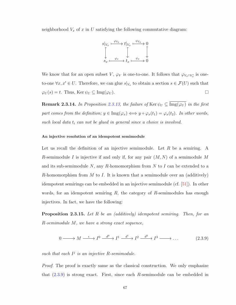
neighborhood Vx of x in U satisfying the following commutative diagram:

s|Vx t|Vx 0

sx tx 0

ϕVx ψVx

ϕx ψx

We know that for an open subset V , ϕV is one-to-one. It follows that ϕVx∩V ′xis one-

to-one ∀x, x′ ∈ U . Therefore, we can glue s|Vx to obtain a section s ∈ F(U) such that

ϕU(s) = t. Thus, KerψU ⊆ Img(ϕU).

Remark 2.3.14. In Proposition 2.3.13, the failure of KerψU ⊆ Img(ϕU) in the first

part comes from the definition; y ∈ Img(ϕx) ⇐⇒ y+ϕx(t1) = ϕx(t2). In other words,

such local data ti can not be glued in general since a choice is involved.

An injective resolution of an idempotent semimodule

Let us recall the definition of an injective semimodule. Let R be a semiring. A

R-semimodule I is injective if and only if, for any pair (M,N) of a semimodule M

and its sub-semimodule N , any R-homomorphism from N to I can be extended to a

R-homomorphism from M to I. It is known that a semimodule over an (additively)

idempotent semirings can be embedded in an injective semimodule (cf. [51]). In other

words, for an idempotent semiring R, the category of R-semimodules has enough

injectives. In fact, we have the following:

Proposition 2.3.15. Let R be an (additively) idempotent semiring. Then, for an

R-semimodule M , we have a strong exact sequence,

0 M I0 I1 I2 I3 . . .ϵ d0 d1 d2 (2.3.9)

such that each Ij is an injective R-semimodule.

Proof. The proof is exactly same as the classical construction. We only emphasize

that (2.3.9) is strong exact. First, since each R-semimodule can be embedded in

67

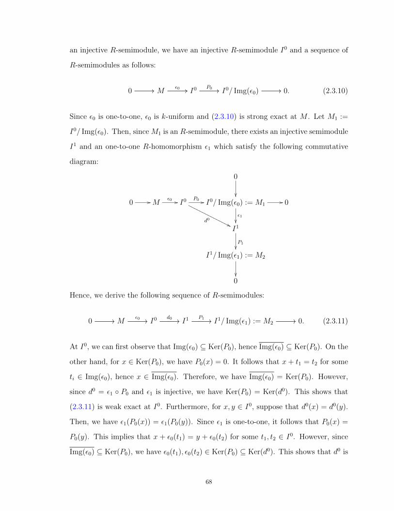
an injective R-semimodule, we have an injective R-semimodule I0 and a sequence of

R-semimodules as follows:

0 M I0 I0/ Img(ϵ0) 0.ϵ0 P0 (2.3.10)

Since ϵ0 is one-to-one, ϵ0 is k-uniform and (2.3.10) is strong exact at M . Let M1 :=

I0/ Img(ϵ0). Then, sinceM1 is an R-semimodule, there exists an injective semimodule

I1 and an one-to-one R-homomorphism ϵ1 which satisfy the following commutative

diagram:

0

0 //M

ϵ0 // I0

d0''

P0 // I0/ Img(ϵ0) :=M1

ϵ1

// 0

I1

P1

I1/ Img(ϵ1) :=M2

0

Hence, we derive the following sequence of R-semimodules:

0 M I0 I1 I1/ Img(ϵ1) :=M2 0.ϵ0 d0 P1 (2.3.11)

At I0, we can first observe that Img(ϵ0) ⊆ Ker(P0), hence Img(ϵ0) ⊆ Ker(P0). On the

other hand, for x ∈ Ker(P0), we have P0(x) = 0. It follows that x+ t1 = t2 for some

ti ∈ Img(ϵ0), hence x ∈ Img(ϵ0). Therefore, we have Img(ϵ0) = Ker(P0). However,

since d0 = ϵ1 P0 and ϵ1 is injective, we have Ker(P0) = Ker(d0). This shows that

(2.3.11) is weak exact at I0. Furthermore, for x, y ∈ I0, suppose that d0(x) = d0(y).

Then, we have ϵ1(P0(x)) = ϵ1(P0(y)). Since ϵ1 is one-to-one, it follows that P0(x) =

P0(y). This implies that x + ϵ0(t1) = y + ϵ0(t2) for some t1, t2 ∈ I0. However, since

Img(ϵ0) ⊆ Ker(P0), we have ϵ0(t1), ϵ0(t2) ∈ Ker(P0) ⊆ Ker(d0). This shows that d0 is

68

k-uniform and hence (2.3.11) is strong exact at I0. One can inductively define Ij and

this gives the desired (strong) injective resolution.

Next, we construct an injective resolution of a sheaf of idempotent semimodules.

Proposition 2.3.16. Let R be a semiring. Let F , G be sheaves of R-semimodules on

a topological space X. Then a morphism ϕ : F −→ G is an isomorphism if and only

if the induced map ϕx : Fx −→ Gx is an isomorphism for each x ∈ X. In particular,

if ϕ is injective, then ϕx is injective for each x ∈ X.

Proof. The proof is identical to the classical case.

LetR be a semiring. For sheaves F , G ofR-semimodules, the sheaf homHom(F ,G)

is again a sheaf of R-semimodules. A subsheaf and a quotient sheaf are defined as

in the classical case. We define a sheaf I of R-semimodules is injective if I satisfies

the following condition: let (G,F) be a pair of a sheaf G and a subsheaf F . Then,

for any morphism ϕ : F −→ I of sheaves, there exists a morphism ψ : G −→ I such

that ψ i = ϕ, where i is an inclusion from F to G. We have the following:

Proposition 2.3.17. Let (X,OX) be a locally semiringed space such that OX,x is an

idempotent semiring for each x ∈ X. Let F be a sheaf of OX-semimodules. Then,

we have the following strong exact sequence of OX-semimodules:

0 F I0 I1 I2 I3 . . .ϵ d0 d1 d2

such that each Ij is an injective sheaf of OX-semimodules.

Proof. Since the category of idempotent semimodules has enough injectives (Propo-

sition 2.3.15) and has limits, products, the proof is same as the classical case. More

precisely, each stalk Fx can be embedded in an injective OX,x-semimodule Ix from

Proposition 2.3.15. As in the classical construction of an injective resolution, we de-

fine I0 :=

x∈X j∗(Ix), where j∗(Ix) is the sheaf such that j∗(Ix)(U) = Ix if x ∈ U

and 0 otherwise. The exact same argument as in the classical case shows that I0 is

69

an injective sheaf of OX-semimodules and the sequence

0 F I0ϵ

is a strong exact sequence from the definition and Proposition 2.3.15. By using

the quotient sheaf I0/F , we can define inductively Ij and hence obtain the desired

injective resolution which is strong exact.

Corollary 2.3.18. Let X is a topological space. Then, the category of sheaves of

idempotent semigroups on X has enough injectives.

Proof. One can impose the constant sheaf B of the idempotent semifield B on X.

Then, (X,B) satisfies the condition of Proposition 2.3.17 and the category of sheaves

of idempotent semigroups is indeed the category of sheaves of B-semimodules.

Remark 2.3.19. Assume that a sheaf F of OX-semimodules has an injective reso-

lution which is both strong and half. Then, it follows from Proposition 2.3.13 that

H0(X,F) = Γ(X,F). However, by far, Proposition 2.3.17 is the best result we have.

Moreover, even if we can find an injective resolution which is both strong and half,

we have to show that two such resolutions are homotopic in order to properly define

the sheaf cohomology. There is some evidence that the derived functors approach to

sheaf cohomology might not be a good way to pursue. More precisely, in [28], Oliver

Lorscheid computed the sheaf cohomology of the projective line P1F1

over F1 via an

injective resolution, however, the computation is not in accordance with the classical

result. For example, H1(P1F1,OP1

F1) is an infinite-dimensional F1-vector space whereas

classically, we have H1(P1,OP1) = 0. Although this is the case of a monoid scheme,

this suggests that one might have to look for other possible approaches.

In the next subsection, we directly generalize Cech cohomology theory and show that

several classical properties are still valid in such framework. In particular, the general-

ized Cech cohomology of the projective line P1Qmax

over Qmax is similar to the classical

case. Moreover, for a semi-scheme (X,OX), we verify the classical cohomological

70

interpretation of a Picard group; Pic(X) ≃ H1(X,O∗X).

2.3.2 Cech cohomology

In [37], Alex Patchkoria generalized the notion of a chain complex of modules to

semimodules. The main idea is that one may consider an alternating sum as the sum

of two sums for which stand for a positive sum and a negative sum respectively. In

this subsection, we use this idea to define Cech cohomology with values in sheaves of

semimodules. Then we compute the simple example of the projective line P1Qmax

over

Qmax.

Definition 2.3.20. (cf. [37])

1. Let R be a semiring. One says that a sequence of R-semimodules and R-

homomorphisms,

X : · · ·∂−n−2

//∂+n−2 //

Xn−1

∂−n−1

//∂+n−1 //

Xn

∂−n

//∂+n //

Xn+1

∂−n+1

//∂+n+1 // · · · , n ∈ Z,

written X = Xn, ∂+n , ∂−n for short, is a cochain complex if

∂+n+1 ∂+n + ∂−n+1 ∂−n = ∂−n+1 ∂+n + ∂+n+1 ∂−n , n ∈ Z. (2.3.12)

2. For a cochain complex X, one defines the following R-semimodule:

Zn(X) := x ∈ Xn | ∂+n (x) = ∂−n (x)

as n-cocycles, and the n-th cohomology as an R-semimodule

Hn(X) := Zn(X)/ρn,

where ρn is a congruence relation on Zn(X) such that xρny if and only if

x+ ∂+n−1(u) + ∂−n−1(v) = y + ∂+n−1(v) + ∂−n−1(u) for some u, v ∈ Xn−1. (2.3.13)

71

Suppose that X = Xn, d+n , d−n and Y = Y n, ∂+n , ∂

−n are cochain complexes of

semimodules. Then, by a ±-morphism from X to Y one means a collection f = fn

of homomorphisms of semimodules which satisfies the following condition:

fn+1 d+n = ∂+n fn, fn+1 d−n = ∂−n fn. (2.3.14)

In [37], it is proven that a ±-morphism f = fn from X = Xn, d+n , d−n to Y =

Y n, ∂+n , ∂−n induces a canonical homomorphism Hn(f) of cohomology semimodules

as follows:

Hn(f) : Hn(X) −→ Hn(Y ), [x] →→ [fn(x)], n ∈ Z, (2.3.15)

where [x] is the equivalence class of x ∈ Zn(X) in Hn(X).

Remark 2.3.21. As pointed out in [37], a sequence G = Gn, d+n , d−n of modules is

a cochain complex in the sense of Definition 2.3.20 if and only if G′ = Gn, ∂n :=

d+n − d−n is a cochain complex of modules in the classical sense. Clearly, in this case,

the cohomology semimodules of G as in Definition 2.3.20 is the cohomology modules

of G′ in the classical sense.

By means of Definition 2.3.20, we introduce Cech cohomology with values in

sheaves of semimodules which generalizes the classical construction. Let R be a

semiring, X be a topological space, and F be a sheaf of R-semimodules on X. Sup-

pose that U = Uii∈I is an open covering of X, where I is a totally ordered set. Let

Ui0,i1...,ip := Ui0 ∩ ... ∩ Uip . Then, as in the classical case, we define the following set:

Cn = Cn(U ,F) :=

i0<...<in

F(Ui0,i1,...,in), n ∈ N. (2.3.16)

Let xi0,...,in be the coordinate of x ∈ Cn in F(Ui0,i1,...,in). The differentials are given

as follows:

(d+n (x))i0,i1,...,in+1 =n+1

k=0,k=even

xi0,...ik,...,in+1|Ui0,i1,...,in+1

, (2.3.17)

72

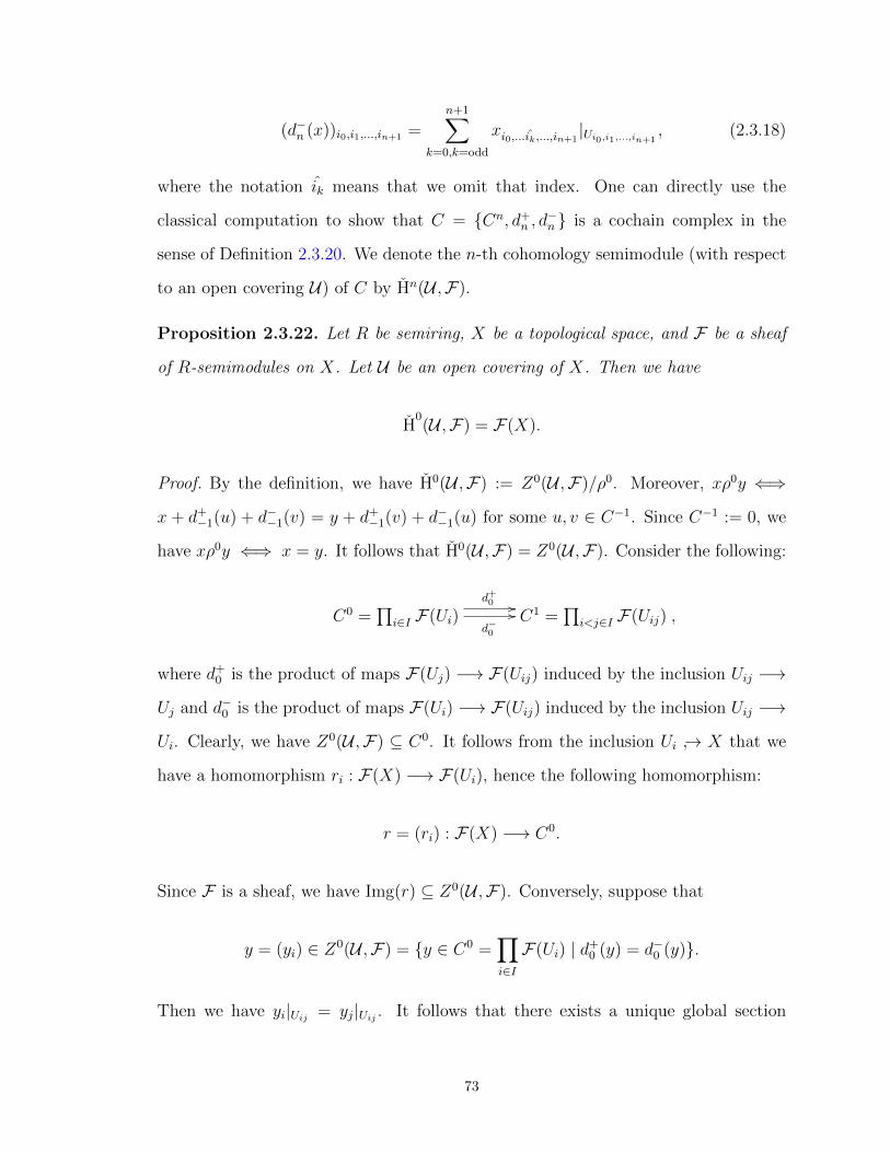
(d−n (x))i0,i1,...,in+1 =n+1

k=0,k=odd

xi0,...ik,...,in+1|Ui0,i1,...,in+1

, (2.3.18)

where the notation ik means that we omit that index. One can directly use the

classical computation to show that C = Cn, d+n , d−n is a cochain complex in the

sense of Definition 2.3.20. We denote the n-th cohomology semimodule (with respect

to an open covering U) of C by Hn(U ,F).

Proposition 2.3.22. Let R be semiring, X be a topological space, and F be a sheaf

of R-semimodules on X. Let U be an open covering of X. Then we have

H0(U ,F) = F(X).

Proof. By the definition, we have H0(U ,F) := Z0(U ,F)/ρ0. Moreover, xρ0y ⇐⇒

x + d+−1(u) + d−−1(v) = y + d+−1(v) + d−−1(u) for some u, v ∈ C−1. Since C−1 := 0, we

have xρ0y ⇐⇒ x = y. It follows that H0(U ,F) = Z0(U ,F). Consider the following:

C0 =

i∈I F(Ui)d−0

//d+0 //

C1 =

i<j∈I F(Uij) ,

where d+0 is the product of maps F(Uj) −→ F(Uij) induced by the inclusion Uij −→

Uj and d−0 is the product of maps F(Ui) −→ F(Uij) induced by the inclusion Uij −→

Ui. Clearly, we have Z0(U ,F) ⊆ C0. It follows from the inclusion Ui → X that we

have a homomorphism ri : F(X) −→ F(Ui), hence the following homomorphism:

r = (ri) : F(X) −→ C0.

Since F is a sheaf, we have Img(r) ⊆ Z0(U ,F). Conversely, suppose that

y = (yi) ∈ Z0(U ,F) = y ∈ C0 =i∈I

F(Ui) | d+0 (y) = d−0 (y).

Then we have yi|Uij= yj|Uij

. It follows that there exists a unique global section

73

yX ∈ F(X) such that (yX)|Ui= yi. Consider the following map:

s : Z0(U ,F) −→ F(X), y →→ yX .

Then s is clearly an R-homomorphism. Furthermore, rs and sr are identity maps.

This shows that H0(U ,F) = F(X) for an open covering U of X.

Proposition 2.3.23. Let R be semiring, X be a topological space, and F be a sheaf

of R-semimodules on X. Let U be an open covering of X which consists of n proper

open subsets of X. Then Hm(U ,F) = 0 ∀m ≥ n.

Proof. The proof is identical to that of the classical case since Cm = 0 for m ≥ n.

We say that a covering V = Vjj∈J of a topological space X is a refinement of

another covering U = Uii∈I if there exists a map σ : J −→ I such that Vj ⊆ Uσ(j)

for each j ∈ J . Suppose that Xn := Cn(U ,F) and Y n := Cn(V ,F). Then the map

σ induces the following ±-morphism:

σn : Xn −→ Y n, σn(x)j0,...,jn = xσ(j0),...,σ(jn)|Vj0,...,jn . (2.3.19)

In fact, let X = Xn, d+n , d−n and Y = Y n, ∂+n , ∂

−n . We have

(σn+1 d+n (x))j0,...,jn+1 = (d+n (x))σ(j0),...,σ(jn+1)|Vj0,...,jn+1

= (n+1

k=0,k=even

xσ(j0),..., ˆσ(jk),σ(jn+1)|Uσ(j0),...,σ(jn+1)

)|Vj0,...,jn+1

= (n+1

k=0,k=even

xσ(j0),..., ˆσ(jk),σ(jn+1))|Vj0,...,jn+1

=n+1

k=0,k=even

σn(x)j0,...,jk,...,jn+1|Vj0,...,jn+1

= (∂+n σn(x))j0,...,jn+1 .

Hence, we obtain σn+1d+n = ∂+n σn. Similarly one can prove that ∂n+1d−n = ∂−n σn.

The ±-morphism σ = σn induces a homomorphism, Hn(U ,F) −→ Hn(V ,F).

74

The collection of open coverings of a topological space X becomes a directed sys-

tem (with a refinement as a partial order). Since (co)limits exist in the category of

semimodules, the following definition is well defined.

Definition 2.3.24. Let R be a semiring. Let X be a topological space and F be a

sheaf of R-semimodules on X. We define the n-th Cech cohomology of X with values

in F as follows:

Hn(X,F) := lim−→

UHn(U ,F).

Note that from Proposition 2.3.22, we have H0(X,F) = F(X).

Example 2.3.25. Consider the projective line X = P1Qmax

over Qmax. More precisely,

we consider X as the semi-scheme with two open affine charts U0 := SpecQmax[T ] and

U1 := SpecQmax[1T] glued along T →→ 1

T. As in the classical case, one observes that

OX(X) = Qmax. From Proposition 2.3.22, we have H0(X,OX) = Qmax. Furthermore,

since X has the open covering U = U0, U1 which consists of two proper open subsets

of X, we have Hn(X,OX) = 0 for n ≥ 2 from Proposition 2.3.23. Finally, with respect

to the covering U = U0, U1, we have

C : OX(U0)⊕OX(U1)d−0

//d+0 // OX(U01)

d−1

//d+1 //

0 .

In other words, we have

C : Qmax[T ]⊕Qmax[1T]

d−0

//d+0 //

Qmax[T,1T]

d−1

//d+1 //

0 ,

where d+0 (a, b) = b and d−0 (a, b) = a. It follows that Z1(U ,OX) = Qmax[T,1T]. Let

x, y ∈ Z1(U ,OX). Then, we can write x = x0+x1, y = y0+y1, where x0, y0 ∈ Qmax[T ]

and x1, y1 ∈ Qmax[1T]. Let u = (x0, y1), v = (y0, x1). Then, we have

x+ d+0 (u) + d−0 (v) = y + d+0 (v) + d−0 (u).

75

It follows that xρ1y and hence H1(U ,OX) = 0. However, this computation depends

on the specific covering U since different from the classical case, we do not know yet

whether H1(X,OX) = H

1(U ,OX) or not. We remark that the above computation is

also valid when we replace Qmax with other totally ordered semifields.

Next, we prove that the Picard group Pic(X) of a semi-scheme X is isomorphic

to the first Cech cohomology group of the sheaf O∗X . The proof is not much different

from the classical case, however, we include the proof for the completeness. Note that

O∗X is the sheaf such that O∗

X(U) = a ∈ OX(U) | ab = 1 for some b ∈ OX(U) for

an open subset U of X. Even though OX is a sheaf of semirings, O∗X is a sheaf of

(multiplicative) abelian groups. Hence, H1(U ,O∗X) is an abelian group. We use the

multiplicative notation for O∗X .

In what follows, let X be a semi-scheme, L be an invertible sheaf of OX-semimodules

on X, and U = Uii∈I be a covering of X such that ϕi : OX |Ui≃ L|Ui

∀i ∈ I. Let

ei ∈ L(Ui) be the image of 1 ∈ OX(Ui) under ϕi(Ui). Through the following lemmas,

we define a corresponding cocyle in H1(X,O∗X) for an invertible sheaf L on X.

Lemma 2.3.26. For i < j ∈ I and Uij = Ui ∩ Uj, there exists fij ∈ O∗X(Uij) such

that

ei|Uij= (ej|Uij

)fij.

Proof. This is clear since ei|Uijand ej|Uij

are invertible elements in O∗X(Uij).

We fix fij in Lemma 2.3.26. We have the following:

Lemma 2.3.27. Let f := (fij) ∈ C1(U ,O∗X). Then we have d+1 (f) = d−1 (f) and

hence f ∈ Z1(U ,O∗X). In particular, f has the canonical image in H

1(U ,O∗

X).

Proof. For i < j < k, we have ei|Uij= (ej|Uij

)fij, ej|Ujk= (ek|Ujk

)fjk. Thus we have

ei|Uijk= (ej|Uijk

)(fij)|Uijk= (ek|Uijk

)(fjk)|Uijk(fij)|Uijk

= ek|Uijk(fik)|Uijk

.

This implies that (fjk)|Uijk(fij)|Uijk

= (fik)|Uijk. It follows that (d+1 (f))ijk = (d−1 (f))|ijk

76

and hence f = (fij) ∈ Z1(U ,O∗X). Therefore, f has the canonical image in H1(U ,O∗

X).

Lemma 2.3.28. The canonical image of f ∈ C1(U ,O∗X) in H

1(U ,O∗

X) as in Lemma

2.3.27 does not depend on the choice of ei.

Proof. Let e′ii∈I be another choice with f ′ij. We can take gii∈I , where gi ∈

O∗X(Ui) such that e′i = giei. Then, we have ei|Uij

= fijej|Uij, e′i|Uij

= f ′ije

′j|Uij

. It

follows that gi|Uijei|Uij

= f ′ijgj|Uij

e′j|Uij= f ′

ijgj|Uijej|Uij

and gi|Uijei|Uij

= gi|Uijfijej|Uij

.

Therefore, fijgi|Uij= f ′

ijgj|Uij. This implies that f ·d−0 (g) = f ′ ·d+0 (g). In other words,

f and f ′ give the same canonical image in H1(U ,O∗X).

We denote the canonical image of f ∈ C1(U ,O∗X) in H1(U ,O∗

X) by φU(L). Let

U = Uii∈I and U ′ = Vjj∈J be two open coverings of X such that L|Ui≃ OX |Ui

and L|Vj ≃ OX |Vj ∀i ∈ I, j ∈ J . We define a new covering U ∩U ′ := Ui∩Uj(i,j)∈I×J

of X. Then, clearly U ∩U ′ is a refinement of U . It follows that φU(L) has a canonical

image in H1(U ∩ U ′,O∗

X).

Lemma 2.3.29. Let U = Uii∈I and U ′ = Vjj∈J be two open coverings of X

such that L|Ui≃ OX |Ui

and L|Vj ≃ OX |Vj ∀i ∈ I, j ∈ J . Let f ∈ C1(U ,O∗X) and

f ′ ∈ C1(U ′,O∗X) (as in Lemma 2.3.27). Then the canonical images of f and f ′ are

same in H1(U ∩ U ′,O∗

X). In particular, each invertible sheaf L determines a unique

element φ(L) in H1(X,O∗

X).

Proof. Let eii∈I , fiji,j∈I for U and e′jj∈J , f ′klk,l∈J for U ′ as in Lemma 2.3.26.

We claim that the images of φU(L) and φU ′(L) in H1(U ∩ U ′,O∗X) are equal. Indeed,

we can find gik ∈ O∗X(Ui ∩ Vk) such that e′k|Ui∩Vk = (gik)ei|Ui∩Vk . Hence, from the

relation e′k|Uij∩Vkl = (f ′kl)|Uij∩Vkl · e′l|Uij∩Vkl , we have that (gik)|Uij∩Vkl · ei|Uij∩Vkl =

(f ′kl)|Uij∩Vkl · e′l|Uij∩Vkl = (f ′

kl)|Uij∩Vkl · (gjl)|Uij∩Vkl · ej|Uij∩Vkl . It follows that

(gik)|Uij∩Vkl · (fij)|Uij∩Vkl = (f ′kl)|Uij∩Vkl · (gjl)|Uij∩Vkl . (2.3.20)

77

Let g = (gik) for i ∈ I, k ∈ J . Then, we have g ∈ C0(U ∩ U ′,O∗X). Give the set I × J

a dictionary order. Then we have

(d+0 (g))|(i,k)×(j,l) = gjl|Uij∩Vkl and (d−0 (g))|(i,k)×(j,l) = gik|Uij∩Vkl . (2.3.21)

Let α : Z1(U ,O∗X) −→ Z1(U ∩ U ′,O∗

X) be the ±-morphism as in (2.3.19). Then α

induces the map α :H1(U ,O∗X) −→H1(U ∩ U ′,O∗

X). Similarly, for U ′, we obtain

β : Z1(U ′,O∗X) −→ Z1(U ∩ U ′,O∗

X), β : H1(U ′,O∗

X) −→ H1(U ∩ U ′,O∗

X).

In particular, if φU(L) = [f ], then α([f ]) = [α(f)], where [f ] is the equivalence class of

f ∈ Z1(U ,O∗X) in H1(U ,O∗

X). To complete the proof, we have to show that [α(f)] =

[β(f ′)]. We know that α(f)(i,k)×(j,l) = fij|Uij∩Vkl and β(f ′)(i,k)×(j,l) = f ′kl|Uij∩Vkl . It

follows from (2.3.20) and (2.3.21) that

(α(f) · d−0 (g))|Uij∩Vkl = (β(f ′) · d+0 (g))|Uij∩Vkl .

This proves that [α(f)] = [β(f ′)]. Thus, f and f ′ have the same image in H1(X,O∗X).

We denote this image by φ(L).

Consider the following map:

φ : Pic(X) −→ H1(X,O∗

X), [L] →→ φ(L),

where [L] is the isomorphism class of L in Pic(X).

Lemma 2.3.30. φ is well defined.

Proof. Suppose that L ≃ L′. We have to show that φ(L) = φ(L′). Let us fix an

isomorphism ϕ : L −→ L′. We can find an open covering U = Uii∈I of X such that

on Ui both L and L′ are isomorphic to OX . Let ei and fij be as in Lemma 2.3.26

for L. Then we have ϕUij(ei)|Uij

= fij · ϕUij(ej)|Uij

. Since φ(L′) does not depend on

78

the choice of e′i, we let e′i = ϕUi(ei) as in Lemma 2.3.26 for L′. Then the desired

property follows.

Lemma 2.3.31. φ is a group homomorphism.

Proof. Suppose that L and L′ are invertible sheaves of OX-semimodules. Then, so is

L⊗OXL′ (directly follows from Lemma 2.2.12). Therefore, we can find an affine open

covering U = Ui = SpecRii∈I of X such that (L⊗OXL′)(Ui) ≃ OX(Ui) ≃ L(Ui) ≃

L′(Ui) ≃ Ri. In particular, we have (L⊗OXL′)(Ui) ≃ (L(Ui)⊗OX

L′(Ui)). Let eii∈I ,

fiji,j∈I for L and e′jj∈J , f ′klk,l∈J for L′ as in Lemma 2.3.26 on the open covering

U . Then, we can take ei ⊗ e′i as a basis for (L ⊗OXL′)(Ui) and the corresponding

transition map is F = (fij · f ′ij). It follows that φ(L ⊗OX

L′) = φ(L)φ(L′).

Lemma 2.3.32. φ([L]) = 1 if and only if [L] is the isomorphism class of OX . In

particular, φ is injective.

Proof. Suppose that φ(L) = 1. Let U = Uii∈I be an open covering of X such that

L|Ui≃ OX |Ui

∀i ∈ I and let f and ei be as in Lemma 2.3.26. Since the canonical

image of f does not depend on the choice of an open covering U , we may assume

that [f ] = [1] ∈H1(U ,O∗X). This implies that there exists g ∈ C0(U ,O∗

X) such that

d+0 (g) = f · d−0 (g). Hence, (d+0 (g))ij = (f · d−0 (g))ij and fij · gi|Uij= gj|Uij

. It follows

that (giei)|Uij= gi|Uij

ei|Uij= gi|Uij

fijej|Uij= gj|Uij

ej|Uij= (gjej)|Uij

. Thus, eigi

and ejgj agree on Uij and hence we can glue them to obtain the global isomorphism

ϕ : L −→ OX . Conversely, if L ≃ OX , then clearly φ(L) = 1. In fact, one can take

ei = e|Ui, where e is the identity in OX(X).

Lemma 2.3.33. φ is surjective.

Proof. Notice that α ∈H1(X,O∗X) comes from [f ] ∈H1(U ,O∗

X) for an open covering

U = Uii∈I of X. Let Li := OX |Uifor each i ∈ I. Let f = (fij) ∈ Z1(U ,O∗

X). Then,

for i < j, each fij defines the following isomorphism:

φij : Li|Uij−→ Lj|Uij

, s →→ fij · s.

79

We define φii := id. Since f ∈ Z1(U ,O∗X), we have d+1 (f) = d−1 (f). It follows

that (d+1 (f))ijk = fjk · fij = (d−1 (f))ijk = fik, and fij · fjk = fik. This implies that

φik = φjk φij and therefore one can glue Li to obtain the invertible sheaf L. Let

ei be the image of 1 under the isomorphism OX(Ui) ≃ L(Ui). Then, we obtain the

corresponding f = (fij). This implies that φ([L]) = α, hence φ is surjective.

Finally, we conclude the following theorem via the isomorphism φ.

Theorem 2.3.34. Pic(X) ≃H1(X,O∗X) for a semi-scheme (X,OX).

Example 2.3.35. Consider the semifield Qmax(T ). We first compute the invertible

elements of the semiring B := Qmax[T ]. If f(T ) =n

i=0 aiTi is an invertible element

of B, then there exists g(T ) =m

i=0 biTi such that

f(T )⊙ g(T ) =n+mi=0

(maxr+l=i

ar + bl)T i = 1B = 0.

This implies that maxr+l=iar + bl := ci = −∞ for i ≥ 1. Hence, aj = bj = −∞ for

j ≥ 1 and f(T ) ∈ Q.

Next, let A := Qmax[T,1T] and A∗ be the set of elements in A which is multiplicatively

invertible (In particular, A∗ is an abelian group). If f(T ) ∈ A∗, then there exists

k ∈ N such that T kf(T ) ∈ B. This implies that T kf(T ) ∈ Q from the first case.

Since T k for k ∈ Z is invertible in A, we conclude that A∗ = qT n | q ∈ Q, n ∈ Z.

Let X := P1Qmax

and U = U1, U2 be an open covering of X such that U1 ≃

SpecQmax[T ] and U2 ≃ SpecQmax[1T]. From the above computation, we have O∗

X(Ui) =

Q and O∗X(U1 ∩ U2) = A∗ = qT n | q ∈ Q, n ∈ Z. Then, we have the following Cech

complex:

C : C0 = Q×Qd−0

//d+0 //

C1 = A∗d−1

//d+1 //

0 ,

where d+0 (a, b) = b, d−0 (a, b) = a. Clearly, we have C1 = Z1(U ,O∗X). Two elements

qT n and q′T n′in A∗ are equivalent if and only if there exist c = (a, b), c′ = (a′, b′) ∈ C0

80

such that

qT n ⊙ d+0 (c)⊙ d−0 (c′) = q′T n

′ ⊙ d+0 (c′)⊙ d−0 (c). (2.3.22)

However, (2.3.22) holds if and only if n = n′. Therefore, we have

H1(U ,O∗

X) = C1/ρ1 = T n | n ∈ Z ≃ Z.

This is coherent with the classical result.

Example 2.3.36. Note that, different from the classical case, Qmax[T ] is not multi-

plicatively cancellative. Therefore the canonical map, S−1 : Qmax[T ] −→ S−1Qmax[T ]

does not have to be injective. In tropical geometry, rather than working directly with

Qmax[T ], one works with the semiring Qmax[T ] := Qmax[T ]/ ∼, where ∼ is a con-

gruence relation such that f(T ) ∼ g(T ) ⇐⇒ f(x) = g(x) ∀x ∈ Qmax (see, §2.4.2

for details about Qmax[T ] together with the classification of valuations on it). Let

B := Qmax[T ]. If f(T ) ∈ B is multiplicatively invertible, then there exists g(T ) such

that f(T )⊙ g(T ) = 1B = 0. However, for l ∈ Qmax, the set l consists of a single

element l. It follows that f(T ) ⊙ g(T ) = 0. From Example 2.3.35, this implies that

f(T ) ∈ Q and hence B∗ = Q. Let S = 1, T , T 2, ... be a multiplicative subset of B,

and A := S−1B. Since B is multiplicatively cancellative (cf. Corollary 2.4.17), B is

canonically embedded into A. Moreover, similar to Example 2.3.35, one can observe

that A∗ = qT n | q ∈ Q, n ∈ Z.

Suppose that the projective line X := P1 over Qmax is the semi-scheme such that

two affine semi-schemes SpecQmax[T ] and SpecQmax[1T] are glued along SpecA. The

exact same argument as in Example 2.3.35 shows the following:

H1(X,O∗

X) = Z.

Remark 2.3.37. One can observe that Example 2.3.35 also shows that any invertible

sheaf L on P1Qmax

should be isomorphic to OX(n) for some n ∈ Z. This classifies all

invertible sheaves on P1Qmax

as in the classical case.

81

Remark 2.3.38. Since differential maps of many (co)homology theories are defined

by alternating sums, it seems that many of those theories can be directly generalized by

using the above framework. For example, if k is a semifield, then Hochschild homology

can be computed via the above framework and the result is same as classical case, i.e.

HH0(k) = k and HHn(k) = 0 for all n > 0.

2.4 Valuation theory over semi-structures

As in the classical case, one might expect that a theory of valuations over semi-

structures provides some geometric information. To shape a theory of valuations

over semi-structures, one first needs to find proper definitions. We will provide three

possible approaches and compute toy examples for each. The first definition directly

extends the definition of classical valuation. The second definition comes from the

observation that for a valuation ν, we have ν(a + b) ∈ ν(a), ν(b) if ν(a) = ν(b).

In the last approach, we shall make use of hyperfields instead of the field R of real

numbers. This is related with the probabilistic intuition: when ν(a) = ν(b), the value

ν(a + b) is not solely determined by ν(a) and ν(b). In the sequel, by an idempotent

semiring we mean a semiring S such that x+x = x ∀x ∈ S. An idempotent semiring

S has a canonical partial order ≤ such that x ≤ y ⇐⇒ x+ y = y ∀x, y ∈ S.

Remark 2.4.1. In fact, a theory of valuations over semirings has been introduced

in [22], but has not been studied in the perspective of F1-geometry. Our goal in this

section is to find an analogue of abstract curves in characteristic one. Furthermore,

the authors of [22] had more concentrated on supertropical semirings which are more

generalized objects than semirings.

Definition 2.4.2. Let S be an idempotent semiring. A valuation on S is a function

ν : S −→ R ∪ ∞ which satisfies the following conditions:

1. ν(x) = ∞ ⇐⇒ x = 0S.

2. ν(xy) = ν(x) + ν(y), where + is the usual addition of R.

82

3. minν(x), ν(y) ≤ ν(x+ y) ∀x, y ∈ S.

Remark 2.4.3. The third condition is redundant in some cases. For example, if S is

a semiring of characteristic one, i.e. x+y ∈ x, y ∀x, y ∈ S, then the third condition

is automatic.

Definition 2.4.4. ( [22, Definition 2.2]) Let S be an idempotent semiring. A strict

valuation on S is a function ν : S −→ Rmax which satisfies the following conditions:

1. ν(x) = −∞ ⇐⇒ x = 0S.

2. ν(xy) = ν(x) + ν(y), where + is the usual addition of R.

3. ν(x+ y) = maxν(x), ν(y) ∀x, y ∈ S.

In other words, a strict valuation ν is a homomorphism of a semiring S to the semi-

fields Rmax which has a trivial kernel.

As we mentioned earlier, Definition 2.4.4 can be justified in the sense that ν(a+b) ∈

ν(a), ν(b) for ν(a) = ν(b) for a valuation ν on a commutative ring. Classically, the

third condition is a subadditivity condition. However, we force the third condition to

be an additivity condition and hence it is named a strict valuation. One can think of

the similar generalization over a hyperfield. To this end, we introduce the following

hyperfield.

Definition 2.4.5. The hyperfield R+,val has an underlying set as R ∪ −∞. The

addition ⊕ is defined as follows: for x, y ∈ R+,val,

x⊕ y =

maxx, y if x = y

[−∞, x] if x = y

The multiplication ⊙ is given by the usual addition of real numbers with a⊙ (−∞) =

−∞ for a ∈ R ∪ −∞.

The addition of R+,val is designed to capture the information we loose when ν(x) =

83

ν(y) since, in this case, ν(x+y) can be any number less than or equal to ν(x). We first

have to show that the above definition makes sense, i.e. R+,val is indeed a hyperfield.

Proposition 2.4.6. R+,val is a hyperfield.

Proof. To avoid any notational confusion, let us use ⊕, ⊙ for the addition and the

multiplication of R+,val. First, we show that R+,val is a canonical hypergroup. The

addition is clearly commutative. We show that

(x⊕ y)⊕ z = x⊕ (y ⊕ z).

The first case is when x = y = z; this is clear. The second case is when x, y, z are

all different. Then we have LHS = RHS = maxx, y, z. The third case is when

x = y is different from z. In this case, we have LHS = [−∞, x] ⊕ z. As the first

sub-case of this, if x < z, then we have LHS = z. On the other hand, in this case,

we have RHS = x ⊕ (y ⊕ z) = x ⊕ z = z. As the second sub-case of this, if z < x,

then LHS = [−∞, x] and RHS = x⊕ (y⊕ z) = x⊕ y = [−∞, x]. The fourth case is

when y = z is different from x; this is similar to the third case. The last case is when

x = z is different from y. As the first sub-case, if x < y, then LHS = y = RHS.

As the second sub-case, if y < x = z, then we have LHS = [−∞, x] = RHS. This

shows that ⊕ is associative. One can observe that −∞ is the additive identity, and

the additive inverse of x is x itself. For the reversibility property, let us assume that

x ∈ y ⊕ z. If y = z, then y ⊕ z = maxy, z. Hence, we may assume that y < z.

Then, x ∈ y ⊕ z means that x = z. Therefore, we have z ∈ x⊕ y = x. If y = z, then

we have x ∈ [−∞, y]. This implies that x ≤ y. In this case, we have z ∈ x⊕ y. This

shows that R+,val is a canonical hypergroup. From the definition, ⊙ is invertible. All

we have to show is the following:

x⊙ (y ⊕ z) = (x⊙ y)⊕ (x⊙ z).

This is trivial if x = −∞, hence we may assume that x = −∞. The first case is when

84

y⊕z is a single element. We may assume that y < z. Then LHS = x⊙z. On the other

hand, if y < z, then we have x⊙y < x⊙z. It follows that RHS = x⊙y⊕x⊙z = x⊙z.

The second case is when y = z, then we have y ⊕ z = [−∞, y]. Hence, we have

LHS = x ⊙ (y ⊕ z) = [−∞, x⊙ y]. On the other hand, since x ⊙ y = x ⊙ z in this

case, we have RHS = [−∞, x⊙ y]. Therefore, R+,val is a hyperfield.

Next, we define a valuation of an idempotent semiring with values in R+,val.

Definition 2.4.7. Let S be an idempotent semiring and H = R+,val. A valuation of

S with values in H is a function ν : S −→ H which satisfies the following conditions:

ν(x+ y) ∈ ν(x)⊕ ν(y), ν(xy) = ν(x)⊙ ν(y), ν(x) = −∞ ⇐⇒ x = 0S. (2.4.1)

We next define absolute values on an idempotent semiring which has values in

hyperfields. First, we recall the following three hyperfields (cf. [50]).

Definition 2.4.8. 1. The hyperfield T R has an underlying set as R. The addition

is defined as follows: for x, y ∈ T R,

x+ y =

x if |x| > |y|

y if |x| < |y|

y if x = y

[−|x|, |x|] if x = −y

and the multiplication is the usual multiplication of R.

2. The hyperfield R+, has the underlying set R≥0. The addition is defined as

follows: for x, y ∈ R+,,

x+ y = c ∈ R+, | |x− y| ≤ c ≤ x+ y,

and the multiplication is the usual multiplication of real numbers.

3. The hyperfield R+,Y has the underlying set R≥0. The addition is defined as

85

follows: for x, y ∈ R+,Y ,

x+ y =

maxx, y if x = y

[0, x] if x = y

and the multiplication is the usual multiplication of real numbers.

Definition 2.4.9. Let H be any of hyperfields in Definition 2.4.8 and S be an idem-

potent semiring. An absolute value on S with values in H is a function |−| : S −→ H

which satisfies the following conditions:

|x| = 0H ⇐⇒ x = 0S, |xy| = |x||y|, |x+ y| ∈ |x|+ |y| ∀x, y ∈ S. (2.4.2)

Note that in Definition 2.4.2, 2.4.4, and 2.4.7, we say that two valuations ν1, ν2 are

equivalent if there exists ρ > 0 such that ν1(x) = ρν2(x) ∀x ∈ S, where ρν2(x) is the

usual multiplication of real numbers. For Definition 2.4.9, since the second condition

is multiplicative, we say that two absolute values | − |1, | − |2 are equivalent if there

exists ρ > 0 such that |x|1 = |x|ρ2 ∀x ∈ S, where |x|ρ2 is the usual exponent of real

numbers.

Next, we let M = Qmax or Qmax(T ) and classify valuations and absolute values on

M up to equivalence.

2.4.1 The first example, Qmax

Proposition 2.4.10. Let M = Qmax. Then,

1. With Definition 2.4.2, the set of valuations onM is equal to R. There are exactly

three valuations on M up to equivalence.

2. With Definition 2.4.4, the set of strict valuations on M is equal to R≥0. There

are exactly two strict valuations on M up to equivalence.

3. With Definition 2.4.7, the set of valuations on M with values in R+,val is equal

to R≥0. There are exactly two valuations on M up to equivalence.

86

4. With Definition 2.4.9 together with any hyperfield in Definition 2.4.8, the set of

absolute values on M is equal to R≥1. There are exactly two absolute values of

M up to equivalence.

Proof. To avoid any possible confusion, let us denote by ⊕, ⊙ the addition and the

multiplication of M respectively.

1. In this case, as we previously remarked, the third condition is redundant since

M is of characteristic one. We claim that any valuation ν onM only depends on

the value ν(1). In fact, since Z is (multiplicatively) generated by 1 in Qmax, it

follows from the second condition that the value ν(1) determines ν(m) ∀m ∈ Z.

Moreover, for 1n, we have ν(1) = ν( 1

n⊙ ...⊙ 1

n) = nν( 1

n) and hence ν( 1

n) = 1

nν(1).

This implies that for mn∈ Q, we have ν(m

n) = m

nν(1). Conversely, let ν : M −→

R∪∞ be a function such that ν(ab) := a

bν(1) for some ν(1) = ∞. Then, clearly

ν is a valuation on M . It follows that the set of valuations on M is equal to R.

Next, suppose that ν1, ν2 are valuations onM such that ν(1) > 0, ν(2) > 0, then

they are equivalent. In fact, if we take ρ := ν1(1)ν2(1)

, then for x ∈ Qmax\−∞,

we have ν1(x) = xν1(1) = xρν2(1) = ρν2(x). Similarly, valuations ν1 and ν2 on

M with νi(1) < 0 are equivalent. Finally, ν(1) = 0 gives a trivial valuation.

Therefore, we have exactly three valuations up to equivalence.

2. In this case, we claim that a strict valuation ν is an order-preserving map.

Indeed, we have x ≤ y ⇐⇒ x ⊕ y = y. Suppose that x ≤ y. Then we have

ν(y) = ν(x ⊕ y) = ν(x) + ν(y) ⇐⇒ ν(x) ≤ ν(y). On the other hand, as in

the above case, a strict valuation ν only depends on ν(1). Since ν is an order-

preserving map and ν(0) = 0, it follows that ν(1) ≥ 0. Therefore, the set of

valuations on M is equal to R≥0. Moreover, if ν(1) = 0, then we have a trivial

valuation and strict valuations ν on M such that ν(1) > 0 are equivalent as in

the above case. Thus, in this case, there are exactly two strict valuations on M

up to equivalence.

87

3. In this case, a valuation ν on M is determined by ν(1) and ν(1) ≥ 0. In fact,

suppose that x ≤ y. Then we have

ν(x⊕ y) = ν(y) ∈ ν(x) + ν(y). (2.4.3)

Assume that ν(y) < ν(x). Then we have ν(x) + ν(y) = ν(x) and it follows

from (2.4.3) that ν(x) = ν(y) which is a contradiction. This shows that ν is

an order-preserving map. Furthermore, we have ν(0) = 0 since ν(0 ⊙ 0) =

ν(0) = ν(0) + ν(0) (· is the usual addition of real numbers). It follows that

ν(1) ≥ 0(= 1R+,val). Finally, similar to the first case, we have ν(a

b) = a

bν(1).

Conversely, it is clear that all maps which satisfy such properties are valuations

on M . Hence, the set of valuations on M is equal to R≥0. Furthermore, two

valuations ν1, ν2 on M with ν1(1), ν2(1) > 0 are equivalent as in the first case.

Hence, there are exactly two valuations on M up to equivalence.

4. First, consider when H = T R. Let | − | be an absolute value on M with

values in H. One can observe that |1| ≥ 0. Indeed, if |1| = t < 0, then we

have |12⊙ 1

2| = |1

2|2 = |1| = t < 0. However, this is impossible since |1

2| is a

real number. Thus, |1| ≥ 0. This implies that for x ∈ Qmax\−∞, we have

|x| ≥ 0. Next, we claim that the condition |x ⊕ y| ∈ |x| + |y| forces | − | to

be an order-preserving map. Indeed, if x ≤ y, then |x ⊕ y| = |y| ∈ |x| + |y|.

From the reversibility property of a hyperfield, we have |x| ∈ |y| − |y|, where

|y| − |y| = [−|y|, |y|]. Since |x|, |y| ≥ 0, it follows that |x| ≤ |y|. Finally, we

claim that 1 ≤ |1|. In fact, let |1| = α. Then we have α = |1| ≤ |n| = αn. From

the first condition of the definition, we have α = 0 and hence 1 ≤ α. Therefore,

as in the first case, an absolute value | − | on M is totally determined by the

value |1|. Conversely, any map | − | : M −→ H which satisfies the following

conditions: |1| ≥ 1, |mn| := |1|mn for m

n∈ Q, and |0M | = 0 is an absolute value

on M . Two absolute values on M with |1|1 = α > 1, |1|2 = β > 1 are equivalent

88

with ρ = logαlog β

. When |1| = α = 1, we have the trivial absolute value. Thus,

there are exactly two absolute values on M up to equivalence.

Next, consider when H = R+,. In this case, the third condition implies that if

x ≤ y, then |y| = |x ⊕ y| ∈ |x| + |y|. From the reversibility property, we have

|x| ∈ |y| − |y| = [0, 2|y|]. In particular,

|x| ≤ 2|y| if x ≤ y. (2.4.4)

Let |1| = α and 0 ≤ m < n for m,n ∈ Z. Then, we have |m| = αm, |n| = αn.

Moreover, it follows from (2.4.4) that |m| = αm ≤ 2|n| = 2αn and hence 12≤ αr

∀r > 0. This implies that |1| = α ≥ 1. Conversely, any such map is an absolute

value onM . Thus, the set of absolute values onM is equal to R≥1. Furthermore,

two absolute values with |1|1 = α > 1, |1|2 = β > 1 are equivalent with ρ = logαlog β

.

Similarly, when |1| = 1, we obtain the trivial absolute value. Therefore, there

are exactly two absolute values on M up to equivalence.

When H = R+,Y , it is similar to the above cases. For example, an absolute

value | − | on M is an order-preserving map and |1| ≥ 1. Furthermore, the exact

same argument shows that any two absolute values with |1|1 > 1, |1|2 > 1 are

equivalent. Similarly, when |1| = 1, we have the trivial valuation. Therefore,

there are exactly two absolute values up to equivalence.

Remark 2.4.11. Note that the hyperfields T R and R+,Y are defined to recast the

archimedean information on M and the hyperfield R+,∆ is defined to recast non-

archimedean information on M .

2.4.2 The second example, Qmax(T )

We begin with investigating Qmax[T ], the idempotent semiring of polynomials with

coefficient inQmax. In the sequel, we use the notations + and · for the usual operations

89

of Q. We use the notations ⊕,⊙ for the operations of Qmax[T ] and +t, ·t for Qmax.

For f(T ) =n

i=0 aiTi, g(T ) =

mi=0 biT

i ∈ Qmax[T ], suppose that n ≤ m. The

addition and the multiplication of Qmax[T ] are given as follows:

(f + g)(T ) =ni=0

maxai, biT i +m

i=n+1

biTi, (2.4.5)

(fg)(T ) =n+mi=0

(r+l=i

arbl)Ti =

n+mi=0

(maxr+l=i

ar + bl)T i. (2.4.6)

Note that we can consider the semifield Qmax as an algebraic closure of Zmax since

any polynomial equation with coefficients in Zmax has a (tropical) solution in Qmax.

However, different from the classical case, any polynomial in Qmax[T ] does not have

to be factored into linear polynomials. Consider the following example.

Example 2.4.12. Let P (T ) = T⊙2 ⊕ T ⊕ 3 ∈ Qmax[T ]. Then, T = 32is a tropical

solution of P (T ). Suppose that T⊙2 ⊕ T ⊕ 3 = (T ⊕ a) ⊙ (T ⊕ b). Then, we have

(T ⊕ a) ⊙ (T ⊕ b) = T⊙2 ⊕ maxa, b ⊙ T ⊕ (a + b). Thus, for P (T ) to be factored

into linear polynomials, we should have maxa, b = 1 and a + b = 3, however, this

is impossible. Hence, P (T ) can not be factored into linear polynomials.

To remedy this issue, in tropical geometry, one imposes a functional equivalence

relation on Qmax[T ] (cf. [18]). Recall that polynomials f(T ), g(T ) ∈ Qmax[T ] are

functionally equivalent, denoted by f(T ) ∼ g(T ), if f(t) = g(t) ∀t ∈ Qmax.

Proposition 2.4.13. For M = Qmax[T ], a functional equivalence relation ∼ on M

is a congruence relation.

Proof. Clearly, ∼ is an equivalence relation. Suppose that f(T ) ∼ g(T ) and h(T ) ∼

q(T ). Then, we have to show that f(T ) ⊕ h(T ) ∼ g(T ) ⊕ q(T ) and f(T ) ⊙ h(T ) ∼

g(T )⊙ q(T ). Let f(T ) =n

i=0 aiTi, g(T ) =

mi=0 biT

i. It is enough to show that

(f ⊕ g)(x) = f(x) +t g(x), (f ⊙ g)(x) = f(x) ·t g(x) ∀x ∈ Qmax.

90

We may assume that n ≤ m. Then we have

(f ⊕ g)(T ) =ni=0

maxai, biT i ⊕m

i=n+1

biTi.

For x ∈ Qmax, we have, by letting ai = −∞ for i = n+ 1, ...,m,

(f ⊕ g)(x) = maxi=0,...,m

maxai, bi+ ix.

However, f(x) = maxi=0,...nai + ix and g(x) = maxi=0,...mbi + ix, thus

f(x) +t g(x) = maxf(x), g(x) = max maxi=0,...,n

ai + ix, maxi=0,...,m

bi + ix

= maxi=0,...,m

maxai, bi+ ix = (f ⊕ g)(x).

This proves the first part. Next, we have

(f ⊙ g)(T ) =n+mi=0

(r+l=i

arbl)Ti =

n+mi=0

(maxr+l=i

ar + bl)T i.

It follows that for x ∈ Qmax, we have

(f ⊙ g)(x) = max0≤i≤n+m

maxr+l=i

ar + bl+ ix = max0≤i≤n+m

maxr+l=i

ar + rx+ bl + lx.

On the other hand, we have

f(x) ·t g(x) = max0≤i≤n

ai + ix+ max0≤j≤m

bj + jx.

Thus, if f(x) = ai0 + i0x and g(x) = bj0 + j0x for some i0 and j0, then we have

f(x) ·t g(x) = (ai0 + i0x) + (bj0 + j0x) = (ai0 + bj0) + (i0 + j0)x.

It follows that f(x) ·t g(x) ≤ (f ⊙ g)(x). But, if (f ⊙ g)(x) = (ar0 + r0x) + (bl0 + l0x),

then (f ⊙ g)(x) ≤ f(x) ·t g(x). Hence, (f ⊙ g)(x) = f(x) ·t g(x).

91

From Proposition 2.4.13, the set Qmax[T ] := Qmax[T ]/ ∼ is an idempotent semir-

ing. In fact, Qmax[T ] is a semiring since ∼ is a congruence relation. Furthermore,

for f(T ) ∈ Qmax[T ], we have f(x) +t f(x) = f(x) ∀x ∈ Qmax. This implies that

f(T )⊕ f(T ) ∼ f(T ) and hence Qmax[T ] is an idempotent semiring. It is known that,

for Qmax[T ], the fundamental theorem of tropical algebra holds. i.e. a polynomial

P (T ) ∈ Qmax[T ] can be uniquely factored into linear polynomials in Qmax[T ] (cf. [43]

or [48]). In particular, this implies that the notion of a degree of f(T ) ∈ Qmax[T ]

is well-defined. Furthermore, Qmax[T ] does not have any multiplicative zero-divisor.

Indeed, suppose that f(T ) · g(T ) = (fg)(T ) ∼ (−∞). Then, for x ∈ Qmax, we have

f(x) ·t g(x) = f(x) + g(x) = −∞. In other words, for x ∈ Qmax, we have f(x) = −∞

or g(x) = −∞. However, this only happens when f(T ) = −∞ or g(T ) = −∞. Thus,

Qmax[T ] does not have a multiplicative zero-divisor. In fact, in Corollary 2.4.17, we

shall prove that Qmax[T ] satisfies the stronger condition: Qmax[T ] is multiplicatively

cancellative.

Next, we prove several lemmas to classify valuations on Qmax(T ).

Lemma 2.4.14. Let M := Qmax[T ]. For f(T ) ∈ M , let rf be the maximum natural

number such that Trf

can divide f(T ). Then, for f(T ), g(T ) ∈M , we have

rf⊕g = minrf , rg, rf⊙g = rf + rg.

Proof. Let f(T ), g(T ) ∈ Qmax[T ]. We first claim that if f(T ) has a constant term

and g(T ) does not have a constant term, then f(T ) and g(T ) are not functionally

equivalent. Indeed, if f(T ) =aiT

i and g(T ) =biT

i, then f(−∞) = a0 = −∞ =

g(−∞). One can further observe that if f(T ) ∼ T , then f(T ) = T . In fact, from the

fundamental theorem of tropical algebra, we know that the degree of f(T ) should be

one. Hence, f(T ) = a⊙ T ⊕ b for some a, b ∈ Qmax. Then b = −∞ since, otherwise,

f(−∞) = b = −∞ and therefore f(T ) ∼ T . Furthermore, a = 0 since, otherwise, we

have f(−a) = 0. However, this is different from the evaluation of T at −a.

92

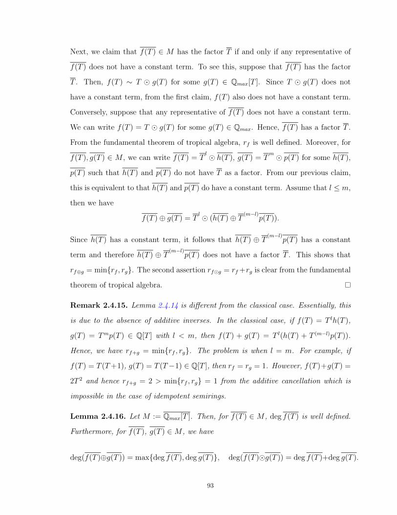
Next, we claim that f(T ) ∈ M has the factor T if and only if any representative of

f(T ) does not have a constant term. To see this, suppose that f(T ) has the factor

T . Then, f(T ) ∼ T ⊙ g(T ) for some g(T ) ∈ Qmax[T ]. Since T ⊙ g(T ) does not

have a constant term, from the first claim, f(T ) also does not have a constant term.

Conversely, suppose that any representative of f(T ) does not have a constant term.

We can write f(T ) = T ⊙ g(T ) for some g(T ) ∈ Qmax. Hence, f(T ) has a factor T .

From the fundamental theorem of tropical algebra, rf is well defined. Moreover, for

f(T ), g(T ) ∈ M , we can write f(T ) = Tl ⊙ h(T ), g(T ) = T

m ⊙ p(T ) for some h(T ),

p(T ) such that h(T ) and p(T ) do not have T as a factor. From our previous claim,

this is equivalent to that h(T ) and p(T ) do have a constant term. Assume that l ≤ m,

then we have

f(T )⊕ g(T ) = Tl ⊙ (h(T )⊕ T

(m−l)p(T )).

Since h(T ) has a constant term, it follows that h(T ) ⊕ T(m−l)

p(T ) has a constant

term and therefore h(T ) ⊕ T(m−l)

p(T ) does not have a factor T . This shows that

rf⊕g = minrf , rg. The second assertion rf⊙g = rf+rg is clear from the fundamental

theorem of tropical algebra.

Remark 2.4.15. Lemma 2.4.14 is different from the classical case. Essentially, this

is due to the absence of additive inverses. In the classical case, if f(T ) = T lh(T ),

g(T ) = Tmp(T ) ∈ Q[T ] with l < m, then f(T ) + g(T ) = T l(h(T ) + T (m−l)p(T )).

Hence, we have rf+g = minrf , rg. The problem is when l = m. For example, if

f(T ) = T (T+1), g(T ) = T (T−1) ∈ Q[T ], then rf = rg = 1. However, f(T )+g(T ) =

2T 2 and hence rf+g = 2 > minrf , rg = 1 from the additive cancellation which is

impossible in the case of idempotent semirings.

Lemma 2.4.16. Let M := Qmax[T ]. Then, for f(T ) ∈ M , deg f(T ) is well defined.

Furthermore, for f(T ), g(T ) ∈M , we have

deg(f(T )⊕g(T )) = maxdeg f(T ), deg g(T ), deg(f(T )⊙g(T )) = deg f(T )+deg g(T ).

93

Proof. This is straightforward from the fundamental theorem of tropical algebra and

the fact that no additive cancellation happens when we add two tropical polynomials.

Corollary 2.4.17. Let M := Qmax[T ]. Then M is multiplicatively cancellative.

Proof. For f(T )⊙ h(T ) = g(T )⊙ h(T ) with h(T ) = −∞, we have to show that

f(T ) = g(T ). We keep using the notation as in Lemma 2.4.14. We know that

f(T )⊙ h(T ) = g(T )⊙ h(T ) is equivalent to the following condition:

f(x) + h(x) = g(x) + h(x) ∀x ∈ Qmax, (2.4.7)

where + is the usual addition. Thus, if h(x) = −∞, we have f(x) = g(x). Since

h(x) = −∞ happens only when x = −∞, it follows that f(x) = g(x) as long as

x = −∞. Hence, all we have to show is that f(−∞) = g(−∞). From Lemma 2.4.14,

we have rf + rh = rg + rh and therefore rf = rg. Fix a representative f(T ) =aiT

i

of f(T ). We then have f(−∞) = a0 if rf = 0 and f(−∞) = −∞ if rf = 0. Thus,

we may assume that rf = rg = 0. Fix a representative g(T ) =biT

i of g(T ).

From [48, Lemma 3.2], there exists a real number M such that if x > M , then

f(x) = a0 and g(x) = b0. Since we know that f(T ) and g(T ) agree on all elements of

Qmax but −∞, we conclude that f(x) = a0 = b0 = g(x) for x > M . Therefore, we

have f(−∞) = a0 = b0 = g(−∞) and hence f(T ) = g(T ).

LetM := Qmax[T ], S :=M\−∞, and Qmax(T ) := S−1M . It follows from Corol-

lary 2.4.17 that the localization map S−1 :M −→ S−1M is injective and Qmax(T ) is

an idempotent semifield.

Proposition 2.4.18. Let M be a multiplicatively cancellative idempotent semiring.

Let S :=M\0M and N := S−1M . Let ν be a valuation (or an absolute value) on N

in the sense of any of Definitions 2.4.2, 2.4.4, 2.4.7, and 2.4.9. Then, a valuations (or

an absolute value) ν on N only depends on the image i(M) of the canonical injection

i :M −→ S−1M = N , m →→ m1.

94

Proof. Since i is an injection, one can identify an element m ∈M with m1∈ S−1M =

N under the canonical injection i. We have 1N = aa∀a ∈ S = M×. Then, with

Definitions 2.4.2, 2.4.4, and 2.4.7, we have ν(1N) = ν(a) + ν( 1a) = 0, where + is

the usual addition of real numbers. It follows that ν( 1a) = −ν(a) and hence ν(a

b) =

ν(a)− ν(b). In the case of Definition 2.4.9, we have ν(1N) = ν(a)ν( 1a) = 1. It follows

that ν( 1a) = 1

ν(a)and hence ν(a

b) = ν(a)

ν(b).

Remark 2.4.19. In the theory of commutative rings, to be multiplicatively cancella-

tive and to have no (multiplicative) zero divisors are equivalent conditions whereas, in

the theory of semirings, the first condition implies the second condition and not con-

versely in general. However, even when M is only a semiring without (multiplicative)

zero divisors, one can derive the statement as in Proposition 2.4.18 in the following

sense. Let M be a semiring without (multiplicative) zero divisors and V al(M) be the

set of valuations on M (with respect to Definition 2.4.4 or 2.4.7). Then, there exists

a set bijection between V al(M) and V al(S−1M). Indeed, for ν ∈ V al(M), one can

define a valuation ν ∈ V al(S−1M) such that ν(ab) = ν(a)ν(b)−1. Conversely, for

ν ∈ V al(S−1M), we define ν = ν i ∈ V al(M), where i : M −→ S−1M . One can

easily check that these two are well defined and inverses to each other. For absolute

values (Definition 2.4.9), one also derives the similar result.

Proposition 2.4.20. Let M := Qmax[T ], S := M\−∞, and Qmax(T ) := S−1M .

Then, with Definition 2.4.4, the set of strict valuations on Qmax(T ) which are trivial

on Qmax is equal to R. There are exactly three strict valuations on Qmax(T ) which

are trivial on Qmax up to equivalence.

Proof. From Proposition 2.4.18 and Corollary 2.4.17, a strict valuation ν on Qmax(T )

only depends on values of ν on M . Let f(T ) ∈ M . Then, from the fundamental

theorem of tropical algebra, we have

f(T ) = l1(T )⊙ l2(T )⊙ ...⊙ ln(T ),

95

where li(T ) = aiT ⊕ bi for some ai ∈ Q, bi ∈ Qmax. It follows that

ν(f(T )) = ν(l1(T )) + ν(l2(T )) + ...+ ν(ln(T )).

Let us first assume that ν(T ) < 0. If bi = −∞, since ν is trivial on Qmax, we have

ν(aiT ⊕ bi) = max(ν(ai) + ν(T )), ν(bi) = maxν(T ), 0 = 0.

Thus, we have

ν(f(T )) = rf (ν(T )), (2.4.8)

where rf is as in Lemma 2.4.14. Conversely, any map ν : Qmax(T ) −→ Rmax satisfying

the following conditions:

ν(q) = 0 ∀q ∈ Q, ν(−∞) = −∞, ν(T ) < 0, ν(f(T )) = rf (ν(T ))

is indeed a strict valuation. In fact, from Lemma 2.4.14, we know that rf⊕g =

minrf , rg. Since ν(T ) < 0 and rf , rg ∈ N, this implies that

ν(f(T )⊕ g(T )) = ν(f(T )⊕ g(T )) = rf⊕gν(T ) = minrf , rgν(T )

= maxrfν(T ), rgν(T ) = maxν(f(T )), ν(g(T )).

Moreover, ν(f(T )⊙ g(T )) = ν(f(T )⊙ g(T )) = rf⊙gν(T ) = (rf + rg)ν(T ) = rfν(T )+

rgν(T ) = ν(f(T ))+ ν(g(T )). Furthermore, all such valuations on Qmax(T ) are equiv-

alent. Indeed, let ν1, ν2 be strict valuations on Qmax(T ) such that ν1(T ) = α and

ν2(T ) = β. Since α, β are negative numbers, ρ := βα

is a positive number and

ν2(f(T )) = rfβ = (rfρ)α = ρν1(f(T )).

Secondly, suppose that ν(T ) = 0. Then, we have

ν(aiT ⊕ bi) = 0.

96

In other words, ν is a trivial valuation since 0 = 1Rmax . Clearly, this is not equivalent

to the first case.

The final case is when ν(T ) > 0. Then we have

ν(aiT ⊕ bi) = max(ν(ai) + ν(T )), ν(bi) = maxν(T ), 0 = ν(T ).

It follows that

ν(f(T )) = deg(f(T ))ν(T ).

Conversely, any map ν : Qmax(T ) −→ Rmax satisfying the following conditions:

ν(q) = 0 ∀q ∈ Q, ν(−∞) = −∞, ν(T ) > 0, ν(f(T )) = deg(f(T ))(ν(T ))

is indeed a strict valuation from Lemma 2.4.16. Furthermore, suppose that ν1, ν2 are

strict valuations on Qmax(T ) such that ν1(f(T )) = α > 0, ν2(f(T )) = β > 0. Then,

with ρ = βα, ν1, ν2 are equivalent. Furthermore, this case is not equivalent to any of

the above. To sum up, the set of strict valuations on Qmax(T ) which are trivial on

Qmax is equal to R (by sending ν to ν(T )). There are exactly three strict valuations

depending on a sign of a value of T .

Proposition 2.4.21. Let M := Qmax[T ], S := M\−∞, and Qmax(T ) := S−1M .

Then, with Definition 2.4.7, the set of valuations on Qmax(T ) with values in R+,val

which are trivial on Qmax is equal to R. There are exactly three valuations on Qmax(T )

which are trivial on Qmax up to equivalence.

Proof. To avoid the notational confusion, we denote by ⊕,⊙ the addition and the

multiplication of idempotent semirings and by ∨, · the addition and the multiplication

of R+,val. From Proposition 2.4.18, a valuation ν on Qmax(T ) only depends on values

of ν onM . Let ν be a valuation on Qmax(T ) which is trivial on Qmax. For f(T ) ∈M ,

from the fundamental theorem of tropical algebra, we have f(T ) = l1(T ) ⊙ l2(T ) ⊙

... ⊙ ln(T ), where li(T ) = aiT ⊕ bi for some ai ∈ Q, bi ∈ Qmax. Hence, ν is entirely

97

determined by values on linear polynomials. Similar to Proposition 2.4.20, we divide

the cases up to a sign of ν(T ). The first case is when ν(T ) < 0. Since ν is trivial on

Qmax, if b = −∞, we have

ν(aT ⊕ b) ∈ ν(aT ) ∨ ν(b) = (ν(a) · ν(T )) ∨ ν(b) = maxν(T ), 0 = 0.

With the same notation as in Lemma 2.4.14, we have

ν(f(T )) = rfν(T ). (2.4.9)

Conversely, any map ν : Qmax(T ) −→ R+,val given by (2.4.9) is indeed a valuation.

Indeed, from the fundamental theorem of tropical algebra, we have ν(f(T )⊙ g(T )) =

(rf + rg)ν(T ) = rfν(T )+ rgν(T ) = ν(f(T )) · ν(g(T )). Moreover, from Lemma 2.4.14,

we have ν(f(T ) ⊕ g(T )) = r(f⊕g)ν(T ) = minrf , rgν(T ) = maxrfν(T ), rgν(T ) =

maxν(f(T )), ν(g(T )) ∈ ν(f(T )) ∨ ν(g(T )). Similar to Proposition 2.4.20, all these

cases are equivalent.

The second case is when ν(T ) = 0. Then we have ν(aiT + bi) = 0 and this case gives

us a trivial valuation since 0 = 1R+,val. Clearly this is not equivalent to the first case.

The final case is when ν(T ) > 0. Then, as in Proposition 2.4.20, we have ν(f(T )) =

deg(f(T ))(ν(T )). Conversely, any map ν : Qmax(T ) −→ R+,val given in this way is

indeed a valuation by Lemma 2.4.16. These are all equivalent from the exact same

argument in Proposition 2.4.20.

Proposition 2.4.22. Let M := Qmax[T ], S := M\−∞, and Qmax(T ) := S−1M .

Then, with Definition 2.4.9 and the hyperfield R+,Y , the set of absolute values on

Qmax(T ) which are trivial on Qmax is equal to R>0. There are exactly three absolute

values on Qmax(T ) which are trivial on Qmax up to equivalence.

Proof. To avoid the notational confusion, we denote by ⊕,⊙ the addition and the

multiplication of idempotent semirings and by ∨, · the addition and the multiplication

of R+,Y . From Proposition 2.4.18, an absolute value | − | on Qmax(T ) only depends

98

on values on M . There are three possibilities. The first case is when |T | = α > 1.

Let aiT ⊕ bi be a linear polynomial. i.e. ai = −∞. Since | − | is trivial on Qmax, if

bi = −∞, we have

|aiT ⊕ bi| ∈ |ai| · |T | ∨ |bi| = |T | ∨ 1 = α ∨ 1.

Since α > 1, we have α∨1 = α and hence |aiT⊕bi| = α. In other words, for f(T ) ∈M ,

we have |f(T )| = αdeg(f(T )). Conversely, any map | − | : Qmax(T ) −→ R+,Y given in

this way is an absolute value which is trivial on Qmax; since α > 1, it directly follows

from Lemma 2.4.16. Furthermore, any two absolute values | − |1, | − |2 such that

|T |1 = α > 1, |T |2 = β > 1 are equivalent with ρ = logαlog β

.

The second case is when |T | = α < 1. In this case, for a ∈ Qmax\−∞, we have

|T ⊕ a| ∈ |T | ∨ 1 = α ∨ 1 = 1.

This implies that for f(T ) ∈ M , we have |f(T )| = αrf , where rf is as in Lemma

2.4.14. Conversely, one can observe that this condition defines an absolute value

which is trivial on Qmax. Indeed, from Lemma 2.4.14, we have |f(T ) ⊕ g(T )| =

αrf⊕g = αminrf ,rg. Since α < 1, we have αminrf ,rg = maxαrf , αrg ∈ αrf ∨ αrg =

|f(T )| ∨ |g(T )|. Furthermore, clearly |f(T )⊙ g(T )| = |f(T )| · |g(T )|. In this case, for

absolute values | − |1, | − |2 such that |T |1 = α, |T |2 = β and α, β < 1, since logα,

log β < 0, we have ρ := logαlog β

> 0 and | − |ρ2 = | − |1. This shows that all such | − |1

and | − |2 are equivalent.

The final case is when |T | = 1. We have |T ⊕ a| ∈ |T | ∨ |a| = |T | ∨ 1 = 1 ∨ 1 = [0, 1]

for a = −∞. Since T ⊕ (T ⊕ a) = T ⊕ a, we have

|T ⊕ a| = |T ⊕ (T ⊕ a)| ∈ |T | ∨ |T ⊕ a|. (2.4.10)

Suppose that |T ⊕ a| = β < 1. Then, since |T | = 1, the right hand side of (2.4.10) is

equal to 1∨β = 1. This implies that |T ⊕ a| = 1 which is a contradiction. Therefore,

99

|T ⊕ a| = 1. It follows that for f(T ) ∈ M , we have |(f(T )| = 1. In other words, this

is the case of a trivial absolute value.

Our motivation in developing a valuation theory of semi-structures is to make an

analogue of abstract curves in characteristic one. To explain this connection, let us

recall several classical definitions and results of abstract curves (cf. [20, §1.5]).

Let k be an algebraically closed field and K be a finitely generated field extension of

k of transcendence degree 1, i.e. a function field of dimension 1. By a valuation ν of

K/k is a valuation on K which is trivial on k. In other words, ν is a valuation on K

such that ν(x) = 1 ∀x ∈ k\0. A valuation ν is discrete if the value group of ν is

isomorphic to the abelian group Z of integers, and the corresponding valuation ring

is called a discrete valuation ring. Let CK be the set of all discrete valuation rings

of K/k. For p ∈ CK , we denote by Rp the discrete valuation ring corresponding to

p. One makes the set CK into a topological space by defining the closed sets to be

the finite subsets of CK and CK itself. Furthermore, if U is an open subset of CK ,

one defines the ring of regular functions on U to be O(U) :=

p∈U Rp. Note that

this is motivated by the same property when X is an integral scheme. An element

f ∈ O(U) defines a function f : U −→ k such that f(p) is the residue of f modulo

the maximal ideal of Rp.

An abstract nonsingular curve over k is an open subset U ⊆ CK with the induced

topology and the induced notion of regular functions. A morphism between two

abstract nonsingular curves X and Y over k is a continuous function ϕ : X −→ Y

such that for each open subset V ⊆ Y and every regular function f : V −→ k, f ϕ

is a regular function on ϕ−1(V ). The following theorem is one of the main theorems

in the theory of abstract curves.

Theorem 2.4.23. ( [20, Theorem 6.9, §1.5]) Let K be a function field of dimension

1 over an algebraically closed field k. An abstract nonsingular curve defined above is

isomorphic to a nonsingular projective curve over k.

100

Since two valuations are equivalent if and only if they have the same valuation

ring, the set CK can be considered as the set of discrete valuations of K/k up to

equivalence. From Propositions 2.4.20 and 2.4.21, the direct analogue of the set CK

with K = Qmax(T ) and k = Qmax is the set V al(Qmax(T )) := ν+, ν−, where ν+

is the class of valuations ν such that ν(T ) > 0 and ν− is the class of valuations ν

such that ν(T ) < 0. Furthermore, since their image is the integers as a set, they

can be considered as discrete valuations. In the spirit of the construction of abstract

curves, one can expect that the set of valuations V al(Qmax(T )) gives some geometric

information about the projective line P1 over Qmax. However, one can observe that

X := Spec(Qmax[T ]) contains many points. For example, in [18], the authors proved

that there is one-to-one correspondence between principle prime ideals of Qmax[T ]

and points of Qmax. Hence, the points of P1 over Qmax are a lot more than the points

of V al(Qmax(T )). It seems more interesting connection of V al(Qmax(T )) is with the

projective line P1 over F1 rather than over Qmax. Let us first recall the construction

of the projective line P1 over F1.

Example 2.4.24. (An example from [16]) One constructs the projective line P1 over

F1 as follows. Let C∞ := ..., t−1, 1, t, ... be an infinite cyclic group generated by

t and let C∞,+ := 1, t, t2, ..., C∞,− := 1, t−1, t−2, ... be sub-monoids of C∞. Let

U+ := Spec(C∞,+), U− := Spec(C∞,−), and U := Spec(C∞) (see [16] for the notion

of monoid spectra). One defines the projective line P1 over F1 by gluing U+ and U−

along U . The space U+ has two points, a generic point c0 and a closed point c+

containing t. Similarly, the space U− has two points, a generic point c0 and a closed

point c− containing t−1. Hence, the projective line P1F1

over F1 consists of three points

c+, c0, c−.

Remark 2.4.25. We can observe that the number of closed points of P1F1

is exactly

same as the number of points of V al(Qmax(T )) = ν+, ν−. Furthermore, ν+ corre-

sponds to c+ which is the prime ideal containing t and ν− corresponds to c− which

is the prime ideal containing t−1. In fact, one may consider that ν0, which is an

101

equivalence class of a trivial valuation, corresponds to c0 which is the prime ideal

consists of 1 = t0. This correspondence can be justified since Theorem 2.4.23 only

concerns closed points of a projective nonsingular curve. Hence, V al(Qmax(T )) can

be considered as the projective line P1F1

understood as an abstract curve.

On the other hand, one can think of an absolute value with the hyperfield R+,Y as

an analogue of a non-archimedean absolute value. In fact, from the definition of the

hyperfield R+,Y and Definition 2.4.9, we have an analogue of the ultrametric inequal-

ity: |x+ y| ∈ |x|+ |y| = max|x|, |y| if |x| = |y|. Furthermore, classically there is a

natural one-to-one correspondence between the set of equivalence classes of valuations

and the set of equivalence classes of non-archimedean absolute values. Hence, the set

of absolute values of Qmax(T ) as in Definition 2.4.9 with the hyperfield R+,Y might

be considered as the set of equivalence classes of valuations of Qmax(T ) with values in

the hyperfield. Let X(Qmax(T )) be a set of equivalence class of such absolute values

such that the image is isomorphic to the integers. Then, from Proposition 2.4.22, we

have X(Qmax(T )) = µ+, µ−, where µ+((T )) > 1, µ−((T )) < 1. Therefore, in this

case, we are also able to give a similar correspondence to P1F1

= c+, c0, c−.

102

3

From semi-structures to

hyper-structures

In this chapter, we first review the symmetrization process introduced in [21], then we

investigate some algebraic properties of this process which will be applied in the next

chapter to link geometries over semi-structures and hyper-structures. Throughout

this chapter, by a semiring of characteristic one we mean a semiring M such that

x+ y ∈ x, y ∀x, y ∈M. (3.0.1)

We recall that B = 0, 1 is the smallest semifield of characteristic one such that

1 + 1 = 1, 0 + 1 = 0 = 1 + 0, 1 · 1 = 1, 1 · 0 = 0.

We denote by S the hyperfield of signs (cf. §1.1.2).

3.1 The symmetrization functor −⊗B S

In his paper [21], S.Henry introduced the symmetrization process which generalizes

in a suitable way the construction of the Grothendieck group completion of a multi-

plicative monoid. This process allows one to encode the structure of a B-semimodule

103

as the ‘positive’ part of a hypergroup interpreted as a S-hypermodule.

Next, we briefly recall this symmetrization process. Let B be a commutative monoid

denoted additively and endowed with a neutral element 0. One can define the follow-

ing canonical partial order on B:

x ≤ y ⇐⇒ x+ y = y. (3.1.1)

By a partial order on B we mean a binary relation on B which is reflexive, transitive,

and antisymmetric. A partial order is said to be total if for any x, y ∈ B, we have

x ≤ y or y ≤ x. We claim that when B satisfies the condition (3.0.1), such order is

total. In fact, we know that x+ y = x or x+ y = y ∀x, y ∈ B, hence x ≤ y or y ≤ x.

We introduce the following notation

s(B) := (s, 1), (s,−1), 0 = (0, 1) = (0,−1) | s ∈ B\0.

To minimize the notation we denote (s, 1) := s, (s,−1) := −s, and |(s, 1))| =

|(s,−1)| = s. For any X = (x, p) ∈ s(B), we define sign(X) = p. s(B) is a hy-

pergroup (cf. §1.1.2 for the definition) with the addition given by

x+ y =

x if |x| > |y| or x = y

y if |x| < |y| or x = y

[−x, x]= (t,±1) | t ≤ |x|) if y = −x

(3.1.2)

We denote with s : B −→ s(B), s →→ (s, 1) the associated map.

Let H be a hypergroup and B be a commutative monoid. We say that a map

f : B −→ H is additive if

f(0) = 0 and f(a+ b) ∈ f(a) + f(b) ⊆ H ∀a, b,∈ B.

We claim that the construction of s(B) determines the minimal hypergroup associated

to a commutative monoid B as the following universal property states.

104

(Universal Property): Let B be a commutative monoid such that the canonical order

as in (3.1.1) is total. Then, for any hypergroup K and an additive map g : B −→ K,

there exists a unique homomorphism h : s(B) −→ K of hypergroups such that

g = h s.

In fact, such h : s(B) −→ K is given by h(X) = sign(X)g(x), ∀X = (x, p) ∈ s(B)

(cf. [21, Theorem 5.1]).

Remark 3.1.1. 1. Let B be a commutative monoid such that the canonical or-

der as in (3.1.1) is total. Assume also that B is equipped with a smallest ele-

ment. Then B can be upgraded to a semiring by defining the addition law as

the maximum(with respect to the canonical order) and the multiplication as the

usual addition. For example, Rmax is the semifield obtained from the (multiplica-

tive)commutative monoid (R ∪ −∞,+).

2. The symmetrization process can be applied to a general class of monoids (cf. [21,

Theorem 5.1]). In fact, for a commutative monoid B, s(B) is a hypergroup if

and only if B satisfies the following condition: for all x, y, z, w ∈ B,

x+ y = z + w =⇒ ∃b ∈ B s.t.

x+ b = z; b+ w = y,

or x = z + b; w = b+ y(3.1.3)

In [21], it is also proved that when B is an idempotent monoid, B fulfills the

condition (3.1.3) if and only if the canonical order of B as in (3.1.1) is total

(cf. [21, Proposition 6.2]).

Let (B,+, ·) be an idempotent semiring. It follows that the additive monoid

(B,+) allows for the symmetrization process if and only if (B,+, ·) is, in fact,

of characteristic one. Since our main interest lies in idempotent semirings, to

this end, we will mostly focus on a semiring of characteristic one.

As Connes and Consani pointed out in [11], the symmetrization process can be un-

derstood in terms of the functor “extension of scalars”. In this section we investigate

105

how this process relates some algebraic properties of semirings to those of hyperrings.

To begin with, we shall provide (cf. Proposition 3.1.8) a partial converse of Henry’s

construction.

Definition 3.1.2. (cf. [32, §5]) Let R be a hyperring. A good ordering on R is a

subset P ⊆ R satisfying the following properties:

P + P ⊆ P, PP ⊆ P, P ∪ −P = R, and P ∩ −P = 0.

Example 3.1.3. Let R = T R be Viro’s hyperfield of real numbers as in Definition

2.4.8. A good ordering on R is provided by the subset P = x ∈ T R | x ≥ 0 ⊆ R.

The easiest example of a good ordering on a hyperfield is given by choosing R = S,

the hyperfield of signs, then P := 0, 1.

Remark 3.1.4. 1. In general, the definition of an ordering P ⊆ R on a commuta-

tive ring R only requires P ∩−P to be a prime ideal of R. In the above definition

this condition is replaced by imposing that P ∩−P = 0. This is done to encode

P as the ‘positive’ part of R. Note that if P is a good ordering on R, then −P

is also a good ordering on R.

2. The conditions P ∪ −P = R, P ∩ −P = 0 mean: x = −x⇐⇒ x = 0.

3. One can easily see that a hyperring R has a good ordering if and only if there

exists a hyperring homomorphism g : R −→ S such that g−1(0) = 0. Indeed,

suppose that R has a good ordering P . We define g : R −→ S such that

g(x) =

1 if x ∈ P\0

−1 if x ∈ −P\0

0 if x = 0

Clearly this is a homomorphism of hyperrings such that g−1(0) = 0. Con-

versely, suppose that g : R −→ S is a homomorphism of hyperrings such that

g−1(0) = 0. Then the set P := g−1(0, 1) becomes a good ordering on R.

106

If B = (B,+, ·) is a semiring such that the symmetrization process can be ap-

plied to the additive monoid (B,+), the multiplicative structure of B induces the

corresponding multiplicative structure on s(B) in the component-wise way. In other

words, one can define the multiplication law on s(B) such that:

(x, p) · (y, q) := (xy, pq), p, q ∈ −1, 1; 1 · 1 = (−1) · (−1) = 1, 1 · (−1) = −1.

Remark 3.1.5. Let M be a semiring allowing for the symmetrization process. We

will prove in Lemma 3.1.6 that under the component-wise multiplication, s(M) is

not a hyperring but only a multiring(cf. [32]). A multiring is a weaker version of a

hyperring in the sense that a hyperring fulfills the distributive law x(y+ z) = xy+ xz

whereas the notion of a multiring only assumes the weak distributive property

x(y + z) ⊆ xy + xz.

For example, letM be the semiring whose underlying set is Z≥0 with the addition given

by x+ y := maxx, y, and the multiplication given by the usual multiplication. Then

s(M) does not satisfy the distributive law. For example, 2(3 − 3) = 6 − 6 = [−6, 6].

Indeed, we have 5 ∈ 6−6 = [−6, 6], but 5 can not be an element of 2(3−3) = 2·[−3, 3]

because 2 can not divide 5 in usual sense. For s(M) to satisfy the distributive law it

seems necessary to add a suitable divisibility condition on the multiplication of s(M).

A particular case will be studied in Proposition 3.1.10.

LetM be a semiring. Since s(M) can be understood as a scalar extensionM⊗BS,

we denote MS := s(M) from now on. If MS is not just a multiring but a hyperring,

then MS together with i :M −→MS is indeed a universal pair among all hyperrings

in the sense of [21].

Lemma 3.1.6. Let B be a semiring of characteristic one. Then BS is a multiring with

the component-wise multiplication. In particular, if B is a semifield of characteristic

one, then BS is a hyperfield.

107

Proof. We first note that x ≤ y implies xz ≤ yz for all z ∈ B. In fact, it follows from

x ≤ y ⇐⇒ x + y = y that xz + yz = yz ⇐⇒ xz ≤ yz. For the first assertion, all we

have to show is that X(Y + Z) ⊆ XY + XZ for all X, Y, Z ∈ BS. If X = 0, then

there is nothing to prove. Therefore we may assume that X = 0. Let Y = (y, p),

Z = (z, q), X = (x, r). When #(Y + Z) = 1, it follows from (3.1.2) that there

are three possible cases. The first case is when Y = Z. In this case, we have

X(Y + Z) = XY = XY + XY = XY + XZ. The second case is when p = q, but

y = z. Since B is of characteristic one, we may further assume that y > z. Therefore,

we have xy ≥ xz and X(Y + Z) = XY ∈ XY +XZ. The final case is when p = q

and y = z. But, in this case, the similar argument as the second case shows that

X(Y + Z) ⊆ XY + XZ. When #(Y + Z) = 1, from (3.1.2), we may assume that

Y = (y, 1), Z = (y,−1), and X = (x, r). Take any T = (t, p) ∈ (Y + Z). It follows

from (3.1.2) that t ≤ y, hence xt ≤ xy. Therefore we haveXT = (xt, pr) ∈ XY +XZ.

When B is a semifield, each non-zero element of BS has a multiplicative inverse.

Therefore BS is a multifield and it is well-known that any multifield is a hyperfield(and

vice versa).

Lemma 3.1.7. Let R be a multiring and H be a hyperring. Suppose that there exists

an isomorphism ϕ : (R,+) −→ (H,+) of hypergroups such that ϕ(xy) = ϕ(x)ϕ(y)

∀x, y ∈ R. Then R is a hyperring and ϕ is an isomorphism of hyperrings.

Proof. First we claim that xy+xz ⊆ x(y+z) for all x, y, z ∈ R. We have ϕ(xy+xz) =

ϕ(xy) + ϕ(xz) = ϕ(x)ϕ(y) + ϕ(x)ϕ(z) = ϕ(x)(ϕ(y) + ϕ(z)) = ϕ(x)ϕ(y + z) =

ϕ(x(y+z)). By taking ϕ−1, we obtain our claim and so R is a hyperring. To show that

ϕ is an isomorphism of hyperrings, we have to prove that ϕ−1(ab) = ϕ−1(a)ϕ−1(b).

This is clear by taking a = ϕ(x), b = ϕ(y).

Proposition 3.1.8. Let R be a hyperring such that

x+ x = x ∀x ∈ R; x+ y ∈ x, y ∀x = −y ∈ R. (3.1.4)

108

Let P be a good ordering on R. Then

1. P is a semiring such that the canonical order deduced from the addition as in

(3.1.1) is a total order and x + x = x for all x ∈ P . i.e. P is a semiring of

characteristic one.

2. Under the symmetrization process, PS is a hyperring with the multiplication given

component-wise and PS is isomorphic to R as hyperrings.

Proof. We first prove that P is a semiring satisfying the properties stated in 1. Triv-

ially we have 0 ∈ P . If 1 ∈ P then −1 ∈ P and since PP ⊆ P , this implies

(−1)(−1) = 1 ∈ P which is a contradiction. Hence 1 ∈ P . Furthermore, the addition

on P induced from R is single-valued since we assumed that for any x, y ∈ R with

x = −y, x + y is a single element. As we mentioned in Remark 3.1.4, if x, y are

non-zero elements of P then they can not be the additive inverse of each other. The

first two conditions of a good ordering imply that the induced addition and multi-

plication are closed. Thus P is a semiring. Furthermore, we have x + x = x for all

x ∈ P . Since x + y ∈ x, y, it follows that the canonical order is total. Moreover,

this order is compatible with the multiplication. In fact, x ≤ y ⇐⇒ x+ y = y. Then

for any z ∈ P we have zx + zy = zy =⇒ zx ≤ zy. This proves the first part of the

proposition.

Because P satisfies the sufficient condition of having the symmetrization, PS is a hy-

pergroup. In fact, it follows from Lemma 3.1.6 that PS is a multiring. We claim that

together with the inclusion map i : P → R, (R, i) is the universal pair. Indeed, let K

be a hypergroup and g : P −→ K be an additive map. Define h : R −→ K such that

h(x) =

g(x) if x ∈ P

−g(−x) if x ∈ −P

This is well-defined since P ∪ −P = R, P ∩ −P = 0, and g(0) = 0. We observe

that h(0) = 0. If x, y ∈ P , then h(x+ y) = g(x+ y) ∈ g(x) + g(y) = h(x) + h(y). If

109

x, y ∈ −P , then so is for x+ y, hence h(x+ y) = −g(−x− y) ∈ −(g(−x) + g(−y)) =

−g(−x) − g(−y) = h(x) + h(y). Finally, if x ∈ P , y ∈ −P , then let t = −y ∈ P .

If z ∈ x + y, we want to show that h(z) ∈ h(x) + h(y). The first case is when

z ∈ P . Then we have z ∈ x + y = x − t = −t + x. From the reversibility property

it follows that x ∈ z − (−t) = z + t. Since x, z, t ∈ P we can use the property of g

to deduce that g(x) ∈ g(z + t) ∈ g(z) + g(t). Again from the reversibility we derive

that g(z) ∈ g(x)− g(t), equivalently we have that h(z) ∈ h(x)+h(−t) = h(x)+h(y).

The second case is when z ∈ −P . We let z = −w,w ∈ P . Then we have z ∈ x+ y =

x− t⇐⇒ −w ∈ x− t⇐⇒ w ∈ t− x = −x+ t. Again from the reversibility we have

t ∈ w + x, then since t, w, x ∈ P , it follows that g(t) ∈ g(w) + g(x) = g(x) + g(w).

From the reversibility, g(w) ∈ g(t) − g(x) ⇐⇒ −g(w) ∈ g(x) − g(t). Therefore, we

conclude that h(−w) ∈ h(x) + h(−t), or h(z) ∈ h(x) + h(y). This shows that h is a

homomorphism of hypergroups.

It follows from the construction that g = h i, and such h is unique. Indeed, suppose

that g = f i. Then for any x ∈ P , we have g(x) = f(i(x)) = f(x) = h(x). For any

x ∈ −P we know that −x ∈ P and 0 ∈ x− x. Hence f(0) = 0 ∈ f(x− x) ∈ f(x) +

f(−x). From the uniqueness of the inverse, f(x) = −f(−x) = −g(−x) = h(x). Since

(R, i) is also the universal pair, as hypergroups, R is isomorphic to PS. Furthermore,

this isomorphism is also a homomorphism of multirings which is an isomorphism of

hypergroups. Thus, from Lemma 3.1.7, it follows that PS is a hyperring which is

isomorphic to R.

Remark 3.1.9. The above proposition has an easier interpretation when we restrict

to the case of a hyperfield R satisfying the condition (3.1.4). In fact, in this case, the

notion of a good ordering on R given in Definition 3.1.2 coincides with the notion

of an ordering on R given in [32]. In that paper, M.Marshall defined real hyperfields

as hyperfields F such that −1 ∈F 2 and proved that F is a real hyperfield if and

only if F has an ordering. Let M be a semifield of characteristic one, then we have

−1 ∈M2

S. Thus it follows that MS is a real hyperfield. Conversely, suppose

110

that R is a real hyperfield satisfying the condition (3.1.4). Since any real hyperfield

has a good ordering P ⊂ R, it follows that R ≃ PS from Proposition 3.1.8. If we

let − ⊗B S be a functor from the category of semifields of characteristic one to the

category of hyperrings, it follows that the category of real hyperfields satisfying the

condition (3.1.4) is the essential image of the functor −⊗B S.

Proposition 3.1.10. Let M be a semiring of characteristic one such that

x < y =⇒ xz < yz ∀x, y, z ∈M\0M, (3.1.5)

where < is the canonical order as in (3.1.1). Suppose that M satisfies the following

condition

∀x, y ∈M, ∃α, β ∈M s.t. xα = y, x = yβ. (3.1.6)

Then MS is a hyperring. Conversely, let us further assume that 1M ≤ x for all

x ∈M\0M. If MS is a hyperring then M satisfies the condition (3.1.6).

Proof. From Lemma 3.1.6, we know that MS is a multiring. Therefore, to prove that

MS is a hyperring under the condition (3.1.6), it is enough to show that XY +XZ ⊆

X(Y + Z) ∀X, Y, Z ∈ MS. If |Y | = |Z| or |Y | = |Z| and sign(Y ) = sign(Z),

then it is straightforward. In fact, in this case, we would only have single-valued

operations. Hence, an inclusion is indeed an equality. The only nontrivial case is

when |Y | = |Z|, sign(Y ) = sign(Z), and X = 0. Therefore, we may assume that

Y = (y, 1), Z = (y,−1), and X = 0. Let X = (x, r) and T = (t, p) ∈ XY + XZ,

then t ≤ xy. It follows from the divisibility condition (3.1.6) on M that t = xβ for

some β ∈ M . Then we have β ≤ y. Otherwise we would have y < β, but from the

condition (3.1.5), this implies that xy < xβ = t which is a contradiction(we assumed

that x = 0). Thus T = (t, p) = (xβ, p) ∈ X(Y + Z).

For the second assertion, for any x, y ∈M , let X = (x, 1), Y = (y, 1), −Y = (y,−1).

Since we assumed that MS is a hyperring we know that X(Y − Y ) = XY − XY .

Furthermore, since 1M ≤ x for all x = 0, we have y ≤ xy. This implies (y, 1) ∈

111

(XY −XY ) = X(Y − Y ), and y = xα for some α ≤ y. Similarly we can find β such

that x = yβ using Y (X − X) = Y X − Y X. Therefore, M satisfies the condition

(3.1.6).

Remark 3.1.11. Any semifield M of characteristic one always satisfies the condition

(3.1.5) and the divisibility condition (3.1.6). Hence it follows from the above proposi-

tion that MS is a hyperfield. One can observe that this agrees with the statement of

Lemma 3.1.6.

Surprisingly, if MS is a hyperring then MS automatically satisfies the following

stronger condition.

Proposition 3.1.12. Let M be a semiring of characteristic one. Suppose that MS is

a hyperring. Then MS is doubly distributive. i.e. for any X, Y, Z,W ∈MS we have

(X + Y )(Z +W ) = XZ +XW + Y Z + YW. (3.1.7)

Proof. In general, one only has

(X + Y )(Z +W ) ⊆ XZ +XW + Y Z + YW.

Thus we have to show the other inclusion. There are two possible cases depending

upon the cardinalities of (X + Y ) and (Z + W ). The first case is when at least

one of (X + Y ) and (W + Z) consists of a single element. If #(X + Y ) = 1, then

we may assume that X + Y = X(cf. (3.1.2) for the definition of the addition in

MS). Then XW + YW = (X + Y )W = XW and XZ + Y Z = (X + Y )Z = XZ,

hence XZ +XW + Y Z + YW = XW +XZ = X(W + Z) = (X + Y )(W + Z). If

#(W+Z) = 1, then the argument is similar. The second case is when neither (X+Y )

nor (W +Z) consists of a single element. Hence we may let that X = −Y , Z = −W ,

and X = (x, 1), Z = (z, 1). Thus we have (X+Y ) = [−X,X] and (Z+W ) = [−Z,Z].

It follows that (X + Y )(Z +W ) = [−X,X] · [−Z,Z]. If T ∈ XZ + XW + Y Z +

112

YW = X(Z +W ) + Y (Z +W ) then there exist α, β ∈ Z +W = [−Z,Z] such that

T ∈ Xα + Y β. Since X = −Y we can rewrite T ∈ Xα − Xβ = X(α − β). We

know that X ∈ (X + Y ) = [−X,X]. Furthermore, for α, β ∈ (Z +W ) = [−Z,Z], we

have −β ∈ [−Z,Z] since |β| ≤ |Z|. In particular, (α − β) ⊆ [−Z,Z]. We conclude

T ∈ (X + Y )(Z +W ), therefore XZ +XW + Y Z + YW ⊆ (X + Y )(Z +W ).

The following corollary shows that MS has many Frobenius endomorphisms.

Corollary 3.1.13. Let M,MS be the same as in Proposition 3.1.12. Then for any

m ∈ N we have

(X + Y )m = Xm + Y m ∀X, Y ∈MS. (3.1.8)

Proof. Let X = (x, p), Y = (y, q). We prove this by induction. If m = 1, then there

is nothing to prove. Let us assume that (3.1.8) holds for m = n. For n+ 1, it follows

from the above proposition and the inductive assumption that

(X + Y )n+1 = Xn+1 +XnY + Y nX + Y n+1. (3.1.9)

If we have #(X + Y ) = 1 then it is clear. In fact, one of the following X = Y ,

x < y, y < x should hold. When x < y we have X + Y = Y . Therefore the left

hand side of (3.1.8) is Y n+1. On the other hand we have (Xn + Y n) = Y n, thus

the right hand side of (3.1.8) is Y n+1. The case when y < x is similar. When

X = Y the outcome is trivial. It follows that the only non-trivial case is when x = y,

p = −q. We may assume that p = 1, hence Y = −X. Then the left hand side

of (3.1.9) is [−X,X]n+1. Moreover, we have that Xn+1 + XnY + Y nX + Y n+1 =

Xn+1 − Xn+1 + Y n+1 − Y n+1 = [−Xn+1, Xn+1] + [−Xn+1, Xn+1]. Therefore the

right hand side of (3.1.9) is that [−Xn+1, Xn+1] + [−Xn+1, Xn+1]. We claim that

[−X,X]n+1 = [−Xn+1, Xn+1]. Let t ∈ [−X,X]n+1. This means t = t1t2...tn+1 for

some ti ∈ [−X,X]. Since each |ti| ≤ X, we have |t| ≤ Xn+1 and t ∈ [−Xn+1, Xn+1].

Conversely, let t ∈ [−Xn+1, Xn+1]. Then |t| ≤ Xn+1. Since MS is a hyperring,

we have [−Xn+1, Xn+1] = Xn+1 − Xn+1 = X(Xn − Xn). Therefore, we can find

113

t1 ∈ Xn − Xn = [−Xn, Xn] such that t = Xt1. Inductively we can write t = Xntn

with |tn| ≤ X. This means t ∈ [−X,X]n+1. This proves our claim. All we have to

show to complete our proof is the following:

[−Z,Z] + [−Z,Z] = [−Z,Z] ∀Z = (z, 1) ∈MS.

By choosing 0 ∈ [−Z,Z] we clearly have [−Z,Z] ⊆ [−Z,Z] + [−Z,Z]. Conversely,

if α ∈ [−Z,Z] + [−Z,Z] then α ∈ t + q for some t, q ∈ [−Z,Z]. But for α ∈ t + q

we have |α| ≤ max|t|, |q| ≤ Z. It follows that α ∈ [−Z,Z]. This completes the

proof.

The next proposition shows that the localization commutes with the symmetriza-

tion.

Proposition 3.1.14. Let M be a semiring of characteristic one and s : M −→ MS

be the symmetrization map. Assume that MS = s(M) is a hyperring. Suppose S

is a multiplicative subset of M . Then S := s(S) is a multiplicative subset of MS.

Furthermore, the following conclusions hold.

1. S−1M is a semiring of characteristic one.

2. s(S−1M) ≃ S−1(MS).

Proof. The fact that s(S) = S is a multiplicative subset of MS is straightforward.

For the first assertion, since clearly S−1M is a semiring, all we have to prove is that

S−1M is of characteristic one. In other words, we have to show that α + β ∈ α, β

∀α, β ∈ S−1M . In fact, for any xs, yt∈ S−1M , we have x

s+ y

t= xt+sy

st. Since

xt + sy ∈ xt, sy it follows that xt+syst

∈ xtst, syst = x

s, yt. Therefore S−1M is a

semiring of characteristic one.

For the second assertion, we prove that the map

i : S−1M −→ S−1(MS)α

s→→ (α, 1)

(s, 1)

114

is a well-defined additive map and that (i, S−1(MS)) is the universal pair. Then it

follows from the universality that s(S−1M) ≃ S−1(MS) as hypergroups. We will

prove that such isomorphism is also an isomorphism of hyperrings. We first show

that i is well-defined. In fact, if αs= β

t∈ S−1M then we have gαt = gβs for some

g ∈ S. It follows that (g, 1)(α, 1)(t, 1) = (gαt, 1) = (gβs, 1) = (g, 1)(β, 1)(s, 1). Since

(g, 1) ∈ S, we have i(αs) = (α,1)

(s,1)= (β,1)

(t,1)= i(β

t). Therefore, i is well-defined. One can

clearly see that i(0) = 0. For any xs, yt∈ S−1M ,

i(x

s+y

t) = i(

xt+ ys

st) =

(xt+ ys, 1)

(st, 1)∈ (x, 1)

(s, 1)+

(y, 1)

(t, 1)= i(

x

s) + i(

y

t).

This shows that i is an additive map. Next, we prove that (i, S−1(MS)) is a universal

pair. Let K be a hypergroup and g : S−1M −→ K be an additive map. We have to

show that there exists a unique homomorphism h : S−1(MS) −→ K of hypergroups

such that g = h i. Let us define a map h : S−1(MS) −→ K as

h((x, p)

(s, 1)) =

g(xs) if p = 1

−g(xs) if p = −1

(3.1.10)

In other words, h( (x,p)(s,1)

) =sign(p)g(xs). Then h is well-defined. In fact, for any (x,p)

(s,q),

we may assume that q = 1 by multiplying 1 = (1,q)(1,q)

. Thus the definition makes sense.

We claim that if (x,1)(s,1)

= (y,p)(t,1)

, then p = 1. This is because (x,1)(s,1)

= (y,p)(t,1)

is equivalent to

the statement that (g, 1)(t, 1)(x, 1) = (gtx, 1) = (gys, p) = (g, 1)(y, p)(s, 1) for some

(g, 1) ∈ S. Furthermore, suppose that (x,1)(s,1)

= (y,1)(t,1)

. Then for some (g, 1) ∈ S, we

have (gtx, 1) = (gys, 1). But since the symmetrization map is injective we have that

gtx = gys, hence xs= y

tand h( (x,1)

(s,1)) = g(x

s) = g(y

t) = h( (y,1)

(t,1)). The exact same

argument shows that for any (x,−1)(s,1)

= (y,−1)(t,1)

we have h( (x,−1)(s,1)

) = h( (y,−1)(s,1)

). Therefore

h is well-defined. Next, we prove that h is a homomorphism of hypergroups. We

have to show that h(X + Y ) ⊆ h(X) + h(Y ) for all X, Y ∈ S−1(MS). We divide

cases depending upon the signs of elements X, Y . The first case is when X = (x,1)(s,1)

,

115

Y = (y,1)(t,1)

. In this case X + Y is a single element, Z = (xt+ys,1)(st,1)

. Since g is additive, it

follows that h(X + Y ) = h(Z) = g(xt+ysst

) = g(xs+ y

t) ∈ g(x

s) + g(y

t) = h(X) + h(Y ).

The second case is when X = (x,−1)(s,1)

, Y = (y,−1)(t,1)

. But the exact same argument

shows that we also have h(X + Y ) ⊆ h(X) + h(Y ) in this case. The third case is

when X = (x,1)(s,1)

, Y = (y,−1)(t,1)

with tx = sy. Since M is totally ordered, it follows that

either tx < sy or tx > sy. We may assume that tx > sy since the argument would

be symmetric. Since tx > sy we have (tx, 1) + (sy,−1) = (tx, 1). It follows that

X + Y = X − Y = X, hence h(X + Y ) = h(X − Y ) = h(X). What we want to show

is that h(X) = h(X + Y ) ∈ h(X) + h(Y ), equivalently g(xs) ∈ g(x

s)− g(y

t). It follows

from the reversibility property of K that it is again equivalent to g(xs) ∈ g(x

s) + g(y

t).

But since g is additive and tx > sy, we have g(xs) = g(x

s+ y

t) ∈ g(x

s) + g(y

t). The

fourth case is when X = (x,1)(s,1)

, Y = (y,−1)(t,1)

with tx = sy(:= d). We want to show

h(X + Y ) ⊆ h(X) + h(Y ), where h(X) = g(xs), h(Y ) = −g(y

t). We have

X + Y = c

(st, 1)| c ∈ (tx, 1) + (sy,−1) = c

(st, 1)| c ∈ [(d,−1), (d, 1)].

The first sub-case of this case is when c = (f, 1), f ≤ d, Z = c(st,1)

∈ X + Y . Let

W = −Y = (y,1)(t,1)

. It follows from the reversibility property of S−1(MS),

Z ∈ X + Y = X −W = −W +X ⇐⇒ X ∈ Z − (−W ) = Z +W.

Since X,Z,W all belong to the first case, we know

h(X) ∈ h(Z) + h(W ) ⇐⇒ g(x

s) ∈ g(

f

st) + g(

y

t).

It follows again from the reversibility of K, the above is equivalent to g( fst) ∈ g(x

s)−

g(yt). Hence we have h(Z) ∈ h(X) + h(Y ). The second sub-case is when c = (f,−1),

f ≤ d, Z = cst∈ X + Y . Similarly let W = −Y = (y,1)

(t,1), D = −Z = (f,1)

(st,1). It follows

116

from the reversibility property,

Z ∈ X + Y ⇐⇒ −D ∈ X −W ⇐⇒ D ∈ W −X = −X +W ⇐⇒ W ∈ D +X.

Since X,D,W belong to the first case we know

h(W ) ∈ h(D) + h(X) ⇐⇒ g(y

t) ∈ g(

f

st) + g(

x

s) ⇐⇒ g(

f

st) ∈ g(

y

t)− g(

x

s).

The above is equivalent to the following.

−g( fst) ∈ g(

x

s)−g(y

t) ⇐⇒ h(

(f,−1)

(st, 1)) ∈ h(

(x, 1)

(s, 1))+h(

(y,−1)

(t, 1)) ⇐⇒ h(Z) ∈ h(X)+h(Y ).

This proves h is a homomorphism of hypergroups. One can observe that from

the construction and the condition g = h i, h is unique. It follows from the

uniqueness of a universal pair, when K = s(S−1M), h is an isomorphism of hy-

pergroups. From Lemma 3.1.7, all we have to prove is that h also preserves mul-

tiplicative structure. Indeed, for any X = (x,p)(s,1)

and Y = (y,q)(t,1)

, it follows from

(3.1.10) that h(XY ) = h( (xy,pq)(st,1)

) =sign(pq)s(xyst) =sign(pq)(xy

st, 1). But we know that

sign(pq)(xyst, 1) =sign(p)sign(q)(x

s, 1)(y

t, 1) = (sign(p)(x

s, 1)(sign(q)(y

t, 1)) = h( (x,p)

(s,1))h( (y,q)

(t,1)) =

h(X)h(Y ). Thus we have that s(S−1M) ≃ S−1(MS) as hyperrings.

Corollary 3.1.15. Let M be a semiring of characteristic one. Suppose that s(M) =

MS is a hyperring. For any non-zero element f ∈ M , let f = (f, 1) ∈ MS. Then we

have the following isomorphism of hyperrings.

s(Mf ) ≃ (MS)f .

Proof. This is straightforward from Proposition 3.1.14 with S = 1, f, f 2, ....

117

4

Algebraic geometry over

hyper-structures

This chapter consists of three parts. In the first section we study congruence rela-

tions on a hyperring and introduce the notion of a quotient hyperring. Unlike the

case of commutative rings, there is no one-to-one correspondence between ideals and

congruence relations on a semiring while such correspondence is valid in the case of

hyperrings (cf. Example 4.1.10, Proposition 4.1.15 and 4.1.17).

The second section is devoted to the development of algebraic geometry over hyper-

structures. We take the view point of an algebraic variety as the set of solutions of

polynomial equations and study several basic notions. Then we use the symmetriza-

tion process described in Chapter 3 to interpret in a suitable way a tropical variety

as the ‘positive part’ of an algebraic variety over hyper-structures (cf. Proposition

4.2.31). Finally, we study an analogue in characteristic one of the analytification of

an affine algebraic variety.

In the third section, we continue our development of algebraic geometry over hyper-

structures. This time, we take the scheme theoretic point of view. We prove that

some classical results, which are essential in development of the scheme theory, are

still valid. Then we define the notion of an integral hyper-scheme. We observe that

in the case of hyperrings, the construction of a structure sheaf is subtle (cf. Remark

118

4.3.8).

In Theorem 4.3.11, we prove that for any hyperring R without (multiplicative) zero

divisors, one recovers the important result: Γ(SpecR,OSpecR) = R.

In the second subsection, we provide a notion of Hasse-Weil zeta function attached to

an algebraic variety over hyper-structures and prove that it agrees with the classical

Hasse-Weil zeta function in some special case (cf. Theorem 4.3.44). Finally, in §4.3.4,

we use the symmetrization process to link algebraic geometry over semi-structures

and hyper-structures in the scheme theoretic sense.

Throughout this chapter we follow basic definitions in the hyperring theory given in

§1.1.2. Also we use the term ideals for hyperideals if there is no possible confusion.

4.1 Quotients of hyperrings

In algebra, the construction of a quotient object is usually essential to develop an

algebraic theory. A particular case of quotient construction for hyperrings has been

studied by means of the notion of normal hyperideals (cf. [14], [15]). Next, we review

the definition of a normal hyperideal.

Definition 4.1.1. (cf. [15]) Let R be a hyperring. A non-empty subset I ⊆ R is a

hyperideal if

a− b ⊆ I, ra ∈ I ∀a, b ∈ I,∀r ∈ R.

A hyperideal I (= R) is prime if

xy ∈ I =⇒ x ∈ I or y ∈ I ∀x, y ∈ R.

A hyperideal is normal if

x+ I − x ⊆ I ∀x ∈ R.

Remark 4.1.2. In [15], B.Davvaz and A.Salasi introduced the notion of a normal

119

hyperideal I of a hyperring R so that the following relation

x ≡ y ⇐⇒ (x− y) ∩ I = ∅ (4.1.1)

becomes an equivalence relation. One may observe that when R is a commutative ring,

any ideal of R is normal. In other words, in the classical case, the normal condition

is redundant.

The definition of a normal hyperideal looks too restrictive for applications. For

example, suppose that R is a hyperring extension of the Krasner hyperfield K. Then

for any x ∈ R we have x + x = 0, x, therefore x = −x. It follows that the only

normal hyperideal of R is R itself.

In the following subsection, we prove that the relation (4.1.1) is, in fact, an equivalence

relation without appealing to the normal condition on a hyperideal I. Furthermore,

we show that one can canonically construct a quotient hyperring R/I for any hyper-

ideal I of a hyperring R.

4.1.1 Construction of quotients

Let R be a hyperring and I an ideal of R. We introduce the following relation on R

(cf. [15])

x ∼ y ⇐⇒ x+ I = y + I (4.1.2)

where x+I :=a∈I(x+a) and the equality on the right side of (4.1.2) is meant as an

equality of sets. Clearly, the relation (4.1.2) is reflexive and symmetric. Also x ∼ y

and y ∼ z imply x + I = y + I and y + I = z + I, therefore x + I = z + I. Hence

x ∼ z. This shows that ∼ is an equivalence relation.

Remark 4.1.3. When R is a commutative ring, (4.1.2) is the classical equivalence

relation obtained from an ideal I: x ∼ y ⇐⇒ x− y ∈ I.

The following lemma provides an equivalent description of (4.1.2).

120

Lemma 4.1.4. Let R be a hyperring and I be an ideal of R. Let ∼ be the relation

on R as in (4.1.2). Then

x ∼ y ⇐⇒ (x− y) ∩ I = ∅, ∀x, y ∈ R. (4.1.3)

Proof. Notice that (x− y)∩ I = ∅ ⇐⇒ (y−x)∩ I = ∅. Suppose that x ∼ y. Then by

definition we have x+ I = y+ I. By choosing 0 ∈ I, it follows that x+0 = x ∈ y+ I.

Thus, x ∈ y + a for some a ∈ I. By the reversibility property of R, we know that

x ∈ y + a is equivalent to a ∈ x − y. Thus we derive that a ∈ (x − y) ∩ I, hence

(x− y) ∩ I = ∅.

Conversely, suppose that (x − y) ∩ I = ∅. We need to show that x + I = y + I.

Since the argument is symmetric, it is enough to show that x + I ⊆ y + I. For any

t ∈ x + I, there exists α ∈ I such that t ∈ x + α. Since (x − y) ∩ I = ∅, it follows

that there exists β ∈ (x− y) ∩ I. From the reversibility, this implies that x ∈ y + β.

Therefore, we have t ∈ x + α ⊆ (y + β) + α = y + (α + β). This implies that there

exists γ ∈ (α + β) such that t ∈ y + γ. But since α, β ∈ I we have γ ∈ I, thus

t ∈ y + I.

Next, we use the equivalence relation (4.1.2) to define quotient hyperrings. We will

use the notations [x] and x + I interchangeably for the equivalence class of x under

(4.1.2). We will also use frequently the reversibility property of a hyperring without

explicitly mentioning it.

Definition 4.1.5. Let R be a hyperring and I be an ideal of R. We define

R/I := [x]|x ∈ R

to be the set of equivalence classes of (4.1.2) on R. We impose on R/I two binary

operations: an addition:

[a]⊕ [b] = (a+ I)⊕ (b+ I) := c+ I|c ∈ a+ b (4.1.4)

121

and a multiplication:

[a]⊙ [b] := a · b+ I. (4.1.5)

Proposition 4.1.6. With the notation as in Definition 4.1.5, R/I is a hyperring

with an addition ⊕ and a multiplication ⊙.

Proof. We first prove that operations ⊕ and ⊙ are well-defined. For the addition, it

is enough to show that (a + I) ⊕ (b + I) = (a′ + I) ⊕ (b + I) for any [a] = [a′]. In

fact, we only have to show one inclusion since the argument is symmetric. Thus, we

show that [a] ⊕ [b] ⊆ [a′] ⊕ [b]. If z + I ∈ (a + I) ⊕ (b + I), then we may assume

z ∈ a + b. We need to show that there exists w ∈ a′ + b such that [z] = [w]. But if

z ∈ a+ b = b+ a then a ∈ z − b. In particular,

(a− a′) ⊆ (z − b)− a′ = z − (a′ + b). (4.1.6)

Since [a] = [a′], it follows from Lemma 4.1.4 that there exists δ ∈ (a − a′) ∩ I. It

also follows from (4.1.6) that we have δ ∈ z −w for some w ∈ a′ + b and this implies

(z − w) ∩ I = ∅. Therefore, we have [z] = [w]. For the multiplication, we need to

show that a ·b+I = a′ ·b+I. Since (a−a′)∩I = ∅, we have δ ∈ (a−a′)∩I ⊆ (a−a′)

which implies that (a − a′)b ∩ I = ∅. Therefore, [a · b] = [a′ · b] from Lemma 4.1.4.

Hence, ⊕ and ⊙ are well-defined.

Next, we prove that (R/I,⊕) is a (canonical) hypergroup. Clearly ⊕ is commutative.

We claim that

X := ([a]⊕ [b])⊕ [c] = [d] = d+ I|d ∈ a+ b+ c := Y.

If [w] ∈ X, then [w] ∈ [r]⊕ [c] for some [r] ∈ [a]⊕ [b]. We may assume w ∈ r+ c and

r ∈ a+b. Then we have w ∈ r+c ⊆ (a+b)+c = a+b+c. Thus [w] ∈ Y . Conversely,

if [z] ∈ Y then we may assume z ∈ a+b+c = (a+b)+c. This means z ∈ t+c for some

t ∈ a+b. In turn, this implies [z] ∈ [t]⊕[c], [t] ∈ [a]⊕[b]. Hence [z] ∈ X. It follows from

the same argument with [a]⊕ ([b]⊕ [c]) that the operation ⊕ is associative. The class

122

[0] is the unique neutral element. In fact, we have [0]⊕ [x] = [d]|d ∈ 0+x = x = [x].

Suppose that we have [w] such that [w] ⊕ [x] = [x] for all [x] ∈ R/I. For x ∈ I, we

have x ∈ w + x = x + w. Hence w ∈ x − x ⊆ I. But one can see that [w] = [0]

for all w ∈ I from Lemma 4.1.4. Therefore, the neutral element is unique. Next, we

claim that [0] ∈ [x]⊕ [y] ⇐⇒ [y] = [−x]. Since 0 ∈ (x− x) we have [0] ∈ [x]⊕ [−x].

Conversely, suppose that 0 + I ∈ (x + I) ⊕ (y + I) for some y ∈ R. We need to

show that y + I = −x + I. Since 0 + I ∈ (x + I) ⊕ (y + I), there exists c ∈ x + y

such that c + I = I. It follows that c ∈ I. Moreover, from c ∈ x + y = y − (−x),

we have that c ∈ (y − (−x)) ∩ I. Thus (y − (−x)) ∩ I = ∅ and [y] = [−x]. For the

reversibility property, if [x] ∈ [y] ⊕ [z], then we need to show that [z] ∈ [x] ⊕ [−y].

But [x] ∈ [y] ⊕ [z] ⇐⇒ (x + I) ∈ (y + I) ⊕ (z + I) ⇐⇒ x + I = c + I for some

c ∈ y + z. From the reversibility property of R, z ∈ c− y. Thus [z] ∈ [c]⊕ [−y]. But

we have [x] = [c], hence [z] ∈ [x]⊕ [−y]. Finally, we only have to prove that ⊕,⊙ are

distributive. i.e.

([a]⊕ [b])⊙ [c] = ([a]⊙ [c])⊕ ([b]⊙ [c]).

But this directly follows from that of R. This completes the proof.

In the sequel, we consider R/I as a hyperring with the addition ⊕ and the multi-

plication ⊙.

Next, we recall (from §1.1.2) the definition of a strict homomorphism of hyperrings.

By a strict homomorphism f : R −→ H of hyperrings we mean a homomorphism of

hyperrings such that

f(x+ y) = f(x) + f(y) ∀x, y ∈ R. (4.1.7)

Proposition 4.1.7. Let R be a hyperring and I be an ideal of R. The projection map

π : R −→ R/I, x →→ [x]

123

is a strict, surjective homomorphism of hyperrings with Ker π = I.

Proof. Clearly, π is surjective and π(xy) = π(x)π(y). By the definition of a hyper-

addition (4.1.4), we have π(x + y) = [x + y] ⊆ [x] ⊕ [y]. This shows that π is

a homomorphism of hyperrings. For the strictness, take [c] ∈ [x] ⊕ [y]. Then there

exists z ∈ x+y such that [z] = [c]. It follows that π(z) = [z] = [c], thus π is strict. For

the last assertion, suppose that π(x) = [0]. This implies that [x] = x+I = 0+I = [0],

hence x ∈ I. Therefore Ker π = I.

The next proposition shows that a quotient hyperring satisfies the universal prop-

erty as in the classical case.

Proposition 4.1.8. Let R and H be hyperrings and ϕ : R −→ H be a homomorphism

of hyperrings. Suppose that I is an ideal of R such that I ⊆ Kerϕ. Then there exists

a unique hyperring homomorphism ϕ : R/I −→ H such that ϕ = π ϕ, where

π : R −→ R/I is the projection map as in Proposition 4.1.7.

Proof. Let us define

ϕ : R/I −→ H, ϕ([x]) = ϕ(x) ∀[x] ∈ R/I.

We first have to show that ϕ is well-defined. Let [x] = [y] for x, y ∈ R. Then we have

x+ I = y + I, hence x ∈ y + c for some c ∈ I. Since c ∈ I ⊆ Kerϕ, it follows that

ϕ(x) ∈ ϕ(y + c) ⊆ ϕ(y) + ϕ(c) = ϕ(y) + 0 = ϕ(y).

Therefore, ϕ(x) = ϕ(y) and ϕ is well-defined. Furthermore, since ϕ is a hyperring

homomorphism, ϕ is also a hyperring homomorphism. By the construction, we have

ϕ = π ϕ. The uniqueness is clear.

Remark 4.1.9. One can easily see that if f and g are strict homomorphisms, then so

is f g. In particular, in Proposition 4.1.8, if ϕ is a strict hyperring homomorphism,

then so is ϕ, since π is strict.

124

4.1.2 Congruence relations

In this subsection, we define a congruence relation on a hyperring R and prove that

there is a one-to-one correspondence between ideals and congruence relations on R.

Note that in the theory of semirings, this correspondence fails in general as the fol-

lowing example shows.

Example 4.1.10. Let M := Q≥0 be the semifield of nonnegative rational numbers

with the usual addition and the usual multiplication. Since M is a semifield, 0 and

M are the only ideals ofM . One can easily see that 0 corresponds to the congruence

relation:

x ≡ 0 ∀x ∈M

and M corresponds to the congruence relation:

x ≡ y ⇐⇒ x = y ∀x, y ∈M.

However there are more congruence relations. For example, one may consider the

following relation:

x ≡2 y ⇐⇒ ∃k ∈ 2Z+ 1 s.t. k(x− y) ∈ 2Z ∀x, y ∈M.

Clearly, ≡2 is reflexive and symmetric. Furthermore, suppose that x ≡2 y and y ≡2 z.

Then there exist odd integers k1 and k2 such that k1(x− y), k2(y− z) ∈ 2Z. One can

easily check that k1k2(x − z) ∈ 2Z. Therefore ≡2 is an equivalence relation. Next,

when x ≡2 y and α ≡2 β, ∃ odd integers k and t such that k(x − y), t(α − β) ∈ 2Z.

It follows that

kt((x+ α)− (y + β)) = tk(x− y) + kt(α− β) ∈ 2Z.

125

Also, one can easily see that kt(xα− yβ) ∈ 2Z. Hence, we conclude that

x ≡2 y and α ≡2 β =⇒ x+ α ≡2 y + β and xα ≡2 yβ.

Therefore ≡2 is a congruence relation on M which does not have a corresponding

ideal of M . This example shows that a one-to-one correspondence between ideals

and congruence relations fails in this case. In fact, it is well-known that if M is a

semiring having no nontrivial proper congruence relations then either M = B or a

field (cf. [19, §7]).

We notice that in hyperring theory, a sum of two element is no longer an element

in general but a set. Therefore, to define a congruence relation on a hyperring R, we

need a suitable notion stating when two subsets of R are equivalent. The following

definition provides such notion.

Definition 4.1.11. Let R be a hyperring and ≡ be an equivalence relation on R. Let

A,B be two subsets of R. We write A ≡ B when the following condition holds:

∀a ∈ A,∀b ∈ B ∃a′ ∈ A and ∃b′ ∈ B s.t. a ≡ b′ and a′ ≡ b. (4.1.8)

Definition 4.1.12. Let R be a hyperring. A congruence relation ≡ on R is an

equivalence relation on R satisfying the following property:

∀x1, x2, y1, y2 ∈ R, x1 ≡ y1, x2 ≡ y2 =⇒ x1x2 ≡ y1y2, x1 + x2 ≡ y1 + y2.

(4.1.9)

The following proposition shows that when a congruence relation ≡ is defined on

R, then there is a canonical hyperring structure on the set R/ ≡ of equivalence classes.

We let [r] denote an equivalence class of r ∈ R under ≡.

Proposition 4.1.13. The set (R/ ≡) := [r]|r ∈ R is a hyperring, where the

126

addition is defined by

[x] + [y] := [t] | t ∈ x′ + y′ ∀[x′] = [x], [y′] = [y] ∀x, y, x′, y′ ∈ R, (4.1.10)

and the multiplication law is given by

[x] · [y] := [xy] ∀x, y ∈ R. (4.1.11)

Proof. Firstly, we prove that the addition and the multiplication are well-defined. One

easily sees that (4.1.10) does not depend on representatives since it is already defined

by all possible representatives. Also it follows from (4.1.9) that the multiplication is

well-defined.

Secondly, we claim that (R/ ≡,+) is a (canonical) hypergroup. We first show that +

is associative by proving the following equality

X := [t]|t ∈ x′ + y′ + z′, [x′] = [x], [y′] = [y], [z′] = [z] = ([x] + [y]) + [z] := Y.

Indeed, if t ∈ x′ + y′ + z′ then t ∈ α + z′ for some α ∈ x′ + y′. This implies that

[t] ∈ [α] + [z] and [α] ∈ [x] + [y], hence [t] ∈ Y . Conversely, if [t] ∈ ([x] + [y]) + [z]

then [t] ∈ [α] + [z] for some [α] ∈ [x] + [y]. From (4.1.10), we have t ∈ α′ + z′ for

some α′, z′ ∈ R such that [α′] = [α], [z′] = [z]. Also [α′] ∈ [x] + [y] since [α] = [α′].

This implies that α′ ∈ x′ + y′ and t ∈ x′ + y′ + z′ for some x′, y′ ∈ R such that

[x′] = [x], [y′] = [y]. The operations are trivially commutative. The class [0] works as

the zero element. Indeed, if [t] ∈ [x] + [0] then t ∈ x′ + y′ with x′ ≡ x and y′ ≡ 0. It

follows from (4.1.9) that x′ + y′ ≡ x, hence t ≡ x. Thus [x] + [0] = [x]. An additive

inverse of [x] is [−x]. Indeed, since 0 ∈ x−x it is clear that [0] ∈ [x]+ [−x]. Next, we

show that an inverse is unique. If [0] ∈ [x] + [y] then we have 0 ∈ x′ + y′ with x′ ≡ x

and y′ ≡ y. It follows that y′ = −x′ and −x ≡ −x′, therefore y ≡ y′ = −x′ ≡ −x.

Thus an additive inverse uniquely exists. The reversibility property directly follows

from that of R and the fact that [x+ y] ⊆ [x] + [y]. This proves that (R/ ≡,+) is a

127

(canonical) hypergroups.

Finally, one can observe that [1] works as the identity element. Therefore, all we have

to show is the distributive property:

[z]([x] + [y]) = [z][x] + [z][y] = [zx] + [zy], ∀[x], [y], [z] ∈ R/ ≡ .

If [α] ∈ [x]+[y], then α ∈ x′+y′ with [x′] = [x], [y′] = [y]. This implies zα ∈ zx′+zy′.

But since [zx′] = [zx], [zy′] = [zy], it follows that [zα] ∈ [zx] + [zy]. Conversely if

[t] ∈ [zx] + [zy] then t ∈ α + β with [α] = [zx], [β] = [zy]. Thus α + β ≡ zx + zy =

z(x+ y), and t ≡ zγ for some γ ∈ x+ y. This completes the proof.

In what follows, for a hyperring R and a congruence relation ≡ on R, we always

consider R/ ≡ as a hyperring with the structure defined in Proposition 4.1.13.

Proposition 4.1.14. Let R be a hyperring and ≡ be a congruence relation on R.

Then the map

π : R −→ R/ ≡, r →→ [r] ∀r ∈ R

is a strict surjective hyperring homomorphism.

Proof. The map π is clearly a surjective hyperring homomorphism. We prove that π

is also strict by showing that [x]+[y] ⊆ [x+y]. If [t] ∈ [x]+[y] then t ∈ x′+y′ for some

x′, y′ ∈ R such that x′ ≡ x and y′ ≡ y. It follows from (4.1.9) that x + y ≡ x′ + y′.

From (4.1.8), there exists α ∈ x+ y such that [α] = [t]. Therefore, [t] = [α] ∈ [x+ y]

and π is strict.

Proposition 4.1.15. Let π : R −→ R/ ≡ be the canonical projection as in Proposi-

tion 4.1.14. Let I = Kerπ. Then

ϕ : R/I −→ R/ ≡, < r > →→ [r] ∀r ∈ R

is an isomorphism of hyperrings, where < r > is an equivalence class of r in R/I

under the equivalence relation (4.1.2) and [r] is an equivalence class of r in R/ ≡

128

under ≡.

Proof. This follows from Proposition 4.1.14 and Proposition 2.11 of [15] which states

that the first isomorphism theorem for hyperrings holds when a given homomorphism

is strict.

It follows from Proposition 4.1.15 that for a congruence relation ≡ on R, one can

find an ideal I of R such that R/I ≃ (R/ ≡). Conversely, in the next proposition,

we prove that for any hyperideal I, one can find a congruence relation ≡ such that

R/I ≃ (R/ ≡).

Remark 4.1.16. Note that some of the algebraic properties of a hyperring differ

greatly from those of a commutative ring. For example, a hyperring does not satisfy

doubly distributive property (cf. Remark 4.3.2). Thus one should be careful when

generalizing classical results of commutative rings to hyperrings.

Proposition 4.1.17. Let R be a hyperring and I be an ideal of R. Then the relation

≡ such that

x ≡ y ⇐⇒ x+ I = y + I

is a congruence relation and R/I ≃ (R/ ≡).

Proof. Clearly ≡ is an equivalence relation. If x1 ≡ y1 and x2 ≡ y2, we have

xi + I = yi + I, i = 1, 2. (4.1.12)

Thus we can find α, β ∈ I such that x1 ∈ y1 + α, x2 ∈ y2 + β. By multiplying these

two, one obtains

x1x2 ∈ (y1 + α)(y2 + β) ⊆ y1y2 + y1β + y2α + αβ.

Therefore, for any t ∈ I, we have x1x2 + t ⊆ y1y2 + (y1β + y2α + αβ + t). But since

α, β, t ∈ I, it follows that (y1β + y2α + αβ + t) ⊆ I. Hence, x1x2 + t ⊆ y1y2 + I and

129

x1x2 + I ⊆ y1y2 + I. Since the argument is symmetric, we have

x1x2 + I = y1y2 + I ⇐⇒ x1x2 ≡ y1y2.

For the other condition of a congruence relation, we need to show (x1+x2) ≡ (y1+y2).

It is enough to show that ∀ t ∈ x1 + x2, there exists y ∈ y1 + y2 such that t ≡ y. We

can take α, β ∈ I such that x1 ∈ y1 + α, x2 ∈ y2 + β from (4.1.12). It follows that

t ∈ (x1 + x2) ⊆ (y1 + y2) + (α + β).

Hence, t ∈ y + γ for some y ∈ y1 + y2, γ ∈ α + β ⊆ I. This implies that t ≡ y

from (4.1.3) and the reversibility property of R. It is clear that in this case the

kernel of a canonical projection map π : R −→ R/ ≡ is I. It follows from the first

isomorphism theorem of hyperrings (cf. [15, Proposition 2.11]) that R/I ≃ R/ ≡

since π is strict.

Remark 4.1.18. Let R be a hyperring and I be an ideal of R. In a quotient hyperring

R/I, we defined the addition as

a⊕ b = [c]|c ∈ a+ b

and we proved that x ∼ y ⇐⇒ x + I = y + I is a congruence relation. In this case,

we defined the addition as

a+ b = [c]|c ∈ a′ + b′ ∀[a′] = [a], [b′] = [b].

At first glance, a ⊕ b and a + b seem different, but in fact they are the same sets.

Clearly a⊕b ⊂ a+b. Conversely, assume that t′ ∈ a′+b′ for some [a′] = [a], [b′] = [b].

Since a′+ I = a+ I, b′+ I = b+ I, we can find α, β ∈ such that a′ ∈ a+α, b′ ∈ b+β.

This implies that t′ ∈ a′+ b′ ⊆ (a+ b)+(α+β). But since (α+β) ⊆ I, it follows that

t′ ∈ t + γ for some t ∈ (a + b), γ ∈ I. By the reversibility property of R, γ ∈ t′ − t.

130

In other words, (t− t′) ∩ I = ∅, hence [t] = [t′]. This shows that [a] + [b] ⊆ [a]⊕ [b].

4.2 Solutions of polynomial equations over hyper-structures

In this section, we study the set of solutions of polynomial equations over hyper-

structures. We also investigate on the notion, in characteristic one, of the analytifi-

cation of a classical algebraic variety. Two are the goals which motivate this study.

Firstly, we would like to link the classical geometric construction to hyper-structures,

while the second goal is to interpret a tropical algebraic variety, in a suitable way,

as the ‘positive part’ of an an algebraic variety over hyper-structures in view of the

symmetrization process described in §3.

In §4.2.1, we shall pursue the first goal. Let A be an integral domain and G be a

multiplicative subgroup of A×. To construct such link, we will use the projection

map π : A −→ A/G from A to the quotient hyperring A/G. Our construction is

motivated by the result, [9, Proposition 6.1], which states that for any commutative

ring A containing the field Q of rational numbers, we have

A⊗Z K = A/Q×, A⊗Z S = A/Q×+.

Therefore, when K and S are respectively the Krasner’s hyperfield and the hyperfield

of signs, and for G = Q×, solutions of polynomials equations over A/G can be roughly

considered as the definition of a suitable scalar extension or equivalently stated passing

from an algebraic variety over A to an algebraic variety over A/G.

In §4.2.2, we will investigate the second goal. In particular we shall study the basic

notion of a polynomial equation ‘f = 0’ in n variables and with coefficients in a

hyperring R. We will consider f as a function

f : Ln −→ P ∗(L)

131

(where P ∗(L) is the set of non-empty subsets of L) under a suitable equivalence

relation which depends on a hyperring extension L of R rather than considering f as

a polynomial (cf. Equation (4.2.21)). Then, we define the set of solutions of ‘f = 0’

on L as the set

x = (x1, ..., xn) ∈ Ln | 0 ∈ f(x)

by defining an appropriate notion of values f(x) (cf. Definition 4.2.18). Using this

framework, we can reinterpret a tropical variety as the ‘positive part’ of an algebraic

variety over hyper-structures via the symmetrization procedure of Chapter 3.

Finally, in the last subsection, we define the notion of a multiplicative seminorm on

a commutative ring with values in either a semifield or a hyperfield (cf. Definitions

4.2.33, 4.2.35). By means of these definitions, we introduce the notion of the ana-

lytification, in characteristic one, of an affine variety X = SpecA over a field K. We

prove (cf. Proposition 4.2.38) that the underlying space of X can be understood as

the analytification of X in characteristic one over the semifield B or the hyperfield

S. We also prove that the analytification of X is equipped with a topology which is

stronger than the Zariski topology provided that B and S have the discrete topology

(cf. Proposition 4.2.39).

4.2.1 Solutions of polynomial equations over quotient hyperrings

In this subsection, we consider the quotient hyperring R = B/G for some fixed

commutative ring B and a multiplicative subgroup G of the group of units B× of B.

Through the implementation of the quotient hyperring R = B/G one can link classical

algebra and hyper-structure theory via the canonical projection map π : B −→ B/G.

We denote [b] = π(b).

Let A be an integral domain and G ≤ A× be a multiplicative subgroup. Let B be an

integral domain containing A. Then one can interpret the quotient B/G as a hyper-

ring extension of A/G: by that we mean that there exists an injective homomorphism

ϕ : A/G −→ B/G of hyperrings.

132

In the classical case, with f =aIX

I ∈ A[X1, ..., Xn] a polynomial, we define the

set of solutions of the equation f = 0 over B as:

b = (b1, ..., bn) ∈ Bn | 0 = f(b1, ..., bn). (4.2.1)

To extend this classical definition for hyper-structures, we introduce the set:

f(t) := α ∈ B/G | α ∈

[aI ][tI ], for all presentations of f =

aIX

I. (4.2.2)

In general, for f ∈ A[X1, ..., Xn], there are several ways to write f =aIX

I so

that they represent the same element of A[X1, ..., Xn]. For example, one can write

x2− 1 ∈ A[x] as (x+1)(x− 1) or x2+x−x− 1. Then the condition α ∈

[aI ][tI ] in

(4.2.2) should hold for all these presentations. In the trivial case of G = e, we have

f(t) = f(t). In other words, f(t) is the evaluation of f at t in the classical sense.

Example 4.2.1. Let A = B = Q, G = Q×, and f(x, y) = 3x − y ∈ Q[x, y]. Take

t = ([1], [1]), d = ([0], [1]), and r = ([1], [0]) in (B/G)2 = K2. Then we have

f(t) ⊆ [0], [1], f(d) ⊆ [1], f(r) ⊆ [1].

Next, we provide two possible definitions for the notion of a solution of a polynomial

equation over a hyperring of type B/G and show that such definitions do not depend

on the choice of the generators of an ideal I ⊆ A[x1, ..., xn]. We shall also prove that

the two definitions agree under certain conditions. We keep the same notation as

above. In particular, A is an integral domain.

Definition 4.2.2. 1. Let f ∈ A[X1, .., Xn] be a polynomial. By a solution of f over

B/G we mean an element t = ([t1], ..., [tn]) ∈ (B/G)n such that 0 ∈ f(t). We

denote by V (f) the set of solutions of f over B/G.

2. For a subset X ⊆ A[X1, ..., Xn], let < X > be the ideal generated by X. We say

that t = ([t1], ..., [tn]) ∈ (B/G)n is a common solution of X over B/G if for any

133

finite subsets f1, ..., fr ⊆< X > and g1, ..., gr ⊆ A[X1, ...Xn], the following

condition is satisfied:

0 ∈ f1(t)g1(t) + ...+ fr(t)gr(t). (4.2.3)

We denote by V (X) the set of common solutions of X over B/G .

Alternately, one can introduce the following definition:

Definition 4.2.3. 1. Let f ∈ A[X1, ...Xn] be a polynomial, we say that t = ([t1], ..., [tn]) ∈

(B/G)n is a solution of f over B/G if

∀i = 1, ..., n ∃yi ∈ B s.t.

[yi] = [ti] and

f(y1, ..., yn) = 0.(4.2.4)

We denote by V (f) the set of solutions of f over B/G.

2. For a subset X ⊆ A[X1, ..., Xn], we say that t = ([t1], ..., [tn]) ∈ (B/G)n is a

common solution of X if for any finite subset f1, ..., fr ⊆ X, the following

condition holds.

∀i = 1, ..., n, ∃yi ∈ B s.t.

[yi] = [ti] ∀i = 1, ..., n and

fj(y1, ..., yn) = 0 ∀j = 1, ..., r.(4.2.5)

We denote by V (X) the set of common solutions of X over B/G.

One may observe that a solution in the sense of Definition 4.2.3 is a classical

solution up to twists by the multiplication of elements of G. For example, consider

the polynomials fg = x − g ∈ A[x] for g ∈ G. Then the set of classical solutions of

fg consists of a single element g. However, the set of solutions of fg over A/G in the

sense of Definition 4.2.3 is [1] for all g ∈ G. In other words, over A/G, all fg has

the same set of solutions in the sense of Definition 4.2.3.

Example 4.2.4. Let A = B = Q, G = Q×, and f = 3x − y ∈ Q[x, y]. Then

t = ([a], [b]) is a solution of f over B/G in the sense of Definition 4.2.3 if and only

134

if there exist q1, q2 ∈ G = Q× such that 3q1a − q2b = 0. This holds if and only if a

and b are both non-zero. Hence t = ([1], [1]) is the only solution of f over B/G = K.

When G = Q×+, the signs of a and b should coincide. It follows that t = ([1], [1]) and

t′ = ([−1], [−1]) are the only solutions of f over B/Q×+ = S.

Remark 4.2.5. 1. When a set X ⊆ A[X1, ..., Xn] consists of a single polynomial

f , we have V (X) = V (f), using either of Definition 4.2.2 and 4.2.3.

2. Let I be an ideal of A[X1, ..., Xn] and X ⊆ I be a set of generators of I. Then

V (I) = V (X) in the sense of Definition 4.2.2 since it is already defined in terms

of an ideal of A[X1, ..., Xn].

3. Following Definition 4.2.3, the set of solutions of an ideal I of A[X1, ...Xn] does

not depend on the choice of generators of I. Indeed, let I =< X > be the ideal

generated by X. Then, by the definition, V (I) ⊆ V (X). Conversely, let us

choose any finite subset h1, ...hs of I and t = ([t1], ..., [tn]) ∈ V (X). We need

to show that t is a common solution of h1, ..., hs. Because I =< X >, there

exist gij ∈ A[X1, ..., Xn] and fj ∈ X such that hi =

i gijfj. However, since

there exist [yi] = [ti] such that fj(y1, ...yn) = 0 ∀j, it follows that t is also a

common solution of h1, ...hs. Therefore, t ∈ V (I).

When G = e, both definitions recover the classical meaning of a solution of a

polynomial equation f = 0. In particular, they agree when G = e. While Definition

4.2.2 is more intuitive, Definition 4.2.3 can be easily linked to classical results and

is easier to work with. Our next goal is to investigate more in details these two

definitions. In Proposition 4.2.8, we will prove that they agree in a particular case.

In the sequel, we let A be an integral domain, B is an integral domain containing

A, and G is a non-trivial multiplicative subgroup of A×. We let R := B/G be the

quotient hyperring.

To start with, we associate a matrix M to each polynomial f ∈ A[X1, ...Xn]. Let us

135

write f = a0 + a1XI1 + ...+ akX

Ik such that Ij = It if j = t. Then we define

M := (mij) ∈Mk×n(Z), where mij is the power of Xj in Ii. (4.2.6)

Note that the rank of M is independent of the ordering of Ij since a choice of a

different ordering will simply permute the rows of M .

Example 4.2.6. Let f = X1X2−X3X4−1 ∈ A[X1, X2, X3, X4]. Note that f = 0 can

be considered as the polynomial equation defining SL2. Then the matrix associated to

f is given by

M =

1 1 0 0

0 0 1 1

.Example 4.2.7. Let f = X2

1X32 +X2

3X4 −X1X3 + 1 ∈∈ A[X1, X2, X3, X4]. Then

M =

2 3 0 0

0 0 2 1

1 0 1 0

.

Proposition 4.2.8. Let f = a0+a1XI1+ ...+akX

Ik ∈ A[X1, ..., Xn] such that Ij = It

if j = t. Suppose that a matrix M associated to f as in (4.2.6) has full rank and that

k ≤ n. If one of the following conditions holds then Definition 4.2.2 and 4.2.3 agree

on I =< f > over R = B/G.

1. For any q ∈ G and u ∈ N, there exists γ ∈ G such that γu = q.

2. M is a square matrix (k = n) and M−1 ∈Mn×n(Z).

3. M is not a square matrix (k < n) and one can add more rows to M to make a

square matrix N so that N−1 exists and becomes an element of Mn×n(Z).

Remark 4.2.9. Before we prove Proposition 4.2.8, we mention that the matrix M

of Example 4.2.6 satisfies the third condition, thus the two definitions agree for SL2

considered here as the set of solutions of the polynomial equation X1X2−X3X4−1 = 0.

136

It follows from Proposition 4.2.8 that the same conclusion fails for SLn with n > 3

since a matrix M will never be of full rank in this case.

Proof. We will use capital letters X, Y , and T to refer to multi-index notation. Take

f =

s asXIs ∈ A[X1, ..., Xn], and let T = ([t1], ..., [tn]) ∈ (B/G)n be a solution of f

in the sense of Definition 4.2.3. Then:

For each i = 1, ..., n, ∃yi such that [yi] = [ti] and f(y1, ..., yn) = 0. (4.2.7)

Thus, for any presentation

s asXIs of f , we have f(y1, ..., yn) =

s asY

Is = 0.

Therefore,

0 = [f(y1, ..., yn)] = [s

asYIs ] ∈

s

[asYIs ] =

s

[as][YIs ] =

s

[as][TIs ].

It follows that 0 ∈ f(T ).

Conversely, let T = ([t1], ..., [tn]) ∈ (B/G)n be a solution of f =

s asXIs in the sense

of Definition 4.2.2. This means that for any presentation f =asX

Is , we have

0 ∈ [a0] + [a1][TI1 ] + ...+ [ak][T

Ik ]. (4.2.8)

It follows that

∃q0, q1, ...qk ∈ G such that 0 = q0a0 + q1a1TI1 + ...+ qkakT

Ik . (4.2.9)

We may assume that q0 = 1 by dividing both side of (4.2.9) by q0. We need to show

the following:

for each i = 1, ..., n ∃yi ∈ B s.t. [yi] = [ti] and a0+a1YI1+...+akY

Ik = 0. (4.2.10)

Firstly, let us assume that the first condition is satisfied. Suppose that n = k. Since

M is of full rank with integer entries, it follows that M−1 exists and has only rational

entries. Denote by q1s any γ ∈ G such that γs = q and also denote by q

ms an element

137

γm, where q ∈ G. Such element exists for all q ∈ G and s,m ∈ N by the assumption

of the first condition. Note that the choice of γ is not canonical. Then, forM = (mij)

and M−1 = (bij), we define

yi := (kj=1

qbijj )ti.

It follows that

ymsii = (

kj=1

qbijj )msitmsi

i = (kj=1

qbijmsi

j )tmsii = (

kj=1

qmsibijj )tmsi

i .

Thus we have

Y Is = yms11 ...ymsn

n = (tms11 ...tmsn

n )ni=1

(kj=1

qmsibijj ) = T Is

ni=1

(kj=1

qmsibijj ).

Furthermore,

T Iskj=1

(ni=1

qmsibijj ) = T Is(

kj=1

qn

i=1msibijj ) = T Is(

kj=1

qδsjj ) = T Isqs = qsT

Is .

In other words, for each s = 1, ..., k, we have Y Is = qsTIs and [yi] = [ti] ∀i. Therefore,

these yi satisfy the condition (4.2.10). It follows that T is a solution of f in the sense

of Definition 4.2.3.

When k < n, one can add more rows to make M into an invertible matrix N since

we assumed that M has full rank. Then we apply the same change of variable to N

as above. This proves the proposition under the first condition.

When the second condition or the third condition holds, since we only have integer

entries, all such qbijj are well-defined without the further assumption onG as in the first

case. The conclusion follows from the same argument. This completes the proof.

We remark that in the proof of Proposition 4.2.8, one can see that Definition 4.2.3

implies Definition 4.2.2 in general, but not conversely.

138

The Hasse-Weil zeta function over hyper-structures

The Hasse-Weil zeta function is the generating function of solutions of polynomial

equations over finite fields extensions. More precisely, let X be an algebraic variety

over the finite field Fq and |X(Fqm)| be the number of solutions of X over the finite

field extension Fqm . The Hasse-Weil zeta function Z(X, t) of X is defined by

Z(X, t) := exp(m≥1

Nm

mtm), Nm = |X(Fqm)|. (4.2.11)

To mimic (4.2.11) in hyper-structures, we need the appropriate notions of a ‘hyper’-

solution and a ‘finite hyperfield extension’. We use Definition 4.2.2 or 4.2.3 of the

previous subsection as the definition of a ‘hyper-solution’, however, there is no natural

analogue of Fqm in hyper-structures. In fact, in the theory of hyperfields, finite hyper-

field extensions of the same (suitably defined) degree do not have to be isomorphic

(cf. [9, Remark 3.7]). In this subsection, we will mostly focus on finite extensions

of the Krasner’s hyperfield K of the type Rm := Fpm/F×p by considering it as the

analogue of the finite extension Fqm of Fq of degree m. Then, either by applying

Definition 4.2.2 or Definition 4.2.3, the direct analogue of (4.2.11) would be to define

ZH(X, t) = exp(m≥1

Nm

mtm), Nm = |X(Rm)|, (4.2.12)

where X(Rm) is the set of solutions of X over Rm.

Recall that a real-valued function N : R −→ R is said to be a counting function of

solutions of an algebraic variety X over Fq when |X(Fqm)| = N(qm) for all m ∈ Z>0.

Let p be an odd prime number, X be an affine algebraic variety over Fp, and X(Rm)

be the set of solutions of X over Rm = Fpm/F×p in the sense of Definition 4.2.2 or

4.2.3 with A = Fp and B = Fpm . We shall restrict to the affine case since we do not

have yet defined the gluing notion in relation to our definitions.

Definition 4.2.10. Let X be an affine algebraic variety over Fp. A real-valued func-

139

tion N : R −→ R is called a counting function of X over the Krasner’s hyperfield K

(with respect to Definition 4.2.2 or 4.2.3) if

|X(Rm)| = N(|Rm|) ∀m ∈ Z>0. (4.2.13)

Example 4.2.11. Suppose that X = An or Gnm over Fp. Then, with any of Definition

4.2.2 and 4.2.3, we obtain the counting functions N(y) = yn and (y−1)n respectively.

These agree with the counting functions of An and Gnm in the classical case.

The next proposition shows that not only simple cases like An and Gnm, but also

for some case a counting function over K agrees with a classical one. Note that the

similar observation to the next proposition has been explained in §5.4 of [49].

Proposition 4.2.12. Let X be an affine algebraic variety defined by a polynomial

f = ya11 ...yann − yb11 ...y

bnn ∈ Fp[y1, ..., yn].

1. The counting function of X over K (with respect to Definition 4.2.3) exists and

agrees with the classical counting function of X over Fp.

2. Let ci = ai− bi. If the row vector [c1...cn] satisfies one of the conditions given in

Proposition 4.2.8, then the counting function of X over K (with respect to any

of Definition 4.2.2 and 4.2.3) agrees with the classical counting function of X

over Fp.

Proof. We prove the first assertion. The second assertion directly follows from Propo-

sition 4.2.8 and the first assertion. We will compare ways to count solutions in each

case in terms of |Gm|. We divide the proof in two cases: when at least one of yi is 0

and when none of yi is 0.

If a (hyper)solution y = (y1, ...yn) contains k zeros, the number sk of such (hy-

per)solutions is given by

sk =

n

k

tn−k, where t = |Gm|.

140

Therefore, in this case, both the numbers of hyper-solutions and classical solutions

agree in terms of t = |Gm|.

Next, we compute s0, the number of (hyper)solutions without a zero. With respect

to multiplications, F×pm and R×

m are cyclic groups of order t = |Gm|. Let us first

consider the classical case. For notational convenience, let k := Fpm , k× :=< α >

with |α| = t. Suppose that y = (y1, ..., yn) is a solution such that yi = 0 ∀i. Then

solving f = ya11 ...yann − yb11 ...y

bnn is equivalent to solving yc11 ...y

cnn − 1. However, since

we are solving yc11 ...ycnn − 1 over k, this is equivalent to finding λ = (λ1, ..., λn) with

1 ≤ λi ≤ t such that λici ≡ 0( mod t). (4.2.14)

This is because we may write yi = αλi for each i = 1, ..., n. Then yc11 ...ycnn =

αλ1c1 ...αλncn = αλici , and |α| = t. Hence s0 is the number of distinct solutions of

(4.2.14). In the case of hyper-solutions, we can count in the similar manner. Since we

are counting solutions do not contain zeros, in this case, solving f = ya11 ...yann −yb11 ...ybnn

is equivalent to solving yc11 ...ycnn −1. One can easily observe that y = (y1, ...yn) ∈ (R×

m)n

is a solution of yc11 ...ycnn −1 in the sense of Definition 4.2.3 if and only if 0 ∈ yc11 ...y

cnn −1.

That is equivalent to solving yc11 ...ycnn = 1. But we can write R×

m =< β > with

|β| = t. Therefore, same as the classical case, it reduces to finding λ = (λ1, ..., λn)

with 1 ≤ λi ≤ t such thatλici ≡ 0( mod t). This proves our proposition.

Suppose that there exists a counting function N(y) of X over K. Then the Hasse-

Weil zeta function attached to X over K as in (4.2.12) becomes the following:

ZH(X, t) = exp(m≥1

N(|Rm|)m

tm). (4.2.15)

Example 4.2.13. Let X = Gm over Fp. Then we have the counting function N(y) =

141

y − 1 over K. One observes that |Rm| = pm−1p−1

+ 1. It follows that

ZH(Gm, t) = exp(m≥1

N(|Rm|)m

tm) = exp(m≥1

pm−1p−1

mtm) = exp(

1

p− 1(m≥1

(pt)m

m−m≥1

tm

m))

= exp(1

p(p− 1)ln(

1

1− pt)− 1

p− 1ln(

1

1− t)) = (

1− t

(1− pt)p)

1p−1 .

Remark 4.2.14. Example 4.2.13 shows that even if a classical counting function

and a counting function over K agree, their Hasse-Weil zeta functions do not have to

agree. Furthermore, it seems hard to derive interesting properties of ZH(X, t) due to

the difficulty in dealing with Definitions 4.2.2 and 4.2.3. However, in §4.3, we define

an integral hyper-scheme and the Hasse-Weil zeta function attached to it. Then, we

generalize several properties of a classical Hasse-Weil zeta function.

4.2.2 A tropical variety over hyper-structures

In this subsection, we recast a tropical variety as the ‘positive part’ of an algebraic

variety over hyper-structures. The basic notion of tropical geometry that we need in

this subsection is reviewed in §2.1.1. For more details about tropical geometry we

refer the reader to [30]. Note that we use the generalized notion of a tropical variety

in this subsection (cf. Equation (4.2.23), Remarks 4.2.30 and 4.2.32), and that such

choice makes no difference in further study.

The main motivation for the study proposed in this subsection comes from the fol-

lowing observation. The definition of a tropical variety does not seem natural in

the sense that it is not defined as the set of solutions of polynomial equations, but

as the set of points where a maximum is attained at least twice. Recently, there

have been several attempts to build an algebraic foundation of tropical geometry:

e.g. [18], [23], [35], [50].

Next, Proposition 4.2.31 shows that there exists a more natural description of a tropi-

cal variety by applying a symmetrization procedure and the definition of an algebraic

142

variety over hyper-structures.

We use the multi-index notation: for I = (i1, ..., in) ∈ Nn, XI := xi11 · · · xinn . Let us

first define the notion of a polynomial equation with coefficients in a hyperring R.

Definition 4.2.15. Let R be a hyperring.

1. By a monomial f with n variables over R we mean a formal sum consisting of

a single term:

f := aIXI , aI ∈ R. (4.2.16)

2. By a polynomial f with n variables over R we mean a finite formal sum:

f :=I∈Nn

aIXI , aI ∈ R, aI = 0 for all but finitely many I (4.2.17)

such that there is no repetition of monomials with the same multi-index I. We

denote by R[x1, ..., xn] the set of polynomials with n variables over R.

One can be easily mislead in hyperring theory. For example, (x−x) is not a poly-

nomial over the hyperfield of signs S since the term x is repeated. The reason why we

do not want (x−x) to be a polynomial is that whenever a repetition of a monomial oc-

curs, an ambiguity follows. For instance, we may have (x−x) = (1−1)x = −x, 0, x.

In other words, (x− x) does not represent a single element.

Furthermore, one can not perform the basic arithmetic in general. For example,

(x2 − 1) differs from (x + 1)(x − 1) as an element of S[x] (cf. Example 4.2.16).

Note that (x + 1)(x − 1) is not even a polynomial over S since it is not of the form

(4.2.17). However, in (4.2.18), we shall explain the meaning of such type. Therefore,

for f, g ∈ R[x1, ..., xn], we say f = g only if they are identical.

We directly generalize the classical addition and multiplication of polynomial equa-

tions to R[x1, ..., xn]. For example, for f =n

i=0 aixi, g =

mj=0 bjx

j ∈ R[x], the

143

addition and the multiplication of f and g are given by

f + g :=ni=0

(ai + bi)xi +

ni=n+1

bixi, fg :=

n+mi=0

(r+l=i

arbl)xi. (n ≤ m) (4.2.18)

However, (ai + bi) and

r+l=i arbl are not elements, but subsets of R in general.

Therefore, the addition and the multiplication defined in this way are in general

multi-valued as the following example shows.

Example 4.2.16. Let R = S, the hyperfield of signs. For x − 1, x + 1 ∈ S[x], we

have

(x+ 1)(x− 1) = x2 + (1− 1)x− 1 = x2 − 1, x2 + x− 1, x2 − x− 1.

(x+ 1) + (x− 1) = (x+ x) + (1− 1) = x, x+ 1, x− 1.

Remark 4.2.17. We emphasize that R[x1, ..., xn] is only a set with two multi-valued

binary operations. However it appears, in some circumstance, that R[x1, ..., xn] be-

haves like a hyperring as Example 4.2.26 shows.

Throughout this subsection, we will simply write a polynomial over R instead of

a polynomial with n variables when there is no possible confusion.

Definition 4.2.18. Let R be a hyperring and R[x1, ..., xn] be the set of polyno-

mials over R. Let L be a hyperring extension of R. By an evaluation f(α) of

f =

I aIXI ∈ R[x1, ..., xn] at α = (α1, ..., αn) ∈ Ln we mean the following set:

f(α) :=I

aIαI ⊆ L. (4.2.19)

Example 4.2.19. Let R = L = S, the hyperfield of signs. Suppose that f = x2−x ∈

R[x]. Then: f(1) = S, f(0) = 0, f(−1) = 1.

Let L = T R, Viro’s hyperfield. Then: f(1) = [−1, 1], f(0) = 0, f(−1) = 1.

An intuitive definition of a set of solutions of f ∈ R[x1, ..., xn] over a hyperring

144

extension L of R would be the following set:

α = (α1, ..., αn) ∈ Ln | 0 ∈ f(α). (4.2.20)

However, (4.2.20) may depend on the way one writes f (cf. [49, §5.2]). Moreover, for

two different elements f, g ∈ R[x1, ..., xn], we may have f(α) = g(α) ∀α ∈ Ln. For

example, suppose that f = x2 − 1, g = x4 − 1 ∈ S[x]. Then f(a) = g(a) ∀a ∈ T R,

but f = g as elements of S[x]. To resolve these issues, we introduce the following

relation on R[x1, ..., xn].

Definition 4.2.20. Let R be a hyperring and R[x1, ..., xn] be the set of polynomials

over R. Let L be a hyperring extension of R. For f, g ∈ R[x1, ..., xn], we define

f ≡L g ⇐⇒ f(α) = g(α) (as sets) ∀α ∈ Ln. (4.2.21)

Remark 4.2.21. The relation (4.2.21) depends on a hyperring extension L of R.

However, we note that if H is a hyperring extension of L then f ≡H g =⇒ f ≡L g.

The following statement is clear in view of the above definition.

Proposition 4.2.22. Let R be a hyperring and L be a hyperring extension of R.

Then the relation (4.2.21) on R[x1, ..., xn] is an equivalence relation.

Proof. This is straightforward since (4.2.21) is defined in terms of an equality of

sets.

Under the equivalence relation (4.2.21), we can consider each polynomial f ∈

R[x1, ..., xn] as the following function:

f : Ln −→ P ∗(L), α = (α1, ..., αn) →→ f(α), (4.2.22)

where P ∗(L) is the set of non-empty subsets of L.

Definition 4.2.23. Let R be a hyperring and R[x1, ..., xn] be the set of polynomials

over R. Let L be a hyperring extension of R. By a solution of f over L we mean an

145

element a = (a1, ..., an) ∈ Ln such that 0 ∈ f(a) where we consider f as in (4.2.22)

under ≡L. We denote by VL(f) the set of solutions of f over L.

Remark 4.2.24. Suppose that H is a hyperring extension of L. It clearly follows

from the definition that VL(f) ⊆ VH(f).

Let R[x1, ..., xn]/ ≡L be the set of equivalence classes of R[x1, ..., xn] under ≡L.

When L is doubly distributive (hence, so is R), the multiplication on R[x1, ..., xn]/ ≡L

induced from the multi-valued multiplication onR[x1, ..., xn] is well-defined and single-

valued. In fact, suppose that f, g ∈ R[x1, ..., xn]. If h ∈ f · g then it follows from

the doubly distributive property of L that h(α) = f(α) · g(α) for all α ∈ Ln (cf. [50]

the remark after Theorem 4.B.). Therefore, under ≡L, the set f · g becomes a single

equivalence class. This is one of the advantages of working with R[x1, ..., xn]/ ≡L

rather than working directly with R[x1, ..., xn].

Example 4.2.25. Let R = S, the hyperfield of signs and L = T R, Viro’s hyperfield.

Then L satisfies the doubly distributive property (cf. [50, Theorem 7.B.]). In Example

4.2.16, we computed (x + 1)(x − 1) = x2 − 1, x2 + x − 1, x2 − x − 1 in S[x]. One

can easily see that

∀a ∈ T R, (a2 − 1) = (a2 + a− 1) = (a2 − a− 1) =

a2 if |a| > 1

[−1, 1] if |a| = 1

−1 if |a| < 1

Therefore (x2 − 1) ≡T R (x2 + x − 1) ≡T R (x2 − x − 1), and x = 1,−1 are the only

solutions of the equivalence class of (x2 − 1) under ≡T R.

However, the following example shows that in general one can not expectR[x1, ..., xn]/ ≡L

to be a hyperring even when L satisfies the doubly distributive property.

Example 4.2.26. Let R = L = K, the Krasner’s hyperfield. Let [f ] be the equivalence

class of f ∈ K[x] under ≡K. Then any two non-constant polynomials over K with

146

the same constant term are equivalent under ≡K. It follows that

(K[x]/ ≡K) = [0], [1], [1 + x], [x].

For the notational convenience, let 0 := [0], 1 := [1], a := [1 + x], and b := [x]. Then

we have the following tables:

+ 0 1 a b

0 0 1 a b

1 1 0, 1 a,b a

a a a, b 0, 1, a, b 1, a

b b a 1, a 0, b

· 0 1 a b

0 0 0 0 0

1 0 1 a b

a 0 a a b

b 0 b b b

One can check by using the above tables that (K[x]/ ≡K,+) is a canonical hypergroup,

but it fails to satisfy the distributive law. For example, we have

a(1 + b) = a ⊆ a+ ab = 1, a.

However, one sees that (K[x]/ ≡K,+, ·) still satisfies the weak version of the distribu-

tive law we previously mentioned (cf. Remark 3.1.5). It follows that (K[x]/ ≡K,+, ·)

is not a hyperring but a multiring.

We recall that if A and B are multirings, one defines a homomorphism of multirings

as a map ϕ : A −→ B such that

ϕ(a+b) ⊆ ϕ(a)+ϕ(b), ϕ(ab) = ϕ(a)ϕ(b), ϕ(1A) = 1B, ϕ(0A) = 0B ∀a, b ∈ A.

Consider the set A1K(K) := Hommulti(K[x]/ ≡K,K) of multiring homomorphisms

from K[x]/ ≡K to K. If ϕ ∈ A1K(K) then one has ϕ(a) = 1 since a+a = (K[x]/ ≡K).

One can also easily check that ϕ(b) can be any point of K. It follows that A1K(K) =

ϕ0, ϕ1, where ϕ0(b) = 0 and ϕ1(b) = 1. This suggests that one might consider

K[x]/ ≡K as the ‘coordinate ring’ of an affine line over K.

147

In the sequel, we will always consider an element f of R[x1, ..., xn] under the equiv-

alence relation (4.2.21) with a predesignated hyperring extension L of R.

We begin with the case of a hypersurface. Recall that a tropical variety (or tropical

hypersurface) trop(V (f)) defined by a polynomial equation f ∈ Zmax[x1, ..., xn] is the

following set:

a ∈ (Zmax)n | the maximum of f is achieved at least twice. (4.2.23)

For the notational convenience, let M = Zmax and MS = R = s(Zmax), the sym-

metrization of M . Note that MS is a hyperfield since M is a semifield (cf. Lemma

3.1.6).

Let f(x1, ..., xn) ∈ M [x1, ..., xn]. Write f(x1, ..., xn) =

imi(x1, ..., xn) as a sum of

distinct monomials and fix this presentation. Then we define

fi(x1, ..., xn) =j =i

mj(x1, ..., xn) ∈M [x1, ..., xn] for each i.

By identifying an element a ∈M with the element (a, 1) ∈MS = R, we define

fi(x1, ..., xn) := (j =i

(mj(x1, ..., xn), 1)) + (mi(x1, ..., xn),−1) ∈ R[x1, ..., xn].

With these notations we have the following description of a tropical hypersurface.

Proposition 4.2.27. With the same notation as above, we let

V (fi) := z ∈ Rn | 0R ∈ fi(z), HV (f) :=i

V (fi).

Then, with ϕ = sn :Mn −→ Rn, we have a set bijection:

trop(V (f)) ≃ (HV (f) ∩ Img(ϕ)),

148

where trop(V (f)) is the tropical variety defined by f ∈M [x1, ..., xn].

Remark 4.2.28. Even though we started by fixing one presentation of a polynomial

equation f ∈M [x1, ..., xn], the set trop(V (f)) does not depend on the chosen presen-

tation of f . Therefore, even though HV (f) may vary depending on a presentation

of f , the set HV (f)

Img(ϕ) is invariant of the presentation as long as there is no

repetition of monomials.

Before we prove Proposition 4.2.27, we present an example to show how this pro-

cedure works.

Example 4.2.29. Let f(x, y) = x+ y + 1 ∈ Zmax[x, y]. Then trop(V (f)) consists of

three rays (cf. Example 2.1.1):

trop(V (f)) = (x, y) ∈ Zmax × Zmax | 1 ≤ y = x, or y ≤ x = 1, or x ≤ y = 1.

With the above notations, we have

fx(x, y) := y + 1, fx(x, y) := (1, 1)y + (1, 1) + (1,−1)x. (4.2.24)

Since we only consider the ‘positive’ solutions, x and y should be of the form (t, 1).

Therefore, in this case, we have

fx(x, y) = (y, 1) + (1, 1) + (x,−1) = (y + 1, 1) + (x,−1). (4.2.25)

By the definition of symmetrization (cf. Equation (3.1.2)), we have

0R ∈ fx(x, y) ⇐⇒ y + 1 = x in Zmax.

Thus, we obtain

(x, y) ∈ Zmax×Zmax | 1 ≤ y = x, or y ≤ x = 1 = V (fx(x, y))

(s(Zmax)×s(Zmax)).

149

Similarly with fy(x, y) = x+ 1 we have

0R ∈ fy(x, y) ⇐⇒ x+ 1 = y in Zmax.

This time, we obtain

(x, y) ∈ Zmax×Zmax | 1 ≤ x = y, or x ≤ y = 1 = V (fy(x, y))

(s(Zmax)×s(Zmax)).

Finally, with f1(x, y) = x+ y, we have

0R ∈ f1(x, y) ⇐⇒ x+ y = 1 in Zmax.

This gives

(x, y) ∈ Zmax×Zmax | y ≤ x = 1, or x ≤ y = 1 = V (f1(x, y))

(s(Zmax)×s(Zmax)).

By taking the union of all three we recover

trop(V (f)) = (

z∈x,y,1

V (fz(x, y)))

(s(Zmax)× s(Zmax)).

Now we give the proof of Proposition 4.2.27.

Proof. When f is a single monomial, the result is clear since 0M and 0R will be

the only solution for each. Thus we may assume that f is not a monomial. If

z = (z1, ..., zn) ∈ trop(V (f)) then there exist mi(x1, ..., xn), mj(x1, ..., xn) with i = j

such that the value mi(z) = mi(z) attains the maximum among all mr(z). Then we

have f(z) = mi(z) = mj(z) ∈M . It follows that

0R ∈ (f(z), 1) + (mi(z),−1) = (fi(z), 1) + (mi(z),−1) = fi(ϕ(z)).

Thus we have ϕ(z) ∈ HV (f).

Conversely, suppose that ϕ(z) ∈ HV (f)∩ Img(ϕ). Let ϕ(z) = (ϕ(zi)), where (zi, 1) ∈

150

M × 1 ⊆ R. Then, by the definition of HV (f) =V (fi), ϕ(z) is an element of

V (fi) for some i. In other words,

0R ∈ (j =i

(mj(z), 1)) + (mi(z),−1) = fi(ϕ(z)).

Therefore, there exists some r = i such that

j =i

(mj(z), 1) = (mr(z), 1) = (mi(z), 1) and mj(z) ≤ mr(z) = mi(z) ∀j = i, r.

It follows that z ∈ trop(V (f)). So far we have showed that

ϕ(trop(V (f))) = HV (f) ∩ Img(ϕ).

Since ϕ is one-to-one, we conclude that trop(V (f)) ≃ HV (f) ∩ Img(ϕ) as sets. In

other words, trop(V (f)) is the ‘positive’ part of HV (f).

Remark 4.2.30. Our definition (4.2.23) of trop(V (f)) may contain a point a =

(a1, ..., an) such that ai = −∞(= 0M) for some i. This is little different from the

conventional definition of a tropical hypersurface in which one excludes such points.

However, from the proof of Proposition 4.2.27, one can observe that the subset of

trop(V (f)) which does not have 0M at any coordinate maps bijectively onto the subset

of H(V (f))

Img(ϕ) which does not have 0R at any coordinate.

When I is an ideal of Zmax[x1, .., xn] one defines a tropical variety defined by I as

follows:

trop(V (I)) :=f∈I

trop(V (f)). (4.2.26)

One has to be careful with (4.2.26) since the intersection is over all polynomials in I

not just over a set of generators of I (cf. [30]).

To understand (4.2.26) as the ‘positive’ part of an algebraic variety over hyper-

structures, we extend the previous proposition as follows.

151

Proposition 4.2.31. Let I be an ideal of Zmax[x1, .., xn]. Then, with the same nota-

tion as Proposition 4.2.27, we have a set bijection via ϕ = sn:

trop(V (I)) :=f∈I

trop(V (f)) ≃ (f∈I

HV (f))

Imgϕ.

Proof. Take any z ∈ trop(V (I)) ⊆ (Zmax)n, then by definition, z ∈f∈I trop(V (f)).

That is z ∈ trop(V (f)) ∀f ∈ I. It follows from the previous proposition that ϕ(z) ∈

HV (f) ∀f ∈ I, thus ϕ(z) ∈ (f∈I HV (f))

Imgϕ.

Conversely, if ϕ(z) ∈ (f∈I HV (f))

Imgϕ then ϕ(z) ∈ HV (f) ∀f ∈ I. From the

previous proposition it follows that z ∈ trop(V (f)) ∀f ∈ I, hence z ∈ trop(V (I)).

Thus we have

ϕ(trop(V (I))) = (f∈I

HV (f))

Imgϕ.

The conclusion follows from the injectivity of ϕ.

Remark 4.2.32. 1. One can replace Zmax with any semifield M of characteris-

tic one. Then the same statement holds with R = MS. In particular, when

M = Rmax, the subset of trop(V (I)) which consists of points without −∞ at any

coordinate is exactly same as the tropical variety defined by I as in [30].

2. Let K be a field with a non-archimedean valuation v and a value group ΓK.

Suppose that K is complete with respect to v. Since ΓK is an additive subgroup

of R, we can consider ΓK ∪ −∞ as the subsemifield of Rmax by defining an

addition law as the maximum and a multiplication law as the usual addition (cf.

Remark 3.1.1).

Let f ∈ K[x1, ..., xn], F = trop(f) ∈ ΓK [x1, ..., xn] as in [30](or see §2.1.1).

Then the following is well-known (cf. Theorem 2.1.4).

trop(V (F )) = (v(x1), ..., v(xn))|x = (x1, ..., xn) ∈ V (f) ⊆ Kn.

152

Thus, together with the above proposition, we have a set bijection:

(v(x1), ..., v(xn))|x = (x1, ..., xn) ∈ V (f) ⊆ Kn ≃ (HV (F )

Imgϕ).

4.2.3 Analytification of affine algebraic varieties in characteristic one

Let us first review the definition of the Berkovich analytification Xan of an affine

algebraic variety X over K, where K is an algebraically closed field which is complete

with respect to a non-archimedean absolute value v. Note that by an algebraic variety

over K we mean a reduced scheme of finite type over K (possibly reducible).

A multiplicative seminorm | − | on a commutative ring A is a multiplicative monoid

map | − | : A −→ R≥0 such that |0A| = 0 and |a + b| ≤ |a| + |b| ∀a, b ∈ A. We

call that a multiplicative seminorm | − | is non-archimedean if |a+ b| ≤ max|a|, |b|

∀a, b ∈ A. When A is a commutative K-algebra, we say that | − | is compatible with

v if |k| = v(k) ∀k ∈ K.

The Berkovich analytification Xan is a topological space whose underlying set consist-

ing of multiplicative seminorms on the coordinate ring OX(X) which are compatible

with a non-archimedean absolute value v on the ground fieldK. The topology is given

by the coarsest topology such that ∀a ∈ OX(X), the following map is continuous.

eva : Xan −→ R≥0, | − | →→ |a|, (4.2.27)

where R≥0 is endowed with the Euclidean topology. For more details about multi-

plicative seminorms or the Berkovich analytification we refer the reader to the first

chapter of [3].

In this subsection, inspired by [18] where authors extended the notion of valuations

on a commutative ring so that a value group is no longer a group but an idempotent

semiring, we generalize the notion of a multiplicative seminorm on a commutative

ring A so that it has values in a semifield of characteristic one or a hyperfield with

a good ordering (cf. Definition 3.1.2). Furthermore, by appealing to such generaliza-

153

tion, we construct the Berkovich analytificaiton, in characteristic one, of a (classical)

affine algebraic variety.

We remark that the situation is different from §2.4 where we investigate a valuation

of a semiring which has values in semifields or hyperfields. However, in this section,

we study a multiplicative seminorm of classical objects which has values in semifields

of characteristic one or hyperfields with good orderings.

Note that in what follows we use the canonical order ≤ on a semifield S of charac-

teristic one reviewed in Chapter 3 unless otherwise stated.

Definition 4.2.33. A multiplicative seminorm on a commutative ring A with values

in a semifield S of characteristic one is a map | − | : A −→ S such that

0S ≤ |a|, |ab| = |a||b|, |a+ b| ≤ |a|+ |b|, |0A| = 0S ∀a, b ∈ A. (4.2.28)

Let K be a field. When A is a commutative K-algebra and v : K −→ S is a multiplica-

tive seminorm on K with values in S, we say | − | is compatible with v if |a| = v(a)

∀a ∈ K.

Example 4.2.34. Let A be a commutative ring and ϕ : A −→ R≥0 be a non-

archimedean multiplicative seminorm in the classical sense. Let S = Rmax. Then

ln(ϕ) : A −→ Rmax, a →→ ln(ϕ(a)), ln(0) := −∞

is a multiplicative seminorm with values in Rmax.

Conversely, suppose that ψ : A −→ Rmax is a multiplicative seminorm in the sense of

Definition 4.2.33. Then

exp(ψ) : A −→ R≥0, a →→ exp(ψ(a)), exp(−∞) := 0

is a non-archimedean multiplicative seminorm on A in the classical sense.

Definition 4.2.35. Let R be a hyperring which has a good ordering P . A multi-

154

plicative seminorm on a commutative ring A with values in a pair (R,P ) is a map

| − | : A −→ R such that ∀a, b ∈ A the following holds.

|a| ∈ P, |ab| = |a||b|, (|a+ b|+ |a|+ |b|)

(|a|+ |b|) = ∅, |0A| = 0R. (4.2.29)

Let K be a field. When A is a commutative K-algebra and v : K −→ R is a multi-

plicative seminorm on K with values in a pair (R,P ), we say that | − | is compatible

with v if |a| = v(a) ∀a ∈ K.

We will say interchangeably a multiplicative seminorm with values in a pair (R,P )

and a multiplicative seminorm with values in a good ordering P when there is no

possible confusion.

Remark 4.2.36. 1. Since a classical multiplicative seminorm maps a commutative

ring to a nonnegative real numbers, we impose the condition 0S ≤ |a| for a

semifield S of characteristic one and the condition |a| ∈ P for a hyperring R

with a good ordering P . However, the condition 0S ≤ |a| is redundant since S is

totally ordered with the canonical order.

2. The semi-algebraic condition |a + b| ≤ |a| + |b| is equivalent to the algebraic

condition |a + b| + |a| + |b| = |a| + |b| provided that |a + b| ≤ max|a|, |b|

(cf. [18]). This motivates the condition (|a + b| + |a| + |b|)(|a| + |b|) = ∅ in

Definition 4.2.35.

Definition 4.2.37. Let X = SpecA be an affine algebraic variety over a field K. Let

P be either a semifield of characteristic one or a good ordering of a hyperfield R. Let

v be a multiplicative seminorm on K with values in P . We denote by XanP,v the set of

multiplicative seminorms on A with values in P which are compatible with v. We call

XanP,v the analytification of X with values in P with respect to v.

In the sequel, we will denote by XanP when there is no ambiguity about a multi-

plicative seminorm v on a ground field K with values in P . For example, when P is

155

either B or the good ordering 0, 1 of the hyperfield S of signs, there exists a unique

non-trivial multiplicative seminorm on K with values in P . Therefore, in this case,

we simply denote by XanP .

Proposition 4.2.38. Let P be either B or the good ordering 0, 1 of S, and A be

a commutative K-algebra. Then there exists a canonical one-to-one correspondence

between the set XanP and the set of prime ideals of A where X = SpecA.

Proof. We first consider when P = B. Let ϕ be a multiplicative seminorm on A with

values in B. We claim that p := Ker(ϕ) is the prime ideal of A. In fact, 0 ∈ p. If

a, b ∈ p then we have

0 ≤ ϕ(a+ b) ≤ ϕ(a) + ϕ(b) = 0 + 0 = 0.

It follows that ϕ(a + b) = 0, hence a + b ∈ p. Next, for r ∈ A, a ∈ p, clearly ra ∈ p

from the multiplicative condition of ϕ. Furthermore, for multiplicative seminorms

ϕ, ψ with values in B, one sees that ϕ = ψ if and only if Ker(ϕ) = Ker(ψ) since B

consists of two points. Therefore, each ϕ uniquely determines the prime ideal of A.

Conversely, for p ∈ SpecA, let us define ϕp to be the map from A to B such that

ϕp(a) = 0 if and only if a ∈ p. We claim that ϕp is a multiplicative seminorm

with values in B. In fact, we have ϕp(0) = 0. There are four possible pairs of

(ϕp(a), ϕp(b)); (1, 1), (1, 0), (0, 1), (0, 0). If it is (1, 1) then a, b ∈ p. Thus ab ∈ p, and

we have ϕp(ab) = 1 = ϕp(a)ϕp(b). Furthermore, since ϕp(a) + ϕp(b) = 1, the second

condition is satisfied. If it is (1, 0) then we have ϕp(ab) = 0 = 1 · 0 = ϕp(a) = ϕp(b).

Furthermore, since ϕp(a+ b) is either 0 or 1, the second condition easily follows. The

case of (0, 1) is same as that of (1, 0). Finally, if the pair is (0, 0), it is straightforward.

The proof when P = 0, 1 of S is similar.

Classically, the Berkovich analytification Xan of an affine algebraic variety X is

equipped with the topology induced from Euclidean topology of R (cf. (4.2.27)).

However, in Definition 4.2.37, we only define an analytification as a set. This is

156

because we do not assume that a semifield of characteristic one or a hyperfield is

equipped with a topology in general. But, one can mimic the classical construction

of the Berkovich analytification to impose the topology on XanP,v as long as P is a

topological space. In other words, as in (4.2.27), we give the weakest topology on

XanP,v such that ∀a ∈ OX(X) the following map is continuous:

eva : XanP,v −→ P, | − | →→ |a|. (4.2.30)

Let P be either B or the good ordering 0, 1 of S with the discrete topology and

X = SpecA be an affine algebraic variety over a field K. The topology on XanP as

above is the subspace topology induced from the product topology of

a∈A P . Let us

denote this topology on XanP as T . Since we have Xan

P = X = SpecA (as sets), one

may wonder the relationship between the Zariski topology on XanP and T . In fact, T

is finer than the Zariski topology. In the next proposition, we use the correspondence

between X and XanP of Proposition 4.2.38.

Proposition 4.2.39. Let P be either B or the good ordering 0, 1 of the hyperfield

S and X = SpecA be an affine algebraic variety over a field K. If U ⊆ XanP is a

Zariski open subset then U is open with the topology T .

Proof. For each a ∈ A, we define

Ba :=i∈A

Pi, Pi =

P if i = a

1 if i = a.

Then Ba is an open subset of

i∈A P with respect to the product topology. Since U

is Zariski open, U = D(I) for some ideal I of A. Let V :=a∈I Ba. Then V is open

with respect to the product topology. Therefore, it is enough to show that U = U∩V .

In fact, clearly we have U ∩ V ⊆ U . Conversely, if ϕ ∈ U then I ⊆ Ker(ϕ). It follows

that ∃a ∈ I\Ker(ϕ). This implies that ϕ(a) = 1, hence ϕ ∈ Ba ⊆ V . This proves the

other inclusion.

157

Remark 4.2.40. 1. The topology T and the Zariski topology are not same in gen-

eral. Let α, β ⊆ A be finite subsets. Let us define

Bα,β :=i∈A

Pi, Pi =

1 if i ∈ α

0 if i ∈ β

P otherwise.

Then Bα,β form a basis of

a∈A P with respect to the product topology. However,

we have Bα,β

XanP = V (< β >)

D(α), and this is not an open set with respect

to the Zariski topology in general.

2. Let M be a semifield of characteristic one and R = MS be the symmetrization

of M . The analytification of an affine algebraic variety X = SpecA with values

in R depends on the choice of a good ordering of R. However, by using the

symmetrization map s : M −→ R, we see that the analytification with values in

M and the analytification with values in (R, s(M)) can be identified (in fact, one

may choose −s(M) as a good ordering of R to identify).

For the rest of this subsection we fix the following notations: P = Rmax and

R = PS, the symmetrization of Rmax.

Lemma 4.2.41. Let K be a field with a non-archimedean multiplicative seminorm

ν : K∗ −→ R≥0. Then ν can be uniquely extended to a multiplicative seminorm on K

with values in Rmax.

Proof. This is straightforward by the exact same argument in Example 4.2.34.

Lemma 4.2.42. Let K be a field and A be a commutative K-algebra. Suppose that

f, g ∈ Homalg(A,K). Then

f = g ⇐⇒ Ker(f) = Ker(g).

Proof. f = g obviously implies the same kernel. Conversely, suppose that f = g.

158

Then there exists a ∈ A such that f(a) = g(a). Since f and g have the same kernel,

it follows that f(a) = b = 0. Then we have f(b−1a) = 1 since b is a non-zero element

of K and f(1) = g(1) = 1. This implies that 1 − b−1a ∈ Ker(f) = Ker(g), hence

g(a) = b. This contradicts our assumption, thus f = g.

As in [38], we give the topology on Rmax which extends the topology of R by

defining the completed rays [−∞, a) for a ∈ R as a basis of neighborhoods of −∞.

Let X = SpecA be an affine algebraic variety over a field K and v be a multiplicative

seminorm on K with values in P . We give the topology on XanP,v the weakest topology

such that all maps

ψf : XanP,v −→ Rmax, | − | →→ |f |

are continuous for each f ∈ A (cf. (4.2.30)). We note that this topology is equivalent

to the topology induced by the product topology on

a∈ARmax.

Proposition 4.2.43. Let ν be a non-archimedean multiplicative seminorm on a field

K and v be the multiplicative seminorm extending ν as in Lemma 4.2.41. Let X =

SpecA be an affine algebraic variety over K. Then the following holds.

1. x−1(−∞) is a proper prime ideal of A ∀x ∈ XanP,v.

2. There exists a canonical injection from X(K) into XanP,v where X(K) is the set

of K-rational points of X.

Proof. 1. Let I := x−1(−∞), then trivially 0A ∈ I. Suppose that α, β ∈ I,

γ ∈ A. It follows from x(α+β) ≤ maxx(α), x(β) = −∞ that α+β ∈ I. Since

x(γβ) = x(γ) + x(β) = −∞, we have γβ ∈ I. This shows that I is an ideal.

Suppose that pq ∈ I. Then x(pq) = x(p) + x(q) = −∞, therefore x(p) = −∞ or

x(q) = −∞. It follows that I is a proper prime ideal since 1A ∈ I.

2. Let us define the following map:

ψ : X(K) = Hom(A,K) −→ XanP,v, p →→ v p.

159

We have to prove that v p : A −→ Rmax is an element of XanP,v. Clearly

v(p(0A)) = v(0K) = −∞ and 0Rmax ≤ v(p(a)). The multiplicative property is

also straightforward from the definition of p and v. Furthermore, we have

v(p(a+ b)) = v(p(a) + p(b)) ≤ maxv(p(a)), v(p(b)).

Therefore, all that remains is to show that v p is compatible with v. However,

for a ∈ K, we have v(p(a)) = v(a). Thus ψ is well-defined.

Next, for the injectivity, suppose that x := vP = vQ := y ∈ XanP,v with P,Q ∈

X(K) = Hom(A,K). It follows from the first assertion that J := x−1(−∞) =

y−1(−∞) is a proper prime ideal of A. We observe that Ker(P ) ⊆ J because

x = v P . Since P is a K-rational point of X, Ker(P ) is a maximal ideal. Thus

Ker(P ) = J and similarly Ker(Q) = J . Then Ker(P ) = Ker(Q), hence P = Q

from Lemma 4.2.42.

4.3 Construction of hyper-schemes

In this section, we study several notions of algebraic geometry over hyper-structures

from the scheme theoretic point of view. In the first subsection, we prove that sev-

eral classical results in commutative algebra can be generalized to hyper-structures.

By means of these results, in the second subsection, we construct an integral hyper-

scheme and prove that Γ(X,OX) ≃ R for an affine integral hyper-scheme (X,OX).

Then, we propose a definition for the Hasse-Weil zeta function of an integral hyper-

scheme and explain how this definition generalizes the classical notion (cf. §4.3.3).

Finally, we link the theories of semi-schemes and hyper-schemes using the symmetriza-

tion process of §3.

160

4.3.1 Analogues of classical lemmas

In this subsection, we reformulate several basic results in commutative algebra in

terms of hyperrings. Throughout this subsection, we denote by R a hyperring and by

V (I) the set of of prime hyperideals of R containing a hyperideal I. We also denote

by Nil(R) the intersection of all prime hyperideals of R.

Lemma 4.3.1. Let I ⊆ R be a hyperideal. Then the following set:

√I := r ∈ R | ∃n ∈ N such that rn ∈ I

is a hyperideal.

Proof. Trivially we have 0 ∈√I. Suppose that a ∈

√I, then an ∈ I for some n ∈ N.

Since I is a hyperideal, for r ∈ R, we have rnan = (ra)n ∈ I. It follows that ra ∈√I.

Clearly, (−a)n is either an or −an. Since both an and −an are in I, it follows that

−a ∈√I. Finally, suppose that a, b ∈

√I and an, bm ∈ I. Then, for l ≥ (n+m), we

have (a + b)l ⊆

lk

akbl−k ⊆ I. This implies that (a + b) ⊆

√I; therefore,

√I is a

hyperideal.

Remark 4.3.2. In general, a hyperring does not satisfy the doubly distributive prop-

erty (cf. [50, pp 13-14]), in other words, the following identity:

(a+ b)(c+ d) = ac+ ad+ bc+ bd

is in general not fulfilled. Instead, the following identity:

(a+ b)(c+ d) ⊆ ac+ ad+ bc+ bd

holds.

161

Lemma 4.3.3. Let R be a hyperring and I a hyperideal of R. Then

√I =

p∈V (I)

p.

Proof. Suppose that a ∈√I, then an ∈ I ⊆ p for all p ∈ V (I). Since p is a prime

hyperideal, it follows that a ∈ p; hence,√I ⊆ p for all p ∈ V (I).

Conversely, suppose that f ∈

p∈V (I) p and f ∈√I. This implies that

S := 1, f, f 2, .... ∩ I = ∅.

Let Σ be the set of hyperideals J of R such that S ∩ J = ∅ and I ⊆ J . Then Σ = ∅

since we have√I ∈ Σ. By Zorn’s lemma (ordered by inclusion), Σ has a maximal

element q. Then q is a prime hyperideal. Indeed, by definition, q is a hyperideal.

Therefore, all we have to prove is that q is prime. One can easily check, for x ∈ R,

the following set:

q+ xR :=

a+ b | a ∈ q, b ∈ xR

is a hyperideal. If x, y ∈ q then q is properly contained in q+ xR and q+ yR. Thus,

q+ xR, q+ yR ∈ Σ from the maximality of q in Σ. It follows that fn ∈ q+ xR and

fm ∈ q + yR for some n,m ∈ N. In other words, fn ∈ a1 + xr1, fm ∈ a2 + yr2 for

some a1, a2 ∈ q and r1, r2 ∈ R. Therefore, we have

fn+m ∈ (a1 + xr1)(a2 + yr2) ⊆ a1a2 + a1yr2 + a2xr1 + xyr1r2 ⊆ q+ xyR.

This implies that xy ∈ q because if xy ∈ q then fn+m ∈ q, and we assumed that

f l ∈ q for all l ∈ N. It follows that q is a prime hyperideal containing I such that

S ∩ q = ∅. However, this is impossible since we took f ∈ ∩p∈V (I)p. This completes

the proof.

For a family Xαα∈J of subsets Xα ⊆ R, we denote by < Xα >α∈J the smallest

hyperideal of R containing (α∈J Xα). Note that < Xα >α∈J always exists since an

162

intersection of hyperideals is a hyperideal as in the classical case. We call < Xα >α∈J

the hyperideal generated by Xαα∈J .

Lemma 4.3.4. Let J be an index set.

1. Let h ∈ R. Then the hyperideal generated by h is

hR := hr | r ∈ R. (4.3.1)

2. Suppose that Ii is the principal hyperideal generated by an element hi ∈ R for

each i ∈ J . Then

< Ii >i∈J= r ∈ R | r ∈ni=1

bihi, bi ∈ R, i ∈ J, n ∈ N. (4.3.2)

3. Let Iii∈J be a family of hyperideals Ij ⊆ R. Then

< Ii >i∈J= r ∈ R | r ∈ni=1

bihi, bi ∈ R, hi ∈ Ii, i ∈ J, n ∈ N. (4.3.3)

Proof. 1. Trivially hR is a hyperideal, and any hyperideal I containing h should

contain hR by definition. It follows that < h >= hR.

2. Let I := r ∈ R | r ∈bihi, bi ∈ R be the right hand side of (4.3.2). Then any

hyperideal containing all Ii should contain I since a hyperideal is closed under

an addition. Thus, it is enough to show that I is a hyperideal. In fact, we have

0 = 0 · hi ∈ I. Suppose that a ∈ I, then a ∈bihi for some bi ∈ R. Therefore,

for r ∈ R, we have ra ∈rbihi and −a ∈

(−bi)hi. Finally, suppose that

a, b ∈ I with a ∈bihi and b ∈

cihi. It follows that a+ b ⊆

(bi+ ci)hi ⊆ I.

Hence I is a hyperideal.

3. The proof is similar to the above case.

Let R× := r ∈ R | rr′ = 1 for some r′ ∈ R and J(R) be the intersection of

163

all maximal hyperideals of R. By a maximal hyperideal of R we mean a hyperideal

m ( R which is properly contained in no other hyperideal but R. The following

lemma has been proven in [15].

Lemma 4.3.5. ( [15, Proposition 2.12, 2.13, 2.14])

1. x ∈ J(R) ⇐⇒ (1− xy) ⊆ R× ∀y ∈ R.

2. For any hyperideal I ( R, we have V (I) = ∅.

One imposes the Zariski topology on the set SpecR of prime hyperideals of R

as in the classical case (cf. §1.1.2). In what follows, we consider X = SpecR as a

topological space equipped with the Zariski topology. Then, as in classical algebraic

geometry, we have the following.

Proposition 4.3.6. X = SpecR is a disconnected topological space if and only if R

has a (multiplicative) idempotent element different from 0, 1.

Proof. Suppose that e = 0, 1 is an idempotent element of R. Then we have e2 = e,

and it follows that 0 ∈ e(e − 1). Therefore there is an element f ∈ e − 1 such that

ef = 0. Moreover, f = 0 since e = 1. Similarly, f can not be 1 since ef = 0 and e = 0.

Together with Lemma 4.3.5, it follows that V (e) and V (f) are non-empty subsets of

X. Since ef = 0, we have X = SpecR = V (e)V (f). Moreover, V (e)

V (f) = ∅.

Indeed, if p ∈ V (e)V (f), then e, f ∈ p. This implies that −e,−f, (f − e) ⊆ p.

However, we have f ∈ e − 1 = −1 + e ⇐⇒ −1 ∈ f − e. Therefore, we should have

1 ∈ p and it is impossible. It follows that V (e)c, V (f)c becomes the disjoint open

cover of X, hence X is disconnected.

Conversely, suppose that X = SpecR = U1

U2, where U1 and U2 are disjoint open

subsets of X. This means that U1 and U2 are also closed. Therefore, we may assume

X = SpecR = V (I)

V (J) = V (IJ), V (I)

V (J) = V (< I, J >) = ∅

for some hyperideals I and J (cf. Proposition 1.1.19). Let Nil(R) :=

p∈X p. It

164

follows from Lemma 4.3.1 and 4.3.3 that Nil(R) is the set of all nilpotent elements

of R. Since V (IJ) = X = V (Nil(R)), we have√IJ = Nil(R) from Lemma 4.3.3.

Moreover, the fact V (< I, J >) = ∅ implies that√< I, J > contains 1. Otherwise,

√< I, J > does not contain any unit element, and V (< I, J >) = ∅ from Lemma

4.3.5. It follows that 1 ∈√< I, J >, hence 1 ∈< I, J >. From Lemma 4.3.4, there

exist a ∈ I and b ∈ J such that 1 ∈ a + b. However, we also have a, b ∈ Nil(R).

Indeed, suppose that a ∈ Nil(R). Then a ∈ p for all p ∈ X, but this implies that for

p ∈ V (J), p contains both a and b. It follows that 1 ∈ (a + b) ⊆ p. Therefore, we

have a, b ∈ Nil(R).

Next, since V (a) ⊇ V (I) ⇐⇒ D(a) ⊆ (V (I))c = V (J), we have D(a) ⊆ V (J),

D(b) ⊆ V (I). This implies (V (a) ∪ V (b))c = D(a) ∩D(b) ⊆ V (I) ∩ V (J) = ∅, thus

V (a) ∪ V (b) = X. Suppose that A =< a > and B =< b >. Then ab ∈ A ∩ B, and

it follows that V (a) ∪ V (b) = V (A) ∪ V (B) = V (AB). Thus we have AB ⊆√AB =

Nil(R). Therefore, ab ∈ Nil(R), in turn, (ab)n = anbn = 0 for some n ∈ N. However,

an, bn = 0 since a, b ∈ Nil(R). We observe the following:

1 ∈ a+ b =⇒ 1 ∈ (a+ b)n ⊆

dkakbn−k =⇒ 1 ∈ (an + bn) + abf, (4.3.4)

for some f ∈ R. Since ab ∈ Nil(R), clearly abf ∈ Nil(R) ⊆ J(R). It follows from

(4.3.4) that

1 ∈ α + abf, for some α ∈ an + bn.

This implies that α ∈ 1− abf . But since abf ∈ J(R), from Lemma 4.3.5, α is a unit.

Let β = α−1. Then

α ∈ an + bn =⇒ αβ = 1 ∈ (an + bn)β = anβ + bnβ =⇒ bnβ ∈ 1− anβ.

One observes that anβ, bnβ = 0 since an, bn = 0 and β is a unit. Furthermore,

anβ, bnβ = 1. Since anβ = 1 ⇐⇒ an = β−1 = α, it would imply that an = α ∈ I.

Therefore V (I) = ∅. But we assumed that V (I) = ∅. Finally let us define an element

165

e = anβ. Then we know, from the above, e = 0, 1. Furthermore, we have

e2 − e = e(e− 1) = anβ(anβ − 1).

Since we have bnβ ∈ 1− anβ and bnβanβ = anbnβ2 = 0, it follows that

0 ∈ e(e− 1) = e2 − e.

Hence, from the uniqueness of an inverse, we have e2 = e and e = 0, 1.

Proposition 4.3.7. X = SpecR is irreducible if and only if Nil(R) is a prime

hyperideal.

Proof. Suppose that X is irreducible. If ab ∈ Nil(R) then from Lemma 4.3.3 there

exists n ∈ N such that (ab)n = anbn = 0. It follows that X = V (an) ∪ V (bn).

We know that V (an) = V (a) and V (bn) = V (b). Since X is irreducible, we have

either X = V (a) or X = V (b), it follows that a ∈ Nil(R) or b ∈ Nil(R). Conversely,

suppose that X = V (I)∪V (J). Since Nil(R) is prime, we should have Nil(R) ∈ V (I)

or Nil(R) ∈ V (J). This implies that X = V (I) or X = V (J). Therefore, X is

irreducible.

4.3.2 Construction of an integral hyper-scheme

In classical algebraic geometry, a scheme is a pair (X,OX) of a topological space X

and the structure sheaf OX on X. The implementation of the notion of structure

sheaf is essential to link local and global algebraic data.

Let A be a commutative ring and (X = SpecA,OX) be an affine scheme. One of

important results in classical algebraic geometry is the following:

OX(X) ≃ A. (4.3.5)

166

In other worlds, a commutative ring A can be understood as the ring of functions on

the topological space X = SpecA. When we directly generalize the construction of

the structure sheaf of a commutative ring to a hyperring, (4.3.5) no longer holds (cf.

Example 4.3.12). Furthermore, in this case, OX does not even have to be a sheaf of

hyperrings (cf. Remark 4.3.8). To this end, we construct the structure sheaf on the

topological space X = SpecR only when R is a hyperring without (multiplicative)

zero-divisors. We follow the classical construction.

Let R be a hyperring and X = SpecR. For an open subset U ⊆ X, we define

OX(U) := s : U →p∈U

Rp (4.3.6)

where s ∈ OX(U) are sections such that s(p) ∈ Rp which also satisfying the following

property: for each p ∈ U , there exist a neighborhood Vp ⊆ U of p and a, f ∈ R such

that

∀q ∈ Vp, f /∈ q and s(q) =a

fin Rq. (4.3.7)

A restriction map OX(U) −→ OX(V ) is given by sending s to s i, where i : V → U

is an inclusion map. Then, clearly OX is a sheaf of sets on X. Moreover, one can

define the multiplication s · t of sections s, t ∈ OX as follows:

s · t : U →

Rp, p →→ s(p)t(p). (4.3.8)

Equipped with the above multiplication, one can easily see that OX becomes a sheaf

of (multiplicative) monoids onX. Furthermore, OX(U) is equipped with the following

hyper-structure:

s+ t = r ∈ OX(U) | r(p) ∈ s(p) + t(p), ∀p ∈ U. (4.3.9)

Remark 4.3.8. This construction is essentially same as in [39]. However, in [39],

the proof is incomplete in the sense that the authors did not prove that (4.3.9) is

167

associative and distributive with respect to (4.3.8). Moreover, the main purpose of

this subsection is to recover a hyperring R as the hyperring of global sections on a

topological space SpecR while the authors of [39] have not considered such property.

In Theorem 4.3.11, we prove that when R does not have (multiplicative) zero-divisors,

OX is indeed the sheaf of hyperrings, and OX(X) ≃ R.

Definition 4.3.9. A hyperring R is called a hyperdomain if R does not have (multi-

plicative) zero-divisors. In other words, for x, y ∈ R, if xy = 0 then either x = 0 or

y = 0.

Let R be a hyperdomain and S := R× the largest multiplicative subset of R.

Then, clearly K := Frac(R) = S−1R is a hyperfield and the canonical homomorphism

S−1 : R −→ K of hyperrings sending r to r1is strict and injective.

Let Sf = 1, f = 0, ..., fn, ... be the multiplicative subset of R and Rf := S−1f R,

then we have the canonical homomorphisms of hyperrings R → Rf → K which

are injective and strict. Therefore, in the sequel, we consider Rf as the hyperring

extension of R and K as the hyperring extension of both R and Rf via the above

canonical maps. For p ∈ SpecR, we denote by Rp the hyperring S−1R, where S =

R\p.

Lemma 4.3.10. Let A be a set equipped with the two binary operations:

+A : A× A −→ P ∗(A), ·A : A× A −→ A,

where P ∗(A) is the set of nonempty subsets of A. Suppose that R is a hyperring

and there exists a set bijection ϕ : A −→ R such that ϕ(a +A b) = ϕ(a) + ϕ(b) and

ϕ(a ·A b) = ϕ(a)ϕ(b). Then, A is a hyperring isomorphic to R.

Proof. The proof is straightforward. For example, ϕ−1(0R) := 0A is the neutral

element. In fact, for a ∈ A, we have ϕ(0A +A a) = ϕ(0A) + ϕ(a) = 0R + ϕ(a) = ϕ(a).

Since ϕ is bijective, it follows that 0A +A a = a ∀a ∈ A. Similarly, 1A := ϕ−1(1R) is

the identity element. For a ∈ A, we can write −ϕ(a) = ϕ(b) for some b ∈ A. Then,

168

we have ϕ(a+A b) = ϕ(a)+ϕ(b) = ϕ(a)−ϕ(a). It follows that 0R ∈ ϕ(a+A b), hence

0A ∈ a+A b. The other properties can be easily checked. Clearly, if A is a hyperring,

then A and R are isomorphic via ϕ.

Theorem 4.3.11. Let R be a hyperdomain, K = Frac(R), and X = SpecR. Let OX

be the sheaf of multiplicative monoids on X as in (4.3.6), equipped with the hyper-

addition (4.3.9). Then, the following holds

1. OX(D(f)) is a hyperring isomorphic to Rf . In particular, if f = 1, we have

R ≃ OX(X)(= Γ(X,OX)).

2. For each open subset U of X, OX(U) is a hyperring. More precisely, OX(U) is

isomorphic to the following hyperring:

OX(U) ≃ Y (U) := u ∈ K | ∀p ∈ U, u =a

bfor some b /∈ p.

Moreover, by considering the canonical map Rf → K, we have

OX(U) ≃

D(f)⊆U

OX(D(f)).

3. For each p ∈ X, the stalk OX,p exists and is isomorphic to Rp.

Proof. 1. The proof is similar to the classical case (cf. [20]). Consider the following

map:

ψ : Rf → OX(D(f)),a

fn→→ s, where s(p) =

a

fnin Rp. (4.3.10)

Clearly, ψ is well-defined since the map s defined as in (4.3.10) satisfies the

condition (4.3.7). It also follows from the definition that

ψ(a

fn· b

fm) = ψ(

a

fn) · ψ( b

fm), ψ(

a

fn+

b

fm) ⊆ ψ(

a

fn) + ψ(

b

fm).

First, we claim that ψ is one-to-one. Indeed, suppose that ψ( afn) = ψ( b

fm). Then,

169

afn

= bfm

as elements of Rp ∀p ∈ D(f). Hence there is an element h ∈ p such

that hfma = hfnb in R. This implies that 0 ∈ hfma − hfnb = h(fma − fnb).

However, since h ∈ p (hence, h = 0) and R is a hyperdomain, it follows that

fma = fnb. This implies that afn

= bfm

in Rf , thus ψ is one-to-one.

Next, we claim that ψ is onto. Take s ∈ OX(D(f)). Then, we can cover D(f)

with open sets Vi so that s is represented by a quotient aigion Vi with gi ∈ p ∀p ∈ Vi

from (4.3.7). Since open subsets of the form D(h) form a basis, we may assume

that Vi = D(hi) for some hi ∈ R. Let (hi) and (gi) be the hyperideals generated

by hi and gi. Since s is represented by aigi

on D(hi), we have D(hi) ⊆ D(gi);

hence, V ((hi)) ⊇ V ((gi)). It follows from Lemma 4.3.3 that

(hi) ⊆(gi). In

particular, hni ∈ (gi) for some n ∈ N. Then, from Lemma 4.3.4, we have hni = cgi

for some c ∈ R. Hence aigi

= caihni. If we replace hi by h

ni (since D(hi) = D(hni ))

and ai by cai, we may assume that D(f) is covered by the open subsets D(hi)

on which s is represented by aihi. Moreover, as in the classical case, we observe

that D(f) can be covered by finitely many D(hi). In fact,

D(f) ⊆

D(hi) ⇐⇒ V ((f)) ⊇

V ((hi)). (4.3.11)

Let Ii = (hi), I =< Ii >, and J = (f). Then, (4.3.11) can be written as follows:

V (Ii) = V (I), D(f) ⊆

D(hi) ⇐⇒ V (J) ⊇ V (I). (4.3.12)

It follows from Lemma 4.3.3 that√J ⊆

√I, thus fn ∈ I for some n ∈ N. Then,

from Lemma 4.3.4, we have

fn ∈ri=1

bihi for some bi ∈ R. (4.3.13)

We claim that D(f) can be covered by D(h1) ∪ ... ∪ D(hr). Indeed, this is

170

equivalent to

V ((f)) ⊇ri=1

V ((hi)) = V (< (hi) >i=1,...,r).

Let I :=< hi >i=1,...,r. Suppose that p ∈ V (I). Since I ⊆ p, it follows from

(4.3.13) that fn ∈ p, hence f ∈ p. This implies that (f) ⊆ p, thus p ∈ V ((f)).

From now on, we fix the elements h1, ..., hr such that D(f) ⊆ D(h1)∪ ...∪D(hr).

Then, on D(hihj), we have two elements aihi,ajhj

of Rhihj which represent the same

element s. It follows from the injectivity of ψ we proved, applied to D(hihj),

one should have aihi

=ajhj

in Rhihj . Therefore, (hihj)nhjai = (hihj)

nhiaj for some

n ∈ N. However, since R is a hyperdomain, we have (hihj)n = 0. It follows that

hjai = hiaj ∀i, j = 1, ..., r from the uniqueness of an additive inverse.

Write fn ∈r

i=1 bihi as in (4.3.13). Then, for each j ∈ 1, ..., r, we have

fnaj ∈ (i

bihi)aj =i

biajhi =i

biaihj = (i

biai)hj.

It follows that for each j = 1, ..., r, there exists βj ∈

i biai such that fnaj =

βjhj. Hence, we have

βjfn

=ajhj

on D(hj). (4.3.14)

However, βi = βj ∀i, j = 1, ..., r. Indeed, on D(hihj), we proved thatajhj

= aihi.

Together with (4.3.14) and the injectivity of ψ, we have

βjfn

=ajhj

=aihi

=βifn

on D(hihj).

Therefore, ∃m ∈ N such that (hihj)mfnβj = (hihj)

mfnβi. Equivalently, we

have 0 ∈ (hihj)mfn(βj − βi). However, we know that (hihj)

m, fn = 0 since

hihj, f = 0 and R is a hyperdomain. It follows that 0 ∈ βi − βj, thus βi = βj

from the uniqueness of an additive inverse. Let β be this common value βi.

Then, we have fnaj = βhj ∀j = 1, ..., r. Therefore, βfn

=ajhj

on D(hj). In other

words, ψ( βfn) = s. This shows that ψ is onto. This, however, does not complete

171

the proof. We need to show that ψ(ab) = ψ(a)ψ(b) and ψ(a+ b) = ψ(a) + ψ(b),

then the result follows from Lemma 4.3.10. Clearly, we have ψ(ab) = ψ(a)ψ(b)

and ψ( afn

+ bfm

) ⊆ ψ( afn) + ψ( b

fm). We show the following:

ψ(a

fn) + ψ(

b

fm) ⊆ ψ(

a

fn+

b

fm).

Let s = ψ( afn), t = ψ( b

fm). Then, we have

s+ t = r ∈ OX(D(f)) | r(p) ∈ s(p) + t(p) ∀p ∈ D(f).

For r ∈ s + t, since ψ is onto, r = ψ( cf l) for some c

f l∈ Rf . It follows from

r(p) ∈ s(p)+ t(p) that cf l

∈ afn

+ bfm

in Rp, and this is equivalent to the following:

c

f l=

d

fn+mfor some d ∈ (afm + bfn) in Rp.

Therefore, ucfn+m = udf l for some u ∈ R\p. Since u = 0, we have cfn+m = df l.

Equivalently, cf l

= dfn+m in Rf . However, d

fn+m ∈ afn

+ bfm

, therefore s + t ⊆

ψ( afn

+ bfm

). This shows the other inclusion. The conclusion follows from Lemma

4.3.10.

2. One can easily see that Y (U) is a hyperring (in fact, a sub-hyperring of K).

We show that there exists a bijection ϕ of sets from OX(U) to Y (U) such that

ϕ(a + b) = ϕ(a) + ϕ(b) and ϕ(ab) = ϕ(a)ϕ(b). Then, the first assertion will

follow from Lemma 4.3.10. Indeed, if s ∈ OX(U), then from the same argument

(in the proof of 1), we can find a cover U =D(hi) such that s = ai

hion D(hi).

However, since R has no (multiplicative) zero-divisor, X = SpecR is irreducible

from Proposition 4.3.7. Thus, D(hi) ∩ D(hj) = ∅ ∀i, j. It follows that aihi

=ajhj

on D(hi) ∩D(hj), equivalently 0 ∈ sij(aihj − hiaj) for some sij = 0 ∈ R. Since

172

sij = 0 and R is a hyperdomain, it follows that

0 ∈ (aihj − hiaj) ⇐⇒ aihj = ajhi ⇐⇒ aihi

=ajhj

as elements of K = Frac(R).

Let u = abbe this common value in K. Then, for each p ∈ U , we have p ∈ D(hi)

for some hi ∈ p and ab= ai

hion D(hi). It follows that u ∈ Y (U). Since OX is a

sheaf, u ∈ Y (U) is uniquely determined by s. We let ϕ(s) := u. Then, we have

ϕ : OX(U) −→ Y (U) := u ∈ K | ∀p ∈ U, u =a

b, b ∈ p ⊆ K.

ϕ is well-defined and one-to-one since OX is a sheaf (of sets). We claim that

ϕ is onto. In fact, for u = ab∈ Y (U), we define s : U −→

p∈U Rp such that

s(p) = ab= a′

b′for b′ ∈ p from the definition of Y (U). Then s ∈ OX(U). Next,

it follows from the definition that ϕ(s · t) = ϕ(s) · ϕ(t). Furthermore, we have

ϕ(s+ t) ⊆ ϕ(s) + ϕ(t). Indeed, we have

α ∈ s+ t⇐⇒ α(p) ∈ s(p) + t(p) ∀p ∈ U. (4.3.15)

However, since ϕ is bijective, each section is globally represented by an element

of K. Suppose that α, s, t are globally represented by gf, ah, bmrespectively. Then,

(4.3.15) is equivalent to the following:

α(p) ∈ s(p) + t(p) ⇐⇒ g

f∈ a

h+

b

m⇐⇒ ϕ(α) ∈ ϕ(s) + ϕ(t).

Conversely, for gf∈ ϕ(s)+ϕ(t) = a

h+ b

m, we have α ∈ OX(U) such that α(p) = g

f

at Rp. It follows that α ∈ s + t, and ϕ(s) + ϕ(t) ⊆ ϕ(s + t). This shows that

OX(U) is isomorphic to Y (U) via ϕ from Lemma 4.3.10.

Next, we prove the second assertion. ForD(f) ⊆ U , we have Y (U) ⊆ Y (D(f)) ⊆

K. This implies that Y (U) ⊆D(f)⊆U Y (D(f)). Conversely, suppose that

u = ab∈

D(f)⊆U Y (D(f)). Then, for each p ∈ U , we have p ∈ D(f) for some

173

D(f) ⊆ U . Since u ∈ Y (D(f)), u can be written as xyso that y ∈ p. It follows

that u ∈ Y (U), and Y (U) =D(f)⊆U Y (D(f)). One observes that Y (D(f)) =

Rf ⊆ K. Thus, under OX(D(f)) ≃ Rf , we have OX(U) ≃D(f)⊆U OX(D(f)).

3. In general, direct limits do not exist in the category of hyperrings. Thus, one

should be careful. Since open sets of the form D(f) form a basis of X, it is

enough to show that

lim−→D(f)∋p

OX(D(f)) = Rp. (4.3.16)

For each f ∈ R, let ψf : OX(D(f)) −→ Rp, s →→ s(p). Then, we have the

following commutative diagram:

OX(D(f))

ψf&&

ρ // OX(D(g))

ψgxxqqq

qqqqqq

qqq

Rp

,

where ρ is a restriction map of the structure sheaf OX . Let H be a hyperring

and suppose that we have another commutative diagram:

OX(D(f))ψf

&&

ρ //

ϕf

OX(D(g))ψg

xxqqqqqq

qqqqqq

ϕg

Rp

H

.

Let us define the map ψ as follows:

ψ : Rp −→ H,b

t→→ ϕt(

b

t),

where btis considered as an element ofOX(D(t)) such that b

t(q) = b

tin Rq for each

q ∈ D(t). We show that ψ is a well-defined homomorphism of hyperrings. Then,

the uniqueness of such map easily follows. Indeed, suppose that ϕ : Rp −→ H

174

is the homomorphism of hyperrings such that ϕf = ϕ ψf ∀f ∈ R for p ∈

D(f). A section s of OX(D(f)) is represented by bfn

(from the first part of the

proposition). Therefore, ψf (s) = ψf (bfn), and ϕf (s) = ϕ ψf (s) = ϕ ψf ( b

fn) =

ϕ( bfn). However, we have ϕf (s) = ψ ψf (s) = ψ( b

f). Thus, such ψ is unique if it

exists.

Next, we show that ψ is well-defined. Indeed, if bt= b′

t′, then we have bt′ = b′t

since R is a hyperdomain. It follows that D(bt′) = D(b′t) ⊆ D(t), and we have

the following commutative diagram:

OX(D(t))

ϕt

&&

ρ // OX(D(b′t)) = OX(D(bt′))

ϕb′tuu

H

.

From the similar argument with t′, we have ϕt(bt) = ϕt′(

b′

t′). This shows that ψ

does not depend on the choice of t, hence ψ is well-defined. For af, bg∈ Rp, by

considering ϕfg, we have ψ( af) = ϕfg(

af), ψ( b

g) = ϕfg(

bg), and ψ( ab

fg) = ϕfg(

abfg).

Thus, ψ( afbg) = ψ( a

f)ψ( b

g). Similarly, we have ψ( a

f+ b

g) ⊆ ψ( a

f) + ψ( b

g). Hence,

ψ is a homomorphism of hyperrings.

Finally, since D(f) is a basis of X, we have

lim−→U∋p

OX(U) = lim−→D(f)∋p

OX(D(f)).

Therefore, we conclude that OX,p ≃ Rp.

When R is a hyperdomain, we call the pair (X = SpecR,OX) as in Theorem

4.3.11 an integral affine hyper-scheme. The following example shows that if R has

zero divisors, then in general R = Γ(X,OX).

Example 4.3.12. Consider the following quotient hyperring R:

R = Q⊕Q/G, where G = (1, 1), (−1,−1).

175

Then, SpecR = p1, p2 with p1 =< [(1, 0)] > and p2 =< [(0, 1)] >. Each pj

becomes one point open and closed subset of X and the intersection p1 ∩ p2 is empty.

Furthermore, one can easily check that Rpi ≃ Q/H, where H = 1,−1. Therefore,

Γ(X,OX) ≃ (Q/H)⊕ (Q/H) = R.

Remark 4.3.13. One can construct other examples of affine hyper-schemes X =

SpecR for which R = Γ(X,OX), but all such examples are disconnected. We do

not have yet any example of a connected topological space X = SpecR with R =

Γ(X,OX). On the other hand, being connected is not a necessary condition. In fact,

let A = Z12 and G = 1, 5 ⊆ (Z12)×. Then, with the quotient hyperring R = A/G,

the space X = SpecR is disconnected (consist of two points), however, one can easily

check that R ≃ Γ(X,OX).

Let R be a hyperring, X = SpecR, and OX be the structure sheaf (of sets) of

X. Then, as we previously mentioned in Remark 4.3.8, Γ(X,OX) does not have to

be a hyperring. Moreover, even if Γ(X,OX) is a hyperring, Example 4.3.12 shows

that the natural map R −→ Γ(X,OX) is not even an injective map in general. By

appealing to the classical construction of Cartier divisors, we define the presheaf FX

of hyperrings on X = SpecR which slightly generalizes OX (cf. Remark 4.3.15 and

Proposition 4.3.17).

Let S := α ∈ R | α is not a zero-divisor. In other words, S is the set of regular

elements of R. Then, S = ∅ since 1 ∈ S. Furthermore, S is a multiplicative subset of

R, therefore one can define K := S−1R. In what follows, we denote by R a hyperring,

and S, K as above. Note that by a sub-hyperring R of a hyperring L we mean a

subset R of L which is a hyperring with the induced operations.

Lemma 4.3.14. Let S be the set as above, and f ∈ S. Let ϕ : R −→ Rf , ϕ(a) =a1

be the natural map of localization and ψ : Rf −→ K := S−1R be a homomorphism of

hyperrings such that ψ( afn) = a

fn. Then ϕ and ψ are strict, injective homomorphisms

176

of hyperrings.

Proof. We only prove the case of ϕ since the proof for ψ is similar. If a1= b

1then

fna = fnb for some n ∈ N. This implies that 0 ∈ fn(a−b). Hence, we have c ∈ (a−b)

such that 0 = fnc. Since fn ∈ S can not be a zero-divisor, we have c = 0, therefore

a = b. This shows that ϕ is injective. Furthermore, if γ ∈ ϕ(a) + ϕ(b) = a1+ b

1, then

γ = t1for some t ∈ a+ b. Therefore γ = ϕ(t), and ϕ is strict.

For each open subset U of X = SpecR, we define the following set:

FX(U) := u ∈ K | ∀p ∈ U, u =a

b, b ∈ S ∩ pc. (4.3.17)

In other words, u ∈ K is an element of FX(U) if u has a representative absuch that

b ∈ p for each p ∈ U . The restriction map is given by the natural injection. i.e. if

V ⊆ U , then we have FX(U) → FX(V ). Then, one can easily observe that FX(U) is

a hyperring. Thus, FX becomes a presheaf of hyperrings on X = SpecR.

Remark 4.3.15. It follows from Theorem 4.3.11 that when R is a hyperdomain, we

have OX(U) ≃ FX(U) for each open subset U of X. Therefore, in this case, FX is

indeed a sheaf of hyperring and FX(X) = R.

Proposition 4.3.16. Let R be a hyperring. If X = SpecR is irreducible, then FX is

a sheaf of hyperrings.

Proof. Since FX(U) is clearly a hyperring, we only have to prove that FX is a sheaf.

Suppose that U =Vi is an open covering of U . Firstly, if s ∈ FX(U) is an element

such that s|Vi = 0 for all i, then we have to show that s = 0. However, this is

clear since the restriction map is injective. Secondly, let si ∈ FX(Vi) such that

si|Vi∩Vj = sj|Vi∩Vj for all i, j. Since X is irreducible, it follows that Vi ∩ Vj = ∅ ∀i, j.

Moreover, the condition si|Vi∩Vj = sj|Vi∩Vj means that si = sj as elements of K. Let s

be this common element of K. Then, si can be glued to s. Clearly, s is an element

of FX(U).

177

The following proposition shows that FX behaves more nicely than OX in some

cases.

Proposition 4.3.17. Let R be a hyperring and assume that X = SpecR is irre-

ducible. Then, for f ∈ S, there exists a canonical injective and strict homomorphism

ϕ : Rf −→ FX(D(f)). In particular, R is a sub-hyperring of FX(X). Furthermore,

if R has a unique maximal hyperideal, then R ≃ FX(X).

Proof. From Lemma 4.3.14, there exists a canonical injective and strict homomor-

phism ψ : Rf −→ K. From the definition of FX(D(f)), one sees that the image of ψ

lies in FX(D(f)) ⊆ K. Therefore, ψ becomes our desired ϕ. When R has a unique

maximal hyperideal, we have to show that any element u of FX(X) is of the form a1

for some a ∈ R. Suppose that m is the maximal ideal of R. Then, u ∈ FX(X) means

that u = abfor some b ∈ S − m. Since m is the only maximal hyperideal of R, it

follows from Lemma 4.3.4 that 1 ∈ a+ b for some a ∈ m. Therefore, b ∈ 1− a and b

is a unit by Lemma 4.3.5. Thus, u = ab= ab−1

1and R ≃ FX(X).

Next, we prove that the category of hyperdomains and the category of integral

affine hyper-schemes are equivalent via the contravariant functor, Spec. Note that

one can directly generalize the notion of a ringed space to define a hyperringed space.

However, the notion of a locally hyperringed space should be treated with greater care

since the category of hyperrings does not have (co)limits in general. Nevertheless, an

integral affine hyper-scheme (X,OX) can be considered as a locally hyperringed space

thank to Theorem 4.3.11. Thus, in what follows we consider (X,OX) as a locally

hyperringed space in the sense of the direct generalization of the classical notion. We

will simply write X instead of (X,OX) if there is no possible confusion. The following

lemma has been proven in [15] and [39], and will be mainly used.

Lemma 4.3.18. ( [15, Theorem 3.6], [39, Proposition 8]) Let ϕ : R −→ H be

a homomorphism of hyperrings. Then, for p ∈ SpecH, ϕ induces the following

178

homomorphism ϕp of hyperrings:

ϕp : Rq −→ Hp,a

b→→ ϕ(a)

ϕ(b), where q = ϕ−1(p)

such that if mp,mq are unique maximal hyperideals of Hp and Rq respectively, then

ϕ−1p (mp) = mq.

Proposition 4.3.19. Let R and H be hyperdomains, and X = SpecR, Y = SpecH.

Then, we have

Hom(R,H) = Hom(Y,X), (4.3.18)

where Hom(R,H) is the set of homomorphisms of hyperrings and Hom(Y,X) is the

set of morphisms of locally hyperringed spaces.

Proof. Clearly, a homomorphism ϕ : R −→ H of hyperdomains induces the continu-

ous map

f : Y = SpecH −→ X = SpecR, p →→ ϕ−1(p).

Then, f induces the morphism of sheaves: f# : OX −→ f∗OY . Indeed, for an

open subset V ⊆ X, we have f∗OY (V ) := OY (f−1(V )) = t | t : f−1(V ) −→

q∈f−1(V )Hq, where t satisfies the local condition (4.3.7). First, we define

ψV :=p∈V

ϕp :

p∈f−1(V )

Rϕ−1(p) −→

p∈f−1(V )

Hp, (4.3.19)

where ϕp is the map induced from ϕ at p as in Lemma 4.3.18. We also define

f#(V ) : OX(V ) −→ OY (f−1(V )), s →→ t := ψV s f. (4.3.20)

We need to check four things. Firstly, we show that t as in (4.3.20) is an element of

OY (f−1(V )). Since t(p) = ψV s(f(p)) = ψV s(ϕ−1(p)) and s(ϕ−1(p)) ∈ Rϕ−1(p), it

follows from ψV (Rϕ−1(p)) ⊆ Hp that t(p) ∈ Hp. Moreover, for p ∈ f−1(V ), suppose

that f(p) = q ∈ V . Then, since s ∈ OX(V ), there exists a neighborhood V1 ⊆ V of q

179

and elements a, f ∈ R such that f ∈ r ∀r ∈ V1 and s(r) = afin Rr. In other words, s

is locally representable by afnear q. We claim that t is locally representable by ϕ(a)

ϕ(f)

near f−1(p). Let us define V2 := f−1(V1) ⊆ f−1(V ), the neighborhood of p. Then,

ϕ(f) ∈ u ∀u ∈ V2 and we have t(u) = ψV s(f(u)) = ψV s(ϕ−1(u)). However, since

f ∈ ϕ−1(u) ∈ V1, we have t(u) = ψV s(ϕ−1(u)) = ψV (af) = ϕu(

af) = ϕ(a)

ϕ(f)in Ru by

Lemma 4.3.18. Therefore, t ∈ OY (f−1(V )).

Secondly, we show that f# is compatible with an inclusion V → U of open sets of

X; this is clear from the construction.

Thirdly, we show that f#(V ) is a homomorphism of hyperrings. Suppose that

s = s1s2 →→ t, where si →→ ti, i = 1, 2. Then, t(p) = ψV sf(p) = ψV (s1s2(ϕ−1(p))) =

ψV (s1(ϕ−1(p))s2(ϕ

−1(p)) = ψV (s1(ϕ−1(p))ψV (s2(ϕ

−1(p)) = t1(p)t2(p). For the addi-

tion, if s ∈ s1 + s2, then we have s(q) ∈ s1(q) + s2(q) ∀q ∈ V . Suppose that s →→ t

and si →→ ti, i = 1, 2. Then, for p ∈ f−1(V ), we have t(p) = ψV s (f(p)) =

ψV s(ϕ−1(p)) ∈ ψV (s1(ϕ−1(p)) + s2(ϕ

−1(p))) ⊆ ψV (s1(ϕ−1(p))) + ψV (s2(ϕ

−1(p))) =

t1(p) + t2(p).

Finally, we show that f#(V ) is local. It easily follows from the third statement of

Theorem 4.3.11 and Lemma 4.3.18.

Conversely, suppose that a morphism

(g, g#) : Y = (SpecH,OY ) −→ X = (SpecR,OX)

of integral affine hyper-schemes is given. Since R and H are hyperdomains, we can re-

cover a homomorphism of hyperrings ϕ : R −→ H by taking global sections thanks to

Theorem 4.3.11. Therefore, all we have to prove is that the map (f, f#) induced from

ϕ as in (4.3.20) is same as (g, g#). But, taking global sections should be compatible

180

with local homomorphisms of stalks. Thus, we have

Rϕ //

H

Rg(p)

g#p // Hp

This implies that f(p) = ϕ−1(p) = g(p) and f#p = g#p . Thus, we have (g, g#) =

(f, f#).

Let R be a hyperdomain. Then, the hyperring Rp has a unique maximal hyperideal

for each p ∈ SpecR. We define k(x) := OX,x/mx for x ∈ SpecR, where mx is a unique

maximal hyperideal of OX,x.

Proposition 4.3.20. Let R be a hyperdomain containing the Krasner’s hyperfield

K. We fix an odd prime number p and let Rm := Fpm/F×p be the hyperfield extension

of K. Then, to give a morphism (of locally hyperringed spaces) from SpecRm to

X = (SpecR,OX) is equivalent to give a point x ∈ SpecR and ϕx : k(x) −→ Rm, a

homomorphism of hyperrings.

Proof. Suppose that (f, f#) : SpecRm −→ X, 0 →→ x is a morphism of integral affine

hyper-schemes. Then, (f, f#) induces the map on stalks; f#x : OX,x −→ Rm. Since

f#x is a local homomorphism of hyperrings, we have f#−1

x 0 = mx, where mx is the

unique maximal hyperideal of OX,x. Since mx ⊆ Ker f#x , f

#x induces a homomorphism

of hyperrings ϕx : OX,x/mx −→ Rm.

Conversely, suppose that x ∈ X and a homomorphism of hyperrings ϕx : k(x) =

OX,x/mx −→ Rm are given. Let f : SpecRm −→ X sending 0 to x. Then, trivially f is

continuous. Next, we define the map of sheaves of hyperrings f# : OX −→ f∗OSpecRm .

We observe the following:

OSpecRm(f−1(U)) =

Rm if x ∈ U ⊆ X

0 if x ∈ U ⊆ X.

181

Thus, for each x ∈ U , we define

f#(U) := ϕx π f#U,x : OX(U) −→ f∗OSpecRm(U) = Rm,

where ϕx is given, π : OX,x −→ OX,x/mx is the canonical projection map, and

f#U,x : OX(U) −→ OX,x is the canonical map to the stalk. If x ∈ U , we simply define

f#(U) as the zero map. We have to show that f# is indeed a map of sheaves. Since

we already know each f#(U) is a homomorphism of hyperrings, we only have to check

the compatibility condition. Suppose that V ⊆ U ⊆ X. If x ∈ U then x ∈ V , hence

nothing to prove. If x ∈ U ∩V c then OX(f−1(U)) = Rm and OX(f

−1(V )) = 0, hence

it is also clearly compatible. If x ∈ V then OSpecRm(f−1(U)) = OSpecRm(f

−1(V )) =

OSpecRm(0) = Rm, and the restriction map resf−1(U),f−1(V ) : OSpecRm(f−1(U)) −→

OSpecRm(f−1(V )) is the identity map from Rm to Rm. Therefore, we first have to

show that the following diagram commutes.

OX(U)resU,V //

f#(U)

OX(V )

f#(V )

Rmid // Rm

However, it follows from f#U,x = f#

V,x resU,V that f#(U) = ϕ π f#U,x = ϕ π f#

V,x

resU,V = f#(V )resU,V . Secondly, we have to show that f#0 is a local homomorphism

of hyperrings. By taking global sections, we have the following commutative diagram.

Rf#(X)//

Rm

id

Rx

f#0 // Rm

Then, one can observe that f#0 is a local homomorphism of local hyperrings since

f#(X)−1(0) = x ∈ SpecR and R −→ Rx sends x to the unique maximal hyperideal

of Rx.

182

Remark 4.3.21. Proposition 4.3.19 works for any hyperfield extension L of K. We

use Rm only because we will use the exact same statement in §4.3.3 to construct the

Hasse-Weil zeta function attached to an integral hyper-scheme over K.

Next, we provide an example showing that an integral hyper-scheme can be linked

to the classical theory, this is the scheme theoretic version of §4.2.1. Let A be an

integral domain containing the field Q of rational numbers, X = SpecA, and Y =

Spec(A/Q×) = Spec(A⊗ZK). We prove that there exists a canonical homeomorphism

ϕ : Y −→ X such that OY (ϕ−1(U)) ≃ OX(U) ⊗Z K for an open subset U ⊆ X.

Indeed, such homeomorphism is very predictable from the following observation. Let

B an integral domain containing the field Q of rational numbers. Then, a polynomial

f ∈ B[X1, ..., Xn] vanishes if and only if qf vanishes ∀q ∈ Q×.

Lemma 4.3.22. Let A be an integral domain containing the field Q of rational num-

bers. Let A ∋ f = 0 and f be the image of f under the canonical projection map

π : A −→ R := A/Q×. Then, we have

Af/Q× ≃ Rf ,

where Rf is the localization of R at f .

Proof. Since A is an integral domain, Af contains A (hence, containsQ). Thus Af/Q×

is well-defined. Let us define the following map:

ψ : Af/Q× −→ Rf , [a

fn] →→ [a]

fn,

where [ afn] is the equivalence class of a

fn∈ Af in Af/Q× and [a] is the equivalence

class of a ∈ A in R = A/Q×. We prove that ψ is an isomorphism of hyperrings. First,

we claim that ψ is well-defined. Indeed, we have

[a

fn] = [

b

fm] ⇐⇒ aq

fn=

b

fmfor some q ∈ Q×. (4.3.21)

183

But, (4.3.21) is equivalent to aqfm = bfn. In other words, we have π(a)π(f)m =

π(b)π(f)n ⇐⇒ [a]fm = [b]fn. It follows that [a]

fn= [b]

fm, and ψ is well-defined. From

the construction, ψ is clearly a map of monoids. Hence, to show that ψ is a homo-

morphism of hyperrings, we only have to show the following:

[c

f l] ∈ [

a

fn] + [

b

fm] =⇒ [c]

f l∈ [a]

fn+

[b]

fm.

However, [ cf l] ∈ [ a

fn] + [ b

fm] implies that c

f l= q1a

fn+ q2b

fm∈ Af for some qi ∈ Q×.

Therefore, it follows from q1afn

+ q2bfm

= q1afm+q2bfn

fn+m that

ψ([c

f l]) = ψ([

q1afm + q2bf

n

fn+m]) =

[q1afm + q2bf

n]

fn+m.

Since we have [q1afm + q2bf

n] ∈ [afm] + [bfn] = [a]fm + [b]fn, this implies that

ψ([c

f l]) ∈ [a]

fn+

[b]

fm= ψ([

a

fn]) + ψ([

b

fm]).

Next, we prove that ψ is strict. We have to show the following:

[c]

f l∈ [a]

fn+

[b]

fm=⇒ [

c

f l] ∈ [

a

fn] + [

b

fm].

By the definition, we have

[a]

fn+

[b]

fm= [c]

fn+m| [c] ∈ [a]fm + [b]fn.

Hence, without loss of generality, we may assume that l = n + m. Furthermore,

it follows from [c] ∈ [a]fm + [b]fn = [a][fm] + [b][fn] = [afm] + [bfn] that c =

q1afm + q2bf

n ∈ A for some qi ∈ Q×. Therefore, we have

[c

fn+m] ∈ [

a

fn] + [

b

fm],

and this shows that ψ is strict. Clearly, ψ is surjective. If [ afn] ∈ Kerψ then [a]

fn= [0]

f,

184

thus [a]f = [af ] = [0] and af = 0, afn

= 0. Finally, it follows from the first isomor-

phism theorem of hyperrings (cf. [15, Proposition 2.11]) that ψ is an isomorphism of

hyperrings.

Lemma 4.3.23. Let A be an integral domain containing the field Q of rational num-

bers and R = A/Q×. Then, we have

Frac(A)/Q× ≃ Frac(R) = Frac(A/Q×).

Proof. The proof is similar to Lemma 4.3.22. For the notational convenience, let us

define the following map:

ψ : Frac(A)/Q× −→ Frac(R), [b

a] →→ [b]

[a].

Again, we have to show that this is well-defined, bijective, and a strict homomorphism

of hyperrings. The proof is almost identical to that of Lemma 4.3.22.

Proposition 4.3.24. Let A be an integral domain containing the field Q of rational

numbers. Let R := A/Q×, X = (SpecA,OX), Y = (SpecR,OY ), and π : A −→

A/Q× be the canonical projection map. Then, the following holds.

1.

ϕ : SpecR −→ SpecA, p →→ π−1(p)

is a homeomorphism.

2. For an open subset U ⊆ X, we have

OY (ϕ−1(U)) ≃ OX(U)/Q×.

Proof. The first assertion will be proved in the next section in more general form (cf.

Lemma 4.3.45). Note that the map induced from the canonical projection π : A −→

A/Q× is the desired homeomorphism ϕ.

185

For the second claim, we use the following classical identification:

OX(U) =

D(f)⊆U

Af ⊆ K := Frac(A). (4.3.22)

Each OX(U) is an integral domain containing Q, hence OX(U)/Q× is well-defined.

From (4.3.22), we may assume that

OX(U)/Q× and Af/Q× are subsets of K/Q×. (4.3.23)

Also, from Lemma 4.3.22 and 4.3.23, we have

Af/Q× ≃ Rf , K/Q× ≃ L := Frac(R). (4.3.24)

It follows from (4.3.23) and (4.3.24) that

OX(U)/Q× = (

D(f)⊆U

Af )/Q× =

D(f)⊆U

(Af/Q×). (4.3.25)

In fact, the first equality simply follows from (4.3.22). It remains to show the

second equality. Indeed, we know that [a] ∈ OX(U)/Q× ⇐⇒ qa ∈ OX(U) =D(f)⊆U Af ⇐⇒ qa ∈ Af ∀f ∈ A such that D(f) ⊆ U for some q ∈ Q×. This

implies that [a] ∈ Af/Q× ∀f ∈ A such that D(f) ⊆ U . It follows that

OX(U)/Q× = (

D(f)⊆U

Af )/Q× ⊆

D(f)⊆U

(Af/Q×).

Conversely, if [a] ∈D(f)⊆U(Af/Q×) then [a] ∈ Af/Q× ∀f ∈ A such that D(f) ⊆ U .

In other words, for each f , there exists qf ∈ Q× such that aqf ∈ Af . However,

Q ⊆ Af ∀f ∈ A, hence a ∈ Af and a ∈D(f)⊆U Af . It follows that

[a] ∈ (

D(f)⊆U

Af )/Q× = OX(U)/Q×,

and this shows (4.3.25).

186

Finally, let f = π(f) as in Lemma 4.3.22. Then, there is a one-to-one correspondence

between the following sets (cf. the proof of Lemma 4.3.45):

A := f ∈ A|D(f) ⊆ U, B := f ∈ R|D(f) ⊆ ϕ−1(U), (4.3.26)

where ϕ is the canonical homeomorphism in the first assertion. Therefore, together

with Theorem 4.3.11, we have

OX(U)/Q× =

D(f)⊆U

(Af/Q×) ≃

D(f)⊆U

Rf =

D(f)⊆ϕ−1(U)

Rf ≃ OY (ϕ−1(U)).

This proves the second assertion.

Remark 4.3.25. Proposition 4.3.24 states that if A is an integral domain containing

Q, then X := SpecA ≃ XK = SpecAK = Spec(A/Q×). In other words, the spaces

are homeomorphic, but their functions(sections) are different. In fact, what the second

assertion states is that sections of XK can be derived from sections of X by tensoring

them with K in the sense of [9].

4.3.3 The Hasse-Weil zeta function revisited

In §4.2.1, we naively constructed the Hasse-Weil zeta function attached to an algebraic

variety over hyper-structures viewed as a set of solutions of polynomial equations. In

this subsection, we construct the Hasse-Weil zeta function attached to an integral

affine hyper-scheme which behaves better, in a way, with respect to the one we con-

structed before. By an algebraic variety over a field k we mean a reduced scheme of

finite type over k. We make use of the following well-known product formula (4.3.27).

Theorem 4.3.26. (Product formula) Let X be an algebraic variety over the finite

field k = Fq. Then, we have

Z(X, t) := exp(m≥1

Nm

mtm) =

x∈|X|

(1− tdeg(x))−1, (4.3.27)

187

where |X| is the set of closed points of X, k(x) is the residue field at x, and deg(x) :=

[k(x) : k] is the degree of the residue field at x.

First, we introduce the notions of residue field and degree in hyper-structures.

Definition 4.3.27. Let T be a hyperfield. By a (left) hyper T -algebra we mean a

pair (R,ϕ) of a hyperring R and a map ϕ : T × R −→ R satisfying the following

properties: ∀r, r1, r2 ∈ R, ∀t, t1, t2 ∈ T ,

1. ϕ(1, r) = r.

2. ϕ(t, r) = 0 ⇐⇒ t = 0 or r = 0.

3. ϕ(t1 + t2, r) = ϕ(t1, r) + ϕ(t2, r), ϕ(t, r1 + r2) = ϕ(t, r1) + ϕ(t, r2).

4. ϕ(t1t2, r) = ϕ(t1, ϕ(t2, r)), ϕ(t, r1r2) = ϕ(t, r2)r2.

We denote ϕ(t, r) := tr if there is no possible confusion. Then, the above definition

can be written as:

1r = r, tr = 0 ⇐⇒ t = 0 or r = 0, (t1 + t2)r = t1r + t2r,

t(r1 + r2) = tr1 + tr2, (t1t2)r = t1(t2r), and t(r1r2) = (tr1)r2.

Furthermore, if R1, R2 are hyper T -algebras with associated maps ϕ1, ϕ2 respectively,

we say that a hyperring homomorphism ψ : R1 −→ R2 is a hyper T -algebra homo-

morphism if ψ(ϕ1(t, r)) = ϕ2(t, ψ(r)), or ψ(tr) = tψ(r).

Note that, in the third condition, t1 + t2 and r1 + r2 are sets in general. Hence,

the equality means that they are equal as sets. In the sequel, for the notational

convenience, we will simply say that R is a hyper T -algebra assuming that ϕ is given.

Example 4.3.28. Let A be a commutative ring containing the field Q of rational

numbers. Then, A/Q× is a hyper K-algebra and A/Q×>0 is a hyper S-algebra (cf. [9]).

188

Remark 4.3.29. Let T , R, and ϕ be as in Definition 4.3.27. Consider the following

map:

ψ : T −→ R, ψ(t) →→ ϕ(t, 1). (4.3.28)

We claim that ψ is a strict and injective homomorphism of hyperrings. In fact, we

first observe that ϕ(t− t, r) = ϕ(t, r)+ϕ(−t, r). Thus, we have 0 ∈ ϕ(t, r)+ϕ(−t, r),

and it follows that −ϕ(t, r) = ϕ(−t, r). Similarly, we have −ϕ(t, r) = ϕ(t,−r). Next,

we have ψ(t1 + t2) = ϕ(t1 + t2, 1) = ϕ(t1, 1) + ϕ(t2, 1) = ψ(t1) + ψ(t2). Further-

more, ψ(t1t2) = ϕ(t1t2, 1) = ϕ(t1, ϕ(t2, 1)) = ϕ(t1, 1 · ϕ(t2, 1)) = ϕ(t1, 1)ϕ(t2, 1) =

ψ(t1)ψ(t2). This shows that ψ is indeed a strict homomorphism of hyperrings. Also,

ψ(t1) = ψ(t2) ⇐⇒ ϕ(t1, 1) = ϕ(t2, 1) ⇐⇒ 0 ∈ ϕ(t1 − t2, 1). Therefore, 0 ∈ t1 − t2,

and t1 = t2. This shows that ψ is injective.

Note that one might define the third condition as follows:

ϕ(t1 + t2, r) ⊆ ϕ(t1, r) + ϕ(t2, r), ϕ(t, r1 + r2) ⊆ ϕ(t, r1) + ϕ(t, r2). (4.3.29)

However, by forcing (4.3.29) to be equalities as in Definition 4.3.27, one can identify

T to a sub-hyperfield of R via ψ. Then, an element ϕ(t, r) is simply a multiplication

of ψ(t) and r as the elements of R. For this reason, we take the ‘equality’ approach

instead of the ‘inclusion’ approach.

Definition 4.3.30. Let T be a hyperfield and R be a hyper T -algebra. By a set X of

generators of R over T we mean a subset X ⊆ R satisfying the following condition:

∀r ∈ R ∃n ∈ N, a1, ..., an ⊆ T, x1, ..., xn ⊆ X s.t. r ∈ni=1

aixi. (4.3.30)

If there exists a finite set X of generators of R over T , then we say that R is finitely

generated over T . When R is finitely generated over T , we define the degree [R : T ] of

R over T as the smallest number among the cardinalities of finite sets of generators

of R over T .

189

Lemma 4.3.31. Let T be a hyperfield and R be a hyper T -algebra. Suppose that I

is a hyperideal of R. Then, R/I has the canonical hyper T -algebra structure induced

from R. Furthermore, if R is finitely generated over T , then so is R/I.

Proof. Let ϕ : T × R −→ R be the hyper T -algebra structure of R and [r] be the

equivalence class of r ∈ R in R/I. Let us define the following map:

ϕI : T ×R/I −→ R/I, (t, [r]) →→ [ϕ(t, r)].

First, we claim that ϕI is well-defined. Suppose that [r′] = [r]. This implies that

there exists α ∈ (r − r′)I (cf. Lemma 4.1.4). It follows that ϕ(t, α) = ϕ(t, α · 1) =

ϕ(t, 1)α ∈ I. However, we have ϕ(t, r)− ϕ(t, r′) = ϕ(t, r) + ϕ(t,−r′) = ϕ(t, r − r′) ∋

ϕ(t, α), thus [ϕ(t, r)] = [ϕ(t, r′)]. Next, we show that ϕI satisfies the conditions

in Definition 4.3.27. We have ϕI(t, [r]) = 0 ⇐⇒ ϕ(t, r) ∈ I. If t = 0, then this

clearly satisfies the first and the second conditions. If t = 0, then we have r =

ϕ(1, r) = ϕ(tt−1, r) = ϕ(t, ϕ(t−1, 1 · r)) = ϕ(t, ϕ(t−1, 1)r) = ϕ(t, r)ϕ(t−1, 1). But,

ϕ(t−1, 1) is a unit since we have ϕ(t, 1)ϕ(t−1, 1) = ϕ(t, ϕ(t−1, 1)) = ϕ(tt−1, 1) =

ϕ(1, 1) = 1. It follows that r ∈ I ⇐⇒ ϕ(t, r) ∈ I. Furthermore, clearly ϕI(1, [r]) =

[ϕ(1, r)] = [r]. This proves the first and the second conditions. Next, we have

ϕI(t1+t2, [r]) = [ϕ(t1+t2, r)] = [ϕ(t1, r)+ϕ(t2, r)]. Since the canonical projection map

is strict (cf. Proposition 4.1.7), we have [ϕ(t1, r) + ϕ(t2, r)] = [ϕ(t1, r)] + [ϕ(t2, r)] =

ϕI(t1, [r])+ϕI(t2, [r]). We also have ϕI(t, [r1]+[r2]) = ϕI(t, [r1+r2]) = [ϕ(t, r1+r2)] =

[ϕ(t, r1) + ϕ(t, r2)] = ϕI(t, [r1]) + ϕI(t, [r2]). This proves the third condition, and the

fourth condition can be proven similarly. Finally, suppose that R is finitely generated

over T and x1, ..., xn is a set of generators of R over T . Then [x1], ..., [xn] is the

set of generators of R/I over T . In fact, if [r] ∈ R/I then r ∈ϕ(ai, xi) for some

ai ∈ T . Therefore, [r] ∈

[ϕ(ai, xi)] =ϕI(ai, [xi]).

Lemma 4.3.32. Let T be a hyperfield and R be a hyper T -algebra. Then, for a

multiplicative subset S ⊆ R, the set S−1R has the canonical hyper T -algebra structure

190

induced from R.

Proof. Let ϕ : T ×R −→ R be the hyper T -algebra structure of R. Let us define

ϕS : T × S−1R −→ S−1R, (t,r

l) →→ ϕ(t, r)

l.

We claim that ϕS is well-defined. Indeed, for rl= r′

l′, we have qrl′ = qr′l for some

q ∈ S. Therefore ϕ(t, r)ql′ = ϕ(t, qrl′) = ϕ(t, qr′l) = ϕ(t, r′)ql, and ϕS(t,rl) = ϕ(t,r)

l=

ϕ(t,r′)l′

= ϕS(t,r′

l′). For the first and the second conditions, ϕS(t,

rl) = ϕ(t,r)

l= 0 if

and only if qϕ(t, r) = ϕ(t, qr) = 0. It follows that t = 0 or qr = 0 ⇐⇒ rl= 0.

Furthermore, ϕS(1,rl) = ϕ(t,r)

l= r

l. The third condition easily follows since r

l+ r′

l′=

r+r′

lin S−1R. The fourth condition is also immediate from that of ϕ.

Remark 4.3.33. When R is finitely generated over T , the induced hyper T -algebra

structure on S−1R does not have to be finitely generated because this is not even true

in general in the classical case.

Lemma 4.3.34. ( [39, Proposition 8]) Let H be a hyperring and S be a multiplicative

subset of H. Let S−1 : H −→ S−1H be the homomorphism of hyperrings sending h

to h1. Let f be a homomorphism of hyperrings f : H −→ K such that any element

y of f(S) is invertible in K. Then, ∃!f : S−1H −→ K such that f S−1 = f . In

particular, f(ab) = f(a)f(b)−1.

Lemma 4.3.35. Let T be a hyperfield and R1, R2 be hyper T -algebras. Suppose that

f : R1 −→ R2 is a surjective homomorphism of hyper T -algebras and R1 is finitely

generated over T . Then, R2 is also finitely generated over T .

Proof. Suppose that x1, ..., xn generates R1 over T . We claim that f(x1), ..., f(xn)

generates R2 over T . Since f is surjective, for β ∈ R2, there exists α ∈ R1 such that

f(α) = β. Then, we can find ai ∈ T such that α ∈n

i=1 aixi. It follows that

f(α) = β ∈ f(ni=1

aixi) ⊆ni=1

f(aixi) =ni=1

aif(xi).

191

Remark 4.3.36. Note that Lemma 4.3.35 implies that if I is a hyperideal of a finitely

generated hyper T -algebra R, then R/I is also finitely generated hyper T -algebra with

the induced hyper T -algebra structure as in Lemma 4.3.31.

Lemma 4.3.37. Let R be a hyperring, m be a maximal hyperideal of R, and π :

R −→ R/m be the canonical projection map. Then, K := R/m is a hyperfield and

the set of nonzero elements of K is S := π(S), where S = R\m.

Proof. We know that R/m is a hyperring. Suppose that [r] ∈ K\0. Since r ∈ m

and m is maximal, it follows that R =< m, r >. Therefore, 1 ∈ rt+ q for some t ∈ R

and q ∈ m. This implies that q ∈ 1 − rt, therefore [1] = [rt] = [r][t] since [q] = 0.

This shows that K is a hyperfield. The second assertion is clear.

Let T be a hyperfield, R be a finitely generated hyper T -algebra, X = SpecR,

and |X| be the set of closed points of X. For x ∈ |X|, we define the residue field at

x as k(x) := Rx/mx, where Rx is the localization of R at x and mx is the maximal

hyperideal of Rx (cf. Proposition 1.1.20). From Lemma 4.3.31 and 4.3.32, we can

impose to k(x) the canonical hyper T -algebra structure induced from R. In the sequel,

we always consider k(x) as a hyper T -algebra with this induced structure. The next

proposition shows that k(x) is finitely generated over T if R is finitely generated over

T .

Proposition 4.3.38. Let T be a hyperfield and R be a finitely generated hyper T -

algebra. Then, for a maximal hyperideal m ⊆ R, k(m) := Rm/mm is a finitely gener-

ated hyper T -algebra and [k(m) : T ] = [R/m : T ].

Proof. We note that [R/m : T ] makes sense since R/m is finitely generated over T

(cf. Remark 4.3.36). Let π : R −→ R/m, S = R\m, and S = π(S). Clearly, S is a

multiplicative subset of R/m. We define S−1 : R/m −→ S−1(R/m), the localization

map. Let f := S−1 π : R −→ S−1(R/m). We observe that for t ∈ S, f(t) is

192

invertible in S−1(R/m). It follows from Lemma 4.3.34 that there exists a unique map

h : S−1R −→ S−1(R/m) satisfying the following commutative diagram:

R S−1//

π

S−1R

∃!h

R/m S−1// S−1(R/m)

(4.3.31)

Let K = R/m. It follows from Lemma 4.3.37 that K is a hyperfield and K× = S.

This implies that S−1 is indeed the identity map on K = R/m. In particular, S−1 is

surjective. Since π is also surjective, from S−1 π = h S−1, we conclude that h is

surjective.

Next, we show that h is strict. From the commutative diagram (4.3.31), we have

h(ab) = π(a)

π(b)for a

b∈ S−1R. Let us denote π(a) = [a] for the notational convenience.

We have to show the following: for all ab, cd∈ S−1R,

h(a

b) + h(

c

d) =

[a]

[b]+

[c]

[d]⊆ h(

a

b+c

d). (4.3.32)

Take y ∈ [a][b]

+ [c][d]. Then y can be written as y = [z]

[bd]for some [z] ∈ [ad] + [bc]. Since

π is a strict homomorphism, we have [z] ∈ [ad] + [bc] = [ad + bc]. Thus, there exists

α ∈ ad+ bc such that [α] = [z]. It follows that αbd

∈ ab+ c

dand h( α

bd) = [α]

[bd]= [z]

[bd]= y,

hence h is strict.

Finally, we show that Ker(h) = S−1m. If αβ∈ S−1m, then h(α

β) = [α]

[β]. Since α

β∈ S−1m,

we may assume α ∈ m. This implies that [α] = 0 and h(αβ) = 0, hence S−1m ⊆ Ker(h).

Conversely, if ra∈ Ker(h), then h( r

a) = [r]

[a]= 0. Since S−1(R/m) is a hyperfield, this

implies that [r] = 0. Therefore, r ∈ m and ra∈ S−1m.

To sum up, h is a strict surjective homomorphism with Ker(h) = S−1m. Then, we

have the following isomorphism of hyper T -algebras:

h : S−1R/S−1m ≃ S−1(R/m) = R/m, h([t]) = h(t), (4.3.33)

193

where [t] is the equivalence class of t ∈ S−1R in S−1R/S−1m. In fact, from the first

isomorphism theorem of hyperrings (cf. [15, Proposition 2.11]), h is the isomorphism

of hyperrings. Moreover, we have

h(t · [ ba]) = h([t · b

a]) = h([

t · ba

]) =[t · b][a]

=t · [b][a]

= t · [b][a].

This shows that h is, in fact, an isomorphism of hyper T -algebras.

It remains to show [k(m) : T ] = [R/m : T ]. However, from (4.3.33), k(m) ≃ R/m as

hyper T -algebras. This completes our proof.

Next, we define a zeta function attached to X = SpecR, where R is a hyperring.

Note that we consider X solely as a topological space since we know that X =

(SpecR,OX) is a locally hyperringed space only when R is a hyperdomain.

Definition 4.3.39. Let T be a hyperfield and R be a finitely generated hyper T -

algebra. Let X = SpecR and |X| be the set of closed points of X. We define the zeta

function Z(X, t) attached to X as follows:

Z(X, t) :=x∈|X|

(1− tdeg(x))−1, (4.3.34)

where deg(x) := [k(x) : T ].

Remark 4.3.40. 1. It follows from Proposition 4.3.38 that if R is finitely generated

then deg(x) is finite ∀x ∈ |X|, hence (4.3.34) is well defined.

2. In the classical case, the Hasse-Weil zeta function is defined only for an algebraic

variety over a finite field. We will similarly consider when T is a finite hyperfield,

however, (4.3.34) makes sense for any hyperfield T .

3. Let Y ⊆ X be a closed subset and U = X\Y . Let us define the following zeta

194

function attached to U :

Z(U, t) :=

x∈|X|∩U

(1− tdeg(x))−1.

Then, as in the classical case, we obtain

Z(X, t) = Z(Y, t) · Z(U, t).

We refer to [9] for details about hyperrings in the following examples.

Example 4.3.41. Let R = K[H] be the hyperring extension of K of dimension 2,

where H is an abelian group of the order greater than 3. Then, X = SpecR = pt

since R is a hyperfield. Thus,

Z(X, t) = (1− t2)−1.

Example 4.3.42. Let R = K[H]∪a be the hyperring extension of K of dimension

2, where H is an abelian group of the order greater than 3 and a2 = 0, au = ua = a

∀u ∈ H. Then, X = SpecR has a unique maximal hyperideal p = 0, a, and

k(p) = K. Hence, we obtain

Z(X, t) = (1− t)−1.

Example 4.3.43. Let R = K[H] ∪ e, f, where H is an abelian group of the order

greater than 3 and e2 = e, f 2 = f , ef = fe = 0, au = ua = a ∀u ∈ H and a ∈ e, f.

Then, R has two maximal hyperideals, m1 = 0, e and m2 = 0, f. One can easily

check that k(m1) = k(m2) = K, hence we obtain,

Z(X, t) = (1− t)−1(1− t)−1 = (1− t)−2.

Let k be a field, G = k×, and A be a commutative k-algebra. Then, the quotient

hyperring R := A/G carries a canonical hyperK-algebra structure since R containsK

195

(cf. [9, Proposition 2.7]). The next theorem illustrates an interesting link between the

classical Hasse-Weil zeta function attached to SpecA and the zeta function attached

to SpecA/G as in (4.3.34).

Theorem 4.3.44. Let k be a field, G = k×, and A be a reduced finitely generated

(commutative) k-algebra. Let R := A/G be the quotient hyperring. Then, R is a

finitely generated hyper K-algebra. Furthermore, if X := SpecA and Y := SpecR,

then we have the following:

Z(Y, t) :=y∈|Y |

(1− tdeg(y))−1 =x∈|X|

(1− tdeg(x))−1. (4.3.35)

In particular, when k is a finite field of odd characteristic, we have Z(Y, t) = Z(X, t),

where Z(X, t) is the classical Hasse-Weil zeta function attached to the algebraic va-

riety X = SpecA.

We prove the following lemma before we prove Theorem 4.3.44.

Lemma 4.3.45. Let A be a commutative ring, G ⊆ A× be a multiplicative subgroup,

and A/G be the quotient hyperring. Then, X = SpecA and Y = Spec(A/G) are

homeomorphic (under the Zariski topology).

Proof. If G = 1 then there is nothing to prove. Thus, we may assume that |G| ≥ 2.

We define the following map:

∼: X −→ Y, q →→ q := αG | α ∈ q.

We claim that the map ∼ is well-defined. Indeed, we have

αG = βG⇐⇒ α = βu, u ∈ G ⊆ A× ⇐⇒ α, β ∈ q or α, β ∈ q,

therefore q is uniquely determined by q. Furthermore, q is a hyperideal. In fact, we

have 0G ∈ q. If aG ∈ q then (−a)G = −(aG) ∈ q. For rG ∈ A/G and aG ∈ q, since

196

(rG)(aG) = raG and ra ∈ q, it follows that (rG)(aG) ∈ q. Suppose that aG, bG ∈ q.

One can observe that aG, bG ∈ q ⇐⇒ a, b ∈ q since G ⊆ A× and q is a prime ideal.

Therefore, for zG ∈ q, we may assume that z = at+ bh for some t, h ∈ G. It follows

that z ∈ q, hence zG ∈ q. This shows that q is a hyperideal. Next, we show that q

is prime. Suppose that (aG)(bG) = (abG) ∈ q and aG ∈ q. This implies that ab ∈ q

and au ∈ q ∀u ∈ G, hence a ∈ q. Since q is prime, this implies that b ∈ q, and bG ∈ q.

Next, we claim that the map ∼ is continuous. Let ϕ :=∼ for the notational conve-

nience. It is enough to show that ϕ−1(D(fG)) is open. We have the following:

ϕ−1(D(fG)) = D(f). (4.3.36)

Indeed, if q ∈ D(f), then ϕ(q) = q can not contain fG by definition. Hence, D(f) ⊆

ϕ−1(D(fG)). Conversely, suppose that p ∈ ϕ−1(D(fG)), then ϕ(p) ∈ D(fG). Since

ϕ(p) = p = αG | α ∈ p and f ∈ p, it follows that p ∈ D(f), hence ϕ−1(D(fG)) ⊆

D(f). This proves (4.3.36), hence ∼ is continuous.

Finally, we construct the inverse of the map ϕ =∼. The canonical projection map

π : A −→ A/G induces the following canonical map:

ψ : Y −→ X, p →→ π−1(p).

Clearly, ψ is continuous since ψ−1(D(f)) = D(fG). We claim that ϕ and ψ are

inverses to each other. Since both ϕ and ψ are continuous, it is enough to show that

ϕ is bijective and ϕ ψ = idY . First, we show that ϕ is injective. Assume that

ϕ(q) = ϕ(p) for p, q ∈ X. Then, for x ∈ q, we have y ∈ p such that xG = yG. It

follows that x = yg for some g ∈ G, hence x ∈ p. Since the argument is symmetric,

we have p = q.

For the surjectivity of ϕ, take an element ℘ ∈ SpecA/G. We consider αG as the

197

subset αG := αg | g ∈ G ⊆ A and define

p :=αG∈℘

αG.

We have to show that p is a prime ideal of A. We have 0 ∈ p. Moreover, a ∈

p ⇐⇒ a ∈ αG for some αG ∈ ℘. It follows that −αG ∈ ℘ and hence −a ∈ p.

Furthermore, for a ∈ p and r ∈ A, we have aG ∈ ℘ and rG ∈ A/G. It follows from

(rG)(aG) = (raG) ∈ ℘ that ra ∈ p. If a, b ∈ p then aG, bG ∈ ℘. This implies that

aG + bG ⊆ ℘ and hence a + b ∈ p. This proves that p is an ideal. We observe that

p can not be A since that implies 1 ∈ p and 1G ∈ ℘, but ℘ = A/G. One further

observes that p is prime since for ab ∈ p and a ∈ p, we have (aG)(bG) ∈ ℘ and

aG ∈ ℘. This implies that bG ∈ ℘, hence b ∈ p. Obviously, we have ϕ(p) = ℘.

This shows that ϕ is surjective. In fact, one can see that p = ψ(℘). Thus, we have

ϕ(p) = ϕ ψ(℘) = ℘ and therefore ϕ ψ = idY . This completes our proof.

Now, we are ready to prove Theorem 4.3.44.

Proof of Theorem 4.3.44. The second assertion follows from the first assertion (4.3.35)

and Theorem 4.3.26 (Product formula). From Lemma 4.3.45, we know that the map

ϕ : X = SpecA −→ Y = SpecR is a homeomorphism, where R = A/G. Therefore,

it is enough to show that

[k(ϕ(x)) : K] = [k(x) : k] ∀x ∈ |X|. (4.3.37)

Let us fix the homeomorphism ϕ of Lemma 4.3.45. Let x ∈ |X| and m be the maximal

ideal of A corresponding to x regarded as the point ofX. Since ϕ is a homeomorphism,

it follows that y := ϕ(x) ∈ |Y |. Let n be the maximal hyperideal of R corresponding

to y. In the classical case, we have Am/mm = (A/m)m = A/m for a maximal ideal

m ⊆ A. Similarly, in the proof of Proposition 4.3.38 (cf. Equation (4.3.33)), we

showed that for a maximal hyperideal n ⊆ R, we have Rn/nn = (R/n)n = R/n.

198

Therefore, to prove (4.3.37), we only have to show the following:

[A/m : k] = [R/n : K]. (4.3.38)

One can observe that n = aG | a ∈ m = m/G ⊆ A/G. We let L := A/m and

H := (A/G)/(m/G) = R/n. For the national convenience, we write a := π(a) and

[aG] := π′(aG), where π : A −→ A/m and π′ : A/G −→ H = (A/G)/(m/G) are the

canonical projection maps.

Let ai be any smallest finite set of generators of L over k = G ∪ 0. This choice

is possible since deg(x) is finite. We claim that [aiG] becomes the set of generators

of H over K. Indeed, if [aG] ∈ H, then a =n

i=1 βiai for some βi ∈ k. It follows

that a−n

i=1 βiai ∈ m, thus a =n

i=1 βiai + l for some l ∈ m. This implies that

aG = (ni=1

βiai + l)G ∈ (ni=1

βiai)G+ lG ( in R = A/G), (4.3.39)

therefore, we have

[aG] ∈ni=1

[βiaiG] =ni=1

[βiG][aiG] ( in H = R/n). (4.3.40)

Since βi ∈ k× = G, we have

[βiG] =

0 if βi = 0

1 if βi = 0.

It follows that

[aG] ∈ni=1

[βiG][aiG] =ni=1

bi[aiG], where bi ∈ K = 0, 1, (4.3.41)

and hence [aiG] generates H over K. This implies that deg(y) ≤ deg(x).

Conversely, suppose that [aiG] is a smallest finite set of generators of H over K.

Note that the choice is possible since deg(y) is finite by Proposition 4.3.38. We claim

199

that ai generates L over k. Indeed, for β ∈ L = A/m, there exist bi ∈ K such that

[βG] ∈ni=1

bi[aiG], where bi ∈ K.

We may assume that bi = 1 ∀i = 1, ..., n. Then we have

[βG] ∈ni=1

[aiG] = [bG] | bG ∈ni=1

aiG,

therefore [βG] = [bG] for some bG ∈n

i=1 aiG. However, by definition, we have the

following:

bG ∈ni=1

aiG⇐⇒ b =ni=1

aigi for some gi ∈ G.

On the other hand, sinceH = R/n is the quotient of the quotient hyperring R = A/G,

we have the following:

[βG] = [bG] ⇐⇒ (βG− bG)

n = ∅, βG, bG ∈ R.

It follows that there exists lG ∈ n such that lG ∈ βG− bG, and l = βg− bh for some

g, h ∈ G = k×. Thus, we derive

β = bhg−1 + lg−1 = (ni=1

aigi)hg−1 + lg−1 =

ni=1

(hg−1)giai + lg−1. (4.3.42)

Since lG ∈ n, it follows that l ∈ m. Then, (4.3.42) implies the following:

β =ni=1

(hg−1)giai =ni=1

(hg−1gi)ai =ni=1

(hg−1gi)ai.

This shows that ai generates L over k and hence deg(x) ≤ deg(y).

Corollary 4.3.46. Let A be a (reduced) finitely generated commutative Q-algebra

containing the field Q of rational numbers. Let R := A ⊗Z K, X = SpecA be the

algebraic variety over Q, and Y = SpecR be the affine hyper-scheme over K. Then,

200

we have

Z(Y, t) =x∈|X|

(1− tdeg(x))−1.

Proof. It follows from A⊗Z K = A/Q× and Theorem 4.3.44.

The Hasse-Weil zeta function Z(X, t) attached to an algebraic variety X over a

finite field Fq is the generating function of the numbers of rational points of X over

Fqm for various m ∈ N. However, in Definition 4.3.39, we define the zeta function

attached to a topological space X = SpecR by directly applying the product formula

at the price of losing the information about the size of ‘rational points’ of X.

Let R be a hyperdomain containing K. We consider R as a hyper K-algebra. Let

X = (SpecR,OX) be an integral affine hyper-scheme over K. We first need a suitable

notion of a ‘finite extension’ of K. To this end, as in §4.2.1, we only focus on the case

Rm := Fpm/F×p with an odd prime p regarded as an analogue of Fpm over K. If we

naively extend the notion of rational points, we may define the set X(Rm) of rational

points of X over Rm as follows:

X(Rm) := HomSpecK(SpecRm, X). (4.3.43)

From Proposition 4.3.19, we have

X(Rm) := HomSpecK(SpecRm, X) = Hom(R,Rm). (4.3.44)

However, unlike the classical case, the set Hom(R,Rm) is generally an infinite set. For

example, if m = 1, then Rm = K. However, it is known that Hom(R,K) = SpecR

(cf. [9, §2]). This suggests that the set of rational points as in (4.3.43) is too large

and hence we need to somehow reduce the size.

In the following subsections, we provide a more suitable notion of rational points (cf.

Definition 4.3.61) and define another zeta function Z(X, t) as the generating function

of the numbers of ‘rational’ points. Then, we prove that Z(X, t) is, in a suitable way,

201

a part of the zeta function Z(X, t) as in Definition 4.3.39. The following subsection

is dedicated to prove several lemmas which will be used to prove the aforementioned

result on Z(X, t).

Some lemmas

Throughout this subsection, by p we always mean a prime number of odd character-

istic. We let Rm := Fpm/F×p and [a] := π(a), where π : Fpm −→ Rm is the canonical

projection map.

Lemma 4.3.47. Let A,B be hyperrings and ϕ : A −→ B, ψ : B −→ A be homo-

morphisms of hyperrings such that ϕ ψ = idB, ψ ϕ = idA. Then ϕ and ψ are

strict.

Proof. Since the argument is symmetric, we only show that ϕ is strict. For a, b ∈ A,

let x = ϕ(a), y = ϕ(b). We need to prove that x + y ⊆ ϕ(a + b). If t ∈ x + y then

ψ(t) ∈ ψ(x + y) ⊆ ψ(x) + ψ(y) = ψ(ϕ(a)) + ψ(ϕ(b)) = a + b, and it follows that

ϕ(ψ(t)) = t ∈ ϕ(a+ b).

Lemma 4.3.48. Let A be a cyclic group of order mn, B ⊆ A be a subgroup of order

n, and G := A/B. Suppose that G =< [β] >, where β ∈ A and [β] is the equivalence

class of β in G. Then there exists γ ∈ B such that A is generated by βγ.

Proof. Without loss of generality, we may assume that A = Z/mnZ = 0, 1, ...,mn,

B = mZ/mnZ = m, 2m, ..., nm = 0, and G = 0, 1, ...,m = Z/mZ. Since [β]

generates G, it follows that gcd(β,m) = 1. By Dirichlet theorem, there are infinitely

many prime numbers of the form αj = β + jm. Let us pick any one of them so that

gcd(αj,mn) = 1. If α = αj ≡ αj(mod mn) then A is generated by α.

Lemma 4.3.49. Let ϕ : Rm −→ Rm be an isomorphism of hyperrings. Then, there

exists ϕ ∈ AutFp(Fpm) such that ϕ([a]) = [ϕ(a)].

Proof. Let α be a generator of the cyclic group F×pm and suppose that ϕ([α]) = [β].

Since ϕ is an isomorphism and [α] generates R×m, [β] should generates R×

m. As a

202

group, we have R×m = F×

pm/F×p . It follows from Lemma 4.3.48 that there exists x ∈ F×

p

such that βx generates F×pm . Then α and βx generate F×

pm and hence there exists

ϕ ∈ AutFp(Fpm) such that ϕ(α) = βx. For a ∈ F×pm , we have [a] = [b] ⇐⇒ a =

by, y ∈ F×p . Since ϕ ∈ AutFp(Fpm), it follows that ϕ(a) = ϕ(by) = yϕ(b), and

[ ˜ϕ(a)] = [yϕ(b)] = [ϕ(b)]. This implies that the homomorphism

[ϕ] : Rm −→ Rm, [ϕ]([a]) := [ϕ(a)]

is a well-defined homomorphism and [ϕ]([α]) = [ϕ(α)] = [βx] = [β]. Hence, ϕ = [ϕ]

since [α] generates R×m.

Proposition 4.3.50. 1. Let ϕp : Rm −→ Rm, [a] →→ [a]p. Then, ϕp is an auto-

morphism of Rm.

2. Let G := Aut(Rm) be the group of automorphisms of Rm. Then, G is a cyclic

group of order m generated by ϕp.

Proof. 1. Trivially, ϕp is a monoid map. For [a], [b] ∈ Rm, if [c] ∈ [a] + [b], then

c = q1a + q2b for some q1, q2 ∈ F×p . It follows that ϕp([c]) = [c]p = [cp] =

[(q1a+ q2b)p] = [qp1a

p + qp2bp] ∈ [ap] + [bp] = [a]p + [b]p = ϕp([a]) + ϕp([b]). Hence

ϕp is a homomorphism of hyperrings. Next, we claim that ϕp is strict. Suppose

that [c] ∈ [ap]+[bp] = [a]p+[b]p = ϕp([a])+ϕp([b]). Then, we have c = q1ap+q2b

p

for some q1, q2 ∈ F×p . However, since the Frobenius map is an automorphism of

Fp and qi = 0, there exist d1, d2 ∈ F×p such that dp1 = q1, d

p2 = q2. It follows

that c = dp1ap + dp2b

p = (d1a + d2b)p. Therefore, we have ϕp([d1a + d2b]) = [c],

[d1a+d2b] ∈ [a]+[b], and it follows that ϕp([a])+ϕp([b]) ⊆ ϕp([a]+[b]). Since Rm

is a hyperfield and ϕp is a non-trivial map, we have Ker(ϕp) = 0 and hence ϕp

is an injection since ϕp is strict. Then ϕp is an injection from the finite set Rm

to Rm, therefore ϕp is surjective as well. It follows that ϕp is an automorphism.

2. Let H be the subgroup of G = Aut(Rm) generated by ϕp. We first show that

H = G. Suppose that ϕ : Rm −→ Rm is an isomorphism. Then, from Lemma

203

4.3.49, we know that ϕ is induced by some ϕ ∈ AutFp(Fpm). However, AutFp(Fpm)

is the cyclic group generated by the Frobenius map, ψ. Thus, ϕ = (ψ)l for some

1 ≤ l ≤ m. Clearly, [ψ] = ϕp, where [ψ] ∈ Aut(Rm) is induced by ψ as in Lemma

4.3.49. It follows that ϕ = ϕlp, thus H = G.

Secondly, we show that |H| = m. Suppose that the order |ϕp| of ϕp is r. Then,

for [a] ∈ Rm, we have ϕmp ([a]) = [a]pm= [ap

m] = [a] since a ∈ Fpm . This implies

that ϕmp is the identity map. It follows that r | m, in particular, r ≤ m. Next,

fix a generator α (as a group) of F×pm . Since |ϕp| = r, we have ϕrp([α]) = [α]p

r=

[αpr] = [α]. Therefore, there exists x ∈ F×

p such that αpr= αx, and αp

r−1 = x

for some x ∈ F×p . It follows that (α

pr−1)(p−1) = α(pr−1)(p−1) = 1. This implies the

following:

(pm − 1) | (pr − 1)(p− 1). (4.3.45)

However, if r < m and 3 ≤ p, then the following function:

f(p) := (pm − 1)− (pr − 1)(p− 1) = p(r+1)(p(m−r−1) − 1) + pr + (p− 2)

is always nonnegative. Thus, it follows from (4.3.45) that m ≤ r and hence

r = m.

Example 4.3.51. (cf. [9, Example 2.8] ) Let F := F9/F×3 = 0, 1, α, α2, α3. Then,

Aut(F ) ≃ Z/2Z. In fact, if g ∈ Aut(F ), then the only possible images of α under g

is α and α3. One can check that both of them are indeed automorphisms of F , and

the later map is the Frobenius of F .

Proposition 4.3.52. Let e | m for e,m ∈ N and suppose that a homomorphism of

hyperfields ϕ : Re −→ Rm satisfies the following condition:

∃ϕ : Fpe −→ Fpm s.t. ϕ(a) = a ∀a ∈ Fp and ϕ([b]) = [ϕ(b)] ∀b ∈ Fpe . (4.3.46)

204

Then, ϕ is strict.

Proof. We have to show that ϕ([a]) + ϕ([b]) ⊆ ϕ([a] + [b]). Suppose that [c] ∈

ϕ([a])+ϕ([b]) = [ϕ(a)]+ [ϕ(a)], then c = q1ϕ(a)+ q2ϕ(b) for some qi ∈ F×p . However,

since ϕ fixes Fp, it follows that c = ϕ(q1a+ q2b). Therefore [q1a+ q2b] ∈ [a] + [b], and

[c] ∈ ϕ([a] + [b]).

When e | m, we have the canonical injection ϕ : Fpe −→ Fpm and ϕ satisfies

the condition (4.3.52). It follows from Proposition 4.3.52 that ϕ induces the strict

homomorphism ϕ : Re −→ Rm of hyperfields. Therefore, we may assume that Rm

contains Re and further may consider Rm as a finitely generated hyper Re-algebra.

With this justification, the notation [Re : Rm] makes sense. Then, we have the

following.

Proposition 4.3.53. [Rm : Re] = [Fpm : Fpe ] for e,m ∈ N such that e | m.

Proof. Let α := [Rm : Re] and β := [Fpm : Fpe ]. Let [xi] be a smallest finite set of

generators of Rm over Re. In other words, for [a] ∈ Rm, there exist [di] ∈ Re such

that [a] ∈α

i=1[di][xi]. We claim that xi is the set of generators of Fpm over Fpe .

Indeed, for a ∈ Fpm , we have [a] ∈α

i=1[di][xi] =α

i=1[dixi], thus a =α

i=1 qidixi for

some qi ∈ F×p . However, qidi ∈ Fpe . Thus, we have β ≤ α.

Conversely, let yi be a smallest finite set of generators of Fpm over Fpe . We show

that [yi] is the set of generators of Rm over Re. In fact, for a [a] ∈ Rm, a can be

written as a =β

i=1 diyi, where di ∈ Fpe . It follows that [a] ∈β

i=1[di][yi]. Thus,

α ≤ β.

When e | m, under the identification Re ⊆ Rm, we define the subgroup

AutRe(Rm) := g ∈ Aut(Rm) | g(r) = r ∀r ∈ Re ⊆ Aut(Rm).

Then, one derives the following.

Proposition 4.3.54. Suppose that m = el. Then, AutRe(Rm) ≃ Z/lZ.

205

Proof. Let H := AutRe(Rm) and ϕp ∈ Aut(Rm) be as in Proposition 4.3.50. We

observe that ϕep ∈ H. Indeed, for β ∈ Fpe , we have ϕep([β]) = [β]pe= [βp

e] = [β]. We

claim that K :=< ϕep >= H. Clearly, we have K ⊆ H. Let f ∈ H. Since Aut(Rm)

is generated by ϕp, there exists r ∈ N such that f = ϕrp. We let β be a generator

of F×pe . Then, by definition, f([β]) = ϕrp([β]) = [βp

r] = [β] since f fixes Re. This

implies that there exists x ∈ F×p such that βp

r= xβ. Thus, βp

r−1 = x ∈ F×p , and

(β(pr−1))(p−1) = β(pr−1)(p−1) = 1. Since β is a generator of F×pe , it follows that

(pe − 1)|(pr − 1)(p− 1).

From the following Lemma 4.3.55, we conclude that e | r, hence f = ϕrp = (ϕep)t,

where r = et. Thus, f ∈ K. Since the order of ϕp is el, the order of ϕep is l. This

implies that K = AutRe(Rm) ≃ Z/lZ.

Lemma 4.3.55. Let p be an odd prime number satisfying the following:

(pe − 1) | (pr − 1)(p− 1).

Then, e divides r.

Proof. Let M := pe−1p−1

. Then 0, (p− 1), (p2− 1), ..., (p(e−1)− 1) are all distinct modulo

M since they are different numbers strictly less than M , and (pe − 1) ≡ 0( mod M).

It follows that (pne−1) ≡ 0( mod M) ∀n ∈ N. Suppose that r = ne+t and 0 ≤ t < e.

Since pne+t−pt = pt(pne−1) ≡ 0( mod M), we have (pr−1) ≡ 0 ≡ (pt−1)( mod M).

However, for 0 ≤ t < e, each pt − 1 is distinct modulo M . It follows that t = 0, thus

e | r.

Let S := f ∈ Hom(Re, Rm) | f is strict be the subset of Hom(Re, Rm). Then,

the group G = Aut(Rm) acts on S in such a way that g.f := g f for g ∈ G and

f ∈ S. By using such action of G on S, we prove that |S| = e (cf. Corollary 4.3.60).

Remark 4.3.56. When e ≥ 3, Corollary 4.3.60 can be derived more easily. Indeed,

206

let us define the following set:

Y := f ∈ Hom(Re, Rm) | the range of f has K-dimension > 2.

From Theorem 3.13 of [9], there exists a unique f : Fpe −→ Fpm which fixes Fp. Then,

it follows from Proposition 4.3.52 that f is strict and hence Y ⊆ S.

Conversely, suppose that f ∈ S. Since f is strict and e ≥ 3, it follows that the

range of f has K-dimension > 2 from Proposition 4.3.53. Therefore, we have S = Y .

However, by Theorem 3.13 of [9], we have |Y | = HomFp(Fpe ,Fpm) = e and we conclude

that |S| = e.

For the rest of the subsection, we let e,m ∈ N such that e | m.

Lemma 4.3.57. Let ϕ : Re −→ Rm be a strict homomorphism of hyperrings. Then,

there exists a homomorphism ϕ : Fpe −→ Fpm of fields fixing Fp such that ϕ([a]) =

[ϕ(a)].

Proof. Let us fix a generator α of F×pe . If ϕ([α]) = [β] then the order of [α] as an

element of R×e is same as the order of [β] as an element of R×

m. Indeed, if not, there

exist i, j such that ϕ([α]i−j) = [1]. In other words, there exists l such that 0 < l < |R×e |

and ϕ([α]l) = [β]l = 1. Since ϕ is strict, we should have ϕ([1] + [α]l) = ϕ([1]) +

ϕ([α]l) = [1] + [1] = 0, 1. We also have Ker(ϕ) = 0 because Re is a hyperfield

and hence we have 0 ∈ [1]+[αl]. However, from the uniqueness of an additive inverse,

we have [αl] = [1]. It follows that αl = x ∈ F×p , thus (α

l)p−1 = αl(p−1) = 1. Since α

generates F×pe , this implies the following:

pe − 1 | l(p− 1), or (pe − 1

p− 1) | l.

But, this is impossible since |R×e | =

pe−1p−1

and 0 < l < |R×e |, therefore |[α]| = |[β]| as

we claimed. Next, from Lemma 4.3.48, there exists x ∈ F×p such that |α| = |βx|. It

follows that we have a homomorphism ϕ : Fpe −→ Fpm of fields which maps α to βx

and fixes Fp. Then, one can observe that ϕ([a]) = [ϕ(a)] ∀[a] ∈ Re as we desired.

207

Proposition 4.3.58. The group G = Aut(Rm) acts transitively on the set S := f ∈

Hom(Re, Rm) | f is strict.

Proof. If ϕ, ψ ∈ S then there exist ϕ, ψ ∈ HomFp(Fpe ,Fpm) which induce ϕ, ψ respec-

tively as in Lemma 4.3.57. Since the group AutFp(Fpm) acts transitively on the set

HomFp(Fpe ,Fpm), it follows that there exists g ∈ AutFp(Fpm) such that ϕ = g ψ.

However, g induces the element g ∈ Aut(Rm) in such a way that g([a]) := [g(a)]. We

obtain ϕ = g ψ and hence G acts transitively on S.

Proposition 4.3.59. For each f ∈ S := f ∈ Hom(Re, Rm) | f is strict, the

stabilizer of f in G = Aut(Rm) is isomorphic to the subgroup AutRe(Rm) of G.

Proof. As we previously mentioned, we may assume that Re ⊆ Rm via the canonical

strict and injective homomorphism ϕ : Re −→ Rm of hyperfields. Let α be a generator

of Fpe . Suppose that f : Re −→ Rm is an element of S sending [α] to [β]. Then,

it follows from the proof of Lemma 4.3.57 that [β] is a generator of R×e ⊆ R×

m. Let

Hf be the stabilizer of f in G = Aut(Rm). Then, we have g.f = g f = f . It

follows that g f([α]) = f([α]) ⇐⇒ g([β]) = [β] and hence g fixes Re. Conversely, if

g ∈ AutRe(Rm), then g f([α]) = g([β]) = [β] = f([α]). Hence, g stabilizes f since

[α] generates Re.

Corollary 4.3.60. Let S := f ∈ Hom(Re, Rm)|f is strict be the subset of Hom(Re, Rm).

Then, |S| = e

Proof. Let m = el. The group G = Aut(Rm) acts transitively on Hom(Re, Rm) by

Proposition 4.3.58 and for each f ∈ S the stabilizer of f in Aut(Rm) has l elements

from Proposition 4.3.54 and 4.3.59. Thus, we obtain |S| = e.

208

The zeta function

Let R be a hyperdomain containing K and X = (SpecR,OX) be the integral affine

hyper-scheme over K. Recall that the zeta function attached to X is the following:

Z(X, t) :=x∈|X|

(1− tdeg(x))−1, (4.3.47)

where deg(x) := [k(x) : K]. We also have, from Propositions 4.3.19 and 4.3.20, the

following:

X(Rm) := HomSpecK(SpecRm, X) =x∈X

Hom(k(x), Rm). (4.3.48)

In this subsection, we shows that the zeta function as in (4.3.47) contains, in a suitable

sense, the information of the number |X(Rm)| of ‘Rm-rational points’ of X ∀m ∈ N.

To this end, we first introduce some definitions. By |X| we mean the set of closed

points of X.

Definition 4.3.61. 1. X := x ∈ |X| | k(x) ≃ Re for some e ∈ N.

2. Let R1 and R2 be hyperrings. Then, we define

S Hom(R1, R2) := f ∈ Hom(R1, R2) | f is strict.

3. Let X(Rm) be the following subset of X(Rm):

X(Rm) :=x∈X

S Hom(k(x), Rm) ⊆x∈X

Hom(k(x), Rm) = X(Rm).

Remark 4.3.62. Suppose that f : Re −→ Rm is a strict homomorphism, then we

have e | m. In fact, since |R×e | should divide |R×

m|, we have

pe − 1

p− 1|pm − 1

p− 1⇐⇒ (pe − 1)|(pm − 1). (4.3.49)

However, by the exact same argument as in Lemma 4.3.55, one can see that (4.3.49)

209

happens only when e | m.

In the sequel, we assume that the number ar := |x ∈ X | [k(x) : K] = r| is finite

for each r ∈ N. Let Nm := |X(Rm)| be the cardinality of the set X(Rm). Then, from

Proposition 4.3.53, Remark 4.3.62, and Corollary 4.3.60, Nm is a finite number and

one can further observe that Nm =

r|m rar as in the classical case. Let us define

the new zeta function:

Z(X, t) := exp(m≥1

Nm

mtm). (4.3.50)

Example 4.3.63. Let R = K[H] ∪ a be the hyperring in Example 4.3.42 and

X := SpecR. Then, X = p and k(p) = K. Therefore, Nm = 1 for all m ∈ N. We

derive

Z(X, t) := exp(m≥1

Nm

mtm) = exp(

m≥1

tm

m) = (1− t)−1 = Z(X, t).

Example 4.3.64. Let R = K[H] ∪ e, f be the hyperring in Example 4.3.43 and

X := SpecR. Then, X = m1,m2 and k(m1) = k(m2) = K. Therefore, Nm = 2 for

all m ∈ N. We obtain

Z(X, t) := exp(m≥1

Nm

mtm) = exp(

m≥1

2tm

m) = (1− t)−2 = Z(X, t).

In general, we have

log(Z(X, t)) =m≥1

Nm

mtm =

m≥1

(r|m

rar)tm

m=

m≥1

r|m

rarmtm

=r≥1

arl≥1

tlr

l=

r≥1

(−ar) log(1− tr) =r≥1

log(1− tr)−ar = log(r≥1

(1− tr)−ar).

Thus, we obtain the following theorem.

210

Theorem 4.3.65.

Z(X, t) := exp(m≥1

Nm

mtm) =

r≥1

(1− tr)−ar =x∈X

(1− tdeg(x))−1.

Since X ⊂ |X|, we see that, on one hand, Z(X, t) is the part of the zeta function

Z(X, t) as in (4.3.47). On the other hand, Z(X, t) contains the information, in a

suitable sense, about the size of the sets of rational points of X. What looks more

interesting is the following observation. When we construct Z(X, t), we fix an odd

prime number p and hence Z(X, t) depends on the choice of such odd prime number.

We can construct possibly different Z(X, t) by using various odd prime numbers,

however, each of them should be a part of Z(X, t) from Theorem 4.3.65. This suggests

that Z(X, t) encodes the information, in a suitable way, about all odd primes.

4.3.4 Connections with semi-structures

In this subsection, we use the symmetrization process of §3 to link a semi-scheme and

a hyper-scheme. Throughout this subsection, we always assume that M is a semiring

of characteristic one, MS is the hyperring symmetrizing M , and s :M −→MS is the

symmetrization map unless otherwise stated.

We show that the topological space SpecMS is homeomorphic to the subset X of real

prime ideals (cf. Definition 4.3.67) of the topological space SpecM with the induced

topology.

Note that the condition of semirings being of characteristic one is somewhat restrictive

even thought it is natural for some applications. For example, Rmax[T ] is not of

characteristic one since T ⊕ T 2 ∈ T, T 2. Ours though is the first attempt to link

semi-scheme theory and hyper-scheme theory.

Proposition 4.3.66. Let

X := q ∈ SpecM | ∀x ∈ q,∀t ∈M if t ≤ x then t ∈ q.

211

Let X be equipped with the topology induced from SpecM . Then, X is homeomorphic

to SpecMS

Proof. Recall the definition of MS = s(M), and the symmetrization map:

s :M −→MS, x →→ (x, 1).

We claim that if p ∈ SpecMS, then q := s−1(p) ∈ SpecM . Indeed, we have 0 ∈ q.

Since s is an injection, it follows that x, y ∈ q ⇐⇒ (x, 1), (y, 1) ∈ p. Therefore, if

x, y ∈ q, then (x, 1), (y, 1) ∈ p, and (x, 1) + (y, 1) = (x+ y, 1) ∈ p. Hence, x+ y ∈ q.

For m ∈ M,x ∈ q, we have (m, 1) ∈ MS, (x, 1) ∈ p. It follows that (mx, 1) ∈ p,

thus mx ∈ q. This shows that q is an ideal of M . Finally, xy ∈ q ⇐⇒ (xy, 1) =

(x, 1)(y, 1) ∈ p. Since p is prime, we know that (x, 1) ∈ p or (y, 1) ∈ p. Equivalently,

x ∈ q or y ∈ q. Therefore, s induces the following well-defined map s#:

s# : SpecMS −→ SpecM, p →→ s−1(p).

Clearly, s# is continuous for the Zariski topology on SpecMS and SpecM . We first

claim that s# is one-to-one. This easily follows from the fact that s is an injection.

Indeed, we have s#(I) = s#(J) ⇐⇒ s−1(I) = s−1(J). If (a, 1) ∈ I, then a ∈ s−1(I) =

s−1(J). Thus, (a, 1) ∈ J . Since I is a hyperideal, for (a,−1) ∈ I, we have (a, 1) ∈ I.

Therefore, (a, 1) ∈ J . Because J is a hyperideal, we have (a,−1) ∈ J . This shows

that I ⊆ J . Since the argument is symmetric, we also have J ⊆ I. Thus, we have

I = J . Secondly, we observe that

s#(SpecMS) ⊆ X = q ∈ SpecM | ∀x ∈ q,∀t ∈M if t ≤ x, then t ∈ q.

To see this, take p ∈ SpecMS. Let s#(p) = s−1(p) := q. Assume that x ∈

q, t ∈ M with t ≤ x. Then, (x, 1) ∈ p. This implies that (x,−1) ∈ p, therefore

[(x,−1), (x, 1)] ⊆ p. Furthermore, t ≤ x implies that (t, 1) ∈ [(x,−1), (x, 1)] ⊆ p.

Hence, t ∈ s−1(p) = q, and we conclude that s#(SpecMS) ⊆ X.

212

Next, consider the following map ψ:

ψ : X −→ SpecMS, q →→ s(q) ∪ −s(q).

We claim that ψ is well-defined; p := s(q) ∪ −s(q) is a prime hyperideal of MS if

q ∈ X. Indeed, we have 0 ∈ p since 0 ∈ q and s(0) = 0. Moreover, if x ∈ p, then

either x = s(a) = (a, 1) or x = −s(a) = (a,−1) for some a ∈ q. If x = s(a) = (a, 1),

then −s(a) = (a,−1) = −x ∈ p. Similarly, if x = −s(a) = (a,−1), then we have

s(a) = −x ∈ p. Hence, for x ∈ p, we have −x ∈ p. Furthermore, for T = (t, w) ∈MS

and X = (x, r) ∈ p, we have TX = (tx, 1) or TX = (tx,−1). Since x ∈ q, t ∈ M , we

have tx ∈ q. Thus, TX ∈ s(q) ∪ −s(q) = p. For x, y ∈ p = s(q) ∪ −s(q), we have to

show that x + y ⊆ p. If x = (a, 1) and y = (b, 1), then this is trivial since x + y ∈

x, y in this case. Similarly, when x = (a,−1), y = (b,−1), this is clear. When

x = (a, 1), (b,−1) with a < b or b < a, we also have x + y ∈ x, y. The only non-

trivial case occurs when x = (a, 1), y = (a,−1). In this case, x+ y = [(a,−1), (a, 1)].

If (t, 1) ∈ x + y, then t ≤ a. Since a ∈ q and q ∈ X, it follows that t ∈ q. Hence,

(t, 1) ∈ p. Similarly, for (t,−1) ∈ x + y, we have t ≤ a. Since a ∈ q and q ∈ X, we

have t ∈ q and (t, 1) ∈ s(q). Thus, (t,−1) ∈ p. Hence, we have x+y ⊆ p. This shows

that p is a hyperideal of MS. Finally, suppose that xy ∈ p with x = (a, w), y = (b, r),

where w, r ∈ −1, 1. Then, xy ∈ p implies that ab ∈ q. Hence, a ∈ q or b ∈ q. This

means that (a, 1), (a,−1) ∈ p or (b, 1), (b,−1) ∈ p since p = s(q)∪−s(q). In any case,

we have x ∈ p or y ∈ p. This proves our claim.

Next, one can observe that ψ is continuous. In fact, let I be a hyperideal of MS.

Then, for a closed subset V (I) of SpecMS, s−1(I) is an ideal of M . Furthermore,

ψ−1(V (I)) = V (s−1(I)) ∩ X. Indeed, clearly s−1(I) is an ideal of M . For q ∈

ψ−1(V (I)), we let ψ(q) = s(q) ∪ −s(q) := p ∈ V (I). Then, I ⊆ s(q) ∪ −s(q).

For t ∈ s−1(I), we have (t, 1) ∈ I. It follows that (t, 1) ∈ s(q) and t ∈ q. Thus,

s−1(I) ⊆ q and q ∈ V (s−1(I)). Since q ∈ ψ−1(V (I)), trivially q ∈ X. Therefore,

ψ−1(V (I)) ⊆ V (s−1(I)) ∩X. Conversely, if q ∈ V (s−1(I)) ∩X, then s−1(I) ⊆ q and

213

I ⊆ s(q) ∪ −s(q) = ψ(q). Thus, q ∈ ψ−1(V (I)).

Now all we have to prove is that s# and ψ are inverses to each other. We have

s#(ψ(qq)) = s#(s(q) ∪ −s(q)) = s−1(s(q) ∪ −s(q)) = q.

On the other hand, we also have

ψ(s#(p)) = ψ(s−1(p)).

We claim that ψ(s−1(p)) = p. Indeed, let T := (t, w) ∈ p. Since p is a hyperideal,

we may assume that w = 1. Then, s−1(T ) = t ∈ s−1(p). However, since ψ(s−1(p))

contains both (t, 1) and (t,−1), we have T ∈ ψ(s−1(p)). Conversely, if T = (t, w) ∈

ψ(s#(p)), then t ∈ s#(p) = s−1(p). Hence, we have (t, 1) ∈ p. Since p is a hyperideal,

we also have (t,−1) ∈ p. Thus, T ∈ p. This completes our proof.

At first glance, the definition of the set X of Proposition 4.3.66 seems to be rather

obscure. However, the prime ideals in X are, in fact, real primes. Let us recall

the definition (cf. [4]). For a commutative ring A, an ideal p ⊆ A is a real ideal ifni=1 r

2i ∈ p, then ri ∈ p. A real prime ideal of A is a prime ideal which is real.

Real prime ideals are of main interest in real algebraic geometry since their notion is

intimately related with that of an ordering. For more details about real prime ideals

in relation with hyper-structures, see [32], [33].

We generalize the notion of a real ideal to semi-structures and hyper-structures, and

show that the set X of Proposition 4.3.66 is indeed the set of real prime ideals of

M . In other words, the topological space SpecMS captures the ‘real part’ of the

topological space SpecM .

Definition 4.3.67. 1. Let M be a semiring, then an ideal I ⊆ M is said to be a

214

real ideal if

si=1

r2i ∈ I =⇒ ri ∈ I ∀i = 1, 2, ..., s, ∀ri ∈M, ∀s ∈ N.

2. Let R be a hyperring, then a hyperideal I ⊆ R is said to be a real hyperideal if

(si=1

r2i ) ∩ I = ∅ =⇒ ri ∈ I ∀i = 1, 2, ..., s, ∀ri ∈ R, ∀s ∈ N.

3. In either case of the above, a prime (hyper)ideal which is also a real (hyper)ideal

is said to be a real prime (hyper)ideal.

Proposition 4.3.68. The set

X := q ∈ SpecM | ∀x ∈ q,∀t ∈M if t ≤ x, then t ∈ q

coincides with the set of real prime ideals of M .

Proof. Let p be an element of X. Suppose thats

i=1 r2i ∈ p. We have to show that

ri ∈ p ∀i. Since M is of characteristic one, we have x + y ∈ x, y ∀x, y ∈ M . It

follows thats

i=1 r2i = r2j for some j ∈ 1, 2, ..., s. This implies that r2i ≤ r2j for all

i, where ≤ is the canonical order of M . Since p ∈ X, this implies that r2i ∈ p for all

i ∈ 1, 2, ..., s. However, r2i ∈ p implies that ri ∈ p since p is a prime ideal. This

shows that p is a real prime ideal.

Conversely, suppose that q is a real prime ideal. Then, for x ∈ q and t ∈ M with

t ≤ x, we have

t ≤ x =⇒ t2 ≤ xt ≤ x2.

Therefore, t2 + x2 = x2 ∈ q. Since q is a real prime ideal, this implies that t ∈ q.

Hence, q ∈ X.

Proposition 4.3.69. Any prime hyperideal of MS is real.

Proof. Let p be a prime hyperideal of MS. Suppose that (s

i=1 r2i )∩ p = ∅. We know

215

that any ri ∈ MS is of the form ri = (ci, w), where ci ∈ M and w ∈ −1, 1. Hence,

r2i = (c2i , 1). It follows that (s

i=1 r2i ) is a single element. In fact, we have

(si=1

r2i ) = r2j for some j ∈ 1, 2, ..., s.

This implies that r2j ∈ p. Since p is a hyperideal, we have also −(r2j ) ∈ p. It

follows that [−(r2j ), r2j ] ⊆ p. Furthermore, for i ∈ 1, 2, ..., s, we have c2i ≤ c2j since

(s

i=1 r2i ) = r2j . Hence, r2i ∈ [−(r2j ), r

2j ] ⊆ p. Since p is a prime hyperideal, this

implies that ri ∈ p for all i. Thus, p is a real prime hyperideal.

In Proposition 4.3.66, we proved that the symmetrization map s : M −→ MS

induces the continuous map s# : SpecMS −→ SpecM . In what follows, we denote

s# by s for the notational convenience and also assume that M is multiplicatively

cancellative. Note that such assumption on M implies that MS is a hyperdomain.

Let X = (SpecMS,OX), Y = (SpecM,OY ). From §2.2, we know that for each open

subset U ⊆ Y , OY (U) is a semiring of characteristic one, hence OY (U) allows for the

symmetrization process. Let SU : OY (U) −→ OY (U)S be the symmetrization map

for an open subset U ⊆ Y .

Lemma 4.3.70. For an open subset U ⊆ Y , we have an isomorphism of hyperrings:

SU(OY (U)) ≃ OX(s−1(U)).

Proof. This follows from the fact that the symmetrization commutes with the local-

ization. Let R := MS, V := s−1(U), and f = (f, 1) ∈ R for f ∈ M . Then, by

Proposition 2.2.8 and Theorem 4.3.11, we have

OY (U) ≃

D(f)⊆U

Mf , OX(s−1(U)) = OX(V ) ≃

D(f)⊆V

Rf . (4.3.51)

Under the isomorphisms of (4.3.51), we may assume that OY (U) ⊆ Frac(M) and

OX(s−1(U)) ⊆ Frac(R). On the other hand, from Proposition 3.1.14, we have an

216

isomorphism:

h : s(Frac(M)) ≃ Frac(MS) = Frac(R).

Furthermore, by the isomorphism h and Corollary 3.1.15, we have

h(

D(f)⊆U

Mf ) ≃

D(f)⊆U

h(Mf ) ≃

D(f)⊆V

Rf .

Since h|U = SU , we derive the desired result.

By combining Proposition 4.3.66 and Lemma 4.3.70, we derive the following

Theorem 4.3.71. Let M be a (multiplicatively) cancellative semiring of charac-

teristic one and MS be the hyperring symmetrizing M . Then, the symmetrization

map s : M −→ MS := R induces a pair of maps (s, s#) between the hyper-scheme

X = (SpecMS,OX) and the semi-scheme Y = (SpecM,OY ) such that

1. s : SpecMS −→ SpecM is a continuous map

2. s# : OY −→ s∗OX is a morphism of sheaves (of sets) such that

s#(U) = SU : OY (U) −→ s∗OX(U) = OX(s−1(U))

and OX(s−1(U)) is the hyperring symmetrizing the semiring OY (U).

217

5

Connections and Applications

5.1 Algebraic structure of affine algebraic group schemes

Let (A,∆,m) be a commutative Hopf algebra over a field k, where ∆ : A −→ A⊗k A

is a coproduct and m : A⊗kA −→ A is a multiplication. Let K be any field extension

of k. Then, the set X(K) = Hom(SpecK, SpecA) = Hom(A,K) of K-rational points

of the affine group scheme X = SpecA over k has a group structure. More precisely,

the group multiplication ∗ on the set X(K) comes from the coproduct ∆ of A. To

be specific, for f, g ∈ Hom(A,K), one defines

f ∗ g := m (f ⊗ g) ∆. (5.1.1)

In this way, (X(K), ∗) becomes a group.

In [7], the authors generalize the group operation (5.1.1) to hyper-structures as fol-

lows.

Definition 5.1.1. ( [7, Definition 6.1]) Let (H,∆) be a commutative ring with a

coproduct ∆ : H −→ H ⊗Z H and let R be a hyperring. Let X = Hom(H, R) be the

set of homomorphisms of hyperrings (by considering H as a hyperring). For ϕj ∈ X,

j = 1, 2, one defines

ϕ1 ∗∆ϕ2 := ϕ ∈ X | ϕ(x) ∈

ϕ1(x(1))ϕ2(x(2)), ∀∆(x) =

x(1)⊗x(2). (5.1.2)

218

In general, ∆(x) can have many presentations as an element of H ⊗Z H, and the

condition in (5.1.2) is required to hold for all presentations of ∆(x).

Lemma 5.1.2. ( [7, Lemma 6.4]) Let (H,∆) be a commutative ring with a coproduct

∆ : H −→ H⊗Z H and Jj be ideals of H for j = 1, 2. Then, the set

J := J1 ⊗Z H +H⊗Z J2 (5.1.3)

is an ideal of H⊗Z H as well as the set

J1 ∗∆ J2 := x ∈ H | ∆(x) ∈ J (5.1.4)

is an ideal of H. Furthermore, for ϕ ∈ ϕ1 ∗∆ ϕ2, we have

Ker(ϕ1) ∗∆ Ker(ϕ2) ⊆ Ker(ϕ). (5.1.5)

In [7], the authors prove that for a commutative ring A and for the Krasner’s

hyperfield K, one has the following identification (of sets):

Hom(A,K) = SpecA, ϕ →→ Ker(ϕ). (5.1.6)

Thus, the underlying topological space SpecA can be considered as the set of ‘K-

rational points’ of the affine scheme X = SpecA. We also report the following

Theorem 5.1.3. ( [7, Theorems 7.1 and 7.13]) Let K be the Krasner’s hyperfield.

1. Let δ be the generic point of SpecQ[T ] = Hom(Q[T ],K). Then, SpecQ[T ]\δ

and SpecQ[T, 1T]\δ are hypergroups via (5.1.2) and (5.1.6). Moreover, we have

SpecQ[T ]\δ ≃ Q/Aut(Q), SpecQ[T,1

T]\δ ≃ Q×/Aut(Q).

2. Let Ω be an algebraic closure of Fp[T ]. Then, SpecFp[T ] and SpecFp[T, 1T] are

219

hypergroups via (5.1.2) and (5.1.6). We also have

SpecFp[T ] ≃ Ω/Aut(Ω), SpecFp[T,1

T] ≃ Ω×/Aut(Ω).

Let (X = SpecA,OX) be an affine group scheme. In general, the underlying

topological space SpecA does not carry any algebraic structure. However, from (5.1.2)

and (5.1.6), the authors define the hyper-operation ∗ on X = SpecA, and show that

in some cases, (X, ∗) is a hypergroup (cf. Theorem 5.1.3).

In this section, we generalize Theorem 5.1.3 in a suitable way. Let A be a finitely

generated (commutative) Hopf algebra over a field k. We show that (X = SpecA, ∗)

is an algebraic object which satisfies the following conditions.

1. (f ∗ (g ∗ h)) ∩ ((f ∗ g) ∗ h) = ∅ ∀f, g, h ∈ X. (weak-associativity)

2. ∃!e ∈ X s.t. f ∗ e = e ∗ f = f ∀f ∈ X. (the identity element)

3. For each f ∈ X, there exists (not necessarily unique) a canonical element f ∈ X

such that e ∈ (f ∗ f) ∩ (f ∗ f). (an inverse element)

4. f ∈ g ∗ h⇐⇒ f ∈ h ∗ g ∀f, g, h ∈ X. (an inversion property)

In other words, (X = SpecA, ∗) is an algebraic object which is more general than a

hypergroup.

Note that in general, we can not expect the hyper-operation ∗ on X = SpecA to

be commutative. Thus, the reversibility property of a hypergroup should be restated

as an inversion property as in 4 above. Furthermore, for a Hopf ring A and f, g ∈

Hom(A,K), we have f |Z = g|Z ( [7, Lemma 6.2]), otherwise f ∗ g would be an empty

set. In other words, the hyper-operation ∗ is non-trivial only within the fibers of the

following restriction map

Φ : Hom(A,K) → Hom(Z,K) = SpecZ, f →→ f |Z.

As explained in [7], one can easily check that for the generic point δ ∈ SpecZ,

220

we have the identification Φ−1(δ) = Hom(A ⊗Z Q,K) which is compatible with the

hyper-operations. Also, for ℘ = (p) ∈ SpecZ, we have the identification Φ−1(℘) =

Hom(A⊗ZFp,K) which is also compatible with the hyper-operations. In the following,

we will focus on the case of a commutative Hopf algebra over a field k rather than

a Hopf ring. In the sequel, all Hopf algebras will be assumed to be commutative.

We begin with a lemma showing that if we work over a field, our hyper-operation is

always non-trivial.

Lemma 5.1.4. Let A be a Hopf algebra over a field k with a coproduct ∆ : A →

A⊗k A. If f, g ∈ Hom(A,K), then the set

P := ∆−1(Ker(f)⊗k A+ A⊗k Ker(g))

is a prime ideal of A.

Proof. Trivially, P is an ideal by being an inverse image of an ideal. Hence, all

we have to show is that P is prime. Suppose that αβ ∈ P . Then, by definition,

∆(αβ) ∈ Ker(f) ⊗k A + A ⊗k Ker(g). This implies that for any decomposition

∆(αβ) =γ(1) ⊗k γ(2), we have

f(γ(1))g(γ(2)) = 0. Assume that α ∈ P . Then,

there is a decomposition ∆α =ai ⊗k bi such that

f(ai)g(bi) = 1 or 0, 1. If

β ∈ P , then we also have a decomposition ∆β =cj⊗kdj such that

f(cj)g(dj) = 1

or 0, 1. For these two specific decompositions, we have

∆(αβ) = ∆(α)∆(β) = (

ai ⊗k bi)(

cj ⊗k dj) =i,j

aicj ⊗k bidj. (5.1.7)

Since αβ ∈ P , we should have

i,j

f(aicj)g(bidj) =i,j

f(ai)f(cj)g(bi)g(dj)

=i,j

f(ai)g(bi)f(cj)g(dj) =i

[(f(ai)g(bi))j

f(cj)g(dj)] = 0. (5.1.8)

221

However, since we know that

i f(ai)g(bi) = 1 or 0, 1 and

j f(cj)g(dj) = 1 or 0, 1,

we only can have

i

[(f(ai)g(bi))j

f(cj)g(dj)] = 1 or 0, 1.

This contradicts to (5.1.8). Hence, either α or β should be in P .

Lemma 5.1.5. Let A be a Hopf algebra over a field k. If f, g ∈ Hom(A,K), then the

set f ∗ g is not empty.

Proof. We use the same notation as in Lemma 5.1.4. For a non-zero element a ∈ k,

we have f(a) = g(a) = 1. It follows that k ⊆ P and hence P = A. Thus, in this case,

P is a proper prime ideal. From the identification Hom(A,K) = SpecA of (5.1.6),

we have the homomorphism ϕ : A → K of hyperrings such that Ker(ϕ) = P . We

claim that ϕ ∈ f ∗ g. Indeed, for α ∈ A, suppose that α ∈ P . Then, ϕ(α) = 0

by Lemma 5.1.2. On the other hand, for any decomposition ∆(α) =ai ⊗ bi, we

havef(ai)g(bi) = 0. If α ∈ P , then ϕ(α) = 1. However, we should also have

f(ai)g(bi) = 1 or 0, 1 in this case. This proves that ϕ ∈ f ∗ g.

Remark 5.1.6. Under the same notation as above, we consider the case of a Hopf

ring A. Let p and q be distinct prime numbers and suppose that p ∈ Ker(f) and

q ∈ Ker(g), where f, g ∈ Hom(A,K). Then, one can easily see that p, q ∈ P . This

implies that 1 ∈ P and hence P = A. Furthermore, for ϕ ∈ f ∗g, we have P ⊆ Ker(ϕ)

from Lemma 5.1.2. It follows that the only possible element ϕ in f ∗g is the zero map.

However, this is impossible since ϕ(1) = 1. Thus, in this case, we have f ∗ g = ∅ as

previously mentioned.

Proposition 5.1.7. Let A be a finitely generated Hopf algebra over a field k. Let

H be a closed subgroup scheme of the affine algebraic group scheme G = SpecA and

let B := Γ(H,OH) be the Hopf algebra of global sections of H. Then, there exists an

222

injection (of sets):

∼: Hom(B,K) → Hom(A,K)

which preserves the hyper-operations. i.e. for f, g ∈ Hom(B,K), we have

f ⋆ g = f ∗ g, (5.1.9)

where ⋆ is the hyper-operation on Hom(B,K) and ∗ is the hyper-operation on Hom(A,K)

as in Definition 5.1.1.

Proof. Since H is a closed subgroup scheme of G, we know that B ≃ A/I for some

Hopf ideal I of A. Consider the following set:

XI = ϕ ∈ Hom(A,K) | ϕ(i) = 0 ∀i ∈ I.

Let π : A→ A/I be a canonical projection map. We define the following map:

∼: Hom(B,K) = Hom(A/I,K) −→ XI , ϕ →→ ϕ,

where ϕ is an element of Hom(A,K) such that Ker(ϕ) := π−1(Kerϕ). Note that from

the identification (5.1.6), the map ∼ is well-defined. Furthermore, since there is an

one-to-one correspondence between the set of prime ideals of A containing I and the

set of prime ideals of B ≃ A/I given by ℘ →→ ℘/I, the map ∼ is a bijection (of sets).

We remark the following two facts:

1. If ϕ ∈ Hom(A/I,K) then ϕ(r) = ϕ([r]) for r ∈ A, where [r] = π(r). In other

words, ϕ = ϕ π. In fact, since Kerϕ = Ker(ϕ)/I, we have

ϕ(r) = 0 ⇐⇒ r ∈ Ker(ϕ) ⇐⇒ ϕ([r]) = ϕ(r/I) = 0.

2. For f , g ∈ XI , we have f ∗ g ⊆ XI . Indeed, suppose that φ ∈ f ∗ g. Then, we

223

have to show that for i ∈ I, φ(i) = 0. However, since I is a Hopf ideal, we have

∆(I) ⊆ I ⊗k A+ A⊗k I.

This implies that φ(i) ∈f(i(1))g(i(2)) = 0 for any decomposition ∆(i) =

i(1) ⊗k i(2) since f(a) = g(a) = 0 ∀a ∈ I.

Next, we prove that the map ∼ is compatible with hyper-operations. i.e. f ⋆ g = f ∗g.

Let ∆A be a coproduct of A and ∆I be a coproduct of B ≃ A/I. Suppose that ϕ ∈ f⋆g

and let ∆A(r) =r(1) ⊗ r(2) be a decomposition of r ∈ A. We have to show that

ϕ(r) ∈

f(r(1))g(r(2)).

Since I is a Hopf ideal, we have the following commutative diagram:

A∆A //

π

A⊗k A

π⊗π

A/I∆I// A/I ⊗k A/I

(5.1.10)

It follows that ∆I([r]) =

[r(1)]⊗k [r(2)]. However, since ϕ ∈ f ⋆ g, we have

ϕ([r]) ∈

f([r(1)])g([r(2)]).

From the above remark 1, this implies that ϕ(r) ∈f(r(1))g(r(2)). Hence, ϕ ∈ f ∗ g.

Conversely, let f , g ∈ XI and suppose that ψ ∈ f ∗ g. Since ∼ is a bijection, from the

above remark 2, ψ = ϕ for some ϕ ∈ Hom(B,K). We claim that ϕ ∈ f ⋆ g. In other

words, for [r] ∈ A/I and a decomposition ∆I([r]) =

[r(1)]⊗k [r(2)],

ϕ([r]) ∈

f([r(1)])g([r(2)]).

Since π is surjective, we have Ker(π ⊗k π) ⊆ Ker π ⊗k A + A ⊗k Ker π. Therefore,

224

from (5.1.10), we can find the following decomposition of r:

∆A(r) =

r(1) ⊗k r(2) +

i(1) ⊗k a(2) +

a(1) ⊗k i(2),

where i(1), i(2) ∈ I and a(1), a(2) ∈ A. Since ϕ ∈ f ∗ g, we have

ϕ(r) ∈

f(r(1))g(r(2)) +

Bibliography

[1] Jawad Abuhlail. Exact sequences of semimodules over semirings. arXiv preprint
arXiv:1210.4566, 2012.
[2] Matthias Beck and Sinai Robins. Computing the continuous discretely: Integer-
point enumeration in polyhedra. Springer, 2007.
[3] Vladimir G Berkovich. Spectral theory and analytic geometry over non-
Archimedean fields. Number 33. American Mathematical Soc., 2012.
[4] Jacek Bochnak, Michel Coste, and Marie-Francoise Roy. Real algebraic geometry.
Springer, 1998.
[5] Claude Chevalley et al. Sur certains groupes simples. Tohoku Mathematical
Journal, 7(1-2):14–66, 1955.
[6] Alain Connes and Caterina Consani. On the notion of geometry over F1. Journal
of Algebraic Geometry 20 n.3 (2011), 525-557; S1056-3911(2010)00535-8, 2008.
[7] Alain Connes and Caterina Consani. From monoids to hyperstructures: in search
of an absolute arithmetic. Casimir Force, Casimir Operators and the Riemann
Hypothesis, de Gruyter, pages 147–198, 2010.
[8] Alain Connes and Caterina Consani. Schemes over F1 and zeta functions. Com-
pos. Math, 146(6):1383–1415, 2010.
[9] Alain Connes and Caterina Consani. The hyperring of adele classes. Journal of
Number Theory, 131(2):159–194, 2011.
230
[10] Alain Connes and Caterina Consani. The universal thickening of the field of real
numbers. arXiv preprint arXiv:1202.4377, 2012.
[11] Alain Connes and Caterina Consani. Projective geometry in characteristic one
and the epicyclic category. to appear on Nagoya Mathematical Journal; arXiv
preprint arXiv:1309.0406, 2013.
[12] Alain Connes and Caterina Consani. The arithmetic site. to appear on Comptes
rendus Mathematique; arXiv preprint arXiv:1405.4527, 2014.
[13] Piergiulio Corsini and Violeta Leoreanu. Applications of hyperstructure theory,
volume 5. Springer, 2003.
[14] B Davvaz and V Leoreanu-Fotea. Hyperring theory and applications, 2007.
[15] B Davvaz and A Salasi. A realization of hyperrings. Communications in
Algebra R⃝, 34(12):4389–4400, 2006.
[16] Anton Deitmar. Schemes over F1. In Number fields and function fieldstwo parallel
worlds, pages 87–100. Springer, 2005.
[17] Anton Deitmar. F1-schemes and toric varieties. Contributions to Algebra and
Geometry, 49(2):517–525, 2008.
[18] Jeffrey Giansiracusa and Noah Giansiracusa. Equations of tropical varieties.
arXiv preprint arXiv:1308.0042, 2013.
[19] JS Golan. Semirings and their applications, updated and expanded version of the
theory of semirings, with applications to mathematics and theoretical computer
science, 1999.
[20] Robin Hartshorne. Algebraic geometry. Number 52. Springer, 1977.
[21] Simon Henry. Symmetrization of monoids as hypergroups. arXiv preprint
arXiv:1309.1963, 2013.
231
[22] Zur Izhakian, Manfred Knebusch, and Louis Rowen. A glimpse at supertropical
valuation theory. An. Stiint. Univ.Ovidius Constanta, 19(2):131–142, 2011.
[23] Zur Izhakian and Louis Rowen. Supertropical algebra. Advances in Mathematics,
225(4):2222–2286, 2010.
[24] Marc Krasner. Approximation des corps values complets de caractristlque p# 0
par ceux de caracteristique o. In Colloque dAlgebre Superleure (Bruxelles, 1956.
[25] Paul Lescot. Algebre absolue. arXiv preprint arXiv:0911.1989, 2009.
[26] Paul Lescot. Absolute algebra iiideals and spectra. Journal of Pure and Applied
Algebra, 215(7):1782–1790, 2011.
[27] Paul Lescot. Absolute algebra iiithe saturated spectrum. Journal of Pure and
Applied Algebra, 216(5):1004–1015, 2012.
[28] Oliver Lorscheid. Calculation of sheaf cohomology over P1F1
by an injective reso-
lution.
[29] Oliver Lorscheid. The geometry of blueprints: Part i: Algebraic background and
scheme theory. Advances in Mathematics, 229(3):1804–1846, 2012.
[30] Diane Maclagan and Bernd Sturmfels. Introduction to tropical geometry. Book
in preparation, 34, 2009.
[31] Yuri Manin. Lectures on zeta functions and motives (according to deninger and
kurokawa). Asterisque, 228(4):121–163, 1995.
[32] MMarshall. Real reduced multirings and multifields. Journal of Pure and Applied
Algebra, 205(2):452–468, 2006.
[33] Murray A Marshall. Spaces of orderings and abstract real spectra, volume 1636.
Springer, 1996.
[34] F Marty. Role de la notion dhypergroupe dans letude des groupes non abeliens.
c. r. Acad. Sci. Paris Math, 201:636–638, 1935.
232
[35] Grigory Mikhalkin. Enumerative tropical algebraic geometry in R2. Journal of
the American Mathematical Society, 18(2):313–377, 2005.
[36] Bodo Pareigis and Helmut Rohrl. Remarks on semimodules. arXiv preprint
arXiv:1305.5531, 2013.
[37] Alex Patchkoria. On exactness of long sequences of homology semimodules.
Journal of Homotopy and Related Structures, 1(1):229–243, 2006.
[38] Sam Payne. Analytification is the limit of all tropicalizations. arXiv preprint
arXiv:0805.1916, 2008.
[39] R Procesi and R Rota Ciampi. The hyperring spectrum. Riv. Mat. Pura Appl,
1:71–80, 1987.
[40] Jurgen Richter-Gebert, Bernd Sturmfels, and Thorsten Theobald. First steps in
tropical geometry. arXiv preprint math/0306366, 2003.
[41] Chr Soule. Les varietes sur le corps a un element. Mosc. Math. J, 4(1):217–244,
2004.
[42] David Speyer and Bernd Sturmfels. The tropical grassmannian. Advances in
Geometry, 4(3):389–411, 2004.
[43] David Speyer and Bernd Sturmfels. Tropical mathematics. arXiv preprint
math/0408099, 2004.
[44] Richard P Stanley. Enumerative combinatorics. Number 49. Cambridge univer-
sity press, 2011.
[45] Jacques Tits. Sur les analogues algebriques des groupes semi-simples complexes.
In Colloque dalgebre superieure, Bruxelles, pages 261–289, 1956.
[46] Bertrand Toen and Michel Vaquie. Au-dessous de spec. Journal of K-theory: K-
theory and its Applications to Algebra, Geometry, and Topology, 3(03):437–500,
2009.
233
[47] Jeffrey Tolliver. Finite extensions of Zmax. arXiv preprint arXiv:1406.1121, 2014.
[48] Yen-Lung Tsai. Working with tropical meromorphic functions of one variable.
arXiv preprint arXiv:1101.2703, 2011.
[49] O Ya Viro. On basic concepts of tropical geometry. Proceedings of the Steklov
Institute of Mathematics, 273(1):252–282, 2011.
[50] Oleg Viro. Hyperfields for tropical geometry i. hyperfields and dequantization.
arXiv preprint arXiv:1006.3034, 2010.
[51] HuaxiongWang. Injective hulls of semimodules over additively-idempotent semir-
ings. In Semigroup Forum, volume 48, pages 377–379. Springer, 1994.
[52] Paul-Hermann Zieschang. Theory of association schemes. Springer Science &
Business Media, 2006.
234
Curriculum Vitae
Jaiung Jun was born on September 4th, 1985 in Gangwon Province, Korea. He
received his Bachelor of Science in Mathematics from Korea Advanced Institute of
Science and Technology (KAIST) in February 2009. He was accepted into a Doctoral
Program at The Johns Hopkins University in the fall of 2009. He received his Master
of Arts in Mathematics from The Johns Hopkins University in May 2011. His disser-
tation was completed under the guidance of Dr. Caterina Consani. His dissertation
was defended on February 25th, 2015.
235
Related Documents