Algebraic geometry and finite frames Jameson Cahill and Nate Strawn Abstract Interesting families of finite frames often admit characterizations in terms of algebraic constraints, and thus it is not entirely surprising that powerful results in finite frame theory can be obtained through utilizing tools from algebraic geom- etry. In this chapter, our goal is to demonstrate the power of these techniques. First, we demonstrate that algebro-geometric ideas can be used to formalize the intuition behind degrees of freedom within spaces of finite unit-norm tight frames (and more general spaces), and that optimal frames can be characterized by useful algebraic conditions. In particular, we construct locally well-defined real-analytic coordinate systems on spaces of finite unit-norm tight frames, and we demonstrate that many types of optimal Parseval frames are dense and that further optimality can be dis- covered through embeddings that naturally arise in algebraic geometry. Key words: Algebraic Geometry, Elimination Theory, Pl¨ ucker embedding, Finite Frames 1 Introduction Our goal in this chapter is to demonstrate that ideas from algebraic geometry can be used to obtain striking results in finite frame theory. Traditionally, the frame theory community has focused on tools from harmonic and functional analysis. By contrast, algebro-geometric techniques have only been exploited in the past few years because of the relatively recent interest in the theory of finite frames. Jameson Cahill University of Missouri, e-mail: [email protected] Nate Strawn Duke University, e-mail: [email protected] 1

Welcome message from author
This document is posted to help you gain knowledge. Please leave a comment to let me know what you think about it! Share it to your friends and learn new things together.
Transcript

Algebraic geometry and finite frames
Jameson Cahill and Nate Strawn
Abstract Interesting families of finite frames often admit characterizations in termsof algebraic constraints, and thus it is not entirely surprising that powerful resultsin finite frame theory can be obtained through utilizing tools from algebraic geom-etry. In this chapter, our goal is to demonstrate the power of these techniques. First,we demonstrate that algebro-geometric ideas can be used to formalize the intuitionbehind degrees of freedom within spaces of finite unit-norm tight frames (and moregeneral spaces), and that optimal frames can be characterized by useful algebraicconditions. In particular, we construct locally well-defined real-analytic coordinatesystems on spaces of finite unit-norm tight frames, and we demonstrate that manytypes of optimal Parseval frames are dense and that further optimality can be dis-covered through embeddings that naturally arise in algebraic geometry.
Key words: Algebraic Geometry, Elimination Theory, Plucker embedding, FiniteFrames
1 Introduction
Our goal in this chapter is to demonstrate that ideas from algebraic geometry canbe used to obtain striking results in finite frame theory. Traditionally, the frametheory community has focused on tools from harmonic and functional analysis. Bycontrast, algebro-geometric techniques have only been exploited in the past fewyears because of the relatively recent interest in the theory of finite frames.
Jameson CahillUniversity of Missouri, e-mail: [email protected]
Nate StrawnDuke University, e-mail: [email protected]
1

2 Jameson Cahill and Nate Strawn
There are two central reasons why the frame theory community has begun todevelop an extensive theory of finite frames. First, there is a hope within the com-munity that a deeper understanding of finite frames may help resolve long standingproblems in the infinite dimensional frame theory (such as the Kadison-Singer prob-lem [8, 25]). Second, computer implementations of frames are necessarily finite,and we must have a theory of finite frames to demonstrate that these implementa-tions are accurate and robust (one manifestation of this is in the Paulsen problem[6]). It turns out that interesting families of finite frames can be identified with al-gebraic varieties. That is, they are solutions to systems of algebraic equations, orthey live in equivalence classes of solutions to algebraic systems. For example, realParseval frames satisfy the algebraic system of equations arising from the entries ofΦΦT = Id . In what follows, we shall apply ideas from algebraic geometry to studyfinite unit-norm tight frames and Parseval frames.
Finite unit-norm tight frames obey length constraints and a frame operator con-straint. Maintaining the frame operator constraint is the most complex obstructionto parameterizing these spaces. A rather fruitful perspective on this constraint isobtained by considering the frame operator as a sum of dyadic products:
S =M
∑i=1
φiφTi .
Supposing that Λ ⊂ [M] contains the indices of a basis inside of the frame Φ , wethen have
∑i∈Λ
φiφTi = S− ∑
i∈[M]\Λφiφ
Ti .
By continuity, we should be able to locally articulate the φi’s with indices in [M]\Λ
while ensuring that the left hand side of this equation remains a viable frame oper-ator for the basis. As the free vectors move, the basis reacts elastically to maintainthe overall frame operator. Additionally, the basis contributes extra degrees of free-dom. It turns out that this intuition can be formalized, and tools from eliminationtheory can be used to explicitly compute the resulting coordinate systems on spacesof finite unit-norm tight frames (more generally, frames with fixed vector lengthsand fixed frame operator). It should be noted that the chapter “Constructing finiteframes with a given spectrum” also contained in this volume has coordinate sys-tems where the free parameters directly control a system of eigensteps. In contrast,the coordinates derived in our chapter have free parameters that directly control thespatial location of frame vectors. We provide a technical justification for these co-ordinate systems by characterizing the tangent spaces (Theorem 3) on the space offinite unit-norm tight frames (and more general frames), and then applying the real-analytic inverse function theorem (Theorem 4). An extensive example is providedto convey the central ideas behind these results.
Parseval frames which are equivalent up to an invertible transform can be iden-tified with the Grassmannian variety, which allows us to define a concrete notionof distance between these equivalence classes. Using this distance, we can demon-strate that equivalence classes of generic frames (robust to M−N arbitrary erasures

Algebraic geometry and finite frames 3
[22]) are dense in the Grassmannian variety. Moreover, the Plucker embedding al-lows us to construct algebraic equations which characterize generic frames that arealso numerically maximally robust to erasures. Finally, we demonstrate that suffi-cient redundancy implies that the frames that can be used to solve the phaselessreconstruction problem form a dense subset.
1.1 Preliminaries
We shall now discuss the necessary preliminary concepts and notation. The Zariskitopology is a fundamental idea in algebraic geometry. The zero sets of multivariatepolynomials form a basis for the closed sets of the Zariski topology on H n. Thus,the closed sets are given by
C =
C ⊂H n : C =
k⋂i=1
p−1i (0) for some polynomials pik
i=1
. (1)
It is not difficult to deduce that this induces a topology [15]. An important prop-erty of this topology is that the nontrivial open sets are dense in the Euclidean topol-ogy.
We shall often use [a] to denote the a-set 1, . . . ,a, and [a,b] = a,a+1, . . . ,b].For sets P ⊂ [M] and Q ⊂ [N] and any M by N matrix X , we let XQ denote thematrix obtained by deleting the columns with indices outside of Q, and we let XP×Qdenote the matrix obtained by deleting entries with indices outside of P×Q. Forany submanifold M embedded in the space of M by N matrices, we set
TXM =
Y : Y =
ddt
γ(t)∣∣∣∣t=0
for a smooth path γ in M with γ(0) = X.
2 Elimination Theory for Frame Constraints
Elimination theory consists of techniques for solving multivariate polynomial sys-tems. Generally, one successively “eliminates” variables by combining equations.Variables are eliminated until a univariate polynomial is obtained, and then thosesolutions are used to ”backsolve” and acquire all of the solutions to the multivari-ate system. Gaussian elimination is perhaps the most well-known application ofelimination-theoretic techniques. Given a consistent system of linear constraints,Gaussian elimination can be carried out to produce a parameterization of the solu-tion space. For higher-order polynomials systems, generalizing this kind of elimi-nation can be quite tricky, but simplifies in a few notable cases. For example, squareroots allow us to construct locally well-defined coordinate systems for the space of

4 Jameson Cahill and Nate Strawn
solutions to a single spherical constraint:
N
∑i=1
x2i = 1 =⇒ x1 =±
√1−
N
∑i=2
x2i .
This example demonstrates that we can parameterize the top or bottom cap of ahypersphere in terms of the variables xi for i = 2, . . . ,N. Note that these parameter-izations are both valid as long as ∑
Ni=2 x2
i ≤ 1, and that they are also analytic insideof this region.
The finite unit-norm tight frames of M vectors in RN are completely character-ized by the algebraic constraints
φTi φi =
N
∑j=1
φ2ji = 1 for i = 1, . . . ,N and ΦΦ
T =MN
IdN ,
and hence the space of finite unit-norm tight frames is an algebraic variety. More-over, these constraints are all quadratic constraints, so the space of finite unit-normtight frames is also a quadratic variety. Computing solutions for a general quadraticvariety is NP-hard [10], but we shall soon see that spaces of finite unit-norm tightframes often admit tractable local solutions.
Finite unit-norm tight frames for R2 admit simple parameterizations because theycan be identified with closed planar chains (see [3]).
Proposition 1. For any frame Φ of M vectors in R2, identify (φi)Mi=1 with the se-
quence of complex variables ziNi=1 with Re(zi) = φ1i and Im(zi) = φ2i. Then Φ is a
finite unit-norm tight frame if and only if |zi|2 = 1 for i = 1, . . . ,N and ∑Ni=1 z2
i = 0.
To induce a parameterization on finite unit-norm tight frames with M vectors inR2, we may place M− 2 links in a planar chain starting at the origin, and to closethe chain with two links of length one, there are only finitely many viable solutions.This parameterization betrays the fact that the local parameterizations arise fromlocally arbitrary perturbation of M−2 vectors. This intuition extends to finite unit-norm tight frames of RN , but the reacting basis for N > 2 has nontrival degrees offreedom.
More generally, for a list of squared vector lengths µ ∈ RM+ and a target frame
operator S (a symmetric, positive definite N by N matrix), we may extend this in-tuition to the algebraic variety of frames with squared vector lengths indexed by µ
and with frame operator S. We shall call these frames the (µ,S)-frames, and we letFµ,S denote the space of all such frames. The following majorization condition (in-troduced to the frame community in [7]) characterizes the µ and S such that Fµ,S isnonempty, and we shall implicitly assume that µ and S satisfy this condition for theremainder of this section.
Theorem 1. Let µ ∈ RM+ and let S denote an N by N symmetric positive definite
operator. The space Fµ,S is not empty if and only if

Algebraic geometry and finite frames 5
maxA⊂[M]:|A|=k
∑i∈A
µi ≤k
∑i=1
λi(S) for all k ∈ [N],
and ∑Mi=1 µi = ∑
Ni=1 λi(S). Here, λi(S)N
i=1 are the eigenvalues of S listed in nonin-creasing order.
In this section, we shall rigorously validate the intuition that coordinates on Fµ,Sessentially arise from free articulation of M−N vectors on a sphere, and restrictedarticulation of a basis. First, we shall present a simple example that depicts howformal local coordinates may be constructed on a space of frames with fixed vec-tor lengths and fixed frame operator. In order to validate the formal local coordi-nates, we first characterize the tangent spaces on these frame varieties and proceedto demonstrate injectivity of the tangent spaces onto candidate parameter spaces.This allows us to invoke the real-analytic inverse function theorem to ensure thatlocally well-defined real-analytic coordinate patches do exist. Finally, we use thisexistence result to validate explicit expressions for the formal coordinates. While allof these results are also true in the complex case, we shall only consider real framesbecause the notation is less cumbersome, and the arguments are very similar.
2.1 A motivating example
In this example, we demonstrate how coordinates can be obtained for a space ofbases in R3 with fixed lengths and a fixed frame operator. This is the simplest non-trivial case, but our approach requires a decent amount of effort. The benefit is thatthe approach of this example works in general, with minor modifications.
We consider the case M = N = 3,
µ =
111
, and Φ =
1√
2/2 00√
2/2√
2/20 0
√2/2
,S = ΦΦT =
3/2 1/2 01/2 1 1/20 1/2 1/2
.Let us count the constrains on Fµ,S to determine its dimension as a manifold. Eachof the three length conditions imposes a constraint. Because of symmetry, the frameoperator condition imposes 3+2+1 = 6 constraints. Since Fµ,S ⊂ R3×3, it wouldseem that this algebraic variety is 0-dimensional. However, we have counted oneof the constraints twice because trace(S) = ∑ µi. Thus, Fµ,S is a one-dimensionalalgebraic variety. Consequently, we look for parameterizations of the form
Φ(t) =
φ11(t) φ12(t) φ13(t)φ21(t) φ22(t) φ23(t)
t φ32(t) φ33(t)
,Φ(0) = Φ .
The constraints are diag(ΦT (t)Φ(t)) = [1 1 1]T and

6 Jameson Cahill and Nate Strawn
Φ(t)Φ(t)T = S⇐⇒Φ(t)T S−1Φ(t) = Φ(t)T
1 −1 1−1 3 −31 −3 5
Φ(t) = Id3.
We proceed inductively through the columns of Φ(t). The constraints that only in-volve the first column are the normality condition and the condition imposed byS11 = 1,
φ211 +φ
221 + t2 = 1
φ211 +3φ
221 +5t2−2φ11φ21 +2φ11t−6φ21t = 1.
Viewing these two multinomials as polynomials in φ21 with coefficients in φ11 andt, we have
φ221 +(φ 2
11 + t2−1) = 03φ
221 +(−2φ11−6t)φ21 +(φ 2
11 +5t2 +2φ11t−1) = 0.
To perform elimination on this system, we need to invoke the following proposition(which is a simple exercise using Gaussian elimination):
Proposition 2. Suppose αi,βi ∈R for i = 0,1,2 and α2,β2 6= 0. The quadratics p =α2ξ 2 +α1ξ +α0 and q = β2ξ 2 + β1ξ + β0 have a mutual zero if and only if theBezout determinant satisfies
Bz(p,q) := (α2β1−α1β2)(α1β0−α0β1)− (α2β0−α0β2)2 = 0. (2)
Applying this propostion to the last two quadratics, we can eliminate φ21 to obtain
0 = [(1)(−2φ11−6t)− (0)(3)][(0)(φ 211 +5t2 +2φ11t−1)− (φ 2
11 + t2−1)(−2φ11−6t)]
−[(1)(φ 211 +5t2 +2φ11t−1)− (3)(φ 2
11 + t2−1)]2
= 8φ411 +16tφ 3
11 +(36t2−12)φ 211 +(32t3−16t)φ11 +(40t4−28t2 +4).
Solving for φ11 in terms of t, we obtain the four possible solutions:
φ11(t) =±√
1−2t2,−t± 12
√−6t2 +2.
The condition φ11(0) = 1 leaves us with just one possible solution:
φ11(t) =√
1−2t2,
and we readily verify that this implies φ21(t) = t. Having solved for the first column,we consider the contraints that have not been satisfied, but which only depend onthe first and second columns:
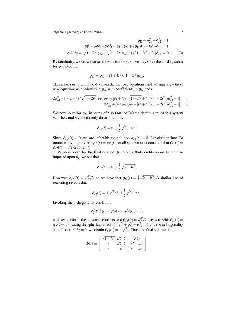
Algebraic geometry and finite frames 7
φ212 +φ
222 +φ
232 = 1
φ212 +3φ
222 +5φ
232−2φ12φ22 +2φ12φ32−6φ22φ32 = 1
xT S−1y =√
1−2t2φ12−√
1−2t2φ22 +(√
1−2t2 +2t)φ32 = 0. (3)
By continuity, we know that φ11(t) 6= 0 near t = 0, so we may solve the third equationfor φ12 to obtain
φ12 = φ22− (1+2t/√
1−2t2)φ32.
This allows us to elimnate φ12 from the first two equations, and we may view thesenew equations as quadratics in φ22 with coefficients in φ32 and t:
2φ222 +[(−2−4t/
√1−2t2)φ32]φ22 +[(2+4t/
√1−2t2 +4t2/(1−2t2))φ 2
32−1] = 02φ
222 +[−4φ32]φ22 +[(4+4t2/(1−2t2))φ 2
32−1] = 0
We now solve for φ32 in terms of t so that the Bezout determinant of this systemvanishes, and we obtain only three solutions,
φ32(t) = 0,±12
√2−4t2.
Since φ32(0) = 0, we are left with the solution φ32(t) = 0. Substitution into (3)immediately implies that φ12(t) = φ22(t) for all t, so we must conclude that φ12(t) =φ22(t) =
√2/2 for all t.
We now solve for the final column, φ3. Noting that conditions on φ2 are alsoimposed upon φ3, we see that
φ33(t) = 0,±12
√2−4t2.
However, φ33(0) =√
2/2, so we have that φ33(t) = 12
√2−4t2. A similar line of
reasoning reveals that
φ23(t) =±√
2/2,±12
√2−4t2.
Invoking the orthogonality condition,
φT2 S−1
φ3 =√
2φ23−√
2φ33 = 0,
we may eliminate the constant solutions, and φ23(0) =√
2/2 leaves us with φ23(t) =12
√2−4t2. Using the spherical condition φ 2
13 +φ 223 +φ 2
33 = 1 and the orthogonalitycondition xT S−1z = 0, we obtain φ13(t) =−
√2t. Thus, the final solution is
Φ(t) =
√
1−2t2√
2/2 −√
2tt
√2/2 1
2
√2−4t2
t 0 12
√2−4t2
.

8 Jameson Cahill and Nate Strawn
This parameterization is relatively simple because the first and third columns forman orthonormal basis of spanφ1(0),φ3(0) for all t. If we had observed this at thebeginning of the example, the parameterizations would follow very quickly. How-ever, a generic frame does not contain an orthonormal basis and the approach of thisexample is generically effective.
We may immediately exploit the idea behind this example to construct formalcoordinate systems around arbitrary frames in Fµ,S, However, it is not immediatelyclear that any of these formal coordinate systems are locally well-defined. Our firstchallenge is to demonstrate that there are unique, valid coordinate systems. We shallthen endeavor to identify these with the formal solutions that can be constructed ina manner echoing this example.
2.2 Tangent spaces on Fµ,S
We first turn our attention to the problem of characterizing the tangent spaces ofFµ,S. The reason for this is twofold. First, if the tangent is not well defined, thenwe are not guaranteed that the algebraic variety is locally diffeomorphic to an opensubset of Euclidean space. That is, smooth coordinate charts may not be available.The second reason is that we have a procedure for constructing formal coordinatesystems (as illustrated by the preceding example), but we would like to know thatthese formal coordinate systems are actually valid in some open neighborhood. Toobtain this validation, want to demonstrate injectivity of a Jacobian in order to in-voke a form of the inverse function theorem. Demonstrating the injectivity ensuresthat our coordinate map does not collapse or exhibit a pinched point, and we haveto characterize the tangent spaces of Fµ,S to carry out the demonstration.
For µ ∈ RM+ and N by N symmetric positive definite S, let
Tµ,N = Φ = (φi)Mi=1 ⊂ RN : ‖φi‖2 = µi for all i = 1, . . . ,M
andStS,M = Φ = (φi)
Mi=1 ⊂ RN : ΦΦ
T = S
denote the generalized torus and generalized Stiefel manifold respectively. Forbrevity, we shall simply call these the torus and Stiefel manifold. Clearly, we havethat
Fµ,S = Tµ,N ∩StS,M.
Suppose that Fµ,S is nonempty, set c = ∑Mi=1 µi, and define the Frobenius sphere of
square radius c by
SM,N,c = Φ = (φi)Mi=1 ⊂ RN :
N
∑i=1‖φi‖2 = c.
Then, we have the following inclusion diagram

Algebraic geometry and finite frames 9
SM,N,c
StS,M Tµ,N
Fµ,S
.
In order to demonstrate that formal coordinates are valid using the implicit func-tion theorem, we shall require an explicit characterization of the tangent spaceTΦFµ,S for a given Φ ∈ Fµ,S. Given the inclusion diagram, it is natural to askwhen
TΦFµ,S = TΦTµ,N ∩TΦ StS,M.
That is, when is the tangent space of the intersection equal to the intersection ofthe tangent spaces? The notion of transversal intersection is our starting point forapproaching this question (see [13]).
Definition 1. Suppose that M and N are smooth submanifolds of the smooth man-ifold K , and let x ∈M ∩N . We say that M and N intersect transversally at x inN if TxK = TxM +TxN . Here, + is the Minkowski sum.
Fig. 1 Full transversality of an intersection (left) ensures that the intersection forms a manifoldwith a formula for the dimension. The central figure demonstrates that local failure of transversalityresults in crossings inside the intersection (the lemniscate). On the right, we see that degeneracyoccurs when transversality fails completely.

10 Jameson Cahill and Nate Strawn
Theorem 2. Suppose that M and N are smooth submanifolds of the smooth man-ifold K , and let x ∈M ∩N . If N and M intersect transversally at x in K , thenTx(M ∩N ) is well-defined and
Tx(M ∩N ) = TxM ∩TxN .
That is, the tangent space of the intersection is the intersection of the tangent spaces.
To exploit this theorem, we must first determine TΦSM,N,c, TΦTµ,N , and TΦ StS,M .The tangent space for the sphere at Φ is simply the set of matrices “orthogonal” toΦ , or
TΦSM,N,c =
X = (xi)
Mi=1 ⊂ RN :
N
∑i=1〈xi,φi〉= 0
.
Since the tangent space of a product of manifolds is the product of the tangentspaces, we also have that
TΦTµ,N = X = (xi)Mi=1 ⊂ RN : 〈xi,φi〉= 0 for all i = 1, . . . ,N.
The most convenient characterization of TΦ StS,M is obtained by noting that the spe-cial orthogonal group SO(N) acts on StS,M on the right: (U,Φ) 7→ ΦU . Since theLie algebra of SO(N) is the skew symmetric matrices, it is not difficult to show that
TΦ StS,M = X = (xi)Mi=1 ⊂ RN : X = ΦZ, where Z =−ZT.
Having characterized these tangent spaces, we now turn to the problem of char-acterizing the Φ ∈Fµ,S at which Tµ,N and StS,M intersect transversally in SM,N,c.It turns out that the “bad” Φ are exactly the orthodecomposble frames (see [9]).
Definition 2. A frame Φ is said to be orthodecomposable if it can be split into twonontrival subcollections, Φ1 and Φ2 satisfying Φ∗1 Φ2 = 0. That is, span Φ1 andspan Φ2 are nontrivial orthogonal subspaces.
Clearly, orthodecomposability is intimately related to the correlation structure ofthe frame’s members. In order to demonstrate this equivalence, we shall require thenotion of a frame’s correlation network.
Definition 3. The correlation network of a frame Φ = (φi)Mi=1 is the undirected
graph γ(Φ) = (V,E), where V = [M] and (i, j)∈ E if and only if⟨φi,φ j
⟩is nonzero.
Example 1. For the Φ defined in the example
[⟨φi,φ j
⟩](i, j)∈[3]2 = Φ
TΦ =
1√
2/2 0√2/2 1 1/20 1/2 1
.We conclude that γ(Φ) = (1,2,3,(1,2),(2,3)), since φ1,φ3 is the only orthog-onal (uncorrelated) pair.

Algebraic geometry and finite frames 11
We can now state the main theorem which relates the transversality of the inter-section at Φ , connectivity of the correlation network γ(Φ), and the orthodecompos-ability of Φ . This result is due to Strawn [24].
Theorem 3. Suppose Φ ∈Fµ,S. Then the following are equivalent:
(i) TΦSM,N,c = TΦTµ,N +TΦ StS,M;(ii) For all Y ∈ TΦSM,N,c, there is a skew-symmetric Z = [zi j] which is a solution to
the system
〈yi,φi〉= ∑j∈[M]
z ji⟨φi,φ j
⟩for all i ∈ [M]; (4)
(iii) Φ is not orthodecomposable;(iv) γ(Φ) is connected.
The proof of this theorem is fairly straightforward, but its technical details obfus-cate the simple intuition. The centerpiece of the argument involves an algorithmfor constructing a solution to (4) given that γ(Φ) is connected. Because Z is skew-symmetric, this procedure can be interpreted as an algorithm for distributing speci-fied amounts of a resource at the nodes of the correlation network. We illustrate thisalgorithm in Figure 2.
Fig. 2 (a) A rooted spanning tree is extracted from γ(Φ). Set zi j = 0 if (i, j) is not in the spanningtree. (b) At nodes whose only children are leaves, fix entries of Z so that (4) holds for all thesechildren. Effectively remove these children from the tree. (c) Inductively apply (b) until only theroot remains. (d) The conditions on Y ensure that the final equation holds. At this point, all entriesof Z have been defined.
From this theorem, we immediately obtain a characterization of the tangentspaces of Fµ,S at non-orthodecomposable frames.

12 Jameson Cahill and Nate Strawn
Corollary 1. Assuming that Φ ∈Fµ,S is not orthodecomposable, we have
TΦFµ,S = TΦTµ,N ∩TΦ StS,M (5)
= X = (xi)Mi=1 ⊂ RN : X = ΦZ,Z =−ZT ,diag(Φ∗X) = 0
2.3 Existence of locally well-defined parameterizations on Fµ,S
Now that we have characterized the tangent spaces on Fµ,S, we proceed to constructa linear map π and a linear parameter space Ω ⊕∆ for each nonorthodecomposableF ∈ Fµ,S so that π : TFFµ,S → Ω ⊕ ∆ (the Jacobian of π : Fµ,S → Ω ⊕ ∆ ) isinjective and hence the map π : Fµ,S → Ω ⊕∆ has a locally well-defined inverseby the inverse function theorem [18]. This allows us to conclude that our formalprocedure produces valid coordinate systems.
We begin by noting that, by counting the governing constraints, the dimension ofa generic nonempty Fµ,S is
dim(Fµ,S) = dimTµ,N +dimStS,M−dimSM,N,c
= (N−1)M+M
∑i=1
(M− i)− (MN−1)
= (N−1)(M−N)+M−2
∑i=1
i.
Based on our initial example, this calculation, and a little intuition, we expect that itmay be possible to obtain a parameterization of the form Φ(Θ ,L) = [Γ (Θ)B(Θ ,L)],where
L ∈ ∆N = δ = (δi)Ni=1 ⊂ RN : δi j = 0 if i≤ j+1,
Θ ∈ΩM,N = ω = (ωi)M−Ni=1 ⊂ RN : ω1i = 0 for all i = 1, . . .M−N,
Γ (Θ) =
φ11(θ1) φ12(θ2) · · · φ1,M−N(θM−N)
θ21 θ22 · · · θ2,M−N...
.... . .
...θN1 θN2 · · · θN,M−N
,and where B(Θ ,L) has the form

Algebraic geometry and finite frames 13
φ1,M−N+1 φ1,M−N+2 · · · φ1,M−3 φ1,M−2 φ1,M−1 φ1Mφ2,M−N+1 φ2,M−N+2 · · · φ2,M−3 φ2,M−2 φ2,M−1 φ2M
l31 φ3,M−N+2 · · · φ3,M−3 φ3,M−2 φ3,M−1 φ3Ml41 l42 · · · φ4,M−3 φ4,M−2 φ4,M−1 φ4M...
.... . .
......
......
lN−1,1 lN−1,2 · · · lN−1,N−3 φN−1,M−2 φN−1,M−1 φN−1,MlN1 lN2 · · · lN,N−3 lN,N−2 φN,M−1 φNM
.
Here. Γ represents the vectors that may be freely perturbed within their sphere, andB parameterizes the basis. Note that Γ (Θ) and B(Θ ,L) are N by M−N and N by Narrays, respectively.
In order to exploit this parameter space, we must rotate all of the vectors of Φ sothat the resulting tangent space is sufficiently aligned with ΩM,N ⊕∆N . Otherwise,we shall fail to acquire a parameterization with the form we have just described. No-tationally, this system of rotations is represented as an array of orthogonal matrices:
Q = (Qi)Mi=1 ⊂ OM(N).
The alignment of the frame Φ using the system of rotations Q is denoted
Q?Φ = (Qiφi)Mi=1,
and we set QT = (QTi )
Mi=1.
This next theorem (also due to Strawn [24]) sets the stage for applying the real-analytic inverse function theorem [18] by demonstrating injectivity of the Jacobian.In particular, it allows us to know how and when we may use the parameter spaceΩM,N⊕∆N to obtain coordinates on Fµ,S.
Theorem 4. Suppose Φ ∈Fµ,S is not orthodecomposable. Then there is a system ofrotations Q∈OM(N) and an M by M permutation matrix P such that the orthogonalprojection
π : QT ?TΦPT FPµ,S→ΩM,N⊕∆N
is injective.
By the real-analytic inverse function theorem, we obtain the following corollary,which ensures us that our procedure for constructing formal coordinates (as in thefirst example) might actually produce well-defined coordinate systems.
Corollary 2. If the conditions of Theorem 4 are satisfied, then there is a unique,locally well-defined, real-analytic inverse of π , Φ ′ : ΩM,N⊕∆N →QT ?FPµ,S.
Remark 1. If Φ ′ is as in the above corollary, then (Q?Φ ′(Θ ,L))P is a parameteri-zation around Φ ∈Fµ,S.
The proof of Theorem 4 is rather technical, but a simple example should illustratethe nuances. Consider the frame

14 Jameson Cahill and Nate Strawn
Φ =
1 1√
33
√3
30 0
√3
3
√3
30 0 −
√3
3
√3
3
,so that µ = [1 1 1 1]T and
S =
83
23 0
23
23 0
0 0 23
.Our first goal is to identify a non-orthodecomposable basis inside of Φ . Note thatthe existence of such a basis is equivalent to connectivity of γ(Φ). We set
B = [φ2 φ3 φ4] =
1√
33
√3
30√
33
√3
30 −
√3
3
√3
3
.Our next gadget is a rooted tree on γ(B). We simply set 4 to be the root of this tree,and 2 and 3 are the children. Let T denote this tree. We have chosen T in this mannerso as to illustrate typical behavior.
Now, the permutation matrix P in Theorem 4 is then chosen so that PT moves allof the “free” vectors to the left side of ΦPT , and also so that if i is a child of j inT , then the ith vector precedes the jth vector. By our choice of Φ and T , we simplyhave that P = Id. Next, we fix the alignment matrices.
The alignment matrices of the“free” vectors are simply chosen so that Qie1 =φi/‖φi‖. Choosing the alignment matrices for the basis is more complicated. In ourcase, Q1 = Id since φ1 = e1. We now choose Q2 so that
[φ2 φ4 φ3] = [φ2 φ3 φ4]P(2 3) = Q2R2,
is the QR decomposition of B after we permute the second and third column. Notethat we have permuted so that the φ2 is followed by the vector whose index is theparent of 2 in T . It is simple to check that1
√3
3
√3
30√
33
√3
30√
33 −
√3
3
=
1 0 00√
22
√2
20 −
√2
2
√2
2
1
√3
3
√3
30√
63 0
0 0√
63
,and hence
Q2 =
1 0 00√
22
√2
20 −
√2
2
√2
2
.The final two alignment matrices are always set to the identity, so Q3 = Q4 = Id.
Now, we set about demonstrating that the projection from this theorem is injec-tive. Suppose that X ∈QT ?TΦFµ,S satisfies π(X) = 0, and hence

Algebraic geometry and finite frames 15
X =
x11 x12 x13 x140 x22 x23 x240 0 x33 x34
.Because γ(Φ) is connected, we know that
TΦFµ,S = Y : Y = ΦZ,Z =−Zt ,diag(ΦTΦZ) = 0.
In particular, we have that X = QT ? (ΦZ) for some Z = −ZT . We shall show thatZ = 0 by induction though its columns. First, we show that we may choose Z so thatz1 = 0. We first note that x1 = Φz1. Since diag(ΦT ΦZ) = 0, we have
0 = φT1 Φz1 = eT
1 Φz1 = eT1 x1 = x11.
Consequently, x1 = 0 and it turns out that we can assume z1 = 0 in this case. Thedetails of this are described in the full proof, but one may think of this as sayingthat any motion that fixes “free” vectors only needs to know how it is acting on thebasis. Now, we show that z2 = 0. We have that
P(2 3)
0z32z42
= R−12 x2 =
1 −√
22 −
√2
20√
62 0
0 0√
62
x12
x220
=
x12−√
22 x22√
62 x22
0
.This means that
z2 =
000
z42
.Now, the other condition on TΦFµ,S, diag(ΦT ΦZ) = 0 implies that φ T
2 Φz2 = 0.But since we have z2 = z42e4, this condition reduces to
z42φT2 φ4 = 0.
In the spanning tree of the correlation network, 4 is the parent of 2, so we havethat φ T
2 φ4 6= 0. Therefore z42 = 0, and hence z2 = 0. Repeating this trick gives usthat z3 = 0 as well; the last three entries of z3 are Φ−1x3, which implies that the onlynonzero entry of z3 is z43, and the diagonal condition ensures that z43 = 0. Finally,z4 = 0 since Z =−ZT .
We have shown that Z = 0, so it follows that X = 0 and π is injective. Aftercounting dimensions, we invoke the real-analytic inverse function theorem to ob-tain unique, analytic, locally well-defined coordinates. This guarantees us that ourformal solutions to this system are locally valid. We now proceed to elucidate theexplicit construction of formal solutions.

16 Jameson Cahill and Nate Strawn
2.4 Deriving explicit coordinates on Fµ,S
Using the same Φ in our last example, we set
φ1 =
√
1−φ 221−φ 2
31
φ21φ31
.Our only condition imposed upon the “ree” vector is that it remains in its sphere.However, as we move φ1, the frame operator of the basis [φ2 φ3 φ4] must change tomaintain the overall frame operator. Explicitly, we want to enforce the constraint
S = φ1φT1 +φ2φ
T2 +φ3φ
T3 +φ4φ
T4 ,
so we must have that
BBT = φ2φT2 +φ3φ
T3 +φ3φ
T3 = S−φ1φ
T1 .
Since B is invertible, we can rearrange to obtain
BT (S−φ1φT1 )−1B = Id.
By rearranging in this manner, all of the conditions on the basis become conditionson the columns. This is the central trick that supplies us with a strategy for carryingout the full derivation of the explicit coordinate systems. With this rearrangement,it is now possible to solve the entire system in a column-by-column fashion.
For this trick to work we must compute (S−φ1φ T1 )−1. The entries of this inverse
are analytic functions, but they are already complicated. While we may be able tofit this expression on a page, we only have one“free” vector to consider. With anarbitrary number of “free” vectors, one can easily see that this inverse has a verydense representation. Even if we were simply solving a linear system involving thebasis and this inverse, the full expression would be vast. In our situation, we’re goingto solve two quadratic equations and a linear system. This dramatically inflates thecomplexity of the explicit expressions.
Forgoing the explicit form of (S− φ1φ T1 ), we now consider the conditions that
must be imposed upon just φ2:
φT2 φ2 = 1 and φ
T2 (S−φ1φ
T1 )−1
φ2 = 1.
The first is a spherical constraint, and the second is an ellipsoidal constraint. Ingeneral, the solution set in R3 bears a striking resemblance to the boundary of aPringle chip. Because of the alignment structure, we set φ2 = Q2ψ and solve
ψT
ψ = 1 and ψT QT
2 (S−φ1φT1 )−1Q2ψ = 1
where

Algebraic geometry and finite frames 17
ψ =
ψ1(t,φ1)ψ2(t,φ1)
t
.As in our first example, these are two quadratic constraints and we may apply theBezout determinant trick to obtain explicit expressions for ψ1 and ψ2. The resultingexpression are entirely dependent upon φ1 and t. We may then set φ2 = QT
2 ψ . Withφ2 hand, we can then solve for φ3 and φ4 just like we did in our first example. Theastute reader will recognize that we obtain numerous branches from solving theseequations. However, we may prune these branches by considering the conditionΦ(0,0,0) = Φ .
While we may write down explicit expressions for these coordinate systems,these expressions will necessarily involve solutions to quartic equations, which areunwieldy when expressed in their full form. For our example, some of the expres-sions are so vast that they exceed LATEX’s allowed buffer. Nevertheless, computer al-gebra packages can manage the expressions. For a full technical derivation of thesecoordinates and a full proof that there is a unique branch with local validity, thereader is referred to [24]
Since the expressions for our example are too large to fit on a page, we concludethis section with Figure 3, which depicts the motion that frame vectors experienceas we traverse the local coordinate system. In this figure, we allow φ1 to move alonga great circle and allow t to vary fully. Consequently, we observe the individualbasis vectors articulating along two dimensional sheets inside of the unit sphere.There are of course three degrees of freedom for this example, but it is much harderto visualize the behavior obtained by submerging a three dimensional space in asphere.
Fig. 3 In this figure, we have allowed φ1 (the small blue curve near the sheet on the left side) tovary along a fixed curve and the movement of φ2 controls the single degree of freedom inside ofthe basis. Consequently, φ2, φ3, and φ4 carve out two-dimensional sheets on the unit sphere.

18 Jameson Cahill and Nate Strawn
3 Grassmannians
In this section we will study a family of well known varieties called Grassmanni-ans. These results originally appeared in [5]. The Grassmannian is defined as theset N-dimensional subspaces of H M and will be denoted by Gr(M,N). It is notclear from this definition how this set forms a variety, but this will be explainedshortly. The motivation for the use of Grassmannians in frame theory comes fromthe following proposition, (see [1],[17]):
Proposition 3. Two frames are isomorphic if and only if their corresponding anal-ysis operators have the same image.
Therefore a point on a Grassmannian corresponds to an entire isomorphism classof frames, but many properties of frames are invariant under isomorphisms, soGrassmannians can give a useful way to discuss families of frames with certainproperties.
In this first section we will explain some basic properties of Grassmannians. Mostof this material is well known, so we will provide appropriate references for techni-cal details that are not included here.
First we will be concerned with the Grassmannian as a metric space. If X ,Y ∈Gr(M,N) then ‖PX −PY ‖ defines a metric on Gr(M,N), where PX denotes theorthogonal projection of H M onto X , and ‖ · ‖ denotes the usual operator norm.This metric has a geometric interpretation in terms of the “angle” between X andY . Define the N-tuple (σ1, ...,σk) as follows:
σ1 = max〈x,y〉 : x ∈X ,y ∈ Y ,‖x‖= ‖y‖= 1= 〈x1,y1〉,
and
σi = max〈x,y〉 : x ∈X ,y∈Y ,‖x‖= ‖y‖= 1,〈x,x j〉= 〈y,y j〉= 0, j < i= 〈xi,yi〉
for i > 1. Now define θi(X ,Y ) = cos−1(σi). The N-tuple θ(X ,Y ) = (θ1, ...,θN)is called the principal angles between X and Y (some authors call these the canon-ical angles). Let X and Y be N×M matrices whose rows for orthonormal bases forX and Y respectively. It turns out that the σi’s are precisely the singular valuesof XY ∗. We also have that ‖PX −PY ‖ = sin(θN(X ,Y )). In fact, there are manymetrics that can be defined in terms of the principal angles. Justifications for thesethree facts can be found in [17].
We now proceed to explain a particular embedding, known as the Plucker em-bedding, of Gr(M,N) into P(
MN)−1 which will be used extensively in this section. Let
X ∈ Gr(M,N) and let X (1) be any N×M matrix whose rows form a basis for X .Let X (1)
i1···iN be the N×N minor consisting of the columns indexed by i1, ..., iN of X (1).
Then the(M
N
)-tuple Plu(X (1)) = (det(X (1)
i1···iN ))1≤i1<···<iN≤M is called the Plucker co-ordinates of X . Note that if X (2) is any other N×M matrix whose rows span Xthen there exists an invertible N×N matrix A such that (X (2)) = A(X (1)). It follows

Algebraic geometry and finite frames 19
that Plu(X (2)) = det(A)Plu(X (1)). Thus the mapping X 7→ Plu(X ) is a well de-fined injective mapping of Gr(M,N) into P(
MN)−1. In most cases this mapping is not
onto, however the image of this mapping is known to be a projective variety, see[11] for more details. In particular, the vanishing locus of the polynomials
xi1...iN x j1... jN −N
∑k=1
x jki2...iN x j1... jk−1i1 jk+1... jN
(where xσ(i1)...σ(iN) = sign(σ)xi1...iN for any permutation σ ) is precisely in the im-age of the Plucker embedding. We use the symbol Plu(M,N) to denote this set ofpolynomials.
By abuse of notation let Plu(X ) denote a unit vector in H (MN). Then we have
that |〈Plu(X ),Plu(Y )〉| is well defined for any X ,Y ∈ Gr(M,N). We define thePlucker angle between X and Y to be
Θ(X ,Y ) = cos−1 |〈Plu(X ),Plu(Y )〉|.
We have the following relationship between Θ(X ,Y ) and θ(X ,Y ), see [16],[19], and [20]:
Proposition 4.
cos(Θ(X ,Y )) =k
∏i=1
cos(θi(X ,Y )). (6)
Proof. Let X and Y be N×M matrices whose rows form orthonormal bases for Xand Y respectively. Then
cos(Θ(X ,Y )) = |〈Plu(X ),Plu(Y )〉|= | ∑
1≤i1<···<iN≤Mdet(Xi1...iN )det(Yi1...iN )|
= | ∑1≤i1<···<iN≤M
det(Xi1...iNY ∗i1...iN )|
= |det(XY ∗)|= |det(UΣV )|= det(Σ)
=N
∏i=1
σi =N
∏i=1
cos(θi(X ,Y )),
where XY ∗ =UΣV is a singular value decomposition, and where we have employedthe Cauchy-Binet formula for the fourth equality .
ut
In particular, θi(X ,Y )≤Θ(X ,Y ) for every i = 1,2, ...,N, Θ(X ,Y ) = π
2 if andonly if θN(X ,Y ) = π
2 , and Θ(X ,Y ) = 0 if and only if θN(X ,Y ) = 0. Also, wehave the following new metric on Gr(M,N):
d(X ,Y ) = ‖Plu(X )−Plu(Y )‖= 2sin(
Θ(X ,Y )
2
),

20 Jameson Cahill and Nate Strawn
which we call the Plucker metric.We now describe a particular way of breaking up the Grassmannian into subsets
known as the matroid stratification of the Grassmannian (see [4]). First we definematroids (note that there are many equivalent ways of defining matroids, we statethe one that we will use here).
Definition 4. A matroid is an ordered pair ([M],B) where B ⊆ 2[M] satisfies:(B1) B 6= /0(B2) A,B ∈B, a ∈ A\B⇒∃b ∈ B\A such that (A\a)∪b ∈B.[M] is called the ground set of M and the elements of B are called the bases of M .
For more background on matroid theory we refer to [21]. The main reason wecare about matroids is summarized in the following proposition which can be foundin [21]:
Proposition 5. Let [M] be the set of column labels of an N ×M matrix F over afield F, and let B be the collection of subsets I ⊆ [M] for which the set of columnslabeled by I is a basis for Fk. Then M (F) := ([M],B) is a matroid.
Matroids encode linear independence; determinants are a measure for this. In par-ticular, observe that Plu(X ) associates to each X ∈Gr(M,N) a matroid M (X ) asfollows: A set i1, ..., iN⊆ [M] is a basis of M (X ) if and only if Plu(X )i1...iN 6= 0.Thus, to each matroid M we can associate the subset of Gr(M,N):
R(M ) = X ∈ Gr(M,N) : M (X ) = M .
Thus, Gr(M,N) can be written as a disjoint union of sets of this type. We will usethis stratification later to prove that generic Parseval frames are dense in the set ofParseval frames.
3.1 Frames and Plucker coordinates
Let Φ = ϕiMi=1 be a frame for H N . We denote Plu(Φ)= (det(Φi1...iN ))1≤i1<...<iN≤M .
(Note that Plu(Φ) is a point in H (MN).) By Proposition 3 we have that Plu(Φ) =
λPlu(Ψ) if and only if there is an invertible operator T so that ϕi = T ψi for ev-ery i = 1,2, ...,M, in which case λ = det(T ). An argument similar to the proof ofProposition (4) yields the following:
Proposition 6. ‖Plu(Φ)‖2 = det(S), where S is the corresponding frame operator.
One important consequence of Proposition 6 is the following corollary whichwill be used extensively later.
Corollary 3. If Φ is a Parseval frame then ‖Plu(Φ)‖= 1.

Algebraic geometry and finite frames 21
Note however that Proposition 6 also says that the converse of the above corollary isnot true. To see this let S be a positive, self adjoint operator such that det(S) = 1, andlet Φ = ϕiM
i=1 be a Parseval frame. Now consider the frame S1/2Φ = S1/2ϕiMi=1
which has S as its frame operator. If S is not the identity operator then S1/2Φ is nota Parseval frame, but we still have that ‖Plu(S1/2Φ)‖= 1.
For notational convenience we denote by Π(Φ) the image of the analysis opera-tor corresponding to the frame Φ . Thus, Plu(Π(Φ)) is a point in projective space.Given a point X ∈ Gr(M,N) we use the symbol Π−1(X ) to denote the entire iso-morphism class of frames whose analysis operator has X as its image. We can nowprove the following result which says that close subspaces are necessarily images ofanalysis operators of close Parseval frames
Theorem 5. Let X ,Y ∈ Gr(M,N), and let ε > 0. Suppose Θ(X ,Y ) < ε
2√
Nand that ϕiM
i=1 ∈ Π−1(X ) is a Parseval frame. Then there is a Parseval frameψiM
i=1 ∈Π−1(Y ) such that ‖ϕi−ψi‖< ε for every i = 1,2, ...,M.
Proof. First note that θN(X ,Y ) ≤ Θ(X ,Y ) < ε
2√
N. We can find orthonormal
bases a jNj=1 for X and b jN
j=1 for Y such that 〈a j,b j〉 = cos(θ j) for everyj = 1, ...,N. Therefore, we have
‖a j−b j‖= 2sin(
θ j
2
)≤ 2sin
(θN
2
)<
ε√N
for every j = 1, ...,N. Now let A and B be the N×M matrices whose jth columnsare a j and b j respectively. Let ai j be the ith entry of a j and let fi be the ith row of A,similarly let bi j be the ith entry of b j and let gi be the ith row of B. Then we have
M
∑i=1
(ai j−bi j)2 <
ε2
Nfor every j = 1, ...,N
which means
(ai j−bi j)2 <
ε2
Nfor every j = 1, ...,N i = 1, ...,M
which further implies that
N
∑j=1
(ai j−bi j)2 = ‖ fi−gi‖2 < ε
2.
Now since the columns of A for an orthonormal basis for X we know that fiMi=1
is an Parseval frame which is isomorphic to ϕiMi=1. This means there is some uni-
tary T : H N →H N such that T fi = ϕi for every i = 1, ...,M. The Parseval frameψiM
i=1 = T giMi=1 can now be seen to have the desired properties. ut
The same argument can be used to prove a similar result for different combina-tions of metrics on the Grassmannian and metrics on frames.

22 Jameson Cahill and Nate Strawn
Theorem 6. Let X ,Y ∈Gr(M,N), and let ε > 0. Suppose ∑Nj=1 sin2(θ j(X ,Y ))<
ε and that ϕiMi=1 ∈ Π−1(X ) is a Parseval frame. Then there is a Parseval frame
ψiMi=1 ∈Π−1(Y ) such that ∑
Mi=1 ‖ϕi−ψi‖2 < ε .
We can also use a similar argument to generalize Theorem 5 in the case that wecare about frames that may not be Parseval frames.
Theorem 7. Let X ,Y ∈ Gr(M,N), and let ε > 0. Let ϕiMi=1 ∈ Π−1(X ) with
frame operator S and assume that
Θ(X ,Y )<ε
‖S 12 ‖2√
N.
Then there is an frame ψiMi=1 ∈ Π−1(Y ) such that ‖ϕi−ψi‖ < ε for every i =
1,2, ...,M. Furthermore, if ϕiMi=1 is a Parseval frame, then ψiM
i=1 can be chosento be a Parseval frame as well.
3.2 Generic frames
A frame is said to be robust to m erasures if the removal of any m vectors leavesa frame. Clearly an frame consisting of M vectors in H N can be robust to at mostM−N erasures. We call such a frame a generic frame. Generic frames have appearedin previous literature under the name maximally robust frame (see [22]). However,we shall see that this is a very weak measure of the robustness of a given frame toerasures. In particular, we will show that there is an open dense set of frames thatare robust to M−N erasures, so we believe the name “maximally robust” should bereserved for a robustness in a more numerical sense. In this section we will studythe set of generic frames. We begin this section with the following fairly simpleobservation:
Proposition 7. Let ϕiMi=1 be an frame, and ε > 0. Then there is a generic frame
ψiMi=1 such that
‖ϕi−ψi‖< ε
for every i = 1, ...,M.
Proof. If ϕiMi=1 is generic then there is nothing to prove, so assume ϕiM
i=1 is notgeneric. Let ϕi jm
j=1 be a minimal dependent set, note that dim(spanϕi jmj=1) =
m− 1. Choose some ϕi j0and let B be the open ball of radius ε centered at ϕi j0
.Now let W be the set of hyperplanes (i.e., codimension 1 subspaces) spanned byany combination of vectors in ϕiM
i=1 that do not include ϕi j0. Notice that H N\W
is an open dense set in H N since W consists of a finite number of hyperplanes, soB∩ (H N\W ) 6= /0. Choose any x in this set and replace ϕi j0
with x. This ensuresthat dim(spanϕi j j 6= j0 ∪x) = m and that we have not created any new dependent

Algebraic geometry and finite frames 23
sets of cardinality less than or equal to N. After repeating this process finitely manytimes we can ensure that we arrive at a generic frame with the desired properties.
ut
Now if ϕiMi=1 is a Parseval frame, can ψiM
i=1 be chosen to be a Parseval frame?The answer is yes, but to prove this we need to use the results of the previous sec-tion. Before proving this we need to explain some further properties of the matroidstratification of the Grassmannian.
Choose 1 ≤ i1 < · · · < iN ≤M and consider the set Vi1...iN = X ∈ Gr(M,N) :Plu(X )i1...iN = 0 =
⋃R(M ) : i1, ..., iN is not a basis of M . Now observe
that Vi1...iN is a proper closed subvariety of Gr(M,N) which tells us that Vi1...iN is aclosed subset of Gr(M,N) in the Zariski topology, which implies it is also closed inthe Euclidean topology (the topology induced by the Plucker metric), so in particu-lar Gr(M,N)\Vi1...iN is an open and dense subset of Gr(M,N) (in both topologies).The uniform matroid of rank N on [M] is the matroid whose bases consist of all sub-sets of [M] of cardinality N; we use the symbol UM,N to denote this matroid. Nowobserve that
R(UM,N) =⋂
1≤i1<···<iN≤M
Gr(M,N)\Vi1...iN ,
which means that R(UM,N) is an open and dense subset of Gr(n,k). Now we canprove our result.
Theorem 8. Let ϕiMi=1 be a Parseval frame, and ε > 0. Then there is a generic
Parseval frame ψiMi=1 such that ‖ϕi−ψi‖< ε for every i = 1, ...,M.
Proof. First note that Φ is generic if and only if Π(Φ) ∈ R(UM,N), so we mayassume Π(Φ) 6∈R(UM,N). By the above remarks we can find a point Y ∈R(UM,N)such that Θ(Π(Φ)),Y )< ε
2√
k, so the result follows from Theorem 5. ut
Now that we have established that almost every frame is generic we would liketo come up with a numerical measure of the genericity of a frame and construct theParseval frames that are somehow the “most generic.” Since we have seen how toassociate points on the Grassmannian to frames, and we know how to compute dis-tance on the Grassmannian, one reasonable way to measure the genericity of a givenframe is to find the shortest distance on the Grassmannian to an isomorphism classof frames that is not generic. However, there are many ways to measure distance onthe Grassmannian, so we will choose one reasonable way.
We pose the following optimization problem:
minX ∈Gr(M,N)
maxΘ(X ,Ei1···iN ) : 1≤ i1 < · · ·< iN ≤M, (7)
where Ei1···iN = spanei1,...,eiN and eiM
i=1 is the standard orthonormal basis ofH M . Recall that by Corollary 3 the Plucker norm of any Parseval frame is 1, sowe would like to find the unit vectors on the (Plucker embedding of) the Grass-mannian whose smallest (in absolute value) Plucker coordinate is as big as possible.

24 Jameson Cahill and Nate Strawn
Intuitively, a small Plucker coordinate says that the corresponding subset is “barely”a basis.
Clearly, if the Plucker embedding is onto then these would be the points whosePlucker coordinates (in absolute value) were all equal to
(MN
)−1/2. However, these
points are only in the image of the Plucker embedding when N = 1 or N = M− 1,i.e., every sequence of unit-modulus scalars is optimal for N = 1 and every simplexis optimal for N =M−1. For other choices of M and N we want to find the points onthe Grassmannian that are as close (in the regular Euclidean sense) to these pointsas possible. An equivalent task is to solve the following optimization problem:
maximize : ∑1≤i1<···<iN≤M
|xi1···iN |
subject to : Plu(M,N)
∑1≤i1<···<iN≤M
x2i1···iN = 1.
We will illustrate this with the first nontrivial example, Gr(4,2). In this casePlu(4,2) contains only the polynomial x12x34− x13x24 + x14x23, so the above opti-mization problem becomes
maximize : |x12|+ |x13|+ |x14|+ |x23|+ |x24|+ |x34|subject to : x12x34− x13x24 + x14x23 = 0
x212 + x2
13 + x214 + x2
23 + x224 + x2
34 = 1.
For the sake of simplicity, we will only look for solutions in the first orthant (i.e.,where all Plucker coordinates are positive), so we can drop the absolute values. Us-ing the method of Lagrange multipliers we arrive at the following system of equa-tions:
2λ1x12 +λ2x34 = 12λ1x34 +λ2x12 = 12λ1x14 +λ2x23 = 12λ1x23 +λ2x14 = 12λ1x13−λ2x24 = 12λ1x24−λ2x13 = 1.
Together, the first two equations imply
2λ1x12 +λ2x34 = 2λ1x34 +λ2x12
⇒ (2λ1−λ2)x12 = (2λ1−λ2)x34
⇒ x12 = x34 as long as λ1 6=λ2
2.

Algebraic geometry and finite frames 25
Similarly, the third and fourth equation imply x14 = x23 as long as λ1 6= λ22 , and the
last two equations imply x13 = x24 as long as λ1 6=−λ22 . This reduces our system of
six equations to the following system of three equations:
(2λ1 +λ2)x12 = 1(2λ1 +λ2)x14 = 1(2λ1−λ2)x13 = 1.
But the first two equations of this system now imply x12 = x14 (under our assump-tions on λ1 and λ2). The Plucker relation now becomes
2x212− x2
13 = 0.
Now we can use our unit norm constraint to find the solutions:
x12 = x14 = x23 = x34 =±√
24
, x13 = x24 =±12.
Thus, we wish to find a 4×2 matrix whose Plucker coordinates are (a scalar multipleof) (
√2
4 , 12 ,√
24 ,√
24 , 1
2 ,√
24 ). The easiest way to do this is to make the first Plucker
coordinate equal to 1:
4√2
(√2
4,
12,
√2
4,
√2
4,
12,
√2
4
)= (1,
√2,1,1,
√2,1),
and find a matrix of the following form:[1 0 a b0 1 c d
].
For example, since x13 =√
2 we see c =√
2. Similarly, we can solve for a,b and dand we arrive at the following matrix:[
1 0 −1 −√
20 1√
2 1
].
Finally, we perform Gram-Schimdt to the columns of this matrix so that they be-come an orthonormal basis for their span in R4, and that means the columns shouldform the Parseval frame that we were looking for:[
12 0 − 1
2 −√
22
12
√2
212 0
].

26 Jameson Cahill and Nate Strawn
3.3 Signal reconstruction without phase
In this section we will discuss a problem known as phaseless reconstruction. Theresults of this section originally appeared in [2]. Suppose we are given a frameΦ = ϕiM
i=1 for H N . We would like to know if we can recover x ∈H N up to ascalar multiple of modulus one if we are just given the vector of absolute values ofinner products with the frame vectors. To be more precise, we define the mappings
f aΦ : H N → RM, f a
Φ(x) = (|〈x,ϕ1〉|, ..., |〈x,ϕM〉|)
and
fΦ : H N/∼→ RM, fΦ(x) = (|〈x,ϕ1〉|, ..., |〈x,ϕM〉|), x ∈ x,
where x,y∈ x ∈H N/∼ if there is a scalar λ with x = λy and |λ |= 1. So we wouldlike to find conditions on the frame Φ which guarantee that fΦ is injective. We willanalyze the real an complex cases separately.
We start with the real case. In this case the domain of fΦ is RN/∼, where x,y ∈x ∈ RN/ ∼ if and only if x = ±y. Before stating our results we need to fix somenotation. Given a subset I ⊆ [M], by abuse of notation use the same symbol I todenote the characteristic function of this set, i.e., for i ∈ [M], I(i) = 1 if i ∈ I andI(i) = 0 if i 6∈ I. Define a mapping σI : RM → RM by
σI(a1, ...,aM) = ((−1)I(1)a1, ...,(−1)I(M)aM).
Note that σ2I = I, and σIc =−σI . Also, let LI = (a1, ...,aM) : ai = 0 for i∈ I. Then
we have that σI(u) = u if and only if u ∈ LI and σI(u) =−u if and only if u ∈ LIc .We need one more definition before stating our theorem.
Definition 5. Let M be a matroid with ground set [M]. We say M has the comple-ment property if for every I ⊆ [M] either I contains a basis of M or Ic contains abasis of M .
Theorem 9. For a frame Φ = ϕiMi=1 ⊆ RN the following are equivalent:
(1) fΦ is injective.(2) For every nonempty proper subset I ⊆ [M] and every u ∈ Π(Φ)\(LI ∪ LIc),σI(u) 6∈Π(Φ).(3) If there is a nonempty proper subset I ⊆ [M] for which Π(Φ)∩ LI 6= /0 thenΠ(Φ)∩LIc = /0.(4) Π(Φ) ∈R(M ) for some matroid M with the complement property.
Proof. (1)⇒(2) Suppose there is a nonempty proper subset I ⊆ [M] and a u ∈Π(Φ)\(LI ∪LIc) for which σI(u)∈Π(Φ). Since u 6∈ LI ∪LIc we know σI(u) 6=±u.Now there is are x,y ∈ RN such that 〈x,ϕi〉 = u(i) and 〈y,ϕi〉(−1)I(i)u(i) for everyi = 1, ...,M. But then f a
Φ(x) = f a
Φ(y) and since σI(u) 6=±u we know that x 6=±y, so
fΦ is not injective.

Algebraic geometry and finite frames 27
(2)⇒(3) Suppose there is a nonempty proper subset I ⊆ [M] for which bothΠ(Φ)∩LI 6= /0 and Π(Φ)∩LIc 6= /0. Choose v ∈ Π(Φ)∩LI and w ∈ Π(Φ)∩LIc .Then v+w ∈Π(Φ)\(LI ∪LIc) but σI(v+w) = v−w ∈Π(Φ).
(3)⇒(4) Suppose there is a subset I ⊆ [M] for which neither ϕii∈I nor ϕii∈Ic
spans RN . Choose x⊥ spanϕii∈I and y⊥ spanϕii∈Ic . Then T (x)∈ LI and T (y)∈LIc .
(4)⇒(1) Suppose x,y∈RN are such that |〈x,ϕi〉|= |〈y,ϕi〉| for every i = 1, ...,M.Let I = i : 〈x,ϕi〉 = −〈y,ϕi〉 and observe that x+ y ⊥ spanϕii∈I and x− y ⊥spanϕii∈Ic . But we know that either spanϕii∈I = RN or spanϕii∈Ic = RN byassumption, so we have either x+y = 0 or x−y = 0, i.e., x =±y and fΦ is injective.
ut
Corollary 4. (1) If M ≥ 2N − 1 then fΦ is injective for almost every frame Φ =ϕiM
i=1 ⊆ RN .(2) If M < 2N−1 then fΦ is not injective.
Proof. To see the first statement just observe that for M ≥ 2N−1 the uniform ma-troid UM,N has the complement property, so if Φ is generic then fΦ is injective. Forthe second statement let I ⊆ [M] be such that |I|= N−1 and note that |Ic| ≤ N−1.Therefore it is impossible for any matroid of rank N whose ground set is [M] to havethe complement property.
ut
We now shift our attention to the complex case. In this case the domain of fΦ isCN/∼ where x∼ y if and only if there is a λ ∈ T so that x = λy, where T is the unitcircle on the complex plane. At this time the complex case is not understood nearlyas well as the real case, however we can still prove the existence of a large familyof frames for which fΦ is injective.
Theorem 10. Suppose M ≥ 4N−2. Then there is an open and dense set of framesfor CN with M elements for which fΦ is injective.
Proof. First note that fΦ is injective if and only if there do not exist nonparallelvectors v,w ∈Π(Φ) such that |v(i)|= |w(i)| for every i = 1, ...,M. So we will showthat the set of subspaces that have this property is a Zariski open subset of Gr(M,N).Denote the complement of this set by A , and choose any X ∈ A . Without lossof generality we may assume we have a basis u jN
j=1 for X so that u j(i) = 1 ifj = i and u j(i) = 0 when j 6= i ≤ N; for i > N u j(i) is undetermined. Therefore, ina neighborhood of X we see that Gr(M,N) has dimension 2N(M−N) as a realvariety.
Now since X ∈A we can choose nonparallel v,w ∈X with |v(i)|= |w(i)| forevery i. Our choice of basis guarantees that at least one of the first N entries of v(and therefore w) is nonzero, which we can assume to be the first entry without lossof generality, so after rescaling we have that v(i) = w(i) = 1. Since v and w arenonparallel we know that for some 2 ≤ i ≤ N we have that v(i) 6= w(i) 6= 0, andagain without loss of generality we can assume this happens for i = 2.

28 Jameson Cahill and Nate Strawn
Now we have that there are λ2, ...,λM ∈ T with λ2 6= 1 such that w(i) = λiv(i) forevery i = 2, ...,M (and v(1) = w(1) = 1). For i > N we have v(i) = ∑
Nj−1 v( j)u j(i)
and w( j) = ∑Nj=1 λ jv( j)u j(i). Thus we have∣∣∣∣∣ N
∑j=1
v( j)u j(i)
∣∣∣∣∣=∣∣∣∣∣ N
∑j=1
λ jv( j)u j(i)
∣∣∣∣∣ . (8)
Consider the variety of all tuples (Y ,v(1), ...,v(N),λ2, ...,λN) with Y ∈Gr(M,N)and v(i) and λi as above. This variety is locally isomorphic to CN(M−N)×(C\0)×CN−2×(T\1)×TN−2 which has dimension 2N(M−N)+3N−3 as a real variety.We also have that A is the image under projection onto the first factor of this vari-ety cut out by the M−N equations (8). Now observe that for a fixed 0 6= v(2), ...,vNand 1 6= λ2, ...,λN these equations are nondegenerate. Since u1(i), ...,uN(i) appearin exactly one equation it follows that these equations define a subspace of CN(M−N)
of real codimension at least M−N. Since this is true for all choices of the v(i)’s andthe λi’s it follows that these equations are independent.
We can now conclude that A is a real variety of (local) dimension 2N(M−N)+3N− 3− (M−N). Therefore if 3N− 3− (M−N) < 0, i.e., M ≥ 4N− 2 then Ais a proper subvariety of Gr(M,N) and so its complement is open in the Zariskitopology.
ut
It is not known whether the value M = 4N− 2 is optimal, i.e., we do not knowif it is possible for fΦ to be injective for a frame consisting of fewer than 4N− 2vectors.
References
1. Balan RV (1999) Equivalence relations and distances between Hilbert frames. Proc AmerMath Soc 127:2353–2366
2. Balan RV, Casazza PG, Edidin D (2006) On signal reconstruction without phase. Appl Com-put Harmon Anal 20:345–356
3. Benedetto JJ, Fickus M (2003) Finite normalized tight frames. Adv Comput Math 18:357–385
4. Bjorner A, Las Vergnas M, Sturmfels B, White N, Ziegler GM (1999) Oriented Matroids.Cambridge University Press, Cambridge
5. Cahill, J (2009) Flags, frames, and Bergman spaces. Master’s Thesis, San Francisco StateUniversity
6. Cahill J, Casazza PG (2011) The Paulsen Problem in Operator Theory. arXiv:1102.23447. Casazza PG, Leon MT (2010) Existence and construction of finite frames with a given frame
operator. Int J Pure Appl Math 63:149–1588. Casazza PG, Tremain JC (2006) The Kadison–Singer problem in mathematics and engineer-
ing. Proc Nat Acad Sci 103:2032–20399. Dykema K, Strawn N (2006) Manifold structure of spaces of spherical tight frames. Int J Pure
Appl Math 28:217–25610. Fraenkel AS, Yesha Y (1979) Complexity of Problems in Games, Graphs, and Algebraic
Equations. Discrete Appl Math 1:15–30

Algebraic geometry and finite frames 29
11. Fulton W (1997) Young Tableaux — With Applications to Representation Theory and Geom-etry. Cambridge University Press, Cambridge
12. Goyal VK, Kovacevic, J, Kelner JA (2001) Quantized frame expansions with erasures. ApplComput Harmon Anal 10:203–233
13. Guillemin V, Pollack A (1974) Differential Topology — History, Theory, and Applications.Prentice-Hall, Englewood Cliffs
14. Han D, Larson DR (2000) Frames, bases, and group representations. Mem Amer Math Soc147
15. Hartshorne R (1997) Algebraic Geometry. Springer-Verlag, New York16. Jiang S (1996) Angles between Euclidean subspaces. Geom Dedicata 63:113–12117. Jordan C (1875) Essai sur la geometrie a n dimensions. Bull. Soc. Math. France 3:103–17418. Krantz SG, Parks HR (2002) The Implicit Function Theorem — History, Theory, and Appli-
cations. Birkhauser, Boston19. Miao JM, Ben-Israel A (1992) On principal angles between subspaces in Rn. Linear Algebra
Appl 171:81–9820. Miao JM, Ben-Israel A (1996) Product cosines of angles between subspaces. Linear Algebra
Appl 237-238:71–8121. Oxley JG (1992) Matroid Theory. Oxford University Press, New York22. Puschel M, Kovacevic J (2005) Real tight frames with maximal robustness to erasures. Proc
IEEE Data Comput Conf 63–7223. Qiu L, Zhang Y, Li C (2005) Unitarily invariant metrics on the Grassmann space. SIAM J
Matrix Anal Appl 27:507–53124. Strawn N (2011) Finite frame varieties: Nonsingular points, tangent spaces, and explicit local
parameterizations. J Fourier Anal Appl 17:821–85325. Weaver N (2004) The Kadison–Singer problem in discrepancy theory. Discrete Math
278:227–239
Related Documents


![The algebraic structure of finite metabelian group …arXiv:1311.1296v1 [math.RT] 6 Nov 2013 The algebraic structure of finite metabelian group algebras Gurmeet K. Bakshi CentreforAdvanced](https://static.cupdf.com/doc/110x72/5f6fff3da482a504d3133dc7/the-algebraic-structure-of-inite-metabelian-group-arxiv13111296v1-mathrt.jpg)
