Algebraic decoder specification: coupling formal-language theory and statistical machine translation Matthias B ¨ uchse [email protected] January 2015 Dissertation zur Erlangung des akademischen Grades Doktor rerum naturalium (Dr. rer. nat.) vorgelegt an der Technischen Universit¨ at Dresden Fakult¨ at Informatik eingereicht von Dipl.-Inf. Matthias B¨ uchse * 1983-08-12 in K ¨ othen (Anhalt) eingereicht am 2014-08-05 verteidigt am 2014-12-18 begutachtet durch Prof. Dr.-Ing. habil. Heiko Vogler Technische Universit¨ at Dresden Prof. Dr. rer. nat. Alexander Koller Universit¨ at Potsdam

Welcome message from author
This document is posted to help you gain knowledge. Please leave a comment to let me know what you think about it! Share it to your friends and learn new things together.
Transcript

Algebraic decoder specification:
coupling formal-language theory
and statistical machine translation
Matthias Buchse
January 2015
Dissertation zur Erlangung des akademischen GradesDoktor rerum naturalium (Dr. rer. nat.)
vorgelegt an der Technischen Universitat Dresden
Fakultat Informatik
eingereicht von Dipl.-Inf. Matthias Buchse
* 1983-08-12 in Kothen (Anhalt)
eingereicht am 2014-08-05
verteidigt am 2014-12-18
begutachtet durch Prof. Dr.-Ing. habil. Heiko Vogler
Technische Universitat Dresden
Prof. Dr. rer. nat. Alexander Koller
Universitat Potsdam

Abstract
The specification of a decoder, i.e., a program that translates sentences from one natural
language into another, is an intricate process, driven by the application and lacking
a canonical methodology. The practical nature of decoder development inhibits the
transfer of knowledge between theory and application, which is unfortunate because
many contemporary decoders are in fact related to formal-language theory. This thesis
proposes an algebraic framework where a decoder is specified by an expression built
from a fixed set of operations. As yet, this framework accommodates contemporary
syntax-based decoders, it spans two levels of abstraction, and, primarily, it encourages
mutual stimulation between the theory of weighted tree automata and the application.
ii

Contents
1 Introduction 1
1.1 Decoder specification . . . . . . . . . . . . . . . . . . . . . . . . . . . 3
1.2 Hierarchical phrases . . . . . . . . . . . . . . . . . . . . . . . . . . . . 4
1.3 Explicit syntax . . . . . . . . . . . . . . . . . . . . . . . . . . . . . . 9
1.4 The algebraic framework, preliminary version . . . . . . . . . . . . . . 12
1.5 Main contributions . . . . . . . . . . . . . . . . . . . . . . . . . . . . 17
1.6 Related work and bibliographic remarks . . . . . . . . . . . . . . . . . 21
2 Preliminaries 25
2.1 Mathematical foundations . . . . . . . . . . . . . . . . . . . . . . . . 25
2.2 Trees . . . . . . . . . . . . . . . . . . . . . . . . . . . . . . . . . . . . 29
2.3 Algebras and semirings . . . . . . . . . . . . . . . . . . . . . . . . . . 32
2.4 Weighted tree automata . . . . . . . . . . . . . . . . . . . . . . . . . . 36
3 Input product and output product of a weighted synchronous context-
free tree grammar and a weighted tree automaton 45
3.1 Introduction . . . . . . . . . . . . . . . . . . . . . . . . . . . . . . . . 45
3.2 Weighted synchronous context-free tree grammars . . . . . . . . . . . . 47
3.3 Closure under input and output product . . . . . . . . . . . . . . . . . 52
3.4 An Earley-like algorithm for the input product . . . . . . . . . . . . . . 61
3.5 Conclusion, discussion, and outlook . . . . . . . . . . . . . . . . . . . 81
4 Generic binarization of weighted grammars 83
4.1 Introduction . . . . . . . . . . . . . . . . . . . . . . . . . . . . . . . . 83
4.2 Interpreted regular tree grammars . . . . . . . . . . . . . . . . . . . . 85
4.3 Binarization mappings . . . . . . . . . . . . . . . . . . . . . . . . . . 91
4.4 Constructing a binarization mapping . . . . . . . . . . . . . . . . . . . 96
4.5 Constructing a computable binarization mapping . . . . . . . . . . . . 105
4.6 Application to established formalisms . . . . . . . . . . . . . . . . . . 114
4.7 Conclusion, discussion, and outlook . . . . . . . . . . . . . . . . . . . 126
iii

5 Determinizing weighted tree automata using factorizations 131
5.1 Introduction . . . . . . . . . . . . . . . . . . . . . . . . . . . . . . . . 131
5.2 Preliminary notions and results . . . . . . . . . . . . . . . . . . . . . . 134
5.3 Determinization of classical WTA . . . . . . . . . . . . . . . . . . . . 143
5.4 Deciding the twins property . . . . . . . . . . . . . . . . . . . . . . . . 151
5.5 The case of non-classical WTA . . . . . . . . . . . . . . . . . . . . . . 161
5.6 Conclusion, discussion, and outlook . . . . . . . . . . . . . . . . . . . 164
6 Conclusion 167
6.1 The algebraic framework, full version . . . . . . . . . . . . . . . . . . 167
6.2 Outlook . . . . . . . . . . . . . . . . . . . . . . . . . . . . . . . . . . 173
Bibliography 183
Index 203
iv

List of Tables
1.1 Long-term objectives vs. achievements. . . . . . . . . . . . . . . . . . 2
1.2 Computability of operations, with worst-case complexity. . . . . . . . . 15
3.1 Results towards closure under Hadamard/input/output product. . . . . . 46
4.1 Results concerning rule-by-rule complete binarization mappings. . . . . 84
4.2 A run of Alg. 4.1. . . . . . . . . . . . . . . . . . . . . . . . . . . . . . 109
4.3 Ranked alphabets and operations for our algebras. . . . . . . . . . . . . 117
4.4 Algebras for strings and hedges, given an alphabet Σ and a maximum
arity K ∈ N. . . . . . . . . . . . . . . . . . . . . . . . . . . . . . . . . 118
5.1 Results concerning determinization of WTA subclasses. . . . . . . . . . 132
6.1 Computability of operations, continued from Tab. 1.2. . . . . . . . . . . 170
6.2 Computability of operations, continued from Tab. 1.2. . . . . . . . . . . 175
v


List of Figures
1.1 Decoder specifications on different levels of abstraction. . . . . . . . . 2
1.2 An SCFG for German-English SMT; the initial state is S. . . . . . . . . 5
1.3 Constituent trees. . . . . . . . . . . . . . . . . . . . . . . . . . . . . . 9
1.4 Tree pairs for an STSG. . . . . . . . . . . . . . . . . . . . . . . . . . . 11
1.5 Operations of the algebraic framework. . . . . . . . . . . . . . . . . . 13
1.6 Applying second-order substitution. . . . . . . . . . . . . . . . . . . . 17
2.1 Visualization of the WTA of Ex. 2.4.1. . . . . . . . . . . . . . . . . . . 37
3.1 WSCFTG with initial state q1 (adapted from [98, Fig. 2.4]). . . . . . . . 49
3.2 Center tree ξex, input tree s = h1(ξex), output tree t = h2(ξex). . . . . . 49
3.3 WSCFTG G from Ex. 3.3.1 (adapted from [98, Ex. 2.2]). . . . . . . . . 52
3.4 (a) Shape of center trees of G, where k ∈ N and n1, . . . , nk ∈ N.
(b) Derived tree pair for k = 2, n1 = 2, and n2 = 1. . . . . . . . . . . . 53
3.5 (a) WTA M from Ex. 3.3.1.
(b) Shape of trees with nonzero weight in JMK, where n ∈ N. . . . . . 53
3.6 WSCFTG M ⊳G for Ex. 3.3.1. . . . . . . . . . . . . . . . . . . . . . 54
3.7 Two base-item trees of Ex. 3.4.2, where the base items are visualized
as boxes. . . . . . . . . . . . . . . . . . . . . . . . . . . . . . . . . . . 62
3.8 Viewing the bullet as a node in a variant of the tree δ(α, β). . . . . . . . 64
3.9 Root base item. . . . . . . . . . . . . . . . . . . . . . . . . . . . . . . 66
3.10 Deductive parsing schema for the input product. . . . . . . . . . . . . . 69
3.11 Item generation on the transition ρ3 of Ex. 3.3.1, where θ1 = y1 7→ 0and θ2 = y1 7→ 0, x1 7→ (1, 1). . . . . . . . . . . . . . . . . . . . . . 71
3.12 Construction for Lm. 3.4.9 (continued in Fig. 3.13). . . . . . . . . . . . 74
3.13 Continuation of Fig. 3.12. . . . . . . . . . . . . . . . . . . . . . . . . . 75
3.14 Construction for Lm. 3.4.10 (continued in Fig. 3.15). . . . . . . . . . . 78
3.15 Continuation of Fig. 3.14. . . . . . . . . . . . . . . . . . . . . . . . . . 79
4.1 Overview of the concept IRTG. . . . . . . . . . . . . . . . . . . . . . . 86
4.2 Tree homomorphisms h1 and h2. . . . . . . . . . . . . . . . . . . . . . 88
4.3 An IRTG of rank 3 encoding an SCFG. . . . . . . . . . . . . . . . . . 91
vii

4.4 Center tree (innermost), semantic terms, derived objects (outermost). . 91
4.5 Binarization of the ternary rule in Fig. 4.3. . . . . . . . . . . . . . . . . 92
4.6 Outline of the binarization algorithm. . . . . . . . . . . . . . . . . . . 98
4.7 RCBM template. . . . . . . . . . . . . . . . . . . . . . . . . . . . . . 106
4.8 A yXTT rule in the notation of [79]. . . . . . . . . . . . . . . . . . . . 121
4.9 An IRTG rule encoding the rule in Fig. 4.8. . . . . . . . . . . . . . . . 121
4.10 Binarization of the rule in Fig. 4.9. . . . . . . . . . . . . . . . . . . . . 121
4.11 yXTT rule, slightly adapted to enable binarization. . . . . . . . . . . . 122
4.12 Rules of a yXTT extracted from Europarl (ext) vs. its binarization (bin). 124
4.13 Illustration of f ′. . . . . . . . . . . . . . . . . . . . . . . . . . . . . . 125
4.14 A rule and its binarization in a binarization-friendly WSCFHG variant. . 129
4.15 Transitions of the FTA for correctly-typed terms. . . . . . . . . . . . . 129
5.1 “Infinite WTA” obtained via Borchardt’s method. . . . . . . . . . . . . 133
5.2 Bu-det WTA obtained via factorization. . . . . . . . . . . . . . . . . . 133
5.3 Cutting out the slice starting at w1 and ending at w2. . . . . . . . . . . 140
5.4 Two cases in the proof of Lm. 5.2.15. . . . . . . . . . . . . . . . . . . 143
5.5 Moving from parallel execution of M (left-hand side) to the union
WTA M ∪ M (right-hand side). . . . . . . . . . . . . . . . . . . . . . 153
5.6 Finding w1 and w2; note that ht(ζ) > 2 · |Q|2. . . . . . . . . . . . . . . 160
5.7 Finding w3 and w4; note that ht(ζ) > 3 · |Q|2. . . . . . . . . . . . . . . 162
6.1 Graphical rendering of a decoder in Vanda Studio (taken from [23]). . . 181
viii
List of Algorithms
3.1 Product construction algorithm. . . . . . . . . . . . . . . . . . . . . . . 70
4.1 Algorithm for computing a variable inspection. . . . . . . . . . . . . . 108
4.2 Binarization algorithm. . . . . . . . . . . . . . . . . . . . . . . . . . . 113
5.1 Decision algorithm. . . . . . . . . . . . . . . . . . . . . . . . . . . . . 156
5.2 Improved decision algorithm. . . . . . . . . . . . . . . . . . . . . . . . 158
ix

1 Introduction
In statistical machine translation, a decoder is a mapping that is used to automatically
translate sentences from one natural language into another. It goes without saying that
such a mapping is typically very intricate. Therefore it is commonly specified on dif-
ferent levels of abstraction, which range from prose to equations to computer programs
with hundreds of thousands of lines (see Fig. 1.1). Decoder development is mainly
driven by the application, and the viability of a decoder has to be evaluated on real-
world data. As a result, advances are usually due to practitioners; ad-hoc methods
abound; and experience trumps codified knowledge, which presents a significant entry
threshold for novices. In the absence of a canonical methodology, the refinement pro-
cess, i.e., going from one level of abstraction to the next one, is particularly involved;
intermediate levels are routinely being neglected; and the relationship between speci-
fications on adjacent levels is informal at best. In the end, the intricate and practical
nature of decoder development inhibits the transfer of knowledge between theory and
application. This situation is unfortunate because many contemporary decoders are in
fact related to formal-language theory.
Any effort to provide a method to mitigate this situation should pursue the long-term
objectives shown in Tab. 1.1 (left column). This thesis seeks to take a first step towards
such a method, with a high priority on Objective (d). To this end, this thesis proposes an
algebraic framework where a decoder is specified by an expression built from a fixed
set of operations. In the present form, the framework achieves the objectives to the
degree shown in Tab. 1.1 (right column). These achievements rest on the three main
contributions of this thesis, which comprise
1. the input product and the output product of a weighted synchronous context-free
tree grammar and a weighted tree automaton (Ch. 3),
2. generic binarization of weighted grammars (Ch. 4), and
3. determinization of weighted tree automata using factorizations (Ch. 5).
We1 proceed as follows. In the subsequent sections, we first review current ap-
proaches to decoder specification. Second, we introduce a preliminary version of the
1Throughout this work, “we” refers to the group of people consisting of the author and the reader.
1

1 Introduction
idea
abstract
specificationeffective
specificationefficient
specificationcomputer
program
formalizes
implements
approximates
implements
Figure 1.1: Decoder specifications on different levels of abstraction.
long-term objective:
any method should . . .
achievement:
the present framework . . .
(a) be versatile enough to accommodate
the state of the art
accommodates contemporary
syntax-based decoders
(b) facilitate the refinement process (the
cascade in Fig. 1.1)
permits refining each operation in
isolation; as yet it only treats the
“abstract” and the “effective” level
(c) include formal relationships between
adjacent levels of abstraction
guarantees equivalence between the
two levels
(d) encourage mutual stimulation
between theory and application
is an interface to theory involving
weighted tree automata and related
devices; it asks for both exploiting
and developing said theory
(e) be easy to learn and to maintain is difficult, because it incorporates
many advanced concepts
Table 1.1: Long-term objectives vs. achievements.
2
1.1 Decoder specification
proposed framework. Third, we review the three main contributions. We conclude this
chapter with a brief overview of related work. In Ch. 2, we recall basic notions from
formal-language theory and algebra, and we introduce the notation that we will use in
the remaining chapters. Chapters 3–5 are dedicated to the three main contributions of
this thesis. These chapters rely on Ch. 2, but are otherwise self-contained. Finally,
Ch. 6 concludes this thesis; in particular, we revisit the achievements from Tab. 1.1, we
consider the full version of the framework, and we discuss potential improvements of
the proposed framework as well as open problems.
1.1 Decoder specification
The aim of machine translation is to use computers to automatically translate texts
from one natural language to another, for example from French into English. Follow-
ing a tradition established in [21], we will use this language pair as a proxy for any
given language pair. In statistical machine translation (SMT), translation rules are in-
ferred automatically from a large body of existing translations, called a parallel corpus.
Parallel corpora are readily available for many language pairs; e.g., the proceedings of
the European parliament constitute several parallel corpora [109].
In the context of SMT, a decoder is a mapping
D : Ω→ EF ,
where Ω is a set called parameter space, E is the set of all English sentences, F is the
set of all French sentences, and EF denotes the set of all mappings from F to E. The
problem of computing D(ω)(f) for given ω and f is called decoding.
The process of devising a decoder is called modelling. In order to translate with
a decoder, one first needs to fix a “good” element ω of Ω, given a parallel corpus
c ∈ (E × F )∗. This process is called training. Some training methods are guided
by fundamental principles, others by heuristics and intuition. Ultimately, whether ω is
indeed good is up to empirical evaluation; for this, we apply D(ω) to previously unseen
sentences, and we evaluate the resulting translations, either manually or automatically
by comparing them with reference translations.
An introduction into SMT is given in [106, 122, 110, 173]; here we focus on how
to build a decoder. Ideally, we follow a “refinement cascade”, thereby specifying two
decoders D0 and D. This cascade consists of five specifications (cf. Fig. 1.1):
1. the idea, i.e., a description in prose based on examples;
2. the abstract specification, i.e., a mathematical description of a decoder D0 that is
not necessarily constructive;
3
1 Introduction
3. the effective specification, i.e., a constructive mathematical description of D0 that
is not concerned with time and space limitations;
4. the efficient specification, i.e., a mathematical description of a decoder D that is
efficient and approximates D0;
5. the computer program that implements D.
In reality, (3) is usually omitted, and (4) is often fragmentary and presented in an oper-
ational style. Then (5) becomes the definitive specification of D.
It is safe to say that (1) and (2) are well suited for a casual conversation and for
formal reasoning, respectively. Since the empirical evaluation is based on (5), the ques-
tion arises whether it permits any conclusions concerning the viability of (1) and (2);
otherwise the conversation and the reasoning could be considered futile. Fortunately,
for certain cases D0 and D coincide on real-world data [36]. In other cases, we assume
that the transition from D0 to D introduces more “unhappy accidents” than “happy ac-
cidents”, i.e., on average D0 is better than D. Again, in certain cases, this assumption
is backed by empirical evidence [39, Sec. 6.2] [164, Sec. 7].
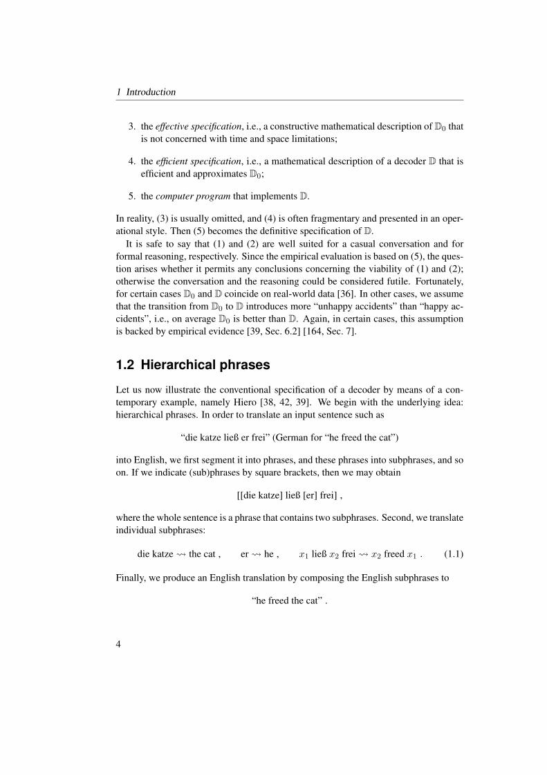
1.2 Hierarchical phrases
Let us now illustrate the conventional specification of a decoder by means of a con-
temporary example, namely Hiero [38, 42, 39]. We begin with the underlying idea:
hierarchical phrases. In order to translate an input sentence such as
“die katze ließ er frei” (German for “he freed the cat”)
into English, we first segment it into phrases, and these phrases into subphrases, and so
on. If we indicate (sub)phrases by square brackets, then we may obtain
[[die katze] ließ [er] frei] ,
where the whole sentence is a phrase that contains two subphrases. Second, we translate
individual subphrases:
die katze the cat , er he , x1 ließ x2 frei x2 freed x1 . (1.1)
Finally, we produce an English translation by composing the English subphrases to
“he freed the cat” .
4

1.2 Hierarchical phrases
ρ1: S → α1(NP) α1 = 〈x1 ließ er frei, he freed x1〉
ρ2: S → α2(PPER) α2 = 〈die katze ließ x1 frei, x1 let the cat out〉
ρ3: S → α3(PPER,NP) α3 = 〈x1 ließ x2 frei, x1 freed x2〉
ρ4: S → α4(PPER,NP) α4 = 〈x2 ließ x1 frei, x1 freed x2〉
ρ5: PPER → α5 α5 = 〈er, he〉
ρ6: NP → α6 α6 = 〈die katze, the cat〉
Figure 1.2: An SCFG for German-English SMT; the initial state is S.
We will see that the segmentation into subphrases as well as their translation can be
captured by a finite set of rules that resemble (1.1).
It is possible that other segmentations and other translations are also valid, such as
[die katze ließ [er] frei] and die katze ließ x1 frei x1 let the cat out ,
respectively. In this example, we obtain a different translation, namely
“he let the cat out” ,
but this need not be the case. At any rate, we want to output a single translation. There-
fore we assign a real number, called score, to each way of segmenting and translating.
Then we can either choose the way with the highest score and output the corresponding
translation; or we can aggregate the scores of all ways that lead to the same translation
and output the translation with highest aggregate score.
This concludes our account of the idea behind Hiero, and we proceed to the abstract
specification. For this, we first formalize the aforementioned rules by means of syn-
chronous context-free grammars (SCFGs). This formalism first appeared in [119] by
the name of syntax-directed transduction, and its viability for SMT was first shown via
Hiero.
Let Σ be an alphabet. An SCFG G over Σ is a triple (Q,R, q0) where Q is a finite
set (of states), q0 ∈ Q is called initial state, and R is a finite set of rules of the form
q → 〈w1, w2〉(q1, . . . , qk) ,
where q, q1, . . . , qk ∈ Q and wi is a string over Σ and the variables x1, . . . , xk such
that xj occurs exactly once for every j ∈ 1, . . . , k. We call k the rank of the
rule. For our example, we might use the SCFG G shown in Fig. 1.2, where Σ =ließ, er, frei, he, freed, . . . .
Technically, we do not distinguish between Σ∗, E, and F ; the latter two are merely
more mnemonic. An SCFGG over Σ represents a set of pairs of strings in Σ∗ by means
5

1 Introduction
of two concepts: abstract syntax trees (ASTs) and center trees. Intuitively, an AST
encodes a derivation of the grammar, and a center tree encodes the information about
the derived string pair. The corresponding French and English strings are extracted
from a center tree via mappings h1 and h2, respectively.
Let us now make these concepts more precise. For this, let Γ be an alphabet. We
denote the set of all trees over Γ by TΓ; it is the smallest set T ⊆ (Γ∪(, )∪, )∗ such
that γ(t1, . . . , tk) ∈ T for every k ∈ N, γ ∈ Γ, and t1, . . . , tk ∈ T . For every state qwe define the set Dq(G) of q-ASTs of G as follows. The family (Dq(G) | q ∈ Q) is the
smallest family (Dq | q ∈ Q) with Dq = ρ(d1, . . . , dk) | ρ ∈ R, ∃q1, . . . , qk, α : ρ =(q → α(q1, . . . , qk)), dj ∈ Dqj. Let Γ be the set of all 〈w1, w2〉 that occur in R,
and let πΓ : TR → TΓ be the mapping that replaces each label q → α(q1, . . . , qk) by
α. Then a center tree is a tree over Γ that is obtained from an element of Dq0(G) by
applying πΓ. In our example, ρ4(ρ5, ρ6) is an S-AST and α4(α5, α6) is a center tree.
We define h1, h2 : TΓ → Σ∗ recursively by letting hi(〈w1, w2〉(t1, . . . , tk)) be the
string obtained from wi by replacing every occurrence of xj by hi(tj). For instance,
h1(α4(α5, α6)) = h1(α6) ließ h1(α5) frei = die katze ließ er frei = h1(α1(α6)) ,
h2(α4(α5, α6)) = h2(α5) freed h2(α6) = he freed the cat = h2(α1(α6)) .
Let f ∈ Σ∗. Then the informal process of segmenting f into phrases corresponds to
finding a center tree t such that h1(t) = f , and the informal process of translating the
subphrases corresponds to computing h2(t). As stated above, there may be several cen-
ter trees t with h1(t) = f , and we intend to use scores in order to choose a translation.
Now we turn to the formalization of these scores.
To this end, we consider an approach that is almost universally applied, namely linear
models [152, 173]. Here we assign to each tree over R a linear combination of feature
values for this tree. A feature is a mapping φ : TR → sR, where sR = R ∪ −∞,∞. It
is up to the engineer to devise suitable features. For the sake of simplicity, we focus on
three of Hiero’s seven features:
• We assume that we have a probability assignment for G, i.e., a mapping µ : R→[0, 1]; we extend µ to TR and we define the feature φµ by letting
µ(ρ(d1, . . . , dk)) = µ(d1) · · ·µ(dk) · µ(ρ) , φµ(d) = logµ(d) ,
where we assume that log 0 = −∞.
• Likewise, we assume that we have a probability distribution PLM on E, called a
language model; and we define the feature φLM by
φLM(d) = logPLM(h2(πΓ(d))) .
6

1.2 Hierarchical phrases
• We also count the number of words in the English string, i.e., we let
φ#(d) = |h2(πΓ(d))| .
The first and the second feature can be regarded as scoring the faithfulness and the
fluency of the translation, respectively [99, Sec. 25.3]. For Hiero, PLM is an n-gram
model. It is beyond the scope of this text to explain how such a language model is
obtained (for details, see [99, Ch. 4]); suffice it to say that it can be simulated by a
deterministic weighted string automaton [4, Sec. 4].
We note that a sequence φ1, . . . , φm of features uniquely determines a mapping
Φ: TR → sRm by
Φ(d) =
φ1(d)...
φm(d)
,
and vice versa. We call Φ a representation mapping (of dimension m).
Let θ ∈ Rm, which we call the feature weight vector. This vector contains the
coefficients for our linear combination. Let d ∈ TR. Then the score of d is Φ(d) · θ,
where · is the operation known variably as the dot product, scalar product, or inner
product, i.e., Φ(d) · θ =∑
j : 1≤j≤m φj(d) · θj .Finally, we arrive at the following abstract specification of Hiero:
Ω = (G,µ, θ) | G is an SCFG, µ is a probability assignment for G, θ ∈ R3 ,
D0 : Ω→ EF , D0(G,µ, θ) :
f 7→ h2(πΓ(argmaxd∈Dq0 (G) : h1(πΓ(d))=f ΦG,µ(d) · θ
)) ,
where ΦG,µ is the representation mapping consisting of φµ, φLM, and φ#; and argmaxis defined as follows. For every set X , we let argmaxX : sR
X → X be a partial map-
ping such that argmaxX(f) is a member of x′ | ∀x : f(x′) ≥ f(x) if that set is
nonempty, and argmaxX(f) is undefined otherwise. Instead of argmaxX(f), we write
argmaxx∈X f(x), and we usually silently assume that it is defined. Note that argmaxXis not uniquely determined; we stipulate that the above “let” fixed exactly the mapping
that the (fictitious, potential) implementation of choice provides.
The structure of the parameter space Ω is in part motivated by the training method
that is used with Hiero. For the sake of completeness, let us briefly sketch this method.
Recall that training amounts to determining a specific triple (G,µ, θ) ∈ Ω, given a par-
allel corpus c ∈ (E×F )∗. First, we split c into two parts c1 and c2. Second, we perform
rule extraction, i.e., we use a simple heuristic based on automatically induced word
7
1 Introduction
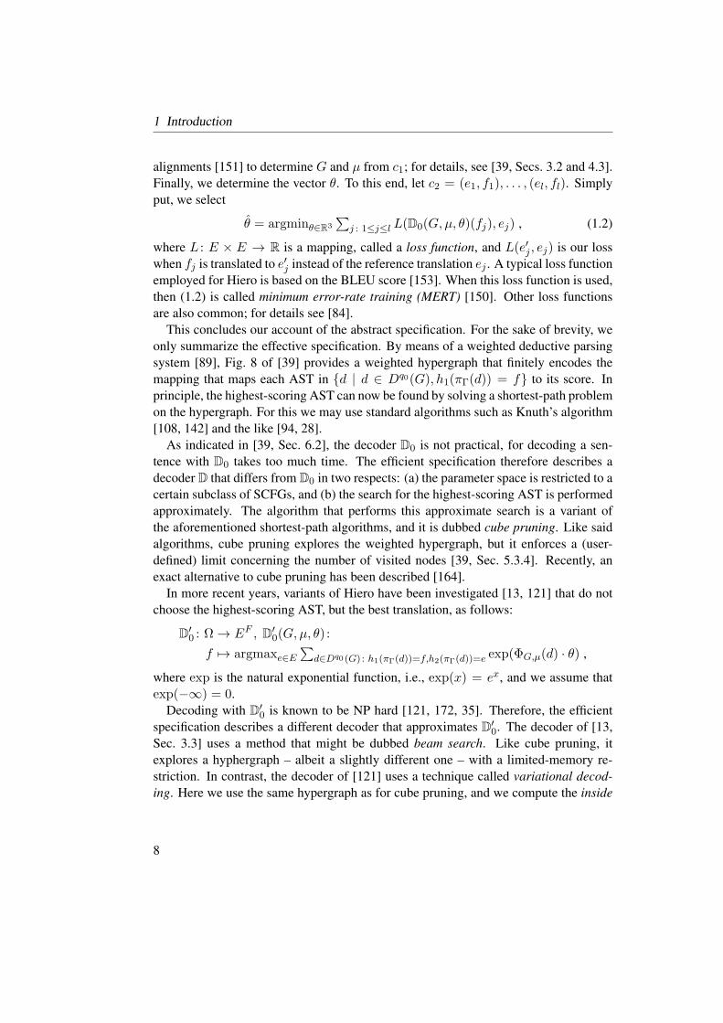
alignments [151] to determine G and µ from c1; for details, see [39, Secs. 3.2 and 4.3].
Finally, we determine the vector θ. To this end, let c2 = (e1, f1), . . . , (el, fl). Simply
put, we select
θ = argminθ∈R3
∑
j : 1≤j≤l L(D0(G,µ, θ)(fj), ej) , (1.2)
where L : E × E → R is a mapping, called a loss function, and L(e′j , ej) is our loss
when fj is translated to e′j instead of the reference translation ej . A typical loss function
employed for Hiero is based on the BLEU score [153]. When this loss function is used,
then (1.2) is called minimum error-rate training (MERT) [150]. Other loss functions
are also common; for details see [84].
This concludes our account of the abstract specification. For the sake of brevity, we
only summarize the effective specification. By means of a weighted deductive parsing
system [89], Fig. 8 of [39] provides a weighted hypergraph that finitely encodes the
mapping that maps each AST in d | d ∈ Dq0(G), h1(πΓ(d)) = f to its score. In
principle, the highest-scoring AST can now be found by solving a shortest-path problem
on the hypergraph. For this we may use standard algorithms such as Knuth’s algorithm
[108, 142] and the like [94, 28].
As indicated in [39, Sec. 6.2], the decoder D0 is not practical, for decoding a sen-
tence with D0 takes too much time. The efficient specification therefore describes a
decoder D that differs from D0 in two respects: (a) the parameter space is restricted to a
certain subclass of SCFGs, and (b) the search for the highest-scoring AST is performed
approximately. The algorithm that performs this approximate search is a variant of
the aforementioned shortest-path algorithms, and it is dubbed cube pruning. Like said
algorithms, cube pruning explores the weighted hypergraph, but it enforces a (user-
defined) limit concerning the number of visited nodes [39, Sec. 5.3.4]. Recently, an
exact alternative to cube pruning has been described [164].
In more recent years, variants of Hiero have been investigated [13, 121] that do not
choose the highest-scoring AST, but the best translation, as follows:
D′0 : Ω→ EF , D′
0(G,µ, θ) :
f 7→ argmaxe∈E∑
d∈Dq0 (G) : h1(πΓ(d))=f,h2(πΓ(d))=eexp(ΦG,µ(d) · θ) ,
where exp is the natural exponential function, i.e., exp(x) = ex, and we assume that
exp(−∞) = 0.
Decoding with D′0 is known to be NP hard [121, 172, 35]. Therefore, the efficient
specification describes a different decoder that approximates D′0. The decoder of [13,
Sec. 3.3] uses a method that might be dubbed beam search. Like cube pruning, it
explores a hyphergraph – albeit a slightly different one – with a limited-memory re-
striction. In contrast, the decoder of [121] uses a technique called variational decod-
ing. Here we use the same hypergraph as for cube pruning, and we compute the inside
8

1.3 Explicit syntax
S
NP
ART
die
NN
katze
VVFIN
ließ
PPER
er
PTKVZ
frei
S
NP
PRP
he
VP
VBD
freed
NP
DT
the
NN
cat
Figure 1.3: Constituent trees.
weight and outside weight of each node [121, 8, 118, 157]. Using these weights, we
determine an n-gram language model that is “as close as possible” to the mapping
e 7→ 1Z ·
∑
d∈Dq0 (G) : h1(πΓ(d))=f,h2(πΓ(d))=eexp(ΦG,µ(d) · θ) ,
where Z is the normalization constant∑
d∈Dq0 (G) : h1(πΓ(d))=fexp(ΦG,µ(d) · θ). Since
the n-gram language model is basically a particular deterministic weighted string au-
tomaton, the highest-weighted string can be found easily using standard shortest-path
algorithms such as Dijkstra’s algorithm [55, 70]. We note that variational decoding is
very similar in spirit to [143].
At this point, it should be evident that we cover substantial distances when we re-
fine a conventional specification, going from an “argmax formula” on the one end to
various algorithms that work on a weighted hypergraph on the other end. This kind of
refinement requires a great deal of mental labor, and it is hard to see how the two ends
are related.
1.3 Explicit syntax
In recent years, decoders have been investigated that go beyond hierarchical phrases by
considering explicit syntax information in the form of constituent trees, such as those
in Fig. 1.3. These decoders are based on formalisms similar to SCFGs, such as
• tree-to-string transducer (yXTT) [79, 96, 90],
• synchronous tree-substitution grammar (STSG) [62],
• synchronous tree-sequence-substitution grammar [183, 130],
• synchronous tree-adjoining grammar (STAG) [171, 1],
9

1 Introduction
• synchronous tree-insertion grammar (STIG) [167, 148, 149, 147, 51, 50],
• extended multi-bottom-up tree transducer (MBOT) [20, 65].
While yXTTs employ explicit syntax information on the source or target side only,
the other formalisms do so on both sides. For the rule extraction of these formalisms,
we use a parallel corpus that contains constituent trees instead of sentences. There are
two principal advantages of explicit syntax information:
• Rule extraction is linguistically more informed due to the constituent trees in the
training data [79, 40].
• We can use the constituent trees generated by the grammar to define more so-
phisticated features [41].
Let us elucidate the syntax-based approach by means of an example decoder that is
based on STSGs. If we replace α1, . . . , α6 in Fig. 1.2 by the values given in Fig. 1.4,
then we obtain an STSG. The rules now have the form q → 〈t1, t2〉(q1, . . . , qk), where
ti is a tree over Σ ∪ x1, . . . , xk, and each variable occurs exactly once in ti. The
notions of a probability assignment, an AST, and a center tree carry over to this new
setting. We define the mappings h1, h2 : TΓ → TΣ as for SCFGs, only that we perform
the variable replacement in a tree instead of a string. For instance, if we denote the trees
of Fig. 1.3 by t1 (left tree) and t2 (right tree), then
hi(α4(α5, α6)) = ti = hi(α1(α6)) .
Moreover, we define the yield mapping yd: TΣ → Σ∗ as follows. Let t ∈ TΣ, t =σ(t1, . . . , tk). If k = 0, then yd(t) = σ. Otherwise, yd(t) = yd(t1) · · · yd(tk).Continuing the example, we have that
yd(t1) = die katze ließ er frei , yd(t2) = he freed the cat .
One feature that capitalizes on syntax information is the following, we call the pars-
ing feature. We assume that we have the conditional probability P (t | f) for every
constituent tree t and foreign sentence f with yd(t) = f . It is outside the scope of
this text to explain how these probabilities are determined; this task is the subject of
statistical natural-language parsing [99, Ch. 14]. Suffice it to say that said probabili-
ties are usually represented finitely using formalisms akin to probabilistic context-free
grammars; for more details, see [155, 156, 47, 12, 37]. Then the parsing feature is
φP(d) = logP (h1(πΓ(d)) | yd(h1(πΓ(d)))) .
10

1.3 Explicit syntax
α1 =
⟨S
x1 VVFIN
ließ
PPER
er
PTKVZ
frei
,
S
x1 VP
VBD
freed
NP
DT
the
NN
cat
⟩
α2 =
⟨
S
NP
ART
die
NN
katze
VVFIN
ließ
x1 PTKVZ
frei,
S
x1 VP
VBD
let
NP
DT
the
NN
cat
PRT
out
⟩
α3 =
⟨S
x1 VVFIN
ließ
x2 PTKVZ
frei
,
S
x1 VP
VBD
freed
x2
⟩
α4 =
⟨S
x2 VVFIN
ließ
x1 PTKVZ
frei
,
S
x1 VP
VBD
freed
x2
⟩
α5 =
⟨PPER
er,
NP
PRP
he
⟩
α6 =
⟨NP
ART
die
NN
katze
,
NP
DT
the
NN
cat
⟩
Figure 1.4: Tree pairs for an STSG.
11

1 Introduction
This feature and variants thereof have been used successfully in [96, 137, 93].
Now we can define our example decoder as follows. We let
Ω = (G,µ, θ) | G is an STSG, µ is a probability assignment for G, θ ∈ R3 ,
D0 : Ω→ EF , D0(G,µ, θ) :
f 7→ yd(h2(πΓ(argmaxd∈Dq0 (G) : yd(h1(πΓ(d)))=f ΦG,µ(d) · θ
))) ,
where ΦG,µ is the representation mapping that consists of the three features φµ, φLM(adapted to the STSG case via yd), and φP.
1.4 The algebraic framework, preliminary version
The algebraic framework is essentially a collection of operations, and it allows us to
define D(ω)(f) as an expression over these operations, ω, and f . In order to keep the
exposition simple, we only consider a preliminary version of the framework; the full
version follows in Sec. 6.1. As a foundation, we utilize the notions of a weighted string
language, a weighted tree language, and a weighted tree transformation [61, 57]. For
the weight domain, we utilize the concept of a commutative semiring [91, 87].
A (commutative) semiring S is an algebraic structure consisting of a set S, called
domain, two binary operations + and · on S, called addition and multiplication, re-
spectively, and neutral elements 0, 1 ∈ S for addition and multiplication, respectively.
Furthermore, there are certain requirements that the operations be “well behaved”; for
the purposes of this introduction, however, it is sufficient to imagine a commutative
semiring as “a field without subtraction and division”. For instance, the nonnegative
reals R≥0, extended by∞, with conventional addition and multiplication constitute the
semiring Real. Another example is the arctic semiring Arct, where the domain is sR,
the operations are maximum for addition and (conventional) addition for multiplication,
and the neutral elements are−∞ and 0, respectively. A semiring is complete if, roughly
speaking, infinite sums are defined. The two aforementioned semirings are complete.
For a formal definition of semirings and complete semirings, see Sec. 2.3.2.
Let S be a commutative semiring and Σ an alphabet. A weighted string language ϕover Σ and S is a mapping ϕ : Σ∗ → S, a weighted tree language ϕ over Σ and S is a
mapping ϕ : TΣ → S, and a weighted tree transformation τ over Σ and S is a mapping
τ : TΣ × TΣ → S. We abbreviate the corresponding sets as follows:
K = SΣ∗
, L = STΣ , T = STΣ×TΣ .
We define the string injection 1., the language yield Yd, the inverse language yield
Yd−1, the Hadamard product ⊙, the input product ⊳, the output product ⊲, the output
12

1.4 The algebraic framework, preliminary version
1. : Σ∗ → K , (1.w)(w′) = if w = w′ then 1 else 0 ,
Yd: L → K , Yd(ϕ)(w) =∑
t : yd(t)=w ϕ(t) , (∗)
Yd−1 : K → L , Yd−1(ϕ)(t) = ϕ(yd(t)) ,
⊙ : L × L → L , (ϕ1 ⊙ ϕ2)(t) = ϕ1(t) · ϕ2(t) ,
⊳ : L × T → T , (ϕ⊳ τ)(s, t) = ϕ(s) · τ(s, t) ,
⊲ : T × L → T , (τ ⊲ ϕ)(s, t) = τ(s, t) · ϕ(t) ,
π2 : T → L , π2(τ)(t) =∑
s τ(s, t) , (†)
best : SI → I , best(ϕ) = argmaxi∈I ϕ(i) . (‡)
restrictions: (∗) S complete or t | yd(t) = w,ϕ(t) 6= 0 finite
(†) S complete or s | τ(s, t) 6= 0 finite
(‡) I set, S ∈ Real,Arct
Figure 1.5: Operations of the algebraic framework.
projection π2, and the best-index operation best as shown in Fig. 1.5. These operations
constitute the preliminary version of the algebraic framework.
In order to illustrate the framework, we devise an alternative specification of D0 of
Sec. 1.3. For this, let S = Arct, G an STSG, µ a probability assignment forG, θ ∈ R3,
and θ = (θ1, θ2, θ3). We claim that
D0(G,µ, θ)(f) = best(Yd(π2((Yd−1(1.f)⊙ ϕP)⊳ τ ⊲Yd−1(ϕLM)
))) , (1.3)
where τ ∈ T , ϕLM ∈ K, and ϕP ∈ L with
τ(t1, t2) = maxθ1 · logµ(d) | d ∈ Dq0(G), hi(πΓ(d)) = ti ,
ϕLM(e) = θ2 · logPLM(e) ,
ϕP(t) = θ3 · logP (t | yd(t)) .
In order to prove the claim, we derive
D0(G,µ, θ)(f)
= yd(h2(πΓ(argmaxd∈Dq0 (G) : yd(h1(πΓ(d)))=f
θ1 · φµ(d) + θ2 · φLM(d) + θ3 · φP(d))))
= argmaxw∈Σ∗ maxt∈TΣ : yd(t)=wmaxs∈TΣ : yd(s)=f
maxd∈Dq0 (G) : h1(πΓ(d))=s,h2(πΓ(d))=t θ1 · φµ(d) + θ2 · φLM(d) + θ3 · φP(d)
13
1 Introduction
= argmaxw∈Σ∗ maxt∈TΣ : yd(t)=wmaxs∈TΣ : yd(s)=f
ϕP(s) + τ(s, t) + ϕLM(yd(t))
= argmaxw∈Σ∗ maxt∈TΣ : yd(t)=wmaxs∈TΣ
(1.f)(yd(s)) + ϕP(s) + τ(s, t) + ϕLM(yd(t))
= best(Yd(π2((Yd−1(1.f)⊙ ϕP)⊳ τ ⊲Yd−1(ϕLM)
))).
Note that, although we continue to use 1. to denote the string injection, the semiring 1and the semiring 0 in our case are 0 and −∞, respectively.
In the following, we unveil that the preliminary framework already exhibits the
achievements from Tab. 1.1. As for (a), we already managed to specify a state-of-the-
art decoder, apart from the limited repertory of features. As for (b)–(e), we proceed as
follows. We will define subclasses ofK, L, and T that correspond to certain formalisms
such as weighted string automaton (WSA, [165, 11, 115, 166]), weighted tree automa-
ton (WTA, cf. Sec. 2.4), or weighted context-free grammar (WCFG, [89, 46, 154]); in
particular, we will define the notion of a weighted STSG (WSTSG, [74, 129]). Then
we will gather established results about settings in which the aforementioned subclasses
are effectively closed under the operations in Fig. 1.5. Finally, we will argue that the
objects τ , ϕLM, and ϕP each belong to one of the new subclasses. At that point, it
will become clear that (1.3) is already effective as it is (cf. (b), (c)), that we exploit the
theory a great deal (cf. (d)), and that many concepts are involved (cf. (e)).
A WSTSG G over Σ and S is a quadruple (Q,R, µ, q0) where (Q,R, q0) is an STSG
over Σ and µ : R → S is called weight assignment. The objects Dq(G), Γ, πΓ, and
h1 and h2 are defined as for (Q,R, q0). We define the mapping 〈.〉µ : TR → S induc-
tively by letting 〈ρ(d1, . . . , dk)〉µ = 〈d1〉µ · · · 〈dk〉µ · µ(ρ). Finally, the meaning JGKof G is the weighted tree transformation with
JGK(t1, t2) =∑
d∈Dq0 (G) : hi(πΓ(d))=ti〈d〉µ .
For this definition to be sound, we require one of two conditions: (i) S is complete
or (ii) the index set of sum is finite for every (t1, t2). We can satisfy Condition (ii) by
requiring thatG be productive (cf. [74]), i.e., for every 〈t1, t2〉 ∈ Γ, we have t1, t2 6= x1.
This is a common requirement (cf. [39, Sec. 3.2]). We note that a WSTSG is a particular
WTA with an alternative meaning assigned to it.
We define the following classes:
KRec = ϕ | ϕ ∈ K, ϕ is the meaning of some WSA ,
KCF = ϕ | ϕ ∈ K, ϕ is the meaning of some WCFG ,
LRec = ϕ | ϕ ∈ L, ϕ is the meaning of some WTA ,
TSTSG = τ | τ ∈ T , τ is the meaning of some WSTSG .
14

1.4 The algebraic framework, preliminary version
operation closure/restrictions publications complexity
1. Σ∗ → KRec [11, 168] O(n)Yd LRec → KCF [176, 71] O(r)
Yd−1 KRec → LRec [132] O(pk)⊙ LRec × LRec → LRec [15, Cor. 3.9] O(r1 · r2)
⊳ LRec × TSTSG → TSTSG [128] O(r2 · pk21 )
⊲ TSTSG × LRec → TSTSG [128] O(r1 · pk12 )
π2 TSTSG → LRec [75] O(r)best KCF → Σ∗, (†) [108, 94, 28] O(r · log p)best LRec → TΣ, (†) [108, 94, 28] O(r · log p)best TSTSG → TΣ × TΣ, (†) [108, 94, 28] O(r · log p)best KRec → Σ∗, (‡) [134, 94], (Thm. 5.5.3) (?)
best LRec → TΣ, (‡) [134, 94], (Thm. 5.5.3) (?)
Yd LCF → KMac [71] O(r)
⊳ LRec × TSCFTG → TSCFTG (Thm. 3.3.3) O(r2 · pc2·k21 )
⊲ TSCFTG × LRec → TSCFTG (Thm. 3.3.3) O(r1 · pc1·k12 )
π2 TSCFTG → LCF (conjecture) O(r)best KMac → Σ∗, (†) (conjecture) O(r · log p)
⊳ LRec × TSTSG → TSTSG, (∗) (Thm. 4.5.10, Sec. 4.6.5) O(r2 · p31)
⊲ TSTSG × LRec → TSTSG, (∗) (Thm. 4.5.10, Sec. 4.6.5) O(r1 · p32)
legend: n . . . length of the string
p . . . number of states
r . . . number of transitions/rules
k . . . maximal rank of a transition/rule
c . . . grammar-dependent constant
index 1, 2: first or second argument
(†) S = Arct and
either CFG/WTA acyclic [94] or weights negative [108]
(‡) S = Real and WTA unambiguous or acyclic [134, 94]
(∗) WSTSG rule-by-rule binarizable
Table 1.2: Computability of operations, with worst-case complexity.
15

1 Introduction
The first section of Tab. 1.2 lists the closure results for our operations. Be advised
that each entry corresponds to an algorithm; for instance, as implied by the table, [15]
presents an algorithm that expects WTA M1 and M2 and outputs a WTA M with
JMK = JM1K⊙ JM2K. We note that constructing a WSA for 1.f is straightforward, but
it is beyond the scope of this text. Suffice it to say that, in the terminology of rational
series [11, 165], 1.f is a polynomial; hence, it is rational and, thus, recognizable [168],
which is tantamount to 1.f ∈ KRec. Furthermore, we note that the second conjunct
in (†) guarantees that a best element exists. Technically, this condition should be incor-
porated into our subclasses KCF and LRec, or additional classes should be introduced,
but we refrain from these complications. In practice, where unbounded translations are
not in demand, it is often acceptable to simply make the CFG or the WTA in question
acyclic, e.g., by removing transitions or “intersecting” it with a finite language.
We argue that (i) τ ∈ TSTSG, (ii) ϕLM ∈ KRec, and (iii) ϕP ∈ LRec. For (i), let G′
be the WSTSG over Σ and Arct that is obtained from the STSG G by using the weight
assignment µ′ with µ′(ρ) = θ1 · logµ(ρ). Then it is easy to verify that JG′K = τ .
For (ii) and (iii), we use that any n-gram model can be equivalently represented by a
deterministic WSA M over Real [4, Sec. 4], and like [137, 93] we assume that the
parsing probabilities are represented by a PCFG, which can be viewed as a bottom-
up deterministic WTA M ′ over Real. Since deterministic devices do not employ the
addition of the semiring, we can transfer them to the arctic semiring by applying log to
each transition weight. (We will treat this construction more thoroughly in Sec. 6.1.)
We transform the resulting WSA and WTA into a WSA for ϕLM and a WTA for ϕP by
multiplying each transition weight by θ2 and θ3, respectively.
At this point, we can evaluate the expression on the right-hand side of (1.3) by com-
posing the algorithms referred to in the table and applying the composite algorithm to
the objects that we constructed for (i)–(iii). Put differently, (1.3) is effective.
So far, we only employed the framework to rephrase the definition of an existing
decoder. Correspondingly, we had to prove (1.3). Now it is time to use the framework
according to its purpose – to specify a decoder. We let S = Arct, and we define
D1 : TSTSG ×KRec × LRec → EF , D1(τ, ϕ, ϕ′) :
f 7→ best(Yd(π2((Yd−1(1.f)⊙ ϕ′)⊳ τ ⊲Yd−1(ϕ)
))) . (1.4)
Since we defined D1 “from scratch”, we were able to define D1(τ, ϕ, ϕ′)(f) by an
expression over the operations and τ , ϕ, ϕ′, and f . Cosmetic details aside, D1 and D0
are very similar; the principal difference is the absence of a feature weight vector in D1.
Technically, we might assume that the feature weights are already present in τ , ϕ,
and ϕ′. However, the training procedure usually determines the feature weight vector
in a dedicated step, and it is at least debatable whether the training procedure should be
16

1.5 Main contributions
x3
S
x1 VP
V
saw
x2
Lx3/
S
Adv
yesterday
y1 M =
S
Adv
yesterday
S
x1 VP
V
saw
x2
.
Figure 1.6: Applying second-order substitution.
burdened with the task of incorporating the feature weight vector into τ , ϕ, and ϕ′. The
bottom line is that D1 lacks feature weights.
We end this section by discussing what differentiates the preliminary version of al-
gebraic framework from the full version of Sec. 6.1. In the preliminary version, all
operations act on the same semiring, and best basically forces us to choose Arct. Re-
call that our construction ofG′ was somewhat monolithic, as it already incorporated θ1.
This begs the question whether we have to provide a similar construction every time we
modify (1.3), and the answer is probably yes. In the definition of τ , we apply the logand the multiplication with θ1 on the level of individual ASTs, and this level is not ex-
posed to the meaning of an WSTSG over the arctic semiring; it is “blurred” by the max.
More precisely, since multiplication does not distribute over max (consider θ1 < 0), we
cannot “pull” this multiplication “out” of the max, where it would be exposed. In other
words, it is not possible to describe the integration of θ1 as an operation on T . This is
the reason why D1 does not include feature weights. The full version of the framework
permits “switching” the semiring via semiring homomorphisms. Then, using the mul-
tiset semiring, we are able to describe, i.a., the integration of θ1 as an operation on T .
On the whole, this relieves us of the burden of constructing grammars, as in (i)–(iii).
1.5 Main contributions
1.5.1 Input product and output product of a weighted synchronouscontext-free tree grammar and a weighted tree automaton
So far, we have dealt with decoders based on SCFGs or on STSGs. Recently it has been
suggested that SCFGs, STSGs, and yXTTs are not well suited to capture all phenomena
that we encounter in real-world parallel corpora, and that STIGs and STAGs, among
others, are better suited in that respect [170, 101, 83, 100].
17
1 Introduction
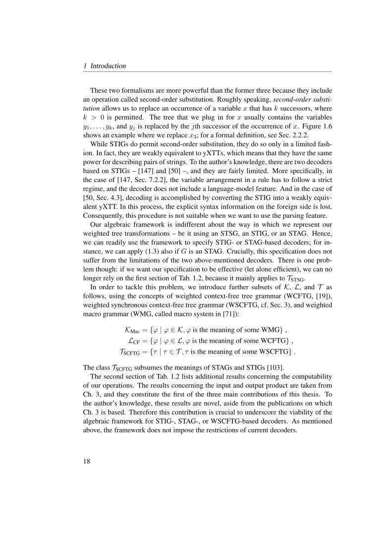
These two formalisms are more powerful than the former three because they include
an operation called second-order substitution. Roughly speaking, second-order substi-
tution allows us to replace an occurrence of a variable x that has k successors, where
k > 0 is permitted. The tree that we plug in for x usually contains the variables
y1, . . . , yk, and yj is replaced by the jth successor of the occurrence of x. Figure 1.6
shows an example where we replace x3; for a formal definition, see Sec. 2.2.2.
While STIGs do permit second-order substitution, they do so only in a limited fash-
ion. In fact, they are weakly equivalent to yXTTs, which means that they have the same
power for describing pairs of strings. To the author’s knowledge, there are two decoders
based on STIGs – [147] and [50] –, and they are fairly limited. More specifically, in
the case of [147, Sec. 7.2.2], the variable arrangement in a rule has to follow a strict
regime, and the decoder does not include a language-model feature. And in the case of
[50, Sec. 4.3], decoding is accomplished by converting the STIG into a weakly equiv-
alent yXTT. In this process, the explicit syntax information on the foreign side is lost.
Consequently, this procedure is not suitable when we want to use the parsing feature.
Our algebraic framework is indifferent about the way in which we represent our
weighted tree transformations – be it using an STSG, an STIG, or an STAG. Hence,
we can readily use the framework to specify STIG- or STAG-based decoders; for in-
stance, we can apply (1.3) also if G is an STAG. Crucially, this specification does not
suffer from the limitations of the two above-mentioned decoders. There is one prob-
lem though: if we want our specification to be effective (let alone efficient), we can no
longer rely on the first section of Tab. 1.2, because it mainly applies to TSTSG.
In order to tackle this problem, we introduce further subsets of K, L, and T as
follows, using the concepts of weighted context-free tree grammar (WCFTG, [19]),
weighted synchronous context-free tree grammar (WSCFTG, cf. Sec. 3), and weighted
macro grammar (WMG, called macro system in [71]):
KMac = ϕ | ϕ ∈ K, ϕ is the meaning of some WMG ,
LCF = ϕ | ϕ ∈ L, ϕ is the meaning of some WCFTG ,
TSCFTG = τ | τ ∈ T , τ is the meaning of some WSCFTG .
The class TSCFTG subsumes the meanings of STAGs and STIGs [103].
The second section of Tab. 1.2 lists additional results concerning the computability
of our operations. The results concerning the input and output product are taken from
Ch. 3, and they constitute the first of the three main contributions of this thesis. To
the author’s knowledge, these results are novel, aside from the publications on which
Ch. 3 is based. Therefore this contribution is crucial to underscore the viability of the
algebraic framework for STIG-, STAG-, or WSCFTG-based decoders. As mentioned
above, the framework does not impose the restrictions of current decoders.
18

1.5 Main contributions
1.5.2 Generic binarization of a weighted grammar
For the next main contribution of this thesis, let us turn to the matter of decoding com-
plexity. As we can see from the first section of Tab. 1.2, the most expensive operations
in decoding are the input and the output product. For both operations, the complexity
is exponential in the maximal rank of any rule of the given WSTSG. The same com-
plexity can be observed with established decoders, which is why they are only applied
to grammars with maximal rank 2 (cf., e.g., [39, Sec. 3.2]) or to otherwise restricted
grammars (cf., e.g., [147, Sec. 7.2.2]).
In view of these complexity considerations, it is a natural question whether we can
transform a given grammar into an equivalent one where the maximal rank of any rule is
bounded by a given constant; in particular, where it is bounded by 2. The latter kind of
transformation is called binarization. It is well known that every CFG can be binarized
[45], and that some SCFGs can not be binarized [2]. Hence, binarization procedures
are in general partial. Here we shall focus on effective binarization procedures (how
to construct a solution in favorable cases) rather than on purely existential statements
(whether a solution exists).
The state of the art in binarization procedures is a rule-by-rule approach, where we
replace each rule of rank greater than 2 by an equivalent collection of rules of rank at
most 2, if possible. This approach has been applied to CFGs (for the Chomsky nor-
mal form) and to SCFGs [97]. On the other hand, binarization of yXTTs, STSGs, or
WSCFTGs has – to the author’s knowledge – not yet been investigated. As indicated by
the third section of Tab. 1.2, having a binarization procedure for STSGs or WSCFTGs
would underscore the viability of the algebraic framework, because it may improve the
complexity. Of course, it is possible to try and construct several binarization proce-
dures, one for yXTTs, one for STSGs, and one for WSCFTGs.
In contrast, the second main contribution of this thesis (Ch. 4) consists of (i) a generic
rule-by-rule binarization procedure that can be tailored to many grammar formalisms
by changing a parameter at runtime and (ii) considerations about the application to
yXTTs and WSCFTGs (which subsume STSGs). The second item is crucial because
said parameter is not trivial to come by, and moreover, it turns out that yXTTs and
WSCFTGs do not lend themselves to binarization. As a remedy, we consider the (ad-
hoc) formalisms of hedge-to-string transducers and weighted synchronous context-free
hedge grammars, which encompass yXTTs and WSCFTGs, respectively.
1.5.3 Determinizing weighted tree automata using factorizations
In [134], it has been suggested that the translation quality can be improved by selecting
the best English constituent tree instead of the best AST. On an abstract level, the
19
1 Introduction
following decoders were compared (albeit for yXTT):
Ω′ = (G,µ) | G is a productive STSG, µ is a probability assignment for G ,
D1,D2 : Ω′ → EF ,
D1(G,µ) : f 7→ yd(h2(πΓ(argmaxd∈Dq0 (G) : yd(h1(πΓ(d)))=f µ(d)
))) ,
D2(G,µ) : f 7→ yd(argmaxt
∑
d∈Dq0 (G) : yd(h1(πΓ(d)))=f,h2(πΓ(d))=tµ(d)
).
It turned out that D2 yields higher translation quality than D1 [134, Sec. 5.1].
In the algebraic framework, we obtain that
yd(best(π2(Yd−1(1.f)⊳ JG′K))) =
D1(G,µ) if S = (sR,max, ·, 0, 1),
D2(G,µ) if S = Real,
whereG′ is the WSTSG over Σ and S obtained fromG by using the weight mapping µ.
SinceG′ is productive, one can derive that the WTA for the output projection is acyclic.
Let us delve into how best is computed in both cases. The workhorse in this com-
putation is a shortest-path algorithm for weighted hypergraphs [108, 94, 28], where a
“path” corresponds to a run of the WTA, which is comparable to an AST of an STSG.
Roughly speaking, the weight of a tree is the (semiring) sum of the weights of all runs
on the tree. For D1, where the addition is max, the highest possible weight of any tree
coincides with the highest possible weight of any run, or: the “shortest” path. For D2,
however, we can only exploit the shortest path if we make further assumptions concern-
ing the given WTA. In fact, if the WTA is unambiguous – that is, for every tree, there
is at most one run with non-zero weight –, then the highest possible weight of any tree
again coincides with the highest possible weight of any run.
These considerations give rise to the question whether we can transform any given
WTA into an equivalent WTA that is unambiguous. As in the case of binarization, we
are interested in effective procedures that work in favorable cases rather than purely
existential statements. Therefore, we turn to a related problem: transform a given WTA
into an equivalent one that is bottom-up deterministic. This transformation is called
determinization. Bottom-up determinism is a syntactic property that is easily decided
in time linear in the number of transitions, and it implies the property of being unam-
biguous. It is well known that bottom-up deterministic WTA are strictly less powerful
than WTA, so determinization procedures are partial.
In [134], the authors present a determinization procedure – albeit without proof –
that applies to acyclic WTA over the nonnegative reals, and they put it in front of the
shortest-path algorithm in order to compute best in Real. As in the case of D′0 of
Sec. 1.2, decoding with D2 is NP hard, which is reflected in the complexity of the de-
terminization procedure. Correspondingly, the authors state that determinization did
20
1.6 Related work and bibliographic remarks
not finish in a reasonable amount of time for 26.7 % of their test sentences. When-
ever the determinization procedure exceeded some fixed time limit, they fell back on
an approximation method called crunching, where they determined the best tree by
examining the 500 best runs of the WTA. Despite this occasional approximation, D2
produced better translations than both D1 and a version of D2 where determinization
was completely replaced by crunching [134, Sec. 5.1].
Apart from best, determinization has another application in SMT, which is connected
to the parsing feature and our argument for ϕP ∈ LRec in Sec. 1.4. Recall that this
argument rested on the assumption that the parsing probabilities are represented by
a PCFG. In contrast, modern-day parsers [155, 156] use an enriched formalism called
PCFG with latent annotations (PCFG-LA). Like a PCFG, a PCFG-LA can be viewed as
a WTA over the nonnegative reals; however, this WTA is far from being unambiguous.
Clearly, if we are able to determinize this WTA, then we can again show that ϕP ∈ LRec.
These two applications of determinization in SMT constitute a part of the motiva-
tion of the third and final main contribution of this thesis (Ch. 5): a determinization
construction that generalizes and consolidates earlier work, including [134], which is
thereby proved correct. However, it should be noted that the contribution is entirely
theoretical, for it does not offer new use cases for SMT.
To be more specific, our construction generalizes [134] from the nonnegative reals to
commutative semirings and [105] from WSA to WTA. The latter work requires that the
semiring be extremal (a+ b ∈ a, b) and that the WSA have a certain property called
the twins property [44]. We transfer this property to the tree case, and we show that our
construction applies with the same requirements. Moreover, we transfer results about
the decidability of the twins property [5, 104] from the string case to the tree case.
1.6 Related work and bibliographic remarks
The algebraic framework proposed here draws inspiration from many sources and from
ideas accumulated over time, and it is hard to trace them back to the origins. Therefore,
the following account is most probably incomplete.
We defined our grammars in the spirit of bimorphisms [6]. The framework uses
weighted tree languages and weighted tree transformations as the foundation, as op-
posed to WTA and WSTSG, respectively, which follows the idea that a specification
should describe the “what” rather than the “how”. This practice goes back to age-old
notions such as a recognizable language or a rational language. Moreover, we used
established operations such as the input product or the output projection.
From the perspective of universal algebra, the algebraic framework is essentially a
many-sorted algebra [85], and the algorithms underlying Tab. 1.2 constitute a many-
21

1 Introduction
sorted algebra as well, albeit with somewhat more fine-grained sorts. With suitable
modifications, we may imagine that these two algebras have a common signature, and
that the expression on the right-hand side of (1.4) is a term over that signature, where τ ,
ϕ, ϕ′, and f are viewed as variables. By applying the corresponding homomorphism,
we can interpret the term in either algebra, obtaining either a function that resembles
D0 or an algorithm for computing said function.
It should be noted that conventional decoder specifications, such as the deductive
system of [39, Fig. 8], do contain the automata-theoretic constructions for said opera-
tions, although in an implicit and interweaved manner, or adapted to special cases. By
close inspection, a reader who is proficient in automata theory can “excavate” these
operations.
A valuable source of information, certainly richer than the scant publications in SMT,
is the program code of those decoders that are freely available, such as Moses [111],
Joshua [120], or cdec [59]. A reader who is proficient in programming can learn a
lot, in particular from cdec; for instance, when we view a synchronous grammar as
a particular WTA, then a feature in cdec is merely a bottom-up deterministic WTA
over the same alphabet, and feature weights are incorporated into said grammar via the
Hadamard product – albeit approximately for complexity reasons.
For the sake of completeness, we note that even further variants of Hiero have been
investigated, which choose neither the highest-scoring AST (cf. D0 in Sec. 1.2) nor the
best translation (cf. D′0), but an English sentence that is similar (according to some sim-
ilarity function) to many high-scoring translations. This approach is called concensus
decoding [53, Sec. 2].
Algebraic decoder specification is not a new idea. For instance, Tiburon [135, 133]
is a toolbox that allows to perform common operations on weighted tree transducers
and weighted tree automata, such as Hadamard product, determinization, composition,
application, and so on. Tiburon differs from our framework in three ways:
1. It focuses on automata and transducers rather than languages and transforma-
tions; therefore it is limited to the aforementioned devices.
2. It is limited to predefined semirings, most notably the tropical semiring and the
nonnegative reals.
3. Next to a specification framework, it is primarily a computer program.
Another strand of research is concerned with interpreted regular tree grammars (or
IRTGs, [112]; see also Sec. 4.2). Using the idea of initial-algebra semantics [86],
this formalism unifies many common grammar formalisms, including CFGs, SCFGs,
STSGs, etc. The IRTG framework differs from ours in three ways:
22

1.6 Related work and bibliographic remarks
1. It is as yet unweighted. (Section 4.2 offers a weighted variant.)
2. It is not limited to tree languages or tree transformations.
3. Like Tiburon, it has a focus on manipulating grammars.
The IRTG framework is probably better viewed as a means of investigating grammar
formalisms and their problems in a uniform way, rather than a specification framework.
In Ch. 4, we will employ the IRTG framework in this spirit. We may also use IRTGs to
produce new effectiveness results for our algebraic framework, comparable to Tab. 1.2.
In fact, a precursor of our first main contribution has been described in this way [113];
cf. Sec. 3.1.
While the documentation for Tiburon and IRTGs describes critical operations for de-
coder specification, it remains vague and sketchy when it comes to the topic of actually
specifying a state-of-the-art decoder.
Coincidentally, our notation for SCFGs is similar to the compact notation of [114]
for linear context-free rewriting systems (LCFRSs). However, in contrast to SCFGs,
LCFRSs do not treat the components in 〈w1, w2〉 independently, and thus, there is a
dedicated set of variables for each component. For instance, in the compact LCFRS
notation, our rule ρ3 could be written as
S → 〈x1 ließ y1 frei, x2 freed y2〉(PPER,NP) .
Here the variants of x refer to the first successor (PPER) and the variants of y refer to
the second successor (NP ).
A promising alternative to STIGs and STAGs may be MBOTs. While they also
exceed the power of STSGs, they are not based on second-order substitution. Instead,
MBOTs permit specifying a sequence of trees on the English (target) side. In this
regard, they can be viewed as “explicit-syntax versions” of synchronous linear context-
free rewriting systems (SLCFRS) whose fanout on the source side is 1 [100].
It is the opinion of the author that the literature in both areas, formal-language the-
ory and SMT, is somewhat unsatisfactory. In formal-language theory, the relevant
sources span several decades, they follow varying notational conventions and vary-
ing approaches to semantics (such as term rewriting, fixpoint semantics, initial algebra
semantics, etc.), and, on top of that, many texts are not available online, so that – even
these days – the esteemed SMT practitioner has to plow through a library catalog, only
to get acquainted with a topic that he is not necessarily fond of in the first place. It
would be desirable to have a survey of modern formal-language theory, in particular,
concerning semiring-weighted devices on strings and trees, that is available online and
mentally accessible to practical and theoretical researchers alike.
23

1 Introduction
In SMT, which admittedly is progressing rapidly, publications are often scant, ad-
hoc, and particularly parsimonious when it comes to citations for established concepts;
for instance, WCFGs are defined ad-hoc in [89, Sec. 2.3] (semiring-weighted) and [145,
Sec. 2] (nonnegative reals), and neither publication cites a source. If this practice is due
to the aforementioned obstacles concerning literature on formal-language theory, then
an authoritative, comprehensive, yet plain survey of modern formal-language theory is
all the more desirable.
24

2 Preliminaries
2.1 Mathematical foundations
Most concepts of this section can be found, e.g., in [179, Sec. 1.1, 1.3].
2.1.1 Sets, relations, mappings
By N we denote the set 0, 1, 2, . . . of nonnegative integers. We denote the empty
set by ∅, set difference by \, and the subset and the strict subset relations by ⊆ and ⊂,
respectively. Let A and B be sets. Then B is a partition of A if ∅ 6∈ B,⋃
b∈B b = A,
and b1 ∩ b2 6= ∅ implies b1 = b2 for every b1, b2 ∈ B. The elements of a partition are
also called blocks. The powerset P(A) of A is the set of all subsets of A; in particular,
∅, A ∈ P(A). If A is finite, then the cardinality |A| of A is the number of elements
of A. If |A| = 1, then we call A a singleton. We denote the Cartesian product of
A and B by A×B.
A relation R from A into B is a subset of A×B. Let R be a relation from A into B.
Instead of (a, b) ∈ R, we also write aRb. The inverse R−1 of R is the relation from Binto A given by R−1 = (b, a) | aRb. Let C be a set and S a relation from B into C.
The relation product (or: composition) R;S of R and S is the relation from A into Cdefined by R;S = (a, c) | ∃b : aRb, bSc. Instead of R;S (read “R, then S”) we also
write S R (read “S after R”).
Let A′ ⊆ A and B′ ⊆ B. By R(A′) we denote the set b | ∃a ∈ A′ : aRb. The
relation R is called
• left-total on A′ if A′ ⊆ R−1(B);
• functional if aRb and aRb′ implies b = b′ for every a ∈ A and b, b′ ∈ B;
• surjective on B′ if R−1 is left-total on B′;
• injective if R−1 is functional;
• a partial mapping from A into B if it is functional; and
• a mapping from A into B if it is functional and left-total on A.
25

2 Preliminaries
Let f be a partial mapping from A into B. We also say that f is of type A → B,
and instead of f(a) = b, we also write f(a) = b or a 7→ b. We call f−1(B) the
domain dom f of f and f(A) the image of f or range of f . For every a ∈ dom f , we
call f(a) the image of a (under f ) and we say that we apply f to a. Note that f is a
partial mapping of type A′ → B′ iff A′ ⊇ dom f and B′ ⊇ f(A); i.e., the type of f is
not unique. If f is a mapping, then dom f = A, and it is a mapping of type A′ → B′
iff A′ = A and B′ ⊇ f(A). We denote the fact that f is a mapping from A into Bby f : A → B. If we explicitly mention “partial mapping”, then we may use the same
notation in that sense as well.
Let f : A → B. Clearly, f is surjective on f(A). For every b ∈ B, we also write
f−1(b) instead of f−1(b), and we call f−1(b) the preimage of b (under f ). The
restriction f |A′ of f to A′ is the mapping f ∩ (A′ × B). The mapping f is bijective
on B′ if it is injective and surjective on B′. If B′ = B, then we omit the reference
to B′. The set of all mappings of type A → B is denoted by BA. Let g : B → C.
Then f ; g (alternatively, g f ) is a mapping from A to C with a 7→ g(f(a)). Now let
g : C → B, C ⊇ A, and g|A = f . Then g is an extension of f ; note that f is already a
partial mapping from C intoB. We will sometimes extend f to C; formally, this means
that we define an extension g of f , but instead of g, we will use the same symbol f .
Naturally, since f |A is known, we will then only define f |C\A.
The identity relation idA onA is defined by idA = (a, a) | a ∈ A. Let f : A→ A.
Then f is idempotent if f = f f . For every n ∈ N, we define n-th iterate fn of fby letting f0 = idA and fn+1 = fn f . An element a ∈ A is called fixpoint of f of
f(a) = a.
The set A is called countably infinite if there is a bijective mapping of type A → N,
and it is countable if it is finite or countably infinite.
2.1.2 Families, sequences, and operations
Let I andA be sets. An I-indexed family of elements ofA is a mapping a from I intoA.
Instead of “domain of a”, we also call I the index set of a, and instead of a(i) we write
ai. We denote the fact that a is an I-indexed family by (ai | i ∈ I). Note that this
notation does not indicate A; in order to compensate, we usually state that (ai | i ∈ I)is a family of elements of A. We extend the Cartesian product to an arbitrary number
of sets as follows. Let (Ai | i ∈ I) be a family of sets. Then by×iAi we denote the
set of all families (ai | i ∈ I) of elements of⋃
iAi with ai ∈ Ai. If I = 1, 2, then
we identify the Cartesian product A1 × A2 with×iAi. If I = N, then each element
of×iAi is called a sequence, and we sometimes denote a sequence a by (a1, a2, . . . ).If I = 1, . . . , n, then we denote ×iAi by A1 × · · · × An, each element a in that
set is called a (finite) sequence (of length n), we denote a by (a1, . . . , an), and we have
26
2.1 Mathematical foundations
|a| = n. We usually identify the sequence (a1) with a1. If I = ∅, then we observe that
×iAi is a singleton, as there is only one mapping from ∅ into another set, namely ∅.In order to reduce confusion, we will denote this empty sequence by () or ε.
A finite sequence of length n is also called an n-tuple; if n = 2, 3, 4, 5, then we also
use the words pair, triple, quadruple, and quintuple, respectively. Let f : A → B. We
call the mapping f n-ary if there are A1, . . . , An such that A = A1 × · · · ×An; if n =0, 1, 2, 3, then we also use the words nullary, unary, binary, and ternary, respectively.
We usually write f(a1, . . . , an) instead of f((a1, . . . , an)).For every n ∈ N, the n-fold product An of A is defined by An = A1×· · ·×An with
Ai = A. The Kleene star A∗ of A is defined by A∗ =⋃
nAn. An n-ary operation f
on A is a mapping from An into A. We often use symbols such as + or · to denote
binary operations, and then we use the infix notation a+ b instead of +(a, b). A binary
operation · is associative if a1 ·(a2 ·a3) = (a1 ·a2) ·a3, and it is commutative if a1 ·a2 =a2 · a1. The concatenation operation, denoted by · or by juxtaposition, is the binary
operation over A∗ defined by (a1, . . . , an) · (b1, . . . , bm) = (a1, . . . , an, b1, . . . , bm).For every w ∈ A∗ and n ∈ N we define the sequence iterate wn inductively by letting
w0 = ε and wn+1 = wwn.
An alphabet is a nonempty, finite set, and we call the elements of an alphabet sym-
bols. Let Σ be an alphabet. We call each element of Σ∗ a string (over Σ), and instead
of (a1, . . . , an), we denote a string also by a1 · · · an. A (string) language (over Σ) is a
subset L ⊆ Σ∗. We extend the concatenation operation to string languages by letting
L1 · L2 = w1w2 | w1 ∈ L1, w2 ∈ L2. Note that L · ∅ = ∅ = ∅ · L.
2.1.3 Orders and equivalence relations
A binary relation R on A is a relation from A into A. Let R be a binary relation on A.
LetA′ ⊆ A and a′ ∈ A′. Then a′ is anR-minimal element inA′ if aRa′ implies a 6∈ A′
for every a ∈ A. We say that R is
• reflexive if idA ⊆ R.
• symmetric if R ⊆ R−1.
• transitive if R;R ⊆ R.
• antisymmetric if R ∩R−1 ⊆ idA.
• well founded if every nonempty subset of A has an R-minimal element.
• a (partial) order on A if it is reflexive, antisymmetric, and transitive.
• an equivalence relation on A if it is reflexive, symmetric, and transitive.
27

2 Preliminaries
We usually denote orders by variants of ≤ or ⊑, their inverses by ≥ or ⊒, respectively,
and equivalence relations by variants of ∼ or ≡. We will often use that the usual order
≤ on N, i.e., 0 ≤ 1 ≤ 2 ≤ · · · , is well founded.
Let≤ be an order onA. Note that≥ is an order onA as well. Two elements a, b ∈ Aare comparable (by ≤) if a ≤ b or b ≤ a. Let A′ ⊆ A. Then A′ is called a chain if
its elements are pairwise comparable. An element a ∈ A is called upper bound of A′
if a′ ≤ a for every a′ ∈ A′. An element a ∈ A′ is called least element (in A′) if
a ≤ a′ for every a′ ∈ A′. Note that each set has at most one least element. If the set
of upper bounds of A′ contains a least element a, then a is called the supremum supA′
of A′. The notions lower bound and greatest element are defined dually, with ≥ in
place of ≤. If the set of lower bounds of A′ contains a greatest element a, then a is
called the infimum inf A′ of A′. The order ≤ is linear or total if A is a chain. If ≤is linear, the notions “least element” and “≤-minimal element” coincide, as well as
“greatest element” and “≥-minimal element”. The least element of a set A′, if it exists,
is denoted by minA′. Likewise, the greatest element is denoted by maxA′. An ω-chain
a is a sequence a ∈ AN such that ai ≤ ai+1 for every i ∈ N. Let a ∈ AN. Recall that
a(N) = ai | i ∈ N. Instead of “upper bound of a(N)” and “supremum of a(N)”, we
say “upper bound of a” and “supremum of a”, respectively. The order ≤ is ω-complete
if A has a least element ⊥ and every ω-chain has a supremum.
A (partially) ordered set (poset) is a pair (A,≤) where A is a set and ≤ is an order
on A. A poset (A,≤) is a linear, total, or ω-complete poset if ≤ is linear, total, or
ω-complete, respectively. We often identify (A,≤) and A. Let A and B be posets
and f : A → B. Then f is monotone if a ≤ a′ implies f(a) ≤ f(a′). Recall that
f a = (f(ai) | i ∈ N) for every a ∈ AN. LetA andB be ω-complete. The mapping fis ω-continuous if, for every ω-chain a, sup(f a) is defined and f(sup a) = sup(f a).If f is ω-continuous, then it is monotone, for if a ≤ a′, then supf(a), f(a′) =f(supa, a′) = f(a′) and, hence, f(a) ≤ f(a′). Consequently, f a is an ω-chain if
a is an ω-chain. We observe that the composition of ω-continuous mappings is again
ω-continuous.
The following theorem is sometimes called fixpoint theorem.
Theorem 2.1.1 ([115, Thm 3.1], [179, Sec. 1.5.2, Thm. 7]) Let A be an ω-complete
poset with least element ⊥ and f : A → A an ω-continuous mapping. Then (f i(⊥) |i ∈ N) is an ω-chain and it has a least upper bound, which is the least fixpoint of f ;
i.e.,
mina | f(a) = a = supf i(⊥) | i ∈ N .
Let ≤ be an order on A and I a set. We extend ≤ pointwise to AI by letting a ≤ a′
if ai ≤ a′i for every a, a′ ∈ AI and i ∈ I . Here we understand the word extend in
28

2.2 Trees
the same way as for mappings, in contrast to other established notions of extending an
ordering that refer to adding pairs to the relation. If the order on A is ω-complete, then
so is the extended order. We define the lexicographic order on N∗, often denoted by ≤,
by letting w1 ≤ w2 if
1. w1 = ε or
2. there are i1, i2 ∈ N and w′1, w
′2 ∈ N
∗ such that w1 = i1 · w′1, w2 = i2 · w
′2,
i1 ≤ i2, and i1 = i2 implies w′1 ≤ w
′2.
Let ≡ be an equivalence relation on A. For every a ∈ A, we define the equivalence
class [a]≡ represented by a by letting [a]≡ = a′ | a ≡ a′; and the quotient set
A/≡ of A modulo ≡ is the partition of A defined by letting A/≡ = [a]≡ | a ∈ A.Conversely, every partition B of A gives rise to the equivalence relation on A that
relates two elements precisely when they belong to the same block. If B = A/≡, then
this equivalence relation is again ≡.
2.1.4 Bibliographic remarks
Our definitions of ω-complete order and ω-continuous mapping mainly follow [115,
Sec. 2]. Other definitions are established as well, cf. [179, Sec. 1.5]. The latter author
uses countable chains instead of ω-chains in his definitions, which is equivalent because
every ω-chain has a supremum precisely when every countable chain has a supremum
[179, Sec. 1.5, Prop. 3]. Moreover, his notion of ω-continuous also applies in the case
that A and B are not ω-complete; correspondingly, he then only considers ω-chains athat have a supremum.
2.2 Trees
2.2.1 Unranked trees
Let Σ be an alphabet and V a set. We write TΣ(V ) for the set of all well-formed
expressions over Σ with variables V , i.e., the smallest set T such that (i) V ⊆ Tand (ii) for every σ ∈ Σ, k ≥ 0, and t1, . . . , tk ∈ T , we have σ(t1, . . . , tk) ∈ T .
Alternatively, we view TΣ(V ) as the set of all (rooted, labeled, ordered, unranked)
trees over Σ indexed by V , and draw them as usual. By TΣ we abbreviate TΣ(∅). We
will often denote the tree σ() just by σ. A tree language over Σ is a subset of TΣ.
Let t ∈ TΣ(V ). Next we define the set pos(t) of positions of t, the height ht(t) of t,the rank rkt(w) of the position w in t, the label t(w) of t at w, the subtree t|w of t at w,
and the tree t[t′]w obtained from t by replacing the subtree at w by t′ [7, Def. 3.1.3].
29
2 Preliminaries
To this end, we define two mappings pos: TΣ(V ) → P(N∗) and ht: TΣ(V ) → N;
for every t ∈ TΣ(V ), three mappings rkt : pos(t) → N, t(.) : pos(t) → Σ ∪ V , and
t|. : pos(t) → TΣ(V ); and for every t, t′ ∈ TΣ(V ), the mapping t[t′]. : pos(t) →TΣ(V ), by induction as follows. For every v ∈ V , we let
pos(v) = ε , ht(v) = 1 , rkv(ε) = 0 , v(ε) = v , v|ε = v , v[t′]ε = t′ ,
and for every σ(t1, . . . , tk) ∈ TΣ(V ), i ∈ 1, . . . , k, and w ∈ pos(ti), we let
pos(σ(t1, . . . , tk)) = ε ∪ iw | i ∈ 1, . . . , k, w ∈ pos(ti) ,
ht(σ(t1, . . . , tk)) = 1 +maxht(ti) | i ∈ 1, . . . , k ,
rkσ(t1,...,tk)(ε) = k , rkσ(t1,...,tk)(iw) = rkti(w) ,
σ(t1, . . . , tk)(ε) = σ , σ(t1, . . . , tk)(iw) = ti(w) ,
σ(t1, . . . , tk)|ε = σ(t1, . . . , tk) , σ(t1, . . . , tk)|iw = ti|w ,
σ(t1, . . . , tk)[t′]ε = t′ , σ(t1, . . . , tk)[t
′]iw = σ(t′1, . . . , t′k) ,
where t′i = ti[t′]w, t′j = tj for j 6= i, and we assume that max ∅ = 0. Sometimes
we use the word node instead of position. The tree t is binary if rkt(w) ≤ 2 for every
w ∈ pos(t); and it is suprabinary otherwise. For each pair w1, w2 of positions, we say
that w1 is above w2 if w1 is a prefix of w2, i.e., there is a w ∈ N∗ with w2 = w1 · w.
Likewise, w1 is strictly above w2 if w1 is above w2 and w1 6= w2.
Let V ′ ⊆ Σ ∪ V . We say that t is linear (nondeleting) in V ′ if every element of V ′
occurs at most once (at least once) in t. Moreover, let W be a set and t′ ∈ TΣ(W ). We
say that t is a V ′-prefix of t′ if there is a mapping κ from w | t(w) ∈ V ′ into TΣ(W )such that t′ is obtained from t by replacing the subtree at each w ∈ domκ by κ(w).If V ′ = V , we omit the reference to V ′, simply speaking of linear, nondeleting, and a
prefix. We denote the set of all linear trees over Σ indexed by V by T lin
Σ (V ), and we
denote the set of all linear nondeleting trees over Σ indexed by V by CΣ(V ). By CΣ
we abbreviate CΣ(z), where z is a special symbol that does not occur in Σ. We call
each element of CΣ a context (over Σ).
2.2.2 Substitution
Let X = x1, x2, . . . and Y = y1, y2, . . . be disjoint sets, whose elements we call
variables. We let Xk = x1, . . . , xk and Yk = y1, . . . , yk for every k ≥ 0.
Let V ′ ⊆ Σ ∪ V ∪ X ∪ Y and f : V ′ → TΣ(V ). Then we define the mappings
f , f : TΣ(V )→ TΣ(V ), called first-order substitution and second-order substitution,
30
2.2 Trees
respectively, as follows. For every v ∈ V , we let
f (v) = f (v) =
f(v) if v ∈ V ′,
v if v 6∈ V ′.
For every σ(t1, . . . , tk) ∈ TΣ(V ), we let
f (σ(t1, . . . , tk)) =
f(σ) if σ ∈ V ′,
σ(f (t1), . . . , f(tk)) if σ 6∈ V ′.
If V ′ = v1, . . . , vl, then we also denote f (t) by t[v1/f(v1)] · · · [vl/f(vl)]. We let
f (σ(t1, . . . , tk)) =
f(σ)[y1/f(t1)] · · · [yk/f
(tk)] if σ ∈ V ′,
σ(f (t1), . . . , f(tk)) if σ 6∈ V ′.
If V ′ = v1, . . . , vl, then we also denote f (t) by tLv1/f(v1)M · · · Lvl/f(vl)M.Although second-order substitution is being performed in parallel, we may often
imagine that we substitute the variables sequentially. This notion is made more precise
in the following observation.
Observation 2.2.1 Let V1, V2 ⊆ Σ ∪ V ∪ X ∪ Y , V1 ∩ V2 = ∅, f1 : V1 → TΣ(V ),f2 : V2 → TΣ(V ), and f = f1 ∪ f2. Then f : V1 ∪ V2 → TΣ(V ). If, for every v1 ∈ V1,
the tree f1(v1) does not contain occurrences of elements of V2, then f = f 1 ; f 2 .
Instead of t[a/t′] we also write t′ ·a t, and we omit the subscript a if a = z; recall
that z is the special symbol that we use for contexts.
The following observation basically states that first-order substitution is “associa-
tive”, e.g., we have that t3 · (t2 · t1) = (t3 · t2) · t1.
Observation 2.2.2 Let k, l ∈ N, f : Xl → T∆(X), and g : Xk → T∆(Xl). Then
f (g(t)) = (f g)(t) for every m ∈ N and t ∈ T∆(Xk) with |pos(t)| ≤ m.
2.2.3 Ranked trees
A ranked alphabet is a pair (Σ, rk) where Σ is an alphabet and rk : Σ → N assigns a
natural number to each symbol, called its arity or rank. We write Σ(k) for the subset of
all k-ary symbols of Σ. We denote the ranked alphabet by Σ as well. A ranked alphabet
is binary if the arities do not exceed 2. Likewise, a symbol is binary if its arity is 2,
and it is suprabinary if its rank exceeds 2. We also use σ(k) to denote that σ ∈ Σ(k), in
31
2 Preliminaries
particular when specifying a ranked alphabet, e.g., Γ = α(0), σ(2). We say that a tree
t ∈ TΣ(V ) is Σ-ranked if t(w) 6∈ V implies rkt(w) = rk(t(w)) for every w ∈ pos(t).We will use the following convention: Σ usually denotes a “plain” alphabet (i.e.,
without ranks), while Γ, ∆, and their variants usually denote ranked alphabets. If Σ is a
ranked alphabet, then we regard TΣ(V ), TΣ, T lin
Σ (V ), CΣ(V ), and CΣ to be restricted
to Σ-ranked trees. The same convention shall hold when we talk about tree languages
over Σ.
2.3 Algebras and semirings
2.3.1 Algebras
Let ∆ be a ranked alphabet. A ∆-algebra A is a pair (A, .A) where A is a nonempty
set called domain and .A maps each symbol δ ∈ ∆ with rank k to a k-ary operation
δA : Ak → A, which is also called the realization of δ in A; .A is called realization
mapping. In the context of algebras, ∆ is also called a (single-sorted) signature, and it
can be viewed as an abstract data type, while a ∆-algebra can be viewed as its imple-
mentation.
Let A and B be ∆-algebras. A mapping h : A → B is a ∆-homomorphism from Ainto B if
h(δA(a1, . . . , ak)) = δB(h(a1), . . . , h(ak))
holds for every k, δ ∈ ∆(k), and a1, . . . , ak ∈ A. We write h : A → B to indicate
that h is a ∆-homomorphism from A into B. Note that the composition of two ∆-
homomorphisms is a ∆-homomorphism. Let h : A → B, A′ ⊆ A, and f : A′ → B. If
h|A′ = f , then h is a homomorphic extension of f (with respect to A).
The ∆-term algebra T∆(V ) over V has the domain T∆(V ), and its operations are
given by
δT∆(V )(t1, . . . , tk) = δ(t1, . . . , tk)
for every k ∈ N, δ ∈ ∆(k), and t1, . . . , tk ∈ T∆(V ). It is well known that every
mapping f : V → B has a unique homomorphic extension f ♯ with respect to T∆(V )[179, Sec. 1.2, Thm. 4]; it is given by
f ♯(v) = f(v) , (v ∈ V )
f ♯(δ(t1, . . . , tk)) = δB(f ♯(t1), . . . , f♯(tk)) . (δ(t1, . . . , tk) ∈ T∆(V ))
Let l ∈ N and t ∈ T∆(Xl). In the area of universal algebra, t is called a term. We
define the term function tB : Bl → B of t by tB(b1, . . . , bl) = f ♯(t) with f(xj) = bj .
32

2.3 Algebras and semirings
In particular, if l = 0, then we often omit the parentheses from tB(), and we view tB as
an element of B.
Observation 2.3.1 Let B be a ∆-algebra, k, l ∈ N, f : Xk → T∆(Xl), and g : Xl →B. For every m ∈ N and t ∈ T∆(Xk) we have that |pos(t)| ≤ m implies g♯(f (t)) =(g♯ f)♯(t).
Corollary 2.3.2 Let B be a ∆-algebra, k, l ∈ N, g : Xl → B, t ∈ T∆(Xk), and
t1, . . . , tk ∈ T∆(Xl). Then g♯(t[x1/t1] · · · [xk/tk]) = tB(g♯(t1), . . . , g♯(tk)). In par-
ticular, with l = 0, we have (t[x1/t1] · · · [xk/tk])B = tB(tB1 , . . . , t
Bk ).
2.3.2 Semirings
A monoid is a ∆-algebra S with ∆ = +(2), 0(0) and carrier set S such that +S is
associative and 0S is neutral with respect to +S , i.e., (omitting the superscript S)
s+ 0 = s = 0 + s .
We represent S by the triple (S,+S , 0S). We call S commutative if +S is commuta-
tive. A monoid homorphism is a ∆-homomorphism h : A → B such that A and B are
monoids. A semiring [91, 87] is a ∆-algebra S with ∆ = +(2), ·(2), 0(0), 1(0) and
carrier set S such that (S,+S , 0S) is a commutative monoid, called additive monoid
of S , (S, ·S , 1S) is a monoid, called multiplicative monoid of S , and the following as-
sertions hold (again omitting the superscript S):
s1 · (s2 + s3) = (s1 · s2) + (s1 · s3) , (· distributes over + from the left)
(s1 + s2) · s3 = (s1 · s3) + (s2 · s3) , (· distributes over + from the right)
s1 · 0 = 0 = 0 · s1 . (absorbing element of ·)
We represent S by the quintuple (S,+S , ·S , 0S , 1S). The operations +S and ·S are
called the addition and the multiplication of S , respectively. A semiring homomorphism
is a ∆-homomorphism h : A → B such that A and B are semirings.
Let S = (S,+, ·, 0, 1) be a semiring. We define seven properties of S as follows.
• It is commutative if · is commutative.
• It is zero-divisor free if s1 · s2 = 0 implies that s1 = 0 or s2 = 0.
• It is zero-sum free if s1 + s2 = 0 implies that s1 = 0 = s2.
• It is a semifield if it is commutative and it admits multiplicative inverses, i.e., for
every s ∈ S \ 0 there is a uniquely determined s−1 ∈ S such that s · s−1 = 1.
33

2 Preliminaries
• It is locally finite if for every finite subset S′ ⊆ S the closure of S′ under 0, 1, +,
and · is finite; said closure is the smallest superset S′′ of S′ such that 0, 1 ∈ S′′
and s1, s2 ∈ S′′ implies s1 + s2, s1 · s2 ∈ S
′′.
• It is extremal if s1 + s2 ∈ s1, s2 for every s1, s2 ∈ S.
• It is naturally ordered if (S,≤) is an ordered set, where the binary relation ≤on S is defined by s1 ≤ s2 if there is an s ∈ S with s1 + s = s2.
Example 2.3.3 We consider seven examples of semirings. To this end, let R≥0∞ denote
the set of nonnegative reals extended by∞ and let sR = R ∪ ∞,−∞.
1. The semiring Real = (R≥0∞ ,+, ·, 0, 1), where∞+ r =∞ = r+∞ for every r,
and∞ · r =∞ = r · ∞ for every r with r 6= 0;
2. the arctic semiring Arct = (sR,max,+,−∞, 0) where max(∞, r) = ∞ =max(r,∞) for every r, and∞+ r =∞ = r +∞ for every r with r 6= −∞;
3. the tropical semiring (R≥0∞ ,min,+,∞, 0);
4. the Viterbi semiring ([0, 1],max, ·, 0, 1);
5. the Boolean semiring (B,∨,∧, 0, 1) where B = 0, 1, and ∨ and ∧ denote
disjunction and conjunction, respectively;
6. the semifield (R≥0,+, ·, 0, 1) of nonnegative real numbers;
7. the formal-language semiring (P(Σ∗),∪, ·, ∅, ε) over an alphabet Σ.
Semirings 1–7 are naturally ordered, zero-sum free, and zero-divisor free; 1–6 are com-
mutative; 2–5 are extremal; and 5 is locally finite.
Example 2.3.4 The mappings log and exp are monoid homomorphism from the mul-
tiplicative monoid of Real into the multiplicative monoid of Arct, and vice versa, re-
spectively.
Let I be a set. Then we refer to the elements in SI also as I-vectors over S. For every
s ∈ S and u ∈ SI , we define s ·u ∈ SI by (s ·u)i = s ·ui. Here and in general, we use
family notation for vectors, i.e., ui instead of u(i). Moreover, SI = (SI ,+,⊙, 0, 1)is a semiring, where si = s, the operations + and · are extended to SI pointwise, i.e.,
(u1 + u2)i = (u1)i + (u2)i and (u1 ⊙ u2)i = (u1)i · (u2)i, and ⊙ is called Hadamard
product. If S is commutative (or zero-sum free, or extremal), then so is SI . However,
SI need not be zero-divisor free (or a semifield), even if S is zero-divisor free (or a
semifield, respectively). Let d ∈ N, d ≥ 1. If I = 1, . . . , d, then we write Sd for SI .
34

2.3 Algebras and semirings
Example 2.3.5 (Ex. 2.3.3 contd.) Let d ∈ N, d > 1. We consider two semirings:
8. Reald = ((R≥0∞ )d,+,⊙, 0, 1) and
9. ((R≥0∞ )d,min,⊕, ∞, 0).
In contrast to Semiring 1, Semiring 8 is not zero-divisor free because
(10
)
⊙
(01
)
=
(00
)
.
Let Σ be an alphabet. A weighted tree language (over Σ and S) is a mapping
ϕ : TΣ → S. A weighted tree transformation (over Σ and S) is a mapping τ : TΣ ×TΣ → S. If Σ is even a ranked alphabet, then TΣ in this definition is understood to be
restricted to Σ-ranked trees. Note that a weighted tree language over Σ and S is a TΣ-
vector over S; consequently, the Hadamard product applies to weighted tree languages
over Σ and S . Similar reasoning applies to weighted tree transformations.
2.3.3 Complete semirings
Now we turn to the problem of computing infinite sums in a semiring. We call S com-
plete if it has an operation∑
I : SI → I for every index set I such that the following
conditions are satisfied [115, Sec. 2]:
(i)∑
i∈∅ si = 0,∑
i∈j si = sj ,∑
i∈j,k si = sj + sk for j 6= k,
(ii)∑
j∈J
∑
i∈Ijsi =
∑
i∈I si if⋃
j∈J Ij = I and Ij ∩ Ij′ = ∅ for j 6= j′,
(iii)∑
i∈I s · si = s ·∑
i∈I si,∑
i∈I si · s =(∑
i∈I si)· s.
Then we call∑
I infinitary sum operation. Roughly, the three conditions mean that
(i) the infinitary sum extends the finite sum, (ii) it is associative and commutative, and
(iii) it satisfies the distributivity laws. A semiring homomorphism from a complete
semiring into a complete semiring is complete if it also preserves the infinite sums.
Let J be a set. If S is complete, then so is SJ , where (∑
i∈I ui)j =∑
i∈I(ui)j .
The semiring S is ω-continuous if it is complete, naturally ordered, and
∀n :∑
i∈0,...,n ai ≤ c =⇒∑
i∈N ai ≤ c
for every a ∈ AN and c ∈ N.
35
2 Preliminaries
Example 2.3.6 (Ex. 2.3.5 contd.) Semirings 1–5 and 7–9 are ω-continuous; following
[115, Ex. 2.2], the infinite sums are defined by∑
i∈I si = sup∑
i∈E si | E ⊆ I, E finite .
It can be desirable to have both an infinitary sum operation (as in Semiring 1, but not
in Semiring 6) and multiplicative inverses (as in Semiring 6, but not in Semiring 1).
However, the only element in Semiring 1 that lacks a multiplicative inverse is∞. Con-
sequently, as long as we avoid “∞−1”, we may utilize Semiring 1.
Theorem 2.3.7 ([115, Thm. 2.3]) Let S be ω-continuous. Then, for every s ∈ SN,
sup∑
i∈0,...,n si | n ∈ N =∑
i∈N si .
Theorem 2.3.8 ([115, Thm. 3.2, Thm. 3.3]) Let S be ω-continuous. Then S is an ω-
complete poset and addition and multiplication are ω-continuous.
2.4 Weighted tree automata
Let Σ be an alphabet and S a semiring. A weighted tree automaton [71] over Σ and Sis a finite-state machine that represents a weighted tree language. It assigns a weight
to every tree based on weighted transitions. The following formal definitions deviate a
little from the literature; the interested reader will find more about the deviations and
the rationale behind them at the end of this section.
2.4.1 Syntax
Formally, a weighted tree automaton M over Σ and S , for short: WTA (over Σ and S),
is a tuple (Q,R, µ, ν) where
• Q is a nonempty, finite set (of states),
• R ⊆ Q∗ × Σ×Q is a finite set (of transitions or (transition) rules),
• µ : R→ S is the weight assignment, and
• ν : Q→ S is the root-weight mapping.
In the following, let M = (Q,R, µ, ν) be a WTA over Σ and S . For a transition
(q1 · · · qk, σ, q), we call σ its terminal symbol and k its rank, so that R can be viewed
as a ranked alphabet. If Σ is a ranked alphabet, then we require that the rank of any
transition coincide with the rank of its terminal symbol. For every q ∈ Q, we denote
by R|q the set of all transitions whose third component is q.
We define four properties of M as follows:
36
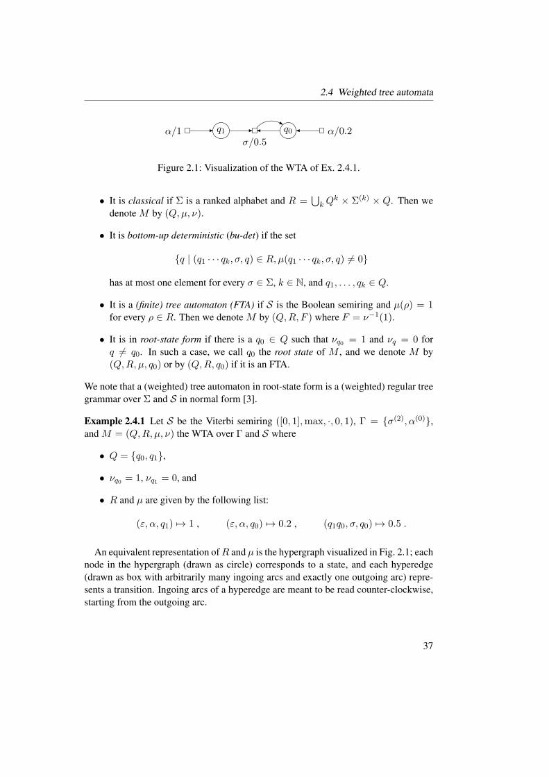
2.4 Weighted tree automata
q1 q0α/1σ/0.5
α/0.2
Figure 2.1: Visualization of the WTA of Ex. 2.4.1.
• It is classical if Σ is a ranked alphabet and R =⋃
kQk × Σ(k) × Q. Then we
denote M by (Q,µ, ν).
• It is bottom-up deterministic (bu-det) if the set
q | (q1 · · · qk, σ, q) ∈ R,µ(q1 · · · qk, σ, q) 6= 0
has at most one element for every σ ∈ Σ, k ∈ N, and q1, . . . , qk ∈ Q.
• It is a (finite) tree automaton (FTA) if S is the Boolean semiring and µ(ρ) = 1for every ρ ∈ R. Then we denote M by (Q,R, F ) where F = ν−1(1).
• It is in root-state form if there is a q0 ∈ Q such that νq0 = 1 and νq = 0 for
q 6= q0. In such a case, we call q0 the root state of M , and we denote M by
(Q,R, µ, q0) or by (Q,R, q0) if it is an FTA.
We note that a (weighted) tree automaton in root-state form is a (weighted) regular tree
grammar over Σ and S in normal form [3].
Example 2.4.1 Let S be the Viterbi semiring ([0, 1],max, ·, 0, 1), Γ = σ(2), α(0),and M = (Q,R, µ, ν) the WTA over Γ and S where
• Q = q0, q1,
• νq0 = 1, νq1 = 0, and
• R and µ are given by the following list:
(ε, α, q1) 7→ 1 , (ε, α, q0) 7→ 0.2 , (q1q0, σ, q0) 7→ 0.5 .
An equivalent representation ofR and µ is the hypergraph visualized in Fig. 2.1; each
node in the hypergraph (drawn as circle) corresponds to a state, and each hyperedge
(drawn as box with arbitrarily many ingoing arcs and exactly one outgoing arc) repre-
sents a transition. Ingoing arcs of a hyperedge are meant to be read counter-clockwise,
starting from the outgoing arc.
37

2 Preliminaries
The WTA M is not bu-det because we have that µ(ε, α, q1), µ(ε, α, q0) 6= 0. Fur-
thermore, it is in root-state form; its root state is q0. An equivalent representation of
R and µ in the spirit of weighted regular tree grammars is the following:
q0 → σ(q1, q0) # 0.5q0 → α # 0.2q1 → α # 1
2.4.2 Semantics
Now we define the weighted tree language JMK recognized by M . To this end, we
employ the approach of run semantics. Roughly speaking, a run d is a tree over Rwith the following property: if a node w is labeled (q1 · · · qk, σ, q), then the node wjis labeled by a transition in R|qj . We say that d is a run for the tree t that is obtained
from d by projecting each label to the second component. Furthermore, the weight of dis the product of µ(d(w)) over all positionsw ∈ pos(d). In order to compute the weight
of a tree t, we consider each run d for t, multiply its weight by the root weight ν(q) if
d(ε) is in R|q, and sum up over all weights thus obtained.
Now we formalize the notions of a run and its weight. For our proofs, we will
need runs and their weights to be as easily composable and decomposable as trees and
contexts. Therefore, we will consider trees indexed by semiring elements and even Q-
vectors over S. Moreover, we will consider each state a (trivial) run as well; this will
enable us to speak about “partial runs”.
Formally, we define the mappings
πQ : TR(Q ∪ (SQ ×Q))→ Q , (root state)
πΣ : TR(Q ∪ (SQ ×Q))→ TΣ(Q ∪ SQ) , and (terminal tree)
〈.〉µ : TR(Q ∪ S ∪ (SQ ×Q))→ S (weight)
as follows. We let 〈s〉µ = s for every s ∈ S. For every q ∈ Q, (u, q) ∈ SQ × Q, and
d ∈ TR(Q ∪ (SQ ×Q)) with d = ρ(d1, . . . , dk) and ρ ∈ R|q, respectively, we let
πQ(q) = q , πQ((u, q)) = q , πQ(d) = q ,
πΣ(q) = q , πΣ((u, q)) = u , πΣ(d) = σ(πΣ(d1), . . . , πΣ(dk)) ,
〈q〉µ = 1 , 〈(u, q)〉µ = u(q) , 〈d〉µ = 〈d1〉µ · · · 〈dk〉µ · µ(ρ) .
The set D(M) of runs of M is the smallest subset D of TR(Q∪ (SQ×Q)) such that
Q ∪ (SQ ×Q) ⊆ D and ρ(d1, . . . , dk) ∈ D for every ρ ∈ R, ρ = (q1 · · · qk, σ, q), and
sequence d1, . . . , dk ∈ D with πQ(dj) = qj .Let d ∈ D(M), q ∈ Q, and t ∈ TΣ(Q ∪ S
Q). We define five properties of d.
38

2.4 Weighted tree automata
• It is proper if d ∈ TR(Q). We denote the set of all proper runs by Dpr(M).
• It is complete if d ∈ TR. We denote the set of all complete runs by Dco(M).
• It is a partial run on t if πΣ(d) is a Q-prefix of t.
• It is a run on t if πΣ(d) = t. We denote the set of all runs on t by D(M, t).
• It is a q-run if πQ(d) = q. We use a superscript q to indicate that a set of runs
is restricted to q-runs; this gives rise to the sets Dq(M), Dqpr(M), Dq
co(M), and
Dq(M, t).
We define the mapping J.KM : TΣ(SQ)→ SQ by
JtKM (q) =∑
d∈Dq(M,t) 〈d〉µ .
We will often omit the subscripts µ and M from 〈.〉µ and J.KM , respectively. It will be
clear from the context which M or µ is meant, respectively; either some WTA M is
fixed throughout a section or paragraph, or we compute 〈d〉 for a run d ∈ D(M), and
then the quantification of d indicates µ.
The (weighted) meaning JMK of M is the weighted tree language over Σ and S with
JMK(t) 7→∑
q∈Q JtKq · νq .
A weighted tree language ϕ over Σ and S is called recognizable if it is the meaning
of some WTA M over Σ and S . We say that two WTA M and M ′ over Σ and S are
equivalent if JMK = JM ′K. The language L(M) of M is the tree language defined by
L(M) = t | t ∈ TΣ, ∃q ∈ Q : Dq(M, t) 6= ∅, νq 6= 0 .
If M is an FTA, then L(M) = JMK−1(1). A tree language L is recognizable if there is
an FTA M such that L = L(M).
Example 2.4.2 (Ex. 2.4.1 contd.) We show the mappings J.KM and JMK. For nota-
tional convenience, we will write the elements of SQ as column vectors, where the first
row is the q1-component. By elementary computation, we obtain
JαK =
(10.2
)
, Jσ(α, α)K =
(0
JαKq1 · JαKq0 · 0.5
)
=
(00.1
)
.
Now we form a general hypothesis. To this end, we define the family (tn | n ∈ N) of
trees in TΓ by letting t0 = α and tn+1 = σ(α, tn). It is easy to prove by induction on tthat
JtKq0 =
0.2 · 0.5n if t = tn ,
0 otherwise .
By the nature of ν, we obtain JMK(t) = JtKq0 .
39

2 Preliminaries
The WTA M is acyclic if, for every q ∈ Q, d ∈ Dqpr(M), and w ∈ pos(d), d(w) = q
implies w = ε. It is unambiguous if, for every t ∈ TΣ, there is at most one run
d ∈ D(M, t) with 〈d〉 6= 0. We observe the following.
Observation 2.4.3 If M is bu-det, then it is unambiguous. Consequently, for every
t ∈ TΣ, there is at most one q ∈ Q with JtKq 6= 0.
The following observation follows from the distributivity law of the semiring.
Observation 2.4.4 Let t ∈ TΣ(SQ) and t = σ(t1, . . . , tk). Then
JtK = Jσ(Jt1K, . . . , JtkK)K .
If Σ is a ranked alphabet, then we may define the Σ-algebraM associated with Mas the algebra with the carrier set SQ and, for every k ∈ N and σ ∈ Σ(k),
σM(u1, . . . , uk) = Jσ(u1, . . . , uk)K .
In the approach of initial-algebra semantics [86], tM is used in lieu of JtK to define
JMK(t). By Obs. 2.4.4, we obtain that JtK = tM. This means that run semantics and
initial-algebra semantics coincide, which is a known fact [77, Sec. 3.2].
The first statement of the next observation follows from Obs. 2.4.4 (and vice versa),
while the second statement is a direct consequence of the definition of 〈.〉µ.
Observation 2.4.5 Let t ∈ TΣ(SQ), t′ ∈ TΣ(S
Q ∪ z), q ∈ Q, d ∈ Dq(M, t), and
d′ ∈ D(M, q · t′). Then
JJtK · t′K = Jt · t′K and 〈〈d〉 ·q d′〉 = 〈d ·q d
′〉 .
2.4.3 Order on runs
Next we define a “prefix” order ⊑ on the set Dpr(M) of proper runs. We begin by
illustrating the idea behind ⊑ by means of an example.
Example 2.4.6 (Ex. 2.4.1 contd.) Two runs d1, d2 are in the ⊑ relation if d2 can be
obtained from d1 by simultaneously replacing arbitrarily many occurrences of states,
each by a corresponding run, for instance:
q0 ⊑ (q1q0, σ, q0)(q1, q0
)
⊑ (q1q0, σ, q0)((ε, α, q1), q0
)
⊑ (q1q0, σ, q0)((ε, α, q1), (ε, α, q0)
).
40

2.4 Weighted tree automata
The setDpr(M) and the relation⊑ bear some resemblance to the set of sentential forms
and the transitive, reflexive closure of the derivation relation of a context-free grammar,
respectively; the main difference is that runs are more akin to abstract syntax trees than
to derivation trees.
Now we make the notion precise. First we define the family (∧q | q ∈ Q), where
∧q is a binary operation on the set Dqpr(M), inductively as follows. Let q ∈ Q and
d, d′ ∈ Dqpr(M). Then
d ∧q d′ =
q if d(ε) 6= d′(ε) or d(ε) 6∈ R,
d(ε)(d|1 ∧q1 d
′|1, . . . , if d(ε) = d′(ε) = (q1 · · · qk, σ, q).
d|k ∧qk d′|k
)
We define the binary relation ⊑p on the set Dqpr(M) by letting d ⊑q d
′ iff d = d ∧q d′,
and we define the binary relation ⊑ on Dpr(M) by letting ⊑ =⋃
q∈Q⊑q. It is easy to
verify that ⊑ is a partial order.
2.4.4 Properness
We call M proper if∑
ρ∈R|qµ(ρ) = 1 for every q ∈ Q.
Lemma 2.4.7 Let S be ω-continuous. Then SQ is an ω-complete poset and there is an
ω-continuous mapping F : SQ → SQ such that
∑
t∈TΣJtK = supFn(0) | n ∈ N .
PROOF. By Thm. 2.3.8, S is an ω-complete poset and addition and multiplication are
ω-continuous. Then SQ is again an ω-complete poset. We define the family (Ti | i ∈N) by letting Ti = TΣ ∩ ht−1(i), and we define F : SQ → SQ by letting
F (u)q =∑
(q1···qk,σ,q)∈R|quq1 · · ·uqk · µ(q1 · · · qk, σ, q) .
Since (a) the semiring operations are ω-continuous, (b) the composition of ω-con-
tinuous mappings is again ω-continuous, and (c) the supremum of a sequence of vectors
can be computed pointwise, we have that F is ω-continuous as well. Moreover, using
distributivity, it is straightforward to show by induction on n that
Fn(0) =∑
i∈0,...,n
∑
t∈TiJtK .
41
2 Preliminaries
Finally, we derive
∑
t∈TΣJtK =
∑
i∈N
∑
t∈TiJtK (infinitary sum operation)
= sup∑
i∈0,...,n
∑
t∈TiJtK | n ∈ N (Thm. 2.3.7)
= supFn(0) | n ∈ N .
Next, we use Lm. 2.4.7 to show that, if M is proper, then∑
t∈TΣJtK ≤ 1. We note
that the mapping F from said lemma can be used to approximate this sum: for this,
we compute F 1(0), F 2(0), . . . until convergence or until some designated amount of
time is up. Details about this approximation and an alternative method that converges
quicker are discussed in [72].
Lemma 2.4.8 Let M be proper and S ω-continuous. Then∑
t∈TΣJtK ≤ 1.
PROOF. Let F be the mapping from Lm. 2.4.7. It is easy to see that 1 is a fixpoint of F .
We derive
∑
t∈TΣJtK = supFn(0) | n ∈ N (Lm. 2.4.7)
= minu | u = F (u) (Thm. 2.1.1)
≤ 1 . (least fixpoint)
2.4.5 Root-state form, trimness
The root-state form is a normal form, i.e., we have the following lemma.
Lemma 2.4.9 ([3, Prop. 3.1], [16, Lm. 6.1.1]) For every WTA M there is a WTA M ′
in root-state form such thatM andM ′ are equivalent; however, bottom-up determinism
is not preserved.
PROOF. Let M = (Q,R, µ, ν). We let f 6∈ Q and M ′ = (Q ∪ f, R ∪ R′, µ′, f)where
• R′ = (q1 · · · qk, σ, f) | ∃q : (q1 · · · qk, σ, q) ∈ R,
• µ′ coincides with µ on R, and
• µ′(q1 · · · qk, σ, f) =∑
q∈Q µ(q1 · · · qk, σ, q) · νq.
Clearly, this construction does not preserve bottom-up determinism. In fact, this
preservation is impossible [16, Lm. 6.1.3].
42

2.4 Weighted tree automata
Let M = (Q,R, µ, ν) be a WTA. A state q ∈ Q is reachable if there are q0 ∈ Q,
d ∈ Dq0(M), and w ∈ pos(d) with ν(q0) 6= 0 and d(w) = q; and it is productive if
Dqco(M) is nonempty. A transition ρ ∈ R is useful if there are q0 ∈ Q, d ∈ Dq0
co(M),and w ∈ pos(d) with ν(q0) 6= 0 and d(w) = ρ; otherwise ρ is useless. The WTA Mis trim if every state is reachable and productive. We note that then every transition
of M is useful. Converting a WTA into an equivalent trim WTA is called trimming or
reducing.
Lemma 2.4.10 Let M = (Q,R, µ, ν) be a WTA and L(M) 6= ∅. Then there is effec-
tively an equivalent trim WTA M ′ such that M ′ is in root-state form if so is M .
PROOF. The reduction proceeds as known from context-free grammars. First, we de-
termine the set of productive states as follows. We let Q0 = ∅ and Qn+1 = q |∃(q1 · · · qk, σ, q) ∈ R : q1, . . . , qk ∈ Qn. Then, for every n,Qn ⊆ Qn+1 andQn ⊆ Q.
Hence, Qn+1 = Qn for some n. We let Q′ = Qn. One can show that Q′ is the set
of productive states. We note that Q′ 6= ∅ because L(M) 6= ∅. Second, we deter-
mine the set of reachable states of the WTA obtained from M by removing any state
that is not in Q′. To this end, we let P0 = ∅ and Pn+1 = q0 | q0 ∈ Q′, ν(q0) 6=0 ∪ qi | ∃(q1 · · · qk, σ, q) ∈ R : q1, . . . , qk ∈ Q′, q ∈ Pn, 1 ≤ i ≤ k. Again,
we find that Pn+1 = Pn for some n, and that Pn is the desired set. We construct
M ′ = (Pn, R′, µ|R′ , ν|Pn) where R′ contains exactly the transitions from R that only
use states from Pn. It is easy to see that M ′ is trim and that JMK = JM ′K.
2.4.6 Bibliographic remarks
There is an established theory of WTA with varying weight domains, namely fields
[10], commutative semirings [3], continuous semirings [71, 116], m-monoids [116,
117, 125, 73, 175, 76], or tree-valuation monoids [56]. An overview of WTA over
semirings is given in [77].
A WTA (over a semiring) from the literature is a classical WTA by our definition.
When Σ is a ranked alphabet, the generative capacity of WTA and classical WTA is the
same. We deviate from the literature by including the set R of transitions; this has four
advantages, as we can more easily
• define a subclass of WTA by restricting the syntax of transitions; in this way, we
will define weighted synchronous context-free tree grammars in Ch. 3,
• consider constructions that replace a single transition at a time; namely, the bina-
rization procedure of Ch. 4,
• consider a notion of usability of a state that does not depend on S , and
43
2 Preliminaries
• handle unranked trees (with bounded rank).
Note that there is a variant of weighted tree automata that allows specifying weighted
tree languages with unbounded rank [58, Sec. 3].
A potential fifth advantage of explicit transitions may emerge in the context of train-
ing, i.e., estimating transition weights from data. As in the case of probabilistic context-
free grammars [145, Sec. 6], it is conceivable that the data naturally suggest a set of
transitions, and focusing on this set may reduce the training effort. In fact, the state-
splitting method of [155] may be construed as WTA training, and the method uses
explicit transitions.
In the literature, a run is usually defined with respect to a tree t, namely as a mapping
from the set pos(t) of its positions into the setQ of states. We deviate from the literature
by defining a run (roughly) as a tree with labels inR∪Q∪SQ; this has three advantages,
as we can
• consider partial runs and the “prefix” order ⊑ on runs, which we will need in
Chs. 3 and 4,
• use tree manipulation functions, from which we will benefit a great deal in Ch. 5,
and
• compute the weight of a run using a homomorphism.
44

3 Input product and output product of
a weighted synchronous
context-free tree grammar and a
weighted tree automaton
This chapter is a considerably expanded and revised version of [33, 32].
3.1 Introduction
Given a weighted tree tansformation τ over Σ and S and a weighted tree language ϕover Σ and S , the input product ϕ ⊳ τ of ϕ and τ and the output product τ ⊲ ϕ of
ϕ and τ are the weighted tree transformations over Σ and S defined by [128]
ϕ⊳ τ : (s, t) 7→ ϕ(s) · τ(s, t) and τ ⊲ ϕ : (s, t) 7→ τ(s, t) · ϕ(t) .
In the following, for the sake of brevity, we restrict our attention to the input product.
The same ideas apply to the output product.
If C is a class of weighted tree transformations over Σ and S , we may ask whether Cis effectively closed under input product (with recognizable weighted tree languages
over Σ and S). In other words, if τ ∈ C and ϕ is recognizable, we ask whether ϕ ⊳ τis again in C, and how to construct it. As argued in Sec. 1.5.1, such a closure result
allows for an effective algebraic decoder specification, e.g., if C is the class of STAG
meanings.
Let us review what is known about closure under input product, with a focus on
classes that contain STAG meanings. As a preparation, we relate the input product to
composition of two weighted tree transformations on the one hand and to the Hadamard
product of two weighted tree languages (also known as weighted intersection [145])
on the other hand. For this, we define the mapping f : STΣ → STΣ×TΣ by letting
f(ϕ)(t, t) = ϕ(t) and f(ϕ)(s, t) = 0 for s 6= t.Given another weighted tree transformation τ ′ over Σ and S , the composition τ ⋄ τ ′
of τ and τ ′ is the weighted tree transformation over Σ and S defined by [75, Sec. 2.6]
τ ⋄ τ ′ : (s, t) 7→∑
u τ(s, u) · τ′(u, t) ,
45

3 Input product for weighted synchronous context-free tree grammars
type∗ grammar product semiring
publication F C A I formalism with restriction remarks
[161] · · CFTG FTA Boolean
[144] · · · WLIG WTA nonnegative reals
[127, Sec. 7.2] · · · STAG FTA Boolean (1)
[113] · STAG tree Boolean (2)
[146] · · SCFTG FTA Boolean
(this chapter) · WSCFTG WTA commutative
* Formal closure result, Construction, Algorithm, Implementation.
(1) represents STAG as XTT with explicit substitution
(2) represents STAG as IRTG
Table 3.1: Results towards closure under Hadamard/input/output product.
where we assume that S is complete. Then we observe that
ϕ⊳ τ = f(ϕ) ⋄ τ and τ ⋄ f(ϕ) = τ ⊲ ϕ .
If the class C contains f(ϕ) for every recognizable ϕ, then closure of C under compo-
sition implies closure of C under both input and output product. For instance, the class
of meanings of extended multi-bottom-up tree transducers is closed under composi-
tion, whereas the class of STAG meanings is not [66]. Consequently, it is worthwile to
consider the input product as a topic of its own.
Given another weighted tree language ϕ′ over Σ and S , we observe that
f(ϕ)⊲ ϕ′ = f(ϕ⊙ ϕ′) = ϕ⊳ f(ϕ′) ;
i.e., the input product can be used to compute the Hadamard product. Conversely,
the input product can be viewed as a simple generalization of the Hadamard product.
In fact, the corresponding constructions can be highly similar; roughly speaking, the
input-product construction is merely an intersection construction that accounts for an
additional, yet “uninvolved” component. This intuitive observation is substantiated
formally in the framework of interpreted regular tree grammars (IRTGs, cf. [112]).
Table 3.1 lists existing results with respect to the Hadamard product and the input
product. The first entry is the seminal result in this area: the class of context-free
tree languages is closed under intersection with regular tree languages. In [144] it is
shown that the class of meanings of weighted linear indexed grammars (WLIGs) is
46

3.2 Weighted synchronous context-free tree grammars
closed under Hadamard product with recognizable weighted tree languages. WLIGs
are equivalent to tree-adjoining grammars (TAGs). It is not clear how this result can be
transferred to the synchronous setting. Providing a corresponding construction, [127]
and [113] indicate that the class of meanings of STAGs is closed under input and output
product with recognizable tree languages and singleton tree languages, respectively.
The work [146] extends this result to the class of meanings of synchronous context-free
tree grammars (SCFTGs), which contains all STAG meanings.
In this chapter, we show that the class of meanings of weighted synchronous context-
free tree grammars (WSCFTGs) is closed under input and output product with recogniz-
able weighted tree languages. Moreover, we show that this closure is effective by means
of a product construction, and we provide an Earley-like algorithm [60] for computing
at least the useful rules of said construction. As argued in [89] and [99, Sec. 13.4],
algorithms such as Earley’s are often used for parsing, which is, ultimately, an appli-
cation of the input product [145]. We note that WSCFTGs subsume many grammar
formalisms mentioned in Ch. 1, such as STSGs, STIGs, and STAGs [102]. WSCFTGs
provide additional expressive power, whose relevance to SMT has already been under-
scored in [146]; in particular, the authors cite recent findings concerning lexicalization
of tree-adjoining grammars [131].
We proceed as follows. First, we define WSCFTGs in terms of particular WTA,
and we define the WSCFTG meaning of these WTA (Sec. 3.2). Second, we prove our
closure result (Sec. 3.3). More specifically, given an WSCFTG G and a WTA M , we
construct a WSCFTGM⊳Gwith JM⊳GK = JMK⊳JGK. We prove our closure result
(Thm. 3.3.3) by showing a stronger statement: we relate the runs of G and M on the
one hand to the runs of M ⊳G on the other (Lm. 3.3.2). Roughly speaking, our result
implies that, if M is unambiguous, then the n best runs of M ⊳ G correspond to the
n best runs of G, when adjusted according to the input product. Third, we derive the
Earley-like algorithm for computing at least the useful rules of M ⊳G, and we indicate
that the algorithm is correct (Sec. 3.4).
We end this chapter with a conclusion, discussion, and outlook (Sec. 3.5).
3.2 Weighted synchronous context-free tree grammars
For the remainder of this chapter, let S be a commutative semiring.
Let Σ be an alphabet and l,m, r1, . . . , rl ∈ N. By CΣ(m, r1, . . . , rl) we denote the
set of all unranked trees t over Σ∪Xl ∪ Ym that are linear and nondeleting in Xl ∪ Ymsuch that (i) t(w) = xj implies rkt(w) = rj and (ii) t(w) = yj implies rkt(w) = 0.
Note that CΣ(m) = CΣ(Ym) and CΣ(0) = TΣ.
A weighted synchronous context-free tree grammar (WSCFTG) G over Σ and S is a
47
3 Input product for weighted synchronous context-free tree grammars
tuple (Q,R, µ, ν) where
• Q is a ranked alphabet with Q(0) 6= ∅,
• R is a finite set of triples (q1 · · · ql, 〈ζζ′〉, q) where
– q, q1, . . . , ql ∈ Q and
– ζ, ζ ′ ∈ CΣ(rk(q), rk(q1), . . . , rk(ql)),
• µ : R→ S, and
• ν : Q(0) → S.
Let G = (Q,R, µ, ν) be a WSCFTG over Σ and S , and let Γ be the ranked alphabet
with
Γ = α(l) | ∃q1, . . . , ql, q : (q1 · · · ql, α, q) ∈ R .
Then G can be viewed as a WTA G′ = (Q,R, µ, ν ′) over Γ and S where ν ′ extends νby mapping every element ofQ\Q(0) to 0. In the following, we will identifyG andG′.
We will also employ the notation G = (Q,R, µ, q0) if G is in root-state form. For a
transition ρ ∈ R, ρ = (q1 · · · ql, 〈ζζ′〉, q), we call ζ and ζ ′ the input tree and output
tree, respectively.
Example 3.2.1 We consider the WSCFTG G = (Q,R, µ, q1) over Σ and Real, where
• Σ = S,NP,VP, . . . ,
• Q(0) = q1, q2, q3 and Q(1) = f,
• R and µ are given in Fig. 3.1; for every transition ρ ∈ R, ρ = (q1 · · · ql, α, q),the figure contains a line q → α(q1, . . . , ql) # µ(ρ), which is preceded by a
shorthand for ρ.
Next we will define the WSCFTG meaning of G, which is a weighted tree transfor-
mation over Σ and S . We do so in the spirit of bimorphisms [6], where the WTA Gspecifies the weighted center language JGK, and we define two embedded tree homo-
morphisms h1 and h2, which retrieve from a center tree the derived input tree and output
tree, respectively.
Let ζ ∈ CΣ(m, r1, . . . , rl). We define the mapping ζI : TΣ(Y )l → TΣ(Y ) by
ζI(t1, . . . , tl) = ζLxl/tlM · · · Lx1/t1M .
As mentioned in Obs. 2.2.1, we may imagine that we substitute the variables sequen-
tially. This lets us specify the type for intermediate results, as follows.
48

3.2 Weighted synchronous context-free tree grammars
ρ1 : q1 → α1(q2, q2, f) # 1 ρ4 : q3 → α4() # 1
ρ2 : q2 → α2() # 0.6 ρ5 : f → α5() # 1
ρ3 : q2 → α3(q3) # 0.4
α1 =
⟨
x3
S
x1 VP
V
saw
x2
x3
S
VP
V
sah
x1 x2⟩
α5 =
⟨
S
Adv
yesterday
y1
S
Adv
gestern
y1⟩
α2 =
⟨NP
N
Mary
NP
N
Mary
⟩
α3 =
⟨
NP
x1 N
man
NP
x1 N
Mann
⟩
α4 =
⟨ D
a
D
einen
⟩
Figure 3.1: WSCFTG with initial state q1 (adapted from [98, Fig. 2.4]).
α1
α2 α3
α4
α5
ξex :
S
Adv
yesterday
S
NP
N
Mary
VP
V
saw
NP
D
a
N
man
s :
S
Adv
gestern
S
VP
V
sah
NP
N
Mary
NP
D
einen
N
Mann
t :
Figure 3.2: Center tree ξex, input tree s = h1(ξex), output tree t = h2(ξex).
49

3 Input product for weighted synchronous context-free tree grammars
Observation 3.2.2 Let ζ ∈ CΣ(m, r1, . . . , rl), t1 ∈ CΣ(r1), . . . , tl ∈ CΣ(rl), and
j ∈ 0, . . . , l. Then ζLxl/tlM · · · Lxj+1/tj+1M ∈ CΣ(m, r1, . . . , rj).
We define the embedded tree homomorphisms h1, h2 : TΓ → TΣ(Y ) by
hi(〈ζ1ζ2〉(ξ1, . . . , ξk)
)= ζIi
(hi(ξ1), . . . , hi(ξk)
)
for every 〈ζ1ζ2〉(ξ1, . . . , ξk) in TΓ. We call the trees in L(G) center trees. For every
center tree ξ, we call (h1(ξ), h2(ξ)) the derived tree pair for ξ.
Example 3.2.3 (Ex. 3.2.1 contd.) Let ξex and s be the trees from Fig. 3.2. We show
that h1(ξex) = s and JGK(ξex) = 0.24. We begin with the former. To this end, let ζ be
the input tree of ρ1.
First, we apply the definitions of h1 and ζI , and we introduce abbreviations:
h1(ξex) = ζLx3/ h1(α5)︸ ︷︷ ︸
t3
MLx2/ h1(α3(α4))︸ ︷︷ ︸
t2
MLx1/ h1(α2)︸ ︷︷ ︸
t1
M .
Second, we perform an auxiliary computation for t1, t2, and t3; we derive
t1 = h1(α2) = NP(N(Mary)) ,
t2 = h1(α3(α4)) = NP(x1,N(man))Lx1/h1(α4)M = NP(D(a),N(man)) ,
t3 = h1(α5) = S(Adv(yesterday), y1) .
Finally, we derive
h1(ξex) = x3(S(x1,VP(V(saw), x2)))Lx3/t3MLx2/t2MLx1/t1M
= S(Adv(yesterday), S(x1,VP(V(saw), x2)))Lx2/t2MLx1/t1M
= S(Adv(yesterday), S(x1,VP(V(saw), t2)))Lx1/t1M
= S(Adv(yesterday), S(t1,VP(V(saw), t2))) = s .
We can show in a similar fashion that h2(ξex) = t, where t is also given in Fig. 3.2.
Now we show that JGK(ξex) = 0.24. It is easy to see that
ρ1(ρ2, ρ3(ρ4), ρ5)
is the only q1-run on ξex. Let us call this run d. We derive
JGK(ξex) = 〈d〉 = µ(ρ2) · µ(ρ4) · µ(ρ3) · µ(ρ5) · µ(ρ1)
= 0.6 · 1 · 0.4 · 1 · 1 = 0.24 .
50

3.2 Weighted synchronous context-free tree grammars
WSCFTGs are “type safe” in the following sense. Let ζ ∈ CΣ(m, r1, . . . , rl). A tree
ξ ∈ TΓ, ξ = 〈ζζ ′〉(ξ1, . . . , ξl), is called type conformant if ξι is type conformant and
hi(ξι) ∈ CΣ(rι). The following lemma comprises our type-safety statement.
Lemma 3.2.4 Let ζ ∈ CΣ(m, r1, . . . , rl), ξ ∈ TΓ, and ξ = 〈ζζ ′〉(ξ1, . . . , ξl). If ξ is
type conformant, then hi(ξ) ∈ CΣ(m). If D(G, ξ) 6= ∅, then ξ is type conformant.
PROOF. The first statement follows from Obs. 3.2.2.
For the second statement, we prove the following statement by induction on n. For
every n ∈ N and ξ ∈ TΓ, if |pos(ξ)| ≤ n and D(G, ξ) 6= ∅, then ξ is type conformant.
For the induction base (n = 0), there is nothing to show. For the induction step (“n→n + 1”), we let ξ ∈ TΓ with |pos(ξ)| ≤ n + 1 and D(G, ξ) 6= ∅. Then there are
〈ζζ ′〉 ∈ Γ, ξ1, . . . , ξl ∈ TΓ, d ∈ D(G, ξ), and ρ = (q1 · · · ql, 〈ζζ′〉, q) such that ξ =
〈ζζ ′〉(ξ1, . . . , ξl) and d(ε) = ρ. Then ζ ∈ CΣ(rk(q), rk(q1), . . . , rk(ql)) and the input
tree ζι of ξι(ε) is in CΣ(rk(qι), r′1, . . . , r
′l′) for some l′ and r′1, . . . , r
′l′ . By the induction
hypothesis, ξ1, . . . , ξl are type conformant, and by the first statement of the lemma, we
obtain that hi(ξι) ∈ CΣ(rk(qι)).
Corollary 3.2.5 For every ξ ∈ TΓ with JGK(ξ) 6= 0, we have that hi(ξ) ∈ TΣ.
PROOF. Since JGK(ξ) 6= 0, we have that Dq(G, ξ) 6= ∅ for some q ∈ Q(0). By
Lm. 3.2.4, hi(ξ) ∈ CΣ(0), that is, hi(ξ) ∈ TΣ.
Finally we define the WSCFTG meaning of G. For this, we call G admissible if
(i) S is complete or (ii) ξ | ξ ∈ L(G), ∀i : hi(ξ) = ti is finite for every (t1, t2) ∈TΣ×TΣ. Let G be admissible. The (WSCFTG) meaning JGK′ of G is the weighted tree
transformation over Σ and S with
JGK′(s, t) =∑
ξ∈h−11 (s)∩h−1
2 (t) JGK(ξ) .
We can satisfy Condition (ii) by requiring that G be productive. This property has
been discussed, e.g., in [74]. In our setting, it amounts to
〈ζ1, ζ2〉 ∈ Γ =⇒ ζi 6∈ x1, x1(y1) ,
which is easily tested for by looking at the transitions of G.
In the following, we usually omit the prime from JGK′; there is no confusion with the
WTA meaning because of the different type.
Example 3.2.6 (Ex. 3.2.3 contd.) Let ξex, s, and t be the trees from Fig. 3.1. It is easy
to see that h−11 (s)∩h−1
2 (t) = ξex, and we compute
JGK(s, t) = JGK(ξex) = 0.24 .
As we will see in Ex. 3.3.4, we can use the input and output product to compute
JGK(s, t) algorithmically.
51

3 Input product for weighted synchronous context-free tree grammars
ρ1 : q → α1(q, f) # 0.3 ρ3 : f → α3(f) # 0.7
ρ2 : q → α2() # 1 ρ4 : f → α4() # 1
α1 =
⟨
x2
S
〈 x1 〉
x2
S
〈 x1 〉
⟩
α3 =
⟨
S
a x1
S
b y1 c
d
S
a d x1
S
b c y1
⟩
α2 =⟨♦ ♦
⟩α4 =
⟨y1 y1
⟩
Figure 3.3: WSCFTG G from Ex. 3.3.1 (adapted from [98, Ex. 2.2]).
3.3 Closure under input and output product
3.3.1 Example and objective
Example 3.3.1 We consider the WSCFTG G given in Fig. 3.3 in the same style as in
Ex. 3.2.1, where q is the root state and f is a unary state. Figure 3.4 shows the shape
of the center trees of G and a concrete derived tree pair. The weight of a center tree of
the given shape is 0.3k · 0.7n1+···+nk , and the derived tree pair for such a center tree
corresponds to the following pair of strings:
(
an1bn1〈 · · · 〈ankbnk〈♦〉cnkdnk〉 · · · 〉cn1dn1 , (ad)n1(bc)n1〈 · · · 〈(ad)nk(bc)nk〈♦〉k)
.
Furthermore, we consider the WTA M = (P,RM , µM , 0) with root state 0 shown
in Fig. 3.5(a). The states 0 and 1 recognize backbones of even and odd lengths, respec-
tively. Then JMK maps trees of the form shown in Fig. 3.5(b), where the unlabeled
nodes may carry any label in a, b, c, d, 〈, 〉, to the weight 0.52n · 0.24n if the number
of occurrences of S is 2n. Every other tree is mapped to 0.
The input product JMK ⊳ JGK maps pairs like in Fig. 3.4(c) to 0.52n · 0.24n · 0.3k ·0.7n1+···+nk if 2n = k + 2(n1 + · · ·+ nk). Every other pair is mapped to 0.
Our aim is to to construct a WSCFTG M ⊳G with JM ⊳GK = JMK⊳ JGK. For our
example, such a WSCFTG is shown in Fig. 3.6. The underlying idea is to incorporate
the behavior of M into G. To this end, we augment the states of G by states of M ,
so that we have sufficient information to simulate M on the input tree of each rule of
M ⊳G. We note that the input tree in α3 contains exactly two nodes labeled S, so this
52

3.3 Closure under input and output product
α1
. ..
α1
α2 α3
...
α3
α4
α3
...
α3
α4
k
nk
n1
(a)
S
a S
a S
b S
b S
〈 S
a S
b S
〈 ♦ 〉
c
d
〉
c
c
d
d
S
a d S
a d S
b c S
b c S
〈 S
a d S
b c S
〈 ♦ 〉
〉
(b)
Figure 3.4: (a) Shape of center trees of G, where k ∈ N and n1, . . . , nk ∈ N.
(b) Derived tree pair for k = 2, n1 = 2, and n2 = 1.
(r1r, S, 0) 7→ 0.5
(r0r, S, 1) 7→ 0.5
(ε,♦, 0) 7→ 1
(ε, x, r) 7→ 0.2 x ∈ a, b, c, d, 〈, 〉
(a)
S
...
S
♦
2n
(b)
Figure 3.5: (a) WTA M from Ex. 3.3.1.
(b) Shape of trees with nonzero weight in JMK, where n ∈ N.
53

3 Input product for weighted synchronous context-free tree grammars
(q, 0, ε)→ α1
((q, 1, ε), (f, 0, 0)
)# 0.3 · (0.5 · 0.22)
(q, 1, ε)→ α1
((q, 0, ε), (f, 1, 1)
)# 0.3 · (0.5 · 0.22)
(q, 0, ε)→ α2() # 1.0
(f, 0, 0)→ α3
((f, 1, 1)
)# 0.7 · (0.52 · 0.24)
(f, 1, 1)→ α3
((f, 0, 0)
)# 0.7 · (0.52 · 0.24)
(f, 0, 0)→ α4() # 1.0
(f, 1, 1)→ α4() # 1.0
Figure 3.6: WSCFTG M ⊳G for Ex. 3.3.1.
tree does not affect the parity of the total number of S-labeled nodes. Hence, transitions
of M ⊳ G with α3 only contain the states (f, 0, 0) and (f, 1, 1), but not (f, 0, 1) or
(f, 1, 0). Also note how these transitions alternate between said states.
In the following, we show that the class of meanings of admissible WSCFTGs is ef-
fectively closed under input product with recognizable weighted tree languages. How-
ever, we do not prove this result directly. We rather consider a stronger statement. For
this, letM = (P,RM , µM , νM ) be a WTA over Σ and S . Moreover, let p ∈ P ,m ∈ N,
s ∈ CΣ(m), and p′ = (p1, . . . , pm). Then we define
D(p,p′)(M, s) = Dp(M, s[y1/p1] · · · [ym/pm]) .
Recall thatG is both an admissible WSCFTG over Σ and S and a WTA over Γ and S .
Lemma 3.3.2 There is effectively an admissible WSCFTG M ⊳ G = (Q′, R′, µ′, ν ′)over Σ and S such that M ⊳G is also a WTA over Γ and S , Q′ =
⋃
mQ(m)×P ×Pm
with the ranks carried over from Q, ν ′(q,p,ε) = νq · (νM )p, and the following holds.
Let ξ ∈ TΓ be type conformant, s = h1(ξ), and s ∈ CΣ(m). Then there are families
(≡(p,p′) | p ∈ P, p′ ∈ Pm) and (πq′ | q
′ ∈ Q′(m)) such that
• ≡(p,p′) is an equivalence relation on D(p,p′)(M, s),
• π(q,p,p′) : D(q,p,p′)(M ⊳G, ξ)→ Dq(G, ξ)×D(p,p′)(M, s)/≡(p,p′)
is bijective,
• πq′(d′) = (d,D) implies 〈d′〉 = 〈d〉 ·
∑
e∈D〈e〉.
Let us consider some intuition for the lemma. As illustrated in Ex. 3.3.1, the con-
struction of M ⊳G involves “guessing” (and thus fixing) a state of M at various posi-
tions in the input tree. Roughly speaking, the equivalence relation ≡(p,p′) relates those
54
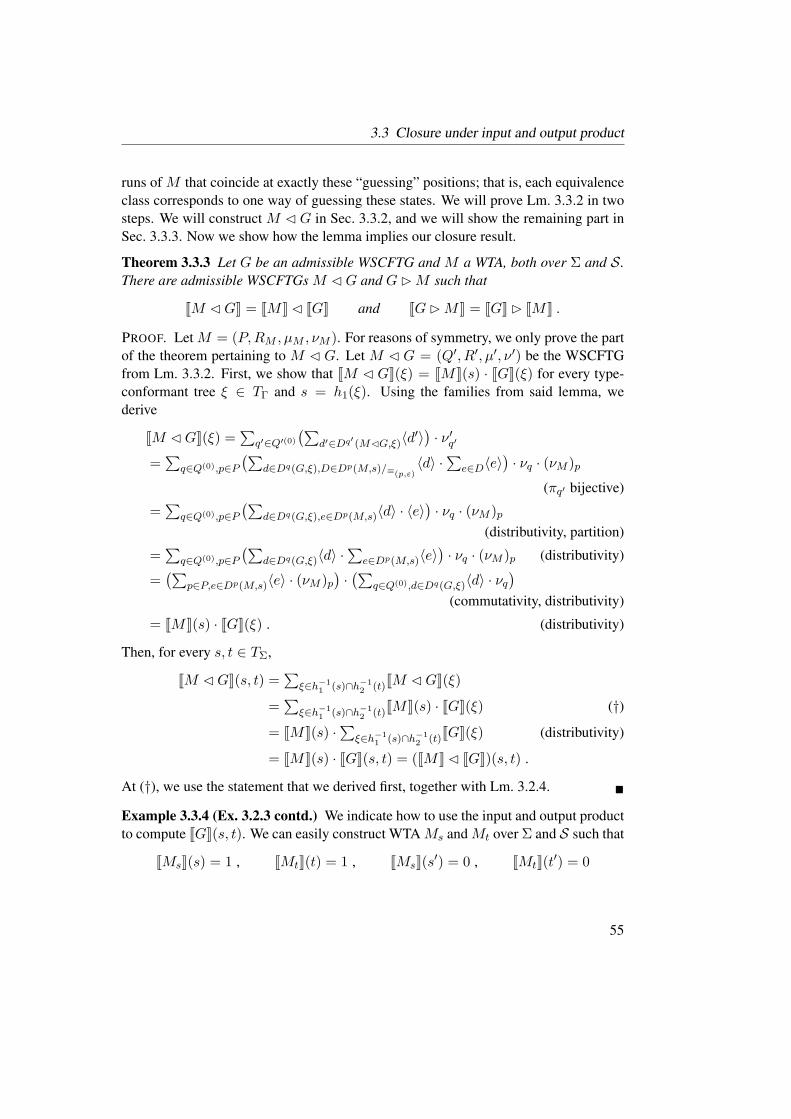
3.3 Closure under input and output product
runs of M that coincide at exactly these “guessing” positions; that is, each equivalence
class corresponds to one way of guessing these states. We will prove Lm. 3.3.2 in two
steps. We will construct M ⊳ G in Sec. 3.3.2, and we will show the remaining part in
Sec. 3.3.3. Now we show how the lemma implies our closure result.
Theorem 3.3.3 Let G be an admissible WSCFTG and M a WTA, both over Σ and S .
There are admissible WSCFTGs M ⊳G and G⊲M such that
JM ⊳GK = JMK⊳ JGK and JG⊲MK = JGK⊲ JMK .
PROOF. Let M = (P,RM , µM , νM ). For reasons of symmetry, we only prove the part
of the theorem pertaining to M ⊳ G. Let M ⊳ G = (Q′, R′, µ′, ν ′) be the WSCFTG
from Lm. 3.3.2. First, we show that JM ⊳ GK(ξ) = JMK(s) · JGK(ξ) for every type-
conformant tree ξ ∈ TΓ and s = h1(ξ). Using the families from said lemma, we
derive
JM ⊳GK(ξ) =∑
q′∈Q′(0)
(∑
d′∈Dq′ (M⊳G,ξ)〈d′〉)· ν ′q′
=∑
q∈Q(0),p∈P
(∑
d∈Dq(G,ξ),D∈Dp(M,s)/≡(p,ε)〈d〉 ·
∑
e∈D〈e〉)· νq · (νM )p
(πq′ bijective)
=∑
q∈Q(0),p∈P
(∑
d∈Dq(G,ξ),e∈Dp(M,s)〈d〉 · 〈e〉)· νq · (νM )p
(distributivity, partition)
=∑
q∈Q(0),p∈P
(∑
d∈Dq(G,ξ)〈d〉 ·∑
e∈Dp(M,s)〈e〉)· νq · (νM )p (distributivity)
=(∑
p∈P,e∈Dp(M,s)〈e〉 · (νM )p)·(∑
q∈Q(0),d∈Dq(G,ξ)〈d〉 · νq)
(commutativity, distributivity)
= JMK(s) · JGK(ξ) . (distributivity)
Then, for every s, t ∈ TΣ,
JM ⊳GK(s, t) =∑
ξ∈h−11 (s)∩h−1
2 (t)JM ⊳GK(ξ)
=∑
ξ∈h−11 (s)∩h−1
2 (t)JMK(s) · JGK(ξ) (†)
= JMK(s) ·∑
ξ∈h−11 (s)∩h−1
2 (t)JGK(ξ) (distributivity)
= JMK(s) · JGK(s, t) = (JMK⊳ JGK)(s, t) .
At (†), we use the statement that we derived first, together with Lm. 3.2.4.
Example 3.3.4 (Ex. 3.2.3 contd.) We indicate how to use the input and output product
to compute JGK(s, t). We can easily construct WTAMs andMt over Σ and S such that
JMsK(s) = 1 , JMtK(t) = 1 , JMsK(s′) = 0 , JMtK(t
′) = 0
55

3 Input product for weighted synchronous context-free tree grammars
for every s′ 6= s and t′ 6= t. Then
JGK(s, t) =∑
s′,t′(JMsK⊳ JGK⊲ JMtK)(s′, t′)
=∑
s′,t′JMs ⊳G⊲MtK(s′, t′) (Thm. 3.3.3)
=∑
ξ∈TΓJMs ⊳G⊲MtK(ξ) =
∑
ξ∈TΓJξKMs⊳G⊲Mt · ν
′
=(∑
ξ∈TΓJξKMs⊳G⊲Mt
)· ν ′, (distributivity)
where ν ′ is the root-weight mapping ofMs⊳G⊲Mt. For every WTAM over Γ and S ,
we can compute∑
ξ∈TΓJξKM at least approximatively by using the fixpoint method that
is indicated below Lm. 2.4.7.
3.3.2 Constructing the product WSCFTG
Here we provide our construction of the WSCFTG M ⊳ G, whose existence is pos-
tulated in Lm. 3.3.2. Let G be a WSCFTG and M a WTA, both over Σ and S , with
G = (Q,R, µ, ν) and M = (P,RM , µM , νM ).
First, we enrich M so that it can accept trees such as those that occur in Γ, that is,
including variables. To this end, let ζ ∈ CΣ(m, r1, . . . , rl). A (state) assignment for ζis a mapping θ that maps each variable xι that occurs in ζ to an element of P ×P rι and
each variable yι to an element of P . Finally, θ maps the special symbol ⋄ to an element
of P . Then, for every assignment θ, we define the WTA Mθ over Σ ∪ Xl ∪ Ym by
Mθ = (P,RMθ, µMθ, θ(⋄)) where
• RMθ = RM ∪ (p′, xι, p) | θ(xι) = (p, p′) ∪ (ε, yι, p) | θ(yι) = p,
• µMθ(ρ) = µM (ρ) if ρ ∈ RM , and
• µMθ(ρ) = 1 if ρ 6∈ RM .
Second, for every transition ρ ∈ R and suitable θ, we let Mθ “run” on the input tree
of ρ. Formally, we define the product WSCFTG M ⊳G of M and G by
M ⊳G =(⋃
mQ(m) × P × Pm, R′, µ′, ν ′
),
where the ranks of the states are carried over fromQ, ν ′(q,p,ε) = νq ·(νM )p, andR′ and µ′
are defined as follows. Let ρ ∈ R, ρ = (q1 · · · ql, 〈ζζ′〉, q), m = rk(q), θ an assignment
for ζ, and p′ = (θ(y1), . . . , θ(ym)). Then we let
ρθ =((q1, θ(x1)
)· · ·
(ql, θ(xl)
), 〈ζζ ′〉,
(q, (θ(⋄), p′)
))
,
56

3.3 Closure under input and output product
and ρθ ∈ R′ if ζ ∈ L(Mθ). Then its weight is given by
µ′(ρθ) = µ(ρ) · JMθK(ζ) .
This definition is sound because the mapping with (ρ, θ) 7→ ρθ is injective. There are
no further elements in R′. We note that we have identified Q(m) × P × P ′ (a set of
triples) with Q(m) × (P × P ′) (a set of pairs whose second component is a pair). We
will continue to do so.
We have that |R′| ≤ |R| · |P |C where C = maxrk(q0) + · · · + rk(ql) + l + 1 |(q1 · · · ql, α, q0) ∈ R. More specifically, the factors |R| and |P |C are due to the
choices of ρ and θ, respectively. An inspection of C suggests that, if we want to keep
the cost for the input product low, then we should try to represent JGK with a WSCFTG
whose states and transitions have as low rank as possible.
Example 3.3.5 (Ex. 3.3.1 contd.) In addition to the transitions shown in Fig. 3.6, the
WSCFTG M ⊳G also contains the following transitions:
(f, 0, 1)→ α3
((f, 1, 0)
)# 0.7 · (0.52 · 0.2) ,
(f, 1, 0)→ α3
((f, 0, 1)
)# 0.7 · (0.52 · 0.2) .
As argued in Ex. 3.3.1, applying ρ3 does not affect the parity of the total number of
S-labeled nodes. Hence, these transitions do not occur in any (q, 0, ε)-run of M ⊳ G,
and they can be discarded.
3.3.3 Proof of Lemma 3.3.2
It is easy to see that M ⊳G is admissible, because L(M ⊳G) ⊆ L(G). We prove the
remaining statement of the lemma by induction on the size of ξ. More precisely, we
prove by induction on n that the following statement P (n) holds for every n:
P (n): Let ξ ∈ TΓ be type conformant, s = h1(ξ), and s ∈ CΣ(m). If
|pos(ξ)| ≤ n, then there are the families as postulated in the lemma.
For the induction base (n = 0), there is nothing to show. We show the induction
step (n → n + 1). For this purpose, let n ∈ N such that P (n) holds (the induction
hypothesis). We show P (n+1). To this end, let ξ ∈ TΓ be type conformant, s = h1(ξ),s ∈ CΣ(m), and |pos(ξ)| ≤ n+ 1. There are 〈ζζ ′〉 ∈ Γ and ξ1, . . . , ξl ∈ TΓ such that
ξ = 〈ζζ ′〉(ξ1, . . . , ξl). Clearly, ξι is type conformant and |pos(ξι)| ≤ n.
By applying the induction hypothesis to ξ1, . . . , ξl, we obtain the families ≡1 and π1up to ≡l and πl, respectively. In the following, we will often omit the subscripts (p, p′)
57

3 Input product for weighted synchronous context-free tree grammars
and q′ from ≡ι and πι, respectively. Before we construct ≡ and π, we introduce the
following notion and lemma.
A composition item s is a tuple (θ, e0, e1, . . . , el) such that θ is an assignment for ζ,
e0 ∈ Dθ(⋄)(Mθ, ζ), and eι ∈ D
θ(xι)(M,h1(ξι)). The composite JsK of s is defined by
JsK = v′(e0)I(v(e1), . . . , v(el)) ,
where v(eι) is obtained from eι by replacing every occurrence of a state in P by the
label of h(ξι) at the same position, and v′ replaces every occurrence of a transition
containing a variable xι or yι by the respective variable or by θ(yι), respectively.
Lemma 3.3.6 For every p ∈ P , p′ ∈ Pm, and e ∈ D(p,p′)(M, s), there is exactly one
composition item s with JsK = e.
PROOF. We prove the following statement by induction on l. For every l ∈ N, ζ ∈CΣ(m, r1, . . . , rl), s1, . . . , sl with sι ∈ CΣ(rι), and e ∈ D(p,p′)(M, ζI(s1, . . . , sl)),there is exactly one tuple (θ, e0, e1, . . . , el) such that θ is an assignment for ζ, e0 ∈Dθ(⋄)(Mθ, ζ), eι ∈ D
θ(xι)(M, sι), and e = v′(e0)I(v(e1), . . . , v(el)), where v′ and v
are defined as before.
We prove the induction base (l = 0). For this, we let w1, . . . , wm be the positions
of y1, . . . , ym in ζ, respectively. Then we construct p1, . . . , pm by letting pι = e(wι),e0 = e[(ε, y1, p1)]w1 · · · [(ε, ym, pm)]wm , θ(⋄) = πP (e), and θ(yι) = pι. It is easy to
see by the definition of v′ that (θ, e0) is the only tuple with the desired property.
For the induction step (l→ l+1), we let ζ ′ = ζLxl+1/sl+1M. By Obs. 3.2.2, we have
that ζ ′ ∈ CΣ(m, r1, . . . , rl) and, thus,
ζI(s1, . . . , sl, sl+1) = (ζ ′)I(s1, . . . , sl) .
Hence, we can apply the induction hypothesis, obtaining the tuple (θ′, e′0, e′1, . . . , e
′l).
Let k = rl+1, w the position of xl+1 in ζ and w1, . . . , wk the positions of y1, . . . , ykin sl+1, respectively. Then we construct p, p1, . . . , pk by letting p = πP (e
′0|w) and
pj = πP (e′0|wwj
), ρ = (p1 · · · pk, xl+1, p), e0 = e′0[ρ(e′0|ww1 , . . . , e
′0|wwk
)]w, eι = e′ιfor ι ∈ 1, . . . , l, el+1 = (e′0[p1]ww1 · · · [pk]wwk
)|w, and we let θ be obtained from θ′
by adding the entry xl+1 7→ (p, p1 · · · pk). We derive
e = v′(e′0)I(v(e′1), . . . , v(e
′l)) (induction hypothesis)
= v′(e0Lρ/v(el+1)M)I(v(e′1), . . . , v(e
′l))
= v′(e0)I(v(e1), . . . , v(el), v(el+1)) .
Again, it is easy to see that (θ, e0, e1, . . . , el+1) is the only tuple that has the desired
property.
58
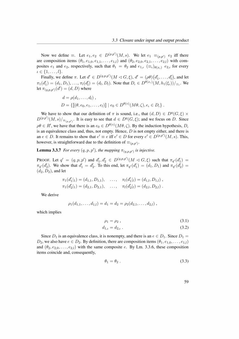
3.3 Closure under input and output product
Now we define ≡. Let e1, e2 ∈ D(p,p′)(M, s). We let e1 ≡(p,p′) e2 iff there
are composition items (θ1, e1,0, e1,1, . . . , e1,l) and (θ2, e2,0, e2,1, . . . , e2,l) with com-
posites e1 and e2, respectively, such that θ1 = θ2 and e1,ι (≡ι)θ(xι) e2,ι for every
ι ∈ 1, . . . , l.Finally, we define π. Let d′ ∈ D(q,p,p′)(M ⊳ G, ξ), d′ = (ρθ)
(d′1, . . . , d
′l
), and let
π1(d′1) = (d1, D1), . . . , πl(d
′l) = (dl, Dl). Note that Dι ∈ D
θ(xι)(M,h1(ξι))/≡ι . We
let π(q,p,p′)(d′) = (d,D) where
d = ρ(d1, . . . , dl) ,
D = J(θ, e0, e1, . . . , el)K | e0 ∈ Dθ(⋄)(Mθ, ζ), eι ∈ Dι .
We have to show that our definition of π is sound, i.e., that (d,D) ∈ Dq(G, ξ) ×D(p,p′)(M, s)/≡(p,p′)
. It is easy to see that d ∈ Dq(G, ξ); and we focus on D. Since
ρθ ∈ R′, we have that there is an e0 ∈ Dθ(⋄)(Mθ, ζ). By the induction hypothesis, Dι
is an equivalence class and, thus, not empty. Hence, D is not empty either, and there is
an e ∈ D. It remains to show that e′ ≡ e iff e′ ∈ D for every e′ ∈ D(p,p′)(M, s). This,
however, is straightforward due to the definition of ≡(p,p′).
Lemma 3.3.7 For every (q, p, p′), the mapping π(q,p,p′) is injective.
PROOF. Let q′ = (q, p, p′) and d′1, d′2 ∈ D(q,p,p′)(M ⊳ G, ξ) such that πq′(d
′1) =
πq′(d′2). We show that d′1 = d′2. To this end, let πq′(d
′1) = (d1, D1) and πq′(d
′2) =
(d2, D2), and let
π1(d′1|1) = (d1,1, D1,1), . . . , πl(d
′1|l) = (d1,l, D1,l) ,
π1(d′2|1) = (d2,1, D2,1), . . . , πl(d
′2|l) = (d2,l, D2,l) .
We derive
ρ1(d1,1, . . . , d1,l) = d1 = d2 = ρ2(d2,1, . . . , d2,l) ,
which implies
ρ1 = ρ2 , (3.1)
d1,ι = d2,ι . (3.2)
SinceD1 is an equivalence class, it is nonempty, and there is an e ∈ D1. SinceD1 =D2, we also have e ∈ D2. By definition, there are composition items (θ1, e1,0, . . . , e1,l)and (θ2, e2,0, . . . , e2,l) with the same composite e. By Lm. 3.3.6, these composition
items coincide and, consequently,
θ1 = θ2 . (3.3)
59

3 Input product for weighted synchronous context-free tree grammars
Furthermore, we obtain that D1,ι and D2,ι share an element (denoted by both e1,ι and
e2,ι). Since these sets are equivalence classes, we conclude that
D1,ι = D2,ι . (3.4)
By the induction hypothesis, (πι)q′ is injective for every q′. Thus, (3.2) and (3.4)
imply d′1|ι = d′2|ι. By (3.1) and (3.3) we obtain d′1(ε) = d′2(ε).
Lemma 3.3.8 For every (q, p, p′), the mapping π(q,p,p′) is surjective.
PROOF. Let q′ = (q, p, p′) and (d,D) ∈ Dq(G, ξ) × D(p,p′)(M, s)/≡(p,p′). We con-
struct a d′ ∈ Dq′(M ⊳ G, ξ) such that πq′(d′) = (d,D). Since D is an equiva-
lence class, it is nonempty, and there is an e ∈ D. By Lm. 3.3.6, there is a com-
position item (θ, e0, e1, . . . , el) with composite e. By Dι we denote the element of
D(pι,p′ι)(M,h1(ξι))/≡(pι,p′ι)
that contains eι, where pι and p′ι are read off from eι in
the obvious way, i.e., such that eι ∈ D(pι,p′ι)(M,h1(ξι)). By the induction hypothesis,
(πι)q′ is surjective for every q′, and there are d′1, . . . , d′l such that πι(d
′ι) = (d|ι, Dι).
We construct d′ = (d(ε)θ)(d′1, . . . , d
′l
).
We show that πq′(d′) = (d,D). To this end, let πq′(d
′) = (d′, D′). Then d = d′ is
straightforward to show, and we turn to the proof of D = D′. We observe that e ∈ D(by assumption) and e ∈ D′ (by definition). Since D and D′ are equivalence classes,
the fact that they share an element (namely, e) implies that they are equal.
Lemma 3.3.9 Let π(q,p,p′)(d′) = (d,D). Then 〈d′〉 = 〈d〉 ·
∑
e∈D〈e〉.
PROOF. There are ρ and θ such that d′(ε) = ρθ. We let π1(d′|1) = (d1, D1) up to
πl(d′|l) = (dl, Dl). Then
〈d′〉 =(∏
ι〈d′|ι〉
)· µ′(ρθ)
=(∏
ι〈dι〉 ·(∑
eι∈Dι〈eι〉
))· µ(ρ) · JMθK(ζ) (Def. µ′, induction hypothesis)
=(∏
ι〈dι〉)· µ(ρ) · JMθK(ζ) ·
∏
ι
(∑
eι∈Dι〈eι〉
)(commutativity)
= 〈d〉 ·∑
e0∈Dθ(⋄)(Mθ,ζ),e1,...,el : eι∈Dι〈e0〉 ·
∏
ι〈eι〉 (distributivity)
= 〈d〉 ·∑
e0∈Dθ(⋄)(Mθ,ζ),e1,...,el : eι∈Dι〈v′(e0)
I(v(e1), . . . , v(el))〉µM(commutativity)
= 〈d〉 ·∑
e∈D〈e〉 .
60
3.4 An Earley-like algorithm for the input product
3.4 An Earley-like algorithm for the input product
As shown in Ex. 3.3.5, the product WSCFTG M ⊳G of a WTA M and a WSCFTG Gmay contain “useless” transitions, in the sense that they do not occur in the computation
of JM ⊳ GK. In this section, we assume that M and G are in root-state form, and we
consider a strategy for enumerating the transitions ofM⊳G that attempts to avoid use-
less transitions. For this, we take inspiration from Earley’s algorithm [60] for parsing
with context-free grammars. Ultimately, this approach leads us to Alg. 3.1. Be advised
that in the worst case, when M ⊳ G does not contain useless transitions, we still have
to construct every transition.
3.4.1 Reasoning about useful transitions
It is possible to compute the set of useful transitions of M ⊳ G: for example, we
can reduce M ⊳ G, as stated in Lm. 2.4.10; then the remaining transitions are useful.
However, this procedure involves exploring the whole set of transitions of M ⊳ G,
which is exactly what we want to avoid. So we settle for an approximation, that is, we
compute a superset of the set of useful transitions. For instance, we can employ the
following simple observation.
Observation 3.4.1 If a transition (q1 · · · qk, α, q) is useful, then the states q1, . . . , qkand q are reachable.
In other words, if we want to avoid computing useless transitions, then we might focus
on transitions that only contain reachable states, which is reasonably simple.
In the remainder of this section, we will develop a more sophisticated approximation,
which is inspired by Earley’s algorithm. For this, we recall from Sec. 2.4.5 that the
notion of a reachable state is defined in terms of the existence of a certain run of M ⊳G. We introduce the concept of a base-item tree, which generalizes the concept of a
run. Roughly speaking, base-item trees incorporate the idea that, instead of treating a
transition ρθ ofM⊳G as an atomic entity, we can construct it gradually by performing
a depth-first left-to-right simulation of M on the input tree of ρ.
Example 3.4.2 (Ex. 3.3.5 contd.) Figure 3.7 shows a visualization of two base-item
trees for (q, 0). In general, a base-item tree δ for a pair (q, p) ∈ Q × P has one of
four possible shapes: either it consists only of the state q, or the pair (q, p), or it is a
complete (q, p, p′)-run of M ⊳G for some p′, or its root is labeled by a base item.
A base item represents a partial construction of a transition of M ⊳ G; and for its
description we need the WTA Mζ , which is obtained from M by adding all suitable
transitions for the variables occurring in ζ, each with weight 1. A base item consists of
61

3In
put
pro
duct
for
wei
ghte
dsy
nch
ronous
conte
xt-
free
tree
gra
mm
ars
ρ1
x2
S
〈 x1 〉
• 0
2
q ρ3
S
a x1
S
b y1 c
d
(r1r, S, 0)
(0, a, r) • 1 r
1
(f, 1)
ρ1
x2
S
〈 x1 〉
(0, x2, 0)
(r1r, S, 0)
(0, 〈, r) • 1 r
1
(q, 1) ((f, 1, 1), α3, (f, 0, 0))
(ε, α4, (f, 1, 1))
(a) (b)
Figure 3.7: Two base-item trees of Ex. 3.4.2, where the base items are visualized as boxes.
62

3.4 An Earley-like algorithm for the input product
a transition ρ ∈ R|q, a partial p-run d of Mζ on the input tree ζ of ρ, a “bullet position”
in d, and an “active index” a. Each base item is visualized as a box whose contents
are, from left to right, ρ, ζ, d, and a. The bullet position is visualized as a • in d. The
run d is of a certain shape: all positions left of the bullet are labeled by a transition; all
positions right of the bullet are labeled by a state. The active index a ranges from 0 to
rk(ρ), and if it is positive, then the bullet is directly in front of the position labeled xain ζ; here we use that every position in d is also a position in ζ.
When the root of δ is labeled by a base item for some transition (q1 · · · ql, α, q) of G,
then it has l successors δ1, . . . , δl. If the active index a is positive, then δa is a base-
item tree for (qa, pa) where pa is the state in d directly behind the bullet. If ι 6= a and
(p′, xι, p) occurs in d, then δι is a complete (qι, p, p′)-run of M ⊳G. If ι 6= a and xι is
right of the bullet, then δι is just qι.
We note that the occurrences of base items in a base-item tree form a “spine”: every
such occurrence is either at the root or a successor of another such occurrence, and then
it is the only successor that is labeled by a base item.
Now we make the concepts of Ex. 3.4.2 precise. Let ζ ∈ CΣ(m, r1, . . . , rl). Then
the WTA Mζ over Σ ∪ Xl ∪ Ym and S is obtained from M by adding the following
transitions with weight 1:
(p′, xι, p) , (1 ≤ ι ≤ l, p ∈ P , p′ ∈ P rι)
(ε, yι, p) . (1 ≤ ι ≤ m, p ∈ P )
Let d ∈ D(Mζ) be a partial run on ζ. We observe that, for every v ∈ Xl ∪ Ym, dcontains at most one transition with the terminal symbol v. If it does contain such a
transition, then we denote it by d(v). If d does not contain the respective transition,
then the notation d(v) is not defined. Accordingly, whenever we employ the notation,
we imply that the transition be contained.
In the following, when we reason about bullet positions, we will often use the lexi-
cographic order on N∗ (see Sec. 2.1.3) and denote it by ≤. Let ∆ be an alphabet and V
a set. For every tree t ∈ T∆(V ), the set bpos(t) of bullet positions of t is defined by
bpos(t) = (ε, 0), (ε, 1) ∪ (1w, j) | w ∈ pos(t), j ∈ 0, . . . , rkt(w) .
Example 3.4.3 We can imagine a bullet position (v, j) of t by means of a tree obtained
from t by putting a special root symbol ⊤ on top and inserting exactly one occurrence
of •, as illustrated in Fig. 3.8. Then v(j+1) is the position of the bullet in the modified
tree, and a position w ∈ pos(t) is left of the bullet if 1w ≤ vj.
63
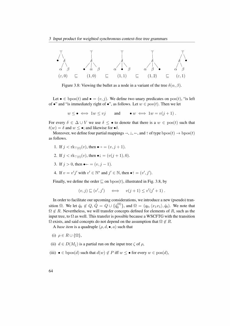
3 Input product for weighted synchronous context-free tree grammars
⊤
• δ
α β
⊤
δ
• α β
⊤
δ
α • β
⊤
δ
α β •
⊤
δ
α β
•
(ε, 0) ⊑ (1, 0) ⊑ (1, 1) ⊑ (1, 2) ⊑ (ε, 1)
Figure 3.8: Viewing the bullet as a node in a variant of the tree δ(α, β).
Let • ∈ bpos(t) and • = (v, j). We define two unary predicates on pos(t), “is left
of •” and “is immediately right of •”, as follows. Let w ∈ pos(t). Then we let
w ≤ • ⇐⇒ 1w ≤ vj and • w ⇐⇒ 1w = v(j + 1) .
For every δ ∈ ∆ ∪ V we use δ ≤ • to denote that there is a w ∈ pos(t) such that
t(w) = δ and w ≤ •; and likewise for •δ.
Moreover, we define four partial mappings , , , and of type bpos(t)→ bpos(t)as follows.
1. If j < rk⊤(t)(v), then • = (v, j + 1).
2. If j < rk⊤(t)(v), then • = (v(j + 1), 0).
3. If j > 0, then • = (v, j − 1).
4. If v = v′j′ with v′ ∈ N∗ and j′ ∈ N, then • = (v′, j′).
Finally, we define the order ⊑ on bpos(t), illustrated in Fig. 3.8, by
(v, j) ⊑ (v′, j′) ⇐⇒ v(j + 1) ≤ v′(j′ + 1) .
In order to facilitate our upcoming considerations, we introduce a new (pseudo) tran-
sition Ω. We let q0 6∈ Q, Q = Q ∪ q(0)0 , and Ω = (q0, 〈x1x1〉, q0). We note that
Ω 6∈ R. Nevertheless, we will transfer concepts defined for elements of R, such as the
input tree, to Ω as well. This transfer is possible because a WSCFTG with the transition
Ω exists, and said concepts do not depend on the assumption that Ω 6∈ R.
A base item is a quadruple (ρ, d, •, a) such that
(i) ρ ∈ R ∪ Ω,
(ii) d ∈ D(Mζ) is a partial run on the input tree ζ of ρ,
(iii) • ∈ bpos(d) such that d(w) 6∈ P iff w ≤ • for every w ∈ pos(d),
64

3.4 An Earley-like algorithm for the input product
(iv) a ∈ 0, . . . , rk(ρ) is called the active index; and if a > 0, then •xa.
We note that we abused notation in the last item. Since • ∈ bpos(d), we also have
• ∈ bpos(ζ), and we interpret •xa in that sense. We will continue to do so. By B
we denote the set of all base items. The same symbol B often denotes the Boolean
semiring, but we will not use this semiring here. We make B a ranked alphabet by
carrying over the rank from the first component of each base item. For every I and ι,we use I % ι to denote that I ∈ B, ι is the active index of I , and ι > 0.
Recall that R′ is the set of transitions of M ⊳ G. For every (q, p) ∈ Q × P the set
D(q,p) of base-item trees for (q, p) is a subset of TR′∪B(Q∪(Q×P )), defined as follows.
The family (D(q,p) | (q, p) ∈ Q × P ) is the smallest family (D(q,p) | (q, p) ∈ Q × P )such that for every (q, p) ∈ Q× P :
• if q ∈ Q, then (q, p) ∈ D(q,p),
• if q ∈ Q(m) and p′ ∈ Pm, then D(q,p,p′)co (M ⊳G) ⊆ D(q,p),
• if I ∈ B, I = (ρ, d, •, a), ρ = (q1 · · · ql, 〈ζζ′〉, q), πP (d) = p, and, for every
ι ∈ 1, . . . , l,
– if xι ≤ •, then δι ∈ D(qι,d(xι))co (M ⊳G);
– if ι = a, then δι ∈ D(qι,pι) where pι is uniquely determined by •pι,
– otherwise, δι = qι,
then I(δ1, . . . , δl) ∈ D(q,p).
3.4.2 Item syntax and semantics
Based on the concept of a base-item tree, we can now define refined versions of notions
such as “reachable” and “productive”. Instead of giving each refined notion a proper
name, we use items, i.e., syntactic representations of statements. Now we define the
syntax and semantics of these items.
We begin with a few auxiliary definitions. Let ζ ∈ CΣ(m, r1, . . . , rl) and w ∈pos(ζ). Aw-assignment θ for ζ is defined like an assignment for ζ, however, its domain
consists only of the variables that occur in ζ|w. Let d ∈ D(Mζ) be a partial run on ζ.
We say that θ and d agree if θ(v) = d(v) for every symbol v in the domain of θ.
Let ρ ∈ R and ρ = (q1 · · · ql, 〈ζζ′〉, q). Then we set Mρ = Mζ , pos(ρ) = pos(ζ),
and rkρ(w) = rkζ(w) for every w ∈ pos(ζ). An assignment for ρ is an assignment
for ζ, and likewise for w-assignments.
For every i ∈ 0, . . . , 5, we define the set Ii of items of type i as follows:
65

3 Input product for weighted synchronous context-free tree grammars
Ω x1 • 0 1
Figure 3.9: Root base item.
• I0 = (q, p) | q ∈ Q, p ∈ P,
• I1 = [q, p, p′] | ∃m : q ∈ Q(m), p ∈ P, p′ ∈ Pm,
• I2 = [ρ, w, p, θ] | ρ ∈ R,w ∈ pos(ρ), p ∈ P, θ is a w-assignment for ρ,
• I3 = [ρ, w, p] | ρ ∈ R,w ∈ pos(ρ), p ∈ P,
• I4 = [ρ, w, j, p, p′] | ρ ∈ R,w ∈ pos(ρ), rkρ(w) = k,
j ∈ 0, . . . , k, p ∈ P, p′ ∈ P k,
• I5 = (ρ, w, p) | ρ ∈ R,w ∈ pos(ρ), p ∈ P.
The set I of items is⋃
i Ii. Note that this is a disjoint union. We define the mapping
type : I→ 0, . . . , 5 such that, for every I ∈ I, type(I) is the unique i with I ∈ Ii.
We define the models relation as the smallest relation
|= ⊆ (δ, ω) | δ ∈ D(q0,p0), ω ∈ pos(δ) × I
such that for every assignment of the free variables the following statements hold:
(δ, ω) |= (q, p) if δ(ω) % ι and δ(ωι) = (q, p);
(δ, ω) |= [q, p, p′] if δ(ω) % ι and δ|ωι ∈ D(q,p,p′)co (M ⊳G);
(δ, ω) |= [ρ,w, p, θ] if δ(ω) = (ρ, d, •, 0), •w, d|w ∈ Dp(Mρ, ζ|w), and θ and d
agree;
(δ, ω) |= [ρ,w, p] if (δ, ω) |= [ρ, w, p, θ];
(δ, ω) |= [ρ,w, j, p, p′] if δ(ω) = (ρ, d, (1w, j), 0) and d(w) = (p′, ζ(w), p);
(δ, ω) |= (ρ,w, p) if δ(ω) = (ρ, d, •, 0), •w, and d(w) = p.
We denote the models relation by |=. An item I is valid if (δ, ω) |= I for some δ and ω;
and it is invalid if it is not valid.
66

3.4 An Earley-like algorithm for the input product
Example 3.4.4 (Ex. 3.4.2 contd.) Let δ1 and δ2 be obtained from the base-item trees
shown in Fig. 3.7 (a) and (b), respectively, by putting the base item from Fig. 3.9 on
top. Then we have, e.g.,
(δ1, 12) |= [ρ3, ε, 1, 0, r1r] , (δ2, 1) |= [ρ1, 1, 1, 0, r1r] ,
(δ1, 12) |= [ρ3, 1, r, ∅] , (δ2, 1) |= [ρ1, 11, r, ∅] ,
(δ1, 12) |= [ρ3, 1, r] , (δ2, 1) |= [ρ1, 11, r] ,
(δ1, 12) |= (ρ3, 2, 1) , (δ2, 1) |= (ρ1, 12, 1) ,
(δ1, 12) |= (f, 1) , (δ2, 1) |= (q, 1) .
We compare our refined notion of reachability with the classical one; more specifically,
we compare the two statements
(a) the item (q, 1) is valid and (b) the state (q, 1) is reachable .
The statements are true because (a) (δ2, 1) |= (q, 1) and (b) ρ′1((q, 1), (f, 0, 0)) ∈D(q,0)(M ⊳ G), where ρ′1 is the transition that stems from ρ1 via the obvious state
augmentation. In δ2, we do not yet see whether the base item for ρ1 can be extended
to a transition such as ρ′1. In this sense, (a) is a weaker statement than (b). On the
other hand, we see in δ2 that the state for x2 is productive. In this sense, (a) is stronger
than (b).
We observe that both the set D(q0,p0) and the set D(q0,p0)(M ⊳G) can be viewed as
superset approximations of D(q0,p0)co (M ⊳G) – albeit with different degrees of sophis-
tication. Hence, we can transfer Obs. 3.4.1 to our new setting, as follows.
Lemma 3.4.5 If a transition ρθ of M ⊳G is useful, then [ρ, ε, θ(⋄), θ′] is valid, where
θ′ is obtained from θ by removing ⋄ from its domain.
PROOF. Let ρθ be a useful transition of M ⊳G. Then there are d′ ∈ D(q0,p0)co (M ⊳G)
and ω ∈ pos(d′) such that d′(ω) = ρθ. We will construct a δ such that (δ, 1ω) |=[ρ, ε, θ(⋄), θ′]. For this, we “prune” d′, removing parts that are not licensed by the
definition of a base-item tree.
To this end, let ω = (ω1, . . . , ωn), ρ1, . . . , ρn+1 ∈ R, and θ1, . . . , θn+1 state as-
signments such that ρjθj = d′(ω1 · · ·ωj−1). Then there are d1, . . . , dn+1 such that
dj ∈ Dθj(⋄)(Mθj , ζj) where ζj is the input tree of ρj . We define trees δ1, . . . , δn+1 in-
ductively. To this end, let j ∈ 1, . . . , n+1 and ρj = (q1 · · · ql, 〈ζζ′〉, q). If j = n+1,
then we let
δj = (ρj , dj , (ε, 1), 0)(d′|ω1, . . . , d
′|ωl)
.
67

3 Input product for weighted synchronous context-free tree grammars
Otherwise, we let w = (w1, . . . , wm) be the position in ζ labeled xωj, and we define
trees d1, . . . , dm+1 inductively. For this, let ∈ 1, . . . ,m+1 and dj(w1 · · ·wj−1) =
(p1 · · · pk, σ, p). If = m+ 1, then we let d = p. Otherwise, we let
d = (p1 · · · pk, σ, p)(d′1, . . . , d
′k
),
where d′j′ = dj |w1···w−1j′ if j′ < w, it is d+1 if j′ = , and it is pj′ otherwise. Now
we let
δj = (ρj , d1, •, ωj)(δ′1, . . . , δ
′l
),
where
• the bullet position • is determined by •w, and
• δ′ι is d′|ω1···ωj−1ι if xι occurs in ζ strictly left of xωj, it is δj+1 if ι = ωj , and it is
qι otherwise.
We let δ = (Ω, p0, (ε, 0), 1)(δ1). We omit the proof of (δ, 1ω) |= [ρ, ε, θ(⋄), θ′].
3.4.3 Algorithm
Lemma 3.4.5 implies that, when we compute every valid item of the form [ρ, ε, p, θ],then we can read off a superset of the useful transitions of M ⊳ G. This is the basic
approach of our algorithm, Alg. 3.1.
The algorithm proceeds in two steps. In the first step (Lines 1–4), it computes the set
of all valid items by means of the deductive system shown in Fig. 3.10. As usual, the
deductive system consists of inference rules, each one being a syntactic representation
of a conditional implication [89, 142]. Since there are only finitely many items, this
process will terminate. Roughly speaking, the items drive a depth-first left-to-right
simulation of M on the input trees of transitions of G. Items with round brackets are
responsible for top-down traversal, and items with square brackets are responsible for
horizontal and bottom-up traversal. In the second step (Lines 5–9), we use the items to
construct transitions of M ⊳G, together with their weights.
Example 3.4.6 (Ex. 3.3.1 contd.) We demonstrate the inference rules of Fig. 3.10 by
showing the generation of items for the transition ρ3 of G. In Fig. 3.11 we show the in-
put tree ζ of ρ3 in bold-face letters and lines. On top of this syntactic structure, we have
drawn another graph, consisting of items and arrows. Close to every position w of ζ,
we have placed those items that involve w. The arrows show the dependencies between
the items as they are expressed by the rules of the deduction schema. Finally, we note
68

3.4 An Earley-like algorithm for the input product
(1)(q0, p0)
(2)(q, p)
(ρ, ε, p)
(3)(q, p) [ρ, ε, p, θ]
[q, p, p′]
p′ = (θ(y1), . . . , θ(ym))
(4)(ρ, w, p)
[ρ, w, 0, p, p′]
(p′, ζ(w), p) ∈ R(rkζ(w))M
(5)[ρ, w, j, p, (p1, . . . , pk)]
(ρ, w(j + 1), pj+1)
0 ≤ j < k
(6)[ρ, w, j, p, (p1, . . . , pk)] [ρ, w(j + 1), pj+1]
[ρ, w, j + 1, p, (p1, . . . , pk)]
0 ≤ j < k
(7)[ρ, w, p, θ]
[ρ, w, p]
(8)(ρ, w, p)
(qι, p)
ζ(w) = xι
(9)(ρ, w, p) [qι, p, p
′]
[ρ, w, 0, p, p′]
ζ(w) = xι
(10)(ρ, w, p)
[ρ, w, p, yι 7→ p]
ζ(w) = yι
(11)
[ρ, w, k, p, p′][ρ, w1, p1, θ1]· · · [ρ, wk, pk, θk]
[ρ, w, p, θ ∪ θ1 ∪ · · · ∪ θk]
p′ = (p1, . . . , pk)
where θ = ζ(w) 7→ (p, p′) if ζ(w) ∈ X , and
θ = ∅ otherwise
Note: we assume that ρ ∈ R, ρ = (q1 · · · ql, 〈ζζ′〉, q), and q ∈ Q(m).
Figure 3.10: Deductive parsing schema for the input product.
69
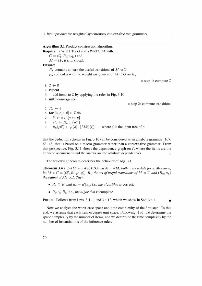
3 Input product for weighted synchronous context-free tree grammars
Algorithm 3.1 Product construction algorithm.
Require: a WSCFTG G and a WRTG M with
G = (Q,R, µ, q0) and
M = (P,RM , µM , p0),Ensure:
Ru contains at least the useful transitions of M ⊳G,
µu coincides with the weight assignment of M ⊳G on Ru
⊲ step 1: compute I1: I ← ∅2: repeat
3: add items to I by applying the rules in Fig. 3.10
4: until convergence
⊲ step 2: compute transitions
5: Ru ← ∅6: for [ρ, ε, p, θ] ∈ I do
7: θ′ ← θ ∪ ⋄ 7→ p8: Ru ← Ru ∪ ρθ
′9: µu(ρθ
′)← µ(ρ) · JMθ′K(ζ) where ζ is the input tree of ρ
that the deduction schema in Fig. 3.10 can be considered as an attribute grammar [107,
63, 48] that is based on a macro grammar rather than a context-free grammar. From
this perspective, Fig. 3.11 shows the dependency graph on ζ, where the items are the
attribute occurrences and the arrows are the attribute dependencies.
The following theorem describes the behavior of Alg. 3.1.
Theorem 3.4.7 LetG be a WSCFTG andM a WTA, both in root-state form. Moreover,
let M ⊳G = (Q′, R′, µ′, q′0), RU the set of useful transitions of M ⊳G, and (Ru, µu)the output of Alg. 3.1. Then
• Ru ⊆ R′ and µu = µ′|Ru , i.e., the algorithm is correct;
• RU ⊆ Ru, i.e., the algorithm is complete.
PROOF. Follows from Lms. 3.4.11 and 3.4.12, which we show in Sec. 3.4.4.
Now we analyze the worst-case space and time complexity of the first step. To this
end, we assume that each item occupies unit space. Following [136] we determine the
space complexity by the number of items, and we determine the time complexity by the
number of instantiations of the inference rules.
70
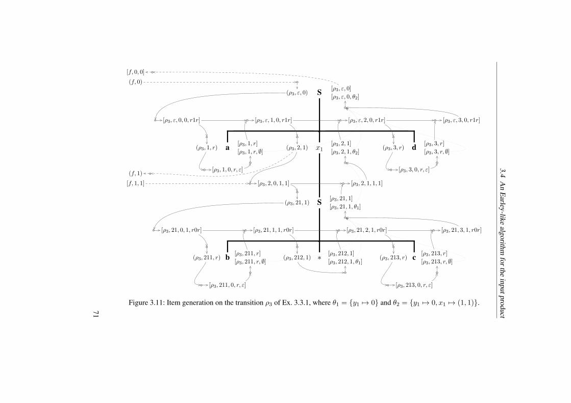
3.4
An
Earley
-like
algorith
mfo
rth
ein
put
pro
duct
(ρ3, ε, 0) S[ρ3, ε, 0]
[ρ3, ε, 0, θ2]
(ρ3, 1, r) a[ρ3, 1, r]
[ρ3, 1, r, ∅](ρ3, 2, 1) x1
[ρ3, 2, 1]
[ρ3, 2, 1, θ2](ρ3, 3, r) d
[ρ3, 3, r]
[ρ3, 3, r, ∅]
(ρ3, 21, 1) S[ρ3, 21, 1]
[ρ3, 21, 1, θ1]
(ρ3, 211, r) b[ρ3, 211, r]
[ρ3, 211, r, ∅](ρ3, 212, 1) ∗
[ρ3, 212, 1]
[ρ3, 212, 1, θ1](ρ3, 213, r) c
[ρ3, 213, r]
[ρ3, 213, r, ∅]
[ρ3, ε, 0, 0, r1r] [ρ3, ε, 1, 0, r1r] [ρ3, ε, 2, 0, r1r] [ρ3, ε, 3, 0, r1r]
[ρ3, 1, 0, r, ε]
[ρ3, 2, 0, 1, 1] [ρ3, 2, 1, 1, 1]
[ρ3, 3, 0, r, ε]
[ρ3, 21, 0, 1, r0r] [ρ3, 21, 1, 1, r0r] [ρ3, 21, 2, 1, r0r] [ρ3, 21, 3, 1, r0r]
[ρ3, 211, 0, r, ε] [ρ3, 213, 0, r, ε]
[f, 1, 1]
(f, 1)
[f, 0, 0]
(f, 0)
Figure 3.11: Item generation on the transition ρ3 of Ex. 3.3.1, where θ1 = y1 7→ 0 and θ2 = y1 7→ 0, x1 7→ (1, 1).
71

3 Input product for weighted synchronous context-free tree grammars
In our case, the space complexity is either dominated by I2 or I4, and we have |I2| ∈O(|G|in ·|P |
C)
and |I4| ∈ O(|G|in ·|RM |
). Here, the factor |G|in denotes the input size
of G, defined by∑
ρ∈R |pos(ζ(ρ))|, where ζ(ρ) is the input tree of ρ. It captures the
components ρ and w (ρ, w, and j, respectively) in said items, which together identify
exactly one node of an input tree of G. The factor |RM | captures the components pand p1 · · · pk. Finally, the factor |P |C captures p and θ, where C is given at the end of
Sec. 3.3.2.
In the worst case, which is what we consider here, the algorithm obviously uses more
space than the resulting M ⊳G. The reason is that we need extra space to manage the
depth-first left-to-right traversal. It is our hope, however, that this traversal pays off in
the average case, and that a lot of useless rules can be avoided.
The time complexity is dominated by Rule 12; so it is in O(|G|in · |RM | · |P |C),
where |P |C captures the union θ ∪ θ1 ∪ · · · ∪ θk, which is disjoint, because the input
tree of any rule is linear in X ∪ Y .
3.4.4 Correctness and completeness
In this section, we show that Alg. 3.1 is correct and complete. We follow a top-down ap-
proach, that is, we prove higher-level statements first and auxiliary statements second.
Formally, we view the deductive system as a relation
R ⊆ I∗ × I .
Figure 3.10 specifies this relation in terse form, and it translates into
R = (ε, (q0, p0)) ∪ ((q, p), (ρ, ε, p)) | ρ ∈ R|q, q ∈ Q, p ∈ P ∪ . . .
We define the mapping F : P(I)→ P(I) such that, for every I ⊆ I, F(I) is the set of
all items that can be generated by applying inference rules to items in I, i.e.,
F(I) = I | ∃n ∈ N, I1, . . . , In ∈ I : (I1 · · · In, I) ∈ R .
Then the set I after Line 4 of Alg. 3.1 is the set⋃
iFi(∅). We show that the deductive
system is correct and complete; that is, we show the following theorem.
Theorem 3.4.8 Let I⋆ ⊆ I be the set of all valid items, and I ⊆ I be the set of items
computed in Alg. 3.1, i.e., I =⋃
iFi(∅). Then
• I ⊆ I⋆, i.e., the deductive system is correct; and
• I⋆ ⊆ I, i.e., the deductive system is complete.
72

3.4 An Earley-like algorithm for the input product
PROOF. Correctness (by contradiction): assume that⋃
iFi(∅) contains an invalid item.
Then there is a minimal i such that F i(∅) contains an invalid item. Let I be such an
item. If i = 0, then I ∈ ∅, which is a contradiction. Thus i > 0. Then there are n ∈ N
and I1, . . . , In ∈ Fi−1(∅) such that (I1 · · · In, I) ∈ R. Assume for the time being that
I1, . . . , In ∈ I⋆. By Lm. 3.4.9, also I ∈ I⋆, which is a contradiction. Hence, there is
a j such that Ij is invalid. But Ij ∈ Fi−1(∅), and thus i is not minimal, which is our
final contradiction.
Completeness (by contradiction): assume that I⋆ \ I is not empty. Then the set
C = (I, δ, ω) | (δ, ω) |= I, I 6∈ I
is not empty. Let ⊑ be the well-founded order postulated in Lm. 3.4.10. Since C 6=∅, this set has a minimal element with respect to ⊑, say (I, δ, ω). By said lemma,
there are (I1, δ1, ω1), . . . , (In, δn, ωn) such that (I1 · · · In, I) ∈ R, (δj , ωj) |= Ij , and
(Ij , δj , ωj) ⊑ (I, δ, ω). Assume for the time being that I1, . . . , In ∈ I. Then there
is an i such that I1, . . . , In ∈ Fi(∅). Since (I1 · · · In, I) ∈ R, I ∈ F i+1(∅), and
thus I ∈ I, which contradicts our assumption that (I, δ, ω) ∈ C. Hence, there is a jsuch that Ij 6∈ I. It is easy to see from the definition of R that Ij 6= I , and thus
(Ij , δj , ωj) 6= (I, δ, ω). But then (Ij , δj , ωj) is strictly smaller than (I, δ, ω), which
contradicts our assumption that (I, δ, ω) is minimal.
Lemma 3.4.9 Let (I1 · · · In, I) ∈ R, and let (δ1, ω1) |= I1, . . . , (δn, ωn) |= In. Then
there is a pair (δ, ω) such that (δ, ω) |= I .
Instead of a full proof, we only consider how to construct (δ, ω). To this end, we use
a terse notation, like in the deductive system itself. The construction is shown in Figs.
3.12 and 3.13. We employ the following auxiliary definitions.
Let ρ ∈ R, ρ = (q1 · · · ql, 〈ζζ′〉, q), δ1 ∈
⋃
pD(q,p), δ1(ε) = (ρ, d, •, 0), w ∈ pos(d),
•w, p ∈ P , and d(w) = p.
− Let r ∈ R(rkζ(w))M , r = (p′, ζ(w), p), and p′ = (p1, . . . , pk). We write (δ1, r)
(4)−−→ δ
to indicate that
δ = (ρ, d[r(p1, . . . , pk)]w, •, 0)(δ1|1, . . . , δ1|l
).
− Let δ2 ∈⋃
pD(q,p), δ2(ε) = (ρ, d2, •, 0), and d2|w ∈ Dp(Mρ, ζ|w). Then
(δ1, δ2)(6)−−→ δ means
δ = (ρ, d[d2|w]w, •, 0)(δ′1, . . . , δ
′l
),
where δ′ι is δ1|ι if xι does not occur in ζ|w; otherwise δ′ι is δ2|ι.
73

3 Input product for weighted synchronous context-free tree grammars
(1)((Ω, p0, (ε, 0), 1)
((q0, p0)
), ε) |= (q0, p0)
(2)(δ1, ω1) |= (q, p)
(δ1[(ρ, p, (ε, 0), 0)(q1, . . . , ql
)]ω1ι, ω1ι) |= (ρ, ε, p)
δ1(ω1) % ι
(4)(δ1, ω1) |= (ρ, w, p)
(δ1[δ]ω1 , ω1) |= [ρ, w, 0, p, p′]
r = (p′, ζ(w), p) r ∈ R(rkζ(w))M
(δ1|ω1 , r)(4)−−→ δ
(5)(δ1, ω1) |= [ρ, w, j, p, (p1, . . . , pk)]
(δ1, ω1) |= (ρ, w(j + 1), pj+1)
0 ≤ j < k
(7)(δ1, ω1) |= [ρ, w, p, θ]
(δ1, ω1) |= [ρ, w, p]
(8)(δ1, ω1) |= (ρ, w, p)
(δ1[δ]ω1 , ω1) |= (qι, p)
ζ(w) = xι δ1|ω1
(8)−−→ δ
(10)(δ1, ω1) |= (ρ, w, p)
(δ1[δ]ω1 , ω1) |= [ρ, w, p, yι 7→ p]
ζ(w) = yι
δ1|ω1
(10)−−→ δ
Note: we assume that ρ ∈ R, ρ = (q1 · · · ql, 〈ζζ′〉, q), and q ∈ Q(m).
Figure 3.12: Construction for Lm. 3.4.9 (continued in Fig. 3.13).
74

3.4
An
Earley
-like
algorith
mfo
rth
ein
put
pro
duct
(3)(δ1, ω1) |= (q, p) (δ2, ω2) |= [ρ, ε, p, θ′]
(δ1[(ρθ)(δ2|ω21, . . . , δ2|ω2l
)]ω1ι, ω1) |= [q, p, p′]
p′ = (θ′(y1), . . . , θ
′(ym))δ1(ω1) % ι θ = θ′ ∪ ⋄ 7→ p
(6)(δ1, ω1) |= [ρ, w, j, p, (p1, . . . , pk)] (δ2, ω2) |= [ρ, w(j + 1), pj+1]
(δ1[δ]ω1 , ω1) |= [ρ, w, j + 1, p, (p1, . . . , pk)]
0 ≤ j < k
(δ1|ω1 , δ2|ω2)(6)−−→ δ
(9)(δ1, ω1) |= (ρ, w, p) (δ2, ω2) |= [qι, p, p
′]
(δ1[δ]ω1 , ω1) |= [ρ, w, 0, p, p′]
ζ(w) = xι δ2(ω2) % ι′
(δ1|ω1 , δ2|ω2ι′)(9)−−→ δ
(11)
(δ′, ω′) |= [ρ, w, k, p, p1 · · · pk](δ1, ω1) |= [ρ, w1, p1, θ1]· · · (δk, ωk) |= [ρ, wk, pk, θk]
(δ′[δ]ω′ , ω′) |= [ρ, w, p, θ ∪ θ1 ∪ · · · ∪ θk]
p′ = (p1, . . . , pk)
(δ1|ω1 , . . . , δk|ωk, δ′|ω′)
(11)−−→ δ
where θ is defined as in Fig. 3.10.
Note: we assume that ρ ∈ R, ρ = (q1 · · · ql, 〈ζζ′〉, q), and q ∈ Q(m).
Figure 3.13: Continuation of Fig. 3.12.
75

3 Input product for weighted synchronous context-free tree grammars
− Let ζ(w) = xa. Then δ1(8)−−→ δ means
δ = (ρ, d, •, a)(δ′1, . . . , δ
′l
),
where δ′ι is δ1|ι if ι 6= a, and δ′a is (qa, p).
− Let ζ(w) = xι, qι ∈ Q(m), p′ ∈ Pm, δ2 ∈ D
(qι,p,p′)co (M⊳G), and p′ = (p1, . . . , pm).
Then (δ1, δ2)(9)−−→ δ shall mean
δ = (ρ, d[(p′, xι, p)(p1, . . . , pm
)]w, •, 0)
(δ′1, . . . , δ
′l
),
where δ′ι′ is δ1|ι′ if ι′ 6= ι, and δ′ι′ is δ2 otherwise.
− Let ζ(w) = yι. Then δ1(10)−−→ δ means
δ = (ρ, d[(ε, yι, d(w))]w, •, 0)(δ1|1, . . . , δ1|l
).
− Let r = (p′, ζ(w), p), p′ ∈ P (rkζ(w)), p′ = (p1, . . . , pk), δ1, . . . , δk, δ′ ∈
⋃
pD(q,p),
δ1(ε) = (ρ, d1, •1, 0), . . . , δk(ε) = (ρ, dk, •k, 0), δ′(ε) = (ρ, d, •k, 0), w ∈ pos(d),
d(w) = r, •j = (1w, j), and dj |wj ∈ Dpj (Mρ, ζ|wj). Then (δ1, . . . , δk, δ′)
(11)−−→ δ
means
δ = (ρ, d[r(d1|w1, . . . , dk|wk)]w, •k, 0)(δ′1, . . . , δ
′l) ,
where δ′ι is δ|ι if xι does not occur in ζ|w; otherwise δ′ι is δj |ι where j is the unique
integer such that xι occurs in ζ|wj .This finishes our proof sketch for Lm. 3.4.9. Now we turn to the lemma that we use
to prove completeness of the deductive system. To this end, we define I′ = (I, δ, ω) |
I ∈ I, δ ∈ D(q0,p0), ω ∈ pos(δ).
Lemma 3.4.10 There is a well-founded order ⊑ on I′ such that the following holds.
Let (δ, ω) |= I . Then there are (I1, δ1, ω1), . . . , (In, δn, ωn) ∈ I′ such that
• (I1 · · · In, I) ∈ R,
• (δj , ωj) |= Ij , and
• (Ij , δj , ωj) ⊑ (I, δ, ω).
Again, we will not provide a full proof, but the definition for ⊑ and the construction of
(I1, δ1, ω1), . . . , (In, δn, ωn).First we define the order ⊑. As intermediate steps, we will define an order on
⋃
(q,p)D(q,p) and one on B as well. As a basis, we will refer back to the order ⊑ on
76
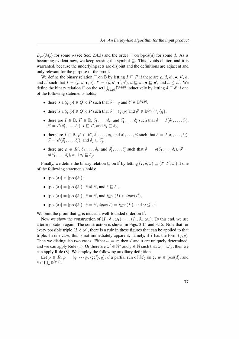
3.4 An Earley-like algorithm for the input product
Dpr(Mρ) for some ρ (see Sec. 2.4.3) and the order ⊑ on bpos(d) for some d. As is
becoming evident now, we keep reusing the symbol ⊑. This avoids clutter, and it is
warranted, because the underlying sets are disjoint and the definitions are adjacent and
only relevant for the purpose of the proof.
We define the binary relation ⊑ on B by letting I ⊑ I ′ if there are ρ, d, d′, •, •′, a,
and a′ such that I = (ρ, d, •, a), I ′ = (ρ, d′, •′, a′), d ⊑ d′, • ⊑ •′, and a ≤ a′. We
define the binary relation ⊑ on the set⋃
(q,p)D(q,p) inductively by letting δ ⊑ δ′ if one
of the following statements holds:
• there is a (q, p) ∈ Q× P such that δ = q and δ′ ∈ D(q,p),
• there is a (q, p) ∈ Q× P such that δ = (q, p) and δ′ ∈ D(q,p) \ q,
• there are I ∈ B, I ′ ∈ B, δ1, . . . , δl, and δ′1, . . . , δ′l such that δ = I(δ1, . . . , δl),
δ′ = I ′(δ′1, . . . , δ′l), I ⊑ I
′, and δj ⊑ δ′j ,
• there are I ∈ B, ρ′ ∈ R′, δ1, . . . , δl, and δ′1, . . . , δ′l such that δ = I(δ1, . . . , δl),
δ′ = ρ′(δ′1, . . . , δ′l), and δj ⊑ δ
′j ,
• there are ρ ∈ R′, δ1, . . . , δl, and δ′1, . . . , δ′l such that δ = ρ(δ1, . . . , δl), δ
′ =ρ(δ′1, . . . , δ
′l), and δj ⊑ δ
′j .
Finally, we define the binary relation ⊑ on I′ by letting (I, δ, ω) ⊑ (I ′, δ′, ω′) if one
of the following statements holds:
• |pos(δ)| < |pos(δ′)|,
• |pos(δ)| = |pos(δ′)|, δ 6= δ′, and δ ⊑ δ′,
• |pos(δ)| = |pos(δ′)|, δ = δ′, and type(I) < type(I ′),
• |pos(δ)| = |pos(δ′)|, δ = δ′, type(I) = type(I ′), and ω ≤ ω′.
We omit the proof that ⊑ is indeed a well-founded order on I′.
Now we show the construction of (I1, δ1, ω1), . . . , (In, δn, ωn). To this end, we use
a terse notation again. The construction is shown in Figs. 3.14 and 3.15. Note that for
every possible triple (I, δ, ω), there is a rule in these figures that can be applied to that
triple. In one case, this is not immediately apparent, namely, if I has the form (q, p).Then we distinguish two cases. Either ω = ε; then I and δ are uniquely determined,
and we can apply Rule (1). Or there are ω′ ∈ N∗ and j ∈ N such that ω = ω′j; then we
can apply Rule (8). We employ the following auxiliary definition.
Let ρ ∈ R, ρ = (q1 · · · ql, 〈ζζ′〉, q), d a partial run of Mζ on ζ, w ∈ pos(d), and
δ ∈⋃
pD(q,p).
77
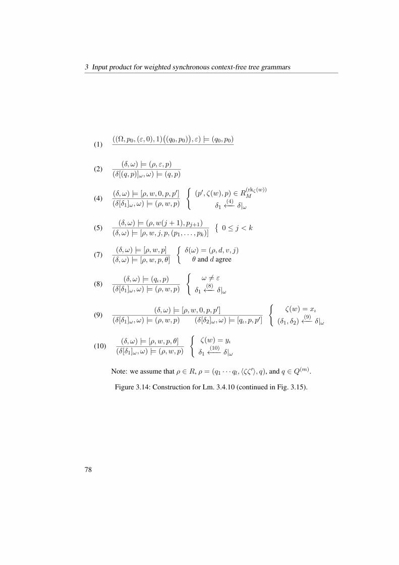
3 Input product for weighted synchronous context-free tree grammars
(1)((Ω, p0, (ε, 0), 1)
((q0, p0)
), ε) |= (q0, p0)
(2)(δ, ω) |= (ρ, ε, p)
(δ[(q, p)]ω, ω) |= (q, p)
(4)(δ, ω) |= [ρ, w, 0, p, p′]
(δ[δ1]ω, ω) |= (ρ, w, p)
(p′, ζ(w), p) ∈ R(rkζ(w))M
δ1(4)←−− δ|ω
(5)(δ, ω) |= (ρ, w(j + 1), pj+1)
(δ, ω) |= [ρ, w, j, p, (p1, . . . , pk)]
0 ≤ j < k
(7)(δ, ω) |= [ρ, w, p]
(δ, ω) |= [ρ, w, p, θ]
δ(ω) = (ρ, d, v, j)θ and d agree
(8)(δ, ω) |= (qι, p)
(δ[δ1]ω, ω) |= (ρ, w, p)
ω 6= ε
δ1(8)←−− δ|ω
(9)(δ, ω) |= [ρ, w, 0, p, p′]
(δ[δ1]ω, ω) |= (ρ, w, p) (δ[δ2]ω, ω) |= [qι, p, p′]
ζ(w) = xι
(δ1, δ2)(9)←−− δ|ω
(10)(δ, ω) |= [ρ, w, p, θ]
(δ[δ1]ω, ω) |= (ρ, w, p)
ζ(w) = yι
δ1(10)←−− δ|ω
Note: we assume that ρ ∈ R, ρ = (q1 · · · ql, 〈ζζ′〉, q), and q ∈ Q(m).
Figure 3.14: Construction for Lm. 3.4.10 (continued in Fig. 3.15).
78

3.4
An
Earley
-like
algorith
mfo
rth
ein
put
pro
duct
(3)(δ, ω) |= [q, p, p′]
(δ[(q, p)]ωι, ω) |= (q, p) (δ[(ρ, d, ε, 1)(δ|ω1, . . . , δ|ωl
)]ω, ω) |= [ρ, ε, p, θ]
δ(ω) % ι ρθ′ = δ(ωι)
d ∈ Dθ′(⋄)(Mθ′, ζ)θ and d agree
(6)(δ, ω) |= [ρ, w, j, p, (p1, . . . , pk)]
(δ[δ1]ω, ω) |= [ρ, w, j − 1, p, (p1, . . . , pk)] (δ, ω) |= [ρ, wj, pj ]
0 < j ≤ k
δ1(6)←−− δ|ω
(11)(δ, ω) |= [ρ, w, p, θ]
(δ[δk]ω, ω) |= [ρ, w, k, p, p′](δ[δ1]ω, ω) |= [ρ, w1, p1, θ|w1]· · · (δ[δk]ω, ω) |= [ρ, wk, pk, θ|wk]
(δ1, . . . , δk, p′)
(11)←−− δ|ω
p′ = (p1, . . . , pk)
where θ|wj is θ restricted to the variables occurring in ζ|wj
Note: we assume that ρ ∈ R, ρ = (q1 · · · ql, 〈ζζ′〉, q), and q ∈ Q(m).
Figure 3.15: Continuation of Fig. 3.14.
79

3 Input product for weighted synchronous context-free tree grammars
− Let δ(ε) = (ρ, d, •, 0) and •w. When we write δ1(4)←−− δ, we mean that
δ1 = (ρ, d[πP (d|w)]w, •, 0)(δ|1, . . . , δ|l
).
− Let δ(ε) = (ρ, d, •, 0), •w, p ∈ P , and d|w ∈ Dp(Mρ, ζ|w). When we write
δ1(6)←−− δ, we mean
δ1 = (ρ, d[p]w, •, 0)(δ′1, . . . , δ
′l
),
where δ′ι is δ1|ι if xι does not occur in ζ|w, and δ′ι is qι otherwise.
− Let δ(ε) = (ρ, d, •, a) and a > 0. Then δ1(8)←−− δ means
δ1 = (ρ, d, •, 0)(δ′1, . . . , δ
′l) ,
where δ′ι is δ1|ι if ι 6= a, and δ′a = qa.
− Let δ(ε) = (ρ, d, •, 0), •w, and d(w) = (p′, xa, p). By (δ1, δ2)(9)←−− δ, we mean
δ1 = (ρ, d[p]w, •, 0)(δ′1, . . . , δ
′l
),
δ2 = (ρ, d[p]w, •, a)(δ|1, . . . , δ|l
),
where δ′ι is δ1|ι if ι 6= a, and δ′a = qa.
− Let δ(ε) = (ρ, d, •, 0), •w, and d(w) = (ε, yι, p). By δ1(10)←−− δ, we mean
δ1 = (ρ, d[p]w, •, 0)(δ|1, . . . , δ|l
).
− Let δ(ε) = (ρ, d, •, 0), •w, and d(w) = (p1 · · · pk, ζ(w), p). Let w1, . . . , wl be the
positions in ζ labeled x1, . . . , xl, respectively. By (δ1, . . . , δk, p′)
(11)←−− δ, we mean
p′ = (p1, . . . , pk) ,
δj = (ρ, dj , (1w, j), 0)(δ′j1, . . . , δ
′jl
),
where
• dk = d and dj−1 = dj [pj ]wj ,
• δ′jι is δ|ι if wι ≤ wj, and δ′jι is qι otherwise.
This finishes our proof sketch for Lm. 3.4.10.
Next we show that Alg. 3.1 is correct.
80

3.5 Conclusion, discussion, and outlook
Lemma 3.4.11 LetM⊳G = (Q′, R′, µ′, q′0) and (Ru, µu) the output of Alg. 3.1. Then
Ru ⊆ R′ and µu = µ′|Ru .
PROOF. Let ρ′ ∈ Ru. By Line 8, there are ρ ∈ R, an ε-assignment θ for ρ, and a p ∈ Psuch that [ρ, ε, p, θ] ∈ I, and ρ′ = ρθ′ with θ′ = θ ∪ ⋄ 7→ p. It remains to show
that ζ ∈ L(Mθ′), where ζ is the input tree of ρ, and that µu(ρ′) = µ′(ρ′). The latter is
trivial because of Line 9 of the algorithm. We focus on the former.
By Thm. 3.4.8, we have that there is a pair (δ, ω) such that (δ, ω) |= [ρ, ε, p, θ]. That
is, there is a d such that δ(ω) = (ρ, d, ε, 1), d ∈ Dp(Mρ, ζ), and θ and d agree. It is
easy to see that then d ∈ Dp(Mθ′, ζ).
Now we show that the algorithm is complete.
Lemma 3.4.12 Let RU be the set of useful transitions of M ⊳ G and (Ru, µu) the
output of Alg. 3.1. Then RU ⊆ Ru.
PROOF. This lemma is a direct consequence of Lm. 3.4.5, Thm. 3.4.8, and Line 8 of
the algorithm.
3.5 Conclusion, discussion, and outlook
We have defined WSCFTGs, we have shown that the class of meanings of WSCFTGs is
closed under input and output product with recognizable weighted tree languages, and
we have considered an Earley-like algorithm for computing the corresponding product
WSCFTG.
Originally, context-free tree grammars (CFTGs) have been defined in [160, 67, 68],
and from that perspective, our WSCFTGs are simple; which refers to the require-
ment that each of the variables y1, . . . , ym shall occur exactly once in every tree in
CΣ(m, r1, . . . , rl). Synchronous CFTGs have already been defined in [146], with the
same requirement. Our definition is inspired by [30, Def. 1].
In view of [102], we might call a WSCFTG whose states have at most rank 1 a
weighted synchronous (non-strict) tree-adjoining grammar. Likewise, if the states have
at most rank 0, we may speak of a weighted synchronous tree-substitution grammar.
Since our product construction does not alter the maximal rank of the states, the closure
result also holds for the restricted classes.
As mentioned at the very top, this chapter is a considerably expanded and revised
version of [33, 32]. In particular, the proofs in these papers are very sketchy and ar-
guably faulty. In the case of Thm. 3.3.3, a corresponding theorem is proved in [33,
Sec. 6.2] in the spirit of Lm. 3.3.2, i.e., using a bijection π and an equivalence relation
81
3 Input product for weighted synchronous context-free tree grammars
≡. However, these objects are defined in a way that does not lend itself to a rigorous
proof, and correspondingly, the proof is very heavy-handed. In this chapter, the key to
the proof of Lm. 3.3.2 is the recursive definition of these objects on the one hand and
Lm. 3.3.6 on the other, which in turn rests on the seemingly simple Obs. 3.2.2.
In the case of Thm. 3.4.7, the proof idea that we used in this chapter is already
present in [33, Sec. 8], using a precursor of our base-item tree, dubbed a partial enriched
derivation. This precursor lacks the pseudo-rule Ω, the bullet position, and the active
index; and the concept of a partial run is only approximated. With these shortcomings,
it is not possible to prove the deductive system sound nor complete; for instance, the
item (q, p) should not mean that R|q is nonempty, but according to [33, Sec. 8] it does.
It should be noted that, in both cases, the proof ideas in [33] are in fact adequate and
the proofs actually quite convincing; this just underscores the obstacles that lie between
an adequate, convincing proof idea and its implementation.
We note that our closure result, when combined with the result of [132], yields clo-
sure under input product and output product with regular weighted string languages.
This combined result is even effective, but most likely inefficient. Consequently, a pos-
sible future contribution might be an algorithm specifically tailored to the input product
with a regular weighted string language. To the author’s knowledge, such an algorithm
has not yet been considered, for existing contributions only consider special cases [178,
141, 149, 52].
One might also explore the possibility of variable-deleting WSCFTGs, i.e., where a
variable xj can be omitted in the input or output tree of a transition. The STSGs of [62]
permit this kind of variable deletion.
Furthermore, it might be interesting to consider alternative approaches to computing
the product WSCFTG. For instance, particularly ifM is bu-det, one might exploreM⊳G bottom-up, as in a productivity analysis. In addition, one could incorporate pruning.
Roughly speaking, pruning amounts to partitioning the set of items and imposing a
bound on the size of each block. Such a technique has already been presented in [39]
for the cube-pruning algorithm.
82

4 Generic binarization of weighted
grammars
This chapter is a greatly expanded version of [29].
4.1 Introduction
In natural-language processing and statistical machine translation (SMT), the tasks of
parsing and decoding play an important role. Both tasks can be described conveniently
using intersection-like operations, e.g., the intersection of a context-free language with
a regular language [9]. The complexity of the corresponding product construction is
usually exponential in the rank of one of the grammars, i.e., the maximum number of
nonterminal occurrences in the right-hand side of any rule. Consequently, we obtain
substantially better parsing and decoding efficiency if we can transform the grammar
into an equivalent grammar of lower rank. Binarizing a grammar, in particular, means
transforming it into an equivalent grammar of rank at most 2.
It will be helpful to view binarization as the application of a binarization mapping;
roughly speaking, a binarization mapping is a partial mapping from a grammar formal-
ism into itself that preserves meaning and reduces the rank to 2. A common way to
construct a binarization mapping might be dubbed “rule by rule”, as known from the
Chomsky-normal-form transformation for context-free grammars (CFGs). In this set-
ting, we replace each rule of rank greater than 2 by an equivalent collection of rules of
rank 2. For instance, given a rule of rank 4 such as
A→ BCDE
we might introduce new nonterminals [[BC]D] and [BC] and replace the rule by
A→ [[BC]D]E , [[BC]D]→ [BC]D , [BC]→ BC .
This way, the rule-by-rule technique replaces each rule of rank k, k > 2, by k− 1 rules
of rank 2. This increase in the number of rules is reasonable because it still improves
parsing complexity. In general, we expect binarization mappings to be reasonable in
this sense, but we do not formalize this requirement for the sake of simplicity.
We can classify any binarization mapping with respect to, in ascending weakness,
83
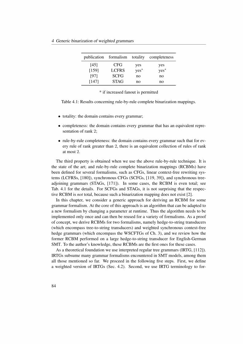
4 Generic binarization of weighted grammars
publication formalism totality completeness
[45] CFG yes yes
[159] LCFRS yes∗ yes∗
[97] SCFG no no
[147] STAG no no
* if increased fanout is permitted
Table 4.1: Results concerning rule-by-rule complete binarization mappings.
• totality: the domain contains every grammar;
• completeness: the domain contains every grammar that has an equivalent repre-
sentation of rank 2;
• rule-by-rule completeness: the domain contains every grammar such that for ev-
ery rule of rank greater than 2, there is an equivalent collection of rules of rank
at most 2.
The third property is obtained when we use the above rule-by-rule technique. It is
the state of the art; and rule-by-rule complete binarization mappings (RCBMs) have
been defined for several formalisms, such as CFGs, linear context-free rewriting sys-
tems (LCFRSs, [180]), synchronous CFGs (SCFGs, [119, 39]), and synchronous tree-
adjoining grammars (STAGs, [171]). In some cases, the RCBM is even total; see
Tab. 4.1 for the details. For SCFGs and STAGs, it is not surprising that the respec-
tive RCBM is not total, because such a binarization mapping does not exist [2].
In this chapter, we consider a generic approach for deriving an RCBM for some
grammar formalism. At the core of this approach is an algorithm that can be adapted to
a new formalism by changing a parameter at runtime. Thus the algorithm needs to be
implemented only once and can then be reused for a variety of formalisms. As a proof
of concept, we derive RCBMs for two formalisms, namely hedge-to-string transducers
(which encompass tree-to-string transducers) and weighted synchronous context-free
hedge grammars (which encompass the WSCFTGs of Ch. 3), and we review how the
former RCBM performed on a large hedge-to-string transducer for English-German
SMT. To the author’s knowledge, these RCBMs are the first ones for these cases.
As a theoretical foundation we use interpreted regular tree grammars (IRTG, [112]).
IRTGs subsume many grammar formalisms encountered in SMT models, among them
all those mentioned so far. We proceed in the following five steps. First, we define
a weighted version of IRTGs (Sec. 4.2). Second, we use IRTG terminology to for-
84
4.2 Interpreted regular tree grammars
malize the concepts “binarization mapping”, “complete”, and “rule-by-rule complete”
(Sec. 4.3). Third, we define a simple “template” that gives rise to a class of RCBMs
for IRTGs (Sec. 4.4). However, these mappings are not computable per se. Fourth, we
therefore “outsource the noncomputable part” to the user; i.e., we introduce the above-
mentioned parameter, called b-rule. We thus arrive at a template for a class of efficiently
computable binarization mappings for IRTGs, and we define a condition with respect
to the b-rules that guarantees that these binarization mappings be rule-by-rule complete
(Sec. 4.5). Fifth, and last, we consider how these RCBMs for IRTGs can be used to
derive RCBMs for established formalisms (Sec. 4.6).
We end this chapter with a conclusion, discussion, and outlook (Sec. 4.7).
4.2 Interpreted regular tree grammars
Grammar formalisms employed in parsing and SMT, such as those mentioned in the
introduction, differ in the derived objects – e.g., strings, trees, and graphs – and the
operations involved in the derivation – e.g., concatenation, substitution, and adjoining.
Interpreted regular tree grammars (IRTGs) permit a uniform treatment of many of these
formalisms. To this end, IRTGs combine the following two concepts:
Algebras IRTGs represent the objects and operations symbolically using terms; the
object in question is obtained by interpreting each symbol in the term as a func-
tion. In the parlance of universal-algebra theory, we are employing initial-algebra
semantics [86].
Tree homomorphisms IRTGs separate the finite control (state behavior) of a deriva-
tion from its derived object (in its term representation; generational behavior); the
former is captured by a recognizable tree language, while the latter is obtained
by applying a tree homomorphism. This idea goes back to the tree bimorphisms
of [6].
Now we define the concept of IRTG formally (cf. Fig. 4.1).
A (linear, nondeleting) tree homomorphism is a mapping h : TΓ(X) → T∆(X)that satisfies the following condition: there is a mapping g : Γ → T∆(X) such that
(i) g(σ) ∈ C∆(Xk) for every σ ∈ Γ(k), (ii) h(σ(t1, . . . , tk)) is the tree obtained from
g(σ) by replacing the occurrence of xj by h(tj), and (iii) h(xj) = xj . This extends the
usual definition of linear and nondeleting homomorphisms [80] to trees with variables.
Note that h(σ(x1, . . . , xk)) = g(σ) for every σ ∈ Γ(k). We abuse notation and write
h(σ) for g(σ) for every σ ∈ Γ.
85
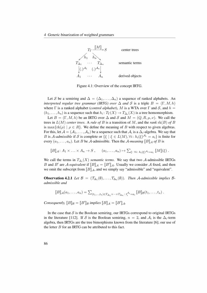
4 Generic binarization of weighted grammars
TΓ
T∆1 · · · T∆n
A1 · · · An
h1 hn
(.)A1 (.)An
S center trees
semantic terms
derived objects
JMK
Figure 4.1: Overview of the concept IRTG.
Let S be a semiring and ∆ = (∆1, . . . ,∆n) a sequence of ranked alphabets. An
interpreted regular tree grammar (IRTG) over ∆ and S is a triple B = (Γ,M, h)where Γ is a ranked alphabet (control alphabet), M is a WTA over Γ and S , and h =(h1, . . . , hn) is a sequence such that hi : TΓ(X)→ T∆i
(X) is a tree homomorphism.
Let B = (Γ,M, h) be an IRTG over ∆ and S and M = (Q,R, µ, ν). We call the
trees in L(M) center trees. A rule of B is a transition of M , and the rank rk(B) of Bis maxrk(ρ) | ρ ∈ R. We define the meaning of B with respect to given algebras.
For this, letA = (A1, . . . ,An) be a sequence such thatAi is a ∆i-algebra. We say that
B is A-admissible if S is complete or ξ | ξ ∈ L(M), ∀i : hi(ξ)Ai = ai is finite for
every (a1, . . . , an). Let B be A-admissible. Then the A-meaning JBKA of B is
JBKA : A1 × . . .×An → S , (a1, . . . , an) 7→∑
ξ : ∀i : hi(ξ)Ai=aiJMK(ξ) .
We call the terms in T∆i(X) semantic terms. We say that two A-admissible IRTGs
B and B′ are A-equivalent if JBKA = JB′KA. Usually we consider A fixed, and then
we omit the subscript from JBKA, and we simply say “admissible” and “equivalent”.
Observation 4.2.1 Let B = (T∆1(∅), . . . , T∆n(∅)). Then A-admissible implies B-
admissible and
JBKA(a1, . . . , an) =∑
(t1,...,tn)∈T∆1×···×T∆n : t
Aii =ai
JBKB(t1, . . . , tn) .
Consequently, JBKB = JB′KB implies JBKA = JB′KA.
In the case that S is the Boolean semiring, our IRTGs correspond to original IRTGs
in the literature [112]. If S is the Boolean semiring, n = 2, and Ai is the ∆i-term
algebra, then IRTGs are the tree bimorphisms known from the literature [6]; our use of
the letter B for an IRTG can be attributed to this fact.
86

4.2 Interpreted regular tree grammars
Example 4.2.2 We consider the following SCFG rule:
S → α3(PPER,NP) , where α3 = 〈x1 ließ x2 frei, x1 freed x2〉 .
Informally, this rule tells us to derive a pair (w1, w2) of strings for the state PPER
as well as a pair (w′1, w
′2) for the state NP . Then we obtain a pair for S from α3 by
replacing x1 and x2 in the first component by w1 and w2, respectively, and replacing
x1 and x2 in the second component by w′1 and w′
2, respectively. Now we make this
procedure explicit by defining an IRTG.
Let Σ = freed, ließ, frei, . . . be the set of terminal symbols of our SCFG. We
consider a ranked alphabet ∆ and a ∆-algebra A with the domain Σ∗ that allows us to
encode string substitution symbolically. We let
∆ = (con2)(2), (con3)(3), (con4)(4), (con5)(5) ∪ σ(0) | σ ∈ Σ ,
(conk)A(w1, . . . , wk) = w1 · · ·wk , (k ∈ 2, 3, 4, 5)
σA = σ . (σ ∈ Σ)
Then the following terms t1 and t2 represent our substitution procedure for the first and
second component, respectively:
t1 = con4(x1, ließ, x2, frei) , t2 = con3(x1, freed, x2) .
That is, the pair for S , given w1, w2, w′1, w
′2 as above, is (tA1 (w1, w2), t
A2 (w
′1, w
′2)).
Now we define the IRTG. We let Γ = α(1)1 , α
(1)2 , α
(2)3 , α
(2)4 , α
(0)5 , α
(0)6 and M =
(Q,R,S ) be the FTA over Γ with Q = S ,PPER,NP and
R = (NP , α1,S ), (PPER, α2,S ), (PPERNP , α3,S ),
(PPERNP , α4,S ), (ε, α5,PPER), (ε, α6,NP) .
The tree homomorphisms h1, h2 : TΓ(X)→ T∆(X) are shown in Fig. 4.2.
Finally, we let B = (Γ,M, (h1, h2)); then B is an IRTG over (∆,∆) and the
Boolean semiring. Since this semiring is complete, B is trivially admissible. We indi-
cate the (A,A)-meaning. To this end, let ξ = α4(α5, α6). Clearly, ξ ∈ L(M) and
h1(ξ)A = die katze ließ er frei , h2(ξ)
A = he freed the cat .
We note that ξ is not the only center tree for this sentence pair, but since we calculate
in the Boolean semiring, we are content with one center tree. We conclude that
JBK(er ließ die katze frei, he freed the cat) = 1 .
87
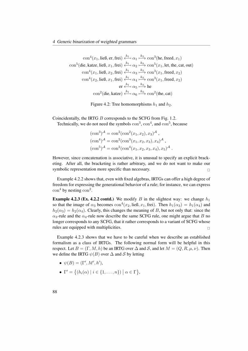
4 Generic binarization of weighted grammars
con4(x1, ließ, er, frei)h1←− [ α1
h27−→ con3(he, freed, x1)
con5(die, katze, ließ, x1, frei)h1←− [ α2
h27−→ con5(x1, let, the, cat, out)
con4(x1, ließ, x2, frei)h1←− [ α3
h27−→ con3(x1, freed, x2)
con4(x2, ließ, x1, frei)h1←− [ α4
h27−→ con3(x1, freed, x2)
erh1←− [ α5
h27−→ he
con2(die, katze)h1←− [ α6
h27−→ con2(the, cat)
Figure 4.2: Tree homomorphisms h1 and h2.
Coincidentally, the IRTG B corresponds to the SCFG from Fig. 1.2.
Technically, we do not need the symbols con3, con4, and con5, because
(con3)A = con2(con2(x1, x2), x3)A ,
(con4)A = con2(con3(x1, x2, x3), x4)A ,
(con5)A = con2(con4(x1, x2, x3, x4), x5)A .
However, since concatenation is associative, it is unusual to specify an explicit brack-
eting. After all, the bracketing is rather arbitrary, and we do not want to make our
symbolic representation more specific than necessary.
Example 4.2.2 shows that, even with fixed algebras, IRTGs can offer a high degree of
freedom for expressing the generational behavior of a rule; for instance, we can express
con4 by nesting con2.
Example 4.2.3 (Ex. 4.2.2 contd.) We modify B in the slightest way: we change h1so that the image of α3 becomes con4(x2, ließ, x1, frei). Then h1(α3) = h1(α4) and
h2(α3) = h2(α4). Clearly, this changes the meaning of B, but not only that: since the
α3-rule and the α4-rule now describe the same SCFG rule, one might argue that B no
longer corresponds to any SCFG, that it rather corresponds to a variant of SCFG whose
rules are equipped with multiplicities.
Example 4.2.3 shows that we have to be careful when we describe an established
formalism as a class of IRTGs. The following normal form will be helpful in this
respect. Let B = (Γ,M, h) be an IRTG over ∆ and S , and let M = (Q,R, µ, ν). Then
we define the IRTG ψ(B) over ∆ and S by letting
• ψ(B) = (Γ′,M ′, h′),
• Γ′ =(hi(α) | i ∈ 1, . . . , n)
∣∣ α ∈ Γ
,
88
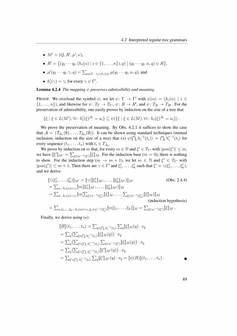
4.2 Interpreted regular tree grammars
• M ′ = (Q,R′, µ′, ν),
• R′ =(q1 · · · ql, (hi(α) | i ∈ 1, . . . , n), q)
∣∣ (q1 · · · ql, α, q) ∈ R
,
• µ′(q1 · · · ql, γ, q) =∑
α∈Γ: γi=hi(α)µ(q1 · · · ql, α, q), and
• h′i(γ) = γi for every γ ∈ Γ′.
Lemma 4.2.4 The mapping ψ preserves admissibility and meaning.
PROOF. We overload the symbol ψ; we let ψ : Γ → Γ′ with ψ(α) = (hi(α) | i ∈1, . . . , n), and likewise for ψ : TΓ → TΓ′ , ψ : R → R′, and ψ : TR → TR′ . For the
preservation of admissibility, one easily proves by induction on the size of a tree that
ξ | ξ ∈ L(M ′), ∀i : h′i(ξ)Ai = ai ⊆ ψ(ξ | ξ ∈ L(M), ∀i : hi(ξ)
Ai = ai) .
We prove the preservation of meaning. By Obs. 4.2.1 it suffices to show the case
that A = (T∆1(∅), . . . , T∆n(∅)). It can be shown using standard techniques (mutual
inclusion, induction on the size of a tree) that (⋆) ψ(⋂
i h−1i (ti)) =
⋂
i h′−1i (ti) for
every sequence (t1, . . . , tn) with ti ∈ T∆i.
We prove by induction on m that, for every m ∈ N and ξ′ ∈ TΓ′ with |pos(ξ′)| ≤ m,
we have Jξ′KM ′ =∑
ξ∈ψ−1(ξ′)JξKM . For the induction base (m = 0), there is nothing
to show. For the induction step (m → m + 1), we let m ∈ N and ξ′ ∈ TΓ′ with
|pos(ξ′)| ≤ m+ 1. Then there are γ ∈ Γ′ and ξ′1, . . . , ξ′k such that ξ′ = γ(ξ′1, . . . , ξ
′k),
and we derive
Jγ(ξ′1, . . . , ξ′k)KM ′ = Jγ(Jξ′1KM ′ , . . . , Jξ′kKM ′)KM ′ (Obs. 2.4.4)
=∑
α : hi(α)=γiJα(Jξ′1KM ′ , . . . , Jξ′kKM ′)KM
=∑
α : hi(α)=γiJα(
∑
ξ∈ψ−1(ξ′1)JξKM , . . . ,
∑
ξ∈ψ−1(ξ′k)JξKM )KM
(induction hypothesis)
=∑
α,ξ1,...,ξk : hi(α)=γi,ξj∈ψ−1(ξ′j)Jα(ξ1, . . . , ξk)KM =
∑
ξ∈ψ−1(ξ′)JξKM .
Finally, we derive using (⋆)
JBK(t1, . . . , tn) =∑
ξ∈⋂
i h−1i (ti)
∑
qJξKM (q) · νq
=∑
q
(∑
ξ∈⋂
i h−1i (ti)
JξKM (q))· νq
=∑
q
(∑
ξ′∈⋂
i h′−1i (ti)
∑
ξ∈ψ−1(ξ′)JξKM (q))· νq
=∑
q
(∑
ξ′∈⋂
i h′−1i (ti)
Jξ′KM ′(q))· νq
=∑
ξ′∈⋂
i h′−1i (ti)
∑
qJξ′KM ′(q) · νq = Jψ(B)K(t1, . . . , tn) .
89
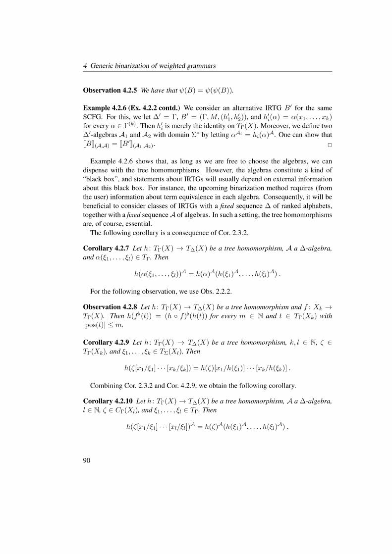
4 Generic binarization of weighted grammars
Observation 4.2.5 We have that ψ(B) = ψ(ψ(B)).
Example 4.2.6 (Ex. 4.2.2 contd.) We consider an alternative IRTG B′ for the same
SCFG. For this, we let ∆′ = Γ, B′ = (Γ,M, (h′1, h′2)), and h′i(α) = α(x1, . . . , xk)
for every α ∈ Γ(k). Then h′i is merely the identity on TΓ(X). Moreover, we define two
∆′-algebras A1 and A2 with domain Σ∗ by letting αAi = hi(α)A. One can show that
JBK(A,A) = JB′K(A1,A2).
Example 4.2.6 shows that, as long as we are free to choose the algebras, we can
dispense with the tree homomorphisms. However, the algebras constitute a kind of
“black box”, and statements about IRTGs will usually depend on external information
about this black box. For instance, the upcoming binarization method requires (from
the user) information about term equivalence in each algebra. Consequently, it will be
beneficial to consider classes of IRTGs with a fixed sequence ∆ of ranked alphabets,
together with a fixed sequenceA of algebras. In such a setting, the tree homomorphisms
are, of course, essential.
The following corollary is a consequence of Cor. 2.3.2.
Corollary 4.2.7 Let h : TΓ(X) → T∆(X) be a tree homomorphism, A a ∆-algebra,
and α(ξ1, . . . , ξl) ∈ TΓ. Then
h(α(ξ1, . . . , ξl))A = h(α)A(h(ξ1)
A, . . . , h(ξl)A) .
For the following observation, we use Obs. 2.2.2.
Observation 4.2.8 Let h : TΓ(X) → T∆(X) be a tree homomorphism and f : Xk →TΓ(X). Then h(f (t)) = (h f)(h(t)) for every m ∈ N and t ∈ TΓ(Xk) with
|pos(t)| ≤ m.
Corollary 4.2.9 Let h : TΓ(X) → T∆(X) be a tree homomorphism, k, l ∈ N, ζ ∈TΓ(Xk), and ξ1, . . . , ξk ∈ TΣ(Xl). Then
h(ζ[x1/ξ1] · · · [xk/ξk]) = h(ζ)[x1/h(ξ1)] · · · [xk/h(ξk)] .
Combining Cor. 2.3.2 and Cor. 4.2.9, we obtain the following corollary.
Corollary 4.2.10 Let h : TΓ(X)→ T∆(X) be a tree homomorphism, A a ∆-algebra,
l ∈ N, ζ ∈ CΓ(Xl), and ξ1, . . . , ξl ∈ TΓ. Then
h(ζ[x1/ξ1] · · · [xl/ξl])A = h(ζ)A(h(ξ1)
A, . . . , h(ξl)A) .
90

4.3 Binarization mappings
(BCD,α,A) , (ε, α1, B) , (ε, α2, C) , (ε, α3, D)
con3(x1, x2, x3)h1←− [ α
h27−→ con4(x3, a, x1, x2)
bh1←− [ α1
h27−→ b
ch1←− [ α2
h27−→ c
dh1←− [ α3
h27−→ d
Figure 4.3: An IRTG of rank 3 encoding an SCFG.
bcd(.)A1
←− [con3
b c d
h1←− [α
α1 α2 α3
h27−→con4
d a b c
(.)A2
7−→ dabc
Figure 4.4: Center tree (innermost), semantic terms, derived objects (outermost).
4.3 Binarization mappings
Roughly speaking, our aim is to construct a partial mapping from IRTGs into IRTGs
that preserves meaning and reduces the rank to 2, and its domain should contain all
IRTGs that can be binarized rule by rule. In this section, we formalize this problem
statement. We proceed as follows. First, we consider an example. Second, we define
what a binarization of a single rule is, and how the rule is to be replaced. Third, we
define the concept of a rule-by-rule complete binarization mapping.
Example 4.3.1 We consider the IRTG shown in Fig. 4.3, which can be viewed as an
SCFG in the same way as in Ex. 4.2.2. In particular, we reuse the algebraA. Figure 4.4
shows a center tree with its two homomorphic images, which evaluate to the strings bcdand dabc.
Consider the first transition in Fig. 4.3, which has rank three. It occurs in the run
(BCD,α,A)(B,C,D
),
which is a partial run on the fragment α(x1, x2, x3) of the center tree in Fig. 4.4. This
fragment is mapped to the semantic terms h1(α) and h2(α) shown in Fig. 4.3.
Now consider the transitions in Fig. 4.5. These transitions make up the run
(A′D,α′, A)((BC,α′′, A′)
(B,C
), D
),
which is a partial run on the fragment α′(α′′(x1, x2), x3). Let us call this fragment ξ.
Note that the terms h′1(ξ) and h1(α) are equivalent in that they denote the same term
91

4 Generic binarization of weighted grammars
(A′D,α′, A) , (BC,α′′, A′)
con2(x1, x2)h′1←− [ α′ h′27−→ con2(con2(x2, a), x1)
con2(x1, x2)h′1←− [ α′′ h′27−→ con2(x1, x2)
Figure 4.5: Binarization of the ternary rule in Fig. 4.3.
function, and so are the terms h′2(ξ) and h2(α). Thus, replacing the α-transition by the
transitions in Fig. 4.5 (and merging hi and h′i accordingly) does not change the meaning
of the IRTG. However, since the new rules are binary, parsing and translation will be
cheaper.
Rule-by-rule binarization of IRTGs closely follows the intuition laid out in this ex-
ample: it means processing each suprabinary rule, attempting to replace it with an
equivalent collection of binary rules. For the remainder of this chapter (unless noted
otherwise), let ∆ = (∆1, . . . ,∆n) be a sequence of ranked alphabets, S a commutative
semiring, and A = (A1, . . . ,An) a sequence such that Ai is a ∆i-algebra. Moreover,
let B = (Γ,M, h) be an A-admissible IRTG over ∆ and S , M = (Q,R, µ, ν), ρ ∈ R,
ρ = (q1 · · · qk, α, q), and k > 2.
4.3.1 Binarization of a rule
Let Γ′ be a binary ranked alphabet and ξ ∈ CΓ′(Xk). A ξ-binarization B′ of ρ is an
IRTG (Γ′,M ′, h′) over ∆ and S such that there is a d with
• d ∈ Dq(M ′, ξ[x1/q1] · · · [xk/qk]),
• 〈d〉 = µ(ρ),
• h′i(ξ)Ai = hi(α)
Ai ,
• d′ ∈ Dqpr(M
′) implies d′ ⊑ d, and
• Dqjpr (M
′) = qj.
We call B′ rank normal if Γ′ = Γ′(2).
Example 4.3.2 (Ex. 4.3.1 contd.) Let ρ = (BCD,α,A). A rank-normal ξ-binari-
zation of ρ is given in Fig. 4.5, where
ξ = α′(α′′(x1, x2), x3) ,
d = (A′D,α′, A)((BC,α′′, A′)
(B,C
), D
).
92

4.3 Binarization mappings
We note that a binarization of ρ need not exist, even if B as a whole admits an
equivalent representation of rank at most 2.
Example 4.3.3 It is easy to specify an SCFG (and, thus, an IRTG) of rank 0 for the sin-
gleton language (abcd, cadb). Likewise, one can use the following SCFG of rank 4:
S → 〈x1x2x3x4, x3x1x4x2〉(A,B,C,D) ,
A→ 〈a, a〉, . . . , D → 〈d, d〉 .
Using an IRTG representation in the spirit of Exs. 4.2.2 and 4.3.1, one will find that
there is no binarization of the first rule. We will elaborate on this in Ex. 4.4.12, when
we will have the appropriate tools at our disposal.
LetB′ = (Γ′,M ′, h′) be a ξ-binarization of ρ andM ′ = (Q′, R′, µ′, ν ′). We say that
B and B′ are compatible if the following conditions are satisfied:
• R′|q ∩R = ∅,
• q′ ∈ Q ∩ (Q′ \ q, q1, . . . , qk) implies R|q′ = R′|q′ , and
• hi|Γ∩Γ′ = h′i|Γ∩Γ′ and µ|R∩R′ = µ′|R∩R′ .
We note that the property of compatibility can be readily established by using suit-
able alphabets Q′ and Γ′; e.g., one can use fresh symbols (Γ ∩ Γ′ = ∅ = Q ∩ (Q′ \q, q1, . . . , qk)), or one can reuse symbols from Q and Γ wherever possible.
Let B and B′ be compatible. Then we define the IRTG B[ρ/B′] over ∆ and S by
• B[ρ/B′] = (Γ ∪ Γ′,M [ρ/M ′], h′′),
• M [ρ/M ′] = (Q ∪Q′, (R ∪R′) \ ρ, µ′′, ν ′′) where
µ′′(ρ′) =
µ(ρ′) if ρ′ ∈ R,
µ′(ρ′) if ρ′ ∈ R′ \R,ν ′′q′ =
νq′ if q′ ∈ Q,
0 otherwise,
• h′′i : TΓ∪Γ′(X)→ T∆i(X) is the tree homomorphism with
h′′i (α) =
hi(α) if α ∈ Γ,
h′i(α) if α ∈ Γ′ \ Γ.
In the following, we will omit the subscript from πΓ and πΓ∪Γ′ .
93

4 Generic binarization of weighted grammars
Lemma 4.3.4 There is a (hq | q ∈ Q) such that hq : Dqco(M) → Dq
co(M [ρ/M ′]) is
bijective and, for every d ∈ Dqco(M),
hi(π(d))Ai = h′′i (π(hq(d)))
Ai and 〈d〉 = 〈hq(d)〉 .
PROOF. SinceB′ is a ξ-binarization, there is a dρ ∈ Dq(M ′, ξ[x1/q1] · · · [xk/qk]) with
the properties mentioned in the definition of a ξ-binarization. We let R′′ = (R ∪ R′) \ρ, w1, . . . , wk be the positions of x1, . . . , xk in ξ, respectively, and h′ : TR(X) →TR′′(X) be the tree homomorphism with
h′(ρ) = dρ[x1]w1 · · · [xk]wk,
h′(ρ′) = ρ′(x1, . . . , xrk(ρ′)) . (ρ′ 6= ρ)
We will prove the statement P (n) for every n ∈ N, where
P (n): Let p ∈ Q.
1. Let d ∈ Dpco(M) with |pos(d)| ≤ n. Then h′(d) ∈ Dp
co(M [ρ/M ′]),hi(π(d))
Ai = h′′i (π(h′(d)))Ai , and 〈d〉 = 〈h′(d)〉.
2. Let d1, d2 ∈ Dpco(M) with |pos(d1)|+|pos(d2)| ≤ n. Then h′(d1) =
h′(d2) implies d1 = d2.
3. Let d′ ∈ Dpco(M [ρ/M ′]) with |pos(d′)| ≤ n. Then there is a d ∈
Dpco(M) with h′(d) = d′.
With this statement, it is clear that we obtain the desired mapping hq for every q ∈ Qsimply by restricting h′ appropriately.
For the induction base (n = 0), there is nothing to show. We show the induction step
(n → n + 1). To this end, let n ∈ N such that P (n) holds. We show that P (n + 1)holds. To this end, let p ∈ Q.
Statement 1: Let d ∈ Dpco(M) and |pos(d)| ≤ n + 1. Then there are ρ′ ∈ R,
ρ′ = (p1 · · · pk, α, p), and d1, . . . , dk such that d = ρ′(d1, . . . , dk), dj ∈ Dpjco (M), and
|pos(dj)| ≤ n. By the induction hypothesis (i.e., P (n) holds), we have that
• h′(dj) ∈ Dpjco (M [ρ/M ′]),
• hi(π(dj))Ai = h′′i (π(h
′(dj)))Ai , and
• 〈dj〉 = 〈h′(dj)〉.
94

4.3 Binarization mappings
We distinguish two cases. The case that ρ′ 6= ρ is easy. We turn to the case that ρ′ = ρ.
Then p = q. It is easy to see that h′(d) ∈ Dqco(M [ρ/M ′]). We derive
hi(π(d))Ai = hi(π(ρ(d1, . . . , dk)))
Ai = hi(α(π(d1), . . . , π(dk)))Ai
=[hi(α)
(hi(π(d1)), . . . , hi(π(dk))
)]Ai
= hi(α)Ai(hi(π(d1))
Ai , . . . , hi(π(dk))Ai)
(Cor. 4.2.7)
= h′′i (π(h′(ρ)))Ai
(
h′′i (π(h′(d1)))
Ai , . . . , h′′i (π(h′(dk)))
Ai
)
(†)
= h′′i (π(h′(d)))Ai , (Cor. 4.2.10)
where, for (†), we derive hi(α)Ai = h′i(ξ)
Ai = h′i(π(h′(ρ)))Ai . Finally, we derive
〈h′(d)〉 = 〈h′(d1)〉 · · · 〈h′(dk)〉 · 〈dρ〉 (commutativity)
= 〈d1〉 · · · 〈dk〉 · µ(ρ) = 〈d〉 .
Statement 2: Let d1, d2 ∈ Dpco(M), |pos(d1)| + |pos(d2)| ≤ n + 1, and h′(d1) =
h′(d2). We distinguish three cases. Case 1: Let d1(ε), d2(ε) 6= ρ or d1(ε) = d2(ε) = ρ.
Then it is easy to apply the induction hypothesis. Case 2: Let d1(ε) = ρ and d2(ε) 6= ρ.
Then h′(d1)(ε) ∈ R′|q and h′(d2)(ε) ∈ R. SinceM andM ′ are compatible,R′|q∩R =
∅. So this case does not occur. Case 3: Let d1(ε) 6= ρ and d2(ε) = ρ. For reasons of
symmetry, this case does not occur either.
Statement 3: Let d′ ∈ Dpco(M [ρ/M ′]) with |pos(d′)| ≤ n + 1. We distinguish
two cases. Case 1: Let d′(ε) ∈ R. Moreover, let d′(ε) = (p1 · · · pk, α, p). Then
p1, . . . , pk ∈ Q and, by the induction hypothesis, there are d1, . . . , dk with h′(dj) =d′|j . We construct d = d′(ε)
(d1, . . . , dk
). It is easy to see that d ∈ Dp
co(M) and
h′(d) = d′. Case 2: Let d′(ε) 6∈ R. Since p ∈ Q, and since M and M ′ are compatible,
we have that p = q. Recall that, for every d′′ ∈ Dqpr(M
′), we have that d′′ ⊑ dρ.
Since the run d′ is complete, we have that dρ ⊑ d′, i.e., there are d′1, . . . , d′k such
that d′ = dρ[d′1]w1 · · · [d
′k]wk
. By the induction hypothesis, we obtain that there are
d1, . . . , dk with h(dj) = d′j . We construct d = ρ(d1, . . . , dk).
Corollary 4.3.5 Let ρ be a suprabinary rule of B and B′ a binarization of ρ. Then
B[ρ/B′] is admissible and equivalent to B.
PROOF. Let (hq | q ∈ Q) be a family of mappings as postulated in Lm. 4.3.4. Using
said lemma, it is easy to see that, for every q ∈ Q and (a1, . . . , an) ∈ A1 × · · · ×An,
hq(d | d ∈ Dqco(M [ρ/M ′]), ∀i : h′′i (π(d))
Ai = ai)
= d | d ∈ Dqco(M), ∀i : hi(π(d))
Ai = ai .
95
4 Generic binarization of weighted grammars
This implies that B[ρ/B′] is admissible.
Moreover, let (a1, . . . , an) ∈ A1 × · · · ×An. Then
JBK(a1, . . . , an) =∑
ξ∈TΓ : hi(ξ)Ai=ai
∑
q∈Q,d∈Dq(M,ξ)〈d〉 · νq
=∑
ξ∈TΓ,q∈Q,d∈Dq(M,ξ) : hi(ξ)Ai=ai〈d〉 · νq
=∑
q∈Q,d∈Dqco(M) : hi(π(d))Ai=ai
〈d〉 · νq
=∑
q∈Q,d∈Dqco(M) : h′′i (π(hq(d)))
Ai=ai〈hq(d)〉 · νq
=∑
q∈Q,d′∈Dqco(M ′) : h′′i (π(d
′))Ai=ai〈d′〉 · ν ′′q (hq is bijective)
=∑
ξ∈TΓ∪Γ′ : h′′i (ξ)Ai=ai
∑
q∈Q,d′∈Dq(M ′,ξ)〈d′〉 · ν ′′q
=∑
ξ∈TΓ∪Γ′ : h′′i (ξ)Ai=ai
∑
q∈Q∪Q′,d′∈Dq(M ′,ξ)〈d′〉 · ν ′′q = JB[ρ/B′]K(a1, . . . , an) .
4.3.2 Binarization mappings
Now we are able to formally define binarization mappings for IRTGs. To this end, let Cbe a set of admissible IRTGs over ∆ and S . A binarization mapping bin for C is a par-
tial mapping bin : C → C that preserves meaning. The binarization domain bdom(bin)of bin is the set B | B ∈ dom(bin), rk(bin(B)) ≤ 2. A binarization mapping bin is
complete if bdom(bin) ⊇ B | B ∈ C, ∃B′ ∈ C : JBK = JB′K, rk(B′) ≤ 2. It is rule-
by-rule complete if bdom(bin) contains every B ∈ C such that for every suprabinary
rule ρ of B there is a binarization of ρ.
We distinguish between the domain of bin and its binarization domain so as to enable
“best-effort binarization”; i.e., even if, for someB ∈ C, we do not find an equivalentB′
of rank 2, we can at least attempt to reduce the number of suprabinary rules. In this
case B ∈ dom(bin) \ bdom(bin). This case can be useful in practice; our theoretical
considerations, however, are limited to bdom(bin).We abbreviate “rule-by-rule complete binarization mapping” by RCBM. If an RCBM
bin exists, then every complete binarization mapping is also rule-by-rule complete,
for then bin(B) is a witness that B is in the binarization domain of every complete
binarization mapping. Such an RCBM bin , however, need not exist; for instance, the
class C may be so severely restricted that replacing a suprabinary rule by its binarization
leads out of C.
4.4 Constructing a binarization mapping
In this section, we construct an RCBM for IRTGs over ∆ and S . First, we consider
an example of our construction, then we define the necessary concepts, and finally, we
96

4.4 Constructing a binarization mapping
arrive at the construction. The binarization mapping will not be computable in general,
and we will tackle this problem in the next section.
Example 4.4.1 (Ex. 4.3.1 contd.) Now we construct the binarization of our rule sys-
tematically. We proceed as follows (cf. Fig. 4.6). For each of the terms h1(α) and
h2(α) (Fig. 4.6a), we consider all terms that satisfy two properties (Fig. 4.6b): (i) they
are equivalent to h1(α) and h2(α), respectively, and (ii) at each node at most two sub-
trees contain variables. As Fig. 4.6 suggests, there may be several different terms of
this kind. For each of these terms, we analyze the bracketing of variables, obtaining
what we call a variable tree (Fig. 4.6c). Now we pick terms t1 and t2 corresponding to
h1(α) and h2(α), respectively, such that (iii) they have the same variable tree, say τ .
We construct a tree ξ from τ by a simple relabeling, and we read off the tree homo-
morphisms h′1 and h′2 from a decomposition we perform on t1 and t2, respectively; see
Fig. 4.6, dotted arrows, and compare the boxes in Fig. 4.6d with the homomorphisms
in Fig. 4.5. Now the rules in Fig. 4.5 are easily extracted from ξ.
With the tree ξ, the rules, and the tree homomorphisms, we have all ingredients for
a ξ-binarization; and, indeed, we obtain a binarization: our rules are equivalent to the
original one because of (i); they are binary because ξ is binary, which in turn holds
because of (ii); finally, the decompositions of t1 and t2 are compatible with ξ because
of (iii). We call a sequence (t1, t2) a binarization hedge if (i)–(iii) are satisfied. We
will see below that the existence of a binarization is tantamount to the existence of a
binarization hedge. Our main task will be finding a binarization hedge.
4.4.1 Variable trees and term decomposition
Let us define the concept of variable trees as well as the decomposition that corresponds
to the two outer dotted arrows in Fig. 4.6. In order to keep notation uncluttered, we will
disregard the IRTG B in this subsection and rather proceed in a general setting. To this
end, let ∆ be an arbitrary ranked alphabet and t ∈ T lin
∆ (X).We begin with a few auxiliary concepts. By var(t) we denote the set of all ele-
ments of X that occur in t, i.e., var(t) = t(w) | t(w) ∈ X. Let t1, . . . , tl ∈T lin
∆ (X). We call this sequence eligible (for a canonical sort) if (i) var(tj) 6= ∅ and
(ii) var(tj) ∩ var(tj′) 6= ∅ implies j = j′. Let t1, . . . , tl be eligible. Then the canoni-
cal sort csort(t1, . . . , tl) of t1, . . . , tl is the sequence obtained from t1, . . . , tl by sorting
the trees according to the least variable index. For instance, we have that
csort(δ′(x3), δ(x2, x4)) =(δ(x2, x4), δ
′(x3))
,
because the least variable index is 3 in the first argument tree, it is 2 in the second, and
3 > 2, so we have to swap the trees. We call the sequence t1, . . . , tl canonically sorted
if it is equal to its canonical sort.
97

4 Generic binarization of weighted grammars
(a)con3
x1 x2 x3
con4
x3 a x1 x2
(b)
con2
x1 con2
x2 x3
con2
con2
x1 x2
x3
t1 : con2
con2
x3 a
con2
x1 x2
t2 :con2
con2
x3 con2
a x1
x2
(c)
(d)
con2
x1 x2
con2
x1 x2
x1 x2
x3
con2
con2
x2 a
x1
con2
x1 x2
x1 x2
x3
(e)
h1←− [ αh27−→
⋆
x1 ⋆
x2 x3
⋆
⋆
x1 x2
x3
τ : ⋆
⋆
x1 x3
x2
con2
con2
x1 x2
x3
t1 :
h′1←− [
α′
α′′
x1 x2
x3
ξ :
h′27−→
con2
con2
x3 a
con2
x1 x2
t2 :
Figure 4.6: Outline of the binarization algorithm.
98

4.4 Constructing a binarization mapping
We define the variable tree v(t) of t by induction. For this, we let v : T lin
∆ (X) →T lin
⋆,∅(X) with
v(xj) = xj ,
v(δ(t1, . . . , tk)) =
∅ if l = 0,
v(t′1) if l = 1,
⋆(v(t′1), . . . , v(t′l)) otherwise,
(δ ∈ ∆)
where t′1, . . . , t′l is the canonical sort of the sequence that is obtained from t1, . . . , tk
by removing every occurrence of any tree that does not contain any variable; since t is
linear, that sequence is eligible.
Example 4.4.2 Let t1, t2, and τ be given by Fig. 4.6. Then v(t1) = τ = v(t2).
Observation 4.4.3 (i) var(t) = ∅ iff v(t) = ∅ and (ii) var(t) = var(v(t)).
Next we show that applying a tree homomorphism to a binary tree preserves the
variable tree.
Lemma 4.4.4 Let h : TΓ(X) → T∆(X) a tree homomorphism. For every m ∈ N and
binary ξ ∈ T lin
Γ (X) with |pos(ξ)| ≤ m, we have v(ξ) = v(h(ξ)).
PROOF. By induction on m. For the induction base (m = 0), there is nothing to show.
For the induction step (m → m + 1), let m ∈ N and ξ ∈ T lin
Γ (X) be binary with
|pos(ξ)| ≤ m+ 1. We distinguish three cases. Case 1: ξ ∈ X . Trivial.
Case 2: ξ(ε) ∈ Γ(2). There are α ∈ Γ and ξ1, ξ2 ∈ Tlin
Σ (X) with ξ = α(ξ1, ξ2). We
let v1 = v(ξ1) and v2 = v(ξ2), and we define the following predicates:
P (j) ⇐⇒ var(ξj) 6= ∅ , P (j, w) ⇐⇒ P (j) ∧ xj occurs in h(α)|w .
Note that P (j) ⇐⇒ P (j, ε). We derive
v(ξ) = v(α(ξ1, ξ2))
=
∅ ¬P (1) ∧ ¬P (2)
v1 P (1) ∧ ¬P (2)
v2 ¬P (1) ∧ P (2)
⋆(csort(v1, v2)
)P (1) ∧ P (2)
= v(h(α)|ε[x1/h(ξ1)][x2/h(ξ2)]) (†)
= v(h(α)[x1/h(ξ1)][x2/h(ξ2)])
= v(h(α(ξ1, ξ2))) = v(h(ξ)) ,
99

4 Generic binarization of weighted grammars
where (†) follows from the following statement, which is easily proved by induction:
for every m′ ∈ N and w ∈ pos(h(α)) with |pos(h(α)|w)| ≤ m′, we have that
v(h(α)|w[x1/h(ξ1)][x2/h(ξ2)]
)
=
∅ ¬P (1, w) ∧ ¬P (2, w)
v1 P (1, w) ∧ ¬P (2, w)
v2 ¬P (1, w) ∧ P (2, w)
⋆(csort(v1, v2)
)P (1, w) ∧ P (2, w)
The outer induction hypothesis, v(ξj) = v(h(ξj)), is needed when h(α)|w = xj .Case 3: ξ(ε) ∈ Γ(0) ∪ Γ(1); similar to Case 2.
Example 4.4.5 (Ex. 4.4.2 contd.) Lemma 4.4.4 requires that ξ be binary. We consider
a tree homomorphism h and a suprabinary ξ where v(ξ) 6= v(h(ξ)). To this end, we
assume a ternary α that is mapped by h to t2. We let ξ = α(x1, x2, x3). Then h(ξ) = t2,
v(t2) = τ , and v(ξ) = ⋆(x1, x2, x3).
Let ∆1 and ∆2 be ranked alphabets, t1 ∈ T∆1(X), and t2 ∈ T∆2(X). We say that
t1 and t2 are congruent if pos(t1) = pos(t2) and, for every w ∈ pos(t1) and j ∈ N,
t1(w) = xj iff t2(w) = xj .Next we define the term decomposition f(t) of t by defining the mapping f . For
instance, the term decompositions of t1 and t2 are shown in Fig. 4.6(d). Our aim is to
make f(t) and v(t) congruent, so that we can read off h′1, . . . , h′n from f(t1), . . . , f(tn).
For the range of f , we stretch the notion of a ranked alphabet and permit an infinite
set of symbols. Ultimately we will apply f only to a finite number of trees, and for
those instances a finite set of symbols suffices, but that set is cumbersome to describe
in advance. Let ∆′ = t(k) | t ∈ C∆(Xk). We call each element of ∆′ a fragment.
Before we define f : T lin
∆ (X)→ T lin
∆′ (X) formally, we consider some intuition. For
this, let t ∈ T lin
∆ (X), t = δ(t1, . . . , tk), and δ ∈ ∆. Then we construct the root label
of f(t) from the fragment δ(x1, . . . , xk) in two steps. First, for every j such that tjdoes not contain any variable, we replace xj by tj . The resulting fragment contains the
variables xj1 , . . . , xjl where tj1 , . . . , tjl are the trees that do contain variables. With the
second step, we avoid nodes of rank 1, because those are not present in a variable tree,
and we want to achieve congruency. So, if l = 1 and the root fragment of f(tj1) is not
a variable itself, we replace xj1 by that fragment. If l 6= 1, then for every ι such that the
root fragment of f(tjι) is unary, we replace xjι by that fragment. The successors of the
root of f(t) are computed accordingly.
Formally, we define f : T lin
∆ (X) → T lin
∆′ (X) inductively as follows. Let t = xj .Then f(t) = xj . Let t = δ(t1, . . . , tk), δ ∈ ∆, and t′1, . . . , t
′l be the canonical sort of
100

4.4 Constructing a binarization mapping
the sequence that is obtained from t1, . . . , tk by removing every occurrence of any tree
that does not contain any variable. There are uniquely determined j1, . . . , jl such that
t′ι = tjι for every ι ∈ 1, . . . , l. Moreover, let u1, . . . , ul with uι = f(t′ι). We proceed
by case distinction.
1. If l = 1 and u1(ε) 6∈ X , then
f(t) = δ(t′′1, . . . , t′′k)(u1|1, . . . , u1|rku1 (ε)
)
where t′′j1 is u1(ε), and t′′j = tj for j 6= j1.
2. Otherwise, we let
f(t) = δ(t′′1, . . . , t′′k)(u′1, . . . , u
′l
)
where, for every ι ∈ 1, . . . , l,
• if rkuι(ε) = 1, then t′′jι = uι(ε)[x1/xι] and u′ι = uι|1,
• if rkuι(ε) 6= 1, then t′′jι = xι and u′ι = uι,
and t′′j = tj for j 6∈ j1, . . . , jl.
Example 4.4.6 (Ex. 4.4.2 contd.) We show how to compute f(t2). First, we perform
the canonical sort of the sequence t2|1, t2|2, which yields t2|2, t2|1. Second, we com-
pute u1 = f(t2|2) and u2 = f(t2|1).For u1, we first observe that the sequence t2|21, t2|22 is already canonically sorted.
We compute f(t2|21) and f(t2|22), which is x1 and x2, respectively. Now we con-
struct u1. Since rkx1(ε), rkx2(ε) 6= 1, we do not merge, and we obtain that u1 =[con2(x1, x2)](x1, x2). For u2, the sequence t2|11 is also already sorted. We compute
f(t2|11), which is x3. Now we construct u2. Since rkx3(ε) 6= 1, we also do not merge,
and we obtain that u2 = [con2(x1, a)](x3).Finally, we construct f(t2). We have that rku1(ε) 6= 1 and rku2(ε) = 1, so we have
to merge once. We derive
f(t2) = [con2(u2(ε)[x1/x2], x1)](u1, u2|1)
= [con2(con2(x2, a), x1)]([con2(x1, x2)](x1, x2), x3
).
We show that v(t) and f(t) are congruent if |var(t)| > 1, and we show how to con-
struct a tree homomorphism that maps f(t) back to t. To this end, let ∆′′ ⊆ ∆′ be finite.
Then we define the tree homomorphism h∆′′ : T∆′′(X) → T∆(X) by h∆′′(δ) = δ for
every δ ∈ ∆′′. Moreover, we define ∆′|t = δ(k) | δ ∈ ∆′(k), ∃w ∈ pos(t) : t(w) =
δ.
101

4 Generic binarization of weighted grammars
Lemma 4.4.7 For every m ∈ N and t ∈ T lin
∆ (X) with |pos(t)| ≤ m, we have the
following. If |var(t)| > 1, then v(t) and f(t) are congruent; otherwise, var(f(t)) =var(t) and pos(f(t)) ⊆ ε, 1. Moreover, for every finite ∆′′ with ∆′|f(t) ⊆ ∆′′ ⊆ ∆′,
we have that h∆′′(f(t)) = t.
PROOF. By induction on m. For the induction base (m = 0), there is nothing to show.
We show the induction step (m→ m+1). To this end, letm ∈ N and t ∈ T lin
∆ (X) with
|pos(t)| ≤ m + 1. If t ∈ X , then the statements are easy to see. Let t = δ(t1, . . . , tk)with δ ∈ ∆, and let t′1, . . . , t
′l, j1, . . . , jl, and u1, . . . , ul be as in the definition of f .
Let |var(t)| ≤ 1. Then l ≤ 1. If l = 0, then it is easy to see that f(t) = t and,
hence, var(f(t)) = ∅ = var(t) and pos(f(t)) = ε (recall that t is the label of the
root of f(t)). If l = 1, then |var(t′1)| = 1. We derive var(f(t)) = var(f(t′1)) =var(t′1) = var(t). By the induction hypothesis, pos(u1) ⊆ ε, 1. By the definition of
f(t), pos(f(t)) ⊆ ε, 1 holds as well.
Let |var(t)| > 1. If l = 1 and u1(ε) 6∈ X , then |var(t′1)| > 1. By the induc-
tion hypothesis, v(t′1) and u1 are congruent. We derive pos(f(t)) = pos(f(t′1)) =pos(v(t′1)) = pos(v(t)). Moreover, f(t)(w) = xj iff f(t′1)(w) = xj iff v(t′1)(w) = xjiff v(t)(w) = xj . If l 6= 1 or u1(ε) ∈ X , we proceed as follows. By the induction
hypothesis, v(t′ι) and f(t′ι) are congruent for every ι with |var(t′ι)| > 1. We derive
pos(f(t)) = ε ∪ ιw | ι ∈ 1, . . . , l, rkuι(ε) = 1, w ∈ pos(uι|1)
∪ ιw | ι ∈ 1, . . . , l, rkuι(ε) 6= 1, w ∈ pos(uι)
= ε ∪ ι | ι ∈ 1, . . . , l, rkuι(ε) = 1
∪ ιw | ι ∈ 1, . . . , l, rkuι(ε) 6= 1, w ∈ pos(v(t′ι))
= pos(v(t)) ,
where we use the following reasoning. If rkuι(ε) = 1, then uι is not congruent with any
variable tree, and the induction hypothesis yields |var(t′ι)| ≤ 1, which in turn implies
that pos(t′ι) ⊆ ε, 1. By assumption, |var(t′ι)| ≥ 0, so |var(t′ι)| = 1. Hence, and
since rkuι(ε) = 1, we obtain that uι|1 ∈ X . By similar reasoning, one can prove that
f(t)(w) = xj iff v(t)(w) = xj .
Now we show that h∆′′(f(t)) = t. We distinguish two cases. First, let l = 1and u1(ε) 6∈ X . Let t′′1, . . . , t
′′k be as in the definition of f . We let l′ = rku1(ε) and
g : Xl′ → T∆(X) with g(xj) = h∆′′(u1|j). First, we prove that g♯(t′′j ) = tj . If j 6= j1,
then this is trivial. If j = j1, then we derive
g♯(t′′j ) = g♯(u1(ε)) = h∆′′(u1)
= tj . (induction hypothesis)
102

4.4 Constructing a binarization mapping
Second, we derive
h∆′′(f(t)) = g♯(δ(t′′1, . . . , t′′k)) = δ(g♯(t′′1), . . . , g
♯(t′′k)) = δ(t1, . . . , tk) = t .
Now let l 6= 1 or u1(ε) ∈ X . Let t′′1, . . . , t′′k and u′1, . . . , u
′l be as in the definition
of f , and let g : Xl′ → T∆(X) with g(xj) = h∆′′(u′j). As a first step, we prove that
g♯(t′′j ) = tj . If j 6∈ j1, . . . , jl, then this is trivial. If there is a ι with j = jι and
rkuι(ε) = 1, then we derive
g♯(t′′j ) = g♯(uι(ε)[x1/xι]) = uι(ε)[x1/h∆′′(uι|1)] = h∆′′(uι)
= tj . (induction hypothesis)
If there is a ι with j = jι and rkuι(ε) 6= 1, then we derive
g♯(t′′j ) = g♯(xι) = h∆′′(uι)
= tj . (induction hypothesis)
The second step, h∆′′(f(t)) = t, is as in the former case.
4.4.2 Constructing a binarization
Now we apply the concepts of the previous subsection in our context of IRTGs. Let
t = (t1, . . . , tn) be a sequence such that ti ∈ T∆i(Xk). We call t a binarization hedge
of ρ if the following two properties hold:
(i) hi(α)Ai = tAi
i ,
(ii) the terms t1, . . . , tn have the same variable tree, which is binary.
Let t be a binarization hedge of ρ, and let
Γ′ = (δ1, . . . , δn)(k) | ∃w ∈ pos(v(t1)) : k = rkv(t1)(w), ∀i : δi = f(ti)(w) .
This definition is sound because pos(f(ti)) = pos(v(ti)), by Lm. 4.4.7, and v(ti) =v(t1), by assumption. We construct a tree ξ ∈ CΓ′(Xk) and a ξ-binarization of ρ.
We let ξ be obtained from v(t1) by replacing, at each ⋆-labeled position w, the label
⋆ by (f(t1)(w), . . . , f(tn)(w)). Since v(t1) is binary, so is ξ. Moreover, we let ξ′ =ξ[x1/q1] · · · [xk/qk], and we define the IRTG B(ρ, t) over ∆ and S with
• B(ρ, t) = (Γ′,M ′, h′),
• M ′ = (Q′ ∪ q, q, R′, µ′),
103

4 Generic binarization of weighted grammars
• Q′ = ξ′|w | w ∈ pos(ξ′), w 6= ε, and
• R′ = ρw | w ∈ pos(ξ′), ξ′(w) 6∈ Q where
ρε : (ξ′|1 · · · ξ′|rkξ′ (ε), ξ
′(ε), q) ,
ρw : (ξ′|w1 · · · ξ′|w rkξ′ (w)
, ξ′(w), ξ′|w) , (w 6= ε)
• µ′(ρε) = µ(ρ) and µ′(ρw) = 1 for w 6= ε,
• h′i((δ1, . . . , δn)) = δi.
By Lm. 4.4.7, we have that hi(α)Ai = tAi
i = h′i(ξ)Ai . With this, it is easy to see that
B(ρ, t) is indeed a ξ-binarization of ρ. It is even rank normal, because a variable tree
such as v(t1) does not contain any unary nodes.
Example 4.4.8 We can view the binarization of Fig. 4.5 as an instance of our construc-
tion, where we have
α′ =(con2(x1, x2), con
2(con2(x2, a), x1))
,
α′′ =(con2(x1, x2), con
2(x1, x2))
,
ξ = α′(α′′(x1, x2), x3) ,
A′ = α′′(B,C) .
Lemma 4.4.9 The following statements are equivalent:
1. There is a binarization of ρ.
2. There is a binarization hedge of ρ.
3. There is a rank-normal binarization of ρ.
PROOF. “1⇒ 2”. Let (Γ′,M ′, h′) be a ξ-binarization of ρ. Then ξ is binary, and so is
v(ξ). By Lm. 4.4.4, the sequence (h′1(ξ), . . . , h′n(ξ)) is a binarization hedge. “2⇒ 3”.
Let t be a binarization hedge of ρ. Then B(ρ, t) is a rank-normal binarization of ρ, as
we have seen. “3⇒ 1”. Trivial.
It remains to show how we can find a binarization hedge of ρ, if there is any. We
begin our investigation with the following observation.
104

4.5 Constructing a computable binarization mapping
Observation 4.4.10 Let (bi | i ∈ 1, . . . , n) with
bi : C∆i(Xk)→ P(C∆i
(Xk)) ,
t 7→ t′ | t′ ∈ C∆i(Xk), t
Ai = t′Ai , v(t′) is binary .
Then there is a binarization hedge of ρ precisely when⋂
i v(bi(hi(α))) 6= ∅.
Example 4.4.11 (Ex. 4.3.1 contd.) Figure 4.6(b) shows some elements of b1(h1(α))and b2(h2(α)).
Example 4.4.12 (Ex. 4.3.3 contd.) Now we can argue that the first rule does not admit
a binarization, by looking at v(b1(h1(α))) ∩ v(b2(h2(α))), where
con4(x1, x2, x3, x4)h1←− [ α
h27−→ con4(x3, x1, x4, x2) .
It is straightforward to enumerate v(bi(hi(α))). For i = 1, each element has yield
x1x2x3x4; for i = 2, no element does. Hence, the corresponding sets are disjoint.
Observation 4.4.10 constitutes an RCBM “template”, which is depicted in Fig. 4.7.
This template gives rise to a class of RCBMs, where we obtain a concrete RCBM
by specifying the precise order in which the for-loop in Line 2 iterates over the rules
and by making the selections in Lines 5 and 8 deterministic. We note that there is
a technical problem with this template: in Line 9, it is not guaranteed that B′ and
B(ρ, (t1, . . . , tn)) are compatible. However, since our construction for B(ρ, t) follows
a rather strict regime with respect to Γ′ and Q′, we can assume that the assignment in
Line 1 also prepares B′ so that conflicts with this regime are ruled out.
The binarization mappings specified by the template are total (technically, left-total
on the set of all IRTGs over ∆ and S): if a rule of the given IRTG does not have a
binarization, then it is simply carried over to the new grammar, which then has a rank
higher than 2.
4.5 Constructing a computable binarization mapping
In Fig. 4.7, we have seen a template for RCBMs. This template is based on the map-
pings b1, . . . , bn of Obs. 4.4.10, which map a term to the set of all equivalent terms
whose variable tree is binary. However, without any restrictions on the algebras, term
equivalence is undecidable, and bi is thus not computable. Consequently, said RCBMs
are not computable either. In this section, we revise our template so that it describes
computable binarization mappings. To this end, we “outsource” bi to the user. Put more
precisely, we require the user to specify an explicit approximation bi of the mapping bi.We call this approximation a binarization rule (b-rule).
105

4 Generic binarization of weighted grammars
Input: IRTG B = (Γ,M, h) over ∆ and S
Output: IRTG B′ over ∆ and S
1: B′ ← B2: for each rule ρ : (q1 · · · qk, α, q) of B with k > 2 do
3: L←⋂
i v(bi(hi(α)))4: if L 6= ∅ then
5: select τ ∈ L6: for i = 1, . . . , n do
7: Li ← bi(hi(α)) ∩ v−1(τ)
8: select ti ∈ Li9: B′ ← B′[ρ/B(ρ, (t1, . . . , tn))]
Figure 4.7: RCBM template.
4.5.1 Binarization rule and algorithmization
Let us define the concept of a b-rule. In order to keep notation uncluttered, we will
disregard the IRTG B in this subsection and rather proceed in a general setting. To this
end, let ∆ be an arbitrary ranked alphabet. For this section, we extend the notion of a
(recognizable) tree language to subsets of T∆(X′) for finite X ′ ⊆ X . We achieve this
by identifying T∆(X′) with T∆∪x(0)|x∈X′.
A binarization rule (b-rule) b over ∆ is a mapping b : ∆→ P(T∆(X)) such that for
every δ ∈ ∆(k)
• b(δ) ⊆ C∆(Xk),
• b(δ) is a recognizable tree language, and
• v(t) is binary for every t ∈ b(δ).
We extend b to T∆(X) by letting
b(xj) = xj
b(δ(t1, . . . , tk)) =t[x1/t
′1] · · · [xk/t
′k]
∣∣ t ∈ b(δ), t′j ∈ b(tj)
.
Given an algebra A over ∆, b is called a b-rule over A if
t′ ∈ b(t) =⇒ tA = t′A .
106

4.5 Constructing a computable binarization mapping
Such a b-rule encodes equivalence in A, and it does so in an explicit and compact way:
since b(δ) is a recognizable tree language, a b-rule can be specified by a finite collection
of FTAs, one for each symbol δ ∈ ∆.
Example 4.5.1 We consider a b-rule b for the algebra A from Ex. 4.3.1. Each symbol
a ∈ ∆(0) is mapped to the language a. Each symbol conk, k ≥ 2, is mapped to
the language recognized by the following FTA with states of the form [j, j′] (where
0 ≤ j < j′ ≤ k) and root state [0, k]:
(ε, xj , [j − 1, j]) , (1 ≤ j ≤ k)
([j, j′′] [j′′, j′], con2, [j, j′]) . (0 ≤ j < j′′ < j′ ≤ k)
This language expresses all possible ways in which conk can be equivalently written in
terms of con2.
Lemma 4.5.2 For every m ∈ N and t ∈ T∆(X) with |pos(t)| ≤ m, the set b(t) is a
recognizable tree language, and effectively so.
PROOF. By induction on m. For the base case (m = 0), there is nothing to show. We
show the induction step (m → m + 1). To this end, let m ∈ N and t ∈ T∆(X) with
|pos(t)| ≤ m+ 1. We distinguish two cases.
Case 1: Let t = xj . Then b(t) = xj, which is trivially recognizable.
Case 2: Let t = δ(t1, . . . , tk) with δ ∈ ∆. By definition, b(δ) is recognizable. By
the induction hypothesis, b(t1), . . . , b(tk) are recognizable. The class of recognizable
tree languages is closed under substitution, and effectively so [80, Prop. 7.3].
Now we show that, for every finite X ′ ⊆ X and recognizable tree language L ⊆C∆(X
′), also v(L) is recognizable. To this end, we introduce an auxiliary result. Let
X ′ ⊆ X be finite and G = (P,R, p0) an FTA over ∆ ∪ X ′ in root-state form. A
(variable) inspection η of G is a mapping η : P → P(X ′) such that for every p ∈ P ,
t ∈ T∆(X′), d ∈ Dp0(G, t), and w ∈ pos(d), we have var(t|w) = η(πP (d|w)).
Lemma 4.5.3 Let L(G) ⊆ C∆(X′). Then there is effectively an inspection η of G.
PROOF. Algorithm 4.1 constructs η, along with the set P ′ of productive states. It ter-
minates when P ′ is saturated, which is bound to happen because P ′ never shrinks, and
it is bounded by P . Now we show that η is a variable inspection of G. We note that
this holds regardless of the order in which the rules are iterated in the for loops. Let us
assume that the order is arbitrary, but fixed.
107
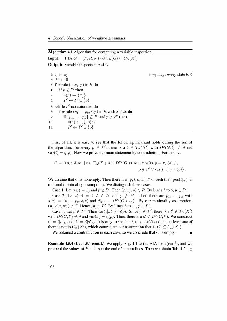
4 Generic binarization of weighted grammars
Algorithm 4.1 Algorithm for computing a variable inspection.
Input: FTA G = (P,R, p0) with L(G) ⊆ C∆(X′)
Output: variable inspection η of G
1: η ← η∅ ⊲ η∅ maps every state to ∅2: P ′ ← ∅3: for rule (ε, xj , p) in R do
4: if p 6∈ P ′ then
5: η(p)← xj6: P ′ ← P ′ ∪ p
7: while P ′ not saturated do
8: for rule (p1 · · · pk, δ, p) in R with δ ∈ ∆ do
9: if p1, . . . , pk ⊆ P′ and p 6∈ P ′ then
10: η(p)←⋃
j η(pj)11: P ′ ← P ′ ∪ p
First of all, it is easy to see that the following invariant holds during the run of
the algorithm: for every p ∈ P ′, there is a t ∈ T∆(X′) with Dp(G, t) 6= ∅ and
var(t) = η(p). Now we prove our main statement by contradiction. For this, let
C = (p, t, d, w) | t ∈ T∆(X′), d ∈ Dp0(G, t), w ∈ pos(t), p = πP (d|w),
p 6∈ P ′ ∨ var(t|w) 6= η(p) .
We assume that C is nonempty. Then there is a (p, t, d, w) ∈ C such that |pos(t|w)| isminimal (minimality assumption). We distinguish three cases.
Case 1: Let t(w) = xj and p 6∈ P ′. Then (ε, xj , p) ∈ R. By Lines 3 to 6, p ∈ P ′.
Case 2: Let t(w) = δ, δ ∈ ∆, and p 6∈ P ′. Then there are p1, . . . , pk with
d(ε) = (p1 · · · pk, δ, p) and d|wj ∈ Dpj (G, t|wj). By our minimality assumption,
(pj , d, t, wj) 6∈ C. Hence, pj ∈ P′. By Lines 8 to 11, p ∈ P ′.
Case 3: Let p ∈ P ′. Then var(t|w) 6= η(p). Since p ∈ P ′, there is a t′ ∈ T∆(X′)
with Dp(G, t′) 6= ∅ and var(t′) = η(p). Thus, there is a d′ ∈ Dp(G, t′). We construct
t′′ = t[t′]w and d′′ = d[d′]w. It is easy to see that t, t′′ ∈ L(G) and that at least one of
them is not in C∆(X′), which contradicts our assumption that L(G) ⊆ C∆(X
′).
We obtained a contradiction in each case, so we conclude that C is empty.
Example 4.5.4 (Ex. 4.5.1 contd.) We apply Alg. 4.1 to the FTA for b(con3), and we
protocol the values of P ′ and η at the end of certain lines. Then we obtain Tab. 4.2.
108
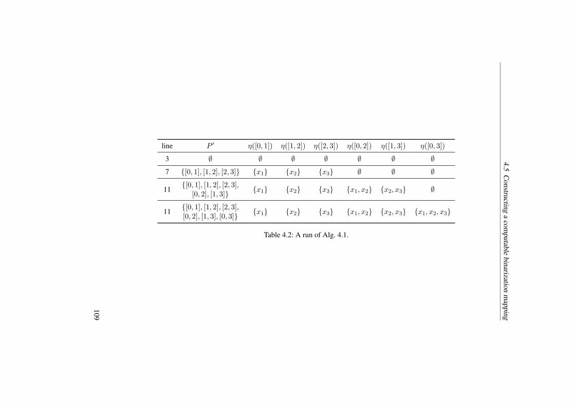
4.5
Constru
cting
aco
mputab
lebin
arization
map
pin
g
line P ′ η([0, 1]) η([1, 2]) η([2, 3]) η([0, 2]) η([1, 3]) η([0, 3])
3 ∅ ∅ ∅ ∅ ∅ ∅ ∅
7 [0, 1], [1, 2], [2, 3] x1 x2 x3 ∅ ∅ ∅
11[0, 1], [1, 2], [2, 3],
[0, 2], [1, 3]x1 x2 x3 x1, x2 x2, x3 ∅
11[0, 1], [1, 2], [2, 3],[0, 2], [1, 3], [0, 3]
x1 x2 x3 x1, x2 x2, x3 x1, x2, x3
Table 4.2: A run of Alg. 4.1.
109
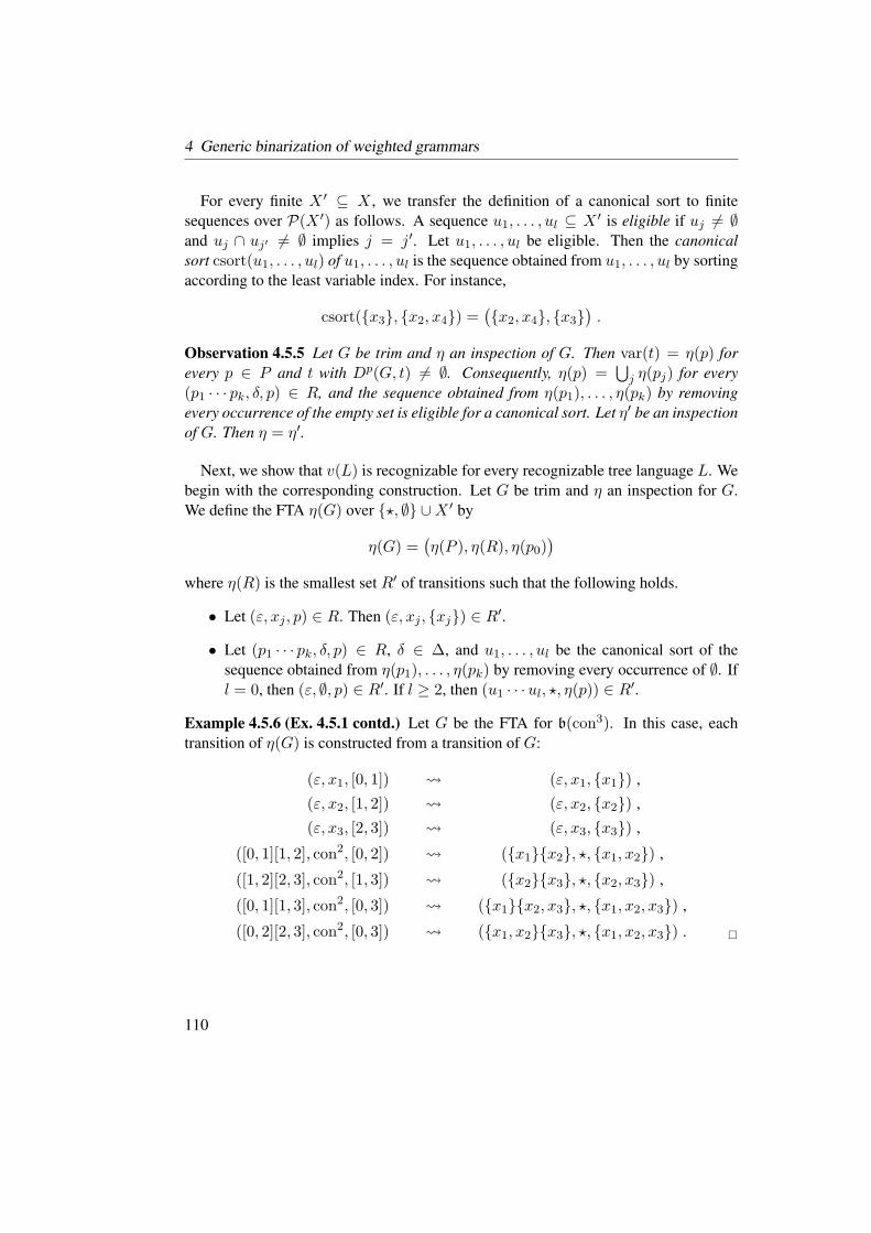
4 Generic binarization of weighted grammars
For every finite X ′ ⊆ X , we transfer the definition of a canonical sort to finite
sequences over P(X ′) as follows. A sequence u1, . . . , ul ⊆ X ′ is eligible if uj 6= ∅and uj ∩ uj′ 6= ∅ implies j = j′. Let u1, . . . , ul be eligible. Then the canonical
sort csort(u1, . . . , ul) of u1, . . . , ul is the sequence obtained from u1, . . . , ul by sorting
according to the least variable index. For instance,
csort(x3, x2, x4) =(x2, x4, x3
).
Observation 4.5.5 Let G be trim and η an inspection of G. Then var(t) = η(p) for
every p ∈ P and t with Dp(G, t) 6= ∅. Consequently, η(p) =⋃
j η(pj) for every
(p1 · · · pk, δ, p) ∈ R, and the sequence obtained from η(p1), . . . , η(pk) by removing
every occurrence of the empty set is eligible for a canonical sort. Let η′ be an inspection
of G. Then η = η′.
Next, we show that v(L) is recognizable for every recognizable tree language L. We
begin with the corresponding construction. Let G be trim and η an inspection for G.
We define the FTA η(G) over ⋆, ∅ ∪X ′ by
η(G) =(η(P ), η(R), η(p0)
)
where η(R) is the smallest set R′ of transitions such that the following holds.
• Let (ε, xj , p) ∈ R. Then (ε, xj , xj) ∈ R′.
• Let (p1 · · · pk, δ, p) ∈ R, δ ∈ ∆, and u1, . . . , ul be the canonical sort of the
sequence obtained from η(p1), . . . , η(pk) by removing every occurrence of ∅. If
l = 0, then (ε, ∅, p) ∈ R′. If l ≥ 2, then (u1 · · ·ul, ⋆, η(p)) ∈ R′.
Example 4.5.6 (Ex. 4.5.1 contd.) Let G be the FTA for b(con3). In this case, each
transition of η(G) is constructed from a transition of G:
(ε, x1, [0, 1]) (ε, x1, x1) ,
(ε, x2, [1, 2]) (ε, x2, x2) ,
(ε, x3, [2, 3]) (ε, x3, x3) ,
([0, 1][1, 2], con2, [0, 2]) (x1x2, ⋆, x1, x2) ,
([1, 2][2, 3], con2, [1, 3]) (x2x3, ⋆, x2, x3) ,
([0, 1][1, 3], con2, [0, 3]) (x1x2, x3, ⋆, x1, x2, x3) ,
([0, 2][2, 3], con2, [0, 3]) (x1, x2x3, ⋆, x1, x2, x3) .
110

4.5 Constructing a computable binarization mapping
Lemma 4.5.7 LetL ⊆ C∆(X′) be recognizable. Then v(L) is effectively recognizable.
PROOF. By Lm. 2.4.10, there is a trim FTA G in root-state form with L(G) = L.
Let G = (P,R, p0). By Lm. 4.5.3, there is an inspection η of G. For the proof of
v(L(G)) = L(η(G)), one shows by induction on m that the following two statements
hold. This is straightforward. Statement 1: For every m ∈ N, p ∈ P , and d ∈ Dpco(G)
with |pos(d)| ≤ m, there is a d′ ∈ Dη(p)co (η(G)) with π⋆,∅∪X′(d′) = v(π∆∪X′(d)).
Statement 2: For every m ∈ N, p ∈ P , and d′ ∈ Dη(p)co (η(G)), there is a d ∈ Dp
co(G)with π⋆,∅∪X′(d′) = v(π∆∪X′(d)).
Now we show that L∩v−1(τ) is recognizable for every recognizable tree language Land every variable tree τ . Again, we begin with the corresponding construction. Let Gbe trim, η an inspection for G, and τ = v(t) for some t ∈ C∆(X
′). We define the FTA
η(G, τ) over ∆ ∪X ′ by
η(G, τ) =(P, η(R, τ), p0
)
where η(R, τ) is the smallest set R′ of transitions such that the following holds.
• Let (ε, xj , p) ∈ R. If τ(w) = xj for some w ∈ pos(τ), then (ε, xj , p) ∈ R′.
• Let (p1 · · · pk, δ, p) ∈ R, δ ∈ ∆, and u1, . . . , ul be the canonical sort of the
sequence obtained from η(p1), . . . , η(pk) by removing every occurrence of ∅. If
l < 2 or if there is a w ∈ pos(τ) with rkτ (w) = l, var(τ |w) = η(p), and
var(τ |wj) = uj , then (p1 · · · pk, δ, p) ∈ R′.
Example 4.5.8 (Ex. 4.5.1 contd.) Let G be the FTA for b(con3) and τ as in Fig. 4.6,
i.e., τ = ⋆(⋆(x1, x2), x3). Then η(G, τ) has the following transitions: (ε, x1, [0, 1]),(ε, x2, [1, 2]), (ε, x3, [2, 3]), ([0, 1][1, 2], con
2, [0, 2]), ([0, 2][2, 3], con2, [0, 3]).
Lemma 4.5.9 Let L ⊆ C∆(X′) be recognizable and τ = v(t) for some t ∈ L. Then
L ∩ v−1(τ) is effectively recognizable.
PROOF. By Lm. 2.4.10, there is a trim FTA G in root-state form with L(G) = L.
Let G = (P,R, p0). By Lm. 4.5.3, there is an inspection η of G. We prove that
L(G) ∩ v−1(τ) = L(η(G, τ)).We begin with “⊆”. To this end, let t ∈ L(G) such that v(t) = τ . Then there is
a p0-run d of G on t. We show by induction on m that d|w ∈ Dp(G) implies d|w ∈
Dp(η(G, τ)) for every m ∈ N, p ∈ P , and w ∈ pos(d) with |pos(d|w)| ≤ m. For the
induction base (m = 0), there is nothing to show. We show the induction step (m →m+1). For this, let m ∈ N, p ∈ P , and w ∈ pos(d) such that |pos(d|w)| ≤ m+1 and
111
4 Generic binarization of weighted grammars
d|w ∈ Dp(G). By the induction hypothesis, it suffices to show that d(w) ∈ η(R, τ).
We distinguish two cases.
Case 1: Let d(w) = (ε, xj , p). Then d(w) ∈ η(R, τ).Case 2: Let d(w) = (p1 · · · pk, δ, p) and δ ∈ ∆. Let u1, . . . , ul be the canonical sort
of the sequence obtained from η(p1), . . . , η(pk) by removing every occurrence of ∅. If
l < 2, then d(w) ∈ η(R, τ) holds trivially. Let l ≥ 2; then by definition v(t|w) =⋆(v(t′1), . . . , v(t
′l)) where t′1, . . . , t
′l is obtained from t|w1, . . . , t|wk by removing every
occurrence of any tree that does not contain any variables. It is easy to see from the
recursive definition of v that v(t|w) occurs in v(t). Since η is an inspection, and since
var(v(t)) = var(t) for every t ∈ T∆, we obtain that η(p) = var(t|w) = var(v(t|w))and η(pj) = var(t|wj) = var(v(t|wj)). Hence, d(w) ∈ η(R, τ).
Now we show “⊇”. Since η(R, τ) ⊆ R, we obtain that L(η(G, τ)) ⊆ L(G) and
that η is also an inspection for η(G, τ). We show that L(η(G, τ)) ⊆ v−1(τ). The case
that η(p0) = ∅ is easy. Let η(p0) 6= ∅. We make the following crucial observation: for
every u ⊆ Xk, there is at most one w′ ∈ pos(τ) with var(τ |w′) = u. Let t ∈ T∆ and
d ∈ Dp0(G, t). We show by induction on m that, for every m ∈ N and w ∈ pos(d), if
|pos(d|w)| ≤ m and η(πP (d|w)) 6= ∅, then there is a w′ ∈ pos(τ) such that v(t|w) =τ |w′ . Then, since var(t) = η(p0) = var(τ |ε) and by our observation, we have that
v(t) = τ .
For the induction base (m = 0), there is nothing to show. We show the induction
step (m→ m+ 1). For this, let m ∈ N and w ∈ pos(d) such that |pos(d|w)| ≤ m+ 1and η(πP (d|w)) 6= ∅. We distinguish two cases.
Case 1: Let d(w) = (ε, xj , p). Clearly, there is a w′ ∈ pos(τ) with τ(w′) = xj .
Case 2: Let d(w) = (p1 · · · pk, δ, p) and δ ∈ ∆. Let u1, . . . , ul be obtained from
η(p1), . . . , η(pk) by removing every occurrence of ∅. There are uniquely determined
j1, . . . , jl such that uι = η(pjι). If l ≤ 2, then l = 1, and ν(p) = u1. By the
induction hypothesis, there is a w′ with v(t|wj1) = τ |w′ . Hence, we can derive that
v(t|w) = v(t|wj1) = τ |w′ . If l ≥ 2, then v(t|w) = ⋆(v(t|wj1), . . . , v(t|wjl)). Since
d(w) ∈ η(R, τ), we have that there is aw′ ∈ τ with var(τ |w′) = η(p) and var(τ |w′ι) =uι. By the induction hypothesis, we have that there arew′
1, . . . , w′l with v(t|wjι) = τ |w′
ι.
By our initial observation, we obtain that w′ι = w′ι. Hence, v(t|w) = τ |w′ .
4.5.2 Binarization under binarization rules
Let b = (b1, . . . , bn) such that bi is a b-rule over Ai. A ξ-binarization (Γ′,M ′, h′)of ρ is called “under b” if h′i(ξ) ∈ bi(hi(α)). Likewise, a binarization hedge t of ρis called “under b” if ti ∈ bi(hi(α)). Lemma 4.4.9 and Obs. 4.4.10 carry over to
these restricted notions. A binarization mapping bin : C → C is called b-complete if
bdom(bin) contains every B ∈ C such that for every suprabinary rule ρ of B there is a
112

4.5 Constructing a computable binarization mapping
Algorithm 4.2 Binarization algorithm.
Input: IRTG B = (Γ,M, h) over ∆ and S ,
b-rules b1, . . . , bn over ∆1, . . . ,∆n, respectively
Output: IRTG B′ over ∆ and S
1: B′ ← B2: for each rule ρ : (q1 · · · qk, α, q) of B with k > 2 do
3: compute FTA G′ for⋂
i v(bi(hi(α)))4: if L(G′) 6= ∅ then
5: select τ ∈ L(G′)6: for i = 1, . . . , n do
7: compute FTA G′i for bi(hi(α)) ∩ v
−1(τ)8: select ti ∈ L(G
′i)
9: B′ ← B′[ρ/B(ρ, t1, . . . , tn)]
binarization of ρ under b.
By definition, rule-by-rule complete implies b-complete. The converse need not be
true. However, if the b-rules b have a certain property, we can guarantee that b-complete
also implies rule-by-rule complete. More specifically, we say that b is complete on B if
v(bi(hi(α)) = v(bi(hi(α)) for every α ∈ Γ and i ∈ 1, . . . , n. Then the intersection
in Obs. 4.4.10 is empty in the restricted case iff it is empty in the general case, i.e.,
⋂
i v(bi(hi(α))) 6= ∅ ⇐⇒⋂
i v(bi(hi(α))) 6= ∅ .
Consequently, if b is complete on every element of C, then b-complete implies rule-by-
rule complete.
Now we have the ingredients that we need for a template that gives rise to a class
of computable binarization mappings. It is shown as Alg. 4.2. As before, we obtain a
concrete binarization mapping by making the for-loop and the selections deterministic.
In Line 3, we use Lms. 4.5.2 and 4.5.7 and that the class of recognizable tree languages
is effectively closed under intersection [80, Prop. 7.1]. In Line 7, we use Lm. 4.5.9.
The following theorem documents the behavior of the template. In short, when we fix
b, the template describes a class of b-complete binarization mappings.
Theorem 4.5.10 Let
• ∆ = (∆1, . . . ,∆n) be a sequence of ranked alphabets,
• S a commutative semiring,
• A = (A1, . . . ,An) a sequence such that Ai is a ∆i-algebra,
113

4 Generic binarization of weighted grammars
• b = (b1, . . . , bn) a sequence such that bi is a b-rule over Ai.Moreover, let B be an IRTG over ∆ and S . If we execute Alg. 4.2 with input B and b,
then it terminates, and it outputs an IRTG B′ over ∆ and S such that (i) B′ is of rank 2iff every suprabinary rule of B has a binarization under b, (ii) if B is A-admissible,
then so is B′, and (iii) in that case, B and B′ are A-equivalent.
The runtime of Alg. 4.2 is dominated by the intersection in Line 3, whose runtime
is in O(m1 · · ·mn), where mi is the size of the FTA for bi(hi(α)). The quantity mi is
linear in the size of the terms in hi(α) | α ∈ Γ and in the number of transitions in
the FTAs for the b-rule bi. It is convenient to consider this quantity to be constant; then
the overall runtime of our algorithm is in O(|R| · cn) for some c ∈ N.
4.6 Application to established formalisms
In this section we consider how the RCBMs for IRTGs can (or cannot) be used to obtain
RCBMs for established formalisms such as SCFGs, tree-to-string transducers (yXTTs),
or WSCFTGs.
4.6.1 General approach
First, we briefly consider two possible approaches to this question: the solution-transfer
approach and the problem-transfer approach. To this end, let F be a class of devices
(such as SCFGs).
In the solution-transfer approach, we are interested in a partial mapping bin : F → Fthat preserves meaning and reduces the rank to 2. We assume that there is a suitable
subclass C of IRTGs for which we already have a binarization mapping bin ′. Then we
define bin as follows: given an element of F , we convert it into an IRTG in C, we
apply (if possible) bin ′, and then we convert the resulting IRTG back; naturally, the
conversion must preserve rank and meaning. The problem is that we cannot make any
meaningful statement about bin (e.g., whether it is rule-by-rule complete) without the
whole formal apparatus for F .
In the problem-transfer approach, we also assume that there is a suitable subclass Cof IRTGs as well as means of converting back and forth. However, we regard this
conversion as rather hypothetical, for when it comes to treating binarization and other
problems formally, we stipulate that C rather than F is the formalism in question, and
that F is effectively obsolete. That is, our aim then is to find a binarization mapping
bin : C → C. This change of perspective enables us to use IRTG terminology through-
out. We note that it remains possible to use existing infrastructure for F , namely via
conversion; we just do not make any formal statements pertaining to F .
114

4.6 Application to established formalisms
In the following, we will pursue the problem-transfer approach. To this end, we
define what a grammar formalism is (from the point of view of IRTGs), we motivate
that definition, and then we define the binarization mapping for a formalism, given
appropriate b-rules. We will consider examples of formalisms, such as SCFGs, and the
respective binarization mappings in the subsequent subsections.
Let ∆ = (∆1, . . . ,∆n) be a sequence of ranked alphabets and S a semiring. A
(grammar) formalism is a triple (C,A, ϕ) such that
• A = (A1, . . . ,An) is a sequence such that Ai is a ∆i-algebra, and
• C is a set of A-admissible IRTGs over ∆ and S ,
• ϕ : C → C is an idempotent mapping (called normal-form mapping) that pre-
serves meaning, rank, and rule-by-rule (non)binarizability, i.e., every suprabinary
rule of B has a binarization iff the same is true for ϕ(B).
Let (C,A, ϕ) be a formalism. We usually identify (C,A, ϕ) with C. For every B ∈ C,
we define the C-meaning JBKC of G by letting JBKC = JBKA.
Let us motivate our definition of a formalism. First, we observe that the definition of
a grammar class such as SCFG implicitly uses a fixed selection of operations, and these
operations can be captured by a fixed sequence A of algebras. Second, it is important
to note that C is often a strict subset of all IRTGs over ∆ and S; e.g., in a WSCFTG
the variables in Y may not occur arbitrarily often in a rule. Third, we recall that IRTGs
can offer a high degree of freedom for expressing the generational behavior of a rule,
as illustrated in Ex. 4.2.2. We accommodate this fact by the normal-form mapping. We
require that rank and rule-by-rule (non)binarizability be preserved so that the normal
form does not interfere with binarization.
Let b = (b1, . . . , bn) be a sequence such that bi is a b-rule over Ai. Moreover, let
binb be a computable b-complete binarization mapping for A-admissible IRTGs over
∆ and S; we know that such a mapping exists because of Thm. 4.5.10. We define the
partial mapping binC : C → C by letting
binC = (binb ϕ) ∩ (C × C) .
There are three possible causes when B ∈ C \ bdom(binC):
1. some suprabinary rule of B does not have a binarization,
2. the b-rules are not complete on ϕ(B), or
3. binb(ϕ(B)) 6∈ C.
115

4 Generic binarization of weighted grammars
In a practical application, each of these causes may be acceptable. We, however, take
a theoretical stance and accept only the first cause. In other words, we want binC
to be rule-by-rule complete. Correspondingly, we say that C and b are admissible if
binb(ϕ(C)) ⊆ C, and they are complete if b is complete on every element of ϕ(C). If
we have admissibility and completeness, then binC is rule-by-rule complete.
We note that the properties “admissible” and “complete” refer to the combination of
formalism and b-rules. However, for the sake of simplicity, we will also say that some
formalism is admissible or complete, assuming that the b-rules are fixed.
In the following subsections we consider concrete algebras and formalisms.
4.6.2 Useful algebras and b-rules
We consider three algebras together with suitable b-rules: the string algebra, the hedge
algebra, and the hedge algebra with substitution. A hedge is a sequence of trees; this
notion is central to XML-related theory [140, 177], and in work related to natural-
language processing, hedges are also called s-terms [169]. In this section, we deviate
from Sec. 2.2 and define trees and hedges anew.
To this end, let Σ and V be sets. Then the set HΣ(V ) of hedges over Σ indexed by Vand the set TΣ(V ) of trees over Σ indexed by V are defined by
(HΣ(V ), TΣ(V )) = (H,T ) ,
where (H,T ) is the smallest pair, according to the pointwise subset relation, such that
• T ∗ ⊆ H ,
• V ⊆ T , and
• σ(u) ∈ T if σ ∈ Σ and u ∈ H .
Let V ′ ⊆ Σ ∪ V ∪ X ∪ Y and f : V ′ → HΣ(V ). Then we define the mappings
f , f : HΣ(V ) → HΣ(V ), called first-order substitution and second-order substitu-
tion, respectively, as follows. We let
f (ε) = f (ε) = ε .
For every v ∈ V and u ∈ HΣ(V ), we let
f (vu) =
f(v)f (u) if v ∈ V ′,
vf (u) if v 6∈ V ′.f (vu) =
f(v)f (u) if v ∈ V ′,
vf (u) if v 6∈ V ′.
116

4.6 Application to established formalisms
Ranked alphabets Σ alphabet, K ∈ N
SYM(Σ) = σ(0) | σ ∈ Σ
TOP(Σ) = σ(1) | σ ∈ Σ
CONK = (conk)(k) | 0 ≤ k ≤ K, k 6= 1
ΠK = πk | 1 ≤ k ≤ K
SUBK = (subk)(k+1) | 1 ≤ k ≤ K
Operations σ ∈ Σ, k ∈ N, D set
symσ : ((Σ ∪X)∗)0 → (Σ ∪X)∗, () 7→ σ
topσ : (HΣ∪X(Y ))1 → HΣ∪X(Y ), (u1) 7→ σ(u1)
conk,D : (D∗)k → D∗, (w1, . . . , wk) = w1 · · ·wkpik : (HΣ∪X(Y ))0 → HΣ∪X(Y ), () 7→ yk
subk : (HΣ∪X(Y ))k+1 → HΣ∪X(Y ),
(u, u1, . . . , uk) 7→ u[y1/u1] · · · [yk/uk]
Table 4.3: Ranked alphabets and operations for our algebras.
For every σ(u1)u2 ∈ HΣ(V ), we let
f (σ(u1)u2) =
f(σ)f (u2) if σ ∈ V ′,
σ(f (u1))f(u2) if σ 6∈ V ′.
If V ′ = v1, . . . , vl, then we also denote f (u) by u[v1/f(v1)] · · · [vl/f(vl)]. We let
f (σ(t1, . . . , tk)u) =
f(σ)[y1/f(t1)] · · · [yk/f
(tk)]f(u) if σ ∈ V ′,
σ(f (t1), . . . , f(tk))f
(u) if σ 6∈ V ′.
If V ′ = v1, . . . , vl, then we also denote f (t) by tLv1/f(v1)M · · · Lvl/f(vl)M.Now we proceed to discuss the three algebras promised above. We define these
algebras based on the alphabets and the operations shown in Tab. 4.3; the algebras
themselves are given in Tab. 4.4.
String algebra Roughly speaking, the string algebra is defined like the algebra Ain Ex. 4.2.2. In addition to the alphabet Σ, we have another parameter K ∈ N that
restricts the number of con-symbols.
117

4G
ener
icbin
ariz
atio
nof
wei
ghte
dgra
mm
ars
hedge algebra
string algebra hedge algebra with substitution
over Σ and K over Σ and K over Σ and K
example term
and
denoted object
con2
a b7→ ab
σ
con2
α
con0
β
con0
7→
σ
α β
sub1
σ
con2
π1 β
con0
α
con0 7→
σ
α β
signature SYM(Σ) ∪ CONK TOP(Σ) ∪ CONK TOP(Σ) ∪ CONK ∪ΠK ∪ SUBK
domain (Σ ∪X)∗ HΣ∪X(Y ) HΣ∪X(Y )
realization
mapping
σ 7→ symσ
conk 7→ conk,Σ∪X
σ 7→ topσconk 7→ conk,TΣ∪X(Y )
σ 7→ topσconk 7→ conk,TΣ∪X(Y )
πk 7→ piksubk 7→ subk
Table 4.4: Algebras for strings and hedges, given an alphabet Σ and a maximum arity K ∈ N.
118

4.6 Application to established formalisms
We use the following b-rule b (cf. Ex. 4.5.1): it maps each σ ∈ Σ to σ, and it maps
con0 to con0. Each symbol conk, k ≥ 2, is mapped to the language recognized by
the following FTA with states of the form [j, j′] (where 0 ≤ j < j′ ≤ k) and root state
[0, k]:
(ε, xj , [j − 1, j]) , (1 ≤ j ≤ k)
([j, j′′] [j′′, j′], con2, [j, j′]) . (0 ≤ j < j′′ < j′ ≤ k)
Hedge algebra This algebra incorporates two main ideas:
1. We can construct a tree σ(t1, . . . , tk) in two steps: first, we construct the hedge
t1 · · · tk of children, and second, we “put” a node labeled σ “on top”.
2. We can identify any tree t with the hedge (t) of length 1.
Correspondingly, the domain is the set HΣ∪X(Y ) of hedges, and we have two kinds of
operations: (i) for every σ ∈ Σ, we can put σ on top of a hedge, yielding a hedge of
length 1; and (ii) we can concatenate k hedges, as in the string algebra.
We use the following b-rule b: it maps con0 to con0 and each unary symbol σ to
σ(x1). Each symbol conk, k ≥ 2, is treated as in the string case.
Hedge algebra with substitution We can supplement the hedge algebra with a
substitution operation; this way we can describe formalisms like WSCFTGs. As an
example for substitution, we consider the term function f of sub1(x2,S (x1)). For
every t1 ∈ TΣ and t2 ∈ CΣ(Y1), we have that f(t1, t2) = tLx2/t2MLx1/t1M, where
t = x2(S(x1)). A similar algebra with substitution has been described in [113, 127];
the basic idea goes back to the derived alphabets of [67].
We use the following b-rule b: it maps con0 to con0 and each unary symbol σ to
σ(x1). Each symbol conk, k ≥ 2, is treated as in the string case. Furthermore, it
maps πk, k ≥ 1, to πk, sub1 to sub1(x1, x2), and subk, k > 1, to ∅.
In the following, when we use a string algebra (or hedge algebra, or hedge algebra
with substitution), say,A1, we will silently assume that ∆1 is its signature and b1 is the
corresponding b-rule.
4.6.3 Synchronous context-free grammars
Let Σ be an alphabet and K ∈ N. We will define the formalism SCFG(Σ,K), which,
informally speaking, represents SCFGs over Σ whose rules contain strings of length at
most K. To this end, let A be the string algebra over Σ and K.
119

4 Generic binarization of weighted grammars
We let SCFG(Σ,K) = (C, (A,A), ϕ), where we define C and ϕ as follows. We
let C be the set of all IRTGs B over (∆,∆) and Real such that, if B = (Γ,M, h),then |hi(α)
A(x1, . . . , xl)| ≤ K for every i ∈ 1, 2, l ∈ N, and α ∈ Γ(l). Now we
define ϕ : C → C. To this end, let B ∈ C and B = (Γ,M, h). We construct ϕ(B) =(Γ,M, h′) where, for every l ∈ N and α ∈ Γ(l), h′i(α) = f(hi(α)
A(x1, . . . , xl)), and
f : (Σ ∪X)∗ → T∆(X) is defined by
f(σ1, . . . , σk) =
conk(σ1, . . . , σk) if k 6= 1,
σ1 otherwise.
It is easy to see that ϕ is idempotent, and that it preserves rank and variable trees (and,
a fortiori, rule-by-rule (non)binarizability).
It remains to show that ϕ preserves meaning. To this end, let i ∈ 1, 2, l ∈ N, and
g : Xl → Σ∗. Recall that g♯ is the homomorphic extension of g to A. For this proof,
we extend g♯ to T∆i(Xl)
∗ by letting g♯((t1, . . . , tk)) = g♯(t1) · · · g♯(tk). A simple
proof by induction on m yields that g♯(t) = g♯(tA(x1, . . . , xl)) for every m ∈ N and
t ∈ T∆i(Xl) with |pos(t)| ≤ m. From this, we conclude that tA = fi(t)
A, which
implies hi(α)A = h′i(α)
A for every α ∈ Γ. Now one can employ Cor. 4.2.7 in another
simple proof by induction to show that hi(ξ)A = h′i(ξ)
A for every ξ ∈ TΓ. From this,
we conclude that JGK = Jϕ(G)K.
The formalism SCFG(Σ,K) is trivially admissible, because the b-rule for the string
algebra does not introduce conk with k > K. It is also complete. We note that our for-
malism would not be complete if ϕ did not collapse occurrences of conk. For instance,
the term con2(con2(x1, x2), x3) is equivalent to itself and to con2(x1, con2(x2, x3)),
but the b-rules only cover the former. Thus they miss one variable tree. For the col-
lapsed version con3(x1, x2, x3), however, the b-rules cover both variable trees.
The binarization mapping binC coincides with that of [97]: any rule can be binarized
in both frameworks or neither. For instance, for the SCFG rule
A→ α(B,C,D,E), α = 〈x1 x2 x3 x4, x2 x4 x1 x3〉,
the sets v(b(h1(α))) and v(b(h2(α))) are disjoint; thus, no binarization exists.
4.6.4 Tree-to-string and hedge-to-string transducers
Some approaches to SMT go beyond string-to-string translation models such as SCFG
by exploiting known syntactic structures in the source or target language. This perspec-
tive on translation naturally leads to the use of yXTTs [181, 79, 95, 90].
120
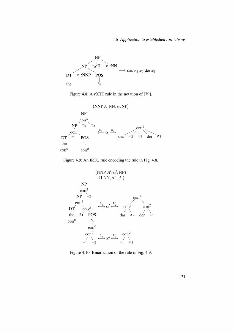
4.6 Application to established formalisms
NP
NP
DT
the
x1:NNP POS
’s
x2:JJ x3:NN−→ das x2 x3 der x1
Figure 4.8: A yXTT rule in the notation of [79].
(NNP JJ NN, α,NP)
NP
con3
NP
con3
DT
the
con0
x1 POS
’s
con0
x2 x3h1←− [ α
h27−→con5
das x2 x3 der x1
Figure 4.9: An IRTG rule encoding the rule in Fig. 4.8.
(NNP A′, α′,NP)(JJ NN, α′′, A′)
NP
con2
NP
con2
DT
the
con0
con2
x1 POS
’s
con0
x2
h′1←− [ α′ h′27−→
con2
con2
das x2
con2
der x1
con2
x1 x2
h′1←− [α′′ h′27−→con2
x1 x2
Figure 4.10: Binarization of the rule in Fig. 4.9.
121

4 Generic binarization of weighted grammars
NP
NP
DT
the
x1:NNP POS
’s
NP
x2:JJ x3:NN
−→ das x2 x3 der x1
Figure 4.11: yXTT rule, slightly adapted to enable binarization.
Example 4.6.1 Figure 4.8 shows an example of a yXTT rule in the notation of [79].
This rule might be used to translate “the Commission’s strategic plan” into “das lang-
fristige Programm der Kommission”. By employing both the hedge and the string alge-
bra, we can represent this rule in an IRTG B, as indicated in Fig. 4.9. We may replace
this suprabinary rule by the two binary rules shown in Fig. 4.10 without affecting the
meaning, obtaining the IRTG B′.
However, the binary rules lack a counterpart in the original notation of yXTT, be-
cause h′1(α′) does not denote a sequence of length 1. Assume that we have a formalism
(C,A, ϕ) and b-rules b1, b2 such that B′ = bin(b1,b2)(ϕ(B)). Now either B′ ∈ C;
then it is unclear what yXTT it corresponds to. Or B′ 6∈ C; then our formalism is not
admissible.
It is not just a coincidence that finding an admissible formalism for yXTT seems
hard. After all, since each child of the root node in Fig. 4.8 contains a variable that may
be replaced with unbounded material, we just cannot factor the rule and at the same
time stay within yXTT. If we are willing to accept a change of meaning, then we could
instead factor the rule in Fig. 4.11.
Example 4.6.1 illustrates that finding an admissible formalism for yXTTs is not
straightforward. In fact, the author is not aware of an admissible combination of a
formalism and b-rules for yXTTs; and, contrary to its appearance, the article [29] cer-
tainly does not provide such an admissible combination.
Instead of yXTTs, we therefore consider hedge-to-string transducers (yXHTs), an
ad-hoc straightforward generalization of yXTTs (not to be confused with the hedge-
to-string transducers of [34]). On the one hand, this course of action seems logical;
for if we identify a hedge of length 1 with its only tree, then every yXTT is also a
yXHT, and its “yXTT meaning” coincides with its “yXHT meaning”. On the other
hand, we should be aware that existing infrastructure needs to be adapted in order to
accommodate yXHTs, e.g., when it comes to computing the input product.
Let Σ be an alphabet and K ∈ N. We will define the formalism yXHT(Σ,K),which, informally speaking, represents hedge-to-string transducers over Σ. To this
122

4.6 Application to established formalisms
end, let A1 be the hedge algebra over Σ and K, and let A2 be the string algebra over
Σ and K. We let yXHT(Σ,K) = (C, (A1,A2), ϕ) as follows. We let C be the set of
all IRTGs B over (∆1,∆2) and Real such that, if B = (Γ,M, h), then, for every l ∈ N
and α ∈ Γ(l),
• maxrkt(w) | w ∈ pos(t) ≤ K, where t = h1(α)A1(x1, . . . , xl), and
• |h2(α)A2(x1, . . . , xl)| ≤ K.
Now we define ϕ : C → C. To this end, let B ∈ C and B = (Γ,M, h). We construct
ϕ(B) = (Γ,M, h′), where h′2 is defined as in the SCFG case and, for every l ∈ N and
α ∈ Γ(l), h′1(α) = f(h1(α)A1(x1, . . . , xl)), where f : HΣ1∪X(Y ) → T∆1(X) inserts
conk appropriately, i.e., we let
f(t1, . . . , tk) = conk(f(t1), . . . , f(tk)) , (k 6= 1)
f(xj) = xj ,
f(σ(t)) = σ(f(t)) ,
f(σ(t1, . . . , tk)) = σ(conk(f(t1), . . . , f(tk))) . (k 6= 1)
We omit the proof that ϕ is idempotent and preserves rank, meaning, and rule-by-rule
(non)binarizability.
The formalism yXHT(Σ,K) is trivially admissible, for the same reason as in the
SCFG case. It is also complete. The binarization mapping binC acts as in Ex. 4.6.1.
The author has implemented Alg. 4.2 and the b-rules b1 and b2. In order to test
the implementation, he extracted a yXHT from about a million parallel sentences of
English-German Europarl data [109], using the GHKM rule extractor [78]. Then he
applied the binarization algorithm to the yXHT. The results are shown in Fig. 4.12: of
the 2.15 million rules in the extracted transducer, 460,000 were suprabinary, and 67 %
of these had a binarization. Binarization took 4.4 minutes on a single core of an Intel
Core i5 2520M processor.
4.6.5 Weighted synchronous context-free hedge grammars
Ideally we would like to embed the class of all WSCFTGs into IRTGs and use the
resulting formalism for binarization. However, as in the case of yXTT, and for the
same reasons, the author is not aware of an admissible combination of a formalism
and b-rules. We follow the same course of action as before: instead of WSCFTGs,
we consider an ad-hoc generalization that we call weighted synchronous context-free
hedge grammars (WSCFHGs). We note that “WSCFHG” is not to be confused with the
context-free hypergraph grammar (CFHG) of [64].
123

4 Generic binarization of weighted grammars
1
1.2
1.4
1.6
1.8
2
2.2
2.4
ext bin
# r
ule
s (m
illi
ons)
rank
0123456-78-10
Figure 4.12: Rules of a yXTT extracted from Europarl (ext) vs. its binarization (bin).
Let Σ be an alphabet,K ∈ N, and S a complete commutative semiring. We define the
formalism CFHG(Σ,K,S), which, informally speaking, represents WSCFHGs over
Σ and S . This definition is the spirit of [30, Def. 5, Def. 7], which is in turn inspired by
[49, Prop. 4.10] and [69, Lm. 5.8]. Let A be the hedge algebra with substitution over
Σ and K. Moreover, let m, r1, . . . , rl ∈ N. Then T∆(m, r1, . . . , rl) denotes the set of
all t ∈ T∆(Xl) such that
• t is linear and nondeleting in Πm,
• for every w ∈ pos(t) and j ∈ N, if t(w) = πj , then j ≤ m,
• for every w ∈ pos(t) and k ∈ N, if t(w) = subk, then there is a ι ∈ 1, . . . , lwith t(w1) = xι and k = rι,
• for every j ∈ 1, . . . , l, if rj 6= 0, then there is a w ∈ pos(t) with t(w) = subrj
and t(w1) = xj .
In addition, we define the mapping f ′ : T∆(m, r1, . . . , rl)→ HΣ∪X(Y ) by letting
f ′(t) = tA(x1(y1, . . . , yr1), . . . , xl(y1, . . . , yrl)) .
Example 4.6.2 Figure 4.13 illustrates f ′.
We let CFHG(Σ,K,S) = (C, (A,A), ϕ) as follows. We let C be the set of all
IRTGs B over (∆,∆) and S such that if B = (Γ,M, h) and M = (Q,R, µ, ν), then
there is a mapping rk : Q → N such that νq 6= 0 implies rk(q) = 0, and, for every
(q1 · · · ql, α, q) ∈ R and i ∈ 1, 2,
124

4.6 Application to established formalisms
sub1
x2 S
con3
〈
con0
x1 〉
con0
7→
x2
S
〈 x1 〉
S
con3
a
con0
sub1
x1 S
con3
b
con0
π1 c
con0
d
con07→
S
a x1
S
b y1 c
d
Figure 4.13: Illustration of f ′.
• hi(α) ∈ T∆(rk(q), rk(q1), . . . , rk(ql)) and
• maxrkt(w) | w ∈ pos(t), t(w) ∈ Σ ≤ K where t = f ′(hi(α)).
Now we define ϕ : C → C. To this end, let B ∈ C and B = (Γ,M, h). We construct
ϕ(B) = (Γ,M, h′), where, for every l ∈ N, α ∈ Γ(l), and i ∈ 1, 2,
h′i(α) = f(f ′(hi(α)))
and f : HΣ∪X(Y )→ T∆(X) inserts conk and subk appropriately, i.e., we let
f(t1, . . . , tk) = conk(f(t1), . . . , f(tk)) , (k 6= 1)
f(xj) = xj ,
f(xj(t1, . . . , tk)) = subk(xj , f(t1), . . . , f(tk)) , (k 6= 0)
f(σ(t1, . . . , tk)) = σ(f(t1)) , (k = 1)
f(σ(t1, . . . , tk)) = σ(conk(f(t1), . . . , f(tk))) . (k 6= 1)
We omit the proof that ϕ is idempotent and preserves rank, meaning, and rule-by-rule
(non)binarizability.
Example 4.6.3 By reversing the arrows in Fig. 4.13, we obtain an illustration of f . In
fact, f ′(f(u)) = u, and one might say that f(u) is a particularly designated element of
f ′−1(u).
The formalism CFHG(Σ,K,S) is trivially admissible, for the same reason as in the
SCFG and yXHT cases. It is not complete; for instance, the term
sub2(x1, σ(con0), σ(con0))
125
4 Generic binarization of weighted grammars
is mapped to the empty set by our b-rule, although the term itself has a binary variable
tree, namely x1. However, we can define a restricted variant of CFHG(Σ,K,S) where
the use of subk and πk with k > 1 is banned; this variant might be called “synchronous
hedge-adjoining grammar”. With the restricted variant, we have both admissibility and
completeness.
We indicate that we can embed the WSCFTGs of Ch. 3 into CFHG(Σ,K,S). To
this end, let M = (Q,R, µ, ν) be a WSCFTG over Σ and S such that for every
(q1 · · · ql, 〈ζ1ζ2〉, q) ∈ R and i ∈ 1, 2, we have that
• maxrkζi(w) | w ∈ pos(ζi), ζi(w) ∈ Σ ≤ K.
We construct the IRTG B = (Γ,M, h) over ∆ and S where
• Γ = γ(k) | ∃q1, . . . , qk, q ∈ Q : (q1 · · · qk, γ, q) ∈ R,
• hi(〈ζ1ζ2〉) = f(ζi).
Then B ∈ CFHG(Σ,K,S). We omit the proof that JBK = JMK.
Conversely, under suitable conditions, we can convert back from CFHG(Σ,K,S)into WSCFTG. To this end, we employ the normal form via ϕ as well as the normal
form via ψ established below Ex. 4.2.3. Let B ∈ ψ(ϕ(C)), B = (Γ,M, h), and
M = (Q,R, µ, ν). Then we construct the quadruple G = (Q,R′, µ′, ν) with
• R′ = (q1 · · · ql, 〈f′(γ1)f
′(γ2)〉, q) | (q1 · · · ql, γ, q) ∈ R and
• µ′(q1 · · · ql, 〈f′(γ1)f
′(γ2)〉, q) = µ(q1 · · · ql, γ, q).
Note that µ′ is well defined because the mapping with γ 7→ 〈f ′(γ1)f′(γ2)〉 is injective.
Let f ′(γi) be a hedge of length 1 for every γ ∈ Γ and i ∈ 1, 2. ThenG is a WSCFTG.
We omit the proof that JBK = JGK.
Example 4.6.4 Recall the WSCFTG of Ex. 3.3.1. The application of f ′ in Fig. 4.13
yields the input trees of the rules ρ1 and ρ3.
4.7 Conclusion, discussion, and outlook
We have developed a template that gives rise to a class of efficiently computable bi-
narization mappings for IRTGs, given b-rules. If the b-rules are complete in a sense,
then these mappings are rule-by-rule complete, which is on par with the state of the
art. We have shown how to apply this technology for deriving rule-by-rule complete
binarization mappings for established formalisms, such as SCFGs. In the process, we
126
4.7 Conclusion, discussion, and outlook
discovered that yXHT and WSCFHGs are better suited for binarization than the con-
ventional formalisms yXTT and WSCFTG, respectively.
As mentioned in the introduction, binarization is used to speed up operations that
occur in a typical decoder. Unfortunately, the binarization domain of a rule-by-rule
complete binarization mapping need not contain every grammar, in particular for n ≥2. According to [54], there is an alternative way of improving the runtime of such a
decoder that only requires binarization for the case n = 1, however at the price that the
result is approximate.
As mentioned at the very top, this chapter is a greatly expanded version of [29]. The
author would like to point out a mistake in said publication: it claims that it provides
a binarization mapping for yXTTs, which is untrue; just like this chapter, it provides a
binarization mapping for yXHTs.
In [113], the authors provide an algebra for representing STAGs as IRTGs. In con-
trast to our hedge algebra with substitution, that algebra is more akin to the Σ-term
algebra, i.e., its domain only covers ranked trees, and it does not provide a string con-
catenation operation. Consequently, the IRTGs using this algebra are indeed close to
STAGs, as opposed to the IRTGs using our algebra, which we therefore call weighted
synchronous context-free hedge grammars. We stress that this deviation is on purpose,
for WSCFHGs are better suited for binarization than WSCFTGs, as illustrated already
for yXTTs in Ex. 4.6.1.
There are at least six items for further research, which we discuss in the following.
First, one might investigate input and output products for the formalisms yXHT and
WSCFHG. To this end, one could start off with existing work for unweighted IRTGs
[112, 113] and “add weights”, or one could start off with existing work for yXTTs or
WSCFTGs (e.g., from Ch. 3) and “add hedges”.
Second, it would be interesting how to select a binarization mapping for “space-
optimal” binarization. To elucidate this problem, we recall the CFG example from
Sec. 4.1, where we replaced
A→ BCDE by A→ [[BC]D]E , [[BC]D]→ [BC]D , [BC]→ BC .
If the next replacement was to be
D → EBCD by D → E[[BC]D] ,
then we could reuse the nonterminal [[BC]D] as well as the corresponding rule. If,
however, we encounter the rule
E → ECDB ,
127

4 Generic binarization of weighted grammars
then we cannot reuse any nonterminal. Then our first replacement had better been
A→ BCDE by A→ [B[CD]]E , [B[CD]]→ B[CD] , [CD]→ CD ,
so that [CD] could be reused. It has been suggested that keeping the number of nonter-
minals of the binarized grammar low also reduces parsing time [174].
In our template, reuse of nonterminals, or rather states, happens automatically due to
the way we construct the binarization B(ρ, t) of a rule ρ from a binarization hedge t.The interesting question is whether we replace A→ BCDE in the former or the latter
way, and this is controlled by the selection of the variable tree in Line 5 of Alg. 4.2. It
has been stated that finding a space-optimal grammar is impractical, because it cannot
be done rule by rule [97, p. 568]. Therefore, it would be interesting to investigate (and
evaluate empirically) criteria that can be satisfied more easily, e.g., using a heuristic.
The third item is concerned with a formalism that is close to WSCFHGs, but bet-
ter suited for binarization. Instead of the operation subk that replaces the variables
y1, . . . , yk all at once, one could use the operation subY ′ , Y ′ ⊆ YK , that replaces
exactly the variables in Y ′ (it is a small technicality to specify which argument corre-
sponds to which variable). Then the operations subk and subYk coincide, but, contrary
to the former, the latter kind of operation can be easily decomposed, e.g.,
subY2(t, t1, t2) = suby2(suby1(t, t1), t2)
for every t, t1, t2 ∈ HΣ∪X(Y ). This kind of decomposition can be captured on the
syntactic level (where subY ′ is represented by the symbol subY ′) by a b-rule. Based on
this new kind of substitution operation, we can define a formalism close to WSCFHG.
Figure 4.14 shows what a rule of this formalism might look like, as well as a bina-
rization of this rule. This example shows that a ranked alphabet is no longer sufficient
to type the states; roughly speaking, a tree pair (t1, t2) described by q′ now contains
exactly the variable y2 in t1 and the variable y1 in t2. It is this heterogeneity that makes
the new formalism binarization-friendly.
Fourth, one might investigate whether it is worthwhile to introduce a type system for
IRTGs. For instance, we might consider a sequence T = (T1, . . . , Tn) where Ti is a
(bottom-up deterministically) recognizable tree language over ∆i, whose elements we
might call correctly-typed terms. Then an IRTG (Γ,M, h) over T and S is an IRTG
over ∆ and S such that hi(L(M)) ⊆ Ti. This property is decidable, because linear tree
homomorphisms preserve recognizability [80, Prop. 7.8] and inclusion of recognizable
tree languages is decidable [80, Prop. 5.3, Prop. 7.1].
For instance, let us consider the hedge algebra with substitution over Σ and K. Each
element u of HΣ∪X(YK) can be categorized as follows:
128

4.7 Conclusion, discussion, and outlook
(q1q2q3, α, q)
subY2(x1, x2, x3)h1←− [ α
h27−→ subY2(x1, x3, x2)
(q′q3, α′, q) , (q1q2, α
′′, q′)
suby2(x1, x2)h1←− [ α′ h27−→ suby1(x1, x2)
suby1(x1, x2)h1←− [ α′′ h27−→ suby2(x1, x2)
Figure 4.14: A rule and its binarization in a binarization-friendly WSCFHG variant.
(q, σ, q) if σ ∈ Σ ,
(ε, πk, yk)
(q1 · · · qk, conk, q) if (i) P (q1, . . . , qk, q), q =
⋃
j qj
or (ii) ¬P (q1, . . . , qk, q), q = ⊥
(Y ′q1 · · · qk, subY ′ , q) if (i) or (ii) as above ,
where P (q1, . . . , qk, q) iff q1, . . . , qk, q ⊆ YK and qj ∩ qj′ 6= ∅ implies j = j′.
Figure 4.15: Transitions of the FTA for correctly-typed terms.
• either there is a Y ′ ⊆ YK such that u ∈ HΣ∪X(Y′) and y occurs exactly once
in u for every y ∈ Y ′;
• or we have no use for u.
Correspondingly, we define the bu-det FTA G = (Q,R, ∅) with Q = ⊥ ∪ P(YK)and R in Fig. 4.15. Now we may define the formalism CFHG(Σ,K,S), or the variant
mentioned in the third item, in terms of IRTGs over (L(G), L(G)) and S , and then we
can dispense with the mapping rk : Q→ N that we currently use.
We note that a more restricted alternative to this kind of type system would be many-
sorted algebras. In that setting, the FTA for the set Tj has exactly one transition for
each operation symbol; such an FTA is called a (many-sorted) signature, and its states
are called sorts. We can adapt above FTA G to this setting by enriching the operation
symbols; e.g., we replace the transition
(Y ′q1 · · · qk, subY ′ , q) by (Y ′q1 · · · qk, subY ′,q1···qk , q) .
Fifth, it is an interesting question how the binarization framework established in this
chapter can be generalized. For instance, one might “k-arize”, i.e., reduce the rank of
129

4 Generic binarization of weighted grammars
a grammar to a fixed k or even some “best possible” value that can be achieved using a
rule-by-rule technique. In our terminology, the latter problem consists in constructing a
mapping from IRTGs into IRTGs that replaces each rule by an equivalent collection of
rules of minimal rank. Naturally, there is no reason for such a mapping to be partial, as
opposed to a binarization mapping. In the case of STAGs, this problem has been dealt
with [147].
Another interesting generalization would be to reduce parsing complexity instead of
rank. Recall from the introduction that the rank of a grammar occurs as an exponent
in the parsing complexity. We note that other factors can be crucial as well. For in-
stance, for LCFRSs and WSCFTGs, the maximum rank of any state (called “fanout”
for LCFRS) also plays a key role in said complexity, and reducing the rank alone need
not be optimal. The topics of reducing (a) fanout and (b) parsing complexity of LCFRSs
have been addressed in [88] and [83], respectively.
Finally, one might investigate IRTGs with deleting homomorphisms.
130

5 Determinizing weighted tree
automata using factorizations
This chapter is an extensively revised version of [31] and [27].
5.1 Introduction
The determinization problem for WTA over Σ and S consists in, given a WTA M ,
finding a WTA M ′ that is bu-det and equivalent to M . Before we elaborate on what is
known about this problem, let us consider the advantages and disadvantages of WTA
that are bu-det, as opposed to WTA that are not bu-det. In other words, let us consider
what we can expect from determinization.
We begin with the advantages. First, bu-det WTA are unambiguous (Obs. 2.4.3).
Consequently, the n best complete runs of a bu-det WTA correspond to the n best
trees. As argued in Sec. 1.5.3, this paves the way for syntax-based decoders that aim
at the best translation rather than some translation with the best run. Second, effi-
cient minimization of WTA either requires that the WTA be bu-det or that the semiring
be a field [126]. Third, bu-det WTA and their meaning can be implemented using
space-efficient data structures, because the weight vector JtK of a tree t has at most one
nonzero component (Obs. 2.4.3).
As for the disadvantages, we observe that WTA generalize weighted finite-state
(string) automata (WSA), which in turn generalize finite-state automata (FSA). It is
well known that deterministic FSA are as powerful as general FSA, but nondetermin-
istic FSA are exponentially more succinct than deterministic ones. More formally, for
each n there is an FSA with n states whose minimal equivalent deterministic FSA has
2n states [182, p. 102]. In the weighted case, it is known that there are WSA for which
an equivalent deterministic WSA does not even exist [22, Sec. 1]. Naturally, we cannot
expect the situation to be any better for WTA than for FSA or WSA.
The determinization problem can, therefore, only be solved partially, i.e., for sub-
classes of WTA. Table 5.1 shows known results in this respect. Given a WSA/WTA
M , each of the underlying constructions defines an object M ′ that differs from a
WSA/WTA in one respect only: the set of states and the set of transitions can be infi-
nite. If, however, these sets are finite, then M ′ is indeed a solution to the problem, i.e.,
131
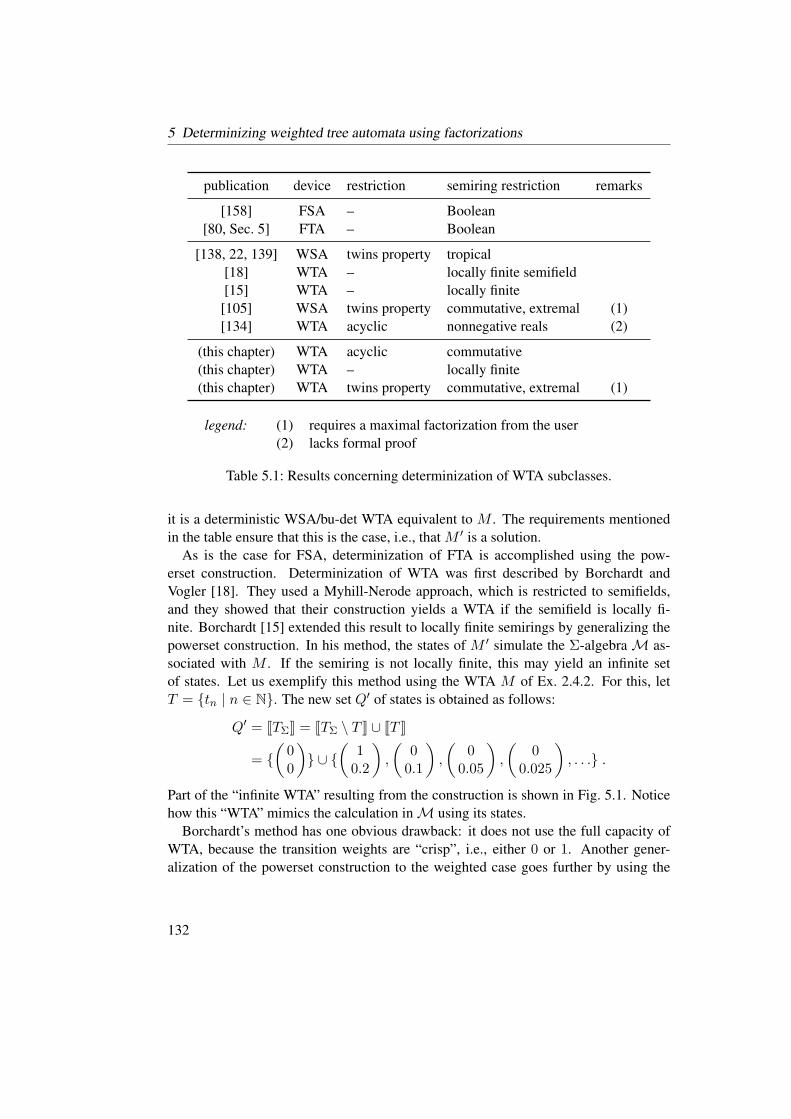
5 Determinizing weighted tree automata using factorizations
publication device restriction semiring restriction remarks
[158] FSA – Boolean
[80, Sec. 5] FTA – Boolean
[138, 22, 139] WSA twins property tropical
[18] WTA – locally finite semifield
[15] WTA – locally finite
[105] WSA twins property commutative, extremal (1)
[134] WTA acyclic nonnegative reals (2)
(this chapter) WTA acyclic commutative
(this chapter) WTA – locally finite
(this chapter) WTA twins property commutative, extremal (1)
legend: (1) requires a maximal factorization from the user
(2) lacks formal proof
Table 5.1: Results concerning determinization of WTA subclasses.
it is a deterministic WSA/bu-det WTA equivalent to M . The requirements mentioned
in the table ensure that this is the case, i.e., that M ′ is a solution.
As is the case for FSA, determinization of FTA is accomplished using the pow-
erset construction. Determinization of WTA was first described by Borchardt and
Vogler [18]. They used a Myhill-Nerode approach, which is restricted to semifields,
and they showed that their construction yields a WTA if the semifield is locally fi-
nite. Borchardt [15] extended this result to locally finite semirings by generalizing the
powerset construction. In his method, the states of M ′ simulate the Σ-algebraM as-
sociated with M . If the semiring is not locally finite, this may yield an infinite set
of states. Let us exemplify this method using the WTA M of Ex. 2.4.2. For this, let
T = tn | n ∈ N. The new set Q′ of states is obtained as follows:
Q′ = JTΣK = JTΣ \ T K ∪ JT K
=
(00
)
∪
(10.2
)
,
(00.1
)
,
(0
0.05
)
,
(0
0.025
)
, . . . .
Part of the “infinite WTA” resulting from the construction is shown in Fig. 5.1. Notice
how this “WTA” mimics the calculation inM using its states.
Borchardt’s method has one obvious drawback: it does not use the full capacity of
WTA, because the transition weights are “crisp”, i.e., either 0 or 1. Another gener-
alization of the powerset construction to the weighted case goes further by using the
132

5.1 Introduction
(10.2
)
(00.1
) (0
0.05
)
. . .
σ/1α/1
σ/1 σ/1
Figure 5.1: “Infinite WTA” obtained via Borchardt’s method.
(10.2
)
(01
)
σ/0.1α/1
σ/0.5
Figure 5.2: Bu-det WTA obtained via factorization.
concept of a factorization. In order to elucidate this approach, let us consider an exam-
ple in the realm of WTA (anticipating this chapter’s results). Roughly speaking, instead
of moving the complete computation of weights fromM into the new states, we factor
the elements of SQ so that the transition mapping in the new automaton is equipped
with the factor common to all components. When we apply this method to the WTA of
Ex. 2.4.2, we obtain the bu-det WTA of Fig. 5.2.
The first method to use the factorization approach, albeit implicitly, was the one by
Mohri for WSA over the tropical semiring [138]. Later, Kirsten and Maurer [105] made
the notion of a factorization explicit. This way, they were able to generalize Mohri’s
method to commutative semirings where a + b ∈ a, b holds; this property is called
extremal [124]. The factorization is a user-supplied parameter that depends on the
semiring. For zero-sum free semifields, a suitable factorization is readily available.
Both Mohri’s and Kirsten and Maurer’s method yields a WSA if M has a certain
property that is called twins property [44]. The question whether the twins property
is decidable has remained open for a long time. Decision procedures existed for sub-
classes of WSA, namely for trim, unambiguous WSA over the tropical semiring [138,
Thm. 13] and for trim, cycle-unambiguous WSA over commutative, cancellative semi-
133

5 Determinizing weighted tree automata using factorizations
rings [5]. Only recently, Kirsten [104] provided a decision procedure for general WSA
over the tropical semiring. He also showed that the decision problem is PSPACE-
complete.
May and Knight [134] transferred Mohri’s method to acyclic WTA over the semiring
of nonnegative reals, and they provided empirical evidence that their algorithm was
effective in machine translation and parsing systems, but they did not provide a formal
proof of correctness.
In this chapter, we use the factorization approach of [138, 105] to develop a deter-
minization construction for WTA that subsumes the above results; cf. Tab. 5.1. More-
over, we transfer the aforementioned decision results regarding the twins property from
WSA to WTA; in particular, we show that the twins property is decidable (i) for cycle-
unambiguous WTA over commutative, zero-sum-free, zero-divisor-free semirings (gen-
eralizing [5]) and (ii) for WTA over extremal semifields (generalizing [104]).
We proceed in the following four steps. First, we formalize and investigate the
necessary notions, such as factorizations, extremal semirings, and the twins property
(Sec. 5.2). Second, we develop our determinization construction for the case of classi-
cal WTA and prove its correctness (Sec. 5.3). Third, we develop our decision results,
again for classical WTA (Sec. 5.4). Finally, we transfer the results from classical WTA
to arbitrary (i.e., not necessarily classical) WTA (Sec. 5.5).
We end this chapter with a conclusion, discussion, and outlook (Sec. 5.6).
5.2 Preliminary notions and results
Let Σ be an alphabet, S = (S,+, ·, 0, 1) a semiring, and M = (Q,R, µ, ν) a WTA
over Σ and S . Recall from Sec. 2.3.2 that SQ is a semiring and that 0 is the vector that
consists of 0’s only.
5.2.1 Factorizations
We adopt the notion of a factorization from [105]. Let Q be a nonempty finite set. A
pair (f, g) is a factorization (of dimension Q) if
• f : SQ \ 0 → SQ,
• g : SQ \ 0 → S, and
• u = g(u) · f(u) for every u ∈ SQ \ 0.
A factorization (f, g) is called maximal if for every u ∈ SQ and s ∈ S, we have that
s · u 6= 0 implies f(u) = f(s · u). Note that even if f(0) were defined, the case
134

5.2 Preliminary notions and results
s · u = 0 would still have to be excluded here, because otherwise we would obtain
that f(u) = f(0 · u) = f(0) for every u ∈ SQ. The trivial factorization is the
factorization (f, g) with f(u) = u and g(u) = 1. We will abbreviate f(JtK) and g(JtK)by fJtK and gJtK, respectively.
Lemma 5.2.1 For every u ∈ SQ \ 0, we have that f(u) 6= 0 and g(u) 6= 0.
PROOF. By contradiction. Let f(u) = 0 or g(u) = 0. Then u = f(u) · g(u) = 0,
which contradicts the assumption that u 6= 0.
The following lemma shows a maximal factorization in the case that S is a semifield
and that there is a certain binary operation +′ on S. In particular, the lemma applies
when S is zero-sum free and +′ = +.
Lemma 5.2.2 Let S be a semifield, c ∈ S \0, +′ an associative, commutative binary
operation on S such that (i) s · (s1 +′ s2) = s · s1 +
′ s · s2 and (ii) s1 +′ s2 = 0 implies
s1 = 0 and s2 = 0; and let (f, g) be the factorization with g(u) = c ·∑′
q∈Q uq and
f(u) = g(u)−1 · u, where∑′
is computed with respect to +′. Then (f, g) is maximal.
PROOF. First, we show that (f, g) is a factorization. Let u ∈ SQ \ 0. Since S is a
semifield and +′ is “zero-sum free”, we obtain that g(u) 6= 0 and, hence, g(u) · f(u) =g(u) ·g(u)−1 ·u = u. Second, we show that (f, g) is maximal. Let s ∈ S with s ·u 6= 0,
and let q ∈ Q. Then
[f(s · u)]q =[g(s · u)−1 · s · u
]
q= (c ·
∑′q′∈Q s · uq′)
−1· s · uq
= (c · s ·∑′
q′∈Q uq′)−1· s · uq = (s · c ·
∑′q′∈Q uq′)
−1· s · uq
= (c ·∑′
q′∈Q uq′)−1· s−1 · s · uq = g(u)−1 · uq = [f(u)]q .
Example 5.2.3 First, we consider four instances of Lm. 5.2.2 where +′ = +. The
factorization (f, g) is maximal if
1. S is the semiring (R≥0,+, ·, 0, 1) of nonnegative reals, g(u) =∑
q∈Q uq, and
f(u) = 1g(u) · u;
2. S is the semiring (R≥0,max, ·, 0, 1), g(u) =∑
q∈Q uq, and f(u) = 1g(u) · u;
3. S is the Viterbi semiring ([0, 1],max, ·, 0, 1), g(u) = maxuq | q ∈ Q, and
f(u) = 1g(u) · u;
135
5 Determinizing weighted tree automata using factorizations
4. S is the tropical semiring (R≥0∞ ,min,+,∞, 0), g(u) = minuq | q ∈ Q, and
f(u) = −g(u) + u.
The settings in [134] and [138] correspond to Cases 1 and 4, respectively. Their con-
structions implicitly employ the corresponding maximal factorization given here.
Second, we consider an instance of the lemma where +′ 6= +, namely when S is the
field (R,+, ·, 0, 1) of real numbers and +′ = max. We note that S itself, being a field,
is not zero-sum free. In addition, we note that the neutral element of max, which is not
a real number, does not play a role in this scenario because, asQ is nonempty, we never
compute the maximum of the empty set.
The following lemma shows that (apart from the case that |Q| ≤ 1) maximal factor-
izations only exist for zero-divisor-free semirings.
Lemma 5.2.4 Let S be commutative and (f, g) a maximal factorization. Then |Q| ≤ 1or S is zero-divisor free.
PROOF. By contradiction. Assume that |Q| > 1 and S has zero divisors, i.e., s1, s2 ∈S \0 such that s1 ·s2 = 0. We choose a pair q1, q2 ∈ Qwith q1 6= q2. This is possible
because |Q| > 1. We define the vectors u1, u2 ∈ SQ such that the qi-component of ui
is 1 while the other components are 0. Since (f, g) is maximal and s1 · s2 = 0, we have
that
f(u1) = f(s1 · u1) = f(s1 · u1 + (s1 · s2) · u2) = f(s1 · (u1 + s2 · u2))
= f(u1 + s2 · u2) .
Thus, and since (f, g) is a factorization, we obtain the following equations (where
u = u1 + s2 · u2)
g(u1) · f(u1)q1 = [u1]q1 = 1 (I)
g(u1) · f(u1)q2 = [u1]q2 = 0 (II)
g(u) · f(u1)q1 = [u]q1 = 1 (III)
g(u) · f(u1)q2 = [u]q2 = s2 (IV)
By (II), (IV), and s2 6= 0, we derive that g(u1) 6= g(u). By (I) and (III), and using
commutativity, we derive
g(u1) = g(u1) ·(f(u1)q1 · g(u)
)=
(g(u1) · f(u1)q1
)· g(u) = g(u) .
Thus, we have a contradiction, proving that |Q| > 1 or S zero-divisor free.
136

5.2 Preliminary notions and results
Let |Q| > 1. Then Lm. 5.2.4 yields that commutative semirings with zero divisors do
not admit maximal factorizations, e.g., Semiring 8 of Ex. 2.3.5. The following example
shows that even zero-divisor-free semirings can defy a maximal factorization.
Example 5.2.5 ([105, Sec. 3.5]) Let S′ be the set of all natural numbers that can be
factored into an even number of primes, e.g., 4 = 2 · 2 and 126 = 2 · 3 · 3 · 7 belong
to S′, but 2 and 18 = 2 · 3 · 3 do not. Let S = S′ ∪ 1,∞. Then (S,min, ·,∞, 1) is a
semiring, where min is defined by the usual ordering of natural numbers, · is the usual
multiplication of natural numbers, and∞ denotes a new maximal element.
Consider the following chain of equations with vectors u and u1, u2, u3:
(2 · 3 · 5 · 73 · 5 · 7 · 11
)
︸ ︷︷ ︸
u
= (3 · 5) ·
(2 · 77 · 11
)
︸ ︷︷ ︸
u1
= (5 · 7) ·
(2 · 33 · 11
)
︸ ︷︷ ︸
u2
= (3 · 7) ·
(2 · 55 · 11
)
︸ ︷︷ ︸
u3
.
Clearly, the vectors u1 up to u3 can not be factored any further in S. Hence g(ui) = 1and f(ui) = ui for every factorization (f, g). Now let (f, g) be a maximal factorization.
We apply f to the above equation, obtaining
f(u) = f(u1) = f(u2) = f(u3) .
Since f(ui) = ui, we obtain u1 = u2 = u3, which is obviously a contradiction. Hence,
there is no maximal factorization.
We will frequently use the following observation, which can be shown by elementary
calculations.
Observation 5.2.6 Let k ∈ N, σ ∈ Σ, u1, . . . , uk ∈ SQ, and s1, . . . , sk ∈ S. If
s1, . . . , sk ∈ 0, 1 or S is commutative, we have that Jσ(s1 · u1, . . . , sk · uk)K =s1 · · · sk · Jσ(u1, . . . , uk)K.
We will use the following two lemmas.
Lemma 5.2.7 Let (f, g) and (f , g) be factorizations, (f, g) maximal, and let u ∈ SQ \0. Then f(f(u)) = f(u). In particular, f(f(u)) = f(u).
PROOF. We apply that (f, g) is maximal and that (f , g) is a factorization:
f(f(u)) = f(g(u) · f(u)) = f(u) .
137

5 Determinizing weighted tree automata using factorizations
Lemma 5.2.8 Let S be commutative and (f, g) maximal. Furthermore, let k ∈ N,
σ ∈ Σ, u1, . . . , uk ∈ SQ, and u′1, . . . , u
′k ∈ S
Q such that u′i ∈ ui, f(ui). Then
Jσ(u1, . . . , uk)K 6= 0 =⇒ Jσ(u′1, . . . , u′k)K 6= 0 ,
and the converse holds if S zero-divisor free. Furthermore,
Jσ(u1, . . . , uk)K 6= 0 =⇒ fJσ(u1, . . . , uk)K = fJσ(u′1, . . . , u′k)K .
PROOF. We construct the sequence s1, . . . , sk ∈ S by letting
si =
g(ui) if u′i = f(ui) ,
1 otherwise.
Using that (f, g) is a factorization and employing Obs. 5.2.6, we derive (⋆):
Jσ(u1, . . . , uk)K = Jσ(s1 · u′1, . . . , sk · u
′k)K = s1 · · · sk · Jσ(u
′1, . . . , u
′k)K .
First, let Jσ(u1, . . . , uk)K 6= 0. By (⋆) also Jσ(u′1, . . . , u′k)K 6= 0. Then
fJσ(u1, . . . , uk)K = f(s1 · · · sk · Jσ(u′1, . . . , u
′k)K) (⋆)
= fJσ(u′1, . . . , u′k)K . ((f, g) maximal)
Second, let S be zero-divisor free and Jσ(u′1, . . . , u′k)K 6= 0. Since si 6= 0, (⋆) yields
that Jσ(u1, . . . , uk)K 6= 0.
5.2.2 Extremal semirings
Observation 5.2.9 If S is extremal, then it is zero-sum free and idempotent.
For every D ⊆ D(M) and d ∈ D we call d victorious on D if 〈d〉 =∑
d∈D〈d〉.Let t ∈ TΣ, d ∈ D(M, t), and d = (q1 · · · qk, σ, q)
(d1, . . . , dk
). We call d recursively
victorious if d is victorious on Dq(M, t) and di is recursively victorious.
Observation 5.2.10 If S is extremal, then, for every t ∈ TΣ(SQ) and q ∈ Q, there is a
victorious run d on Dq(M, t). Consequently, 〈d〉 = JtKq.
Lemma 5.2.11 Let S be extremal. For every m ∈ N, q ∈ Q and t ∈ TΣ with
|pos(t)| ≤ m, there is a recursively victorious run d ∈ Dq(M, t).
138

5.2 Preliminary notions and results
PROOF. By induction (on m). For the induction base (m = 0), there is nothing to
show. We show the induction step (m → m + 1). To this end, let m ∈ N, q ∈ Q,
t ∈ TΣ, t = σ(t1, . . . , tk), and |pos(t)| ≤ m+ 1. By Obs. 5.2.10, there is a victorious
run d′ on Dq(M, t). Let d′(ε) = (q1 · · · qk, σ, q). By the induction hypothesis, there
are recursively victorious runs d1 ∈ Dq1(M, t1) up to dk ∈ D
qk(M, tk). We construct
d = d′(ε)(d1, . . . , dk
). It remains to show that d is victorious. We derive
〈d′〉 =∑
d′′∈Dq(M,t)〈d′′〉 (d′ victorious)
= 〈d′〉+(∑
d′′∈Dq(M,t) : 〈d′′〉6=〈d′〉〈d′′〉)
(S idempotent)
=(
〈d′〉+(∑
d′′∈Dq(M,t) : 〈d′′〉6=〈d′〉,d′′(ε)=d′(ε)〈d′′〉))
+(∑
d′′∈Dq(M,t) : 〈d′′〉6=〈d′〉,d′′(ε)6=d′(ε)〈d′′〉)
= 〈d′〉+(∑
d′′∈Dq(M,t) : 〈d′′〉6=〈d′〉,d′′(ε)=d′(ε)〈d′′〉)
(†)
=∑
d′1∈Dq1 (M,t1),...,d′k∈D
qk (M,tk)〈d′(ε)
(d′1, . . . , d
′k
)〉 (S idempotent)
=(∑
d′1∈Dq1 (M,t1)
〈d′1〉)· · ·
(∑
d′k∈Dqk (M,tk)
〈d′k〉)· µ(d′(ε)) (distributivity)
= 〈d1〉 · · · 〈dk〉 · µ(d′(ε)) = 〈d〉 . (di victorious)
where (†) holds because the outer sum on the left-hand side is known to be 〈d′〉, thus it
discards the second argument, which is known not to be 〈d′〉.
Observation 5.2.12 Let S be extremal. Let ζ ∈ CΣ, t ∈ TΣ, p, q ∈ P , d ∈ Dp(M, t),and d′ ∈ Dq(M,p · ζ) such that d ·p d
′ is victorious on Dq(M, t · ζ). Then 〈d ·p d′〉 =
J(〈d〉 · ep) · ζKq.
PROOF. We derive
〈d ·p d′〉 =
∑
d′′∈Dq(M,t·ζ)〈d′′〉 (victorious run)
= 〈d ·p d′〉+
∑
d′′∈Dq(M,t·ζ) : 〈d′′〉6=〈d·pd′〉〈d′′〉 (S idempotent)
= 〈d ·p d′〉+
∑
d′′∈Dq(M,p·ζ) : 〈〈d〉·pd′′〉6=〈d·pd′〉〈〈d〉 ·p d
′′〉 (†)
=∑
d′′∈Dq(M,p·ζ)〈〈d〉 ·p d′′〉 (S idempotent)
=∑
d′′∈Dq(M,(〈d〉·ep)·ζ)〈d′′〉 = J(〈d〉 · ep) · ζKq .
For (†), we use the same kind of reasoning as for (†) in the proof of Lm. 5.2.11.
5.2.3 Twins property
We define two binary relations SIB(M) (for siblings) and TWINS(M) on Q as follows.
Let p, q ∈ Q. Then
139

5 Determinizing weighted tree automata using factorizations
w1
w2
t1, dq
t2, d′q
Figure 5.3: Cutting out the slice starting at w1 and ending at w2.
• (p, q) ∈ SIB(M) iff there is a tree t ∈ TΣ such that JtKp 6= 0 and JtKq 6= 0.
• (p, q) ∈ TWINS(M) iff for every context ζ ∈ CΣ we have that Jep · ζKp 6= 0 and
Jeq · ζKq 6= 0 implies Jep · ζKp = Jeq · ζKq.
The WTA M has the twins property if SIB(M) ⊆ TWINS(M).
Example 5.2.13 (Ex. 2.4.1 contd.) We show that M has the twins property. For this,
let (p, q) ∈ SIB(M). Then there is a t ∈ TΓ such that JtKp 6= 0 and JtKq 6= 0. Moreover,
let ζ ∈ CΓ such that Jep · ζKp 6= 0 and Jeq · ζKq 6= 0. We show that Jep · ζKp = Jeq · ζKq.If p = q, this is trivial. For reasons of symmetry, it suffices to consider the case that
p = q1 and q = q0. Since Jeq1 · ζKq1 6= 0 and JtKq1 6= 0, we conclude that ζ = z and
t = α. Thus we obtain Jeq1 · zKq1 = 1 = Jeq0 · zKq0 .
The matter of deciding the twins property is the subject of Sec. 5.4. In short: it is
known that the twins property is decidable for cycle-unambiguous WTA over commuta-
tive, zero-sum-free, zero-divisor-free semirings and for WTA over extremal semifields.
Next, we show a fundamental property that follows from the twins property when
S is commutative and extremal. Before we show the result in detail, we begin with a
simple corollary that summarizes the result. Here and in the following, we use S ·U to
denote s · u | s ∈ S, u ∈ U for every set U ⊆ SQ.
Corollary 5.2.14 Let S be commutative and extremal, and let M have the twins prop-
erty. Then there is a finite set U ⊆ SQ with JTΣK ⊆ S · U .
PROOF. Direct consequence of Lm. 5.2.15.
First, we sketch the proof idea; we develop the formal infrastructure and the cor-
responding lemma afterwards. Let t1 ∈ TΣ. Since S is extremal, for every q ∈ Qthere is a victorious run dq on Dq(M, t1). If t1 is sufficiently “large”, then we find
140

5.2 Preliminary notions and results
positions w1 and w2 such that w1 is strictly above w2 and πQ(dq|w1) = πQ(dq|w2)for every q ∈ Q. Provided that we have chosen the family (dq | q ∈ Q) of runs in
a suitable manner, the twins property guarantees that each run in this family assigns
the same weight, say s1, to the “slice” of t1 starting at position w1 and ending at po-
sition w2 (depicted as the shaded area in Fig. 5.3). We can remove this slice from t1,
obtaining the smaller tree t2 and family of runs (d′q | q ∈ Q) on t2 with 〈dq〉 = s1 ·〈d′q〉.
This procedure can be iterated a finite number of times, yielding the trees t1, . . . , tn and
weights s1, . . . , sn−1, where tn is in a finite set of “small” trees (giving rise to a finite
set U of vectors).
Now we formalize this idea. For this, let t ∈ TΣ and Q′ ⊆ Q. A Q′-run family d
for t is a family (dq | q ∈ Q′) with dq ∈ D(M, t) and 〈dq〉 6= 0 for every q ∈ Q′. Let
d = (dq | q ∈ Q′) be a Q′-run family for t. We define JdK ∈ SQ by
JdKq =
〈dq〉 if q ∈ Q′,
0 otherwise.
For every w ∈ pos(t), we define the Q′-run family d|w for t|w to be (dq|w | q ∈ Q′).
We define π′Q(d) ∈ QQ′
by letting π′Q(d)q = πQ(dq) for every q ∈ Q′; and we will
omit the prime from π′Q. We define three properties of d:
• It is victorious if dq is victorious on DπQ(dq)(M, t) for every q ∈ Q′.
• It is root if πQ(d)q = q for every q ∈ Q′.
• It is admissible if it is root and for every w1, w2 ∈ pos(t) with w1 strictly above
w2 and πQ(d|w1) = πQ(d|w2), we have that d|w1 is victorious.
For every T ⊆ TΣ, we let
D(T ) = d | ∃Q′ ⊆ Q, t ∈ T : d is an admissible Q′-run family for t .
We define the state number of d by c(d) = |πQ(d|w) | w ∈ pos(t)| and the state
number of M by c(M) = maxc(d) | d ∈ D(TΣ). We note that c(M) ≤ |Q||Q|. The
following lemma corresponds to a part of the proof of [105, Thm. 5].
Lemma 5.2.15 Let S be commutative and extremal, and letM have the twins property.
Then JTΣK ⊆ JD(TΣ)K ⊆ S · JD(t | t ∈ TΣ, ht(t) ≤ c(M))K.
PROOF. We begin with the first inclusion. To this end, let t ∈ TΣ. By Lm. 5.2.11,
there is a recursively victorious run d ∈ Dq(M, t) for every q ∈ Q. We let Q′ = q |JtKq 6= 0, and we construct the family (dq | q ∈ Q
′) by letting dq ∈ Dq(M, t) be some
141

5 Determinizing weighted tree automata using factorizations
recursively victorious run. Then (dq | q ∈ Q′) is an admissible Q′-run family for t, and
JtK = JdK.
Now we show the second inclusion by contradiction. To this end, we let T = t |t ∈ TΣ, ht(t) ≤ c(M) and
C = (Q′, t, d, |pos(t)|) | t ∈ TΣ, Q′ ⊆ Q, d is an admissible Q′-run family for t,
JdK ∈ JD(TΣ)K, JdK 6∈ S · JD(T )K .
Let (Q′, t, d,m) ∈ C such thatm is minimal. Then ht(t) > c(M) andQ′ 6= ∅, because
otherwise d ∈ D(T ). We let d = (dq | q ∈ Q′), and we fix some q0 ∈ Q
′ for later use.
We let
B = (w1, w2) | w1, w2 ∈ pos(t), w1 strictly above w2, πQ(d|w1) = πQ(d|w2) .
Since ht(t) > c(d), and by the pigeonhole principle, the set B is not empty – in other
words, there is a w2 ∈ pos(t) of sufficient length such that a prefix w1 of w2 exists such
that w1 and w2 have the same image under w 7→ πQ(d|w).Let (w1, w2) ∈ B such that w1 has minimal length. We construct the tree t′ =
t[t|w2 ]w1 , the run family d′ = (dq[dq|w2 ]w1 | q ∈ Q′), the state q′0 = πQ(d|w2)q0 ,
and the semiring element s = Jt[eq′0 ]w2 |w1Kq′0 . We claim that (i) d′ is admissible and
(ii) JdK = s·Jd′K. Then either Jd′K 6∈ S ·JD(T )K. But then, by (i), (Q′, t′, d′, |pos(t′)|) ∈C. Since |pos(t′)| < |pos(t)|, this contradicts our assumption that m be minimal. Or
Jd′K ∈ S · JD(T )K, but then so is JdK, due to (ii), which contradicts our assumption that
(Q′, t, d,m) ∈ C.
It remains to show Statements (i) and (ii). For (i), let w′1, w
′2 ∈ pos(t′) such that
w1 is above w2 and πQ(d′|w′
1) = πQ(d
′|w′2). We distinguish two cases, illustrated in
Fig. 5.4. Either (a) there are v1, v2 ∈ N∗ such that w′
1 = w1 · v1 and w′2 = w1 · v2.
Then d′|w′
1= d|w2v1 and d
′|w′2= d|w2v2 . Or (b) d′|w′
1= d|w1 and d
′|w′2= d|w2 . Since
d is admissible, we can derive that d′|w′1
is victorious in both cases.
For (ii), we let q ∈ Q′, q′ = πQ(d|w2)q, and ζ = t[z]w2 |w1 . Then
JdKq = 〈dq〉 = 〈〈dq|w1〉 · dq[z]w1〉
= 〈J(〈dq|w2〉 · eq′) · ζKq′ · dq[z]w1〉 (Obs. 5.2.12)
= 〈dq|w2〉 · Jeq′ · ζKq′ · 〈1 · dq[z]w1〉 (commutativity)
= 〈dq|w2〉 · Jeq′0 · ζKq′0 · 〈1 · dq[z]w1〉 (†)
= s · 〈〈dq|w2〉 · dq[z]w1〉 = s · Jd′Kq . (commutativity)
We show (†). First, we show that (q′, q′0) ∈ SIB(M). By definition we have 〈dq0〉 6= 0and 〈dq〉 6= 0. Hence, also 〈dq0 |w2〉 6= 0 and 〈dq|w2〉 6= 0. Since S is extremal, it is
142
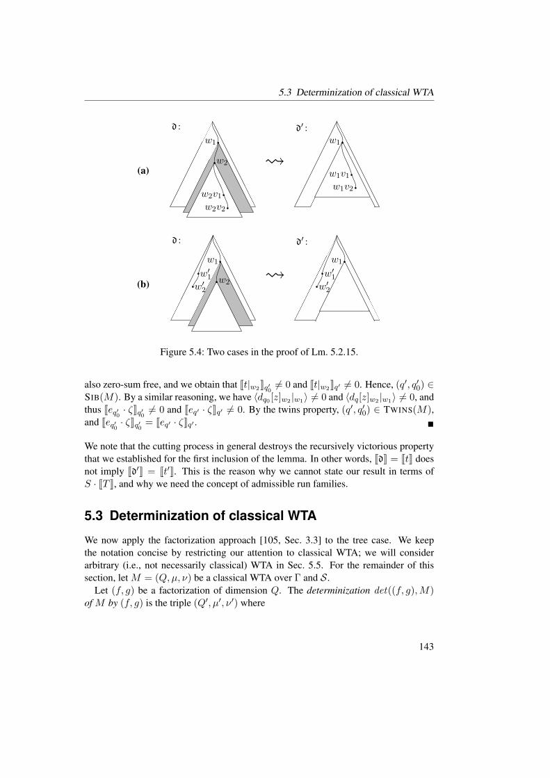
5.3 Determinization of classical WTA
(a)
w1
w2
w2v1w2v2
d :
w1
w1v1w1v2
d′ :
(b)
w1
w2w′1
w′2
d :
w1
w′1
w′2
d′ :
Figure 5.4: Two cases in the proof of Lm. 5.2.15.
also zero-sum free, and we obtain that Jt|w2Kq′0 6= 0 and Jt|w2Kq′ 6= 0. Hence, (q′, q′0) ∈SIB(M). By a similar reasoning, we have 〈dq0 [z]w2 |w1〉 6= 0 and 〈dq[z]w2 |w1〉 6= 0, and
thus Jeq′0 · ζKq′0 6= 0 and Jeq′ · ζKq′ 6= 0. By the twins property, (q′, q′0) ∈ TWINS(M),and Jeq′0 · ζKq′0 = Jeq′ · ζKq′ .
We note that the cutting process in general destroys the recursively victorious property
that we established for the first inclusion of the lemma. In other words, JdK = JtK does
not imply Jd′K = Jt′K. This is the reason why we cannot state our result in terms of
S · JT K, and why we need the concept of admissible run families.
5.3 Determinization of classical WTA
We now apply the factorization approach [105, Sec. 3.3] to the tree case. We keep
the notation concise by restricting our attention to classical WTA; we will consider
arbitrary (i.e., not necessarily classical) WTA in Sec. 5.5. For the remainder of this
section, let M = (Q,µ, ν) be a classical WTA over Γ and S .
Let (f, g) be a factorization of dimension Q. The determinization det((f, g),M)of M by (f, g) is the triple (Q′, µ′, ν ′) where
143

5 Determinizing weighted tree automata using factorizations
• Q′ is the smallest set P ⊆ SQ such that 0 ∈ P and, for every k ∈ N, σ ∈ Γ(k),
and u1, . . . , uk ∈ P , if Jσ(u1, . . . , uk)K 6= 0, then fJσ(u1, . . . , uk)K ∈ P .
• µ′ :⋃
k(Q′)k × Γ(k) ×Q′ → S with
µ′(u1 · · ·uk, σ, u) =
gJσ(u1, . . . , uk)K if Jσ(u1, . . . , uk)K 6= 0 and
u = fJσ(u1, . . . , uk)K ,
0 otherwise ,
• ν ′ : Q′ → S with ν ′u =∑
q∈Q uq · νq.
We note that Q′ is uniquely determined because it is chosen from a set which is closed
under intersection.
In the following, let M ′ = det((f, g),M) and M ′ = (Q′, µ′, ν ′).
Observation 5.3.1 The triple M ′ is a classical WTA over Γ and S iff Q′ is finite. If M ′
is a WTA, then it is bu-det.
The following observation, which can be proved using Thm. 2.1.1, shows a stratifi-
cation of Q′; this basically gives an algorithm for computing Q′ (in case it is finite).
Observation 5.3.2 Let (Q′i | i ∈ N) be the family with
Q′0 = ∅ ,
Q′i+1 = 0 ∪ fJσ(u1, . . . , uk)K | k ∈ N, σ ∈ Γ(k), u1, . . . , uk ∈ Q
′i,
Jσ(u1, . . . , uk)K 6= 0 .
Then Q′ =⋃
i∈NQ′i; moreover, Q′ is finite iff there is an n ∈ N with Q′ = Q′
n.
Example 5.3.3 (Ex. 2.4.1 contd.) We compute det((f, g),M) = (Q′, µ′, ν ′) using the
maximal factorization (f, g) given for the Viterbi semiring in Ex. 5.2.3. First, we com-
puteQ′ according to Obs. 5.3.2. We write the elements of SQ as column vectors, where
the first row is the q1-component; and we use the following abbreviations:
u1 =
(10.2
)
and u2 =
(01
)
.
Then Q′0 = ∅ and
Q′1 = 0 ∪ fJαK = 0, f(u1) = 0, u1 ,
Q′2 = Q′
1 ∪ fJσ(u1, u1)K = Q′1 ∪ f(0.1 · u2) = 0, u1, u2 ,
Q′3 = Q′
2 ∪ fJσ(u1, u2)K = Q′2 ∪ f(0.5 · u2) = 0, u1, u2 , (⋆)
144
5.3 Determinization of classical WTA
where we note for (⋆) that Jσ(u2, u1)K = 0 = Jσ(u2, u2)K. Clearly, we have Q′i = Q′
2
for i ≥ 2. Hence, Q′ = Q2. Figure 5.2 shows µ′. In particular, we can read off from
the above calculation that
µ′(u1u1, σ, u2) = gJσ(u1, u1)K = g(0.1 · u2) = 0.1 ,
µ′(u1u2, σ, u2) = gJσ(u1, u2)K = g(0.5 · u2) = 0.5 ,
and that µ′ maps every remaining transition to 0. Finally, ν ′0= 0, ν ′u1 = 0.2, and
ν ′u2 = 1.
The following theorem summarizes the behavior of det((f, g),M). We will prove
the individual statements of the theorem below.
Theorem 5.3.4 Let M = (Q,µ, ν) be a classical WTA over Γ and S , and let (f, g) be
the trivial or a maximal factorization. If (f, g) is not the trivial factorization, let S be
commutative. Moreover, let one of the following conditions hold:
• M is acyclic,
• S is locally finite,
• (f, g) is maximal and M is bu-det, or
• (f, g) is maximal, M has the twins property, and S is extremal.
Then det((f, g),M) is a bu-det classical WTA over Γ and S , and it is equivalent to M .
Moreover, if (f, g) is maximal, then, regarding the number of states, det((f, g),M) is
minimal among all WTA which are obtained by factorization.
PROOF. Let M ′ = det((f, g),M) and M ′ = (Q′, µ′, ν ′). By Obs. 5.3.1, M ′ is a
WTA iff Q′ is finite. If M ′ is a WTA, then, by the same observation, it is bu-det, and
M and M ′ are equivalent, as shown in Thm. 5.3.7. The statement about the number of
states is shown in Thm. 5.3.8.
Finally, the set Q′ is finite if
• M is acyclic – by Lm. 5.3.10 –,
• (f, g) is the trivial factorization and the semiring S is locally finite – by Lm. 4.7
of [15],
• (f, g) is maximal and S is commutative and locally finite – which follows from
the previous item and Thm. 5.3.8 –,
145

5 Determinizing weighted tree automata using factorizations
• (f, g) is maximal, S is commutative, and M is bu-det – by Lm. 5.3.11 –,
• (f, g) is maximal, M has the twins property, and S is commutative and extremal
– by Cor. 5.3.12.
The reader is invited to compare Thm. 5.3.4 to the overview given in Tab. 5.1.
The theorem lists four conditions that guarantee that det((f, g),M) be a WTA. With
the first condition we provide a formal verification of [134]. The second condition is
adapted from [15]. The third condition ensures that we can determinize a WTA that
is already bu-det. The fourth condition is adapted from [105, Thm. 5]. We note that
the third condition is mainly of theoretical interest. In fact, since testing bottom-up
determinism can be done in linear time, we might precede the determinization proce-
dure with such a test and, if the WTA is already bu-det, refrain from determinization
altogether.
One might be led to believe that the trivial factorization on the one hand and maximal
factorizations on the other hand represent two ends of a spectrum. In view of this, it
may seem curious that we require the factorization to be trivial or maximal. However,
as the following example shows, if this requirement is not satisfied, then det((f, g),M)can be infinite, even if the semiring is locally finite and M is bu-det.
Example 5.3.5 Let Γ = γ(1), α(0), S = (R≥0 ∪ ∞,−∞,min,max,∞,−∞),and M the WTA over Γ and S given by (final weights do not matter)
(ε, α, q) 7→ 1 and (q, γ, q) 7→ 0 .
Then Jγn(α)K = 1 for every n ∈ N. If (f, g) is the trivial factorization, then the
determinization det((f, g),M) is given by (again disregarding final weights)
(ε, α, 1) 7→ 1 and (1, γ, 1) 7→ 1 .
Now we let (f, g) be the factorization with
g(u) = minuq | q ∈ Q , f(u)q =
0.9 · uq if uq = g(u),
uq otherwise,
where 0.9 · uq is the usual product in the reals. For instance, we may calculate
g
(22.5
)
· f
(22.5
)
= 2 ·
(1.82.5
)
=
(max(2, 1.8)max(2, 2.5)
)
=
(22.5
)
,
146

5.3 Determinization of classical WTA
where · is the scalar product in our semiring. This example already shows that (f, g) is
not trivial. It is not maximal either:
f(2 ·
(22.5
)
) = f
(22.5
)
=
(1.82.5
)
6=
(2.72.7
)
= f
(33
)
= f(3 ·
(22.5
)
) .
We compute det((f, g),M) again, this time with the new factorization:
(ε, α, 0.9) 7→ 1 , (0.9, γ, 0.81) 7→ 0.9 , (0.81, γ, 0.729) 7→ 0.81 , . . .
As the following example shows, however, there are cases where a maximal factor-
ization does not exist, the trivial factorization leads to an infinite result, and another
factorization does the trick. These cases are obviously not covered by our theorem.
Example 5.3.6 Let S be the semiring of Ex. 5.2.5. We define the factorization (f, g)as follows: g(u) is the greatest common divisor (gcd) of the components of u if this
number is in S, and otherwise g(u) is the gcd divided by the largest prime factor it
contains, e.g.,
g(
(23
24
)
) =23
2= 22 .
Finally, we let f(u) = ug(u) .
Let Γ = γ(1), α(0) and M = (Q,µ, ν) be the WTA over Γ and S where Q =q, p, ν is immaterial to our concerns, and µ is given by
(ε, α, q) 7→ 2 · 3 , (p, γ, q) 7→ 2 · 3 , (q, γ, q) 7→ ∞ ,
(ε, α, p) 7→ 5 · 7 , (q, γ, p) 7→ 5 · 7 , (p, γ, p) 7→ ∞ .
We denote the elements of SQ as vectors, with the q-component shown first. Let
u1 =
(2 · 35 · 7
)
, u2 =
(11
)
.
It can be shown that
Jγ2n(α)K = (2 · 3 · 5 · 7)n · u1 , Jγ2n+1(α)K = (2 · 3 · 5 · 7)n+1 · u2 .
Hence, determinization using the trivial factorization yields an infinite result. On the
other hand, det((f, g),M) = (Q′, µ′, ν ′) where Q′ = u1, u2, ν′ is again immaterial,
and µ′:
(ε, α, u1) 7→ 1 , (u1, γ, u2) 7→ 2 · 3 · 5 · 7 , (u2, γ, u1) 7→ 1 ,
and every other transition is mapped to∞.
147
5 Determinizing weighted tree automata using factorizations
The following theorem is our correctness result; it corresponds to Thm. 1 of [105].
Theorem 5.3.7 Let (f, g) be a factorization. If (f, g) is not the trivial factorization,
then let S be commutative. If M ′ is a WTA, then JMK = JM ′K.
PROOF. Let M ′ be a WTA, i.e., let Q′ be finite. We abbreviate J.KM by J.K and 〈.〉µ′ by
〈.〉. By Obs. 5.3.1, M ′ is bu-det.
We show the following statement by induction on t: for every t ∈ TΓ there are u ∈ Q′
and d ∈ Du(M ′, t) such that (i) 〈d〉 · u = JtK and (ii) 〈d′〉 6= 0 implies d′ = d for every
d′ ∈ D(M ′, t). Note that, if (f, g) is the trivial factorization, then 〈d〉 ∈ 0, 1 for
every t ∈ TΓ, u ∈ Q′, and d ∈ Du(M ′, t).Let t = σ(t1, . . . , tk). By the induction hypothesis, there are u1, . . . , uk ∈ Q
′ and
d1, . . . , dk with dj ∈ Duj (M, tj) such that (i) 〈dj〉·uj = JtjK, and (ii) 〈d′j〉 6= 0 implies
d′j = dj . We set u′ = Jσ(u1, . . . , uk)K. We derive (⋆):
JtK = Jσ(Jt1K, . . . , JtkK)K (Obs. 2.4.4)
= Jσ(〈d1〉 · u1, . . . , 〈dk〉 · uk)K (induction hypothesis)
= 〈d1〉 · · · 〈dk〉 · u′ . (Obs. 5.2.6)
Now we distinguish two cases.
Case 1: Let u′ = 0. Then, by (⋆), JtK = 0. We construct ρ = (u1 · · ·uk, σ, u′) and
d = ρ(d1, . . . , dk
). Then µ′(ρ) = 0, 〈d〉 = 0, and 〈d〉 · u′ = 0. Now let d′ ∈ D(M ′, t)
and 〈d′〉 6= 0. Then each of the factors 〈d′|1〉, . . . , 〈d′|k〉, and µ′(d′(ε)) is non-zero.
By the induction hypothesis, d′|j = dj . By definition, µ′(u1 · · ·uk, σ, u) = 0 for
every u ∈ Q′. Hence, µ′(d′(ε)) = 0, and our assumption that 〈d′〉 6= 0 was wrong.
Case 2: Let u′ 6= 0. Then we construct u = f(u′), ρ = (u1 · · ·uk, σ, u), and
d = ρ(d1, . . . , dk
), and we derive
JtK = 〈d1〉 · · · 〈dk〉 · u′ (⋆)
=(〈d1〉 · · · 〈dk〉 · g(u
′))· f(u′) ((f, g) fact.)
= 〈d〉 · u .
Let d′ ∈ D(M ′, t) and 〈d′〉 6= 0. Then each of the factors 〈d′|1〉, . . . , 〈d′|k〉, and
µ′(d′(ε)) is non-zero. By the induction hypothesis, d′|j = dj , and by the definition of
µ′, d′(ε) = d(ε).Now we show that JMK = JM ′K. Let t ∈ TΓ. Then there are u ∈ Q′ and d ∈
Du(M ′, t) such that 〈d〉 · u = JtK and 〈d′〉 6= 0 implies d′ = d. We derive
JM ′K(t) = 〈d〉 · ν ′u =∑
q∈Q 〈d〉 · uq · νq =∑
q∈Q JtKq · νq = JMK(t) .
148
5.3 Determinization of classical WTA
The next theorem is our minimality statement; it corresponds to Thm. 3 of [105].
Theorem 5.3.8 Let S be commutative, (f, g) and (f , g) factorizations, (f, g) maxi-
mal, det((f, g),M) = (Q′, µ′, ν ′), and det((f , g),M) = (Q, µ, ν). Then Q′ \ 0 =f(Q \ 0). Consequently, |Q′| ≤ |Q| and, if det((f , g),M) is a WTA, then so
is det((f, g),M).
PROOF. We first consider the case that |Q| = 1. Then we can identify SQ with S.
Since (f, g) is maximal, we have that f(S \ 0) = f(1). By Lm. 5.2.1, f(1) 6= 0.
Now either Q′ = 0 = Q or Q′ = 0, f(1) and Q ⊃ 0. In both cases, we have
that Q′ \ 0 = f(Q \ 0).Now let |Q| > 1. By Lm. 5.2.4, S is zero-divisor free. We prove f(Q \ 0) =
Q′\0. We begin with “⊆”. By Obs. 5.3.2, it suffices to prove the following statement
by induction on i: for every i ∈ N, f(Qi \ 0) ⊆ Q′ \ 0. To this end, let i ∈ N
and u ∈ Qi+1 \ 0. Then there are k ∈ N, σ ∈ Γ(k), and u1, . . . , uk ∈ Qi such that
u = fJσ(u1, . . . , uk)K. By Lm. 5.2.1, u 6= 0 and f(u) 6= 0. We show that f(u) ∈ Q′
by deriving
f(u) = f(fJσ(u1, . . . , uk)K) = f(Jσ(u1, . . . , uk)K) (Lm. 5.2.7)
= f(Jσ(f(u1), . . . , f(uk))K) (Lm. 5.2.8)
∈ Q′ . (induction hypothesis, def. of Q′)
Now we prove “⊇”. Using Obs. 5.3.2 again, it suffices to prove the following state-
ment by induction on i: for every i ∈ N, Q′i \ 0 ⊆ f(Q \ 0). To this end, let i ∈ N
and u′ ∈ Q′i+1 \ 0. Then there are k ∈ N, σ ∈ Γ(k), and u′1, . . . , u
′k ∈ Q
′i such that
Jσ(u′1, . . . , u′k)K 6= 0 and u′ = fJσ(u′1, . . . , u
′k)K. By the induction hypothesis, there
are u1, . . . , uk ∈ Q \ 0 such that u′i = f(ui). By Lm. 5.2.1, u′ 6= 0. We show that
u′ ∈ f(Q) by deriving
u′ = fJσ(f(u1), . . . , f(uk))K = fJσ(u1, . . . , uk)K (Lm. 5.2.8)
= f(fJσ(u1, . . . , uk)K) (Lm. 5.2.7)
∈ f(Q) .
The following corollary corresponds to [105, Lm. 2].
Corollary 5.3.9 Let S be commutative and (f, g) maximal. Then Q′ \ 0 = f(JTΓK \0).
PROOF. Follows from Thm. 5.3.8 when (f , g) is the trivial factorization.
149
5 Determinizing weighted tree automata using factorizations
In the remainder of this section, we deal with the sufficient conditions for Q′ to be
finite. We begin with a lemma that is useful when M is acyclic.
Lemma 5.3.10 There is an injective mapping ϕ : Q′ \ 0 → t | t ∈ TΓ, JtK 6= 0.
PROOF. The main idea is to define ϕ as the supremum of an ω-chain of injective map-
pings. To this end, let T = t | t ∈ TΓ, JtK 6= 0. We use Obs. 5.3.2. For every i ∈ N,
we let
T ′i = σ(u1, . . . , uk) | σ ∈ Γ(k), uι ∈ Q
′i, Jσ(u1, . . . , uk)K 6= 0 .
Note that T ′i is finite. We assume that T ′
i is well ordered in some way. Then we define,
for every i ∈ N, the mapping ϕi : Q′i \ 0 → T as follows. If i = 0, there is nothing
to define. If u ∈ Q′i, then we let ϕi+1(u) = ϕi(u). Otherwise, we proceed as follows.
There is a least σ(u1, . . . , uk) ∈ T′i with u = fJσ(u1, . . . , uk)K. This implies uι 6= 0.
We define ϕi+1(u) = σ(ϕi(u1), . . . , ϕi(uk)).First, we show by induction on i that, for every i ∈ N, we have
(i) ϕi|Q′j\0
= ϕj for every j ≤ i,
(ii) i > 0, u ∈ Q′i, u 6∈ Q
′i−1, and u 6= 0 implies ht(ϕi(u)) = i,
(iii) ϕi is injective.
The induction base (i = 0) is trivial. We show the induction step (i → i + 1). To this
end, let i ∈ N such that the hypothesis holds.
We show (i). For this, let j ≤ i+ 1. The case j = i+ 1 is trivial. If j ≤ i, we derive
ϕi+1|Q′j\0
= ϕi|Q′j\0
= ϕj .
We show (ii). Let i + 1 > 0, u ∈ Q′i+1, u 6∈ Q′
i, and u 6= 0. There is a least
σ(u1, . . . , uk) ∈ T′i with u = fJσ(u1, . . . , uk)K. If i = 0, then k = 0, and we obtain
ht(ϕi+1(u)) = 1. Let i > 0. Assume for the time being that uι ∈ Q′i−1 for every ι.
Then u ∈ Qi. Hence, there is a ι such that uι 6∈ Q′i−1. By the induction hypothesis,
ht(ϕi(uι)) = i. Then ht(ϕi+1(u)) = i+ 1.
We show (iii). To this end, let u, u′ ∈ Q′i+1 \ 0 and ϕi+1(u) = ϕi+1(u
′). Then
ht(ϕi+1(u)) = ht(ϕi+1(u′)). By (ii), either u, u′ ∈ Q′
i or u, u′ 6∈ Q′i. In the former
case, we invoke the induction hypothesis. Otherwise we proceed as follows. There
are least σ(u1, . . . , uk), σ′(u′1, . . . , u
′k′) ∈ T ′
i with u = fJσ(u1, . . . , uk)K and u′ =fJσ′(u′1, . . . , u
′k′)K. Since ϕi+1(u) = ϕi+1(u
′), we have σ = σ′, k = k′, and ϕi(uι) =ϕi(u
′ι). By the induction hypothesis, uι = u′ι. Hence, u = u′.
This completes the inductive proof. Now we construct ϕ : Q′ \ 0 → T as follows.
Let u ∈ Q′. Then there is a least i ∈ N with u ∈ Q′i. We let ϕ(u) = ϕi(u). It remains
150
5.4 Deciding the twins property
to show that ϕ is injective. For this, let u, u′ ∈ Q′ and ϕ(u) = ϕ(u′). There are least
i, i′ with u ∈ Q′i and u′ ∈ Q′
i′ . Then ϕ(u) = ϕi(u) and ϕ(u′) = ϕi′(u′). Without loss
of generality, we assume that i ≥ i′. Using (i), we derive
ϕi(u) = ϕ(u) = ϕ(u′) = ϕi′(u′) = ϕi(u
′) .
Then (iii) yields that u = u′.
Now we turn to the cases where (f, g) is a maximal factorization, S is commutative,
and either M is already bu-det or M has the twins property and S is extremal.
Lemma 5.3.11 Let S be commutative, (f, g) maximal, andM bu-det. ThenQ′ is finite.
PROOF. By Cor. 5.3.9, Q′ \ 0 = f(JTΓK \ 0). Observation 2.4.3 yields that each
vector in JTΓK has at most one nonzero component. By this fact and since (f, g) is
maximal, we can derive that |f(JTΓK \ 0)| ≤ |Q|.
The following corollary generalizes Thm. 5 of [105] from strings to trees.
Corollary 5.3.12 Let S be commutative and extremal, (f, g) maximal, andM have the
twins property. Then Q′ is finite.
PROOF. By Cor. 5.2.14 there is a finite set U ⊆ SQ such that JTΓK ⊆ S ·U . We derive
Q′ \ 0 = f(JTΓK \ 0) (Cor. 5.3.9)
⊆ f((S · U) \ 0) (Cor. 5.2.14)
⊆ f(U \ 0) . ((f, g) maximal)
Since U is finite, so is Q′.
5.4 Deciding the twins property
In this section, we consider two approaches to deciding the twins property. In both ap-
proaches we require that the semiring be commutative, zero-sum free, and zero-divisor
free. For the first approach, we put an additional restriction on the semiring – namely,
that it be an extremal semifield. For the second one, we put a restriction on the WTA –
namely, that it be cycle-unambiguous. As a preparation for both approaches, we show
that we can enumerate SIB(M) in finite time. For the remainder of this section, let
M = (Q,µ, ν) be a classical WTA over Γ and S .
151

5 Determinizing weighted tree automata using factorizations
Lemma 5.4.1 If S is zero-sum free, then SIB(M) ⊆ SIB′(M), where SIB
′(M) is de-
fined like SIB(M), with the additional condition that ht(t) ≤ |Q|2.
PROOF. By contradiction. Let
C = (p, q, t, |pos(t)|
)| p, q ∈ Q, t ∈ TΓ, JtKp 6= 0, JtKq 6= 0, (p, q) 6∈ SIB
′(M) ,
and let (p, q, t,m) ∈ C such that m is minimal.
Since JtKp 6= 0 and JtKq 6= 0, there are dp ∈ Dp(M, t) and dq ∈ D
q(M, t) such that
〈dp〉 6= 0 and 〈dq〉 6= 0. Since (p, q) 6∈ SIB′(M), we have that ht(t) > |Q|2. By the
pigeonhole principle, there are w1, w2 ∈ pos(t) and p′, q′ ∈ Q such that w1 is strictly
above w2, dp|w1 , dp|w2 ∈ Dp′(M), and dq|w1 , dq|w2 ∈ D
q′(M). Cutting out the slice
between w1 and w2, we construct the tree t′ = t[t|w2 ]w1 . Moreover, we construct the
runs d′p and d′q accordingly, i.e., d′x = dx[dx|w2 ]w1 for x ∈ p, q.We have that 〈d′p〉 6= 0 and 〈d′q〉 6= 0, because otherwise 〈dp〉 = 0 or 〈dq〉 =
0. Since S is zero-sum free, we obtain that Jt′Kp 6= 0 and Jt′Kq 6= 0. Clearly,
(p, q, t′, |pos(t′)|) ∈ C and |pos(t′)| < |pos(t)|, which is our contradiction.
5.4.1 Extremal semifields
In this section we prove the following theorem.
Theorem 5.4.2 Let S be an extremal semifield. There is a procedure that takes any
classical WTA M over Γ and S and outputs whether M has the twins property.
PROOF. Follows from Lm. 5.4.10.
We proceed as follows. First, we rephrase the problem of deciding the twins property
as the problem of searching a set of vectors for “critical elements”. Moreover, we
indicate that applying a factorization to that set allows us to solve the search problem
in finite time. Finally, we consider two algorithms that solve our problem.
Henceforth, let S be an extremal semifield. Then it is also zero-sum free. By
Lm. 5.2.2, there is a maximal factorization (f, g).
In the definition of TWINS(M), we deal with two vectors Jep · ζK and Jeq · ζK for
each ζ ∈ CΓ. In the following we concatenate these vectors, which enables us to use a
factorization. To this end, we construct a WTA M ∪ M that runs two instances of M in
parallel, as shown in Fig. 5.5. We let M = (Q, µ, ν) be the WTA obtained from M by
renaming states via q 7→ q. We construct the WTA M ∪ M = (Q∪ Q, µ′, ν ′) where µ′
coincides with µ and µ on the transitions of M and M , respectively; it maps all other
transitions to 0; and ν ′ coincides with ν and ν on Q and Q, respectively.
152
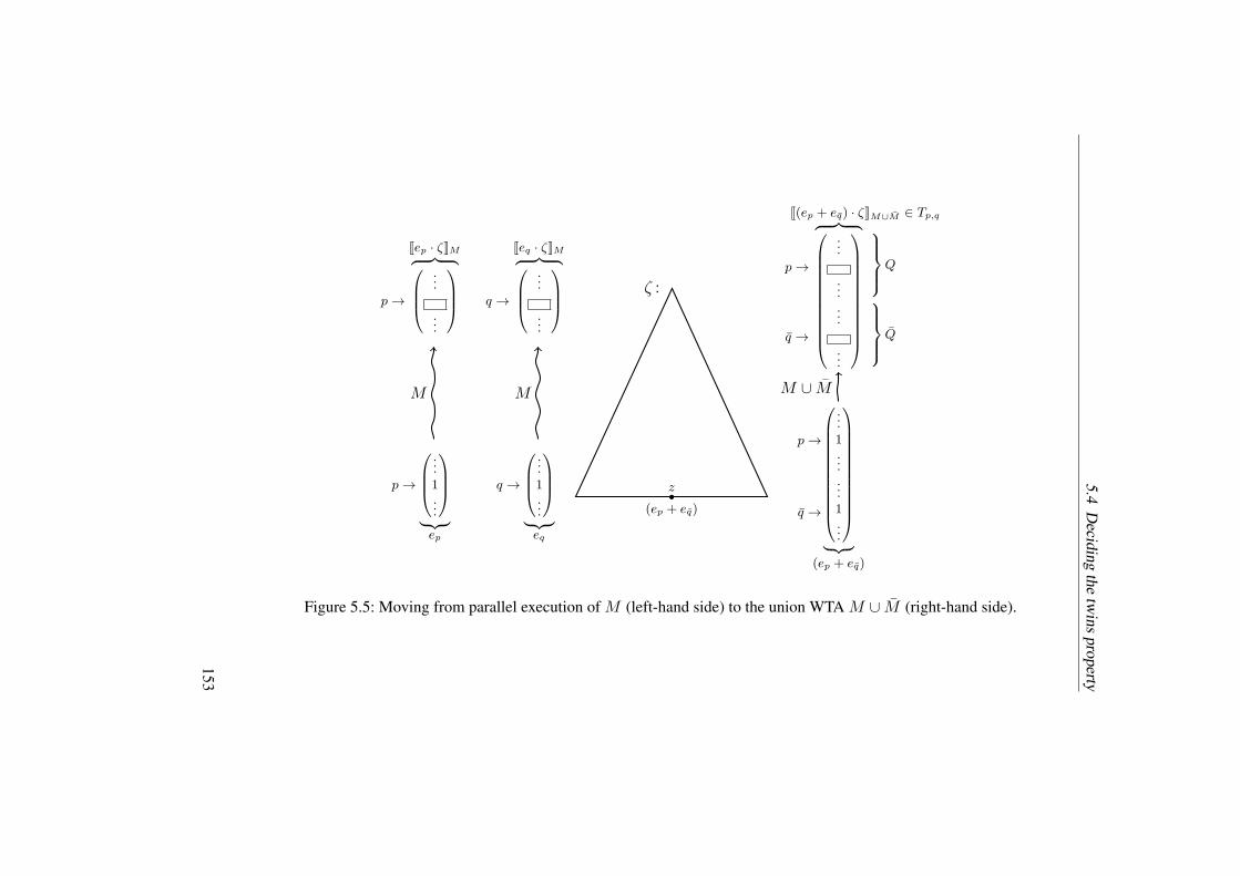
5.4
Decid
ing
the
twin
spro
perty
ζ :
(ep + eq)
z
p →
Jep · ζKM︷ ︸︸ ︷
...
...
p →
...
1...
︸ ︷︷ ︸
ep
M
q →
Jeq · ζKM︷ ︸︸ ︷
...
...
q →
...
1...
︸ ︷︷ ︸
eq
M
J(ep + eq) · ζKM∪M ∈ Tp,q︷ ︸︸ ︷
...
...
...
...
p →
q →
Q
Q
...
1...
...
1...
︸ ︷︷ ︸
(ep + eq)
p →
q →
M ∪ M
Figure 5.5: Moving from parallel execution of M (left-hand side) to the union WTA M ∪ M (right-hand side).
153
5 Determinizing weighted tree automata using factorizations
Observation 5.4.3 If M has the twins property, then so does M ∪ M .
Using M ∪ M , we are now able to describe the search space of our problem. For
every p, q ∈ Q we define the set Tp,q ⊆ SQ∪Q by
Tp,q = J(ep + eq) · ζ | ζ ∈ CΓKM∪M ,
where we note that ep, eq ∈ SQ∪Q. Moreover, we call any vector u ∈ SQ∪Q critical
(for (p, q)) if up 6= 0, uq 6= 0, and up 6= uq. We note that 0 is not a critical vector, and
that a vector u ∈ SQ∪Q \ 0 is critical iff f(u) is critical. With these prerequisites, we
can make two easy observations.
Observation 5.4.4 Let p, q ∈ Q. Then (p, q) ∈ TWINS(M) iff Tp,q does not contain
any critical vector.
Observation 5.4.5 The following three statements are equivalent.
(a) The WTA M has the twins property.
(b) The set⋃
(p,q)∈SIB(M) Tp,q is devoid of critical vectors.
(c) The set⋃
(p,q)∈SIB(M) f(Tp,q \ 0) is devoid of critical vectors.
We call the sets in Obs. 5.4.5(b) and (c) the search space and the compressed search
space, respectively.
In the following, we show that the compressed search space is finite if M has the
twins property. To this end, we will construct, for every (p, q) ∈ SIB(M), a WTA
M(p,q) over Γ ∪ ∗ and S such that (i) there is an injective mapping from Tp,q into
JTΓ∪∗KM(p,q)and (ii) if M has the twins property, then so does M(p,q). This will
enable us later to apply Cor. 5.2.14.
Let M ∪ M = (Q′, µ′, ν ′). We let M(p,q) = (Q′′, µ′′, ν ′′) where
• Q′′ = 0, 1 ×Q′,
• µ′′((b1, q′1) · · · (bk, q
′k), σ, (b, q
′)) = µ′(q′1 · · · q′k, σ, q
′) if b =∑
j bj ,
• µ′′(ε, ∗, (1, p)) = µ′′(ε, ∗, (1, q)) = 1,
• µ′′ maps all other transitions to 0,
• ν ′′(1, q′) = ν ′(q′), and ν ′′ maps all other states to 0.
154

5.4 Deciding the twins property
For every b ∈ 0, 1, we define the mappings
ϕb : SQ∪Q → S0,1×(Q∪Q) and ϕ′
b : S0,1×(Q∪Q) → SQ∪Q
by letting ϕb(u)(b,q′) = uq′ , ϕb(u)(b′,q′) = 0 for b′ 6= b, and ϕ′b(u)q′ = u(b,q′). The
following observation is easy to show by induction on m.
Observation 5.4.6 For every m ∈ N and t ∈ TΓ∪∗, if |pos(t)| ≤ m, then
JtKM(p,q)=
ϕ0(JtKM∪M ) if t ∈ TΓ,
ϕ1(Jt[∗/(ep + eq)]KM∪M ) if ∗ occurs exactly once in t,
0 otherwise.
Corollary 5.4.7 We have that ϕ1(Tp,q) \ 0 = (ϕ1(SQ∩Q) ∩ JTΓ∪∗KM(p,q)
) \ 0.
PROOF. Let u ∈ ϕ1(Tp,q) and u 6= 0. Then there is a ζ ∈ CΓ such that u = ϕ1(J(ep +
eq) · ζKM∪M ). By Obs. 5.4.6, we have that J∗ · ζKM(p,q)= u. Hence, u ∈ (ϕ1(S
Q∩Q)∩
JTΓ∪∗KM(p,q)) \ 0. Now let u ∈ ϕ1(S
Q∪Q) ∩ JTΓ∪∗KM(p,q)and u 6= 0. Then
there is a t ∈ TΓ∪∗ with u = JtKM(p,q). Since u ∈ ϕ1(S
Q∪Q) \ 0, Obs. 5.4.6
yields that ∗ occurs exactly once in t and that u = ϕ1(Jt[∗/(ep + eq)]KM∪M ). Hence,
u ∈ ϕ1(Tp,q).
Lemma 5.4.8 If M has the twins property, then so does M(p,q).
PROOF. Let ((b, p′), (c, q′)) ∈ SIB(M(p,q)). Then there is a t ∈ TΓ∪∗ such that
JtK(b,p′) 6= 0 and JtK(c,q′) 6= 0. Using Obs. 5.4.6, we obtain that either (i) t ∈ TΓ and
b = c = 0 or (ii) ∗ occurs exactly once in t and b = c = 1.
We show that (p′, q′) ∈ SIB(M ∪ M). In Case (i), this is trivial. In Case (ii), we
use that (p, q) ∈ SIB(M), thus (p, q) ∈ SIB(M ∪ M), and thus there is a t′ ∈ TΓwith (Jt′KM∪M )p 6= 0 and (Jt′KM∪M )q 6= 0. Since S is an extremal semifield, it is
zero-sum free and zero-divisor free, and we obtain that (Jt[∗/t′]KM∪M )p′ 6= 0 and
(Jt[∗/t′]KM∪M )q′ 6= 0.
We show that ((b, p′), (c, q′)) ∈ TWINS(M(p,q)). Let ζ ∈ CΓ∪∗ such that Je(b,p′) ·ζK(b,p′) 6= 0 and Je(c,q′) ·ζK(c,q′) 6= 0. It is easy to see that then ∗ does not occur in ζ, and
that Je(b,p′) · ζK(b,p′) = Jep′ · ζKp′ and Je(c,q′) · ζK(c,q′) = Jeq′ · ζKq′ . Then the statement
follows because M ∪ M has the twins property, by Obs. 5.4.3.
Lemma 5.4.9 Let M have the twins property. For every (p, q) ∈ SIB(M) the set
f(Tp,q \ 0) is finite.
155

5 Determinizing weighted tree automata using factorizations
Algorithm 5.1 Decision algorithm.
Require:
M = (Q,µ, ν) a classical WTA over Γ and S ,
S commutative and extremal,
(f, g) a maximal factorization of dimension Q ∪ QEnsure:
print “yes” iff M has the twins property
1: compute SIB(M)2: for (p, q) ∈ SIB(M) in parallel do
3: for u ∈ f(Tp,q \ 0) do
4: if u is a critical vector then
5: print “no” and terminate
6: print “yes”
PROOF. Since S is an extremal semifield, it is also zero-sum free, and Lm. 5.2.2 yields
that there is a maximal factorization (f ′, g′) of dimension 0, 1 × (Q ∪ Q). We con-
struct a new factorization (f ′′, g′′) where
(f ′′(u), g′′(u)) = (ϕ1(f(ϕ′1(u))), g(ϕ
′1(u))) , (if u = ϕ1(ϕ
′1(u)))
(f ′′(u), g′′(u)) = (f ′(u), g′(u)) . (otherwise)
It is easy to see that (f ′′, g′′) is indeed a factorization; even a maximal one.
By Lm. 5.4.8 and Cor. 5.2.14, there is a finite set U such that
ϕ1(f(Tp,q \ 0)) = f ′′(ϕ1(Tp,q \ 0))
= f ′′((ϕ1(SQ∪Q) ∩ JTΓ∪∗K) \ 0) (Cor. 5.4.7)
⊆ f ′′(JTΓ∪∗K \ 0) ⊆ f′′(S · U \ 0) (Cor. 5.2.14)
= f ′′(U \ 0) . (maximal factorization)
Since U is finite and ϕ1 is injective, f(Tp,q \ 0) is finite as well.
Now we consider two decision algorithms that are based on Lm. 5.4.9. The first one,
Alg. 5.1, searches the compressed search space for critical vectors.
Lemma 5.4.10 Algorithm 5.1 terminates, and it is correct.
PROOF. First, the algorithm enumerates SIB(M). This is possible due to Lm. 5.4.1.
Second, for each (p, q) ∈ SIB(M) in parallel, it enumerates f(Tp,q \0), checking for
critical vectors. For this step, we distinguish two cases.
156

5.4 Deciding the twins property
If M has the twins property, then, by Lm. 5.4.9 and Obs. 5.4.5, f(Tp,q \0) is finite
and devoid of critical vectors, and the algorithm terminates with output “yes”.
Otherwise, by Obs. 5.4.5, the algorithm finds a critical vector at some point and
outputs “no”. For this, the parallel processing (Line 2) is critical because there may be
(p, q) ∈ SIB(M) such that f(Tp,q \ 0) is infinite, yet devoid of critical vectors.
Algorithm 5.1 is rather straightforward, but that comes at a price. In order to enu-
merate the compressed search space, we can in principle enumerate CΓ and compute
fJ(ep + eq) · ζK for each ζ ∈ CΓ. However, the weights already computed for subtrees
and subcontexts of ζ are not reused in this approach. For this reason, we consider an
alternative procedure – Alg. 5.2.
Algorithm 5.2 does not enumerate CΓ explicitly; instead, it works on weight vectors,
thereby avoiding redundant calculation. Roughly speaking, it employs a maximal fac-
torization (f, g) of appropriate dimension and computes det((f, g),M(p,q)) for every
(p, q) ∈ SIB(M). The following lemma shows that the state sets of these WTA com-
prise a legitimate alternative to our compressed search space. Let u ∈ S0,1×(Q∪Q);
then u is a critical vector if ϕ′1(u) is a critical vector.
Lemma 5.4.11 Let (f, g) be a maximal factorization of dimension 0, 1 × (Q ∪ Q),and let (Q′
(p,q) | (p, q) ∈ SIB(M)) be the family such that Q′(p,q) is the set of states of
det((f, g),M(p,q)). Then the following are equivalent:
(a)⋃
(p,q)∈SIB(M) Tp,q contains a critical vector,
(b) f(ϕ1(⋃
(p,q)∈SIB(M) Tp,q \ 0)) contains a critical vector,
(c) ϕ1(SQ∩Q) ∩
⋃
(p,q)∈SIB(M)Q′(p,q) contains a critical vector.
PROOF. The first equivalence is easy to see. For the second equivalence, we derive
f(ϕ1(⋃
(p,q)∈SIB(M) Tp,q \ 0))
=⋃
(p,q)∈SIB(M) f(ϕ1(Tp,q \ 0))
=⋃
(p,q)∈SIB(M) f((ϕ−11 (SQ∩Q) ∩ JTΓ∪∗KM(p,q)
) \ 0) (Cor. 5.4.7)
= ϕ1(SQ∩Q) ∩
⋃
(p,q)∈SIB(M) f(JTΓ∪∗KM(p,q)\ 0)
= ϕ1(SQ∩Q) ∩
⋃
(p,q)∈SIB(M)Q′(p,q) \ 0 . (Cor. 5.3.9)
Recall that 0 is not a critical vector.
157
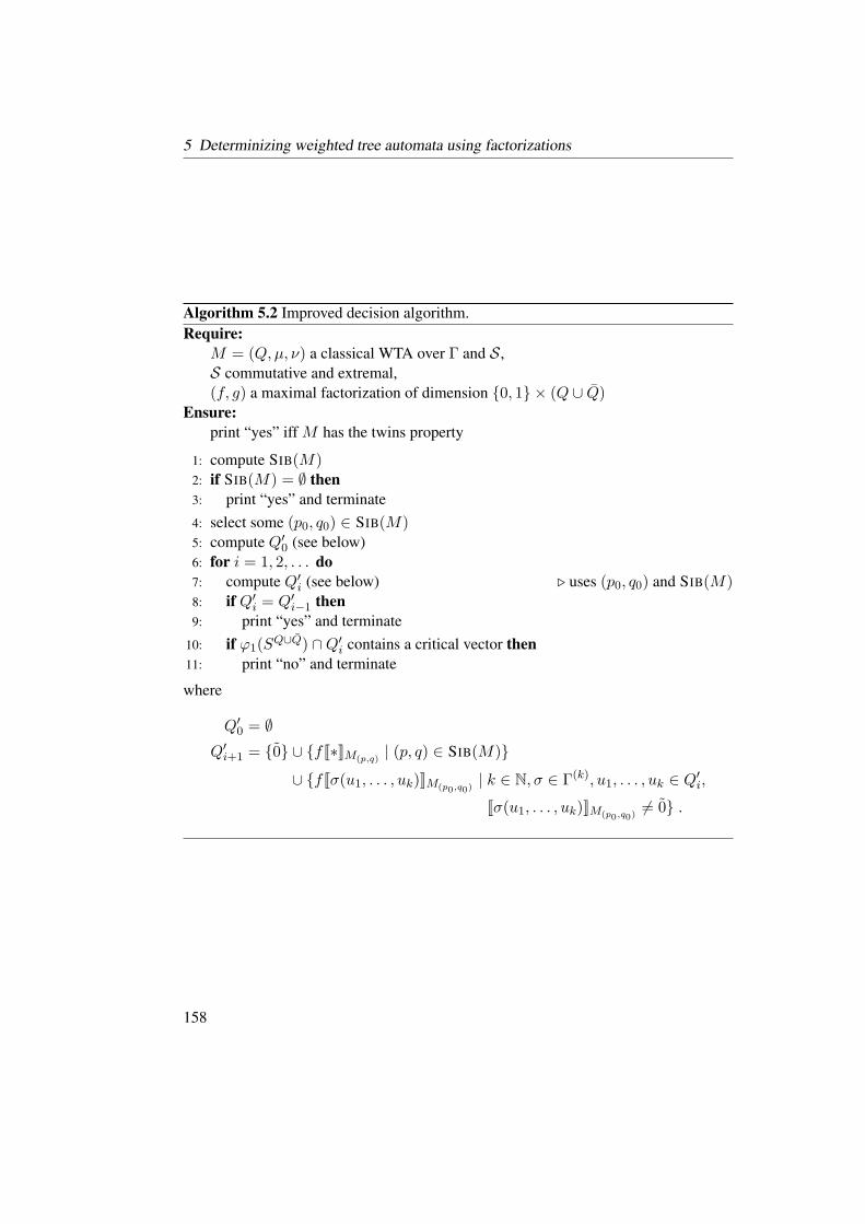
5 Determinizing weighted tree automata using factorizations
Algorithm 5.2 Improved decision algorithm.
Require:
M = (Q,µ, ν) a classical WTA over Γ and S ,
S commutative and extremal,
(f, g) a maximal factorization of dimension 0, 1 × (Q ∪ Q)Ensure:
print “yes” iff M has the twins property
1: compute SIB(M)2: if SIB(M) = ∅ then
3: print “yes” and terminate
4: select some (p0, q0) ∈ SIB(M)5: compute Q′
0 (see below)
6: for i = 1, 2, . . . do
7: compute Q′i (see below) ⊲ uses (p0, q0) and SIB(M)
8: if Q′i = Q′
i−1 then
9: print “yes” and terminate
10: if ϕ1(SQ∪Q) ∩Q′
i contains a critical vector then
11: print “no” and terminate
where
Q′0 = ∅
Q′i+1 = 0 ∪ fJ∗KM(p,q)
| (p, q) ∈ SIB(M)
∪ fJσ(u1, . . . , uk)KM(p0,q0)| k ∈ N, σ ∈ Γ(k), u1, . . . , uk ∈ Q
′i,
Jσ(u1, . . . , uk)KM(p0,q0)6= 0 .
158

5.4 Deciding the twins property
Lemma 5.4.12 Algorithm 5.2 terminates, and it is correct.
PROOF. The case that SIB(M) = ∅ is trivial. We turn to the converse case. We
let (Q′(p,q) | (p, q) ∈ SIB(M)) be the family such that Q′
(p,q) is the set of states of
det((f, g),M(p,q)). For every (p, q) ∈ SIB(M), we apply Obs. 5.3.2 to M(p,q) and
denote the corresponding family by (Q′(p,q),i | i ∈ N). Let (Q′
i | i ∈ N) be the family
defined in Alg. 5.2. A straightforward proof by induction on i yields that
Q′i =
⋃
(p,q)∈SIB(M)Q′(p,q),i . (∗)
Now we distinguish two cases. EitherM has the twins property. Then, by Lm. 5.4.8,
so does M(p,q) for every (p, q) ∈ SIB(M), and by Lm. 5.3.12, the set Q′(p,q) is finite,
and Q′(p,q),i = Q′
(p,q),i+1 for some i. By (∗), then, also Q′i = Q′
i+1 for some i, and the
algorithm terminates. By Lm. 5.4.11, it outputs “yes”.
Or M does not have the twins property. By Obs. 5.4.5 and Lm. 5.4.11, the algorithm
finds a critical vector at some point and outputs “no”.
We note that, as is evident from Obs. 5.4.6, at least half of the components of every
vector in Q′i is zero, so there is room for optimizing the algorithm. For instance, one
can partition Q′i into the following three blocks:
0 ,(ϕ0(S
Q∪Q) ∩Q′i
)\ 0 ,
(ϕ1(S
Q∪Q) ∩Q′i
)\ 0 .
Then the first block is irrelevant for the algorithm and may be omitted, and the remain-
ing blocks can be represented by their images under ϕ′0 and ϕ′
1, respectively.
5.4.2 Cycle-unambiguous weighted tree automata
In this section, we show that the twins property is decidable for a decidable subclass of
WTA called cycle unambiguous. This result is inspired by a similar one for the string
case found in [5, Thm. 5]. The following definition is also adapted from [5, Sec. 2.1].
A WTAN = (Q,R, µ, ν) over Σ and S is called cycle unambiguous if for every q ∈ Qand ζ ∈ CΣ there is at most one d ∈ Dq(N, q · ζ) such that 〈d〉 6= 0. For instance, the
WTA of Ex. 2.4.1 is cycle unambiguous.
Lemma 5.4.13 Let S be commutative, zero-sum-free, and zero-divisor-free, and let Mbe cycle unambiguous. Then TWINS
′(M) ⊆ TWINS(M), where TWINS′(M) is defined
like TWINS(M), with the additional condition that ht(ζ) ≤ 2 · |Q|2.
159
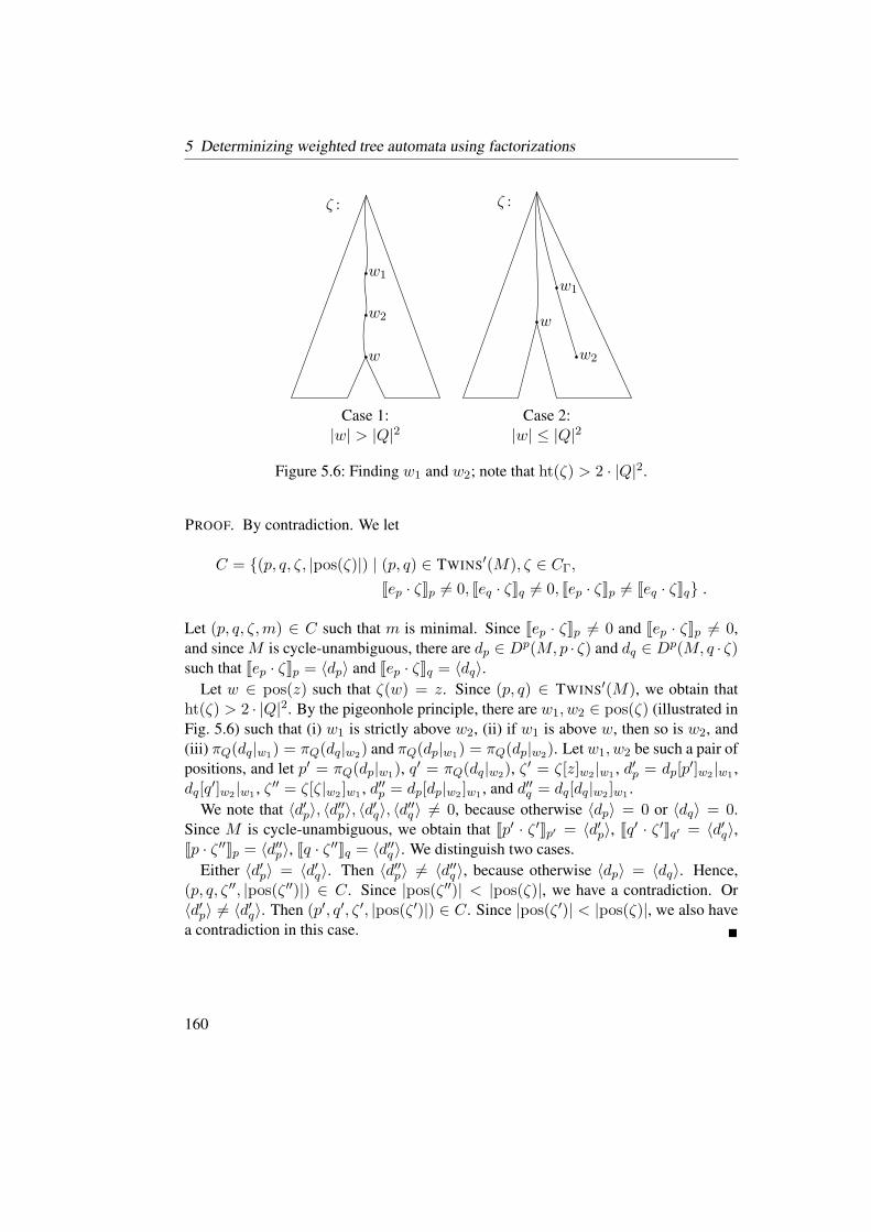
5 Determinizing weighted tree automata using factorizations
w
w1
w2
ζ :
w
w1
w2
ζ :
Case 1: Case 2:
|w| > |Q|2 |w| ≤ |Q|2
Figure 5.6: Finding w1 and w2; note that ht(ζ) > 2 · |Q|2.
PROOF. By contradiction. We let
C = (p, q, ζ, |pos(ζ)|) | (p, q) ∈ TWINS′(M), ζ ∈ CΓ,
Jep · ζKp 6= 0, Jeq · ζKq 6= 0, Jep · ζKp 6= Jeq · ζKq .
Let (p, q, ζ,m) ∈ C such that m is minimal. Since Jep · ζKp 6= 0 and Jep · ζKp 6= 0,
and since M is cycle-unambiguous, there are dp ∈ Dp(M,p · ζ) and dq ∈ D
p(M, q · ζ)such that Jep · ζKp = 〈dp〉 and Jep · ζKq = 〈dq〉.
Let w ∈ pos(z) such that ζ(w) = z. Since (p, q) ∈ TWINS′(M), we obtain that
ht(ζ) > 2 · |Q|2. By the pigeonhole principle, there are w1, w2 ∈ pos(ζ) (illustrated in
Fig. 5.6) such that (i) w1 is strictly above w2, (ii) if w1 is above w, then so is w2, and
(iii) πQ(dq|w1) = πQ(dq|w2) and πQ(dp|w1) = πQ(dp|w2). Let w1, w2 be such a pair of
positions, and let p′ = πQ(dp|w1), q′ = πQ(dq|w2), ζ
′ = ζ[z]w2 |w1 , d′p = dp[p′]w2 |w1 ,
dq[q′]w2 |w1 , ζ ′′ = ζ[ζ|w2 ]w1 , d′′p = dp[dp|w2 ]w1 , and d′′q = dq[dq|w2 ]w1 .
We note that 〈d′p〉, 〈d′′p〉, 〈d
′q〉, 〈d
′′q 〉 6= 0, because otherwise 〈dp〉 = 0 or 〈dq〉 = 0.
Since M is cycle-unambiguous, we obtain that Jp′ · ζ ′Kp′ = 〈d′p〉, Jq′ · ζ ′Kq′ = 〈d′q〉,Jp · ζ ′′Kp = 〈d
′′p〉, Jq · ζ ′′Kq = 〈d
′′q 〉. We distinguish two cases.
Either 〈d′p〉 = 〈d′q〉. Then 〈d′′p〉 6= 〈d
′′q 〉, because otherwise 〈dp〉 = 〈dq〉. Hence,
(p, q, ζ ′′, |pos(ζ ′′)|) ∈ C. Since |pos(ζ ′′)| < |pos(ζ)|, we have a contradiction. Or
〈d′p〉 6= 〈d′q〉. Then (p′, q′, ζ ′, |pos(ζ ′)|) ∈ C. Since |pos(ζ ′)| < |pos(ζ)|, we also have
a contradiction in this case.
160

5.5 The case of non-classical WTA
Theorem 5.4.14 Let S be a commutative, zero-sum-free, zero-divisor-free semiring.
There is a procedure that takes any cycle-unambiguous classical WTA M over Γ and Sand outputs whether M has the twins property.
PROOF. By Lm. 5.4.1, we have that SIB(M) ⊆ SIB′(M). By Lm. 5.4.13, we have
that TWINS′(M) ⊆ TWINS(M). In both cases, the converse is trivial, so we obtain
that SIB′(M) = SIB(M) and TWINS
′(M) = TWINS(M). Hence, the sets SIB(M)and TWINS(M) can be computed in finite time. Since these sets are finite, checking
SIB(M) ⊆ TWINS(M) is a trivial matter.
We conclude this section by proving that the property “cycle unambiguous” is decid-
able. We call M finitely cycle unambiguous (fcu) if for every q ∈ Q and ζ ∈ CΓ with
ht(ζ) ≤ 3 · |Q|2, there is at most one d ∈ Dq(M, q · ζ) such that 〈d〉 6= 0.
Lemma 5.4.15 If M is fcu, then it is cycle unambiguous.
PROOF. By contradiction. To this end, let M be fcu, and let
C = (q, ζ, d, d′, |pos(ζ)|) | q ∈ Q, ζ ∈ CΓ, d, d′ ∈ Dq(M, q · ζ),
d 6= d′, 〈d〉 6= 0, 〈d′〉 6= 0 .
Let (q, ζ, d, d′,m) ∈ C such that m is minimal. Since d 6= d′, there is a w1 ∈ pos(ζ)with d(w1) 6= d′(w1). Let w2 ∈ pos(ζ) with ζ(z) = w2, and let w ∈ pos(ζ) be the
longest common prefix of w1 and w2.
Since M is fcu, |pos(ζ)| > 3 · |Q|2. By the pigeonhole principle, there are w3, w4 ∈pos(ζ) (illustrated in Fig. 5.7) such that (i) w3 is strictly above w4, (ii) if w3 is above w,
w1, or w2, then so is w4, respectively, and (iii) πQ(d|w3) = πQ(d|w4) and πQ(d′|w3) =
πQ(d′|w4). We let ζ ′ = ζ[ζ|w4 ]w3 , e = d[d|w4 ]w3 , and e′ = d′[d′|w4 ]w3 . We note that
ζ ′ ∈ CΓ and e 6= e′, both due to Condition (ii). Moreover, we have that 〈e〉, 〈e′〉 6= 0,
because otherwise 〈d〉 = 0 or 〈d〉′ = 0. Hence, (q, ζ ′, e, e′, |pos(ζ ′)|) ∈ C. Since
|pos(ζ ′)| < m, we have the contradiction.
Corollary 5.4.16 There is a procedure that takes any classical WTA M and outputs
whether M is cycle-unambiguous.
PROOF. Direct consequence of Lm. 5.4.15.
5.5 The case of non-classical WTA
In this section, we transfer the results of the preceding two sections to arbitrary, i.e., not
necessarily classical, WTA.
161

5D
eter
min
izin
gw
eighte
dtr
eeau
tom
ata
usi
ng
fact
ori
zati
ons w3
w4
w
w1 w2
ζ :
w
w3
w4
w1 w2
ζ :
w
w3
w4
w1 w2
ζ :
w3
w4
w
w1 w2
ζ :
Case 1: Case 2: Case 3: Case 4:
|w| > |Q|2 |w| ≤ |Q|2 |w| ≤ |Q|2 |w| ≤ |Q|2
|w1| > 2|Q|2 |w1| ≤ 2|Q|2 |w1|, |w2| ≤ 2|Q|2
|w2| > |Q|2
Figure 5.7: Finding w3 and w4; note that ht(ζ) > 3 · |Q|2.
162

5.5 The case of non-classical WTA
To this end, let Σ be an alphabet, Γ ⊆ Σ × N a ranked alphabet with rk(σ, k) = k,
and f : TΓ → TΣ the mapping that replaces each label by its first component. Two
weighted tree languages ϕ : TΣ → S and ϕ′ : TΓ → S are related if ϕ(f(t)) = ϕ′(t)for every t ∈ TΓ and ϕ(t) = 0 for every t ∈ TΣ \ f(TΓ).
Observation 5.5.1 If ϕ1 and ϕ′ are related, and so are ϕ2 and ϕ′, then ϕ1 = ϕ2.
Moreover, let M = (P,R, µ, ν) be a WTA over Σ and S and M ′ = (P ′, µ′, ν ′) a
classical WTA over Γ and S . We say that M and M ′ are related if (p1 · · · pk, σ, p) ∈ Rimplies (σ, k) ∈ Γ, P = P ′, ν = ν ′, and
µ′(p1 · · · pk, (σ, k), p) =
µ(p1 · · · pk, σ, p) if (p1 · · · pk, σ, p) ∈ R ,
0 otherwise.
Observation 5.5.2 Let M and M ′ be related. Then
(i) M is bu-det iff M ′ is bu-det,
(ii) M has the twins property iff M ′ has the twins property,
(iii) M is acyclic iff M ′ is acyclic,
(iv) M is cycle-unambiguous iff M ′ is cycle-unambiguous, and
(v) JMK and JM ′K are related.
We note that the definition of “related” gives rise to a natural construction turning
any WTA M into a related classical WTA M ′, as well as the converse construction.
From now on, we assume that these constructions are understood, and when we speak
of “the (classical) WTA related to . . . ”, we refer to these constructions.
Let M = (Q,R, µ, ν) be a WTA over Σ and S , and let (f, g) be a factorization of
dimension Q. The unranked determinization udet((f, g),M) of M by (f, g) is either a
WTA over Σ and S or it is undefined, as follows. Let M ′ be the classical WTA related
to M . If det((f, g),M ′) is a WTA, then we let det((f, g),M) be the WTA related to
det((f, g),M ′). Otherwise, udet((f, g),M) is undefined.
Theorem 5.5.3 Let M = (Q,R, µ, ν) be a WTA over Σ and S , and let (f, g) be the
trivial or a maximal factorization. If (f, g) is not the trivial factorization, let S be
commutative. Moreover, let one of the following conditions hold:
• M is acyclic,
• S is locally finite,
163
5 Determinizing weighted tree automata using factorizations
• (f, g) is maximal and M is bu-det, or
• (f, g) is maximal, M has the twins property, and S is extremal.
Then udet((f, g),M) is a bu-det WTA over Σ and S , and it is equivalent to M .
PROOF. This follows from Thm. 5.3.4, Obs. 5.5.1, and Obs. 5.5.2.
Theorem 5.5.4 Let S be an extremal semifield. Then there is a procedure that takes
any WTA M over Σ and S and outputs whether M has the twins property.
PROOF. This follows from Thm. 5.4.2 and Obs. 5.5.2.
Theorem 5.5.5 Let S be a commutative, zero-sum-free, and zero-divisor-free semiring.
Then there is a procedure that takes any cycle-unambiguous WTA M over Σ and S and
outputs whether M has the twins property.
PROOF. This follows from Thm. 5.4.14 and Obs. 5.5.2.
Theorem 5.5.6 There is a procedure that takes any WTA M and outputs whether M is
cycle-unambiguous.
PROOF. This follows from Cor. 5.4.16 and Obs. 5.5.2.
5.6 Conclusion, discussion, and outlook
We have used the factorization approach of [138, 105] to develop a determinization
construction for WTA. Theorem 5.5.3 and Tab. 5.1 summarize the requirements un-
der which our construction solves the determinization problem. We have also shown
that, roughly speaking, maximal factorizations only exist for zero-divisor-free semi-
rings. Furthermore, we have shown that the twins property is decidable (i) for cycle-
unambiguous WTA over commutative, zero-sum-free, zero-divisor-free semirings and
(ii) for WTA over extremal semifields.
The present determinization result was largely obtained by generalizing [105] from
strings to trees, and many of our proofs follow theirs. Likewise, the decidability result
in Case (i) was obtained by generalizing [5] from strings to trees, but our proofs do
not follow theirs. In particular, they provide a polynomial-time decision algorithm. In
contrast, while our proofs are effective, they do not suggest efficient decision proce-
dures. It is open whether efficient algorithms exist for WTA. We note that the transition
from strings to trees made the proofs more intricate and at some points necessitated
commutativity of the semiring.
164

5.6 Conclusion, discussion, and outlook
As for Case (ii), the notion that the twins property can be decided by searching
for critical vectors in a compressed search space is due to Kirsten [104]. We have
generalized his work in the following two ways. First, we allow arbitrary extremal
semifields instead of the tropical semiring. To this end, we use the notion of a maximal
factorization, which is implicit in his work. Second, we consider WTA instead of WSA.
This makes the proof more complex, as we have to distinguish between contexts and
trees.
Kirsten’s result that deciding the twins property is PSPACE-hard directly transfers to
our setting, giving a lower bound on the complexity of our algorithms. In addition, he
shows that the problem is PSPACE-complete by giving a PSPACE algorithm. It is open
whether this result can be transferred to our setting as well. It is also an open question
which algorithm, Alg. 5.1 or Alg. 5.2, performs better in practice.
As mentioned at the very top, this chapter is an extensively revised version of the
papers [31] and [27]. The former work covers the determinization construction and
Case (i) of the decidability problem, while the latter work is concerned with Case (ii).
In this chapter, we added the case of non-classical WTA. Moreover, we reduced the
question whether the compressed search space is finite to the question whether the set
of all weight vectors of some WTA is finite (cf. the proof of Lm. 5.4.9). The original
contribution, on the other hand, contains a direct proof [27, Lm. 3.3]. Likewise, we
reused the determinization construction for the decision procedure in Alg. 5.2, in con-
trast to the original contribution [27, Alg. 2]. In both instances, the original contribution
duplicates proof work considerably.
We already mentioned some items for further research in passing, namely efficient
decision procedures for Case (i), PSPACE membership of the problem in Case (ii),
and which decision algorithm performs better in practice. We name two more items,
which are related to sufficient conditions for the determinization to be finite. First, one
could consider general requirements that also cover cases like Ex. 5.3.6, where neither
the trivial nor any maximal factorization is viable. Second, it might be desirable to
determinize a WTA that is not acyclic over a semiring that is not extremal, say, the
nonnegative reals.
165


6 Conclusion
Chapter 1 proposed a preliminary version of an algebraic framework for specifying
decoders, promising the achievements in Tab. 1.1. Let us scrutinize this promise:
(a) Sections 1.4 and 1.5.1 showed how to specify syntax-based decoders in the pre-
liminary framework. Our decoders were mostly inspired by Hiero, as are SMT
systems to this day [14]. That being said, current research in SMT is largely con-
cerned with discovering and selecting useful feature functions. The three features
that we covered are not representative of the state of the art; the framework may
need amendments for supporting contemporary features.
(b) We convinced ourselves that our specifications were readily effective from the out-
set. To this end, we treated each operation in isolation and gathered a suitable
closure result. As a whole, the closure results imply a 1:1 translation of a spec-
ification into a (composite) algorithm. The preliminary version still forced us to
provide small constructions ourselves; the full version is supposed to fix that. For
the next refinement steps – the efficient specification and the computer program –
it is yet to be shown that the same per-operation approach works.
(c) The closure results imply that said composite algorithm is correct.
(d) We exploited the theory of weighted tree automata and related devices in Sec. 1.4.
We saw potential for developing the theory in Sec. 1.5. The three main contribu-
tions of this thesis (Chs. 3–5) underscore the viability of the framework, both as a
specification mechanism and as an interface between theory and application.
In the following sections, we consider the full version of the framework, and we dis-
cuss further ways of developing both said theory and the framework itself. In particular,
we gather preliminary evidence that the per-operation approach may be successful for
said refinement steps.
6.1 The algebraic framework, full version
The full version of the algebraic framework capitalizes on semiring homomorphisms
and the multiset semiring. Let us define the multiset semiring, as well as several useful
167

6 Conclusion
homomorphisms. For this, let S = (S,, 1) be a monoid. A (finite) multiset (over
S) is a mapping u : S → N such that s | us 6= 0 is finite. We denote the set of
all finite multisets over S by N〈S〉. We define (1.) : S → N〈S〉 by letting (1.s)s = 1and (1.s)s′ = 0 for s 6= s′. The (multiset) Cauchy product · is the binary operation
on N〈S〉 such that (u1 · u2)s =∑
s1,s2∈S : s=s1s2(u1)s1 · (u2)s2 . The semiring N〈S〉
of (finite) multisets over S is (N〈S〉,+, ·, 0, 1.1), where + is the conventional addition
applied pointwise. The mapping (1.) is a monoid homomorphism from S into the
multiplicative monoid of N〈S〉; and if S is commutative, then so is N〈S〉.Let S ′ be a monoid and h : S → S ′. We define h♯ : N〈S〉 → N〈S′〉 by letting
h♯(u)s′ =∑
s : h(s)=s′ us. Then h♯ : N〈S〉 → N〈S ′〉 and (h2 h1)♯ = h♯2 h
♯1 (see
Lm. 6.1.1 below). Now let S ′ be a semiring whose multiplicative monoid is S . Then
the semiring N〈S ′〉 of multisets over S ′ is N〈S〉. We define hS′ : N〈S〉 → S with
hS′(u) =∑
s∈S
∑
j : 0≤j<uss. Then hS′ : N〈S ′〉 → S ′ (see Lm. 6.1.2 below), and we
call it the S ′-aggregation homomorphism.
Let Γ be an alphabet, S a semiring, and M = (Q,R, µ, ν) a WTA over Γ and S .
We define the WTA 1.M over Γ and N〈S〉 by letting 1.M = (Q,R, (1.) µ, (1.) ν).The m-meaning of M is J1.MK. The m-meaning of a WSA/a productive WSTSG is
defined analogously. Let us develop some intuition for the multiset semiring and the
m-meaning. Since (1.) is a monoid homomorphism, we obtain that 〈d〉(1.)µ · 1.νq =1.(〈d〉µ · νq) for every d ∈ Dq(M). Hence, thanks to the multiset semiring, J1.MK(t)stells us how many runs with weight s contribute to JMK(t). Of course, this information
is sufficient to compute JMK(t) itself; formally, hS(J1.MK(t)) = JMK(t). Intuitively
speaking, the multiset semiring allows us to expose the runs to the meaning, and this is
exactly what we were looking for in the closing remarks of Sec. 1.4.
Let I be a set, S,S ′ semirings, and h : S → S′. We define h : SI → (S′)I by
letting h(u)i = h(ui). If h : S → S ′, then h : SI → (S ′)I (proof omitted). Note
that (h2 h1) = h2 h
1. For every d ∈ N, d ≥ 1, and u ∈ R
d, we define the unary
operation (·u) on sRd by letting (·u)(u′) = u′ · u, where · is the inner product. This
operation is a homomorphism from the multiplicative monoid of Arctd into itself. Here
we do not distinguish between Arct1 and Arct. For every j ∈ 1, . . . , d, we define
in(d)j : sR→ sR
d by letting
in(d)j (r)j′ =
−∞ if r = −∞,
r if r 6= −∞, j = j′,
0 otherwise.
Then in(d)j : Arct→ Arctd. This concludes the general definitions.
The full version of the algebraic framework is constituted by the operations of the
preliminary version, as well as all operations of the form h, provided that the underly-
168

6.1 The algebraic framework, full version
ing semirings are commutative.
In order to illustrate the framework, we rephrase (1.3). For this, let G be an STSG, µa probability assignment for G, θ ∈ R
3, and θ = (θ1, θ2, θ3). Moreover, let G′ be the
WSTSG over Σ and Real that is obtained from G by using the weight assignment µ,
let M be a deterministic WSA with JMK(e) = PLM(e), and let M ′ be a bu-det WTA
with JM ′K(t) = P (t | yd(t)). Since N〈Real〉 is not complete, we additionally require
that G′ be productive. We claim (without proof) that
τ = (hArct ((·θ1) log)♯)(J1.G′K) , (6.1)
ϕLM = ((·θ2) log)(JMK) , (6.2)
ϕP = ((·θ3) log)(JM ′K) , (6.3)
where, via composition, hArct ((·θj) log)♯ : N〈Real〉 → Arct.
We show that the specification is again effective. To this end, we enhance the notation
of our classes K, L, T , and their subclasses by adding the underlying semiring as a
superscript. We introduce the five classes
KSdRec = ϕ | ϕ ∈ K
S , ϕ is the meaning of some deterministic WSA ,
LSdRec = ϕ | ϕ ∈ LS , ϕ is the meaning of some bu-det WTA ,
KN〈S〉mdRec = ϕ | ϕ ∈ K
N〈S〉, ϕ is the m-meaning of some deterministic WSA ,
LN〈S〉mdRec = ϕ | ϕ ∈ L
N〈S〉, ϕ is the m-meaning of some bu-det WTA ,
TN〈S〉
mSTSG = τ | τ ∈ T N〈S〉, τ is the m-meaning of some productive WSTSG .
Table 6.1 lists results about the computability of the additional operations. For the
second section of the table, we merely switch from “meaning” to “m-meaning” without
touching the underlying device. For the third section of the table, we perform the
corresponding constructions from Tab. 1.2 on the underlying device (over S); note that
the determinism requirement in LN〈S〉mdRec is crucial for ⊙, ⊳, and ⊲. For the fourth
section, we perform g on the underlying device.
The entries referring to g in the first section of the table deserve some discussion.
Although it seems plausible that the semiring addition is immaterial for deterministic
devices, caution is in fact advised: when there is no run, then the empty sum (the
semiring zero) comes into play, and g need not map the zero of S to the zero of S ′. We
can recover the closure result in two ways:
• Either we simply require that g(0) = 0. This property holds for g = log, but
not for g = (1.), because multisets distinguish between 1.0 (“exactly one run; its
weight is 0”) and 0 (“no run”). For our application above (ϕ′LM and ϕ′
P), we can
as well use a variation of (1.) that maps 0 to 0.
169
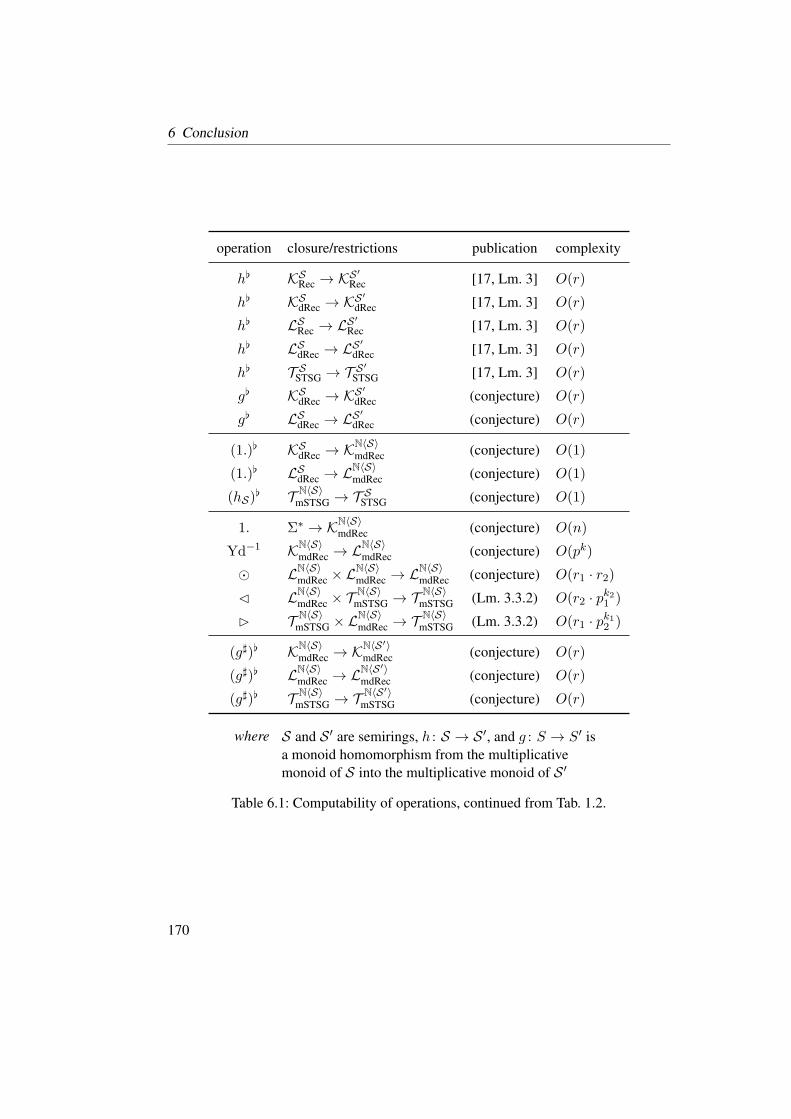
6 Conclusion
operation closure/restrictions publication complexity
h KSRec → K
S′
Rec [17, Lm. 3] O(r)
h KSdRec → K
S′
dRec [17, Lm. 3] O(r)
h LSRec → LS′
Rec [17, Lm. 3] O(r)
h LSdRec → LS′
dRec [17, Lm. 3] O(r)
h T SSTSG → T
S′
STSG [17, Lm. 3] O(r)
g KSdRec → K
S′
dRec (conjecture) O(r)
g LSdRec → LS′
dRec (conjecture) O(r)
(1.) KSdRec → K
N〈S〉mdRec (conjecture) O(1)
(1.) LSdRec → LN〈S〉mdRec (conjecture) O(1)
(hS) T
N〈S〉mSTSG → T
SSTSG (conjecture) O(1)
1. Σ∗ → KN〈S〉mdRec (conjecture) O(n)
Yd−1 KN〈S〉mdRec → L
N〈S〉mdRec (conjecture) O(pk)
⊙ LN〈S〉mdRec × L
N〈S〉mdRec → L
N〈S〉mdRec (conjecture) O(r1 · r2)
⊳ LN〈S〉mdRec × T
N〈S〉mSTSG → T
N〈S〉mSTSG (Lm. 3.3.2) O(r2 · p
k21 )
⊲ TN〈S〉
mSTSG × LN〈S〉mdRec → T
N〈S〉mSTSG (Lm. 3.3.2) O(r1 · p
k12 )
(g♯) KN〈S〉mdRec → K
N〈S′〉mdRec (conjecture) O(r)
(g♯) LN〈S〉mdRec → L
N〈S′〉mdRec (conjecture) O(r)
(g♯) TN〈S〉
mSTSG → TN〈S′〉
mSTSG (conjecture) O(r)
where S and S ′ are semirings, h : S → S ′, and g : S → S′ is
a monoid homomorphism from the multiplicative
monoid of S into the multiplicative monoid of S ′
Table 6.1: Computability of operations, continued from Tab. 1.2.
170

6.1 The algebraic framework, full version
• Or we preprocess the given WSA or WTA: roughly speaking, we add a sink state
and, where necessary, transitions of weight 0. This intrusion does not affect the
meaning, but it guarantees that there is exactly one run for every string or tree, so
that empty sums are ruled out.
As in Sec. 1.4, let us now use the framework according to its purpose and specify a
new decoder. We let χj = ((in(3)j log)
♯) and define
D2 : TN〈Real〉
mSTSG ×KN〈Real〉mdRec × L
N〈Real〉mdRec × R
3 → EF , D2(τ, ϕ, ϕ′, θ) :
f 7→ best(Yd(π2([hArct (·θ)
♯](ϕ0)))) , where (6.4)
ϕ0 =(Yd−1(1.f)⊙ χ3(ϕ
′))⊳ χ1(τ)⊲Yd−1
(χ2(ϕ)
).
This specification enjoys the nice property that, by a minor change, we obtain a decoder
in the spirit of D′0 of Sec. 1.2, which selects the translation with the highest aggregate
score. The change consists in replacing hArct by hReal exp♯. Be advised that, like D′
0,
the resulting decoder is NP hard.
We conclude this section by providing the two promised lemmas and by discussing
the prospects of “infinite multisets”.
Lemma 6.1.1 Let S,S ′,S ′′ be monoids and h : S → S ′. Then h♯ : N〈S〉 → N〈S ′〉.
Moreover, let h1 : S → S′, h2 : S
′ → S ′′. Then (h2 h1)♯ = h♯2 h
♯1.
PROOF. For the first statement, only the multiplication is somewhat tricky. We derive
[h♯(u1) · h♯(u2)]s′
=∑
s′1,s′2 : s
′=s′1′s′2h♯(u1)s′1 · h
♯(u2)s′2
=∑
s′1,s′2 : s
′=s′1′s′2
(∑
s1 : h(s1)=s′1(u1)s1
)·(∑
s2 : h(s2)=s′2(u2)s2
)
=∑
s′1,s′2 : s
′=s′1′s′2
∑
s1 : h(s1)=s′1
∑
s2 : h(s2)=s′2(u1)s1 · (u2)s2 (distributivity)
=∑
s′1,s′2,s1,s2 : s
′=h(s1)′h(s2),h(s1)=s′1,h(s2)=s′2(u1)s1 · (u2)s2
=∑
s′1,s′2,s1,s2 : s
′=h(s1s2),h(s1)=s′1,h(s2)=s′2(u1)s1 · (u2)s2
=∑
s1,s2 : s′=h(s1s2)(u1)s1 · (u2)s2 =
∑
s,s1,s2 : h(s)=s′,s=s1s2(u1)s1 · (u2)s2
=∑
s : h(s)=s′∑
s1,s2 : s=s1s2(u1)s1 · (u2)s2 = h♯(u1 · u2)s′ .
For the second statement, we derive
(h2 h1)♯(u)s′′ =
∑
s : h2(h1(s))=s′′us =
∑
s′,s : h2(s′)=s′′,h1(s)=s′us
=∑
s′ : h2(s′)=s′′∑
s : h1(s)=s′us =
∑
s′ : h2(s′)=s′′h♯1(u)s = h♯2(h
♯1(u))s′′ .
171

6 Conclusion
Lemma 6.1.2 Let S be a semiring. Then hS : N〈S〉 → S .
PROOF. Let h = hS . We have that h(0) = 0 and h(1.1) = 1. For every j ∈ N, let
[j] = j′ | 0 ≤ j′ < j. We derive
h(u1 + u2) =∑
s∈S
∑
j∈[(u1)s+(u2)s]s
=∑
s∈S
∑
j∈s×1×[(u1)s]∪s×2×[(u2)s]s (⋆)
=∑
j∈⋃
s∈S
(s×1×[(u1)s]∪s×2×[(u2)s]
) s
=∑
j∈(⋃
s∈Ss×1×[(u1)s])∪(⋃
s∈Ss×2×[(u2)s]) s
=(∑
j∈⋃
s∈Ss×1×[(u1)s]s)+(∑
j∈⋃
s∈Ss×2×[(u2)s]s)
=(∑
s∈S
∑
j∈s×1×[(u1)s]s)+(∑
s∈S
∑
j∈s×2×[(u2)s]s)
=(∑
s∈S
∑
j∈[(u1)s]s)+(∑
s∈S
∑
j∈[(u2)s]s)= h(u1) + h(u2) .
Next, we derive
h(u1 · u2) =∑
s∈S
∑
j∈[(u1·u2)s]s
=∑
s∈S
∑
j∈[∑
s1,s2∈S : s=s1·s2(u1)s1 ·(u2)s2 ]
s
=∑
s∈S
∑
j∈⋃
s1,s2∈S : s=s1·s2s1×s2×[(u1)s1 ]×[(u2)s2 ]
s
=∑
s1∈S
∑
s∈S
∑
j∈⋃
s2∈S : s=s1·s2s1×s2×[(u1)s1 ]×[(u2)s2 ]
s
=∑
s1∈S
∑
s2∈S
∑
s∈S : s1·s2=s
∑
j∈s1×s2×[(u1)s1 ]×[(u2)s2 ]s
=∑
s1∈S
∑
s2∈S
∑
j′∈[(u1)s1 ]
∑
j∈s1×s2×j′×[(u2)s2 ]s1 · s2
=∑
s1∈S
∑
j∈[(u1)s1 ]
∑
s2∈S
∑
j∈[(u2)s2 ]s1 · s2
=∑
s1∈S
∑
j∈[(u1)s1 ]
(s1 ·
∑
s2∈S
∑
j∈[(u2)s2 ]s2)
=(∑
s1∈S
∑
j∈[(u1)s1 ]s1)·(∑
s2∈S
∑
j∈[(u2)s2 ]s2)= h(u1) · h(u2) .
Let S be a complete semiring. We let N∞ = N ∪ ∞. A multiset over S is a
mapping u : S → N∞; we denote the set of all multisets over S by N∞〈〈S〉〉. Note
that this is a generalization of the finite multisets over S . Recall that (N∞,+, ·, 0, 1)with conventional addition and multiplication is a complete semiring. The semiring
N∞〈〈S〉〉 is defined in the same way as N〈S〉, and it is complete. The definition of an
S-aggregation mapping transfers to the new setting easily – unlike Lm. 6.1.2.
In fact, we can not readily prove that hS is a complete semiring homomorphism,
even if S is complete. To see this, we inspect (⋆) of the proof. There we switch the
172

6.2 Outlook
index set of the innermost sum:
[(u1)s + (u2)s] (s × 1 × [(u1)s]
)∪(s × 2 × [(u2)s]
).
Here either both sets have the same finite cardinality, so the corresponding sums co-
incide, or both sets are countably infinite, and the sums coincide as well, because the
infinitary sum is invariant with respect to renaming of index elements. When we try out
the same technique to prove h(∑
i∈I ui) =∑
i∈I h(u)i, we are faced with
[∑
i∈I(ui)s] ⋃
i∈Is × i × [(ui)s] .
Here the following case can occur: the left set is countably infinite, while the right set
is uncountable. Then the sums need not coincide. However, it should be possible to
recover the result by considering countable multisets and “countably complete” semi-
rings throughout, for countable unions of countable sets are again countable (assuming
the axiom of choice). Or, should one be so inclined, one might try and define multisets
where the multiplicities are cardinal numbers.
6.2 Outlook
Throughout this thesis, we encountered open problems. For instance, some entries in
Tabs. 1.2 and 6.1 are marked as conjectures; they should be looked into. It was sug-
gested to investigate variable-deleting WSCFTGs (Sec. 3.5) and IRTGs with deleting
homomorphisms, to study the input product for yXHGs and WSCFHGs, to examine
binarization-friendly WSCFHGs, and to work on the problem of rank-optimization (all
Sec. 4.7). One might also consider determinization of non-acyclic WTA over non-
extremal semirings (Sec. 5.6). Finally, it would be interesting to replace the concept
of complete semirings by the concept of countably complete semirings, and to show
whether Lm. 6.1.2 can be generalized to countable multisets.
In the remainder, we consider how to extend the algebraic framework.
6.2.1 An n-best operation
Our definition of a decoder as a mapping D : Ω → EF is closely tailored to its appli-
cation for translation: we assume that some “good” ω is known, and we translate any
sentence f by computing D(ω)(f). From this idealized perspective, the inner work-
ings of D – e.g., the flow of information through the defining expression of D – are
irrelevant, and therefore these inner workings are not exposed in the type of D.
However, during development it is likely that a decoder does not meet our expecta-
tions. That is, it performs poorly on a test sentence, as measured by our professional
173

6 Conclusion
intuition. Simply put, we feel that the translation selected by best is bad. It is natural
to ask whether the argument WSA of best offers a better, yet lower-scored translation.
Maybe our defining expression of D needs a revision. Or maybe ω was not so good
after all, and we can spot a problem with our training procedure.
An established diagnostic tool for this situation is the list of n best runs of said WSA
[70, 94]. This list is also used to finitely approximate the meaning of the WSA: for
instance, many training procedures work on this list, in particular, to select the feature
weight vector (cf. [150, Sec. 4], [43, Sec. 2], [92, Sec. 2], [84, Sec. 2]).
In our algebraic ideology, we express the computation of the n-best list as an oper-
ation on the meaning level, and we already have the right notions at our disposal: the
multiset semiring and the m-meaning. In order to keep the presentation simple, we let
S be Arct or Real.Let n ∈ N and I a set. We define nbest : N∞〈〈S〉〉
I → N〈S〉I , also denoted [.]n, as
follows. Let ϕ ∈ N〈S〉I . Using the pointwise extension of ≤, we define
C(n, ϕ) = ϕ′ | ϕ′ ∈ N〈S〉I ,∑
i∈I,s∈S ϕ′(i)s ≤ n, ϕ
′ ≤ ϕ ,
nbest(ϕ) = argmaxϕ′∈C(n,ϕ)
∑
i∈I hS(ϕ′(i)) .
With this operation, we can express the n-best list for D2(τ, ϕ, ϕ′, θ)(f) as
[Yd(π2
([(·θ)♯](ϕ0)
))]
n. (6.5)
Transferring the m-meaning from N〈S〉 to N∞〈〈S〉〉, we define the six classes
KN∞〈〈S〉〉mRec = ϕ | ϕ ∈ KN∞〈〈S〉〉, ϕ is the m-meaning of some WSA ,
LN∞〈〈S〉〉mRec = ϕ | ϕ ∈ LN∞〈〈S〉〉, ϕ is the m-meaning of some WTA ,
TN∞〈〈S〉〉
mSTSG = τ | τ ∈ T N∞〈〈S〉〉, τ is the m-meaning of some WSTSG ,
KSfin = ϕ | ϕ ∈ KS , i | ϕ(i) 6= 0 finite ,
LSfin = ϕ | ϕ ∈ LS , i | ϕ(i) 6= 0 finite ,
T Sfin = τ | τ ∈ T S , i | τ(i) 6= 0 finite .
Table 6.2 shows computability results for nbest. Let us briefly sketch the idea behind
the second section in the table on the basis of the string case. We convert the underlying
WSA M into a WSA M ′ with weights in 1.S such that [JMK]n = [JM ′K]n as follows.
For every transition whose weight u is not in 1.S, we introduce at most n “dummy”
states, corresponding to the n best entries in u, we remove said transition, and for
each dummy state, we introduce a transition from the original source to the dummy,
reading the original symbol with the appropriate weight in 1.S, and we a introduce
174
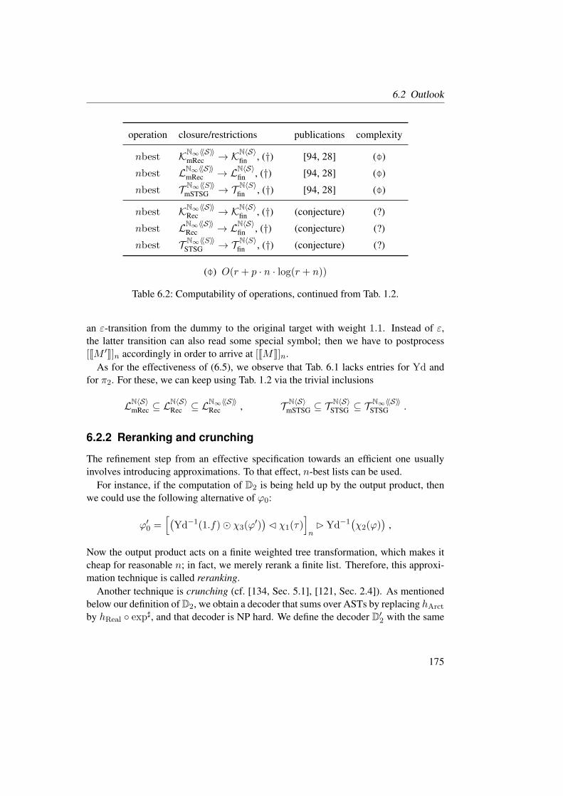
6.2 Outlook
operation closure/restrictions publications complexity
nbest KN∞〈〈S〉〉mRec → K
N〈S〉fin , (†) [94, 28] ()
nbest LN∞〈〈S〉〉mRec → L
N〈S〉fin , (†) [94, 28] ()
nbest TN∞〈〈S〉〉
mSTSG → TN〈S〉
fin , (†) [94, 28] ()
nbest KN∞〈〈S〉〉Rec → K
N〈S〉fin , (†) (conjecture) (?)
nbest LN∞〈〈S〉〉Rec → L
N〈S〉fin , (†) (conjecture) (?)
nbest TN∞〈〈S〉〉
STSG → TN〈S〉
fin , (†) (conjecture) (?)
() O(r + p · n · log(r + n))
Table 6.2: Computability of operations, continued from Tab. 1.2.
an ε-transition from the dummy to the original target with weight 1.1. Instead of ε,the latter transition can also read some special symbol; then we have to postprocess
[JM ′K]n accordingly in order to arrive at [JMK]n.
As for the effectiveness of (6.5), we observe that Tab. 6.1 lacks entries for Yd and
for π2. For these, we can keep using Tab. 1.2 via the trivial inclusions
LN〈S〉mRec ⊆ L
N〈S〉Rec ⊆ L
N∞〈〈S〉〉Rec , T
N〈S〉mSTSG ⊆ T
N〈S〉STSG ⊆ T
N∞〈〈S〉〉STSG .
6.2.2 Reranking and crunching
The refinement step from an effective specification towards an efficient one usually
involves introducing approximations. To that effect, n-best lists can be used.
For instance, if the computation of D2 is being held up by the output product, then
we could use the following alternative of ϕ0:
ϕ′0 =
[(Yd−1(1.f)⊙ χ3(ϕ
′))⊳ χ1(τ)
]
n⊲Yd−1
(χ2(ϕ)
),
Now the output product acts on a finite weighted tree transformation, which makes it
cheap for reasonable n; in fact, we merely rerank a finite list. Therefore, this approxi-
mation technique is called reranking.
Another technique is crunching (cf. [134, Sec. 5.1], [121, Sec. 2.4]). As mentioned
below our definition of D2, we obtain a decoder that sums over ASTs by replacing hArct
by hReal exp♯, and that decoder is NP hard. We define the decoder D′
2 with the same
175

6 Conclusion
parameter space and with
D′2(τ, ϕ, ϕ
′, θ)(f) = best(hReal([
Yd(π2([[exp (·θ)]♯](ϕ0)))
]
n)) .
Here the aggregation homomorphism can be imagined as “crunching” a finite list. Evi-
dently, computing best of a finite weighted string language is trivial.
6.2.3 Relatively-useless pruning
Reducing a WSA to a finite list of runs, nbest is a quite drastic and crude measure. In
contrast, pruning refers to a class of more refined techniques, which merely reduce the
number of states or the number of transitions in one way or another.
For instance, relatively-useless pruning (RUP) [93, Sec. 4.3] is based on evolving
the useful/useless dichotomy for transitions that we established in Sec. 2.4.5. Let M =(Q,R, µ, q0) be a WTA over Σ and Arct in root-state form. We define the utility η(ρ)of a transition ρ ∈ R as the highest weight of any complete run that contains said
transition, i.e.,
η(ρ) = max〈d〉 | d ∈ Dq0co(M), ∃w ∈ pos(d) : d(w) = ρ .
In [93], the utility is called merit, and it is computed efficiently using the inside and
outside weights of M (where the former correspond to the mapping F of Lm. 2.4.7).
Clearly, a useless transition has utility 0, but not vice versa. We also consider the
highest weight of any run
η0 = max〈d〉 | d ∈ Dq0co(M) = maxη(ρ) | ρ ∈ R .
For RUP, we let δ ∈ R≥0. We construct the WTA δrup(M) from M by dropping
every transition ρ with η0 − η(ρ) > δ. We observe that
d | d ∈ Dq0co(M), 〈d〉 ≥ η0 − δ ⊆ Dq0
co(δrup(M)) ⊆ Dq0co(M) , (6.6)
where the second set may still contain runs with weight below η0 − δ. It is hard to
estimate, without inspecting R, the number of dropped transitions, and thus the gain in
efficiency of subsequent operations. We may need to try different values of δ until we
find a practical trade-off between accuracy and efficiency.
Let us attempt to express RUP on the m-meaning level. For this, let I a set. A δ-rup
mapping is an operation δrup: N∞〈〈Arct〉〉I → N∞〈〈Arct〉〉I such that
ϕδ ≤ δrup(ϕ) ≤ ϕ , (6.7)
176

6.2 Outlook
where ϕδ ∈ N∞〈〈Arct〉〉I with
ϕδ(i)s =
ϕ(i)s if s ≥ s0(ϕ)− δ,
0 otherwise,
s0(ϕ) = maxs | ∃i : ϕ(i)s 6= 0 .
The inequations (6.7) model (6.6). This definition of a δ-rup mapping is permissive:
for instance, it includes the identity on N∞〈〈Arct〉〉I . It is unclear how to narrow down
the definition, because the identities of the runs and their interdependencies via the
transitions are masked on the m-meaning level. For use in decoder specifications, we
let δrup be a δ-rup mapping; and we stipulate that it be the one that the (fictitious,
potential) implementation of choice provides.
6.2.4 Cube pruning
In the strict sense [39, 81, 82], cube pruning is an algorithm that explores a certain
weighted hypergraph under a limited-memory restriction concerning the number of
nodes. Roughly speaking, this weighted hypergraph encodes the output-product con-
struction of an acyclic WSCFG and an n-gram model. In the broad sense [25], which
we adopt, cube pruning is a general technique for approximating product constructions
such as the output product, the input product, or the Hadamard product, when at least
one operand is given by an acyclic device.
Although a detailed formal account of this technique is long overdue, it would go
beyond the scope of this text. Suffice it to say the following. Since cube pruning is very
operational in nature, it cannot be easily expressed as an operation on the m-meaning
level. As was the case for RUP, one can probably only give a very permissive (or
even vacuous) definition; for instance, one that does not reflect the limited-memory
restriction. It may turn out inevitable that we supplement the formal definition with
informal requirements that refer to the automata level.
6.2.5 Support for more feature functions
We have considered four features: one that is induced by a probability assignment, one
that incorporates a language model for English, one that counts the number of words
in the English string, and one that incorporates parsing probabilities for French. Each
feature can be regarded as the composition of an “adapter mapping” and a “substance
mapping”; for instance, in the setting of Sec. 1.3, we observe that
φLM = (log PLM) (yd h2 πΓ) ,
177
6 Conclusion
where yd h2 πΓ is the adapter and log PLM caters for the substance.
For these features, the substance is either a probability assignment or the meaning
of some grammar; and the adapter is either the identity, or it refers to the French side
(via h1), or it refers to the English side (via h2). We could transfer these features into
the algebraic framework easily, by using a WSTSG, by using the input product, or by
using the output product, respectively.
Current SMT systems use features that depend on both the French and the English
side, e.g., the feature τ0 ad with
ad : TR → TΣ × TΣ ,
ad(d) = (h1(πΓ(d)), h2(πΓ(d))) ,
τ0 : TΣ × TΣ → sR ,
τ0(t1, t2) =
1 if t1 contains NN(katze) and t2 contains NN(cat),
0 otherwise.
In order to incorporate such a feature into the framework, we need a subclass T ′ ⊆ Tsuch that (i) T ′ contains τ0 (and the like) and (ii) τ ∈ TSTSG, τ
′ ∈ T ′ implies τ ⊙ τ ′ ∈TSTSG, where we use the Hadamard product in the general sense of Sec. 2.3.2.
For instance, one might define the notion of a “duplex WTA” M that basically con-
sists of two WTA M1 and M2, but it has a central root-weight mapping ν that acts
on the product state space. Then the meaning JMK of M would be the weighted tree
transformation defined by
JMK(t1, t2) =∑
(q1,q2)Jt1KM1(q1) · Jt2KM2(q2) · ν(q1, q2) .
The author conjectures that the class of meanings of WSTSGs is closed under Hada-
mard product with meanings of duplex WTA, which includes τ0.
6.2.6 Improving the learning curve
Evidently the framework incorporates a great many concepts, and its current form is
closer to a proposal than to a product. Furthermore, the presentation in this thesis is
geared towards researchers who may work on the framework itself, rather than towards
practitioners. As a result, this thesis fails to achieve Objective (e). However, that does
not mean that the framework inherently defies an instructive presentation.
Already, the “native” specifications in (1.4) and (6.4) are rather concise and instruc-
tive. We can make them more palatable by introducing a few conventions, e.g.,
• we omit the Yd−1, the ♯, and the ,
178

6.2 Outlook
• we abbreviate (·θ)(τ) by τ · θ, and
• if S = N∞〈〈S′〉〉, then we define best = best hS′ (this definition is not circular
because the semiring is being switched).
Thereby we reduce redundancy, which is warranted because decoder specifications will
consist of a number of established stereotypes. Metaphorically speaking, decoder spec-
ifications will usually be variations on a well-known theme.
Now D2 can be expressed by
D2 : TN〈Real〉
mSTSG ×KN〈Real〉mdRec × L
N〈Real〉mdRec × R
3 → EF , D2(τ, ϕ, ϕ′, θ) :
f 7→ best(Yd(π2([χ3(1.f ⊙ ϕ
′)⊳ χ1(τ)⊲ χ2(ϕ)] · θ))) ,
and we can attach a casual narrative to this specification, e.g.,
We take the tree transformation (τ ), the target language model (ϕ), and the
parsing model (ϕ′); we intersect the parsing model with our sentence (f );
we convert all weights into vector form; we combine the three pieces; and
we incorporate the feature weight vector. It remains to project the resulting
transformation to the output string language and find the translation with
the highest score.
It is an interesting open question whether the algebraic notation can be taught to a
practitioner by means of a collection of pairs (example, narrative), without delving into
concepts such as a multiset semiring, a complete semiring, or a closure result.
6.2.7 Formal syntax and term rewriting
So far, we were content with treating specifications informally. For instance, when we
sloppily refer to “the defining expression of D2(τ, ϕ, ϕ′, θ)(f)”, we mean the mathe-
matical expression shown in (6.4). In contrast to a tree over ∆, this expression is itself
not a mathematical object, i.e., we cannot use mathematics to describe its properties or
potential transformations.
The informal treatment got us very far, for we could in many cases prove that a speci-
fication is effective, using tables such as Tab. 1.2. However, these proofs still amounted
to manual labor. If we are to automate these proofs, to implement a specification in
a programming language, or to build an integrated development environment (IDE)
for our specifications, then there is no way around a formal treatment, either in said
programming language itself or in a more abstract framework.
One possible framework is the initial-algebra approach of [86, 85]. As mentioned
in Sec. 1.6, we may view our algebraic framework as a many-sorted algebra over a
179
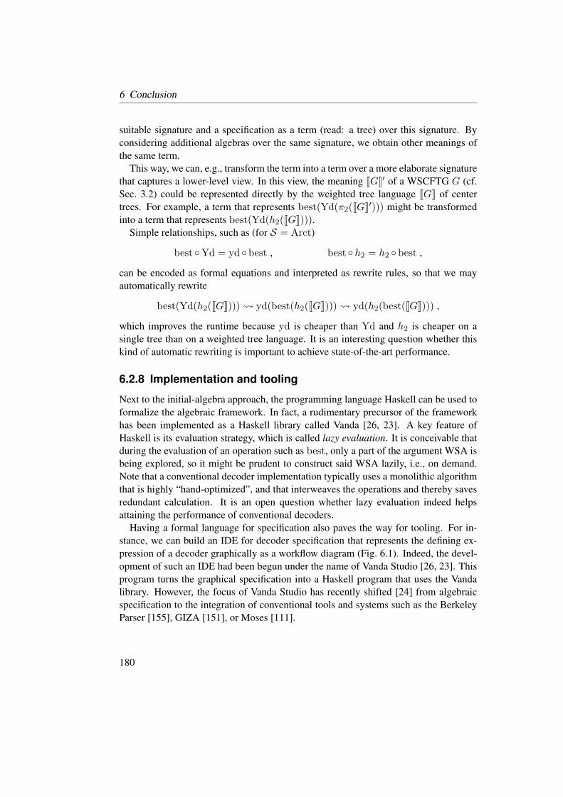
6 Conclusion
suitable signature and a specification as a term (read: a tree) over this signature. By
considering additional algebras over the same signature, we obtain other meanings of
the same term.
This way, we can, e.g., transform the term into a term over a more elaborate signature
that captures a lower-level view. In this view, the meaning JGK′ of a WSCFTG G (cf.
Sec. 3.2) could be represented directly by the weighted tree language JGK of center
trees. For example, a term that represents best(Yd(π2(JGK′))) might be transformed
into a term that represents best(Yd(h2(JGK))).Simple relationships, such as (for S = Arct)
best Yd = yd best , best h2 = h2 best ,
can be encoded as formal equations and interpreted as rewrite rules, so that we may
automatically rewrite
best(Yd(h2(JGK))) yd(best(h2(JGK))) yd(h2(best(JGK))) ,
which improves the runtime because yd is cheaper than Yd and h2 is cheaper on a
single tree than on a weighted tree language. It is an interesting question whether this
kind of automatic rewriting is important to achieve state-of-the-art performance.
6.2.8 Implementation and tooling
Next to the initial-algebra approach, the programming language Haskell can be used to
formalize the algebraic framework. In fact, a rudimentary precursor of the framework
has been implemented as a Haskell library called Vanda [26, 23]. A key feature of
Haskell is its evaluation strategy, which is called lazy evaluation. It is conceivable that
during the evaluation of an operation such as best, only a part of the argument WSA is
being explored, so it might be prudent to construct said WSA lazily, i.e., on demand.
Note that a conventional decoder implementation typically uses a monolithic algorithm
that is highly “hand-optimized”, and that interweaves the operations and thereby saves
redundant calculation. It is an open question whether lazy evaluation indeed helps
attaining the performance of conventional decoders.
Having a formal language for specification also paves the way for tooling. For in-
stance, we can build an IDE for decoder specification that represents the defining ex-
pression of a decoder graphically as a workflow diagram (Fig. 6.1). Indeed, the devel-
opment of such an IDE had been begun under the name of Vanda Studio [26, 23]. This
program turns the graphical specification into a Haskell program that uses the Vanda
library. However, the focus of Vanda Studio has recently shifted [24] from algebraic
specification to the integration of conventional tools and systems such as the Berkeley
Parser [155], GIZA [151], or Moses [111].
180
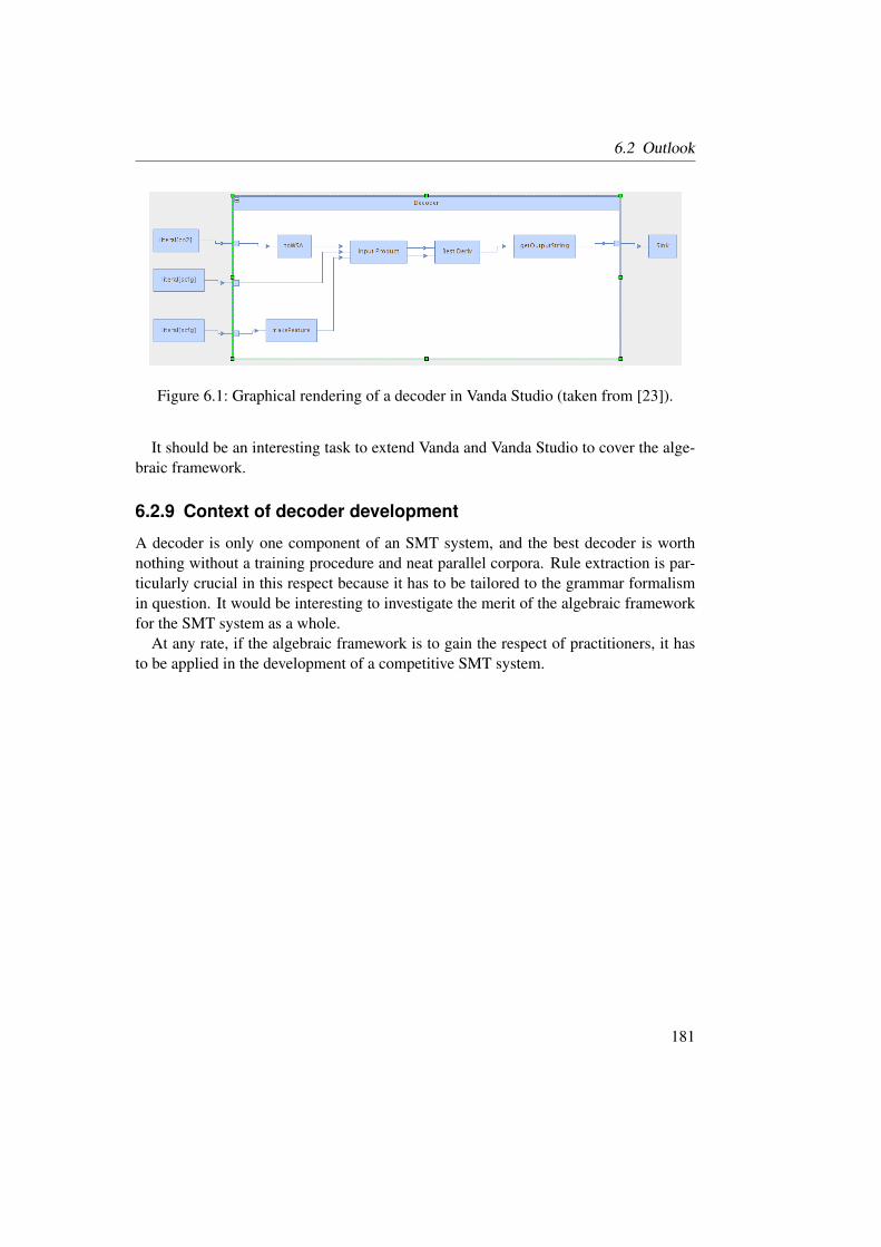
6.2 Outlook
Figure 6.1: Graphical rendering of a decoder in Vanda Studio (taken from [23]).
It should be an interesting task to extend Vanda and Vanda Studio to cover the alge-
braic framework.
6.2.9 Context of decoder development
A decoder is only one component of an SMT system, and the best decoder is worth
nothing without a training procedure and neat parallel corpora. Rule extraction is par-
ticularly crucial in this respect because it has to be tailored to the grammar formalism
in question. It would be interesting to investigate the merit of the algebraic framework
for the SMT system as a whole.
At any rate, if the algebraic framework is to gain the respect of practitioners, it has
to be applied in the development of a competitive SMT system.
181

Bibliography
[1] Anne Abeille, Yves Schabes, and Aravind K. Joshi. “Using lexicalized tags for
machine translation”. In: Proceedings of the Thirteenth International Confer-
ence on Computational Linguistics (COLING ’90). Vol. 3. 1990, pp. 1–6 (cit.
on p. 9).
[2] Alfred V. Aho and Jeffrey D. Ullman. “Syntax directed translations and the
pushdown assembler”. In: Journal of Computer and System Sciences 3 (1969),
pp. 37–56 (cit. on pp. 19, 84).
[3] Athanasios Alexandrakis and Symeon Bozapalidis. “Weighted grammars and
Kleene’s theorem”. In: Information Processing Letters 24.1 (1987), pp. 1–4
(cit. on pp. 37, 42, 43).
[4] Cyril Allauzen, Mehryar Mohri, and Brian Roark. “Generalized Algorithms for
Constructing Statistical Language Models”. In: Proceedings of the 41st Annual
Meeting on Association for Computational Linguistics - Volume 1. ACL ’03.
2003, pp. 40–47. DOI: 10.3115/1075096.1075102 (cit. on pp. 7, 16).
[5] Cyrill Allauzen and Mehryar Mohri. “Efficient Algorithms for Testing the
Twins Property”. In: J. of Automata, Languages and Combinatorics 8.2 (2003),
pp. 117–144 (cit. on pp. 21, 134, 159, 164).
[6] Andre Arnold and Max Dauchet. “Bi-transduction de forets”. In: Proc. 3rd Int.
Coll. Automata, Languages and Programming. 1976, pp. 74–86 (cit. on pp. 21,
48, 85, 86).
[7] Franz Baader and Tobias Nipkow. Term Rewriting and All That. Cambridge
University Press, 1998 (cit. on p. 29).
[8] James K. Baker. “Trainable grammars for speech recognition”. In: Speech Com-
munication Papers for the 97th Meeting of the Acoustical Society of America.
Ed. by D. H. Klatt and J. J. Wolf. 1979, pp. 547–550 (cit. on p. 9).
[9] Yehoshua Bar-Hillel, Micha Perles, and Eli Shamir. “On formal properties of
simple phrase structure grammars”. In: Z. Phonetik Sprach. Komm. 14 (1961),
pp. 143–172 (cit. on p. 83).
[10] Jean Berstel and Christophe Reutenauer. “Recognizable formal power series on
trees”. In: Theoret. Comput. Sci. 18.2 (1982), pp. 115–148 (cit. on p. 43).
183
Bibliography
[11] Jean Berstel and Christophe Reutenauer. Rational Series and Their Languages.
Vol. 12. EATCS Monographs on Theoretical Computer Science. Springer, 1988
(cit. on pp. 14–16).
[12] Dan Bikel. “On The Parameter Space of Generative Lexicalized Statistical Pars-
ing Models”. PhD thesis. University of Pennsylvania, 2004 (cit. on p. 10).
[13] Phil Blunsom, Trevor Cohn, and Miles Osborne. “A discriminative latent vari-
able model for statistical machine translation”. In: Proceedings ACL-HLT 2008.
2008, pp. 200–208. URL: http://aclweb.org/anthology-new/P/
P08/P08-1024.pdf (cit. on p. 8).
[14] Ondrej Bojar, Christian Buck, Chris Callison-Burch, Barry Haddow, Philipp
Koehn, Christof Monz, Matt Post, Herve Saint-Amand, Radu Soricut, and Lu-
cia Specia, eds. Proceedings of the Eighth Workshop on Statistical Machine
Translation. ACL, 2013. URL: http://www.aclweb.org/anthology/
W13-22 (cit. on p. 167).
[15] Bjorn Borchardt. “A pumping lemma and decidability problems for recogniz-
able tree series”. In: Acta Cybernet. 16.4 (2004), pp. 509–544 (cit. on pp. 15,
16, 132, 145, 146).
[16] Bjorn Borchardt. “The Theory of Recognizable Tree Series”. PhD thesis. Tech-
nische Universitat Dresden, 2005 (cit. on p. 42).
[17] Bjorn Borchardt, Andreas Maletti, Branimir Seselja, Andreja Tepavcevic, and
Heiko Vogler. “Cut sets as recognizable tree languages”. In: Fuzzy Sets and
Systems 157.11 (2006), pp. 1560–1571. DOI: 10.1016/j.fss.2005.11.
004 (cit. on p. 170).
[18] Bjorn Borchardt and Heiko Vogler. “Determinization of finite state weighted
tree automata”. In: J. Autom. Lang. Combin. 8.3 (2003), pp. 417–463 (cit. on
p. 132).
[19] Symeon Bozapalidis. “Context-free series on trees”. In: Inform. and Comput.
169.2 (2001), pp. 186–229 (cit. on p. 18).
[20] Fabienne Braune, Andreas Maletti, Daniel Quernheim, and Nina Seemann.
“Shallow local multi bottom-up tree transducers in statistical machine trans-
lation”. In: Proc. 51st Annual Meeting of the Association for Computational
Linguistics. Ed. by Pascale Fung and Massimo Poesio. 2013, pp. 811–821 (cit.
on p. 10).
[21] Peter F. Brown, Vincent J. Della Pietra, Stephen A. Della Pietra, and Robert L.
Mercer. “The mathematics of statistical machine translation: parameter estima-
tion”. In: Comp. Ling. 19 (2 1993), pp. 263–311 (cit. on p. 3).
184
Bibliography
[22] Adam L. Buchsbaum, Raffaele Giancarlo, and Jeffery R. Westbrook. “On the
Determinization of Weighted Finite Automata”. In: SIAM J. Comput. 30.5
(2000), pp. 1502–1531. DOI: 10.1137/S0097539798346676 (cit. on
pp. 131, 132).
[23] Matthias Buchse. “As Easy As Vanda, Two, Three: Components for Machine
Translation Based on Formal Grammars”. In: Proceedings 22nd Theorietag
“Automata and Formal Languages”, Prague, Czech Republic, October 3–5,
2012. Ed. by Frantisek Mraz. Charles University in Prague, Faculty of Mathe-
matics and Physics. 2012, pp. 41–44 (cit. on pp. 180, 181).
[24] Matthias Buchse. “Vanda Studio – Instructive, Rapid Experiment Develop-
ment”. Unpublished manuscript. 2013. URL: http : / / www . inf . tu -
dresden . de / content / institutes / thi / gdp / research /
vanda-demo.pdf (cit. on p. 180).
[25] Matthias Buchse, David Chiang, Liang Huang, and Michael Pust. “Some re-
marks on cube pruning”. Unpublished manuscript. 2011 (cit. on p. 177).
[26] Matthias Buchse, Toni Dietze, Johannes Osterholzer, Anja Fischer, and Linda
Leuschner. “Vanda – A Statistical Machine Translation Toolkit”. In: Proceed-
ings 6th International Workshop “Weighted Automata: Theory and Applica-
tions” (WATA 2012). Ed. by Manfred Droste and Heiko Vogler. Online pro-
ceedings. 2012, pp. 36–38. URL: http://wwwtcs.inf.tu-dresden.
de/wata2012/Proceedings.pdf (cit. on p. 180).
[27] Matthias Buchse and Anja Fischer. “Deciding the Twins Property for Weighted
Tree Automata over Extremal Semifields”. In: Proceedings of the Workshop
on Applications of Tree Automata Techniques in Natural Language Processing.
2012, pp. 11–20. URL: http://www.aclweb.org/anthology/W/
W12/W12-0802 (cit. on pp. 131, 165).
[28] Matthias Buchse, Daniel Geisler, Torsten Stuber, and Heiko Vogler. “n-Best
Parsing Revisited”. In: Proceedings of the 2010 Workshop on Applications of
Tree Automata in Natural Language Processing, ACL 2010. Uppsala, Sweden,
16 July 2010. 2010, pp. 46–54 (cit. on pp. 8, 15, 20, 175).
[29] Matthias Buchse, Alexander Koller, and Heiko Vogler. “Generic binarization
for parsing and translation”. In: Proceedings of the 51st Annual Meeting of
the Association for Computational Linguistics (Volume 1: Long Papers). 2013,
pp. 145–154. URL: http://www.aclweb.org/anthology/P13-
1015 (cit. on pp. 83, 122, 127).
185

Bibliography
[30] Matthias Buchse, Andreas Maletti, and Heiko Vogler. “Unidirectional deriva-
tion semantics for synchronous tree-adjoining grammars”. In: Proc. 16th Int.
Conf. Developments in Language Theory. Ed. by Hsu-Chun Yen and Oscar H.
Ibarra. Vol. 7410. LNCS. 2012, pp. 368–379. DOI: 10.1007/978-3-642-
31653-1_33 (cit. on pp. 81, 124).
[31] Matthias Buchse, Jonathan May, and Heiko Vogler. “Determinization of
weighted tree automata using factorizations”. In: Journal of Automata, Lan-
guages and Combinatorics 15.3/4 (2010) (cit. on pp. 131, 165).
[32] Matthias Buchse, Mark-Jan Nederhof, and Heiko Vogler. “Tree Parsing with
Synchronous Tree-Adjoining Grammars”. In: Proceedings of the 12th Inter-
national Conference on Parsing Technologies. 2011, pp. 14–25. URL: http:
//www.aclweb.org/anthology/W11-2903 (cit. on pp. 45, 81).
[33] Matthias Buchse, Heiko Vogler, and Mark-Jan Nederhof. “Tree parsing for tree-
adjoining machine translation”. In: Journal of Logic and Computation 24.2
(2014). first published online December 6, 2012, pp. 351–373 (cit. on pp. 45,
81, 82).
[34] Mathieu Caralp, Emmanuel Filiot, Pierre-Alain Reynier, Frederic Servais, and
Jean-Marc Talbot. “Expressiveness of Visibly Pushdown Transducers”. In: Pro-
ceedings TTATT 2013. 2013, pp. 17–26. URL: http://arxiv.org/abs/
1311.5571 (cit. on p. 122).
[35] Francisco Casacuberta and Colin de la Higuera. “Computational Complexity
of Problems on Probabilistic Grammars and Transducers”. In: ICGI. Ed. by Ar-
lindo L. Oliveira. Vol. 1891. Lecture Notes in Computer Science. 2000, pp. 15–
24 (cit. on p. 8).
[36] Yin-Wen Chang and Michael Collins. “Exact Decoding of Phrase-Based Trans-
lation Models through Lagrangian Relaxation”. In: Proceedings of the 2011
Conference on Empirical Methods in Natural Language Processing. 2011,
pp. 26–37. URL: http://www.aclweb.org/anthology/D11-1003
(cit. on p. 4).
[37] Eugene Charniak and Mark Johnson. “Coarse-to-Fine n-Best Parsing and Max-
Ent Discriminative Reranking”. In: Proceedings of the 43rd Annual Meeting of
the Association for Computational Linguistics (ACL’05). 2005, pp. 173–180.
URL: http://www.aclweb.org/anthology/P05-1022 (cit. on
p. 10).
186

Bibliography
[38] David Chiang. “A hierarchical phrase-based model for statistical machine
translation”. In: ACL ’05: Proceedings of the 43rd Annual Meeting on Asso-
ciation for Computational Linguistics. 2005, pp. 263–270 (cit. on p. 4).
[39] David Chiang. “Hierarchical Phrase-Based Translation”. In: Comp. Ling. 33.2
(2007), pp. 201–228 (cit. on pp. 4, 8, 14, 19, 22, 82, 84, 177).
[40] David Chiang. “Learning to Translate with Source and Target Syntax”. In: Pro-
ceedings of the 48th Annual Meeting of the Association for Computational
Linguistics. 2010, pp. 1443–1452. URL: http://www.aclweb.org/
anthology/P10-1146 (cit. on p. 10).
[41] David Chiang, Kevin Knight, and Wei Wang. “11,001 New Features for Statis-
tical Machine Translation”. In: Proceedings of Human Language Technologies:
The 2009 Annual Conference of the North American Chapter of the Associa-
tion for Computational Linguistics. 2009, pp. 218–226. URL: http://www.
aclweb.org/anthology/N/N09/N09-1025 (cit. on p. 10).
[42] David Chiang, Adam Lopez, Nitin Madnani, Christof Monz, Philip Resnik,
and Michael Subotin. “The Hiero machine translation system: extensions, eval-
uation, and analysis”. In: HLT ’05: Proceedings of the conference on Human
Language Technology and Empirical Methods in Natural Language Process-
ing. 2005, pp. 779–786 (cit. on p. 4).
[43] David Chiang, Yuval Marton, and Philip Resnik. “Online large-margin training
of syntactic and structural translation features”. In: Proceedings EMNLP 2008.
2008. URL: http://www.isi.edu/˜chiang/papers/mira.pdf
(cit. on p. 174).
[44] Christian Choffrut. “Une Caracterisation des Fonctions Sequentielles et des
Fonctions Sous-Sequentielles en tant que Relations Rationnelles.” In: Theoret.
Comput. Sci. 5.3 (1977), pp. 325–337 (cit. on pp. 21, 133).
[45] Noam Chomsky. “On certain formal properties of grammars”. In: Inform. Con-
trol 2 (1959), pp. 137–167 (cit. on pp. 19, 84).
[46] Noam Chomsky and Marcel-Paul Schutzenberger. “The algebraic theory of
context-free languages”. In: Computer Programming and Formal Systems. Ed.
by Paul Braffort and David Hirschberg. 1963, pp. 118–161 (cit. on p. 14).
[47] Michael Collins. “Head-driven Statistical Models for Natural Language Pars-
ing”. PhD thesis. University of Pennsylvania, 1999 (cit. on p. 10).
[48] Bruno Courcelle. “Attribute grammars: definitions, analysis of dependencies,
proof methods”. In: Methods and tools for compiler construction. Ed. by
Bernard Lorho. 1984, pp. 81–102 (cit. on p. 70).
187

Bibliography
[49] Bruno Courcelle and Paul Franchi-Zannettacci. “Attribute grammars and recur-
sive program schemes I”. In: Theoret. Comput. Sci. 17.2 (1982), pp. 163–191
(cit. on p. 124).
[50] Steve DeNeefe. “Tree-Adjoining Machine Translation”. PhD thesis. University
of Southern California, 2011 (cit. on pp. 10, 18).
[51] Steve DeNeefe and Kevin Knight. “Synchronous Tree-Adjoining Machine
Translation”. In: EMNLP ’09: Proceedings of the 2009 Conference on Em-
pirical Methods in Natural Language Processing. 2009, pp. 727–736 (cit. on
p. 10).
[52] John DeNero, Mohit Bansal, Adam Pauls, and Dan Klein. “Efficient Parsing
for Transducer Grammars”. In: Proceedings of Human Language Technologies:
The 2009 Annual Conference of the North American Chapter of the Associa-
tion for Computational Linguistics. 2009, pp. 227–235. URL: http://www.
aclweb.org/anthology/N/N09/N09-1026 (cit. on p. 82).
[53] John DeNero, David Chiang, and Kevin Knight. “Fast Consensus Decoding
over Translation Forests”. In: Proceedings of the Joint Conference of the 47th
Annual Meeting of the ACL and the 4th International Joint Conference on Nat-
ural Language Processing of the AFNLP. 2009, pp. 567–575. URL: http:
//www.aclweb.org/anthology/P/P09/P09-1064 (cit. on p. 22).
[54] John DeNero, Adam Pauls, and Dan Klein. “Asynchronous Binarization for
Synchronous Grammars”. In: Proceedings of the ACL-IJCNLP 2009 Confer-
ence Short Papers. 2009, pp. 141–144. URL: http://www.aclweb.org/
anthology/P/P09/P09-2036 (cit. on p. 127).
[55] Edsger W. Dijkstra. “A note on two problems in connection with graphs”. In:
Numerische Mathematik 1 (1959), pp. 269–271 (cit. on p. 9).
[56] Manfred Droste, Doreen Gotze, Steffen Marcker, and Ingmar Meinecke.
“Weighted Tree Automata over Valuation Monoids and Their Characterization
by Weighted Logics”. In: Algebraic Foundations in Computer Science. Ed. by
Werner Kuich and George Rahonis. Vol. 7020. Lecture Notes in Computer Sci-
ence. 2011, pp. 30–55. DOI: 10.1007/978-3-642-24897-9_2 (cit. on
p. 43).
[57] Manfred Droste, Werner Kuich, and Heiko Vogler, eds. Handbook of Weighted
Automata. EATCS Monographs in Theoretical Computer Science. Springer,
2009 (cit. on p. 12).
188

Bibliography
[58] Manfred Droste and Heiko Vogler. “Weighted logics for unranked tree au-
tomata”. In: Theory of Computing Systems 48.1 (2011). first published online
June 29, 2009, pp. 23–47. DOI: 10.1007/s00224-009-9224-4 (cit. on
p. 44).
[59] Chris Dyer, Adam Lopez, Juri Ganitkevitch, Jonathan Weese, Ferhan Ture, Phil
Blunsom, Hendra Setiawan, Vladimir Eidelman, and Philip Resnik. “cdec: A
Decoder, Alignment, and Learning Framework for Finite-State and Context-
Free Translation Models”. In: Proceedings of the ACL 2010 System Demonstra-
tions. 2010, pp. 7–12. URL: http://www.aclweb.org/anthology/
P10-4002 (cit. on p. 22).
[60] Jay Earley. “An Efficient Context-Free Parsing Algorithm”. In: Communica-
tions of the ACM 13.2 (1970), pp. 94–102 (cit. on pp. 47, 61).
[61] Samuel Eilenberg. Automata, Languages, and Machines – Volume A. Vol. 59.
Pure and Applied Mathematics. Academic Press, 1974 (cit. on p. 12).
[62] Jason Eisner. “Learning non-isomorphic tree mappings for machine transla-
tion”. In: Proceedings of the 41st Annual Meeting on Association for Compu-
tational Linguistics - Volume 2. ACL ’03. 2003, pp. 205–208 (cit. on pp. 9,
82).
[63] Joost Engelfriet. “Attribute grammars: attribute evaluation methods”. In: Meth-
ods and tools for compiler construction. Ed. by Bernard Lorho. 1984, pp. 103–
138 (cit. on p. 70).
[64] Joost Engelfriet and Linda Heyker. “The string generating power of context-
free hypergraph grammars”. In: Journal of Computer and System Sciences
43.2 (1991), pp. 328–360. URL: http://www.sciencedirect.com/
science/article/pii/002200009190018Z (cit. on p. 123).
[65] Joost Engelfriet, Eric Lilin, and Andreas Maletti. “Extended Multi Bottom-up
Tree Transducers”. In: Proc. 12th Int. Conf. Developments in Language Theory.
Ed. by Masami Ito and F. M. Toyama. Vol. 5257. LNCS. 2008, pp. 289–300 (cit.
on p. 10).
[66] Joost Engelfriet, Eric Lilin, and Andreas Maletti. “Extended Multi Bottom-up
Tree Transducers – Composition and Decomposition”. In: Acta Inf. 46.8 (2009),
pp. 561–590 (cit. on p. 46).
[67] Joost Engelfriet and Erik M. Schmidt. “IO and OI I”. In: J. Comput. System Sci.
15.3 (1977), pp. 328–353 (cit. on pp. 81, 119).
[68] Joost Engelfriet and Erik M. Schmidt. “IO and OI II”. In: J. Comput. System
Sci. 16.1 (1978), pp. 67–99 (cit. on p. 81).
189

Bibliography
[69] Joost Engelfriet and Heiko Vogler. “Macro Tree Transducers”. In: Journal of
Computer and System Sciences 31 (1985), pp. 71–146 (cit. on p. 124).
[70] David Eppstein. “Finding the k Shortest Paths”. In: SIAM Journal on Comput-
ing 28.2 (1998), pp. 652–673. DOI: 10.1137/S0097539795290477 (cit.
on pp. 9, 174).
[71] Zoltan Esik and Werner Kuich. “Formal Tree Series”. In: J. Autom. Lang. Com-
bin. 8.2 (2003), pp. 219–285 (cit. on pp. 15, 18, 36, 43).
[72] Javier Esparza, Stefan Kiefer, and Michael Luttenberger. “Derivation Tree
Analysis for Accelerated Fixed-Point Computation”. In: Theoretical Computer
Science 412.28 (2011), pp. 3226–3241 (cit. on p. 42).
[73] Zoltan Fulop, Andreas Maletti, and Heiko Vogler. “A Kleene theorem for
weighted tree automata over distributive multioperator monoids”. In: Theory
Comput. Syst. 44 (2009), pp. 455–499 (cit. on p. 43).
[74] Zoltan Fulop, Andreas Maletti, and Heiko Vogler. “Preservation of Recog-
nizability for Synchronous Tree Substitution Grammars”. In: Proceedings of
the 2010 Workshop on Applications of Tree Automata in Natural Language
Processing, ACL 2010. Uppsala, Sweden, 16 July 2010. 2010, pp. 1–9. URL:
http://www.aclweb.org/anthology/W/W10/W10-2501.pdf
(cit. on pp. 14, 51).
[75] Zoltan Fulop, Andreas Maletti, and Heiko Vogler. “Weighted Extended Tree
Transducers”. In: Fundam. Inform. 111.2 (2011), pp. 163–202 (cit. on pp. 15,
45).
[76] Zoltan Fulop, Torsten Stuber, and Heiko Vogler. “A Buchi-like theorem for
weighted tree automata over multioperator monoids”. In: Theory of Computing
Systems 50.2 (2012). first published online October 28, 2010, pp. 241–278. DOI:
10.1007/s00224-010-9296-1 (cit. on p. 43).
[77] Zoltan Fulop and Heiko Vogler. “Weighted tree automata and tree transduc-
ers”. In: Handbook of Weighted Automata. Ed. by Manfred Droste, Werner
Kuich, and Heiko Vogler. EATCS Monographs in Theoretical Computer Sci-
ence. 2009. Chap. 9 (cit. on pp. 40, 43).
[78] Michael Galley. GHKM Rule Extractor. http://www-nlp.stanford.
edu/˜mgalley/software/stanford-ghkm-latest.tar.gz,
retrieved on March 28, 2012. 2010 (cit. on p. 123).
190

Bibliography
[79] Michel Galley, Mark Hopkins, Kevin Knight, and Daniel Marcu. “What’s in
a translation rule?” In: HLT-NAACL 2004: Main Proceedings. Ed. by Susan
Dumais, Daniel Marcu, and Salim Roukos. 2004, pp. 273–280 (cit. on pp. 9,
10, 120–122).
[80] Ferenc Gecseg and Magnus Steinby. “Tree Languages”. In: Handbook of For-
mal Languages. Ed. by Grzegorz Rozenberg and Arto Salomaa. Vol. 3. 1997.
Chap. 1, pp. 1–68 (cit. on pp. 85, 107, 113, 128, 132).
[81] Andrea Gesmundo and James Henderson. “Faster Cube Pruning”. In: Proceed-
ings of the seventh International Workshop on Spoken Language Translation
(IWSLT). Ed. by Marcello Federico, Ian Lane, Michael Paul, and Francois
Yvon. 2010, pp. 267–274. URL: http://www.mt- archive.info/
IWSLT-2010-Gesmundo.pdf (cit. on p. 177).
[82] Andrea Gesmundo, Giorgio Satta, and James Henderson. “Heuristic Cube
Pruning in Linear Time”. In: Proceedings of the 50th Annual Meeting of the
Association for Computational Linguistics (Volume 2: Short Papers). 2012,
pp. 296–300. URL: http://www.aclweb.org/anthology/P12-
2058 (cit. on p. 177).
[83] Daniel Gildea. “Optimal Parsing Strategies for Linear Context-Free Rewriting
Systems”. In: Human Language Technologies: The 2010 Annual Conference of
the North American Chapter of the Association for Computational Linguistics.
2010, pp. 769–776. URL: http://www.aclweb.org/anthology/
N10-1118 (cit. on pp. 17, 130).
[84] Kevin Gimpel and Noah A. Smith. “Structured Ramp Loss Minimization for
Machine Translation”. In: Proceedings of the 2012 Conference of the North
American Chapter of the Association for Computational Linguistics: Human
Language Technologies. 2012, pp. 221–231. URL: http://www.aclweb.
org/anthology/N12-1023 (cit. on pp. 8, 174).
[85] Joseph A. Goguen, Jim W. Thatcher, and Eric G. Wagner. “An Initial Alge-
bra Approach to the Specification, Correctness and Implementation of Abstract
Data Types”. In: Current Trends in Programming Methodology. Ed. by Ray-
mond T. Yeh. Vol. IV: Data Structuring. also IBM Research Report RC-6487
(1976). 1978 (cit. on pp. 21, 179).
[86] Joseph A. Goguen, Jim W. Thatcher, Eric G. Wagner, and Jesse B. Wright. “Ini-
tial algebra semantics and continuous algebras”. In: J. ACM 24 (1977), pp. 68–
95 (cit. on pp. 22, 40, 85, 179).
191

Bibliography
[87] Jonathan S. Golan. Semirings and their Applications. Kluwer Academic, 1999
(cit. on pp. 12, 33).
[88] Carlos Gomez-Rodrıguez, Marco Kuhlmann, Giorgio Satta, and David Weir.
“Optimal Reduction of Rule Length in Linear Context-Free Rewriting Sys-
tems”. In: Proceedings of Human Language Technologies: The 2009 Annual
Conference of the North American Chapter of the Association for Computa-
tional Linguistics. 2009, pp. 539–547. URL: http://www.aclweb.org/
anthology/N/N09/N09-1061 (cit. on p. 130).
[89] Joshua Goodman. “Semiring Parsing”. In: Comp. Ling. 25.4 (1999), pp. 573–
605 (cit. on pp. 8, 14, 24, 47, 68).
[90] Jonathan Graehl, Kevin Knight, and Jonathan May. “Training Tree Transduc-
ers”. In: Comp. Ling. 34.3 (2008), pp. 391–427 (cit. on pp. 9, 120).
[91] Udo Hebisch and Hanns Joachim Weinert. Semirings: Algebraic Theory and
Applications in Computer Science. Vol. 5. Series in Algebra. World Scientific,
1998 (cit. on pp. 12, 33).
[92] Mark Hopkins and Jonathan May. “Tuning as Ranking”. In: Proceedings
EMNLP 2011. 2011 (cit. on p. 174).
[93] Liang Huang. “Forest-based Algorithms in Natural-Language Processing”.
PhD thesis. University of Pennsylvania, 2008. URL: http://www.cis.
upenn.edu/˜lhuang3/Dissertation.pdf (cit. on pp. 12, 16, 176).
[94] Liang Huang and David Chiang. “Better k-best parsing”. In: Parsing ’05: Pro-
ceedings of the Ninth International Workshop on Parsing Technology. 2005,
pp. 53–64. URL: http://www.cis.upenn.edu/˜lhuang3/huang-
iwpt-correct.pdf (cit. on pp. 8, 15, 20, 174, 175).
[95] Liang Huang, Kevin Knight, and Aravind Joshi. “A syntax-directed translator
with extended domain of locality”. In: Proceedings of the Workshop on Com-
putationally Hard Problems and Joint Inference in Speech and Language Pro-
cessing. CHSLP ’06. 2006, pp. 1–8 (cit. on p. 120).
[96] Liang Huang, Kevin Knight, and Aravind Joshi. “Statistical syntax-directed
translation with extended domain of locality”. In: Proceedings AMTA 2006.
2006, pp. 66–73. URL: http://www.cis.upenn.edu/˜lhuang3/
amta06-sdtedl.pdf (cit. on pp. 9, 12).
[97] Liang Huang, Hao Zhang, Daniel Gildea, and Kevin Knight. “Binarization of
Synchronous Context-Free Grammars”. In: Comp. Ling. 35.4 (2009), pp. 559–
595. URL: http://www.aclweb.org/anthology/J/J09/J09-
4009.pdf (cit. on pp. 19, 84, 120, 128).
192

Bibliography
[98] Aravind K. Joshi and Yves Schabes. “Tree-Adjoining Grammars”. In: Hand-
book of Formal Languages. Ed. by Grzegorz Rozenberg and Arto Salomaa.
Vol. 3. 1997 (cit. on pp. 49, 52).
[99] Daniel Jurafsky and James H. Martin. Speech and Language Processing – An
Introduction to Natural Language Processing, Computational Linguistics, and
Speech Recognition. Second edition. Prentice-Hall, 2009 (cit. on pp. 7, 10, 47).
[100] Miriam Kaeshammer. “Synchronous Linear Context-Free Rewriting Systems
for Machine Translation”. In: Proceedings of the Seventh Workshop on Syn-
tax, Semantics and Structure in Statistical Translation. 2013, pp. 68–77. URL:
http://www.aclweb.org/anthology/W13-0808 (cit. on pp. 17,
23).
[101] Laura Kallmeyer, Wolfgang Maier, and Giorgio Satta. “Synchronous Rewriting
in Treebanks”. In: Proceedings of the 11th International Conference on Parsing
Technologies (IWPT’09). 2009, pp. 69–72. URL: http://www.aclweb.
org/anthology/W09-3810 (cit. on p. 17).
[102] Stephan Kepser and James Rogers. “The Equivalence of Tree Adjoining Gram-
mars and Monadic Linear Context-Free Tree Grammars”. In: The Mathemat-
ics of Language. Ed. by Christian Ebert, Gerhard Jager, and Jens Michaelis.
Vol. 6149. Lecture Notes in Computer Science. 2010, pp. 129–144. DOI: 10.
1007/978-3-642-14322-9_11 (cit. on pp. 47, 81).
[103] Stephan Kepser and Jim Rogers. “The Equivalence of Tree Adjoining Gram-
mars and Monadic Linear Context-free Tree Grammars”. In: Journal of Logic,
Language and Information 20.3 (2011), pp. 361–384 (cit. on p. 18).
[104] Daniel Kirsten. “Decidability, Undecidability, and PSPACE-Completeness of
the Twins Property in the Tropical Semiring”. In: Theoretical Computer Science
420 (2012), pp. 56–63 (cit. on pp. 21, 134, 165).
[105] Daniel Kirsten and Ina Maurer. “On the determinization of weighted automata”.
In: J. Autom. Lang. Comb. 10 (2005), pp. 287–312 (cit. on pp. 21, 132–134, 137,
141, 143, 146, 148, 149, 151, 164).
[106] Kevin Knight. “Automating knowledge acquisition for machine translation”.
In: AI Magazine 18.4 (1997), pp. 81–96. URL: http://www.aaai.org/
ojs/index.php/aimagazine/article/viewArticle/1323 (cit.
on p. 3).
[107] Donald E. Knuth. “Semantics of context–free languages”. In: Math. Systems
Theory 2 (1968), pp. 127–145 (cit. on p. 70).
193
Bibliography
[108] Donald E. Knuth. “A Generalization of Dijkstra’s Algorithm”. In: Inform. Pro-
cess. Lett. 6.1 (1977), pp. 1–5 (cit. on pp. 8, 15, 20).
[109] Philipp Koehn. “Europarl: A Parallel Corpus for Statistical Machine Transla-
tion”. In: Proceedings of MT Summit X. 2005, pp. 79–86 (cit. on pp. 3, 123).
[110] Philipp Koehn. Statistical Machine Translation. Cambridge University Press,
2010 (cit. on p. 3).
[111] Philipp Koehn, Hieu Hoang, Alexandra Birch, Chris Callison-Burch, Mar-
cello Federico, Nicola Bertoldi, Brooke Cowan, Wade Shen, Christine Moran,
Richard Zens, Chris Dyer, Ondrej Bojar, Alexandra Constantin, and Evan
Herbst. “Moses: open source toolkit for statistical machine translation”. In:
Proceedings of the 45th Annual Meeting of the ACL on Interactive Poster and
Demonstration Sessions. ACL ’07. 2007, pp. 177–180. URL: http://www.
aclweb.org/anthology/P07-2045 (cit. on pp. 22, 180).
[112] Alexander Koller and Marco Kuhlmann. “A Generalized View on Parsing and
Translation”. In: Proceedings of the 12th International Conference on Pars-
ing Technologies. 2011, pp. 2–13. URL: http://www.aclweb.org/
anthology/W11-2902 (cit. on pp. 22, 46, 84, 86, 127).
[113] Alexander Koller and Marco Kuhlmann. “Decomposing TAG Algorithms Us-
ing Simple Algebraizations”. In: Proceedings of the 11th Workshop on TAG
and related formalisms (TAG+). 2012, pp. 135–143 (cit. on pp. 23, 46, 47, 119,
127).
[114] Marco Kuhlmann. “Mildly Non-Projective Dependency Grammar”. In: Com-
putational Linguistics 39.2 (2013), pp. 355–387 (cit. on p. 23).
[115] Werner Kuich. “Semirings and Formal Power Series: Their Relevance to For-
mal Languages and Automata”. In: Handbook of Formal Languages. Ed. by
Grzegorz Rozenberg and Arto Salomaa. Vol. 1. 1997. Chap. 9, pp. 609–677
(cit. on pp. 14, 28, 29, 35, 36).
[116] Werner Kuich. “Formal power series over trees”. In: 3rd International Confer-
ence on Developments in Language Theory, DLT 1997, Thessaloniki, Greece,
Proceedings. Ed. by Symeon Bozapalidis. 1998, pp. 61–101 (cit. on p. 43).
[117] Werner Kuich. “Linear systems of equations and automata on distributive mul-
tioperator monoids”. In: Contributions to General Algebra 12 - Proceedings of
the 58th Workshop on General Algebra “58. Arbeitstagung Allgemeine Alge-
bra”, Vienna University of Technology. June 3-6, 1999. 1999, pp. 1–10 (cit. on
p. 43).
194

Bibliography
[118] Karim Lari and Steve J. Young. “The estimation of stochastic context-free
grammars using the Inside-Outside algorithm”. In: Computer Speech and Lan-
guage 4 (1990), pp. 35–56 (cit. on p. 9).
[119] Philip M. Lewis and Richard E. Stearns. “Syntax directed transduction”. In:
Foundations of Computer Science, IEEE Annual Symposium on (1966), pp. 21–
35 (cit. on pp. 5, 84).
[120] Zhifei Li, Chris Callison-Burch, Chris Dyer, Juri Ganitkevitch, Sanjeev Khu-
danpur, Lane Schwartz, Wren N. G. Thornton, Jonathan Weese, and Omar F.
Zaidan. “Joshua: an open source toolkit for parsing-based machine translation”.
In: Proceedings of the Fourth Workshop on Statistical Machine Translation.
StatMT ’09. 2009, pp. 135–139. URL: http://dl.acm.org/citation.
cfm?id=1626431.1626459 (cit. on p. 22).
[121] Zhifei Li, Jason Eisner, and Sanjeev Khudanpur. “Variational decoding for sta-
tistical machine translation”. In: ACL-IJCNLP ’09: Proceedings of the Joint
Conference of the 47th Annual Meeting of the ACL and the 4th International
Joint Conference on Natural Language Processing of the AFNLP: Volume 2.
2009, pp. 593–601 (cit. on pp. 8, 9, 175).
[122] Adam Lopez. “Statistical machine translation”. In: ACM Comput. Surv. 40.3
(2008), pp. 1–49 (cit. on p. 3).
[123] Bernard Lorho, ed. Methods and tools for compiler construction. Cambridge
University Press, 1984.
[124] Bernd Mahr. “Iteration and summability in semirings”. In: Annals of Discrete
Mathematics 19 (1984), pp. 229–256 (cit. on p. 133).
[125] Andreas Maletti. “Relating Tree Series Transducers and Weighted Tree Au-
tomata”. In: Int. J. Found. Comput. Sci. 16.4 (2005), pp. 723–741 (cit. on p. 43).
[126] Andreas Maletti. “Minimizing Deterministic Weighted Tree Automata”. In: In-
form. and Comput. 207.11 (2009), pp. 1284–1299 (cit. on p. 131).
[127] Andreas Maletti. “A Tree Transducer Model for Synchronous Tree-Adjoining
Grammars”. In: Proc. 48th Annual Meeting Association for Computational Lin-
guistics. Ed. by Jan Hajic, Sandra Carberry, Stephen Clark, and Joakim Nivre.
2010, pp. 1067–1076 (cit. on pp. 46, 47, 119).
[128] Andreas Maletti. “Input and Output Products for Weighted Extended Top-down
Tree Transducers”. In: Proc. 14th Int. Conf. Developments in Language The-
ory. Ed. by Yuan Gao, Hanlin Lu, Shinnosuke Seki, and Sheng Yu. Vol. 6224.
LNCS. 2010, pp. 316–327 (cit. on pp. 15, 45).
195

Bibliography
[129] Andreas Maletti. “Why Synchronous Tree Substitution Grammars?” In: Human
Language Technologies: The 2010 Annual Conference of the North American
Chapter of the Association for Computational Linguistics. 2010, pp. 876–884.
URL: http://www.aclweb.org/anthology/N10-1130 (cit. on
p. 14).
[130] Andreas Maletti. “Synchronous Forest Substitution Grammars”. In: Proc. 5th
Int. Conf. Algebraic Informatics. Ed. by Traian Muntean, Dimitris Poulakis,
and Robert Rolland. Vol. 8080. LNCS. 2013, pp. 235–246 (cit. on p. 9).
[131] Andreas Maletti and Joost Engelfriet. “Strong Lexicalization of Tree Adjoining
Grammars”. In: Proceedings of the 50th Annual Meeting of the Association for
Computational Linguistics (Volume 1: Long Papers). 2012, pp. 506–515. URL:
http://www.aclweb.org/anthology/P12-1053 (cit. on p. 47).
[132] Andreas Maletti and Giorgio Satta. “Parsing Algorithms based on Tree Au-
tomata”. In: Proc. 11th Int. Conf. Parsing Technologies. 2009, pp. 1–12 (cit. on
pp. 15, 82).
[133] Jonathan May. “Weighted Tree Automata and Transducers for Syntactic Natu-
ral Language Processing”. PhD thesis. University of Southern California, 2010
(cit. on p. 22).
[134] Jonathan May and Kevin Knight. “A better N-best list: practical determiniza-
tion of weighted finite tree automata”. In: Proceedings of the main conference
on Human Language Technology Conference of the North American Chapter
of the Association of Computational Linguistics. 2006, pp. 351–358 (cit. on
pp. 15, 19–21, 132, 134, 136, 146, 175).
[135] Jonathan May and Kevin Knight. “Tiburon: A Weighted Tree Automata
Toolkit”. In: Proceedings of the 11th International Conference of Implemen-
tation and Application of Automata, CIAA 2006. Ed. by Oscar H. Ibarra and
Hsu-Chun Yen. Vol. 4094. Lecture Notes in Computer Science. 2006, pp. 102–
113 (cit. on p. 22).
[136] David McAllester. “On the complexity analysis of static analyses”. In: J. ACM
49 (4 2002), pp. 512–537 (cit. on p. 70).
[137] Haitao Mi, Liang Huang, and Qun Liu. “Forest-Based Translation”. In: Pro-
ceedings of ACL-08: HLT. 2008, pp. 192–199. URL: http://www.aclweb.
org/anthology/P/P08/P08-1023 (cit. on pp. 12, 16).
[138] Mehryar Mohri. “Finite-State Transducers in Language and Speech Process-
ing”. In: Comp. Ling. 23.2 (1997), pp. 1–42 (cit. on pp. 132–134, 136, 164).
196

Bibliography
[139] Mehryar Mohri. “Weighted automata algorithms”. In: Handbook of Weighted
Automata. Ed. by Manfred Droste, Werner Kuich, and Heiko Vogler. EATCS
Monographs in Theoretical Computer Science. 2009. Chap. 6, pp. 213–254 (cit.
on p. 132).
[140] Makoto Murata. “Extended Path Expressions of XML”. In: Proceedings of
the Twentieth ACM SIGMOD-SIGACT-SIGART Symposium on Principles of
Database Systems. PODS ’01. 2001, pp. 126–137. DOI: 10.1145/375551.
375569 (cit. on p. 116).
[141] Mark-Jan Nederhof. “The computational complexity of the correct-prefix prop-
erty for TAGs”. In: Computational Linguistics 25.3 (1999), pp. 345–360 (cit. on
p. 82).
[142] Mark-Jan Nederhof. “Weighted deductive parsing and Knuth’s algorithm”. In:
Comp. Ling. 29(1) (2003), pp. 135–143 (cit. on pp. 8, 68).
[143] Mark-Jan Nederhof. “A General Technique to Train Language Models on Lan-
guage Models”. In: Computational Linguistics 31.2 (2005), pp. 173–185 (cit.
on p. 9).
[144] Mark-Jan Nederhof. “Weighted parsing of trees”. In: Proceedings of the 11th
International Conference on Parsing Technologies. 2009, pp. 13–24 (cit. on
p. 46).
[145] Mark-Jan Nederhof and Giorgio Satta. “Probabilistic Parsing”. In: New Devel-
opments in Formal Languages and Applications. Ed. by G. Bel-Enguix, M. Do-
lores Jimenez-Lopez, and C. Martın-Vide. Vol. 113. Studies in Computational
Intelligence. 2008, pp. 229–258 (cit. on pp. 24, 44, 45, 47).
[146] Mark-Jan Nederhof and Heiko Vogler. “Synchronous Context-Free Tree Gram-
mars”. In: Proceedings of the 11th International Workshop on Tree Adjoining
Grammars and Related Formalisms (TAG+11). 2012, pp. 55–63. URL: http:
//www.aclweb.org/anthology-new/W/W12/W12-4607 (cit. on
pp. 46, 47, 81).
[147] Rebecca Nesson. “Synchronous and Multicomponent Tree-Adjoining Gram-
mars: Complexity, Algorithms and Linguistic Applications”. PhD thesis. Har-
vard University, 2009 (cit. on pp. 10, 18, 19, 84, 130).
[148] Rebecca Nesson, Stuart M. Shieber, and Alexander Rush. Induction of Prob-
abilistic Synchronous Tree-Insertion Grammars. Tech. rep. Computer Science
Group, Harvard University, Cambridge, Massachusetts, 2005 (cit. on p. 10).
197

Bibliography
[149] Rebecca Nesson, Stuart M. Shieber, and Alexander Rush. “Induction of Prob-
abilistic Synchronous Tree-Insertion Grammars for Machine Translation”. In:
Proceedings of the 7th Conference of the Association for Machine Translation
in the Americas (AMTA 2006). 2006, pp. 128–137 (cit. on pp. 10, 82).
[150] Franz Josef Och. “Minimum Error Rate Training in Statistical Machine Trans-
lation”. In: Proceedings ACL 2003. 2003, pp. 160–167 (cit. on pp. 8, 174).
[151] Franz Josef Och and Hermann Ney. “Improved statistical alignment models”.
In: Proceedings of the 38th Annual Meeting on Association for Computa-
tional Linguistics. ACL ’00. 2000, pp. 440–447. DOI: 10.3115/1075218.
1075274 (cit. on pp. 8, 180).
[152] Franz Josef Och and Hermann Ney. “Discriminative Training and Maximum
Entropy Models for Statistical Machine Translation”. In: Proceedings ACL
2002. 2002, pp. 295–302 (cit. on p. 6).
[153] Kishore Papineni, Salim Roukos, Todd Ward, and Wei-Jing Zhu. “BLEU: a
method for automatic evaluation of machine translation”. In: ACL ’02: Proceed-
ings of the 40th Annual Meeting on Association for Computational Linguistics.
2002, pp. 311–318 (cit. on p. 8).
[154] Ion Petre and Arto Salomaa. “Algebraic systems and pushdown automata”. In:
Handbook of Weighted Automata. Ed. by Manfred Droste, Werner Kuich, and
Heiko Vogler. EATCS Monographs in Theoretical Computer Science. 2009.
Chap. 7, pp. 257–289 (cit. on p. 14).
[155] Slav Petrov, Leon Barrett, Romain Thibaux, and Dan Klein. “Learning Accu-
rate, Compact, and Interpretable Tree Annotation”. In: Proceedings of the 21st
International Conference on Computational Linguistics and 44th Annual Meet-
ing of the Association for Computational Linguistics. 2006, pp. 433–440. URL:
http://www.aclweb.org/anthology/P/P06/P06-1055 (cit. on
pp. 10, 21, 44, 180).
[156] Slav Petrov and Dan Klein. “Improved Inference for Unlexicalized Parsing”. In:
Human Language Technologies 2007: The Conference of the North American
Chapter of the Association for Computational Linguistics; Proceedings of the
Main Conference. 2007, pp. 404–411. URL: http://www.aclweb.org/
anthology/N/N07/N07-1051 (cit. on pp. 10, 21).
[157] Detlef Prescher. “Inside-Outside Estimation Meets Dynamic EM”. In: Proceed-
ings of the 7th International Workshop on Parsing Technologies (IWPT-01),
October 17-19. 2001, pp. 241–244 (cit. on p. 9).
198

Bibliography
[158] Michael O. Rabin and Dana Scott. “Finite automata and their decision prob-
lems”. In: IBM J. Res. 3 (1959), pp. 115–125 (cit. on p. 132).
[159] Owen Rambow and Giorgio Satta. “Independent parallelism in finite copying
parallel rewriting systems”. In: Theoretical Computer Science 223.1–2 (1999),
pp. 87–120 (cit. on p. 84).
[160] William C. Rounds. “Mappings and Grammars on Trees”. In: Math. Systems
Theory 4.3 (1970), pp. 257–287 (cit. on p. 81).
[161] William C. Rounds. “Tree-oriented Proofs of Some Theorems on Context-free
and Indexed Languages”. In: Proceedings of the Second Annual ACM Sympo-
sium on Theory of Computing. STOC ’70. 1970, pp. 109–116. DOI: 10.1145/
800161.805156 (cit. on p. 46).
[162] Grzegorz Rozenberg and Arto Salomaa, eds. Handbook of Formal Languages.
Vol. 1. Springer, 1997.
[163] Grzegorz Rozenberg and Arto Salomaa, eds. Handbook of Formal Languages.
Vol. 3. Springer, 1997.
[164] Alexander M. Rush and Michael Collins. “Exact Decoding of Syntactic Trans-
lation Models through Lagrangian Relaxation”. In: Proceedings of the 49th An-
nual Meeting of the Association for Computational Linguistics: Human Lan-
guage Techologies. 2011, pp. 72–82. URL: http://www.aclweb.org/
anthology/P11-1008 (cit. on pp. 4, 8).
[165] Jacques Sakarovitch. “Rational and recognisable power series”. In: Handbook
of Weighted Automata. Ed. by Manfred Droste, Werner Kuich, and Heiko
Vogler. EATCS Monographs in Theoretical Computer Science. 2009. Chap. 4
(cit. on pp. 14, 16).
[166] Arto Salomaa and Matti Soittola. Automata-Theoretic Aspects of Formal Power
Series. Texts and Monographs in Computer Science. Springer, 1978 (cit. on
p. 14).
[167] Yves Schabes and Richard C. Waters. “Tree insertion grammars: a cubic-time,
parsable formalism that lexicalizes context-free grammar without changing the
trees produced”. In: Comput. Linguist. 21 (1994), pp. 479–513 (cit. on p. 10).
[168] Marcel-Paul Schutzenberger. “On the definition of a family of automata”. In:
Information and Control 4 (1961), pp. 245–270 (cit. on pp. 15, 16).
[169] Hiroyuki Seki and Yuki Kato. “On the Generative Power of Multiple Context-
Free Grammars and Macro Grammars”. In: IEICE - Trans. Inf. Syst. E91-D.2
(2008), pp. 209–221. DOI: 10.1093/ietisy/e91-d.2.209 (cit. on
p. 116).
199

Bibliography
[170] Stuart M. Shieber. “Probabilistic Synchronous Tree-Adjoining Grammars for
Machine Translation: The Argument from Bilingual Dictionaries”. In: Proceed-
ings of the Workshop on Syntax and Structure in Statistical Translation. Ed. by
Dekai Wu and David Chiang. 2007 (cit. on p. 17).
[171] Stuart M. Shieber and Yves Schabes. “Synchronous Tree-Adjoining Gram-
mars”. In: Proceedings of the 13th International Conference on Computational
Linguistics (COLING ’90). Vol. 3. 1990, pp. 253–258 (cit. on pp. 9, 84).
[172] Khalil Sima’an. “Computational complexity of probabilistic disambiguation by
means of tree-grammars”. In: Proceedings of the 16th Conference on Compu-
tational Linguistics - Volume 2. 1996, pp. 1175–1180 (cit. on p. 8).
[173] Noah A. Smith. Linguistic Structure Prediction. Synthesis Lectures on Human
Language Technologies. Morgan and Claypool, 2011 (cit. on pp. 3, 6).
[174] Xinying Song, Shilin Ding, and Chin-Yew Lin. “Better Binarization for the
CKY Parsing”. In: Proceedings of the Conference on Empirical Methods in
Natural Language Processing. EMNLP ’08. 2008, pp. 167–176. URL: http:
//dl.acm.org/citation.cfm?id=1613715.1613739 (cit. on
p. 128).
[175] Torsten Stuber, Heiko Vogler, and Zoltan Fulop. “Decomposition of Weighted
Multioperator Tree Automata”. In: Int. J. Found. Comput. Sci. 20.2 (2009),
pp. 221–245 (cit. on p. 43).
[176] James W. Thatcher. “Characterizing derivation trees of context-free grammars
through a generalization of finite automata theory.” In: J. Comput. System Sci.
1.4 (1967), pp. 317–322 (cit. on p. 15).
[177] Akihiko Tozawa. “Towards Static Type Checking for XSLT”. In: Proceedings
of the 2001 ACM Symposium on Document Engineering. DocEng ’01. 2001,
pp. 18–27. DOI: 10.1145/502187.502191 (cit. on p. 116).
[178] K. Vijay-Shanker and Aravind K. Joshi. “Some computational properties of
tree adjoining grammars”. In: Proceedings of the 23rd Annual Meeting of the
Association for Computational Linguistics. 1985, pp. 82–93. URL: http://
www.aclweb.org/anthology/P85-1011 (cit. on p. 82).
[179] Wolfgang Wechler. Universal Algebra for Computer Scientists. First edition.
Vol. 25. Monogr. Theoret. Comput. Sci. EATCS Ser. Springer, 1992 (cit. on
pp. 25, 28, 29, 32).
[180] David J. Weir. “Characterizing Mildly Context-Sensitive Grammar For-
malisms”. PhD thesis. University of Pennsylvania, 1988 (cit. on p. 84).
200

Bibliography
[181] Kenji Yamada and Kevin Knight. “A syntax-based statistical translation
model”. In: ACL ’01: Proceedings of the 39th Annual Meeting on Association
for Computational Linguistics. 2001, pp. 523–530 (cit. on p. 120).
[182] Sheng Yu. “Regular Languages”. In: Handbook of Formal Languages. Ed. by
Grzegorz Rozenberg and Arto Salomaa. Vol. 1. 1997. Chap. 2, pp. 41–110 (cit.
on p. 131).
[183] Min Zhang, Hongfei Jiang, Aiti Aw, Haizhou Li, Chew Lim Tan, and Sheng Li.
“A Tree Sequence Alignment-based Tree-to-Tree Translation Model”. In: Pro-
ceedings of ACL-08: HLT. 2008, pp. 559–567. URL: http://www.aclweb.
org/anthology/P/P08/P08-1064 (cit. on p. 9).
201


Index
abstract syntax tree, 6
score, 7
active index, 65
aggregation homomorphism, 168
agreement
of w-assignment and run, 65
algebra, 32
domain, 32
of hedges with substitution, 119
of strings, 117
algebra of hedges, 119
alphabet, 27
assignment
state assignment, 56
w-assignment, 65
weight assignment, 36
AST, see abstract syntax tree
b-rule, see binarization rule
base item, 63, 64
active index, 65
order, 77
base-item tree, 61, 65
order, 77
bdom, see binarization mapping,
binarization domain
binarization, 83
best-effort, 96
compatible, 93
of a rule, 92
of a rule under b-rules, 112
rank normal, 92
binarization hedge, 97, 103
under b-rules, 112
binarization mapping, 83, 96
binarization domain, 96
complete, 84, 96
rule-by-rule complete, 84, 96
total, 84
binarization rule, 85, 106
admissible, 116
complete on a formalism, 116
complete on a grammar, 113
over an algebra, 106
block, 25
bpos, 63
bullet position, 63
immediately-right-of predicate, 64
left-of predicate, 64
operations, 64
order, 64
canonical sort
of a set sequence, 110
of a tree sequence, 97
canonically sorted, 97
Cartesian product, 25
generalized, 26
Cauchy product, 168
center tree, 6, 50, 86
203

Index
type conformant, 51
chain, 28
comparable, 28
composite, 58
composition, 45
composition item, 58
concatenation, 27
congruent, 100
context, 30
control alphabet, 86
countable, 26
countably infinite, 26
critical vector, 154, 157
crunching, 175
cube pruning, 8
decoder, 3
decoding, 3, 8
deductive system, 68
derived tree pair, 50
determinization, 143
unranked, 163
eligible
for a canonical sort, 97, 110
embedded tree homomorphism, 50
equivalence class, 29
equivalence relation, 27
evaluation, 3
extended multi-bottom-up tree
transducer, 10, 46
factorization, 134
maximal, 134
trivial, 135
family, 26
index set, 26
fcu, see weighted tree automaton,
finitely cycle unambiguous
feature, 6
parsing, 10
finite tree automaton, 37
fixpoint, see mapping, fixpoint
fixpoint theorem, 28
formalism, see grammar formalism
fragment, 100
FTA, see finite tree automaton
generational behavior, 85
grammar formalism
admissible, 116
complete, 116
in IRTG terminology, 115
normal-form mapping, 115
greatest bound, 28
Hadamard product, 34
hedge
tree sequence, 116
hedge algebra, 119
with substitution, 119
hedge-to-string transducer, 122
homomorphic extension, 32
homomorphism, 32
aggregation homomorphism, 168
ht, 30
inference rule, 68
infimum, 28
infinitary sum operation, 35
initial-algebra semantics, 40, 85
injective, see relation, injective
input product, 45
inspection, see variable inspection
interpreted regular tree grammar, 85,
86
admissible, 86
compatible, 93
control alphabet, 86
normal form ψ, 88
204

Index
normal form ϕ, 115
IRTG, see interpreted regular tree
grammar
item, 65
invalid, 66
type, 65
valid, 66
language, 27
language model, 6
least element, 28
linear model, 6
loss function, 8
lower bound, 28
m-meaning, 168
machine translation, 3
statistical, 3
mapping, 25
extension, 26
fixpoint, 26
iterate, 26
preimage, 26
restriction, 26
MBOT, see extended multi-bottom-up
tree transducer
meaning
grammar formalism, 115
IRTG, 86
weighted synchronous
context-free tree grammar, 51
weighted tree automaton, 39
MERT, see minimum error-rate
training
minimum error-rate training, 8
model
linear, 6
models relation, 66
monoid, 33
additive, 33
commutative, 33
multiplicative, 33
n-ary mapping, 27
binary, 27
nullary, 27
ternary, 27
unary, 27
n-ary operation, 27
n-best list, 174
n-fold product, 27
n-tuple, 27
pair, 27
quadruple, 27
quintuple, 27
triple, 27
operation, 27
associative, 27
commutative, 27
order, 27
ω-complete, 28
lexicographic, 29
linear, 28
pointwise, 29
total, 28
ordered set, see poset
output product, 45
parallel corpus, 3
parsing feature, 10
partial mapping, 25
domain, 26
image, 26
range, 26
partition, 25
pos, 30
poset, 28
ω-complete, 28
205

Index
linear, 28
total, 28
position, 30
above, 30
strictly above, 30
powerset, 25
product WSCFTG, 56
quotient set, 29
rank
of a grammar, 83
ranked alphabet, 32
binary, 32
RCBM, see binarization mapping,
rule-by-rule complete
realization mapping, 32
recognizable
tree language, 39
weighted tree language, 39
relation, 25
antisymmetric, 27
binary, 27
functional, 25
identity, 26
injective, 25
inverse, 25
left-total, 25
product, 25
reflexive, 27
surjective, 25
symmetric, 27
transitive, 27
well founded, 27
reranking, 175
rk (rank)
of a position, 30
of a symbol, 32
of an IRTG, 86
root state, 37
root-state form, 37
root-weight mapping, 36
rule
of an IRTG, 86
transition rule, 36
rule extraction, 7
run, 38
complete, 39
on a tree, 39
order, 41
partial run on a tree, 39
proper, 39
q-run, 39
recursively victorious, 138
root state, 38
terminal tree, 38
victorious, 138
weight, 38
run family, 141
admissible, 141
root, 141
state number, 141
victorious, 141
run semantics, 38
SCFG, see synchronous context-free
grammar
score, 7
search space, 154
compressed, 154
semantic term, 86
congruent, 100
semifield, 33
semiring, 12, 33
addition, 12, 33
Arct, 12, 34
arctic, 12, 34
Boolean, 34
206

Index
commutative, 33
complete, 12, 35
ω-continuous, 35
domain, 12
extremal, 34
formal-language semiring, 34
locally finite, 34
multiplication, 12, 33
naturally ordered, 34
Real, 12, 34
tropical, 34
Viterbi, 34
zero-divisor free, 33
zero-sum free, 33
sequence, 26
concatenation, 27
eligible for a canonical sort, 97,
110
empty, 27
finite, 26
iterate, 27
SIB(M), 139
TWINS(M), 139
signature, 32
singleton, 25
SMT, see statistical machine
translation
STAG, see synchronous tree-adjoining
grammar
state, 36
productive, 43
reachable, 43
state assignment, 56
state behavior, 85
statistical machine translation, 3
STIG, see synchronous tree-insertion
grammar
string, 27
string algebra, 117
STSG, see synchronous
tree-substitution grammar
substitution
first order, 31
first order (hedges), 116
second order, 18, 31
second order (hedges), 116
supremum, 28
surjective, see relation, surjective
symbol, 27
binary, 32
rank, 32
realization, 32
suprabinary, 32
synchronous context-free grammar, 5
synchronous tree-adjoining grammar, 9
synchronous tree-insertion grammar,
10
synchronous
tree-sequence-substitution
grammar, 9
synchronous tree-substitution
grammar, 9
term, 33
term algebra, 32
term decomposition, 100
term function, 33
training, 3, 7
minimum error rate, 8
transition, 36
input tree, 48
output tree, 48
rank, 36
terminal symbol, 36
useful, 43
useless, 43
transition rule, 36
tree, 29
207

Index
binary, 30
height, 30
label, 30
linear, 30
nondeleting, 30
positions, 30
ranked, 32
subtree, 30
suprabinary, 30
unranked, 29
tree bimorphisms, 85
tree homomorphism, 85
tree language, 29
recognizable, 39
weighted, 35
tree-to-string transducer, 9
twins property, 140
type conformant, 51
type safety
of WSCFTG, 51
upper bound, 28
variable
formal, 30
variable inspection, 107
variable tree, 97, 99
vector, 34
w-assignment, 65
weight assignment, 14, 36
weighted synchronous context-free
hedge grammar, 123
weighted synchronous context-free
tree grammar, 47
admissible, 51
input size, 72
productive, 51
weighted synchronous tree-substitution
grammar, 14
productive, 14
weighted tree automaton, 36
acyclic, 40
associated algebra, 40
bottom-up deterministic, 37
bu-det, 37
classical, 37
cycle unambiguous, 159
finitely cycle unambiguous, 161
proper, 41
reducing, 43
root-state form, 37
run semantics, 38
state number, 141
trim, 43
twins property, 140
unambiguous, 40
weighted tree language, 35
recognizable, 39
weighted tree transformation, 35
WSCFHG, see weighted synchronous
context-free hedge grammar
WSCFTG, see weighted synchronous
context-free tree grammar
WSTSG, see weighted synchronous
tree-substitution grammar
WTA, see weighted tree automaton
yXHT, see hedge-to-string transducer
yXTT, see tree-to-string transducer
208
Related Documents
![A LINGUAGEM DE ESPECIFICAC¸AO ALG˜ EBRICA CASL E O´ … · 2017. 11. 4. · A linguagem de especifica¸c˜ao CASL, Common Algebraic Specification Language, [9] ´e uma linguagem](https://static.cupdf.com/doc/110x72/60c84501c3d1f3647026dd64/a-linguagem-de-especificacao-algoe-ebrica-casl-e-o-2017-11-4-a-linguagem.jpg)