Paper Code: BA1007-I Semester-I ALGEBRA, CALCULUS & SOLID GEOMETRY Bachelor of Arts (B.A.) Three Year Programme New Scheme of Examination DIRECTORATE OF DISTANCE EDUCATION MAHARSHI DAYANAND UNIVERSITY, ROHTAK (A State University established under Haryana Act No. XXV of 1975) NAAC 'A + ’ Grade Accredited University

Welcome message from author
This document is posted to help you gain knowledge. Please leave a comment to let me know what you think about it! Share it to your friends and learn new things together.
Transcript
Paper Code: BA1007-I Semester-I
ALGEBRA, CALCULUS & SOLID GEOMETRY
Bachelor of Arts (B.A.)
Three Year Programme
New Scheme of Examination
DIRECTORATE OF DISTANCE EDUCATION MAHARSHI DAYANAND UNIVERSITY, ROHTAK
(A State University established under Haryana Act No. XXV of 1975) NAAC 'A+’ Grade Accredited University

Copyright © 2003, Maharshi Dayanand University, ROHTAK
All Rights Reserved. No part of this publication may be reproduced or stored in a retrieval system or transmitted in any form or by any means; electronic, mechanical, photocopying, recording or otherwise, without the written
permission of the copyright holder.
Maharshi Dayanand University
ROHTAK – 124 001
Contents
S. No. Title Page No.
1. MATRICES 1–42
2. SYSTEM OF LINEAR EQUATIONS 43–52
3. EQUATION AND POLYNOMIAL 53–74
4. SOLUTION OF CUBIC AND BIQUADRATIC EQUATIONS 75-86
❉❉❉

UNIT – 1
MMAATTRRIICCEESS
1.0 Introduction 1.1 Objectives 1.2 Review of Matrices 1.2.1 Matrix 1.2.2 Zero Matrix or Null Matrix. 1.2.3 Square matrix. 1.2.4 Row Matrix. 1.2.5 Column Matrix.
1.2.6 Diagonal Matrix. 1.2.7 Scalar Matrix. 1.2.8 Unit Matrix or Identity Matrix. 1.2.9 Triangular matrix. 1.2.10 Sub Matrix 1.2.11 Transpose of a matrix 1.2.12 Conjugate of a Matrix 1.2.13 Transpose Conjugate of a Matrix 1.2.14 Adjoint of a Square Matrix 1.2.15 Inverse of Square Matrix 1.2.16 Singular and Non Singular Matrices 1.2.17 Solution of System of Linear Equations 1.3 Symmetric and Skew-Symmetric Matrices 1.3.1 Symmetric Matrix 1.3.2 Skew Symmetric Matrix 1.4 Hermitian and Skew-Hermitian Matrix 1.4.1 Hremitian Matrix 1.4.2 Skew Hermitian Matrix 1.5 Rank of a Matrix 1.5.1 Elementary Row (column) Operation on a Matrix 1.5.2 Row Echelon Matrix 1.5.3 Row reduced Echelon Form 1.5.4 Row Rank and Column Rank of a Matrix 1.5.5 Rank of Product of Two Matrices 1.6 Elementary Matrices 1.6.1 Some Theorems on Elementary Matrices 1.7 Inverse of a Matrix 1.8 Linear Dependence and Independence of Row and Column Matrices 1.8.1 Linear Dependence 1.8.2 Linear Independence 1.9 Characteristics Matrix 1.10 Cayley-Hamilton Theorem 1.10.1 Inverse of a Matrix using Cayley-Hamilton Theorem 1.12 Summary 1.13 Key Terms 1.14 Question and Exercises 1.15 Further Reading
2 Matrices
1.0 INTRODUCTION We have studied about matrices and their properties in the previous classes. Now, we are going to learn about matrices holding some special properties. In this chapter, we learn about symmetric, skew-symmetric, Hermitian, Skew-Hermitian matrices. We shall also study rank of a matrix, row rank and column rank of a matrix. We shall show that for every matrix its rank, row rank and column rank are all equal.
1.1 OBJECTIVES
After going through this unit you will be able to: • Differentiate between Symmetric and Skew- Symmetric matrices.
• Differentiate between Hermitian and Skeew Herrmitian matrices.
• Know about the sub-matrix and minor of a matrix
• Find the rank of any matrix
• Find the inverse of a matrix
• Differentiate between linearly dependent and independent vectors
• Find characteristics roots and corresponding characteristic vectors of a matrix
• Verify Cayley Hamilton theorem for various matrices and use it to find the inverse of a matrix.
• Learn important theorems related to characteristic roots and characteristics vectors
1.2 REVIEW OF MATRICES 1.2.1. Matrix An array of mn numbers arranged in m rows and n columns and bounded by square bracket [ ], brackets ( ) or || || is called m by n matrix and is represented as
A =
mn2m1m
in2i1i
n33231
n22221
n11211
a...aa....a
.......
....a
....a
....a
.......
....a
....a
a...aaa....aa
=
mn2m1m
in2i1i
n22221
n11211
a....aa................a....aa................a...aaa...aa
…(1)
(1) is known as m × n matrix in which there are m rows and n columns. Each member of m × n matrix is known as an element of the matrix. Note: 1. In general, we denote a Matrix by capital letter A = [aij], where aij are elements of Matrix in which
its position is in ith row and jth column i.e. first suffix denote row number and second suffix denote column number.
2. The elements a11, a22,..., ann in which both suffix are same called diagonal elements, all other elements in which suffix are not same are called non diagonal elements.
3. The line along which the diagonal element lie is called the Principal Diagonal.
Algebra, Calculus & Solid Geometry 3
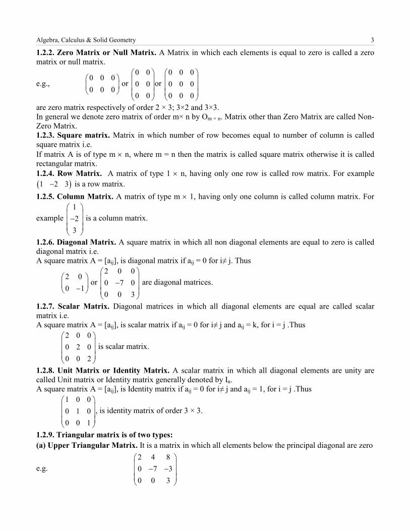
1.2.2. Zero Matrix or Null Matrix. A Matrix in which each elements is equal to zero is called a zero matrix or null matrix.
e.g., 0 0 00 0 0
or 0 00 00 0
or 0 0 00 0 00 0 0
are zero matrix respectively of order 2 × 3; 3×2 and 3×3. In general we denote zero matrix of order m× n by Om × n. Matrix other than Zero Matrix are called Non- Zero Matrix. 1.2.3. Square matrix. Matrix in which number of row becomes equal to number of column is called square matrix i.e. If matrix A is of type m × n, where m = n then the matrix is called square matrix otherwise it is called rectangular matrix. 1.2.4. Row Matrix. A matrix of type 1 × n, having only one row is called row matrix. For example ( )1 2 3− is a row matrix. 1.2.5. Column Matrix. A matrix of type m × 1, having only one column is called column matrix. For
example 12
3
−
is a column matrix.
1.2.6. Diagonal Matrix. A square matrix in which all non diagonal elements are equal to zero is called diagonal matrix i.e. A square matrix A = [aij], is diagonal matrix if aij = 0 for i≠ j. Thus
2 00 1 −
or 2 0 00 7 00 0 3
−
are diagonal matrices.
1.2.7. Scalar Matrix. Diagonal matrices in which all diagonal elements are equal are called scalar matrix i.e. A square matrix A = [aij], is scalar matrix if aij = 0 for i≠ j and aij = k, for i = j .Thus
2 0 00 2 00 0 2
is scalar matrix.
1.2.8. Unit Matrix or Identity Matrix. A scalar matrix in which all diagonal elements are unity are called Unit matrix or Identity matrix generally denoted by In. A square matrix A = [aij], is Identity matrix if aij = 0 for i≠ j and aij = 1, for i = j .Thus
1 0 00 1 00 0 1
, is identity matrix of order 3 × 3.
1.2.9. Triangular matrix is of two types: (a) Upper Triangular Matrix. It is a matrix in which all elements below the principal diagonal are zero
e.g. 2 4 80 7 30 0 3
− −
4 Matrices
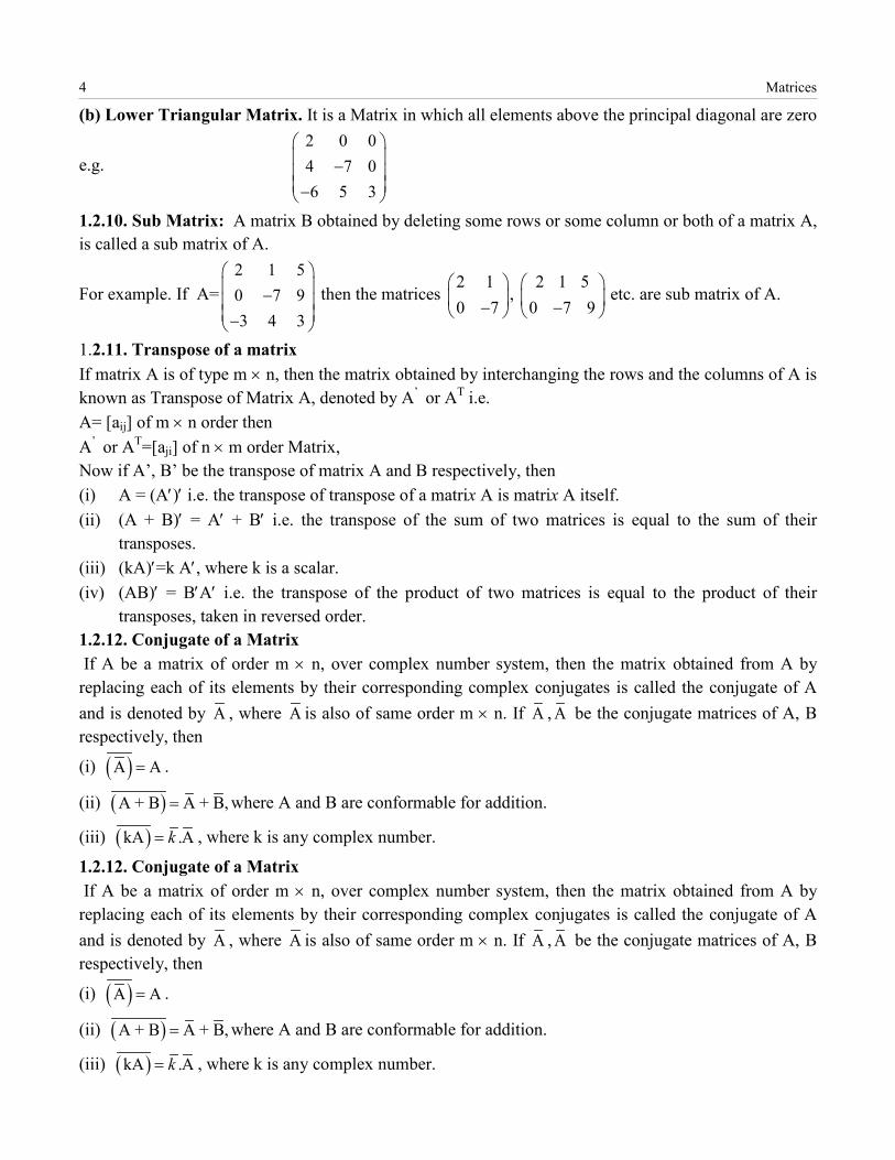
(b) Lower Triangular Matrix. It is a Matrix in which all elements above the principal diagonal are zero
e.g. 2 0 04 7 06 5 3
− −
1.2.10. Sub Matrix: A matrix B obtained by deleting some rows or some column or both of a matrix A, is called a sub matrix of A.
For example. If A=2 1 50 7 93 4 3
− −
then the matrices 2 10 7 −
, 2 1 5
0 7 9 −
etc. are sub matrix of A.
1.2.11. Transpose of a matrix If matrix A is of type m × n, then the matrix obtained by interchanging the rows and the columns of A is known as Transpose of Matrix A, denoted by A’ or AT i.e. A= [aij] of m × n order then A’ or AT=[aji] of n × m order Matrix, Now if A’, B’ be the transpose of matrix A and B respectively, then (i) A = (A′)′ i.e. the transpose of transpose of a matrix A is matrix A itself. (ii) (A + B)′ = A′ + B′ i.e. the transpose of the sum of two matrices is equal to the sum of their
transposes. (iii) (kA)′=k A′, where k is a scalar. (iv) (AB)′ = B′A′ i.e. the transpose of the product of two matrices is equal to the product of their
transposes, taken in reversed order. 1.2.12. Conjugate of a Matrix If A be a matrix of order m × n, over complex number system, then the matrix obtained from A by replacing each of its elements by their corresponding complex conjugates is called the conjugate of A and is denoted by A , where A is also of same order m × n. If A , A be the conjugate matrices of A, B respectively, then
(i) ( )A A= .
(ii) ( )A + B A + B,= where A and B are conformable for addition.
(iii) ( )kA .Ak= , where k is any complex number.
1.2.12. Conjugate of a Matrix If A be a matrix of order m × n, over complex number system, then the matrix obtained from A by replacing each of its elements by their corresponding complex conjugates is called the conjugate of A and is denoted by A , where A is also of same order m × n. If A , A be the conjugate matrices of A, B respectively, then
(i) ( )A A= .
(ii) ( )A + B A + B,= where A and B are conformable for addition.
(iii) ( )kA .Ak= , where k is any complex number.
Algebra, Calculus & Solid Geometry 5
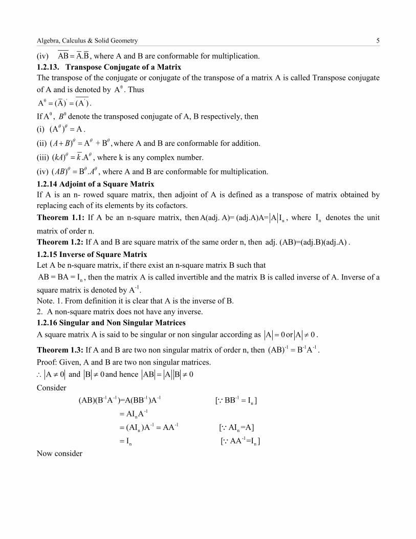
(iv) AB A.B= , where A and B are conformable for multiplication. 1.2.13. Transpose Conjugate of a Matrix The transpose of the conjugate or conjugate of the transpose of a matrix A is called Transpose conjugate of A and is denoted by θA . Thus
θ ' 'A (A) (A )= = . If θA , θB denote the transposed conjugate of A, B respectively, then (i) (A ) Aθ θ = .
(ii) ( ) A + B ,A B θ θ θ+ = where A and B are conformable for addition.
(iii) ( ) .AkA kθ θ= , where k is any complex number.
(iv) ( ) B .AB Aθ θ θ= , where A and B are conformable for multiplication. 1.2.14 Adjoint of a Square Matrix If A is an n- rowed square matrix, then adjoint of A is defined as a transpose of matrix obtained by replacing each of its elements by its cofactors. Theorem 1.1: If A be an n-square matrix, then nA(adj. A)= (adj.A)A= A I , where nI denotes the unit
matrix of order n. Theorem 1.2: If A and B are square matrix of the same order n, then adj. (AB)=(adj.B)(adj.A) . 1.2.15 Inverse of Square Matrix Let A be n-square matrix, if there exist an n-square matrix B such that
nAB = BA = I , then the matrix A is called invertible and the matrix B is called inverse of A. Inverse of a square matrix is denoted by A-1. Note. 1. From definition it is clear that A is the inverse of B. 2. A non-square matrix does not have any inverse. 1.2.16 Singular and Non Singular Matrices A square matrix A is said to be singular or non singular according as A 0= or A 0≠ .
Theorem 1.3: If A and B are two non singular matrix of order n, then -1 -1 -1(AB) B A= . Proof: Given, A and B are two non singular matrices.
A 0∴ ≠ and B 0≠ and hence AB A B 0= ≠
Consider
-1 -1 -1 -1 -1n
-1n
-1 -1n n
-1n n
(AB)(B A )=A(BB )A [ BB I ]AI A(AI )A AA [ AI =A]I [ AA =I ]
=
=
= =
=
Now consider
6 Matrices
-1 -1 -1 -1 -1n
-1n
-1 -1n n
-1n n
(B A )(AB)=B(A A)B [ AA =I ]BI B(BI )B =BB [ BI =B]I [ BB =I ]
=
=
=
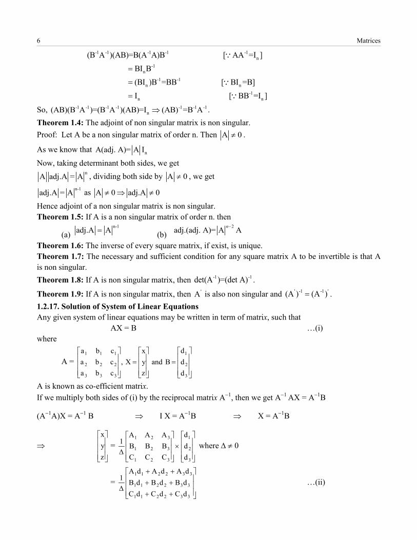
So, -1 -1 -1 -1 -1 -1 -1n(AB)(B A )=(B A )(AB)=I (AB) =B A⇒ .
Theorem 1.4: The adjoint of non singular matrix is non singular. Proof: Let A be a non singular matrix of order n. Then A 0≠ .
As we know that nA(adj. A)= A I
Now, taking determinant both sides, we get nA adj.A = A , dividing both side by A 0≠ , we get
n-1adj.A = A as A 0 adj.A 0≠ ⇒ ≠
Hence adjoint of a non singular matrix is non singular. Theorem 1.5: If A is a non singular matrix of order n. then
(a) n-1adj.A A= (b)
2adj.(adj. A)= A An−
Theorem 1.6: The inverse of every square matrix, if exist, is unique. Theorem 1.7: The necessary and sufficient condition for any square matrix A to be invertible is that A is non singular. Theorem 1.8: If A is non singular matrix, then -1 -1det(A )=(det A) .
Theorem 1.9: If A is non singular matrix, then 'A is also non singular and ' -1 -1 '(A ) (A )= . 1.2.17. Solution of System of Linear Equations Any given system of linear equations may be written in term of matrix, such that AX = B …(i) where
A =
=
=
3
2
1
333
222
111
ddd
Bandzyx
X,cbacbacba
A is known as co-efficient matrix. If we multiply both sides of (i) by the reciprocal matrix A−1, then we get A−1 AX = A−1B
(A−1A)X = A−1 B ⇒ I X = A−1B ⇒ X = A−1B
⇒
zyx
=
×
∆3
2
1
321
321
321
ddd
CCCBBBAAA
1 where ∆ ≠ 0
=
++++++
∆332211
332211
332211
dCdCdCdBdBdBdAdAdA
1 …(ii)

Algebra, Calculus & Solid Geometry 7
Hence from (ii) equating the values of x, y and z we get the desired result. This method is true only when (i) ∆ ≠ 0 (ii) number of equations and number of unknowns (e.g. x, y, z etc.) are the same. Example 1. Solve the equations with the help of determinants : x + y + z = 3, x + 2y + 3z = 4, x + 4y + 9z = 6.
Sol. The co-efficient determinant is ∆ = 941321111
= 2 ≠ 0
∴ x =
946324113
21 ⇒ x =
21 × 4 = 2
y =
961341131
21 ⇒ y =
21 (2) = 1 ⇒ y = 1
z =
+++
641421311
21 ⇒ z =
21 [−4 + 6 + (4 − 6)] = 0 ⇒ z = 0
∴ Solution is x = 2, y = 1, z = 0. 1. 3. Symmetric And Skew Symmetric Matrices 1.3.1. Symmetric Matrix A square matrix A = [aij] is said to be symmetric if aij = aji for all i and j
Examples
cfgfbhgha
,
743452321
1.3.2. Skew Symmetric Matrix If a square matrix A has its elements such that aij = −aji for i and j and the leading diagonal elements are
zeros, then matrix A is known as skew matrix. For example
−−
−
013102320
,
−−−0fgf0h
gh0 are skew
symmetric matrices.
Example 1: Every square matrix can be expressed as the sum of symmetric matrix and a skew-symmetric matrix in one and only one way. Solution. If A be any square matrix, then we consider
B = 21 (A + A′) and C =
21 (A − A′)
⇒ B + C = 21 (A + A′) +
21 (A − A′) =
21 (A + A′ + A − A′) = A
Similarly B′ = 21 (A + A′)′ =
21 [A′ + (A′)′] =
21 [A′ + A] =
21 (A + A′) = B
8 Matrices
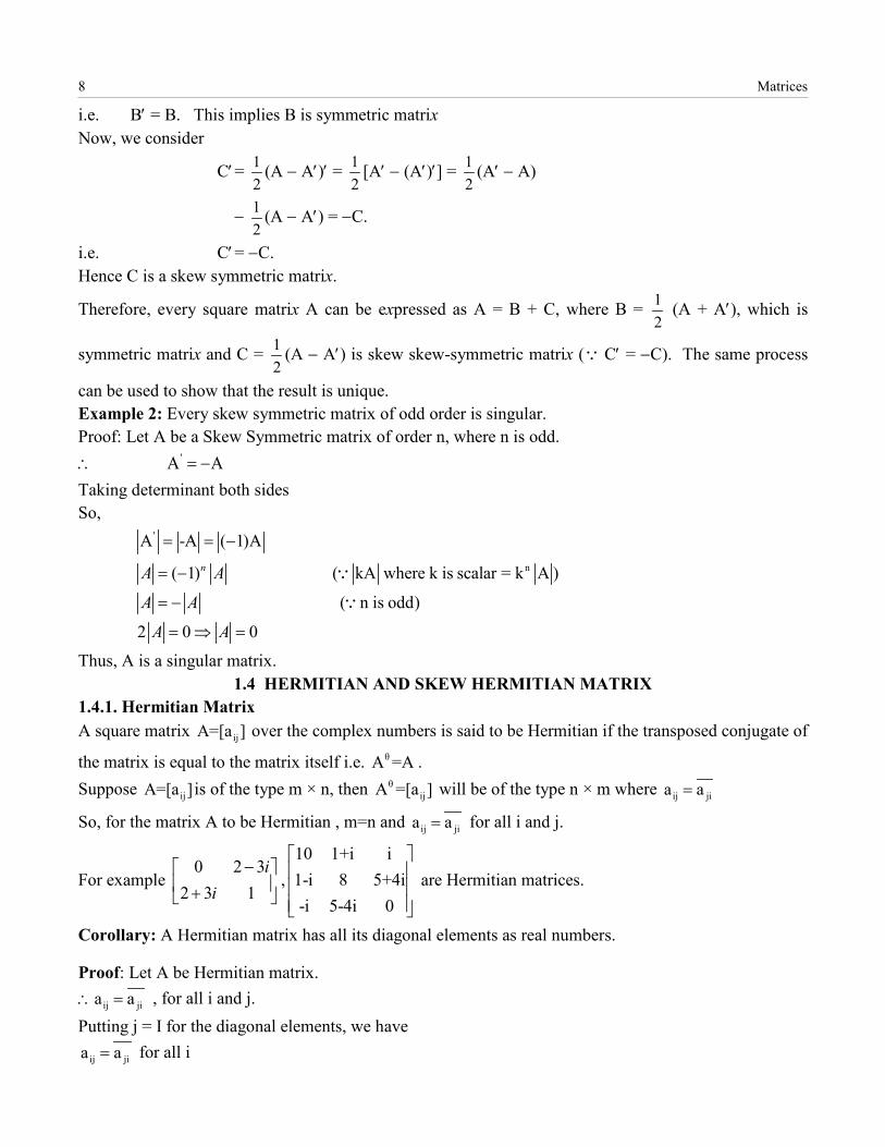
i.e. B′ = B. This implies B is symmetric matrix Now, we consider
C′ = 21 (A − A′)′ =
21 [A′ − (A′)′] =
21 (A′ − A)
− 21 (A − A′) = −C.
i.e. C′ = −C. Hence C is a skew symmetric matrix.
Therefore, every square matrix A can be expressed as A = B + C, where B = 21 (A + A′), which is
symmetric matrix and C = 21 (A − A′) is skew skew-symmetric matrix ( C′ = −C). The same process
can be used to show that the result is unique. Example 2: Every skew symmetric matrix of odd order is singular. Proof: Let A be a Skew Symmetric matrix of order n, where n is odd.
'A A∴ = − Taking determinant both sides So,
'
n
A -A ( 1)A
( 1) ( kA where k is scalar = k A )
( n is odd)
2 0 0
nA A
A A
A A
= = −
= −
= −
= ⇒ =
Thus, A is a singular matrix. 1.4 HERMITIAN AND SKEW HERMITIAN MATRIX
1.4.1. Hermitian Matrix A square matrix ijA=[a ] over the complex numbers is said to be Hermitian if the transposed conjugate of
the matrix is equal to the matrix itself i.e. θA =A . Suppose ijA=[a ]is of the type m × n, then θ
ijA =[a ] will be of the type n × m where ij jia a=
So, for the matrix A to be Hermitian , m=n and ij jia a= for all i and j.
For example 0 2 3
2 3 1i
i−
+ ,
10 1+i i1-i 8 5+4i-i 5-4i 0
are Hermitian matrices.
Corollary: A Hermitian matrix has all its diagonal elements as real numbers.
Proof: Let A be Hermitian matrix.
ij jia a∴ = , for all i and j. Putting j = I for the diagonal elements, we have
ij jia a= for all i
Algebra, Calculus & Solid Geometry 9
[ ]2 0 0
ij iji i a i a ii
α β α β α β α β
β β
⇒ + = − = + ⇒ = −
⇒ = ⇒ =
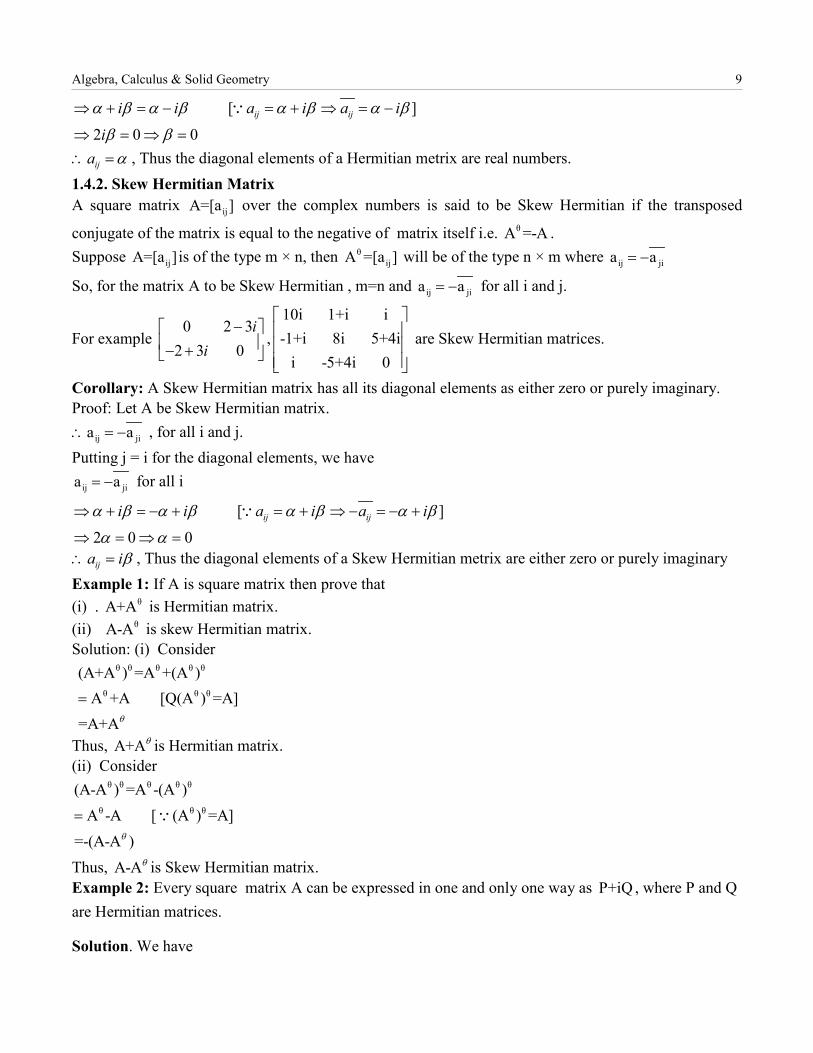
ija α∴ = , Thus the diagonal elements of a Hermitian metrix are real numbers. 1.4.2. Skew Hermitian Matrix A square matrix ijA=[a ] over the complex numbers is said to be Skew Hermitian if the transposed
conjugate of the matrix is equal to the negative of matrix itself i.e. θA =-A . Suppose ijA=[a ]is of the type m × n, then θ
ijA =[a ] will be of the type n × m where ij jia a= −
So, for the matrix A to be Skew Hermitian , m=n and ij jia a= − for all i and j.
For example 0 2 3
2 3 0i
i−
− + ,
10i 1+i i-1+i 8i 5+4i
i -5+4i 0
are Skew Hermitian matrices.
Corollary: A Skew Hermitian matrix has all its diagonal elements as either zero or purely imaginary. Proof: Let A be Skew Hermitian matrix.
ij jia a∴ = − , for all i and j. Putting j = i for the diagonal elements, we have
ij jia a= − for all i
[ ]2 0 0
ij iji i a i a iα β α β α β α β
α α
⇒ + = − + = + ⇒ − = − +
⇒ = ⇒ =
ija iβ∴ = , Thus the diagonal elements of a Skew Hermitian metrix are either zero or purely imaginary Example 1: If A is square matrix then prove that (i) . θA+A is Hermitian matrix. (ii) θA-A is skew Hermitian matrix. Solution: (i) Consider
θ θ θ θ θ
θ θ θ
(A+A ) =A +(A )A +A [Q(A ) =A]
=A+Aθ
=
Thus, A+Aθ is Hermitian matrix. (ii) Consider
θ θ θ θ θ
θ θ θ
(A-A ) =A -(A )A -A [ (A ) =A]
=-(A-A )θ
=
Thus, A-Aθ is Skew Hermitian matrix. Example 2: Every square matrix A can be expressed in one and only one way as P+iQ , where P and Q are Hermitian matrices.
Solution. We have
10 Matrices
1 1A= (2A) [ ]2 2
1 1( ) ( )2 21 1( ) i. ( ) P+iQ2 2i
A A A A
A A A A
A A A A
θ θ
θ θ
θ θ
= + + −
= + + −
= + + − =
where, θ1P= (A+A )2
and θ1Q= (A-A )2i
Now, θ θ θ θ1 1P = (A+A ) (A +A)=P2 2
=
and
θ θ θ θ
θ θ θ
1 1Q =- (A-A ) - (A -A)2i 2i
1 (A-A ) = Q [ (kA) =kA ]2i
=
=
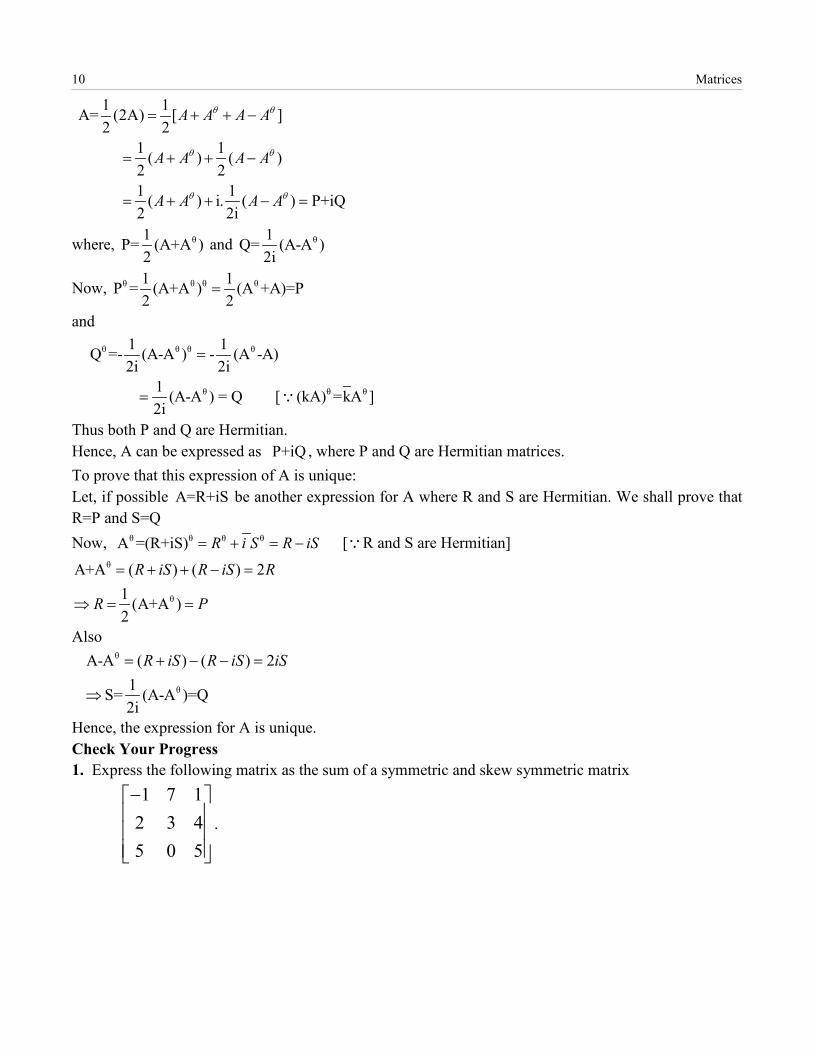
Thus both P and Q are Hermitian. Hence, A can be expressed as P+iQ , where P and Q are Hermitian matrices. To prove that this expression of A is unique: Let, if possible A=R+iS be another expression for A where R and S are Hermitian. We shall prove that R=P and S=Q Now, θ θ θ θA =(R+iS) R i S R iS= + = − [R and S are Hermitian]
θ
θ
A+A ( ) ( ) 21 (A+A )2
R iS R iS R
R P
= + + − =
⇒ = =
Also
θ
θ
A-A ( ) ( ) 21S= (A-A )=Q2i
R iS R iS iS= + − − =
⇒
Hence, the expression for A is unique. Check Your Progress 1. Express the following matrix as the sum of a symmetric and skew symmetric matrix
1 7 12 3 45 0 5
−
.
Algebra, Calculus & Solid Geometry 11
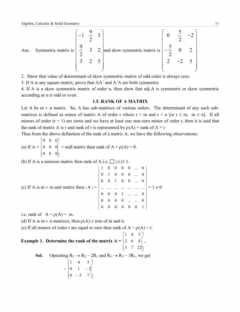
Ans. Symmetric matrix is
91 32
9 3 223 2 5
−
and skew symmetric matrix is
50 22
5 0 22
2 2 5
− − −
.
2. Show that value of determinant of skew symmetric matrix of odd order is always zero. 3. If A is any square matrix, prove that AA’ and A’A are both symmetric 4. If A is a skew symmetric matrix of order n, then show that adj.A is symmetric or skew symmetric according as n is odd or even .
1.5. RANK OF A MATRIX Let A be m × n matrix. So, A has sub-matrices of various orders. The determinant of any such sub-matrices is defined as minor of matrix A of order r where r < m and r < n [or r ≤ m, m ≤ n]. If all minors of order (r + 1) are zeros and we have at least one non-zero minor of order r, then it is said that the rank of matrix A is r and rank of r is represented by ρ(A) = rank of A = r. Thus from the above definition of the rank of a matrix A, we have the following observations:
(a) If A =
000000000
= null matrix then rank of A = ρ(A) = 0.
(b) If A is a nonzero matrix then rank of A i.e. (A) ≥ 1.
(c) If A is m × m unit matrix then | A | =
10000000......00000......1000.....................0...001000...000100...00001
= 1 ≠ 0
i.e. rank of A = ρ(A) = m. (d) If A is m × n matrices, then ρ(A) ≤ min of m and n. (e) If all minors of order r are equal to zero then rank of A = ρ(A) < r.
Example 1. Determine the rank of the matrix A =
2273862541
.
Sol. Operating R2 → R2 − 2R1 and R3 → R3 − 3R1, we get
~
−−750210
541
12 Matrices
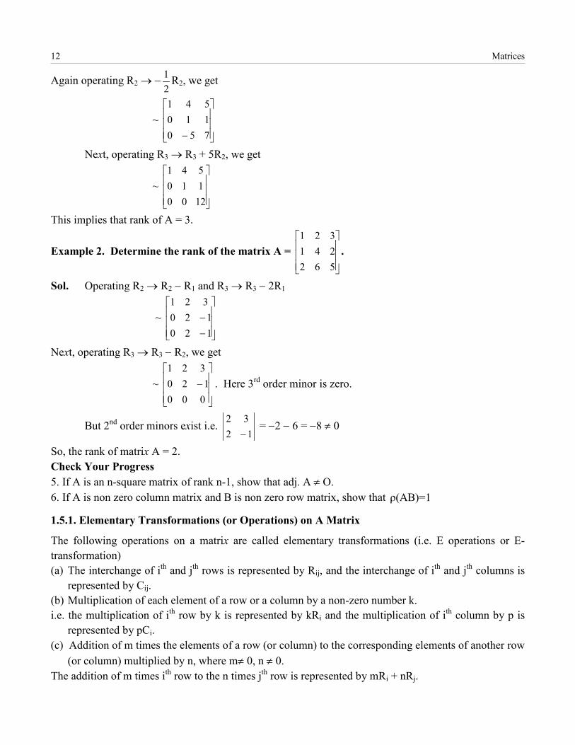
Again operating R2 → −21 R2, we get
~
− 750110541
Next, operating R3 → R3 + 5R2, we get
~
1200110541
This implies that rank of A = 3.
Example 2. Determine the rank of the matrix A =
562241321
.
Sol. Operating R2 → R2 − R1 and R3 → R3 − 2R1
~
−−
120120
321
Next, operating R3 → R3 − R2, we get
~
−000120
321. Here 3rd order minor is zero.
But 2nd order minors exist i.e. 12
32−
= −2 − 6 = −8 ≠ 0
So, the rank of matrix A = 2. Check Your Progress 5. If A is an n-square matrix of rank n-1, show that adj. A ≠ O. 6. If A is non zero column matrix and B is non zero row matrix, show that ρ(AB)=1
1.5.1. Elementary Transformations (or Operations) on A Matrix
The following operations on a matrix are called elementary transformations (i.e. E operations or E-transformation) (a) The interchange of ith and jth rows is represented by Rij, and the interchange of ith and jth columns is
represented by Cij. (b) Multiplication of each element of a row or a column by a non-zero number k. i.e. the multiplication of ith row by k is represented by kRi and the multiplication of ith column by p is
represented by pCi. (c) Addition of m times the elements of a row (or column) to the corresponding elements of another row
(or column) multiplied by n, where m≠ 0, n ≠ 0. The addition of m times ith row to the n times jth row is represented by mRi + nRj.
Algebra, Calculus & Solid Geometry 13
If a matrix B is obtained from matrix A by such transformation, then the matrix B is called the equivalent matrix to matrix A. If matrix B is obtained from A by applying finite number of elementary row operation on A, then B is row equivalent to A. If matrix B is obtained from A by applying finite number of elementary column operation on A, then B is column equivalent to A. Two such equivalent matrices A and B are denoted as A ~ B and the symbol ~ is used for equivalence. So, two equivalent matrices have the same order and same rank. Theorem 1.15: The rank of a matrix remains unaltered by the application of elementary row and column operations. Proof: Let A be m × n matrix, such that
11 1
1
A=n
m mn
a a
a a
If ρ(A)=r , then every minor of order r+1, if any vanishes and there will be at least one non zero minor of A of order r. Now consider a minor of order r+1 denoted by Mr+1. (1) If we interchange any two rows or columns of A, the value of determinant remains unaltered by numerically value but the sign is changed. (2) If one row and column of A is multiplied by any scalar k, the value of determinant multiplied by the scalar k. (3) If we apply i i j i i jR R +kR or C C +kC→ → , then the determinant remains unchanged.
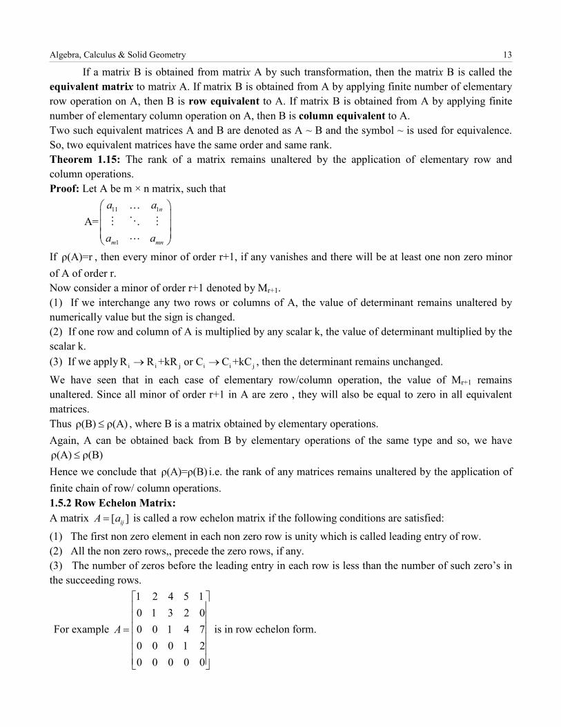
We have seen that in each case of elementary row/column operation, the value of Mr+1 remains unaltered. Since all minor of order r+1 in A are zero , they will also be equal to zero in all equivalent matrices. Thus ρ(B) ρ(A)≤ , where B is a matrix obtained by elementary operations. Again, A can be obtained back from B by elementary operations of the same type and so, we have ρ(A) ρ(B)≤ Hence we conclude that ρ(A)=ρ(B) i.e. the rank of any matrices remains unaltered by the application of finite chain of row/ column operations. 1.5.2 Row Echelon Matrix: A matrix [ ]ijA a= is called a row echelon matrix if the following conditions are satisfied:
(1) The first non zero element in each non zero row is unity which is called leading entry of row. (2) All the non zero rows,, precede the zero rows, if any. (3) The number of zeros before the leading entry in each row is less than the number of such zero’s in the succeeding rows.
For example
1 2 4 5 10 1 3 2 00 0 1 4 70 0 0 1 20 0 0 0 0
A
=
is in row echelon form.
14 Matrices
1.5.3 Row reduced Echelon Form: In addition to the above three conditions, if a matrix satisfies the following conditions: Each column which contains a leading entry of a row has all other entries zeros, then the matrix is said to be in row reduced echelon matrix.
1.5.4 Row Rank and Column Rank of a Matrix Row rank of a matrix, say A is the number of non zero rows in the row echelon matrix A and is denoted by Rρ (A) .
Column Rank of a matrix, say A is the number of non zero columns in the column echelon matrix A and is denoted by Cρ (A) .
Note: (i) Every matrix is row equivalent to row echelon matrix. (ii) Every matrix is column equivalent to a column echelon matrix. (iii) If a matrix A is in row echelon form, then its transpose is in column echelon form.
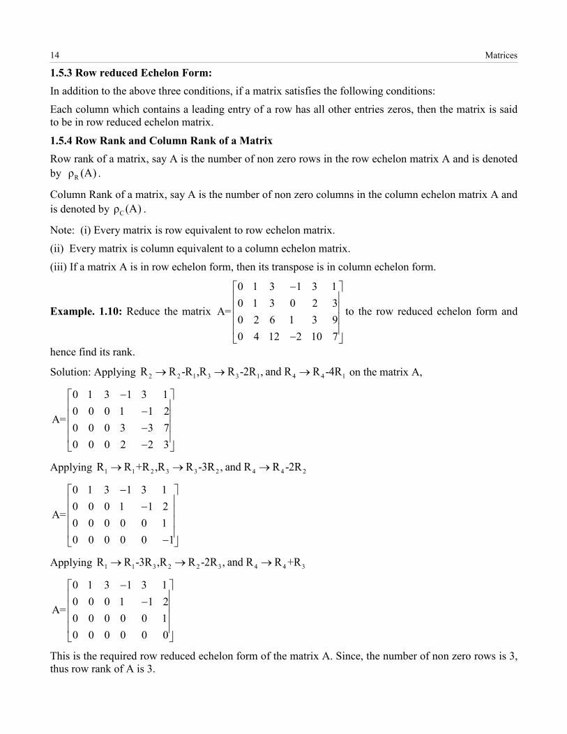
Example. 1.10: Reduce the matrix
0 1 3 1 3 10 1 3 0 2 3
A=0 2 6 1 3 90 4 12 2 10 7
− −
to the row reduced echelon form and
hence find its rank.
Solution: Applying 2 2 1 3 3 1 4 4 1R R -R ,R R -2R , and R R -4R→ → → on the matrix A,
0 1 3 1 3 10 0 0 1 1 2
A=0 0 0 3 3 70 0 0 2 2 3
− − − −
Applying 1 1 2 3 3 2 4 4 2R R +R ,R R -3R , and R R -2R→ → →
0 1 3 1 3 10 0 0 1 1 2
A=0 0 0 0 0 10 0 0 0 0 1
− − −
Applying 1 1 3 2 2 3 4 4 3R R -3R ,R R -2R , and R R +R→ → →
0 1 3 1 3 10 0 0 1 1 2
A=0 0 0 0 0 10 0 0 0 0 0
− −
This is the required row reduced echelon form of the matrix A. Since, the number of non zero rows is 3, thus row rank of A is 3.
Algebra, Calculus & Solid Geometry 15
Check Your Progress
7. Find the row rank of matrix 3 4 1 2
A= 3 2 1 47 6 2 5
.
Ans. 3
8. Reduce the matrix 1 2 31 4 22 6 5
to the row reduced echelon form. Also find their row rank.
Ans. 2
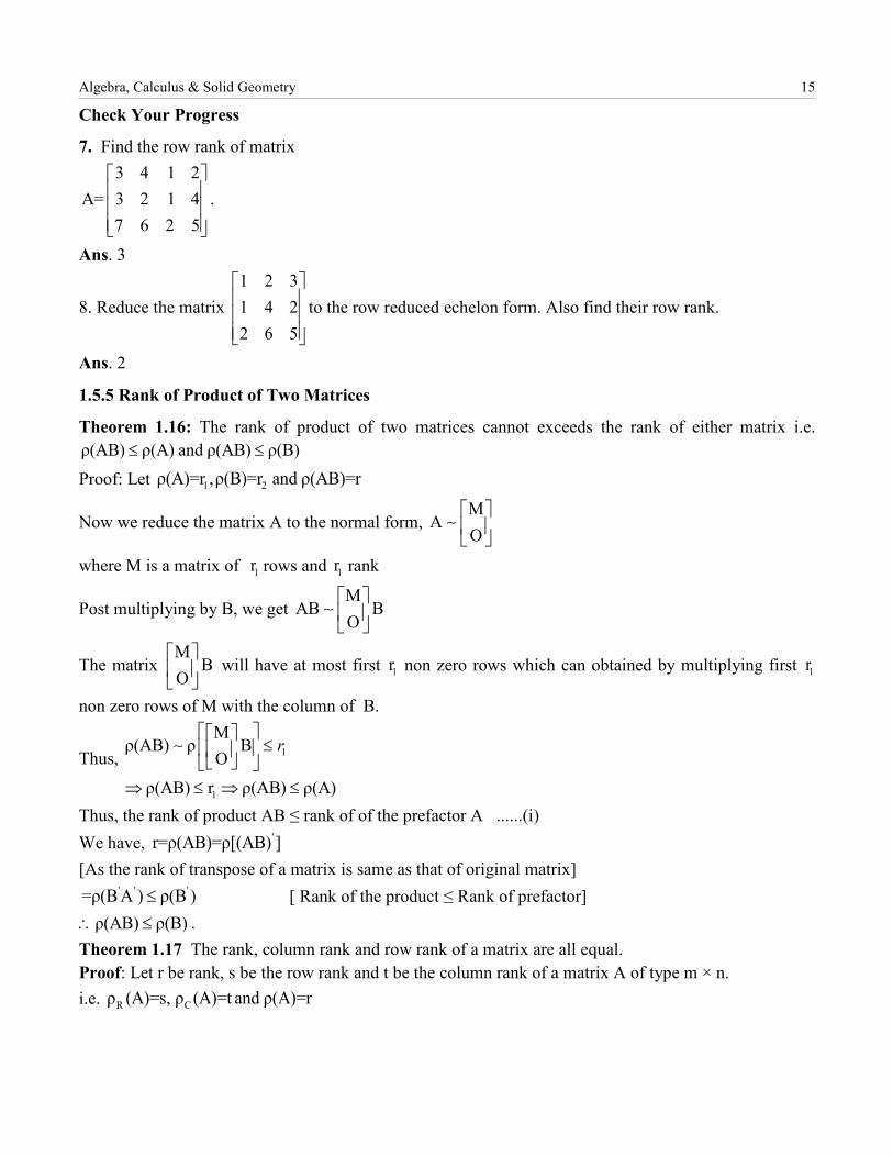
1.5.5 Rank of Product of Two Matrices
Theorem 1.16: The rank of product of two matrices cannot exceeds the rank of either matrix i.e. ρ(AB) ρ(A) and ρ(AB) ρ(B)≤ ≤
Proof: Let 1 2ρ(A)=r ,ρ(B)=r and ρ(AB)=r
Now we reduce the matrix A to the normal form, M
AO
where M is a matrix of 1r rows and 1r rank
Post multiplying by B, we get M
AB BO
The matrix M
BO
will have at most first 1r non zero rows which can obtained by multiplying first 1r
non zero rows of M with the column of B.
Thus, 1
1
Mρ(AB) ρ B
O
ρ(AB) r ρ(AB) ρ(A)
r
≤
⇒ ≤ ⇒ ≤
Thus, the rank of product AB ≤ rank of of the prefactor A ......(i) We have, 'r=ρ(AB)=ρ[(AB) ] [As the rank of transpose of a matrix is same as that of original matrix]
' ' '=ρ(B A ) ρ(B )≤ [ Rank of the product ≤ Rank of prefactor] ρ(AB) ρ(B)∴ ≤ .
Theorem 1.17 The rank, column rank and row rank of a matrix are all equal. Proof: Let r be rank, s be the row rank and t be the column rank of a matrix A of type m × n. i.e. R Cρ (A)=s, ρ (A)=t and ρ(A)=r
16 Matrices
As the row rank of the matrix A is s, thus there must be non singular matrix P such that B
PA=O
,
where B is a matrix of type s × n. We know that pre or post multiplication by non singular matrix does not affect the rank of matrix, therefore ρ(PA)=ρ(A)=r .......(i) Since every square minor of of PA of order (s+1) has atleast one row of zeros, thus, each minor of PA of order (s+1) is equal to zero. ρ(PA) s r s [Using (i)]≤ ⇒ ≤ ...(ii)
As ρ(PA)=r , thus there must be a non singular matrix Q such that C
QA=O
, where C is a matrix of
type r × n.
R Rρ (QA)=ρ (A)=s∴ Since the matrix QA has only r non zero rows, thus ρ(QA) r s r≤ ⇒ ≤ ...(iii) From (ii) and (iii), we have r = s ...(iv) Similarly, r=t and hence s=r=t Thus, R Cρ(A)=ρ (A)=ρ (A) .
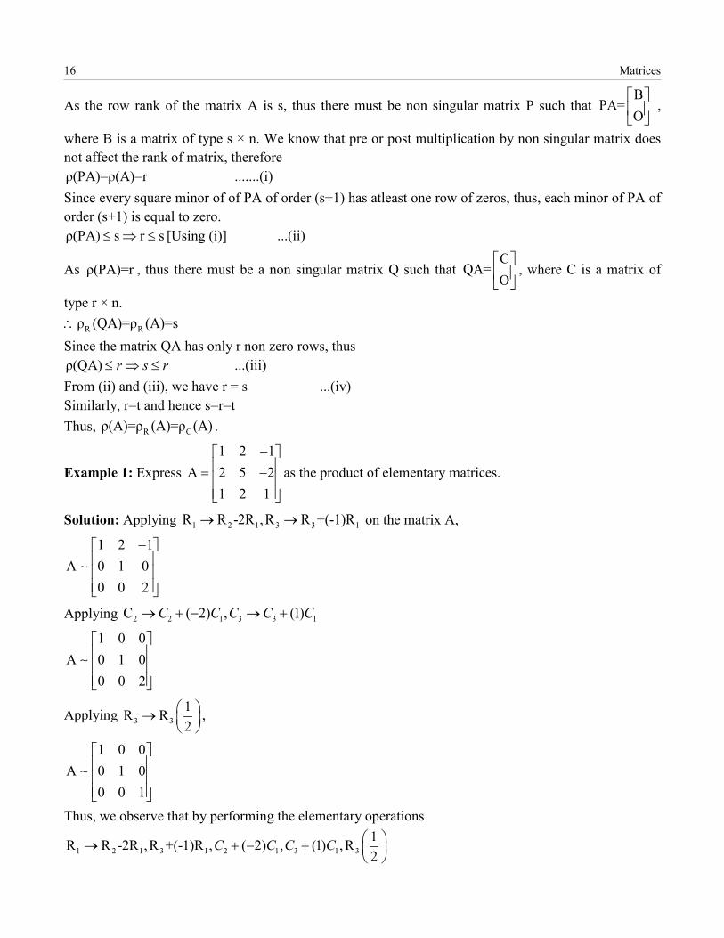
Example 1: Express 1 2 1
A 2 5 21 2 1
− = −
as the product of elementary matrices.
Solution: Applying 1 2 1 3 3 1R R -2R ,R R +(-1)R→ → on the matrix A,
1 2 1A 0 1 0
0 0 2
−
Applying 2 2 1 3 3 1C ( 2) , (1)C C C C C→ + − → +
1 0 0A 0 1 0
0 0 2
Applying 3 31R R2
→
,
1 0 0A 0 1 0
0 0 1
Thus, we observe that by performing the elementary operations
1 2 1 3 1 2 1 3 1 31R R -2R ,R +(-1)R , ( 2) , (1) ,R2
C C C C → + − +
Algebra, Calculus & Solid Geometry 17
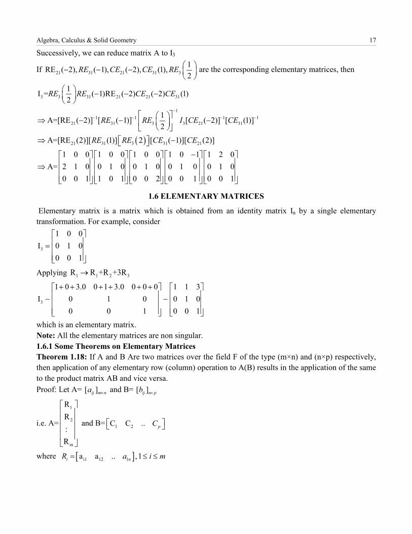
Successively, we can reduce matrix A to I3
If 21 31 21 31 31RE ( 2), ( 1), ( 2), (1),2
RE CE CE RE − − −
are the corresponding elementary matrices, then
3 3 31 21 21 311I = ( 1)RE ( 2) ( 2) (1)2
RE RE CE CE − − −
( )
11 1 1 1
21 31 3 3 21 31
21 31 3 31 21
1A=[RE ( 2)] [ ( 1)] [ ( 2)] [ (1)]2
A=[RE (2)][ (1)] 2 [ ( 1)][ (2)]
1 0 0 1 0 0 1 0 0 1 0 1 1A= 2 1 0 0 1 0 0 1 0 0 1 0
0 0 1 1 0 1 0 0 2 0 0 1
RE RE I CE CE
RE RE CE CE
−− − − − ⇒ − − −
⇒ − −
⇒
2 00 1 00 0 1
1.6 ELEMENTARY MATRICES
Elementary matrix is a matrix which is obtained from an identity matrix In by a single elementary transformation. For example, consider
3
1 0 0I 0 1 0
0 0 1
=
Applying 1 1 2 3R R +R +3R→
3
1 0 3.0 0 1 3.0 0 0 0 1 1 3I 0 1 0 0 1 0
0 0 1 0 0 1
+ + + + + +
which is an elementary matrix. Note: All the elementary matrices are non singular. 1.6.1 Some Theorems on Elementary Matrices Theorem 1.18: If A and B Are two matrices over the field F of the type (m×n) and (n×p) respectively, then application of any elementary row (column) operation to A(B) results in the application of the same to the product matrix AB and vice versa. Proof: Let A= [ ]ij m na × and B= [ ]ij n pb ×
i.e. A=
1
2
m
RR:R
and B= 1 2C C .. pC
where [ ]i1 12 1a a .. ,1i nR a i m= ≤ ≤
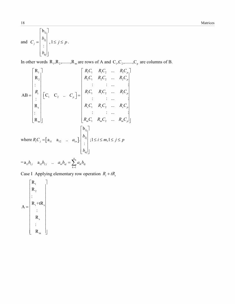
18 Matrices
and
1j
2j
nj
b
,1:j
bC j p
b
= ≤ ≤
.
In other words 1 2 mR ,R ,.......,R are rows of A and 1 2 pC ,C ,.......,C are columns of B.
1 1 1 2 11
2 1 2 2 22
1 21 2
1 2s
1 2m
...R
...R: : ... ::
...AB C C ..
: : ... ::...R
: : ... ::...R
p
p
i i i pip
s s s p
m m m p
R C R C R CR C R C R C
R C R C R CRC
R C R C R C
R C R C R C
= =
where [ ]
1j
2ji1 12 1
nj
b
a a .. . ;1 ,1:i j n
bR C a i m j p
b
= ≤ ≤ ≤ ≤
= i1 1 i2 21
a a ..n
j j in nj ik kjk
b b a b a b=
=∑
Case I Applying elementary row operation i sR tR+ 1
2
i s
s
m
RR:R +tR
A:R:R
=
Algebra, Calculus & Solid Geometry 19
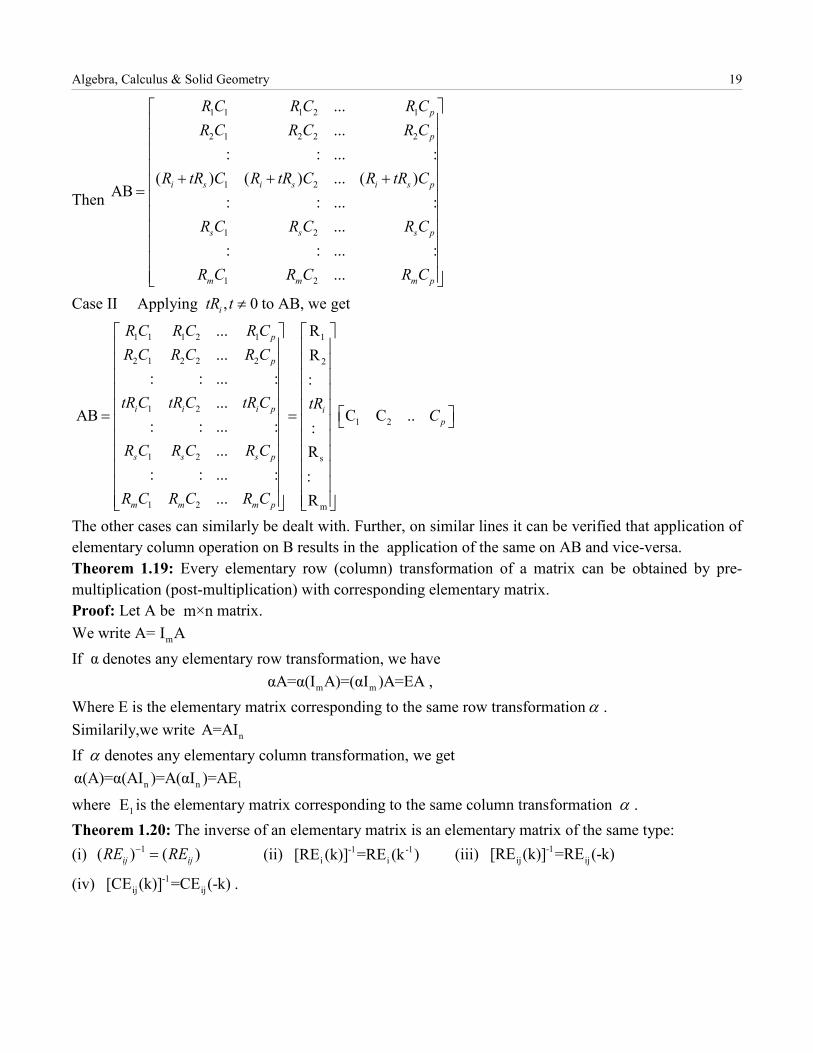
Then
1 1 1 2 1
2 1 2 2 2
1 2
1 2
1 2
...
...: : ... :
( ) ( ) ... ( )AB
: : ... :...
: : ... :...
p
p
i s i s i s p
s s s p
m m m p
R C R C R CR C R C R C
R tR C R tR C R tR C
R C R C R C
R C R C R C
+ + + =
Case II Applying to AB, we get
The other cases can similarly be dealt with. Further, on similar lines it can be verified that application of elementary column operation on B results in the application of the same on AB and vice-versa. Theorem 1.19: Every elementary row (column) transformation of a matrix can be obtained by pre-multiplication (post-multiplication) with corresponding elementary matrix. Proof: Let A be matrix. We write A= If denotes any elementary row transformation, we have , Where E is the elementary matrix corresponding to the same row transformation . Similarily,we write If denotes any elementary column transformation, we get
where is the elementary matrix corresponding to the same column transformation . Theorem 1.20: The inverse of an elementary matrix is an elementary matrix of the same type: (i) (ii) (iii)
(iv) .
, 0itR t ≠
1 1 1 2 1 1
2 1 2 2 2 2
1 21 2
1 2 s
1 2 m
... R
... R: : ... : :
...AB C C ..
: : ... : :... R
: : ... : :... R
p
p
i i i p ip
s s s p
m m m p
R C R C R CR C R C R C
tR C tR C tR C tRC
R C R C R C
R C R C R C
= =
m×nmI A
αm mαA=α(I A)=(αI )A=EA
α
nA=AIα
n n 1α(A)=α(AI )=A(αI )=AE
1E α
1( ) ( )ij ijRE RE− = -1 -1i i[RE (k)] =RE (k ) -1
ij ij[RE (k)] =RE (-k)-1
ij ij[CE (k)] =CE (-k)
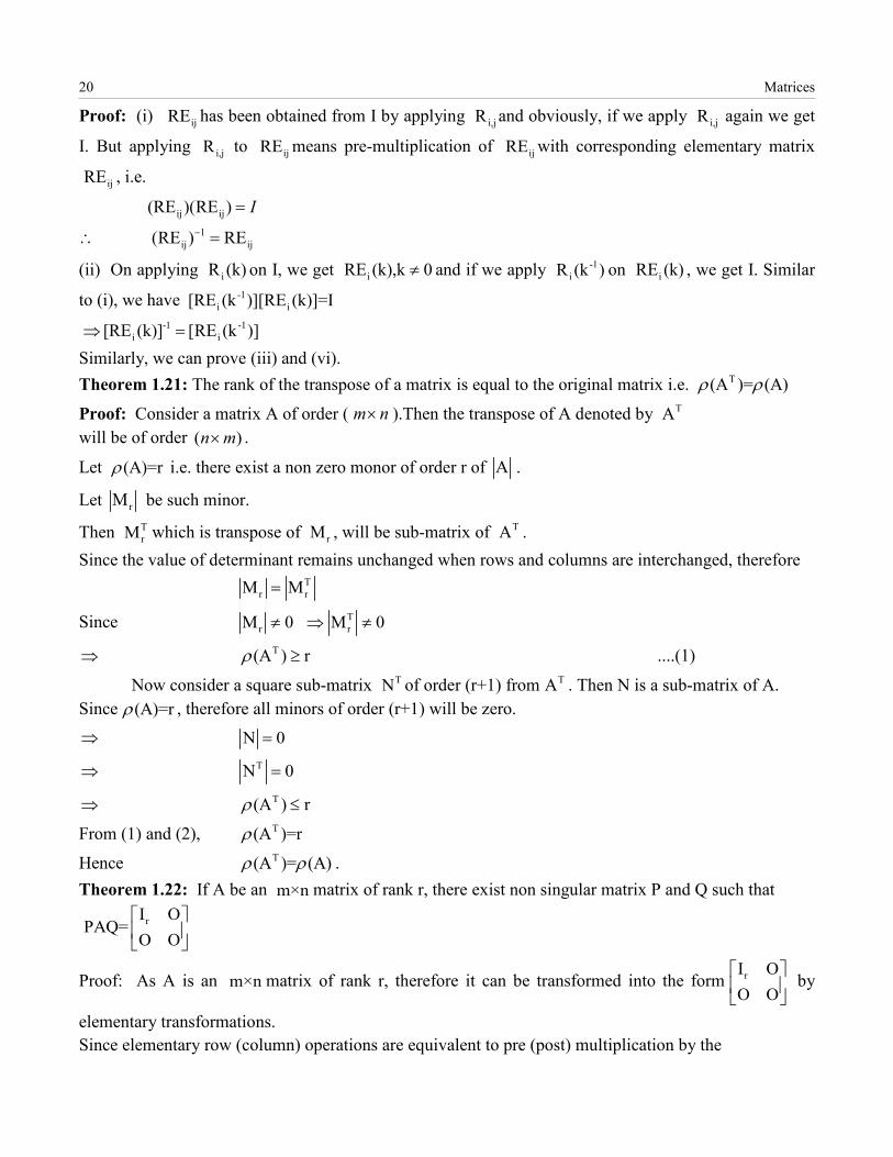
20 Matrices
Proof: (i) has been obtained from I by applying and obviously, if we apply again we get
I. But applying to means pre-multiplication of with corresponding elementary matrix
, i.e.
(ii) On applying on I, we get and if we apply on , we get I. Similar
to (i), we have
Similarly, we can prove (iii) and (vi). Theorem 1.21: The rank of the transpose of a matrix is equal to the original matrix i.e.
Proof: Consider a matrix A of order ( ).Then the transpose of A denoted by will be of order .
Let i.e. there exist a non zero monor of order r of .
Let be such minor.
Then which is transpose of , will be sub-matrix of . Since the value of determinant remains unchanged when rows and columns are interchanged, therefore
Since
....(1)
Now consider a square sub-matrix of order (r+1) from . Then N is a sub-matrix of A. Since , therefore all minors of order (r+1) will be zero.
From (1) and (2),
Hence . Theorem 1.22: If A be an matrix of rank r, there exist non singular matrix P and Q such that
Proof: As A is an matrix of rank r, therefore it can be transformed into the form by
elementary transformations. Since elementary row (column) operations are equivalent to pre (post) multiplication by the
ijRE i,jR i,jR
i,jR ijRE ijRE
ijRE
ij ij
1ij ij
(RE )(RE )
(RE ) RE
I−
=
∴ =
iR (k) iRE (k),k 0≠ -1iR (k ) iRE (k)
-1i i[RE (k )][RE (k)]=I
-1 -1i i[RE (k)] [RE (k )]⇒ =
T(A )= (A)ρ ρ
m n× TA( )n m×
(A)=rρ A
rMTrM rM TA
Tr rM M=
Tr rM 0 M 0≠ ⇒ ≠
⇒ T(A ) rρ ≥TN TA
(A)=rρ
⇒ N 0=
⇒ TN 0=
⇒ T(A ) rρ ≤T(A )=rρT(A )= (A)ρ ρm×n
rI OPAQ=
O O
m×n rI OO O
Algebra, Calculus & Solid Geometry 21
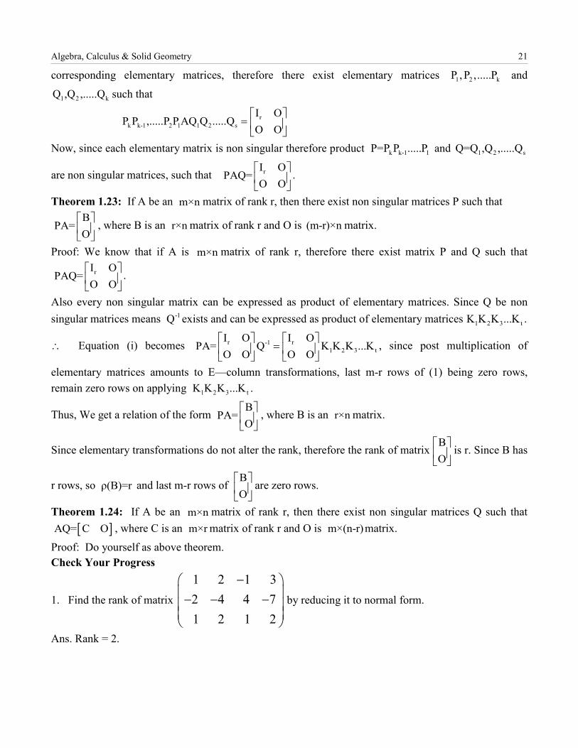
corresponding elementary matrices, therefore there exist elementary matrices and
such that
Now, since each elementary matrix is non singular therefore product and
are non singular matrices, such that .
Theorem 1.23: If A be an matrix of rank r, then there exist non singular matrices P such that
, where B is an matrix of rank r and O is matrix.
Proof: We know that if A is matrix of rank r, therefore there exist matrix P and Q such that
.
Also every non singular matrix can be expressed as product of elementary matrices. Since Q be non singular matrices means exists and can be expressed as product of elementary matrices .
Equation (i) becomes , since post multiplication of
elementary matrices amounts to E—column transformations, last m-r rows of (1) being zero rows, remain zero rows on applying .
Thus, We get a relation of the form , where B is an matrix.
Since elementary transformations do not alter the rank, therefore the rank of matrix is r. Since B has
r rows, so and last m-r rows of are zero rows.
Theorem 1.24: If A be an matrix of rank r, then there exist non singular matrices Q such that, where C is an matrix of rank r and O is matrix.
Proof: Do yourself as above theorem. Check Your Progress
1. Find the rank of matrix by reducing it to normal form.
Ans. Rank = 2.
1 2 kP ,P ,.....P
1 2 kQ ,Q ,.....Q
rk k-1 2 1 1 2 s
I OP P ,.....P P AQ Q .....Q
O O
=
k k-1 1P=P P .....P 1 2 sQ=Q ,Q ,.....Q
rI OPAQ=
O O
m×nB
PA=O
r×n (m-r)×n
m×n
rI OPAQ=
O O
-1Q 1 2 3 tK K K ...K
∴ r r-11 2 3 t
I O I OPA= Q K K K ...K
O O O O
=
1 2 3 tK K K ...K
BPA=
O
r×n
BO
ρ(B)=rBO
m×n[ ]AQ= C O m×r m×(n-r)
1 2 1 32 4 4 71 2 1 2
− − − −
22 Matrices
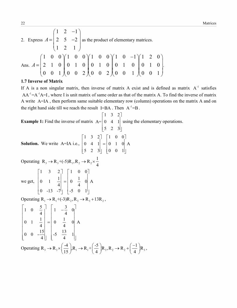
2. Express as the product of elementary matrices.
Ans. .
1.7 Inverse of Matrix If A is a non singular matrix, then inverse of matrix A exist and is defined as matrix satisfies
, where I is unit matrix of same order as that of the matrix A. To find the inverse of matrix A write , then perform same suitable elementary row (column) operations on the matrix A and on the right hand side till we reach the result . Then .
Example 1: Find the inverse of matrix using the elementary operations.
Solution. We write i.e.,
Operating
we get,
Operating ,
Operating ,
1 2 12 5 21 2 1
A−
= −
1 0 0 1 0 0 1 0 0 1 0 1 1 2 02 1 0 0 1 0 0 1 0 0 1 0 0 1 00 0 1 0 0 2 0 0 2 0 0 1 0 0 1
A−
=
-1A-1 -1AA =A A=I
A=IAI=BA -1A =B
1 3 2A= 0 4 1
5 2 3
A=IA1 3 2 1 0 00 4 1 0 1 0 A5 2 3 0 0 1
=
3 3 1 2 21R R +(-5)R ,R R4
→ → ×
1 3 2 1 0 01 10 1 0 0 A4 4
0 -13 -7 -5 0 1
=
1 1 2 3 3 2R R +(-3)R ,R R 13R→ → +
5 31 0 1 04 41 10 1 0 0 A4 415 130 0 - -5 14 4
− =
3 3 1 1 3 2 2 3-4 -5 1R R ,R R + R ,R R R15 4 4
− → × → → +
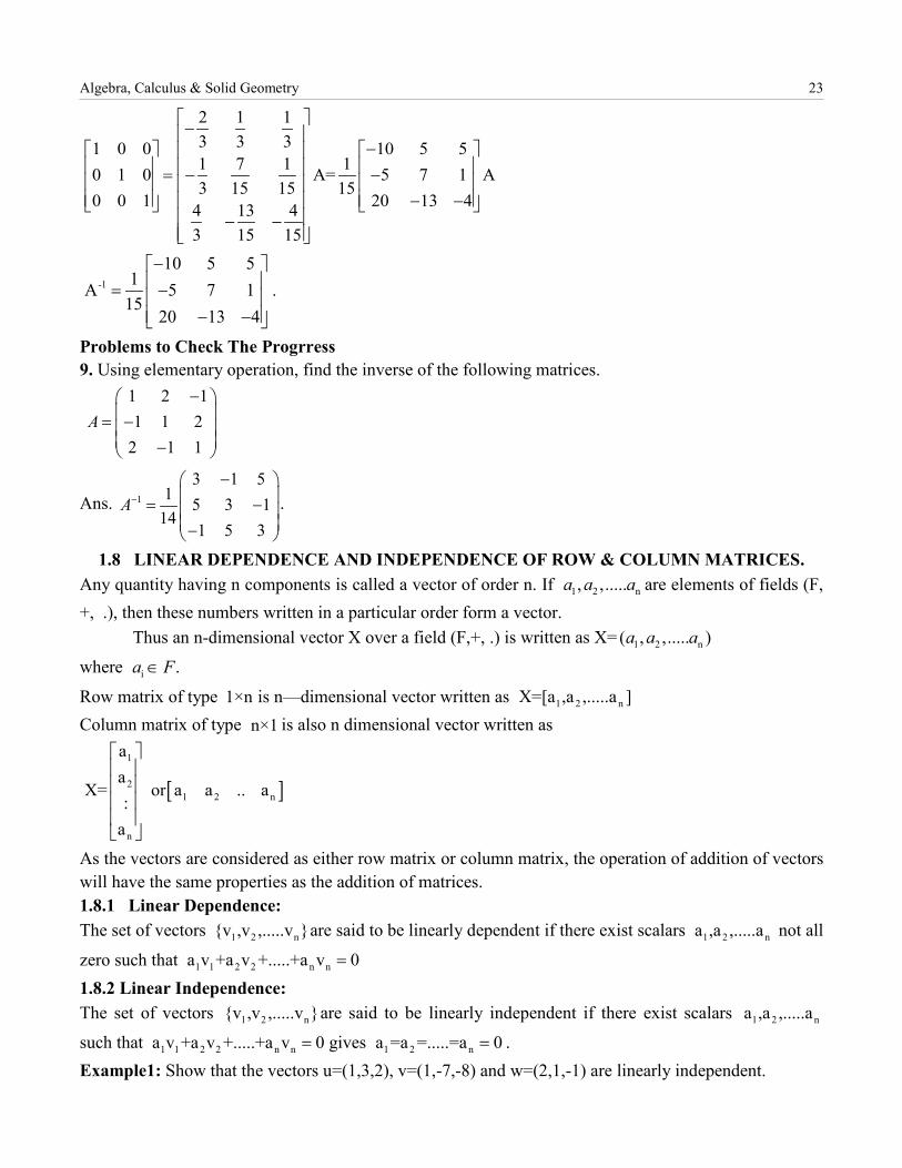
Algebra, Calculus & Solid Geometry 23
.
Problems to Check The Progrress 9. Using elementary operation, find the inverse of the following matrices.
1 2 11 1 2
2 1 1A
− = − −
Ans. 1
3 1 51 5 3 1
141 5 3
A−
− = − −
.
1.8 LINEAR DEPENDENCE AND INDEPENDENCE OF ROW & COLUMN MATRICES. Any quantity having n components is called a vector of order n. If are elements of fields (F, +, .), then these numbers written in a particular order form a vector. Thus an n-dimensional vector X over a field (F,+, .) is written as X=
where
Row matrix of type is n—dimensional vector written as Column matrix of type is also n dimensional vector written as
As the vectors are considered as either row matrix or column matrix, the operation of addition of vectors will have the same properties as the addition of matrices. 1.8.1 Linear Dependence: The set of vectors are said to be linearly dependent if there exist scalars not all
zero such that 1.8.2 Linear Independence: The set of vectors are said to be linearly independent if there exist scalars
such that gives . Example1: Show that the vectors u=(1,3,2), v=(1,-7,-8) and w=(2,1,-1) are linearly independent.
2 1 13 3 31 0 0 10 5 51 7 1 10 1 0 A= 5 7 1 A3 15 15 15
0 0 1 20 13 44 13 43 15 15
− −
= − − − −
− −
-1
10 5 51A 5 7 1
1520 13 4
− = − − −
1 2 n, ,.....a a a
1 2 n( , ,..... )a a a
i .a F∈
1×n 1 2 nX=[a ,a ,.....a ]n×1
[ ]1
21 2 n
n
aa
X= or a a .. a:
a
1 2 n{v ,v ,.....v } 1 2 na ,a ,.....a
1 1 2 2 n na v +a v +.....+a v 0=
1 2 n{v ,v ,.....v } 1 2 na ,a ,.....a
1 1 2 2 n na v +a v +.....+a v 0= 1 2 na =a =.....=a 0=
24 Matrices
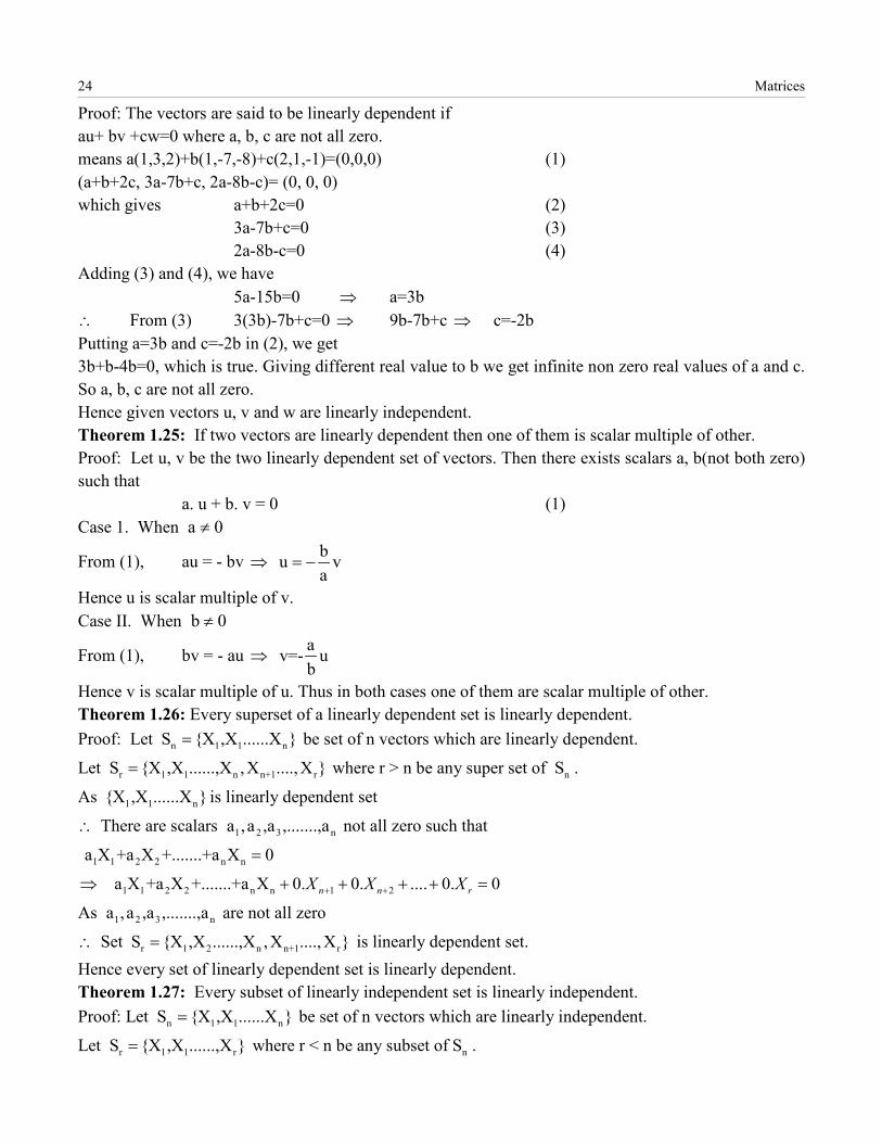
Proof: The vectors are said to be linearly dependent if au+ bv +cw=0 where a, b, c are not all zero. means a(1,3,2)+b(1,-7,-8)+c(2,1,-1)=(0,0,0) (1) (a+b+2c, 3a-7b+c, 2a-8b-c)= (0, 0, 0) which gives a+b+2c=0 (2) 3a-7b+c=0 (3) 2a-8b-c=0 (4) Adding (3) and (4), we have 5a-15b=0 a=3b
From (3) 3(3b)-7b+c=0 9b-7b+c c=-2b Putting a=3b and c=-2b in (2), we get 3b+b-4b=0, which is true. Giving different real value to b we get infinite non zero real values of a and c. So a, b, c are not all zero. Hence given vectors u, v and w are linearly independent. Theorem 1.25: If two vectors are linearly dependent then one of them is scalar multiple of other. Proof: Let u, v be the two linearly dependent set of vectors. Then there exists scalars a, b(not both zero) such that a. u + b. v = 0 (1) Case 1. When
From (1), au = - bv
Hence u is scalar multiple of v. Case II. When
From (1), bv = - au
Hence v is scalar multiple of u. Thus in both cases one of them are scalar multiple of other. Theorem 1.26: Every superset of a linearly dependent set is linearly dependent. Proof: Let be set of n vectors which are linearly dependent.
Let where r > n be any super set of .
As is linearly dependent set
There are scalars not all zero such that
As are not all zero
Set is linearly dependent set. Hence every set of linearly dependent set is linearly dependent. Theorem 1.27: Every subset of linearly independent set is linearly independent. Proof: Let be set of n vectors which are linearly independent.
Let where r < n be any subset of .
⇒∴ ⇒ ⇒
a 0≠
⇒bu va
= −
b 0≠
⇒av=- ub
n 1 1 nS {X ,X ......X }=
r 1 1 n n+1 rS {X ,X ......,X ,X ....,X }= nS
1 1 n{X ,X ......X }
∴ 1 2 3 na ,a ,a ,.......,a
1 1 2 2 n na X +a X +.......+a X 0=
1 1 2 2 n n 1 2 a X +a X +.......+a X 0. 0. .... 0. 0n n rX X X+ +⇒ + + + + =
1 2 3 na ,a ,a ,.......,a
∴ r 1 2 n n+1 rS {X ,X ......,X ,X ....,X }=
n 1 1 nS {X ,X ......X }=
r 1 1 rS {X ,X ......,X }= nS
Algebra, Calculus & Solid Geometry 25
As is linearly independent set thus
gives
where
Set is linearly independent set. Hence every subset of linearly independent set is linearly independent. Theorem 1.28: If vectors are linearly dependent, then at least one of them may be written as linear combination of the rest. Proof: Since the vectors , are linearly dependent, therefore there exist scalars
not all zero, such that
Or
Suppose .
or
Hence vector is a linear combination of the rest.
Theorem 1.30: If the set is linearly independent and the set is linearly
dependent, then Y is linear combination of the vectors . Proof: Consider the relation (1)
As set is linearly dependent
are not all zero We claim that . If a=0, then (1) becomes
As set is linearly independent
Then from (1), the set is linearly independent which a contradiction to the given condition is. Thus a = 0 is not possible. Hence From (1), we have
or , which proves the result.
Theorem 1.31: The kn-vectors are linearly dependent iff the rank of the matrix
with the given vectors as columns is less than k.
1 1 n{X ,X ......X }
1 1 2 2 n na X +a X +.......+a X 0=
1 2 3 na = a = a ,.......= a 0=
1 1 2 2 r ra X +a X +.......+a X 0= 1 2 3 ra = a = a ,.......= a 0=
∴ r 1 1 rS {X ,X ......,X }=
1 1 nX ,X ......X
1 1 nX ,X ......X
1 2 3 na ,a ,a ,.......,a
1 1 2 2 n na X +a X +.......+a X 0=
1 1 2 2 i i i+1 i+1 n na X +a X +....+a X +a X ...+a X 0=
ia 0≠
i i 1 1 2 2 i-1 i-1 i+1 i+1 n n-a X =a X +a X +....a X +a X ...+a X
1 2 i-1 i+1 ni 1 2 i-1 i+1 n
i i i i i
a a a a aX = X + X +....+ X + X ...+ X-a -a -a -a -a
iX
1 1 n{X ,X ......X } 1 1 n{X ,X ......X ,Y}
1 1 nX ,X ......X
1 1 2 2 n na X +a X +.......+a X aY 0+ =
1 1 n{X ,X ......X ,Y}
∴ 1 2 3 na ,a ,a ,.......,a ,aa 0≠
1 1 2 2 n na X +a X +.......+a X 0=
1 1 n{X ,X ......X }
∴ 1 2 3 na = a = a ,.......= a 0=
1 1 n{X ,X ......X ,Y}a 0≠
1 1 2 2 n n-aY=a X +a X +.......+a X
1 2 n1 2 n
a a aY= X + X +.......+ X-a -a -a
1 2 kA ,A ,......,A
1 2 kA=[A ,A ,.....,A ]
26 Matrices
Proof: Let
where are scalars
Which can be written in matrix form as
Let the vectors be linearly dependent.
So, from the relation (i), scalars are not all zero and thus the homogeneous system of equations given by (ii) has non-trivial solution. Hence .Converse of this theorem is also true.
Theorem 1.32: A square matrix A is singular iff its columns (rows) are linearly dependent.
Proof: Let n be the order of the square matrix A and be its columns.
Proceed in same way as above theorem to prove
Since , thus and hence A is singular matrix.
Conversely, the column vectors of A are linearly dependent.
Theorem 1.33: The kn-vectors are linearly independent if the rank of the matrix
is equal to k.
Proof: Proceed in the same way as above theorem to obtain . Now suppose .
Then and homogeneous system of equations given by (ii) has trivial solution only.
Thus, the vectors are linearly independent.
1 1 2 2 kx A A ,...... A 0kx x+ + =
1 2 k, ,......,x x x
11 12 1
21 22 21 1 k
1 2
x x ..... x O: : :
k
k
n n nk
a a aa a a
a a a
⇒ + + + =
11 1 12 2 1
21 1 22 2 2
n1 1 2 2
a ...... 0a ...... 0..............................................a ...... 0
k k
k k
n nk k
x a x a xx a x a x
x a x a x
⇒ + + + =+ + + =
+ + + =
111 12 1k
221 22 2k
n1 n2 nk
a a ... a 0a a ... a 0
:: : : : ::: : : : :
a a ... a 0k
xx
x
=
AX=O⇒
1 2 kA ,A ,......,A
1 2 k, ,......,x x xρ(A)<k
1 2 nA ,A ,......,A
1 2 n A=[A ,A ,......,A ]∴
ρ(A)<n
ρ(A)<n A 0=
1 2 kA ,A ,......,A
1 2 kA=[A ,A ,.....,A ]
AX=O
A 0≠
1 2 x ..... 0kx x∴ = = = =
1 2 kA ,A ,.....,A
Algebra, Calculus & Solid Geometry 27
Theorem 1.34: The number of linearly independent solution of the equation AX=O is (n-r) where r is the rank of matrix A. Proof: Given that rank of A is r which means A has r linearly independent columns. Let first r columns are linearly independent.
Now, , where are column vectors of A.
...(i)
As the set is linearly independent, thus each vector can be written as linear combination of .
Now,
.................................................
where k=n-r ...(ii) From (i) and (ii), we get
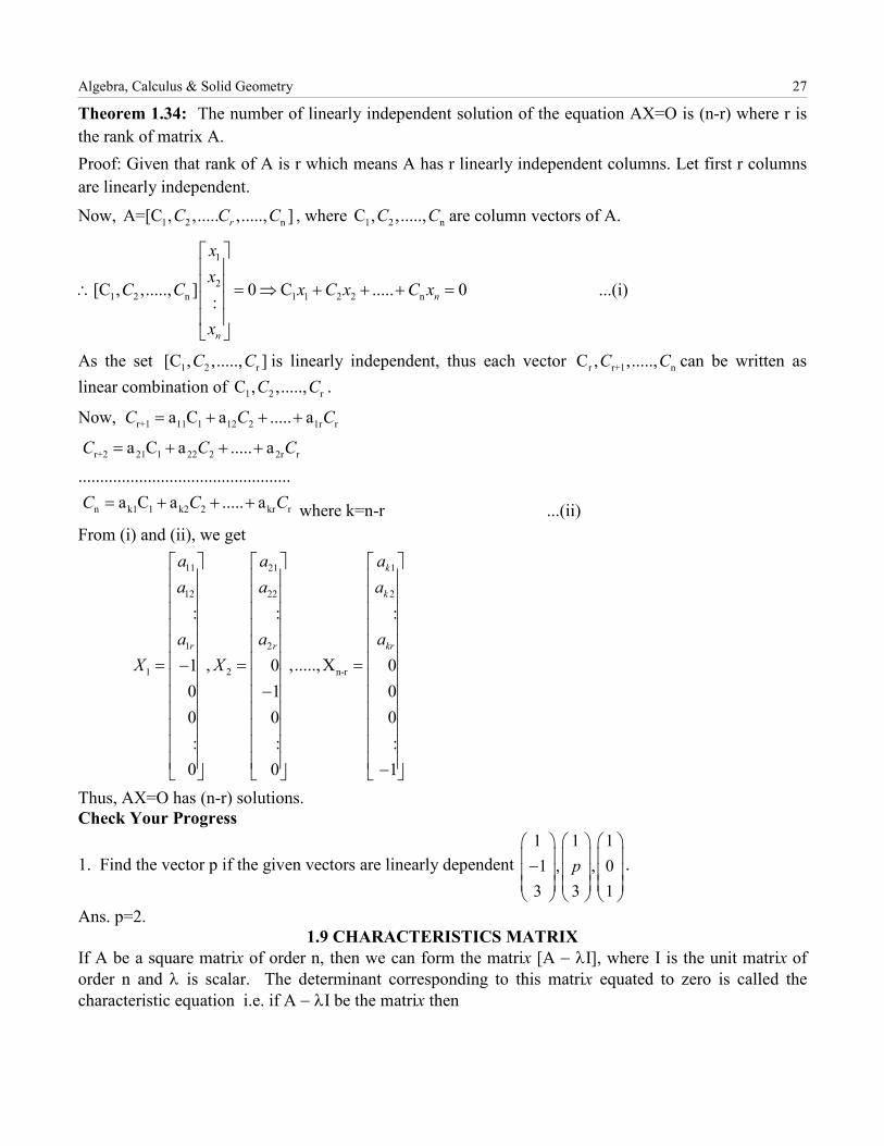
Thus, AX=O has (n-r) solutions. Check Your Progress
1. Find the vector p if the given vectors are linearly dependent 1 1 11 , , 0
3 3 1p
−
.
Ans. p=2. 1.9 CHARACTERISTICS MATRIX
If A be a square matrix of order n, then we can form the matrix [A − λI], where I is the unit matrix of order n and λ is scalar. The determinant corresponding to this matrix equated to zero is called the characteristic equation i.e. if A − λI be the matrix then
1 2 nA=[C , ,..... ,....., ]rC C C 1 2 nC , ,.....,C C
1
21 2 n 1 1 2 2 n[C , ,....., ] 0 C ..... 0
: n
n
xx
C C x C x C x
x
∴ = ⇒ + + + =
1 2 r[C , ,....., ]C C r r+1 nC , ,.....,C C
1 2 rC , ,.....,C C
r+1 11 1 12 2 1r ra C a ..... aC C C= + + +
r+2 21 1 22 2 2r ra C a ..... aC C C= + + +
n k1 1 k2 2 kr ra C a ..... aC C C= + + +
11 21 1
12 22 2
1 2
1 2 n-r
: : :
, ,.....,X1 0 00 1 00 0 0: : :
0 0 1
k
k
r r kr
a a aa a a
a a aX X
= = =−
− −
28 Matrices
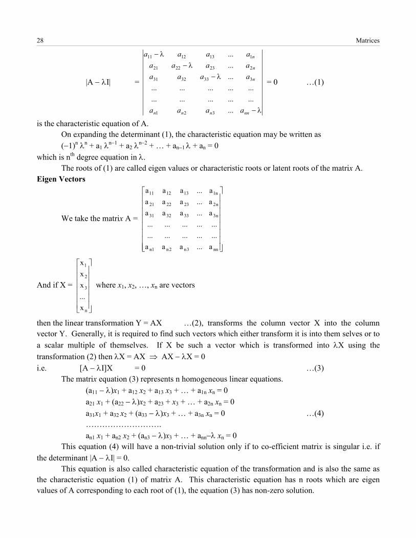
|A − λI| = = 0 …(1)
is the characteristic equation of A. On expanding the determinant (1), the characteristic equation may be written as (−1)n λn + a1 λn−1 + a2 λn−2 + … + an−1
λ + an = 0 which is nth degree equation in λ. The roots of (1) are called eigen values or characteristic roots or latent roots of the matrix A. Eigen Vectors
We take the matrix A =
And if X = where x1, x2, …, xn are vectors
then the linear transformation Y = AX …(2), transforms the column vector X into the column vector Y. Generally, it is required to find such vectors which either transform it is into them selves or to a scalar multiple of themselves. If X be such a vector which is transformed into λX using the transformation (2) then λX = AX ⇒ AX − λX = 0 i.e. [A − λI]X = 0 …(3) The matrix equation (3) represents n homogeneous linear equations. (a11 − λ)x1 + a12 x2 + a13 x3 + … + a1n xn = 0 a21 x1 + (a22 − λ)x2 + a23 + x3 + … + a2n xn = 0 a31x1 + a32 x2 + (a33 − λ)x3 + … + a3n xn = 0 …(4) ………………………. an1 x1 + an2 x2 + (an3 − λ)x3 + … + ann−λ xn = 0 This equation (4) will have a non-trivial solution only if to co-efficient matrix is singular i.e. if the determinant |A − λI| = 0. This equation is also called characteristic equation of the transformation and is also the same as the characteristic equation (1) of matrix A. This characteristic equation has n roots which are eigen values of A corresponding to each root of (1), the equation (3) has non-zero solution.
λ−
λ−λ−
λ−
nnnnn
n
n
n
aaaa
aaaaaaaaaaaa
.................................
...
...
...
321
3333231
2232221
1131211
nn3n2n1n
n3333231
n2232221
n1131211
a...aaa..............................
a...aaaa...aaaa...aaa
n
3
2
1
x...xxx
Algebra, Calculus & Solid Geometry 29
X =
which is known as an eigen vector or latent vector. So, if X is a solution of (3) then KX is also a solution, where K is an arbitrary constant. So, we see that the eigen vector corresponding to an eigen value is not unique.
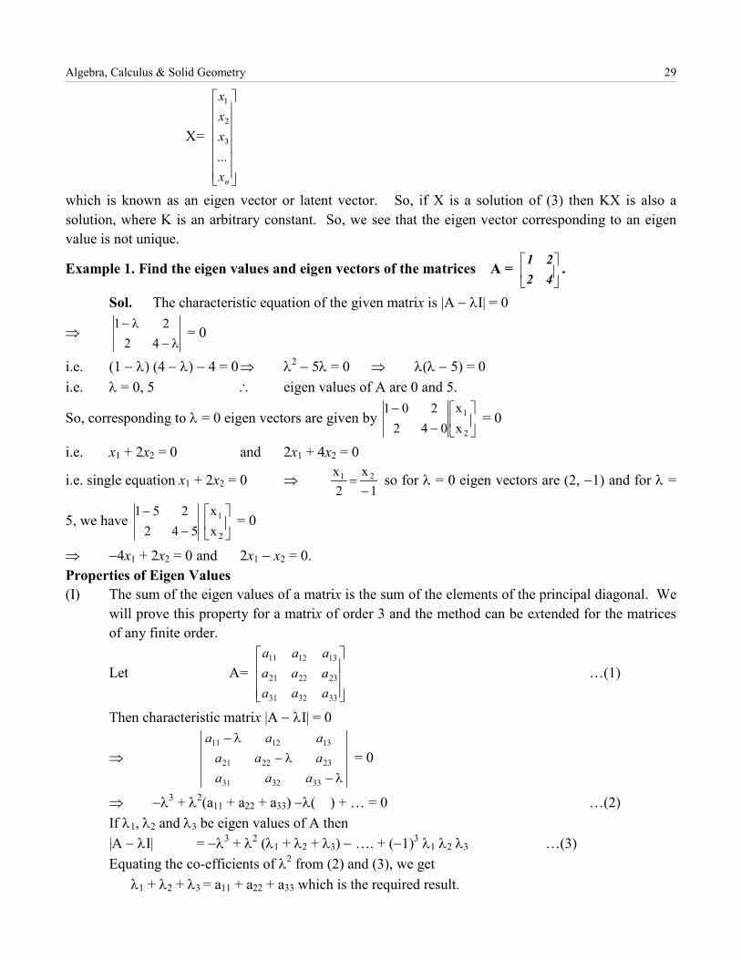
Example 1. Find the eigen values and eigen vectors of the matrices A = .
Sol. The characteristic equation of the given matrix is |A − λI| = 0
⇒ = 0
i.e. (1 − λ) (4 − λ) − 4 = 0 ⇒ λ2 − 5λ = 0 ⇒ λ(λ − 5) = 0 i.e. λ = 0, 5 ∴ eigen values of A are 0 and 5.
So, corresponding to λ = 0 eigen vectors are given by = 0
i.e. x1 + 2x2 = 0 and 2x1 + 4x2 = 0
i.e. single equation x1 + 2x2 = 0 ⇒ so for λ = 0 eigen vectors are (2, −1) and for λ =
5, we have = 0
⇒ −4x1 + 2x2 = 0 and 2x1 − x2 = 0. Properties of Eigen Values (I) The sum of the eigen values of a matrix is the sum of the elements of the principal diagonal. We
will prove this property for a matrix of order 3 and the method can be extended for the matrices of any finite order.
Let A = …(1)
Then characteristic matrix |A − λI| = 0
⇒ = 0
⇒ −λ3 + λ2(a11 + a22 + a33) −λ( ) + … = 0 …(2) If λ1, λ2 and λ3 be eigen values of A then
|A − λI| = −λ3 + λ2 (λ1 + λ2 + λ3) − …. + (−1)3 λ1 λ2 λ3 …(3) Equating the co-efficients of λ2 from (2) and (3), we get
λ1 + λ2 + λ3 = a11 + a22 + a33 which is the required result.
nx
xxx
...3
2
1
4221
λ−λ−
4221
−
−
2
1
xx
042201
1x
2x 21
−=
−
−
2
1
xx
542251
333231
232221
131211
aaaaaaaaa
λ−λ−
λ−
333231
232221
131211
aaaaaaaaa
30 Matrices
(II) The product of the eigen values of a matrix A is equal to its determinants. If take λ = 0 in (3) then, we get |A − 0| = −λ1λ2λ3 which is the required result.
(III) If λ is an eigen values of a matrix A, then is the eigen value of inverse matrix A−1. If X be the
eigen vector corresponding to the eigen value λ then AX = λX …(4) Pre-multiplying (4) by A−1, we get A−1AX = A−1λX
i.e. IX = λA−1X ⇒ X = λ(A−1X) ⇒ A−1X = X
This is of the same form as that in (1) from which we get that is an eigen value of the inverse
matrix A−1.
(IV) If λ is an eigen value of a matrix A, then is an eigen value of A−1. As A is an orthogonal
matrix so A−1 will be same as the transpose of matrix A i.e. A′ = A−1. So, is an eigen value of
A′. But the matrix A and A′ have the same eigen values.
[since we know that |A − λI| = |A′ − λI| ]. Hence is also an eigen value of A.
(V) If λ1, λ2,…, λn are eigen values of a matrix A then Am has the eigen values λ1m, λ2
m, …, λnm
where m is a positive ineteger. If Ai be the eigen value of A and Xi be the corresponding eigen vector, then AXi = λi Xi …(1) Consider A2 Xi = A(AXi) = A(λi Xi) = λi (AXi) = λi(λi Xi) = λi
2 Xi similarly, we proceed and find A3 Xi = λi
3 Xi and so on such that in general we get AmXi = λi
m Xi …(2) which has the same form as (1). Hence λi
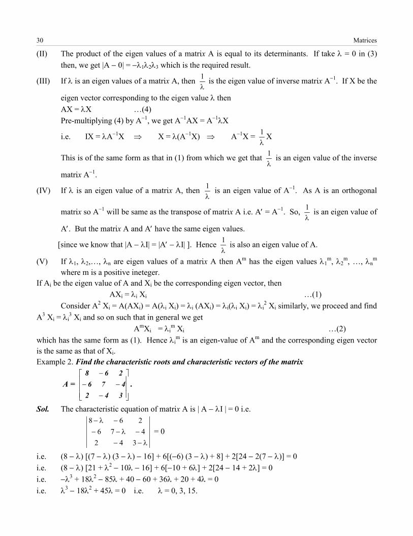
m is an eigen-value of Am and the corresponding eigen vector is the same as that of Xi. Example 2. Find the characteristic roots and characteristic vectors of the matrix
A = .
Sol. The characteristic equation of matrix A is | A − λI | = 0 i.e.
= 0
i.e. (8 − λ) [(7 − λ) (3 − λ) − 16] + 6[(−6) (3 − λ) + 8] + 2[24 − 2(7 − λ)] = 0 i.e. (8 − λ) [21 + λ2 − 10λ − 16] + 6[−10 + 6λ] + 2[24 − 14 + 2λ] = 0 i.e. −λ3 + 18λ2 − 85λ + 40 − 60 + 36λ + 20 + 4λ = 0 i.e. λ3 − 18λ2 + 45λ = 0 i.e. λ = 0, 3, 15.
λ1
λ1
λ1
λ1
λ1
λ1
−−−
−
342476
268
λ−−−λ−−
−λ−
342476
268
Algebra, Calculus & Solid Geometry 31
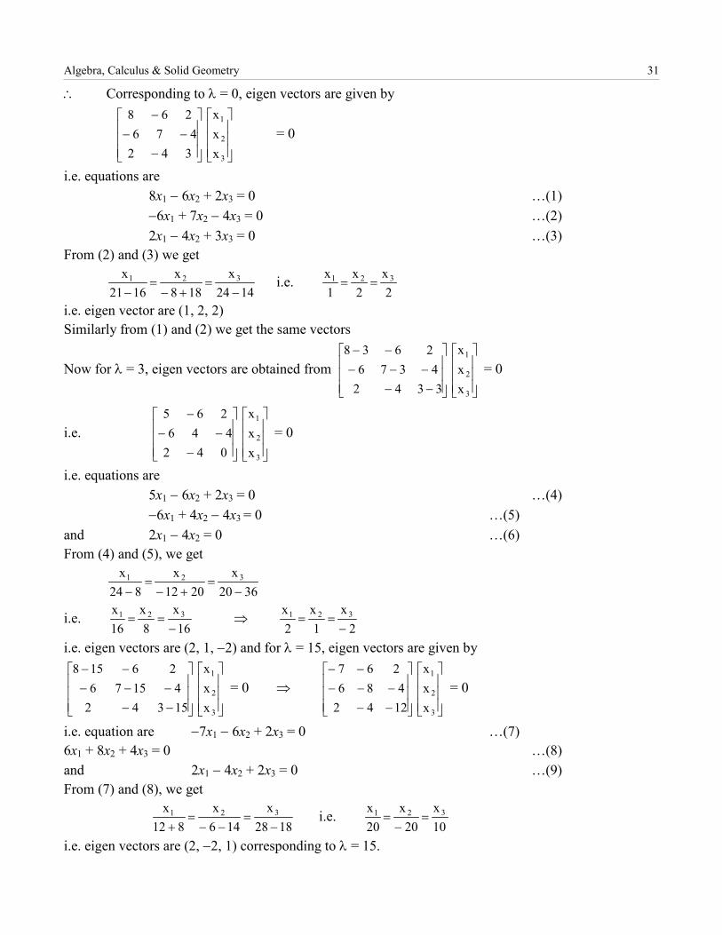
∴ Corresponding to λ = 0, eigen vectors are given by
= 0
i.e. equations are 8x1 − 6x2 + 2x3 = 0 …(1) −6x1 + 7x2 − 4x3 = 0 …(2) 2x1 − 4x2 + 3x3 = 0 …(3) From (2) and (3) we get
i.e.
i.e. eigen vector are (1, 2, 2) Similarly from (1) and (2) we get the same vectors
Now for λ = 3, eigen vectors are obtained from = 0
i.e. = 0
i.e. equations are 5x1 − 6x2 + 2x3 = 0 …(4) −6x1 + 4x2 − 4x3 = 0 …(5) and 2x1 − 4x2 = 0 …(6) From (4) and (5), we get
i.e. ⇒
i.e. eigen vectors are (2, 1, −2) and for λ = 15, eigen vectors are given by
= 0 ⇒ = 0
i.e. equation are −7x1 − 6x2 + 2x3 = 0 …(7) 6x1 + 8x2 + 4x3 = 0 …(8) and 2x1 − 4x2 + 2x3 = 0 …(9) From (7) and (8), we get
i.e.
i.e. eigen vectors are (2, −2, 1) corresponding to λ = 15.
−−−
−
3
2
1
xxx
342476
268
1424x
188x
1621x 321
−=
+−=
− 2x
2x
1x 321 ==
−−−−−
−−
3
2
1
xxx
33424376
2638
−−−
−
3
2
1
xxx
042446
265
3620x
2012x
824x 321
−=
+−=
−
16x
8x
16x 321
−==
2x
1x
2x 321
−==
−−−−−
−−
3
2
1
xxx
1534241576
26158
−−−−−
−−
3
2
1
xxx
1242486
267
1828x
146x
812x 321
−=
−−=
+ 10x
20x
20x 321 =
−=
32 Matrices
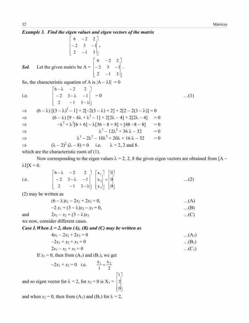
Example 3. Find the eigen values and eigen vectors of the matrix
.
Sol. Let the given matrix be A = .
So, the characteristic equation of A is |A − λI| = 0
i.e. = 0 …(1)
⇒ (6 − λ) [(3 − λ)2 − 1] + 2[−2(3 − λ) + 2] + 2[2 − 2(3 − λ)] = 0 ⇒ (6 − λ) [9 − 6λ + λ2 − 1] + 2[2λ − 4] + 2[2λ − 4] = 0 ⇒ −λ3 + λ2[6 + 6] − λ[36 − 8 + 8] + [48 −8 − 8] = 0 ⇒ λ3 − 12λ2 + 36 λ − 32 = 0 ⇒ λ3 − 2λ2 − 10λ2 + 20λ + 16 λ − 32 = 0 ⇒ (λ − 2)2 (λ − 8) = 0 i.e. λ = 2, 2 and 8. which are the characteristic roots of (1). Now corresponding to the eigen values λ = 2, 2, 8 the given eigen vectors are obtained from [A − λI]X = 0.
i.e. …(2)
(2) may be written as (6 − λ)x1 − 2x2 + 2x3 = 0, …(A) −2 x1 + (3 − λ)x2 − x3 = 0, …(B) and 2x1 − x2 + (3 − λ)x3 …(C) we now, consider different cases. Case I. When λ = 2, then (A), (B) and (C) may be written as 4x1 − 2x2 + 2x3 = 0 …(A1) −2x1 + x2 + x3 = 0 …(B1) 2x1 − x2 + x3 = 0 …(C1) If x3 = 0, then from (A1) and (B1), we get
−2x1 + x2 = 0 i.e.
and so eigen vector for λ = 2, for x3 = 0 is X1 =
and when x2 = 0, then from (A1) and (B1) for λ = 2,
−−−
−
312132
226
−−−
−
312132
226
λ−−−λ−−
−λ−
312132
226
λ−−−λ−−
−λ−
312132
226
=
000
xxx
3
2
1
2x
1x 21 =
021
Algebra, Calculus & Solid Geometry 33
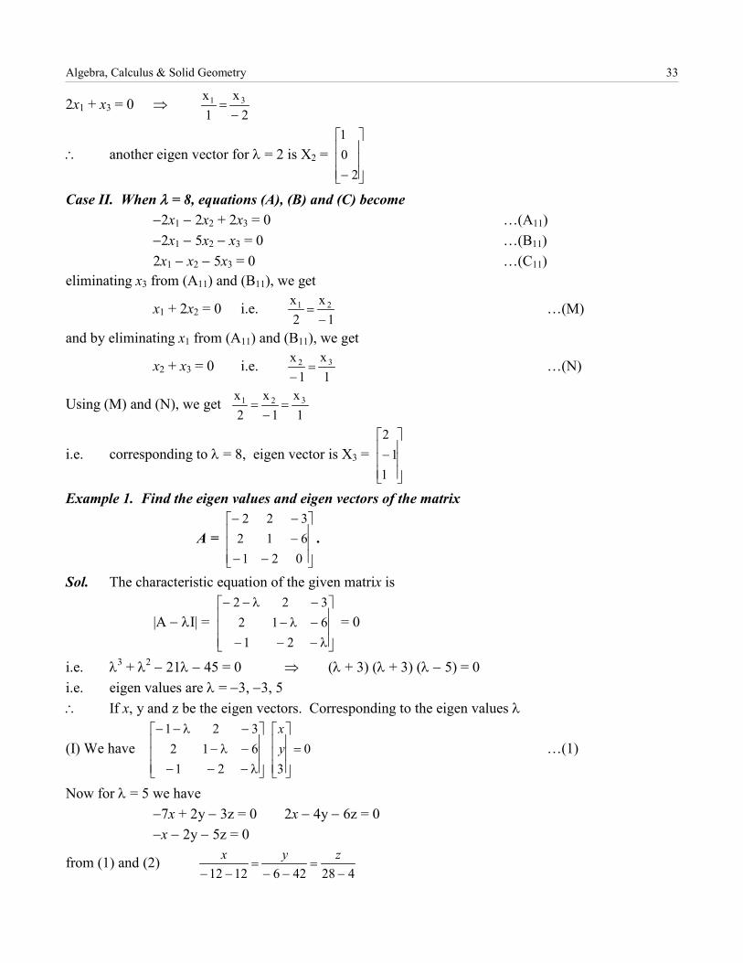
2x1 + x3 = 0 ⇒
∴ another eigen vector for λ = 2 is X2 =
Case II. When λ = 8, equations (A), (B) and (C) become −2x1 − 2x2 + 2x3 = 0 …(A11) −2x1 − 5x2 − x3 = 0 …(B11) 2x1 − x2 − 5x3 = 0 …(C11) eliminating x3 from (A11) and (B11), we get
x1 + 2x2 = 0 i.e. …(M)
and by eliminating x1 from (A11) and (B11), we get
x2 + x3 = 0 i.e. …(N)
Using (M) and (N), we get
i.e. corresponding to λ = 8, eigen vector is X3 =
Example 1. Find the eigen values and eigen vectors of the matrix
A = .
Sol. The characteristic equation of the given matrix is
|A − λI| = = 0
i.e. λ3 + λ2 − 21λ − 45 = 0 ⇒ (λ + 3) (λ + 3) (λ − 5) = 0 i.e. eigen values are λ = −3, −3, 5 ∴ If x, y and z be the eigen vectors. Corresponding to the eigen values λ
(I) We have …(1)
Now for λ = 5 we have −7x + 2y − 3z = 0 2x − 4y − 6z = 0 −x − 2y − 5z = 0
from (1) and (2)
2x
1x 31
−=
− 201
1x
2x 21
−=
1x
1x 32 =−
1x
1x
2x 321 =
−=
−1
12
−−−−−
021612322
λ−−−−λ−−λ−−
21612322
0321
612321
=
λ−−−−λ−−λ−−
yx
4284261212 −=
−−=
−−zyx
34 Matrices
Hence eigen vector is [1, 2, −1]
(II) If λ = −3, then from (1), we get = 0 which gives only one independent
x + 2y − 3z = 0 …(3)
if we take y = 0, we get x − 3z = 0 ⇒
∴ for λ = −3, eigen vector is (3, 0, 1) when y = 0.
at when z = 0, (3) gives x + 2y = 0 ⇒
i.e. eigen vector in this case is (2, −1, 0) ∴ the eigen vectors obtained are (1, 2, −1), (3, 0, 1) and (2, −1, 0) which are the required result.
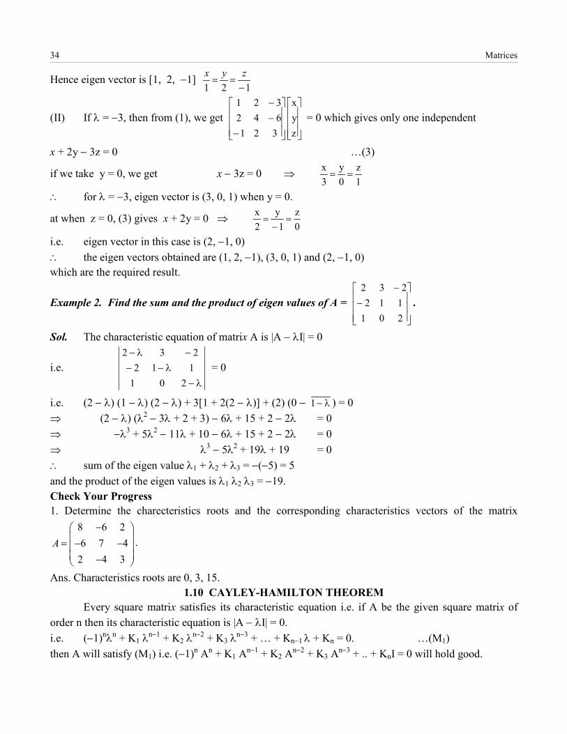
Example 2. Find the sum and the product of eigen values of A = .
Sol. The characteristic equation of matrix A is |A − λI| = 0
i.e. = 0
i.e. (2 − λ) (1 − λ) (2 − λ) + 3[1 + 2(2 − λ)] + (2) (0 − ) = 0 ⇒ (2 − λ) (λ2 − 3λ + 2 + 3) − 6λ + 15 + 2 − 2λ = 0 ⇒ −λ3 + 5λ2 − 11λ + 10 − 6λ + 15 + 2 − 2λ = 0 ⇒ λ3 − 5λ2 + 19λ + 19 = 0 ∴ sum of the eigen value λ1 + λ2 + λ3 = −(−5) = 5 and the product of the eigen values is λ1 λ2 λ3 = −19. Check Your Progress 1. Determine the charecteristics roots and the corresponding characteristics vectors of the matrix
8 6 26 7 4
2 4 3A
− = − − −
.
Ans. Characteristics roots are 0, 3, 15. 1.10 CAYLEY-HAMILTON THEOREM
Every square matrix satisfies its characteristic equation i.e. if A be the given square matrix of order n then its characteristic equation is |A − λI| = 0. i.e. (−1)nλn + K1 λn−1 + K2 λn−2 + K3 λn−3 + … + Kn−1
λ + Kn = 0. …(M1) then A will satisfy (M1) i.e. (−1)n An + K1 An−1 + K2 An−2 + K3 An−3 + .. + KnI = 0 will hold good.
121 −==
zyx
−−−
zyx
321642321
1z
0y
3x
==
0z
1y
2x
=−
=
−
−
201112232
λ−λ−−
−λ−
201112232
λ−1
Algebra, Calculus & Solid Geometry 35
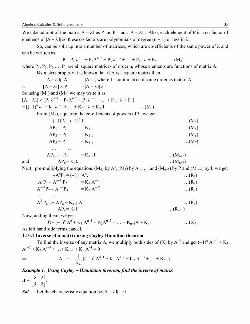
We take adjoint of the matrix A − λI as P i.e. P = adj. |A − λI|. Also, each element of P is a co-factor of elements of |A − λI| so these co-factors are polynomials of degree (n − 1) or less in λ. So, can be split up into a number of matrices, which are co-efficients of the same power of λ and can be written as P = P1 λn−1 + P2 λn−2 + P3 λn−3 + … + Pn−1λ + Pn …(M2) where P1, P2, P3,…, Pn are all square matrices of order n, whose elements are functions of matrix A. By matrix property it is known that if A is a square matrix then A × adj. A = |A|×I, where I is unit matrix of same order as that of A. ∴ [A − λI] × P = |A − λI| × I So using (M1) and (M2) we may write it as [A − λI] × [P1 λn−1 + P2 λn−2 + P3 λn−3 + … + Pn−1 λ + Pn] = [(−1)n λn + K1 λn−1 + … + Kn−1 λ + Kn]I …(M3) From (M3), equating the co-efficients of powers of λ, we get (−1)P1 = (−1)n I, …(M4) AP1 − P2 = K1I, …(M5) AP2 − P3 = K2I, …(M6) AP3 − P4 = K3I, …(M7) … … APn−1 − Pn = Kn−1I, …(Mn+3) and APn = KnI. …(Mn+4) Next, pre-multiplying the equations (M4) by An, (M5) by An−1, .. and (Mn+3) by P and (Mn+4) by I, we get −AnP1 = (−1)n An, …(R1) AnP1 − An−1 P2 = K1 An−1 …(R2) An−1P2 − An−2P3 = K2 An−2 …(R3) … … … A2 Pn−1
− APn = Kn−1 A …(Rn) APn = KnI …(Rn+1) Now, adding them, we get O = (−1)n An + K1 An−1 + K2An−2 + … + Kn−1A + KnI …(X) As left hand side terms cancel. 1.10.1 Inverse of a matrix using Cayley Hamilton theorem To find the inverse of any matrix A, we multiply both sides of (X) by A−1 and get (−1)n An−1 + K1 An−2 + K2 An−3 + …+ Kn−1 + Kn A−1 = 0
⇒ A−1 = − [(−1)n An−1 + K1 An−2 + K2 An−3 + … + Kn−1]
Example 1. Using Cayley − Hamilaton theorem, find the inverse of matrix
A = .
Sol. Let the characteristic equation be |A − λI| = 0
nK1
2335
36 Matrices
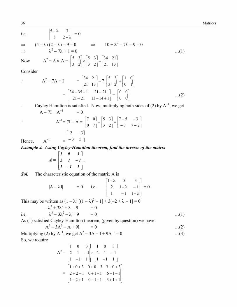
i.e. = 0
⇒ (5 − λ) (2 − λ) − 9 = 0 ⇒ 10 + λ2 − 7λ − 9 = 0 ⇒ λ2 − 7λ + 1 = 0 …(1)
Now A2 = A × A =
Consider
∴ A2 − 7A + I = 7
= = …(2)
∴ Cayley Hamilton is satisfied. Now, multiplying both sides of (2) by A−1, we get A − 7I + A−1 = 0
∴ A−1 = 7I − A =
Hence, A−1 = Example 2. Using Cayley-Hamilton theorem, find the inverse of the matrix
A = .
Sol. The characteristic equation of the matrix A is
|A − λI| = 0 i.e. = 0
This may be written as (1 − λ) [(1 − λ)2 − 1] + 3(−2 + λ − 1] = 0 −λ3 + 3λ2 + λ − 9 = 0 i.e. λ3 − 3λ2 − λ + 9 = 0 …(1) As (1) satisfied Cayley-Hamilton theorem, (given by question) we have A3 − 3A2 − A + 9I = 0 …(2) Multiplying (2) by A−1, we get A2 − 3A − I + 9A−1 = 0 …(3) So, we require
A2 =
=
λ−λ−
2335
=
×
13212134
2335
2335
−
13212134
+
1001
2335
+−−
−+−114132121
212113534
0000
−−−−
=
−
273
3572335
7007
−
−5332
−−111112
301
λ−−−λ−
λ−
111112
301
−−×
−−
111112
301
111112
301
++−−+−−−++−+++−+++
113110121116110122303300301
Algebra, Calculus & Solid Geometry 37
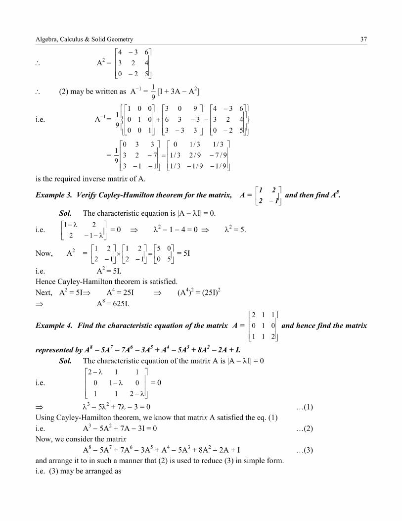
∴ A2 =
∴ (2) may be written as A−1 = [I + 3A − A2]
i.e. A−1 =
=
is the required inverse matrix of A.
Example 3. Verify Cayley-Hamilton theorem for the matrix, A = and then find A8.
Sol. The characteristic equation is |A − λI| = 0.
i.e. = 0 ⇒ λ2 − 1 − 4 = 0 ⇒ λ2 = 5.
Now, A2 = = 5I
i.e. A2 = 5I. Hence Cayley-Hamilton theorem is satisfied. Next, A2 = 5I ⇒ A4 = 25I ⇒ (A4)2 = (25I)2 ⇒ A8 = 625I.
Example 4. Find the characteristic equation of the matrix A = and hence find the matrix
represented by A8 − 5A7 − 7A6 − 3A5 + A4 − 5A3 + 8A2 − 2A + I. Sol. The characteristic equation of the matrix A is |A − λI| = 0
i.e. = 0
⇒ λ3 − 5λ2 + 7λ − 3 = 0 …(1) Using Cayley-Hamilton theorem, we know that matrix A satisfied the eq. (1) i.e. A3 − 5A2 + 7A − 3I = 0 …(2) Now, we consider the matrix A8 − 5A7 + 7A6 − 3A5 + A4 − 5A3 + 8A2 − 2A + I …(3) and arrange it to in such a manner that (2) is used to reduce (3) in simple form. i.e. (3) may be arranged as
−
−
520423634
91
−
−−
−−+
520423634
333336
903
100010001
91
−−−=
−−−
9/19/13/19/79/23/1
3/13/10
113723
330
91
− 1221
λ−−
λ−1221
=
−
×
− 50
0512
2112
21
211010112
λ−λ−
λ−
211010112
38 Matrices
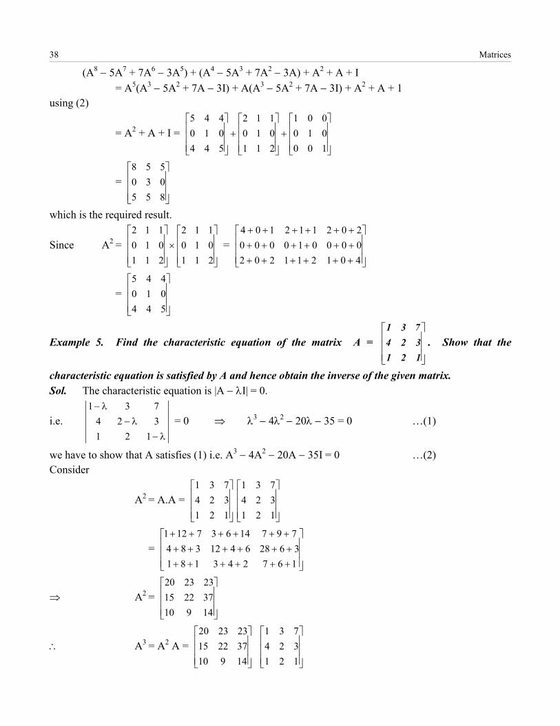
(A8 − 5A7 + 7A6 − 3A5) + (A4 − 5A3 + 7A2 − 3A) + A2 + A + I = A5(A3 − 5A2 + 7A − 3I) + A(A3 − 5A2 + 7A − 3I) + A2 + A + 1 using (2)
= A2 + A + I =
=
which is the required result.
Since A2 = =
=
Example 5. Find the characteristic equation of the matrix A = . Show that the
characteristic equation is satisfied by A and hence obtain the inverse of the given matrix. Sol. The characteristic equation is |A − λI| = 0.
i.e. = 0 ⇒ λ3 − 4λ2 − 20λ − 35 = 0 …(1)
we have to show that A satisfies (1) i.e. A3 − 4A2 − 20A − 35I = 0 …(2) Consider
A2 = A.A =
=
⇒ A2 =
∴ A3 = A2 A =
+
+
100010001
211010112
544010445
855030558
×
211010112
211010112
++++++++++++++++++
401211202000010000202112104
544010445
121324731
λ−λ−
λ−
121324731
121324731
121324731
++++++++++++++++++
16724318136286412384
79714637121
14910372215232320
14910372215232320
121324731
Algebra, Calculus & Solid Geometry 39
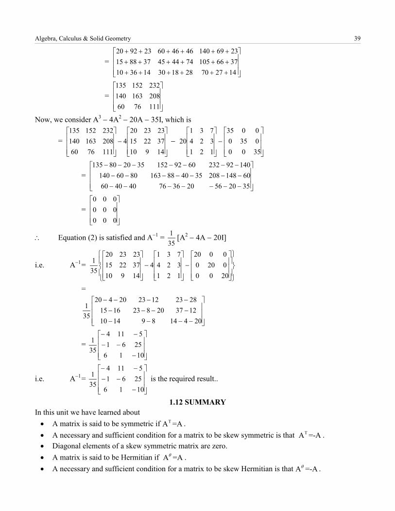
=
=
Now, we consider A3 − 4A2 − 20A − 35I, which is
= −
=
=
∴ Equation (2) is satisfied and A−1 = [A2 − 4A − 20I]
i.e. A−1 =
=
=
i.e. A−1 = is the required result..
1.12 SUMMARY In this unit we have learned about • A matrix is said to be symmetric if . • A necessary and sufficient condition for a matrix to be skew symmetric is that . • Diagonal elements of a skew symmetric matrix are zero. • A matrix is said to be Hermitian if . • A necessary and sufficient condition for a matrix to be skew Hermitian is that .
++++++++++++++++++
14277028183014361037661057444453788152369140464660239220
1117660208163140232152135
−
14910372215232320
41117660208163140232152135
−
350003500035
121324731
20
−−−−−−−−−−−−−−−−−−−−−
352056203676404060601482083540881638060140
140922326092152352080135
000000000
351
−
−
200002000020
121324731
414910372215232320
351
−−−−−−−−−−−−
2041489141012372082316152823122320420
351
−−−
−−
10162561
5114
351
−−−
−−
10162561
5114
351
TA =ATA =-A
A =Aθ
A =-Aθ
40 Matrices
• Diagonal element for a skew Hermitian matrix are either zero or purely imaginary. • The rank of a matrix is the largest order of any non zero minor of the matrix. • The elementary operation is operation on any row/column like interchange of row/column,
multiplication of all element of row/column by a number, addition of any row or column. The rank of a matrix is not changed when we apply elementary operation on a matrix.
• Two matrices are said to be equivalent if one can be obtained from other by applying finite number of elementary operation. Equivalent matrices have same rank.
• A matrix is said to be row echelon matrix if the leading entry of each non zero row is unity, the number of zero before the leading entry is less than the number of zero in the succeeding rows and the non zero rows precede the zero rows. A row echelon matrix is said to be row reduced echelon matrix if each column containing the leading entry of a row has all the other elements as zero.
• A matrix of order and rank r is equivalent to the matrix in the normal form.
• The matrix obtained by applying a single elementary operation on identity matrix is called elementary matrix.
• The rank of the product of two matrices cannot exceed the rank of either matrix. The rank, row rank and column rank are all equal.
• If A is matrix, then the matrix , for some scalar is called characteristics matrix of A. • The determinant of the matrix is a non null polynomial of degree n in and is called
characteristics polynomial of matrix A. • The equation , for some scalar is called the characteristics equation of matrix A and
its roots , are called the characteristics roots of matrix A.
• If is the characteristic root of an matrix A, then any solution of the equation except is called a characteristic vector of matrix A.
• If A is non singular, then the eigen value of is the reciprocal of the eigen value of A. • The eigen value of diagonal matrix is the diagonal elements of the matrix. • The eigen value of triangular matrix is the diagonal elements of the matrix.
• If a is eigen value of a non singular matrix A, then is an eigen value of adj. A.
• The characteristic vectors corresponding to distinct characteristic roots of a matrix are linearly independent.
• The distinct roots of the characteristic equation of a matrix A are also the distinct roots of the minimal equation of the matrix A.
1.13 KEY TERMS • Symmetric matrix: A square matrix A = [aij] is said to be symmetric if aij = aji for all i and j. • Skew Symmetric matrix: If a square matrix A has its elements such that aij = −aji for i and j and
the leading diagonal elements are zeros, then matrix A is known as skew matrix.
m×n rI OO O
n×n A- Iλ λA- Iλ λ
A- I 0λ = λ
1 2, ,...., nλ λ λ
λ n×n AX= XλX=0
-1A
Aa
( )=0φ λm( )=0λ
Algebra, Calculus & Solid Geometry 41
• Hermitian Matrix: A square matrix over the complex numbers is said to be Hermitian if
the transposed conjugate of the matrix is equal to the matrix itself i.e. . • Skew Hermitian Matrix: A square matrix over the complex numbers is said to be Skew
Hermitian if the transposed conjugate of the matrix is equal to the negative of matrix itself i.e. .
• Rank of a Matrix: A non zero matrix has rank r if every minor of order r+1 vanishes and it has at least one non non zero minor off order r.
• Linear Dependence and Independence of row and column Matrices: The set of vectors are said to be linearly dependent if there exist scalars not all zero such
that .The set of vectors are said to be linearly independent
if there exist scalars such that gives . 1.14 QUESTION AND EXERCISE
1. Define inverse of a square matrix and show that inverse of a matrix is unique if it exists 2. Prove that square matrix A is invertible iff A is non singular.
3. Find the adjoint of the matrix and verify A(adj. A)=(adj.A)A= .
4. Calculate the inverse of the matrix if exists.
5. If A and B are square matrix of same order and a is non singular, then prove that .
6. Solve the system of equation using matrix method
(i) (ii)
7. If A is any square matrix, prove that and are both symmetric. 8. Prove that is symmetric or skew symmetric according as A is symmetric or skew symmetric. 9. If A is skew symmetric matrix of order n, then show that adj. A is symmetric or skew symmetric according as n is odd and even.
10. Express as the sum of symmetric and skew symmetric matrix.
11. Show all positive odd integral power of a skew symmetric matrix are skew symmetric while positive even integral power are symmetric. 12. If A and B are Hermitian, show that AB +BA is Hermitian and AB is Hermitian iff AB = BA.
ijA=[a ]θA =A
ijA=[a ]
θA =-A
1 2 n{v ,v ,.....v } 1 2 na ,a ,.....a
1 1 2 2 n na v +a v +.....+a v 0= 1 2 n{v ,v ,.....v }
1 2 na ,a ,.....a 1 1 2 2 n na v +a v +.....+a v 0= 1 2 na =a =.....=a 0=
2 1 33 1 21 2 3
3 A I
1 2 13 1 20 1 2
-1A BA B =
2x-3y+z=9x+y+z=6x-y+z=2
x+z=72x+y=73x+2y+z=17TA A TAA
TABB
1 3 5-6 8 3-4 6 5
42 Matrices
13. Find the rank of matrix .
14. Find the rank of matrix , a, b, c being real.
15. If A is a square matrix of rank n -1, show that adj. A .
16. Reduce the following matrix to normal form .
17. Reduce the matrix to . Hence find .
18. Express as product of elementary matrices.
19. For the given matrix A, find non singular matrix P and Q such that PAQ is in normal form and hence determine the rank of A.
.
20. Prove that the set of vector (0, 2, -4), (1,-2,-1), (1,-4, 3) is linearly dependent.
21. Find p if the vectors , , are linearly dependent.
22. Verify Cayley Hamilton theorem for the given matrix and also find also:
.
1.15 FURTHER READING L.N. Herstein Topic in Algebra, , Wiley Eastern Ltd. New Delhi, 1975 K.B. Datta, Matrix and Linear Algebra, Prentice hall of India Pvt. Ltd. New Delhi, 2002 P.B.Bhattacharya, S.K.Jain and S.R.Nagpaul, First Course in Linear Algebra, Wiley Eastern, New Delhi, 1983 S.K.Jain, A. Gunawardena and P.B.Bhattacharya, Basic Linear Algebra with Maatlab., Key College Publishing (Springer- Verlag), 2001 Shanti Narayan, A Text Book of Matrices, S.Chand & Co., New Delhi Lischutz, 3000 Solved Problems in Linear Algebra, Schaum Outline Series, Tata McGraw-Hill.
1 -3 4 69 1 2 0
3 3 3
1 1 1A a b c
a b c
=
O≠0 2 3 42 3 5 44 8 13 2
1 -1 2 -1A 4 2 -1 2
2 2 -2 0
=
[ ]3I O (A)ρ
1 3 3A 1 4 3
1 3 4
=
1 1 1A 1 -1 -1
3 1 1
=
1-13
12-3
101
-1A2 1 2
A 5 3 3-1 0 -2
=
UNIT – II
SSYYSSTTEEMM OOFF LLIINNEEAARR EEQQUUAATTIIOONNSS
2.0 Introduction 2.1 Objectives 2.2 System of Linear Equations
2.2.1 System of Non-homogeneous Linear Equations 2.2.2 System of Homogeneous Linear Equations
2.3 Orthogonal and Unitary Matrices 2.4 Summary 2.5 Key Terms 2.6 Question and Exercises 2.7 Further Reading
2.0 INTRODUCTION In this chapter we will use these concepts to study the solutions of systems of linear equations. Here, we will concentrate on the solution of system of homogeneous as well as non-homogeneous linear equations. We also learn orthogonal and unitary matrices.
2.1 OBJECTIVES After going through this unit you will be able to: • Determine whether the system of non homogeneous and homogeneous linear equation is consistent
or inconsistent.. • Solve non homogeneous and homogeneous system of linear equations.
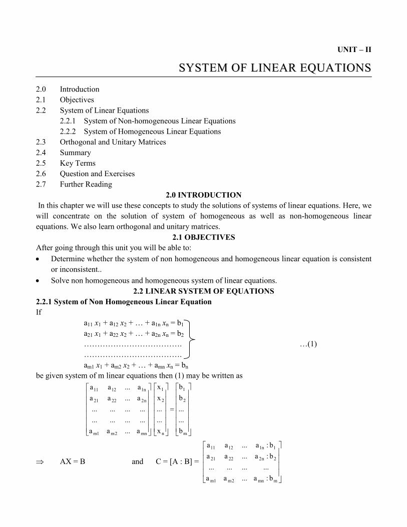
2.2 LINEAR SYSTEM OF EQUATIONS 2.2.1 System of Non Homogeneous Linear Equation If a11 x1 + a12 x2 + … + a1n xn = b1 a21 x1 + a22 x2 + … + a2n xn = b2 ………………………………. …(1) ………………………………. am1 x1 + am2 x2 + … + amn xn = bn
be given system of m linear equations then (1) may be written as
⇒ AX = B and C = [A : B] =
=
m
2
1
n
2
1
mn2m1m
n22221
n11211
b......bb
x......xx
a...aa........................
a...aaa...aa
mmn2m1m
2n22221
1n11211
b:a...aa............
b:a...aab:a...aa
44 System of Linear Equations
then [A : B] or C is called augmented matrix. Sometime we also write A : B for [A : B] Consistent Equations.
(i) If rank of A = rank of [A : B] and there is unique solution when rank of A=rank of [A : B]=n (ii) rank of A = rank of [A : B] = r < n.
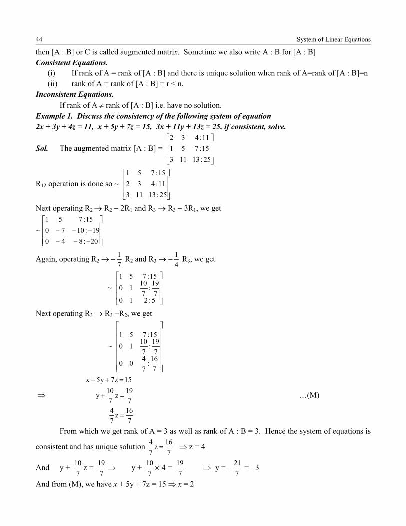
Inconsistent Equations. If rank of A ≠ rank of [A : B] i.e. have no solution. Example 1. Discuss the consistency of the following system of equation 2x + 3y + 4z = 11, x + 5y + 7z = 15, 3x + 11y + 13z = 25, if consistent, solve.
Sol. The augmented matrix [A : B] =
R12 operation is done so ~
Next operating R2 → R2 − 2R1 and R3 → R3 − 3R1, we get
~
Again, operating R2 → − R2 and R3 → − R3, we get
~
Next operating R3 → R3 −R2, we get
~
⇒ …(M)
From which we get rank of A = 3 as well as rank of A : B = 3. Hence the system of equations is
consistent and has unique solution ⇒ z = 4
And y + z = ⇒ y + × 4 = ⇒ y = − = −3
And from (M), we have x + 5y + 7z = 15 ⇒ x = 2
25:1311315:75111:432
25:1311311:43215:751
−−−−−−20:84019:1070
15:751
71
41
5:2107
19:7
101015:751
716:
7400
719:
71010
15:751
716z
74
719z
710y
15z7y5x
=
=+
=++
716z
74
=
710
719
710
719
721
Algebra, Calculus & Solid Geometry 45
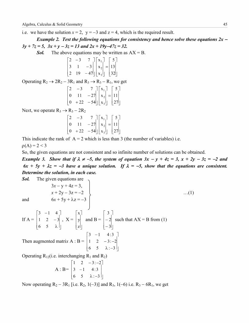
i.e. we have the solution x = 2, y = −3 and z = 4, which is the required result. Example 2. Test the following equations for consistency and hence solve these equations 2x − 3y + 7z = 5, 3x + y − 3z = 13 and 2x + 19y−47z = 32. Sol. The above equations may be written as AX = B.
Operating R2 → 2R2 − 3R1 and R3 → R3 − R1, we get
Next, we operate R3 → R3 − 2R2
This indicate the rank of A = 2 which is less than 3 (the number of variables) i.e. ρ(A) = 2 < 3 So, the given equations are not consistent and so infinite number of solutions can be obtained. Example 3. Show that if λ ≠ −5, the system of equation 3x − y + 4z = 3, x + 2y − 3z = −2 and 6x + 5y + λz = −3 have a unique solution. If λ = −5, show that the equations are consistent. Determine the solution, in each case. Sol. The given equations are 3x − y + 4z = 3, x + 2y − 3z = −2 …(1) and 6x + 5y + λz = −3
If A = , X = and B = such that AX = B from (1)
Then augmented matrix A : B =
Operating R12(i.e. interchanging R1 and R2)
A : B =
Now operating R2 − 3R1 [i.e. R2, 1(−3)] and R3, 1(−6) i.e. R3 − 6R1, we get
=
−−
−
32135
xxx
47192313
732
3
2
1
=
−+−
−
27115
xxx
5422027110732
3
2
1
=
−+−
−
27115
xxx
5422027110732
3
2
1
λ−
−
56321
413
zyx
−−
32
3
−λ−−
−
3:562:321
3:413
−λ−
−−
3:563:413
2:321
46 System of Linear Equations
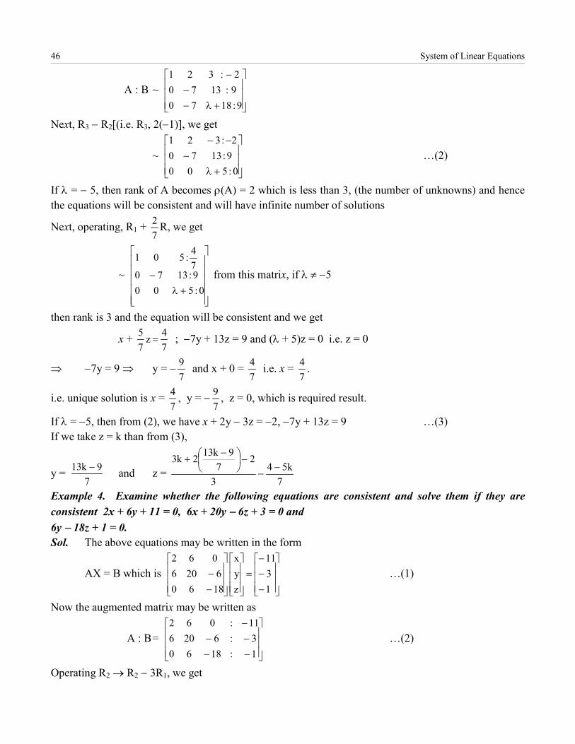
A : B ~
Next, R3 − R2[(i.e. R3, 2(−1)], we get
~ …(2)
If λ = − 5, then rank of A becomes ρ(A) = 2 which is less than 3, (the number of unknowns) and hence the equations will be consistent and will have infinite number of solutions
Next, operating, R1 + R, we get
~ from this matrix, if λ ≠ −5
then rank is 3 and the equation will be consistent and we get
x + ; −7y + 13z = 9 and (λ + 5)z = 0 i.e. z = 0
⇒ −7y = 9 ⇒ y = − and x + 0 = i.e. x = .
i.e. unique solution is x = , y = − , z = 0, which is required result.
If λ = −5, then from (2), we have x + 2y − 3z = −2, −7y + 13z = 9 …(3) If we take z = k than from (3),
y = and z =
Example 4. Examine whether the following equations are consistent and solve them if they are consistent 2x + 6y + 11 = 0, 6x + 20y − 6z + 3 = 0 and 6y − 18z + 1 = 0. Sol. The above equations may be written in the form
AX = B which is …(1)
Now the augmented matrix may be written as
A : B = …(2)
Operating R2 → R2 − 3R1, we get
+λ−−
−
9:18709:13702:321
+λ−
−−
0:5009:13702:321
72
+λ−
0:5009:137074:501
74z
75
=
79
74
74
74
79
79k13 −
7k54
3
27
9k132k3−
−−
−
+
−−−
=
−−
1311
zyx
18606206
062
−−−−−
1:18603:6206
11:062
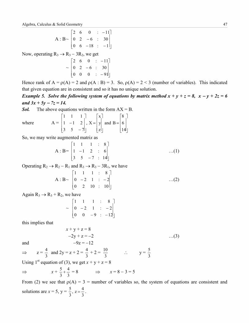
Algebra, Calculus & Solid Geometry 47
A : B ~
Now, operating R3 → R3 − 3R2, we get
~
Hence rank of A = ρ(A) = 2 and ρ(A : B) = 3. So, ρ(A) = 2 < 3 (number of variables). This indicated that given equation are in consistent and so it has no unique solution. Example 5. Solve the following system of equations by matrix method x + y + z = 8, x − y + 2z = 6 and 3x + 5y − 7z = 14. Sol. The above equations written in the form AX = B.
where A =
So, we may write augmented matrix as
A : B = …(1)
Operating R2 → R2 − R1 and R3 → R3 − 3R1, we have
A : B ~ …(2)
Again R3 → R3 + R2, we have
~
this implies that x + y + z = 8
−2y + z = −2 …(3) and −9z = −12
⇒ z = and 2y = z + 2 = + 2 = ∴ y =
Using 1st equation of (3), we get x + y + z = 8
⇒ x + = 8 ⇒ x = 8 − 3 = 5
From (2) we see that ρ(A) = 3 = number of variables so, the system of equations are consistent and
solutions are x = 5, y = .
−−−
−
1:186030:62011:062
−−
−
91:00030:62011:062
=
=
−−
1468
Bandzyx
X,753
211111
−−
14:7536:2118:111
−−10:1020
2:1208:111
−−−−12:9002:120
8:111
34
34
310
35
34
35+
34z,
35
=
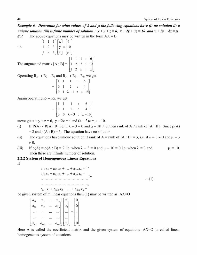
48 System of Linear Equations
Example 6. Determine for what values of λ and µ the following equations have (i) no solution ii) a unique solution (iii) infinite number of solution : x + y + z = 6, x + 2y + 3z = 10 and x + 2y + λz = µ. Sol. The above equations may be written in the form AX = B.
i.e.
The augmented matrix [A : B] =
Operating R2 → R2 − R1 and R3 → R3 − R1, we get
~
Again operating R3 − R2, we get
~
⇒we get x + y + z = 6, y + 2z = 4 and (λ − 3)z = µ − 10. (i) If R(A) ≠ R[A : B] i.e. if λ − 3 = 0 and µ − 10 ≠ 0, then rank of A ≠ rank of [A : B]. Since ρ(A)
= 2 and ρ(A : B) = 3. The equation have no solution. (ii) The equations have unique solution if rank of A = rank of [A : B] = 3, i.e. if λ − 3 ≠ 0 and µ − 3
≠ 0. (iii) If ρ(A) = ρ(A : B) = 2 i.e. when λ − 3 = 0 and µ − 10 = 0 i.e. when λ = 3 and µ = 10.
Then these are infinite number of solution. 2.2.2 System of Homogeneous Linear Equations If a11 x1 + a12 x2 + … + a1n xn = a21 x1 + a22 x2 + … + a2n xn = ………………………………. …(1) ………………………………. am1 x1 + am2 x2 + … + amn xn = be given system of m linear equations then (1) may be written as
Here A is called the coefficient matrix and the given system of equations is called linear homogeneous system of equations.
µ=
λ106
zyx
21321111
µλ :2110:3216:111
−µ−λ 6:1104:2106:111
−µ−λ 10:3004:2106:111
AX=O
111 12 1
221 22 2
1 2
... 0
... 0... ... ... ... ... ...... ... ... ... ... ...
... 0
n
n
m m mn n
xa a axa a a
a a a x
=
AX=O
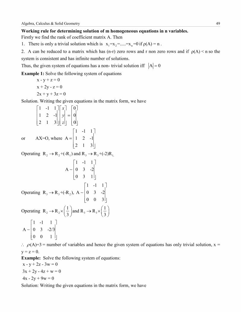
Algebra, Calculus & Solid Geometry 49
Working rule for determining solution of m homogeneous equations in n variables. Firstly we find the rank of coefficient matrix A. Then 1. There is only a trivial solution which is . 2. A can be reduced to a matrix which has (n-r) zero rows and r non zero rows and if so the system is consistent and has infinite number of solutions. Thus, the given system of equations has a non- trivial solution iff
Example 1: Solve the following system of equations
Solution. Writing the given equations in the matrix form, we have
or AX=O, where
Operating
Operating
Operating
= number of variables and hence the given system of equations has only trivial solution, x = y = z = 0. Example: Solve the following system of equations:
Solution: Writing the given equations in the matrix form, we have
1 2 n x =x =.....=x =0 if ρ(A) = nρ(A) < n
A 0=
x - y + z = 0x + 2y - z = 02x + y + 3z = 0
1 -1 1 01 2 -1 02 1 3 0
xyz
=
1 -1 1A 1 2 -1
2 1 3
=
2 2 1 3 3 1,R R +(-R ) and R R +(-2)R→ →
1 -1 1A 0 3 -2
0 3 1
3 3 2R R +(-R ),→1 -1 1
A 0 3 -20 0 3
2 2 3 31 1R R and R R3 3
→ × → ×
1 -1 1A 0 3 -2/3
0 0 1
(A)=3ρ∴
x - y + 2z - 3w = 03x + 2y - 4z + w = 04x - 2y + 9w = 0
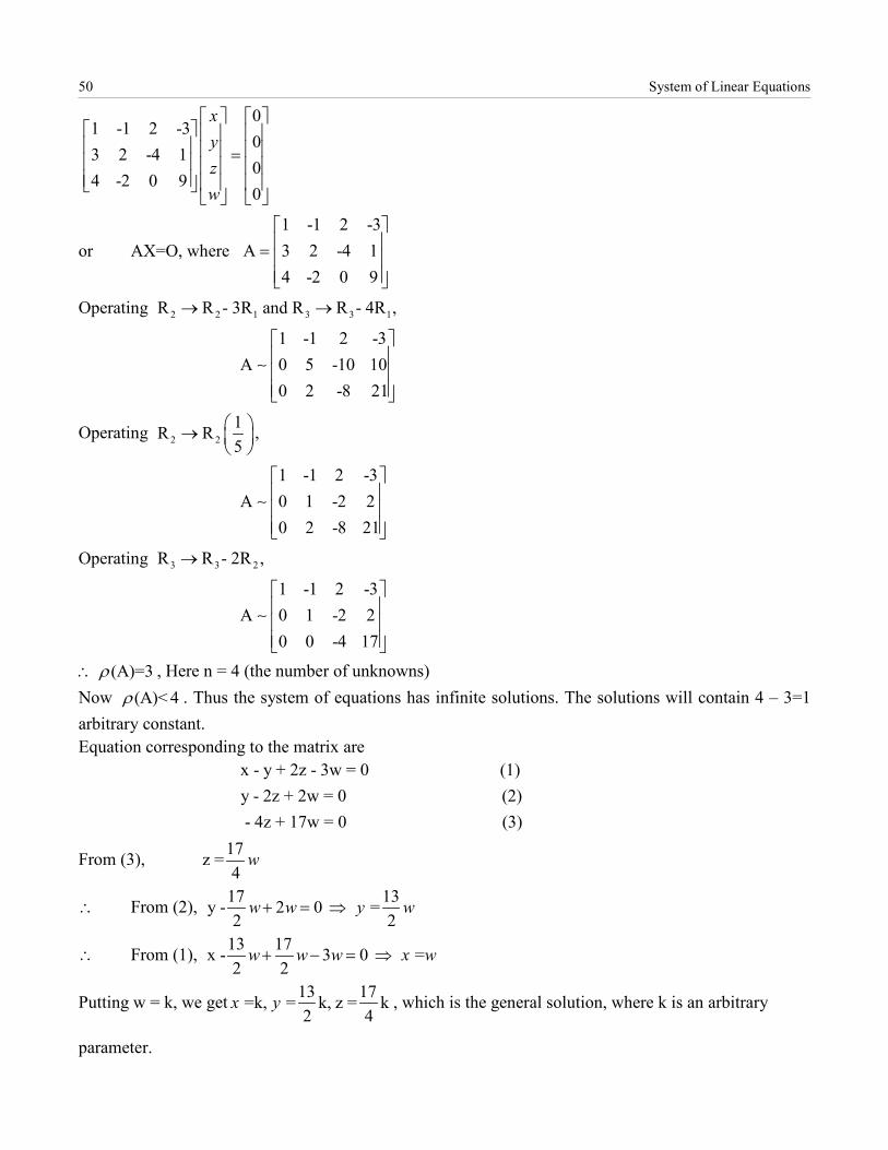
50 System of Linear Equations
or AX=O, where
Operating
Operating ,
Operating
, Here n = 4 (the number of unknowns) Now . Thus the system of equations has infinite solutions. The solutions will contain 4 – 3=1 arbitrary constant. Equation corresponding to the matrix are
From (3),
From (2),
From (1),
Putting w = k, we get , which is the general solution, where k is an arbitrary
parameter.
01 -1 2 -3
03 2 -4 1
04 -2 0 9
0
xyzw
=
1 -1 2 -3
A 3 2 -4 14 -2 0 9
=
2 2 1 3 3 1R R - 3R and R R - 4R ,→ →
1 -1 2 -3A 0 5 -10 10
0 2 -8 21
2 21R R5
→
1 -1 2 -3A 0 1 -2 2
0 2 -8 21
3 3 2R R - 2R ,→
1 -1 2 -3A 0 1 -2 2
0 0 -4 17
(A)=3ρ∴
(A)< 4ρ
x - y + 2z - 3w = 0 (1)y - 2z + 2w = 0 (2) - 4z + 17w = 0 (3)
17z =4
w
∴17 13y - 2 0 =2 2
w w y w+ = ⇒
∴13 17x - 3 0 =2 2
w w w x w+ − = ⇒
13 17 =k, = k, z = k2 4
x y
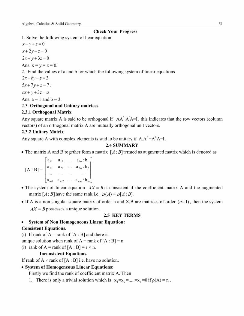
Algebra, Calculus & Solid Geometry 51
Check Your Progress 1. Solve the following system of liear equation
02 0
2 3 0
x y zx y z
x y z
− + =+ − =+ + =
Ans. x = y = z = 0. 2. Find the values of a and b for which the following system of linear equations 2 35 7 7
3
x by zx y z
ax y z a
+ − =+ + =+ + =
.
Ans. a = 1 and b = 3. 2.3. Orthogonal and Unitary matrices 2.3.1 Orthogonal Matrix Any square matrix A is said to be orthogonal if '= 'AA A A=I , this indicates that the row vectors (column vectors) of an orthogonal matrix A are mutually orthogonal unit vectors. 2.3.2 Unitary Matrix Any square A with complex elements is said to be unitary if θ θA.A =A A=I .
2.4 SUMMARY • The matrix A and B together form a matrix termed as augmented matrix which is denoted as
[A : B] =
• The system of linear equation is consistent if the coefficient matrix A and the augmented matrix have the same rank i.e. .
• If A is a non singular square matrix of order n and X,B are matrices of order , then the system possesses a unique solution.
2.5 KEY TERMS • System of Non Homogeneous Linear Equation: Consistent Equations. (i) If rank of A = rank of [A : B] and there is unique solution when rank of A = rank of [A : B] = n (i) rank of A = rank of [A : B] = r < n.
Inconsistent Equations. If rank of A ≠ rank of [A : B] i.e. have no solution. • System of Homogeneous Linear Equations:
Firstly we find the rank of coefficient matrix A. Then 1. There is only a trivial solution which is .
[ : ]A B
mmn2m1m
2n22221
1n11211
b:a...aa............
b:a...aab:a...aa
AX B=[ : ]A B ( ) [ : ]A A Bρ ρ=
( 1)n×AX B=
1 2 n x =x =.....=x =0 if ρ(A) = n
52 System of Linear Equations
2. A can be reduced to a matrix which has (n-r) zero rows and r non zero rows and if so the system is consistent and has infinite number of solutions.
Thus, the given system of equations has a non- trivial solution iff .
2.6 QUESTION AND EXERCISE 1. Solve the system of linear equation:
, considering special the case when .
2. Show that the only real value of for which the equations
, have a non zero solution is 6.
2.7 FURTHER READING
L.N. Herstein Topic in Algebra, Wiley Eastern Ltd. New Delhi, 1975 K.B. Datta, Matrix and Linear Algebra, Prentice hall of India Pvt. Ltd. New Delhi, 2002 P.B.Bhattacharya, S.K.Jain and S.R.Nagpaul, First Course in Linear Algebra, Wiley Eastern, New Delhi, 1983 S.K.Jain, A. Gunawardena and P.B.Bhattacharya, Basic Linear Algebra with Maatlab., Key College Publishing (Springer- Verlag), 2001 Shanti Narayan, A Text Book of Matrices, S.Chand & Co., New Delhi Lischutz, 3000 Solved Problems in Linear Algebra, Schaum Outline Series, Tata McGraw-Hill
ρ(A) < n
A 0=
x+2y-2z=14x+2 y-z=26x+6y+ z=3
λλλ
2λ =
λx+2y+3z= x3x+y+2z=2x+3y+z=
yz
λλλ
UNIT – III
EEQQUUAATTIIOONN AANNDD PPOOLLYYNNOOMMIIAALL
STRUCTURE 3.0 Introduction 3.1 Unit Objectives 3.2 Polynomial 3.2.1 Division Algorithm 3.2.2 Remainder Theorem 3.2.3 Factor Theorem 3.3 General Equation 3.3.1 Degree of an Equation 3.3.2 Complete and Incomplete Equation 3.3.3 Root of an Equation 3.4 Synthetic Division 3.4.1 To find the Quotient and Remainder, when f(x) is divided by (ax-b) 3.5 Relation between roots and coefficient of an equation 3.5.1 Solution of polynomial equation having condition on roots 3.5.2 To find the condition that the root of given equation satisfy a given Relation 3.5.3 Common root of two equations 3.5.4 Equal or multiple roots of an equation 3.6 Transformation of Equations 3.6.1 Roots multiplied by a given number 3.6.2 Reciprocal roots 3.6.3 Root diminished by a given number 3.6.4 Removal of term in general 3.6.5 Transformation of the cubic 3.6.6 Transformation of biquadratic 3.6.7 Removal of second and third term 3.6.8 Transformation in general 3.6.9 Equation of squared and difference of a cubic 3.7 Summary 3.8 Key Terms 3.9 Question and Exercises 3.10 Further Reading
3.0 INTRODUCTION In this unit, we will learn synthetic division . We will also find the relation between the roots and the co-efficient of an equation. In this unit we will transform equations in another equations whose roots are related. Transformation of an equation into another is a very useful as we can connect the roots of the new equation with that of the given equation or convert the co-efficient of the new equation in particular forms. Also the transformed equation may be easier to solve and having solved the transformed equation
54 Equation and Polynomial
we can find out the roots of the given equation with the help of the relation between the roots of the given equation and the transformed equation.
3.1 UNIT OBJECTIVES After going through this unit, you will be able to: Know about polynomials and their co-efficient, terms and value. Know about degree and roots of complete and incomplete equations. Learn synthetic division. Find the relation between the roots and co-efficient of an equation. Find a condition so that the roots of a given equation satisfy a given relation and the common roots of two equations. Find multiple roots of an equation and the common roots of two equations. Transform an equation into another having roots with sigh. Changed, roots multiplied by a number, roots as the reciprocal of the roots of the given equation. Remove the fractional co-efficient removed of the given equation. Diminish the roots of an equation by a given number. Remove particular terms of the given equation . To find an equation having roots as squared differences of the roots of the equation x3. To find an equation having roots as squared differences of the roots of the equation.
3.2 POLYNOMIAL An expression in x of the form where are constants known as the coefficients and x is a variable. We shall denote a polynomial by or etc. A polynomial
is said to be of degree n when .
If all the coefficients in are real then polynomial is said to be real polynomial. If all the coefficients in are zero then polynomial is said to be zero polynomial. If we substitute x=a in then the number is called value of the polynomial for x=a. The number x=a is called zero of the polynomial if and only if . The highest index of variable x occurring in the terms of polynomial is called degree of . Example: The polynomial is of degree three. 3.2.1 Division Algorithm If and are two nonzero polynomial, then there exist unique polynomial and such that , where is either a zero polynomial or degree of < degree of . Where is called quotient and is called remainder when is divided by . Degree of = degree of - degree of ( )g x . If degree of =1 then, either =0 or degree of is zero means a constants polynomial.
10 1 ...n n
na x a x a−+ + + 0 1, ,..., na a a( )f x ( )g x
10 1( ) ...n n
nf x a x a x a−= + + + 0 0a ≠
0 1, ,..., na a a ( )f x
0 1, ,..., na a a ( )f x
( )f x ( )f a ( )f x
( )f x ( ) 0f a =
( )f x( )f x
2 3( ) 5 7 3f x x x= + +
( )f x ( )g x ( )q x ( )r x( ) ( ). ( ) ( )f x q x g x r x= + ( )r x ( )r x ( )g x
( )q x ( )r x ( )f x ( )g x( )r x ( )f x
( )g x ( )r x ( )r x
Algebra, Calculus & Solid Geometry 55
2.2.2 Remainder Theorem Theorem 2.1: If a polynomial is divided by x-a, then the remainder is equal to . Proof: Let be quotient and R be the remainder then using division algorithm for polynomial
and x-a, we have
By putting x=a, we get =Remainder
Example 1: Find the remainder when polynomial is divided by x+2. Sol: Comparing x+2 with x-h, we get h=-2
Now Remainder R= = [ ] = =32+8-24-8-8=0 Thus remainder is zero. Note: When Remainder R=0, we say that is exactly divisible by x+2. 2.2.3 Factor Theorem Theorem 2.2: If h is a root of the equation f(x)=0, then (x-h) is a factor of f(x) and conversely. Proof: Using Division algorithm for f(x) and (x-h), we have f (x)=q(x)(x-h)+R (1) where q(x) is quotient and R is remainder. Now as h is a root of equation f(x) =0 f(h)=0 (2) from (1), we have f(h)= q(h)(h-h)+R f(h)=R, but from (2) R=0, using in (1), we have f(x)=q(x)(x-h) , this imply (x-h) is factor of f(x). Converse: Do yourself.
3.3 GENERAL EQUATION If is a polynomial then =0 is called general equation. 3.3.1 Degree of an Equation: The degree of an equation is highest index of variable x occurring in the terms of polynomial equation . The polynomial equation of 1st degree, 2nd degree, 3rd degree, 4th degree, are respectively known as Linear, Quadratic, Cubic, biquadratic Equation. 3.3.2 Complete and Incomplete Equations A General Equation of degree n is said to be complete if it contains all power of the variable x from 0 to n. For example is complete equation of third degree. If any of the powers of the variable are missing from an equation of degree n is called incomplete equations. For example is incomplete equation of third degree. [ The Term is missing.]
( )f x ( )f a( )q x
( )f x( ) ( )( )f x q x x a R= − +
( ) ( )( ) ( )f a q a a a R R f a= − + ⇒ =4 3 22 6 4 8x x x x− − + −
4 3 2( ) 2 6 4 8f x x x x x= − − + −
∴ ( )f h ( 2)f − 2h = −
4 3 22( 2) ( 2) 6( 2) 4( 2) 8− − − − − + − −
( )f x
⇒
( )f x ( )f x
( ) 0f x =
( ) 0f x =
3 20 1 3 4 0a x a x a x a+ − + =
3 20 1 4 0a x a x a+ + = 3a x−
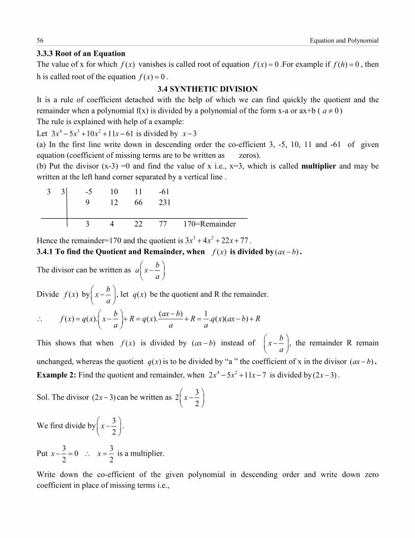
56 Equation and Polynomial
3.3.3 Root of an Equation The value of x for which vanishes is called root of equation .For example if , then h is called root of the equation .
3.4 SYNTHETIC DIVISION It is a rule of coefficient detached with the help of which we can find quickly the quotient and the remainder when a polynomial f(x) is divided by a polynomial of the form x-a or ax+b ( ) The rule is explained with help of a example: Let is divided by (a) In the first line write down in descending order the co-efficient 3, -5, 10, 11 and -61 of given equation (coefficient of missing terms are to be written as zeros). (b) Put the divisor (x-3) =0 and find the value of x i.e., x=3, which is called multiplier and may be written at the left hand corner separated by a vertical line .
3 3 -5 10 11 -61 9 12 66 231
3 4 22 77 170=Remainder
Hence the remainder=170 and the quotient is . 3.4.1 To find the Quotient and Remainder, when is divided by .
The divisor can be written as
Divide by , let be the quotient and R the remainder.
This shows that when is divided by instead of , the remainder R remain
unchanged, whereas the quotient is to be divided by “a ” the coefficient of x in the divisor . Example 2: Find the quotient and remainder, when is divided by .
Sol. The divisor can be written as
We first divide by .
Put is a multiplier.
Write down the co-efficient of the given polynomial in descending order and write down zero coefficient in place of missing terms i.e.,
( )f x ( ) 0f x = ( ) 0f h =
( ) 0f x =
0a ≠
4 3 23 5 10 11 61x x x x− + + − 3x −
3 23 4 22 77x x x+ + +( )f x ( )ax b−
ba xa
−
( )f x bxa
−
( )q x
∴( ) 1( ) ( ). ( ). . ( )( )b ax bf x q x x R q x R q x ax b R
a a a− = − + = + = − +
( )f x ( )ax b− bxa
−
( )q x ( )ax b−4 22 5 11 7x x x− + − (2 3)x −
(2 3)x − 322
x −
32
x −
3 302 2
x x− = ∴ =
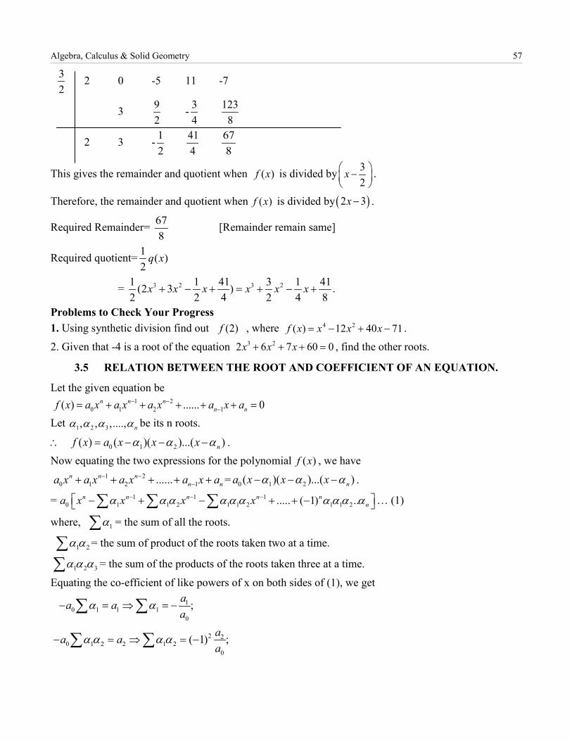
Algebra, Calculus & Solid Geometry 57
2 0 -5 11 -7
3 -
2 3 -
This gives the remainder and quotient when is divided by .
Therefore, the remainder and quotient when is divided by .
Required Remainder= [Remainder remain same]
Required quotient=
= .
Problems to Check Your Progress 1. Using synthetic division find out , where .
2. Given that -4 is a root of the equation , find the other roots.
3.5 RELATION BETWEEN THE ROOT AND COEFFICIENT OF AN EQUATION.
Let the given equation be
Let be its n roots.
. Now equating the two expressions for the polynomial , we have
= .
= … (1)
where, = the sum of all the roots.
= the sum of product of the roots taken two at a time.
= the sum of the products of the roots taken three at a time.
Equating the co-efficient of like powers of x on both sides of (1), we get
32
92
34
1238
12
414
678
( )f x 32
x −
( )f x ( )2 3x −
678
1 ( )2
q x
3 2 3 21 1 41 3 1 41(2 3 )2 2 4 2 4 8
x x x x x x+ − + = + − +
(2)f 4 2( ) 12 40 71f x x x x= − + −3 22 6 7 60 0x x x+ + + =
1 20 1 2 1( ) ...... 0n n n
n nf x a x a x a x a x a− −−= + + + + + =
1 2 3, , ,...., nα α α α
0 1 2( ) ( )( )...( )nf x a x x xα α α∴ = − − −
( )f x1 2
0 1 2 1......n n nn na x a x a x a x a− −−+ + + + + 0 1 2( )( )...( )na x x xα α α− − −
1 1 10 1 1 2 1 1 2 1 1 2..... ( 1) ..n n n n n
na x x x xα α α α α α α α α α− − − − + − + + − ∑ ∑ ∑1α∑
1 2α α∑1 2 3α α α∑
10 1 1 1
0
;aa aa
α α− = ⇒ = −∑ ∑
2 20 1 2 2 1 2
0
( 1) ;aa aa
α α α α− = ⇒ = −∑ ∑
58 Equation and Polynomial
Thus, above results gives the required relations between the roots and coefficients of the equation.
Sum of the products of roots taken r at a time is
Particular Case: (i) If α, β are roots of the equation
, then and
(ii) If and are roots of the equation
, then
,
(iii) If and are roots of the equation
, then
, and .
3.5.1 Solution of Polynomial Equation having Condition on the Roots We can solve given polynomial equation with the help of relations , ….., where denotes
the roots of given equation. In case of cubic equation: (i) If the roots are given in A.P. can be taken as .
(ii) If the roots are given in G.P. can be taken as .
In case of bi-quadratic equation: (i) If the roots are given in A.P. can be taken as .
(ii) If the roots are given in G.P. can be taken as .
Example 3: Solve the equation , the sum of two of the roots being zero. Solution: The given equation is Let the roots be such that
Now
3 30 1 2 3 3 1 2 3
0
( 1) ;aa aa
α α α α α α− = ⇒ = −∑ ∑
0 1 2 3 1 2 30
( 1) ...... ...... ( 1) ;n n nn n n
aa aa
α α α α α α α α− = ⇒ = −
( ) 0f x =
r+11 2 3
1
coeff. of T... ( 1)coeff. of T
rrα α α α = −∑
2ax 0bx c+ + =ba
α β+ = −ca
αβ =
,α β γ
3 2ax 0bx cx d+ + + =ba
α β γ+ + = −
2( 1) ca
αβ βγ γα+ + = − 3( 1) da
αβγ = −
, ,α β γ δ
4 3 2ax 0bx cx dx e+ + + + =ba
α β γ δ+ + + = −
2( 1) ca
αβ βγ γδ δα+ + + = − 3( 1) da
αβγ βγδ γδα+ + = − 4( 1) ea
αβγδ = −
α∑ 21α α∑ iα
, ,α β α α β− +
, ,α α αββ
3 , , , 3α β α β α β α β− − + +
33 , , ,α α αβ αβ
β β3 24 16 9 36 0x x x+ − − =3 24 16 9 36 0x x x+ − − =
, ,α β γ 0α β+ =
16 44
α β γ+ + = − = −
Algebra, Calculus & Solid Geometry 59
Since Thus one root of equation is -4 and hence x + 4 is a factor of given equation Dividing the given equation by x + 4, we have
Depressed equation is
Hence the roots are -4, .
Check Your Progress 1. Solve the equation 3 212 39 28 0x x x− + − = the roots being in A.P. Ans. Roots are 1, 4, 7. 2. Solve the equation 3 23 26 52 24 0x x x− + − = , the roots being in G.P.
Ans. Roots are 23
, 2, 6.
3.5.2 To find the condition that roots of given equation satisfy a given relation. Example 4: Find the condition that one root of the equation be equal to the sum of the other two.
Solution: The given equation is (1) Let the roots of the equation be such that
From (1),
But is a root of (1)
or
or which is the required condition.
3.5.3 Common Roots of Two Equations
Let and be two equations of degree n and m respectively.
Let (r < n, r < m) be their common roots.
Then both and are divisible by which is,
therefore, the H.C.F of and .
Hence the common roots of the two equations such as and are given by ,
where is H.C.F. of and .
0 4α β γ+ = ⇒ = −
2 2 9 34 9 04 2
x x x− = ⇒ = ⇒ = ±
32
±
3 2 0px qx rx s+ + + =
3 2 0px qx rx s+ + + =
, ,α β γ α β γ= +
2q q qp p p
α β γ α α α+ + = − ⇒ + = − ⇒ = −
2qp
α = −
3 2
02 2 2q q qp q r sp p p
∴ − + − + − + =
3 3 22 4 8 0q q pqr p s− + − + =
3 24 8 0q pqr p s− + =
( ) 0nf x = ( ) 0mf x =
1 2 3, , ,....., rα α α α
( ) 0nf x = ( ) 0mf x = 1 2( ) ( )( )....( )rx x x xϕ α α α= − − −
( )nf x ( )mf x
( ) 0nf x = ( ) 0mf x = ( ) 0xϕ =
( )xϕ ( )nf x ( )mf x
60 Equation and Polynomial
3.5.4 Equal or Multiple Roots of an Equation
A root is said to be multiple root or repeated root of an equation if occurs more than
once in the roots of the equation . If is repeated m-times then will be roots of
repeated m-1 times, where is differential of with respect to x. Rules to find multiple roots of an equation: To find the multiple root of an equation :
(i) Find
(ii) Find the H.C.F of and .Let it be . (iii) Put and solve it. (iv) If a root of equation is repeated r times, then the same root will be repeated r+1 times in the equation . Cor. 1. If is double root of the equation , then we have and . The required condition will be obtained by eliminating from the equation and . Cor.2. If is triple root of the equation , then we have , and
. The required condition will be obtained by eliminating from the equation , and .
Check Your Progress 1. Solve the equation 3 23 19 33 9 0x x x− + − = which has repeated roots.
Ans.3, 3, 13
2. Solve the equation 5 3 215 10 60 72 0x x x x− + + − = by testing for equal roots. Ans. 2,2,2,-3 and -3.
3.6 TRANSFORMATION OF EQUATIONS To transform an equation into another whose root shall be equal in magnitude but opposite in sign to those of the given equation. Let , , ……, be the root of the equation
(1)
We will find out an equation whose roots are 1α− , 2α− , 3α− ……, nα− . If the new equation is in y then the functional relation between the roots of the equation is, y=-x or x=-y Putting the value of x in (1), we get ( ) 0f y− =
1 20 1 2 1( ) ( ) ( ) .... ( ) 0n n n
n na y a y a y a y a− −−− + − + − + + − + =
1 1 2 20 1 2 1( 1) ( 1) ( 1) .... ( 1) 0n n n n n n
n na y a y a y a y a− − − −−− + − + − + + − + =
Since n can be even as well as odd, we cannot conclude regarding the sign of ( 1)n− , 1( 1)n−− etc.
So multiplying throughout by ( 1)n− , we have
α ( ) 0f x = α
( ) 0f x = α α ( ) 0f xι =
( ) 0f xι = ( ) 0f x =
( ) 0f x =
( )f xι
( )f x ( )f xι ( )xϕ( ) 0xϕ =
α ( ) 0xϕ = α( ) 0f x =
α ( ) 0f x = ( ) 0f α = ( ) 0f ι α =
α ( ) 0f α = ( ) 0f ι α =
α ( ) 0f x = ( ) 0f α = ( ) 0f ι α =
( ) 0f ιι α = α ( ) 0f α =
( ) 0f ι α = ( ) 0f ιι α =
1α 2α 3α nα1 2
0 1 2 1( ) .... 0n n nn nf x a x a x a x a x a− −−= + + + + + =
Algebra, Calculus & Solid Geometry 61 2 2 1 1 2 2 2 1
0 1 2 1( 1) ( 1) ( 1) .... ( 1) ( 1) 0n n n n n n n nn na y a y a y a y a− − − − +−− + − + − + + − + − =
But 2( 1) 1n− =
2 1 2 1( 1) ( 1) ( 1) 1n n− −− = − − = − …………………………………………………. 1 1 2 1( 1) ( 1) ( 1) ( 1)n n n+ − −− = − − = − Thus the required equation is
1 2 10 1 2 1.... ( 1) ( 1) 0n n n n n
n na y a y a y a y a− − −−− + + + − + − =
Expressing the equation in term of variable x, we get 1 2 1
0 1 2 1.... ( 1) ( 1) 0n n n n nn na x a x a x a x a− − −−− + + + − + − =
Which is the required transformed equation. 3.6.1 Root Multiplied by a Given Number: To transform an equation into another whose roots are m times those of the given equation. Let 1α , 2α , 3α ……, nα be the roots of the given equation
1 20 1 2 1( ) .... 0n n n
n nf x a x a x a x a x a− −−= + + + + + =
It is required to find out an equation whose roots are m times the roots of one (1) i.e., we require an equation whose roots are 1mα , 2mα , 3mα ……, nmα . If the new equation is in y, then the functional relation between the roots of the two equation is
y = mx or yxm
=
Putting this value of x in (1), we get yf =0m
i.e., 1 2
0 1 2 1..... 0n n n
n ny y y ya a a a am m m m
− −
− + + + + + =
Multiplying throughout by nm , we get 1 2
0 1 2 1..... 0n n nn na y a y a y a y a− −−+ + + + + =
Expressing it in x, we have 1 2
0 1 2 1..... 0n n nn na x a x a x a x a− −−+ + + + + =
Which is the required transformed equation. Note: 1. In order to form an equation whose roots are m times the roots of the given equation, multiply the successive coefficients beginning with the coefficient of 1nx − by m, 2m , 3m ...., nm .respectively. If any power of x is missing it should be regarded as supplied with a zero coefficient.
2. If the roots of the given equation are to be divided by m, it means they are to be multiplied by 1m
.
3.6.2 Reciprocal Roots We will transform an equation whose roots are reciprocal of the roots of the given equation.
62 Equation and Polynomial
Consider an equation 1 20 1 2 1( ) .... 0n n n
n nf x a x a x a x a x a− −−= + + + + + = (i)
Let 1α , 2α , 3α ……, nα be the roots of the given equation. We will find out an equation whose roots are
1
1α
,2
1α
,3
1α
,……,1
nα
Let us suppose that the new equation formed will be in y. Then yx
or 1xy
= is the functional relation
between the roots of the two equations. By putting this value of x in (1), we get
1 2
0 1 2 11 1 1 1 1( ) .... 0
n n n
n nf a a a a ay y y y y
− −
−
= + + + + + =
Multiplying throughout by ny , we get 2 1
0 1 2 1.... 0n nn na a y a y a y a y−−+ + + + + =
Expressing it in x, we have 2 1
0 1 2 1.... 0n nn na a x a x a x a x−−+ + + + + =
Example 5: Find an equation whose roots are equal in magnitude but opposite in sign to the equation 5 4 3 211 7 16 12 15 0x x x x x+ + − − + = .
Solution: We know that when we change x to –x, the signs of the coefficients of terms with odd powers of x change. Thus, the required equation is 5 4 3 211 7 16 12 15 0x x x x x− + − − + + = or 5 4 3 211 7 16 12 15 0x x x x x− + + − − = Example 6: Find an equation whose roots are four times the roots of the equation 3 22 3 5 0x x x+ + + − =. Solution. The given equation is 3 22 3 5 0x x x+ + − = . Since the given equation is complete, therefore, multiplying the successive terms by 0 1 2 34 , 4 , 4 , 4respectively, we have 0 3 1 2 2 34 . 4 .2 4 .3 4 .5 0x x x+ + − = or 3 28 48 320 0x x x+ + − = . Which is the required equation. Example 7: Remove the fractional coefficients from the equation
4 3 21 5 2 1 02 3 3
x x x x+ − + − =
Solution. To remove the fractional coefficients, we multiply the roots of equation (1) by 6 which is the L.C.M of 2 and 3, the denominator of the fractional coefficients, which are prime to each other.
Thus, the transformed equation is 4 3 2 2 3 41 5 26. 6 . 6 . 6 .1 02 3 3
x x x x+ − + − =
or 4 3 23 60 144 1296 0x x x x+ − + − = .
Algebra, Calculus & Solid Geometry 63
Example 8: Transform the equation into one whose roots are twice the reciprocals of the roots of the equation 4 3 23 6 2 4 0x x x x+ − + − = Solution. The given equation is 4 3 23 6 2 4 0x x x x+ − + − =
Replacing x by 2x
, we get
4 3 22 2 2 23 6 2 4 0x x x x
+ − + − =
or 2 3 416 24 24 4 4 0x x x x+ − + − = or 4 3 26 6 4 0x x x x− + − − = Which is the required equation. Example 9: Find the condition that the roots of the cubic 3 2 0x px qx r− + − = may be in H.P . Hence or
otherwise solve the equation 3 26 11 6 1 0x x x− + − = Solution. (i) The given equation is 3 2 0x px qx r− + − = It is given that its roots are in H.P.
Changing x to 1y
in (1), we get 3 2
1 1 1 0p q ry y y
− + − =
i.e. 3 2 1 0ry qy py− + − = Clearly the roots of (2) are in A.P. Let the roots of (20 be a – d, a, a + d.
Then sum of the roots = 3a=3
q qar r⇒ =
⇒ 3qyr
= is one root of (2)
⇒ 3 2
1 03 3 3q q qr q pr r r
− + − =
or 3 3
3 3 22 2
q q pq- + -1=0 i.e., q -3q +9pqr-27r =027r 9r 3r
∴ Required condition is 3 22q - 9pqr + 27r =0
The given equation is 3 26 11 6 1 0x x x− + − =
Dividing by 6, we get 3 211 1 06 6
x x x− + − =
Comparing (1) and (3), we get 116
p = , 1q = and 6r =
L.H.S of (3)= 3 22 9 27q pqr r− +
=211 1 12 9 (1) 27 0
6 6 36 − + =
This shows that equation (1) and (4) satisfy the same conditions.

64 Equation and Polynomial
∴ 1 3 12
rxy q
= = = is one root of equation (4)
∴ 12
x − is a factor of L.H.S. of (4).
By synthetic division,
12
6 -11 6 -1
..... -3 -4 1 6 -8 2 0 ∴ Depressed equation is 26 8 2 0x x− + = i.e. 23 4 1 0x x− + =
or 1(3 1)( 1) 0 ,13
x x x− − = ⇒ =
Hence the roots of (1) are 1, 12
, 13
.
Check Your Progress
1. Remove the fractional coefficient from the equation 4 3 21 5 2 1 02 3 3
x x x x+ − + − =
Ans. 4 224 65 55 0x x x− + − = . 2. Solve the equation 4 3 240 22 21 2 1 0x x x x− − + + = if the roots are in H.P.
Ans. 1 1 1, ,1,5 2 4
− − .
3.6.3 Root Diminished by a Given Number: We will transform an equation in to another equation whose roots will be the roots of the given equation diminished by h. Consider an equation 1 2
0 1 2 1( ) .... 0n n nn nf x a x a x a x a x a− −−= + + + + + = (i)
Let 1α , 2α , 3α ……, nα be the roots of the given equation. We will find out an equation whose roots are
1 hα − , 2 hα − , 3 hα − ,……, n hα − . Let the new equation formed will be in y. Then y= x- h or x = y + h is the functional relation between the roots of two equations. By putting the value of x in (i), we get
1 20 1 2 1( ) ( ) ( ) ( ) .... ( ) 0n n n
n nf y h a y h a y h a y h a y h a− −−+ = + + + + + + + + + =
Simplifying and arranging in descending power of y, we get 1 2
0 1 2 1A A A .... A A 0n n nn ny y y y− −−+ + + + + =
Where 0A , 1A ,....., An are constants to be determined. ... (ii) Putting y = x – h in (ii) 1 2
0 1 2 1( ) A ( ) A ( ) A ( ) .... A ( ) A 0n n nn nf x x h x h x h x h− −−∴ = − + − + − + + − + =
L.H.S of this equation is identical with the L.H.S. of equation (i).
Algebra, Calculus & Solid Geometry 65
This shows that if f(x) is divided by (x-h), then the remainder is An and the quotient is 1 2 3
0 1 2 1A ( ) A ( ) A ( ) .... A 0n n nnx h x h x h− − −−− + − + − + + =
If we divide this quotient by (x-h), then we get 1An− as the remainder and the second quotient is 2 3 4
0 1 2 2A ( ) A ( ) A ( ) .... A 0n n nnx h x h x h− − −−− + − + − + + =
Repeating this process n time, the nth remainder will be 1A and the nth quotient will be 0A By equating the coefficients of nx in (i) and (iii), we get 0 0A a= . Thus, the division of f(x) successively by (x-h) we get An , 1An− ,....., 1A , 0A as the successive remainders and 0 0A ( )a= as the last quotient. Then the transformed equation in x is
1 20 1 2 1A A A .... A A 0n n n
n nx x x x− −−+ + + + + = .
2.6.4 Removal of terms in General We will remove a particular term from the transformed equation by decreasing the roots of the given equation by a suitable number. Consider an equation 1 2
0 1 2 1( ) .... 0n n nn nf x a x a x a x a x a− −−= + + + + + = .......(i)
Suppose the roots of the equation (i) are diminished by h. Let the new equation formed will be in y. Then y= x – h or x = y + h is the functional relation between the roots of two equations. By putting the value of x in (i), we get
1 20 1 2 1( ) ( ) ( ) ( ) .... ( ) 0n n n
n nf y h a y h a y h a y h a y h a− −−+ = + + + + + + + + + =
By applying binomial theorem and arranging the terms in the descending power of y, we get 1 2 2
0 0 1 0 1 2
10 1 1
( 1)( ) ( 1) ...2!
( .. )
n n n
n nn n
n na y na h a y a h n a h a y
a h a h a h a
− −
−−
− + + + + − + + + + + + +
Now to remove any particular term we equate the coefficient of that term to zero and the values of h thus obtained will be the required numbers by which the roots are to be diminished to get the required transformed equation.
Note: (i) To remove the second term: 0 1na h a+ or 1
0
ahna
= −
(ii) To remove the third term: 20 1 2
( 1) ( 1) 02!
n n a h n a h a−+ − + =
(iii) To remove the fourth term, solve a cubic in h. To remove the last term, solve the equation ( ) 0f h = . 3.6.5 Transformation of Cubic We will reduce the cubic 3 2
0 1 2 33 3 0a x a x a x a+ + + = to the form in which second term is missing and the coefficient of the leading term is unity, all other coefficients being integers. And we will find the relation between the roots of the transformed equation and the given equation. Consider an equation 3 2
0 1 2 3( ) 3 3 0f x a x a x a x a= + + + = .....(i) Suppose the transformed equation is in y. Then y = x – h or y=x+h Let us diminish the roots of (i) by h by putting x = y + h
3 20 1 2 3( ) ( ) 3 ( ) 3 ( ) 0f y h a y h a y h a y h a+ = + + + + + + =
66 Equation and Polynomial
Now, arranging the term in descending power of y, we get 3 2 2 3 2
0 0 1 0 1 2 0 1 2 33( ) 3( 2 ) ( 3 3 ) 0a y a h a y a h a h a y a h a h a h a+ + + + + + + + + = Let us write this equation as
3 20 1 2 33 3 0A y A y A y A+ + + = ....(ii) 0 0[ ]A a=
For removing the second term, take 0 1 0a h a+ = or 1
0
aha
= −
We have 2
2 1 1 12 0 1 2 0 1 2
0 0 0
2 2a a aA a h a h a a a a ha a a
= + + = − + − + = −
220 2 1
0 2 10 0
Where H=a a a H a a aa a−
= = −
Also, 3 2
3 2 1 1 13 0 1 2 3 0 1 2 3
0 0 0
3 3 3 3a a aA a h a h a h a a a a aa a a
= + + + = − + − + − +
2 32 30 3 0 1 2 1
0 3 0 1 2 12 20 0
3 2 , where G= 3 2a a a a a a G a a a a a aa a
− += = − +
Now putting this value in (ii), we get 3
0 20 0
3 0H Ga y ya a
+ + =
To make the coefficients of the leading term as unity, we divide this equation by 0a
30 2 3
0 0
3 0H Ga y ya a
⇒ + + =
Multiplying roots by 0a , we get 303 0 where Z=aZ HZ G y+ + =
This is the required transformed equation. If ' ' ', andα β γ be the roots of this transformed equation. Then
0 0Z=a ( )y a x h= − 0[ Z=a and ( )]y y x h= −
1 10 0 1
0 0
=a [ ]a ax a x a ha a
+ = + = −
' ' '0 1 0 1 0 1; ;a a a a a aα α β β γ γ⇒ = + = + = + , where , andα β γ are the roots of equation (i).
From (i), we have sum of the roots = 1
0
3aa
α β γ+ + = −
( )' 010 0
0
23 3
aaa aa
α β γα α α α β γ + + ∴ = + = − = − −
( ) ( )' '0 02 and 23 3a aβ β α γ γ γ β α∴ = − − = − − .
3.6.6 Transformation of Biquardatic We will reduce the cubic 4 3 2
0 1 2 3 44 6 4 0a x a x a x a x a+ + + + = to the form in which second term is missing and the coefficient of the leading term is unity, all other coefficients being integers. And we will find the relation between the roots of the transformed equation and the given equation. Consider an equation 4 3 2
0 1 2 3 4( ) 4 6 4 0f x a x a x a x a x a= + + + + = .....(i)
Algebra, Calculus & Solid Geometry 67
Suppose the transformed equation is in y. Then y = x - h or x = y + h Let us diminish the roots of (i) by h by putting x = y + h
4 3 20 1 2 3 4( ) ( ) 4 ( ) 6 ( ) 4 ( ) 0f y h a y h a y h a y h a y h a+ = + + + + + + + + =
Now, arranging the term in descending power of y, we get 4 3 2 2 3 2
0 0 1 0 1 2 0 1 2 34 3 2
0 1 2 3 4
4( ) 6( 2 ) 4( 3 3 )( 4 6 4 ) 0
a y a h a y a h a h a y a h a h a h a ya h a h a h a h a+ + + + + + + + +
+ + + + + =
Let us write this equation as 4 3 2
0 1 2 3 44 6 4 0A y A y A y A y A+ + + + = ....(ii) 0 0[ ]A a=
For removing the second term, take 0 1a h a+ or 1
0
aha
= −
We have 2
2 1 1 12 0 1 2 0 1 2
0 0 0
2 2a a aA a h a h a a a a ha a a
= + + = − + − + = −
220 2 1
0 2 10 0
Where H=a a a H a a aa a−
= = −
Also, 3 2
3 2 1 1 13 0 1 2 3 0 1 2 3
0 0 0
3 3 3 3a a aA a h a h a h a a a a aa a a
= + + + = − + − + − +
2 32 30 3 0 1 2 1
0 3 0 1 2 12 20 0
3 2 , where G= 3 2a a a a a a G a a a a a aa a
− += = − +
and 4 3 2
4 3 2 1 1 1 14 0 1 2 3 4 0 1 2 3 4
0 0 0 0
a a a aA =a h +4a h +6a h +4a h+ a =a - +4a - +6a - +4a - aa a a a
+
3 2 2 40 4 0 1 3 0 1 2 1
30
a 4 6 3= a a a a a a a aa
− + −
2 2 2 2 20 0 4 1 3 2 0 2 1 0
3 30 0
a ( 4 3 ) 3( ) I-3H= a a a a a a a a aa a
− + − −=
where 20 4 1 3 2I 4 3a a a a a= − +
Now putting these values in (ii), we get 2
4 2 00 2 3
0 0 02
4 2 02 3 4
0 0 0
I-3H6 4 0
I-3H6 4 0
aH Ga y y ya a a
aH Gy y ya a a
+ + + =
⇒ + + + =
Multiplying roots by 0a , we get 4 2 20 06 4 ( I-3H ) 0 where Z=aZ HZ GZ a y+ + + =
This is the required transformed equation. If ' ' ' ', , andα β γ δ be the roots of this transformed equation. Then 0 0Z=a ( )y a x h= − 0[ Z=a and ( )]y y x h= −
1 10 0 1
0 0
=a [ ]a ax a x a ha a
+ = + = −
68 Equation and Polynomial ' ' ' '
0 1 0 1 0 1 0 1; ; and a a a a a a a aα α β β γ γ δ δ⇒ = + = + = + = + , where , , andα β γ δ are the roots of equation (i).
From (i), we have sum of the roots = 1
0
4aa
α β γ δ+ + + = −
( )' 010 0
0
34 4
aaa aa
α β γ δα α α α β γ δ + + + ∴ = + = − = − − −
( ) ( ) ( )' ' '0 0 03 , 3 and 34 4 4a a aβ β α γ δ γ γ β α δ δ δ β α γ∴ = − − − = − − − = − − − .
3.6.7 Removal of Second and Third Term Consider an equation 3 2
0 1 2 3( ) 3 3 0f x a x a x a x a= + + + = .....(i) Suppose the transformed equation is in y. Then y = x - h or x = y + h Let us diminish the roots of (i) by h by putting x = y + h
3 20 1 2 3( ) ( ) 3 ( ) 3 ( ) 0f y h a y h a y h a y h a+ = + + + + + + =
Now, arranging the term in descending power of y, we get 3 2 2 3 2
0 0 1 0 1 2 0 1 2 33( ) 3( 2 ) ( 3 3 ) 0a y a h a y a h a h a y a h a h a h a+ + + + + + + + + =
The second and third terms will be removed simultaneously if 0 1 0a h a+ = or 1
0
aha
= − and
20 1 22 0a h a h a+ + =
Putting the value of h in (ii), we get 2 2 2
1 1 1 10 1 2 2
0 0 0 0
20 2 1
2 0 2 0
0
a a a aa a a aa a a a
a a a
− + − + = ⇒ − + =
⇒ − =
H=0⇒ is the required condition. Example 1: Diminish the roots of 5 32 10 8 0x x x− + − = by 5. Solution. The given equation is 5 32 10 8 0x x x− + − = In order to diminish the roots by 5 we have to divide the given equation successively by (x-5) Thus h (the multiplier) = 5. By successive application of synthetic division, we have 5 2 0 -1 0 10 -18 ... 10 50 245 1225 6175 2 10 49 245 1235 6167 ... 10 100 745 4950 2 20 149 990 6185 .... 10 150 1495 2 30 299 2485 … 10 200 2 40 499 ... 10 2 50 ... 2
Algebra, Calculus & Solid Geometry 69
Check Your Progress 1. Diminish the roots of equation 4 3 25 7 17 11 0x x x x− + − + = , by 4. 3.6.8 Transformation in General Consider an equation ( ) 0f x =
and let 1 2, ,...., nα α α be its roots.
We will find out an equation whose roots are 1 2( ), ( ),...., ( )nφ α φ α φ α where ( )xφ is an algebraic function of x. Let us suppose that the new equation formed will be in y. Then the functional relation between the roots of the two equation is
( )y xφ= ......(ii) Now, we eliminate x from (i) and (ii) and get an equation F(y) = 0 which is the required transformed equation. Example 2: Find the equation whose roots are the squares of the roots of 3 0x qx r+ + = .
Solution. The given equation is 3 0x qx r+ + = (1) Let its roots be , ,α β γ
It is required to find out an equation whose roots are 2 2 2, ,α β γ .
If the new equation is in y, then 2y=x (2) Eliminating x between (1) and (2), we get 0xy xq r+ + = or x(y+q)=-r [Transposing]
or 2 2 2x (y+q) =r [Squaring]
or 2 2y(y+q) =r [ 2x y= ]
or 2 2 2y(y +q +2yq)=r
or 3 2 2y +2yq+q y-r 0= Which is the required equation. Example 3: If , ,α β γ are the roots of the equation 3 2 0;x px qx r+ + + = form an equation whose roots
are 1 1 1, ,α β γβγ γα αβ
− − − .
Solution. Since , ,α β γ are the roots of the equation 3 2 0;x px qx r+ + + = ..... (1)
pα β γ+ + = − ..... (2) qαβ βγ γα+ + = ..... (3)
rαβγ = − ...... (4) If the transformed equation is in y, then
1yr
α αα α αβγ αβγ
= − = − = −−
[From (4)]
70 Equation and Polynomial
= xxr rαα + = + [ α is a root of (1) ]
= 1 ryi.e. x=r+1
rxr+
Putting this value of x in (1), we get 3 3 2 2
3 2. . 0( 1) ( 1) 1
r y r y ryp q rr r r
+ + + =+ + +
or 2 3 2 2 3( 1) ( 1) ( 1) 0r y pry r qy r r+ + + + + + =
or 2 3 2 2 3( 1) ( 1) ( 1) 0r y pr r y q r y r+ + + + + + = Which is the required transformed equation. Example 4: Form an equation whose roots shall be the squares of the roots of the equation
3 23 6 1 0x x x+ + + = . Solution: The given equation is 3 23 6 1 0x x x+ + + = (i) Let the new equation be in y. Then 2y x= (ii) From (i) and (ii), 3 6 1 0xy y x+ + + =
( 6) (1 3 )x y y∴ + = + By squaring both sides, we get
2 2 2 2 2( 6) (1 3 ) ( 36 12 ) (9 1 6 )x y y y y y y y+ = + ⇒ + + = + + 3 23 30 1 0y y y+ + − = , which is the required equation.
3.6.9 Equation of Squared Difference of a Cubic Equation whose roots are the squares of the differences of the roots of the equation 3x +qx+r=0
Consider the cubic equation 3x +qx+r=0 (i) Let , ,α β γ are the roots of the equation
3 0;x qx r+ + = ..... (1) 0α β γ+ + = ...... (2)
qαβ βγ γα+ + = ....... (3) rαβγ = − ....... (4)
We have to find an equation whose roots are 2 2 2( ) , ( ) , ( )α β β γ γ α− − − If the transformed equation is in y, then
2 2
2
2
( ) ( ) 4
[( ) ] 4
[0 ] 4 [ 0; ]
y
r r
α β α β αβαβγα β γ αγ
α α β γ αβγα
= − = + −
= + + − −
= − − + + = = −
2 4 [ α is a root of (i)]ry xx
⇒ = +
Algebra, Calculus & Solid Geometry 71 3 4 0x xy r⇒ − + = ....((ii)
Subtracting (ii) from (i), we get 3( ) 3 0 rx q y r x
q y+ − = ⇒ =
+ ....(iii)
Putting this value of x in (i), we get 3
3 3 4 0r r y rq y q y
− + = + +
3 2 327 3 ( ) ( ) 0r qr q y r q y⇒ + + + + = 3 2 2
3 2 2 3 2
( ) 3 ( ) 27 06 9 (4 27 ) 0
q y q q y ry qy q y q r
⇒ + + + + =
⇒ + + + + =
which is the required equation. Equation whose Roots are Squares of the Differences of the Roots of the Cubic 2 2
0 1 2 33 3 0a x a x a x a+ + + = .
Consider the cubic equation 2 20 1 2 33 3 0a x a x a x a+ + + = ... (i)
and let 1 2 3x ,x and x be the roots of this equation.
We have to find an equation whose roots are 2 2 21 2 2 3 3 1(x - x ) , ( ) and (x )x x x− −
By putting 2 2 30 1 0 2 1 0 3 0 1 2 1y=a , H=a and G=a 3 2x a a a a a a a a+ − − + equation (i) reduces to
3y 3Hy+G=0+ .... (ii)
Let the roots of (ii) be , and α β γ .
0 1 1 0 2 1 0 3 1
0 1 2
0 2 3
0 3 1
=a ; ;( )( )( )
x a a x a a x aa x xa x xa x x
α β γα ββ γγ α
∴ + = + = +
⇒ − = −
⇒ − = −
⇒ − = −
Let the new equation be in Z. Then 2( ) ( ) 4Z α β α β αβ= − = + −
2 24 4[( ) ] ( ) Gαβγα β γ γ γγ γ
= + + − − = − + [By (ii), 0 and =-Gα β γ αβγ+ + = ]
2 24 4 [ γ is a root of (ii)]G Gyy
γγ
= + = +
3 4 0y Zy G⇒ − + = ...... (iii) Subtracting (iii) from (ii), we get
3G(3H+Z)y - 3G=0 y=3H+Z
⇒
Putting this value of y in (ii), 33G 3G3H +G=0
3H+Z 3H+Z +
3 2 2(3H+Z) +9H(3H+Z) +27G 0⇒ =
72 Equation and Polynomial 3 2 2 2 3Z +18HZ +81H Z+27(G +4H )=0⇒ ..... (iv)
The roots of this equation are 2 2 2( ) , ( ) and ( )α β β γ γ α− − −
i.e. 2 2 2 2 2 20 1 2 0 2 3 0 3 1a (x - x ) , ( ) and a (x )a x x x− −
If the new equation is in t, then 2 2 21 2 0 1 22 2
0 0
1 1t = (x - x ) (x - x ) Zaa a
= =
20Z=a t⇒
By putting this value of Z in (iv), we get 6 3 4 2 2 2 2 3
0 0 0a t +18a Ht +81a H t+27(G +4H )=0 Which is the required equation. Example 5: Find the equation of squared difference of the roots of the equation 3 7 6 0x x− + = . Solution: The given equation 3 7 6 0x x− + = .... (i) Let , ,α β γ be the roots of the equation
06
α β γαβγ
∴ + + == −
Now we have to form an equation whose roots are 2 2 2( ) , ( ) , ( )α β β γ γ α− − −
If the new equation is in y, then 2( )y β γ= −
or 2( ) 4y β α βγ= + −
3
2 26 24 24(0 ) 4( ) αα αα α α
+= − − − = + =
or 3 24xy
x+
= [Replacing α by x]
or 3 24xy x= +
or 3 24 0x xy− + = ....(ii) To eliminate x between (i) and (ii), subtracting (ii) from (i), we have
7 18 0x xy− + − =
or 18( 7) 187
x y xy
− = ⇒ =−
Putting this value of x in (1), we have 3
18 187 6 07 7y y
− + = − −
or 2 35832 7(18)( 7) 6( 7) 0y y− − + − =
or 2 3 25832 126[ 14 49] 6[ 343 21 147 ] 0y y y y y− − + + − − + =
or 2 3 25832 126 1764 6174 6 2058 126 882 0y y y y y− + − + − − + =
or 3 26 252 2646 2400 0y y y− + − =
or 3 242 441 400 0y y y− + − = .
Algebra, Calculus & Solid Geometry 73
3.7 SUMMARY • If ( )f x and ( )g x are two nonzero polynomial, then there exist unique polynomial ( )q x and ( )r x
such that ( ) ( ). ( ) ( )f x q x g x r x= + , where ( )r x is either a zero polynomial or degree of ( )r x < degree of ( )g x . Where ( )q x is called quotient and ( )r x is called remainder when ( )f x is
divided by ( )g x . • If a polynomial ( )f x is divided by x-a, then the remainder is equal to ( )f a . • If h is a root of the equation f(x)=0, then (x-h) is a factor of f(x) and conversely. • To transform an equation into another whose root shall be equal in magnitude but opposite in sign,
change signs of coefficients of the terms with odd powers of x in the given equation. • In order to form an equation whose roots are m times the roots of the given equation, multiply the
successive coefficients beginning with the coefficient of 1nx − by m, 2m , 3m ...., nm .respectively. If any power of x is missing it should be regarded as supplied with a zero coefficient.
• We transform an equation 1 20 1 2 1( ) .... 0n n n
n nf x a x a x a x a x a− −−= + + + + + = in to another equation
whose roots will be the roots of the given equation diminished by h. Then the transformed equation is 1 2
0 1 2 1A A A .... A A 0n n nn nx x x x− −−+ + + + + = ,where 0 0A a= , An , 1An− ,....., 1A are constants.
3.8 KEY TERMS
• Real Polynomial: A polynomial 10 1( ) ...n n
nf x a x a x a−= + + + is said to be real polynomial If all the coefficients 0 1, ,..., na a a in ( )f x are real.
• Zero Polynomial: If all the coefficients 0 1, ,..., na a a in ( )f x are zero then polynomial is said to be zero polynomial.
• Complete and Incomplete equation:A General Equation of degree n is said to be complete if it contains all power of the variable x from 0 to n. For example 3 2
0 1 3 4 0a x a x a x a+ − + = is complete equation of third degree.
• Root of an Equation:The value of x for which ( )f x vanishes is called root of equation ( ) 0f x = .For example if ( ) 0f h = , then h is called root of the equation ( ) 0f x = .
3.9. QUESTIONS AND EXERCISES
1. Given that -6 is a root of equation 3 22 17 42 0x x x+ − + = , solve it. 2. From an equation with rational coefficients two of whose roots are 1 5 and 5-ii+ .
3. Show that the equation 2 2 2 2
.......A B C H Kx a x b x c x h
+ + + + =− − − −
has all real roots.
4. Find an equation of the lowest degree with real coefficients which has 1+2i and 3-I as two of its roots. 5. Solve the equation 4 3 24 6 4 5 0x x x x+ + + + = given that one root is i. 6. If , ,α β γ are the roots of the equation ( )( )( ) 1 0a x b x c x− − − + = , then prove that a,b,c are the roots of the equation ( )( )( ) 1 0x x xα β γ− − − + = . 7. Solve the equation 3 24 4 15 18 0x x x− − + = , two of its roots being equal. 8. Solve the equation 4 3 23 40 130 120 27 0x x x x− + − + = given that the product of two roots is equal to the product of the other two roots. 9. Solve the equation 4 3 216 4 48 0x x x x+ − − + = , having given that the product of two of the roots is 6.
74 Equation and Polynomial
10. Find the condition that the roots of the equation 3 2 0x px qx r+ + + = should have two roots ,α β , connected by the relation 1 0αβ + = .
11. Prove that for two roots of the cubic 3 0x ax b+ + = to be equal, the condition is 2 3
04 27
b a+ = .
12. If , , ,α β γ δ are the roots of the biquadratic 4 3 2 0x px qx rx s+ + + + = , find the condition that the root should be connected by the relation β γ α δ+ = + and hence solve the equation
4 3 28 21 20 5 0x x x x− + − + = . 13. Without solving the equation 3 2 2 2 0x x x− − + = , prove that it has no multiple roots. 14. Solve the equation 5 3 215 10 60 72 0x x x x− + + − = , by testing for equal roots. 15. Solve the equation 4 3 240 22 21 2 1 0x x x x− − + + = , if the roots are given to be in H.P. 16. The difference between two roots of the equation 3 22 7 6 0x x x+ − − = is 3. Solve it by diminishing the roots by 3. 17. Remove the second term from the equation 4 3 24 2 4 2 0x x x x+ + − − = . 18. The difference of two roots of the equation 3 213 15 189 0x x x− + + = is 2. Solve it by increasing the roots by 2. 19. Transform the equation 4 3 24 18 3 2 0x x x x− − − + = into one which is wanting in the third term. 20. If , ,α β γ are the roots of the cubic 3 2 0x ax bx c+ + + = find the equation whose roots are
, ,α β γβ γ α γ α β+ + +
.
21. If the roots of equation 3 26 11 6 0x x x− + − = be , ,α β γ , find the equation whose roots are 2 2 2 2 2 2, ,β γ γ α α β+ + + .
3.10 FURTHER READING
L.N. Herstein Topic in Algebra, , Wiley Eastern Ltd. New Delhi, 1975 K.B. Datta, Matrix and Linear Algebra, Prentice hall of India Pvt. Ltd. New Delhi, 2002 P.B.Bhattacharya, S.K.Jain and S.R.Nagpaul, First Course in Linear Algebra, Wiley Eastern, New Delhi, 1983 S.K.Jain, A. Gunawardena and P.B.Bhattacharya, Basic Linear Algebra with Maatlab., Key College Publishing (Springer- Verlag), 2001 Shanti Narayan, A Text Book of Matrices, S.Chand & Co., New Delhi Lischutz, 3000 Solved Problems in Linear Algebra, Schaum Outline Series, Tata McGraw-Hill.
UNIT – IV
SSOOLLUUTTIIOONN OOFF CCUUBBIICC AANNDD BBIIQQUUAADDRRAATTIICC EEQQUUAATTIIOONNSS
STRUCTURE 4.0 Introduction 4.1 Unit Objectives 4.2 Descarte’s rule of signs 4.3 Solution of cubic equations 4.3.1 Cubic equation 4.3.2 Cardans’s method of solving a cubic equation 4.4 Solution of biquadratic equations 4.4.1 Descarte’s solution of the biquadratic equation 4.4.2 Ferrari Method of solving a biquardatic equation 4.5 Summary 4.6 Key Terms 4.7 Question and Exercises 4.8 Further Reading
4.0 INTRODUCTION Descarte’s rule of signs was first described by Rene Descartes. It is a method for determining the number of positive or negative real roots of a polynomial. This rule gives us an upper bound number of positive or negative roots of a polynomial. It is not a deterministic rule i.e., It does not tell the exact number of positive or negative roots. , we are going to learn the solution of cubic and biquadratic equations.
4.1 UNIT OBJECTIVES
After going through this unit, you will be able to: Find out the maximum number of positive and negative roots of a complete equation. Find out the maximum number of positive, negative and imaginary roots of an incomplete equation. Solve cubic equation by Cardan’s Method. Solve biquadratic equation by Descarte’s and Ferrari’s method.
4.2 DESCARTE’S RULES OF SIGNS
Here we will discuss the definition of some concept related to Descate’s rule of sign. Continuation or Permanence of sign A continuation or permanence of sign is said to occur in a polynomial ( )f x , whose terms are arranged in descending power of x, if the two successive terms have the same sign. For example: In 7 6 5 4 3 27 9 7 4 11 10x x x x x x x+ − − − + − + , there are three continuation of sign occurring at 6x+ , 49x− , 37x− . For example: In 6 5 4 3 27 11 5 6 19 11x x x x x x− + − − − + , there are four changes or variations of signs occurring at 57x− , 411x , 35x− and 11.
76 Solution of Cubic and Biquadratic Equations
Complete equation An equation: (i) The degree of the equation is equal to the sum of the number of continuation and variations of signs. (ii) A continuation of sign becomes a variation of sign, if x is changed into –x and vice a versa. Ambiguity of Sign When any term of a polynomial ( )f x has the double sign ± , , the ambiguity of sign is said to occur. Rule 1: The number of changes of signs of the coefficients in ( )f x always exceed the number of positive roots in any polynomial equation ( ) 0f x = with real coefficients. Rule 2: The number of changes of signs of the coefficients in ( )f x− always exceed the number of negative roots in any polynomial equation ( ) 0f x = with real coefficients. Proof: Let the sign of terms in a polynomial ( )f x be + + - - - + - + - There are five changes of signs in the given polynomial. On multiplying the given polynomial by a binomial x-h (h > 0) in which the signs are + -, we get + + - - - + - + - + - + + - - - + - + -
- - + + + - + - + + ± - + - + - + ... (i) We have three ambiguous signs in the resulting polynomial which replace each continuation of sign in the original polynomial. Now, consider the most unfavorable case in which continuation replace each ambiguity. It can be seen that the resulting series of signs is same as the original with an additional change of sign at end. Now, if we take the lower signs of equation (i), we get + - - + + + - + - + Thus, we can see that in both cases there are six changes of signs which is at least one more than the number of changes of signs in the original polynomial. Hence on multiplying a polynomial by a factor of the form x-h (h > 0), at least one additional change of signs will always introduced. Now, let an nth degree equation ( ) 0f x = has p positive roots (p < n) say, 1 2, ,......., ph h h and
remaining roots are negative, zero or imaginary. Then, 1 2( ) ( )( ).......( ) ( )pf x x h x h x h xφ= − − − , where ( )xφ is of (n - p)th degree.
The expression ( )xφ may or may not have any change of sign, but when it is multiplied by
1 2( )( ).......( )px h x h x h− − − then at least p new changes of signs introduce in the product so that ( )f x will
have at least p changes of signs.
Algebra, Calculus & Solid Geometry 77
Hence, the number of changes of signs in ( )f x always exceeds the number of positive roots of( ) 0f x = .
Again the number of negative roots of ( ) 0f x = are the positive roots of ( ) 0f x− = and therefore the number of changes of signs in ( )f x− always exceed the number of negative roots of ( ) 0f x = .
4.3 SOLUTION OF CUBIC AND BIQUARDATIC EQUATION
4.3.1 Cubic Equation Cubic equation is an equation of third degree. The most general form of a cubic equation is
3 2 0x ax bx c+ + + = and by increasing each root of the cubic by 3a it can be transformed into simpler
form 3 0x px q+ + = . 4.3.2 Cardan’s method of solving a cubic equation Let the general cubic equation be 3 2
0 1 2 33 3 0a x a x a x a+ + + = ...(i)
After removing the second term and multiplying the roots by 0a , equation (i) reduces to 3Z +3HZ+G=0 .....(ii)
Where 2 2 30 1 0 2 1 0 3 0 1 2 1Z=a , H=a and G=a 3 2x a a a a a a a a+ − − +
Let Z=u+v By cubing, we get
3 3 3 3 3 3 3
3 3 3
Z ( ) Z 3 ( ) 33 ( )
u v u uv u v v u uvZ vZ uvZ u v= + ⇒ = + + + = + +
⇒ − − + ... (iii)
Comparing the coefficient of like terms in equations (ii) and (iii), we get 3 3 3 3 3-3uv = 3H uv = -H u H and u Gv v⇒ ⇒ = − + = −
Quadratic equation having roots 3 3u , v is 2 3 3 3 3t -(u +v )t+u 0v = 2 3t +Gt-H 0⇒ = .... (iv)
2 3-G G 4Ht = 2
± +⇒
Suppose 22 3
3 3 G - G 4H-G+ G 4Hu = and v2 2
− ++=
3
From above we get three values of u and v as 2u, uω, uω and 2v, vω, vω respectively, where 2ω, ω are the imaginary cube roots of unity. We get the values of Z=u+v by choosing, the values of u and v such that their product uv= -H is real. Thus, we have 2 2u+v, uω+vω , uω +vω as the three values of Z and we can get the corresponding values of x from the relation 0 1Z=a x a+ .
Nature of the Roots of the Cubic equation 3Z 3+ HZ+G =0
78 Solution of Cubic and Biquadratic Equations
From the above section, we have 22 3
3 3 G - G 4H-G+ G 4Hu = and v2 2
− ++=
3
and hence the three
values of u and v are 2u, uω, uω and 2v, vω, vω respectively, where 2ω, ω are the imaginary cube roots of unity. We obtain the values of Z = u+ v, by choosing the values of u and v such that their product uv= -H is real. Let , ,α β γ be the roots of equation (ii), then =u+vα
2 -1+i 3 1 3 1 3β=uω+vω u (u+v) (u-v)2 2 2 2
iv i − −
= + = − +
and 2 -1-i 3 1 3 1 3γ=uω +vω=u (u+v) (u-v)2 2 2 2
iv i − +
+ = − −
Now four cases arise: Case I: If 2 3G 4H+ is positive, 2 3G 4H 0+ > , then the roots of equation (iv) are real
3 3u and v⇒ are both real or u and v are both real. α⇒ is real while β and γ are conjugate complex numbers.
Case II: If 2 3G 4H+ is negative, i.e. 2 3G 4H 0+ < , then the roots of equation (iv) are conjugate complex.
3 3u and v⇒ are conjugate complex numbers. ⇒ u and v are conjugate complex numbers. ∴(u + v) is real and (u - v) is purely imaginary.
α⇒ , β and γ are real roots
Case III: If 2 3G 4H+ is zero, i.e. 2 3G 4H 0+ = , then the roots of equation (iv) are equal 3 3u = v u = v∴ ⇒
∴All the roots are real while β and γ are equal roots.
Case IV: If G H= 0= , then equation (ii) becomes 3 0Z α β γ= ⇒ = = Hence, all the roots are equal. The irreducible case of Cardan’s method If 2 3G 4H+ is negative, i.e. 2 3G 4H 0+ < , then the roots of equation 3 3t +Gt-H 0= are conjugate complex.
3 3u and v⇒ are conjugate complex numbers. u and v⇒ are conjugate complex numbers.
In this case, we use De-Moivre’s theorem to find the cube roots of complex numbers.
Let 3 3u a+ib and v a-ib= = By putting a=rcosθ and b=rsinθ so that 2 2r a +b= and -1θ=tan ba
we get, 3u (cos sin ) r[cos(θ+2nπ)+isin(θ+2nπ)]r iθ θ= + =
Algebra, Calculus & Solid Geometry 79 1 13 3[cos(θ+2nπ)+isin(θ+2nπ)]u r⇒ =
13 θ+2nπ θ+2nπcos +isin
3 3r =
, where n=0, 1, 2
Similarly, 13 θ+2nπ θ+2nπv=r cos -isin
3 3
,where n=0, 1, 2
1 1 13 3 3θ+2nπ θ+2nπ θ+2nπ θ+2nπ θ+2nπZ=u+v=r cos +isin r cos -isin 2r cos
3 3 3 3 3 ∴ + =
where n=0, 1, 2
Hence, the three values of Z are 13 θ2r cos
3
,13 θ+2π2r cos
3
,13 θ+4π2r cos
3
, where 2 2r a +b= and -1θ=tan ba
.
Example: Solve the equation 3 228x 9 1 0x− + = by Cardan’s method. Solution: The given equation is 3 228x 9 1 0x− + = ...(i) Here the third term is missing. First of all we transform it into an equation in which the second term
from the beginning is missing. This can be done by substituting 1x=y
in (i).
Putting 1x=y
in (i), we get
33 2
28 9 1 0 9 28 0y
y yy
− + = ⇒ − + = ...(ii)
Let y=u+v ∴ 3 3y =(u+v) or 3 3 3 3 3y =u +v 3uv(u+v)=u 3uvyv+ + +
3 3 3y 3uvy (u +v ) 0− − = ...(iii) Comparing the coefficients of like terms in (ii) and (iii), we get
3 3 3 3uv=3 (uv) (3) u v =27⇒ = ⇒
and 3 3u +v 28= − Thus 3u and 3v are the roots of the equation 2 3 3 3 3t (u +v )t+u 0v− =
i.e. 2t 28t+27 0− = i.e., (t+1)(t+27) 0 t=-1 or -27= ⇒
Let 3u 1= − and 3 3v = − One real value of u is -1 and one real value of v is -3 ∴One real value of y=u+v is -4
i.e., One real value of 1xy
= is 14
−
Thus 14
− is a root of equation (i). By synthetic division, we have
80 Solution of Cubic and Biquadratic Equations
14
− 28 -9 0 1
-7 4 -1 28 -16 4 0 ∴Depressed equation of (i) is 228 16 4 0x x− + = or 27 4 1 0x x− + =
∴ 4 16 28 4 12 4 2 3 2 314 14 14 7
i ix ± − ± − ± ±= = = =
Hence the roots are 14
− , 2 37
i± .
Example: Solve the equation 3x 3 14 0x+ − = by Cardan’s method. Solution: The given equation 3x 3 14 0x+ − = ...(i) Let x=u+v ∴ 3 3=(u+v)x or 3 3 3 3 3=u +v 3uv(u+v)=u 3uvxx v+ + + i.e. 3 3 33uvx (u +v ) 0x − − = ...(iii) Comparing the coefficients of like terms in (ii) and (iii), we get
3 3 3 3uv=-1 (uv) ( 1) u v =-1⇒ = − ⇒ and 3 3u +v 14= Thus 3u and 3v are the roots of the equation 2 3 3 3 3t (u +v )t+u 0v− = i.e. 2t 14t-1 0− =
Solving for t, we get 14 196 4 14 10 2 14 10 2 7 5 22 2 2
t ± + ± ±= = = = ±
Let 3u 7 5 2= + and 3 7 5 2v = − ∴ u and v are of the form 2p q± Let 3 3u 7 5 2 (p+q 2)= + = and 3 37 5 2 (p-q 2)v = − = Then 3 3 2 27 5 2 2 2 6 3 2p q pq p q+ = + + − and 3 3 2 27 5 2 2 2 6 3 2p q pq p q− = − + − Adding and subtracting, we have
3 2 2 27 p +6pq p(p +6q )= = ...(iii)
and 3 2 2 25 2 3 (3 2 )q p q q p q= + = + ...(iv) From (iii) and (iv), it is clear that p is a factor of 7 and q is a factor of 5. By inspection we find that p=1, q=1 satisfy (iii) and (iv). ∴ 2 1 2u p q= + = + and 2 1 2u p q= − = − are real cube roots of 3u and
3v satisfying 1uv = − ∴ One root of (i) is given by 2x u v= + = By synthetic division, we have
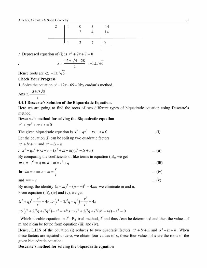
Algebra, Calculus & Solid Geometry 81
2 1 0 3 -14 2 4 14 1 2 7 0 ∴Depressed equation of (i) is 2 2 7 0x x+ + =
∴ 2 4 28 1 62
x i− ± −= = − ±
Hence roots are -2, 1 6i− ± . Check Your Progress 1. Solve the equation 3 12 65 0x x− − = by cardan’s method.
Ans 5 3 35,2i− ±
4.4.1 Descarte’s Solution of the Biquardatic Equation. Here we are going to find the roots of two different types of biquadratic equation using Descarte’s method. Descarte’s method for solving the Biquadratic equation
4 2 0x qx rx s+ + + =
The given biquadratic equation is 4 2 0x qx rx s+ + + = ... (i) Let the equation (i) can be split up two quadratic factors
2x lx m+ + and 2x lx n− + 4 2 2 2( )( )x qx rx s x lx m x lx n∴ + + + = + + − + ... (ii)
By comparing the coefficients of like terms in equation (ii),, we get 2 2m n l q n m l q+ − = ⇒ + = + ... (iii)
ln rlm r n ml
− = ⇒ − = ... (iv)
and mn s= ... (v) By using, the identity 2 2( ) ( ) 4n m n m mn+ − − = we eliminate m and n. From equation (iii), (iv) and (v), we get
( )2 2
2 2 4 2 22 2( ) 4 2 4r rl q s l l q q s
l l+ − = ⇒ + + − =
( )6 4 2 2 2 2 6 4 2 2 22 4 2 ( 4 ) 0l l q l q r l s l l q l q s r⇒ + + − = ⇒ + + − − =
Which is cubic equation in 2l . By trial method, 2l and thus l can be determined and then the values of m and n can be found from equation (iii) and (iv). Hence, L.H.S of the equation (i) reduces to two quadratic factors 2x lx m+ + and 2x lx n− + . When these factors are equated to zero, we obtain four values of x, these four values of x are the roots of the given biquadratic equation. Descarte’s method for solving the biquadratic equation
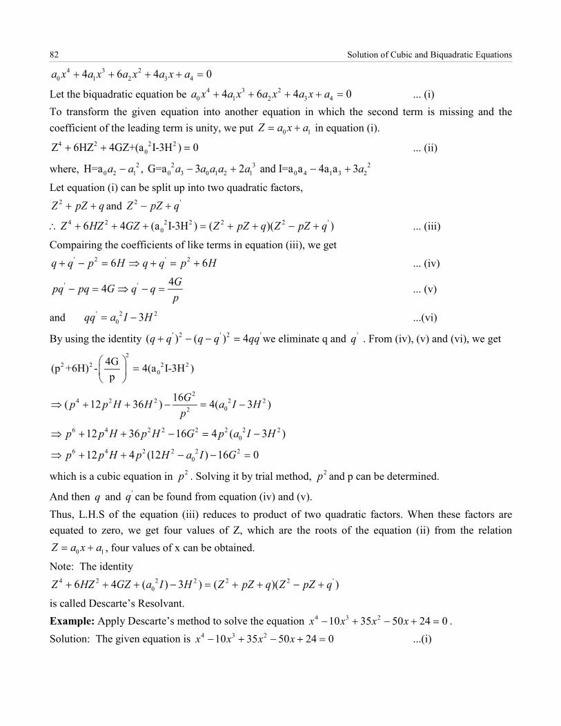
82 Solution of Cubic and Biquadratic Equations 4 3 2
0 1 2 3 44 6 4 0a x a x a x a x a+ + + + =
Let the biquadratic equation be 4 3 20 1 2 3 44 6 4 0a x a x a x a x a+ + + + = ... (i)
To transform the given equation into another equation in which the second term is missing and the coefficient of the leading term is unity, we put 0 1Z a x a= + in equation (i).
4 2 2 20Z 6HZ 4GZ+(a I-3H ) 0+ + = ... (ii)
where, 2 2 3 20 2 1 0 3 0 1 2 1 0 4 1 3 2H=a , G=a 3 2 and I=a a 4a a 3a a a a a a a a− − + − +
Let equation (i) can be split up into two quadratic factors, 2Z pZ q+ + and 2 'Z pZ q− +
4 2 2 2 2 2 '06 4 (a I-3H ) ( )( )Z HZ GZ Z pZ q Z pZ q∴ + + + = + + − + ... (iii)
Compairing the coefficients of like terms in equation (iii), we get ' 2 ' 26 6q q p H q q p H+ − = ⇒ + = + ... (iv)
' ' 44 Gpq pq G q qp
− = ⇒ − = ... (v)
and ' 2 20 3qq a I H= − ...(vi)
By using the identity ' 2 ' 2 '( ) ( ) 4q q q q qq+ − − = we eliminate q and 'q . From (iv), (v) and (vi), we get 2
2 2 2 20
4G(p +6H) - 4(a I-3H )p
=
24 2 2 2 2
02
16( 12 36 ) 4( 3 )Gp p H H a I Hp
⇒ + + − = −
6 4 2 2 2 2 2 2012 36 16 4 ( 3 )p p H p H G p a I H⇒ + + − = −
6 4 2 2 2 2012 4 (12 ) 16 0p p H p H a I G⇒ + + − − =
which is a cubic equation in 2p . Solving it by trial method, 2p and p can be determined.
And then q and 'q can be found from equation (iv) and (v). Thus, L.H.S of the equation (iii) reduces to product of two quadratic factors. When these factors are equated to zero, we get four values of Z, which are the roots of the equation (ii) from the relation
0 1Z a x a= + , four values of x can be obtained.
Note: The identity 4 2 2 2 2 2 '
06 4 ( ) 3 ) ( )( )Z HZ GZ a I H Z pZ q Z pZ q+ + + − = + + − + is called Descarte’s Resolvant. Example: Apply Descarte’s method to solve the equation 4 3 210 35 50 24 0x x x x− + − + = . Solution: The given equation is 4 3 210 35 50 24 0x x x x− + − + = ...(i)
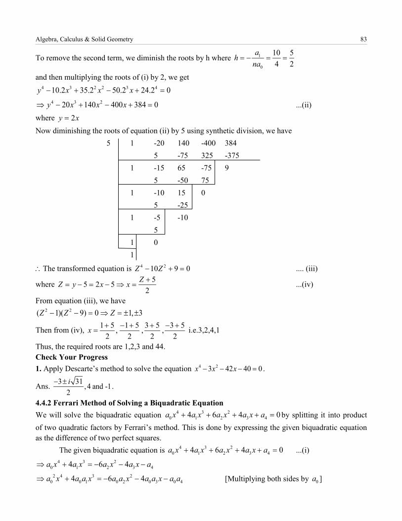
Algebra, Calculus & Solid Geometry 83
To remove the second term, we diminish the roots by h where 1
0
10 54 2
ah
na= − = =
and then multiplying the roots of (i) by 2, we get 4 3 2 2 3 410.2 35.2 50.2 24.2 0y x x x− + − + =
4 3 220 140 400 384 0y x x x⇒ − + − + = ...(ii) where 2y x= Now diminishing the roots of equation (ii) by 5 using synthetic division, we have 5 1 -20 140 -400 384 5 -75 325 -375 1 -15 65 -75 9 5 -50 75 1 -10 15 0 5 -25 1 -5 -10 5 1 0 1
∴The transformed equation is 4 210 9 0Z Z− + = .... (iii)
where 55 2 52
ZZ y x x += − = − ⇒ = ...(iv)
From equation (iii), we have 2 2( 1)( 9) 0 1, 3Z Z Z− − = ⇒ = ± ±
Then from (iv), 1 5 1 5 3 5 3 5, , ,2 2 2 2
x + − + + − += i.e.3,2,4,1
Thus, the required roots are 1,2,3 and 44. Check Your Progress 1. Apply Descarte’s method to solve the equation 4 23 42 40 0x x x− − − = .
Ans. 3 31 ,4 and -12i− ± .
4.4.2 Ferrari Method of Solving a Biquadratic Equation We will solve the biquadratic equation 4 3 2
0 1 2 3 44 6 4 0a x a x a x a x a+ + + + = by splitting it into product of two quadratic factors by Ferrari’s method. This is done by expressing the given biquadratic equation as the difference of two perfect squares. The given biquadratic equation is 4 3 2
0 1 2 3 44 6 4 0a x a x a x a x a+ + + + = ...(i) 4 3 2
0 1 2 3 44 6 4a x a x a x a x a⇒ + = − − − 2 4 3 2
0 0 1 0 2 0 3 0 44 6 4a x a a x a a x a a x a a⇒ + = − − − [Multiplying both sides by 0a ]
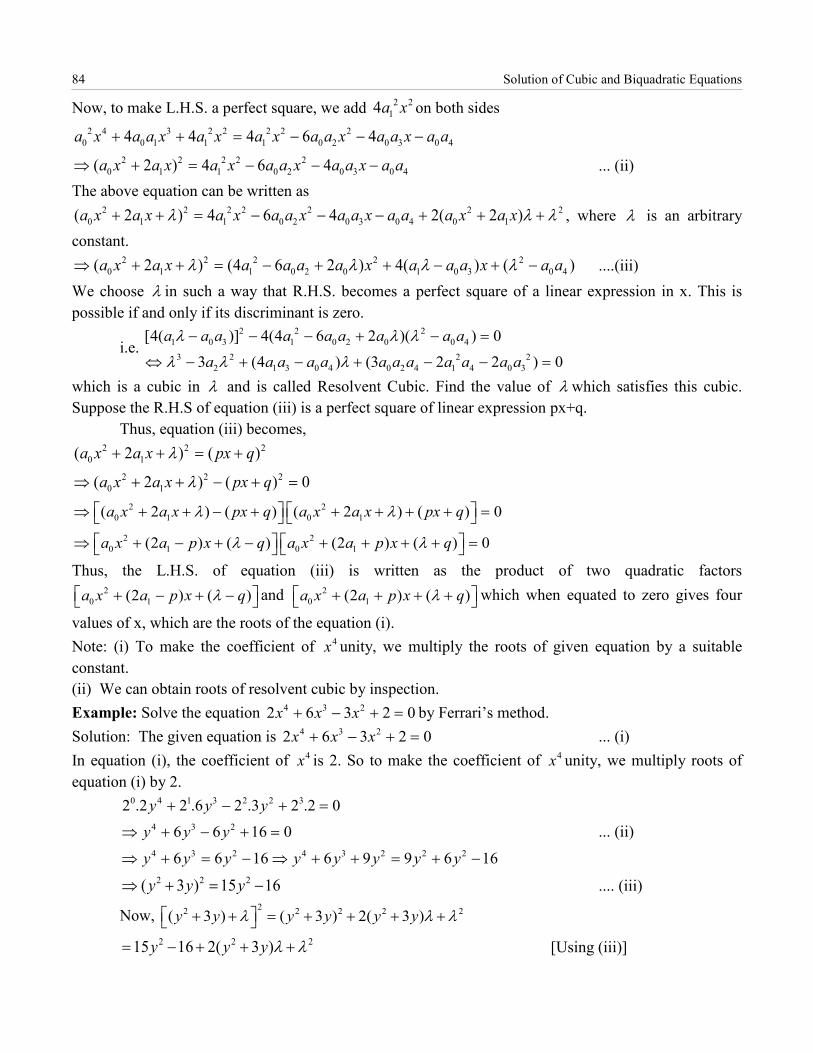
84 Solution of Cubic and Biquadratic Equations
Now, to make L.H.S. a perfect square, we add 2 214a x on both sides
2 4 3 2 2 2 2 20 0 1 1 1 0 2 0 3 0 44 4 4 6 4a x a a x a x a x a a x a a x a a+ + = − − −
2 2 2 2 20 1 1 0 2 0 3 0 4( 2 ) 4 6 4a x a x a x a a x a a x a a⇒ + = − − − ... (ii)
The above equation can be written as 2 2 2 2 2 2 2
0 1 1 0 2 0 3 0 4 0 1( 2 ) 4 6 4 2( 2 )a x a x a x a a x a a x a a a x a xλ λ λ+ + = − − − + + + , where λ is an arbitrary constant.
2 2 2 2 20 1 1 0 2 0 1 0 3 0 4( 2 ) (4 6 2 ) 4( ) ( )a x a x a a a a x a a a x a aλ λ λ λ⇒ + + = − + + − + − ....(iii)
We choose λ in such a way that R.H.S. becomes a perfect square of a linear expression in x. This is possible if and only if its discriminant is zero.
i.e. 2 2 2
1 0 3 1 0 2 0 0 43 2 2 2
2 1 3 0 4 0 2 4 1 4 0 3
[4( )] 4(4 6 2 )( ) 03 (4 ) (3 2 2 ) 0
a a a a a a a a aa a a a a a a a a a a a
λ λ λ
λ λ λ
− − − + − =
⇔ − + − + − − =
which is a cubic in λ and is called Resolvent Cubic. Find the value of λ which satisfies this cubic. Suppose the R.H.S of equation (iii) is a perfect square of linear expression px+q. Thus, equation (iii) becomes,
2 2 20 1( 2 ) ( )a x a x px qλ+ + = +
2 2 20 1( 2 ) ( ) 0a x a x px qλ⇒ + + − + =
2 20 1 0 1( 2 ) ( ) ( 2 ) ( ) 0a x a x px q a x a x px qλ λ ⇒ + + − + + + + + =
2 20 1 0 1(2 ) ( ) (2 ) ( ) 0a x a p x q a x a p x qλ λ ⇒ + − + − + + + + =
Thus, the L.H.S. of equation (iii) is written as the product of two quadratic factors 2
0 1(2 ) ( )a x a p x qλ + − + − and 20 1(2 ) ( )a x a p x qλ + + + + which when equated to zero gives four
values of x, which are the roots of the equation (i). Note: (i) To make the coefficient of 4x unity, we multiply the roots of given equation by a suitable constant. (ii) We can obtain roots of resolvent cubic by inspection. Example: Solve the equation 4 3 22 6 3 2 0x x x+ − + = by Ferrari’s method. Solution: The given equation is 4 3 22 6 3 2 0x x x+ − + = ... (i) In equation (i), the coefficient of 4x is 2. So to make the coefficient of 4x unity, we multiply roots of equation (i) by 2.
0 4 1 3 2 2 32 .2 2 .6 2 .3 2 .2 0y y y+ − + = 4 3 26 6 16 0y y y⇒ + − + = ... (ii) 4 3 2 4 3 2 2 26 6 16 6 9 9 6 16y y y y y y y y⇒ + = − ⇒ + + = + −
2 2 2( 3 ) 15 16y y y⇒ + = − .... (iii)
Now, 22 2 2 2 2( 3 ) ( 3 ) 2( 3 )y y y y y yλ λ λ + + = + + + +
2 2 215 16 2( 3 )y y y λ λ= − + + + [Using (iii)]
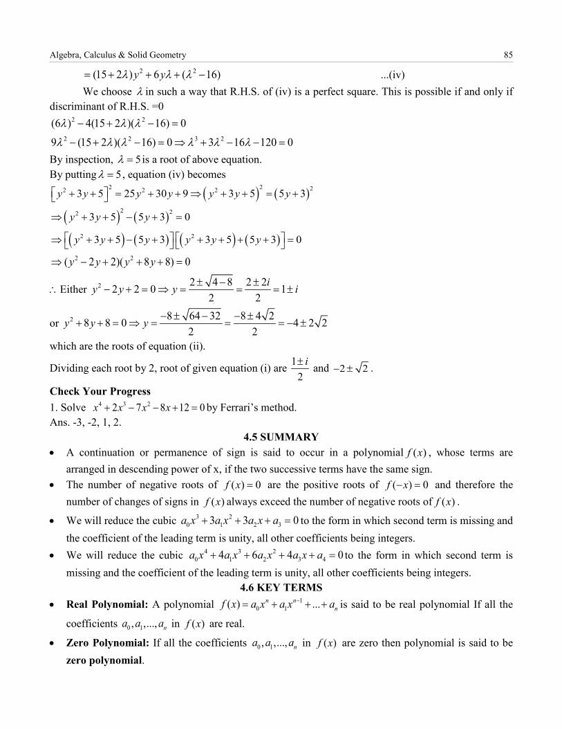
Algebra, Calculus & Solid Geometry 85 2 2(15 2 ) 6 ( 16)y yλ λ λ= + + + − ...(iv)
We choose λ in such a way that R.H.S. of (iv) is a perfect square. This is possible if and only if discriminant of R.H.S. =0
2 2(6 ) 4(15 2 )( 16) 0λ λ λ− + − = 2 2 3 29 (15 2 )( 16) 0 3 16 120 0λ λ λ λ λ λ− + − = ⇒ + − − =
By inspection, 5λ = is a root of above equation. By putting 5λ = , equation (iv) becomes
( ) ( )22 22 2 23 5 25 30 9 3 5 5 3y y y y y y y + + = + + ⇒ + + = +
( ) ( )2 22 3 5 5 3 0y y y⇒ + + − + =
( ) ( ) ( ) ( )2 23 5 5 3 3 5 5 3 0y y y y y y ⇒ + + − + + + + + = 2 2( 2 2)( 8 8) 0y y y y⇒ − + + + =
∴Either 2 2 4 8 2 22 2 0 12 2
iy y y i± − ±− + = ⇒ = = = ±
or 2 8 64 32 8 4 28 8 0 4 2 22 2
y y y − ± − − ±+ + = ⇒ = = = − ±
which are the roots of equation (ii).
Dividing each root by 2, root of given equation (i) are 12
i± and 2 2− ± .
Check Your Progress 1. Solve 4 3 22 7 8 12 0x x x x+ − − + = by Ferrari’s method. Ans. -3, -2, 1, 2.
4.5 SUMMARY • A continuation or permanence of sign is said to occur in a polynomial ( )f x , whose terms are
arranged in descending power of x, if the two successive terms have the same sign. • The number of negative roots of ( ) 0f x = are the positive roots of ( ) 0f x− = and therefore the
number of changes of signs in ( )f x always exceed the number of negative roots of ( )f x .
• We will reduce the cubic 3 20 1 2 33 3 0a x a x a x a+ + + = to the form in which second term is missing and
the coefficient of the leading term is unity, all other coefficients being integers. • We will reduce the cubic 4 3 2
0 1 2 3 44 6 4 0a x a x a x a x a+ + + + = to the form in which second term is missing and the coefficient of the leading term is unity, all other coefficients being integers.
4.6 KEY TERMS • Real Polynomial: A polynomial 1
0 1( ) ...n nnf x a x a x a−= + + + is said to be real polynomial If all the
coefficients 0 1, ,..., na a a in ( )f x are real.
• Zero Polynomial: If all the coefficients 0 1, ,..., na a a in ( )f x are zero then polynomial is said to be zero polynomial.
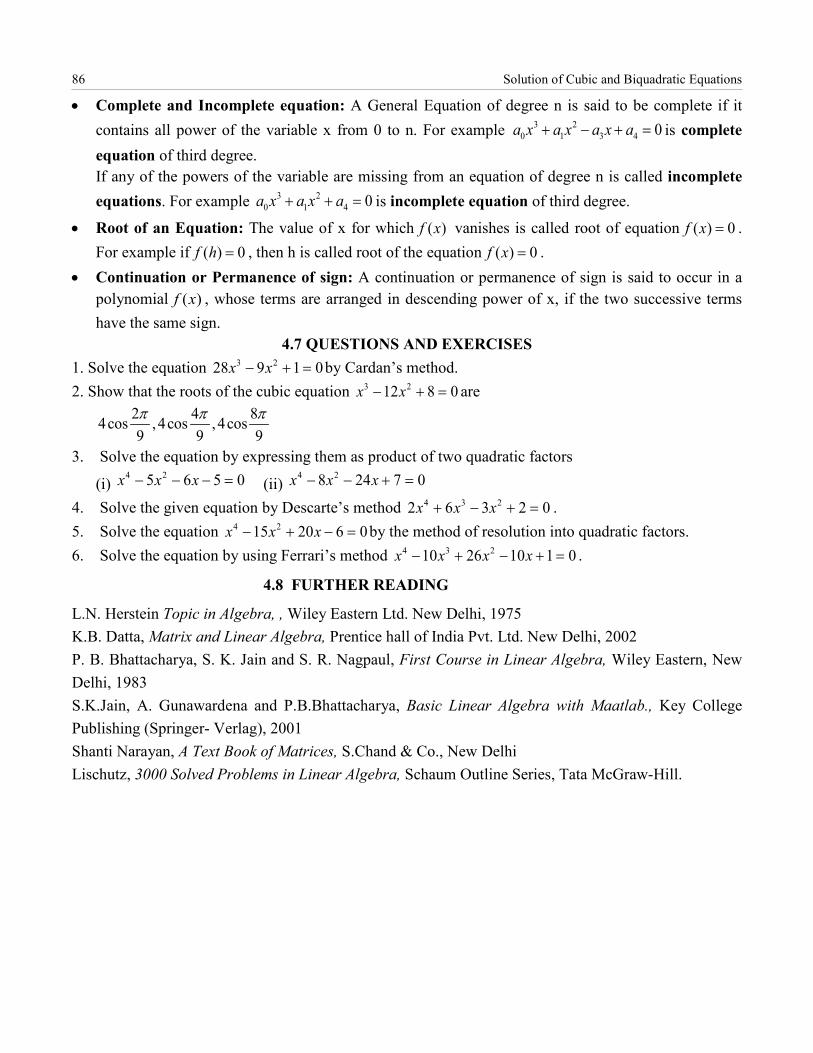
86 Solution of Cubic and Biquadratic Equations
• Complete and Incomplete equation: A General Equation of degree n is said to be complete if it contains all power of the variable x from 0 to n. For example 3 2
0 1 3 4 0a x a x a x a+ − + = is complete equation of third degree. If any of the powers of the variable are missing from an equation of degree n is called incomplete equations. For example 3 2
0 1 4 0a x a x a+ + = is incomplete equation of third degree.
• Root of an Equation: The value of x for which ( )f x vanishes is called root of equation ( ) 0f x = . For example if ( ) 0f h = , then h is called root of the equation ( ) 0f x = .
• Continuation or Permanence of sign: A continuation or permanence of sign is said to occur in a polynomial ( )f x , whose terms are arranged in descending power of x, if the two successive terms have the same sign.
4.7 QUESTIONS AND EXERCISES 1. Solve the equation 3 228 9 1 0x x− + = by Cardan’s method. 2. Show that the roots of the cubic equation 3 212 8 0x x− + = are
2 4 84cos ,4cos ,4cos9 9 9π π π
3. Solve the equation by expressing them as product of two quadratic factors
(i) 4 25 6 5 0x x x− − − = (ii)
4 28 24 7 0x x x− − + = 4. Solve the given equation by Descarte’s method 4 3 22 6 3 2 0x x x+ − + = . 5. Solve the equation 4 215 20 6 0x x x− + − = by the method of resolution into quadratic factors. 6. Solve the equation by using Ferrari’s method 4 3 210 26 10 1 0x x x x− + − + = .
4.8 FURTHER READING
L.N. Herstein Topic in Algebra, , Wiley Eastern Ltd. New Delhi, 1975 K.B. Datta, Matrix and Linear Algebra, Prentice hall of India Pvt. Ltd. New Delhi, 2002 P. B. Bhattacharya, S. K. Jain and S. R. Nagpaul, First Course in Linear Algebra, Wiley Eastern, New Delhi, 1983 S.K.Jain, A. Gunawardena and P.B.Bhattacharya, Basic Linear Algebra with Maatlab., Key College Publishing (Springer- Verlag), 2001 Shanti Narayan, A Text Book of Matrices, S.Chand & Co., New Delhi Lischutz, 3000 Solved Problems in Linear Algebra, Schaum Outline Series, Tata McGraw-Hill.
Related Documents


![[Thomas] Calculus and Analytic Geometry Ninth Edition](https://static.cupdf.com/doc/110x72/56d6be591a28ab301691bd9e/thomas-calculus-and-analytic-geometry-ninth-edition.jpg)


![Calculus with analytic geometry [Louis leithold]](https://static.cupdf.com/doc/110x72/557d0e89d8b42a8c2f8b5288/calculus-with-analytic-geometry-louis-leithold.jpg)