Alexander A Schekochihin and Steven C Cowley- Turbulence and Magnetic Fields in Astrophysical Plasmas

8/3/2019 Alexander A Schekochihin and Steven C Cowley- Turbulence and Magnetic Fields in Astrophysical Plasmas

http://slidepdf.com/reader/full/alexander-a-schekochihin-and-steven-c-cowley-turbulence-and-magnetic-fields 1/31

Magnetohydrodynamics — Historical Evolution and Trends

S. Molokov, R. Moreau and H. K. Moffatt, Eds.(Berlin: Springer 2007) pp. 85–115 [E-print: astro-ph/0507686 ]

Turbulence and Magnetic Fields in

Astrophysical Plasmas

Alexander A Schekochihin1 and Steven C Cowley2

1 DAMTP, University of Cambridge, Cambridge CB3 0WA and Department of Physics, Imperial College, London SW7 2BW, United Kingdom([email protected] )

2 Department of Physics and Astronomy, UCLA, Los Angeles, CA 90095-1547,

USA and Department of Physics, Imperial College, London SW7 2BW, UnitedKingdom ([email protected] )

1 Introduction

Magnetic fields permeate the Universe. They are found in planets, stars, accre-tion discs, galaxies, clusters of galaxies, and the intergalactic medium. Whilethere is often a component of the field that is spatially coherent at the scaleof the astrophysical object, the field lines are tangled chaotically and thereare magnetic fluctuations at scales that range over orders of magnitude. Thecause of this disorder is the turbulent state of the plasma in these systems.This plasma is, as a rule, highly conducting, so the magnetic field lines are en-trained by (frozen into) the fluid motion. As the fields are stretched and bent

by the turbulence, they can resist deformation by exerting the Lorentz forceon the plasma. The turbulent advection of the magnetic field and the field’sback reaction together give rise to the statistically steady state of fully devel-oped MHD turbulence. In this state, energy and momentum injected at large(object-size) scales are transfered to smaller scales and eventually dissipated.

Despite over fifty years of research and many major advances, a satisfactorytheory of MHD turbulence remains elusive. Indeed, even the simplest (mostidealised) cases are still not fully understood. One would hope that there areuniversal properties of MHD turbulence that hold in all applications — orat least in a class of applications. Among the most important questions forastrophysics that a successful theory of turbulence must answer are:

•How does the turbulence amplify, sustain and shape magnetic fields? What

is the structure and spectrum of this field at large and small scales? Theproblem of turbulence in astrophysics is thus directly related to the fun-damental problem of magnetogenesis.



2 Alexander A Schekochihin and Steven C Cowley

• How is energy cascaded and dissipated in plasma turbulence? In accretiondiscs and the solar corona, for example, one would like to know if theturbulence heats ions or electrons predominantly [52].

•How does the turbulent flow and magnetic field enhance or inhibit the

transport of heat, (angular) momentum, and cosmic rays? Again in accre-tion discs, a key parameter is the effective turbulent viscosity that causesthe transport of angular momentum and enables accretion [62]. In clusterphysics, an understanding of how viscous heating and thermal conductionin a turbulent magnetised plasma balance the radiative cooling is necessaryto explain the observed global temperature profiles [12].

In this chapter, we discuss the current understanding of the most basicproperties of astrophysical MHD turbulence. We emphasise possible universalaspects of the theory. We shall touch primarily on two applications: turbu-lence in the solar wind and in clusters of galaxies. These are, in a certain (veryapproximate) sense, two “pure” cases of small-scale turbulence, where theo-retical models of the two main regimes of MHD turbulence (discussed in

§2

and § 3) can be put to the test. They are also good examples of a complicationthat is more or less generic in astrophysical plasmas: the MHD description is,in fact, insufficient for astrophysical turbulence and plasma physics must makean entrance. Why this is so will be explained in § 4.

The astrophysical plasma turbulence is even more of a terra incognita thanthe MHD turbulence, so we shall start with the equations of incompressibleMHD — the simplest equations that describe (subsonic) turbulent dynamicsin a conducting medium:

du

dt= − p + ν ∆u + B ·B + f , · u = 0, (1)

dB

dt

= B

·u + η∆B, (2)

where u is the velocity field, d/dt = ∂ t + u · the convective derivative, p thepressure (scaled by the constant density ρ and determined by the incompress-ibility constraint), B the magnetic field scaled by (4πρ)1/2, ν the kinematicviscosity, η the magnetic diffusivity, and f the body force that models large-scale energy input. The specific energy injection mechanisms vary: typically,in astrophysics, these are either background gradients (e.g., the temperaturegradient in stellar convective zones, the Keplerian velocity shear in accretiondiscs), which mediate the conversion of gravitational energy into kinetic en-ergy of fluid motion, or direct sources of energy such as the supernovae in theinterstellar medium or active galactic nuclei in galaxy clusters. What all theseinjection mechanisms have in common is that the scale at which they oper-

ate, hereafter denoted by L, is large, comparable with the size of the system.While the large-scale dynamics depend on the specific astrophysical situation,it is common to assume that, once the energy has cascaded down to scalessubstantially smaller than L, the nonlinear dynamics are universal.



Turbulence and Magnetic Fields in Astrophysical Plasmas 3

The universality of small scales is a cornerstone of all theories of turbu-lence. It goes back to Kolmogorov’s 1941 dimensional theory (or K41 [33]; see[37], §33 for a lucid and concise exposition). Here is an outline Kolmogorov’sreasoning. Consider Eq. (1) without the magnetic term. Denote the typical

fluctuating velocity difference across scale L by δuL. The energy associatedwith these fluctuations is δu2

L and the characteristic time for this energy to cas-cade to smaller scales by nonlinear coupling is L/δuL. The total specific power(energy flux) going into the turbulent cascade is then = u · f ∼ δu3

L/L.In a statistically stationary situation, all this power must be dissipated, so = ν |u|2. Since is a finite quantity completely defined by the large-scaleenergy-injection process, it cannot depend on ν . For very small ν , this im-plies that the velocity must develop very small scales so that ν |u|2 hasa constant limit as ν → +0. The only quantity with dimensions of lengththat one can construct out of and ν is lν ∼ (ν 3/)1/4 ∼ Re−3/4L, whereRe ∼ δuLL/ν is the Reynolds number. In astrophysical applications, Re isusually large, so the viscous dissipation occurs at scales lν L. The energy

injected at the large scale L must be transfered to the small scale lν acrossa range of scales (the inertial range). The hydrodynamic turbulence theoryassumes that the physics in this range is universal, i.e., it depends neitheron the energy-injection mechanism nor on the dissipation mechanism. Fourfurther assumptions are made about the inertial range: homogeneity (nospecial points), scale invariance (no special scales), isotropy (no specialdirections), and locality of interactions (interactions between comparablescales dominate). Then, at each scale l such that L l lν , the total power must arrive from larger scales and be passed on to smaller scales:

∼ δu2l /τ l, (3)

where δul is the velocity difference across scale l and τ l the cascade time.

Dimensionally, only one time scale can be constructed out of the local quan-tities δul and l: τ l ∼ l/δul. Substituting this into Eq. (3) and solving for δul,we arrive at Kolmogorov’s scaling: δul ∼ (l)1/3, or, for the energy spectrumE (k),

δu2l ∼

∞k=1/l

dkE (k) ∼ 2/3k−2/3 ⇒ E (k) ∼ 2/3k−5/3. (4)

The history of the theory of MHD turbulence over the last half century hasbeen that of a succession of attempts to adapt the K41-style thinking to fluidscarrying magnetic fields. In the next two sections, we give an overview of theseefforts and of the resulting gradual realisation that the key assumptions of the small-scale universality, isotropy and locality of interactions fail in various

MHD contexts.




2 Alfvenic turbulence

Let us consider the case of a plasma threaded by a straight uniform magneticfield B0 of some external (i.e., large-scale) origin. Let us also consider weak

forcing so that the fundamental turbulent excitations are small-amplitudewave-like disturbances propagating along the mean field. We will refer to sucha limit as Alfvenic turbulence — it is manifestly anisotropic.

2.1 Iroshnikov–Kraichnan turbulence

If we split the magnetic field into the mean and fluctuating parts, B = B0+δB,and introduce Elsasser [14] variables z± = u ± δB, Eqs. (1) and (2) take asymmetric form:

∂ tz± vAz± + z ·z± = − p +ν + η

2∆z± +

ν − η

2∆z + f , (5)

where vA = |B0| is the Alfven speed and is the gradient in the direction of the mean field B0. The Elsasser equations have a simple exact solution: if z+ =0 or z− = 0, the nonlinear term vanishes and the other, non-zero, Elsasser fieldis simply a fluctuation of arbitrary shape and magnitude propagating alongthe mean field at the Alfven speed vA. Kraichnan [34] realised in 1965 thatthe Elsasser form of the MHD equations only allows nonlinear interactionsbetween counterpropagating such fluctuations. The phenomenological theorythat he and, independently, Iroshnikov [30], developed on the basis of thisidea (the IK theory) can be summarised as follows.

Following the general philosophy of K41, assume that only fluctuationsof comparable scales interact (locality of interactions) and consider theseinteractions in the inertial range, comprising scales l smaller than the forcingscale L and larger than the (still to be determined) dissipation scale. Let us

think of the fluctuations propagating in either direction as trains of spatiallylocalised Alfven-wave3 packets of parallel (to the mean field) extent l andperpendicular extent l (we shall not, for the time being, specify how l relates

to l). Assume further that δz+l ∼ δz−l ∼ δul ∼ δBl. We can again use Eq.(3) for the energy flux through scale l, but there is, unlike in the case of purely hydrodynamic turbulence, no longer a dimensional inevitability aboutthe determination of the cascade time τ l because two physical time scalesare associated with each wave packet: the Alfven time τ A(l) ∼ l/vA and thestrain (or “eddy”) time τ s(l) ∼ l/δul. To state this complication in a somewhatmore formal way, there are three dimensionless combinations in the problemof MHD turbulence: l/δu3l , δul/vA and l/l, so the dimensional analysis doesnot uniquely determine scalings and further physics input is needed.

3 Waves in incompressible MHD can have either the Alfven- or the slow-wave polar-isation. Since both propagate at the Alfven speed, we shall, for simplicity, referto them as Alfven waves. The differences between the Alfven- and slow-wavecascades are explained in detail at the end of § 2.4.




Two counterpropagating wave packets take an Alfven time to pass througheach other. During this time, the amplitude of either packet is changed by

∆δul

∼δu2

l

l

τ A

∼δul

τ A

τ s. (6)

The IK theory now assumes weak interactions, ∆δul δul ⇔ τ A τ s.The cascade time τ l is estimated as the time it takes (after many interactions)to change δul by an amount comparable to itself. If the changes in amplitudeaccumulate like a random walk, we have

t∆δul ∼ δul

τ Aτ s

t

τ A∼ δul for t ∼ τ l ⇒ τ l ∼ τ 2s

τ A∼ l2vA

lδu2l

. (7)

Substituting the latter formula into Eq. (3), we get

δul ∼ (vA)1/4l−1/4

l1/2. (8)

The final IK assumption, which at the time seemed reasonable in light of the

success of the K41 theory, was that of isotropy, fixing the dimensionless ratiol/l ∼ 1, and, therefore, the scaling:

δul ∼ (vA)1/4l1/4 ⇒ E (k) ∼ (vA)1/2k−3/2. (9)

2.2 Turbulence in the solar wind

The solar wind, famously predicted by Parker [50], was the first astrophysicalplasma in which direct measurements of turbulence became possible [11]. Ahost of subsequent observations (for a concise review, see [24]) revealed pow-erlike spectra of velocity and magnetic fluctuations in what is believed to bethe inertial range of scales extending roughly from 106 to 103 km. The meanmagnetic field is B0

∼10...102 µG, while the fluctuating part δB is a factor

of a few smaller. The velocity dispersion is δu ∼ 102 km/s, approximately inenergy equipartition with δB. The u and B fluctuations are highly correlatedat all scales and almost undoubtedly Alfvenic. It is, therefore, natural to thinkof the solar wind as a space laboratory conveniently at our disposal to testtheories of Alfvenic turbulence in astrophysical conditions.

For nearly 30 years following Kraichnan’s paper [34], the IK theory wasaccepted as the correct extension of K41 to MHD turbulence and, therefore,with minor modifications allowing for the observed imbalance between theenergies of the z+ and z− fluctuations [13], also to the turbulence in thesolar wind. However, alarm bells were sounding already in 1970s and 1980swhen measurements of the solar-wind turbulence revealed that it was stronglyanisotropic with l > l⊥ [3] (see also [43]) and that its spectral index was

closer to −5/3 than to −3/2 [42].4

Numerical simulations have confirmed theanisotropy of MHD turbulence in the presence of a strong mean field [40, 9, 46].

4 Another classic example of a −5/3 scaling in astrophysical turbulence is thespectrum of electron density fluctuations (thought to trace the velocity spectrum)




2.3 Weak turbulence

The realisation that the isotropy assumption must be abandoned led to areexamination of the Alfven-wave interactions in MHD turbulence. If the as-

sumption of weak interactions is kept, MHD turbulence can be regarded asan ensemble of waves, whose wavevectors k and frequencies ω±(k) = ±kvAhave to satisfy resonance conditions in order for an interaction to occur. Forthree-wave interactions (1 and 2 counterpropagating, giving rise to 3),

k1 + k2 = k3 ⇒ k1 + k2 = k3, (10)

ω±(k1) + ω(k2) = ω±(k3) ⇒ k1 − k2 = k3, (11)

whence k2 = 0 and k3 = k1. Thus (i) interactions do not change k; (ii)interactions are mediated by modes with k = 0, which are quasi-2D fluctua-tions rather than waves [45, 63, 47].5

The first of these conclusions suggests a quick fix of the IK theory: take

l ∼ k

−1

0 = const (the wavenumber at which the waves are launched) andl ∼ l⊥ in Eq. (8) (no parallel cascade). Then the spectrum is [23]

E (k⊥) ∼ (k0vA)1/2k−2⊥ . (12)

The same result can be obtained via a formal calculation based on the stan-dard weak-turbulence theory [20, 39]. However, it is not uniformly valid at allk⊥. Indeed, let us check if the assumption of weak interactions, τ A τ s, isactually satisfied by the scaling relation (8) with l ∼ k−10 :

τ Aτ s

∼ 1/4

k0vA

3/4l1/2⊥

1 ⇔ l⊥ l∗ =1/2

k0vA

3/2∼ δu2

L

v2A

1

k20L, (13)

where δuL is the velocity at the outer scale (the rms velocity). Thus, if Re =δuLL/ν and Rm = δuLL/η are large enough, the inertial range will alwayscontain a scale l∗ below which the interactions are no longer weak.6

in the interstellar medium — the famous “power law in the sky,” which appearsto hold across 12 decades of scales [1].

5 Goldreich & Sridhar [23] argued that the time it takes three waves to realise thatone of them has zero frequency is infinite and, therefore, the weak-interactionapproximation cannot be used. This difficulty can, in fact, be removed by noticingthat the k = 0 modes have a finite correlation time, but we do not have spaceto discuss this rather subtle issue here (two relevant references are [20, 39]).

6 There is also an upper limit to the scales at which Eq. (12) is applicable. Theboundary conditions at the ends of the “box” are unimportant only if the cascadetime (7) is shorter than the time it takes an Alfvenic fluctuation to cross the box:τ l L/vA ⇔ l⊥ L∗ = (/k0v3A)1/2L, where L is the length of the boxalong the mean field. Demanding that L∗ > L, the perpendicular size of the box,we get a lower limit on the aspect ratio of the box: L/L > k0L(vA/δuL)2. If this




2.4 Goldreich–Sridhar turbulence

In 1995, Goldreich & Sridhar [22] conjectured that the strong turbulence belowthe scale l∗ should satisfy

τ A ∼ τ s ⇔ l/l⊥ ∼ vA/δul, (14)

a property that has come to be known as the critical balance. Goldreich &Sridhar argued that when τ A τ s, the weak turbulence theory ”pushes” thespectrum towards the approximate equality (14). They also argued that whenτ A τ s, motions along the field lines are decorrelated and naturally developthe critical balance.

The critical balance fixes the relation between two of the three dimension-less combinations in MHD turbulence. Since now there is only one natural timescale associated with fluctuations at scale l, this time scale is now assumedto be the cascade time, τ l ∼ τ s. This brings back Kolmogorov’s spectrum (4)for the perpendicular cascade. The parallel cascade is now also present but is

weaker: from Eq. (14),

l ∼ vA−1/3l2/3⊥ ∼ k−10

l⊥/l∗

2/3. (15)

The scalings (4) and (15) should hold at all scales l⊥ l∗ and abovethe dissipation scale: either viscous lν ∼ (ν 3/)1/4 or resistive lη ∼ (η3/)1/4,whichever is larger. Comparing these scales with l∗ [Eq. (13)], we note that the

strong-turbulence range is non-empty only if Re,Rm k0L

3vA/δuL

3, a

condition that is effortlessly satisfied in most astrophysical cases but shouldbe kept in mind when numerical simulations are undertaken.

The Goldreich–Sridhar (GS) theory has now replaced the IK theory as thestandard accepted description of MHD turbulence. The feeling that the GS

theory is the right one, created by the solar wind [42] and ISM [1] observationsthat show a k−5/3 spectrum, is, however, somewhat spoiled by the consistentfailure of the numerical simulations to produce such a spectrum [40, 46]. In-stead, a spectral index closer to IK’s −3/2 is obtained (this seems to be themore pronounced the stronger the mean field), although the turbulence isdefinitely anisotropic and the GS relation (15) appears to be satisfied [40, 9]!This trouble has been blamed on intermittency [40], a perennial scapegoat of turbulence theory, but a non-speculative solution remains to be found.

The puzzling refusal of the numerical MHD turbulence to agree with ei-ther the GS theory or, indeed, with the solar-wind observations highlightsthe rather shaky quality of the existing physical understanding of what reallyhappens in a turbulent magnetic fluid on the dynamical level. One conceptual

is not satisfied, the physical (non-periodic) boundary conditions may impose alimit on the perpendicular field-line wander and thus effectively forbid the k = 0modes. It has been suggested [23] that a weak-turbulence theory based on 4-waveinteractions [65] should then be used at l⊥ > L∗.




R. S. Iroshnikov (1937-1991) R. H. Kraichnan

P. Goldreich S. Sridhar

Fig. 1. IK and GS (photo of R. S. Iroshnikov courtesy of Sternberg AstronomicalInstitute; photo of R. H. Kraichnan courtesy of the Johns Hopkins University).

difference between MHD and hydrodynamic turbulence is the possibility of long-time correlations. In the large-Rm limit, the magnetic field is determinedby the displacement of the plasma, i.e., the time integral of the (Lagrangian)velocity. In a stable plasma, the field-line tension tries to return the field lineto the unperturbed equilibrium position. Only “interchange” (k = 0) mo-tions of the entire field lines are not subject to this “spring-back” effect. Suchmotions are often ruled out by geometry or boundary conditions (cf. footnote6). Thus, fluid elements in MHD cannot simply random walk as this wouldincrease (without bound) the field-line tension. However, they may randomwalk for a substantial period before the tension returns them back to theequilibrium state. The role of such long-time correlations in MHD turbulenceis unknown.




Reduced MHD, the decoupling of the Alfven-wave cascade, and turbu-

lence in the interstellar medium. We now give a rigourous demonstration of how the turbulent cascade associated with the Alfven waves (or, more precisely,Alfven-wave-polarised fluctuations) decouples from the cascades of the slow waves

and entropy fluctuations. Let us start with the equations of compressible MHD:

dρ

dt= −ρ · u, (16)

ρdu

dt= −

„ p +

B2

8π

«+

B ·B

4π, (17)

ds

dt= 0, s =

p

ργ, γ =

5

3, (18)

dB

dt= B ·u − B · u. (19)

Consider a uniform static equilibrium with a straight magnetic field, so ρ = ρ0 + δρ, p = p0 + δp, B = B0 + δB. Based on observational and numerical evidence, itis safe to assume that the turbulence in such a system will be anisotropic with

k k⊥. Let us, therefore, introduce a small parameter ∼ k/k⊥ and carry outa systematic expansion of Eqs. (16)-(19) in . In this expansion, the fluctuationsare treated as small, but not arbitrarily so: in order to estimate their size, we shalladopt the critical-balance conjecture (14), which is now treated not as a detailedscaling prescription but as an ordering assumption. This allows us to introduce thefollowing ordering:

δρ

ρ0∼ u⊥

vA∼ u

vA∼ δp

p0∼ δB⊥

B0∼ δB

B0∼ k

k⊥∼ , (20)

where we have also assumed that the velocity and magnetic-field fluctuations havethe character of Alfven and slow waves (δB ∼ u) and that the relative amplitudes of the Alfven-wave-polarised fluctuations (u⊥/vA, δB⊥/B0), slow-wave-polarised fluc-tuations (u/vA, δB/B0) and density fluctuations (δρ/ρ0) are all the same order.7

We further assume that the characteristic frequency of the fluctuations is ω ∼ kvA,which means that the fast waves, for which ω k⊥p

v2A + c2s, where cs = γp0/ρ0 isthe sound speed, are ordered out.

We start by observing that the Alfven-wave-polarised fluctuations are two-dimensionally solenoidal: since · u = O(2) [from Eq. (16)] and · B = 0,separating the O() part of these divergences gives ⊥ · u⊥ = ⊥ · δB⊥ = 0. Wemay, therefore, express u⊥ and δB⊥ in terms of scalar stream (flux) functions:

u⊥ = b0 ×⊥φ,δB⊥√4πρ0

= b0 ×⊥ψ, (21)

where b0 = B0/B0. Evolution equations for φ and ψ are obtained by substitutingthe expressions (21) into the perpendicular parts of the induction equation (19) and

7 Strictly speaking, whether this is the case depends on the energy sources thatdrive the turbulence: as we are about to see, if no slow waves are launched, nonewill be present. However, it is safe to assume in astrophysical contexts that thelarge-scale energy input is random and, therefore, comparable power is injectedin all types of fluctuations.




the momentum equation (17) — of the latter the curl is taken to annihilate thepressure term. Keeping only the terms of the lowest order, O(2), we get

∂

∂t

ψ +

φ, ψ

= vA

φ, (22)

∂

∂t2⊥φ +

˘φ, 2

⊥φ¯

= vA2⊥ψ +

˘ψ, 2

⊥ψ¯

, (23)

where φ, ψ = b0 · (⊥φ ×⊥ψ) and, to lowest order,

d

dt=

∂

∂t+ u⊥ ·⊥ =

∂

∂t+ φ, · · · , (24)

B

B0· = +

δB⊥

B0·⊥ = +

1

vAψ, · · · . (25)

Eqs. (22) and (23) are known as the Reduced Magnetohydrodynamics (RMHD).They were first derived by Strauss [66] in the context of fusion plasmas. They forma closed set, meaning that the Alfven-wave cascade decouples from the slow wavesand density fluctuations.

In order to derive evolution equations for the latter, let us revisit the perpendic-ular part of the momentum equation and use Eq. (20) to order terms in it. In thelowest order, O(), we get the pressure balance

⊥

„δp +

B0δB

4π

«= 0 ⇒ δp

p0= −γ

v2Ac2s

δB

B0. (26)

Using Eq. (26) and the entropy equation (18), we get

d

dt

δs

s0= 0,

δs

s0=

δp

p0− γ

δρ

ρ0= −γ

„δρ

ρ0+

v2Ac2s

δB

B0

«, (27)

where s0 = p0/ργ0 . On the other hand, from the continuity equation (16) and theparallel component of the induction equation (19),

ddt

„δρρ0

− δB

B0

«+ B

B0·u = 0. (28)

Combining Eqs. (27) and (28), we obtain

d

dt

δρ

ρ0= − 1

1 + c2s/v2A

B

B0·u, (29)

dδB

dt=

1

1 + v2A/c2s

B

B0·u. (30)

Finally, we take the parallel component of the momentum equation (17) and noticethat, due to Eq. (26) and to the smallness of the parallel gradients, the pressureterm is O(3), while the inertial and tension terms are O(2). Therefore,

dudt

= v2A BB0

· δBB0

. (31)

Eqs. (30) and (31) describe the slow-wave-polarised fluctuations, while Eq. (27) de-scribes the zero-frequency entropy mode. The nonlinearity in these equations enters




via the derivatives defined in Eqs. (24)-(25) and is due solely to interactions withAlfven waves.

Naturally, the reduced equations derived above can be cast in the Elsasser form.If we introduce Elsasser potentials ζ ± = φ ± ψ, Eqs. (22) and (23) become

∂ ∂t

2⊥ζ ± vA2

⊥ζ ± = −12

ˆ˘ζ +, 2

⊥ζ −¯

+˘

ζ −, 2⊥ζ +

¯ 2⊥

˘ζ +, ζ −

¯˜. (32)

This is the same as the perpendicular part of Eq. (5) with z±⊥ = b0 ×⊥ζ ±. Thekey property that only counterpropagating Alfven waves interact is manifest here.For the slow-wave variables, we may introduce generalised Elsasser fields:

z± = u ± δB√4πρ0

„1 +

v2Ac2s

«1/2

. (33)

Straightforwardly, the evolution equation for these fields is

∂z±∂t

vAp 1 + v2A/c2s

z± = −1

2

1 1p

1 + v2A/c2s

!˘ζ +, z±

¯

−1

2

1 ±1p

1 + v2A/c2s

!˘ζ −, z±

¯. (34)

This equation reduces to the parallel part of Eq. (5) in the limit vA cs. Thisis known as the high-β limit, with the plasma beta defined by β = 8πp0/B2

0 =(2/γ )c2s/v2A. We see that only in this limit do the slow waves interact exclusivelywith the counterpropagating Alfven waves. For general β , the phase speed of theslow waves is smaller than that of the Alfven waves and, therefore, Alfven wavescan “catch up” and interact with the slow waves that travel in the same direction.

In astrophysical turbulence, β tends to be moderately high:8 for example, in theinterstellar medium, β ∼ 10 by order of magnitude. In the high-β limit, which isequivalent to the incompressible approximation for the slow waves, density fluctua-tions are due solely to the entropy mode. They decouple from the slow-wave cascadeand are passively mixed by the Alfven-wave turbulence: dδρ/dt = 0 [Eq. (27) or

Eq. (29), cs vA]. By a dimensional argument similar to K41, the spectrum of such a field is expected to follow the spectrum of the underlying turbulence [48]: in

the GS theory, k−5/3⊥ . It is precisely the electron-density spectrum (deduced from

observations of the scintillation of radio sources due to the scattering of radio wavesby the interstellar medium) that provides the evidence of the k−5/3 scaling in theinterstellar turbulence [1]. The explanation of this density spectrum in terms of pas-sive mixing of the entropy mode, originally conjectured by Higdon [28], is developedon the basis of the GS theory in Ref. [38].

Thus, the anisotropy and critical balance taken as ordering assumptions lead to a

neat decomposition of the MHD turbulent cascade into a decoupled Alfven-wave cas-

cade and cascades of slow waves and entropy fluctuations passively scattered/mixed

by the Alfven waves.9 The validity of this decomposition and, especially, of the

RMHD equations (22) and (23) turns out to extend to collisionless scales, where the

MHD equations (16)-(19) cannot be used: this will be briefly discussed in § 4.3.8 The solar corona, where β ∼ 10−6, is one prominent exception.9 Eqs. (27), (32) and (34) imply that, at arbitrary β , there are five conserved quan-

tities: I s = |δs|2 (entropy fluctuations), I ±⊥ = |ζ ±|2 (right/left-propagating




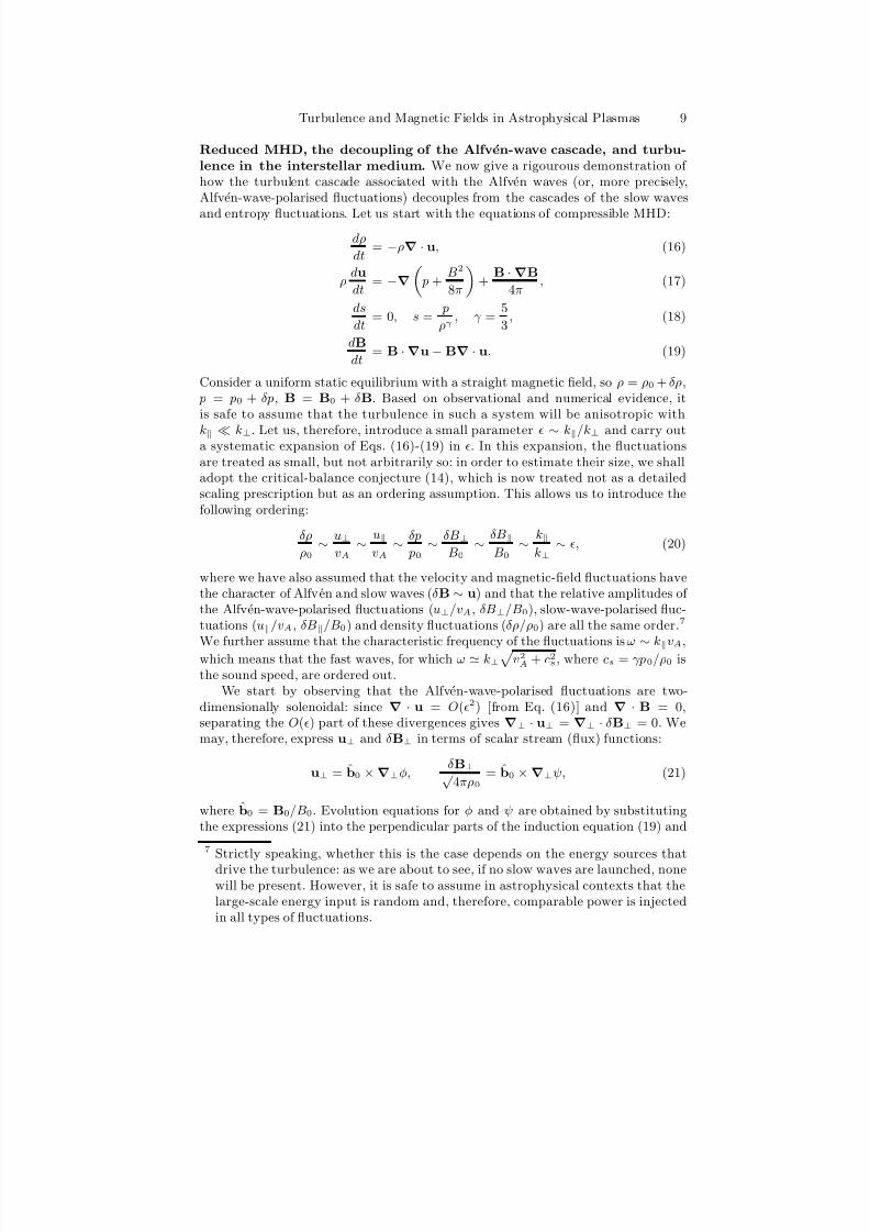
Fig. 2. Cross sections of the absolute values of u (left panel) and B (right panel)in the saturated state of a simulation with Re 100, P rm = 10 (run B of [57]).

3 Isotropic MHD turbulence

Let us now consider the case of isotropic MHD turbulence, i.e., a turbulentplasma where no mean field is imposed externally. Can the scaling theoriesreviewed above be adapted to this case? A popular view, due originally toKraichnan [34], is that everything remains the same with the role of the meanfield B0 now played by the magnetic fluctuations at the outer scale, δBL,while at smaller scales, the turbulence is again a local (in scale) cascade of Alfvenic (δul ∼ δBl) fluctuations. This picture is only plausible if the mag-netic energy is dominated by the outer-scale fluctuations, an assumption thatdoes not appear to hold in the numerical simulations of forced isotropic MHDturbulence [57]. Instead, the magnetic energy is concentrated at small scales,

where the magnetic fluctuations significantly exceed the velocity fluctuations,with no sign of the scale-by-scale equipartition implied for an Alfvenic cas-cade.10 These features are especially pronounced when the magnetic Prandtlnumber P rm = ν/η = Rm/Re 1, i.e., when the magnetic cutoff scale liesbelow the viscous cutoff of the velocity fluctuations (Fig. 2). The numericallymore accessible case of P rm 1, while non-asymptotic and, therefore, harder

Alfven waves), I ± = |z± |2 (right/left-propagating slow waves). I +⊥ and I −⊥ are

always cascaded by interaction with each other, I s is passively mixed by I +⊥ andI −⊥ , I ± are passively scattered by I ⊥ and, unless β 1, also by I ±⊥ .

10 This is true for the case of forced turbulence. Simulations of the decaying case [4]present a rather different picture: there is still no scale-by-scale equipartition butthe magnetic energy heavily dominates at the large scales — most likely due to alarge-scale force-free component controlling the decay. The difference between thenumerical results on the decaying and forced MHD turbulence points to anotherbreak down in universality in stark contrast with the basic similarity of the tworegimes in the hydrodynamic case.




to interpret, retains most of the features of the large-P rm regime. A handyformula for P rm based on the Spitzer [64] values of ν and η for fully ionisedplasmas is

P rm ∼ 10−5T 4/n, (35)

where T is the temperature in Kelvin and n the particle density in cm−3. Eq.(35) tends to give very large values for hot diffuse astrophysical plasmas: e.g.,1011 for the warm interstellar medium, 1029 for galaxy clusters.

Let us examine the situation in more detail. In the absence of a meanfield, all magnetic fields are generated and maintained by the turbulence itself,i.e., isotropic MHD turbulence is the saturated state of the turbulent (small-scale) dynamo. Therefore, we start by considering how a weak (dynamicallyunimportant) magnetic field is amplified by turbulence in a large-P rm MHDfluid and what kind of field can be produced this way.

3.1 Small-scale dynamo

Many specific deterministic flows have been studied numerically and analy-tically and shown to be dynamos [8]. While rigourously determining whetherany given flow is a dynamo is virtually always a formidable mathematicalchallenge, the combination of numerical and analytical experience of the lastfifty years suggests that smooth three-dimensional flows with chaotic trajec-tories tend to have the dynamo property provided the magnetic Reynoldsnumber exceeds a certain threshold, Rm > Rm,c ∼ 101...102. In particular,the ability of Kolmogorov turbulence to amplify magnetic fields is a solid nu-merical fact first established by Meneguzzi et al. in 1981 [44] and since thenconfirmed in many numerical studies with ever-increasing resolutions (mostrecently [57, 27]). It was, in fact, Batchelor who realised already in 1950 [2]

that the growth of magnetic fluctuations in a random flow should occur sim-ply as a consequence of the random stretching of the field lines and that itshould proceed at the rate of strain associated with the flow. In Kolmogorovturbulence, the largest rate of strain ∼ δul/l is associated with the smallestscale l ∼ lν — the viscous scale, so it is the viscous-scale motions that dom-inantly amplify the field (at large P rm). Note that the velocity field at theviscous scale is random but smooth, so the small-scale dynamo in Kolmogorovturbulence belongs to the same class as fast dynamos in smooth single-scaleflows [8, 57].

A repeated application of random stretching/shearing to a tangled mag-netic field produces direction reversals at arbitrarily small scales, giving riseto a folded field structure (Fig. 3). It is an essential property of this structure

that the strength of the field and the curvature of the field lines are anticor-related: wherever the field is growing it is relatively straight (i.e., curved onlyon the scale of the flow), whereas in the bending regions, where the curvatureis large, the field is weak. A quantitative theory of the folded structure can




Fig. 3. Stretching/shearing a magnetic-field line.

be constructed based on the joint statistics of the field strength B = |B| and

curvature K = b ·b, where b = B/B [55].11 The curvature is a quantityeasily measured in numerical simulations, which confirm the overall straight-ness of the field and the curvature–field-strength anticorrelation [57]. At theend of this section, we shall give a simple demonstration of the validity of the

folded structure.The scale of the direction reversals is limited from below only by Ohmicdiffusion: for Kolmogorov turbulence, balancing the rate of strain at the vis-cous scale with diffusion and taking P rm 1 gives the resistive cutoff lη:

δulν/lν ∼ η/l2η ⇒ lη ∼ P r−1/2m lν . (36)

If random stretching gives rise to magnetic fields with reversals at the re-sistive scale, why are these fields not eliminated by diffusion? In other words,how is the small-scale dynamo possible? It turns out that, in 3D, there aremagnetic-field configurations that can be stretched without being destroyedby the concurrent refinement of the reversal scale and that add up to give riseto exponential growth of the magnetic energy. Below we give an analytical

demonstration of this. It is a (somewhat modified) version of an ingenious ar-gument originally proposed by Zeldovich et al. in 1984 [71]. A reader lookingsolely for a broad qualitative picture of isotropic MHD turbulence may skipto § 3.2.

Overcoming diffusion. Let us study magnetic fields with reversals at subviscousscales: at these scales, the velocity field is smooth and can, therefore, be expanded

ui(t, x) = ui(t, 0) + σim(t)xm + . . . , (37)

where σim(t) is the rate-of-strain tensor. The expansion is around some reference

point x = 0. We can always go to the reference frame that moves with the velocity

11 This is not the only existing way of diagnosing the field structure. Ott and cowork-ers studied field reversals by measuring magnetic-flux cancellations [49]. Chertkovet al. [7] considered two-point correlation functions of the magnetic field in amodel of small-scale dynamo and found large-scale correlations along the fieldand short-scale correlations across.




Fig. 4. Ya. B. Zeldovich (1914-1987) (photo courtesy of M. Ya. Ovchinnikova).

at this point, so that ui(t, 0) = 0. Let us seek the solution to Eq. (2) with velocity(37) as a sum of random plane waves with time-dependent wave vectors:

Bi(t, x) =

Z d3k0(2π)3

Bi(t, k0)eik(t,k0)·x, (38)

where k(0, k0) = k0, so Bi(0, k0) = Bi0(k0) is the Fourier transform of the initial

field. Since Eq. (2) is linear, it is sufficient to ensure that each of the plane wavesis individually a solution. This leads to two ordinary differential equations for everyk0:

∂ tBi = σi

mBm

−ηk2Bi, ∂ tkl =

−σi

lki, (39)

subject to initial conditions Bi(0, k0) = Bi0(k0) and kl(0, k0) = k0l. The solution of

these equations can be written explicitly in terms of the Lagragian transformationof variables x0 → x(t, x0), where

∂ txi(t, x0) = ui(t, x(t, x0)) = σim(t)xm(t, x0), xi(0, x0) = xi

0. (40)

Because of the linearity of the velocity field, the strain tensor ∂xi/∂xm0 and its

inverse ∂xr0/∂xl are functions of time only. At t = 0, they are unit matrices. At

t > 0, they satisfy

∂ t∂xi

∂xm0

= σil

∂xl

∂xm0

, ∂ t∂xr

0

∂xl= −σi

l∂xr

∂xi0

. (41)

We can check by direct substitution that

Bi(t, k0) =∂xi

∂xm0

Bm0 (k0)exp

»−η

Z t0

dtk2(t)

–, kl(t, k0) =

∂xr0

∂xlk0r. (42)




These formulae express the evolution of one mode in the integral (38). Using thefact that det(∂xr

0/∂xl) = 1 in an incompressible flow and that Eq. (42) thereforeestablishes a one-to-one correspondence k ↔ k0, it is easy to prove that the volume-integrated magnetic energy is the sum of the energies of individual modes:

B2(t) ≡Z

d3x |B(t, x)|2 =

Z d3k0

(2π)3|B(t, k0)|2. (43)

From Eq. (42),

|B(t, k0)|2 = B0(k0) · M(t) · B∗0(k0)exp

»−2η

Z t0

dt k0 · M−1(t) · k0

–, (44)

where the matrices M and M−1 have elements defined by

M mn(t) =∂xi

∂xm0

∂xi

∂xn0

and M rs(t) =∂xr

0

∂xl

∂xs0

∂xl, (45)

respectively. They are the co- and contravariant metric tensors of the inverse La-

grangian transformation x → x0.Let us consider the simplest possible case of a flow (37) with constant σ =

diag λ1, λ2, λ3, where λ1 > λ2 ≥ 0 > λ3 and λ1 + λ2 + λ3 = 0 by incompressibility.Then M = diag

˘e2λ1t, e2λ2t, e2λ3t

¯and Eq. (44) becomes, in the limit t → ∞,

|B(t, k0)|2 ∼ |B10(k0)|2 exp

»2λ1t − η

„k201λ1

+k202λ2

+k203|λ3| e2|λ3|t

«–, (46)

where we have dropped terms that decay exponentially with time compared to thoseretained.12 We see that for most k0, the corresponding modes decay superexponen-tially fast with time. The domain in the k0 space containing modes that are notexponentially small at any given time t is given by

k201

λ21t/η

+k202

λ1λ2t/η

+k203

λ1|λ3|te2λ3t

/η

< const. (47)

The volume of this domain at time t is ∼ λ21(λ2|λ3|)1/2(t/η)3/2eλ3t. Within this

volume, |B(t, k0)|2 ∼ |B10(k0)|2e2λ1t. Using λ3 = −λ1 − λ2 and Eq. (43), we get

B2(t) ∝ exp [(λ1 − λ2)t] . (48)

Let us discuss the physics behind the Zeldovich et al. calculation sketched above.When the magnetic field is stretched by the flow, it naturally aligns with the stretch-ing Lyapunov direction: B ∼ e1B1

0eλ1t. The wave vector k has a tendency to alignwith the compression direction: k ∼ e3k03e|λ3|t, which makes most modes decaysuperexponentially. The only ones that survive are those whose k0’s were nearlyperpendicular to e3, with the permitted angular deviation from 90 decaying ex-ponentially in time ∼ e−|λ3|t. Since the magnetic field is solenoidal, B0 ⊥ k0, the

12 If λ2 = 0, k202/λ2 in Eq. (46) is replaced with 2k202t. The case λ2 < 0 is treated ina way similar to that described below and also leads to magnetic-energy growth.The difference is that for λ2 ≥ 0, the magnetic structures are flux sheets, orribbons, while for λ2 < 0, they are flux ropes.




Fig. 5. Magnetic fields vs. the Lyapunov directions (from [57]). Zeldovich et al.

[71] did not give this exact interpretation of their calculation because the foldedstructure of the field was not yet clearly understood at the time.

modes that get stretched the most have B0 e1 and k0 e2 (Fig. 5). In contrast,in 2D, the field aligns with e1 and must, therefore, reverse along e2, which is alwaysthe compression direction (Fig. 5), so the stretching is always overwhelmed by thediffusion and no dynamo is possible (as should be the case according to the rigourousearly result of Zeldovich [70]).

The above construction can be generalised to time-dependent and random ve-locity fields. The matrix M is symmetric and can, therefore, be diagonalised byan appropriate rotation R of the coordinate system: M = R

T · L · R, where, by

definition, L = diagn

eζ1(t), eζ2(t), eζ3(t)o

. It is possible to prove that, as t → ∞,

R(t) → e1, e2, e3 and ζ i(t)/2t → λi, where ei are constant orthogonal unit vec-tors, which make up the Lyapunov basis, and λi are the Lyapunov exponents of the flow [21]. The instantaneous values of ζ i(t)/2t are called finite-time Lyapunov

exponents. For a random flow, ζ i(t) are random functions. Eq. (48) generalises to

B2(t) ∝ exp [(ζ 1 − ζ 2)/2], (49)

where the overline means averaging over the distribution of ζ i. The only randomflow for which this distribution is known is a Gaussian white-in-time velocity firstconsidered in the dynamo context in 1967 by Kazantsev [31].13 The distribution of ζ i for this flow is Gaussian in the long-time limit and Eq. (49) gives B2 ∝ e(5/4)λ1t,where λ1 = ζ 1/2t [7]. For Kazantsev’s velocity, it is also possible to calculate themagnetic-energy spectrum [31, 36], which is the spectrum of the direction reversals.

13 As the only analytically solvable model of random advection, Kazantsev’s modelhas played a crucial role. Developed extensively in 1980s by Zeldovich and cowork-ers [72], the model became a tool of choice in the theories of anomalous scalingand intermittency that flourished in 1990s [16] (in this context, it has been associ-ated with the name of Kraichnan who, independently from Kazantsev, proposedto use it for the passive scalar problem [35]). It remains useful to this day as oldtheories are reevaluated and new questions demand analytical answers [55].




It has a peak at the resistive scale and a k+3/2 power law stretching across the sub-viscous range, l−1ν k l−1η . This scaling appears to be corroborated by numericalsimulations [57, 27].

Folded structure revisited. We shall now give a very simple demonstration thatlinear stretching does indeed produce folded fields with straight/curved field linescorresponding to larger/smaller field strength. Using Eq. (2), we can write evolutionequations for the field strength B = |B|, the field direction b = B/B and thefield-line curvature K = b ·b. Omitting the resistive terms,

dB

dt=`

bb :u´

B, (50)

db

dt= b · ù

´ · Ì− bb´

, (51)

dK

dt= K · ù

´ · Ì− bb´− 2(bb :u)K − ˆ

b · ù´ · K

˜b

+bb :

ù

´·Ì− bb

´. (52)

For simplicity, we again use the velocity field (37) with constant σ = diag λ1, λ2, λ3.Then the stable fixed point of Eq. (51) in the comoving frame is b = e1 (magneticfield aligns with the principal stretching direction), whence B ∝ eλ1t. Since K·b = 0,we set K 1 = 0. Denoting Σ = bb :u, we can now write Eq. (52) as

dK 2dt

= −`2λ1 − λ2

´K 2 + Σ 2,

dK 3dt

= −`3λ1 + λ2

´K 3 + Σ 3. (53)

Both components of K decay exponentially,14 until they are comparable to theinverse scale of the velocity field (i.e., the terms containingu become important).The stationary solution is K 2 = Σ 2/(2λ1 − λ2), K 3 = Σ 3/(3λ1 + λ2).

If the field is to reverse direction, it must turn somewhere (see Fig. 3). At sucha turning point, the field must be perpendicular to the stretching direction. Settingb1 = 0, we find two fixed points of Eq. (51) under this condition: b = e2 and b = e3.

Only the former is stable, so the field at the turning point will tend to align with the“null” direction. Thus, stretching favours configurations with field reversals alongthe “null” direction, which are also those that survive diffusion (see Fig. 5). FromEq. (52) we find that at the turning point, K 2 = 0, K 3 = Σ 3/(λ1 + 3λ2), while K 1grows at the rate λ1 − 2λ2 (assumed positive). This growth continues until limitedby diffusion at K ∼ 1/lη. The strength of the field in this curved region is ∝ eλ2t,so the fields are weaker than in the straight segments, where B ∝ eλ1t.

When the problem is solved for the Kazantsev velocity, the above solution gener-

alises to a field of random curvatures anticorrelated with the magnetic-field strength

and with a stationary PDF of K that has a peak at K ∼ flow scale−1 and a power

tail ∼ K −13/7 describing the distribution of curvatures at the turning points [55].

Numerical simulations support these results [57].

14 K 3 decays faster than K 2. If the velocity is exactly linear (Σ = 0), K alignswith e2 and decreases indefinitely, while the combination BK 1/(2−λ2/λ1) staysconstant. This rhymes with the result that can be proven for a linear Kazantsevvelocity: at zero η, B ∝ eζ1/2, while BK 1/2 ∝ eζ2/4 and λ2 = ζ 2/2t = 0.




G. K. Batchelor (1920-2000)

A. Schluter L. Biermann (1907-1986)

Fig. 6. Photo of A. Schluter courtesy of MPI fur Plasmaphysik; photo of L. Bier-mann courtesy of Max-Planck-Gesellschaft/AIP Emilio Segre Visual Archives.

3.2 Saturation of the dynamo

The small-scale dynamo gave us exponentially growing magnetic fields withenergy concentrated at small (resistive) scales. How is the growth of magneticenergy saturated and what is the final state? Will magnetic energy stay at

small scales or will it proceed to scale-by-scale equipartition via some formof inverse cascade? This basic dichotomy dates back to the 1950 papers byBatchelor [2] and Schluter & Biermann [60]. Batchelor thought that magneticfield was basically analogous to the vorticity field ω =× u (which satisfies




the same equation (2) except for the difference between η and ν ) and would,

therefore, saturate at a low energy, B2 ∼ Re−1/2u2, with a spectrumpeaked at the viscous scale. Schluter and Biermann disagreed and argued thatthe saturated state would be a scale-by-scale balance between the Lorentz and

inertial forces, with turbulent motions at each scale giving rise to magneticfluctuations of matching energy at the same scale. Schluter and Biermann’sargument (and, implicitly, also Batchelor’s) was based on the assumption of locality of interaction (in scale space) between the magnetic and velocityfields: locality both of the dynamo action and of the back reaction. As wesaw in the previous section, this assumption is certainly incorrect for thedynamo: a linear velocity field, i.e., a velocity field of a formally infinitely large(in practice, viscous) scale can produce magnetic fields with reversals at thesmallest scale allowed by diffusion. A key implication of the folded structureof these fields concerns the Lorentz force, the essential part of which, in thecase of incompressible flow, is the curvature force B2K. Since it is a quantitythat depends only on the parallel gradient of the magnetic field and does not

know about direction reversals, it will possess a degree of velocity-scale spatialcoherence necessary to oppose stretching. Thus, a field that is formally at theresistive scale will exert a back reaction at the scale of the velocity field. Inother words, interactions are nonlocal: a random flow at a given scale l,having amplified the magnetic fields at the resistive scale lη l, will seethese magnetic fields back react at the scale l. Given the nonlocality of backreaction, we can update Batchelor’s and Schluter & Biermann’s scenarios forsaturation in the following way [56, 57].

The magnetic energy is amplified by the viscous-scale motions until thefield is strong enough to resist stretching, i.e., until B·B ∼ u·u ∼ δu2

lν/lν .

Since B ·B ∼ B2K ∼ B2/lν (folded field), this happens when

B2

∼δu2

lν

∼Re−1/2

u2

. (54)

Let us suppose that the viscous motions are suppressed by the back reaction,at least in their ability to amplify the field. Then the motions at larger scales inthe inertial range come into play: while their rates of strain and, therefore, theassociated stretching rates are smaller than that of the viscous-scale motions,they are more energetic [see Eq. (4)], so the magnetic field is too weak to resistbeing stretched by them. As the field continues to grow, it will suppress themotions at ever larger scales. If we define a stretching scale ls(t) as the scaleof the motions whose energy is δuls ∼ B2(t), we can estimate

d

dtB2 ∼ δuls

lsB2 ∼ δu3

ls

ls∼ = const ⇒ B2(t) ∼ t. (55)

Thus, exponential growth gives way to secular growth of the magnetic en-ergy. This is accompanied by elongation of the folds (their length is always of the order of the stretching scale, l ∼ ls), while the resistive (reversal) scaleincreases because the stretching rate goes down:




l(t) ∼ ls(t) ∼ δu3ls/ ∼ √

t3/2, lη(t) ∼ [η/(δuls/ls)]1/2 ∼ √

ηt. (56)

This secular stage can continue until the entire inertial range is suppressed,ls

∼L, at which point saturation must occur. This happens after t

∼−1/3L2/3 ∼ L/δuL. Using Eqs. (55)-(56), we have, in saturation,

B2 ∼ u2, l ∼ L, lη ∼ [η/(δuL/L)]1/2 ∼ R−1/2

m L. (57)

Comparing Eqs. (57) and (36), we see that the resistive scale has increased only

by a factor of Re1/4 over its value in the weak-field growth stage. Note that thisimposes a very stringent requirement on any numerical experiment strivingto distinguish between the viscous and resistive scales: P rm Re1/2 1.

If, as in the above scenario, the magnetic field retains its folded struc-ture in saturation, with direction reversals at the resistive scale, this explainsqualitatively why the numerical simulations of the developed isotropic MHDturbulence with P rm ≥ 1 [57] show the magnetic-energy pile-up at the smallscales. What then is the saturated state of the turbulent velocity field? We as-sumed above that the inertial-range motions were “suppressed” — this appliedto their ability to amplify magnetic field, but needed not imply a completeevacuation of the inertial range. Indeed, simulations at modest P rm show apowerlike velocity spectrum [57, 27]. The most obvious class of motions thatcan populate the inertial range without affecting the magnetic-field strengthare a type of Alfven waves that propagate not along a mean (or large-scale)magnetic field but along the folded structure (Fig. 7). Mathematically, thedispersion relation for such waves is derived via a linear theory carried outfor the inertial-range perturbations (L−1 k l−1ν ) of the tensor BiBj (cf.[26]). The unperturbed state is the average of this tensor over the subviscous

scales: BiBj = bibjB2, where B2 is the total magnetic energy and the

tensor bibj only varies at the outer scale L [Eq. (57)]. The resulting disper-

sion relation is ω = ±|k · b|B21/2 [56]. The presence of these waves will notchange the resistive-scale-dominated nature of the magnetic-energy spectrum,but should be manifest in the kinetic-energy spectrum. There is, at present,no theory of a cascade of such waves, although a line of argument similar to § 2might work, since it does not depend on the field having a specific direction.A numerical detection of these waves is also a challenge for the future.

What we have proposed above can be thought of as a modernised ver-sion of the Schluter & Biermann scenario, retaining the intermediate secular-growth stage and saturation with B2 ∼ u2, but not scale-by-scale equipar-tition. However, an alternative possibility, which is in a similar relationshipto Batchelor’s scenario, can also be envisioned. In Eqs. (55)-(56), the scale lηat which diffusion cuts off the small-scale magnetic fluctuations was assumed

to be determined by the stretching rate δuls/ls. However, since the nonlinearsuppression of the viscous-scale eddies only needs to eliminate motions withbb :u = 0 [Eq. (50)], two-dimensional “interchange” motions (velocity gra-

dients ⊥ b) are, in principle, allowed to survive at the viscous scale. These




Fig. 7. Alfven waves propagating along folded fields (from [56]).

could “two-dimensionally” mix the direction-reversing magnetic fields at therate δulν/lν — much faster than the unsuppressed larger-scale stretching canamplify the field, — with the consequence that the resistive scale is pinnedat the value given by Eq. (36) and the field cannot grow above the Batch-elor limit (54). The mixing efficiency of the suppressed motions is the keyto choosing between the two saturation scenarios. Numerical simulations [57]

corroborate the existence of an intermediate stage of slower-than-exponentialgrowth accompanied by fold elongation and a modest increase of the resistivescale [Eq. (56)]. This tips the scales in favour of the first scenario, but, in viewof limited resolutions, we hesitate to declare the matter definitively resolved.

3.3 Turbulence and magnetic fields in galaxy clusters

The intracluster medium (hereafter, ICM) is a hot (T ∼ 108 K) diffuse(n ∼ 10−2...10−3 cm−3) fully ionised plasma, which accounts for most of theluminous matter in the Universe (note that it is not entirely dissimilar fromthe ionised phases of the interstellar medium: e.g., the so-called hot ISM).It is a natural astrophysical environment to which the large-P rm isotropicregime of MHD turbulence appears to be applicable: indeed, Eq. (35) givesP rm ∼ 1029.

The ICM is believed to be in a state of turbulence driven by a varietyof mechanisms: merger events, galactic and subcluster wakes, active galac-tic nuclei. One expects the outer scale L ∼ 102...103 kpc and the velocitydispersions δuL ∼ 102...103 km/s (a fraction of the sound speed). Indirectobservational evidence supporting the possibility of a turbulent ICM withroughly these parameters already exists (an apparently powerlike spectrumof pressure fluctuations found in the Coma cluster [61], broadened abundanceprofiles in Perseus believed to be caused by turbulent diffusion [53]), and di-rect detection may be achieved in the near future [29]. However, there is asyet no consensus on whether turbulence, at least in the usual hydrodynamicsense, is a generic feature of clusters [15]. The main difficulty is the very large

values of the ICM viscosity obtained via the standard estimate ν ∼ vth,iλmfp,where vth,i ∼ 103 km/s is the ion thermal speed and λmfp ∼ 1...10 kpc is theion mean free path. This gives Re ∼ 102 if not less, which makes the exis-tence of a well-developed inertial range problematic. Postponing the problem




of viscosity until § 4, we observe that the small-scale dynamo does not, infact, require a turbulent velocity field in the sense of a broad inertial range:in the weak-field regime discussed in § 3.1, the dynamo was controlled by thesmooth single-scale random flow associated with the viscous-scale motions;

in saturation, we argued in § 3.2 that the main effect was the direct nonlocalinteraction between the outer-scale (random) motions and the magnetic field.Given the available menu of large-scale stirring mechanisms in clusters, it islikely that, whatever the value of Re, the velocity field is random.15

The cluster turbulence is certainly magnetic. The presence of magneticfields was first demonstrated for the Coma cluster, for which Willson detectedin 1970 a diffuse synchrotron radio emission [69] and Kim et al. in 1990 wereable to estimate directly the magnetic-field strength and scale using the Fara-day rotation measure (RM) data [32]. Such observations of magnetic fields inclusters have now become a vibrant area of astronomy (reviewed most recentlyin [25]), usually reporting a field B ∼ 1...10 µG at scales ∼ 1...10 kpc [10].16

All of this field is small-scale fluctuations: no appreciable mean component

has been detected. The field is dynamically significant: the magnetic energyis less but not much less than the kinetic energy of the turbulent motions.Do clusters fit the theoretical expectations reviewed above? The magnetic-

field scale seen in clusters is usually 10 to 100 times smaller than the expectedouter scale of turbulent motions and, indeed, is also smaller than the viscousscale based on Re ∼ 102. However, it is certainly far above the resistive scale,which turns out be lη ∼ 103...104 km! Faced with these numbers, we mustsuspend the discussion of cluster physics and finally take account of the factthat astrophysical bodies are made of plasma, not of an MHD fluid.

4 Enter plasma physics

4.1 Braginskii viscosity

In all of the above, we have used the MHD equations (1) and (2) to developturbulence theories supposed to be relevant for astrophysical plasmas. His-torically, such has been the approach followed in most of the astrophysicalliterature. The philosophy underpinning this approach is again that of univer-sality: the “microphysics” at and below the dissipation scale are not expectedto matter for the fluid-like dynamics at larger scales. However, in consideringthe MHD turbulence with large P rm, we saw that dissipation scales, deter-mined by the values of the viscosity ν and magnetic diffusivity η, played a

15 Numerical simulations of the large-P rm regime at currently accessible resolutionsalso rely on a random forcing to produce “turbulence” with Re ∼ 1...102 [57, 27].

16 Because of the availability of the RM maps from extended radio sources in clus-ters, it is possible to go beyond field-strength and scale estimates and constructmagnetic-energy spectra with spatial resolution of ∼ 0.1 kpc [68].




very prominent role: the growth of the small-scale magnetic fields was con-trolled by the turbulent rate of strain at the viscous scale and resulted in themagnetic energy piling up, in the form of direction-reversing folded fields, atthe resistive scale — both in the growth and saturation stages of the dynamo.

It is then natural to revisit the question of whether the Laplacian diffusionterms in Eqs. (1)-(2) are a good description of the dissipation in astrophysicalplasmas.

The answer to this question is, of course, that they are not. A necessaryassumption in the derivation of these terms is that the ion cyclotron frequencyΩi = eB/mic exceeds the ion-ion collision frequency ν ii or, equivalently, theion gyroradius ρi = vth,i/Ωi exceeds the mean free path λmfp = vth,i/ν ii. Thisis patently not the case in many astrophysical plasmas: for example, in galaxyclusters, λmfp ∼ 1...10 kpc, while ρi ∼ 104 km. In such a weakly collisionalmagnetised plasma, the momentum equation (1) assumes the following form,valid at spatial scales ρi and at time scales Ω−1

i ,

du

dt = − p⊥ +

B2

2

+ · bb( p⊥ − p + B2

)

+ f , (58)

where p⊥ and p are plasma pressures perpendicular and parallel to the localdirection of the magnetic field, respectively, and we have used B · B = · (bbB2). The evolution of the magnetic field is controlled by the electrons— the field remains frozen into the flow and we may use Eq. (2) with η = 0.

If we are interested in subsonic motions, ( p⊥ + B2/2) in Eq. (58) can befound from the incompressibility condition · u = 0 and the only quantitystill to be determined is p⊥− p. The proper way to compute it is by a ratherlengthy kinetic calculation due to Braginskii [5], which cannot be repeatedhere. The result of this calculation can, however, be obtained in the followingheuristic way [58].

The fundamental property of charged particles moving in a magnetic fieldis the conservation of the first adiabatic invariant µ = miv2⊥/2B.17 Whenλmfp ρi, this conservation is only weakly broken by collisions. As long as µis conserved, any change in B must be accompanied by a proportional changein p⊥. Thus, the emergence of the pressure anisotropy is a natural consequenceof the changes in the magnetic-field strength and vice versa: indeed, summingup the first adiabatic invariants of all particles, we get p⊥/B = const. Then

1

p⊥

dp⊥dt

=1

B

dB

dt− ν ii

p⊥ − p p⊥

, (59)

where the second term on the right-hand sight represents the collisional relax-ation of the pressure anisotropy p⊥ − p at the rate ν ii ∼ vth,i/λmfp.18 UsingEq. (50) for B and balancing the terms in the rhs of Eq. (59), we get

17 It may be helpful to the reader to think of this property as the conservation of the angular momentum of a gyrating particle: miv⊥ρi ∝ miv

2⊥/B = 2µ.

18 This is only valid if the characteristic parallel scales k−1 of all fields are larger thanλmfp. In the collisionless regime, kλmfp 1, we may assume that the pressure




p⊥ − p = ν 1

B

dB

dt= ν bb :u, (60)

where ν ∼ p/ν ii ∼ vth,iλmfp is the “parallel viscosity.” This equation turns

out to be exact [5] up to numerical prefactors in the definition of ν .The energy conservation law based on Eqs. (58) and (2) is

d

dt

u22

+B2

2

= − ν

|bb :u|2 = − ν

1

B

dB

dt

2

, (61)

where Ohmic diffusion has been omitted. Thus, the Braginskii viscosity onlydissipates such velocity gradients that change the strength of the magneticfield. The motions that do not affect B are allowed to exist in the subviscousscale range. In the weak-field regime, these motions take the form of plasmainstabilities. When the magnetic field is strong, a cascade of shear-Alfvenwaves can be set up below the viscous scale. Let us elaborate.

4.2 Plasma instabilities

The simplest way to see that the pressure anisotropy in Eq. (58) leads toinstabilities is as follows [58]. Imagine a “fluid” solution with u, p⊥, p, B

changing on viscous time and spatial scales, t ∼ |u|−1 ∼ lν/δulν and l ∼ lν .Would such a solution be stable with respect to fast (ω |u|−1) small-scale(k l−1ν ) perturbations? Linearising Eq. (58) and denoting perturbations byδ, we get

−iωδu = −ik (δp⊥ + BδB) + p⊥ − p + B2

δK

+ ib k

δp⊥ − δp −

p⊥ − p − B2

δB/B

, (62)

where the perturbation of the field curvature is δK = k2δu⊥/iω [see Eq. (52)].We see that regardless of the origin of the pressure anisotropy, the shear-Alfven-polarised perturbations (δu ∝ k × b) have the dispersion relation

ω = ±k p⊥ − p + B2

1/2. (63)

When p − p⊥ > B2, ω is purely imaginary and we have what is known asthe firehose instability [54, 6, 51, 67]. The growth rate of the instability is∝ k, which means that the fastest-growing perturbations will be at scales farbelow the viscous scale or, indeed, the mean free path. Therefore, adoptingthe Braginskii viscosity [Eq. (60)] exposes a fundamental problem with theuse of the MHD approximation for fully ionised plasmas: the equations are

ill posed wherever p − p⊥ > B

2

. To take into account the instability and itsimpact on the large-scale dynamics, the fluid equations must be abandoned

anisotropy is relaxed in the time particles streaming along the field cover thedistance k−1 : this entails replacing ν ii in Eq. (59) by kvth,i.




and a kinetic description adopted. A linear kinetic calculation shows that theinstability growth rate peaks at kρi ∼ 1, so the fluctuations grow fastest atthe ion gyroscale. While the firehose instability occurs in regions where thevelocity field leads to a decrease in the magnetic-field strength [Eq. (60)], a

kinetic calculation of the pressure perturbations in Eq. (62) shows that anotherinstability, called the mirror mode [51], is triggered wherever the field increases( p⊥ > p). Its growth rate is also ∝ k and peaks at the ion gyroscale.

In weakly collisional astrophysical plasmas such as the ICM, the randommotions produced by the large-scale stirring will stretch and fold magneticfields, giving rise to regions both of increasing and decreasing field strength(§ 3.1). The instabilities should, therefore, be present in weak-field regionswhere | p − p⊥| > B2 and, since their growth rates are much larger thanthe fluid rates of strain, their growth and saturation should have a profoundeffect on the structure of the turbulence. A quantitative theory of what ex-actly happens is not as yet available, but one might plausibly expect that thefluctuations excited by the instabilities will lead to some effective renormali-

sation of both the viscosity and the magnetic diffusivity. A successful theoryof turbulence in clusters requires a quantitative calculation of this effectivetransport. In particular, this should resolve the uncertainties around the ICMviscosity and produce a prediction of the magnetic-field scale to be comparedwith the observed values reviewed in § 3.3.

In the solar wind, the plasma is magnetised (ρi ∼ 102 km), while collisionsare virtually absent: the mean free path exceeds the distance from the Sun(108 km). Ion pressure (temperature) anisotropies with respect to the fielddirection were directly measured in 1970s [17, 41]. As was first suggested byParker [51], firehose and mirror instabilities (as well as several others) shouldplay a major, although not entirely understood role [19]. A vast geophysicalliterature now exists on this subject, which cannot be reviewed here.

4.3 Kinetic turbulence

The instabilities are quenched when the magnetic field is sufficiently strong:B2 overwhelms p⊥− p in the second term on the right-hand side of Eq. (58).If we use the collisional estimate (60), this happens when

B2 ν δulν/lν ∼ Re−1/2δu2L. (64)

The firehose-unstable perturbations become Alfven waves in this limit. Inthe strong-field regime (δB B0), the appropriate mathematical descriptionof the weakly collisional turbulence of Alfven waves is the low-frequency limitof the plasma kinetic theory called the gyrokinetics [18, 59].19 It is obtainedunder an ordering scheme that stipulates

19 While originally developed and widely used for fusion plasmas, this “kinetic-fluid”description has only recently started to be applied to astrophysical problems suchas the relative heating of ions and electrons by Alfvenic turbulence in advection-dominated accretion flows [52].




k⊥ρi ∼ 1, ω/Ωi ∼ k/k⊥ ∼ δu/vA ∼ δB/B0 1. (65)

The second relation in Eq. (65) coincides with the GS critical-balance conjec-ture (14) if the latter is treated as an ordering assumption. The gyrokinetics

can be cast as a systematic expansion of the full kinetic description of theplasma in the small parameter ∼ k/k⊥ — the direct generalisation of thesimilar expansion of MHD equations given at the end of § 2.4. It turns outthat the decoupling of the Alfven-wave cascade that we demonstrated there isalso a property of the gyrokinetics and that this cascade is correctly describedby the RMHD equations (22) and (23) all the way down to the ion gyroscale,k⊥ρi ∼ 1 [59]. Broad fluctuation spectra observed in the solar wind [24] andin the ISM [1] are likely to be manifestations of just such a cascade. The slowwaves and the entropy mode are passively mixed by the Alfven-wave cascade,but Eqs. (29)-(31) have to be replaced by a kinetic equation.

When magnetic fields are not stronger than the turbulent motions — as isthe case for clusters, where the magnetic energy is, in fact, quite close to the

threshold (64) — the situation is more complicated and much more obscurebecause small-scale dynamo (§ 3.1), back reaction (§ 3.2), plasma instabilities(in weak-field regions such as, for example, the bending regions of the foldedfields, § 3.1), and Alfven waves (possibly of the kind discussed in § 3.2) allenter into the mix and remain to be sorted out.

5 Conclusion

We conclude here in the hope that we have provided the reader with a fairoverview of the state of affairs to which the MHD turbulence theory has ar-rived after its first fifty years. Perhaps, despite much insight gained along theway, not very far. It is clear that a simple extension of Kolmogorov’s theoryhas so far proven unattainable. Two of the key assumptions of that theory— isotropy and locality of interactions — are manifestly incorrect forMHD. Indeed, even the applicability of the fundamental principle of small-scale universality is suspect. Although a fair amount is known about Alfvenicturbulence, progress in answering many important astrophysical questions (seethe Introduction) has been elusive because there is little knowledge of the gen-eral spectral and structural properties of the fully developed turbulence in anMHD fluid and, more generally, in magnetised weakly collisional or collision-less plasmas. Thus, while many unanswered questions demand further efforton MHD turbulence, there is also an imperative, mandated by astrophysicalapplications, to go beyond the fluid description.

Acknowledgments. We would like to thank Russell Kulsrud who is origi-nally responsible for our interest in these matters. We are grateful to N. A.Lipunova, M. Bernard, R. A. Sunyaev, R. Buchstab and H. Lindsay for help-ing us obtain the photos used in this chapter. Our work was supported by




the UKAFF Fellowship, PPARC Advanced Fellowship, King’s College, Cam-bridge (A.A.S.) and in part by the US DOE Center for Multiscale PlasmaDynamics (S.C.C.).

References

1. Armstrong JW, Rickett BJ, Spangler SR (1995) Electron density power spec-trum in the local interstellar medium. Astrophys J 443:209–221

2. Batchelor GK (1950) On the spontaneous magnetic field in a conducting liquidin turbulent motion. Proc Roy Soc London A 201:405–416

3. Belcher JW, Davis L (1971) Large-amplitude Alfven waves in interplanetarymedium, 2. J Geophys Res 76:3534–3563

4. Biskamp D, Muller W-C (2000) Scaling properties of three-dimensionalisotropic magnetohydrodynamic turbulence. Phys Plasmas 7:4889–4900

5. Braginskii SI (1965) Transport processes in a plasma. Rev Plasma Phys 1:205–310

6. Chandrasekhar S, Kaufman AN, Watson KM (1958) The stability of the pinch.Proc R Soc London A 245:435–455

7. Chertkov M, Falkovich G, Kolokolov I, Vergassola M (1999) Small-scale turbu-lent dynamo. Phys Rev Lett 83:4065–4068

8. Childress S, Gilbert AD (1995) Stretch, Twist, Fold: The Fast Dynamo.Springer

9. Cho J, Lazarian A, Vishniac ET (2002) Simulations of magnetohydrodynamicturbulence in a strongly magnetized medium. Astrophys J 564:291–301

10. Clarke TE, Kronberg PP, Bohringer H (2001) A new radio-X-ray probe of galaxy cluster magnetic fields. Astrophys J 547:L111–L114

11. Coleman PJ (1968) Turbulence, viscosity, and dissipation in the solar-windplasma. Astrophys J 153:371–388

12. Dennis TJ, Chandran BDG (2005) Turbulent heating of galaxy-cluster plasmas.Astrophys J 622:205–216

13. Dobrowolny M, Mangeney A, Veltri P (1980) Fully developed anisotropic hy-dromagnetic turbulence in the interplanetary space. Phys Rev Lett 45:144–147

14. Elsasser WM (1950) The hydromagnetic equations. Phys Rev 79:18315. Fabian AC, Sanders JS, Crawford CS, Conselice CJ, Gallagher JS, Wyse RFG

(2003) The relationship between optical Hα filaments and the X-ray emissionin the core of the Perseus cluster. Mon Not R Astr Soc 344:L48–L52

16. Falkovich G, Gawedzki K, Vergassola M (2001) Particles and fields in fluidturbulence. Rev Mod Phys 73:913–975

17. Feldman WC, Asbridge JR, Bame SJ, Montgomery MD (1974) Interpenetratingsolar wind streams. Rev Geophys Space Phys 12:715–723

18. Frieman EA, Chen L (1982) Nonlinear gyrokinetic equations for low-frequencyelectromagnetic waves in general plasma equilibria. Phys Fluids 25:502–508

19. Gary SP (1993) Theory of space plasma microinstabilities. Cambridge: Cam-

bridge University Press20. Galtier S, Nazarenko SV, Newell AC, Pouquet A (2000) A weak turbulence

theory for incompressible magnetohydrodynamics. J Plasma Phys 63:447–488




21. Goldhirsch I, Sulem P-L, Orszag SA (1987) Stability and Lyapunov stability of dynamical systems: a differential approach and a numerical method. Physica D27:311–337

22. Goldreich P, Sridhar S (1995) Toward a theory of interstellar turbulence. II.

Strong Alfvenic turbulence. Astrophys J 438:763–77523. Goldreich P, Sridhar S (1997) Magnetohydrodynamic turbulence revisited. As-

trophys J 485:680–68824. Goldstein ML, Roberts DA (1999) Magnetohydrodynamic turbulence in the

solar wind. Phys Plasmas 6:4154–416025. Govoni F, Feretti L (2004) Magnetic fields in clusters of galaxies. Int J Mod

Phys D 13:1549–159426. Gruzinov AV, Diamond PH (1996) Nonlinear mean field electrodynamics of

turbulent dynamos. Phys Plasmas 3:1853–185727. Haugen NEL, Brandenburg A, Dobler W (2004) Simulations of nonhelical hy-

dromagnetic turbulence. Phys Rev E 70:01630828. Higdon JC (1984) Density fluctuations in the interstellar medium: evidence for

anisotropic magnetogasdynamic turbulence. I. Model and astrophysical sites.Astrophys J 285:109–123

29. Inogamov NA, Sunyaev RA (2003) Turbulence in clusters of galaxies and X-ray-line profiles. Astron Lett 29:791–824

30. Iroshnikov RS (1963) Turbulence of a conducting fluid in a strong magneticfield. Astron Zh 40:742-750 [English translation: Sov Astron 7:566–571 (1964)Note that Iroshnikov’s initials are given incorrectly as PS in the translation]

31. Kazantsev AP (1967) Enhancement of a magnetic field by a conducting fluid.Zh Eksp Teor Fiz 53:1806–1813 [English translation: Sov Phys JETP 26:1031–1034 (1968)]

32. Kim K-T, Kronberg PP, Dewdney PE, Landecker TL (1990) The halo andmagnetic field of the Coma cluster of galaxies. Astrophys J 355:29-37

33. Kolmogorov AN (1941) The local structure of turbulence in incompressibleviscous fluid at very large Reynolds numbers. Dokl Akad Nauk SSSR 30:299–303 [English translation: Proc Roy Soc London A 434:9–13 (1991)]

34. Kraichnan RH (1965) Inertial-range spectrum of hydromagnetic turbulence.Phys Fluids 8:1385–138735. Kraichnan RH (1968) Small-scale structure of a scalar field convected by tur-

bulence. Phys Fluids 11:945–95336. Kulsrud RM, Anderson SW (1992) The spectrum of random magnetic fields

in the mean field dynamo theory of the galactic magnetic field. Astrophys J396:606–630

37. Landau LD, Lifshitz EM (1987) Fluid Mechanics. Butterworth-Heinemann38. Lithwick Y, Goldreich P (2001) Compressible magnetohydrodynamic turbu-

lence in interstellar plasmas. Astrophys J 562:279–29639. Lithwick Y, Goldreich P (2003) Imbalanced weak magnetohydrodynamic tur-

bulence. Astrophys J 582:1220–124040. Maron J, Goldreich P (2001) Simulations of incompressible magnetohydrody-

namic turbulence. Astrophys J 554:1175–1196

41. Marsch E, Ao X-Z, Tu C-Y (2004) On the temperature anisotropy of the corepart of the proton velocity distribution function in the solar wind. J GeophysRes 109:A04102




42. Matthaeus WH, Goldstein ML (1982) Measurement of the rugged invariants of magnetohydrodynamic turbulence in the solar wind. J Geophys Res 87:6011–1028

43. Matthaeus WH, Goldstein ML, Roberts DA (1990) Evidence for the presence

of quasi-two-dimensional nearly incompressible fluctuations in the solar wind.J Geophys Res 95:20673–20683

44. Meneguzzi M, Frisch U, Pouquet A (1981) Helical and nonhelical turbulentdynamos. Phys Rev Lett 47:1060–1064

45. Montgomery D, Turner L (1981) Anisotropic magnetohydrodynamic turbulencein a strong external magnetic field. Phys Fluids 24:825–831

46. Muller W-C, Biskamp D, Grappin R (2003) Statistical anisotropy of magnto-hydrodynamic turbulence. Phys Rev E 67:066302

47. Ng CS, Bhattacharjee A (1996) Interaction of shear-Alfven wave packets: im-plication for weak magnetohydrodynamic turbulence in astrophysical plasmas.Astrophys J 465:845–854

48. Obukhov AM (1949) Structure of a temperature field in a turbulent flow. IzvAkad Nauk SSSR Ser Geogr Geofiz 13:58–69

49. Ott E (1998) Chaotic flows and kinematic magnetic dynamos: A tutorial review.

Phys Plasmas 5:1636–164650. Parker EN (1958) Dynamics of the interplanetary gas and magnetic fields. As-

trophys J 128:664–67651. Parker EN (1958) Dynamical instability in an anisotropic ionized gas of low

density. Phys Rev 109:1874–187652. Quataert E, Gruzinov A (1999) Turbulence and particle heating in advection-

dominated accretion flows. Astrophys J 520:248–25553. Rebusco P, Churazov E, Bohringer H, Forman W (2005) Impact of stochas-

tic gas motions on galaxy cluster abundance profiles. Mon Not R Astr Soc359:1041–1048

54. Rosenbluth MN (1956) Stability of the pinch. Los Alamos Scientific LaboratoryReport LA-2030

55. Schekochihin A, Cowley S, Maron J, Malyshkin L (2002) Structure of small-scale magnetic fields in the kinematic dynamo theory. Phys Rev E 65:016305

56. Schekochihin AA, Cowley CS, Hammett GW, Maron JL, McWilliams JC (2002)A model of nonlinear evolution and saturation of the turbulent MHD dynamo.New J Phys 4:84

57. Schekochihin AA, Cowley CS, Taylor SF, Maron JL, McWilliams JC (2004)Simulations of the small-scale turbulent dynamo. Astrophys J 612:276–307

58. Schekochihin AA, Cowley CS, Kulsrud RM, Hammett GW, Sharma P (2005)Plasma instabilities and magnetic-field growth in clusters of galaxies. AstrophysJ 629:139–142

59. Schekochihin AA, Cowley CS, Dorland WD, Hammett GW, Howes GG,Quataert E, Tatsuno T (2007) Kinetic and fluid turbulent cascades in magne-tized weakly collisional astrophysical plasmas. Astrophys J (submitted; E-printarXiv:0704.0044)

60. Schluter A, Biermann L (1950) Interstellare Magnetfelder. Z Naturforsch5a:237–251

61. Schuecker P, Finoguenov A, Miniati F, Bohringer H, Briel UG (2004) Probingturbulence in the Coma galaxy cluster. Astron Astrophys 426:387–397

62. Shakura NI, Sunyaev RA (1973) Black holes in binary systems. Observationalappearance. Astron Astrophys 24:337–355




63. Shebalin JV, Matthaeus WH, Montgomery D (1983) Anisotropy in MHD tur-bulence due to a mean magnetic field. J Plasma Phys 29:525–547

64. Spitzer L (1962) Physics of fully ionized gases. New York: Wiley65. Sridhar S, Goldreich P (1994) Toward a theory of interstellar turbulence. I.

Weak Alfvenic turbulence. Astrophys J 432:612–62166. Strauss HR (1976) Nonlinear, three-dimensional magnetohydrodynamics of

noncircular tokamaks. Phys Fluids 19:134–14067. Vedenov AA, Sagdeev RZ (1958) Some properties of the plasma with

anisotropic distribution of the velocities of ions in the magnetic field. Sov PhysDokl 3:278

68. Vogt C, Enßlin TA (2005) A Bayesian view on Fraday rotation maps — Seeingthe magnetic power spectra in galaxy clusters. Astron Astrophys 434:67–76

69. Willson MAG (1970) Radio observations of the cluster of galaxies in ComaBerenices — The 5C4 survey. Mon Not R Astr Soc 151:1–44

70. Zeldovich YaB (1956) The magnetic field in the two-dimensional motion of aconducting turbulent liquid. Zh Exp Teor Fiz 31:154–155 [English translation:Sov Phys JETP 4:460–462 (1957)]

71. Zeldovich YaB, Ruzmaikin AA, Molchanov SA, Sokoloff DD (1984) Kinematic

dynamo problem in a linear velocity field. J Fluid Mech 144:1–1172. Zeldovich YaB, Ruzmaikin AA, Sokoloff DD (1990) The Almighty Chance.

Singapore: World Scientific

Alexander A Schekochihin and Steven C Cowley- Turbulence and Magnetic Fields in Astrophysical Plasmas

Documents