Alaska Division of Geological & Geophysical Surveys RAW ...dggs.alaska.gov/webpubs/dggs/rdf/text/rdf2016_001.pdf · Model (DSM) raster, (3) Hillshade raster produced from DSM, and

Alaska Division of Geological & Geophysical Surveys

RAW-DATA FILE 2016-1

PHOTOGRAMMETRIC DIGITAL SURFACE MODELS AND ORTHOIMAGERY FOR 26 COASTAL COMMUNITIES OF WESTERN ALASKA

by Jacquelyn R. Overbeck, Michael D. Hendricks, and Nicole E.M. Kinsman

May 2016

Digital surface model (top) and orthoimage (bottom) of Shaktoolik and surrounding area (collected by Fairbanks Fodar, 2015).

Released by:

STATE OF ALASKA DEPARTMENT OF NATURAL RESOURCES Division of Geological & Geophysical Surveys

3354 College Road, Fairbanks, Alaska 99709-3707 Email: [email protected]

Website: dggs.alaska.gov

CONTENTS

Abstract ...................................................................................................................................................................... 1

Data Acquisition ......................................................................................................................................................... 2

Data Processing .......................................................................................................................................................... 3

Data Products ............................................................................................................................................................. 3

Orthoimagery .......................................................................................................................................................... 3

DSMs ...................................................................................................................................................................... 3

Point Cloud Data .................................................................................................................................................... 3

Index Files .............................................................................................................................................................. 4

Data Quality ............................................................................................................................................................... 4

Acknowledgments ...................................................................................................................................................... 5

FIGURES

Figure 1. Location map of 26 western Alaska communities mapped in 2015 ............................................................ 1 Figure 2. Example of anomalous elevation values over water at Tununak, Alaska ................................................... 5

TABLES

Table 1. Community-specific data quality and reference information ....................................................................... 2 Table 2. Polygon shapefile attribute descriptions ....................................................................................................... 4

APPENDICES

Appendix A. Western Alaska Collection: Technical Data Report (Fairbanks Fodar, February 20, 2016) ............... 6 Appendix B. Ground Control Data for Aerial Survey of Western Alaska, Final Product Report (RECON,

LLC, October 15, 2015) .................................................................................................................... 14 Note: This report, including all digital data, explanations, and tables, is available in digital format from the DGGS website (http://dggs.alaska.gov).

RDF 2016-1 Page 1

PHOTOGRAMMETRIC DIGITAL SURFACE MODELS AND ORTHOIMAGERY FOR 26 COASTAL COMMUNITIES OF WESTERN ALASKA

by

Jacquelyn R. Overbeck1, Michael D. Hendricks1, and Nicole E.M. Kinsman2

ABSTRACT

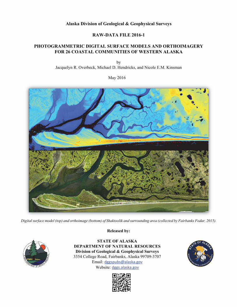
The State of Alaska Division of Geological & Geophysical Surveys acquired photogrammetric digital surface models (DSMs) and co-registered orthorectified aerial images (orthoimages) for the west coast of Alaska in support of coastal vulnerability mapping efforts. This report is a summary of the data collected over 26 developed areas along approximately 3,500 km of coastline in the Bering Sea, Norton Sound, and Yukon–Kuskokwim Delta regions (fig. 1). Aerial photographs were collected between July 31 and September 6, 2015, and processed using Structure-from-Motion (SfM) photogrammetry techniques. Ground control points (GCPs) and checkpoints were collected in support of these data products during a Global Navigation Satellite System (GNSS) survey conducted between August 15 and September 14, 2015. For the purposes of open access to elevation and orthoimagery datasets in coastal regions of Alaska, this collection is being released as a Raw Data File with an open end-user license. The data available for each of the 26 communities consist of the following: (1) Orthoimage raster, (2) Digital Surface Model (DSM) raster, (3) Hillshade raster produced from DSM, and (4) an Orthoimage Hillshade combination raster.

Figure 1. Location map of 26 western Alaska communities mapped in 2015.

1 Alaska Division of Geological & Geophysical Surveys, 3354 College Road, Fairbanks, AK, 99709-3707; [email protected] 2 Alaska Division of Geological & Geophysical Surveys, 3354 College Road, Fairbanks, AK, 99709-3707; now with NOAA/NOS/National

Geodetic Survey (NGS), 222 West 7th Avenue, Room 517, Anchorage, AK 99513-7575

RDF 2016-1 Page 2

DATA ACQUISITION

Fairbanks Fodar collected aerial photographs between July 31 and September 11, 2015, using a small aircraft (Cessna 170B) platform. The aerial survey was planned so flight lines and photograph frequency provided 60 per-cent side lap and 80 percent end lap photo coverage, with flying heights between 800 and 2,700 ft (244–823 m) resulting in 10–20 cm ground sample distance (GSD; see table 1) of the aerial photos. A Nikon D800E with a 24 mm Nikkor f/1.4 lens was used to collect 36-megapixel photographs (7,360 × 4,912 pixels per image), in Joint Photographic Experts Group (JPEG) or Nikon Electronic Format (NEF), depending on flight length for the day (because the JPEG format had a smaller file size, it was used on longer flights). Photos were collected at 1- to 3-second intervals. On-board global positioning system (GPS) data were acquired by a Trimble 5700 with roof-mounted antenna approximately 1 m above the camera, collecting at 5 Hertz. Each camera shutter trip placed an event marker onto the GPS datastream for precise timing and location. For more detailed information on flying dates at specific locations, see Appendix A.

Table 1. Community-specific data quality and reference information.

Location Airport

identification code

Orthoimage ground sample distance (GSD)

(cm)

Digital surface model

GSD (cm)

Vertical shift (m)

Root mean square error (RMSE) (m)

Number of points used to calculate

RMSE

Universal transverse mercator

zone Alakanuk AUK 17 20 0.48 0.063 3 3 Brevig Mission KTS 15 20 -0.18 0.113 8 3 Chevak VAK 13 20 0.28 0.040 5 3 Chefornak CFK 10 20 0.36 0.075 5 3 Elim ELI 10 20 -0.09 0.103 4 3 Emmonak EMN 17 20 0.43 0.110 4 3 Golovin GLV 10 20 0.15 0.030 4 3 Hooper Bay HPB 9 19 0.37 0.013 4 3 Kipnuk IIK 19 19 0.25 0.048 4 3 Kongiganak DUY 9 10 0.19 0.068 5 3 Kotlik KOT 15 20 0.50 0.071 4 3 Koyuk KKA 16 20 0.61 0.125 4 4 Kwigillingok GGV 15 20 0.37 0.081 5 3 Newtok EWU 9 18 0.28 0.054 4 3 Nightmute IGT 9 17 0.12 0.040 5 3 Nome OME 9 18 0.17 0.090 5 3 Nunam Iqua SXP 16 20 0.43 0.071 4 3 Scammon Bay SCM 20 20 0.55 0.097 5 4 Shaktoolik SKK 9 9 -0.21 0.117 4 3 Stebbins WBB 10 20 -0.21 0.068 4 3 St. Michael SMK 10 20 -0.21 0.033 4 3 Teller TER 15 20 0.08 0.127 4 3 Toksook Bay OOK 16 20 0.23 0.106 5 3 Tununak TNK 20 20 0.00 0.070 4 3 Unalakleet UNK 8 17 0.23 0.037 5 4 Wales WAA 15 20 0.00 0.063 5 3

RDF 2016-1 Page 3

DATA PROCESSING

Aerial survey GNSS data were processed using Waypoint’s Grafnav commercial GNSS software using GPS con-stellation. Each project was processed using either post-processing kinematic (PPK) or precise point positioning (PPP) methods, depending on the quality of the solution, which was primarily dependent on the distance from Continually Operating Reference Stations (CORS), such that all flights resulted in data with better than 10 cm separation in forward and reverse trajectory solutions. GPS data were processed to the North American Datum 1983 (NAD83; 2011) European Petroleum Survey Group Well Known Identification Number (EPSG) 6318, and the North American Vertical Datum of 1988 (NAVD88; Geoid12A; EPOCH 2010.00).

Photos were individually processed for optimum contrast and exposure using Adobe Camera Raw. To accommodate the large data acquisition volumes, most photos were shot and processed to JPEG format.

Aerial survey GPS data (event marker coordinates) were manually correlated to image filenames using the image timestamp to create a camera external orientation file for import into Agisoft Photoscan Professional (Photoscan) software. The external orientation file provides the X, Y, Z position of the camera for each photograph taken during the survey. Aerial stereophotographs were imported into the photogrammetric software, which uses an SfM algo-rithm to create a three-dimensional terrain model from the stereo-imagery. The terrain model was then used to orthometrically correct the photos and produce the final orthoimage mosaic in Photoscan. Within the Photoscan software application, standard workflow steps were followed: photo-alignment, alignment optimization, dense point cloud building, mesh creation, DSM and orthoimage creation, and exporting the results.

DATA PRODUCTS

The data available for each of the 26 communities consist of the following: (1) Orthoimage raster, (2) DSM raster, (3) Hillshade raster produced from DSM, and (4) an Orthoimage Hillshade combination raster. In addition, a poly-gon shapefile is available that shows the data extent and attributes recorded in table 2 for all 26 communities. These data are stored in NAD83 (2011) horizontal datum and projected in Universal Transverse Mercator (UTM) Zone 3 or 4 coordinate systems (meters; EPSG 6332 or 6333, respectively) and NAVD88 (Geoid12A; EPOCH 2010.00) vertical datum, as outlined in the accompanying metadata.

Orthoimagery

Orthoimages contain 3-band, 8-bit, unsigned raster data (red/green/blue; file format–GeoTIFF; source–Fairbanks Fodar) and differential GSD between communities (see table 1). The No Data value is set to 0. The file employs Lempel-Ziv-Welch (LZW) compression. Light exposures in the orthoimages are a result of daily weather condi-tions, which ranged from low cloud cover, rain, and full sun.

Digital Surface Model (DSM)

The single-band, 32-bit float DSMs represent surface elevations of buildings, vegetation, and uncovered ground surfaces (file format–GeoTIFF; source–Fairbanks Fodar) with differential GSD between communities (see table 1). The No Data value is set to -32767. The file employs LZW compression.

DSM Hillshade

The single-band, 8-bit, unsigned integer rasters represent hillshading of the DSM (file format–GeoTIFF; source–DGGS) with differential GSD between communities (see table 1). The No Data value is set to 255. The file employs LZW compression. The hillshade was produced using Blue Marble Geographic’s Global Mapper GIS application. This file has the same spatial resolution as the DSM.

Orthoimagery Hillshade Combination Raster

The orthoimagery hillshade combination rasters contain 3-band, 8-bit, unsigned raster data (red/green/blue; file format–GeoTIFF; source–DGGS) and represents a hillshade-tinted orthoimage. The No Data value is set to 0. The

RDF 2016-1 Page 4

file employs LZW compression. The file was produced with ESRI’s ArcGIS using Raster Function templates. This file has the same spatial resolution as the DSM.

Community Data Extent Polygon File

One polygon shapefile is available that shows the data extent and data attributes for all 26 communities (table 2).

Table 2. Polygon shapefile attribute descriptions.

Field Type Description community String Community name code String 3 digit airport code for community ortho_gsd Double Orthoimage ground sample distance (gsd), that is, raster cell size, in

meters dsm_gsd Double DSM ground sample distance (gsd), that is, raster cell size, in meters vert_shift Double Vertical shift, in meters Rmse Double Root mean square error (RMSE) in meters Num_pts Short Integer Number of points used to calculate RMSE Utm_zone Short Integer UTM zone of the delivered data ortho_gb Double Size, in gigabytes, of orthoimage raster file dsm_gb Double Size, in gigabytes, of DSM raster file dsm_hs_gb Double Size, in gigabytes, of DSM hillshade raster file tint_gb Double Size, in gigabytes, of orthoimage hillshade tint raster file

DATA QUALITY

Horizontal accuracies of the orthoimagery were evaluated by comparing the locations of photo-identifiable GCPs to the same point visible in the aerial photos (see Appendix A for examples). The 37 photo-identifiable GCPs and 75 checkpoint elevations taken on stable surfaces across the 26 communities were collected by RECON, LLC (see Appendix B). No horizontal offsets were identified at the pixel scale at any location (see table 1 for location-based GSD), so no horizontal transformation was performed.

The vertical accuracies of the DSMs were evaluated by comparing both the GCP elevations and checkpoint eleva-tions with the DSM elevations separately for each non-contiguous community (with the exception of Stebbins/St. Michael, the data are not contiguous between communities). We reduced the residual difference between GCPs and DSM pixels to zero mean using a vertical shift (see table 1). The remaining residuals were used to determine the Root Mean Square Error (RMSE) at each community, then combined to determine RMSE for the dataset as a whole. The final DSMs had a mean vertical residual of 6.2 cm with +/- one standard deviation of 5.2 cm, with 95 percent of all GCP and checkpoint residuals within 16.7 cm. The RMSE of all GCPs and checkpoints was 8.1 cm, but varied by location (see table 1).

Known anomalies within the data exist on the DSMs over water bodies; these anomalies have not been edited in this data release. Because waves in the nearshore marine or lacustrine environment move at a higher speed than photo-collection, the SfM processing technique for producing DSMs defines those points irregularly (for an ex-ample, see fig. 2).

RDF 2016-1 Page 5

Figure 2. Examples of anomalous elevation values over water at Tununak, Alaska.

ACKNOWLEDGMENTS

This publication is funded with qualified outer continental shelf oil and gas revenues by the Coastal Impact Assis-tance Program, U.S. Fish and Wildlife Service, U.S. Department of the Interior.

The views and conclusions contained in this document are those of the authors and should not be interpreted as representing the opinions or policies of the U.S. Government. Mention of trade names or commercial products does not constitute their endorsement by the U.S. Government.

Contract 10-15-053

Coastal Village Data Report20 February 2016

Submitted to Alaska Department of Natural Resources

Submitted by

Fairbanks FodarPO Box 82416 • Fairbanks • AK • 99708

www.fairbanksfodar.com

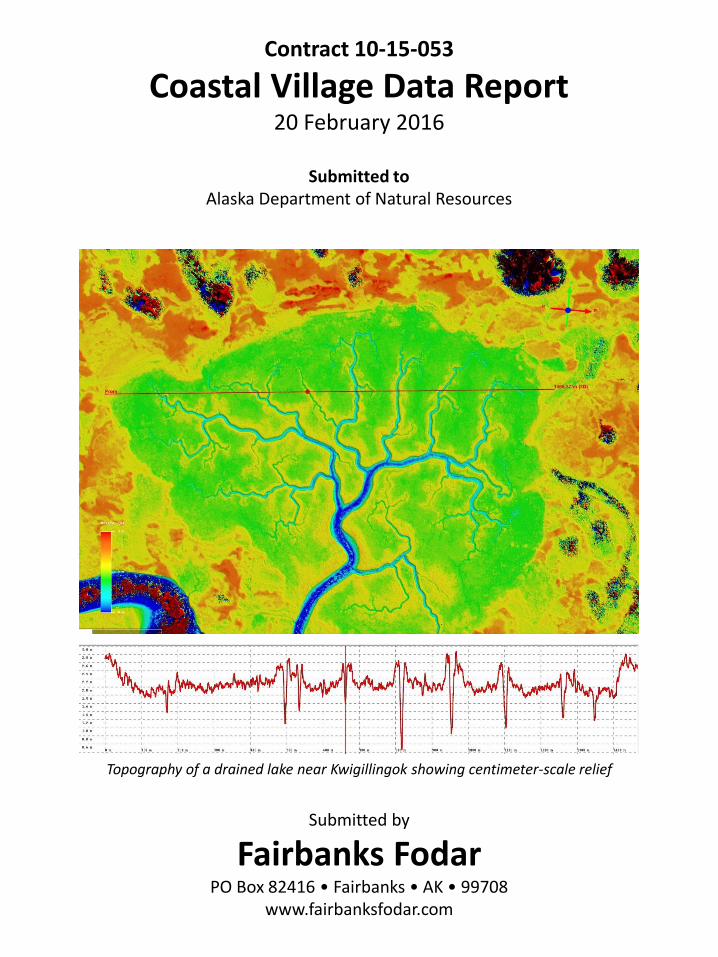
Topography of a drained lake near Kwigillingok showing centimeter-scale relief

February 2016 www.fairbanksfodar.com Page 1

Alaska DNR Contract 10-15-053

Coastal Village Data Report

Fairbanks Fodar 20 February 2016

Executive Summary

This report is a brief summary of the delivery of DSMs and orthomosaics of 29 developed areas

along the coast between Wales and Bethel. As part of a much larger effort mapping the entire

coastline between these villages to assess coastal vulnerability, in this village delivery we

acquired and individually processed over 50,000 photos covering over 1200 km2 of area at 10-

20 cm resolution and performed various quality assessment checks on the data. The data

exceed all specs – we delivered more than double the area specified for the villages and the

resolutions exceed spec by 10-100%, leading to over 3x more total pixels delivered than

required by the contract. Data quality meets or exceeds expectations based on prior work.

Compared to GCPs provided by DGGS from another contractor at 27 villages, no horizontal

offsets were found; that is, the directly georeferenced data had essentially perfect horizontal

placement in the real world. Vertical offsets between GCPs and our directly georeferenced

maps had a mean of 10 cm and all were within spec; after reducing the data to zero mean

offset, the RMSE residuals were less than 10 cm. For example, the 5 vertical GCPs acquired in

Wales had a mean residual of 4 cm compared to our DSMs and a total range of +/7 cm, so here

if we applied a 4 cm vertical shift to the data, our vertical accuracy reduces to the precision

level of about +/- 7 cm. All villages where multiple GCPs were acquired show a precision level

+/- 11 cm or better. Similarly, comparison of millions of points at Unalakleet to a map we made

there in 2014 showed a scatter of better than +/- 10 cm in most locations we identified as

stable (that is, non-vegetated, not eroding, etc). This report gives a brief overview of our

processing methods and data quality checks.

Data Acquisition and Processing

Fairbanks Fodar was awarded contract 10-15-053 on 21 July 2015 and our field work began ten

days later on 31 July 2015. Our methods are described in the report associated with this

Appendix and in detail in Nolan, M., C. Larsen, and M. Sturm. "Mapping snow depth from

manned aircraft on landscape scales at centimeter resolution using structure-from-motion

photogrammetry." The Cryosphere 9.4 (2015): 1445-1463. For all acquisitions, we used a

Cessna 170B flown by a single pilot/operator, controlling a Nikon D800E connected to a survey-

grade GPS. Flying altitudes were planned at 2700 feet AGL, though cloud cover often required

flying lower and thus decreasing the spacing between flight lines. The target ground sample


distance was 17 cm, but was often as low as 8-10 cm by flying lower. As originally planned, the

project was due to start in June with a final delivery on October 16, however a variety of issues

led to a late start with the contract. Given the unlikelihood of complete project acquisition due

to weather, sunlight and tidal constraints in August, our project performance plan prioritized

village acquisitions. While we were still able to acquire about 85% of the total area (villages

plus coast lines in between), we were able to acquire 100% of the village data. GPS processing

was done in the field to ensure data quality. Photographic pre-processing included optimizing

the images for contrast and exposure and was mostly accomplished after return to Fairbanks.

Data processing was performed in Agisoft Photoscan, as described in this DNR report and the

paper cited above. About half of the village data were delivered on October 16 and the

remainder on December 1st. DNR found all data within spec and suggested a final vertical shift

of the DSMs to optimize with checkpoints which were not provided to Fairbanks Fodar. These

optimization shifts were on the order of 10 cm vertically, as detailed in the report. The final

data were thus shifted as recommended and delivered on January 12th. As described below,

the data were not cropped to match the DCRA village outlines provided by DNR, but rather

substantial bonus area was delivered outside of these outlines. Note that these are first-

surface DSM and no bald earth or other value-added processing have been performed.

Data Quality Overview

We acquired these data between July 31 and September 6, as noted in Table A1. There are 29

villages in total; note however that we processed Stebbins and St Michaels in the same block

and that the DCRA shapefiles use a single outline for Brevig Mission and Teller, which we

processed separately, so there is some potential confusion when counting them.

As can be seen in Table A1, we have not only met all specifications but greatly exceeded them

in terms of area, GSD, and total pixels delivered. Here we calculated the pixel overdelivery by

comparing the measured pixels within a file to the pixels that would have been contained in a

file that only met the minimum specs, as calculated by the DCRA area and the GSD spec. This

metric indicates a 3.5x over-delivery. The majority of the bonus area comes from extending

flight lines beyond the DCRA boundary to ensure complete coverage of it. The majority of the

higher resolution comes from flying lower than planned to maximize use of available weather

windows (that is, working under lower ceilings than planned). Two villages currently have

slightly less than full coverage within the DCRA boundary: Brevig Mission is missing a corner

(which will be processed with coastal data) and Tuntutuliak had some cloud cover that

obscured <10 % of the area within the DCRA boundary which we will attempt to re-acquire in

2016.

Not only has the data exceeded the geometric specifications above, but it also has exceeded

the specs for accuracy and precision. Table 1 in the main report shows the comparisons of the

DGGS GCPs to our maps. Note that in all cases, horizontal accuracy was essentially perfect.


‘Essentially’ here means to the best of our ability to determine reliably by eye, but is well within

a single pixel; see Figure A1 for some examples. The vertical accuracy was determined by the

State to have an RMSE residual offset of only 8 cm for all GCP points, substantially below the 40

cm specification. Further, we compared our 2015 Unalakleet DEM to our 2014 Unalakleet

DEM. The results are shown in Figure A2. Here the yellow/green colors represent about +/- 10

cm, and this covers the bulk of the comparison; nearly all locations with larger differences have

changed due to vegetation or disturbance, or spatial biasing at building edges. These results,

combined with our prior research on technique validation, indicate that these data will be

excellent baselines for documenting future change.

Table A1. Data delivery overview. Columns 2 and 3 are postings of the delivered orthomosaics and DEMs

respectively. Delivered Area was measured based on actual pixel counts within the DEMs, not the size of

the bounding box of the DEM. Overdelivery as a percentage of area was calculated from the DCRA Area

and Delivered Area. Overdelivery as a percentage of pixels was calculated comparing actual pixels to files

based on the DCRA area and specified GSD. There was no DCRA village outline for Nome, so it is excluded

from the percentage calculations. Stebbins and St Michaels were acquired and delivered within a single

block, so are grouped for calculations.

Spec Actual DEM Post DCRA Area Delivered Area Overdelivery Overdelivery Acquisition

Village GSD (cm) GSD (cm) (cm) (km2) (km2) (Area, %) (Pixels, %) DateWales 20 15.5 20.0 20 40 101% 334% 8/27-28/2015

Brevig 20 15.1 20.0 58 53 53% 161% 8/27-28/2015

Teller 20 15.2 20.0 n/a 35 n/a n/a 8/27-28/2015

Nome 10 9.2 18.4 n/a 33 n/a n/a 8/23/2015

White Mountain 20 18.2 20.0 20 38 89% 228% 8/23/2015

Golovin 10 9.8 20.0 47 70 50% 155% 8/23/2015

Elim 10 10.7 20.0 20 24 21% 107% 8/5/2015

Koyuk 20 16.5 20.0 20 23 16% 171% 8/5/2015

Shaktoolik 10 9.4 9.4 21 32 54% 175% 8/6/2015

Unalakleet 10 8.5 16.9 32 42 31% 184% 7/31/2015

St Michaels 10 10.0 20.0 n/a n/a n/a n/a 8/6/2015

Stebbins 10 10.0 20.0 40 73 181% 182% 8/6/2015

Kotlik 20 15.1 20.0 25 49 97% 345% 8/22/2015

Emmonak 20 17.2 20.0 24 48 100% 271% 8/31/2015

Alakanuk 20 16.8 20.0 27 51 94% 276% 8/31/2015

Nunam 20 16.5 20.0 20 41 104% 299% 8/14/2015

Scammon Bay 20 19.7 20.0 15 99 581% 701% 8/13/2015

Hooper Bay 10 9.5 19.0 13 32 148% 276% 8/13/2015

Cheevak 20 12.8 20.0 13 47 264% 889% 8/13/2015

Newtok 10 9.4 18.0 26 51 93% 219% 9/1/2015

Tunanak 20 19.7 20.0 20 43 115% 222% 9/1/2015

Toksook Bay 20 16.6 20.0 20 33 63% 237% 9/1/2015

Nightmute 20 8.8 18.0 23 47 99% 1042% 8/21, 9/1/2015

Chefornak 20 9.0 20.0 46 83 99% 891% 9/6/2015

Kipnuk 10 9.6 19.2 12 41 249% 380% 8/19/2015

Kwig 20 15.1 20.0 13 57 343% 775% 8/21/2015

Kong 10 9.2 18.0 20 32 64% 195% 8/12/2015

Tunt 20 16.5 20.0 12 53 355% 672% 8/21/2015

Napakiak 20 15.2 20.0 13 36 184% 493% 8/21/2015

Totals: 618 1307 111% 266%


DSM Noise

Within the DCRA village boundaries used as AOIs for this delivery, we have not found nor do we expect

to find any spatially correlated noise that exceeds specifications. We planned our flight lines so that all

of the area inside the boundary would have a consistent amount of sidelap. The reduction of side lap

near the edges of an acquired block often leads to spatially correlated noise in the form of corduroy

banding or slight warps. With our data outside the DCRA boundary, this is noise is usually less than +/-

40 cm, but it can sometimes be around +/- 80 cm. When it is exists, it is easy to spot on a shaded relief

of a DSM. Again, such noise can only be found outside the AOIs in the ‘bonus’ area delivered, and

typically only within a few hundred meters of the edges. Thus some care should be taken in using the

DSMs near the edges. This noise does not affect the orthomosaics.

There are several types of spatially uncorrelated noise. A large and easily observed one is over water

bodies. It was known in advance that water bodies would require manual editing and thus our contract

was only for solid land surfaces, as photogrammetry cannot resolve water surfaces as accurately as land

surfaces. When waves are present, their motion introduces an additional parallax that can causes noise

well over 10 m. On calm days when the bottom of a lake is imaged, the refraction caused by the water

is not accounted for and also causes larger errors. Thus water bodies require manual hydroflattening.

The base random noise level is about +/- 3 cm. Much of this is likely caused by slight uncertainties

within the bundle adjustment as well as difficulties in gridding the DSM. On flat surfaces, this noise can

sometimes be apparent in the form of small ripples, but usually it is more random. Another source of

noise is primarily found on rooftops. Here, metal roofing facing into the sun simply cause exposures to

fall outside of what was recordable by the camera in JPG mode, thus point density is greatly reduced

and sensor noise is more likely to be interpreted as real, causing lumpy or spiky roofs. The majority of

the considerable time we spent photo processing was to manually edit rooftops for best exposure.

Overall the roofs came out fine, but there are many ugly ones, though mostly all within spec. In nearly

all case however, there is enough real information (eg, ridgelines, edges) that someone could

reconstruct an accurate 3D model by hand for each roof, if that were desired.

The only true errors we found in the delivered village data were at Tuntutuliak, where low cloud cover

interfered with acquisitions. We attempted to acquire Tunt on two days, with the same problems each

day. As it stands, the affected area is less than 10% of the DCRA outline.

More Information

For more information about these acquisitions, please visit the Latest News section of our website for

the period July 31 – August 11: http://fairbanksfodar.com/fodar-news .

http://fairbanksfodar.com/fodar-news

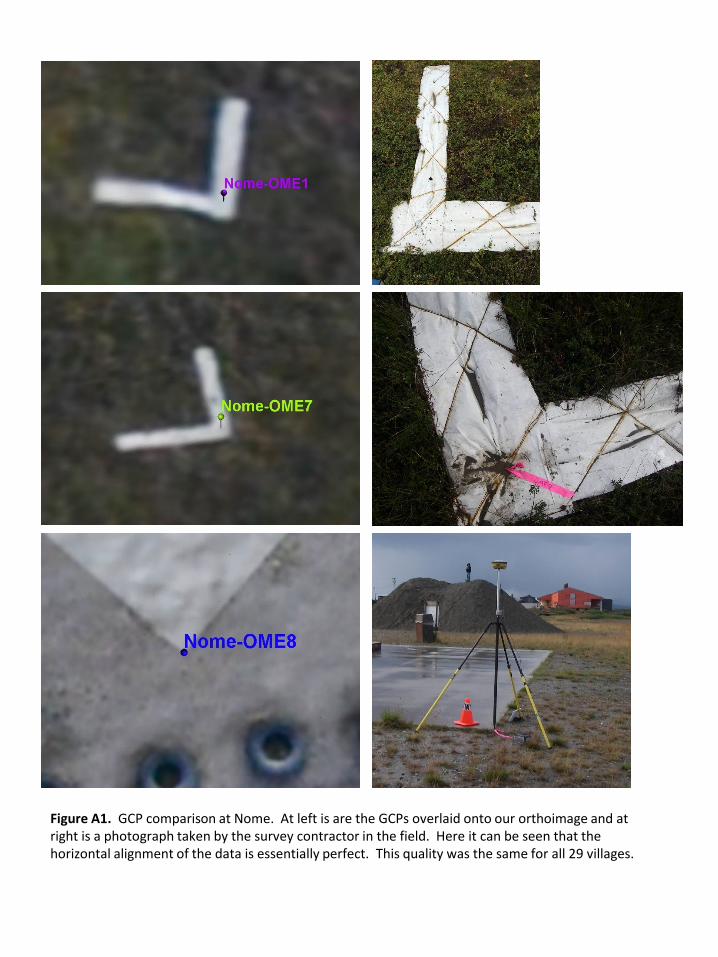
Figure A1. GCP comparison at Nome. At left is are the GCPs overlaid onto our orthoimage and at right is a photograph taken by the survey contractor in the field. Here it can be seen that the horizontal alignment of the data is essentially perfect. This quality was the same for all 29 villages.

Figure A2 A-B. We subtracted our September 2014 DEM of Unalakleet from our July 2015 one, and colored the results in A. Here the green-yellow transition is no change. As seen in the profile spanning both runways, nearly all of the difference is within +/- 10 cm (vertical ticks are 5 cm). Not all of this difference is noise, some of the longer wavelength variations are motion of the runway itself.

A.

B.

FigureA 2 C-D. Another comparison of 2014-2015 Unalakleet data, as in A-B. Here a transect (50 cm vertical ticks) is run across the complex roof of the clinic, which shows no horizontal offsets and a vertical change of essentially zero, as expected. Small spikes are at the edges of the buildings, with amplitudes of only ~1 m, which is excellent considering the spatial biasing such edges cause. The ~1.5 m excursion on the right side of the clinic is caused by a parked car having moved. Careful examination of the difference image reveals moved boats, cars, snow machines, and small buildings, as well as gravel extraction.

D.

C.

Ground Control Data for Aerial Survey of Western Alaska

FINAL PRODUCT REPORT

State of Alaska Department of Natural Resources

ASP #10-15-047

October 15, 2015

RECON LLC

481 W. Arctic Ave.

Palmer, AK 99645

Rowland Engineering Consultants FINAL REPORT

ASP #10-15-047

15 October 2015 TOC i

TABLE OF CONTENTS

INTRODUCTION ...................................................................................................................................................... 1

1.0 PROJECT OVERVIEW ................................................................................................................................. 1

2.0 PROJECT METHODOLOGY ........................................................................................................................ 1

Project Execution Plan ............................................................................................................... 1 2.1

Field Operations ......................................................................................................................... 2 2.2

Survey Procedure ....................................................................................................................... 2 2.3

2.3.1 Selection of Photo-Identifiable GCPs ........................................................................... 3

2.3.2 Data Acquisition........................................................................................................... 4

2.3.3 Equipment and Software ............................................................................................. 4

2.3.4 Spatial Reference Framework...................................................................................... 4

3.0 DATA PROCESSING ................................................................................................................................... 5

Quality Control ........................................................................................................................... 6 3.1

4.0 DELIVERABLES .......................................................................................................................................... 6

Final Product Deliverables ......................................................................................................... 7 4.1

SUMMARY .............................................................................................................................................................. 7


ASP #10-15-047

15 October 2015 Page 1 WAK 015

INTRODUCTION

This final project report has been produced by RECON LLC (RECON) for the Alaska Department of Natural

Resources (DNR) under project contract ASP 10-15-047, providing Ground Control Data for Aerial Survey

of Western Alaska.

1.0 PROJECT OVERVIEW

RECON's scope of work under ASP 10-15-047 is to obtain an accurate and useful database of ground

control points (GCPs) along the western coastline of Alaska, according to the criteria described in the

project contract. DNR's Division of Geological & Geophysical Surveys (DGGS) intends to use this network

of GCPs, including check points and benchmark ties, to verify the accuracy and quality of coastal

orthoimagery and topographic data to be acquired by DNR in 2015. DNR's overall goal in the acquisition

of these data is to improve the ability to orthorectify future products of aerial imaging to be acquired in

Alaska's coastal regions, which products may be used as resources for conducting critical tasks such as

emergency support, community planning, and environmental monitoring along the coast and within

coastal communities. The project's area of interest (AOI) follows approximately 3,500 km of Alaska's

western coast from Bering Strait to Kuskokwim Bay (see Appendix A – Map of Area of Interest). DNR has

contracted with Fairbanks Fodar to provide aerial imagery products immediately related to this control

survey, using structure-from-motion (SfM) technology.

The Final Point Summary included in the Final Products should be used for final control and

orthorectification of aerial imagery products and for publication as DNR sees fit.

2.0 PROJECT METHODOLOGY

RECON's general methodology has been developed over time to support several successful surveying

and mapping projects involving a variety of traditional remote sensing technologies. This survey

methodology and GCP selection criteria have been adapted to suit the particular needs of the DNR

ground control project scope and to meet the project specifications as defined by the contract. All

survey work supporting this project was performed directly by or under the supervision of a Professional

Land Surveyor registered in the State of Alaska. RECON subcontracted with Hattenburg Dilley & Linnell,

LLC (HDL), and JOA Surveys, LLC (JOA), to assemble a strong and experienced survey team to complete

the project within DNR's specified timeframe.

Project Execution Plan 2.1

RECON submitted the official Project Execution Plan to DNR on 11 August 2015. The plan was

developed in coordination with the DGGS Project Technical Manager, Nicole Kinsman, who reviewed

and approved the plan with only two clarifications: 1) ellipsoid height was added as a data item to be


ASP #10-15-047


provided in the Preliminary Coordinate File, and 2) it was confirmed that sufficient documentation

would be provided in the Final Report to identify ground control features.

In general, project methodology conformed to the specifications of the Project Execution Plan as

approved. Any subsequent deviations from the methodology have been described in the appropriate

section of this Final Report.

Field Operations 2.2

Field work was completed within the expected schedule and with no significant issues. Field activities

commenced on 15 August 2015 and concluded on 14 September 2015. Field survey was conducted by

three task forces made up of personnel from RECON, HDL, and JOA, as described in the Project

Execution Plan:

Developed Area Sites, Northern Region (Brevig Mission to Unalakleet)

Developed Area Sites, Southern Region (Saint Michael to Kongiganak)

Remote Sites, Entire Region

Logistics of accommodations, fuel supply, and other resources were organized in advance by RECON

staff. Major support hubs included Bethel, St Mary's, Unalakleet, and Nome, as expected. In the

interest of community outreach, RECON developed a brief written description of the project goals and

basic methodology, which permitting staff used in their advance communications with landowners and

which field personnel distributed as needed while traveling throughout the AOI.

Personnel working in the developed areas used a combination of scheduled air travel and chartered

fixed-wing travel to reach survey sites. Personnel working in the remote sites used a light helicopter to

reach survey sites. This approach worked very well, and field personnel and pilots paid close attention

to active weather patterns in their respective region, focusing each day's work in the area where

weather-related delays were least likely to impact progress.

Survey Procedure 2.3

Field personnel surveyed 67 photo-identifiable GCPs along the coast, with at least one GCP in each of

the 25 developed areas identified in the contract. A total of 81 check points (including GCP bases) were

surveyed throughout the AOI, including at least 2 within 5 km of each of the 25 developed areas. A total

of 27 GNSS ties to tidal benchmarks were surveyed. Ties were made to three or more existing tidal

benchmarks in Lost River, Elim, Hooper Bay, Nome, Toksook Bay, Shaktoolik, and Nunam Iqua. Ties

were made to two existing tidal benchmarks in Teller and Unalakleet, because only two tidal

benchmarks were suitable for GPS occupations. Positioning was tied to CORS stations as outlined in

Section 3.0 (Data Processing). Maps of the general location of GCPs are included with the final

deliverables. All in all, the total number of points surveyed was more than the project contract required.


ASP #10-15-047


All GCPs surveyed under this contract were spaced in intervals no greater than 50 km. It may be worth

noting that the northernmost GCP in RECON's project scope was located at the area of Lost River, taking

advantage of the opportunity to acquire GPS at additional existing tide stations there. RECON

understands that DGGS intended to survey a GCP in Wales, in support of similar project goals but

independent of RECON's project scope. RECON estimates that the GCP at Lost River is approximately

49.6 km (straight-line distance) from the approximate village center at Wales, so depending on where

the DGGS GCP is located, the interval between those two points may be slightly greater than 50 km.

RECON discussed survey methodology with Fairbanks Fodar and made every effort to define our GCP

site criteria in a way that complemented their data acquisition plan using SfM technology. In any cases

of uncertainty, RECON employed the method that would best reflect the intent of DNR's scope and

specifications as defined in the project contract for the ground control survey.

2.3.1 Selection of Photo-Identifiable GCPs

Community-based GCPs were used as often as possible. Site selection efforts utilized existing imagery

and topographic data to locate GCPs within villages, focusing on photo-identifiable locations at or near

airstrips, schools, or DOT facilities in the communities. Examples of these photo-identifiable points

include: historical photo panels, sidewalk corners, asphalt and concrete aprons, basketball courts,

boardwalks, concrete transformer bases, etc. A permanent survey monument appropriate for the site

conditions was set as required.

For GCPs in remote areas between communities, RECON selected sites based on image and topographic

interpretation of historic beach ridges above debris line, "high" points in the Yukon-Kuskokwim Delta

region, and rock outcrops in the northern region. In the Yukon-Kuskokwim Delta region, RECON's

strategy was to gain an aerial view and identify "micro-features." Where no photo-identifiable points

exist, RECON field surveyors set a permanent survey mark with a 40 cm x 40 cm aluminum plate

appropriate for site conditions. Some plates remain as permanent monuments, and some were

removed at the conclusion of the field season when requested by the landowner. Due to the necessity

of establishing new photo-identifiable features (such as aluminum plates) in especially remote areas,

RECON periodically informed Fairbanks Fodar of the field survey progress in an effort to coordinate the

SfM data acquisition with the actions of the field surveyors.

GCPs will be identifiable from aerial or satellite photos with ground sampling distances between 0.2 m

and 1.0 m. All permanent survey marks were marked with the project identifier (WAK015) and GCP

code. All GCPs were documented with photos as described in Section 2.3.2, and all remote GCPs were

further documented with a low-level oblique photo and field sketches to aid in imagery identification.


ASP #10-15-047


2.3.2 Data Acquisition

Project data were collected using dual-frequency static GPS receivers. At each GCP or GCP base, a single

point was selected as the primary control station. This primary control station had a minimum of two 4-

hour sessions of data collected. In cases where a permanent monument was not able to be set or was

impractical to set at the GCP, a GCP base monument was set and the GCP was surveyed with RTK or fast-

static sessions. When possible, the GCP and tidal benchmarks were occupied in two 4-hour sessions on

each mark, with longer sessions if conditions allowed. Occupations used a combination of fixed-height

tripods or tripods and rods with bipods, with each occupation at a different height than was used

previously at the same point when not using a fixed-height rod. The height of the antenna was

measured vertically from the survey mark or geographical feature to the bottom of the antenna. Data

was collected at 15-second epochs at all occupations. Check points were acquired using static, real-

time-kinematic (RTK), or fast-static techniques collected at the beginning and ending of GCP or GCP base

occupation.

At each GCP, GCP base, or tidal benchmark session, the observer completed a GPS field form citing the

name of the point, the antenna height, the measurement point, start time, stop time, antenna type,

personnel, a site description, and a site sketch. These Field Survey Forms were developed by and are

owned by JOA Surveys. In addition, the observer obtained detailed photographs of the point surveyed,

including the following views: from standing height, horizontal image(s) showing the tripod relative to

the vicinity, the antenna model, the antenna height, and a legible sign identifier of each set monument.

2.3.3 Equipment and Software

Project data were collected using dual-frequency static GPS receivers. Processing methods and software

are described in Section 3.0.

The following equipment models were used by field surveyors:

Leica: 1200, GS10, GS14, GS15

CHC: OPUS X90-D

Topcon: Hiper II, Hiper V2

2.3.4 Spatial Reference Framework

RECON complied with the spatial reference framework established in the contract, using the following

specifications:

Vertical Datum: NAVD 88, using the GEOID 12B model

Horizontal Datum: NAD 83 (2011) epoch 2010.00

Projection: UTM (zones 3, 4 within AOI)

Units: Meters


ASP #10-15-047


3.0 DATA PROCESSING

GPS observations were processed using OPUS Projects, the latest GPS processing software from the

National Geodetic Survey (NGS). OPUS Projects is a web-based online processor, so the user is not

responsible for any software installation, maintenance, setup, and dependencies, and this reduces the

likelihood of processing inconsistencies or errors. OPUS Projects uses the latest NGS PAGES baseline

processing software which is required for publication by the NGS. The trained user sets up a project and

assigns the project a code, which is used by the field crews to upload static GPS observations to the

appropriate project. For this project in western Alaska, the field crews populated OPUS Projects with

their data using the code WAK015.

The processing approach was based on Dr. Gerald L. Mader's approach of relative positioning with HUB

and Distant CORS. Dr. Mader recommends a maximum baseline length of 100km from the hub to the

furthest point in the network, but a 100km baseline length in western Alaska would require the

installation of dozens of base stations in remote locations with limited accessibility. To make this

project viable, the Data Manager extended the baseline length to 150km as stated in the Project

Execution Plan. Due to a gap in the Yukon-Kuskokwim Delta region, the existing CORS network does not

provide coverage for baseline lengths of <150 km throughout the entire project area, and this gap was

filled for the purposes of this project by installing a temporary GNSS base station in Emmonak. The base

station consisted of a GNSS antenna mounted to a building roof. The antenna and receiver were

connected to a laptop via USB and serial adapter cable. The receiver logged data every 30 seconds and

wrote a data file every 24 hours to an FTP server. The Distant CORS is one which is more than 1000 km

from the HUB CORS. The use of a Distant CORS helps to stabilize the tropospheric corrections. Long

observations (>24 hrs) reduced mutual visibility issues at the two CORS. The HUB CORS provided the

relative positioning.

Initially, the entire project was conceptualized as a single GPS processing project. However, the three

task forces in the field did not observe GPS simultaneously in the same 150km region due to a number

of logistical factors and project needs. The resulting baseline sessions would not allow for a single hub

processing schema. Processing was initially conducted by carefully selecting observations within 150km

of a CORS, and then processing other points for the same session in a different processing scenario, but

this method was troublesome due to the volume of data and the multitudes of sessions. As a productive

solution, the single project in OPUS was translated into six smaller projects, each with points within a

150km radius of the nearest CORS or the base in Emmonak. The respective GPS observations were

uploaded to each of the six projects for processing as originally anticipated.

Prior to baseline processing, either IGS station WHIT in Whitehorse, Yukon Territory, or IGS station FAIR

in Fairbanks, Alaska, was brought into each project to better resolve the tropospheric conditions. Data

was processed in a radial method, with the nearest CORS being the only hub station. The exception is


ASP #10-15-047


the base station installed at Emmonak. All of the remaining CORS plus the IGS station were included in

the processing. Piecewise continuous tropospheric models were used in the processing.

OPUS Projects has defaults of 0.020m peak-to-peak horizontally and 0.040m vertically. This threshold

had to be increased to 0.035m horizontally, while the vertical threshold remained the same. OPUS

Projects also has defaults of 80% of the observations and 80% of the fixed integers, both of which had to

be reduced to 70%, the minimums for OPUS Shared. All stations met the modified minimums with the

exception of OME5, which used 63.8% of the observations in the processing.

When processing was complete for each of the six projects, adjustments were performed using

GPSCOM, a Helmert blocking program within OPUS Projects. A free adjustment was first made

constraining only the nearest CORS. A constrained adjustment was then performed constraining all

CORS positions. No vertical constraints were applied as none of the stations observed were vertical

marks. A TIGHT constraint was applied to all CORS, as NGS currently is having problems with the

NORMAL constraint. With the TIGHT constraint, the CORS are fixed at the sub-millimeter level of their

published positions. All adjustments came out favorably, with millimeter-level correction to the

positions.

Quality Control 3.1

All field personnel adhered to the methodology and field procedures listed in the Project Execution Plan.

The Lead Surveyor and Survey Manager held conferences with field personnel prior to mobilization to

discuss and clarify methodology, and each team member had opportunities to review the document.

The field techniques followed NGS Technical Memorandum 58: Guidelines for Establishing GPS Derived

Ellipsoid Heights (Standards: 2 cm and 5 cm). Predetermined point and file naming conventions along

with form, photo, and field book structure were defined prior to survey and were followed by all field

personnel.

4.0 DELIVERABLES

Items deliverable to DNR were completed according to the schedule and specifications defined in the

signed contract. All items were delivered in soft copy (digital) format, with hard copies of reports

available upon request.

Project Execution Plan: 11 August 2015

Monthly Reports: 31 August 2015, 30 September 2015, and 15 October 2015

Preliminary Coordinate File: 30 September 2015

Final Products: 15 October 2015

The Final Point Summary included in the Final Products should be used for final control and

orthorectification of aerial imagery products and for publication as DNR sees fit.


ASP #10-15-047


Final Product Deliverables 4.1

This report document is delivered with several attachments in fulfillment of the contract requirements.

Following is a list of deliverables as organized by RECON and provided in digital folders.

1. Report – description of the completed project, survey methodology, and data processing

2. Data Dictionary – outline of data delivered and file naming scheme

3. Digital Photos – record photographs of survey sites (as described in Section 2.3.2)

4. RINEX Files – survey data files

5. Field Notes – PDF scans of original field notebooks (as described in Section 2.3.2)

6. Location Maps – reference maps of as-surveyed points

7. Processing Summary – summary of processing information

8. Final Point Summary – XLS file of final point locations for GCPs, check points, and tidal bench

marks

SUMMARY

RECON appreciates the opportunity to provide ground control surveying services to the Alaska

Department of Natural Resources. With any comments on this report or the overall project, please

contact Megan Ross at 907-746-3630 or [email protected].

Alaska Division of Geological & Geophysical Surveys RAW ...dggs.alaska.gov/webpubs/dggs/rdf/text/rdf2016_001.pdf · Model (DSM) raster, (3) Hillshade raster produced from DSM, and

Documents