Akhter_Tahmina.pdf - uWaterloo LaTeX Thesis Template

Stochastic Effects and FractalKinetics in the Pharmacokinetics of

Drug Transport

by

Tahmina Akhter

A thesispresented to the University of Waterloo

in fulfillment of thethesis requirement for the degree of

Doctor of Philosophyin

Applied Mathematics

Waterloo, Ontario, Canada, 2018

c© Tahmina Akhter 2018

Examining Committee Membership

The following served on the Examining Committee for this thesis. The decision of theExamining Committee is by majority vote.

External Examiner: Huaxiong HuangProfessor, Department of Mathematics and Statistics,York university and Fields Institute

Supervisor(s): Siv SivaloganathanProfessor, Dept. of Applied Mathematics,University of Waterloo

Internal Member: Mohammad KohandelAssociate Professor, Dept. of Applied Mathematics,University of Waterloo

Internal Member: Henry ShumAssistant Professor, Dept. of Applied Mathematics,University of Waterloo

Internal-External Member: Alfred MenezesProfessor, Dept. of Combinatorics and Optimization,University of Waterloo

ii

I hereby declare that I am the sole author of this thesis. This is a true copy of the thesis,including any required final revisions, as accepted by my examiners.

I understand that my thesis may be made electronically available to the public.

iii

Abstract

Pharmacokinetics (PK) attempts to model the progression and time evolution of adrug in the human body from administration to the elimination stage. It is the primaryquantitative approach used in drug discovery/development (in the pharma industry). Theoverwhelming majority of PK models are based on equilibrium kinetics with all the reactionkinetics occurring in a well mixed, homogeneous environment. Of course as is well known,the human body is comprised of heterogeneous media with non equilibrium chemical ki-netics. As a result, the transport processes and reaction mechanisms are often atypical. Inthis thesis, we apply ideas from stochastic processes and fractal kinetics in order to bettercapture the time course of a drug through the body when there is spatial and temporalheterogeneity. We discuss the limitations of the Langevin equation and Bourret’s approx-imation and apply Van Kampen’s approach to the random differential equations arisingfrom the stochastic formulation of standard one compartmental extra vascular model. Al-though one compartment models can produce good fits if a drug dispersed rapidly so thatequilibrium is achieved (in all tissues) swiftly, in general they are oversimplification of acomplex process . Thus we also extend the two compartmental model Kearns et al., toincorporate fractal Michaelis Menten kinetics and compare with experimental data fromthe literature for paclitaxel. Finally, we conclude with a discussion and appraisal of thecontribution in the thesis to the field of pharmacokinetics.

iv

Acknowledgements

This is a great opportunity to show my gratitude to all those great people, who madethis work possible. First of all, I would like to thank my supervisor, Professor SivabalSivaloganathan for his continuous inspiration to finish this journey. I am so grateful forhaving someone as my supervisor who is not only an honorable professor in this field butalso a person with great heart and desire to do good for others. Every meeting I had withhim was a new dimension about my work and a new interpretation to continue my PhD withall the obstacles I have in my life. I feel blessed and precious for having him throughout thisjourney. I was very fortunate to start my work with Professor Giuseppe (Pino) Tenti, whowas someone with strong research background. It was truly heart breaking when he passedaway after battling with cancer. Dr. Muhammed Kohandel, whose continuous challengingquestions always gave me new ideas to innovate and work on. I believe that if we helpothers, one day our good deeds will come back to us as miracles. That miracle for me in thisjourney was Dr. Henry Shum, who is a new faculty in the applied mathematics department.Thanks a lot Dr. Henry for your continuous support and time to help me to organize myideas whenever I needed. Dr. Mathew Scott, I am grateful for your help to compute someof my tough calculations. You showed me the road to follow with your great knowledgeabout the subject. Dr. Francis Poulin, I want to say thank you as you were always there tolisten to me whenever I knocked on your door. I want to thank my M.Sc supervisor fromRyerson University, Dr. Katrin Rohlf, for encouraging me to pursue my degree. I wouldlike to thank everyone in the department, faculty members and administrative officers,for all their care and constant support throughout these years. I want to thank my bestfriend in the department, Mitdhun, for his continuous support to help me through harshtimes during this study. I want to thank my wonderful daughter Dazana and lovable sonTahmeed for their constant cheerfulness. My father, mother, father-in-law, mother-in-lawand my siblings, whom I missed all throughout this study, as I was constantly busy withthe semesters and was not able to make time to visit them very often. I want to thank allmy classmates, group members, my friends inside and outside of the university for helpingthrough this journey. Finally, last but not the least I want to say thanks to my husband,for all his care and love throughout my study.

v

Dedication

I would like to dedicate this thesis to my loving family and friends, for their endlesscare and support.

vi

Table of Contents

List of Tables x

List of Figures xi

1 Introduction 1

1.1 What is pharmacokinetics (PK) . . . . . . . . . . . . . . . . . . . . . . . . 1

1.2 Processes of PK . . . . . . . . . . . . . . . . . . . . . . . . . . . . . . . . . 3

1.3 PK models . . . . . . . . . . . . . . . . . . . . . . . . . . . . . . . . . . . . 7

1.3.1 Non-compartmental models . . . . . . . . . . . . . . . . . . . . . . 8

1.3.2 Linearity and Non-linearity . . . . . . . . . . . . . . . . . . . . . . 9

1.3.3 Enzyme kinetics . . . . . . . . . . . . . . . . . . . . . . . . . . . . . 10

2 The relevance of Stochasticity in PK models 14

2.1 Introduction . . . . . . . . . . . . . . . . . . . . . . . . . . . . . . . . . . . 14

2.2 Stochastic PK models and additive noise . . . . . . . . . . . . . . . . . . . 16

2.3 Some basic concepts before solving a random system . . . . . . . . . . . . 18

2.4 Limitations of the Langevin process . . . . . . . . . . . . . . . . . . . . . . 25

2.5 The Bourret integral equation for the mean . . . . . . . . . . . . . . . . . 27

2.6 Van Kampen differential equation for the mean . . . . . . . . . . . . . . . 31

2.7 The Random Harmonic Oscillator . . . . . . . . . . . . . . . . . . . . . . . 32

2.7.1 Van Kampen approach . . . . . . . . . . . . . . . . . . . . . . . . . 32

vii

2.7.2 Bourret’s approach . . . . . . . . . . . . . . . . . . . . . . . . . . . 39

2.8 Some similar examples . . . . . . . . . . . . . . . . . . . . . . . . . . . . . 42

2.8.1 Example:1 . . . . . . . . . . . . . . . . . . . . . . . . . . . . . . . . 42

2.8.2 Example: 2 . . . . . . . . . . . . . . . . . . . . . . . . . . . . . . . 43

3 Application of Van Kampen’s theory to Pharmacokinetics 47

3.1 Deterministic formulation of the model . . . . . . . . . . . . . . . . . . . . 47

3.2 Stochastic formulation of the model . . . . . . . . . . . . . . . . . . . . . . 48

3.3 The Van Kampen approximation of the model . . . . . . . . . . . . . . . . 49

3.3.1 Calculation of the second moment using Van Kampen’s method . . 52

3.4 Numerical solution of the model . . . . . . . . . . . . . . . . . . . . . . . . 54

3.4.1 To solve RDE’s ( 3.9) and (3.10) . . . . . . . . . . . . . . . . . . . 54

3.4.2 To solve Van Kampen’s form of the model . . . . . . . . . . . . . . 56

3.4.3 Parameters choice and initial conditions . . . . . . . . . . . . . . . 57

3.5 Results . . . . . . . . . . . . . . . . . . . . . . . . . . . . . . . . . . . . . . 61

3.5.1 Test case 1. . . . . . . . . . . . . . . . . . . . . . . . . . . . . . . . 61

3.5.2 Test case 2. . . . . . . . . . . . . . . . . . . . . . . . . . . . . . . . 64

3.6 Conclusion . . . . . . . . . . . . . . . . . . . . . . . . . . . . . . . . . . . . 67

4 Saturable and fractal kinetics 68

4.1 Introduction . . . . . . . . . . . . . . . . . . . . . . . . . . . . . . . . . . . 68

4.2 Description of the Mathematical and Computational models . . . . . . . . 70

4.3 fractal Michaelis Menten kinetics . . . . . . . . . . . . . . . . . . . . . . . 71

4.3.1 Batch/Transient case . . . . . . . . . . . . . . . . . . . . . . . . . . 71

4.3.2 Steady State/Steady Source . . . . . . . . . . . . . . . . . . . . . . 73

4.3.3 Dose dependent fractal Michaelis Menten kinetics . . . . . . . . . . 75

4.4 Experimental data . . . . . . . . . . . . . . . . . . . . . . . . . . . . . . . 79

4.5 Parameter values and model simulation . . . . . . . . . . . . . . . . . . . . 82

4.6 Discussion . . . . . . . . . . . . . . . . . . . . . . . . . . . . . . . . . . . . 87

4.7 Conclusion . . . . . . . . . . . . . . . . . . . . . . . . . . . . . . . . . . . . 88

viii

5 Conclusion 89

References 93

APPENDICES 101

A Application of Van Kampen’s theory to Pharmacokinetics 102

A.0.1 Numerical method to evaluate mean and variance for random DE . 102

B Saturable and fractal kinetics 110

B.1 Genetic Algorithm . . . . . . . . . . . . . . . . . . . . . . . . . . . . . . . 110

B.2 Akaike Information Criterion (AIC) . . . . . . . . . . . . . . . . . . . . . . 111

C PDF Plots From Matlab 113

C.1 Maple Code for chapter 2 . . . . . . . . . . . . . . . . . . . . . . . . . . . 113

C.2 Matlab Code for chapter 3 . . . . . . . . . . . . . . . . . . . . . . . . . . . 115

C.3 Mtalb code for Chapter 4 . . . . . . . . . . . . . . . . . . . . . . . . . . . 127

ix

List of Tables

3.1 Concentration of Theophyline in serum for subject #1 [50] . . . . 60

4.1 Optimum parameter values reported by Kearns et al. [40] and the optimumvalues for the fractal model evaluated by a genetic algorithm (Matlab). . . 83

4.2 Optimum parameter values evaluated by using Genetic Algorithm (Matlab)for both Kearns et al. [40] model and the proposed fractal model (datadigitized from Zuylen et al., [89]). . . . . . . . . . . . . . . . . . . . . . . 83

4.3 Optimum parameters values evaluated by using Genetic Algorithm (Matlab)for both Kearns et al. [40] model and the proposed fractal model (datadigitized from Brown et al., [9]). . . . . . . . . . . . . . . . . . . . . . . . 87

x

List of Figures

1.1 Typical time concentration profile for one compartmental absorption pkmodel . . . . . . . . . . . . . . . . . . . . . . . . . . . . . . . . . . . . . . 3

1.2 Michaelis Menten Kinetics: where we have taken reaction rates. k1 = 0.5e−3, k2 = 0.5 and k−1 = 0.5e − 4 and initial substrate S(0) = 1000, initialenzyme E(0) = 500 , initial product P (0) = 0. . . . . . . . . . . . . . . . 11

2.1 An illustration of the solution of random harmonic oscillator using VanKampen differential equation of mean for α = .1 and τc = .1 . . . . . . . . 39

2.2 An illustration of the solution of random harmonic oscillator using Bourretintegral equation of mean for α = .1 and τc = .1 where γ = 1/τc . . . . . . 42

3.1 Comparing the deterministic solution with the mean of Stochastic and VanKampen’s form of the model, for α = .2, ∆t = .25 hour and τc = .001 hourwhile drug in the absorption site . . . . . . . . . . . . . . . . . . . . . . . . 62

3.2 Comparison of stochastic standard deviation of the mean and approximatevariance using Van Kampen method for α = .3, ∆t = .3 hour and τc = .01hour while drug in the blood plasma. . . . . . . . . . . . . . . . . . . . . . 63

3.3 Comparison of a few stochastic simulations with the mean and variance ofthe Van Kampen approximation, for α = .1, ∆t = .25 hour and τc = .01 hour. 64

3.4 Comparison of the stochastic and Van Kampen means for α = .2, ∆t =.25 hour and τc = .01 hour along with deterministic solution using theexperimental data for subject # 1. . . . . . . . . . . . . . . . . . . . . . . 65

3.5 An illustration of the possible stochastic variability using Van Kampen’sapproximation mean ± standard deviation of the mean for α = .2, ∆t = .25hour and τc = .01 hour among the experimental data for subject # 1. . . . 66

xi

4.1 Schematic diagram of three compartmental model with both saturable dis-tribution and elimination from the central plasma compartment . . . . . . 77

4.2 Comparing Kearns et al., three compartmental model with the proposedfractal two compartmental model (data from kearns et al., [40]). . . . . . . 84

4.3 Comparing Kearns et al., three compartmental model with the proposedfractal two compartmental model (data from Zuylen et al., [89]). . . . . . . 85

4.4 Comparing Kearns et al., three compartmental model with the proposedfractal two compartmental model for six hour infusion (data from Brown etal., [9]). . . . . . . . . . . . . . . . . . . . . . . . . . . . . . . . . . . . . . 86

xii

Chapter 1

Introduction

1.1 What is pharmacokinetics (PK)

The word Pharmacokinetics means the application of kinetics to a pharmakon (a Greekword, means drugs and poisons [83]). Knowledge about the change of one or more variablesas a function of time is known as kinetics. The objective of Pharmacokinetics is to study thetime course of drug and metabolite concentrations in biological fluids, tissues and excreta,and also of pharmacological response, and to construct suitable models to interpret suchdata. The data are analyzed using a mathematical representation of a part or the wholeof an organism. Broadly speaking then, the purpose of pharmacokinetics is to reduce datato a number of meaningful parameter values, and to use the reduced data to predict eitherthe results of future experiments or the results of a host of studies which would be toocostly and time-consuming to complete.

A similar definition has been given by other authors (Gibaldi and Levy, 1976, page 129)as follows:

’Pharmaco-kinetics is concerned with the study and characterization of the timecourse of drug absorption, distribution, metabolism and excretion, and with therelationship of these processes to the intensity and time course of therapeuticand adverse effects of drugs. The ultimate role or purpose of PK methods is topredict tools that characterize the drug behavior over time with the ultimateobjective of optimizing drugs efficacy (whilst simultaneously becoming toxicside effects to a minimum). It involves the application of mathematical andbiochemical techniques in a physiologic and pharmacological context.’

1

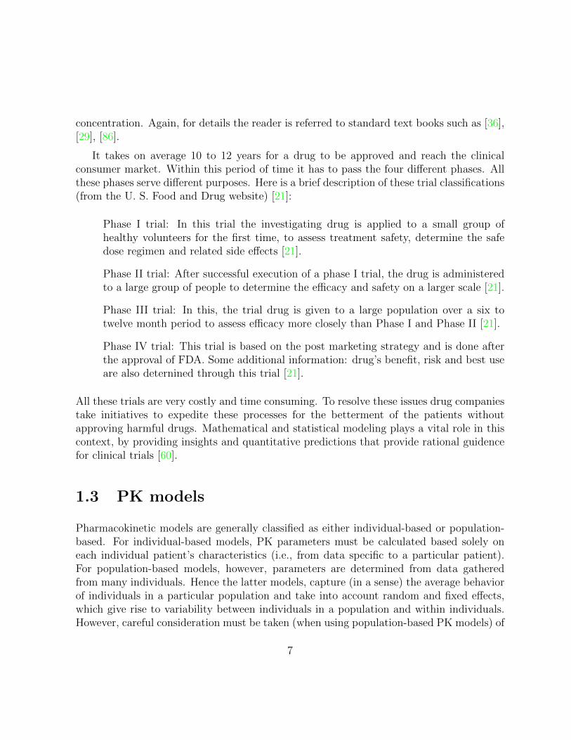
The effects and the duration of action of the drug are also taken into account. Byusing experimental PK data from humans or animals which are typically a discrete timesequence of drug concentrations obtained from a fixed volume. The data obtained fromsuch studies are useful for the design and execution of subsequent clinical trials, also forthe important goals of drug development by the pharmaceutical industry. Clinical phar-macokinetics is the application of pharmacokinetic studies to clinical practice and to thesafe and effective therapeutic management of the individual patient. There are diversemeans of drug administration ranging from subcutaneous, intramuscular, oral, bolus, in-travenous and infusion. In the last two cases, the drugs are introduced directly into theblood plasma and so no absorption phase has to be taken into consideration. Typically,as a drug dissipates through the body and is eliminated this gives rise to a prototypicalconcentration/time curve that rises to a maximum concentration as the absorption phaseof the drug predominates and then decreases asymptotically to zero with time.

2

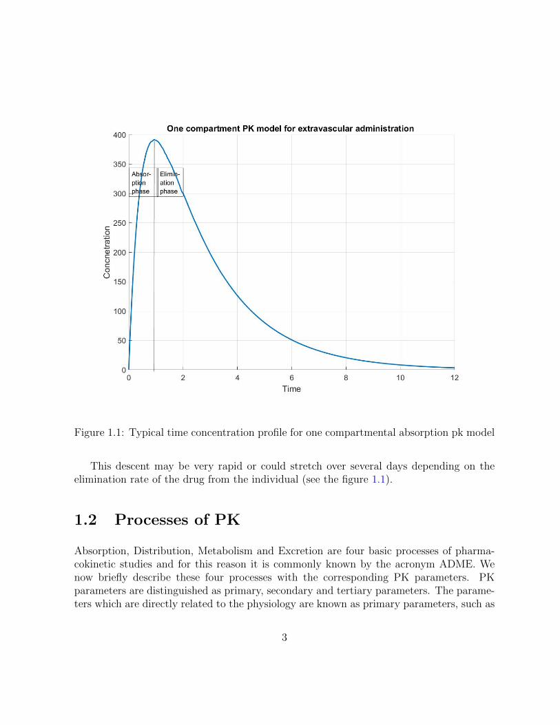
Figure 1.1: Typical time concentration profile for one compartmental absorption pk model

This descent may be very rapid or could stretch over several days depending on theelimination rate of the drug from the individual (see the figure 1.1).

1.2 Processes of PK

Absorption, Distribution, Metabolism and Excretion are four basic processes of pharma-cokinetic studies and for this reason it is commonly known by the acronym ADME. Wenow briefly describe these four processes with the corresponding PK parameters. PKparameters are distinguished as primary, secondary and tertiary parameters. The parame-ters which are directly related to the physiology are known as primary parameters, such as

3

volume of distribution, clearance, absorption rate constant and dose. By using primary pa-rameters we can calculate the secondary parameters, such as the elimination rate constant,area under the plasma concentration time data curve (AUC) and by using the secondaryparameters we can calculate the tertiary parameters such as Cmax (the maximum concen-tration), tmax (the time taken to reach at maximum concentration), t1/2 (time taken for Cmax to drop its value to half). For details the reader is referred to reference [36].

Absorption is the process by which a drug moves from the administration site to thesystemic circulation and this is fully dependent on the routes of drug administration,mainly oral, dermal, topical, subcutaneous, intravenous. Absorption is defined by a ratewhich is the amount of drug per unit time and an extent which is the total amount ofdrug. The parameter absorption rate constant usually is a first order rate constant fordrug absorption from the site of administration to the systemic circulation and can beestimated using the curve stripping method (also known as the method of residuals) [36],[29], [86].The absorption rate is influenced by some factors such as, types of transport, thephysicochemical properties of the drug, protein binding, dosage form, circulation at the siteof absorption, concentration of the drug etc. Unless the administration is IV (intravenous),there is an absorption phase. Bioavailability is another important parameter related to theabsorption process, which defines the fraction (F ) of the administered drug that reaches thesystemic circulation and it’s value varies from 0 to 1. If F is less than 10 percent then thedrug is classified as “low bioavailable” and if it is greater than 90 percent then it is said tobe “high bioavailable”. Absorption kinetics are the basis of classification of bioequivalenceof generic drugs. If absorption profiles are identical for both the test formulation andreference formulation, then the two formulations are said to be bioequivalent.

Distribution is the process by which a drug moves from the systemic circulation to othertissues in the body. The process is largely determined by the physicochemical characteristicof the drug molecules. Distribution occurs throughout the drug time course in the bodyand it is very difficult to quantify the distribution with a PK parameter. There are twomain factors that affect distribution, one is the rate of distribution (i.e., how fast the drugis distributed) and this is dependent on membrane permeability and blood perfusion [36],[29], [86]. and another is the extent of distribution (i.e., how far the drug is distributed)and this depends on the drug lipid (fat) solubility, pH-pKa, protein binding [36], [29], [86].Distribution occurs in two different phases. In the first phase the heart, liver, kidney andbrain receive most of the drug during the first few minutes of absorption. The secondphase involves the muscles, most viscera, skin and adipose tissue.

To determine the appropriate drug dose regimen, the main PK parameter associatedwith the distribution process is, the volume of distribution or apparent volume of distribu-tion. Volume of distribution does not have any true physiological significance but by this

4

parameter it is possible to identify the extent of drug distribution which help to determinedosage requirements. Typically, dosing and volume of distribution are proportional to eachother. For instance, if the volume of distribution is large then the dosage should be pro-portionally large to obtain a desired target concentration [14]. The (apparent) volume ofdistribution can be calculated using the following equation:

volume of distribution=[amount of drug administered (dose)]/[initial drug concentration]

=⇒ Vd(l) = D(mg)C0(mg/l)

C0 is the initial concentration, which is usually evaluated by direct measurement or can beestimated by back-extrapolation from concentrations time data which has been collectedafter the dose administered [14].

Metabolism or biotransformation refers to the chemical or enzymatic transformation ofa parent drug to another chemical form (metabolite). Metabolites tend to be more polarwhich promotes excretion via the urine. The liver is primarily responsible for metabolism,but the kidneys, intestines and lungs also contribute to metabolism [36].

Metabolism is influenced by some factors such as:

Age: Older people have less efficient metabolism

Sex: Hormonal differences linked with the metabolic processes

Heredity: Genetic differences can influence the amounts and efficiency of metabolicenzymes

Disease state: The state of the liver, Kidney, cardiac disease also have impact on themetabolism

Enzyme induction and Enzyme inhibition have some effect on the metabolism.

Excretion is the process by which drugs (and metabolites) are removed from the body.Primarily excretion occurs through the kidney (urinary excretion), but it also occursthrough the lungs (volatile compounds), saliva, breast milk, sweat and bile (fecal excre-tion).

Clearance is another important parameter in PK studies and quantifies the removalof a drug from a volume of plasma in a given unit of time (drug loss from the body).Clearance does not indicate the amount of drug being removed, it indicates the volume ofplasma (or blood) from which the drug is completely removed [14]. A drug can be cleared

5

from the body by many different mechanisms, pathways, or organs, including hepaticbiotransformation and renal and biliary excretion. Total body clearance of a drug is thesum of all the clearances by various mechanisms.

Another way of defining clearance is by using the relationship between drug dose andAUC. Since AUC is a secondary parameter, it can be exactly calculated from concentration-time data (or can be estimated). Some common AUC estimates are: exact AUC, AUC0−tor AUC0−last, AUCall, AUC0−∞ [86].

Exact calculation of AUC for IV administration:

AUC =

∫ ∞0

C(t)dt (1.1)

and for IV we have

C(t) =D

Vde−(CL/Vd)t (1.2)

Now by substituting this in the AUC definition we have

AUC =

∫ ∞0

D

Vde−(CL/Vd)tdt (1.3)

AUC =D

CL(1.4)

that mean

CL =Dose

AUC(1.5)

and if the administration is not IV, then this will be

CL =S × F ×Dose

AUC(1.6)

where S is the salt fraction which is used when the dose amount refers to the drug insalt form and F is the absolute bioavailability for the specific route. In cases where thebioavailability is unknown, the apparent clearance can be calculated as

CL

F=S ×DoseAUC

(1.7)

Another PK parameter corresponding to elimination is rate of elimination and is givenby: Rate of elimination (mg/hr)=Clearance CL (l/hr)× Concentration C(mg/l). Eventhough the clearance may be constant, the rate of drug elimination (mg/hr) can vary with

6

concentration. Again, for details the reader is referred to standard text books such as [36],[29], [86].

It takes on average 10 to 12 years for a drug to be approved and reach the clinicalconsumer market. Within this period of time it has to pass the four different phases. Allthese phases serve different purposes. Here is a brief description of these trial classifications(from the U. S. Food and Drug website) [21]:

Phase I trial: In this trial the investigating drug is applied to a small group ofhealthy volunteers for the first time, to assess treatment safety, determine the safedose regimen and related side effects [21].

Phase II trial: After successful execution of a phase I trial, the drug is administeredto a large group of people to determine the efficacy and safety on a larger scale [21].

Phase III trial: In this, the trial drug is given to a large population over a six totwelve month period to assess efficacy more closely than Phase I and Phase II [21].

Phase IV trial: This trial is based on the post marketing strategy and is done afterthe approval of FDA. Some additional information: drug’s benefit, risk and best useare also deternined through this trial [21].

All these trials are very costly and time consuming. To resolve these issues drug companiestake initiatives to expedite these processes for the betterment of the patients withoutapproving harmful drugs. Mathematical and statistical modeling plays a vital role in thiscontext, by providing insights and quantitative predictions that provide rational guidencefor clinical trials [60].

1.3 PK models

Pharmacokinetic models are generally classified as either individual-based or population-based. For individual-based models, PK parameters must be calculated based solely oneach individual patient’s characteristics (i.e., from data specific to a particular patient).For population-based models, however, parameters are determined from data gatheredfrom many individuals. Hence the latter models, capture (in a sense) the average behaviorof individuals in a particular population and take into account random and fixed effects,which give rise to variability between individuals in a population and within individuals.However, careful consideration must be taken (when using population-based PK models) of

7

the underlying assumptions made when combining different patient data from a particularstudy as well as patient data from different studies. In particular careful thought must begiven to the choice of sampling distributions of population estimates. The most commonand widespread approach in pharmacokinetics is the use of compartmental models. Herethe body, is considered to be an interconnected system of compartments where, ideallyeach compartment can be given some physiological interpretation. Each compartmentis assumed to be homogeneous and well mixed. The interchange and transfer of drugmolecules between compartments is determined by the kinetic rate constants. The law ofmass action is widely applied in classical pharmacokinetic compartmental models. Thusa chemical reaction rate is assumed to be directly proportional to the product of theconcentrations of m reactants each raised to a power ni(i = 1, 2, ....,m). For a general PKmodel with n− compartments, the governing system of DE’s can be written as :

dC(t)

dt= KC(t) (1.8)

where CT (t) = (C1(t), C2(t), .....Cn(t)) and K is the matrix of kinetic rate coefficientsK = kij, where the kij are non-zero if compartments i and j are coupled in the model.The solution to the system (1.8) can be written down as:

Ci(t) =m∑j=1

aij

(mj−1∑k=0

bijktk)exp(−λjt) (1.9)

where aij and bijk are constants and the matrix K has m distinct eigenvalues λj withmultiplicity mj [53]

Compartmental models are widely applicable and have the advantage of being able tobe interpreted in terms of physiological processes or body organs/components. There are,of course, limitations to the classical compartmental models; the major objections relateto the assumption of homogeneity of each compartment and the assumption that eachcompartment is well mixed. However, a compartmental model might be assessed suitableif the relative mixing rates within the compartments is on a much faster time scale thanthe transfer rate between compartments.

1.3.1 Non-compartmental models

Non-compartmental models were developed to overcome some of the limitations of com-partmental models. Approaches include linear Systems Analysis, Mean Residence Time

8

Theory and the Method of Moments amongst others. They have the distinct advantagethat fewer assumptions are made, and many of these assumptions are based on experi-mental observations rather than on assumptions about the underlying mechanisms. Themethodology is also applicable to a wide range of date.

There are clearly drawbacks and limitations to compartmental models, and to circum-vent some of these problems, several non- compartmental models have been proposed inthe literature. For example [85] uses the method of moments and quantifies such as meanresidence time, and area under the moment curve to analyze and extract information froma data set. Another approach is taken by [61], where linear system analysis (convolution,deconvolution, disposition decomposition analysis) is applied to deduce information froma data set. The attraction of this approach is that fewer assumptions are usually made(compared to compartmental models), and even these are based generally on observedoutcomes or behaviors rather than on the underlying mechanisms or state of the system.However [45] shows how a non-compartmental circulation model is equivalent to a multicompartmental model, where the compartments are connected in series. So it is apparentthat in many cases “non-compartmental” models can be framed in terms of a correspondingcompartmental model. In both contexts, the models can be formulated in terms of deter-ministic or random variables. Stochastic effects can be captured in the models by usingeither random inputs/random initial conditions, or by making the kinetic rate coefficientsmatrix K a random matrix, or by using the random walk formalism.

1.3.2 Linearity and Non-linearity

If the output of a system is directly proportional to input then a system is generallyclassified as linear. Systems are governed by zeroth order or first order kinetics guaranteethis property and are described, for one compartmental models, by the linear differentialequation

dC

dt= kC (1.10)

Solutions to linear differential equations satisfy the linear superposition principle. Thusif the drug concentration C is a linear function of the dosage d, then for any arbitraryconstants a1 and a2, the concentration C for a dosage d = a1d1 + a2d2, is given by:C = a1C1 + a2C2. Linear superposition indicates that the drug molecules interact in astochastically independent fashion [82]. In contrast, for a molecular system the action ofa drug molecule is altered and changed by the behavior of other drug molecules [13]. Forexample, assuming stochasticity of drug absorption and elimination, if random components

9

are added to the kinetic rate coefficient k then the system is still considered to be linearwith a stochastic input, e. g., consider the one compartmental model

dC

dt= k∗C + i(t) (1.11)

where k∗ = k + r, and k represents the deterministic rate and r represents the stochasticcontribution to the kinetic rate coefficient k∗, then equation (1.11) can be written as:

dC

dt= kC + [rC + i(t)] (1.12)

where [rC + i(t)] can be considered to be the stochastic input. However if the randomeffects are considered to be actually in the concentration C, then the effects are nonlinear.

The nonlinear dependence of the drug concentration on dosage and other factors, clearlyadds a further complication for clinicians when trying to design effective dosage schedules,and in trying to predict a drug’s efficacy and toxicity. Broadly speaking, nonlinearity inPK is split into dose-dependent and time-dependent. In phase I clinical trials, the conceptof dose proportionality is commonly used when carrying out dose escalation experiments.Here, patient response to varying drug dosage is measured. If PK parameters remainconstant with variation of dosage, the system PK is classified as dose independent (overthe therapeutic range of interest). If increase in dosage of a drug produces a proportionalincrease in the PK parameters (AUC (area under the curve) or Cmax), the system isclassified as linear and dose dependent. If the variations in parameter values are not directlyproportional to the variation in drug dosage, the system is classified as non-linear and dosedependent. PK parameters may also vary in time due to physiological change in the body orthrough drug induced changes in the body. Clearly, the PK parameters can be both dose-dependent and time-dependent. The proposed reasons and sources for this dependencyappear to be similar in both cases. Lin [49], suggests that non-linear dose dependence isrooted in the absorption process, drug distribution variation in tissue and in the eliminationprocess. [47] proposes that non-linear time-dependence arises from variations in absorptionand elimination parameters, enzyme activity, plasma protein binding and the eliminationprocesses.

1.3.3 Enzyme kinetics

Biological and biochemical processes are common characteristic features present in all ani-mals and living organisms. There are complex biochemical reactions catalyzed by proteins

10

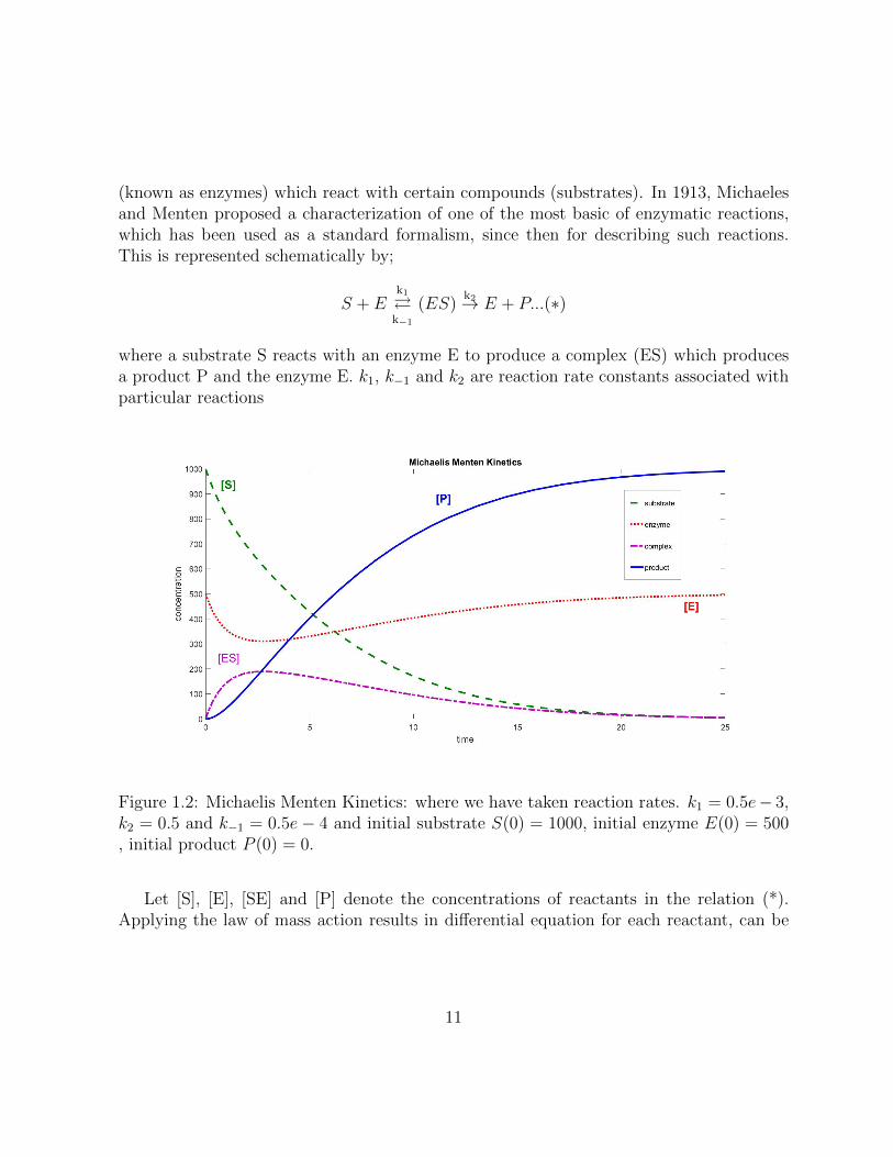
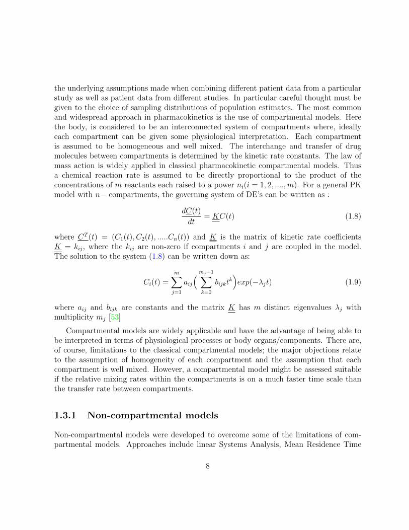
(known as enzymes) which react with certain compounds (substrates). In 1913, Michaelesand Menten proposed a characterization of one of the most basic of enzymatic reactions,which has been used as a standard formalism, since then for describing such reactions.This is represented schematically by;

S + Ek1

�k−1

(ES)k2→ E + P...(∗)

where a substrate S reacts with an enzyme E to produce a complex (ES) which producesa product P and the enzyme E. k1, k−1 and k2 are reaction rate constants associated withparticular reactions

Figure 1.2: Michaelis Menten Kinetics: where we have taken reaction rates. k1 = 0.5e− 3,k2 = 0.5 and k−1 = 0.5e− 4 and initial substrate S(0) = 1000, initial enzyme E(0) = 500, initial product P (0) = 0.

Let [S], [E], [SE] and [P] denote the concentrations of reactants in the relation (*).Applying the law of mass action results in differential equation for each reactant, can be

11

described as following:

d[S]

dt= −k1[S][E] + k−1[ES], (1.13)

d[E]

dt= −k1[S][E] + (k−1 + k2)[ES],

d[ES]

dt= k1[S][E]− (k−1 + k2)[ES],

dP

dt= vp = k2[ES].

The mathematical formulation is completed by a set of initial conditions, corresponding tothe start of the whole process of conversion of S to P:

S(0)=[S]0, E(0)=[E]0, ES(0)=0, P(0)=0.

On adding the second and third DEs, we obtain

[dE]

dt+d[ES]

dt= 0, (1.14)

i.e., E(t)+ES(t)=E0 and by using this and substituting for [E] in the third DE (for theenzyme substrate complex), we obtain

d[ES]

dt= k1(E0 − [ES])[S]− (k−1 + k2)[ES]. (1.15)

Assuming that the initial formation of the complex [ES] is very rapid (after which it is, forall intents and purposes, at equilibrium), we have

k1(E0 − [ES])[S]− (k−1 + k2)[ES] ≈ 0, (1.16)

from which we can evaluate:

[ES] =k1[S]E0

k−1 + k2 + k1[S],

or

[ES] =E0[S]

kM + [S],

where

kM =k−1 + k2

k1

12

is the Michaeles Menten constant. Since the velocity of the reaction is given by: v = k2[ES],this implies

v =k2E0[S]

kM + [S]=

vmax[S]

kM + [S],

where vmax = k2E0 is the maximum velocity of the reaction and kM (the Michaelis-Mentenconstant) gives substrate concentration at 1

2vmax

13

Chapter 2

The relevance of Stochasticity in PKmodels

2.1 Introduction

The traditional approach to the study of Pharmacokinetics (PK) is to imagine the humanbody as subdivided into various communicating compartments, in each of which a drug(administered in various forms) enters and exits at certain constant rates which must bedetermined from experimental data.

The translation of this hypothesis into a mathematical model leads to a set of coupledordinary differential equations (ODEs), and the procedure and its uses are given in greatdetail in classic text books, such as Gibaldi and Perrier’s “Pharmacokinetics” [29]

Although used successfully in many instances, this approach is not free of serious diffi-culties. For, on the one hand, to be physiologically accurate the number of compartmentsmust be large in order to reflect the different ways in which organs process the drug; but,on the other hand, the larger the number of compartments the more unknown rates ap-pear in the system of ODEs. As the aim of PK is to describe the total concentration ofthe drug in the body, the solution of the mathematical model would require many moreconcentration measurements than actually possible. Furthermore, the assumption that therates are constant is also on shaky grounds, as the effects of (unknown) fluctuations fromcompartment to compartment suggest a time dependence of the rates.

In order to illustrate some of these difficulties, consider the problem of determining therate of drug absorption and its related bioavailability. This has long been recognized as a

14

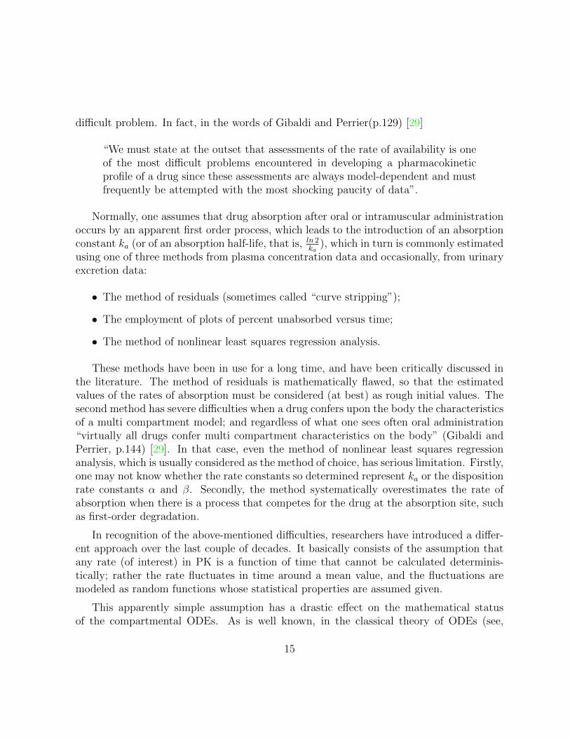
difficult problem. In fact, in the words of Gibaldi and Perrier(p.129) [29]

“We must state at the outset that assessments of the rate of availability is oneof the most difficult problems encountered in developing a pharmacokineticprofile of a drug since these assessments are always model-dependent and mustfrequently be attempted with the most shocking paucity of data”.

Normally, one assumes that drug absorption after oral or intramuscular administrationoccurs by an apparent first order process, which leads to the introduction of an absorptionconstant ka (or of an absorption half-life, that is, ln 2

ka), which in turn is commonly estimated

using one of three methods from plasma concentration data and occasionally, from urinaryexcretion data:

• The method of residuals (sometimes called “curve stripping”);

• The employment of plots of percent unabsorbed versus time;

• The method of nonlinear least squares regression analysis.

These methods have been in use for a long time, and have been critically discussed inthe literature. The method of residuals is mathematically flawed, so that the estimatedvalues of the rates of absorption must be considered (at best) as rough initial values. Thesecond method has severe difficulties when a drug confers upon the body the characteristicsof a multi compartment model; and regardless of what one sees often oral administration“virtually all drugs confer multi compartment characteristics on the body” (Gibaldi andPerrier, p.144) [29]. In that case, even the method of nonlinear least squares regressionanalysis, which is usually considered as the method of choice, has serious limitation. Firstly,one may not know whether the rate constants so determined represent ka or the dispositionrate constants α and β. Secondly, the method systematically overestimates the rate ofabsorption when there is a process that competes for the drug at the absorption site, suchas first-order degradation.

In recognition of the above-mentioned difficulties, researchers have introduced a differ-ent approach over the last couple of decades. It basically consists of the assumption thatany rate (of interest) in PK is a function of time that cannot be calculated determinis-tically; rather the rate fluctuates in time around a mean value, and the fluctuations aremodeled as random functions whose statistical properties are assumed given.

This apparently simple assumption has a drastic effect on the mathematical statusof the compartmental ODEs. As is well known, in the classical theory of ODEs (see,

15

e.g., Ince “Ordinary Differential Equations”, [35]), once the coefficients and appropriateinitial conditions are specified one can then prove fundamental theorems of existence anduniqueness, and then develop techniques for finding exact or approximate solutions. But ifthe coefficients are random variables, or random functions, no part of the classical theoryapplies and the resulting Stochastic Differential Equations (SDEs) require new concepts,starting with the meaning of “solutions” for them.

There is a vast literature on SDEs in mathematics and physics (going back to thebeginning of the 20th century) which is impossible to review here. Suffice it to say that theinterested reader can find excellent text books, such as “Stochastic Differential Equations:Theory and Applications” [3], whose focus is on rigorous mathematics. For those readerswho are more interested in the applications of SDEs to physical and chemical phenomenathe book by Van Kampen, “Stochastic Process in Physics and Chemistry” [79] is highlyrecommended. Also useful in this regard is the book by Gardiner, “Handbook of StochasticMethods” [25], which contains many worked-out examples, including a thorough discussionof the most famous of all stochastic processes, namely Brownian motion, which we shallreview momentarily.

The role played by stochastic processes in biological and pharmacological phenomenais not as well understood as in older areas of science. There have been early attempts atdescribing the drug’s molecules as a discrete population of N particles whose steady statemotion among m components is described probabilistically [58].

In the next section, we present some mathematical details relevant to the applicationof stochastic processes to PK.

2.2 Stochastic PK models and additive noise

Deterministic models are not capable of taking into account the uncertainties, which mayrise either from the measurement errors or from the intrinsic fluctuations of the biologicalsystem itself. This has been recognized for a long time, and many stochastic models havebeen proposed where the fluctuations have been represented by random functions of time.Some of these studies we are going to discuss here. Limic [48] studied the stochasticnature of the compartment models due to randomness of the parameters. The focus ofthe study was to evaluate the statistical average of the model by considering transitionrates as constant and fluctuations are described by Gaussian process. D’Argenio and Park[15], reviewed design, estimation, and control of uncertain PK/PD systems. The focusof this work was the study of biological systems for which measurement of some process

16

variables occurs infrequently and at irregular intervals that is, the analysis of sparse datasystem. The authors assumed that the model under consideration can be written as alinear continuous dynamical systems with uncertainty due to both system (biological)noise and to measurement error. Kalman filter formulation [38], used to compute themaximum likelihood function which determines the estimates of the unknown parameters.An important point in this paper is the assumption that the model parameters are constant,and therefore the noise is additive. Ramanathan [66], provided an introduction to Ito’scalculus [25], for researchers in pharmaceutics. Ito’s lemma is applied to the simplestcase of PK (first order PK process with elimination rate constant ke) and to the standardMichaelis-Menten effect E (E = EmaxC

E50+C) of PD. As already mentioned, the noise is supposed

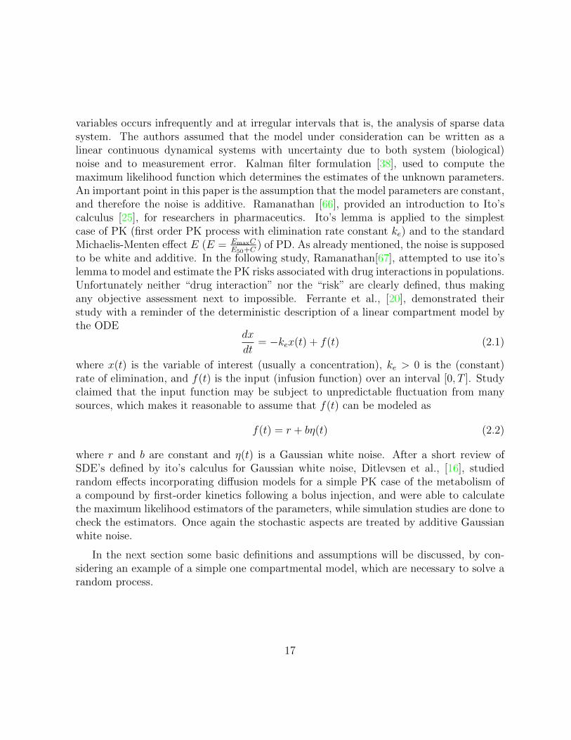
to be white and additive. In the following study, Ramanathan[67], attempted to use ito’slemma to model and estimate the PK risks associated with drug interactions in populations.Unfortunately neither “drug interaction” nor the “risk” are clearly defined, thus makingany objective assessment next to impossible. Ferrante et al., [20], demonstrated theirstudy with a reminder of the deterministic description of a linear compartment model bythe ODE

dx

dt= −kex(t) + f(t) (2.1)

where x(t) is the variable of interest (usually a concentration), ke > 0 is the (constant)rate of elimination, and f(t) is the input (infusion function) over an interval [0, T ]. Studyclaimed that the input function may be subject to unpredictable fluctuation from manysources, which makes it reasonable to assume that f(t) can be modeled as

f(t) = r + bη(t) (2.2)

where r and b are constant and η(t) is a Gaussian white noise. After a short review ofSDE’s defined by ito’s calculus for Gaussian white noise, Ditlevsen et al., [16], studiedrandom effects incorporating diffusion models for a simple PK case of the metabolism ofa compound by first-order kinetics following a bolus injection, and were able to calculatethe maximum likelihood estimators of the parameters, while simulation studies are done tocheck the estimators. Once again the stochastic aspects are treated by additive Gaussianwhite noise.

In the next section some basic definitions and assumptions will be discussed, by con-sidering an example of a simple one compartmental model, which are necessary to solve arandom process.

17

2.3 Some basic concepts before solving a random sys-

tem

The basic assumptions of compartmental PK models have already been discussed in theprevious chapter. We now focus on the basic (deterministic) one compartmental model,its extension to a random differential equation, and the concepts and methods used in theformulation and approximation of such random differential equations.

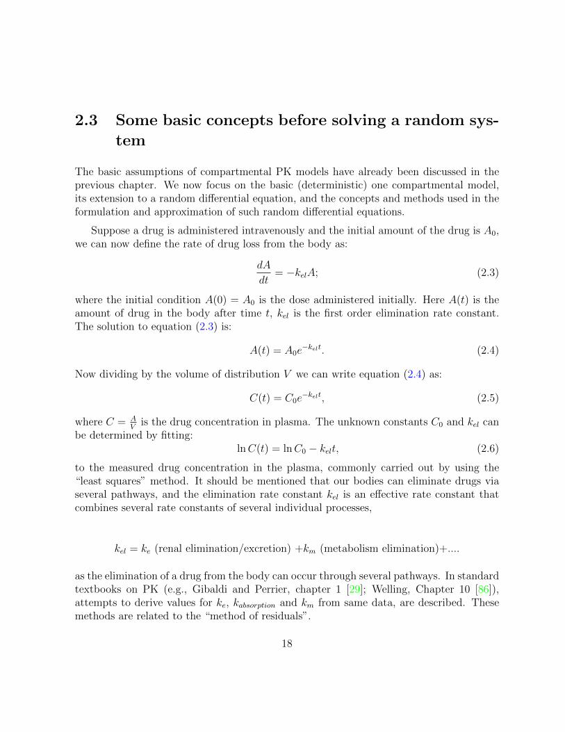
Suppose a drug is administered intravenously and the initial amount of the drug is A0,we can now define the rate of drug loss from the body as:

dA

dt= −kelA; (2.3)

where the initial condition A(0) = A0 is the dose administered initially. Here A(t) is theamount of drug in the body after time t, kel is the first order elimination rate constant.The solution to equation (2.3) is:

A(t) = A0e−kelt. (2.4)

Now dividing by the volume of distribution V we can write equation (2.4) as:

C(t) = C0e−kelt, (2.5)

where C = AV

is the drug concentration in plasma. The unknown constants C0 and kel canbe determined by fitting:

lnC(t) = lnC0 − kelt, (2.6)

to the measured drug concentration in the plasma, commonly carried out by using the“least squares” method. It should be mentioned that our bodies can eliminate drugs viaseveral pathways, and the elimination rate constant kel is an effective rate constant thatcombines several rate constants of several individual processes,

kel = ke (renal elimination/excretion) +km (metabolism elimination)+....

as the elimination of a drug from the body can occur through several pathways. In standardtextbooks on PK (e.g., Gibaldi and Perrier, chapter 1 [29]; Welling, Chapter 10 [86]),attempts to derive values for ke, kabsorption and km from same data, are described. Thesemethods are related to the “method of residuals”.

18

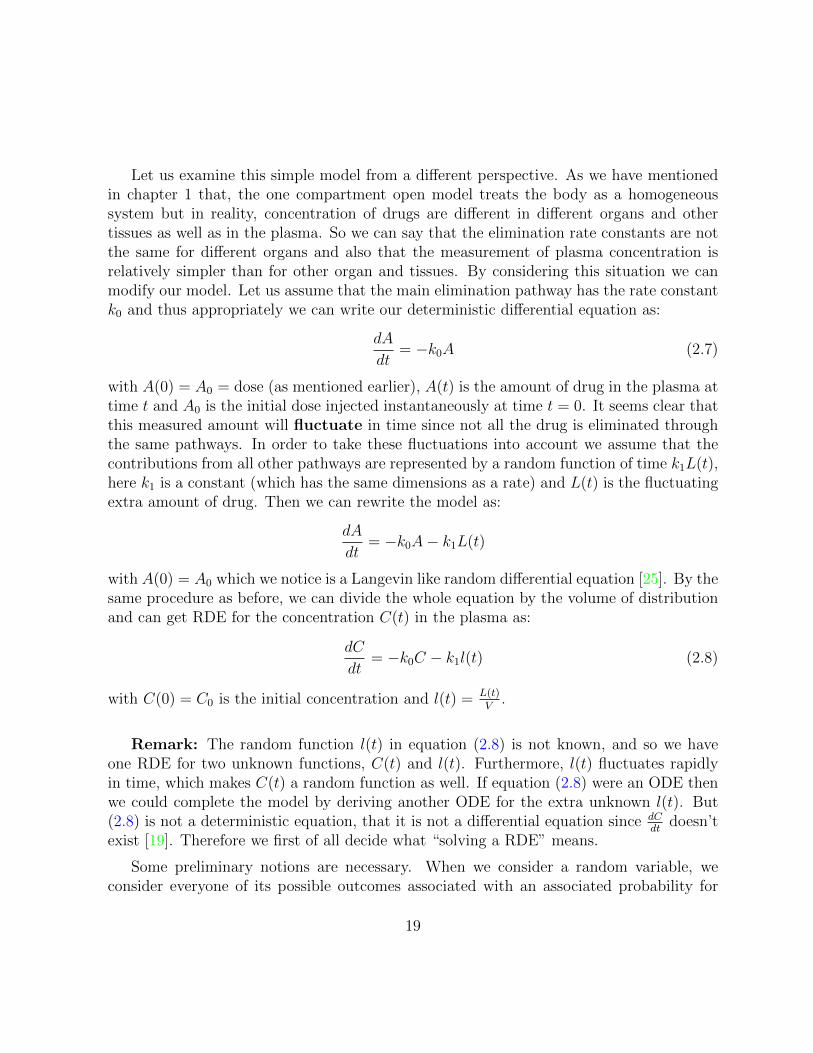
Let us examine this simple model from a different perspective. As we have mentionedin chapter 1 that, the one compartment open model treats the body as a homogeneoussystem but in reality, concentration of drugs are different in different organs and othertissues as well as in the plasma. So we can say that the elimination rate constants are notthe same for different organs and also that the measurement of plasma concentration isrelatively simpler than for other organ and tissues. By considering this situation we canmodify our model. Let us assume that the main elimination pathway has the rate constantk0 and thus appropriately we can write our deterministic differential equation as:

dA

dt= −k0A (2.7)

with A(0) = A0 = dose (as mentioned earlier), A(t) is the amount of drug in the plasma attime t and A0 is the initial dose injected instantaneously at time t = 0. It seems clear thatthis measured amount will fluctuate in time since not all the drug is eliminated throughthe same pathways. In order to take these fluctuations into account we assume that thecontributions from all other pathways are represented by a random function of time k1L(t),here k1 is a constant (which has the same dimensions as a rate) and L(t) is the fluctuatingextra amount of drug. Then we can rewrite the model as:

dA

dt= −k0A− k1L(t)

with A(0) = A0 which we notice is a Langevin like random differential equation [25]. By thesame procedure as before, we can divide the whole equation by the volume of distributionand can get RDE for the concentration C(t) in the plasma as:

dC

dt= −k0C − k1l(t) (2.8)

with C(0) = C0 is the initial concentration and l(t) = L(t)V

.

Remark: The random function l(t) in equation (2.8) is not known, and so we haveone RDE for two unknown functions, C(t) and l(t). Furthermore, l(t) fluctuates rapidlyin time, which makes C(t) a random function as well. If equation (2.8) were an ODE thenwe could complete the model by deriving another ODE for the extra unknown l(t). But(2.8) is not a deterministic equation, that it is not a differential equation since dC

dtdoesn’t

exist [19]. Therefore we first of all decide what “solving a RDE” means.

Some preliminary notions are necessary. When we consider a random variable, weconsider everyone of its possible outcomes associated with an associated probability for

19

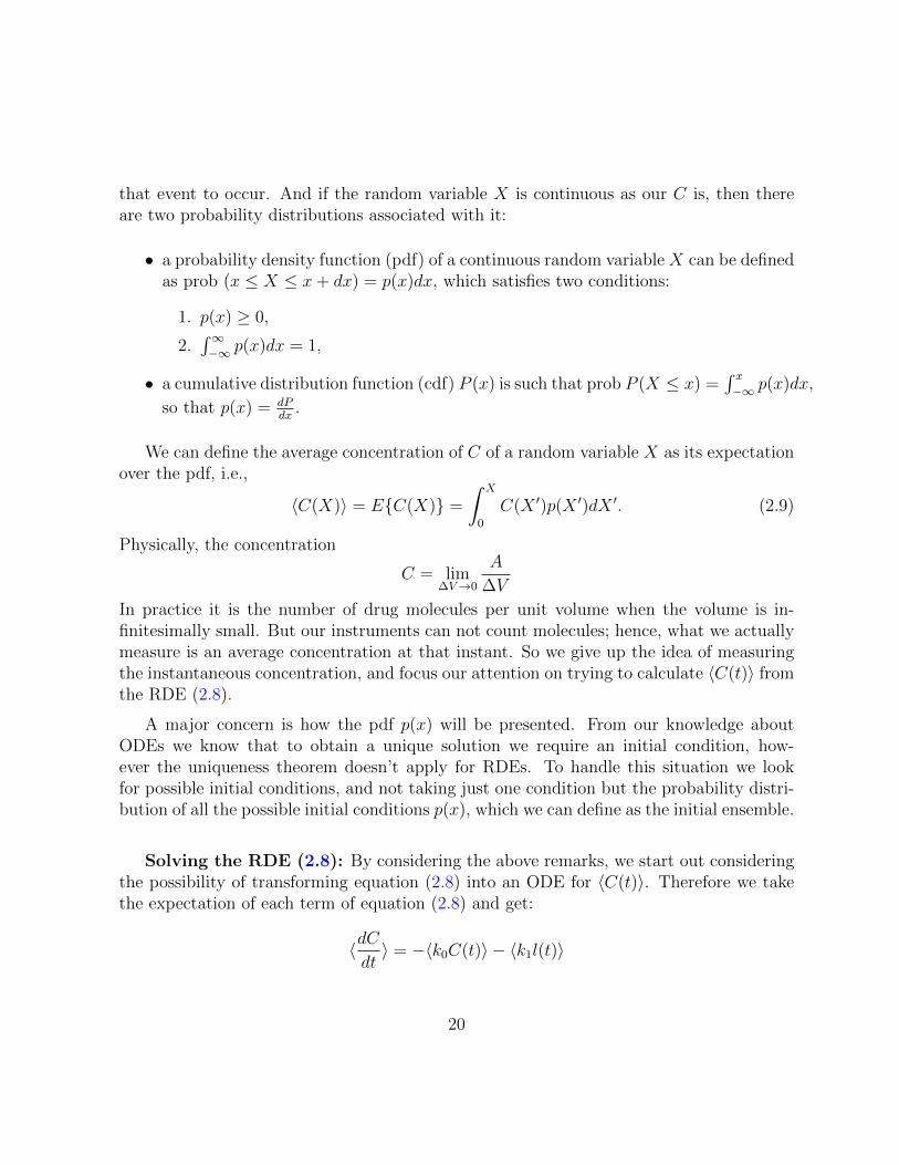
that event to occur. And if the random variable X is continuous as our C is, then thereare two probability distributions associated with it:

• a probability density function (pdf) of a continuous random variable X can be definedas prob (x ≤ X ≤ x+ dx) = p(x)dx, which satisfies two conditions:

1. p(x) ≥ 0,

2.∫∞−∞ p(x)dx = 1,

• a cumulative distribution function (cdf) P (x) is such that prob P (X ≤ x) =∫ x−∞ p(x)dx,

so that p(x) = dPdx

.

We can define the average concentration of C of a random variable X as its expectationover the pdf, i.e.,

〈C(X)〉 = E{C(X)} =

∫ X

0

C(X ′)p(X ′)dX ′. (2.9)

Physically, the concentration

C = lim∆V→0

A

∆V

In practice it is the number of drug molecules per unit volume when the volume is in-finitesimally small. But our instruments can not count molecules; hence, what we actuallymeasure is an average concentration at that instant. So we give up the idea of measuringthe instantaneous concentration, and focus our attention on trying to calculate 〈C(t)〉 fromthe RDE (2.8).

A major concern is how the pdf p(x) will be presented. From our knowledge aboutODEs we know that to obtain a unique solution we require an initial condition, how-ever the uniqueness theorem doesn’t apply for RDEs. To handle this situation we lookfor possible initial conditions, and not taking just one condition but the probability distri-bution of all the possible initial conditions p(x), which we can define as the initial ensemble.

Solving the RDE (2.8): By considering the above remarks, we start out consideringthe possibility of transforming equation (2.8) into an ODE for 〈C(t)〉. Therefore we takethe expectation of each term of equation (2.8) and get:

〈dCdt〉 = −〈k0C(t)〉 − 〈k1l(t)〉

20

where k0 and k1 are constants. Now as we saw above the average 〈...〉 is an integral overthe initial ensemble, and so 〈...〉 and d

dt〈...〉 commute. Therefore we may rewrite the above

equation as:

d

dt〈C〉 = −k0〈C(t)〉 − k1〈l(t)〉.

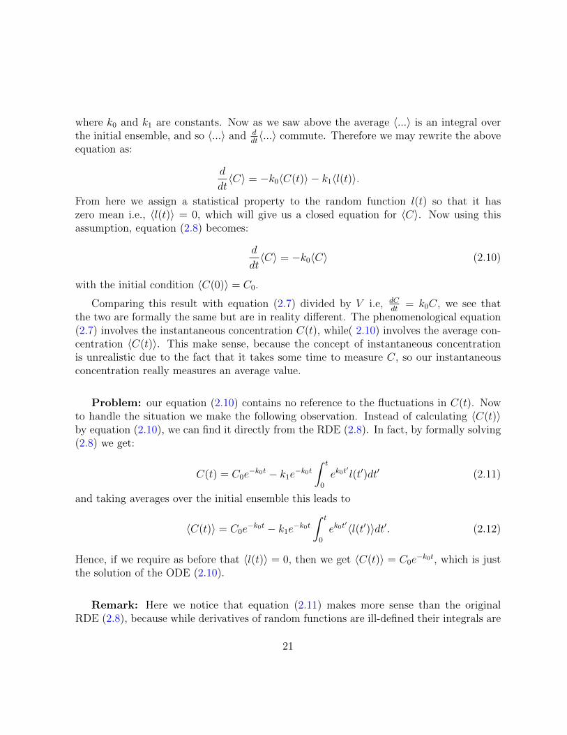
From here we assign a statistical property to the random function l(t) so that it haszero mean i.e., 〈l(t)〉 = 0, which will give us a closed equation for 〈C〉. Now using thisassumption, equation (2.8) becomes:

d

dt〈C〉 = −k0〈C〉 (2.10)

with the initial condition 〈C(0)〉 = C0.

Comparing this result with equation (2.7) divided by V i.e, dCdt

= k0C, we see thatthe two are formally the same but are in reality different. The phenomenological equation(2.7) involves the instantaneous concentration C(t), while( 2.10) involves the average con-centration 〈C(t)〉. This make sense, because the concept of instantaneous concentrationis unrealistic due to the fact that it takes some time to measure C, so our instantaneousconcentration really measures an average value.

Problem: our equation (2.10) contains no reference to the fluctuations in C(t). Nowto handle the situation we make the following observation. Instead of calculating 〈C(t)〉by equation (2.10), we can find it directly from the RDE (2.8). In fact, by formally solving(2.8) we get:

C(t) = C0e−k0t − k1e

−k0t

∫ t

0

ek0t′l(t′)dt′ (2.11)

and taking averages over the initial ensemble this leads to

〈C(t)〉 = C0e−k0t − k1e

−k0t

∫ t

0

ek0t′〈l(t′)〉dt′. (2.12)

Hence, if we require as before that 〈l(t)〉 = 0, then we get 〈C(t)〉 = C0e−k0t, which is just

the solution of the ODE (2.10).

Remark: Here we notice that equation (2.11) makes more sense than the originalRDE (2.8), because while derivatives of random functions are ill-defined their integrals are

21

perfectly respectable at least in the mean square sense.

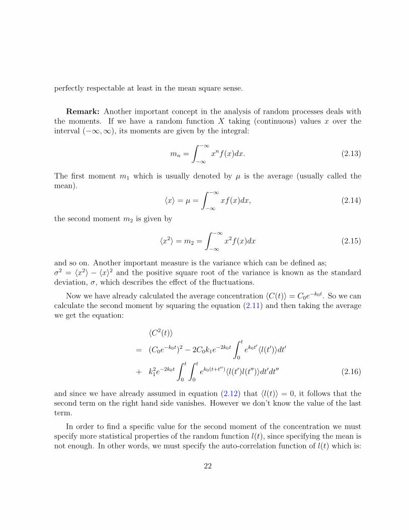
Remark: Another important concept in the analysis of random processes deals withthe moments. If we have a random function X taking (continuous) values x over theinterval (−∞,∞), its moments are given by the integral:

mn =

∫ −∞−∞

xnf(x)dx. (2.13)

The first moment m1 which is usually denoted by µ is the average (usually called themean).

〈x〉 = µ =

∫ −∞−∞

xf(x)dx, (2.14)

the second moment m2 is given by

〈x2〉 = m2 =

∫ −∞−∞

x2f(x)dx (2.15)

and so on. Another important measure is the variance which can be defined as;σ2 = 〈x2〉 − 〈x〉2 and the positive square root of the variance is known as the standarddeviation, σ, which describes the effect of the fluctuations.

Now we have already calculated the average concentration 〈C(t)〉 = C0e−k0t. So we can

calculate the second moment by squaring the equation (2.11) and then taking the averagewe get the equation:

〈C2(t)〉

= (C0e−k0t)2 − 2C0k1e

−2k0t

∫ t

0

ek0t′〈l(t′)〉dt′

+ k21e−2k0t

∫ t

0

∫ t

0

ek0(t+t′′)〈l(t′)l(t′′)〉dt′dt′′ (2.16)

and since we have already assumed in equation (2.12) that 〈l(t)〉 = 0, it follows that thesecond term on the right hand side vanishes. However we don’t know the value of the lastterm.

In order to find a specific value for the second moment of the concentration we mustspecify more statistical properties of the random function l(t), since specifying the mean isnot enough. In other words, we must specify the auto-correlation function of l(t) which is:

22

〈l(t)l(t′′)〉. Now we can take l(t) to be delta-correlated, as is done in the Langevin theoryof Brownian motion, i.e; 〈l(t)l(t′′)〉 = δ(t− t′′), which is the simplest assumption and usingthis relation we can write equation (2.16) as

〈C2(t)〉 = (C0e−k0t)2 + k2

1e−2k0t

∫ t

0

e2k0t′dt′ (2.17)

= 〈C(t)〉2 +k2

1

2k0

(1− e−2k0t)

and therefore variance is given by;

〈C2(t)〉 − 〈C(t)〉2 =k2

1

2k0

(1− e−2k0t), (2.18)

which reflects the effect of fluctuations around the average.

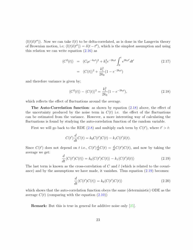
The Auto-Correlation function: as shown by equation (2.18) above, the effect ofthe uncertainty produced by the noise term in C(t) i.e. the effect of the fluctuationscan be estimated from the variance. However, a more interesting way of calculating thefluctuations is found by studying the auto-correlation function of the random variable.

First we will go back to the RDE (2.8) and multiply each term by C(t′), where t′ > t:

C(t′)d

dtC(t) = k0C(t′)C(t)− k1C(t′)l(t).

Since C(t′) does not depend on t i.e., C(t′) ddtC(t) = d

dtC(t′)C(t), and now by taking the

average we get:d

dt〈C(t′)C(t)〉 = k0〈C(t′)C(t)〉 − k1〈C(t′)l(t)〉 (2.19)

The last term is known as the cross-correlation of C and l (which is related to the covari-ance) and by the assumptions we have made, it vanishes. Thus equation (2.19) becomes:

d

dt〈C(t′)C(t)〉 = k0〈C(t′)C(t)〉 (2.20)

which shows that the auto-correlation function obeys the same (deterministic) ODE as theaverage C(t) (comparing with the equation (2.10))

Remark: But this is true in general for additive noise only [25].

23

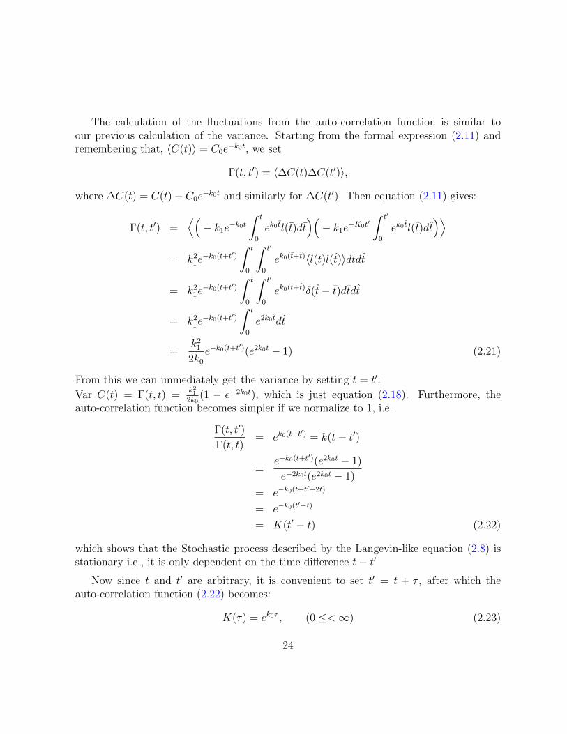
The calculation of the fluctuations from the auto-correlation function is similar toour previous calculation of the variance. Starting from the formal expression (2.11) andremembering that, 〈C(t)〉 = C0e

−k0t, we set

Γ(t, t′) = 〈∆C(t)∆C(t′)〉,

where ∆C(t) = C(t)− C0e−k0t and similarly for ∆C(t′). Then equation (2.11) gives:

Γ(t, t′) =⟨(− k1e

−k0t

∫ t

0

ek0 tl(t)dt)(− k1e

−K0t′∫ t′

0

ek0 tl(t)dt)⟩

= k21e−k0(t+t′)

∫ t

0

∫ t′

0

ek0(t+t)〈l(t)l(t)〉dtdt

= k21e−k0(t+t′)

∫ t

0

∫ t′

0

ek0(t+t)δ(t− t)dtdt

= k21e−k0(t+t′)

∫ t

0

e2k0 tdt

=k2

1

2k0

e−k0(t+t′)(e2k0t − 1) (2.21)

From this we can immediately get the variance by setting t = t′:

Var C(t) = Γ(t, t) =k2

1

2k0(1 − e−2k0t), which is just equation (2.18). Furthermore, the

auto-correlation function becomes simpler if we normalize to 1, i.e.

Γ(t, t′)

Γ(t, t)= ek0(t−t′) = k(t− t′)

=e−k0(t+t′)(e2k0t − 1)

e−2k0t(e2k0t − 1)

= e−k0(t+t′−2t)

= e−k0(t′−t)

= K(t′ − t) (2.22)

which shows that the Stochastic process described by the Langevin-like equation (2.8) isstationary i.e., it is only dependent on the time difference t− t′

Now since t and t′ are arbitrary, it is convenient to set t′ = t + τ , after which theauto-correlation function (2.22) becomes:

K(τ) = ek0τ , (0 ≤<∞) (2.23)

24

Remark: The simple exponential form of the auto-correlation function implies that theStochastic process under study is stationary and Markovian, as proved by Doob [19]. Infact Doob proved that K obeys the functional equation K(t3 − t1) = K(t3 − t2).K(2−t1),(t3 > t2 > t1) whose only non-singular solution is (2.23).

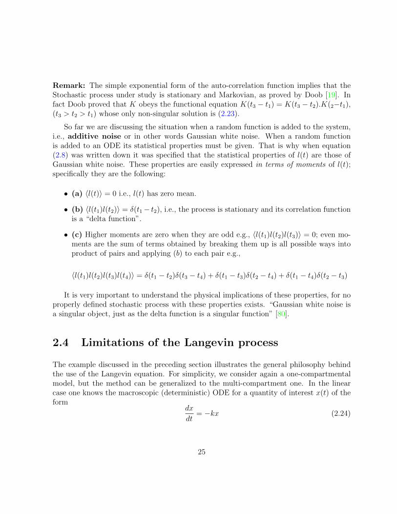
So far we are discussing the situation when a random function is added to the system,i.e., additive noise or in other words Gaussian white noise. When a random functionis added to an ODE its statistical properties must be given. That is why when equation(2.8) was written down it was specified that the statistical properties of l(t) are those ofGaussian white noise. These properties are easily expressed in terms of moments of l(t);specifically they are the following:

• (a) 〈l(t)〉 = 0 i.e., l(t) has zero mean.

• (b) 〈l(t1)l(t2)〉 = δ(t1− t2), i.e., the process is stationary and its correlation functionis a “delta function”.

• (c) Higher moments are zero when they are odd e.g., 〈l(t1)l(t2)l(t3)〉 = 0; even mo-ments are the sum of terms obtained by breaking them up is all possible ways intoproduct of pairs and applying (b) to each pair e.g.,

〈l(t1)l(t2)l(t3)l(t4)〉 = δ(t1 − t2)δ(t3 − t4) + δ(t1 − t3)δ(t2 − t4) + δ(t1 − t4)δ(t2 − t3)

It is very important to understand the physical implications of these properties, for noproperly defined stochastic process with these properties exists. “Gaussian white noise isa singular object, just as the delta function is a singular function” [80].

2.4 Limitations of the Langevin process

The example discussed in the preceding section illustrates the general philosophy behindthe use of the Langevin equation. For simplicity, we consider again a one-compartmentalmodel, but the method can be generalized to the multi-compartment one. In the linearcase one knows the macroscopic (deterministic) ODE for a quantity of interest x(t) of theform

dx

dt= −kx (2.24)

25

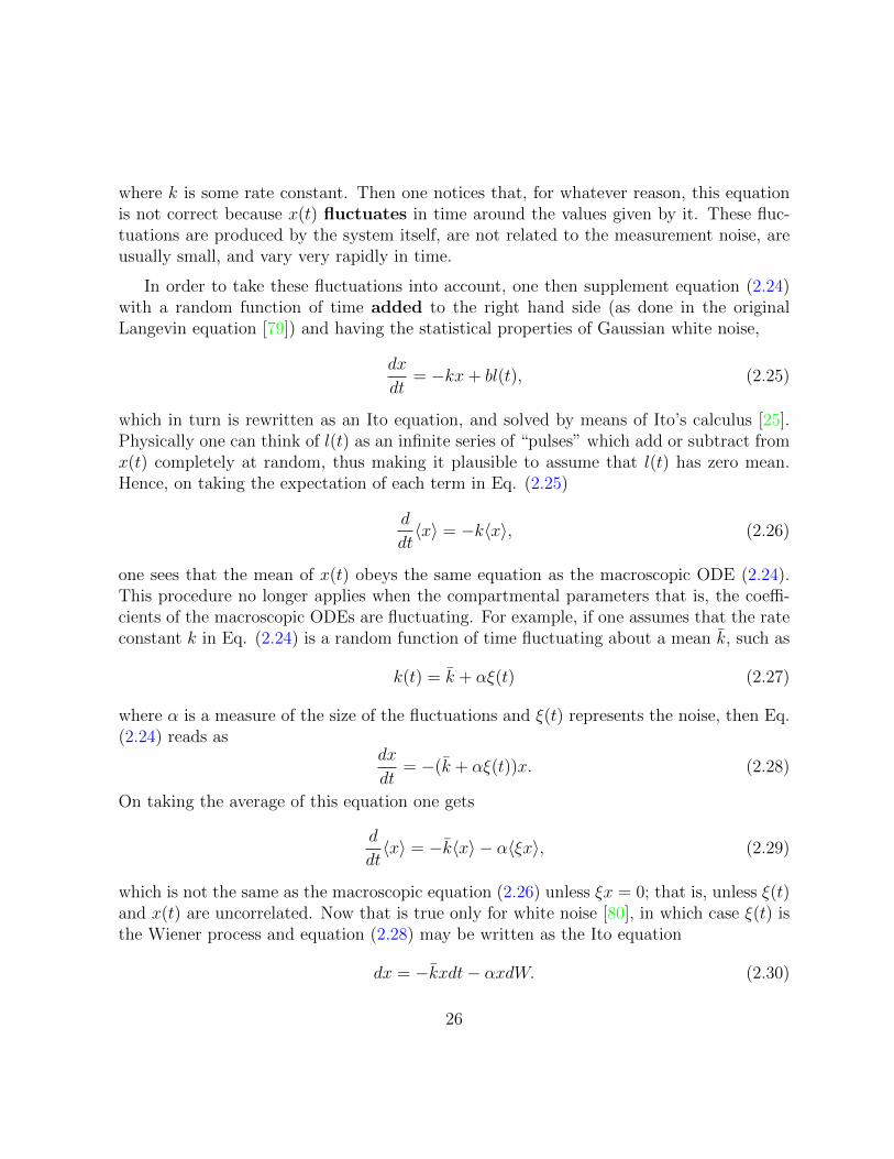
where k is some rate constant. Then one notices that, for whatever reason, this equationis not correct because x(t) fluctuates in time around the values given by it. These fluc-tuations are produced by the system itself, are not related to the measurement noise, areusually small, and vary very rapidly in time.

In order to take these fluctuations into account, one then supplement equation (2.24)with a random function of time added to the right hand side (as done in the originalLangevin equation [79]) and having the statistical properties of Gaussian white noise,

dx

dt= −kx+ bl(t), (2.25)

which in turn is rewritten as an Ito equation, and solved by means of Ito’s calculus [25].Physically one can think of l(t) as an infinite series of “pulses” which add or subtract fromx(t) completely at random, thus making it plausible to assume that l(t) has zero mean.Hence, on taking the expectation of each term in Eq. (2.25)

d

dt〈x〉 = −k〈x〉, (2.26)

one sees that the mean of x(t) obeys the same equation as the macroscopic ODE (2.24).This procedure no longer applies when the compartmental parameters that is, the coeffi-cients of the macroscopic ODEs are fluctuating. For example, if one assumes that the rateconstant k in Eq. (2.24) is a random function of time fluctuating about a mean k, such as

k(t) = k + αξ(t) (2.27)

where α is a measure of the size of the fluctuations and ξ(t) represents the noise, then Eq.(2.24) reads as

dx

dt= −(k + αξ(t))x. (2.28)

On taking the average of this equation one gets

d

dt〈x〉 = −k〈x〉 − α〈ξx〉, (2.29)

which is not the same as the macroscopic equation (2.26) unless ξx = 0; that is, unless ξ(t)and x(t) are uncorrelated. Now that is true only for white noise [80], in which case ξ(t) isthe Wiener process and equation (2.28) may be written as the Ito equation

dx = −kxdt− αxdW. (2.30)

26

These facts explain why most of the literature in this area consists of stochastic PK/PDmodels assuming that the noise is white, and the reader can find many examples in therecent review by Donnet and Samson [18].

Another way of characterizing white noise is by means of the parameter tc, the cor-relation time of the noise. As white noise is delta-function correlated we have tc = 0; incontrast, non-white noise (also known as “colored noise”) has a finite tc 6= 0. Therefore,the question arises: Can Eq. (2.28) be “solved” in some sense when ξ(t) is colored noiseand 〈ξ(t)ξ(t′)〉 6= δ(t− t′)? No exact method of solution is known in this case, but approx-imation methods have been developed and applied successfully in the physical sciences, atleast in the case of realistic noise whose correlation time is short, but not infinitely short .Therefore the purpose of this thesis is to investigate whether these approximation tech-niques can also be successful in the study of stochastic PK/PD models. For the convenienceof the reader these new methods will be reviewed in the next two sections. Furthermore,in order to avoid confusion with the terminology used in the literature when the noise isassumed to be white, it will be useful to refer to differential equations whose coefficientsare random functions as Random Differential Equations (RDE’) to remind ourselves thatwe are dealing with non-white noise.

2.5 The Bourret integral equation for the mean

In a series of papers starting in 1961, Bourret was the first to propose a systematic approx-imation method to deal with RDE’s [6], [7], [8]. He borrowed mathematical techniquesdeveloped by physicists in Quantum field theory, and so his papers are very difficult tounderstand. Fortunately, however, Van Kampen [79] showed a decade later how to obtainBourret’s approximation by a much simpler heuristic method. Therefore, we shall followVan Kampen’s approach systematically.

We have already seen in Eq. (2.28) the structure of the RDE’s one has to deal within the study of stochastic PK models. That example pertained to a one-dimensional (onecompartment) model, but it can be easily generalized to a multi-compartment model withrandom coefficients. Thus we shall consider the RDE

du

dt= (A0 + αA1(t))u (2.31)

with the initial condition u(0) = u0, where u is an n-component vector, A0 is constant n×nmatrix, α is a parameter determining the size of the fluctuations and is usually small, andA1 is an n× n random matrix with zero mean, i.e., 〈A1〉 = 0.

27

The goal here is to find deterministic equation for the moments of u by choosing aproper mathematical model, for small α. Now by simply averaging equation (2.31) we get:

d〈u〉dt

= A0〈u〉+ α〈A1(t)u〉. (2.32)

To approximate cross correlation 〈A1(t)u〉 following assumptions are commonly used inthe literature:

1. 〈A1(t)〉 = 0

2. A1(t) has a finite (nonzero) correlation time say τc=⇒ for any two times t1 and t2, |t1 − t2| >> τc,A1(t1) and A1(t2) are statistically independent.

Following Van Kampen [81], we first perform a change of variables in (2.31) by setting aninteraction expression:

u(t) = eA0tv(t) (2.33)

obtaining in a straight forward way the new RDE

dv

dt= αV (t)v(t)

v(0) = u(0) = u0 (2.34)

where V (t) is a new random matrix given by

V (t) = e−A0tA1(t)eA0t (2.35)

Since α is small the obvious method seems to be perturbation series in α:

v(t) = v0(t) + αv1(t) + α2v2(t) + .... (2.36)

where

u0 = v0(0) + αv1(0) + α2v2(0) + ....

=⇒ v0(0) = u0; vi(0) = 0 ∀i ≥ 0

Substituting these into equation (2.34) we get:

dv0

dt+ α

dv1

dt+ α2dv2

dt+ .... = αV v0 + α2V v1 + α3V v2 + .... (2.37)

28

Equating α on both sides

dv0

dt= 0

dv1

dt= V v0

dv2

dt= V v1

and so on. Now by solving the above relations we can get:

v0 = constant = u0

v1 = u0

∫ t

0

V (t′)dt′

v2 = u0

∫ t

0

∫ t′

0

V (t′)V (t′′)dt′dt′′

Now using all these values equation (2.36) becomes:

v(t) = u0 + α(∫ t

0

V (t′)dt′)u0 (2.38)

+ α2(∫ t

0

∫ t′

0

V (t′)V (t′′)dt′dt′′)u0 + .....

Upon taking average with fixed u0, one can get:

〈v(t)〉 = u0 + α(∫ t

0

〈V (t′)〉dt′)u0 (2.39)

+ α2(∫ t

0

∫ t′

0

〈V (t′)V (t′′)〉dt′dt′′)u0 + .....

=⇒ 〈v(t)〉 = u0 + α2(∫ t

0

∫ t′

0

〈V (t′)V (t′′)〉dt′dt′′)u0 + ..... (2.40)

since V (t) = e−tA0A1(t)etA0 and we assumed 〈A1(t)〉 = 0 =⇒ 〈V (t)〉 = 0

From the perturbation, one can claim the previous expression of 〈v〉 is an approximationup to 2nd order in α but this is not a suitable perturbation as it is increasing not only inα but also in αt and is therefore valid only αt << 1

29

To overcome the situation Bourret demonstrated a heuristic approach for which equa-tion (2.34) is strictly equivalent to the integral equation

v(t) = a+ α

∫ t

0

V (t′)v(t′)dt′. (2.41)

Equation (2.41), after one iteration can be written as:

v(t) = u0 + α

∫ t

0

V (t′)(u0 + α

∫ t′

0

V (t′′)v(t′′)dt′′)dt′

= u0 + u0α

∫ t

0

V (t′)dt′ + α2

∫ t

0

∫ t′

0

V (t′)V (t′′)v(t′′)dt′′dt′

and by taking average we can get (recall that 〈V (t′)〉 = 0):

〈v(t)〉 = u0 + α2

∫ t

0

∫ t′

0

〈V (t′)V (t′′)v(t′′)〉dt′′dt′. (2.42)

This equation is exact but no help in finding 〈v(t)〉, as it contains higher order corre-lation 〈V (t′)V (t′′)v(t′′)〉 [81].

In order to make progress Bourret assumed that the integrand in (2.42) can be approx-imated as

〈V (t′)V (t′′)v(t′′)〉 ≈ 〈V (t′)V (t′′)〉〈v(t′′)〉, (2.43)

after which (2.42) becomes a closed integral equation for 〈v(t)〉 as

〈v(t)〉 = u0 + α2

∫ t

0

∫ t′

0

〈V (t′)V (t′′)〉〈v(t′′)〉dt′′dt′, (2.44)

or equivalentlyd

dt〈v(t)〉 = α2

∫ t

0

〈V (t)V (t′′)〉〈v(t′′)〉dt′′, (2.45)

which in terms of the original variables read as

d

dt〈u(t)〉 = A0〈u(t)〉+ α2

∫ t

0

〈A1(t)e(t−t′)A0A1(t′)〉〈u(t′)〉dt′. (2.46)

Equation (2.46) is known as Bourret’s integral equation and is a very impressive form toevaluate the mean of u(t) as it is a closed equation. It is possible to find 〈u(t)〉 withoutknowing the higher moments and also without solving RDE: du

dt= A(t;ω)u

Of course it remains to find out the region of validity of the approximation [81], andthis in turn will depend on the region of validity of the basic approximation (2.43). Thiswill be discussed in the next section.

30

2.6 Van Kampen differential equation for the mean

Van Kampen [81],[79], starts out by observing that Bourret’s fundamental assumption(2.43) is unsatisfactory, because it is in general not true that the average of a productequals the product of the averages. He notices, however, that this assumption has been usedsuccessfully in the physics literature for a very long period of time, and therefore he setsout to determine under what condition the assumption represents a good approximation.The equation (2.34) determines two important time scales. The first one is the scale onwhich v(t) varies, and is measured by α−1; the second scale is represented by the correlationtime tc of V (t), which is the time scale on which the random nature of V (t) becomesappreciable. If we call 4t a time interval large enough that its relation to the two timescales is given by

tc << 4t << α−1

or equivalently (since α > 0)αtc << α4t << 1 (2.47)

then at a time t > tc the autocorrelation of the noise has vanished, which means thatby the time 4t is reached the random function V (t) has “forgotten its past”, and thestochastic process is approximately Markovian [81]. The same argument can be used inthe next interval from4t to 24t, and so on. Thus Van Kampen’s argument shows that theBourret integral equation (2.46) is simply the first step in a perturbation theory solutionof Eq. (2.31) in powers of αtc in which powers of the order (αtc)

3 have been neglected [79].

Next Van Kampen notices that Eq. (2.46) still contains the initial time, and thereforeare restricted to solutions that are uncorrelated with A1(t) at that time. however thisproblem can simply be solved by the change of variables t′′ = t− t′ in Eq. (2.45) to given

d

dt〈v(t)〉 = α2

∫ t

0

〈V (t)V (t− t′)〉〈v(t− t′)〉dt′, (2.48)

and then by observing that as soon as t > tc the autocorrelation of V (t) vanishes, so thatno appreciable error is made by extending the integral to ∞. Hence, on the macroscopictime scale, Eq. (2.48) may be rewritten as

d〈v(t)〉dt

= α2

∫ ∞0

〈V (t)V (t− t′)〉〈v(t− t′)〉dt′, (2.49)

where the initial time has disappeared so that this equation applies to all solutions of Eq.(2.31), regardless of the time instant at which the initial value is imposed. The final step

31

in van Kampen’s argument is to show that (2.49) is equivalent to the ODE obtained byreplacing v(t− t′) in the integral with 〈v(t)〉 namely

d

dt〈v(t)〉 = α2

[ ∫ ∞0

〈V (t)V (t− t′)〉dt′]〈v(t)〉. (2.50)

In fact, since the integral is only different from zero over a time tc, the relative error madeby this replacement is of order

〈4v〉〈v〉

∼tc〈4v〉4t

〈v〉.

Moreover, according to the equation itself, we have

〈4v〉4t

∼ α2tc〈v〉

and so the relative error is of the order

〈4v〉〈v〉

∼ α2t2c . (2.51)

But in the derivation of the perturbation solution terms of relative order (αtc) were alreadyneglected; therefore, the error (2.51) is of no consequence [79].

The conclusion is that the ODE for the average derived by Van Kampen (2.50) can berewritten in the original variables as

d

dt〈u(t)〉 =

[A0 + α2

∫ ∞0

〈A1(t)eA0t′A1(t− t′)〉e−A0t′dt′]〈u(t)〉 (2.52)

and in the next section it will be applied to study the example of random harmonic oscil-lator. This ODE is also the basic equation of the study of stochastic models of PK in thefollowing chapters.

2.7 The Random Harmonic Oscillator

2.7.1 Van Kampen approach

Here we are going to consider the harmonic oscillator and will solve them by using boththe Van Kampen random differential equation and Bourret integral equation. We knowthe simple harmonic oscillator is described by the following equation:

x+ ω2x = 0 (2.53)

32

with x(0) = a, x(0) = 0. If ω is a constant, then the solution is trivially given byx(t) = a sinωt. But if ω = ω(t), then no analytical solution can be found. Suppose ω(t) isa random function of time, such as

ω2(t) = ω20(1 + αξ(t)),

where ω0=constant. Then the differential equation can be written as

x+ ω20(1 + αξ(t))x = 0, (2.54)

which is a Random Differential Equation (RDE), physically the frequency of the oscillatorvaries in time in a random way i.e., unpredictable way, and we can interpret this as theresult of an external perturbation of size α (the size of the fluctuation is ω), which usuallyis a small parameter. On the other hand, the random function ξ(t) is not known exceptfor some statistical properties such as, for example,

〈ξ(t)〉 = 0 (2.55)

where 〈.〉 denotes the expectation (average) value. Rewrite the equation (2.54) in matrixform:

dx

dt= x,

dx

dt= −ω2

0(1 + αξ(t))x,

where x(0) = a, x = 0, and so

d

dt

(xx

)(0 1

−ω20(1 + αξ(t)) 0

)(xx

). (2.56)

Furthermore, since the product αξ is dimensionless, we can eliminate the constant ω20 by

making the whole problem dimensionless. Accordingly, we let y = xa; τ = ω0t. Now we

have the equation (2.54) in dimensionless form as

y(τ) = −(1 + αξ(τ))y(τ), (2.57)

where y(0) = 1, y(0) = 0 and in matrix form which can be written as:

d

dτ

(yy

)=

[ (0 1−1 0

)+ αξ(τ)

(0 0−1 0

) ](yy

). (2.58)

33

Hence using the notation introduced by Van Kampen [81] we have:

A0 =

(0 1−1 0

), (2.59)

A1 = ξ(t)B = ξ(t)

(0 0−1 0

), (2.60)

and introducing the vector

u =

(yy

),

the RDE (2.58) becomes:du

dt= (A0 + αξ(t)B)u, (2.61)

to which we can apply Van Kampen’s argument that, as long as α is small and the correla-tion time τc is short, we may neglect terms of order (ατc)

3 in the perturbation expansion toconclude that under these conditions the first moment 〈u(t)〉 i.e., the mean obeys a closedODE, given by equation (10.4) of Van Kampen [81], viz:

d

dt〈u(t)〉 = [A0 + α2

∫ ∞0

〈A1(t)eA0τA1(t− τ)〉e−A0τdτ ]〈u(t)〉 (2.62)

using the definition (2.59) and (2.60) as well as dimensionless time τ

d

dτ〈u(τ)〉 = [A0 + α2

∫ ∞0

〈ξ(τ)ξ(τ − τ ′)〉BeA0τ ′Be−A0τ ′dτ ′]〈u〉. (2.63)

First we compute

eA0τ ′ = 1 + A0τ′ +

1

2(A0τ

′)2 + ....

=

(1 00 1

)+

(0 τ ′

−τ ′ 0

)+

1

2τ ′2(

0 1−1 0

)(0 1−1 0

)+ .....

=

(1 00 1

)+

1

2τ ′2(−1 00 −1

)+ τ ′

(0 1−1 0

)+ .....

=

(1 00 1

){1− 1

2τ ′2 +

1

4!τ ′4 − ....}+

(0 1−1 0

){τ ′ − 1

3!τ ′3 + ...}

= I cos τ ′ + A0 sin τ ′. (2.64)

34

Next we compute the complete non-random term in the integrand in (2.63), namelythe matrix products BeA0τ ′Be−A0τ ′ where A0 and B are defined in (2.59) and (2.60). Wehave;

BeA0τ ′ =

(0 0−1 0

)[(1 00 1

)cos τ ′ +

(0 1−1 0

)sin τ ′

]=

(0 0−1 0

)cos τ ′ +

(0 00 −1

)sin τ ′

Be−A0τ ′ =

(0 0−1 0

)[(1 00 1

)cos τ ′ −

(0 1−1 0

)sin τ ′

]=

(0 0−1 0

)cos τ ′ −

(0 00 −1

)sin τ ′

BeA0τ ′Be−A0τ ′ =

[(0 0−1 0

)cos τ ′ +

(0 00 −1

)sin τ ′

] [(0 0−1 0

)cos τ ′ −

(0 00 −1

)sin τ ′

]=

(0 0−1 0

)(0 0−1 0

)cos2 τ ′ −

(0 0−1 0

)(0 00 −1

)sin τ ′ cos τ ′ +(

0 00 −1

)(0 0−1 0

)sin τ ′ cos τ ′ −

(0 00 −1

)(0 00 −1

)sin2 τ ′

=

(0 00 0

)cos2 τ ′ −

(0 00 0

)cos τ ′ sin τ ′ +

(0 01 0

)sin τ ′ cos τ ′ −

(0 00 1

)sin2 τ ′

=

(0 0

sin τ ′ cos τ ′ 0

)+

(0 00 − sin2 τ ′

)=

(0 0

sin τ ′ cos τ ′ − sin2 τ ′

), (2.65)

which agrees with Van kampen’s equation (14.3) [81]. Substituting (2.65) into (2.63) andswitching back to the explicit matrix format gives us:

d

dτ

(〈y〉〈y〉

)=

(0 1−1 0

)(〈y〉〈y〉

)+ α2

∫ ∞0

〈ξ(τ)ξ(τ − τ ′)〉(

0 0sin τ ′ cos τ ′ − sin2 τ ′

)dτ ′(〈y〉〈y〉

). (2.66)

35

Next we are going to use the half-angle formula

sin τ ′ cos τ ′ =1

2sin 2τ ′,

− sin2 τ ′ = −(1− cos 2τ ′

2

),

and define the two coefficients

c1 =

∫ ∞0

〈ξ(τ)ξ(τ − τ ′)〉 sin 2τ ′ dτ ′, (2.67)

c2 =

∫ ∞0

〈ξ(τ)ξ(τ − τ ′)〉(cos 2τ ′ − 1) dτ ′, (2.68)

in order to rewrite equation (2.66) in the simple form

d

dt

(〈y〉〈y〉

)=

(0 1−1 0

)(〈y〉〈y〉

)+α2

2

(0 0c1 c2

)(〈y〉〈y〉

)(2.69)

or as a single ODE;d2

dτ 2〈y〉 =

α2

2c2〈y〉 −

(1− α2

2c1

), (2.70)

and in dimensional form will be:

d2

dt2〈x〉 =

1

2α2ω0c2

d

dt〈x〉 − ω2

0

(1− 1

2α2c1

)〈x〉 (2.71)

This coincides with Van kampen’s equation (14.7) [81] for the special case ω0 = 1.

Remarks:

(a) On comparing our equation (2.71) with the non-random oscillator equation (2.53)that is:

d2

dt2x = −ω2x

we see that RDE (2.54) introduces two important physical effects in the ODE for the firstmoment (the mean) of the oscillator’s displacement:

• It’s frequency is shifted by the quantity 12α2c1 and

• Damping of the average 〈x〉 in the form 12α2ω0c2 is produced by the small fluctuations

of the oscillator’s frequency.

36

(b) Van Kampen (1976, p. 201) [81] noticed that if there is resonance between thefluctuations and the double frequency of the oscillator, then the coefficient c2 in (2.68) canbecome positive, in which case the mean 〈x〉 would grow exponentially.

To proceed further we need to specify the auto correlation function, in order to computethe coefficients c1 and c2. This means that we describe the statistical properties of ξ(t) byprescribing

〈ξ(t)〉 = 0,

〈ξ(t)ξ(t− τ)〉 = a(τ),

where a(τ) is a given function of τ . Note that specifying the auto-correlation function fora stationary stochastic process means that the variance is also specified. In fact, since

Γ(t, t′) = 〈ξ(t)ξ(t+ t′)〉 − 〈ξ(t)〉〈ξ(t+ t′)〉,

and since Γ(t, t′) = Γ(t− t′), due to stationary, we have

Γ(t′) = 〈ξ(0)ξ(t′)〉 − 〈ξ(0)〉〈ξ(t′)〉,

and, for t′ = 0,Γ(0) = 〈ξ2(0)〉 − 〈ξ(0)〉2,

which is just the variance.

The simplest assumption is to assume that the (normalized) auto-correlation functiondecays exponentially according to (recall that 〈ξ〉 = 0)

B(τ) = 〈ξ(0)ξ(τ)〉 = e−γτ , γ > 0 (2.72)

so that γ−1 = τc is the correlation time, which was assumed to be short both in Bourretand Van kampen approximations. In other words, we assume that the auto-correlationfunction is exponentially small after a duration of a few correlation times.

Now we can compute c1 and c2 from (2.67) and (2.68):

c1 =

∫ ∞0

e−γτ sin 2τdτ

=2τ 2c

1 + 4τ 2c

, (2.73)

37

c2 =

∫ ∞0

e−γτ(

cos 2τ − 1)dτ

= − 4τ 3c

1 + 4τ 2c

. (2.74)

Substituting these expressions into (2.71) gives:

d2

dt2〈x〉 = 2α2

0ω0τ 3c

1 + 4τ 2c

d

dt〈x〉 − ω2

0

(1− α2τ 2

c

1 + 4τ 2c

)〈x〉 (2.75)

and we see that the damping (1st term on the right hand side) has the proper negativesign that guarantees the stability of the motion. In other words, for a correlation functiondecaying exponentially (as in (2.72) above) the resonance mentioned by Van Kampen(Remark (b)) does not occur.

Now we are going to solve for this average using maple (code is in appendix C) and alsoby the observations we have made when we are taking the values of the parameter. Theassumption is that the correlation time τc << 1 that mean γ >> 1 we get the followingsolution:

〈x(τ)〉 = e(−9.62×10−6 τ) cos(1.00 τ)

+ (9.62× 10−6e(−9.62×10−6 τ) sin(1.00 τ). (2.76)

From figure 2.1, it is clear that the effects of the correlation time vanish for long timesalthough for short times the solution is seem to be highly oscillatory.

38

Figure 2.1: An illustration of the solution of random harmonic oscillator using Van Kampendifferential equation of mean for α = .1 and τc = .1.

2.7.2 Bourret’s approach

Now we are going to solve equation (2.54) using Bourret’s integral equation:

d

dτ〈u(τ)〉 = A0〈u(τ)〉+ α2

∫ τ

0

〈A1(τ)eA0(τ−τ ′)A1(τ ′)〉〈u(τ ′)〉dτ ′, (2.77)

where A0 and A1 are as in (2.59) and (2.60). Using the previous results, we can write

eA0(τ−τ ′)A1(τ ′) =(I cos(τ − τ ′) + A0 sin(τ − τ ′)

)Bξ(τ ′)

= Bξ(τ ′) cos(τ − τ ′) + A0Bξ(τ′) sin(τ − τ ′)

=

(0 0−1 0

)ξ(τ ′) cos(τ − τ ′) +

(−1 00 0

)ξ(τ ′) sin(τ − τ ′), (2.78)

39

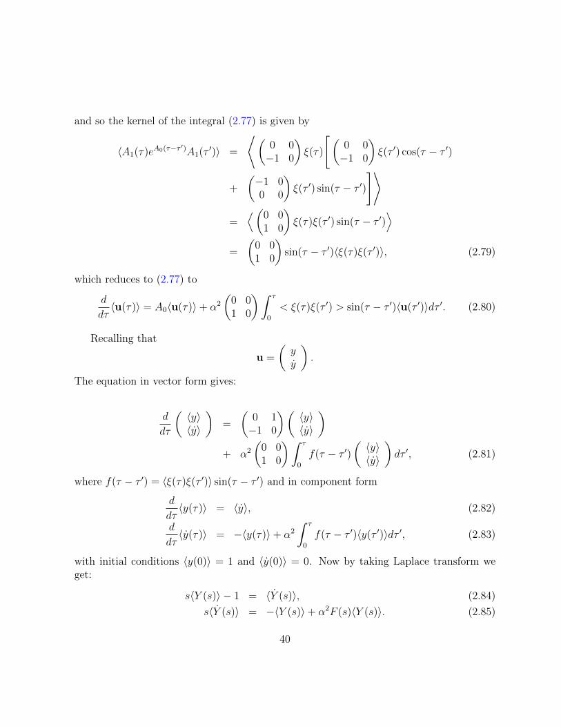
and so the kernel of the integral (2.77) is given by

〈A1(τ)eA0(τ−τ ′)A1(τ ′)〉 =

⟨(0 0−1 0

)ξ(τ)

[(0 0−1 0

)ξ(τ ′) cos(τ − τ ′)

+

(−1 00 0

)ξ(τ ′) sin(τ − τ ′)

]⟩

=⟨(0 0

1 0

)ξ(τ)ξ(τ ′) sin(τ − τ ′)

⟩=

(0 01 0

)sin(τ − τ ′)〈ξ(τ)ξ(τ ′)〉, (2.79)

which reduces to (2.77) to

d

dτ〈u(τ)〉 = A0〈u(τ)〉+ α2

(0 01 0

)∫ τ

0

< ξ(τ)ξ(τ ′) > sin(τ − τ ′)〈u(τ ′)〉dτ ′. (2.80)

Recalling that

u =

(yy

).

The equation in vector form gives:

d

dτ

(〈y〉〈y〉

)=

(0 1−1 0

)(〈y〉〈y〉

)+ α2

(0 01 0

)∫ τ

0

f(τ − τ ′)(〈y〉〈y〉

)dτ ′, (2.81)

where f(τ − τ ′) = 〈ξ(τ)ξ(τ ′)〉 sin(τ − τ ′) and in component form

d

dτ〈y(τ)〉 = 〈y〉, (2.82)

d

dτ〈y(τ)〉 = −〈y(τ)〉+ α2

∫ τ

0

f(τ − τ ′)〈y(τ ′)〉dτ ′, (2.83)

with initial conditions 〈y(0)〉 = 1 and 〈y(0)〉 = 0. Now by taking Laplace transform weget:

s〈Y (s)〉 − 1 = 〈Y (s)〉, (2.84)

s〈Y (s)〉 = −〈Y (s)〉+ α2F (s)〈Y (s)〉. (2.85)

40

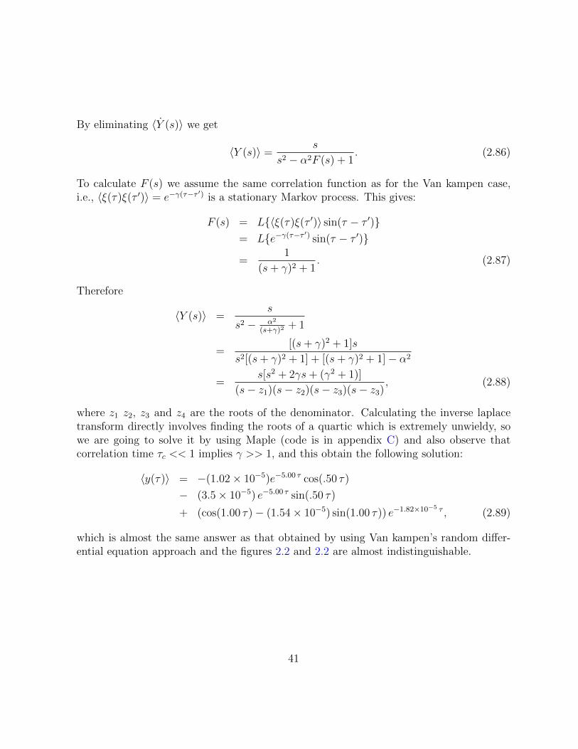
By eliminating 〈Y (s)〉 we get

〈Y (s)〉 =s

s2 − α2F (s) + 1. (2.86)

To calculate F (s) we assume the same correlation function as for the Van kampen case,i.e., 〈ξ(τ)ξ(τ ′)〉 = e−γ(τ−τ ′) is a stationary Markov process. This gives:

F (s) = L{〈ξ(τ)ξ(τ ′)〉 sin(τ − τ ′)}= L{e−γ(τ−τ ′) sin(τ − τ ′)}

=1

(s+ γ)2 + 1. (2.87)

Therefore

〈Y (s)〉 =s

s2 − α2

(s+γ)2 + 1

=[(s+ γ)2 + 1]s

s2[(s+ γ)2 + 1] + [(s+ γ)2 + 1]− α2

=s[s2 + 2γs+ (γ2 + 1)]

(s− z1)(s− z2)(s− z3)(s− z3), (2.88)

where z1 z2, z3 and z4 are the roots of the denominator. Calculating the inverse laplacetransform directly involves finding the roots of a quartic which is extremely unwieldy, sowe are going to solve it by using Maple (code is in appendix C) and also observe thatcorrelation time τc << 1 implies γ >> 1, and this obtain the following solution:

〈y(τ)〉 = −(1.02× 10−5)e−5.00 τ cos(.50 τ)

− (3.5× 10−5) e−5.00 τ sin(.50 τ)

+ (cos(1.00 τ)− (1.54× 10−5) sin(1.00 τ)) e−1.82×10−5 τ , (2.89)

which is almost the same answer as that obtained by using Van kampen’s random differ-ential equation approach and the figures 2.2 and 2.2 are almost indistinguishable.

41

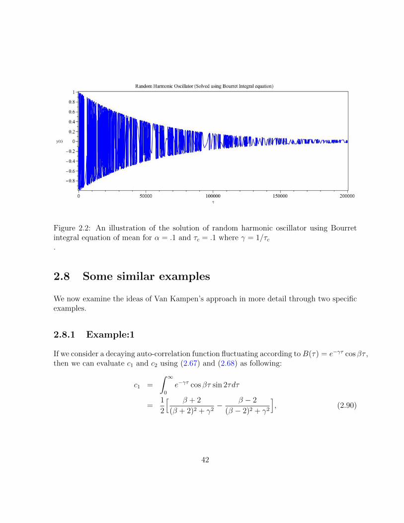
Figure 2.2: An illustration of the solution of random harmonic oscillator using Bourretintegral equation of mean for α = .1 and τc = .1 where γ = 1/τc.

2.8 Some similar examples

We now examine the ideas of Van Kampen’s approach in more detail through two specificexamples.

2.8.1 Example:1

If we consider a decaying auto-correlation function fluctuating according toB(τ) = e−γτ cos βτ ,then we can evaluate c1 and c2 using (2.67) and (2.68) as following:

c1 =

∫ ∞0

e−γτ cos βτ sin 2τdτ

=1

2

[ β + 2

(β + 2)2 + γ2− β − 2

(β − 2)2 + γ2

], (2.90)

42

c2 =

∫ ∞0

e−γτ cos βτ(

cos 2τ − 1)dτ

=γ

2

[ 1

(β − 2)2 + γ2+

1

(β + 2)2 + γ2− 1

β2 + γ2

]. (2.91)

Substituting c1 and c2 in (2.70), we get

d2

dτ 2〈x〉 =

γ

4α2ω0

[ 1

(β − 2)2 + γ2+

1

(β + 2)2 + γ2− 1

β2 + γ2

] ddτ〈x〉

− ω20

[1− α2

4

( β + 2

(β + 2)2 + γ2− β − 2

(β − 2)2 + γ2

)]〈x〉. (2.92)

2.8.2 Example: 2

We now consider the following problem

x = −δx− ω2x (2.93)

with x(0) = a, x(0) = 0. Suppose ω(t) is a random function of time, such that

ω2(t) = ω20(1 + αξ(t)) (2.94)

where ω0=constant. Then the differential equation can be written as

x = −δx− ω20(1 + αξ(t))x (2.95)

where ξ(t) is an external perturbation of size α and the size of the fluctuation is ω. Therandom function ξ(t) is unknown except for some statistical properties such as, for example,

〈ξ(t)〉 = 0. (2.96)

Rewriting the equation (2.95):

dx

dt= x

dx

dt= −δdx

dt− ω2

0(1 + αξ(t))x

where x(0) = a, x = 0, and so in matrix form, we have

43

d

dt

(xx

)(0 1

−ω20(1 + αξ(t)) −δ

)(xx

). (2.97)

Since the product αξ is dimensionless, we can eliminate the constant ω20 by making the

whole problem dimensionless. Accordingly, we let y = xa; τ = t

√ω0. Now equation (2.95)

in dimensionless form becomes

y(τ) = −ky − (1 + αξ(τ))y(τ), (2.98)

where y(0) = 1, k = − δ√ω0

and in matrix form this equation can be written as:

d

dτ

(yy

)=

[ (0 1−1 k

)+ αξ(τ)

(0 0−1 0

) ](yy

). (2.99)

Using the notation introduced by Van Kampen (1976) [81] we have:

A0 =

(0 1−1 k

), (2.100)

A1 = ξ(t)B = ξ(t)

(0 0−1 0

), (2.101)

and introducing the vector

u =

(yy

),

RDE (2.95) becomes:du

dt= (A0 + αξ(t)B)u, (2.102)

to which we can apply Van Kampen’s argument that, as long as α is small and the correla-tion time τc is short, we may neglect terms of order (ατc)

3 in the perturbation expansion toconclude that under these conditions the first moment 〈u(t)〉 i.e., the mean obeys a closedODE, given by equation (10.4) of Van Kampen [81], viz:

d

dt〈u(t)〉 = [A0 + α2

∫ ∞0

〈A1(t)eA0τA1(t− τ)〉e−A0τdτ ]〈u(t)〉, (2.103)

44

using the definition (2.59) and (2.60) as well as dimensionless time τ , equation (2.103)becomes

d

dτ〈u(τ)〉 = [A0 + α2

∫ ∞0

〈ξ(τ)ξ(τ − τ ′)〉BeA0τ ′Be−A0τ ′dτ ′]〈u〉. (2.104)

We now evaluate the matrix exponential eA0τ by using the Cayley-Hamilton theorem,which is eA0τ = a0I + a1A0, where the coefficients a0 and a1 must be found.

Eigenvalues of A0 are λ = k±√k2−42

.

let λ1 = k+√k2−42

and λ2 = k−√k2−42

.

By using the relation eA0τ = a0I + a1A0 we get the following:

eλ1τ = a0 + a1λ1 and eλ2τ = a0 + a1λ2,

from which we get the values of a0 and a1 as following:

a0 = λ2eλ1τ−λ1eλ2τ

λ2−λ1and a1 = eλ1τ−eλ2τ

λ1−λ2

Now

BeA0τ ′ = a0

(0 0−1 0

)[(1 00 1

)+ a1

(0 1−1 0

)]= a0

(0 0−1 0

)+ a1

(0 00 −1

)and

BeA0τ ′Be−A0τ ′ =

[a0

(0 0−1 0

)+ a1

(0 00 −1

)][a0

(0 0−1 0

)− a1

(0 00 −1

)]=

(0 0

a0a1 a21

). (2.105)

45

Substituting the above expression into the equation (2.104) and switching back to theexplicit matrix format we get:

d

dτ

(〈y〉〈y〉

)=

(0 1−1 k

)(〈y〉〈y〉

)+ α2

∫ ∞0

〈ξ(τ)ξ(τ − τ ′)〉(

0 0a0a1 −a2

1

)dτ ′(〈y〉〈y〉

). (2.106)

If we define the two coefficients

c1 =

∫ ∞0

〈ξ(τ)ξ(τ − τ ′)〉a0a1 dτ ′, (2.107)

c2 = −∫ ∞

0

〈ξ(τ)ξ(τ − τ ′)〉a21 dτ ′, (2.108)

we can rewrite equation (2.106) in the simple form

d

dτ

(〈y〉〈y〉

)=

(0 1−1 k

)(〈y〉〈y〉

)+α2

2

(0 0c1 c2

)(〈y〉〈y〉

), (2.109)

or as a single ODE

d2

dτ 2〈y〉 = (1 + k + α2c2)〈y〉 − (1− α2c1)〈y〉, (2.110)

and in dimensional form as:

d2

dt2〈x〉 =

√ω0

(1− δ√ω0

+ α2c2

) ddt〈x〉 − ω0

(1− α2c1

)〈x〉. (2.111)

46

Chapter 3

Application of Van Kampen’s theoryto Pharmacokinetics

3.1 Deterministic formulation of the model

To model this situation deterministically, we proceed as follows. Let X(t) be the amountof drug at the absorption site at time t, and let ka be the apparent first-order absorptionrate constant; then

dX

dt= −kaX (3.1)

is the rate of drug loss from the absorption site. Next let A(t) be the amount of drug inthe body at time t; then

dA

dt= kaX − keA (3.2)

is the rate of change of the amount of drug in the body, with the elimination rate constantke and the initial conditions

X(0) = X0, A(0) = 0 (3.3)

where X0 is the dose administered at time t = 0 orally or intramuscularly, the solution ofthe system (3.1) to (3.3) is given by

X = X0e−kat, (3.4)

A =kaX0

ka− ke(e−ket − e−kat).

47

The volume of distribution is often referred to as the apparent volume of distributionand can aid in the determination of dosage requirements. Generally, dosing is assumed tobe proportional to the volume of distribution [14]. For example, the larger the volume ofdistribution, the larger the dose must be to achieve a desire target concentration. Nowdividing by the volume of distribution V we can write A in concentration form as (where

C(t) = A(t)V

and V is the apparent volume of distribution [14]):

C(t) =kaX0

V (ka − ke)(e−ket − e−kat). (3.5)

Now from the plasma concentration curve, we can extract the parameters ka and ke andthe methods of extracting the parameter values from the concentration versus time curvehave been discussed in chapter 2, along with their characteristics.

In the next section the stochastic version of this PK model will be introduced.

3.2 Stochastic formulation of the model

Drug absorption kinetics for oral or intramuscular administration is a complex phenomenon.The loss of a drug from the absorption site is due, in large part, to intrinsic absorption,that is to the passage of the drug directly into the circulation. However, a (usually) smallfraction of the loss may be due to other phenomena, such as degradation of the drug atintramuscular sites or due to drug precipitation. The result is that there is uncertainty asto the meaning of the absorption rate constant ka, used in the traditional deterministicmodel (3.1)-(3.3).

On the other hand, one can take the uncertainty into account in a statistical sense,by assuming that the absorption rate is not constant, but fluctuates in time around someaverage value ka. Therefore, one can write that the full absorption rate ka(t) is given by

ka(t) = ka(1 + αξ(t)); ke = ke, (3.6)

where ξ(t) is a random function and α is a (small) constant coupling the average absorptionrate to the random fluctuations.

The random function ξ is not known, of course, but reasonable statistical assumptionsabout it can be made. Thus, since by definition 〈ka(t)〉 = ka it follows from equation (3.6)that the expectation of ξ(t) must vanish; i.e.,

〈ξ(t)〉 = 0, (3.7)

48

A further statistical property of ξ(t) can be prescribed by specifying its auto-correlationfunction, viz.

Γ(t, t′) = 〈ξ(t)ξ(t′)〉 (3.8)

which will be discussed in detail in a later section.

The result of these stipulations is that the system of deterministic ODE’s (3.1)-(3.3)become a stochastic system of RDE’s, namely

dX

dt= −ka(1 + αξ(t))X (3.9)

dA

dt= ka(1 + αξ(t))X − keA (3.10)

3.3 The Van Kampen approximation of the model

In this section we are going to apply the Van Kampen approximation to solve our RDEs(3.9) and (3.10). For convenience we simplify these equations by making them dimen-sionless, for which proper scales need to be used. For both the amount of drug at theabsorption site X and the amount of drug in the circulation A there is an obvious scalenamely the initial dose X0 so that their dimensionless version are simply

x =X

X0

y =A

X0

(3.11)

However, there is no obvious time scale t . Hence, as done in these cases in ordinaryperturbation theory, one can introduce a dimensionless time

τ =t

T0

(3.12)

and determine T0 by choosing the value that makes the RDE’s take the simplest possibleform. Using the definitions (3.11)-(3.12) reduces the system of RDE’s (3.9)-(3.10) to thefollowing form:

dx(τ)

dτ= −kaT0(1 + αξ)x(τ) (3.13)

dy(τ)

dτ= kaT0(1 + αξ)x(τ)− keT0y(τ) (3.14)

49

and it is now obvious that the simplest form of these equations is obtained with the choice

T0 = (ka)−1; ρ = ke(ka)

−1 (3.15)

after which the final form of the model can be written in the form useful for the applicationof van kampen’s theory, namely

du

dτ= (A0 + αA1(τ))u(τ), (3.16)

u(0) =

(10

), (3.17)

where

u =

(xy

); A0 =

(−1 01 −ρ

); A1(τ) = ξ(τ)B = ξ(τ)

(−1 01 0

). (3.18)

When these quantities are substituted into van Kampen’s general differential equationfor the mean (reviewed in section 2.5), the result is:

d

dτ〈u(τ)〉 =

[A0 + α2

∫ ∞0

〈ξ(τ)ξ(τ − τ ′)〉BeA0τ ′Be−A0τ ′dτ ′

]〈u(τ)〉, (3.19)

which shows explicitly the importance of the noise auto-correlation function.

Now we are going to solve (3.19) for A0 and A1. First we are evaluating eA0τ :

A0 =

(−1 01 −ρ

)

Eigen values are: λ = −1,−ρ and the corresponding Eigen vectors are :

(11ρ−1

)and(

01

). So the fundamental matrix for φ(τ) for A0 is:

φ(τ) =

[e−τ

(ρ− 1

1

)e−ρτ

(01

) ]=

[e−τ (ρ− 1) 0

e−τ e−ρτ

],

50

φ−(τ) =1

e−τe−ρτ (ρ− 1)

[e−ρτ 0−e−τ e−τ (ρ− 1)

],

φ−(0) =1

(ρ− 1)

[1 0−1 ρ− 1

],

eA0τ = φ(τ)φ−(0) =

[e−τ 0

e−τ−e−ρτρ−1

e−ρτ

],

e−A0τ =

[eτ 0

eτ−eρτρ−1

eρτ

],

BeA0τ =

(−1 01 0

)(e−τ 0

e−τ−e−ρτρ−1

e−ρτ

)=

[−e−τ 0e−τ 0

],

Be−A0τ =

[−eτ 0eτ 0

].

Now

BeA0τBe−A0τ =

[1 0−1 0

](3.20)

Substitute the equation (3.20) into equation (3.19), we get

d

dτ〈u(τ)〉 =

[A0 + α2

∫ ∞0

〈ξ(τ)ξ(τ − τ ′)〉[

1 0−1 0

]dτ ′

]〈u(τ)〉,

in matrix form:

d

dτ

(〈x〉〈y〉

)=

(−1 01 −ρ

)(〈x〉〈y〉

)+ α2

∫ ∞0

〈ξ(τ)ξ(τ − τ ′)〉(

1 0−1 0

)dτ ′(〈x〉〈y〉

).

51

In practice, often, Orstein-Uhlenbeck process with mean zero and 〈ξ(τ)ξ(τ − τ ′)〉 =e−|τ

′|/τc with a correlation time τc, used to describe colored noise. In our model we alsoconsidered ξ(t) as an Orstein-Uhlenbeck process, with mean zero and auto-correlationfunction e−|τ

′|/τc ( i.e.,∫∞

0〈ξ(τ)ξ(τ − τ ′)〉dτ ′ =

∫∞0e−|τ

′|/τcdτ ′ = τc) and using this we willbe able to get:

d

dτ

(〈x〉〈y〉

)=

(−1 01 −ρ

)(〈x〉〈y〉

)+ α2

(τc−τc

)(〈x〉〈y〉

). (3.21)

Now it is possible to write our stochastic DE as following form:

d

dτ〈x〉 = −(1− α2τc)〈x〉, (3.22)

d

dτ〈y〉 = (1− α2τc)〈x〉 − ρ〈y〉, (3.23)

and the dimensional form will be (for simplicity we use ka and ke instead of ka and ke):

d

dt〈X〉 = −ka(1− α2τc)〈X〉, (3.24)

d

dt〈A〉 = ka(1− α2τc)〈X〉 − ke〈A〉. (3.25)

Equations (3.22) and (3.23) are the representation of the RDE’s using Van Kampen ap-proximation.

3.3.1 Calculation of the second moment using Van Kampen’smethod

We have calculated the mean equation using Van Kampen’s method for both X and A. Ournext step is to calculate the second moments which we will be able to use to capture thevariability of the random effects, induced by the random variations in the absorption rate.We compare Van Kampen’s approximation to the model with the full numerical solution byevaluating the variance. In this section we describe how we calculate the second momentsof X and A using Van Kampen method.

The non dimensional form of the Van Kampen approximation to our model, i.e., (3.16)can be written as:

dX

dτ= −(1 + αξ(τ))X, (3.26)

52

dA

dτ= (1 + αξ(τ))X − ρA. (3.27)

Using the Einstein summation convention, it is convenient to write the linear systemin indicial notation:

duidt

= Aijuj (3.28)

d

dtuiuk = uiuk + uiuk = ukAijuj + uiAkjuj (3.29)

Now using (3.29) for our model we can write the system as:

d

dτ(AX) = (−(1 + αξ(τ))− ρ)AX + (1 + αξ(τ))X2,

d

dτ(A2) = 2A((1 + αξ(τ))X − ρA),

d

dτ(X2) = 2X(−(1 + αξ(τ))X). (3.30)

In matrix form (3.30) can be written as:

d

dτ

AXA2

X2

=

−1− ρ 0 12 −2ρ 00 0 −2

AXA2

X2

+ αξ(τ)

−1 0 12 0 00 0 −2

AXA2

X2

.=⇒ dU

dτ= (A0 + αξ(τ)B)U

where

U =

AXA2

X2

,

A0 =

−1− ρ 0 12 −2ρ 00 0 −2

,

53

B =

−1 0 12 0 00 0 −2

.Following the method we have used to evaluate the mean by using Van Kampen’s approx-imation equation (3.19), also can be calculate the evolution equations for 〈AX〉, 〈A2〉 and〈X2〉 as:

d

dτ

〈AX〉〈A2〉〈X2〉

=

−1− ρ 0 12 −2ρ 00 0 −2

〈AX〉〈A2〉〈X2〉

+ α2τc

1 0 −(2ρ−3)+ ρ

1+τc(ρ−1)

ρ−1

−2 0 −2− 2ρ

1+τc(ρ−1)

ρ−1

0 0 4

, 〈AX〉〈A2〉〈X2〉

(3.31)

where we have considered as before < ξ(τ)ξ(τ − τ ′) >= e−|τ′|/τc , with a correlation time τc

3.4 Numerical solution of the model

3.4.1 To solve RDE’s ( 3.9) and (3.10)

In this section we describe the method used to solve the model numerically. We have usedthe modified Euler’s method to solve the system of DE, where the noise term is treatedwith the algorithm described by Gillespie [30] in his 1996 paper. The noise we consider isassumed to be an Ornstein-Uhlenbeck process [78], which is often used to model colorednoise. Gillespie [30] developed an algorithm for any exact time step ∆t > 0 for the Ornstein-Uhlenbeck process and its time integral. Detailed evaluation of the Ornstein Uhlenbeckprocess from Newton’s second law is in the appendix B.

A Langevin equation governed by a Ornstein Uhlenbeck process can be written as:

dy

dt= G(y, t) + c(y, t)F (t), (3.32)

where F (t) is an Ornstein Uhlenbeck process and can be defined as:

dF (t)

dt= − 1

τcF (t) +

1

τcη(t) (3.33)

54

where η(t) represents the Gaussian white noise with mean zero and variance 1 and τc isthe correlation time of the colored noise F (t) [71].Remark: The steady-state auto-correlation function of F (t) can be written as :

〈F (t)F (t− τ)〉 =1

2τce−|τ |/τc

τc→0−−−→ δ(τ), (3.34)

which shows that, if auto-correlation time approaches to 0, then the colored noise will bewhite noise, i.e, the noise will be δ correlated.

The simulation algorithm of a system of random differential equations of the form(3.32)-(3.33) consists of following steps [71]:

• Step 1: Initialize: t = t0, y = y0 and F = F0;

• Step 2: We have to choose a suitable small ∆t > 0 (according to the assumption(2.47));

• Step 3: Next we are going to draw a sample value n of the unit normal randomvariable N(0, 1);

• Step 4: In this step the process will advance as following:•y(t+ ∆t) = y(t) + nc(y, t)[∆t]1/2 +G(y, t)∆t,

• F (t+ ∆t) = F (t)e−∆t/τc + n

[( 1

2τc)(1− e−2∆t/τc)

]1/2

,

• t = t+ ∆t,where n is the unit normal random variable chosen in step 3;

• Step 5: In this step we are going to record y(t) = y and can use it for sample plottingand to continue the process further we have to return to step 3, otherwise stop.

The RDE system of our model has been solved following steps 1-5 above:

dX

dt= −ka(1 + αξ(t))X,

dA

dt= ka(1 + αξ(t))X − keA, (3.35)

dξ(t)

dt= − 1

τcξ(t) +

1

τcη(t),

55

where η(t) again represents Gaussian white noise with mean zero and variance 1 and τc isthe correlation time [71].

Matlab 9.1 R2016b has been used to solve the RDE’s (3.35). Following the stepsdescribed above for the random process (3.32), where in this particular case:

y(t) =

(y1(t)y2(t)

)=

(X(t)A(t)

).

Now, comparing with equation (3.32), our system can be written as:

G(y, t) =

(−kaX(t)

kaX(t)− keA(t)

),

c(y, t) =

(−kaαX(t)kaαX(t)

),

and F (t) = ξ(t).

At the initial time t = 0, we have considered the initial conditions X(0) = X0 = Doseand A(0) = 0 (as there is no drug in the system at initial time) and iterate until the finaltime t=tfinal. We run a large number of simulations to obtain individual trajectories (say10000 or so) to get the ensemble mean and use the Matlab built in command “std” to getthe standard deviation of the trajectories around the mean. (Detailed codes have beenincluded in appendix B).

3.4.2 To solve Van Kampen’s form of the model

We have used the Runge Kutta method to solve the Van Kampen form of the model (codeis in the appendix B) for both the moments. Here we have a system of two decoupled equa-tions: two equations for the mean and three for the second moments ( i.e., the variance).The following relation has been used to evaluate the variances for both X and A:

• variance of X=(〈XX〉 − 〈X〉2);

• variance of A= (〈AA〉 − 〈(A)〉2).

56

Now before solving the system of DE (for mean and variance), we need to considerthe conditions which will assure us to get the stable solutions, i.e, criterion for linear,homogeneous differential equations which will converge to zero. We are going to use theRouth-Hurwitz criterion for this purpose, which states that: the necessary and sufficientconditions for the roots of characteristic polynomial (with real coefficients) is to lie in theleft half of the complex plane [23]. According to this criterion, a polynomial is stableif all the roots of the polynomial have strictly negative real parts, if and only if all theleading principal minors of a square matrix are positive. Using Matlab for equation(3.31) toevaluate the characteristic polynomial by neglecting τ 2

c and τ 3c terms (as we are considering

very small correlation time), we calculated the following cubic equation for eigenvalues λ:

λ3+(−5τcα2+3ρ+3)λ2+(−α2τc(14ρ+6)+(2ρ2+8ρ+2))λ+(−α2ρτc(8ρ+12)+4ρ(ρ+1)) = 0

(3.36)Now using the Routh-Hurwitz criterion [23], for this cubic polynomial we can compare thecoefficients of (3.36) to evaluate the conditions to get the stable solutions.

α2τc <3(ρ+ 1)

5(3.37)

and

α2τc <3ρ3 + 13ρ2 + 13ρ+ 3

22ρ2 + 44ρ+ 14. (3.38)

From, conditions (3.37) and (3.38) we should choose the right hand side that is smaller (inorder to satisfy both the conditions). Now, say (3.37)<(3.38) we obtain the following:

51ρ3 + 133ρ2 + 109ρ+ 27 < 0 (3.39)

which is a contradiction as ρ > 0, so we can conclude the condition should be (3.38).

By applying the same criterion in the relation (3.21), we can calculate the stability forthe mean is:

ατc < 1 (3.40)

which is satisfied under the assumption only α is small enough.

3.4.3 Parameters choice and initial conditions

Example 1.

For the numerical simulation we use data and information from some practical applications(i.e., some regularly used drugs with their common dosage). Acetaminophen is a very

57

popular and common drug which has been used for a long time as a pain reliever andalso to reduce fever. There are various other conditions which have also been treatedwith acetaminophen and these include head aches, muscle aches, arthritis, back aches,tooth aches, colds, and fevers. Acetaminophen is a major ingredient in most cold and flumedications which can be bought over the counter and is also present in some prescriptionmedications.

A pharmaceutical window (or popularly known as therapeutic window) of a drug is aregion of the drug dosage, where a disease can be effectively treated without showing no-ticeable evidence of toxic side effects. Drugs, which have a narrow or very small therapeuticwindow must be administered with extreme care and control, by measuring concentrationsof the drug in the body, in order to minimize any harmful side effects. Acetaminophen hasa narrow therapeutic window and due to its availability and wide range of use, there areclear possibilities for accidental or deliberate overdose. Overdose may create hepatoxicity,which can lead major problems, such as abnormalities in liver function, acute liver failureand even death [37].

According to the FDA, the standard dose of acetaminophen for adults (for 12 yearsand older) is 4000 mg per day [77].

The values of the parameters, we consider are taken from the study [60]. The half lifeof acetaminophen is 2.5 hours, so ke can be calculated using the relation:

ke =ln(2)

half life=

ln(2)

2.5= .28/hour (3.41)

Volume of distribution is .60 L/kg, which will be .60L/kg × 70kg = 42L for an average70 kg adult. The absorption rate constant ka = 1.80/hour and the bioavailability F=.89(fraction of amount absorbed by the stomach) [60]. In this case we see that there is nopossibility to get the “flip-flop” kinetics ( i.e., ke will not be greater than ka).

For the choice of α and τc, we considered the conditions of mean and mean-squaredstability to get the stable solutions, which is described in (3.38), where ρ = ke

ka.

To consider the initial conditions for meanX (amount of drug in the absorption site) andA (amount of drug in the systemic circulation), we chose X(0) = X0 = Dose = 1000 mgand A0 = 0 as there is no drug initially in the blood plasma. As we are considering multipledosages, so we add a dose every six hours by dividing our total time (24 hours) into foursub intervals and adding a dose instantaneously at the beginning of each interval. For thisreason, X has a jump discontinuity when ever the dose is added to the system, figure 3.1.

Now for the initial conditions to evaluate 〈X2〉, 〈AX〉 and 〈A2〉 we assume the following:

58

• X = the amount of drug before adding a dose at time t1 and Y= amount of druginstantaneously after adding a dose at time t1;

• then we can say Y = X + Dose and can write 〈Y 〉 = 〈X〉+ Dose;

• 〈Y Y 〉 = 〈(X +Dose)2〉 = 〈X2 + 2XDose + Dose2〉 = 〈XX〉+ 2〈X〉Dose + Dose2;

• 〈AY 〉 = 〈A(X + Dose)〉 = 〈AX + ADose〉 = 〈AX〉+ 〈A〉Dose.

For the time step to solve the system we chose ∆t by taking into consideration the constraintαtc << α∆t << 1, from the assumption of theorem (2.47).

Example 2.

For this example we consider the drug Theophylline, which is a methylxanthine drug usedin therapy for respiratory diseases, for example: chronic asthma, Chronic Obstructive Pul-monary Disease (COPD) or chronic bronchitis. The oral dose of the drug is well absorbedas tablet or as liquid solution [64]. Data is taken from Lixoft - Modeling and simulationsoftware for drug development [50]. In this study, 12 subjects were chosen to administerthe drug orally and the concentration of blood serum were collected at 11 times over thenext 25 hours.

We use the method of residuals (describe below) to evaluate ka and ke for the drugTheophyline from the data provided by the study [50]. This data set is for 12 patients, weconsider patient#1, a male of weight 79.6 kg, the amount of drug given is 4.02/kg. As weknow from the equation (3.5) concentration can be represented as:

C(t) =kaFX0

V (ka − ke)(e−ket − e−kat). (3.42)

Now if we assume ka > ke, then the term e−kat will approach zero faster than e−ket, and soequation (3.42) can be approximated by:

C(t) =kaFX0

V (ka − ke)e−ket. (3.43)

By taking logarithm of both sides of the above equation we get:

log(C(t)) = logkaFX0

V (ka − ke)− ket

2.303. (3.44)

59

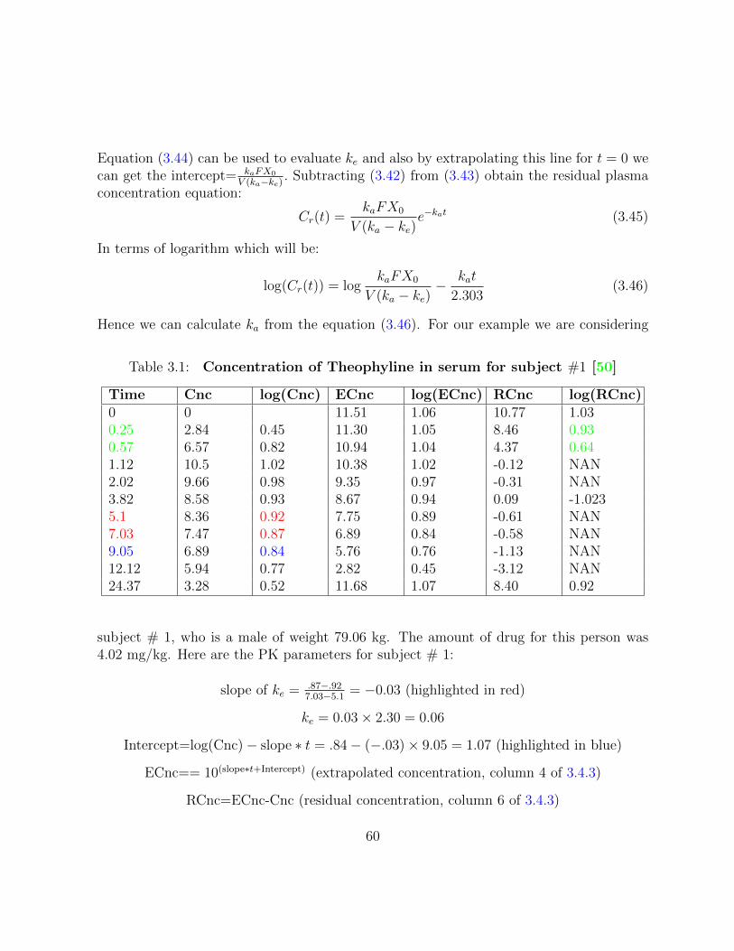
Equation (3.44) can be used to evaluate ke and also by extrapolating this line for t = 0 wecan get the intercept= kaFX0

V (ka−ke) . Subtracting (3.42) from (3.43) obtain the residual plasmaconcentration equation:

Cr(t) =kaFX0

V (ka − ke)e−kat (3.45)

In terms of logarithm which will be:

log(Cr(t)) = logkaFX0

V (ka − ke)− kat

2.303(3.46)

Hence we can calculate ka from the equation (3.46). For our example we are considering

Table 3.1: Concentration of Theophyline in serum for subject #1 [50]

Time Cnc log(Cnc) ECnc log(ECnc) RCnc log(RCnc)0 0 11.51 1.06 10.77 1.030.25 2.84 0.45 11.30 1.05 8.46 0.930.57 6.57 0.82 10.94 1.04 4.37 0.641.12 10.5 1.02 10.38 1.02 -0.12 NAN2.02 9.66 0.98 9.35 0.97 -0.31 NAN3.82 8.58 0.93 8.67 0.94 0.09 -1.0235.1 8.36 0.92 7.75 0.89 -0.61 NAN7.03 7.47 0.87 6.89 0.84 -0.58 NAN9.05 6.89 0.84 5.76 0.76 -1.13 NAN12.12 5.94 0.77 2.82 0.45 -3.12 NAN24.37 3.28 0.52 11.68 1.07 8.40 0.92

subject # 1, who is a male of weight 79.06 kg. The amount of drug for this person was4.02 mg/kg. Here are the PK parameters for subject # 1:

slope of ke = .87−.927.03−5.1

= −0.03 (highlighted in red)

ke = 0.03× 2.30 = 0.06

Intercept=log(Cnc)− slope ∗ t = .84− (−.03)× 9.05 = 1.07 (highlighted in blue)

ECnc== 10(slope∗t+Intercept) (extrapolated concentration, column 4 of 3.4.3)

RCnc=ECnc-Cnc (residual concentration, column 6 of 3.4.3)

60

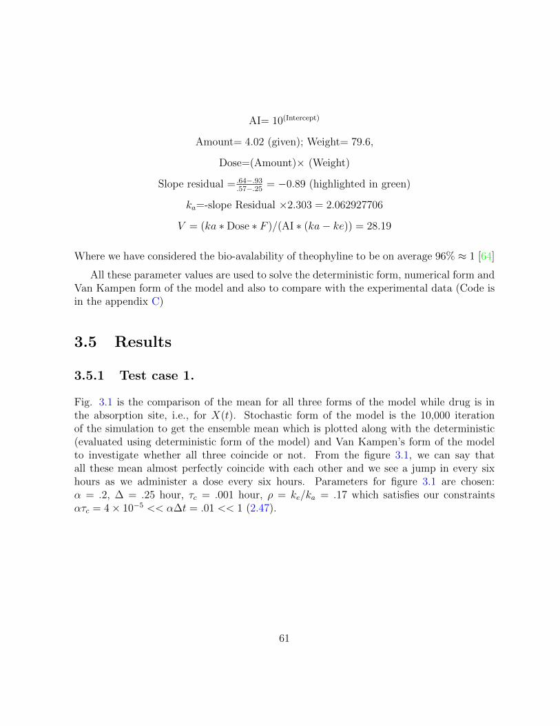
AI= 10(Intercept)

Amount= 4.02 (given); Weight= 79.6,

Dose=(Amount)× (Weight)

Slope residual = .64−.93.57−.25

= −0.89 (highlighted in green)

ka=-slope Residual ×2.303 = 2.062927706

V = (ka ∗Dose ∗ F )/(AI ∗ (ka− ke)) = 28.19

Where we have considered the bio-avalability of theophyline to be on average 96% ≈ 1 [64]

All these parameter values are used to solve the deterministic form, numerical form andVan Kampen form of the model and also to compare with the experimental data (Code isin the appendix C)

3.5 Results

3.5.1 Test case 1.

Fig. 3.1 is the comparison of the mean for all three forms of the model while drug is inthe absorption site, i.e., for X(t). Stochastic form of the model is the 10,000 iterationof the simulation to get the ensemble mean which is plotted along with the deterministic(evaluated using deterministic form of the model) and Van Kampen’s form of the modelto investigate whether all three coincide or not. From the figure 3.1, we can say thatall these mean almost perfectly coincide with each other and we see a jump in every sixhours as we administer a dose every six hours. Parameters for figure 3.1 are chosen:α = .2, ∆ = .25 hour, τc = .001 hour, ρ = ke/ka = .17 which satisfies our constraintsατc = 4× 10−5 << α∆t = .01 << 1 (2.47).

61

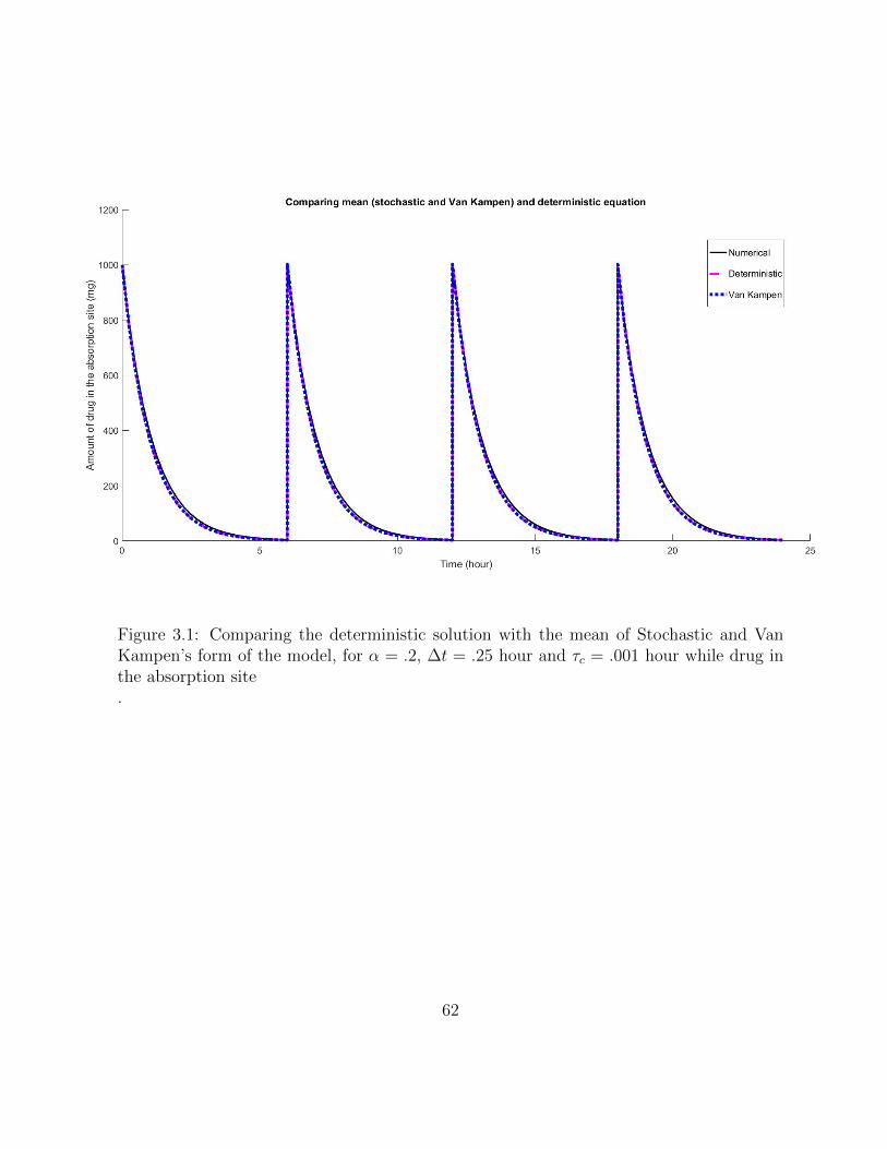
Figure 3.1: Comparing the deterministic solution with the mean of Stochastic and VanKampen’s form of the model, for α = .2, ∆t = .25 hour and τc = .001 hour while drug inthe absorption site.

62

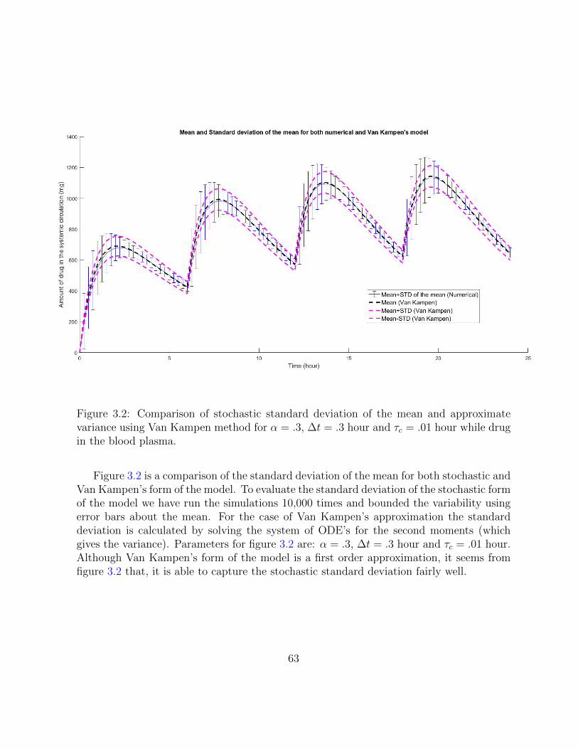
Figure 3.2: Comparison of stochastic standard deviation of the mean and approximatevariance using Van Kampen method for α = .3, ∆t = .3 hour and τc = .01 hour while drugin the blood plasma.

Figure 3.2 is a comparison of the standard deviation of the mean for both stochastic andVan Kampen’s form of the model. To evaluate the standard deviation of the stochastic formof the model we have run the simulations 10,000 times and bounded the variability usingerror bars about the mean. For the case of Van Kampen’s approximation the standarddeviation is calculated by solving the system of ODE’s for the second moments (whichgives the variance). Parameters for figure 3.2 are: α = .3, ∆t = .3 hour and τc = .01 hour.Although Van Kampen’s form of the model is a first order approximation, it seems fromfigure 3.2 that, it is able to capture the stochastic standard deviation fairly well.

63

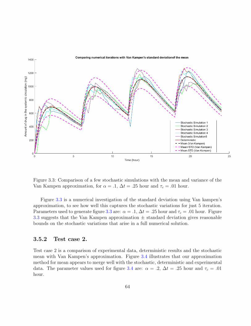
Figure 3.3: Comparison of a few stochastic simulations with the mean and variance of theVan Kampen approximation, for α = .1, ∆t = .25 hour and τc = .01 hour.

Figure 3.3 is a numerical investigation of the standard deviation using Van kampen’sapproximation, to see how well this captures the stochastic variations for just 5 iteration.Parameters used to generate figure 3.3 are: α = .1, ∆t = .25 hour and τc = .01 hour. Figure3.3 suggests that the Van Kampen approximation ± standard deviation gives reasonablebounds on the stochastic variations that arise in a full numerical solution.

3.5.2 Test case 2.

Test case 2 is a comparison of experimental data, deterministic results and the stochasticmean with Van Kampen’s approximation. Figure 3.4 illustrates that our approximationmethod for mean appears to merge well with the stochastic, deterministic and experimentaldata. The parameter values used for figure 3.4 are: α = .2, ∆t = .25 hour and τc = .01hour.

64

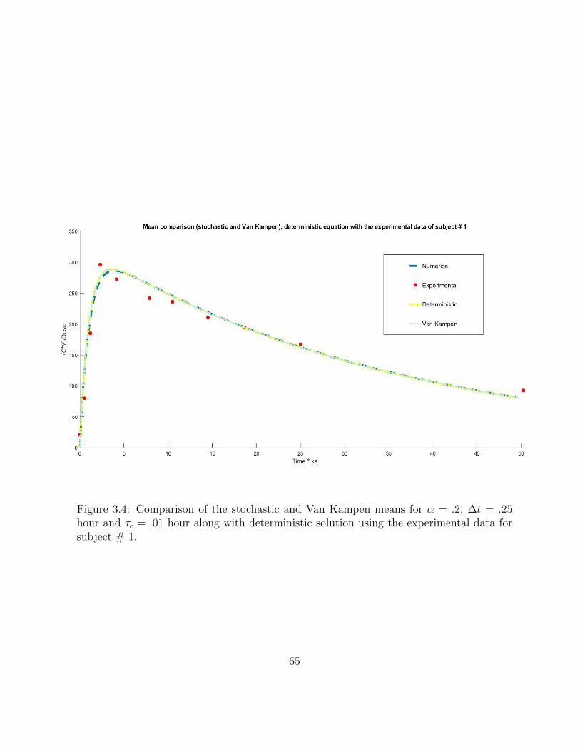
Figure 3.4: Comparison of the stochastic and Van Kampen means for α = .2, ∆t = .25hour and τc = .01 hour along with deterministic solution using the experimental data forsubject # 1.

65

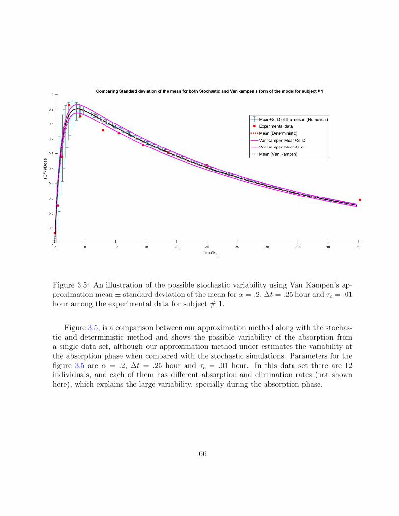
Figure 3.5: An illustration of the possible stochastic variability using Van Kampen’s ap-proximation mean ± standard deviation of the mean for α = .2, ∆t = .25 hour and τc = .01hour among the experimental data for subject # 1.

Figure 3.5, is a comparison between our approximation method along with the stochas-tic and deterministic method and shows the possible variability of the absorption froma single data set, although our approximation method under estimates the variability atthe absorption phase when compared with the stochastic simulations. Parameters for thefigure 3.5 are α = .2, ∆t = .25 hour and τc = .01 hour. In this data set there are 12individuals, and each of them has different absorption and elimination rates (not shownhere), which explains the large variability, specially during the absorption phase.

66

3.6 Conclusion

Absorption is a physiological process that results in the uptake of a drug into the systemiccirculation from the site of administration. It is clear that drug efficacy depends crucially onmaintaining critical drug concentration levels during the therapeutic window. At the sametime, this has to be balanced judiciously against the toxic side effects of a therapeutic drug.We have presented in this chapter an approximate model (based on Van Kampen’s method)together with error bounds that delimit the stochastic variability of drug concentrationlevels in the body. Simulations of drug concentration that bound stochastic variabilitygive us some confidence that an individual’s plasma drug concentration levels are beingmaintained at appropriate levels for drug efficacy. In addition, the error bounds providesalutary warning of the possibility of exceeding toxic concentration levels which may haveadverse effects on a patient and hence on therapeutic efficacy.

Biological systems are inherently stochastic, and hence it is not possible to developa deterministic model with perfect predictive power. As in all of Applied Mathematics,perfection is unattainable, but through judicious application of Okham’s razor and in-corporating refinements guided by experiments, we may hope to arrive at a model thatprovides insight and rational guidance for clinicians and experimentalists.

67

Chapter 4

Saturable and fractal kinetics

4.1 Introduction

Identifying appropriate drugs and determining the right dosages are two prerequisites forsuccessful treatment of cancer using chemotherapy. Searching for effective new drugs andevaluating their performance on various tumors is the main focus of pre-clinical and clini-cal studies [33]. Furthermore, the correct or optimum dose with minimum toxicity is alsoa crucial requirement for any effective therapy [33]. This in turn requires extensive ex-perimental and empirical studies (both in vitro and in vivo). In this chapter we developa mathematical model to study a well known chemotherapeutic cancer drug paclitaxel,in order to facilitate the design of dose administration strategies along with combinationschedules. Paclitaxel was the first taxane to gain widespread clinical acceptance and isused now as a chemotherapeutic agent to treat a wide spectrum of tumors. Although pa-clitaxel was initially thought to display linear pharmacokientics, but Sonnichsen et al,[75],highlighted the fact that the pharmacokineticss is nonlinear by showing that a two com-partmental model that incorporated saturable transport and saturable elimination bestcaptured pediatric PK data. A three compartmental model that incorporated saturabletransport from the central compartment to peripheral compartments, as well as saturableelimination was used by [27] to capture the concentration/time behavior of paclitaxel, inthe case of adults. The data from Giani et al., [27], and Sonnichsen et al., [75] clearlydemonstrated that drug distribution saturated and it was also clear from the data thatsaturation of transport processes occurred at lower plasma concentrations than for elimi-nation. It is often the case that several PK models of varying complexity may be able tocapture the behavior of any given data set. The choice of an appropriate model is often

68

guided by physiological considerations and the use of Ockham’s Razor (or the law of par-simony). For drugs that are governed by underlying linear processes, compartmental PKmodels have provided excellent characterizations for a variety of pharmaceuticals. Sim-ilarly the incorporation of saturable elimination (based on the Michaelis Menten theoryof bi-molecular chemical interaction between substrates and enzyme) has led to an evenbetter characterization of the PK of these pharmaceuticals. Although saturable bindingand transport are based on sound physiological principles, the processes by which pacli-taxel is distributed through tissue suggest that saturable binding is the dominant process,not saturable transport. Thus a possible fruitful future direction of research might be theinvestigation of PK models that incorporate saturable binding compared with those thatincorporate saturable transport (these latter have tended to predominate PK studies ofpaclitaxel.) From experimental studies it is well established that the time concentrationprofile of paclitaxel shows nonlinear dose dependence [40, 27, 56].

Various models have been developed based on linear and non-linear time-concentrationprofile of paclitaxel, using saturable distribution and elimination for two, three or morecompartments [40, 27, 56, 57, 34, 59]. For example, Giani et al.,[27] developed a multi-compartmental model which includes a metabolite component. Sonnichsen et al., [75]developed a two compartmental model for children with solid tumors. Both models haveassumed two saturable processes, one during the distribution phase and the other duringthe elimination phase. These saturable processes have been incorporated in the models byassuming Michaelis Menten kinetics [40].

The derivation of Michaelis Menten kinetics is based on traditional mass action kinetics.If the reaction occurs in dimensionally restricted environments (which occurs specially invivo), then traditional mass action kinetics fail to capture well the underlying mechanism[69] and resulting behavior of drug concentration levels. Thus to better capture the chem-ical kinetics, the Michaelis Menten formalism has to be extended to (what is known in theliterature) as fractal Michaelis Menten kinetics [69].

We extend the existing mathematical model in the literature of Kearns et., al [40],by incorporating fractal kinetics to better capture the saturable distribution process andelimination for the time concentration profile of the drug paclitaxel.

In section 4.2, we describe the mathematical formulation of the model along with adescription of how the numerical simulations are carried out. In section 4.4, we brieflydiscuss the three experimental studies from which we have drawn data in order to validateour model. In section 4.5, we present the choice of parameter values for our study andcompare these with those by Kearns et al., [40] in their model. In section 4.6, we discussand appraise our findings.

69

4.2 Description of the Mathematical and Computa-

tional models

Classical compartmental Pk models treat the body as a combination of a number of com-partments. This is a popular approach to describe biological systems transport of materialsthrough the body. The usual practice is to consider the kinetic rates as constants. How-ever the measurement of biological systems present unique challenges where drug moleculesinteract with membrane interfaces, metabolic enzymes and have to navigate through re-stricted and crowded micro-environments, where the system is clearly unstirred, heteroge-neous and geometrically fractal [63]. Kopelman [41] first pointed out that, classical kineticsare unsatisfactory, especially if the microscopic environment of the reactants are spatiallyconstrained. Fractal order of elementary reactions, rate coefficients with temporal mem-ories, self ordering and self non-mixing criteria have a great impact on the heterogeneousreaction kinetics [41]. A number of publications on diffusion in fractal spaces using fractalcalculus, have appeared in the literature. These studies show that all classical pharma-cokinetics modeling are essentially a subset of fractal pharmacokinetics. Fuite et al., [22]discussed the fractal nature of the liver for the drug miberfradil, which is used to reduceventricular fibrillation [73].

In this chapter, we focus on the anti cancer drug Paclitaxel. It is derived from thePacific or European Yew tree [68]. In 1962 US National Cancer Institute studied the toxiceffects of paclitaxel for the first time. Phase I trials were carried out in 1983, subsequentlyPhase II trials began 1988 [11]. Paclitaxel blocks the G2/M phase of the cell cycle and asa result, such cells can’t go through normal mitosis [11]. Microtubules are responsible forcell shape, motility of cells, intracellular transport and mitosis and Paclitaxel is now wellknown as a mitotic inhibitor as it binds to microtubules [57]. It is now accepted as a mosteffective anticancer drug and has been used for solid tumors; such as breast, ovarian, lung,head and neck etc. Usually this drug is administered via intravenous infusion at a highdose [40]. It has a long residence time in the body and is capable of staying in cancer cellsfor over a week [59].

The characterization of drug transport and absorption has attracted much interestover the last several decades, and remains arguably the central focus of much PK research.Drugs interact with target organs by crossing epithelial membranes either by passive dif-fusion, pinocytosis or via carrier-mediated transport. Carrier mediated transport of drugsis the primary means of delivering drugs to a variety of tissues ranging from organs suchas the kidney, gut and the choroid plexus in the central nervous system. The mathemat-ical modeling and analysis of this process has been based on classical reaction kinetics

70

(with time independent rate constants). This has, however, been known to be far fromsatisfactory for media composed of heterogeneous micro environments, and especially forreactions that are spatially constrained. Fractal reaction kinetics have been proposed as abetter approach to modeling the pharmacokinetics of drug transport in the human body.Work of Mandelbrot [52] and West et al., [87] have shown that organs such as the lungs,kidneys and anatomical structures such as the circulatory system have a fractal geometry.Other time dependent processes (leading to limit cycle oscillations) have been implicatedas leading to nonlinear pharmacokinetics. This suggests that the extension of the MichaelisMenten formalism, incorporating fractal kinetics may be a better approach to study thetime course of a drug in the body.

4.3 fractal Michaelis Menten kinetics

4.3.1 Batch/Transient case

The underlying assumptions of homogenity and well-stirred environments lead to time-independent constant reaction rates in classical chemical kinetics. However in the real casescenarios, reactions often occur in restricted geometries where the kinetics can be affectedby fluctuations in concentration levels [31]. This situation can be captured mathematicallyby taking the rates time dependent [39]. If we want to consider the simplest applicablebimolecular elementary reaction:

A+B → Products. (4.1)

By the law of mass action this has the macroscopic description [41]

dC

dt= −kCACB, (4.2)

where C(t) is the reactant concentration and k is the “rate constant” which does notdepend on time or concentration.

Another underlying mechanism influencing this reaction is diffusion, which arises fromdifferences in drug concentration in different parts of the body. In this case the system canbe described by two fundamental time scales: one is the diffusion time, time the particlesrequire before meeting each other to react and the time particles will take to react witheach other [4]. The process is known as reaction limited, when the reaction time is largerthan the diffusion time and laws of mass actions are used to define the kinetic rates. On

71

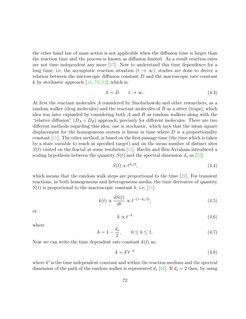
the other hand law of mass action is not applicable when the diffusion time is larger thanthe reaction time and the process is known as diffusion limited. As a result reaction ratesare not time independent any more [17]. Now to understand this time dependence for along time, i.e, the asymptotic reaction situation (t → ∞), studies are done to derive arelation between the microscopic diffusion constant D and the macroscopic rate constantk by stochastic approach [41, 74, 12], which is:

k ∼ D t→∞. (4.3)

At first the reactant molecules A considered by Smoluchowski and other researchers, as arandom walker (drug molecules) and the reactant molecules of B as a sitter (traps), whichidea was later expanded by considering both A and B as random walkers along with the“relative diffusion” (DA + DB) approach, precisely for different molecules. There are twodifferent methods regarding this idea; one is stochastic, which says that the mean squaredisplacement for the homogeneous system is linear in time where D is a proportionalityconstant [41]. The other method, is based on the first passage time (the time which is takenby a state variable to reach at specified target) and on the mean number of distinct sitesS(t) visited on the fractal at some resolution [41]. Havlin and Ben-Avraham introduced ascaling hypothesis between the quantity S(t) and the spectral dimension ds as [22]:

S(t) ∝ tds/2, (4.4)

which means that the random walk steps are proportional to the time [22]. For transientreactions, in both homogeneous and heterogeneous media, the time derivative of quantityS(t) is proportional to the macroscopic constant k, i.e, [41]:

k(t) ∝ dS(t)

dt∝ t−(1−ds/2), (4.5)

ork ∝ t−h (4.6)

where

h = 1− ds2, 0 ≤ h ≤ 1. (4.7)

Now we can write the time dependent rate constant k(t) as:

k = k′t−h (4.8)

where k′ is the time independent constant and within the reaction medium and the spectraldimension of the path of the random walker is represented ds [41]. If ds = 2 then, by using

72

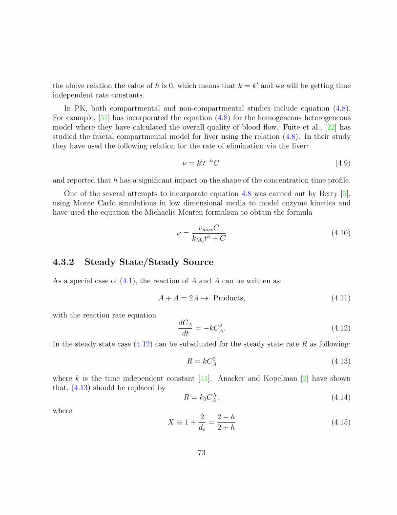
the above relation the value of h is 0, which means that k = k′ and we will be getting timeindependent rate constants.

In PK, both compartmental and non-compartmental studies include equation (4.8).For example, [51] has incorporated the equation (4.8) for the homogeneous heterogeneousmodel where they have calculated the overall quality of blood flow. Fuite et al., [22] hasstudied the fractal compartmental model for liver using the relation (4.8). In their studythey have used the following relation for the rate of elimination via the liver:

ν = k′t−hC. (4.9)

and reported that h has a significant impact on the shape of the concentration time profile.

One of the several attempts to incorporate equation 4.8 was carried out by Berry [5],using Monte Carlo simulations in low dimensional media to model enzyme kinetics andhave used the equation the Michaelis Menten formalism to obtain the formula

ν =vmaxC

kM0th + C

(4.10)

4.3.2 Steady State/Steady Source

As a special case of (4.1), the reaction of A and A can be written as:

A+ A = 2A→ Products, (4.11)

with the reaction rate equationdCAdt

= −kC2A. (4.12)

In the steady state case (4.12) can be substituted for the steady state rate R as following:

R = kC2A (4.13)

where k is the time independent constant [41]. Anacker and Kopelman [2] have shownthat, (4.13) should be replaced by

R = k0CXA , (4.14)

where

X ≡ 1 +2

ds=

2− h2 + h

(4.15)

73

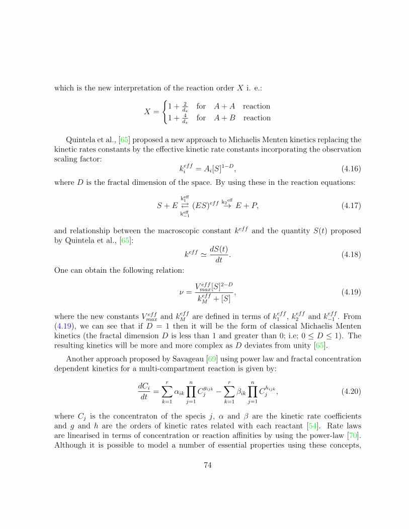
which is the new interpretation of the reaction order X i. e.:

X =

{1 + 2

dsfor A+ A reaction

1 + 4ds

for A+B reaction

Quintela et al., [65] proposed a new approach to Michaelis Menten kinetics replacing thekinetic rates constants by the effective kinetic rate constants incorporating the observationscaling factor:

keffi = Ai[S]1−D, (4.16)

where D is the fractal dimension of the space. By using these in the reaction equations:

S + Ekeff

1

�keff−1

(ES)effk2

eff

→ E + P, (4.17)

and relationship between the macroscopic constant keff and the quantity S(t) proposedby Quintela et al., [65]:

keff ' dS(t)

dt. (4.18)

One can obtain the following relation:

ν =V effmax[S]2−D

keffM + [S], (4.19)

where the new constants V effmax and keffM are defined in terms of keff1 , keff2 and keff−1 . From

(4.19), we can see that if D = 1 then it will be the form of classical Michaelis Mentenkinetics (the fractal dimension D is less than 1 and greater than 0; i.e; 0 ≤ D ≤ 1). Theresulting kinetics will be more and more complex as D deviates from unity [65].

Another approach proposed by Savageau [69] using power law and fractal concentrationdependent kinetics for a multi-compartment reaction is given by:

dCidt

=r∑

k=1

αik

n∏j=1

Cgijkj −

r∑k=1

βik

n∏j=1

Chijkj , (4.20)

where Cj is the concentraton of the specis j, α and β are the kinetic rate coefficientsand g and h are the orders of kinetic rates related with each reactant [54]. Rate lawsare linearised in terms of concentration or reaction affinities by using the power-law [70].Although it is possible to model a number of essential properties using these concepts,

74

it is not applicable for other important biochemical effects like saturation [70]. Savageau[69] argues that although the power law formalism may have complex mathematical form,it nevertheless has significant benefits, as it is capable of capturing fractal phenomenamathematically. Marsh et al., [54] state that the equation proposed by Savageau [69] canbe derived by summing over several Michaelis Menten reactions.

4.3.3 Dose dependent fractal Michaelis Menten kinetics

Kopleman [41] mentions that, for the transient state, reactants follow random distributionsand reactants/walkers (drug molecules), gradually loose their efficiency while they aretraversing the fractal space (which has dimension ds). As a result of this, anomalouskinetics is observed in this state [54]. Where as in steady state, there is an inflow of themolecules, which can be treated as well stirred in Euclidean geometry, [41]. However, inthe fractal case, as self stirring is unlikely, then it can be a result of extensive fluctuationsin the regional concentration along with the growing isolation of molecules, which is knownas reaction-diffusion phenomena and as a result of these, at the steady state, distributionmolecules can be taken as partially ordered with a reduced reaction rate [54].

Marsh et al., [54] proposed an alternative formulation of fractal kinetics which dependson the dose concentration under steady state conditions. If we consider a single compart-ment model in the steady state, this implies that the drug concentration is constant asa function of time. Even though physiologically, there may be considerable variations indrug concentrations from one location to another, it may still be possible to achieve asteady state scenario if the drug concentration is far higher than enzyme concentrationlevels. Although drug molecules are lost through the elimination, the heterogeneity of theenvironment, can give rise to re-circulation of released drug molecules trapped long timeat various locations. Thus modifying the DEs (1.15) appropriately, we can rewrite it for aheterogeneous environment as follows [54]:

d[ES]

dt= k1(E0 − [ES])[S]X − (k−1 + k2)[ES] (4.21)

dP

dt= k2[ES]

where X is the fractal reaction order and using this relation in (1.17), we obtain thefollowing form for the fractal Michaelis-Menten function:

v0 =vmaxS

X0

km + SX0, (4.22)

75

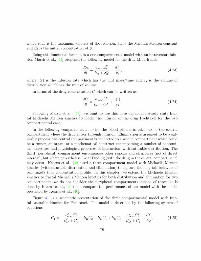
where vmax is the maximum velocity of the reaction, km is the Micaelis Menten constantand S0 is the initial concentration of S.

Using this functional formula in a one-compartmental model with an intravenous infu-sion Marsh et al., [54] proposed the following model for the drug Miberfradil:

dS0

dt=

vmaxSX0

km + SX0+i(t)

vd, (4.23)

where i(t) is the infusion rate which has the unit mass/time and vd is the volume ofdistribution which has the unit of volume.

In terms of the drug concentration C which can be written as:

dC

dt=

vmaxCX

km + CX+i(t)

vd. (4.24)

Following Marsh et al., [55], we want to use this dose dependent steady state frac-tal Michaelis Menten kinetics to model the infusion of the drug Paclitaxel for the twocompartmental case.

In the following compartmental model, the blood plasma is taken to be the centralcompartment where the drug enters through infusion. Elimination is assumed to be a sat-urable process, the central compartment is connected to a second compartment which couldbe a tumor, an organ, or a mathematical construct encompassing a number of anatomi-cal structures and physiological processes of interaction, with saturable distribution. Thethird (peripheral) compartment encompasses other regions and structures (not of directinterest), but where nevertheless linear binding (with the drug in the central compartment)may occur. Kearns et al., [40] used a three compartment model with Michaelis Mentenkinetics (with saturable distribution and elimination) to capture the long tail behavior ofpaclitaxel’s time concentration profile. In this chapter, we extend the Michaelis Mentenkinetics to fractal Michaelis Menten kinetics for both distribution and elimination for twocompartments (we do not consider the peripheral compartment) instead of three (as isdone by Kearns et al., [40]) and compare the performance of our model with the modelpresented by Kearns et al., [40].

Figure 4.1 is a schematic presentation of the three compartmental model with frac-tal saturable kinetics for Paclitaxel. The model is described by the following system ofequations:

C1 = − vdmaxCp1

kdM + Cp1

+ k21C2 − k13C1 + k31C3 −vemaxC

q1

keM + Cq1

+i(t)

Vd, (4.25)

76

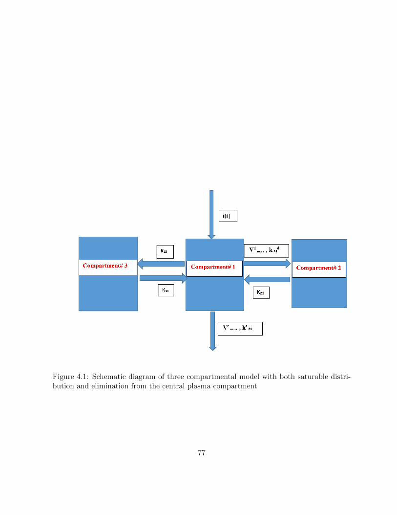
Figure 4.1: Schematic diagram of three compartmental model with both saturable distri-bution and elimination from the central plasma compartment

77

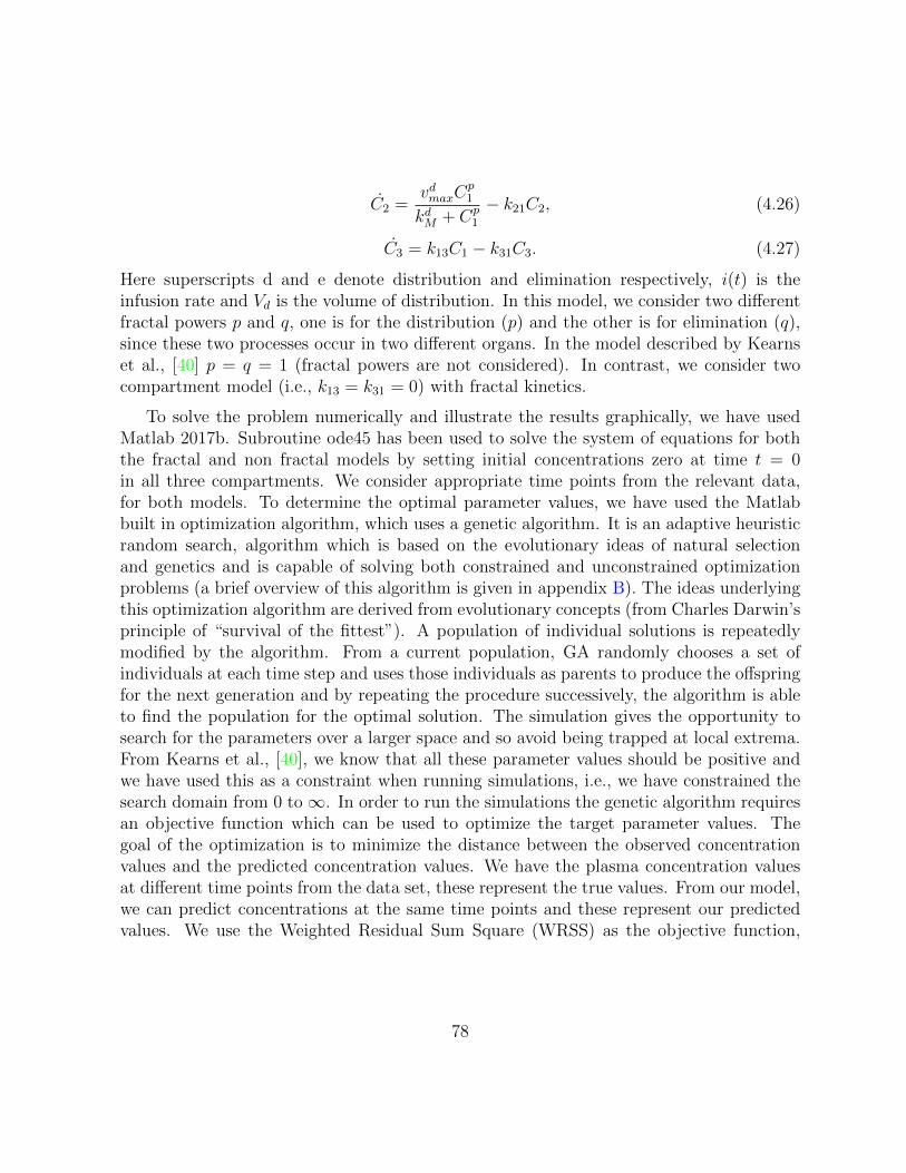
C2 =vdmaxC

p1

kdM + Cp1

− k21C2, (4.26)

C3 = k13C1 − k31C3. (4.27)

Here superscripts d and e denote distribution and elimination respectively, i(t) is theinfusion rate and Vd is the volume of distribution. In this model, we consider two differentfractal powers p and q, one is for the distribution (p) and the other is for elimination (q),since these two processes occur in two different organs. In the model described by Kearnset al., [40] p = q = 1 (fractal powers are not considered). In contrast, we consider twocompartment model (i.e., k13 = k31 = 0) with fractal kinetics.

To solve the problem numerically and illustrate the results graphically, we have usedMatlab 2017b. Subroutine ode45 has been used to solve the system of equations for boththe fractal and non fractal models by setting initial concentrations zero at time t = 0in all three compartments. We consider appropriate time points from the relevant data,for both models. To determine the optimal parameter values, we have used the Matlabbuilt in optimization algorithm, which uses a genetic algorithm. It is an adaptive heuristicrandom search, algorithm which is based on the evolutionary ideas of natural selectionand genetics and is capable of solving both constrained and unconstrained optimizationproblems (a brief overview of this algorithm is given in appendix B). The ideas underlyingthis optimization algorithm are derived from evolutionary concepts (from Charles Darwin’sprinciple of “survival of the fittest”). A population of individual solutions is repeatedlymodified by the algorithm. From a current population, GA randomly chooses a set ofindividuals at each time step and uses those individuals as parents to produce the offspringfor the next generation and by repeating the procedure successively, the algorithm is ableto find the population for the optimal solution. The simulation gives the opportunity tosearch for the parameters over a larger space and so avoid being trapped at local extrema.From Kearns et al., [40], we know that all these parameter values should be positive andwe have used this as a constraint when running simulations, i.e., we have constrained thesearch domain from 0 to∞. In order to run the simulations the genetic algorithm requiresan objective function which can be used to optimize the target parameter values. Thegoal of the optimization is to minimize the distance between the observed concentrationvalues and the predicted concentration values. We have the plasma concentration valuesat different time points from the data set, these represent the true values. From our model,we can predict concentrations at the same time points and these represent our predictedvalues. We use the Weighted Residual Sum Square (WRSS) as the objective function,

78

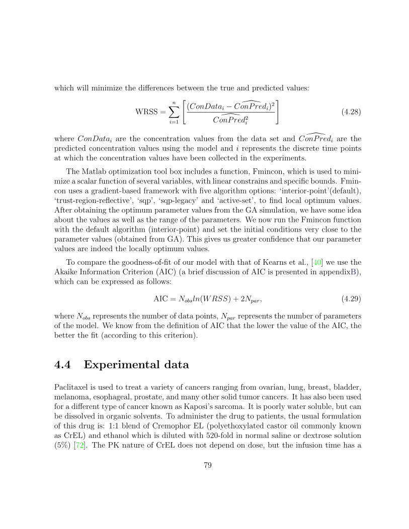
which will minimize the differences between the true and predicted values:

WRSS =n∑i=1

[(ConDatai − ConPredi)

2

ConPred2i

](4.28)

where ConDatai are the concentration values from the data set and ConPredi are thepredicted concentration values using the model and i represents the discrete time pointsat which the concentration values have been collected in the experiments.

The Matlab optimization tool box includes a function, Fmincon, which is used to mini-mize a scalar function of several variables, with linear constrains and specific bounds. Fmin-con uses a gradient-based framework with five algorithm options: ‘interior-point’(default),‘trust-region-reflective’, ‘sqp’, ‘sqp-legacy’ and ‘active-set’, to find local optimum values.After obtaining the optimum parameter values from the GA simulation, we have some ideaabout the values as well as the range of the parameters. We now run the Fmincon functionwith the default algorithm (interior-point) and set the initial conditions very close to theparameter values (obtained from GA). This gives us greater confidence that our parametervalues are indeed the locally optimum values.

To compare the goodness-of-fit of our model with that of Kearns et al., [40] we use theAkaike Information Criterion (AIC) (a brief discussion of AIC is presented in appendixB),which can be expressed as follows:

AIC = Nobsln(WRSS) + 2Npar, (4.29)

where Nobs represents the number of data points, Npar represents the number of parametersof the model. We know from the definition of AIC that the lower the value of the AIC, thebetter the fit (according to this criterion).

4.4 Experimental data

Paclitaxel is used to treat a variety of cancers ranging from ovarian, lung, breast, bladder,melanoma, esophageal, prostate, and many other solid tumor cancers. It has also been usedfor a different type of cancer known as Kaposi’s sarcoma. It is poorly water soluble, but canbe dissolved in organic solvents. To administer the drug to patients, the usual formulationof this drug is: 1:1 blend of Cremophor EL (polyethoxylated castor oil commonly knownas CrEL) and ethanol which is diluted with 520-fold in normal saline or dextrose solution(5%) [72]. The PK nature of CrEL does not depend on dose, but the infusion time has a

79

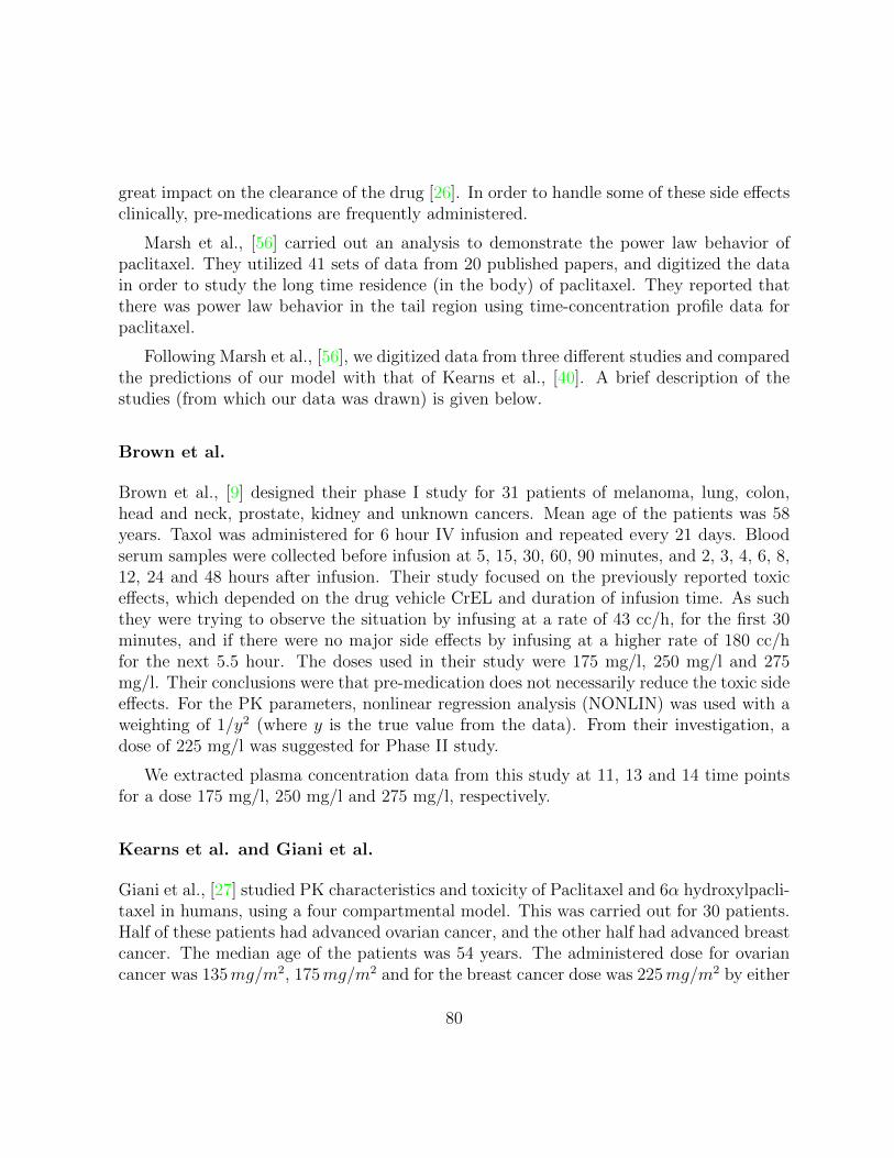
great impact on the clearance of the drug [26]. In order to handle some of these side effectsclinically, pre-medications are frequently administered.

Marsh et al., [56] carried out an analysis to demonstrate the power law behavior ofpaclitaxel. They utilized 41 sets of data from 20 published papers, and digitized the datain order to study the long time residence (in the body) of paclitaxel. They reported thatthere was power law behavior in the tail region using time-concentration profile data forpaclitaxel.

Following Marsh et al., [56], we digitized data from three different studies and comparedthe predictions of our model with that of Kearns et al., [40]. A brief description of thestudies (from which our data was drawn) is given below.

Brown et al.

Brown et al., [9] designed their phase I study for 31 patients of melanoma, lung, colon,head and neck, prostate, kidney and unknown cancers. Mean age of the patients was 58years. Taxol was administered for 6 hour IV infusion and repeated every 21 days. Bloodserum samples were collected before infusion at 5, 15, 30, 60, 90 minutes, and 2, 3, 4, 6, 8,12, 24 and 48 hours after infusion. Their study focused on the previously reported toxiceffects, which depended on the drug vehicle CrEL and duration of infusion time. As suchthey were trying to observe the situation by infusing at a rate of 43 cc/h, for the first 30minutes, and if there were no major side effects by infusing at a higher rate of 180 cc/hfor the next 5.5 hour. The doses used in their study were 175 mg/l, 250 mg/l and 275mg/l. Their conclusions were that pre-medication does not necessarily reduce the toxic sideeffects. For the PK parameters, nonlinear regression analysis (NONLIN) was used with aweighting of 1/y2 (where y is the true value from the data). From their investigation, adose of 225 mg/l was suggested for Phase II study.

We extracted plasma concentration data from this study at 11, 13 and 14 time pointsfor a dose 175 mg/l, 250 mg/l and 275 mg/l, respectively.

Kearns et al. and Giani et al.

Giani et al., [27] studied PK characteristics and toxicity of Paclitaxel and 6α hydroxylpacli-taxel in humans, using a four compartmental model. This was carried out for 30 patients.Half of these patients had advanced ovarian cancer, and the other half had advanced breastcancer. The median age of the patients was 54 years. The administered dose for ovariancancer was 135mg/m2, 175mg/m2 and for the breast cancer dose was 225mg/m2 by either

80

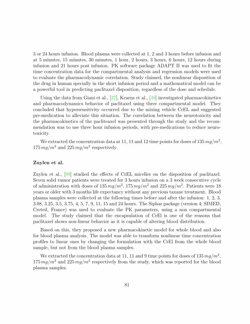
3 or 24 hours infusion. Blood plasma were collected at 1, 2 and 3 hours before infusion andat 5 minutes, 15 minutes, 30 minutes, 1 hour, 2 hours, 3 hours, 6 hours, 12 hours duringinfusion and 21 hours post infusion. PK software package ADAPT II was used to fit thetime concentration data for the compartmental analysis and regression models were usedto evaluate the pharmacodynamic correlation. Study claimed, the nonlinear disposition ofthe drug in human specially in the short infusion period and a mathematical model can bea powerful tool in predicting paclitaxel disposition, regardless of the dose and schedule.

Using the data from Giani et al., [27], Kearns et al., [40] investigated pharmacokineticsand pharmacodynamics behavior of paclitaxel using three compartmental model. Theyconcluded that hypersensitivity occurred due to the mixing vehicle CrEL and suggestedpre-medication to alleviate this situation. The correlation between the neurotoxicity andthe pharmacokinetics of the pacliteaxel was presented through the study and the recom-mendation was to use three hour infusion periods, with pre-medications to reduce neuro-toxicity.

We extracted the concentration data at 11, 11 and 12 time points for doses of 135mg/m2,175mg/m2 and 225mg/m2 respectively.

Zuylen et al.

Zuylen et al., [89] studied the effects of CrEL micelles on the disposition of paclitaxel.Seven solid tumor patients were treated for 3 hours infusion on a 3 week consecutive cycleof administration with doses of 135mg/m2, 175mg/m2 and 225mg/m2. Patients were 18years or older with 3 months life expectancy without any previous taxane treatment. Bloodplasma samples were collected at the following times before and after the infusion: 1, 2, 3,3.08, 3.25, 3.5, 3.75, 4, 5, 7, 9, 11, 15 and 24 hours. The Siphar package (version 4; SIMED,Creteil, France) was used to evaluate the PK parameters, using a non compartmentalmodel. The study claimed that the encapsulation of CrEl is one of the reasons thatpaclitaxel shows non-linear behavior as it is capable of altering blood distribution.

Based on this, they proposed a new pharmacokinetic model for whole blood and alsofor blood plasma analysis. The model was able to transform nonlinear time concentrationprofiles to linear ones by changing the formulation with the CrEl from the whole bloodsample, but not from the blood plasma samples.

We extracted the concentration data at 11, 11 and 9 time points for doses of 135mg/m2,175mg/m2 and 225mg/m2 respectively from the study, which was reported for the bloodplasma samples.

81

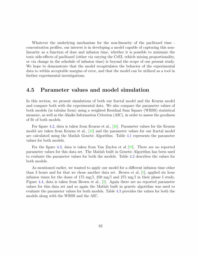
Whatever the underlying mechanism for the non-linearity of the paclitaxel time -concentration profiles, our interest is in developing a model capable of capturing this non-linearity as a function of dose and infusion time, whether it is possible to minimize thetoxic side-effects of paclitaxel (either via varying the CrEL vehicle mixing proportionality,or via change in the schedule of infusion time) is beyond the scope of our present study.We hope to demonstrate that the model recapitulates the behavior of the experimentaldata to within acceptable margins of error, and that the model can be utilized as a tool infurther experimental investigations.

4.5 Parameter values and model simulation

In this section, we present simulations of both our fractal model and the Kearns modeland compare both with the experimental data. We also compare the parameter values ofboth models (in tabular form) using a weighted Residual Sum Square (WRSS) statisticalmeasure, as well as the Akaike Information Criterion (AIC), in order to assess the goodnessof fit of both models.

For figure 4.2, data is taken from Kearns et al., [40]. Parameter values for the Kearnsmodel are taken from Kearns et al., [40] and the parameter values for our fractal modelare calculated using the Matlab Genetic Algorithm. Table 4.1 represents the parametervalues for both models.

For the figure 4.3, data is taken from Van Zuylen et al [89]. There are no reportedparameter values for this data set. The Matlab built in Genetic Algorithm has been usedto evaluate the parameter values for both the models. Table 4.2 describes the values forboth models.

As mentioned earlier, we wanted to apply our model for a different infusion time otherthan 3 hours and for that we chose another data set. Brown et al, [9], applied six hourinfusion times for the doses of 175 mg/l, 250 mg/l and 275 mg/l in their phase I study.Figure 4.4, data is taken from Brown et al., [9]. Again there are no reported parametervalues for this data set and so again the Matlab built in genetic algorithm was used toevaluate the parameter values for both models. Table 4.3 provides the values for both themodels along with the WRSS and the AIC.

82

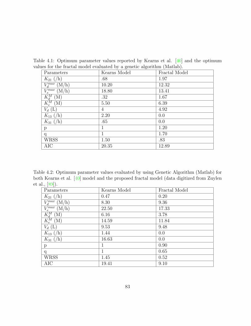
Table 4.1: Optimum parameter values reported by Kearns et al. [40] and the optimumvalues for the fractal model evaluated by a genetic algorithm (Matlab).

Parameters Kearns Model Fractal ModelK21 (/h) .68 1.97V maxd (M/h) 10.20 12.32V maxe (M/h) 18.80 13.41KMd (M) .32 1.67

KMe (M) 5.50 6.39

Vd (L) 4 4.92K13 (/h) 2.20 0.0K31 (/h) .65 0.0p 1 1.20q 1 1.70WRSS 1.50 .83AIC 20.35 12.89

Table 4.2: Optimum parameter values evaluated by using Genetic Algorithm (Matlab) forboth Kearns et al. [40] model and the proposed fractal model (data digitized from Zuylenet al., [89]).

Parameters Kearns Model Fractal ModelK21 (/h) 0.47 0.20V maxd (M/h) 8.30 9.36V maxe (M/h) 22.50 17.33KMd (M) 6.16 3.78

KMe (M) 14.59 11.84

Vd (L) 9.53 9.48K13 (/h) 1.44 0.0K31 (/h) 16.63 0.0p 1 0.90q 1 0.65WRSS 1.45 0.52AIC 19.41 9.10

83

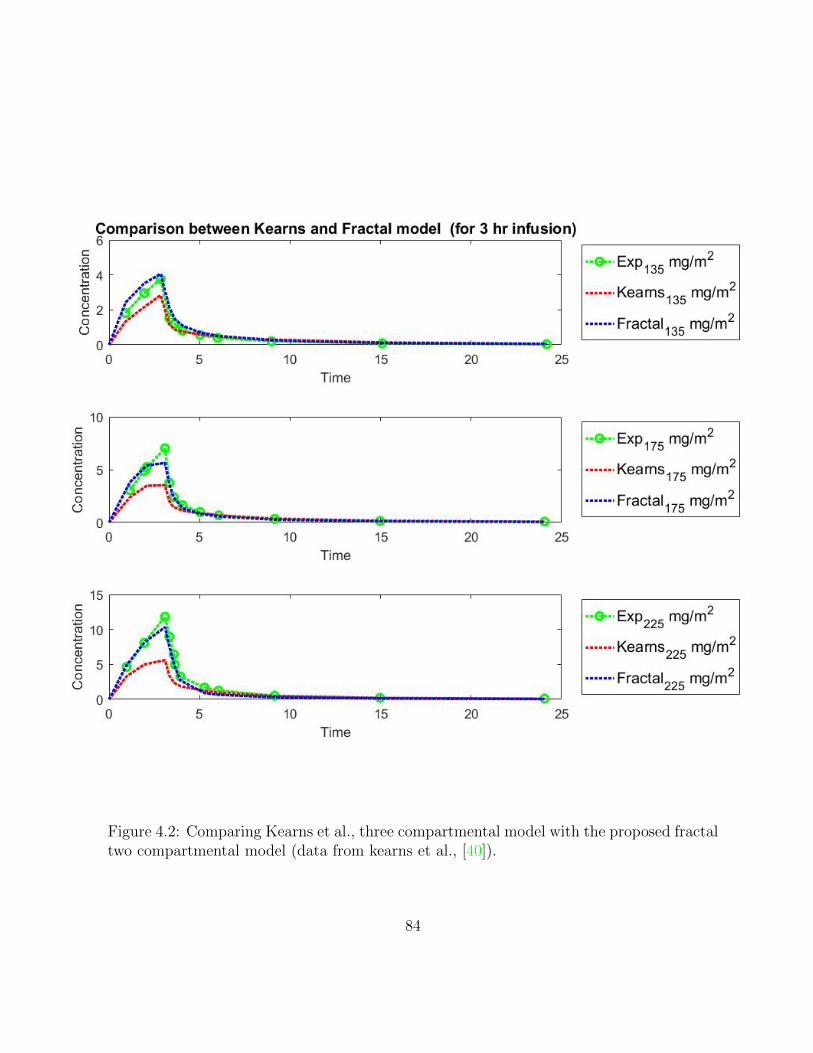
Figure 4.2: Comparing Kearns et al., three compartmental model with the proposed fractaltwo compartmental model (data from kearns et al., [40]).

84

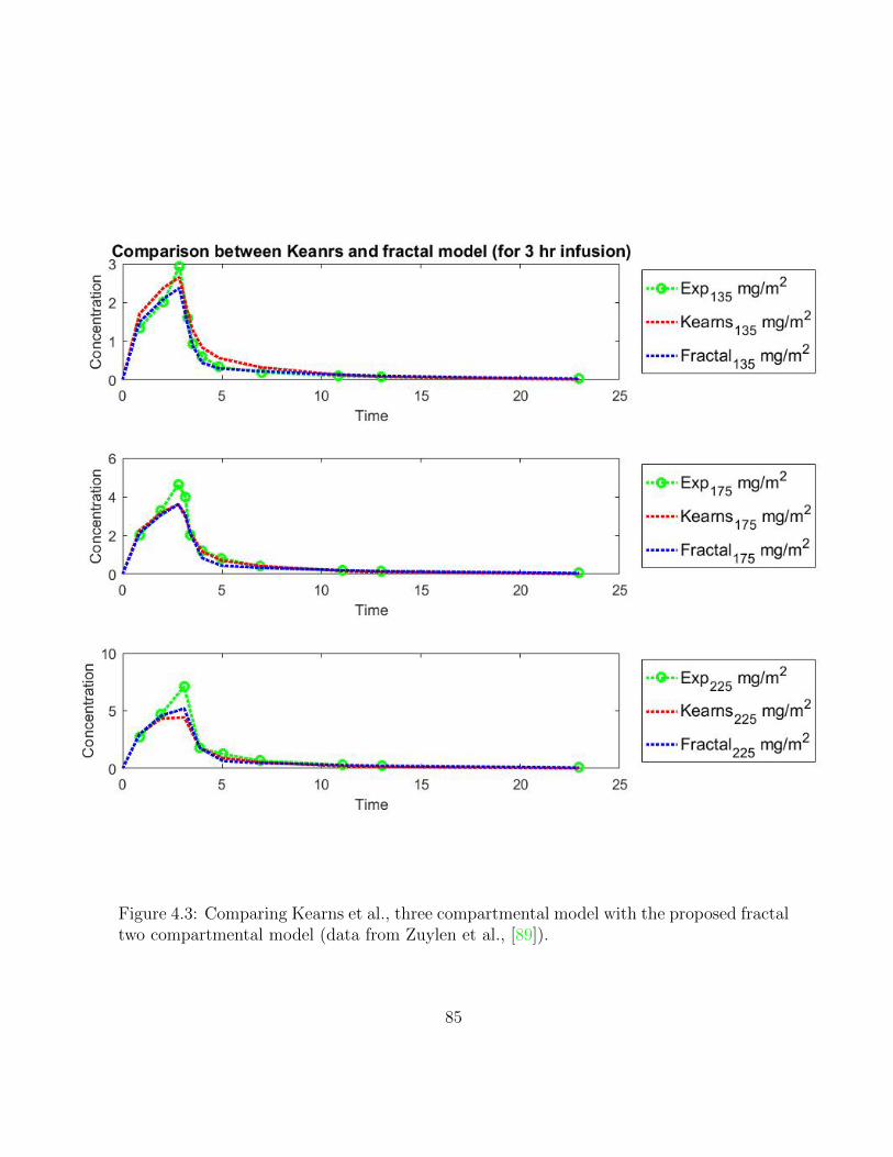
Figure 4.3: Comparing Kearns et al., three compartmental model with the proposed fractaltwo compartmental model (data from Zuylen et al., [89]).

85

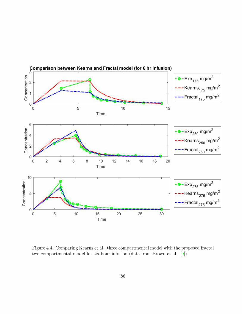
Figure 4.4: Comparing Kearns et al., three compartmental model with the proposed fractaltwo compartmental model for six hour infusion (data from Brown et al., [9]).

86

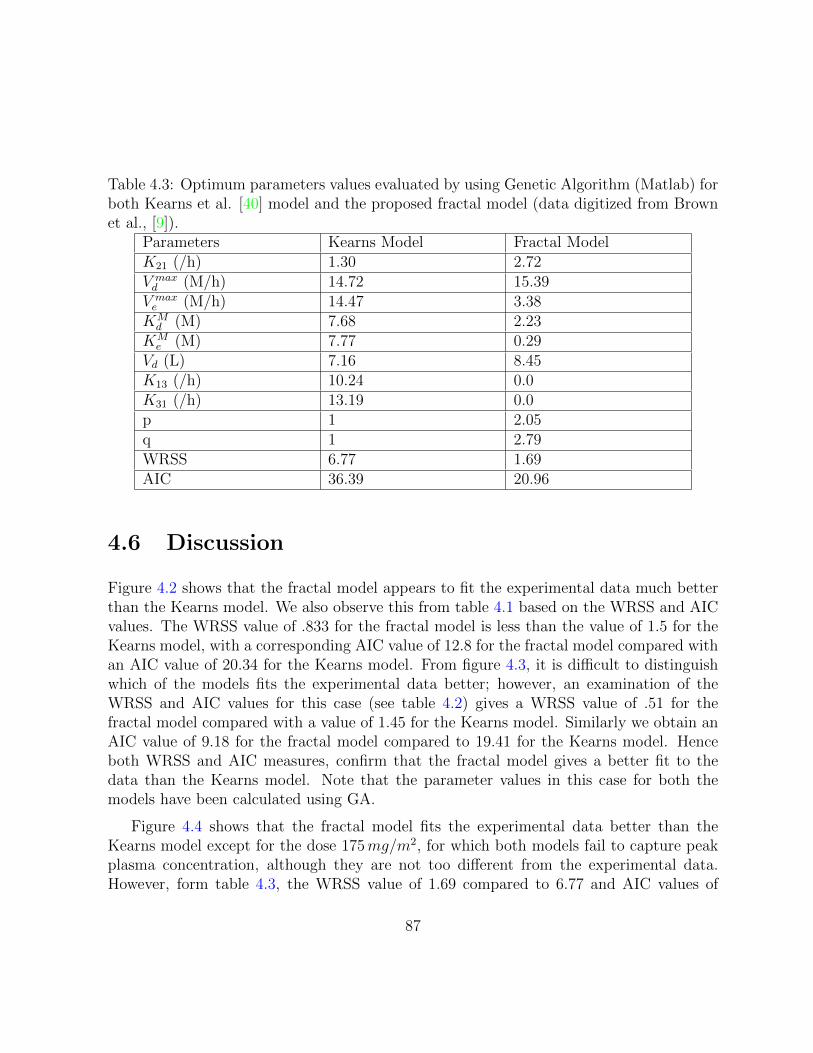
Table 4.3: Optimum parameters values evaluated by using Genetic Algorithm (Matlab) forboth Kearns et al. [40] model and the proposed fractal model (data digitized from Brownet al., [9]).

Parameters Kearns Model Fractal ModelK21 (/h) 1.30 2.72V maxd (M/h) 14.72 15.39V maxe (M/h) 14.47 3.38KMd (M) 7.68 2.23

KMe (M) 7.77 0.29

Vd (L) 7.16 8.45K13 (/h) 10.24 0.0K31 (/h) 13.19 0.0p 1 2.05q 1 2.79WRSS 6.77 1.69AIC 36.39 20.96

4.6 Discussion

Figure 4.2 shows that the fractal model appears to fit the experimental data much betterthan the Kearns model. We also observe this from table 4.1 based on the WRSS and AICvalues. The WRSS value of .833 for the fractal model is less than the value of 1.5 for theKearns model, with a corresponding AIC value of 12.8 for the fractal model compared withan AIC value of 20.34 for the Kearns model. From figure 4.3, it is difficult to distinguishwhich of the models fits the experimental data better; however, an examination of theWRSS and AIC values for this case (see table 4.2) gives a WRSS value of .51 for thefractal model compared with a value of 1.45 for the Kearns model. Similarly we obtain anAIC value of 9.18 for the fractal model compared to 19.41 for the Kearns model. Henceboth WRSS and AIC measures, confirm that the fractal model gives a better fit to thedata than the Kearns model. Note that the parameter values in this case for both themodels have been calculated using GA.

Figure 4.4 shows that the fractal model fits the experimental data better than theKearns model except for the dose 175mg/m2, for which both models fail to capture peakplasma concentration, although they are not too different from the experimental data.However, form table 4.3, the WRSS value of 1.69 compared to 6.77 and AIC values of

87

20.69 compared to 36.39 again confirm that the fractal model provided a better fit to thedata than the Kearns model.

4.7 Conclusion

We extended an existing model (that used Michalis Menten formalism to model the non-linear behavior of the chemotherapeutic drug paclitaxel) by incorporating fractal MichaelisMenten kinetics, to better capture the effects of two competitive saturable processes. Wehave compared our model with the existing model on three different data sets from threedifferent studies. Although it might appear that one shortcoming of our fractal modeland that of Kearns et al., is that a different set of parameter values have to be used inboth models for each of the three data sets, a closer examination reveals why it may be,unreasonable to expect that one set of parameter values should be sufficient to predict thethree different scenarios. Firstly, the three data sets have been obtained for patients withvery different cancers. Secondly, the age groups of the patients, vary significantly for thethree data sets. Thirdly, the pre-medication used on the patients are very different foreach of the three data sets. Taking into consideration all of these different factors, it isclear that the three data sets obtained are for three very different clinical situations andso clearly we should expect that the parameter values calculated for one data set will notnecessarily give the best fit for a data set from a different clinical situation. Naturally,given patients of similar age groups, with the same type of cancer (who received a similartherapeutic drugs), one would expect that parameter values extracted previously from adifferent patient cohort would still give an effective predictive model, which could be usedto evaluate the impact of different infusion times and different doses on a new patientcohort. However, it is clear that the model needs to be validated on a broader range ofdata before it can be evaluated in a clinical setting. Despite all these challenges, we believethat well validated mathematical compartmental models of this nature are indispensabletools in preclinical studies and play a crucial role in the eventual development of effectiveclinical therapies.

88

Chapter 5

Conclusion

Sixty five years have elapsed since F. H. Dost introduced the term pharmacokinetics(PK) in his 1953 paper, Der BliitspiegeI-Kinetic der Konzentrationsablaiife in der Kries-laufJ ssigkeit [83]. By 1979, the number of published articles in clinical pharmacokineticshad exceeded 400 to 500 articles per year, and PK is now an entrenched and integral partof the clinical drug development pipeline. PK is based on four basic processes: absorption,distribution, metabolism and excretion. All these processes are quantified by the variousPK parameters. As discussed earlier in chapter 2, there are several frequently used methodsto calculate the absorption rate constant, these are the Wagner-Nelson or Loo-Riegelmanmethod, nonlinear least-squares regression analysis and method of residuals. Perrier andGibaldi [62] stated in their study that these methods can overestimate the absorption rateconstant as they do not take into account the variations in absorption rate over time andbioavailability [62].

In Chapter 1 of this thesis, we presented a summary of basic concepts of pharmacoki-netics. In general, it is unreasonable to expect that drug concentration as a function oftime (for a specific patient) follows a deterministic ODE model. There may be variations asa result of incorrect or inaccurate model specification, as well as due to physiological varia-tions or uncertainty in the distribution, absorption and elimination processes. A means ofdescribing such errors is to develop random differential equation (or stochastic differentialequation) models. The simplest one compartmental elimination model:

dx

dt= −kex, (5.1)

(where x is the drug concentration and ke is the first order elimination rate constant) can

89

be extended to a random differential equation by writing:

dx = −kexdt+ σwdw (5.2)

where dw is an infinitesimal increment of the Wiener process, and so the model can bedescribed simply as a deterministic ODE perturbed by a normally distributed noise (orrandom differential equation). The solution of (5.2) is :

x(t) = x0e−ket +

∫ t

0

σwe−ke(t−s)dw. (5.3)

Clearly there are some obvious problems with the model (5.2), primarily, it appears thatthere is no limitation on the drug concentration, and so (even though the model describes asimple drug elimination process) the drug concentration can increase when the incrementsof the Wiener process are positive. Further more, the model will fluctuate around the meanzero, even after the initial drug dose has been eliminated, and so the model will predictnonphysical negative concentrations. A more realistic model is obtained by adding noiseto the rate constant, in this case in the elimination rate constant ke. Now if we want tomake the elimination rate as a random function of t with mean ke such that:

ke(t) = ke + αξ(t), (5.4)

where α is the amplitude of the fluctuation and ξ(t) represents the noise.

In this case (5.1) can be written as:

dx

dt= −(ke + αξ(t))x. (5.5)

In the case that ξ(t) is a Wiener process (i.e. in the case of white noise), equation (5.4)can be written as the Ito equation

dx = −kexdt− αxdw (5.6)

In our work, by taking into account randomness in the absorption rate our deterministicmodel becomes a random differential equation and we make some statistical assumptionsconcerning the nature of the noise. We consider the noise, to be an Ornstein Uhlenbeckprocess [78]. It is a Gaussian process, with bounded variance which admits a stationaryprobability distribution. The stochastic DE of an Ornstein-Uhlenbek process is often writ-ten as a Langevin equation. The random differential equation is solved numerically usingthe Gillespie algorithm [30].

90

However, in this thesis we consider the more physically realistic case of “colored noise”,where the correlation time of the noise is not a delta function. In this case the Ito calculusis not applicable and no exact solution method is available. However, approximation meth-ods have been developed in the physical science for realistic noise (with short correlationtimes), and in chapters 2 and 3, we examined these approaches and showed that they canbe successfully applied to PK models. We started by considering the Bourret approxima-tion to handle random differential equations and then the more amenable Van Kampenapproximation applied to the random harmonic oscillations and a one compartment model.

In chapter 3, we examined a stochastic model of a simple compartment model withboth absorption and elimination and applied Van Kampen’s approximation method to themodel, to obtain first and second moments. We also compared Van Kampen’s approxima-tion for the first moments to full stochastic simulations for the mean, and the solution ofthe deterministic equation for small amplitude noise and short correlation times. Our re-sults give us some degree of confidence that Van Kampen’s method allows us to determinerealistic error bounds on the mean drug concentration levels that allow us to bound thestochastic variability of drug concentration in the body.

In chapter 4, we use the theory of fractal kinetics in the context of pharmacokineticswhere saturable reactions may occur in heterogeneous micro environments. Although onecompartment models are often oversimplifications, they are able to produce accurate, goodfits if drug distribution occurs on a fast time scale and equilibrium is reached rapidly inall tissues. We extended a standard two-compartment PK model to include steady-statefractal Michaelis-Menten kinetics. Transient fractal kinetics is to be expected in well-mixed heterogeneous environments, where as steady-state fractal kinetics is characteristicin poorly mixed heterogeneous environments [54]. Klymko and Kopelman [42] suggest thatnon-integer values of p and q appearing in equations (4.25) and (4.26), are characteristics ofthese heterogeneous media which are essentially an assemblage of kinetically independentbundles. In this case, the kinetic rate coefficients are averages taken over regions of varyingsizes and varying local concentrations. We applied our two compartmental PK model,incorporating fractal steady-state Micahelis-Menten kinetics to paclitaxel data from theliterature. Paclitaxel is a long studied chemotherapeutic drug which has proved effectivein the treatment of solid tumors (for example lung, breast, ovarian etc). The plasmaconcentration time profile of this drug is nonlinear [40], [27], [89]. Our results show thatour model best captured the absorption and elimination of paclitaxel, for three differentdigitized data sets (compared to the Kearns et al., [40] model).

In the thesis we have explored the use of random differential equations as well as frac-tal kinetics to characterize the PK of therapeutic drugs. In particular, in the latter case(compartmental model of fractal kinetics) the models are deterministic and essentially

91

characterize macroscopic behavior. It would be fruitful, and a possible future direction ofresearch to investigate the connections and relationship between individual drug molecules,macroscopic drug behavior and the mean, using the theory of stochastic processes. In thiscontext, the incorporation of the idea of Levy flights in PK modeling appears promising.The theory of random walks has been extended to a continuous time random walk for-malism, and thus could be used incorporating Levy trapping times to develop a stochasticPK model which includes saturable and fractal kinetics elimination effects with Levy timetemporary trapping. These types of models could then be used to infer target doses, usingplasma data, as well as to predict the response to different dosing strategies. The approachmay avoid assumptions about underlying reasons (e.g., fractal kinetics, heterogeneous cellpopulations, different cell death mechanism) leading to dispersion in molecule residencetimes. It might also be possible to understand and explain (using this approach) clinicalobservations such as delayed reactions in some patients (in terms of this dispersion).

92

References

[1] Advil Canada https://www.advil.ca

[2] L. W. Anacker and R. Kopelman, Fractal chemical kinetics: Simulations and experi-ments, J. Chem. Phys, 81, (1984), pp. 6402–6403.

[3] L. Arnold, Stochastic Differential Equations, Theory and Applications. John Wiley &Sons, New York (1974).

[4] D. ben-Avraham, M. A. Burschka, C. R. Doering, Statics and Dynamics of a Diffusion-Limited Reaction: Anomalous Kinetics, Noneqnilibrium Self-Ordering, and a DynamicTransition, Journal of Statistical Physics, 60, (5/6), (1990).

[5] H. Berry, Monte carlo simulations of enzyme reactions in two dimensions: Fractalkinetics and spatial segregation, Biophys. J. 83, (2002), pp. 1891–1901.

[6] R. C. Bourret, Propagation of randomly perturbed fields, Canadian Journal of Physics,40(6), (1962), pp. 62–084

[7] R. C. Bourret, Stochastically perturbed fields, with applications to wave propagation inrandom media, Nuovo Cimento, 26, (1962), pp. 1–31.

[8] R. C. Bourret, Fiction theory of dynamical systems with noisy parameters, CanadianJournal of Physics, 43, (1965), pp. 619–639.

[9] T. Brown, K. Havlin, G. Weiss, J. Cagnola, J. Koeller, J. Kuhn, J. Rizzo, J. Craig, J.Phillips, D. V. Hoff. A phase I trial of taxol given by a 6- hour intravenous infusion. JClin Oncol 7, (1991), pp. 1261–1267.

[10] K. P. Burnham and D. R. Anderson, Model Selection and Multimodel Inference: APractical Information-Theoretic Approach Springer-Verlag New York, 2nd ED., 2002.

[11] Cancer Care Ontario Canada https://www.cancercare.on.ca

93

[12] S. Chandrasekhar, Stochastic Problems in Physics and Astronomy, Rev. Mod. Phys,15 (1), (1943), DOI:https://doi.org/10.1103/RevModPhys.15.1

[13] D. J. Cutler, A comment regarding mean residence times in non-linear sys-tems, Biopharmaceutics & Drug Disposition, 10, (1989), pp. 529–530, DOI:10.1002/bdd.2510100510

[14] J. T. Dipiro, Concepts in Clinical Pharmacokinetics, American Society of Health-system Pharmacists, 5th ED., 2010.

[15] D. Z. D’Argenio and K. Park, Uncertain pharmacokinetic/pharmacodynamic systems:Design, estimation and control, Control Engineering Practice, 5, (12), (1997), pp. 1707–1716

[16] S. Ditlevsen and A. D. Gaetano, Mixed Effects In Stochastic Differential EquationModels, Statistical Journal, 3, (2), (2005), pp. 137–153

[17] C. R. Doering and D. ben-Avraham, Interparticle distribution functions and rate equa-tions for diffusion-limited reactions, Physical Review A, 38, (6), (1988).

[18] S. Donnet and A. Samson, A review of stochastic differential equations for pharma-cokinetic/pharmacodynamic models, Advanced Drug Delivery Reviews, 65, (2013), pp929–939.

[19] J. L Doob, The Brownian movement and Stochastic equations, Ann Math, 43, (1942),pp. 351–369.

[20] L. Ferrante, S. Bompadre, and L. Leone,A Stochastic Compartmental Model with LongLasting Infusion, Biometrical Journal, 45, (2003), pp. 182–194.

[21] U.S. Food and Drug Administration,https://www.fda.gov/ForPatients/ClinicalTrials/Types/default.htm

[22] J. Fuite, R. Marsh and J. Tuszynski, Fractal pharmacokinetics of the drug mibefradilin the liver, Phys. Rev. E, 66 (2002), Art. Id. 021904, pp. 1-11.

[23] A. T. Fuller, Conditions for a Matrix to Have Only Characteristic Roots with NegativeReal Parts, Journal of Mathematical Analysis and Applications, 23, (1968), pp. 71–98.Conditions

[24] http://www.obitko.com/tutorials/genetic-algorithms/ga-basic-description.php

94

[25] C. W. Gardiner, Stochastic Methods: A Hand book for the Natural and Social Sciences,Springer, 4rth ED., 2009.

[26] H. Gelderblom, J. Verweij, K. Nooter, A. Sparreboom Cremophor EL: the drawbacksand advantages of vehicle selection for drug formulation, European Journal of Cancer37 (2001) pp. 1590–1598.

[27] L. Gianni, C.M. Kearns, A. Giani, G. Capri, L. Vigano, A. Lacatelli, G. Bonadonna,M.J. Egorin. Nonlinear pharmacokinetics and metabolism of paclitaxel and its phar-macokinetic/pharmacodynamic relationships in humans., J Clin Oncol 13, (1995), pp.180–190.

[28] M. Gibaldi and G. Levy, Pharmacokinetics in clinical practice I. Concepts. JAMA.235, (17), (1976), pp. 1864–1867.

[29] M. Gibaldi and D. Perrier, Pharmacokinetics, Marcel Dekker Inc, Newyork and basel,1975.

[30] D. T. Gillespie, Exact numerical simulation of the Ornstein-Uhlenbeck process and itsintegral, Physical Review E, 54(2), DOI:https://doi.org/10.1103/PhysRevE.54.2084,(1996)

[31] D. T. Gregory, Fractals in Molecular Biophysics, Oxford Universities Press (NewYork), 1997.

[32] K. M. van De Graff and S. I. Fox,Concepts of Human Anatomy and Physiology, 2ndED., W. M. C. Brown, Iowa, 1988.

[33] H. Gurney, How to calculate the dose of chemotherapy. Br J Cancer. 86 (2002) pp.1297–1302.

[34] A. Henningsson, M.O. Karlsson, L. Vigano, L. Gianni, J. Verweij, A. Spar-reboom. Mechanismbased pharmacokinetic model for paclitaxel, J.Clin Oncol 19, (2001),pp.4065–4073.

[35] E. L. Ince, Ordinary Differential Equations, Dover books on Mathematics, 1956.

[36] S. S. Jambhekar and P. J. Breen, Basic Pharmacokinetics, Pharmaceutical Press,London, UK, 2009.

[37] L. James, J. E Sullivan and D. Roberts, Narrative Review: The proper use of ac-etaminophen, Paediatr Child Health, 16(9), November 2011.

95

[38] R. E. Kalman, A New Approach to Linear Filtering and Prediction Problems, Journalof Basic Engineering, 82 (35), (1960), DOI:10.1115/1.3662552.

[39] K. Kang and S. Redner, Fluctuation effects in Smoluchowski reaction kinetics, Phys.Rev. A 30, (2833(R)), (1984).

[40] C. M. Kearns, L. Gianni and M. J. Egorin, Egorin, Paclitaxel pharmacokinetics andpharmacodynamics, Semin. Oncol., 22 (1995), pp. 16-23.

[41] R. Kopelman, Rate processes on fractals: Theory, simulations, and experiments, J.Stat. Phys, 42, (1986), pp. 185–200.

[42] P. W. Klymko and R. Kopelman, Fractal reaction kinetics: exciton fusion onclusters, The Journal of Physical Chemistry, 87(23), (1983), pp.4565–4567, DOI:10.1021/j100246a006

[43] B. F. Krippendorff, K. Kuester, C. Kloft and W. Huisinga Nonlinear pharmacokineticsof therapeutic proteins resulting from receptor mediated endocytosis, J PharmacokinetPharmacodyn. 36(3), (2009 Jun) pp. 239-260, DOI: 10.1007/s10928-009-9120-1

[44] D. S. Lemons, Paul Langevin’s 1908 paper “On the Theory of Brownian Motion” [“Surla thorie du mouvement brownien,” C. R. Acad. Sci. (Paris) 146, 530-533 (1908)],American Journal of Physics, 65, Issue 11, pp. 1079–1081 (1997).

[45] P. Lanskey, A Stochastic Model for Circulatory Transport in Pharmocoki-netics, Mathematical Biosciences, 132,(2), (March 1996), pp. 141-167, DOI:https://doi.org/10.1016/0025-5564(95)00050-X

[46] D. S. Lemons, An Introduction to Stochastic Processes in Physics, The Johns HopkinsUniversity Press, 2002.

[47] RenH. Levy, Time-dependent pharmacokinetics, Pharmacology & Therapeutics,17,(3), (1982), pp. 383–397, DOI: https://doi.org/10.1016/0163-7258(82)90022-5.

[48] N. Limi, On stochastic compartmental models, Journal of Mathematical Biology, 27(1), (1989), pp. 105-113

[49] JH. Lin, Dose-dependent pharmacokinetics: experimental observations and theoreticalconsiderations, Biopharm Drug Dispos, 15(1)(1994 Jan), pp. 1–31.

[50] Lixofit: Modeling and simulation software for drug development,http://dataset.lixoft.com/data-set-examples/theophylline-data-set

96

[51] P. Macheras, A fractal approach to heterogeneous drug distribution: Calcium pharma-cokinetics, Pharm. Res., 13, (1996), pp. 663–670.

[52] B. B. Mandelbrot, The Fractal Geometry of Nature, (1983).

[53] A. H. Marcus, Power laws in compartmental analysis. part I: a unified stochasticmodel, Mathematical Biosciences, 23, Issues 34, pp. 337–350, Issues 34, (April 1975),doi.org/10.1016/0025-5564(75)90046-2

[54] R. E. Marsh and J. A. Tuszynski Saturable Fractal Pharmacokinetics and Its Appli-cations, Mathematical Methods and Models in Biomedicine, Springer, New York, NY,pp. 339–366, DOI: https://doi.org/10.1007/978-1-4614-4178-6 12, 2013.

[55] R. E. Marsh and J. A. Tuszynski, Fractal MichaelisMenten kinetics under steady stateconditions, application to mibefradil, Pharmaceut. Res. 23, (2006), pp. 27602767.

[56] R. E. Marsh, J. A. Tuszynski, M. B. Sawyer and K. J. E. Vos, Emergence of power lawsin the pharmacokientics of paclitaxel due to competing saturable processes, J. Pharm.Pharmaceut. Sci.,11 (2008), pp. 77–96.

[57] R. E. Marsh and J. A. Tuszyski, Sawyer, M.B., Vos, K.J.E.: Emergence of power lawsin the pharmacokinetics of paclitaxel due to competing saturable processes. J. Pharm.Pharm. Sci. 11, (2008), pp. 77–96

[58] J. H. Matis and H. O. Hartley, Stochastic compartmental analysis: model and leastsquares estimation from time series data. Biometrics, 27, pp. 77–102 (1971).

[59] T. Mori, Y. Kinoshita, A. Watanabe, T.Yamaguchi, K. Hosokawa, H. Honjo. Reten-tion of paclitaxel in cancer cells for 1 week in vivo and in vitro. Cancer ChemotherPharmacol: Eprint, 2006.

[60] S. B. Mortensen, A. H. Jnsdttir, S. Klim and H. Madsen, Introduction to PK/PDmodelling - with focus on PK and stochastic differential equations, Danish NationalResearch Database, ID 2389479862 (2008)

[61] P. Veng-Pedersen, Noncompartmentally-based pharmacokinetic modeling, AdvancedDrug Delivery Reviews, 48, (2001), pp. 265–300

[62] D. Perrier and M. Gibaldi, Calculation of Absorption Rate Constants for Drugs withIncomplete Availability, Journal of Pharmaceutical Sciences, 62(2), (1973), pp. 225–228, DOI: https://doi.org/10.1002/jps.2600620208

97

[63] L. M. Pereira Fractal pharmacokinetics, Computational and Mathematical Methodsin Medicine, 11 (2), (June 2010), pp. 161–184

[64] PHARMACOKINETICS, An Online resource for students,https://sepia.unil.ch/pharmacology/index.php?id=90

[65] M. A. Lopez-Quintela and J. Casado, Revision of the Methodology in Enzyme Kinetics:A Fractal Approach, J. theor. Biol. 139,(1989), pp. 129–139

[66] M. Ramanathan, An application of Ito’s Lemma in Population Pharmacokinetics andPharmacodynamics , Pharmaceutical Research, 16 (4), (1999)

[67] M. Ramanathan, A Method For Estimating Pharmacokinetic Risks of Concentration-Dependent Drug Interactions from Preclinical data, Drug Metabolism and Disposition,27, (12), (1999).

[68] E. K. Rowinsky, M. Wright, B. Monsarrat, G. J. Lesser and R. C. Donehower, Taxol:Pharmacology, metabolism and clinical implications, Cancer Surv., 17 (1993), pp. 283–304.

[69] M. A. Savageau, Development of fractal kinetic theory for enzyme-catalysed reactionsand implications for the design of biochemical pathways, BioSystems 47, (1998), pp.9–36.

[70] S. Schnell and T.E. Turner, Reaction kinetics in intracellular environments withmacromolecular crowding: simulations and rate laws, Progress in Biophysics & Molec-ular Biology 85, (2004), pp. 235–260.

[71] M. Scott, Applied Stochastic Processes in physics and engineering, 2013.

[72] A. K. Singla, A. Garg, and D. Aggarwal, Paclitaxel and its formulations,InternationalJournal of Pharmaceutics 235, (2002) pp. 179–192

[73] A. Skerjanec, S. Tawfik and Y. K. Tam, Mechanisms of nonlinear pharmacokineticsof mibefradil in chronically instrumented dogs. J. Pharmacol. Exp. Ther. 278, (1996),pp. 817–825

[74] M. Smoluchowski, Mathematical Theory of the Kinetics of the Coagulation of ColloidalSolutions, Zeitschrift fr Physikalische Chemie, 19, (1917), pp. 129–135.

98

[75] D.S. Sonnichsen, C.A. Hurwitz, C.B. Pratt, J.J. Shuster, M.V. Relling. Saturablepharmacokinetics and paclitaxel pharmacodynamics in children with solid tumors. JClin Oncol 12, (1994), pp. 532–538.

[76] M. I. Stefan and N. L. Novre, Cooperative Binding, PLOS— Computational Biology,(June 27, 2013), DOI: https://doi.org/10.1371/journal.pcbi.1003106

[77] Tylenol Canada, https://www.tylenol.ca/safety-dosing/adult/dosage-for-adults

[78] G. E. Uhlenbeck and L. S. Ornstein ,On the theory of the Brownian motion, PhysicalReview, 36, (1930), pp. 823–841, DOI:https://doi.org/10.1103/PhysRev.36.823.

[79] N. G. VanKampen, Stochastic Process in Physics and Chemistry, North-Holland,1992).

[80] N. G. VanKampen, Ito versus Stratonovich, J. Stat. phys, 24, pp 175–187, 1981.

[81] N. G Vankampen, Stochastic Differential Equations, Physics Reports (section c ofphysics letters), 23(3), (1975), pp: 171–228.

[82] Veng-Pedersen , Stochastic interpretation of linear pharmacokinetics: a linear systemanalysis approach , J Pharm Sci., 80(7) , (1991 Jul), pp. 621-31

[83] J.G. Wagner, History of Pharmacokinetics, Pharraac. Ther, 12, (1981), PergamonPress Ltd, Printed in Great Britain, pp. 537–562

[84] J. G. Wagner, Do You Need a Pharmacokinetic model, and, if so, Which one?, journalof Pharmacokinetics and Biopharmaceutics, 3(6), (1975).

[85] M Weiss, Drug metabolite kinetics: noncompartmental analysis, Br J Clin Pharmacol,19(6), (1985 Jun), pp. 855856.

[86] P. G. Welling, Pharmacokinetics processes and Mathematics, American Chemical So-ciety, Washington DC, 1986.

[87] B. J. West and A. L. Goldberger. ”Physiology in Fractal Dimensions.” AmericanScientist 75(4), (1987), pp. 354–65. http://www.jstor.org/stable/27854715.

[88] K. Yamaoka, T. Nakagawa and T. Uno, Application of Akaike’s Information Criterion(AIC) in the Evaluation of Linear Pharmacokinetic Equations, Journal of Pharmacoki-netics and Biopharmaceutics, 6 (2), (1978).

99

[89] L. Van Zuylen, M.O. Karlsson, J. Verweij, E. Brouwer, P. de Bruijn, K. Nooter, G.Stoter, A. Sparreboom. Pharmacokinetic modeling of paclitaxel encapsulation in Cre-mophor EL micelles. Cancer Chemother Pharmacol, 47, (2001), pp. 309-318.

100

APPENDICES

101

Appendix A

Application of Van Kampen’s theoryto Pharmacokinetics

A.0.1 Numerical method to evaluate mean and variance for ran-dom DE

From Langevin to Ornstein-Uhlenbeck process

A particle of mass M , changes its velocity V (t) along the rate follows Newton’s second lawof motion, which is described as net force F (t). Again the velocity V (t) describes the rateof changes of its position X(t). All these mathematically can be written as:

dV (t)

dt=F (t)

M(A.1)

anddX(t)

dt= V (t) (A.2)

If we consider V (t) and X(t) are random, the idea of Newton’s second law is also applicableand can be written in differential form:

V (t+ dt)− V (t) =

[F (t)

M

]dt (A.3)

andX(t+ dt)−X(t) = V (t)dt (A.4)

102

We can think of that X(t) is a process variable which can be describes by its probabilitydensity p(x, t), it means, X(t) can vary in time t and in value x at each time. More preciselyspeaking, X(t) and X(t + dt) are two distinct random variables and they are presentingdifferent piece of Markov process and are associate with the following dynamical form [46].

X(t+ dt)−X(t) = G[X(t), dt] (A.5)

where G[X(t), dt] is known as a Markov propagator function and it is also a randomvariable.Equation A.5 is the Einstein’s way of defining randomness. The random variableG[X(t), dt] probabilistically determines the other random variables X(t+dt) from X(t) viathe relation (A.5). The assumption here is that the time domain and the process variableare continuous, i.e., G[X(t), dt]→ 0 as dt→ 0, where smoothness is not mandatory [46] .The Markov propagator is described by Wiener as following:

G[X(t), dt] =√δ2dtN t+dt

t (0, 1) (A.6)

where N t+dtt (0, 1) unit normal random variable with mean 0 , variance 1 and connected

clearly with the time interval (t, t+ dt). δ2 is a process characterizing parameter. Now thedynamical equation of the process variable X(t) can be written as by substituting A.6 intoA.5 and will be of the form:

X(t+ dt)−X(t) =√δ2dtN t+dt

t (0, 1) (A.7)

The meaning of the A.7 is that the Wiener process variable X(t) when realizes the surevalue x(t) at any time t then the variableX(t+dt) is a normally distributed random variablewith mean x(t) and variance δ2dt or we can write the variable as X(t+dt) = N(x(t), δ2dt).

French physicist Paul Langevin (1872-1946) modeled introduced the randomness in

Newtons second law A.3, by specifying impulse

[F (t)M

]dt as a viscous drag −γV (t)dt plus

the random fluctuation√β2dtZt [46]. Langevin stated that the random variable Zt has

mean 0 and variance 1 and is uncorrelated with the position X(t). If we want to definethis random variable as Zt = N t+dt

t (0, 1), then we can write the equation A.3 as following:

V (t+ dt)− V (t) = −γV (t)dt+√β2dtN t+dt

t (0, 1) (A.8)

L. S. Ornstein and G. E. Uhlenbeck [78] are the two who formalized the properties ofthis continuous Markov process and is known as Langevin equation governed by Ornstein-Uhlenbeck or simply O-U process [46]. The O-U process V (t) ( equation A.8)and its time

103

integral X(t) ( equation A.4), together characterize Langevin’s Brownian motion.

From the theory of statistics we know that a linear combination of independent normalrandom variables will also be normal. We are going to use this logic in our evaluation.Here in the sequence of random variables V (dt), V (2dt), ....V (t), each variable is a linearcombination of independent normal variables Ndt

0 (0, 1), Ndt2dt(0, 1), .....N t

t−dt(0, 1). Fromwhich we can say that V (t) is itself normal and can be written as [46]:

V (t) = N t0(mean[V (t), var[V (t)]]) (A.9)

now, we just have to find the mean and variance of the sure function V (t) and then haveto substitute into the equation A.9.Taking the mean on both sides of equation A.8 we will get:

< V (t+ dt)− V (t) > = < −γV (t) +√β2dtN t+dt

t (0, 1) > (A.10)

=⇒ < V (t+ dt) > − < V (t) > = −γ < V (t) > +√β2dt < N t+dt

t (0, 1) > (A.11)

=⇒ d < V (t) >

dt= −γ < V (t) > (A.12)

where we have used the condition that the mean of < N t+dtt (0, 1) > is 0 and also have

used the linearity property for the operator <>. Now we can see the A.12 is an ordinarydifferential equation and we can solve this to get following expression of mean V (t):

mean[V (t)] =< V (t) >= v0e−γ(t−t0) (A.13)

where the initial condition V (0) = v0 at time t = t0 has been used.

To evaluate the variance of V (t) we can use the definition of variance < V (t)2 >− < V (t) >2, from where we have < V (t) >2= v2

0e−2γ(t−t0) and we just have to evaluate

< V (t)2 >. We can use the definition as following:

d[V (t)2] = [V (t+ dt)]2 − [V (t)]2 (A.14)

Now using equation A.8 we can get the following:

V (t+ dt) = V (t)− γV (t) +√β2dtN t+dt

t (0, 1) (A.15)

=⇒ V (t+ dt) = V (t)(1− γdt) +√β2dtN t+dt

t (0, 1)

=⇒ [V (t+ dt)]2 = [V (t)(1− γdt) +√β2dtN t+dt

t (0, 1)]2 squaring both sides

(A.16)

104

Now using this relation into the right hand side of the equation A.14 we get:

d[V (t)2] = [V (t+ dt)]2 − [V (t)]2

= [V (t)(1− γdt) +√β2dtN t+dt

t (0, 1)]2 − [V (t)]2

= V (t)2(1− γdt)2 + 2V (t)(1− γdt)√β2dtN t+dt

t (0, 1) + β2dt[N t+dtt (0, 1)]2 − V (t)2

= −2V (t)2γdt+ 2V (t)√β2dtN t+dt

t (0, 1) + β2dt[N t+dtt (0, 1)]2 (A.17)

where we have dropped the terms of order dt2 and dt3/2 who are very small comparing todt. Taking the mean on the both side of equation A.17 we get:

d < V (t)2 > = −2 < V (t)2 > γdt+ 2 < V (t)N t+dtt (0, 1) >

√β2dt

+ β2dt < [N t+dtt (0, 1)]2 >

= −2 < V (t)2 > γdt+ 2 < V (t)N t+dtt (0, 1) >

√β2dt+ β2dt (A.18)

From the statistical condition we have defined before; we can say that V (t) is the linearcombination of Ndt

0 (0, 1), Ndt2dt(0, 1), .....N t

t−dt(0, 1) but not of N t+dtt (t), which means V (t)

and N t+dtt (t) are statistically independent and we can have:

< V (t)N t+dtt (0, 1) >=< V (t) >< N t+dt

t (0, 1) >= 0 (A.19)

By using this equation A.18 becomes:

d < V (t)2 > = −2 < V (t)2 > γdt+ β2dt

=⇒ d

dt< V (t)2 > = −2 < V (t)2 > γ + β2 (A.20)

Now solving the differential equation A.20 with the initial condition V (0) = v0 at timet = t0, we will get:

< V (t)2 >= v20e−2γ(t−t0) +

(β2

2γ

)(1− e−2γ(t−t0)) (A.21)

Now using the definition of variance together with the equations A.21 and A.13 we can getthe expression for variance of V (t)

var[V (t)] = < V (t)2 > − < V (t) >2

=

(β2

2γ

)(1− e−2γ(t−t0)) (A.22)

105

Now using the mean and variance from equations A.13 and A.22 we can have the O-Uprocess as:

V (t) = N t0

(v0e−γ(t−t0),

(β2

2γ

)(1− e−2γ(t−t0))

)(A.23)

From the characteristics of the random variables we know that, two random variables canbe determined by their mean, variance and covariance. As we have evaluated the meanand variance for V (t), our next attempt is to evaluate the mean and variance for the timeintegral of the process, i. e., X(t). Taking the average on A.4 we will get:

d < X(t) >

dt= < V (t) >

= v0e−γ(t−t0) using equation A.13 (A.24)

Now solving the differential equation A.24 using the initial condition X(t0) = x0 we willget:

< X(t) >= x0 + v0/γ(1− e−(t−t0)γ) (A.25)

Now we are going to multiply equation A.8 with the equation A.4 to evaluate the relationof the covariance between V (t) and X(t) as following:

V (t+ dt)X(t+ dt) = V (t)X(t)− γV (t)X(t)dt+√β2dtN t+dt

t (0, 1)X(t) + V 2(t)dt+ o(dt)(A.26)

Here o(dt) stands for the order of dt for > 1 in dt. Now taking the average on A.26and also by using the condition that N(t) and X(t) are two independent random variablesmeans < N(t)X(t) >=< N(t) >< X(t) >= 0 < X(t) >= 0 we will get:

d < V (t)X(t) >

dt= −γ < V (t)X(t) > + < V 2(t) > (A.27)

Now using the relation A.22 and A.13 we can solve solve the DE A.27 using the initialcondition < V (t0)X(t0) >= v0x0 and also using the equations A.13 and A.22 we can findthe result as following:

< V (t)X(t) >=β2

2γ2+ (v0x0 + v2

0/γ − β2/γ2)e−(t−t0)γ +

(β2

2γ2− v2

0

γ

)e−2γ(t−t0) (A.28)

The definition of the covariance for V (t) and X(t) can be written as:

cov(V (t)X(t)) ≡< V (t)X(t) > − < V (t) >< X(t) > (A.29)

106

and using all these result we can get the relation of the covariance of V (t) and X(t) asfollowing:

cov(V (t)X(t)) =β2

2γ2(1− 2e−(t−t0)γ + e−2(t−t0)γ) (A.30)

Now to evaluate the variance of X(t), we will square the equation A.4 and neglecting theterms of order of dt > 1 we will get:

< X2(t+ dt) > − < X2(t) > = 2 < V (t)X(t) > dt

=⇒ d < X2(t) >

dt= 2 < V (t)X(t) >

=⇒ < X2(t) >= x20 + 2

∫ t

t0

< V (t′)X(t′) > dt′ (A.31)

Now using the result of A.28 in the above A.31 we can solve the equation and then we canuse the definition of variance to get the following:

var(X(t)) =β2

γ3

[γ(t− t0)− 2(1− e−γ(t−t0)) +

1

2(1− e−2γ(t−t0))

](A.32)

Exact Updating formula

From the above section we can say that we have a complete solution of the OnrsteinUhlenbeck process of V (t) and its time integral X(t). Now we are going use all of theseinformation to evaluate exact updating formulas for random variables V (t) and X(t). Herewe are assumed that the values of V (t) and X(t) are given which will be used to evaluatethe random variables V (t + ∆t) and X(t + ∆t) for any ∆t > 0 and also we are going tosubstitute t0 to t and t to t+ ∆t in the expression of the means, variances and covariance,which will give us the new expressions are as following:

mean(V (t+ ∆t)) = V (t)e−γ∆t (A.33)

mean(X(t+ ∆t)) = X(t) + V (t)/γ(1− e−γ∆t) (A.34)

var(V (t+ ∆t)) ≡ σ2V = (β2/2γ)(1− e−2γ∆t) (A.35)

var(X(t+ ∆t)) ≡ σ2X =

β2

γ3

[γ∆t− 2(1− e−γ(∆t) +

1

2(1− e−2γ∆t)

](A.36)

cov ≡ kV X =β2

2γ2(1− 2e−γ∆t + e−2γ∆t) (A.37)

107

Now we are going to use the theory of the random variable, which stated that if N1 andN2 are statistically independent unit normal random variables, then two random variablesX1 and X2 which have the mean: m1, m2; variances σ2

1, σ22, and covariance k12, can be

determined [30]:X1 = m1 + σ1N1 (A.38)

X2 = m2 +

(σ2

2 −k2

12

σ21

)1/2

N2 +k12

σ1

N1 (A.39)

Now using A.38 and also using the condition that a random variable with mean m andvariance σ2 can be written as:

α + βN(m,σ2) = N(α + βm, β2σ2) (A.40)

it is possible to get expressions for X1, X2 and cov(X1, X2) as following [30]:

X1 = m1 + σN(0, 1) = N(m1, σ21) (A.41)

X2 = m2 +

(σ2

2 −k2

12

σ21

)1/2

N(0, 1) +k12

σ1

N(0, 1)

= N

(m2,

(σ2

2 −k2

12

σ21

))+N(0,

k212

σ21

)

= N

(m2 + 0, σ2

2 −k2

12

σ21

k212

σ21

)

= N

(m2, σ

22

)(A.42)

cov(X1, X2) ≡ < (X1− < X1 >)(X2− < X2 >) >

= < (X1 −m1)(X2 −m2) >

=

⟨[σ1N1]

[(σ2

2 −k2

12

σ21

)1/2

N2 +k12

σ1

N1

]⟩

= σ1

(σ2

2 −k2

12

σ21

)1/2

< N1N2 > +k12 < N21 > (A.43)

108

By using A.38 and A.39, it is possible to express the dependent normals V (t + ∆t) andX(t + ∆t) as a linear combination of independent unit normals. Now by substitutingµ ≡ e−γ∆t into the moment equations A.33 we will get:

σ2V = (

β2

2γ)(1− µ2) (A.44)

σ2X =

β2

γ3[γ∆t− 2(1− µ) + (1/2)(1− µ2)] (A.45)

kV X = (β2

2γ2)(1− µ)2 (A.46)

Using all these information and relation it is possible to get the exact updating formulafor the Ornstein Uhlenbeck process V and its time integral X as [30]:

V (t+ ∆t) = V (t)µ+ σV n1 (A.47)

X(t+ ∆t) = X(t) +1

γV (t)(1− µ) +

(σ2x −

k2V X

σ2V

)n2 +

kV XσV

n1 (A.48)

where n1 and n2 are independent normal numbers, µ, σV , σX and kV X are characterize bythe time step ∆t, relaxation time γ and the diffusion constant β

109

Appendix B

Saturable and fractal kinetics

B.1 Genetic Algorithm

To find an optimal or best solution, optimization techniques have been used in differentareas of science and engineering. These techniques are considering the following factors[24]:

• An objective function: the function we want to minimize or maximize, for examplewe want to minimize the cost and maximize the profit in manufacturing.

• A set of unknown variables: the variables by which the objective function canbe effected.

• A set of constraints: which can be used to include certain conditions while evalu-ating values of the unknown parameters.

So, an optimization technique is a technique which can be used to find the variables thatmaximize or minimize the objective function while satisfying the constraints. Genetic Al-gorithm (GA) is a heuristic search algorithm to optimize a problem, inspired by Darwinsevolution theory, which uses random search process. The basics of GA can be stated asfollows:

• It starts by generating a random population of n chromosome which can be think ofthe solution of the problem.

110

• Calculate f(x), the fitness function of x (chromosome) in the population.

• Creates new population by repeating the following processes:

– (a) Two different parent chromosomes are selected from the population which wecan think as Selection by comparing with evolution process (when the fitnessis better, then the chance to be selected is bigger).

– (b) Perform a Crossover probability. The offspring (children) will be exactsame copy of the parents if there is no crossover (but this does not mean thatthe new generation is same) and the offspring will be made from parts of parentschromosome then crossover probability performed.

– (c) How often the parts of the chromosome mutated is measured by the Muta-tion probability and offspring can be taken as is after the crossover if there isno mutation.

– (d) Place the new offspring in the new population which is known as Acceptingthe new population.

• The new generated population is replaced for the next run of the algorithm.

• By testing the constraint conditions it will stop and return the best solution of thecurrent population.

• And it will go to the step 2 to continue the loop as long as the tolerance is achieved.

B.2 Akaike Information Criterion (AIC)

In statistical study we are engaging ourselves to estimate the effects for a given variableusing certain parameters. While doing this we certainly may include parameters for whichwe might loose the physical information we are trying to predict via a mathematical model.And we may also over fit the available data. Form the Occam’s razor philosophical principlewe know that, if we can describe something with a simple model or with also a morecomplicated model then we should choose the simple one. Which indicates to rely on thesimpler model than to the complicated model. Now when we are fitting some observationhow do we know that we are including less or more parameters? In 1973, Akaike H., aJapanese Statistician came with a theory which will compare with the models and thatcomparison will give the idea which model we should choose among the models are availableto choose. By doing so, it restricts us from under or over fit the model. Since this is a

111

comparison with the available models we have, it will not tell us that this is the bestmodel rather give us the information that this a better one among the models we have.In statistics this means that a model with less parameters is preferable than a model withmore parameters. Again a model with too less parameters will be biased and a model withtoo many parameters will have low precision [10]The theory is from the information field theory and named as Akaike Information Criterionor AIC. Good model would be the one which will minimize the loss of information. Akaikein 1973 proposed an information criterion as follows:AIC=-2(log-likely hood)+2Kwhere K is the number of estimated parameters used in the model. For a given sets of datalog-likelihood can be calculated and from there one can tell about the model, is that it isover or under fit or not (smaller value means worse fit) [10]. If the models are based onconventional least squares regression then the assumption is that the error obeys Gaussiandistribution. And we can compute the AIC formula as following:

AIC = Nobs + ln(WRSS) + 2Npar;

where Nobs, is the number of observed data point, Npar is the number of model parame-ters, WRSS is the weighted residual sum squares [88]. WRSS can be calculated from thefollowing relation:

WRSS = Σni=1

(Ci − Ci)2

Ci2

where Ci is the predicted value and Ci is the true value. A lower AIC value indicate abetter fit. Idea about the weighted factor is, if at high concentration i.e., at the beginningof the time plasma profile, data are showing more accuracy than the tail, then the datacan be weighted with WRSS ∼ 1; [88]. On the other hand if the tail end of the profile

showing more accuracy then the data might be weighted with 1/C2 [88]. Following thisidea in our model we have used the weighted factor for WRSS is 1/Ci.

112

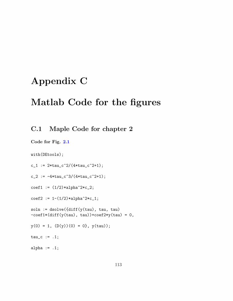
Appendix C

Matlab Code for the figures

C.1 Maple Code for chapter 2

Code for Fig. 2.1

with(DEtools);

c_1 := 2*tau_c^2/(4*tau_c^2+1);

c_2 := -4*tau_c^3/(4*tau_c^2+1);

coef1 := (1/2)*alpha^2*c_2;

coef2 := 1-(1/2)*alpha^2*c_1;

soln := dsolve({diff(y(tau), tau, tau)

-coef1*(diff(y(tau), tau))+coef2*y(tau) = 0,

y(0) = 1, (D(y))(0) = 0}, y(tau));

tau_c := .1;

alpha := .1;

113

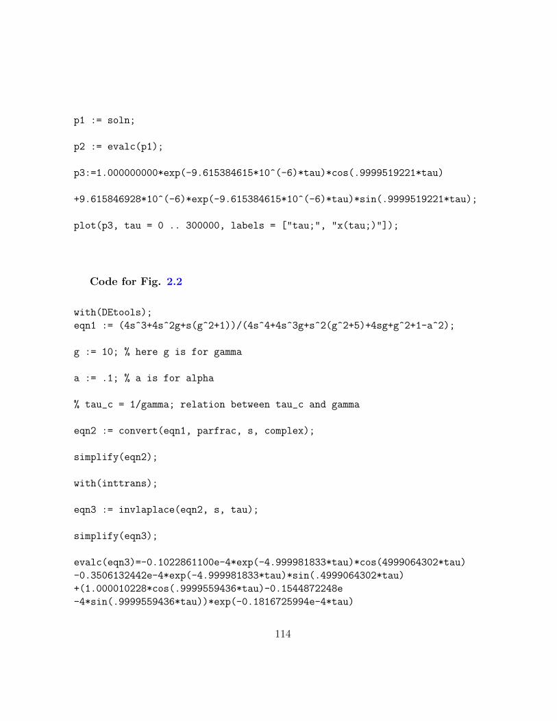
p1 := soln;

p2 := evalc(p1);

p3:=1.000000000*exp(-9.615384615*10^(-6)*tau)*cos(.9999519221*tau)

+9.615846928*10^(-6)*exp(-9.615384615*10^(-6)*tau)*sin(.9999519221*tau);

plot(p3, tau = 0 .. 300000, labels = ["tau;", "x(tau;)"]);

Code for Fig. 2.2

with(DEtools);

eqn1 := (4s^3+4s^2g+s(g^2+1))/(4s^4+4s^3g+s^2(g^2+5)+4sg+g^2+1-a^2);

g := 10; % here g is for gamma

a := .1; % a is for alpha

% tau_c = 1/gamma; relation between tau_c and gamma

eqn2 := convert(eqn1, parfrac, s, complex);

simplify(eqn2);

with(inttrans);

eqn3 := invlaplace(eqn2, s, tau);

simplify(eqn3);

evalc(eqn3)=-0.1022861100e-4*exp(-4.999981833*tau)*cos(4999064302*tau)

-0.3506132442e-4*exp(-4.999981833*tau)*sin(.4999064302*tau)

+(1.000010228*cos(.9999559436*tau)-0.1544872248e

-4*sin(.9999559436*tau))*exp(-0.1816725994e-4*tau)

114

+I*(3.801992999*10^(-17)*cos(.9999559436*tau)

-1.*10^(-31)*sin(.9999559436*tau))*exp(-0.1816725994e-4*tau)

eqn4:=-0.1022861100e-4*exp(-4.999981833*tau)*cos(4999064302*tau)

-0.3506132442e-4*exp(-4.999981833*tau)*sin(.4999064302*tau)

+(1.000010228*cos(.9999559436*tau)

-0.1544872248e-4*sin(.9999559436*tau))*exp(-0.1816725994e-4*tau)

plot(eqn4, tau = 0 .. 200000, labels = ["tau;", "y(tau;)"]);

C.2 Matlab Code for chapter 3

Matlab files for test case 1:

% This is the script file to run the numerical form of the model

% Time set-up for Acetaminophen for maximum dose 4000 mg

% We are checking the simulation by giving the maximum dose

% in every six hours time interval

dt=0.3; % dt=delta_t=time step

t=0:dt:6;% First Dose

tfull=[t,t+6,t+12,t+18];

iteration=5;%100000;

x_mat=zeros(length(tfull),iteration);

A_mat=zeros(length(tfull),iteration);

global tauC D

D = .2;

tauC = .01;

%Initial condition

dose=1000; % dose=x(0)=X_0

y0=[dose;0;0]; % A(0)=0, noise xi(0)=0

for i=1:iteration

[x1,xi1,A1]=Acetaminophen(t,y0);

115

[x2,xi2,A2]=Acetaminophen(t+6,[x1(end)+dose,xi1(end),A1(end)]);

[x3,xi3,A3]=Acetaminophen(t+12,[x2(end)+dose,xi2(end),A2(end)]);

[x4,xi4,A4]=Acetaminophen(t+18,[x3(end)+dose,xi3(end),A3(end)]);

x_mat(:,i)=[x1’;x2’;x3’;x4’];

A_mat(:,i)=[A1’;A2’;A3’;A4’];

disp (i)

end

figure(1); hold on; plot(tfull,x_mat)

figure(2); hold on; plot(tfull,A_mat)

figure(3); hold on; plot(tfull,mean(x_mat,2)’,’Linewidth’,2)

figure(4); hold on; plot(tfull,mean(A_mat,2)’,’Linewidth’,2)

figure(5); hold on; e1 = errorbar(tfull,mean(x_mat,2)’,std(x_mat’)’);

figure(6); hold on; e2 = errorbar(tfull,mean(A_mat,2)’,std(A_mat’)’);

%%%%%%%%%%%%%%%%%%%%%%%%%%%%%%%%%%%%%%%%%%%%%%

%%%%%%%%%%%%%%%%%%%%%%%%%%%%%%%%%%%%%%%%%%%%%%

% The basic idea of the codes are taken from

% Dr. Mathew Scott’s lecture note AMATH 777

% http://www.math.uwaterloo.ca/~mscott/

%%%%%%%%%%%%%%%%%%%%%%%%%%%%%%%%%%%%%%%%%%%%%%

%%%%%%%%%%%%%%%%%%%%%%%%%%%%%%%%%%%%%%%%%%%%%%

function [x, xi, A]=Acetaminophen(tdom, y0)

% The syntax for this function is 777_jenny([tauC, D],

% [t_start, t_end])

% where tauC is the correlation time of the colored noise,

% D is the standard

% deviation of the noise, t_start is the initial time

% and t_end is the end time

global tauC

x=zeros(1,length(tdom));

xi=zeros(1,length(tdom));

A=zeros(1,length(tdom));

116

[t,y] = Eulers(@PKFun, [tdom(1),tdom(end)], y0, min(.01,tauC/10));

x = x+interp1(t,y(:,1),tdom);

xi = xi+interp1(t,y(:,2),tdom);

A = A+interp1(t,y(:,3),tdom);

end

%%%%%%%%%%%%%%%%%%%%%%%%%%%%%%%%%%%%%%%%%%%%%%%%%%

%%%%%%%%%%%%%%%%%%%%%%%%%%%%%%%%%%%%%%%%%%%%%%%%%%

function dy=PKFun(~,y,h)

% The vector right-hand sides of the differential equations

% dy(1) is the trajectory of the drug in the absorption site,

% dy(2) is the noise,

% and dy(3) is the drug in the systemic circulation

global tauC D

rho=exp(-h/tauC);

ke=.28; F=.89; ka=1.80*F; p=ke/ka;

% Random form of the model

dy(1)=-(1+y(2))*y(1);

dy(2)=1/h*((rho-1)*y(2)+(1-rho^2)^(1/2)*(D/(2*tauC))^(1/2)*randn);

dy(3)=(1+y(2))*y(1)-p*y(3);

end

%%%%%%%%%%%%%%%%%%%%%%%%%%%%%%%%%%%%%%%%%%%%%%%%%%%%%

%%%%%%%%%%%%%%%%%%%%%%%%%%%%%%%%%%%%%%%%%%%%%%%%%%%%%

function [tout, yout] = Eulers(FunFcn, tspan, y0, ssize)

% This function will integrate a system of ordinary

% differential equations using Euler’s method.

% INPUT:

% F - String containing name of user-supplied

% problem description.

% Call: yprime = fun(t,y) where F = ’fun’.

% t - Time (scalar).

% y - Solution vector.

% yprime - Returned derivative vector; yprime(i) = dy (i)/dt.

% tspan = [t0, tfinal], where t0 is the initial value of t,

% and tfinal is the final value of t.

117

% y0 - Initial value vector.

% ssize - The step size to be used.

%(Default: ssize = (tfinal - t0)/100).

%

% OUTPUT:

% t - Returned integration time points (column-vector).

% y - Returned solution, one solution row-vector per tout-value.

% Initialization

t0=tspan(1);

tfinal=tspan(2);

pm = sign(tfinal - t0); % Which way are we computing?

if (nargin < 4), ssize = abs (tfinal - t0)/1000; end

if ssize < 0, ssize = -ssize; end

h = pm*ssize;

t = t0;

y = y0(:);

% To compute the number of steps.

dt = abs(tfinal - t0);

N = floor(dt/ssize) + 1;

if (N-1)*ssize < dt

N = N + 1;

end

% Initialize the output.

tout = zeros(N,1);

tout(1) = t;

yout = zeros(N,size(y,1));

yout(1,:) = y.’;

k = 1;

% The main loop

while k < N

if pm*(t + h - tfinal) > 0

h = tfinal - t;

tout(k+1) = tfinal;

else

118

tout(k+1) = t0 +k*h;

end

k = k+1;

% Compute the slope

s1 = feval(FunFcn, t, y,ssize); s1 = s1(:); % s1=f(t(k),y(k))

y = y + h*s1; % y(k+1) = y(k) + h*f(t(k),y(k))

t = tout(k);

yout(k,:) = y.’;

end

end

%%%%%%%%%%%%%%%%%%%%%%%%%%%%%%%%%%%%%%%%%%%%%%%%%%%%%%%%%%

%%%%%%%%%%%%%%%%%%%%%%%%%%%%%%%%%%%%%%%%%%%%%%%%%%%%%%%%%%

% This is the script file is to evaluate Van Kampen’s

% mean and Variance along with the deterministic solution

%%

% Constants

DoseInterval = 6; tfinal= DoseInterval*4; h =.3;

t=0:h:6;% First Dose

t=[t,t+6,t+12,t+18];

dose = 1e3;

ke=.28; F=.89; ka=1.80*F; p=ke/ka; % p is rho in the writing

alpha=.3; tauc=.01;

Cond0 = alpha^2*tauc

Cond1 = 3*(p + 1)/5

Cond2 = (3*p^3+13*p^2+13*p+3)/(22*p^2 + 44*p + 14)

Cond0 < Cond1

Cond0 < Cond2

%% First portion is the solution of the coupled DE

% Deterministic form of the model

fx=@(t,x) (-x);

fA=@(t,x,A)(x-p*A);

%%%Set initial conditions

N = length(t);

A = zeros(N,1);

x = zeros(N,1); x(1)=dose;

for i=2:N

119

if(t(i) == t(i-1))

x(i) = x(i-1) + dose;

A(i) = A(i-1);

else

% Update x, A

K1x=fx(t(i-1), x(i-1) );

K1A=fA(t(i-1) ,x(i-1) ,A(i-1));

K2x=fx(t(i-1)+h/2 ,x(i-1)+h/2*K1x);

K2A=fA(t(i-1)+h/2 ,x(i-1)+h/2*K1x ,A(i-1)+h/2*K1A);

K3x=fx(t(i-1)+h/2 , x(i-1)+h/2*K2x);

K3A=fA(t(i-1)+h/2 ,x(i-1)+h/2*K2x ,A(i-1)+h/2*K2A);

K4x=fx(t(i-1)+h , x(i-1)+h*K3x);

K4A=fA(t(i-1)+h ,x(i-1)+h*K3x ,A(i-1)+h*K3A);

%

x(i)=x(i-1)+(h/6)*(K1x +2*K2x +2*K3x +K4x);

A(i)=A(i-1)+(h/6)*(K1A +2*K2A +2*K3A +K4A);

end

end

% Deterministic solution

figure (3); hold on ; plot(t,x,’b:’,’LineWidth’,2)

figure (4); hold on; plot(t,A,’b:’,’LineWidth’,2)

%% Script file to evaluate <x>, <A>, <AX>, <AA> and <XX>

x = zeros(N,1); x(1) = dose;

A = zeros(N,1); A(1) = 0;

Ax = zeros(N,1); Ax(1) = A(1)*dose;

xx = zeros(N,1); xx(1) = dose^2;

AA = zeros(N,1); AA(1) = 0;

%Function handle for mean

fx=@(t,x) (-(1-alpha^2*tauc)*x);

fA=@(t,x,A) ((1-alpha^2*tauc)*x-p*A);

% These are the coefficients for the second moment

coef1=tauc*alpha^2 - p - 1;

coef2=2*tauc*alpha^2 + 2;

=((3*tauc - 2*p*tauc + (p*tauc)/(tauc*(p - 1) ...

+ 1))*alpha^2)/(p - 1) + 1;

coef4=-(alpha^2*(2*tauc - (2*p*tauc)/(tauc*(p - 1) ...

120

+ 1)))/(p - 1);

coef5=4*tauc*alpha^2 - 2;

%Function Handle for second moemnt

fAx=@(t,Ax,xx)(coef1*Ax+coef3*xx);

fAA=@(t,Ax,AA,xx) (coef2*Ax-2*p*AA+coef4*xx);

fxx=@(t, xx) (coef5*xx);

% Loop to use for multiple dosage

for i=2:N

if(t(i) == t(i-1))

x(i) = x(i-1) + dose;

xx(i) = xx(i-1) + dose^2 + 2*(x(i-1))*dose;

Ax(i) = Ax(i-1) + A(i-1)*dose;

A(i) = A(i-1);

AA(i) = AA(i-1);

else

% Update x, A, Ax, AA, xx

K1x=fx(t(i-1), x(i-1));

K1A=fA(t(i-1), x(i-1), A(i-1));

K1Ax=fAx(t(i-1), Ax(i-1), xx(i-1));

K1AA=fAA(t(i-1), Ax(i-1), AA(i-1), xx(i-1));

K1xx=fxx(t(i-1), xx(i-1));

K2x=fx(t(i-1)+h/2, x(i-1)+h/2*K1x);

K2A=fA(t(i-1)+h/2, x(i-1)+h/2*K1x, A(i-1)+h/2*K1A);

K2Ax=fAx(t(i-1)+h/2, Ax(i-1)+h/2*K1Ax, xx(i-1)+h/2*K1xx);

K2AA=fAA(t(i-1)+h/2, Ax(i-1)+h/2*K1Ax, AA(i-1)+h/2*K1AA, ...

xx(i-1)+h/2*K1xx);

K2xx=fxx(t(i-1)+h/2, xx(i-1)+h/2*K1xx);

K3x=fx(t(i-1)+h/2, x(i-1)+h/2*K2x);

K3A=fA(t(i-1)+h/2, x(i-1)+h/2*K2x, A(i-1)+h/2*K2A);

K3Ax=fAx(t(i-1)+h/2, Ax(i-1)+h/2*K2Ax, xx(i-1)+h/2*K2xx);

K3AA=fAA(t(i-1)+h/2, Ax(i-1)+h/2*K2Ax, AA(i-1)+h/2*K2AA, ...

xx(i-1)+h/2*K2xx);

K3xx=fxx(t(i-1)+h/2, xx(i-1)+h/2*K2xx);

K4x=fx(t(i-1)+h, x(i-1)+h*K3x);

K4A=fA(t(i-1)+h, x(i-1)+h*K3x , A(i-1)+h*K3A);

K4Ax=fAx(t(i-1)+h, Ax(i-1)+h*K3Ax, xx(i-1)+h*K3xx);

121

K4AA=fAA(t(i-1)+h, Ax(i-1)+h*K3Ax, AA(i-1)+h*K3AA, ...

xx(i-1)+h*K3xx);

K4xx=fxx(t(i-1)+h, xx(i-1)+h*K3xx);

x(i)=x(i-1)+(h/6)*(K1x +2*K2x +2*K3x +K4x);

A(i)=A(i-1)+(h/6)*(K1A +2*K2A +2*K3A +K4A);

Ax(i)=Ax(i-1)+(h/6)*(K1Ax +2*K2Ax +2*K3Ax +K4Ax);

AA(i)=AA(i-1)+(h/6)*(K1AA +2*K2AA +2*K3AA +K4AA);

xx(i)=xx(i-1)+(h/6)*(K1xx +2*K2xx +2*K3xx +K4xx);

end

end

varx=(xx-(x).^2);

varA=(AA-(A).^2);

EnvelopxPlus = x+sqrt(varx);

EnvelopxMinus = x-sqrt(varx);

EnvelopAPlus = A+sqrt(varA);

EnvelopAMinus = A-sqrt(varA);

figure(5);hold on

plot(t,x,’k--’,’LineWidth’,2)

plot(t,EnvelopxPlus ,’m--’,’LineWidth’,2)

plot(t,EnvelopxMinus ,’m--’,’LineWidth’,2)

figure(6);hold on

plot(t,A’,’k--’,’LineWidth’,2)

plot(t,EnvelopAPlus ,’m--’,’LineWidth’,2)

plot(t,EnvelopAMinus,’m--’, ’LineWidth’,2 )

%%%%%%%%%%%%%%%%%%%%%%%%%%%%%%%%%%%%%%%%%

%%%%%%%%%%%%%%%%%%%%%%%%%%%%%%%%%%%%%%%%%

Matlab files for test case 2:

% This code is to solve the Random form of the model

% for the data of subject # 1 of the drug Theophyline

122

ka=2.062927706; dt=0.25; t=0:dt:24*ka;

x_mat=zeros(length(t),iteration);

A_mat=zeros(length(t),iteration);

%Initial condition

Amount=4.02; Weight=79.6; dose=Amount*Weight;

y0=[dose;0;0];

global tauC D

D = .2;

tauC = .01;

% How many times I want to run the simulation

iteration=10000;

for i=1:iteration

[x,xi,A]=Theophyline(t,y0);

A_mat(:,i)=A’;

disp (i)

end

figure(1); hold on;

plot(t,A_mat’/dose,’Linewidth’,2)

figure(1); hold on;

plot(t,mean(A_mat’)’/dose,’k:’,’Linewidth’,2)

figure(1); hold on;

e2 = errorbar(t,mean(A_mat’)’/dose,std(A_mat’)’/dose);

%%%%%%%%%%%%%%%%%%%%%%%%%%%%%%%%%%%%%%%%%%%%%%%%%%%%%%%

%%%%%%%%%%%%%%%%%%%%%%%%%%%%%%%%%%%%%%%%%%%%%%%%%%%%%%%

function [x, xi, A]=Theophyline(tdom, y0)

% tauC is the correlation time of the colored noise,

% D is the standard deviation of the noise,

% tdom(1) is the initial time and tdom(2) is the end time

global tauC

x=zeros(1,length(tdom));

xi=zeros(1,length(tdom));

A=zeros(1,length(tdom));

[t,y] = Euler(@TheoFun, [tdom(1),tdom(end)], ...

y0, min(.01,tauC/10));

x = x+interp1(t,y(:,1),tdom);

123

xi = xi+interp1(t,y(:,2),tdom);

A = A+interp1(t,y(:,3),tdom);

end

%%%%%%%%%%%%%%%%%%%%%%%%%%%%%%%%%%%%%%%%%%%%%%

%%%%%%%%%%%%%%%%%%%%%%%%%%%%%%%%%%%%%%%%%%%%%%

function dy=TheoFun(~,y,h)

global tauC D

rho=exp(-h/tauC);

ke= 0.058333529; ka=2.062927706; p=ke/ka;

dy(1)=-(1+y(2))*y(1);

dy(2)=1/h*((rho-1)*y(2)+(1-rho^2)^(1/2)*(D/(2*tauC))^(1/2)*randn);

dy(3)=(1+y(2))*y(1)-p*y(3);

end

%%%%%%%%%%%%%%%%%%%%%%%%%%%%%%%%%%%%%%%%%%%%%%%%%%%%%%%%%%%%%

%%%%%%%%%%%%%%%%%%%%%%%%%%%%%%%%%%%%%%%%%%%%%%%%%%%%%%%%%%%%%

%%

% This is the script file for comapre the theophyline

% Subject # 1 data with the deterministic equation,

% Van Kampan Mean and Variance

ke= 0.058333529; Intercept=1.067449981;

AI=10^(Intercept); ka=2.062927706; p=ke/ka;

Amount=4.02;% mg/kg

Weight=79.6; %kg

dose=Amount*Weight; %mg

F=1;% Bioavalability aproximately 1

V=(ka*F*dose)/(AI*(ka-ke));

alpha=.2; tc=.01; tauc=.01;

%%

% Data for Subject # 1

t_exp1=[0 0.25 0.57 1.12 2.02 3.82 5.1 7.03 9.05 12.12 24.37 ];

C_exp1=[0.74 2.84 6.57 10.5 9.66 8.58 8.36 7.47 6.89 5.94 3.28 ];

figure (1)% FOr the data

plot(t_exp1*ka,C_exp1.*V/dose,’r*’,’linewidth’,2)

hold on

%%

124

% Time steps and initial conditions

x(1)=dose; A(1)=0; tfinal=24*ka; h = .25; t =0:h:tfinal;

xx(1)=dose^2; AA(1)=0; Ax(1)=0;

N=ceil(tfinal/h);

%% Deterministic form

fx=@(t,x) (-x);

fA=@(t,x,A) (x-p*A);

for i=1:N

% update time

t(i+1)=t(i)+h;

% Update x, A

K1x=fx(t(i), x(i) );

K1A=fA(t(i) ,x(i) ,A(i));

K2x=fx(t(i)+h/2 ,x(i)+h/2*K1x);

K2A=fA(t(i)+h/2 ,x(i)+h/2*K1x ,A(i)+h/2*K1A);

K3x=fx(t(i)+h/2 , x(i)+h/2*K2x);

K3A=fA(t(i)+h/2 ,x(i)+h/2*K2x ,A(i)+h/2*K2A);

K4x=fx(t(i)+h , x(i)+h*K3x);

K4A=fA(t(i)+h ,x(i)+h*K3x ,A(i)+h*K3A);

x(i+1)=x(i)+(h/6)*(K1x +2*K2x +2*K3x +K4x);

A(i+1)=A(i)+(h/6)*(K1A +2*K2A +2*K3A +K4A);

end

figure (1)

plot(t,A/dose,’y:’,’LineWidth’,2)

hold on

%%

% Van Kampen equations for first and second moments:

% By using Runge Kutta method

% Function handle for the mean

fx=@(t,x) (-(1-alpha^2*tc)*x);

fA=@(t,x,A) ((1-alpha^2*tc)*x-p*A);

% These are the coefficients for the second moment

125

coef1=tauc*alpha^2 - p - 1;

coef2=2*tauc*alpha^2 + 2;

coef3=((3*tauc - 2*p*tauc + (p*tauc)/(tauc*(p - 1) + 1)) ...

*alpha^2)/(p - 1) + 1;

coef4=-(alpha^2*(2*tauc - (2*p*tauc)/(tauc*(p - 1) ...

+ 1)))/(p - 1);

coef5=4*tauc*alpha^2 - 2;

%Function Handle for second moemnt

fAx=@(t,Ax,xx)(coef1*Ax+coef3*xx);

fAA=@(t,Ax,AA,xx) (coef2*Ax-2*p*AA+coef4*xx);

fxx=@(t, xx) (coef5*xx);

for i=1:N

% update time

t(i+1)=t(i)+h;

% Update x, A, Ax, AA, xx

K1x=fx(t(i), x(i) );

K1A=fA(t(i) ,x(i) ,A(i));

K1Ax=fAx(t(i), Ax(i), xx(i) );

K1AA=fAA(t(i) ,Ax(i) ,AA(i), xx(i));

K1xx=fxx(t(i), xx(i));

%

K2x=fx(t(i)+h/2 ,x(i)+h/2*K1x);

K2A=fA(t(i)+h/2 ,x(i)+h/2*K1x ,A(i)+h/2*K1A);

K2Ax=fAx(t(i)+h/2 ,Ax(i)+h/2*K1Ax, xx(i)+h/2*K1xx);

K2AA=fAA(t(i)+h/2 ,Ax(i)+h/2*K1Ax, ...

AA(i)+h/2*K1AA, xx(i)+h/2*K1xx);

K2xx=fxx(t(i)+h/2, xx(i)+h/2*K1xx);

%

K3x=fx(t(i)+h/2 , x(i)+h/2*K2x);

K3A=fA(t(i)+h/2 ,x(i)+h/2*K2x ,A(i)+h/2*K2A);

K3Ax=fAx(t(i)+h/2 ,Ax(i)+h/2*K2Ax, xx(i)+h/2*K2xx);

K3AA=fAA(t(i)+h/2 ,Ax(i)+h/2*K2Ax ,AA(i)+h/2*K2AA, ...

xx(i)+h/2*K2xx);

K3xx=fxx(t(i)+h/2, xx(i)+h/2*K2xx);

%

K4x=fx(t(i)+h , x(i)+h*K3x);

K4A=fA(t(i)+h ,x(i)+h*K3x , A(i)+h*K3A);

126

K4Ax=fAx(t(i)+h ,Ax(i)+h*K3Ax, xx(i)+h*K3xx);

K4AA=fAA(t(i)+h ,Ax(i)+h*K3Ax , AA(i)+h*K3AA, ...

xx(i)+h*K3xx);

K4xx=fxx(t(i)+h, xx(i)+h*K3xx);

%

x(i+1)=x(i)+(h/6)*(K1x +2*K2x +2*K3x +K4x);

A(i+1)=A(i)+(h/6)*(K1A +2*K2A +2*K3A +K4A);

Ax(i+1)=Ax(i)+(h/6)*(K1Ax +2*K2Ax +2*K3Ax +K4Ax);

AA(i+1)=AA(i)+(h/6)*(K1AA +2*K2AA +2*K3AA +K4AA);

xx(i+1)=xx(i)+(h/6)*(K1xx +2*K2xx +2*K3xx +K4xx);

end

figure (1)% for plot the mean

plot(t,A/dose,’b:’,’LineWidth’,2)

hold on

% Definition of the variance

varA=(AA-(A).^2);

EnvelopAPlus = A+sqrt(varA);

EnvelopAMinus =A-sqrt(varA);

figure(1); %To plot the standard deviation of the mean

plot(t,EnvelopAPlus/dose,’m’,’LineWidth’,2)

plot(t,EnvelopAMinus/dose,’m’, ’LineWidth’,2 )

hold on

C.3 Mtalb code for Chapter 4

Matlab script file for figure 4.2

% These data are dizitized from Kearns et.al

Time_135=[0.909 1.939 2.848 3.333 3.636 4.061 5.03 6 8.97

15.091 24.182 ];

Cnc_135=[1.814 2.95 3.762 1.528 1.199 0.805 0.56 0.396 0.205

0.081 0.037];

127

Time_175=[1.152 1.939 2.091 3.091 3.333 3.576 4.061 5.03 6.061

9.152 14.97 24.061 ];

Cnc_175=[3.052 4.876 5.23 7.022 3.763 2.398 1.638 0.991 0.666

0.333 0.141 0.083 ];

Time_225=[0.97 1.939 3.091 3.333 3.576 3.636 3.939 5.273 6.061

9.152 14.97 24.061 ];

Cnc_225=[4.626 8.061 11.811 8.952 6.441 4.966 3.277 1.697 1.243

0.523 0.213 0.103 ];

% Plot for experimental data

figure (1)

subplot(3,1,1)

plot(Time_135,Cnc_135,’go:’,’LineWidth’,2)

hold on

figure (1)

subplot(3,1,2)

plot(Time_175,Cnc_175,’go:’,’LineWidth’,2)

hold on

figure (1)

subplot(3,1,3)

plot(Time_225,Cnc_225,’go:’,’LineWidth’,2)

hold on

%% kearns Three compartmental model for dose 135

infusion=3; dose=135;

% Optimum Parameters reported by Kearns et., al., for Kearns model

k21=.68; vdmax = 10.20;

vemax = 18.80; kdm=.32;

kem=5.50; vd=4;

k13=2.20; k31=.65;

gr = @(t,x)[(-vdmax*x(1))/(kdm+x(1)) ...

-(vemax*x(1))/(kem+x(1)) ...

-k13*x(1)+k31*x(3)+k21*x(2) ...

+(t<=infusion)*dose/(infusion*vd); ...

(vdmax*x(1))/(kdm+x(1))-k21*x(2); ...

k13*x(1)-k31*x(3)];

[t,yr] = ode45(@(t,x) gr(t,x),[0,Time_135],[0 0 0]);

figure (1)

128

subplot(3,1,1)

plot(t, yr(:,1),’r:’,’LineWidth’,2)

hold on

% Calculation for AIC and WRSS

WRSS_yr_135=sum((Cnc_135’-yr(2:end,1)).^2./Cnc_135’.^2);

Number_Of_obs_135=11;

Number_Of_par_MR=8;

AIC_MR_135=(Number_Of_obs_135)*(log(WRSS_yr_135)) ...

+(2*Number_Of_par_MR);

%% kearns Three compartmental model for dose 175

dose=175;

gr = @(t,x)[(-vdmax*x(1))/(kdm+x(1)) ...

-(vemax*x(1))/(kem+x(1))-k13*x(1) ...

+k31*x(3)+k21*x(2)+(t<=infusion)*dose/(infusion*vd); ...

(vdmax*x(1))/(kdm+x(1))-k21*x(2); ...

k13*x(1)-k31*x(3)];

[t,yr] = ode45(@(t,x) gr(t,x),[0,Time_175],[0 0 0]);

figure (1)

subplot(3,1,2)

plot(t, yr(:,1),’r:’,’LineWidth’,2)

hold on

% Calculation for AIC and WRSS

WRSS_yr_175=sum((Cnc_175’-yr(2:end,1)).^2./Cnc_175’.^2);

Number_Of_obs_175=12;

Number_Of_par_MR=8;

AIC_MR_175=(Number_Of_obs_175)*(log(WRSS_yr_175)) ...

+(2*Number_Of_par_MR);

%% kearns Three compartmental model for dose 225

dose = 225;

gr = @(t,x)[(-vdmax*x(1))/(kdm+x(1)) ...

-(vemax*x(1))/(kem+x(1)) ...

-k13*x(1)+k31*x(3)+k21*x(2) ...

+(t<=infusion)*dose/(infusion*vd); ...

(vdmax*x(1))/(kdm+x(1))-k21*x(2); ...

k13*x(1)-k31*x(3)];

[t,yr] = ode45(@(t,x) gr(t,x),[0,Time_225],[0 0 0]);

129

figure (1)

subplot(3,1,3)

plot(t, yr(:,1),’r:’,’LineWidth’,2)

hold on

% Calculation for AIC and WRSS

WRSS_yr_225=sum((Cnc_225’-yr(2:end,1)).^2./Cnc_225’.^2);

Number_Of_obs_225=12;

Number_Of_par_MR=8;

AIC_MR_225=(Number_Of_obs_225)*(log(WRSS_yr_225)) ...

+(2*Number_Of_par_MR);

%% Fractal Two Compartmental model for dose 135

dose=135;

% Optimum Parameters evaluated by GA for Fractal model

k21= 1.9727 ; vdmax = 12.3198 ;

vemax = 13.4051; kdm= 1.6703;

kem=6.3906; vd= 4.9185;

p=1.2019 ; q=1.7010;

k13=0; k31=0;

gf = @(t,x)[(-vdmax*(x(1).^p))/(kdm+(x(1).^p))- ...

(vemax*(x(1).^q))/(kem+(x(1).^q)) ...

-k13*x(1)+k31*x(3)+k21*x(2) ...

+(t<=infusion)*dose/(infusion*vd); ...

(vdmax*(x(1).^p))/(kdm+(x(1).^p))-k21*x(2); ...

k13*x(1)-k31*x(3)];

[t,yf] = ode45(@(t,x) gf(t,x),[0,Time_135],[0 0 0]);

figure (1)

subplot(3,1,1)

plot(t, yf(:,1),’b:’,’LineWidth’,2)

hold on

% Calculation for AIC and WRSS

WRSS_yf_135=sum((Cnc_135’-yf(2:end,1)).^2./Cnc_135’.^2);

Number_Of_obs_135=11;

Number_Of_par_MF=8;

130

AIC_MF_135=Number_Of_obs_135*log(WRSS_yf_135) ...

+2*Number_Of_par_MF;

%% Fractal Two Compartmental model for dose 175

dose=175;

gf = @(t,x)[(-vdmax*(x(1).^p))/(kdm+(x(1).^p)) ...

-(vemax*(x(1).^q))/(kem+(x(1).^q)) ...

-k13*x(1)+k31*x(3)+k21*x(2)...

+(t<=infusion)*dose/(infusion*vd); ...

(vdmax*(x(1).^p))/(kdm+(x(1).^p))-k21*x(2); ...

k13*x(1)-k31*x(3)];

[t,yf] = ode45(@(t,x) gf(t,x),[0,Time_175],[0 0 0]);

figure (1)

subplot(3,1,2)

plot(t, yf(:,1),’b:’,’LineWidth’,2)

hold on

% Calculation for AIC and WRSS

WRSS_yf_175=sum((Cnc_175’-yf(2:end,1)).^2./Cnc_175’.^2);

Number_Of_obs_175=12;

Number_Of_par_MF=8;

AIC_MF_175=(Number_Of_obs_175)*(log(WRSS_yf_175))...

+(2*Number_Of_par_MF);

%% Fractal Two Compartmental model for dose 225

dose=225;

gf = @(t,x)[(-vdmax*(x(1).^p))/(kdm+(x(1).^p)) ...

-(vemax*(x(1).^q))/(kem+(x(1).^q)) ...

-k13*x(1)+k31*x(3)+k21*x(2) ...

+(t<=infusion)*dose/(infusion*vd); ...

(vdmax*(x(1).^p))/(kdm+(x(1).^p))-k21*x(2); ...

k13*x(1)-k31*x(3)];

[t,yf] = ode45(@(t,x) gf(t,x),[0,Time_225],[0 0 0]);

figure (1)

subplot(3,1,3)

plot(t, yf(:,1),’b:’,’LineWidth’,2)

hold on

% Calculation for AIC and WRSS

WRSS_yf_225=sum((Cnc_225’-yf(2:end,1)).^2./Cnc_225’.^2);

131

Number_Of_obs_225=12;

Number_Of_par_MF=8;

AIC_MF_225=(Number_Of_obs_225)*(log(WRSS_yf_225)) ...

+(2*Number_Of_par_MF);

Matlab script file for figure 4.3

% These are digitized directly from VZ

Time_135=[0.85 2.065 2.854 3.279 3.522 4.008 4.858 6.984 10.87

12.996 22.955 ];

Cnc_135=[1.338 2.015 2.931 1.59 0.923 0.594 0.328 0.194 0.095

0.078 0.032 ];

Time_175=[0.85 1.943 2.794 3.158 3.401 4.008 4.98 6.923 11.053

12.996 22.955 ];

Cnc_175=[2.012 3.298 4.638 3.982 2.018 1.213 0.807 0.396 0.195

0.141 0.054 ];

Time_225=[0.85 1.943 3.097 3.887 5.04 6.923 11.053 13.057

22.955 ];

Cnc_225=[2.732 4.713 7.096 1.762 1.256 0.66 0.298 0.22

0.084 ];

% Plot for experimental data

figure (2)

subplot(3,1,1)

plot(Time_135,Cnc_135,’ko:’,’LineWidth’,2)

hold on

figure (2)

subplot(3,1,2)

plot(Time_175,Cnc_175,’ko:’,’LineWidth’,2)

hold on

figure (2)

subplot(3,1,3)

plot(Time_225,Cnc_225,’ko:’,’LineWidth’,2)

hold on

%% kearns Three compartmental model for dose 135

dose =135; infusion=3;

% Optimum Parameters evaluated by GA for Kearns model

132

k21=0.474533333; vdmax=8.297633333;

vemax=22.49566667; kdm=6.160566667;

kem=14.5877; vd=9.526266667;

k13=1.4423; k31=16.63193333;

gr = @(t,x)[(-vdmax*x(1))/(kdm+x(1)) ...

-(vemax*x(1))/(kem+x(1))-k13*x(1)+k31*x(3) ...

+k21*x(2)+(t<=infusion)*dose/(infusion*vd); ...

(vdmax*x(1))/(kdm+x(1))-k21*x(2); ...

k13*x(1)-k31*x(3)];

[t,yr] = ode45(@(t,x) gr(t,x),[0,Time_135],[0 0 0]);

figure (2)

subplot(3,1,1)

plot(t, yr(:,1),’r:’,’LineWidth’,2)

hold on

% Calculation for WRSS and AIC

WRSS_yr_135=sum((Cnc_135’-yr(2:end,1)).^2./Cnc_135’.^2);

Number_Of_obs_135=11;

Number_Of_par_MR=8;

AIC_MR_135=(Number_Of_obs_135)*(log(WRSS_yr_135))...

+(2*Number_Of_par_MR);

%% kearns Three compartmental model for dose 175

dose=175;

gr = @(t,x)[(-vdmax*x(1))/(kdm+x(1)) ...

-(vemax*x(1))/(kem+x(1))-k13*x(1)+k31*x(3) ...

+k21*x(2)+(t<=infusion)*dose/(infusion*vd); ...

(vdmax*x(1))/(kdm+x(1))-k21*x(2); ...

k13*x(1)-k31*x(3)];

[t,yr] = ode45(@(t,x) gr(t,x),[0,Time_175],[0 0 0]);

figure (2)

subplot(3,1,2)

plot(t, yr(:,1),’r:’,’LineWidth’,2)

hold on

% Calculation for WRSS and AIC

WRSS_yr_175=sum((Cnc_175’-yr(2:end,1)).^2./Cnc_175’.^2);

Number_Of_obs_175=11;

Number_Of_par_MR=8;

133

AIC_MR_175=(Number_Of_obs_175)*(log(WRSS_yr_175)) ...

+(2*Number_Of_par_MR);

%% kearns Three compartmental model for dose 225

dose=225;

gr = @(t,x)[(-vdmax*x(1))/(kdm+x(1)) ...

-(vemax*x(1))/(kem+x(1))-k13*x(1) ...

+k31*x(3)+k21*x(2)+(t<=infusion)*dose/(infusion*vd); ...

(vdmax*x(1))/(kdm+x(1))-k21*x(2); ...

k13*x(1)-k31*x(3)];

[t,yr] = ode45(@(t,x) gr(t,x),[0,Time_225],[0 0 0]);

figure (2)

subplot(3,1,3)

plot(t, yr(:,1),’r:’,’LineWidth’,2)

hold on

% Calculation for WRSS and AIC

WRSS_yr_225=sum((Cnc_225’-yr(2:end,1)).^2./Cnc_225’.^2);

Number_Of_obs_225=9;

Number_Of_par_MR=8;

AIC_MR_225=(Number_Of_obs_225)*(log(WRSS_yr_225)) ...

+(2*Number_Of_par_MR);

%% Fractal Two Compartmental model for dose 135

dose=135;

k21=0.2043 ; vdmax=9.3617;

vemax=17.3286; kdm=3.7843;

kem=11.8432 ; vd= 9.4833 ;

p=0.8972 ; q=0.6474;

gf = @(t,x)[(-vdmax*(x(1).^p))/(kdm+(x(1).^p)) ...

-(vemax*(x(1).^q))/(kem+(x(1).^q))-k13*x(1) ...

+k31*x(3)+k21*x(2)+(t<=infusion)*dose/(infusion*vd); ...

(vdmax*(x(1).^p))/(kdm+(x(1).^p))-k21*x(2); ...

k13*x(1)-k31*x(3)];

[t,yf] = ode45(@(t,x) gf(t,x),[0,Time_135],[0 0 0]);

figure (2)

subplot(3,1,1)

plot(t, yf(:,1),’b:’,’LineWidth’,2)

134

hold on

% Calculation for WRSS and AIC

WRSS_yf_135=sum((Cnc_135’-yf(2:end,1)).^2./Cnc_135’.^2);

Number_Of_obs_135=11;

Number_Of_par_MF=8;

AIC_MF_135=Number_Of_obs_135*log(WRSS_yf_135) ...

+2*Number_Of_par_MF;

%% Fractal Two Compartmental model for dose 175

dose=175;

gf = @(t,x)[(-vdmax*(x(1).^p))/(kdm+(x(1).^p)) ...

-(vemax*(x(1).^q))/(kem+(x(1).^q)) ...

-k13*x(1)+k31*x(3)+k21*x(2) ...

+(t<=infusion)*dose/(infusion*vd); ...

(vdmax*(x(1).^p))/(kdm+(x(1).^p))-k21*x(2); ...

k13*x(1)-k31*x(3)];

[t,yf] = ode45(@(t,x) gf(t,x),[0 Time_175],[0 0 0]);

figure (2)

subplot(3,1,2)

plot(t, yf(:,1),’b:’,’LineWidth’,2)

hold on

% Calculation for WRSS and AIC

WRSS_yf_175=sum((Cnc_175’-yf(2:end,1)).^2./Cnc_175’.^2);

Number_Of_obs_175=11;

Number_Of_par_MF=8;

AIC_MF_175=(Number_Of_obs_175)*(log(WRSS_yf_175)) ...

+(2*Number_Of_par_MF);

%% Fractal Two Compartmental model for dose 225

dose=225;

gf = @(t,x)[(-vdmax*(x(1).^p))/(kdm+(x(1).^p)) ...

-(vemax*(x(1).^q))/(kem+(x(1).^q)) ...

-k13*x(1)+k31*x(3)+k21*x(2) ...

+(t<=infusion)*dose/(infusion*vd); ...

(vdmax*(x(1).^p))/(kdm+(x(1).^p))-k21*x(2); ...

k13*x(1)-k31*x(3)];

[t,yf] = ode45(@(t,x) gf(t,x),[0 Time_225],[0 0 0]);

135

figure (2)

subplot(3,1,3)

plot(t, yf(:,1),’b:’,’LineWidth’,2)

hold on

% Calculation for WRSS and AIC

WRSS_yf_225=sum((Cnc_225’-yf(2:end,1)).^2./Cnc_225’.^2);

Number_Of_obs_225=9;

Number_Of_par_MF=8;

AIC_MF_225=(Number_Of_obs_225)*(log(WRSS_yf_225)) ...

+(2*Number_Of_par_MF);

Matlab script file for figure 4.4:

% This data are dizitized from Brown et.al

Time_175=[3.11 6.31 6.32 6.66 7.14 7.54 8.22 9.09 10.2

12.3 14.3 ];

Cnc_175=[1.45 2.24 1.14 0.729 0.53 0.37 0.318 0.222 0.13

0.0964 0.0629 ];

Time_250=[3.1 6.3 6.57 6.84 7.11 7.52 7.92 8.46 9.81 10.7

12.6 15.2 18.9 ];

Cnc_250=[2.46 3.97 3.43 3.01 1.85 1.47 1.18 0.808 0.506 0.409

0.303 0.174 0.0913 ];

Time_275=[3.168 6.41 6.464 6.468 6.924 7.44 7.968 8.491 9.287

10.352 12.338 14.595 18.315 30.026 ];

Cnc_275=[3.398 8.747 6.217 6.916 5.122 3.197 2.69 2.034 1.746

1.596 0.99 0.697 0.411 0.129 ];

% Plot for experimental data

figure (3)

subplot(3,1,1)

plot(Time_175,Cnc_175,’mo:’,’LineWidth’,2)

hold on

136

figure (3)

subplot(3,1,2)

plot(Time_250,Cnc_250,’mo:’,’LineWidth’,2)

hold on

figure (3)

subplot(3,1,3)

plot(Time_275,Cnc_275,’mo:’,’LineWidth’,2)

hold on

%% kearns Three compartmental model for dose 175

infusion=6; dose=175;

% Optimum Parameters evaluated by GA for Kearns model

k21=1.295266; vdmax = 14.72393;

vemax =14.465566; kdm=7.67703;

kem=7.7655; vd=7.157733;

k13=10.235866; k31=13.187833;

gr = @(t,x)[(-vdmax*x(1))/(kdm+x(1)) ...

-(vemax*x(1))/(kem+x(1))-k13*x(1) ...

+k31*x(3)+k21*x(2) ...

+(t<=infusion)*dose/(infusion*vd); ...

(vdmax*x(1))/(kdm+x(1))-k21*x(2); ...

k13*x(1)-k31*x(3)];

[t,yr] = ode45(@(t,x) gr(t,x),[0,Time_175],[0 0 0]);

figure (3)

subplot(3,1,1)

plot(t, yr(:,1),’r:’,’LineWidth’,2)

hold on

% Calculation for WRSS and AIC

WRSS_yr_175=sum((Cnc_175’-yr(2:end,1)).^2./Cnc_175’.^2);

Number_Of_obs_175=11;

Number_Of_par_MR=8;

AIC_MR_175=(Number_Of_obs_175)*(log(WRSS_yr_175))...

+(2*Number_Of_par_MR);

%% kearns Three compartmental model for dose 250

dose=250;

137

gr = @(t,x)[(-vdmax*x(1))/(kdm+x(1)) ...

-(vemax*x(1))/(kem+x(1))-k13*x(1)+k31*x(3) ...

+k21*x(2)+(t<=infusion)*dose/(infusion*vd); ...

(vdmax*x(1))/(kdm+x(1))-k21*x(2); ...

k13*x(1)-k31*x(3)];

[t,yr] = ode45(@(t,x) gr(t,x),[0,Time_250],[0 0 0]);

figure (3)

subplot(3,1,2)

plot(t, yr(:,1),’r:’,’LineWidth’,2)

hold on

% Calculation for WRSS and AIC

WRSS_yr_250=sum((Cnc_250’-yr(2:end,1)).^2./Cnc_250’.^2);

Number_Of_obs_250=13;

Number_Of_par_MR=8;

AIC_MR_250=(Number_Of_obs_250)*(log(WRSS_yr_250))...

+(2*Number_Of_par_MR);

%% kearns Three compartmental model for dose 275

dose=275;

gr = @(t,x)[(-vdmax*x(1))/(kdm+x(1)) ...

-(vemax*x(1))/(kem+x(1)) ...

-k13*x(1)+k31*x(3)+k21*x(2) ...

+(t<=infusion)*dose/(infusion*vd); ...

(vdmax*x(1))/(kdm+x(1))-k21*x(2); ...

k13*x(1)-k31*x(3)];

[t,yr] = ode45(@(t,x) gr(t,x),[0,Time_275],[0 0 0]);

figure (3)

subplot(3,1,3)

plot(t, yr(:,1),’r:’,’LineWidth’,2)

hold on

% Calculation for WRSS and AIC

WRSS_yr_275=sum((Cnc_275’-yr(2:end,1)).^2./Cnc_275’.^2);

Number_Of_obs_275=14;

Number_Of_par_MR=8;

AIC_MR_275=(Number_Of_obs_275)*(log(WRSS_yr_275)) ...

+(2*Number_Of_par_MR);

%% Fractal Two Compartmental model for dose 175

138

dose=175;

% Optimum Parameters evaluated by GA for Fractal model

k21=2.7243; vdmax = 15.3931;

vemax = 3.3773; kdm=2.2279 ;

kem=0.2860; vd=8.4541;

p=2.0532; q=2.7943;

k13=0; k31=0;

gf = @(t,x)[(-vdmax*(x(1).^p))/(kdm+(x(1).^p)) ...

-(vemax*(x(1).^q))/(kem+(x(1).^q)) ...

-k13*x(1)+k31*x(3)+k21*x(2) ...

+(t<=infusion)*dose/(infusion*vd); ...

(vdmax*(x(1).^p))/(kdm+(x(1).^p))-k21*x(2); ...

k13*x(1)-k31*x(3)];

[t,yf] = ode45(@(t,x) gf(t,x),[0,Time_175],[0 0 0]);

figure (3)

subplot(3,1,1)

plot(t, yf(:,1),’b:’,’LineWidth’,2)

hold on

% Calculation for WRSS and AIC

WRSS_yf_175=sum(((Cnc_175’-yf(2:end,1)).^2)./Cnc_175’.^2);

Number_Of_obs_175=11;

Number_Of_par_MF=8;

AIC_MF_175=(Number_Of_obs_175)*(log(WRSS_yf_175)) ...

+(2*Number_Of_par_MF);

%% Fractal Two Compartmental model for dose 250

dose=250;

gf = @(t,x)[(-vdmax*(x(1).^p))/(kdm+(x(1).^p)) ...

-(vemax*(x(1).^q))/(kem+(x(1).^q)) ...

-k13*x(1)+k31*x(3)+k21*x(2) ...

+(t<=infusion)*dose/(infusion*vd); ...

(vdmax*(x(1).^p))/(kdm+(x(1).^p))-k21*x(2); ...

k13*x(1)-k31*x(3)];

[t,yf] = ode45(@(t,x) gf(t,x),[0,Time_250],[0 0 0]);

figure (3)

subplot(3,1,2)

plot(t, yf(:,1),’b:’,’LineWidth’,2)

hold on

139

% Calculation for WRSS and AIC

WRSS_yf_250=sum((Cnc_250’-yf(2:end,1)).^2./Cnc_250’.^2);

Number_Of_obs_250=12;

Number_Of_par_MF=8;

AIC_MF_250=(Number_Of_obs_250)*(log(WRSS_yf_250)) ...

+(2*Number_Of_par_MF);

%% Fractal Two Compartmental model for dose 275

dose=275;

gf = @(t,x)[(-vdmax*(x(1).^p))/(kdm+(x(1).^p)) ...

-(vemax*(x(1).^q))/(kem+(x(1).^q)) ...

-k13*x(1)+k31*x(3) ...

+k21*x(2)+(t<=infusion)*dose/(infusion*vd); ...

(vdmax*(x(1).^p))/(kdm+(x(1).^p))-k21*x(2); ...

k13*x(1)-k31*x(3)];

[t,yf] = ode45(@(t,x) gf(t,x),[0,Time_275],[0 0 0]);

figure (3)

subplot(3,1,3)

plot(t, yf(:,1),’b:’,’LineWidth’,2)

hold on

% Calculation for WRSS and AIC

WRSS_yf_275=sum((Cnc_275’-yf(2:end,1)).^2./Cnc_275’.^2);

Number_Of_obs_275=14;

Number_Of_par_MF=8;

AIC_MF_275=(Number_Of_obs_275)*(log(WRSS_yf_275)) ...

+(2*Number_Of_par_MF);

Matlab script file to evaluate the optimum parameter values using Van Zuylen data forboth Kearns and Fractal model:

% Optimization parameter evaluation using VZ data For Fractal Model

function f= OptForDose135VZ_fn(y )

Time_135=[0.85 2.065 2.854 3.279 3.522 4.008 4.858 6.984 10.87

12.996 22.955 ];

Cnc_135=[1.338 2.015 2.931 1.59 0.923 0.594 0.328 0.194 0.095

0.078 0.032 ];

infusion=3; dose =135;

% The parametrs name assigned here to call this function

140

% from mainfem.m

%k21=y(1) vdmax =y(2) vemax =y(3) kdm=y(4) kem=y(5)

%vd=y(6) p=y(7) q=y(8);

%k13=y(9) k31=y(10);

%For Two compartment Fractal model:

k13=0; k31=0;

gf = @(t,x)[(-y(2)*(x(1).^y(7)))/(y(4)+(x(1).^y(7))) ...

-(y(3)*(x(1).^y(8)))/(y(5)+(x(1).^y(8))) ...

-k13*x(1)+k31*x(3)+y(1)*x(2) ...

+(t<=infusion)*dose/(infusion*y(6)); ...

(y(2)*(x(1).^y(7)))/(y(4)+(x(1).^y(7)))-y(1)*x(2); ...

k13*x(1)-k31*x(3)];

[~,yf] = ode45(@(t,x) gf(t,x),[0 Time_135],[0 0 0]);

f=sum((Cnc_135’-yf(2:end,1)).^2./Cnc_135’.^2);

end

%%

function f= OptForDose175VZ_fn(y )

Time_175=[0.85 1.943 2.794 3.158 3.401 4.008 4.98 6.923 11.053

12.996 22.955 ];

Cnc_175=[2.012 3.298 4.638 3.982 2.018 1.213 0.807 0.396 0.195

0.141 0.054 ];

infusion=3; dose=175;

%For Two compartment Fractal model

k13=0; k31=0;

gf = @(t,x)[(-y(2)*(x(1).^y(7)))/(y(4)+(x(1).^y(7))) ...

-(y(3)*(x(1).^y(8)))/(y(5)+(x(1).^y(8))) ...

-k13*x(1)+k31*x(3) ...

+y(1)*x(2)+(t<=infusion)*dose/(infusion*y(6)); ...

(y(2)*(x(1).^y(7)))/(y(4)+(x(1).^y(7)))-y(1)*x(2); ...

k13*x(1)-k31*x(3)];

[~,yf] = ode45(@(t,x) gf(t,x),[0 Time_175],[0 0 0]);

f=sum((Cnc_175’-yf(2:end,1)).^2./Cnc_175’.^2);

end

%%

function f= OptForDose225VZ_fn(y )

141

Time_225=[0.85 1.943 3.097 3.887 5.04 6.923 11.053

13.057 22.955 ];

Cnc_225=[2.732 4.713 7.096 1.762 1.256 0.66 0.298

0.22 0.084 ];

infusion=3; dose=225;

% For Two compartment Fractal mdeol

k13=0; k31=0;

gf = @(t,x)[(-y(2)*(x(1).^y(7)))/(y(4) ...

+(x(1).^y(7)))-(y(3)*(x(1).^y(8)))/(y(5) ...

+(x(1).^y(8)))-k13*x(1) ...

+k31*x(3)+y(1)*x(2)+(t<=infusion)*dose/(infusion*y(6)); ...

(y(2)*(x(1).^y(7)))/(y(4)+(x(1).^y(7)))-y(1)*x(2); ...

k13*x(1)-k31*x(3)];

[~,yf] = ode45(@(t,x) gf(t,x),[0 Time_225],[0 0 0]);

f=sum((Cnc_225’-yf(2:end,1)).^2./Cnc_225’.^2);

end

%%

function f= optwrssVZ_Fractal(y )

f1 = OptForDose135VZ_fn(y);

f2 = OptForDose175VZ_fn(y);

f3 = OptForDose225VZ_fn(y);

f = (f1+f2+f3)/3;

end

%% calling the functions using GA and fmincon

LB=[0 0 0 0 0 0 0 0 ];

x0=[ 0.3537 9.4241 17.2961 3.7221 11.8402

9.4698 0.8386 0.8880];

UB=[ 100 100 100 100 100 100 100 100];

[x,fval] = fmincon(@optwrssVZ_Fractal,x0,[],[],[],[],lb,ub);

[x,fval] = ga(@optwrssVZ_Fractal,8,[],[],[],[],LB,UB,[],[]);

%% Optimize parameters evaluation using VZ data for Kearns model

function f= OptForDose135VZ_M_fn(y )

Time_135=[0.85 2.065 2.854 3.279 3.522 4.008 4.858 6.984 10.87

12.996 22.955 ];

Cnc_135=[1.338 2.015 2.931 1.59 0.923 0.594 0.328 0.194 0.095

0.078 0.032 ];

142

infusion=3; dose =135;

% The parametrs name assigned here to call this function

from mainfem.m

%k21=y(1); vdmax =y(2); vemax =y(3); kdm=y(4); kem=y(5); vd=y(6);

%k13=y(7); k31=y(8);

%For three compartment Kearns model

gf = @(t,x)[(-y(2)*(x(1)))/(y(4)+(x(1))) ...

-(y(3)*(x(1)))/(y(5) ...

+(x(1)))-y(7)*x(1) ...

+y(8)*x(3)+y(1)*x(2)+(t<=infusion)*dose/(infusion*y(6)); ...

(y(2)*(x(1)))/(y(4)+(x(1)))-y(1)*x(2); ...

y(7)*x(1)-y(8)*x(3)];

[t,yf] = ode45(@(t,x) gf(t,x),[0 Time_135],[0 0 0]);

f=sum((Cnc_135’-yf(2:end,1)).^2./Cnc_135’.^2);

end

%%

function f= OptForDose175VZ_M_fn(y )

Time_175=[0.85 1.943 2.794 3.158 3.401 4.008 4.98 6.923

11.053 12.996 22.955 ];

Cnc_175=[2.012 3.298 4.638 3.982 2.018 1.213 0.807 0.396

0.195 0.141 0.054 ];

infusion=3; dose=175;

%For three compartment Kearns Model

gf = @(t,x)[(-y(2)*(x(1)))/(y(4)+(x(1))) ...

-(y(3)*(x(1)))/(y(5)+(x(1)))-y(7)*x(1) ...

+y(8)*x(3)+y(1)*x(2)+(t<=infusion)*dose/(infusion*y(6)); ...

(y(2)*(x(1)))/(y(4)+(x(1)))-y(1)*x(2); ...

y(7)*x(1)-y(8)*x(3)];

[t,yf] = ode45(@(t,x) gf(t,x),[0 Time_175],[0 0 0]);

f=sum((Cnc_175’-yf(2:end,1)).^2./Cnc_175’.^2);

end

%%

function f= OptForDose225VZ_M_fn(y )

Time_225=[0.85 1.943 3.097 3.887 5.04 6.923 11.053

13.057 22.955 ];

Cnc_225=[2.732 4.713 7.096 1.762 1.256 0.66 0.298

0.22 0.084 ];

143

infusion=3; dose=225;

%For three compartment Kearns Model

gf = @(t,x)[(-y(2)*(x(1)))/(y(4)+(x(1))) ...

-(y(3)*(x(1)))/(y(5)+(x(1)))-y(7)*x(1) ...

+y(8)*x(3)+y(1)*x(2)+(t<=infusion)*dose/(infusion*y(6)); ...

(y(2)*(x(1)))/(y(4)+(x(1)))-y(1)*x(2); ...

y(7)*x(1)-y(8)*x(3)];

[t,yf] = ode45(@(t,x) gf(t,x),[0 Time_225],[0 0 0]);

f=sum((Cnc_225’-yf(2:end,1)).^2./Cnc_225’.^2);

end

%%

function f= optwrssVZ_M(y )

f1 = OptForDose135VZ_M_fn(y);

f2 = OptForDose175VZ_M_fn(y);

f3 = OptForDose225VZ_M_fn(y);

f = (f1+f2+f3)/3;

end

%%

lb=[0 0 0 0 0 0 0 0 ];

ub=[ 100 100 100 100 100 100 100 100]; ];

x0 = [1E-1, 1E-1, 1E-1, 1E-1, 1E-1, 1E-1 1E-1, 1E-1];

[x,fval] = fmincon(@optwrssBrown,x0,[],[],[],[],lb,ub);

[x,fval] = ga(@optwrssVZ_M,8,[],[],[],[],LB,UB,[],[])

144