AKAIKE INFORMATION CRITERION FOR SELECTING COMPONENTS OF THE MEAN VECTOR IN HIGH DIMENSIONAL DATA WITH FEWER OBSERVATIONS

J. Japan Statist. Soc.Vol. 38 No. 2 2008 259–283

AKAIKE INFORMATION CRITERION FOR SELECTINGCOMPONENTS OF THE MEAN VECTOR IN HIGH

DIMENSIONAL DATA WITH FEWER OBSERVATIONS

Muni S. Srivastava* and Tatsuya Kubokawa**

The Akaike information criterion (AIC) has been successfully used in the liter-ature in model selection when there are a small number of parameters p and a largenumber of observations N . The cases when p is large and close to N or when p > Nhave not been considered in the literature. In fact, when p is large and close to N ,the available AIC does not perform well at all. We consider these cases in the contextof finding the number of components of the mean vector that may be different fromzero in one-sample multivariate analysis. In fact, we consider this problem in moregenerality by considering it as a growth curve model introduced in Rao (1959) andPotthoff and Roy (1964). Using simulation, it has been shown that the proposed AICprocedures perform well.

Key words and phrases: Akaike information criterion, high correlation, high dimen-sional model, ridge estimator, selection of means.

1. Introduction

Let x1, . . . ,xN be p-dimensional random vectors, independently and iden-tically distributed (hereafter, i.i.d.) as multivariate normal with mean vector θand covariance matrix Σ, which is assumed to be positive definite (hereafter,p.d., or simply > 0). We usually wish to test the global hypothesis H : θ = 0against the alternative A : θ �= 0. The global hypothesis H can also be written asH =

⋂pi=1 Hi, where Hi : θi = 0 and θ = (θ1, . . . , θp)

′. When the global hypothe-sis H is rejected, it is often desired to find out which component or components θimay have caused the rejection of the hypothesis H. Often, it is accomplished byconsidering the confidence intervals for θi by the Bonferroni inequality methodor Roy’s (1953) method. The confidence intervals that do not include zero arethe ones that may have caused the rejection of the hypothesis H. The abovetwo methods provide a satisfactory solution for small p < 10. However, whenp ≥ 10, the above two methods fail to provide a satisfactory solution, and eitherthe FDR (False Discovery Rate) method of Benjamini and Hochberg (1995) orthe k-FWER (Familywise Error Rate) method of Hommel and Hoffman (1988),and Lehmann and Romano (2005) are used. The FDR method, however, requiresthat the test statistics that are used for testing the hypotheses Hi are either inde-pendently distributed or positively related, see Benjamini and Yekutieli (2001).

Received March, 3 2007. Revised August 27, 2007. Accepted December 15, 2007.

*Department of Statistics, University of Toronto, 100 St George Street, Toronto, Ontario, Canada

M5S 3G3. Email: [email protected]

**Faculty of Economics, University of Tokyo, Hongo, Bunkyo-ku, Tokyo 113-0033, Japan. Email:

[email protected]

260 MUNI S. SRIVASTAVA AND TATSUYA KUBOKAWA

Similarly, in the k-FWER method, it is not known how to choose ‘k’.As an alternative to the FDR and k-FWER procedures, which have limita-

tions as pointed out above, we consider the Akaike information criterion (1973)to determine the number of components that may have caused the rejection.Essentially the problem is that for some r × 1 vector η, r ≤ p,

θ =

(η

0

)= Bη,

where B is a p × r matrix given by (Ir,0′)′. For a general known p × r matrix

B , this problem is called the growth curve model introduced by Rao (1959). Amodel for the mean matrix was introduced by Potthoff and Roy (1964). For ageneral discussion of these models, see Srivastava and Khatri (1979), Srivastava(2002) and Kollo and von Rosen (2005).

The aim of this article is to use the Akaike information criterion to chooser, the number of components of θ that are different from zero. We consider thecase when N > p as well as the case when N ≤ p. In Section 2, we define theAkaike information criterion as well as obtain its exact expression in the growthcurve model when N ≥ p + 2. The AIC is recognized to be a useful method forselecting models when N is large, but it does not perform well when p is largeand close to N , because the inverse of the sample covariance matrix is unstable.When p ≥ N , no information criteria have been considered in the literature.In Section 3, we derive the AIC variants based on the ridge-type estimators ofthe precision matrix. The case of N > p is treated in Subsection 3.1, and theridge information criterion AICλ is obtained for large N . The case of p ≥ N ishandled in Subsection 3.2, and the ridge information criterion AIC∗

λ is derivedfor large p. Subsection 3.3 presents a numerical investigation of the proposedinformation criteria and shows that the AIC variants based on the ridge-typeestimators of the precision matrix have nice behaviors, especially in the highdimensional cases and/or high correlation cases. In Section 4, we extend theresults to the two-sample problem. All the analytical proofs of the results aregiven in Appendix.

2. Akaike information criterion for growth curve model

2.1. Akaike information criterion and its variantFor model selection and its evaluation, Akaike (1973, 1974) developed an

information criterion, known in the literature as AIC. It is based on the Kullbackand Leibler (1951) information of the true model with respect to the fitted model.Let f be the true but unknown density of the data X = (x1, . . . ,xN ), a p × Nmatrix of observation vectors x1, . . . ,xN . And let gθθθ ∈ G = {g(x | θ),θ ∈ Θ}be the density of the approximating model, where θ ∈ Rk. It will be assumedthat f ∈ G. Since θ is unknown, it can be estimated by an efficient estimatorsuch as the maximum likelihood estimator (MLE) θ. Thus, for a future p × Nobservation matrix Z , its predictive density can be approximated by g

θθθ(z ). For

model selection, Akaike (1973) proposed to choose that g ∈ G for which the

AIC IN HIGH DIMENSIONAL DATA FOR FEWER OBSERVATIONS 261

average quantity

Ef(X )[I{f(z ); gθθθ(z )}] = Ef(z )[log f(Z )] − Ef(X )[Ef(z )[log g

θθθ(Z )]],(2.1)

is small. The first term on the right-side of (2.1) does not depend on the model.The Akaike information AI is defined by the second term in (2.1), namely,

AI = −2Ef(X )[Ef(z )[log gθθθ(Z )]].

The AIC is an estimator of AI. When f ∈ G and θ is MLE, it is given by

AIC0 = −2 log gθθθ(X ) + 2d(2.2)

where d is the number of free parameters in the model G.Let ∆ be the bias in estimating AI by −2 log g

θθθ(X ), namely,

∆ = E[−2 log gθθθ(X )] −AI.

Akaike (1973) showed that ∆ = −2d + o(1) as N → ∞ when f ∈ G and θ isthe MLE. Thus 2d in AIC0 is interpreted as an approximated value of the biascorrection term. An exact value of ∆ can be derived for a specific model, and if∆ is free of parameters, then the corrected version of AIC is given by

AICC = −2 log gθθθ(X ) − ∆,

which was introduced by Sugiura (1978) and studied by Hurvich and Tsai (1989).When the MLE of θ is unstable or inefficient, we use a stable or efficient

estimator. In this case, the bias ∆ may depend on unknown parameters. We usean estimator ∆, then the AIC-variant based on the estimator is given by

AICG = −2 log gθθθ(X ) − ∆.

For the generalization and recent development of AIC, see Konishi and Kitagawa(1996), Konishi et al. (2004) and Fujikoshi and Satoh (1997). In this paper,we shall derive the AIC variants AICG for the growth curve model in varioussituations.

2.2. AIC for the growth curve modelLet X = (x1, . . . ,xN ) be the p × N observation matrix, where xi are i.i.d.,

Np(θ,Σ), Σ > 0, p < N . The true model density f is also normal with meanvector θ∗ and covariance matrix Σ∗ except that

θ∗ = Bη∗

where B : p×r and η∗ ∈ Rr. The model that we wish to fit to the data (hereaftercalled candidate model), namely gθθθ,Σ is also normal with mean vector θ = Bηand covariance matrix Σ > 0. Thus the class of candidate models includes thetrue model. For simplicity of notation we shall write

AI = Ef(X )Ef(Z )[−2 log gθθθ,Σ

(Z )] = E∗XE∗

Z [−2 log g(Z | θ, Σ)],(2.3)


where x = N−1∑Ni=1 xi, V =

∑Ni=1(xi − x )(xi − x )′,

θ = B η = B(B ′V −1B)−1B ′V −1x ,

NΣ = V + N(x − θ)(x − θ)′.

As seen in Srivastava and Khatri (1979, p. 120), θ and Σ are the MLE of θ andΣ respectively for the candidate model. Note that

−2 log g(X | θ, Σ)(2.4)

= Np log 2π + N log |Σ| +N∑i=1

tr[Σ−1(xi − θ)(xi − θ)′]

= Np log 2π + N log |Σ| + Np.

When the Akaike information AI is estimated by the estimator −2 log g(X |θ, Σ), the resulting bias is denoted by ∆, given by

∆ = E∗X [−2 log g(X | θ, Σ)] −AI.(2.5)

The following proposition gives the value of ∆, where all the proofs of Proposi-tions will be given in Appendix.

Proposition 2.1. For N = n + 1 > p + 2, the bias ∆ in estimating AI by(2.4) is given by

∆ = −Np(p + 3)

n− p− 1+

N(p− r)(2n− p + r + 1)

(n− p + r)(n− p + r − 1).(2.6)

Thus, from Proposition 2.1, we get the following corollary.

Corollary 2.1. The so-called corrected AIC is given by

AICC = −2 log g(X | θ, Σ) − ∆,(2.7)

and the uncorrected AIC is given by

AIC0 = −2 log g(X | θ, Σ) + p(p + 1) + 2r.(2.8)

It may be noted that ∆ given in (2.6) can be approximated by

∆A = −[p(p + 1) + 2r] − 1

n[p(p + 2)(p + 3) − (p− r)(3(p− r) + 5)](2.9)

− 1

n2{p(p + 1)(p + 2)(p + 3)

− 2(p− r)(2(p− r) + 1)(p− r + 2)}.

Since the results in the remainder of the paper are asymptotic, and it is easierto handle ∆A, we will use ∆A given by (2.9).


3. Ridge information criterion

When N > p and p is large and close to N , the sample matrix V is veryunstable, because of many small eigenvalues, and the available AIC does notperform well. And, in the case of p ≥ N , no information criterion has beenconsidered in the literature. In this section, we obtain information criteria basedon a ridge-type estimator of the precision matrix and show numerically that theproposed information criteria perform well in both cases. The usefulness of theridge-type estimators has been recognized recently. For example, Srivastava andKubokawa (2007) and Kubokawa and Srivastava (2008) showed that discriminantprocedures based on the ridge estimators yield high correct classification rates inmultivariate classification problems.

3.1. Case of N > pConsider the case when N > p. In the situation that V is not stable, we

consider the ridge-type estimator for Σ given by

Vλ = V + λIp,(3.1)

where λ is a positive function of V . Thus we consider the estimator of θ = Bηgiven by

θλ = B(B ′V −1λ B)−1B ′V −1

λ x ,(3.2)

and the corresponding estimator of Σ by

NΣλ = Vλ + N [I −B(B ′V −1λ B)−1B ′V −1

λ ]xx ′(3.3)

× [I −B(B ′V −1λ B)−1B ′V −1

λ ]′.

Define the Akaike information AIλ by

AIλ = E∗XE∗

Z [−2 log g(Z | θλ, Σλ)],(3.4)

and it is estimated by

−2 log g(X | θλ, Σλ) = Np log 2π + N log |Σλ| +N∑i=1

tr[Σ−1λ (xi − θλ)(xi − θλ)

′]

= Np log 2π + Np + N log |Σλ| − λ tr Σ−1λ ,

since∑N

i=1(xi − θλ)(xi − θλ)′ = NΣλ − λIp. Then the bias is given by

∆λ = E∗X [−2 log g(X | θλ, Σλ)] −AIλ.(3.5)

Proposition 3.1. Let ∆A be given by (2.9). Then for larger n and λsatisfying λ = Op(

√n), the bias ∆λ can be approximated as

∆λ = ∆ + NE∗X [λ trV −1

λ ] − E∗X [λ tr Σ−1

λ ] + o(1),(3.6)

where ∆ is given in (2.6).


We choose

λ =√npa1, for a1 = trV /(np).(3.7)

It is noted that λ is of the order Op(√n) for fixed p, and for bounded a1 =

trΣ/p > 0 for all p, a1 converges to a1 as n → ∞, see Srivastava (2005). Thus λincreases as p gets large in the order of

√p. Thus, we get the following corollary

for the corrected AIC.

Corollary 3.1. For N > p, and ∆A defined in (2.9), the corrected AICusing θλ and Σλ given in (3.2) and (3.3), respectively , as estimators of θ and Σcan be approximated by

AICλ = −2 log g(X | θλ, Σλ) − ∆A −Nλ trV −1λ + λ tr Σ−1

λ(3.8)

= Np log 2π + Np + N log |Σλ| − ∆A −Nλ trV −1λ ,

where ∆A is given in (2.9).

Our numerical evaluation shows that AICλ behaves well in our model selec-tion when p is close to n and n > p, see Table 1.

3.2. Case of p ≥ NConsider the case when N ≤ p. In this case, V =

∑Ni=1(xi − x )(xi − x )′ is

a singular matrix and its inverse does not exist. Thus, while n−1V , n = N − 1,

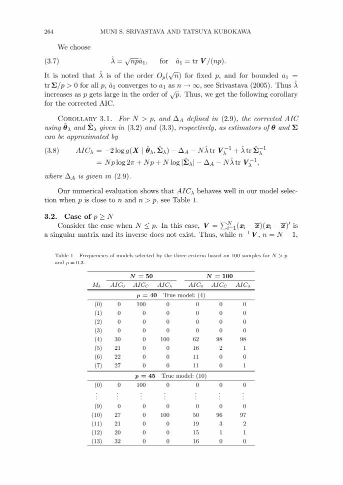
Table 1. Frequencies of models selected by the three criteria based on 100 samples for N > p

and ρ = 0.3.

N = 50 N = 100

Mk AIC0 AICC AICλ AIC0 AICC AICλ

p = 40 True model: (4)

(0) 0 100 0 0 0 0

(1) 0 0 0 0 0 0

(2) 0 0 0 0 0 0

(3) 0 0 0 0 0 0

(4) 30 0 100 62 98 98

(5) 21 0 0 16 2 1

(6) 22 0 0 11 0 0

(7) 27 0 0 11 0 1

p = 45 True model: (10)

(0) 0 100 0 0 0 0...

......

......

......

(9) 0 0 0 0 0 0

(10) 27 0 100 50 96 97

(11) 21 0 0 19 3 2

(12) 20 0 0 15 1 1

(13) 32 0 0 16 0 0


is an unbiased estimator of Σ∗, we need an estimator of the precision matrixΣ∗−1. Two types of estimators have been proposed in the literature by Srivastava(2007), Srivastava and Kubokawa (2007) and Kubokawa and Srivastava (2008).One is based on the Moore-Penrose inverse of V such as an,pV

+ = an,pHL−1H ′,where H ′H = In and L = diag(�1, . . . , �n) is the diagonal matrix of the non-zeroeigenvalues of V and an,p is a constant depending on n and p. The other is aridge-type estimator given by

Vλ = V + λIp,

as employed in (3.1). However, since n is usually much smaller than p, we willuse

λ =√pa1,(3.9)

instead of the one given in (3.7). Let ai = trΣi/p for i = 1, 2, 3, 4. We shallassume the following conditions:

(C.1) 0 < limp→∞ ai ≡ ai0 < ∞,(C.2) n = O(pδ) for 0 < δ ≤ 1/2,(C.3) the maximum eigenvalue of Σ∗ is bounded in large p.

Then from Lemma A.3, it can be observed that E[trV /(np)] = a1 andlimp→∞ trV /(np) = a10 in probability. Hence, the ridge function λ goes to in-finity as p → ∞. The parameters θ and Σ are estimated by the ridge-estimators(3.2) and (3.3) for the ridge function (3.9). Although the MLEs of θ∗ and Σ∗ donot exist, we define the Akaike information AIλ as in (3.4) with the estimators θλ

and Σλ in place of the MLE. This gives ∆λ defined by (3.5) instead of ∆ givenin (2.5). When the dimension p tends to infinity, a second-order approximationof ∆λ is given by the following proposition.

Proposition 3.2. Let aic = tr(C ′ΣC )i/q for q = p − r and i = 1, 2,where C is a p × (p − r) matrix such that C ′B = 0 and C ′C = Ip−r. Also let

a = (a1, a2, a1c, a2c). Then under the assumptions (C.1)–(C.3) and λ =√pa1,

∆λ can be approximated as

∆λ(a) = Np− E∗X [λ tr Σ−1

λ ] − h(a) + o(p−1/2),(3.10)

where

h(a) =√pN

(N + 1 − qa1c

pa1

)(1 +

2a2

npa21

)− N(N + 1)

1 + 1/√p

na2√pa2

1

(3.11)

−√pN

qa2c

pa1

1√pa1 + qa1c

.

The bias ∆λ includes the unknown values ai and aic for i = 1, 2, which areestimated by the consistent estimators

a1 =trV

np, a2 =

1

(n− 1)(n + 2)p[tr[V 2] − (trV )2/n],(3.12)


a1c =tr[C ′VC ]

nq,(3.13)

a2c =1

(n− 1)(n + 2)q[tr[(C ′VC )2] − (tr[C ′VC ])2/n],

for i = 1, 2. Replacing the unknown values with their estimators yields an esti-mator of ∆λ(a), denoted by ∆λ(a), where a = (a1, a2, a1c, a2c).

Corollary 3.2. The AIC∗λ can be approximated by

AIC∗λ = −2 log g(X | θλ, Σλ) − ∆λ(a)(3.14)

= Np log 2π + N log |Σλ| + h(a),

for the function h(·) given in (3.11).

It is noted that the term ∆λ(a) depends on the data, namely, it may beaffected by random fluctuation. Another choice is to use the rough approxima-tions such that ai = 1 and aic = 1 for i = 1, 2, namely a = (1, 1, 1, 1), and theresulting information criterion is given in the following corollary.

Corollary 3.3.

AIC∗A = Np log 2π + N log |Σλ| + h(1).(3.15)

In the estimation of Σ−1, it may be important how to estimate λ. As seenfrom Lemma A.3, λ given in (3.9) goes to infinity as p → ∞, namely λ = Op(p

1/2),and it is interesting to consider another estimate of λ with the order Op(1). Wehere consider such an estimator of the form

λ# =√na1.(3.16)

Using the same arguments as in Proposition 3.2, we get the following proposition.

Proposition 3.3. Assume (C.1)–(C.3) and λ =√na1. Then the bias ∆#

λ

corresponding to ∆λ can be approximated as

∆#λ = Np− λ tr Σ−1

λ − h#(a) + o(1),(3.17)

where

h#(a) =Np√n

(N + 1 − qa1c

pa1

)(1 +

2a2

npa21

)− N(N + 1)

1 +√n/p

√na2

a21

(3.18)

−Nqa2c√na1

1√na1 + qa1c

.


Corollary 3.4. The AIC#λ for λ# =

√na1 can be approximated by

AIC#λ = −2 log g(X | θλ, Σλ) − ∆#

λ (a)(3.19)

= Np log 2π + N log |Σλ| + h#(a).

Srivastava and Kubokawa (2007) proposed the ridge-type empirical Bayesestimator of λ given by λ† = trV /n = pa1. Using this estimate, we can alsohave estimates of θ and Σ based on (3.2) and (3.3). Although intuitive, we hereinverstigate the performance of the following criterion such that the bias termcorresponds to that of the conventional AIC, namely 2×(the number of unknownparameters).

AIC†R = −2 log g(X | θλ, Σλ) + 2 × {p(p + 1) + r}.(3.20)

It is noted that AIC†R is motivated from the conventional AIC, but no justification

can be guranteed in the asymptotics of p → ∞. The performances of AIC†R,

AIC#λ , AIC∗

λ and AIC∗A are investigated in the following section.

3.3. Simulation experimentsWe now compare numerical performances of the proposed selection criteria

through simulation experiments. As the true model, we consider the model thatx1, . . . ,xN are i.i.d. ∼ Np(θ

∗,Σ∗) where

θ∗ = (θ∗1, . . . , θ∗k, 0, . . . , 0)′, θ∗i = (−1)i(1 + ui), i = 1, . . . , k,

for random variable ui from a uniform distribution on the interval [0, 1], and

Σ∗ =

σ1

σ2

. . .

σp

ρ|1−1|1/7 ρ|1−2|1/7 · · · ρ|1−p|1/7

ρ|2−1|1/7 ρ|2−2|1/7 · · · ρ|2−p|1/7

· · ·ρ|p−1|1/7 ρ|p−2|1/7 · · · ρ|p−p|1/7

σ1

σ2

. . .

σp

,

for a constant ρ on the interval (−1, 1) and σi = 2 + (p − i + 1)/p. Let (r)be the set {0, 1, . . . , r}, and we write the model using the first r nonnegativecomponents by Mr or simply (r), namely, the model (r) means that x1, . . . ,xN

are i.i.d. ∼ Np(θ(r),Σ) where θ(r) = (θ1, . . . , θr, 0, . . . , 0)′. For this model, B

corresponds to (Ir,0)′. In our experiments, the true model is Mk or (k), and weconsider the set {Mr; r = 0, 1, . . . , 7} as candidate models.

When N > p, we investigate the performances of the information criteriaAIC0, AICC and AICλ defined in Subsection 3.1. The following two cases areexamined: (A) N = 50, 100, p = 40, k = 4 and models (0) ∼ (7); (B) N = 50,100, p = 45, k = 10 and models (0) ∼ (13). The frequencies of models (r),selected by the three criteria are reported in Table 1 based on 100 samples forρ = 0.3. From Table 1, we can find some properties and features about the


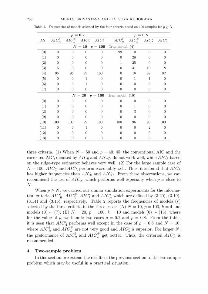
Table 2. Frequencies of models selected by the four criteria based on 100 samples for p ≥ N .

ρ = 0.2 ρ = 0.8

Mk AIC†R AIC#

λ AIC∗λ AIC∗

A AIC†R AIC#

λ AIC∗λ AIC∗

A

N = 10 p = 100 True model: (4)

(0) 0 0 0 0 99 0 0 0

(1) 0 0 0 0 0 28 0 0

(2) 0 0 0 0 1 25 0 0

(3) 5 0 0 0 0 31 10 18

(4) 95 95 99 100 0 16 89 82

(5) 0 0 1 0 0 1 1 0

(6) 0 0 1 0 0 0 0 0

(7) 0 0 0 0 0 0 0 0

N = 20 p = 100 True model: (10)

(0) 0 0 0 0 0 0 0 0

(1) 0 0 0 0 0 1 0 0

(2) 0 0 0 0 0 3 0 0

(9) 0 0 0 0 0 0 0 0

(10) 100 100 99 100 100 96 98 100

(11) 0 0 1 0 0 0 2 0

(12) 0 0 0 0 0 0 0 0

(13) 0 0 0 0 0 0 0 0

three criteria. (1) When N = 50 and p = 40, 45, the conventional AIC and thecorrected AIC, denoted by AIC0 and AICC , do not work well, while AICλ basedon the ridge-type estimator behaves very well. (2) For the large sample case ofN = 100, AICC and AICλ perform reasonably well. Thus, it is found that AICλ

has higher frequencies than AIC0 and AICC . From these observations, we canrecommend the use of AICλ, which performs well especially when p is close toN .

When p ≥ N , we carried out similar simulation experiments for the informa-tion criteria AIC†

R, AIC#λ , AIC∗

λ and AIC∗A which are defined by (3.20), (3.19),

(3.14) and (3.15), respectively. Table 2 reports the frequencies of models (r)selected by the three criteria in the three cases: (A) N = 10, p = 100, k = 4 andmodels (0) ∼ (7); (B) N = 20, p = 100, k = 10 and models (0) ∼ (13), wherefor the value of ρ, we handle two cases ρ = 0.2 and ρ = 0.8. From the table,it is seen that AIC∗

A performs well except in the case of ρ = 0.8 and N = 10,

where AIC†R and AIC#

λ are not very good and AIC∗λ is superior. For larger N ,

the preformance of AIC†R and AIC#

λ get better. Thus, the criterion AIC∗A is

recommended.

4. Two-sample problem

In this section, we extend the results of the previous section to the two sampleproblem which may be useful in a practical situation.


4.1. Extension to the two-sample modelLet X1 = (x11, . . . ,x1N1) and X2 = (x21, . . . ,x2N2) be the two p × N1 and

p × N2 observation matrices independently distributed in which x1i are i.i.d.Np(θ1,Σ) and x2i are i.i.d. Np(θ2,Σ). We wish to investigate which componentsof θ1 are different from θ2. Thus, in this model,

θ1 =

(θ11

µ2

), and θ2 =

(θ21

µ2

),

where θ11 and θ21 are the r-vectors and µ2 is a (p− r) vector. That is,

δ = θ1 − θ2 =

(θ11 − θ21

0

)=

(η

0

)=

(Ir0

)η = Bη,

where B = (Ir,0)′, and η is an r-vector of unknown parameters.Since all the information from the two observation matrices are contained in

the sufficient statistics x 1 = N−11

∑N1i=1 x1i, x 2 = N−1

2

∑N2i=1 x2i and

Vx =N1∑i=1

(x1i − x 1)(x1i − x 1)′ +

N2∑i=1

(x2i − x 2)(x2i − x 2)′

for the parameters (θ1,θ2,Σ), we will consider these sufficient statistics insteadof the entire observation matrices X1 and X2. Let

dx = x 1 − x 2, and ux = (N1x 1 + N2x 2)/N,

where N = N1+N2. Then dx, ux and Vx are independently distributed and since(dx,ux) are one-to-one transformation from (x 1,x 2), it contains the same amountof information as x 1 and x 2. Let ν = (N1µ1+N2µ2)/N and k = N1N2/N . Then,dx ∼ Np(δ, k

−1Σ) and ux ∼ Np(ν, N−1Σ), where

δ = Bη.

Let Vλ = Vx + λIp, where λ is a function of Vx and will be specified later. We

shall also consider the case when λ = 0. Let

AV = B(B ′V −1λ B)−1B ′V −1

λ .

Then we estimate δ, ν and Σ by δx = AV dx, νx = ux and

NΣλ = Vλ + k(I −AV )dxd′x(I −AV ) = Vλ + kVλGdxd

′xGVλ,

where G = C (C ′VλC )−1C ′ and C ′ = (0, Ip−r) : (p− r) × p, that is the first rcolums of C ′ are zeros. In general for p×r matrix B of rank r, C is a p× (p−r)matrix such that C ′C = Ip−r, and C ′B = 0. Let g be the approximating model

with estimates δx, νx and Σλ used for the unknown parameters in the normal


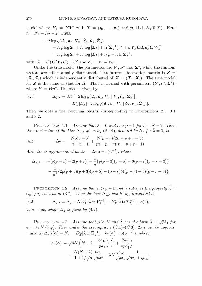
model where Vx = YY ′ with Y = (y1, . . . ,yn) and yi i.i.d. Np(0,Σ). Heren = N1 + N2 − 2. Thus,

− 2 log g(dx,ux,Vx | δx, νx, Σλ)

= Np log 2π + N log |Σλ| + tr[Σ−1λ (V + kVλGdxd

′xGVλ)]

= Np log 2π + N log |Σλ| + Np− λ tr Σ−1λ ,

with G = C (C ′VλC )−1C ′ and dx = x 1 − x 2.Under the true model, the parameters are δ∗, ν∗ and Σ∗, while the random

vectors are still normally distributed. The futurre observation matrix is Z =(Z1,Z2) which is independently distributed of X = (X1,X2). The true modelfor Z is the same as that for X . That is, normal with parameters (δ∗,ν∗,Σ∗),where δ∗ = Bη∗. The bias is given by

∆2,λ = E∗X [−2 log g(dx,ux,Vx | δx, νx, Σλ)](4.1)

− E∗X [E∗

Z [−2 log g(dz,uz,Vz | δx, νx, Σλ)]].

Then we obtain the following results corresponding to Propositions 2.1, 3.1and 3.2.

Proposition 4.1. Assume that λ = 0 and n > p+ 1 for n = N − 2. Thenthe exact value of the bias ∆2,λ given by (A.19), denoted by ∆2 for λ = 0, is

∆2 = −Np(p + 5)

n− p− 1+

N(p− r)(2n− p + r + 3)

(n− p + r)(n− p + r − 1).(4.2)

Also, ∆2 is approximated as ∆2 = ∆2,A + o(n−2), where

∆2,A = −[p(p + 1) + 2(p + r)] − 1

n{p(p + 3)(p + 5) − 3(p− r)(p− r + 3)}

− 1

n2{2p(p + 1)(p + 3)(p + 5) − (p− r)(4(p− r) + 5)(p− r + 3)}.

Proposition 4.2. Assume that n > p + 1 and λ satisfies the property λ =Op(

√n) such as in (3.7). Then the bias ∆2,λ can be approximated as

∆2,λ = ∆2 + NE∗X [λ trV −1

λ ] − E∗X [λ tr Σ−1

λ ] + o(1),(4.3)

as n → ∞, where ∆2 is given by (4.2).

Proposition 4.3. Assume that p ≥ N and λ has the form λ =√pa1 for

a1 = trV /(np). Then under the assumptions (C.1)–(C.3), ∆2,λ can be approxi-

mated as ∆2,λ(a) = Np− E∗X [λ tr Σ−1

λ ] − h2(a) + o(p−1/2), where

h2(a) =√pN

(N + 2 − qa1c

pa1

)(1 +

2a2

npa21

)

− N(N + 2)

1 + 1/√p

na2√pa2

1

− 3Nqa2c√pa1

1√pa1 + qa1c

.


Taking the simulation results in Subsection 3.3 into account, we suggest thefollowing ridge information criteria from Propositions 2.1, 3.1 and 3.2. WhenN > p, let λ =

√npa1 and consider the ridge information criterion

AICλ = −2 log g(dx,ux,Vx | δx, νx, Σλ) − ∆2,A −Nλ trV −1λ + λ tr Σ−1

λ

= Np log 2π + Np + N log |Σλ| − ∆2,A −Nλ trV −1λ ,

where ∆2,A is given in Proposition 4.1. When p ≥ N , we can propose the criteria

corresponding to (3.14) and (3.15). Let λ =√pa1 and consider

AIC∗λ = −2 log g(dx,ux,Vx | δx, νx, Σλ) − ∆2,λ(a)

= Np log 2π + N log |Σλ| + h2(a),

and the AIC corresponding to (3.15) is given by

AIC∗A = Np log 2π + N log |Σλ| + h2(1).

Since AIC†R and AIC#

λ do not perform well as examined in Subsection 3.3, wedo not investigate them in the comparison.

4.2. Numerical studiesWe briefly state the numerical results of the information criteria proposed

in the previous subsection through the simulation and empirical studies whenp ≥ N for N = N1 + N2.

For the simulation study, we carried out similar experiments to Subsection3.3 where the mean vectors of the true model are given by

θ∗1 = (θ∗11, . . . , θ

∗1k, 0, . . . , 0)′, θ∗1i = 1.5 × u1i, i = 1, . . . , k,

θ∗2 = (θ∗21, . . . , θ

∗2k, 0, . . . , 0)′, θ∗2i = −1.5 × u2i, i = 1, . . . , k,

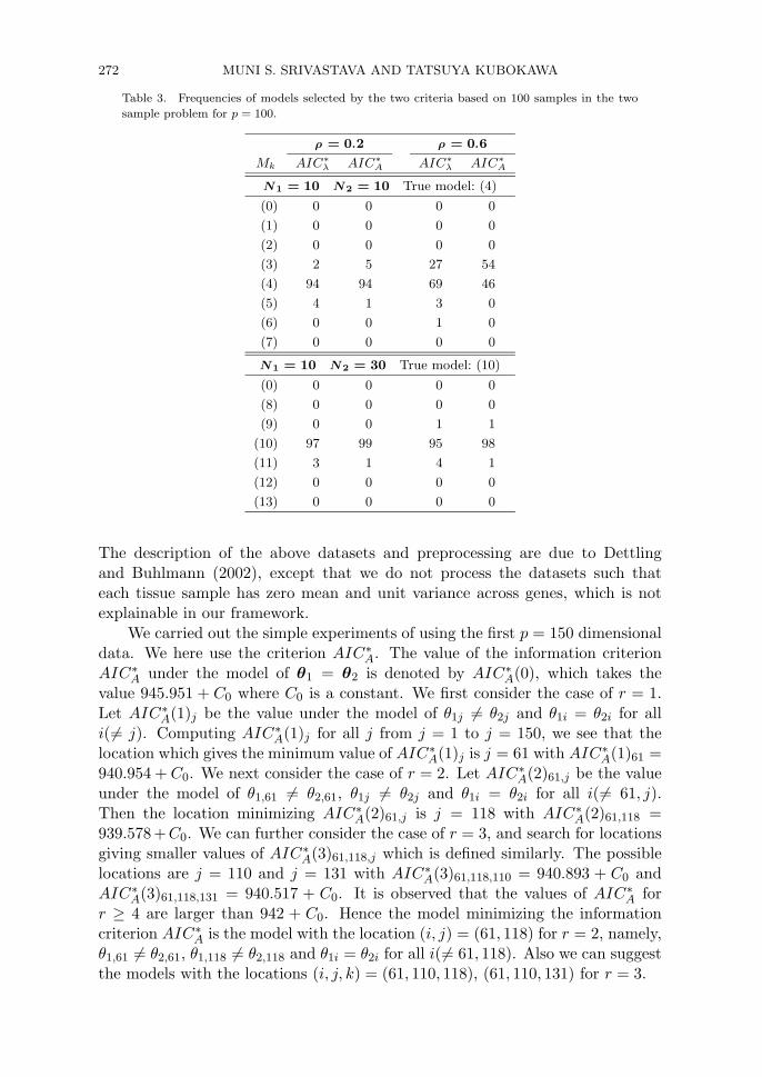
for random variables u1i and u2i from a uniform distribution on the interval [0, 1],and the covarinace matrix Σ∗ of the true model has the same structure as usedthere. The performances of the criteria AIC∗

λ and AIC∗A are examined in the

two cases: (A) N1 = 10, N2 = 10, k = 4 and models (0) ∼ (7); (B) N1 = 10,N2 = 30, k = 10 and models (0) ∼ (13). Table 3 reports the frequencies of models(r) selected by the three criteria based on 100 samples for p = 100 and ρ = 0.2,0.6. Table 3 shows that both AIC∗

λ and AIC∗A have good performances except

for the case of small sample sizes (N1, N2) = (10, 10) and the high-correlationρ = 0.6. In this case, AIC∗

λ is slightly better.We next apply the information criterion to the real datasets of microar-

ray referred to as Leukemia. This dataset contains gene expression levels of 72patients either suffering from acute lymphoblastic leukemia(N1 = 47 cases) oracute myeloid leukemia(N2 = 25 cases) for 3571 genes. These data are publiclyavailable at

“http://www-genome.wi.mit.edu/cancer”.


Table 3. Frequencies of models selected by the two criteria based on 100 samples in the two

sample problem for p = 100.

ρ = 0.2 ρ = 0.6

Mk AIC∗λ AIC∗

A AIC∗λ AIC∗

A

N1 = 10 N2 = 10 True model: (4)

(0) 0 0 0 0

(1) 0 0 0 0

(2) 0 0 0 0

(3) 2 5 27 54

(4) 94 94 69 46

(5) 4 1 3 0

(6) 0 0 1 0

(7) 0 0 0 0

N1 = 10 N2 = 30 True model: (10)

(0) 0 0 0 0

(8) 0 0 0 0

(9) 0 0 1 1

(10) 97 99 95 98

(11) 3 1 4 1

(12) 0 0 0 0

(13) 0 0 0 0

The description of the above datasets and preprocessing are due to Dettlingand Buhlmann (2002), except that we do not process the datasets such thateach tissue sample has zero mean and unit variance across genes, which is notexplainable in our framework.

We carried out the simple experiments of using the first p = 150 dimensionaldata. We here use the criterion AIC∗

A. The value of the information criterionAIC∗

A under the model of θ1 = θ2 is denoted by AIC∗A(0), which takes the

value 945.951 + C0 where C0 is a constant. We first consider the case of r = 1.Let AIC∗

A(1)j be the value under the model of θ1j �= θ2j and θ1i = θ2i for alli(�= j). Computing AIC∗

A(1)j for all j from j = 1 to j = 150, we see that thelocation which gives the minimum value of AIC∗

A(1)j is j = 61 with AIC∗A(1)61 =

940.954 + C0. We next consider the case of r = 2. Let AIC∗A(2)61,j be the value

under the model of θ1,61 �= θ2,61, θ1j �= θ2j and θ1i = θ2i for all i(�= 61, j).Then the location minimizing AIC∗

A(2)61,j is j = 118 with AIC∗A(2)61,118 =

939.578+C0. We can further consider the case of r = 3, and search for locationsgiving smaller values of AIC∗

A(3)61,118,j which is defined similarly. The possiblelocations are j = 110 and j = 131 with AIC∗

A(3)61,118,110 = 940.893 + C0 andAIC∗

A(3)61,118,131 = 940.517 + C0. It is observed that the values of AIC∗A for

r ≥ 4 are larger than 942 + C0. Hence the model minimizing the informationcriterion AIC∗

A is the model with the location (i, j) = (61, 118) for r = 2, namely,θ1,61 �= θ2,61, θ1,118 �= θ2,118 and θ1i = θ2i for all i(�= 61, 118). Also we can suggestthe models with the locations (i, j, k) = (61, 110, 118), (61, 110, 131) for r = 3.


5. Concluding remarks

The Akaike information criterion has been very successfully used in modelselection. But so far the focus has been for small p (dimension or parameters)and large sample size N . For large p and or when p is close to N , the estimatorsof the parameters are unstable. However nothing has been known about the per-formance of AIC. In this article we have modified AIC using the ridge estimatorof the precision matrix and evaluated its performance not only for the case whenp < N and close to N but have also considered the case when p ≥ N . We haveproposed AICλ given in (3.8) for the case when N > p, and AIC∗

λ and AIC∗A

given by (3.14) and (3.15) for the case when p ≥ N . Finally, we have extendedthe results to the two sample problem.

AppendixBefore proving Propositions, we provide a unified expression of the bias ∆λ

given by (3.5), where the ridge-type estimators θλ and Σλ are given by (3.2) and(3.3). To evaluate the bias, we need the following two lemmas which are referredto in Srivastava and Khatri (1979, Corollary 1.9.2 and Theorem 1.4.1).

Lemma A.1. Let B be a p × r matrix of rank r ≤ p, and V be a p × ppositive definite matrix. Then there exists a matrix C : p × (p − r) such thatC ′B = 0, C ′C = Ip−r, and

V −1 = V −1B(B ′V −1B)−1B ′V −1 + C (C ′VC )−1C ′.

Lemma A.2. Let P and Q be nonsingular matrices of proper orders. Then,if Q = P + UV ,

Q−1 = P−1 −P−1U (I + VP−1U )−1VP−1.

From Lemma A.1, it follows that

NΣλ = Vλ + N [I −B(B ′V −1λ B)−1B ′V −1

λ ]xx ′[I −B(B ′V −1λ B)−1B ′V −1

λ ]′

= Vλ + NVλC (C ′VλC )−1C ′xx ′C (C ′VλC )−1C ′Vλ.

From Lemma A.2, it is seen that

Σ−1λ = N

{V −1

λ −NC (C ′VλC )−1C ′xx ′C (C ′VλC )−1C ′

1 + Nx ′C (C ′VλC )−1C ′x

}.(A.1)

For z1, . . . , zN i.i.d. Np(θ∗,Σ∗) and Z = (z1, . . . , zN ), the Akaike information

AIλ of (3.4) is written as

AIλ = E∗XE∗

Z

[Np log 2π + N log |Σλ| +

N∑i=1

tr[Σ−1λ (zi − θλ)(zi − θλ)

′]

]

= E∗X [Np log 2π + N log |Σλ| + N tr[Σ−1

λ {Σ∗ + (θλ − θ∗)(θλ − θ∗)′}]].


Then the bias (3.5) is expressed as

∆λ = E[−2 log g(X | θλ, Σλ)] −AIλ(A.2)

= E∗X

[tr

[Σ−1

λ

N∑i=1

(xi − θλ)(xi − θλ)′]−N tr[Σ−1

λ Σ∗]

−N tr[Σ−1λ (θλ − θ∗)(θλ − θ∗)′]

]

= Np− E∗X [λ tr Σ−1

λ ] −NE∗X [tr[Σ−1

λ Σ∗]]

−NE∗X [tr[Σ−1

λ (θλ − θ∗)(θλ − θ∗)′]].

To calculate ∆λ in (A.2), we need to evaluate the two terms E∗X [tr[Σ−1

λ Σ∗]]and E∗

X [tr[Σ−1λ (θλ − θ∗)(θλ − θ∗)′]], where θ∗ = Bη∗. Then from (A.1),

E∗X [tr[Σ−1

λ Σ∗]]

= NE∗X

[trΣ∗V −1

λ −Nx ′C (C ′VλC )−1C ′Σ∗C (C ′VλC )−1C ′x

1 + Nx ′C (C ′VλC )−1C ′x

].

Noting that C ′Bθ∗ = 0, we get u =√N(C ′Σ∗C )−1/2C ′x ∼ Np−r(0, I ). Let

Wλ = (C ′Σ∗C )−1/2(C ′VλC )(C ′Σ∗C )−1/2;(A.3)

W is Wλ with λ = 0. Then, it is observed that

E∗X

[N

x ′C (C ′VλC )−1C ′Σ∗C (C ′VλC )−1C ′x1 + Nx ′C (C ′VλC )−1C ′x

]= E∗

X

[u ′W −2

λ u

1 + u ′W −1λ u

],

which yields that

E∗X [tr[Σ−1

λ Σ∗]] = NE∗X [tr[V −1

λ Σ∗]] −NE∗X

[u ′W −2

λ u

1 + u ′W −1λ u

].(A.4)

Let AV = B(B ′V −1λ B)−1B ′V −1

λ . Noting that B ′Σ−1λ B = NB ′V −1

λ B sinceC ′B = 0, we see that

E∗X [tr[Σ−1

λ (θλ − θ∗)(θλ − θ∗)′]]

= E∗X [tr[Σ−1

λ AV (x −Bη∗)(x −Bη∗)′A′V ]]

=1

NE∗

X [tr[Σ−1λ AV Σ∗A′

V ]],

which is equal to

E∗X [tr[Σ∗V −1

λ B(B ′V −1λ B)−1V −1

λ ]](A.5)

= E∗X [tr[Σ∗{V −1

λ −C (C ′VλC )−1C ′}]]= E∗

X [tr[Σ∗V −1λ ] − trW −1

λ ].


Combining (A.2), (A.4) and (A.5), ∆λ given by (A.2) is expressed as

∆λ = Np−N(N + 1)E∗X [tr[Σ∗V −1

λ ]] − E∗X [λ tr Σ−1

λ ](A.6)

+ NE∗X [trW −1

λ ] + N2E∗X

[u ′W −2

λ u

1 + u ′W −1λ u

].

Propositions 2.1, 3.1 and 3.2 can be proved using the expression (A.6).

A.1. Proof of Proposition 2.1For this proof, let λ = 0, and denote Vλ and Wλ for λ = 0 by V and W , re-

spectively. In the expression (A.6), it can be easily shown that E∗X [tr[Σ∗V −1]] =

p/(n−p−1) and E∗X [trW −1] = (p−r)/(n−(p−r)−1) for n = N−1. To evaluate

the second term E∗X [u ′W −2u/(1 + u ′W −1u)], the arguments as in Srivastava

(1995) are useful. It is noted that under the true model u ∼ Np−r(0, I ) andW ∼ Wp−r(I , n) are independently distributed. Let Γ be an orthogonal matrixwith the last row as u ′/‖u‖, where ‖u‖ = (u ′u)1/2. Then making the transfor-mation W = ΓWΓ′, we find that W is still distributed as Wishart, Wp−r(I , n)and hence is independent of u . Let W = TT ′, where

T =

(T1 0

t ′12 tqq

)

is the unique triangular factorization of W for q = p − r. Then, u ′W −1u =u ′u/t2qq, and

u ′W −2u = (u ′u)(0′, 1)W −2(0′, 1)′

= (u ′u)[(w12)′w12 + (wqq)2]

= (u ′u)[t−4qq + t−4

qq t ′12(T′1T1)

−1t12],

where 0′ is an q − 1 row vector of zeros and

W −1 =

(W 11 w12

(w12)′ wqq

)= (T T ′)−1.

Hence,u ′W −2u

1 + u ′W −1u=

u ′ut2qq

1 + t ′12(T′1T1)

−1t12t2qq + u ′u

,

where u ′u ∼ χ2q , t2qq ∼ χ2

n−q+1 and [1 + t ′12(T′1T1)

−1t12] are independentlydistributed. And from Basu’s theorem, u ′u/t2qq and t2qq +u ′u are independentlydistributed. Since t12 is independently distributed of T1 and t12 ∼ Nq−1(0, I ),it follows that

E∗X [1 + t ′12(T

′1T1)

−1t12] = 1 + E∗X [tr(T ′

1T1)−1] = 1 + E∗

X [tr(T1T′1)

−1]

= 1 + (q − 1)/(n− q) = (n− 1)/(n− p + r).


Note that E∗X [(t2qq + u ′u)−1] = E[(χ2

n+1)−1] = (n − 1)−1 and E∗

X [u ′u/t2qq] =q/(n− q − 1) = (p− r)/(n− p + r − 1). Hence,

E∗X

[u ′W −2u

1 + u ′W −1u

]=

p− r

(n− p + r)(n− p + r − 1).(A.7)

Combining (A.6) and (A.7), we get

∆ = Np−N(N + 1)p

n− p− 1+ N

p− r

n− p + r − 1

+ N2 p− r

(n− p + r)(n− p + r − 1),

which is equal to the expression (2.6).

A.2. Proof of Proposition 3.1We shall evaluate each term in (A.6). It is noted that λ/n = Op(1/

√n) and

that nV −1λ = {V /n + (λ/n)I }−1 = nV −1 + op(1). Then it can be shown that

NE∗X [trW −1

λ ] = NE∗X [trW −1] + o(1),

N2E∗X

[u ′W −2

λ u

1 + u ′W −1λ u

]= N2E∗

X

[u ′W −2u

1 + u ′W −1u

]+ o(1),

for W defined below (A.3). Since tr[Σ∗(V /n)−1]− tr[Σ∗{V /n+ (λ/n)I }−1] =(λ/n) tr[Σ∗{V /n + (λ/n)I }−1(V /n)−1], it is observed that

∆λ = ∆ +N

n(N + 1)E[(λ/n) tr[Σ∗{V /n + (λ/n)I }−1(V /n)−1]] + o(1),

so that we need to evaluate the second term in the r.h.s. of the equality. Notethat V /n−Σ∗ = Op(1/

√n) and λ/n = Op(1/

√n). From the Taylor expansion,

(V /n)−1 = Σ∗−1 − Σ∗−1(V /n− Σ∗)Σ∗−1 + Op(1/n).

Substituting this expansion in the second expression on the r.h.s. of ∆λ, we cansee that

N

n(N + 1)E[(λ/n) tr[Σ∗{V /n + (λ/n)I }−1(V /n)−1]](A.8)

= N(1 + 2/n)E[(λ/n) tr{V /n + (λ/n)I }−1]

−N(1 + 2/n)E[(λ/n) tr[{V /n + (λ/n)I }−1Σ∗−1(V /n− Σ∗)]]

+ O(1/√n).

The first term in the r.h.s. of (A.8) can be written as N(1+2/n)E[(λ/n) tr{V /n+(λ/n)I }−1] = NE[λ tr(V +λI )−1]+O(1/

√n). The second term can be expressed

as√nE[tr(V /n) tr[{V /n + (λ/n)I }−1Σ∗−1(V /n− Σ∗)]]

=√nE[trΣ∗ tr[{V /n + (λ/n)I }−1Σ∗−1(V /n− Σ∗)]]

+√nE[tr(V /n− Σ∗) tr[{V /n + (λ/n)I }−1Σ∗−1(V /n− Σ∗)]]

=√nE[trΣ∗ tr[(V /n)−1Σ∗−1(V /n− Σ∗)]] + O(1/

√n),


which can be seen to be O(1/√n) by substituting in the Taylor expansion of

(V /n)−1. Therefore, the proof of Proposition 3.1 is complete.

A.3. Proof of Proposition 3.2To calculate ∆λ given by (A.6), we need some preliminary results. The

following lemmas due to Srivastava (2005, 2007) are useful for evaluating expec-tations based on a1 and a2 given by (3.12).

Lemma A.3 (Srivastava (2005)). Let V ∼ Wp(Σ, n). Then,(i) E[ai] = ai for i = 1, 2.(ii) limp→∞ ai = ai0 in probability for i = 1, 2 if the conditions (C.1) and (C.2)

are satisfied.(iii) Var(a1) = 2a2/(np).

Corollary A.1. Under the conditions (C.1) and (C.2), ai is a consistentestimator of ai for i = 1, 2, if p → ∞, or (n, p) → ∞.

Lemma A.4 (Srivastava (2007)). Let V ∼ Wp(Σ, n), n < p, and V = H1LH ′1,

where H ′1H1 = In and L = (�1, . . . , �n), an n×n diagonal matrix which contains

the non-zero eigenvalues of V . Then,(i) limp→∞ L/p = a10In in probability.(ii) limp→∞ H ′

1ΣH1 = (a20/a10)In in probability.

For the proofs, see Srivastava (2005, 2007). For the estimators a1c and a2c

given by (3.13), similar results hold.To prove Proposition 3.2, we need to evaluate each term in (A.6). We first

evaluate the term E∗X [tr[Σ∗V −1

λ ]]. Let H : p × p be an orthogonal matrixHH ′ = Ip such that

V = H

(L 0

0 0

)H ′,

where H = (H1,H2), H1 : p× n, L : n× n diagonal matrix defined above, andH2H

′2 = Ip −H1H

′1. Then we get from Lemma A.4,


λ ]] = E∗X

[tr

[Σ∗H

((L + λI )−1 0

0 λ−1Ip−n

)H ′]]

= E∗X [trΣ∗{H1(L + λI )−1H ′

1 + λ−1H2H′2}]

= E∗X [pλ−1 trΣ∗/p− λ−1 tr[(In + λL−1)−1H ′

1Σ∗H1]].

Note that λ =√pa1. Then, E∗

X [tr[Σ∗V −1λ ]] is expressed as


λ ]] = E∗X

[√pa1

a1− 1√

pa1tr[(In +

√pa1L

−1)−1H ′1Σ

∗H1]

].


It is here noted that

a1

a1=

1

1 + (a1 − a1)/a1= 1 − a1 − a1

a1+

(a1 − a1)2

a21

+ op(p−1),

which gives from Lemma A.3

E∗X

[a1

a1

]= 1 +

Var(a1)

a21

+ o(p−1) = 1 +2a2

npa21

+ o(p−1).

Also from Lemmas A.3 and A.4,

E∗X

[1√pa1

tr[(In +√pa1L

−1)−1H ′1Σ

∗H1]

]

=1√pa1

tr

[(In + In/

√p)−1a2

a1In

]+ o(p−1/2)

=na2

(1 + 1/√p)√pa2

1

+ o(p−1/2).

Combining these evaluations, we get


λ ]] =√p

(1 +

2a2

npa21

− na2

(1 + 1/√p)pa2

1

)+ o(p−1/2).(A.9)

We next evaluate the term E∗X [trW −1

λ ]. Let q = p−r, and let Σ∗c = C ′Σ∗C

and Vc = C ′VC . Let Hc : q × q be an orthogonal matrix such that HcH′c = Iq

and

C ′VC = Hc

(Lc 0

0 0

)H ′

c ,

where Hc = (H1c,H2c), H1c : q × n, Lc : n× n diagonal matrix, and H2cH′2c =

Iq −H1cH′1c. Then, we get

trW −1λ = tr[Σ∗

c(Vc + λIq)−1](A.10)

= tr

[Σ∗

cHc

((Lc + λIn)−1 0

0 λ−1Iq−n

)H ′

c

]

= tr[Σ∗c{H1c(Lc + λIn)−1H ′

1c + λ−1H2cH′2c}]

= trΣ∗c/λ− λ−1 tr[(In + λL−1

c )−1H ′1cΣ

∗cH1c]

=qa1c√pa1

− 1√pa1

tr[(In + (√pa1/q)qL

−1c )−1H ′

1cΣcH1c],

where λ =√pa1. Using similar arguments as in (A.9), we can see that

E∗X [trW −1

λ ](A.11)

=qa1c√pa1

{1 +

1

a21

Var(a1)

}− 1√

pa1tr

(In +

√pa1

qa1cIn

)−1 a2c

a1c

+ o(p−1/2)

=qa1c√pa1

{1 +

2a2

npa21

}− na2c√

pa1a1c

qa1c√pa1 + qa1c

+ o(p−1/2).


Finally, we shall show that E∗X [u ′W −2

λ u/(1 + u ′W −1λ u)] can be evaluated

as

E

[u ′W −2

λ u

1 + u ′W −1λ u

∣∣∣∣ V]

=tr(W −2

λ )

1 + tr(W −1λ )

+ op(p−1/2).(A.12)

To this end, it is noted that

E

[u ′W −2

λ u

(1 + u ′W −1λ u)

∣∣∣∣ V]− tr(W −2

λ )

1 + tr(W −1λ )

= E

[u ′W −2

λ u

(1 + u ′W −1λ u)

∣∣∣∣ V]− E

[u ′W −2

λ u

1 + tr(W −1λ )

∣∣∣∣ V]

= −E

[u ′W −2

λ u(u ′W −1λ u − tr(W −1

λ ))

(1 + u ′W −1λ u)(1 + tr(W −1

λ ))

∣∣∣∣ V],

the absolute value of which, from the Cauchy-Schwartz inequality, is less than orequal toE

{ u ′W −2

λ u

1 + u ′W −1λ u

}2 ∣∣∣∣ V× E

{u ′W −1

λ u − tr(W −1λ )

1 + tr(W −1λ )

}2 ∣∣∣∣ V

1/2

≤

E

(u ′W −2

λ u

u ′W −1λ u

)2 ∣∣∣∣ V

1/2

× {E[(u ′W −1λ u − tr(W −1

λ ))2 | V ]}1/2

1 + tr(W −1λ )

.

Hence, it is sufficient to show that

limp→∞

pE

(u ′W −2

λ u

u ′W −1λ u

)2 ∣∣∣∣ V(A.13)

× E[(u ′W −1λ u − tr(W −1

λ ))2 | V ]

{1 + tr(W −1λ )}2

= 0,

for the proof of (A.12). It can be verified that for q × q matrices G and Q ,

E[u ′Gu × u ′Qu ] = tr(G) tr(Q) + 2 tr(GQ),

which is used to get that

E[(u ′W −1λ u − tr(W −1

λ ))2 | V ](A.14)

= (trW −1λ )2 + 2 trW −2

λ − 2(trW −1λ )2 + (trW −1

λ )2

= 2 trW −2λ .

Using the same arguments as in (A.10), we can show that

trW −1λ =

qa1c√pa1

+ op(p1/2),(A.15)

trW −2λ =

1

pa21

tr[Σ∗c(Iq −H1c(In +

√pa1L

−1c )−1H ′

1c)(A.16)

× Σ∗c(Iq −H1c(In +

√pa1L

−1c )−1H ′

1c)]

=qa2c

pa21

+ op(1).


Hence, it is observed that

limp→∞

pE[(u ′W −1

λ u − tr(W −1λ ))2 | V ]

{1 + tr(W −1λ )}2

= 2 limp→∞

ptrW −2

λ

{1 + tr(W −1λ )}2

= 2 limp→∞

qa2c/(pa21)

{1/√p + a1c/a1}2,

which is bounded. On the other hand, it is noted that

u ′W −2λ u

u ′W −1λ u

≤ supu

u ′W −2λ u

u ′W −1λ u

≤ chmax(Σ∗c) × chmax{(C ′VλC )−1}

≤ chmax(Σ∗c) ×

1

λ=

chmax(Σ∗c)√

pa1,

where chmax(A) denotes the maximum eigenvalue of a matrix A. Since chmax(Σ∗c)

is bounded from the condition (C.3), it is seen that u ′W −2λ u/u ′W −1

λ u =Op(1/

√p). Hence, the approximation (A.12) is proved, so that

E

[u ′W −2

λ u

1 + u ′W −1λ u

]= E

[tr(W −2

λ )

1 + tr(W −1λ )

]+ o(p−1/2).

Using (A.15) and (A.16) again, we obtain that

E

[u ′W −2

λ u

1 + u ′W −1λ u

]=

qa2c/(pa21)

1 + qa1c/(√pa1)

+ o(p−1/2)(A.17)

=qa2c√pa1

1√pa1 + qa1c

+ o(p−1/2).

Combining (A.6), (A.9), (A.11) and (A.17), we get the second order approx-imation given by

∆λ = Np− λ tr Σ−1λ − h(a) + o(p−1/2),(A.18)

where

h(a) = N(N + 1)√p

{1 +

2a2

npa21

− na2

pa21

1

1 + 1/√p

}

−N√p

{qa1c

pa1

(1 +

2a2

npa21

)− na2c

pa1a1c

1

1 +√pa1/(qa1c)

}

−N2 qa2c

pa21

1

1 + qa1c/(√pa1)

,

which can be expressed as in (3.10), and the proof of Proposition 3.2 is complete.


A.4. Proof of Proposition 3.3This can be shown by using the same arguments as in the proof of Proposition

3.2, and we observe that

∆λ = Np− λ tr Σ−1λ − h#(a) + o(1),

where

h#(a) = N(N + 1)p√n

{1 +

2a2

npa21

− na2

pa21

1

1 +√n/p

}

− Np√n

{qa1c

pa1

(1 +

2a2

npa21

)− na2c

pa1a1c

1

1 +√na1/(qa1c)

}

−N2 qa2c

na21

1

1 + qa1c/(√na1)

,

which can be expressed as in (3.17), and the proof of Proposition 3.3 is complete.

A.5. Proof of Propositions 4.1, 4.2 and 4.3We shall evaluate the bias (4.1). Let R∗ = E∗

Z [−2 log g(dz,uz,Vz | δx, νx,Σλ) −Np log 2π]. Then,

R∗ = N log |Σλ| + E∗Z [tr[Σ−1

λ {Vz + k(dz − δx)(dz − δx)′

+ N(uz − νx)(uz − νx)′}]]

= N log |Σλ| + tr[Σ−1λ {NΣ∗ + k(δx − δ∗)(δx − δ∗)′

+ N(νx − ν∗)(νx − ν∗)′}],

and thus using the results from (A.3) and (A.4), we observe that

E∗X [R∗] = NE∗

X [log |Σλ|] + E∗X [(N + 1) tr[Σ−1

λ Σ∗]]

+ E∗X [k tr[Σ−1

λ (δx − δ∗)(δx − δ∗)′]]

= NE∗X [log |Σλ|] + (N + 1)E∗

X [tr[Σ∗Σ−1λ ]]

+ E∗X [tr[Σ−1

λ AV Σ∗A′V ]]

= NE∗X [log |Σλ|] + N(N + 2)E∗

X [Σ∗V −1λ ] −NE∗

X [trW −1λ ]

−N(N + 1)E∗X

[u ′W −2

λ u

1 + u ′W −1λ u

],

where u =√k(C ′Σ∗C )−1/2C ′ux ∼ Np−r(0, I ) and

Wλ = (C ′Σ∗C )−1/2(C ′VλC )(C ′Σ∗C )−1/2.

Hence, the bias is given by

∆2,λ = E∗X [−2 log g(dx,ux,Vx | δx, νx, Σλ)](A.19)

− E∗X [E∗

Z [−2 log g(dz,uz,Vz | δx, νx, Σλ)]]

= Np− EX [λ tr Σ−1λ ] −N(N + 2)E∗

X [Σ∗V −1λ ]

+ NE∗X [trW −1

λ ] −N(N + 1)E∗X

[u ′W −2

λ u

1 + u ′W −1λ u

],


which leads to the expression (A.6). Hence Propositions 4.1, 4.2 and 4.3 followfrom Propositions 2.1, 3.1 and 3.2, respectively.

AcknowledgementsWe are also grateful to the editor, the associate editor and the two reviewers

for their valuable comments and helpful suggestions. The research of the firstauthor was supported by the Natural Sciences and Engineering Research Councilof Canada. The research of the second author was supported in part by a grantfrom the Ministry of Education, Japan, No. 16500172 and in part by a grant fromthe 21st Century COE Program at Faculty of Economics, University of Tokyo.

References

Akaike, H. (1973). Information theory and an extension of the maximum likelihood principle,2nd International Symposium on Information Theory (eds. B. N. Petrov and F. Csaki),267–281, Akademia Kiado, Budapest.

Akaike, H. (1974). A new look at the statistical model identification. System identification andtime-series analysis, IEEE Trans. Autom. Contr., AC-19, 716–723.

Benjamini, Y. and Hockberg, Y. (1995). Controlling the false discovery rate: A practical andpowerful approach to multiple testing, J. Roy. Statist. Soc., B 57, 289–300.

Benjamini, Y. and Yekutieli, D. (2001). The control of the false discovery rate in multipletesting under dependency, Ann. Statist., 29, 1165–1181.

Dettling, M. and Buhlmann, P. (2002). Boosting for tumor classification with gene expressiondata, Bioinformatics, 19, 1061–1069.

Fujikoshi, Y. and Satoh, K. (1997). Modified AIC and Cp in multivariate linear regression,Biometrika, 84, 707–716.

Hommel, G. and Hoffman, T. (1988). Controlled uncertainty, Multiple Hypotheses Testing (eds.P. Bauer, G. Hommel and E. Sonnemann), 154–161, Springer, Heidelberg.

Hurvich, C. and Tsai C.-L. (1989). Regression and time series model selection in small samples,Biometrika, 76, 297–307.

Kollo, T. and von Rosen, D. (2005). Advanced Multivariate Statistics with Matrices, Springer,Dordrecht.

Konishi, S. and Kitagawa, G. (1996). Generalised information criteria in model selection,Biometrika, 83, 875–890.

Konishi, S., Ando, T. and Imoto, S. (2004). Bayesian information criteria and smoothingparameter selection in radial basis function networks, Biometrika, 91, 27–43.

Kubokawa, T. and Srivastava, M. S. (2008). Estimation of the precision matrix of a singularWishart distribution and its application in high dimensional data, J. Multivariate Analysis(to appear).

Kullback, S. and Leibler, R. A. (1951). On information and sufficiency, Ann. Math. Statist.,22, 79–86.

Lehmann, E. L. and Romano, J. P. (2005). Generalizations of the familywise error rate, Ann.Statist., 33, 1138–1154.

Potthoff, R. F. and Roy, S. N. (1964). A generalized multivariate analysis of variance modeluseful especially for growth curve problems, Biometrika, 51, 313–326.

Rao, C. R. (1959). Some problems involving linear hypothesis in multivariate analysis,Biometrika, 46, 49–58.

Roy, S. N. (1953). On a heuristic method of test construction and its use in multivariate analysis,Ann. Math. Statist., 24, 220–238.

Srivastava, M. S. (1995). Comparison of the inverse and classical estimators in multi-univariatelinear calibration, Comm. Statist.-Theory Methods, 24, 2753–2767.

Srivastava, M. S. (2002). Methods of Multivariate Statistics, Wiley, New York.


Srivastava, M. S. (2005). Some tests concerning the covariance matrix in high dimensional data,J. Japan Statist. Soc., 35, 251–272.

Srivastava, M. S. (2007). Multivariate theory for analyzing high dimensional data, J. JapanStatist. Soc., 37, 53–86.

Srivastava, M. S. and Khatri, C. G. (1979). An Introduction to Multivariate Statistics, North-Holland, New York.

Srivastava, M. S. and Kubokawa, T. (2007). Comparison of discrimination methods for highdimensional data, J. Japan Statist. Soc., 37, 123–134.

Sugiura, N. (1978). Further analysis of the data by Akaike’s information criterion and the finitecorrections, Commun. Statist.-Theory Methods, 1, 13–26.

AKAIKE INFORMATION CRITERION FOR SELECTING COMPONENTS OF THE MEAN VECTOR IN HIGH DIMENSIONAL DATA WITH FEWER OBSERVATIONS

Documents