ajeassp.2013.178.204.pdf - Science Publications

American Journal of Engineering and Applied Sciences, 6 (2): 178-204, 2013 ISSN: 1941-7020 © 2014 F. Calise et al., This open access article is distributed under a Creative Commons Attribution (CC-BY) 3.0 license doi:10.3844/ajeassp.2013.178.204 Published Online 6 (2) 2013 (http://www.thescipub.com/ajeas.toc)

Corresponding Author: Francesco Calise, DETEC, University of Naples Federico II, Naples, Italy

178 AJEAS Science Publications

DESIGN AND PARAMETRIC OPTIMIZATION OF AN ORGANIC

RANKINE CYCLE POWERED BY SOLAR ENERGY

1Francesco Calise, 2Claudio Capuozzo and 2Laura Vanoli

1DETEC, University of Naples Federico II, Naples, Italy

2DIT, University of Naples Parthenope, Naples, Italy

Received 2013-02-04, Revised 2013-03-08; Accepted 2013-05-15

ABSTRACT

This study presents the simulation and performance analysis of a regenerative and superheated Organic Rankine Cycle (ORC). To this scope, anew simulation model has been developed. The model is based on zero-dimensional energy and mass balances for all the components of the system. Shell and tube heat expanders with single shell and double tube pass have been chosen. Pump and expander have been considered only form a thermodynamic point of view, with constant compressor and expansion efficiency. The simulations have been carried out in order to find different optimization criteria to use as preliminary design tools, especially for the organic fluid choice and the heat exchanger design. Firstly, the ORC performances have been evaluated for different organic medium, varying the temperature of the heat source. The global efficiency of the plant, the net electric power generation and the volumetric expansion ratio has been considered as evaluation parameters. The simulation results show that two hydrocarbons demonstrate good performance for low, medium and high heat source, namely Isobutene, n-Butene; R245fa can add to them for the exploitation of heat source up to 170°C. Additional simulations have been carried out to discover an optimization criterion for the heat exchanger design. The plant performances have been first evaluated varying one by one the following parameters: tube length, tube number and shell diameter. Then a global optimization was also performed using the Golden Search technique. The total cost of the plant has been considered as objective functions. With respect to the objective function, higher the boiling heat transfer area higher the electric power generation and the economical benefit. The optimal configuration, compared to the initial one, shows an increase of incomes and mechanical power equal to 60.1 and 48.2% respectively, against a decrease of global efficiency equal to 10.9%. Keywords: ORC, Design, Optimization

1. INTRODUCTION

In the last decades, the global energy crisis and the higher environmental awareness have been pushing developed countries to do incentives for promoting renewable energy source exploitation. Furthermore in many countries, liberal policies produced the electric market deregulation, in hopes of reducing prices, favouring customers and promoting distributed power generation. Due to all these reasons, the technologies dedicated to the exploitation of low-medium temperature heat sources have been strongly developing and widely

increasing. In this framework, the Organic Rankine Cycles (ORC) is commonly considered one of the most promising technologies. The Rankine cycle is one of the most used power cycle in the world electricity production. The working fluid commonly used is water. This is due to (ORCycle, 2011): • Excellent thermal and chemical stability • High evaporation heat • High specific heat • Low viscosity • Non toxicity

Francesco Calise et al. / American Journal of Engineering and Applied Sciences 6 (2): 178-204, 2013


• Not ignitability • Great availability • Low cost Nevertheless the use of water/steam as working fluid causes some problems (Wali, 1980): • Superheating is required to avoid the condensation

inside the last stages of turbine • Low pressure during the condensation process is

required • Multistage turbine is needed because of the high

pressure ratio • High volume flow rate • High temperature heat sources are required For these reasons, the use of water is strongly recommended for the exploitation of high temperature heat sources and large thermal power plant. However, when the temperature of the heat source is lower, the use of water as working fluids may be unfeasible, through the specific trend of its saturation curve. In such case, an organic fluid shows a significantly better performance than water. The high molecular weight, the low evaporation heat, the positive slope of the saturated vapour curve in the T-s diagram and the low critic and boiling temperatures allow the organic fluids to: • Reduce the heat per unit mass required during the

evaporation process • Reduce the temperature and pressure inside the

evaporator • Increase the pressure in the condenser • Reduce the pressure ratio • Reduce the stage number of turbine (the use of

single stage turbines is allowed) • Reduce the vapour density at turbine inlet • Reduce the volume flow rate • Eliminate the superheating process These features make the ORC technology very attractive in application where low and medium temperature sources are considered as solar energy, geothermal energy, biomass products, waste heat. This is underline by multitude of studies on potential and existing application of ORC power plant (Tchanche et al., 2011). The choice of working fluid plays a key role in ORC design. Many studies on the organic fluid selection criteria are available in the scientific literature. Hung et al. (2010) indicated the specific heat, the

latent heat and the slope of the saturated vapour curve in T-s diagram as discriminating factors for the selection of organic mediums. Kuo et al. (2011) proposed a dimensionless “figure of merit”, combining the Jacob number, condensing temperature and evaporating temperature as very effective tool for fluid screening. The authors showed that the thermal efficiency normally decreases with the rise of “figure of merit”. Yamamoto et al. (2001) made a numerical simulation model of an ORC plant using HCFC-123. The authors concluded that the ORC plant is well fitted to low temperature heat source exploitation. Furthermore the HCFC-123 drastically improves the cycle performance compared with water. Hettiarachchi et al. (2007) investigated on the performance of an ORC power plant powered by low temperature geothermal heat source, by using four different mediums: ammonia, n-pentane, HCFC-123 and PF 5050. The authors utilized the ratio of the total heat exchanger area to the net power output as objective function. They stated that the choice of the working fluid has a deep influence on the power plant cost and also that the ammonia has the lower value of the objective function but not the maximum cycle efficiency; instead HCFC-123 and the n-pentane show better performance than PF 5050. Dai et al. (2009) made a parameter optimization of ORC systems for waste heat exploitation by using a genetic algorithm. They compared the optimum performance of cycles with 10 different working fluid under the same heat source conditions. The results showed that the R236EA has the higher exergy efficiency. Rayegan and Tao (2011) classified the organic fluids in refrigerants and hydrocarbons. They suggested R-245fa and R-245ca as refrigerants and acetone, benzene, butane, isopentane, trans-butene and cis-butene as non-refrigerants, when the evaporating temperature is 130°C. For lower evaporating temperature, equal to 85°C, the E134, the authors suggested also the cyclohexane and the isobutene Saleh et al. (2007) made a comparison of 31 organic fluids, suggesting R236ea, R245ca, R245fa, n-butene, isobutene, isopentane, RE134 and R245 as working fluids for application with high temperature heat sources. Increasing the heat source temperature the n-pentane and n-hexane show a good behaviour as well. Both the last two studies showed that the higher the critical temperature, the higher the cycle performances. For that reason, the performance of the hydrocarbons is generally better than that of the refrigerants. Hence, for the exploitation of heat sources at low and medium temperature levels, refrigerants are commonly selected, also thanks to their low inflammability and toxicity.



The organic medium choice only represents the first step in the ORC optimization process that is strictly related to the heat source nature. This justifies the huge number of scientific works on ORC design and performance analysis. Bruno et al. (2008) developed a simulation model, by using the process simulator aspen plus coupled with the software Trnsys, to study and optimize a thermal-solar ORC for reverse osmosis desalination. Franco and Villani (2009) studied an hierarchical optimization procedure for the design of a binary plant dedicated to the exploitation of water-dominated medium-temperature geothermal heat source. Shengjun at al. (2011) made a parameter optimization and a performance comparison of the organic fluids in sub-critical and trans-critical ORC system for low-temperature geothermal heat sources. The optimization procedure, written in Matlab, makes reference to five indicator for evaluating the system performance: thermal efficiency, exergy efficiency, recovery efficiency, heat exchanger area per unit power output (APR) and the Levelized Energy Cost (LEC). Sun and Li (2011) presented a detailed analysis of an ORC recovery heat power plant using R134a as working fluid. The authors developed new mathematical models of ORC components in order to evaluate the plant performance. The ROSENB algorithm with penalty function method is used to search the optimal set of controlled variables: relative working fluid mass flow rate, condenser air fan mass flow rate and expander inlet pressure. Wang et al. (2012) made a simulation of a solar-driver regenerative ORC analyzing the influences of thermodynamic parameters on the system performance in steady-state conditions. Furthermore the authors employed a genetic algorithm to conduct the parameter optimization using the daily average efficiency as objective function. As above-mentioned, most of studies on ORC design were exclusively dedicated to the definition of new fluid selection criteria. Moreover not all of them took into account the geometrical features of the heat exchangers, at the contrary they just realized a thermodynamic analysis of ORC system. Scope of the present paper is the development of a simulation model, using the software Engineering Equation Solver (EES), aiming at detecting the optimal design parameters for the system under investigation. This model is used not only for the organic working fluid selection but also for determining the best set of some heat exchangers design parameters. Furthermore in this model, thanks to the EES solve method, the cycle operating pressure and the working fluid flow rate are considered as dependent variables and are function of working fluid, heat source nature and heat exchanger geometrical parameters.

1.1. System Layout

The basic layout of an ORC is the same of a conventional water/steam Rankine cycle. It basically consists of: pump, heat exchangers, expander and condenser. It is well known that in conventional water/steam Rankine cycles, the superheating determines an increase of the efficiency and an increase of the work produced per unit mass flow rate. The increase in system efficiency is due to higher value of the average heat supply temperature, achieved in case of superheated cycles. Similarly, the increase of the specific work is due to the increase of cycle area in the (T,s) chart, due to the superheating process. However, it is also well known that the improvement of system efficiency, due to the superheating process, may be lower when the turbine outlet stream is in the superheated steam area. In fact, when the steam turbine outlet flow is a superheated steam, the process occurring in the condenser is first a sensible heat transfer and then a latent heat transfer. As a consequence, the higher the rate of the first heat transfer, the higher the average heat removal temperature, determining a decrease of system efficiency. However, in case of "dry" fluids, the steam turbine outlet stream is always a superheated steam. In fact, such fluids show a positive slope of saturated vapour curve. In such circumstance, the expander may be fed by dry saturated steam avoiding the superheating process and the formulation of droplet at turbine exhaust. Therefore, from a thermodynamic point of view, the superheating process for “dry” fluids determines a bimodal trend of the efficiency, due to simultaneous increase of the heat supply and heat removal temperature. Furthermore, it must also be considered that the use of a superheater also determines a significant increase of system capital costs, since its heat exchange area is generally large, because of the low value of the heat transfer coefficient (U = 5-15 W/m2-K). Therefore, the selection of the superheater and its exchange area is a typical thermo-economic problem in which the optimal value of the superheating degree must be selected balancing the possible increase in system efficiency and the corresponding increase in system capital costs. Many studies agree on the best ORC design configuration does not include any superheater (Kuo et al., 2011; Yamamoto et al., 2001; Bejan, 1982; Schuster et al., 2009). A different behaviour of the cycle could be observed when the recuperator is combined with a superheater. In that case, the recoverable heat (sensible) is significantly higher than the one achievable in case of non superheated cycles.



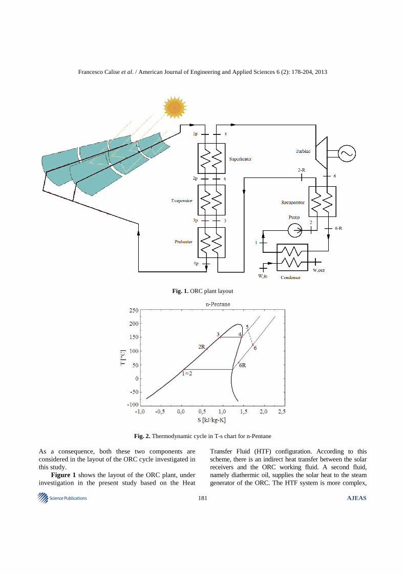
Fig. 1. ORC plant layout

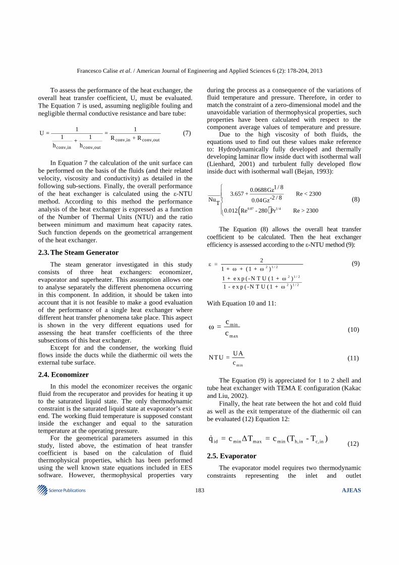
Fig. 2. Thermodynamic cycle in T-s chart for n-Pentane As a consequence, both these two components are considered in the layout of the ORC cycle investigated in this study. Figure 1 shows the layout of the ORC plant, under investigation in the present study based on the Heat

Transfer Fluid (HTF) configuration. According to this scheme, there is an indirect heat transfer between the solar receivers and the ORC working fluid. A second fluid, namely diathermic oil, supplies the solar heat to the steam generator of the ORC. The HTF system is more complex,



more expensive and less efficient then the Direct Vapour Generating (DVG) configuration, but it guarantees best control and regulation of cycle performances. Figure 2 shows a representation of the thermodynamic cycle of the system under investigation in the temperature-entropy chart. The operating principle of the system can be summarized as follows. The working fluid leaves the condenser as saturated liquid (state point 1) at condenser pressure. Then it is compressed by the pump to the evaporator pressure and leaves the pump itself as subcooled liquid. It flows inside the recuperator where it is preheated by the superheated vapour (state point 2R). Then the stream enters into the steam generator, which is divided in three different heat exchangers: economizer, evaporator and superheater. The working fluid, heated by the diathermic oil, leaves the economizer as saturated liquid (state point 3) at evaporating pressure. The heating continues inside the evaporator up to the saturated vapour condition is reached (state point 4). Then the organic fluid is superheated inside the last heat exchanger (state point 5). The cycle continues with the expansion from the maximum pressure to the condenser one (state point 6). The working fluid flows into the recuperator where provides for preheating the subcooled liquid thanks to its high temperature. It leaves the recuperator still as superheated vapour (state point 6R) and reaches the condenser. Here the last phase of the cycle takes place. The stream is condensed by a cold fluid, namely water which can be also used for low-temperature cogenerative purposes and leaves again the condenser as saturated liquid (state point 1).

2. MATERIALS AND METHODS

2.1. Simulation Model

The aim of this study is the development of a steady-state zero-dimensional model of the ORC system under investigation, to be used for energetic, exergetic and thermo-economic analyses and optimizations. As a consequence the model is based on the typical simplifying assumptions, commonly utilized for these kind of problems, namely: • Steady state • Thermodynamic equilibrium at inlet and outlet

sections of each component • Negligibility of kinetic and gravitational terms in the

energy balances • Negligible heat losses toward the environment in

heat exchangers

• Negligible heat losses toward the environment in the pump

• Negligible heat losses toward the environment in the expander

• One-dimensional flow 2.2. Heat Exchangers

The heat exchangers are equipped with a shell and tubes arrangement with single shell and double tube pass in E configuration (Saha and Sekulic, 2003). The reasons of this choice are: • Great flexibility in terms of heat power transferred

between hot and cold fluid • Wide range of operating pressures and temperatures • Wide choice of construction materials • High value of heat power transferred/weight and/or

volume ratio • Great market availability • Low costs Fixing some geometric parameters of heat exchanger as tube length, shell diameter, inner tube diameter, tube thickness, pitch tube and tube number it is possible to calculate all the other geometrical dimensions as follow Equation 1-5:

2oA = d LN m

(1)

i od = d - 2s mm (2)

22i

int,p

πd NA = m

4n

(3)

SB = 0.6D mm (4)

( )S T oS

T

D P - dA = mm

P (5)

To evaluate the shell side heat transfer coefficient the estimation of the equivalent diameter is necessary (Dai et al., 2009). Its expression varies with the tube arrangement. Equation 6 makes reference to the triangular arrangement:

22oT

eqo

dP 34 -π

4 8D = mm

dπ

2

(6)



To assess the performance of the heat exchanger, the overall heat transfer coefficient, U, must be evaluated. The Equation 7 is used, assuming negligible fouling and negligible thermal conductive resistance and bare tube:

conv,in conv,out

conv,in conv,out

1 1U = =

1 1 R + R+h h

(7)

In Equation 7 the calculation of the unit surface can be performed on the basis of the fluids (and their related velocity, viscosity and conductivity) as detailed in the following sub-sections. Finally, the overall performance of the heat exchanger is calculated using the ε-NTU method. According to this method the performance analysis of the heat exchanger is expressed as a function of the Number of Thermal Units (NTU) and the ratio between minimum and maximum heat capacity rates. Such function depends on the geometrical arrangement of the heat exchanger.

2.3. The Steam Generator

The steam generator investigated in this study consists of three heat exchangers: economizer, evaporator and superheater. This assumption allows one to analyse separately the different phenomena occurring in this component. In addition, it should be taken into account that it is not feasible to make a good evaluation of the performance of a single heat exchanger where different heat transfer phenomena take place. This aspect is shown in the very different equations used for assessing the heat transfer coefficients of the three subsections of this heat exchanger. Except for and the condenser, the working fluid flows inside the ducts while the diathermic oil wets the external tube surface.

2.4. Economizer

In this model the economizer receives the organic fluid from the recuperator and provides for heating it up to the saturated liquid state. The only thermodynamic constraint is the saturated liquid state at evaporator’s exit end. The working fluid temperature is supposed constant inside the exchanger and equal to the saturation temperature at the operating pressure. For the geometrical parameters assumed in this study, listed above, the estimation of heat transfer coefficient is based on the calculation of fluid thermophysical properties, which has been performed using the well known state equations included in EES software. However, thermophysical properties vary

during the process as a consequence of the variations of fluid temperature and pressure. Therefore, in order to match the constraint of a zero-dimensional model and the unavoidable variation of thermophysical properties, such properties have been calculated with respect to the component average values of temperature and pressure. Due to the high viscosity of both fluids, the equations used to find out these values make reference to: Hydrodynamically fully developed and thermally developing laminar flow inside duct with isothermal wall (Lienhard, 2001) and turbulent fully developed flow inside duct with isothermal wall (Bejan, 1993):

( )0.87 1/4

1 / 80.0688Gz3.657 + Re < 2300

-2 / 8Nu 0.04GzT0.012 Re - 280 Pr Re > 2300

(8)

The Equation (8) allows the overall heat transfer coefficient to be calculated. Then the heat exchanger efficiency is assessed according to the ε-NTU method (9):

2 1 / 2

2 1 / 2

2 1 / 2

2ε =

1 + ω + (1 + ω )

1 + e x p ( -N T U (1 +ω )1 - e x p ( -N T U (1 + ω )

(9)

With Equation 10 and 11:

min

max

cω =

c (10)

min

UANTU =

c (11)

The Equation (9) is appreciated for 1 to 2 shell and tube heat exchanger with TEMA E configuration (Kakac and Liu, 2002). Finally, the heat rate between the hot and cold fluid as well as the exit temperature of the diathermic oil can be evaluated (12) Equation 12:

id min max min h,in c,inq = c ∆T = c (T - T )& (12)

2.5. Evaporator

The evaporator model requires two thermodynamic constraints representing the inlet and outlet



thermodynamic state points of the working fluid: saturated liquid and saturated dry vapour. The evaluation of the tube-side heat transfer coefficient is extremely hard because of the evaporation process that takes place in that component. This is primarily due to the simultaneous presence of two phases, liquid and vapour, characterized by very different thermodynamic properties. The heat transfer coefficient is calculated according to the procedure suggested by (Kakac and Liu, 2002; Shah, 1976). Shah’s correlation is based on four dimensionless parameters that are employed for evaluating the two-phase convective contribution to heat transfer in boiling: FrL, BO, CO and F0. The Froude number is a measure of stratification effects. If the Froude number is higher than 0.04 inertial forces are greater than gravitational ones Equation 13:

2

L 2l i

GFr =

ρ gd (13)

The convection number is defined as (Smith, 1976) Equation 14:

0.50.8v

O FRl

ρ1- xC = K

x ρ

(14)

When the Froude number is higher than 0,04 the correction factor, KFR is equal to 1 vice versa it is equal to Equation 15:

-0.3FR LK = (25Fr ) (15)

The boiling number, BO, measures the effect of nucleate boiling in heat transfer process. It is defined as Equation 16:

Olv

qB =

mi

&&

& (16)

The enhancement factor, F0, is strictly related to the characteristics of boiling. It is the ratio of convective heat transfer coefficient for two-phase to liquid-only flow. It is defined as:

TP0

LO

hF =

h (17)

0F = F(1- x) (18) Like the Equation (17) explains the two-phase heat transfer coefficient can be evaluated by means the liquid-only heat transfer coefficient, calculated by the well known heat transfer correlation for flow inside duct. Nevertheless the enhancement factor is function of heat transfer regime that occurs inside ducts. This feature is taken into account by means the factor F, used in the Equation (18). For pure convection boiling, that occurs at high vapour qualities, the factor F is defined as (Smith, 1976) Equation 19 and 20:

CB

-0.8O O

0.5O O

-5O

F = F =

1.8C C < 1.0

1.0 + 0.8exp 1- C C > 1.0

et B < 1.9×10

(19)

NB O

O O

0.5

-5

F = F = 231B

C > 1.0 et B > 1.9×10 (20)

When the vapour quality growths both nucleate and convection boiling effects must be take into account. The factor F is define as (Smith, 1976) Equation 21:

CNB NB CB

O

F = F = F (0.77 + 0.13F )

0.02 < C < 1.0 (21)

Making reference to the correlations just mentioned, in this study the boiling heat transfer is evaluated as arithmetic mean of different heat transfer coefficient each one assessed for a specific quality value. The shell-side heat transfer coefficient can be evaluated using the Equation 8. Then using the ε-NTU method it is possible to determinate the evaporator efficiency (22). It is worth noting that the expression is easier than before due to the cold fluid boiling that leads to zero the value of ω (10) Equation 22:

-NTUε = 1 - e (22)

The organic fluid flows through the superheater where it is heated by the diathermic oil. There is only one thermodynamic constraint related to the fluid inlet state point as saturated vapour. The working fluid temperature is supposed constant.



To evaluate the tube-side heat transfer coefficient the following expressions are used (23-24). They can be applied for fully developed laminar flow inside duct with isothermal wall (Saha and London, 1978) and fully developed turbulent flow inside duct with isothermal wall (Bejan, 1993) Equation 23 and 24:

( )( )

3

T 0.5

2/3

3.66 Re < 2300

0.5f Re -10 PrNu = Re > 2300

f1+12.7 Pr -1

2

(23)

-1/4 4

-1/5 4

0.079Re 2300 < Re < 2×10f =

0.046Re Re > 2×10

(24)

To calculate the shell-side heat transfer coefficient the Equation (8) is used. The Equation (9) allows one to evaluate the superheater efficiency and then the remaining temperatures of diathermic oil and organic fluid.

2.6. Recuperator

The recuperator provides the preheating of the organic fluid using the energy available by the expander outlet stream. In the recuperator the equations used to calculate the shell and tube side heat transfer coefficient are the same of those applied in economizer and superheater: (23-24) for the shell-side and (8) for the tube-side.

2.7. Condenser

The condensation process implies the simultaneous presence of two phases: liquid and vapour. Unlike the evaporator, the phase transition occurs outside the tubes while a cold fluid, e.g. water, provides for the cooling process. The Nusselt’s theory is used to evaluate the shell-side heat transfer coefficient (Nusselt, 1916). This theory can be applied in case of laminar film condensation of a quiescent vapour on an isothermal horizontal tube (25):

( ) 1/ 43l l v lv oc o

l l sat w

ρ ρ - ρ gi dh d= 0.728

k µ (T - T )

(25)

The Equation (25) does not take into account the influence of aerodynamic forces, of shear stress between the vapour and the condensate, of separation effects and of tube bundles configuration. Many studies, made by

Kern (1958); Eissenberg (1972) and Nusselt (1916) in discovering the effects of condensate inundation, establish that the number of rows has a big influence in the condensation process. In the present paper, Equation (26), proposed by Kern and recommended by Butterworth (1977), is used in calculating the shell-side heat transfer coefficient:

-1/6c c rowh = h n

(26)

To evaluate the tube-side heat transfer coefficient the Equation (23-24) are used. Finally the condenser efficiency is calculated with the simplified Equation 22:

2.8. Expander

The expanders can be classified in two categories: volumetric and dynamic expander. According to Quoilin et al. (2010) the expander selection depends on the thermodynamic properties of the working fluid, the mechanical power required, the mass and volume flow rate and the volumetric expansion ratio. In this work the expander is modelled only from a thermodynamic point of view. It is considered adiabatic and its isentropic efficiency, expressed as the ratio of effective to isentropic enthalpy drop (27), is constant and fixed to 0.80, independently from the effective expander working point Equation 27:

5 6ex

5 6s

i - iη =

i - i (27)

The power generated by the expander can be given as Equation 28:

( ) ( )ex 5 6 5 6s exW = m i - i = m i - i η& & & (28)

2.9. Pump

The feed pump as the expander is modelled only from a thermodynamic point of view. It is considered adiabatic and its adiabatic efficiency is constant and fixed to 0.85, regardless of the compression ratio (29) Equation 29:

2s 1pump

2 1

i - iη =

i - i

(29)

The mechanical power employed by the pump is Equation 30:



( ) ( )2s 1pump 2 1

pump

m i - iW = m i - i =

η

&& & (30)

2.10. Diathermic Oil

The selection of the diathermic oil has a great influence in a solar thermal ORC power plant. The oil receives the solar thermal radiation and supplies the heat to the organic fluid. The principal features of good diathermic oil are: • Good thermal and chemical stability • High specific heat • Not toxic • Low inflammability • Good material compatibility • Low viscosity • Low cost The diathermic fluid chosen is a eutectic mixture of two very stable compounds, biphenyl and diphenyl oxide. It can be used in the heat transfer application both in liquid and vapour phase. It is used in liquid phase in the model and its application range starts from 15°C up to 400°C. The analytical functions of the fluid properties, namely specific heat, viscosity, thermal conductivity and density are shown below Equation 31-34:

-3c = 2.90×10 T +1.51 (31)

-12 5 -8 4 -6 3

-3 2 -1

µ = -8.76×10 T +1.06×10 T - 4.93×10 T

+1.10×10 T -1.23×10 T + 6.11 (32)

-4 -1k = -2.00×10 T +1.42×10 (33)

-4 2 -1 3

ρ = -7.00×10 T - 6.65×10 T +1.07×10 (34) 2.11. Simulation Algorithm

Each simulation model includes a certain number of variables. They may be divided in three groups: design, input and output variables. The design variables are: • The geometric features of each heat exchanger • The adiabatic efficiency of expander • The adiabatic efficiency of pump • The electric efficiency of alternator The input variables are:

• The diathermic oil mass flow rate • The diathermic oil inlet temperature • The cooling water inlet temperature • The temperature difference between water and

organic medium at the exit end of condenser The output variables are not only the thermodynamic states of diathermic oil and working fluid at the entrance and exit ends of each element of the plant, but also the global performances of ORC system, in terms of heat power transferred through the exchangers, the electric power generated and the cycle efficiency. The working criterion of the simulation program is particularly complex. First of all, specific subprograms are developed for each component of the power plant. The subprogram consists in input and output variables and in a certain numbers of equations. It allows one to calculate the output variables in the basis of the fixed input parameters. Obviously, the subprograms are strictly inter-related. Calling all of them in the main program a complex network of relationships is realized. It represents the real physic connections that occur between the components of the power plant. The number of unknown variables is eighteen since the heat power transferred in the recuperator and the mechanical power produced by the expander are only function of organic fluid mass flow rate, being known variables the temperatures T6R , T6 and T5. To have a consistent system eighteen equations are also needed. Seven “equations” come from the subprogram statements. Four equations are the input parameters of the cycle. Six equations are represented by the thermodynamic bonds of the cycle. The last equation guarantees that the pressure level and the organic fluid mass flow rate are able to ensure the respect of two bonds of the cycle: organic fluid as saturated liquid and saturates vapour at the entrance and exit ends of the evaporator respectively. With these statements the number of equation is equal to the number of unknown variables. The equation system is well-posed and the simulations can be done. In fact one of the most important feature of EES is that the equation can be entered in any order and the program itself provides to calculate the solution, if any.

2.12. Total Cost Function

In the present work the optimization analysis has been realized minimizing the total cost function. The total cost function is defined as:



ORCtot

€€ = - I

FA (35)

The term €ORC makes reference to the capital cost of the power plant. It neglects the cost of the solar plant because this analysis could be extended also to the exploitation of different heat sources. Moreover the cost of the auxiliary devices (pumps, pipes, control system) is also neglected. Conversely, the costs of heat exchangers and working fluid are taken into account, using empirical equations or assessments Equation 36:

ORC hex fluid ex€ = € + € + € (36) The main cost of the plant is the cost of shell and tube heat exchangers that can be evaluated with the following equation (Cheung and Hui, 2001) Equation 37:

0.6hex hex€ =Φ +Ψ× A (37)

The values of Φ and Ψ are shown in the Table 1 and are only function of total heat exchanger’s area. The specific cost of the working fluid is valued 3 $/kg. The knowledge of punctual density value of working fluid should be requested to evaluate the total working fluid mass. This is unfeasible in a zero-dimensional analysis, so the total working fluid mass is evaluated considering the known density value at the entrance or exit ends of each heat exchanger. Unlike the heat exchangers, no empirical equation is available in literature for estimating the cost of small-sized expanders. Considering radial turbines, used for supercharger groups, a specific cost of 400 €/kW is here considered. In the Equation (35) the ORC cost is divided by the annuity factor FA. This factor is necessary to contextualize the investment costs. It is evaluated making reference to ten years of service life and an interest rate of 5% Equation 38:

-y1- (1+ r)FA =

r (38)

Finally the income, that is computed with the minus sign (35), is evaluated taking into account the electricity tariff, the state energy incentives and the net power generated. Table 1. Cost function’s parameters

Φ Ψ

0 ≤ Ahex ≤ 80 4500 600 80 ≤ Ahex ≤ 160 15000 250 160 ≤ Ahex ≤ 240 21000 120

The plant operating time is estimated in 3650 h/year Equation 39:

net pI = 3650× W e (39)

The unit electricity price is given as Equation 40:

p sales ince = e + e (40) According to the Italian energy incentives for renewable energy promotion (MDSE, 2008) and the unit average electricity price in January 2012 (GMP, 2012) the unit electricity price is equal to 0.33 €/kWh.

3. RESULTS AND DISCUSSION

The simulation model presented in the previous section was used to perform some analyses aiming at detecting the optimal synthesis/design parameters for the plant under investigation. In particular, special attention has been paid to the selection of the working fluid, performing a sensitivity analysis aiming at evaluating the performance of the system using some of the most common organic fluids. Then, for the fluid considered as the best candidate, parametric analyses and optimizations have been performed in order to determine the set of design and operating parameters maximizing the thermo-economic performance of the system under investigation.

3.1. Selection of the Organic Working Fluid

The selection of the organic fluid is the very first step in the design procedure of an ORC power plant. Such selection strongly depends on the temperature level of heat source. The selection criteria are different, both the thermodynamic properties and the environmental impact of the fluids must be taken into account. Table 2. Limit values of temperature and pressure for each fluid Critical Critical Maximum temperature pressure temperature Substance [°C] [bar] [°C] Acetone 234,95 47 281 Benzene 288,87 48,94 476 Cyclohexane 280,49 40,75 426 Isobutane (R600a) 134,67 36,40 296 Isopentane 187,24 33,69 276 n-Butane (R600) 151,97 37,96 315 n-Hexane 234,7 30,58 370 n-Pentane 196,54 33,64 315 Toluene 318,6 41,26 426 R245fa 154,01 36,51 166



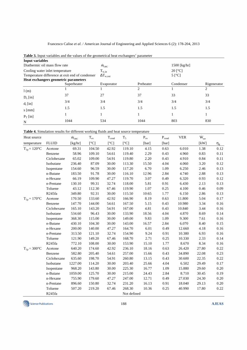
Table 3. Input variables and the values of the geometrical heat exchangers’ parameter Input variables Diathermic oil mass flow rate &ORCm 1500 [kg/hr]

Cooling water inlet temperature Tw,in 20 [°C] Temperature difference at exit end of condenser ∆Tw,out 5 [°C] Heat exchangers geometric parameters Superheater Evaporator Preheater Condenser Rigenerator

l (m) 1 1 2 1 2

Ds [in] 37 27 37 33 33

di [in] 3/4 3/4 3/4 3/4 3/4

s [mm] 1.5 1.5 1.5 1.5 1.5

PT [in] 1 1 1 1 1

N 1044 534 1044 803 830

Table 4. Simulation results for different working fluids and heat source temperature

Heat source &ORCm Tev Tcond T5 Pev Pcond VER netW&

temperature FLUID [kg/hr] [°C] [°C] [°C] [bar] [bar] [kW] ηg

T1p = 120°C Acetone 69.31 104.50 42.92 119.10 4.15 0.63 6.010 1.38 0.12 Benzene 58.96 109.10 54.61 119.40 2.29 0.43 4.960 0.83 0.11 Ciclohexane 65.02 109.00 54.91 119.80 2.20 0.43 4.910 0.84 0.11 Isobutane 236.40 87.09 30.00 113.30 15.50 4.04 4.060 3.20 0.12 Isopentane 154.60 96.59 30.00 117.20 6.70 1.09 6.250 2.46 0.13 n-Butane 183.50 91.78 30.00 116.10 12.96 2.84 4.740 2.88 0.13 n-Hexane 66.19 109.90 47.27 119.70 3.07 0.49 6.320 0.93 0.12 n-Pentane 130.10 99.31 32.74 118.00 5.81 0.91 6.430 2.13 0.13 Toluene 43.12 112.30 67.46 119.90 1.07 0.25 4.100 0.46 0.09 R245fa 349.80 92.31 30.00 115.50 10:65 1.77 6.150 2.86 0.13 T1p = 170°C Acetone 170.50 133.60 42.92 166.90 8.19 0.63 11.800 5.04 0.17 Benzene 147.70 144.00 54.61 167.50 5.15 0.43 10.980 3.34 0.16 Ciclohexane 165.10 143.20 54.91 167.00 4.81 0.43 10.840 3.44 0.16 Isobutane 534.60 96.43 30.00 133.90 18.56 4.04 4.870 8.69 0.14 Isopentane 368.30 115.00 30.00 149.00 9.83 1.09 9.300 7.61 0.16 n-Butane 430.10 104.30 30.00 143.00 16.57 2.84 6.070 8.40 0.15 n-Hexane 200.00 140.00 47.27 164.70 6.01 0.49 12.660 4.18 0.16 n-Pentane 313.50 121.10 32.74 154.90 9.24 0.91 10.380 6.93 0.16 Toluene 121.90 149.20 67.46 168.70 2.71 0.25 10.330 2.33 0.14 R245fa 772.10 108.00 30.00 153.90 15.10 1.77 8.670 8.34 0.16 T1p = 300°C Acetone 640.20 174.60 42.92 236.10 18.16 0.63 26.420 27.80 0.22 Benzene 582.80 205.40 54.61 257.00 15.66 0.43 34.890 22.08 0.23 Ciclohexane 635.60 198.70 54.91 260.80 13.15 0.43 30.600 22.35 0.22 Isobutane 1227.00 114.20 30.00 203.40 25.66 4.04 6.502 29.49 0.17 Isopentane 968.20 143.80 30.00 225.30 16.77 1.09 15.880 29.60 0.20 n-Butane 1059.00 125.70 30.00 215.00 24.43 2.84 8.710 30.45 0.19 n-Hexane 755.90 179.60 47.27 247.00 12.71 0.49 27.030 24.30 0.20 n-Pentane 896.60 150.80 32.74 231.20 16.13 0.91 18.040 29.13 0.20 Toluene 507.20 219.20 67.46 268.30 10.36 0.25 40.990 17.80 0.22 R245fa Not defined



Many studies on the organic fluid selection criteria are available in scientific literature. Despite the different results, according to the different final goals, most of studies agree that the optimization parameters that must be taken into account are: the first law efficiency, the mechanical power generated, the Volume Expansion Ratio (VER) and the exergy efficiency (Bejan, 1982). From a thermodynamic point of view, the optimal cycle is characterized by the higher first law efficiency. Nevertheless the thermal efficiency allows one to find out only thermodynamic information about the cycle. Because it does not bring with itself any technical information, another parameter becomes important: the Volume Expansion Ratio (VER) Equation 41:

ex,out

ex,in

VVER =

V

&

& (41)

The higher the VER, the higher the fluid volume mass flow rate at expander outlet. This causes a growth of the expander, pipes and condenser since an increase in power plant’s cost. Furthermore if the expander is a turbine, high value of VER, joined with high fluid mass flow rate, may generate problem of supersonic flow inside the final stage of turbine, so the aim is to reduce as much as possible the VER. The group of organic fluids under investigation in this study is shown in Table 2. The cycle performances have been evaluated using three different values of the diathermic oil inlet temperature, T1p, unchanging the geometric features of the heat exchangers and the diathermic oil mass flow

rate. Table 3 shows the common input variables and the values of the geometrical heat exchangers’ parameter. Note that the outlet temperature of the fluid exiting from the parabolic trough collectors is limited only by the type of operating fluid selected. Therefore, in this study the following temperature levels of the heat sources are assumed: low temperature (T1p=120°C), medium temperature (T1p=170°C) and high temperature (T1p=300°C). Considering the physical properties of fluids shown in Table 2, the simulations at low and medium temperature level can be performed using all the fluids included in that table. Conversely, the R245fa cannot be employed with the high temperature heat source because the difference between the diathermic oil inlet temperature and the maximum temperature, allowed by the EES’s state equations, is too high. The results of simulations are shown in Fig. 3-5 and Table 4. The trend of the first law efficiency is as one can expect from it, Fig. 3. Rising the diathermic oil inlet temperature, the cycle efficiency increases. This growth is particularly appreciated for the substances with high critical temperature. Moving from lower to higher temperature heat source, Toluene, the substance with the highest critical temperature (318.6°C), shows the biggest growth in first law efficiency, from 9% to 22%, at the contrary isobutene, that has the lowest critical temperature (134.7°C), shows the lowest increase, from 12% to 17%. In fact, when the critical temperature is high, an increase of the heat source temperature is followed by a growth of boiling one.

Fig. 3. First law efficiency Vs organic medium



Fig. 4. Net power Vs organic medium

Fig. 5. VER Vs organic medium Going from low to high heat source temperature the boiling temperature increment is equal to 107°C for Toluene while it is only 27°C for Isobutene. This causes an increase of the average heat supply temperature that corresponds to an improvement of system efficiency. The mechanical net power generation shows a similar behaviour varying the heat source temperature, Fig. 4. As above-mentioned, using high temperature heat sources, the evaporation temperature growths as well as the temperature of the organic fluid at the exit end of steam generator. This temperature increase is brought under control by the working fluid mass flow rate that

prevents the organic medium from achieving the heat source temperature. Increasing the boiling pressure the expansion ratio becomes significant. Because of these trends the specific work of expander growths, thanks also to the constant condenser pressure and the unvarying isentropic efficiency of expander. Hence the increase of both specific work of expander and working fluid mass flow rate justify the mechanical power trend, Fig. 4. Moreover fixing the heat source, the hydrocarbons isobutene, n-butene, isopentane and n-pentane and the coolant R245fa show their capability of generating more power than the other substances,



especially for low and medium temperature heat source. That behaviour is strictly linked to the critic temperature of the substance. In fact for light hydrocarbons the lower critical temperature, the lower evaporating temperature and the higher working fluid mass flow rate in order to prevent the organic fluid from reaching the diathermic oil inlet temperature. The high mass flow rate coupled with the low condensing temperature and the high expander inlet temperature well explain the mechanical power increase. These trends are well explain comparing the light hydrocarbons to Toluene performances. It is well known that Toluene has the highest critical temperature and shows, for each heat source temperature, the lowest mechanical power generation, the lowest working fluid mass flow rate and the higher evaporation temperature. Nevertheless the gap in mechanical power produced between Toluene and the best working fluid deeply decreases moving from low to high temperature heat source. For the lowest temperature heat source, the mechanical power generated by isobutene is quite seven times the one of Toluene while for the highest temperature heat source this difference is a little bit less than two. This aspect again underlines the influence of the temperature level of heat source on the working fluid selection criterion. Finally, it is worth noting that Toluene has the highest condenser temperature, equal to 67.46°C. Even if an high condenser temperature reduces the electric power generation and the global efficiency of the plant, it also makes feasible a cogeneration use of waste heat that it does not take into account in the present work. The VER shows a completely different trend, Fig. 5. It is strictly related to the expansion ratio namely to the boiling and condensing pressure. Increasing the temperature level of heat source the expansion ratio increases, due to the higher boiling temperature and VER progressively growths. Considering the lower heat source temperature, the substance with the lowest VER value is Isobutene, 4.06, instead the worst fluid is n-Pentane with a VER value equal to 6.43, that is 53.4% greater than Isobutene. The differences of VAR values become significant as the temperature heat source increases. At 120°C the VER ratio of n-Pentane to Isobutene is 1.58 and it slowly increases moving from lower to higher temperature heat source up to 2.76 at 300°C. At the contrary, other substances like Toluene or Benzene show a completely different trend. At the lower heat source temperature their VER values are almost the same of Isobutene, 4.10 and 4.96 respectively. As the heat source temperature increases, the VER values

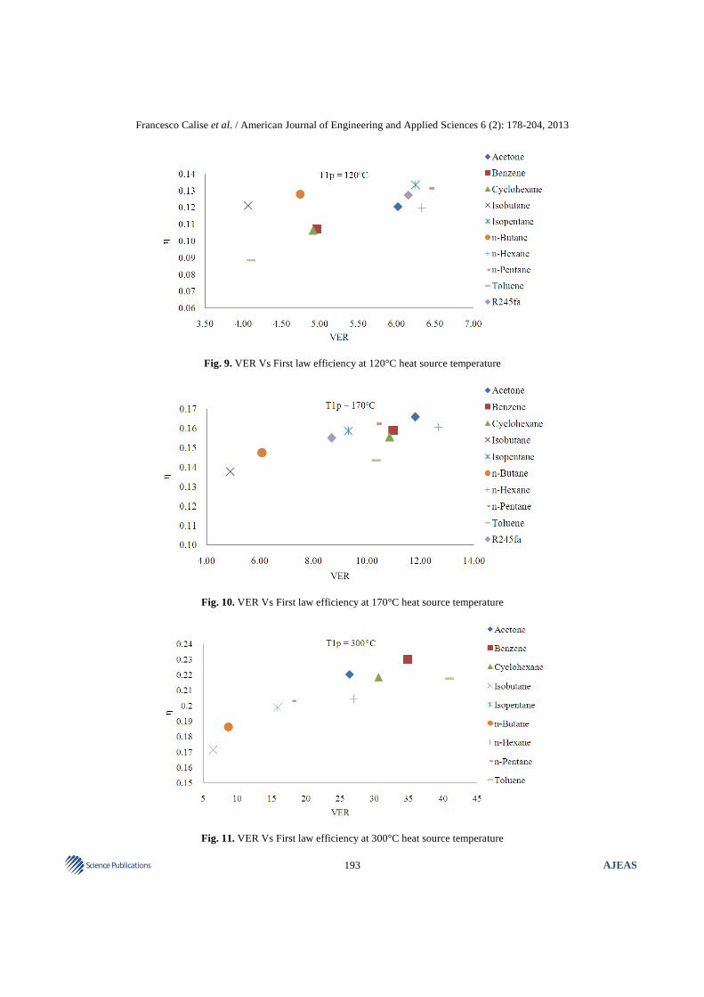
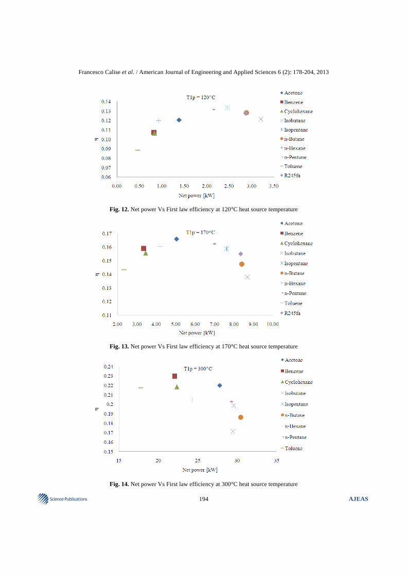
rapidly growth. In fact at the higher heat source temperature, Toluene and Benzene VER value are 40.99 and 34.89 and their ratios to Isobutene VER are 6.30 and 5.37 respectively. This trend is essentially due to the boiling pressure increase that occurs when the temperature of heat source growths. In fact the higher boiling pressure, the higher expansion ratio and the higher the VER. Finally Fig. 5 shows that Isobutene has the lowest value of VER, independently of heat source temperature. Isopentane, n-Pentane and n-Butane also show good value of VER. Figure 6-8 compare the VER values to the mechanical power generated by the cycle varying the heat source temperature. It is well known that the best fluid must have the higher mechanical power generation and the lower volume expansion ratio. The Isobutane has these features for each temperature heat source, closely followed by n-Butane. It is worth noting that higher the heat source temperature, the lower the VER gap between Isobutane and n-Butane and the higher the mechanical power of n-Butane. Figure 9 shows that Isobutane and n-Butane have the lower VER and good first law efficiency values. Hence they can be still considered as the best fluid for low temperature heat source exploitation. Instead Fig. 10 and 11 show that Isobutane and n-Butane have the lower cycle efficiency but also the lower VER values. At 170°C the Isobutane first law efficiency is 17.6% lower than the highest efficiency value (Acetone) but the ratio of their VAR values is 2.60, Fig. 10. This means that in fluid selection the VER difference between the best and worst fluid has more influence than first law efficiency. Figure 11 also shows the same trend. In this case the Isobutane first law efficiency is 26.1% lower than Benzene but their VER ratio is 5.37, in other words Benzene’s VER value is more than five times Isobutene one. Finally Fig. 12-14 compare the first law efficiency values to the mechanical power generated by the cycle. Figure 12 shows that five fluid have both good values of fist law efficiency and mechanical power namely n-Pentane, n-Hexane, n-Butane, R245fa and Isobutane. Same trend can be detected in Fig. 13 and in Fig. 14. In conclusion the simulation results show that two substances are suitable for the exploitation of all heat sources: Isobutane and n-Butane. Independently of heat source temperature, these hydrocarbons have low VAR values generate more power than other substances and have good values of fist law efficiency as well. Finally, for low and medium temperature heat source, the refrigerant R245fa also shows good performances.



Fig. 6. VER Vs Net power at 120°C heat source temperature





Fig. 9. VER Vs First law efficiency at 120°C heat source temperature





Fig. 12. Net power Vs First law efficiency at 120°C heat source temperature





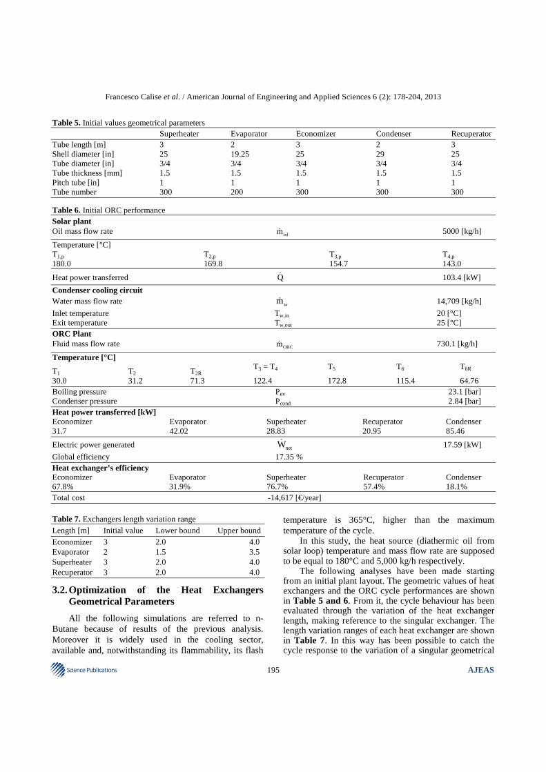
Table 5. Initial values geometrical parameters Superheater Evaporator Economizer Condenser Recuperator Tube length [m] 3 2 3 2 3 Shell diameter [in] 25 19.25 25 29 25 Tube diameter [in] 3/4 3/4 3/4 3/4 3/4 Tube thickness [mm] 1.5 1.5 1.5 1.5 1.5 Pitch tube [in] 1 1 1 1 1 Tube number 300 200 300 300 300 Table 6. Initial ORC performance Solar plant Oil mass flow rate oilm& 5000 [kg/h]

Temperature [°C] T1,p T2,p T3,p T4,p 180.0 169.8 154.7 143.0

Heat power transferred Q& 103.4 [kW]

Condenser cooling circuit Water mass flow rate wm& 14,709 [kg/h]

Inlet temperature Tw,in 20 [°C] Exit temperature Tw,out 25 [°C] ORC Plant Fluid mass flow rate ORCm&

730.1 [kg/h]

Temperature [°C]

T1

T2

T2R T3 = T4 T5 T6 T6R

30.0 31.2 71.3 122.4 172.8 115.4 64.76 Boiling pressure Pev 23.1 [bar] Condenser pressure Pcond 2.84 [bar] Heat power transferred [kW] Economizer Evaporator Superheater Recuperator Condenser 31.7 42.02 28.83 20.95 85.46

Electric power generated netW& 17.59 [kW]

Global efficiency 17.35 % Heat exchanger’s efficiency Economizer Evaporator Superheater Recuperator Condenser 67.8% 31.9% 76.7% 57.4% 18.1% Total cost -14,617 [€/year] Table 7. Exchangers length variation range

Length [m] Initial value Lower bound Upper bound

Economizer 3 2.0 4.0 Evaporator 2 1.5 3.5 Superheater 3 2.0 4.0 Recuperator 3 2.0 4.0

3.2. Optimization of the Heat Exchangers Geometrical Parameters

All the following simulations are referred to n-Butane because of results of the previous analysis. Moreover it is widely used in the cooling sector, available and, notwithstanding its flammability, its flash

temperature is 365°C, higher than the maximum temperature of the cycle. In this study, the heat source (diathermic oil from solar loop) temperature and mass flow rate are supposed to be equal to 180°C and 5,000 kg/h respectively. The following analyses have been made starting from an initial plant layout. The geometric values of heat exchangers and the ORC cycle performances are shown in Table 5 and 6. From it, the cycle behaviour has been evaluated through the variation of the heat exchanger length, making reference to the singular exchanger. The length variation ranges of each heat exchanger are shown in Table 7. In this way has been possible to catch the cycle response to the variation of a singular geometrical



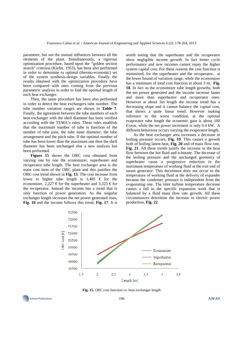
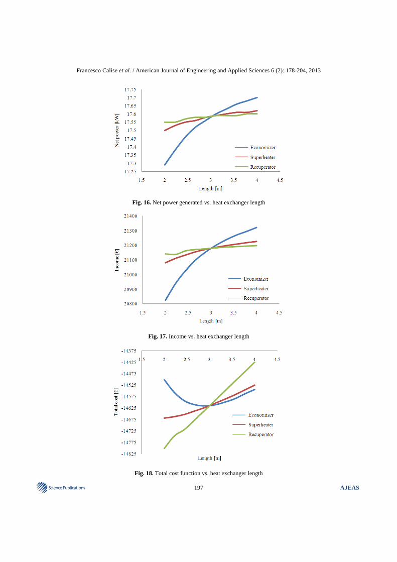
parameter, but not the mutual influences between all the elements of the plant. Simultaneously, a rigorous optimization procedure, based upon the “golden section search” criterion (Kiefer, 1953), has been also performed in order to determine to optimal (thermo-economic) set of the system synthesis-design variables. Finally the results obtained with the optimization procedure have been compared with ones coming from the previous parametric analysis in order to find the optimal length of each heat exchanger. Then, the same procedure has been also performed in order to detect the heat exchangers tube number. The tube number variation ranges are shown in Table 7. Finally, the agreement between the tube numbers of each heat exchanger with the shell diameter has been verified according with the TEMA’s rules. These rules establish that the maximum number of tube is function of the number of tube pass, the tube inner diameter, the tube arrangement and the pitch tube. If the optimal number of tube has been lower than the maximum one then the shell diameter has been unchanged else a new analysis has been performed. Figure 15 shows the ORC cost obtained from varying one by one the economizer, superheater and recuperator tube length. The heat exchanger area is the main cost item of the ORC plant and this justifies the ORC cost trend shown in Fig. 15. The cost increase from lower to higher tube length is 3,485 € for the economizer, 2,227 € for the superheater and 3,325 € for the recuperator. Instead the income has a trend that is only function of power generation. As the singular exchanger length increases the net power generated rises, Fig. 16 and the income follows this trend, Fig. 17. It is

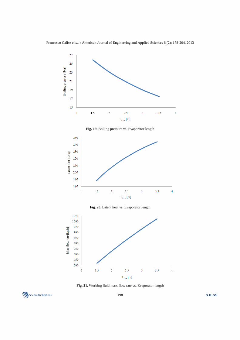
worth noting that the superheater and the recuperator show negligible income growth. In fact better cycle performance and new incomes cannot repay the higher system capital cost. For these reasons the cost function is minimized, for the superheater and the recuperator, at the lower bound of variation range, while the economizer has a minimum of total cost function at about 3 m, Fig. 18. In fact as the economizer tube length growths, both the net power generated and the income increase faster and more than superheater and recuperator ones. However at about 3m length the income trend has a decreasing slope and it cannot balance the capital cost, that shows a quite linear trend. However making reference to the worst condition, at the optimal evaporator tube length the economic gain is about 100 €/year, while the net power increment is only 0.4 kW. A different behaviour occurs varying the evaporator length. As the heat exchanger area increases a decrease in boiling pressure occurs, Fig. 19. This causes a growth both of boiling latent heat, Fig. 20 and of mass flow rate, Fig. 21. All these trends justify the increase in the heat flow between the hot fluid and n-butane. The decrease of the boiling pressure and the unchanged geometry of superheater cause a progressive reduction in the maximum temperature of working fluid at the exit end of steam generator. This decrement does not occur to the temperature of working fluid at the delivery of expander because the condenser pressure is independent from the evaporating one. The inlet turbine temperature decrease causes a fall in the specific expansion work that is balanced by a fluid mass flow rate growth. All these circumstances determine the increase in electric power production, Fig. 22.

Fig. 15. ORC cost function vs. heat exchanger length



Fig. 16. Net power generated vs. heat exchanger length

Fig. 17. Income vs. heat exchanger length

Fig. 18. Total cost function vs. heat exchanger length



Fig. 19. Boiling pressure vs. Evaporator length

Fig. 20. Latent heat vs. Evaporator length

Fig. 21. Working fluid mass flow rate vs. Evaporator length



Fig. 22. Net power vs. evaporator length

Fig. 23. Production cost function vs. evaporator length Figure 22 and 23 show that the higher evaporator area the higher power generated and income. At 1.5m length the net power and income are 18,816 €/year and is 15.62 kW, while at 3.5m length are 21.53 kW and 25.930 €/year respectively, showing an increment of 37.8%. It is worth noting that the income increase is quite two order of magnitude higher than the economizer one. As always the ORC cost follows the heat exchanger trend, Fig. 24. At 1.5m and 3.5m length the ORC capital cost is 6,325 €/year and 6,777 €/year respectively. This low capital cost increment (452 €/year) coupled with the significant income increase (7,069 €/year) justify the total cost trend, Fig. 25. Hence the optimal evaporator length corresponds to the upper bound of the evaporator length. The results of the rigorous mathematical optimization agree with the ones just described. It is

performed through a simultaneous variation of economizer, evaporator, superheater and recuperator tube length. Finally the optimal exchangers lengths are summarized in Table 8. The next analysis aims at finding the optimal number of tubes for each heat exchanger. This analysis is referred to the heat exchangers lengths equal to the optimal ones, as calculated above. As it can be expected, increasing the number of tubes the total heat exchanger area increases too. This means that the ORC behaviour is basically similar to the one achieved in case of higher tube lengths. Figure 26 and 27 performed through a singular heat exchangers tube number variation confirm this assessment.



Fig. 24. ORC cost function vs. evaporator length

Fig. 25. Total cost function vs. evaporator length

Fig. 26. Total cost vs. Exchanger tube number



Fig. 27. Total cost vs. Evaporator tube number

Fig. 28. Total cost function vs. shell diameter The economizer has a minimum of total cost function (-19,050 €/year) at about 330 tubes and the income is 2.1% higher than the worst solution. The superheater and the recuperator minimize the objective function at the lower bound of variation range, 200 tubes. Nevertheless their influence in total cost function variation is negligible, as Fig. 26 well shows. Finally, also in this case, the main contribution to the income increase is given by the evaporator, Fig. 27. It has the minimum of total cost function (-23,325 €/year) at the higher tube number, 350 tubes and the income is 52,6% higher than the worst solution. A rigorous mathematical optimization procedure has been also performed in order to take into account the mutual influences between all the exchangers. The results are summarized in Table 8. After the definition of the optimal tube numbers it is necessary to verify the optimal value of the shell

diameter in agreement with TEMA’s prescriptions (Kakac and Liu, 2002; Kern, 1950). The simulation shows that the evaporator tube number is higher than the maximum one instead for the superheater and the recuperator the number of tube is lower than its upper limit. For these reasons the analyses are performed making reference to higher and lower value of shell diameter for the evaporator and the superheater and recuperator respectively. The analysis of results shows that the decrease in the shell diameter causes a decrement in the total cost function for each exchanger, Fig. 28. It is important to underline that in the Equation (37) the shell diameter variation is not taken into account. When the shell diameter decreases the transversal encumbrance as well as the material amount is reduced hence the total cost of the exchanger will be lower.



Table 8. Optimal geometric parameters Superheater Evaporator Economizer Condenser Recuperator Tube length [m] 2.00 3.5 3 2 2.00 Shell diameter [in] 19.25 21.25 25 29 21.25 Tube number 219.00 300.00 300 300 262.00

Table 9. ORC performance Solar plant Oil mass flow rate oilm& 5000 [kg/h]

Temperature [°C] T1,p

T2,p

T3,p

T4,p

180.0 163.2 132.6 117.7

Heat power transferred Q& 172.1 [kW]

Condenser cooling circuit Water mass flow rate wm& 25,084 [kg/h]

Inlet temperature Tw,in 20 [°C] Exit temperature Tw,out 25 [°C] ORC Plant Fluid mass flow rate ORCm& 956.8 [kg/h]

Temperature [°C] T1

T2

T2R

T3 = T4

T5

T6

T6R

30.0 30.9 68.7 107.4 160.4 112.1 64.12 Boiling pressure Pev 17.6 [bar] Condenser pressure Pcond 2.84 [bar] Heat power transferred [kW] Economizer Evaporator Superheater Recuperator Condenser 39.3 84.3 47.4 33.8 145.5

Electric power generated netW& 26.1 [kW]

Global efficiency 15.45 % Heat exchanger’s efficiency Economizer Evaporator Superheater Recuperator Condenser 64.8% 54.9% 68.6% 56.5% 26.3% Total cost -23,522 [€/year] Finally the optimal geometrical parameters, able to minimize the total cost function, are shown in Table 8, while the ORC performances are summarized in Table 9. The net power generated is 26.01 kW, the total cost function is -23,522 €/year and the global efficiency is 15.45%. Comparing these values with the initial condition, it results an increment of net power and economic benefit equal to 48.2% and 60.9% respectively, against a global efficiency decrement equal to 10.9%.

4. CONCLUSION

In this study the effect of fluid and heat exchanger design parameter on performances of an Organic Rankine Cycle (ORC) are examined. A new simulation model is developed to this scope.

Two different simulations are made. The first simulation describes a working fluid evaluation criterion varying the heat sources level of temperature: low temperature (120°C), medium temperature (170°C) and high temperature (300°C). The second simulation aims at selecting a design optimization criterion of some geometrical parameters of the shell and tube heat exchangers. The total cost of power plant has been chosen as objective function. The simulation results show that two organic mediums are suitable for the exploitation from low to high temperature heat source: n-Butane and Isobutane. These hydrocarbons have low VAR values generate more power than other substances and have good values of fist law efficiency as well. It is worth noting that the refrigerant R245fa can add to n-Butane and Isobutane for heat source up to 170°C.



The second round of simulations shows that the geometric features of heat exchangers have great influence on the cycle performance. Furthermore the evaporator geometric parameters have the highest influence in cycle performance. With respect to the total cost minimization, as objective function, higher the heat transfer area, higher the electric power generation and the economical benefit. The optimal configuration, compared to the initial one, shows an increase of incomes and mechanical power equal to 48.2% and 60.1% respectively, against a global efficiency decrease from 17.35 to 15.45%, equal to 10.9%.

5. REFRENCES

Bejan, A., 1982. Entropy Generation through Heat and Fluid Flow. 1st Edn., John Wiley and Sons, New York, ISBN-10: 0471094382, pp: 248.

Bejan, A., 1993. Heat Transfer. 1st Edn., John Wiley and Sons, New York, ISBN-10: 0471502901, pp: 675.

Bruno, J.C., J. Lopez-Villada, E. Letelier, S. Romera and A. Coronas, 2008. Modelling and optimisation of solar organic rankine cycle engines for reverse osmosis desalination. Applied Thermal Eng., 28: 2212-2226. DOI: 10.1016/j.applthermaleng.2007.12.022

Butterworth, D., 1977. Development in the design of shell and tube condensers. Proceedings of the ASME Winter Annual Meeting, (WAM’ 77), A. Preprint, Atlanta.

Cheung, K.Y. and C.W. Hui, 2001. Heat exchanger network optimization with discontinuous exchanger cost function. Applied Thermal Eng., 21: 1397-1405. DOI: 10.1016/S1359-4311(01)00029-1

Dai, Y., J. Wang and L. Gao, 2009. Parametric optimization and comparative study of Organic Rankine Cycle (ORC) for low grade waste heat recovery. Energy Conversion Manage., 50: 576-582.

DOI: 10.1016/j.enconman.2008.10.018 Eissenberg, D.M., 1972. An investigation of the

variables affective steam condensation on the outside of a horizontal tube bundle. University of Tennessee, Knoxville.

Franco, A. and M. Villani, 2009. Optimal design of binary cycle power plants for water-dominated, medium-temperature geothermal fields. Geothermics, 38: 379-391. DOI: 10.1016/j.geothermics.2009.08.001

GMP, 2012. Mercato del giorno prima, Gennaio. Hettiarachchi, H.D.M., M. Golubovic, W.M. Worek and

Y. Ikegami, 2007. Optimum design criteria for an organic rankine cycle using low-temperature geothermal heat sources. Energy, 32: 1698-1706.

DOI: 10.1016/j.energy.2007.01.005

Hung, T.C., S.K. Wang, C.H. Kuo, B.S. Pei and K.F. Tsai, 2010. A study of organic working fluids on system efficiency of an ORC using low-grade energy sources. Energy, 35: 1403-1411. DOI: 10.1016/j.energy.2009.11.025

Kakac, S. and H. Liu, 2002. Heat Exchangers-Selection, Rating and Thermal Design. 2nd Edn., CRC Press, Boca Raton, ISBN-10: 0849309026, pp: 501.

Kern, D.Q., 1950. Process Heat Transfer. 1st Edn., McGraw-Hill, New York, pp: 871.

Kern, D.Q., 1958. Mathematical development of tube loading in horizontal condensers. AIChE J., 4: 157-160. DOI: 10.1002/aic.690040208

Kiefer, J., 1953. Sequential minimax search for a maximum. Proc. Am. Math. Soc., 4: 502-506.

Kuo, C.R., S.W. Hsu, K.H. Chang and C.C. Wang, 2011. Analysis of a 50 kW organic Rankine cycle system. Energy, 36: 5877-5885. DOI: 10.1016/j.energy.2011.08.035

Lienhard, J.H., 2001. Heat Transfer Textbook. 3th Edn., Phlogiston Press.

MDSE, 2008. Criteri e modalità per incentivare la produzione di energia elettrica da fonte solare mediante cicli termodinamici. Gazzetta Ufficiale.

Nusselt, W., 1916. The condensation of steam on cold surface. Z.D. Ver. Deut. Ing., 60: 541-541.

ORCycle, 2011. Organic Rankine Cycle. Quoilin, S., S. Declaye and V. Lemort, 2010. Expansion

machine and fluid selection for the organic rankine cycle. Proceedings of the 7th International Conference on Heat Transfer, Fluid Mechanics and Thermodynamics, (HTFMT’ 10), Turkey.

Rayegan, R. and Y.X. Tao, 2011. A procedure to select working fluids for Solar Organic Rankine Cycles (ORCs). Renew. Energy, 36: 659-670. DOI: 10.1016/j.renene.2010.07.010

Saha, R.K. and A.L. London, 1978. Laminar Flow: Forced Convection in Ducts. 1st Edn., Academic Press, New York, ISBN-10: 0120200511, pp: 477.

Saha, R.K. and D.P. Sekulic, 2003. Fundamentals of Heat Exchanger Design. 1st Edn., Wiley, Hoboken, NJ., ISBN-10: 0471321710, pp: 976.

Saleh, B., G. Koglbauer, M. Wendland and J. Fischer, 2007. Working fluids for low-temperature organic rankine cycles. Energy, 32: 1210-1221. DOI: 10.1016/j.energy.2006.07.001

Schuster, A., S. Karellas, E. Kakaras and H. Spliethoff, 2009. Energetic and economic investigation of organic rankine cycle applications. Applied Thermal Eng., 29: 1809-1817. DOI: 10.1016/j.applthermaleng.2008.08.016



Shah, M.M., 1976. A new correlation for heat transfer during boiling flow through pipes. ASHRAE Trans., 82: 66-86.

Shengjun, Z., W. Huaixin and G. Tao, 2011. Performance comparison and parametric optimization of subcritical Organic Rankine Cycle (ORC) and transcritical power cycle system for low-temperature geothermal power generation. Applied Energy, 88: 2740-2754. DOI: 10.1016/j.apenergy.2011.02.034

Smith, R.A., 1976. Vaporisers: Selection, Design and Operation. 1st Edn., Longman Scientific and Technical and John Wiley and Sons.

Sun, J. and W. Li, 2011. Operation optimization of an organic rankine cycle (ORC) heat recovery power plant. Applied Thermal Eng., 31: 2032-2041. DOI: 10.1016/j.applthermaleng.2011.03.012

Tchanche, B.F., G. Lambrinos, A. Frangoudakis and G. Papadakis, 2011. Low-grade heat conversion into power using organic rankine cycles-a review of various applications. Renew. Sustain. Energy Rev., 15: 3963-3979. DOI: 10.1016/j.rser.2011.07.024

Wali, E., 1980. Optimum working fluids for solar powered Rankine cycle cooling of buildings. Solar Energy, 25: 235-241. DOI: 10.1016/0038-092X(80)90330-8

Wang, M., J. Wang, Y. Zhao, P. Zhao and Y. Dai, 2012. Thermodynamic analysis and optimization of a solar-driven regenerative Organic Rankine Cycle (ORC) based on flat-plate solar collectors. Applied Thermal Eng., 50: 816-825. DOI: 10.1016/j.applthermaleng.2012.08.013

Yamamoto, T., T. Furuhata, N. Arai and K. Mori, 2001. Design and testing of the organic rankine cycle. Energy, 26: 239-251. DOI: 10.1016/S0360-5442(00)00063-3

ajeassp.2013.178.204.pdf - Science Publications

Documents