AJAE Appendix: Homogeneity and Supply

Title: AJAE Appendix for “Homogeneity and Supply”

Authors: Jeffrey T. LaFrance and Rulon D. Pope

Date: October 18, 2007

“Note: The material contained herein is supplementary to the article named in the

title and published in the American Journal of Agricultural Economics (AJAE).”

2

Unique Representations and Linear Independence

In this section of the Appendix, we discuss the concept of linear independence of the in-

put and output price functions used throughout this article. Let the K×1 vector of input

price functions be 1

( ) [ ( ) ( )]K

α α=w w wα �

T and the K×1 vector of output price func-

tions be h(p). For the supply equation to have a unique representation on n

+ + + +� � , we

need two conditions.

The first condition is that the output price functions, 1

{ ( )}Kk kh p = , must be linearly in-

dependent with respect to the K–dimensional constants. In other words, there can not ex-

ist any K∈c � , ≠c 0 , such that 1 1( ) 0 ( ) ,p p p= ∀ ∈ ⊂c h �T

N over any open neighbor-

hood ( )pN of any point in the interior of the domain for p. The reason we must have this

condition is if it were not satisfied, then K∀ ∈d � , if we add ( ) [ ( )] 0p ≡w d c hα T T to the

supply equation, we do not change its value,

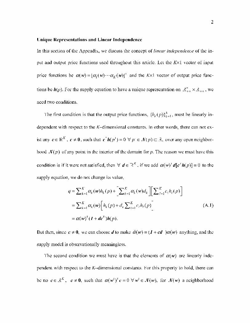
1 1 1

1 1

( ) ( ) ( ) ( )

( ) ( ) ( )

( ) ( ) ( ) .

K K K

k k k kk k

K K

k k kk

q h p d c h p

h p d c h p

p

α α

α

= = =

= =

⎡ ⎤ ⎡ ⎤= +⎣ ⎦ ⎣ ⎦

⎡ ⎤= +⎣ ⎦

= +

∑ ∑ ∑

∑ ∑

w w

w

w I dc hα

� ��

� ��

T T

(A.1)

But then, since ,≠c 0 we can choose d to make ( ) ( ) ( )≡ +w I cd wα α�

T

anything, and the

supply model is observationally meaningless.

The second condition we must have is that the elements of ( )wα are linearly inde-

pendent with respect to the K–dimensional constants. For this property to hold, there can

be no K∈c � , ,≠c 0 such that 1 1( ) 0 ( ),= ∀ ∈w c w wα T

N for ( )wN a neighborhood

3

of an arbitrary point in the interior of the domain for w. We need this property because if

it is not satisfied, then ,

K∀ ∈d � if we add [ ( ) ] ( ) 0p ≡w c d hα T T to the supply equation,

we do not change its value,

( ) ( ) ( )q p= +w I cd hα T T . (A.2)

But then, since ,≠c 0 we could choose d to make ( )( ) ( )p p≡ +h I cd h�

T anything, and

the supply model again has no empirical content.

These conditions are necessary and sufficient for the present purpose. If both are not

satisfied, then we can always reduce the number of both the input and the output price

functions by a linear combination of the original functions with no change in the model.

To illustrate, without loss of generality (WLOG), assume that 1

1( ) ( ),

K

K k kkh p c h p

−== ∑ so

that the supply equation is

1 1

1 1

1

1

1

1

( ) ( ) ( ) ( )

[ ( ) ( )] ( )

( ) ( ).

K K

k k K k kk k

K

k k K kk

K

k kk

q h p c h p

c h p

h p

α α

α α

α

− −= =

−=

−=

= +

= +

≡

∑ ∑

∑

∑

w w

w w

w�

(A.3)

Thus, the supply model can always be written with the Gorman structure as a sum of at

most K–1 products if the output price functions are linearly dependent. Alternatively,

again WLOG, assume that 1

1( ) ( ),

K

K k kkcα α−

== ∑w w so that now the supply equation is

1 1

1 1

1

1

1

1

( ) ( ) ( ) ( )

( )[ ( ) ( )]

( ) ( ).

K K

k k k k Kk k

K

k k k Kk

K

k kk

q h p c h p

h p c h p

h p

α α

α

α

− −= =

−=

−=

⎡ ⎤= +⎣ ⎦

= +

≡

∑ ∑

∑

∑

w w

w

w�

(A.4)

4

Once again, the supply model can always be written with the Gorman structure as a sum

of at most K–1 products if the input price functions are linearly dependent.

A unique representation requires that no linear reductions of this type are possible.

Various ways have been developed to check for the linear independence of a K–vector of

functions. For example, in the case of the output price functions where there is a single

argument, p, if the Wronksian – which is the determinant of the K×K matrix whose first

row is the vector of functions, 1

[ ( ) ( )],K

h p h p� the second row is the vector of first-

order derivatives, 1

[ ( ) ( )],K

h p h p′ ′� and so on through K–1 derivatives – does not vanish

at any point in an interval, then the K functions are linearly independent on that interval.

For vector-valued functions of several variables, such as the input price functions,

1{ ( )} ,K

k kα =w the matter is significantly more involved. However, for each element of w, a

sufficient condition for the linear independence across the K–dimensional constants is

that each Wronksian made up of the K×K matrix of levels of the 1

{ ( )}Kk k

α =w functions

plus the row vectors of their partial derivatives with respect to wj through order K–1 does

not vanish on any one-dimensional open interval, for each j=1,…,n. Interested readers are

referred to Gorman (1981), the appendix in Russell and Farris (1998) written by Robert

Bryant, Cohen (1933), or Boyce and diPrima (1977) for additional details on linear inde-

pendence of a vector of functions of one or several variables.

Proof of Proposition 1

Proposition 1: Let the supply function take the Gorman form, 1

( ) ( )K

k kkq h pα== ∑ w ,

with K smooth, linearly independent, functions of input prices, w, and K smooth, linearly

5

independent, functions of output price, p. If q is 0° homogeneous in ( , )pw , then each

output price function is either: (i) ,pε with ε ∈� ; (ii) (ln ) ,jp p

ε with ,ε ∈�

{1,..., }j K∈ ; (iii) sin( ln ),p pε τ cos( ln ),p p

ε τ with ,ε ∈� ,τ +∈� appearing in

pairs with the same { , }ε τ for each pair; or (iv) (ln ) sin( ln )jp p p

ε τ ,

(ln ) cos( ln )jp p p

ε τ , with ,ε ∈� {1,...,[½ ]},j K∈ ,τ +∈� and 4,K ≥ appearing in

pairs with the same { , , }jε τ for each pair, where [½ ]K is the largest integer no greater

than ½K. If {1, 2,3}K ∈ , then the supply of q can be written as:

(a) K=1

[ ] 1

1( ) ;q p

εα= w

(b) K=2

i. [ ] [ ]1 2

1 2( ) ( ) ;q p p

ε εα α= +w w

ii. [ ] ( )1

1 2( ) ln ( ) ;q p p

εα α= w w or

iii. [ ] ( )( ) ( )( )1

1 2 2( ) sin ln ( ) cos ln ( ) ;q p p p

εα τ α τ α⎡ ⎤= +⎣ ⎦w w w

(c) K=3

i. [ ] [ ] [ ] 31 2

1 2 3( ) ( ) ( ) ;q p p p

εε εα α α= + +w w w

ii. [ ] [ ] ( )1 2

1 2 3( ) ( ) ln ( ) ;q p p p

ε εα α α= +w w w

iii. [ ] ( ){ }12

1 2( ) ( ) ln ( ) ;q p p

εα α α3= + ⎡ ⎤⎣ ⎦w w w or

iv. [ ] [ ] [ ]( ) [ ]( ){ }1 2

1 2 3 3( ) ( ) sin ln ( ) cos ln ( ) .q p p p p

ε εα α τ α τ α= + +w w w w

6

In each case except (c) iii, where 2( )α w is homogeneous of degree zero, each ( )

iα w is

positively linearly homogeneous for 1, 2,3.i =

Proof: The Euler equation for 0° homogeneity is:

1 1

( )( ) ( ) ( ) 0.

K K

k

k k k

k k

h p h p pα α

= =

∂ ′+ =∂∑ ∑w

w w

wT

(A.5)

If K=1 and 1( ) 0h p′ = , this reduces to

1( ) 0α∂ ∂ =w w w

T , so that 1( )h p c= and

1( )α w is

homogeneous of degree zero. Absorb the constant c into the price index and set 1

0ε = to

obtain a special case of (a) i. If either K=1 and 1( ) 0h p′ ≠ or K≥2, then neither sum in

(A.5) can vanish without contradicting the linear independence of the {αk(w)} or the

{hk(p)}.1 Write the Euler equation as

1

1

( ) ( )1.

( ) ( )

K

k kk

K

k kk

h p p

h p

α

α=

=

′= −

⎡ ⎤∂ ∂⎣ ⎦

∑

∑

w

w w wT

(A.6)

Since the right-hand side is constant, we must be able to recombine the left-hand side

to be independent of both w and p. In other words, the terms in the numerator must re-

combine in some way so that it is proportional to the denominator, with –1 as the propor-

tionality factor. Clearly, if these two sums are proportional, identically in ( , )pw , then the

functional forms of the two sums must be the same.

1 Note, in particular, that the terms ( )k

α∂ ∂w w wT are constant with respect to p, and that the terms

( )kh p p′ are constant with respect to w.

7

To see this, for any ,

n

+ +∈w � let ( )wN be an open neighborhood of w. Fix K unique

vectors, ( ), 1, , ,K∈ =w w�

� �N and define the K×K matrices [ ], 1, ,

( )k k K

α ==B w� � �

and

, 1, ,( ) .

kk K

α=

⎡ ⎤= ∂ ∂⎣ ⎦D w w w� �

� �

T The linear independence of the input price functions

implies that we can choose { }w�

such that B is nonsingular, and therefore write (A.5) in

the form

1( ) ( ) ( ),p p p p−′ = − ≡h B Dh Ch (A.7)

Now, since both ( )p p′h and ( )ph only depend on p and not on w, the K×K matrix C

also must be independent of w, i.e., each of its elements must be constant.

Thus, the linear independence of {h1(p),…, hK(p)} and 1

{ ( ), , ( )}K

α αw w� implies

that each ( )kh p p′ is a linear function of {h1(p),…, hK(p)} with constant coefficients:

,1( ) ( ), 1, , .

K

k kh p p c h p k K=

′ = =∑ � ��� (A.8)

This is a complete system of K linear, homogeneous, ordinary differential equations

(odes), of the form commonly known as Cauchy’s linear differential equation. Our strat-

egy is the following. First, we convert (A.8) through the change of variables from p to

lnx p= to a system of linear odes with constant coefficients (Cohen 1933, pp. 124-125).

Second, we identify the set of solutions for the converted system of odes. Third, we re-

turn to (A.5) with these solutions in hand and identify the implied restrictions among the

input price functions for each K=1,2,3.

Since ( ) x

p x e= and ( ) ( )p x p x′ = , defining ( ) ( ( )), 1,..., ,k kh x h p x k K≡ =� and ap-

plying this change of variables yields:

8

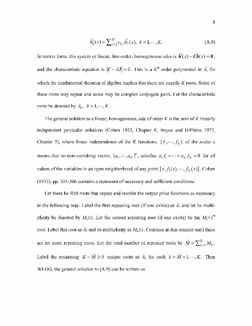
,1( ) ( ), 1, , .

K

k kh x c h x k K=

′ = =∑ � ��

� �

� (A.9)

In matrix form, this system of linear, first-order, homogeneous odes is ( ) ( )x x′ − =h Ch 0� � ,

and the characteristic equation is 0λ− =C I . This is a Kth

order polynomial in λ, for

which the fundamental theorem of algebra implies that there are exactly K roots. Some of

these roots may repeat and some may be complex conjugate pairs. Let the characteristic

roots be denoted by , 1, ,k

k Kλ = � .

The general solution to a linear, homogeneous, ode of order K is the sum of K linearly

independent particular solutions (Cohen 1933, Chapter 6; Boyce and DiPrima 1977,

Chapter 5), where linear independence of the K functions, 1

{ , , }K

f f� of the scalar x

means that no non-vanishing vector, 1

[ , , ]K

a a�

T , satisfies 1 1

0K K

a f a f+ + =� for all

values of the variables in an open neighborhood of any point [ ]1, ( ), , ( )

Kx f x f x� . Cohen

(1933), pp. 303-306 contains a statement of necessary and sufficient conditions.

Let there be R≥0 roots that repeat and reorder the output price functions as necessary

in the following way. Label the first repeating root (if one exists) as λ1 and let its multi-

plicity be denoted by M1≥1. Let the second repeating root (if one exists) be the M1+1st

root. Label this root as λ2 and its multiplicity as M2≥1. Continue in this manner until there

are no more repeating roots. Let the total number of repeated roots be 1

.

R

kkM M==∑�

Label the remaining 0K M− ≥� unique roots as λk for each 1, , .k M K= +�

� Then

WLOG, the general solution to (A.9) can be written as

9

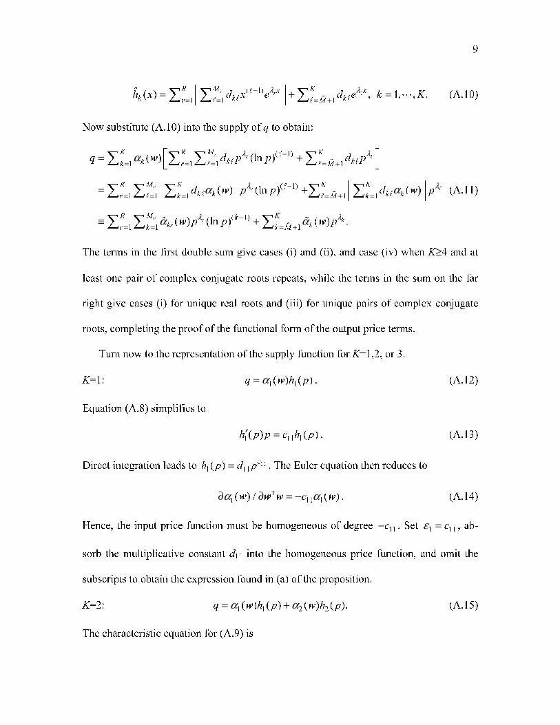
( 1)

1 1 1( ) , 1, , .r

r

R M Kx x

k k kr Mh x d x e d e k K

λ λ−= = = +

⎡ ⎤= + =⎣ ⎦∑ ∑ ∑ �

�

� ��� �

�

� (A.10)

Now substitute (A.10) into the supply of q to obtain:

( 1)

1 1 1 1

( 1)

1 1 1 1 1

( 1)

1 1 1

( ) (ln )

( ) (ln ) ( )

( ) (ln ) ( ) .

r r

r r

r kr

K R M K

k k kk r M

R M K K K

k k k kr k M k

R M Kk

kr kr k k M

q d p p d p

d p p d p

p p p

λ λ

λ λ

λλ

α

α α

α α

−= = = = +

−= = = = + =

−= = = +

⎡ ⎤= +⎣ ⎦

⎡ ⎤ ⎡ ⎤= +⎣ ⎦ ⎣ ⎦

≡ +

∑ ∑ ∑ ∑

∑ ∑ ∑ ∑ ∑

∑ ∑ ∑

w

w w

w w

�

�

�

� ��� �

�

� ��� �

�� �

(A.11)

The terms in the first double sum give cases (i) and (ii), and case (iv) when K≥4 and at

least one pair of complex conjugate roots repeats, while the terms in the sum on the far

right give cases (i) for unique real roots and (iii) for unique pairs of complex conjugate

roots, completing the proof of the functional form of the output price terms.

Turn now to the representation of the supply function for K=1,2, or 3.

K=1: 1 1( ) ( )q h pα= w . (A.12)

Equation (A.8) simplifies to

1 11 1( ) ( )h p p c h p′ = . (A.13)

Direct integration leads to 11

1 11( )

ch p d p= . The Euler equation then reduces to

1 11 1( ) / ( )cα α∂ ∂ = −w w w w

T . (A.14)

Hence, the input price function must be homogeneous of degree 11c− . Set

1 11cε = , ab-

sorb the multiplicative constant d11 into the homogeneous price function, and omit the

subscripts to obtain the expression found in (a) of the proposition.

K=2: 1 1 2 2( ) ( ) ( ) ( ).q h p h pα α= +w w (A.15)

The characteristic equation for (A.9) is

10

11 22 11 22 12 21

( ) ( ) 0c c c c c cλ λ2 − + + − = . (A.16)

The characteristic roots are

2

1 2 11 22 11 22 12 21, ½( ) ½ ( ) 4c c c c c cλ λ = + ± − + . (A.17)

Three cases are possible:

(1) unique real roots, 1 2

λ λ≠ , 1 2,λ λ ∈� , and 2

11 22 12 21( ) 4 0c c c c− + > ;

(2) one real root, 1 2 11 22

½( ) ,c cλ λ= = + ∈� and 2

11 22 12 21( ) 4 0c c c c− + = ; or

(3) complex conjugate roots, 1

,λ κ ιτ= + 2

λ κ ιτ= − , 11 22

½( )c cκ = + ,

2

11 22 12 21½ | ( ) 4 |,c c c cτ = − + and 2

11 22 12 21( ) 4 0c c c c− + < .

With unique roots (whether real or complex), the general solution is

1 2

1 2( ) , 1, 2.x x

k k kh x d e d e k

λ λ= + =� (A.18)

Substituting these expressions into the supply of q yields

[ ] [ ]1 2

1 2

11 1 12 2 21 1 22 2

1 2

( ) ( ) ( ) ( )

( ) ( ) .

q d d p d d p

p p

λ λ

λ λ

α α α α

α α

= + + +

≡ +

w w w w

w w� �

(A.19)

If the roots are real, then the Euler equation is

1 2

1 1 1 2 2 2( ) ( ) ( ) ( ) 0.p p

λ λα λ α α λ α⎡ ⎤ ⎡ ⎤∂ ∂ + + ∂ ∂ + =⎣ ⎦ ⎣ ⎦w w w w w w w w� � � �

T T (A.20)

Linear independence of the output price functions implies that the term premultiplying

each output price function vanishes. Hence, ( )i

α w� must be homogeneous of degree i

λ−

for i=1,2. Relabel terms so that i i

ε λ= and 1

( ) ( ) , 1, 2,i

i ii

εα α −= =w w� for case (b) i.

If the characteristic root repeats, the general solution is

11

1 2

( ) , 1, 2.x x

k k kh x d e d xe k

λ λ= + =� (A.21)

Making the same substitutions as before yields:

1 2( ) ( ) ln .q p p p

λ λα α= +w w� � (A.22)

The Euler equation now is

1 2

1 2 2

( ) ( )( ) ( ) ( ) ln 0.p p

λα αλα α λα∂ ∂⎡ ⎤⎛ ⎞ ⎛ ⎞+ + + + =⎜ ⎟ ⎜ ⎟⎢ ⎥∂ ∂⎝ ⎠ ⎝ ⎠⎣ ⎦

w w

w w w w w

w w

� �

� � �

T T (A.23)

Since 0pλ > and {1,lnp} is linearly independent,

2( )α w� must be homogeneous of de-

gree –λ. Therefore, factor it and pλ out on the right-hand side of (A.22),

[ ]2 1ˆ( ) ( ) ln ,q p p

λα α= +w w� (A.24)

where 1 1 2ˆ ( ) ( ) ( )α α α≡w w w� � . The Euler equation then simplifies to

1ˆ ( ) 1.α∂ ∂ = −w w w

T (A.25)

Let { }ˆ( ) exp ( )β α= −w w and note that 1ˆ( ) ( ) ( ) ( )β β α β∂ ∂ = − ∂ ∂ =w w w w w w w w

T T if

and only if 1ˆ ( )α w satisfies (A.25). Relabel terms so that

1,ε λ=

1 2( ) ( ),α α=w w� and

2( ) ( )α β=w w to obtain case (b) ii.

When the roots are complex, we first require conditions on the input price functions

so that q is real-valued. From (A.19), we have

1 2( ) ( ) ,q p p p

κ ιτ ιτα α −⎡ ⎤= +⎣ ⎦w w� � (A.26)

while deMoivre’s theorem implies (Abramowitz and Stegun 1972)

cos( ln ) sin( ln ).p p pιτ τ ι τ± = ± (A.27)

12

Thus, complex functions 1 0 1

ˆ ˆ( ) ( ) ( )α α ια= +w w w� and 2 0 1

ˆ ˆ( ) ( ) ( )α β ιβ= +w w w� are re-

quired if q is real-valued. Substituting these definitions and (A.27) into (A.26) yields:

0 1 0 1 0 1 0 1

ˆ ˆ ˆ ˆˆ ˆ ˆ ˆ( ) cos( ln ) ( ) sin( ln ) .q p p pκ α ια β ιβ τ ια α ιβ β τ⎡ ⎤= + + + + − − +⎣ ⎦ (A.28)

We must have 1 1ˆ ˆ( ) ( )β α= −w w for the term in front of cos( ln )pτ to be real-valued

and 0 0ˆ ˆ( ) ( )β α=w w for the term in front of sin( ln )pτ to be real-valued, so that the input

price functions are complex conjugates. Omitting the ^’s and the subscripts and absorbing

the multiplicative constant 2 into the price functions for conciseness, we then have:

[ ]( ) cos( ln ) ( ) sin( ln )q p p pκ α τ β τ= +w w . (A.29)

The Euler equation now has the form:

{}

( ) ( ) ( ) cos( ln )

( ) ( ) ( ) sin( ln ) 0.

p

p pκ

α κα τβ τ

β τα κβ τ

⎡ ⎤+ +⎣ ⎦

⎡ ⎤+ − + =⎣ ⎦

w

w

w w w w

w w w w

T

T

(A.30)

Define the smooth and invertible transformation

( ) ( )( ) ( )

( ) ) cos ln ( ) sin ln ( ) ,

( ) ( ) sin ln ( ) cos ln ( ) ,

α α τ β τ β

β α τ β τ β

⎡ ⎤= ( −⎣ ⎦

⎡ ⎤= +⎣ ⎦

w w w w

w w w w

� �

�

� �

�

(A.31)

for ( ) 0α ≠w� any smooth, homogeneous of degree κ− function and ( ) 0β >w� any posi-

tive linearly homogeneous function. A direct calculation then yields

( ) ( ) ( ),

( ) ( ) ( ),

α κα τβ

β τα κβ

= − −

= −

w

w

w w w w

w w w w

T

T

(A.32)

as required.

13

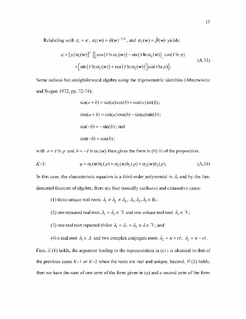
Relabeling with 1

ε κ= , 1

1( ) ( ) κα α −=w w� , and

2( ) ( )α β=w w

� yields:

[ ] ( ) ( ){

( ) ( ) }

1

1 2 2

2 2

( ) cos ln ( ) sin ln ( ) cos( ln )

sin ln ( ) cos ln ( ) sin( ln ) .

q p p

p

εα τ α τ α τ

τ α τ α τ

= −⎡ ⎤⎣ ⎦

+ +⎡ ⎤⎣ ⎦

w w w

w w

(A.33)

Some tedious but straightforward algebra using the trigonometric identities (Abramowitz

and Stegun 1972, pp. 72-74):

sin( ) sin( ) cos( ) cos( ) sin( )a b a b a b+ = + ;

cos( ) cos( ) cos( ) sin( ) sin( )a b a b a b+ = − ;

sin( ) sin( )b b− = − ; and

cos( ) cos( )b b− = ;

with lna pτ= and 2

ln )b τ α= − (w then gives the form in (b) iii of the proposition.

K=3: 1 1 2 2 3 3( ) ( ) ( ) ( ) ( ) ( ).q h p h p h pα α α= + +w w w (A.34)

In this case, the characteristic equation is a third-order polynomial in λ, and by the fun-

damental theorem of algebra, there are four mutually exclusive and exhaustive cases:

(1) three unique real roots 1 2 3

λ λ λ≠ ≠ , 1 2 3, ,λ λ λ ∈� ;

(2) one repeated real root,1 2

λ λ= ∈� and one unique real root 3

λ ∈� ;

(3) one real root repeated thrice 1 2 3

λ λ λ λ= = ≡ ∈� ; and

(4) a real root 1

λ ∈� and two complex conjugate roots 2

,λ κ ιτ= + 3

λ κ ιτ= − .

First, if (1) holds, the argument leading to the representation in (c) i is identical to that of

the previous cases K=1 or K=2 when the roots are real and unique. Second, if (2) holds,

then we have the sum of one term of the form given in (a) and a second term of the form

14

given in (b) ii of the proposition, leading to case (c) ii. Third, if (4) holds, then we have

the sum of one term of the form given in (a) and a second term of the form given in (b) iii

of the proposition, leading to case (c) iv.

Therefore, consider case (3), for which the general solution to (A.9) has the form:

2

1 2 3( ) , 1, 2,3.x x x

k k k kh x d e d xe d x e k

λ λ λ= + + =� (A.35)

Rewriting this in terms of p and the {hk(p)}, substituting the result into (A.34), and re-

grouping terms as before yields:

2

1 2 3( ) ( ) ln ( )(ln ) .q p p p

λ α α α⎡ ⎤= + +⎣ ⎦w w w� � � (A.36)

The Euler equation is:

{

}

1 1 2

2 2 3

2

3 3

( ) ( ) ( )

( ) ( ) 2 ( ) ln

( ) ( ) (ln ) 0.

p

p

p

λ α λα α

α λα α

α λα

⎡ ⎤∂ ∂ + +⎣ ⎦

⎡ ⎤+ ∂ ∂ + +⎣ ⎦

⎡ ⎤+ ∂ ∂ + =⎣ ⎦

w w w w w

w w w w w

w w w w

� � �

� � �

� �

T

T

T

(A.37)

As before, 0pλ > and the linear independence of { }21, ln , (ln )p p requires each sum

in square brackets to vanish. In particular, 3( )α w� must be homogeneous of degree λ− ,

and we can factor it out of the term in square brackets in (A.36), yielding:

2

3 1 2ˆ ˆ( ) ( ) ( ) ln (ln ) ,q p p p

λα α α⎡ ⎤= + +⎣ ⎦w w w� (A.38)

with 1 1 3ˆ ( ) ( ) ( )α α α=w w w� � and

2 2 3ˆ ( ) ( ) ( ) .α α α=w w w� �

Now the term in brackets on the right-hand side must be homogeneous of degree

zero, which implies:

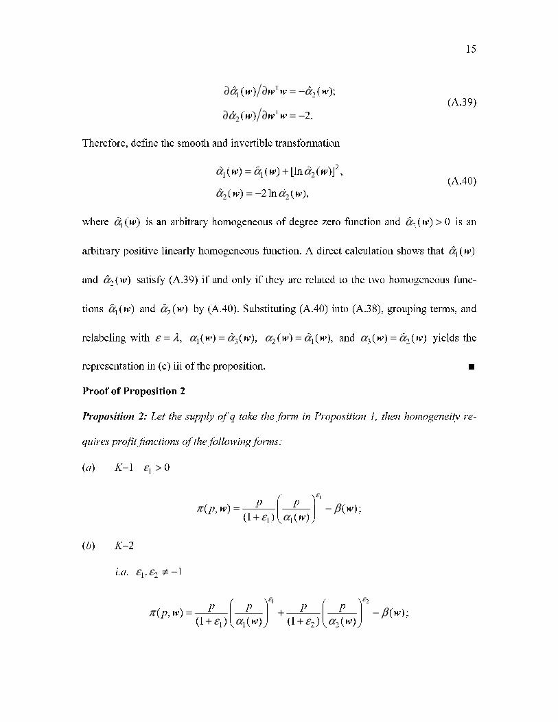
15

1 2ˆ ˆ( ) ( );

ˆ ( ) 2.

α α

α2

∂ ∂ = −

∂ ∂ = −

w w w w

w w w

T

T

(A.39)

Therefore, define the smooth and invertible transformation

2

1 1ˆ ( ) ( ) [ln ( )] ,

ˆ ( ) 2 ln ( ),

α α α

α α

2

2 2

= +

= −

w w w

w w

� �

�

(A.40)

where 1( )α w

�

is an arbitrary homogeneous of degree zero function and 2( ) 0α >w

�

is an

arbitrary positive linearly homogeneous function. A direct calculation shows that 1ˆ ( )α w

and 2

ˆ ( )α w satisfy (A.39) if and only if they are related to the two homogeneous func-

tions 1( )α w

�

and 2( )α w

�

by (A.40). Substituting (A.40) into (A.38), grouping terms, and

relabeling with ,ε λ= 1 3

ˆ( ) ( ),α α=w w 2 1( ) ( ),α α=w w

�

and 3 2( ) ( )α α=w w

�

yields the

representation in (c) iii of the proposition. ■

Proof of Proposition 2

Proposition 2: Let the supply of q take the form in Proposition 1, then homogeneity re-

quires profit functions of the following forms:

(a) K=1 1

0ε >

1

1 1

( , ) ( ) ;(1 ) ( )

p pp

ε

π βε α

⎛ ⎞= −⎜ ⎟+ ⎝ ⎠

w w

w

(b) K=2

i.a. 1 2, 1ε ε ≠ −

1 2

1 1 2 2

( , ) ( ) ;(1 ) ( ) (1 ) ( )

p p p pp

ε ε

π βε α ε α

⎛ ⎞ ⎛ ⎞= + −⎜ ⎟ ⎜ ⎟+ +⎝ ⎠ ⎝ ⎠

w w

w w

16

i.b. 1 2

1, 1ε ε≠ − = −

1

2

1 1

( , ) ( ) ln ( ) ;(1 ) ( ) ( )

p p pp

ε

π α γε α β

⎛ ⎞ ⎛ ⎞= + −⎜ ⎟ ⎜ ⎟+ ⎝ ⎠⎝ ⎠w w w

w w

ii.a. 1

1ε ≠ −

1

1 1 2 1

1( , ) ln ( ) ;

(1 ) ( ) ( ) (1 )

p p pp

ε

π βε α α ε

⎡ ⎤⎛ ⎞ ⎛ ⎞= − −⎢ ⎥⎜ ⎟ ⎜ ⎟+ +⎝ ⎠ ⎝ ⎠⎣ ⎦

w w

w w

ii.b. 1

1ε = −

2

1

2

( , ) ½ ( ) ln ( ) ;( )

ppπ α β

α⎡ ⎤⎛ ⎞

= −⎢ ⎥⎜ ⎟⎝ ⎠⎣ ⎦

w w w

w

iii.

1

12 2

1 21

1

2

( , ) (1 ) sin ln( ) ( )(1 )

(1 ) cos ln ( ) ;( )

p p pp

p

ε

π ε τ τα αε τ

ε τ τ βα

⎡⎛ ⎞ ⎛ ⎞⎛ ⎞ ⎛ ⎞= + +⎢⎜ ⎟ ⎜ ⎟⎜ ⎟ ⎜ ⎟+ + ⎢⎝ ⎠ ⎝ ⎠⎝ ⎠⎝ ⎠ ⎣

⎤⎛ ⎞⎛ ⎞+ + − −⎥⎜ ⎟⎜ ⎟

⎥⎝ ⎠⎝ ⎠⎦

w

w w

w

w

(c) K=3

iii.a. 1

1ε ≠ −

12

2

1 2 13

1 31

( , ) 1 (1 ) ( ) (1 ) ln 1 ( ) ;( ) ( )(1 )

p p pp

ε

π ε α ε βα αε

⎧ ⎫⎡ ⎤⎛ ⎞⎛ ⎞ ⎪ ⎪= + + + + − −⎨ ⎬⎢ ⎥⎜ ⎟⎜ ⎟+ ⎝ ⎠ ⎝ ⎠⎣ ⎦⎪ ⎪⎩ ⎭

w w w

w w

iii.b. 1

1ε = −

3

11 2 3

3

( , ) ( ) ( ) ln ln ( ).( ) ( )

p ppπ α α γ

β α

⎡ ⎤⎛ ⎞⎛ ⎞⎛ ⎞⎢ ⎥= + −⎜ ⎟⎜ ⎟⎜ ⎟⎢ ⎥⎝ ⎠ ⎝ ⎠⎝ ⎠⎣ ⎦

w w w w

w w

17

In each case, ( )β w and ( )γ w are positively linearly homogeneous functions of w.

Proof: Throughout the proof, omit the input prices as arguments to simplify the notation.

(a) K=1 1

0ε >

1

1

.p

q

ε

α⎛ ⎞

= ⎜ ⎟⎝ ⎠

(A.41)

Direct integration leads to

1

1 1

.1

p pε

π βε α

⎛ ⎞ ⎛ ⎞= −⎜ ⎟ ⎜ ⎟+⎝ ⎠ ⎝ ⎠

(A.42)

(b) K=2 i.a. 1 2, 1ε ε ≠ −

1 2

1 2

.p p

q

ε ε

α α⎛ ⎞ ⎛ ⎞

= +⎜ ⎟ ⎜ ⎟⎝ ⎠ ⎝ ⎠

(A.43)

This is equivalent to the previous case with two power functions, so that

1 2

1 1 2 2

.1 1

p p p pε ε

π βε α ε α

⎛ ⎞ ⎛ ⎞ ⎛ ⎞ ⎛ ⎞= + −⎜ ⎟ ⎜ ⎟ ⎜ ⎟ ⎜ ⎟+ +⎝ ⎠ ⎝ ⎠ ⎝ ⎠ ⎝ ⎠

(A.44)

i. b. 1 2

1, 1ε ε≠ − = − .

1

2

1

pq

p

εα

α⎛ ⎞ ⎛ ⎞= +⎜ ⎟ ⎜ ⎟

⎝ ⎠⎝ ⎠. (A.45)

Direct integration now leads to

1

2

1 1

ln1

p p pε

π α γε α β

⎛ ⎞ ⎛ ⎞ ⎛ ⎞= + −⎜ ⎟ ⎜ ⎟ ⎜ ⎟+ ⎝ ⎠⎝ ⎠ ⎝ ⎠. (A.46)

Here, the constant of integration must take the form 2

( ln )α β γ− + , ,β γ 1º homogene-

ous if π is to be 1º homogeneous.

18

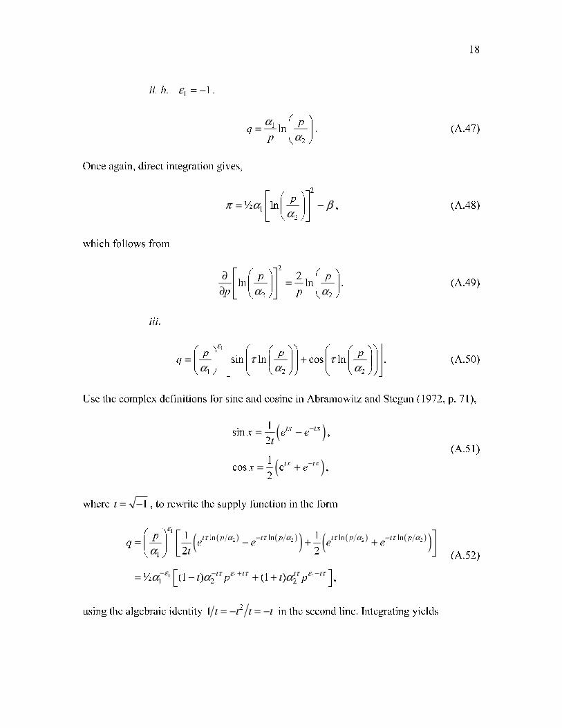
ii. b. 1

1ε = − .

1

2

lnp

qp

αα

⎛ ⎞= ⎜ ⎟

⎝ ⎠. (A.47)

Once again, direct integration gives,

2

1

2

½ lnpπ α β

α⎡ ⎤⎛ ⎞

= −⎢ ⎥⎜ ⎟⎝ ⎠⎣ ⎦

, (A.48)

which follows from

2

2 2

2ln ln .

p p

p pα α⎡ ⎤⎛ ⎞ ⎛ ⎞∂ =⎢ ⎥⎜ ⎟ ⎜ ⎟∂ ⎝ ⎠ ⎝ ⎠⎣ ⎦

(A.49)

iii.

1

1 2 2

sin ln cos ln .p p p

q

ε

τ τα α α

⎡ ⎤⎛ ⎞ ⎛ ⎞⎛ ⎞ ⎛ ⎞ ⎛ ⎞= +⎢ ⎥⎜ ⎟ ⎜ ⎟⎜ ⎟ ⎜ ⎟ ⎜ ⎟

⎢ ⎥⎝ ⎠ ⎝ ⎠ ⎝ ⎠⎝ ⎠ ⎝ ⎠⎣ ⎦ (A.50)

Use the complex definitions for sine and cosine in Abramowitz and Stegun (1972, p. 71),

( )

( )

1sin ,

2

1cos e ,

2

x x

x x

x e e

x e

ι ι

ι ι

ι−

−

= −

= +

(A.51)

where 1ι = − , to rewrite the supply function in the form

( ) ( )( ) ( ) ( )( )1

2 2 2 2

1 1 1

ln ln ln ln

1

2 21

1 1

2 2

½ (1 ) (1 ) ,

p p p ppq e e e e

p p

ειτ α ιτ α ιτ α ιτ α

ε ε ιτ ε ιτιτ ιτ

α ι

α ι α ι α

− −

− + −−

⎛ ⎞ ⎡ ⎤= − + +⎜ ⎟ ⎢ ⎥⎣ ⎦⎝ ⎠

⎡ ⎤= − + +⎣ ⎦

(A.52)

using the algebraic identity 21 ι ι ι ι= − = − in the second line. Integrating yields

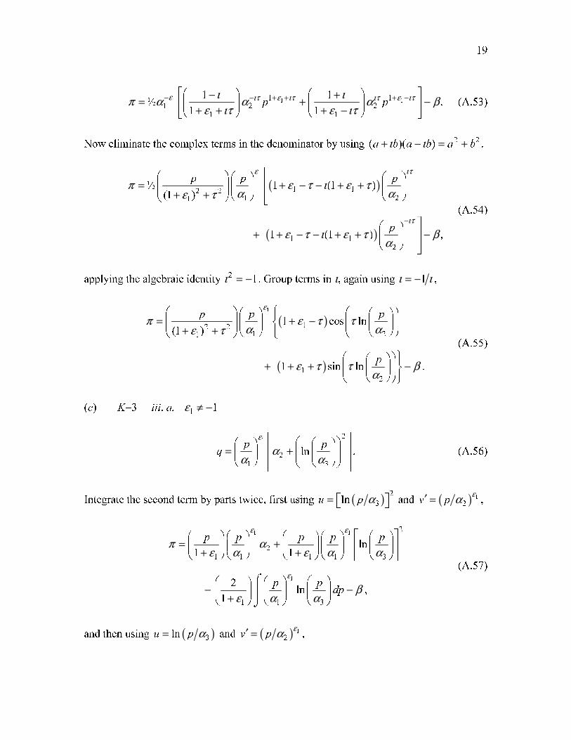
19

1 1 11 1

2 21

1 1

1 1½ .

1 1p p

ε ε ιτ ε ιτιτ ιτι ιπ α α α βε ιτ ε ιτ

− + + + −−⎡ ⎤⎛ ⎞ ⎛ ⎞− += + −⎢ ⎥⎜ ⎟ ⎜ ⎟+ + + −⎝ ⎠ ⎝ ⎠⎣ ⎦ (A.53)

Now eliminate the complex terms in the denominator by using 2 2( )( )a b a b a bι ι+ − = + ,

( )

( )

1

1 12 2

1 21

1 1

2

½ 1 (1 )(1 )

1 (1 ) ,

p p p

p

ε ιτ

ιτ

π ε τ ι ε τα αε τ

ε τ ι ε τ βα

−

⎡⎛ ⎞ ⎛ ⎞ ⎛ ⎞⎢= + − − + +⎜ ⎟ ⎜ ⎟ ⎜ ⎟+ + ⎢⎝ ⎠ ⎝ ⎠⎝ ⎠ ⎣

⎤⎛ ⎞⎥+ + − − + + −⎜ ⎟⎥⎝ ⎠ ⎦

(A.54)

applying the algebraic identity 21ι = − . Group terms in ι, again using 1ι ι= − ,

( )

( )

1

12 2

1 21

1

2

1 cos ln(1 )

1 sin ln .

p p p

p

ε

π ε τ τα αε τ

ε τ τ βα

⎧⎛ ⎞ ⎛ ⎞⎛ ⎞ ⎛ ⎞⎪= + −⎜ ⎟ ⎜ ⎟⎨⎜ ⎟ ⎜ ⎟+ + ⎝ ⎠ ⎝ ⎠⎪ ⎝ ⎠⎝ ⎠ ⎩

⎫⎛ ⎞⎛ ⎞ ⎪+ + + −⎜ ⎟⎬⎜ ⎟⎝ ⎠ ⎪⎝ ⎠⎭

(A.55)

(c) K=3 iii. a. 1

1ε ≠ −

12

2

1 3

ln .p p

q

ε

αα α

⎡ ⎤⎛ ⎞⎛ ⎞⎛ ⎞⎢ ⎥= + ⎜ ⎟⎜ ⎟⎜ ⎟⎢ ⎥⎝ ⎠ ⎝ ⎠⎝ ⎠⎣ ⎦

(A.56)

Integrate the second term by parts twice, first using ( ) 2

3lnu p α= ⎡ ⎤⎣ ⎦ and ( ) 1

2v p

εα′ = ,

1 1

1

2

2

1 1 1 1 3

1 1 3

ln1 1

2ln ,

1

p p p p p

p pdp

ε ε

ε

π αε α ε α α

βε α α

⎡ ⎤⎛ ⎞⎛ ⎞ ⎛ ⎞ ⎛ ⎞ ⎛ ⎞= + ⎢ ⎥⎜ ⎟⎜ ⎟ ⎜ ⎟ ⎜ ⎟ ⎜ ⎟+ +⎝ ⎠ ⎝ ⎠ ⎝ ⎠ ⎝ ⎠ ⎝ ⎠⎣ ⎦

⎛ ⎞⎛ ⎞ ⎛ ⎞− −⎜ ⎟⎜ ⎟ ⎜ ⎟+⎝ ⎠ ⎝ ⎠ ⎝ ⎠

⌠⎮⌡

(A.57)

and then using ( )3lnu p α= and ( ) 1

2v p

εα′ = ,

20

12

2

1 2 13

1 31

1 (1 ) (1 ) ln 1 .(1 )

p p pε

π ε α ε βα αε

⎧ ⎫⎡ ⎤⎛ ⎞⎛ ⎞ ⎪ ⎪= + + + + − −⎨ ⎬⎢ ⎥⎜ ⎟⎜ ⎟+ ⎝ ⎠ ⎝ ⎠⎣ ⎦⎪ ⎪⎩ ⎭

(A.58)

iii. b. 1

1ε = −

2

1

2

3

ln .p

qp

α αα

⎡ ⎤⎛ ⎞⎛ ⎞⎛ ⎞ ⎢ ⎥= + ⎜ ⎟⎜ ⎟⎜ ⎟⎢ ⎥⎝ ⎠ ⎝ ⎠⎝ ⎠⎣ ⎦

(A.59)

Distribute the first term on the right-hand-side of the supply function and integrate,

3

11 2 13

3

ln ln ,p

pπ α α α βα

⎡ ⎤⎛ ⎞= + −⎢ ⎥⎜ ⎟

⎝ ⎠⎣ ⎦

� (A.60)

which follows from

3 2

3 3

3ln ln .

p p

p pα α⎡ ⎤ ⎡ ⎤⎛ ⎞ ⎛ ⎞∂ =⎢ ⎥ ⎢ ⎥⎜ ⎟ ⎜ ⎟∂ ⎝ ⎠ ⎝ ⎠⎣ ⎦ ⎣ ⎦

(A.61)

The constant of integration must be such that the sum 1 2

ln pα α β− � is 1º homogeneous.

Set 1 2

lnβ α α β γ= +� , where ,β γ are arbitrary positive 1º homogeneous functions of w,

3

11 2 3

3

ln ln .p pπ α α γβ α

⎡ ⎤⎛ ⎞⎛ ⎞⎛ ⎞⎢ ⎥= + −⎜ ⎟⎜ ⎟⎜ ⎟⎢ ⎥⎝ ⎠ ⎝ ⎠⎝ ⎠⎣ ⎦

(A.62)

The remaining K=3 cases are linear combinations of the solutions for K=1 and 2. �

Remark: Sufficiency in each case can be shown simply by differentiating the profit func-

tion with respect to p.

References

Abramowitz, M. and I.A. Stegun, eds. 1972. Handbook of Mathematical Functions. New

York: Dover Publications.

21

Boyce, W.E. and R.C. DiPrima. 1977. Elementary Differential Equations. 3rd

Edition,

New York: John Wiley & Sons.

Cohen, A. 1933. An Elementary Treatise on Differential Equations. 2nd

Edition, Boston:

D.C. Heath & Company.

Gorman, W.M. “Some Engel Curves.” 1981. In A. Deaton, ed. Essays in Honour of Sir

Richard Stone, Cambridge: Cambridge University Press: 7-29.

Russell, T. and F. Farris. 1998. “Integrability, Gorman Systems, and the Lie Bracket

Structure of the Real Line.” Journal of Mathematical Economics 29: 183-209.