Aircraft spin recovery, with and without thrust vectoring, using nonlinear dynamic inversion

JOURNAL OF AIRCRAFT

Vol. 42, No. 6, November–December 2005

Aircraft Spin Recovery, with and without Thrust Vectoring,Using Nonlinear Dynamic Inversion

P. K. Raghavendra,∗ Tuhin Sahai,∗ P. Ashwani Kumar,† Manan Chauhan,‡ and N. Ananthkrishnan§

Indian Institute of Technology Bombay, Mumbai 400 076, India

The present paper addresses the problem of spin recovery of an aircraft as a nonlinear inverse dynamicsproblem of determining the control inputs that need to be applied to transfer the aircraft from a spin state to alevel trim flight condition. A stable, oscillatory, flat, left spin state is first identified from a standard bifurcationanalysis of the aircraft model considered, and this is chosen as the starting point for all recovery attempts. Threedifferent symmetric, level-flight trim states, representative of high, moderate, and low-angle-of-attack trims for thechosen aircraft model, are computed by using an extended-bifurcation-analysis procedure. A standard form of thenonlinear dynamic inversion algorithm is implemented to recover the aircraft from the oscillatory spin state to eachof the selected level trims. The required control inputs in each case, obtained by solving the inverse problem, arecompared against each other and with the standard recovery procedure for a modern, low-aspect-ratio, fuselageheavy configuration. The spin recovery procedure is seen to be restricted because of limitations in control surfacedeflections and rates and because of loss of control effectiveness at high angles of attack. In particular, theserestrictions adversely affect attempts at recovery directly from high-angle-of-attack oscillatory spins to low-angle-of-attack trims using only aerodynamic controls. Further, two different control strategies are examined in an effortto overcome difficulties in spin recovery because of these restrictions. The first strategy uses an indirect, two-steprecovery procedure in which the airplane is first recovered to a high- or moderate-angle-of-attack level-flight trimcondition, followed by a second step where the airplane is then transitioned to the desired low-angle-of-attacktrim. The second strategy involves the use of thrust-vectoring controls in addition to the standard aerodynamiccontrol surfaces to directly recover the aircraft from high-angle-of-attack oscillatory spin to a low-angle-of-attacklevel-flight trim state. Our studies reveal that both strategies are successful, highlighting the importance of effectivethrust management in conjunction with suitable use of all of the aerodynamic control surfaces for spin recoverystrategies.

I. Introduction

S PIN has been and continues to be one of the most complex anddangerous phenomena encountered in flight. Stall/spin-related

incidents account for a significant proportion of accidents in bothmilitary and general aviation airplanes.1,2 Not surprisingly, spinprediction and spin recovery have been issues that have attractedconsiderable attention among flight dynamicists over the years.3

By the early 1980s, approximate methods based on reduced-ordermodels had been developed for equilibrium spin prediction.4,5 (Fordefinitions of various spin types or modes—equilibrium or steadyvs oscillatory, erect vs inverted, flat vs steep, etc.—the reader isreferred to standard books, e.g., Ref. 6.) The introduction of bifur-cation methods around that period, however, brought about a majoradvancement in spin prediction capabilities.7,8 It became possibleto work with the complete equations of aircraft motion with no ap-proximation and to numerically compute not just equilibrium spinstates but also oscillatory spin solutions.9,10 Jumps from a nonspinstate to a spin state, or between two different spin states, hysteresis,and other nonlinear phenomena observed in poststall flight couldalso be predicted.11,12 One could even think in terms of a spin pre-vention/recovery control system based on the results of a bifurcationanalysis for a given aircraft.13

Presented as Paper 2004-0378 at the AIAA Aerospace Sciences Meetingand Exhibit, Reno, NV, 5–8 January 2004; received 15 July 2004; revisionreceived 6 October 2004; accepted for publication 9 October 2004. Copyrightc© 2004 by the American Institute of Aeronautics and Astronautics, Inc. Allrights reserved. Copies of this paper may be made for personal or internaluse, on condition that the copier pay the $10.00 per-copy fee to the CopyrightClearance Center, Inc., 222 Rosewood Drive, Danvers, MA 01923; includethe code 0021-8669/05 $10.00 in correspondence with the CCC.

∗Masters (Dual Degree) Student.†Undergraduate Student.‡Research Assistant.§Associate Professor, Department of Aerospace Engineering; akn@

aero.iitb.ac.in. Senior Member AIAA.

One strategy for spin prevention is to avoid the jump phenomenonleading to spin entry by suitably scheduling the control surfaces ineither a feedforward or a feedback manner.7,14 Control schedulingeffectively changes the topology of the equilibrium spin solutions athigh angles of attack, either eliminating the stable spin solutions ordeleting the bifurcation points at which departure to spin occurs.15

However, bifurcation analysis essentially presents a quasi-static pic-ture of the aircraft dynamics, and consequently, control schedulesdeduced from the results of a bifurcation analysis are also quasi-static in nature. Such control strategies are not always successful inpractice, and when they do succeed, the solutions typically turn outto be suboptimal.7 Instead, a better approach would be to use theresults from a bifurcation analysis as a guide to designing a non-linear control law that can extend the stable flight envelope of theairplane by removing the bifurcation points that give rise to onsetof spin.16 However, given the possibility that a variety of complexaerodynamic phenomena might be encountered at high angles of at-tack, it has not been possible to come up with a simple, reliable, andfoolproof control system that can, without seriously reducing air-craft maneuverability, guarantee protection against entry into spin.13

Instead, attention has been focused on devising control systems forspin recovery.

Piloting strategies for spin recovery have undergone drasticchanges over the years.3 In the initial years, the prescription for spinrecovery was to increase the thrust and simultaneously apply rudderto oppose the rotation. Later, as airplanes grew wing heavy, downele-vator became the primary control input applied to recover from spin.For modern military aircraft, with low-aspect-ratio wings, which arefuselage heavy, the primary spin recovery control has been aileronwith the spin, supplemented with rudder against the direction ofrotation. However, present-generation military airplanes frequentlyexhibit oscillatory spins requiring nonstandard and nonintuitive con-trol inputs for recovery. For example, steady and oscillatory spinsfor the F-14 were studied in Ref. 17, and attempts at spin recoverywere made based on the results of the bifurcation analysis carriedout to predict the various spin solutions. Unfortunately, none of the

1492

RAGHAVENDRA ET AL. 1493

control strategies tried out for spin recovery were successful, pos-sibly because of the quasi-static nature of the bifurcation analysisresults, as pointed out earlier. In particular, the tendency for a stableequilibrium spin, on application of recovery controls, to give wayto a sustained oscillatory spin was observed. It was concluded thatit was very important to account for oscillatory spin modes whenconsidering spin recovery strategies.

Control strategies for aircraft spin recovery are necessarily com-plex and nonlinear.18 Synthesis of a nonlinear controller for recov-ery of an unstable aircraft from a time-dependent spin mode wasattempted in Ref. 19. Following a two-step procedure, they first sta-bilized the aircraft at a high-angle-of-attack equilibrium spin stateand then applied a predefined set of control inputs to recover the air-craft to a low-angle-of-attack trim. Initial attempts, however, weremet with failure, and extensive studies had to be carried out to gen-erate a set of control inputs that could achieve recovery.

Properly speaking, the problem of spin recovery is one of de-termining the control inputs that need to be applied to transfer theaircraft from a spin state S to a level-trim-flight condition L . The con-trol strategy for spin recovery therefore requires a solution of whatis called the inverse problem of flight dynamics.20 A solution to theinverse problem has been possible by use of the theory of nonlineardynamic inversion applied to the equations of aircraft dynamics.21

However, dynamic inversion in its basic, first-order form requiresas many control inputs as state variables, which is generally not thecase for aircraft flight dynamics. This problem was overcome byderiving dynamic inversion laws for flight control based on a de-composition of the aircraft dynamics into fast inner-loop dynamicsfor the angular rates and slow outer-loop dynamics for the attitudevariables.22,23 Dynamic inversion in this form has been applied tononlinear flight maneuvers,24 trajectory control,25 poststall flight,26

and for many other applications.27 It is apparent that the method ofnonlinear dynamic inversion is ideally suited for solving the problemof recovering an aircraft from spin to a level-trim-flight condition.

The present paper addresses the problem of spin recovery of anaircraft using nonlinear dynamic inversion techniques. In particu-lar, we first consider the problem of determining the control in-puts that need to be given to recover an airplane from an oscilla-tory spin state to three different level-flight conditions representinghigh-, moderate-, and low-angle-of-attack trim states, respectively.The aircraft model used for this study is the F-18/HARV, whichhas been used several times in the past as a testbed for researchassociated with high-angle-of-attack dynamics and control.24,28−30

Both equilibrium and oscillatory spin states are identified by car-rying out a standard bifurcation analysis (SBA) of the open-loopaircraft dynamics model. Computation of stable, level-flight-trimstates to which the airplane could be recovered is done by usingan extended-bifurcation-analysis (EBA) procedure, as proposed inRef. 31. Three branches of stable, level-flight trims are identifiedfrom the EBA computations at high, moderate, and low values ofangle of attack. One representative trim state, labeled A, B, andC, respectively, is selected from each of these stable, level-flightbranches. The dynamic inversion algorithm in the form proposed inRef. 26 is implemented to recover the aircraft from an oscillatoryspin state to each of the level trims, A, B, C. The required controlinputs in each case, obtained by solving the inverse problem, arecompared against each other and with the standard recovery con-trols for a modern, low-aspect-ratio, fuselage heavy configuration.

It is well known, and is also observed in our studies, that the spinrecovery procedure is restricted because of limitations in controlsurface deflections and rates and because of loss of control effec-tiveness at high angles of attack. In particular, these restrictionscan adversely affect attempts at recovery directly from high-angle-of-attack oscillatory spins to low-angle-of-attack trims using onlyaerodynamic controls. In the second part of this paper, two differentcontrol strategies are examined in an effort to overcome difficultiesin spin recovery as a result of these restrictions. The first strat-egy uses an indirect, two-step recovery procedure in which the air-plane is first recovered to a high- or moderate-angle-of-attack level-flight trim condition, followed by a second step where the airplaneis then transitioned to the desired low-angle-of-attack trim. The

second strategy involves the use of thrust-vectoring controls in ad-dition to the standard aerodynamic control surfaces to directly re-cover the aircraft from high-angle-of-attack oscillatory spin to alow-angle-of-attack level-flight trim state.

The potential of thrust vectoring as a tool for poststallmaneuvering32 and spin recovery33 has been examined in the past,but with mixed results. In Ref. 33, using bifurcation methods, itwas possible to deduce the direction in which the thrust-vectoringnozzles ought to be deflected in order to aid in spin recovery, butnot the precise amount of deflection nor the moment at which thevectoring control was to be removed. Simulations showed that im-proper vectoring nozzle deflection angles or delayed removal of thethrust-vectoring controls could drive the airplane into deeper, os-cillatory spin, or even push it into a spin with opposite rotation.Again employing bifurcation analysis as a tool, Ref. 34 showedthat it was possible to use pitch thrust vectoring to eliminate anoscillatory spin state and replace it with a symmetric high-angle-of-attack trim. Unfortunately, in this process a new stable steep spinbranch gets created, and simulations reveal that application of re-covery controls from the oscillatory spin state leads to the aircraftdynamics being attracted to the newly formed steep spin solution.Poststall pitch reversal maneuvers have, however, been successfullysimulated recently in Ref. 35 for the F-18/HARV airplane, includ-ing thrust-vectoring controls, using the nonlinear dynamic inversioncontrol law presented in Ref. 26. Following the work in Ref. 35, ourproposal to use a dynamic inversion algorithm to examine the effec-tiveness of thrust vectoring controls in spin recovery gains interest.Our studies reveal that both the strategies, the first involving a two-step angle-of-attack command along with an increase in static thrustto trim at an intermediate high/moderate-angle-of-attack level trimstate and the second employing pitch and yaw thrust vectoring, aresuccessful in spin recovery to a low-angle-of-attack level-flight trimcondition. These results highlight the importance of effective thrustmanagement in conjunction with suitable use of all of the aerody-namic control surfaces for successful spin recovery strategies.

II. Bifurcation Analysis for Spin PredictionThe aircraft dynamics equations used for this study have been

presented in full in Appendix A. The complete system of equationscan be represented as follows:

x = f (x, u) (1)

where x, the vector of state variables, and u, the vector of controlinputs, consist of the following elements:

x = [V, α, β, p, q, r, φ, θ, ψ, X, Y, Z ]

u = [δe, η, δa, δr, δpv, δyv]

In keeping with the standard practice, a subset of Eq. (1) consistingof the eight state equations in the first eight variables of the vectorx, as follows,

x1 = f1(x1, u) (2)

where

x1 = [V, α, β, p, q, r, φ, θ]

is considered for the bifurcation analysis to determine the equilib-rium states and limit cycles and their stability. All simulations ofthe aircraft dynamics are, however, carried out with the completeset of 12 equations in Eq. (1). The control deflections, their positionand rate limits, and the various constants used in the simulationsare defined and their values given in Appendix A (see Tables A1and A2).

To identify the spin solutions for the aircraft model under con-sideration, the AUTO continuation and bifurcation algorithm36 isused to carry out a SBA of the aircraft dynamics.31 The AUTO codewas enabled to handle stability/control derivative data in the tab-ular look-up format as specified in Table A3 in Appendix A. Thedata for each stability/control derivative were originally available

1494 RAGHAVENDRA ET AL.

a)

b)

c)

d)

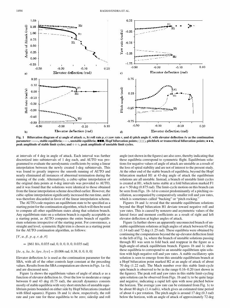
Fig. 1 Bifurcation diagram of a) angle of attack α, b) roll rate p, c) yaw rate r, and d) pitch angle θ, with elevator deflection δe as the continuationparameter: ——, stable equilibria; - - - -, unstable equilibria; ��, Hopf bifurcation points; ��, pitchfork or transcritical bifurcation points; • • •,peak amplitude of stable limit cycles; and ◦ ◦ ◦, peak amplitude of unstable limit cycles.

at intervals of 4 deg in angle of attack. Each interval was furtherdiscretized into subintervals of 1 deg each, and AUTO was pro-grammed to evaluate the aerodynamic coefficients by using a linearinterpolation between the newly created 1-deg subintervals. Thiswas found to greatly improve the smooth running of AUTO andnearly eliminated all instances of abnormal termination during therunning of the code. Alternatively, a cubic-spline interpolation ofthe original data points at 4-deg intervals was provided to AUTO,and it was found that the solutions were identical to those obtainedfrom the linear interpolation scheme described earlier. However, thecubic-spline interpolation significantly increased the run time, and itwas therefore discarded in favor of the linear interpolation scheme.

The AUTO code requires an equilibrium state to be specified as astarting point for the continuation algorithm, which will then be usedto compute all other equilibrium states along that solution branch.Any equilibrium state on a solution branch is equally acceptable asa starting point, as AUTO computes the entire branch of equilib-rium solutions irrespective of the starting point. For convenience, astraight and level, symmetric flight trim is chosen as a starting pointfor the AUTO continuation algorithm, as follows:

[V, α, β, p, q, r, φ, θ]

= [661 ft/s, 0.035 rad, 0, 0, 0, 0, 0, 0.035 rad]

[δe, η, δa, δr, δpv, δyv] = [0.006 rad, 0.38, 0, 0, 0, 0]

Elevator deflection δe is used as the continuation parameter for theSBA, with all of the other controls kept constant at the precedingvalues. Results from the SBA computation are shown in Figs. 1a–1d,and are discussed next.

Figure 1a shows the equilibrium values of angle of attack α as afunction of elevator deflection δe. Over the low to moderate α rangebetween 0 and 43 deg (0.75 rad), the aircraft dynamics consistsmostly of stable equilibria with very short stretches of unstable equi-librium points bounded on either side by Hopf bifurcations (markedwith filled squares). Figures 1b and 1c show, respectively, the rollrate and yaw rate for these equilibria to be zero; sideslip and roll

angle (not shown in the figures) are also zero, thereby indicating thatthese equilibria correspond to symmetric flight. Equilibrium solu-tions for negative values of angle of attack are unstable as a result ofthe loss of spiral stability and are not of interest to the present study.At the other end of the stable branch of equilibria, beyond the Hopfbifurcation marked H1 at 43-deg angle of attack the equilibriumsolutions are all unstable. Instead, a branch of unstable limit cyclesis created at H1, which turns stable at a fold bifurcation marked F1at α ≈ 50 deg (0.875 rad). The limit-cycle motion on this branch canbe seen from Figs. 1b–1d to consist predominantly of a pitching os-cillation, accompanied by comparatively smaller roll and yaw rates,which is sometimes called “bucking” or “pitch rocking.”

Figures 1b and 1c reveal that the unstable equilibrium solutionsbeyond the Hopf bifurcation H1 deviate toward negative roll andyaw rates. This is caused by nonzero and asymmetric values of thelateral force and moment coefficients as a result of right and leftelevator deflection at higher angles of attack.

Figure 1a further shows an apparently unconnected branch of un-stable equilibrium solutions at high angles of attack between 65 deg(1.14 rad) and 72 deg (1.25 rad). These equilibria were obtained bycontinuing the computations beyond the up-elevator deflection limitto the left of Fig. 1a, where the branch of unstable solutions passingthrough H1 was seen to fold back and reappear in the figure as ahigh-angle-of-attack equilibrium branch. Figures 1b and 1c showthese equilibria to correspond to an unstable equilibrium spin solu-tion with high negative roll and yaw rates. A stable oscillatory spinsolution is seen to emerge from this unstable equilibrium branch ata Hopf bifurcation point marked H2 at an angle of attack of about70 deg (1.22 rad). The Mach number over this stable limit-cyclespin branch is observed to be in the range 0.16–0.20 (not shown inthe figures). The peak roll and yaw rates in this stable limit-cyclingspin solution can be observed from Figs. 1b and 1c to be quite largeand negative, indicating a rapid left spin with nose pitched belowthe horizon. The average yaw rate can be estimated from Fig. 1c tobe about 80 deg/s (1.4 rad/s), which gives an estimated time periodof about 4 s per rotation. The pitch angle is around 17 deg (0.3 rad)below the horizon, with an angle of attack of approximately 72 deg


a) Angle of attack α (——) and sideslip angle β (- - - -)

b) Roll angle φ (——), pitch angle θ (- - - -), and flight path angleγ (–·–)

c) Roll p (- - - -), pitch q (——), and yaw r (–·–) rates

Fig. 2 Numerically simulated time histories of different state variablesin fully developed oscillatory spin.

(1.25 rad), which gives the flight-path angle to be nearly −90 deg,that is, velocity vector pointing nearly vertically downwards. Theairplane therefore appears to enter a flat, oscillatory left spin at theHopf bifurcation point H2, descending vertically with a full turncompleted in around 4 s.

The oscillatory spin dynamics is numerically simulated to con-firm the predictions made by the bifurcation analysis. All numericalsimulations reported in this paper are carried out by using Simulink

a)

b)

c)

Fig. 3 Numerically simulated time histories of a) heading angle ψ andposition variables b) Y and c) Z in fully developed oscillatory spin.

under a MATLAB® environment. The following values of the con-trol deflections are used for this simulation:

δe = −25 deg(−0.44 rad), η = 0.38

δa = δr = δpv = δyv = 0

Time histories of the aircraft attitude, angular rates, and positionvariables in a fully developed spin over a 50-s time interval areplotted in Figs. 2 and 3. Figure 2a shows oscillations in angle ofattack and sideslip angle about a mean α of about 72 deg (1.25 rad)and a mean β of 2 deg (0.035 rad). Figure 2b shows small oscillations


in roll angle about a mean left bank angle of φ ≈ 2 deg; consequently,the component of the angular velocity � about the body Y axis, thatis, the pitch rate q, is also quite small, as seen in Fig. 2c. Figure 2balso shows small oscillations in pitch angle θ , while the flight-pathangle γ is seen to be nearly constant at approximately −86 deg(−1.5 rad). Reasonably large negative values of roll rate are seen inFig. 2c with a peak-to-peak variation of about 12 deg/s (0.2 rad/s),whereas the average yaw rate is very high at around −82 deg/s(−1.43 rad/s). The plot of heading angle ψ in Fig. 3a has a slopeof around 1.6 rad/s, which implies that the airplane executes oneturn in just under 4 s. Figure 3b reveals the radius of the turn to beof the order of 8–10 ft, whereas, from Fig. 3c, the loss in altitudecan be seen to be about 200 ft per second. The oscillatory spinpredicted by the bifurcation analysis and confirmed by the numericalsimulation appears to match fairly well with observations on a scaledF-18/HARV model in a spin tunnel.37

III. Level-Flight Trim ComputationNext, the stable, level, symmetric flight trim states to which

the airplane could be recovered are computed by using an EBAprocedure.31 The EBA procedure, briefly, allows the computationof equilibrium solutions subject to constraints on the state variablesx1. The aircraft dynamics given by Eq. (2) along with the constraintequations are represented in the following form:

x1 = f1(x1, u1, u2, . . . , um + 1, um + 2, . . . , ur )

gi (x1) = 0, i = 1, . . . , m (3)

where gi are the m constraint functions; u1 is the principal con-tinuation parameter; u2, . . . , um + 1 are the m control parametersthat are to be varied as a function of u1 so as to satisfy the con-straints represented by the gi ; and um + 2, . . . , ur are the controlsthat are kept constant. The EBA computations are carried out intwo steps. In the first step, both the state and constraint equations inEq. (3) are solved together to simultaneously obtain the constrainedequilibrium solutions x1(u1) and the control parameter schedulesu2(u1), . . . , um + 1(u1) required to satisfy the constraints gi . In thesecond step, only the state equations in Eq. (3), with the parameterschedules computed in the first step incorporated as follows

x1 = f1[x1, u1, u2(u1), . . . , um + 1(u1), um + 2, . . . , ur ] (4)

are solved to obtain the equilibrium states, their stability, bifurca-tion points, and bifurcated equilibrium branches. The equilibriumsolutions on the bifurcated branches represent departures from theconstrained trim states; these are valid solutions for the control pa-rameter schedules u2(u1), . . . , um + 1(u1), but do not satisfy the con-straints gi .

In the present instance, the specification of level, symmetric flighttrims requires the following constraints to be imposed on the flight-path angle γ , roll angle φ, and sideslip angle β:

g1 = γ = 0, g2 = φ = 0, g3 = β = 0 (5)

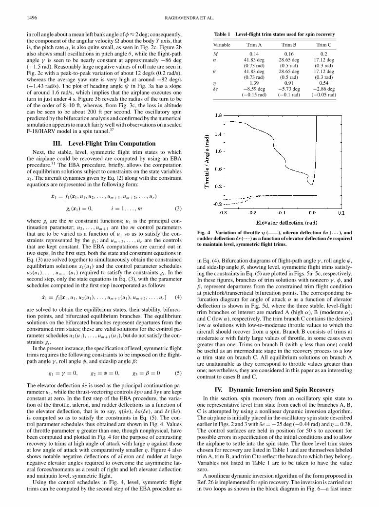
The elevator deflection δe is used as the principal continuation pa-rameter u1, while the thrust-vectoring controls δpv and δyv are keptconstant at zero. In the first step of the EBA procedure, the varia-tion of the throttle, aileron, and rudder deflections as a function ofthe elevator deflection, that is to say, η(δe), δa(δe), and δr(δe),is computed so as to satisfy the constraints in Eq. (5). The con-trol parameter schedules thus obtained are shown in Fig. 4. Valuesof throttle parameter η greater than one, though nonphysical, havebeen computed and plotted in Fig. 4 for the purpose of contrastingrecovery to trims at high angle of attack with large η against thoseat low angle of attack with comparatively smaller η. Figure 4 alsoshows notable negative deflections of aileron and rudder at largenegative elevator angles required to overcome the asymmetric lat-eral forces/moments as a result of right and left elevator deflectionand maintain level, symmetric flight.

Using the control schedules in Fig. 4, level, symmetric flighttrims can be computed by the second step of the EBA procedure as

Table 1 Level-flight trim states used for spin recovery

Variable Trim A Trim B Trim C

M 0.14 0.16 0.2α 41.83 deg 28.65 deg 17.12 deg

(0.73 rad) (0.5 rad) (0.3 rad)θ 41.83 deg 28.65 deg 17.12 deg

(0.73 rad) (0.5 rad) (0.3 rad)η 1.39 0.91 0.54δe −8.59 deg −5.73 deg −2.86 deg

(−0.15 rad) (−0.1 rad) (−0.05 rad)

Fig. 4 Variation of throttle η (——), aileron deflection δa (- - - ), andrudder deflection δr (–·–) as a function of elevator deflection δe requiredto maintain level, symmetric flight trims.

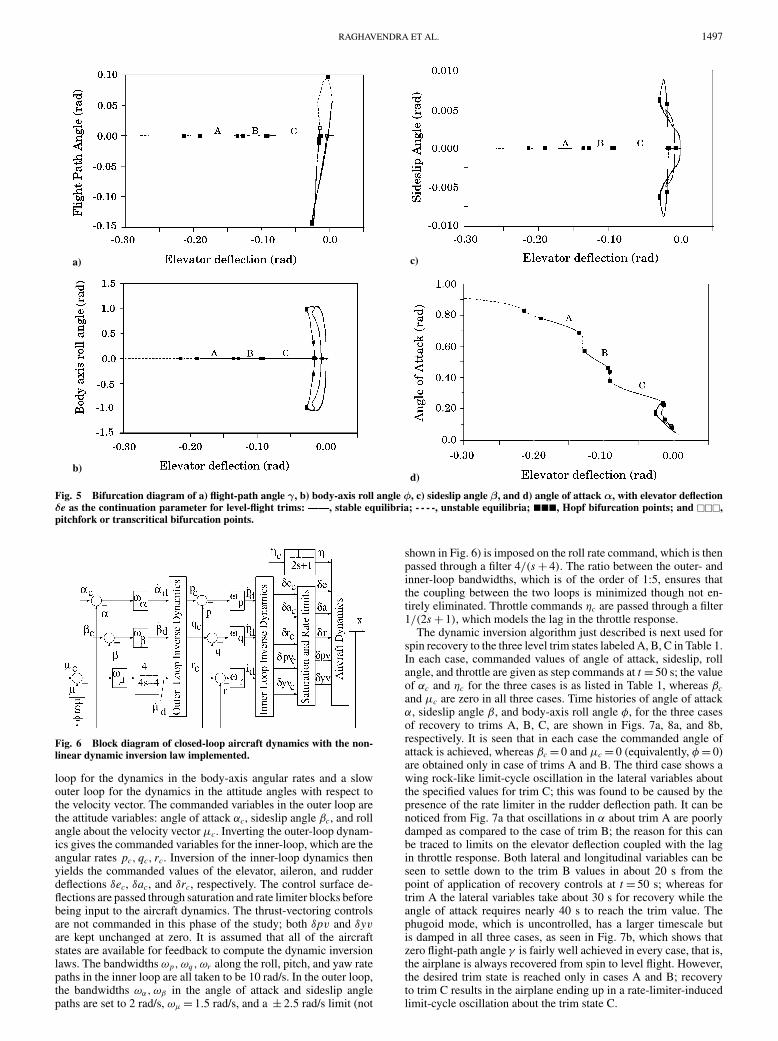
in Eq. (4). Bifurcation diagrams of flight-path angle γ , roll angle φ,and sideslip angle β, showing level, symmetric flight trims satisfy-ing the constraints in Eq. (5) are plotted in Figs. 5a–5c, respectively.In these figures, branches of trim solutions with nonzero γ , φ, andβ, represent departures from the constrained trim flight conditionat pitchfork/transcritical bifurcation points. The corresponding bi-furcation diagram for angle of attack α as a function of elevatordeflection is shown in Fig. 5d, where the three stable, level-flighttrim branches of interest are marked A (high α), B (moderate α),and C (low α), respectively. The trim branch C contains the desiredlow α solutions with low-to-moderate throttle values to which theaircraft should recover from a spin. Branch B consists of trims atmoderate α with fairly large values of throttle, in some cases evengreater than one. Trims on branch B (with η less than one) couldbe useful as an intermediate stage in the recovery process to a lowα trim state on branch C. All equilibrium solutions on branch Aare unattainable as they correspond to throttle values greater thanone; nevertheless, they are considered in this paper as an interestingcontrast to cases B and C.

IV. Dynamic Inversion and Spin RecoveryIn this section, spin recovery from an oscillatory spin state to

one representative level trim state from each of the branches A, B,C is attempted by using a nonlinear dynamic inversion algorithm.The airplane is initially placed in the oscillatory spin state describedearlier in Figs. 2 and 3 with δe = −25 deg (−0.44 rad) and η = 0.38.The control surfaces are held in position for 50 s to account forpossible errors in specification of the initial conditions and to allowthe airplane to settle into the spin state. The three level trim stateschosen for recovery are listed in Table 1 and are themselves labeledtrim A, trim B, and trim C to reflect the branch to which they belong.Variables not listed in Table 1 are to be taken to have the valuezero.

A nonlinear dynamic inversion algorithm of the form proposed inRef. 26 is implemented for spin recovery. The inversion is carried outin two loops as shown in the block diagram in Fig. 6—a fast inner


a)

b)

c)

d)

Fig. 5 Bifurcation diagram of a) flight-path angle γ, b) body-axis roll angle φ, c) sideslip angle β, and d) angle of attack α, with elevator deflectionδe as the continuation parameter for level-flight trims: ——, stable equilibria; - - - -, unstable equilibria; ��, Hopf bifurcation points; and ��,pitchfork or transcritical bifurcation points.

Fig. 6 Block diagram of closed-loop aircraft dynamics with the non-linear dynamic inversion law implemented.

loop for the dynamics in the body-axis angular rates and a slowouter loop for the dynamics in the attitude angles with respect tothe velocity vector. The commanded variables in the outer loop arethe attitude variables: angle of attack αc, sideslip angle βc, and rollangle about the velocity vector µc. Inverting the outer-loop dynam-ics gives the commanded variables for the inner-loop, which are theangular rates pc, qc, rc. Inversion of the inner-loop dynamics thenyields the commanded values of the elevator, aileron, and rudderdeflections δec, δac, and δrc, respectively. The control surface de-flections are passed through saturation and rate limiter blocks beforebeing input to the aircraft dynamics. The thrust-vectoring controlsare not commanded in this phase of the study; both δpv and δyvare kept unchanged at zero. It is assumed that all of the aircraftstates are available for feedback to compute the dynamic inversionlaws. The bandwidths ωp, ωq , ωr along the roll, pitch, and yaw ratepaths in the inner loop are all taken to be 10 rad/s. In the outer loop,the bandwidths ωα, ωβ in the angle of attack and sideslip anglepaths are set to 2 rad/s, ωµ = 1.5 rad/s, and a ± 2.5 rad/s limit (not

shown in Fig. 6) is imposed on the roll rate command, which is thenpassed through a filter 4/(s + 4). The ratio between the outer- andinner-loop bandwidths, which is of the order of 1:5, ensures thatthe coupling between the two loops is minimized though not en-tirely eliminated. Throttle commands ηc are passed through a filter1/(2s + 1), which models the lag in the throttle response.

The dynamic inversion algorithm just described is next used forspin recovery to the three level trim states labeled A, B, C in Table 1.In each case, commanded values of angle of attack, sideslip, rollangle, and throttle are given as step commands at t = 50 s; the valueof αc and ηc for the three cases is as listed in Table 1, whereas βc

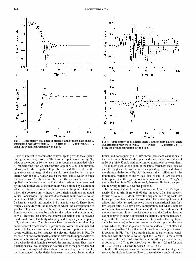
and µc are zero in all three cases. Time histories of angle of attackα, sideslip angle β, and body-axis roll angle φ, for the three casesof recovery to trims A, B, C, are shown in Figs. 7a, 8a, and 8b,respectively. It is seen that in each case the commanded angle ofattack is achieved, whereas βc = 0 and µc = 0 (equivalently, φ = 0)are obtained only in case of trims A and B. The third case shows awing rock-like limit-cycle oscillation in the lateral variables aboutthe specified values for trim C; this was found to be caused by thepresence of the rate limiter in the rudder deflection path. It can benoticed from Fig. 7a that oscillations in α about trim A are poorlydamped as compared to the case of trim B; the reason for this canbe traced to limits on the elevator deflection coupled with the lagin throttle response. Both lateral and longitudinal variables can beseen to settle down to the trim B values in about 20 s from thepoint of application of recovery controls at t = 50 s; whereas fortrim A the lateral variables take about 30 s for recovery while theangle of attack requires nearly 40 s to reach the trim value. Thephugoid mode, which is uncontrolled, has a larger timescale butis damped in all three cases, as seen in Fig. 7b, which shows thatzero flight-path angle γ is fairly well achieved in every case, that is,the airplane is always recovered from spin to level flight. However,the desired trim state is reached only in cases A and B; recoveryto trim C results in the airplane ending up in a rate-limiter-inducedlimit-cycle oscillation about the trim state C.


a)

b)

Fig. 7 Time history of a) angle of attack α and b) flight-path angle γ,during spin recovery to trim A (——), trim B (- - - -), and trim C (–·–),using the dynamic inversion law in Fig. 6.

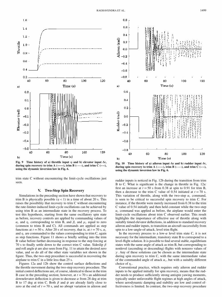
It is of interest to examine the control inputs given to the airplaneduring the recovery process. The throttle input, shown in Fig. 9a,takes of the order of 10 s to reach the respective commanded valueηc, reflecting the time lag in the throttle loop of Ts = 2 s. The elevator,aileron, and rudder inputs in Figs. 9b, 10a, and 10b reveal that thespin recovery strategy of the dynamic inversion law is to applyaileron with the roll, rudder against the turn, and elevator to pitchthe nose down. All three controls, in all three cases A, B, C, areapplied simultaneously at t = 50 s at the maximum rate permittedby the rate limiter and to the maximum value limited by saturation;what is different between the three cases is the point of time atwhich the controls are withdrawn from their maximum saturatedvalues. For example, Fig. 9b shows that the maximum down-elevatordeflection of 10 deg (0.175 rad) is released at t ≈ 61 s for case A,2 s later for case B, and another 1–2 s later for case C. These timesroughly coincide with the moments at which the corresponding αgraphs in Fig. 7a first cross the respective commanded values αc.Similar observations can be made for the rudder and aileron inputsas well. Beyond that point, the control deflections aim to providethe desired level of stability (damping and frequency) in the pitch,roll, and yaw loops. Thus, in cases where the aerodynamic dampingand/or control effectiveness is presumably lower, the commandedcontrol deflections are larger, and the control inputs show moresevere oscillations. For instance, the elevator deflection in Fig. 9bfor case A shows continued fluctuations between the upper and lowersaturation limits indicating that the elevator input required to obtainthe desired level of damping exceeds the limiting values. Thus, thesefluctuations in elevator input can be correlated to the poorly dampedoscillations in angle of attack about trim A in Fig. 7a. In case C,the commanded rudder deflections seem to exceed the saturation

a)

b)

Fig. 8 Time history of a) sideslip angle β and b) body-axis roll angleφ, during spin recovery to trim A (——), trim B (- - - -), and trim C (–·–),using the dynamic inversion law in Fig. 6.

limits, and consequently Fig. 10b shows persistent oscillations inthe rudder input between the upper and lower saturation values of± 30 deg ( ± 0.52 rad) with rate-limited transitions between them.This induces oscillations in all of the lateral variables (see Figs. 8aand 8b for β and φ), in the aileron input (Fig. 10a), and also inthe elevator deflection (Fig. 9b); however, the oscillations in thelongitudinal variables α and γ (see Figs. 7a and 7b) are too smallto be apparent in the figures. When the rate limit of ± 82 deg/s inthe rudder loop is sufficiently relaxed, these oscillations disappear,and recovery to trim C becomes possible.

In summary, the airplane recovers to trim A (α = 41.83 deg) innearly 40 s, to trim B (α = 28.65 deg) in about 20 s, but recoveryto trim C (α = 17.12 deg) leaves the airplane in a wing rock-likelimit-cycle oscillation about the trim state. The initial application ofaileron and rudder for spin recovery is along conventional lines for alow-aspect-ratio, fuselage-heavy configuration, but what is notableis the simultaneous use of elevator and throttle, the withdrawal ofthe recovery controls at a precise moment, and the further vigoroususe of controls to damp out residual oscillations. In particular, open-ing the throttle picks up the velocity vector (makes the flight-pathangle less negative) at the same time as the elevator pitches the nosedown, which together help attain the commanded angle of attack asquickly as possible. The influence of throttle on the angle of attackis apparent in Fig. 7a, where starting from the same initial condi-tion and with the same elevator input for t = 50–61 s the aircraftresponse at the end of 61 s for different throttle inputs is different,as follows: α ≈ 0.7 rad for case A (ηc = 1.39); α ≈ 0.9 rad for caseB (ηc = 0.91); α ≈ 1.0 rad for case C (ηc = 0.54).

In the following sections, we examine two different strategies torecover the airplane from oscillatory spin to the low-angle-of-attack


a)

b)

Fig. 9 Time history of a) throttle input η and b) elevator input δe,during spin recovery to trim A (——), trim B (- - - -), and trim C (–·–),using the dynamic inversion law in Fig. 6.

trim state C without encountering the limit-cycle oscillations justseen.

V. Two-Step Spin RecoverySimulations in the preceding section have shown that recovery to

trim B is physically possible (η < 1) in a time of about 20 s. Thisraises the possibility that recovery to trim C without encounteringthe rate-limiter-induced limit-cycle oscillations can be achieved byusing trim B as an intermediate state in the recovery process. Totest this hypothesis, starting from the same oscillatory spin stateas before, recovery controls are applied by commanding values ofαc and ηc corresponding to trim B, and βc and µc equal to zero(common to trims B and C). All commands are applied as stepfunctions at t = 50 s. After 20 s of recovery, that is, at t = 70 s, αc

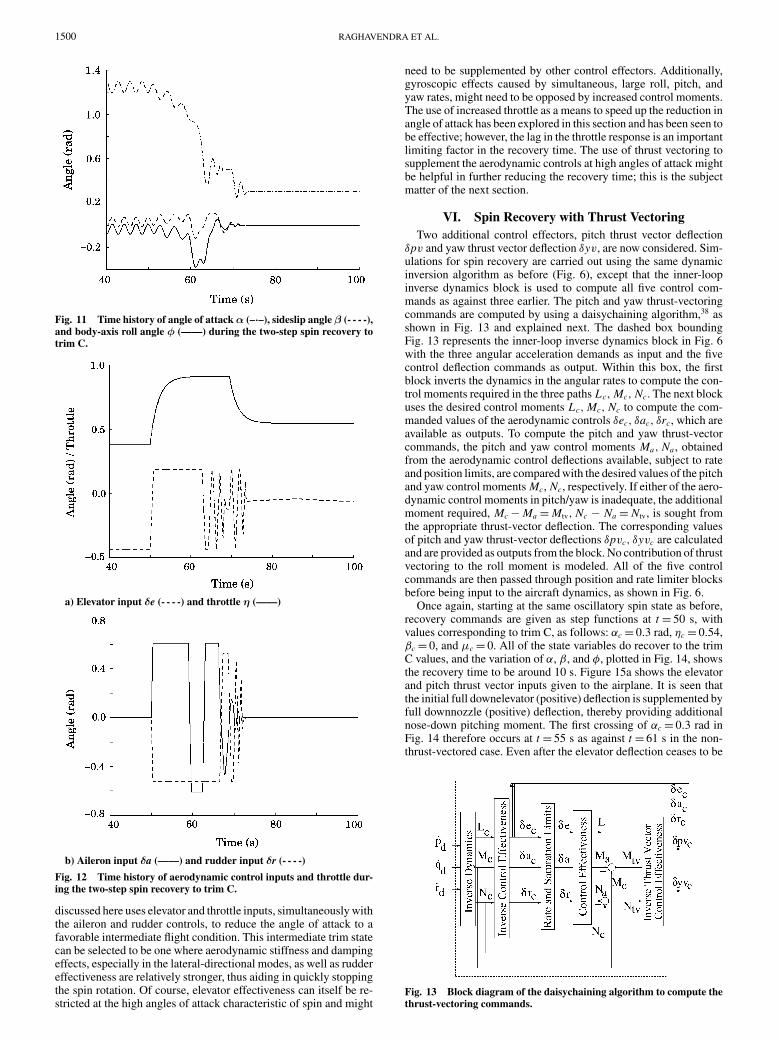
and ηc are commanded to the values corresponding to trim C, againas step functions. Figure 11 shows α briefly settling into the trimB value before further decreasing in response to the step forcing at70 s to finally settle down to the correct trim C value. Sideslip βand roll angle φ are also seen from Fig. 11 to attain the desired zerovalue, and so do all of the other state variables not shown in thefigure. Thus, the two-step procedure is successful in recovering theairplane to trim C in a little less than 25 s.

Figures 12a and 12b show the control surface deflections andthe throttle movement during the two-step recovery procedure. Theinitial control deflections are, of course, identical to those in the trimB case in the preceding section; however, at t = 70 s an additionaldownelevator deflection is given to decrease α from 28 deg at trimB to 17 deg at trim C. Both β and φ are already fairly close tozero at the end of t = 70 s, and no abrupt variation in aileron and

a)

b)

Fig. 10 Time history of a) aileron input δa and b) rudder input δr,during spin recovery to trim A (——), trim B (- - - -), and trim C (–·–),using the dynamic inversion law in Fig. 6.

rudder inputs is noticed in Fig. 12b during the transition from trimB to C. What is significant is the change in throttle in Fig. 12a:first an increase at t = 50 s from 0.38 at spin to 0.91 for trim B,then a decrease to the trim C value of 0.54 initiated at t = 70 s.This variation of throttle, along with the two-step αc command,is seen to be critical to successful spin recovery to trim C. Forinstance, if the throttle were merely increased from 0.38 to the trimC value of 0.54 initially and then held constant while the two-stepαc command was applied as before, the airplane would enter thelimit-cycle oscillations about trim C observed earlier. This resulthighlights the importance of effective use of throttle along withsuitably timed elevator deflections, in addition to standard recoveryaileron and rudder inputs, to transition an aircraft successfully fromspin to a low-angle-of-attack, level trim flight.

In the recovery process to a low-α level trim state C, it is notnecessary for the intermediate, transitory state B to correspond to alevel-flight solution. It is possible to find several stable, equilibriumstates with the same angle of attack as trim B, but corresponding tononlevel (ascending or descending) flights with nonzero values ofγ . Any of these solutions can be chosen as the intermediate stateduring spin recovery to trim C, with the same intermediate valueof the commanded angle of attack αc, but with a suitably differentchoice of ηc.

Conventional practice, which requires only aileron and rudderinputs to be applied initially for spin recovery, means that the rud-der needs to produce sufficiently strong antispin yawing moments,typically under unfavorable flight regimes at high angles of attack,where aerodynamic damping and stability are low and control ef-fectiveness is limited. In contrast, the two-step recovery procedure


Fig. 11 Time history of angle of attack α (–·–), sideslip angle β (- - - -),and body-axis roll angle φ (——) during the two-step spin recovery totrim C.

a) Elevator input δe (- - - -) and throttle η (——)

b) Aileron input δa (——) and rudder input δr (- - - -)

Fig. 12 Time history of aerodynamic control inputs and throttle dur-ing the two-step spin recovery to trim C.

discussed here uses elevator and throttle inputs, simultaneously withthe aileron and rudder controls, to reduce the angle of attack to afavorable intermediate flight condition. This intermediate trim statecan be selected to be one where aerodynamic stiffness and dampingeffects, especially in the lateral-directional modes, as well as ruddereffectiveness are relatively stronger, thus aiding in quickly stoppingthe spin rotation. Of course, elevator effectiveness can itself be re-stricted at the high angles of attack characteristic of spin and might

need to be supplemented by other control effectors. Additionally,gyroscopic effects caused by simultaneous, large roll, pitch, andyaw rates, might need to be opposed by increased control moments.The use of increased throttle as a means to speed up the reduction inangle of attack has been explored in this section and has been seen tobe effective; however, the lag in the throttle response is an importantlimiting factor in the recovery time. The use of thrust vectoring tosupplement the aerodynamic controls at high angles of attack mightbe helpful in further reducing the recovery time; this is the subjectmatter of the next section.

VI. Spin Recovery with Thrust VectoringTwo additional control effectors, pitch thrust vector deflection

δpv and yaw thrust vector deflection δyv, are now considered. Sim-ulations for spin recovery are carried out using the same dynamicinversion algorithm as before (Fig. 6), except that the inner-loopinverse dynamics block is used to compute all five control com-mands as against three earlier. The pitch and yaw thrust-vectoringcommands are computed by using a daisychaining algorithm,38 asshown in Fig. 13 and explained next. The dashed box boundingFig. 13 represents the inner-loop inverse dynamics block in Fig. 6with the three angular acceleration demands as input and the fivecontrol deflection commands as output. Within this box, the firstblock inverts the dynamics in the angular rates to compute the con-trol moments required in the three paths Lc, Mc, Nc. The next blockuses the desired control moments Lc, Mc, Nc to compute the com-manded values of the aerodynamic controls δec, δac, δrc, which areavailable as outputs. To compute the pitch and yaw thrust-vectorcommands, the pitch and yaw control moments Ma, Na , obtainedfrom the aerodynamic control deflections available, subject to rateand position limits, are compared with the desired values of the pitchand yaw control moments Mc, Nc, respectively. If either of the aero-dynamic control moments in pitch/yaw is inadequate, the additionalmoment required, Mc − Ma = Mtv, Nc − Na = Ntv, is sought fromthe appropriate thrust-vector deflection. The corresponding valuesof pitch and yaw thrust-vector deflections δpvc, δyvc are calculatedand are provided as outputs from the block. No contribution of thrustvectoring to the roll moment is modeled. All of the five controlcommands are then passed through position and rate limiter blocksbefore being input to the aircraft dynamics, as shown in Fig. 6.

Once again, starting at the same oscillatory spin state as before,recovery commands are given as step functions at t = 50 s, withvalues corresponding to trim C, as follows: αc = 0.3 rad, ηc = 0.54,βc = 0, and µc = 0. All of the state variables do recover to the trimC values, and the variation of α, β, and φ, plotted in Fig. 14, showsthe recovery time to be around 10 s. Figure 15a shows the elevatorand pitch thrust vector inputs given to the airplane. It is seen thatthe initial full downelevator (positive) deflection is supplemented byfull downnozzle (positive) deflection, thereby providing additionalnose-down pitching moment. The first crossing of αc = 0.3 rad inFig. 14 therefore occurs at t = 55 s as against t = 61 s in the non-thrust-vectored case. Even after the elevator deflection ceases to be

Fig. 13 Block diagram of the daisychaining algorithm to compute thethrust-vectoring commands.


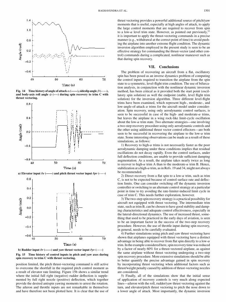
Fig. 14 Time history of angle of attackα (——), sideslip angleβ (- - - -),and body-axis roll angle φ (–·–) during spin recovery to trim C withthrust vectoring.

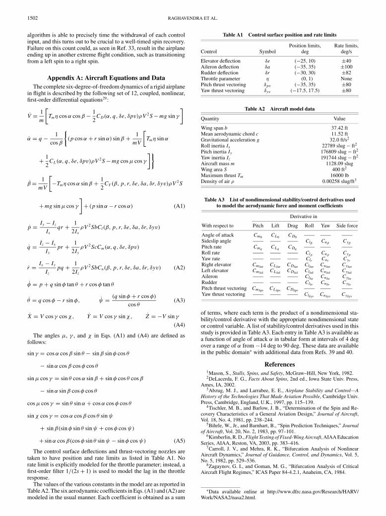
a) Elevator input δe (——) and pitch thrust vector input δpv (- - - -)

b) Rudder input δr (——) and yaw thrust vector input δyv (- - - -)

Fig. 15 Time history of control inputs in pitch and yaw axes duringspin recovery to trim C with thrust vectoring.

position limited, the pitch thrust-vectoring command is still activeto overcome the shortfall in the required pitch control moment asa result of elevator rate limiting. Figure 15b shows a similar trendwhere the initial full right (negative) rudder deflection is supple-mented by full right nozzle (positive) deflection, which togetherprovide the desired antispin yawing moments to arrest the rotation.The aileron and throttle inputs are not remarkable in themselvesand have therefore not been plotted here. It is clear that the use of

thrust vectoring provides a powerful additional source of pitch/yawmoments that is useful, especially at high angles of attack, to applythe large control moments that are required to recover from spinto a low-α level trim state. However, as pointed out previously,33

it is important to apply the thrust-vectoring commands in a precisemanner (e.g., withdrawal at the correct point of time) to avoid push-ing the airplane into another extreme flight condition. The dynamicinversion algorithm employed in the present study is seen to be aneffective strategy for commanding the thrust-vector (and other con-trol) commands during a complicated, nonlinear maneuver such asthat during spin recovery.

VII. ConclusionsThe problem of recovering an aircraft from a flat, oscillatory

spin has been posed as an inverse dynamics problem of computingthe control inputs required to transition the airplane from the spinstate to a symmetric, level-flight trim condition. The use of bifurca-tion analysis, in conjunction with the nonlinear dynamic inversionmethod, has been critical as it provided both the start point (oscil-latory spin solution) as well the endpoint (stable, level flight trimsolution) for the inversion algorithm. Three different level-flighttrims have been examined, which represent high-, moderate-, andlow-angle-of-attack α trims for the aircraft model under consider-ation. Spin recovery, using only aerodynamic control surfaces, isseen to be successful in case of the high- and moderate-α trims,but leaves the airplane in a wing rock-like limit-cycle oscillationabout the low-α trim state. Two alternate strategies—one involvinga two-step recovery procedure using only aerodynamic controls andthe other using additional thrust vector control effectors—are bothseen to be successful in recovering the airplane to the low-α trimstate. Some interesting observations can be made as a result of thesesimulations, as follows:

1) Recovery to high-α trims is not necessarily faster as the pooraerodynamic damping under these conditions implies that residualoscillations do not decay rapidly. Even the control surfaces, underfull deflection conditions, are unable to provide sufficient dampingaugmentation. As a result, the airplane takes nearly twice as longto recover to high-α trim A than to the moderate-α trim B. Hence,stabilization at a high-α trim, as in Refs. 19 and 34, might not alwaysbe recommended.

2) Direct recovery from a flat spin to a low-α trim, such as trimC, is not to be expected because of control surface rate and deflec-tion limits. One can consider switching off the dynamic inversioncontroller or switching to an alternate control strategy at a particularpoint in time to try avoiding the rate-limiter-induced limit cycle incase of trim C. This needs further exploration, however.

3) The two-step spin recovery strategy is a practical possibility foraircraft not equipped with thrust vectoring. The intermediate trimstate, such as trim B, can be chosen to have good stability and damp-ing characteristics and adequate control effectiveness, especially inthe lateral-directional dynamics. The use of increased thrust, some-thing that used to be practiced in the early days of aviation, is seento be an important factor in the success of the two-step recoveryprocedure. However, the use of throttle input during spin recovery,in general, needs to be carefully evaluated.

4) Further simulations using pitch and yaw thrust vectoring haveshown that airplanes equipped with thrust vectoring have a distinctadvantage in being able to recover from flat spin directly to a low-αtrim. In the example considered here, spin recovery time was reducedby a factor of nearly 60% for a thrust-vectored airplane, as againstthe same airplane without thrust vectoring undergoing a two-stepspin recovery procedure. More extensive simulations should be ableto better quantify the precise advantage gained in spin recoveryby incorporating thrust vectoring when additional factors such asthrust/weight penalty caused by addition of thrust-vectoring nozzlesare considered.

5) Finally, all of the simulations show that the initial senseof application of recovery controls is very much along expectedlines—aileron with the roll, rudder/yaw thrust vectoring against theturn, and elevator/pitch thrust vectoring to pitch the nose down toa lower angle of attack. Most importantly, the dynamic inversion


algorithm is able to precisely time the withdrawal of each controlinput, and this turns out to be crucial to a well-timed spin recovery.Failure on this count could, as seen in Ref. 33, result in the airplaneending up in another extreme flight condition, such as transitioningfrom a left spin to a right spin.

Appendix A: Aircraft Equations and DataThe complete six-degree-of-freedom dynamics of a rigid airplane

in flight is described by the following set of 12, coupled, nonlinear,first-order differential equations29:

V = 1

m

[Tmη cos α cos β − 1

2CD(α, q, δe, δpv)ρV 2 S − mg sin γ

]

α = q − 1

cos β

{(p cos α + r sin α) sin β + 1

mV

[Tmη sin α

+ 1

2CL(α, q, δe, δpv)ρV 2 S − mg cos µ cos γ

]}

β = 1

mV

[−Tmη cos α sin β + 1

2CY (β, p, r, δe, δa, δr, δyv)ρV 2 S

+ mg sin µ cos γ

]+ (p sin α − r cos α) (A1)

p = Iy − Iz

Ixqr + 1

2IxρV 2 SbCl(β, p, r, δe, δa, δr, δyv)

q = Iz − Ix

Iypr + 1

2IyρV 2 ScCm(α, q, δe, δpv)

r = Ix − Iy

Izpq + 1

2IzρV 2 SbCn(β, p, r, δe, δa, δr, δyv) (A2)

φ = p + q sin φ tan θ + r cos φ tan θ

θ = q cos φ − r sin φ, ψ = (q sin φ + r cos φ)

cos θ(A3)

X = V cos γ cos χ, Y = V cos γ sin χ, Z = −V sin γ

(A4)

The angles µ, γ , and χ in Eqs. (A1) and (A4) are defined asfollows:

sin γ = cos α cos β sin θ − sin β sin φ cos θ

− sin α cos β cos φ cos θ

sin µ cos γ = sin θ cos α sin β + sin φ cos θ cos β

− sin α sin β cos φ cos θ

cos µ cos γ = sin θ sin α + cos α cos φ cos θ

sin χ cos γ = cos α cos β cos θ sin ψ

+ sin β(sin φ sin θ sin ψ + cos φ cos ψ)

+ sin α cos β(cos φ sin θ sin ψ − sin φ cos ψ) (A5)

The control surface deflections and thrust-vectoring nozzles aretaken to have position and rate limits as listed in Table A1. Norate limit is explicitly modeled for the throttle parameter; instead, afirst-order filter 1/(2s + 1) is used to model the lag in the throttleresponse.

The values of the various constants in the model are as reported inTable A2. The six aerodynamic coefficients in Eqs. (A1) and (A2) aremodeled in the usual manner. Each coefficient is obtained as a sum

Table A1 Control surface position and rate limits

Position limits, Rate limits,Control Symbol deg deg/s

Elevator deflection δe (−25, 10) ±40Aileron deflection δa (−35, 35) ±100Rudder deflection δr (−30, 30) ±82Throttle parameter η (0, 1) NonePitch thrust vectoring δpv (−35, 35) ±80Yaw thrust vectoring δyv (−17.5, 17.5) ±80

Table A2 Aircraft model data

Quantity Value

Wing span b 37.42 ftMean aerodynamic chord c 11.52 ftGravitational acceleration g 32.0 ft/s2

Roll inertia Ix 22789 slug − ft2

Pitch inertia Iy 176809 slug − ft2

Yaw inertia Iz 191744 slug − ft2

Aircraft mass m 1128.09 slugWing area S 400 ft2

Maximum thrust Tm 16000 lbDensity of air ρ 0.00258 slug/ft3

Table A3 List of nondimensional stability/control derivatives usedto model the aerodynamic force and moment coefficients

Derivative in

With respect to Pitch Lift Drag Roll Yaw Side force

Angle of attack Cm0 CL0 CD0 —— —— ——Sideslip angle —— —— —— Clβ Cnβ

Cyβ

Pitch rate Cmq CLq CDq —— —— ——Roll rate —— —— —— Cl p Cn p Cyp

Yaw rate —— —— —— Clr Cnr Cyr

Right elevator Cmδer CLδer CDδer Clδer Cnδer CyδerLeft elevator Cmδel CLδel CDδel Clδel Cnδel CyδelAileron —— —— —— Clδa Cnδa CyδaRudder —— —— —— Clδr Cnδr CyδrPitch thrust vectoring Cmδpv CLδpv CDδpv —— —— ——Yaw thrust vectoring —— —— —— Clδyv Cnδyv Cyδyv

of terms, where each term is the product of a nondimensional sta-bility/control derivative with the appropriate nondimensional stateor control variable. A list of stability/control derivatives used in thisstudy is provided in Table A3. Each entry in Table A3 is available asa function of angle of attack α in tabular form at intervals of 4 degover a range of α from −14 deg to 90 deg. These data are availablein the public domain∗ with additional data from Refs. 39 and 40.

References1Mason, S., Stalls, Spins, and Safety, McGraw–Hill, New York, 1982.2DeLacerda, F. G., Facts About Spins, 2nd ed., Iowa State Univ. Press,

Ames, IA, 2002.3Abzug, M. J., and Larrabee, E. E., Airplane Stability and Control—A

History of the Technologies That Made Aviation Possible, Cambridge Univ.Press, Cambridge, England, U.K., 1997, pp. 115–139.

4Tischler, M. B., and Barlow, J. B., “Determination of the Spin and Re-covery Characteristics of a General Aviation Design,” Journal of Aircraft,Vol. 18, No. 4, 1981, pp. 238–244.

5Bihrle, W., Jr., and Barnhart, B., “Spin Prediction Techniques,” Journalof Aircraft, Vol. 20, No. 2, 1983, pp. 97–101.

6Kimberlin, R. D., Flight Testing of Fixed-Wing Aircraft, AIAA EducationSeries, AIAA, Reston, VA, 2003, pp. 383–416.

7Carroll, J. V., and Mehra, R. K., “Bifurcation Analysis of NonlinearAircraft Dynamics,” Journal of Guidance, Control, and Dynamics, Vol. 5,No. 5, 1982, pp. 529–536.

8Zagaynov, G. I., and Goman, M. G., “Bifurcation Analysis of CriticalAircraft Flight Regimes,” ICAS Paper 84-4.2.1, Anaheim, CA, 1984.

∗Data available online at http://www.dfrc.nasa.gov/Research/HARV/Work/NASA2/nasa2.html.


9Goman, M. G., Zagaynov, G. I., and Khramtsovsky, A. V., “Applicationof Bifurcation Methods to Nonlinear Flight Dynamics Problems,” Progressin Aerospace Sciences, Vol. 33, No. 59, 1997, pp. 539–586.

10Sinha, N. K., “Application of Bifurcation Methods to Nonlinear FlightDynamics,” Journal of the Aeronautical Society of India, Vol. 53, No. 4,2001, pp. 253–270.

11Planeaux, J. B., and Barth, T. J., “High-Angle-of-Attack DynamicBehavior of a Model High-Performance Fighter Aircraft,” AIAA Paper 1988-4368, Aug. 1988.

12Guicheteau, P., “Bifurcation Theory in Flight Dynamics—An Applica-tion to a Real Combat Aircraft,” ICAS Paper 90-5.10.4, Stockholm, 1990.

13Goman, M., Khramtsovsky, A., Soukhanov, V., Syrovatsky, V., andTatarnikov, K., “Aircraft Spin Prevention/Recovery Control System,”TsAGI, Nov. 1993.

14Ananthkrishnan, N., and Sudhakar, K., “Prevention of Jump in Inertia-Coupled Roll Maneuvers of Aircraft,” Journal of Aircraft, Vol. 31, No. 4,1994, pp. 981–983.

15Lowenberg, M. H., “Development of Control Schedules to Modify SpinBehavior,” AIAA Paper 1998-4267, Aug. 1998.

16Littleboy, D. M., and Smith, P. R., “Using Bifurcation Methods to AidNonlinear Dynamic Inversion Control Law Design,” Journal of Guidance,Control, and Dynamics, Vol. 21, No. 4, 1998, pp. 632–638.

17Jahnke, C. C., and Culick, F. E. C., “Application of Bifurcation Theoryto the High-Angle-of-Attack Dynamics of the F-14,” Journal of Aircraft,Vol. 31, No. 1, 1994, pp. 26–34.

18Goman, M. G., and Khramtsovsky, A. V., “Application of Continuationand Bifurcation Methods to the Design of Control Systems,” PhilosophicalTransactions of the Royal Society of London Series A—Mathematical, Phys-ical, and Engineering Sciences, Vol. 356, No. 1745, 1998, pp. 2277–2295.

19Saraf, A., Deodhare, G., and Ghose, D., “Synthesis of Nonlinear Con-troller to Recover an Unstable Aircraft from Poststall Regime,” Journal ofGuidance, Control, and Dynamics, Vol. 22, No. 5, 1999, pp. 710–717.

20Kato, O., and Sugiura, I., “An Interpretation of Airplane General Mo-tion and Control as Inverse Problem,” Journal of Guidance, Control, andDynamics, Vol. 9, No. 2, 1986, pp. 198–204.

21Asseo, S. J., “Decoupling of a Class of Nonlinear Systems and Appli-cations to an Aircraft Control Problem,” Journal of Aircraft, Vol. 10, No. 12,1973, pp. 739–747.

22Menon, P. K. A., Badgett, M. E., Walker, R. A., and Duke, E. L.,“Nonlinear Flight Test Trajectory Controllers for Aircraft,” Journal of Guid-ance, Control, and Dynamics, Vol. 10, No. 1, 1987, pp. 67–72.

23Lane, S. H., and Stengel, R. F., “Flight Control Design Using NonlinearInverse Dynamics,” Automatica, Vol. 24, No. 4, 1988, pp. 471–483.

24Bugajski, D. J., and Enns, D. F., “Nonlinear Control Law with Appli-cation to High Angle of Attack Flight,” Journal of Guidance, Control, andDynamics, Vol. 15, No. 3, 1992, pp. 761–767.

25Azam, M., and Singh, S. N., “Invertibility and Trajectory Controlfor Nonlinear Maneuvers of Aircraft,” Journal of Guidance, Control, andDynamics, Vol. 17, No. 1, 1994, pp. 192–200.

26Snell, S. A., Enns, D. F., and Garrard, W. L., Jr., “Nonlinear InversionFlight Control for a Supermaneuverable Aircraft,” Journal of Guidance,Control, and Dynamics, Vol. 15, No. 4, 1992, pp. 976–984.

27Georgie, J., and Valasek, J., “Evaluation of Longitudinal DesiredDynamics for Dynamic-Inversion Controlled Generic Reentry Vehicles,”Journal of Guidance, Control, and Dynamics, Vol. 26, No. 5, 2003,pp. 811–819.

28Enns, D., Bugajski, D., Hendrick, R., and Stein, G., “DynamicInversion: An Evolving Methodology for Flight Control Design,” Interna-tional Journal of Control, Vol. 59, No. 1, 1994, pp. 71–91.

29Fan, Y., Lutze, F. H., and Cliff, E. M., “Time-Optimal LateralManeuvers of an Aircraft,” Journal of Guidance, Control, and Dynamics,Vol. 18, No. 5, 1995, pp. 1106–1112.

30Sinha, N. K., “Application of Bifurcation Methods to the F-18 HARVOpen-Loop Dynamics in Landing Configuration,” Defense Science Journal,Vol. 52, No. 2, 2002, pp. 103–115.

31Ananthkrishnan, N., and Sinha, N. K., “Level Flight Trim and Sta-bility Analysis Using Extended Bifurcation and Continuation Procedure,”Journal of Guidance, Control, and Dynamics, Vol. 24, No. 6, 2001,pp. 1225–1228.

32Lichtsinder, A., Kreindler, E., and Gal-Or, B., “Minimum-Time Ma-neuvers of Thrust-Vectored Aircraft,” Journal of Guidance, Control, andDynamics, Vol. 21, No. 2, 1998, pp. 244–250.

33Planeaux, J. B., and McDonnell, R. J., “Thrust Contributions to theSpin Characteristics of a Model Fighter Aircraft,” AIAA Paper 1991-2887,Aug. 1991.

34Lowenberg, M. H., “Bifurcation Analysis as a Tool for Post-DepartureStability Enhancement,” AIAA Paper 1997-3716, Aug. 1997.

35Komduur, H. J., and Visser, H. G., “Optimization of Vertical PlaneCobralike Pitch Reversal Maneuvers,” Journal of Guidance, Control, andDynamics, Vol. 25, No. 4, 2002, pp. 693–702.

36Doedel, E. J., Paffenroth, R. C., Champneys, A. R., Fairgrieve, T. F.,Kuznetsov, Y. A., Sandstede, B., and Wang, X., “AUTO2000: Continua-tion and Bifurcation Software for Ordinary Differential Equations (withHomCont),” California Inst. of Technology, Technical Rept., Pasadena,2001.

37Fremaux, C. M., “Spin Tunnel Investigation of a 1/28-Scale Model ofthe NASA F-18 High Alpha Research Vehicle (HARV) with and WithoutVertical Tails,” NASA CR-201687, April 1997.

38Durham, “Constrained Control Allocation,” Journal of Guidance,Control, and Dynamics, Vol. 16, No. 4, 1993, pp. 717–725.

39Iliff, K. W., and Wang, K. C., “Flight-Determined Subsonic Longi-tudinal Stability and Control Derivatives of the F-18 High Angle of At-tack Research Vehicle (HARV) with Thrust Vectoring,” NASA TP-206539,Dec. 1997.

40Iliff, K. W., and Wang, K. C., “Flight-Determined Subsonic Lateral-Directional Stability and Control Derivatives of the Thrust-Vectoring F-18High Angle of Attack Research Vehicle (HARV), and Comparisons to theBasic F-18 and Predicted Derivatives,” NASA TP-206573, Jan. 1999.

Aircraft spin recovery, with and without thrust vectoring, using nonlinear dynamic inversion

Documents