AA283 Course Reader Aircraft and Rocket Propulsion by Brian J. Cantwell Department of Aeronautics and Astronautics Stanford University, Stanford, California 94305 This AA283 course reader by Brian J. Cantwell is licensed under a Creative Commons Attribution-NonCommercial 4.0 International License. https://creativecommons.org/licenses/by-nc/4.0/ January 25, 2022

Welcome message from author
This document is posted to help you gain knowledge. Please leave a comment to let me know what you think about it! Share it to your friends and learn new things together.
Transcript
AA283
Course Reader
Aircraft and Rocket Propulsion
by
Brian J. Cantwell
Department of Aeronautics and Astronautics
Stanford University, Stanford, California 94305
This AA283 course reader by Brian J. Cantwell is licensed under a Creative CommonsAttribution-NonCommercial 4.0 International License.
https://creativecommons.org/licenses/by-nc/4.0/
January 25, 2022
Contents
1 Propulsion Thermodynamics 1-11.1 Introduction . . . . . . . . . . . . . . . . . . . . . . . . . . . . . . . . . . . . 1-11.2 Thermodynamic cycles . . . . . . . . . . . . . . . . . . . . . . . . . . . . . . 1-8
1.2.1 The Carnot cycle . . . . . . . . . . . . . . . . . . . . . . . . . . . . . 1-81.2.2 The Brayton cycle . . . . . . . . . . . . . . . . . . . . . . . . . . . . 1-11
1.3 The standard atmosphere . . . . . . . . . . . . . . . . . . . . . . . . . . . . 1-141.4 Problems . . . . . . . . . . . . . . . . . . . . . . . . . . . . . . . . . . . . . 1-14
2 Engine performance parameters 2-12.1 The definition of thrust . . . . . . . . . . . . . . . . . . . . . . . . . . . . . 2-12.2 Energy balance . . . . . . . . . . . . . . . . . . . . . . . . . . . . . . . . . . 2-62.3 Capture area . . . . . . . . . . . . . . . . . . . . . . . . . . . . . . . . . . . 2-82.4 Overall efficiency . . . . . . . . . . . . . . . . . . . . . . . . . . . . . . . . . 2-92.5 Breguet aircraft range equation . . . . . . . . . . . . . . . . . . . . . . . . . 2-102.6 Propulsive efficiency . . . . . . . . . . . . . . . . . . . . . . . . . . . . . . . 2-112.7 Thermal efficiency . . . . . . . . . . . . . . . . . . . . . . . . . . . . . . . . 2-122.8 Specific impulse, specific fuel consumption . . . . . . . . . . . . . . . . . . . 2-142.9 Dimensionless forms . . . . . . . . . . . . . . . . . . . . . . . . . . . . . . . 2-142.10 Engine notation . . . . . . . . . . . . . . . . . . . . . . . . . . . . . . . . . . 2-152.11 Problems . . . . . . . . . . . . . . . . . . . . . . . . . . . . . . . . . . . . . 2-21
3 The ramjet cycle 3-13.1 Ramjet flow field . . . . . . . . . . . . . . . . . . . . . . . . . . . . . . . . . 3-13.2 The role of the nozzle . . . . . . . . . . . . . . . . . . . . . . . . . . . . . . 3-93.3 The ideal ramjet cycle . . . . . . . . . . . . . . . . . . . . . . . . . . . . . . 3-113.4 Optimization of the ideal ramjet cycle . . . . . . . . . . . . . . . . . . . . . 3-143.5 The non-ideal ramjet . . . . . . . . . . . . . . . . . . . . . . . . . . . . . . . 3-163.6 Ramjet control . . . . . . . . . . . . . . . . . . . . . . . . . . . . . . . . . . 3-173.7 Example - Ramjet with un-started inlet . . . . . . . . . . . . . . . . . . . . 3-183.8 Very high speed flight - scramjets . . . . . . . . . . . . . . . . . . . . . . . . 3-29
1
CONTENTS 2
3.8.1 Real chemistry effects . . . . . . . . . . . . . . . . . . . . . . . . . . 3-323.8.2 Scramjet operating envelope . . . . . . . . . . . . . . . . . . . . . . . 3-33
3.9 Problems . . . . . . . . . . . . . . . . . . . . . . . . . . . . . . . . . . . . . 3-35
4 The Turbojet cycle 4-14.1 Thermal efficiency of the ideal turbojet . . . . . . . . . . . . . . . . . . . . 4-14.2 Thrust of an ideal turbojet engine . . . . . . . . . . . . . . . . . . . . . . . 4-64.3 Maximum thrust ideal turbojet . . . . . . . . . . . . . . . . . . . . . . . . . 4-94.4 Turbine-nozzle mass flow matching . . . . . . . . . . . . . . . . . . . . . . . 4-124.5 Free-stream-compressor inlet flow matching . . . . . . . . . . . . . . . . . . 4-134.6 Compressor-turbine mass flow matching . . . . . . . . . . . . . . . . . . . . 4-134.7 Summary - engine matching conditions . . . . . . . . . . . . . . . . . . . . . 4-14
4.7.1 Example - turbojet in supersonic flow with an inlet shock . . . . . . 4-154.8 How does a turbojet work? . . . . . . . . . . . . . . . . . . . . . . . . . . . 4-19
4.8.1 The compressor operating line . . . . . . . . . . . . . . . . . . . . . 4-204.8.2 The gas generator . . . . . . . . . . . . . . . . . . . . . . . . . . . . 4-204.8.3 Corrected weight flow is related to f (M2). . . . . . . . . . . . . . . . 4-224.8.4 A simple model of compressor blade aerodynamics . . . . . . . . . . 4-244.8.5 Turbojet engine control . . . . . . . . . . . . . . . . . . . . . . . . . 4-294.8.6 Inlet operation . . . . . . . . . . . . . . . . . . . . . . . . . . . . . . 4-30
4.9 The non-ideal turbojet cycle . . . . . . . . . . . . . . . . . . . . . . . . . . . 4-334.9.1 The polytropic efficiency of compression . . . . . . . . . . . . . . . . 4-35
4.10 The polytropic efficiency of expansion . . . . . . . . . . . . . . . . . . . . . 4-384.11 The effect of afterburning . . . . . . . . . . . . . . . . . . . . . . . . . . . . 4-394.12 Nozzle operation . . . . . . . . . . . . . . . . . . . . . . . . . . . . . . . . . 4-404.13 Problems . . . . . . . . . . . . . . . . . . . . . . . . . . . . . . . . . . . . . 4-41
5 The Turbofan cycle 5-15.1 Turbofan thrust . . . . . . . . . . . . . . . . . . . . . . . . . . . . . . . . . . 5-15.2 The ideal turbofan cycle . . . . . . . . . . . . . . . . . . . . . . . . . . . . . 5-3
5.2.1 The fan bypass stream . . . . . . . . . . . . . . . . . . . . . . . . . . 5-45.2.2 The core stream . . . . . . . . . . . . . . . . . . . . . . . . . . . . . 5-55.2.3 Turbine-compressor-fan matching . . . . . . . . . . . . . . . . . . . . 5-65.2.4 The fuel/air ratio . . . . . . . . . . . . . . . . . . . . . . . . . . . . . 5-7
5.3 Maximum specific impulse ideal turbofan . . . . . . . . . . . . . . . . . . . 5-75.4 Turbofan thermal efficiency . . . . . . . . . . . . . . . . . . . . . . . . . . . 5-10
5.4.1 Thermal efficiency of the ideal turbofan . . . . . . . . . . . . . . . . 5-125.5 The non-ideal turbofan . . . . . . . . . . . . . . . . . . . . . . . . . . . . . . 5-12
5.5.1 Non-ideal fan stream . . . . . . . . . . . . . . . . . . . . . . . . . . . 5-135.5.2 Non-ideal core stream . . . . . . . . . . . . . . . . . . . . . . . . . . 5-145.5.3 Maximum specific impulse non-ideal cycle . . . . . . . . . . . . . . . 5-15
CONTENTS 3
5.6 Problems . . . . . . . . . . . . . . . . . . . . . . . . . . . . . . . . . . . . . 5-16
6 The Turboprop cycle 6-16.1 Propellor efficiency . . . . . . . . . . . . . . . . . . . . . . . . . . . . . . . . 6-16.2 Work output coefficient . . . . . . . . . . . . . . . . . . . . . . . . . . . . . 6-76.3 Power balance . . . . . . . . . . . . . . . . . . . . . . . . . . . . . . . . . . . 6-86.4 The ideal turboprop . . . . . . . . . . . . . . . . . . . . . . . . . . . . . . . 6-8
6.4.1 Optimization of the ideal turboprop cycle . . . . . . . . . . . . . . . 6-106.4.2 Compression for maximum thrust of an ideal turboprop . . . . . . . 6-11
6.5 Turbine sizing for the non-ideal turboprop . . . . . . . . . . . . . . . . . . . 6-126.6 Problems . . . . . . . . . . . . . . . . . . . . . . . . . . . . . . . . . . . . . 6-13
7 Rocket performance 7-17.1 Thrust . . . . . . . . . . . . . . . . . . . . . . . . . . . . . . . . . . . . . . . 7-17.2 Momentum balance in center-of-mass coordinates . . . . . . . . . . . . . . . 7-47.3 Effective exhaust velocity . . . . . . . . . . . . . . . . . . . . . . . . . . . . 7-97.4 C∗ efficiency . . . . . . . . . . . . . . . . . . . . . . . . . . . . . . . . . . . . 7-117.5 Specific impulse . . . . . . . . . . . . . . . . . . . . . . . . . . . . . . . . . . 7-117.6 Chamber pressure . . . . . . . . . . . . . . . . . . . . . . . . . . . . . . . . 7-127.7 Combustion chamber stagnation pressure drop . . . . . . . . . . . . . . . . 7-147.8 The Tsiolkovsky rocket equation . . . . . . . . . . . . . . . . . . . . . . . . 7-157.9 Reaching orbit . . . . . . . . . . . . . . . . . . . . . . . . . . . . . . . . . . 7-177.10 The thrust coefficient . . . . . . . . . . . . . . . . . . . . . . . . . . . . . . . 7-187.11 Problems . . . . . . . . . . . . . . . . . . . . . . . . . . . . . . . . . . . . . 7-20
8 Multistage Rockets 8-18.1 Notation . . . . . . . . . . . . . . . . . . . . . . . . . . . . . . . . . . . . . . 8-18.2 The variational problem . . . . . . . . . . . . . . . . . . . . . . . . . . . . . 8-38.3 Example - exhaust velocity and structural coefficient the same for all stages 8-68.4 Problems . . . . . . . . . . . . . . . . . . . . . . . . . . . . . . . . . . . . . 8-7
9 Thermodynamics of reacting mixtures 9-19.1 Introduction . . . . . . . . . . . . . . . . . . . . . . . . . . . . . . . . . . . . 9-19.2 Ideal mixtures . . . . . . . . . . . . . . . . . . . . . . . . . . . . . . . . . . . 9-29.3 Criterion for equilibrium . . . . . . . . . . . . . . . . . . . . . . . . . . . . . 9-59.4 The entropy of mixing . . . . . . . . . . . . . . . . . . . . . . . . . . . . . . 9-59.5 Entropy of an ideal mixture of condensed species . . . . . . . . . . . . . . . 9-109.6 Thermodynamics of incompressible liquids and solids . . . . . . . . . . . . . 9-129.7 Enthalpy . . . . . . . . . . . . . . . . . . . . . . . . . . . . . . . . . . . . . 9-14
9.7.1 Enthalpy of formation and the reference reaction . . . . . . . . . . . 9-159.8 Condensed phase equilibrium . . . . . . . . . . . . . . . . . . . . . . . . . . 9-17
CONTENTS 4
9.9 Chemical equilibrium, the method of element potentials . . . . . . . . . . . 9-239.9.1 Rescaled equations . . . . . . . . . . . . . . . . . . . . . . . . . . . . 9-29
9.10 Example - combustion of carbon monoxide . . . . . . . . . . . . . . . . . . . 9-329.10.1 CO Combustion at 2975.34K using Gibbs free energy of formation. 9-379.10.2 Adiabatic flame temperature . . . . . . . . . . . . . . . . . . . . . . 9-409.10.3 Isentropic expansion . . . . . . . . . . . . . . . . . . . . . . . . . . . 9-429.10.4 Nozzle expansion . . . . . . . . . . . . . . . . . . . . . . . . . . . . . 9-439.10.5 Fuel-rich combustion, multiple phases . . . . . . . . . . . . . . . . . 9-44
9.11 Rocket performance using CEA . . . . . . . . . . . . . . . . . . . . . . . . . 9-469.12 Problems . . . . . . . . . . . . . . . . . . . . . . . . . . . . . . . . . . . . . 9-47
10 Solid Rockets 10-110.1 Introduction . . . . . . . . . . . . . . . . . . . . . . . . . . . . . . . . . . . . 10-110.2 Combustion chamber pressure . . . . . . . . . . . . . . . . . . . . . . . . . . 10-210.3 Dynamic analysis . . . . . . . . . . . . . . . . . . . . . . . . . . . . . . . . . 10-4
10.3.1 Exact solution . . . . . . . . . . . . . . . . . . . . . . . . . . . . . . 10-610.3.2 Chamber pressure history . . . . . . . . . . . . . . . . . . . . . . . . 10-8
10.4 Problems . . . . . . . . . . . . . . . . . . . . . . . . . . . . . . . . . . . . . 10-9
11 Hybrid Rockets 11-111.1 Conventional bi-propellant systems . . . . . . . . . . . . . . . . . . . . . . . 11-111.2 The hybrid rocket idea . . . . . . . . . . . . . . . . . . . . . . . . . . . . . . 11-3
11.2.1 The fuel regression rate law . . . . . . . . . . . . . . . . . . . . . . . 11-411.2.2 Specific impulse . . . . . . . . . . . . . . . . . . . . . . . . . . . . . . 11-711.2.3 The problem of low regression rate . . . . . . . . . . . . . . . . . . . 11-7
11.3 Historical perspective . . . . . . . . . . . . . . . . . . . . . . . . . . . . . . 11-911.4 High regression rate fuels . . . . . . . . . . . . . . . . . . . . . . . . . . . . 11-1211.5 The O/F shift . . . . . . . . . . . . . . . . . . . . . . . . . . . . . . . . . . 11-1511.6 Scale-up tests . . . . . . . . . . . . . . . . . . . . . . . . . . . . . . . . . . . 11-1611.7 Regression rate analysis . . . . . . . . . . . . . . . . . . . . . . . . . . . . . 11-17
11.7.1 Regression rate with the effect of fuel mass flow neglected. . . . . . . 11-1711.7.2 Exact solution of the coupled space-time problem for n = 1/2. . . . 11-1811.7.3 Similarity solution of the coupled space-time problem for general n
and m. . . . . . . . . . . . . . . . . . . . . . . . . . . . . . . . . . . . 11-1911.7.4 Numerical solution for the coupled space-time problem, for general
n and m and variable oxidizer flow rate. . . . . . . . . . . . . . . . . 11-2011.7.5 Example - Numerical solution of the coupled problem for a long burn-
ing, midsize motor as presented in reference [1]. . . . . . . . . . . . . 11-2311.7.6 Sensitivity of the coupled space-time problem to small changes in a,
n, and m. . . . . . . . . . . . . . . . . . . . . . . . . . . . . . . . . . 11-2511.8 Problems . . . . . . . . . . . . . . . . . . . . . . . . . . . . . . . . . . . . . 11-27
CONTENTS 5
A Thermochemistry A-1A.1 Thermochemical tables . . . . . . . . . . . . . . . . . . . . . . . . . . . . . . A-1A.2 Standard pressure . . . . . . . . . . . . . . . . . . . . . . . . . . . . . . . . A-2
A.2.1 What about pressures other than standard? . . . . . . . . . . . . . . A-4A.2.2 Equilibrium between phases . . . . . . . . . . . . . . . . . . . . . . . A-5A.2.3 Reference temperature . . . . . . . . . . . . . . . . . . . . . . . . . . A-7
A.3 Reference reaction and reference state for elements . . . . . . . . . . . . . . A-7A.4 The heat of formation . . . . . . . . . . . . . . . . . . . . . . . . . . . . . . A-8
A.4.1 Example - heat of formation of monatomic hydrogen at 298.15 K andat 1000 K. . . . . . . . . . . . . . . . . . . . . . . . . . . . . . . . . . A-9
A.4.2 Example - heat of formation of gaseous and liquid water . . . . . . . A-11A.4.3 Example - combustion of hydrogen and oxygen diluted by nitrogen . A-13A.4.4 Example - combustion of methane . . . . . . . . . . . . . . . . . . . A-14A.4.5 Example - the heating value of JP-4 . . . . . . . . . . . . . . . . . . A-16
A.5 Heat capacity . . . . . . . . . . . . . . . . . . . . . . . . . . . . . . . . . . . A-17A.6 Chemical bonds and the heat of formation . . . . . . . . . . . . . . . . . . . A-20
A.6.1 Potential energy of two hydrogen atoms . . . . . . . . . . . . . . . . A-20A.6.2 Atomic hydrogen . . . . . . . . . . . . . . . . . . . . . . . . . . . . . A-22A.6.3 Diatomic hydrogen . . . . . . . . . . . . . . . . . . . . . . . . . . . . A-23
A.7 Heats of formation computed from bond energies . . . . . . . . . . . . . . . A-26A.8 References . . . . . . . . . . . . . . . . . . . . . . . . . . . . . . . . . . . . . A-28
B Selected JANAF data B-1
Chapter 1
Propulsion Thermodynamics
1.1 Introduction
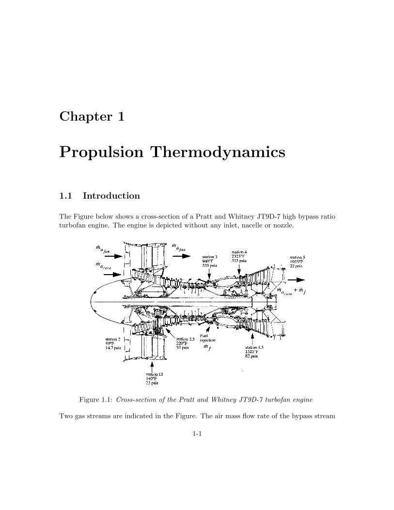
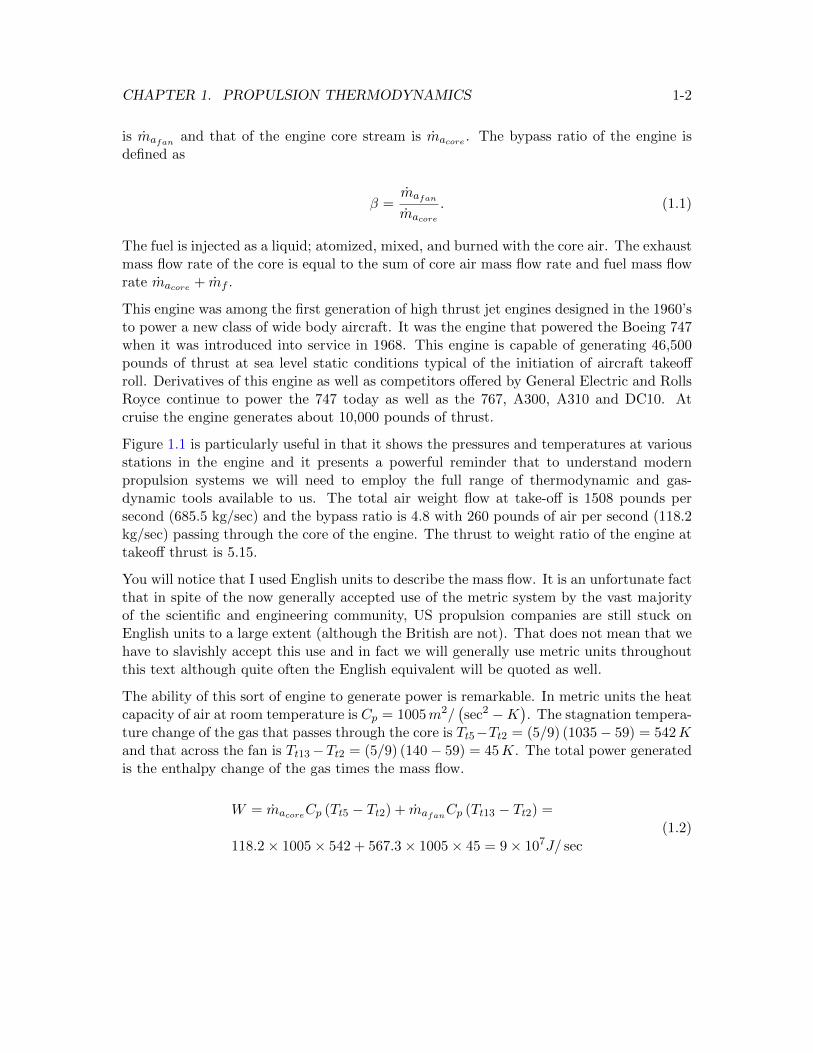
The Figure below shows a cross-section of a Pratt and Whitney JT9D-7 high bypass ratioturbofan engine. The engine is depicted without any inlet, nacelle or nozzle.
Figure 1.1: Cross-section of the Pratt and Whitney JT9D-7 turbofan engine
Two gas streams are indicated in the Figure. The air mass flow rate of the bypass stream
1-1
CHAPTER 1. PROPULSION THERMODYNAMICS 1-2
is mafan and that of the engine core stream is macore . The bypass ratio of the engine isdefined as
β =mafan
macore
. (1.1)
The fuel is injected as a liquid; atomized, mixed, and burned with the core air. The exhaustmass flow rate of the core is equal to the sum of core air mass flow rate and fuel mass flowrate macore + mf .
This engine was among the first generation of high thrust jet engines designed in the 1960’sto power a new class of wide body aircraft. It was the engine that powered the Boeing 747when it was introduced into service in 1968. This engine is capable of generating 46,500pounds of thrust at sea level static conditions typical of the initiation of aircraft takeoffroll. Derivatives of this engine as well as competitors offered by General Electric and RollsRoyce continue to power the 747 today as well as the 767, A300, A310 and DC10. Atcruise the engine generates about 10,000 pounds of thrust.
Figure 1.1 is particularly useful in that it shows the pressures and temperatures at variousstations in the engine and it presents a powerful reminder that to understand modernpropulsion systems we will need to employ the full range of thermodynamic and gas-dynamic tools available to us. The total air weight flow at take-off is 1508 pounds persecond (685.5 kg/sec) and the bypass ratio is 4.8 with 260 pounds of air per second (118.2kg/sec) passing through the core of the engine. The thrust to weight ratio of the engine attakeoff thrust is 5.15.
You will notice that I used English units to describe the mass flow. It is an unfortunate factthat in spite of the now generally accepted use of the metric system by the vast majorityof the scientific and engineering community, US propulsion companies are still stuck onEnglish units to a large extent (although the British are not). That does not mean that wehave to slavishly accept this use and in fact we will generally use metric units throughoutthis text although quite often the English equivalent will be quoted as well.
The ability of this sort of engine to generate power is remarkable. In metric units the heatcapacity of air at room temperature is Cp = 1005m2/
(sec2 −K
). The stagnation tempera-
ture change of the gas that passes through the core is Tt5−Tt2 = (5/9) (1035− 59) = 542Kand that across the fan is Tt13−Tt2 = (5/9) (140− 59) = 45K. The total power generatedis the enthalpy change of the gas times the mass flow.
W = macoreCp (Tt5 − Tt2) + mafanCp (Tt13 − Tt2) =
118.2× 1005× 542 + 567.3× 1005× 45 = 9× 10⁷J/ sec
(1.2)
CHAPTER 1. PROPULSION THERMODYNAMICS 1-3
In English units this is equivalent to approximately 120,000 horsepower (1 horsepower=746Watts, 1 Watt = 1 Joule/sec). Note that the engine is designed so that the static pressureof the core exhaust flow is nearly equal to the static pressure of the fan exhaust to avoidlarge changes in flow direction where the two streams meet. The overall engine stagnationpressure ratio is approximately 1.5.
Now let’s examine the work done per second across some of the components. The workdone by the gas on the high pressure turbine is
Whpt = 118.2× 1005× (5/9)× (2325− 1525) = 5.28× 10⁷ J/ sec (1.3)
where the added fuel mass flow is neglected. The high pressure turbine drives the highpressure compressor through a shaft that connects the two components. The work persecond done by the high pressure compressor on the core air is
Whpc = 118.2× 1005× (5/9)× (940− 220) = 4.75× 10⁷ J/ sec . (1.4)
Note that the work per second done by the gas on the turbine is very close to but slightlylarger than that done by the compressor on the gas. If the shaft connecting the compressorand turbine has no frictional losses and if the mass flow through both components is indeedthe same and if both components are adiabatic then the work terms would be identical.The system is not quite adiabatic due to heat loss to the surroundings. The mass flow isnot precisely the same because of the added fuel and because some of the relatively coolercompressor flow is bled off to be used for power generation and to internally cool the hightemperature components of the turbine.
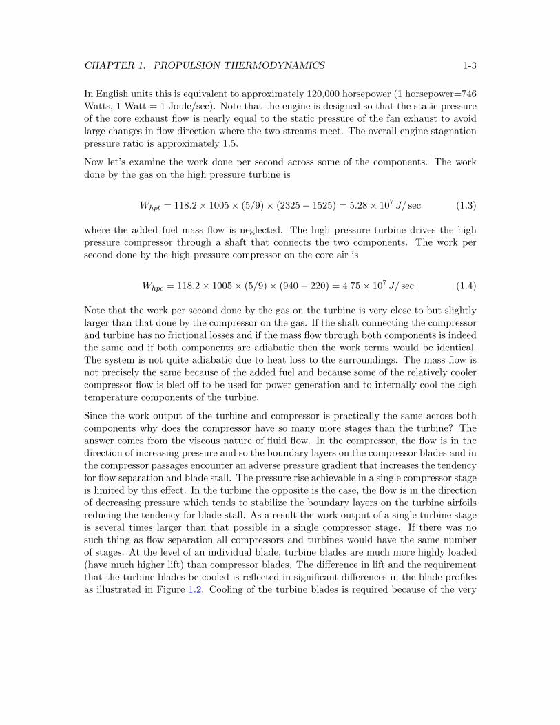
Since the work output of the turbine and compressor is practically the same across bothcomponents why does the compressor have so many more stages than the turbine? Theanswer comes from the viscous nature of fluid flow. In the compressor, the flow is in thedirection of increasing pressure and so the boundary layers on the compressor blades and inthe compressor passages encounter an adverse pressure gradient that increases the tendencyfor flow separation and blade stall. The pressure rise achievable in a single compressor stageis limited by this effect. In the turbine the opposite is the case, the flow is in the directionof decreasing pressure which tends to stabilize the boundary layers on the turbine airfoilsreducing the tendency for blade stall. As a result the work output of a single turbine stageis several times larger than that possible in a single compressor stage. If there was nosuch thing as flow separation all compressors and turbines would have the same numberof stages. At the level of an individual blade, turbine blades are much more highly loaded(have much higher lift) than compressor blades. The difference in lift and the requirementthat the turbine blades be cooled is reflected in significant differences in the blade profilesas illustrated in Figure 1.2. Cooling of the turbine blades is required because of the very
CHAPTER 1. PROPULSION THERMODYNAMICS 1-4
high temperature of the gas entering the turbine from the combustor. In modern enginesthe turbine inlet temperature may be several hundred degrees higher than the meltingtemperature of the turbine blade material and complex cooling schemes are needed toenable the turbine to operate for tens of thousands of hours before overhaul.
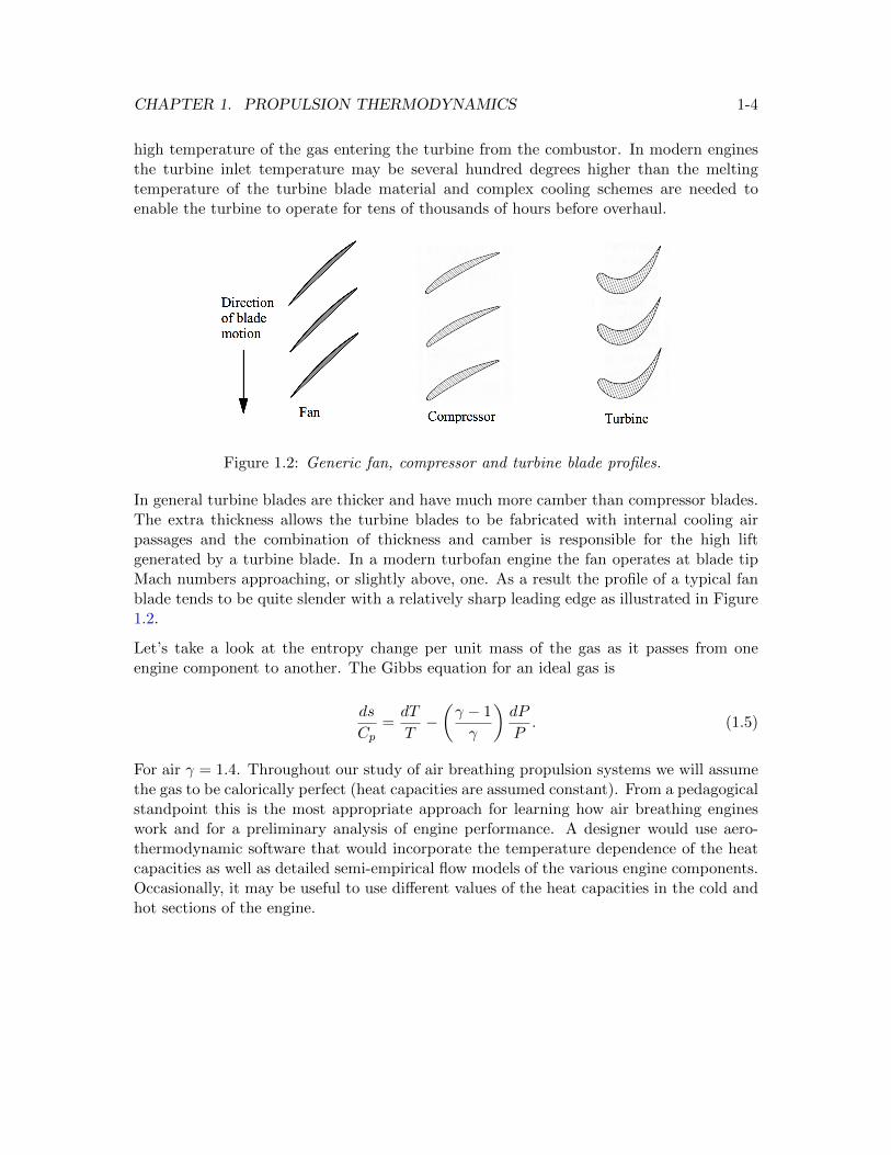
Figure 1.2: Generic fan, compressor and turbine blade profiles.
In general turbine blades are thicker and have much more camber than compressor blades.The extra thickness allows the turbine blades to be fabricated with internal cooling airpassages and the combination of thickness and camber is responsible for the high liftgenerated by a turbine blade. In a modern turbofan engine the fan operates at blade tipMach numbers approaching, or slightly above, one. As a result the profile of a typical fanblade tends to be quite slender with a relatively sharp leading edge as illustrated in Figure1.2.
Let’s take a look at the entropy change per unit mass of the gas as it passes from oneengine component to another. The Gibbs equation for an ideal gas is
ds
Cp=dT
T−(γ − 1
γ
)dP
P. (1.5)
For air γ = 1.4. Throughout our study of air breathing propulsion systems we will assumethe gas to be calorically perfect (heat capacities are assumed constant). From a pedagogicalstandpoint this is the most appropriate approach for learning how air breathing engineswork and for a preliminary analysis of engine performance. A designer would use aero-thermodynamic software that would incorporate the temperature dependence of the heatcapacities as well as detailed semi-empirical flow models of the various engine components.Occasionally, it may be useful to use different values of the heat capacities in the cold andhot sections of the engine.
CHAPTER 1. PROPULSION THERMODYNAMICS 1-5
Between any two points a and b the Gibbs equation integrates to
sb − saCp
= Ln
(TbTa
)−(γ − 1
γ
)Ln
(PbPa
). (1.6)
Integrating between the various stations of the engine shown in Figure 1.1 leads to thefollowing. Note that station 0 is in the free stream and station 1 is at the entrance to theinlet. Neither station is shown in Figure 1.1.
Station 2 - Sea level static conditions from Figure 1.1 are
Pt2 = 14.7 psia
Tt2 = 519R(1.7)
where the inlet (not shown) is assumed to be adiabatic and isentropic.
Station 3 - At the outlet of the high pressure compressor
Pt3 = 335 psia
Tt3 = 1400R.(1.8)
The non-dimensional entropy change per unit mass across the inlet compression systemis
sb − saCp
= Ln
(1400
519
)−(
0.4
1.4
)Ln
(335
14.7
)= 0.992− 0.893 = 0.099. (1.9)
Station 4 - The heat put into the cycle is equal to the stagnation enthalpy change acrossthe burner.
mfhf = (macore + mf )ht4 − macoreht3 (1.10)
The thermodynamic heat of combustion of a fuel is calculated as the heat that mustbe removed to bring all the products of combustion back to the original pre-combustiontemperature. The enthalpy of combustion for fuels is usually expressed as a higher orlower heating value. The higher heating value is realized if the original temperature isbelow the condensation temperature of water and any water vapor is condensed giving upits vaporization energy as heat. The lower heating value is calculated by subtracting the
CHAPTER 1. PROPULSION THERMODYNAMICS 1-6
heat of vaporization of the water in the combustion products from the higher heating value.In this case any water formed is treated as a gas.
The enthalpy of combustion of a typical jet fuel such as JP-4 is generally taken to be thelower heating value since the water vapor in the combustion products does not condensebefore leaving the nozzle. The value we will use is
hf |JP−4 = 4.28× 10⁷ J/ sec . (1.11)
The higher heating value of JP-4 is about 4.6 × 10⁷ J/kg and can be calculated from aknowledge of the water vapor content in the combustion products. The higher and lowerheating values of most other hydrocarbon fuels are within about 10% of these values. Atthe outlet of the burner
Pt4 = 315 psia
Tt4 = 2785R.(1.12)
Note the very small stagnation pressure loss across the burner. The stagnation pres-sure drop across any segment of a channel flow is proportional to the Mach numbersquared.
dPtPt
= −γM2
2
(dTtTt
+ 4Cfdx
D
)(1.13)
A key feature of virtually all propulsion systems is that the heat addition is carried outat very low Mach number in part to keep stagnation pressure losses across the burner assmall as possible. The exception to this is the scramjet concept used in hypersonic flightwhere the heat addition inside the engine occurs at supersonic Mach numbers that are wellbelow the flight Mach number.
The non-dimensional entropy change per unit mass across the burner of the JT9D-7 is
s4 − s3
Cp= Ln
(2785
1400
)−(
0.4
1.4
)Ln
(315
335
)= 0.688 + 0.0176 = 0.706. (1.14)
Station 5 - At the outlet of the turbine
Pt5 = 22 psia
Tt5 = 1495R.(1.15)
CHAPTER 1. PROPULSION THERMODYNAMICS 1-7
The non-dimensional entropy change per unit mass across the turbine is
s5 − s4
Cp= Ln
(1495
2785
)−(
0.4
1.4
)Ln
(22
315
)= −0.622 + 0.760 = 0.138. (1.16)
Station 0 - The exhaust gas returns to the reference state through nozzle expansion toambient pressure and thermal mixing with the surrounding atmosphere.
Pt0 = 14.7 psia
Tt0 = 519R(1.17)
The non-dimensional entropy change back to the reference state is
s0 − s5
Cp= Ln
(519
1495
)−(
0.4
1.4
)Ln
(14.7
22
)= −1.058 + 0.115 = −0.943. (1.18)
The net change in entropy around the cycle is zero as would be expected. That is ∆s =0.099 + 0.706 + 0.138− 0.943 = 0.
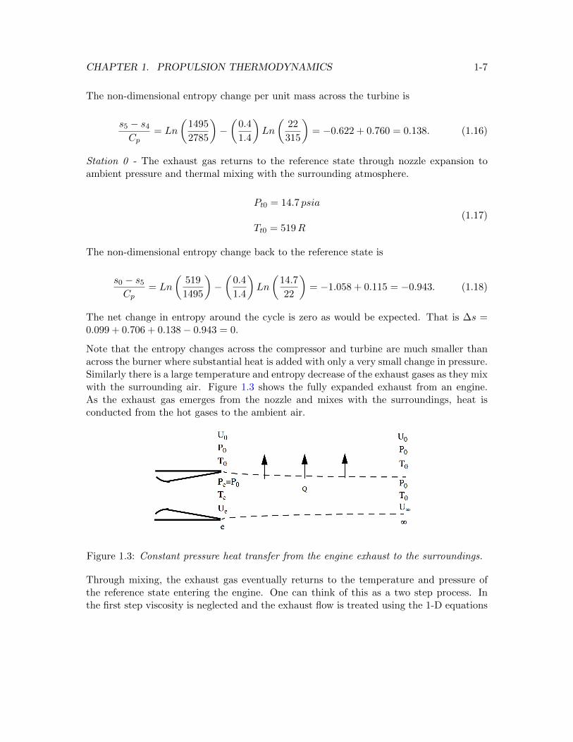
Note that the entropy changes across the compressor and turbine are much smaller thanacross the burner where substantial heat is added with only a very small change in pressure.Similarly there is a large temperature and entropy decrease of the exhaust gases as they mixwith the surrounding air. Figure 1.3 shows the fully expanded exhaust from an engine.As the exhaust gas emerges from the nozzle and mixes with the surroundings, heat isconducted from the hot gases to the ambient air.
Figure 1.3: Constant pressure heat transfer from the engine exhaust to the surroundings.
Through mixing, the exhaust gas eventually returns to the temperature and pressure ofthe reference state entering the engine. One can think of this as a two step process. Inthe first step viscosity is neglected and the exhaust flow is treated using the 1-D equations
CHAPTER 1. PROPULSION THERMODYNAMICS 1-8
of motion. In this approximation, the flow in the stream-tube within the dashed lines inFigure 1.3 is governed by the 1-D momentum equation (the Euler equation).
dP + ρUdU = 0 (1.19)
According to (1.19) since the pressure is constant along this stream-tube, the velocity mustalso be constant (dP = 0, dU = 0) and the flow velocity at the end of the stream-tube mustbe the same as at the nozzle exit U∞ = Ue. The 1-D energy equation for the flow in thestream tube is
δq = dht (1.20)
and so the heat rejected to the surroundings per unit mass flow is given by
q = hte − ht∞ = he +1
2Ue
2 − h∞ −1
2U∞
2 = he − h∞. (1.21)
The heat rejected through conduction to the surrounding air in the wake of the engine isequal to the change in static enthalpy of the exhaust gas as it returns to the initial state.At this point the cycle is complete.
In the second step, viscosity is turned on and the kinetic energy of the exhaust gas iseventually lost through viscous dissipation. The temperature of the atmosphere is raised byan infinitesimal amount in the process. In actual fact both processes occur simultaneouslythrough a complex process of nearly constant pressure heat transfer and turbulent mixingin the engine wake.
The process of constant pressure heat addition and rejection illustrated by this example isknown as the Brayton cycle.
1.2 Thermodynamic cycles
1.2.1 The Carnot cycle
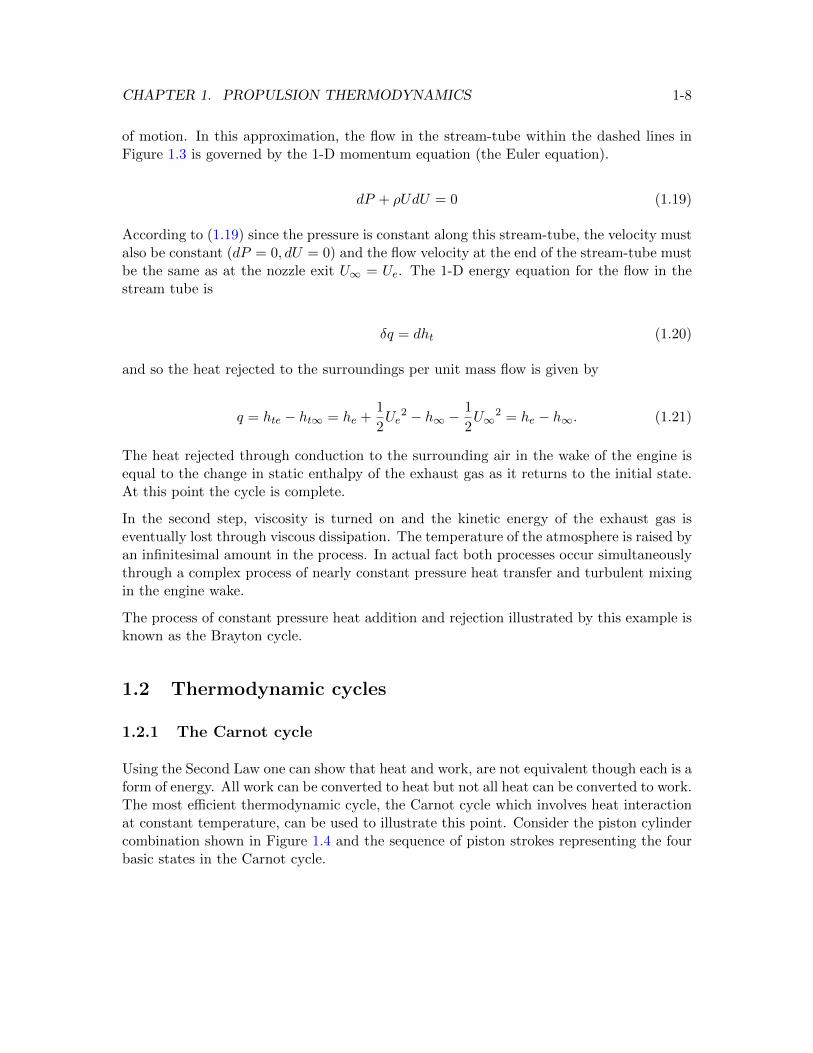
Using the Second Law one can show that heat and work, are not equivalent though each is aform of energy. All work can be converted to heat but not all heat can be converted to work.The most efficient thermodynamic cycle, the Carnot cycle which involves heat interactionat constant temperature, can be used to illustrate this point. Consider the piston cylindercombination shown in Figure 1.4 and the sequence of piston strokes representing the fourbasic states in the Carnot cycle.
CHAPTER 1. PROPULSION THERMODYNAMICS 1-9
Figure 1.4: The Carnot cycle heat engine.
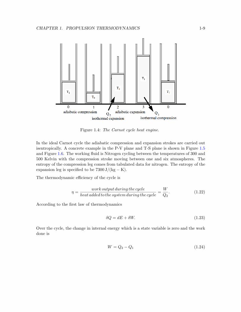
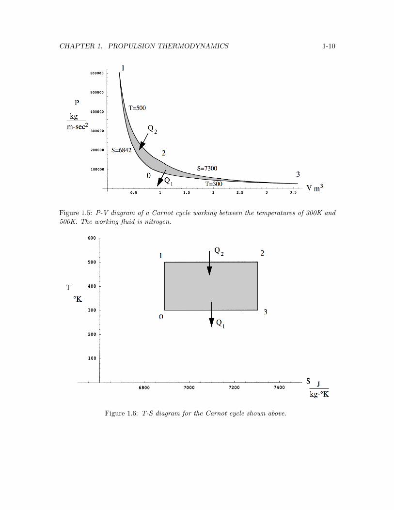
In the ideal Carnot cycle the adiabatic compression and expansion strokes are carried outisentropically. A concrete example in the P-V plane and T-S plane is shown in Figure 1.5and Figure 1.6. The working fluid is Nitrogen cycling between the temperatures of 300 and500 Kelvin with the compression stroke moving between one and six atmospheres. Theentropy of the compression leg comes from tabulated data for nitrogen. The entropy of theexpansion leg is specified to be 7300 J/(kg −K).
The thermodynamic efficiency of the cycle is
η =work output during the cycle
heat added to the systemduring the cycle=W
Q2. (1.22)
According to the first law of thermodynamics
δQ = dE + δW. (1.23)
Over the cycle, the change in internal energy which is a state variable is zero and the workdone is
W = Q2 −Q1 (1.24)
CHAPTER 1. PROPULSION THERMODYNAMICS 1-10
Figure 1.5: P-V diagram of a Carnot cycle working between the temperatures of 300K and500K. The working fluid is nitrogen.
Figure 1.6: T-S diagram for the Carnot cycle shown above.
CHAPTER 1. PROPULSION THERMODYNAMICS 1-11
and so the efficiency is
η = 1− Q1
Q2. (1.25)
The change in entropy over the cycle is also zero and so from the Second Law
∮ds =
∮δQ
T= 0. (1.26)
Since the temperature is constant during the heat interaction we can use this result towrite
Q1
T1=Q2
T2. (1.27)
Thus the efficiency of the Carnot cycle is
ηC = 1− T1
T2< 1. (1.28)
For the example shownηC = 0.4. At most only 40% of the heat added to the system can beconverted to work. The maximum work that can be generated by a heat engine workingbetween two finite temperatures is limited by the temperature ratio of the system and isalways less than the heat put into the system.
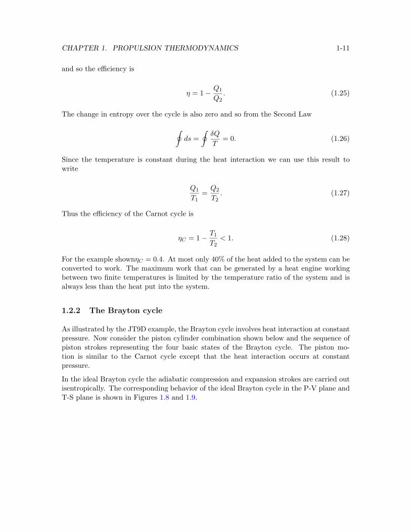
1.2.2 The Brayton cycle
As illustrated by the JT9D example, the Brayton cycle involves heat interaction at constantpressure. Now consider the piston cylinder combination shown below and the sequence ofpiston strokes representing the four basic states of the Brayton cycle. The piston mo-tion is similar to the Carnot cycle except that the heat interaction occurs at constantpressure.
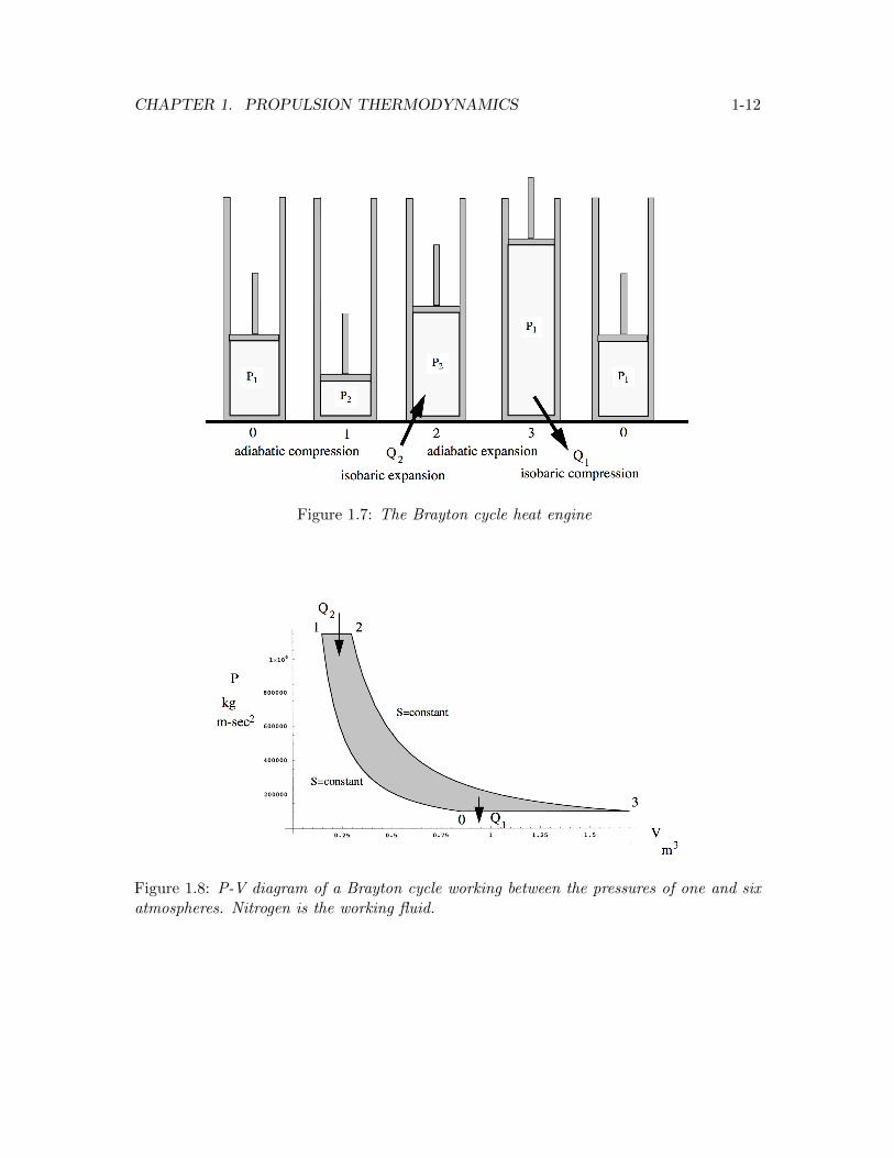
In the ideal Brayton cycle the adiabatic compression and expansion strokes are carried outisentropically. The corresponding behavior of the ideal Brayton cycle in the P-V plane andT-S plane is shown in Figures 1.8 and 1.9.
CHAPTER 1. PROPULSION THERMODYNAMICS 1-12
Figure 1.7: The Brayton cycle heat engine
Figure 1.8: P-V diagram of a Brayton cycle working between the pressures of one and sixatmospheres. Nitrogen is the working fluid.
CHAPTER 1. PROPULSION THERMODYNAMICS 1-13
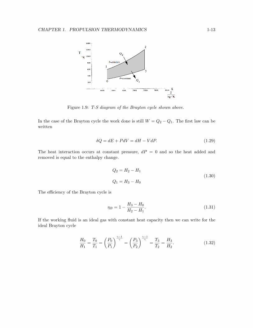
Figure 1.9: T-S diagram of the Brayton cycle shown above.
In the case of the Brayton cycle the work done is still W = Q2 −Q1. The first law can bewritten
δQ = dE + PdV = dH − V dP. (1.29)
The heat interaction occurs at constant pressure, dP = 0 and so the heat added andremoved is equal to the enthalpy change.
Q2 = H2 −H1
Q1 = H3 −H0
(1.30)
The efficiency of the Brayton cycle is
ηB = 1− H3 −H0
H2 −H1. (1.31)
If the working fluid is an ideal gas with constant heat capacity then we can write for theideal Brayton cycle
H0
H1=T0
T1=
(P0
P1
) γ−1γ
=
(P3
P2
) γ−1γ
=T3
T2=H3
H2. (1.32)
CHAPTER 1. PROPULSION THERMODYNAMICS 1-14
Using (1.32) the Brayton efficiency can be written
ηB = 1− T0
T1
(T3T0− 1
T2T1− 1
). (1.33)
From (1.32) the term in parentheses is one and so the efficiency of the ideal Brayton cycleis finally
ηB = 1− T0
T1. (1.34)
The important point to realize here is that the efficiency of a Brayton process is deter-mined entirely by the temperature increase during the compression step of the cycle (orequivalently the temperature decrease during the expansion step.
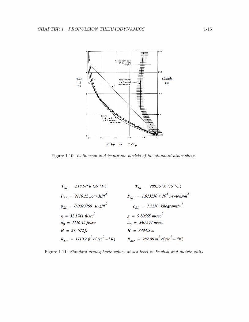
1.3 The standard atmosphere
Figure 1.10 below shows the distribution of temperature and density in the atmospherewith comparisons with isothermal and isentropic models of the atmosphere. The scaleheight of the atmosphere is
H =a0
2
γg=RT0
g. (1.35)
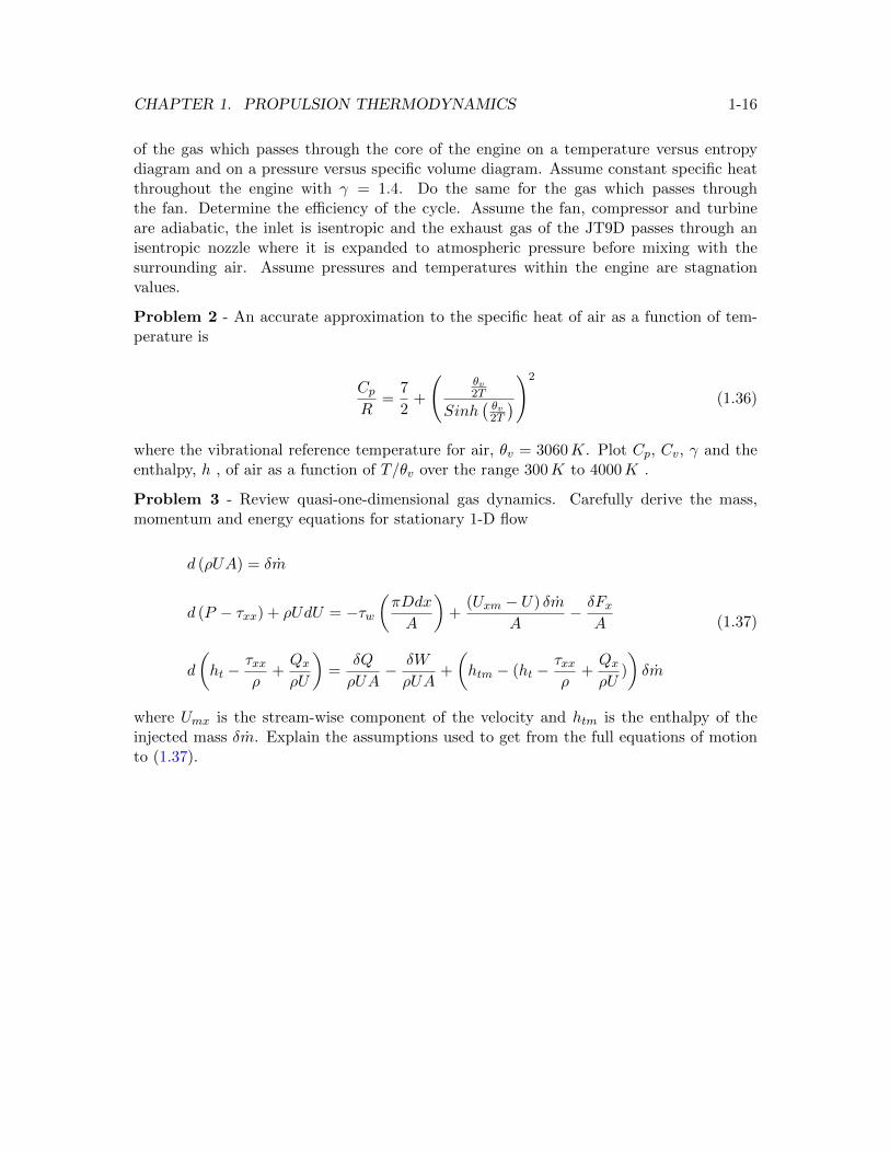
The speed of sound, temperature, and gravitational acceleration in (1.35) are evaluated atzero altitude. For air at 288.15K the scale height is 8,435 meters (27,674 feet). At thisaltitude the thermal and potential energy of the atmosphere are of the same order. Belowa scale height of one the atmosphere is approximately isentropic and the temperaturefalls off almost linearly. Above a scale height of about 1.5 the temperature is almostconstant. In order to standardize aircraft performance calculations Diehl (Ref. W. S. Diehl,Some Approximate Equations for the Standard Atmosphere N.A.C.A. Technical Report No.375, 1930) defined a standard atmosphere which was widely adopted by the aeronauticscommunity. According to this standard the atmospheric values at sea level in Figure 1.11are assumed.
1.4 Problems
Problem 1 - Consider the JT9D-7 turbofan cross-section discussed above. Plot the state
CHAPTER 1. PROPULSION THERMODYNAMICS 1-15
Figure 1.10: Isothermal and isentropic models of the standard atmosphere.
Figure 1.11: Standard atmospheric values at sea level in English and metric units
CHAPTER 1. PROPULSION THERMODYNAMICS 1-16
of the gas which passes through the core of the engine on a temperature versus entropydiagram and on a pressure versus specific volume diagram. Assume constant specific heatthroughout the engine with γ = 1.4. Do the same for the gas which passes throughthe fan. Determine the efficiency of the cycle. Assume the fan, compressor and turbineare adiabatic, the inlet is isentropic and the exhaust gas of the JT9D passes through anisentropic nozzle where it is expanded to atmospheric pressure before mixing with thesurrounding air. Assume pressures and temperatures within the engine are stagnationvalues.
Problem 2 - An accurate approximation to the specific heat of air as a function of tem-perature is
CpR
=7
2+
(θv2T
Sinh(θv2T
))2
(1.36)
where the vibrational reference temperature for air, θv = 3060K. Plot Cp, Cv, γ and theenthalpy, h , of air as a function of T/θv over the range 300K to 4000K .
Problem 3 - Review quasi-one-dimensional gas dynamics. Carefully derive the mass,momentum and energy equations for stationary 1-D flow
d (ρUA) = δm
d (P − τxx) + ρUdU = −τw(πDdx
A
)+
(Uxm − U) δm
A− δFx
A
d
(ht −
τxxρ
+QxρU
)=
δQ
ρUA− δW
ρUA+
(htm − (ht −
τxxρ
+QxρU
)
)δm
(1.37)
where Umx is the stream-wise component of the velocity and htm is the enthalpy of theinjected mass δm. Explain the assumptions used to get from the full equations of motionto (1.37).
Chapter 2
Engine performance parameters
2.1 The definition of thrust
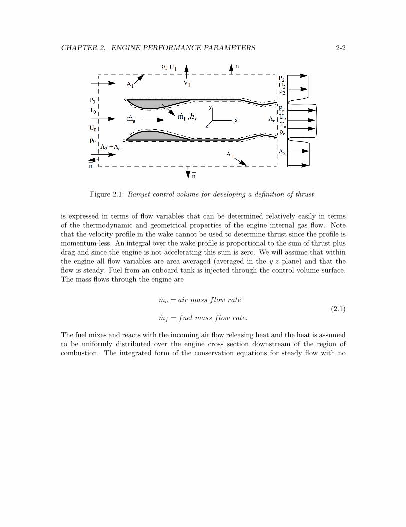
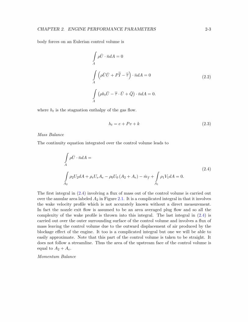
One might be surprised to learn that there is no direct way to determine the thrust gen-erated by a propulsion system. The reason for this is that the flow over and through aninstalled engine on an aircraft or an engine attached to a test stand is responsible for thetotal force on the engine and its nacelle. On any part of the propulsion surface the com-bination of pressure and viscous stress forces produced by the flow may contribute to thethrust or to the drag and there is no practical way to extricate one force component fromthe other. Even the most sophisticated test facility can measure the thrust produced byan engine only up to an accuracy of about 0.5%. Wind and weather conditions during thetest, inaccuracies in measurement, poorly known flow characteristics in the entrance flowand exhaust and a variety of minor effects limit the ability of a test engineer to preciselymeasure or predict the thrust of an engine. Thus as a practical matter we must be satisfiedwith a thrust formula that is purely a definition. Such a definition is only useful to theextent that it reflects the actual thrust force produced by an engine up to some reasonablelevel of accuracy. In the following, we will use mass and momentum conservation overan Eulerian control volume surrounding a ramjet to motivate a definition of thrust. Thecontrol volume is indicated as the dashed line shown in Figure 2.1.
The control volume is in the shape of a cylinder centered about the ramjet.Note thatthe control volume is simply connected. That is, by suitable distortions without tearing,it is developable into a sphere. The surface of the control volume runs along the entirewetted surface of the ramjet and encloses the inside of the engine. The upstream surfaceis far enough upstream so that flow variables there correspond to free-stream values. Thedownstream surface of the control volume coincides with the nozzle exit. The reason forpositioning the downstream surface this way is that we need a definition of thrust that
2-1
CHAPTER 2. ENGINE PERFORMANCE PARAMETERS 2-2
Figure 2.1: Ramjet control volume for developing a definition of thrust
is expressed in terms of flow variables that can be determined relatively easily in termsof the thermodynamic and geometrical properties of the engine internal gas flow. Notethat the velocity profile in the wake cannot be used to determine thrust since the profile ismomentum-less. An integral over the wake profile is proportional to the sum of thrust plusdrag and since the engine is not accelerating this sum is zero. We will assume that withinthe engine all flow variables are area averaged (averaged in the y-z plane) and that theflow is steady. Fuel from an onboard tank is injected through the control volume surface.The mass flows through the engine are
ma = air mass flow rate
mf = fuel mass flow rate.(2.1)
The fuel mixes and reacts with the incoming air flow releasing heat and the heat is assumedto be uniformly distributed over the engine cross section downstream of the region ofcombustion. The integrated form of the conservation equations for steady flow with no
CHAPTER 2. ENGINE PERFORMANCE PARAMETERS 2-3
body forces on an Eulerian control volume is
∫A
ρU · ndA = 0
∫A
(ρUU + PI − τ
)· ndA = 0
∫A
(ρhtU − τ · U + Q
)· ndA = 0.
(2.2)
where ht is the stagnation enthalpy of the gas flow.
ht = e+ Pv + k (2.3)
Mass Balance
The continuity equation integrated over the control volume leads to
∫A
ρU · ndA =
∫A2
ρ2U2dA+ ρeUeAe − ρ0U0 (A2 +Ae)− mf +
∫A1
ρ1V1dA = 0.
(2.4)
The first integral in (2.4) involving a flux of mass out of the control volume is carried outover the annular area labeled A2 in Figure 2.1. It is a complicated integral in that it involvesthe wake velocity profile which is not accurately known without a direct measurement.In fact the nozzle exit flow is assumed to be an area averaged plug flow and so all thecomplexity of the wake profile is thrown into this integral. The last integral in (2.4) iscarried out over the outer surrounding surface of the control volume and involves a flux ofmass leaving the control volume due to the outward displacement of air produced by theblockage effect of the engine. It too is a complicated integral but one we will be able toeasily approximate. Note that this part of the control volume is taken to be straight. Itdoes not follow a streamline. Thus the area of the upstream face of the control volume isequal to A2 +Ae.
Momentum Balance
CHAPTER 2. ENGINE PERFORMANCE PARAMETERS 2-4
Now integrate the x-momentum equation over the control volume.
∫A
(ρUU + PI − τ
)· ndA
∣∣∣∣∣∣x
=
∫A2
(ρ2U2
2 + P2
)dA+
(ρeUe
2Ae + PeAe)−(ρ0U0
2 + P0
)(A2 +Ae) +
∫A1
ρ1U1V1dA+
∫Aw
(PI − τ
)· ndA
∣∣∣∣∣∣x
= 0
(2.5)
Note that the x-momentum of the injected fuel mass has been neglected. The first integralinvolves a complicated distribution of pressure and momentum over the area A2 and thereis little we can do with it. The last integral involves the pressure and stress forces actingover the entire wetted surface of the engine and although the kernel of this integral maybe an incredibly complicated function, the integral itself must be zero since the engine isnot accelerating or decelerating (the free stream speed is not a function of time).
∫Aw
(PI − τ
)· ndA
∣∣∣∣∣∣x
= Thrust−Drag = 0 (2.6)
The second to last integral in (2.5) can be approximated as follows.
∫A1
ρ1U1V1dA ∼=∫A1
ρ1U0V1dA (2.7)
The argument for this approximation is that at the outside surface of the control volumethe x-component of the fluid velocity is very close to the free stream value. This is a goodapproximation as long as the control volume surface is reasonably far away from the engine.This approximation allows us to use the mass balance to get rid of this integral. Multiply(2.4) by U0. and subtract from (2.5). The result is
ρeUe (Ue − U0)Ae+ (Pe − P0)Ae+ mfU0 +
∫A2
(ρ2U2 (U2 − U0) + (P2 − P0)) dA = 0. (2.8)
CHAPTER 2. ENGINE PERFORMANCE PARAMETERS 2-5
This is as far as we can go with our analysis and at this point we have to make an arbitrarychoice. We will define the drag of the engine as
Drag =
∫A2
(ρ2U2 (U0 − U2) + (P0 − P2)) dA (2.9)
and the thrust as
Thrust = ρeUe (Ue − U0)Ae + (Pe − P0)Ae + mfU0. (2.10)
This is a purely practical choice where the thrust is defined in terms of flow variablesthat can be determined from a thermo-gas-dynamic analysis of the area-averaged engineinternal flow. All the complexity of the flow over the engine has been thrown into the dragintegral (2.9) which of course could very well have contributions that could be negative.This would be the case, for example, if some part of the pressure profile had P2 −P0 > 0 .The exit mass flow is the sum of the air mass flow plus the fuel mass flow.
ρeUeAe = ma + mf (2.11)
Using (2.11) the thrust definition (2.10) can be written in the form
T = ma (Ue − U0) + (Pe − P0)Ae + mfUe. (2.12)
In this form the thrust definition can be interpreted as the momentum change of the airmass flow across the engine plus the momentum change of the fuel mass flow. The pressureterm reflects the acceleration of the exit flow that occurs as the jet exhaust eventuallymatches the free stream pressure in the far wake. Keep in mind that the fuel is carried onboard the aircraft, and in the frame of reference attached to the engine, the fuel has zerovelocity before it is injected and mixed with the air.
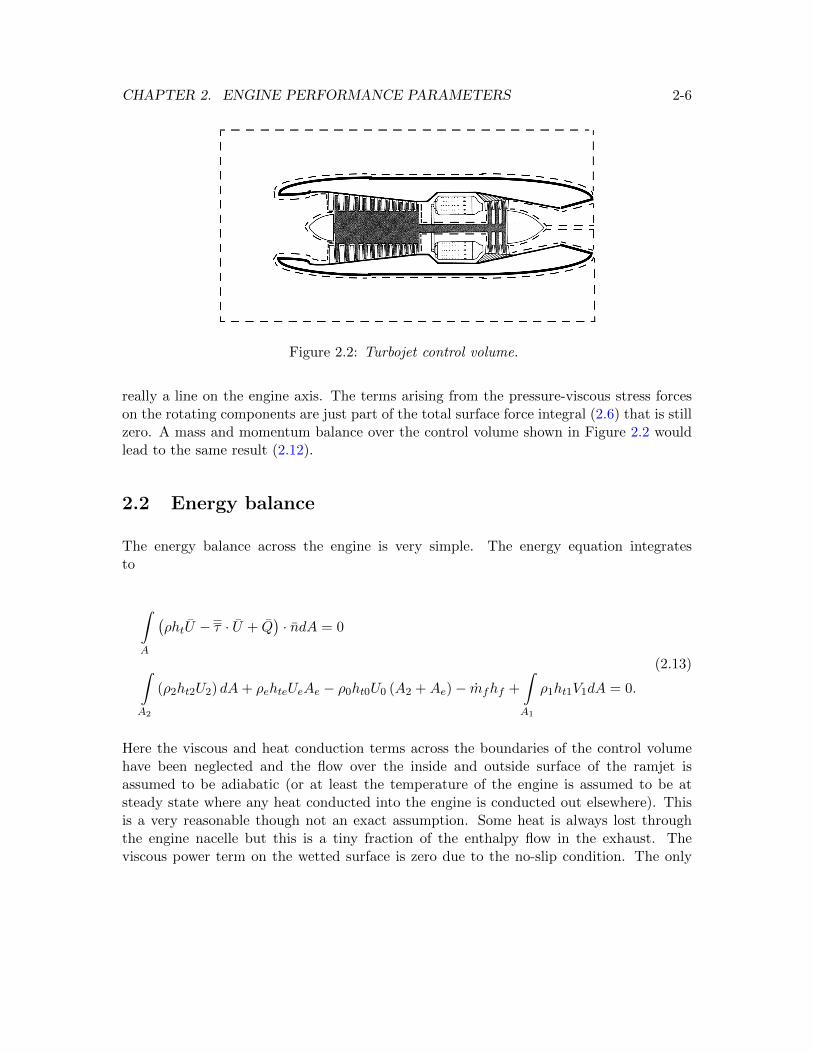
The thrust definition (2.12) is very general and applies to much more complex systems. Ifthe selected engine was a turbojet the control volume would look like that shown in Figure2.2.
The surface of the control volume covers the entire wetted surface of the engine includingthe struts that hold the rotating components in place as well as the rotating compressor,shaft and turbine. In this case the control volume is of mixed Eulerian-Lagrangian typewith part of the control volume surface attached to and moving with the rotating parts.The cut on the engine centerline comes from the wrapping of the control volume about thesupports and rotating components. All fluxes cancel on the surface of the cut, which is
CHAPTER 2. ENGINE PERFORMANCE PARAMETERS 2-6
Figure 2.2: Turbojet control volume.
really a line on the engine axis. The terms arising from the pressure-viscous stress forceson the rotating components are just part of the total surface force integral (2.6) that is stillzero. A mass and momentum balance over the control volume shown in Figure 2.2 wouldlead to the same result (2.12).
2.2 Energy balance
The energy balance across the engine is very simple. The energy equation integratesto
∫A
(ρhtU − τ · U + Q
)· ndA = 0
∫A2
(ρ2ht2U2) dA+ ρehteUeAe − ρ0ht0U0 (A2 +Ae)− mfhf +
∫A1
ρ1ht1V1dA = 0.
(2.13)
Here the viscous and heat conduction terms across the boundaries of the control volumehave been neglected and the flow over the inside and outside surface of the ramjet isassumed to be adiabatic (or at least the temperature of the engine is assumed to be atsteady state where any heat conducted into the engine is conducted out elsewhere). Thisis a very reasonable though not an exact assumption. Some heat is always lost throughthe engine nacelle but this is a tiny fraction of the enthalpy flow in the exhaust. Theviscous power term on the wetted surface is zero due to the no-slip condition. The only
CHAPTER 2. ENGINE PERFORMANCE PARAMETERS 2-7
contribution over the wetted surface is from the flux of fuel which carries with it its fuelenthalpy hf .
A typical value of fuel enthalpy for JP-4 jet fuel is
hf |JP−4 = 4.28× 10⁷ J/kg. (2.14)
As a comparison, the enthalpy of Air at sea level static conditions is
h|Airat288.15K = CpTSL = 1005× 288.15 = 2.896× 10⁵ J/kg. (2.15)
The ratio is
hf |JP−4
h|Airat288.15K
= 148. (2.16)
The energy content of a kilogram of hydrocarbon fuel is remarkably large and constitutesone of the important facts of nature that makes extended powered flight possible.
If the flow over the outside of the engine is adiabatic then the stagnation enthalpy of flowover the outside control volume surfaces is equal to the free-stream value and we can writethe energy balance as
∫A2
(ρ2ht0U2) dA+ ρehteUeAe − ρ0ht0U0 (A2 +Ae)− mfhf +
∫A1
ρ1ht0V1dA = 0. (2.17)
Now multiply the continuity equation (2.4) by ht0 and subtract from (2.17). The resultis
ρehteUeAe − ρeht0UeAe − mf (hf − ht0) = 0. (2.18)
Using (2.11) the energy balance across the engine can be written as
(ma + mf )hte = maht0 + mfhf . (2.19)
The energy balance boils down to a simple algebraic relationship that states that the changein the stagnation enthalpy per second of the gas flow between the exit and entrance of theengine is equal to the added chemical enthalpy per second of the injected fuel flow.
CHAPTER 2. ENGINE PERFORMANCE PARAMETERS 2-8
2.3 Capture area
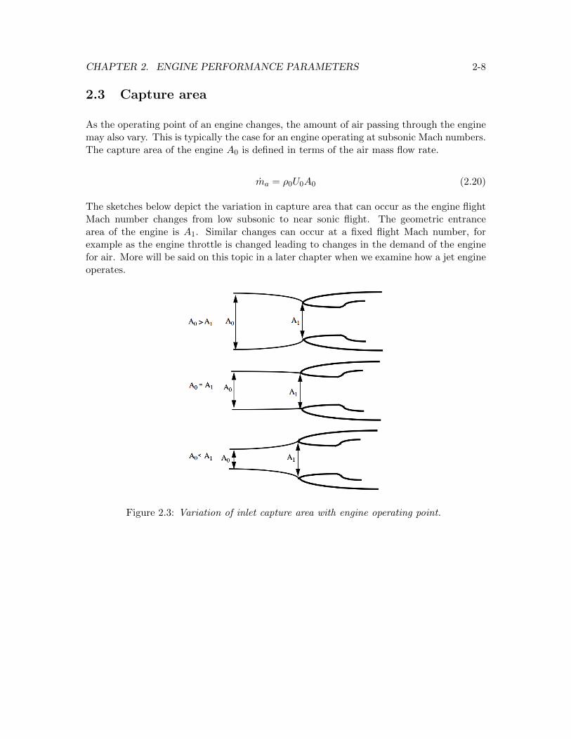
As the operating point of an engine changes, the amount of air passing through the enginemay also vary. This is typically the case for an engine operating at subsonic Mach numbers.The capture area of the engine A0 is defined in terms of the air mass flow rate.
ma = ρ0U0A0 (2.20)
The sketches below depict the variation in capture area that can occur as the engine flightMach number changes from low subsonic to near sonic flight. The geometric entrancearea of the engine is A1. Similar changes can occur at a fixed flight Mach number, forexample as the engine throttle is changed leading to changes in the demand of the enginefor air. More will be said on this topic in a later chapter when we examine how a jet engineoperates.
Figure 2.3: Variation of inlet capture area with engine operating point.
CHAPTER 2. ENGINE PERFORMANCE PARAMETERS 2-9
2.4 Overall efficiency
The overall efficiency of a propulsion system is defined as
ηov =The power delivered to the vehicle
The total energy released per second through combustion. (2.21)
That is
ηov =TU0
mfhf. (2.22)
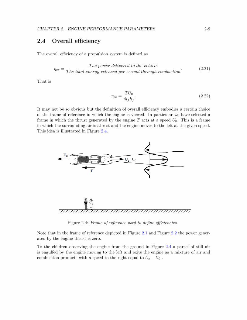
It may not be so obvious but the definition of overall efficiency embodies a certain choiceof the frame of reference in which the engine is viewed. In particular we have selected aframe in which the thrust generated by the engine T acts at a speed U0. This is a framein which the surrounding air is at rest and the engine moves to the left at the given speed.This idea is illustrated in Figure 2.4.
Figure 2.4: Frame of reference used to define efficiencies.
Note that in the frame of reference depicted in Figure 2.1 and Figure 2.2 the power gener-ated by the engine thrust is zero.
To the children observing the engine from the ground in Figure 2.4 a parcel of still airis engulfed by the engine moving to the left and exits the engine as a mixture of air andcombustion products with a speed to the right equal to Ue − U0 .
CHAPTER 2. ENGINE PERFORMANCE PARAMETERS 2-10
2.5 Breguet aircraft range equation
There are a number of models of aircraft range. The simplest assumes that the aircraftflies at a constant value of lift to drag ratio and constant engine overall efficiency. Therange is
R =
∫U0dt =
∫mfhfηov
Tdt. (2.23)
The fuel mass flow is directly related to the change in aircraft weight, w , per second.
mf = −1
g
dw
dt(2.24)
Since thrust equals drag and aircraft weight equals lift we can write
T = D =
(D
L
)L =
(D
L
)w. (2.25)
Now the range integral becomes
R = −ηovhfg
(L
D
)∫ wfinal
winitial
dw
w. (2.26)
The result is
R = ηovhfg
(L
D
)Ln
(winitialwfinal
). (2.27)
The range formula (2.27) is generally attributed to the great French aircraft pioneer LouisCharles Breguet who in 1919 founded a commercial airline company that would eventuallybecome Air France. This result highlights the key role played by the engine overall efficiencyin determining aircraft range. Note that as the aircraft burns fuel it must increase altitudeto maintain constant L/D . and the required thrust decreases. The small, time dependenteffects due to the upward acceleration are neglected.
CHAPTER 2. ENGINE PERFORMANCE PARAMETERS 2-11
2.6 Propulsive efficiency
It is instructive to decompose the overall efficiency into an aerodynamic factor and athermal factor. To accomplish this, the overall efficiency is written as the product of apropulsive and thermal efficiency.
ηov = ηpr × ηth (2.28)
The propulsive efficiency is
ηpr =Power delivered to the vehicle
Power delivered to the vehicle + ∆ kinetic energy of airsecond + ∆ kinetic energy of fuel
second(2.29)
or
ηpr =TU0
TU0 +(ma(Ue−U0)2
2 − ma(0)2
2
)+(mf (Ue−U0)2
2 − mf (U0)2
2
) . (2.30)
If the exhaust is fully expanded so that Pe = P0 and the fuel mass flow is much less thanthe air mass flow mf � ma, the propulsive efficiency reduces to
ηpr =2U0
Ue + U0. (2.31)
This is quite a general result and shows the fundamentally aerodynamic nature of thepropulsive efficiency. It indicates that for maximum propulsive efficiency we want to gen-erate thrust by moving as much air as possible with as little a change in velocity across theengine as possible. We shall see later that this is the basis for the increased efficiency of aturbofan over a turbojet with the same thrust. This is also the basis for comparison of awide variety of thrusters. For example, the larger the area of a helicopter rotor the moreefficient the lift system tends to be.
CHAPTER 2. ENGINE PERFORMANCE PARAMETERS 2-12
2.7 Thermal efficiency
The thermal efficiency is defined as
ηth =Power delivered to the vehicle + ∆ kinetic energy of air
second + ∆ kinetic energy of fuelsecond
mfhf(2.32)
or
ηth =TU0 +
(ma(Ue−U0)2
2 − ma(0)2
2
)+(mf (Ue−U0)2
2 − mf (U0)2
2
)mfhf
. (2.33)
If the exhaust is fully expanded so that Pe = P0 the thermal efficiency reduces to
ηth =(ma + mf ) Ue
2
2 − maU0
2
2
mfhf. (2.34)
The thermal efficiency directly compares the change in gas kinetic energy across the engineto the energy released through combustion.
The thermal efficiency of a thermodynamic cycle compares the work out of the cycle to theheat added to the cycle.
ηth =W
Qinput during the cycle=
Qinput during the cycle −Qrejected during the cycleQinput during the cycle
= 1−Qrejected during the cycleQinput during the cycle
(2.35)
We can compare (2.34) and (2.35) by rewriting (2.34) as
ηth = 1−
(mfhf + ma
U02
2 − (ma + mf ) Ue2
2
mfhf
). (2.36)
CHAPTER 2. ENGINE PERFORMANCE PARAMETERS 2-13
This equation for the thermal efficiency can also be expressed in terms of the gas enthalpies.Recall that
hte = he +Ue
2
2
ht0 = h0 +U0
2
2.
(2.37)
Replace the velocities in (2.36).
ηth = 1−(mfhf + ma (ht0 − h0)− (ma + mf ) (hte − he)
mfhf
)(2.38)
Use (2.19) to replace mfhf in (2.38). The result is
ηth = 1−Qrejected during the cycleQinput during the cycle
= 1−(
(ma + mf ) (he − h0) + mfh0
mfhf
). (2.39)
According to (2.39) the heat rejected during the cycle is
Qrejected during the cycle = (ma + mf ) (he − h0) + mfh0. (2.40)
This expression deserves some discussion. Strictly speaking the engine is not a closedsystem because of the fuel mass addition across the burner. So the question is; How doesthe definition of thermal efficiency account for this mass exchange within the concept of thethermodynamic cycle? The answer is that the heat rejected from the exhaust is comprisedof two distinct parts. There is the heat rejected by conduction from the nozzle flow to thesurrounding atmosphere plus physical removal from the thermally equilibrated nozzle flowof a portion equal to the added fuel mass flow. From this perspective, the fuel mass flowcarries its fuel enthalpy into the system by injection in the burner and the exhaust fuelmass flow carries its ambient enthalpy out of the system by mixing with the surroundings.There is no net mass increase or decrease to the system.
Note that there is no assumption that the compression or expansion process operatesisentropically, only that the exhaust is fully expanded.
CHAPTER 2. ENGINE PERFORMANCE PARAMETERS 2-14
2.8 Specific impulse, specific fuel consumption
An important measure of engine performance is the amount of thrust produced for a givenamount of fuel burned. This leads to the definition of specific impulse
Isp =Thrust force
Weight flow of fuel burned=
T
mfg(2.41)
with units of seconds. The specific fuel consumption is essentially the inverse of the specificimpulse.
SFC =Pounds of fuel burned per hour
Pounds of thrust=
3600
Isp(2.42)
The specific fuel consumption is a relatively easy to remember number of order one. Sometypical values are
SFC|JT9D−takeoff∼= 0.35
SFC|JT9D−cruise∼= 0.6
SFC|militaryengine ∼= 0.9to1.2
SFC|militaryenginewithafterburning ∼= 2.
(2.43)
The SFC generally goes up as an engine moves from takeoff to cruise, as the energyrequired to produce a pound of thrust goes up with increased percentage of stagnationpressure losses and with the increased momentum of the incoming air.
2.9 Dimensionless forms
We have already noted the tendency to use both Metric and English units in dealing withpropulsion systems. Unfortunately, despite great effort, the US propulsion industry hasbeen unable to move away from the clumsy system of English units. Whereas the restof the world, including the British, has gone fully metric. This is a real headache andsomething we will just have to live with, but the problem is vastly reduced by expressingall of our equations in dimensionless form.
CHAPTER 2. ENGINE PERFORMANCE PARAMETERS 2-15
Dimensionless forms of the Thrust.
T
P0A0= γM0
2
((1 + f)
UeU0− 1
)+AeA0
(PeP0− 1
)T
maa0=
(1
γM0
)T
P0A0
(2.44)
Normalizing the thrust by P0A0 produces a number that compares the thrust to a forceequal to the ambient pressure multiplied by the capture area. In order to overcome dragit is essential that this be a number considerably larger than one.
Dimensionless Specific impulse.
Ispg
a0=
(1
f
)T
maa0(2.45)
The quantity f is the fuel/air ratio defined as
f =mf
ma. (2.46)
Overall efficiency.
ηov =
(γ − 1
γ
)(1
fτf
)(T
P0A0
)(2.47)
The ratio of fuel to ambient enthalpy appears in this definition.
τf =hfCpT0
(2.48)
And T0 is the temperature of the ambient air. Note that the fuel/air ratio is relatively smallwhereas τf is rather large (See (2.16)). Thus 1/ (fτf ) is generally a fraction somewhat lessthan one.
2.10 Engine notation
An important part of analyzing the performance of a propulsion system has to do withbeing able to determine how each component of the engine contributes to the overall thrust
CHAPTER 2. ENGINE PERFORMANCE PARAMETERS 2-16
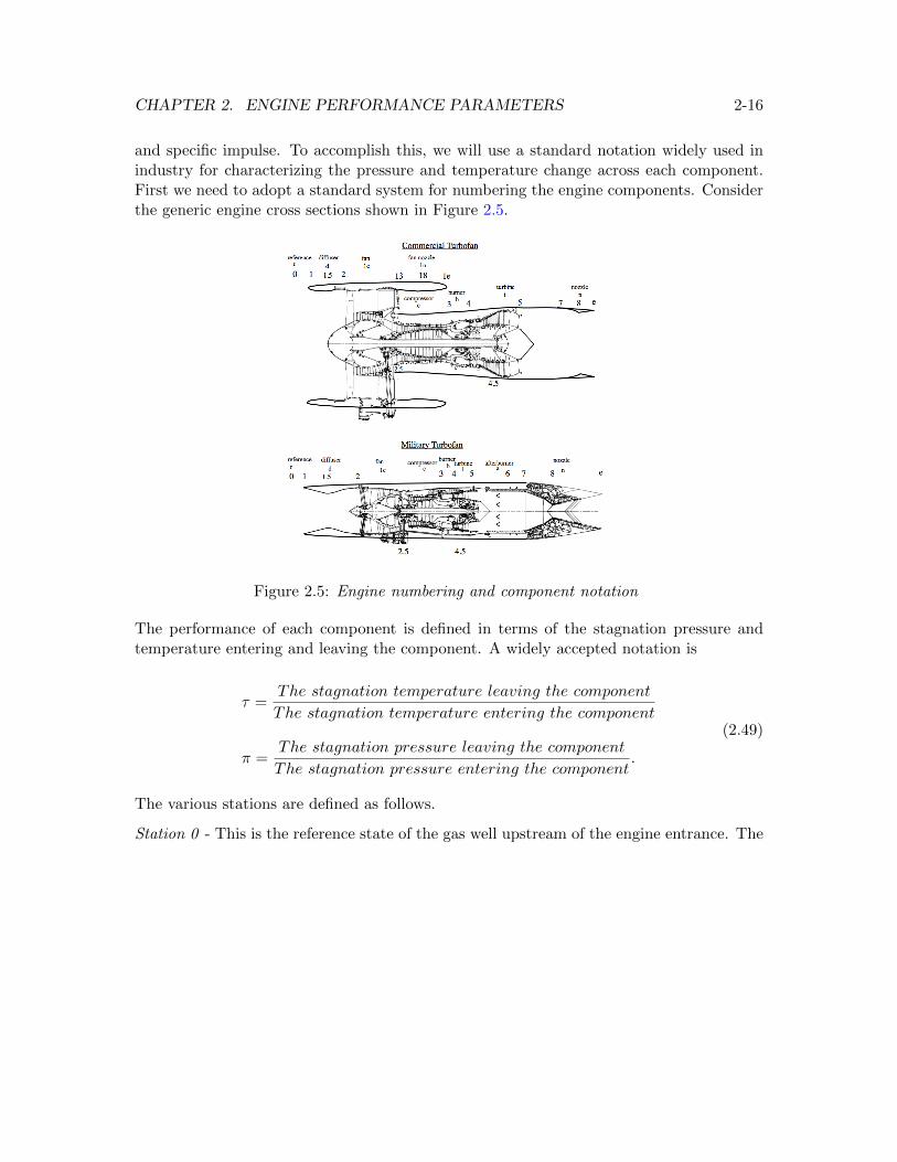
and specific impulse. To accomplish this, we will use a standard notation widely used inindustry for characterizing the pressure and temperature change across each component.First we need to adopt a standard system for numbering the engine components. Considerthe generic engine cross sections shown in Figure 2.5.
Figure 2.5: Engine numbering and component notation
The performance of each component is defined in terms of the stagnation pressure andtemperature entering and leaving the component. A widely accepted notation is
τ =The stagnation temperature leaving the component
The stagnation temperature entering the component
π =The stagnation pressure leaving the component
The stagnation pressure entering the component.
(2.49)
The various stations are defined as follows.
Station 0 - This is the reference state of the gas well upstream of the engine entrance. The
CHAPTER 2. ENGINE PERFORMANCE PARAMETERS 2-17
temperature/pressure parameters are
τr =Tt0
T0= 1 +
(γ − 1
2
)M0
2
πr =Pt0P0
=
(1 +
(γ − 1
2
)M0
2
) γγ−1
.
(2.50)
Note that these definitions are exceptional in that the denominator is the static temperatureand pressure of the free stream.
Station 1 - Entrance to the engine inlet. The purpose of the inlet is to reduce the Machnumber of the incoming flow to a low subsonic value with as small a stagnation pressureloss as possible. From the entrance to the end of the inlet there is always an increase inarea and so the component is appropriately called a diffuser.
Station 1.5 - The inlet throat.
Station 2 - The fan or compressor face. The temperature/pressure parameters across thediffuser are
τd =Tt2
Tt1
πd =Pt2Pt1
.
(2.51)
In the absence of an upstream shock wave the flow from the reference state is regarded asadiabatic and isentropic so that
Tt1 = Tt0
Pt1 = Pt0.(2.52)
The inlet is usually modeled as an adiabatic flow so the stagnation temperature is approx-imately constant, however the stagnation pressure decreases due to the presence of viscousboundary layers and possibly shock waves.
Station 2.5 - All turbofan engines comprise at least two spools. The fan is usually ac-companied by a low pressure compressor driven by a low pressure turbine through a shaftalong the centerline of the engine. A concentric shaft connects the high pressure turbineand high pressure compressor. Station 2.5 is generally taken at the interface between the
CHAPTER 2. ENGINE PERFORMANCE PARAMETERS 2-18
low and high pressure compressor. Roll Royce turbofans commonly employ three spoolswith the high pressure compressor broken into two spools.
Station 13 - This is a station in the bypass stream corresponding to the fan exit ahead ofthe entrance to the fan exhaust nozzle. The temperature/pressure parameters across thefan are
τ1c =Tt13
Tt2
π1c =Pt13
Pt2.
(2.53)
Station 18 - The fan nozzle throat.
Station 1e - The fan nozzle exit. The temperature/pressure parameters across the fannozzle are
τ1n =Tt1e
Tt13
π1n =Pt1ePt13
.
(2.54)
Station 3 - The exit of the high pressure compressor. The temperature/pressure parametersacross the compressor are
τc =Tt3
Tt2
πc =Pt3Pt2
.
(2.55)
Note that the compression includes that due to the fan. From a cycle perspective it isusually not necessary to distinguish the high and low pressure sections of the compressor.The goal of the designer is to produce a compression system that is as near to isentropicas possible.
Station 4 - The exit of the burner. The temperature/pressure parameters across the burner
CHAPTER 2. ENGINE PERFORMANCE PARAMETERS 2-19
are
τb =Tt4
Tt3
πb =Pt4Pt3
.
(2.56)
The temperature at the exit of the burner is regarded as the highest temperature in theBrayton cycle although generally higher temperatures do occur at the upstream end of theburner where combustion takes place. The burner is designed to allow an influx of coolercompressor air to mix with the combustion gases bringing the temperature down to a levelthat the high pressure turbine structure can tolerate. Modern engines use sophisticatedcooling methods to enable operation at values of Tt4 that approach 3700R(2050K), wellabove the melting temperature of the turbine materials.
Station 4.5 - This station is at the interface of the high and low pressure turbines.
Station 5 - The exit of the turbine. The temperature/pressure parameters across theturbine are
τt =Tt5
Tt4
πt =Pt5Pt4
.
(2.57)
As with the compressor the goal of the designer is to produce a turbine system that operatesas isentropically as possible.
Station 6 - The exit of the afterburner if there is one. The temperature/pressure parametersacross the afterburner are
τa =Tt6
Tt5
πa =Pt6Pt5
.
(2.58)
The Mach number entering the afterburner is fairly low and so the stagnation pressureratio of the afterburner is fairly close to, and always less than, one.
Station 7 - The entrance to the nozzle.
CHAPTER 2. ENGINE PERFORMANCE PARAMETERS 2-20
Station 8 - The nozzle throat. Over the vast range of operating conditions of modernengines the nozzle throat is choked or very nearly so.
Station e - The nozzle exit. The temperature/pressure component parameters across thenozzle are
τn =Tte
Tt7
πn =PtePt7
.
(2.59)
In the absence of the afterburner, the nozzle parameters are generally referenced to theturbine exit condition so that
τn =Tte
Tt5
πn =PtePt5
.
(2.60)
In general the goal of the designer is to minimize heat loss and stagnation pressure lossthrough the inlet, burner and nozzle.
There are two more very important parameters that need to be defined. The first is one weencountered before when we compared the fuel enthalpy to the ambient air enthalpy.
τf =hfCpT0
(2.61)
The second parameter is, in a sense, the most important quantity needed to characterizethe performance of an engine.
τλ =Tt4T0
(2.62)
In general every performance measure of the engine gets better as τλ is increased and atremendous investment has been made over the years to devise turbine cooling and ceramiccoating schemes that permit ever higher turbine inlet temperatures, Tt4.
CHAPTER 2. ENGINE PERFORMANCE PARAMETERS 2-21
2.11 Problems
Problem 1 - Suppose 10% of the heat generated in a ramjet combustor is lost throughconduction to the surroundings. How would this change the energy balance (2.19)? Howwould it affect the thrust?
Problem 2 - Write down the appropriate form of the thrust definition (2.12) for a turbofanengine with two independent streams. Suppose 5% of the air from the high pressurecompressor is to be used to power aircraft systems. What would be the appropriate thrustformula?
Problem 3 - Consider the flow through a turbojet. The energy balance across the burneris
(ma + mf )ht4 = maht3 + mfhf . (2.63)
The enthalpy rise across the compressor is equal to the enthalpy decrease across the turbine.Show that the energy balance (2.63) can also be written
(ma + mf )ht5 = maht2 + mfhf . (2.64)
The inlet and nozzle are usually assumed to operate adiabatically. Show that (2.64) canbe expressed as
(ma + mf )hte = maht0 + mfhf (2.65)
which is the same as the overall enthalpy balance for a ramjet (2.19).
Problem 4 - Work out the dimensionless forms in Section 2.9.
Chapter 3
The ramjet cycle
3.1 Ramjet flow field
Before we begin to analyze the ramjet cycle we will consider an example that can help usunderstand how the flow through a ramjet comes about. The key to understanding the flowfield is the intelligent use of the relationship for mass flow conservation. In this connectionthere are two equations that we will rely upon. The first is the expression for 1-D massflow in terms of the stagnation pressure and temperature.
m = ρUA =γ(
γ+12
) γ+12(γ−1)
(PtA√γRTt
)f (M) (3.1)
The second is the all-important area-Mach number function.
f (M) =A∗
A=
(γ + 1
2
) γ+12(γ−1) M(
1 + γ−12 M2
) γ+12(γ−1)
(3.2)
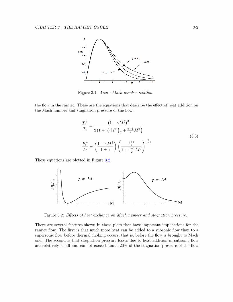
This function is plotted in Figure 3.1 for three values of γ.
For adiabatic, isentropic flow of a calorically perfect gas along a channel Equation (3.1)provides a direct connection between the local channel cross sectional area and Machnumber.
In addition to the mass flow relations there are two relationships from Rayleigh line theorythat are also very helpful in guiding our understanding of the effect of heat addition on
3-1
CHAPTER 3. THE RAMJET CYCLE 3-2
Figure 3.1: Area - Mach number relation.
the flow in the ramjet. These are the equations that describe the effect of heat addition onthe Mach number and stagnation pressure of the flow.
Tt∗
Tt=
(1 + γM2
)22 (1 + γ)M2
(1 + γ−1
2 M2)
Pt∗
Pt=
(1 + γM2
1 + γ
)( γ+12
1 + γ−12 M2
) γγ−1
(3.3)
These equations are plotted in Figure 3.2.
Figure 3.2: Effects of heat exchange on Mach number and stagnation pressure.
There are several features shown in these plots that have important implications for theramjet flow. The first is that much more heat can be added to a subsonic flow than to asupersonic flow before thermal choking occurs; that is, before the flow is brought to Machone. The second is that stagnation pressure losses due to heat addition in subsonic floware relatively small and cannot exceed about 20% of the stagnation pressure of the flow
CHAPTER 3. THE RAMJET CYCLE 3-3
entering the region of heat addition. In contrast stagnation pressure losses due to heataddition can be quite large in a supersonic flow.
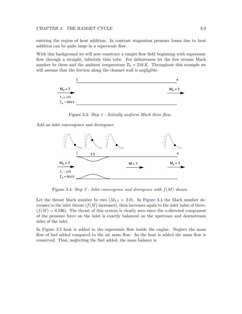
With this background we will now construct a ramjet flow field beginning with supersonicflow through a straight, infinitely thin tube. For definiteness let the free stream Machnumber be three and the ambient temperature T0 = 216K. Throughout this example wewill assume that the friction along the channel wall is negligible.
Figure 3.3: Step 1 - Initially uniform Mach three flow.
Add an inlet convergence and divergence.
Figure 3.4: Step 2 - Inlet convergence and divergence with f(M) shown.
Let the throat Mach number be two (M1.5 = 2.0). In Figure 3.4 the Mach number de-creases to the inlet throat (f(M) increases), then increases again to the inlet value of three,(f(M) = 0.236). The thrust of this system is clearly zero since the x-directed componentof the pressure force on the inlet is exactly balanced on the upstream and downstreamsides of the inlet.
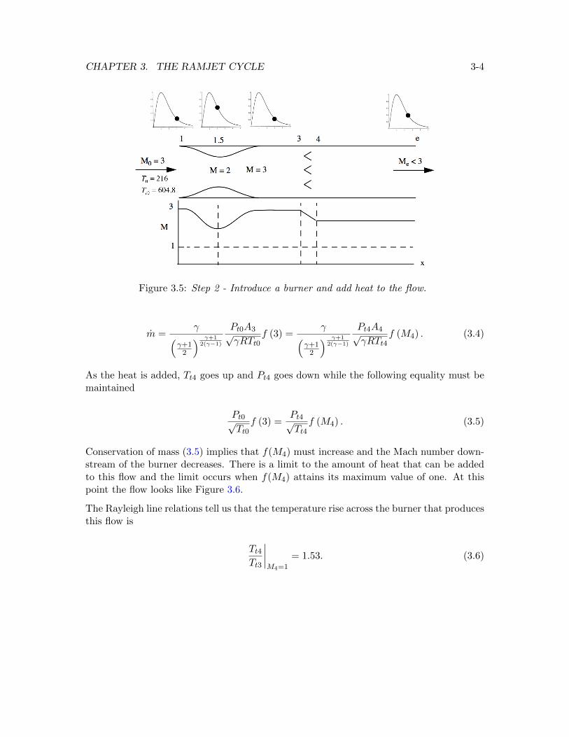
In Figure 3.5 heat is added to the supersonic flow inside the engine. Neglect the massflow of fuel added compared to the air mass flow. As the heat is added the mass flow isconserved. Thus, neglecting the fuel added, the mass balance is
CHAPTER 3. THE RAMJET CYCLE 3-4
Figure 3.5: Step 2 - Introduce a burner and add heat to the flow.
m =γ(
γ+12
) γ+12(γ−1)
Pt0A3√γRTt0
f (3) =γ(
γ+12
) γ+12(γ−1)
Pt4A4√γRTt4
f (M4) . (3.4)
As the heat is added, Tt4 goes up and Pt4 goes down while the following equality must bemaintained
Pt0√Tt0
f (3) =Pt4√Tt4
f (M4) . (3.5)
Conservation of mass (3.5) implies that f(M4) must increase and the Mach number down-stream of the burner decreases. There is a limit to the amount of heat that can be addedto this flow and the limit occurs when f(M4) attains its maximum value of one. At thispoint the flow looks like Figure 3.6.
The Rayleigh line relations tell us that the temperature rise across the burner that producesthis flow is
Tt4Tt3
∣∣∣∣M4=1
= 1.53. (3.6)
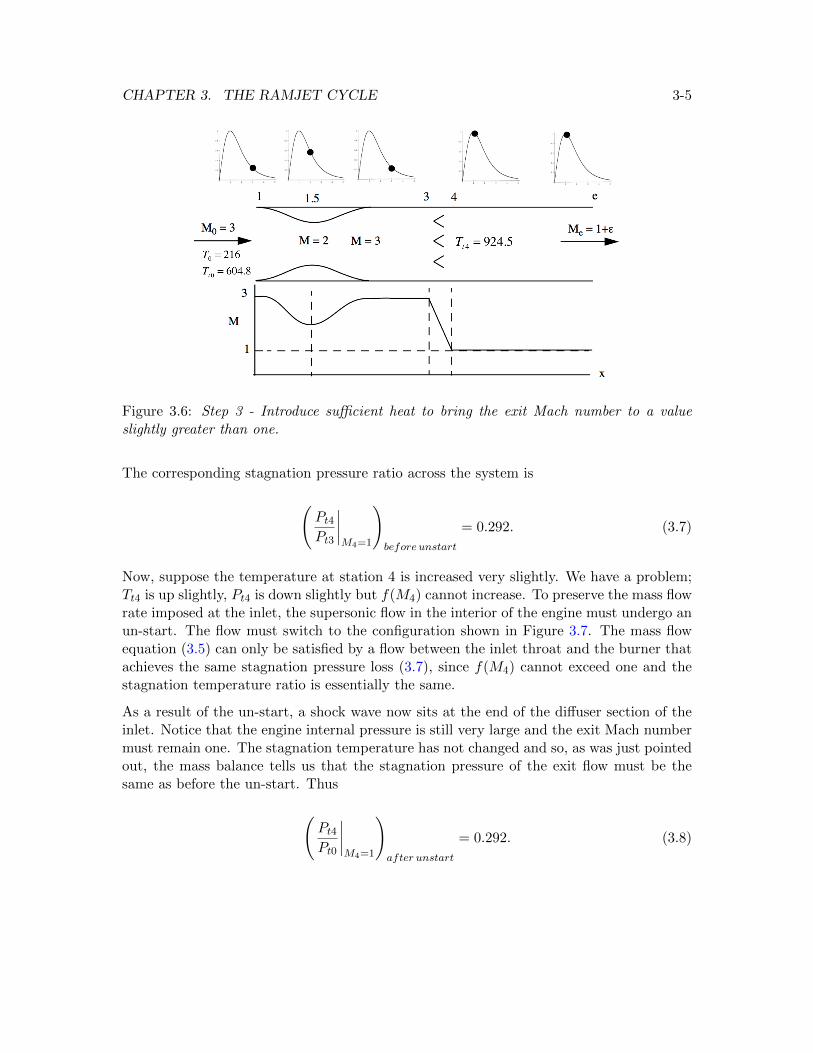
CHAPTER 3. THE RAMJET CYCLE 3-5
Figure 3.6: Step 3 - Introduce sufficient heat to bring the exit Mach number to a valueslightly greater than one.
The corresponding stagnation pressure ratio across the system is
(Pt4Pt3
∣∣∣∣M4=1
)before unstart
= 0.292. (3.7)
Now, suppose the temperature at station 4 is increased very slightly. We have a problem;Tt4 is up slightly, Pt4 is down slightly but f(M4) cannot increase. To preserve the mass flowrate imposed at the inlet, the supersonic flow in the interior of the engine must undergo anun-start. The flow must switch to the configuration shown in Figure 3.7. The mass flowequation (3.5) can only be satisfied by a flow between the inlet throat and the burner thatachieves the same stagnation pressure loss (3.7), since f(M4) cannot exceed one and thestagnation temperature ratio is essentially the same.
As a result of the un-start, a shock wave now sits at the end of the diffuser section of theinlet. Notice that the engine internal pressure is still very large and the exit Mach numbermust remain one. The stagnation temperature has not changed and so, as was just pointedout, the mass balance tells us that the stagnation pressure of the exit flow must be thesame as before the un-start. Thus
(Pt4Pt0
∣∣∣∣M4=1
)after unstart
= 0.292. (3.8)
CHAPTER 3. THE RAMJET CYCLE 3-6
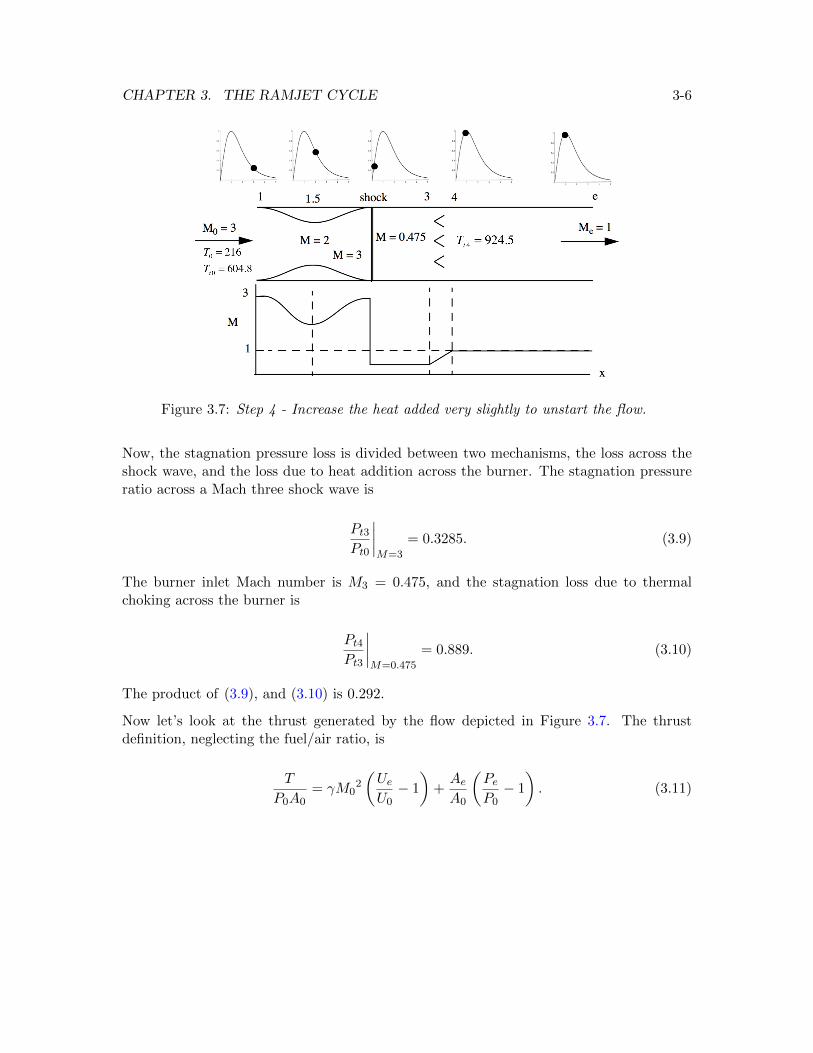
Figure 3.7: Step 4 - Increase the heat added very slightly to unstart the flow.
Now, the stagnation pressure loss is divided between two mechanisms, the loss across theshock wave, and the loss due to heat addition across the burner. The stagnation pressureratio across a Mach three shock wave is
Pt3Pt0
∣∣∣∣M=3
= 0.3285. (3.9)
The burner inlet Mach number is M3 = 0.475, and the stagnation loss due to thermalchoking across the burner is
Pt4Pt3
∣∣∣∣M=0.475
= 0.889. (3.10)
The product of (3.9), and (3.10) is 0.292.
Now let’s look at the thrust generated by the flow depicted in Figure 3.7. The thrustdefinition, neglecting the fuel/air ratio, is
T
P0A0= γM0
2
(UeU0− 1
)+AeA0
(PeP0− 1
). (3.11)
CHAPTER 3. THE RAMJET CYCLE 3-7
The pressure ratio across the engine is
PeP0
=PtePt0
(1 + γ−1
2 M02
1 + γ−12 Me
2
) γγ−1
= 0.292
(2.8
1.2
)3.5
= 5.66 (3.12)
and the temperature ratio is
TeT0
=TteTt0
(1 + γ−1
2 M02
1 + γ−12 Me
2
)= 1.53
(2.8
1.2
)= 3.5667. (3.13)
This produces the velocity ratio
UeU0
=Me
M0
√TeT0
= 0.6295. (3.14)
Now substitute into (3.11).
T
P0A0= 1.4× 9× (0.6295− 1) + 1× (5.66− 1) = −4.66 + 4.66 = 0 (3.15)
The thrust is zero. We would expect this from the symmetry of the upstream and down-stream distribution of pressure on the inlet. Now let’s see if we can produce some thrust.First adjust the inlet so that the throat area is reduced until the throat Mach number isjust slightly larger than one. This will only effect the flow in the inlet and all flow variablesin the rest of the engine will remain the same.
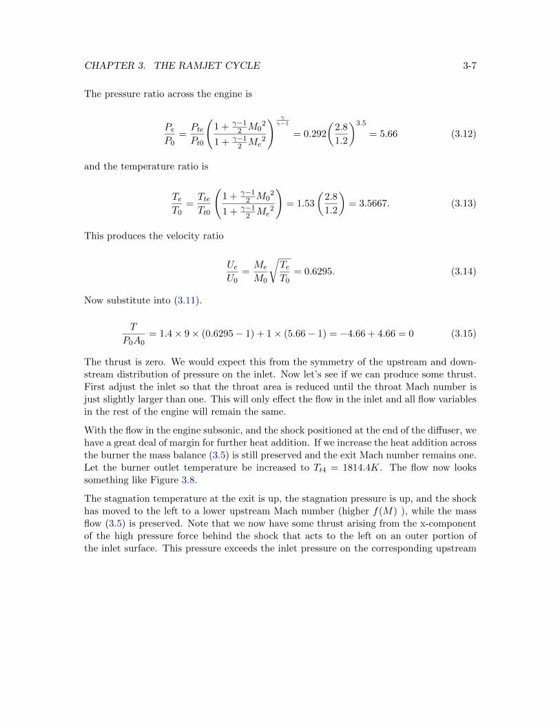
With the flow in the engine subsonic, and the shock positioned at the end of the diffuser, wehave a great deal of margin for further heat addition. If we increase the heat addition acrossthe burner the mass balance (3.5) is still preserved and the exit Mach number remains one.Let the burner outlet temperature be increased to Tt4 = 1814.4K. The flow now lookssomething like Figure 3.8.
The stagnation temperature at the exit is up, the stagnation pressure is up, and the shockhas moved to the left to a lower upstream Mach number (higher f(M) ), while the massflow (3.5) is preserved. Note that we now have some thrust arising from the x-componentof the high pressure force behind the shock that acts to the left on an outer portion ofthe inlet surface. This pressure exceeds the inlet pressure on the corresponding upstream
CHAPTER 3. THE RAMJET CYCLE 3-8
Figure 3.8: Step 5 - Increase the heat addition to produce some thrust.
portion of the inlet surface. The stagnation pressure ratio across the engine is determinedfrom the mass balance (3.5).
PtePt0
= f (3)
√TteTt0
= 0.263√
3 = 0.409 (3.16)
Let’s check the thrust. The pressure ratio across the engine is
PeP0
= 0.409
(2.8
1.2
)3.5
= 7.94. (3.17)
The temperature ratio is
TeT0
=TteTt0
(1 + γ−1
2 M02
1 + γ−12 Me
2
)= 3
(2.8
1.2
)= 7 (3.18)
and the velocity ratio is now
UeU0
=Me
M0
√TeT0
=
√7
3= 0.882. (3.19)
CHAPTER 3. THE RAMJET CYCLE 3-9
The thrust is
T
P0A0= 1.4× 9× (0.882− 1) + 1× (7.94− 1) = −1.49 + 6.94 = 5.45. (3.20)
This is a pretty substantial amount of thrust. Note that, so far, the pressure term in thethrust definition is the important thrust component in this design.
3.2 The role of the nozzle
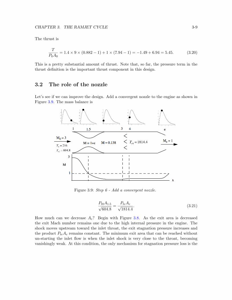
Let’s see if we can improve the design. Add a convergent nozzle to the engine as shown inFigure 3.9. The mass balance is
Figure 3.9: Step 6 - Add a convergent nozzle.
Pt0A1.5√604.8
=PteAe√1814.4
. (3.21)
How much can we decrease Ae? Begin with Figure 3.8. As the exit area is decreasedthe exit Mach number remains one due to the high internal pressure in the engine. Theshock moves upstream toward the inlet throat, the exit stagnation pressure increases andthe product PteAe remains constant. The minimum exit area that can be reached withoutun-starting the inlet flow is when the inlet shock is very close to the throat, becomingvanishingly weak. At this condition, the only mechanism for stagnation pressure loss is the
CHAPTER 3. THE RAMJET CYCLE 3-10
heat addition across the burner. The Mach number entering the burner is M3 = 0.138 asshown in Figure 3.9. The stagnation pressure loss across the burner is proportional to thesquare of the entering Mach number.
dPtPt
= −γM2dTtTt
(3.22)
To a reasonable approximation the stagnation loss across the burner can be neglected andwe can take Pte ∼= Pt0. In this approximation, the area ratio that leads to the flow depictedin Figure 3.9 is
AeA1.5
∣∣∣∣ideal
=
√1814.4
604.8= 1.732. (3.23)
This relatively large area ratio is expected considering the greatly increased temperatureand lower density of the exhaust gases compared to the gas that passes through the up-stream throat. What about the thrust? Now the static pressure ratio across the engineis
PeP0
=
(2.8
1.2
)3.5
= 19.41. (3.24)
The temperatures and Mach numbers at the nozzle exit are the same as before so thevelocity ratio does not change between Figure 3.8 and Figure 3.9. The dimensionlessthrust is
T
P0A0= 1.4×9× (0.882− 1) + 1.732×0.236× (19.41− 1) = −1.49 + 7.53 = 6.034. (3.25)
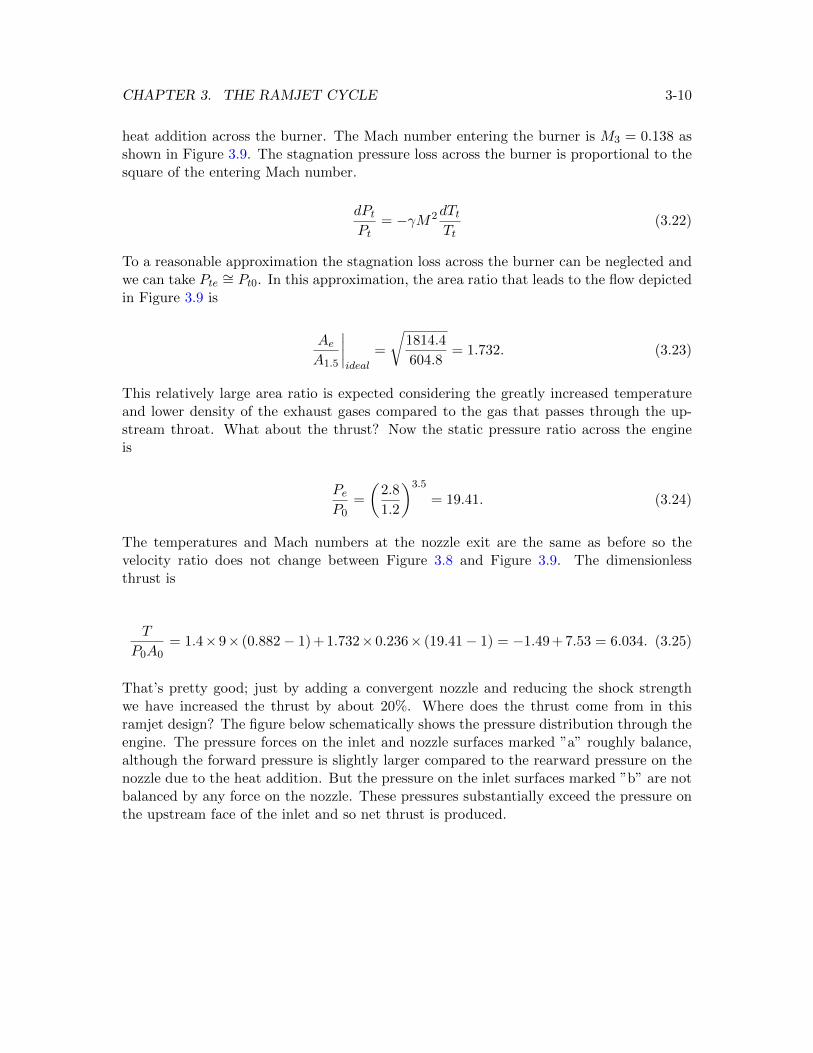
That’s pretty good; just by adding a convergent nozzle and reducing the shock strengthwe have increased the thrust by about 20%. Where does the thrust come from in thisramjet design? The figure below schematically shows the pressure distribution through theengine. The pressure forces on the inlet and nozzle surfaces marked ”a” roughly balance,although the forward pressure is slightly larger compared to the rearward pressure on thenozzle due to the heat addition. But the pressure on the inlet surfaces marked ”b” are notbalanced by any force on the nozzle. These pressures substantially exceed the pressure onthe upstream face of the inlet and so net thrust is produced.
CHAPTER 3. THE RAMJET CYCLE 3-11
Figure 3.10: Imbalance of pressure forces leading to net thrust.
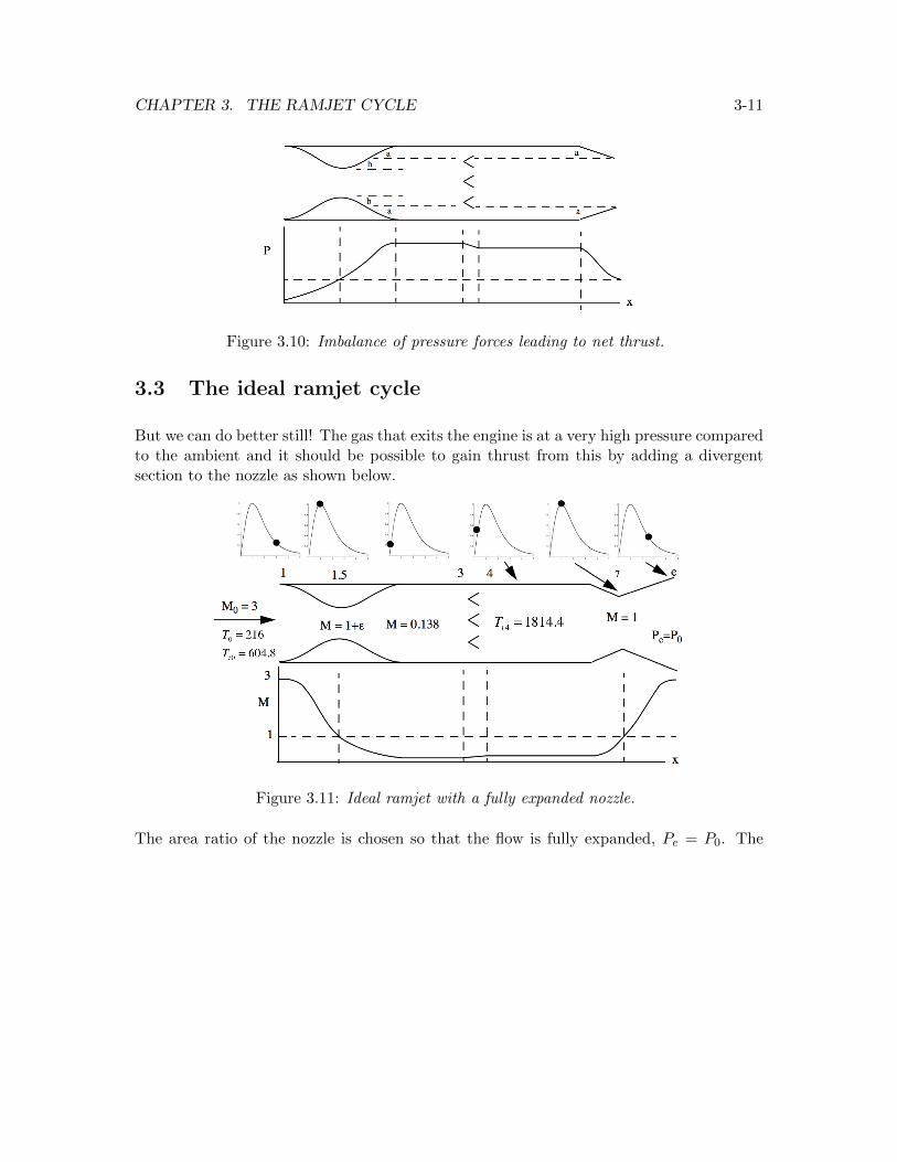
3.3 The ideal ramjet cycle
But we can do better still! The gas that exits the engine is at a very high pressure comparedto the ambient and it should be possible to gain thrust from this by adding a divergentsection to the nozzle as shown below.
Figure 3.11: Ideal ramjet with a fully expanded nozzle.
The area ratio of the nozzle is chosen so that the flow is fully expanded, Pe = P0. The
CHAPTER 3. THE RAMJET CYCLE 3-12
stagnation pressure is constant through the engine and so we can conclude from
PeP0
=PtePt0
(1 + γ−1
2 M02
1 + γ−12 Me
2
) γγ−1
1 = 1×
(1 + γ−1
2 M02
1 + γ−12 Me
2
) γγ−1
(3.26)
that Me = M0. The temperature ratio is
TeT0
=TteTt0
(1 + γ−1
2 M02
1 + γ−12 Me
2
)=TteTt0
= 3. (3.27)
Finally, the dimensionless thrust is
T
P0A0= γM0
2
(Me
M0
√TeT0− 1
)= 1.4× 9×
(√3− 1
)= 9.22. (3.28)
Adding a divergent section to the nozzle at this relatively high Mach number increases thethrust by 50%.
Now work out the other engine parameters. The fuel/air ratio is determined from
mfhf = (ma + mf )ht4 − maht3. (3.29)
Assume the fuel added is JP-4 with hf = 4.28× 10⁷J/kg. Equation (3.29) becomes
f =Tt4Tt3− 1
hfCpTt3
− Tt4Tt3
=1814.4604.8 − 1
70.41− 1814.4604.8
= 0.0297. (3.30)
The relatively small value of fuel/air ratio is the a posteriori justification of our earlierneglect of the fuel mass flow compared to the air mass flow. If we include the fuel/airratio in the thrust calculation (but still ignore the effect of mass addition on the stagnationpressure change across the burner) the result is
T
P0A0= γM0
2
((1 + f)
Me
M0
√TeT0− 1
)= 1.4× 9×
(1.0297×
√3− 1
)= 9.872. (3.31)
CHAPTER 3. THE RAMJET CYCLE 3-13
The error in the thrust is about 7% when the fuel contribution is neglected. The dimen-sionless specific impulse is
Ispg
a0=
(1
f
)(1
γM0
)T
P0A0=
9.872
0.0297× 1.4× 3= 79.14 (3.32)
and the overall efficiency is, (τf = hf/CpT0 = 197.2),
ηov =
(γ − 1
γ
)(1
fτf
)T
P0A0=
(0.4
1.4
)(9.872
0.0297× 197.2
)= 0.482. (3.33)
The propulsive efficiency is
ηpr =2U0
Ue + U0=
2
1 +√
3= 0.732. (3.34)
The thermal efficiency of the engine shown in Figure 3.11 can be expressed as follows
ηth =(ma + mf ) Ue
2
2 − maU0
2
2
mfhf=
(ma + mf ) (hte − he)− ma (ht0 − h0)
(ma + mf )hte − maht0
ηth = 1−Qrejected during the cycleQinput during the cycle
= 1−(ma + mf )he − mah0
(ma + mf )hte − maht0
ηth = 1− T0
Tt0
((1 + f) TeT0
− 1
(1 + f) TteTt0 − 1
).
(3.35)
The heat rejection is accomplished by mixing of the hot exhaust stream with surroundingair at constant pressure. Noting (3.27) for the ideal ramjet, the last term in brackets isone and the thermal efficiency becomes
ηth ideal ramjet = 1− T0
Tt0. (3.36)
For the ramjet conditions of this example the thermal efficiency is 2/3 . The Brayton cycleefficiency is
ηB = 1− T0
T3. (3.37)
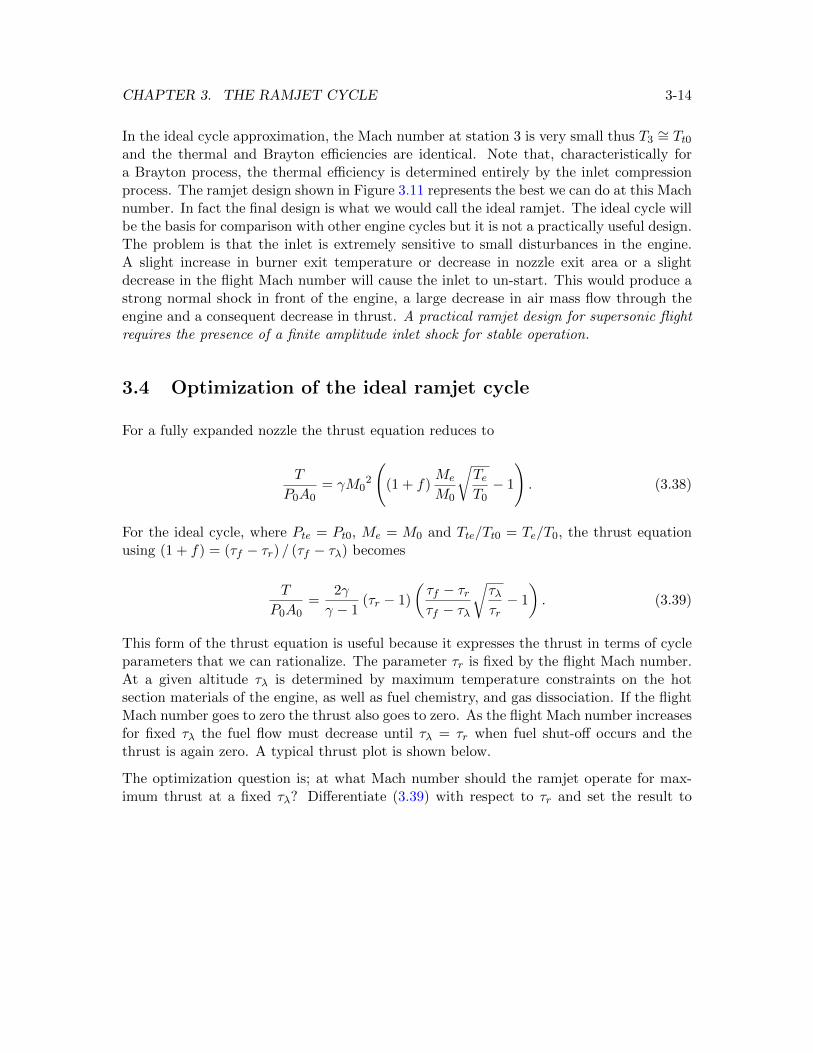
CHAPTER 3. THE RAMJET CYCLE 3-14
In the ideal cycle approximation, the Mach number at station 3 is very small thus T3∼= Tt0
and the thermal and Brayton efficiencies are identical. Note that, characteristically fora Brayton process, the thermal efficiency is determined entirely by the inlet compressionprocess. The ramjet design shown in Figure 3.11 represents the best we can do at this Machnumber. In fact the final design is what we would call the ideal ramjet. The ideal cycle willbe the basis for comparison with other engine cycles but it is not a practically useful design.The problem is that the inlet is extremely sensitive to small disturbances in the engine.A slight increase in burner exit temperature or decrease in nozzle exit area or a slightdecrease in the flight Mach number will cause the inlet to un-start. This would produce astrong normal shock in front of the engine, a large decrease in air mass flow through theengine and a consequent decrease in thrust. A practical ramjet design for supersonic flightrequires the presence of a finite amplitude inlet shock for stable operation.
3.4 Optimization of the ideal ramjet cycle
For a fully expanded nozzle the thrust equation reduces to
T
P0A0= γM0
2
((1 + f)
Me
M0
√TeT0− 1
). (3.38)
For the ideal cycle, where Pte = Pt0, Me = M0 and Tte/Tt0 = Te/T0, the thrust equationusing (1 + f) = (τf − τr) / (τf − τλ) becomes
T
P0A0=
2γ
γ − 1(τr − 1)
(τf − τrτf − τλ
√τλτr− 1
). (3.39)
This form of the thrust equation is useful because it expresses the thrust in terms of cycleparameters that we can rationalize. The parameter τr is fixed by the flight Mach number.At a given altitude τλ is determined by maximum temperature constraints on the hotsection materials of the engine, as well as fuel chemistry, and gas dissociation. If the flightMach number goes to zero the thrust also goes to zero. As the flight Mach number increasesfor fixed τλ the fuel flow must decrease until τλ = τr when fuel shut-off occurs and thethrust is again zero. A typical thrust plot is shown below.
The optimization question is; at what Mach number should the ramjet operate for max-imum thrust at a fixed τλ? Differentiate (3.39) with respect to τr and set the result to
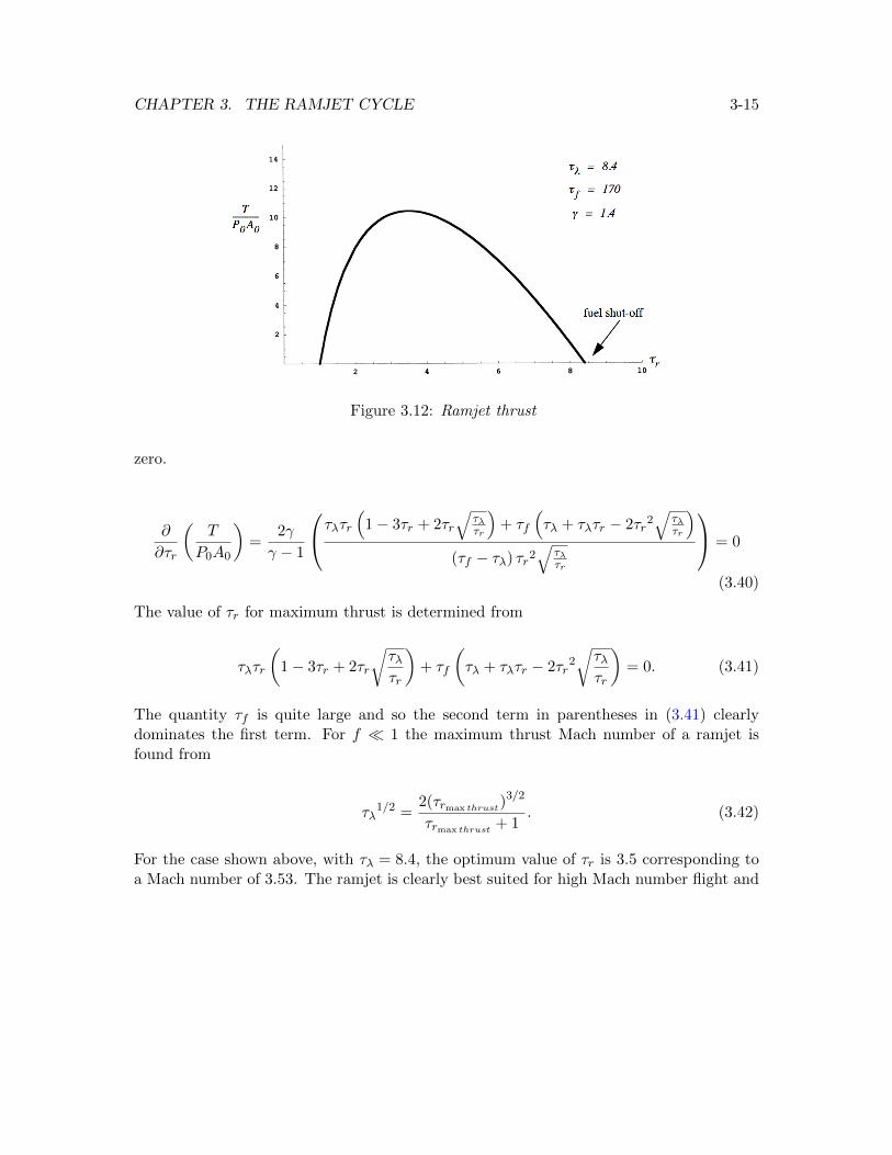
CHAPTER 3. THE RAMJET CYCLE 3-15
Figure 3.12: Ramjet thrust
zero.
∂
∂τr
(T
P0A0
)=
2γ
γ − 1
τλτr(
1− 3τr + 2τr√
τλτr
)+ τf
(τλ + τλτr − 2τr
2√
τλτr
)(τf − τλ) τr2
√τλτr
= 0
(3.40)
The value of τr for maximum thrust is determined from
τλτr
(1− 3τr + 2τr
√τλτr
)+ τf
(τλ + τλτr − 2τr
2
√τλτr
)= 0. (3.41)
The quantity τf is quite large and so the second term in parentheses in (3.41) clearlydominates the first term. For f � 1 the maximum thrust Mach number of a ramjet isfound from
τλ1/2 =
2(τrmax thrust)3/2
τrmax thrust+ 1
. (3.42)
For the case shown above, with τλ = 8.4, the optimum value of τr is 3.5 corresponding toa Mach number of 3.53. The ramjet is clearly best suited for high Mach number flight and
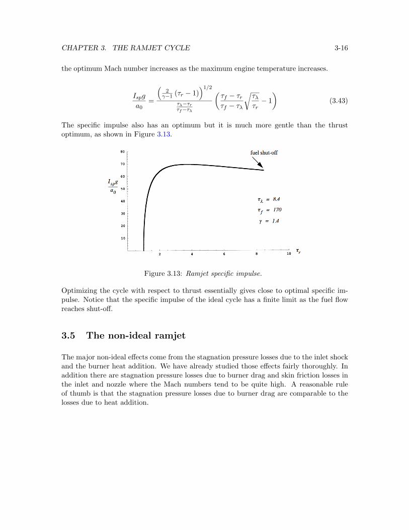
CHAPTER 3. THE RAMJET CYCLE 3-16
the optimum Mach number increases as the maximum engine temperature increases.
Ispg
a0=
(2
γ−1 (τr − 1))1/2
τλ−τrτf−τλ
(τf − τrτf − τλ
√τλτr− 1
)(3.43)
The specific impulse also has an optimum but it is much more gentle than the thrustoptimum, as shown in Figure 3.13.
Figure 3.13: Ramjet specific impulse.
Optimizing the cycle with respect to thrust essentially gives close to optimal specific im-pulse. Notice that the specific impulse of the ideal cycle has a finite limit as the fuel flowreaches shut-off.
3.5 The non-ideal ramjet
The major non-ideal effects come from the stagnation pressure losses due to the inlet shockand the burner heat addition. We have already studied those effects fairly thoroughly. Inaddition there are stagnation pressure losses due to burner drag and skin friction losses inthe inlet and nozzle where the Mach numbers tend to be quite high. A reasonable ruleof thumb is that the stagnation pressure losses due to burner drag are comparable to thelosses due to heat addition.
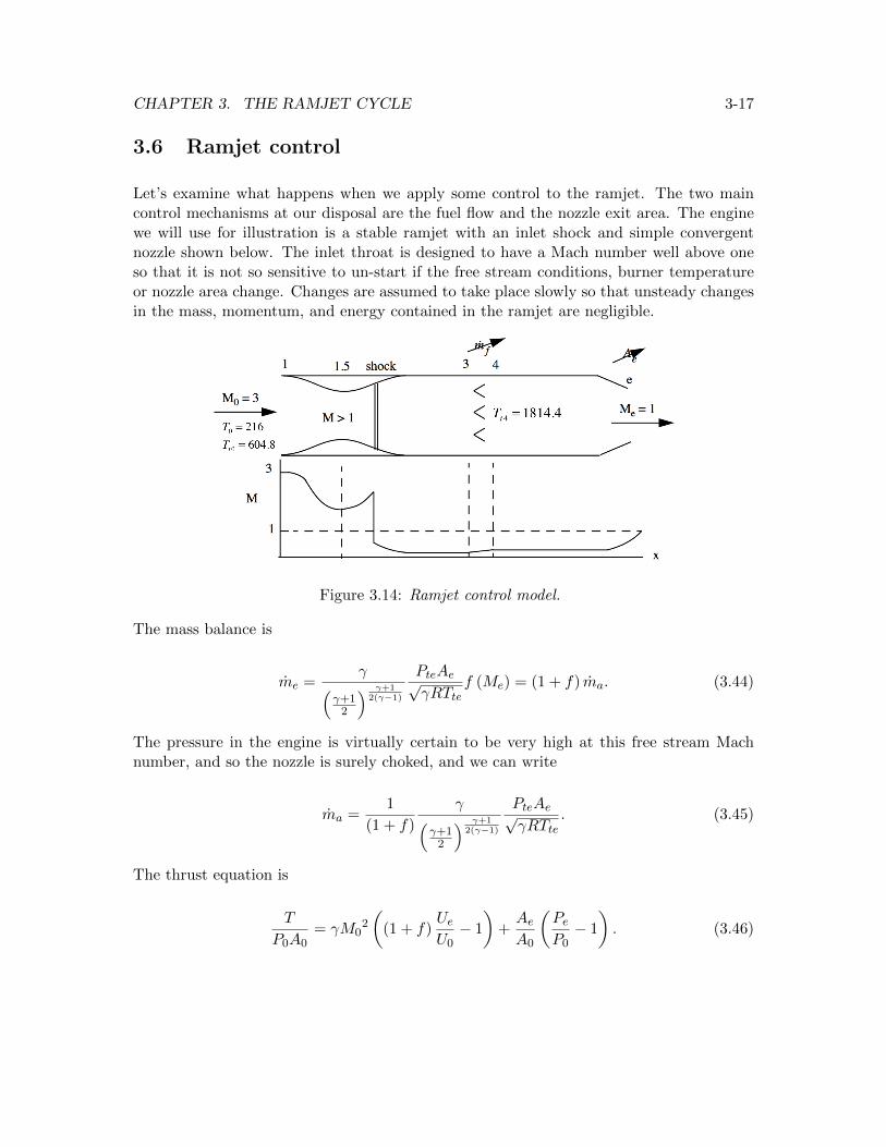
CHAPTER 3. THE RAMJET CYCLE 3-17
3.6 Ramjet control
Let’s examine what happens when we apply some control to the ramjet. The two maincontrol mechanisms at our disposal are the fuel flow and the nozzle exit area. The enginewe will use for illustration is a stable ramjet with an inlet shock and simple convergentnozzle shown below. The inlet throat is designed to have a Mach number well above oneso that it is not so sensitive to un-start if the free stream conditions, burner temperatureor nozzle area change. Changes are assumed to take place slowly so that unsteady changesin the mass, momentum, and energy contained in the ramjet are negligible.
Figure 3.14: Ramjet control model.
The mass balance is
me =γ(
γ+12
) γ+12(γ−1)
PteAe√γRTte
f (Me) = (1 + f) ma. (3.44)
The pressure in the engine is virtually certain to be very high at this free stream Machnumber, and so the nozzle is surely choked, and we can write
ma =1
(1 + f)
γ(γ+1
2
) γ+12(γ−1)
PteAe√γRTte
. (3.45)
The thrust equation is
T
P0A0= γM0
2
((1 + f)
UeU0− 1
)+AeA0
(PeP0− 1
). (3.46)
CHAPTER 3. THE RAMJET CYCLE 3-18
Our main concern is to figure out what happens to the velocity ratio and pressure ratio aswe control the fuel flow and nozzle exit area.
Nozzle exit area control
First, suppose Ae is increased with Tte constant. In order for (3.45) to be satisfied Ptemust drop keeping PteAe constant. The shock moves downstream to a higher shock Machnumber. The velocity ratio remains the same and, since the exit Mach number does notchange, the product PeAe remains constant. Note that the thrust decreases. This can beseen by writing the second term in (3.46) as
AeA0
PeP0− AeA0. (3.47)
The left term in (3.47) is constant but the right term increases leading to a decrease inthrust. If Ae is decreased, the reverse happens, the inlet operates more efficiently and thethrust goes up. But remember, the amount by which the area can be decreased is limitedby the Mach number of the inlet throat.
Fuel flow control
Now, suppose Tte is decreased with Ae constant. In order for (3.45) to be satisfied, Ptemust drop keeping Pte/
√Tte constant. Once again the shock moves downstream to a higher
shock Mach number. The velocity ratio goes down since the exit stagnation temperature isdown and the Mach numbers do not change.The pressure ratio also decreases since the exitstagnation pressure is down. The thrust clearly decreases in this case. If Tte is increased,the reverse happens, the inlet operates more efficiently and the thrust goes up. The amountby which the burner exit temperature can be increased is again limited by the Mach numberof the inlet throat.
3.7 Example - Ramjet with un-started inlet
For simplicity, assume constant heat capacity with γ = 1.4 , Cp = 1005M2/(sec2 −K
).
The gas constant is R = 287M2/(sec2 −K
). The ambient temperature and pressure are
T0 = 216K and P0 = 2× 10⁴N/M2. The fuel heating value is hf = 4.28× 10⁷ J/kg. Thesketch below shows a ramjet operating at a free stream Mach number of 3.0. A normalshock stands in front of the inlet. Heat is added between stations 3 and 4.
The stagnation temperature at station 4 is Tt4 = 2000K. Relevant areas are A3/A1.5 = 8,A1 = A3 = A4 and A4/Ae = 3. Determine the dimensionless thrust T/(P0A1). Do notassume f � 1. Neglect stagnation pressure losses due to wall friction and burner drag.Assume that the static pressure outside the nozzle has recovered to the ambient value.
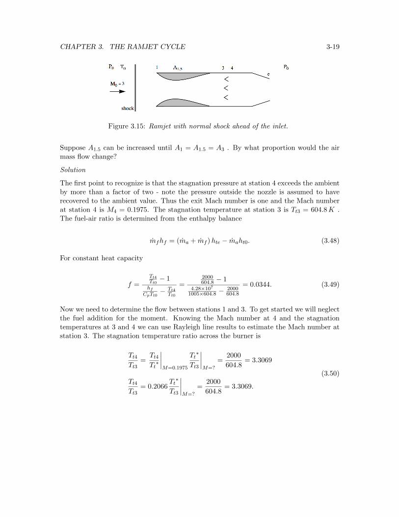
CHAPTER 3. THE RAMJET CYCLE 3-19
Figure 3.15: Ramjet with normal shock ahead of the inlet.
Suppose A1.5 can be increased until A1 = A1.5 = A3 . By what proportion would the airmass flow change?
Solution
The first point to recognize is that the stagnation pressure at station 4 exceeds the ambientby more than a factor of two - note the pressure outside the nozzle is assumed to haverecovered to the ambient value. Thus the exit Mach number is one and the Mach numberat station 4 is M4 = 0.1975. The stagnation temperature at station 3 is Tt3 = 604.8K .The fuel-air ratio is determined from the enthalpy balance
mfhf = (ma + mf )hte − maht0. (3.48)
For constant heat capacity
f =Tt4Tt0− 1
hfCpTt0
− Tt4Tt0
=2000604.8 − 1
4.28×10⁷
1005×604.8 −2000604.8
= 0.0344. (3.49)
Now we need to determine the flow between stations 1 and 3. To get started we will neglectthe fuel addition for the moment. Knowing the Mach number at 4 and the stagnationtemperatures at 3 and 4 we can use Rayleigh line results to estimate the Mach number atstation 3. The stagnation temperature ratio across the burner is
Tt4Tt3
=Tt4Tt∗
∣∣∣∣M=0.1975
Tt∗
Tt3
∣∣∣∣M=?
=2000
604.8= 3.3069
Tt4Tt3
= 0.2066Tt∗
Tt3
∣∣∣∣M=?
=2000
604.8= 3.3069.
(3.50)
CHAPTER 3. THE RAMJET CYCLE 3-20
The Rayleigh line tables give
Tt∗
Tt3
∣∣∣∣M=?
=3.3069
0.2066= 16.006⇒M3 = 0.103. (3.51)
This is a reasonable approximation to the Mach number at station 3. The stagnationpressure ratio across the burner is
Pt4Pt3
=Pt4Pt∗
∣∣∣∣M=0.1975
Pt∗
Pt3
∣∣∣∣M=0.103
=1.235
1.258= 0.981. (3.52)
The subsonic critical Mach number for an area ratio of 8 is 0.0725. The fact that the Machnumber at station 3 is higher than this value implies that there is a shock in the divergingpart of the inlet and the inlet throat Mach number is equal to one. The stagnation pressureratio between the inlet throat and the exit can be determined from a mass balance betweenstations 1.5 and e.
Pt1.5A1.5 (1 + f)√Tt1.5
=PteAe√Tte
=
PtePt1.5
=1.0344× 3
8
√2000
604.8= 0.7054
(3.53)
The results (3.52) and (3.53) determine the stagnation pressure ratio across the inlet shockand this determines the Mach number of the inlet shock.
πshock =0.7054
0.981= 0.719⇒Mshock = 2.004 (3.54)
Thus far the ramjet flow looks as shown in Figure 3.16.
The stagnation pressure ratio across the external shock is
Pt1Pt0
∣∣∣∣M=3
= 0.3283 (3.55)
and so the overall stagnation pressure ratio is
PtePt0
=Pt1Pt0
PtePt1.5
= 0.3283× 0.7054 = 0.2316. (3.56)
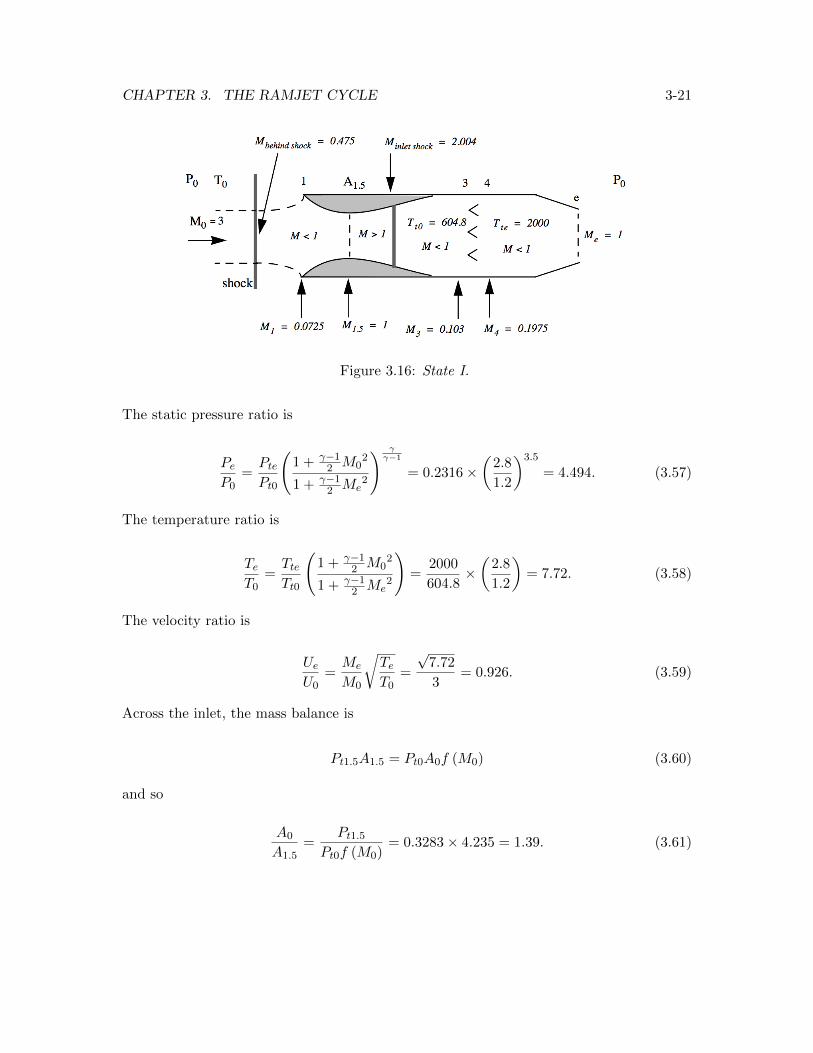
CHAPTER 3. THE RAMJET CYCLE 3-21
Figure 3.16: State I.
The static pressure ratio is
PeP0
=PtePt0
(1 + γ−1
2 M02
1 + γ−12 Me
2
) γγ−1
= 0.2316×(
2.8
1.2
)3.5
= 4.494. (3.57)
The temperature ratio is
TeT0
=TteTt0
(1 + γ−1
2 M02
1 + γ−12 Me
2
)=
2000
604.8×(
2.8
1.2
)= 7.72. (3.58)
The velocity ratio is
UeU0
=Me
M0
√TeT0
=
√7.72
3= 0.926. (3.59)
Across the inlet, the mass balance is
Pt1.5A1.5 = Pt0A0f (M0) (3.60)
and so
A0
A1.5=
Pt1.5Pt0f (M0)
= 0.3283× 4.235 = 1.39. (3.61)
CHAPTER 3. THE RAMJET CYCLE 3-22
Finally the thrust is
T
P0A1= γM0
2 A0
A1.5
A1.5
A1
((1 + f)
UeU0− 1
)+AeA1
(PeP0− 1
)(3.62)
and
T
P0A1
∣∣∣∣StateI
= 1.4× 9× 1.39× (1/8)× (1.0344× 0.926− 1) + (1/3)× (4.494− 1) =
−0.0923 + 1.165 = 1.0724.(3.63)
State II
Now increase the inlet throat area to the point where the inlet un-chokes. As the inletthroat area is increased the Mach number at station 3 will remain the same since it isdetermined by the choking at the nozzle exit and the fixed enthalpy rise across the burner.The mass balance between the inlet throat and the nozzle exit is again
Pt1.5A1.5 (1 + f)√Tt1.5
=PteAe√Tte
. (3.64)
The stagnation pressure at station 1.5 is fixed by the loss across the external shock. Thefuel-air ratio is fixed as are the temperatures in (3.64). As A1.5 is increased, the equality(3.64) is maintained and the inlet shock moves to the left increasing Pte . At the pointwhere the the inlet throat un-chokes the shock is infinitely weak and the only stagnationpressure loss between station 1.5 and the nozzle exit is across the burner.
A1.5State II
Ae=
1
1 + f
Pte State IIPt1.5
√Tt1.5Tte
=0.982
1.0344
√604.8
2000= 0.522 (3.65)
This corresponds to
A1
A1.5State II=
(A1
Ae
)(Ae
A1.5State II
)=
3
0.522= 5.747. (3.66)
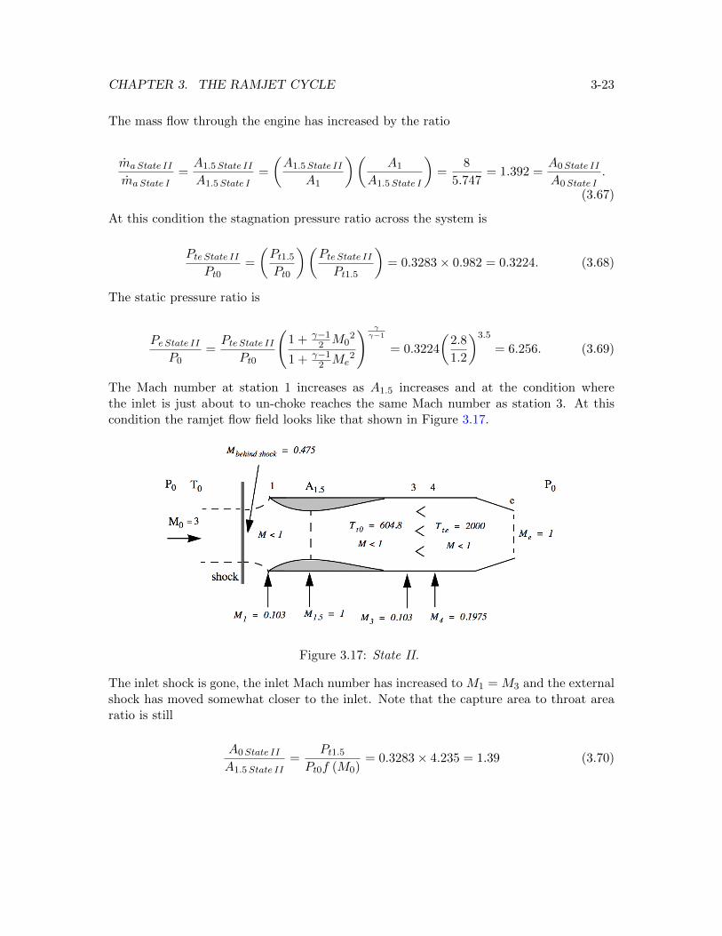
CHAPTER 3. THE RAMJET CYCLE 3-23
The mass flow through the engine has increased by the ratio
maState II
maState I=A1.5State II
A1.5State I=
(A1.5State II
A1
)(A1
A1.5State I
)=
8
5.747= 1.392 =
A0State II
A0State I.
(3.67)
At this condition the stagnation pressure ratio across the system is
Pte State IIPt0
=
(Pt1.5Pt0
)(Pte State IIPt1.5
)= 0.3283× 0.982 = 0.3224. (3.68)
The static pressure ratio is
Pe State IIP0
=Pte State II
Pt0
(1 + γ−1
2 M02
1 + γ−12 Me
2
) γγ−1
= 0.3224
(2.8
1.2
)3.5
= 6.256. (3.69)
The Mach number at station 1 increases as A1.5 increases and at the condition wherethe inlet is just about to un-choke reaches the same Mach number as station 3. At thiscondition the ramjet flow field looks like that shown in Figure 3.17.
Figure 3.17: State II.
The inlet shock is gone, the inlet Mach number has increased to M1 = M3 and the externalshock has moved somewhat closer to the inlet. Note that the capture area to throat arearatio is still
A0State II
A1.5State II=
Pt1.5Pt0f (M0)
= 0.3283× 4.235 = 1.39 (3.70)
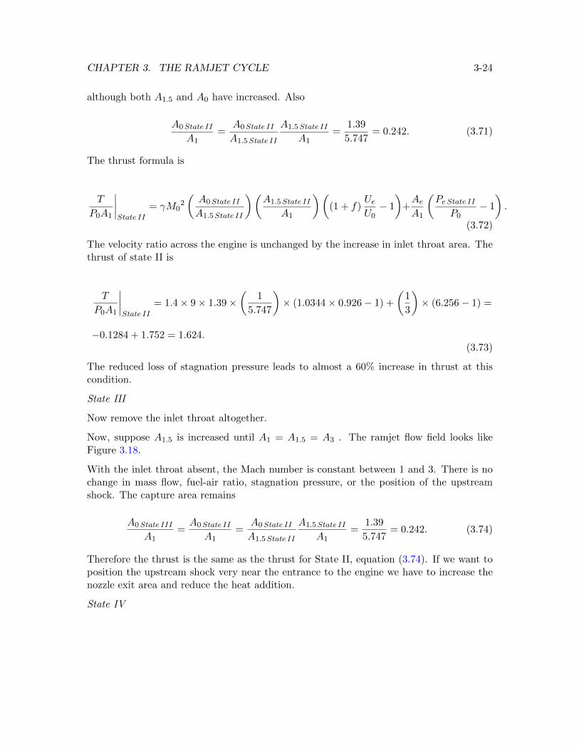
CHAPTER 3. THE RAMJET CYCLE 3-24
although both A1.5 and A0 have increased. Also
A0State II
A1=
A0State II
A1.5State II
A1.5State II
A1=
1.39
5.747= 0.242. (3.71)
The thrust formula is
T
P0A1
∣∣∣∣State II
= γM02
(A0State II
A1.5State II
)(A1.5State II
A1
)((1 + f)
UeU0− 1
)+AeA1
(Pe State II
P0− 1
).
(3.72)
The velocity ratio across the engine is unchanged by the increase in inlet throat area. Thethrust of state II is
T
P0A1
∣∣∣∣State II
= 1.4× 9× 1.39×(
1
5.747
)× (1.0344× 0.926− 1) +
(1
3
)× (6.256− 1) =
−0.1284 + 1.752 = 1.624.(3.73)
The reduced loss of stagnation pressure leads to almost a 60% increase in thrust at thiscondition.
State III
Now remove the inlet throat altogether.
Now, suppose A1.5 is increased until A1 = A1.5 = A3 . The ramjet flow field looks likeFigure 3.18.
With the inlet throat absent, the Mach number is constant between 1 and 3. There is nochange in mass flow, fuel-air ratio, stagnation pressure, or the position of the upstreamshock. The capture area remains
A0State III
A1=A0State II
A1=
A0State II
A1.5State II
A1.5State II
A1=
1.39
5.747= 0.242. (3.74)
Therefore the thrust is the same as the thrust for State II, equation (3.74). If we want toposition the upstream shock very near the entrance to the engine we have to increase thenozzle exit area and reduce the heat addition.
State IV
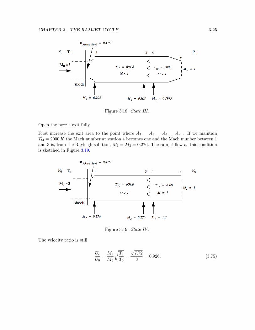
CHAPTER 3. THE RAMJET CYCLE 3-25
Figure 3.18: State III.
Open the nozzle exit fully.
First increase the exit area to the point where A1 = A3 = A4 = Ae . If we maintainTt4 = 2000K the Mach number at station 4 becomes one and the Mach number between 1and 3 is, from the Rayleigh solution, M1 = M3 = 0.276. The ramjet flow at this conditionis sketched in Figure 3.19.
Figure 3.19: State IV.
The velocity ratio is still
UeU0
=Me
M0
√TeT0
=
√7.72
3= 0.926. (3.75)
CHAPTER 3. THE RAMJET CYCLE 3-26
The stagnation pressure ratio across the burner is, from the Rayleigh solution,
PtePt1
∣∣∣∣State IV
= 0.8278. (3.76)
Across the whole system
PtePt0
∣∣∣∣State IV
=Pt1.5Pt0
∣∣∣∣State IV
PtePt1.5
∣∣∣∣State IV
= 0.3283× 0.8278 = 0.2718 (3.77)
and the static pressure ratio is
Pe State IVP0
=Pte State IV
Pt0
(1 + γ−1
2 M02
1 + γ−12 Me
2
) γγ−1
= 0.2718
(2.8
1.2
)3.5
= 5.274. (3.78)
The area ratio is
A0State IV
A1=Pt1f (M1)
Pt0f (M0)= 0.3283× 0.4558
0.2362= 0.634. (3.79)
The thrust formula for state IV is
T
P0A1
∣∣∣∣State IV
= γM02
(A0State IV
A1
)((1 + f)
UeU0− 1
)+AeA1
(Pe State IV
P0− 1
)(3.80)
which evaluates to
T
P0A1
∣∣∣∣State IV
= 1.4× 9× 0.634× (1.0344× 0.926− 1) + 1× (5.274− 1) =
−0.3367 + 4.274 = 3.937.
(3.81)
Note the considerable increase in mass flow for state IV compared to state III. From(3.74)
maState IV
maState III=
(A0State IV
A1
)(A1
A0State III
)=
0.634
0.242= 2.62 (3.82)
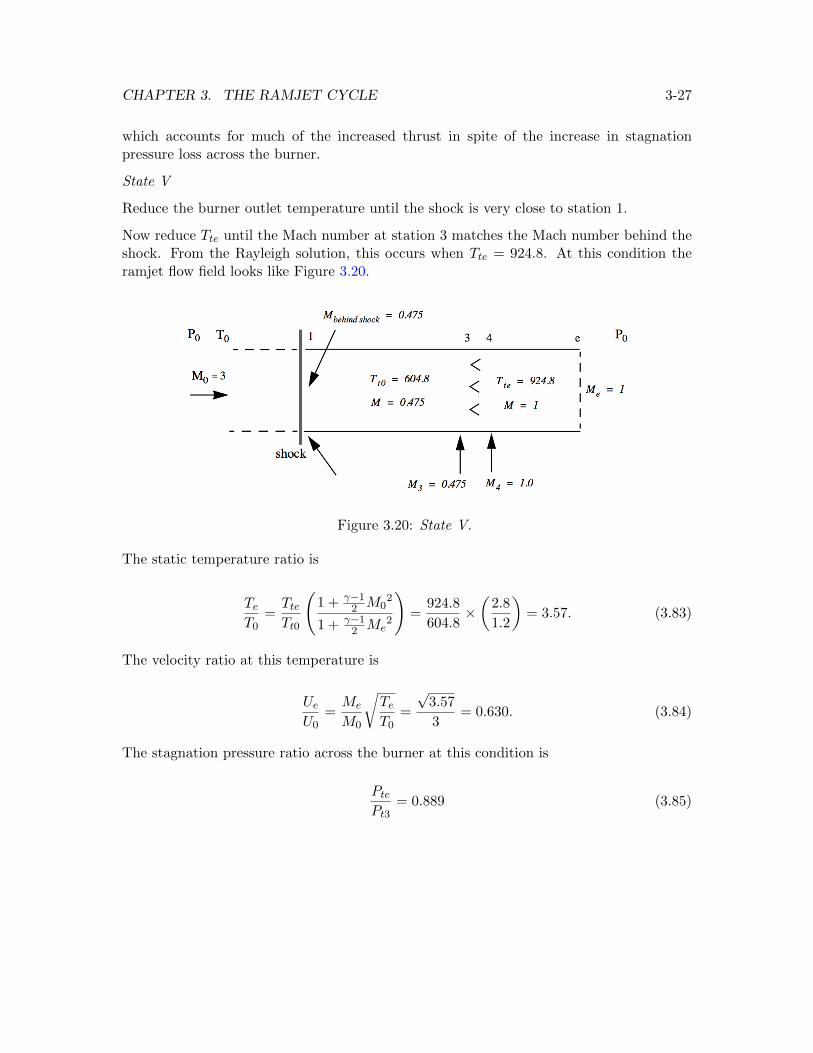
CHAPTER 3. THE RAMJET CYCLE 3-27
which accounts for much of the increased thrust in spite of the increase in stagnationpressure loss across the burner.
State V
Reduce the burner outlet temperature until the shock is very close to station 1.
Now reduce Tte until the Mach number at station 3 matches the Mach number behind theshock. From the Rayleigh solution, this occurs when Tte = 924.8. At this condition theramjet flow field looks like Figure 3.20.
Figure 3.20: State V.
The static temperature ratio is
TeT0
=TteTt0
(1 + γ−1
2 M02
1 + γ−12 Me
2
)=
924.8
604.8×(
2.8
1.2
)= 3.57. (3.83)
The velocity ratio at this temperature is
UeU0
=Me
M0
√TeT0
=
√3.57
3= 0.630. (3.84)
The stagnation pressure ratio across the burner at this condition is
PtePt3
= 0.889 (3.85)
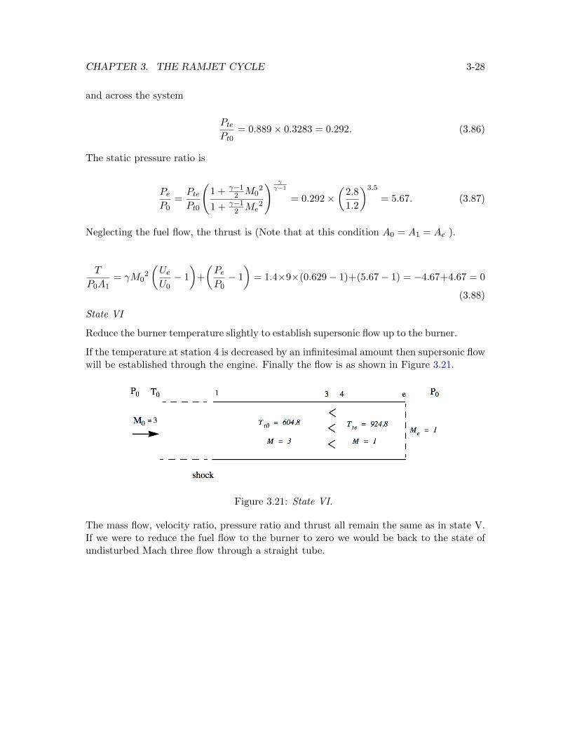
CHAPTER 3. THE RAMJET CYCLE 3-28
and across the system
PtePt0
= 0.889× 0.3283 = 0.292. (3.86)
The static pressure ratio is
PeP0
=PtePt0
(1 + γ−1
2 M02
1 + γ−12 Me
2
) γγ−1
= 0.292×(
2.8
1.2
)3.5
= 5.67. (3.87)
Neglecting the fuel flow, the thrust is (Note that at this condition A0 = A1 = Ae ).
T
P0A1= γM0
2
(UeU0− 1
)+
(PeP0− 1
)= 1.4×9×(0.629− 1)+(5.67− 1) = −4.67+4.67 = 0
(3.88)
State VI
Reduce the burner temperature slightly to establish supersonic flow up to the burner.
If the temperature at station 4 is decreased by an infinitesimal amount then supersonic flowwill be established through the engine. Finally the flow is as shown in Figure 3.21.
Figure 3.21: State VI.
The mass flow, velocity ratio, pressure ratio and thrust all remain the same as in state V.If we were to reduce the fuel flow to the burner to zero we would be back to the state ofundisturbed Mach three flow through a straight tube.
CHAPTER 3. THE RAMJET CYCLE 3-29
3.8 Very high speed flight - scramjets
As the Mach number reaches values above 5 or so the ramjet cycle begins to becomeunusable and a new design has to be considered where the heat addition across the burneris carried out at supersonic Mach numbers. There are several reasons why this is so, allrelated to the very high stagnation temperature and stagnation pressure of high Machnumber flight. To get started let’s recall the thrust equation for the ramjet with a fullyexpanded nozzle.
T
P0A1= γM0
2
((1 + f)
Me
M0
√TeT0− 1
)(3.89)
Define the thrust coefficient as
Cthrust =Thrust
12ρ0U0
2A0=
Tγ2M0
2P0A0. (3.90)
If we assume ideal behavior (Me = M0) the thrust coefficient becomes
Cthrust = 2
((1 + f)
√TteTt0− 1
). (3.91)
When we carried out the energy balance across the burner
mfhf = (ma + mf )ht4 − maht3 (3.92)
we assumed that the fuel enthalpy was simply added to the flow without regard to thechemistry of the process. In fact the chemistry highly limits the range of fuel-air ratiosthat are possible. The stoichiometric reaction of JP-4 with air where the fuel and oxygenare completely consumed is
CH1.94 + 1.485O2 + 5.536N2 → CO2 + 0.97H2O + 5.536N2. (3.93)
corresponding to a fuel-air ratio
f =12.01 + 1.94× 1.008
1.485× 32.00 + 5.536× 28.02= 0.0689. (3.94)
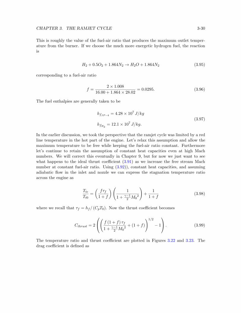
CHAPTER 3. THE RAMJET CYCLE 3-30
This is roughly the value of the fuel-air ratio that produces the maximum outlet temper-ature from the burner. If we choose the much more energetic hydrogen fuel, the reactionis
H2 + 0.5O2 + 1.864N2 → H2O + 1.864N2 (3.95)
corresponding to a fuel-air ratio
f =2× 1.008
16.00 + 1.864× 28.02= 0.0295. (3.96)
The fuel enthalpies are generally taken to be
hfJP−4= 4.28× 10⁷ J/kg
hfH2= 12.1× 10⁷ J/kg.
(3.97)
In the earlier discussion, we took the perspective that the ramjet cycle was limited by a redline temperature in the hot part of the engine. Let’s relax this assumption and allow themaximum temperature to be free while keeping the fuel-air ratio constant. Furthermorelet’s continue to retain the assumption of constant heat capacities even at high Machnumbers. We will correct this eventually in Chapter 9, but for now we just want to seewhat happens to the ideal thrust coefficient (3.91) as we increase the free stream Machnumber at constant fuel-air ratio. Using (3.92)), constant heat capacities, and assumingadiabatic flow in the inlet and nozzle we can express the stagnation temperature ratioacross the engine as
TteTt0
=
(fτf
1 + f
)(1
1 + γ−12 M0
2
)+
1
1 + f(3.98)
where we recall that τf = hf/ (CpT0). Now the thrust coefficient becomes
Cthrust = 2
( f (1 + f) τf
1 + γ−12 M0
2+ (1 + f)
)1/2
− 1
. (3.99)
The temperature ratio and thrust coefficient are plotted in Figures 3.22 and 3.23. Thedrag coefficient is defined as
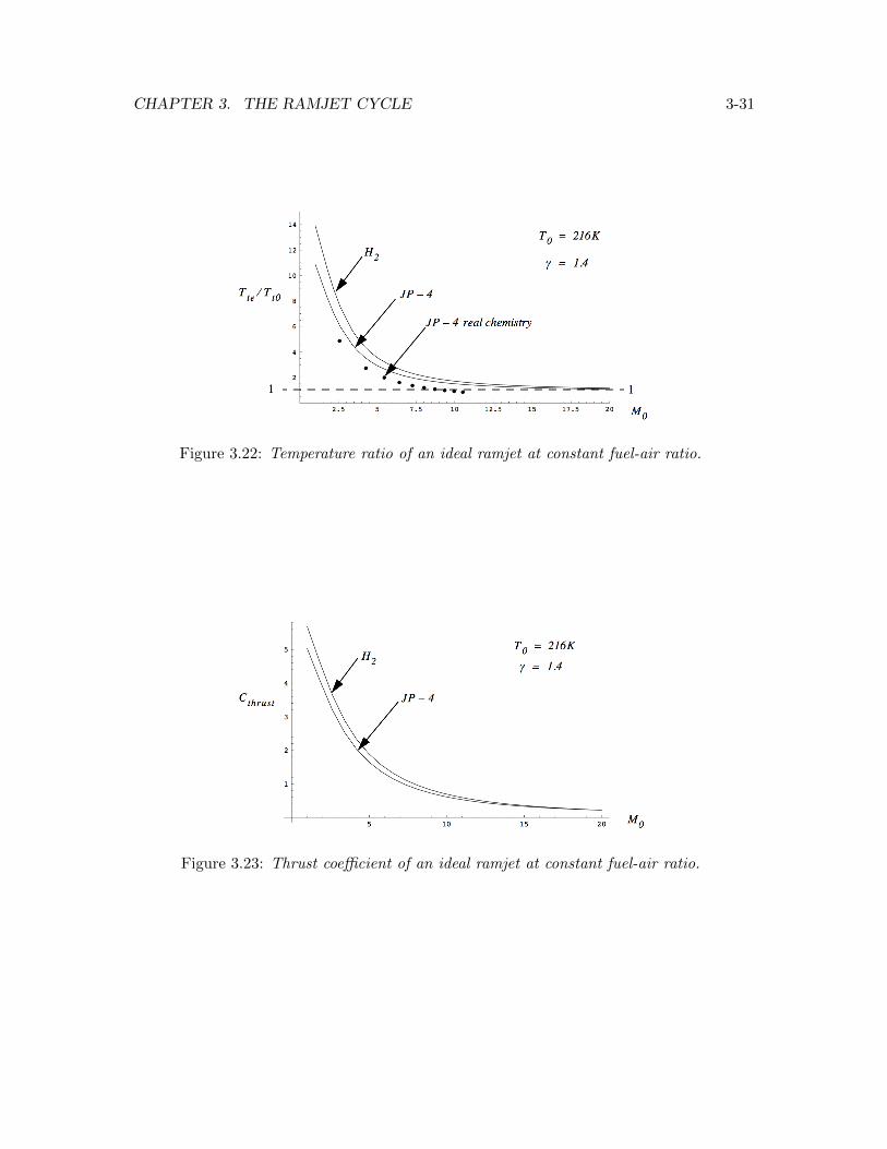
CHAPTER 3. THE RAMJET CYCLE 3-31
Figure 3.22: Temperature ratio of an ideal ramjet at constant fuel-air ratio.
Figure 3.23: Thrust coefficient of an ideal ramjet at constant fuel-air ratio.
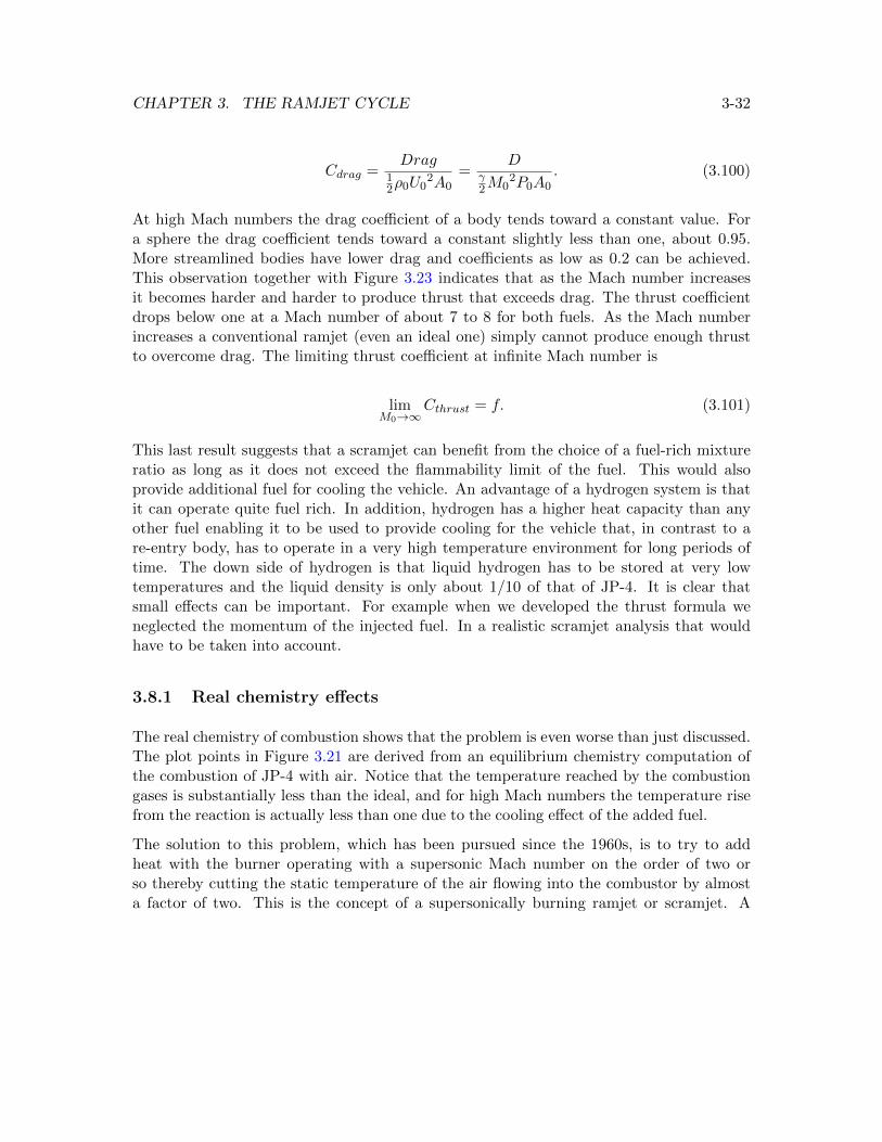
CHAPTER 3. THE RAMJET CYCLE 3-32
Cdrag =Drag
12ρ0U0
2A0=
Dγ2M0
2P0A0. (3.100)
At high Mach numbers the drag coefficient of a body tends toward a constant value. Fora sphere the drag coefficient tends toward a constant slightly less than one, about 0.95.More streamlined bodies have lower drag and coefficients as low as 0.2 can be achieved.This observation together with Figure 3.23 indicates that as the Mach number increasesit becomes harder and harder to produce thrust that exceeds drag. The thrust coefficientdrops below one at a Mach number of about 7 to 8 for both fuels. As the Mach numberincreases a conventional ramjet (even an ideal one) simply cannot produce enough thrustto overcome drag. The limiting thrust coefficient at infinite Mach number is
limM0→∞
Cthrust = f. (3.101)
This last result suggests that a scramjet can benefit from the choice of a fuel-rich mixtureratio as long as it does not exceed the flammability limit of the fuel. This would alsoprovide additional fuel for cooling the vehicle. An advantage of a hydrogen system is thatit can operate quite fuel rich. In addition, hydrogen has a higher heat capacity than anyother fuel enabling it to be used to provide cooling for the vehicle that, in contrast to are-entry body, has to operate in a very high temperature environment for long periods oftime. The down side of hydrogen is that liquid hydrogen has to be stored at very lowtemperatures and the liquid density is only about 1/10 of that of JP-4. It is clear thatsmall effects can be important. For example when we developed the thrust formula weneglected the momentum of the injected fuel. In a realistic scramjet analysis that wouldhave to be taken into account.
3.8.1 Real chemistry effects
The real chemistry of combustion shows that the problem is even worse than just discussed.The plot points in Figure 3.21 are derived from an equilibrium chemistry computation ofthe combustion of JP-4 with air. Notice that the temperature reached by the combustiongases is substantially less than the ideal, and for high Mach numbers the temperature risefrom the reaction is actually less than one due to the cooling effect of the added fuel.
The solution to this problem, which has been pursued since the 1960s, is to try to addheat with the burner operating with a supersonic Mach number on the order of two orso thereby cutting the static temperature of the air flowing into the combustor by almosta factor of two. This is the concept of a supersonically burning ramjet or scramjet. A
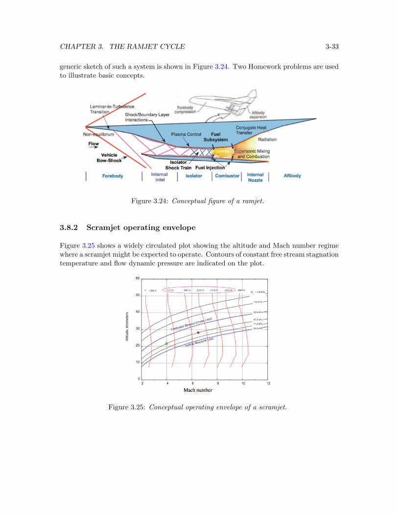
CHAPTER 3. THE RAMJET CYCLE 3-33
generic sketch of such a system is shown in Figure 3.24. Two Homework problems are usedto illustrate basic concepts.
Figure 3.24: Conceptual figure of a ramjet.
3.8.2 Scramjet operating envelope
Figure 3.25 shows a widely circulated plot showing the altitude and Mach number regimewhere a scramjet might be expected to operate. Contours of constant free stream stagnationtemperature and flow dynamic pressure are indicated on the plot.
Figure 3.25: Conceptual operating envelope of a scramjet.
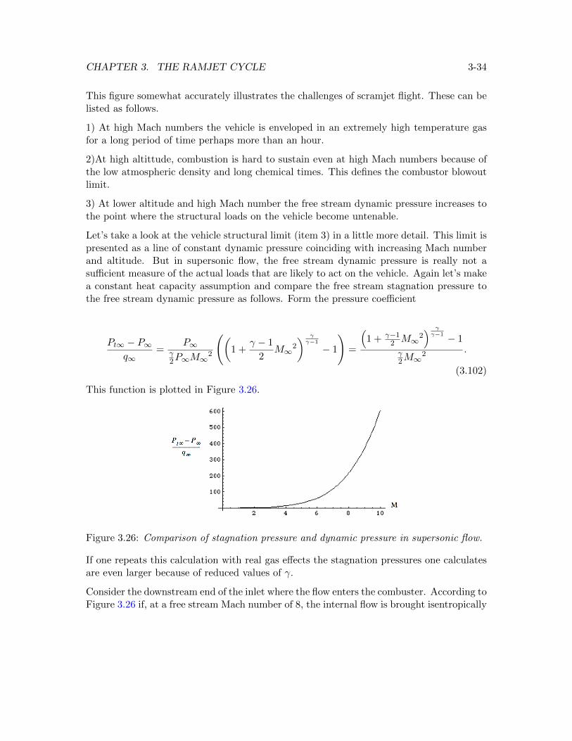
CHAPTER 3. THE RAMJET CYCLE 3-34
This figure somewhat accurately illustrates the challenges of scramjet flight. These can belisted as follows.
1) At high Mach numbers the vehicle is enveloped in an extremely high temperature gasfor a long period of time perhaps more than an hour.
2)At high altittude, combustion is hard to sustain even at high Mach numbers because ofthe low atmospheric density and long chemical times. This defines the combustor blowoutlimit.
3) At lower altitude and high Mach number the free stream dynamic pressure increases tothe point where the structural loads on the vehicle become untenable.
Let’s take a look at the vehicle structural limit (item 3) in a little more detail. This limit ispresented as a line of constant dynamic pressure coinciding with increasing Mach numberand altitude. But in supersonic flow, the free stream dynamic pressure is really not asufficient measure of the actual loads that are likely to act on the vehicle. Again let’s makea constant heat capacity assumption and compare the free stream stagnation pressure tothe free stream dynamic pressure as follows. Form the pressure coefficient
Pt∞ − P∞q∞
=P∞
γ2P∞M∞
2
((1 +
γ − 1
2M∞
2
) γγ−1
− 1
)=
(1 + γ−1
2 M∞2) γγ−1 − 1
γ2M∞
2 .
(3.102)
This function is plotted in Figure 3.26.
Figure 3.26: Comparison of stagnation pressure and dynamic pressure in supersonic flow.
If one repeats this calculation with real gas effects the stagnation pressures one calculatesare even larger because of reduced values of γ.
Consider the downstream end of the inlet where the flow enters the combuster. According toFigure 3.26 if, at a free stream Mach number of 8, the internal flow is brought isentropically
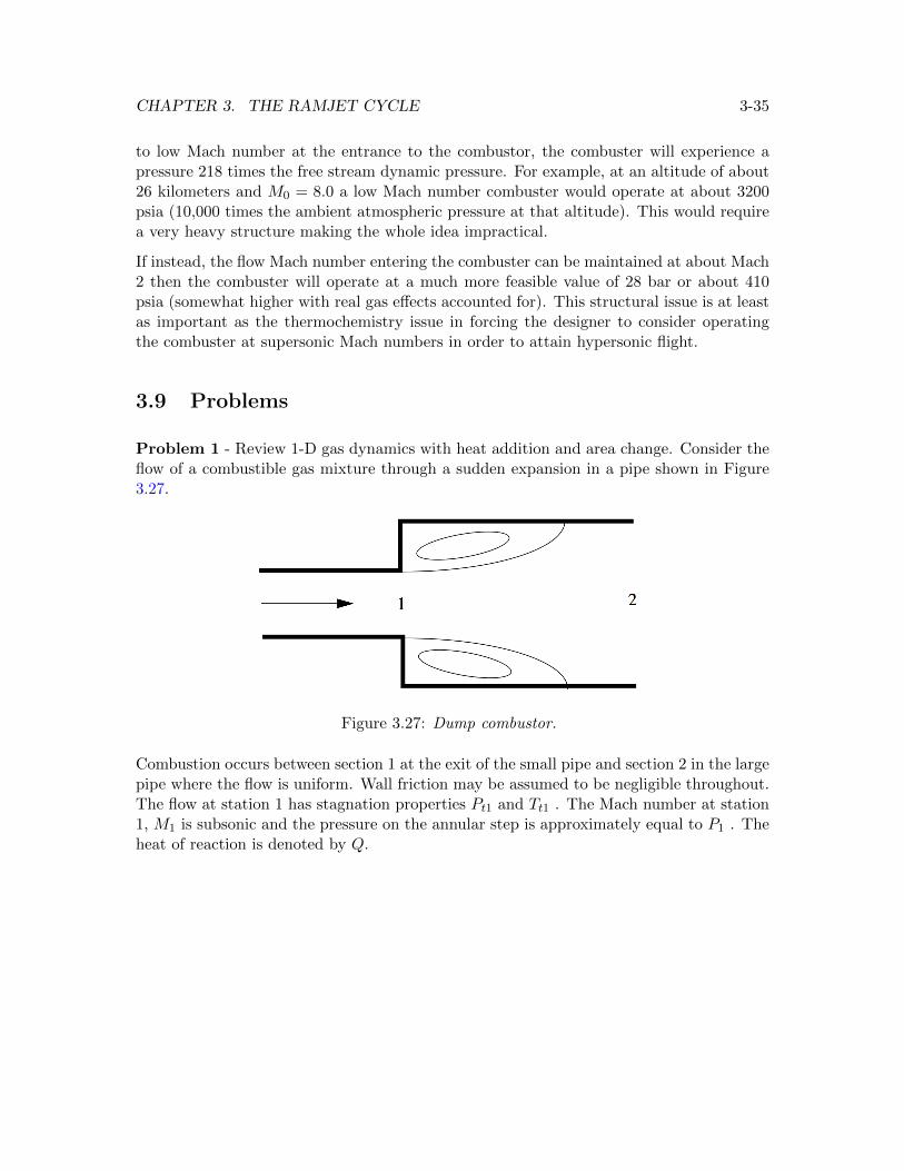
CHAPTER 3. THE RAMJET CYCLE 3-35
to low Mach number at the entrance to the combustor, the combuster will experience apressure 218 times the free stream dynamic pressure. For example, at an altitude of about26 kilometers and M0 = 8.0 a low Mach number combuster would operate at about 3200psia (10,000 times the ambient atmospheric pressure at that altitude). This would requirea very heavy structure making the whole idea impractical.
If instead, the flow Mach number entering the combuster can be maintained at about Mach2 then the combuster will operate at a much more feasible value of 28 bar or about 410psia (somewhat higher with real gas effects accounted for). This structural issue is at leastas important as the thermochemistry issue in forcing the designer to consider operatingthe combuster at supersonic Mach numbers in order to attain hypersonic flight.
3.9 Problems
Problem 1 - Review 1-D gas dynamics with heat addition and area change. Consider theflow of a combustible gas mixture through a sudden expansion in a pipe shown in Figure3.27.
Figure 3.27: Dump combustor.
Combustion occurs between section 1 at the exit of the small pipe and section 2 in the largepipe where the flow is uniform. Wall friction may be assumed to be negligible throughout.The flow at station 1 has stagnation properties Pt1 and Tt1 . The Mach number at station1, M1 is subsonic and the pressure on the annular step is approximately equal to P1 . Theheat of reaction is denoted by Q.
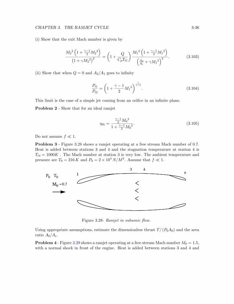
CHAPTER 3. THE RAMJET CYCLE 3-36
(i) Show that the exit Mach number is given by
M22(
1 + γ−12 M2
2)
(1 + γM2
2)2 =
(1 +
Q
CpTt1
)M12(
1 + γ−12 M1
2)
(A2A1
+ γM12)2 . (3.103)
(ii) Show that when Q = 0 and A2/A1 goes to infinity
Pt1Pt2
=
(1 +
γ − 1
2M1
2
) γγ−1
. (3.104)
This limit is the case of a simple jet coming from an orifice in an infinite plane.
Problem 2 - Show that for an ideal ramjet
ηth =γ−1
2 M02
1 + γ−12 M0
2. (3.105)
Do not assume f � 1.
Problem 3 - Figure 3.28 shows a ramjet operating at a free stream Mach number of 0.7.Heat is added between stations 3 and 4 and the stagnation temperature at station 4 isTt4 = 1000K . The Mach number at station 3 is very low. The ambient temperature andpressure are T0 = 216K and P0 = 2× 10⁴N/M2. Assume that f � 1.
Figure 3.28: Ramjet in subsonic flow.
Using appropriate assumptions, estimate the dimensionless thrust T/ (P0A0) and the arearatio A0/Ae.
Problem 4 - Figure 3.29 shows a ramjet operating at a free stream Mach number M0 = 1.5,with a normal shock in front of the engine. Heat is added between stations 3 and 4 and
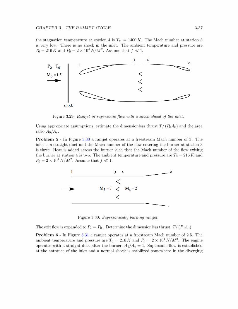
CHAPTER 3. THE RAMJET CYCLE 3-37
the stagnation temperature at station 4 is Tt4 = 1400K. The Mach number at station 3is very low. There is no shock in the inlet. The ambient temperature and pressure areT0 = 216K and P0 = 2× 10⁴N/M2. Assume that f � 1.
Figure 3.29: Ramjet in supersonic flow with a shock ahead of the inlet.
Using appropriate assumptions, estimate the dimensionless thrust T/ (P0A0) and the arearatio A0/Ae.
Problem 5 - In Figure 3.30 a ramjet operates at a freestream Mach number of 3. Theinlet is a straight duct and the Mach number of the flow entering the burner at station 3is three. Heat is added across the burner such that the Mach number of the flow exitingthe burner at station 4 is two. The ambient temperature and pressure are T0 = 216K andP0 = 2× 10⁴N/M2. Assume that f � 1.
Figure 3.30: Supersonically burning ramjet.
The exit flow is expanded to Pe = P0 . Determine the dimensionless thrust, T/ (P0A0).
Problem 6 - In Figure 3.31 a ramjet operates at a freestream Mach number of 2.5. Theambient temperature and pressure are T0 = 216K and P0 = 2 × 10⁴N/M2. The engineoperates with a straight duct after the burner, A1/Ae = 1. Supersonic flow is establishedat the entrance of the inlet and a normal shock is stabilized somewhere in the diverging
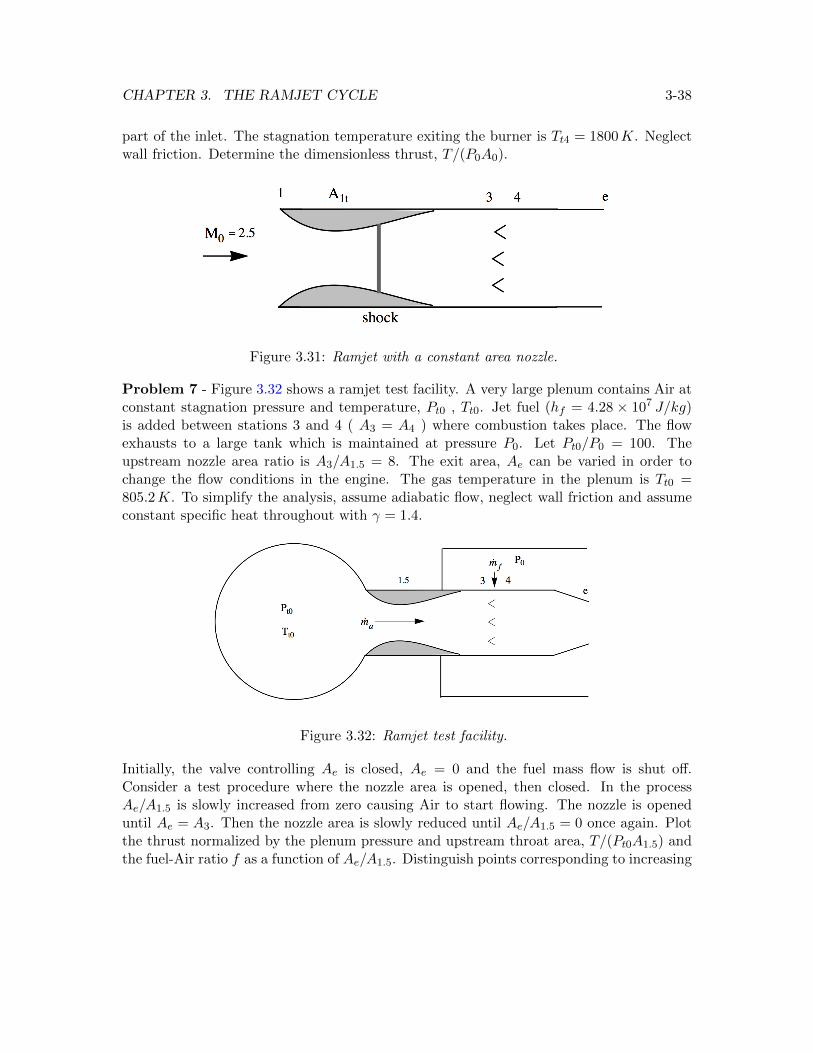
CHAPTER 3. THE RAMJET CYCLE 3-38
part of the inlet. The stagnation temperature exiting the burner is Tt4 = 1800K. Neglectwall friction. Determine the dimensionless thrust, T/(P0A0).
Figure 3.31: Ramjet with a constant area nozzle.
Problem 7 - Figure 3.32 shows a ramjet test facility. A very large plenum contains Air atconstant stagnation pressure and temperature, Pt0 , Tt0. Jet fuel (hf = 4.28 × 10⁷ J/kg)is added between stations 3 and 4 ( A3 = A4 ) where combustion takes place. The flowexhausts to a large tank which is maintained at pressure P0. Let Pt0/P0 = 100. Theupstream nozzle area ratio is A3/A1.5 = 8. The exit area, Ae can be varied in order tochange the flow conditions in the engine. The gas temperature in the plenum is Tt0 =805.2K. To simplify the analysis, assume adiabatic flow, neglect wall friction and assumeconstant specific heat throughout with γ = 1.4.
Figure 3.32: Ramjet test facility.
Initially, the valve controlling Ae is closed, Ae = 0 and the fuel mass flow is shut off.Consider a test procedure where the nozzle area is opened, then closed. In the processAe/A1.5 is slowly increased from zero causing Air to start flowing. The nozzle is openeduntil Ae = A3. Then the nozzle area is slowly reduced until Ae/A1.5 = 0 once again. Plotthe thrust normalized by the plenum pressure and upstream throat area, T/(Pt0A1.5) andthe fuel-Air ratio f as a function of Ae/A1.5. Distinguish points corresponding to increasing
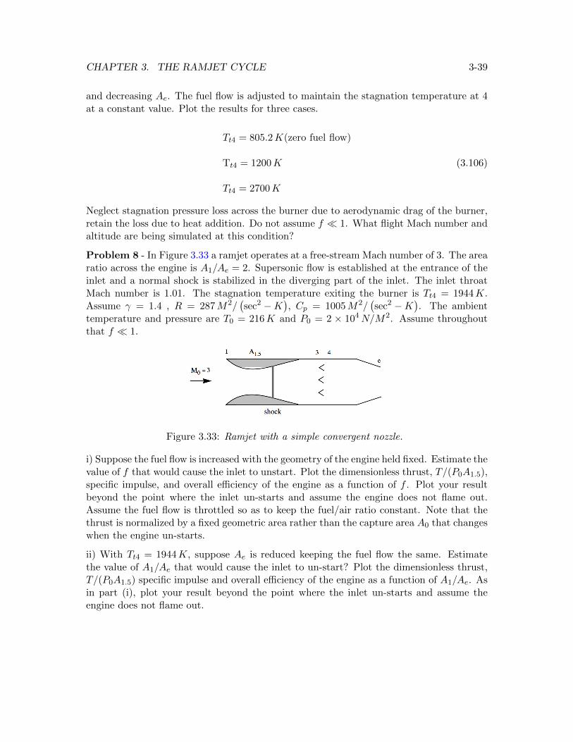
CHAPTER 3. THE RAMJET CYCLE 3-39
and decreasing Ae. The fuel flow is adjusted to maintain the stagnation temperature at 4at a constant value. Plot the results for three cases.
Tt4 = 805.2K(zero fuel flow)
Tt4 = 1200K
Tt4 = 2700K
(3.106)
Neglect stagnation pressure loss across the burner due to aerodynamic drag of the burner,retain the loss due to heat addition. Do not assume f � 1. What flight Mach number andaltitude are being simulated at this condition?
Problem 8 - In Figure 3.33 a ramjet operates at a free-stream Mach number of 3. The arearatio across the engine is A1/Ae = 2. Supersonic flow is established at the entrance of theinlet and a normal shock is stabilized in the diverging part of the inlet. The inlet throatMach number is 1.01. The stagnation temperature exiting the burner is Tt4 = 1944K.Assume γ = 1.4 , R = 287M2/
(sec2 −K
), Cp = 1005M2/
(sec2 −K
). The ambient
temperature and pressure are T0 = 216K and P0 = 2 × 10⁴N/M2. Assume throughoutthat f � 1.
Figure 3.33: Ramjet with a simple convergent nozzle.
i) Suppose the fuel flow is increased with the geometry of the engine held fixed. Estimate thevalue of f that would cause the inlet to unstart. Plot the dimensionless thrust, T/(P0A1.5),specific impulse, and overall efficiency of the engine as a function of f . Plot your resultbeyond the point where the inlet un-starts and assume the engine does not flame out.Assume the fuel flow is throttled so as to keep the fuel/air ratio constant. Note that thethrust is normalized by a fixed geometric area rather than the capture area A0 that changeswhen the engine un-starts.
ii) With Tt4 = 1944K, suppose Ae is reduced keeping the fuel flow the same. Estimatethe value of A1/Ae that would cause the inlet to un-start? Plot the dimensionless thrust,T/(P0A1.5) specific impulse and overall efficiency of the engine as a function of A1/Ae. Asin part (i), plot your result beyond the point where the inlet un-starts and assume theengine does not flame out.
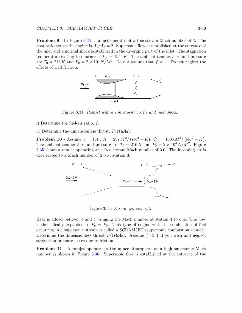
CHAPTER 3. THE RAMJET CYCLE 3-40
Problem 9 - In Figure 3.34 a ramjet operates at a free-stream Mach number of 3. Thearea ratio across the engine is A1/Ae = 2. Supersonic flow is established at the entrance ofthe inlet and a normal shock is stabilized in the diverging part of the inlet. The stagnationtemperature exiting the burner is Tt4 = 1944K. The ambient temperature and pressureare T0 = 216K and P0 = 2 × 10⁴N/M2. Do not assume that f � 1. Do not neglect theeffects of wall friction.
Figure 3.34: Ramjet with a convergent nozzle and inlet shock.
i) Determine the fuel-air ratio, f .
ii) Determine the dimensionless thrust, T/(P0A0).
Problem 10 - Assume γ = 1.4 , R = 287M2/(sec2 −K
), Cp = 1005M2/
(sec2 −K
).
The ambient temperature and pressure are T0 = 216K and P0 = 2 × 10⁴N/M2. Figure3.35 shows a ramjet operating at a free stream Mach number of 3.0. The incoming air isdecelerated to a Mach number of 2.0 at station 3.
Figure 3.35: A scramjet concept.
Heat is added between 3 and 4 bringing the Mach number at station 4 to one. The flowis then ideally expanded to Pe = P0. This type of engine with the combustion of fueloccurring in a supersonic stream is called a SCRAMJET (supersonic combustion ramjet).Determine the dimensionless thrust T/(P0A0). Assume f � 1 if you wish and neglectstagnation pressure losses due to friction.
Problem 11 - A ramjet operates in the upper atmosphere at a high supersonic Machnumber as shown in Figure 3.36. Supersonic flow is established at the entrance of the
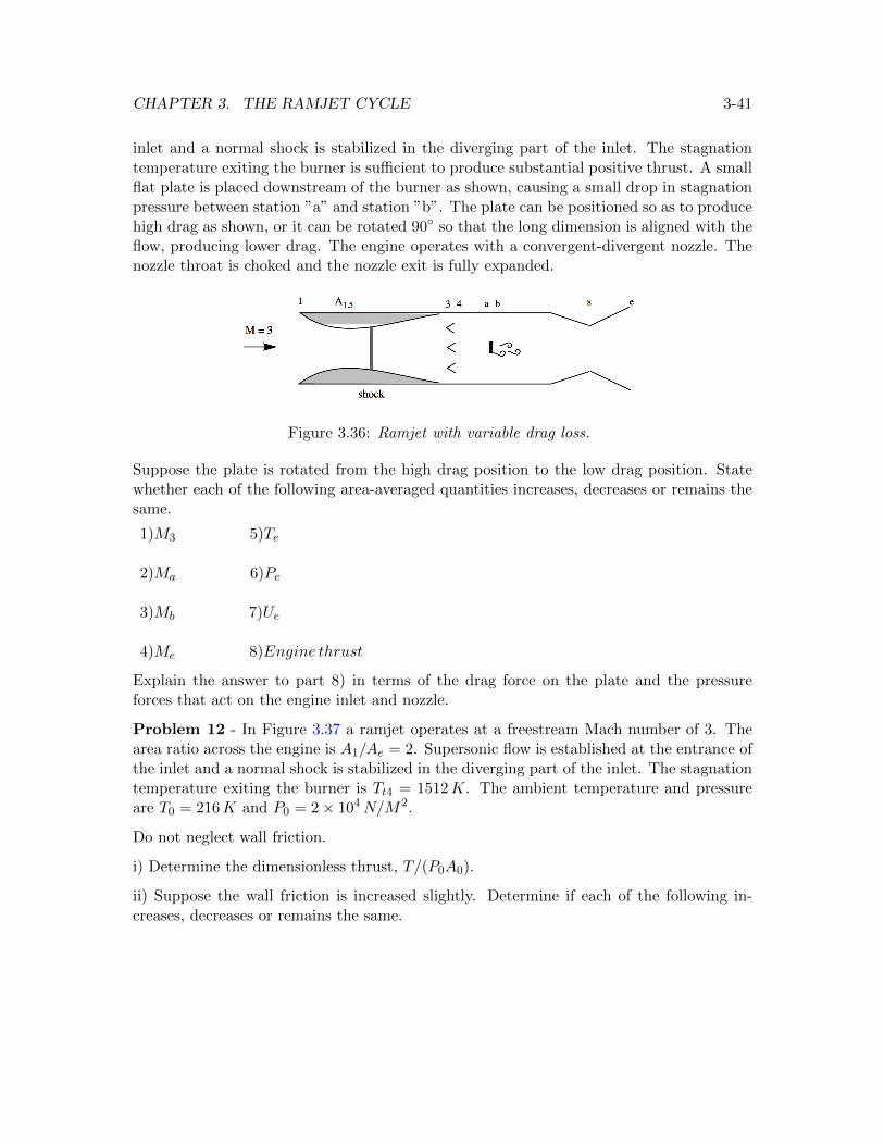
CHAPTER 3. THE RAMJET CYCLE 3-41
inlet and a normal shock is stabilized in the diverging part of the inlet. The stagnationtemperature exiting the burner is sufficient to produce substantial positive thrust. A smallflat plate is placed downstream of the burner as shown, causing a small drop in stagnationpressure between station ”a” and station ”b”. The plate can be positioned so as to producehigh drag as shown, or it can be rotated 90◦ so that the long dimension is aligned with theflow, producing lower drag. The engine operates with a convergent-divergent nozzle. Thenozzle throat is choked and the nozzle exit is fully expanded.
Figure 3.36: Ramjet with variable drag loss.
Suppose the plate is rotated from the high drag position to the low drag position. Statewhether each of the following area-averaged quantities increases, decreases or remains thesame.
1)M3 5)Te
2)Ma 6)Pe
3)Mb 7)Ue
4)Me 8)Engine thrust
Explain the answer to part 8) in terms of the drag force on the plate and the pressureforces that act on the engine inlet and nozzle.
Problem 12 - In Figure 3.37 a ramjet operates at a freestream Mach number of 3. Thearea ratio across the engine is A1/Ae = 2. Supersonic flow is established at the entrance ofthe inlet and a normal shock is stabilized in the diverging part of the inlet. The stagnationtemperature exiting the burner is Tt4 = 1512K. The ambient temperature and pressureare T0 = 216K and P0 = 2× 10⁴N/M2.
Do not neglect wall friction.
i) Determine the dimensionless thrust, T/(P0A0).
ii) Suppose the wall friction is increased slightly. Determine if each of the following in-creases, decreases or remains the same.
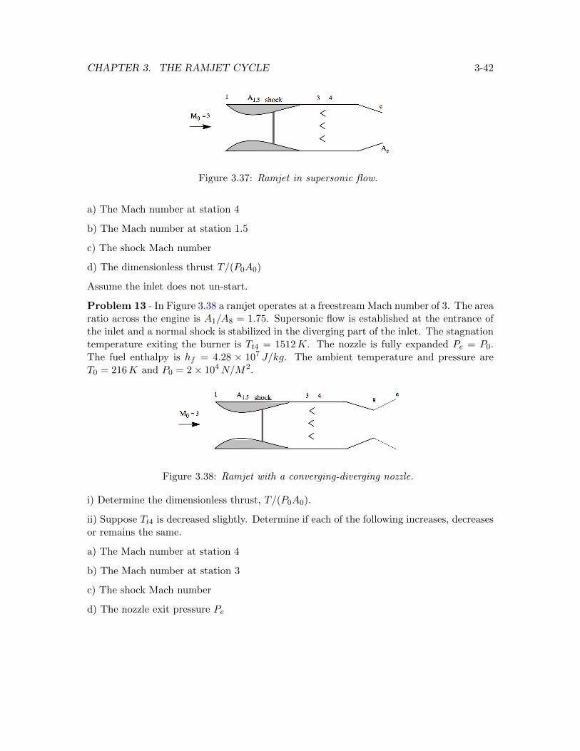
CHAPTER 3. THE RAMJET CYCLE 3-42
Figure 3.37: Ramjet in supersonic flow.
a) The Mach number at station 4
b) The Mach number at station 1.5
c) The shock Mach number
d) The dimensionless thrust T/(P0A0)
Assume the inlet does not un-start.
Problem 13 - In Figure 3.38 a ramjet operates at a freestream Mach number of 3. The arearatio across the engine is A1/A8 = 1.75. Supersonic flow is established at the entrance ofthe inlet and a normal shock is stabilized in the diverging part of the inlet. The stagnationtemperature exiting the burner is Tt4 = 1512K. The nozzle is fully expanded Pe = P0.The fuel enthalpy is hf = 4.28 × 10⁷ J/kg. The ambient temperature and pressure areT0 = 216K and P0 = 2× 10⁴N/M2.
Figure 3.38: Ramjet with a converging-diverging nozzle.
i) Determine the dimensionless thrust, T/(P0A0).
ii) Suppose Tt4 is decreased slightly. Determine if each of the following increases, decreasesor remains the same.
a) The Mach number at station 4
b) The Mach number at station 3
c) The shock Mach number
d) The nozzle exit pressure Pe
Chapter 4
The Turbojet cycle
4.1 Thermal efficiency of the ideal turbojet
Recalling our discussion in Chapter 2, the thermal efficiency of a jet engine propulsionsystem is defined as
ηth =power to the vehicle + ∆kinetic energy of air
second + ∆kinetic energy of fuelsecond
mfhf(4.1)
or
ηth =TU0+
[ma(Ue−U0)2
2 − ma(0)2
2
]+[mf (Ue−U0)2
2 − mf (U0)2
2
]mfhf
. (4.2)
If the exhaust is fully expanded so that Pe = P0 the thermal efficiency reduces to
ηth =
(ma+mf)Ue2
2 − maU02
2
mfhf. (4.3)
4-1
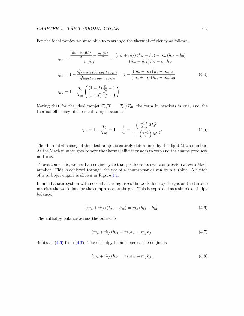
CHAPTER 4. THE TURBOJET CYCLE 4-2
For the ideal ramjet we were able to rearrange the thermal efficiency as follows.
ηth =
(ma+mf)Ue2
2 − maU02
2
mfhf=
(ma + mf ) (hte − he)− ma (ht0 − h0)
(ma + mf )hte − maht0
ηth = 1−Qrejected during the cycleQinput during the cycle
= 1−(ma + mf )he − mah0
(ma + mf )hte − maht0
ηth = 1− T0
Tt0
((1 + f) TeT0
− 1
(1 + f) TteTt0 − 1
)(4.4)
Noting that for the ideal ramjet Te/T0 = Tte/Tt0, the term in brackets is one, and thethermal efficiency of the ideal ramjet becomes
ηth = 1− T0
Tt0= 1− 1
τr=
(γ−1
2
)M0
2
1 +(γ−1
2
)M0
2. (4.5)
The thermal efficiency of the ideal ramjet is entirely determined by the flight Mach number.As the Mach number goes to zero the thermal efficiency goes to zero and the engine producesno thrust.
To overcome this, we need an engine cycle that produces its own compression at zero Machnumber. This is achieved through the use of a compressor driven by a turbine. A sketchof a turbojet engine is shown in Figure 4.1.
In an adiabatic system with no shaft bearing losses the work done by the gas on the turbinematches the work done by the compressor on the gas. This is expressed as a simple enthalpybalance.
(ma + mf ) (ht4 − ht5) = ma (ht3 − ht2) (4.6)
The enthalpy balance across the burner is
(ma + mf )ht4 = maht3 + mfhf . (4.7)
Subtract (4.6) from (4.7). The enthalpy balance across the engine is
(ma + mf )ht5 = maht2 + mfhf . (4.8)
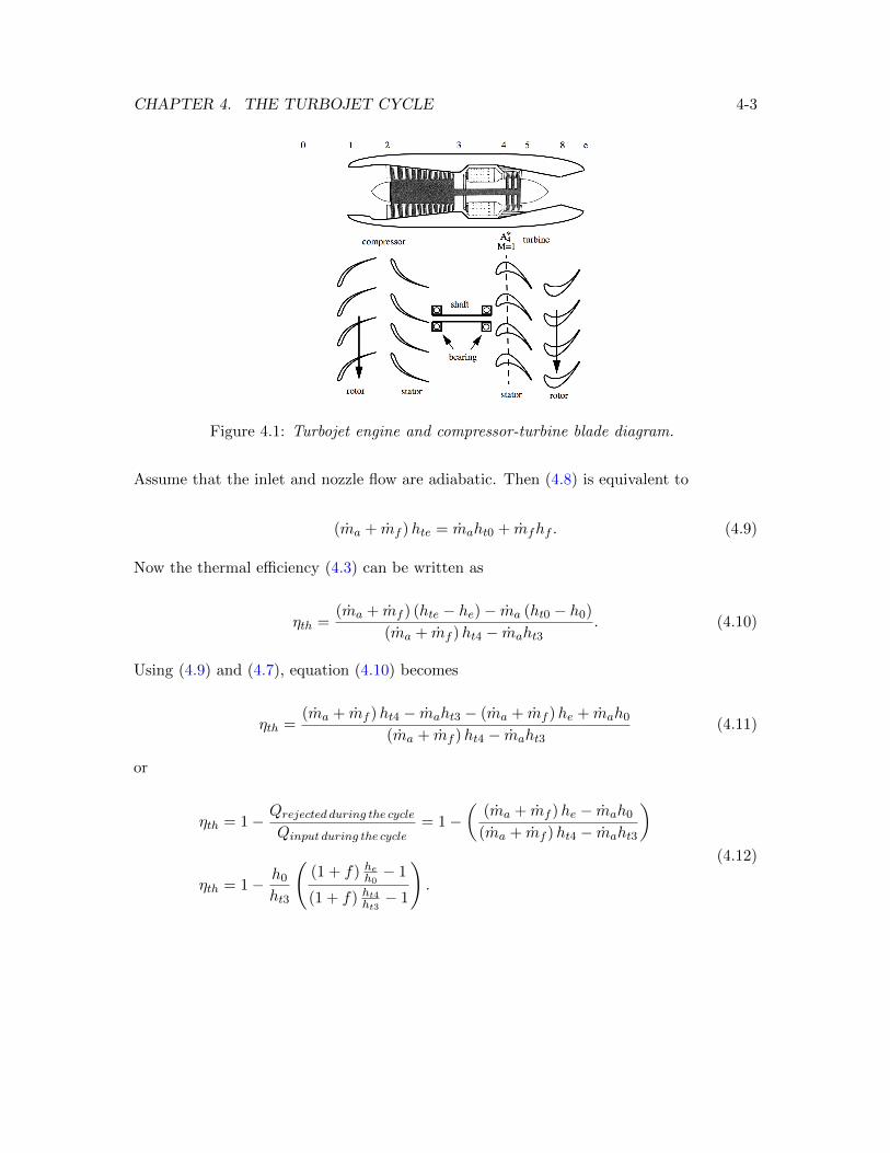
CHAPTER 4. THE TURBOJET CYCLE 4-3
Figure 4.1: Turbojet engine and compressor-turbine blade diagram.
Assume that the inlet and nozzle flow are adiabatic. Then (4.8) is equivalent to
(ma + mf )hte = maht0 + mfhf . (4.9)
Now the thermal efficiency (4.3) can be written as
ηth =(ma + mf ) (hte − he)− ma (ht0 − h0)
(ma + mf )ht4 − maht3. (4.10)
Using (4.9) and (4.7), equation (4.10) becomes
ηth =(ma + mf )ht4 − maht3 − (ma + mf )he + mah0
(ma + mf )ht4 − maht3(4.11)
or
ηth = 1−Qrejected during the cycleQinput during the cycle
= 1−(
(ma + mf )he − mah0
(ma + mf )ht4 − maht3
)
ηth = 1− h0
ht3
((1 + f) heh0
− 1
(1 + f) ht4ht3− 1
).
(4.12)
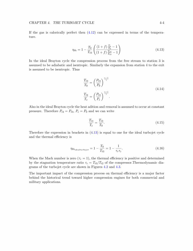
CHAPTER 4. THE TURBOJET CYCLE 4-4
If the gas is calorically perfect then (4.12) can be expressed in terms of the tempera-ture.
ηth = 1− T0
Tt3
((1 + f) TeT0
− 1
(1 + f) Tt4Tt3− 1
)(4.13)
In the ideal Brayton cycle the compression process from the free stream to station 3 isassumed to be adiabatic and isentropic. Similarly the expansion from station 4 to the exitis assumed to be isentropic. Thus
Tt3T0
=
(Pt3P0
) γ−1γ
Tt4Te
=
(Pt4Pe
) γ−1γ
.
(4.14)
Also in the ideal Brayton cycle the heat adition and removal is assumed to occur at constantpressure. Therefore Pt4 = Pt3, Pe = P0 and we can write
Tt4Te
=Tt3T0. (4.15)
Therefore the expression in brackets in (4.13) is equal to one for the ideal turbojet cycleand the thermal efficiency is
ηthidealturbojet = 1− T0
Tt3= 1− 1
τrτc. (4.16)
When the Mach number is zero (τr = 1), the thermal efficiency is positive and determinedby the stagnation temperature ratio τc = Tt3/Tt2 of the compressor.Thermodynamic dia-grams of the turbojet cycle are shown in Figures 4.2 and 4.3.
The important impact of the compression process on thermal efficiency is a major factorbehind the historical trend toward higher compression engines for both commercial andmilitary applications.
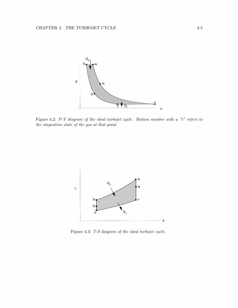
CHAPTER 4. THE TURBOJET CYCLE 4-5
Figure 4.2: P-V diagram of the ideal turbojet cycle. Station number with a ”t” refers tothe stagnation state of the gas at that point.
Figure 4.3: T-S diagram of the ideal turbojet cycle.
CHAPTER 4. THE TURBOJET CYCLE 4-6
4.2 Thrust of an ideal turbojet engine
The thrust equation for a fully expanded nozzle is
T
P0A0= γM0
2
((1 + f)
UeU0− 1
). (4.17)
To determine the thrust we need to work out the velocity ratio.
UeU0
=Me
M0
√TeT0
(4.18)
To determine the Mach numbers we focus on the variation of stagnation pressure throughthe engine. Begin with the following identity.
Pte = P0
(Pt0P0
)(Pt2Pt0
)(Pt3Pt2
)(Pt4Pt3
)(Pt5Pt4
)(PtePt5
)(4.19)
Using our engine parameters this would be written as
Pte = P0πrπdπcπbπtπn. (4.20)
Under the assumptions of the ideal cycle the stagnation pressure losses in the diffuser andnozzle are negligible. In other words, skin friction and shock losses are negligible.
πd = 1
πn = 1(4.21)
Similarly, the Mach number through the burner is assumed to be so low that the stagna-tion pressure losses due to heat addition and aerodynamic drag are assumed to be negligi-ble.
πb = 1 (4.22)
Therefore
Pte = P0πrπcπt = Pe
(1 +
γ − 1
2Me
2
) γγ−1
. (4.23)
CHAPTER 4. THE TURBOJET CYCLE 4-7
Another assumption of the ideal cycle is that the nozzle is fully expanded.
πrπcπt =
(1 +
γ − 1
2Me
2
) γγ−1
(4.24)
The final assumption of the ideal turbojet is that the compressor and turbine behaveisentropically.
πc = τcγγ−1
πt = τtγγ−1
(4.25)
Using (4.25) in (4.24) and the relation πr = τrγ/(γ−1), the exit Mach number can be
determined from
Me2 =
2
γ − 1(τrτcτt − 1) (4.26)
and the Mach number ratio is
Me2
M02 =
(τrτcτt − 1
τr − 1
). (4.27)
We take a similar approach to determining the temperature ratio across the engine. Beginwith the identity
Tte = T0
(Tt0T0
)(Tt2Tt0
)(Tt3Tt2
)(Tt4Tt3
)(Tt5Tt4
)(TteTt5
)(4.28)
or, in terms of component temperature parameters
Tte = T0τrτdτcτbτtτn. (4.29)
In the ideal turbojet we assume that the diffuser and nozzle flows are adiabatic and so
Tte = T0τrτcτbτt = Te
(1 +
γ − 1
2Me
2
)= Teτrτcτt. (4.30)
CHAPTER 4. THE TURBOJET CYCLE 4-8
From (4.30) we have the result
TeT0
= τb =Tt4Tt3
. (4.31)
This is the same result we deduced earlier in (4.15) when we analyzed the thermal efficiency.Actually it is more convenient to express the temperature ratio in terms of the all-importantparameter τλ = Tt4/T0.
TeT0
=τλτrτc
(4.32)
The reason is that τλ is a parameter that we would like to make as large as possible,but is limited by the highest temperature that can be tolerated by the turbine materialsbefore they begin to lose strength and undergo creep. The maximum allowable turbine inlettemperature (and therefore the maximum design operating temperature) is one of the cyclevariables that is essentially fixed when an engine manufacturer begins the development of anew engine. Enormous sums of money have been invested in turbine materials technologyand turbine cooling schemes in an effort to enable jet engines to operate with as high aturbine inlet temperature as possible.
Our thrust formula is now
T
P0A0=
2γ
γ − 1(τr − 1)
((1 + f)
((τrτcτt − 1
τr − 1
)τλτrτc
)1/2
− 1
). (4.33)
The fuel/air ratio is found from
f =τλ − τrτcτf − τλ
. (4.34)
At this point it would appear that for fixed γ, and τf the thrust is a function of fourvariables.
T
P0A0= F (τr, τc, τλ, τt) (4.35)
But the turbine and compressor are not independent components. They are connected bya shaft and the work done across the compressor is the same as the work done across the
CHAPTER 4. THE TURBOJET CYCLE 4-9
turbine. They are related by the work matching condition (4.6) repeated here in terms ofthe temperatures.
(ma + mf )CP (Tt4 − Tt5) = maCP (Tt3 − Tt2) (4.36)
For simplicity we have assumed the same value of Cp for the compressor and turbine. Ifwe divide (4.36) by CpT0 then it becomes
(1 + f) τλ (1− τt) = τr (τc − 1) (4.37)
or
τt = 1− τr (τc − 1)
(1 + f) τλ(4.38)
where we have assumed Tt2 = Tt0. The result (4.38) only assumes adiabatic flow in theinlet and no shaft losses. It is not tied to the other assumptions of the ideal cycle. Thevelocity ratio across the engine is now
(UeU0
)2
=1
(τr − 1)
(τλ − τr (τc − 1)− τλ
τrτc
)(4.39)
where the fuel/air ratio has been neglected.
4.3 Maximum thrust ideal turbojet
How much compression should we use? If there is too little the engine is like a ramjet andmay not produce enough thrust at low Mach number. If we use too much then the fuel flowhas to be reduced to avoid raising the temperature above the ”do not exceed” (redline)value of Tt4. The thrust and specific impulse of a typical ideal turbojet is shown in Figure4.4. Recall that
Ispg
a0=
(1
f
)(1
γM0
)(T
P0A0
). (4.40)
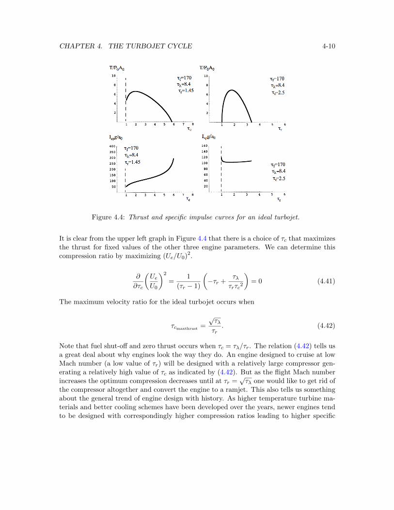
CHAPTER 4. THE TURBOJET CYCLE 4-10
Figure 4.4: Thrust and specific impulse curves for an ideal turbojet.
It is clear from the upper left graph in Figure 4.4 that there is a choice of τc that maximizesthe thrust for fixed values of the other three engine parameters. We can determine thiscompression ratio by maximizing (Ue/U0)2.
∂
∂τc
(UeU0
)2
=1
(τr − 1)
(−τr +
τλτrτc2
)= 0 (4.41)
The maximum velocity ratio for the ideal turbojet occurs when
τcmaxthrust=
√τλτr
. (4.42)
Note that fuel shut-off and zero thrust occurs when τc = τλ/τr. The relation (4.42) tells usa great deal about why engines look the way they do. An engine designed to cruise at lowMach number (a low value of τr) will be designed with a relatively large compressor gen-erating a relatively high value of τc as indicated by (4.42). But as the flight Mach numberincreases the optimum compression decreases until at τr =
√τλ one would like to get rid of
the compressor altogether and convert the engine to a ramjet. This also tells us somethingabout the general trend of engine design with history. As higher temperature turbine ma-terials and better cooling schemes have been developed over the years, newer engines tendto be designed with correspondingly higher compression ratios leading to higher specific
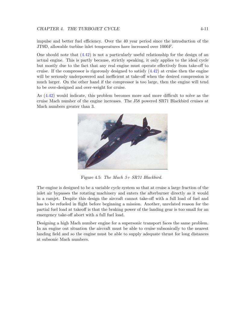
CHAPTER 4. THE TURBOJET CYCLE 4-11
impulse and better fuel efficiency. Over the 40 year period since the introduction of theJT9D, allowable turbine inlet temperatures have increased over 1000F .
One should note that (4.42) is not a particularly useful relationship for the design of anactual engine. This is partly because, strictly speaking, it only applies to the ideal cyclebut mostly due to the fact that any real engine must operate effectively from take-off tocruise. If the compressor is rigorously designed to satisfy (4.42) at cruise then the enginewill be seriously underpowered and inefficient at take-off when the desired compression ismuch larger. On the other hand if the compressor is too large, then the engine will tendto be over-designed and over-weight for cruise.
As (4.42) would indicate, this problem becomes more and more difficult to solve as thecruise Mach number of the engine increases. The J58 powered SR71 Blackbird cruises atMach numbers greater than 3.
Figure 4.5: The Mach 3+ SR71 Blackbird.
The engine is designed to be a variable cycle system so that at cruise a large fraction of theinlet air bypasses the rotating machinery and enters the afterburner directly as it wouldin a ramjet. Despite this design the aircraft cannot take-off with a full load of fuel andhas to be refueled in flight before beginning a mission. Another, unrelated reason for thepartial fuel load at takeoff is that the braking power of the landing gear is too small for anemergency take-off abort with a full fuel load.
Designing a high Mach number engine for a supersonic transport faces the same problem.In an engine out situation the aircraft must be able to cruise subsonically to the nearestlanding field and so the engine must be able to supply adequate thrust for long distancesat subsonic Mach numbers.
CHAPTER 4. THE TURBOJET CYCLE 4-12
4.4 Turbine-nozzle mass flow matching
The mass balance between the entrance of the turbine and the nozzle throat is
m4 = me
Pt4A4√γRTt4
f (M4) =Pt8A8√γRTt8
f (M8) .(4.43)
In general, the turbine is designed to provide a large pressure drop per stage. This ispossible because of the favorable pressure gradient that stabilizes the boundary layers onthe turbine airfoils. The result is a large amount of work per stage and this can be seenin the highly cambered, high lift shape of typical turbine airfoils shown in Figure 4.1. Thelarge pressure drop across each stage implies that at some point near the entrance to thefirst stage turbine stator (also called the turbine nozzle) the flow is choked as indicated inFigure 4.1. At this point A4f (M4) = A∗4. The choked area occurs somewhere in the statorpassage. Similarly for the vast range of practical engine operations the nozzle throat isalso choked. Therefore the mass balance (4.43) can be written
Pt4A∗4√
Tt4=Pt8A8√Tt8
. (4.44)
Under the assumption of an ideal cycle the turbine operates isentropically.
Pt5Pt4
=
(Tt5Tt4
) γγ−1
(4.45)
The skin friction losses in the nozzle duct are assumed to be negligible and the duct isadiabatic (Pt5 = Pt8) and (Tt5 = Tt8). Therefore
τt =Tt5Tt4
=
(A∗4A8
) 2(γ−1)γ+1
. (4.46)
The temperature and pressure ratio across the turbine is determined entirely by the arearatio from the turbine inlet to the nozzle throat. As the fuel flow to the engine is increasedor decreased with the areas fixed, the temperature drop across the turbine may increase ordecrease changing the amount of work done while the temperature ratio remains constant.The turbine inlet and nozzle throat are choked over almost the entire practical range ofengine operating conditions except during brief transients at start-up and shut-down.
CHAPTER 4. THE TURBOJET CYCLE 4-13
4.5 Free-stream-compressor inlet flow matching
The mass balance between the free stream and the compressor face is
ma = m2
Pt0A0√Tt0
f (M0) =Pt2A2√Tt2
f (M2) .(4.47)
The flow from the free-stream to the compressor face is assumed to be adiabatic so thatTt2 = Tt0. Thus the mass balance is
Pt0A0f (M0) = Pt2A2f (M2) (4.48)
which we write as follows
f (M2) =Pt0A0f (M0)
Pt2A2. (4.49)
In terms of our engine parameters (4.49) is
f (M2) =
(1
πd
)(A0
A2
)f (M0) . (4.50)
We shall see that the fuel setting and nozzle throat area determine the value of f (M2)independently of what is happening in the free stream and inlet. In other words the enginedemands a certain value of f (M2) and the gas dynamics of the inlet adjust A0 and/or πdin (4.50) to supply this value.
4.6 Compressor-turbine mass flow matching
The mass balance between the compressor face and the turbine inlet is
m2 (1 + f) = m4
(1 + f)Pt2A2√Tt2
f (M2) =Pt4A
∗4√
Tt4.
(4.51)
CHAPTER 4. THE TURBOJET CYCLE 4-14
We can write (4.51) in terms of our flow parameters as follows.
f (M2) =
(1
1 + f
)πcπb√τλ/τr
(A∗4A2
)(4.52)
Under the ideal cycle assumption πb = 1. Neglecting the fuel-air ratio, (4.52) becomes
f (M2) =πc√τλ/τr
(A∗4A2
). (4.53)
Notice that we have written f (M2) on the left hand side of (4.53). In this point of viewf (M2) is an outcome of the interaction of the nozzle with the turbine and compressor.The inlet behavior is then determined from (4.50).
4.7 Summary - engine matching conditions
In summary, the various component matching conditions needed to understand the oper-ation of the turbojet in order, from the nozzle to the inlet are as follows.
τt =
(A∗4A8
) 2(γ−1)γ+1
(4.54)
τc − 1 =τλτr
(1− τt) (4.55)
f (M2) =πc√τλ/τr
(A∗4A2
)(4.56)
f (M2) =
(1
πd
)(A0
A2
)f (M0) (4.57)
The quantity A0 in (4.57) is the area of the external stream tube of air captured by theengine. At first this seems like a vaguely defined quantity. In fact it is precisely determinedby the engine pumping characteristics as we shall see shortly.
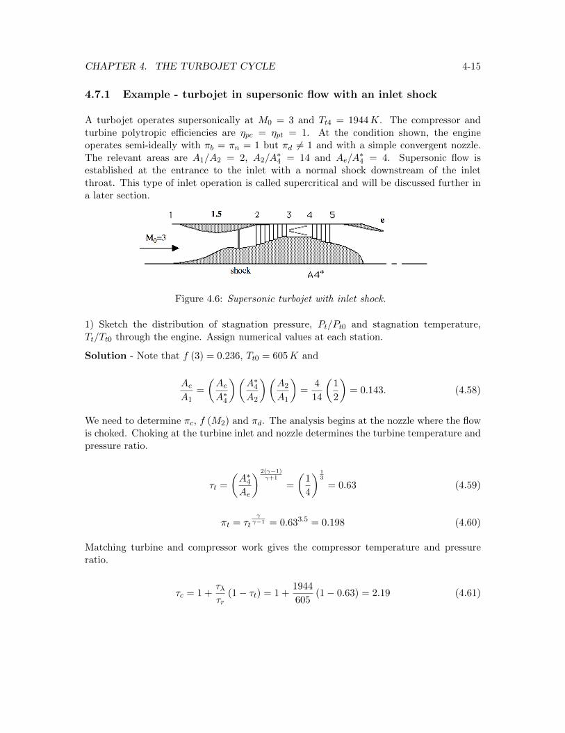
CHAPTER 4. THE TURBOJET CYCLE 4-15
4.7.1 Example - turbojet in supersonic flow with an inlet shock
A turbojet operates supersonically at M0 = 3 and Tt4 = 1944K. The compressor andturbine polytropic efficiencies are ηpc = ηpt = 1. At the condition shown, the engineoperates semi-ideally with πb = πn = 1 but πd 6= 1 and with a simple convergent nozzle.The relevant areas are A1/A2 = 2, A2/A
∗4 = 14 and Ae/A
∗4 = 4. Supersonic flow is
established at the entrance to the inlet with a normal shock downstream of the inletthroat. This type of inlet operation is called supercritical and will be discussed further ina later section.
Figure 4.6: Supersonic turbojet with inlet shock.
1) Sketch the distribution of stagnation pressure, Pt/Pt0 and stagnation temperature,Tt/Tt0 through the engine. Assign numerical values at each station.
Solution - Note that f (3) = 0.236, Tt0 = 605K and
AeA1
=
(AeA∗4
)(A∗4A2
)(A2
A1
)=
4
14
(1
2
)= 0.143. (4.58)
We need to determine πc, f (M2) and πd. The analysis begins at the nozzle where the flowis choked. Choking at the turbine inlet and nozzle determines the turbine temperature andpressure ratio.
τt =
(A∗4Ae
) 2(γ−1)γ+1
=
(1
4
) 13
= 0.63 (4.59)
πt = τtγγ−1 = 0.633.5 = 0.198 (4.60)
Matching turbine and compressor work gives the compressor temperature and pressureratio.
τc = 1 +τλτr
(1− τt) = 1 +1944
605(1− 0.63) = 2.19 (4.61)
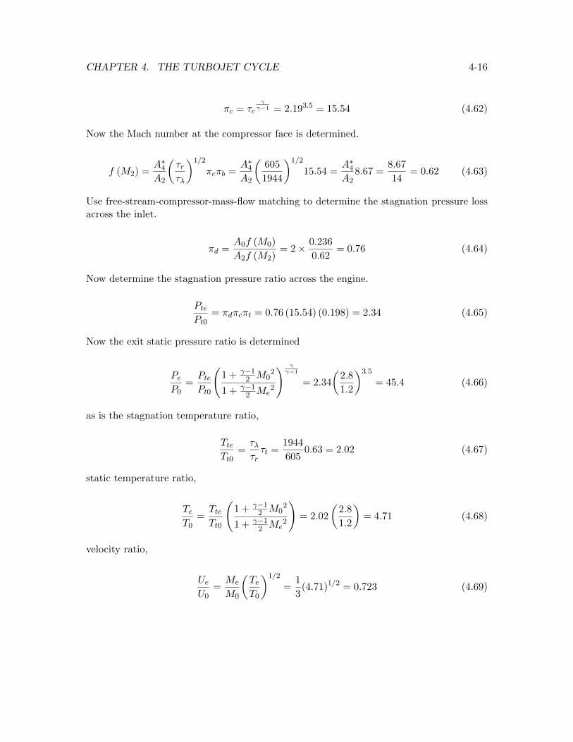
CHAPTER 4. THE TURBOJET CYCLE 4-16
πc = τcγγ−1 = 2.193.5 = 15.54 (4.62)
Now the Mach number at the compressor face is determined.
f (M2) =A∗4A2
(τrτλ
)1/2
πcπb =A∗4A2
(605
1944
)1/2
15.54 =A∗4A2
8.67 =8.67
14= 0.62 (4.63)
Use free-stream-compressor-mass-flow matching to determine the stagnation pressure lossacross the inlet.
πd =A0f (M0)
A2f (M2)= 2× 0.236
0.62= 0.76 (4.64)
Now determine the stagnation pressure ratio across the engine.
PtePt0
= πdπcπt = 0.76 (15.54) (0.198) = 2.34 (4.65)
Now the exit static pressure ratio is determined
PeP0
=PtePt0
(1 + γ−1
2 M02
1 + γ−12 Me
2
) γγ−1
= 2.34
(2.8
1.2
)3.5
= 45.4 (4.66)
as is the stagnation temperature ratio,
TteTt0
=τλτrτt =
1944
6050.63 = 2.02 (4.67)
static temperature ratio,
TeT0
=TteTt0
(1 + γ−1
2 M02
1 + γ−12 Me
2
)= 2.02
(2.8
1.2
)= 4.71 (4.68)
velocity ratio,
UeU0
=Me
M0
(TeT0
)1/2
=1
3(4.71)1/2 = 0.723 (4.69)
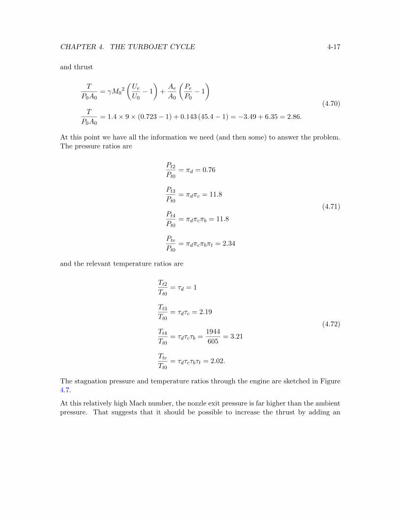
CHAPTER 4. THE TURBOJET CYCLE 4-17
and thrust
T
P0A0= γM0
2
(UeU0− 1
)+AeA0
(PeP0− 1
)T
P0A0= 1.4× 9× (0.723− 1) + 0.143 (45.4− 1) = −3.49 + 6.35 = 2.86.
(4.70)
At this point we have all the information we need (and then some) to answer the problem.The pressure ratios are
Pt2Pt0
= πd = 0.76
Pt3Pt0
= πdπc = 11.8
Pt4Pt0
= πdπcπb = 11.8
PtePt0
= πdπcπbπt = 2.34
(4.71)
and the relevant temperature ratios are
Tt2Tt0
= τd = 1
Tt3Tt0
= τdτc = 2.19
Tt4Tt0
= τdτcτb =1944
605= 3.21
TteTt0
= τdτcτbτt = 2.02.
(4.72)
The stagnation pressure and temperature ratios through the engine are sketched in Figure4.7.
At this relatively high Mach number, the nozzle exit pressure is far higher than the ambientpressure. That suggests that it should be possible to increase the thrust by adding an
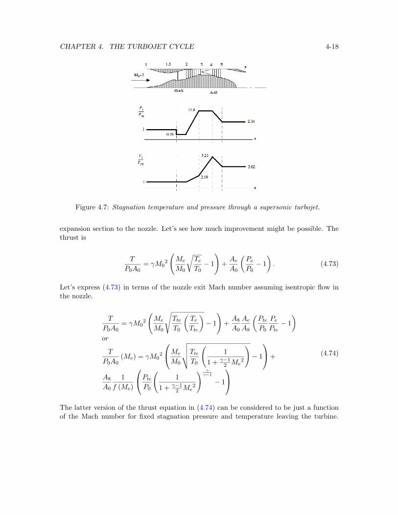
CHAPTER 4. THE TURBOJET CYCLE 4-18
Figure 4.7: Stagnation temperature and pressure through a supersonic turbojet.
expansion section to the nozzle. Let’s see how much improvement might be possible. Thethrust is
T
P0A0= γM0
2
(Me
M0
√TeT0− 1
)+AeA0
(PeP0− 1
). (4.73)
Let’s express (4.73) in terms of the nozzle exit Mach number assuming isentropic flow inthe nozzle.
T
P0A0= γM0
2
(Me
M0
√TteT0
(TeTte
)− 1
)+A8
A0
AeA8
(PteP0
PePte− 1
)or
T
P0A0(Me) = γM0
2
Me
M0
√√√√TteT0
(1
1 + γ−12 Me
2
)− 1
+
A8
A0
1
f (Me)
PteP0
(1
1 + γ−12 Me
2
) γγ−1
− 1
(4.74)
The latter version of the thrust equation in (4.74) can be considered to be just a functionof the Mach number for fixed stagnation pressure and temperature leaving the turbine.
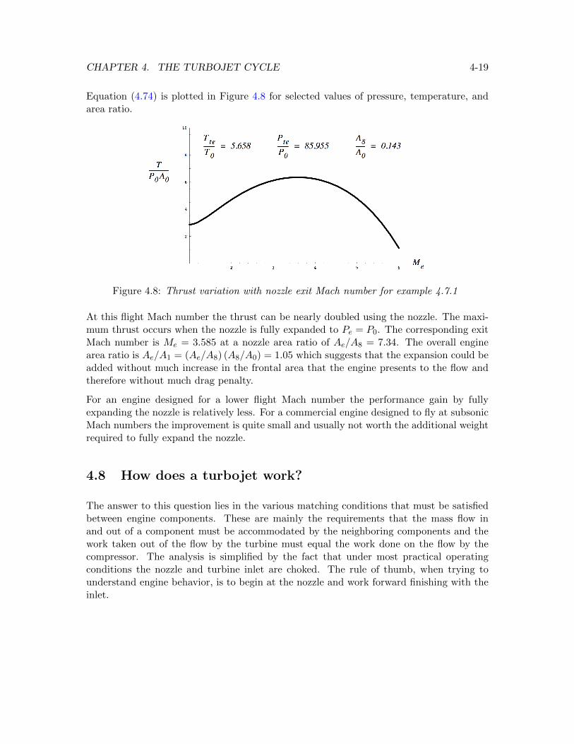
CHAPTER 4. THE TURBOJET CYCLE 4-19
Equation (4.74) is plotted in Figure 4.8 for selected values of pressure, temperature, andarea ratio.
Figure 4.8: Thrust variation with nozzle exit Mach number for example 4.7.1
At this flight Mach number the thrust can be nearly doubled using the nozzle. The maxi-mum thrust occurs when the nozzle is fully expanded to Pe = P0. The corresponding exitMach number is Me = 3.585 at a nozzle area ratio of Ae/A8 = 7.34. The overall enginearea ratio is Ae/A1 = (Ae/A8) (A8/A0) = 1.05 which suggests that the expansion could beadded without much increase in the frontal area that the engine presents to the flow andtherefore without much drag penalty.
For an engine designed for a lower flight Mach number the performance gain by fullyexpanding the nozzle is relatively less. For a commercial engine designed to fly at subsonicMach numbers the improvement is quite small and usually not worth the additional weightrequired to fully expand the nozzle.
4.8 How does a turbojet work?
The answer to this question lies in the various matching conditions that must be satisfiedbetween engine components. These are mainly the requirements that the mass flow inand out of a component must be accommodated by the neighboring components and thework taken out of the flow by the turbine must equal the work done on the flow by thecompressor. The analysis is simplified by the fact that under most practical operatingconditions the nozzle and turbine inlet are choked. The rule of thumb, when trying tounderstand engine behavior, is to begin at the nozzle and work forward finishing with theinlet.
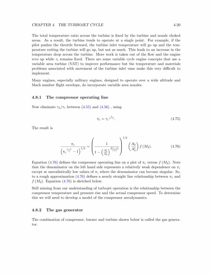
CHAPTER 4. THE TURBOJET CYCLE 4-20
The total temperature ratio across the turbine is fixed by the turbine and nozzle chokedareas. As a result, the turbine tends to operate at a single point. For example, if thepilot pushes the throttle forward, the turbine inlet temperature will go up and the tem-perature exiting the turbine will go up, but not as much. This leads to an increase in thetemperature drop across the turbine. More work is taken out of the flow and the enginerevs up while τt remains fixed. There are some variable cycle engine concepts that use avariable area turbine (VAT) to improve performance but the temperature and materialsproblems associated with movement of the turbine inlet vane make this very difficult toimplement.
Many engines, especially military engines, designed to operate over a wide altitude andMach number flight envelope, do incorporate variable area nozzles.
4.8.1 The compressor operating line
Now eliminate τλ/τr between (4.55) and (4.56) , using
πc = τcγγ−1 . (4.75)
The result is
πc(πc
γ−1γ − 1
)1/2=
1
1−(A∗4A8
) 2(γ−1)γ+1
1/2(
A2
A∗4
)f (M2) . (4.76)
Equation (4.76) defines the compressor operating line on a plot of πc versus f (M2). Notethat the denominator on the left hand side represents a relatively weak dependence on πcexcept at unrealistically low values of πc where the denominator can become singular. So,to a rough approximation (4.76) defines a nearly straight line relationship between πc andf (M2). Equation (4.76) is sketched below.
Still missing from our understanding of turbojet operation is the relationship between thecompressor temperature and pressure rise and the actual compressor speed. To determinethis we will need to develop a model of the compressor aerodynamics.
4.8.2 The gas generator
The combination of compressor, burner and turbine shown below is called the gas genera-tor.
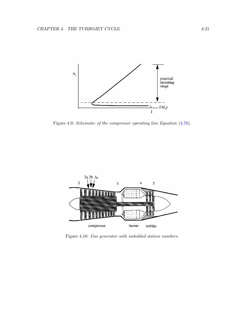
CHAPTER 4. THE TURBOJET CYCLE 4-21
Figure 4.9: Schematic of the compressor operating line Equation (4.76).
Figure 4.10: Gas generator with imbedded station numbers.
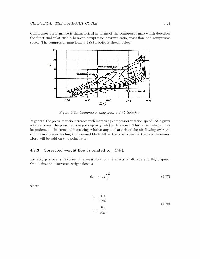
CHAPTER 4. THE TURBOJET CYCLE 4-22
Compressor performance is characterized in terms of the compressor map which describesthe functional relationship between compressor pressure ratio, mass flow and compressorspeed. The compressor map from a J85 turbojet is shown below.
Figure 4.11: Compressor map from a J-85 turbojet.
In general the pressure ratio increases with increasing compressor rotation speed. At a givenrotation speed the pressure ratio goes up as f (M2) is decreased. This latter behavior canbe understood in terms of increasing relative angle of attack of the air flowing over thecompressor blades leading to increased blade lift as the axial speed of the flow decreases.More will be said on this point later.
4.8.3 Corrected weight flow is related to f (M2).
Industry practice is to correct the mass flow for the effects of altitude and flight speed.One defines the corrected weight flow as
wc = mag
√θ
δ(4.77)
where
θ =Tt2TSL
δ =Pt2PSL
.
(4.78)
CHAPTER 4. THE TURBOJET CYCLE 4-23
The quantities TSL and PSL refer to sea level standard pressure and temperature. InEnglish units
TSL = 518.67R
PSL = 2116.22pounds/ft2.(4.79)
The gas constant for air is
Rair = 1710.2ft2/(sec2 −R
). (4.80)
We can write (4.77) as
wc = mg
√θ
δ=
1(γ+1
2
) γ+12(γ−1)
γgPSL√γRTSL
Af (M) . (4.81)
Note that the quantity in parentheses is a constant. Thus the corrected mass flow isproportional to f (M2). At the compressor face
wc = 49.459A2f (M2) pounds/sec (4.82)
where A2 is expressed in terms of square feet. Throughout this course f (M2) will bethe preferred measure of reduced mass flow through the compressor instead of the usualcorrected weight flow. This quantity has several significant advantages. It is dimensionless,independent of compressor size and for practical purposes lies in a fairly narrow range ofvalues that is more or less the same for all engines. The compressor entrance Mach number,M2, is generally restricted to lie in the range between 0.2 and 0.6. Unusually low valuesof f (M2) imply that the engine diameter is too large. If f (M2) gets too large ( f (M2)approaches one), the compressor blade passages begin to choke and stagnation pressurelosses increase dramatically.
The compressor map can be regarded as a cross plot of three independent functions. Thefirst is determined by the compressor-turbine inlet matching function (4.52). Rearrangingvariables (4.52) becomes
πc = F1
(τλτr, f (M2)
)=
((1 + f)
πb
A2
A∗4
)√τλτrf (M2) (4.83)
CHAPTER 4. THE TURBOJET CYCLE 4-24
where the contribution of the fuel/air ratio and burner pressure loss has been included.The factor in parentheses in (4.83) is approximately constant.
The second function relates the compressor efficiency to the pressure ratio and massflow.
ηc = F2 (πc, f (M2)) (4.84)
This is a function that can only be determined empirically through extensive compressortesting. The contours of constant efficiency in Figure 4.11 illustrate a typical case.
The third function relates the pressure ratio and mass flow to the rotational speed of thecompressor. This function is of the form
πc = F3
(Mb0√τr, f (M2)
)(4.85)
where
Mb0 =Ublade√γRT0
(4.86)
is the compressor blade Mach number based on the free stream speed of sound and Ubladeis the blade speed. Equation (4.85) is shown as lines of constant percent corrected speedin Figure 4.11.
4.8.4 A simple model of compressor blade aerodynamics
An accurate model of (4.85) can be derived from a detailed computation of the aerodynam-ics of the flow over the individual compressor blade elements. This is beyond the scope ofthis course but we can develop a simplified model of blade aerodynamics that reproducesthe most important features of the relation between pressure ratio, mass flow and bladespeed illustrated by the family of speed curves in Figure 4.11. Figure 4.12 shows the flowthrough a typical compressor stage called an imbedded stage. The stations labeled in Fig-ure 4.12 are 2a (the space just ahead of the compressor rotor), 2b (the space between therotor and stator) and 3a (the space after the stator and just ahead of the next rotor). The
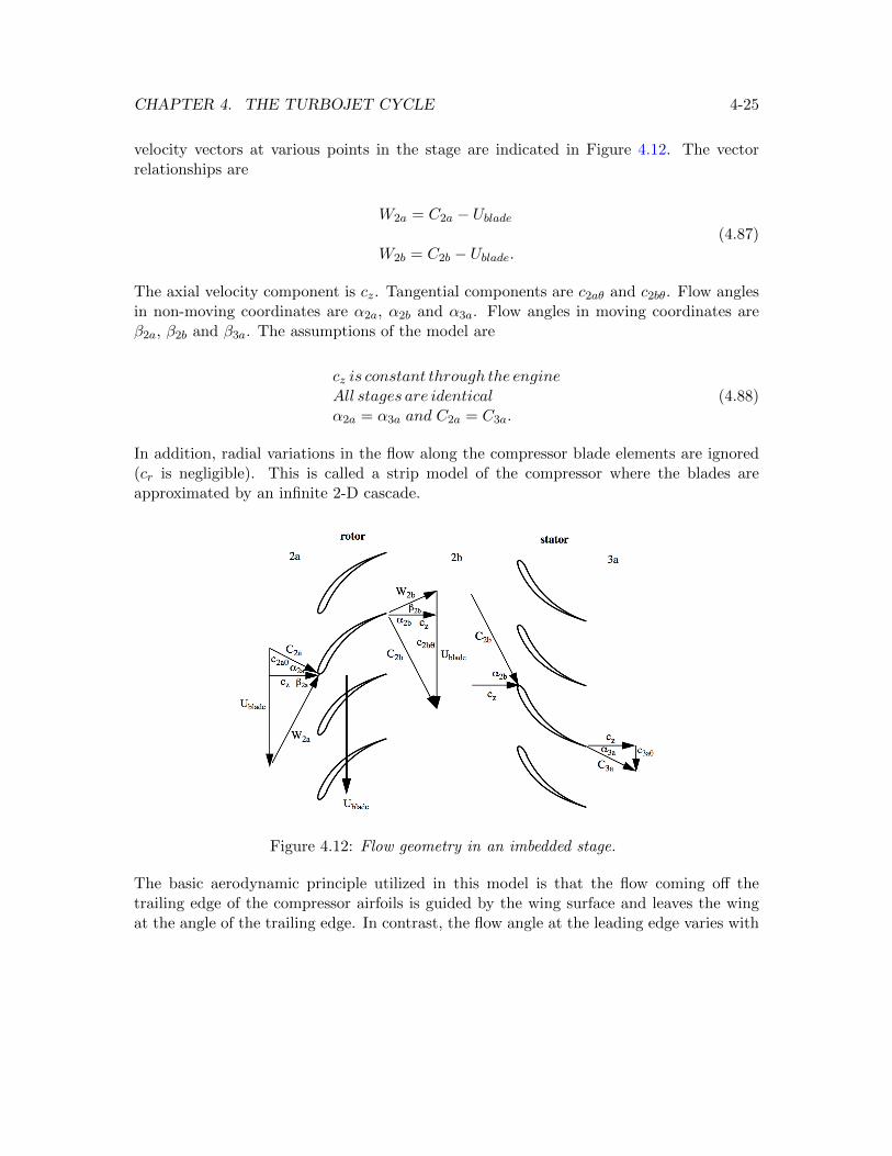
CHAPTER 4. THE TURBOJET CYCLE 4-25
velocity vectors at various points in the stage are indicated in Figure 4.12. The vectorrelationships are
W2a = C2a − Ublade
W2b = C2b − Ublade.(4.87)
The axial velocity component is cz. Tangential components are c2aθ and c2bθ. Flow anglesin non-moving coordinates are α2a, α2b and α3a. Flow angles in moving coordinates areβ2a, β2b and β3a. The assumptions of the model are
cz is constant through the engineAll stages are identicalα2a = α3a and C2a = C3a.
(4.88)
In addition, radial variations in the flow along the compressor blade elements are ignored(cr is negligible). This is called a strip model of the compressor where the blades areapproximated by an infinite 2-D cascade.
Figure 4.12: Flow geometry in an imbedded stage.
The basic aerodynamic principle utilized in this model is that the flow coming off thetrailing edge of the compressor airfoils is guided by the wing surface and leaves the wingat the angle of the trailing edge. In contrast, the flow angle at the leading edge varies with
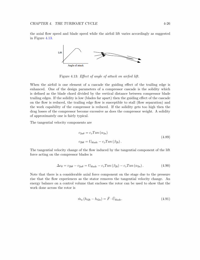
CHAPTER 4. THE TURBOJET CYCLE 4-26
the axial flow speed and blade speed while the airfoil lift varies accordingly as suggestedin Figure 4.13.
Figure 4.13: Effect of angle of attack on airfoil lift.
When the airfoil is one element of a cascade the guiding effect of the trailing edge isenhanced. One of the design parameters of a compressor cascade is the solidity whichis defined as the blade chord divided by the vertical distance between compressor bladetrailing edges. If the solidity is low (blades far apart) then the guiding effect of the cascadeon the flow is reduced, the trailing edge flow is susceptible to stall (flow separation) andthe work capability of the compressor is reduced. If the solidity gets too high then thedrag losses of the compressor become excessive as does the compressor weight. A solidityof approximately one is fairly typical.
The tangential velocity components are
c2aθ = czTan (α2a)
c2bθ = Ublade − czTan (β2b) .(4.89)
The tangential velocity change of the flow induced by the tangential component of the liftforce acting on the compressor blades is
∆cθ = c2bθ − c2aθ = Ublade − czTan (β2b)− czTan (α2a) . (4.90)
Note that there is a considerable axial force component on the stage due to the pressurerise that the flow experiences as the stator removes the tangential velocity change. Anenergy balance on a control volume that encloses the rotor can be used to show that thework done across the rotor is
ma (ht2b − ht2a) = F · Ublade. (4.91)
CHAPTER 4. THE TURBOJET CYCLE 4-27
In terms of the tangential velocity change
ma (ht2b − ht2a) = ma∆cθUblade. (4.92)
This is a key equation that connects the work done across a cascade with the speed of theblade and the tangential velocity change. Note that all of the stage work is done by therotor and so we can write
(ht3a − ht2a) = ∆cθUblade. (4.93)
Assume there are n identical stages. Then the enthalpy rise across the compressor is
(ht3 − ht2) = n (∆cθ)Ublade. (4.94)
Assume constant heat capacity and divide (4.94) by CpT0.
τr (τc − 1) = n (γ − 1)U2blade
γRT0
(∆cθUblade
)(4.95)
Solve for τc
τc = 1 + n (γ − 1)
(Mb0√τr
)2
ψ (4.96)
where the stage load factor
ψ =∆cθUblade
(4.97)
is introduced. The stage load factor compares the tangential velocity change of the flowacross the rotor to the rotor speed. The upper limit of this parameter is about 1/4 andis a measure of the maximum pressure rise achievable in a stage. Equation (4.96) isexpressed in terms of the basic compressor speed parameter introduced in (4.85). Now weneed to express the stage load factor in terms of this speed parameter and f (M). From(4.90).
ψ = 1− czUblade
(Tan (β2b) + Tan (α2a)) (4.98)
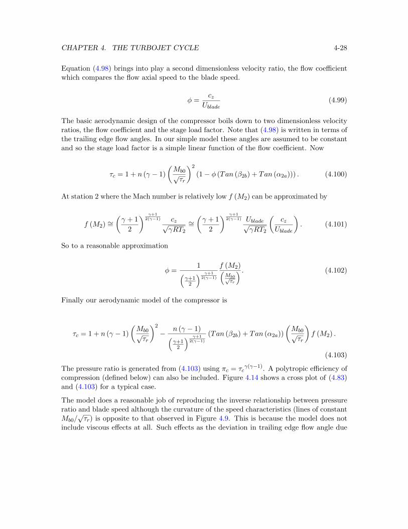
CHAPTER 4. THE TURBOJET CYCLE 4-28
Equation (4.98) brings into play a second dimensionless velocity ratio, the flow coefficientwhich compares the flow axial speed to the blade speed.
φ =cz
Ublade(4.99)
The basic aerodynamic design of the compressor boils down to two dimensionless velocityratios, the flow coefficient and the stage load factor. Note that (4.98) is written in terms ofthe trailing edge flow angles. In our simple model these angles are assumed to be constantand so the stage load factor is a simple linear function of the flow coefficient. Now
τc = 1 + n (γ − 1)
(Mb0√τr
)2
(1− φ (Tan (β2b) + Tan (α2a))) . (4.100)
At station 2 where the Mach number is relatively low f (M2) can be approximated by
f (M2) ∼=(γ + 1
2
) γ+12(γ−1) cz√
γRT2
∼=(γ + 1
2
) γ+12(γ−1) Ublade√
γRT2
(cz
Ublade
). (4.101)
So to a reasonable approximation
φ =1(
γ+12
) γ+12(γ−1)
f (M2)(Mb0√τr
) . (4.102)
Finally our aerodynamic model of the compressor is
τc = 1 + n (γ − 1)
(Mb0√τr
)2
− n (γ − 1)(γ+1
2
) γ+12(γ−1)
(Tan (β2b) + Tan (α2a))
(Mb0√τr
)f (M2) .
(4.103)
The pressure ratio is generated from (4.103) using πc = τcγ(γ−1). A polytropic efficiency of
compression (defined below) can also be included. Figure 4.14 shows a cross plot of (4.83)and (4.103) for a typical case.
The model does a reasonable job of reproducing the inverse relationship between pressureratio and blade speed although the curvature of the speed characteristics (lines of constantMb0/
√τr) is opposite to that observed in Figure 4.9. This is because the model does not
include viscous effects at all. Such effects as the deviation in trailing edge flow angle due
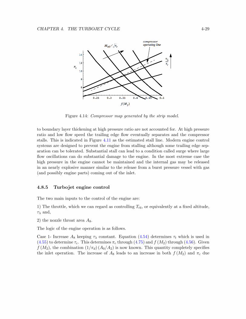
CHAPTER 4. THE TURBOJET CYCLE 4-29
Figure 4.14: Compressor map generated by the strip model.
to boundary layer thickening at high pressure ratio are not accounted for. At high pressureratio and low flow speed the trailing edge flow eventually separates and the compressorstalls. This is indicated in Figure 4.11 as the estimated stall line. Modern engine controlsystems are designed to prevent the engine from stalling although some trailing edge sep-aration can be tolerated. Substantial stall can lead to a condition called surge where largeflow oscillations can do substantial damage to the engine. In the most extreme case thehigh pressure in the engine cannot be maintained and the internal gas may be releasedin an nearly explosive manner similar to the release from a burst pressure vessel with gas(and possibly engine parts) coming out of the inlet.
4.8.5 Turbojet engine control
The two main inputs to the control of the engine are:
1) The throttle, which we can regard as controlling Tt4, or equivalently at a fixed altitude,τλ and,
2) the nozzle throat area A8.
The logic of the engine operation is as follows.
Case 1- Increase A8 keeping τλ constant. Equation (4.54) determines τt which is used in(4.55) to determine τc. This determines πc through (4.75) and f (M2) through (4.56). Givenf (M2), the combination (1/πd) (A0/A2) is now known. This quantity completely specifiesthe inlet operation. The increase of A8 leads to an increase in both f (M2) and πc due
CHAPTER 4. THE TURBOJET CYCLE 4-30
to an increase in compressor speed as indicated on the compressor map. The compressoroperating point moves along a constant τλ/τr characteristic.
Case 2 - Increase τλ keeping A8 constant. The logic in this case is very similar to case1 except that the compressor-turbine work matching condition, has τt = constant. Thisdetermines πc through (4.75) and f (M2) through the (in this case fixed) compressor op-erating line (4.76). Given f (M2) then (1/πd) (A0/A2) is known and the inlet operation isdefined. As in case 1 the change of f (M2) and πc is achieved by an increase in compressorspeed according to the compressor map. The compressor operating point moves along theoperating line (4.76) which crosses the constant τλ/τr characteristics as shown in Figure4.12.
4.8.6 Inlet operation
There are two main points to take away from the previous discussion of engine control. Thefirst is that to understand engine operation one begins at the nozzle and works forward.The other is that the inlet flow is essentially defined by the engine operating point throughthe value of f (M2). In effect, the engine sets the back pressure for the inlet. This isthe fundamental purpose of the inlet; to provide the air mass flow to the engine at theMach number dictated by the engine operating point with as small a stagnation pressureloss as possible. This whole mechanism is referred to as the pumping characteristic of theengine.
Lets look at the various possible modes of inlet operation recalling the discussion of capturearea in Chapter 2. Figure 4.15 depicts an engine in subsonic flow. Shown is the variationin inlet flow as the nozzle throat A8 area is increased with τλ held constant.
The Mach number at station 2 entering the compressor increases from top to bottom inFigure 4.15. In the top four figures (a, b, c, d) there is no inlet shock and so, neglecting skinfriction, the only way the increase in the Mach number at station 2 can be accommodatedaccording to the matching condition (4.57) is for the capture area A0 to increase leadingto an increase in the air mass flow through the engine with πd = 1.
As A8 is increased further the inlet eventually chokes (this is the situation shown as cased). The condition for inlet choking is determined from the mass balance between the inletthroat A1.5 and compressor face A2.
Pt2A2√Tt2
f (M2) =Pt1.5A1.5√
Tt1.5f (M1.5) (4.104)
Neglecting skin friction and heat transfer, the flow from A1.5 to A2 is adiabatic and isen-
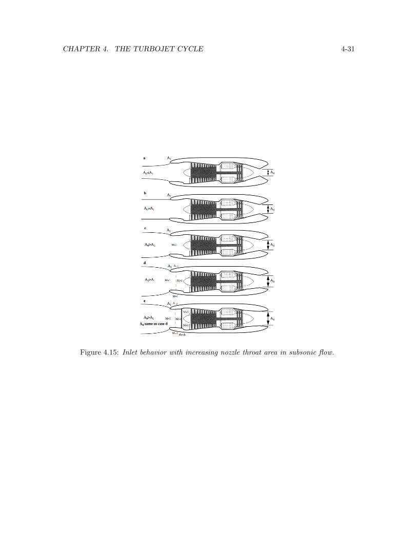
CHAPTER 4. THE TURBOJET CYCLE 4-31
Figure 4.15: Inlet behavior with increasing nozzle throat area in subsonic flow.
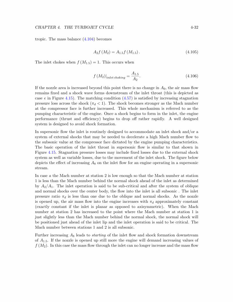
CHAPTER 4. THE TURBOJET CYCLE 4-32
tropic. The mass balance (4.104) becomes
A2f (M2) = A1.5f (M1.5) . (4.105)
The inlet chokes when f (M1.5) = 1. This occurs when
f (M2)|inlet choking =A1.5
A2. (4.106)
If the nozzle area is increased beyond this point there is no change in A0, the air mass flowremains fixed and a shock wave forms downstream of the inlet throat (this is depicted ascase e in Figure 4.15). The matching condition (4.57) is satisfied by increasing stagnationpressure loss across the shock (πd < 1). The shock becomes stronger as the Mach numberat the compressor face is further increased. This whole mechanism is referred to as thepumping characteristic of the engine. Once a shock begins to form in the inlet, the engineperformance (thrust and efficiency) begins to drop off rather rapidly. A well designedsystem is designed to avoid shock formation.
In supersonic flow the inlet is routinely designed to accommodate an inlet shock and/or asystem of external shocks that may be needed to decelerate a high Mach number flow tothe subsonic value at the compressor face dictated by the engine pumping characteristics.The basic operation of the inlet throat in supersonic flow is similar to that shown inFigure 4.15. Stagnation pressure losses may include fixed losses due to the external shocksystem as well as variable losses, due to the movement of the inlet shock. The figure belowdepicts the effect of increasing A8 on the inlet flow for an engine operating in a supersonicstream.
In case a the Mach number at station 2 is low enough so that the Mach number at station1 is less than the Mach number behind the normal shock ahead of the inlet as determinedby A2/A1. The inlet operation is said to be sub-critical and after the system of obliqueand normal shocks over the center body, the flow into the inlet is all subsonic . The inletpressure ratio πd is less than one due to the oblique and normal shocks. As the nozzleis opened up, the air mass flow into the engine increases with πd approximately constant(exactly constant if the inlet is planar as opposed to axisymmetric). When the Machnumber at station 2 has increased to the point where the Mach number at station 1 isjust slightly less than the Mach number behind the normal shock, the normal shock willbe positioned just ahead of the inlet lip and the inlet operation is said to be critical. TheMach number between stations 1 and 2 is all subsonic.
Further increasing A8 leads to starting of the inlet flow and shock formation downstreamof A1.5. If the nozzle is opened up still more the engine will demand increasing values off (M2). In this case the mass flow through the inlet can no longer increase and the mass flow
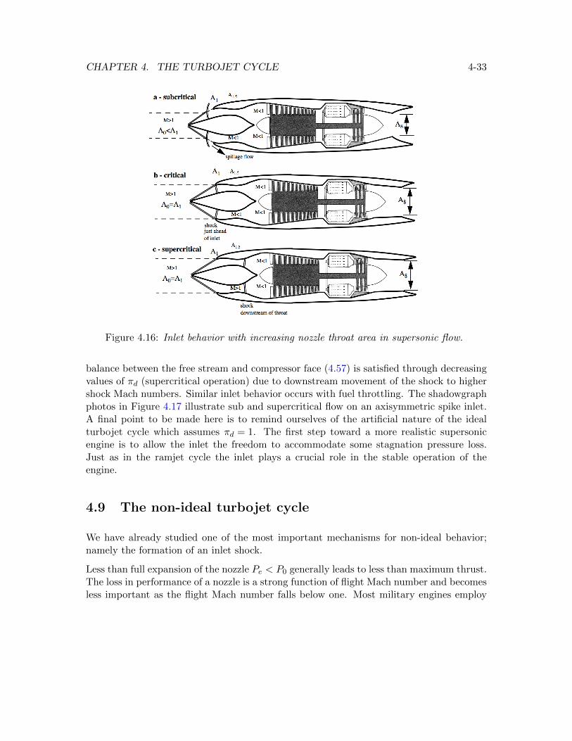
CHAPTER 4. THE TURBOJET CYCLE 4-33
Figure 4.16: Inlet behavior with increasing nozzle throat area in supersonic flow.
balance between the free stream and compressor face (4.57) is satisfied through decreasingvalues of πd (supercritical operation) due to downstream movement of the shock to highershock Mach numbers. Similar inlet behavior occurs with fuel throttling. The shadowgraphphotos in Figure 4.17 illustrate sub and supercritical flow on an axisymmetric spike inlet.A final point to be made here is to remind ourselves of the artificial nature of the idealturbojet cycle which assumes πd = 1. The first step toward a more realistic supersonicengine is to allow the inlet the freedom to accommodate some stagnation pressure loss.Just as in the ramjet cycle the inlet plays a crucial role in the stable operation of theengine.
4.9 The non-ideal turbojet cycle
We have already studied one of the most important mechanisms for non-ideal behavior;namely the formation of an inlet shock.
Less than full expansion of the nozzle Pe < P0 generally leads to less than maximum thrust.The loss in performance of a nozzle is a strong function of flight Mach number and becomesless important as the flight Mach number falls below one. Most military engines employ
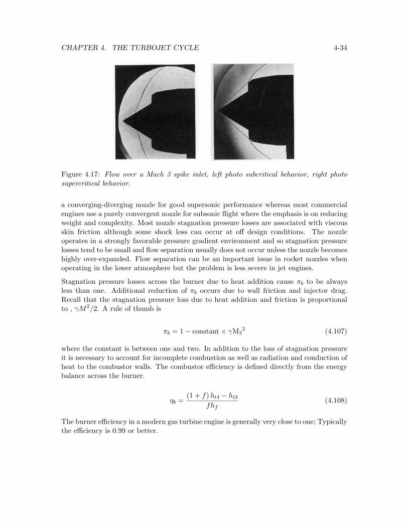
CHAPTER 4. THE TURBOJET CYCLE 4-34
Figure 4.17: Flow over a Mach 3 spike inlet, left photo subcritical behavior, right photosupercritical behavior.
a converging-diverging nozzle for good supersonic performance whereas most commercialengines use a purely convergent nozzle for subsonic flight where the emphasis is on reducingweight and complexity. Most nozzle stagnation pressure losses are associated with viscousskin friction although some shock loss can occur at off design conditions. The nozzleoperates in a strongly favorable pressure gradient environment and so stagnation pressurelosses tend to be small and flow separation usually does not occur unless the nozzle becomeshighly over-expanded. Flow separation can be an important issue in rocket nozzles whenoperating in the lower atmosphere but the problem is less severe in jet engines.
Stagnation pressure losses across the burner due to heat addition cause πb to be alwaysless than one. Additional reduction of πb occurs due to wall friction and injector drag.Recall that the stagnation pressure loss due to heat addition and friction is proportionalto , γM2/2. A rule of thumb is
πb = 1− constant× γM32 (4.107)
where the constant is between one and two. In addition to the loss of stagnation pressureit is necessary to account for incomplete combustion as well as radiation and conduction ofheat to the combustor walls. The combustor efficiency is defined directly from the energybalance across the burner.
ηb =(1 + f)ht4 − ht3
fhf(4.108)
The burner efficiency in a modern gas turbine engine is generally very close to one; Typicallythe efficiency is 0.99 or better.
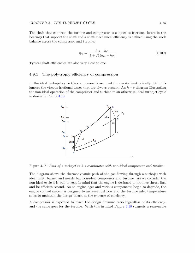
CHAPTER 4. THE TURBOJET CYCLE 4-35
The shaft that connects the turbine and compressor is subject to frictional losses in thebearings that support the shaft and a shaft mechanical efficiency is defined using the workbalance across the compressor and turbine.
ηm =ht3 − ht2
(1 + f) (ht4 − ht5)(4.109)
Typical shaft efficiencies are also very close to one.
4.9.1 The polytropic efficiency of compression
In the ideal turbojet cycle the compressor is assumed to operate isentropically. But thisignores the viscous frictional losses that are always present. An h− s diagram illustratingthe non-ideal operation of the compressor and turbine in an otherwise ideal turbojet cycleis shown in Figure 4.18.
Figure 4.18: Path of a turbojet in h-s coordinates with non-ideal compressor and turbine.
The diagram shows the thermodynamic path of the gas flowing through a turbojet withideal inlet, burner and nozzle but non-ideal compressor and turbine. As we consider thenon-ideal cycle it is well to keep in mind that the engine is designed to produce thrust firstand be efficient second. As an engine ages and various components begin to degrade, theengine control system is designed to increase fuel flow and the turbine inlet temperatureso as to maintain the design thrust at the expense of efficiency.
A compressor is expected to reach the design pressure ratio regardless of its efficiency.and the same goes for the turbine. With this in mind Figure 4.18 suggests a reasonable
CHAPTER 4. THE TURBOJET CYCLE 4-36
definition of compressor and turbine efficiency
ηc =The work input needed to reach Pt3/Pt2 in an isentropic compression process
The work input needed to reach Pt3/Pt2 in the real compression process
ηc =ht3s − ht2ht3 − ht2
(4.110)
and
ηe =The work output needed to reach Pt5/Pt4 in the real expansion process
The work output needed to reach Pt5/Pt4 in an isentropic expansion process
ηe =ht5 − ht4ht5s − ht4
(4.111)
In terms of the temperature for a calorically perfect gas these definitions become
ηc =Tt3s − Tt2Tt3 − Tt2
ηe =Tt5 − Tt4Tt5s − Tt4
.
(4.112)
These definitions are useful but a little hard to interpret when comparing one compressorwith another if the compression ratios are not the same. We can use the approach suggestedby Figure 4.18 to define an efficiency that characterizes the compression process itself.Consider an infinitesimal compression process defined by the T − s diagram shown inFigure 4.19.
Define the polytropic efficiency of compression as the efficiency of an infinitesimal com-pression process.
ηpc =
(Tt3s − Tt2Tt3 − Tt2
)infinitesimal compression
=dTtsdTt
(4.113)
For an isentropic process of a calorically perfect gas the Gibbs equation is
dTtsTt
=
(γ − 1
γ
)dPtPt
. (4.114)
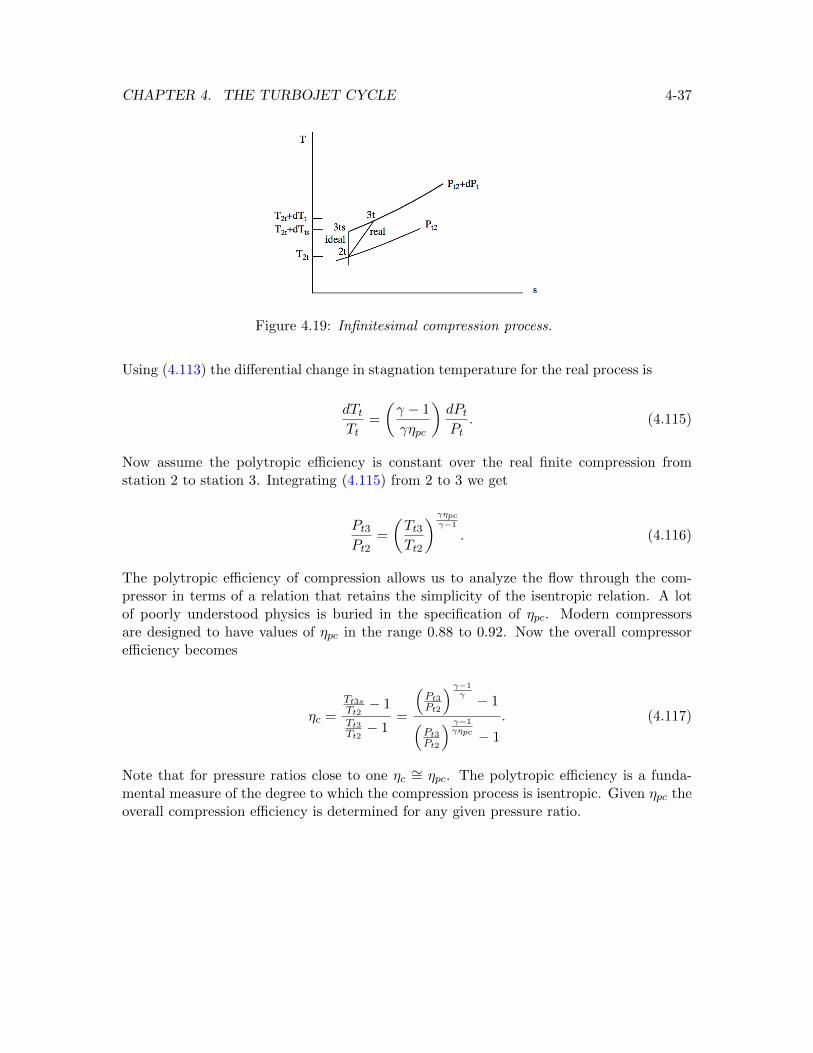
CHAPTER 4. THE TURBOJET CYCLE 4-37
Figure 4.19: Infinitesimal compression process.
Using (4.113) the differential change in stagnation temperature for the real process is
dTtTt
=
(γ − 1
γηpc
)dPtPt
. (4.115)
Now assume the polytropic efficiency is constant over the real finite compression fromstation 2 to station 3. Integrating (4.115) from 2 to 3 we get
Pt3Pt2
=
(Tt3Tt2
) γηpcγ−1
. (4.116)
The polytropic efficiency of compression allows us to analyze the flow through the com-pressor in terms of a relation that retains the simplicity of the isentropic relation. A lotof poorly understood physics is buried in the specification of ηpc. Modern compressorsare designed to have values of ηpc in the range 0.88 to 0.92. Now the overall compressorefficiency becomes
ηc =Tt3sTt2− 1
Tt3Tt2− 1
=
(Pt3Pt2
) γ−1γ − 1(
Pt3Pt2
) γ−1γηpc − 1
. (4.117)
Note that for pressure ratios close to one ηc ∼= ηpc. The polytropic efficiency is a funda-mental measure of the degree to which the compression process is isentropic. Given ηpc theoverall compression efficiency is determined for any given pressure ratio.
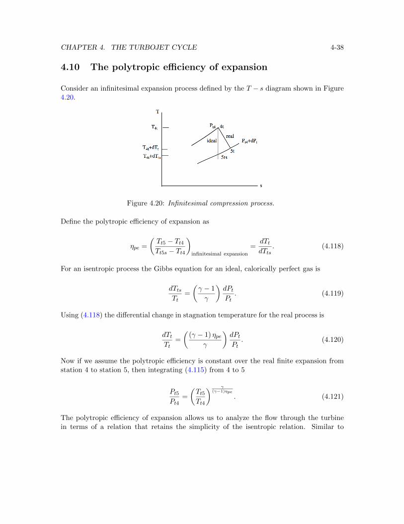
CHAPTER 4. THE TURBOJET CYCLE 4-38
4.10 The polytropic efficiency of expansion
Consider an infinitesimal expansion process defined by the T − s diagram shown in Figure4.20.
Figure 4.20: Infinitesimal compression process.
Define the polytropic efficiency of expansion as
ηpe =
(Tt5 − Tt4Tt5s − Tt4
)infinitesimal expansion
=dTtdTts
. (4.118)
For an isentropic process the Gibbs equation for an ideal, calorically perfect gas is
dTtsTt
=
(γ − 1
γ
)dPtPt
. (4.119)
Using (4.118) the differential change in stagnation temperature for the real process is
dTtTt
=
((γ − 1) ηpe
γ
)dPtPt
. (4.120)
Now if we assume the polytropic efficiency is constant over the real finite expansion fromstation 4 to station 5, then integrating (4.115) from 4 to 5
Pt5Pt4
=
(Tt5Tt4
) γ(γ−1)ηpe
. (4.121)
The polytropic efficiency of expansion allows us to analyze the flow through the turbinein terms of a relation that retains the simplicity of the isentropic relation. Similar to
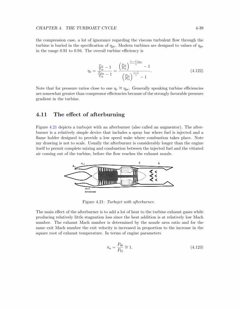
CHAPTER 4. THE TURBOJET CYCLE 4-39
the compression case, a lot of ignorance regarding the viscous turbulent flow through theturbine is buried in the specification of ηpe. Modern turbines are designed to values of ηpein the range 0.91 to 0.94. The overall turbine efficiency is
ηe =Tt5Tt4− 1
Tt5sTt4− 1
=
(Pt5Pt4
) (γ−1)ηpeγ − 1(
Pt5Pt4
) γ−1γ − 1
. (4.122)
Note that for pressure ratios close to one ηe ∼= ηpe. Generally speaking turbine efficienciesare somewhat greater than compressor efficiencies because of the strongly favorable pressuregradient in the turbine.
4.11 The effect of afterburning
Figure 4.21 depicts a turbojet with an afterburner (also called an augmentor). The after-burner is a relatively simple device that includes a spray bar where fuel is injected and aflame holder designed to provide a low speed wake where combustion takes place. Notemy drawing is not to scale. Usually the afterburner is considerably longer than the engineitself to permit complete mixing and combustion between the injected fuel and the vitiatedair coming out of the turbine, before the flow reaches the exhaust nozzle.
Figure 4.21: Turbojet with afterburner.
The main effect of the afterburner is to add a lot of heat to the turbine exhaust gases whileproducing relatively little stagnation loss since the heat addition is at relatively low Machnumber. The exhaust Mach number is determined by the nozzle area ratio and for thesame exit Mach number the exit velocity is increased in proportion to the increase in thesquare root of exhaust temperature. In terms of engine parameters
πa =Pt6Pt5∼= 1. (4.123)
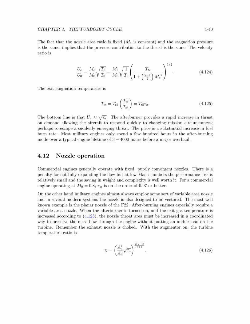
CHAPTER 4. THE TURBOJET CYCLE 4-40
The fact that the nozzle area ratio is fixed (Me is constant) and the stagnation pressureis the same, implies that the pressure contribution to the thrust is the same. The velocityratio is
UeU0
=Me
M0
√TeT0
=Me
M0
√1
T0
Tte
1 +(γ−1
2
)Me
2
1/2
. (4.124)
The exit stagnation temperature is
Tte = Tt5
(TteTt5
)= Tt5τa. (4.125)
The bottom line is that Ue ≈√τa. The afterburner provides a rapid increase in thrust
on demand allowing the aircraft to respond quickly to changing mission circumstances;perhaps to escape a suddenly emerging threat. The price is a substantial increase in fuelburn rate. Most military engines only spend a few hundred hours in the after-burningmode over a typical engine lifetime of 3− 4000 hours before a major overhaul.
4.12 Nozzle operation
Commercial engines generally operate with fixed, purely convergent nozzles. There is apenalty for not fully expanding the flow but at low Mach numbers the performance loss isrelatively small and the saving in weight and complexity is well worth it. For a commercialengine operating at M0 = 0.8, πn is on the order of 0.97 or better.
On the other hand military engines almost always employ some sort of variable area nozzleand in several modern systems the nozzle is also designed to be vectored. The most wellknown example is the planar nozzle of the F22. After-burning engines especially require avariable area nozzle. When the afterburner is turned on, and the exit gas temperature isincreased according to (4.125), the nozzle throat area must be increased in a coordinatedway to preserve the mass flow through the engine without putting an undue load on theturbine. Remember the exhaust nozzle is choked. With the augmentor on, the turbinetemperature ratio is
τt =
(A∗4A8
√τa
) 2(γ−1)γ+1
. (4.126)
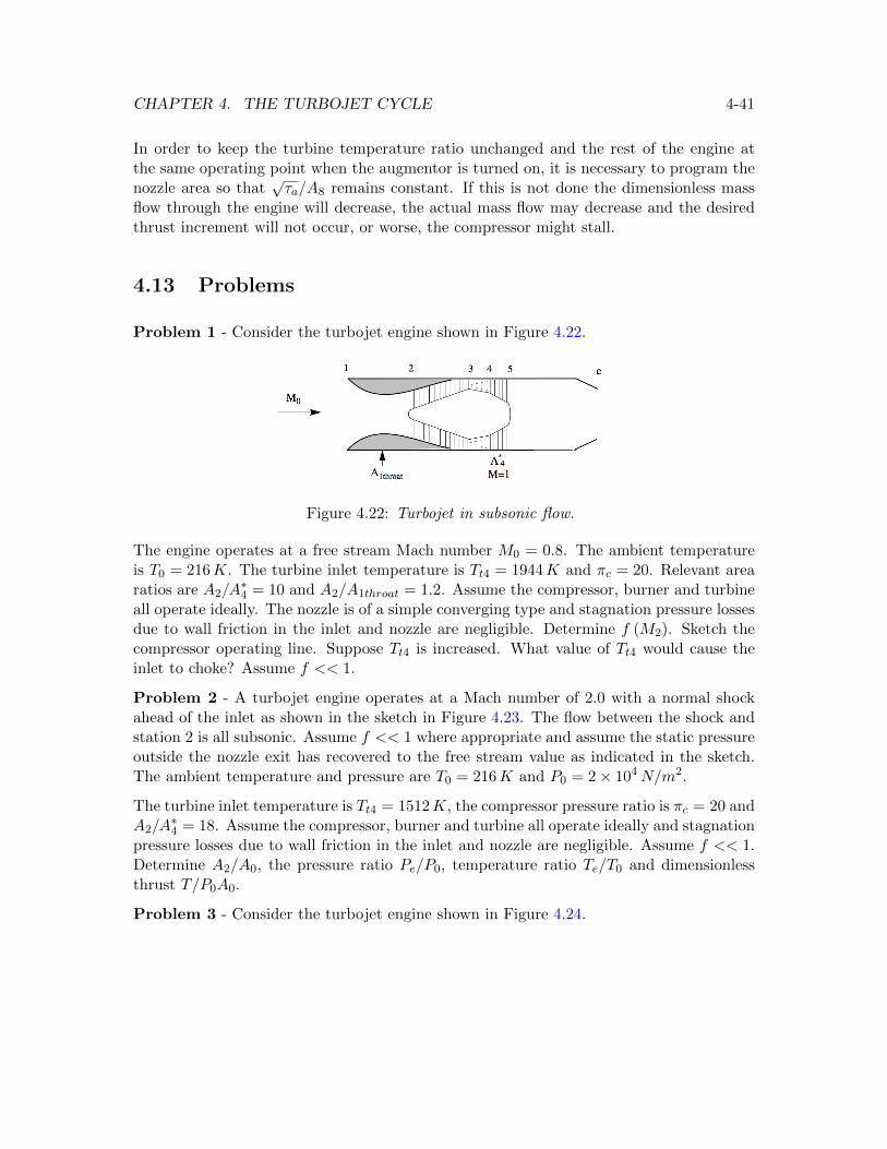
CHAPTER 4. THE TURBOJET CYCLE 4-41
In order to keep the turbine temperature ratio unchanged and the rest of the engine atthe same operating point when the augmentor is turned on, it is necessary to program thenozzle area so that
√τa/A8 remains constant. If this is not done the dimensionless mass
flow through the engine will decrease, the actual mass flow may decrease and the desiredthrust increment will not occur, or worse, the compressor might stall.
4.13 Problems
Problem 1 - Consider the turbojet engine shown in Figure 4.22.
Figure 4.22: Turbojet in subsonic flow.
The engine operates at a free stream Mach number M0 = 0.8. The ambient temperatureis T0 = 216K. The turbine inlet temperature is Tt4 = 1944K and πc = 20. Relevant arearatios are A2/A
∗4 = 10 and A2/A1throat = 1.2. Assume the compressor, burner and turbine
all operate ideally. The nozzle is of a simple converging type and stagnation pressure lossesdue to wall friction in the inlet and nozzle are negligible. Determine f (M2). Sketch thecompressor operating line. Suppose Tt4 is increased. What value of Tt4 would cause theinlet to choke? Assume f << 1.
Problem 2 - A turbojet engine operates at a Mach number of 2.0 with a normal shockahead of the inlet as shown in the sketch in Figure 4.23. The flow between the shock andstation 2 is all subsonic. Assume f << 1 where appropriate and assume the static pressureoutside the nozzle exit has recovered to the free stream value as indicated in the sketch.The ambient temperature and pressure are T0 = 216K and P0 = 2× 10⁴N/m2.
The turbine inlet temperature is Tt4 = 1512K, the compressor pressure ratio is πc = 20 andA2/A
∗4 = 18. Assume the compressor, burner and turbine all operate ideally and stagnation
pressure losses due to wall friction in the inlet and nozzle are negligible. Assume f << 1.Determine A2/A0, the pressure ratio Pe/P0, temperature ratio Te/T0 and dimensionlessthrust T/P0A0.
Problem 3 - Consider the turbojet engine shown in Figure 4.24.
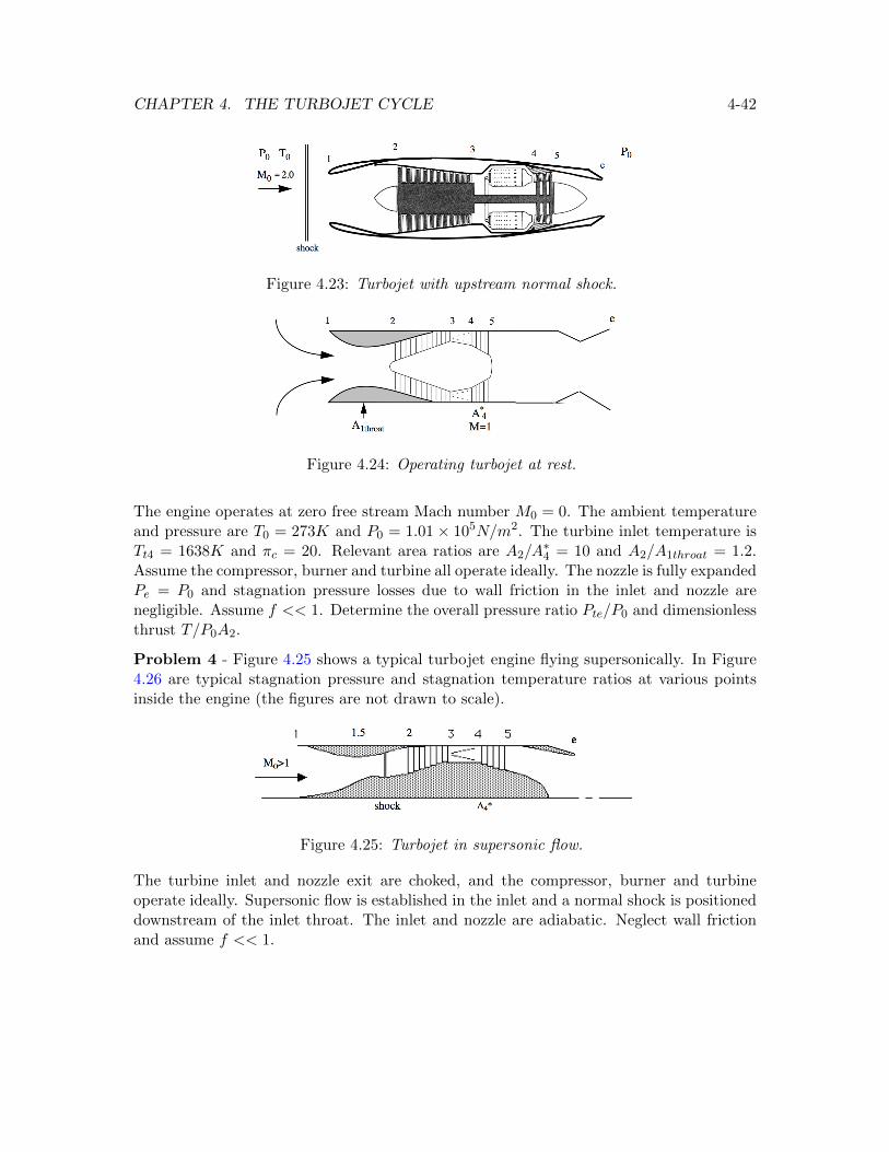
CHAPTER 4. THE TURBOJET CYCLE 4-42
Figure 4.23: Turbojet with upstream normal shock.
Figure 4.24: Operating turbojet at rest.
The engine operates at zero free stream Mach number M0 = 0. The ambient temperatureand pressure are T0 = 273K and P0 = 1.01× 10⁵N/m2. The turbine inlet temperature isTt4 = 1638K and πc = 20. Relevant area ratios are A2/A
∗4 = 10 and A2/A1throat = 1.2.
Assume the compressor, burner and turbine all operate ideally. The nozzle is fully expandedPe = P0 and stagnation pressure losses due to wall friction in the inlet and nozzle arenegligible. Assume f << 1. Determine the overall pressure ratio Pte/P0 and dimensionlessthrust T/P0A2.
Problem 4 - Figure 4.25 shows a typical turbojet engine flying supersonically. In Figure4.26 are typical stagnation pressure and stagnation temperature ratios at various pointsinside the engine (the figures are not drawn to scale).
Figure 4.25: Turbojet in supersonic flow.
The turbine inlet and nozzle exit are choked, and the compressor, burner and turbineoperate ideally. Supersonic flow is established in the inlet and a normal shock is positioneddownstream of the inlet throat. The inlet and nozzle are adiabatic. Neglect wall frictionand assume f << 1.
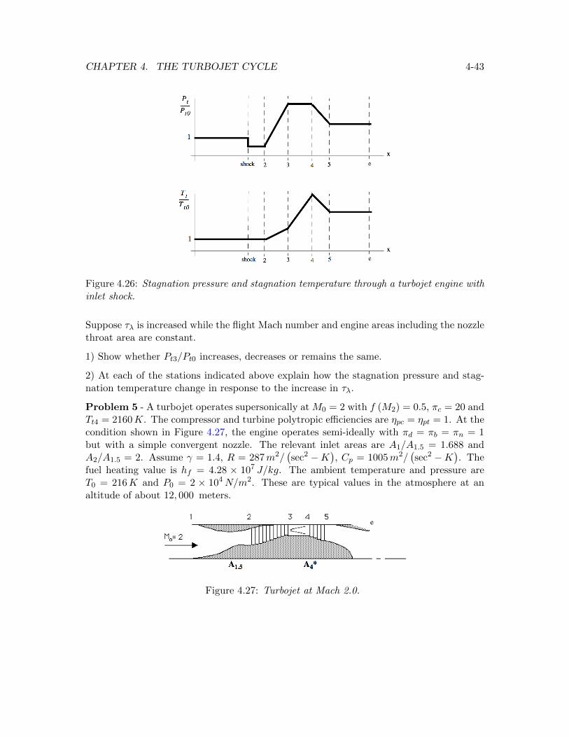
CHAPTER 4. THE TURBOJET CYCLE 4-43
Figure 4.26: Stagnation pressure and stagnation temperature through a turbojet engine withinlet shock.
Suppose τλ is increased while the flight Mach number and engine areas including the nozzlethroat area are constant.
1) Show whether Pt3/Pt0 increases, decreases or remains the same.
2) At each of the stations indicated above explain how the stagnation pressure and stag-nation temperature change in response to the increase in τλ.
Problem 5 - A turbojet operates supersonically at M0 = 2 with f (M2) = 0.5, πc = 20 andTt4 = 2160K. The compressor and turbine polytropic efficiencies are ηpc = ηpt = 1. At thecondition shown in Figure 4.27, the engine operates semi-ideally with πd = πb = πn = 1but with a simple convergent nozzle. The relevant inlet areas are A1/A1.5 = 1.688 andA2/A1.5 = 2. Assume γ = 1.4, R = 287m2/
(sec2 −K
), Cp = 1005m2/
(sec2 −K
). The
fuel heating value is hf = 4.28 × 10⁷ J/kg. The ambient temperature and pressure areT0 = 216K and P0 = 2 × 10⁴N/m2. These are typical values in the atmosphere at analtitude of about 12, 000 meters.
Figure 4.27: Turbojet at Mach 2.0.
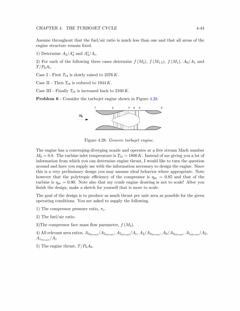
CHAPTER 4. THE TURBOJET CYCLE 4-44
Assume throughout that the fuel/air ratio is much less than one and that all areas of theengine structure remain fixed.
1) Determine A2/A∗4 and A∗4/Ae.
2) For each of the following three cases determine f (M2), f (M1.5), f (M1), A0/A1 andT/P0A1.
Case I - First Tt4 is slowly raised to 2376K.
Case II - Then Tt4 is reduced to 1944K.
Case III - Finally Tt4 is increased back to 2160K.
Problem 6 - Consider the turbojet engine shown in Figure 4.28.
Figure 4.28: Generic turbojet engine.
The engine has a converging-diverging nozzle and operates at a free stream Mach numberM0 = 0.8. The turbine inlet temperature is Tt4 = 1800K. Instead of me giving you a lot ofinformation from which you can determine engine thrust, I would like to turn the questionaround and have you supply me with the information necessary to design the engine. Sincethis is a very preliminary design you may assume ideal behavior where appropriate. Notehowever that the polytropic efficiency of the compressor is ηpc = 0.85 and that of theturbine is ηpe = 0.90. Note also that my crude engine drawing is not to scale! After youfinish the design, make a sketch for yourself that is more to scale.
The goal of the design is to produce as much thrust per unit area as possible for the givenoperating conditions. You are asked to supply the following.
1) The compressor pressure ratio, πc.
2) The fuel/air ratio.
3)The compressor face mass flow parameter, f (M2).
4) All relevant area ratios, A4throat/A5throat , A5throat/Ae, A2/A4throat , A0/A4throat , A1throat/A2,A1throat/A1
5) The engine thrust, T/P0A0.
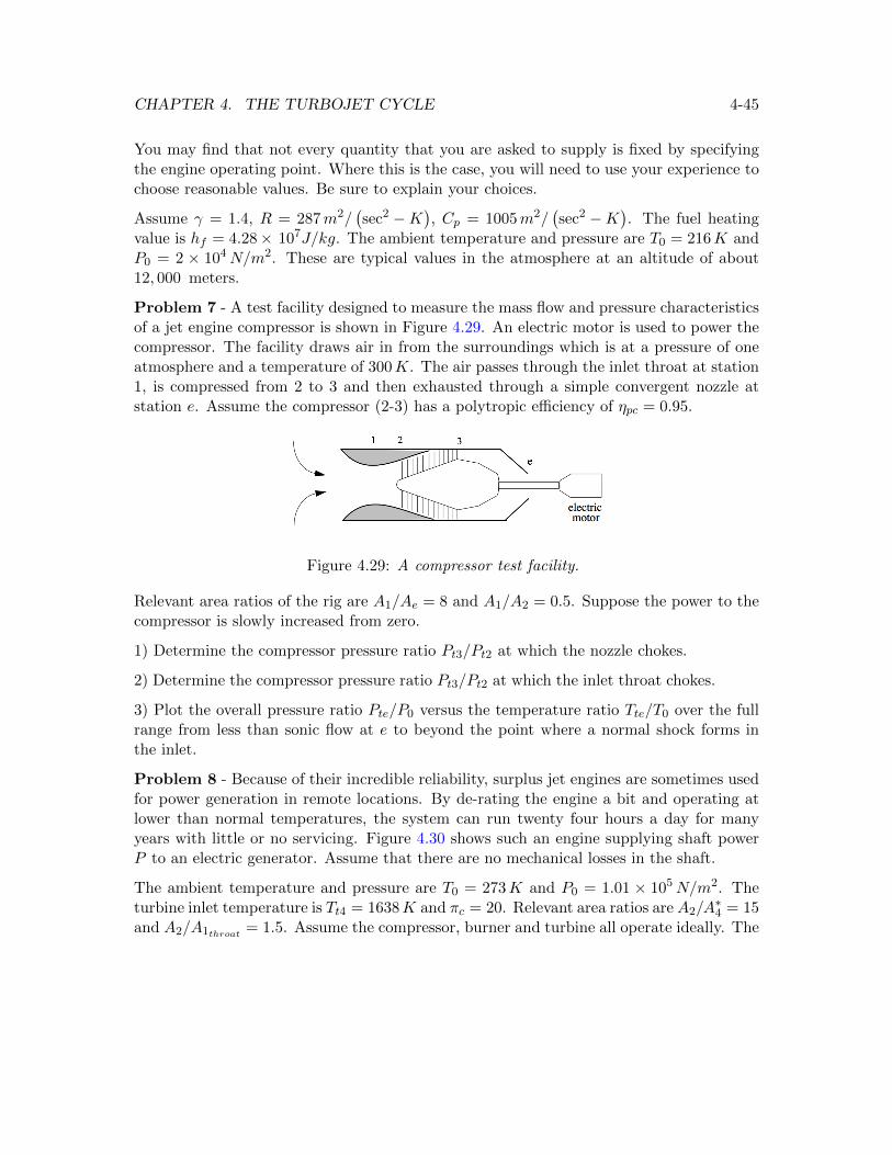
CHAPTER 4. THE TURBOJET CYCLE 4-45
You may find that not every quantity that you are asked to supply is fixed by specifyingthe engine operating point. Where this is the case, you will need to use your experience tochoose reasonable values. Be sure to explain your choices.
Assume γ = 1.4, R = 287m2/(sec2 −K
), Cp = 1005m2/
(sec2 −K
). The fuel heating
value is hf = 4.28× 10⁷J/kg. The ambient temperature and pressure are T0 = 216K andP0 = 2 × 10⁴N/m2. These are typical values in the atmosphere at an altitude of about12, 000 meters.
Problem 7 - A test facility designed to measure the mass flow and pressure characteristicsof a jet engine compressor is shown in Figure 4.29. An electric motor is used to power thecompressor. The facility draws air in from the surroundings which is at a pressure of oneatmosphere and a temperature of 300K. The air passes through the inlet throat at station1, is compressed from 2 to 3 and then exhausted through a simple convergent nozzle atstation e. Assume the compressor (2-3) has a polytropic efficiency of ηpc = 0.95.
Figure 4.29: A compressor test facility.
Relevant area ratios of the rig are A1/Ae = 8 and A1/A2 = 0.5. Suppose the power to thecompressor is slowly increased from zero.
1) Determine the compressor pressure ratio Pt3/Pt2 at which the nozzle chokes.
2) Determine the compressor pressure ratio Pt3/Pt2 at which the inlet throat chokes.
3) Plot the overall pressure ratio Pte/P0 versus the temperature ratio Tte/T0 over the fullrange from less than sonic flow at e to beyond the point where a normal shock forms inthe inlet.
Problem 8 - Because of their incredible reliability, surplus jet engines are sometimes usedfor power generation in remote locations. By de-rating the engine a bit and operating atlower than normal temperatures, the system can run twenty four hours a day for manyyears with little or no servicing. Figure 4.30 shows such an engine supplying shaft powerP to an electric generator. Assume that there are no mechanical losses in the shaft.
The ambient temperature and pressure are T0 = 273K and P0 = 1.01 × 10⁵N/m2. Theturbine inlet temperature is Tt4 = 1638K and πc = 20. Relevant area ratios are A2/A
∗4 = 15
and A2/A1throat = 1.5. Assume the compressor, burner and turbine all operate ideally. The
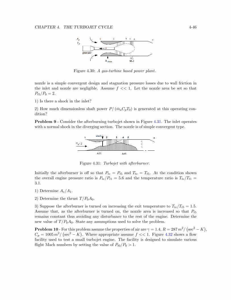
CHAPTER 4. THE TURBOJET CYCLE 4-46
Figure 4.30: A gas-turbine based power plant.
nozzle is a simple convergent design and stagnation pressure losses due to wall friction inthe inlet and nozzle are negligible. Assume f << 1. Let the nozzle area be set so thatPt5/P0 = 2.
1) Is there a shock in the inlet?
2) How much dimensionless shaft power P/ (maCpT0) is generated at this operating con-dition?
Problem 9 - Consider the afterburning turbojet shown in Figure 4.31. The inlet operateswith a normal shock in the diverging section. The nozzle is of simple convergent type.
Figure 4.31: Turbojet with afterburner.
Initially the afterburner is off so that Pte = Pt5 and Tte = Tt5. At the condition shownthe overall engine pressure ratio is Pte/Pt1 = 5.6 and the temperature ratio is Tte/Tt1 =3.1.
1) Determine Ae/A1.
2) Determine the thrust T/P0A0.
3) Suppose the afterburner is turned on increasing the exit temperature to Tte/Tt5 = 1.5.Assume that, as the afterburner is turned on, the nozzle area is increased so that Pt5remains constant thus avoiding any disturbance to the rest of the engine. Determine thenew value of T/P0A0. State any assumptions used to solve the problem.
Problem 10 - For this problem assume the properties of air are γ = 1.4, R = 287m2/(sec2 −K
),
Cp = 1005m2/(sec2 −K
). Where appropriate assume f << 1. Figure 4.32 shows a flow
facility used to test a small turbojet engine. The facility is designed to simulate variousflight Mach numbers by setting the value of Pt0/P0 > 1.
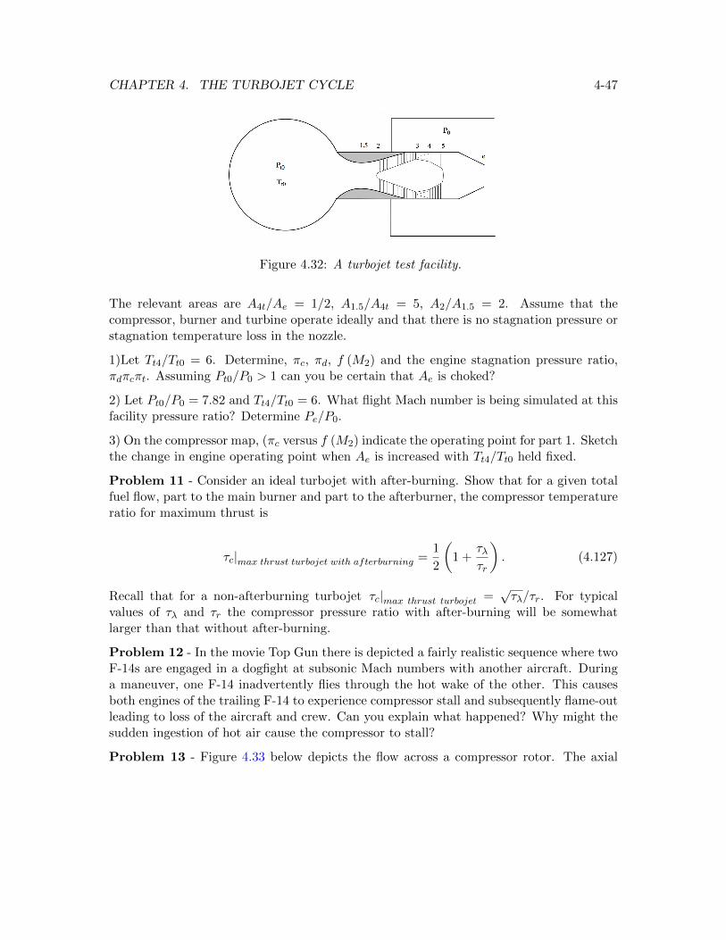
CHAPTER 4. THE TURBOJET CYCLE 4-47
Figure 4.32: A turbojet test facility.
The relevant areas are A4t/Ae = 1/2, A1.5/A4t = 5, A2/A1.5 = 2. Assume that thecompressor, burner and turbine operate ideally and that there is no stagnation pressure orstagnation temperature loss in the nozzle.
1)Let Tt4/Tt0 = 6. Determine, πc, πd, f (M2) and the engine stagnation pressure ratio,πdπcπt. Assuming Pt0/P0 > 1 can you be certain that Ae is choked?
2) Let Pt0/P0 = 7.82 and Tt4/Tt0 = 6. What flight Mach number is being simulated at thisfacility pressure ratio? Determine Pe/P0.
3) On the compressor map, (πc versus f (M2) indicate the operating point for part 1. Sketchthe change in engine operating point when Ae is increased with Tt4/Tt0 held fixed.
Problem 11 - Consider an ideal turbojet with after-burning. Show that for a given totalfuel flow, part to the main burner and part to the afterburner, the compressor temperatureratio for maximum thrust is
τc|max thrust turbojet with afterburning =1
2
(1 +
τλτr
). (4.127)
Recall that for a non-afterburning turbojet τc|max thrust turbojet =√τλ/τr. For typical
values of τλ and τr the compressor pressure ratio with after-burning will be somewhatlarger than that without after-burning.
Problem 12 - In the movie Top Gun there is depicted a fairly realistic sequence where twoF-14s are engaged in a dogfight at subsonic Mach numbers with another aircraft. Duringa maneuver, one F-14 inadvertently flies through the hot wake of the other. This causesboth engines of the trailing F-14 to experience compressor stall and subsequently flame-outleading to loss of the aircraft and crew. Can you explain what happened? Why might thesudden ingestion of hot air cause the compressor to stall?
Problem 13 - Figure 4.33 below depicts the flow across a compressor rotor. The axial
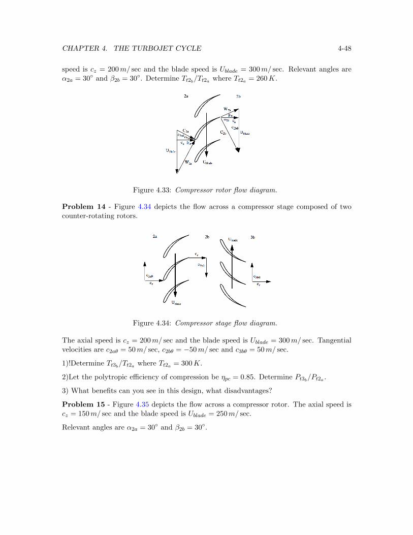
CHAPTER 4. THE TURBOJET CYCLE 4-48
speed is cz = 200m/ sec and the blade speed is Ublade = 300m/ sec. Relevant angles areα2a = 30◦ and β2b = 30◦. Determine Tt2b/Tt2a where Tt2a = 260K.
Figure 4.33: Compressor rotor flow diagram.
Problem 14 - Figure 4.34 depicts the flow across a compressor stage composed of twocounter-rotating rotors.
Figure 4.34: Compressor stage flow diagram.
The axial speed is cz = 200m/ sec and the blade speed is Ublade = 300m/ sec. Tangentialvelocities are c2aθ = 50m/ sec, c2bθ = −50m/ sec and c3bθ = 50m/ sec.
1)!Determine Tt3b/Tt2a where Tt2a = 300K.
2)Let the polytropic efficiency of compression be ηpc = 0.85. Determine Pt3b/Pt2a .
3) What benefits can you see in this design, what disadvantages?
Problem 15 - Figure 4.35 depicts the flow across a compressor rotor. The axial speed iscz = 150m/ sec and the blade speed is Ublade = 250m/ sec.
Relevant angles are α2a = 30◦ and β2b = 30◦.
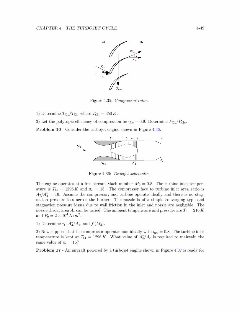
CHAPTER 4. THE TURBOJET CYCLE 4-49
Figure 4.35: Compressor rotor.
1) Determine Tt2b/Tt2a where Tt2a = 350K.
2) Let the polytopic efficiency of compression be ηpc = 0.9. Determine Pt2b/Pt2a.
Problem 16 - Consider the turbojet engine shown in Figure 4.36.
Figure 4.36: Turbojet schematic.
The engine operates at a free stream Mach number M0 = 0.8. The turbine inlet temper-ature is Tt4 = 1296K and πc = 15. The compressor face to turbine inlet area ratio isA2/A
∗4 = 10. Assume the compressor, and turbine operate ideally and there is no stag-
nation pressure loss across the burner. The nozzle is of a simple converging type andstagnation pressure losses due to wall friction in the inlet and nozzle are negligible. Thenozzle throat area Ae can be varied. The ambient temperature and pressure are T0 = 216Kand P0 = 2× 10⁴N/m2.
1) Determine τt, A∗4/Ae, and f (M2).
2) Now suppose that the compressor operates non-ideally with ηpc = 0.8. The turbine inlettemperature is kept at Tt4 = 1296K. What value of A∗4/Ae is required to maintain thesame value of πc = 15?
Problem 17 - An aircraft powered by a turbojet engine shown in Figure 4.37 is ready for
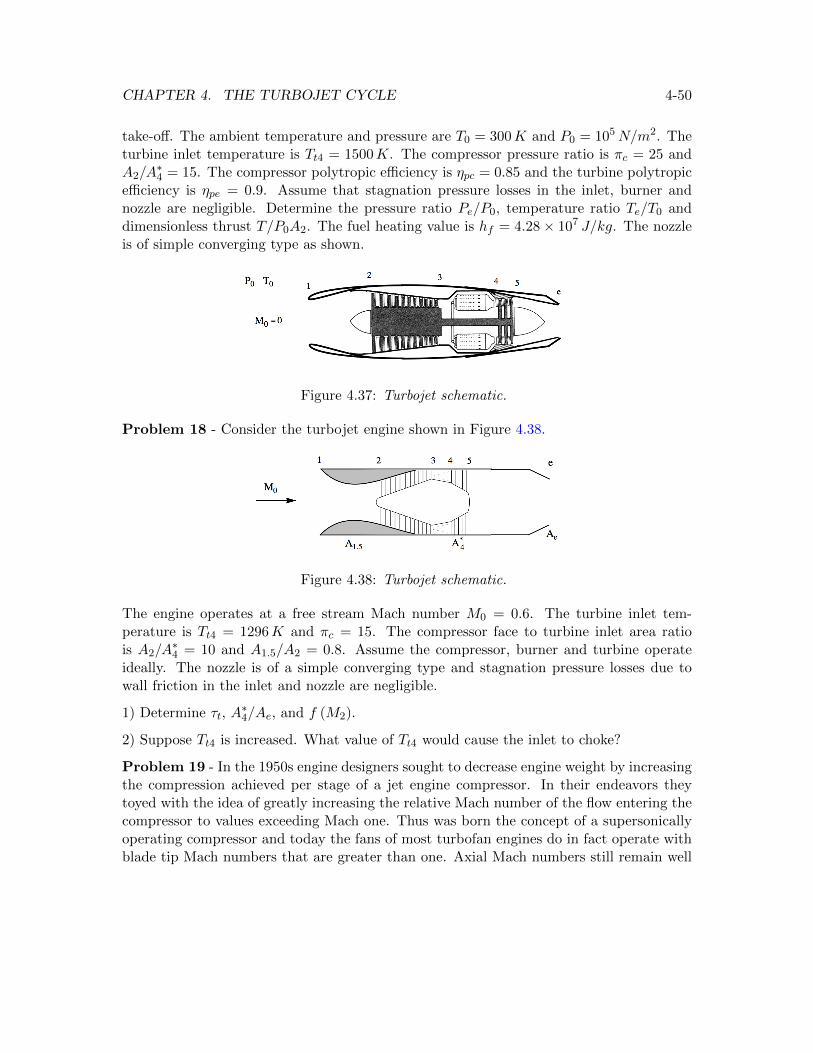
CHAPTER 4. THE TURBOJET CYCLE 4-50
take-off. The ambient temperature and pressure are T0 = 300K and P0 = 105N/m2. Theturbine inlet temperature is Tt4 = 1500K. The compressor pressure ratio is πc = 25 andA2/A
∗4 = 15. The compressor polytropic efficiency is ηpc = 0.85 and the turbine polytropic
efficiency is ηpe = 0.9. Assume that stagnation pressure losses in the inlet, burner andnozzle are negligible. Determine the pressure ratio Pe/P0, temperature ratio Te/T0 anddimensionless thrust T/P0A2. The fuel heating value is hf = 4.28× 10⁷ J/kg. The nozzleis of simple converging type as shown.
Figure 4.37: Turbojet schematic.
Problem 18 - Consider the turbojet engine shown in Figure 4.38.
Figure 4.38: Turbojet schematic.
The engine operates at a free stream Mach number M0 = 0.6. The turbine inlet tem-perature is Tt4 = 1296K and πc = 15. The compressor face to turbine inlet area ratiois A2/A
∗4 = 10 and A1.5/A2 = 0.8. Assume the compressor, burner and turbine operate
ideally. The nozzle is of a simple converging type and stagnation pressure losses due towall friction in the inlet and nozzle are negligible.
1) Determine τt, A∗4/Ae, and f (M2).
2) Suppose Tt4 is increased. What value of Tt4 would cause the inlet to choke?
Problem 19 - In the 1950s engine designers sought to decrease engine weight by increasingthe compression achieved per stage of a jet engine compressor. In their endeavors theytoyed with the idea of greatly increasing the relative Mach number of the flow entering thecompressor to values exceeding Mach one. Thus was born the concept of a supersonicallyoperating compressor and today the fans of most turbofan engines do in fact operate withblade tip Mach numbers that are greater than one. Axial Mach numbers still remain well
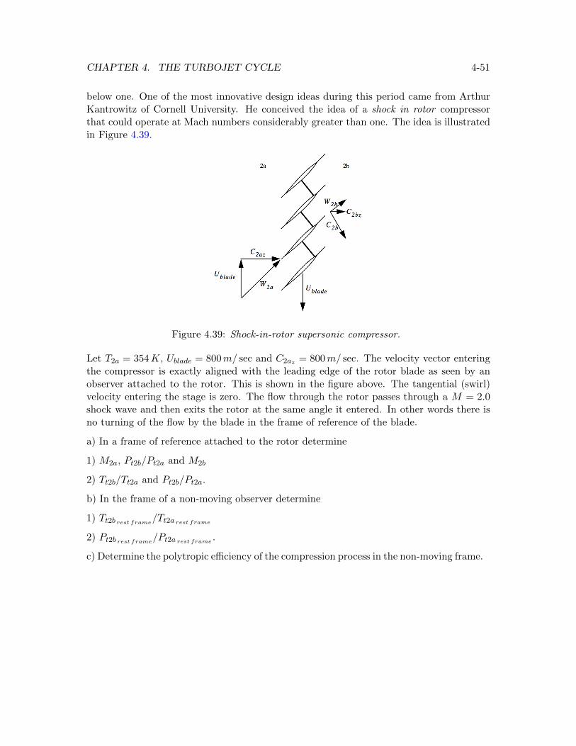
CHAPTER 4. THE TURBOJET CYCLE 4-51
below one. One of the most innovative design ideas during this period came from ArthurKantrowitz of Cornell University. He conceived the idea of a shock in rotor compressorthat could operate at Mach numbers considerably greater than one. The idea is illustratedin Figure 4.39.
Figure 4.39: Shock-in-rotor supersonic compressor.
Let T2a = 354K, Ublade = 800m/ sec and C2az = 800m/ sec. The velocity vector enteringthe compressor is exactly aligned with the leading edge of the rotor blade as seen by anobserver attached to the rotor. This is shown in the figure above. The tangential (swirl)velocity entering the stage is zero. The flow through the rotor passes through a M = 2.0shock wave and then exits the rotor at the same angle it entered. In other words there isno turning of the flow by the blade in the frame of reference of the blade.
a) In a frame of reference attached to the rotor determine
1) M2a, Pt2b/Pt2a and M2b
2) Tt2b/Tt2a and Pt2b/Pt2a.
b) In the frame of a non-moving observer determine
1) Tt2b rest frame/Tt2a rest frame
2) Pt2b rest frame/Pt2a rest frame .
c) Determine the polytropic efficiency of the compression process in the non-moving frame.
Chapter 5
The Turbofan cycle
5.1 Turbofan thrust
Figure 5.1 illustrates two generic turbofan engine designs. The upper figure shows a modernhigh bypass ratio engine designed for long distance cruise at subsonic Mach numbers around0.83 typical of a commercial aircraft. The fan utilizes a single stage composed of a largediameter fan (rotor) with wide chord blades followed by a single nozzle stage (stator). Thebypass ratio is 5.8 and the fan pressure ratio is 1.9. The lower figure shows a militaryturbofan designed for high performance at supersonic Mach numbers in the range of 1.1to 1.5. The fan on this engine has three stages with an overall pressure ratio of about 6and a bypass ratio of only about 0.6. One of the goals of this chapter is to understandwhy these engines look so different in terms the differences in flight condition for whichthey are designed. In this context we will begin to appreciate that the thermodynamic andgas dynamic analysis of these engines defines a continuum of cycles as a function of Machnumber. We had a glimpse of this when we determined that the maximum thrust turbojetis characterized by
τcmax thrust=
√τλτr
. (5.1)
For fixed turbine inlet temperature and altitude, as the Mach number increases the opti-mum compression decreases and at some point it becomes desirable to convert the turbojetto a ramjet. We will see a similar kind of trend emerge for the turbofan where it replacesthe turbojet as the optimum cycle for lower Mach numbers. Superimposed on all this is ahistorical technology trend where, with better materials and cooling schemes, the allowableturbine inlet temperature has increased with time. This tends to lead to an optimum cyclewith higher compression and higher bypass ratio at a given Mach number.
5-1
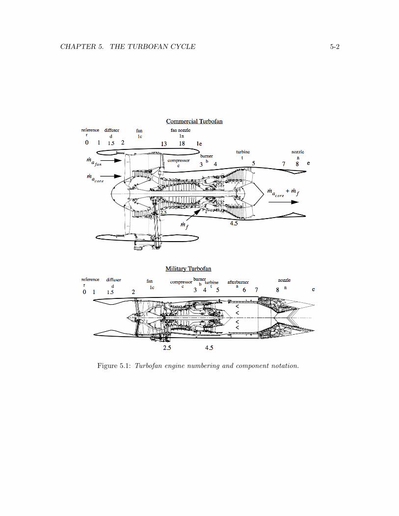
CHAPTER 5. THE TURBOFAN CYCLE 5-2
Figure 5.1: Turbofan engine numbering and component notation.
CHAPTER 5. THE TURBOFAN CYCLE 5-3
The thrust equation for the turbofan is similar to the usual relation except that it includesthe thrust produced by the fan.
T = macore (Ue − U0) + mafan (Ue1 − U0) + mfUe + (Pe − P0)Ae + (Pe1 − P0)A1e (5.2)
The total air mass flow is
ma = macore + mafan . (5.3)
The fuel/air ratio is defined in terms of the total air mass flow.
f =mf
ma(5.4)
The bypass fraction is defined as
B =mafan
mafan + macore
(5.5)
and the bypass ratio is
β =mafan
macore
. (5.6)
Note that
β =B
1−B
B =β
1 + β.
(5.7)
5.2 The ideal turbofan cycle
The ideal turbofan cycle is characterized by the following assumptions
Pe = P0
Pe1 = P0
(5.8)
CHAPTER 5. THE TURBOFAN CYCLE 5-4
and
πd = 1
πb = 1
πn = 1
πn1 = 1
(5.9)
and
πc = τcγγ−1
πc1 = τc1γγ−1
πt = τtγγ−1 .
(5.10)
For a fully expanded exhaust the normalized thrust is
T
maa0= M0
((1−B + f)
(UeU0− 1
)+B
(Ue1U0− 1
)+ f
)(5.11)
or, in terms of the bypass ratio with f << 1,
T
maa0= M0
((1
1 + β
)(UeU0− 1
)+
(β
1 + β
)(Ue1U0− 1
)). (5.12)
5.2.1 The fan bypass stream
First work out the velocity ratio for the fan stream.
Ue1U0
=Me1
M0
√Te1T0
(5.13)
The exit Mach number is determined from the stagnation pressure.
Pte1 = P0πrπc1 = Pe1
(1 +
γ − 1
2Me1
2
) γγ−1
(5.14)
CHAPTER 5. THE TURBOFAN CYCLE 5-5
Since the nozzle is fully expanded and the fan is assumed to behave isentropically, we canwrite
τrτc1 =
(1 +
γ − 1
2Me1
2
)(5.15)
therefore
Me12
M02 =
τrτc1 − 1
τr − 1. (5.16)
The exit temperature is determined from the stagnation temperature.
Tte1 = T0τrτc1 = Te1
(1 +
γ − 1
2Me1
2
)(5.17)
Noting (5.15) we can conclude that for the ideal fan
Te1 = T0. (5.18)
The exit static temperature is equal to the ambient static temperature. The velocity ratioof the fan stream is
(Ue1U0
)2
=τrτc1 − 1
τr − 1. (5.19)
5.2.2 The core stream
The velocity ratio across the core is
UeU0
=Me
M0
√TeT0. (5.20)
The analysis of the stagnation pressure and temperature is exactly the same as for theideal turbojet.
Pte = P0πrπcπt = Pe
(1 +
γ − 1
2Me
2
) γγ−1
(5.21)
CHAPTER 5. THE TURBOFAN CYCLE 5-6
Since the nozzle is fully expanded and the compressor and turbine operate ideally the Machnumber ratio is
Me2
M02 =
τrτcτt − 1
τr − 1. (5.22)
The temperature ratio is also determined in the same way in terms of component temper-ature parameters.
Tte = T0τrτdτcτbτtτn (5.23)
In the ideal turbofan we assume that the diffuser and nozzle flows are adiabatic and so
Tte = T0τrτcτbτt = Te
(1 +
γ − 1
2Me
2
)= Teτrτcτt (5.24)
from which is determined
TeT0
= τb =τλτrτc
. (5.25)
The velocity ratio across the core is
(UeU0
)2
=
(τrτcτt − 1
τr − 1
)τλτrτc
. (5.26)
5.2.3 Turbine-compressor-fan matching
The work taken out of the flow by the high and low pressure turbine is used to drive boththe compressor and the fan.
(macore + mf ) (ht4 − ht5) = macore (ht3 − ht2) + mafan (ht31 − ht2) (5.27)
Divide (5.27) by maCpT0 and rearrange. The work matching condition for a turbofanis
τt = 1− τrτλ
(1−B
1−B + f(τc − 1) +
B
1−B + f(τc1 − 1)
). (5.28)
CHAPTER 5. THE TURBOFAN CYCLE 5-7
The approximation f � 1 is generally pretty good for a turbofan. Using this approximationthe work matching condition becomes
τt = 1− τrτλ
((τc − 1) + β (τc1 − 1)) (5.29)
where the bypass ratio β appears for the first time. If the bypass ratio goes to zero thematching condition reduces to the usual turbojet formula.
5.2.4 The fuel/air ratio
The fuel/air ratio is determined from the energy balance across the burner.
mf (hf − ht4) = macore (ht4 − ht3) (5.30)
Divide (5.30) by maCpT0 and rearrange. The result is
f =
(1
1 + β
)τλ − τrτcτf − τλ
. (5.31)
5.3 Maximum specific impulse ideal turbofan
The non-dimensionalized specific impulse can be expressed in terms of thrust and fuel/airratio as
Ispg
a0=
(T
mfg
)(g
a0
)=
(T
maa0
)(1
f
). (5.32)
Substitute (5.12) and (5.31) into (5.32). The result is
Ispg
a0= M0
(τf − τλτλ − τrτc
)((UeU0− 1
)+ β
(Ue1U0− 1
)). (5.33)
The question is: what value of β maximizes the specific impulse? Differentiate (5.33) withrespect to β and note that β appears in (5.29).
∂
∂β
(Ispg
a0
)= M0
(τf − τλτλ − τrτc
)(∂
∂β
(UeU0
)+
(Ue1U0− 1
))= 0 (5.34)
CHAPTER 5. THE TURBOFAN CYCLE 5-8
We can write (5.34) as
1
2 (Ue/U0)
∂
∂β
(UeU0
)2
+
(Ue1U0− 1
)= 0 (5.35)
or
1
2 (Ue/U0)
(τλ
τr − 1
)∂τt∂β
= −(Ue1U0− 1
). (5.36)
Equation (5.36) becomes
1
2 (Ue/U0)
(τr (τc1 − 1)
τr − 1
)=
(Ue1U0− 1
). (5.37)
From (5.19),the expression in parentheses on the left side of (5.37) can be written
1
2 (Ue/U0)
((Ue1U0
)2
− 1
)=
(Ue1U0− 1
). (5.38)
Factor the left side of (5.38) and cancel common factors on both sides. The velocitycondition for a maximum impulse ideal turbofan is
(Ue1U0− 1
)= 2
(UeU0− 1
). (5.39)
According to this result, for an ideal turbofan one would want to design the turbine suchthat the velocity increment across the fan was twice that across the core in order to achievemaximum specific impulse. Recall that Ue/U0 depends on β through (5.29) (and weaklythough (5.31) which we neglect). The value of β that produces the condition (5.39) corre-sponding to the maximum impulse ideal turbofan is
β max impulse ideal turbofan =
1
τc1 − 1
((τλτrτc
− 1
)(τc − 1) +
τλ (τr − 1)
τr2τc− 1
4
(τr − 1
τr
)((τrτc1 − 1
τr − 1
)1/2
+ 1
)).
(5.40)
Figure 5.2 shows how the optimum bypass ratio (5.40) varies with flight Mach number fora given set of engine parameters.
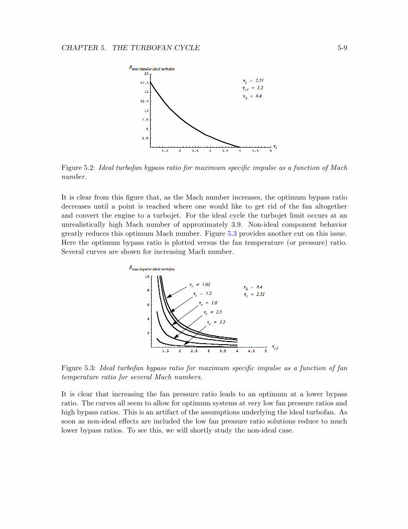
CHAPTER 5. THE TURBOFAN CYCLE 5-9
Figure 5.2: Ideal turbofan bypass ratio for maximum specific impulse as a function of Machnumber.
It is clear from this figure that, as the Mach number increases, the optimum bypass ratiodecreases until a point is reached where one would like to get rid of the fan altogetherand convert the engine to a turbojet. For the ideal cycle the turbojet limit occurs at anunrealistically high Mach number of approximately 3.9. Non-ideal component behaviorgreatly reduces this optimum Mach number. Figure 5.3 provides another cut on this issue.Here the optimum bypass ratio is plotted versus the fan temperature (or pressure) ratio.Several curves are shown for increasing Mach number.
Figure 5.3: Ideal turbofan bypass ratio for maximum specific impulse as a function of fantemperature ratio for several Mach numbers.
It is clear that increasing the fan pressure ratio leads to an optimum at a lower bypassratio. The curves all seem to allow for optimum systems at very low fan pressure ratios andhigh bypass ratios. This is an artifact of the assumptions underlying the ideal turbofan. Assoon as non-ideal effects are included the low fan pressure ratio solutions reduce to muchlower bypass ratios. To see this, we will shortly study the non-ideal case.
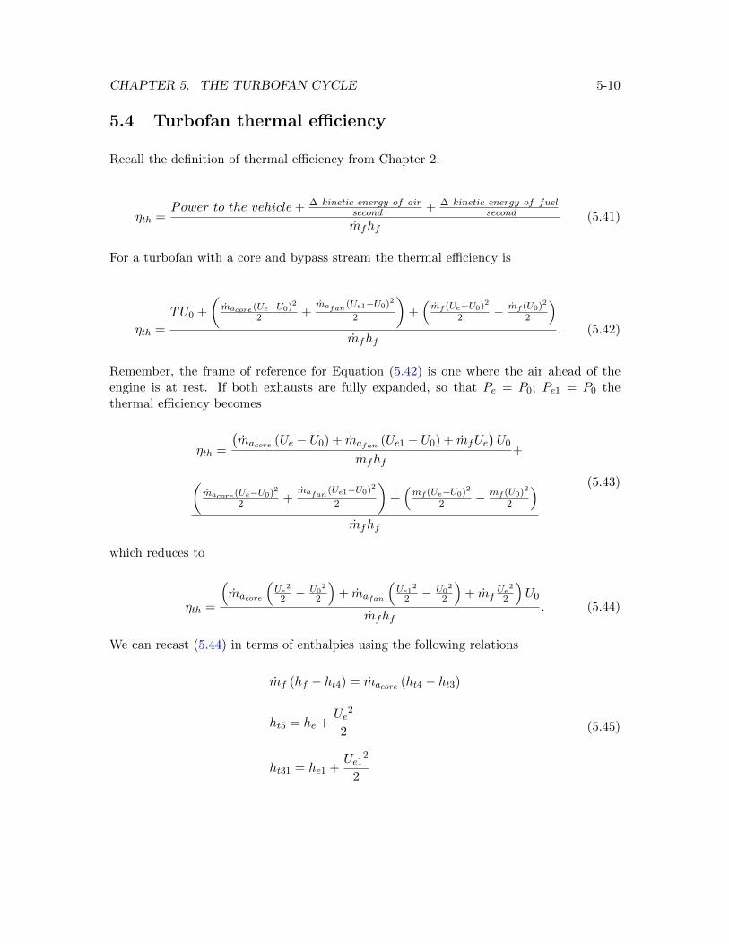
CHAPTER 5. THE TURBOFAN CYCLE 5-10
5.4 Turbofan thermal efficiency
Recall the definition of thermal efficiency from Chapter 2.
ηth =Power to the vehicle+ ∆ kinetic energy of air
second + ∆ kinetic energy of fuelsecond
mfhf(5.41)
For a turbofan with a core and bypass stream the thermal efficiency is
ηth =
TU0 +
(macore (Ue−U0)2
2 +mafan (Ue1−U0)2
2
)+(mf (Ue−U0)2
2 − mf (U0)2
2
)mfhf
. (5.42)
Remember, the frame of reference for Equation (5.42) is one where the air ahead of theengine is at rest. If both exhausts are fully expanded, so that Pe = P0; Pe1 = P0 thethermal efficiency becomes
ηth =
(macore (Ue − U0) + mafan (Ue1 − U0) + mfUe
)U0
mfhf+
(macore (Ue−U0)2
2 +mafan (Ue1−U0)2
2
)+(mf (Ue−U0)2
2 − mf (U0)2
2
)mfhf
(5.43)
which reduces to
ηth =
(macore
(Ue2
2 −U0
2
2
)+ mafan
(Ue1
2
2 − U02
2
)+ mf
Ue2
2
)U0
mfhf. (5.44)
We can recast (5.44) in terms of enthalpies using the following relations
mf (hf − ht4) = macore (ht4 − ht3)
ht5 = he +Ue
2
2
ht31 = he1 +Ue1
2
2
(5.45)
CHAPTER 5. THE TURBOFAN CYCLE 5-11
where the fan and core nozzle streams are assumed to be adiabatic. Now
ηth =macore ((ht5 − he)− (ht0 − h0)) + mafan ((ht31 − h1e)− (ht0 − h0)) + mf (ht5 − he)
(mf + macore)ht4 − macoreht3.
(5.46)
Rearrange (5.46) to read
ηth =(macore + mf )ht5 + mafanht31 −
(macore + mafan
)ht0
(mf + macore)ht4 − macoreht3−
macore (he − h0) + mafan (he1 − h0) + mfhe
(mf + macore)ht4 − macoreht3.
(5.47)
Recall the turbofan work balance (5.27). This relation can be rearranged to read
(mf + macore)ht4 − macoreht3 = (macore + mf )ht5 + mafanht31 −(macore + mafan
)ht0(5.48)
where it has been assumed that the inlet is adiabatic ht2 = ht0. Now use (5.48) to replacethe numerator or denominator in the first term of (5.47). The thermal efficiency finallyreads
ηth = 1−Qrejected during the cycleQinput during the cycle
= 1−(macore + mf ) (he − h0) + mafan (he1 − h0) + mfh0
(mf + macore)ht4 − macoreht3.
(5.49)
The expression in (5.49) for the heat rejected during the cycle
Qrejected during the cycle = (macore + mf ) (he − h0) + mafan (he1 − h0) + mfh0 (5.50)
brings to mind the discussion of thermal efficiency in Chapter 2. The heat rejected com-prises heat conduction to the surrounding atmosphere from the fan and core mass flowsplus physical removal from the thermally equilibrated nozzle flow of a portion equal to theadded fuel mass flow. From this perspective the added fuel mass carries its fuel enthalpyinto the system and the exhausted fuel mass carries its ambient enthalpy out of the systemand there is no net mass increase or decrease to the system.
CHAPTER 5. THE TURBOFAN CYCLE 5-12
The main assumptions underlying (5.49) are that the engine operates adiabatically, theshaft mechanical efficiency is one, and the burner combustion efficiency is one. Engine com-ponents are not assumed to operate ideally; They are not assumed to be isentropic.
5.4.1 Thermal efficiency of the ideal turbofan
For the ideal cycle, assuming constant Cp, equation (5.49) in terms of temperatures be-comes
ηthideal turbofan = 1−(
(1 + (1 + β) f)Te − T0
(1 + (1 + β) f)Tt4 − Tt3
)= 1−
(1
τrτc
)((1 + (1 + β) f) TeT0
− 1
(1 + (1 + β) f) τλτrτc− 1
).
(5.51)
Using (5.25) Equation (5.51) becomes
ηth ideal turbofan = 1−(
1
τrτc
)(5.52)
which is identical to the thermal efficiency of the ideal turbojet. Notice that for the idealturbofan with
he1 = h0
the heat rejected by the fan stream is zero. Therefore the thermal efficiency of the idealturbofan is independent of the parameters of the fan stream.
5.5 The non-ideal turbofan
The fan, compressor and turbine polytropic relations are
πc1 = τc1γηpc1γ−1
πc = τcγηpcγ−1
πt = τtγ
(γ−1)ηpe
(5.53)
CHAPTER 5. THE TURBOFAN CYCLE 5-13
where ηpc1 is the polytropic efficiency of the fan. The polytropic efficiencies ηpc, ηpc1 andηpe are all less than one. The inlet, burner and nozzles all operate with some stagnationpressure loss.
πd < 1
πn1 < 1
πn < 1
πb < 1
(5.54)
5.5.1 Non-ideal fan stream
The stagnation pressure ratio across the fan is
Pte1 = P0πrπdπc1πn1 = Pe1
(1 +
γ − 1
2Me1
2
) γγ−1
. (5.55)
The fan nozzle is still assumed to be fully expanded and so the Mach number ratio for thenon-ideal turbofan is
(Me1
M0
)2
=τrτc1
ηpc1(πdπn1)γ−1γ − 1
τr − 1. (5.56)
The stagnation temperature is (assuming the inlet and fan nozzle are adiabatic)
Tte1 = T0τrτc1 = Te1
(1 +
γ − 1
2Me1
2
)= Te1τrτc1
ηpc1(πdπn1)γ−1γ (5.57)
and
Te1T0
=τc1
1−ηpc1
(πdπn1)γ−1γ
. (5.58)
Now the velocity ratio across the non-ideal fan is
(Ue1U0
)2
=1
τr − 1
(τrτc1 −
τc11−ηpc1
(πdπn1)γ−1γ
). (5.59)
CHAPTER 5. THE TURBOFAN CYCLE 5-14
5.5.2 Non-ideal core stream
The stagnation pressure across the core is
Pte1 = P0πrπdπcπbπtπn = Pe
(1 +
γ − 1
2Me
2
) γγ−1
. (5.60)
The core nozzle is fully expanded and so the Mach number ratio across the non-ideal coreis
(Me
M0
)2
=τrτc
ηpcτt1ηpe (πdπbπn)
γ−1γ − 1
τr − 1. (5.61)
In the non-ideal turbofan we continue to assume that the diffuser and nozzle flows areadiabatic and so
Tte = Teτrτcηpcτt
1ηpe (πdπbπn)
γ−1γ (5.62)
from which is determined
TeT0
=τc
1−ηpcτt
(1− 1
ηpe
)τλ
τrτc(πdπbπn)γ−1γ
. (5.63)
The velocity ratio across the non-ideal core is
(UeU0
)2
=1
τr − 1
τλτt − τc1−ηpcτt
(1− 1
ηpe
)τλ
τrτc(πdπbπn)γ−1γ
. (5.64)
The work balance across the engine remains essentially the same as in the ideal cycle
τt = 1− τrηmτλ
((τc − 1) + β (τc1 − 1)) (5.65)
where the shaft mechanical efficiency is defined as
ηm =macore (ht3 − ht2) + mafan (ht31 − ht2)
(mf + macore) (ht4 − ht5). (5.66)
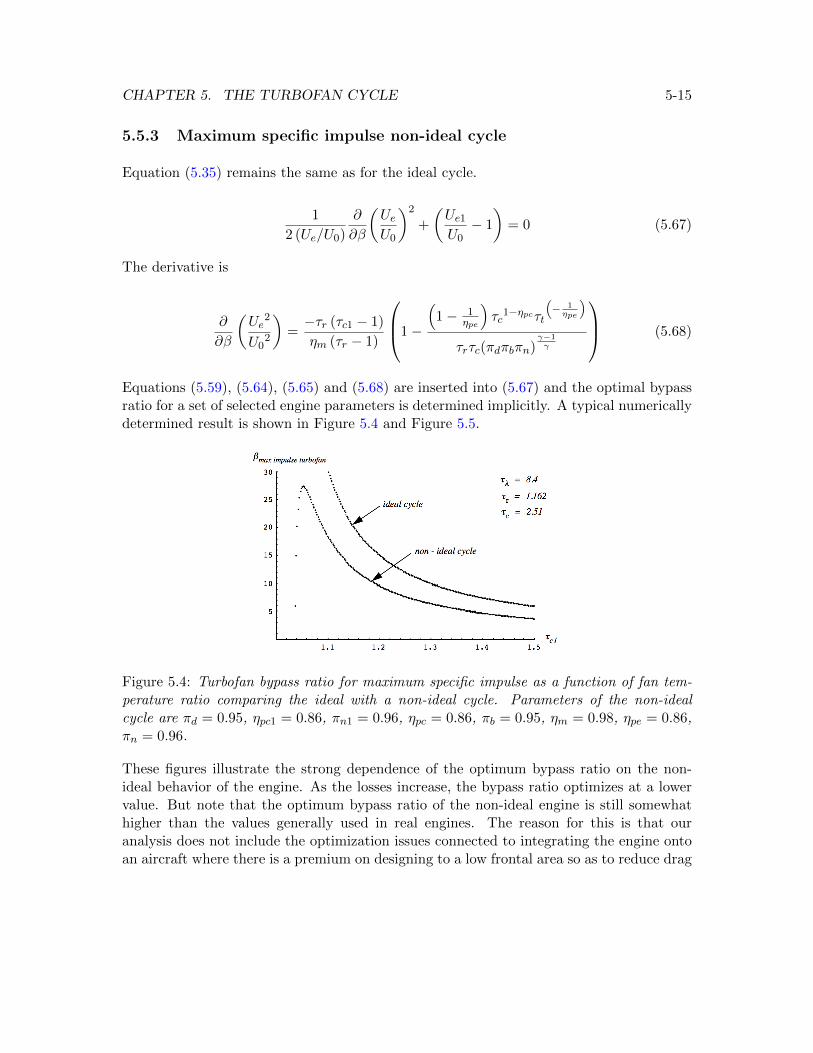
CHAPTER 5. THE TURBOFAN CYCLE 5-15
5.5.3 Maximum specific impulse non-ideal cycle
Equation (5.35) remains the same as for the ideal cycle.
1
2 (Ue/U0)
∂
∂β
(UeU0
)2
+
(Ue1U0− 1
)= 0 (5.67)
The derivative is
∂
∂β
(Ue
2
U02
)=−τr (τc1 − 1)
ηm (τr − 1)
1−
(1− 1
ηpe
)τc
1−ηpcτt
(− 1ηpe
)
τrτc(πdπbπn)γ−1γ
(5.68)
Equations (5.59), (5.64), (5.65) and (5.68) are inserted into (5.67) and the optimal bypassratio for a set of selected engine parameters is determined implicitly. A typical numericallydetermined result is shown in Figure 5.4 and Figure 5.5.
Figure 5.4: Turbofan bypass ratio for maximum specific impulse as a function of fan tem-perature ratio comparing the ideal with a non-ideal cycle. Parameters of the non-idealcycle are πd = 0.95, ηpc1 = 0.86, πn1 = 0.96, ηpc = 0.86, πb = 0.95, ηm = 0.98, ηpe = 0.86,πn = 0.96.
These figures illustrate the strong dependence of the optimum bypass ratio on the non-ideal behavior of the engine. As the losses increase, the bypass ratio optimizes at a lowervalue. But note that the optimum bypass ratio of the non-ideal engine is still somewhathigher than the values generally used in real engines. The reason for this is that ouranalysis does not include the optimization issues connected to integrating the engine ontoan aircraft where there is a premium on designing to a low frontal area so as to reduce drag
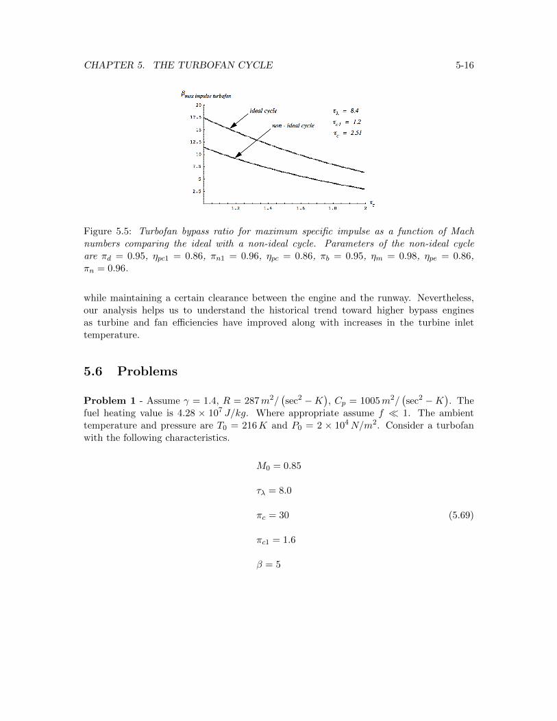
CHAPTER 5. THE TURBOFAN CYCLE 5-16
Figure 5.5: Turbofan bypass ratio for maximum specific impulse as a function of Machnumbers comparing the ideal with a non-ideal cycle. Parameters of the non-ideal cycleare πd = 0.95, ηpc1 = 0.86, πn1 = 0.96, ηpc = 0.86, πb = 0.95, ηm = 0.98, ηpe = 0.86,πn = 0.96.
while maintaining a certain clearance between the engine and the runway. Nevertheless,our analysis helps us to understand the historical trend toward higher bypass enginesas turbine and fan efficiencies have improved along with increases in the turbine inlettemperature.
5.6 Problems
Problem 1 - Assume γ = 1.4, R = 287m2/(sec2 −K
), Cp = 1005m2/
(sec2 −K
). The
fuel heating value is 4.28 × 10⁷ J/kg. Where appropriate assume f � 1. The ambienttemperature and pressure are T0 = 216K and P0 = 2 × 10⁴N/m2. Consider a turbofanwith the following characteristics.
M0 = 0.85
τλ = 8.0
πc = 30
πc1 = 1.6
β = 5
(5.69)
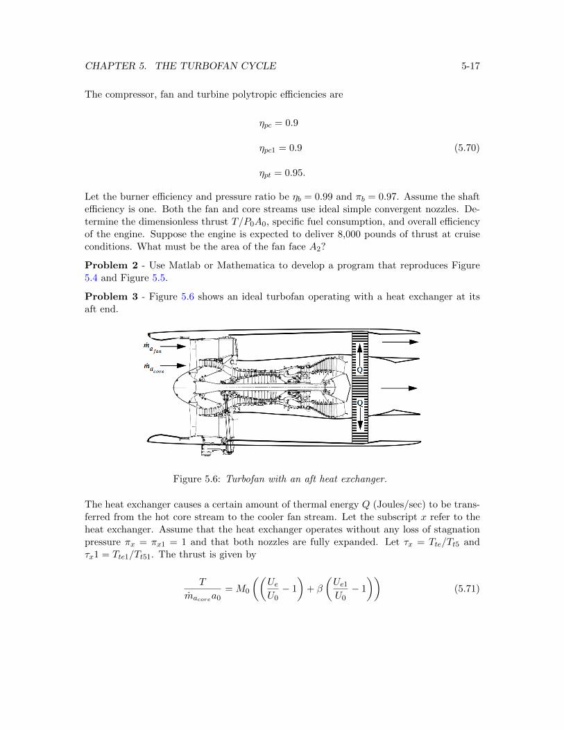
CHAPTER 5. THE TURBOFAN CYCLE 5-17
The compressor, fan and turbine polytropic efficiencies are
ηpc = 0.9
ηpc1 = 0.9
ηpt = 0.95.
(5.70)
Let the burner efficiency and pressure ratio be ηb = 0.99 and πb = 0.97. Assume the shaftefficiency is one. Both the fan and core streams use ideal simple convergent nozzles. De-termine the dimensionless thrust T/P0A0, specific fuel consumption, and overall efficiencyof the engine. Suppose the engine is expected to deliver 8,000 pounds of thrust at cruiseconditions. What must be the area of the fan face A2?
Problem 2 - Use Matlab or Mathematica to develop a program that reproduces Figure5.4 and Figure 5.5.
Problem 3 - Figure 5.6 shows an ideal turbofan operating with a heat exchanger at itsaft end.
Figure 5.6: Turbofan with an aft heat exchanger.
The heat exchanger causes a certain amount of thermal energy Q (Joules/sec) to be trans-ferred from the hot core stream to the cooler fan stream. Let the subscript x refer to theheat exchanger. Assume that the heat exchanger operates without any loss of stagnationpressure πx = πx1 = 1 and that both nozzles are fully expanded. Let τx = Tte/Tt5 andτx1 = Tte1/Tt51. The thrust is given by
T
macorea0= M0
((UeU0− 1
)+ β
(Ue1U0− 1
))(5.71)
CHAPTER 5. THE TURBOFAN CYCLE 5-18
where we have assumed f � 1.
1) Derive an expression for T/ (macorea0) in terms of τλ, τr, τc, τc1, β and τx, τx1.
2) Write down an energy balance between the core and fan streams. Suppose an amountof heat Q is exchanged. Let τx = 1−α where α = Q/macoreCpTt5, Q > 0. Show that
τx1 = 1 +
(τλτtβτrτc1
)α. (5.72)
3) Consider an ideal turbofan with the following characteristics.
T0 = 216K
M0 = 0.85
τλ = 7.5
πc = 30
πc1 = 1.6
β = 5
(5.73)
Plot T/macorea0 versus α for 0 < α < αmax where αmax corresponds to the value of α suchthat the two streams are brought to the same stagnation temperature coming out of theheat exchanger.
Problem 4 - Figure 5.7 shows a turbojet engine supplying shaft power to a lift fan. Assumethat there are no mechanical losses in the shaft but the clutch and gear box that transferspower to the fan has an efficiency of 80%. That is, only 80% of the shaft power is used toincrease the enthalpy of the air flow through the lift fan. The air mass flow rate throughthe lift fan is equal to twice the air mass flow rate through the engine mLift Fan = 2ma.The polytropic efficiency of the lift fan is ηpLift Fan = 0.9 and the air flow through the liftfan is all subsonic. The flight speed is zero.
The ambient temperature and pressure are T0 = 300K and P0 = 1.01 × 10⁵N/m2. Theturbine inlet temperature is Tt4 = 1800K and πc = 25. Relevant area ratios are A2/A
∗4 = 15
and A1throat/A2 = 0.5. Assume the compressor, burner and turbine all operate ideally. Thenozzle is a simple convergent design and stagnation pressure losses due to wall friction inthe inlet and nozzle are negligible. Assume f � 1. Let the nozzle area be set so thatPt5/P0 = 3.
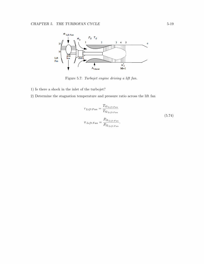
CHAPTER 5. THE TURBOFAN CYCLE 5-19
Figure 5.7: Turbojet engine driving a lift fan.
1) Is there a shock in the inlet of the turbojet?
2) Determine the stagnation temperature and pressure ratio across the lift fan
τLift Fan =Tt3Lift FanTt2Lift Fan
πLift Fan =Pt3Lift FanPt2Lift Fan
.
(5.74)
Chapter 6
The Turboprop cycle
6.1 Propellor efficiency
The turboprop cycle can be regarded as a very high bypass limit of a turbofan. Recall thatthe propulsive efficiency of a thruster with Pe = P0 and f � 1 is
ηpr =2
1 + Ue/U0. (6.1)
This expression is relevant to a propeller also where Ue is replaced by U∞ the velocity,shown schematically in Figure 6.1, that would occur far downstream of the propeller ifthere were no mixing of the propeller wake.
The achievement of high propulsive efficiency at a given thrust requires a large mass flowwith a small velocity increment. The turboprop accomplishes this by using a low pressureturbine to produce shaft power to drive a propeller. Since the propeller disc is quite largethe mass flow rate is large and a high propulsive efficiency can be achieved.
The power output of a turbine is proportional to the square of the blade speed and soturbines generally operate at high rotational speeds limited by compressibility effects atthe blade tips. The propeller diameter is much larger than the turbine diameter and so toavoid compressibility losses over the outer portion of the propeller a gearbox is required tostep the turbine rotational speed down to values that keep the propeller tip Mach numbersbelow one.
It should be pointed out that Figure 6.1 is purely a schematic and the relative size of thegearbox shown in this figure is quite unrealistic. The figure below shows a cross section of
6-1
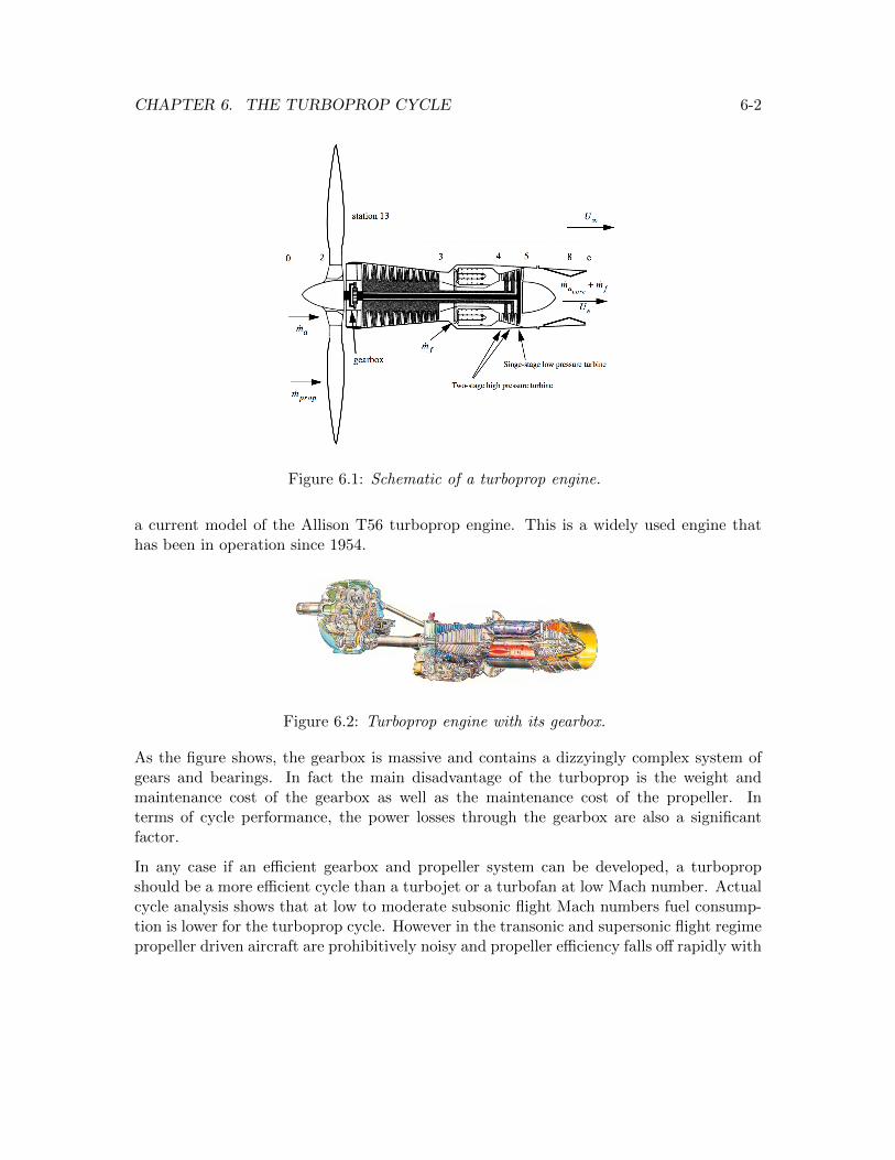
CHAPTER 6. THE TURBOPROP CYCLE 6-2
Figure 6.1: Schematic of a turboprop engine.
a current model of the Allison T56 turboprop engine. This is a widely used engine thathas been in operation since 1954.
Figure 6.2: Turboprop engine with its gearbox.
As the figure shows, the gearbox is massive and contains a dizzyingly complex system ofgears and bearings. In fact the main disadvantage of the turboprop is the weight andmaintenance cost of the gearbox as well as the maintenance cost of the propeller. Interms of cycle performance, the power losses through the gearbox are also a significantfactor.
In any case if an efficient gearbox and propeller system can be developed, a turbopropshould be a more efficient cycle than a turbojet or a turbofan at low Mach number. Actualcycle analysis shows that at low to moderate subsonic flight Mach numbers fuel consump-tion is lower for the turboprop cycle. However in the transonic and supersonic flight regimepropeller driven aircraft are prohibitively noisy and propeller efficiency falls off rapidly with
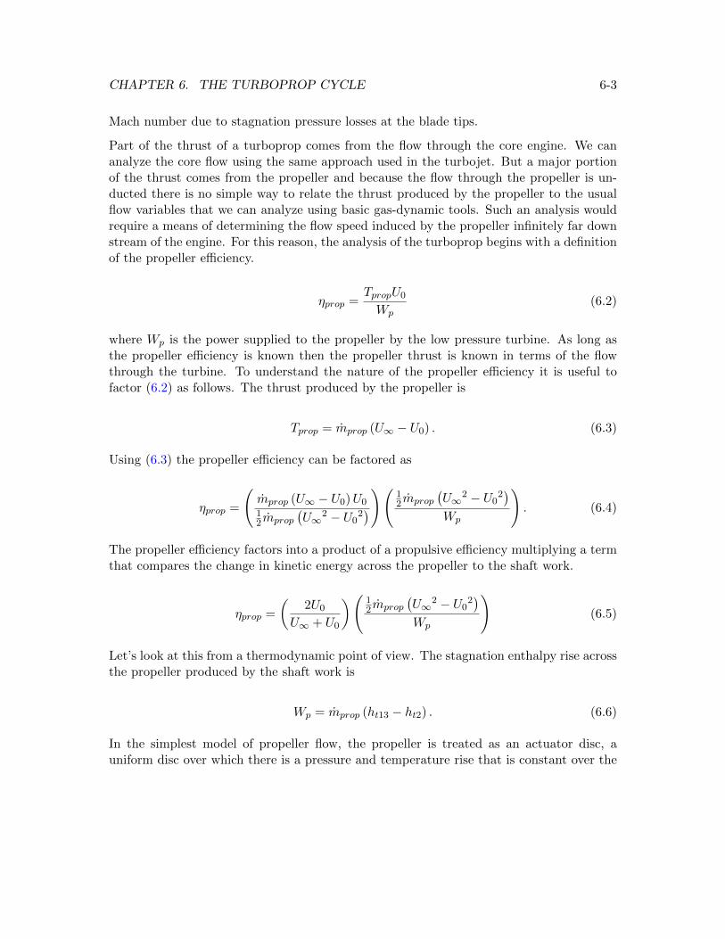
CHAPTER 6. THE TURBOPROP CYCLE 6-3
Mach number due to stagnation pressure losses at the blade tips.
Part of the thrust of a turboprop comes from the flow through the core engine. We cananalyze the core flow using the same approach used in the turbojet. But a major portionof the thrust comes from the propeller and because the flow through the propeller is un-ducted there is no simple way to relate the thrust produced by the propeller to the usualflow variables that we can analyze using basic gas-dynamic tools. Such an analysis wouldrequire a means of determining the flow speed induced by the propeller infinitely far downstream of the engine. For this reason, the analysis of the turboprop begins with a definitionof the propeller efficiency.
ηprop =TpropU0
Wp(6.2)
where Wp is the power supplied to the propeller by the low pressure turbine. As long asthe propeller efficiency is known then the propeller thrust is known in terms of the flowthrough the turbine. To understand the nature of the propeller efficiency it is useful tofactor (6.2) as follows. The thrust produced by the propeller is
Tprop = mprop (U∞ − U0) . (6.3)
Using (6.3) the propeller efficiency can be factored as
ηprop =
(mprop (U∞ − U0)U012mprop
(U∞
2 − U02))( 1
2mprop
(U∞
2 − U02)
Wp
). (6.4)
The propeller efficiency factors into a product of a propulsive efficiency multiplying a termthat compares the change in kinetic energy across the propeller to the shaft work.
ηprop =
(2U0
U∞ + U0
)( 12mprop
(U∞
2 − U02)
Wp
)(6.5)
Let’s look at this from a thermodynamic point of view. The stagnation enthalpy rise acrossthe propeller produced by the shaft work is
Wp = mprop (ht13 − ht2) . (6.6)
In the simplest model of propeller flow, the propeller is treated as an actuator disc, auniform disc over which there is a pressure and temperature rise that is constant over the
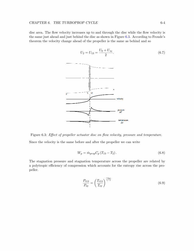
CHAPTER 6. THE TURBOPROP CYCLE 6-4
disc area. The flow velocity increases up to and through the disc while the flow velocity isthe same just ahead and just behind the disc as shown in Figure 6.3. According to Froude’stheorem the velocity change ahead of the propeller is the same as behind and so
U2 = U13 =U0 + U∞
2. (6.7)
Figure 6.3: Effect of propeller actuator disc on flow velocity, pressure and temperature.
Since the velocity is the same before and after the propeller we can write
Wp = mpropCp (T13 − T2) . (6.8)
The stagnation pressure and stagnation temperature across the propeller are related bya polytropic efficiency of compression which accounts for the entropy rise across the pro-peller.
Pt13
Pt2=
(Tt13
Tt2
) γηpcγ−1
(6.9)
CHAPTER 6. THE TURBOPROP CYCLE 6-5
Equation (6.9) can be written as
P13
P2
(1 + γ−1
2 M132
1 + γ−12 M2
2
) γγ−1
=
(T13
T2
) γηpcγ−1
(1 + γ−1
2 M132
1 + γ−12 M2
2
) γηpcγ−1
. (6.10)
The Mach number change across the propeller is small due to the small temperature changeand to a good approximation (6.10) relates the static temperatures and pressures
P13
P2=
(T13
T2
) γηpcγ−1
(6.11)
which we can write as
1 +
(P13 − P2
P2
)=
(1 +
T13 − T2
T2
) γηpcγ−1
. (6.12)
For a propeller that is lightly loaded, (6.12) can be approximated as
P13 − P2
P2
∼=γηpcγ − 1
(T13 − T2
T2
)(6.13)
or
P13 − P2∼= ηpcρ2Cp (T13 − T2) . (6.14)
The propeller thrust is
T = (P13 − P2)A (6.15)
where A is the effective area of the actuator disc. Now combine (6.8), (6.14) and (6.15) toform the propeller efficiency.
ηprop =ηpcρ2U0ACp (T13 − T2)
mpropCp (T13 − T2)=ηpcρ2U0A
ρ2U2A(6.16)
Using (6.7), the propeller efficiency becomes finally
ηprop =
(2U0
U0 + U∞
)ηpc (6.17)
CHAPTER 6. THE TURBOPROP CYCLE 6-6
which should be compared with (6.5). We can now interpret the energy factor in (6.5)as
ηpc ∼=12mprop
(U∞
2 − U02)
Wp. (6.18)
The polytropic efficiency is also related to the entropy change across the propeller. From(6.13)
dP
P= ηpc
(γ
γ − 1
)dT
T. (6.19)
According to the Gibbs equation, the entropy change across a differential part of thecompression process is
ds
Cp=dT
T−(γ − 1
γ
)dP
P= (1− ηpc)
dT
T(6.20)
and so the propeller efficiency can also be written as
ηprop =
(2U0
U0 + U∞
)(1− T
Cp
ds
dT
). (6.21)
These results tell us that the propeller efficiency is determined by two distinct mecha-nisms. The first is the propulsive efficiency that is directly related to the propeller loading(Thrust/Area). The higher the loading, the more power is lost to increasing the kineticenergy of the flow. A very highly loaded propeller is sensitive to blade stall and one of theadvantages of putting a duct around the propeller, turning it into a fan, is that a higherthrust per unit area can be achieved.
The second mechanism is the entropy rise across the propeller due to viscous friction andstagnation pressure losses due to compressibility effects. A well designed propeller shouldachieve as low an entropy rise per unit temperature rise, ds/dT , as possible. Note that evenif we could design a propeller that operated isentropically it would still have an efficiencythat is less than one.
CHAPTER 6. THE TURBOPROP CYCLE 6-7
6.2 Work output coefficient
The thrust equation for the turboprop is
Ttotal = Tcore + Tprop
or
T = ma (Ue − U0) + mfUe + (Pe − P0)Ae + mprop (U∞ − U0) .
(6.22)
Substitute the propeller efficiency
Ttotal = ma (Ue − U0) + mfUe + (Pe − P0)Ae + ηpropWp
U0. (6.23)
The core thrust has the usual form
Tcoremaa0
= M0
((1 + f)
Me
M0
√TeT0− 1
)(6.24)
where the nozzle is taken to be fully expanded Pe = P0.
The presence of U0 in the denominator of (6.23) indicates the inadequacy of the propellerefficiency for describing propeller thrust at low speeds. As a consequence the performanceof a turboprop is usually characterized in terms of power output instead of thrust. Definethe work output coefficient as
Ctotal =TtotalU0
maCpT0= Ccore + Cprop (6.25)
where from (6.23)
Ccore = (γ − 1)M02
((1 + f)
Me
M0
√TeT0− 1
)(6.26)
and
Cprop = ηpropWp
maCpT0. (6.27)
CHAPTER 6. THE TURBOPROP CYCLE 6-8
The work output coefficient and the dimensionless thrust are directly proportional to oneanother
T
P0A0=
γ
γ − 1Ctotal. (6.28)
The fuel efficiency of the turboprop is expressed in terms of the specific horsepower
SHP =pounds of fuel burned per hour
output horsepower= 3600
mfg
TtotalU0
or
SHP =2545
CpT0
(f
Ctotal
) (6.29)
where the temperature is in degrees Rankine and the heat capacity is in BTU/lbm-hr.
6.3 Power balance
The turbine drives both the compressor and propeller. The power to the propeller is
Wp = ηg ((ma + mf ) ηm (ht4 − ht5)− ma (ht3 − ht2)) (6.30)
where ηg is the gearbox efficiency and ηm is the shaft mechanical efficiency. Substitute(6.30) into (6.27) and assume the gas is calorically perfect. The work output coefficient ofthe propeller is expressed in terms of cycle parameters as
Cprop = ηpropηg ((1 + f) ηmτλ (1− τt)− τr (τc − 1)) . (6.31)
6.4 The ideal turboprop
The assumptions of the ideal turboprop are essentially the same as for the ideal turbojet,
CHAPTER 6. THE TURBOPROP CYCLE 6-9
namely
πd = 1
ηpc = 1
πb = 1
ηpe = 1
πn = 1
(6.32)
along with Pe = P0. Notice that the propeller efficiency is not assumed to be one. Theideal turboprop cycle begins with a propeller efficiency below one as reflected in the pro-portionality of the propeller efficiency to a propulsive efficiency that is inherently less thanone. There is a little bit of an inconsistency here in that the compressor is assumed to beisentropic, whereas a small part of the compression of the core air is accomplished by thepropeller. This portion of the compression is assumed to be isentropic even though the restof the propeller may behave non-isentropically. In any case there is no way to distinguishbetween the propulsive and frictional parts of the propeller efficiency in practice and so allof the entropy change across the propeller can be assigned to the portion of the mass flowthat passes outside of the core engine.
The exit Mach number is generated in the same manner as for the ideal turbojet. TheMach number ratio is
(Me
M0
)2
=
(τrτcτt − 1
τr − 1
). (6.33)
The temperature ratio is also generated in the same way.
TeT0
=τλτrτc
(6.34)
The work output coefficient of the core is
Ccore = 2 (τr − 1)
((1 + f)
(τλτrτc
)1/2(τrτcτt − 1
τr − 1
)1/2
− 1
). (6.35)
CHAPTER 6. THE TURBOPROP CYCLE 6-10
6.4.1 Optimization of the ideal turboprop cycle
The question now is: what fraction of the total thrust should be generated by the corein order to produce the maximum work output coefficient. The answer to this question isrequired in order to properly select the size of the turbine. Now determine an extremumin Ctotal with respect to τt.
∂Ctotal∂τt
=∂Ccore∂τt
+∂Cprop∂τt
= 0 (6.36)
Substitute Ccore, (6.35) and Cprop, (6.31) into (6.36) and carry out the differentiation
2 (τr − 1) (1 + f)
(τλτrτc
)1/2 1
2
(τrτcτt − 1
τr − 1
)−1/2( τrτcτr − 1
)− ηpropηg (1 + f) ηmτλ = 0
(6.37)
which simplifies to
(τλτrτc)1/2
(τrτcτt − 1
τr − 1
)−1/2
= ηpropηgηmτλ. (6.38)
Notice that the propeller, gearbox and shaft efficiencies enter the analysis as one product.Let
η = ηpropηgηm. (6.39)
Square (6.38) and solve for τt.
τt| max thrust ideal turboprop =1
τrτc+
(τr − 1)
η2τλ(6.40)
This result essentially defines the size of the turbine needed to achieve maximum workoutput coefficient which is equivalent to maximum thrust. Lets see what core enginevelocity ratio this corresponds to.
(UeU0
)2∣∣∣∣∣max thrust ideal turboprop
=τλτrτc
(1
τr − 1
)(τrτc τt|max thrust ideal turboprop − 1
)(6.41)

CHAPTER 6. THE TURBOPROP CYCLE 6-11
Substitute (6.40) into (6.41). The result is the very simple relationship
UeU0
∣∣∣∣max thrust ideal turboprop
=1
η. (6.42)
As the propeller-gearbox-shaft efficiency improves, the optimum turboprop cycle takes alarger and larger fraction of the thrust out of the propeller. This is accomplished with alarger turbine and a smaller core thrust.
The result (6.42) gives us some additional insight into the nature of the propeller efficiency.An ideal turboprop with a propeller that produced isentropic compression would have acore velocity that satisfies
Ue|max thrust ideal turboprop =U0 + U∞
2. (6.43)
The core exit speed would be the average of the upstream and far downstream veloci-ties. Referring back to (6.7) we can see that in this limit the core thruster becomes anindistinguishable part of the propeller actuator disc.
6.4.2 Compression for maximum thrust of an ideal turboprop
Once the turbine has been sized according to the above, then the thrust due to the coreengine is fixed by (6.42). It is then a matter of choosing the compressor that maximizesCprop. Differentiate (6.31) with respect to τc. Neglect f .
∂Cprop∂τc
= ηpropηg
(−ηmτλ
(∂τt∂τc
)− τr
)= ηpropηg
(−ηmτλ
(−1
τrτc2
)− τr
)(6.44)
Maximum Cprop is achieved for
τc =
√ηmτλτr
(6.45)
which is essentially the same result we obtained for the turbojet (exactly the same if we hadincluded the shaft efficiency in the turbojet analysis). At this point the required turbinetemperature ratio can determined from (6.40).
CHAPTER 6. THE TURBOPROP CYCLE 6-12
6.5 Turbine sizing for the non-ideal turboprop
The optimization problem is still essentially the same; we need to select the turbine tem-perature ratio so as to maximize the total work output coefficient.
∂Ctotal∂τt
=∂Ccore∂τt
+∂Cprop∂τt
= 0 (6.46)
Assume the core flow is fully expanded. The squared velocity ratio across the non-idealcore is
(UeU0
)2
=1
τr − 1
(τλτrτc
)τrτcτt − τc1−ηpcτt
(1− 1
ηpe
)(πdπbπn)
γ−1γ
(6.47)
and the core work output coefficient of the non-ideal turboprop is
Ccore = 2 (τr − 1)
(1 + f)
(τr − 1)1/2
(τλτrτc
)1/2τrτcτt − τc
1−ηpcτt
(1− 1
ηpe
)(πdπbπn)
γ−1γ
1/2
− 1
. (6.48)
For the non-ideal cycle the condition (6.46) becomes
(τr − 1)1/2
(τλτrτc
)1/2τrτcτt − τc
1−ηpcτt
(1− 1
ηpe
)(πdπbπn)
γ−1γ
−1/2
×τrτc − (1− 1
ηpe
)τc
1−ηpcτt
(− 1ηpe
)(πdπbπn)
γ−1γ
− ηpropηgηmτλ = 0.
(6.49)
Various flow parameters are specified in (6.49) and the turbine temperature ratio for max-imum work output coefficient is determined implicitly. Figure 6.4 shows a typical calcula-tion.
The optimum turbine temperature ratio increases with non-ideal effects indicating thata larger fraction of the total thrust is developed across the core engine of a non-idealturboprop.
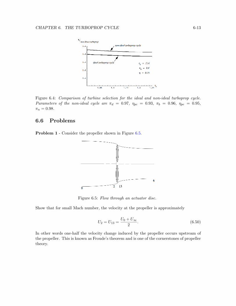
CHAPTER 6. THE TURBOPROP CYCLE 6-13
Figure 6.4: Comparison of turbine selection for the ideal and non-ideal turboprop cycle.Parameters of the non-ideal cycle are πd = 0.97, ηpc = 0.93, πb = 0.96, ηpe = 0.95,πn = 0.98.
6.6 Problems
Problem 1 - Consider the propeller shown in Figure 6.5.
Figure 6.5: Flow through an actuator disc.
Show that for small Mach number, the velocity at the propeller is approximately
U2 = U13 =U0 + U∞
2. (6.50)
In other words one-half the velocity change induced by the propeller occurs upstream ofthe propeller. This is known as Froude’s theorem and is one of the cornerstones of propellertheory.
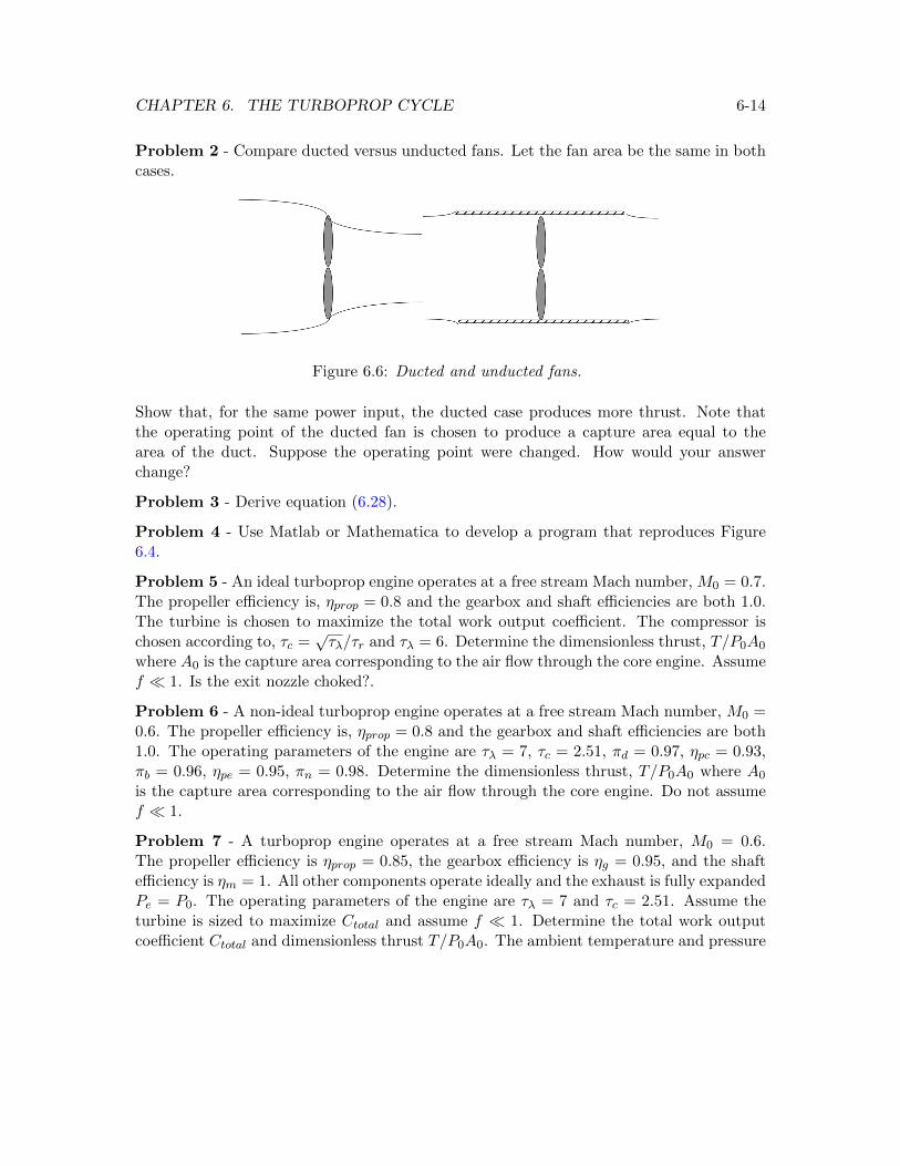
CHAPTER 6. THE TURBOPROP CYCLE 6-14
Problem 2 - Compare ducted versus unducted fans. Let the fan area be the same in bothcases.
Figure 6.6: Ducted and unducted fans.
Show that, for the same power input, the ducted case produces more thrust. Note thatthe operating point of the ducted fan is chosen to produce a capture area equal to thearea of the duct. Suppose the operating point were changed. How would your answerchange?
Problem 3 - Derive equation (6.28).
Problem 4 - Use Matlab or Mathematica to develop a program that reproduces Figure6.4.
Problem 5 - An ideal turboprop engine operates at a free stream Mach number, M0 = 0.7.The propeller efficiency is, ηprop = 0.8 and the gearbox and shaft efficiencies are both 1.0.The turbine is chosen to maximize the total work output coefficient. The compressor ischosen according to, τc =
√τλ/τr and τλ = 6. Determine the dimensionless thrust, T/P0A0
where A0 is the capture area corresponding to the air flow through the core engine. Assumef � 1. Is the exit nozzle choked?.
Problem 6 - A non-ideal turboprop engine operates at a free stream Mach number, M0 =0.6. The propeller efficiency is, ηprop = 0.8 and the gearbox and shaft efficiencies are both1.0. The operating parameters of the engine are τλ = 7, τc = 2.51, πd = 0.97, ηpc = 0.93,πb = 0.96, ηpe = 0.95, πn = 0.98. Determine the dimensionless thrust, T/P0A0 where A0
is the capture area corresponding to the air flow through the core engine. Do not assumef � 1.
Problem 7 - A turboprop engine operates at a free stream Mach number, M0 = 0.6.The propeller efficiency is ηprop = 0.85, the gearbox efficiency is ηg = 0.95, and the shaftefficiency is ηm = 1. All other components operate ideally and the exhaust is fully expandedPe = P0. The operating parameters of the engine are τλ = 7 and τc = 2.51. Assume theturbine is sized to maximize Ctotal and assume f � 1. Determine the total work outputcoefficient Ctotal and dimensionless thrust T/P0A0. The ambient temperature and pressure
CHAPTER 6. THE TURBOPROP CYCLE 6-15
are T0 = 216K and P0 = 2× 10⁴N/m2.
Problem 8 - A propulsion engineer is asked by her supervisor to determine the thrust ofa turboprop engine at cruise conditions. The engine is designed to cruise at M0 = 0.5. Atthat Mach number the engine is known to be operating close to its maximum total workoutput coefficient Ctotal. She responds by asking the supervisor to provide some data onthe operation of the engine at this condition. List the minimum information she wouldneed in order to provide a rough estimate of the thrust of the engine. What assumptionswould she need to make in order to produce this estimate?
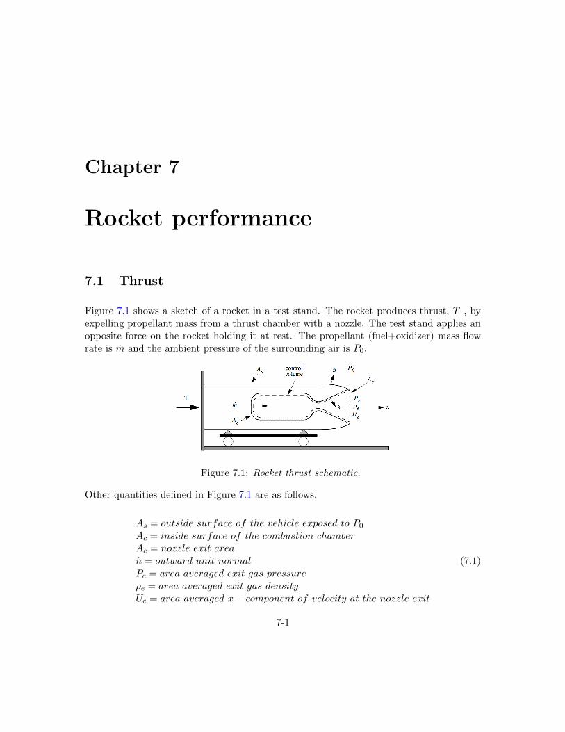
Chapter 7
Rocket performance
7.1 Thrust
Figure 7.1 shows a sketch of a rocket in a test stand. The rocket produces thrust, T , byexpelling propellant mass from a thrust chamber with a nozzle. The test stand applies anopposite force on the rocket holding it at rest. The propellant (fuel+oxidizer) mass flowrate is m and the ambient pressure of the surrounding air is P0.
Figure 7.1: Rocket thrust schematic.
Other quantities defined in Figure 7.1 are as follows.
As = outside surface of the vehicle exposed to P0
Ac = inside surface of the combustion chamberAe = nozzle exit arean = outward unit normalPe = area averaged exit gas pressureρe = area averaged exit gas densityUe = area averaged x− component of velocity at the nozzle exit
(7.1)
7-1
CHAPTER 7. ROCKET PERFORMANCE 7-2
The vehicle is at rest and so the total force acting on it is zero.
0 = T +
∫As
(PI − τ
)· ndA
∣∣∣∣x
+
∫Ac
(PI − τ
)· ndA
∣∣∣∣x
+ mUxm (7.2)
The variable P is the gas pressure acting at any point on the surface of the rocket, τ isthe viscous stress tensor, and mUxm is the x-momentum of the propellant injected into thethrust chamber. If the rocket were inactive so that there was no force on the restraint andthe outside surface and thrust chamber were all at a pressure P0 then
0 =
∫As
P0I · ndA∣∣∣∣x
+
∫Ac
P0I · ndA∣∣∣∣x
. (7.3)
In this situation the control volume contains fluid all at rest and
0 =
∫Ac
P0I · ndA∣∣∣∣x
+
∫Ae
P0I · ndA∣∣∣∣x
. (7.4)
The last relation can be written as
0 =
∫Ac
P0I · ndA∣∣∣∣x
+ P0Ae. (7.5)
Note that a unit normal vector that is consistent between the control volume and theoutside surface of the vehicle points inward on Ae. Thus equation (7.3) becomes
0 =
∫As
P0I · ndA∣∣∣∣x
− P0Ae (7.6)
and the original force balance (7.2) can be written as
0 = T + P0Ae +
∫Ac
(PI − τ
)· ndA
∣∣∣∣x
+ mUxm. (7.7)
Built into (7.7) is the assumption that when the engine is operating the external surfacepressure and stress distribution is unchanged.
(∫As
(PI − τ
)· ndA
∣∣∣∣x
)after engine turn on
=
(∫As
P0I · ndA∣∣∣∣x
)before engine turn on
(7.8)
CHAPTER 7. ROCKET PERFORMANCE 7-3
In fact, the jet from the rocket mixes with the surrounding air setting the air near thevehicle into motion leading to slight deviations in the pressure acting on the outside of thevehicle. For a rocket of reasonable size and thrust, this is a very small effect.
With the engine on, a balance of momentum over the control volume gives
D
Dt
∫V
(ρU)dV =
∫V
(∂ρU
∂t
)dV = −
∫V∇ ·(ρUU + PI − τ
)dV. (7.9)
We are treating the case where the flow in the combustion chamber is stationary and theintegral on the left hand side of (7.9) is zero. Our goal is to relate the thrust of the engineto flow conditions on Ae and with this in mind we convert the right hand side to an integralover the surface of the control volume.
0 =
∫V∇ ·(ρUU + PI − τ
)dV =∫
Ac
(ρUU + PI − τ
)· ndA+
∫Ae
(ρUU + PI − τ
)· ndA
(7.10)
Note that the unit normal that appears in the surface integrals in (7.10) is an inwardpointing unit normal. On the surface Ac, the velocity is zero by the no-slip condition(except over the injector holes) and on the surface Ae we use area-averaged values ofvelocity, pressure, and density
∫Ac
(PI − τ
)· ndA
∣∣∣∣x
+ mUxm + ρeUe2Ae + PeAe = 0 (7.11)
where the momentum of the propellant injected into the combustion chamber has beenincluded. Small viscous normal forces on Ae are neglected. Our force balance (7.7) nowbecomes
0 = T + P0Ae −(ρeUe
2Ae + PeAe). (7.12)
Finally our rocket thrust formula is
T = ρeUe2Ae + (Pe − P0)Ae. (7.13)
The propellant mass flow is
m = ρeUeAe (7.14)
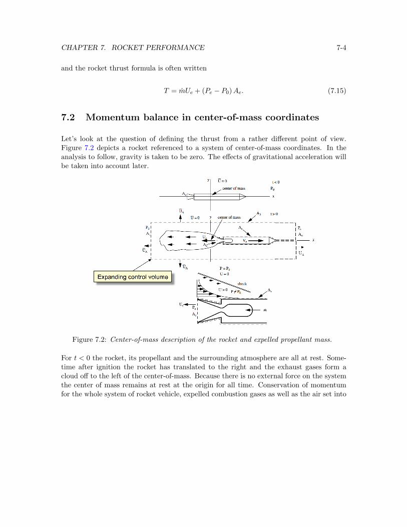
CHAPTER 7. ROCKET PERFORMANCE 7-4
and the rocket thrust formula is often written
T = mUe + (Pe − P0)Ae. (7.15)
7.2 Momentum balance in center-of-mass coordinates
Let’s look at the question of defining the thrust from a rather different point of view.Figure 7.2 depicts a rocket referenced to a system of center-of-mass coordinates. In theanalysis to follow, gravity is taken to be zero. The effects of gravitational acceleration willbe taken into account later.
Figure 7.2: Center-of-mass description of the rocket and expelled propellant mass.
For t < 0 the rocket, its propellant and the surrounding atmosphere are all at rest. Some-time after ignition the rocket has translated to the right and the exhaust gases form acloud off to the left of the center-of-mass. Because there is no external force on the systemthe center of mass remains at rest at the origin for all time. Conservation of momentumfor the whole system of rocket vehicle, expelled combustion gases as well as the air set into
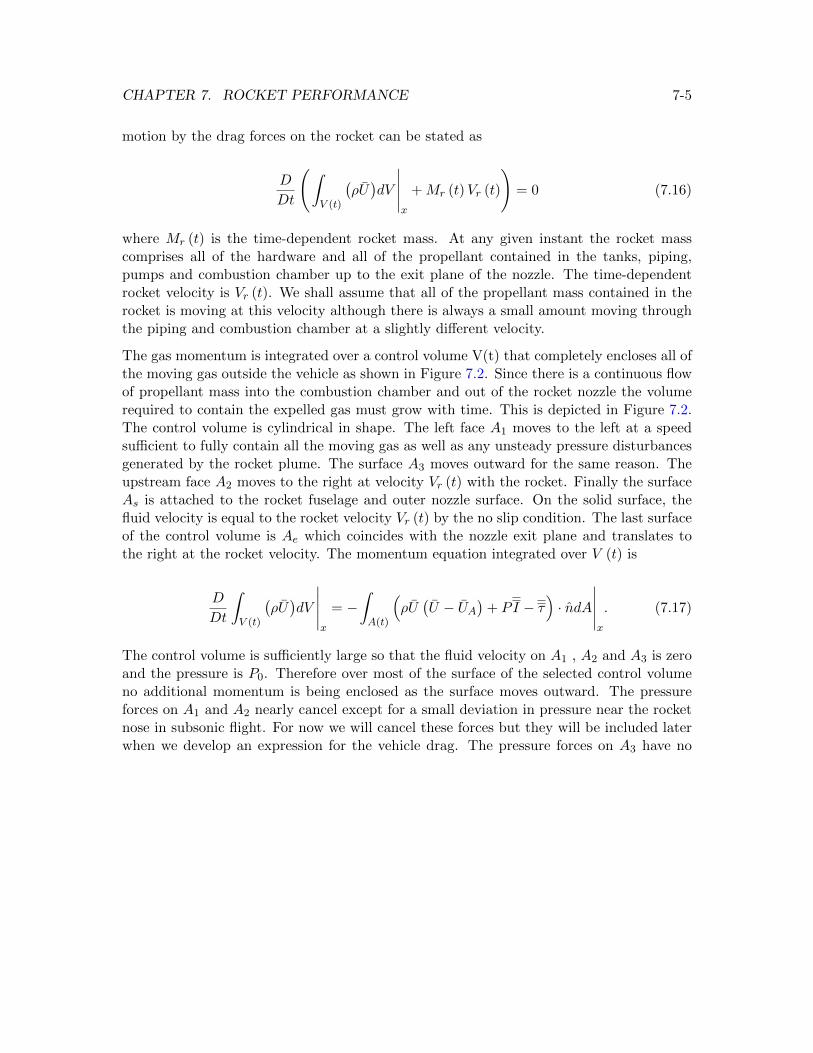
CHAPTER 7. ROCKET PERFORMANCE 7-5
motion by the drag forces on the rocket can be stated as
D
Dt
(∫V (t)
(ρU)dV
∣∣∣∣∣x
+Mr (t)Vr (t)
)= 0 (7.16)
where Mr (t) is the time-dependent rocket mass. At any given instant the rocket masscomprises all of the hardware and all of the propellant contained in the tanks, piping,pumps and combustion chamber up to the exit plane of the nozzle. The time-dependentrocket velocity is Vr (t). We shall assume that all of the propellant mass contained in therocket is moving at this velocity although there is always a small amount moving throughthe piping and combustion chamber at a slightly different velocity.
The gas momentum is integrated over a control volume V(t) that completely encloses all ofthe moving gas outside the vehicle as shown in Figure 7.2. Since there is a continuous flowof propellant mass into the combustion chamber and out of the rocket nozzle the volumerequired to contain the expelled gas must grow with time. This is depicted in Figure 7.2.The control volume is cylindrical in shape. The left face A1 moves to the left at a speedsufficient to fully contain all the moving gas as well as any unsteady pressure disturbancesgenerated by the rocket plume. The surface A3 moves outward for the same reason. Theupstream face A2 moves to the right at velocity Vr (t) with the rocket. Finally the surfaceAs is attached to the rocket fuselage and outer nozzle surface. On the solid surface, thefluid velocity is equal to the rocket velocity Vr (t) by the no slip condition. The last surfaceof the control volume is Ae which coincides with the nozzle exit plane and translates tothe right at the rocket velocity. The momentum equation integrated over V (t) is
D
Dt
∫V (t)
(ρU)dV
∣∣∣∣∣x
= −∫A(t)
(ρU(U − UA
)+ PI − τ
)· ndA
∣∣∣∣∣x
. (7.17)
The control volume is sufficiently large so that the fluid velocity on A1 , A2 and A3 is zeroand the pressure is P0. Therefore over most of the surface of the selected control volumeno additional momentum is being enclosed as the surface moves outward. The pressureforces on A1 and A2 nearly cancel except for a small deviation in pressure near the rocketnose in subsonic flight. For now we will cancel these forces but they will be included laterwhen we develop an expression for the vehicle drag. The pressure forces on A3 have no
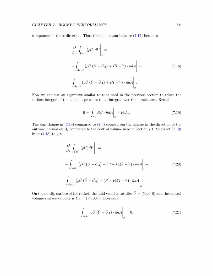
CHAPTER 7. ROCKET PERFORMANCE 7-6
component in the x direction. Thus the momentum balance (7.17) becomes
D
Dt
∫V (t)
(ρU)dV
∣∣∣∣∣x
=
−∫As(t)
(ρU(U − UA
)+ P I −¯τ
)· ndA
∣∣∣∣∣x
−
∫Ae(t)
(ρU(U − UA
)+ P I −¯τ
)· ndA
∣∣∣∣∣x
.
(7.18)
Now we can use an argument similar to that used in the previous section to relate thesurface integral of the ambient pressure to an integral over the nozzle area. Recall
0 =
∫As
P0I · ndA∣∣∣∣x
+ P0Ae. (7.19)
The sign change in (7.19) compared to (7.6) comes from the change in the direction of theoutward normal on Ae compared to the control volume used in Section 7.1. Subtract (7.19)from (7.18) to get
D
Dt
∫V (t)
(ρU)dV
∣∣∣∣∣x
=
−∫As(t)
(ρU(U − UA
)+ (P − P0 ) I −¯τ
)· ndA
∣∣∣∣∣x
−
∫Ae(t)
(ρU(U − UA
)+ (P − P0 ) I −¯τ
)· ndA
∣∣∣∣∣x
.
(7.20)
On the no-slip surface of the rocket, the fluid velocity satisfies U = (Vr, 0, 0) and the controlvolume surface velocity is UA = (Vr, 0, 0). Therefore
∫As(t)
ρU(U − UA
)· ndA
∣∣∣∣∣x
= 0. (7.21)
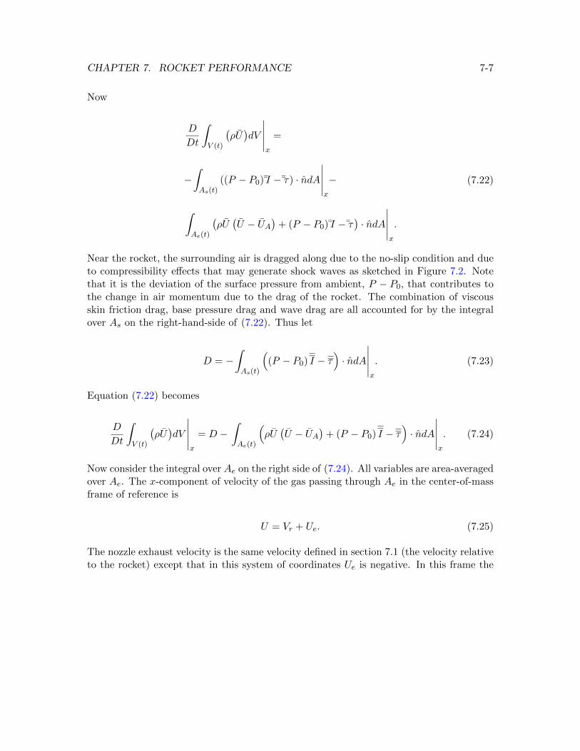
CHAPTER 7. ROCKET PERFORMANCE 7-7
Now
D
Dt
∫V (t)
(ρU)dV
∣∣∣∣∣x
=
−∫As(t)
((P − P0 ) I −¯τ) · ndA
∣∣∣∣∣x
−
∫Ae(t)
(ρU(U − UA
)+ (P − P0 ) I −¯τ
)· ndA
∣∣∣∣∣x
.
(7.22)
Near the rocket, the surrounding air is dragged along due to the no-slip condition and dueto compressibility effects that may generate shock waves as sketched in Figure 7.2. Notethat it is the deviation of the surface pressure from ambient, P − P0, that contributes tothe change in air momentum due to the drag of the rocket. The combination of viscousskin friction drag, base pressure drag and wave drag are all accounted for by the integralover As on the right-hand-side of (7.22). Thus let
D = −∫As(t)
((P − P0) I − τ
)· ndA
∣∣∣∣∣x
. (7.23)
Equation (7.22) becomes
D
Dt
∫V (t)
(ρU)dV
∣∣∣∣∣x
= D −∫Ae(t)
(ρU(U − UA
)+ (P − P0) I − τ
)· ndA
∣∣∣∣∣x
. (7.24)
Now consider the integral over Ae on the right side of (7.24). All variables are area-averagedover Ae. The x-component of velocity of the gas passing through Ae in the center-of-massframe of reference is
U = Vr + Ue. (7.25)
The nozzle exhaust velocity is the same velocity defined in section 7.1 (the velocity relativeto the rocket) except that in this system of coordinates Ue is negative. In this frame the
CHAPTER 7. ROCKET PERFORMANCE 7-8
speed of the surface Ae is Vr (t).
∫Ae(t)
(ρU(U − UA
)+ (P − P0) I − τ
)· ndA
∣∣∣∣∣x
=
ρeAe (Ue + Vr) (Ue + Vr − Vr) + (Pe − P0)Ae.
(7.26)
Now the momentum change of the expelled gas is
D
Dt
∫V (t)
(ρU)dV
∣∣∣∣∣x
= D − (ρeAe (Ue + Vr) (Ue + Vr − Vr) + (Pe − P0)Ae) . (7.27)
Substitute (7.27) into (7.16)
D
Dt(Mr (t)Vr (t)) +D − (ρeAeUe (Ue + Vr) + (Pe − P0)Ae) = 0 (7.28)
or
Mr (t)dVr (t)
dt+ Vr (t)
dMr (t)
dt+D − (ρeAeUe (Ue + Vr) + (Pe − P0)Ae) = 0. (7.29)
Note that
dMr (t)
dt= ρeUeAe (7.30)
and the second and fifth terms in (7.29) cancel. Remember that in the chosen set ofcoordinates, Ue is negative and (7.30) is consistent with the fact that dMr/dt < 0. Finallyour momentum balance in the center-of-mass system boils down to
Mr (t)dVr (t)
dt=(ρeUe
2Ae + (Pe − P0)Ae)−D. (7.31)
In words, Equation (7.31) simply states
Rocket mass×Acceleration = Thrust−Drag. (7.32)
The first term on the right-hand-side of (7.31) is the same thrust expression derived in theprevious section.
CHAPTER 7. ROCKET PERFORMANCE 7-9
7.3 Effective exhaust velocity
The total mechanical impulse (total change of momentum) generated by an applied force,T , is
I =
∫ t
0Tdt. (7.33)
The total propellant mass expended is
Mp =
∫ t
0mdt. (7.34)
The instantaneous change of momentum per unit expenditure of propellant mass definesthe effective exhaust velocity.
C =dI
dMp=T
m= Ue +
Aem
(Pe − P0) (7.35)
This can be expressed in terms of the exit Mach number as follows
C = Ue
(1 +
PeAe
ρeUe2Ae
(1− P0
Pe
))(7.36)
or
C = Ue
(1 +
1
γMe2
(1− P0
Pe
)). (7.37)
For a large area ratio exhaust with a large exit Mach number the pressure part of thethrust becomes a small fraction of the overall thrust.
Let’s estimate the theoretical maximum exhaust velocity that can be generated by a givenset of propellants characterized by the heating value per unit propellant mass, q. Considerthe simple model of a rocket thrust chamber shown in Figure 7.3.
Between stations 1 and 2 combustion takes place leading to a change in stagnation enthalpyof the propellant mass.
ht2 = ht1 + q = he +1
2Ue
2 (7.38)
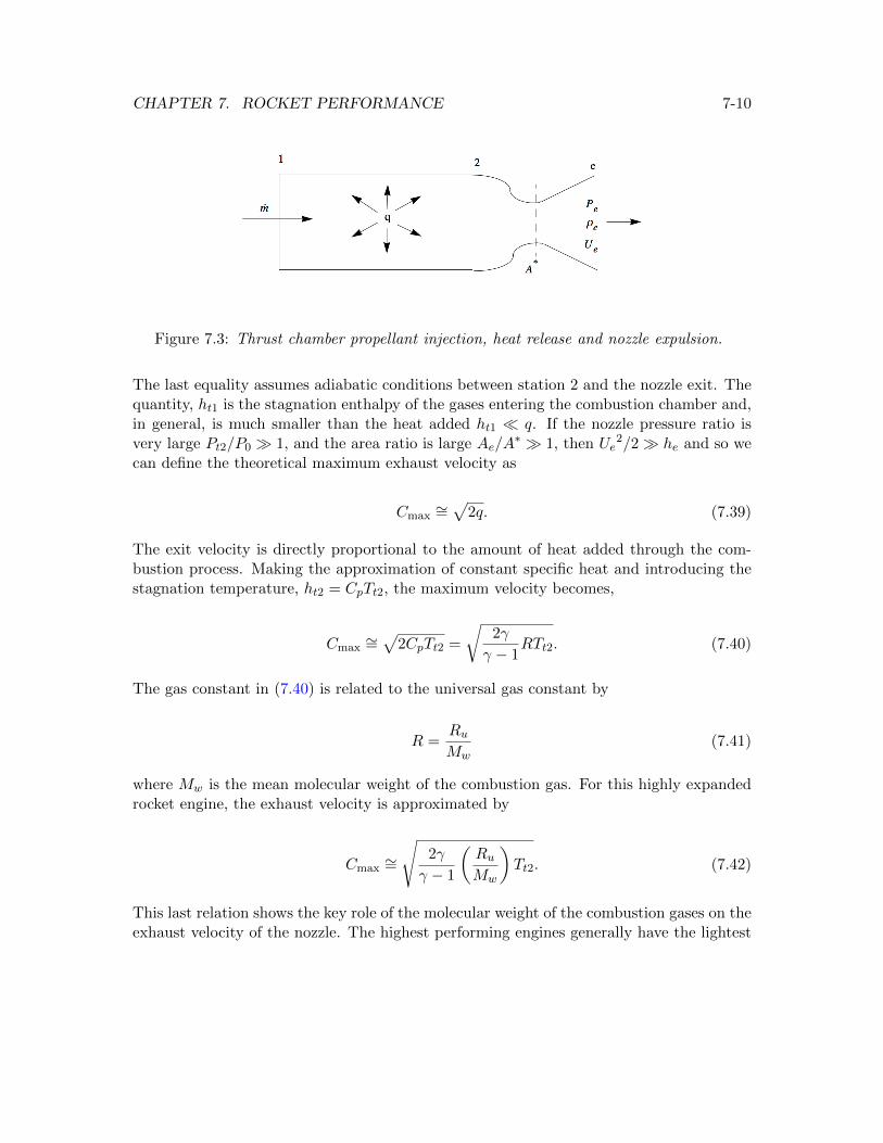
CHAPTER 7. ROCKET PERFORMANCE 7-10
Figure 7.3: Thrust chamber propellant injection, heat release and nozzle expulsion.
The last equality assumes adiabatic conditions between station 2 and the nozzle exit. Thequantity, ht1 is the stagnation enthalpy of the gases entering the combustion chamber and,in general, is much smaller than the heat added ht1 � q. If the nozzle pressure ratio isvery large Pt2/P0 � 1, and the area ratio is large Ae/A
∗ � 1, then Ue2/2� he and so we
can define the theoretical maximum exhaust velocity as
Cmax∼=√
2q. (7.39)
The exit velocity is directly proportional to the amount of heat added through the com-bustion process. Making the approximation of constant specific heat and introducing thestagnation temperature, ht2 = CpTt2, the maximum velocity becomes,
Cmax∼=√
2CpTt2 =
√2γ
γ − 1RTt2. (7.40)
The gas constant in (7.40) is related to the universal gas constant by
R =RuMw
(7.41)
where Mw is the mean molecular weight of the combustion gas. For this highly expandedrocket engine, the exhaust velocity is approximated by
Cmax∼=
√2γ
γ − 1
(RuMw
)Tt2. (7.42)
This last relation shows the key role of the molecular weight of the combustion gases on theexhaust velocity of the nozzle. The highest performing engines generally have the lightest
CHAPTER 7. ROCKET PERFORMANCE 7-11
weight exhaust gases. The most outstanding example of this is the Space Shuttle MainEngine (SSME) which uses hydrogen and oxygen, with water vapor as the main exhaustconstituent.
7.4 C∗ efficiency
A very important characteristic velocity that is widely used in rocket motor testing is C∗
defined by the mass balance
m =Pt2A
∗
C∗. (7.43)
The reason (7.43) is so useful is that it can be used to express the combustion efficiencyin the rocket chamber in terms of quantities that are relatively easy to measure: chamberpressure, propellant mass flow rate and nozzle throat area. These variables are much easierand less expensive to measure than the combustion chamber temperature and chemicalcomposition. The C∗ efficiency of a motor is defined as
ηC∗ =
(Pt2A∗
m
)measured(
Pt2A∗
m
)ideal
. (7.44)
The ideal value of C∗ is determined using a thermochemical calculator such as CEA dis-cussed in Chapter 9. Since the ideal calculation is assumed to take place at the samepropellant mass flow rate and nozzle throat area, A∗ , the C∗ efficiency reduces to a sim-ple comparison between the achieved chamber pressure and the chamber pressure thatwould be reached if there was complete mixing and complete combustion under adiabaticconditions.
ηC∗ =Pt2measuredPt2ideal
(7.45)
7.5 Specific impulse
For historical reasons, the specific impulse has always been defined as the thrust per unitweight flow of propellant and so the gravitational acceleration at the surface of the Earth
CHAPTER 7. ROCKET PERFORMANCE 7-12
is always inserted. The specific impulse is defined as
Isp =T
mg0=C
g0(7.46)
even though the parameter g0 = 9.8m/sec2 has no particular relevance to the problem.Generally one distinguishes between the sea level specific impulse of a vehicle where theambient pressure detracts from the thrust and the ideal vacuum specific impulse wherethe exhaust is assumed to be expanded to the exhaust pressure Pe with P0 = 0. Fromthe previous discussion of the theoretical maximum exhaust velocity, it is clear that thevacuum specific impulse at a very large area ratio effectively characterizes a given propellantcombination. Typical solid propellant systems have specific Ispvac in the range 230−290 sec.Liquid propellant systems using a hydrocarbon fuel with liquid oxygen have Ispvac around360 seconds with hydrogen-oxygen systems reaching 455 seconds. One needs to not takethese Isp numbers too literally. Such values are often quoted for some typical real systemsuch as the Space Shuttle Main Engine without stating the actual chamber pressure andarea ratio and in some cases without identifying the system. The question of the arearatio corresponding to the ideal specific impulse is particularly important. For example,for a hydrogen-oxygen system at an area ratio of, say, 4, 000 the ideal Isp is over 500seconds.
An accurate specification of the specific impulse of a working system requires a knowledgeof the chamber pressure, nozzle area ratio, combustion efficiency and nozzle efficiency. Thechamber pressure is needed to determine the composition of the combustion chamber gasat the chamber temperature. This will become clear when we study the thermochemistryof gases in Chapter 9.
7.6 Chamber pressure
The mass flow of propellant injected into the rocket engine and the amount of heat addedbetween stations 1 and 2 through combustion determine the engine chamber pressure. Wecan see this by considering the relationship between the mass exiting the nozzle and thestagnation conditions of the gas at station 2. In general, at any point in a channel flow ofa compressible gas, the mass flow can be expressed as
m = ρUA =1(
γ+12
) γ+12(γ−1)
γPtA√γRTt
f (M) (7.47)
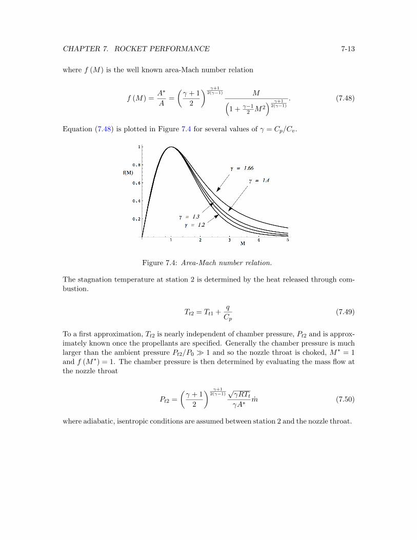
CHAPTER 7. ROCKET PERFORMANCE 7-13
where f (M) is the well known area-Mach number relation
f (M) =A∗
A=
(γ + 1
2
) γ+12(γ−1) M(
1 + γ−12 M2
) γ+12(γ−1)
. (7.48)
Equation (7.48) is plotted in Figure 7.4 for several values of γ = Cp/Cv.
Figure 7.4: Area-Mach number relation.
The stagnation temperature at station 2 is determined by the heat released through com-bustion.
Tt2 = Tt1 +q
Cp(7.49)
To a first approximation, Tt2 is nearly independent of chamber pressure, Pt2 and is approx-imately known once the propellants are specified. Generally the chamber pressure is muchlarger than the ambient pressure Pt2/P0 � 1 and so the nozzle throat is choked, M∗ = 1and f (M∗) = 1. The chamber pressure is then determined by evaluating the mass flow atthe nozzle throat
Pt2 =
(γ + 1
2
) γ+12(γ−1)
√γRTtγA∗
m (7.50)
where adiabatic, isentropic conditions are assumed between station 2 and the nozzle throat.
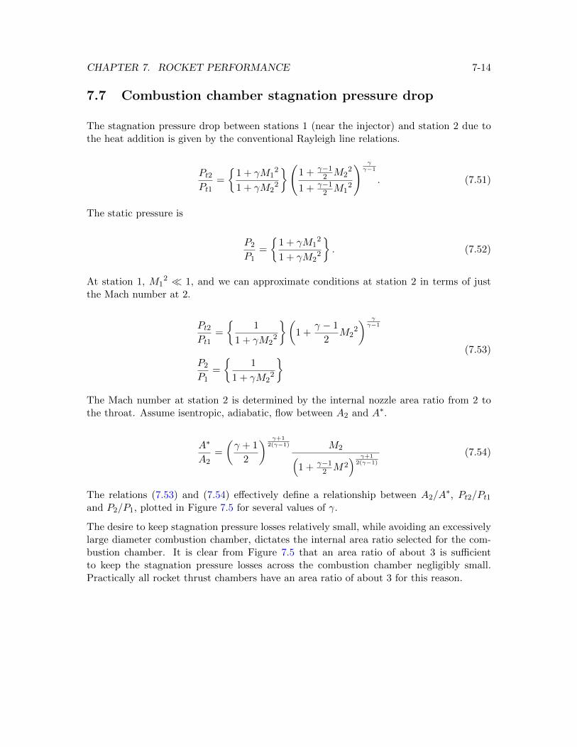
CHAPTER 7. ROCKET PERFORMANCE 7-14
7.7 Combustion chamber stagnation pressure drop
The stagnation pressure drop between stations 1 (near the injector) and station 2 due tothe heat addition is given by the conventional Rayleigh line relations.
Pt2Pt1
=
{1 + γM1
2
1 + γM22
}(1 + γ−1
2 M22
1 + γ−12 M1
2
) γγ−1
. (7.51)
The static pressure is
P2
P1=
{1 + γM1
2
1 + γM22
}. (7.52)
At station 1, M12 � 1, and we can approximate conditions at station 2 in terms of just
the Mach number at 2.
Pt2Pt1
=
{1
1 + γM22
}(1 +
γ − 1
2M2
2
) γγ−1
P2
P1=
{1
1 + γM22
} (7.53)
The Mach number at station 2 is determined by the internal nozzle area ratio from 2 tothe throat. Assume isentropic, adiabatic, flow between A2 and A∗.
A∗
A2=
(γ + 1
2
) γ+12(γ−1) M2(
1 + γ−12 M2
) γ+12(γ−1)
(7.54)
The relations (7.53) and (7.54) effectively define a relationship between A2/A∗, Pt2/Pt1
and P2/P1, plotted in Figure 7.5 for several values of γ.
The desire to keep stagnation pressure losses relatively small, while avoiding an excessivelylarge diameter combustion chamber, dictates the internal area ratio selected for the com-bustion chamber. It is clear from Figure 7.5 that an area ratio of about 3 is sufficientto keep the stagnation pressure losses across the combustion chamber negligibly small.Practically all rocket thrust chambers have an area ratio of about 3 for this reason.
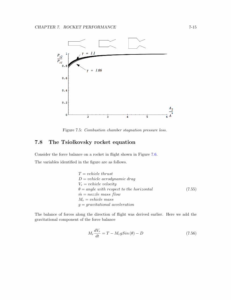
CHAPTER 7. ROCKET PERFORMANCE 7-15
Figure 7.5: Combustion chamber stagnation pressure loss.
7.8 The Tsiolkovsky rocket equation
Consider the force balance on a rocket in flight shown in Figure 7.6.
The variables identified in the figure are as follows.
T = vehicle thrustD = vehicle aerodynamic dragVr = vehicle velocityθ = angle with respect to the horizontalm = nozzle mass flowMr = vehicle massg = gravitational acceleration
(7.55)
The balance of forces along the direction of flight was derived earlier. Here we add thegravitational component of the force balance
MrdVrdt
= T −MrgSin (θ)−D (7.56)
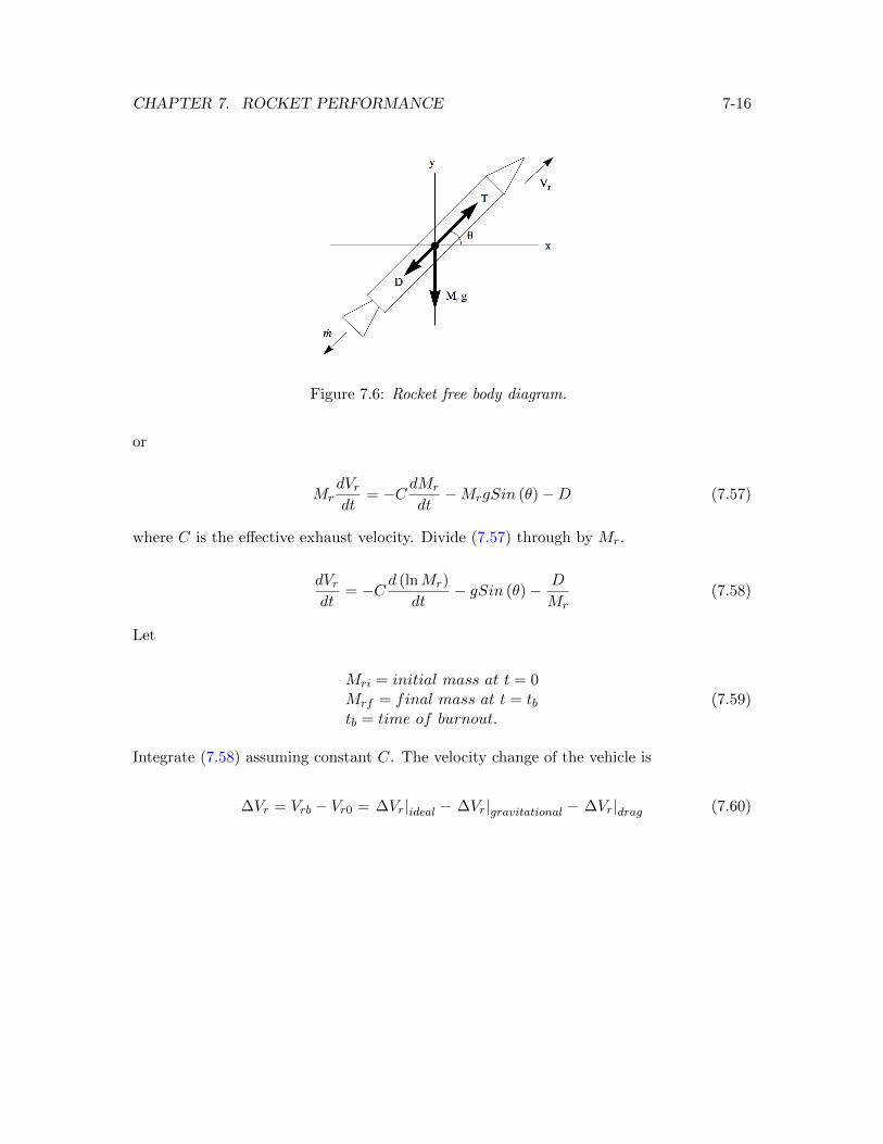
CHAPTER 7. ROCKET PERFORMANCE 7-16
Figure 7.6: Rocket free body diagram.
or
MrdVrdt
= −CdMr
dt−MrgSin (θ)−D (7.57)
where C is the effective exhaust velocity. Divide (7.57) through by Mr.
dVrdt
= −Cd (lnMr)
dt− gSin (θ)− D
Mr(7.58)
Let
Mri = initial mass at t = 0Mrf = final mass at t = tbtb = time of burnout.
(7.59)
Integrate (7.58) assuming constant C. The velocity change of the vehicle is
∆Vr = Vrb − Vr0 = ∆Vr|ideal − ∆Vr|gravitational − ∆Vr|drag (7.60)
CHAPTER 7. ROCKET PERFORMANCE 7-17
where
∆Vr|gravitational =
∫ tb
0gSin (θ)dt
∆Vr|drag =
∫ tb
0
(D
Mr
)dt.
(7.61)
For a typical launch vehicle headed to orbit, aerodynamic drag losses are generally quitesmall on the order of 100 to 500m/ sec. Gravitational losses are larger, generally rangingfrom 700 to 1500m/ sec depending on the shape of the trajectory to orbit. By far thelargest term is the equation for the ideal velocity increment
∆Vr|ideal = C ln
(Mri
Mrf
)(7.62)
first derived in 1903 by the soviet rocket pioneer Konstantin Tsiolkovsky who is creditedwith developing much of the early theory of rocket flight. Equation (7.62) shows the de-pendence of the velocity achieved by a rocket on the effective exhaust velocity (determinedby the choice of propellants) and the initial to final mass ratio which is determined by whatmight be termed the structural efficiency of the vehicle and the density of the propellants.Notice the similarity of (7.62) to the Bruguet range equation discussed in chapter 2. Ingeneral, one seeks a very lightweight vehicle to carry high density propellants which aftercombustion produce very lightweight products. In practice these requirements conflict.Generally solid rockets use relatively dense, low energy propellants which do not producevery lightweight products of combustion. Whereas liquid rockets use more energetic pro-pellants that produce light products but are not particularly dense.
7.9 Reaching orbit
Orbital velocity at an altitude of 115 miles, which is about the lowest altitude where a stableorbit can be maintained, is approximately 7777m/ sec. To reach this velocity from theKennedy Space Center where the velocity due to the rotation of the Earth is approximately427m/ sec, assuming gravitational plus drag losses of 1700m/ sec, requires an ideal velocityincrement of 9050m/ sec. A hydrogen-oxygen system with an effective average exhaustvelocity (from sea- level to vacuum) of 4000m/ sec would require Mi/Mf = 9.7. Thisrepresents a very high level of structural efficiency and is the fundamental challenge beingaddressed by single-stage-to-orbit concepts. At the present time existing launch vehiclesrequire multiple stages to achieve orbit with a reasonable payload size.
CHAPTER 7. ROCKET PERFORMANCE 7-18
Strategies for reducing gravitational losses are mainly limited to optimizing the trajectoryto orbit and expending the maximum amount of propellant as possible near the earth’s sur-face (to avoid the work required to lift it to altitude). The latter strategy suggests that themost efficient way to orbit would be an artillery shell, however practical limitations preventlarge acceleration loads on the payload. Most large launch vehicles are relatively delicateand require throttling back on thrust at low altitude to avoid large dynamic pressure loadson the vehicle.
The drag losses can be minimized by designing a slender vehicle. This can be seen asfollows
∆Vr|drag =
∫ tb
0
(D
Mr
)dt =
∫ tb
0
1
2
ρVr2ACDMri
(Mri
Mr
)dt =
A
2Mri
∫ tb
0
(ρVr
2CD)(Mri
Mr
)dt
(7.63)
where A is the cross-sectional area of the vehicle. The integral on the right-hand-side is ap-proximately independent of vehicle size and the initial mass of the vehicle is approximatelyproportional to the vehicle volume, Mri
∼= ρvehicleVvehicle.
∆Vrocket|drag ∼=FrontalArearocket
2densityrocketV olumerocket
∫ tb
0
(ρVrocket
2CD)(Mrocketi
Mrocket
)dt ∼ 1
Lengthrocket(7.64)
The last result suggests that the vehicle should be long and thin, roughly like a pencil.Note that the drag losses go down as the mass goes up, and so the velocity loss due to dragtends to become smaller as the vehicle absolute size goes up. The length to diameter ratioof the vehicle does not come into the analysis directly but, in general, the drag coefficient,Cd, decreases as the L/D goes up.
7.10 The thrust coefficient
The thrust coefficient provides a useful dimensionless measure of engine thrust.
CF =T
Pt2A∗=mUe + (Pe − P0)Ae
Pt2A∗=
(PePt2
)(AeA∗
)(γMe
2 + 1− P0
Pe
)(7.65)
This rather complicated looking expression can be written in terms of the nozzle exit Mach
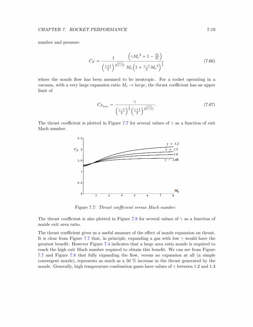
CHAPTER 7. ROCKET PERFORMANCE 7-19
number and pressure
CF =1(
γ+12
) γ+12(γ−1)
(γMe
2 + 1− P0Pe
)Me
(1 + γ−1
2 Me2) 1
2
(7.66)
where the nozzle flow has been assumed to be isentropic. For a rocket operating in avacuum, with a very large expansion ratio Me → large, the thrust coefficient has an upperlimit of
CFmax =γ(
γ−12
) 12(γ+1
2
) γ+12(γ−1)
. (7.67)
The thrust coefficient is plotted in Figure 7.7 for several values of γ as a function of exitMach number.
Figure 7.7: Thrust coefficient versus Mach number.
The thrust coefficient is also plotted in Figure 7.8 for several values of γ as a function ofnozzle exit area ratio.
The thrust coefficient gives us a useful measure of the effect of nozzle expansion on thrust.It is clear from Figure 7.7 that, in principle, expanding a gas with low γ would have thegreatest benefit. However Figure 7.4 indicates that a large area ratio nozzle is required toreach the high exit Mach number required to obtain this benefit. We can see from Figure7.7 and Figure 7.8 that fully expanding the flow, versus no expansion at all (a simpleconvergent nozzle), represents as much as a 50 % increase in the thrust generated by thenozzle. Generally, high temperature combustion gases have values of γ between 1.2 and 1.3
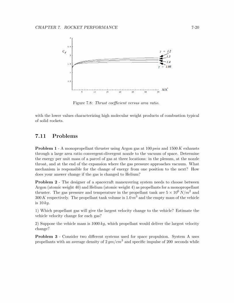
CHAPTER 7. ROCKET PERFORMANCE 7-20
Figure 7.8: Thrust coefficient versus area ratio.
with the lower values characterizing high molecular weight products of combustion typicalof solid rockets.
7.11 Problems
Problem 1 - A monopropellant thruster using Argon gas at 100 psia and 1500K exhauststhrough a large area ratio convergent-divergent nozzle to the vacuum of space. Determinethe energy per unit mass of a parcel of gas at three locations: in the plenum, at the nozzlethroat, and at the end of the expansion where the gas pressure approaches vacuum. Whatmechanism is responsible for the change of energy from one position to the next? Howdoes your answer change if the gas is changed to Helium?
Problem 2 - The designer of a spacecraft maneuvering system needs to choose betweenArgon (atomic weight 40) and Helium (atomic weight 4) as propellants for a monopropellantthruster. The gas pressure and temperature in the propellant tank are 5× 10⁶N/m2 and300K respectively. The propellant tank volume is 1.0m3 and the empty mass of the vehicleis 10 kg.
1) Which propellant gas will give the largest velocity change to the vehicle? Estimate thevehicle velocity change for each gas?
2) Suppose the vehicle mass is 1000 kg, which propellant would deliver the largest velocitychange?
Problem 3 - Consider two different systems used for space propulsion. System A usespropellants with an average density of 2 gm/cm3 and specific impulse of 200 seconds while
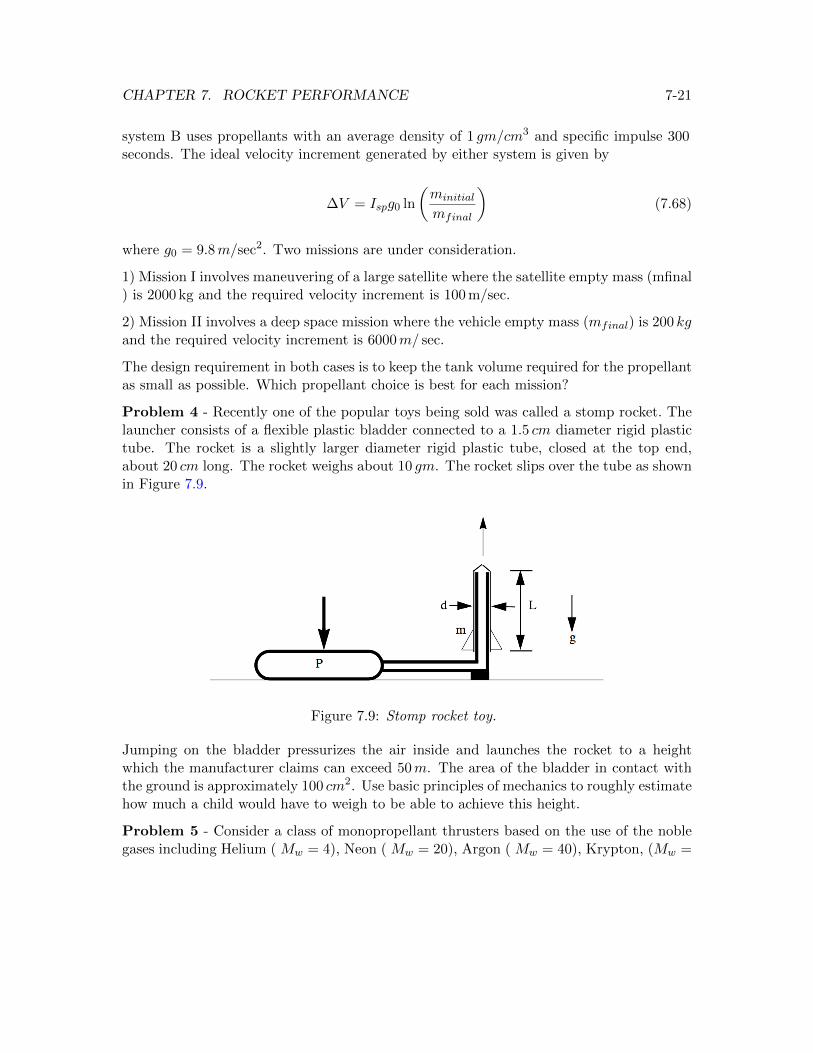
CHAPTER 7. ROCKET PERFORMANCE 7-21
system B uses propellants with an average density of 1 gm/cm3 and specific impulse 300seconds. The ideal velocity increment generated by either system is given by
∆V = Ispg0 ln
(minitial
mfinal
)(7.68)
where g0 = 9.8m/sec2. Two missions are under consideration.
1) Mission I involves maneuvering of a large satellite where the satellite empty mass (mfinal) is 2000 kg and the required velocity increment is 100 m/sec.
2) Mission II involves a deep space mission where the vehicle empty mass (mfinal) is 200 kgand the required velocity increment is 6000m/ sec.
The design requirement in both cases is to keep the tank volume required for the propellantas small as possible. Which propellant choice is best for each mission?
Problem 4 - Recently one of the popular toys being sold was called a stomp rocket. Thelauncher consists of a flexible plastic bladder connected to a 1.5 cm diameter rigid plastictube. The rocket is a slightly larger diameter rigid plastic tube, closed at the top end,about 20 cm long. The rocket weighs about 10 gm. The rocket slips over the tube as shownin Figure 7.9.
Figure 7.9: Stomp rocket toy.
Jumping on the bladder pressurizes the air inside and launches the rocket to a heightwhich the manufacturer claims can exceed 50m. The area of the bladder in contact withthe ground is approximately 100 cm2. Use basic principles of mechanics to roughly estimatehow much a child would have to weigh to be able to achieve this height.
Problem 5 - Consider a class of monopropellant thrusters based on the use of the noblegases including Helium ( Mw = 4), Neon ( Mw = 20), Argon ( Mw = 40), Krypton, (Mw =
CHAPTER 7. ROCKET PERFORMANCE 7-22
84) and Xenon (Mw = 131). Radon (Mw = 222) is excluded because of its radioactivity.The thruster is comprised of a tank that exhausts through a simple convergent nozzle to thevacuum of space. Onboard heaters are used to maintain the gas in the tank at a constantstagnation temperature Tt2 as it is exhausted.
1) The thrust is often expressed in terms of an effective exhaust velocity T = mC. Showthat the effective exhaust velocity of this system can be expressed as
C =
(2 (γ + 1)
γ
(RuMw
)Tt2
)1/2
. (7.69)
2) The mass of propellant contained in the tank is
Mpropellant =Pt2initialVtan kMw
RuTt2. (7.70)
The initial tank pressure is some rated value (a do-not-exceed pressure) independent of thetype of gas used. The designer would like to choose the propellant gas so that the velocityincrement produced by the propulsion system ∆V is as large as possible for fixed tankvolume, initial pressure and gas temperature. The problem is to decide whether to choosea gas with low Mw, thus achieving a high value of C but low propellant mass, or a gaswith high Mw reducing C but increasing propellant mass. By mixing two or more gases,any mean atomic mass between 4 and 131 can be selected by the designer. Note that γ isthe same regardless of what gas or mixture of gases is used.
Show that the maximum ∆V occurs when the ratio Mpropellant/Mstructure is approximately4 (actually 3.922). In other words, once the tank volume, pressure and temperature aredetermined and the vehicle empty mass is known, show that for maximum ∆V the gasshould be selected to have a mean atomic weight Mw such that
Pt2initialVtan kMw
RuTt2Mstructure= 3.922. (7.71)
Problem 6 - The space shuttle main engine has a nozzle throat diameter of 10.22 ina nozzle area ratio of 77.5 and produces 418, 000 pounds of thrust at lift-off from CapeCanaveral. Determine the engine thrust when it reaches the vacuum of space.
Chapter 8
Multistage Rockets
8.1 Notation
With current technology and fuels, and without greatly increasing the effective Isp byair-breathing, a single stage rocket to Earth orbit is still not possible. So it is necessaryto reach orbit using a multistage system where a certain fraction of the vehicle mass isdropped off after use, thus allowing the non-payload mass carried to orbit to be as smallas possible. The final velocity of an n stage launch system is the sum of the velocity gainsfrom each stage.
Vn = ∆v1 + ∆v2 + ∆v3 + . . . . . .+ ∆vn (8.1)
The performance of an n -stage system can be optimized by proper selection of the struc-tural mass, propellant mass and specific impulse of each of the n stages.
Let the index i refer to the ith stage of an n stage launch system.The structural andpropellant parameters of the system are as follows.
M0i - The total initial mass of the ith vehicle prior to firing including the payload mass,ie, the mass of i, i+ 1, i+ 2, i+ 3,...., n stages.
Mpi - The mass of propellant in the ith stage.
Msi - Structural mass of the ith stage alone including the mass of its engine, controllersand instrumentation as well as any residual propellant which is not expended by the endof the stage burn.
ML - The payload mass
8-1
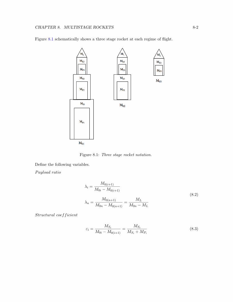
CHAPTER 8. MULTISTAGE ROCKETS 8-2
Figure 8.1 schematically shows a three stage rocket at each regime of flight.
Figure 8.1: Three stage rocket notation.
Define the following variables.
Payload ratio
λi =M0(i+1)
M0i −M0(i+1)
λn =M0(n+1)
M0n −M0(n+1)=
ML
M0n −ML
(8.2)
Structural coefficient
εi =MSi
M0i −M0(i+1)=
MSi
MSi +MPi
(8.3)
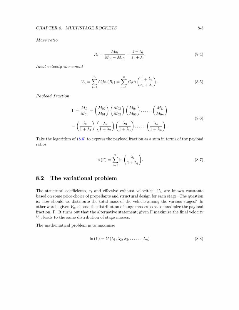
CHAPTER 8. MULTISTAGE ROCKETS 8-3
Mass ratio
Ri =M0i
M0i −MPi=
1 + λiεi + λi
. (8.4)
Ideal velocity increment
Vn =
n∑i=1
Ciln (Ri) =
n∑i=1
Ciln
(1 + λiεi + λi
). (8.5)
Payload fraction
Γ =ML
M01=
(M02
M01
)(M03
M02
)(M04
M03
). . . . . .
(ML
M0n
)
=
(λ1
1 + λ1
)(λ2
1 + λ2
)(λ3
1 + λ3
). . . . . .
(λn
1 + λn
).
(8.6)
Take the logarithm of (8.6) to express the payload fraction as a sum in terms of the payloadratios
ln (Γ) =n∑i=1
ln
(λi
1 + λi
). (8.7)
8.2 The variational problem
The structural coefficients, εi and effective exhaust velocities, Ci, are known constantsbased on some prior choice of propellants and structural design for each stage. The questionis: how should we distribute the total mass of the vehicle among the various stages? Inother words, given Vn, choose the distribution of stage masses so as to maximize the payloadfraction, Γ. It turns out that the alternative statement; given Γ maximize the final velocityVn, leads to the same distribution of stage masses.
The mathematical problem is to maximize
ln (Γ) = G (λ1, λ2, λ3, . . . . . . , λn) (8.8)
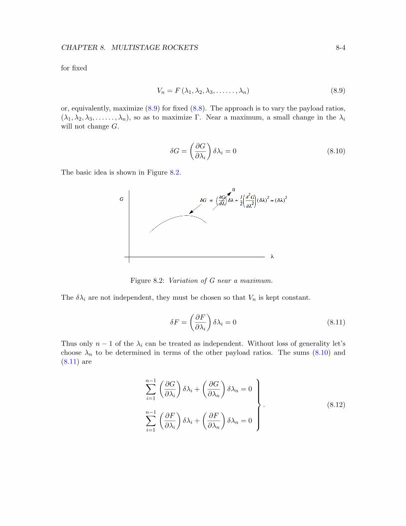
CHAPTER 8. MULTISTAGE ROCKETS 8-4
for fixed
Vn = F (λ1, λ2, λ3, . . . . . . , λn) (8.9)
or, equivalently, maximize (8.9) for fixed (8.8). The approach is to vary the payload ratios,(λ1, λ2, λ3, . . . . . . , λn), so as to maximize Γ. Near a maximum, a small change in the λiwill not change G.
δG =
(∂G
∂λi
)δλi = 0 (8.10)
The basic idea is shown in Figure 8.2.
Figure 8.2: Variation of G near a maximum.
The δλi are not independent, they must be chosen so that Vn is kept constant.
δF =
(∂F
∂λi
)δλi = 0 (8.11)
Thus only n − 1 of the λi can be treated as independent. Without loss of generality let’schoose λn to be determined in terms of the other payload ratios. The sums (8.10) and(8.11) are
n−1∑i=1
(∂G
∂λi
)δλi +
(∂G
∂λn
)δλn = 0
n−1∑i=1
(∂F
∂λi
)δλi +
(∂F
∂λn
)δλn = 0
. (8.12)
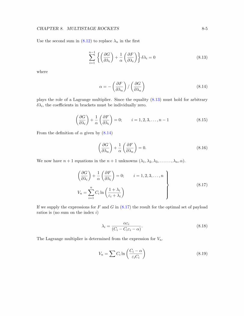
CHAPTER 8. MULTISTAGE ROCKETS 8-5
Use the second sum in (8.12) to replace λn in the first
n−1∑i=1
{(∂G
∂λi
)+
1
α
(∂F
∂λi
)}δλi = 0 (8.13)
where
α = −(∂F
∂λn
)/
(∂G
∂λn
)(8.14)
plays the role of a Lagrange multiplier. Since the equality (8.13) must hold for arbitraryδλi, the coefficients in brackets must be individually zero.
(∂G
∂λi
)+
1
α
(∂F
∂λi
)= 0; i = 1, 2, 3, . . . , n− 1 (8.15)
From the definition of α given by (8.14)
(∂G
∂λn
)+
1
α
(∂F
∂λn
)= 0. (8.16)
We now have n+ 1 equations in the n+ 1 unknowns (λ1, λ2, λ3, . . . . . . , λn, α).
(∂G
∂λi
)+
1
α
(∂F
∂λi
)= 0; i = 1, 2, 3, . . . , n
Vn =n∑i=1
Ci ln
(1 + λiεi + λi
)
(8.17)
If we supply the expressions for F and G in (8.17) the result for the optimal set of payloadratios is (no sum on the index i)
λi =αεi
(Ci − Ciεi − α). (8.18)
The Lagrange multiplier is determined from the expression for Vn.
Vn =∑
Ci ln
(Ci − αεiCi
)(8.19)
CHAPTER 8. MULTISTAGE ROCKETS 8-6
Note that α has units of velocity. Finally, the optimum overall payload fraction is
ln (Γ) =
n∑i=1
ln
(αεi
(Ci − Ciεi − α+ αεi)
). (8.20)
8.3 Example - exhaust velocity and structural coefficient thesame for all stages
Let Ci = C and εi = ε be the same for all stages. In this case
α = C(
1− εe(VnnC )). (8.21)
The payload ratio is
λ =1− εe(
VnnC )
e(VnnC ) − 1
. (8.22)
The payload fraction is
Γ =
(1− εe(
VnnC )
(1− ε) e(VnnC )
)n(8.23)
and the mass ratio is
R = e(VnnC ). (8.24)
Consider a liquid oxygen, kerosene system. Take the specific impulse to be 360 sec implyingC = 3528m/ sec; a very high performance system. Let Vn = 9077m/ sec needed to reachorbital speed. The structural coefficient is ε = 0.1 and let the number of stages be n = 3.The stage design results are α = 2696m/ sec, λ = 0.563, R = 2.3575 and the payloadfraction is
Γ = 0.047. (8.25)
Less than 5% of the overall mass of the vehicle is payload. It is of interest to see how muchbetter we can do by increasing the number of stages in this problem. Equation (8.23) isplotted in Figure 8.3 using the parameters of the problem.
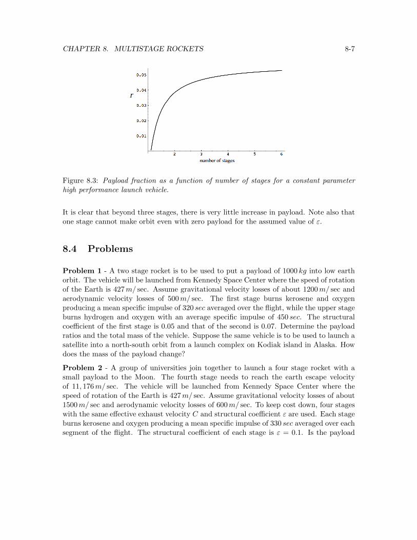
CHAPTER 8. MULTISTAGE ROCKETS 8-7
Figure 8.3: Payload fraction as a function of number of stages for a constant parameterhigh performance launch vehicle.
It is clear that beyond three stages, there is very little increase in payload. Note also thatone stage cannot make orbit even with zero payload for the assumed value of ε.
8.4 Problems
Problem 1 - A two stage rocket is to be used to put a payload of 1000 kg into low earthorbit. The vehicle will be launched from Kennedy Space Center where the speed of rotationof the Earth is 427m/ sec. Assume gravitational velocity losses of about 1200m/ sec andaerodynamic velocity losses of 500m/ sec. The first stage burns kerosene and oxygenproducing a mean specific impulse of 320 sec averaged over the flight, while the upper stageburns hydrogen and oxygen with an average specific impulse of 450 sec. The structuralcoefficient of the first stage is 0.05 and that of the second is 0.07. Determine the payloadratios and the total mass of the vehicle. Suppose the same vehicle is to be used to launch asatellite into a north-south orbit from a launch complex on Kodiak island in Alaska. Howdoes the mass of the payload change?
Problem 2 - A group of universities join together to launch a four stage rocket with asmall payload to the Moon. The fourth stage needs to reach the earth escape velocityof 11, 176m/ sec. The vehicle will be launched from Kennedy Space Center where thespeed of rotation of the Earth is 427m/ sec. Assume gravitational velocity losses of about1500m/ sec and aerodynamic velocity losses of 600m/ sec. To keep cost down, four stageswith the same effective exhaust velocity C and structural coefficient ε are used. Each stageburns kerosene and oxygen producing a mean specific impulse of 330 sec averaged over eachsegment of the flight. The structural coefficient of each stage is ε = 0.1. Is the payload

CHAPTER 8. MULTISTAGE ROCKETS 8-8
fraction greater than zero?
Problem 3 - A low-cost four stage rocket is to be used to launch small payloads to orbit.The concept proposed for the system utilizes propellants that are safe and cheap but providea specific impulse of only 200 sec. All four stages are identical. What structural efficiencyis required to reach orbit with a finite payload?
Chapter 9
Thermodynamics of reactingmixtures
9.1 Introduction
For an open system containing several reacting chemical species that can exchange massand work with its surroundings the fundamental Gibbs equation relating equilibrium statesis
TdS = dE + PdV −I∑i=1
µidni +
K∑k=1
Fkdlk. (9.1)
The Fk are forces that can act on the system through differential displacements. Ordinarily,lower case letters will be used to denote intensive (per unit mole) quantities (h, s, e, etc)and upper case will designate extensive quantities (H,S,E, etc). Heat capacities, pressureand temperature are symbolized in capital letters. One mole is an Avagadro’s number ofmolecules, 6.0221415× 10²³.
The chemical potential energy per unit mole µi is the amount by which the extensive energyof the system is changed when a differential number of moles dni of species i is added orremoved from the system. If the system is closed so no mass can enter or leave and if it isisolated from external forces, the Gibbs equation becomes
TdS = dE + PdV −I∑i=1
µidni (9.2)
9-1
CHAPTER 9. THERMODYNAMICS OF REACTING MIXTURES 9-2
where the differential changes in the number of moles of species i occur through chemicalreactions that may take place within the closed volume. The main difference between(9.1) and (9.2) is that, in the closed system, changes in mole numbers are subject to theconstraint that the number of atoms of each element in the system is strictly constant.The precise expression of the chemical potential in terms of conventional thermodynamicvariables of state will be established shortly. For the present it can be regarded as a new,intensive state variable for the species i. Mathematically, equation (9.2) implies that
µi (E, V, n1, . . . , nI) = −T(∂S
∂ni
)E,V,nj 6=i
. (9.3)
If no reactions occur then (9.2) reduces to the familiar form
TdS = dE + PdV. (9.4)
According to the second law of thermodynamics, for any process of a closed, isolatedsystem
TdS ≥ dE + PdV. (9.5)
Spatial gradients in any variable of the system can lead to an increase in the entropy.Smoothing out of velocity gradients (kinetic energy dissipation) and temperature gradients(temperature dissipation) constitute the two most important physical mechanisms thatcontribute to the increase in entropy experienced by a non-reacting system during a non-equilibrium process. If the system contains a set of chemical species that can mix, thenchanges in entropy can also occur through the smoothing out of concentration gradientsfor the various species. If the species can react, then entropy changes will occur throughchanges in the chemical binding energy of the various species undergoing reactions.
The inequality (9.5) can be used to establish the direction of a thermodynamic system asit evolves toward a state of equilibrium.
9.2 Ideal mixtures
Consider a mixture of species with mole numbers (n1, n2, . . . , nI). The extensive internalenergy of the system is E and the volume is V . The extensive entropy of the system is thefunction, S (E, V, n1, n2, . . . , nI). An ideal mixture is one where all molecules experience thesame intermolecular forces. In an ideal mixture surface effects, (surface energy and surfacetension) can be neglected and the enthalpy change when the constituents are mixed is
CHAPTER 9. THERMODYNAMICS OF REACTING MIXTURES 9-3
zero. Ideal mixtures obey Raoult’s law that states that the vapor pressure of a componentof an ideal mixture is equal to the vapor pressure of the pure component times the molefraction of that component in the mixture. In the ideal approximation the volume ofthe system is the sum of the volumes occupied by the pure species alone. Similarly theinternal energy is the sum of internal energies of the pure species. Most real mixturesapproximate ideal behavior to one degree or another. A mixture of ideal gases is perhapsthe best example of an ideal mixture. Liquid mixtures where the component moleculesare chemically similar, such as a mixture of benzene and toluene, behave nearly ideally.Mixtures of strongly different molecules such as water and alcohol deviate considerablyfrom ideal behavior.
Let the mole numbers of the mixture be scaled by a common factor α.
n1 = αn1, n2 = αn2, n3 = αn3, . . . , nI = αnI (9.6)
According to the ideal assumption, the extensive properties of the system will scale by thesame factor.
E = αE, V = αV (9.7)
Similarly the extensive entropy of the system scales as
S (E, V, n1, . . . , nI) = αS(E, V , n1, . . . , nI
). (9.8)
Functions that follow this scaling are said to be homogeneous functions of order one.Differentiate (9.8) with respect to α.
E∂S
∂E+ V
∂S
∂V+
I∑i=1
ni∂S
∂ni= S
(E, V , n1, . . . , nI
)(9.9)
Multiply (9.9) by α and substitute (9.8).
E∂S
∂E+ V
∂S
∂V+
I∑i=1
ni∂S
∂ni= S (E, V, n1, . . . , nI) (9.10)
CHAPTER 9. THERMODYNAMICS OF REACTING MIXTURES 9-4
The Gibbs equation is
dS =dE
T+P
TdV −
I∑i=1
µiTdni. (9.11)
According to (9.11) the partial derivatives of the entropy are
∂S
∂E=
1
T
∂S
∂V=P
T
∂S
∂ni= −µi
T.
(9.12)
Inserting (9.12) into (9.10) leads to a remarkable result for an ideal mixture.
E + PV − TS =I∑i=1
niµi (9.13)
Equation (9.13) is called the Duhem-Gibbs relation. The combination of state variablesthat appears in (9.13) is called the Gibbs free energy.
G = E + PV − TS = H − TS (9.14)
Equation (9.13) expresses the extensive Gibbs free energy of an ideal mixture in terms ofthe mole numbers and chemical potentials.
G =I∑i=1
niµi (9.15)
This important result shows that the chemical potential of species i is not really a newstate variable but is defined in terms of the familiar state variables, enthalpy, temperatureand entropy. The chemical potential of species i is its molar Gibbs free energy.
µi = gi = hi − Tsi (9.16)
CHAPTER 9. THERMODYNAMICS OF REACTING MIXTURES 9-5
The enthalpy in (9.16) includes the chemical enthalpy associated with the formation of thespecies from its constituent elements.
9.3 Criterion for equilibrium
The Gibbs free energy is sometimes described as the ”escaping tendency” of a substance.At low temperatures the enthalpy dominates. A chemical species with a positive enthalpywould like to break apart releasing some of its chemical enthalpy as heat and producingproducts with lower enthalpy. A few examples are ozone (O3), hydrogen peroxide (H2O2),and nitrous oxide (N2O). These are stable chemicals at room temperature but will de-compose readily if their activation energy is exceeded in the presence of a heat source or acatalyst. The entropy of any substance is positive and at high temperatures the entropyterm dominates the Gibbs free energy. In a chemical reaction the Gibbs free energy ofany species or mixture will increasingly tend toward a state of higher entropy and lowerGibbs free energy as the temperature is increased. Take the differential of the Gibbs freeenergy.
dG = dE + PdV + V dP − TdS − SdT (9.17)
For a process that takes place at constant temperature and pressure dT = dP = 0. TheSecond Law (9.5) leads to the result that for such a process
dG = dE + PdV − TdS ≤ 0. (9.18)
A spontaneous change of a system at constant temperature and pressure leads to a decreaseof the Gibbs free energy. Equilibrium of the system is established when the Gibbs freeenergy reaches a minimum. This result leads to a complete theory for the equilibrium of areacting system.
9.4 The entropy of mixing
Consider the adiabatic system shown in Figure 9.1 consisting of a set of (n1, n2, . . . , ni, . . . , nI)moles of gas species segregated into volumes of various sizes such that the volumes are allat the same temperature and pressure.
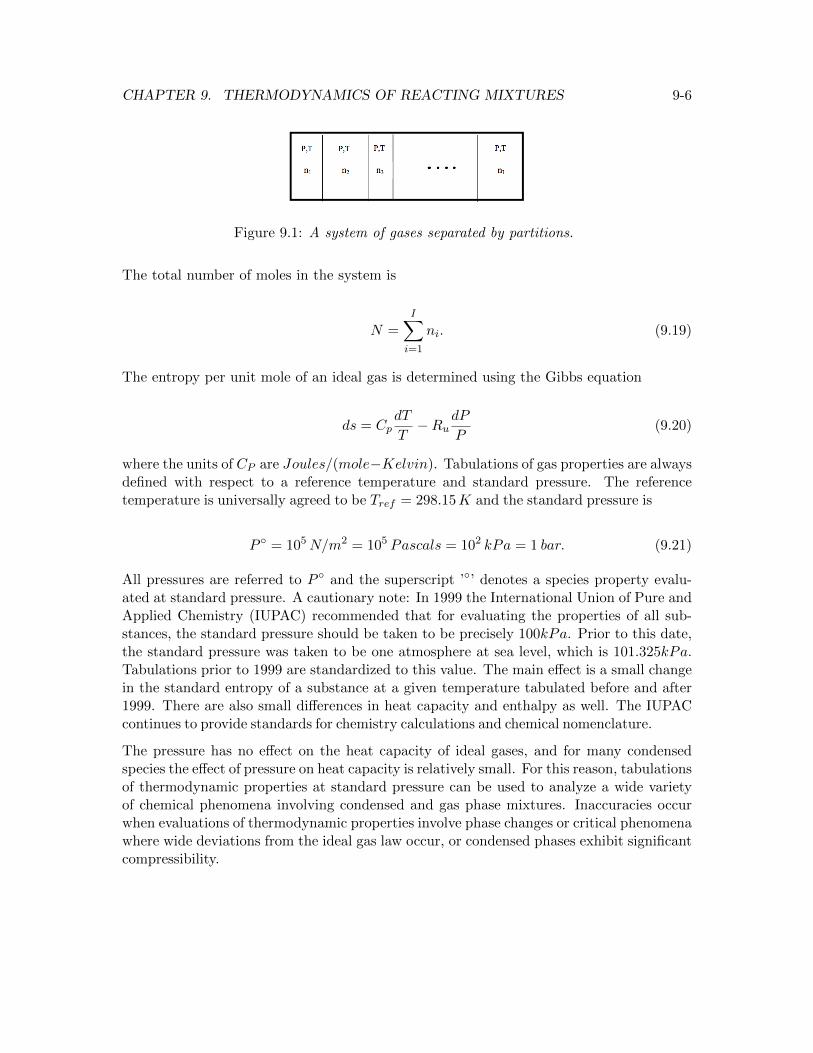
CHAPTER 9. THERMODYNAMICS OF REACTING MIXTURES 9-6
Figure 9.1: A system of gases separated by partitions.
The total number of moles in the system is
N =
I∑i=1
ni. (9.19)
The entropy per unit mole of an ideal gas is determined using the Gibbs equation
ds = CpdT
T−Ru
dP
P(9.20)
where the units of CP are Joules/(mole−Kelvin). Tabulations of gas properties are alwaysdefined with respect to a reference temperature and standard pressure. The referencetemperature is universally agreed to be Tref = 298.15K and the standard pressure is
P ◦ = 105N/m2 = 105 Pascals = 102 kPa = 1 bar. (9.21)
All pressures are referred to P ◦ and the superscript ’◦’ denotes a species property evalu-ated at standard pressure. A cautionary note: In 1999 the International Union of Pure andApplied Chemistry (IUPAC) recommended that for evaluating the properties of all sub-stances, the standard pressure should be taken to be precisely 100kPa. Prior to this date,the standard pressure was taken to be one atmosphere at sea level, which is 101.325kPa.Tabulations prior to 1999 are standardized to this value. The main effect is a small changein the standard entropy of a substance at a given temperature tabulated before and after1999. There are also small differences in heat capacity and enthalpy as well. The IUPACcontinues to provide standards for chemistry calculations and chemical nomenclature.
The pressure has no effect on the heat capacity of ideal gases, and for many condensedspecies the effect of pressure on heat capacity is relatively small. For this reason, tabulationsof thermodynamic properties at standard pressure can be used to analyze a wide varietyof chemical phenomena involving condensed and gas phase mixtures. Inaccuracies occurwhen evaluations of thermodynamic properties involve phase changes or critical phenomenawhere wide deviations from the ideal gas law occur, or condensed phases exhibit significantcompressibility.
CHAPTER 9. THERMODYNAMICS OF REACTING MIXTURES 9-7
Integrating (9.20) from the reference temperature at standard pressure, the entropy perunit mole of the ith gas species is
si(T, P )− s◦i (Tref ) =
∫ T
Tref
C◦pi (T )dT
T−Ru ln
(P
P ◦
). (9.22)
where the molar heat capacity C◦pi is tabulated as a function of temperature at standardpressure. The standard entropy of a gas species at the reference temperature is
s◦i (Tref ) =
∫ Tref
0C◦pi (T )
dT
T+ si
◦(0) (9.23)
where the integration is carried out at P = P ◦. To evaluate the standard entropy, heatcapacity data is required down to absolute zero. For virtually all substances, with theexception of superfluid helium (II), the heat capacity falls off rapidly as T → 0 so thatthe integral in (9.23) converges despite the apparent singularity at T = 0. From the thirdlaw, the entropy constant at absolute zero, s◦i (0), is generally taken to be zero for a puresubstance in its simplest crystalline state. For alloys and pure substances such as COwhere more than one crystalline structure is possible, the entropy at absolute zero may benonzero and tabulated entropy data for a substance may be revised from time to time asnew research results become available. Generally the entropy constant is very small.
The entropy per unit mole of the ith gas species is
si(T, P ) = s◦i (T )−Ru ln
(P
P ◦
). (9.24)
The entire effect of pressure on the system is in the logarithmic term of the entropy. Theextensive entropy of the whole system before mixing is
Sbefore =
I∑i=1
nisi (T, P ) =
I∑i=1
nis◦i (T )−
I∑i=1
niRu ln
(P
P ◦
). (9.25)
If the partitions are removed as shown in Figure 9.2 then, after complete mixing, each gastakes up the entire volume and the entropy of the ith species is
si(T, Pi) = s◦i (T )−Ru ln
(PiP ◦
). (9.26)
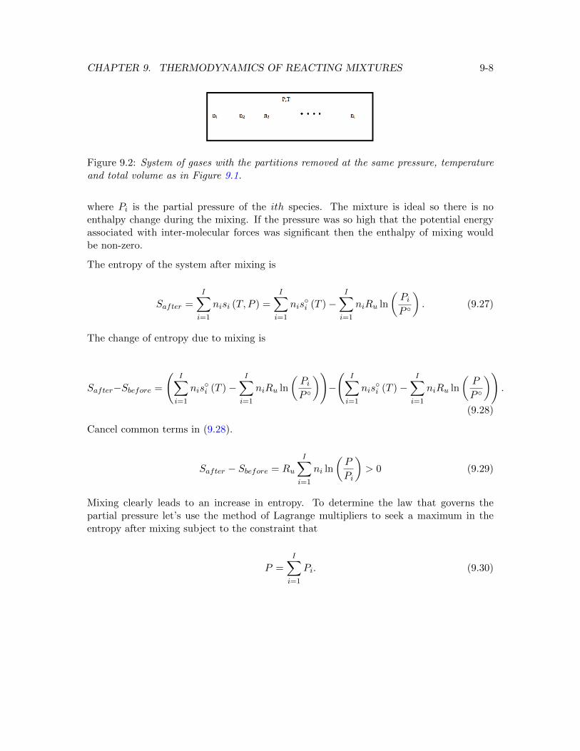
CHAPTER 9. THERMODYNAMICS OF REACTING MIXTURES 9-8
Figure 9.2: System of gases with the partitions removed at the same pressure, temperatureand total volume as in Figure 9.1.
where Pi is the partial pressure of the ith species. The mixture is ideal so there is noenthalpy change during the mixing. If the pressure was so high that the potential energyassociated with inter-molecular forces was significant then the enthalpy of mixing wouldbe non-zero.
The entropy of the system after mixing is
Safter =I∑i=1
nisi (T, P ) =I∑i=1
nis◦i (T )−
I∑i=1
niRu ln
(PiP ◦
). (9.27)
The change of entropy due to mixing is
Safter−Sbefore =
(I∑i=1
nis◦i (T )−
I∑i=1
niRu ln
(PiP ◦
))−
(I∑i=1
nis◦i (T )−
I∑i=1
niRu ln
(P
P ◦
)).
(9.28)
Cancel common terms in (9.28).
Safter − Sbefore = Ru
I∑i=1
ni ln
(P
Pi
)> 0 (9.29)
Mixing clearly leads to an increase in entropy. To determine the law that governs thepartial pressure let’s use the method of Lagrange multipliers to seek a maximum in theentropy after mixing subject to the constraint that
P =I∑i=1
Pi. (9.30)
CHAPTER 9. THERMODYNAMICS OF REACTING MIXTURES 9-9
That is, we seek a maximum in the function
W (T, n1, n2, ..., nI , P1, P2, ..., PI , λ) =I∑i=1
nis◦i (T )−
I∑i=1
niRu ln
(PiP ◦
)+ λ
(I∑i=1
Pi − P
)(9.31)
where λ is an, as yet unknown, Lagrange multiplier. The temperature of the system andnumber of moles of each species in the mixture are constant. Differentiate (9.31) and setthe differential to zero for an extremum.
dW =∂W
∂P1dP1 +
∂W
∂P2dP2 + .....+
∂W
∂PIdPI +
∂W
∂λdλ = 0 (9.32)
Now
dW = −I∑i=1
niRu
(dPiPi
)+ λ
(I∑i=1
dPi
)+ dλ
(I∑i=1
Pi − P
)= 0. (9.33)
The last term in (9.33) is zero by the constraint and the maximum entropy conditionbecomes.
I∑i=1
(−niRu
Pi+ λ
)dPi = 0 (9.34)
Since the dPi are completely independent, the only way (9.34) can be satisfied is if theLagrange multiplier satisfies
λ =niRuPi
(9.35)
for all i. In the original, unmixed, system each species satisfies the ideal gas law.
PVi = niRuT (9.36)
Using (9.35) and (9.36) we can form the sum
λ
I∑i=1
Pi =
I∑i=1
PViT
. (9.37)
CHAPTER 9. THERMODYNAMICS OF REACTING MIXTURES 9-10
Finally the Lagrange multiplier is
λ =V
T(9.38)
where, V =
I∑i=1
Vi. Using (9.35) and (9.38) the partial pressure satisfies
PiV = niRuT (9.39)
which is Dalton’s law of partial pressures. What we learn from this exercise is, not onlythat the entropy increases when the gases mix, but that the equilibrium state is one wherethe entropy is a maximum. Using Dalton’s law, the mole fraction of the ith gas species isrelated to the partial pressure as follows
xi =niN
=PiP
(9.40)
The entropy of a mixture of ideal gases expressed in terms of mole fractions is
Sgas =
I∑i=1
ni(s◦igas (T )−Ru ln (xi)
)−NRu ln
(P
P ◦
)(9.41)
and the entropy change due to mixing, (9.29), is expressed as
Safter − Sbefore = −NRuI∑i=1
xi ln (xi) > 0. (9.42)
9.5 Entropy of an ideal mixture of condensed species
The extensive entropy of an ideal mixture of condensed species (liquid or solid) with molenumbers n1, . . . , nI is S (T, P, n1, . . . , nI). If sipure (T, P ) is the entropy of the pure form ofthe ith component, then in a system where the mole numbers are fixed, the differential ofthe entropy is
dS (T, P, n1, . . . , nI) =
I∑i=1
nidsipure (T, P ) (9.43)
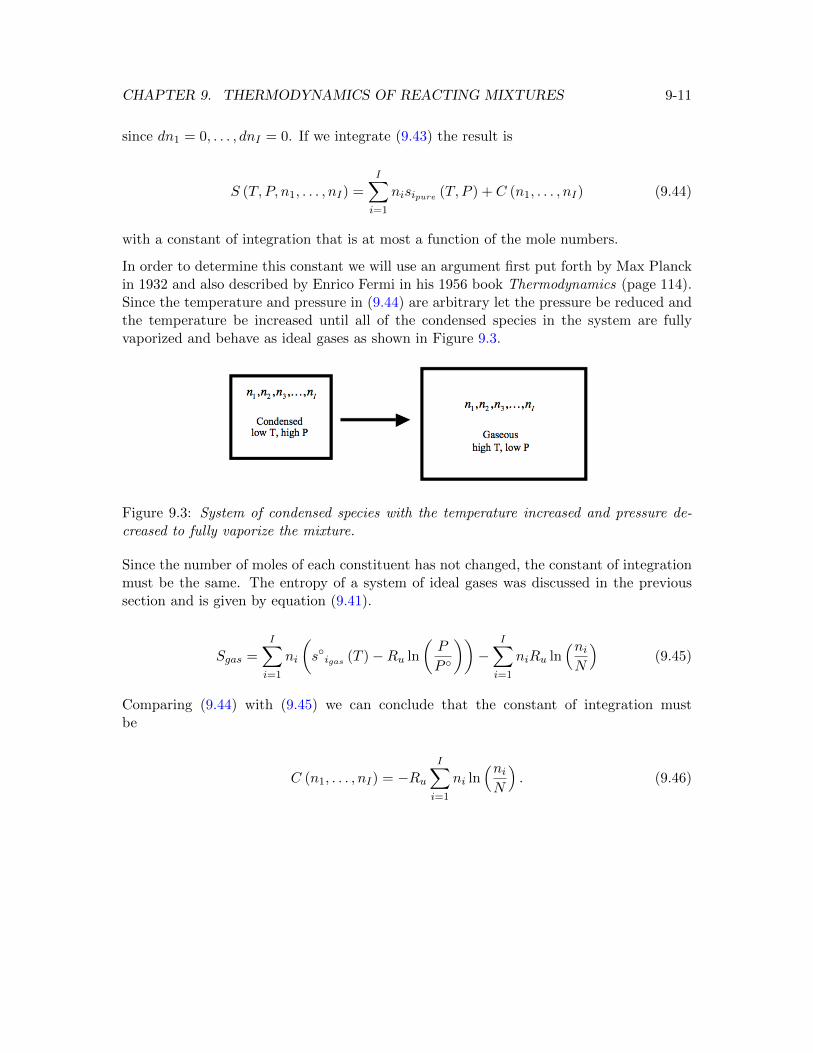
CHAPTER 9. THERMODYNAMICS OF REACTING MIXTURES 9-11
since dn1 = 0, . . . , dnI = 0. If we integrate (9.43) the result is
S (T, P, n1, . . . , nI) =I∑i=1
nisipure (T, P ) + C (n1, . . . , nI) (9.44)
with a constant of integration that is at most a function of the mole numbers.
In order to determine this constant we will use an argument first put forth by Max Planckin 1932 and also described by Enrico Fermi in his 1956 book Thermodynamics (page 114).Since the temperature and pressure in (9.44) are arbitrary let the pressure be reduced andthe temperature be increased until all of the condensed species in the system are fullyvaporized and behave as ideal gases as shown in Figure 9.3.
Figure 9.3: System of condensed species with the temperature increased and pressure de-creased to fully vaporize the mixture.
Since the number of moles of each constituent has not changed, the constant of integrationmust be the same. The entropy of a system of ideal gases was discussed in the previoussection and is given by equation (9.41).
Sgas =
I∑i=1
ni
(s◦igas (T )−Ru ln
(P
P ◦
))−
I∑i=1
niRu ln(niN
)(9.45)
Comparing (9.44) with (9.45) we can conclude that the constant of integration mustbe
C (n1, . . . , nI) = −RuI∑i=1
ni ln(niN
). (9.46)
CHAPTER 9. THERMODYNAMICS OF REACTING MIXTURES 9-12
Therefore, the entropy of a mixture of condensed species is
S (T, P, n1, . . . , nI) =I∑i=1
ni(sipure (T, P )−Ru ln (xi)
)(9.47)
where the mole fraction, xi = ni/N is used. Finally, the contribution of each componentto the extensive entropy of the mixture of condensed species is
si (T, P ) = sipure (T, P )−Ru ln (xi) . (9.48)
The form of this equation is very similar to that for gases and comes as something of asurprise since it involves the ideal gas constant which would seem to have no particularrelevance to a liquid or a solid. According to Kestin (A Course in Thermodynamics,Ginn Blaisdell 1966) when (9.48) was first introduced it was ”met with general incredulity,but its validity has since been confirmed experimentally beyond any reasonable doubtwhatever.”
It can be noted that if the gases in the mixing problem described in the last section werereplaced by ideal liquids, and those liquids were allowed to evolve from the unmixed to themixed state, the entropy change would be given by an expression identical to (9.29).
(Safter − Sbefore)ideal liquids = −NRuI∑i=1
xi ln (xi) (9.49)
9.6 Thermodynamics of incompressible liquids and solids
For a single homogeneous substance the Gibbs equation is
dS =dE
T+P
TdV. (9.50)
If the substance is an incompressible solid or liquid the Gibbs equation reduces to
dS = Cv(T )dT
T(9.51)
CHAPTER 9. THERMODYNAMICS OF REACTING MIXTURES 9-13
and the entropy is
S − Sref =
∫ T
Tref
Cv(T )dT
T. (9.52)
The entropy and internal energy of an incompressible substance depend only on its temper-ature. The constant volume and constant pressure heat capacities are essentially equivalentCp (T ) = Cv (T ) = C (T ).
Since liquids and solids tend to be nearly incompressible, the entropy sipure (T, P ) tends tobe independent of pressure and in most circumstances one can use
sipure (T, P ) = s◦i (T ) . (9.53)
Now the entropy of a condensed species in a mixture really does resemble that of an idealgas, but without the dependence on mixture pressure.
si (T, P ) = s◦i (T )−Ru ln (xi) (9.54)
For a general substance, the differential of the Gibbs function is
dG = dE + PdV + V dP − TdS − SdT = −SdT + V dP (9.55)
where the Gibbs equation (9.4) has been used. The cross derivative test applied to theright side of (9.55) produces the Maxwell relation
(∂S
∂P
)T
= −(∂V
∂T
)P
. (9.56)
For an incompressible material, the entropy is independent of the pressure and (9.56)implies that the coefficient of thermal expansion of the material is also zero. Therefore, for
CHAPTER 9. THERMODYNAMICS OF REACTING MIXTURES 9-14
an incompressible substance
(∂V
∂P
)T
= 0(∂V
∂T
)P
= 0
V = constantCP = CV = CdE = CdT
dS =C
TdT
dH = CdT + V dP.
(9.57)
On a per unit mole basis, the enthalpy of an incompressible material referenced to thestandard state is
h(T, P ) = h◦ (T ) + (P − P ◦) v◦ (9.58)
where v◦ = constant is the molar volume of the material. The superscript on v◦ is notreally necessary since it assumed to be a constant at all pressures and temperatures butas a practical matter, when using (9.58) as an approximation for a real condensed solid orliquid, the value of the molar density will be taken to be at the standard pressure 105Paand the reference temperature 298.15K. Often the pressure term in (9.58) is neglectedwhen dealing with reacting systems of gases and condensed materials. The reason is that,while the molar enthalpy of the condensed and gaseous form of a species are of the sameorder, the molar volume of a solid or liquid is generally two to three orders of magnitudesmaller than the gaseous molar volume.
9.7 Enthalpy
The enthalpy per unit mole of a gas is determined from
dh = Cp(T )dT. (9.59)
The enthalpy of a gas species is
hi (T )− hi (Tref ) = h◦i (T )− h◦i (Tref ) =
∫ T
TrefC◦pi (T )dT. (9.60)
CHAPTER 9. THERMODYNAMICS OF REACTING MIXTURES 9-15
In principle the standard enthalpy of the ith gas species at the reference temperature couldbe taken as
h◦i (Tref ) =
∫ Tref
0C◦pidT + h◦i (0). (9.61)
In this approach the enthalpy constant is the enthalpy change associated with chemicalbond breaking and making that occurs when the atoms composing the species are broughttogether from infinity to form the molecule at absolute zero. Note that even for an atomicspecies, the enthalpy constant is not exactly zero. A quantum mechanical system containsenergy or enthalpy arising from ground state motions that cannot be removed completelyeven at absolute zero temperature. In practice, enthalpies for most substances are tabulatedas differences from the enthalpy at the reference temperature of 298.15K which is muchmore easily accessible than absolute zero so the question of the zero point enthalpy rarelycomes up. Thus the standard enthalpy of a species is
h◦i (T ) =
∫ T
TrefC◦pi (T )dT + ∆h◦fi (Tref ) (9.62)
where ∆h◦fi (T ) is the enthalpy change that occurs when the atoms of the species arebrought together from at infinity at the finite temperature T . The enthalpy including theheat of formation (9.62) is sometimes called the complete enthalpy. In practice certain con-ventions are used to facilitate the tabulation of the heat of formation of a substance.
9.7.1 Enthalpy of formation and the reference reaction
The enthalpy of formation of a substance, denoted ∆h◦f (Tref ), is defined as the enthalpychange that occurs when one mole of the substance is formed from its elements in theirreference state at the given temperature T and standard pressure P ◦. The reference statefor an element is generally taken to be its most stable state at the given temperature andstandard pressure. The reference reaction for a substance is one where the substance is thesingle product of a chemical reaction between its elements in their most stable state.
This convention for defining the heat of formation of a substance is useful even if thereference reaction is physically unlikely to ever actually occur. A consequence of thisdefinition is that the heat of formation of a pure element in its reference state at anytemperature is always zero. For example, the enthalpy of formation of any of the diatomicgases is zero at all temperatures. This is clear when we write the trivial reaction to form,
CHAPTER 9. THERMODYNAMICS OF REACTING MIXTURES 9-16
for example hydrogen, from its elements in their reference state.
H2 → H2 (9.63)
The enthalpy change is clearly zero. In fact the change in any thermodynamic variablefor any element in its reference state is zero at all temperatures. A similar referencereaction applies to any of the other diatomic species O2, N2, F2, Cl2, Br2, I2, and the heatof formation of these substances is zero at all temperatures. The most stable form of carbonis solid carbon or graphite and the reference reaction is
C(s) → C(s) (9.64)
with zero heat of formation at all temperatures.
The reference reaction for carbon dioxide at 298.15K is
C(s) +O2 → CO2 ∆h◦fCO2(298.15) = −393.522 kJ/mole. (9.65)
Here the carbon is taken to be in the solid (graphite) form and the oxygen is taken to bethe diatomic form. Both are the most stable forms over a wide range of temperatures.Even if the temperature is well above the point where carbon sublimates to a gas (3915K)and significant oxygen is dissociated, the heats of formation of C(s) and O2 remain zeroeven though the most stable form of carbon at this temperature is carbon gas.
The heats of formation of metal elements are treated a little differently. The heat offormation of crystalline aluminum is zero at temperatures below the melting point and theheat of formation of liquid aluminum is zero at temperatures above the melting point. Thesame applies to boron, magnesium, sulfur, titanium and other metals.
The enthalpy (9.62) is usually expressed in terms of tabulated data as
hi (T ) = h◦i (T ) = ∆h◦fi (Tref ) + {h◦i (T )− h◦i (Tref )} . (9.66)
For a general reaction the enthalpy balance is
∆h◦ (Tfinal) =
Iproduct∑iproduct
niproducth◦iproduct
(Tfinal)−Ireactant∑ireactant
nireactanth◦ireactant
(Tinitialireactant
).
(9.67)
CHAPTER 9. THERMODYNAMICS OF REACTING MIXTURES 9-17
So for example, to determine the heat of formation of CO2 at 1000K where the initialreactants are also at 1000K, the calculation would be
∆h◦fCO2(1000) =(
∆h◦fCO2(298.15) +
{h◦CO2
(1000)− h◦CO2(298.15)
})−
(∆h◦fC(s)
(298.15) +{h◦C(s)
(1000)− h◦C(s)(298.15)
})−
(∆h◦fO2
(298.15) +{h◦O2
(1000)− h◦O2(298.15)
}).
(9.68)
Putting in the numbers from tabulated data (See Appendix 2) gives
∆h◦fCO2(1000) =
[−393.522 + 33.397]− [0 + 11.795]− [0 + 22.703] = −394.623(9.69)
which is the tabulated value of the heat of formation of carbon dioxide at 1000K. Note thatthe enthalpy of the reference reactants at the reaction temperature must be included in thecalculation of the heat of formation calculation. Further discussion of heats of formationcan be found in Appendix 1 and tables of thermo-chemical data for selected species can befound in Appendix 2.
9.8 Condensed phase equilibrium
The pressure and temperature of the system may be such that one or more or all of thespecies may be evolving with their condensed phase. In this case it may be necessary tovary the volume to keep the temperature and pressure constant until the system reachesequilibrium.
Figure 9.4 depicts the various species of the system in several phases all of which are in con-tact with each other. Let the total number of moles in each phase beN1, N2, . . . , Np, . . . , NP .Generally only a subset of the species will be evolving with their condensed phase and sothere is a different maximal index Ip for each phase. Effects of surface tensions betweenphases are ignored.
Note the total numbers of moles in each phase are related to the species mole numbers
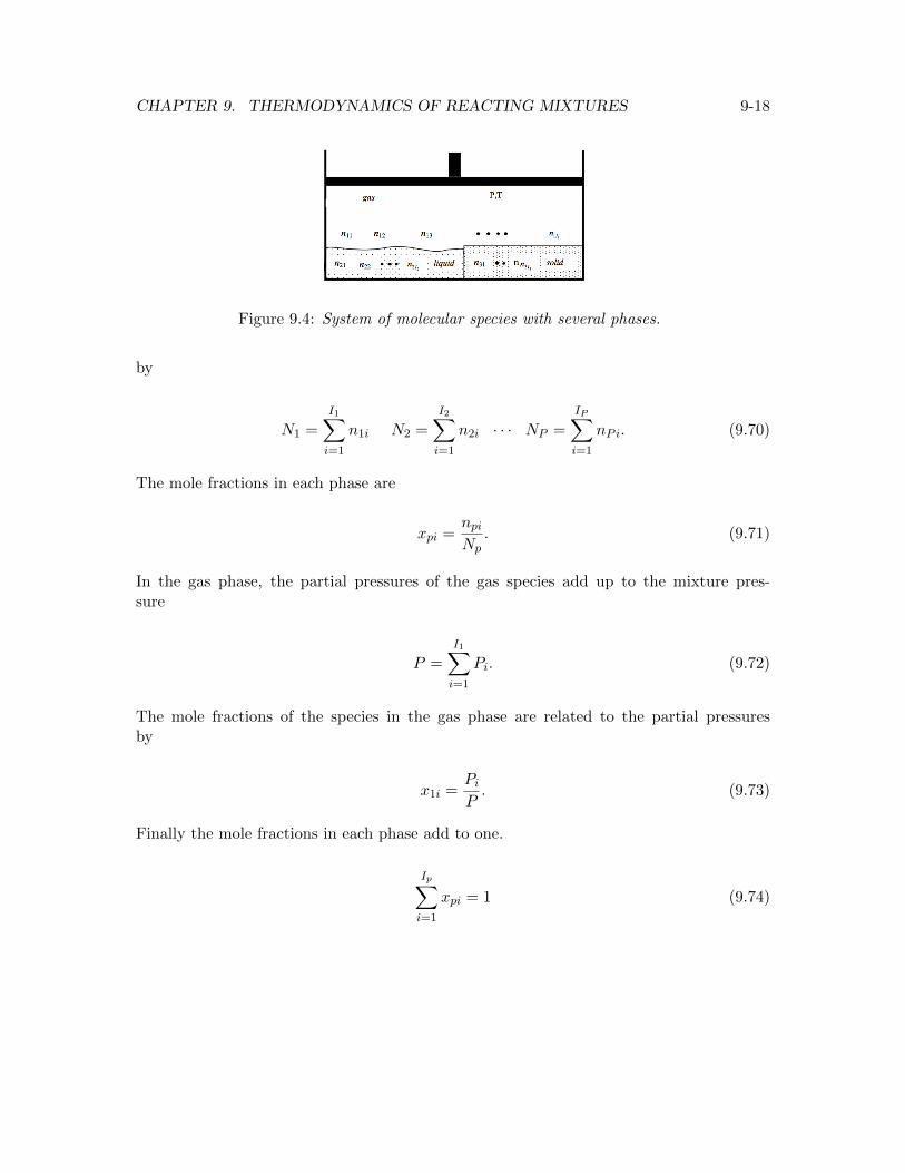
CHAPTER 9. THERMODYNAMICS OF REACTING MIXTURES 9-18
Figure 9.4: System of molecular species with several phases.
by
N1 =
I1∑i=1
n1i N2 =
I2∑i=1
n2i · · · NP =
IP∑i=1
nPi. (9.70)
The mole fractions in each phase are
xpi =npiNp
. (9.71)
In the gas phase, the partial pressures of the gas species add up to the mixture pres-sure
P =
I1∑i=1
Pi. (9.72)
The mole fractions of the species in the gas phase are related to the partial pressuresby
x1i =PiP. (9.73)
Finally the mole fractions in each phase add to one.
Ip∑i=1
xpi = 1 (9.74)
CHAPTER 9. THERMODYNAMICS OF REACTING MIXTURES 9-19
The extensive Gibbs free energies in each phase are
G1 (T, P, n11, n12, n13, ..., n1I1) = N1
{I1∑i=1
x1i (g◦1i(T ) +RuT ln (x1i)) +RuT ln
(P
P ◦
)}
G2 (T, P, n21, n22, n23, ..., n2I2) = N2
I2∑i2=1
x2i (g2i(T, P ) +RuT ln (x2i))
...
GP (T, P, nP1, nP2, nP3, ..., nPIP ) = NP
IP∑iP=1
xpi (gpi(T, P ) +RuT ln (xpi))
(9.75)
where phase 1 is assumed to be the gas phase. In (9.75) we have assumed that all condensedphases are ideal mixtures and the entropy per mole of the condensed phase of species idoes not depend on the pressure. This is a reasonable assumption for a condensed phasethat is approximately incompressible as was argued earlier in conjunction with equation(9.58). There are a few examples of liquids such as liquid helium and liquid nitrous oxidethat are quite compressible and the assumption would break down. This treatment of thecondensed phases is similar to that used by Bill Reynolds in the development of STANJAN.The NASA Glenn code CEA is a little different. In CEA, each condensed phase is treatedas a pure substance. For example, if there are two species that condense out as liquids, eachis treated as a separate, distinct phase. In the approach used by CEA the mole fractionsof each condensed species are one by definition. In CEA the pressure term in (9.58) isneglected. See equation 2.11 in NASA Reference Publication 1311 (1994) by Gordon andMcBride.
In the case of a gas, the Gibbs free energy does depend on pressure through the dependenceof entropy on pressure. This is connected to the fact that, as quantum mechanics tells us,the number of energy states that a gas can occupy (and therefore the entropy of the gas)increases with the volume containing the gas (see Appendix 1 of the AA210a notes).
The Gibbs free energy of the whole system is
G (T, P, n11, n12, . . . , n1I1 , n21, n22, . . . , n2I2 , ..., nP1, nP2, ..., nPIP ) =
P∑p=1
IP∑i=1
npigpi (T, P, npi) .(9.76)
CHAPTER 9. THERMODYNAMICS OF REACTING MIXTURES 9-20
With the gas phase written separately Equation (9.76) is
G (T, P, n11, n12, . . . , n1I1 , n21, n22, . . . , n2I2 , ..., nP1, nP2, ..., nPIP ) =
P∑p=1
IP∑i=1
n1i
g◦1i (T ) +RuT ln (n1i)−RuT ln
I1∑i=1
n1i
+
P∑p=2
IP∑i=1
npi
gpi (T, P ) +RuT ln (npi)−RuT ln
IP∑i=1
npi
.
(9.77)
Differentiate (9.77).
dG =∂G
∂TdT +
∂G
∂PdP+
∂G
∂n11dn11 +
∂G
∂n12dn12 + · · ·+ ∂G
∂n1I1
dn1I1+
∂G
∂n21dn21 +
∂G
∂n22dn22 + · · ·+ ∂G
∂n2I2
dn2I2 + . . .+
∂G
∂nP1dnP1 +
∂G
∂nP2dnP2 + · · ·+ ∂G
∂nPIPdnPIP .
(9.78)
CHAPTER 9. THERMODYNAMICS OF REACTING MIXTURES 9-21
Written out fully (9.78) is
dG =
I1∑i=1
dn1i
g◦1i(T ) +RuT ln (n1i)−RuT ln
I1∑_i =1
n1_i
+
I1∑i=1
n1i
RuT(dn1i
n1i
)−RuT
I1∑
_i =1
dn1_i
I1∑_i =1
n1_i
+RuT ln
(P
P ◦
) I1∑i=1
dn1i+
I1∑i=1
n1i
∂g◦1i(T )
∂T+Ru ln (n1i)−Ru ln
I1∑_i =1
n1_i
dT+
(I1∑i=1
n1i
)RuT
(dP
P
)+
(I1∑i=1
n1i
)Ru ln
(P
P ◦
)dT+
P∑p=2
Ip∑i=1
dnpi
gpi(T, P ) +RuT ln (npi)−RuT ln
Ip∑_i =1
np_i
+
P∑p=2
Ip∑i=1
npi
RuT(dnpinpi
)−RuT
Ip∑
_i =1
dnp_i
Ip∑i=1
np_i
+
P∑p=2
Ip∑i=1
npi
∂gpi(T, P )
∂T+Ru ln (n1i)−Ru ln
Ip∑_i =1
n1_i
dT +P∑p=2
Ip∑i=1
npi
(∂gpi(T, P )
∂T
)dP .
(9.79)
Note that
Ip∑i=1
npi
dnpinpi−
Ip∑_i =1
dnp_i
Ip∑_i =1
np_i
= dNp − dNp = 0. (9.80)
CHAPTER 9. THERMODYNAMICS OF REACTING MIXTURES 9-22
At constant temperature and pressure dT = dP = 0 and(9.79) becomes
dG =
I1∑i=1
dn1i
g◦1i(T ) +RuT ln (n1i)−RuT ln
I1∑_i =1
n1_i
+RuT ln
(P
P ◦
)+
P∑p=2
Ip∑i=1
dnpi
gpi(T, P ) +RuT ln (npi)−RuT ln
Ip∑_i =1
np_i
.
(9.81)
In terms of mole fractions (9.81) reads
dG =
I1∑i=1
dn1i
(g◦1i(T ) +RuT ln (x1i) +RuT ln
(P
P ◦
))+
P∑p=2
Ip∑i=1
dnpi (gpi(T, P ) +RuT ln (xpi)).
. (9.82)
At equilibrium dG = 0. For species that are only present in one phase, dnpi = 0 atequilibrium. For those species that are in equilibrium with another phase, dnphase1i =−dnphase pi and equation dG = 0 can only be satisfied if
gphase1i = gphase pi. (9.83)
If phase 1 is a gas species (9.83) is
g◦phase1i(T )+RuT ln (xphase1i)+RuT ln
(P
P ◦
)= gphase pi(T, P )+RuT ln (xphase pi) . (9.84)
At equilibrium, the Gibbs free energy (or chemical potential) of species i is the sameregardless of its phase. For example if gas species 1 is in equilibrium with its liquid phase,then ggas1 (T, P ) = gliquid1 (T, P ). There can also be more than one solid phase and so thetotal number of phases can exceed three. For example, in helium at very low temperaturethere can be multiple liquid phases.
Suppose phase p in is a pure liquid so the mole fraction is one. Also assume the liquid isincompressible so that the Gibbs function of the liquid is given by
g◦gasi(T ) +RuT ln (xgasi) +RuT ln
(P
P ◦
)= g◦liquidi(T ) + (P − P ◦) v◦liquid. (9.85)
CHAPTER 9. THERMODYNAMICS OF REACTING MIXTURES 9-23
Solve for the partial pressure of the species in the gas phase.
PiP ◦
= e(P−P◦)v◦liquidi
RuT
(eg◦liquidi
(T )−g◦gasi (T )
RuT
)(9.86)
The term in brackets is the classical form of the Clausius-Clapeyron equation that relatesthe vapor pressure of a gas in equilibrium with its condensed phase to the temperature ofthe system.
9.9 Chemical equilibrium, the method of element poten-tials
If the species are allowed to react at constant temperature and pressure, the mole fractionswill evolve toward values that minimize the extensive Gibbs free energy of the systemsubject to the constraint that the number of moles of each element in the mixture remainsfixed. The number of moles of each atom in the system is given by
aj =
P∑p=1
Ip∑i=1
npiApij (9.87)
where Apij is the number of atoms of the jth element in the ith molecular species of thepth phase. The appropriate picture of our system is shown in Figure 9.5.
Figure 9.5: System of reacting molecular species in several phases at constant temperatureand pressure with fixed number of moles of each element.
Generally the number of species in each phase will be different. This may be the case evenin a situation where, at a given temperature and pressure, there is phase equilibrium fora given species. Consider graphite in equilibrium with its vapor at low temperature, themole fraction in the vapor phase may be so small as to be essentially zero and the species
CHAPTER 9. THERMODYNAMICS OF REACTING MIXTURES 9-24
may be rightly excluded from the vapor mixture. The volume required to maintain thesystem at constant pressure and temperature must be allowed to vary.
The Gibbs free energy of the system is
G (T, P, n11, n12, ..., np1, ..., nPIP ) =P∑p=1
Np
Ip∑i=1
xpigpi (T, P, xpi) . (9.88)
With the gas phase written separately
G (T, P, n11, n12, ..., n21, ..., nPIP ) = N1
I1∑i=1
x1i (g◦1i(T ) +RuT ln (x1i)) +N1RuT ln
(P
P ◦
)+
P∑p=2
Np
Ip∑i=1
xpi (gpi(T, P ) +RuT ln (xpi))
.
(9.89)
We will use the method of Lagrange multipliers to minimize the Gibbs free energy subjectto the atom constraints. Minimize the function
W(T, P, n11, n12, ..., n1I1 , n21, n22, ..., n2I2 , ...., np1, np2, ..., npIp , λ1, ..., λJ
)=
G(T, P, n11, n12, ..., n1I1 , n21, n22, ..., n2I2 , ...., np1, np2, ..., npIp
)−
RuTJ∑j=1
λj
P∑p=1
Ip∑i=1
npiApij − aj
.
(9.90)
where the J unknown Lagrange multipliers, λj , are dimensionless. Our modified equilib-rium condition is
dW =∂W
∂TdT+
∂W
∂PdP+
∂W
∂n11dn11+....+
∂W
∂npIdnpIP +
∂W
∂λ1dλ1+....+
∂W
∂λJdλJ = 0. (9.91)
CHAPTER 9. THERMODYNAMICS OF REACTING MIXTURES 9-25
Substitute (9.76) into (9.91) and impose dP = dT = 0.
dW =P∑p=1
Ip∑i=1
(npidgpi (T, P, xpi) + gpi (T, P, xpi) dnpi)−RuTj∑j=1
λj
P∑p=1
Ip∑i=1
dnpiApij
(9.92)
The order of the sums can be rearranged so (9.92) can be written as
dW =
P∑p=1
Ip∑i=1
npidgpi (T, P, xpi) +
P∑p=1
Ip∑i=1
gpi (T, P, xpi)−RuTJ∑j=1
λjApij
dnpi = 0.
(9.93)
The differential of the molar Gibbs free energy is
dgpi =∂gpi∂T
dT +∂gpi∂P
dP +RuTdxpixpi
. (9.94)
For a process that takes place at constant temperature and pressure
dW = RuT
P∑p=1
Ip∑i=1
npidxpixpi
+
P∑p=1
Ip∑i=1
gpi (T, P, xpi)−RuTJ∑j=1
λjApij
dnpi = 0. (9.95)
The first sum in (9.95) can be re-written as follows
dW = RuTP∑p=1
Np
Ip∑i=1
xpidxpixpi
+P∑p=1
Ip∑i=1
gpi (T, P, xpi)−RuTJ∑j=1
λjApij
dnpi = 0
(9.96)
or
dW = RuT
P∑p=1
Np
Ip∑i=1
dxpi +P∑p=1
Ip∑i=1
gpi (T, P, xpi)−RuTJ∑j=1
λjApij
dnpi = 0. (9.97)
CHAPTER 9. THERMODYNAMICS OF REACTING MIXTURES 9-26
But the normalization conditions for the mole fractions of each phase imply that
Ip∑i=1
dxpi = d
Ip∑i=1
xpi
= d (1) = 0. (9.98)
Finally our modified equilibrium condition is
dW =P∑p=1
Ip∑i=1
gpi (T, P, xpi)−RuTJ∑j=1
λjApij
dnpi = 0. (9.99)
Since the dnpi are completely free, the condition (9.99) can only be satisfied if
gpi (T, P, xpi) = RuT
J∑j=1
λjApij . (9.100)
The Gibbs free energy of the system is
G (T, P, n11, n12, ..., np1, ..., nPIP ) = RuTP∑p=1
Ip∑i=1
J∑j=1
npiλjApij . (9.101)
Each atom in the mixture contributes equally to the extensive Gibbs free energy regardlessof which molecule it is in or which phase it is in. The molar Gibbs free energy of the ithgas phase species is
g1i(T, P ) = g◦1i(T ) +RuT ln (x1i) +RuT ln
(P
P ◦
). (9.102)
Insert into (9.100). For the gas phase species
g◦1i(T )
RuT+ ln (x1i) + ln
(P
P ◦
)=
J∑j=1
λjA1ij . (9.103)
For the condensed phase species
gpi(T, P )
RuT+ ln (xpi) =
J∑j=1
λjApij p = 2, . . . , P . (9.104)
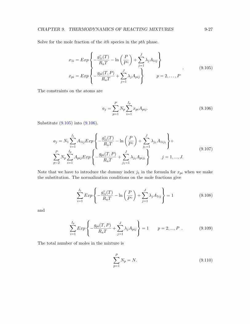
CHAPTER 9. THERMODYNAMICS OF REACTING MIXTURES 9-27
Solve for the mole fraction of the ith species in the pth phase.
x1i = Exp
−g◦1i(T )
RuT− ln
(P
P ◦
)+
J∑j=1
λjA1ij
xpi = Exp
−gpi(T, P )
RuT+
J∑j=1
λjApij
p = 2, . . . , P
. (9.105)
The constraints on the atoms are
aj =P∑p=1
Np
Ip∑i=1
xpiApij . (9.106)
Substitute (9.105) into (9.106).
aj = N1
I1∑i=1
A1ijExp
−g◦1i(T )
RuT− ln
(P
P ◦
)+
J∑j1=1
λj1A1ij1
+
P∑p=2
Np
Ip∑i=1
ApijExp
−gpi(T, P )
RuT+
J∑j1=1
λj1Apij1
j = 1, ..., J.
(9.107)
Note that we have to introduce the dummy index j1 in the formula for xpi when we makethe substitution. The normalization conditions on the mole fractions give
I1∑i=1
Exp
−g◦1i(T )
RuT− ln
(P
P ◦
)+
J∑j=1
λjA1ij
= 1 (9.108)
and
Ip∑i=1
Exp
−gpi(T, P )
RuT+
J∑j=1
λjApij
= 1 p = 2, ..., P . (9.109)
The total number of moles in the mixture is
P∑p=1
Np = N. (9.110)
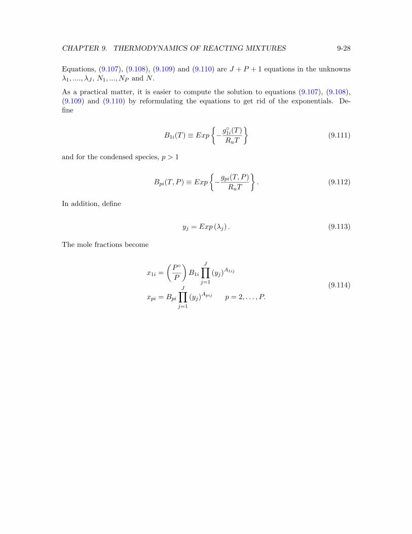
CHAPTER 9. THERMODYNAMICS OF REACTING MIXTURES 9-28
Equations, (9.107), (9.108), (9.109) and (9.110) are J + P + 1 equations in the unknownsλ1, ...., λJ , N1, ..., NP and N .
As a practical matter, it is easier to compute the solution to equations (9.107), (9.108),(9.109) and (9.110) by reformulating the equations to get rid of the exponentials. De-fine
B1i(T ) ≡ Exp{−g◦1i(T )
RuT
}(9.111)
and for the condensed species, p > 1
Bpi(T, P ) ≡ Exp{−gpi(T, P )
RuT
}. (9.112)
In addition, define
yj = Exp (λj) . (9.113)
The mole fractions become
x1i =
(P ◦
P
)B1i
J∏j=1
(yj)A1ij
xpi = Bpi
J∏j=1
(yj)Apij p = 2, . . . , P.
(9.114)
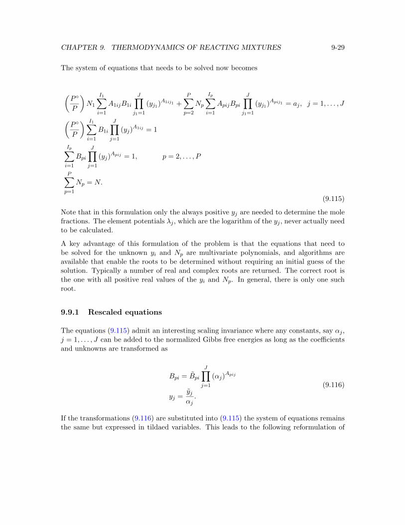
CHAPTER 9. THERMODYNAMICS OF REACTING MIXTURES 9-29
The system of equations that needs to be solved now becomes
(P ◦
P
)N1
I1∑i=1
A1ijB1i
J∏j1=1
(yj1)A1ij1 +P∑p=2
Np
Ip∑i=1
ApijBpi
J∏j1=1
(yj1)Apij1 = aj , j = 1, . . . , J
(P ◦
P
) I1∑i=1
B1i
J∏j=1
(yj)A1ij = 1
Ip∑i=1
Bpi
J∏j=1
(yj)Apij = 1, p = 2, . . . , P
P∑p=1
Np = N.
(9.115)
Note that in this formulation only the always positive yj are needed to determine the molefractions. The element potentials λj , which are the logarithm of the yj , never actually needto be calculated.
A key advantage of this formulation of the problem is that the equations that need tobe solved for the unknown yi and Np are multivariate polynomials, and algorithms areavailable that enable the roots to be determined without requiring an initial guess of thesolution. Typically a number of real and complex roots are returned. The correct root isthe one with all positive real values of the yi and Np. In general, there is only one suchroot.
9.9.1 Rescaled equations
The equations (9.115) admit an interesting scaling invariance where any constants, say αj ,j = 1, . . . , J can be added to the normalized Gibbs free energies as long as the coefficientsand unknowns are transformed as
Bpi = Bpi
J∏j=1
(αj)Apij
yj =yjαj.
(9.116)
If the transformations (9.116) are substituted into (9.115) the system of equations remainsthe same but expressed in tildaed variables. This leads to the following reformulation of
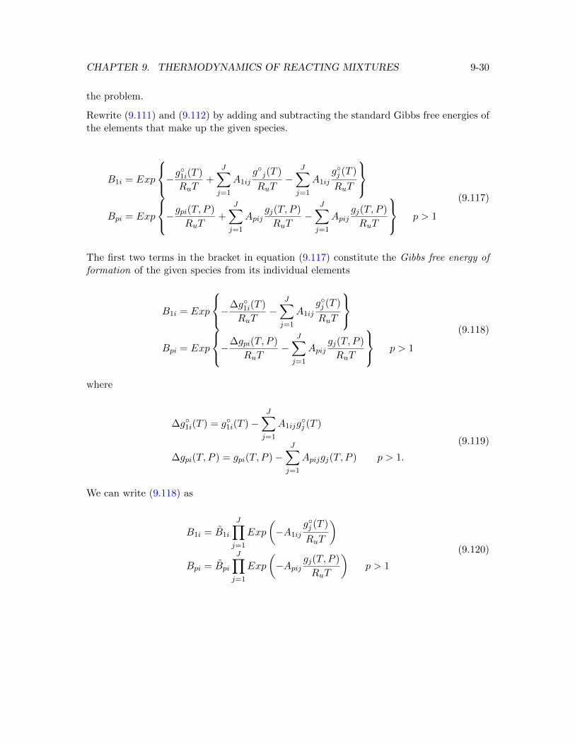
CHAPTER 9. THERMODYNAMICS OF REACTING MIXTURES 9-30
the problem.
Rewrite (9.111) and (9.112) by adding and subtracting the standard Gibbs free energies ofthe elements that make up the given species.
B1i = Exp
−g◦1i(T )
RuT+
J∑j=1
A1ij
g◦j(T )
RuT−
J∑j=1
A1ij
g◦j (T )
RuT
Bpi = Exp
−gpi(T, P )
RuT+
J∑j=1
Apijgj(T, P )
RuT−
J∑j=1
Apijgj(T, P )
RuT
p > 1
(9.117)
The first two terms in the bracket in equation (9.117) constitute the Gibbs free energy offormation of the given species from its individual elements
B1i = Exp
−∆g◦1i(T )
RuT−
J∑j=1
A1ij
g◦j (T )
RuT
Bpi = Exp
−∆gpi(T, P )
RuT−
J∑j=1
Apijgj(T, P )
RuT
p > 1
(9.118)
where
∆g◦1i(T ) = g◦1i(T )−J∑j=1
A1ijg◦j (T )
∆gpi(T, P ) = gpi(T, P )−J∑j=1
Apijgj(T, P ) p > 1.
(9.119)
We can write (9.118) as
B1i = B1i
J∏j=1
Exp
(−A1ij
g◦j (T )
RuT
)
Bpi = Bpi
J∏j=1
Exp
(−Apij
gj(T, P )
RuT
)p > 1
(9.120)
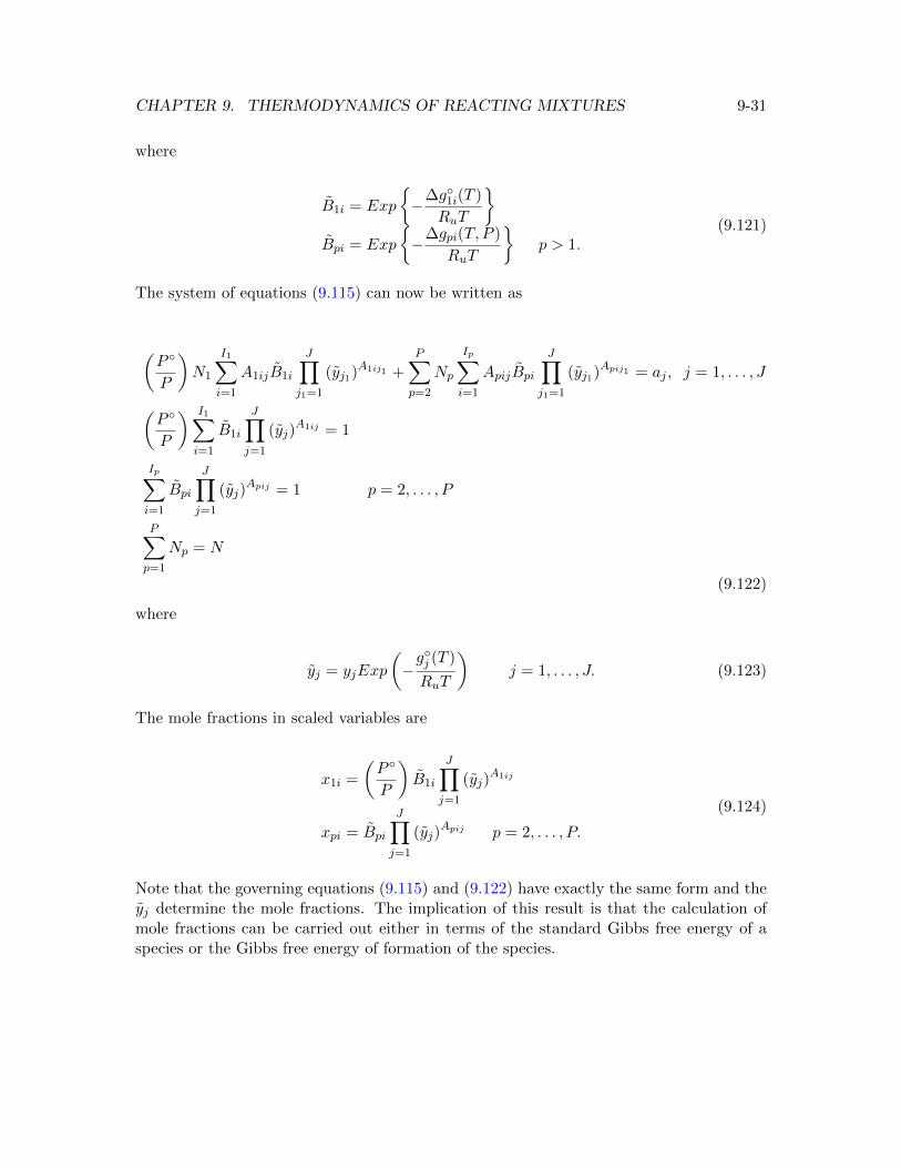
CHAPTER 9. THERMODYNAMICS OF REACTING MIXTURES 9-31
where
B1i = Exp
{−∆g◦1i(T )
RuT
}Bpi = Exp
{−∆gpi(T, P )
RuT
}p > 1.
(9.121)
The system of equations (9.115) can now be written as
(P ◦
P
)N1
I1∑i=1
A1ijB1i
J∏j1=1
(yj1)A1ij1 +
P∑p=2
Np
Ip∑i=1
ApijBpi
J∏j1=1
(yj1)Apij1 = aj , j = 1, . . . , J
(P ◦
P
) I1∑i=1
B1i
J∏j=1
(yj)A1ij = 1
Ip∑i=1
Bpi
J∏j=1
(yj)Apij = 1 p = 2, . . . , P
P∑p=1
Np = N
(9.122)
where
yj = yjExp
(−g◦j (T )
RuT
)j = 1, . . . , J. (9.123)
The mole fractions in scaled variables are
x1i =
(P ◦
P
)B1i
J∏j=1
(yj)A1ij
xpi = Bpi
J∏j=1
(yj)Apij p = 2, . . . , P.
(9.124)
Note that the governing equations (9.115) and (9.122) have exactly the same form and theyj determine the mole fractions. The implication of this result is that the calculation ofmole fractions can be carried out either in terms of the standard Gibbs free energy of aspecies or the Gibbs free energy of formation of the species.
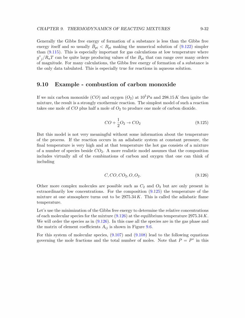
CHAPTER 9. THERMODYNAMICS OF REACTING MIXTURES 9-32
Generally the Gibbs free energy of formation of a substance is less than the Gibbs freeenergy itself and so usually Bpi < Bpi making the numerical solution of (9.122) simplerthan (9.115). This is especially important for gas calculations at low temperature whereg◦j/RuT can be quite large producing values of the Bpi that can range over many ordersof magnitude. For many calculations, the Gibbs free energy of formation of a substance isthe only data tabulated. This is especially true for reactions in aqueous solution.
9.10 Example - combustion of carbon monoxide
If we mix carbon monoxide (CO) and oxygen (O2) at 105Pa and 298.15K then ignite themixture, the result is a strongly exothermic reaction. The simplest model of such a reactiontakes one mole of CO plus half a mole of O2 to produce one mole of carbon dioxide.
CO +1
2O2 → CO2 (9.125)
But this model is not very meaningful without some information about the temperatureof the process. If the reaction occurs in an adiabatic system at constant pressure, thefinal temperature is very high and at that temperature the hot gas consists of a mixtureof a number of species beside CO2. A more realistic model assumes that the compositionincludes virtually all of the combinations of carbon and oxygen that one can think ofincluding
C,CO,CO2, O,O2. (9.126)
Other more complex molecules are possible such as C2 and O3 but are only present inextraordinarily low concentrations. For the composition (9.125) the temperature of themixture at one atmosphere turns out to be 2975.34K. This is called the adiabatic flametemperature.
Let’s use the minimization of the Gibbs free energy to determine the relative concentrationsof each molecular species for the mixture (9.126) at the equilibrium temperature 2975.34K.We will order the species as in (9.126). In this case all the species are in the gas phase andthe matrix of element coefficients Aij is shown in Figure 9.6.
For this system of molecular species, (9.107) and (9.108) lead to the following equationsgoverning the mole fractions and the total number of moles. Note that P = P ◦ in this
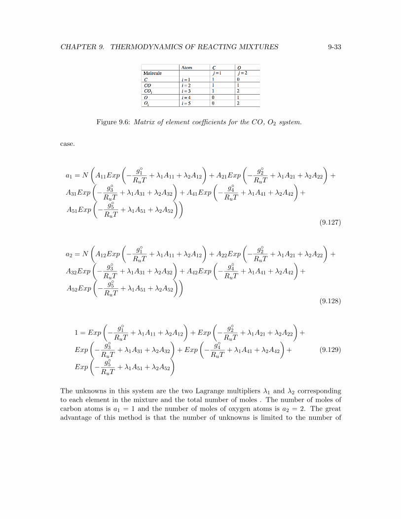
CHAPTER 9. THERMODYNAMICS OF REACTING MIXTURES 9-33
Figure 9.6: Matrix of element coefficients for the CO, O2 system.
case.
a1 = N
(A11Exp
(− g◦1RuT
+ λ1A11 + λ2A12
)+A21Exp
(− g◦2RuT
+ λ1A21 + λ2A22
)+
A31Exp
(− g◦3RuT
+ λ1A31 + λ2A32
)+A41Exp
(− g◦4RuT
+ λ1A41 + λ2A42
)+
A51Exp
(− g◦5RuT
+ λ1A51 + λ2A52
))(9.127)
a2 = N
(A12Exp
(− g◦1RuT
+ λ1A11 + λ2A12
)+A22Exp
(− g◦2RuT
+ λ1A21 + λ2A22
)+
A32Exp
(− g◦3RuT
+ λ1A31 + λ2A32
)+A42Exp
(− g◦4RuT
+ λ1A41 + λ2A42
)+
A52Exp
(− g◦5RuT
+ λ1A51 + λ2A52
))(9.128)
1 = Exp
(− g◦1RuT
+ λ1A11 + λ2A12
)+ Exp
(− g◦2RuT
+ λ1A21 + λ2A22
)+
Exp
(− g◦3RuT
+ λ1A31 + λ2A32
)+ Exp
(− g◦4RuT
+ λ1A41 + λ2A42
)+
Exp
(− g◦5RuT
+ λ1A51 + λ2A52
) (9.129)
The unknowns in this system are the two Lagrange multipliers λ1 and λ2 correspondingto each element in the mixture and the total number of moles . The number of moles ofcarbon atoms is a1 = 1 and the number of moles of oxygen atoms is a2 = 2. The greatadvantage of this method is that the number of unknowns is limited to the number of
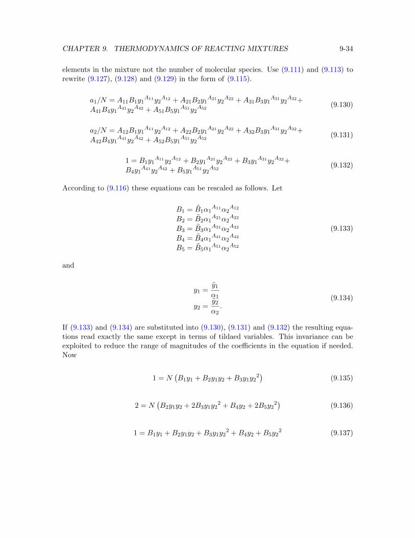
CHAPTER 9. THERMODYNAMICS OF REACTING MIXTURES 9-34
elements in the mixture not the number of molecular species. Use (9.111) and (9.113) torewrite (9.127), (9.128) and (9.129) in the form of (9.115).
a1/N = A11B1y1A11y2
A12 +A21B2y1A21y2
A22 +A31B3y1A31y2
A32+
A41B4y1A41y2
A42 +A51B5y1A51y2
A52(9.130)
a2/N = A12B1y1A11y2
A12 +A22B2y1A21y2
A22 +A32B3y1A31y2
A32+
A42B4y1A41y2
A42 +A52B5y1A51y2
A52(9.131)
1 = B1y1A11y2
A12 +B2y1A21y2
A22 +B3y1A31y2
A32+
B4y1A41y2
A42 +B5y1A51y2
A52(9.132)
According to (9.116) these equations can be rescaled as follows. Let
B1 = B1α1A11α2
A12
B2 = B2α1A21α2
A22
B3 = B3α1A31α2
A32
B4 = B4α1A41α2
A42
B5 = B5α1A51α2
A52
(9.133)
and
y1 =y1
α1
y2 =y2
α2.
(9.134)
If (9.133) and (9.134) are substituted into (9.130), (9.131) and (9.132) the resulting equa-tions read exactly the same except in terms of tildaed variables. This invariance can beexploited to reduce the range of magnitudes of the coefficients in the equation if needed.Now
1 = N(B1y1 +B2y1y2 +B3y1y2
2)
(9.135)
2 = N(B2y1y2 + 2B3y1y2
2 +B4y2 + 2B5y22)
(9.136)
1 = B1y1 +B2y1y2 +B3y1y22 +B4y2 +B5y2
2 (9.137)
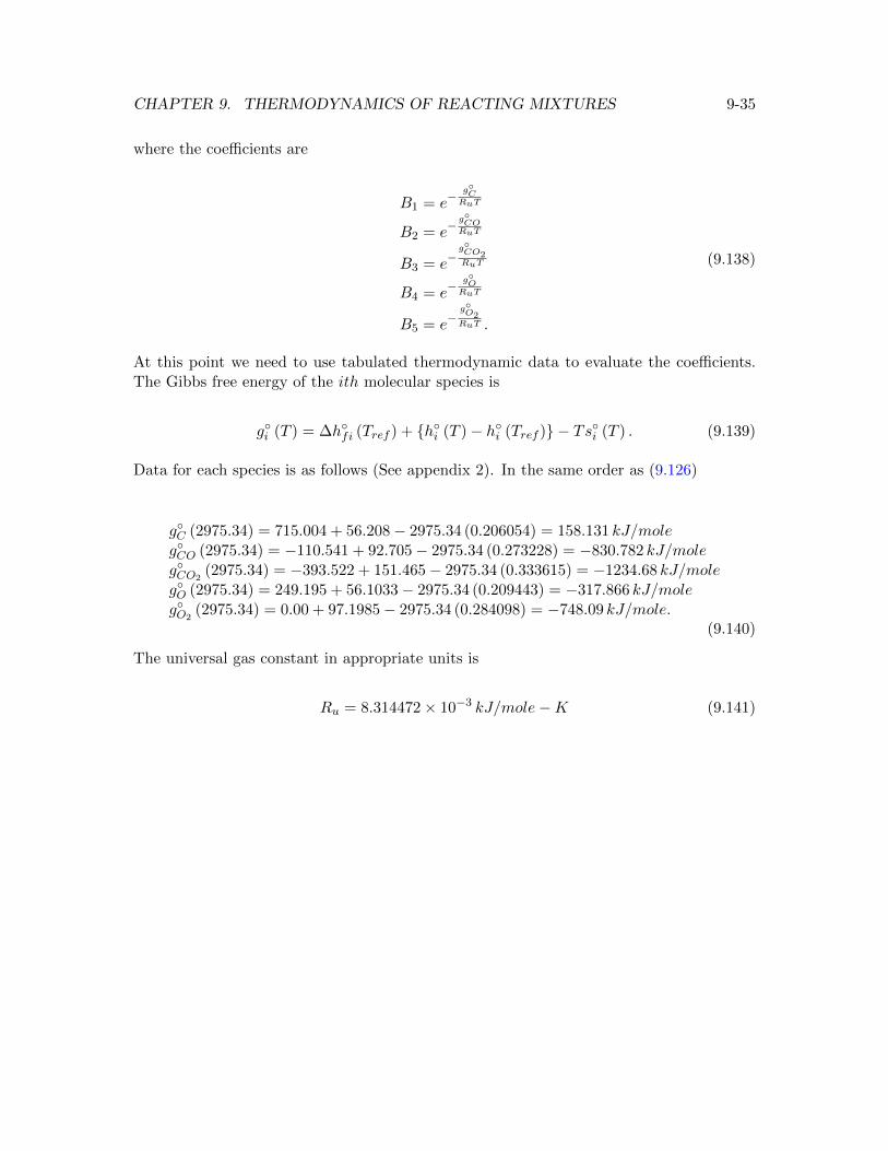
CHAPTER 9. THERMODYNAMICS OF REACTING MIXTURES 9-35
where the coefficients are
B1 = e−g◦CRuT
B2 = e−g◦CORuT
B3 = e−g◦CO2RuT
B4 = e−g◦ORuT
B5 = e−g◦O2RuT .
(9.138)
At this point we need to use tabulated thermodynamic data to evaluate the coefficients.The Gibbs free energy of the ith molecular species is
g◦i (T ) = ∆h◦fi (Tref ) + {h◦i (T )− h◦i (Tref )} − Ts◦i (T ) . (9.139)
Data for each species is as follows (See appendix 2). In the same order as (9.126)
g◦C (2975.34) = 715.004 + 56.208− 2975.34 (0.206054) = 158.131 kJ/moleg◦CO (2975.34) = −110.541 + 92.705− 2975.34 (0.273228) = −830.782 kJ/moleg◦CO2
(2975.34) = −393.522 + 151.465− 2975.34 (0.333615) = −1234.68 kJ/moleg◦O (2975.34) = 249.195 + 56.1033− 2975.34 (0.209443) = −317.866 kJ/moleg◦O2
(2975.34) = 0.00 + 97.1985− 2975.34 (0.284098) = −748.09 kJ/mole.(9.140)
The universal gas constant in appropriate units is
Ru = 8.314472× 10⁻³ kJ/mole−K (9.141)
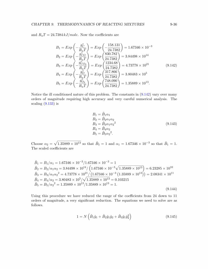
CHAPTER 9. THERMODYNAMICS OF REACTING MIXTURES 9-36
and RuT = 24.7384 kJ/mole. Now the coefficients are
B1 = Exp
(−
g◦CRuT
)= Exp
(−158.131
24.7382
)= 1.67346× 10⁻³
B2 = Exp
(−g◦CORuT
)= Exp
(830.782
24.7382
)= 3.84498× 10¹⁴
B3 = Exp
(−g◦CO2
RuT
)= Exp
(1234.68
24.7382
)= 4.73778× 10²¹
B4 = Exp
(−
g◦ORuT
)= Exp
(317.866
24.7382
)= 3.80483× 10⁵
B5 = Exp
(−g◦O2
RuT
)= Exp
(748.090
24.7382
)= 1.35889× 10¹³.
(9.142)
Notice the ill conditioned nature of this problem. The constants in (9.142) vary over manyorders of magnitude requiring high accuracy and very careful numerical analysis. Thescaling (9.133) is
B1 = B1α1
B2 = B2α1α2
B3 = B3α1α22
B4 = B4α2
B5 = B5α22.
(9.143)
Choose α2 =√
1.35889× 10¹³ so that B5 = 1 and α1 = 1.67346 × 10⁻³ so that B1 = 1.The scaled coefficients are
B1 = B1/α1 = 1.67346× 10⁻³/1.67346× 10−3 = 1
B2 = B2/α1α2 = 3.84498× 10¹⁴/(
1.67346× 10⁻³√
1.35889× 10¹³)
= 6.23285× 10¹⁰
B3 = B3/α1α22 = 4.73778× 10²¹/
(1.67346× 10⁻³
(1.35889× 10¹³
))= 2.08341× 10¹¹
B4 = B4/α2 = 3.80483× 10⁵/√
1.35889× 1013 = 0.103215
B5 = B5/α22 = 1.35889× 10¹³/1.35889× 1013 = 1.
(9.144)
Using this procedure we have reduced the range of the coefficients from 24 down to 11orders of magnitude, a very significant reduction. The equations we need to solve are asfollows.
1 = N(B1y1 + B2y1y2 + B3y1y
22
)(9.145)
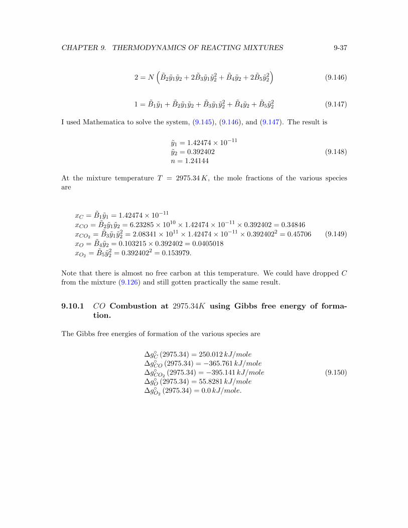
CHAPTER 9. THERMODYNAMICS OF REACTING MIXTURES 9-37
2 = N(B2y1y2 + 2B3y1y
22 + B4y2 + 2B5y
22
)(9.146)
1 = B1y1 + B2y1y2 + B3y1y22 + B4y2 + B5y
22 (9.147)
I used Mathematica to solve the system, (9.145), (9.146), and (9.147). The result is
y1 = 1.42474× 10⁻¹¹
y2 = 0.392402n = 1.24144
(9.148)
At the mixture temperature T = 2975.34K, the mole fractions of the various speciesare
xC = B1y1 = 1.42474× 10⁻¹¹
xCO = B2y1y2 = 6.23285× 1010 × 1.42474× 10−11 × 0.392402 = 0.34846
xCO2 = B3y1y22 = 2.08341× 1011 × 1.42474× 10−11 × 0.3924022 = 0.45706
xO = B4y2 = 0.103215× 0.392402 = 0.0405018
xO2 = B5y22 = 0.3924022 = 0.153979.
(9.149)
Note that there is almost no free carbon at this temperature. We could have dropped Cfrom the mixture (9.126) and still gotten practically the same result.
9.10.1 CO Combustion at 2975.34K using Gibbs free energy of forma-tion.
The Gibbs free energies of formation of the various species are
∆g◦C (2975.34) = 250.012 kJ/mole∆g◦CO (2975.34) = −365.761 kJ/mole∆g◦CO2
(2975.34) = −395.141 kJ/mole∆g◦O (2975.34) = 55.8281 kJ/mole∆g◦O2
(2975.34) = 0.0 kJ/mole.
(9.150)
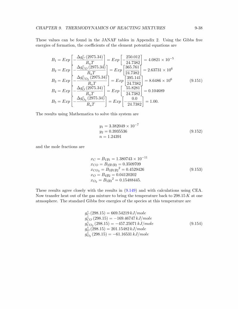
CHAPTER 9. THERMODYNAMICS OF REACTING MIXTURES 9-38
These values can be found in the JANAF tables in Appendix 2. Using the Gibbs freeenergies of formation, the coefficients of the element potential equations are
B1 = Exp
[−
∆g◦C (2975.34)
RuT
]= Exp
[−250.012
24.7382
]= 4.0821× 10⁻⁵
B2 = Exp
[−
∆g◦CO (2975.34)
RuT
]= Exp
[365.761
24.7382
]= 2.63731× 10⁶
B3 = Exp
[−
∆g◦CO2(2975.34)
RuT
]= Exp
[395.141
24.7382
]= 8.6486× 10⁶
B4 = Exp
[−
∆g◦O (2975.34)
RuT
]= Exp
[−55.8281
24.7382
]= 0.104689
B5 = Exp
[−
∆g◦O2(2975.34)
RuT
]= Exp
[− 0.0
24.7382
]= 1.00.
(9.151)
The results using Mathematica to solve this system are
y1 = 3.382049× 10⁻⁷
y2 = 0.3935536n = 1.24391
(9.152)
and the mole fractions are
xC = B1y1 = 1.380743× 10⁻¹¹
xCO = B2y1y2 = 0.3509709
xCO2 = B3y1y22 = 0.4529426
xO = B4y2 = 0.04120202
xO2 = B5y22 = 0.15488445.
(9.153)
These results agree closely with the results in (9.149) and with calculations using CEA.Now transfer heat out of the gas mixture to bring the temperature back to 298.15K at oneatmosphere. The standard Gibbs free energies of the species at this temperature are
g◦C (298.15) = 669.54219 kJ/moleg◦CO (298.15) = −169.46747 kJ/moleg◦CO2
(298.15) = −457.25071 kJ/moleg◦O (298.15) = 201.15482 kJ/moleg◦O2
(298.15) = −61.16531 kJ/mole
(9.154)
CHAPTER 9. THERMODYNAMICS OF REACTING MIXTURES 9-39
and RuT = 2.47897 kJ/mole. The coefficients are
B1 = Exp
(−
g◦CRuT
)= Exp
(−669.54219
2.47897
)= 5.03442× 10−118
B2 = Exp
(−g◦CORuT
)= Exp
(169.46747
2.47897
)= 4.88930× 1029
B3 = Exp
(−g◦CO2
RuT
)= Exp
(457.25071
2.47897
)= 1.277622× 1080
B4 = Exp
(−
g◦ORuT
)= Exp
(−201.15482
2.47897
)= 5.74645× 10−36
B5 = Exp
(−g◦O2
RuT
)= Exp
(61.16531
2.47897
)= 5.19563× 10¹⁰.
(9.155)
At this relatively low temperature the coefficients range over 198 orders of magnitude! De-spite this a good modern solver should be able to find the solution of (9.135), (9.136) and(9.137) for this difficult case even without the scaling used earlier. For example, Mathemat-ica has a feature where the user can specify an arbitrary number of digits of precision forthe calculation. The solution of (9.135), (9.136) and (9.137) at this temperature is
y1 = 7.07098× 10−40
y2 = 3.32704× 10⁻²¹
n = 1.0000.
(9.156)
The resulting mole fractions at T = 298.15K are
xC = B1y1 = 3.55983× 10−157
xCO = B2y1y2 = 1.15023× 10⁻³⁰
xCO2 = B3y1y22 = 1.00000
xO = B4y2 = 1.91187× 10−56
xO2 = B5y22 = 5.75116× 10⁻³¹.
(9.157)
Only when the mixture is brought back to low temperature is the reaction model (9.125)valid. The enthalpy change for this last step is
h◦|mixture at 298.15K − h◦|mixture at 2975.34K = −8.94× 10⁶ + 2.51× 106 = −6.43× 10⁶ J/kg.(9.158)
This is the chemical energy released by the reaction (9.125) and is called the heat ofreaction.
CHAPTER 9. THERMODYNAMICS OF REACTING MIXTURES 9-40
9.10.2 Adiabatic flame temperature
In the example in the previous section the products of combustion were evaluated at theadiabatic flame temperature. This can be defined at constant volume or constant pressure.For our purposes we will use the adiabatic flame temperature at constant pressure. Imaginethe reactants brought together in a piston-cylinder combination permitting the volume tobe adjusted to keep the pressure constant as the reaction proceeds. A source of ignition isused to start the reaction that evolves to the equilibrium state defined by the equilibriumspecies concentrations at the original pressure and at an elevated temperature called theadiabatic flame temperature. In the process the Gibbs function is minimized and since theprocess is adiabatic, the enthalpy before and after the reaction is the same.
The general enthalpy balance for a reaction is given in (9.67). Fully written out the balanceis
∆h◦ (Tfinal) =
Iproduct∑iproduct
niproduct
{∆h◦fiproduct (298.15) +
(h◦iproduct (Tfinal)− h◦iproduct (298.15)
)}−
Ireactant∑ireactant
nireactant{
∆h◦fireactant (298.15) +(h◦ireactant (Tireactant)− h◦ireactant (298.15)
)}.
(9.159)
If the reaction takes place adiabatically then ∆h◦ (Tfinal) = 0 and
Iproduct∑iproduct
niproduct
{∆h◦fiproduct (298.15) +
(h◦iproduct (Tfinal)− h◦iproduct (298.15)
)}=
Ireactant∑ireactant
nireactant{
∆h◦fireactant (298.15) +(h◦ireactant (Tireactant)− h◦ireactant (298.15)
)}.
(9.160)
Equation (9.160) can be solved along with (9.135), (9.136) and (9.137) to determine thefinal temperature of the mixture along with the mole fractions and total number of moles.
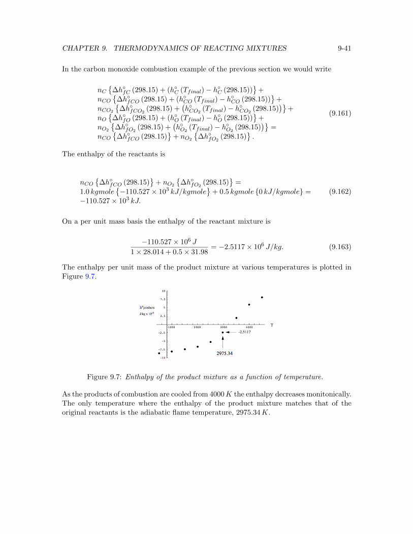
CHAPTER 9. THERMODYNAMICS OF REACTING MIXTURES 9-41
In the carbon monoxide combustion example of the previous section we would write
nC{
∆h◦fC (298.15) + (h◦C (Tfinal)− h◦C (298.15))}
+
nCO{
∆h◦fCO (298.15) + (h◦CO (Tfinal)− h◦CO (298.15))}
+
nCO2
{∆h◦fCO2
(298.15) +(h◦CO2
(Tfinal)− h◦CO2(298.15)
)}+
nO{
∆h◦fO (298.15) + (h◦O (Tfinal)− h◦O (298.15))}
+
nO2
{∆h◦fO2
(298.15) +(h◦O2
(Tfinal)− h◦O2(298.15)
)}=
nCO{
∆h◦fCO (298.15)}
+ nO2
{∆h◦fO2
(298.15)}.
(9.161)
The enthalpy of the reactants is
nCO{
∆h◦fCO (298.15)}
+ nO2
{∆h◦fO2
(298.15)}
=
1.0 kgmole{−110.527× 10³ kJ/kgmole
}+ 0.5 kgmole {0 kJ/kgmole} =
−110.527× 10³ kJ.
(9.162)
On a per unit mass basis the enthalpy of the reactant mixture is
−110.527× 10⁶ J
1× 28.014 + 0.5× 31.98= −2.5117× 10⁶ J/kg. (9.163)
The enthalpy per unit mass of the product mixture at various temperatures is plotted inFigure 9.7.
Figure 9.7: Enthalpy of the product mixture as a function of temperature.
As the products of combustion are cooled from 4000K the enthalpy decreases monitonically.The only temperature where the enthalpy of the product mixture matches that of theoriginal reactants is the adiabatic flame temperature, 2975.34K.
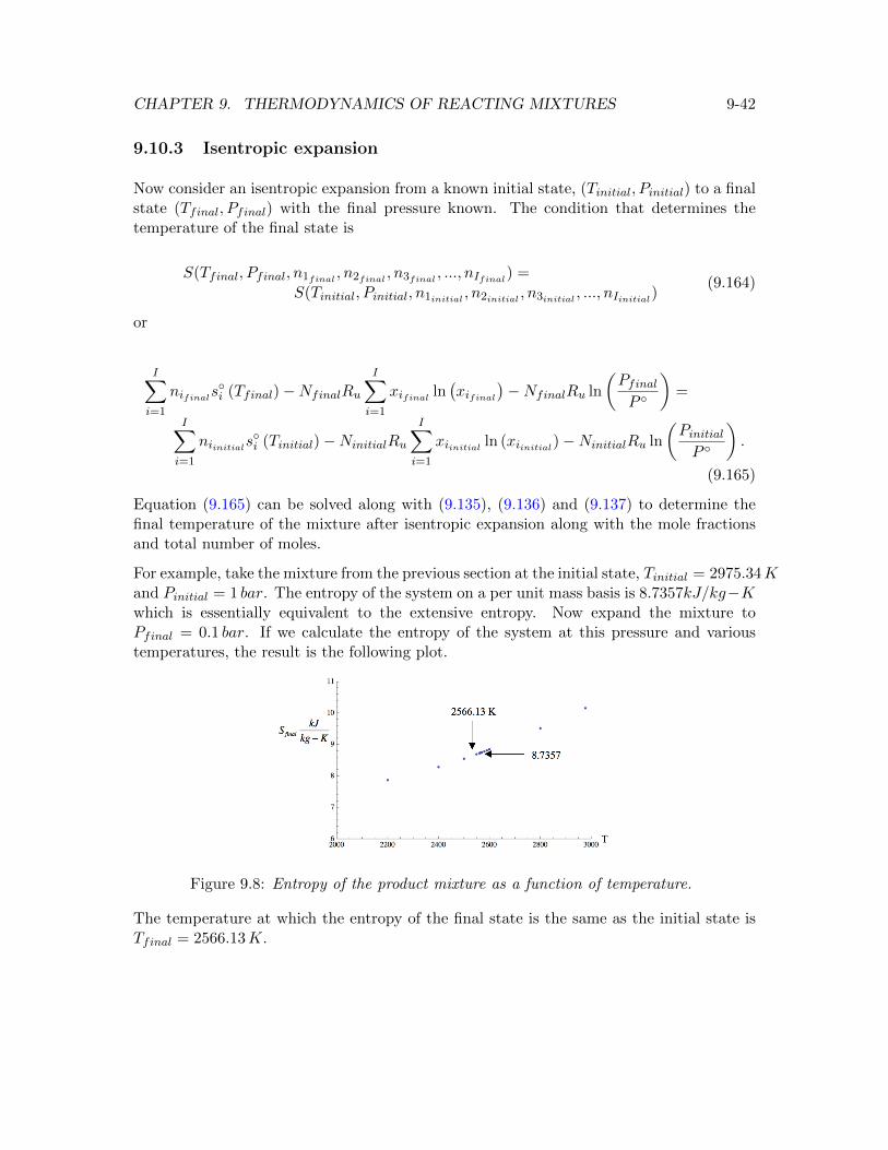
CHAPTER 9. THERMODYNAMICS OF REACTING MIXTURES 9-42
9.10.3 Isentropic expansion
Now consider an isentropic expansion from a known initial state, (Tinitial, Pinitial) to a finalstate (Tfinal, Pfinal) with the final pressure known. The condition that determines thetemperature of the final state is
S(Tfinal, Pfinal, n1final , n2final , n3final , ..., nIfinal) =
S(Tinitial, Pinitial, n1initial , n2initial , n3initial , ..., nIinitial)(9.164)
or
I∑i=1
nifinals◦i (Tfinal)−NfinalRu
I∑i=1
xifinal ln(xifinal
)−NfinalRu ln
(PfinalP ◦
)=
I∑i=1
niinitials◦i (Tinitial)−NinitialRu
I∑i=1
xiinitial ln (xiinitial)−NinitialRu ln
(PinitialP ◦
).
(9.165)
Equation (9.165) can be solved along with (9.135), (9.136) and (9.137) to determine thefinal temperature of the mixture after isentropic expansion along with the mole fractionsand total number of moles.
For example, take the mixture from the previous section at the initial state, Tinitial = 2975.34Kand Pinitial = 1 bar. The entropy of the system on a per unit mass basis is 8.7357kJ/kg−Kwhich is essentially equivalent to the extensive entropy. Now expand the mixture toPfinal = 0.1 bar. If we calculate the entropy of the system at this pressure and varioustemperatures, the result is the following plot.
Figure 9.8: Entropy of the product mixture as a function of temperature.
The temperature at which the entropy of the final state is the same as the initial state isTfinal = 2566.13K.
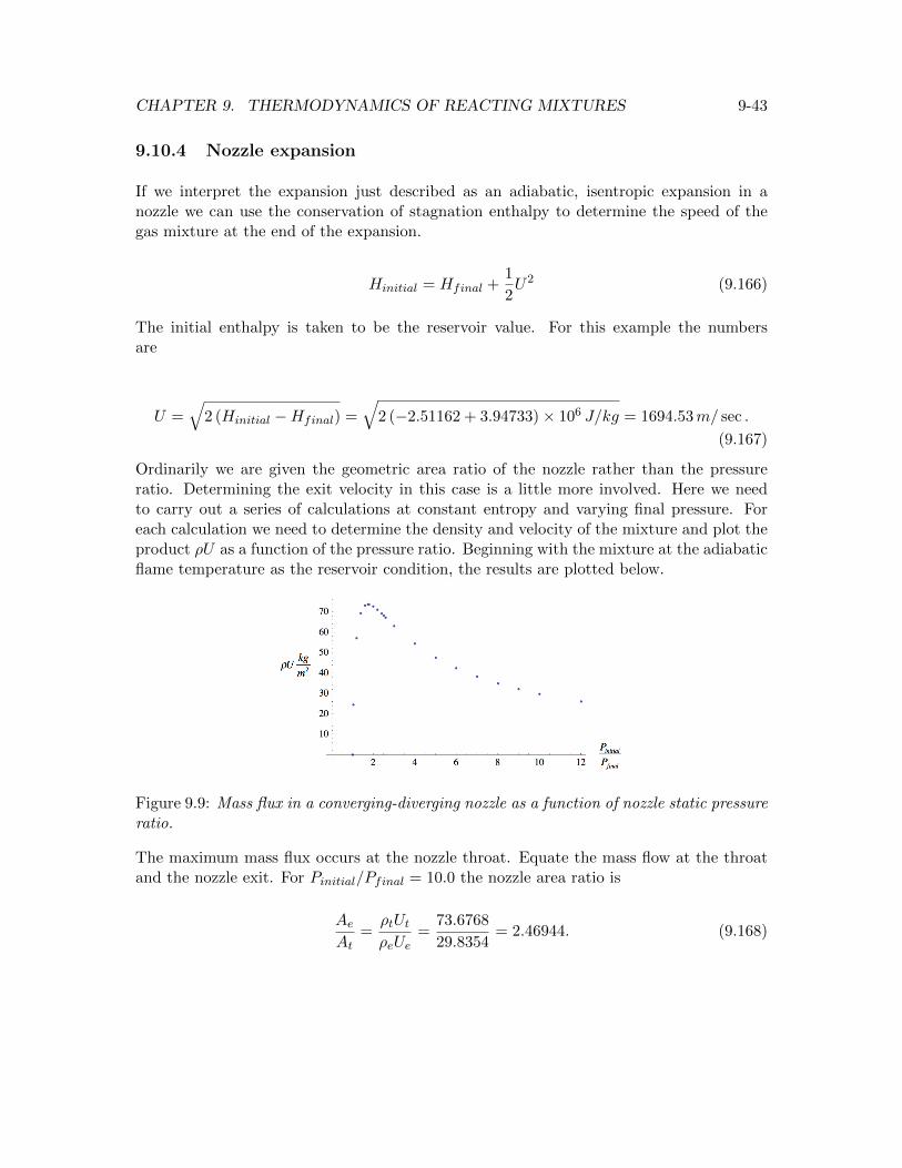
CHAPTER 9. THERMODYNAMICS OF REACTING MIXTURES 9-43
9.10.4 Nozzle expansion
If we interpret the expansion just described as an adiabatic, isentropic expansion in anozzle we can use the conservation of stagnation enthalpy to determine the speed of thegas mixture at the end of the expansion.
Hinitial = Hfinal +1
2U2 (9.166)
The initial enthalpy is taken to be the reservoir value. For this example the numbersare
U =√
2 (Hinitial −Hfinal) =√
2 (−2.51162 + 3.94733)× 106 J/kg = 1694.53m/ sec .
(9.167)
Ordinarily we are given the geometric area ratio of the nozzle rather than the pressureratio. Determining the exit velocity in this case is a little more involved. Here we needto carry out a series of calculations at constant entropy and varying final pressure. Foreach calculation we need to determine the density and velocity of the mixture and plot theproduct ρU as a function of the pressure ratio. Beginning with the mixture at the adiabaticflame temperature as the reservoir condition, the results are plotted below.
Figure 9.9: Mass flux in a converging-diverging nozzle as a function of nozzle static pressureratio.
The maximum mass flux occurs at the nozzle throat. Equate the mass flow at the throatand the nozzle exit. For Pinitial/Pfinal = 10.0 the nozzle area ratio is
AeAt
=ρtUtρeUe
=73.6768
29.8354= 2.46944. (9.168)
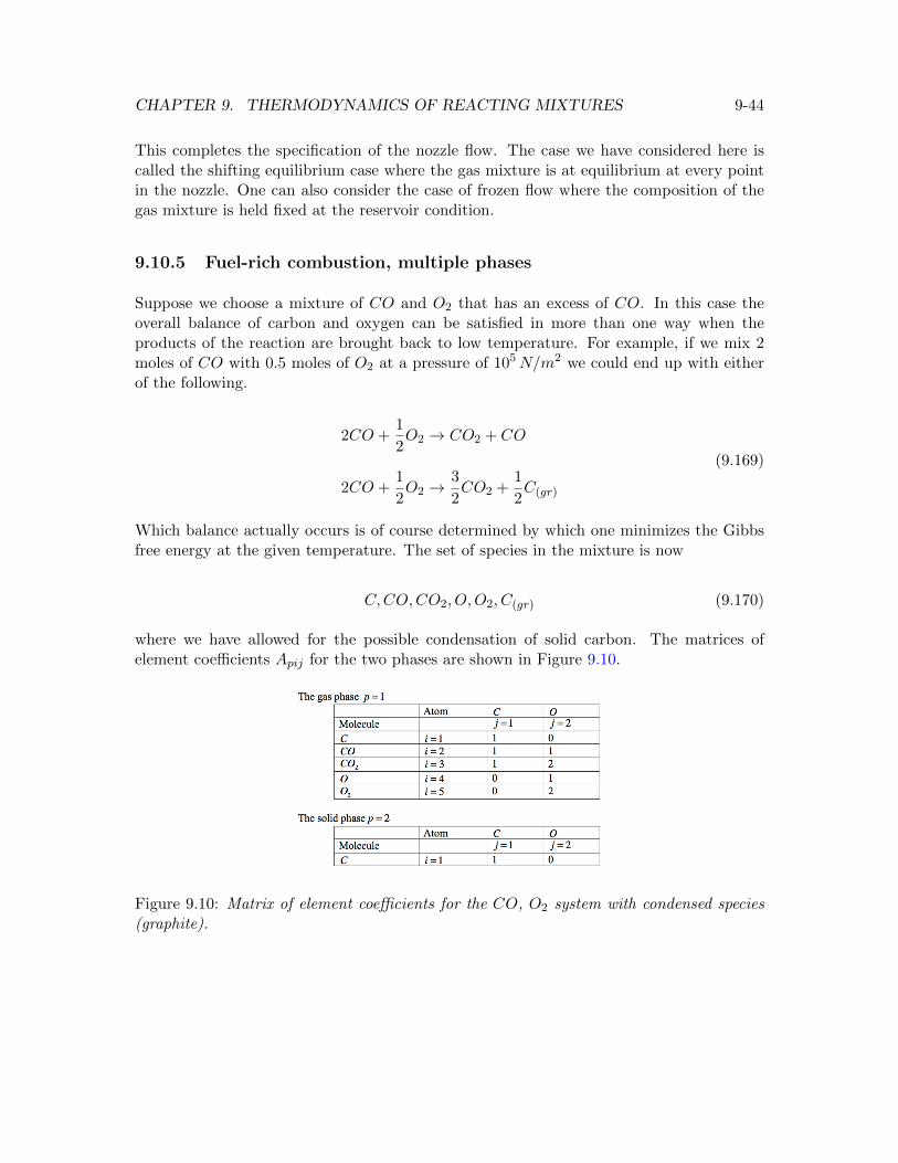
CHAPTER 9. THERMODYNAMICS OF REACTING MIXTURES 9-44
This completes the specification of the nozzle flow. The case we have considered here iscalled the shifting equilibrium case where the gas mixture is at equilibrium at every pointin the nozzle. One can also consider the case of frozen flow where the composition of thegas mixture is held fixed at the reservoir condition.
9.10.5 Fuel-rich combustion, multiple phases
Suppose we choose a mixture of CO and O2 that has an excess of CO. In this case theoverall balance of carbon and oxygen can be satisfied in more than one way when theproducts of the reaction are brought back to low temperature. For example, if we mix 2moles of CO with 0.5 moles of O2 at a pressure of 105N/m2 we could end up with eitherof the following.
2CO +1
2O2 → CO2 + CO
2CO +1
2O2 →
3
2CO2 +
1
2C(gr)
(9.169)
Which balance actually occurs is of course determined by which one minimizes the Gibbsfree energy at the given temperature. The set of species in the mixture is now
C,CO,CO2, O,O2, C(gr) (9.170)
where we have allowed for the possible condensation of solid carbon. The matrices ofelement coefficients Apij for the two phases are shown in Figure 9.10.
Figure 9.10: Matrix of element coefficients for the CO, O2 system with condensed species(graphite).
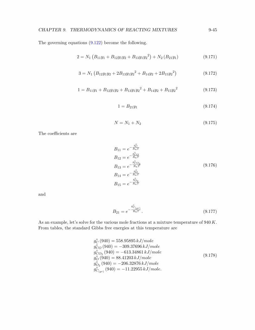
CHAPTER 9. THERMODYNAMICS OF REACTING MIXTURES 9-45
The governing equations (9.122) become the following.
2 = N1
(B11y1 +B12y1y2 +B13y1y2
2)
+N2 (B21y1) (9.171)
3 = N1
(B12y1y2 + 2B13y1y2
2 +B14y2 + 2B15y22)
(9.172)
1 = B11y1 +B12y1y2 +B13y1y22 +B14y2 +B15y2
2 (9.173)
1 = B21y1 (9.174)
N = N1 +N2 (9.175)
The coefficients are
B11 = e−g◦CRuT
B12 = e−g◦CORuT
B13 = e−g◦CO2RuT
B14 = e−g◦ORuT
B15 = e−g◦O2RuT
(9.176)
and
B21 = e−g◦C(gr)RuT . (9.177)
As an example, let’s solve for the various mole fractions at a mixture temperature of 940K.From tables, the standard Gibbs free energies at this temperature are
g◦C (940) = 558.95895 kJ/moleg◦CO (940) = −309.37696 kJ/moleg◦CO2
(940) = −613.34861 kJ/moleg◦O (940) = 88.41203 kJ/moleg◦O2
(940) = −206.32876 kJ/moleg◦C(gr)
(940) = −11.22955 kJ/mole.
(9.178)
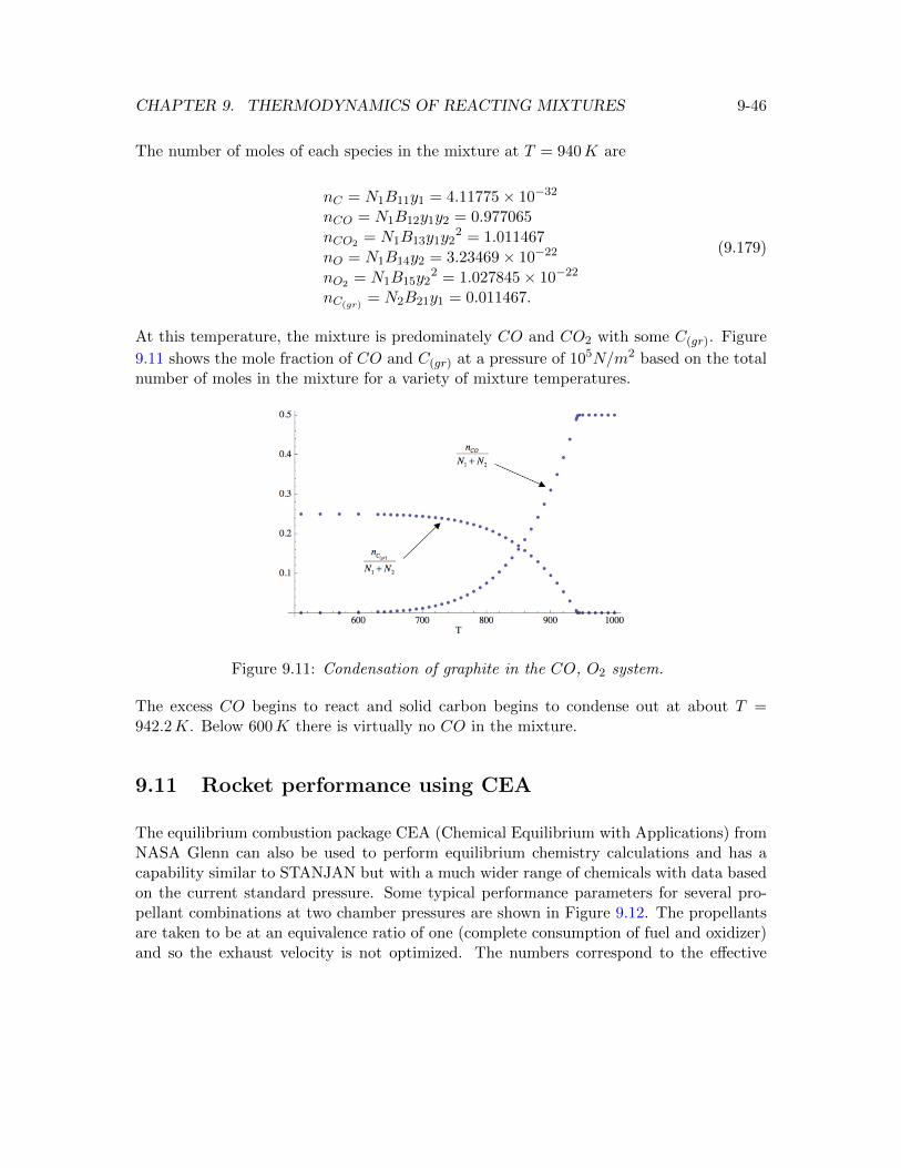
CHAPTER 9. THERMODYNAMICS OF REACTING MIXTURES 9-46
The number of moles of each species in the mixture at T = 940K are
nC = N1B11y1 = 4.11775× 10⁻³²
nCO = N1B12y1y2 = 0.977065
nCO2 = N1B13y1y22 = 1.011467
nO = N1B14y2 = 3.23469× 10⁻²²
nO2 = N1B15y22 = 1.027845× 10⁻²²
nC(gr)= N2B21y1 = 0.011467.
(9.179)
At this temperature, the mixture is predominately CO and CO2 with some C(gr). Figure
9.11 shows the mole fraction of CO and C(gr) at a pressure of 105N/m2 based on the totalnumber of moles in the mixture for a variety of mixture temperatures.
Figure 9.11: Condensation of graphite in the CO, O2 system.
The excess CO begins to react and solid carbon begins to condense out at about T =942.2K. Below 600K there is virtually no CO in the mixture.
9.11 Rocket performance using CEA
The equilibrium combustion package CEA (Chemical Equilibrium with Applications) fromNASA Glenn can also be used to perform equilibrium chemistry calculations and has acapability similar to STANJAN but with a much wider range of chemicals with data basedon the current standard pressure. Some typical performance parameters for several pro-pellant combinations at two chamber pressures are shown in Figure 9.12. The propellantsare taken to be at an equivalence ratio of one (complete consumption of fuel and oxidizer)and so the exhaust velocity is not optimized. The numbers correspond to the effective
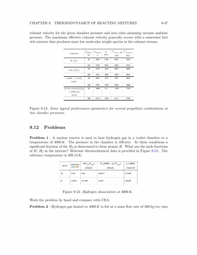
CHAPTER 9. THERMODYNAMICS OF REACTING MIXTURES 9-47
exhaust velocity for the given chamber pressure and area ratio assuming vacuum ambientpressure. The maximum effective exhaust velocity generally occurs with a somewhat fuelrich mixture that produces more low molecular weight species in the exhaust stream.
Figure 9.12: Some typical performance parameters for several propellant combinations attwo chamber pressures.
9.12 Problems
Problem 1 - A nuclear reactor is used to heat hydrogen gas in a rocket chamber to atemperature of 4000K. The pressure in the chamber is 100 atm. At these conditions asignificant fraction of the H2 is dissociated to form atomic H. What are the mole fractionsof H, H2 in the mixture? Relevant thermochemical data is provided in Figure 9.13 . Thereference temperature is 298.15K.
Figure 9.13: Hydrogen dissociation at 4000K.
Work the problem by hand and compare with CEA.
Problem 2 - Hydrogen gas heated to 4000K is fed at a mass flow rate of 200 kg/sec into
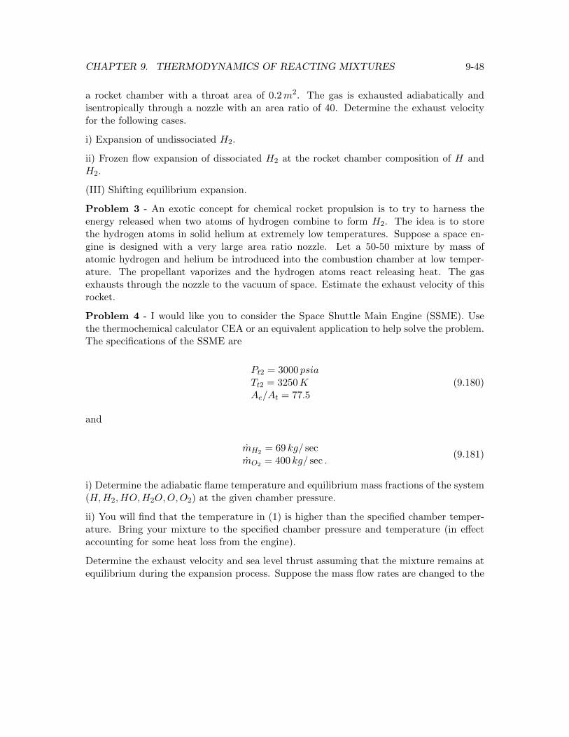
CHAPTER 9. THERMODYNAMICS OF REACTING MIXTURES 9-48
a rocket chamber with a throat area of 0.2m2. The gas is exhausted adiabatically andisentropically through a nozzle with an area ratio of 40. Determine the exhaust velocityfor the following cases.
i) Expansion of undissociated H2.
ii) Frozen flow expansion of dissociated H2 at the rocket chamber composition of H andH2.
(III) Shifting equilibrium expansion.
Problem 3 - An exotic concept for chemical rocket propulsion is to try to harness theenergy released when two atoms of hydrogen combine to form H2. The idea is to storethe hydrogen atoms in solid helium at extremely low temperatures. Suppose a space en-gine is designed with a very large area ratio nozzle. Let a 50-50 mixture by mass ofatomic hydrogen and helium be introduced into the combustion chamber at low temper-ature. The propellant vaporizes and the hydrogen atoms react releasing heat. The gasexhausts through the nozzle to the vacuum of space. Estimate the exhaust velocity of thisrocket.
Problem 4 - I would like you to consider the Space Shuttle Main Engine (SSME). Usethe thermochemical calculator CEA or an equivalent application to help solve the problem.The specifications of the SSME are
Pt2 = 3000 psiaTt2 = 3250KAe/At = 77.5
(9.180)
and
mH2 = 69 kg/ secmO2 = 400 kg/ sec .
(9.181)
i) Determine the adiabatic flame temperature and equilibrium mass fractions of the system(H,H2, HO,H2O,O,O2) at the given chamber pressure.
ii) You will find that the temperature in (1) is higher than the specified chamber temper-ature. Bring your mixture to the specified chamber pressure and temperature (in effectaccounting for some heat loss from the engine).
Determine the exhaust velocity and sea level thrust assuming that the mixture remains atequilibrium during the expansion process. Suppose the mass flow rates are changed to the
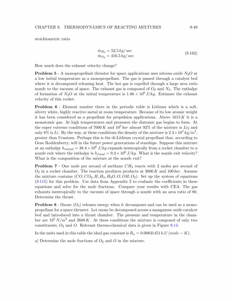
CHAPTER 9. THERMODYNAMICS OF REACTING MIXTURES 9-49
stoichiometric ratio
mH2 = 52.5 kg/ secmO2 = 416.5 kg/ sec.
(9.182)
How much does the exhaust velocity change?
Problem 5 - A monopropellant thruster for space applications uses nitrous oxide N2O ata low initial temperature as a monopropellant. The gas is passed through a catalyst bedwhere it is decomposed releasing heat. The hot gas is expelled through a large area rationozzle to the vacuum of space. The exhaust gas is composed of O2 and N2. The enthalpyof formation of N2O at the initial temperature is 1.86 × 10⁶ J/kg. Estimate the exhaustvelocity of this rocket.
Problem 6 - Element number three in the periodic table is Lithium which is a soft,silvery white, highly reactive metal at room temperature. Because of its low atomic weightit has been considered as a propellant for propulsion applications. Above 1615K it is amonatomic gas. At high temperatures and pressures the diatomic gas begins to form. Atthe super extreme conditions of 7000K and 105 bar almost 92% of the mixture is Li2 andonly 8% is Li. By the way, at these conditions the density of the mixture is 2.3×10⁴ kg/m3,greater than Uranium. Perhaps this is the di-Lithium crystal propellant that, according toGene Roddenberry, will in the future power generations of starships. Suppose this mixtureat an enthalpy hinitial = 38.4×10⁶ J/kg expands isentropically from a rocket chamber to anozzle exit where the enthalpy is hfinal = 9.3× 10⁶ J/kg. What is the nozzle exit velocity?What is the composition of the mixture at the nozzle exit?
Problem 7 - One mole per second of methane CH4 reacts with 2 moles per second ofO2 in a rocket chamber. The reaction produces products at 3000K and 100 bar. Assumethe mixture contains (CO,CO2, H,H2, H2O,O,OH,O2). Set up the system of equations(9.115) for this problem. Use data from Appendix 2 to evaluate the coefficients in theseequations and solve for the mole fractions. Compare your results with CEA. The gasexhausts isentropically to the vacuum of space through a nozzle with an area ratio of 80.Determine the thrust.
Problem 8 - Ozone (O3) releases energy when it decomposes and can be used as a mono-propellant for a space thruster. Let ozone be decomposed across a manganese oxide catalystbed and introduced into a thrust chamber. The pressure and temperature in the cham-ber are 105N/m2 and 2688K. At these conditions the mixture is composed of only twoconstituents, O2 and O. Relevant thermo-chemical data is given in Figure 9.14.
In the units used in this table the ideal gas constant isRu = 0.00831451 kJ/ (mole−K).
a) Determine the mole fractions of O2 and O in the mixture.
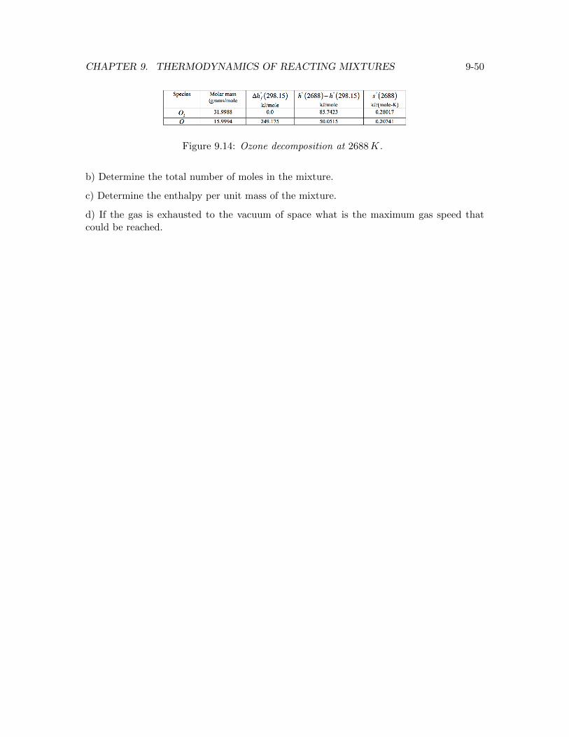
CHAPTER 9. THERMODYNAMICS OF REACTING MIXTURES 9-50
Figure 9.14: Ozone decomposition at 2688K.
b) Determine the total number of moles in the mixture.
c) Determine the enthalpy per unit mass of the mixture.
d) If the gas is exhausted to the vacuum of space what is the maximum gas speed thatcould be reached.
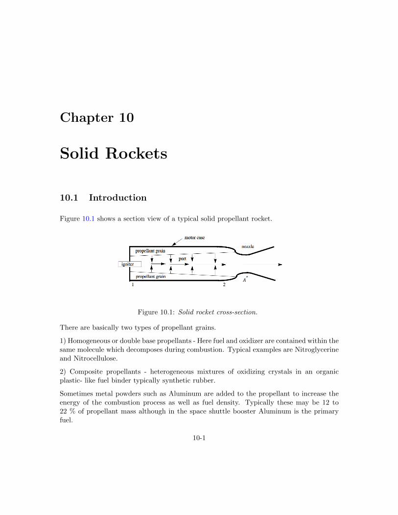
Chapter 10
Solid Rockets
10.1 Introduction
Figure 10.1 shows a section view of a typical solid propellant rocket.
Figure 10.1: Solid rocket cross-section.
There are basically two types of propellant grains.
1) Homogeneous or double base propellants - Here fuel and oxidizer are contained within thesame molecule which decomposes during combustion. Typical examples are Nitroglycerineand Nitrocellulose.
2) Composite propellants - heterogeneous mixtures of oxidizing crystals in an organicplastic- like fuel binder typically synthetic rubber.
Sometimes metal powders such as Aluminum are added to the propellant to increase theenergy of the combustion process as well as fuel density. Typically these may be 12 to22 % of propellant mass although in the space shuttle booster Aluminum is the primaryfuel.
10-1
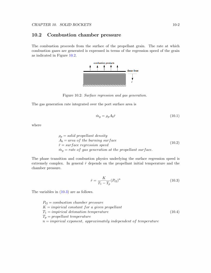
CHAPTER 10. SOLID ROCKETS 10-2
10.2 Combustion chamber pressure
The combustion proceeds from the surface of the propellant grain. The rate at whichcombustion gases are generated is expressed in terms of the regression speed of the grainas indicated in Figure 10.2.
Figure 10.2: Surface regression and gas generation.
The gas generation rate integrated over the port surface area is
mg = ρpAbr (10.1)
where
ρp = solid propellant densityAb = area of the burning surfacer = surface regression speedmg = rate of gas generation at the propellant surface.
(10.2)
The phase transition and combustion physics underlying the surface regression speed isextremely complex. In general r depends on the propellant initial temperature and thechamber pressure.
r =K
T1 − Tp(Pt2)n (10.3)
The variables in (10.3) are as follows.
Pt2 = combustion chamber pressureK = impirical constant for a given propellantT1 = impirical detonation temperatureTp = propellant temperaturen = impirical exponent, approximately independent of temperature
(10.4)
CHAPTER 10. SOLID ROCKETS 10-3
In general 0.4 < n < 0.7 and T1 is considerably larger than Tp by several hundred de-grees.
Let Mg be the mass of gas in the combustion chamber at a given instant, ρg is the gasdensity and V is the chamber volume.
dMg
dt=
d
dt(ρgV ) = ρg
dV
dt+ V
dρgdt
(10.5)
The chamber volume changes as the propellant is converted from solid to gas.
dV
dt= rAb (10.6)
To a good approximation, the chamber stagnation temperature, Tt2, is determined by thepropellant energy density and tends to be independent of Pt2. From the ideal gas law,Pt2 = ρgRTt2 and
dρgdt
=1
RTt2
dPt2dt
. (10.7)
The mass flow out of the nozzle is
mn =γ(
γ+12
) γ+12(γ−1)
Pt2A∗
√γRTt2
. (10.8)
The mass generated at the propellant surface is divided between the mass flow exitingthe nozzle and the time dependent mass accumulation in the combustion chamber vol-ume.
mg =dMg
dt+ mn (10.9)
Fill in the various terms in (10.9)
ρprAb = ρg rAb + Vdρgdt
+γ(
γ+12
) γ+12(γ−1)
Pt2A∗
√γRTt2
(10.10)
CHAPTER 10. SOLID ROCKETS 10-4
or
K (ρp − ρg)AbT1 − Tp
(Pt2)n =V
RTt2
dPt2dt
+γ(
γ+12
) γ+12(γ−1)
Pt2A∗
√γRTt2
. (10.11)
Rearrange (10.11) to read
V
RTt2
dPt2dt
+γ(
γ+12
) γ+12(γ−1)
Pt2A∗
√γRTt2
− K (ρp − ρg)AbT1 − Tp
(Pt2)n = 0. (10.12)
After a startup transient, during which Pt2 changes rapidly with time, the pressure reachesa quasi-steady state where the time derivative term in (10.12) can be regarded as smallcompared to the other terms. To a good approximation
γ(γ+1
2
) γ+12(γ−1)
Pt2A∗
√γRTt2
=K (ρp − ρg)Ab
T1 − Tp(Pt2)n. (10.13)
Solve for the chamber pressure
Pt2 =
((γ + 1
2
) γ+12(γ−1) K (ρp − ρg)
γ (T1 − Tp)
(AbA∗
)√γRTt2
) 11−n
. (10.14)
This formula can be used as long as Ab(t) is a slow function of time. All the quantities in(10.14) are apriori data with the exception of Tt2 which must be estimated or calculatedfrom a propellant chemistry model. Note that there is a tendency for the chamber pressureto increase as the burning area increases.
10.3 Dynamic analysis
Rearrange (10.12) to read
dPt2dt
+
(γRTt2)1/2(γ+1
2
) γ+12(γ−1)
(A∗
V
)Pt2 −(K (ρp − ρg)Ab
T1 − Tp
(RTt2V
))(Pt2)n = 0. (10.15)
CHAPTER 10. SOLID ROCKETS 10-5
This is a nonlinear first order ordinary differential equation for the chamber pressure ofthe form
dPt2dt
+
(1
τ
)Pt2 − β(Pt2)n = 0 (10.16)
where the characteristic time is
τ =
(γ+1
2
) γ+12(γ−1)
(γRTt2)1/2
(V
A∗
). (10.17)
This time is proportional to the time required for an acoustic wave to travel the length ofthe combustion chamber multiplied by the internal area ratio of the nozzle. The systemhas the character of a Helmholtz resonator and the inverse of (10.17) is the natural ”Cokebottle” frequency of the rocket motor.
The constant in the nonlinear term is
β =
(K (ρp − ρg)Ab
T1 − Tp
(RTt2V
)). (10.18)
Let’s look at the linearized behavior of (10.16) near a steady state operating point. Let
Pt2 (t) = Pt2 + pt2 (t) (10.19)
where pt2 is a small deviation in the pressure from the steady state. Substitute into (10.16)and expand the nonlinear term in a binomial series. With higher order terms in the seriesneglected, the result is
dpt2dt
+
(1
τ
)Pt2 +
(1
τ
)pt2 − β
(Pt2)n − βn(Pt2)n−1
pt2 = 0. (10.20)
The steady state terms satisfy
(1
τ
)Pt2 − β
(Pt2)n
= 0 (10.21)
CHAPTER 10. SOLID ROCKETS 10-6
and the dynamical equation becomes
dpt2dt
+
(1
τ− βn
(Pt2)n−1
)pt2 = 0. (10.22)
Note that from (10.21)
1
τ= βn
(Pt2)n−1
(10.23)
and so
dpt2dt
+
(1− nτ
)pt2 = 0. (10.24)
The solution of (10.24) is
pt2pt2 (0)
= e−( 1−nτ )t. (10.25)
If n < 1 a small deviation in pressure will be restored to the equilibrium value (the extranozzle flow exceeds the extra gas generation from the propellant surface). But if n > 1 thegas generation rate exceeds the nozzle exhaust mass flow and the chamber pressure willincrease exponentially; The vehicle will explode!
If the fluid velocity over the surface becomes very large, enhanced heat transfer can leadto a situation called erosive burning. In this case the burning rate can vary considerablyalong the port and excessive gas generation can lead to a failure.
In the case of very low chamber pressure, the combustion process can become unsteady orcease altogether this defines the combustion limit of a particular propellant. There is alsoan upper pressure limit above which combustion again becomes erratic or unpredictable.For most propellants this is above 5000 psi.
10.3.1 Exact solution
The chamber pressure is governed by the equation
dPt2dt
+
(1
τ
)Pt2 − β(Pt2)n = 0. (10.26)
CHAPTER 10. SOLID ROCKETS 10-7
Let’s determine the exact integral of this equation and compare the behavior of the systemwith the linearized solution for both n < 1 and n > 1. It is virtually always best to work interms of dimensionless variables. The steady state solution of (10.26) for which the timederivative term is zero is
Pt2 = (τβ)1
1−n . (10.27)
Let
H =Pt2
Pt2
η =t− t0τ
.
(10.28)
In terms of new variables (10.26) becomes
dH
dη= Hn −H. (10.29)
Equation (10.29) is rearranged as
dH
Hn −H= dη (10.30)
which integrates to
1−H1−n
1−H01−n = e−(1−n)η (10.31)
where H0 is the initial value of Pt2/Pt2 and the initial value of η is taken to be zero. Nowsolve for H.
H =(
1−(1−H0
1−n) e−(1−n)η) 1
1−n(10.32)
Several cases are shown in Figure 10.3.
The exact solution is consistent with the linear analysis and shows that if n > 1 thereis no actual steady state, the chamber pressure either decays to zero or blows up. Ifn < 1 then the chamber pressure will return to the steady state value even in the face
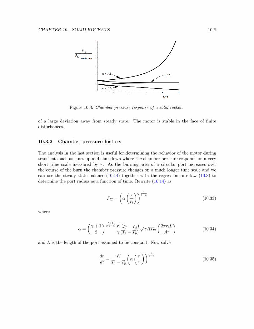
CHAPTER 10. SOLID ROCKETS 10-8
Figure 10.3: Chamber pressure response of a solid rocket.
of a large deviation away from steady state. The motor is stable in the face of finitedisturbances.
10.3.2 Chamber pressure history
The analysis in the last section is useful for determining the behavior of the motor duringtransients such as start-up and shut down where the chamber pressure responds on a veryshort time scale measured by τ . As the burning area of a circular port increases overthe course of the burn the chamber pressure changes on a much longer time scale and wecan use the steady state balance (10.14) together with the regression rate law (10.3) todetermine the port radius as a function of time. Rewrite (10.14) as
Pt2 =
(α
(r
ri
)) 11−n
(10.33)
where
α =
(γ + 1
2
) γ+12(γ−1) K (ρp − ρg)
γ (T1 − Tp)√γRTt2
(2πriL
A∗
)(10.34)
and L is the length of the port assumed to be constant. Now solve
dr
dt=
K
T1 − Tp
(α
(r
ri
)) n1−n
(10.35)
CHAPTER 10. SOLID ROCKETS 10-9
for the radius of the port as a function of time.
d(rri
)(rri
) n1−n
=
(K
(T1 − Tp) ri(α)
n1−n
)dt (10.36)
Integrating (10.36) leads to
r
ri=
(1 +
(1− 2n
1− n
)Kα( n
1−n)t
(T1 − Tp) ri
) 1−n1−2n
n 6= 0.5
r
ri= e
Kα( n
1−n)t
(T1−Tp)ri n = 0.5.
(10.37)
This defines a much longer time scale
τburn =(T1 − Tp) riKα( n
1−n)(10.38)
This time scale characterizes the change in chamber pressure during the burn. The burntime is determined by the outer radius of the motor.
tburnout =
((rfri
) 1−2n1−n− 1
)(1− n1− 2n
)τburn n 6= 0.5
tburnout = Ln
(rfri
)τburn n = 0.5
(10.39)
10.4 Problems
Problem 1 - It is a beautiful summer day at the Cape and a space shuttle astronaut on hersecond mission finds that the g forces during launch are noticeably larger than during herfirst mission that previous December. Can you offer a plausible explanation for this?
Problem 2 - A solid propellant rocket operates in a vacuum with a 10 cm diameter nozzlethroat and a nozzle area ratio of 100. The motor has a cylindrical port 300 cm long. At thebeginning of the burn the port is 20 cm in diameter and the propellant recession velocity
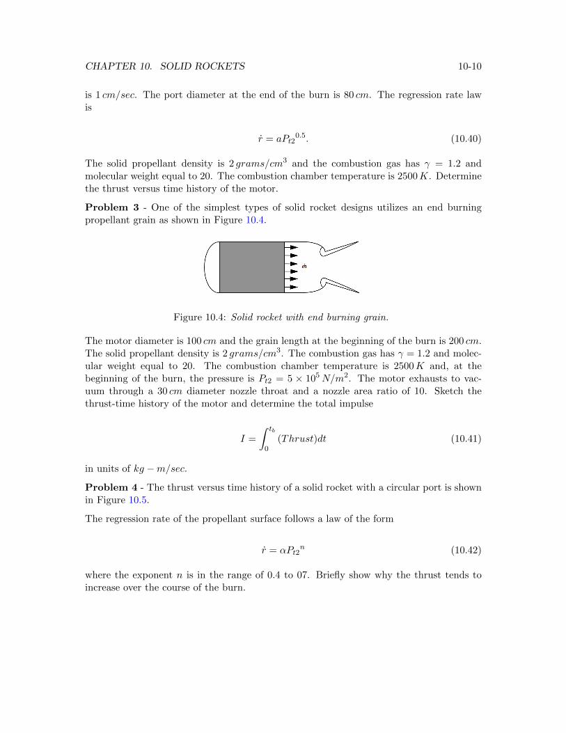
CHAPTER 10. SOLID ROCKETS 10-10
is 1 cm/sec. The port diameter at the end of the burn is 80 cm. The regression rate lawis
r = aPt20.5. (10.40)
The solid propellant density is 2 grams/cm3 and the combustion gas has γ = 1.2 andmolecular weight equal to 20. The combustion chamber temperature is 2500K. Determinethe thrust versus time history of the motor.
Problem 3 - One of the simplest types of solid rocket designs utilizes an end burningpropellant grain as shown in Figure 10.4.
Figure 10.4: Solid rocket with end burning grain.
The motor diameter is 100 cm and the grain length at the beginning of the burn is 200 cm.The solid propellant density is 2 grams/cm3. The combustion gas has γ = 1.2 and molec-ular weight equal to 20. The combustion chamber temperature is 2500K and, at thebeginning of the burn, the pressure is Pt2 = 5 × 10⁵N/m2. The motor exhausts to vac-uum through a 30 cm diameter nozzle throat and a nozzle area ratio of 10. Sketch thethrust-time history of the motor and determine the total impulse
I =
∫ tb
0(Thrust)dt (10.41)
in units of kg −m/sec.
Problem 4 - The thrust versus time history of a solid rocket with a circular port is shownin Figure 10.5.
The regression rate of the propellant surface follows a law of the form
r = αPt2n (10.42)
where the exponent n is in the range of 0.4 to 07. Briefly show why the thrust tends toincrease over the course of the burn.
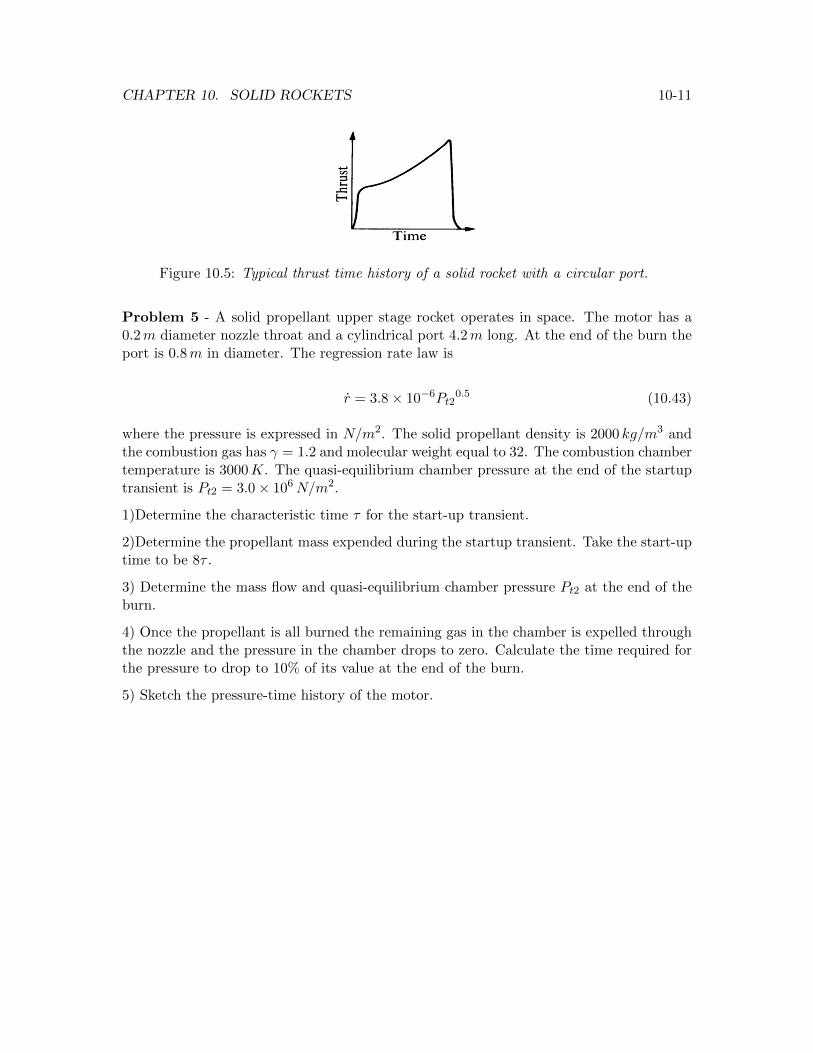
CHAPTER 10. SOLID ROCKETS 10-11
Figure 10.5: Typical thrust time history of a solid rocket with a circular port.
Problem 5 - A solid propellant upper stage rocket operates in space. The motor has a0.2m diameter nozzle throat and a cylindrical port 4.2m long. At the end of the burn theport is 0.8m in diameter. The regression rate law is
r = 3.8× 10⁻⁶Pt20.5 (10.43)
where the pressure is expressed in N/m2. The solid propellant density is 2000 kg/m3 andthe combustion gas has γ = 1.2 and molecular weight equal to 32. The combustion chambertemperature is 3000K. The quasi-equilibrium chamber pressure at the end of the startuptransient is Pt2 = 3.0× 10⁶N/m2.
1)Determine the characteristic time τ for the start-up transient.
2)Determine the propellant mass expended during the startup transient. Take the start-uptime to be 8τ .
3) Determine the mass flow and quasi-equilibrium chamber pressure Pt2 at the end of theburn.
4) Once the propellant is all burned the remaining gas in the chamber is expelled throughthe nozzle and the pressure in the chamber drops to zero. Calculate the time required forthe pressure to drop to 10% of its value at the end of the burn.
5) Sketch the pressure-time history of the motor.
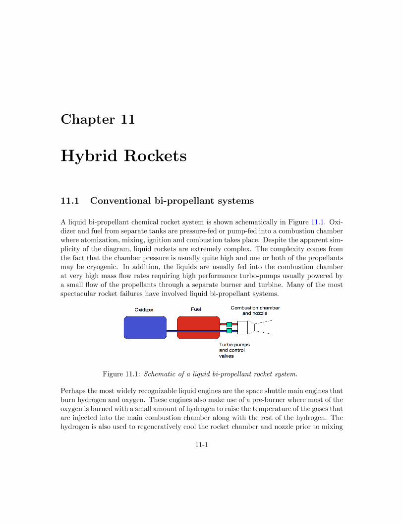
Chapter 11
Hybrid Rockets
11.1 Conventional bi-propellant systems
A liquid bi-propellant chemical rocket system is shown schematically in Figure 11.1. Oxi-dizer and fuel from separate tanks are pressure-fed or pump-fed into a combustion chamberwhere atomization, mixing, ignition and combustion takes place. Despite the apparent sim-plicity of the diagram, liquid rockets are extremely complex. The complexity comes fromthe fact that the chamber pressure is usually quite high and one or both of the propellantsmay be cryogenic. In addition, the liquids are usually fed into the combustion chamberat very high mass flow rates requiring high performance turbo-pumps usually powered bya small flow of the propellants through a separate burner and turbine. Many of the mostspectacular rocket failures have involved liquid bi-propellant systems.
Figure 11.1: Schematic of a liquid bi-propellant rocket system.
Perhaps the most widely recognizable liquid engines are the space shuttle main engines thatburn hydrogen and oxygen. These engines also make use of a pre-burner where most of theoxygen is burned with a small amount of hydrogen to raise the temperature of the gases thatare injected into the main combustion chamber along with the rest of the hydrogen. Thehydrogen is also used to regeneratively cool the rocket chamber and nozzle prior to mixing
11-1
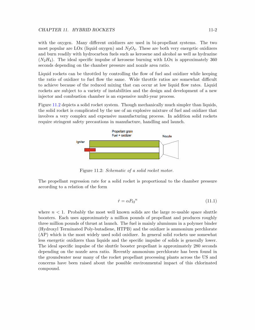
CHAPTER 11. HYBRID ROCKETS 11-2
with the oxygen. Many different oxidizers are used in bi-propellant systems. The twomost popular are LOx (liquid oxygen) and N2O4. These are both very energetic oxidizersand burn readily with hydrocarbon fuels such as kerosene and alcohol as well as hydrazine(N2H4). The ideal specific impulse of kerosene burning with LOx is approximately 360seconds depending on the chamber pressure and nozzle area ratio.
Liquid rockets can be throttled by controlling the flow of fuel and oxidizer while keepingthe ratio of oxidizer to fuel flow the same. Wide throttle ratios are somewhat difficultto achieve because of the reduced mixing that can occur at low liquid flow rates. Liquidrockets are subject to a variety of instabilities and the design and development of a newinjector and combustion chamber is an expensive multi-year process.
Figure 11.2 depicts a solid rocket system. Though mechanically much simpler than liquids,the solid rocket is complicated by the use of an explosive mixture of fuel and oxidizer thatinvolves a very complex and expensive manufacturing process. In addition solid rocketsrequire stringent safety precautions in manufacture, handling and launch.
Figure 11.2: Schematic of a solid rocket motor.
The propellant regression rate for a solid rocket is proportional to the chamber pressureaccording to a relation of the form
r = αPt2n (11.1)
where n < 1. Probably the most well known solids are the large re-usable space shuttleboosters. Each uses approximately a million pounds of propellant and produces roughlythree million pounds of thrust at launch. The fuel is mainly aluminum in a polymer binder(Hydroxyl Terminated Poly-butadiene, HTPB) and the oxidizer is ammonium perchlorate(AP) which is the most widely used solid oxidizer. In general solid rockets use somewhatless energetic oxidizers than liquids and the specific impulse of solids is generally lower.The ideal specific impulse of the shuttle booster propellant is approximately 280 secondsdepending on the nozzle area ratio. Recently ammonium perchlorate has been found inthe groundwater near many of the rocket propellant processing plants across the US andconcerns have been raised about the possible environmental impact of this chlorinatedcompound.
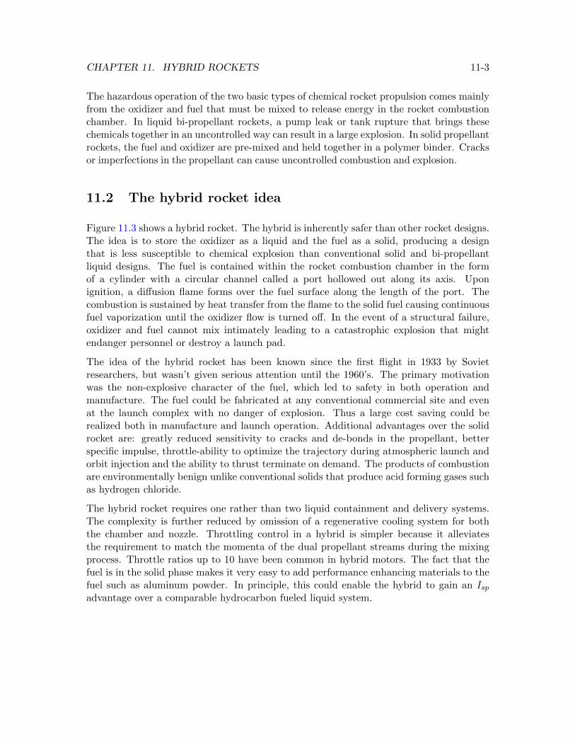
CHAPTER 11. HYBRID ROCKETS 11-3
The hazardous operation of the two basic types of chemical rocket propulsion comes mainlyfrom the oxidizer and fuel that must be mixed to release energy in the rocket combustionchamber. In liquid bi-propellant rockets, a pump leak or tank rupture that brings thesechemicals together in an uncontrolled way can result in a large explosion. In solid propellantrockets, the fuel and oxidizer are pre-mixed and held together in a polymer binder. Cracksor imperfections in the propellant can cause uncontrolled combustion and explosion.
11.2 The hybrid rocket idea
Figure 11.3 shows a hybrid rocket. The hybrid is inherently safer than other rocket designs.The idea is to store the oxidizer as a liquid and the fuel as a solid, producing a designthat is less susceptible to chemical explosion than conventional solid and bi-propellantliquid designs. The fuel is contained within the rocket combustion chamber in the formof a cylinder with a circular channel called a port hollowed out along its axis. Uponignition, a diffusion flame forms over the fuel surface along the length of the port. Thecombustion is sustained by heat transfer from the flame to the solid fuel causing continuousfuel vaporization until the oxidizer flow is turned off. In the event of a structural failure,oxidizer and fuel cannot mix intimately leading to a catastrophic explosion that mightendanger personnel or destroy a launch pad.
The idea of the hybrid rocket has been known since the first flight in 1933 by Sovietresearchers, but wasn’t given serious attention until the 1960’s. The primary motivationwas the non-explosive character of the fuel, which led to safety in both operation andmanufacture. The fuel could be fabricated at any conventional commercial site and evenat the launch complex with no danger of explosion. Thus a large cost saving could berealized both in manufacture and launch operation. Additional advantages over the solidrocket are: greatly reduced sensitivity to cracks and de-bonds in the propellant, betterspecific impulse, throttle-ability to optimize the trajectory during atmospheric launch andorbit injection and the ability to thrust terminate on demand. The products of combustionare environmentally benign unlike conventional solids that produce acid forming gases suchas hydrogen chloride.
The hybrid rocket requires one rather than two liquid containment and delivery systems.The complexity is further reduced by omission of a regenerative cooling system for boththe chamber and nozzle. Throttling control in a hybrid is simpler because it alleviatesthe requirement to match the momenta of the dual propellant streams during the mixingprocess. Throttle ratios up to 10 have been common in hybrid motors. The fact that thefuel is in the solid phase makes it very easy to add performance enhancing materials to thefuel such as aluminum powder. In principle, this could enable the hybrid to gain an Ispadvantage over a comparable hydrocarbon fueled liquid system.
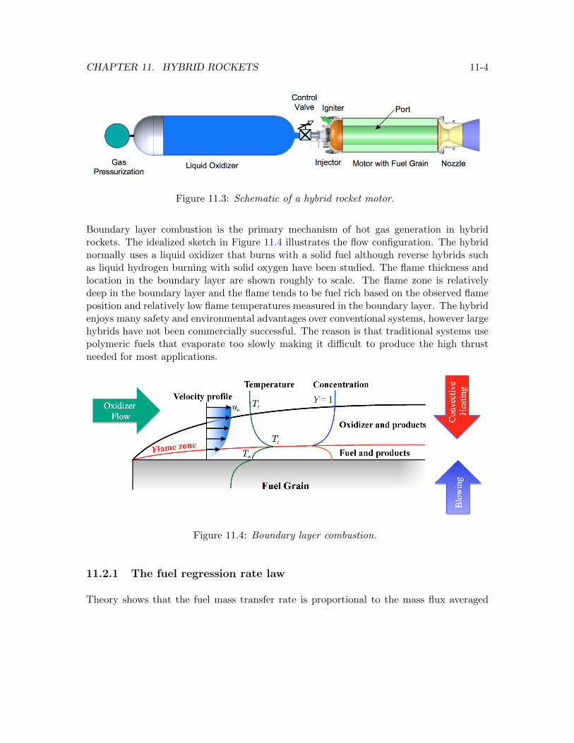
CHAPTER 11. HYBRID ROCKETS 11-4
Figure 11.3: Schematic of a hybrid rocket motor.
Boundary layer combustion is the primary mechanism of hot gas generation in hybridrockets. The idealized sketch in Figure 11.4 illustrates the flow configuration. The hybridnormally uses a liquid oxidizer that burns with a solid fuel although reverse hybrids suchas liquid hydrogen burning with solid oxygen have been studied. The flame thickness andlocation in the boundary layer are shown roughly to scale. The flame zone is relativelydeep in the boundary layer and the flame tends to be fuel rich based on the observed flameposition and relatively low flame temperatures measured in the boundary layer. The hybridenjoys many safety and environmental advantages over conventional systems, however largehybrids have not been commercially successful. The reason is that traditional systems usepolymeric fuels that evaporate too slowly making it difficult to produce the high thrustneeded for most applications.
Figure 11.4: Boundary layer combustion.
11.2.1 The fuel regression rate law
Theory shows that the fuel mass transfer rate is proportional to the mass flux averaged
CHAPTER 11. HYBRID ROCKETS 11-5
across the port. The mass flow rate increases with axial distance along the port leading tocoupling between the local fuel regression rate and the local mass flux. For proper design,accurate expressions are needed for both the time dependent oxidizer-to-fuel ratio at theend of the port, and the time at which all the fuel is consumed. As the fuel is depleted theflame approaches the motor case at which point the burn must be terminated. The couplingbetween the local regression rate and the local mass flow rate means that both variablesdepend on time and space. This complicates the analysis of the thrust time behavior ofthe hybrid compared to a solid rocket. The problem is governed by two coupled first-orderpartial differential equations, the regression rate equation
∂r (x, t)
∂t=
a
xm
(mport
πr2
)n(11.2)
and the mass flow growth equation
∂mport (x, t)
∂x= ρf (2πr)
a
xm
(mport
πr2
)n. (11.3)
The local mass flux in the port is generally denoted G where
G =mport
πr2=mox + mf
πr2. (11.4)
The local port mass flow rate, mport, is the sum of the oxidizer mass flow rate, mox, injectedat the entrance to the port and the accumulated fuel mass flow rate, mf , transferredfrom the fuel grain upstream of a location x. The coefficient a is an empirical constantdetermined by the choice of fuel and oxidizer. The units of the regression rate constantare
[a] =Length2n+m+1
MassnTime1−n . (11.5)
The dependence of regression rate on mass flux G and stream-wise coordinate x arisesfrom the dependence of the skin friction and heat transfer rate on Reynolds number basedon distance along the port. Values of the exponents suggested by theory are m = 0.2 andn = 0.8. Measured values of n tend to be in the range 0.3 to 0.8 depending on the choiceof fuel and oxidizer. Values of n greater than 0.8 or less than about 0.3 are generallynot observed. The length exponent turns out to be very difficult to measure since it isrelatively small and would require a large number of motor tests at a wide range of scalesto be determined accurately. As nearly as one can tell at this point m is considerablysmaller than the prediction of classical theory.
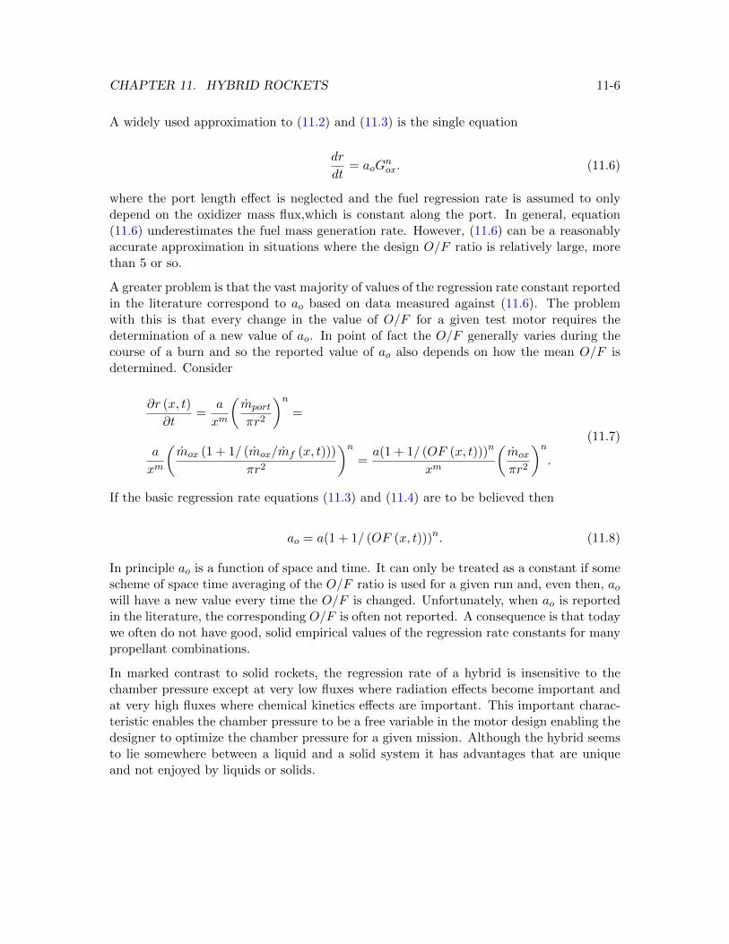
CHAPTER 11. HYBRID ROCKETS 11-6
A widely used approximation to (11.2) and (11.3) is the single equation
dr
dt= aoG
nox. (11.6)
where the port length effect is neglected and the fuel regression rate is assumed to onlydepend on the oxidizer mass flux,which is constant along the port. In general, equation(11.6) underestimates the fuel mass generation rate. However, (11.6) can be a reasonablyaccurate approximation in situations where the design O/F ratio is relatively large, morethan 5 or so.
A greater problem is that the vast majority of values of the regression rate constant reportedin the literature correspond to ao based on data measured against (11.6). The problemwith this is that every change in the value of O/F for a given test motor requires thedetermination of a new value of ao. In point of fact the O/F generally varies during thecourse of a burn and so the reported value of ao also depends on how the mean O/F isdetermined. Consider
∂r (x, t)
∂t=
a
xm
(mport
πr2
)n=
a
xm
(mox (1 + 1/ (mox/mf (x, t)))
πr2
)n=a(1 + 1/ (OF (x, t)))n
xm
(mox
πr2
)n.
(11.7)
If the basic regression rate equations (11.3) and (11.4) are to be believed then
ao = a(1 + 1/ (OF (x, t)))n. (11.8)
In principle ao is a function of space and time. It can only be treated as a constant if somescheme of space time averaging of the O/F ratio is used for a given run and, even then, aowill have a new value every time the O/F is changed. Unfortunately, when ao is reportedin the literature, the corresponding O/F is often not reported. A consequence is that todaywe often do not have good, solid empirical values of the regression rate constants for manypropellant combinations.
In marked contrast to solid rockets, the regression rate of a hybrid is insensitive to thechamber pressure except at very low fluxes where radiation effects become important andat very high fluxes where chemical kinetics effects are important. This important charac-teristic enables the chamber pressure to be a free variable in the motor design enabling thedesigner to optimize the chamber pressure for a given mission. Although the hybrid seemsto lie somewhere between a liquid and a solid system it has advantages that are uniqueand not enjoyed by liquids or solids.
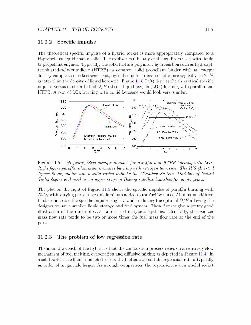
CHAPTER 11. HYBRID ROCKETS 11-7
11.2.2 Specific impulse
The theoretical specific impulse of a hybrid rocket is more appropriately compared to abi-propellant liquid than a solid. The oxidizer can be any of the oxidizers used with liquidbi-propellant engines. Typically, the solid fuel is a polymeric hydrocarbon such as hydroxyl-terminated-poly-butadiene (HTPB), a common solid propellant binder with an energydensity comparable to kerosene. But, hybrid solid fuel mass densities are typically 15-20 %greater than the density of liquid kerosene. Figure 11.5 (left) depicts the theoretical specificimpulse versus oxidizer to fuel O/F ratio of liquid oxygen (LOx) burning with paraffin andHTPB. A plot of LOx burning with liquid kerosene would look very similar.
Figure 11.5: Left figure, ideal specific impulse for paraffin and HTPB burning with LOx.Right figure paraffin-aluminum mixtures burning with nitrogen tetroxide. The IUS (InertialUpper Stage) motor was a solid rocket built by the Chemical Systems Division of UnitedTechnologies and used as an upper stage in Boeing satellite launches for many years.
The plot on the right of Figure 11.5 shows the specific impulse of paraffin burning withN2O4 with varying percentages of aluminum added to the fuel by mass. Aluminum additiontends to increase the specific impulse slightly while reducing the optimal O/F allowing thedesigner to use a smaller liquid storage and feed system. These figures give a pretty goodillustration of the range of O/F ratios used in typical systems. Generally, the oxidizermass flow rate tends to be two or more times the fuel mass flow rate at the end of theport.
11.2.3 The problem of low regression rate
The main drawback of the hybrid is that the combustion process relies on a relatively slowmechanism of fuel melting, evaporation and diffusive mixing as depicted in Figure 11.4. Ina solid rocket, the flame is much closer to the fuel surface and the regression rate is typicallyan order of magnitude larger. As a rough comparison, the regression rate in a solid rocket
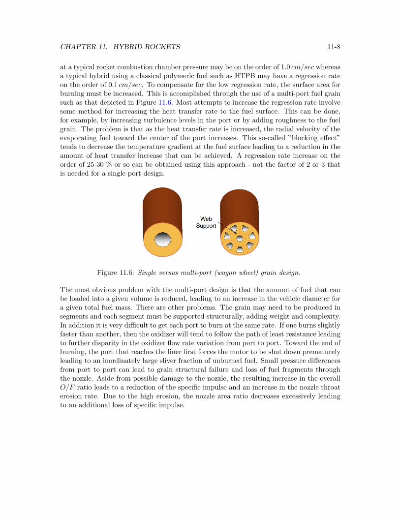
CHAPTER 11. HYBRID ROCKETS 11-8
at a typical rocket combustion chamber pressure may be on the order of 1.0 cm/sec whereasa typical hybrid using a classical polymeric fuel such as HTPB may have a regression rateon the order of 0.1 cm/sec. To compensate for the low regression rate, the surface area forburning must be increased. This is accomplished through the use of a multi-port fuel grainsuch as that depicted in Figure 11.6. Most attempts to increase the regression rate involvesome method for increasing the heat transfer rate to the fuel surface. This can be done,for example, by increasing turbulence levels in the port or by adding roughness to the fuelgrain. The problem is that as the heat transfer rate is increased, the radial velocity of theevaporating fuel toward the center of the port increases. This so-called ”blocking effect”tends to decrease the temperature gradient at the fuel surface leading to a reduction in theamount of heat transfer increase that can be achieved. A regression rate increase on theorder of 25-30 % or so can be obtained using this approach - not the factor of 2 or 3 thatis needed for a single port design.
Figure 11.6: Single versus multi-port (wagon wheel) grain design.
The most obvious problem with the multi-port design is that the amount of fuel that canbe loaded into a given volume is reduced, leading to an increase in the vehicle diameter fora given total fuel mass. There are other problems. The grain may need to be produced insegments and each segment must be supported structurally, adding weight and complexity.In addition it is very difficult to get each port to burn at the same rate. If one burns slightlyfaster than another, then the oxidizer will tend to follow the path of least resistance leadingto further disparity in the oxidizer flow rate variation from port to port. Toward the end ofburning, the port that reaches the liner first forces the motor to be shut down prematurelyleading to an inordinately large sliver fraction of unburned fuel. Small pressure differencesfrom port to port can lead to grain structural failure and loss of fuel fragments throughthe nozzle. Aside from possible damage to the nozzle, the resulting increase in the overallO/F ratio leads to a reduction of the specific impulse and an increase in the nozzle throaterosion rate. Due to the high erosion, the nozzle area ratio decreases excessively leadingto an additional loss of specific impulse.
CHAPTER 11. HYBRID ROCKETS 11-9
11.3 Historical perspective
Early hybrid rocket development and flight test programs were initiated both in Europeand the U.S. in the 1960’s. The European programs in France and Sweden involved smallsounding rockets, whereas the American flight programs were target drones (Sandpiper,HAST, and Firebolt) which required supersonic flight in the upper atmosphere for up to5 minutes. These latter applications were suitable for the conventional hybrid because itsvery low burning rate was ideal for a long duration sustainer operation.
Despite the very low regression rate of the fuel, in the late 1960’s Chemical Systems Divisionof United Technologies (CSD/UTC) investigated motor designs of larger diameters thatcould produce high thrust suitable for space launch vehicles. They experimented with a38 inch diameter motor delivering 40, 000 lbs of thrust. In order to achieve a high massflow rate, a motor with 12 ports in the fuel grain was required. Although the motor wassuccessfully fired several times, it was recognized that the poor volumetric fuel loadingefficiency would lead to a deficit in vehicle performance.
Interest in the hybrid was revived again in the late 1970’s when concern was expressedfor the storage and handling of the large solid propellant segments of the Shuttle booster.The storage of potentially explosive grains is costly in terms of requirements for reinforcedstructures and interline distance separation. The same safety concern arose again afterthe Space Shuttle Challenger disaster, where it was recognized that a thrust terminationoption might have avoided the failure. This concern was heightened when, a few monthslater, there was a Titan failure, caused by an explosion of one of the solid boosters.
Several hybrid propulsion programs were initiated in the late 80’s and early 90’s. The JointGovernment/Industry Research and Development (JIRAD) program involved the testingof 11 and 24 inch diameter hybrid motors at the Marshall Space Flight Center. Anotherhybrid program initiated during the early 90s was DARPA’s Hybrid Technology OptionsProject (HyTOP). The goal of this program was to develop the HyFlyer launch vehicle anddemonstrate the feasibility of hybrid boosters for space applications. The members of theHyTOP team were AMROC, Martin Marietta and CSD/UTC.
In the 1990s, two significant hybrid efforts occurred. One was the formation of the Amer-ican Rocket Company (AMROC), an entrepreneurial industrial company devoted entirelyto the development of large hybrid boosters. The second, with encouragement from NASA,was the formation of the Hybrid Propulsion Industry Action Group (HPIAG) composedof both system and propulsion companies devoted to exploring the possible use of hybridsfor the Shuttle booster and other launch booster applications. Both efforts ran into tech-nical stumbling blocks, basically caused by the low regression rate fuels, which resultedin large diameter motors with many ports to satisfy thrust requirements. The resultingconfiguration not only compromised potential retrofit for the Shuttle and Titan boosters
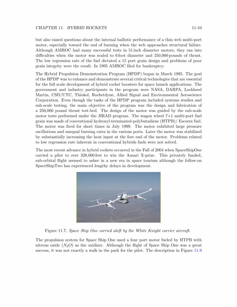
CHAPTER 11. HYBRID ROCKETS 11-10
but also raised questions about the internal ballistic performance of a thin web multi-portmotor, especially toward the end of burning when the web approaches structural failure.Although AMROC had many successful tests in 51 inch diameter motors, they ran intodifficulties when the motor was scaled to 6 foot diameter and 250,000 pounds of thrust.The low regression rate of the fuel dictated a 15 port grain design and problems of poorgrain integrity were the result. In 1995 AMROC filed for bankruptcy.
The Hybrid Propulsion Demonstration Program (HPDP) began in March 1995. The goalof the HPDP was to enhance and demonstrate several critical technologies that are essentialfor the full scale development of hybrid rocket boosters for space launch applications. Thegovernment and industry participants in the program were NASA, DARPA, LockheedMartin, CSD/UTC, Thiokol, Rocketdyne, Allied Signal and Environmental AeroscienceCorporation. Even though the tasks of the HPDP program included systems studies andsub-scale testing, the main objective of the program was the design and fabrication ofa 250,000 pound thrust test-bed. The design of the motor was guided by the sub-scalemotor tests performed under the JIRAD program. The wagon wheel 7+1 multi-port fuelgrain was made of conventional hydroxyl-terminated-polybutadiene (HTPB)/ Escorez fuel.The motor was fired for short times in July 1999. The motor exhibited large pressureoscillations and unequal burning rates in the various ports. Later the motor was stabilizedby substantially increasing the heat input at the fore end of the motor. Problems relatedto low regression rate inherent in conventional hybrids fuels were not solved.
The most recent advance in hybrid rockets occurred in the Fall of 2004 when SpaceShipOnecarried a pilot to over 328,000 feet to win the Ansari X-prize. This privately funded,sub-orbital flight seemed to usher in a new era in space tourism although the follow-onSpaceShipTwo has experienced lengthy delays in development.
Figure 11.7: Space Ship One carried aloft by the White Knight carrier aircraft.
The propulsion system for Space Ship One used a four port motor fueled by HTPB withnitrous oxide (N2O) as the oxidizer. Although the flight of Space Ship One was a greatsuccess, it was not exactly a walk in the park for the pilot. The description in Figure 11.9
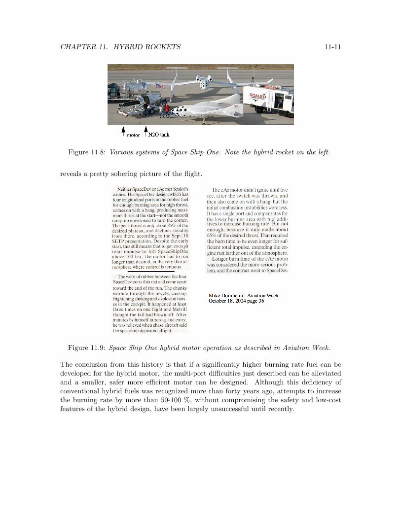
CHAPTER 11. HYBRID ROCKETS 11-11
Figure 11.8: Various systems of Space Ship One. Note the hybrid rocket on the left.
reveals a pretty sobering picture of the flight.
Figure 11.9: Space Ship One hybrid motor operation as described in Aviation Week.
The conclusion from this history is that if a significantly higher burning rate fuel can bedeveloped for the hybrid motor, the multi-port difficulties just described can be alleviatedand a smaller, safer more efficient motor can be designed. Although this deficiency ofconventional hybrid fuels was recognized more than forty years ago, attempts to increasethe burning rate by more than 50-100 %, without compromising the safety and low-costfeatures of the hybrid design, have been largely unsuccessful until recently.
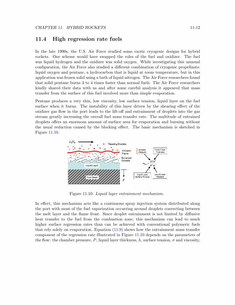
CHAPTER 11. HYBRID ROCKETS 11-12
11.4 High regression rate fuels
In the late 1990s, the U.S. Air Force studied some exotic cryogenic designs for hybridrockets. One scheme would have swapped the roles of the fuel and oxidizer. The fuelwas liquid hydrogen and the oxidizer was solid oxygen. While investigating this unusualconfiguration, the Air Force also studied a different combination of cryogenic propellants:liquid oxygen and pentane, a hydrocarbon that is liquid at room temperature, but in thisapplication was frozen solid using a bath of liquid nitrogen. The Air Force researchers foundthat solid pentane burns 3 to 4 times faster than normal fuels. The Air Force researcherskindly shared their data with us and after some careful analysis it appeared that masstransfer from the surface of this fuel involved more than simple evaporation.
Pentane produces a very thin, low viscosity, low surface tension, liquid layer on the fuelsurface when it burns. The instability of this layer driven by the shearing effect of theoxidizer gas flow in the port leads to the lift-off and entrainment of droplets into the gasstream greatly increasing the overall fuel mass transfer rate. The multitude of entraineddroplets offers an enormous amount of surface area for evaporation and burning withoutthe usual reduction caused by the blocking effect. The basic mechanism is sketched inFigure 11.10.
Figure 11.10: Liquid layer entrainment mechanism.
In effect, this mechanism acts like a continuous spray injection system distributed alongthe port with most of the fuel vaporization occurring around droplets convecting betweenthe melt layer and the flame front. Since droplet entrainment is not limited by diffusiveheat transfer to the fuel from the combustion zone, this mechanism can lead to muchhigher surface regression rates than can be achieved with conventional polymeric fuelsthat rely solely on evaporation. Equation (11.9) shows how the entrainment mass transfercomponent of the regression rate illustrated in Figure 11.10 depends on the parameters ofthe flow: the chamber pressure, P , liquid layer thickness, h, surface tension, σ and viscosity,
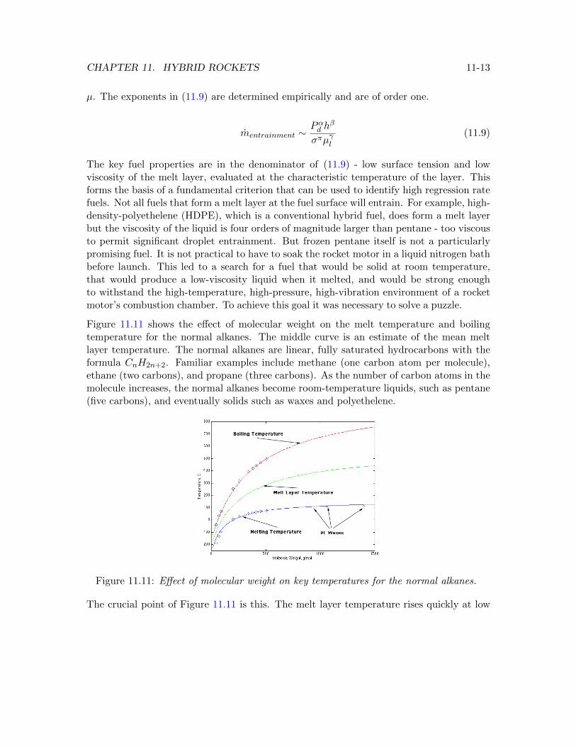
CHAPTER 11. HYBRID ROCKETS 11-13
µ. The exponents in (11.9) are determined empirically and are of order one.
mentrainment ∼Pαd h
β
σπµγl(11.9)
The key fuel properties are in the denominator of (11.9) - low surface tension and lowviscosity of the melt layer, evaluated at the characteristic temperature of the layer. Thisforms the basis of a fundamental criterion that can be used to identify high regression ratefuels. Not all fuels that form a melt layer at the fuel surface will entrain. For example, high-density-polyethelene (HDPE), which is a conventional hybrid fuel, does form a melt layerbut the viscosity of the liquid is four orders of magnitude larger than pentane - too viscousto permit significant droplet entrainment. But frozen pentane itself is not a particularlypromising fuel. It is not practical to have to soak the rocket motor in a liquid nitrogen bathbefore launch. This led to a search for a fuel that would be solid at room temperature,that would produce a low-viscosity liquid when it melted, and would be strong enoughto withstand the high-temperature, high-pressure, high-vibration environment of a rocketmotor’s combustion chamber. To achieve this goal it was necessary to solve a puzzle.
Figure 11.11 shows the effect of molecular weight on the melt temperature and boilingtemperature for the normal alkanes. The middle curve is an estimate of the mean meltlayer temperature. The normal alkanes are linear, fully saturated hydrocarbons with theformula CnH2n+2. Familiar examples include methane (one carbon atom per molecule),ethane (two carbons), and propane (three carbons). As the number of carbon atoms in themolecule increases, the normal alkanes become room-temperature liquids, such as pentane(five carbons), and eventually solids such as waxes and polyethelene.
Figure 11.11: Effect of molecular weight on key temperatures for the normal alkanes.
The crucial point of Figure 11.11 is this. The melt layer temperature rises quickly at low
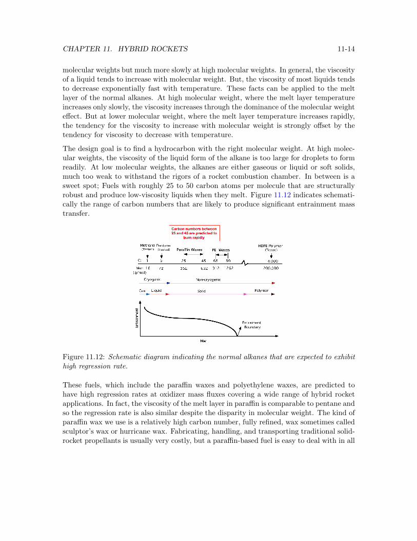
CHAPTER 11. HYBRID ROCKETS 11-14
molecular weights but much more slowly at high molecular weights. In general, the viscosityof a liquid tends to increase with molecular weight. But, the viscosity of most liquids tendsto decrease exponentially fast with temperature. These facts can be applied to the meltlayer of the normal alkanes. At high molecular weight, where the melt layer temperatureincreases only slowly, the viscosity increases through the dominance of the molecular weighteffect. But at lower molecular weight, where the melt layer temperature increases rapidly,the tendency for the viscosity to increase with molecular weight is strongly offset by thetendency for viscosity to decrease with temperature.
The design goal is to find a hydrocarbon with the right molecular weight. At high molec-ular weights, the viscosity of the liquid form of the alkane is too large for droplets to formreadily. At low molecular weights, the alkanes are either gaseous or liquid or soft solids,much too weak to withstand the rigors of a rocket combustion chamber. In between is asweet spot; Fuels with roughly 25 to 50 carbon atoms per molecule that are structurallyrobust and produce low-viscosity liquids when they melt. Figure 11.12 indicates schemati-cally the range of carbon numbers that are likely to produce significant entrainment masstransfer.
Figure 11.12: Schematic diagram indicating the normal alkanes that are expected to exhibithigh regression rate.
These fuels, which include the paraffin waxes and polyethylene waxes, are predicted tohave high regression rates at oxidizer mass fluxes covering a wide range of hybrid rocketapplications. In fact, the viscosity of the melt layer in paraffin is comparable to pentane andso the regression rate is also similar despite the disparity in molecular weight. The kind ofparaffin wax we use is a relatively high carbon number, fully refined, wax sometimes calledsculptor’s wax or hurricane wax. Fabricating, handling, and transporting traditional solid-rocket propellants is usually very costly, but a paraffin-based fuel is easy to deal with in all
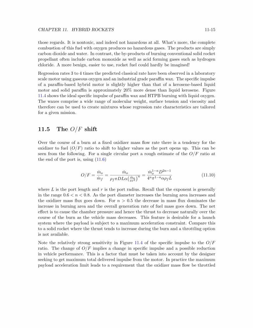
CHAPTER 11. HYBRID ROCKETS 11-15
those regards. It is nontoxic, and indeed not hazardous at all. What’s more, the completecombustion of this fuel with oxygen produces no hazardous gases. The products are simplycarbon dioxide and water. In contrast, the by-products of burning conventional solid rocketpropellant often include carbon monoxide as well as acid forming gases such as hydrogenchloride. A more benign, easier to use, rocket fuel could hardly be imagined!
Regression rates 3 to 4 times the predicted classical rate have been observed in a laboratoryscale motor using gaseous oxygen and an industrial grade paraffin wax. The specific impulseof a paraffin-based hybrid motor is slightly higher than that of a kerosene-based liquidmotor and solid paraffin is approximately 20% more dense than liquid kerosene. Figure11.4 shows the ideal specific impulse of paraffin wax and HTPB burning with liquid oxygen.The waxes comprise a wide range of molecular weight, surface tension and viscosity andtherefore can be used to create mixtures whose regression rate characteristics are tailoredfor a given mission.
11.5 The O/F shift
Over the course of a burn at a fixed oxidizer mass flow rate there is a tendency for theoxidizer to fuel (O/F ) ratio to shift to higher values as the port opens up. This can beseen from the following. For a single circular port a rough estimate of the O/F ratio atthe end of the port is, using (11.6)
O/F =mo
mf=
mo
ρfπDLα(moπr2
)n =m1−no D2n−1
4nπ1−nαρfL(11.10)
where L is the port length and r is the port radius. Recall that the exponent is generallyin the range 0.6 < n < 0.8. As the port diameter increases the burning area increases andthe oxidizer mass flux goes down. For n > 0.5 the decrease in mass flux dominates theincrease in burning area and the overall generation rate of fuel mass goes down. The neteffect is to cause the chamber pressure and hence the thrust to decrease naturally over thecourse of the burn as the vehicle mass decreases. This feature is desirable for a launchsystem where the payload is subject to a maximum acceleration constraint. Compare thisto a solid rocket where the thrust tends to increase during the burn and a throttling optionis not available.
Note the relatively strong sensitivity in Figure 11.4 of the specific impulse to the O/Fratio. The change of O/F implies a change in specific impulse and a possible reductionin vehicle performance. This is a factor that must be taken into account by the designerseeking to get maximum total delivered impulse from the motor. In practice the maximumpayload acceleration limit leads to a requirement that the oxidizer mass flow be throttled
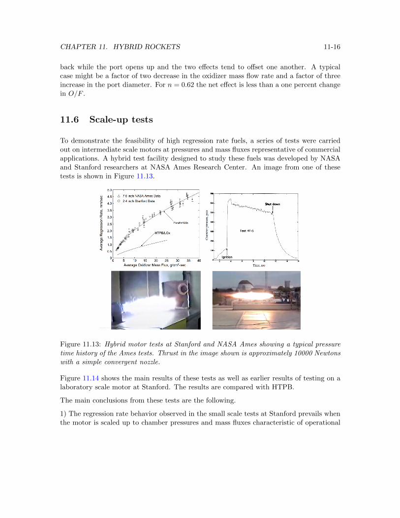
CHAPTER 11. HYBRID ROCKETS 11-16
back while the port opens up and the two effects tend to offset one another. A typicalcase might be a factor of two decrease in the oxidizer mass flow rate and a factor of threeincrease in the port diameter. For n = 0.62 the net effect is less than a one percent changein O/F .
11.6 Scale-up tests
To demonstrate the feasibility of high regression rate fuels, a series of tests were carriedout on intermediate scale motors at pressures and mass fluxes representative of commercialapplications. A hybrid test facility designed to study these fuels was developed by NASAand Stanford researchers at NASA Ames Research Center. An image from one of thesetests is shown in Figure 11.13.
Figure 11.13: Hybrid motor tests at Stanford and NASA Ames showing a typical pressuretime history of the Ames tests. Thrust in the image shown is approximately 10000 Newtonswith a simple convergent nozzle.
Figure 11.14 shows the main results of these tests as well as earlier results of testing on alaboratory scale motor at Stanford. The results are compared with HTPB.
The main conclusions from these tests are the following.
1) The regression rate behavior observed in the small scale tests at Stanford prevails whenthe motor is scaled up to chamber pressures and mass fluxes characteristic of operational
CHAPTER 11. HYBRID ROCKETS 11-17
Figure 11.14: Regression rate versus oxidizer mass flux for paraffin and HTPB.
systems. Moreover the regression rate data from large and small motors matches quitewell indicating that small scale tests can be used to infer the behavior of larger motors.This is extremely useful when it comes to developing the right fuel formulation for a givenmission.
2) Paraffin-based fuels provide reliable ignition and stable combustion over the entire rangeof mass fluxes encountered (50− 600 kg/m2 − sec).
3) The fuel exhibited excellent structural integrity over the range of chamber pressuresused (10− 65 bar).
11.7 Regression rate analysis
11.7.1 Regression rate with the effect of fuel mass flow neglected.
The simplest approach to determining how the port radius varies with time is to neglect theeffect of accumulated fuel mass flow on the regression rate and assume the length exponentm = 0 so the port radius is independent of x. This utilizes the fact that m is known to besmall allowing the singularity at x = 0 to be removed. Moreover the optimal O/F is oftenthree or more so the oxidizer usually comprises most of the mass flow. Recall (11.6) and
CHAPTER 11. HYBRID ROCKETS 11-18
express the mass flux in terms of the radius and oxidizer mass flow.
dr (t)
dt= ao
(mox (t)
πr2
)n(11.11)
Integrate (11.11) with respect to time.
r (t) =
(r(0)2n+1 + (2n+ 1)
aoπn
∫ t
0mox
(t′)ndt′) 1
2n+1
(11.12)
Under the assumed regression rate (11.11) law the mass flow increases linearly along theport.
mport
mox=mf + mox
mox= 1 +
2π1−naoρf
m1−nox
(r(0)2n+1 + (2n+ 1) aoxπn
∫ t0 mox(t′)ndt′
) 2n−12n+1
x
(11.13)
11.7.2 Exact solution of the coupled space-time problem for n = 1/2.
In reality the regression rate is dependent on the local total mass flux including the fuelmass accumulated along the port and, in turn, the local mass flux depends on the localradius. The problem is governed by two coupled first-order partial differential equations,(11.2) and (11.3). For n = 1/2 the equations simplify to
∂
∂t
(r2)
= 2π−1/2am
1/2port
xm(11.14)
and
∂mport
∂x= 2π1/2aρf
m1/2port
xm(11.15)
The solution of (11.14) and (11.15) is
r (x, t) =
(r(x, 0)2 +
2a
xmπ1/2
(∫ t
0mox
(t′)1/2
dt′ +π1/2aρfx
1−mt
1−m
))1/2
(11.16)
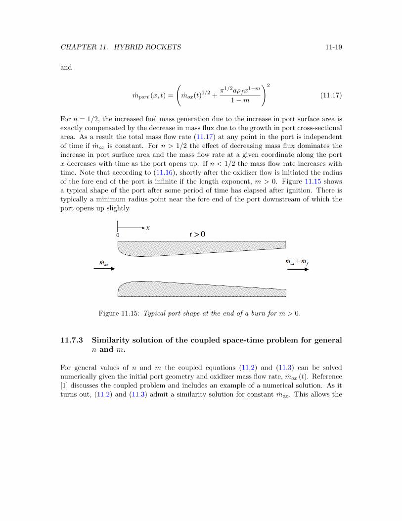
CHAPTER 11. HYBRID ROCKETS 11-19
and
mport (x, t) =
(mox(t)1/2 +
π1/2aρfx1−m
1−m
)2
(11.17)
For n = 1/2, the increased fuel mass generation due to the increase in port surface area isexactly compensated by the decrease in mass flux due to the growth in port cross-sectionalarea. As a result the total mass flow rate (11.17) at any point in the port is independentof time if mox is constant. For n > 1/2 the effect of decreasing mass flux dominates theincrease in port surface area and the mass flow rate at a given coordinate along the portx decreases with time as the port opens up. If n < 1/2 the mass flow rate increases withtime. Note that according to (11.16), shortly after the oxidizer flow is initiated the radiusof the fore end of the port is infinite if the length exponent, m > 0. Figure 11.15 showsa typical shape of the port after some period of time has elapsed after ignition. There istypically a minimum radius point near the fore end of the port downstream of which theport opens up slightly.
Figure 11.15: Typical port shape at the end of a burn for m > 0.
11.7.3 Similarity solution of the coupled space-time problem for generaln and m.
For general values of n and m the coupled equations (11.2) and (11.3) can be solvednumerically given the initial port geometry and oxidizer mass flow rate, mox (t). Reference[1] discusses the coupled problem and includes an example of a numerical solution. As itturns out, (11.2) and (11.3) admit a similarity solution for constant mox. This allows the
CHAPTER 11. HYBRID ROCKETS 11-20
equations to be reduced to a pair of ODEs in the similarity variable
θ =
((π−na)
2(2πρf )(2n+1)
mox
) 12n−2m+1 x
t(2n−1
2n−2m+1). (11.18)
The similarity solution is derived in reference [2]. It can be used to generate accuratesolutions for the port radius and O/F ratio. The similarity solution can even be appliedto the case where mox does change with time by using a staircase function to approximatemox.
11.7.4 Numerical solution for the coupled space-time problem, for gen-eral n and m and variable oxidizer flow rate.
The coupled equations (11.2) and (11.3) can be solved for a general initial port radiusdistribution and variable oxidizer mass flow rate using a first order forward differencescheme. First, the equations are non-dimensionalized using the initial oxidizer mass flowrate, mox (0), the initial port radius at the fore end, r (0, 0) and the burn time, tburntime.
CHAPTER 11. HYBRID ROCKETS 11-21
Dimensionless variables as follows.
χ =x
r (0, 0)
τ =t
tburntime
R =r (x, t)
r (0, 0)
J (x, t) =mport
mox (0)=mox (t) + mf (x, t)
mox (0)=
mox (0) + mf (x, t)
mox (0)+
(mox (t)− mox (0)
mox (0)
)
J (x, t) =mox (0) + mf (x, t)
mox (0)
λ (t) =mox (t)− mox (0)
mox (0)
(11.19)
In dimensionless form, the coupled equations are
∂R
∂τ= CR
1
χm
(J + λ
πR2
)n(11.20)
and
∂J
∂τ= CJ
(2πR)
χm
(J + λ
πR2
)n(11.21)
where
CR =atburntimemox(0)n
r(0, 0)2n+m+1 (11.22)
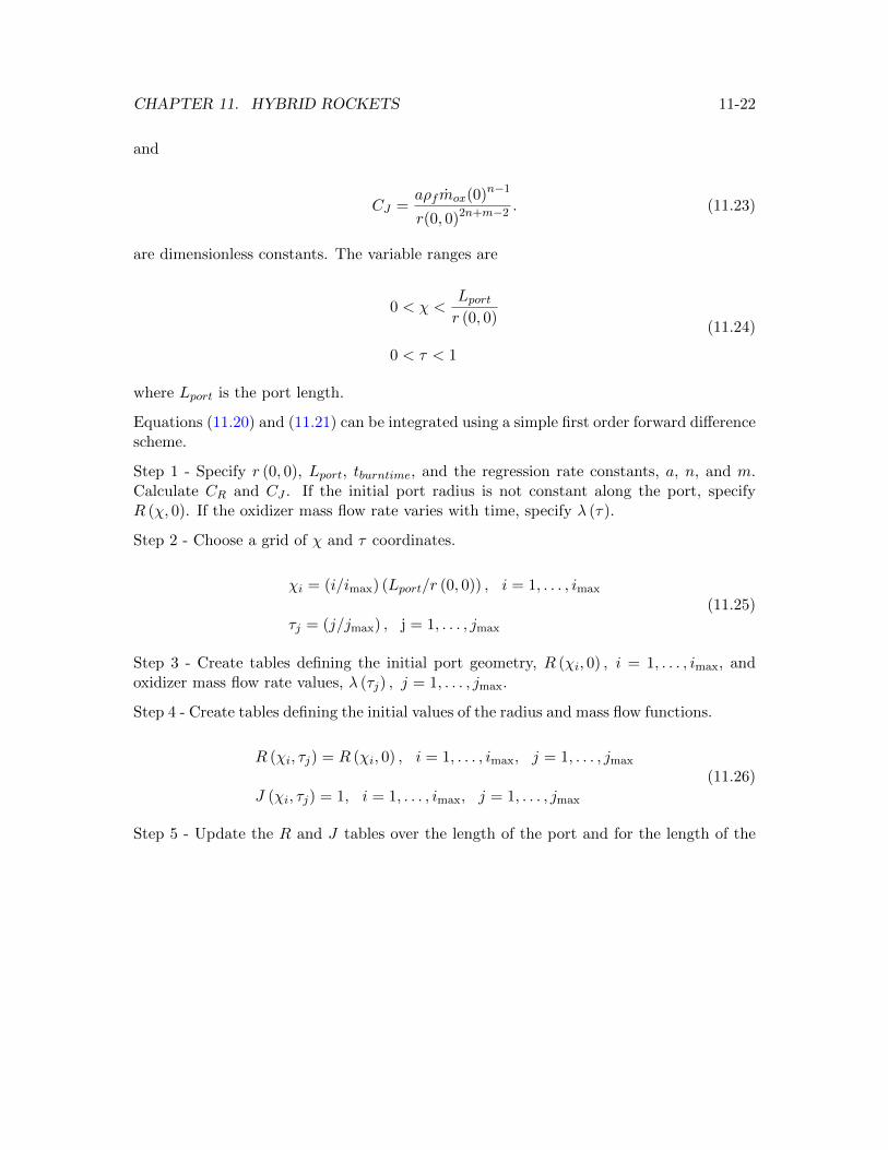
CHAPTER 11. HYBRID ROCKETS 11-22
and
CJ =aρfmox(0)n−1
r(0, 0)2n+m−2 . (11.23)
are dimensionless constants. The variable ranges are
0 < χ <Lportr (0, 0)
0 < τ < 1
(11.24)
where Lport is the port length.
Equations (11.20) and (11.21) can be integrated using a simple first order forward differencescheme.
Step 1 - Specify r (0, 0), Lport, tburntime, and the regression rate constants, a, n, and m.Calculate CR and CJ . If the initial port radius is not constant along the port, specifyR (χ, 0). If the oxidizer mass flow rate varies with time, specify λ (τ).
Step 2 - Choose a grid of χ and τ coordinates.
χi = (i/imax) (Lport/r (0, 0)) , i = 1, . . . , imax
τj = (j/jmax) , j = 1, . . . , jmax
(11.25)
Step 3 - Create tables defining the initial port geometry, R (χi, 0) , i = 1, . . . , imax, andoxidizer mass flow rate values, λ (τj) , j = 1, . . . , jmax.
Step 4 - Create tables defining the initial values of the radius and mass flow functions.
R (χi, τj) = R (χi, 0) , i = 1, . . . , imax, j = 1, . . . , jmax
J (χi, τj) = 1, i = 1, . . . , imax, j = 1, . . . , jmax
(11.26)
Step 5 - Update the R and J tables over the length of the port and for the length of the
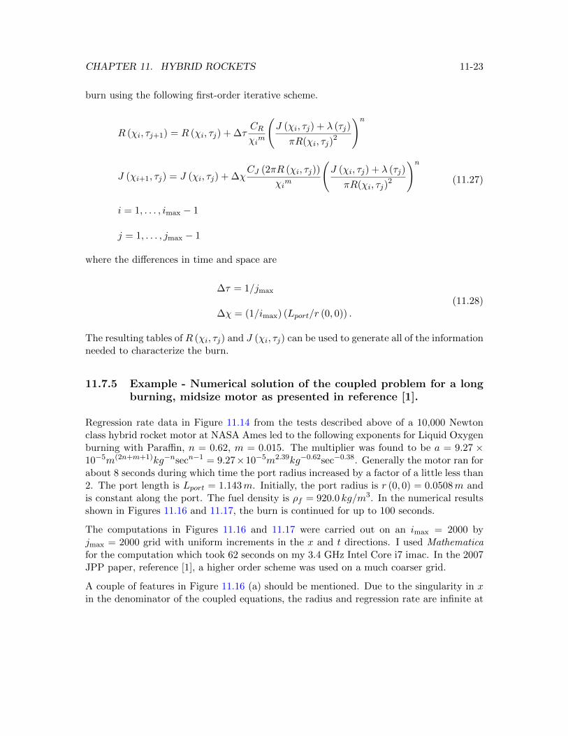
CHAPTER 11. HYBRID ROCKETS 11-23
burn using the following first-order iterative scheme.
R (χi, τj+1) = R (χi, τj) + ∆τCRχim
(J (χi, τj) + λ (τj)
πR(χi, τj)2
)n
J (χi+1, τj) = J (χi, τj) + ∆χCJ (2πR (χi, τj))
χim
(J (χi, τj) + λ (τj)
πR(χi, τj)2
)n
i = 1, . . . , imax − 1
j = 1, . . . , jmax − 1
(11.27)
where the differences in time and space are
∆τ = 1/jmax
∆χ = (1/imax) (Lport/r (0, 0)) .(11.28)
The resulting tables of R (χi, τj) and J (χi, τj) can be used to generate all of the informationneeded to characterize the burn.
11.7.5 Example - Numerical solution of the coupled problem for a longburning, midsize motor as presented in reference [1].
Regression rate data in Figure 11.14 from the tests described above of a 10,000 Newtonclass hybrid rocket motor at NASA Ames led to the following exponents for Liquid Oxygenburning with Paraffin, n = 0.62, m = 0.015. The multiplier was found to be a = 9.27 ×10⁻⁵m(2n+m+1)kg−nsecn−1 = 9.27×10⁻⁵m2.39kg−0.62sec−0.38. Generally the motor ran forabout 8 seconds during which time the port radius increased by a factor of a little less than2. The port length is Lport = 1.143m. Initially, the port radius is r (0, 0) = 0.0508m andis constant along the port. The fuel density is ρf = 920.0 kg/m3. In the numerical resultsshown in Figures 11.16 and 11.17, the burn is continued for up to 100 seconds.
The computations in Figures 11.16 and 11.17 were carried out on an imax = 2000 byjmax = 2000 grid with uniform increments in the x and t directions. I used Mathematicafor the computation which took 62 seconds on my 3.4 GHz Intel Core i7 imac. In the 2007JPP paper, reference [1], a higher order scheme was used on a much coarser grid.
A couple of features in Figure 11.16 (a) should be mentioned. Due to the singularity in xin the denominator of the coupled equations, the radius and regression rate are infinite at
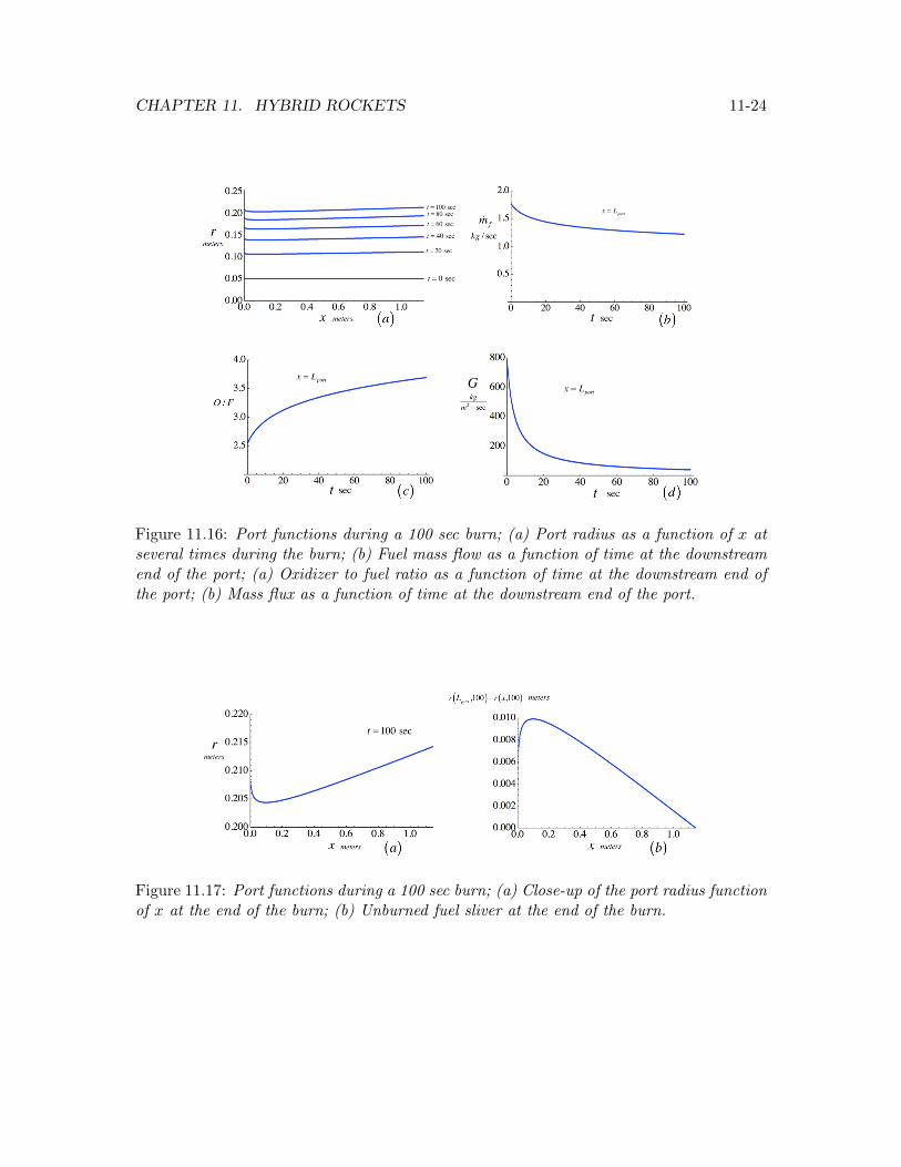
CHAPTER 11. HYBRID ROCKETS 11-24
Figure 11.16: Port functions during a 100 sec burn; (a) Port radius as a function of x atseveral times during the burn; (b) Fuel mass flow as a function of time at the downstreamend of the port; (a) Oxidizer to fuel ratio as a function of time at the downstream end ofthe port; (b) Mass flux as a function of time at the downstream end of the port.
Figure 11.17: Port functions during a 100 sec burn; (a) Close-up of the port radius functionof x at the end of the burn; (b) Unburned fuel sliver at the end of the burn.
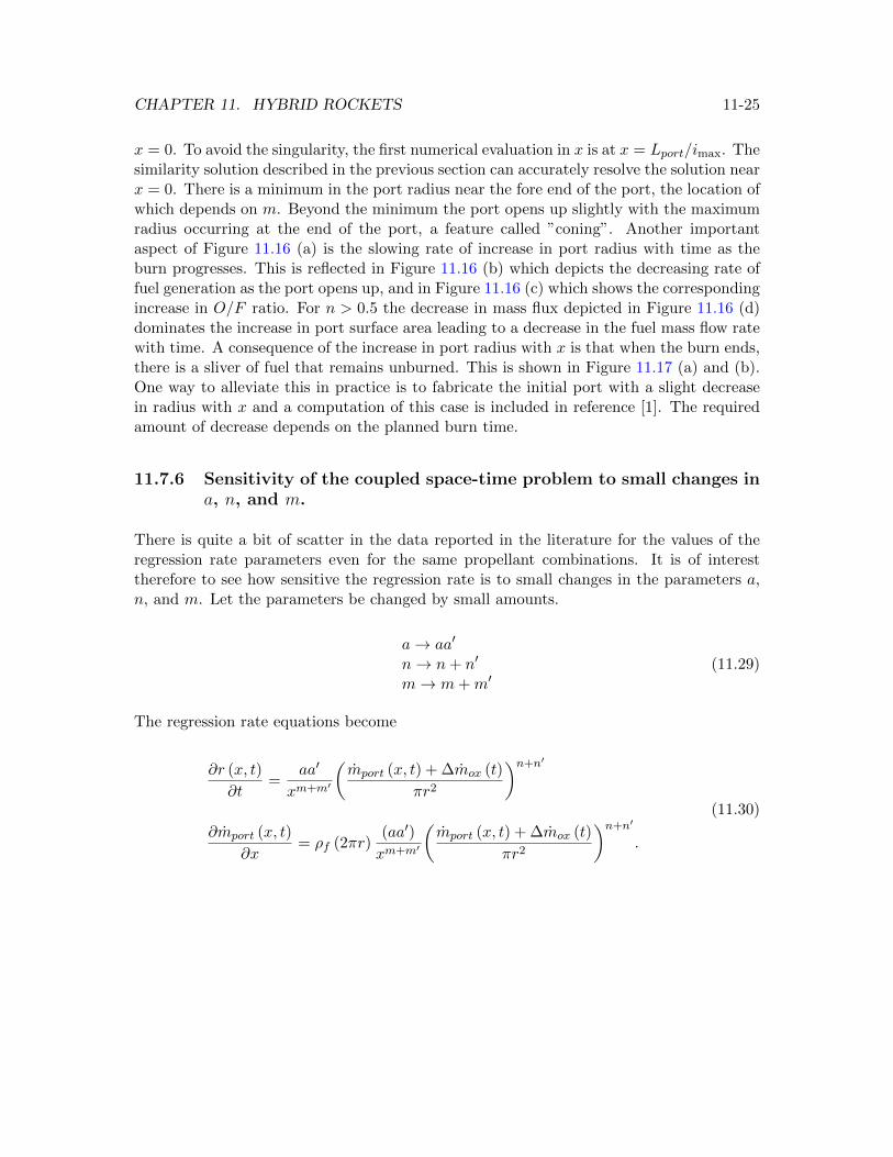
CHAPTER 11. HYBRID ROCKETS 11-25
x = 0. To avoid the singularity, the first numerical evaluation in x is at x = Lport/imax. Thesimilarity solution described in the previous section can accurately resolve the solution nearx = 0. There is a minimum in the port radius near the fore end of the port, the location ofwhich depends on m. Beyond the minimum the port opens up slightly with the maximumradius occurring at the end of the port, a feature called ”coning”. Another importantaspect of Figure 11.16 (a) is the slowing rate of increase in port radius with time as theburn progresses. This is reflected in Figure 11.16 (b) which depicts the decreasing rate offuel generation as the port opens up, and in Figure 11.16 (c) which shows the correspondingincrease in O/F ratio. For n > 0.5 the decrease in mass flux depicted in Figure 11.16 (d)dominates the increase in port surface area leading to a decrease in the fuel mass flow ratewith time. A consequence of the increase in port radius with x is that when the burn ends,there is a sliver of fuel that remains unburned. This is shown in Figure 11.17 (a) and (b).One way to alleviate this in practice is to fabricate the initial port with a slight decreasein radius with x and a computation of this case is included in reference [1]. The requiredamount of decrease depends on the planned burn time.
11.7.6 Sensitivity of the coupled space-time problem to small changes ina, n, and m.
There is quite a bit of scatter in the data reported in the literature for the values of theregression rate parameters even for the same propellant combinations. It is of interesttherefore to see how sensitive the regression rate is to small changes in the parameters a,n, and m. Let the parameters be changed by small amounts.
a→ aa′
n→ n+ n′
m→ m+m′(11.29)
The regression rate equations become
∂r (x, t)
∂t=
aa′
xm+m′
(mport (x, t) + ∆mox (t)
πr2
)n+n′
∂mport (x, t)
∂x= ρf (2πr)
(aa′)
xm+m′
(mport (x, t) + ∆mox (t)
πr2
)n+n′
.
(11.30)
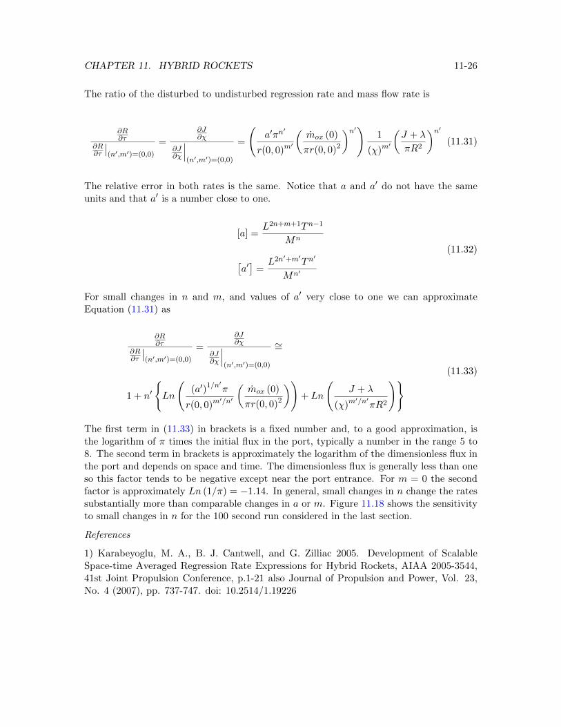
CHAPTER 11. HYBRID ROCKETS 11-26
The ratio of the disturbed to undisturbed regression rate and mass flow rate is
∂R∂τ
∂R∂τ
∣∣(n′,m′)=(0,0)
=
∂J∂χ
∂J∂χ
∣∣∣(n′,m′)=(0,0)
=
(a′πn
′
r(0, 0)m′
(mox (0)
πr(0, 0)2
)n′) 1
(χ)m′
(J + λ
πR2
)n′(11.31)
The relative error in both rates is the same. Notice that a and a′ do not have the sameunits and that a′ is a number close to one.
[a] =L2n+m+1Tn−1
Mn
[a′]
=L2n′+m′Tn
′
Mn′
(11.32)
For small changes in n and m, and values of a′ very close to one we can approximateEquation (11.31) as
∂R∂τ
∂R∂τ
∣∣(n′,m′)=(0,0)
=
∂J∂χ
∂J∂χ
∣∣∣(n′,m′)=(0,0)
∼=
1 + n′
{Ln
((a′)1/n′π
r(0, 0)m′/n′
(mox (0)
πr(0, 0)2
))+ Ln
(J + λ
(χ)m′/n′πR2
)} (11.33)
The first term in (11.33) in brackets is a fixed number and, to a good approximation, isthe logarithm of π times the initial flux in the port, typically a number in the range 5 to8. The second term in brackets is approximately the logarithm of the dimensionless flux inthe port and depends on space and time. The dimensionless flux is generally less than oneso this factor tends to be negative except near the port entrance. For m = 0 the secondfactor is approximately Ln (1/π) = −1.14. In general, small changes in n change the ratessubstantially more than comparable changes in a or m. Figure 11.18 shows the sensitivityto small changes in n for the 100 second run considered in the last section.
References
1) Karabeyoglu, M. A., B. J. Cantwell, and G. Zilliac 2005. Development of ScalableSpace-time Averaged Regression Rate Expressions for Hybrid Rockets, AIAA 2005-3544,41st Joint Propulsion Conference, p.1-21 also Journal of Propulsion and Power, Vol. 23,No. 4 (2007), pp. 737-747. doi: 10.2514/1.19226
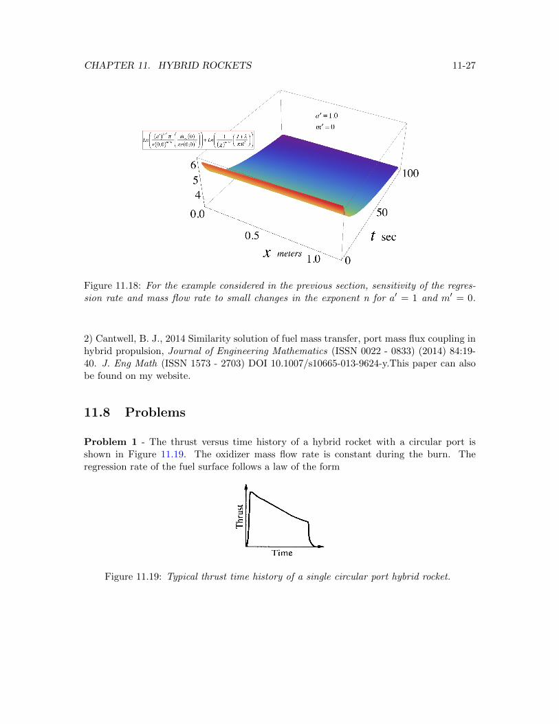
CHAPTER 11. HYBRID ROCKETS 11-27
Figure 11.18: For the example considered in the previous section, sensitivity of the regres-sion rate and mass flow rate to small changes in the exponent n for a′ = 1 and m′ = 0.
2) Cantwell, B. J., 2014 Similarity solution of fuel mass transfer, port mass flux coupling inhybrid propulsion, Journal of Engineering Mathematics (ISSN 0022 - 0833) (2014) 84:19-40. J. Eng Math (ISSN 1573 - 2703) DOI 10.1007/s10665-013-9624-y.This paper can alsobe found on my website.
11.8 Problems
Problem 1 - The thrust versus time history of a hybrid rocket with a circular port isshown in Figure 11.19. The oxidizer mass flow rate is constant during the burn. Theregression rate of the fuel surface follows a law of the form
Figure 11.19: Typical thrust time history of a single circular port hybrid rocket.
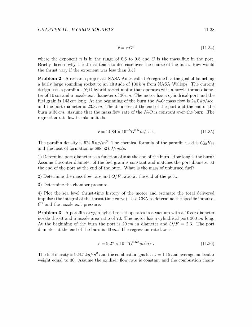
CHAPTER 11. HYBRID ROCKETS 11-28
r = αGn (11.34)
where the exponent n is in the range of 0.6 to 0.8 and G is the mass flux in the port.Briefly discuss why the thrust tends to decrease over the course of the burn. How wouldthe thrust vary if the exponent was less than 0.5?
Problem 2 - A research project at NASA Ames called Peregrine has the goal of launchinga fairly large sounding rocket to an altitude of 100 km from NASA Wallops. The currentdesign uses a paraffin - N2O hybrid rocket motor that operates with a nozzle throat diame-ter of 10 cm and a nozzle exit diameter of 30 cm. The motor has a cylindrical port and thefuel grain is 143 cm long. At the beginning of the burn the N2O mass flow is 24.0 kg/sec,and the port diameter is 23.3 cm. The diameter at the end of the port and the end of theburn is 38 cm. Assume that the mass flow rate of the N2O is constant over the burn. Theregression rate law in mks units is
r = 14.84× 10⁻⁵G0.5m/ sec . (11.35)
The paraffin density is 924.5 kg/m3. The chemical formula of the paraffin used is C32H66
and the heat of formation is 698.52 kJ/mole.
1) Determine port diameter as a function of x at the end of the burn. How long is the burn?Assume the outer diameter of the fuel grain is constant and matches the port diameter atthe end of the port at the end of the burn. What is the mass of unburned fuel?
2) Determine the mass flow rate and O/F ratio at the end of the port.
3) Determine the chamber pressure.
4) Plot the sea level thrust-time history of the motor and estimate the total deliveredimpulse (the integral of the thrust time curve). Use CEA to determine the specific impulse,C∗ and the nozzle exit pressure.
Problem 3 - A paraffin-oxygen hybrid rocket operates in a vacuum with a 10 cm diameternozzle throat and a nozzle area ratio of 70. The motor has a cylindrical port 300 cm long.At the beginning of the burn the port is 20 cm in diameter and O/F = 2.3. The portdiameter at the end of the burn is 60 cm. The regression rate law is
r = 9.27× 10⁻⁵G0.62m/ sec . (11.36)
The fuel density is 924.5 kg/m3 and the combustion gas has γ = 1.15 and average molecularweight equal to 30. Assume the oxidizer flow rate is constant and the combustion cham-

CHAPTER 11. HYBRID ROCKETS 29
ber temperature remains constant over the course of the burn. Approximate the specificimpulse by a mean value of 360 sec over the course of the burn.
1) Estimate the chamber pressure at the beginning of the burn.
2) Plot the diameter of the port as a function of time.
3) Plot the thrust-time history of the burn and estimate the total delivered impulse (theintegral of the thrust time curve).
4) Use Figure 11.4 to estimate the specific impulse at the end of the burn.
Problem 4 - A hybrid rocket with an initial mass of minitial = 900 kg operates in space.The fuel is paraffin with a density 0.93 gm/cm3 and the oxidizer is nitrous oxide. Theoxidizer mass flow rate is held fixed at 2.4× 10⁴ gm/sec. The motor has a 10 cm diameternozzle throat, 30 cm diameter exit, and a cylindrical port 143 cm long. The initial portradius is 8.75 cm. At the end of the burn the port radius is 15.5 cm. The regressionrate law is r = 0.035G0.6
o cm/ sec. A calculation using CEA shows that c∗ = 1.64 ×105 cm/ sec where C∗ is defined by m = Pt2A
∗/C∗ and the effective nozzle exit velocity isC = 2.8× 105 cm/sec.
1) When the fuel is all burned the oxidizer flow is turned off. Determine the time whenthis occurs.
2) Determine the total mass flow rate and motor thrust at the beginning and end of theburn.
3) Determine the chamber pressure at the beginning and end of the burn.
4) Determine the velocity change of the vehicle.
Appendix A
Thermochemistry
A.1 Thermochemical tables
In Chapter 9 we developed the theory for determining the equilibrium composition of amixture of reacting gases. The procedure requires knowledge of the standard Gibbs freeenergy for each molecule in the mixture
g◦i (T ) = ∆h◦fi (Tref ) + {h◦i (T )− h◦i (Tref )} − Ts◦i (T ) (A.1)
where ∆h◦fi (Tref ) is the standard heat of formation of the ith chemical species at somereference temperature, {h◦i (T )− h◦i (Tref )} is the change in the standard enthalpy fromthe reference temperature and s◦i (T ) is the standard entropy. Data for these variablesfor a given chemical species can be found in tabulations of thermochemical properties thathave been developed from experimental measurements of heat capacity over many decades.The purpose of this appendix is to describe the tables, explain the data and connectthermodynamic properties of gases to the chemical bonds between the atoms that makeup the gas. Perhaps the most widely used thermochemical data is from the compilationproduced by the JANAF (Joint Army, Navy, Air Force) Committee. Parts of the JANAFtables for monatomic and diatomic hydrogen are shown in Figure A.1.
All quantities are quoted on a per mole basis and in units of Joules and degrees Kelvin.One mole is an Avagadros number, 6.0221415× 10²³, of molecules. In the table headingsin Figure A.1 properties are symbolized using capital letters, whereas, we have adopted theconvention that all intensive (per unit mass or per unit mole) variables are denoted withlower case letters as in (A.1) and we will stick to that convention. Full tables for a varietyof chemical species are provided in Appendix B.
A-1
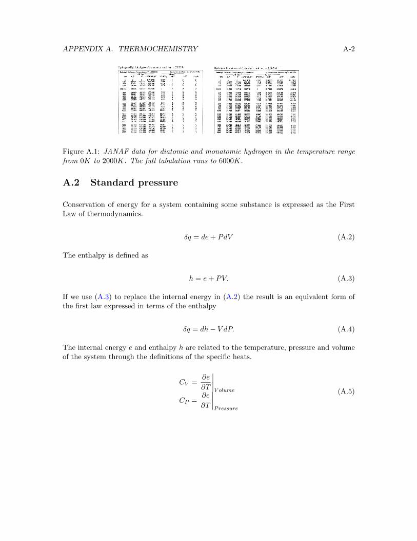
APPENDIX A. THERMOCHEMISTRY A-2
Figure A.1: JANAF data for diatomic and monatomic hydrogen in the temperature rangefrom 0K to 2000K. The full tabulation runs to 6000K.
A.2 Standard pressure
Conservation of energy for a system containing some substance is expressed as the FirstLaw of thermodynamics.
δq = de+ PdV (A.2)
The enthalpy is defined as
h = e+ PV. (A.3)
If we use (A.3) to replace the internal energy in (A.2) the result is an equivalent form ofthe first law expressed in terms of the enthalpy
δq = dh− V dP. (A.4)
The internal energy e and enthalpy h are related to the temperature, pressure and volumeof the system through the definitions of the specific heats.
CV =∂e
∂T
∣∣∣∣V olume
CP =∂e
∂T
∣∣∣∣Pressure
(A.5)
APPENDIX A. THERMOCHEMISTRY A-3
For a process that takes place at constant pressure, the heat added or removed from thesystem is given by the change of enthalpy.
δq|P=constant = dh|P=constant = CPdT (A.6)
It is probably fair to say that the use of the tables of thermochemical properties is dom-inated by applications to mixtures of reacting gases typical of combustion at elevatedtemperatures. As long as the pressure is not extreme, and the system is not near a phaseboundary, the equation of state for each gas in the mixture is the ideal gas law
PiV = niRuT (A.7)
where ni is the number of moles of the ith component of the mixture, Pi is the partialpressure and V is the volume of the mixture. The universal gas constant is
Ru = 8.314510 J/mole−K. (A.8)
For a general substance the heat capacity, enthalpy, entropy and Gibbs potential are func-tions of temperature and pressure.
CP (T, P )h (T, P )s (T, P )g (T, P )
(A.9)
For any substance that follows the ideal gas law equation of state, the heat capacities,internal energy and enthalpy are independent of pressure and the entropy and Gibbs freeenergy depend in a known way on the logarithm of the pressure. It therefore makes senseto standardize all thermochemical data at a standard pressure rather than, say, at standardvolume.
The thermodynamic properties of a substance, whether it is an ideal gas or not, are alwaystabulated as a function of temperature at standard pressure. That the data is tabulatedthis way is indicated by the ”◦” superscript that appears with each symbol in the tables.In various units, the standard pressure we will use in this course is
P ◦ = 105N/m2 = 105 Pascals = 100 kPa = 1bar. (A.10)
APPENDIX A. THERMOCHEMISTRY A-4
The various thermodynamic variables for any species at standard pressure are denotedby
CP (T, 100) = C◦P (T )h (T, P ) = h◦ (T )s (T, P ) = s◦ (T )g (T, P ) = g◦ (T ) .
(A.11)
The standard pressure is very close to one atmosphere 1atm = 1.01325×10⁵ Pa and indeedbefore 1982 the standard was atmospheric pressure at sea level. In 1982 the InternationalUnion of Pure and Applied Chemistry (IUPAC) recommended that for the purposes ofspecifying the physical properties of substances the standard pressure should be defined asprecisely 100 kPa. This had the immediate effect of simplifying thermochemical calcula-tions and the practical effect of specifying the standard pressure to be closer to the actualaverage altitude above sea level where most people around the world live.
A.2.1 What about pressures other than standard?
For substances in their gaseous state at elevated temperatures where the ideal gas law ap-plies and the heat capacities, energy and enthalpy are independent of pressure the enthalpyis simply
h (T, P ) = h◦ (T ) = ∆hf (298.15) +
∫ T
Tref
C◦P (T ) dT. (A.12)
The entropy is
s (T, P ) =
∫ T
Tref
C◦P (T )dT
T−RuLn
(P
100
)= s◦ (T )−RuLn
(P
100
)(A.13)
and the Gibbs free energy is determined from the definition
g (T, P ) = h− Ts = h◦ (T )− Ts◦ (T ) + (RuT )Ln
(P
100
)= g◦ (T ) + (RuT )Ln
(P
100
).
(A.14)
In principle, the standard entropy requires an integration of the heat capacity from absolutezero.
APPENDIX A. THERMOCHEMISTRY A-5
A.2.2 Equilibrium between phases
For a liquid in equilibrium with its vapor the Gibbs free energy of the liquid is equal tothe Gibbs free energy of the vapor.
gliquid (T, P ) = ggas (T, P ) (A.15)
In terms of the definition of the Gibbs free energy
hliquid (T, P )− Tsliquid (T, P ) = hgas (T, P )− Tsgas (T, P ) . (A.16)
Differentiate (A.16).
dhliquid (T, P )−Tdsliquid (T, P )−sliquid (T, P ) dT = dhgas (T, P )−Tdsgas (T, P )−sgas (T, P ) dT(A.17)
The Gibbs equation is
Tdsliquid (T, P ) = dhliquid (T, P )− vliquiddPTdsgas (T, P ) = dhgas (T, P )− vgasdP
(A.18)
where v = V/n is the molar density of the substance. Substitute (A.18) into (A.17). Theresult is
vliquiddP − sliquiddT = vgasdP − sgasdT. (A.19)
With a little bit of rearrangement (A.19) becomes
dP
dT=sgas − sliquidvgas − vliquid
. (A.20)
The heat required to convert a mole of liquid to gas at constant temperature is called thelatent heat of vaporization. From (A.16)
∆hvap = hgas − hliquid = T (sgas − sliquid) . (A.21)
APPENDIX A. THERMOCHEMISTRY A-6
If we substitute (A.21) into (A.20) the result is the famous Clausius-Clapeyron equa-tion
dP
dT=
∆hvapT (vgas − vliquid)
(A.22)
that relates the vapor pressure of a gas-liquid system to the temperature. Generally thetemperature of the system is specified and the vapor pressure is to be determined. In somecases the condensed phase is a solid such as the graphite form of carbon or solid iodinesublimating directly from the solid to the vapor phase.
In the case of a solid in equilibrium with its liquid such as water and ice, the Gibbs freeenergies of the solid and liquid phases are equal and a similar relation governs the transitionbetween phases. The enthalpy change is called the latent heat of fusion. In a solid-liquidsystem, usually the pressure is the specified condition and the temperature of melting isthe property to be determined.
The heat of vaporization depends on the temperature according to
hgas (T ) = hgas (Tref ) + CPgas (T − Tref )hliquid (T ) = hliquid (Tref ) + CPliquid (T − Tref )
∆hvap (T ) = ∆hvap (Tref ) +(CPgas − CPliquid
)(T − Tref ) .
(A.23)
Generally speaking the heat capacity term is relatively small for modest changes in tem-perature. For example, for water between its freezing and boiling point
∆hvap (273.15K) = ∆hvap (373.15K) + (33− 75) (−100)= 40.65 kJ/mole+ 4.20 kJ/mole = 44.85 kJ/mole.
(A.24)
If the effect of heat capacity differences on the latent heat of vaporization is neglected, andthe liquid molar volume is much smaller than the gas, and the gas follows the ideal gaslaw, then (A.22) can be integrated to give
P
Pref= e−
∆hvap(Tref)Ru
(1T− 1Tref
). (A.25)
The reference temperature and pressure are generally taken at the boiling point where thevapor pressure equals the gas pressure.
The Clausius -Clapeyron equation provides a direct connection between the temperatureof a mixture of gases and the partial pressure of any constituent that is in equilibrium withits condensed phase.
APPENDIX A. THERMOCHEMISTRY A-7
In order to determine the heat capacity and enthalpy of a substance at conditions wherepressure effects do apply, either in its condensed state or in a gaseous state close to thevaporization temperature at some given pressure, an equation of state is needed in order toevaluate h(T, P ) = e(T, P ) +PV . The heat capacities are determined using the definitionsin (A.5). Generally the effect of pressure on the heat capacities of most liquids and solidsis well understood and relatively small.
A.2.3 Reference temperature
The standard enthalpy of a species is usually tabulated as the difference between the stan-dard enthalpy at a given temperature and the standard enthalpy at a reference temperature.In this course, and in most combustion applications, the reference temperature is takento be 298.15K and this temperature is indicated in the headings of the tables shown inFigure A.1. The enthalpy of a species is expressed as
h◦ (T ) = h◦ (298.15) + {h◦ (T )− h◦ (298.15)} . (A.26)
This seemingly trivial representation of the enthalpy in (A.26) is explained in the next twosections.
A.3 Reference reaction and reference state for elements
The thermochemical tables are designed to enable one to analyze systems of reacting gasesand condensed materials. To facilitate this, the enthalpy of a substance is defined to includethe energy contained in the chemical bonds that hold together the various atoms thatcompose the substance. This leads to the concept of a reference reaction for a substance,the corresponding reference state for the elements that make up the substance, and theheat of formation for the substance.
The reference reaction for a given substance is the reaction in which the substance is createdfrom its elements when those elements are in their reference state. The reference state forelements is always taken to be the thermodynamically stable state of the element at thestandard temperature 298.15K. For elements that are gases at 298.15K and 100 kPa thereference state is taken by convention to be gaseous over the entire range of temperaturesfrom 0K up to the highest temperature tabulated (typically 6000K). For elements thatare condensed at 298.15K such as metals like aluminum or titanium, the reference state istaken to be the element in its condensed state over the entire temperature range.
APPENDIX A. THERMOCHEMISTRY A-8
The great advantage of using a reference temperature of 25C close to room temperatureis that, for applications at elevated temperature the enthalpy can be determined by inte-grating the heat capacity from the reference temperature without having to address thecomplexities of a given substance at low temperature. A choice of, say, 0K for the refer-ence temperature would not offer this same convenience. For the analysis of systems atlow temperature such as the cryogenic liquids used in rocket propulsion applications thetables are not very useful since the heat capacity data and enthalpy are often not providedbelow 100K. Often the best source of data in this range is from the commercial suppliersof the liquid.
A.4 The heat of formation
The enthalpy (heat) of formation of a substance is defined as the enthalpy change that oc-curs when the substance is formed from its elements in their reference state at temperatureT and standard pressure P ◦ and is denoted
∆h◦f (T ) (A.27)
A consequence of this definition is that the heat of formation of a pure element in itsreference state at any temperature is always zero. For example, the enthalpy of formationof any of the diatomic gases is zero at all temperatures. This is clear when we write the(trivial) reaction to form H2 from its elements in their reference state as
H2 → H2. (A.28)
The enthalpy change is clearly zero. In fact the change in any thermodynamic variablefor any element in its reference state is zero at all temperatures. This is the reason for allthe zeros in the last three columns in the left data set in Figure A.1. A similar referencereaction applies to any of the other diatomic species O2, N2, F2, Cl2, Br2, I2, etc and theheat of formation of these elements is zero at all temperatures.
The most stable form of carbon is solid carbon or graphite and the reference reactionis
Csolid → Csolid (A.29)
with zero heat of formation at all temperatures. The heat of formation of crystallinealuminum is zero at temperatures below the melting point, and the heat of formation of
APPENDIX A. THERMOCHEMISTRY A-9
liquid aluminum is zero at temperatures above the melting point. The same applies toBoron, Magnesium, Sulfur, Titanium, and other metals.
The enthalpy of a substance is tied to its heat of formation by the equality
h◦ (298.15) = ∆h◦f (298.15) . (A.30)
Using (A.30) in (A.26), the standard enthalpy of a substance is expressed as
h◦ (T ) = ∆h◦f (298.15) + {h◦ (T )− h◦ (298.15)} . (A.31)
The two terms in (A.31) are the quantities that are tabulated.
A.4.1 Example - heat of formation of monatomic hydrogen at 298.15 Kand at 1000 K.
The heat of formation of atomic hydrogen at 298.15K is by definition the enthalpy changeof the reference reaction.
1
2H2
∣∣∣∣gas@ 298.15K
→ H| gas@ 298.15K (A.32)
Using the data in Figure A.1, the enthalpy change for (A.32) is
∆h◦f (298.15)∣∣H
=
∆h◦f (298.15)∣∣H− 1
2∆h◦f (298.15)
∣∣H2 in its reference state
=
217.999− 1
2(0) =
217.999 kJ/mole of H formed.
(A.33)
The positive heat of formation of (A.33) indicates that the heat is absorbed in the pro-cess and the reaction is said to be endothermic. The conceptual physical process that isinvisioned by these calculations is illustrated in Figure A.2. The emphasis here is on theword conceptual. This is not an experiment that actually could be performed since thereactivity of monatomic hydrogen is so strong that it would be impossible to stabilize thegas depicted in state 2 at room temperature. However that does not stop us from analyzingthe energetics of such a reaction.
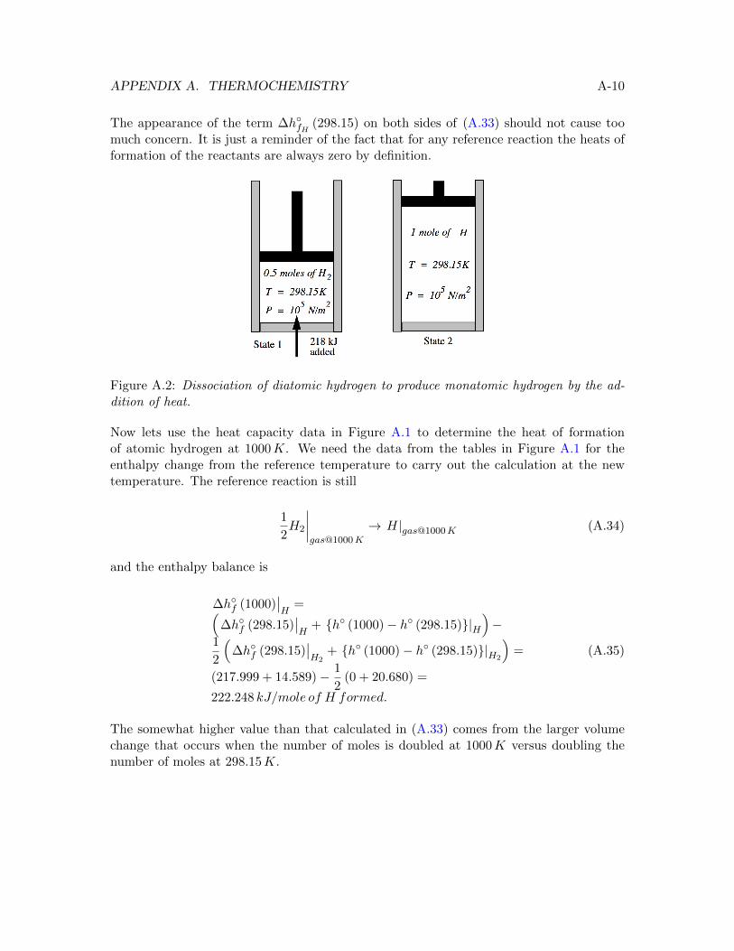
APPENDIX A. THERMOCHEMISTRY A-10
The appearance of the term ∆h◦fH (298.15) on both sides of (A.33) should not cause toomuch concern. It is just a reminder of the fact that for any reference reaction the heats offormation of the reactants are always zero by definition.
Figure A.2: Dissociation of diatomic hydrogen to produce monatomic hydrogen by the ad-dition of heat.
Now lets use the heat capacity data in Figure A.1 to determine the heat of formationof atomic hydrogen at 1000K. We need the data from the tables in Figure A.1 for theenthalpy change from the reference temperature to carry out the calculation at the newtemperature. The reference reaction is still
1
2H2
∣∣∣∣gas@1000K
→ H|gas@1000K (A.34)
and the enthalpy balance is
∆h◦f (1000)∣∣H
=(∆h◦f (298.15)
∣∣H
+ {h◦ (1000)− h◦ (298.15)}|H)−
1
2
(∆h◦f (298.15)
∣∣H2
+ {h◦ (1000)− h◦ (298.15)}|H2
)=
(217.999 + 14.589)− 1
2(0 + 20.680) =
222.248 kJ/mole of H formed.
(A.35)
The somewhat higher value than that calculated in (A.33) comes from the larger volumechange that occurs when the number of moles is doubled at 1000K versus doubling thenumber of moles at 298.15K.

APPENDIX A. THERMOCHEMISTRY A-11
A.4.2 Example - heat of formation of gaseous and liquid water
In this case the reference reaction is
H2 +1
2O2 → H2O|gas. (A.36)
Using the data for gaseous water in Appendix B, the enthalpy balance is
∆h◦f (298.15)∣∣H2O
=
∆h◦f (298.15)∣∣H2O−(
1
2∆h◦f (298.15)
∣∣O2in its reference state
+ ∆h◦f (298.15)∣∣H2 in its reference state
)=
−241.826− 1
2(0)− (0) =
−241.826 kJ/moles of H2O formed.
(A.37)
Figure A.3 below depicts one possible experiment that would be used to measure this heatof formation.
Figure A.3: Reference reaction for (gaseous) water.
Half a mole of diatomic oxygen and one mole of diatomic hydrogen are placed in an adi-abatic piston-cylinder combination. The two will not react spontaneously and so a smallsource of ignition is needed to exceed the threshold energy to start the reaction. Oncethe reaction proceeds, the chemical energy contained in the chemical bonds of the reac-tants is released and a mixture of gases at a temperature of 3078K results. The piston iswithdrawn to keep the pressure constant during the reaction. The mixture contains atoms
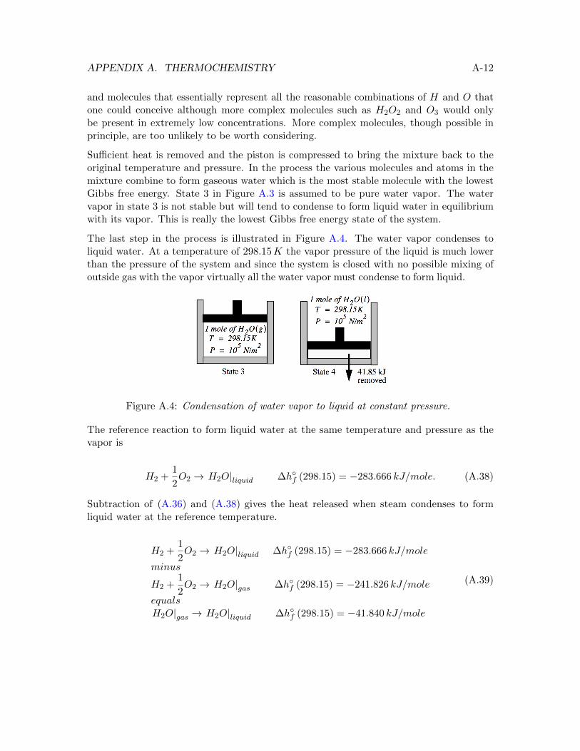
APPENDIX A. THERMOCHEMISTRY A-12
and molecules that essentially represent all the reasonable combinations of H and O thatone could conceive although more complex molecules such as H2O2 and O3 would onlybe present in extremely low concentrations. More complex molecules, though possible inprinciple, are too unlikely to be worth considering.
Sufficient heat is removed and the piston is compressed to bring the mixture back to theoriginal temperature and pressure. In the process the various molecules and atoms in themixture combine to form gaseous water which is the most stable molecule with the lowestGibbs free energy. State 3 in Figure A.3 is assumed to be pure water vapor. The watervapor in state 3 is not stable but will tend to condense to form liquid water in equilibriumwith its vapor. This is really the lowest Gibbs free energy state of the system.
The last step in the process is illustrated in Figure A.4. The water vapor condenses toliquid water. At a temperature of 298.15K the vapor pressure of the liquid is much lowerthan the pressure of the system and since the system is closed with no possible mixing ofoutside gas with the vapor virtually all the water vapor must condense to form liquid.
Figure A.4: Condensation of water vapor to liquid at constant pressure.
The reference reaction to form liquid water at the same temperature and pressure as thevapor is
H2 +1
2O2 → H2O|liquid ∆h◦f (298.15) = −283.666 kJ/mole. (A.38)
Subtraction of (A.36) and (A.38) gives the heat released when steam condenses to formliquid water at the reference temperature.
H2 +1
2O2 → H2O|liquid ∆h◦f (298.15) = −283.666 kJ/mole
minus
H2 +1
2O2 → H2O|gas ∆h◦f (298.15) = −241.826 kJ/mole
equalsH2O|gas → H2O|liquid ∆h◦f (298.15) = −41.840 kJ/mole
(A.39)
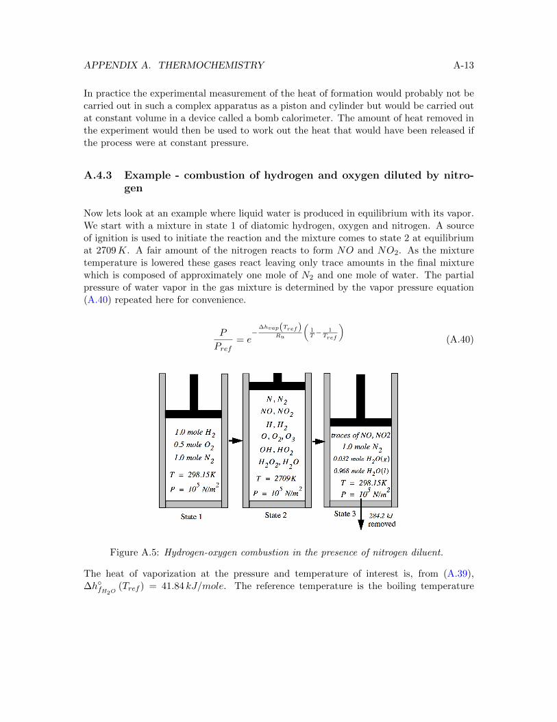
APPENDIX A. THERMOCHEMISTRY A-13
In practice the experimental measurement of the heat of formation would probably not becarried out in such a complex apparatus as a piston and cylinder but would be carried outat constant volume in a device called a bomb calorimeter. The amount of heat removed inthe experiment would then be used to work out the heat that would have been released ifthe process were at constant pressure.
A.4.3 Example - combustion of hydrogen and oxygen diluted by nitro-gen
Now lets look at an example where liquid water is produced in equilibrium with its vapor.We start with a mixture in state 1 of diatomic hydrogen, oxygen and nitrogen. A sourceof ignition is used to initiate the reaction and the mixture comes to state 2 at equilibriumat 2709K. A fair amount of the nitrogen reacts to form NO and NO2. As the mixturetemperature is lowered these gases react leaving only trace amounts in the final mixturewhich is composed of approximately one mole of N2 and one mole of water. The partialpressure of water vapor in the gas mixture is determined by the vapor pressure equation(A.40) repeated here for convenience.
P
Pref= e−
∆hvap(Tref)Ru
(1T− 1Tref
)(A.40)
Figure A.5: Hydrogen-oxygen combustion in the presence of nitrogen diluent.
The heat of vaporization at the pressure and temperature of interest is, from (A.39),∆h◦fH2O
(Tref ) = 41.84 kJ/mole. The reference temperature is the boiling temperature
APPENDIX A. THERMOCHEMISTRY A-14
Tref = 373.15K at the reference pressure of one atmosphere, P ◦ = 1.0132 × 10⁵ Pa. Thesimplified solution of the Clausius-Clapeyron, Equation (A.40) gives the vapor pressureas
P
1.0132× 105 = e−41.840×10³
8.314510 ( 1298.15
− 1373.15) = 0.03363 (A.41)
corresponding to nH2O|gas = 0.035moles which is reasonably close to the more precisevalue of 0.032moles shown in Figure A.5 derived from the tables.
A.4.4 Example - combustion of methane
The heats of formation of various species can be used to evaluate the enthalpy releasedor absorbed during a reaction involving those species. From the data in Appendix B, thereference reactions to produce carbon dioxide and methane are
C|solid +O2 → CO2 ∆h◦f (298.15) = −393.510 kJ/mole (A.42)
and
C|solid + 2H2 → CH4 ∆h◦f (298.15) = −74.600 kJ/mole (A.43)
This data together with (A.36) and (A.38) can be used to evaluate the heat released by thecombustion of methane with oxygen to form carbon dioxide and liquid water at 298.15K.The reaction is
CH4 + 2O2 → CO2 + 2H2O|liquid (A.44)
APPENDIX A. THERMOCHEMISTRY A-15
To produce (A.44) the algebra for the various reactions can be viewed as
C|solid +O2 → CO2
plus
2×(H2 +
1
2O2 → H2O|liquid
)minusC|solid + 2H2 → CH4
minus2× (O2 → O2)equalsCH4 + 2O2 → CO2 + H2O|liquid
(A.45)
and the algebra for the heats of formation is
∆h◦ (298.15)|reaction =(∆h◦f (298.15)
∣∣CO2
+ 2×∆h◦f (298.15)∣∣H2O|liquid
)−(
∆h◦f (298.15)∣∣CH4
+ 2×∆h◦f (298.15)∣∣O2
)=
−393.510 + 2 (−283.666)− (−74.600)− 2 (0) =−886.242 kJ/mole of CH4 burned.
(A.46)
In general the reactants can be at different temperatures. Note that the reaction (A.45)is somewhat artificial in that, at equilibrium, there would actually be a small amount ofwater vapor mixed with the carbon dioxide and in equilibrium with the liquid water.
The general enthalpy balance for a reaction at standard pressure is
∆h◦ (Tfinal) =
(I∑i=1
nih◦i (Tfinal)
)products
−
J∑j=1
njh◦j (Tj)
reactants
(A.47)
where it is recognized that the products are mixed at the final temperature of the reaction.Equation (A.47) fully written out is
∆h◦ (Tfinal) =I∑i=1
ni(∆h◦fi (298.15) + {h◦i (Tfinal)− h◦i (298.15)}
)−
J∑j=1
nj
(∆h◦fj (298.15) +
{h◦j (Tj)− h◦j (298.15)
}).
(A.48)
APPENDIX A. THERMOCHEMISTRY A-16
For example, suppose in the methane-oxygen combustion problem above, the methane isinitially at 600K and the oxygen is at 800K while the products are assumed to be at1500K. The heat of reaction is determined from
∆h◦ (1500) =(∆h◦fCO2
(298.15) +{h◦CO2
(1500)− h◦CO2(298.15)
})+
2(
∆h◦fH2O|gas(298.15) +
{h◦H2O|gas
(1500)− h◦H2O|gas(298.15)
})−(
∆h◦fCH4(298.15) +
{h◦CH4
(600)− h◦CH4(298.15)
})−
2(
∆h◦fO2(298.15) +
{h◦O2
(800)− h◦O2(298.15)
}).
(A.49)
The data is
∆h◦ (1500) =(−393.510 + 61.705) + 2 (−241.826 + 48.151)−(−74.600 + 13.130)− 2 (0 + 15.835) =−689.355 kJ/mole of CH4 burned.
(A.50)
Somewhat less enthalpy is evolved compared to the enthalpy change at the reference tem-perature.
A.4.5 Example - the heating value of JP-4
In Chapter 2 a typical value of the fuel enthalpy for JP-4 jet fuel was given as
hf |JP−4 @ 298.15K = 4.28× 10⁷ J/kg (A.51)
although we never stated explicitly that this refers to the fuel and its products of combustionat a temperature of 298.15K. Where does this number come from and how does it relateto the heat of formation of JP-4? According to CEA the effective molecular formula andheat of formation of JP-4 are
CH1.94 ∆h◦f (298.15) = −22.723 kJ/mole. (A.52)
The reaction of this fuel with oxygen is
CH1.94 + 1.485O2 → CO2 + 0.97H2O (A.53)
APPENDIX A. THERMOCHEMISTRY A-17
and the enthalpy released by the reaction is
∆h◦ (298.15) =(∆h◦f (298.15)
∣∣CO2
+ 0.97×∆h◦f (298.15)∣∣H2O|gas
)−(
∆h◦f (298.15)∣∣CH1.94
+ 1.485×∆h◦f (298.15)∣∣O2
)=
−393.510 + 0.97 (−241.826)− (−22.723)− 1.485 (0) =−605.358 kJ/mole of CH1.94 burned.
(A.54)
On a per mass basis the heating value is
hf |JP−4 @ 298.15K =−605.358 kJ/mole
13.9664× 10⁻³ kg/mole= −4.33× 10⁷ J/kg (A.55)
which agrees closely with the accepted value (A.51). Notice the relatively small contributionof the actual enthalpy of formation of JP-4 to the calculation of the heat of reaction (A.54).Note also that the water formed in the reaction is taken to be in the gas phase and thevalues given in (A.51) and (A.55) are what would be called the lower heating value of JP-4.If the water is assumed to condense to its liquid phase in equilibrium with its vapor at298.15K (see Figure A.5) , which of course it does, the enthalpy change is
hf |JP−[email protected] =−605.358− 0.97× 0.968× 41.85
13.9664× 10−3 =
−644.653kJ/mole
13.9664× 10⁻³kg/mole= −4.62× 10⁷J/kg
(A.56)
which would be called the higher heating value.
A.5 Heat capacity
The key piece of data needed for any species is its heat capacity. One of the most completecollections of such data can be found in the well known reference NASA/TP - 2002-211556 -NASA Glenn Coefficients for Calculating Thermodynamic Properties of Individual Speciesby Bonnie J. McBride, Michael J. Zehe, and Sanford Gordon, Glenn Research Center,Cleveland, Ohio. These authors provide accurate curve fits for the standard heat capacities,enthalpies and entropies of a vast range of species over the temperature range 200K to6000K.
APPENDIX A. THERMOCHEMISTRY A-18
The enthalpy change terms in (A.35) are
h◦H (1000)− h◦H (298.15) =
∫ 1000
298.15C◦PH (T ) dT
h◦H2(1000)− h◦H2
(298.15) =
∫ 1000
298.15C◦PH2
(T ) dT.
(A.57)
The molar heat gas capacities of both monatomic hydrogen and gaseous diatomic hydrogenare consistent with the classic formula from kinetic theory
CP =
(β + 2
2
)Ru (A.58)
where β is the number of degrees of freedom of the gas molecular model. Atomic hydrogenis a gas at all temperatures with three translational degrees of freedom, β = 3 and one canexpect that
C◦PH =5
2Ru = 20.786J/ (mole−K) (A.59)
over a wide temperature range. That this is the case is clear from the right-hand table inFigure A.1. In fact, by convention, this value of the heat capacity of monatomic hydrogen isassumed valid up to 6000K which is the temperature at which the tables stop. Somewhatbelow this temperature the actual heat capacity of a gas of hydrogen atoms would begin toincrease slightly as electronic degrees of freedom begin to be excited. The enthalpy changefor monatomic hydrogen is
h◦H (T )− h◦H (298.15) =5
2Ru (T − 298.15) (A.60)
which reproduces the tabulated data very well.
The number of degrees of freedom for diatomic hydrogen at room temperature is nominallyβ = 5 with three translational degrees of freedom and two rotational degrees. Kinetictheory (A.58) predicts
C◦PH2=
7
2Ru = 29.101J/ (mole−K) . (A.61)
Actually the tabulated heat capacity is slightly less than this since the rotational degreesare not absolutely fully excited at room temperature.
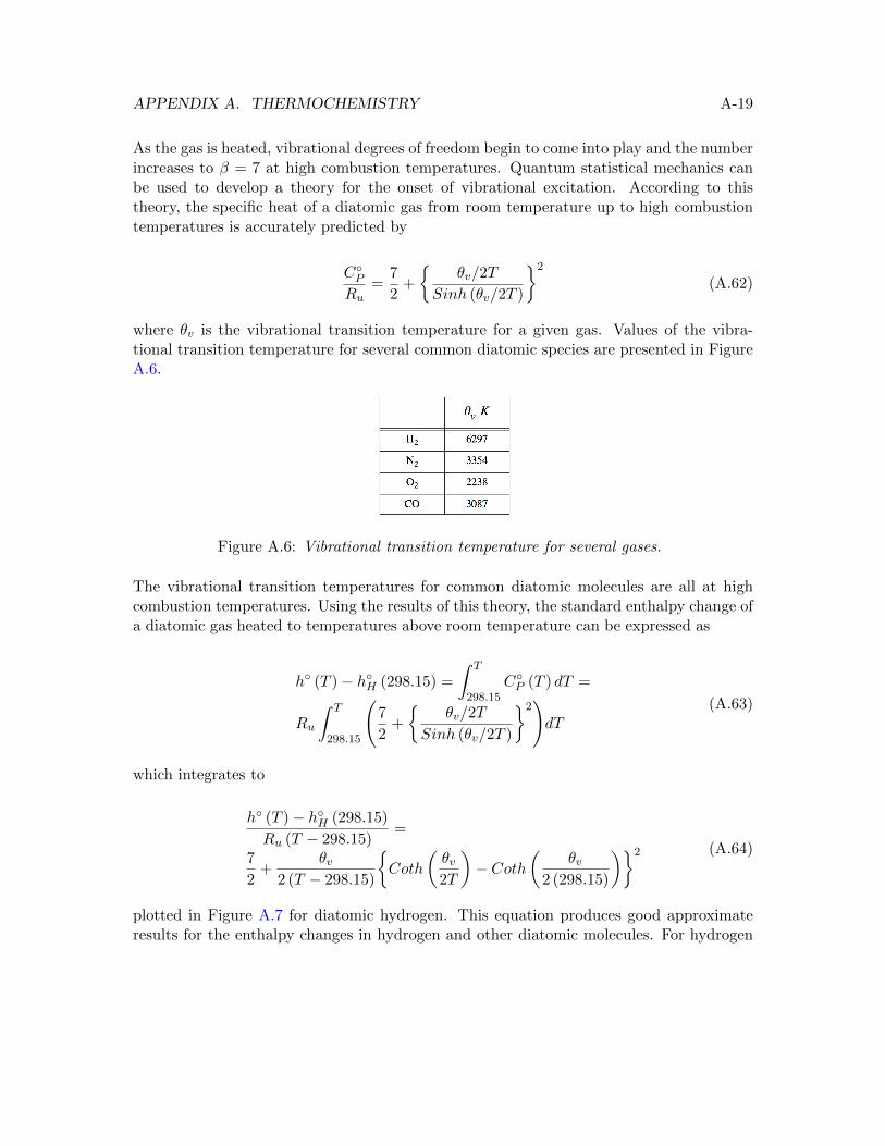
APPENDIX A. THERMOCHEMISTRY A-19
As the gas is heated, vibrational degrees of freedom begin to come into play and the numberincreases to β = 7 at high combustion temperatures. Quantum statistical mechanics canbe used to develop a theory for the onset of vibrational excitation. According to thistheory, the specific heat of a diatomic gas from room temperature up to high combustiontemperatures is accurately predicted by
C◦PRu
=7
2+
{θv/2T
Sinh (θv/2T )
}2
(A.62)
where θv is the vibrational transition temperature for a given gas. Values of the vibra-tional transition temperature for several common diatomic species are presented in FigureA.6.
Figure A.6: Vibrational transition temperature for several gases.
The vibrational transition temperatures for common diatomic molecules are all at highcombustion temperatures. Using the results of this theory, the standard enthalpy change ofa diatomic gas heated to temperatures above room temperature can be expressed as
h◦ (T )− h◦H (298.15) =
∫ T
298.15C◦P (T ) dT =
Ru
∫ T
298.15
(7
2+
{θv/2T
Sinh (θv/2T )
}2)dT
(A.63)
which integrates to
h◦ (T )− h◦H (298.15)
Ru (T − 298.15)=
7
2+
θv2 (T − 298.15)
{Coth
(θv2T
)− Coth
(θv
2 (298.15)
)}2 (A.64)
plotted in Figure A.7 for diatomic hydrogen. This equation produces good approximateresults for the enthalpy changes in hydrogen and other diatomic molecules. For hydrogen
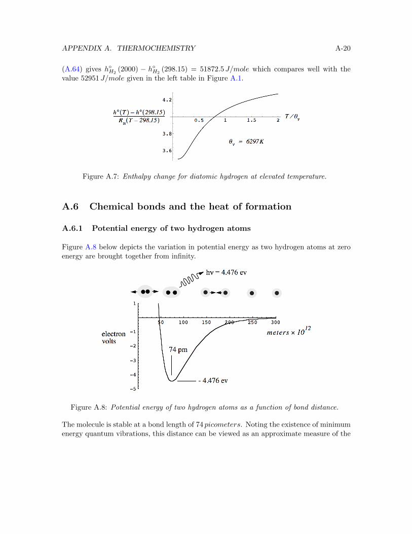
APPENDIX A. THERMOCHEMISTRY A-20
(A.64) gives h◦H2(2000) − h◦H2
(298.15) = 51872.5 J/mole which compares well with thevalue 52951 J/mole given in the left table in Figure A.1.
Figure A.7: Enthalpy change for diatomic hydrogen at elevated temperature.
A.6 Chemical bonds and the heat of formation
A.6.1 Potential energy of two hydrogen atoms
Figure A.8 below depicts the variation in potential energy as two hydrogen atoms at zeroenergy are brought together from infinity.
Figure A.8: Potential energy of two hydrogen atoms as a function of bond distance.
The molecule is stable at a bond length of 74 picometers. Noting the existence of minimumenergy quantum vibrations, this distance can be viewed as an approximate measure of the
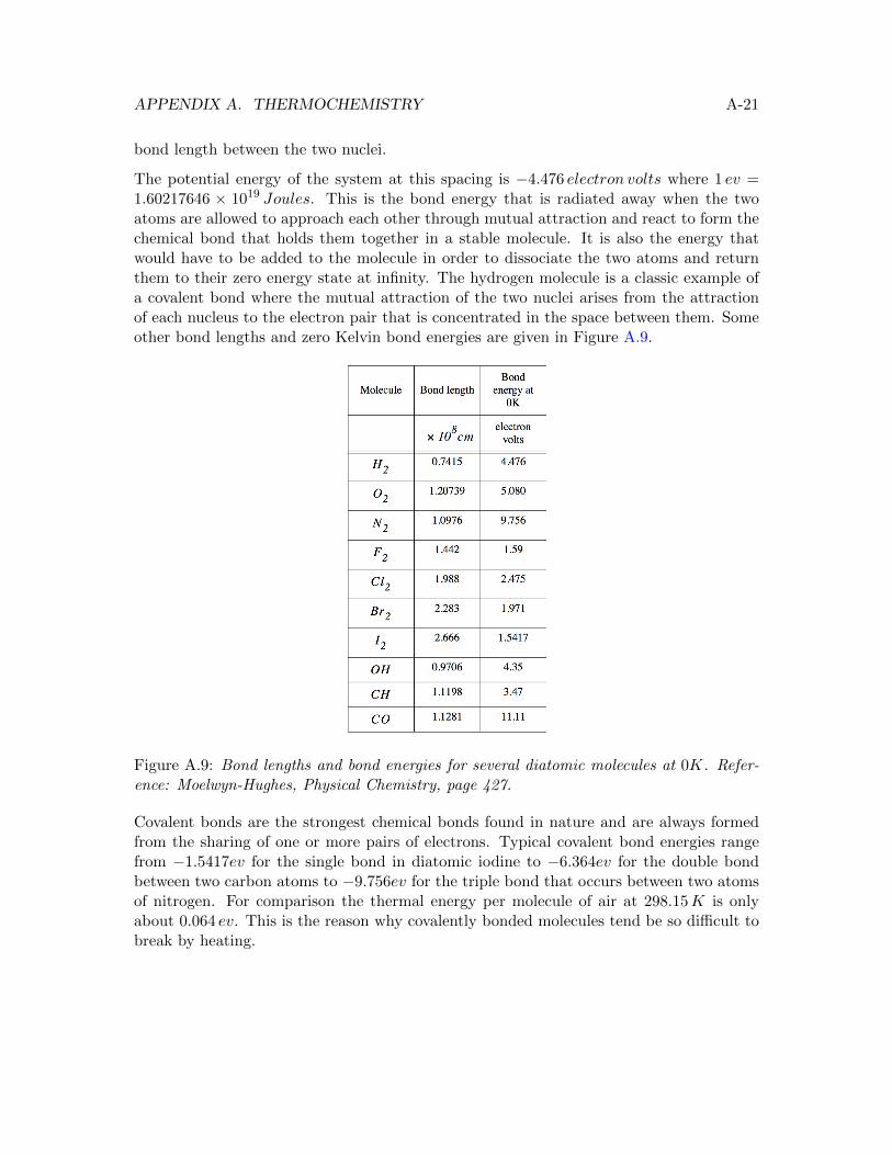
APPENDIX A. THERMOCHEMISTRY A-21
bond length between the two nuclei.
The potential energy of the system at this spacing is −4.476 electron volts where 1 ev =1.60217646 × 10¹⁹ Joules. This is the bond energy that is radiated away when the twoatoms are allowed to approach each other through mutual attraction and react to form thechemical bond that holds them together in a stable molecule. It is also the energy thatwould have to be added to the molecule in order to dissociate the two atoms and returnthem to their zero energy state at infinity. The hydrogen molecule is a classic example ofa covalent bond where the mutual attraction of the two nuclei arises from the attractionof each nucleus to the electron pair that is concentrated in the space between them. Someother bond lengths and zero Kelvin bond energies are given in Figure A.9.
Figure A.9: Bond lengths and bond energies for several diatomic molecules at 0K. Refer-ence: Moelwyn-Hughes, Physical Chemistry, page 427.
Covalent bonds are the strongest chemical bonds found in nature and are always formedfrom the sharing of one or more pairs of electrons. Typical covalent bond energies rangefrom −1.5417ev for the single bond in diatomic iodine to −6.364ev for the double bondbetween two carbon atoms to −9.756ev for the triple bond that occurs between two atomsof nitrogen. For comparison the thermal energy per molecule of air at 298.15K is onlyabout 0.064 ev. This is the reason why covalently bonded molecules tend be so difficult tobreak by heating.
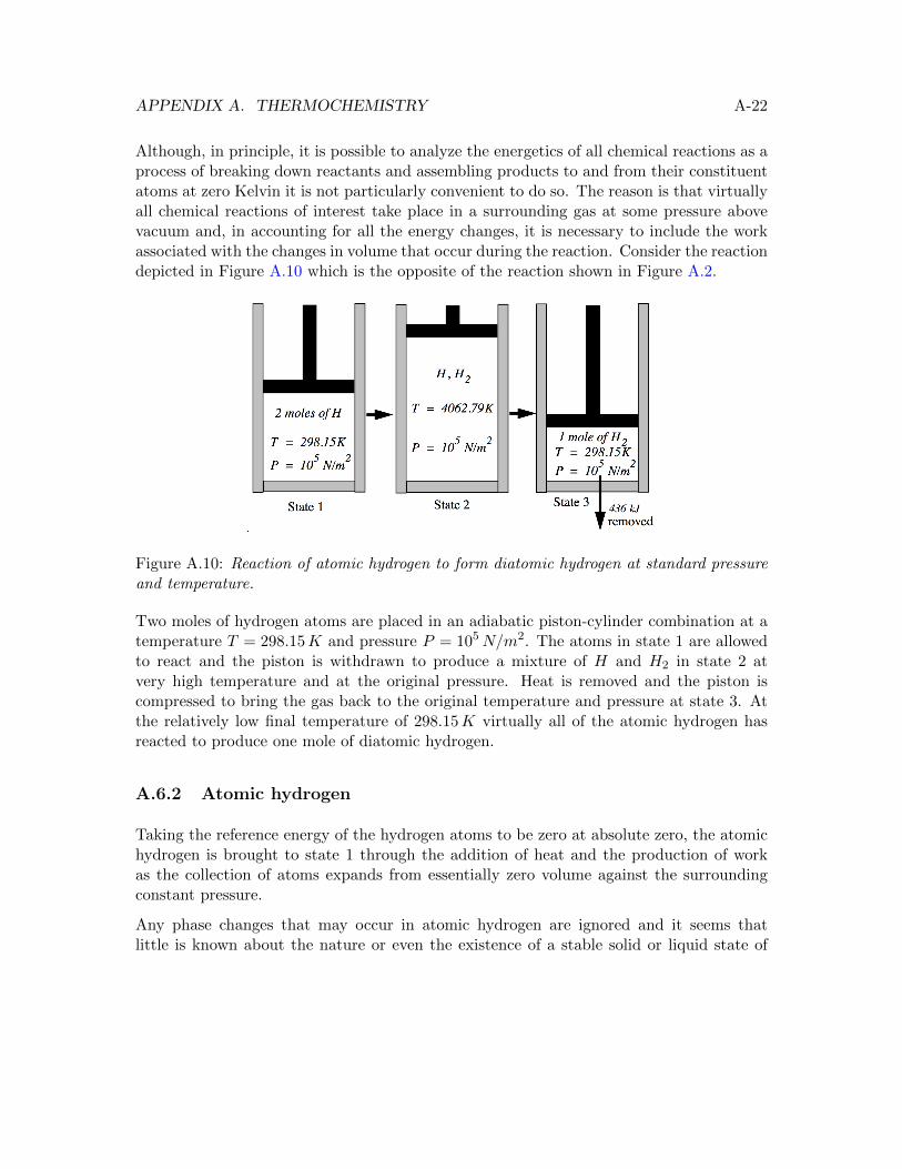
APPENDIX A. THERMOCHEMISTRY A-22
Although, in principle, it is possible to analyze the energetics of all chemical reactions as aprocess of breaking down reactants and assembling products to and from their constituentatoms at zero Kelvin it is not particularly convenient to do so. The reason is that virtuallyall chemical reactions of interest take place in a surrounding gas at some pressure abovevacuum and, in accounting for all the energy changes, it is necessary to include the workassociated with the changes in volume that occur during the reaction. Consider the reactiondepicted in Figure A.10 which is the opposite of the reaction shown in Figure A.2.
Figure A.10: Reaction of atomic hydrogen to form diatomic hydrogen at standard pressureand temperature.
Two moles of hydrogen atoms are placed in an adiabatic piston-cylinder combination at atemperature T = 298.15K and pressure P = 105N/m2. The atoms in state 1 are allowedto react and the piston is withdrawn to produce a mixture of H and H2 in state 2 atvery high temperature and at the original pressure. Heat is removed and the piston iscompressed to bring the gas back to the original temperature and pressure at state 3. Atthe relatively low final temperature of 298.15K virtually all of the atomic hydrogen hasreacted to produce one mole of diatomic hydrogen.
A.6.2 Atomic hydrogen
Taking the reference energy of the hydrogen atoms to be zero at absolute zero, the atomichydrogen is brought to state 1 through the addition of heat and the production of workas the collection of atoms expands from essentially zero volume against the surroundingconstant pressure.
Any phase changes that may occur in atomic hydrogen are ignored and it seems thatlittle is known about the nature or even the existence of a stable solid or liquid state of
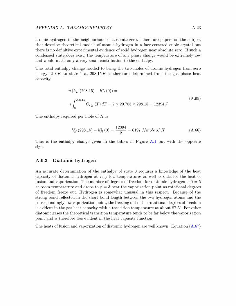
APPENDIX A. THERMOCHEMISTRY A-23
atomic hydrogen in the neighborhood of absolute zero. There are papers on the subjectthat describe theoretical models of atomic hydrogen in a face-centered cubic crystal butthere is no definitive experimental evidence of solid hydrogen near absolute zero. If such acondensed state does exist, the temperature of any phase change would be extremely lowand would make only a very small contribution to the enthalpy.
The total enthalpy change needed to bring the two moles of atomic hydrogen from zeroenergy at 0K to state 1 at 298.15K is therefore determined from the gas phase heatcapacity.
n (h◦H (298.15)− h◦H (0)) =
n
∫ 298.15
0CPH (T ) dT = 2× 20.785× 298.15 = 12394J
(A.65)
The enthalpy required per mole of H is
h◦H (298.15)− h◦H (0) =12394
2= 6197 J/mole of H (A.66)
This is the enthalpy change given in the tables in Figure A.1 but with the oppositesign.
A.6.3 Diatomic hydrogen
An accurate determination of the enthalpy of state 3 requires a knowledge of the heatcapacity of diatomic hydrogen at very low temperatures as well as data for the heat offusion and vaporization. The number of degrees of freedom for diatomic hydrogen is β = 5at room temperature and drops to β = 3 near the vaporization point as rotational degreesof freedom freeze out. Hydrogen is somewhat unusual in this respect. Because of thestrong bond reflected in the short bond length between the two hydrogen atoms and thecorrespondingly low vaporization point, the freezing out of the rotational degrees of freedomis evident in the gas heat capacity with a transition temperature at about 87K. For otherdiatomic gases the theoretical transition temperature tends to be far below the vaporizationpoint and is therefore less evident in the heat capacity function.
The heats of fusion and vaporization of diatomic hydrogen are well known. Equation (A.67)
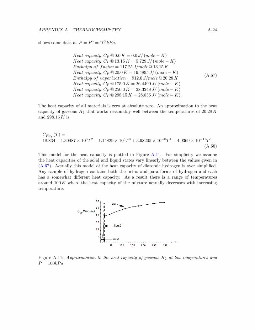
APPENDIX A. THERMOCHEMISTRY A-24
shows some data at P = P ◦ = 102kPa.
Heat capacity, CP @ 0.0K = 0.0 J/ (mole−K)Heat capacity, CP @ 13.15K = 5.729 J/ (mole−K)Enthalpy of fusion = 117.25 J/mole@ 13.15KHeat capacity, CP @ 20.0K = 19.4895 J/ (mole−K)Enthalpy of vaporization = 912.0 J/mole@ 20.28KHeat capacity, CP @ 175.0K = 26.4499 J/ (mole−K)Heat capacity, CP @ 250.0K = 28.3248 J/ (mole−K)Heat capacity, CP @ 298.15K = 28.836 J/ (mole−K) .
(A.67)
The heat capacity of all materials is zero at absolute zero. An approximation to the heatcapacity of gaseous H2 that works reasonably well between the temperatures of 20.28Kand 298.15K is
CPH2(T ) =
18.834 + 1.30487× 10³T 2 − 1.14829× 10⁵T 3 + 3.98205× 10⁻⁸T 4 − 4.9369× 10⁻¹¹T 5.(A.68)
This model for the heat capacity is plotted in Figure A.11. For simplicity we assumethe heat capacities of the solid and liquid states vary linearly between the values given in(A.67). Actually this model of the heat capacity of diatomic hydrogen is over simplified.Any sample of hydrogen contains both the ortho and para forms of hydrogen and eachhas a somewhat different heat capacity. As a result there is a range of temperaturesaround 100K where the heat capacity of the mixture actually decreases with increasingtemperature.
Figure A.11: Approximation to the heat capacity of gaseous H2 at low temperatures andP = 100kPa.
APPENDIX A. THERMOCHEMISTRY A-25
The enthalpy of a species including the absolute zero energy of the chemical bond is
h (T, P ) =
Echemical bond energy/mole (0, P ) +
∫ Tmelting(P )
0CP (T, P ) dT + ∆hfusion (Tmelting (P ) , P ) +
∫ Tvaporization(P )
Tmelting(P )CP (T, P ) dT + ∆hvaporization (Tvaporization (P ) , P ) +
∫ T
Tvaporization(P )CP (T, P ) dT.
(A.69)
The pressure dependence comes primarily from the effect of pressure on the heat of va-porization and to a lesser extent on the heat of fusion as well as the possible pressuredependence of the heat capacities of the condensed phases particularly near phase tran-sition points. The gas phase heat capacity becomes independent of pressure as the gasapproaches ideal gas behavior at increasing temperatures above the vaporization temper-ature.
On a per unit mole basis the chemical bond energy of H2 at zero Kelvin is
Echemical bond energy/mole (0, P ◦) =
−4.476electron volts
molecule× 6.0221415× 10²³molecules
mole× 1.60217646× 10⁻¹⁹ J
electron volts=
−431.87× 10³ J/mole(A.70)
Using the data in (A.67), the enthalpy at T = 298.15K and P = 100 kPa including thechemical bond energy is
h◦H2(298.15, 100) = −431.87× 10³ +
∫ 13.95
0
(5.729
13.95
)TdT + 117.25+
∫ 20.28
13.95
(5.729 +
(19.49− 5.729
20.28− 13.95
)(T − 13.95)
)dT + 912 +
∫ 298.15
20.28C◦P (T ) dT
(A.71)
APPENDIX A. THERMOCHEMISTRY A-26
Use (A.68) to carry out the last integral in (A.71) giving
h◦H2(298.15, 100) = −431.87× 10³ +
(5.729× 13.95
2
)+ 117.25+
(19.49 + 5.729
2
)(20.28− 13.95) + 912 + 7057 = −431.87× 10³ + 8206
(A.72)
The heat released by the reaction to form diatomic hydrogen from its atoms at 298.15Kand 1 atmosphere is
∆h◦ = h◦H2(298.15, 100)− 2h◦H (298.15, 100) =(
−431.87× 10³ + 8206)− 2× 6197.35 =
−436.059× 10³ J/moles of H2 formed
(A.73)
The result (A.73) is the enthalpy released during the reaction of atomic hydrogen to formdiatomic hydrogen at a temperature of 298.15K and pressure 105N/m2. This result canbe found in the right table in Figure A.1 as twice the heat of formation of one mole ofmonatomic hydrogen. We worked this out in equation (A.33).
Note that, because the heat input and work needed to bring two moles of atomic hydrogento the initial temperature of 298.15K is greater that that needed to bring one mole ofdiatomic hydrogen to the same temperature, the reaction releases four more kilo-Joules ofenthalpy than it would if the reaction was carried out at zero Kelvin.
A.7 Heats of formation computed from bond energies
We began this appendix by discussing tabulations of the heats of formation of variousspecies from their elements in their reference state. In this last section we will describehow heats of formation can be determined from bond energies. The enthalpy changesinvolved in chemical reactions come from the breaking and making of chemical bonds todecompose the reactants and then compose the products.
Figure A.12 gives average bond energies for a variety of diatomic molecules.
Consider the reference reaction for water
H2 +1
2O2 → H2O|gas ∆h◦fH2O|gas
(298.15) = −241.826kJ/mole (A.74)
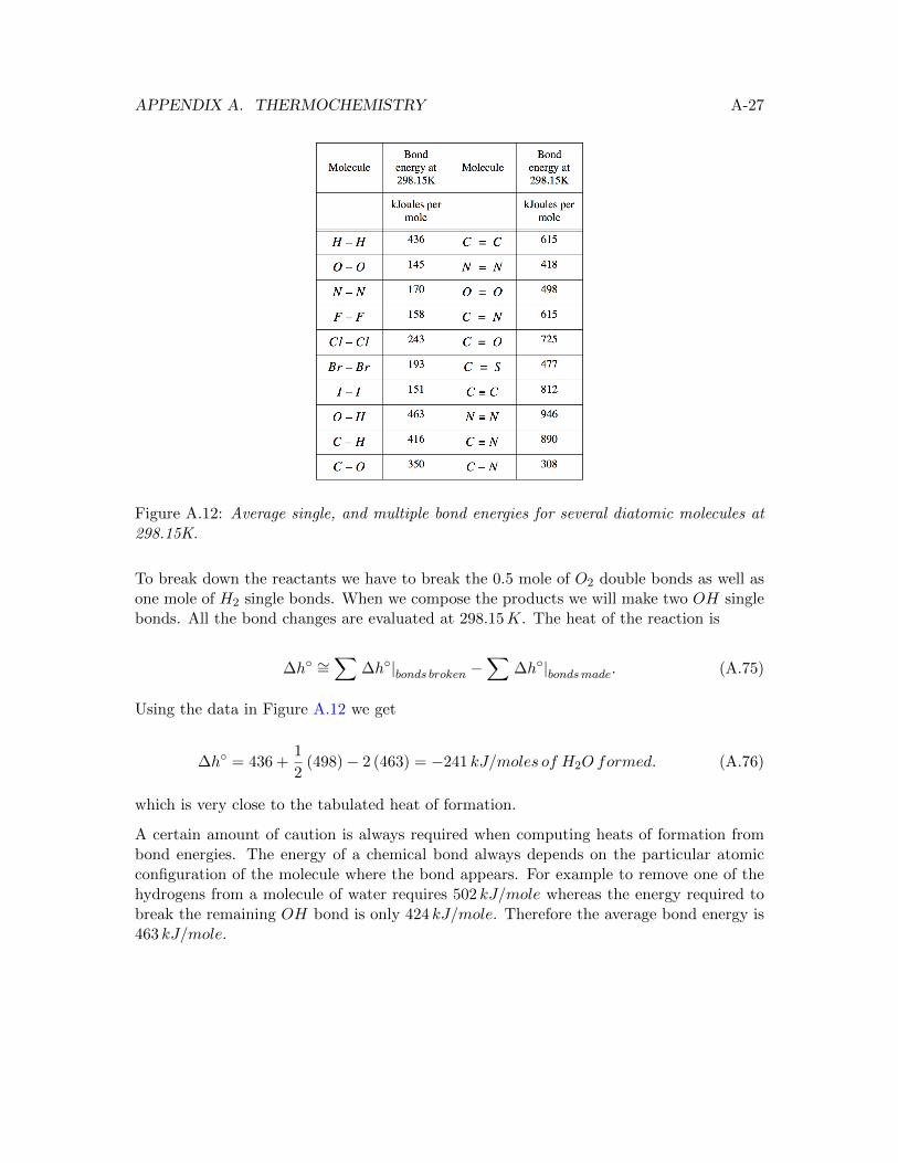
APPENDIX A. THERMOCHEMISTRY A-27
Figure A.12: Average single, and multiple bond energies for several diatomic molecules at298.15K.
To break down the reactants we have to break the 0.5 mole of O2 double bonds as well asone mole of H2 single bonds. When we compose the products we will make two OH singlebonds. All the bond changes are evaluated at 298.15K. The heat of the reaction is
∆h◦ ∼=∑
∆h◦|bonds broken −∑
∆h◦|bondsmade. (A.75)
Using the data in Figure A.12 we get
∆h◦ = 436 +1
2(498)− 2 (463) = −241 kJ/moles of H2O formed. (A.76)
which is very close to the tabulated heat of formation.
A certain amount of caution is always required when computing heats of formation frombond energies. The energy of a chemical bond always depends on the particular atomicconfiguration of the molecule where the bond appears. For example to remove one of thehydrogens from a molecule of water requires 502 kJ/mole whereas the energy required tobreak the remaining OH bond is only 424 kJ/mole. Therefore the average bond energy is463 kJ/mole.
APPENDIX A. THERMOCHEMISTRY A-28
For methane 435 kJ/mole is required to break a single CH whereas it takes 1662 kJ/mole tobreak all four bonds therefore the average bond energy is 416 kJ/mole not 435 kJ/mole.
A.8 References
1) Linus Pauling, General Chemistry, Dover 1970.
2) Irvin Glassman, Combustion, Third Edition, Academic Press 1996.
3) NASA/TP - 2002-211556 - NASA Glenn Coefficients for Calculating Thermo- dynamicProperties of Individual Species by Bonnie J. McBride, Michael J. Zehe, and Sanford Gor-don, Glenn Research Center, Cleveland, Ohio.
In addition to providing curve fits for the heat capacity, enthalpy and entropy for awide range of species, a number of variables are also tabulated in this reference includ-ing ∆h◦f (298.15), h◦ (0) and ∆h◦f (0).

Appendix B
Selected JANAF data
B-1
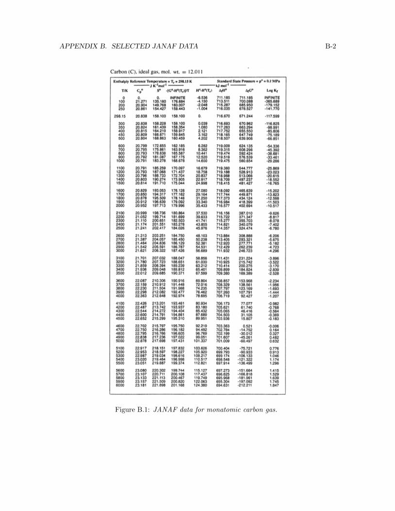
APPENDIX B. SELECTED JANAF DATA B-2
Figure B.1: JANAF data for monatomic carbon gas.
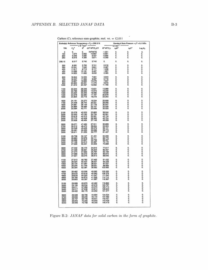
APPENDIX B. SELECTED JANAF DATA B-3
Figure B.2: JANAF data for solid carbon in the form of graphite.
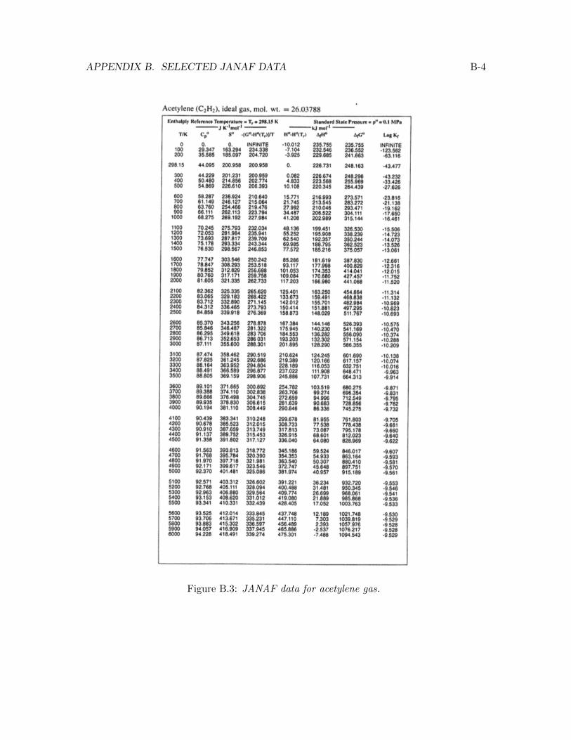
APPENDIX B. SELECTED JANAF DATA B-4
Figure B.3: JANAF data for acetylene gas.
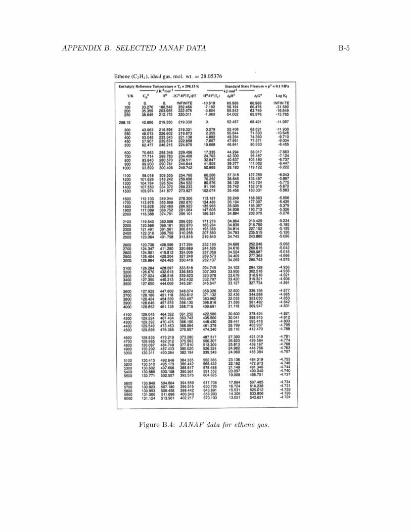
APPENDIX B. SELECTED JANAF DATA B-5
Figure B.4: JANAF data for ethene gas.
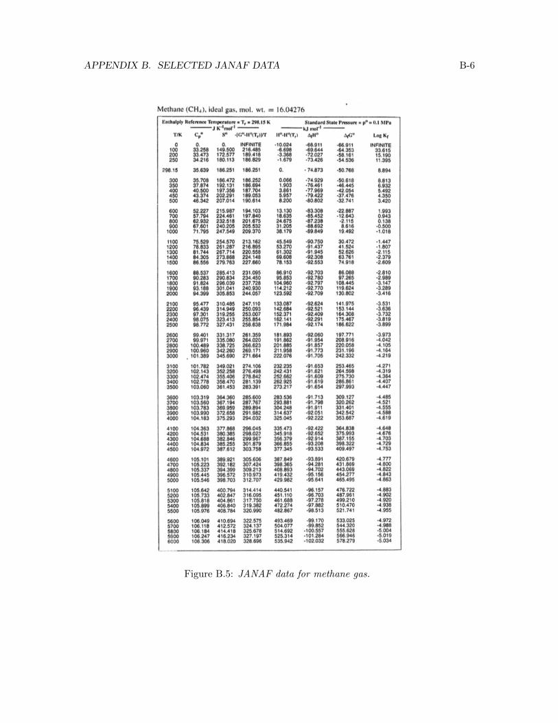
APPENDIX B. SELECTED JANAF DATA B-6
Figure B.5: JANAF data for methane gas.
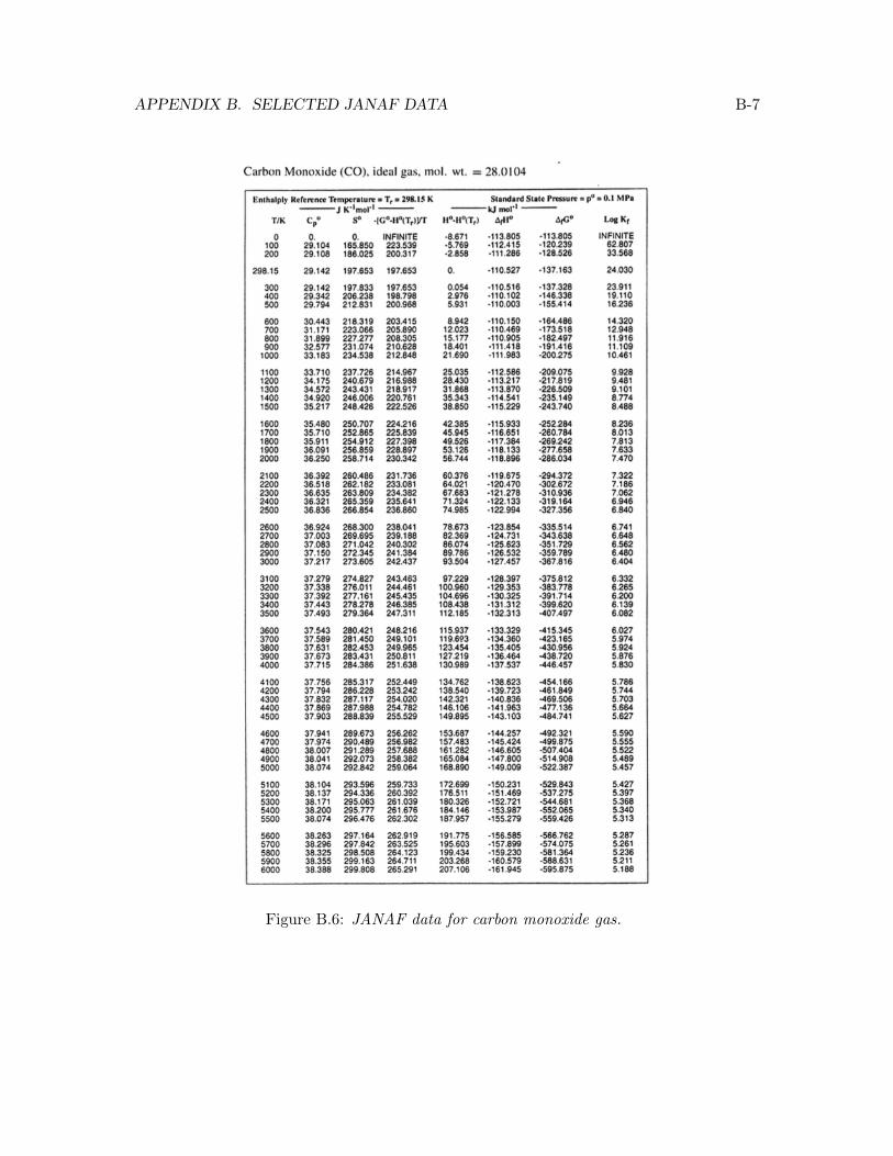
APPENDIX B. SELECTED JANAF DATA B-7
Figure B.6: JANAF data for carbon monoxide gas.

APPENDIX B. SELECTED JANAF DATA B-8
Figure B.7: JANAF data for carbon dioxide gas.
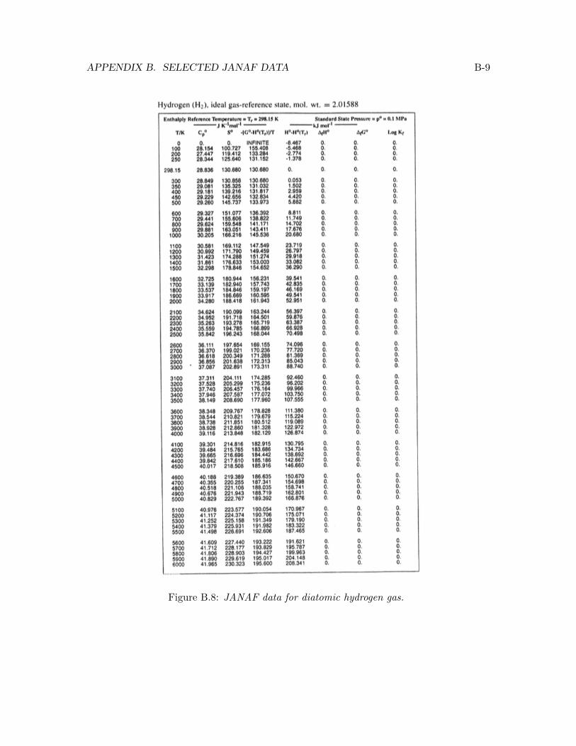
APPENDIX B. SELECTED JANAF DATA B-9
Figure B.8: JANAF data for diatomic hydrogen gas.
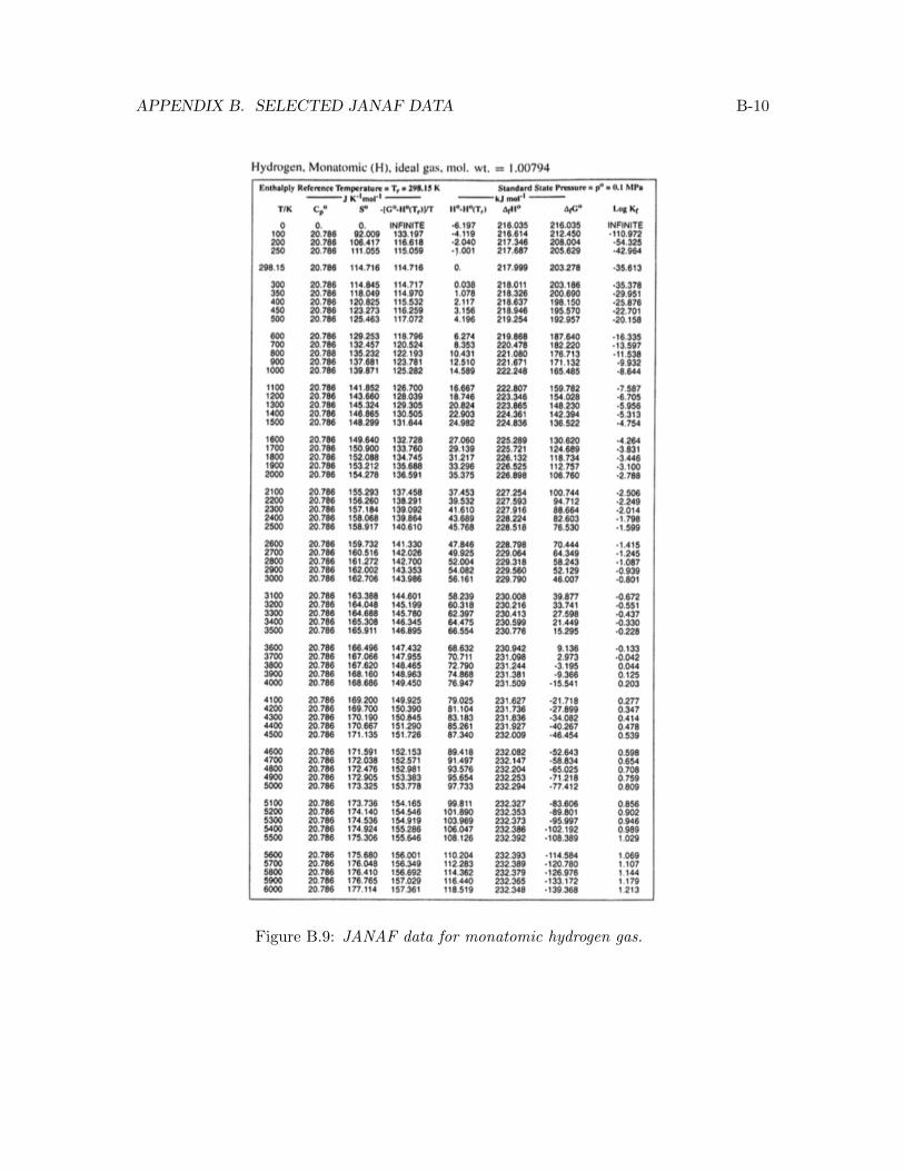
APPENDIX B. SELECTED JANAF DATA B-10
Figure B.9: JANAF data for monatomic hydrogen gas.
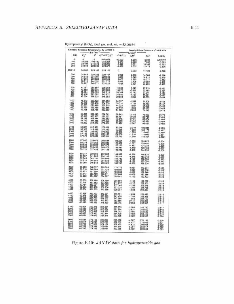
APPENDIX B. SELECTED JANAF DATA B-11
Figure B.10: JANAF data for hydroperoxide gas.
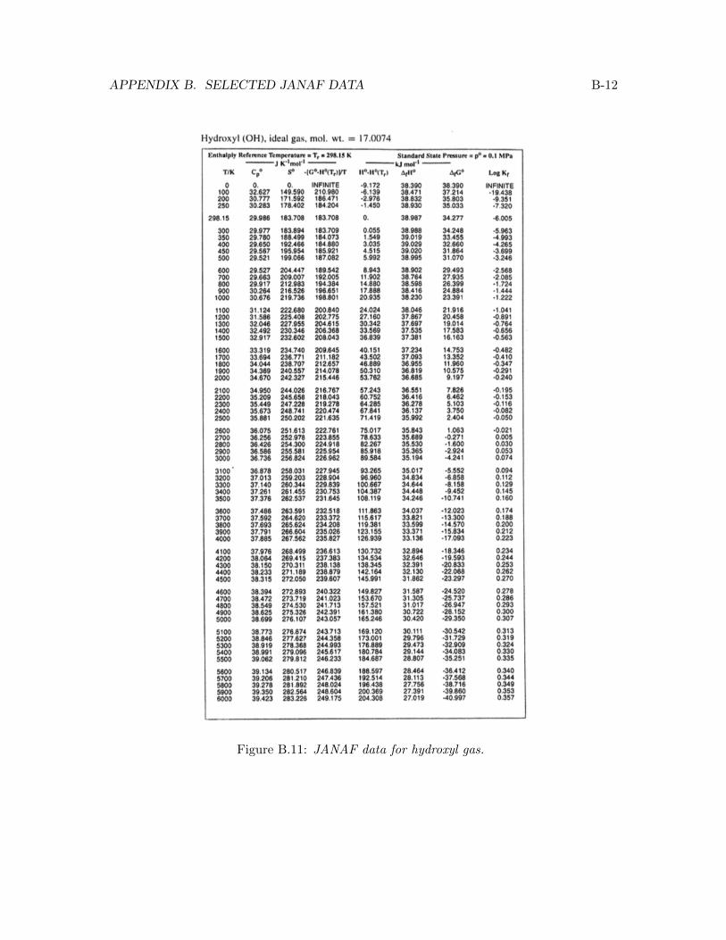
APPENDIX B. SELECTED JANAF DATA B-12
Figure B.11: JANAF data for hydroxyl gas.

APPENDIX B. SELECTED JANAF DATA B-13
Figure B.12: JANAF data for water vapor.
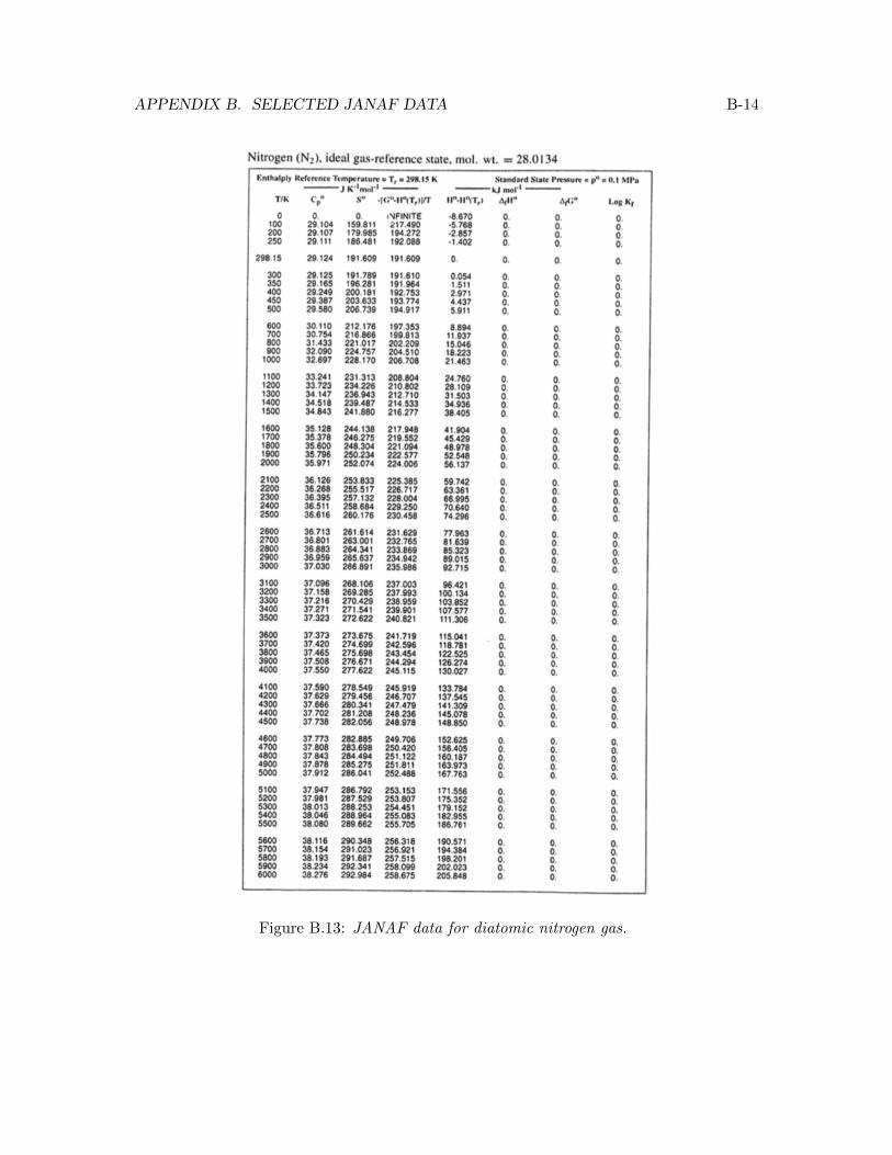
APPENDIX B. SELECTED JANAF DATA B-14
Figure B.13: JANAF data for diatomic nitrogen gas.
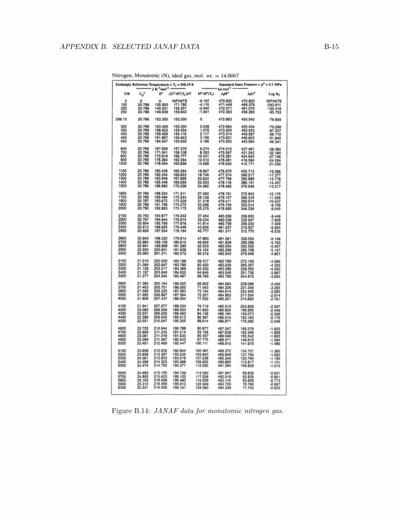
APPENDIX B. SELECTED JANAF DATA B-15
Figure B.14: JANAF data for monatomic nitrogen gas.
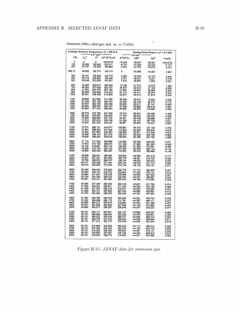
APPENDIX B. SELECTED JANAF DATA B-16
Figure B.15: JANAF data for ammonia gas.
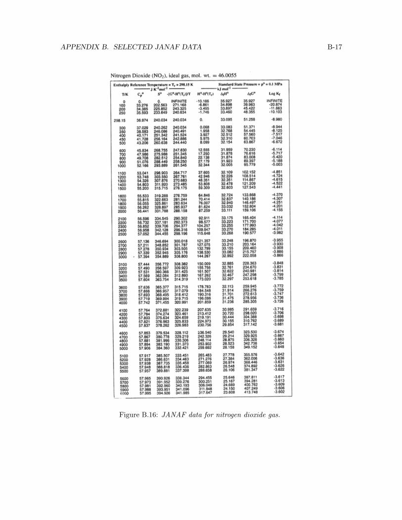
APPENDIX B. SELECTED JANAF DATA B-17
Figure B.16: JANAF data for nitrogen dioxide gas.
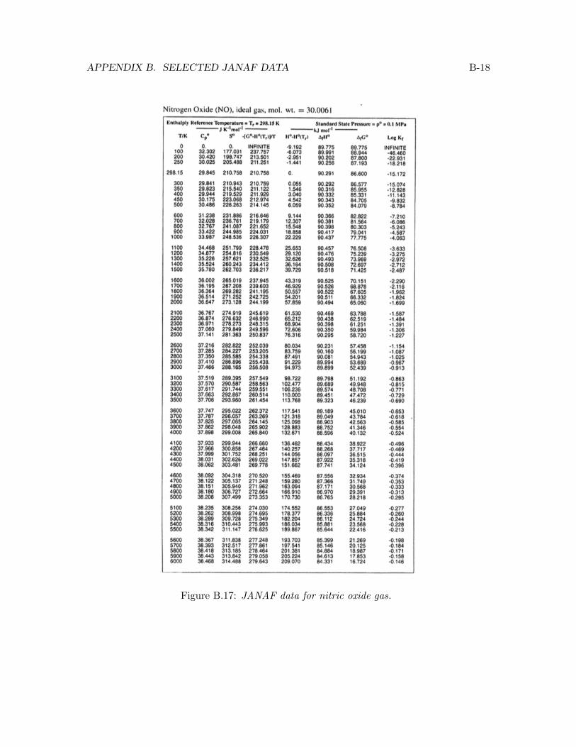
APPENDIX B. SELECTED JANAF DATA B-18
Figure B.17: JANAF data for nitric oxide gas.
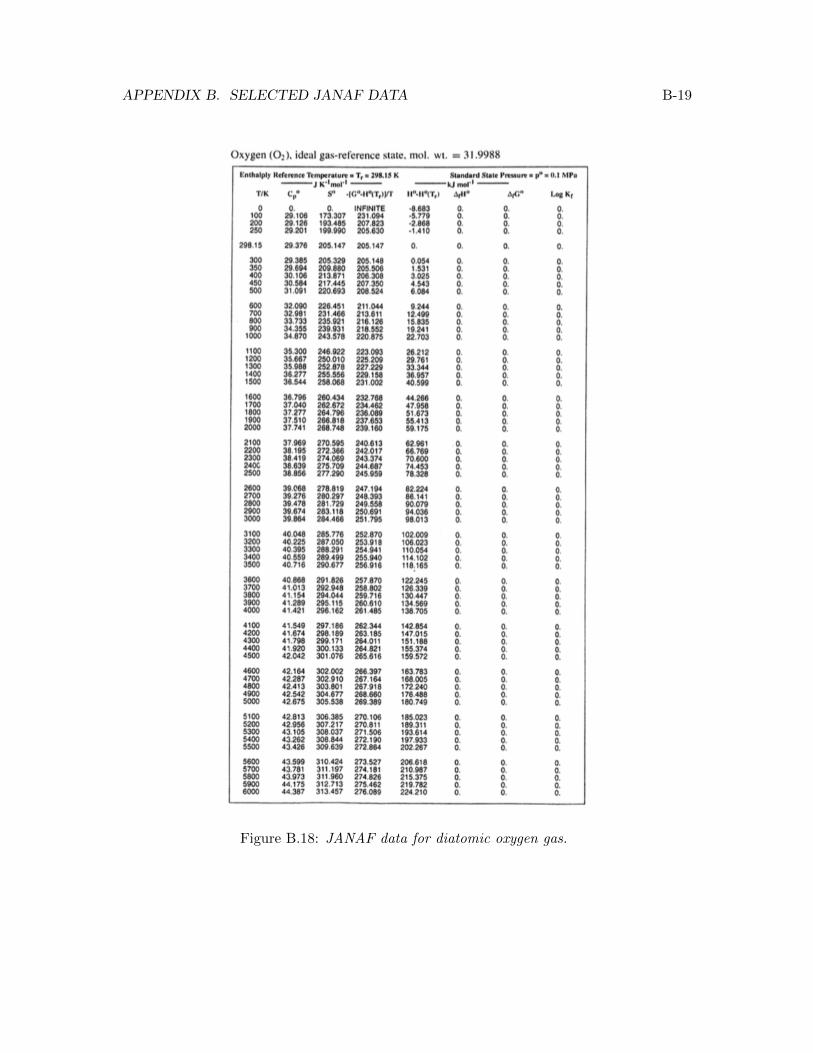
APPENDIX B. SELECTED JANAF DATA B-19
Figure B.18: JANAF data for diatomic oxygen gas.
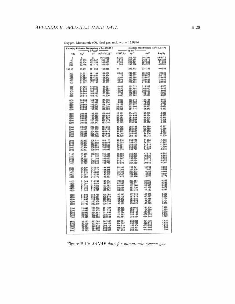
APPENDIX B. SELECTED JANAF DATA B-20
Figure B.19: JANAF data for monatomic oxygen gas.
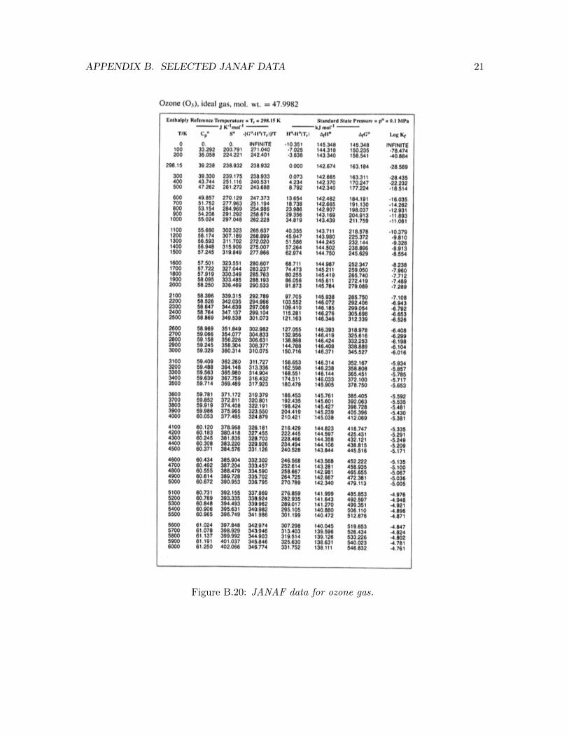
APPENDIX B. SELECTED JANAF DATA 21
Figure B.20: JANAF data for ozone gas.
Related Documents