Airborne radar ground clutter return - CORE

AIRBORNE RADAR GROUND CLUTTERRETURN

by

ROBERT A. iMcMILLEN

B. S., Kansas State University, 1960

A MASTER'S THESIS

submitted in partial fulfillment of the

requirements for the degree

MASTER OF SCIENCE

Department of Electrical Engineering

KANSAS STATE UNIVERSITYManhattan, Kansas

1964

Approved by:

a £ A.laj or /professor /

MIGt.ln/,. ,_ L TABLE OF CONTENTSPact?MM »

">G

INTRODUCTION 1

BASIC RADAR RETURN THEORY 2

The Basic Radar 2

Electromagnetic Wave Scattering From Terrain 3

SIGNAL CORRELATION AND POWER SPECTRUM 6

CLUTTER MODELS AND POWER SPECTRUM CALCULATIONS 9

Random Models 12

Deterministic Models 26

MATHEMATICAL MODEL FOR GROUND CLUTTER POWER SPECTRUMFOR AN AIRBORNE PULSE RADAR 41

Clutter Geometry 41

Calculation of Received Power 46

CALCULATED POWER SPECTRUMS 53

Incremental Areas 53

Scattering Coefficients 54

Antenna Pattern 56

Altitude and Power 57

Power Spectrum 57

Results 58

SUMMARY 63

ACKNOWLEDGMENTS 66

REFERENCES 67

APPENDIX 69

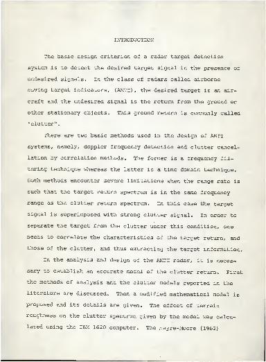
INTRODUCTION

The basic design criterion of a radar target detection

system is to detect the desired target signal in the presence of

undesired signals. In the class of radars called airborne

moving target indicators, (AMTI) , the desired target is an air-

craft and the undesired signal is the return from the ground or

other stationary objects. This ground return is commonly called

"clutter".

There are two basic methods used in the design of AMTI

systems, namely, doppler frequency detection and clutter cancel-

lation by correlation methods. The former is a frequency fil-

tering technique whereas the latter is a time domain technique.

Both methods encounter severe limitations when the range rate is

such that the target return spectrum is in the same frequency

range as the clutter return spectrum. In this case the target

signal is superimposed with strong clutter signal. In order to

separate the target from the clutter under this condition, one

needs to correlate the characteristics of the target return, and

those of the clutter, and thus extracting the target information.

In the analysis and design of the AMTI radar, it is neces-

sary to establish an accurate model of the clutter return. First

the methods of analysis and the clutter models reported in the

literature are discussed. Then a modified mathematical model is

proposed and its details are given. The effect of terrain

roughness on the clutter spectrum given by the model was calcu-

lated using the IBM 1620 computer. The Hayre-Moore (1962)

derivation for the scattering coefficient plays a central role

in this analysis.

BASIC RADAR RETURN THEORY

The Basic Radar

A radar is an electronic device for detection and location

of targets by transmitting an electromagnetic signal and detect-

ing the reflected return signal. An elementary radar consists

of a transmitter to generate the signal, an antenna to radiate

the outgoing signal and collect the incoming signal, and a

receiver to detect and process the return signal.

The range to the target is measured by the time required

for the incident signal to reach the target and the reflected

signal to arrive back at the radar. If there is relative motion

between the radar and the target, the shift in the carrier fre-

quency of the reflected wave (doppler shift) is a measure of

the target's relative velocity. This property distinguishes

moving targets from stationary objects. The distance or range,

R, to the target is

R - Sf (1)

where

gC = 3 X 10 meters/second (velocity of light)

At = time required for the wave to travel out and back.

The received power, P , of the return signal from a point

source is given by the radar equation

Pr " 3 4 < 2 >

where

P. = power transmitted

G = antenna gain

\ = wavelength

'' = radar cross-section

This basic expression is a simplified form and does not adequately

describe the performance of a practical radar because the para-

meters in general are variable functions.

Electromagnetic Wave Scattering From Terrain

(Hayre and Moore, 1962)

Electromagnetic waves are reflected, refracted, and ab-

sorbed by media present in their propagation path, depending on

the properties of the media. Some of the energy of such incident

waves is deflected away from the original direction of propaga-

tion. Energy deflected back toward the source is called back-

scatter and energy deflected away from the source is called

forward scatter.

Surface scattering is the scattering of the incident wave

in various directions by the surface irregularities. A complete

solution for scattering from randomly rough surfaces is not yet

known, although a great many approximations have been attempted.

This type of scattering is of primary concern in this paper since

clutter is the return signal from a rough surface.

Hayre (1962) has developed a model for the radar scattering

cross-section per unit area (01) of a rough surface, based on

statistical parameters of the terrain. Scattering phenomenon

is measured by the radar scattering cross-section per unit area,

where

<r - £L™2

2

3E2

1

(3)

and

E^ = scattered electric field at the receiving antenna

E. = incident plane wave field.

The total radar scattering cross-section is obtained by

integrating (j over the target surface. The average power

received from the target surface is

\2Pr=—

r327T

where

2 IJPT(T--|p)G

2(O,0)(£(e,M -3g dRdtf (4)

p = average power received

T = delay time measured from the start of the transmitted

pulse

= angle in the ground plane from antenna boresight

to the target

Q = angle of incidence measured outward from the surface

normal

.

The radar scattering cross-section is assumed to be independent

of 0. This equation forms the basis of a model used in this

analysis.

The Hayre and Moore (1962) scattering coefficient is based

on statistical parameters determined from contour map data.

Their results were used to calculate scattering coefficients for

comparison with experimental data. It has been shown that the

normalized values of <3~ compare very closely with both experi-

mental values, and the results of acoustical simulation. Their

scattering coefficient is given as

_* 4/2VB2

/ Q \ f „„2_2 2A V\

oo _

E,., 2 __2, n , 2^, n + 1

(4k <T ) (cos Q) ,

5 j

. (n- l)i (2k2B2sin

2+ n

2)

3/2n =1

where

B = characteristic constant determined from the surface

roughness autocovariance function p(r)

C = standard deviation of the target terrain heights

about the mean

k = wavenumber (2tt/\)

p (r) = exp(-|rl/B) normalized space-height autocorrelation

function

r = distance between points on the surface.

For values of 1/B small as compared to k, the above

expression becomes

2

CTo= \f (©cot

49) for G ? 0°

(6)

The scattering coefficient listed in Equation (5) shows the

effect of small scale surface roughness on the radar return.

The increasing value of B/\ indicates increasing horizontal

roughness. The value C/X indicates the relative small scale

vertical terrain heights. (Hayre and Moore, 1962)

SIGNAL CORRELATION AND POWER SPECTRUM

A basic technique used in the detection of signals in the

presence of noise is correlation of the return signal and a

reference signal. If the reference signal is the return signal

delayed in time, then the process is called autocorrelation.

If a signal other than the return signal is used as the reference,

then the process is called cross-correlation. The basic rela-

tionship for the correlation functions and the power spectra are

later derived using random variable theory.

One of the major problems in the analysis and design of

radar systems, is that the signal return has random variations

that must be described statistically. The main features of a

random process, x(t) , are indeterminacy in the expected behavior

of any single record, together with strong statistical properties

of a collection (ensemble) of its records. A random process can

then be defined as an ensemble of time functions | x(t)j

,

_oo<t<co, k = 1,2, ***, such that the ensemble can be characterized

by statistical properties. (Bendat, 1958)

There are two averages associated with a random process,

namely the time average, and the ensemble average. The time

average of a single record over the time interval is given by

^tt> = Ji^^ 1? x(t)dt (7)

The ensemble average is the average of all the records at a

particular time t,, as given by

oo

EpScttj] = j"Kx(t)p(x)dx (8)

1 J _oo

With this introduction to random processes, the relation-

ship between correlation functions and power spectrum is derived

(Lanning and Battin, 1956) . First the autocorrelation function,

(t, t +T), is defined to be

^xx (t'

t +r) = [*<*>*** +r )] ( 9 )

It is desired to show that a relationship exists between the

correlation function and the power spectra for any random

process. We define a quantity ^T (T) to be

fT ir) = •%$ J xT(t)x

T (t +r)dt do)-oo

where x_(t) denotes a truncated time function. Next the quantity

l/^(r) is defined as

y-(r) = Ji"U VTm = Jis»^ ;

T*<t)x<t +r) dt cid

Taking the Fourier Transform of ^(T) , one obtains

oo oo

£j Ifm e"J wr dr= 1^ IJ f(fl e-J^dT (12)

" -oo -oo

oo oo=T^oo 2^T * e

~J dT * x (t)x (t +T)dt (13)

-oo -oo

oo oolimT-*oo 27TT _oo -oo

i=J dt J [x

T(t)eJ WtJ

-OO -oo

[xT(ttr)a-J W (t+t )]dT (14)

8

CO . .. L CO

X ~ «H J. _co * _co

The two integrals in Equation (15) can be recognized as the

Fourier Transform of x_(t) , denoted as AT(w) , and the complex

conjugate A*(w) . Equation (15) can then be rewritten as

£ 1 ^(t) e"J Wrd? = t^oo T= G(W ' X) U6)

-CO

where G(w, x) is defined (Lanning and Battin, 1956) as the power

density spectrum for a given record of x(t) . To obtain the

power density spectrum for the ensemble, G(w,x) must be averaged

over the ensemble as

CO

G (w) = E[G(w,x)] = J J E[^(r)l e-JwT dt (17)

•*"X' —CO

where

Te1>(2-)] =t-co2T^ E[x(t)x(t +T)] dt (18)

From Equation (9) , our definition of the autocorrelation function,

Equation (18) becomes

CO

-COGxx^ = * L e

"JWrdr[T^co^ $ ««(*. t + T)dt]

-i(19)

The last equation holds for any random process. If the process

x(t) is stationary, the equation is simplified. A stationary

process is one in which statistical properties are a function

of T only. Then vv (t, t +2T) can be rewritten as (2*) , and

Equation (19) becomes

co

Gxx<w

> .L ^ 6"3 ""7 (20)

andoo

^xx (r) =^ Gxx (w)cosMdw (21)o

Equations (20) and (21) are known as the Wiener-Khinchin

relations.

A similar derivation for the cross-correlation and cross-

power spectral density for two random processes x(t) and y(t)

yields

xy (t, t +r) = E[x(t)y(t +T)J (22)

oo _. _ _ Pij_ i T

-T

Gxy(w) =

i L e"JWrdrb— 4 * Vt(

'+r)dt

](23)

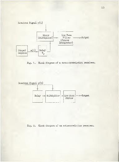
The principles of autocorrelation and cross-correlation are

often used as the basis for radar receiver design. In actual

practice, the time limited autocorrelation function is measured

as

iT

R(r,T) - iJ x(t)x(t +T)dt (24)o

That a finite time must be used is the main reason why differ-

ences exist between theorectical and experimental results (Bendat,

1956) . Figures 1 and 2 show the basic block diagrams for cor-

relation receivers (Skolnik, 1962)

.

CLUTTER MODELS AND POWER SPECTRUM CALCULATIONS

The analysis of airborne moving target indicator radar

effectiveness for detecting targets in the presence of ground

clutter requires a knowledge of the clutter signal. Although

clutter targets such as buildings, bare hills, or mountains

produce echo signals that are constant in both phase and

10

Received Signal y(t)

'

Mixer(Multiplier)

w,

*

StoredReplica

1

DelayTr

Low PassFilter

(FiniteIntegrator)

-Output

Fig. 1 . Block diagram of a cross-correlation receiver.

Received Signal y(t)

\ \

-

Delay -* Mii1t-i~"H ~~ —*- Low PassFilter

r--__--- Output

Fig. 2. Block diagram of an autocorrelation receiver.

11

amplitude as a function of time, there are many types of clutter

that cannot be considered as absolutely stationary. Echoes from

trees, vegetation, sea, and rain fluctuate with time, and these

fluctuations can limit performance of MTI (Skolnik, 1962)

.

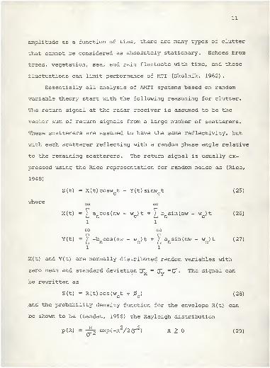
Essentially all analysis of AMTI systems based on random

variable theory start with the following reasoning for clutter.

The return signal at the radar receiver is assumed to be the

vector sum of return signals from a large number of scatterers.

These scatterers are assumed to have the same reflectivity, but

with each scatterer reflecting with a random phase angle relative

to the remaining scatterers. The return signal is usually ex-

pressed using the Rice representation for random noise as (Rice,

1948)

S(t) - X(t)cosw t - Y(t)sinw t (25)

where

X(t) = £ ancos(nw - w )t + Y b

nsin(nw - w )t (26)

1 1

oo oo

Y(t) = ) -b cos(nw - w )t + V a sin(nw - w )t (27)Li n c i—i n c1 1

X(t) and Y(t) are normally distributed random variables with

zero mean and standard deviation CT =0" =(o - The signal canx y

be rewritten as

S(t) = R(t)cos(wct +

Q ) (28)

and the probability density function for the envelope R(t) can

be shown to be (Bendat, 1956) the Rayleigh distribution

p(R) = -§~ exp(-R2/2 6-2) R > (29)

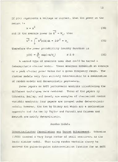
12

If S(t) represents a voltage or current, then the power in the

return is

W = R2

(30)~~2

and if the average power is R = W , then

— oo

R2 = J R2p(R)dR = 2C2 = WQ (31)

o

Therefore the power probablility density function is

p(W) = ~- exp(-W/W ) W > (32)o

A second type of analysis uses what could be termed a

deterministic clutter model. These analyses establish an average

or a peak clutter power value for a given frequency range. The

clutter models vary from strictly deterministic to a combination

of random models and deterministic parameters.

Seven papers on AMTI performance analysis illustrating the

different techniques were reviewed. Three of the papers by

Urkowitz, Bailey, and Remely are examples of theoretical random

variable analysis; four papers are grouped under deterministic

models; however, the two by Dickey and Welch are a combination

approach; and the two by Taylor and Farrell, and Coleman and

Hetrich are mainly deterministic.

Random Models

Urkowitz-Clutter Cancellation and Target Enhancement . Urkowitz

(1958) assumed a very large number of small scatterers as the

basic clutter model. Then using random variable theory he

derived the pulse-to-pulse autocorrelation function for an AMTI

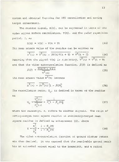
13

system and obtained formulas for MTI cancellation and moving

target enhancement.

The residue signal, R(t), can be expressed in terms of the

video signal before cancellation, V(t) , and the radar repetition

period, T, as

R(t) = V(t) - V(t + T) (33)

The mean square value of the residue can be written as

R2(t) = V2

(t) - 2V(t)V(t + T) + V2(t + T) (34)

2 2Assuming that the signal V(t) is stationary, V (t) = V (t + T)

and that the video autocorrelation function, 0{T) is defined as

*(T> = v< t)v(t+r)

(35)\r(t)

~~

2

the mean square value R (t) becomes

R (t) = 2V2(t) [l - 0(T)] (36)

The cancellation ratio, C , is defined in terms of the residue

asr2v:(t) i

Cc

=-=§== = 2[1 - {t)] (37)

Rc(t)

where the subscript, c, refers to clutter signals. The ratio of

moving-target mean square residue to stationary-target mean

square residue is defined as enhancement (E) , where

R2

1 - 0(T)E =+rrfw (38)

R^ ss

The video autocorrelation function of ground clutter return

was then derived. It was assumed that the resolvable ground patch

has an azimuthal extent equal to the beamwidth, and a radial

14

extent approximately equal to Q.T/2, where X is the pulse duration.

It was assumed that the illuminated ground patch, in the absence

of large reflectors, is made up of a very large number of very

small reflectors. These reflectors were assumed to be motion-

less. The fluctuation in the return is caused by the motion of

the aircraft between pulses. The return was assumed to be

N

ix(t) = £ C

ncos(w

Qt -

n ) (39)

n =1

where

w = transmitted angular frequency

= random phase angle with uniform distribution (0,27r)

Urkowitz used Rice's notation in the following derivations.

2Let b equal the uniform reflectivity of the patch where A is

the area of the patch, then

cn =vfb (40)

and

i1(t) = I.cosw t + I

2sinw t (41)

-n N

*1 = JH h l cos*n (42)

n = l

N

n = l

At a time T later, the second pulse is received and is expressed

N

i2(t + T) =

Vn"b I c°s (w t + wQT -

n - an ) (44)

n = l

15

where a is not random, but is equal to the phase change between

received pulses. Now, a(r,6) may be expressed as

2-

a(r,9) u 47r[vrTcos9 - (h) (VT) 3(45)

,Vr

2+ Z

2

where V and V' are aircraft and target velocities respectively, and

Z = altitude

r = ground range to a point in the ground patch

= azimuth angle of a point in the ground patch

Equation (44) is then rewritten as

i2(t + T) = I

3cosw

Q(t + T) + I

4sinwQ (t + T) (46)

whereN

X 3= vf B^cos(0

n+ a

n ) (47)

n = l

N

J4

=vf b Z sin ^n + a

n>(48)

n = l

The RF mean square clutter current is defined as

2

Jl = J

2 = A ' *4 = A^ " A^ ~m Ho = f (49 >

The second-order central moments are defined as

[i

I1I 3

=^13

=~A J"Icosc(r,e)rdrde (50)

I1I 4

= Ha =~A

JJcosa(r,e)rdrde (51)

In order to simplify notation, the parameter p was defined as

P2=^3 V" CM)

Ho

The above statistical averages were derived by George (1952) but

16

Urkowitz rewrites them in Rice's notation. The integrals (50)

and (51) are known as the radar "scatter integrals".

(Computa-

tions Lab, 1952). In the absence of a target, the square-law

video autocorrelation function is

^c (T) = ^^T^- (53)

Next, Urkowitz considered the case of a single-point object

plus the ground clutter. It was assumed that the radar return

from the object is of constant amplitude and frequency. The

first return is then

i.. (t) = Pcosw t + Lcosw t + I sinw t (54)1 O 1 O A O

where P is the amplitude of the object return. The second

return is given as

i2(t + T) = Pcos(w

Qt + w

Qr - y) + I

3cosw

o(t +T)

+ I„sinw (t +T) (55)4r O

where y 1S t^ie phase change of the return from the object and is

derived from

Y - f (S, - S2 ) (56)

where

S. = \lr\ + Z2

(57)x a

S2= [(r

acos9

a+ V^tcosq - V )

2

+ (rasinG

a+ V£tsini$

2

f* (58)

Urkowitz' s complete autocorrelation function after a square-law

device is

17

4 2T 9 P COS ^WnT " Y)

Y (T) = (p2/2 + v )

+ ^r

+ 2P2 l^(r)cos(w^ - y) + 2^

2(r) (59)

where, V(^) is t^ie RF autocorrelation function of the ground

clutter return given by

\y<X) = i1(t)i

2(t +T) = il ^2 E cosa

n

Nn = l

coswJFo

I I b2 I sinan

n = l

sinwor (60)

For large N, the summation becomes an integral and Equation (60)

becomes

The normalized video autocorrelation function is

'2

Q (T) m (x + 1) + 2xcos(9 - y) ? (62)T (x + 1)2 + 2x + 1

where

2x = P /2a = RF signal-to-clutter power ratio

9o

= arctan (^14/^3) .

These results are now combined in final expressions for

clutter cancellation and moving target enhancement. When Equa-

tion (53) is substituted into Equation (37) , the clutter cancel-

lation ratio becomes

1Cc

= l~rp (63)

The subscripts s and m are used to distinguish the autocorrela-

tion functions for stationary and moving targets. For a moving

target the function is

18

(T) =^m v

'

(x + l)2 + 2xcos(Gn - Y ) + p

2

m(64)

(x + 1) + 2x + 1

whereas, for a stationary target, it is

S(T) =

(x + l)2+ 2xcos(9 - y ) + p

2

(65)(x + 1) + 2x + 1

When Equations (65) and (66) are substituted into Equation (38) ,

the result for moving target enhancement is

2x[l - cos(9o

- Ym)] + 1/CC

E ~ 2x[l - cos(0o

- Ts )] + 1/CC

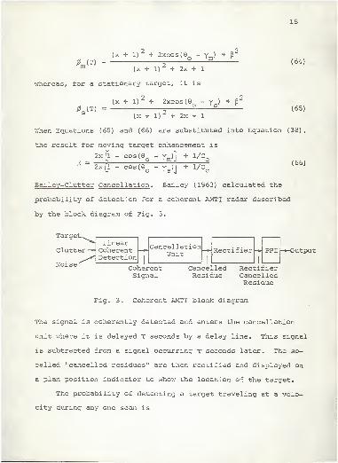
Bai ley-Clutter Cancellation . Bailey (1963) calculated the

probability of detection for a coherent AMTI radar described

by the block diagram of Fig. 3.

(66)

Target^

Clutter-

Noise

LinearCoherentDetection

1

CancellationUnit Rectifier PPI -Output

CoherentSignal

CancelledResidue

RectifierCancelledResidue

Fig. 3. Coherent AMTI block diagram

The signal is coherently detected and enters the cancellation

unit where it is delayed t seconds by a delay line. This signal

is subtracted from a signal occurring f seconds later. The so-

called "cancelled residues" are then rectified and displayed on

a plan position indicator to show the location of the target.

The probability of detecting a target traveling at a velo-

city during any one scan is

19

00

PD=

*Pl(Z

o>dZo

(67)

where

Pl(Zj = probability density function of target and clutter

at output

ZQB= threshold level.

The probability of false alarm is

pf " * V Z

o>dZ

oZ0B

(63)

where

Po(Z ) = probability density of clutter alone.

In order to determine P, (Z ) and P (Z ) , it is necessary • to

determine the following probability den sity functions:

1. The joint density function at the output of thej receiver,

p[R(t), 0(t); R(t -T), Q(t - r>] (69)

2. The second probability density function at the output of

the phase cancellation unit.

p[e(t) - G(t -T)]4

(70)

3. The second probability density function at the output

of the rectifier.•

p[e(t) - e(t -rj] (71)

Bailey assumed a Rayleigh ground and expressed the .Input signal

asN

Cq(t) a I^K cos(w t + K -

K=0«*> (72)

where

C (t) = current from the qth pulseSi

20

wo= carrier frequency

V= phase of the kth scatterer

*= change in phase angle between the first and qth look

crk-= power received from kth scatterer.

This equation is expanded and rewritten as

Cq(t) = X

qcosw

Qt + Y

qsinwQt (73)

N

Xq = I >/5* C° S(% " *%J (74)

k =0

- N

Yq=Z V^3in(0k -q^) (75)

k =

The target signal was written as

S(t) = v/551

f (t)cos(wTt + a)cosw

Qt (76)

where

wT

= 2n times center frequency of the signal power

spectrum

density

a = random phase angle which is constant for any

target

particular

s = RMS signal power

f(t) = term that accounts for target fluctuations.

The probability density function was then calculated as

pj[s(t) + C(t)J ;[s(t -T) + C(t -T)]} =

PJR(t) ,9(t) ;R(t -r)/©(t -T)] (77)

where

S(t) + C(t) = [x(t) + A(t)] coswQt + Y(t)sinw

Qt (78)

The final result requires determination of a four-dimen sional

probability distribution. The final expression for the joint

21

probability density function for the amplitude of a target-plus-

clutter signal arriving at (t -T) and one arriving at (t) , with

a linearly detecting receiver, was given as

R R r

P(Rr R2 , 0^ G

2 ) = -^ «*|" M^l + ^- 2^, 12

R1R2cos(G

1-

2)

- 2p, 14R1R2sin(9

1- 9^ J

(79)

where

R1

= /[x(t) + A(t)]2

+ [y(t)]

91

= arctan{jffl. A(t) j

R2

= 7[x(t -T) + A(t -t)] 2+ [y(t -T)] 2

92

= arctan{ x(t j£ l\\ t _ T } ]

In terms of the power density spectrums of the target signal

and the clutter.

4 2 2A i —cr - p-12 - h-14

ex;

(^ = 1 [G (f - f ) + G (f - f )]dfo -*oo

^12=

* ["GT (f " V + Gc(f " V^ 003 2?r(f " f

c) df

oo

P-14 = J [GT (f - fT )

+ Gc ( f - f

c)]sin 277- (f - f ) df

o

Next the second probability density function P (|0l) at the

output of the phase cancellation unit was derived. The phase

difference was defined as

= 9±

- &2 (80)

and the probability density function of the output is

22

P(|0l) = P( 0) + P(-0) (31)

After a change of variable and integrating out R, and R2the

density function is

(1 - S2

)

1/2 + 3(tt - arccos 3)

(1 -{32

)

3/2P(0) = —

427r(T

(82

where

f3 =

"^2 COSi2J7^2

Sin^

The final expression for P(|0|) was then obtained by evaluating

2q- , \i--t2' an(^ ^14* Tlle Power density spectrum of both the

clutter and target was assumed to be gaussian as given by

GT (f - fT ) = —§— exp{- (f - fT )

2/2(Tg] (S3)

s

and

G<:<£" *<='

=

Jtf SXP1"

<f ~ f=)2/2Cr

c)<84>

c

After integrating and making some simplifying approximations

Bailey obtained

H 12= foexp(-27r

2(T

2T2

) + S cos 2?rfD2- (85)

[i14

= S sin 27rfDr (86)

CT2 = ^ + S (87)

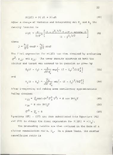
Equations (85) - (87) are then substituted into Equations (81)

and (82) to obtain the final expression for P(|0|) = P(Z ).

The preceeding results are then combined in the form of a

clutter cancellation ratio, C . On a phase basis, the clutter

cancellation ratio is

23

n2!f (Z ) P(Z )dZ (correlated)

o P P P^—;}

j" (Z ) P(Z )dZ (uncorrelated)P P P

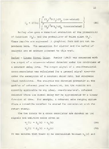
Bailey also gave a numerical evaluation of the probability

of detection (P ) , and the probability of false alarm (Pf

)

.

These results are expressed in graphical form and are not re-

produced here. The assumption for clutter and the method of

analysis are of primary interest to this work.

Remley - Linear Signal Delay . Remley (1963) was concerned with

the output of a cross-correlator detector under the conditions of

a constant delay rate. The output signal of a one-dimensional

cross-correlator was calculated for a general signal spectrum

under the assumption of a constant delay rate, but otherwise

ideal conditions.,The analysis was directed primarily at the

problem of coherent passive detection, but the results are

directly applicable to any ideal, one-dimensional, coherent

detector where the signal delay may be approximated by a linear

function of time. For example, a coherent echo ranging system

where a noiselike waveform is stored for correlation with the

return energy.

The two inputs to a cross correlator are denoted as che

signals and additive noise given as

Vr(t) = S1(t) + n

x(t) (89)

v2(t) = S

2(t) + n

2(t) (90)

It was assumed that there is no correlation between n1(t) and

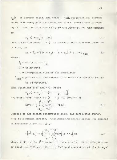
24

n2(t) or between signal and noise. Each component was assumed

to be stationary with zero mean and signal powers were assumed

equal. The instantaneous delay of the signals, At, was defined

as

S1(t) = S

2[t - At] (91)

Over a short interval A(t) was assumed to be a linear function

of time, or

At = ro

+ f (t - to ) ? 1

1 - to |

i Jj(t + rmax ) (92)

where

2" = delay at t = to * o

7" = delay rate

T = integration time of the correlator

2" = parametric time interval for which the correlation ismax ^

to be computed.

Then Equations (91) and (92) yield

S1'(t) = S

2jt --fr(t - t

Q ) -rol (93)

The correlator output at (t = t ) was defined as

(tQ

+ JfT)

R(T) = ^ J v2 (t)V1 (t +T)dt (94)

(t - h?)

Because of the finite integration time, the correlator output

R(T) is a random variate. Therefore the output signal was defined

as the expectation of R{t) ,

(tQ

+ J$T)

e[rj(T)] = ^ I E[VJ(t)vJ(t +T)j dt (95)

o

where RJ (T) is the j member of the ensemble. After substitution

of Equations (90) and (93) into (95) and evaluation of the integral

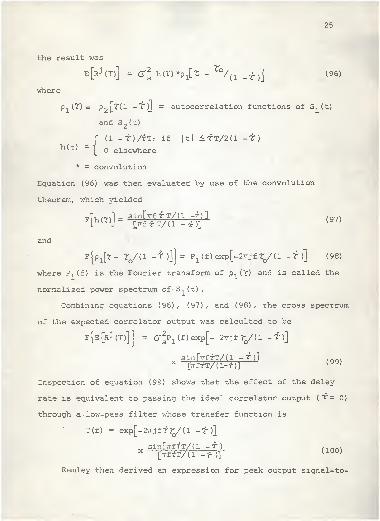
25

the result was

e[rJ(T)] = (^M^pi* ~ '<1 _ f)](96)

wnere

p,(7)= p 2r?"( 1 -T)j = autocorrelation functions of S..(t)

and S2(t)

r (1 -T)/fT; if |t| £TT/2(1 -t)h(t) =

( elsewhere

* = convolution

Equation (96) was then evaluated by use of the convolution

theorem, which yielded

Th ml = sin[7rfrT/(l -f)]lhU,

J J^TTf fT/(l --£)](97)

and

(98)Fip l[

r_ To/(1 -^O) 88 P1(f)exp[-27rjfr

o/(l - r )]

where P, (f ) is the Fourier transform of p-i(T) and is called the

normalized power spectrum of-S.(t).

Combining equations (96) , (97) , and (98) , the cross spectrum

of the expected correlator output was calculted to be

f{e[rj(T)]J

= CT^ (f)exp[- 27rjfro/(l - f )]

sinfTTfrT/d -r)]x (VffT/d-?)] ^ yy;

Inspection of equation (99) shows that the effect of the delay

rate is equivalent to passing the ideal correlator output (t= 0)

through a low-pass filter whose transfer function is

T(f) = exp[-27rjff?y(l -f )]

sinQffT/(l -T?X

[TrffT/(l -r )]U00)

Remley then derived an expression for peak output signal-to-

26

noise ratio for an active detector system. One input to the

system was assumed to be a known signal and the second input was

assumed to be noise. The noise output is given as

n = rr2nr

2/(2w T) (101)o w s u n n

where

wn

= equivalent rectangular bandwidth of the noise.

The final expression for signal to noise ratio was given as

?T/2(1 -f ) )

2

(5/N)o

= 2WnT

j(S/N)

i

2(1tT

r)Jp^tjdt

J(102)

Finally it was shown that for zero delay rate (S/N) is a

linearly increasing function of the time-bandwidth product, but

for non-zero delay rates, maximum points exist, when the signal

is white noise.

Deterministic Models

Dickey - Clutter Cancellation . Dickey's paper (1953) considered

the effect of antenna motion on clutter cancellation. A

stationary target and a perfectly stable radar platform were

assumed. The clutter cancellation as a function of antenna point-

ing angle in azimuth was calculated. The mean square value of the

residual clutter was found to be the sum of four components, one

due to antenna rotation and three others due to aircraft motion.

The quanity £ was defined as

c - Mean Square Pulse-to Pulse Voltage Chancre cik-wMean Square Voltage U03 '

The received signal was assumed to result from a large number of

small component signals with random phase. The amplitudes of

the individual components of the signal are weighted as a

27

function of the azimuth antenna pattern and as a function of the

elevation angle. In the case of a short duration pulse, the

elevation function depends on the pulse width and shape. The

variations in signal strength, which prevent complete cancella-

tion, are said to be caused by changes in relative phase of

various components due to displacement of the radar platform and

change in the amplitude of various components due to rotation of

the antenna, during the interpulse period. Although the com-

ponent phase angles are random, the changes in relative phase of

a component during the interpulse period can be calculated.

The displacement of the antenna during the interpulse period

is expressed in terms of its components along X, Y, Z axies of an

orthogonal coordinate system. The Z axis is oriented along the

antenna boresight. The displacement is then

X = VT sin(9 - GQ ) (104)

Y = VT cos(0 - G ) sin (105)

Z = VT cos(G - ) cos . (106)

where •

'

V = velocity of the aircraft

T = time interval between pulses

©, = azimuth and elevation angles respectively, measured

from Z

eQ / O

- azimuth and elevation angles of the direction of motion.

The function F(G,0), which expresses the phase shift produced by

a given antenna displacement, is given as

F(G,0) = — (Xsin © + Ycos e sin + Z(cos G cos 0) )

(107)

28

or assuming a small beamwidth, Equation (107) becomes

F(©,0) «4J (XG + Y0 - z(e

2+

2)) (103)

The weighting functions A(G) and B(0) are then defined as

A(0) = round-trip voltage antenna pattern in azimuth

B (0) = elevation weighting function.

The vector difference between two successive signals is then

found to be

D = A(9 + %w T)B(0)exp(jisF(G,0) )

where

- A(0 - i2waT)B(0)exp(-ji5F(e / 0)) (109)

w^ = angular rotation rate of the antenna,a /

Combining Equations (103) and (109) , the quantity £ becomes+ oo

h J jiDrded0

€ = ^ (no)

J I|A(9)B(0)|2d©d0

- oo

Equations (108) and (110) were then combined and the results

reduced to the form

where 6R is the residual clutter component due to antenna rota-

tion, and 6X , €y, £„are the residual clutter components due to

radar displacement along the X, Y, Z axies. These components

were then calculated using rectangular, gaussian, and (sin x) /x

round-trip azimuth antenna patterns. From these results, the

clutter attenuation for a given set of parameters was calculated.

These results show that the greatest clutter attenuation or

cancellation occurs within 15° to 20° of the aircraft direction

29

of motion, whereas the least attenuation occurs at 90 to the

motion. For the parameters selected there was a difference of

24 db between the maximum and the minimum cancellation.

Coleman and Hetrich - Ground Clutter . Coleman and Hetrich (1961)

presented a method for the calculation of approximate ground

clutter power return based on an approximation to the return from

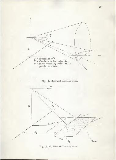
a given doppler frequency region. Figure 4 shows the basic

clutter geometry used in the derivation. The intersection of

the cone with the ground is a hyperbola for horizontal flight,

and it represents the locus of all points on the ground having

the given relative velocities with respect to the radar. The

hyperbola also represents the locus of all points on the ground

which reflect clutter having the same doppler frequency shift,

£-, wherea

fd

= 2vA (112)

The redar clutter spectrum may be subdivided into a finite

number of equal contiguous doppler increments, Af ,, between

f_ - f and f + f , where f is the carrier frequency and fOVOV O V

is the maximum doppler frequency shift.

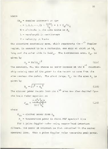
Size and range of the clutter reflecting area is determined

by the relationships in Fig. 5. The increment Ad is the dis-

tance between the n hyperbola and the n + 1 hyperbola and is

given by(n - l)HAf A

Ad = d(113)n

/(103V) 2 _( n - l)2(Af \)2

30

= arccosine v/VV = absolute radar velocity

v = radar velocity relative to

points in space

Tig. b. Constant doppler loci.

Fig. 5* Clutter reflecting area.

31

where

Afa

= doppler increment in cps

n

H

= 1,2,3, / (1 + € )- 1 +

rd

= altitude in the same units

VAfa

as dn

X = wavelength in centimeters

V = velocity in knots

The effective scattering area, which represents the n doppler

region, is assumed to be a rectangle, one side of which is Adn

long and the other side is KaAd . The incremental area,n V is

given by

A^ = Ka(Ad )

2

n n

The constant, Ka, was chosen as unity because of the

(114)

-4R relation-

ship causing most of the power in the return to come from the

area nearest the radar. The slant range, R , to the area A isn

given by

(115)R = \/H2

+ d2

n v n

The clutter power return from the n area was then <derived from

the basic radar equation as

2 2P.G1VA1 n uo n

Cn '

(47T)3R4

n

(116)

where

Pen

= clutter power from A

Pl

= transmitted power in first PRF spectral 1 Lne

For a pulse doppler radar using narrow band detecti.on

filters, the power of interest is that contained in the center

spectral line. When a pulse doppler radar transmits peak power,

32

p , at a duty cycle, d, the power in the carrier or center

spectral line, P , is

P . = P d2

(117)csl t

where

d = pulse width times the pulse repetition frequency (Tf ) .

The power in the spectral line which is mf cycles per second

from the carrier has an amplitude

= pfd2

f-m t L

and

7Td

p_ = p^r^tspf <"8)

*1 " v2

[^ :or m = 1 (119)TTd

The gain was determined from the geometry of the problem

and the antenna pattern. The reflection coefficient, (j was

determined by the type of terrain. Finally, the clutter power

density was expressed as

G (Af ,) = P /Af

,

(120)en d en' d ***«*

The major approximation made in this development is that

return from areas between the isodops, but outside the defined

ground patch, is negligble.

Welch - Radar Terrain Return Fading Spectra . In work performed

by the Physical Science Laboratory of New Mexico State University

for Sandia Corporation, (Welch, 1960) a method similar to Hetrich's

was used to compute the clutter power from incremental ground

areas. However, the New Mexico procedure calculated the return

from all areas defined by a grid related to flight conditions,

instead of approximating A . The basic approach is the same for

33

calculation of power return. This power spectrum is then used

to calculate a pulse-to-pulse variance spectrum, V(f)

,

+00

V(f) - 2 j P(g)P(g - f)dg (121)_ CO

where

P(f) = calculated power spectrum.

The ground plane was divided into a set of incremental

areas by means of two families of curves, namely,

1. A set of concentric circles (loci of constant

angle of incidence) centered ebout the point directly

beneath the radar.

2. A set of hyperbolas, with the radar at the foci,

as a function of the angle between the radar

velocity vector and the ground point.

A grid was constructed for the horizontal case and the areas

4were measured by a planimeter, weighted by cos 9 and tabulated.

The RF power spectrum was computed by the basic radar equation

applied to the incremental areas and the results were summed

over a given doppler frequency band. The calculations were re-

stricted to angles of incidence near the vertical. Chia (1960)

in his master's thesis at the University of New Mexico developed

a computer program for the above model. This work and the paper

by Farrell and Taylor form the basis for the model developed in

this paper.

Farrell and Taylor - Doppler Radar Clutter . J. L. Farrell and

R. L. Taylor (1963) have extended the method of Coleman and

34

Hetrich (1961) and derived a method for computation of the clutter

sprectrum for doppler radar. They were interested in obtaining a

relatively simple and accurate method of calculating the clutter

spectrum for both main beam and side-lobe contributions.

The following system restrictions were used throughout

their analysis.

1. The antenna bes.mwidth fL 15 .

2. Antenna E-plane and H-plane beamwidths are equal.

3. The transmitter duty radio is the reciprocal of an

integral number, so that the receiver is divided

into an integral number of range gates. During each

interpulse period, each gate is opened only once,

for a time interval equal to the duration of the

transmitted pulse.

4. The radar detection range is far in excess of the

maximum unambiguous radar range.

5. The clutter return is from a large number of scat-

terers, each of which reflects the same percentage

of energy when illuminated at normal incidence.

The basic approach was to divide the spectrum into three

regions, which correspond to the antenna main beam, the first

side-lobe, and the remaining lobes. Side-lobe clutter is taken

to be stationary or, the clutter is assumed to be uniformly dis-

tributed in all range gates. The main beam clutter is in general

time-varying. Upper and lower bounds are determined by computing

the spectrum under the conditions, all main beam clutter is in a

35

single range gate, and that it is uniformly distributed among

all range gates.

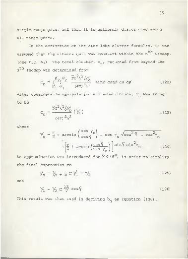
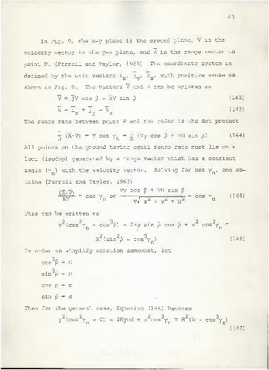
In the derivation of the side-lobe clutter formulas, it was

assumed that the ettenna gain was constant within the n '' isodop.

(See Fig. 6.) The total clutter, C , returned from beyond the

n isodop was determined from

c =rr n sin cos dG d (122)n

±61

(47T)VAfter considerable manipulation and substitution, C was found

to be

(47T)JhZ

where

If = -x - arcs:n 2

• /COS Tn l /

—q 2—:in

I cos 9 J" cos

^nn/cos V " cos

^n

it , / tan 9 \ sin 7 sin y /i^/n2

+ £rcsin (t^n~7;) J

n (124)

An approximation was introduced for J < 45 , in orc;er to simplify

the final expression to

ya - &+ d-Vi -Y2 (125)

and

"Vi - Y2 - v cos<r < 126 >

This result was then used in deriving b as Equation (138)

.

36

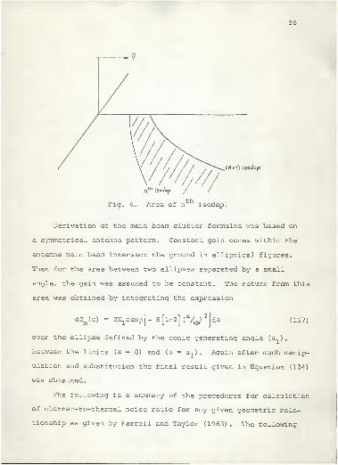
(rtf -i) isodop

Ath iaodop

thFig. 6. Area of n ' isodop.

Derivation of the main beam clutter formulas was based on

a symmetrical antenna pattern. Constant gain cones within the

antenna main beam intersect the ground in elliptical figures.

Then for the area between two ellipses separated by a small

angle, the gain was assumed to be constant. The return from this

area was obtained by integrating the expression

(127)dCm U)= 2K

1aexp(- 8 [in 2] (

a/^

2Ida

over the ellipse defined by the conic generating angle (ex..) ,

between the limits (a = 0) and (a = a1

) . Again after much manip-

ulation and substitution the final result given in Equation (134)

was obtained.

The following is a summary of the procedures for calculation

of clutter-to-thermal noise ratio for eny given geometric rela-

tionship as given by Farrell and Taylor (1963) . The following

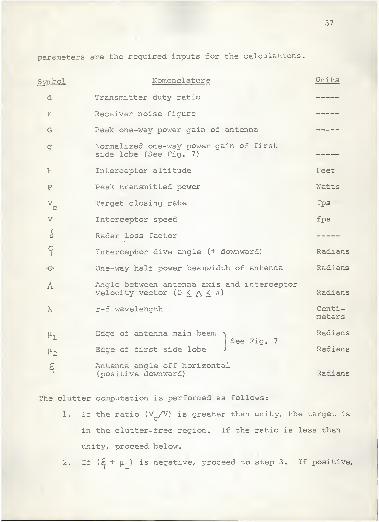
37

parameters are the required inputs for the calculations.

Svmbol Nomenclature Units

d Transmitter duty ratio

F Receiver noise figure

G Peak one-way power gain of antenna

g Normalized one-way power gain of firstsice lobe (See Fig. 7)

h Interceptor altitude Feet

p Peak transmitted power Watts

Vc

Target closing rate fps •

V Interceptor speed fps

s Radar loss factor

s Interceptor dive angle (+ downward) Radians

>& One-way half power beamwidth of antenna Radians

A Angle between antenna axis and interceptorvelocity vector (0 <_ /\ < rr) Radians

\ r-f wavelength Centi-meters

P-2

Edge of antenna main beam -\ RadiansSee Fig. 7

Edge of first side lobe J Radians

5Antenna angle off horizontal(positive downward) Radians

The clutter computation is performed as follows:

1. If the ratio (V /V) is greater than unity, the target is

in the clutter-free region. If the ratio is less than

unity, proceed below.

2. If (£ + u--,) is negative, proceed to step 3. If positive,

38

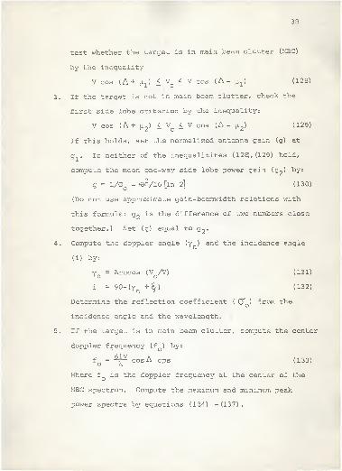
test whether the target is in main beam clutter (MBC)

by the inequality

V cos (A+ \i.}) £ V £ V cos (A- jj.^) (128)

3. If the target is not in main beam clutter, check the

first side lobe criterion by the inequality:

V cos (A +|j,2 ) £ V

c< V cos (A -

;j,

2) (129)

If this holds, set the normalized antenna gain (g) at

g . If neither of the inequalitites (12S), (129) hold,

compute the mean one-way side lobe power gain (g2 ) by:

g = 1/G - >G<2/16 [In 2~] (130)

(Do not use approximate gain-beamwidth relations with

this formula; g~ is the difference of two numbers close

together.) Set (g) equal to g„.

4. Compute the doppler angle (y ) and the incidence angle

(i) by:

y = Arccos (V /V) (131)1 n c

i = 90-(yn +§) (132)

Determine the reflection coefficient ( <o ) from theo

incidence angle and the wavelength.

5. If the target is in main beam clutter, compute the center

doppler frequency (f ) by:

f = —7— cos A cps (133)

Where f is the doppler frequency at the center of the

MBC spectrum. Compute the maximum and minimum peak

power spectra by equations (134) - (137)

.

39

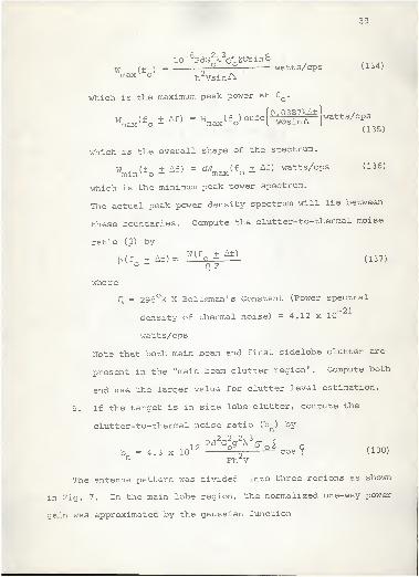
(f )= 1—2 2 watts/cps (134)

10"8PdG^K3cro J>'

eSin^

max o h2VsinA

which is the maximum peak power at fQ

.

•

Q.0387XAf| 7

(135)W (f ± Af) = W (f )erfcmax o — max o

which is the overall shape of the spectrum.

W . (f + Af) = dWm= (f + Af) watts/cps (136)mm o — max o

which is the minimum peak power spectrum.

The actual peak power density spectrum will lie between

these boundaries. Compute the clutter-to-thermal moise

ratio ((3) by

P (f + Af)= W(f o * Af)(137)

where

f[ = 298°K X Boltzman's Constant (Power spectral

-21density of thermal noise) = 4.12 x 10

watts/cps

Note that both main beam and first sidelobe clutter are

present in the "main beam clutter region". Compute both

and use the larger value for clutter level estimation.

6. If the target is in side lobe clutter, compute the

clutter-to-thermal noise ratio (bn ) by

b =4.3xl012 °%(r ° b

cos <

r (138)n FhV

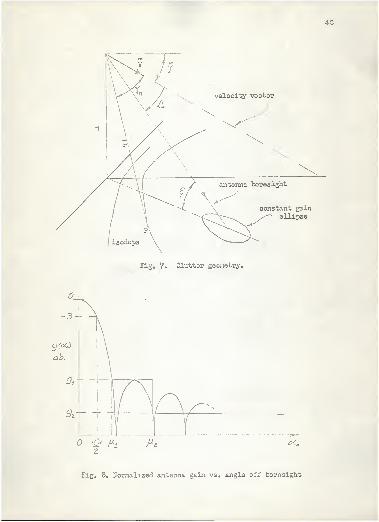
The antenna pattern was divided into three regions es shown

in Fig. 7. In the main lobe region, the normalized one-way power

gain was approximated by the gaussian function

40

velocity vector

constant gainellipse

Fig. 7. Clutter gec^etry.

Fig. 8. Normalized antenna gain vs. angle off boresight

41

2

g(0) = exp[(-4)(|<)

In 2] £ a < jj>1 (139)

and normalized side lobe gain is

g = g ^ < a £ .^ (140)

g = g2a > H-2 (141)

The peak of the first side lobe was taken from the antenna

pattern as shown in Fig. 7. Beyond the first sidelobe, the mean

sidelobe gain was calculated using Equation (130)

.

In Section 5 of this report, the clutter geometry and nota-

tion of Farrell and Taylor is used to formulate a mathematical

model for the calculation of ground clutter power spectrum.

MATHEMATICAL MODEL FOR GROUND CLUTTER POWER SPECTRUM

FOR AN AIRBORNE PULSE RADAR

Clutter Geometry

Relative motion between the radar platform and a point on

the ground produces a doppler frequency shift in the return

signal. This frequency shift is directly proportions 1 to the

closing rate (or range rate) between the radar and the point on

the ground. In general the velocity vector of the radar may be

oriented at any angle with respect to the ground plane, however,

the two cases of interest are when the radar is in horizontal

flight or approaching the ground plane in a dive angle. When

the radar is in a climb, clutter is not usually a problem. The

basic relationships for the clutter model are derived from the

geometry of Fig. 9.

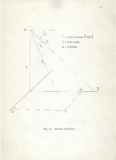
42

|

kZ

V- in = 'angle between V and £

\ A* v /3 = dive angle

H = altitude

H

eV\

y/ \

.

/ \

3*

\ // \ /

12V̂

P

Elg. 9. Clutter geometry.

43

In Fig. 9, the x-y plane is the ground plane, V is the

velocity vector in the y-z plane, and R is the range vector to

point P. (Farrell and Taylor, 1963) The coordinate system is

defined by the unit vectors i , j , k , with positive sense as

shown in Fig. 9. The vectors V and R can be written as

V = ~Jv cos p - kV sin p (142)

R = i +7 - k (143)

The range rate between point P and the radar is the dot product

J (R-V) = V cos v =| (Vy cos £ + VH sin 0) (144)

All points on the ground having equal range rate must lie on a

loci (isodop) generated by a range vector which has a constant

angle (y ) with the velocity vector. Solving for cos y , one ob-

tains (Farrell and Taylor, 1963)

(^.V)Vy cos p + VH sin p

W x2

+ y2

+ K= COS Tn or

„j _2,„2 ; TT 2

= cos rn

This can be written as

2 2 2 2 2y (cos y - cos £) - 2HY sin P cos $ + x cos Yn

=

H2(sin

2p - cos

2y ) (146)r

' n

In order to simplify notation somewhat, let

cos2p = C

sin 2p = D

cos p = c

sin p = d

Then for the general case, Equation (144) becomes

2 2 2 2 2 2y (cos y - C) - 2Kycd + x cos y = H (D - cos y )1 n . ' n ' n

(147)

4 4

For horizontal flight, (£ = 0) , Equation (146) reduces to

2 2 2 2 2 2(y ; (cos y - 1) + x cos Yn 7 ~K GOS Tn

or

x2

+ H2 = y2tan

2Y (148)

1 n

For a given value of (p) , (y ) / snd (II) , the general equation can

be recognized (Farrell and Taylor, 1963) as a simple conic

section, with the following possible forms

£ < y — hyperabola (14 9)

P = y parabola (150)

P > y ellipse (151)

and a degenerate case when Yi= ^Z2 which reduces Equation (147)

to the straight line

y = - K tan (152)

This straight line in the x-y plane separates the regions of

opening and closing doppler and is designated as the first isodop.

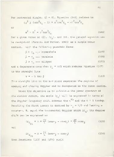
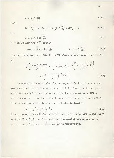
Since the objective is to calculate the power spectrum of

the clutter return, the angle (y ) will be expressed in terms of

the doppler frequency shift between the n and the n + 1 isodop.

Recalling the first isodop is defined by y- = rr/2 and letting a

constant, B, equal the incremental doppler shift Af ,/ the doppler

shift can be expressed as

2V 2VAfd = B = — (cosy, - cosy-,) = T" cos^2 (153)

and

2VAf , = B = =— (cosy n - cosyJ (154)

a31

k '3 '2

Then Equations (153) and (154) yield

45

and

B\cosY

2" ^

B = y~ (cosY3

- cosY2

)=Y" C0SY3 - B

(153)

(154)

cosY3 - (2) 2v

similarly for the n isodop

, ,, KBcosY

n = (n - 1) 2v^ y / 2V1 < n '. Ttr— — A.B

(155)

(156)

The substitution of (156) in (147) changes the general equation

to

2 2 2(n - 1) X 3^

- C(2V)

- 2Hycd + x2f"(n- 1)W

[_(2V)

= Hp _ (n - 1)

2>.2B2

(2V)2

(157)

A second parameter that has a major effect on the clutter

return is 9. The range to the point P in the ground plane and

scattering coefficient corresponding to the area at P are a

function of 9. The loci of all- points in the x-y plane having

the same angle of incidence is a circle defined by

(158)

The intersections of the sets of loci defined by Equations (157)

and (153) will be used to define incremental areas for power

return calculations in the following paragraphs.

x2 + y

2 = H2tan

29

46

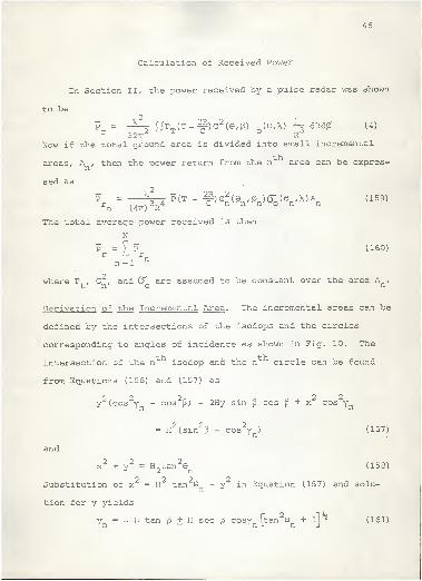
Calculation of Received Power

In Section II, the power received by a pulse radar was shown

to be

\2

P = IjPT(T-^)G 2

(e,0)o(GA) ^3 dRd0 (4)

32rr2

R'

Now if the total ground area is divided into small incremental

areas, A , then the power return from the n area can be expres-

sed as

?r

" 777^4 5 <T - tx^n-fy^o'V^n (159)n (47r) R

The total average power received is then

N

P = £ P (160)

n = 1

2where P,., G , and C are assumed to be constant over the area A .

t n o n

Derivation of the Incremental Area . The incremental areas can be

defined by the intersections of the isodops and the circles

corresponding to angles of incidence as shown in Fig. 10. The

intersection of the n^ isodop and the n circle can be found

from Equations (156) and (157) as

2 2 2 2 2y (cos y - cos $) - 2Hy sin p cos ]3 + x cos yn

= H2(sin

23 - cos

2y ) (157)

*' n

and

x2 + y2 = H otan

2(158)2 2 n

2 2 2 2Substitution of x = H tan - y in Equation (157) and solu-

n

tion for y yields

y = - H tan p + H sec p cosyn[tan

2Gn

+ l] ** (161)

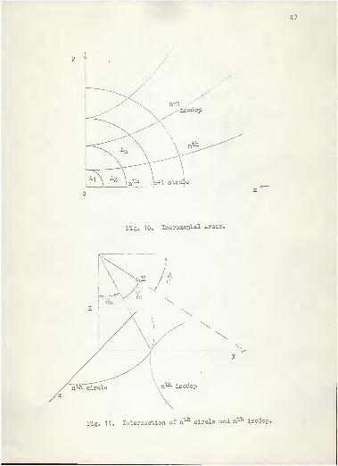
47

Fig. 10. Incremental areas.

nth isodop

Fig. 1 1 . Intersection of nth circle and nth isodop.

43

andi

xn

= [K2tan

29n

- y2 ^ (162)

If the coordinates are normalized for H = 1, Equations (161) and

(162) become

xn

= |Wsn

- yff (163)

2 Uy = -tan {3 + sec £ cosy

n(tan G

n+ 1)

2 (164)

where x and y ere the normalized coordinates of the intersection

of the nth

circle and n isodop. The above equations are now

modified, so that the desired doppler bandwidth defines the

angles G and y • *t was shown in Equation (156) that cosy can

be expressed as

cosyn

= (n - 1)|§ (156)

The angle G is related to y as shown in Fig. 11 as3 n ' n

n 2 ' n r

t"h thThe intersection of the n

l circle and the n ' isodop will always

be on the y axis. This was chosen to simplify the computer pro-

gram and does not limit the solution.

Antenna Gain Associated wi th A . In general, the antenna gain_n

is a function of both G and , which are modified forms of the

pattern reference angles. For the case of a circularly symmetri-

cal pattern (E plane and H plane beamwidths equal) the gain cor-

responding to a given A , can be determined as follows. The

angle a is the desired antenna pattern parameter. It is a

function of the lines AP, AB, and PB, as shown in Fig. 12. The

line PB is determined from the angles and by the law ofn n J

49

cosines for oblique triangles. For areas in the first quedrant,

2V is defined as

V2 = F2

+ Y2 - 2FY cos (166)

where

F = OP = K tan Qn

Y = OB = H/tan i

The angle a is then found from the lines AB, AP, and PB asJ n

2 2 2X + D - V ,,,.,

cos an

=23S

(167)

or2 2Xz + D - Vz

Mfta *

a = arccos xr^: (loo)n zad

where

D = AB = H/ sin &

X = AP = H/ cos G' n

For areas in the 2nd quadrant, the angle must be modified.

The interior angle is now defined as

Z = TT - en

and the calculation of a is the same as before except withn ri

replaced by Z. The angle a is then used to compute the antenna

gain for the given incremental area.

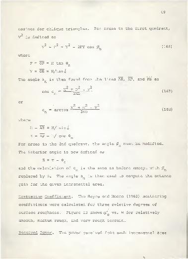
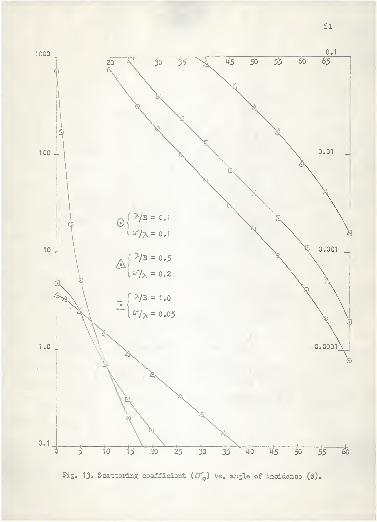
Scattering Coefficient . The Hayre and Moore (1962) scattering

coefficients were calculated for three relative degrees of

surface roughness. Figure 13 shows tf vs. 9 for relatively

smooth, medium rough, and very rough terrain.

Received Power . The power received from each incremental area

^

50

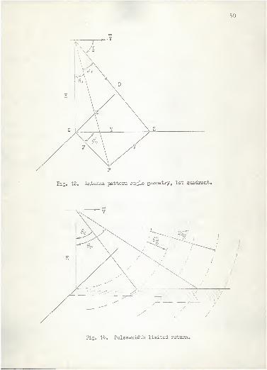
Pig. 12. Antenna pattern angle geometry, 1st quadrant.

/

Fig. 1^. Pulse-vriidth limited return.

51

1000

55 "ft0.1

0.1

To b 20 £~5 to 35 4o 45 50 %~5 <&>

Fig. 13» Scattering coefficient (C ) vs. angle of incidence (©),

52

is in general a function of time, and the power spectrum is time

varying. The return power is nearly proportional to the illumi-

nated area, which varies directly with the pulse width for a

narrow pulse. Therefore, the average return power for a pulse-

width limited return is approximately proportional to the pulse

width (T) at a fixed frequency. (Hayre and Moore, 1962) . The

relationship between the time of arrival, the illuminated ground

area, and the angle of incidence can be derived as follows.

Assume that the average power return from the firsc pulse period

is from range (H + cT/2) and the return from the n pulse

period is from the range (H + (2n-l) c'C/2) , as shown in Fig. 14.

If t, is the time of arrival of the first return, and t is the1 n

4-Vi

time of arrival of the n return, then

t, ,- t+ 2H/c (169)

and

t - (2n - 1) X + 2H/c (170)il

These returns correspond to the area in the annular ring defined

by the angles of incidence, such that

H Harccos . . , , rr—- < 9 < arccos „ ,

'—- (171)d + {r\ - 1) cT — ~ H + ncTT

Thus if a time variation of the power spectrum is desired, the

return is summed over the sequence of annular rings. If the

average power spectrum is desired, the return is summed over the

sequence of ccooler bands cefir.ed by the isoccos.

53

CALCULATED POWER SPECTRUMS

The main objective in establishing the preceeding clutter

model was to determine the effect of terrain roughness on the

power spectrum using the Hayre-Moore (1962) scattering co-

efficient. Data was compiled for four scattering coefficients

using the IBM 1620 digital computer.

Incremental Areas

The original program was set up for coverage out to 82.5

from the vertical. The parameters XB/2V, Equation (156), were

chosen to give 0.00377193, or approximately one-half degree

increments of y near the vertical. This resulted in 6441 incre-

mental areas in- the first quadrant for thehorizontal flight

condition. The program calculated the x,y coordinates of the

intersections of the isodop-hyperbolas and the angle of inci-

dence circles. Each incremental area was then approximated by

the area enclosed by straight lines connecting the points of

intersection. This area was calculated using the determinant

solution for the area of a triangle given as (Burlington, 3rd

Ed.)

A = HX Y

] 1 7xr y, l

X3

Y3

X

Area of a triangle with vertices

(X1,Y

1), (X

2,Y

2), (X

3,Y

3). (172)

Equation (172) was modified to account for the two triangles

making up the incremental area. The excessive computer time

necessary for the IBM 1620 to run the program for 6441 incre-

mental sreas made it impractical for the intended use. The

54

areas for the first three isodops were calculated by integration

and compared with the computed areas. An error of approximately

-3% was obtained. Computation time was about twenty minutes for

these idodops using Fortran II. It was estimated that five to

eight hours would be required for the total 6441 incremental area

program.

The parameters were then changed to give XB/2V = 0.01745, or

approximately one degree increments of y near the vertical, and

the coverage was reduced to 73.7 . This resulted in 1540 incre-

mental areas in the first quadrant. This program was checked for

the first three isodops and for the total area in the first quad-

rant. The computational error was approximately -7.5% for the

first three isodops, but was only -0.33% for the total area.

The modified program was then run to calculate the incre-

4mental areas weighted by cos 9 , to give the normalized (H = 1)

range weighted areas. The values of and A were punched out

for use as data input cards for the remaining portion of the

spectrum calculations. The program parameters used for the range

weighted incremental areas were X = 3.2 centimeters, V = 850 feet

per second (approximately 500 knots), and B = 282.6 cycles per

second.

Scattering Coefficients

The program for the Hayre-Moore (1962) scattering coefficient

was run for the following parameters:

55

Case #1 X/B =0.5 medium roughness

<^/\ = 0.4

Case #2 X/B =0.1 relatively smooth

(T/X =0.1

Case #3 X/3 =1.0 very rough

<r/X =0.8

The first runs were made using ten iterations for the series

term of Equation (5) . This resulted in fast convergence in

Case #2 only. The results for Case #1 and Case #3 were greatly

in error. A modified program was run to check the value of the

nth term of the series. For Case #1, the value reached a maxi-

mum on the 23rd term. After the 34th term, the value was still

in excess of 106

. For Case #3, the value was still increasing

and was in excess of 1021

after the 24th term. In both cases,

computer capacity was exceeded at these points and the program

was stopped. A check for slowest convergence was initiated and

found to occur for 9=0 when the scattering coefficient is of

the form ^

K y (i5s(oyx) 2)

n(173)

n-1 (n - 1)inn — l

If C/X is greater than 0.4, the convergence is very slow. In

order to reduce the computer time, different values of X/B and

0/X were chosen. Another set of values were selected to cover

the entire range of surface roughness as

56

Case #1 X/B = 1.0 medium roughness

C/\ = 0.05

Case #2 X/B =0.1 relatively smooth

o/X =o.i

Case #3 X/B =0.5 rough

oA = 0.2

The increasing value of BA indicates increasing size of along-

the-surface terrain roughness. The value 0/X indicates the

relative vertical heights (Havre and Moore, 1962)

.

Antenna Pattern

It was desired to approximate a pencil beam antenna since

this type would be used in many AMTI applications. The antenna

pattern chosen for the comparison was of the form (sinx)/x. A

three degree beamwidth was chosen to simulate a pencil beam

tracking antenna. Skolnik (1962) gives the expression for such

a pattern as

ptnt) _ sin(7r(aA) sin0)KYn

7r(a/X)sin0 (174)

where the angular distance between nulls adjacent to the peak is

X/a radians, and the beamwidth, as measured between the half-

power points is 0.38 X/a radian, or 5lX/a degrees. For a three

degree beamwidth the expression for the pattern becomes

E(0) = sin (7T(51/3) sin0)^ 7r(51/3)sin0 (175)

The pattern was assumed to be symmetrical about the antenna bore-sight. A depression angle was chosen as approximately 58°, which

57

gave a 41 increment for checking the effect of the antenna

sidelobes past the main beam in the direction of flight.

Altitude and Power

The altitude was chosen arbitrarily as 20,000 feet. The

shape of the spectrum is of primary interest and not the actual

values, therefore, the transmitted power and all constants in

the radar equation were chosen as unity. The return was summed

over the isodops to give an average power spectrum.

Power Spectrum

A program for the power spectrum was written to include

all parameters of the radar equation. This program calculated

the power spectrum for all 56 positive doppler frequency bands

and the first 30 negative doppler bands. This included all

returns from the first quadrant and returns from the second

quadrant out to 65 from the antenna boresight. The program was

processed in Fortran II and after the first few doppler bands

were calculated it became apparent that the program would re-

quire two to three hours running time. Therefore the program

was changed to calculate the incremental areas weighted by the

antenna gain and the altitude factors, but omitting the scat-

tering coefficient. The incremental areas were punched out for

use as input data in the final program. The running time was

approximately three hours.

A final program which multiplied the incremental areas by

58

the appropriate scattering coefficient and summed the results

over each doppler band, was then written. The inputs were the

weighted incremental area cards, and the scattering coefficient

cards. It required fifteen minutes running time. The power

spectrum was calculated for four scattering coefficients. The

previously calculated Hayre-Moore (1962) scattering coefficients,

were used, and an assumed constant scattering coefficient equal

to 0.00316 (Grant and Yaplee, 1957) was used for comparison.

Results

The analysis gave data for power spectrums from four scat-

tering coefficients in the form of return in 55 positive doppler

frequency bands and 30 negative doppler frequency bands.

In order to evaluate the effect of the terrain roughness

on the power spectrum, the smallest value from all data was

chosen as the reference. A program to transform the results to

decibles referenced to this value was then run. The final power

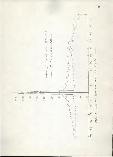
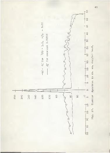
spectrums are shown in Figs. 15-17 as db vs. doppler frequency.

The power spectrums for the Hayre-Moore (1962) scattering co-

efficients are plotted with the spectrum for <TQ

equal to a con-

stant for comparison. The spectrums all have a sharp peak at

the first doppler band. This is the altitude return and shows

the inverse fourth power effect of range. For all four spectrums,

the width of the major peak is approximately 360 cycles per

second. This return is from areas within 2 to 3 of the

vertical.

59

For a smooth surface, (See Fig. 15) where \/B = 0.1 and

O/K = 0.1, the peak return is approximately 135 db above the

majority of the remaining spectrum. This shows the effect of

the strong specular components near the vertical. The amplitude

of the spectrum has a decreasing slope between the peak return

and the antenna main beam, showing the effect of the rapidly

decreasing scattering coefficient for angles away from the

vertical.

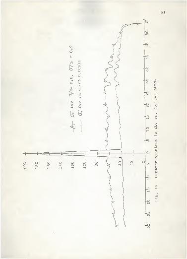
The spectrum for X/B =0.5 and C/\ =0.2 (See Fig. 16) very

nearly parallels the spectrum forG" equal to a constant. Theo

peak value is about 110 db above the average value. There is a

general 20-23 db difference between the spectrum for the computed

coefficient and the one for the constant coefficient out to the

antenna main beam portion of the spectrum. Beyond this, they

converge as the CT for the Hayre-Moore values approach the con-

stant value. Both spectrums show a tendency to be flat in the

sidelobe region.

The spectrum for X/3 = 1.0 and <j/\ = 0.05 (See Fig. 17) is

almost the same as that for the smooth surface except for the

peak value, which is about 110 db above the average value. This

was to be expected since the scattering coefficient curves are

very close for G > 3° (See Fig. 13)

.

All four spectrums have a lower amplitude in the main beam

region than was expected. This was evidently the result of the

antenna pattern sidelobe levels increasing at about the same

gain slope that <j was decreasing. Another factor was the

60

cCO

u<D

rHftP.O

>

Xi

g

Ph

o

co

CD•p•p

)—

i

o

LO

•H

62

-Sc

ooCv

o o oCO «> ^M i-i H

O

o

o

COrHtoOOo

opctfPm

Oo

£h

O

t? b*

qj

ocu

ooH

OCO

o ovfl Cvi

#1 I

- O

—

o

•aa

cu

rHP,ao

>

•a

c

e

s^po0)

ftt/3

o

pHO

inrH

rH

oCv

•H

Cv

oto

63

angular width of the incremental areas. These were wider than

desirable because of the computing time considerations previously

mentioned. This may have caused the peak of the main beam gain

to have had less effect than it should have. The spectrums do,

however, show that terrain roughness variations have a relatively

minor effect away from the vertical (3 -5 ) angles of incidence.

They also show that the assumption of 0"o

equal to a constant

holds relatively well over a large portion of the spectrum, but

is very pessimisstic at the ends of the spectrum. This is just

the portion of the spectrum which is important in evaluation of

radars using doppler frequency detection techniques. The use of

a constant C causes the computed power to be too high at these

frequencies and will not give an accurate evaluation of the radar's

capability in the critical low velocity region.

The curves for (j given by Hayre and Moore (1961), those in

Fig. 13, and the corresponding power spectrums seem to indicate

that the value of G/\ determines the average power level, whereas

the value of X/B determines the slope of the spectrum. This

relationship needs further investigation.

SUMMARY

Airborne radar AMTI clutter models and methods of analysis

are discussed. The basic radar return theory is briefly re-

viewed. Emphasis is placed on the Hayre-Moore (1962) scattering

coefficient, which allows a quantitative expression for the

effect of surface roughness on the radar return. The relation-

64

ship between signal correlation and power spectrum are discussed

and two basic correlation receivers are diagramed.

Analyses of clutter and AMTI performance reported in the

literature are reviewed. There are two general forms of analysis

used, namely, random variable theory and deterministic models.

Much of the effort reported in the literature has been concerned

with calculation of clutter cancellation ratios and the proba-

bility of detection for radars using phase or amplitude clutter

cancellation. These papers fall in the random variable theory

class. In theorectical analysis, Urkowitz's assumption of a

"white noise" spectrum for the clutter and Bailey's assumption

of a gaussian spectrum for the clutter are commonly used. The

second class of analysis is concerned with calculation of ground

clutter power spectrum for given parameters. The work done by

Welch at the New Mexico State University and a recent paper by

Farrell and Taylor of Westinghouse are used as a basis for a mod-

ified mathematical model for calculation of ground clutter power

spectrum. The major contribution of this thesis is use of the

Hayre-Moore (1962) scattering coefficient for investigation of

the effect of terrain roughness on the clutter spectrum.

Clutter spectrums are calculated for three Hayre-Moore (1962)

scattering coefficients and an assumed constant scattering co-

efficient. Data was compiled using the IBM 1620 digital computer.

The increments in the final modified program were slightly larger

than desirable, but the program had sufficient accuracy to show

the usefulness of the technique. Better results would be obtained

65

with smaller increments on a larger and faster computer than the

IBM 1620. The effect of terrain roughness is most prominent

near the vertical or for 0< Q< 3°. At angles greater than

approximately three to four degrees, there is no major change in

the shape of the spectrum as the roughness varies. A comparison

of the spectrums for the Hayre-Moore (1962) scattering coefficients

with that for a constant coefficient, showed that the assumption

of C as a constant gives a very large error in the power spec-

trum at the high frequency end. This is the area of prime impor-

tance in a doppler frequency detection system, as the performance

against low velocity targets is determined by the signal to

clutter ratio as the signal moves into the clutter region of the

spectrum.

66

ACKNOWLEDGMENTS

The author wishes to express his gratitude to Dr. H. S.

Hayre, of the Department of Electrical Engineering, for his

guidance while preparing this paper. Also special thanks are

due to Dr. C. A. Halijak, Department of Electrical Engineering,

for his suggestions on the area approximation; to Dr. B. D.

Weathers, Department of Electrical Engineering, for his help in

early computer programming problems; and to W. Hull, fellow

graduate student, for his time and instruction on the IBM 1620

computer.

67

REFERENCES

1. Bailey, F. B.A method for calculating the probability of detection fora coherent (AMTI) radar unit with phase cancellation.Jour. Frank. Inst. April 1963.

2. Bendat, J. B.Principles and applications of random noise theory. JohnWiley & Sons, Inc. 1953.

3. Chia, C.Computer programs for determining radar return power andfading spectra. Master's Thesis. The University of NewMexico. 1960.

4. Coleman, S. D. and Hetrich, G. R.Ground clutter and its calculation for airborne pulsedoppler radar. IRE Conv. Rec. Mil-E-Con. June 1961.

5. Dickey, F. R. Jr.Theoretical performance of airborne moving target indicators,IRE Trans. PGAE-8. June 1953.

6. Farrell, J. L. and Taylor, R. L.Doppler radar clutter. Westinghouse Elec. Corp. ReportNo. AA-4285. July 1963.

7. Grant, C. R. and Yaplee, B. S.Back scattering from water and land at centimeter andmillimeter wavelengths. Proc. IRE. July 1957.

8. Havre, H. S. and Moore, R. K.Theoretical scattering coefficients for near verticalincidence from contour maps. Jour. Res., Nat. 3u. Stds.Vol. 65D. No. 5. Sept. -Oct. 1961.

9. Hayre, H. S. and Moore, R. K.Radar back-scattering theories for near-vertical incidenceand their application to an estimate of the lunar surfaceroughness. Dissertation for D. Sc. at The University ofNew Mexico. 1962.

10. Remely, W. R.Correlation of signals having a linear delay. Jour. Acoust.Soc. of Amer. Vol. 35. No. 1. January 1963.

11. Rice. 0. S.Mathematical analysis of random noise. Bell Sys. Tech.Jour. Vol. 23 and 24. 1948.

68

12. Skolnik, M. I.

Introduction to radar systems. McGraw-Hill. 1962.

13. Urkowitz, H.An extension to the theory of the performance of airbornemoving target indicators. IRE Tans, on Aero, and Nav.Elect. Vol. ANE-5. December 1958.

14. Welch, P. D.Interpretation and prediction of radar terrain returnfading spectra, progress reports I, II, and III. SandiaCorporation Reprints SCR-212, SCR-214, and SCR-215.July 1960.

69

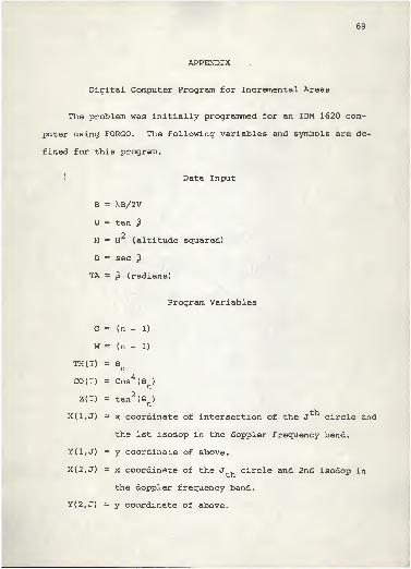
APPENDIX

Digital Computer Program for Incremental Areas

The problem was initially programmed for an IBM 1620 com-

puter using FORGO. The following variables and symbols are de-

fined for thi 3 program.

i Data Input

B = XB/2V

U = tan

H 2H (altitude squared)

D = sec P

TA P (radians)

Program Variables

G = (n - 1)

w = (n - 1)

TH(I) = en

00(1) = cos4(e )n

Z(I) = tan2(0 )n

X(1,J) ~- x coordinate of intersection of the J circle and

the 1st isodop in the doppler frequency band.

Y(l, J) y coordinate of above.

X(2,J) = x coordinate of the J., circle and 2nd isodop in

the doppler frequency band.

Y(2,J) y coordinate of above.

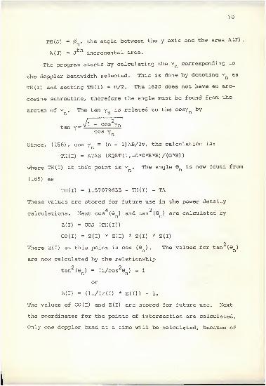
70

PH(J) =, the angle between the y axis and the area A (J)

.

A (J) = J incremental area.

The program starts by calculating the yncorresponding to

the doppler bandwidth selected. This is done by denoting yn as

TH(I) and setting TH(1) - tt/2. The 1620 does not have an arc-

cosine subroutine, therefore the angle must be found from the

arctan of y . The tan y is related to the cosy by1 n n ll

..6v 1 - cos yntan y= 1 LHcos Y

1 n

Since, (156), cos y = (n - l)\B/2v, the calculation is:

TH(I) = ATAN (SQRT(1.-G*G*B*B)/(G*B) )

where TH(I) at this point is y . The angle 9n

is now found from

(165) as

TH(I) = 1.57079633 - TH(I) - TA

These values are stored for future use in the power density

calculations. Next cos (G ) and tan (9n

) are calculated by

Z(I) = COS (TH(I)

)

CO(I) = Z(I) * Z(I) * Z(I) * Z(I)

2Where Z(I) at this point is cos (9 ) . The values for tan (9 )x n n

are now calculated by the relationship

tan2(9n

) = (l/cos29n

) - 1

or

z(i) = (i./(z(i) * z(D) - l.

The values of CO (I) and Z(I) are stored for future use. Next

the coordinates for the points of intersection are calculated.

Only one doppler band at a time will be calculated, because of

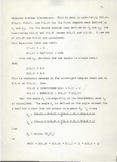
71

computer storage limitations. This is done by calculating X(l, J)

,

Y(l, J), X(2, J) , and Y(2,J) for the first doppler band defined by

y 1and y 2

. For the second doppler band defined by y2and y3

, the

coordinates X(2,J) and Y(2,J) become X(l, J) and Y(1,J) . A new set

of X(2,J) and Y(2,J) are calculated.

From Equations (163) and (164)

:

Y(l, J) = - U

X(1,J) = SQRT(Z(J) - U*U)

(the cos Yi' defining the 1st isodop is always zero.)

then

Y(2,l) = 0.0

X(2,l) = 0.0

This is necessary because in the subscripts adopted there are no

Y(2,l) or X(2,l) . Then

Y(2,J) = (W*B*D*SQRT(Z(J) + 1.)) - U

X(2,J) = SQRT(2(J) - Y(2,J) * Y(2,J))

Next the angle corresponding to the incremental area A

is calculated. The angle is defined as the angle between the

y axis and a line from the origin to a point X , Y where

v - X(1,J) + X(2,J) + X(1,J + 1) + X(2,J + 1)

n 4

v - Y(l, J) + Y(2,J) + Y(l, J ± 1) + Y(2,J + 1)Yn 4

then

or

n= arctan i\/*n )

PH(J) = X(1,J) + X(2,J) + X(1,J + 1) + X(2,J + 1)

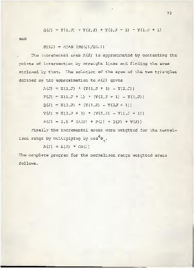
72

Q(J) = Y(l, J) + Y(2,J) + Y(2,J + 1) + Y(1,J + 1)

and

PH(J) = ATAN (PH(J)/Q(J))

The incremental area A (J) is approximated by connecting the

points of intersection by straight lines and finding the area

enclosed by them. The solution of the area of the two triangles

defined by the approximation to A (J) gives

A(J) = X(1,J) * (Yd, J + 1) - Y(2,J))

F(J) = X(1,J + 1) * (Y(2,J + 1) - Y(l, J))

Q(J) = X(2,J) * (Y(l, J) - Y(2,J + 1))

V(J) = X(2,J + 1) * (Y(2,J) - Y(l, J + 1))

A(J) = 0.5 * (A(J) + F(J) + Q(J) + V(J))

Finally the incremental areas were weighted for the normal-

4ized range by multiplying by cos 8 .

A(J) = A(J) * C0(J)

The complete program for the normalized range weighted areas

follows.

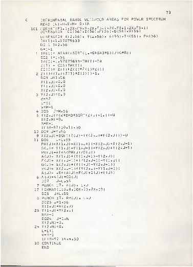
73

c INCREMENTAL RANGE WEIGHTED AREAS FOR POWER SPECTRUMREAD 101,U*B»H* D*TA

101 FORMAT ( F3. 1 ,2X,F9. 9, 2X,F3.1*2X,F3.1»2X,F3.1>DIMENSION CO(56) »Z(56),F(56) »G(56) »V(56)

DIMENSION X(2,56)» Y(2,56), A 1 55 ) , TH ( 56 ) » PH(56)TH( 1) = 1. 57079633DO 1 1=2,566-1-1

1 TH( I ) = ATAN( (SQRT( l.-G*G*8*B> )/(G*6)

)

D02 1=1,56TH( I ) =1.5 707963 3-TH( I )-TAZ( I > = COS(TH( I )

)

C0( I )= 2(1 )*Z( I )*Z( I )*Z( I

)

2 Z( I ) = (1./(Z( I)*Z( I ) ) )-l.D03 J=l»56X(1,J)=0.0Y( 1 ,J)=0.0X(2,J)=0.0

3 Y(2,J)=0.0M = 52L = 51W =M-1

4 D05 J=M»565 Y(2,J)=(W*B*D*SQRT(Z(J)+1. ) )-UX(2,M)=0.M=M + 1

IF(M-57) 10,11,3010 D09 J=M,569 X(2,J)=SQRT(Z< J)-(Y(2,J)*Y(2,J) ) )-U

11 D06 J=L,55PH< J)=X< 1,J)+X( 1»J+1 )+X(2,J)+X(2,J+l)0(J)= Y( 1,J)+Y( 1»J+1 )+Y(2,J)+Y(2»J+l)PH( J)=ATAN(PH( J)/Q( J)

)

A(J)= X(1,J)*(Y(1»J+1)-Y(2»J) )

F(J)= X( 1,J+1)*( <(2,J+1)-Y(1,J)

)

Q(J)= X(2»J)*(Y< 1»J)-Y(2»J+1 )

)

V(J)= X(2,J+1 )*(Y<2»J)-Y( 1,J+1)

)

A(J)= .5*(A( J)+F( J)+Q(J)+VU) )

6 A(J)=A( J) *CG(J)D07 J=L,55

7 PUNCH 17, A( J) , L»J17 FORMAT ( El 5. 8, 10X, I 3, 2 X, 13)

D08 J=L,558 PUNCH 17, PH( J) , L,J

D023 J=l,56X(1,J)=X(2,J)

23 Y( 1,J)=Y(2,J)N =M-1D024 J=1,NX(2,N)=0.

24 Y(2,N)=0.L = L + 1

W =M-1IFtM-57 )4,4,30

30 CONTINUEEND

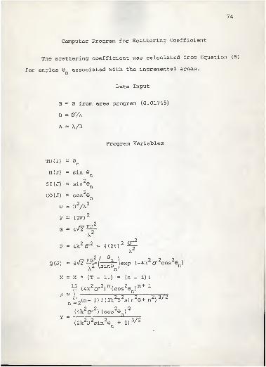
74

Computer Program for Scattering Coefficient

The scattering coefficient was calculated from Equation (5)

for angles 9 associated with the incremental areas.

Data Input

B = B from area program (0.01745)

D = cr/x

A = \/B

Program Variables

TH(I) = Gn

H(J) = sinn

SI (J) = sin2

n

CO (J) = cos2en

u = b2A 2

. F = (27f)2

G= 4/2^2

P = 4k2(T

2 = 4(2tt)2 ^r-

Q(J) = 4^^f-^")exp (-4k2 0- 2cos

2Gn )

A n

X - X * (T - 1.) = (n - 1) i

V5 (4kV 2

)

n(cos

29 )

n+1R =

L_An- 1) i (2k2B2sin

2G+ n2

)

3/2n — z

(4k2<r

2) (cos

2Gn )

2

Y =

(2k2B2sin

29 + 1)

3/2n

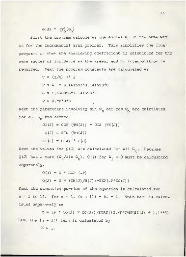
75

e(J) - cr <vFirst the program calculates the angles © in the same way

as for the incremental area program. This simplifies the final •

program, in that the scattering coefficient is calculated for the

same angles of incidence as the areas, and no interpolation is

required Next the program constants are ca lculated as

U = (1/A) ** 2

F = 4. * 3. 141593*3. 141593*U

G = 5. 656856*3. 141593*U

P = 4.*F*D*D•

Next the parameters involving sin and cos 0„ are calculatedn

for all © and stored.n

CO (J) = COS (TH(J)) * COS (TH(J))

H(J) = SIN (TH(J) )

SI (J) = H(J) * H(J)

Next the values for Q(J) are calculated for all 9 . Becausen

Q(J) has a term (Q /sin ) , Q(l) for ©. = C must be calculated

separate!Ly.

Q(l) = G * EXP (-P)

Q(J) = G * (TH(J)/H(J))*EXP(-P*CO(J))

Next the summation portion of the equation is calculated for

n = L to 15. For n = 1, (n - 1) 1 = Oi = 1. This term is calcu-

lated separately as

Y = (? * CO (J) * CO (J) )/SQRT( (2.*F*U*SKSI(J) + l.)**3)

Next the (n - 1)1 term is calculated by

X = 1.

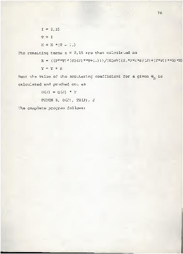
76

I = 2,15

T = I

X = X *(T - 1.)

The remaining terms n = 2,15 are then calculated as

R = ((P**T)*(CO(J) **T+1.) ) )/(SQRT((2.*F*U*SI(J) + (T*T))**-3) *X)

Y = Y + R

Next the value of the scattering coefficient for a given © is

calculated and punched out as

0(J) - Q(J) * Y

PUNCH 9, 0(J), TH(J), J

The complete program follows:

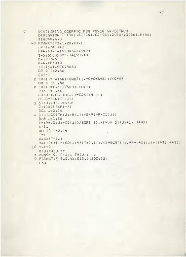
77

SCATTIRING CCEFFIC FOR POWER SPRECTRUMDIMENSION TH(56) »SI ( 56) ,CO<56) ,Q<56) ,0(56) ,H(56)READ40,A,D

40 FORMAT(F3.1,2X»F3.1)U=( l./A)**2F=4.*3. 14159 3*3. 141593G=5. 65685 6*3. 141593*UB=. 01745P=4.*F*D*DTH(1)=1. 57079633DO 2 1=2,56C=I-1

2 TH{I)= ATAN< (SQRT( l.-C*C*B*B) >/(C*B> )

DO 8 1=1,568 TH( I)=1.57079633-TH( I

)

D03 J=l,56C0( J)=COS(TH( J) )*C0S(TH( J)

)

H( J)=SIN( TH( J)

)

3 SI ( J)=H( J)*H(J)0(1 )=G*EXP(-P)D04 J=2,56

4 Q( J)=G*(TH(J)/H(J) )*EXP(-P*CO( J) )

D05 J=l,56Y=(P*CO(J)*CO( J) )/SQRT( (2.*F*U* SHJ1 + 1. >**3)

X = l.

DO 10 1=2,15*

T = I

X=X*(T-1.

)

r=( |p* *T)*iCO( J)**(T+1. ) ) )/(X*SQRT( (2.*F*U*SI ( J)+(T*T) )**3)

)

10 Y=Y+R0< J)=Q( J)*Y

5 PUNCH 9, 0(J) , TH( J) J

9 FORMAT(E15.8,4X»E15.8,30X,I2

)

END '

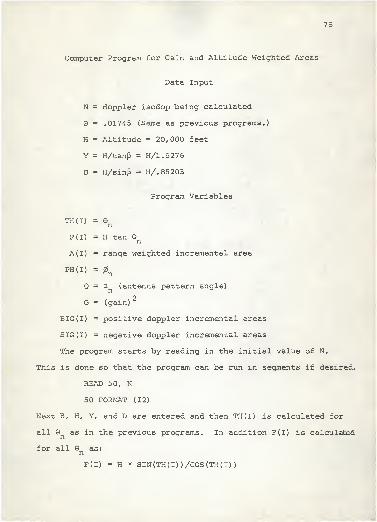
78

Computer Program for Gain and Altitude Weighted Areas

Data Input

N = doppler isodop being calculated

B = .01745 (Same as previous programs.)

H = Altitude = 20,000 feet

Y = H/tanP = H/1.6276

D = H/sinj3 = H/. 35203

Program Variables

nTH(I) = 0.

F(I) = H tan ©n

A (I) = range weighted incremental area

PH(I) ='n

Q = a (antenna pattern angle)n

2G = (gain)

BIG (I) = positive doppler incremental areas

SIG(I) = negative doppler incremental areas

The program starts by reading in the initial value of N.

This is done so that the program can be run in segments if desired.

READ 50, N

50 FORMAT (12)

Next B, H, Y, and D are entered and then TH(I) is calculated for

all 9 as in the previous programs. In addition F(I) is calculated

for all as:n

F(I) = H * SIN(TH(I))/COS(TH(I) )

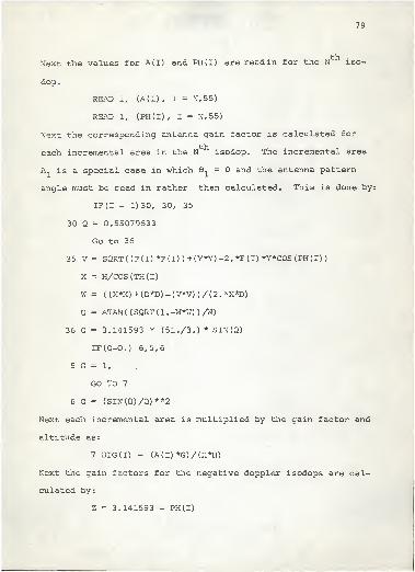
79

Next the values for A(I) and PH(I) are read in for the N ' iso-

dop.

READ 1, (A(I) , I = N,55)

READ 1, (PH(I) , I = N,55)

Next the corresponding antenna gain factor is calculated for

each incremental area in the N isodop. The incremental area

A. is a special case in which Q* = and the antenna pattern

angle must be read in rather than calculated. This is done by:

IF(I - 1)30, 30, 35

30 Q = 0.55079633

Go to 36

35 V= SQRT((F(I) *F (I) ) +(Y*Y) -2. *F (I) *Y*C0S (PH (I)

)

X = H/C0S(TH(I)

W = ((X*X) + (D*D)-(V*V))/(2.*X*D)

Q = ATAN ( ( SQRT ( 1 . -W*W) ) /W)

36 Q = 3.141593 * (51./3.) * SIN(Q)

IF(Q-Q.) 6,5,6

5 G = 1.

GO TO 7

6 G = (SIN(Q)/Q)**2

Next each incremental area is multiplied by the gain factor and

altitude as:

7 BIG(I) = (A(I) *G)/(H*H)

Next the gain factors for the negative doppler isodops are cal-

culated by:

Z = 3.141593 - PH(I)

30

The remainder of the program for the gain is the same as

above except, PH(I) is replaced by Z. The complete program is

as follows.

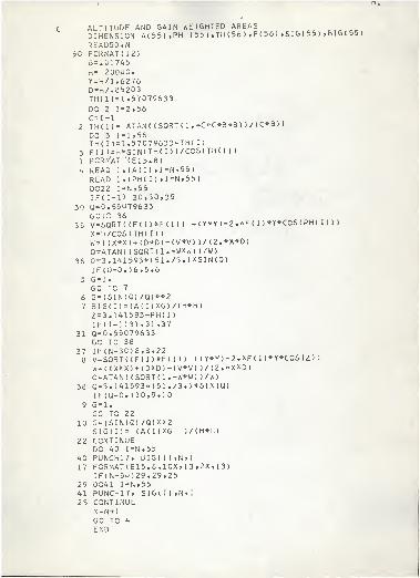
ai

c ALTITUDE AND GAIN WEIGHTED AREASDIMENSION A(55)»PH ( 55 ) , TH ( 56 ) , F ( 56 ) ,SI G ( 55 ) » BIG ( 55

)

READ50.N50 FORMAT I 12)

13 = . 01745H= 20000.Y=H/1.6276D =H/. 85203TH( 1)= 1.57079633DO 2 1=2,56C=I-1

2 TH( I)= ATAN( (SQRT(1.-C*C*B*B) )/(C*B)

)

DO 3 I=l»56TH( I ) = 1.57079633-TH( I

)

3 F( I )=H*SIN(TH( I ) )/COS(TH( I ) )

1 FORMAT (E15.8)4 READ 1»(A( I ) ,I=N»55)

READ 1* (PH( I ) ,I=N,55

)

D022 I=N»55I F {

I - 1 > 30,30,3530 0=0.55079633

GOTO 3635 V = SQRT( (F( I)*F( H ) +(Y*Y)-2-*F( I )*Y*CCS(PH( I )) )

X=H/COS(TH( I )

)

W=( (X*X)+(D*D)-(V*V) J/(2.*X*D)Q=ATAN( (SQRT( l.-W*W) )/W)

36 0=3.141593*1 51. /3.)*SIN(Q)IF(Q-0. )6,5»6

5 G=l.GO TO 7

6 G=(SIN(0)/Q)**27 BIG( I ) = (A( I )*G)/(H*H)2=3.141593-PH{ I

)

I F (1 -1 )31, 31,37

31 0=0.55079633GO TO 38

37 IF(N-3C)8,8,228 V=SQRT( (F( I)*F( I ) ) +(Y*YJ-2.*F( I )*Y*COS(Z)

)

W=( (X*X)+(D*D)-(V*V) )/(2.*X*D)Q=ATAN{ (SQRT( l.-W*W) )/W)

38 Q=3.141593*(51./3. )*SIN(Q)IF(Q-0. )10,9,10

9 G = l.

GO TO 2210 G=(SIN(Q) /Q)**2

SIG(I)= (A(I)*G )/(H*H)22 CONTINUE

DO 40 I=N»5540 PUNCH17. BIG(I),N,I17 F0RMAT(E15.8,10X»I3,2X,I3)

IF(N-3^)29,29,2529 D041 I=N,5541 PUNCH17, SIG( I ) ,N»I25 CONTINUE

N = N+1GO TO 4END

82

Computer Program for Final Power Spectrum

The program for the final power spectrum reads in data

cards from the programs for weighted incremental areas and

scattering coefficients. This data is multiplied and summed

over each isodop for the final spectrum. The complete program

is as follows:

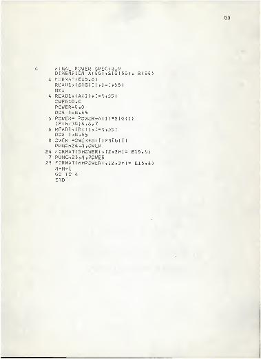
83

FINAL POWER SPECTRUMDIMENSION A(55) »SIG(55) » B<55)

1 FORMAT (El 5. 8)

READ1»(SI6( I ) .1=1*55)N=l

4 READ1,(A( I ) , I=N»55)OWER=0.0POWER=0.0D05 I=N»55

5 POWER= POWER+A( I )*SIG< I

)

IF(N-30)6»6»76 READ1,(B( I ) ,I = N»55)

D08 I=N»558 OWER =OWER + B( I )*~>IG( I )

PUNCH24,N,0WER24 FORMAT(5HOWER( »I2i3H}= E15.8)7 PUNCH23»N»POWER

23 F0RMAT(6HP0WER( »I2»3H)= E15.8)N = N + 1

GO TO 4END'

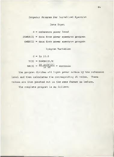
84

Computer Program for Normalized Spectrum

Data Input

X = reference power level

POWER (I) = data from power spectrum program

OWER(I) = data from power spectrum program

Program Variables

C = In 10.0

Y(I) = POWER(I)/X

DB(I) = 10 j-MY(i)) = decibels

The program divides all input power levels by the reference

level and then calculates the corresponding db value. These

values are then punched out in the same format as before.

The complete program is as follows:

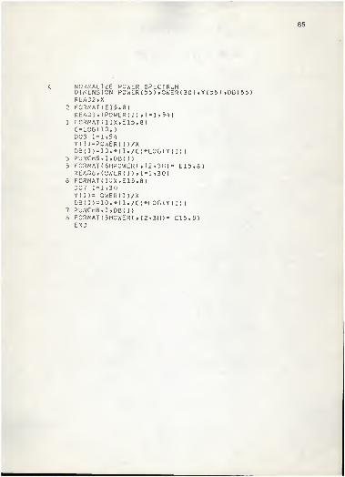
85

NORMALIZE POWER SPECTRUMDIMENSION POWER (55) ,OWER(30) * Y ( 55 ) ,DB( 55

)

READ2»X2 FCRMAT(E15.8)

READ1. (POWER( I

)

»I=1»54)1 FCRMAT(11X.E15.8)C=LOG(10.

)

003 1*1*54Y( I )=POWER< I )/XDB{ I )=10.*( l./C)*LOG(Y( I )

)

3 PUNCH5,I ,DB( I

)

5 FORMAT (6HP0WERI »I2»3H)= E15.8)READ6»(0WER( I). 1*1 .30)

6 FORMAT! 10XfE15. 8)D07 1=1,30Y( I )= OWER( I )/XDB( I )=10.*( l./C)*LOG(Y< I )

)

7 PUNCH8,I ,DB( I

)

8 F0RMAT(5H0WER( ,I2»3H)= E15.8)END

AIRBORNE RADAR GROUND CLUTTERRETURN

by

ROBERT A. McMILLEN

B. S., Kansas State University, 1960

AN ABSTRACT OF A MASTER'S THESIS

submitted in partial fulfillment of the

requirements for the degree

MASTER OF SCIENCE

Department of Electrical Engineering

KANSAS STATE UNIVERSITYManhattan, Kansas

1964

In analysis and design of airborne moving target indication

(AMTI) radars, it is necessary to establish an accurate model

for return from the ground, commonly called "clutter". This

paper investigates the effect of surface roughness on clutter

power spectrum. A review of the basic radar return theory with

emphasis on a scattering coefficient derived by Hayre and Moore

is given. This coefficient incorporates a quantitative expression

for the effect of surface roughness on radar return. Signal cor-

relation and power spectrum for random processes are also briefly

reviewed.

Analyses of clutter and AMTI performance reported in the

literature are included. These analyses techniques may be

divided in two classes, namely, random variable models and

deterministic models. Random variable models have been used

extensively to calculate clutter cancellation ratios and the

probability of detection for AMTI radars. Deterministic models

have been used for calculation of the return power spectrum for

specified parameters. A deterministic approach of Welch and

recently of Farrell and Taylor was used as a basis for a modified

mathematical model for the calculation of ground clutter power

spectrum. The major contribution of this work is the use of the

Hayre-Moore scattering coefficient for investigation of the effect

of terrain roughness on the clutter spectrum.

Clutter spectrums were calculated for three varying degrees

of surface roughness using Hayre-Moore scattering coefficients

and for an assumed constant scattering coefficient. Data was

compiled, using an IBM 1620 digital computer, from the appended

programs. Effect of terrain roughness on clutter spectrum was

found to be most significant near the vertical. At angles greater

than approximately three to four degrees, the shape of the spec-

trum is relatively insensitive to changes in surface roughness.

It was found that the use of a constant scattering coefficient,

as is often done in practice, may result a large error in the

power spectrum at the high frequency end. This is the area of

prime importance in a doppler frequency detection system, because

AMTI performance against low velocity targets is primarily deter-

mined by signal to clutter ratio as the signal moves into the

clutter region of the spectrum.