Air Shower Simulations

Air Shower Simulations' Marco Alania*, Ignacio J. Araya^, Adolfo V. Chamorro Gomez*, Humberto

Martinez Huerta**, Alejandra Parra Flores^ and Johannes Knapp§

*Centro de Tecnologias de Informacion y Comunicaciones, Universidad Nacional de Ingenieria, Lima, Peru

Wepartamento de Astronomiay Astrofisica, Pontificia Universidad Catolica de Chile, Av. Vicuna Mackenna 4860, Santiago, Chile

**Facultadde Ciencias Fisico Matemdticas, Benemerita Universidad Autonoma dePuebla, Puebla, Mexico

^Facultad de Ciencias Fisico Matemdticas, Benemerita Universidad Autonoma dePuebla, Puebla, Mexico

^School of Physics and Astronomy, University of Leeds, Leeds LS2 9JT, UK

Abstract. Air shower simulations are a vital part of the design of air shower experiments and the analysis of their data. We describe the basic features of air showers and explain why numerical simulations are the appropriate approach to model the shower simulation. The CORSIKA program, the standard simulation program in this field, is introduced and its features, performance and limitations are discussed. The basic principles of hadronic interaction models and some gemeral simulation techniques are explained. Also a brief introduction to the installation and use of CORSIKA is given.

Keywords: cosmic rays, air showers, simulations, hadronic interactions PACS: 02.70.Uu, I3.85.Tp, 96.50.sd, 96.50.sf

Introduction

Cosmic rays (CR) are charged particles, mostly protons and ionised nuclei, from outer space. CR energies range from 10^ to > 10̂ *̂ eV, following an approximate power law. The flux of the highest energy cosmic rays is very low. Above 10̂ *̂ eV it is less than 1 particle per km^ per century. Therefore high-energy CRs are only detectable by their interaction with the Earth atmosphere.

The main questions about cosmic rays are: Where do Cosmic Rays come from? What are they? How do they get their energies? To answer these questions requires to measure the energy and arrival directions and identify the primary CRs first.

Numerical simulation of the shower development in the atmosphere is a powerful approach to link the properties of the measured shower to those of the primary particle. In this work we discuss how simulations are used in CR physics, we describe the main ingredients needed in a numerical model, present the CORSIKA EAS simulation program and discuss its strengths and limitations. Finally we present a short tutorial on how to install and use CORSIKA.

^ This article is based on a series of lectures given at the "Third School on Cosmic Rays and Astrophysics", August 25 to September 5, 2008, Arequipa - Peru, (http://www.physics.adelaide.edu.au/)

CP1123, Cosmic Rays and Astrophysics, edited by C. J. Solano Salinas, D. Wahl, J. Bellido, and 6. Saavedra © 2009 American Institute of Physics 978-0-7354-0659-9/09/$25.00

150

Downloaded 25 May 2009 to 128.83.63.22. Redistribution subject to AIP license or copyright; see http://proceedings.aip.org/proceedings/cpcr.jsp

http://02.70.Uu

http://www.physics.adelaide.edu.au/

Air Showers and Simulations

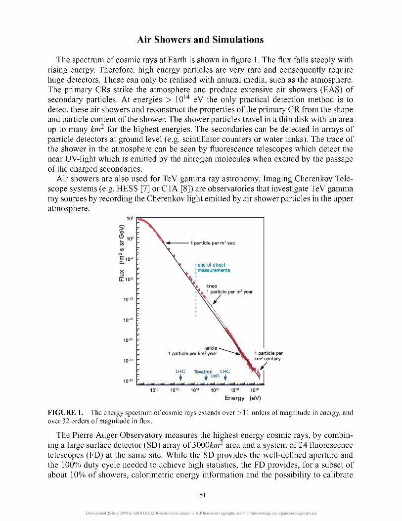
The spectrum of cosmic rays at Earth is shown in figure 1. The flux falls steeply with rising energy. Therefore, high energy particles are very rare and consequently require huge detectors. These can only be realised with natural media, such as the atmosphere. The primary CRs strike the atmosphere and produce extensive air showers (EAS) of secondary particles. At energies > lO '̂̂ eV the only practical detection method is to detect these air showers and reconstruct the properties of the primary CR from the shape and particle content of the shower. The shower particles travel in a thin disk with an area up to many kn? for the highest energies. The secondaries can be detected in arrays of particle detectors at ground level (e.g. scintillator counters or water tanks). The trace of the shower in the atmosphere can be seen by fluorescence telescopes which detect the near UV-light which is emitted by the nitrogen molecules when excited by the passage of the charged secondaries.

Air showers are also used for TeV gamma ray astronomy. Imaging Cherenkov Telescope systems (e.g. HESS [7] or CTA [8]) are observatories that investigate TeV gamma ray sources by recording the Cherenkov light emitted by air shower particles in the upper atmosphere.

10*

1 particle per m^ sec

end of direct measurements

knee •^ 1 particie per m^ year

1 particie per km^ century

LHC Tevatron LHC

Energy (eV)

FIGURE 1. The energy spectrum of cosmic rays extends over >11 orders of magnitude in energy, and over 32 orders of magnitude in flux.

The Pierre Auger Observatory measures the highest energy cosmic rays, by combining a large surface detector (SD) array of 3000^m^ area and a system of 24 fluorescence telescopes (FD) at the same site. While the SD provides the well-defined aperture and the 100% duty cycle needed to achieve high statistics, the FD provides, for a subset of about 10%) of showers, calorimetric energy information and the possibility to calibrate

151


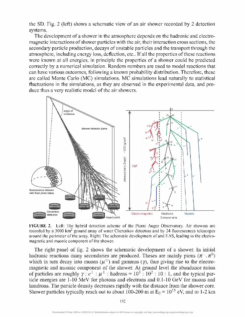
the SD. Fig. 2 (left) shows a schematic view of an air shower recorded by 2 detection systems.

The development of a shower in the atmosphere depends on the hadronic and electromagnetic interactions of shower particles with the air, their interaction cross sections, the secondary particle production, decays of unstable particles and the transport through the atmosphere, including energy loss, deflection, etc.. If all the properties of these reactions were known at all energies, in principle the properties of a shower could be predicted correctly by a numerical simulation. Random numbers are used to model reactions that can have various outcomes, following a known probability distribution. Therefore, these are called Monte Carlo (MC) simulations. MC simulations lead naturally to statistical fluctuations in the simulations, as they are observed in the experimental data, and produce thus a very realistic model of the air showers.

Hadronic Components

Muonic

FIGURE 2. Left: The hybrid detection scheme of the Pierre Auger Observatory. Air showers are recorded by a 3000 km̂ ground array of water Cherenkov detectors and by 24 fluorescences telescopes around the perimeter of the array. Right: The schematic development of and EAS, leading to the electromagnetic and muonic component of the shower

The right panel of fig. 2 shows the schematic development of a shower. In initial hadronic reactions many secondaries are produced. Theses are mainly pions (7r̂ ,7r* )̂ which in turn decay into muons (/i^) and gammas (7), thus giving rise to the electromagnetic and muonic component of the shower. At ground level the abundance ratios of particles are roughly 7 : e^ : / i ^ : hadrons = 10-̂ : 10^ : 10 : 1, and the typical particle energies are 1-10 MeV for photons and electrons and 0.1-10 GeV for muons and handrons. The particle density decreases rapidly with the distance from the shower core. Shower particles typically reach out to about 100-200 m at EQ = 10^^ eV, and to 1-2 km

152


at 10^^ eV. The charged particles ionise the air and produce Cherenkov and fluorescence light. The former is emitted in the forward direction, collimated in an opening angle of about 1° around the shower axis, the latter is emitted isotropically.

The air shower analysis aim primarily at the energy spectrum, the arrival direction distribution and the mass composition of the primary cosmic rays. The direction of a cosmic ray is easily determined from the arrival times of shower particles at distributed detectors in an array. The energy of the primary is deduced from the "size" of the shower, i.e. from the number of secondaries produced. The mass of the primary is reflected in the height of the shower development, the muon to electron ratio in the shower and the amount of fluctuations. On average, Fe showers have a higher 1st interaction and a higher shower maximum than proton showers. This is due to dpe-Air being larger than cjp_Air and the energy per nucleon is smaller. Fe interactions produce more secondaries (since #sec ^ ln(£')), and therefore more muons and less electrons-positrons and photons at ground level. They exhibit smaller fluctuations, since each shower is a composition of 56 subshowers which average out larger fluctuations. The height of the development and the increased muon number leads also to a faster signal rise time. To quantify how exactly primary energy and mass affect the observable quantitites in an air shower is the subject of air shower analysis. However, the analysis is complicated by the fact that at high energies also the hadronic interaction are rather uncertain. There are no testbeams at CR energies, where the relevant hadronic reactions could be measured, nor is there a fundamental theory (such as QED for the electromagnetic interaction) on which extrapolation to the highest energies could be based. A variety of phenomenological models, tuned to the existing collider data, have been proposed. These models describe the overall features of air showers quite well, but fall short, if a precision in the prediction of less than about 30% is needed, (e.g. for telling proton and iron showers apart). Then the fundamental uncertainties in the details of the hadronic and nuclear interactions are the limiting factor. Thus, understanding the astro-particles means to find a combination of primary spectrum & composition and hadronic interaction model such that simulations and data are consistent with each other in all respects.

With recent air shower experiments progress has been made in various fields: • TeV gamma ray experiments [7, 9, 11, 12] have detected more than 80 sources with a wealth of results on all many astrophysical objects and acceleration mechanisms. Thus, TeV astronomy has been established as a field with tremendous potential. • The spectrum and the composition in the knee region has been measured by the KASCADE Collaboration [10]. • At highest energies the existence of the Greisen-Zatsepin-Kuz'min cut-off in the CR spectrum has been found [6, 13], limits on primary neutrinos [5] and photons [4] have been placed, and, for the first time, an anisotropy in the CR arrival directions has been detected, hinting at nearby AGN as sources of the CRs [2, 3].

153


EAS Models and the CORSIKA Program

To build a realistic air shower model requires a number of ingredients. The composition and layering of the iteraction medium (atmosphere) needs to be specified. The projectile particles (primary and secondaries) can be virtually any known particles being produced in collisions (nuclei, p, n, e^, 7, / i^ , K^, TI^, K ^ , p , Q., A, A, E, ...). Their interactions (cross section and particle production) with the nuclei in air and their decay properties need to be known. Tracking, deflection in the Earth magnetic field, multiple scattering, energy loss, absorption, ionization, Cherenkov light production are to be taken into account.

Most of these ingredients are well known. Thus, the Monte Carlo technique provides the ideal method to provide a convolution of all the elementary processes to form the complex model of the whole shower. If the individual parts are simulated properly, then also the overall shower is modelled realistically. The main uncertainties of the shower simulation come from the hadronic and nuclear interaction, where there are still large uncertainties.

An example of such an Air Shower Monte Carlo is CORSIKA (Cosmic Ray Simulations for Kascade) [1]. CORSIKA is a program for very detailed simulation of extensive air showers initiated by high energy cosmic ray particles. It used proven components whereever possible. For the uncertain hadronic interactions at high energies a number of interaction models have been implemented: QGSJET, DPMJET, EPOS, (models are based on the successful Gribov-Regge theory of multiple Pomeron exchange), SIBYLL (a minijet model with Gribov-Regge type features), and FLUKA and UrQMD are used for hadronic interactions at low energies.

For electromagnetic interactions a modified version of the shower program EGS4 (or the analytical NKG formulae) can be used. Options for the simulations of Cherenkov radiation and neutrinos exist. CORSIKA can be used from 10^ up to 10̂ ^ eV and beyond. For references to the models, see the references in ref [1]. CORSIKA allows production of very educational shower images, and movies of the shower development (see e.g. [14, 15]). Examples of simulated showers are shown in figs. 7 and 8. Note the richness of details and the complexity of individual trajectories.

Hadronic Interactions

The features of hadronic interaction models that are most relevant for the air shower development are the interaction cross sections and the secondary particle productions. The latter is usually described by the inelasticity, the fraction of the projectile's energy spent to produce secondary particles. Larger cross sections and bigger inelasticities produce short showers. Conversely, lower cross sections and smaller inelasticities lead to longer showers.

Hadronic interaction can be of very different types: Elastic scattering leaves projectile and target unchanged. Very little energy and

momentum and no charge or colour are transferred. The scattering of the projectile is very small. As these interactions are elastic, i.e. do not produce secondaries, they do not

154


contribute to the air shower development. They can be ignored in the simulations. Inelastic, diffractive scattering has very similar characteristics to elastic scattering

(small scattering, small energy and momentum transfer, no charge or colour transfer), but one or both of the collision partners are put into an excited state, which decays in a small number of secondaries that are emitted in the forward direction (i.e. the direction of one of the incoming collision partners). About 10% of all inelastic p-p reactions are found to be diffractive. These interactions have a very small inelasticity and therefore make the showers longer. The actual fraction (and its change with energy) is therefore one of the crucial inputs to an hadronic interaction model.

Inelastic, non-diffractive, soft scattering is the lion's share of the interactions happening in an air shower (about 90% for p-p). The energy and momentum transfer is still small, but as colour is transferred between quarks of the collision partners, 2 colour strings are stretched between a quark from one collision partner to a di-quark from the other one, and vice versa. Upon fragmentation of the colour strings many secondaries are produced which carry away much of the available energy. The secondaries are still largely emitted along the initial direction of the collision partners. As these reactions have only a small momentum transfer (i.e. they are "soft"), they cannot be calculated within QCD. This is the domain of the Gribov-Regge theory, that is also used to describe elastic scattering.

Inelastic, non-diffractive, hard scattering has also colour transfer, creating strings and many secondaries. In addition, hard reactions have a large momentum transfer, and thus these reactions can be computed in QCD. This is the domain of particle physics and collider experiments. Due to the large momentum transfer the secondary particles are emitted under large angles to the incoming collision partners, and can easily be recorded in detectors placed around the beam pipe. These reactions are best suited for producing new particles (such as W, Z, t-quarks or the HIGGS), but the cross sections for hard interactions are 10^ to 10^ x smaller than those for soft interactions. Therefore, hard interactions play only a minor role in air shower physics.

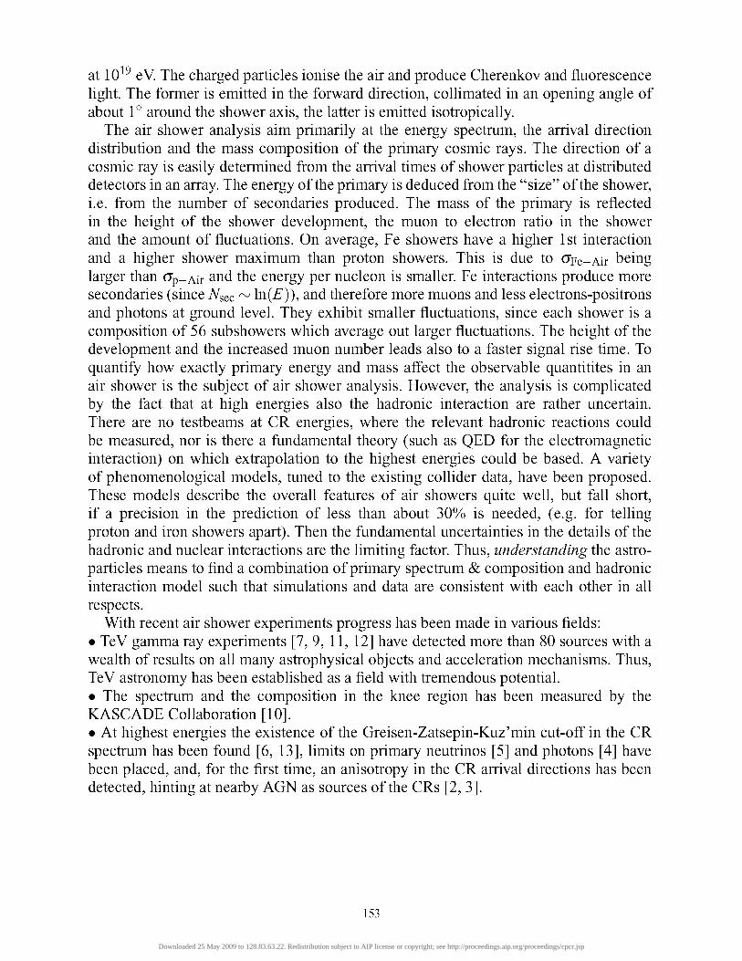
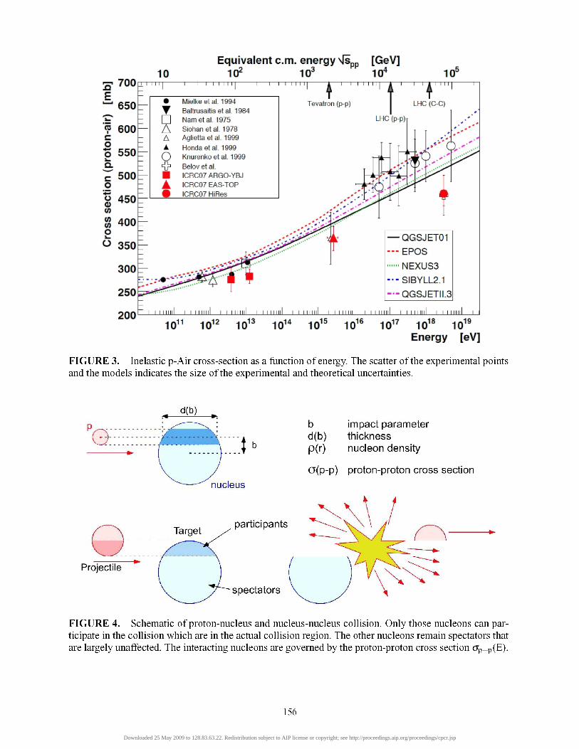
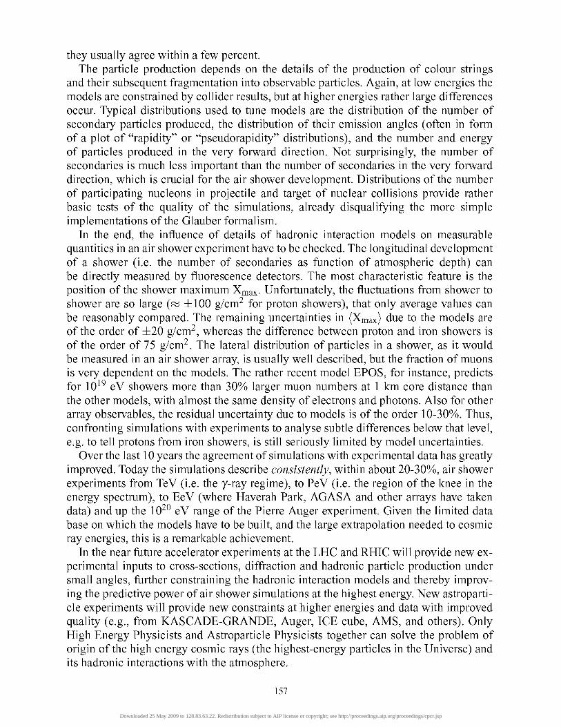
The change of cross sections with energy has been measured for p-p collisions and shows the resonance region (p < 2 GeV/c), a smooth decrease (2 < p < 100 GeV/c), and then a steady rise (p > 100 GeV/c), and are usually explained by the exchange of complex, hypothetical exchange particles, called the "Reggeon" (responsible for the falling part of the cross section) and the "Pomeron" (for the rising part). The highest available measurement is still at Tevatron energies (i.e. 2x900 GeV in the centre of mass system, corresponding to p = 1.7 x 10^ GeV/c), but for the highest-energy cosmic rays cross sections up to > 10̂ *̂ eV = 10̂ ^ GeV are needed. The large extrapolation (over 5 orders of magnitude) depends crucially on the assumptions made on the energy dependence of the p-p cross section. The more relevant p-nucleus, TT-nucleus (see fig. 3) and nucleus-nucleus cross sections as function of energy are then computed via the Glauber formalism (see fig. 4, where nucleus-nucleus collisions are effectively reduced to nucleon-nucleon collisions of a subset of participating nucleons, while the other nucleons remain spectators as illustrated in fig. 4. The uncertainties in cjp_p translate directly into similar uncertainties in cjp_Air, (yn-K\x and cJnucieus-Air- Despite a sizeable reduction over the last 10 years, typical systematic uncertainties are still of the order of ± 25%) at high energies. An average value at E=10^^ eV, for instance, is cjp_Air ~ 500 mb. At much lower energies, where measurements from colliders constrain the models,

155


Equivalent c m . energy \ I i [GeV]

3 -700 E " 650

n 600 c o o 5 5 0 ^ Q.

^ 500 o -g 450 (/)

|g 400 o

O 3 5 0 -

300

250

200

10 Itf T I I I I I

10^ pp

10" 10 '

•

• rj 2 A A

u <>

• • •

Mielkeetal. 1994 Baltmsaitis et al 1984 Nam etal. 1975 Slohanetal 1978 Agliettaetal 1999

Honda etal. 1999 Knurenko et al. 1999 Belov et al ICRC07 ARGO-YBJ ICRC07 EAS-TOP ICRC07HiRes

T Tevatron (p-p) r n I I I I I I I

LHC (C-C)

LHC (p-p)

— QGSJET01

- - - EPOS

NEXUS3

-••SIBYLL2.1

— QGSJETII.3

I I null I I I mill I

10 i l l 10 12 10 13 10 i14 10 15 10 ,16 10 ,17 10 18 10 19

Energy [eV]

FIGURE 3. Inelastic p-Air cross-section as a function of energy. The scatter of the experimental points and the models indicates the size of the experimental and theoretical uncertainties.

nucleus

participants

Projectile

spectators

b impact parameter d(b) thickness p(r) nucleon density

o(p-p) proton-proton cross section

FIGURE 4. Schematic of proton-nucleus and nucleus-nucleus collision. Only those nucleons can participate in the collision which are in the actual collision region. The other nucleons remain spectators that are largely unaffected. The interacting nucleons are governed by the proton-proton cross section ap_p(E).

156


they usually agree within a few percent. The particle production depends on the details of the production of colour strings

and their subsequent fragmentation into observable particles. Again, at low energies the models are constrained by collider results, but at higher energies rather large differences occur. Typical distributions used to tune models are the distribution of the number of secondary particles produced, the distribution of their emission angles (often in form of a plot of "rapidity" or "pseudorapidity" distributions), and the number and energy of particles produced in the very forward direction. Not surprisingly, the number of secondaries is much less important than the number of secondaries in the very forward direction, which is crucial for the air shower development. Distributions of the number of participating nucleons in projectile and target of nuclear collisions provide rather basic tests of the quality of the simulations, already disqualifying the more simple implementations of the Glauber formalism.

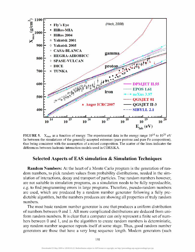
In the end, the influence of details of hadronic interaction models on measurable quantities in an air shower experiment have to be checked. The longitudinal development of a shower (i.e. the number of secondaries as function of atmospheric depth) can be directly measured by fluorescence detectors. The most characteristic feature is the position of the shower maximum Xmax- Unfortunately, the fluctuations from shower to shower are so large (^ ±100 g/cm^ for proton showers), that only average values can be reasonably compared. The remaining uncertainties in (Xmax) due to the models are of the order of ±20 g/cm^, whereas the difference between proton and iron showers is of the order of 75 g/cm^. The lateral distribution of particles in a shower, as it would be measured in an air shower array, is usually well described, but the fraction of muons is very dependent on the models. The rather recent model EPOS, for instance, predicts for 10^^ eV showers more than 30% larger muon numbers at 1 km core distance than the other models, with almost the same density of electrons and photons. Also for other array observables, the residual uncertainty due to models is of the order 10-30%. Thus, confronting simulations with experiments to analyse subtle differences below that level, e.g. to tell protons from iron showers, is still seriously limited by model uncertainties.

Over the last 10 years the agreement of simulations with experimental data has greatly improved. Today the simulations describe consistently, within about 20-30%), air shower experiments from TeV (i.e. the y-ray regime), to PeV (i.e. the region of the knee in the energy spectrum), to EeV (where Haverah Park, AGASA and other arrays have taken data) and up the 10̂ *̂ eV range of the Pierre Auger experiment. Given the limited data base on which the models have to be built, and the large extrapolation needed to cosmic ray energies, this is a remarkable achievement.

In the near future accelerator experiments at the LHC and RHIC will provide new experimental inputs to cross-sections, diffraction and hadronic particle production under small angles, further constraining the hadronic interaction models and thereby improving the predictive power of air shower simulations at the highest energy. New astroparticle experiments will provide new constraints at higher energies and data with improved quality (e.g., from KASCADE-GRANDE, Auger, ICE cube, AMS, and others). Only High Energy Physicists and Astroparticle Physicists together can solve the problem of origin of the high energy cosmic rays (the highest-energy particles in the Universe) and its hadronic interactions with the atmosphere.

157


-̂-- 1100 F B

^,1000 E

500

400 -

• Fly's Eye • HiRes-MlA ' HiRes2004 1̂ Yakutsk 2001

9001- * Yakutsk 2005 ° CASABLANCA ^ HEGRA-AIROBICC

800 h h 0 SPASE-VULCAN

° DICE 7001- ^ TUNKA

600 -

(Heck, 2008)

gamma.

Auger ICRC2007

DPMJET IIS5 EPOS 1.61

-*"* neXus 3.97 QGSJET 01 QGSJET n-3 SIBYLL2.1

10 14

10 15

10 16

10 17

J ' • • " • "

10 18 19

10 10 20

FIGURE 5. Xniax as a function of energy. The experimental data in the energy range 10̂ "̂ to 10̂ ° eV lie between the simulations of the generally accepted extremes (pure protons and pure Fe composition), thus being consistent with the assumption of a mixed composition. The scatter of the lines indicates the differences between hadronic interaction models used in CORSIKA.

Selected Aspects of EAS simulation & Simulation Techniques

Random Numbers: At the heart of a Monte Carlo program is the generation of random numbers, to pick random values from probability distributions, needed in the simulation of interactions, decay and transport of particles. True random numbers however, are not suitable in simulation programs, as a simulation needs to be fully reproducible, e.g. to find programming errors in large programs. Therefore, pseudo-random numbers are used, which are produced by a random number generator following a fully predictable algorithm, but the numbers produces are showing all properties of truly random numbers.

The most basic random number generator is one that produces a uniform distribution of numbers between 0 and 1. All more complicated distributions are deduced from uniform random numbers. It is clear that a computer can only represent a finite set of numbers between 0 and 1, and as the algorithm to create random numbers is deterministic, any random number sequence repeats itself at some stage. Thus, good random number generators are those that have a very long sequence length. Modem generators (such

158


as RANMAR or RANLUX from the CERN library) can produce more than 9 x 10^ independent sequences of a period length of lO'̂ -̂ .

There are several methods to produce random numbers following a certain distribution from uniformly distributed random numbers.

Gaussian distributed random numbers, for instance, can be produced by the following method. If xi and X2 are two independent, uniformly distributed random numbers, then yi = •\/—21n(xi) •cos(27rx2) and72 = 21n(xi) •sin(27rx2) are independent, Gaussian distributed random numbers.

More general, if random numbers are needed that follow the probability density function f{x), then one can form the integral function F{x) = J^^f{x)dx. By construction, the values ofy = F{x) are between 0 and 1. In the case we can form the inverse function G(y) = F~^ iy), we can draw a random number j uniformly from the interval 0 to 1, then compute z = G(y), and get z which is distributed as f{x). This is a very fast and elegant method, but it requires that we are able to invert F(x), which is not always the case.

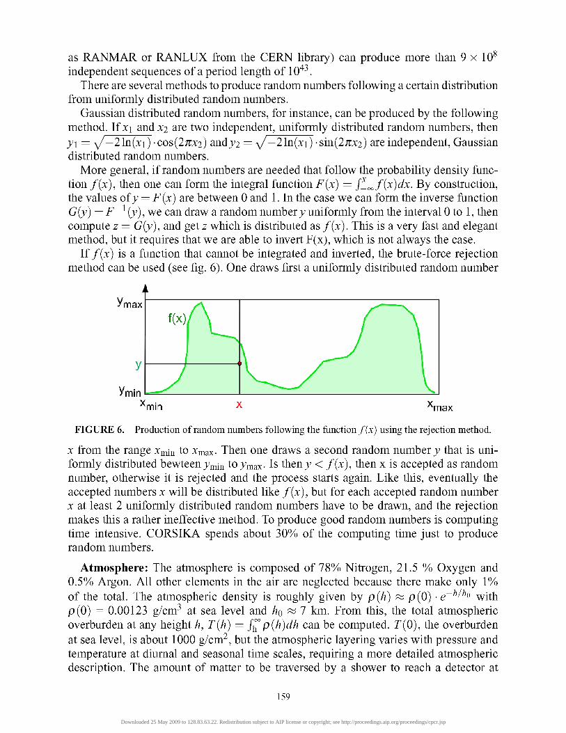
If/(x) is a function that cannot be integrated and inverted, the brute-force rejection method can be used (see fig. 6). One draws first a uniformly distributed random number

Vmax

ymin ^min X ^max

FIGURE 6. Production of random numbers following the function /(x) using the rejection method.

X from the range Xmin to Xmax- Then one draws a second random number j that is uniformly distributed bewteen jmin to jmax- Is then j < f{x), then x is accepted as random number, otherwise it is rejected and the process starts again. Like this, eventually the accepted numbers x will be distributed like f{x), but for each accepted random number X at least 2 uniformly distributed random numbers have to be drawn, and the rejection makes this a rather ineffective method. To produce good random numbers is computing time intensive. CORSIKA spends about 30% of the computing time just to produce random numbers.

Atmosphere: The atmosphere is composed of 78% Nitrogen, 21.5 % Oxygen and 0.5% Argon. All other elements in the air are neglected because there make only 1% of the total. The atmospheric density is roughly given by p{h) ^ p(0) • e~ /̂̂ o with p(0) = 0.00123 g/cm-̂ at sea level and AQ ~ 7 km. From this, the total atmospheric overburden at any height h, T{h) = J^p{h)dh can be computed. T{0), the overburden at sea level, is about 1000 g/cm^, but the atmospheric layering varies with pressure and temperature at diurnal and seasonal time scales, requiring a more detailed atmospheric description. The amount of matter to be traversed by a shower to reach a detector at

159


height h is then T{h)/ cos{6), with 6 being the zenith angle of the shower. A typical development of the number of shower particles with atmospheric depth t (in g/cm^) is often described by N{t) ^ c-t^ • e~^\ with t"^ giving the rising part and e~^^ giving the falling part of the shower. A 10̂ *̂ eV proton shower coming in vertically maximises around at sea level, a shower at a zenith angle of 70° will have to penetrate >3000 g/cm^ such that its electromagnetic component is practically absorbed and only muons arrive at ground level. The atmospheric model in CORSIKA uses various atmospheres that are parameterised in 5 layers with piece-wise fitted exponential. Special versions for different locations and seasons can be introduced.

Decay versus interaction: For secondary particles which are unstable, it is complicated to determine the location of the next action point, as collision and decay compete. The location of the next collsion depends on the matter traversed (x) according to the following simple probability distribution: dN/dx ^ e~^l^^, where AQ is the collision mean free path. The location of the next decay depends on the time, according to dN/dt r^ e~^l^ with T = /TQ being the proper life time TQ multiplied with the Lorentz factor 7. Since t = s/c = x/pc it follows that dN/dx ^ g-^/P^r^ where p is again an exponential depending on the height. Thus an analytic evaluation of the combined probability for collision or decay becomes quite difficult. The Monte Carlo method solves this problem elegantly, by computing independently a next action point due to a collision and the one due to decay, and selecting the one that happens first: (i) determine Xc from dN/dx ^ e~^l^^, (ii) determine t̂ from dN /dt ^ e~^l^, and compute x^ = t^cp (iii) if Xc < Xd then do a collision, otherwise a decay. This is a very fast procedure and it is exactly how nature determines the fate of an unstable particle.

Electromagnetic showers - from a toy model to EGS4: The main reaction of high-energy photons is eê~ pair production and of energetic electrons it is bremsstrahlung. Both reactions have about the same characteristic length, the radiation length (JTQ f̂ 37 g/cm^ in air), and lead to 2 particles in the final state. The Bethe-Heitler model describes qualitatively the development of an electromagnetic shower of energy EQ, by using a very simple description of these reactions: After each XQ, the particle number doubles, and the energy per particle is halved, until the energy of the secondaries falls below the critical QYievgy Ec, where particle multiplication stops. Here is the number of secondaries maximal. Thus, we find at depth t = k-X{) (with k = 1, 2, ...) that N{t) = 2^ and ^(^)=ô/2k. Atthe maximum of the shower development we find that

A'max = EQ/EC and Wx = ^0 • ln(ô/^c)/ ln(2) ,

i.e. the number of secondaries at the maximum is proportional to the primary energy EQ, and the position of the maximum increases with ln(E). The latter follows directly from Ec = -£'o/2max ^̂ <i Wx = XQ • kmax- These findings hold also for the much more complicated full simulation.

A better, but still analytic description of electromagnetic showers is provided by the Nishimura-Kamata-Greisen (NKG) formulae. The electron number as a function

160


of atmospheric depth is

Ne{t) = - With ^\n{Eo/Ec) t + 2\n{Eo/Ec)

s is the so-called age of the shower. In the shower maximum, i.e. t = tmax, the value of s=l. The lateral distribution of electrons at ground level is given by:

, , Ne r{4.5-s) fr^'-^' -^'-'•' Pe{r)- V ; /

iTirl r (^ ) r (4 .5 -^ ) \rmj

where Pe is the electron density as function of the core distance r, and rm = (0.78 — 0.21^)

• ^moh with the Moliere radius rmoi ~ 9.6 g/cm^. The NKG formulae do describe the shower shape of purely electromagnetic showers quite well, but they fail to deliver information on the fluctuations and are not strictly valid for hadronic showers. Nevertheless, the same functional forms are used to describe also hadronic cosmic ray showers. The variables rm and the powers s — 2 and s — 4.5 lose then their physical meaning and become free parameters in the fit.

The well-proven Electron Gamma Shower code (EGS) simulates all reactions of e+, e~ and photons in much greater detail and, therefore, provides a much better description of an electromagnetic shower, including fluctuations, lateral extension, energy distribution of shower particles and so on. EGS has been checked and verified by many researches in a big variety of different experiments. As EGS is based on QED, the extrapolation to the highest energies have fairly small uncertainties. Therefore, it is recommended to rely on EGS whenever possible. However, due to the large number of electrons and photons in an air shower and due to its complexity, EGS is relatively slow and dominates by far the computing time.

Simulation Speed-up: Computing time and disk space needed for a shower simulation grow approximately linear with primary energy. As a 10^^ eV shower needs about one hour to be simulated and produces close to 300 MB particle output on the disk, it is straight forward to estimate that a single shower at 10̂ *̂ eV, with about 10̂ ^ secondary particles, needs about 10^ hours (= 11.4 years) and a disk space of 30 Tera bytes. Obviously this is not practical.

Therefore, statistical subsampling (or thinning) [17] is used to discard most of the shower particles and follow only a representative subset of them, which carry a weight to account for the discarded ones. Thinning sets in once the particle energies drop below a certain threshold (typically 10~^ of the primary energy) allowing the initial part of the shower to develop without thinning. While the energy and the average properties of the shower are preserved, the statistical fluctuations are enhanced due to thinning and may bias the simulations in regions where only few particles are followed, e.g. at very large core distances. The fluctuations are especially large when particle acquire very high weights. Therefore, a limitation of weights is introduced which costs some computing time, but keeps the artefacts due to thinning relatively small. For a good compromise of thinning and weight limitation, typical seed-up factors of lO'̂ -lO^ are reached. Thus, the simulation of one 10̂ *̂ eV shower is reduced to about 20 hours.

161


With CORSIKA also unthinned showers at high energies can be simulated, by distributing subshowers onto many processors to reduce the computing time. The outputs of the subshowers are then stored in thousands of output files, which need to be combined for the analysis.

Install and run CORSIKA

The first point of contact and the place to find user manuals and general informations is the CORSIKA webpage: ht tp: / /www-ik.fzk.de/corsika/ . CORSIKA is a set of routines written in Fortran and C. The source and all files belonging to CORSIKA can be downloaded from the anonymous ftp server f tp- ik . fzk .de . However, to get access. You have to be registered. Send a request to Tanguy Pierog (e-mail: [email protected]) or Dieter Heck (e-mail: [email protected]), with the hostname of the computer (or static IP addresses) from which you intend to access the CORSIKA ftp site. Once the hostname of your computer has been registered you will receive instructions on how to download of CORSIKA code from this server. To install the software on LINUX systems one needs

gcc - the GNU C/C++ compiler make - a Compilation tool g77 - the GNU Fortran 77 compiler.

For the version to make shower plots one needs in addition libpngl2 - the PNG library (used by PL0TSH2 option) libpngl2-dev - the development header files for libpngl2 (used for PL0TSH2 option).

The CORSIKA set is distributed as a compressed tape archive (.tar.gz) file for each version (e.g. corsika-6735.tar.gz). Once you have got the CORSIKA file, unpack and compile CORSIKA by typing:

$ tar zxvf corsika-6735.tar.gz $ cd corsika-6735/ $ ./corsika-install

The corsika-install script lets you configure the version of CORSIKA you want to use. For information about the program variants consult the CORSIKA Users Guide. By always typing <Enter> you will install the default version.

The PLOTSH and PL0TSH2 are necessary to produce plots of the air shower. Finally, if all goes well, you end up with an message similar to the following :

--> "corsika6735Linux_QGSJET_gheisha" successfully installed in: /home/marko/cors ika-6735/run/

--> You can run CORSIKA in /home/marko/corsika-6735/run/ using: ./corsika6735Linux_QGSJET_gheisha < all-inputs > output.txt

To run a simulation, change to the "run/" subdirectory of the installation, where you find the executable generated by the compilation process. Execute it by typing:

$ ./corsika6735Linux_QGSJET_gheisha < all-inputs > output.txt

162


http://www-ik.fzk.de/corsika/

http://ik.fzk.de

mailto:[email protected]



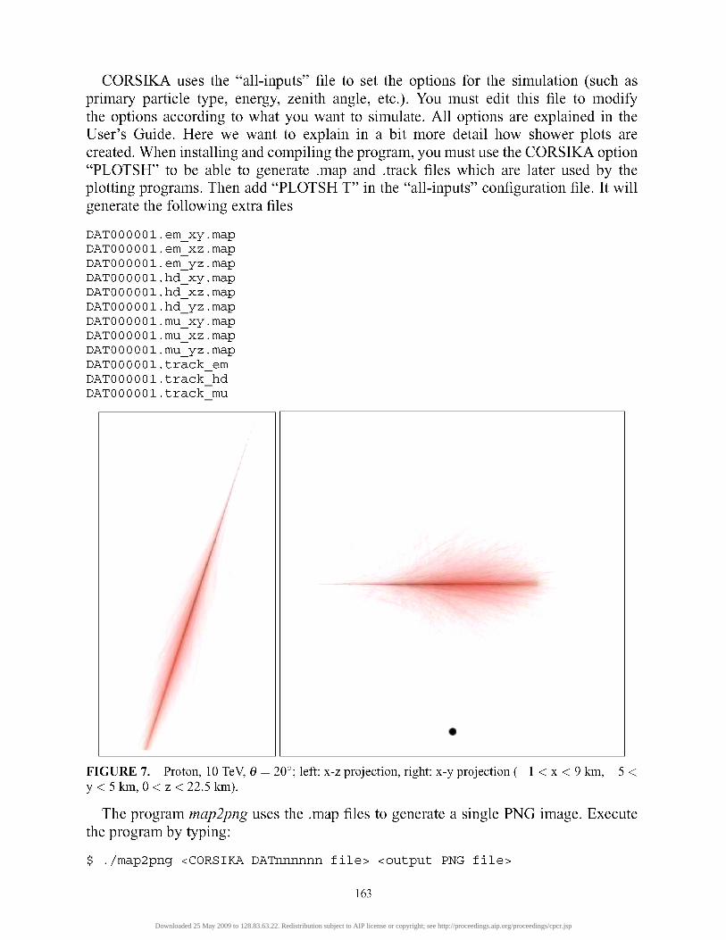
CORSIKA uses the "all-inputs" file to set the options for the simulation (such as primary particle type, energy, zenith angle, etc.). You must edit this file to modify the options according to what you want to simulate. All options are explained in the User's Guide. Here we want to explain in a bit more detail how shower plots are created. When installing and compiling the program, you must use the CORSIKA option "PLOTSH" to be able to generate .map and .track files which are later used by the plotting programs. Then add "PLOTSH T" in the "all-inputs" configuration file. It will generate the following extra files

DATOOOOOl DATOOOOOl DATOOOOOl DATOOOOOl DATOOOOOl DATOOOOOl DATOOOOOl DATOOOOOl DATOOOOOl DATOOOOOl DATOOOOOl DATOOOOOl

em xy em xz em yz hd xy hd xz hd yz mu xy mu xz mu yz track track track

map map map map map map map map map em hd mu

FIGURE 7. Proton, 10 TeV, 6 = 20°; left: x-z projection, right: x-y projection ( -1 < x < 9 km, - 5 < y < 5 k m , 0 < z < 22.5 km).

The program map2png uses the .map files to generate a single PNG image. Execute the program by typing:

$ ./map2png <CORSIKA DATnnnnnn file> <output PNG file>

163


The colours used by default in the plot are red for electromagnetic, green for muon, blue for hadronic, and black for the background. Also by default, we get a projection xz of the shower. However, it is possible to specify other colours or projections to be used. To see a list of options run map2png without arguments. To control the axis range displayed, the keyword "PLAXES" followed by 6 parameters (xMin xMax yMin yMax zMin zMax) must be used in the "all-inputs" file. The default values (in cm) are

PLAXES - 5 . E 5 5 . E 5 - 5 . E 5 5 . E 5 0 . 3 . E 6

In Figs. 7 examples of high-resolution shower plots made with map2png are shown.

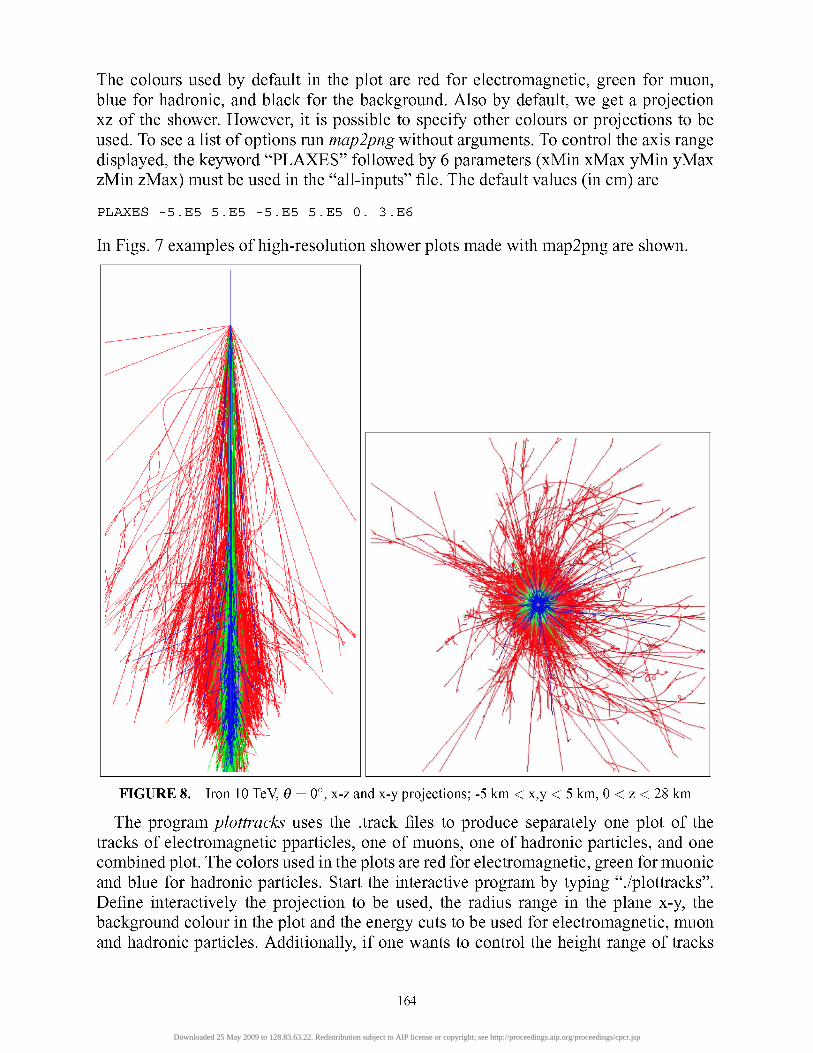
FIGURE 8. Iron 10 TeV, 6 = 0°, x-z and x-y projections; -5 k m < x,y < 5 km, 0 < z < 28 km

The program plottracks uses the .track files to produce separately one plot of the tracks of electromagnetic pparticles, one of muons, one of hadronic particles, and one combined plot. The colors used in the plots are red for electromagnetic, green for muonic and blue for hadronic particles. Start the interactive program by typing "./plottracks". Define interactively the projection to be used, the radius range in the plane x-y, the background colour in the plot and the energy cuts to be used for electromagnetic, muon and hadronic particles. Additionally, if one wants to control the height range of tracks

164


plotted, one needs to modify the Fortran code plottracksSc.f (available in the directory src/) in the following lines:

c height : 2 8 km zmin = 0.110 zmax = 2 8.

and recompile it. Fig. 8 shows an Iron-induced shower at 10 TeV, produced with plottracks.

Acknowledgements: The authors are very grateful for the invitation to the V^ School on Cosmic Rays and Astrophysics. JK acknowledges the financial support from the organisers. AVCG acknowledges support from the Centro de Tecnologias de Informacion y Comunicaciones, Universidad Nacional de Ingenieria, Lima, Peru.

REFERENCES

1. CORSIKAweb site: h t t p : / /www- ik . f z k . d e / c o r s i k a / 2. J Abraham et al., Auger Collaboration, Science 938 (2007) 318 3. J Abraham et al., Auger Collaboration, Astropart. Phys. 27 (2007) 244 4. J Abraham et al.. Auger Collaboration, Astropart. Phys. 27 (2007) 155

J Abraham et al.. Auger Collaboration, Astropart. Phys. 29 (2008) 243 5. J Abraham et al.. Auger Collaboration, PRL 100 (2008) 211101 6. J Abraham et al.. Auger Collaboration, PRL 101 (2008) 061101 7. HESS website: h t t p : / /www.mpi -hd .mpg.de /hfm/HESS/ 8. CTAweb site: h t t p : / /www.mpi-hd .mpg.de /hfm/CTA/ 9. Magic web site: h t t p : //wwwmagic . mppmu. mpg. d e / 10. KASCADE web site: h t t p : //www- i k . f zk . de/KASCADE_home . h tml 11. Tibet air shower array web site: h t t p : //www. i c r r . u - t o k y o . a c . j p / e m / i n d e x , h tml 12. MILAGRO web site h t t p : //www. l a n l . g o v / m i l a g r o / 13. HIRES web site: h t t p : //www. c o s m i c - r a y . o r g / 14. CORSIKA images: h t t p : / / w w w . a s t . l e e d s . a c . u k / ~ f s / 15. CORSIKA movies: h t t p : / / w w w . a s t . l e e d s . a c . u k / ~ k n a p p / m o v i e s / and

h t t p : / / w w w - i k . f z k . d e / c o r s i k a / m o v i e s / 16. M Nagano, AA Watson, Rev. Mod. Phys. 72 (2000) 689 17. M Kobal, Astropart. Phys. 15 (2001) 259

165


http://fzk.de/corsika/

http://www.mpi-hd.mpg.de/hfm/HESS/

http://www.mpi-hd.mpg.de/hfm/CTA/

http://www.ast

http://www.ast

http://www-ik.fzk.de/corsika/movies/

Air Shower Simulations

Documents