Air Quality Impact Assessment - Royal HaskoningDHV dEIAR_/Appendix C3.1 Air Quality... · Air Quality Impact Assessment ... to determine how different sources of pollution contribute

Air Quality Impact Assessment

Prepared for the Southern Waste Water Treatment Works

04 March 2015

DOCUMENT DESCRIPTION

Client:

AECOM

Report Name:

Southern Waste Water Treatment Works - Air Quality impact assessment

Authority Reference Number:

N/A

Compiled by:

Nicole Singh

Date:

04 March 2015

Location:

Southern Basin, Durban. Kwa-Zulu Natal

Reviewed by: Stuart Thompson

Approval:

_____________________________

Signature

© Royal HaskoningDHV

All rights reserved.

No part of this publication may be reproduced or transmitted in any form or by any means, electronic or

mechanical, without the written permission from Royal HaskoningDHV

TABLE OF CONTENTS

1 INTRODUCTION 9

1.1 Process Description 10

1.2 Terms of Reference 10

1.3 Methodology 11

1.3.1 Baseline Assessment 11

1.3.2 Impact Assessment 11

1.3.2.1 Overview of the Aermod Dispersion Model 11

1.3.2.2 Overview of the WATER9 (Waste water treatment) Model 11

1.4 Report Structure 12

2 BASELINE DESCRIPTION OF THE AREA 13

2.1 Meso-Scale Meteorology 13

2.1.1 Wind 13

2.1.2 Atmospheric stability 1

2.1.3 Temperature and Humidity 2

2.1.4 Precipitation 2

3 APPLICABLE LEGISLATION 4

3.1 National Environmental Management: Air Quality Act 39 of 2004 4

3.2 National Ambient Air Quality Standards 4

3.2.1 Particulate matter 5

3.2.2 Nitrogen dioxide 6

3.2.3 Sulphur dioxide 7

3.2.4 Volatile Organic Compounds 8

3.2.4.1 Health and Nuisance Evaluation Criteria 9

3.2.5 Cancer Risk Assessment 10

3.2.5.1 Odour Impact Evaluation 11

3.3 Other Polluting Sources in the Area 17

3.3.1 Vehicle emissions 17

3.3.2 Industries 17

3.3.3 Landfill site 18

3.4 Sensitive receptors 18

3.5 Baseline Air Quality 19

Figure 3-2: Map indicating the location of the monitoring stations 19

3.5.1 Sulphur dioxide 19

3.5.2 Nitrogen dioxide 20

3.5.3 Particulate Matter 21

3.5.4 TRS (Total Reduced Sulphur) 21

4 IMPACT ASSESSMENT 23

4.1 Methodology 23

4.1.1 Model overview 23

4.1.2 Model requirements 23

4.2 Emissions inventory 24

4.2.1 Assumptions and Knowledge gaps 25

4.3 Impact assessment 26

4.3.1 Construction/ Upgrade Impacts 26

4.3.2 Operational Impacts 28

4.4 Decommissioning impacts 38s

5 ODOUR MANAGEMENT 39

5.1.1 Good housekeeping practices 39

5.1.2 Plant performance and maintenance 39

5.1.3 Plant design and upgrades 39

5.1.4 Transport of sewage to the works 40

5.1.5 Inlet works 40

5.1.6 Primary and secondary treatment 40

5.1.7 Sludge handling, storage and thickening 40

5.1.8 Anaerobic digestion 41

5.1.9 Odour abatement 41

6 CONCLUSION 42

7 REFERENCES 43

LIST OF FIGURES

FIGURE 1-1: LOCATION OF THE SOUTHERN WASTE WATER TREATMENT WORKS 9

FIGURE 2-1: PERIOD WIND ROSE FOR THE PERIOD JAN 2009 – DEC 2013 14

FIGURE 2-2: WIND CLASS FREQUENCY DISTRIBUTION. 15

FIGURE 2-3: SEASONAL WIND ROSE (SPRING AND SUMMER) FOR THE JAN 2009 – DEC 2013 MONITORING PERIOD. 1

FIGURE 2-4: SEASONAL WIND ROSES (AUTUMN AND WINTER) FOR THE JAN 2009 – DEC 2013 MONITORING PERIOD. 2

FIGURE 2-5: DIURNAL WIND ROSES (00:00 – 12:00) FOR THE JAN 2009 – DEC 2013 MONITORING PERIOD. 3

FIGURE 2-6: DIURNAL WIND ROSES (12:00 – 00:00) FOR THE JAN 2009 – DEC 2013 MONITORING PERIOD. 4

FIGURE 2-7: WIND CLASS FREQUENCY DISTRIBUTION 1

FIGURE 2-8: AVERAGE TEMPERATURE (°C) AND RELATIVE HUMIDITY (%) FOR THE PERIOD JAN 2009 – DEC 2013 2

FIGURE 2-9: AVERAGE PRECIPITATION (MM) FOR THE PERIOD JAN 2009 – DEC 2013 3

FIGURE 3-1: ODOUR IMPACT ASSESSMENT PROCEDURE STIPULATED BY THE NEW SOUTH WALES ENVIRONMENTAL

PROTECTION AGENCY FOR EXISTING FACILITIES (NSW EPA, 2001) 16

FIGURE 3-2: MAP INDICATING THE LOCATION OF THE MONITORING STATIONS 19

FIGURE 3-3: ANNUAL TRENDS IN SULPHUR DIOXIDE CONCENTRATIONS (µG/M3) FROM 2004 – 2013. 20

FIGURE 3-4: ANNUAL TRENDS IN NITROGEN DIOXIDE CONCENTRATIONS (µG/M3) FROM 2004 – 2013. 20

FIGURE 3-5: ANNUAL TRENDS IN PARTICULATE MATTER CONCENTRATIONS (µG/M3) FROM 2004 – 2013. 21

FIGURE 3-6: ANNUAL TRS CONCENTRATIONS (PPB) FROM 2008-2009 22

FIGURE 4-1: PHASE 1- HOURLY AVERAGE PREDICTED GROUND LEVEL CONCENTRATION (µG/M3) FOR THE SOUTHERN

WASTE WATER TREATMENT WORKS. 28

FIGURE 4-2: PHASE 1 - DAILY AVERAGE PREDICTED GROUND LEVEL CONCENTRATION (µG/M3) FOR THE SOUTHERN

WASTE WATER TREATMENT WORKS. 29

FIGURE 4-3: PHASE 1 - ANNUAL AVERAGE GROUND LEVEL CONCENTRATION (µG/M3) FOR THE SOUTHERN WASTE WATER

TREATMENT WORKS 30

FIGURE 4-4: PHASE 2 – HOURLY AVERAGE PREDICTED GROUND LEVEL CONCENTRATION (µG/M3) FOR THE SOUTHERN

WASTE WATER TREATMENT WORKS. 33

FIGURE 4-5: PHASE 2 - DAILY AVERAGE PREDICTED GROUND LEVEL CONCENTRATION (µG/M3) FOR THE SOUTHERN

WASTE WATER TREATMENT WORKS. 34

FIGURE 4-6: PHASE 2 - ANNUAL AVERAGE GROUND LEVEL CONCENTRATION (µG/M3) FOR THE SOUTHERN WASTE WATER

TREATMENT WORKS. 35

LIST OF TABLES

TABLE 2-1: ATMOSPHERIC STABILITY CLASS ........................................................................................................................... 1

TABLE 3-1: AMBIENT AIR QUALITY STANDARDS AND GUIDELINES FOR PARTICULATE MATTER. ........................................... 5

TABLE 3-2: AMBIENT AIR QUALITY GUIDELINES AND STANDARDS FOR OXIDES OF NITROGEN ............................................. 6

TABLE 3-3: AMBIENT AIR QUALITY STANDARDS AND GUIDELINES FOR SULPHUR DIOXIDE .................................................. 8

TABLE 3-4: AMBIENT AIR QUALITY GUIDELINES APPLICABLE TO THE STUDY ......................................................................... 9

TABLE 3-5: CANCER RISK FACTORS FOR COMPOUNDS INVESTIGATED AT THE WASTE WATER TREATMENT WORKS. ........ 10

TABLE 3-6: ODOUR THRESHOLD VALUES FOR ODOUR COMPOUNDS .................................................................................. 11

TABLE 3-7: NSW EPA ODOUR PERFORMANCE CRITERIA DEFINED BASED ON POPULATION DENSITY (NSW EPS, 2001A). .. 13

TABLE 3-8: ODOUR PERFORMANCE CRITERIA USED IN VARIOUS JURISDICTION IN THE US AND AUSTRALIA (AFTER NSW

EPA, 2001B). .................................................................................................................................................................. 14

TABLE 3-9: SENSITIVE RECEPTORS WITH APPROXIMATE DISTANCE AND DIRECTION FROM THE SOUTHERN WASTE WATER

TREATMENT WORKS. .................................................................................................................................................... 18

TABLE 3-10: LOCATION OF MONITORING STATIONS AND PARAMETERS MEASURED. ........................................................ 19

TABLE 4-1: SOURCE SPECIFICATIONS .................................................................................................................................... 24

TABLE 4-2: POLLUTANTS OF CONCERN ANTICIPATED TO BE RELEASED FROM THE WASTE WATER TREATMENT WORKS

AND THEIR CALCULATED EMISSION RATES. .................................................................................................................. 24

TABLE 4-3: PHASE1 - MAXIMUM PREDICTED GROUND LEVEL CONCENTRATION (µG/M3). ................................................. 31

TABLE 4-4: PHASE 1 - PREDICTED CANCER RISK .................................................................................................................... 31

TABLE 4-5: PHASE 1 - PREDICTED ODOUR NUISANCE IMPACTS ........................................................................................... 32

TABLE 4-6: ODOUR CONCENTRATION AT EACH SENSITIVE RECEPTOR. ................................................................................ 32

TABLE 4-7:PHASE 2 – MAXIMUM PREDICTED GROUND LEVEL CONCENTRATION (µG/M3) ................................................. 36

TABLE 4-8: PHASE 2 – CANCER RISK ASSESSMENT ................................................................................................................ 36

TABLE 4-9: PHASE 2 - PREDICTED ODOUR NUISANCE IMPACTS ........................................................................................... 37

TABLE 4-10: ODOUR CONCENTRATION AT EACH SENSITIVE RECEPTOR (EXCEEDANCE HIGHLIGHTED IN BOLD) ................ 37

TABLE 4-12: MAXIMUM PREDICTED CONCENTRATION (µG/M3) AFTER MITIGATION MEASURES. (COVERS USED ON THE

PRIMARY SEDIMENTATION TANKS). ....................................................................... ERROR! BOOKMARK NOT DEFINED.

TABLE 4-13: PREDICTED ODOUR NUISANCE AFTER MITIGATION MEASURES USING COVERS AT PST.ERROR! BOOKMARK

NOT DEFINED.

Glossary

Ambient air The air of the surrounding environment.

Baseline The current and existing condition before any development or action.

Boundary layer In terms of the earth’s planetary boundary layer is the air layer near the ground affected

by diurnal heat, moisture or momentum to or from the surface.

Concentration When a pollutant is measured in ambient air it is referred to as the concentration of that

pollutant in air. Pollutant concentrations are measured in ambient air for various

reasons, i.e. to determine whether concentrations are exceeding available health risk

thresholds (air quality standards); to determine how different sources of pollution

contribute to ambient air concentrations in an area; to validate dispersion modelling

conducted for an area; to determine how pollutant concentrations fluctuate over time in

an area; and to determine the areas with the highest pollution concentrations.

Condensation The change in the physical state of matter from a gaseous into liquid phase.

Dispersion

potential

The potential a pollutant has of being transported from the source of emission by wind

or upward diffusion. Dispersion potential is determined by wind velocity, wind direction,

height of the mixing layer, atmospheric stability, presence of inversion layers and

various other meteorological conditions.

Emission The rate at which a pollutant is emitted from a source of pollution.

Emission Factor A representative value, relating the quantity of a pollutant to a specific activity resulting

in the release of the pollutant to atmosphere.

Evaporation The opposite of condensation

Inversion An increase of atmospheric temperature with an increase in height.

Meteorological The atmospheric phenomena and weather of a region.

Mixing layer

The layer of air within which pollutants are mixed by turbulence. Mixing depth is the

height of this layer from the earth’s surface

Oxides of Nitrogen Refers to NO and NO2. The gas is produced during combustion especially at high

temperatures.

Particulate matter

(PM)

The collective name for fine solid or liquid particles added to the atmosphere by

processes at the earth's surface and includes dust, smoke, soot, pollen and soil

particles. Particulate matter is classified as a criteria pollutant, thus national air quality

standards have been developed in order to protect the public from exposure to the

inhalable fractions. PM can be principally characterised as discrete particles spanning

several orders of magnitude in size, with inhalable particles falling into the following

general size fractions:

* PM10 (generally defined as all particles equal to and less than 10 microns in

aerodynamic diameter; particles larger than this are not generally deposited in the

lung);

* PM2.5, also known as fine fraction particles (generally defined as those particles

with an aerodynamic diameter of 2.5 microns or less) ;

* PM10-2.5, also known as coarse fraction particles (generally defined as those

particles with an aerodynamic diameter greater than 2.5 microns, but equal to or

less than a nominal 10 microns); and

* Ultra fine particles generally defined as those less than 0.1 microns.

Precipitation Ice particles or water droplets large enough to fall at least 100 m below the cloud base

before evaporating.

Relative Humidity The vapour content of the air as a percentage of the vapour content needed to saturate

air at the same temperature

Wastewater

treatment plant

An industrial structure designed to remove biological or chemical waste products from

water, thereby permitting treated water to be used for other purposes.

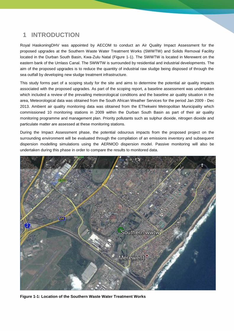
1 INTRODUCTION

Royal HaskoningDHV was appointed by AECOM to conduct an Air Quality Impact Assessment for the

proposed upgrades at the Southern Waste Water Treatment Works (SWWTW) and Solids Removal Facility

located in the Durban South Basin, Kwa-Zulu Natal (Figure 1-1). The SWWTW is located in Merewent on the

eastern bank of the Umlass Canal. The SWWTW is surrounded by residential and industrial developments. The

aim of the proposed upgrades is to reduce the quantity of industrial raw sludge being disposed of through the

sea outfall by developing new sludge treatment infrastructure.

This study forms part of a scoping study for the site and aims to determine the potential air quality impacts

associated with the proposed upgrades. As part of the scoping report, a baseline assessment was undertaken

which included a review of the prevailing meteorological conditions and the baseline air quality situation in the

area, Meteorological data was obtained from the South African Weather Services for the period Jan 2009 - Dec

2013. Ambient air quality monitoring data was obtained from the EThekwini Metropolitan Municipality which

commissioned 10 monitoring stations in 2009 within the Durban South Basin as part of their air quality

monitoring programme and management plan. Priority pollutants such as sulphur dioxide, nitrogen dioxide and

particulate matter are assessed at these monitoring stations.

During the Impact Assessment phase, the potential odourous impacts from the proposed project on the

surrounding environment will be evaluated through the compilation of an emissions inventory and subsequent

dispersion modelling simulations using the AERMOD dispersion model. Passive monitoring will also be

undertaken during this phase in order to compare the results to monitored data.

Figure 1-1: Location of the Southern Waste Water Treatment Works

1.1 Process Description

The Southern Waste Water Treatment Works receives the majority of its raw sewage effluent through three

large (1500 mm diameter) trunk sewers, i.e. the Main Southern Trunk Sewer (referred to as the Jacobs Trunk

Sewer), the Wentworth Valley Trunk Sewer and the Umlaas Trunk Sewer. Other smaller diameter pipelines

coming to this Works includes those from Mondi and SAPREF (each separately discharging at the inlet of this

Works) and Illovo (discharging closer to the outlet of this Works). The total average daily flow to this works is in

the region of 130 Mega (million) litres per day and all the treated flows leaving this works is discharged directly

to sea (by gravity and by pumping) through a 1500 mm diameter, 4,2 km long sea outfall.

The Umlaas Trunk Sewer which serves the areas of Chatsworth and Umlazi discharges effluent to this Works

is predominantly domestic in origin. The discharged flow [currently in the region of 35 Mega (million) litres per

day] is immediately directed to a separate treatment facility where it undergoes preliminary, primary, secondary

and tertiary treatment. The secondary and tertiary treatment processes are managed by a private entity (Veolia

Water) who stores and sells the tertiary treated (or reclaimed) effluent to industry. All sludge generated from the

treatment of this effluent is discharged to sea.

The Jacobs Trunk Sewer which serves the residential areas of Yellow Wood Park and Woodlands and the

industrial areas of Jacobs and Mobeni, discharges sewage effluent that is a combination of domestic and

industrial in origin. The Wentworth Valley Trunk Sewer which serves the areas of the Bluff, Wentworth,

Clairwood, Bayhead and Island View discharges sewage effluent that is also a combination of domestic and

industrial in origin. The flows conveyed by these two trunk sewers [currently in the region of 95 Mega (million)

litres per day] combine at the main inlet works and undergo preliminary treatment only (i.e. removal of

screenings and grit) before being discharged to sea.

In addition to the pipeline discharge of sewage effluent to this works, smaller volumes of effluent are also

discharged by various road tankers. The effluent discharged by these road tankers also undergoes preliminary

treatment before being discharged to sea.

1.2 Terms of Reference

The terms of reference for the Air Quality Impact Assessment for the proposed project can be summarised as

follows:

Baseline Assessment

o Provide an overview of the prevailing meteorological conditions in the area;

o Review applicable legislation and policies related to air quality management which are applicable

to the treatment works;

o Review potential health effects associated with emissions released from the proposed upgrades;

o Identification of existing sources of emission and sensitive receptors, such as local communities,

surrounding the treatment works;

o Assess the baseline air quality using available ambient air quality monitored data.

Impact Assessment

o Compilation of an emissions inventory for the proposed air quality sources identified on site;

o Undertake dispersion modelling simulations using AERMOD to determine the potential air quality

impacts of the proposed activities on the surrounding area;

o Comparison of the modelled results to the National ambient air quality standards to determine

compliance;

o Provide recommendations for the implementation of appropriate mitigation measures;

o Compilation of an Air Quality Impact Assessment Report.

1.3 Methodology

An overview of the methodological approach to be followed during the development of the Air Quality Impact

Assessment is outlined in the section which follows.

1.3.1 Baseline Assessment

During the baseline assessment, a qualitative approach was used to assess the baseline conditions in the

project area. Meteorological data was obtained from the South Weather Services weather station located in the

Durban South Basin (Latitude: -29.9650; Longitude: 30.9460) for the period January 2009 to December 2013.

Applicable air quality legislation was reviewed and criteria pollutants relevant to the project and their potential

human health effects were also discussed. The existing sources of air pollution surrounding the treatment plant

will be qualitatively assessed in section 3 of the report. The sensitive receptors, such as local communities in

close proximity to the treatment works will be identified through satellite imagery and a site visit.

Ambient data from ten monitoring stations located in the Southern basin was obtained from the South African

Air Quality Information System (SAAQIS) in order to assess the baseline air quality conditions.

1.3.2 Impact Assessment

During this phase, an emissions inventory will be compiled to estimate emissions from the identified emission

sources associated with the proposed upgrades and activities on site. Dispersion modelling simulations will be

undertaken using the AERMOD dispersion model and will be presented graphically as isopleth plots.

Comparison with the National and international ambient air quality standards (GN263; 2009) will be made to

determine compliance. Based on the predicted results, recommendations for appropriate mitigation measures

will also be provided

1.3.2.1 Overview of the Aermod Dispersion Model

Dispersion modelling will be undertaken using the US EPA approved AERMOD Model. Aermod is based on the

Gaussian plume equation and is capable of providing ground level concentration estimates of various

averaging times, for a number of meteorological and emission source configuration (point, area, volume

sources for gaseous and particle emissions). Input data into AERMOD includes: source and receptor data,

meteorological parameters and terrain data. The meteorological data includes: wind velocity and direction,

ambient temperature, mixing heights, stability class, barometric pressure, average precipitation and relative

humidity.

1.3.2.2 Overview of the WATER9 (Waste water treatment) Model

WATER9 is a Windows based program and consists of analytical expressions for estimating air emissions of

individual waste constituents in waste water collection, storage, and treatment and disposal facilities; a data

base listing many of the organic compounds and procedures for obtaining reports of constituent fates, including

air emissions and treatment effectiveness. WATER9 is used to estimate air emissions from site specific water

treatment plants (including the prediction of biodegradation and sludge sorption or organics) for common waste

water treatment units.

Once the WATER9 emission estimates have been made and the AERMOD model has been run, an output of

potential impacts will be provided. The assessment of the potential air quality impacts will then be undertaken

by comparing AERMOD results, with local and international standards for the pollutants identified.

1.4 Report Structure

Section 1 of the report provides the background to the project. Section 2 includes a meteorological overview

of the region. A review of applicable air quality legislation, pollutants and their potential health effects and the

existing baseline air quality situation are presented in Section 3. Section 4 gives a summary of the general

impacts associated with the proposed upgrade at the SWWTW. Section 5 provides a literature review of odour

management.

2 BASELINE DESCRIPTION OF THE AREA

2.1 Meso-Scale Meteorology

The nature of the local climate will determine what will happen to particulates when released into the

atmosphere (Tyson and Preston-Whyte, 2000). Concentration levels fluctuate daily and hourly, in response to

changes in atmospheric stability and variations in mixing depth. Similarly, atmospheric circulation patterns will

have an effect on the rate of transport and dispersion.

The release of atmospheric pollutants into a large volume of air results in the dilution of those pollutants. This is

best achieved during conditions of free convection and when the mixing layer is deep (unstable atmospheric

conditions). These conditions occur most frequently in summer during the daytime. This dilution effect can

however be inhibited under stable atmospheric conditions in the boundary layer (shallow mixing layer). Most

surface pollution is thus trapped under a surface inversion (Tyson and Preston-Whyte, 2000).

Inversion occurs under conditions of stability when a layer of warm air lies directly above a layer of cool air.

This layer prevents a pollutant from diffusing freely upward, resulting in an increased pollutant concentration at

or close to the earth’s surface. Surface inversions develop under conditions of clear, calm and dry conditions

and often occur at night and during winter (Tyson and Preston-Whyte, 2000). Radiative loss during the night

results in the development of a cold layer of air close to the earth’s surface. These surface inversions are

however, usually destroyed as soon as the sun rises and warm the earth’s surface. With the absence of

surface inversions, the pollutants are able to diffuse freely upward; this upward motion may however be

prevented by the presence of an elevated inversion (Tyson and Preston-Whyte, 2000).

The climatic profile of the coastal regions of South Africa is typical of a humid subtropical climate, with hot and

humid summers and warm dry winters. The coastal region is occasionally affected by tropical storms and

cyclones during the cyclone season (November – April). Generally cold, dry conditions prevail during the

winter, with strong winds and cold air drainage off the Drakensburg Mountains exacerbating the drying effect,

particularly in the southern part of the province where the high mountains lie closer to the coast. Summer

months are usually marked by strong, high pressure easterly winds.

2.1.1 Wind

Wind roses comprise of 16 spokes which represents the direction from which the winds blew during the period

under review. The colours reflect the different categories of wind speeds. The dotted circles provide information

regarding the frequency of occurrence of wind speed and direction categories.

Based on an evaluation of the site specific meteorological data obtained from the Durban South monitoring

station, Kwa-Zulu Natal, the following deductions regarding the prevailing wind direction and wind frequency

can be presented. The parameters such as wind direction, wind speed, temperature, relative humidity,

barometric pressure and precipitation.

Based on the available meteorological data (Figure 2-1), winds occur predominantly from the north-north-east

(13% of the time), south-west (10% of the time) and south-south-west (10% of the time).

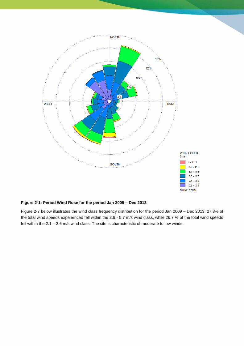
Figure 2-1: Period Wind Rose for the period Jan 2009 – Dec 2013

Figure 2-7 below illustrates the wind class frequency distribution for the period Jan 2009 – Dec 2013. 27.8% of

the total wind speeds experienced fell within the 3.6 - 5.7 m/s wind class, while 26.7 % of the total wind speeds

fell within the 2.1 – 3.6 m/s wind class. The site is characteristic of moderate to low winds.

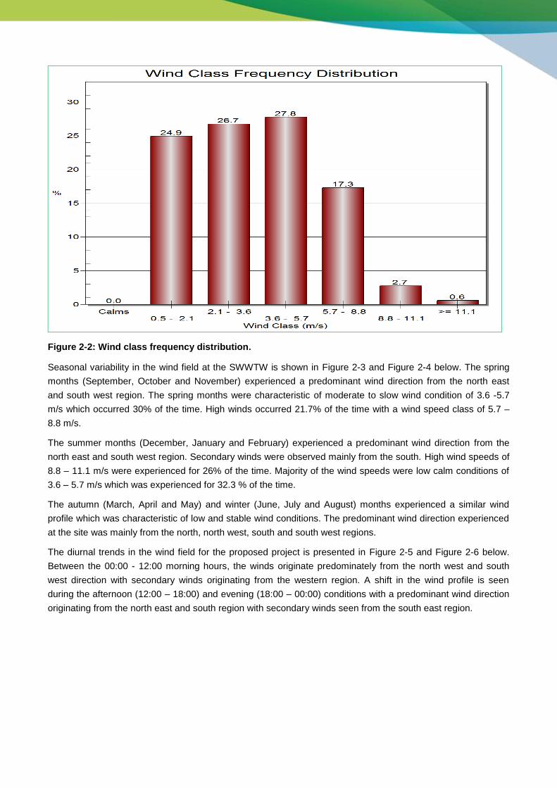
Figure 2-2: Wind class frequency distribution.

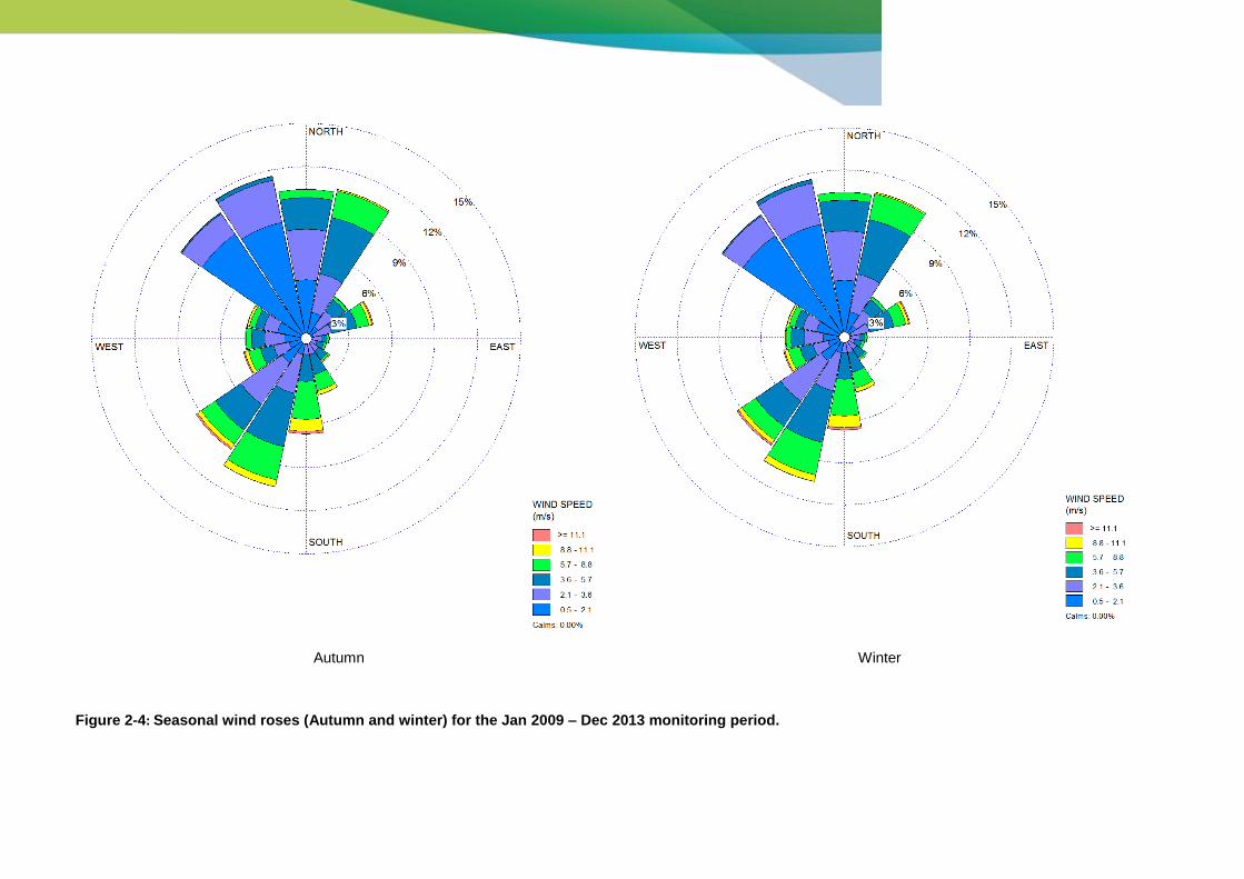
Seasonal variability in the wind field at the SWWTW is shown in Figure 2-3 and Figure 2-4 below. The spring

months (September, October and November) experienced a predominant wind direction from the north east

and south west region. The spring months were characteristic of moderate to slow wind condition of 3.6 -5.7

m/s which occurred 30% of the time. High winds occurred 21.7% of the time with a wind speed class of 5.7 –

8.8 m/s.

The summer months (December, January and February) experienced a predominant wind direction from the

north east and south west region. Secondary winds were observed mainly from the south. High wind speeds of

8.8 – 11.1 m/s were experienced for 26% of the time. Majority of the wind speeds were low calm conditions of

3.6 – 5.7 m/s which was experienced for 32.3 % of the time.

The autumn (March, April and May) and winter (June, July and August) months experienced a similar wind

profile which was characteristic of low and stable wind conditions. The predominant wind direction experienced

at the site was mainly from the north, north west, south and south west regions.

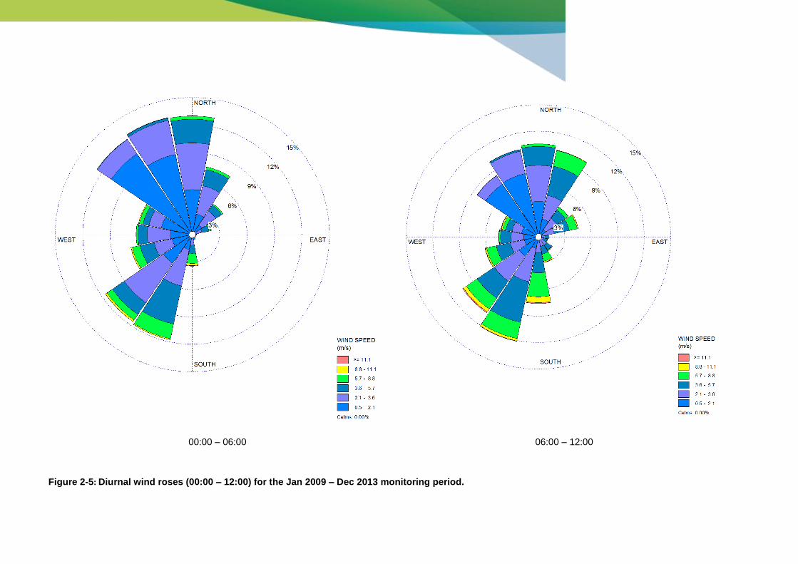
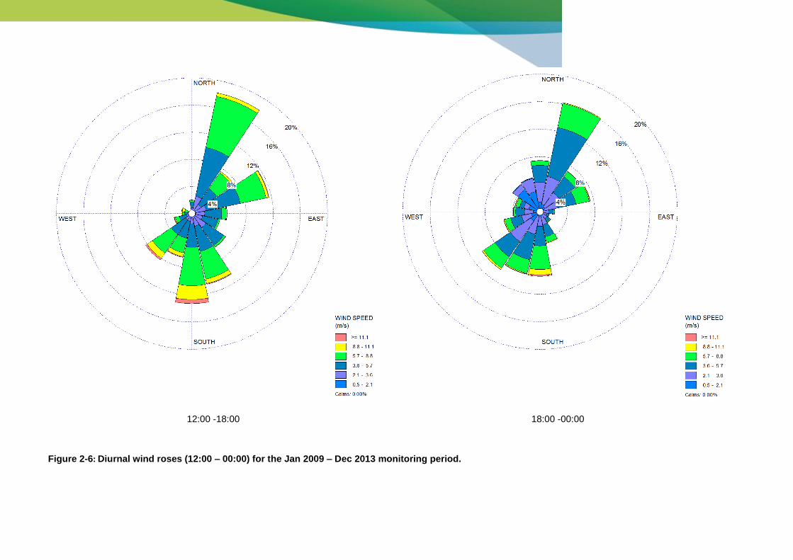
The diurnal trends in the wind field for the proposed project is presented in Figure 2-5 and Figure 2-6 below.

Between the 00:00 - 12:00 morning hours, the winds originate predominately from the north west and south

west direction with secondary winds originating from the western region. A shift in the wind profile is seen

during the afternoon (12:00 – 18:00) and evening (18:00 – 00:00) conditions with a predominant wind direction

originating from the north east and south region with secondary winds seen from the south east region.

Spring

Summer

Figure 2-3: Seasonal wind rose (Spring and summer) for the Jan 2009 – Dec 2013 monitoring period.

Autumn

Winter

Figure 2-4: Seasonal wind roses (Autumn and winter) for the Jan 2009 – Dec 2013 monitoring period.

00:00 – 06:00

06:00 – 12:00

Figure 2-5: Diurnal wind roses (00:00 – 12:00) for the Jan 2009 – Dec 2013 monitoring period.

12:00 -18:00

18:00 -00:00

Figure 2-6: Diurnal wind roses (12:00 – 00:00) for the Jan 2009 – Dec 2013 monitoring period.

2.1.2 Atmospheric stability

Atmospheric stability is commonly categorised into one of seven stability classes. These are briefly described

in Table 2-1 below. The atmospheric boundary layer is usually unstable during the day due to turbulence

caused by the sun's heating effect on the earth's surface. The depth of this mixing layer depends mainly on the

amount of solar radiation, increasing in size gradually from sunrise to reach a maximum at about 5-6 hours

after sunrise. The degree of thermal turbulence is increased on clear warm days with light winds. During the

night a stable layer, with limited vertical mixing, exists. During windy and/or cloudy conditions, the atmosphere

is normally neutral. A neutral atmospheric potential neither enhances nor inhibits mechanical turbulences. An

unstable atmospheric condition enhances turbulence, whereas a stable atmospheric condition inhibits mechanical

turbulence.

Table 2-1: Atmospheric Stability Class

A Very unstable calm wind, clear skies, hot daytime conditions

B Moderately unstable clear skies, daytime conditions

C Slightly Unstable moderate wind, slightly overcast daytime conditions

D Neutral high winds or cloudy days and nights

E Slightly Stable moderate wind, slightly overcast night-time conditions

F Moderately stable low winds, clear skies, cold night-time conditions

G Very stable Calm winds, clear skies, cold clear night-time conditions

Figure 2-7 below indicates the stability class frequency distribution for the area under review. Majority of the

wind class fell within class F with 23.9%, which is characteristic of moderately stable conditions with low winds,

clear skies and cold night time conditions. Slightly unstable conditions were noted for 17.8% of the time which

is indicative of slightly unstable climatic conditions with moderate winds and slightly overcast daytime

conditions.

Figure 2-7: Wind Class Frequency Distribution

2.1.3 Temperature and Humidity

Temperature affects the formation, action, and interactions of pollutants in various ways (Kupchella and

Hyland, 1993). Chemical reaction rates tend to increase with temperature and the warmer the air, the more

water it can hold and hence the higher the humidity. Temperature also provides an indication of the rate of

development and dissipation of the mixing layer as well as determining the effect of plume buoyancy; the larger

the temperature difference between the plume and ambient air, the higher the plume is able to rise.

Higher plume buoyancy will result in an increased lag time between the pollutant leaving the source, and

reaching the ground. This additional time will allow for greater dilution and ultimately a decrease in the pollutant

concentrations when reaching ground level.

Humidity is the mass of water vapour per unit volume of natural air. When temperatures are at their highest the

humidity is also high, the moisture is trapped inside the droplets of the water vapour. This makes the moisture

content of the air high. When relative humidity exceeds 70%, light scattering by suspended particles begins to

increase, as a function of increased water uptake by the particles (CEPA/FPAC Working Group, 1999). This

results in decreased visibility due to the resultant haze. Many pollutants may also dissolve in water to form acids,

as well as secondary pollutants within the atmosphere.

The average monthly temperature and relative humidity for the period Jan 2009 - Dec 2013 is presented in

Figure 2-8 below with the average humidity indicated with a blue line. Daily average summer temperatures

ranged between 22.5 ºC – 25.1 ºC, while the average winter temperatures ranged between 16.8 ºC – 20.0 ºC.

Relative humidity for the period Jan 2009 – Dec 2013 was highest during the summer months and lowest

during the winter months.

Figure 2-8: Average Temperature (°C) and Relative Humidity (%) for the period Jan 2009 – Dec 2013

2.1.4 Precipitation

Precipitation cleanses the air by washing out particles suspended in the atmosphere (Kupchella and Hyland,

1993). It is calculated that precipitation accounts for about 80-90% of the mass of particles removed from the

atmosphere (CEPA/FPAC Working Group, 1999).

The total rainfall profile for the period Jan 2009 – Dec 2013 is illustrated in Figure 2-9 below. The spring and

summer months recorded the highest rainfall with 242.26 mm and 250.7 6mm recorded respectively while the

winter months recorded the lowest precipitation with 92.24 mm.

Figure 2-9: Average Precipitation (mm) for the period Jan 2009 – Dec 2013

3 APPLICABLE LEGISLATION

3.1 National Environmental Management: Air Quality Act 39 of

2004

The National Environmental Management: Air Quality Act 39 of 2004 has shifted the approach of air quality

management from source-based control to receptor-based control. The main objectives of the Act are to:

Give effect to everyone’s right ‘to an environment that is not harmful to their health and well-being’

Protect the environment by providing reasonable legislative and other measures that (i) prevent

pollution and ecological degradation, (ii) promote conservation and (iii) secure ecologically sustainable

development and use of natural resources while promoting justifiable economic and social

development

The Act makes provision for the setting and formulation of National ambient air quality standards for

‘substances or mixtures of substances which present a threat to health, well-being or the environment’. More

stringent standards can be established at the provincial and local levels.

The control and management of emissions in AQA relates to the listing of activities that are sources of emission

and the issuing of emission licences. Listed activities are defined as activities which ‘result in atmospheric

emissions and are regarded to have a significant detrimental effect on the environment, including human

health’. Listed activities have been identified by the minister of the Department of Environmental Affairs and

atmospheric emission standards have been established for each of these activities. These listed activities now

require an atmospheric emission licence to operate. The issuing of emission licences for Listed Activities is the

responsibility of the metropolitan and district municipalities.

In addition, the minister may declare any substance contributing to air pollution as a priority pollutant. Any

industries or industrial sectors that emit these priority pollutants will be required to implement a Pollution

Prevention Plan. Municipalities are required to ‘designate an air quality officer to be responsible for co-

ordinating matters pertaining to air quality management in the Municipality’. The appointed Air Quality Officer is

responsible for the issuing of atmospheric emission licences.

3.2 National Ambient Air Quality Standards

Air quality guidelines and standards are fundamental to effective air quality management, providing the link

between the source of atmospheric emissions and the user of that air at the downstream receptor site. The

ambient air quality guideline values indicate safe daily exposure levels for the majority of the population,

including the very young and the elderly, throughout an individual’s lifetime. Air quality guidelines and

standards are normally given for specific averaging periods. These averaging periods refer to the time-span

over which the air concentration of the pollutant was monitored at a location. Generally, five averaging periods

are applicable, namely an instantaneous peak, 1-hour average, 24-hour average, 1-month average, and annual

average.

The Department of Environmental Affairs (DEA) has issued ambient air quality standards to support receiving

environment management practices. Ambient air quality standards are only available for criteria pollutants

which are commonly emitted, such as particulates, sulphur dioxide (SO2), lead (Pb), nitrogen oxides (NOx),

benzene (C6H6) and carbon monoxide (CO). Local and international guidelines applicable to the project are

provided in the sections below.

3.2.1 Particulate matter

Particulate matter is the collective name for fine solid or liquid particles added to the atmosphere by processes

at the earth's surface. Particulate matter includes dust, smoke, soot, pollen and soil particles (Kemp, 1998).

Particulate matter has been linked to a range of serious respiratory and cardiovascular health problems. The

key effects associated with exposure to ambient particulate matter include: premature mortality, aggravation of

respiratory and cardiovascular disease, aggravated asthma, acute respiratory symptoms, chronic bronchitis,

decreased lung function, and an increased risk of myocardial infarction (USEPA, 1996).

Particulate matter represents a broad class of chemically and physically diverse substances. Particles can be

described by size, formation mechanism, origin, chemical composition, atmospheric behaviour and method of

measurement. The concentration of particles in the air varies across space and time, and is related to the

source of the particles and the transformations that occur in the atmosphere (USEPA, 1996).

Particulate Matter can be principally characterised as discrete particles spanning several orders of magnitude

in size, with inhalable particles falling into the following general size fractions (USEPA, 1996):

PM10 (generally defined as all particles equal to and less than 10 microns in aerodynamic diameter;

particles larger than this are not generally deposited in the lung);

PM2.5, also known as fine fraction particles (generally defined as those particles with an aerodynamic

diameter of 2.5 microns or less)

PM10-2.5, also known as coarse fraction particles (generally defined as those particles with an

aerodynamic diameter greater than 2.5 microns, but equal to or less than a nominal 10 microns); and

Ultra fine particles generally defined as those less than 0.1 microns.

Fine and coarse particles are distinct in terms of the emission sources, formation processes, chemical

composition, atmospheric residence times, transport distances and other parameters. Fine particles are directly

emitted from combustion sources and are also formed secondarily from gaseous precursors such as sulphur

dioxide, nitrogen oxides, or organic compounds. Fine particles are generally composed of sulphate, nitrate,

chloride and ammonium compounds, organic and elemental carbon, and metals.

Table 3-1: Ambient air quality standards and guidelines for particulate matter.

Pollutant Averaging period (µg/m3)

Guideline

(µg/m3)

Number of Exceedance

Allowed Per Year

PM10

Daily average 75 4

4

Annual average 40 0

0

PM2.5

Daily average

65 (3)

40 (4)

25 (5)

4

4

4

Annual average

25 (3)

20 (4)

15 (5)

0

0

0

3.2.2 Nitrogen dioxide

Air quality guidelines and standards issued by most other countries and organisations tend to be given

exclusively for NO2 concentrations as NO2 is the most important species from a human health point of view.

International and South African standards for NO2 are presented in Table 3-2.

Table 3-2: ambient air quality guidelines and standards for oxides of nitrogen

Averaging

Period

South Africa WHO EC Australia

µg/m3 ppm µg/m

3 ppm µg/m

3 ppm µg/m

3 Ppm

Annual Ave 40 0.021 40 0.021 40 0.021 57 0.03

Max. 1-hr 200 0.10 200 0.10 200 0.10 240 0.12

NO2 is an irritating gas that is absorbed into the mucous membrane of the respiratory tract. The most adverse

health effect occurs at the junction of the conducting airway and the gas exchange region of the lungs. The

upper airways are less affected because NO2 is not very soluble in aqueous surfaces. Exposure to NO2 is

linked with increased susceptibility to respiratory infection, increased airway resistance in asthmatics and

decreased pulmonary function.

Available data from animal toxicology experiments indicate that acute exposure to NO2 concentrations of less

than 1 880 µg/m3 (1 ppm) rarely produces observable effects (WHO 2000). Normal healthy humans, exposed

at rest or with light exercise for less than two hours to concentrations above 4 700 µg/m3 (2.5 ppm), experience

pronounced decreases in pulmonary function; generally, normal subjects are not affected by concentrations

less than 1 880 µg/m3 (1.0 ppm). One study showed that the lung function of subjects with chronic obstructive

pulmonary disease is slightly affected by a 3.75-hour exposure to 560 µg/m3 (0.3 ppm) (WHO 2000).

Asthmatics are likely to be the most sensitive subjects, although uncertainties exist in the health database. The

lowest concentration causing effects on pulmonary function was reported from two laboratories that exposed

mild asthmatics for 30 to 110 minutes to 565 µg/m3 (0.3 ppm) NO2 during intermittent exercise. However,

neither of these laboratories was able to replicate these responses with a larger group of asthmatic subjects.

NO2 increases bronchial reactivity, as measured by the response of normal and asthmatic subjects following

exposure to pharmacological bronchoconstrictor agents, even at levels that do not affect pulmonary function

directly in the absence of a bronchoconstrictor. Some, but not all, studies show increased responsiveness to

bronchoconstrictors at NO2 levels as low as 376-565 µg/m3 (0.2 to 0.3 ppm); in other studies, higher levels had

no such effect. Because the actual mechanisms of effect are not fully defined and NO2 studies with allergen

challenges showed no effects at the lowest concentration tested (188 µg/m3; 0.1 ppm), full evaluation of the

health consequences of the increased responsiveness to bronchoconstrictors is not yet possible.

Studies with animals have clearly shown that several weeks to months of exposure to NO2 concentrations of

less than 1 880 µg/ m3 (1ppm) causes a range of effects, primarily in the lung, but also in other organs such as

the spleen and liver, and in blood. Both reversible and irreversible lung effects have been observed. Structural

changes range from a change in cell type in the tracheobronchial and pulmonary regions (at a lowest reported

level of 640 µg/m3), to emphysema-like effects. Biochemical changes often reflect cellular alterations, with the

lowest effective NO2 concentrations in several studies ranging from 380-750µg/m3. NO2 levels of about 940

µg/m3 (0.5ppm) also increase susceptibility to bacterial and viral infection of the lung. Children of between 5-12

years old are estimated to have a 20% increased risk for respiratory symptoms and disease for each increase

of 28 µg/m3 NO2 (2-week average), where the weekly average concentrations are in the range of 15-128 µg/m

3

or possibly higher. However, the observed effects cannot clearly be attributed to either the repeated short-term

high-level peak, or to long-term exposures in the range of the stated weekly averages (or possibly both). The

results of outdoor studies consistently indicate that children with long-term ambient NO2 exposures exhibit

increased respiratory symptoms that are of longer duration, and show a decrease in lung function.

3.2.3 Sulphur dioxide

SO2 is an irritant that is absorbed in the nose and aqueous surfaces of the upper respiratory tract, and is

associated with reduced lung function and increased risk of mortality and morbidity. Adverse health effects of

SO2 include coughing, phlegm, chest discomfort and bronchitis.

Short-period exposures (less than 24 hours)

Most information on the acute effects of SO2 comes from controlled chamber experiments on volunteers

exposed to SO2 for periods ranging from a few minutes up to one hour (WHO 2000). Acute responses occur

within the first few minutes after commencement of inhalation. Further exposure does not increase effects.

Effects include reductions in the mean forced expiratory volume over one second (FEV1), increases in specific

airway resistance, and symptoms such as wheezing or shortness of breath. These effects are enhanced by

exercise that increases the volume of air inspired, as it allows SO2 to penetrate further into the respiratory tract.

A wide range of sensitivity has been demonstrated, both among normal subjects and among those with

asthma. People with asthma are the most sensitive group in the community. Continuous exposure-response

relationships, without any clearly defined threshold, are evident.

Sub-chronic exposure over a 24-hour period

Information on the effects of exposure averaged over a 24-hour period is derived mainly from epidemiological

studies in which the effects of SO2, suspended particulate matter and other associated pollutants are

considered. Exacerbation of symptoms among panels of selected sensitive patients seems to arise in a

consistent manner when the concentration of SO2 exceeds 250 µg/m3 in the presence of suspended particulate

matter. Several more recent studies in Europe have involved mixed industrial and vehicular emissions now

common in ambient air. At low levels of exposure (mean annual levels below 50 µg/m3; daily levels usually not

exceeding 125 µg/m3) effects on mortality (total, cardiovascular and respiratory) and on hospital emergency

admissions for total respiratory causes and chronic obstructive pulmonary disease (COPD), have been

consistently demonstrated. These results have been shown, in some instances, to persist when black smoke

and suspended particulate matter levels were controlled for, while in others no attempts have been made to

separate the pollutant effects. In these studies no obvious threshold levels for SO2 has been identified.

Long-term exposure

Earlier assessments, using data from the coal-burning era in Europe judged the lowest-observed-adverse-

effect level of SO2 to be at an annual average of 100 µg/m3, when present with suspended particulate matter.

More recent studies related to industrial sources of SO2, or to the changed urban mixture of air pollutants, have

shown adverse effects below this level. There is, however, some difficulty in finding this value.

Based upon controlled studies with asthmatics exposed to SO2 for short periods, the WHO (WHO 2000)

recommends that a value of 500 µg/m3 (0.175 ppm) should not be exceeded over averaging periods of 10

minutes. Because exposure to sharp peaks depends on the nature of local sources, no single factor can be

applied to estimate corresponding guideline values over longer periods, such as an hour. Day-to-day changes

in mortality, morbidity, or lung function related to 24-hour average concentrations of SO2 are necessarily based

on epidemiological studies, in which people are in general exposed to a mixture of pollutants; and guideline

values for SO2 have previously been linked with corresponding values for suspended particulate matter. This

approach led to a previous guideline 24-hour average value of 125 µg/m3 (0.04 ppm) for SO2, after applying an

uncertainty factor of two to the lowest-observed-adverse-effect level. In more recent studies, adverse effects

with significant public health importance have been observed at much lower levels of exposure. However,

there is still a large uncertainty with this and hence no concrete basis for numerical changes of the 1987-

guideline values for SO2.

Table 3-3: Ambient Air quality Standards and guidelines for Sulphur dioxide

Origin Annual Average

Maximum (µg/m3)

24-Hour Maximum

(µg/m3)

1-Hour Maximum

(µg/m3)

<1-Hour Maximum

(µg/m3)

RSA 50

125

350

500 (10 min average)

WHO 50

10-30 125 -

500

(10 min average)

EC 20 125 350

UK 20 125 350 266

(15 min mean)

World Bank 50 125 - -

US-EPA 80 365 - -

Australia 53 209 520 -

3.2.4 Volatile Organic Compounds

Volatile Organic Compounds (VOCs) are compounds that have a high vapour pressure at ordinary, room-

temperature conditions. It is noted that some organic compounds have little or no known direct human health

effects, while others are extremely toxic and/or carcinogenic. The USEPA has classified benzene as a Group

A, known human carcinogen. Increased incidence of leukemia (cancer of the tissues that form white blood

cells) has been observed in humans occupationally exposed to benzene. The USEPA has derived a range of

inhalation cancer unit risk estimates for benzene. The value at the high end of the range was used in this

assessment. Chronic (long-term) inhalation exposure has caused various disorders in the blood, including

reduced numbers of red blood cells and aplastic anemia, in occupationally exposed humans. Reproductive

effects have been reported in women exposed by inhalation to high levels of benzene, and adverse effects on

the developing foetus have been observed in animal tests (USEPA, 2001).

The USEPA calculated a range of 2.2x10-5

to 7.8x10-6

as the increase in the lifetime cancer risk to an individual

who is continuously exposed to 1 µg/m3 of benzene in the air over his or her lifetime. EPA estimates that, if an

individual were to continuously breathe air containing benzene at an average of 0.13 to 0.45 µg/m3 over his or

her entire lifetime, that person would have no more than a 1 in a million increased chance of developing cancer

as a direct result (USEPA, 2001).

Chronic inhalation of certain levels of benzene causes disorders in the blood of humans. Benzene specifically

affects bone marrow (the tissues that produce blood cells). Aplastic anemia, excessive bleeding, and damage

to the immune system (by changes in blood levels of antibodies and loss of white blood cells) may develop. In

animals, chronic inhalation and oral exposure to benzene produce the same effects as seen in humans.

Reproductive effects have been reported for women exposed by inhalation to high levels, and adverse effects

on the developing foetus have been observed in animal tests (USEPA, 2001).

Benzene is the only VOC for which a National ambient air quality standard has been established. An annual

average standard of 10 µg/m3 and 5 µg/m

3, respectively, has been established for current and future compliance (1

Jan 2015). Although standards for exposure to VOCs in non-industrial settings do not exist, a number of exposure

limits have been recommended. The European Collaborative Action (ECA) Report No. 11 titled Guidelines for

Ventilation Requirements in Buildings (CEC, 1992) lists the following Total Volatile Organic Compound (TVOC)

concentration ranges as measured with a flame ionisation detector calibrated to toluene. These recommendations

are based on Mølhave’s toxicological work on mucous membrane irritation (Mølhave, 1990).

Comfort range: <200 µg/m³

Multi-factoral exposure range: 200 to 3 000 µg/m³

Discomfort range: 3 000 to 25 000 µg/m³

Toxic range: >25 000 µg/m³

The same European report also lists a second method based on Seifert’s work (Seifert, 1990). This method

established TVOC guidelines based on the ten most prevalent compounds in each of seven chemical classes. The

concentrations in each of these classes should be below the maximums listed below.

Alkanes: 100 µg/m³

Aromatic hydrocarbons: 50 µg/m³

Terpenes: 30 µg/m³

Halocarbons: 30 µg/m³

Esters: 20 µg/m³

Aldehydes and ketones (excl. formaldehyde): 20 µg/m³

Other: 50 µg/m³

The TVOC concentration is calculated by adding the totals from each class. Seifert gives a target TVOC

concentration of 300 µg/m³ which is the sum of the above listed target concentrations. The author also states that

no individual compound concentration should exceed 50 percent of the guideline for its class or 10 percent of the

TVOC guideline concentration. However, Seifert states that “…the proposed target value is not based on

toxicological considerations but – to the author’s best judgement.”

3.2.4.1 Health and Nuisance Evaluation Criteria

Table 3-7 below summarises the US EPA and California guidelines for the pollutants applicable in this study.

Table 3-4: Ambient Air Quality Guidelines applicable to the study

Pollutant Averaging period US –EPA (µg/m

3)

(µg/m3)

California

(µg/m3)

Ammonia Hourly average

Annual average 100

Hydrogen Sulphide

30 minute average 7

Hourly average 10

Daily average 150

Annual average 42

Acetone Hourly average

Annual average

Benzene Hourly average 30 60

Annual average 1300

Chloroform Hourly average 300

Annual average 150

Methanol Hourly average 28000

Annual average 4000

Phenol Hourly average 5800

Annual average 200

Toulene Hourly average 37000

Annual average 5000 300

3.2.5 Cancer Risk Assessment

Unit risk factors are applied in the calculation of carcinogenic risks. These factors are defined as the estimated

probability of a person (60-70 kg) contracting cancer as a result of constant exposure to an ambient

concentration of 1 μg/m³ over a 70-year lifetime. In the generic health risk assessment undertaken as part of

the current study, maximum possible exposures (24-hours a day over a 70-year lifetime) are assumed for all

areas beyond the boundary of the proposed development site. Unit risk factors were obtained from the WHO

(2000) and from the US-EPA IRIS database (accessed May 2005). Unit Risk Factors for compounds of interest

in the current study are given in Table 3-5.

The definition of what is deemed to be an acceptable risk remains one of the most controversial aspects of risk

characterization studies. An important point to be borne in mind is the crucial distinction between voluntary and

involuntary risks. The risk to which a member of the public is exposed from an industrial activity is an

involuntary one. In general, people are prepared to tolerate higher levels of risk for hazards to which they

exposure themselves voluntarily. There appears to be a measure of uncertainty as to what level of risk would

be acceptable to the public. Pollutants are often excluded from further assessment when they contribute an

individual risk of less than 1 x 10-7

. (A carcinogenic risk of 1 x 10-7

corresponds to a one-in ten- million chance

of an individual developing cancer during their lifetime.) The US-EPA adopts a 1 in a million chance for cancer

risks (i.e. 1 x 10-6

), applied to a person being in contact with the chemical for 70 years, 24-hours per day.

Although a risk of 10-7

(1 in 10 million) would be desirable, and a risk of less than 10-6

(1 in 1 million) acceptable

in terms of US regulations, some authors (Kletz, 1976; Lees, 1980; Travis et al., 1987) suggest that a risk level

of between 10-5

and 10-6

per year (i.e. 1:100 000 and 1: 1000 000) could still be acceptable. Further work by

Travis et al. (1987) indicated that for small populations, risks of less than 10-4

(1 in 10 000) may also potentially

be acceptable, whereas risks greater than 10-4

are likely to prompt action. Locally the Department of

Environmental Affairs (DEA) has only been noted to give an indication of cancer risk acceptability in the case of

dioxin and furan exposures. According to the DEA, emissions of dioxins and furans from a hazardous waste

incinerator may not result in an excess cancer risk of greater than 1: 100 000 on the basis of annual average

exposure (DEAT, 1994). Excess cancer risks of less than 1:100 000 appear therefore to be viewed as

acceptable to the DEA.

Table 3-5: Cancer risk factors for compounds investigated at the waste water treatment works.

Compound US EPA Cancer Risk factor

Benzene 2.2E 6 – 7.8 E

-6

Chloroform 2.3 E-5

3.2.5.1 Odour Impact Evaluation

Odour thresholds are defined in several ways including absolute perception thresholds, recognition thresholds

and objectionability thresholds. At the perception threshold one is barely certain that an odour is detected but it

is too faint to identify further. Recognition thresholds are normally given for 50% and 100% recognition by an

odour panel. The acute WHO guideline values given for odourants most frequently represent odour limits rather

than health risk thresholds as was indicated in Table 3-6.

Table 3-6: Odour Threshold values for odour compounds

Pollutant

Odour Recognition thresholds Other odour

thresholds WHO 100% Recognition 50%

Recognition

µg/m3 µg/m

3 µg/m

3 µg/m

3

Ammonia 500 (a)

Hydrogen sulphide 1430 11.2 4.29 (a) 7

Acetone 1100 (a)

Benzene 3000 (b)

Chloroform 20000 (c)

Methanol 2660 (b)

Phenol 184

Toluene 700 1000

a) South African guideline (personnel communication, M Lloyd, 8/10/98).

b) Odour threshold concentration (Verschueren, 1996).

c) Absolute perception threshold (Verschueren, 1996).

Evaluation Odour Impact Accessibility

Due to the absence of detailed local guidance, reference was made to the international literature in identifying a

suitable method to use in assessing the potential acceptability of odour impacts associated with the waste

water treatment works. Reference was primarily made to approaches adopted in the US and in Australia due

to the availability of literature on the approaches adopted in these countries.

There are two main steps in odour assessment, viz.: (i) calculation of odour units based on predicted or

measured ground level air pollution concentrations, and (ii) evaluation of odour unit acceptability based on

defined odour performance criteria. The manners in which these steps are carried out are discussed in

subsequent subsections and a method recommended for adoption in the current study.

Odour unit calculation

The detectability of an odour is a sensory property that refers to the theoretical minimum concentration that

produces an olfactory response or sensation. This point is called the odour thresholds and defines one odour

unit per cubic metre (OU/m³). I.e. The odour unit is the concentration of a substance divided by the odour

threshold for that substance or the number of dilutions required for the sample to reach the threshold. This

threshold is typically the numerical value equivalent to when 50% of a testing panel correctly detect an odour.

Therefore, an odour criterion of less than 1 OU/m³ would theoretically result in no odour impact being

experienced.

Different states in the US and Australia apply varying methodologies in the calculation of odour units and also

differ in their selection of suitable detection limits. Examples of such differences include the following:

Averaging periods - the New South Wales (NSW) EPA (2001b) and Victoria EPA recommend the use

of 3-minute average air pollution concentrations in OU calculation, whereas the Draft Queensland EPA

(1999) guideline refers to 1-hour averages.

Percentiles - the NSW EPA (2001b) specify the use of the 99.9th percentile when selecting 3-minute

averaging air pollutant concentrations to be used in OU calculation given a “level 3”1 assessment. The

Queensland and Victoria EPAs both recommend that the 99.5th

percentile be used.

Detection Limits (Refer to detection by human olfactory system) - the NSW EPA includes odour

detection levels in a Technical Note as the basis for the calculation of odour units. These detection

levels were found to be very low in certain instances representing the lower bounds of the detection

range. The California Air Resources Board (CARB) refers to a detection range and specifies the use of

the geometric mean for use as a detection threshold for use in odour unit estimation. E.g. For

hydrogen sulphide the NSW EPA detection limit is given as 0.14 µg/m³, whereas the CARB recognise

a detection range of 0.098 µg/m³ to 1960 µg/m³ but specify the use of the geometric mean which is

11.2 µg/m³ (0.008 ppm).

Odour Performance Criteria

In practice, the character of a particular odour can only be judged by the receiver’s reaction to it, and preferably

only compared to another odour under similar social and regional conditions. The NWS EPA, having referred

to the literature in its determining the level at which an odour is perceived to be of nuisance, gives this level as

ranging from 2 OU/m³ to 10 OU/m³ depending on a combination of the following factors:

Odour Quality – whether the odour results from a pure compound or from a mixture of compounds

(Pure compounds tend to have higher threshold, lower offensiveness than a mixed compound)

Population Sensitivity - any given population contains individuals with a range of sensitivities to odour.

The larger the population, generally the greater the number of sensitive individuals contained.

Background Level - refers to the likelihood of cumulative odour impacts due to the co-location of

sources emitting odours

Public expectation - whether a given community is tolerant of a particular type of odour and does not

find it offensive. Background agricultural odours may, for example, not be considered offensive until a

higher threshold is reached whereas odours from a waste disposal site or chemical facility may be

considered offensive at lower thresholds.

Source Characteristics – emissions from a point source are more easily controlled than those that are

diffused, e.g.: waste disposal sites

1 A level 3 assessment requires that comprehensive atmospheric dispersion modelling be done, as opposed to screening

dispersion modelling acceptable in a level 2 odour impact assessments.

Health Effects – whether a particular odour is likely to be associated with adverse health effects. In

general, odour from an agricultural operation is less likely to present a health risk than emissions from

a waste disposal or chemical facility.

Experience gained in NSW through odour assessments for proposed and existing facilities has indicated that

an odour performance criterion of 7 OU/m³ is likely to represent the level below which “offensive” odours should

not occur for an individual with a “standard sensitivity”2 to odours.

The NSW EPA policy therefore recommends that, as design criteria, no individual be exposed to ambient odour

levels of greater than 7 OU/m3. Where a number of the factors listed above simultaneously contribute to

making an odour ‘offensive’, odour criteria of 2 OU/m3 at the nearest sensitive receptor (existing or any likely

future receptor) is appropriate. This is given as generally occurring for affected populations equal to or above

2000 people. A summary of the NSW EPA’s odour performance criteria for various population densities is

shown in the Table 3-7 below.

Table 3-7: NSW EPA odour performance criteria defined based on population density (NSW EPS,

2001a).

Population of Affected Community Odour performance criteria (odour units/m³) (a)

Urban area (>2000) 2.0

500 – 2000 3.0

125 – 500 4.0

30 – 125 5.0

10 – 30 6.0

Single residences (2) 7.0

a) The NSW EPA indicates that these should be regarded as interim criteria to be refined over time through

experience and case studies. The EPA makes provision for the future updating of the odour performance criteria

as new industry-specific research is completed, with the acceptable procedure for developing future criteria being

outlined in a Technical Note.

The odour performance criteria specified by the NSW EPA is compared to that used in other jurisdictions is

presented in Table 3-8 below. It is evident that the odour performance criteria range specified by the NSW EPA

includes the criteria stipulated in various other jurisdictions. The exception being the South Coast Air Quality

Management District in the US which permits odour units of up to 10 OU in certain instances.

2 “Standard Sensitivity” is defined by the Draft Australia and European CEN Standards, which require that the geometric

mean of individual odour thresholds estimates must fall between 20 ppb and 80 ppb for n-butanol (the reference

compound).

Table 3-8: Odour performance criteria used in various jurisdiction in the US and Australia (after NSW

EPA, 2001b).

Jurisdiction

Odour Performance

Criteria (given for application to

odour units) (OU)

New South Wales EPA (NSW EPA, 2001a, 2001b) 2 to 7

California Air Resources Board (Amoore, 1999) 5

South Coast Air Quality Management District (SCAQMD) (CEQA, 1993) 5 to 10

Massachusetts (Leonardos, 1995) 5

Connecticut (Warren Spring Laboratory, 1990) 7

Queensland (Queensland Department of Environment and Heritage,

1994) 5

Recommended approach for use in current study

It is recommended that the NSW EPA draft approach (NSW EPA, 2001a and 2001b) be largely adopted for use

in the current study given that it has been recently drafted and is comprehensively documented. Reference

will, however, be made to the CARB method of selecting detection limits for use in the odour unit calculation.

The approach recommended may be summarised as follows:

(i) 3-minute average air pollutant concentrations will be calculated based on predicted 1-hourly average

concentrations (since most dispersion models, including the Australian regulatory model Ausplume and

the US-EPA regulatory model used in this study, do not allow for the prediction of averages over a

shorter time interval than 1 hour);

The equation for calculating concentrations for different averaging periods than the period over which they were

monitored can be seen below. Although this is a function of both source configuration and atmospheric

turbulence, it can be generally shown that concentrations obtained over different averaging times are related as

follows:

C1/C2 = (T2/T1)p

Where

C1 and C2 are concentrations for averaging times T1 and T2, respectively;

T1 and T2 are any two averaging times;

P is a parameter ranging from 0.16 to 0.68, depending on the atmospheric stability. Most widely

used values range between 0.16 and 0.25. Until locally derived values become available, it is

recommended to use 0.2. For the purpose of the current study a value of 0.68 was applied to

provide for a conservative assessment of the potential for short term peaks in ambient

concentrations.

(ii) recognition of the detection range for a substance and calculation of the geometric mean detection limit

within the range;

(iii) calculation of odour units by calculating ratios between the 99.9th percentile 3-minute average air

pollutant concentrations and the respective geometric mean detection limits; and

(iv) application of the odour performance criteria set out by the NSW EPA in Table 3-4

It is recognised that the NSW EPA odour assessment procedure is still a draft procedure and that the odour

performance criteria are given as being interim criteria to be tested in the field and modified as necessary

(NSW EPA, 2001b). The above approach is similarly recommended as a test method, with experience gained

locally in the field to be used to inform and tailor this approach.

Application of odour performance criteria

It is interesting to note how odour assessment and management is carried out in countries in which the

regulators have documented approaches. The procedure outlined, for example, by the NSW EPA for the

assessment of odour impacts for existing facilities is depicted in Figure 3-1 below. It is notable that the NSW

EPA’s odour performance criteria are not used as environment protection licence conditions. Compliance with

these criteria is considered difficult to measure and therefore meaningless as licence conditions.

The NSW EPA policy identifies the potential for using negotiation between stakeholder to deal with cases

where feasible and reasonable avoidance and mitigation strategies would not curb all potentially offensive

odour impacts. Such negotiation processes are generally only regarded to be relevant to odour management

for existing facilities. It is recommended that any negotiated solution between a facility operator and a

neighbour be formalised (e.g. though a contract) so the agreement is clearly documented and understood.

Figure 3-1: Odour impact assessment procedure stipulated by the New South Wales Environmental

Protection Agency for existing facilities (NSW EPA, 2001)

3.3 Other Polluting Sources in the Area

Based on satellite imagery and a site visit; the following surrounding sources of air pollution were identified in

the area:

Vehicle tailpipe emissions;

Industrial emissions;

Landfill site

3.3.1 Vehicle emissions

Traffic volume is high within the Merebank and Jacob’s Commercial area. Vehicle exhaust emissions play a

significant role in the contribution to air pollution within the area. Vehicles are a major source of criteria and

hazardous air pollutants such as NOx, CO, carbon dioxide (CO2), HCs, SO2, particulate matter, VOCs and Pb.

Light petrol motor vehicles not equipped with pollution control devices have the highest exhaust emissions

during acceleration, followed by deceleration and idling cycles. Frequent cycle changes characteristic of

congested urban traffic patterns thus tend to increase pollutant emissions. At higher cruise speeds HC and CO

emissions decrease, while NOx and CO2 emissions increase. Emissions from diesel-fuelled vehicles include

particulate matter, NOx, SO2, CO and HC, the majority of which occurs from the exhaust. Operating at higher

air-fuel ratios (about 30:1 as opposed to 15:1 characteristic of petrol-fuelled vehicles with electronic fuel

injection engines), diesel-powered vehicles tend to have low HC and CO emissions, despite having

considerably higher particulate emissions.

Particulate emissions from petrol-driven vehicles are usually negligible. Such emissions when they do occur

would result from unburned lubricating oil, and ash-forming fuel and oil additives. Higher particulate emissions

are associated with diesel-powered vehicles. Particulates emitted from diesel vehicles consist of soot formed

during combustion, heavy HC condensed or adsorbed on the soot and sulphates. In older diesel-fuelled

vehicles the contribution of soot to particulate emissions is between 40% and 80%. The black smoke observed

to emanate from poorly maintained diesel-fuelled vehicles is caused by oxygen deficiency during the fuel

combustion or expansion phase.

3.3.2 Industries

Mondi paper mill is located adjacent to the southern waste water treatment works. The production of paper has

a number of adverse effects on the environment causing pollution of the atmosphere, water and land. Air

emissions of hydrogen sulphide, methyl mercaptan, dimethyl disulphide and other volatile organic compounds

are the source of the odorous characteristics of pulp mills utilizing the Kraft process. Other chemicals released

into the atmosphere and water are as follows:

Ammonia

Carbon monoxide

Nitrogen dioxide

Mercury

Nitrates

Methanol

Benzene

Volatile organic compounds, chloroform

Emissions released from refinery industrial processes such as Engen and Sapref include SO2, CO, NOX and

PM10. Through the combustion of various fuels such as coal, paraffin and diesel, various levels of volatile

organic compounds or heavy metals are also expected to be released to the atmosphere.

3.3.3 Landfill site

Landfill poses a risk to air, land and groundwater. Landfill gas emissions and fugitive dust are the main

concerns arising from landfill operations. Fugitive dust emissions arise from vehicle entrainment on paved and

unpaved roads, material handling activities, wind erosion from exposed surfaces and earth moving activities.

Landfill gas is produced by the chemical reactions and microbes acting on the waste and as biodegradable

wastes decomposes. Landfill gas is composed of 60% methane and the remainder of carbon dioxide. Varying

amounts of nitrogen, oxygen, water vapour, hydrogen sulphide and other contaminants are present in landfill

gas. Contaminants are known as “non methane organic compounds” and include toxic chemicals such as

benzene, toluene, chloroform, vinyl chloride and carbon tetrachloride. The US-EPA has identified 41

halogenated compounds present in landfill gases such as chlorine, bromine, and fluorine.

The major environmental concern is the influence of landfill gas on climate change as the major components

are the greenhouse gases; methane and carbon dioxide.

3.4 Sensitive receptors

A sensitive receptor for the purpose of this report is identified as a place or activity which could involuntarily be

exposed to odour and air emissions generated from the proposed abattoir operations. Based on this definition

the residential, educational and recreational land uses in the area are considered to be sensitive receptors.

For this study, the position of houses/dwellings was taken off 1:50 000 topographical cadastral maps and

verified as far as possible using Google Earth and a site visit. Even though the latest editions were used, maps

may be out of date and there may be new dwellings and/or some of the existing shown buildings may be

derelict.

The area surrounding the waste water treatment work is surrounded by residential communities. Several

schools and communities are situated in close proximity to the treatment works as shown in Table 3-9 below.

Other sensitive receptors within the area would be the local fauna and flora. It has been identified that dust

settling on the leaves of plants can result in damage to plants and inhalation of dust may result in sickness and

associated lung diseases for wildlife and humans which will be present in the vicinity of the treatment works. A

more detailed inventory of settlements and sensitive receptors will be obtained on a site visit and with

assistance of the public participation specialists working on the project.

Table 3-9: Sensitive receptors with approximate distance and direction from the southern waste water

treatment works.

Sensitive receptor Direction Distance

Settlers Primary School NE ~ 1 km

PRP Secondary school SE ~ 1.5 km

Merebank Secondary school N ~1

Nizam Primary school SE ~ 1.2 km

Religious centre E ~800m

3.5 Baseline Air Quality

In response to the air quality issues within the southern basin, the eThekwini Metropolitan Municipality

commissioned ten monitoring stations. The southern basin is located on the eastern seaboard of Kwa- Zulu

Natal and has a mixture of heavy industrial activity and residential settlements in close proximity. The objective

of the monitoring stations is to target and provide a quantitative measure on the two main sources of air

pollution namely; industrial and traffic emissions.

The established monitoring network, whilst primarily focused on the southern basin, also extends into the city

centre and has background sites (Alverstone, Ferndale and Prospecton). The pollutants measured include SO2,

NO2, PM10, Total Reduced Sulphur (TRS) and CO. Table 3-10 below provides a list of all the monitoring

stations and the measured parameters.

Table 3-10: Location of Monitoring stations and parameters measured.

Monitoring

station Meteorology SO2 NO2 PM10

TRS CO

Prospecton X

Southern

Works

X X X X X

Settlers

School

X X

Ganges

School

X X X

Grosvenor X

Wentworth X X X X

Jacobs X X X

Ferndale X X X

Warwick X X

City Hall X X

Figure 3-2: Map indicating the location of the monitoring stations

3.5.1 Sulphur dioxide

Figure 3-3 below illustrates the annual trends of SO2 from 2004 – 2013. There is gradual decrease in the

annual concentrations of SO2 since 2004. The monitoring stations, with the exception of the 2004 exceedance

at the Southern Works, all fell below the annual SO2 standard of 50 µg/m3.

Figure 3-3: Annual trends in sulphur dioxide concentrations (µg/m3) from 2004 – 2013.

3.5.2 Nitrogen dioxide

Figure 3-4 below illustrates the annual trends of NO2 from 2004 – 2013. The monitoring station located at the

Ganges School exceeded the annual limit of 40 µg/m3

for NO2 on 4 occasions in 2004, 2005, 2006 and 2009.

The Warwick monitoring station exceeded the annual standard of NO2 during the 2004 and 2008 monitoring

period, while the City Hall exceeded the annual standard in 2006 and Jacobs Monitoring station in 2007 and

2011 respectively.

Figure 3-4: Annual trends in nitrogen dioxide concentrations (µg/m3) from 2004 – 2013.

3.5.3 Particulate Matter

Particulate matter represents a broad class of chemically and physically diverse substances. Particles can be

described by size, formation mechanism, origin, chemical composition, atmospheric behaviour and method of

measurement. The concentration of particles in the air varies across space and time, and is related to the

source of the particles and the transformations that occur in the atmosphere (USEPA, 1996).

Figure 3-5 below illustrates the annual trends for particulate matter at the various monitoring stations. As seen

from the trends illustrated in the graph below, PM10 concentrations at all stations fell below the annual

standard of 50 µg/m3. The highest PM10 concentrations were experienced at the Ganges monitoring station.

Figure 3-5: Annual trends in particulate matter concentrations (µg/m3) from 2004 – 2013.

3.5.4 TRS (Total Reduced Sulphur)

Total reduced sulphur is not classified as a priority pollutant as thus has no prescribed South African Ambient

Air Quality Standards. Use is therefore made of the European Union standards for hydrogen sulphide which

comprises of 60% of TRS.

Figure 3-6 below illustrates the TRS concentrations measured during 2008 - 2013. Both monitoring stations

recorded an annual average below the annual H2S standard of 7.8 ppb.

Figure 3-6: Annual TRS concentrations (ppb) from 2008-2009

4 IMPACT ASSESSMENT

This section of the report outlines the potential impacts associated with the upgrades at the Waste Water

Treatment Works. To clearly detail the potential impacts in ambient ground level concentration, operational

emissions will be discussed quantitatively. The construction and decommissioning impacts will be discussed

qualitatively due to the variability and unpredictable nature of the construction operations on site, and initial

details are provided in the subsections to follow.

4.1 Methodology

4.1.1 Model overview

AERMOD, a state-of-the-art Planetary Boundary Layer (PBL) air dispersion model, was developed by the

American Meteorological Society and USEPA Regulatory Model Improvement Committee (AERMIC). AERMOD

utilizes a similar input and output structure to ISCST3 and shares many of the same features, as well as

offering additional features. AERMOD fully incorporates the PRIME building downwash algorithms, advanced

depositional parameters, local terrain effects, and advanced meteorological turbulence calculations.

The AERMOD atmospheric dispersion modelling system is an integrated system that includes three modules:

A steady-state dispersion model designed for short-range (up to 50 km) dispersion of air pollutant

emissions from stationary industrial sources.

A meteorological data pre-processor (AERMET) for surface meteorological data, upper air soundings, and

optionally, data from on-site instrument towers. It then calculates atmospheric parameters needed by the

dispersion model, such as atmospheric turbulence characteristics, mixing heights, friction velocity, Monin-

Obukov length and surface heat flux.

A terrain pre-processor (AERMAP) which provides a physical relationship between terrain features and the

behaviour of air pollution plumes. It generates location and height data for each receptor location. It also

provides information that allows the dispersion model to simulate the effects of air flowing over hills or

splitting to flow around hills.

4.1.2 Model requirements

Input data requirements for Aermod include meteorological and emissions source data. Meteorological data

which includes wind speed, wind direction, relative humidity, pressure, temperature, precipitation, cloud cover

and ceiling height was obtained from the South African weather services for the Jan 2009 – Dec 2013

monitoring period. Source and emission parameters for the model are detailed in the section below.

The emissions inventory will need to be developed to determine the emissions generated from each source.

This is likely to be undertaken using the US-EPA waste water treatments emission model – Water9. The

inventory will be developed based on the processes carried out on site such as source specifications and

characteristics.

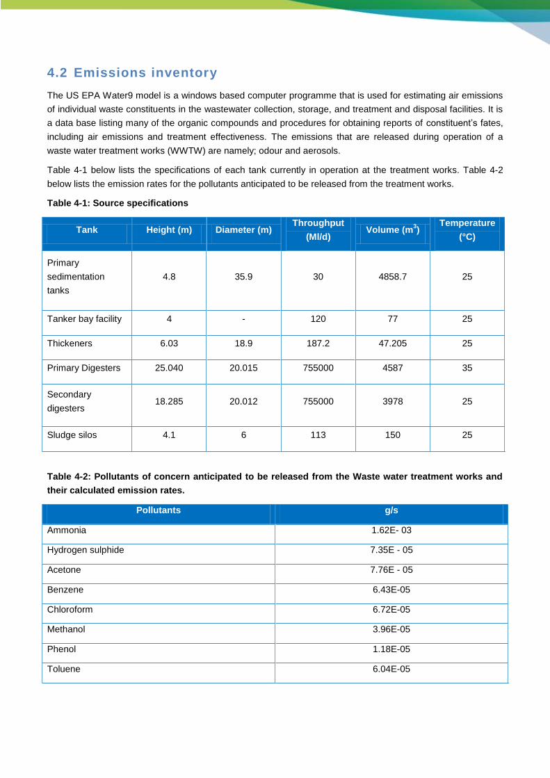
4.2 Emissions inventory

The US EPA Water9 model is a windows based computer programme that is used for estimating air emissions

of individual waste constituents in the wastewater collection, storage, and treatment and disposal facilities. It is

a data base listing many of the organic compounds and procedures for obtaining reports of constituent’s fates,

including air emissions and treatment effectiveness. The emissions that are released during operation of a

waste water treatment works (WWTW) are namely; odour and aerosols.

Table 4-1 below lists the specifications of each tank currently in operation at the treatment works. Table 4-2

below lists the emission rates for the pollutants anticipated to be released from the treatment works.

Table 4-1: Source specifications

Tank Height (m) Diameter (m) Throughput

(Ml/d) Volume (m

3)

Temperature

(°C)

Primary

sedimentation

tanks

4.8 35.9 30 4858.7 25

Tanker bay facility 4 - 120 77 25

Thickeners 6.03 18.9 187.2 47.205 25

Primary Digesters 25.040 20.015 755000 4587 35

Secondary

digesters 18.285 20.012 755000 3978 25

Sludge silos 4.1 6 113 150 25

Table 4-2: Pollutants of concern anticipated to be released from the Waste water treatment works and

their calculated emission rates.

Pollutants g/s

Ammonia 1.62E- 03

Hydrogen sulphide 7.35E - 05

Acetone 7.76E - 05

Benzene 6.43E-05

Chloroform 6.72E-05

Methanol 3.96E-05

Phenol 1.18E-05

Toluene 6.04E-05

4.2.1 Assumptions and Knowledge gaps

It is assumed that all source characteristics and volumes provided for by the client are correct;

The low lying sump was incorporated within the Water9 model in order to calculate emissions,

Emission from other surrounding industries were taken into consideration.

4.3 Impact assessment

4.3.1 Construction/ Upgrade Impacts

Construction is a source of dust emission which has a temporary impact on the local air quality. Infrastructure

and road construction are the two types of construction activity with high emission potentials.

The temporary nature of construction activities is what distinguishes it from other fugitive sources present within

the locality. Emissions from construction activities are expected to have a definitive start and end period and

will vary depending on the various construction phases. In contrast to other fugitive sources, here the

emissions occur in a steady state or follow a discernible pattern. The quantity of dust emissions from

construction activities is proportional to the area of land under construction (USEPA, 1996).

The impact on air quality and air pollution of fugitive dust is dependent on the quantity and drift potential of the

dust particles (USEPA, 1996). Large particles settle out near the source causing a local nuisance problem.

Fine particles can be dispersed over much greater distances. Fugitive dust may have significant adverse

impacts such as reduced visibility, soiling of buildings and materials, reduced growth and production in

vegetation and may affect sensitive areas and aesthetics. Fugitive dust can also adversely affect human

health.

The following component of the environment which may be impacted upon during the upgrades at the Southern

Waste Water Treatment Works includes:

The ambient air quality

Local residents and neighbouring communities

The surrounding environment and possible the fauna and flora.

Because construction is of a temporary nature, it is recommended that mitigation control measures be put in

place to limit the impacts on the local air quality. Wet suppression and wind speed reduction are common

methods used to control open dust sources at construction sites.

The aim of the proposed SWWTW upgrades is to reduce the quantity of suspended solids being disposed of to

sea by affording primary treatment to the combined effluent discharges from the Jacobs and Wentworth Valley

Trunk Sewers. This physical treatment process (through primary settling) will result in the organic load to sea

being drastically reduced. The settled solids (referred to as primary (or raw) sludge) will then be removed and

stabilised through a process of anaerobic digestion, before being dewatered. The options proposed for the

disposal of the dewatered sludge are as follows:

• Removal off-site to agriculture and/or landfill;

• Thermal drying and then removal off-site to agriculture;

• Manufacture of fertilizer through a separate sludge pelletizing process to be established on site by a

private entity (unconfirmed at this stage) and then removal off-site. This option may be investigated

under a separate study and does not form part of this study nor the scope of work described

hereunder.

The work will be undertaken in 2 phases, with Phase 1 being the immediate upgrade and Phase 2 being the

future upgrade. The Phase 1 upgrade will result in the primary treatment of approximately 60 Mega (million)

litres (or 63.5 %) of the present combined flow (i.e. 95 Mega [million] litres) being discharged from the Jacobs

and Wentworth Valley Trunk Sewers. The solids (or sludge) to be removed will then be combined with that

currently being removed from the treatment of the sewage effluent being discharged from the Umlaas Trunk

Sewer, before being pumped to the anaerobic digesters. The biogas (which is made up of approximately 60 %

methane and 40 % carbon dioxide) and emanating from the anaerobic digestion process will be stored in gas

holders. The options proposed for the use of the biogas are as follows:

• Consumption of at least one third of the stored volume for heating of the sludge (as part of the

digestion process) and flaring (or burning) of the remainder;

• Utilising most of the stored gas to dry the sludge through a mechanical thermal drying process and

then using the waste heat from the drying process to heat the sludge. It is important to note that the

drying of sludge would greatly reduce the road transportation requirements for removal of sludge off

site.

The work to be completed under each phase is proposed as follows:

Phase 1:

a) Refurbish and bring back on line two out of six existing primary settling tanks;

b) Refurbish and bring back on line existing two anaerobic primary digesters and secondary digester and

construct two new primary digesters and one secondary digester, all of same capacity as existing;

c) Refurbish and bring back on line existing raw sludge gravity thickener and construct a new gravity

thickener of the same capacity;

d) Refurbish and bring back on line existing gas holder and construct a new gas holder of the same

capacity.

e) Refurbish and bring back on line various existing (unused) electrical substation buildings and small

pumping stations;

f) Establishing a new mechanical sludge dewatering facility on site and 2 x 150 000 litres fully enclosed

steel sludge storage silos;

g) Establishment a new mechanical sludge thermal drying facility on site.

h) Provide additional effluent storage capacity of 23 000 000 litres at existing low level pumping station

and install two new 350 kilowatt pumps;

i) Replace the last 70 m of the landline section of the sea outfall pipeline with new 2x 1000 m diameter

pipe;

j) Construct new road tanker effluent discharge bays in close proximity to the entrance of the Works;

k) Install new medium voltage and low voltage electrical cables and equipment;

l) Minor road works and new tanker bay facility access designs;

m) The installation of a standby generator.

Phase 2:

a) Refurbish and bring back on line remaining four of the existing six primary settling tanks and construct

two new primary settling tanks of the same capacity as existing;

b) Construct four new anaerobic primary digesters and two new secondary digesters, all of the same

capacity as existing;

c) Construct a new raw sludge gravity thickener, of the same capacity as existing;

d) Construct a new gas holder;

e) Install additional mechanical sludge dewatering equipment.

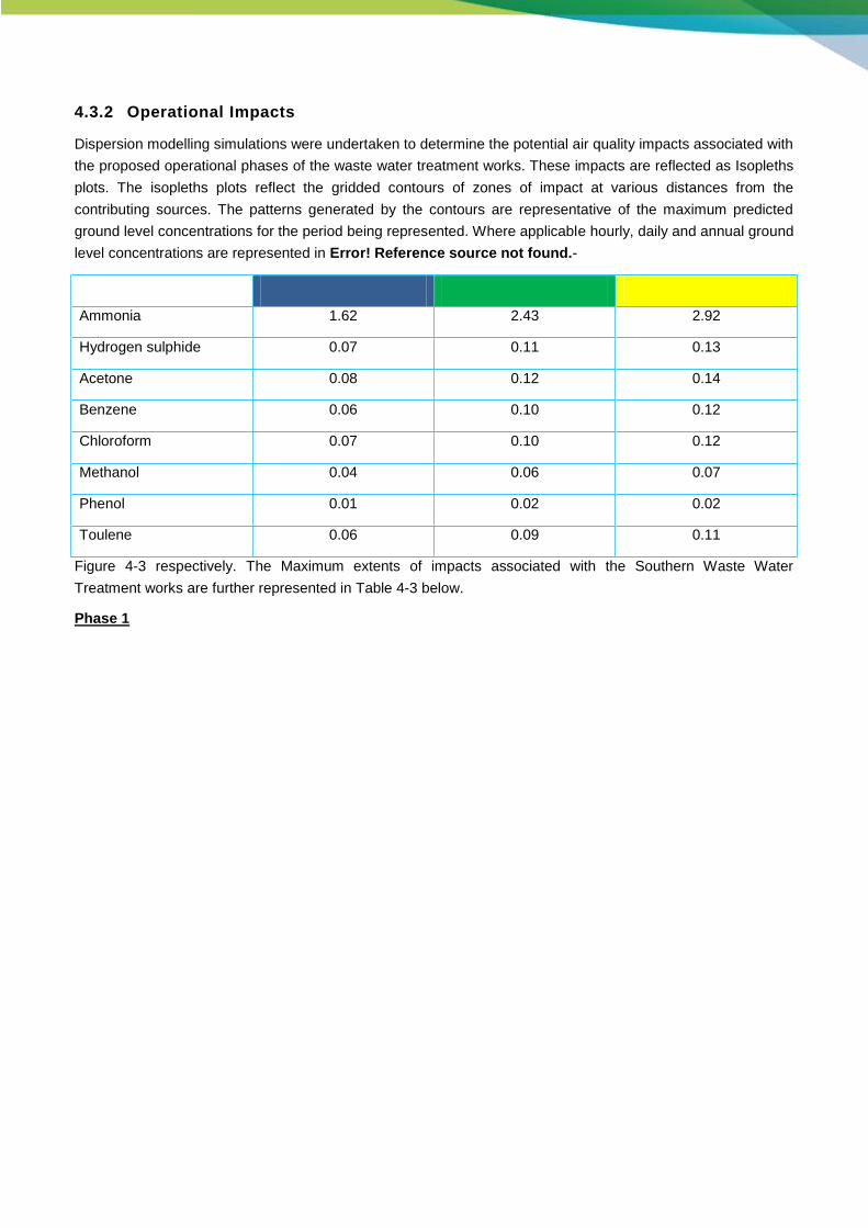
4.3.2 Operational Impacts

Dispersion modelling simulations were undertaken to determine the potential air quality impacts associated with

the proposed operational phases of the waste water treatment works. These impacts are reflected as Isopleths

plots. The isopleths plots reflect the gridded contours of zones of impact at various distances from the

contributing sources. The patterns generated by the contours are representative of the maximum predicted

ground level concentrations for the period being represented. Where applicable hourly, daily and annual ground

level concentrations are represented in Error! Reference source not found.-

Ammonia 1.62 2.43 2.92

Hydrogen sulphide 0.07 0.11 0.13

Acetone 0.08 0.12 0.14

Benzene 0.06 0.10 0.12

Chloroform 0.07 0.10 0.12

Methanol 0.04 0.06 0.07

Phenol 0.01 0.02 0.02

Toulene 0.06 0.09 0.11

Figure 4-3 respectively. The Maximum extents of impacts associated with the Southern Waste Water

Treatment works are further represented in Table 4-3 below.

Phase 1

Ammonia 56.70 64.80 68.04

Hydrogen sulphide 2.57 2.94 3.09

Acetone 2.72 3.10 3.26

Benzene 2.25 2.57 2.70

Chloroform 2.35 2.69 2.82

Methanol 1.39 1.58 1.66

Phenol 0.41 0.47 0.50

Toulene 2.11 2.42 2.54

Figure 4-1: Phase 1- hourly average predicted ground level concentration (µg/m3) for the Southern

Waste Water Treatment Works.

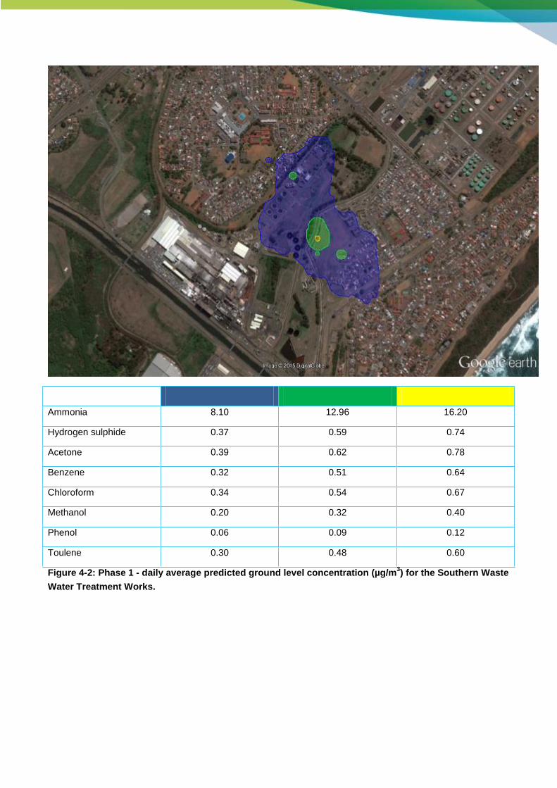
Ammonia 8.10 12.96 16.20

Hydrogen sulphide 0.37 0.59 0.74

Acetone 0.39 0.62 0.78

Benzene 0.32 0.51 0.64

Chloroform 0.34 0.54 0.67

Methanol 0.20 0.32 0.40

Phenol 0.06 0.09 0.12

Toulene 0.30 0.48 0.60

Figure 4-2: Phase 1 - daily average predicted ground level concentration (µg/m3) for the Southern Waste

Water Treatment Works.

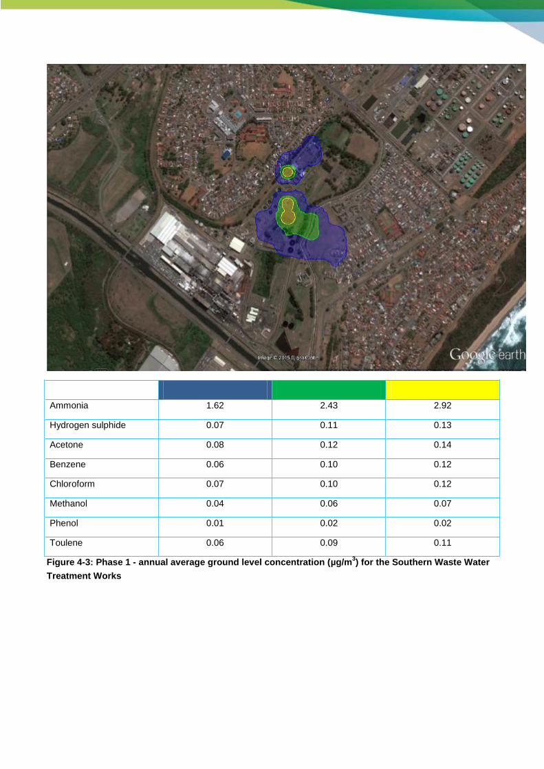
Ammonia 1.62 2.43 2.92

Hydrogen sulphide 0.07 0.11 0.13

Acetone 0.08 0.12 0.14

Benzene 0.06 0.10 0.12

Chloroform 0.07 0.10 0.12

Methanol 0.04 0.06 0.07

Phenol 0.01 0.02 0.02

Toulene 0.06 0.09 0.11

Figure 4-3: Phase 1 - annual average ground level concentration (µg/m3) for the Southern Waste Water

Treatment Works

Table 4-3: Phase1 - Maximum predicted ground level concentration (µg/m3).

Pollutants

Maximum Predicted

Concentrations Guidelines

Fraction of the

Guidelines (%)

Hourly Daily Annual Hourly Daily Annual Hourly Daily Annual

Ammonia 81.00 16.20 4.05 100 0.4

Hydrogen

sulphide 3.68 0.74 0.18 10 150 42 0.3 <0.1 <0.1

Acetone 3.88 0.78 0.19

Benzene 3.22 0.64 0.16 1300 30 <0.1 <0.1

Chloroform 3.36 0.67 0.17 300 150 <0.1 <0.1

Methanol 1.98 0.40 0.10 28000 4000 <0.1 <0.1

Phenol 0.59 0.12 0.03 5800 200 <0.1 <0.1

Toluene 3.02 0.60 0.15 37000 300 <0.1 <0.1

Table 4-3 above compares the maximum ground level concentration as a fraction of the standards. There were

no exceedances of the hourly, daily and annual standards for the pollutants anticipated to be released as a

result of the treatment works. All concentrations during phase 1 of the upgrades were less than 1 % of the

respective guidelines.

The Cancer risk due to exposure from certain pollutants is presented in Table 4-4 below. The table evaluated

the various cancer risk factors on the US EPA unit risk factor. The Total cancer risk assessment indicated

benzene with a cancer risk of 3.5 individuals in a population of 10 million, while Chloroform had an estimated

cancer risk of 3.86 individuals in a population of 1 million.

Usually a cancer risk of 1 individual in a population of hundred thousand is deemed to be an acceptable risk

level. Based on these factors, the cancer risk associated with these pollutants are not significant.

Table 4-4: Phase 1 - Predicted cancer Risk

Pollutant Annual average

concentration (µg/m3)

US-EPA Cancer Risk

Factor Estimated Cancer Risk

Benzene 3.54E-07 2.2E-06 3.5 in 10 million

Chloroform 3.86E-06 2.3E-05 3.86 in 1 million

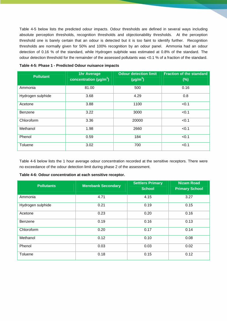
Table 4-5 below lists the predicted odour impacts. Odour thresholds are defined in several ways including

absolute perception thresholds, recognition thresholds and objectionability thresholds. At the perception

threshold one is barely certain that an odour is detected but it is too faint to identify further. Recognition

thresholds are normally given for 50% and 100% recognition by an odour panel. Ammonia had an odour

detection of 0.16 % of the standard, while Hydrogen sulphide was estimated at 0.8% of the standard. The

odour detection threshold for the remainder of the assessed pollutants was <0.1 % of a fraction of the standard.

Table 4-5: Phase 1 - Predicted Odour nuisance impacts

Pollutant 1hr Average

concentration (µg/m3)

Odour detection limit

(µg/m3)

Fraction of the standard

(%)

Ammonia 81.00 500 0.16

Hydrogen sulphide 3.68 4.29 0.8

Acetone 3.88 1100 <0.1

Benzene 3.22 3000 <0.1

Chloroform 3.36 20000 <0.1

Methanol 1.98 2660 <0.1

Phenol 0.59 184 <0.1

Toluene 3.02 700 <0.1

Table 4-6 below lists the 1 hour average odour concentration recorded at the sensitive receptors. There were

no exceedance of the odour detection limit during phase 2 of the assessment.

Table 4-6: Odour concentration at each sensitive receptor.

Pollutants Merebank Secondary Settlers Primary

School

Nizam Road

Primary School

Ammonia 4.71 4.15 3.27

Hydrogen sulphide 0.21 0.19 0.15

Acetone 0.23 0.20 0.16

Benzene 0.19 0.16 0.13

Chloroform 0.20 0.17 0.14

Methanol 0.12 0.10 0.08

Phenol 0.03 0.03 0.02

Toluene 0.18 0.15 0.12

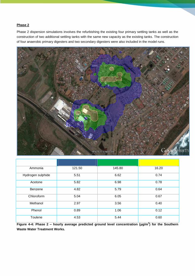
Phase 2

Phase 2 dispersion simulations involves the refurbishing the existing four primary settling tanks as well as the

construction of two additional settling tanks with the same new capacity as the existing tanks. The construction

of four anaerobic primary digesters and two secondary digesters were also included in the model runs.

Ammonia 121.50 145.80 16.20

Hydrogen sulphide 5.51 6.62 0.74

Acetone 5.82 6.98 0.78

Benzene 4.82 5.79 0.64

Chloroform 5.04 6.05 0.67

Methanol 2.97 3.56 0.40

Phenol 0.89 1.06 0.12

Toulene 4.53 5.44 0.60

Figure 4-4: Phase 2 – hourly average predicted ground level concentration (µg/m3) for the Southern

Waste Water Treatment Works.

Ammonia 14.58 19.44 19.44

Hydrogen sulphide 0.66 0.88 0.88

Acetone 0.70 0.93 0.93

Benzene 0.58 0.77 0.77

Chloroform 0.60 0.81 0.81

Methanol 0.36 0.48 0.48

Phenol 0.11 0.14 0.14

Toulene 0.54 0.72 0.72

Figure 4-5: Phase 2 - daily average predicted ground level concentration (µg/m3) for the Southern Waste

Water Treatment Works.

Ammonia 3.24 4.05 4.86

Hydrogen sulphide 0.15 0.18 0.22

Acetone 0.16 0.19 0.23

Benzene 0.13 0.16 0.19

Chloroform 0.13 0.17 0.20

Methanol 0.08 0.10 0.12

Phenol 0.02 0.03 0.04

Toulene 0.12 0.15 0.18

Figure 4-6: Phase 2 - annual average ground level concentration (µg/m3) for the Southern Waste Water

Treatment Works.

Table 4-7 below compares the maximum ground level concentration as a fraction of the standards. There were

no exceedances of the hourly, daily and annual standards for the pollutants anticipated to be released as a

result of the treatment works. All concentrations of pollutants complied with the respective hourly, daily and

annual standard. The highest emission assessed was ammonia and hydrogen sulphide.

Table 4-7:Phase 2 – Maximum predicted ground level concentration (µg/m3)

Pollutants

Maximum Predicted

Concentrations (µg/m3)

Guidelines Fraction of the

Guidelines (%)

Hourly Daily Annual Hourly Daily Annual Hourly Daily Annual

Ammonia 178.20 40.50 9.72 100 0.1

Hydrogen

sulphide 8.09 1.84 0.44 10 150 42 0.8 <0.1 <0.1

Acetone 8.54 1.94 0.47

Benzene 7.07 1.61 0.39 1300 30 <0.1 <0.1

Chloroform 7.39 1.68 0.40 300 150 <0.1 <0.1

Methanol 4.36 0.99 0.24 28000 4000 <0.1 <0.1

Phenol 1.30 0.30 0.07 5800 200 <0.1 <0.1

Toluene 6.64 1.51 0.36 37000 300 <0.1 <0.1

Table 4-8 below show the cancer risk assessment for phase 2 model runs. Benzene had an estimated cancer

risk of 1.02 in 10 million which is significantly lower than the cancer risk factor. Chloroform had an estimated

cancer risk of 8.87 in 10 million which is lower than the US –EPA cancer risk factor. The cancer risk factor

arising from the treatment works is not significant.

Table 4-8: Phase 2 – Cancer risk assessment

Pollutant Annual average

concentration (µg/m3)

US-EPA Cancer Risk

Factor Estimated Cancer Risk

Benzene 4.66E-01 2.2E-06 1.02 in 10 million

Chloroform 3.86E-01 2.3E-05 8.87 in 10 million

Table 4-9 below lists the predicted odour impact. Odour thresholds are defined in several ways including

absolute perception thresholds, recognition thresholds and objectionability thresholds. At the perception

threshold one is barely certain that an odour is detected but it is too faint to identify further. Recognition

thresholds are normally given for 50% and 100% recognition by an odour panel. The only pollutant noted to

exceed the odour detection limit is hydrogen sulphide during phase 2 of the upgrades.

Table 4-9: Phase 2 - Predicted Odour nuisance impacts

Pollutant 1hr Average

concentration (µg/m3)

Odour detection limit

(µg/m3)

Fraction of the standard

(%)

Ammonia 121.50 500 0.2

Hydrogen sulphide 5.51 4.29 1.2

Acetone 5.82 1100 <0.1

Benzene 4.82 3000 <0.1

Chloroform 5.04 20000 <0.1

Methanol 2.97 2660 <0.1

Phenol 0.89 184 <0.1

Toluene 4.53 700 <0.1

Table 4-10: Odour concentration at each sensitive receptor (Exceedance highlighted in Bold)

Pollutants Merebank Secondary Settlers Primary

School

Nizam Road

Primary School

Ammonia 91.76 108.33 112.53

Hydrogen sulphide 4.16 4.91 5.11

Acetone 4.40 5.19 5.39

Benzene 3.64 4.30 4.47

Chloroform 3.81 4.49 4.67

Methanol 2.24 2.65 2.75

Phenol 0.67 0.79 0.82

Toluene 3.42 4.04 4.20

Table 4-10 above lists the 1 hour average odour concentration recorded at the sensitive receptors. Hydrogen

sulphide odour emission was exceeded at Settlers Primary and Nizam Road Primary school during phase 2 of

the upgrades.

4.4 Decommissioning impacts

The decommissioning phase is associated with activities related to the demolition of infrastructure and the

rehabilitation of disturbed areas. The total rehabilitation will ensure that the total area will be a free draining

covered with topsoil and grassed. The following activities are associated with the decommissioning phase (US-

EPA, 1996):

Existing buildings and structures demolished, rubble removed and the area levelled;

Land and permanent waste piles prepared for re-vegetation.

Possible sources of fugitive dust emission during the closure and post-closure phase include:

Grading of sites;

Infrastructure demolition;

Infrastructure rubble piles;

Transport and dumping of building rubble;

Preparation of soil for re-vegetation – ploughing and addition of fertiliser, compost etc.

Exposed soil is often prone to erosion by water. The erodability of soil depends on the amount of rainfall and its

intensity, soil type and structure, slope of the terrain and the amount of vegetation cover (Brady, 1974). Re-

vegetation of exposed areas for long-term dust and water erosion control is commonly used and is the most

cost-effective option. Plant roots bind the soil, and vegetation cover breaks the impact of falling raindrops, thus

preventing wind and water erosion. Plants used for revegetation should be indigenous to the area, hardy, fast-

growing, nitrogen-fixing, provide high plant cover, be adapted to growing on exposed and disturbed soil

(pioneer plants) and should easily be propagated by seed or cuttings.

5 ODOUR MANAGEMENT

The purpose of an odour management plan is to ensure that the waste water treatment works is managed in

such a way that the risk of odour nuisance is minimised as far as practical.

Sewage is produced as a by-product of human existence and numerous industrial processes and is odorous by

nature. Even though the constituents of sewage are primarily water, it also contains various other biological and

chemical materials which if released in an uncontrolled manner to the environment, are capable of causing

pollution.

5.1.1 Good housekeeping practices

The general means of odour management at a treatment works includes the following:

Good housekeeping and raw material handlings practices;

Control and minimization of odours from residual material and waste which includes imported sludge or

septic tank waste;

Maintaining the effluent aeration for aerobic processes;

Avoiding anaerobic conditions and minimizing septicity;

Selecting process steps that presents the least risk of odour generation;

Minimization of sludge retention time in primary settlement;

Application of extended aeration to avoid primary settlements;

The build-up of scum and foam on tank surfaces can at times contribute and lead to odour. The draining of

tanks for cleaning has been implicated as a prominent source of odour complaints. Practical measures

such as use of appropriate chemicals can be used to minimize and mitigate odour impacts.

Storage of sludge and products on site needs to be minimized;

The cleaning of screens and grit should be done regularly, so as to reduce the odour potential;

5.1.2 Plant performance and maintenance

Research has shown that some odour problems which occur at waste water treatment works had been due to

plant maintenance and proper operations of odour abatement equipment. These problems were said to be due

partly to difficulties in operations and lack of training. Plant performance, maintenance, inspection and operator

training are therefore crucial in maintaining the effectiveness of odour control measures. The following should

be kept in mind for an efficient operation of a treatment works;

Sufficient supply of reagents and consumables should be kept on site;

A record of maintenance should be available for inspection;

The operator should maintain a record of training requirements for each operational post as well as a

record of training received by each personnel whose actions have an impact on the environment;

Minimisation of emissions on start up and shut down;

5.1.3 Plant design and upgrades

Odour problems can occur at almost any stage of the WWTW depending upon the influent, plant location,

operation and design. The areas most commonly responsible for potentially offensive odour releases are the

inlet works, primary sedimentation, high rate storage. However the areas most commonly responsible for

potentially offensive odour releases are the inlet works, primary sedimentation tank, high rate secondary

treatment processes and all stages of un-stabilised sludge handling and storage.

However there exists opportunities for the minimization of odour emissions at certain stages of the process for

instance during the primary settlement stage as the tanks are usually large; there is a significant surface area

with which to emit pollutants. An effective method may be to use a low rate biological treatment step such as

extended aeration of sewage or a high rate process within a building to avoid primary treatment. However there

is cost implications and is dependant upon the size of the plant.

5.1.4 Transport of sewage to the works

Measures which can be put in place to reduce the septicity and minimize the retention time of sewage in

transport under anaerobic conditions includes the following;

Improve ventilation;

If septic conditions develop, chemical dosing will assist in reducing the concentration of odorous emissions;

Minimize intermediate storage;

Regular cleaning to remove accumulations;

Also ensure that the slope of gravity prevents sedimentation and accumulation.

5.1.5 Inlet works

Screening and pre-treatment of raw sewage is required to remove grit and other compounds prior to primary

treatment. Procedures that should be considered to minimize emissions released during this stage of treatment

involve the following:

Lowering discharge points to minimise emissions;

Balancing the flow of sludge liquors to even the load over the day;

Regular cleaning and flushing of screens and influent channels.

5.1.6 Primary and secondary treatment

During the primary treatment, sewage flows through large tanks known as the primary sedimentation tanks.

The tanks are used to settle sludge, while oil and grease rises to the surface and is skimmed. The minimization

of the sludge retention time in the primary tanks can reduce odour emissions. The appropriate steps taken to

reduce odorous emissions during primary treatment are as follows;

Use of covers to reduce the impact of odour emissions;

A reduction in the hydraulic retention time;

Improving the efficiency of the de-sludge process and ensure regular cleaning of the tanks, sumps, scum

and grease removal equipment.

The conditions during secondary aerobic treatment should ensure that aerobic conditions are maintained at all

times for activated sludge plants. Increasing the aeration can minimize the generation of aerosols.

5.1.7 Sludge handling, storage and thickening

Sludge and bio-solid handling is usually the most significant source of odour release and good sludge

management is essential. All raw sludge and bio solids will release odour largely dependent upon age. In

general, sludge handling, storage and processing should be enclosed or covered and provided with ventilation

to odour abatement equipment.

Sludge which has been lime treated can generate odour, particularly ammonia, and should be stored under

cover to prevent odour generation;

Sludge should be processed as soon as possible after generation as retention will lead to anaerobic

conditions. It is good practice to minimise the potential storage of sludge before treatment and storage for

un-stabilised sludge should be limited to a maximum capacity of 24-hours production.

5.1.8 Anaerobic digestion

The gas produced in an anaerobic digester will be odorous;

Routinely drain condensate traps to remove water ad avoid back pressure;

Secondary digesters are often not covered and they can lose up to 10% of methane generated and

odorous pollutants.

The primary digester should reduce the risk of odour generation at the secondary stage. In instances where

the operation of the primary digester leads to emissions in the secondary stage, the secondary digester

may require covering and venting to an odour and methane treatment facility.

5.1.9 Odour abatement

There is a wide range of odour abatement equipment that can be used to treat emissions of contained air from

the SWWTW. There are many factors which will affect the choice of equipment including odour removal

efficiency, flow rate and inlet odour concentration, type of chemical species in the odour, variability in flow and

load, space requirements and infrastructure.

Any odour abatement equipment installed on contained emissions should have an odour removal efficiency of

not less than 95%. However abatement measure has severe cost implications.

6 CONCLUSION

The Air Quality Impact Assessment undertaken for the Southern Waste Water Treatment Works includes a

meteorological overview of the area. Meteorological data was obtained from the South African Weather

services in Amersfoort for the Jan 2009 – Dec 2013 monitoring period.

An emissions inventory was undertaken with the aim of quantifying emissions associated with the operational

processes of the treatment works. Use was made of the Water9 model in order to quantify the emission

anticipated to be released.

Dispersion modelling simulations were undertaken using AERMOD. Hourly, daily and annual average

concentrations were evaluated and compared to best available standards and guidelines.

Based on the dispersion modelling simulations, the main conclusions can be summarised are as follows;

Phase 1;

All hourly, daily and annual maximum average concentrations of pollutants were below the respective

standards. There were no exceedances of any guidelines.

The odour perception threshold was below the 50% recognition for a given population size

The concentrations were highest during the primary treatment particularly from the Primary

sedimentation tanks.

Phase 2;

All hourly, daily and annual average concentrations of pollutants for phase 2 were below the respective

standards. There were no exceedances of any guidelines.

The odour perception threshold was below the 50% recognition for a given population size, with the

exception of Hydrogen sulphide which exceeded the detection limit.

The concentrations were highest at the Primary sedimentation tanks;

There are expected to be nuisance impacts associated with the phased upgrades at the Southern Waste Water

Treatment Works. It is primarily the result of the release of hydrogen sulphide into the atmosphere during

phase 2. These impacts are noted to extend beyond the site boundary for hydrogen sulphide. All other

pollutants evaluated during the assessment were compliant with their guidelines and thresholds.

In conclusion there alternative scenario will have any effect on the air quality situation and emissions will

remain the same.

7 REFERENCES

CEPA/FPAC WORKING GROUP, 1998. National Ambient Air Quality Objectives for Particulate Matter. Part 1.

Science Assessment Document, A Report by the Canadian Environmental Protection Agency (CEPA) Federal-

Provincial Advisory Committee (FPAC)on Air Quality Objectives and Guidelines.

EPA (1996). Users Guide for the Industrial Source Complex (ISC3) Dispersion Models., EPA-454/B-95-003a,

US-Environmental Protection Agency, Research Triangle Park, North Carolina

EPA (1996). Compilation of Air Pollution Emission Factors (AP-42), 6th Edition, Volume 1, as contained in the

AirCHIEF (AIR Clearinghouse for Inventories and Emission Factors) CD-ROM (compact disk read only

memory), US Environmental Protection Agency, Research Triangle Park, North Carolina.

IRIS (1998). US-EPA's Integrated Risk Information Data Base, available from www.epa.gov/iris (last updated

20 February 1998).

Tyson P. D., Preston-Whyte R.A. (2002). The weather and climate of southern Africa. International journal of

climatology, 22, pp 883-884.

WHO (2000). Guidelines for Air Quality, World Health Organisation, Geneva.