A PEL Company REPORT AIR QUALITY APPRAISAL TOOL (AQAT) – FINAL REPORT NSW Environment Protection Authority – Air Policy Job No: 6620 4 April 2013

Welcome message from author
This document is posted to help you gain knowledge. Please leave a comment to let me know what you think about it! Share it to your friends and learn new things together.
Transcript

A PEL Company
REPORT
AIR QUALITY APPRAISAL TOOL (AQAT) – FINAL
REPORT
NSW Environment Protection Authority – Air Policy
Job No: 6620
4 April 2013

Air Quality Appraisal Tool - Final Report V5.doc ii
Air Quality Appraisal Tool – Final Report
NSW Environment Protection Authority – Air Policy | PAEHolmes Job 6620
DISCLAIMER & COPYRIGHT:
©
munnelj
Typewritten Text
This report was prepared by PAEHolmes in good faith exercising all due care and attention, but no representation or warranty, express or implied, is made as to the relevance, accuracy, completeness or fitness for purpose of this document in respect of any particular user’s circumstances. Users of this document should satisfy themselves concerning its application to, and where necessary seek expert advice in respect of, their situation. The views expressed within are not necessarily the views of the Environment Protection Authority (EPA) and may not represent EPA policy.
munnelj
Typewritten Text
Copyright State of NSW and the NSW Environment Protection Authority
munnelj
Typewritten Text
munnelj
Typewritten Text

Air Quality Appraisal Tool - Final Report V5.doc iii
Air Quality Appraisal Tool – Final Report
NSW Environment Protection Authority – Air Policy | PAEHolmes Job 6620
EXECUTIVE SUMMARY
The improvement of transport infrastructure is one of the priorities of the New South Wales (NSW)
Government. However, it is essential that any adverse impacts of transport developments - as well
as land use changes near transport corridors - are minimised. One of the main considerations in
this respect is air quality, as air pollution from transport is associated with detrimental effects on
human health, natural ecosystems and climate.
Monetary valuation is commonly used when evaluating the potential benefits of developments or
policies and measures, as the diverse range of impacts can be quantified in a simple and
consistent manner. An important factor in any economic appraisal of air pollution is the cost of
health impacts. The overall costs of air pollution are dominated by costs linked to mortality, which
in turn are dominated by the effects of airborne particulate matter (PM). Consideration of the
overall exposure of the population to PM is therefore critical when determining health impacts and
costs.
This report describes the development of an ‘Air Quality Appraisal Tool’ (AQAT) for quantifying and
monetising the air quality impacts of transport and land use developments in NSW. AQAT will allow
planners to consider actions relating to transport and land use alongside other measures that are
designed to improve air quality and reduce population exposure as part of the planning process. In
addition, it will support the assessment of air pollutant emissions in Environmental Impact
Statements and economic appraisals.
The report describes the development of AQAT. It includes the context and scope of the work, a
review of existing approaches for estimating emissions and health costs in NSW, the development
of the methodology, guidance on implementation, and recommendations for improvement. Several
case studies are examined to demonstrate the functionality of AQAT and its application to local and
State government projects.
The methodology used in AQAT builds upon existing models. The Tool itself takes the form of a
spreadsheet with relatively simple inputs such as road traffic flows, rail freight activity, and local
population density (defined in terms of ‘Significant Urban Areas’). The outputs are annual
emissions of criteria pollutants and the damage costs associated with PM2.5 emissions.
The single most important consideration in the development of AQAT was the selection of a
method for quantifying the health costs of air pollution, as this dictated the outputs that would be
required for other elements of AQAT. Damage costs are calculated using unit costs (in A$ per
tonne) for primary PM2.5 emissions from transport, based on a method derived for NSW EPA by
PAEHolmes in which the unit costs are a function of population density. Damage costs for other
sectors of activity and for secondary particles are not included at present.
This therefore meant that the changes in emissions from road and rail for a given development
had to be quantified. For large developments, data on transport activity and emissions will
generally have been obtained, especially where an Environmental Impact Statement has been
compiled, or could be estimated from the available data, and therefore damage cost values can be
applied directly. For smaller local developments there are generally very few data, and therefore
algorithms are incorporated into AQAT to enable emissions to be calculated.
The Roads and Maritime Services Tool for Roadside Air Quality (TRAQ) was considered to be the
most suitable approach for modelling road traffic emissions in AQAT. The level of the approach in
Air Quality Appraisal Tool - Final Report V5.doc iv
Air Quality Appraisal Tool – Final Report
NSW Environment Protection Authority – Air Policy | PAEHolmes Job 6620
TRAQ is in keeping with the need for simple calculations in AQAT, and the calculation methods are
consistent with those used in the 2008 NSW GMR air emissions inventory
The capabilities for modelling rail emissions in Australia are rather limited, and there is a heavy
reliance upon emission factors from the USEPA. Given that most of the rail diesel consumption in
NSW relates to the haulage of freight and that passenger trains are predominantly electrified, a
decision was made to exclude passenger transport from AQAT. Based on a consideration of the
available options, it was concluded that the method used in the 2008 GMR inventory would be the
most suitable approach for use in AQAT.
The tool takes the form of an Excel spreadsheet which calculates changes in emissions and
damage costs based on conditions before and after a development. The required inputs are the
type(s) of affected road, road length, road gradient, traffic flow, traffic speed, traffic composition,
and the local population density. Guidance on developing the base case and assessment scenarios
is provided.
An indicative sensitivity analysis was conducted using the user-defined model parameters for road
transport. The analysis was based on a Monte Carlo simulation, with the fractional contribution of
each input variable to the variance in the output being determined. For the assumptions used,
road gradient was found to be an important parameter for emissions of some pollutants, but less
so for PM emissions. For PM emissions and damage cost, road length was an important variable,
and population density was also an important variable for damage costs. It is therefore important
to characterise these as accurately as possible when using AQAT. The number of HDVs and traffic
speed were less important. The analysis could be refined using more appropriate data prior to any
specific case study being undertaken.
The report also provides guidance on the use of AQAT in the economic appraisal of developments,
some useful sources of information and data, and recommendations for future improvement.
Air Quality Appraisal Tool - Final Report V5.doc v
Air Quality Appraisal Tool – Final Report
NSW Environment Protection Authority – Air Policy | PAEHolmes Job 6620
TABLE OF CONTENTS
1 INTRODUCTION 1 1.1 Background 1 1.2 Objectives 2 1.3 Development approach 2
2 UNDERSTANDING THE CONTEXT 4 2.1 The regulatory framework 4 2.2 The planning process and environmental assessment 5
2.2.1 State-significant developments and infrastructure 5 2.2.2 Part 4 developments 7 2.2.3 Part 5 developments 9
2.3 Economic appraisal 9 2.4 Guidelines for air quality assessment and mitigation 10
2.4.1 NSW ‘Approved Methods’ 10 2.4.2 RTA guidelines for road projects 10 2.4.3 Local Government Air Quality Training Toolkit 12 2.4.4 Interim guideline on development near rail corridors and busy roads 12
2.5 Types of development 12
3 REVIEW OF METHODS AND MODELS 16 3.1 Road transport emission models 16
3.1.1 National Pollutant Inventory 16 3.1.2 NSW GMR emissions inventory model 16 3.1.3 TRAQ 18 3.1.4 PIARC 19
3.2 Road transport data 19 3.2.1 Data requirements 19 3.2.2 Types of model 19 3.2.3 Comparison of model attributes 21 3.2.4 Models used in NSW and typical outputs 22 3.2.5 Models used in environmental impact assessment in NSW 23
3.3 Rail transport emission models 24 3.3.1 National Pollutant Inventory 25 3.3.2 NSW GMR emissions inventory model 25 3.3.3 Other models 26
3.4 Rail transport data 26 3.5 Methods for monetising air pollution impacts 26
3.5.1 General approaches 26 3.5.2 Australian examples 27 3.5.3 Updated Australian methodology 29
4 DEVELOPMENT OF AIR QUALITY APPRAISAL TOOL 30 4.1 Overall approach 30 4.2 Selection of approach for monetising impacts 30 4.3 Selection of emission modelling approaches 31
4.3.1 Road transport 31 4.3.2 Rail transport 32
4.4 Use of models within AQAT 32
5 CASE STUDIES 34 5.1 Overview 34 5.2 Study 1: Local transport - road bypass 34
5.2.1 Description of case study 34

Air Quality Appraisal Tool - Final Report V5.doc vi
Air Quality Appraisal Tool – Final Report
NSW Environment Protection Authority – Air Policy | PAEHolmes Job 6620
5.2.2 Input data 35 5.2.3 Results 39
5.3 Study 2: Local land use – growth centre 39 5.3.1 Description of case study 39 5.3.2 Scenarios and input data 41 5.3.3 Results 44
5.4 Study 3: State transport – rail freight link 45 5.4.1 Description of case study 45 5.4.2 Scenarios and input data 45 5.4.3 Results 46
5.5 Study 4: Comparison between two local land use developments 49 5.5.1 Description of case study 49 5.5.2 Scenarios and input data 50 5.5.3 Results 50
6 SENSITIVITY ANALYSIS 53 6.1 Overview 53 6.2 Method 53 6.3 Results and discussion 54
7 IMPLEMENTATION AND FUTURE IMPROVEMENTS 57 7.1 Implementation 57
7.1.1 Role in planning process 57 7.1.2 General guidance on appraisal of developments 58
7.2 Sources of information and data 59 7.2.1 Road transport 59 7.2.2 Rail transport 61 7.2.3 Population density 61
7.3 Future improvements 61
8 REFERENCES 63
APPENDIX A: Glossary of terms and abbreviations
APPENDIX B: Consultees
APPENDIX C: Air Quality Appraisal Tool – Calculation Methodology
APPENDIX D: Air Quality Appraisal Tool - User Guide

Air Quality Appraisal Tool - Final Report V5.doc 1
Air Quality Appraisal Tool – Final Report
NSW Environment Protection Authority – Air Policy | PAEHolmes Job 6620
1 INTRODUCTION
1.1 Background
The improvement of transport infrastructure is one of the priorities of the New South Wales (NSW)
Government, as expressed in the NSW 2021 plan1. However, it is essential that any adverse
impacts of transport developments - as well as land use changes near transport corridors - are
minimised. Planning authorities must therefore assess development applications against various
social, economic and environmental criteria, and one of the main environmental considerations is
air quality2. To ensure that new developments do not exacerbate the impacts of air pollution,
development applications need to be accompanied by an air quality assessment, including
mitigation measures where appropriate.
Air pollution from transport is associated with detrimental effects on human health, natural
ecosystems and climate. When evaluating the potential benefits of developments or pollution-
reduction policies it is desirable to quantify impacts in a simple and consistent manner. Whilst this
is difficult given the diversity of the impacts, approaches based on monetary valuation are the
most common, and these have several advantages. They make explicit the real cost of pollution
impacts on society, and enable alternative proposals to be compared directly using a single index
(money). A framework for the valuation of costs and benefits of policies, including the economic
assessment of environmental impacts, has been established in Guidelines published by the NSW
Treasury (2007). The Guidelines aim to ensure that all public sector agencies undertake
economic appraisals on a consistent basis. Economic appraisal is also an important prerequisite of
any new statutory instrument.
An important factor in any economic appraisal of air pollution is the cost of health impacts. The
health costs of air pollution are dominated by its effects on mortality, which in turn are dominated
by the effects of airborne particulate matter (PM) (Jalaludin et al., 2011).
The current approach to air quality management in Australia focuses on reducing exceedances of
ambient air quality standards at specific locations. The standards are designed to protect human
health. However, for PM there is no evidence of a threshold concentration below which adverse
health effects are not observed (Pope and Dockery, 2006; Brook et al., 2010; USEPA,
2009a; COMEAP, 2009). The evidence indicates that long-term exposure to the prevailing
background PM concentration is the most important determinant of health outcomes relating to air
quality. Therefore, whilst PM concentrations in Australian cities are significantly below the
standards for most of the time3 (Commonwealth of Australia, 2010), the health impacts are
actually driven by large-scale exposure to relatively low pollution levels4. Consideration of the
overall exposure of the population is therefore critical when determining the effects of policies,
measures and developments on health and costs. This is rather different to the current assessment
approach for developments, in which air pollution is given a low priority when there is unlikely to
be an exceedance of air quality standards.
1 http://2021.nsw.gov.au/renovate-infrastructure 2 Influencing the outcomes of transport and planning decisions is also a priority in the development of the
national strategy to improve air quality, as well as the NSW Government’s 25-Year Air Quality Management Plan Action for Air.
3 High observed PM concentrations are typically a result of bushfires and dust storms. 4 The development of an exposure-reduction framework for PM was an important recommendation of a review
of the National Environment Protection Measure for Ambient Air Quality (‘Air NEPM’) (NEPC, 2011), and the NSW government is currently in the process of developing such a framework.

Air Quality Appraisal Tool - Final Report V5.doc 2
Air Quality Appraisal Tool – Final Report
NSW Environment Protection Authority – Air Policy | PAEHolmes Job 6620
Against this background, in February 2012 the Air Policy division of the NSW Environment
Protection Authority (EPA) (then Office of Environment and Heritage, OEH) commissioned
PAEHolmes to develop an ‘Air Quality Appraisal Tool’ (AQAT) for quantifying and monetising the air
quality impacts of transport and land use developments in the State. The tool will allow planners to
consider actions relating to transport and land use alongside other measures that are designed to
improve air quality and reduce population exposure as part of the planning process.
This report describes the development of AQAT. It includes the context and scope of the work, a
review of existing approaches for estimating transport emissions and health costs, the
development of the methodology, and guidance on implementation.
A glossary of the terms and abbreviations used in the report is provided in Appendix A.
1.2 Objectives
The main objective of the study was to develop a methodology and tool for monetising the likely
health impacts of changes in air pollutant emissions associated with transport and land use
developments in NSW, and in particular in the Sydney Greater Metropolitan Region (GMR). For the
reasons mentioned earlier, priority was given to valuing the impacts of PM.
NSW EPA requested the following:
An appraisal methodology which:
o Would build upon existing NSW approaches.
o Would be based on sound principles, with any assumptions being clearly stated.
o Would give reproducible results.
o Would address a wide variety of planning projects.
A tool that was very simple, easy to use and not resource-intensive.
Clear guidance and instructions on its use.
Examples to demonstrate the use of the method for local and State government projects.
Advice on how best to incorporate the methodology and tool within planning law, as any
tools need to be acceptable to all affected departments.
An indication of the potential for extending the methodology to other Australian jurisdictions.
1.3 Development approach
The approach used to develop AQAT is summarised in Figure 1. In order to achieve the objectives
of the project it was necessary to consider a number of different aspects.
Firstly, there had to be clear understanding of the context. This required consideration of: (i) the
NSW planning requirements for transport and land use developments (and how these relate to air
quality), (ii) the types of development being considered by local and State governments, and (iii)
any existing guidelines on appraisal and assessment. Secondly, there was a need to review the
methods and models used in NSW for estimating transport emissions and health-related costs.
Thirdly, it was important to understand the data and resources available to those responsible for
air quality assessments and potential end users of AQAT.

Air Quality Appraisal Tool - Final Report V5.doc 3
Air Quality Appraisal Tool – Final Report
NSW Environment Protection Authority – Air Policy | PAEHolmes Job 6620
During the project information was collected through a combination of literature reviews and
discussions with stakeholders. PAEHolmes consulted with several different authorities at the State
and local levels, as well as with specialists in the monetisation of health impacts. The consultees
are listed in Appendix B.
The content of AQAT was then based on the collected information, and the first draft of AQAT was
developed using existing models and data. The draft tool was applied to a number of case studies,
and then a final version was implemented. Guidance on the use and application of AQAT was also
compiled.
Figure 1: Development process for AQAT
A stakeholder workshop was held at the end of the project to determine whether any further
refinements to AQAT were required and to establish precisely how and when it should be used.
Air Quality Appraisal Tool - Final Report V5.doc 4
Air Quality Appraisal Tool – Final Report
NSW Environment Protection Authority – Air Policy | PAEHolmes Job 6620
2 UNDERSTANDING THE CONTEXT
This Chapter of the report describes the context within which AQAT was developed. It summarises
the following:
Section 2.1: The regulatory framework in NSW in relation to planning and air quality.
Section 2.2: The planning process and requirements for environmental assessment.
Section 2.3: The process for economic appraisal of capital projects in NSW.
Section 2.4: Guidelines for air quality appraisal, assessment and mitigation.
Section 2.5: Specific examples of developments which can require an environmental
assessment.
In terms of the impacts of developments, the emphasis in the report is on air quality and external
health costs. The aims are to understand how AQAT would fit into the planning process, and to
ensure that the methodology would be consistent, as far as possible, with the overall process in
terms of ethos, tone, level of detail and terminology.
2.1 The regulatory framework
There are three main elements to the planning and development legislation in NSW:
Environmental Planning and Assessment (EP&A) Act 1979. This is the primary
legislation governing land use, development and environmental assessment in NSW. It sets
out the major concepts and principles involved.
Environmental planning instruments (EPIs). EPIs can relate to either a local government
area (Local Environment Plans - LEPs) or to the whole or part of the State (State
Environmental Planning Policies - SEPPs)5. LEPs and SEPPs define when development
consent is required, and the consent authority for specific types of development. LEPs are
usually prepared by local councils and divide areas into ‘zones’ such as ‘rural’, ‘residential’,
‘industrial’, ‘recreational’, and ‘business’. SEPPs address planning issues within the State,
often making the Planning Minister the consent authority for developments. As an example,
State Environmental Planning Policy (Infrastructure) 2007 simplifies the process for
providing infrastructure in areas such as education, hospitals, roads, railways, emergency
services, water supply and electricity supply.
Environmental Planning and Assessment Regulation 2000. This addresses the
practical implementation of the 1979 Act, and contains many of the details for the various
processes.
Other relevant legislation includes:
The National Environment Protection Measure (NEPM) for Ambient Air Quality, which
sets air quality standards and goals to ensure adequate protection of health and wellbeing.
The Protection of the Environment Operations (POEO) Act 1997. The POEO Act
regulates commercial, industrial and domestic activities. The Act also contains provisions
5 Development control plans (DCPs) are also used to support LEPs by providing specific, comprehensive requirements for certain types of development or locations. Unlike LEPs and SEPPs, DCPs are not legally binding. However, a consent authority must take a DCP into account when considering a development application.

Air Quality Appraisal Tool - Final Report V5.doc 5
Air Quality Appraisal Tool – Final Report
NSW Environment Protection Authority – Air Policy | PAEHolmes Job 6620
concerning air pollution arising from motor vehicles and open burning. It is supported by the
Protection of the Environment Operations (General) Regulation 1998 and the Protection of
the Environment Operations (Clean Air) Regulation 2002.
2.2 The planning process and environmental assessment
In NSW there are a number of different systems for the assessment of development proposals.
These systems are specifically tailored to cater for the varying size, nature and complexity of
different projects. These factors will determine which assessment system applies to a particular
development. Under the legislative scheme of the EP&A Act, development proposals can fall into
one of the following categories:
Part 3A projects. These are major public or private projects of State or regional
significance which require approval by the Minister for Planning. However, the NSW
Government announced in April 2011 that it will not be accepting any new applications
under the Part 3A system, and Part 3A will be replaced with two separate regimes:
o State-significant development (SSD). This will apply to private sector development
and some classes of public sector development.
o State-significant infrastructure (SSI). This will apply to other classes of public
sector development.
Part 4 development proposals. These are dealt with through the local council
development application process.
Part 5 development proposals. These are proposals which do not fall under either Part 3A
or Part 4, and are usually infrastructure projects.
Any environmental assessment will generally include air quality impacts, with the level of detail
depending on the pathway which is followed. More information on the planning pathways – and the
role of air quality - is provided below.
2.2.1 State-significant developments and infrastructure
There are a small number of projects whose scale, significance or potential impacts mean they are
of State, rather than just local, significance. The NSW Department of Planning and Infrastructure
(DoPI) is usually responsible for dealing with applications under the state-significant assessment
system. The system has been established to allow planning decisions on major developments or
infrastructure proposals which do not require consent but which could have a significant
environmental impact. Some examples are given in Table 1. A full list of SSD development types
and specified sites can be found in Schedules 1 and 2 of the State and Regional Development SEPP
2011.
In assessing a development application the consent authority must take into consideration a
number of factors under section 79C of the EP&A Act, including impacts on both the natural and
built environments, as well as social and economic impacts.

Air Quality Appraisal Tool - Final Report V5.doc 6
Air Quality Appraisal Tool – Final Report
NSW Environment Protection Authority – Air Policy | PAEHolmes Job 6620
Table 1: Examples of state-significant development and infrastructure
State-significant development
State-significant infrastructure
Large mines Timber processing Railways
Ports Water supply Roads
Quarries Processing plant Water supply works
Aquaculture Electricity generation Pipelines
Marinas Chemical industries Sewerage systems
Hospitals Distribution facilities Telecommunications
Rail facilities Correctional facilities Soil conservation works
Education facilities Medical research facilities Flood mitigation works
Manufacturing industries Sporting facilities Ports, wharf or boating facilities
Film and television facilities
Intensive livestock industries
Electricity transmission or distribution
Tourism and entertainment facilities
Sewage, pipelines & waste facilities
Public parks or reserves management
Petroleum oil or gas production
Stormwater management systems
Waterway or foreshore management
The planning process for SSD and SSI is summarised in Figure 2. Different levels of air quality
assessment are required at different stages. State-significant developments and infrastructure
demand a full and detailed Environmental Impact Statement (EIS), whereas relatively simple
assessments are required during the strategic and concept stages. Economic appraisal (see
Section 2.3) usually forms part of the concept phase, and increases in rigour as the project
progresses.
The EIS is usually a very complex document, and should give a detailed analysis of all potential
areas of concern in relation to a development. Schedule 2, Part 2, Clause 7 of the Environmental
Planning and Assessment Regulation 2000 describes the general content of an EIS. The EIS must
have regard to the specific Director-General's Requirements (DGRs).
However, the Regulation is not prescriptive in terms of the specific requirements for emissions and
air quality (e.g. which time periods are to be assessed, which models are to be used, which
pollutants are to be modelled, etc.). The Approved Methods and Guidance for the Modelling and
Assessment of Air Pollutants in New South Wales (DEC, 2005a) (see section 2.4.1) should be
referred to when considering air quality in the consent assessment process for developments with
air pollution potential.

Air Quality Appraisal Tool - Final Report V5.doc 7
Air Quality Appraisal Tool – Final Report
NSW Environment Protection Authority – Air Policy | PAEHolmes Job 6620
Figure 2: Planning process for State-Significant Development and State-Significant Infrastructure
2.2.2 Part 4 developments
The overwhelming majority of development applications in NSW are for local and regional projects,
and are assessed by local councils under Part 4 of the EP&A Act 1979. A number of different types
of development fall under the Part 4 assessment system. To be approved under the Part 4 system,
a development must be permitted with consent in the relevant land-use zone, and is assessed
against local and State planning controls.

Air Quality Appraisal Tool - Final Report V5.doc 8
Air Quality Appraisal Tool – Final Report
NSW Environment Protection Authority – Air Policy | PAEHolmes Job 6620
2.2.2.1 Local developments
Most local development proposals in NSW require lodgement of a development application with the
local council. Dependent on council policy, the council will publicly exhibit the application, and then
make a decision on it. When assessing development applications, local authorities may be required
to consult with either environmental or health departments in making a decision, or may choose to
do so. Alternatively, developments affecting air quality may be required to be referred directly to
regional or national authorities with expertise in air quality, bypassing local authorities (Scholl,
2006).
2.2.2.2 Regional developments
Regional developments are those which are notified and assessed by a local council and then
determined by the relevant Joint Regional Planning Panel. Regional developments include:
Developments with a capital investment value (CIV) of more than $20 million.
Developments with a CIV over $5 million which are council-related, lodged by or on behalf of
the Crown (State of NSW), involve private infrastructure and community facilities, or involve
eco-tourist facilities.
Extractive industries, waste facilities and marinas that are ‘designated’ developments (see
below).
Certain coastal subdivisions.
Developments with a CIV between $10 million and $20 million which are referred to the
regional panel by the applicant after 120 days.
Crown development applications (with a CIV under $5 million) referred to the regional panel
by the applicant or local council after 70 days from lodgement as undetermined, including
where recommended conditions are in dispute.
Developments that meet the specific CIV - or other criteria to be state-significant development -
are excluded from being regional development. For example, manufacturing industries, hospitals
and education establishments with a CIV over $30 million are considered to be state-significant. It
is also worth noting that the principle of regional development does not apply in the City of Sydney
Council area.
2.2.2.3 Designated developments
Developments classed as 'designated' require particular scrutiny because of their potential to have
adverse environmental impacts on account of their scale or their location near sensitive
environmental areas. These designated developments are listed in Schedule 3 of the
Environmental Planning and Assessment Regulation 2000 or in planning instruments such as
SEPPs. Examples include chemical factories, large marinas, quarries and sewerage treatment
works. For designated developments applicants need to submit an EIS with the development
application.
All applications must be accompanied by a Statement of Environmental Effects (SEE), unless the
development is designated, in which case an EIS is required automatically. The SEE must identify
the environmental impacts of the development, and the steps which will be taken to protect the
environment or reduce the impact. However, road traffic is not usually considered in the SEE,
although SEEs can be influenced by consent authority requirements.
Air Quality Appraisal Tool - Final Report V5.doc 9
Air Quality Appraisal Tool – Final Report
NSW Environment Protection Authority – Air Policy | PAEHolmes Job 6620
Some jurisdictions have waived the assessment process based on the size of the development
(e.g. small residential developments). Buffer zones are also being applied for development close to
major roads, based on health studies relevant to the jurisdiction (Scholl, 2006).
2.2.3 Part 5 developments
Certain developments and activities do not fall under the state-significant or Part 4 systems and do
not require development consent. Examples include the construction of roads, railways or
electricity infrastructure by public authorities, and mining exploration. The purpose of the Part 5
system is to ensure that public authorities fully consider environmental issues before they
undertake or approve such activities.
For this reason, Part 5 of the EP&A Act contains a separate environmental assessment procedure
which applies to these types of development and activity. Part 5 projects are usually assessed
through a preliminary ‘Review of Environmental Factors’ (REF), which precedes the granting of an
approval for an activity. The REF examines the significance of likely environmental impacts of a
proposal, and the measures required to mitigate any adverse impacts to the environment. A REF
has no statutory basis, but is required as part of the standard practice of the DoPI and other public
authorities.
A REF can be very short or very detailed depending on the nature of the activity, the sensitivity of
the environment and the proposed environmental safeguards. DECC (2008) specifies the issues
that need to be covered in a REF, and these include ‘any environmental impact on a community’,
‘any degradation of the quality of the environment’ and ‘any pollution of the environment’. Air
quality is mentioned specifically, and the REF may include a specialist air quality report. Each
impact should be estimated on its extent, size, scope, intensity and duration in order to categorise
the impacts (‘negligible’, ‘low’, ‘medium’, ‘high adverse’ or ‘positive’). If the activity is likely to
have a significant effect on the environment, then an EIS must be prepared.
For road projects a relatively simple screening assessment will be required as part of the REF
(RTA, 2007). A more detailed assessment would be required for an EIS. The detailed air quality
assessment will also need to present a number of management measures to minimise impacts
from the project both in terms of construction and operation. These measures will form the basis
for the implementation phase of the project. Therefore, the measures need to be achievable,
practical and formulated in conjunction with the project team (RTA, 2007).
2.3 Economic appraisal
In 1988 the NSW Government decided that economic appraisal techniques should be applied to all
capital works proposals, and appraisal Guidelines have been published by the NSW Treasury
(2007). The Guidelines indicate that various methodologies can be employed for the economic
appraisal of impacts, including cost-benefit analysis, risk benefit analysis and multi-criteria
analysis, and outline the advantages and disadvantages of each approach. The techniques require
as many as possible of the benefits and costs to be quantified in monetary terms.
Annex 4 of the Guidelines deals specifically with the economic appraisal of environmental impacts.
It is stated that economic appraisal is separate from, and does not replace, the EIS process. It
may rely on input from, and in turn provide input to, the EIS process.
The methodologies and techniques used are strongly influenced by the stage of a project.
Generally, the closer a project is to being commissioned, the more involved and exacting the

Air Quality Appraisal Tool - Final Report V5.doc 10
Air Quality Appraisal Tool – Final Report
NSW Environment Protection Authority – Air Policy | PAEHolmes Job 6620
economic appraisal needs to be. Ex-Post evaluation is also encouraged so that forecasts can be
compared with observed outcomes (NSW Treasury, 2007).
The Guidelines do not address road and rail projects specifically, and do not provide a method for
monetising air pollution impacts. Nevertheless, it was important that the Air Quality Appraisal Tool
was consistent as far as possible with the Guidelines, and could assist with their implementation.
2.4 Guidelines for air quality assessment and mitigation
2.4.1 NSW ‘Approved Methods’
The document Approved Methods for the Modelling and Assessment of Air Pollutants in NSW (DEC,
2005a) lists the statutory methods that are to be used in NSW. The approved methods are
designed to address stationary sources, and contain little information on the assessment of
transport schemes and land use changes. However, the document does introduce an overall
approach for assessment in which two ‘levels’ are specified:
Level 1 – A simple screening level assessment using worst-case input data.
Level 2 – A detailed assessment using refined modelling techniques and site-specific
input data.
The assessment levels are designed so that the results from the second level are more accurate
than those from the first. If a Level 1 assessment conclusively demonstrates that adverse impacts
will not occur, there is no need to progress to Level 2. The Level 1 assessment therefore needs to
be sufficiently conservative. In other words, it needs to ensure that the predicted impacts are
likely to be greater than the actual impacts, but not so great that projects unnecessarily require
the more expensive and time-consuming Level 2 process.
2.4.2 RTA guidelines for road projects
Although there are currently no approved methods which specifically address the assessment of
road transport (and land use) developments in NSW, the two-level approach is also relevant to
such developments.
In 2007 Roads and Maritime Services (RMS)(then the Roads and Traffic Authority – RTA)
developed a set of guidelines for assessing the air quality impacts of significant new road projects
or changes to existing roads. These guidelines were not formally adopted; at the time of writing it
is understood that they are being revised by RMS.
The relevant assessment pathway for a proposed road will largely depend on the local planning
provisions, the scale of the development and/or on the level of environmental impact posed by the road
itself. RTA projects are usually assessed in one of two ways – through the state-significant system
or through the Part 5 system. State-significant projects will require detailed air quality assessment
and modelling (see below) at the EIS stage. For Part 5 projects the REF may include an air quality
assessment report. Part 4 projects (which require local council consent) do occur, but are less
common and will generally be assessed in a SEE. The process is similar to that for Part 5, although
the council is the consent authority rather than RTA (RTA, 2007).
A threshold screening process was provided by RTA (2007) to determine whether any
quantitative assessment of air quality impacts is required. Roadway projects which are considered
to be unlikely to have significant air quality impacts do not require a quantitative air quality

Air Quality Appraisal Tool - Final Report V5.doc 11
Air Quality Appraisal Tool – Final Report
NSW Environment Protection Authority – Air Policy | PAEHolmes Job 6620
assessment. In the RTA guidelines, these projects are categorised as ‘low-impact’ projects. Table
2 summarises the criteria for new or existing roads that determine whether a project is
categorised as low-impact. For projects including a number of interlinked roadways, all roads being
considered must meet the criteria in Table 2 for the project to be classified as low-impact.
Table 2: Summary of ‘low-impact’ criteria (RTA, 2007)
Parameter New road Existing road
Road type Construction of minor residential or
Secondary roadway
Changes to minor residential or secondary roadway.
Traffic volume Maximum of 20,000 vehicles per day.
Unchanged alignment and less than 10% increase in traffic flows and no change to traffic mix.
Maximum of 1,200 vehicles per hour.
Receptor proximity No receptor within 200 metres for all traffic flows.
Unchanged traffic volume and composition.
Realignment decreases distance to receptors by less than 5 m with no receptor closer than 10 m.
The ‘two-level’ approach is also described in the RMS Guidelines. The Level 1 methodology uses
relatively simple estimation techniques and conservative meteorological conditions to estimate the
air quality impact of a particular section of road. If the Level 1 assessment indicates that the
concentration contributed by the source may result in exceedances of the air quality criteria, then
the Level 2 methodology should be applied. The Level 2 methodology involves a more detailed
treatment of physical and chemical atmospheric processes, requires more detailed and precise
input data, and provides more specialised emission estimates. The Level 2 assessment will also
need to present a number of measures to minimise impacts from the project, both in terms of
construction and operation. Table 3 shows the likely NSW planning assessment level and RMS air
quality assessment level for different types of road project.
Table 3: Likely assessment level under the NSW Planning Process (RTA, 2007)
Project type Likely assessment level
Planning Air quality
Ventilated road tunnel Part 3A 2
Non-ventilated road tunnel Part 3A 2
Major intersection (including signals/roundabouts) Part 3A/5 2
Area significantly impacted by existing air quality Part 3A/5 2
Arterial Part 3A/5 1
Highway / freeway Part 3A 1
Commercial arterial Part 3A/5 1
Commercial freeway Part 3A 1
Residential, minor or secondary roadways Part 4/5 1 (>20,000 vpd)
Congested conditions Part 3A/4/5 1
Air Quality Appraisal Tool - Final Report V5.doc 12
Air Quality Appraisal Tool – Final Report
NSW Environment Protection Authority – Air Policy | PAEHolmes Job 6620
2.4.3 Local Government Air Quality Training Toolkit
The Department of Environment and Climate Change (DECC) (now EPA) has developed a ‘Local
Government Air Quality Training Toolkit’6 to provide information to help local government officers
better understand and manage the air quality issues under local planning and regulatory control.
The Toolkit contains information on the following:
Air pollution, its sources and impacts.
The regulatory framework for protecting air quality in NSW.
General information about air quality management procedures and technologies.
Specific information in the form of guidelines for managing a number of air polluting
activities that have been identified by council officers as priority issues.
However, the Toolkit does not specifically address road or rail transport.
2.4.4 Interim guideline on development near rail corridors and busy roads
The NSW Department of Planning (2008) has produced an Interim Guideline to help planners
reduce the health impacts of rail noise, road noise and adverse air quality on sensitive adjacent
developments. The Guideline supports the specific rail and road provisions of the 2007
Infrastructure SEPP and provides a number of recommendations, including:
Minimising the formation of urban canyons that reduce dispersion.
Incorporating an appropriate separation distance between sensitive uses and the road.
Ventilation design for developments located adjacent to roadway emission sources.
Using vegetative screens, barriers or earth mounds.
2.5 Types of development
To optimise the usefulness of AQAT it was important to understand the specific types of land use
and transport development in NSW, and which planning procedures apply to which developments.
This was important for two main reasons. Firstly, there was a need to determine the nature of the
emission calculations required in AQAT, as the calculation methods were likely to be dependent
upon the types of development being assessed. Secondly, there was a need to identify suitable
examples for the case studies. Although hypothetical, these needed to be as representative as
possible, with realistic scenarios and data.
State-level projects include major transport and building developments. Table 4 provides some
examples of SSDs and SSIs which were considered to be relevant to the project, based on the
consultation with NSW authorities. The Table also identifies the current requirements for
environmental assessment, the role of NSW EPA, and where the assessment and economic
evaluation of air quality impacts might be improved.
6 http://www.environment.nsw.gov.au/air/aqt.htm
Air Quality Appraisal Tool - Final Report V5.doc 13
Air Quality Appraisal Tool – Final Report
NSW Environment Protection Authority – Air Policy | PAEHolmes Job 6620
Where transport projects are assessed, AQAT could be used to value the impacts of the changes in
pollutant emissions. The DGRs would then need to include a request for provision in the EIS of the
change in emissions and the location of the change. When choosing where to site new homes,
AQAT could be used to value the differences in emission impacts for alternative locations. In this
case, the likely population and likely travel patterns will need to be assumed. The changes in the
traffic on specific roads could be entered into the tool to determine alternative values of the air
emission impacts, and to enable a comparison between alternative proposals.
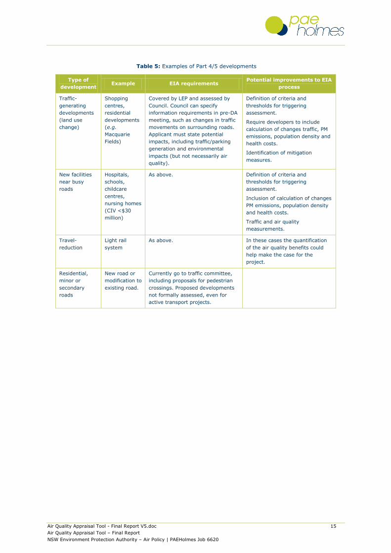
Some examples of relevant Part 4 and Part 5 developments are given in Table 5. Local council and
regional planners assess developments costing up to $30 million. At a local level, AQAT could be
used to value the impacts of alternative traffic-generating developments, such as hospitals and
shopping centres. For larger developments, council planners can request that the proponents use
the tool as part of an Environmental Impact Statement. For smaller developments, council
planners can request changes in traffic movements on affected roads in the Statement of the
Environmental Effects, and assess the changes using AQAT when the SEE is submitted. Local
councils might also wish to value the benefits of schemes that reduce motor vehicle use. In this
case, the council would need to estimate changes in vehicle movements and enter these into the
spreadsheet to value the changes.
Table 4 and Table 5 show that there is some scope for more detailed information on changes in
emissions, population density and associated health costs to be included in the requirements for
SEE, REF and EIS.
Following consultation with local planning authorities it was concluded that AQAT would probably
be applicable to the following types of local government project:
Traffic-generating developments, such as new residential areas, shopping centres and
commercial/industrial areas.
The construction of new facilities with sensitive populations (e.g. hospitals, schools) near
busy roads.
Transport proposals to reduce motor vehicle travel, such as light rail developments. In
these cases the quantification of the air quality benefits could help make the case for the
project.
The costs associated with the impacts of air pollutant emissions could be used to justify
expenditure on mitigation measures.

Air Quality Appraisal Tool - Final Report V5.doc 14
Air Quality Appraisal Tool – Final Report
NSW Environment Protection Authority – Air Policy | PAEHolmes Job 6620
Table 4: Examples of state-significant developments and infrastructure
Type of development
(SSD) Example EIA requirements EPA role Potential improvements to EIA process
Commonwealth projects Moorebank intermodal
terminal facility to handle
container traffic from
interstate rail freight and
Port Botany.
EIS required. Australian Government cannot
intervene if a project has no significant
impact on one of eight matters of ‘national
environmental significance’ (World Heritage
Sites, RAMSAR sites, etc.). The consent
authority becomes the State Government.
DGR requests sent to
EPA. EPA can request
information/
assessment through
the DGRs.
Clear guidelines on method, assumptions, base
case conditions, extent and output of transport
models. Identification of mitigation measures.
Land use change
(rezoning)
Currently no formal environment or health
impact assessment.
Clear guidelines on method, assumptions, extent
and output. Tools are required for calculating
health impacts and costs.
New facilities Hospitals, education
facilities, sport, tourism
and entertainment
facilities (CIV >$30
million).
EIS required. DoPI specifies requirements of
DGRs.
EPA can request that
specific information
be included in DGRs.
Clear guidelines on method, assumptions, base
case conditions, extent and output of transport
models. Identification of mitigation measures.
Industrial developments Chemical plant. EIS required. DoPI specifies requirements of
DGRs.
Considering formally
requesting Health
Impact Assessment.
Type of
infrastructure (SSI) Example EIA requirements EPA role Potential improvements to EIA process
Transport infrastructure Major roads or railway
lines which cross council
boundaries.
EIS required. Preferred route is normally
decided at concept stage prior to DoPI
approval. DGRs define type and level of
assessment. DoPI consults with authorities
(e.g. DfT, RMS, Railcorp) to determine
content of DGRs.
EPA can request that
specific information
be included in DGRs.
Guidance required on level of air quality impact
assessment for different road projects (e.g.
changes in emissions, changes in population
density, how outputs from transport models are
used). RMS is currently revising its guidelines.
Tools are required for calculating emissions,
health impacts and costs. Identification of
mitigation measures.
Air Quality Appraisal Tool - Final Report V5.doc 15
Air Quality Appraisal Tool – Final Report
NSW Environment Protection Authority – Air Policy | PAEHolmes Job 6620
Table 5: Examples of Part 4/5 developments
Type of
development Example EIA requirements
Potential improvements to EIA
process
Traffic-
generating
developments
(land use
change)
Shopping
centres,
residential
developments
(e.g.
Macquarie
Fields)
Covered by LEP and assessed by
Council. Council can specify
information requirements in pre-DA
meeting, such as changes in traffic
movements on surrounding roads.
Applicant must state potential
impacts, including traffic/parking
generation and environmental
impacts (but not necessarily air
quality).
Definition of criteria and
thresholds for triggering
assessment.
Require developers to include
calculation of changes traffic, PM
emissions, population density and
health costs.
Identification of mitigation
measures.
New facilities
near busy
roads
Hospitals,
schools,
childcare
centres,
nursing homes
(CIV <$30
million)
As above. Definition of criteria and
thresholds for triggering
assessment.
Inclusion of calculation of changes
PM emissions, population density
and health costs.
Traffic and air quality
measurements.
Travel-
reduction
Light rail
system
As above. In these cases the quantification
of the air quality benefits could
help make the case for the
project.
Residential,
minor or
secondary
roads
New road or
modification to
existing road.
Currently go to traffic committee,
including proposals for pedestrian
crossings. Proposed developments
not formally assessed, even for
active transport projects.
Air Quality Appraisal Tool - Final Report V5.doc 16
Air Quality Appraisal Tool – Final Report
NSW Environment Protection Authority – Air Policy | PAEHolmes Job 6620
3 REVIEW OF METHODS AND MODELS
This Chapter of the report contains a review of the methods, models and data which are used in
Australia and other countries to estimate transport/traffic activity, emissions, and health-related
costs. The implications for AQAT are also considered.
3.1 Road transport emission models
The models which have been used in NSW for estimating emissions from road and rail transport
are summarised below. It does not specifically deal with models commonly used elsewhere, such
as COPERT 47 and the Handbook of Emission Factors8 in Europe, and MOBILE 69 and CMEM10 in the
United States, although the Australian methods have, in some cases, drawn heavily upon these. It
is worth noting that the move to European emission standards in Australia makes the European
models increasingly relevant.
3.1.1 National Pollutant Inventory
The Australian Government compiles and maintains a National Pollutant Inventory (NPI). Manuals
are also provided to enable emissions from each sector of activity to be calculated. For road
vehicles Environment Australia (2000a) provides the emissions estimation techniques for the
relevant NPI substances, as well as guidance on the spatial allocation of emissions.
Hot running emissions from motor vehicles are estimated by multiplying vehicle-kilometres
travelled (VKT) by emission factors (in g/km), taking into account the structure and composition of
the vehicle fleet. The emission factors vary for different road types, vehicle/fuel type combinations,
vehicle ages, and emission processes (i.e. exhaust, evaporative, tyre and brake wear).
However, the NPI manual is now well out of date. For example, it only includes emission factors for
the reporting year 2000, and only covers the vehicle technologies up to that date. In addition,
whilst some of the emission factors are based on tests on Australian vehicles, most are taken from
USEPA models (MOBILE 5a and PART5) and vehicles. The NPI method could not therefore be
recommended for use in AQAT.
3.1.2 NSW GMR emissions inventory model
3.1.2.1 2003 inventory
An emissions inventory for the Greater Metropolitan region of NSW was compiled for the calendar
year of 2003 (DECC, 2007a). The 2003 inventory superseded the existing official inventory – the
Metropolitan Air Quality Study (MAQS) for 1992 (Carnovale et al., 1996).
Improvements relative to MAQS included the redevelopment of the emission factors for petrol and
diesel cars, incorporating test data obtained under Australian conditions as well as information
from overseas. The data on VKT were also completely redeveloped using the Sydney Strategic
Transport Model (STM) and Household Travel Survey. The number of inventoried substances
increased from five criteria pollutants (VOC, NOx, CO, PM and SO2) in the MAQS inventory to over
220, including specific PAHs and other air toxic substances.
7 http://www.emisia.com/copert/ 8 http://www.hbefa.net/e/index.html 9 http://www.epa.gov/otaq/m6.htm 10 http://www.cert.ucr.edu/cmem/

Air Quality Appraisal Tool - Final Report V5.doc 17
Air Quality Appraisal Tool – Final Report
NSW Environment Protection Authority – Air Policy | PAEHolmes Job 6620
According to DECC (2007a), aggregated (fleet-weighted) emission factors were developed for five
road types defined in the MAQS inventory – highway, arterial road, commercial highway,
commercial arterial road and local/residential road, as well as two traffic flow conditions – free-
flow and congested – for each type of road. Emission projections for future years were also made.
3.1.2.2 2008 inventory
The 2003 inventory has recently been superseded by the 2008 inventory. At the time of writing
the description of the road methodology had not been published and no software was available.
The method for calculating hot running emissions involves the use of base ‘composite’ emission
factors for various vehicle types (CP, CD, LDCP, LDCD, HDCP, RT, AT, BusD and MC)11, with the
emission factor for each vehicle type taking into account VKT by age (and associated emission
factors by sub-type). Five road types (residential, arterial, commercial arterial, commercial
highway, highway/freeway), are specified in the emissions inventory. In the development of the
emission factors EPA has taken various real-world effects into consideration, including the
deterioration in emissions performance with mileage, the effects of tampering or failures in
emission-control systems, and the use of ethanol in petrol. For each case, the base emission factor
is defined for a VKT-weighted average speed (the base speed) associated with the corresponding
road type. Correction factors – in the form of 6th-order polynomial functions - are then applied to
the base emission factors taking into account the actual speed on a road (Jones, 2012). The data
show that some types of road – notably arterial roads – are associated with higher emissions for a
given average speed than others (Figure 3).
0.0
0.5
1.0
1.5
2.0
2.5
3.0
3.5
4.0
0 20 40 60 80 100 120
NO
x (g
/km
)
Average speed (km/h)
Diesel cars, NOx, 2008
Residential
Arterial
Commercial arterial
Commercial highway
Highway / Freeway
Figure 3: NOX emission factors vs speed for diesel cars (2008 fleet)
11 CP = petrol passenger vehicles; CD = diesel passenger vehicles; LDCP = light-duty commercial petrol vehicles (<=3500 kg); LDCD = light-duty commercial diesel vehicles (<=3500 kg); HDCP = heavy-duty commercial petrol vehicles (>3500kg); RT = rigid trucks (3.5-25 tonnes, diesel only); AT = articulated trucks (> 25 tonnes, diesel only); BusD = heavy public transport buses (diesel only); MC = motorcycles.

Air Quality Appraisal Tool - Final Report V5.doc 18
Air Quality Appraisal Tool – Final Report
NSW Environment Protection Authority – Air Policy | PAEHolmes Job 6620
3.1.3 TRAQ
TRAQ12 is a tool for assessing the air quality and greenhouse gas impacts of a new or existing
roadway in NSW. TRAQ was initially developed on behalf of the RTA (now RMS) by Holmes Air
Sciences (now PAEHolmes) in 2008, and was updated by Sinclair Knight Merz (SKM) for RMS in
February 2012 to reflect a number of recent developments.
TRAQ has been designed as a ‘first-pass’ screening assessment to facilitate a Level 1 assessment
(see section 2.4.1), and uses a relatively simple approach which should generally provide
conservative results. The tool has been designed to assess air quality associated with a single
segment of road, and is not suitable for complex situations such as roads through urban canyons,
intersections or tunnels (RMS, 2012).
The original version of TRAQ contained two different emission estimation techniques: NSW Motor
Vehicle Emission Projection System (MVEPS) and PIARC (the World Road Association), and
estimated pollutant concentrations using the USEPA dispersion model CALINE4. The revised model
incorporates the following changes to the emission calculation method:
Updated emission factors for criteria pollutants from the aforementioned 2008 GMR
emissions inventory model.
The speed-correction method from the 2008 inventory model.
An alternative method for estimating gradient effects.
A new cold-start emission calculation methodology.
A new routine to calculate greenhouse gas emissions.
Custom traffic mix profiles.
The required inputs for running TRAQ for calculating emissions on a given road are:
The road type (e.g. residential, arterial, highway)
The number of lanes.
For each lane:
The traffic volume
The peak hour speed
The road gradient
The road length
The traffic mix
The year of assessment
The season (which influences cold-start emissions)
Additional inputs are required for estimating pollutant dispersion.
12 Tool for Roadside Air Quality (TRAQ).
Air Quality Appraisal Tool - Final Report V5.doc 19
Air Quality Appraisal Tool – Final Report
NSW Environment Protection Authority – Air Policy | PAEHolmes Job 6620
The TRAQ model was considered to be appropriate for use in the EPA Air Quality Appraisal Tool, as
it is relatively simple and contains up-to-date emission factors which have been specifically
designed for use in NSW.
It is worth noting that VicRoads has also developed a screening Tool to enable project engineers to
assess air quality impacts of roads using a worst case approach (Murphy and Shen, 2011).
There is little documentation on the tool, but it appears to be very similar in concept to TRAQ.
3.1.4 PIARC
PIARC provides emission factors for different vehicle types, emission standards, speeds and road
gradients. Prior to the development of emission factors designed specifically for use in NSW and
elsewhere in Australia the PIARC emission factors were widely used. Because the PIARC emissions
data are based on European studies, the emission factors have usually been modified to take
account of the vehicle age profile, vehicle mix and emission standards of the Australian vehicle
fleet (e.g. SKM and Connell Wagner, 2005). PIARC emission factors were also used in the 2008
version of TRAQ.
Given the recent development of emission factors based on Australian data, there is no longer a
need for the PIARC emission factors to be used.
3.2 Road transport data
3.2.1 Data requirements
All transport emission modelling requires the use of data on activity. For road transport, in simple
terms this includes data on traffic volume (or VKT), composition and speed. Whilst the direct
measurement of traffic may be possible for some assessments, it is not practical for complex
networks. Moreover, traffic characteristics vary with time, and hence long-term measurements are
needed to give a representative picture. Measurements cannot be used to provide data for
alternative (future) scenarios, or the potential impacts of the construction of a roadway. The use of
traffic and transport models is therefore usually essential for an air quality assessment for a
proposed roadway.
For this project the most important point was to ensure that AQAT could accept the outputs from
different traffic models.
3.2.2 Types of model
In road traffic models the network is represented by zones, links, nodes and lanes. A zone is the
source or sink of traffic where vehicles enter or leave the network. A link is a roadway between
two nodes, and consists of one or more lanes. A node is either an external connection to a zone or
a junction between links inside the network.
According to Akcelik and Associates (2006), models seldom fall into clear-cut categories.
Nevertheless, generally speaking there are three main types of model:
Junction-based models
Traffic assignment models
Micro-simulation models

Air Quality Appraisal Tool - Final Report V5.doc 20
Air Quality Appraisal Tool – Final Report
NSW Environment Protection Authority – Air Policy | PAEHolmes Job 6620
The boundaries between these types of model are increasingly blurred. Many models also have
built-in functionality for estimating emissions and fuel consumption.
3.2.2.1 Junction-based models
Some specialist traffic modelling tools are used to analyse individual junctions and roundabouts.
There are several models in the UK, such as PICADY13, ARCADY14, OSCADY15, TRANSYT16 and
LINSIG17. These models typically estimate queuing delays and fuel consumption for a given traffic
demand and junction configuration, but the impacts of junction changes on the network as a whole
cannot be estimated. Travel patterns (i.e. the numbers of trips per time-period) and the routing of
traffic through the network are fixed. An Australian junction model is SIDRA INTERSECTION18.
Unlike the other models, this treats various features (different types of signalised intersection and
roundabout) in one package.
Junction models provide an aggregated representation of demand, employing empirical algorithms.
It can be difficult to apply such models to complex types of junction, such a signalised
roundabouts and gyratory systems, and micro-simulation models are now often used for such
applications.
3.2.2.2 Traffic assignment models
Where the wider implications of transport policies and infrastructure changes need to be analysed
it is normal to construct a ‘traffic assignment’ model. Such models predict traffic volumes and
delays on the network using travel demand and aggregate relationships between volume, speed
and density. Travel routes are determined by minimising a combination of journey time and cost.
The time period covered by assignment models may vary from 30 minutes to 24 hours. In some
cases the travel demand routines are quite sophisticated, employing discreet packets of vehicles
but still using the same aggregate relationships as simpler models. These are therefore termed
‘mesoscopic’ models.
Examples of traffic assignment models include:
CONTRAM (CONtinuous TRaffic Assignment Model)19.
SATURN (Simulation and Assignment of Traffic to Urban Road Networks)20.
CUBE21.
EMME/222.
VISUM23.
13 Priority Junction Capacity and Delay 14 Assessment of Roundabout Capacity and Delay 15 Optimised Signal Capacity and Delay 16 Traffic Network Study Tool 17 Traffic Signal Design Tool for Isolated Junctions and Small Networks 18 http://www.sidrasolutions.com/ 19 http://www.contram.com/news/developments.shtml 20 http://www.saturnsoftware.co.uk/index.html 21 http://www.citilabs.com/ 22 http://www.inro.ca/en/products/emme2/index.php 23 http://www.english.ptv.de/cgi-bin/traffic/traf_visum.pl

Air Quality Appraisal Tool - Final Report V5.doc 21
Air Quality Appraisal Tool – Final Report
NSW Environment Protection Authority – Air Policy | PAEHolmes Job 6620
The last three models can also be used to assign public transport passengers to different modes.
Such models can be used in conjunction with simple emission factors to estimate emissions over a
wide area.
3.2.2.3 Micro-simulation models
In recent years increases in computing power have enabled more practical use to be made of
micro-simulation traffic models. An essential property of all micro-simulation traffic models is the
prediction of the operation of individual vehicles in real time, over a series of short time intervals,
and using models of driver behaviour such as car-following, gap acceptance, lane-changing and
signal behaviour theories, rather than aggregate relationships. Vehicle operation is usually defined
in terms of speed and acceleration for a number of vehicle types. These are the only tools which
can be used to assess the impacts of measures on individual types of driver, time-varying policies,
and complex junctions and layouts. For example, they can be used to assess the effects of ramp
metering, route diversion, variable speed limits and travel information systems.
Different micro-simulation packages vary in their ability to deal traffic situations and behaviour.
Some of them were developed to deal with motorway corridors and are unable to represent traffic
behaviour in urban centres where there is a high level of interaction between different road users.
The best-known models include:
VISSIM (a German acronym for ‘Traffic in Towns – Simulation’).
PARAMICS (PARAllel MICroscopic Simulation).
DRACULA (Dynamic Route Assignment Combining User Learning and micro-simulation).
Other models are AIMSUN24, HUTSIM25, SISTM, TRAF-NETSIM and FRESIM, aaSIDRA and
aaMOTION (TfL, 2003; Abbott et al. 2000; Akcelik and Besley, 2003).
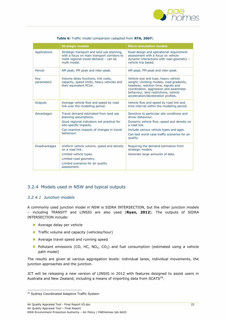
3.2.3 Comparison of model attributes
The attributes of strategic traffic models and micro-simulation traffic models were summarised and
compared by RTA (2007), as shown in Table 6. The comparison suggests that emissions based
on the output from a traffic micro-simulation model would tend to be more accurate than those
based on a strategic traffic model, as the representation of traffic is more site-specific and vehicle
operation is treated in more detail. The fuel mix required for estimating emissions is usually
exogenous in both instances. However, micro-simulation modelling is restricted to (relatively
small) geographical areas, and data may not be available for a particular location. For assessing
transport and land use developments, as in AQAT, it is more likely that the traffic data would
originate from a strategic traffic assignment model.
24 Advanced Interactive Microscopic Simulator for Urban and Non-urban Networks.
http://www.aimsun.com/site/ 25 http://www.tkk.fi/Units/Transportation/HUTSIM/
Air Quality Appraisal Tool - Final Report V5.doc 22
Air Quality Appraisal Tool – Final Report
NSW Environment Protection Authority – Air Policy | PAEHolmes Job 6620
Table 6: Traffic model comparison (adapted from RTA, 2007)
Strategic models Micro-simulation models
Applications Strategic transport and land use planning, with a focus on main transport corridors to meet regional travel demand – can be multi modal.
Road design and operational requirement assessment with a focus on vehicle dynamic interactions with road geometry – vehicle trip based.
Period AM peak, PM peak and inter-peak. AM peak, PM peak and inter-peak.
Key parameters
Volume delay functions, link costs, capacity, speed limits, heavy vehicles and their equivalent PCUs.
Vehicle size and type, heavy vehicle weight, climbing models, road gradients, headway, reaction time, signals and coordination, aggression and awareness behaviour, lane restrictions, vehicle acceleration/deceleration profiles.
Outputs Average vehicle flow and speed by road link over the modelling period.
Vehicle flow and speed by road link and time interval within the modelling period.
Advantages Travel demand estimated from land use planning assumptions.
Good regional indicators not practical for site-specific impacts.
Can examine impacts of changes in travel behaviour.
Sensitive to particular site conditions and driver behaviour.
Dynamic vehicle flow, speed and density on a road link.
Include various vehicle types and ages.
Can test worst-case traffic scenarios for air quality.
Disadvantages Uniform vehicle volume, speed and density on a road link.
Limited vehicle types.
Limited road geometry.
Limited scenarios for air quality assessment.
Requiring the demand estimation from strategic models.
Generate large amounts of data.
3.2.4 Models used in NSW and typical outputs
3.2.4.1 Junction models
A commonly used junction model in NSW is SIDRA INTERSECTION, but the other junction models
– including TRANSYT and LINSIG are also used (Ryan, 2012). The outputs of SIDRA
INTERSECTION include:
Average delay per vehicle
Traffic volume and capacity (vehicles/hour)
Average travel speed and running speed
Pollutant emissions (CO, HC, NOX, CO2) and fuel consumption (estimated using a vehicle
path model)
The results are given at various aggregation levels: individual lanes, individual movements, the
junction approaches and the junction.
JCT will be releasing a new version of LINSIG in 2012 with features designed to assist users in
Australia and New Zealand, including a means of importing data from SCATS26.
26 Sydney Coordinated Adaptive Traffic System

Air Quality Appraisal Tool - Final Report V5.doc 23
Air Quality Appraisal Tool – Final Report
NSW Environment Protection Authority – Air Policy | PAEHolmes Job 6620
3.2.4.2 Assignment models
According to Taylor (2009), most Australian States and Territories have developed strategic
transport demand modelling (STDM) tools. Each of the Australian strategic transport models
operate on either the CUBE or EMME software platforms (Taylor, 2009). The standard outputs of
these tools are typically AM peak and PM peak hour vehicle delay, intersection degree of
saturation, and ‘level of service’ (on a scale from A to F which is based on average delay). Traffic
volumes and speeds may also be estimated, but these are not always part of the standard output.
A high-profile example is the Sydney STM which is operated by the NSW Bureau of Transport
Statistics and is built largely in the EMME software (BTS, 2012). This model will be used for most
large infrastructure projects in the GMR. The STM projects travel patterns in Sydney, Newcastle
and Wollongong under different land use, transport and pricing scenarios. It can be used to test
alternative settlement, employment and transport policies, to identify likely future capacity
constraints, or to determine potential usage levels of proposed new transport infrastructure or
services.
The STM produces travel forecasts for:
Five yearly intervals from 2006 to 2036.
Nine travel modes: car driver, car passenger, rail, bus, light rail, ferry, bike, walking and
taxi.
Seven trip purposes: work, business, primary/secondary/tertiary education, shopping, other.
24-hour and average workday (Monday to Friday, excluding public holidays) travel.
Travel during the AM peak (07:00-09:00), PM peak (15:00-18:00), the inter-peak (09:00-
15:00) and the rest of the day.
Road assignment statistics (e.g. total vehicle travel time and distance) by time period - as
‘passenger car units’ (PCUs).
The Bureau of Transport Statistics also has a separate commercial vehicle model forecasting
system (Milthorpe, 2012).
3.2.4.3 Micro-simulation models
Micro-simulation tools are also in use in NSW, including PARAMICS (Ryan, 2012).
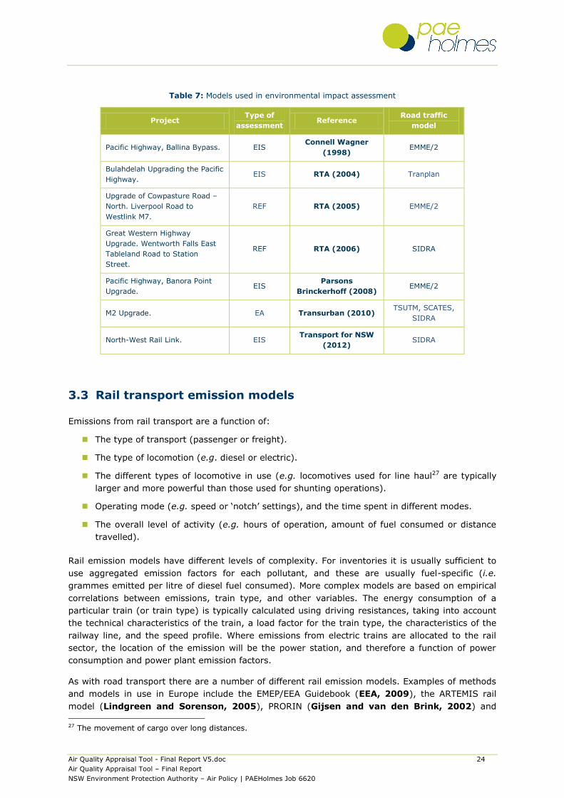
3.2.5 Models used in environmental impact assessment in NSW
A number of EISs were examined to determine the traffic models used. The findings are
summarised in Table 7.
Air Quality Appraisal Tool - Final Report V5.doc 24
Air Quality Appraisal Tool – Final Report
NSW Environment Protection Authority – Air Policy | PAEHolmes Job 6620
Table 7: Models used in environmental impact assessment
Project Type of
assessment Reference
Road traffic
model
Pacific Highway, Ballina Bypass. EIS Connell Wagner
(1998) EMME/2
Bulahdelah Upgrading the Pacific
Highway. EIS RTA (2004) Tranplan
Upgrade of Cowpasture Road –
North. Liverpool Road to
Westlink M7.
REF RTA (2005) EMME/2
Great Western Highway
Upgrade. Wentworth Falls East
Tableland Road to Station
Street.
REF RTA (2006) SIDRA
Pacific Highway, Banora Point
Upgrade. EIS
Parsons
Brinckerhoff (2008) EMME/2
M2 Upgrade. EA Transurban (2010) TSUTM, SCATES,
SIDRA
North-West Rail Link. EIS Transport for NSW
(2012) SIDRA
3.3 Rail transport emission models
Emissions from rail transport are a function of:
The type of transport (passenger or freight).
The type of locomotion (e.g. diesel or electric).
The different types of locomotive in use (e.g. locomotives used for line haul27 are typically
larger and more powerful than those used for shunting operations).
Operating mode (e.g. speed or ‘notch’ settings), and the time spent in different modes.
The overall level of activity (e.g. hours of operation, amount of fuel consumed or distance
travelled).
Rail emission models have different levels of complexity. For inventories it is usually sufficient to
use aggregated emission factors for each pollutant, and these are usually fuel-specific (i.e.
grammes emitted per litre of diesel fuel consumed). More complex models are based on empirical
correlations between emissions, train type, and other variables. The energy consumption of a
particular train (or train type) is typically calculated using driving resistances, taking into account
the technical characteristics of the train, a load factor for the train type, the characteristics of the
railway line, and the speed profile. Where emissions from electric trains are allocated to the rail
sector, the location of the emission will be the power station, and therefore a function of power
consumption and power plant emission factors.
As with road transport there are a number of different rail emission models. Examples of methods
and models in use in Europe include the EMEP/EEA Guidebook (EEA, 2009), the ARTEMIS rail
model (Lindgreen and Sorenson, 2005), PRORIN (Gijsen and van den Brink, 2002) and
27 The movement of cargo over long distances.
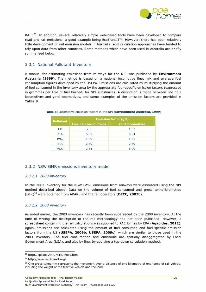
Air Quality Appraisal Tool - Final Report V5.doc 25
Air Quality Appraisal Tool – Final Report
NSW Environment Protection Authority – Air Policy | PAEHolmes Job 6620
RAILI28. In addition, several relatively simple web-based tools have been developed to compare
road and rail emissions, a good example being EcoTransIT29. However, there has been relatively
little development of rail emission models in Australia, and calculation approaches have tended to
rely upon data from other countries. Some methods which have been used in Australia are briefly
summarised below.
3.3.1 National Pollutant Inventory
A manual for estimating emissions from railways for the NPI was published by Environment
Australia (1999). The method is based on a national locomotive fleet mix and average fuel
consumption figures developed by the USEPA. Emissions are calculated by multiplying the amount
of fuel consumed in the inventory area by the appropriate fuel-specific emission factors (expressed
in grammes per litre of fuel burned) for NPI substances. A distinction is made between line haul
locomotives and yard locomotives, and some examples of the emission factors are provided in
Table 8.
Table 8: Locomotive emission factors in the NPI (Environment Australia, 1999)
Pollutant Emission factor (g/l)
Line haul locomotives Yard locomotives
CO 7.5 10.7
NOx 59.1 60.4
PM10 1.39 1.65
SO2 2.59 2.59
VOC 2.54 6.09
3.3.2 NSW GMR emissions inventory model
3.3.2.1 2003 inventory
In the 2003 inventory for the NSW GMR, emissions from railways were estimated using the NPI
method described above. Data on the volume of fuel consumed and gross tonne-kilometres
(GTK)30 were obtained from ABARE and the rail operators (DECC, 2007b).
3.3.2.2 2008 inventory
As noted earlier, the 2003 inventory has recently been superseded by the 2008 inventory. At the
time of writing the description of the rail methodology had not been published. However, a
spreadsheet containing the rail calculations was supplied to PAEHolmes by EPA (Agapides, 2012).
Again, emissions are calculated using the amount of fuel consumed and fuel-specific emission
factors from the US (USEPA, 2009b; USEPA, 2009c), which are similar to those used in the
2003 inventory. The fuel consumption and emissions are spatially disaggregated by Local
Government Area (LGA), and also by line, by applying a top-down calculation method.
28 http://lipasto.vtt.fi/railie/index.htm 29 http://www.ecotransit.org/ 30 One gross tonne-km represents the movement over a distance of one kilometre of one tonne of rail vehicle, including the weight of the tractive vehicle and the load.

Air Quality Appraisal Tool - Final Report V5.doc 26
Air Quality Appraisal Tool – Final Report
NSW Environment Protection Authority – Air Policy | PAEHolmes Job 6620
3.3.3 Other models
Other models have been for specific studies in Australia. For example, in an emissions inventory
for the Port of Brisbane, Smit et al. (2010) used the EMEP/EEA Guidebook approach to estimate
emissions from locomotives. In an air quality assessment of the Koolbury Rail Loop, Kellaghan
(2010) used emission data for class 81 and class 90 locomotives from Lilley (1996) and data for
class 82 and 90 locomotives from manufacturer specifications.
3.4 Rail transport data
Data on diesel fuel consumption can usually be obtained from the rail operators. Other activity
data for passenger trains, where required, are available from timetables, but information on
freight traffic scheduling and activity data are more difficult to obtain. Indeed, freight trains,
although subject to timetabled movements, routinely deviate from schedules to allow priority to
late-running passenger services.
3.5 Methods for monetising air pollution impacts
3.5.1 General approaches
The following Sections provide brief descriptions of the two main approaches to valuing changes in
air pollution: the ‘impact pathway’ approach and the ‘damage cost’ approach. For more detail on
these approaches the reader is referred to the report by Aust et al. (2012).
3.5.1.1 Impact pathway approach
The approach taken for the detailed valuation of the health impacts of air pollution is often referred
to as the impact pathway approach. This approach was developed through a series of joint EU-US
research projects in the 1990s, and involves the following steps:
Step 1: Quantification of emissions, with disaggregated road-based or grid-based source
apportionment.
Step 2: Analysis of pollutant dispersion and chemistry across different spatial scales. This
includes the consideration of primary pollutants and secondary pollutants
(secondary particles such as sulphates, or gaseous pollutants such as ozone), and
the assessment of changes in pollutant concentrations.
Step 3: Quantification of the exposure of people, the environment and buildings that are
affected by air pollution (i.e. linking pollution with the ‘stock at risk’ using, for
example, population data).
Step 4: Quantification of the impacts of air pollution using relationships from studies that
link pollutant concentrations with physical impacts such as health outcomes. The
outcomes are typically based on epidemiological studies, which may have been
undertaken in the country of interest or may be transferred from other countries.
Step 5: Valuation of the impacts. This is usually undertaken using a ‘willingness to pay’
(WTP) approach based on stated and revealed preference techniques. It requires
analysis of three components, each of which captures a different element of the
total effect: the resource costs (i.e. medical treatment costs), the opportunity costs

Air Quality Appraisal Tool - Final Report V5.doc 27
Air Quality Appraisal Tool – Final Report
NSW Environment Protection Authority – Air Policy | PAEHolmes Job 6620
in terms of lost productivity, and dis-utility (i.e. pain or suffering, concern and
inconvenience to family and others).
The impact-pathway approach is recommended best practice for monetising the impacts of air
quality policies as it uses a more detailed location-specific approach to quantifying and valuing the
impact of air pollution changes. However, it is important to note that there are uncertainties
associated with each step of the pathway, particularly relating to the quantification of emissions,
the health and non-health impacts of changes in air quality, and the valuation of these impacts.
The impact pathway approach is also resource intensive – and prohibitively so for many policy
impact assessments - with a large volume of information being required (Defra, 2007). As a
consequence, some simplified approaches have been developed.
In some cases - such as standard setting - Steps 1 and 2 may not be required as changes in the
exposure of the stock at risk is estimated using current and predicted future air quality for the
base case, and the assumed standard for the alternative case for which benefits are evaluated.
3.5.1.2 Damage cost approach
Some countries have adopted tables or models to allow a valuation of the marginal costs of air
quality impacts based solely on emissions, whereby the only information available is the change in
the amount of pollutant emitted. These are frequently referred to as ‘damage cost’ or ‘unit cost’
methods, and use approximate monetary values per tonne of pollutant. Examples include the
damage costs from the UK Interdepartmental Group on Costs and Benefits (IGCB) and the EU
Clean Air for Europe (CAFE) programme. It is worth noting that the specific damage costs for a
particular country or region are usually developed using the impact pathway approach and
location-specific inputs (e.g. population density, life expectancy). However, this is not always
possible.
In the UK a simple decision tree is used to determine when it is appropriate to use the more
detailed impact pathway approach or damage costs. For cases that involve state (or national) level
policies that affect air quality, an impact pathway approach is probably needed. For individual
policy proposals a damage cost approach may be sufficient.
In the UK the damage cost approach is used when the estimated impacts of a proposal on air
quality are less than £20 million, when the impacts will last for less than 20 years, or where air
quality impacts are ancillary to the policy or policies (Defra, 2011). The use of damage costs is
not, however, considered a replacement for detailed modelling and analysis. Damage costs are
more appropriate as part of a filtering mechanism to narrow down a wide range of policy options
into a smaller number that are then taken forward for more comprehensive assessment.
3.5.2 Australian examples
An international review of the approaches used for valuing the health impacts of PM emissions and
concentrations was recently completed on behalf of EPA31 by Aust et al. (2012). The review
covered work undertaken by overseas jurisdictions - including the EU, the US, Canada and New
Zealand - and also Australian jurisdictions. For the international methodologies the reader is
referred to the original review. The Australian studies are briefly summarised below. Again, further
details on the methodologies are available from the review. The damage cost values from the
Australian studies are given in Table 9.
31 EPA project (OEH-1072-2011 – Methodology for Valuing the Health Impacts of Changes in Particle
Emissions).
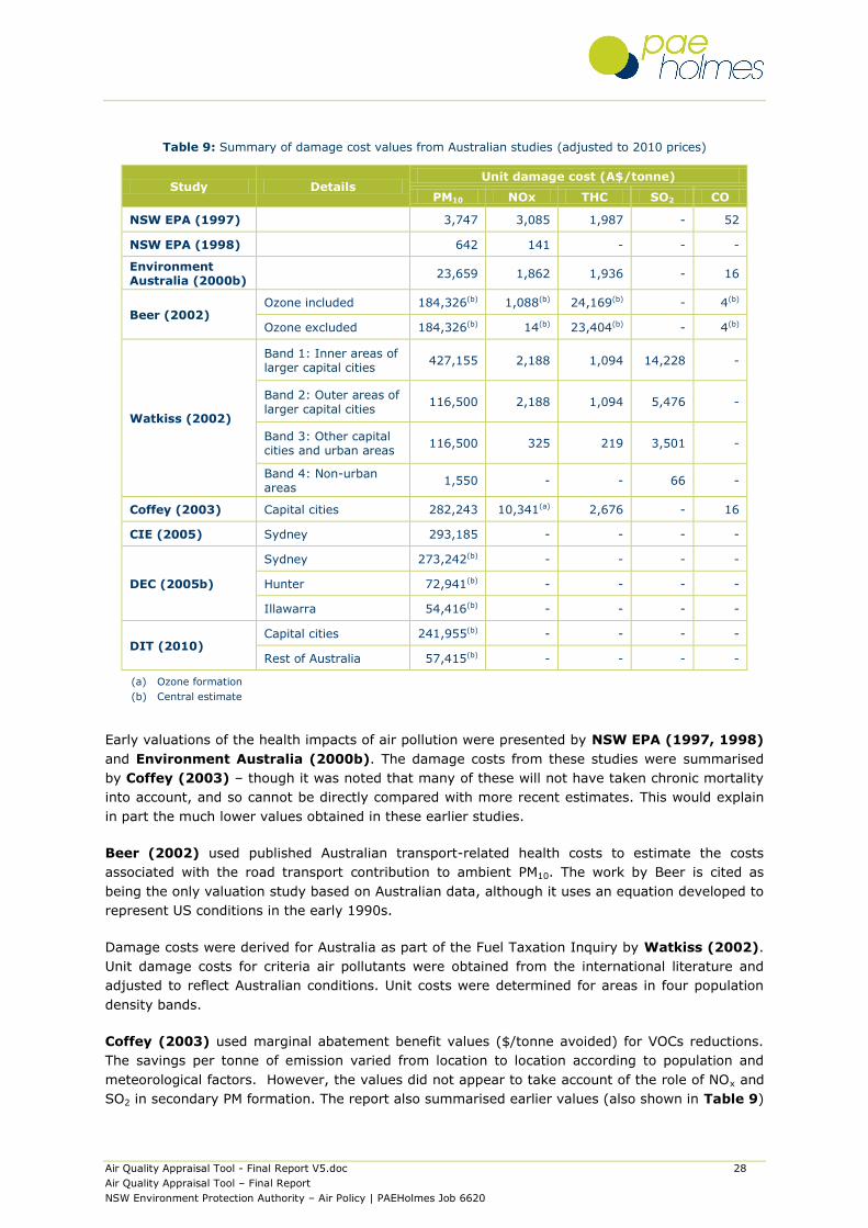
Air Quality Appraisal Tool - Final Report V5.doc 28
Air Quality Appraisal Tool – Final Report
NSW Environment Protection Authority – Air Policy | PAEHolmes Job 6620
Table 9: Summary of damage cost values from Australian studies (adjusted to 2010 prices)
Study Details Unit damage cost (A$/tonne)
PM10 NOx THC SO2 CO
NSW EPA (1997) 3,747 3,085 1,987 - 52
NSW EPA (1998) 642 141 - - -
Environment Australia (2000b)
23,659 1,862 1,936 - 16
Beer (2002) Ozone included 184,326(b) 1,088(b) 24,169(b) - 4(b)
Ozone excluded 184,326(b) 14(b) 23,404(b) - 4(b)
Watkiss (2002)
Band 1: Inner areas of larger capital cities
427,155 2,188 1,094 14,228 -
Band 2: Outer areas of larger capital cities
116,500 2,188 1,094 5,476 -
Band 3: Other capital cities and urban areas
116,500 325 219 3,501 -
Band 4: Non-urban areas
1,550 - - 66 -
Coffey (2003) Capital cities 282,243 10,341(a) 2,676 - 16
CIE (2005) Sydney 293,185 - - - -
DEC (2005b)
Sydney 273,242(b) - - - -
Hunter 72,941(b) - - - -
Illawarra 54,416(b) - - - -
DIT (2010) Capital cities 241,955(b) - - - -
Rest of Australia 57,415(b) - - - -
(a) Ozone formation
(b) Central estimate
Early valuations of the health impacts of air pollution were presented by NSW EPA (1997, 1998)
and Environment Australia (2000b). The damage costs from these studies were summarised
by Coffey (2003) – though it was noted that many of these will not have taken chronic mortality
into account, and so cannot be directly compared with more recent estimates. This would explain
in part the much lower values obtained in these earlier studies.
Beer (2002) used published Australian transport-related health costs to estimate the costs
associated with the road transport contribution to ambient PM10. The work by Beer is cited as
being the only valuation study based on Australian data, although it uses an equation developed to
represent US conditions in the early 1990s.
Damage costs were derived for Australia as part of the Fuel Taxation Inquiry by Watkiss (2002).
Unit damage costs for criteria air pollutants were obtained from the international literature and
adjusted to reflect Australian conditions. Unit costs were determined for areas in four population
density bands.
Coffey (2003) used marginal abatement benefit values ($/tonne avoided) for VOCs reductions.
The savings per tonne of emission varied from location to location according to population and
meteorological factors. However, the values did not appear to take account of the role of NOx and
SO2 in secondary PM formation. The report also summarised earlier values (also shown in Table 9)

Air Quality Appraisal Tool - Final Report V5.doc 29
Air Quality Appraisal Tool – Final Report
NSW Environment Protection Authority – Air Policy | PAEHolmes Job 6620
– though it was noted that many of these will not have taken chronic mortality into account, and
so cannot be directly compared with more recent estimates.
In 2005, the Centre for International Economics undertook an evaluation of Sydney’s existing and
future transport infrastructure. As part of the study, CIE assessed damage costs for PM10 (CIE,
2005).
DEC (2005) derived damage costs for the NSW GMR (defined as ‘Hunter’, ‘Sydney’ and
‘Illawarra’), and obtained values for PM10 of A$236,000 per tonne for Sydney, falling to A$47,000
for Illawarra.
The NSW Department of Infrastructure and Transport (DIT, 2010) undertook a review of health
benefits as part of a Regulatory Impact Statement for adopting the Euro 5 and Euro 6 emissions
standards for light-duty vehicles. The study used an avoided health cost approach, whereby
monetary values (in $/tonne) were assigned to HC, NOx and PM. The studies by Coffey (2003),
Watkiss (2002) and Beer (2002) were used to calculate the total health benefit. Unit damge
cost values for capital cities were calculated by taking the simple average of the estimates from
the three studies. Unit values for the rest of Australia were based on the simple average of the
estimates for Band 3 and Band 4 contained in Watkiss (2002).
The most recent cost-benefit analysis of air pollution in the GMR was completed by Jalaludin et
al. (2011). The authors estimated the number of adverse health effects that could be avoided
(and the associated monetary benefit) by reducing concentrations of PM2.5, PM10 and O3 to near-
background levels. It was found that the associated health benefit for the GMR equated to A$5.7
billion, the greatest proportion of which was due to avoiding premature deaths due to long-term
exposure to PM2.5. However, unit damage costs for emissions were not determined.
3.5.3 Updated Australian methodology
Aust et al. (2012) concluded that the most robust method for valuing health impacts from air
pollution follows the impact pathway approach, and the most advanced and detailed studies have
been those undertaken in Europe and the US. These studies have also captured the complexity
associated with chronic health effects. This is not reflected in the earlier Australian studies, though
this is in part due to their age.
The report by Aust et al. (2012) also included as analysis of Australian needs and conditions, and
the availability of data and information to support the use of potential methodologies, a review of
the literature on secondary particles, and a proposed methodology for estimating the health costs
associated with changes in PM emissions in NSW and Australia.
The authors proposed a new methodological framework based on a two-level approach, as used in
the UK, in which the impact pathway or damage cost approach is recommended based on the type
of application and the anticipated effects of the changes. However, it was concluded that Australia
currently lacks sufficient and readily available PM emission modelling information to permit a full
impact pathway process and, by extension, to generate a set of accurate, location-specific damage
costs. Consequently, a method was provided for calculating damage costs for primary PM2.5
emissions based on UK data which can be used until more reliable data are available for Australia.
The approach relates unit damage costs for PM2.5 emissions to population density, and provides
specific unit damage costs for the ‘Significant Urban Areas’ (SUAs) defined by the Australian
Bureau of Statistics.
Air Quality Appraisal Tool - Final Report V5.doc 30
Air Quality Appraisal Tool – Final Report
NSW Environment Protection Authority – Air Policy | PAEHolmes Job 6620
4 DEVELOPMENT OF AIR QUALITY APPRAISAL TOOL
This Chapter summarises the development of AQAT based on the information presented in the
previous Chapters. The calculation methodology is described in more detail in Appendix C, and a
User Guide is provided in Appendix D. The User Guide also includes further guidance on the
application of AQAT, and potential sources of input data.
4.1 Overall approach
The single most important consideration in the development of AQAT was the selection of a
method for quantifying the health costs of air pollution, as this dictated the outputs that would be
required for other elements of AQAT. In fact, the impact pathway approach is a resource intensive
process, and was not considered to be a realistic option for deriving Australian air pollution costs
for AQAT. The complexity and cost of the approach precluded its use for evaluation at the level
envisaged by EPA. An approach based on damage costs (in A$ per tonne of pollutant emitted) was
therefore considered to be more appropriate for use in AQAT.
This therefore meant that the changes in emissions from road and rail for a given development
had to be quantified. As noted earlier, varying levels of data and resources will be available to the
potential end user of AQAT. The availability of data will differ for different types of development,
and in particular whether an EIS has been compiled. For large developments, data on transport
activity and emissions will generally have been obtained, or could be estimated from the available
data, and therefore damage cost values could be used directly. For smaller, local developments
there are generally very few data, and therefore algorithms had to be incorporated into AQAT to
enable emissions to be calculated.
The selection of the methods and models for monetising impacts and quantifying emissions is
described in the following sections. No resources were available for the development of new
emission models, and therefore existing models were adapted for use in AQAT.
Microsoft Excel was selected as the platform for AQAT because it is widely available and can be
used with little training.
4.2 Selection of approach for monetising impacts
The different approaches to quantifying the health impacts of air pollution have recently been
reviewed in the EPA project Methodology for Valuing the Health Impacts of Changes in Particle
Emissions (Aust et al., 2012), and the findings from this informed the development of AQAT.
More specifically, Aust et al. (2012) provided Australia-specific unit damage costs for pollution
from transport sources32. The damage costs correspond to the effects of air pollution on chronic
mortality, acute mortality, and all respiratory and all cardiovascular hospital admissions.
These unit damage costs for transport have been included in AQAT. These are specified in terms of
population density (which acts as a surrogate for exposure to air pollution), and include relevant
uplifts and discounts for future years (an explanation of these terms is provided in Section C3.1
of Appendix C).
32 On a cost-per-tonne basis, the non-transport damage costs are substantially lower than those for transport.
Air Quality Appraisal Tool - Final Report V5.doc 31
Air Quality Appraisal Tool – Final Report
NSW Environment Protection Authority – Air Policy | PAEHolmes Job 6620
Aust et al. (2012) did not provide damage costs for secondary PM, as it is more difficult to
accurately transfer these between countries. Further modelling and analysis of Australian
conditions was recommended to develop a set of appropriate values. Once this work has been
undertaken, the possibility of including secondary PM in AQAT should be re-evaluated.
It should also be noted that the unit damage costs provided by Aust et al. (2012) exclude
several key effects, as the quantification and valuation of these was not possible or was highly
uncertain. The key effects that have not been included are:
Effects on ecosystems (through acidification, eutrophication, etc.).
Impacts of trans-boundary pollution.
Effects on cultural or historic buildings from air pollution.
Potential additional morbidity from acute exposure to PM.
Potential mortality effects in children from acute exposure to PM.
Potential morbidity effects from chronic (long-term) exposure to PM or other pollutants.
Effects of exposure to ozone, including both health impacts and effects on materials.
Change in visibility (visual range).
Macroeconomic effects of reduced crop yield and damage to building materials.
Non-ozone effects on agriculture.
4.3 Selection of emission modelling approaches
4.3.1 Road transport
Based on a consideration of the available options, it was decided that the TRAQ model was the
most suitable approach for modelling road traffic emissions in AQAT for the following reasons:
The level of the approach in TRAQ is in keeping with the need for simple calculations in
AQAT, and it is easy to update the model.
TRAQ offers sufficient flexibility for the assessment of road transport developments.
It is relatively straightforward to adapt the TRAQ databases for use in AQAT.
The TRAQ emission factors are consistent with those used in the 2008 NSW emissions
inventory.
Importantly, NSW Roads and Maritime Services (RMS) also agreed for TRAQ to be used in the EPA
Air Quality Appraisal Tool.
Road traffic emissions are therefore calculated using the aggregated emission factors developed by
EPA for the 2008 GMR inventory and supplied to RMS for use in the TRAQ model (Version 2,
release date 12 April 2012)33. The emission factors in TRAQ are not available through the user
interface (the calculations are managed using macros), and therefore in AQAT the emission factors
are reconfigured using Excel functions.
33 RMS granted PAEHolmes permission to use the data and algorithms from TRAQ in the Air Quality Appraisal
Tool.

Air Quality Appraisal Tool - Final Report V5.doc 32
Air Quality Appraisal Tool – Final Report
NSW Environment Protection Authority – Air Policy | PAEHolmes Job 6620
TRAQ does, however, have some limitations at present. For example, calculations can only be
made for specific years (2008, 2011, 2016, 2021 and 2026), due to the fleet data only being
included for these years. However, it is assumed that EPA could provide fleet data for other years
if needed. The calculations in TRAQ are also managed using macros in Visual Basic for Applications
(VBA), and therefore these were converted to functions in Excel.
4.3.2 Rail transport
The capabilities for modelling rail emissions in Australia are rather limited, and there is a heavy
reliance upon emission factors from the USEPA. The existing calculation methods also require
knowledge of actual fuel consumption. However, it is unlikely that the user of AQAT will have ready
access to train fuel consumption data. Based on a consideration of the available options, it was
concluded that the method used in the 2008 GMR inventory would, with some adaptation, be the
most suitable approach for use in AQAT.
In NSW most rail passenger services are electrified, whereas diesel locomotives are used for line
haul and shunting operations. Including electricity generation complicates the analysis in AQAT
(and in particular the selection of appropriate damage costs), since the location of energy use is
not the same location as where emissions are being produced. Electricity generation does not
therefore directly affect the local area under consideration. If emissions are to be allocated
spatially and temporally then the locations of power stations must be known (or otherwise a
general ‘area type’ must be defined for the air pollution health costs associated with power
stations). However, a number of assumptions may be required, such as power distribution losses,
the use of regenerative braking systems, etc.
A spreadsheet summarising the calculation of rail emissions for the 2008 GMR inventory was
supplied to PAEHolmes by EPA (Agapides, 2012). The EPA spreadsheet contained activity data in
gross tonne-kilometres for all trains in the GMR (31,940,182 tonne-km) during 2008, as well as
total diesel consumption by freight (128,836,774 litres) during the same period. Given that most
of the rail diesel consumption in NSW relates to the haulage of freight and that passenger trains
are predominantly electrified, a decision was made to exclude passenger transport from AQAT. It
was therefore assumed that the gross tonne-km value related to freight trains only, giving a single
average unit fuel consumption value of 4.03 litres per thousand gross tonne-km for freight trains.
This is very similar to values reported in the literature (e.g. Pacific National, 2006; ARTC,
2010). No further disaggregation was possible.
4.4 Use of models within AQAT
The calculation of damage costs for the health impacts associated with air pollution requires data
on both emissions from road and/or rail transport, as well as population density. Without one or
the other the calculation is not possible. A given development could affect costs through a change
transport emissions, a change in population density, or both.
For example, the construction of a new road will result in a change in road transport emissions,
but not necessarily a change in nearby population density. Nevertheless, the population density
must still be quantified. Other developments (e.g. construction of a new housing estate) will result
in a change in land use and population density. The change in land use alone will have implications
in terms of the damage costs of air pollution. There may or may not be a change in the activity on
the transport corridor and local roads, and there may also be some new roads.

Air Quality Appraisal Tool - Final Report V5.doc 33
Air Quality Appraisal Tool – Final Report
NSW Environment Protection Authority – Air Policy | PAEHolmes Job 6620
In AQAT the potential damage costs for different types of development are accommodated by
allowing the user to specify road transport emissions, rail transport emissions and population
density (through the use of SUAs).
The damage cost methodology is similar to that described by Defra (2008, 2011). However,
whereas the Defra approach involves calculating damage costs for policies which have a timescale
of several years, for AQAT it was assumed that the air pollution impacts of a development would
be considered for a specific year. The user needs to select the particular year for which air
pollution is being considered (the options being 2008, 2011, 2016, 2021 or 2026). AQAT is
restricted to these years because they are the only ones covered by the road traffic emission
model.
The changes in emissions of CO, HC, NOx, PM2.5 and CO2-e, and also the changes in damage costs,
are presented separately for road and rail traffic, as well as in combination.

Air Quality Appraisal Tool - Final Report V5.doc 34
Air Quality Appraisal Tool – Final Report
NSW Environment Protection Authority – Air Policy | PAEHolmes Job 6620
5 CASE STUDIES
5.1 Overview
It was important to demonstrate that AQAT could deal with different types of development. In this
Chapter the functionality of AQAT has been demonstrated through application in four case studies:
A local transport development involving a road bypass
A local land use development involving a growth centre
A state-significant transport development involving a rail freight link
A comparison between two local land use developments
It should be noted that the examples are only designed to show how AQAT could be used and to
identify some of the issues that may be encountered. The assessments are not meant to be
comprehensive and are not designed to address all aspects of the developments. They are not
substitutes for EIA, nor are they designed to replicate the results of EIAs.
5.2 Study 1: Local transport - road bypass
5.2.1 Description of case study
This case study illustrates how AQAT could be used to evaluate the change in the exposure of a
local population to air pollution following the introduction of a road bypass scheme.
The Ballina Bypass project34 will provide 12 km of dual carriageway on the Pacific Highway,
extending from south of Ballina at the intersection of the Bruxner and Pacific highways to north of
Ballina at the intersection of Ross Lane at Tintenbar. The NSW Minister for Planning approved the
Ballina bypass project on 22 May 2003. Construction began in May 2008, and the bypass opened
to traffic in 2012.
The project is designed to improve traffic and environmental conditions within Ballina by removing
through traffic, improving road safety, providing uninterrupted traffic flow on the Highway, and
providing easy access to and from the Highway for local traffic. The location and alignment of the
Bypass are shown in Figure 4.
The reduction in the volume of traffic on the roads in Ballina should result in a reduction in
emissions on those roads and a reduction in overall exposure to air pollution.
34 http://www.rta.nsw.gov.au/roadprojects/projects/pac_hwy/ballina_tweed_heads/ballina_bypass/index.html

Air Quality Appraisal Tool - Final Report V5.doc 35
Air Quality Appraisal Tool – Final Report
NSW Environment Protection Authority – Air Policy | PAEHolmes Job 6620
Figure 4: Ballina Bypass location and alignment (RTA, 2008a)
5.2.2 Input data
In order to evaluate the Ballina Bypass (or any similar scheme), the following information was
required for each affected road in the study area before and after the development:
The road type
The road gradient
The road length
The daily traffic volume
The traffic mix
The traffic speed
The local population density (i.e. the SUAs affected)
The data for each road are entered on a separate line in the AQAT spreadsheet, which then
estimates the emissions from the traffic and the associated damage costs.
The actual inputs used in the Ballina case study are summarised below.

Air Quality Appraisal Tool - Final Report V5.doc 36
Air Quality Appraisal Tool – Final Report
NSW Environment Protection Authority – Air Policy | PAEHolmes Job 6620
5.2.2.1 Road and traffic data
The roads affected by the Ballina Bypass – as defined in the EIS (Connell Wagner, 1998) - are
shown in Figure 5. It should be noted that links 1, 2 and 14 extended some way beyond the town
of Ballina. For the purpose of this example, it would have been necessary to assume that the
bypass had an influence on the traffic on these roads over a fixed distance. However, the results
would have been dependent upon the actual distance used. Therefore, these road links were
excluded from the calculations to maintain a ‘closed’ system.
Road lengths were determined using Google Earth. In addition, the road type in each case was
based on a visual inspection in Google Maps. The traffic volume data were taken from the EIS and
from RTA (2008b). For each road the traffic speed was assumed to be the same as the speed
limit, which was obtained using Google Maps. The default traffic composition data for each road
type were taken from AQAT.
The road and traffic data are summarised in Table 10. The data with and without the bypass were
available for the year 2022 (including expected traffic growth), and therefore the closest year to
this in AQAT, 2021, was used in the assessment.
Figure 5: Roads affected by the Ballina Bypass. The Bypass itself is identified by sections A and
B (Background image from Google Maps).

Air Quality Appraisal Tool - Final Report V5.doc 37
Air Quality Appraisal Tool – Final Report
NSW Environment Protection Authority – Air Policy | PAEHolmes Job 6620
Table 10: Traffic data for roads affected by Ballina Bypass (2021)
Road Road name Road type Grade
(%)
Length
(km)
Daily
traffic
(vpd)
Traffic mix (%) Speed
(km/h) CP CD LDCP LDCD HDCP RT AT BusD MC
Before development
3 Pacific Highway, east of Bruxner Highway Highway/freeway 0% 2.1 23,208 64 1.8 9.5 3.2 0.4 10.8 9.6 0.2 0.5 50
4 Teven Road Arterial 0% 7.5 7,288 75.6 2.2 9.6 3.2 0.2 5.3 2.7 0.6 0.6 80
5 Pacific Highway, east of Teven Road Highway/freeway 0% 2 35,132 64 1.8 9.5 3.2 0.4 10.8 9.6 0.2 0.5 100
6 Pacific Highway Fishery Creek Highway/freeway 0% 1.6 39,319 64 1.8 9.5 3.2 0.4 10.8 9.6 0.2 0.5 100
7 Kerr Street Arterial 0% 1.4 26,938 75.6 2.2 9.6 3.2 0.2 5.3 2.7 0.6 0.6 60
8 Angels Beach Drive Arterial 0% 4.6 16,566 75.6 2.2 9.6 3.2 0.2 5.3 2.7 0.6 0.6 80
9 Pacific Highway, east of industrial area Highway/freeway 0% 4.7 29,732 64 1.8 9.5 3.2 0.4 10.8 9.6 0.2 0.5 100
10 Pacific Highway, north of Cumbalum Interchange Highway/freeway 0% 3.2 13,800 64 1.8 9.5 3.2 0.4 10.8 9.6 0.2 0.5 100
11 Pacific Highway, Tintenbar Highway/freeway 0% 3.4 12,910 64 1.8 9.5 3.2 0.4 10.8 9.6 0.2 0.5 100
12 Tintenbar Road Arterial 0% 3.5 20,356 75.6 2.2 9.6 3.2 0.2 5.3 2.7 0.6 0.6 80
13 Ross Lane Arterial 0% 5.7 12,180 75.6 2.2 9.6 3.2 0.2 5.3 2.7 0.6 0.6 80
15 The Coast Road Arterial 0% 8 15,282 75.6 2.2 9.6 3.2 0.2 5.3 2.7 0.6 0.6 100
A Bypass, south of Cumbalum Highway/freeway - - - - - - - - - - - - -
B Bypass, south of Cumbalum Highway/freeway - - - - - - - - - - - - -
After development
3 Pacific Highway, east of Bruxner Highway Highway/freeway 0% 2.1 26,736 64 1.8 9.5 3.2 0.4 10.8 9.6 0.2 0.5 50
4 Teven Road Arterial 0% 7.5 2,290 75.6 2.2 9.6 3.2 0.2 5.3 2.7 0.6 0.6 80
5 Pacific Highway, east of Teven Road Highway/freeway 0% 2 32,702 64 1.8 9.5 3.2 0.4 10.8 9.6 0.2 0.5 100
6 Pacific Highway Fishery Creek Highway/freeway 0% 1.6 36,834 64 1.8 9.5 3.2 0.4 10.8 9.6 0.2 0.5 100
7 Kerr Street Arterial 0% 1.4 23,752 75.6 2.2 9.6 3.2 0.2 5.3 2.7 0.6 0.6 60
8 Angels Beach Drive Arterial 0% 4.6 13,786 75.6 2.2 9.6 3.2 0.2 5.3 2.7 0.6 0.6 80
9 Pacific Highway, east of industrial area Highway/freeway 0% 4.7 29,486 64 1.8 9.5 3.2 0.4 10.8 9.6 0.2 0.5 100
10 Pacific Highway, north of Cumbalum Interchange Highway/freeway 0% 3.2 5,734 64 1.8 9.5 3.2 0.4 10.8 9.6 0.2 0.5 100
11 Pacific Highway, Tintenbar Highway/freeway 0% 3.4 10,268 64 1.8 9.5 3.2 0.4 10.8 9.6 0.2 0.5 100
12 Tintenbar Road Arterial 0% 3.5 12,300 75.6 2.2 9.6 3.2 0.2 5.3 2.7 0.6 0.6 80
13 Ross Lane Arterial 0% 5.7 14,896 75.6 2.2 9.6 3.2 0.2 5.3 2.7 0.6 0.6 80
15 The Coast Road Arterial 0% 8 11,200 75.6 2.2 9.6 3.2 0.2 5.3 2.7 0.6 0.6 100
A Bypass, south of Cumbalum Highway/freeway 0% 3.8 12,740 64 1.8 9.5 3.2 0.4 10.8 9.6 0.2 0.5 100
B Bypass, south of Cumbalum Highway/freeway 0% 5.4 23,100 64 1.8 9.5 3.2 0.4 10.8 9.6 0.2 0.5 100

Air Quality Appraisal Tool - Final Report V5.doc 38
Air Quality Appraisal Tool – Final Report
NSW Environment Protection Authority – Air Policy | PAEHolmes Job 6620
5.2.2.2 SUA allocation
In this case study it was necessary to distinguish between two NSW SUAs: ‘Ballina’ and ‘Not in any
significant urban area’. The Boundary of the Ballina SUA is shown in Figure 6. The SUA covers the
‘A’ section of the bypass area, but not the ‘B’ section. However, for the purpose the case study it
was assumed that the SUA did not include the bypass, and that development will occur around the
bypass in future years. It was therefore concluded that road links 5, 6, 7, 8, 9 and 15 were inside
the SUA and the remaining links were not in any significant urban area (Table 11). In a rigorous
assessment more accurate data could be obtained using a geographical information system (GIS).
A future population growth rate of 1% per annum was used.
Figure 6: Boundary of Ballina SUA (REF)
Table 11: Assumed SUAs for roads affected by Ballina Bypass
Road Road name Significant urban area Unit damage cost for PM2.5 in SUA
(A$/tonne, 2011)
3 Pacific Highway, east of Bruxner Highway Not in any Signif. Urban Area $360
4 Teven Road Not in any Signif. Urban Area $360
5 Pacific Highway, east of Teven Road Ballina $90,000
6 Pacific Highway Fishery Creek Ballina $90,000
7 Kerr Street Ballina $90,000
8 Angels Beach Drive Ballina $90,000
9 Pacific Highway, east of industrial area Ballina $90,000
10 Pacific Highway, north of Cumbalum I’change Not in any Signif. Urban Area $360
11 Pacific Highway, Tintenbar Not in any Signif. Urban Area $360
12 Tintenbar Road Not in any Signif. Urban Area $360
13 Ross Lane Not in any Signif. Urban Area $360
15 The Coast Road Ballina $90,000
A Bypass, south of Cumbalum Not in any Signif. Urban Area $360
B Bypass, south of Cumbalum Not in any Signif. Urban Area $360
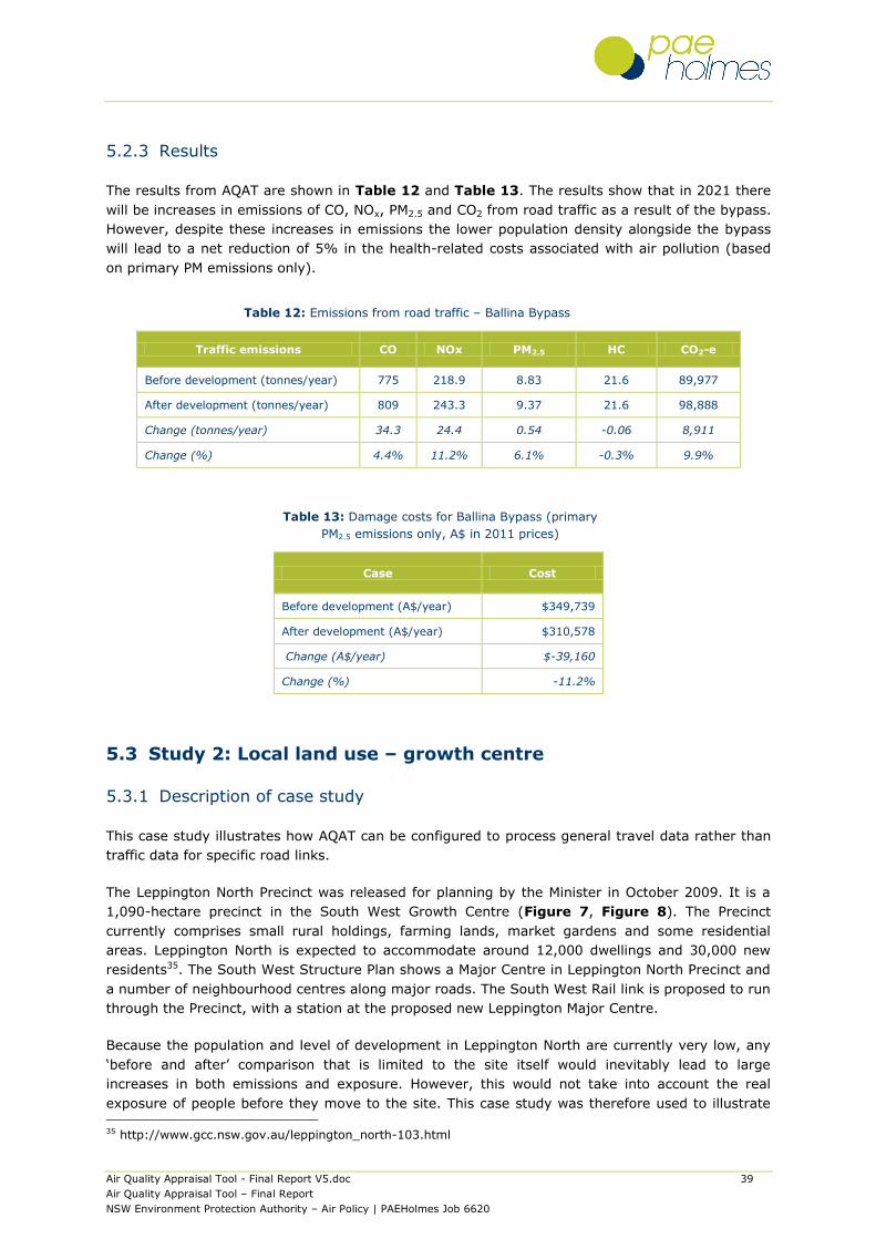
Air Quality Appraisal Tool - Final Report V5.doc 39
Air Quality Appraisal Tool – Final Report
NSW Environment Protection Authority – Air Policy | PAEHolmes Job 6620
5.2.3 Results
The results from AQAT are shown in Table 12 and Table 13. The results show that in 2021 there
will be increases in emissions of CO, NOx, PM2.5 and CO2 from road traffic as a result of the bypass.
However, despite these increases in emissions the lower population density alongside the bypass
will lead to a net reduction of 5% in the health-related costs associated with air pollution (based
on primary PM emissions only).
Table 12: Emissions from road traffic – Ballina Bypass
Traffic emissions CO NOx PM2.5 HC CO2-e
Before development (tonnes/year) 775 218.9 8.83 21.6 89,977
After development (tonnes/year) 809 243.3 9.37 21.6 98,888
Change (tonnes/year) 34.3 24.4 0.54 -0.06 8,911
Change (%) 4.4% 11.2% 6.1% -0.3% 9.9%
Table 13: Damage costs for Ballina Bypass (primary
PM2.5 emissions only, A$ in 2011 prices)
Case Cost
Before development (A$/year) $349,739
After development (A$/year) $310,578
Change (A$/year) $-39,160
Change (%) -11.2%
5.3 Study 2: Local land use – growth centre
5.3.1 Description of case study
This case study illustrates how AQAT can be configured to process general travel data rather than
traffic data for specific road links.
The Leppington North Precinct was released for planning by the Minister in October 2009. It is a
1,090-hectare precinct in the South West Growth Centre (Figure 7, Figure 8). The Precinct
currently comprises small rural holdings, farming lands, market gardens and some residential
areas. Leppington North is expected to accommodate around 12,000 dwellings and 30,000 new
residents35. The South West Structure Plan shows a Major Centre in Leppington North Precinct and
a number of neighbourhood centres along major roads. The South West Rail link is proposed to run
through the Precinct, with a station at the proposed new Leppington Major Centre.
Because the population and level of development in Leppington North are currently very low, any
‘before and after’ comparison that is limited to the site itself would inevitably lead to large
increases in both emissions and exposure. However, this would not take into account the real
exposure of people before they move to the site. This case study was therefore used to illustrate
35 http://www.gcc.nsw.gov.au/leppington_north-103.html
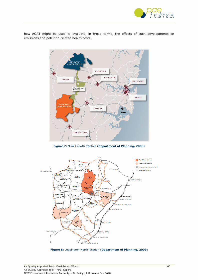
Air Quality Appraisal Tool - Final Report V5.doc 40
Air Quality Appraisal Tool – Final Report
NSW Environment Protection Authority – Air Policy | PAEHolmes Job 6620
how AQAT might be used to evaluate, in broad terms, the effects of such developments on
emissions and pollution-related health costs.
Figure 7: NSW Growth Centres (Department of Planning, 2009)
Figure 8: Leppington North location (Department of Planning, 2009)

Air Quality Appraisal Tool - Final Report V5.doc 41
Air Quality Appraisal Tool – Final Report
NSW Environment Protection Authority – Air Policy | PAEHolmes Job 6620
5.3.2 Scenarios and input data
Essentially, the case study examined the effects of two travel scenarios relative to a baseline. As
noted above, the Leppington North Development will accommodate 30,000 new residents.
Although the new residents will be relocating from various different places, for the purpose of this
example it was assumed that they would be moving from a single inner-city area (the example
selected was Leichhardt) with high population density.
The study focussed on the number of people being relocated who were of working age, and
assumed that the place of work would be either local or in an urban centre (involving a longer
trip). It was also assumed that all trips to work would be made either by car or by public transport.
The assessment year was 2016.
A baseline and three scenarios were developed, representing the following situations:
Baseline: This situation represented people living in Leichhardt prior to the Leppington
North development. It was assumed that 50% of the people of working age would travel to a
local place of work, and the remaining 50% would travel to Sydney. The distances to work
were relatively short and the proportion of travel by bus was relatively high. The population
density was also relatively high.
Scenario 1: This scenario represented a situation in which people had moved to Leppington
North, but there was no local employment and no public transport. Consequently, the
distances to work were relatively high and all work trips were made by car. However, the
population density was lower than in the baseline case.
Scenario 2: In this scenario local employment and public transport (bus only) were
available in Leppington North. The distance to local employment was therefore lower than in
scenario 1, and the proportion of travel by bus was higher.
Scenario 3: One of the main features of the Leppington North development is that it will be
situated on the line of the South-West Rail Link. In this scenario the assumptions are the
same as those in scenario 2, with the exception that all public transport travel is by train
rather than by bus. Because the emission factor for passenger rail in AQAT is effectively
zero, there was no need to calculate the number of train journeys.
Assumptions concerning modal split were based on Household Travel Survey36 data for Leichhardt
and Campbelltown (a centre near to Leppington which would be likely to have similar
demographics). Further assumptions were made concerning the road types in each case, and
default speed data were taken from TRAQ. The data used for the baseline and scenarios are
summarised in Table 14. The Sydney SUA area map (Figure 9) excludes the Leppington area. As
Leppington is an urban growth area, it was classified here as ‘Outer Sydney’. Leichhardt was
classified as ‘Inner Sydney’ and Ryde ‘Mid Sydney’. A population growth rate of 2% per year was
used.
The transport input data for AQAT are shown in Table 15.
36 http://www.bts.nsw.gov.au/Statistics/HTS/default.aspx#top

Air Quality Appraisal Tool - Final Report V5.doc 42
Air Quality Appraisal Tool – Final Report
NSW Environment Protection Authority – Air Policy | PAEHolmes Job 6620
Figure 9: Boundary of Sydney SUA (REF)
Table 14: Baseline and scenario assumptions – Leppington North
Baseline
(Leichhardt)
Scenario 1
(Leppington North, no local
employment or
public transport)
Scenario 2
(Leppington North,
with local
employment and
public transport -
bus)
Scenario 3
(Leppington North,
with local employment
and public transport -
train)
Population
Population affected 33,000 33,000 33,000 33,000
% of population in work 60% 60% 60% 60%
People in work 19,800 19,800 19,800 19,800
Local work trips
Proportion of local work trips 50% 50% 80% 80%
Number of round trips day 9,900 9,900 15,840 15,840
Length of round trip (km) 4 10 4 4
% of trips by car 50% 100% 80% 80%
Car movements per day(c) 3,300 6,600 8,448 8,448
% of trips by bus 10% 0% 5% 5%
% of trips by train/non-motorised mode 40% 0% 15% 15%
Bus movements per day(d) 33 0 26 26
Work trips to city
Proportion of work trips to city 50% 50% 20% 20%
Number of round trips day 9,900 9,900 3,960 3,960
Length of round trip (km) 7 30 30 30
% of trips by car 30% 100% 60% 60%
Car movements per day(c) 1,980 6,600 1,584 1,584
% of trips by bus 70% 0% 40% 0%
% of trips by train 0% 0% 0% 40%
Bus movements per day(d) 231 0 53 0
(a) Approximate value.
(b) Assuming 33,000 people in 1,000 ha (10 km/2).
(c) Assuming an average occupancy of 1.5.
(d) Assuming an average occupancy of 30.
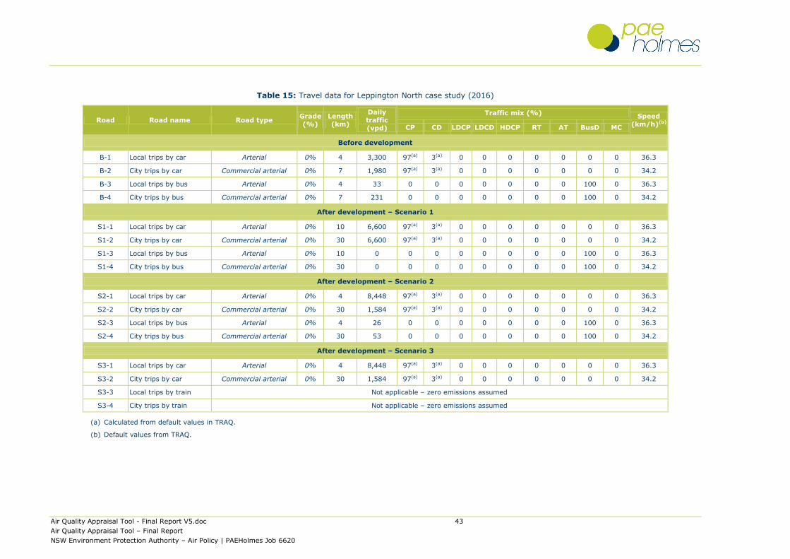
Air Quality Appraisal Tool - Final Report V5.doc 43
Air Quality Appraisal Tool – Final Report
NSW Environment Protection Authority – Air Policy | PAEHolmes Job 6620
Table 15: Travel data for Leppington North case study (2016)
Road Road name Road type Grade
(%)
Length
(km)
Daily
traffic
(vpd)
Traffic mix (%) Speed
(km/h)(b) CP CD LDCP LDCD HDCP RT AT BusD MC
Before development
B-1 Local trips by car Arterial 0% 4 3,300 97(a) 3(a) 0 0 0 0 0 0 0 36.3
B-2 City trips by car Commercial arterial 0% 7 1,980 97(a) 3(a) 0 0 0 0 0 0 0 34.2
B-3 Local trips by bus Arterial 0% 4 33 0 0 0 0 0 0 0 100 0 36.3
B-4 City trips by bus Commercial arterial 0% 7 231 0 0 0 0 0 0 0 100 0 34.2
After development – Scenario 1
S1-1 Local trips by car Arterial 0% 10 6,600 97(a) 3(a) 0 0 0 0 0 0 0 36.3
S1-2 City trips by car Commercial arterial 0% 30 6,600 97(a) 3(a) 0 0 0 0 0 0 0 34.2
S1-3 Local trips by bus Arterial 0% 10 0 0 0 0 0 0 0 0 100 0 36.3
S1-4 City trips by bus Commercial arterial 0% 30 0 0 0 0 0 0 0 0 100 0 34.2
After development – Scenario 2
S2-1 Local trips by car Arterial 0% 4 8,448 97(a) 3(a) 0 0 0 0 0 0 0 36.3
S2-2 City trips by car Commercial arterial 0% 30 1,584 97(a) 3(a) 0 0 0 0 0 0 0 34.2
S2-3 Local trips by bus Arterial 0% 4 26 0 0 0 0 0 0 0 100 0 36.3
S2-4 City trips by bus Commercial arterial 0% 30 53 0 0 0 0 0 0 0 100 0 34.2
After development – Scenario 3
S3-1 Local trips by car Arterial 0% 4 8,448 97(a) 3(a) 0 0 0 0 0 0 0 36.3
S3-2 City trips by car Commercial arterial 0% 30 1,584 97(a) 3(a) 0 0 0 0 0 0 0 34.2
S3-3 Local trips by train Not applicable – zero emissions assumed
S3-4 City trips by train Not applicable – zero emissions assumed
(a) Calculated from default values in TRAQ.
(b) Default values from TRAQ.
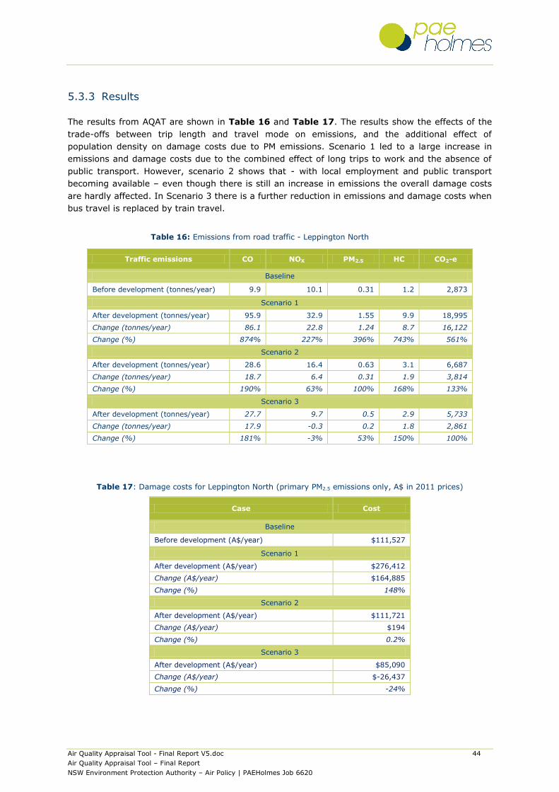
Air Quality Appraisal Tool - Final Report V5.doc 44
Air Quality Appraisal Tool – Final Report
NSW Environment Protection Authority – Air Policy | PAEHolmes Job 6620
5.3.3 Results
The results from AQAT are shown in Table 16 and Table 17. The results show the effects of the
trade-offs between trip length and travel mode on emissions, and the additional effect of
population density on damage costs due to PM emissions. Scenario 1 led to a large increase in
emissions and damage costs due to the combined effect of long trips to work and the absence of
public transport. However, scenario 2 shows that - with local employment and public transport
becoming available – even though there is still an increase in emissions the overall damage costs
are hardly affected. In Scenario 3 there is a further reduction in emissions and damage costs when
bus travel is replaced by train travel.
Table 16: Emissions from road traffic - Leppington North
Traffic emissions CO NOX PM2.5 HC CO2-e
Baseline
Before development (tonnes/year) 9.9 10.1 0.31 1.2 2,873
Scenario 1
After development (tonnes/year) 95.9 32.9 1.55 9.9 18,995
Change (tonnes/year) 86.1 22.8 1.24 8.7 16,122
Change (%) 874% 227% 396% 743% 561%
Scenario 2
After development (tonnes/year) 28.6 16.4 0.63 3.1 6,687
Change (tonnes/year) 18.7 6.4 0.31 1.9 3,814
Change (%) 190% 63% 100% 168% 133%
Scenario 3
After development (tonnes/year) 27.7 9.7 0.5 2.9 5,733
Change (tonnes/year) 17.9 -0.3 0.2 1.8 2,861
Change (%) 181% -3% 53% 150% 100%
Table 17: Damage costs for Leppington North (primary PM2.5 emissions only, A$ in 2011 prices)
Case Cost
Baseline
Before development (A$/year) $111,527
Scenario 1
After development (A$/year) $276,412
Change (A$/year) $164,885
Change (%) 148%
Scenario 2
After development (A$/year) $111,721
Change (A$/year) $194
Change (%) 0.2%
Scenario 3
After development (A$/year) $85,090
Change (A$/year) $-26,437
Change (%) -24%

Air Quality Appraisal Tool - Final Report V5.doc 45
Air Quality Appraisal Tool – Final Report
NSW Environment Protection Authority – Air Policy | PAEHolmes Job 6620
5.4 Study 3: State transport – rail freight link
5.4.1 Description of case study
This study shows how AQAT can be used to compare the impacts of transporting freight by road
and by rail.
A dedicated rail freight line exists between Port Botany and Enfield/Chullora, a distance of
approximately 18 kilometres (Figure 10). This case study examined the effects of transferring
different amounts of freight from rail transport to road transport along the same corridor (and
hence the cost savings associated with the rail freight link).
Figure 10: Botany-Enfield/Chullora freight rail link
5.4.2 Scenarios and input data
Emissions and costs were estimated for transporting an additional one million tonnes of freight
annually along the full length of the rail link (in 2016). The change in population density along the
rail link was also taken into account in the calculations by considering the SUAs through which it
passes.
A baseline case and four scenarios were evaluated:
Baseline: The additional amount of freight is transported by rail.
Scenario 1: The additional amount of freight is transported by articulated trucks, each
carrying a load of 20 tonnes.

Air Quality Appraisal Tool - Final Report V5.doc 46
Air Quality Appraisal Tool – Final Report
NSW Environment Protection Authority – Air Policy | PAEHolmes Job 6620
Scenario 2: The additional amount of freight is transported by articulated trucks, each
carrying a load of 30 tonnes.
Scenario 3: The additional amount of freight is transported by articulated trucks, each
carrying a load of 40 tonnes.
Scenario 4: The additional amount of freight is transported by articulated trucks, each
carrying a load of 50 tonnes.
For each scenario the number of trucks required per year was calculated by dividing the additional
amount of freight (one million tonnes) by the truck load (e.g. 20 tonnes). For example, in this case
the number of trucks required per year would have been 50,000, or 137 per day (as the daily flow
is required in AQAT). There are no adjustments to the emission factors in AQAT to account for
changes in vehicle load37, and therefore the same emission factors were used for all articulated
trucks. In each scenario the road type was assumed to be ‘Commercial Arterial’ (the worst-case in
terms of emission factors).
The rail and population data and SUAs used in the calculations are given in Table 18. The road
transport inputs are summarised in Table 19 (note – only the daily traffic flows were changed).
An annual population growth rate of 2% was assumed for all SUAs.
Table 18: Rail transport and population data for rail freight link case study
LGAs through which line
passes
Length of line in LGA
(km)
Thousand gross tonne-km per year of freight transported
SUA Unit damage cost for PM2.5 in SUA
(A$/tonne, 2011)
Randwick 0.71 706 Mid-Sydney $300,000
Botany Bay 3.18 3,177 Mid-Sydney $300,000
Marrickville 4.94 4,941 Inner Sydney $400,000
Canterbury 6.00 6,000 Mid-Sydney $300,000
Strathfield 3.18 3,177 Mid-Sydney $300,000
Total 18.00 18,000 Mid-Sydney $300,000
5.4.3 Results
The results from AQAT are shown in Table 20 and Table 21. It can be seen that the transfer of
freight from rail to road would lead to large increases in emissions of some pollutants, but
decreases in emissions of others. The attractiveness of road transport increases as the weight
carried per road vehicle increases, and in terms of damage costs road becomes more beneficial
than rail when the load per truck approaches 40 tonnes. Further refinements to the damage cost
calculations could be made by considering alternative routes by road through areas of lower
population density. Importantly, CO2 emissions from road transport were much higher than those
from rail in all scenarios. The different behaviour of CO2 and the air quality criteria pollutants is
due to the fact that for road transport the latter are controlled, whereas at present no pollution
controls are assumed for rail transport.
37 Vehicle load is not included in TRAQ.

Air Quality Appraisal Tool - Final Report V5.doc 47
Air Quality Appraisal Tool – Final Report
NSW Environment Protection Authority – Air Policy | PAEHolmes Job 6620
Table 19: Road transport data for rail freight link case study
Link Link name Road type Grade
(%)
Length
(km)
Daily
traffic
(vpd)
Traffic mix (%) Speed
(km/h)(b) CP CD LDCP LDCD HDCP RT AT BusD MC
Scenario 1: Transport by articulated truck, 20 t load
S1-1 Randwick Commercial arterial 0% 0.7 137 0 0 0 0 0 0 100 0 0 36.3
S1-2 Botany Bay Commercial arterial 0% 3.2 137 0 0 0 0 0 0 100 0 0 36.3
S1-3 Marrickville Commercial arterial 0% 4.9 137 0 0 0 0 0 0 100 0 0 36.3
S1-4 Canterbury Commercial arterial 0% 6.0 137 0 0 0 0 0 0 100 0 0 36.3
S1-5 Strathfield Commercial arterial 0% 3.2 137 0 0 0 0 0 0 100 0 0 36.3
Scenario 2: Transport by articulated truck, 30 t load
S2-1 Randwick Commercial arterial 0% 0.7 91 0 0 0 0 0 0 100 0 0 36.3
S2-2 Botany Bay Commercial arterial 0% 3.2 91 0 0 0 0 0 0 100 0 0 36.3
S2-3 Marrickville Commercial arterial 0% 4.9 91 0 0 0 0 0 0 100 0 0 36.3
S2-4 Canterbury Commercial arterial 0% 6.0 91 0 0 0 0 0 0 100 0 0 36.3
S2-5 Strathfield Commercial arterial 0% 3.2 91 0 0 0 0 0 0 100 0 0 36.3
Scenario3: Transport by articulated truck, 40 t load
S3-1 Randwick Commercial arterial 0% 0.7 69 0 0 0 0 0 0 100 0 0 36.3
S3-2 Botany Bay Commercial arterial 0% 3.2 69 0 0 0 0 0 0 100 0 0 36.3
S3-3 Marrickville Commercial arterial 0% 4.9 69 0 0 0 0 0 0 100 0 0 36.3
S3-4 Canterbury Commercial arterial 0% 6.0 69 0 0 0 0 0 0 100 0 0 36.3
S3-5 Strathfield Commercial arterial 0% 3.2 69 0 0 0 0 0 0 100 0 0 36.3
Scenario3: Transport by articulated truck, 50 t load
S4-1 Randwick Commercial arterial 0% 0.7 55 0 0 0 0 0 0 100 0 0 36.3
S4-2 Botany Bay Commercial arterial 0% 3.2 55 0 0 0 0 0 0 100 0 0 36.3
S4-3 Marrickville Commercial arterial 0% 4.9 55 0 0 0 0 0 0 100 0 0 36.3
S4-4 Canterbury Commercial arterial 0% 6.0 55 0 0 0 0 0 0 100 0 0 36.3
S4-5 Strathfield Commercial arterial 0% 3.2 55 0 0 0 0 0 0 100 0 0 36.3

Air Quality Appraisal Tool - Final Report V5.doc 48
Air Quality Appraisal Tool – Final Report
NSW Environment Protection Authority – Air Policy | PAEHolmes Job 6620
Table 20: Emissions from road and rail traffic (2016)
Traffic emissions CO NOx PM2.5 HC CO2-e
Baseline: Transport by rail
Before development (tonnes/year) 0.58 3.88 0.11 0.22 220.5
Scenario 1: Transport by articulated truck, 20 t load
After development (tonnes/year) 0.91 7.91 0.18 0.18 1,532.3
Change (tonnes/year) 0.33 4.03 0.08 -0.04 1,311.8
Change (%) 58% 104% 74% -19% 595%
Scenario 2: Transport by articulated truck, 30 t load
After development (tonnes/year) 0.60 5.25 0.12 0.12 1,017.8
Change (tonnes/year) 0.03 1.38 0.02 -0.10 797.3
Change (%) 5% 36% 16% -46% 362%
Scenario3: Transport by articulated truck, 40 t load
After development (tonnes/year) 0.46 3.98 0.09 0.09 771.8
Change (tonnes/year) -0.12 0.11 -0.01 -0.13 551.2
Change (%) -21% 2% -12% -59% 250%
Scenario3: Transport by articulated truck, 50 t load
After development (tonnes/year) 0.37 3.17 0.07 0.07 615.2
Change (tonnes/year) -0.21 -0.70 -0.03 -0.15 394.6
Change (%) -37% -18% -30% -68% 179%
Table 21: Damage costs (primary PM2.5 emissions only, A$ in 2011 prices)
Case Cost (A$)
Baseline: Transport by rail
Before development (A$/year) $30,780
Scenario 1: Transport by articulated truck, 20 t load
After development (A$/year) $53,608
Change (A$/year) $22,828
Change (%) 74.2%
Scenario 2: Transport by articulated truck, 30 t load
After development (A$/year) $35,608
Change (A$/year) $4,829
Change (%) 15.7%
Scenario 3: Transport by articulated truck, 40 t load
After development (A$/year) $27,000
Change (A$/year) $-3,780
Change (%) -12.3%
Scenario 4: Transport by articulated truck, 50 t load
After development (A$/year) $21,521
Change (A$/year) $-9,258
Change (%) -30.1%

Air Quality Appraisal Tool - Final Report V5.doc 49
Air Quality Appraisal Tool – Final Report
NSW Environment Protection Authority – Air Policy | PAEHolmes Job 6620
5.5 Study 4: Comparison between two local land use
developments
5.5.1 Description of case study
This case study involved a comparison between two rather different growth centres. The first
growth centre was the Leppington North development described earlier. The second growth centre
was Macquarie Park. Whilst Leppington North will eventually have a higher population density than
Macquarie Park, the levels of traffic will be lower.
Macquarie Park is located 12 km north-west of the Sydney CBD in the local government area of
the City of Ryde. It is bounded in the north by Culloden Road and the perimeter of Macquarie
University, in the east by Lane Cove River, in the south by Delhi Road, and in the west by Epping
Road (Figure 11)38. The M2 motorway passes through Macquarie Park, and the Epping-Chatswood
Rail Link provides direct rail access.
Figure 11: Macquarie Park area
The Macquarie Park Corridor is a major (and growing) centre for business and employment in
NSW. Macquarie Park is nominated as a ‘Specialised Centre’ under the State Government’s
Metropolitan Strategy. Macquarie Park’s existing and future development land use activity is
outlined in Ryde Local Environmental Plan 201039. The Corridor will include new housing, business
and retail areas, new roads, and three railway stations.
38 http://forecast2.id.com.au/default.aspx?id=306&pg=5230&gid=130 39 http://www.ryde.nsw.gov.au/Development/Planning+Controls/Local+Environmental+Plan

Air Quality Appraisal Tool - Final Report V5.doc 50
Air Quality Appraisal Tool – Final Report
NSW Environment Protection Authority – Air Policy | PAEHolmes Job 6620
5.5.2 Scenarios and input data
Damage costs for Leppington North and Macquarie Park were based on traffic data for the main
roads in the two areas and assumptions concerning population. The calculations were conducted
for the year 2026, by which time the developments will have been completed. The input data used
in the calculations are shown in Table 22 and Table 23.
For the Leppington North development very little information on projected traffic volume was
available. For Bringelly Road the traffic volume in 2026 was assumed based on the Review of
Environmental Factors40. The volumes of traffic on the other main roads in the area were
estimated based on likely road type. The default values in TRAQ for traffic mix and speed were
applied.
For Macquarie Park the traffic implications of the existing and future land use activity to 2031 are
available in the Macquarie Park Corridor Traffic Study41, and traffic data for the M2 upgrade are
given by the RTA42. These sources were used to estimate the traffic volumes on the main roads in
the area. The default values in TRAQ for traffic mix and speed were applied.
The ‘Outer Sydney’ SUA was assumed for Leppington North, whereas ‘Mid-Sydney’ was assumed
for Macquarie Park.
An annual growth rate of 1% was assumed for both areas.
5.5.3 Results
The impacts of the two areas on emissions and damage costs are shown in Table 24 and Table
25 respectively. Due the much larger traffic activity at Macquarie Park, emissions are considerably
higher than at Leppington North. There was a smaller difference in total damage costs due to the
lower population density on Macquarie Park. However, the affected population in Leppington North
was higher. Consequently, damage costs were also estimated on a per person basis. As noted
above, the Leppington North Development will accommodate 30,000 new residents. For Macquarie
Park the population in 2026 (around 9,750) was taken from the projections on the City of Ryde
web site43.
This showed that costs per person at Macquarie Park were several times higher than those at
Leppington North. The difference may be less pronounced in the future if more major roads are
built in Leppington North than currently forecast.
40
http://www.rta.nsw.gov.au/roadprojects/projects/sydney_region/south_west_sydney/bringelly_road/
documents/ref/br_ref_section_2.pdf 41 http://www.ryde.nsw.gov.au/_Documents/Dev-Macquarie+Park/Traffic+Study+-+Coverpage+and+TOC.pdf 42 http://www.rta.nsw.gov.au/roadprojects/projects/building_sydney_motorways/m2/m2_upgrade/index.html 43 http://forecast2.id.com.au/default.aspx?id=306&pg=5230&gid=130

Air Quality Appraisal Tool - Final Report V5.doc 51
Air Quality Appraisal Tool – Final Report
NSW Environment Protection Authority – Air Policy | PAEHolmes Job 6620
Table 22: Assumed road traffic data
Link Link name Road type Grade
(%)
Length
(km)
Daily
traffic
(vpd)
Traffic mix (%) Speed
(km/h)(b) CP CD LDCP LDCD HDCP RT AT BusD MC
Leppington North
S1-1 Bringelly Road Commercial highway 0% 3 45,000 72.8 2.1 10.2 3.5 0.2 6.5 3.6 0.5 0.6 34
S1-2 Fourth Avenue Arterial 0% 2 30,000 75.6 2.2 9.6 3.2 0.2 5.3 2.7 0.6 0.6 36
S1-3 Edmondson Avenue Arterial 0% 2 30,000 75.6 2.2 9.6 3.2 0.2 5.3 2.7 0.6 0.6 36
Macquarie Park
S2-1 M2 Highway / freeway 0% 4.1 110,000 64 1.8 9.5 3.2 0.4 10.8 9.6 0.2 0.5 100
S2-2 Epping road Commercial highway 0% 3.5 45,000 72.8 2.1 10.2 3.5 0.2 6.5 3.6 0.5 0.6 70
S2-3 Herring Road Arterial 0% 1 20,000 75.6 2.2 9.6 3.2 0.2 5.3 2.7 0.6 0.6 60
S2-4 Lane Cove Road Arterial 0% 0.8 60,000 75.6 2.2 9.6 3.2 0.2 5.3 2.7 0.6 0.6 60
Table 23: Assumed SUAs
Area SUA Unit damage cost for
PM2.5 in SUA (A$/tonne, 2011)
Leppington North Outer Sydney $200,000
Macquarie Park Mid-Sydney $300,000

Air Quality Appraisal Tool - Final Report V5.doc 52
Air Quality Appraisal Tool – Final Report
NSW Environment Protection Authority – Air Policy | PAEHolmes Job 6620
Table 24: Emissions from road traffic
Traffic emissions CO NOx PM2.5 HC CO2-e
Leppington North (tonnes/year) 47.8 39.2 2.2 4.8 24,650
Macquarie Park (tonnes/year) 610.6 138.0 6.1 11.2 75,476
Table 25: Damage costs (primary PM2.5 emissions only, A$ in 2011 prices)
Case Cost (A$ per
year) Population
in 2026 Cost (A$ per
person per year)
Leppington North $267,705 30,000 $9
Macquarie Park $1,123,174 9,750 $115
Air Quality Appraisal Tool - Final Report V5.doc 53
Air Quality Appraisal Tool – Final Report
NSW Environment Protection Authority – Air Policy | PAEHolmes Job 6620
6 SENSITIVITY ANALYSIS
6.1 Overview
Any mathematical model represents the relationships between input and output variables using
functions (which are often non-linear), data and assumptions, and at each step in the
calculation there are a number of uncertainties. In the context of AQAT these include, for
example, uncertainties in the emission factors, uncertainties in the internal model data, and
uncertainties in the user input. The chain of uncertainties results in an overall uncertainty in the
model output.
Sensitivity analysis identifies the variation in model output resulting from the collective variation
in the model inputs, and exposes the relative importance of different variables and assumptions
within the model. This allows prioritisation in data collection and, if needed, further research.
For the variables which have little effect on the overall results, less emphasis can be placed on
data collection or they can be discarded altogether.
In this part of the work a basic sensitivity analysis was conducted using just the user-defined
model parameters for road transport and an assessment year of 2011. This work should be
considered to be indicative rather than definitive, given that some arbitrary assumptions were
required (e.g. road length, traffic flow).
6.2 Method
Rather than examining the sensitivity of the model output to changes in one input variable at a
time – which cannot be used to explore the entire range of possible outcomes and does not
indicate the likelihood of achieving any particular outcome - the analysis involved an approach
based on Monte Carlo simulation.
The Crystal Ball software package was used to run the Monte Carlo simulation and to
decompose the output variance (the software estimates the fractional contribution of each input
variable to the variance in the output). A similar - but much more detailed - approach has been
used in the past to characterise the uncertainty in European road transport emission inventories
(e.g. Kioutsioukis et al., 2004).
In the Monte Carlo simulation, Crystal Ball generates a random number for every input variable,
according to the pre-defined range of values and an idealised probability distribution (which can
take any one of several forms (e.g. normal, log-normal, uniform, gamma, etc.). The inputs are
entered into the model, and the outputs are recalculated. This process is repeated a large
number of times; in this example 10,000 iterations were used.
The characterisation of the full chain of uncertainties, from errors in primary data down to
model selection and use, is an important part of the analysis. For the purpose of illustration, in
this example a simplified approach was used for AQAT. Only user-defined values were
considered. The sensitivity of the results to internal parameters (such as emission factors, cold-
start adjustments, petrol/diesel splits, etc.) was not considered, as supporting data (e.g.
standard deviations of datasets used to develop emission factors) were not readily available.
The rail transport part of AQAT was also excluded, as there is effectively only one input variable
(gross tonne-km).

Air Quality Appraisal Tool - Final Report V5.doc 54
Air Quality Appraisal Tool – Final Report
NSW Environment Protection Authority – Air Policy | PAEHolmes Job 6620
The probability distributions of the input variables shown in Table 12 were characterised. For
simplicity, the only vehicle types used were light-duty vehicles (LDVs) and heavy-duty vehicles
(HDVs). Apart from road type, which was assumed to have a uniform distribution, each variable
was assumed to be distributed normally. This is not actually the case in reality (e.g. population
density for the LGAs does not follow a normal distribution), but was considered to be a
reasonable assumption for this example. In an intermediate step, the data were prepared for
entry into AQAT (e.g. LDVs and HDVs were disaggregated according to the vehicle types in
AQAT).
Table 26: Assumptions for variables included in the simulation
Variable Units Distribution Mean Standard deviation
Road type - Uniform (each road type equally likely) - -
Road gradient % Normal 0 3
Road length km Normal 10 2
Number of LDVs vpd Normal 18,000(a) 1,800
Number of HDVs vpd Normal 2,000(a) 200
Speed km/h Normal 50(b) 10
Local population density people/km2 Normal 2,000(c) 500
(a) Based on an assumed traffic volume of 20,000 vpd, and 90% LDV.
(b) Close to the average of the default values for all road types in TRAQ.
(c) Close to the average population density of the LGAs in the NSW GMR.
6.3 Results and discussion
Running Crystal Ball over 10,000 iterations produced the probability distributions for the
selected input variables shown in Figure 12. The more iterations that are run, the closer the
simulated distribution approaches the target distribution. In this case, 10,000 iterations were
considered to be more than sufficient, as the target distributions were closely replicated.
The results obtained from the model for emissions of CO, NOx and PM2.5, and also for damage
costs, are shown in Figure 13. The contribution of each variable to the total variance in the
model output is shown in Table 27. It can be seen that, for the assumptions used in the
example, road gradient is an important parameter for CO and NOx emissions, but less so for
PM2.5 emissions. For PM2.5 emissions and damage cost, road length is an important variable, and
population density is also an important variable for damage costs. It would therefore be
important to characterise these as accurately as possible when modelling. The number of HDVs
and traffic speed were not important parameters.
As noted earlier, this work should be considered to be indicative rather than definitive.
Nevertheless, it illustrates how such an approach can be used to examine model sensitivity
more thoroughly than examining simple ‘one at a time’ changes, and it could be refined using
more appropriate data prior to any specific case study being undertaken. This also ties in the
with NSW Guidelines for Economic Appraisal (NSW Treasury, 2007), which state that
sensitivity analysis should be performed in order to identify those factors with the greatest
influence on a project’s overall net present value (NPV).
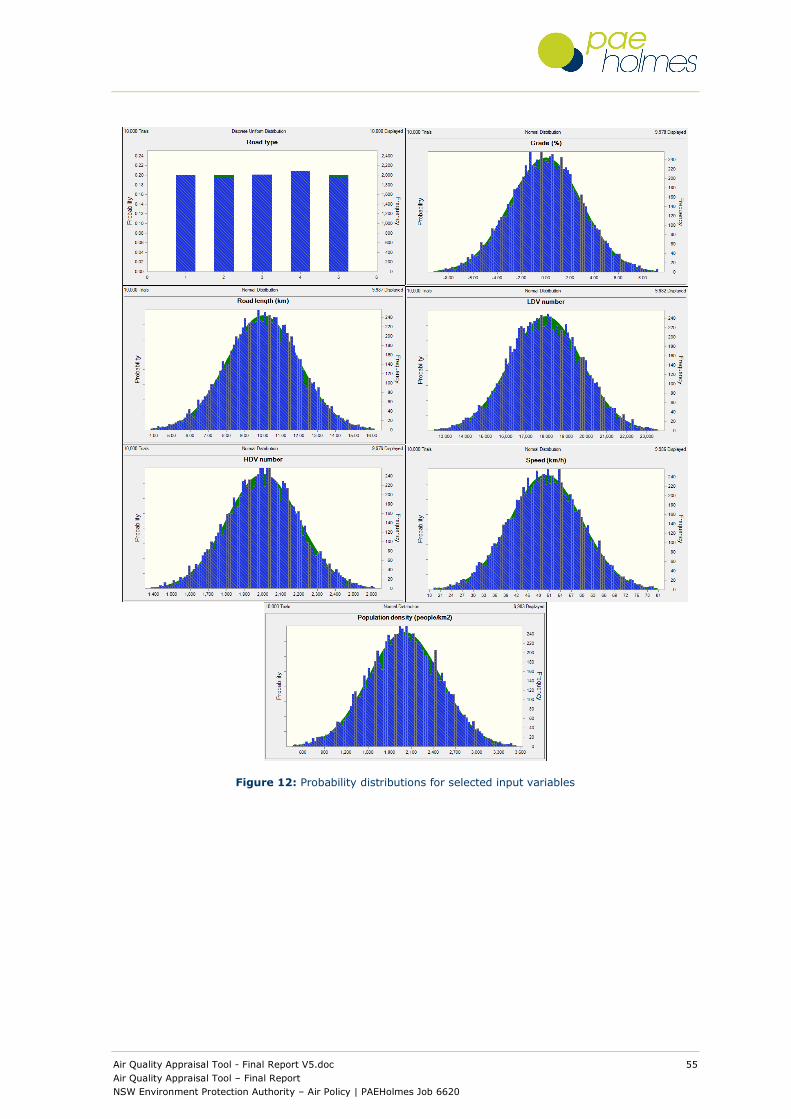
Air Quality Appraisal Tool - Final Report V5.doc 55
Air Quality Appraisal Tool – Final Report
NSW Environment Protection Authority – Air Policy | PAEHolmes Job 6620
Figure 12: Probability distributions for selected input variables
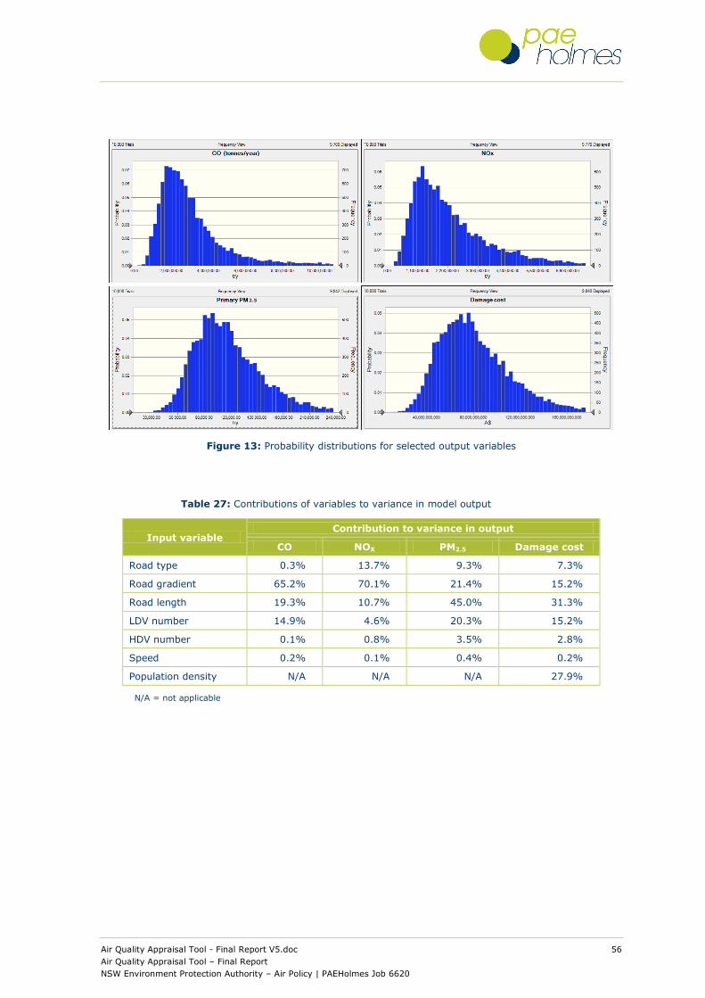
Air Quality Appraisal Tool - Final Report V5.doc 56
Air Quality Appraisal Tool – Final Report
NSW Environment Protection Authority – Air Policy | PAEHolmes Job 6620
Figure 13: Probability distributions for selected output variables
Table 27: Contributions of variables to variance in model output
Input variable Contribution to variance in output
CO NOX PM2.5 Damage cost
Road type 0.3% 13.7% 9.3% 7.3%
Road gradient 65.2% 70.1% 21.4% 15.2%
Road length 19.3% 10.7% 45.0% 31.3%
LDV number 14.9% 4.6% 20.3% 15.2%
HDV number 0.1% 0.8% 3.5% 2.8%
Speed 0.2% 0.1% 0.4% 0.2%
Population density N/A N/A N/A 27.9%
N/A = not applicable
2.5

Air Quality Appraisal Tool - Final Report V5.doc 57
Air Quality Appraisal Tool – Final Report
NSW Environment Protection Authority – Air Policy | PAEHolmes Job 6620
7 IMPLEMENTATION AND FUTURE IMPROVEMENTS
This chapter of the report suggests how AQAT might be implemented, provides some useful
sources of information and data, and considers potential ways in which it might be improved in
the future.
7.1 Implementation
7.1.1 Role in planning process
7.1.1.1 Capital projects
For large capital projects there is scope for the formal integration of AQAT in Annex 4 of the
NSW Government Guidelines for Economic Appraisal (NSW Treasury, 2007), which deals
specifically with environmental impacts. In this sense, there is potential for it to be used at
several different stages: within strategic planning, as part of scoping of developments, as part
of environmental impact assessment, and within so-called Ex-Post44 evaluation. Given that the
rigour of the appraisal generally increases as a project progresses, this should be reflected in
any guidelines which relate specifically to air quality, and some considerations are provided
below. These will be discussed in more detail with EPA, the DoPI, other potential users of AQAT,
and other stakeholders. A workshop will be held at the end of the project, and this will provide a
suitable forum for discussion.
Large transport and land use projects are assessed by NSW DoPI, although such projects are
also referred to the Environment Protection Authority (EPA). The EPA could request that DoPI
includes a requirement to undertake an air quality assessment using AQAT as part of the EIS,
and AQAT could be made available for this purpose.
For rezoning and land release proposals DoPI is responsible for the original assessment.
Guidance is required on how to set up the base case and scenarios, and how to develop
reasonable assumptions about future travel patterns.
7.1.1.2 Small projects
Smaller one-off, local projects – defined as those costing less than A$1 million - are unlikely to
merit a full, formal appraisal (NSW Treasury, 2007). Whilst in some cases it may still be
useful to characterise economic impacts, the general approach can be much simpler than that
for capital projects. The unpublished guidance from the RTA (Section 2.4.2) provides examples
of screening criteria for road schemes which might be used to determine whether an
assessment of emissions and health costs is required.
Local government is responsible for the assessment of new traffic-generating developments.
Either the proponents could be required to undertake an assessment using AQAT (for larger
projects), or the local authority could ask for a description of the roads affected and the likely
changes in traffic movement as part of the SEE. In the latter case, the council planner would
need to undertake an assessment. For local traffic schemes (e.g. to increase walking/cycling)
council planners would need to estimate the changes in traffic movements.
44 ‘Ex-Post’ refers to the situation after a project has been implemented or constructed.

Air Quality Appraisal Tool - Final Report V5.doc 58
Air Quality Appraisal Tool – Final Report
NSW Environment Protection Authority – Air Policy | PAEHolmes Job 6620
7.1.2 General guidance on appraisal of developments
7.1.2.1 Capital projects
When appraising the health impacts of capital transport and land use developments, attention
should be paid to the specific requirements of the planning process. As noted above, the rigour
of the appraisal generally increases as a project progresses. As a general rule, it is therefore
advisable that the effort required of an end user of AQAT should be in proportion to the size or
impact of the development being evaluated.
There are three general areas in which guidance is required:
1. Characterisation of the development
2. Application of AQAT
3. Using the results from AQAT
An important first step in the appraisal of any development is the accurate characterisation and
definition of the development being investigated, and also the boundary conditions relating to
the calculations. For example, there is a need to define the precise objectives of the appraisal,
and which roads, railway lines and affected populations are likely to be affected. In most cases
this information should be available in increasing detail as the project progresses.
The application of AQAT should essentially follow the steps described in the User Guide,
irrespective of the size of the development. However, different procedures could be used to
collect the relevant input data during the various stages of the project cycle. Some examples
are provided below.
Strategic planning: Here, the inputs (such as the total amount of road or rail transport)
could be based on generic estimates or simple calculations for one or two routes, and
average population densities for regions could be assumed.
Project concept: At this stage slightly more accurate information would be required. For
example, specific routes would need to be more clearly defined and traffic flows would
either be predicted based on simple assumptions or obtained from models. Population
density could be used at the LGA level.
Environmental Impact Statement: For the EIS, the traffic inputs would have to be based
on model predictions for specific road links with detailed information on traffic flow,
composition and speed, and an accurate description of rail freight activity. There would
also be greater spatial resolution in the population density data.
Ex-Post evaluation: In the Ex-Post evaluation it would be appropriate to undertake
measurements. The inputs to AQAT could therefore include real-world measurements of
road traffic flow, composition and speed, and/or rail freight activity and fuel consumption.
The use of the results from AQAT in the economic appraisal process should be made clear.
7.1.2.2 Small projects
In the case of small projects it is difficult to provide general guidance, as the requirements will
depend on the nature of the project. However, the level of effort should again be in proportion
to the scale of the development, and therefore quite simple calculations would generally be
sufficient.
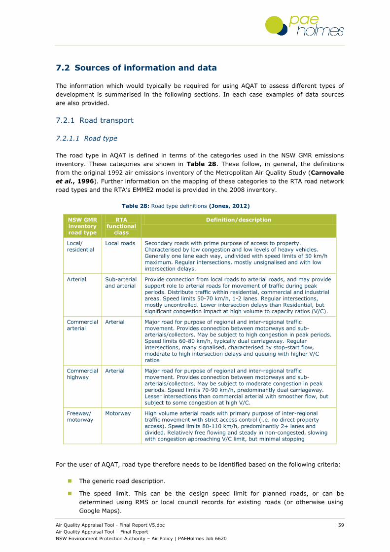
Air Quality Appraisal Tool - Final Report V5.doc 59
Air Quality Appraisal Tool – Final Report
NSW Environment Protection Authority – Air Policy | PAEHolmes Job 6620
7.2 Sources of information and data
The information which would typically be required for using AQAT to assess different types of
development is summarised in the following sections. In each case examples of data sources
are also provided.
7.2.1 Road transport
7.2.1.1 Road type
The road type in AQAT is defined in terms of the categories used in the NSW GMR emissions
inventory. These categories are shown in Table 28. These follow, in general, the definitions
from the original 1992 air emissions inventory of the Metropolitan Air Quality Study (Carnovale
et al., 1996). Further information on the mapping of these categories to the RTA road network
road types and the RTA’s EMME2 model is provided in the 2008 inventory.
Table 28: Road type definitions (Jones, 2012)
NSW GMR inventory road type
RTA functional
class
Definition/description
Local/ residential
Local roads Secondary roads with prime purpose of access to property. Characterised by low congestion and low levels of heavy vehicles. Generally one lane each way, undivided with speed limits of 50 km/h maximum. Regular intersections, mostly unsignalised and with low intersection delays.
Arterial Sub-arterial and arterial
Provide connection from local roads to arterial roads, and may provide support role to arterial roads for movement of traffic during peak periods. Distribute traffic within residential, commercial and industrial areas. Speed limits 50-70 km/h, 1-2 lanes. Regular intersections, mostly uncontrolled. Lower intersection delays than Residential, but significant congestion impact at high volume to capacity ratios (V/C).
Commercial arterial
Arterial Major road for purpose of regional and inter-regional traffic movement. Provides connection between motorways and sub-arterials/collectors. May be subject to high congestion in peak periods. Speed limits 60-80 km/h, typically dual carriageway. Regular intersections, many signalised, characterised by stop-start flow, moderate to high intersection delays and queuing with higher V/C ratios
Commercial highway
Arterial Major road for purpose of regional and inter-regional traffic movement. Provides connection between motorways and sub-arterials/collectors. May be subject to moderate congestion in peak periods. Speed limits 70-90 km/h, predominantly dual carriageway. Lesser intersections than commercial arterial with smoother flow, but subject to some congestion at high V/C.
Freeway/ motorway
Motorway High volume arterial roads with primary purpose of inter-regional traffic movement with strict access control (i.e. no direct property
access). Speed limits 80-110 km/h, predominantly 2+ lanes and divided. Relatively free flowing and steady in non-congested, slowing with congestion approaching V/C limit, but minimal stopping
For the user of AQAT, road type therefore needs to be identified based on the following criteria:
The generic road description.
The speed limit. This can be the design speed limit for planned roads, or can be
determined using RMS or local council records for existing roads (or otherwise using
Google Maps).
Air Quality Appraisal Tool - Final Report V5.doc 60
Air Quality Appraisal Tool – Final Report
NSW Environment Protection Authority – Air Policy | PAEHolmes Job 6620
The number of lanes.
The frequency of intersections and the level of signalisation.
7.2.1.2 Road length
For an existing road the length can be determined using the ‘Ruler’ tool in Google Earth. For a
planned road the length can be determined from planning documents held by DoPI, RMS or,
council transport/traffic departments.
7.2.1.3 Road gradient
For an existing road the average gradient can be calculated using Google Earth. The ‘Ruler’ tool
can be used to give the road length as above, and the elevation values can be obtained for the
start and end points of the road. For planned roads the gradient can be obtained from the
relevant planning authority.
7.2.1.4 Traffic volume, composition and speed
It is anticipated that for many developments the road traffic activity data will be produced by a
traffic assignment model (such as the Sydney STM). However, there are a number of difficulties
associated with using the outputs from a traffic assignment model as inputs to an emission
model. The outputs of the former are not usually defined in a manner which is ideal for use in
the latter (Boulter and Turpin, 2007). The main differences are summarised below.
Road classification: Road types tend not to be defined explicitly in traffic assignment
models. The distinction made with regards to road type in some types of emission model
is typically between ‘urban’, ‘rural’ and ‘motorway’, which is rather ambiguous. AQAT uses
a different classification (see section 3.1.3). This does not usually represent a serious
problem as, if needed, road type can be assumed or inferred. Nevertheless, slightly
different approaches would be required for different types of road/link.
Time periods: The time period being covered is one of the principal differences between
traffic assignment models and emission models. Because many road schemes are
designed for times of maximum travel demand, it is conventional practice to model hourly
average traffic flows for the peak and inter-peak periods during an ‘average weekday’ of a
‘neutral month’. The ‘average weekday’ often relates to four days (Monday to Thursday).
Outputs are not usually provided specifically for Fridays, Saturdays and Sundays, or for
minor roads. However, in AQAT annual average 24-hour traffic data are required.
Vehicle classification: In emission models traffic data are required for large number of
vehicle categories, whereas traffic models tend to deal with fewer vehicle categories. An
appropriate mapping is therefore required between the categories defined in the two
types of model. In some cases, the traffic model may only provide data for ‘passenger car
units’ (PCUs), or for light-duty vehicles and heavy-duty vehicles. To reduce uncertainties
in the overall emission estimates, the traffic model needs to maximise the detail in the
compositional data. Buses and taxis are significant contributors to air pollution but are
often poorly characterised in traffic models.
Vehicle operation: Traffic speed is a common output of traffic assignment models, but
again the data are for specific time periods. For AQAT there is a need for something
simpler (average daily speed). It would be feasible to use speed distributions rather than
a daily average value, but this would complicate what is supposed to be a simple tool.

Air Quality Appraisal Tool - Final Report V5.doc 61
Air Quality Appraisal Tool – Final Report
NSW Environment Protection Authority – Air Policy | PAEHolmes Job 6620
The general implication is that there will be a need for a post-processing of any traffic model
data, such as the development of scaling factors for traffic flow, traffic composition and speed.
However, this was beyond the scope of the project.
It is also possible that in some cases the traffic activity data for developments will be provided
by micro-simulation models. In general the considerations mentioned for traffic assignment
models also apply here. The main difficulty is simplifying the large amount of data from such
models (unless appropriate summary values are already provided by the model).
Alternative sources of traffic data include:
Automatic and manual classified traffic counts for specific roads. Data will be available
from local authorities and the RTA web site
(http://www.rta.nsw.gov.au/trafficinformation/downloads/aadtdata_dl1.html).
Video surveys for existing roads. These can also be used in conjunction with RTA
registration data to give details petrol/diesel splits for cars and light commercial
vehicles.
For travel-based assessments, data are available by LGA from the NSW Bureau of
Transport Statistics, Household Travel Survey
(http://www.bts.nsw.gov.au/Statistics/HTS/default.aspx#top).
Road project assessments. A range of information is available for specific road projects
from the RMS web site (http://www.rta.nsw.gov.au/roadprojects/projects/index.html).
For assessments in future years, information on traffic growth projections in Australian cities
can be found in a BITRE report (http://www.bitre.gov.au/publications/2012/report_127.aspx).
7.2.2 Rail transport
It seems likely that in the near future the required rail activity data will have to be obtained
from the sources which are currently used (e.g. train operators and infrastructure managers).
However, this is probably sufficient for many applications. Locomotive fuel usage activity data
may be sourced from the Australian Bureau of Agricultural and Resource Economics (ABARE)
and Australian Bureau of Statistics.
7.2.3 Population density
The principal source of population data is the Australian Bureau of Statistics
(http://www.abs.gov.au). ABS provides population by LGA. Land area or LGAs is also available
from ABS, and can also be estimated using GIS or Google Earth.
7.3 Future improvements
Some considerations for the future improvement of AQAT are presented below.
Inclusion of additional model years. At present AQAT is restricted to appraisals for five
model years (2008, 2011, 2016, 2021 and 2026), as road transport emission factors were
only available for these years. This limits the applicability of AQAT.
Greater disaggregation of vehicle types. The Tool currently predicts emissions for nine
different types of vehicle, but for each model year an aggregated emission factor is used,
and the vehicle age/technology distribution and weight distributions are implicit. This

Air Quality Appraisal Tool - Final Report V5.doc 62
Air Quality Appraisal Tool – Final Report
NSW Environment Protection Authority – Air Policy | PAEHolmes Job 6620
means that the effects of developments, policies and measures which affect these
distributions cannot currently be evaluated. Examples of these include:
Accelerated introduction of the most recent emission standards, low-carbon technologies
(such as hybrids) or specific engine or exhaust after-treatment technologies (e.g. diesel
particulate filters).
Low-emission zones.
Accelerated vehicle scrappage schemes.
Shifting freight between heavy goods vehicles having different load-carrying capacity, or
shifting passengers between different types of bus.
In the future, consideration should be given to extending AQAT so that it incorporates
more detail from the full 2008 GMR road emissions inventory model.
Improvement of the rail freight emission calculation. The rail freight calculation is
currently very coarse. It could be improved by including specific train types and weights,
and allowing for train operation.
Inclusion of rail passenger transport. At the moment it is assumed that there are no
emissions from passenger trains, as most trains are electric. However, passenger trains
could be included if and when data become available, along with emission factors for
power generation and other related assumptions (e.g. power losses during transmission).
This would improve the accuracy of inter-modal comparisons. Reliable data on train (and
bus) occupancy would help to improve the estimation of emissions on a per passenger
basis.
A module for processing traffic data. Whilst AQAT will accept the outputs from different
traffic models, some post-processing of the traffic model data will be required to ensure
that the data are in the correct format, and it is likely that traffic scaling factors will also
be required. The possibility of including a specific module in AQAT for processing traffic
data could be investigated.
Additional damage costs. Additional costs for secondary particles should be included in
AQAT, as and when the scientific understanding is sufficiently robust to permit this.
Further sensitivity analyses. The importance of different model variables will vary
depending on the specific type of development being investigated. A procedure for
identifying the most important variables for any given type of development would
therefore be useful. It would also be of interest to undertake a global sensitivity analysis
for the 2008 GMR inventory model for road transport, as this would provide a more
general indication of model uncertainty.
The use of significance criteria for indicating the importance of impacts. It may be
appropriate to apply such criteria before the results from AQAT are used in economic
appraisal (e.g. to reduce work where impacts are not likely to be significant).
Adaptation to other jurisdictions. The Tool is designed for use in NSW, and the road and
rail emission factors are designed for use in the State. However, there is no reason why
AQAT cannot be used in other Australian jurisdictions, and all SUAs are included in AQAT.
The confidence in the predictions should improve where State-specific emission factors
and model data are used in place of the NSW data.
Air Quality Appraisal Tool - Final Report V5.doc 63
Air Quality Appraisal Tool – Final Report
NSW Environment Protection Authority – Air Policy | PAEHolmes Job 6620
8 REFERENCES
Abbott P G, Al-Rukabi H, Babb E, Baguley P C, Hardman E J, Smith R and Strong T R (2000).
Creation of a prototype version of SISTM to model MIDAS. TRL unpublished report
PR/TT/064/99. TRL, Crowthorne.
Agapides N (2012). Personal communication from Nick Agapides of NSW Office of Environment
and Heritage to Paul Boulter.
Akcelik and Associates (2006). Traffic models. http://www.akcelik.com.au/TrafficModels.htm
Akcelik R and Besley M (2003). Operating cost, fuel consumption and emission models in
aaSIDRA and aaMOTION. 25th conference of Australian Institutes of Transport Research (CAITR
2003). University of South Australia, Adelaide. 2-5 December 2003.
ARTC (2010). Melbourne–Brisbane Inland Rail Alignment Study - Final Report, July 2010.
Appendix G - Train Operations. http://www.artc.com.au/library/IRAS_Appendix_G.pdf
Aust N, Watkiss P and Boulter P (2012). Methodology for valuing the health impacts of changes
in particle emissions. PAEHolmes Report 6695. PAEHolmes, Epping NSW.
Beer T (2002). Valuation of pollutants emitted by road transport into the Australian atmosphere,
Proceedings of the 16th International Clean Air & Environment Conf, Christchurch, New Zealand.
Boulter P G and Turpin K (2007). West London Alliance traffic and enhanced emissions model.
Sub-project 2 - Traffic scaling factors: Inception Report. TRL Report PPR189. Transport
Research Laboratory, Wokingham, United Kingdom.
Brook R D, Rajagopalan S, Pope C A, Brook J R, Bhatnagar A, Diez-Roux A V, Holguin F, Hong Y,
Luepker R V, Mittleman M A, Peters A, Siscovick D, Smith S C Jr, Whitsel L and Kaufman J D
(2012). American Heart Association Council on Epidemiology and Prevention, Council on the
Kidney in Cardiovascular Disease, and Council on Nutrition, Physical Activity and Metabolism:
Particulate matter air pollution and cardiovascular disease: An update to the scientific statement
from the American Heart Association. Circulation, 2010, 121, pp. 2331-2378.
BTS (2012). BTS InfoSheet - Strategic Travel Model Standard Outputs. NSW Bureau of
Statistics, Chippendale NSW. February 2012.
Carnovale F, Tilly K, Stuart A, Carvalho C, Summers M and Eriksen P. (1996). Metropolitan Air
Quality Study – Air Emissions Inventory, Environment Protection Authority of Victoria.
Coffey (2003). Fuel quality and vehicle emissions standards Cost benefit analysis prepared for
MVEC Review of Vehicle Emissions and Fuel Standards Post 2006. Coffey Geosciences Pty Ltd.
October 2003. Available at: http://www.ephc.gov.au/ltec/pdfs/CBAFinalReport23October.pdf
COMEAP (2009). Long-term exposure to air pollution: effect on mortality. A report by the
Committee on the Medical Effects of Air Pollutants. London, Department of Health, United
Kingdom. ISBN 978-0-85951-640-2.
Commonwealth of Australia (2010). State of the Air in Australia 1999–2008. Department of
Sustainability, Environment, Water, Population and Communities, Canberra, Australia.
Air Quality Appraisal Tool - Final Report V5.doc 64
Air Quality Appraisal Tool – Final Report
NSW Environment Protection Authority – Air Policy | PAEHolmes Job 6620
Connell Wagner (1998). Pacific Highway, Ballina Bypass – Environmental Impact Statement –
Main Volume. Connell Wagner, Neutral Bay, NSW.
http://www.rta.nsw.gov.au/roadprojects/projects/pac_hwy/ballina_tweed_heads/ballina_bypass
/public_information.html
DCCEE (2011). Technical Guidelines for the estimation of greenhouse gas emissions by facilities
in Australia. Published by the Department of Climate Change and Energy Efficiency.
DEC (2005a). Approved Methods for the Modelling and Assessment of Air Pollutants in NSW.
NSW Department of Environment and Conservation, Sydney.
DEC (2005b). Air Pollution Economics: Health Costs of Air Pollution in the Greater Sydney
Metropolitan Region. Sydney, Department of Environment and Conservation, NSW.
DECC (2007a). Technical Report No. 8 - Air Emissions Inventory for the Greater Metropolitan
Region in New South Wales. On-Road Mobile Emissions Module: Results. Department of
Environment and Climate Change NSW, Sydney.
DECC (2007b). Technical Report No. 7 - Air Emissions Inventory for the Greater Metropolitan
Region in New South Wales. Off-Road Mobile Emissions Module: Results. Department of
Environment and Climate Change NSW, Sydney.
DECC (2008). Proponents Guidelines for the Review of Environmental Factors. Department of
Environment and Climate Change, Sydney.
Defra (2007). An Economic Analysis to inform the Air Quality Strategy- Updated Third Report of
the Interdepartmental Group on Costs and Benefits. July 2007. Department for Environment,
Food and Rural Affairs, London.
Defra (2008). Damage cost guidance. Available from:
http://archive.defra.gov.uk/environment/quality/air/airquality/panels/igcb/documents/damage-
cost-calculator-guidancepaper.pdf
Defra (2011). Air Quality Appraisal – Damage Cost Methodology. Interdepartmental Group on
Costs and Benefits, Air Quality Subject Group February 2011. Department for Environment,
Food and Rural Affairs, London.
Department of Planning (2008). Development Near Rail Corridors and Busy Roads – Interim
Guideline. ISBN 978-0-7347-5504-9.
Department of Planning (2009). Sydney’s Growth Centres. Guide to the new release Precincts.
www.growthcentres.nsw.gov.au
DIT (2010). Final Regulatory Impact Statement for Euro 5/6 Light Vehicle Emissions Standards.
Department of Infrastructure and Transport, NSW, Australia.
EEA (2009). EMEP/EEA Air Pollutant Emission Inventory Guidebook - 2009. Technical report No
6/2009. European Environment Agency EEA, Copenhagen.
http://www.eea.europa.eu/publications/emep-eea-emission-inventory-guidebook-2009/
Environment Australia (1999). Emissions Estimation Technique Manual for Aggregated
Emissions from Railways. Version 1.0 - First Published 1 November 1999. Environment
Australia, Canberra, Australia.
Air Quality Appraisal Tool - Final Report V5.doc 65
Air Quality Appraisal Tool – Final Report
NSW Environment Protection Authority – Air Policy | PAEHolmes Job 6620
Environment Australia (2000a). Emissions Estimation Technique Manual for Aggregated
Emissions from Motor Vehicles, 22 November 2000 – Version 1.0. Environment Australia,
Canberra, Australia. http://www.npi.gov.au/publications/aedmanuals/motorvehicles.html
Environment Australia (2000b). Setting National Fuel Quality Standards, Paper 1, Summary
report of Fuel Quality Requirements for Australian Transport, Commonwealth of Australia,
Canberra, ACT.
Gijsen A and van den Brink RMM (2002). Energy use and emissions by rail transport;
description and results of the model PRORIN (in Dutch). Report no. 773002021. RIVM,
Bilthoven, The Netherlands.
Jalaludin B, Morgan G, Salkeld G and Gaskin C (2011). Health benefits of reducing ambient air
pollution levels in the Greater Metropolitan Region. A report for the NSW Ministry of Health and
the NSW Office of Environment and Heritage (unpublished).
Jones G (2012). Personal communication from Gareth Jones of NSW Office of Environment and
Heritage to Paul Boulter.
Kellaghan R (2010). Air quality assessment - Koolbury Rail Loop. PAEHolmes report.
Kioutsioukis I, Tarantola S, Saltelli A and Gatelli D (2004).Uncertainty and global sensitivity
analysis of road transport emission estimates. Atmospheric Environment Vol. 38 (2004), pp.
6609–6620.
Lilley W E (1996). Quantification and dispersion modelling of diesel locomotives emissions.
Submitted to the Department of Geography University of Newcastle in partial fulfilment of the
requirements for the degree of Bachelor of Science with Honour.
Lindgreen E and Sorenson S C (2005). Simulation of energy consumption and emissions from
rail traffic. Report MEK-ET-2005-4, Department of Mechanical Engineering, Danish Technical
University, February, 2005. Deliverable 7a for ARTEMIS, DG-TREN contract 1999-RD.10429.
Milthorpe F (2012). Personal communication from Frank Milthorpe of NSW Bureau of Transport
Statistics to Paul Boulter.
Murphy H and Shen J (2011). Assessment of air quality impacts using screening tools. Paper
presented at CASANZ conference, Auckland, July 30 - Aug 2, 2011.
NEPC (2011). National Environment Protection (Ambient Air Quality) Measure Review. National
Environment Protection Council, Adelaide.
http://www.ephc.gov.au/sites/default/files/AAQ%20NEPM%20review%20report_0.pdf
NSW EPA (1997). Proposed Clean Air (Motor Vehicles and Motor Vehicle Fuels) Regulation 1997
– Regulatory Impact Statement, NSW EPA, Chatswood, NSW.
NSW EPA (1998). Proposed Pollution Control Regulation 1998 – Regulatory Impact Statement,
NSW EPA, Chatswood, NSW.
NSW Treasury (2007). NSW Government Guidelines for Economic Appraisal: Policy & Guidelines
Paper. Office of financial Management, NSW, Australia.
http://www.treasury.nsw.gov.au/__data/assets/pdf_file/0016/7414/tpp07-5.pdf
Air Quality Appraisal Tool - Final Report V5.doc 66
Air Quality Appraisal Tool – Final Report
NSW Environment Protection Authority – Air Policy | PAEHolmes Job 6620
Pacific National (2006). Submission to Senate Rural and Regional Affairs and Transport
Committee. Inquiry into Australia’s Future Oil Supply and Alternative Transport Fuels. March
2006.
Parsons Brinckerhoff (2008). Upgrading the Pacific Highway, Banora Point Upgrade Technical
Paper 1 - Traffic, Transport and Access. February 2008.
http://www.planning.nsw.gov.au/DevelopmentAssessments/Majorprojectregister/ProjectPacificH
ighwayUpgradeBanoraPointM/tabid/343/Default.aspx
Pope C A III and Dockery D W (2006). Health effects of fine particulate air pollution: lines that
connect. J Air Waste Manag Assoc 2006, 56:709-742.
RMS (2012). Tool for Roadside Air Quality (TRAQ) – User Manual and supporting
documentation. NSW Roads and Maritime Services, February 2012.
RTA (2004). Bulahdelah Upgrading the Pacific Highway Environmental Impact Statement
Technical Paper 6 Traffic and Transport. NSW Roads and Traffic Authority, Surry Hills.
RTA (2005). Upgrade of Cowpasture Road – North Liverpool Road to Westlink M7. Review of
Environmental Factors, Volume 1 – Main Report. NSW Roads and Traffic Authority, Surry Hills.
RTA (2006). Great Western Highway Upgrade. Wentworth Falls East Tableland Road to Station
Street - Review of Environmental Factors. Volume 3 – Appendices. NSW Roads and Traffic
Authority, Surry Hills.
RTA (2007). Air Quality Assessment and Monitoring Guidelines: Roadways and Road Tunnels.
NSW Roads and Traffic Authority, Surry Hills.
RTA (2008a). Ballina Bypass - Upgrading the Pacific Highway. Refined design report. NSW
Roads and Traffic Authority, August 2008.
RTA (2008b). Ballina Bypass - Upgrading the Pacific Highway. Modification of the Ballina Bypass,
Environmental Assessment Report. NSW Roads and Traffic Authority, August 2008
Ryan L (2012). Personal communication from Liam Ryan of NSW Office of Environment and
Heritage to Paul Boulter.
Scholl M (2006). Best Practice Planning for Vehicle Air Emissions along Land-Based Transport
Corridors and in Transit-Oriented Centres. Report for NSW DEC. PAEHolmes Report.
SKM and Connell Wagner (2005). North-South Bypass Tunnel – Draft Environmental Impact
Statement, Volume 1.
Smit R, Warren B, Kelly M, Steele J, Bawden K, Anyon P, O’Reilly H and Pekol A (2010).
Landside emission inventory for the Port of Brisbane precinct. PAE Holmes Report.
Taylor J (2009). Critical Review of Transport Modelling Tools (Implementation Options). Sinclair
Knight Merz, Malvern VIC, Australia.
TfL (2003). Micro-simulation modelling guidance note for TfL. July 2003. Transport for London
Street Management, London.
Transport for NSW (2012). North West Rail Link Environmental Assessment No. 1. Technical
Paper 1 – Construction Traffic and Transport Management. Transport for NSW, Chippendale.

Air Quality Appraisal Tool - Final Report V5.doc 67
Air Quality Appraisal Tool – Final Report
NSW Environment Protection Authority – Air Policy | PAEHolmes Job 6620
Transurban (2010). M2 Upgrade Environmental Assessment Volume 2 – Part 1: Technical
Papers. EA Technical Report: Traffic and Transport Impact Assessment. Transurban Traffic
Services Group.
USEPA (2003). Draft 2003 Report to Congress on the Costs and Benefits of Federal Regulations.
Federal Register, Volume 68, Number 22, 3 February 2003, Notices. US Environment Protection
Authority.
USEPA (2009a). Integrated Science Assessment for Particulate Matter. EPA/600/R-08/139F,
United States Environmental Protection Agency, available at:
http://cfpub.epa.gov/ncea/cfm/recordisplay.cfm?deid=216546
USEPA (2009b). Emission Factors for Locomotives, EPA-420-F-09-025, Office of Transportation
and Air Quality, United States Environment Protection Agency (USEPA), 2000 Traverwood Drive,
Ann Arbor, MI 48105, USA.
USEPA (2009c). NONROAD 2008 Model. United Stated Environmental Protection Agency
(USEPA), Research Triangle Park, NC, USA.
Watkiss P (2002). Fuel Taxation Inquiry: the Air Pollution Costs of Transport in Australia, Report
No. ED44525 to Commonwealth of Australia, AEA.

Air Quality Appraisal Tool - Final Report V5.doc A-1
Air Quality Appraisal Tool – Final Report
NSW Environment Protection Authority – Air Policy | PAEHolmes Job 6620
APPENDIX A
Glossary of terms and abbreviations
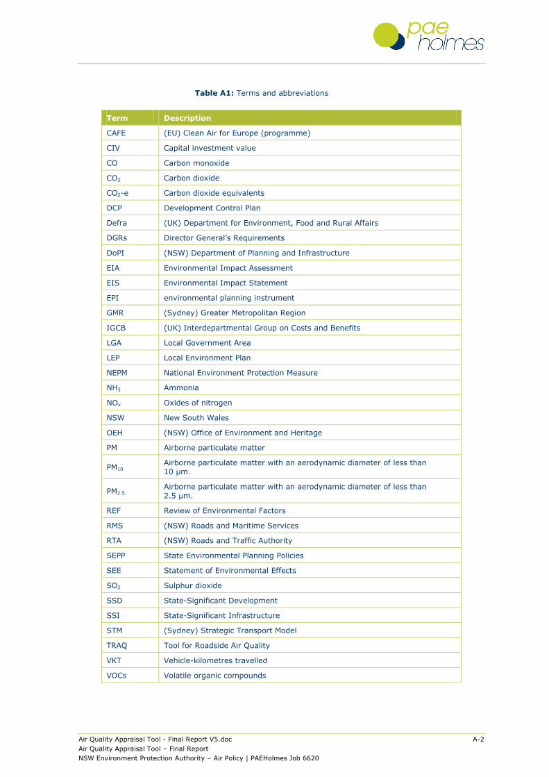
Air Quality Appraisal Tool - Final Report V5.doc A-2
Air Quality Appraisal Tool – Final Report
NSW Environment Protection Authority – Air Policy | PAEHolmes Job 6620
Table A1: Terms and abbreviations
Term Description
CAFE (EU) Clean Air for Europe (programme)
CIV Capital investment value
CO Carbon monoxide
CO2 Carbon dioxide
CO2-e Carbon dioxide equivalents
DCP Development Control Plan
Defra (UK) Department for Environment, Food and Rural Affairs
DGRs Director General’s Requirements
DoPI (NSW) Department of Planning and Infrastructure
EIA Environmental Impact Assessment
EIS Environmental Impact Statement
EPI environmental planning instrument
GMR (Sydney) Greater Metropolitan Region
IGCB (UK) Interdepartmental Group on Costs and Benefits
LGA Local Government Area
LEP Local Environment Plan
NEPM National Environment Protection Measure
NH3 Ammonia
NOx Oxides of nitrogen
NSW New South Wales
OEH (NSW) Office of Environment and Heritage
PM Airborne particulate matter
PM10 Airborne particulate matter with an aerodynamic diameter of less than 10 µm.
PM2.5 Airborne particulate matter with an aerodynamic diameter of less than
2.5 µm.
REF Review of Environmental Factors
RMS (NSW) Roads and Maritime Services
RTA (NSW) Roads and Traffic Authority
SEPP State Environmental Planning Policies
SEE Statement of Environmental Effects
SO2 Sulphur dioxide
SSD State-Significant Development
SSI State-Significant Infrastructure
STM (Sydney) Strategic Transport Model
TRAQ Tool for Roadside Air Quality
VKT Vehicle-kilometres travelled
VOCs Volatile organic compounds
Air Quality Appraisal Tool - Final Report V5.doc B-1
Air Quality Appraisal Tool – Final Report
NSW Environment Protection Authority – Air Policy | PAEHolmes Job 6620
APPENDIX B
Consultees

Air Quality Appraisal Tool - Final Report V5.doc B-2
Air Quality Appraisal Tool – Final Report
NSW Environment Protection Authority – Air Policy | PAEHolmes Job 6620
Table B1: Consultees.
a EPA project OEH-1072-2011 (Methodology for valuing health impacts of changes in particle emissions).
Consultee Contacted?
Organisation Contact Position Y/N Notes
NSW Dept. of Planning and Infrastructure
Principal Assessment Officer (rail)
Manager, Infrastructure Projects Department of Planning Y Meeting 13/3/12
Principal Assessment Officer (road)
Y Meeting 13/3/12
Transport for NSW Bruce Dowdell Manager – Freight Emissions, Transport for NSW Y Meeting 19/3/12
City of Ryde Vince Galletto Client Manager Y Meeting 8/3/12
NSW EPA (2008 GMR Emissions Inventory)
Gareth Jones (road) Senior Atmospheric Scientist, NSW EPA Y Meeting 21/2/12
Nick Agapides (non-road) Manager Major Air Projects, Air Policy Y Telephone discussion 17/4/12
Transport for NSW Bureau of Transport Statistics
Frank Milthorpe Transport Model Development Manager Y Email
NSW Office of Environment and Heritage
Liam Ryan Policy officer: Emissions Reduction, Climate Change Air and Noise
Y Kick-off meeting, email
Paul Watkiss Associates Paul Watkiss Director Y Contacted through separate EPA projecta
Air Quality Appraisal Tool - Final Report V5.doc C-1
Air Quality Appraisal Tool – Final Report
NSW Environment Protection Authority – Air Policy | PAEHolmes Job 6620
APPENDIX C
Air Quality Appraisal Tool – Calculation Methodology
Air Quality Appraisal Tool - Final Report V5.doc C-2
Air Quality Appraisal Tool – Final Report
NSW Environment Protection Authority – Air Policy | PAEHolmes Job 6620
C1 Emissions from road transport
AQAT estimates hot running emissions, cold-start emissions and non-exhaust PM2.5 emissions, as
well as emissions of other pollutants (although these are not used in the damage cost calculation).
For these processes the calculations are described below. Evaporative emissions of VOCs are not
included in AQAT.
C1.1 Calculation of hot running emissions
C1.1.1 Base emission factors and speed-correction
The method for calculating hot running emissions in AQAT involves the use of base ‘composite’
emission factors for the following matrix of cases:
Five pollutants (CO, NOX, PM10, HC, CO2)45.
Nine vehicle types (CP, CD, LDCP, LDCD, HDCP, RT, AT, BusD and MC)46, with the emission
factor for each vehicle type taking into account the VKT by age (and associated emission
factors by sub-type).
Five road types (residential, arterial, commercial arterial, commercial highway,
highway/freeway), as specified in the 2008 GMR emissions inventory.
Five years (2008, 2011, 2016, 2021, 2026). The year is used to define the vehicle fleet.
Three seasons (summer, winter, spring/autumn) were used for emission estimation by EPA.
In developing AQAT, a worst-case ‘season’ (using the highest emission factor of the three
seasons for each case) is also defined.
In the development of the emission factors EPA has taken various real-world effects into
consideration, including the deterioration in emissions performance with mileage, the effects
of tampering or failures in emission-control systems, and the use of ethanol in petrol. These
assumptions are built into the base emission factors in AQAT, and cannot be modified by the
user.
For each case in the matrix, the base emission factor is defined for a VKT-weighted average speed
(the base speed) associated with the corresponding road type. Dimensionless correction factors –
in the form of 6th-order polynomial functions - are then applied to the base emission factors taking
into account the actual speed on a road. According to EPA, the speed correction factors are valid
up to 110 km/h for light-duty vehicles, and up to 100 km/h for heavy-duty vehicles (Jones,
2012).
Therefore, the emission factor for a given traffic speed is calculated using Equation C1.
Equation C1
Where:
45 It was assumed that PM2.5 was equivalent to PM10, which is appropriate for exhaust emissions.
46 CP = petrol passenger vehicles; CD = diesel passenger vehicles; LDCP = light-duty commercial petrol vehicles (<=3500 kg); LDCD = light-duty commercial diesel vehicles (<=3500 kg); HDCP = heavy-duty commercial petrol vehicles (>3500kg); RT = rigid trucks (3.5-25 tonnes, diesel only); AT = articulated trucks (> 25 tonnes, diesel only); BusD = heavy public transport buses (diesel only); MC = motorcycles.
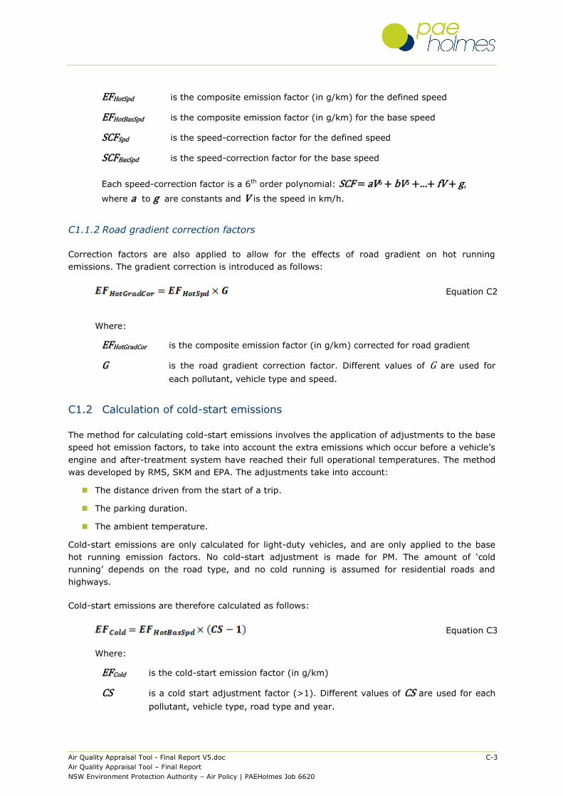
Air Quality Appraisal Tool - Final Report V5.doc C-3
Air Quality Appraisal Tool – Final Report
NSW Environment Protection Authority – Air Policy | PAEHolmes Job 6620
EFHotSpd is the composite emission factor (in g/km) for the defined speed
EFHotBasSpd is the composite emission factor (in g/km) for the base speed
SCFSpd is the speed-correction factor for the defined speed
SCFBasSpd is the speed-correction factor for the base speed
Each speed-correction factor is a 6th order polynomial: SCF = aV6 + bV5 +…+ fV + g,
where a to g are constants and V is the speed in km/h.
C1.1.2 Road gradient correction factors
Correction factors are also applied to allow for the effects of road gradient on hot running
emissions. The gradient correction is introduced as follows:
Equation C2
Where:
EFHotGradCor is the composite emission factor (in g/km) corrected for road gradient
G is the road gradient correction factor. Different values of G are used for
each pollutant, vehicle type and speed.
C1.2 Calculation of cold-start emissions
The method for calculating cold-start emissions involves the application of adjustments to the base
speed hot emission factors, to take into account the extra emissions which occur before a vehicle’s
engine and after-treatment system have reached their full operational temperatures. The method
was developed by RMS, SKM and EPA. The adjustments take into account:
The distance driven from the start of a trip.
The parking duration.
The ambient temperature.
Cold-start emissions are only calculated for light-duty vehicles, and are only applied to the base
hot running emission factors. No cold-start adjustment is made for PM. The amount of ‘cold
running’ depends on the road type, and no cold running is assumed for residential roads and
highways.
Cold-start emissions are therefore calculated as follows:
Equation C3
Where:
EFCold is the cold-start emission factor (in g/km)
CS is a cold start adjustment factor (>1). Different values of CS are used for each
pollutant, vehicle type, road type and year.

Air Quality Appraisal Tool - Final Report V5.doc C-4
Air Quality Appraisal Tool – Final Report
NSW Environment Protection Authority – Air Policy | PAEHolmes Job 6620
C1.3 Calculation of non-exhaust PM emissions
The method for non-exhaust PM2.5 is drawn from the EMEP/EEA Air Pollutant Emission Inventory
Guidebook (EEA, 2009), and includes tyre wear, brake wear and road surface wear. Emission
factors (EFNonEx in g/km) are provided for each vehicle type, road type and year.
C1.4 Calculation of emissions per link
For each vehicle category (v), the total emission factor (EFTot,v) is then calculated by summating
the hot running emission, cold-start and non-exhaust emission factors:
Equation C4
Again, cold-start emission factors are only used for light-duty vehicles, and non-exhaust emissions
are only relevant to PM2.5.
For a given road link, pollutant and year, total annual emissions are then calculated using the
following equation:
Equation C5
Where:
eL,y is the total annual emission (in tonnes/year) from the traffic on link L in year y,
summated over all nine vehicle categories
FL is the average total daily traffic volume on link L
PL,v is the proportion of the traffic on link L in vehicle category v
C1.5 Summation of link emissions
Total emissions (eTot,y) for the before-development and after-development cases are then
calculated as follows:
Equation C6
C1.6 Calculation of greenhouse gas emissions
A carbon balance method supplied by EPA is used to calculate fuel consumption for petrol and
diesel vehicles. The fuel consumption (in litres per 100 km) is calculated from the emission factors
for CO, HC and CO2 (determined using the daily traffic flows and base speeds) and density values
for petrol and diesel fuel. The fuel consumption values are then scaled according to the road length
in km and restated as a function of time. Finally, annual CO2-equivalent (CO2-e) emissions are
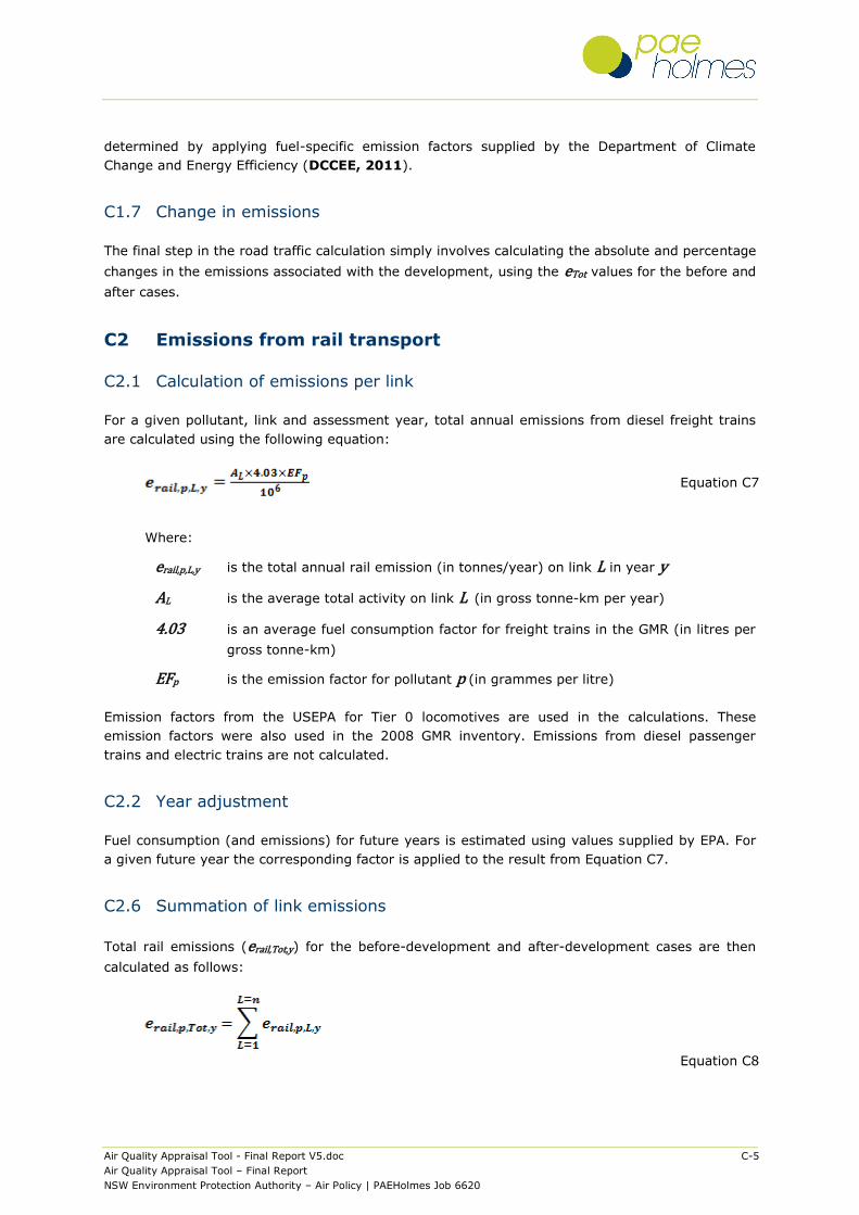
Air Quality Appraisal Tool - Final Report V5.doc C-5
Air Quality Appraisal Tool – Final Report
NSW Environment Protection Authority – Air Policy | PAEHolmes Job 6620
determined by applying fuel-specific emission factors supplied by the Department of Climate
Change and Energy Efficiency (DCCEE, 2011).
C1.7 Change in emissions
The final step in the road traffic calculation simply involves calculating the absolute and percentage
changes in the emissions associated with the development, using the eTot values for the before and
after cases.
C2 Emissions from rail transport
C2.1 Calculation of emissions per link
For a given pollutant, link and assessment year, total annual emissions from diesel freight trains
are calculated using the following equation:
Equation C7
Where:
erail,p,L,y is the total annual rail emission (in tonnes/year) on link L in year y
AL is the average total activity on link L (in gross tonne-km per year)
4.03 is an average fuel consumption factor for freight trains in the GMR (in litres per
gross tonne-km)
EFp is the emission factor for pollutant p (in grammes per litre)
Emission factors from the USEPA for Tier 0 locomotives are used in the calculations. These
emission factors were also used in the 2008 GMR inventory. Emissions from diesel passenger
trains and electric trains are not calculated.
C2.2 Year adjustment
Fuel consumption (and emissions) for future years is estimated using values supplied by EPA. For
a given future year the corresponding factor is applied to the result from Equation C7.
C2.6 Summation of link emissions
Total rail emissions (erail,Tot,y) for the before-development and after-development cases are then
calculated as follows:
Equation C8
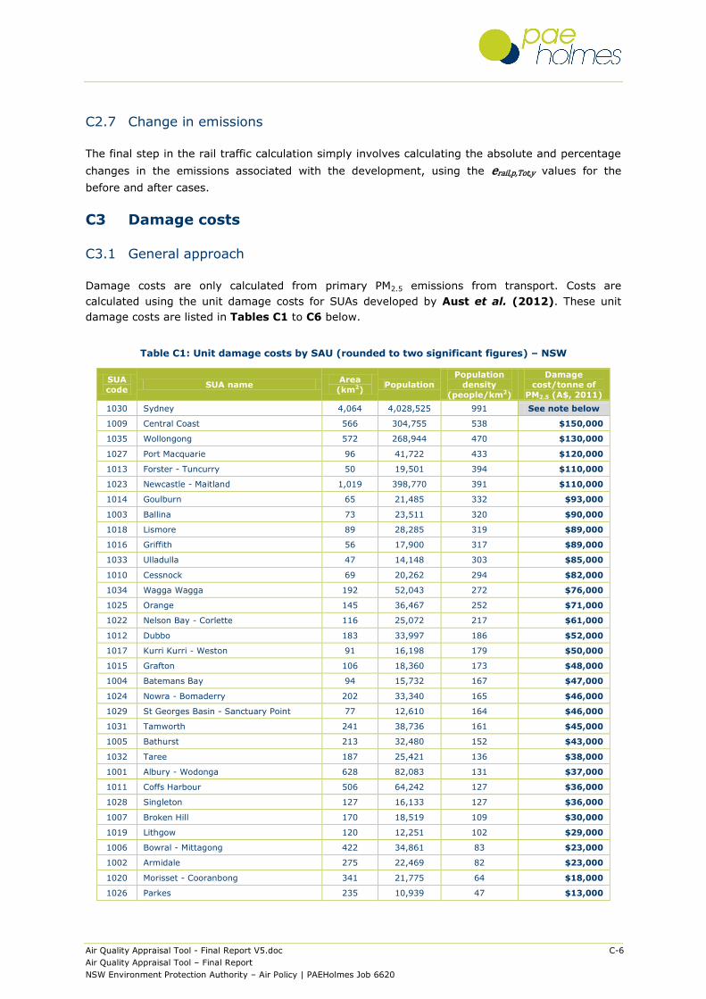
Air Quality Appraisal Tool - Final Report V5.doc C-6
Air Quality Appraisal Tool – Final Report
NSW Environment Protection Authority – Air Policy | PAEHolmes Job 6620
C2.7 Change in emissions
The final step in the rail traffic calculation simply involves calculating the absolute and percentage
changes in the emissions associated with the development, using the erail,p,Tot,y values for the
before and after cases.
C3 Damage costs
C3.1 General approach
Damage costs are only calculated from primary PM2.5 emissions from transport. Costs are
calculated using the unit damage costs for SUAs developed by Aust et al. (2012). These unit
damage costs are listed in Tables C1 to C6 below.
Table C1: Unit damage costs by SAU (rounded to two significant figures) – NSW
SUA
code SUA name
Area
(km2) Population
Population
density
(people/km2)
Damage
cost/tonne of
PM2.5 (A$, 2011)
1030 Sydney 4,064 4,028,525 991 See note below
1009 Central Coast 566 304,755 538 $150,000
1035 Wollongong 572 268,944 470 $130,000
1027 Port Macquarie 96 41,722 433 $120,000
1013 Forster - Tuncurry 50 19,501 394 $110,000
1023 Newcastle - Maitland 1,019 398,770 391 $110,000
1014 Goulburn 65 21,485 332 $93,000
1003 Ballina 73 23,511 320 $90,000
1018 Lismore 89 28,285 319 $89,000
1016 Griffith 56 17,900 317 $89,000
1033 Ulladulla 47 14,148 303 $85,000
1010 Cessnock 69 20,262 294 $82,000
1034 Wagga Wagga 192 52,043 272 $76,000
1025 Orange 145 36,467 252 $71,000
1022 Nelson Bay - Corlette 116 25,072 217 $61,000
1012 Dubbo 183 33,997 186 $52,000
1017 Kurri Kurri - Weston 91 16,198 179 $50,000
1015 Grafton 106 18,360 173 $48,000
1004 Batemans Bay 94 15,732 167 $47,000
1024 Nowra - Bomaderry 202 33,340 165 $46,000
1029 St Georges Basin - Sanctuary Point 77 12,610 164 $46,000
1031 Tamworth 241 38,736 161 $45,000
1005 Bathurst 213 32,480 152 $43,000
1032 Taree 187 25,421 136 $38,000
1001 Albury - Wodonga 628 82,083 131 $37,000
1011 Coffs Harbour 506 64,242 127 $36,000
1028 Singleton 127 16,133 127 $36,000
1007 Broken Hill 170 18,519 109 $30,000
1019 Lithgow 120 12,251 102 $29,000
1006 Bowral - Mittagong 422 34,861 83 $23,000
1002 Armidale 275 22,469 82 $23,000
1020 Morisset - Cooranbong 341 21,775 64 $18,000
1026 Parkes 235 10,939 47 $13,000

Air Quality Appraisal Tool - Final Report V5.doc C-7
Air Quality Appraisal Tool – Final Report
NSW Environment Protection Authority – Air Policy | PAEHolmes Job 6620
SUA
code SUA name
Area
(km2) Population
Population
density
(people/km2)
Damage
cost/tonne of
PM2.5 (A$, 2011)
1021 Muswellbrook 262 11,791 45 $13,000
1008 Camden Haven 525 15,739 30 $8,400
1000 Not in any Significant Urban Area (NSW) 788,116 999,873 1.3 $360
Note: In order to discriminate between different areas of Sydney, three damage cost bands were used: ‘Inner Sydney’ ($200,000/tonne of PM2.5), ‘Mid-Sydney’ ($300,000/tonne of PM2.5) and ‘Inner Sydney’ ($400,000 per tonne of PM2.5).
Table C2: Unit damage costs by SAU (rounded to two significant figures) – Victoria
SUA
code SUA name
Area
(km2) Population
Population
density
(people/km2)
Damage
cost/tonne of
PM2.5 (A$, 2011)
2011 Melbourne 5,679 3,847,567 677 $190,000
2016 Sale 46 14,259 313 $88,000
2020 Wangaratta 58 17,687 307 $86,000
2004 Bendigo 287 86,078 299 $84,000
2003 Ballarat 344 91,800 267 $75,000
2005 Colac 55 11,776 215 $60,000
2010 Horsham 83 15,894 191 $54,000
2008 Geelong 919 173,450 189 $53,000
2017 Shepparton - Mooroopna 249 46,503 187 $52,000
2006 Drysdale - Clifton Springs 65 11,699 180 $50,000
2012 Melton 266 47,670 179 $50,000
20+22 Warrnambool 183 32,381 177 $50,000
2019 Traralgon - Morwell 235 39,706 169 $47,000
2014 Moe - Newborough 105 16,675 158 $44,000
2018 Torquay 126 15,043 119 $33,000
2015 Ocean Grove - Point Lonsdale 219 22,424 103 $29,000
2001 Bacchus Marsh 196 17,156 87 $24,000
2002 Bairnsdale 155 13,239 85 $24,000
2013 Mildura - Wentworth 589 47,538 81 $23,000
2007 Echuca - Moama 351 19,308 55 $15,000
2009 Gisborne - Macedon 367 18,014 49 $14,000
2021 Warragul - Drouin 680 29,946 44 $12,000
2000 Not in any Significant Urban Area (Vic.) 216,296 693,578 3 $900
Table C3: Unit damage costs by SAU (rounded to two significant figures) - Queensland
SUA
code SUA name
Area
(km2) Population
Population
density
(people/km2)
Damage
cost/tonne of
PM2.5 (A$, 2011)
3003 Cairns 254 133,912 527 $150,000
3008 Hervey Bay 93 48,678 523 $150,000
3006 Gold Coast - Tweed Heads 1,403 557,823 398 $110,000
3001 Brisbane 5,065 1,977,316 390 $110,000
3010 Mackay 208 77,293 371 $100,000
3004 Emerald 39 13,219 337 $94,000
3012 Mount Isa 63 20,569 328 $92,000
3007 Gympie 69 19,511 282 $79,000
3016 Townsville 696 162,291 233 $65,000
3002 Bundaberg 306 67,341 220 $62,000

Air Quality Appraisal Tool - Final Report V5.doc C-8
Air Quality Appraisal Tool – Final Report
NSW Environment Protection Authority – Air Policy | PAEHolmes Job 6620
SUA
code SUA name
Area
(km2) Population
Population
density
(people/km2)
Damage
cost/tonne of
PM2.5 (A$, 2011)
3015 Toowoomba 498 105,984 213 $60,000
3018 Yeppoon 79 16,372 208 $58,000
3005 Gladstone - Tannum Sands 240 41,966 175 $49,000
3014 Sunshine Coast 1,633 270,771 166 $46,000
3011 Maryborough 171 26,215 154 $43,000
3013 Rockhampton 580 73,680 127 $36,000
3017 Warwick 159 14,609 92 $26,000
3009 Highfields 230 16,820 73 $20,000
3000 Not in any Significant Urban Area (Qld) 1,718,546 755,687 0.4 $120
Table C4: Unit damage costs by SAU (rounded to two significant figures) – South Australia
SUA
code SUA name
Area
(km2) Population
Population
density
(people/km2)
Damage
cost/tonne of
PM2.5 (A$, 2011)
4001 Adelaide 2,024 1,198,467 592 $170,000
4006 Port Pirie 75 14,044 187 $52,000
4008 Whyalla 121 21,991 181 $51,000
4003 Murray Bridge 98 16,706 171 $48,000
4002 Mount Gambier 193 27,754 144 $40,000
4005 Port Lincoln 136 15,222 112 $31,000
4007 Victor Harbor - Goolwa 309 23,851 77 $22,000
4004 Port Augusta 249 13,657 55 $15,000
4000 Not in any Significant Urban Area (SA) 980,973 264,882 0.3 $76
Table C5: Unit damage costs by SAU (rounded to two significant figures) – Western Australia
SUA
code SUA name
Area
(km2) Population
Population
density (people/km2)
Damage
cost/tonne of PM2.5 (A$, 2011)
5009 Perth 3,367 1,670,952 496 $140,000
5007 Kalgoorlie - Boulder 75 30,839 411 $110,000
5003 Bunbury 223 65,608 295 $83,000
5005 Ellenbrook 105 28,802 276 $77,000
5002 Broome 50 12,765 255 $71,000
5006 Geraldton 271 35,749 132 $37,000
5008 Karratha 134 16,474 123 $34,000
5010 Port Hedland 116 13,770 118 $33,000
5001 Albany 297 30,656 103 $29,000
5004 Busselton 1,423 30,286 21 $6,000
5000 Not in any Significant Urban Area (WA) 2,520,513 30,654 0.01 $3
Table C6: Unit damage costs by SAU (rounded to two significant figures) - Other
State SUA
code SUA name
Area
(km2) Population
Population
density
(people/km2)
Damage
cost/tonne of
PM2.5 (A$, 2011)
Tasmania
6001 Burnie - Wynyard 131 29,050 223 $62,000
6004 Launceston 435 82,222 189 $53,000

Air Quality Appraisal Tool - Final Report V5.doc C-9
Air Quality Appraisal Tool – Final Report
NSW Environment Protection Authority – Air Policy | PAEHolmes Job 6620
State SUA
code SUA name
Area
(km2) Population
Population density
(people/km2)
Damage cost/tonne of
PM2.5 (A$, 2011)
6003 Hobart 1,213 200,498 165 $46,000
6005 Ulverstone 130 14,110 108 $30,000
6002 Devonport 290 26,871 93 $26,000
6000 Not in any Significant Urban Area (Tas.) 65,819 142,598 2 $610
Northern
territory
7002 Darwin 295 106,257 361 $100,000
7001 Alice Springs 328 25,187 77 $22,000
7000 Not in any Significant Urban Area (NT) 1,347,577 80,504 0.06 $17
ACT
8001 Canberra – Queanbeyan 482 391,643 812 $230,000
8000 Not in any Significant Urban Area (ACT) 1,914 1,622 0.85 $240
Other 9000 Not in any Significant Urban Area (OT) 218 3,029 14 $3,900
As noted above, the damage cost function is only applicable to primary PM2.5 emissions from
transport. No method was provided for estimating the costs associated with exposure to secondary
particles, but in any case these would be rather difficult to quantify in a tool of this kind, given that
secondary particle formation occurs over distances of hundreds to thousands of kilometres, and
therefore the location of exposure is not known.
It is important that costs are expressed in equivalent terms, so the effects of emission changes in,
say, 2021 can be compared with those in, say, 2015. In addition, the costs of any development
(which will involve up-front capital costs and operating costs over time) need to be compared with
the benefits in the same price year. It is therefore necessary to make two adjustments to the unit
damage cost. These are:
An ‘uplift’ to reflect the change in per capita GDP growth between the assessment year and
2011. This is currently assumed to be 2.5%, based on the guidance from Defra (2011).
This reflects any change in health risk (e.g. the value of a life). In other words, the real cost
of air pollution impacts on health will rise in line with economic output.
A ‘discount’, based on the principle that future costs are less important than current costs.
This is assumed to be 7%.
The unit damage cost for the assessment year is then calculated using the following equation:
Equation C9
Where:
cy is the unit damage cost for primary PM emissions from transport in the assessment
year (A$/tonne)
u is the uplift for the annual rate of economic growth (%) – assumed to be 2.5%
d is the annual discount rate – assumed to be 0.07 (i.e. 7%)47
y is the assessment year
Consequently, all costs are expressed in 2011 prices.
47 The NSW Treasury (2007) has suggested an appropriate real discount rate for Australia of 7% which
needs to be repeated for each year in the appraisal period.

Air Quality Appraisal Tool - Final Report V5.doc C-10
Air Quality Appraisal Tool – Final Report
NSW Environment Protection Authority – Air Policy | PAEHolmes Job 6620
The total damage cost in the assessment year is the calculated as follows:
Cy = cy × ey Equation C10
Where:
Cy is the damage cost in the assessment year y (A$)
cy is the unit damage cost for the SUA
ey is the emission of PM2.5 in year y.
C3.2 Application to road and rail traffic
For road and rail transport, the damage costs for the before-development and after-development
cases are summated over all links as follows:
Equation C11
CTot,y is the total damage cost for either the before-development or after-development
case in the assessment year y (A$).
cL,y is the damage cost for link L in assessment year y.
The absolute and percentage changes in damage costs associated with the development are then
determined using the CTot,y values for the before and after cases described above.
Air Quality Appraisal Tool - Final Report V5.doc D-1
Air Quality Appraisal Tool – Final Report
NSW Environment Protection Authority – Air Policy | PAEHolmes Job 6620
APPENDIX D
Air Quality Appraisal Tool - User Guide

Air Quality Appraisal Tool - Final Report V5.doc D-2
Air Quality Appraisal Tool – Final Report
NSW Environment Protection Authority – Air Policy | PAEHolmes Job 6620
D1 Tool description
AQAT is a Microsoft Excel spreadsheet (Air Quality Appraisal Tool - Version 1.1 (locked).xlsx).
The Tool has been tested using a Windows 7 64-bit operating system.
The spreadsheet contains ten worksheets, as described below:
Cover. This sheet gives the title of AQAT, along with the version number and the release
date.
Versions. This sheet lists the versions of AQAT and the amendments in each version.
Instructions. This sheet explains how to use AQAT.
Data sources. This lists the sources of data used in AQAT. It gives default values of the
traffic mix and speed by road type, and the population density by LGA in the NSW GMR.
Planning Guidance, which explains the role of AQAT in the planning process.
References. This sheet provides the references for the methods and default data used in
AQAT.
Inputs (A). This sheet is used to enter model inputs were emission estimates are not
already available.
Inputs (B). This sheet is used to enter model inputs where emission estimates are already
available.
Results (A). This sheet provides the model results, based on the information entered in
the Inputs (A) sheet.
Results (B). This sheet provides the model results, based on the information entered in
the Inputs (B) sheet.
Additional sheets contain the calculations for road transport, rail transport, although these are
hidden from the user.
D2 Instructions
D2.1 Data entry
As noted above, different approaches are used depending on whether emissions data are
already available for the development. It may be necessary for the user to follow a combination
of approaches (A) and (B) – such as where emissions data are available for road transport, but
not for rail.
D2.1.1 Approach A: No emission estimates available
Where emission estimates for a development are not already available, these can be calculated
using the Inputs (A) sheet. The following steps are required:
Step A1: Generic inputs. The user enters the assessment year - which can be 2008, 2011,
2016, 2021 or 2026 – using the drop-down menu provided. The economic growth rate
(applied to all years) can also be modified, though justification for doing so should be
provided.

Air Quality Appraisal Tool - Final Report V5.doc D-3
Air Quality Appraisal Tool – Final Report
NSW Environment Protection Authority – Air Policy | PAEHolmes Job 6620
Step A2: The user enters the road transport activity data for the ‘before development’ and
‘after development’ cases. In each case data can be entered for up to 20 road links. For each
link the following information is required:
The name of the link (as text, or a combination of numbers and text).
The road type (selected using the drop-down menu).
The road gradient (selected using the drop-down menu).
The road length in km.
The total daily bi-directional traffic volume (in vehicles per day)
The traffic mix (% of vehicles in nine categories, as defined earlier). Default values for
different road types are provided on the ‘Info’ sheet of AQAT.
The average daily traffic speed in km/h.
Whether cold-start emissions are to be included in the calculations.
Step A3: The user enters the rail transport activity data for the ‘before development’ and
‘after development’ cases. In each case data can be entered for up to 10 rail links. Only two
inputs are required:
The name of the rail link.
The amount of freight transport in gross tonne-km per year (i.e. the combined weight of
the train and load multiplied by the distance travelled).
Step A4: For all road and rail links included in the ‘before development’ and ‘after
development’ cases the user enters the local SUA affected. The concept of ‘local’ is open to
some interpretation here, and therefore the user must make an informed decision as to what
a sensible value would be, clearly stating the assumptions made when reporting. The
average population growth rate for the SUA also needs to be entered, as this is used to
adjust the unit damage costs.
D2.1.2 Approach B: Emission estimates already available
Where emission estimates for a development are already available, these can be entered in the
appropriate cells of the Inputs (B) sheet. The following steps are required:
Step B1: Generic inputs are entered as in Step A1. In this case any year between 2008 and
2036 can be entered.
Step B2: The user enters the road transport emission data (in tonnes per year) for the
‘before development’ and ‘after development’ cases. Again, in each case data can be entered
for up to 20 road links. For each link the following information is required:
The name of the link (as text, or a combination of numbers and text)
The emissions of each pollutant (CO, NOx, PM2.5, HC, CO2-e) in tonnes per year. NB: Only
the PM2.5 emissions data are currently used in the damage cost calculation.
Step B3: The user enters the rail transport emissions data (in tonnes per year) for the
‘before development’ and ‘after development’ cases.
Step B4: For all road and rail links included in the ‘before development’ and ‘after
development’ cases the user enters the SUA and population growth, as in Approach A.

Air Quality Appraisal Tool - Final Report V5.doc D-4
Air Quality Appraisal Tool – Final Report
NSW Environment Protection Authority – Air Policy | PAEHolmes Job 6620
D2.2 Results
The results for approaches A and B are presented on the Results (A) and Results (B) sheets
respectively. If any of the input data are changed then the results will automatically be updated.
Related Documents