Air Pollution, Weather, an d Violent Crimes : Concomitant ...sherrytowers.com/crime_temperature_and_ozone.pdf · This conclusion, however, was qualified by a discussion of the limitations

Journal of Personality and Social Psychology1985, Vol. 49, No. 5, 1207-1220

Copyright 1985 by the American Psychological Association, Inc.0022-35 M/85/M0.75

Air Pollution, Weather, and Violent Crimes: ConcomitantTime-Series Analysis of Archival Data

James RottonFlorida International University

James FreySchool of Medicine

Wright State University

Archival data covering a 2-year period were obtained from three sources in orderto assess relations among ozone levels, nine measures of meteorological conditions,day of the week, holidays, seasonal trends, family disturbances, and assaults againstpersons. Confirming results obtained in laboratory studies, more family disturbanceswere recorded when ozone levels were high than when they were low. Two-stageregression analyses indicated that disturbances and assaults against persons werealso positively correlated with daily temperatures and negatively correlated withwind speed and levels of humidity. Further, distributed lag (Box-Jenkins) analysesindicated that high temperatures and low winds preceded violent episodes, whichoccurred more often on dry than humid days. In addition to hypothesized relations,it was also found that assaults follow complaints about family disturbances, whichsuggests that the latter could be used to predict and lessen physical violence. It wasconcluded that atmospheric conditions and violent episodes are not only correlatedbut also appear to be linked in a causal fashion. This conclusion, however, wasqualified by a discussion of the limitations of archival data and concomitant time-series analysis.

This archival analysis was undertaken to as-sess the generalizability and real-world rele-vance (i.e., ecological validity) of results ob-tained in laboratory studies on the social effectsof air pollution. In these studies (Rotton, 1983;Rotton, Barry, Frey, & Soler, 1978; Rotton,Frey, Barry, Milligan, & Fitzpatrick, 1979),undergraduates were exposed to odors pro-duced by ammonium sulnde and other foul-smelling chemicals. Compared with individ-uals who had not been exposed, students inpolluted settings described their moods andemotions in more negative terms, expressedless liking for individuals not sharing their fate,gave lower evaluations of their surroundings,formed more negative attitudes about socialstimuli, and spent less time in the setting (anindirect measure of escape). By and large, these

We would like to thank Walter Carr of the Police De-partment in Dayton, Ohio, and S. Brodshoder and L.Froebe of the Montgomery County, Ohio, EnvironmentalProtection Agency for their help in gaining access to agencyfiles. We are also grateful to Tim Barry, Robert A. Baron,Paul A. Bell, Gary Evans, Charles Kimble, and David R.Mandel for commenting on earlier versions of this report.

Requests for reprints should be sent to James Rotton,Psychology Department, Florida International University,North Miami, Florida 33181.

results are consistent with predictions derivedfrom models that emphasize the motivatingand reinforcing properties of affective states.As Clore and Byrne's (1974) affect-reinforce-ment model predicts, malodor elicited un-pleasant emotional states (e.g., annoyance andirritability) that reinforced negative evalua-tions. In addition, as Baron's (1978) affect-aggression model predicts, moderately un-pleasant odors facilitated aggression, whereasextremely unpleasant ones led to incompatibleresponses, such as flight, which appeared toinhibit aggressive behavior.

Serious questions have been raised about theexternal validity of results obtained in labo-ratory studies on environmental stressors. Al-though laboratory research (e.g., Baron & Bell,1976) suggests that violence reaches a peak atmoderately high temperatures and then de-clines, only monotonic (and apparently linear)relations have emerged in archival analyses ofviolent episodes (Anderson & Anderson, 1984;Cotton, in press; Harries & Stadler, 1983; butcf. Baron & Ransberger, 1978). Kenrick andJohnson (1979) have also raised questionsabout the generalizability of results obtainedin research on malodor and interpersonal at-traction. Under conditions of shared stress,

1207

1208 JAMES ROTTON AND JAMES FREY

Rotton et al. (1978) found that malodor in-creased liking for another student. It was onlyafter the possibility of shared stress was elim-inated, in a second experiment, that malodorled to negative evaluations. Kenrick and John-son suggested that results obtained in the first(shared-stress) experiment "are more likely togeneralize to actual interpersonal encounters,since attraction would seem to be rarely de-veloped when one is in isolation" (p. 576).However, because one of the denning featuresof urban life is interaction with strangers, wepredicted that more violent episodes would berecorded under high than low levels of outdoorpollution.

Inconsistent results have been obtained inthe few studies that have examined relationsbetween outdoor pollution and behavior (forreviews of the literature, see Evans & Jacobs,1981; Evans, Jacobs, & Frager, 1982). On theone hand, positive correlations between out-door pollutants and psychiatric disturbanceshave been reported in three studies (Briere,Downes, & Spensley, 1983; Rotton & Frey,1985; Strahilevitz, Strahilevitz, & Miller,1979). On the other hand, Lave and Seskin(1977) obtained nonsignificant results in anepidemiological study that examined relationsbetween two pollutants and social ills (namely,venereal diseases, suicides, homicides, rapes,robberies, assaults, larcenies, burglaries, andauto thefts).

Evans and Campbell (1983) have correctlycriticized the common practice of employingcatastrophic indices, such as suicide rates, inresearch on air pollution and behavior. As astimulus that elicits negative affect, air pollu-tion might be correlated with less serious butmore frequent disorders, such as complaintsabout family disturbances and physical threats.In addition, Lave and Seskin (1977) consideredonly two types of pollutants (sulfates and sus-pended particulates). In a study that also ob-tained nonsignificant results for sulfur andpaniculate levels, Rotton and Frey (1985)found that psychiatric emergencies were moreprevalent when ozone levels were high thanwhen they were low. Ozone is an indicant ofphotochemical oxidants (or smog), which is ageneric term that describes several pollutants(e.g., aldehydes, hydrocarbons, peroxyacetylnitrate). Epidemiological and laboratory stud-ies have linked oxidants to complaints about

headaches, eye irritation, coughing, and chestpains (Coffin & Stokinger, 1977; Goldsmith &Friberg, 1977). On the basis of past researchand a model that emphasizes affective states(Clore & Byrne, 1974), it was hypothesized thatozone levels would be correlated with familydisturbances and assault rates.

Although Lave and Seskin (1977) controlledfor day-to-day variations in weather conditionsin their often-cited work on morbidity andmortality rates, they did not include controlsfor meteorological conditions when they ex-amined relations between air pollution andsocial ills. In this study, we included controlsfor temperature and eight other weather vari-ables. We did not formulate a priori hypothesesfor meterological variables, however, becausecontradictory results have been obtained inresearch on weather and behavior (for reviewsof the literature, see Fisher, Bell, & Baum,1984; Rotton, 1982b). Of the meteorologicalvariables examined in this study, only tem-perature has consistently emerged as a reliableconcomitant of violent behavior. Archivalanalyses indicate that more violent and ag-gressive crimes occur on warm than on cooldays (e.g., Cotton, in press; Harries, Stadler,&Zdorkowski, 1984).

Because Baron (1978) has suggested that vi-olence declines after reaching a peak at mod-erately high temperatures, we also assessedquadratic relations between temperature andcomplaints about violence; however, becausetemperatures during the period of time coveredby this analysis never exceeded 85 °F (29.4°C), it must be emphasized that our data didnot provide a truly fair test of the affect-aggression model, nor were they collected todo so. Instead, our aim was to obtain unbiasedestimates of relations between air pollution andviolent crime. For this reason, subsidiary anal-yses were undertaken to determine if our pre-diction equations should also include quadraticpolynomials for barometric pressure, sunshine,and other meteorological variables.

Weather effects are sometimes inferred fromseasonal differences in behavior. As Quetelet'sthermic law of delinquency (Falk, 1952) pre-dicts, crimes against persons occur more fre-quently during summer months than othermonths of the year (Dodge & Lentzner, 1980;Lewis & Alford, 1975). Until quite recently,most criminologists (e.g., Sutherland & Cres-

AIR POLLUTION, WEATHER, AND VIOLENT CRIMES 1209

sey, 1978) and social psychologists (e.g., Rubin,1979) have followed Durkheim's (1897/1951)lead in attributing seasonal differences to cul-tural factors, such as the frequency and inten-sity of social contact. Yet, as surprising as itmay seem, it has not been shown that seasonaltrends attain significance after day-to-dayvariations in meteorological conditions arepartialed out. In this study, we performedregression analyses to determine if seasonaldifferences emerge when weather conditionsare held constant (i.e., are partialed out statis-tically).

Finally, although secular trends were tan-gential to the major aims of this research, weexpanded our models to include holidays, dayof the week, and linear trend (or drift). Thiswas done because there has been a fairly steadyincrease in the number of crimes reported topolice during the past 50 years (Sutherland &Cressey, 1978), and a disproportionate numberof violent crimes occur on weekends and hol-idays (Anderson & Anderson, 1984; Harries& Stadler, 1983).

serial dependencies—an operation known asprewhitening—that an investigator can deter-mine if two series are related.

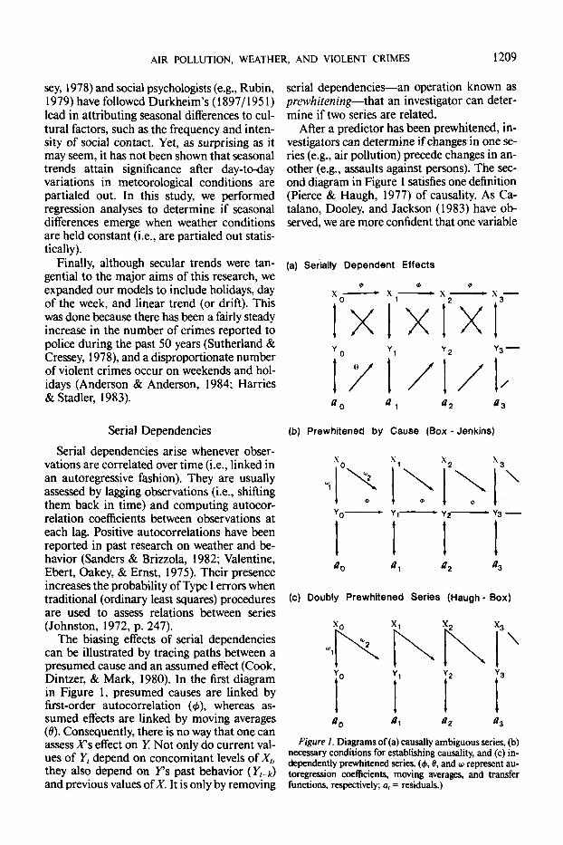
After a predictor has been prewhitened, in-vestigators can determine if changes in one se-ries (e.g., air pollution) precede changes in an-other (e.g., assaults against persons). The sec-ond diagram in Figure 1 satisfies one definition(Pierce & Haugh, 1977) of causality. As Ca-talano, Dooley, and Jackson (1983) have ob-served, we are more confident that one variable

(a) Serially Dependent Effects

x " x f x

Serial DependenciesSerial dependencies arise whenever obser-

vations are correlated over time (i.e., linked inan autoregressive fashion). They are usuallyassessed by lagging observations (i.e., shiftingthem back in time) and computing autocor-relation coefficients between observations ateach lag. Positive autocorrelations have beenreported in past research on weather and be-havior (Sanders & Brizzola, 1982; Valentine,Ebert, Oakey, & Ernst, 1975). Their presenceincreases the probability of Type I errors whentraditional (ordinary least squares) proceduresare used to assess relations between series(Johnston, 1972, p. 247).

The biasing effects of serial dependenciescan be illustrated by tracing paths between apresumed cause and an assumed effect (Cook,Dintzer, & Mark, 1980). In the first diagramin Figure 1, presumed causes are linked byfirst-order autocorrelation (<t>), whereas as-sumed effects are linked by moving averages(6). Consequently, there is no way that one canassess Fs effect on Y. Not only do current val-ues of Y, depend on concomitant levels of X,,they also depend on Fs past behavior (Y,-k)and previous values of X. It is only by removing

(b) Prewhitened by Cause (Box - Jenkins)

\ X1 *2 X3

\

an a, az

(c) Doubly Prewhitened Series (Haugh • Box)

x.

aFigure 1. Diagrams of (a) causally ambiguous series, (b)

necessary conditions for establishing causality, and (c) in-dependently prewhitened series. (<t>, 9, and a represent au-toregression coefficients, moving averages, and transferfunctions, respectively; a, = residuals.)

1210 JAMES ROTTON AND JAMES FREY

(X) causes changes in another (Y) if the former(X) reduces our uncertainty about future val-ues of Y more than the latter's (Fs) past values.Stating things more simply, temporal prece-dence is a necessary but not sufficient condi-tion for establishing causality. It goes almostwithout saying that lagged relations betweenair pollution and violence might be due to athird variable; for example, automobiles arenot only a source of photochemical oxidants,but driving in traffic is also frustrating (Stokols& Novako, 1981), which would facilitate ag-gressive behavior. Keeping this caveat in mind,however, we can draw tentative conclusionsabout causality if there is a transfer function(w) that links current values in one series topast values in another (Box & Jenkins, 1976).Although relations can be established after aninput (or predictor) variable has been pre-whitened, using Box-Jenkins methodology,Haugh and Box (1977) have shown that thetask of identifying relations is simplified whendependencies are removed from the criterionas well as predictors. This approach to con-comitant time-series analysis, which is illus-trated by the third diagram in Figure 1, is usu-ally termed independent prewhitening (Cooketal., 1980).

Prewhitening is accomplished by buildingan ARIMA (autoregressive integrated movingaverage) model. Procedures for building AR-IMA models have been described in recentbooks written especially for social scientists(e.g., Gottman, 1981; McCleary & Hay, 1980).Although models for individual series are pre-sented in this report, as a means of docu-menting our results, we were primarily inter-ested in relations between series, and we ac-cordingly focus on transfer functions that linkindependent and dependent variables.

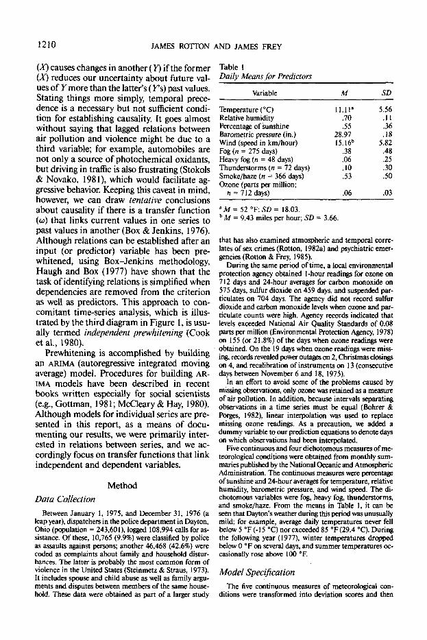
Table 1Daily Means for Predictors

MethodData Collection

Between January 1, 1975, and December 31, 1976 (aleap year), dispatchers in the police department in Dayton,Ohio (population = 243,601), logged 108,994 calls for as-sistance. Of these, 10,765 (9.9%) were classified by policeas assaults against persons; another 46,468 (42.6%) werecoded as complaints about family and household distur-bances. The latter is probably the most common form ofviolence in the United States (Steinmetz & Straus, 1973).It includes spouse and child abuse as well as family argu-ments and disputes between members of the same house-hold. These data were obtained as part of a larger study

Variable M SD

Temperature (°C)Relative humidityPercentage of sunshineBarometric pressure (in.)Wind (speed in km/hour)Fog (n = 275 days)Heavy fog (n = 48 days)Thunderstorms (n = 72 days)Smoke/haze (n = 366 days)Ozone (parts per million;

n = 712 days)

11.11".70.55

28.9715.16"

.38

.06

.10

.53

.06

5.56.11.36.18

5.82.48.25.30.50

.03

' M = 52 °F; SD = 18.03." M = 9.43 miles per hour; SD = 3.66.

that has also examined atmospheric and temporal corre-lates of sex crimes (Rotton, 1982a) and psychiatric emer-gencies (Rotton & Frey, 1985).

During the same period of time, a local environmentalprotection agency obtained 1-hour readings for ozone on712 days and 24-hour averages for carbon monoxide on575 days, sulfur dioxide on 459 days, and suspended par-ticulates on 704 days. The agency did not record sulfurdioxide and carbon monoxide levels when ozone and par-ticulate counts were high. Agency records indicated thatlevels exceeded National Air Quality Standards of 0.08parts per million (Environmental Protection Agency, 1978)on 155 (or 21.8%) of the days when ozone readings wereobtained. On the 19 days when ozone readings were miss-ing, records revealed power outages on 2, Christmas closingson 4, and recalibration of instruments on 13 (consecutivedays between November 6 and 18, 1975).

In an effort to avoid some of the problems caused bymissing observations, only ozone was retained as a measureof air pollution. In addition, because intervals separatingobservations in a time series must be equal (Bohrer &Porges, 1982), linear interpolation was used to replacemissing ozone readings. As a precaution, we added adummy variable to our prediction equations to denote dayson which observations had been interpolated.

Five continuous and four dichotomous measures of me-teorological conditions were obtained from monthly sum-maries published by the National Oceanic and AtmosphericAdministration. The continuous measures were percentageof sunshine and 24-hour averages for temperature, relativehumidity, barometric pressure, and wind speed. The di-chotomous variables were fog, heavy fog, thunderstorms,and smoke/haze. From the means in Table 1, it can beseen that Dayton's weather during this period was unusuallymild; for example, average daily temperatures never fellbelow 5 °F(-15 °C) nor exceeded 85 °F(29.4 °C). Duringthe following year (1977), winter temperatures droppedbelow 0 °F on several days, and summer temperatures oc-casionally rose above 100 °F.

Model SpecificationThe five continuous measures of meteorological con-

ditions were transformed into deviation scores and then

AIR POLLUTION, WEATHER, AND VIOLENT CRIMES 1211

squared in order to assess nonlinear relations. Simplepolynomials were also created to estimate and control forlinear, secular (holiday, day of the week), and seasonaltrends. The first was estimated by assigning numbers fromI to 731 to each day. Secular trends were estimated bysubtracting complaints on Sundays from every other dayof the week; this was accomplished by constructing a designmatrix composed of Os and plus and minus Is (Cohen &Cohen, 1983). Plus Is were also assigned to the days before,after, and including Easter, Memorial Day, IndependenceDay, Halloween, Labor Day, Thanksgiving, Christmas, andNew Year's Eve. These time periods were expanded to 4days when a holiday fell on a Friday or Monday. Finally,seasonal trends were estimated by including a sinewaveand its complement (cosine) as predictors. These curveshad periods of 365 days, and each was aligned so that its1st day (i.e., initial phase) was the preceding year's wintersolstice (December 21).

ResultsThree sets of increasingly complex analyses

were undertaken to assess relations betweenatmospheric variables and violence. First, or-dinary least squares (OLS) regression analyseswere performed to obtain preliminary (or first-stage) estimates of each parameter. This stepwas also employed to identify variables thataccounted for so little variance that they couldbe dropped from the model. Second, two-stageregression analyses were undertaken to obtaingeneralized least squares (GLS) estimates ofbeta weights (Ostrom, 1978). The latter pro-vided guidelines for building distributed lag(Box-Jenkins) models in a third set of analyses.

Only one nonlinear relation attained sig-nificance in the first (OLS) analyses. Temper-ature's quadratic component emerged as apredictor of family disturbances, F(\, 704) =42.24, p< .01, but not assaults against persons,F < 1. The other polynomials for quadratictrends, whose betas did not attain significance(ps > .05), were dropped from the model. Inaddition, an inspection of scatterplots did notreveal any obvious departures from linearityor homoscedasticity.

Results from first-stage (OLS) analyses arenot presented here, because Durbin-Watson'sd statistic revealed serious violations of serialindependence. For household disturbances, ad statistic of 1.57 was obtained; for assaultsagainst persons, one of 1.78 was obtained. Bothare significant (p < .01) when compared withvalues found in tables (King, 1981) for regres-sion equations with seasonal and dummyvariables.

Generalized Least SquaresSerial dependencies were removed by lag-

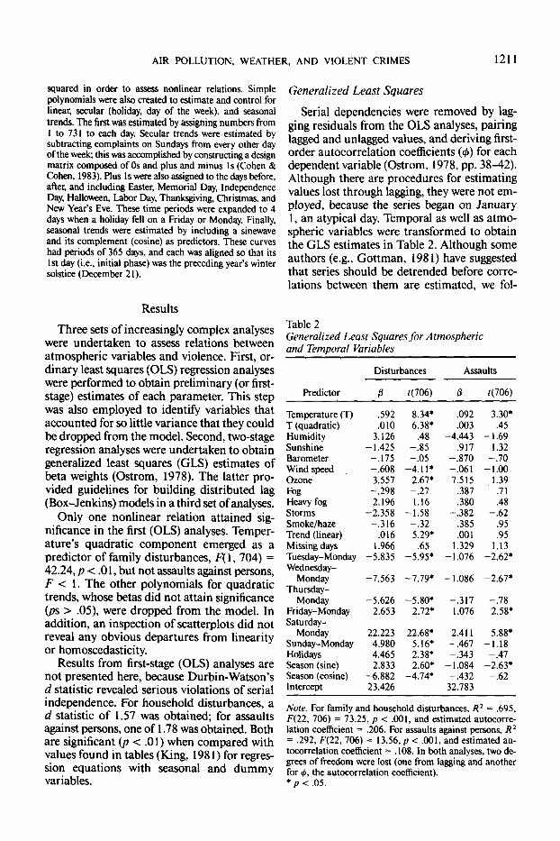
ging residuals from the OLS analyses, pairinglagged and unlagged values, and deriving first-order autocorrelation coefficients ($) for eachdependent variable (Ostrom, 1978, pp. 38-42).Although there are procedures for estimatingvalues lost through lagging, they were not em-ployed, because the series began on January1, an atypical day. Temporal as well as atmo-spheric variables were transformed to obtainthe GLS estimates in Table 2. Although someauthors (e.g., Gottman, 1981) have suggestedthat series should be detrended before corre-lations between them are estimated, we fol-

Table 2Generalized Least Squares for Atmosphericand Temporal Variables

Disturbances

Predictor

Temperature (T)T (quadratic)HumiditySunshineBarometerWind speedOzoneFogHeavy fogStormsSmoke/hazeTrend (linear)Missing daysTuesday-MondayWednesday-

MondayThursday-

MondayFriday-MondaySaturday-

MondaySunday-MondayHolidaysSeason (sine)Season (cosine)Intercept

P

.592

.0103.126

-1.425-.175-.6083.557-.2982.196

-2.358-.316

.0161.966

-5.835

-7.563

-5.6262.653

22.2234.9804.4652.833

-6.88223.426

H706)

8.34*6.38*

.48-.85-.05

-4.11*2.67*-.271.16

-1.58-.325.29*

.65-5.95*

-7.79*

-5.80*2.72*

22.68*5.16*2.38*2.60*

-4.74*

Assaults

(3

.092

.003-4.443

.917-.870-.0617.515

.387

.380-.382

.385

.0011.329

-1.076

-1.086

-.3171.076

2.411-.467-.343

-1.084-.432

32.783

*(706)

3.30*.45

-1.691.32

-.70-1.00

1.39.71.48

-.62.95.95

1.13-2.62*

-2.67*

-.782.58*

5.88*-1.18-.47

-2.63*-.62

Note. For family and household disturbances, R2 = .695,F(22, 706) = 73.25, p < .001, and estimated autocorre-lation coefficient = .206. For assaults against persons, R2

= .292, F(22, 706) = 13.56, p < .001, and estimated au-tocorrelation coefficient = .108. In both analyses, two de-grees of freedom were lost (one from lagging and anotherfor 4>, the autocorrelation coefficient).* p < .05.

1212 JAMES ROTTON AND JAMES FREY

lowed Hibbs (1974, pp. 284-289) and obtainedGLS estimates for temporal controls as well asrandom variables. Also, simultaneous ratherthan stepwise regression analyses were per-formed, because second-stage (GLS) estimatesdepend on residuals obtained in the first (OLS)stage, which in turn depend on every predictorin a regression equation.

Atmospheric variables. As hypothesized,ozone was correlated with family disturbances,GLS K727) = .50, p < .01, and it emerged asa predictor in the simultaneous regressionanalysis. Although ozone was also correlatedwith assaults against persons, ^727) = .37, p <.01, it was not retained as a predictor whenother variables were partialed out. Tempera-ture was selected as a predictor in both sets ofanalyses. For assaults and family disturbances,OLS correlations were r(729) = .48 and .65,respectively; corresponding GLS correlationswere r(727) = .44, p < .01, for assaults andr(727) = .58, p < .01, for family disturbances.Further, as implied by the negative beta weightfor temperature's quadratic component, a dis-proportionate number of complaints aboutfamily disturbances were received on warmdays. That is, the curve relating disturbancesto temperatures was a positively accelerated(or J-shaped) one rather than the inverted U-shaped curve that might have been observed(Baron, 1978) if warmer days had been avail-able for study.

Wind speed was the only other atmosphericvariable that attained significance in theseanalyses. As suggested by the negative betaweight in Table 2, fewer complaints aboutfamily and household disturbances were re-ceived on windy than calm (or windless) days.

Temporal variables. The positive beta fortrend in Table 2 indicates that complaintsabout family disturbances increased linearlyover time. Holidays also attained significancein the analysis of family and household dis-turbances. Covariate-adjusted and steady-statemeans for holiday and nonholiday periods were63.66 and 57.93, respectively.1 To learn moreabout this difference, we dropped holidaysfrom the regression equation and inspected theresulting residuals for outliers. A far outlier isone that exceeds a distribution's upper andlower quartiles by two steps, where a step is1.5 times the interquartile range (Tukey, 1977).More than half (7 of 13) of the far outliers fell

Table 3Daily Means for Seasonal Trends

Disturbances

Season

WinterSpringSummerFall

Actual

48.4663.4484.8357.31

Adjusted

66.37.66.88,72.2553.65

Assaults

Actual

11.4113.9118.0715.47

Adjusted

14.02,13.75,15.67b15.42b

Note. Means sharing common subscripts in each columndo not differ, p < .05 by Fisher's least significant differencetest.

during a holiday period. In 1975, a dispro-portionate number of disturbances occurredon Halloween, Christmas, and New Year's Eve;in 1976, disproportionate numbers occurredduring Memorial, Labor, and IndependenceDay periods.

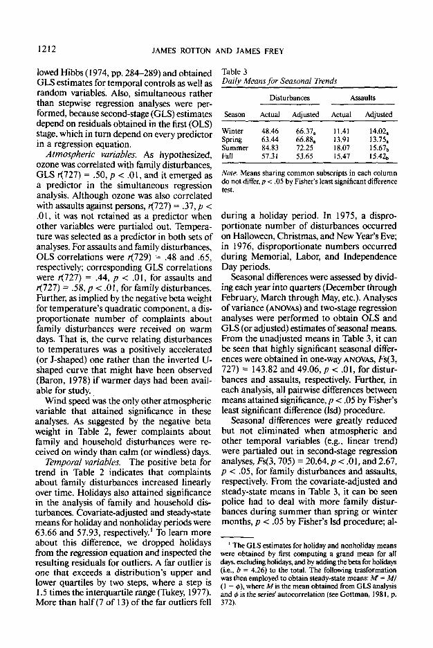
Seasonal differences were assessed by divid-ing each year into quarters (December throughFebruary, March through May, etc.). Analysesof variance (ANOVAS) and two-stage regressionanalyses were performed to obtain OLS andGLS (or adjusted) estimates of seasonal means.From the unadjusted means in Table 3, it canbe seen that highly significant seasonal differ-ences were obtained in one-way ANOVAS, Fs(3,727) = 143.82 and 49.06, p < .01, for distur-bances and assaults, respectively. Further, ineach analysis, all pairwise differences betweenmeans attained significance, p < .05 by Fisher'sleast significant difference (Isd) procedure.

Seasonal differences were greatly reducedbut not eliminated when atmospheric andother temporal variables (e.g., linear trend)were partialed out in second-stage regressionanalyses, Fs(3, 705) = 20.64, p < .01, and 2.67,p < .05, for family disturbances and assaults,respectively. From the covariate-adjusted andsteady-state means in Table 3, it can be seenpolice had to deal with more family distur-bances during summer than spring or wintermonths, p < .05 by Fisher's Isd procedure; al-

1 The GLS estimates for holiday and nonholiday meanswere obtained by first computing a grand mean for alldays, excluding holidays, and by adding the beta for holidays(i.e., b = 4.26) to the total. The following trasformationwas then employed to obtain steady-state means: M = Ml(1 - 0), where M is the mean obtained from GLS analysisand <t> is the series' autocorrelation (see Gottman, 1981, p.372).

AIR POLLUTION, WEATHER, AND VIOLENT CRIMES 1213

Table 4Daily Means for Secular Trends

Disturbances

Day

MondayTuesdayWednesdayThursdayFridaySaturdaySunday

Actual

52.61.56.86ab57.86.58.11*65.98*85.9968.21C

Adjusted

63.58.56.23b54.05b56.49b66.92K91.5765.53C

Assaults

Actual

14.18.13.83.13.70,14.32.15.66*17.24C14.15.

Adjusted

14.72ab13.51.13.50.14.36*15.92*17.42C14.17*

Note. Means sharing common subscripts in each columndo not differ, p < .05 by Fisher's least significant differencetest.

though the latter did not differ, both springand winter means exceeded the mean for thefall months, p < .05. Turning to assaults, ad-justed means did not differ during summer andfall months, but both were higher than winterand spring means, p < .05, and the latter werenot reliably different. In sum, seasonal trendswere greatly attenuated when adjustments forday-to-day variations in atmospheric condi-tions were made; however, as sociologists havesuggested, seasonal differences did not dependentirely on weather conditions.

Daily means for family disturbances and as-saults are listed in Table 4. As other investi-gators (e.g., Harries & Stadler, 1983) havefound, more violent episodes occurred on Fri-days than on other weekdays. They reached apeak on Saturdays and then declined so mark-edly that means on Sundays were close tomeans on working days.

Distributed Lag AnalysisGeneralized least squares analyses are lim-

ited to uncovering synchronous relations be-tween variables. Despite this and other limi-tations (Cook et al., 1980, p. 107), GLS pro-cedures are useful for screening data beforedeveloping more complicated (distributed lag)models. In particular, the preceding resultssuggested that little was to be gained by re-taining binary variables (fog, storms, smoke/haze) as predictors.

Prewhitening. Ordinary least squares pro-cedures were employed to remove linear, sec-ular (i.e., holiday, day of the week), and sea-

sonal trends from the family disturbance, as-sault, and ozone series. Seasonal but notsecular trends were removed from the seriesfor temperature, humidity, sunshine, windspeed, and barometric pressure. An iterativestrategy (Box & Jenkins, 1976) was then fol-lowed to obtain the ARIMA models in Table 5.To be accepted, each model had to pass twotests (see McCleary & Hay, 1980, pp. 98-99).First, residuals had to be independent on thefirst and second lag; as indicated by the auto-correlations in Table 5, each set of residualspassed this test. Second, each autocorrelationfunction had to pass an omnibus test of fitwhen residuals were lagged 25 time periods.For this test, we computed a Ljung-Box Q,which is distributed as a chi-square statisticwith 25 — k degrees of freedom, where k is thenumber of autoregression coefficients andmoving averages in one's model (Ljung & Box,1978). From the rightmost column in Table5, it can be seen that models passed this testas well.

Cross-correlations. Residuals from the AR-IMA models were paired with each other to ob-tain cross-correlation coefficients for 10 leadsand lags. To conserve space, only the first fourlead and lag coefficients are listed in Table 6.Although a few investigators (e.g., Persinger,1975) have suggested that weather exerts de-layed effects on behavior, none has postulatedlags of more than 3 or 4 days.

Most of the significant cross-correlationsin Table 6 are synchronous ones, but tempera-ture and ozone led disturbances by 1 day. Fur-ther, wind speed led disturbances by 1 and 4days, and assaults were also preceded by lowwinds. On the other hand, a disturbing numberof r(-t) or reverse correlations attained signif-icance when atmospheric variables werelagged. For example, disturbances led highs insunshine by 3 days, and both assaults and dis-turbances preceded lows in humidity.

Haugh-Box causal models. Reverse corre-lations are less of a problem when one buildsa multiple-input model for each criterion. Al-though cross-correlation and transfer functionanalyses lead to identical conclusions when twoseries are examined (Haugh & Box, 1977),transfer functions (w) allow one to assess theeffects of two or more independent variables.Transfer function identification differs littlefrom regression analysis when cross-correla-

1214 JAMES ROTTON AND JAMES FREY

Table 5ARMA Models for Deseasonalized Series

Variable Model

/(713) = 10.30, 2.58, 4.46, 2.87, �2.47, �2.75

Diagnostic test

df

Disturbances

Assaults

Temperature

Humidity

Sunshine

Wind

Barometricpressure

Ozone

(1 � 32B � .15fl2Xl � .09fi')(l � .\3BX)Y, = a,;t(6№) = 8.73,4.01,2.35, 3.46

(1 � .145 � .03B2 + .I2fi')y, = a,;<(719) = 3.90, 2.22, �3.36

(1 � MB + .34B2 � AlB^Y, = a,;f(725) = 23.49, �7.14,4.58

Y, = (1 + ,56.8 + .\5B2)a,;t(129) = �15.40, �4.07

Y, = (l+.25B)a,;((730) = �6.99

(1 — 3\B — .08S3 — .10B5)F, = a,;r(719) = 8.81, 2.25, 2.70

(1 �.59B+.21B2)(1 �.07B'°�.08B")F, = a,;r(714)= 16.11, �5.81, 1.88,2.18

(1 �.36BX1 �.09B3�.16B4�.11B6)F, =

.00

.00

.00

.01

.00

.01

.01

.02

.01

.02

.00

.04

.01

�.05

�.02

�.04

21

22

22

23

24

21

21

19

25

21

21

22

24

25

28

26

Note. ARMA = autoregressive moving average. B is a backshift operator that moves observations back one unit in time;that is, BY, = Xt_,, More generally, BkY, = r,_t so that B2Y, = B(Y,~,) = Y,�2 (see McCleary & Hay, 1980, pp. 45�48).Q is distributed as a chi�square. All / values are significant, p < .05.

Table 6Cross�Correlation Functions

Y leads X (in days) X leads Y (in days)

Variable (X) �4 �3 �2 �1 0 +1 +2 +3 +4

Y = disturbances

TemperatureHumiditySunshineWind speedAir pressureOzone

.01

.08*�.05�.01

.00�.07

�.04�.07*

.10*�.05

.04

.05

.01

.07�.01�.06�.05

.01

.05

.06

.02�.08*�.02

.07

.20*

.01

.04�.09*

.01

.19*

.14*

.02

.02�.08*

.01

.09*

.05

.03

.02

.00

.02

.04

�.01.03

�.01�.03

.05

.07

.01�.03�.02�.08*

.03

.02

Y = Assaults

TemperatureHumiditySunshineWind speedAir pressureOzoneDisturbances

.00

.00

.02

.02

.01

.02�.07

.01�.08*

.08*

.05�.01�.01

.00

.01

.04�.03

.05�.02

.00�.03

.09*

.06

.03

.06�.07

.08*

.06

.14*�.11*

.13*�.03

.00

.16*

.12*

.07*

.01

.06�.02

.00

.06

.07*

.01

.02

.00�.10*

.03

.01

.13*

.04

.00�.03�.01�.01

.08*

.04

�.02.01.00

�.02.04.02

�.01

Note. No other cross�correlations for assaults attained significance within 10 leads and lags. In addition to values listed,the following cross�correlations with disturbances attained significance for 10 leads and lags: r(8) = —.07 for temperatureleading, r(�5) = .07 for wind speed trailing, r(7) = �.07 and r{8) = �.08 for ozone leading, and r(5) = .08 and r(8)= .11 for barometric pressure leading.* p < .05.

AIR POLLUTION, WEATHER, AND VIOLENT CRIMES 1215

Table 7Transfer Functions (w)for Distributed Lag Models

Haugh-Box Box-Jenkins

Disturbances Assaults

Predictor

Temperature (0Temperature (t - 1)Wind (0Wind (t - 2)Ozone (t)Ozone (t - 3)Humidity (t)Disturbances (/)Disturbances (t - 2)0i<t>20906 for (1 -0B6)2

030for(l-0B30)3

« f(724) u

.23 4.95 .20

.22 4.76-.14 -4.06

-.11.12 3.24

-.18.09.13

.09 2.44.15

1(724)

3.78

-2.99

-4.312.303.26

4.14

Disturbances

to

.23

.12-.67

.12

.08

.23

.09

.14

,(684)

4.982.65

-4.84

3.321.97

6.16

2.533.83

Assaults

0)

.15

-.08

-.16.09.10.11

-.09

,(709)

3.69

-2.04

-4.242.282.692.97

-2.39

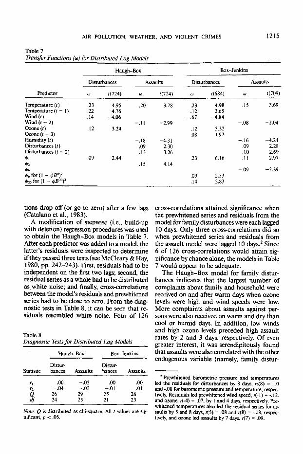
tions drop off (or go to zero) after a few lags(Catalano et al., 1983).

A modification of stepwise (i.e., build-upwith deletion) regression procedures was usedto obtain the Haugh-Box models in Table 7.After each predictor was added to a model, thelatter's residuals were inspected to determineif they passed three tests (see McCleary & Hay,1980, pp. 242-243). First, residuals had to beindependent on the first two lags; second, theresidual series as a whole had to be distributedas white noise; and finally, cross-correlationsbetween the model's residuals and prewhitenedseries had to be close to zero. From the diag-nostic tests in Table 8, it can be seen that re-siduals resembled white noise. Four of 126

Table 8Diagnostic Tests for Distributed Lag Models

Haugh-Box

Statistic

'ir2Qdf

Distur-bances

.00-.04

2624

Assaults

-.03-.03

2925

Box-Jenkins

Distur-bances

.00-.01

2521

Assaults

.00

.012823

cross-correlations attained significance whenthe prewhitened series and residuals from themodel for family disturbances were each lagged10 days. Only three cross-correlations did sowhen prewhitened series and residuals fromthe assault model were lagged 10 days.2 Since6 of 126 cross-correlations would attain sig-nificance by chance alone, the models in Table7 would appear to be adequate.

The Haugh-Box model for family distur-bances indicates that the largest number ofcomplaints about family and household werereceived on and after warm days when ozonelevels were high and wind speeds were low.More complaints about assaults against per-sons were also received on warm and dry thancool or humid days. In addition, low windsand high ozone levels preceded high assaultrates by 2 and 3 days, respectively. Of evengreater interest, it was serendipitously foundthat assaults were also correlated with the otherendogenous variable (namely, family distur-

Note. Q is distributed as chi-square. All t values are sig-nificant, p < .05.

2 Prewhitened barometric pressure and temperaturesled the residuals for disturbances by 8 days, rs(8) = .10and -.08 for barometric pressure and temperature, respec-tively. Residuals led prewhitened wind speed, ^-1) = -.12,and ozone, r(-4) = .07, by 1 and 4 days, respectively. Pre-whitened temperatures also led the residual series for as-saults by 5 and 8 days, r{5) = .08 and K8) = -.08, respec-tively, and ozone led assaults by 7 days, r{l) = .09.

1216 JAMES ROTTON AND JAMES FREY

bances). As the model for assaults implies, po-lice not only received more complaints aboutfamily disturbances and assaults on the sameday, but they also had to deal with more as-saults 2 days after highs in family disturbances.

Box-Jenkins transfer functions. Haugh-Boxprocedures suffice when investigators are pri-marily interested in showing that unpredict-able changes in one variable precede changesin another. Procedures developed by Box andJenkins (1976) allow one to draw conclusionsabout actual (and not prewhitened) values andforecast trends. It has been our experience thatthese procedures work best when they arebased on initial estimates provided by Haugh-Box models.

The first step in obtaining Box-Jenkinstransfer functions is to build an ARIMA modelthat simultaneously removes dependenciesfrom residuals and estimates transfer func-tions. That is, we began with a tentative modelthat included both ARIMA components (seeTable 5) and transfer functions from Haugh-Box models (see Table 7). This was the onlystep that was required to obtain a Box-Jenkinsmodel for family and household disturbances.From the model in Table 7, it can be seen that,once again, low winds and high oxidant/ozonelevels, as well as high temperatures on the sameand preceding days, were correlated with andcould be used to predict family and householddisturbances. Only 7 of 120 cross-correlationsfor this model attained significance when itsresiduals were paired with the prewhitened se-ries of predictors.3

Backward elimination (or teardown withreplacement) procedures were followed to ob-tain the Box-Jenkins model for assaults. Thatis, nonsignificant terms were dropped from ourtentative model, beginning with the one withthe smallest / value, until (a) only significantterms remained, (b) the model's residuals re-sembled white noise, and (c) only a few cross-correlations between residuals and the pre-whitened series attained significance. From theBox-Jenkins model in Table 7, it can be seenthat ozone was not retained as a predictor;however, as in the previous (Haugh-Box)analysis, more assaults occurred on warm anddry than cool or humid days, and once again,family disturbances and low winds precededhighs in assaults.

DiscussionThis study's correlational results confirm

predictions derived from laboratory studies(e.g., Rotton, 1983) on malodorous pollution.As was hypothesized, ozone/oxidant levelswere correlated with complaints about familydisturbances, and Haugh-Box analyses sug-gested that highs in ozone levels also led as-saults by 3 days. However, the latter (delayed)relation is probably a spurious one. Ozone wasnot selected as a predictor of assaults in morestringent Box-Jenkins analyses. The delayedeffect for ozone might be due to other chem-icals (e.g., hydrocarbons, aldehydes) found inphotochemical oxidants. Although ozone is theprincipal element in photochemical oxidants(sometimes 90% of total volume), formalde-hyde and hydrocarbons are responsible forsome of the effects (e.g., eye irritation) attrib-uted to ozone (Jones, 1972). Further, higherlevels of nitrogen dioxide and other pollutantsare preceded by declines in ozone levels(Goldsmith & Friberg, 1977). Thus, althoughsome faith can be placed in concurrent (orsame-day) correlations between ozone and be-havior, it is very likely that the lagged relationwas due to pollutants associated with earlierincreases in ozone levels.

Nevertheless, the overall pattern of corre-lations in this study suggests that air pollutionmay be responsible for effects sometimes at-tributed to weather. For example, without tak-ing air pollution into account, it would be hardto explain why fewer complaints about familydisturbances were received on windy days, anddelayed relations between wind speed and as-saults would also resist easy interpretation.However, these findings are consistent with thewell-known fact that high winds disperse pol-lutants (McCormick & Holzworth, 1972). Itis likely that individuals experience less an-noyance and irritability on windy than wind-less days. To take another example, one wouldexpect that individuals would experience more

3 Prewhitened series for barometric pressure and tem-perature led residuals for family disturbances by 8 and 9days, r(8) = .11 and r(9) = -.09, respectively. The residualseries for disturbances led the prewhitened series for sun-shine, r(-3) = .08; humidity, r(-4) = .08; and wind speed,r(-5) = .07. Only prewhitened temperatures led the residualseries for assaults, r(8) = -.08.

AIR POLLUTION, WEATHER, AND VIOLENT CRIMES 1217

discomfort on humid days, especially whentemperatures are high (Griffitt & Veitch, 1971),yet in this study, fewer assaults occurred onhumid than dry days. This finding makes sensewhen it is realized that humidity levels arehigher before and after a rainfall, which re-moves pollution from the air.

Although air pollution appears to accountfor effects often attributed to meteorologicalvariables, temperature emerged as the bestpredictor of complaints about violent episodes.As several investigators have found, more vi-olent episodes occurred on warm than cool orcold days. Given the fact that high tempera-tures also preceded complaints about familydisturbances, it is tempting to conclude thatweather and behavior not only are correlatedbut some types of weather (e.g., high temper-atures and low winds) also cause behavior thatrequires police intervention. However, evendelayed relations may be due to another vari-able, such as alchohol consumption. Harrieset al. (1984) have observed that individualsconsume more alchohol on warm than cooldays; suffering from hangovers, they might alsobe more prone to engage in violent behavioron "the day after." One way to deal with thisrival hypothesis would be to include surrogatemeasures of alchohol consumption (e.g., dailysales figures) in future studies.

Discounting rival hypotheses can be distin-guished from speculating about factors thatmay be responsible for relations betweenweather and behavior. Excluding work done inEurope, which has emphasized thermoregu-latory and biochemical processes (e.g., Tromp,1980), investigators have adopted one of twotheoretical approaches in this area. On the onehand, sociologists and criminologists have at-tributed weather effects, as well as seasonal dif-ferences, to the frequency and intensity of so-cial contact. On the other hand, social andenvironmental psychologists (Baron, 1978;Cunningham, 1979; Fisher et al., 1984) havefavored models that emphasize affective states.

As social contact models suggest, seasonaldifferences attained significance after meteo-rological variables were partialed out. Socialcontact also provides a parsimonious expla-nation for holiday and weekend highs in familydisturbances. However, although social contactmodels can account for relations between

weather and assaults against persons, they donot explain why more family disturbances oc-curred on warm than cool days. In a temperateclimate, such as the one studied here, fewerindividuals venture outdoors during winterthan summer months of the year (Michelson,1971). As a consequence, contacts amongfamily members should be more frequent andperhaps more intense during winter monthsand on cold days. However, in this study, wefound that family disturbances occurred morefrequently on and after warm than cool or colddays.

On the surface, it might be thought that the-ories emphasizing affective states faired betterthan theories emphasizing interaction rates.First, the positive correlation between ozoneand family disturbances is consistent with aprediction derived from the affect-reinforce-ment model (Clore & Byrne, 1974). Second,as this and Baron's (1978) model suggest, moreviolent episodes occurred on and after warmthan cool days. However, although tempera-tures in this locale sometimes reached a lowof 5 °F, which is uncomfortable (i.e., elicitsnegative affect), fewer episodes occurred at coldthan temperate or comfortable temperatures.It is possible that discomfort on a moderatelycool day is, in part, negated by behavioral ad-aptations, such as wearing warmer clothes(P. A. Bell, personal communication, August27, 1982). Another possibility is that the effectsof ozone and temperature stem from higherlevels of arousal.

As an arousing stimulus (Provins, 1966),heat would be expected to intensify aggressiveresponses, leading to more violent crimes onwarm than cool days. However, low as well ashigh temperatures are arousing; unless one as-sumes that individuals are too busy trying tokeep warm to engage in aggression, arousalmodels do not explain why less violence wasobserved on cold than warm days. There isalso some reason to believe that ozone isarousing as well as irritating. It was not toolong ago that Huntington (1945) and others(e.g., Peters, 1939) attributed the stimulatingeffects of some kinds of weather to ozone inthe atmosphere. What has been called "Hung-tington's ozone hypothesis" (McGregor, 1976)was formulated before biologists linked ozoneto pulmonary edema and other respiratory

1218 JAMES ROTTON AND JAMES FREY

ailments. Given the prevalence of photochem-ical oxidants in many urban settings and theresults obtained in this study, there would seemto be a need to assess the behavioral effects ofozone under laboratory conditions.

However, in speculating about emotionalstates, we run the risk of committing an eco-logical fallacy (Firebaugh, 1978; Langbein &Lichtman, 1978). Strictly speaking, on the ba-sis of aggregate data, we can do no more thanconclude that the probability of violent epi-sodes is higher when temperatures and levelsof air pollution are high than when they arelow. It is possible that only a few at-risk (e.g.,asthmatic or overweight) individuals are af-fected by high temperatures and levels of airpollution. For example, on the basis of resultsobtained in this study, relation between levelsof air pollution and violence might be strongerfor people living closer to expressways thanthose living in suburbs or rural areas. One wayto explore this possibility would be to followthe lead of epidemiologists who, as a matterof course, disaggregate by type of population.To take another example, our analyses suggestthat family disturbances predict and may leadto subsequent highs in assault rates. However,it has yet to be shown that assaults occurredin households whose members were earlier in-volved in a disturbance. Further research isneeded to determine if similar relations emergewhen assaults are classifed by locale (e.g., tav-erns as well as family dwellings).

With further research, it should be possibleto determine whether this study's results aregeneralizable or limited to one geographicallocale and period of time. It will be recalledthat weather conditions in Dayton were un-usually mild. A first step in assessing thisstudy's generalizability would be to see if sim-ilar results are obtained in subsequent years.In this regard, it might be noted that Box-Jenkins models are ideally suited for forecast-ing future trends. A second and even more im-portant step would be to examine correlationsbetween atmospheric variables and crime inother geographical regions. However, it goesalmost without saying that relations betweenpredictors and criteria are, in part, dependenton correlations among predictors. Because ofthe problems that multicollinearity introduces,weaker results might be obtained in regions

(e.g., some northeastern cities) where levels ofair pollution and meteorological conditions aremore highly correlated. At the same time, wewould expect that stronger relations wouldemerge in a region (e.g., southern California)where weather conditions are more stable andlevels of air pollution are higher.

Future research in this area also needs toexplore the combined (or synergistic) effectsof pollutants and different types of weather.For example, one would expect to find thatozone interacts with percentage of sunshine,simply because light is necessary for the pro-duction of photochemical oxidants. Past re-search suggests that the effects of ozone mightalso be dependent on daily temperatures (Rot-ton, 1982b) and humidity levels (Graves &Krumm, 1981). In addition, results obtainedin one study (Cunningham, 1979) suggest thatdifferent sets of correlations might be obtainedduring summer and winter months.

Unfortunately, serial dependencies placeconstraints on the number and type of relationsthat can be examined in a time-series analysis.First, it will be recalled that second-stage es-timates in the GLS analyses were derived fromsimultaneous rather than more conventional(stepwise or hierarchial) regression equations.Adding predictors to our equations to assessinteractions would have increased the proba-bility of Type I errors (Cohen & Cohen, 1983)and, at the same time, reduced the power ofindividual tests of significance (Rotton &Schonemann, 1978). Second, with regard totypes of hypotheses, it will also be recalled thatserial dependencies had to be removed fromeach predictor (prewhitening) before transferfunctions were estimated. This operation couldnot have been accomplished if the predictorshad been previously transformed to obtainpolynomial terms for estimating interactions.At the very least, polynomial transformationswould have produced nonstationary predictors(i.e., series whose means and variances changeover time). It is for this reason we did not in-clude temperature's quadratic component asa predictor in our distributed lag analyses, eventhough it accounted for a significant amountof variance in the GLS analysis of family dis-turbances.

In sum, our findings should be regarded asa first approximation of true and undoubtedly

AIR POLLUTION, WEATHER, AND VIOLENT CRIMES 1219

much more complex relations between at-mospheric conditions and violent behavior.However, even as a first approximation, theyclearly implicate meteorological variables asconcomitants and possible causes of violentcrimes. Finally, they suggest that cost-benefitanalyses of the effects of air pollution shouldinclude the social and psychological costs ofdealing with violent crimes.

ReferencesAnderson, C. A., & Anderson, D. C. (1984). Ambient tem-

perature and violent crime: Tests of the linear and cur-vilinear hypotheses. Journal of Personality and SocialPsychology, 46, 91-97.

Baron, R. A. (1978). Aggression and heat: "The long hotsummer" revisited. In A. Baum, J. E. Singer, & S. Valins(Eds.), Advances in environmental psychology (Vol. 1,pp. 67-84). Hillsdale, NJ: Erlbaum.

Baron, R. A., & Bell, P. A. (1976). Aggression and heat:The influence of ambient temperature, negative affect,and a cooling drink on physical aggression. Journal ofPersonality and Social Psychology, 33, 245-255.

Baron, R. A., & Ransberger, V. M. (1978). Ambient tem-perature and the occurrence of collective violence: The"long hot summer" revisited. Journal of Personality andSocial Psychology, 36, 351-380.

Bohrer, R. E., & Forges, S. W. (1982). The application oftime series statistics to psychological research: An in-troduction. In S. Keren (Ed.), Statistical and method-ological issues in behavioral sciences research (pp. 309-345). Hillsdale, NJ: Erlbaum.

Box, G. E. P., & Jenkins, G. M. (1976). Time series anal-ysis: Forecasting and control (rev. ed.). San Francisco:Holden-Day.

Briere, J., Downes, A., & Spensley, J. (1983). Summer inthe city: Urban weather conditions and psychiatricemergency-room visits. Journal of Abnormal Psychology,92, 77-80.

Catalano, R. A., Dooley, D., & Jackson, R. (1983). Selectinga time-series strategy. Psychological Bulletin, 94, 506-523.

Clore, G. L., & Byrne, D. (1974). A reinforcement-affectmodel of attraction. In T. L. Huston (Ed.), Foundationsof interpersonal attraction. New York: Academic Press.

Coffin, D. L., & Stokinger, H. E. (1977). Biological effectsof air pollutants. In A. C. Stern (Ed.), Air pollution (3rded., Vol. 2, pp. 231-360). New York: Academic Press.

Cohen, J., & Cohen, P. (1983). Applied multiple regression/correlation analysis for the behavioral sciences (2nd ed.).Hillsdale, NJ: Erlbaum.

Cook, T. D., Dintzer, L., & Mark, M. M. (1980). The causalanalysis of concomitant time series. In L. Bickman (Ed.),Applied social psychology annual (Vol. 1, pp. 93-136).Beverly Hills: Sage.

Cotton, J. L. (in press). Ambient temperature and violentcrime. Journal of Applied Social Psychology.

Cunningham, M. R. (1979). Weather, mood, and helpingbehavior: Quasi-experiments with the sunshine Samar-itan. Journal of Personality and Social Psychology, 37,1947-1956.

Dodge, R. W, & Lentzner, H. R. (1980, May). Crime andseasonality (Report SD-NCS-N-15, NCJ-64818).Washington, DC: National Crime Survey.

Durkheim, E. (1951). Suicide: A study in sociology. NewYork: Free Press. (Original work published 1897)

Environmental Protection Agency. (1978). National am-bient air quality standards. Annual air quality report.Washington, DC: Author.

Evans, G. W., & Campbell, J. M. (1983). Psychologicalperspectives on air pollution and health. Basic and Ap-plied Social Psychology, 4, 137-169.

Evans, G. W., & Jacobs, S. V. (1981). Air pollution andhuman behavior. Journal of Social Issues, 37, 95-125.

Evans, G. W., Jacobs, S. V, & Frager, N. B. (1982). Be-havioral responses to air pollution. In A. Baum & J.Singer (Eds.), Advances in environmental psychology (Vol.4, pp. 237-269). Hillsdale, NJ: Erlbaum.

Falk, G. J. (1952). The influence of seasons on the crimerate. Journal of Criminal Law and Criminal Law Sci-ence, 43, 199-213.

Firebaugh, G. (1978). A rule for inferring individual-levelrelationships from aggregate data. American SociologicalReview, 43, 557-572.

Fisher, J. D., Bell, P. A., & Baum, A. (1984). Environmentalpsychology (2nd ed.). New York: Holt, Rinehart & Win-ston.

Goldsmith, J. R., & Friberg, L. T. (1977). Effects of airpollution on human health. In A. C. Stern (Ed.), Airpollution (3rd ed., Vol. 2, pp. 457-610). New York: Ac-ademic Press.

Gottman, J. M. (1981). Time-series analysis: A compre-hensive introduction for social scientists. New York:Cambridge University Press.

Graves, P. E., & Krumm, R. J. (1981). Health and airquality: Evaluating the effects of policy. Washington, DC:American Enterprise Institute for Public Policy Re-search.

Griffitt, W., & Veitch, R. (1971). Hot and crowded: Influ-ence of population density and temperature on inter-personal affective behavior. Journal of Personality andSocial Psychology, 17, 92-98.

Harries, K. D., & Stadler, S. J. (1983). Determinism re-visited: Assault and heat stress in Dallas, 1980. Envi-ronment and Behavior, 15, 235-256.

Harries, K. D., Stadler, S. J., & Zdorkowski, R. T. (1984).Seasonality and assault: Explorations in inter-neighbor-hood variation, Dallas 1980. Annals of the Associationof American Geographers, 74, 590-604.

Haugh, L. D., & Box, G. E. P. (1977). Identification ofdynamic regression (distributed lag) models connectingtwo time series. Journal of the American Statistical As-sociation, 72, 121-130.

Hibbs, D. A. (1974). Problems of statistical estimation andcausal inference in time-series regression models. InH. L. Costner (Ed.), Sociological methology 1973-1974.San Francisco: Jossey-Bass.

Huntington, E. (1945). Mainsprings of civilization. NewYork: Wiley.

Johnston, J. (1972). Econometric methods. New York:McGraw-Hill.

Jones, M. H. (1972). Pain thresholds for smog components.In J. F. Wohlwill & D. H. Carson (Eds.), Environmentand the social sciences: Perspectives and applications

1220 JAMES ROTTON AND JAMES FREY

(pp. 61-65). Washington, DC: American PsychologicalAssociation.

Kenrick, D. T., & Johnson, G. A. (1979). Interpersonalattraction in aversive environments: A problem for theclassical conditioning paradigm? Journal of Personalityand Social Psychology, 37, 572-579.

King, M. L. (1981). The Durbin-Watson test for serial cor-relation: Bounds for regressions with trend and/or sea-sonal dummy variables. Econometrica, 49, 1571-1581.

Langbein, L. I., & Lichtman, A. J. (1978). Ecological in-ference. Beverly Hills: Sage.

Lave, L. B., ASeskin, E. P. (1977). Air pollution and humanhealth. Baltimore, MD: Johns Hopkins University Press.

Lewis, L. T., & Alford, J. J. (1975). The influence of seasonson assaults. Professional Geographer, 27, 214-217.

Ljung, G., & Box, G. E. P. (1978). On a measure of lackof fit in time series models. Biometrika, 65, 297-303.

McCleary, R., & Hay, R. A. (1980). Applied time-seriesanalysis for the social sciences. Beverly Hills, CA: Sage.

McCormick, R. A., & Holzworth, G. C. (1972). Air pol-lution climatology. In A. C. Stern (Ed.), Air pollution(3rd ed., Vol. 1). New York: Academic Press.

McGregor, K. M. (1976). Evaluation ofHuntington's ozonehypothesis as a basis for his cyclonic man theory. Un-published master's thesis, University of Kansas, Law-rence.

Michelson, W (1971). Some like it hot: Social participationand environmental use as functions of the season.American Journal of Sociology,. 76, 1072-1083.

Ostrom, C. W., Jr. (1978). Time series analysis: Regressiontechniques. Beverly Hills, CA: Sage.

Persinger, M. A. (1975). Lag responses in mood reports tochanges in the weather matrix. International Journal ofBiometerology, 19, 108-114.

Peters, C. A. (1939). Ozone in the 1938 hurricane. Science,90,491.

Pierce, D. A., & Haugh, L. D. (1977). Causality in temporalsystems: Characterizations and a survey. Journal ofEconometrics, 5, 265-293.

Provins, K. A. (1966). Environmental heat, body temper-ature, and behavior: A hypothesis. Australian Journalof Psychology. 18, 118-129.

Rotton, J. (1982a, March). Seasonal and atmospheric de-terminants of sex crimes: Time series analysis of archivaldata. Paper presented at the annual convention of theSoutheastern Psychological Association, New Orleans,Louisiana.

Rotton, J. (1982b, August). Weather, climate, and coping

with stress. Paper presented at the annual meeting ofthe American Psychological Association, Washington,DC.

Rotton, J. (1983). Affective and cognitive consequences ofmalodorous pollution. Basic and Applied Social Psy-chology, 4, 171-191.

Rotton, J., Barry, T, Frey, J., & Soler, E. (1978). Air pol-lution and interpersonal attraction. Journal of AppliedSocial Psychology, 8, 57-71.

Rotton, J., & Frey, J. (1985). Psychological costs of airpollution: Atmospheric conditions, seasonal trends, andpsychiatric emergencies. Population and Environment,7, 3-16.

Rotton, J., Frey, J., Barry, T, Milligan, M., & Fritzpatrick,M. (1979). The air pollution experience and physicalaggression. Journal of Applied Social Psychology, 9, 397-412.

Rotton, J., & Schonemann, P. H. (1978). Power tables foranalysis of variance. Educational and PsychologicalMeasurement, 38, 213-228.

Rubin, Z. (1979, December). Seasonal rhythms in behavior.Psychology Today, pp. 12, 14, 16.

Sanders, J. L., & Brizzola, M. S. (1982). Relationships be-tween weather and mood. Journal of General Psychology,107, 155-156.

Steinmetz, S. K., & Straus, M. A. (1973). The family ascradle of violence. Transaction, 10, 50-60.

Stokols, D., & Novako, R. W. (1981). Transportation andwell-being: An ecological perspective. In I. Altman, J. F.Wohlwill, & P. B. Everett (Eds.), Human behavior andenvironment: Transportation and behavior (Vol. 6, pp.85-130). New York: Plenum.

Strahilevitz, N., Strahilevitz, A., & Miller, J. E. (1979). Airpollution and the admission rate of psychiatric patients.American Journal of Psychiatry, 136, 206-207.

Sutherland, E. H., & Cressey, D. R. (1978). Criminology(10th ed.). Philadelphia: Lippincott.

Tromp, S. W. (1980). Biometerology: The impact of theweather and climate on humans and their environment.Philadelphia: Heyden.

Tukey, J. W. (1977). Exploratory data analysis. Reading,MA: Addison-Wesley.

Valentine, J. H., Ebert, J., Oakey, R., & Ernst, K. (1975).Human crises and the physical environment. Man-En-vironment Systems, 5(1), 23-28.

Received July 24, 1984Revision received December 10, 1984 •