AIR FORCE INSTITUTE OF TECHNOLOGY - DTIC

Interference Suppression for Spread Spectrum Signals

Using Adaptive Beamforming and Adaptive Temporal Filter

THESIS

Wonjin ParkCaptain, Republic of Korea Army

AFIT/GE/ENG/96D-14

Ip v im Pub ill I

DEPARTMENT OF THE AIR FORCEAIR UNIVERSITY

AIR FORCE INSTITUTE OF TECHNOLOGY

Wright-Patterson Air Force Base, OhioDTC QUTALITY IVEP E'I*D I

AFIT/GE/ENG/96D-14

Interference Suppression for Spread Spectrum Signals

Using Adaptive Beamforming and Adaptive Temporal Filter

THESIS

Wonjin ParkCaptain, Republic of Korea Army

AFIT/GE/ENG/6D-14

Approved for public release; distribution unlimited

The views expressed in this thesis are those of the author and do not reflect the official policy or

position of the Department of Defense or the U. S. Government.

AFIT/GE/ENG/96D-14

Interference Suppression for Spread Spectrum Signals

Using Adaptive Beamforming and Adaptive Temporal Filter

THESIS

Presented to the Faculty of the School of Engineering

of the Air Force Institute of Technology

Air University

In Partial Fulfillment of the

Requirements for the Degree of

Master of Science in Electrical Engineering

Wonjin Park, B.S.E.E

Captain, Republic of Korea Army

December, 1996

Approved for public release; distribution unlimited

Acknowledgements

There are many people to thank for their patience, support and knowledge. Without them

this thesis would not have been in birth.

Foremost, to my wife, KyungRan, thank you your love, support, and hard work over the

last 30 months with me. I would like to thank my advisor, Major Gerald Gerace, for his guidance

and motivation throughout this research effort. I would also like to thank all of my senior officers,

especially Capt Hyunki Cho, for providing me with the support, encouragement and help with the

computer problems I experienced. Finally, to the Republic Korean Army for affording me this great

opportunity.

Wonjin Park

ii

Table of Contents

Page

Acknowledgem ents ....................................... ii

List of Figures ......... .. ......................................... vi

List of Tables ............ .......................................... viii

Abstract ............ ............................................. ix

I. Introduction .......... ....................................... 1-1

1.1 Background ......... ................................. 1-1

1.1.1 Spread Spectrum Modulation ...... .................. 1-1

1.1.2 Interference Suppression ...... ..................... 1-2

1.1.3 Spatial Discrimination Technique ..... ................ 1-3

1.2 Problem Statement and Objective ....... .................... 1-3

1.3 Assumption ......... ................................. 1-4

1.4 Scope .......... .................................... 1-5

1.5 Material and Equipment ........ ......................... 1-5

1.6 Thesis Organization ........ ............................ 1-6

II. Literature Review .......... ................................... 2-1

2.1 Adaptive Filtering Algorithm ....... ....................... 2-1

2.2 Adaptive Beamforming ........ .......................... 2-2

2.2.1 General Aspect ........ .......................... 2-2

2.2.2 Adaptive Beamforming for Wideband Interference Suppression 2-4

2.3 Adaptive Signal Processing in Spread Spectrum ................. 2-6

2.3.1 Direct Sequence Spread Spectrum with Adaptive Filter . . . 2-6

2.3.2 Frequency Hopping Spread Spectrum with Adaptive Beam-

forming ......... .............................. 2-9

2.4 Conclusion ......... ................................. 2-11

iii

Page

III. Adaptive Signal Processing ......... .............................. 3-1

3.1 Background ......... ................................. 3-1

3.1.1 Overview ........ ............................. 3-1

3.1.2 Notation ......... ............................. 3-1

3.1.3 Definition ..................................... 3-1

3.1.4 Temporal Filter versus Spatial Filter ..... .............. 3-1

3.2 Adaptive Filter : Temporal Filter ....... .................... 3-3

3.2.1 Input Signal and Weight Vector ..... ................. 3-3

3.2.2 Minimum Mean Squared Error ...................... 3-4

3.2.3 LMS Adaptation Algorithm ......................... 3-5

3.2.4 Summary ........ ............................. 3-6

3.3 Adaptive Beamforming ........ .......................... 3-6

3.3.1 Introduction ........ ........................... 3-6

3.3.2 Input Signal and Weight Vector ...... ................ 3-7

3.3.3 Antenna Array Response Vector ...................... 3-8

3.3.4 Basic Concept of LCMV Beamforming ..... ............ 3-9

3.3.5 LCMV-GSC Beamformer .......................... 3-11

3.3.6 Summary ........ ............................. 3-18

3.4 Adaptive Beamforming in the Presence of Correlated Signals ..... 3-19

3.4.1 Introduction ........ ........................... 3-19

3.4.2 Analysis of the Decorrelation Effect of Spatial Smoothing . 3-19

3.4.3 Summary ........ ............................. 3-23

3.5 Conclusion ......... ................................. 3-24

IV. Simulation ........... ........................................ 4-1

4.1 Wideband Jamming Suppression in Antenna Arrays .............. 4-1

4.1.1 LAS Antenna Array and Frequency Characteristics ...... .... 4-1

4.1.2 TDL Antenna Array and Frequency Characteristics ..... .... 4-4

iv

Page

4.1.3 Comparison of Two Antennas ........................ 4-7

4.2 Jamming Suppression in Frequency-Hopped Environment ....... .... 4-15

4.2.1 Conventional Technique for Frequency-Hopped Environment 4-15

4.2.2 New Technique for Frequency-Hopped Environment ..... 4-17

4.2.3 Comparison of the Two Techniques ................... 4-18

4.3 The Performance of a Spatial Smoothing Technique for Correlated Sig-

nals ......... ..................................... 4-22

4.4 Adaptive Filter for Narrowband Interference Suppression .......... 4-25

4.5 Conclusion ......... ................................. 4-27

V. Conclusion and Recommendations for Future Research .................... 5-1

5.1 Conclusion ......... ................................. 5-1

5.2 Recommendation for Future Study ........................... 5-2

Appendix A. Constrained Optimization ................................ A-i

Appendix B. Matlab Coding ....................................... B-1

B.1 Generation of the Signals ....... ......................... B-1

B.I.1 General Wideband Signals .......................... B-1

B.1.2 Frequency Hopping Signals ......................... B-1

B.2 LCMV Adaptive Beamforming ............................. B-3

B.3 Spatial Smoothing Technique ............................. B-6

B.4 Adaptive Filter ........ ............................... B-8

Bibliography .......... .......................................... BIB-1

Vita ......... ............................................... VITA-1

v

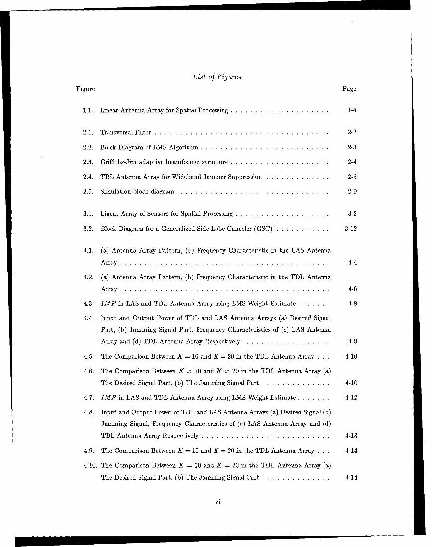
List of Figures

Figure Page

1.1. Linear Antenna Array for Spatial Processing ....... .................... 1-4

2.1. Transversal Filter ......... ................................... 2-2

2.2. Block Diagram of LMS Algorithm ........ .......................... 2-3

2.3. Griffiths-Jim adaptive beamformer structure ....... .................... 2-4

2.4. TDL Antenna Array for Wideband Jammer Suppression ..... ............. 2-5

2.5. Simulation block diagram ......... .............................. 2-9

3.1. Linear Array of Sensors for Spatial Processing ...... ................... 3-2

3.2. Block Diagram for a Generalized Side-Lobe Canceler (GSC) ............... 3-12

4.1. (a) Antenna Array Pattern, (b) Frequency Characteristic in the LAS Antenna

Array ........... .......................................... 4-4

4.2. (a) Antenna Array Pattern, (b) Frequency Characteristic in the TDL Antenna

Array ........... ......................................... 4-6

4.3. IMP in LAS and TDL Antenna Array using LMS Weight Estimate ....... .... 4-8

4.4. Input and Output Power of TDL and LAS Antenna Arrays (a) Desired Signal

Part, (b) Jamming Signal Part, Frequency Characteristics of (c) LAS Antenna

Array and (d) TDL Antenna Array Respectively ...... ................. 4-9

4.5. The Comparison Between K = 10 and K = 20 in the TDL Antenna Array . . . 4-10

4.6. The Comparison Between K = 10 and K = 20 in the TDL Antenna Array (a)

The Desired Signal Part, (b) The Jamming Signal Part ..... ............. 4-10

4.7. IMP in LAS and TDL Antenna Array using LMS Weight Estimate ....... .... 4-12

4.8. Input and Output Power of TDL and LAS Antenna Arrays (a) Desired Signal (b)

Jamming Signal, Frequency Characteristics of (c) LAS Antenna Array and (d)

TDL Antenna Array Respectively ....... .......................... 4-13

4.9. The Comparison Between K = 10 and K = 20 in the TDL Antenna Array . . . 4-14

4.10. The Comparison Between K = 10 and K = 20 in the TDL Antenna Array (a)

The Desired Signal Part, (b) The Jamming Signal Part ..... ............. 4-14

vi

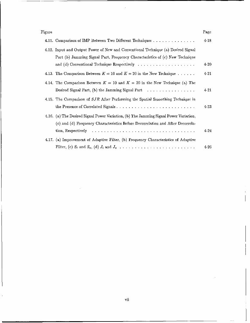
Figure Page

4.11. Comparison of IMP Between Two Different Techniques ................... 4-18

4.12. Input and Output Power of New and Conventional Technique (a) Desired Signal

Part (b) Jamming Signal Part, Frequency Characteristics of (c) New Technique

and (d) Conventional Technique Respectively ...... ................... 4-20

4.13. The Comparison Between K = 10 and K = 20 in the New Technique ...... .... 4-21

4.14. The Comparison Between K = 10 and K = 20 in the New Technique (a) The

Desired Signal Part, (b) the Jamming Signal Part ...... ................ 4-21

4.15. The Comparison of SJR After Performing the Spatial Smoothing Technique in

the Presence of Correlated Signals ....... .......................... 4-23

4.16. (a) The Desired Signal Power Variation, (b) The Jamming Signal Power Variation,

(c) and (d) Frequency Characteristics Before Decorrelation and After Decorrela-

tion, Respectively .......... .................................. 4-24

4.17. (a) Improvement of Adaptive Filter, (b) Frequency Characteristics of Adaptive

Filter, (c) Si and S., (d) Ji and Jo ................................. 4-26

vii

List of Tables

Table Page

4.1. Specification for First Computer Simulation ....... .................... 4-7

4.2. Specification for Second Computer Simulation ...... ................... 4-11

viii

AFIT/GE/ENG/96D-14

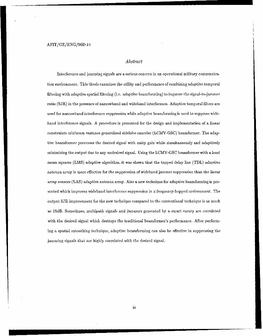
Abstract

Interference and jamming signals are a serious concern in an operational military communica-

tion environment. This thesis examines the utility and performance of combining adaptive temporal

filtering with adaptive spatial filtering (i.e. adaptive beamforming) to improve the signal-to-jammer

ratio (SJR) in the presence of narrowband and wideband interference. Adaptive temporal filters are

used for narrowband interference suppression while adaptive beamforming is used to suppress wide-

band interference signals. A procedure is presented for the design and implementation of a linear

constraints minimum variance generalized sidelobe canceler (LCMV-GSC) beamformer. The adap-

tive beamformer processes the desired signal with unity gain while simultaneously and adaptively

minimizing the output due to any undesired signal. Using the LCMV-GSC beamformer with a least

mean squares (LMS) adaptive algorithm, it was shown that the tapped delay line (TDL) adaptive

antenna array is more effective for the suppression of wideband jammer suppression than the linear

array sensors (LAS) adaptive antenna array. Also a new technique for adaptive beamforming is pre-

sented which improves wideband interference suppression in a frequency-hopped environment. The

output SJR improvement for the new technique compared to the conventional technique is as much

as 15dB. Sometimes, multipath signals and jammers generated by a smart enemy are correlated

with the desired signal which destroys the traditional beamformer's performance. After perform-

ing a spatial smoothing technique, adaptive beamforming can also be effective in suppressing the

jamming signals that are highly correlated with the desired signal.

ix

Interference Suppression for Spread Spectrum Signals

Using Adaptive Beamforming and Adaptive Temporal Filter

L Introduction

1.1 Background

The final goal of communication is to transmit information without error from a transmit-

ter to a receiver. In the real world, there are several interference sources with various powers

and bandwidths to prevent this goal. These interfering signals might arise from intentional jam-

ming, multipath, multiple users on the same bandwidth, or a variety of other sources. In a noisy,

crowded, or hostile environment, a number of techniques may be implemented in order to increase

the anti-jam characteristics of a communication system. Some methods include spread spectrum

modulation, interference suppression and spatial discrimination techniques.

The objective of this research is to examine the effectiveness of adaptive algorithms for in-

terference suppression in spread spectrum communication. It is desirable to achieve temporal and

spatial filtering using adaptive algorithms to maintain an acceptable signal-to-noise ratio (and

hence, probability of bit error) in any kind of interference such as intentional jamming, multipath,

and co-channel interference.

1.1.1 Spread Spectrum Modulation. Spread Spectrum techniques have an inherent ability

to suppress interference (Peterson at el, 1995). These are modulation schemes that produce a

spectrum with a much wider bandwidth than that of the information bearing signal. By increasing

the bandwidth over which signal energy is contained, the energy density of the signal is reduced

and hidden in the noise levels so that unintended receivers cannot detect it. Hence the signals have

a low probability of intercept. Upon reception of the desired signal and undesired jammer signal

by the Spread Spectrum (SS) receiver, the coding process is reversed and the signal energy density

1-1

is returned to its original level while the jammer energy density is reduced. Hence the receiver is

resistant to interference and jamming.

Two common spread spectrum schemes are direct sequence (DS) and frequency hopping

(FH). Direct Sequence is achieved by combining a binary message sequence and a higher rate

pseudorandom binary sequence. A pseudorandom binary sequence code has a much higher rate

than the original digital data which expands the bandwidth beyond that of the original information

bandwidth. Frequency hopping is achieved by changing the frequency of the carrier periodically.

Typically, each carrier frequency is chosen from a set of 2k frequencies which are spaced apart

approximately the width of the data modulation bandwidth. The frequency is translated to one

of 2k frequency hop bands by the FH modulator. The processing gain is 2k. The spreading code

in this case does not directly modulate the carrier but is instead used to control the sequence of

carrier frequencies.

1.1.2 Interference Suppression. The inherent processing gain of a spread spectrum signal

will, in many case, provide the system with a sufficient degree of interference rejection capability.

However, if the combined interference signal power relative to the desired signal power exceeds the

spread spectrum processing gain, additional filtering is required. If the interference is relatively

narrowband compared with the bandwidth of the spread spectrum, then interference suppression

by the use of notch filters often results in an improvement in system performance.

There are two techniques for building notch filters, The first technique uses a transversal filter

in the time domain (Milstain and Das, 1980; Saulnier, 1990). The system can be made adaptive

by using a tapped delay line with variable tap weights. These tap weights can be adapted, for

example, by using the well-known least-mean-square (LMS) algorithm.

The second technique is that of transform domain processing. A notch filter is implemented

by Fourier transforming the received waveform, applying some type of signal processing algorithm,

and then inverse Fourier transforming the signal back to the time domain. One type of signal

1-2

processing algorithm excises the frequency bin which exceeds a specific threshold (Milstain and

Das, 1980). Another way is to use adaptive transform domain filtering (Saulnier, 1992). This

type of suppressor combines features of the time domain adaptive filter and the transform domain

excisor. The transform domain technique works more effectively than the time domain technique

for all interference bandwidth. Transform domain techniques are also more robust since they can

handle multiple narrowband jammers simultaneously.

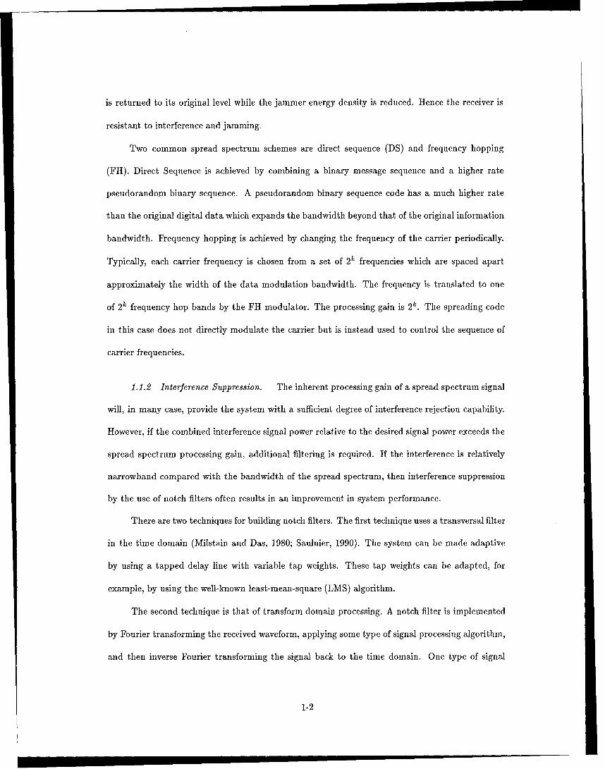
1.1.3 Spatial Discrimination Technique. Spatial discrimination techniques include adap-

tive null steering antennas and high-gain directional antennas (Widrow et al, 1982). Together,

they place nulls of the receiver's antenna pattern in the direction of enemy jammers to avoid front

end saturation of the receiver and to increase the gain in the direction of the desired signal. In an

adaptive array, the phase and amplitude of the signal at each receiving antenna element is weighted

and the resulting signals summed to produce the array output. The values of the element weights

are determined by an algorithm that can act to steer nulls in the direction of interfering signals

(Fig. 1.1).

1.2 Problem Statement and Objective

Any kind of interference signals are a serious concern in an operational military communica-

tion environment. Many researchers have developed lots of techniques for narrowband interference

suppression, i.e. adaptive filter in time and transform domain and excisor. In the case of wideband

interferences, those techniques can't work, because the desired signal is also suppressed when they

suppress the wideband interferences. Until now, the adaptive beamforming is known as the way to

suppress the wideband interferences. However, the wideband interferences suppression remains an

important research topic. Furthermore, multipath signals are correlated to the desired signal and

the smart jammer uses the correlated signal with the desired signal to prevent our communication.

1-3

w1 Output

y(n)

W M

Sensors Weights

Adaptive

Algorithm

Figure 1.1 Linear Antenna Array for Spatial Processing

The conventional adaptive beamforming is totally destroyed in the presence of correlated signals.

The correlated interference is a serious problem in the traditional adaptive beamformer.

This research combines a notch filter technique and spatial discrimination technique which

are two of the most powerful methods for providing interference signal suppression. In other words,

by achieving adaptive temporal and spatial filtering using adaptive algorithm, the system maintains

the reasonable signal power to jammer power ratio (SJR).

1.3 Assumption

The research assumes that the received signal is composed of a sum of jamming and desired

signals. It is also assumed that code synchronization is maintained at the communication receiver,

and thus, there is no propagation delay. Finally, unless explicitly mentioned, the desired signal and

jamming signal are uncorrelated each other. The antenna elements are uniformly distributed and

1-4

the distance between elements is a half wavelength of the desired signal center frequency in order to

prevent the grating lobe. Those assumptions are reasonable for real situation and hardware, thus

they doesn't affect the result of simulation.

1.4 Scope

The desired signal considered in this research has wide bandwidth. Specifically, frequency

hopped signals are considered because FH (Frequency Hopping) signals and antenna arrays are

closely related. Each antenna element is omni-directional. Jammer models consist of both narrow

and wide bandwidth. The adaptive algorithm used in both schemes is the LMS (Least Mean

Squares) algorithm. This algorithm is the best known and most easily implemented algorithm

which implement an iterative solution to the Wiener-Hoff equation without making use of any a

priori statistical information about the received signal. The Wiener-Hoff equation determines the

optimal tap weight settings for the transversal filter.

The class of adaptive beamformer discussed is LCMV-LMS (Linearly Constrained Minimum

Variance - Least Mean Squares) beamforming which constrains the gain and phase in the desired

signal direction and minimizes the output due to the undesired signals (Griffiths and Jim, 1982).

For LCMV beamforming, a GSC (Generalized Side-lobe Canceller) structure is used because this

structure is useful for implementation and analysis of LCMV beamforming.

1.5 Material and Equipment

All system models and simulations were developed using the version 4.1 Matlab simulation

software developed by The Math Works, Natric, Massachusetts. The software was run on a Sun

Workstation.

1-5

1.6 Thesis Organization

Chapter II of this thesis highlights a literature review of adaptive algorithm, adaptive beam-

forming, and adaptive signal processing in spread spectrum modulation. Chapter III presents a

basic introduction into the concept of adaptive signal processing. It compares the temporal fil-

ter versus spatial filter. It then discusses the theory of adaptive temporal filters and adaptive

beamforming. Moreover, the adaptive beamforming in the presence of correlated signals is pre-

sented. Chapter IV provides the simulation results related to jamming suppression and especially

emphasizes the jamming suppression in frequency-hopped environment. In addition, it provides

the performance of a spatial smoothing technique for suppression of correlated jammers. Chapter

V summarizes the thesis, states conclusions based on the simulation results, and provides recom-

mendations for future research.

1-6

I. Literature Review

This chapter reviews the published literature on the interference rejection problems as it

relates to adaptive signal processing. Adaptive filtering algorithms and adaptive beamforming for

wideband interferences and for the specific case spread spectrum signals are reviewed.

2.1 Adaptive Filtering Algorithm

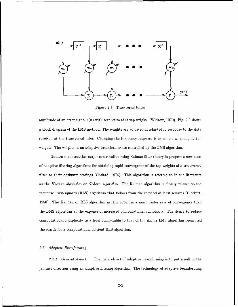
The first studies of minimum mean-square estimation in stochastic processes may be traced

back to the late 1930s and early 1940s. Wiener formulated the continuous time linear prediction

problem and derived an explicit formula for the optimum predictor. He also considered the filtering

problem of estimating a process corrupted by an additive noise process. The explicit formula for the

optimum estimate required the solution of an integral equation known as the Wiener-Hoff equation

(Wiener and Hoff, 1931)

In 1947, Levinson formulated the Wiener filtering problem in discrete time. The Wiener-Hoff

equation can be expressed in matrix form as follows,

Rw 0 = p (2.1)

where wo is the tap weight vector of the optimum Wiener filter in the form of a transversal filter,

which is shown in Fig. 2.1. R is the correlation matrix of the tap inputs u(n), and p is the

cross-correlation matrix of the tap inputs u(n) and the desired response d(n) shown in Fig. 2.1.

(Levinson, 1947).

The simple adaptive filtering least-mean-square (LMS) algorithm emerged as a algorithm for

the operation of adaptive transversal filters in the late 1950s. The LMS algorithm was devised by

Widrow and Hoff in 1959 in their study of a pattern recognition scheme known as the adaptive

linear threshold logic element. The LMS algorithm is a stochastic gradient algorithm in that it

iterates each tap weight in the transversal filter in the direction of the gradient of the squared

2-1

y(n)

Figure 2.1 Transversal Filter

amplitude of an error signal e(n) with respect to that tap weight. (Widrow, 1970). Fig. 2.2 shows

a block diagram of the LMS method. The weights are adjusted or adapted in response to the data

received at the transversal filter. Changing the frequency response is as simple as changing the

weights. The weights in an adaptive beamformer are controlled by the LMS algorithm.

Godarn made another major contribution using Kalman filter theory to propose a new class

of adaptive filtering algorithms for obtaining rapid convergence of the tap weights of a transversal

filter to their optimum settings (Godard, 1974). This algorithm is referred to in the literature

as the Kalman algorithm or Godarn algorithm. The Kalman algorithm is closely related to the

recursive least-squares (RLS) algorithm that follows from the method of least squares (Plackett,

1950). The Kalman or RLS algorithm usually provides a much faster rate of convergence than

the LMS algorithm at the expense of increased computational complexity. The desire to reduce

computational complexity to a level comparable to that of the simple LMS algorithm prompted

the search for a computational efficient RLS algorithm.

2.2 Adaptive Beamforming

2.2.1 General Aspect. The main object of adaptive beamforming is to put a null in the

jammer direction using an adaptive filtering algorithm. The technology of adaptive beamforming

2-2

u(n) Transversal 01y(n) >

filter w(n)

control

d(n)

Figure 2.2 Block Diagram of LMS Algorithm

has been developed with adaptive filtering algorithms. The initial work of adaptive beamforming

may be traced back to the invention of the intermediate frequency (IF) sidelobe canceler by Howells

in the late 1950. In his historical report, Howells described a sidelobe canceler capable of automat-

ically nulling out the effect of a jammer. The sidelobe antenna uses a primary (high gain) antenna

and a reference omni-directional (low gain) antenna to form a two-element array with one degree

of freedom. (Howells, 1976)

The poor performance of the delay-and-sum beamformer (the transversal filter) is due to

the fact that its response along a direction of interest depends not only on the power of the in-

coming target but also undesirable contributions received from other sources of interference. To

overcome this limitation, Capon proposed a new beamformer in which the weight vector w(n) is

chosen to minimize the variance (i.e., average power) of the beamformer output, subject to the

constraint wH(n)s(O) = 1 for all n, where s() is a prescribed steering vector (Capon, 1969). This

constrained minimization yields an adaptive beamformer with a minimum variance distortionless

response (MVDR) which processes the desired signal from certain directions with specified gain and

phases using the constraints and then minimize the output power to suppress undesired signals.

2-3

n o

z! Blocking

ZN1 Matrix

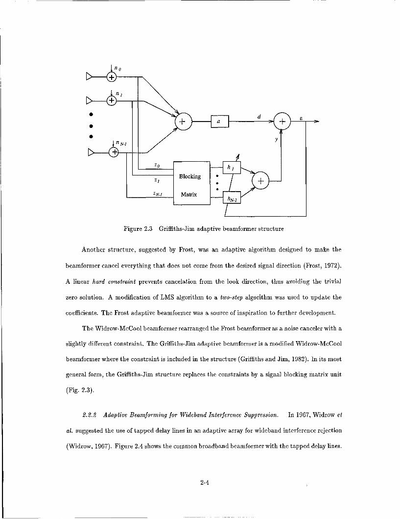
Figure 2.3 Griffiths-Jim adaptive beamformer structure

Another structure, suggested by Frost, was an adaptive algorithm designed to make the

beamformer cancel everything that does not come from the desired signal direction (Frost, 1972).

A linear hard constraint prevents cancelation from the look direction, thus avoiding the trivial

zero solution. A modification of LMS algorithm to a two-step algorithm was used to update the

coefficients. The Frost adaptive beamformer was a source of inspiration to further development.

The Widrow-McCool beamformer rearranged the Frost beamformer as a noise canceler with a

slightly different constraint. The Griffiths-Jim adaptive beamformer is a modified Widrow-McCool

beamformer where the constraint is included in the structure (Griffiths and Jim, 1982). In its most

general form, the Griffiths-Jim structure replaces the constraints by a signal blocking matrix unit

(Fig. 2.3).

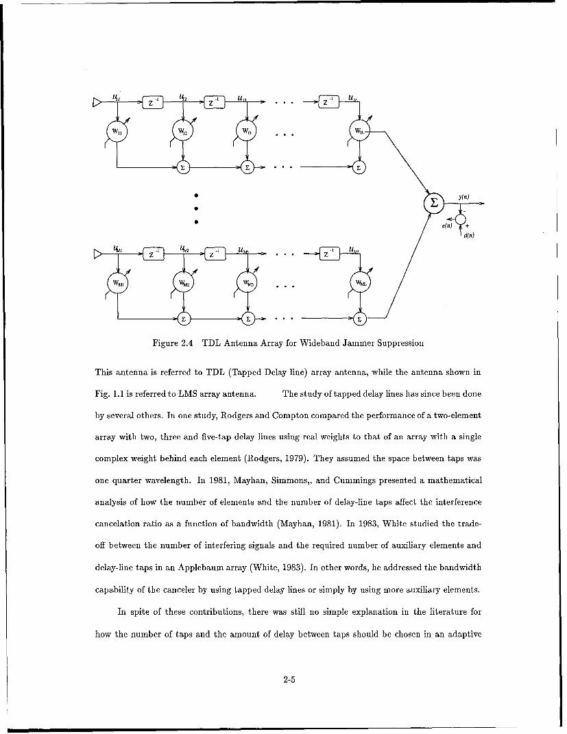
2.2.2 Adaptive Beamforming for Wideband Interference Suppression. In 1967, Widrow et

al. suggested the use of tapped delay lines in an adaptive array for wideband interference rejection

(Widrow, 1967). Figure 2.4 shows the common broadband beamformer with the tapped delay lines.

2-4

~y(n)

Figure 2.4 TDL Antenna Array for Wideband Jammer Suppression

This antenna is referred to TDL (Tapped Delay line) array antenna, while the antenna shown in

Fig. 1.1 is referred to LMS array antenna. The study of tapped delay lines has since been done

by several others. In one study, Rodgers and Compton compared the performance of a two-element

array with two, three and five-tap delay lines using real weights to that of an array with a single

complex weight behind each element (Rodgers, 1979). They assumed the space between taps was

one quarter wavelength. In 1981, Mayhan, Simmons,, and Cummings presented a mathematical

analysis of how the number of elements and the number of delay-line taps affect the interference

cancelation ratio as a function of bandwidth (Mayhan, 1981). In 1983, White studied the trade-

off between the number of interfering signals and the required number of auxiliary elements and

delay-line taps in an Applebaum array (White, 1983). In other words, he addressed the bandwidth

capability of the canceler by using tapped delay lines or simply by using more auxiliary elements.

In spite of these contributions, there was still no simple explanation in the literature for

how the number of taps and the amount of delay between taps should be chosen in an adaptive

2-5

array to achieve a given bandwidth performance. In 1988, Compton addressed this question by

examining a two-element adaptive array with a tapped delay-line behind each element (Compton,

1988). In the same year, he also considered the use of fast Fourier transform (FFT) processing

behind the elements in adaptive arrays (Compton, 1988). However, he concluded the performance

of FFT processing wasn't an improvement over tapped delay lines. He used the LMS algorithm for

changing the weights in both cases.

In 1986, Buckley and Griffiths presented an adaptive broadband beamforming structure which

added the Frost beamformer and TDL antenna array. This beamformer employed a gradient-based

weight adjustment to minimize output variance subject to a set of J linear constraints on broadband

directional derivatives in the desired look direction. Generalized sidelobe-cancelling structure was

employed in which a nonadaptive beamformer operates in parallel with an adaptive beamformer

(Buckley and Griffiths, 1986).

2.3 Adaptive Signal Processing in Spread Spectrum

2.3.1 Direct Sequence Spread Spectrum with Adaptive Filter. Specific implementation of

an adaptive algorithm for interference suppression in Direct Sequence Spread Spectrum(DS-SS)

systems has been investigated since the mid- to late-1970's. Hsu and Giordano have laid down the

foundation in interference suppression in DS-SS systems (Hsu and Giordano, 1978). Their digital

whitening is accomplished by using a transversal filter whose coefficients are selected by either a

Wiener algorithm or a maximum entropy algorithm. Filters obtained by use of these algorithms

are evaluated for various jamming and signaling conditions and are found to exhibit comparable

performance over a wide range of input signal and noise ratios. The Wiener filter was implemented

recursively using a least-mean-square criterion and a form of Levinson's algorithm in the actual

computation.

Ketchem and Proakis further improved the results of Hsu and Giordano by combining the

2-6

interference rejection filter with its matched filter, resulting in an overall linear filter having a linear

phase characteristic. They further defined the performance of the SS receiver as measured in terms

of the probability of error, which was obtained by applying a Gaussian assumption on the total

residual noise and interference followed by Monte Carlo simulation. Ketchum and Proakis also

investigated the size of the interference suppression filter (in terms of number of taps) required to

handle multiple-band interference. The frequency response improves with increasing filter order

(the number of taps) in terms of providing a deeper notch at the interfering tone frequencies and

less attenuation in the frequency range between notches (Ketchum and Proakis, 1932).

Saulnier has performed hardware implementations of interference suppression filters using

three different transversal filter structures: charge transfer device (CTD), digital filter techniques,

and surface acoustic wave (SAW) device (Saulnier et al, 1984; Saulnier et al, 1985; Saulnier, 1990).

These three implementations were of the estimation-type adaptive filter. A CTD-based adaptive

filter was designed using the Widrow-Hoff LMS algorithm to implement the adaptive filter archi-

tecture consisting of only two multipliers (Saulnier et al, 1984). This hardware simplification was

achieved through the use of a burst processing technique. Saulnier, Das, and Milstein followed this

work with an identical setup with a digital hardware implementation instead of the CTD (Saulnier

et al, 1985). They recently performed a hardware experimentation using a SAW-based adaptive

filter to perform the interference suppression (Saulnier, 1990). The primary advantage of using the

SAW-based transversal filter is the availability of higher bandwidths and operating frequencies (i.e.

correlation of the DS signal at RF).

The researches mentioned so far primarily performed interference suppression in the time-

domain using the estimation-type predictive filter. However, throughout the 1980's, work has been

accomplished in the frequency domain using transform-domain interference excisors.

In 1980, Milstein and Das provided a detailed analysis of the performance of systems in which

the received signal is Fourier transformed in real time (usually with a surface acoustic wave device)

and then filtered by a multiplication of the transformed signal by an appropriate transfer function

2-7

(Milstein and Das, 1980). In 1989, Gevargiz , Das and Milstein developed the transform domain

processing and presented two transfer domain processing techniques. In the first technique, the

narrow band interference is detected and excised in the transform domain by using an adaptive

notch filter. In the second technique, the interference is suppressed using soft-limiting in the trans-

form domain (Gevargiz et al, 1989).

Usage of a Hamming window was proposed to concentrate the energy of the narrow-band

interference in a smaller fraction of the spectrum by Davidovici and Kanterakis (Davidovici and

Kanterakis, 1989). The Hamming Window effectively reduced the interferences sidelobe at the

expense of a wider main lobe. They presented the overlap and save algorithm in order to eliminate

transient effects and inter-symbol interference. Due to the overlap and save method the system's

filter complexity is double that of Milstein's.

Saulnier suggested the use of transform-domain adaptive filters which combined some features

of the time-domain adaptive filter and the transform domain excisor (Saulnier, 1992). Weight leak-

age is employed to allow jammer suppression while preserving the desired DS signal, which made

the desired signal power lower to indicate the high-power jammer. Bit error rate (BER) results

obtained by computer simulation were presented to illustrate performance for a single-tone jammer

and for a jammer consisting of a second DS signal having a lower chip rate. These results were

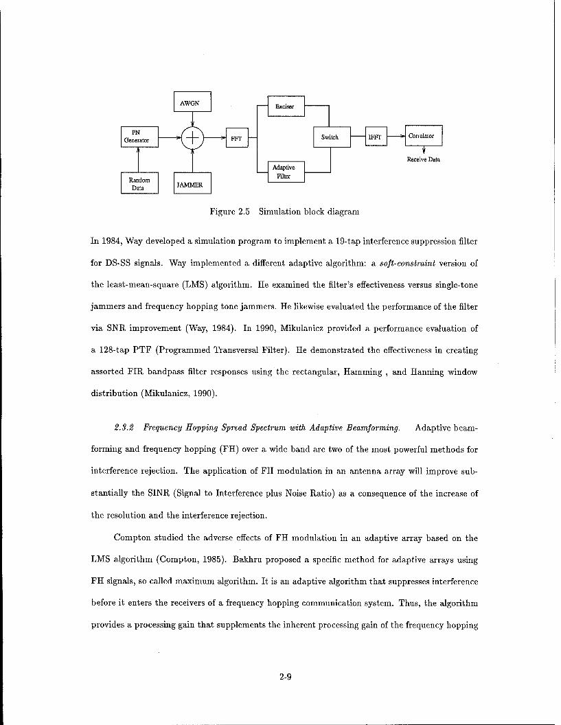
compared to those for a transform domain excisor. Figure 2.5 show the simulation block diagram

for comparison the adaptive filter with excisor in transform domain.

Another paper by Reed and Feintuch reported a comparison between implementations in

the time and frequency domains (Reed and Feintuch, 1981). In addition, a thorough review paper

covers many of the areas of interest within the interference rejection domain of spread spectrum

communication (Milstein, 1988)

Relevant research at the Air Force Institute of Technology (AFIT) includes the following

work. Shepard's 1982 master's thesis evaluated the performance of a DS (Direct Sequence) spread

spectrum receiver preceded by an adaptive interference suppression (AIS) filter (Shephard, 1982).

2-8

AWG N - Exeiser

Receive Data. Adaptive

Rl ~ AME Filter

Figure 2.5 Simulation block diagram

In 1984, Way developed a simulation program to implement a 19-tap interference suppression filter

for DS-SS signals. Way implemented a different adaptive algorithm: a soft-constraint version of

the least-mean-square (LMS) algorithm. He examined the filter's effectiveness versus single-tone

jammers and frequency hopping tone jammers. He likewise evaluated the performance of the filter

via SNR improvement (Way, 1984). In 1990, Mikulanicz provided a performance evaluation of

a 128-tap PTF (Programmed Transversal Filter). He demonstrated the effectiveness in creating

assorted FIR bandpass filter responses using the rectangular, Hamming , and Hanning window

distribution (Mikulanicz, 1990).

2.3.2 Frequency Hopping Spread Spectrum with Adaptive Beamforming. Adaptive beam-

forming and frequency hopping (FH) over a wide band are two of the most powerful methods for

interference rejection. The application of FH modulation in an antenna array will improve sub-

stantially the SINR (Signal to Interference plus Noise Ratio) as a consequence of the increase of

the resolution and the interference rejection.

Compton studied the adverse effects of FH modulation in an adaptive array based on the

LMS algorithm (Compton, 1985). Bakhru proposed a specific method for adaptive arrays using

FH signals, so called maximum algorithm. It is an adaptive algorithm that suppresses interference

before it enters the receivers of a frequency hopping communication system. Thus, the algorithm

provides a processing gain that supplements the inherent processing gain of the frequency hopping

2-9

system. The algorithm discriminates between the desired signal and the interference on the basis

of the distinct spectral characteristics of frequency hopping signals. The maximum algorithm is so

named because the desired signal is enhanced and the interference is suppressed simultaneously by

parallel sub-processors. The algorithm is blind in the sense that neither the direction of the desired

signal nor its waveform needs to be known (Bakhru and Torrieri, 1984). Nonetheless any adaptive

algorithm presents some discontinuities when used with FH modulated signals. The reason is that

the changes in the signal frequency due to FH are seen by the algorithm as changes in the direction

of arrival.

Torrieri suggested three different techniques of frequency compensation for the maximum al-

gorithm to solve this problem (Torrieri and Bakhru, 1987). The parameter dependent processing

uses an adaptive filter behind each antenna element. Each adaptive filter has enough adjustable

parameters to allow the formation of nulls in the directions of the sources of interference for all

frequencies. This processing is the most complicated to implement but presents faster convergence.

Spectral processing is based upon dividing that total hopping band into a number of spectral re-

gions called bins and adapting the weight vector independently each time the carrier frequency of

the frequency hopping signal is in one of the bins. This processing is the simplest to implement but

the achieved improvement is not significant. An anticipative adaptive system begins adaptation

toward the optimal weights for a carrier frequency before that frequency is transmitted. A time

advanced frequency hopping replica hops approximately one hop duration ahead of the replica hops

for dehopping the received signal. While the main adaptive filter produces the output, the auxiliary

filter adapts its weights to suppress the next carrier frequency. After each hop, the weight values

associated with the new carrier frequency are transferred from the auxiliary filter to the main filter.

Anticipate processing provides the fastest convergence to the steady state, but exhibits the largest

variation in the steady state SINR.

Najar and Lagunas further developed the anticipative processing by adding a generalized

sidelobe canceller (GSC). His approach to the optimum solution consists two different stages. The

2-10

first stage, named the anticipative stage, is devoted to cancel interference at fixed frequencies that

are already present or active at the frequency of interest at the hop time. The second state, named

GSC stage, is used for combating interferences that are not present at the frequency of interest at

the time of the frequency hop (Najar and Lagunas, 1995). They showed the grating lobe is reduced

significantly in the mean array factor when the FH signals is used with antenna array.

2.4 Conclusion

This chapter presented a brief historical review of developments in three areas that are closely

related in so far as the subject matter of this research. Those areas are adaptive filtering algorithm,

adaptive beamforming for wideband interference suppression. Many researchers have investigated

the adaptive filters for narrowband interference suppression and adaptive beamforming for wide-

band interference suppression. Special attention was devoted to adaptive filters in the DS-SS

system. In the FH-SS signal environments, the researches relating adaptive antenna array and

FH modulation for interference suppression have been developed because the antenna array and

FH modulation is closely related with each other. In the next chapter, we derive the theories of

adaptive filter and beamforming.

2-11

III. Adaptive Signal Processing

3.1 Background

3.1.1 Overview. This chapter discusses the similarity of temporal and spatial filters.

Then, the time domain adaptive filters are considered using LMS adaptive algorithm and the spatial

filter (i.e., adaptive beamforming) is discussed using the linear constrained minimum variance

(LCMV) algorithm with generalized sidelobe canceller (GSC). An optimum value and LMS estimate

of weights are also computed. Finally, the adaptive beamformer in the presence of correlated signals

is considered.

3.1.2 Notation. Since vectors and matrices are used throughout this research, it is

important to establish the notation that will be used. Vectors are always represented with lowercase

boldface symbols, for example, w, and are assumed to be column vector. Matrices are denoted

by boldface upper case symbols, for example C. Superscripts *, T, H, and -1 represent complex

conjugate, transpose, complex conjugate transpose, and matrix inverse, respectively.

3.1.3 Definition, Signals may be classified as either narrowband or wideband. Narrow-

band is defined in terms of the fractional bandwidth ofjthe signal. The fractional bandwidth is

the signal bandwidth as a percentage of the carrier frequency. Signals whose fractional bandwidths

are much less than 2 percent will be characterized as narrowband, while those with fractional

bandwidths much greater than 2 percent will be called wideband (Haykin and Steinhardt, 1992).

3.1.4 Temporal Filter versus Spatial Filter. Although the temporal filter problem in

additive receiver noise and the spatial filter problem corrupted by additive sensor noise arise in

different application areas, their mathematical formulations and procedures for their solution are

indeed similar.

For the temporal filtering of data, we propose using a transversal filter of length M as indicated

3-1

y(n)

Output

Figure 3.1 Linear Array of Sensors for Spatial Processing

in Fig. 2.1. The filter output, in response to the tap inputs, is given by

M-1

y(n) = 1 wu(n - k), (3.1)k=O

where wk is kth tap weight and u(n) is tap input in time n. For the special case of a sinusoidal

excitation

u(n) = eif, (3.2)

we may rewrite Eq. 3.1 asM-1

y(n) = e w e-jk, (3.3)k=O

where w is the angular frequency of the excitation, which is normalized with respect to the sampling

rate.

Consider next the spatial analog of this temporal problem. Fig. 3.1 depicts a receiving linear

array of uniformly spaced sensors labeled 1,..., M. Let d denote the separation between adjacent

elements of the array. In Fig. 3.1 a single plane wave was impinging on the array at angle of

3-2

incidence 0, measured with respect to the boresight. It is assumed that the inter-element distance

is a half wavelength so as to avoid the appearance of grating lobes (Skolnik, 1980). The resulting

beamforming output is given by

M-1

y(n) = u(n) E we-j"¢' (3.4)k=O

where the direction of arrival is defined by the electrical angle = 2 sin 0 that is related to the

angle of incidence 0 and the antenna interelements distance d, u(n) is the electrical signal picked up

by the antenna element labeled ul in Fig. 3.1 that is treated as the point of reference, and the wk

denote the element weights of the beamformer. The important point to note is the mathematical

similarity between the temporal model of Eq. 3.3 and the spatial model of Eq. 3.4.

3.2 Adaptive Filter : Temporal Filter

An adaptive filter converges to the optimum Wiener solution in a stationary environment.

The LMS algorithm starts from some predetermined set of initial conditions and is self-designing.

It relies for its operation on a recursive algorithm, which makes it possible for the filter to perform

satisfactorily in an environment where complete knowledge of the relevant signal characteristics is

not available. On the other hand, the design of a Wiener filter requires prior information about

the statistics of the data to be processed (Widrow, 1985). For real-time operation, this procedure

has the disadvantage of requiring excessively elaborate and costly hardware.

3.2.1 Input Signal and Weight Vector. The operation of a linear adaptive filtering algo-

rithm involves two basic processes: (1) a filtering process designed to produce an output in response

to sequence of input data, and (2) an adaptive process. The transversal filter type is used, which

referred to as a tapped-delay line filter, as depicted in Fig. 2.1. For the transversal filter, we obtain

3-3

the input-output relationships as follows:

M-1

y(n) = wu(n - k). (3.5)k=O

In vector notation, this can be written as

y(n) = w'u(n), (3.6)

where the input and weight vector are expressed by vector notation as,

u(n) = [u(n),u(n-1),...,u(n- M+ 1)]T

W = [WlW2, ,WMI T .

3.2.2 Minimum Mean Squared Error. For the case of stationary inputs, the performance

function is defined as the mean square error which is the mean squared value of the difference

between the desired response and the transversal filter output. As in Fig. 2.2 the error signal is

e(n) = d(n)- y(n)

= d(n)-wH u.

Squaring the error signal to obtain the squared error, one obtains

e(n)' = d(n)2 + w'uu'w - 2d(n)uHw. (3.7)

Then taking the expected value, the MSE (Mean Squared Error) becomes

MSE = E{d(n)2} + WHE{uuH}w - 2E{d(n)uH}w

3-4

- E{d2 } + wHRw - 2pw, (3.8)

where R is defined as the square matrix :

R = E{uuH}. (3.9)

Correspondingly, p is denoted by the M-by-1 cross correlation vector between the tap inputs of

the filter and the desired response d(n) :

p = E{ud(n)*J}. (3.10)

Many useful adaptive processes work by seeking the weight vector which minimizes the perfor-

mance function using gradient search methods. The gradient of the mean squared error performance

surface, designated V, can be obtained by differentiating Eq. 3.8 to obtain the column vector:

OMS = 2Rw-Ow -p

3.2.3 LMS Adaptation Algorithm. Since the gradient vector must be estimated from the

available data, the simplest estimate of gradient vector is the instantaneous estimates based on

sample values of the tap-input vector and desired response:

= 21* - 2f3 = 2u(n)u"(n)*r - 2u(n)d*(n)

Let *(n) denote the value of the tap weight vector at time n. The updated value of the

tap-weight vector at time n + 1 is computed by using the simple recursive relation

*(n + 1) = *(n) + [u(n)Ed*(n) - u"(n)*] (3.11)

3-5

3.2.4 Summary. Adaptive temporal filter have a built in mechanism for the automatic

adjustment of its weight in response to statistical variations of the environment in which the filter

operates. The weight adjustments are made iteratively by using standard adaptive algorithms that

seeks an optimum value. The filter input consisting of a vector of uniformly spaced samples taken

from a long data stream is used to determine weights that minimize the performance function

calculated by gradient methods. The updated weight vector is computed by using the simple

recursive relation as depicted in Eq. 3.11.

3.3 Adaptive Beamforming

3.3.1 Introduction. A beam former is a signal processor used in conjunction with a set of

antennas that are spatially separated. The beamformer output is simply a weighted combination

of the outputs of the set of antennas. Usually the goal of beamforming is spatial filtering, that is,

separation of signals which have similar temporal frequency content but originate from different

spatial locations. Here, we use digital beamforming that detects and digitizes the received signal

at the element level via discrete processing techniques.

In an adaptive beamformer the weights are adjusted or adapted in response to the data re-

ceived at the antennas to optimize the beamformer's spatial response. Changing the beamformer's

spatial response is as simple as changing the weights. The weights in an adaptive beamformer are

controlled by an adaptive algorithm. All adaptive antennas to date have been arrays, because the

pattern of an array is easily controlled by adjusting the amplitude and phase of the signal from each

element before combining the signals. Adaptive antennas are useful in radar and communication

systems that are subject to interference and jamming. They change their patterns in a way that

optimizes the signal-to-interference-plus-noise ratio at the array output.

3-6

3.3.2 Input Signal and Weight Vector . Fig. 1.1 illustrated a beamformer typically

used for processing narrowband signals. The antenna outputs are sampled and are represented

in discrete time for notational convenience and consistency. The M antenna sensor outputs are

weighted and then summed to compute the beamformer output. This method is called as delay-

and-sum beamformer. Each sensor is assumed to have any necessary receiver electronics and an

A/D converter. The discrete time delay and sum beamformer y(n) is given by

M

y(n) = u ..u(n), (3.12)/=1

where Wm and um(n) are the weight and input data, respectively, in the mth antenna channel.

A beamforming structure commonly utilized to process wideband signals is depicted in Fig. 2.4.

In this case there are tap delay lines in each channel. The output, y(n) is expressed as

M-1 L-1

y(n) = >um,i(n), (3.13)m=1 1=0

where L is the number of taps in each of the M channels and wm,l is the weight applied to the

lth tap of the mth channel. This means that the output of each sensor is then passed through a

FIR filter having L weights. The time domain filtering is intended to provide some rejection of

interference not lying in the proper temporal frequency region. The resulting FIR filter describing

the relation between array input and output has tap values equal to the sum of component-filter tap

values occurring at the temporal delay. Once each antenna sensor's output delayed by an amount

appropriate for the propagation direction is passed through a FIR filter whose weights are selected

individually.

Both Eq. 3.12 and Eq. 3.13 are compactly written as the inner product

y(n) = w u(n), (3.14)

3-7

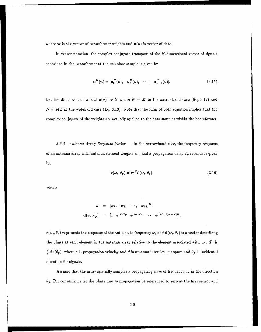
where w is the vector of beamformer weights and u(n) is vector of data.

In vector notation, the complex conjugate transpose of the N-dimensional vector of signals

contained in the beamformer at the nth time sample is given by

u' (n) -- [u' (n), u' (n), -. u' 1 (n)]. (3.15)

Let the dimension of w and u(n) be N where N = M in the narrowband case (Eq. 3.12) and

N = ML in the wideband case (Eq. 3.13). Note that the form of both equation implies that the

complex conjugate of the weights are actually applied to the data samples within the beamformer.

3.3.3 Antenna Array Response Vector. In the narrowband case, the frequency response

of an antenna array with antenna element weights Wm and a propagation delay Tp seconds is given

by,

r(wc, Op) = w Hd(weOp), (3.16)

where

w = [W1, W2, WMI H.

d(wc, Op) = [1 ej "- TP ej 2-c

T p ... ej(M-1)TP]H.

r(w,, Op) represents the response of the antenna to frequency w, and d(w,, Op) is a vector describing

the phase at each element in the antenna array relative to the element associated with wl. Tp is

d sin(Op), where c is propagation velocity and d is antenna interelement space and Op is incidental

direction for signals.

Assume that the array spatially samples a propagating wave of frequency w, in the direction

Op. For convenience let the phase due to propagation be referenced to zero at the first sensor and

3-8

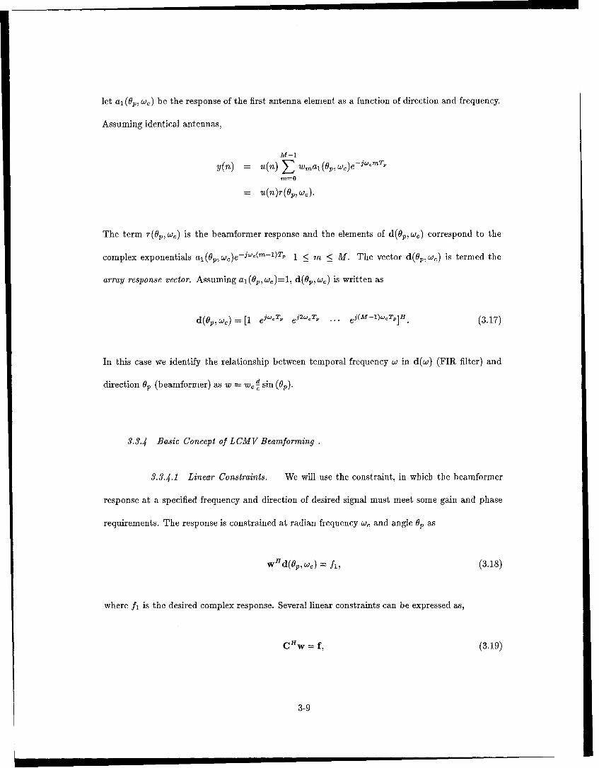
let a, (OP, w,) be the response of the first antenna element as a function of direction and frequency.

Assuming identical antennas,

M-1

y(n) = u(n) E wmai(9p,w)e-wmTp

M=O

= u(n)r(Op,w c).

The term r(Op,w,) is the beamformer response and the elements of d(0p, w,) correspond to the

complex exponentials aj(Op,w,)e- jwc(m - 1)T 1 < m < M. The vector d(O,w,) is termed the

array response vector. Assuming a, (0p, w,)=1, d(Op, w,) is written as

d(Op,wc) = [1 ej'cTp ej2"cT ... ej(M-1)wcTp]H . (3.17)

In this case we identify the relationship between temporal frequency w in d(w) (FIR filter) and

direction Op (beamformer) as w = w, dsin (0p).

3.3.4 Basic Concept of LCMV Beamforming.

3.3.4.1 Linear Constraints. We will use the constraint, in which the beamformer

response at a specified frequency and direction of desired signal must meet some gain and phase

requirements. The response is constrained at radian frequency w, and angle OP as

wHd(0p,w,) = fl, (3.18)

where fl is the desired complex response. Several linear constraints can be expressed as,

C'fw = f, (3.19)

3-9

where C is the constraint matrix and f is the response vector.

In the narrowband case, the matrix C is chosen to contain r linear constraints so the above

equation represents r linearly independent columns in M unknowns. The weight vector w has length

M, while C is an M xr matrix. If M = r, then w is uniquely determined by the constraints. To

ensure there is a w which satisfies the constraints, r is chosen to be less than M. Here we consider

the desired signal gain-only constraint,

C = d(Or, w,) (3.20)

where

d(Op, we) - [le jwcTv 6j2w0Tp

... eI(u1)WCTP]H, (3.21)

d(Op, we) is M x 1 and Tp is E sin Op, c is propagation velocity and d is antenna interelement space

and Op is incidental direction for signals.

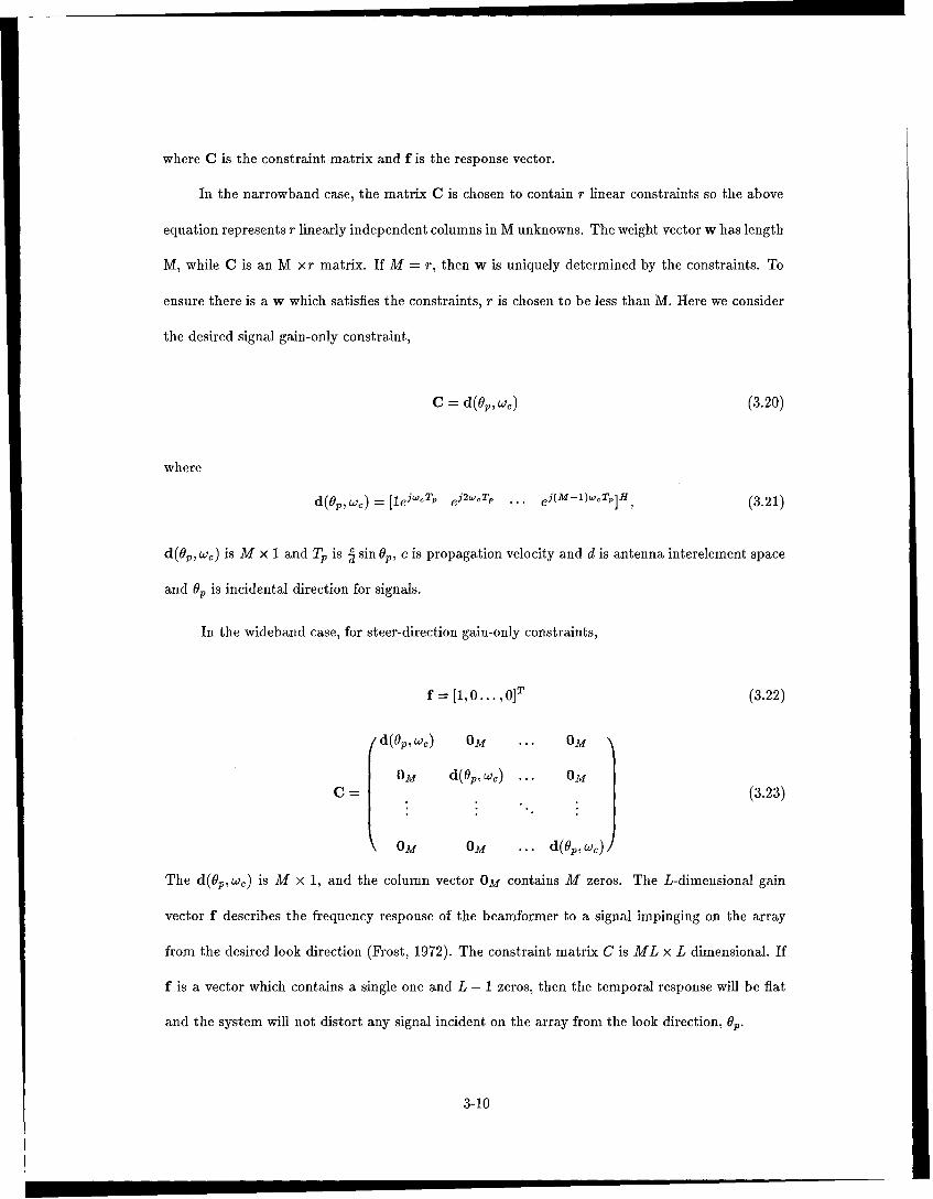
In the wideband case, for steer-direction gain-only constraints,

f = [1, 0... ,] (3.22)

d(0p, w,) Om ... Om

0M d(Op, w,) ... OM

C= (3.23)

0 M 0 M ... d(0p ,we)

The d(Op, w,) is M x 1, and the column vector 0 M contains M zeros. The L-dimensional gain

vector f describes the frequency response of the beamformer to a signal impinging on the array

from the desired look direction (Frost, 1972). The constraint matrix C is ML x L dimensional. If

f is a vector which contains a single one and L - 1 zeros, then the temporal response will be flat

and the system will not distort any signal incident on the array from the look direction, Op.

3-10

3.3.4.2 LCMV Approach. Variance minimization effectively minimizes the interfer-

ence and noise power at the beamformer output while the constraints preserve the signal of interest.

Formally stated, we derive

min(Po) = min(wHR w), subject to CHw = f, (3.24)w W

where P0 represents the output power. Ru = E{uuH} represents the exact covariance matrix of

the received signal u. The Eq. 3.24 is to find out the weight vector for minimum output P,. The

solution is derived in Appendix A using Lagrange multipliers, given by,

wopt = R-lC[CHR-lC]-lf. (3.25)

The inverse exists because C is full rank and R, is positive definite because the data always contains

an uncorrelated noise component.

3.3.5 LCMV-GSC Beamformer.

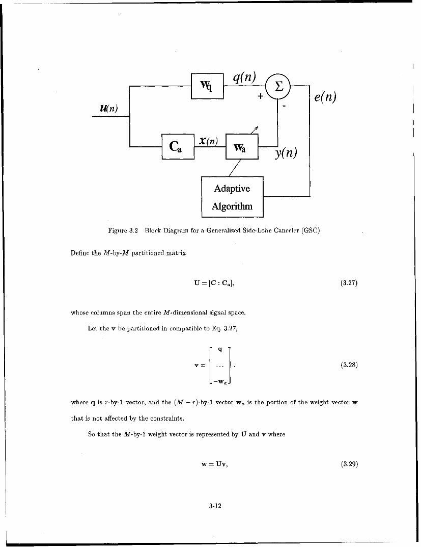
3.3.5.1 Basic Concept of GSC. Fig. 3.2 shows the generalized sidelobe canceler

(GSC) block diagram. Note that the input vector is the M-dimensional stacked data vector u(n)

for the narrowband signal. For steer direction gain only constraints (r = 1), the linear constraint

is defined in Eq. 3.20. Let the columns of an M x (M - r) matrix Ca be defined as a basis for

the orthogonal complement of the space spanned by the columns of matrix C which is composed

of orthonormal columns. Using the definition of an orthogonal complement, we may thus write

CHCa = 0. (3.26)

3-11

1kn)

Adaptive

Algorithm

Figure 3.2 Block Diagram for a Generalized Side-Lobe Canceler (GSC)

Define the M-by-M partitioned matrix

U = [C: Ca], (3.27)

whose columns span the entire M-dimensional signal space.

Let the v be partitioned in compatible to Eq. 3.27,

q

V = . . (3.28)

- a-

where q is r-by-1 vector, and the (M - r)-by-1 vector Wa is the portion of the weight vector w

that is not affected by the constraints.

So that the M-by-1 weight vector is represented by U and v where

w = Uv, (3.29)

3-12

and U-' exists because the determinant U is not zero,

v = U-w. (3.30)

We may use Eq. 3.27 and Eq. 3.28 in Eq. 3.29 to obtain

.q

w = [c:co . (3.31)

- a .

= Cq- CaWa. (3.32)

Now, inserting Eq. 3.32 into Eq. 3.19, we obtain

C5Cq - CHCaWa = f. (3.33)

Through Eq. 3.26, the Eq. 3.33 will be,

CHCq = f. (3.34)

Therefore, solving for the vector q,

q = (CHC)-f, (3.35)

which shows the linear constraint doesn't affect wa.

Define the non-adaptive beamformer component represented by, which is the first part of

Eq. 3.32,

Wq = Cq = C(CHC)-lf. (3.36)

3-13

Substituting Eq. 3.36 into Eq. 3.32 yields the follow equation relating,

W Wq - Cawa. (3.37)

Substituting Eq. 3.37 into Eq. 3.19,

CHWq - CHCaWa - f. (3.38)

By virtue of Eq. 3.26,

CHWq = f (3.39)

which shows the non-adaptive component Wq of the weights w satisfies the linear constraints. The

weight vector wq is termed the quiescent weight vector because it is optimum LCMV weight vector

when the environment is quiet. As the results, the GSC has only one data dependent element Wa

due to the fact that both the quiescent beamformer Wq in the upper path and the blocking matrix

Ca in the lower path depend only on the constraint equations.

Note that the constraint does not affect wa because wa embodies the available degrees of

freedom in w. The second term on the right side of Eq. 3.37 is incorporated in the lower branch

of the GSC and is essentially an unconstrained adaptive beamforming, which have the M - T the

number of adaptive weights. The constraint matrix C preserves the desired signal. But the matrix

Ca blocks any portion of the data that is constrained in the space spanned by the columns of C.

Consequently, no part of the received signal subspace is allowed to pass through the lower branch

of the GSC. The matrix C is for this reason called the blocking matrix.

3.3.5.2 LMS Estimate of Weights for LCMV-GSC Beamforming. We perform the

unconstrained minimization of the mean-squared value to minimize the effect of the jammer by

adjusting the weight vector Wa using LMS algorithm. According to Eq. 3.14, the beamformer

3-14

output y(n) is expressed by the inner product,

y(n) = w'u(n), (3.40)

where u(n) is the electrical signal picked up by first antenna element of the linear array in Fig. 1.1

and Fig. 2.4 at time n. By substituting Eq. 3.37 in Eq. 3.40, the beamformer output in Fig. 3.2 is,

y(n) = wwu(n) - w,, C'u(n). (3.41)

In Eq. 3.41, the inner product w Hu(n) plays the role of quiescent response:

q(n) = wq'u(n). (3.42)

Similary, the matrix product CH u(n) plays the role of input vector for the adjustable weight vector

Wa. To emphasize this point, we let

x(n) = Canu(n). (3.43)

We are now ready to formulate the LMS algorithm for the adaption of weight vector wa(n)

in the GSC. The derivation is based on Section 3.2, especially Eq. 3.11. We may write

Wa(n +i) = Wa(n)±/XCau(T)e*(h)

Wa(l) +/ Cau(n)(wH u(n) - WHCHu(n))*

= wa(n) + - HCU(n)u(n)H(wq - CaWa(fl)). (3.44)

3.3.5.3 Optimum Value of Weights for LCMV-GSC Beamforming. Based upon

this explanation of the GSC, we can now express the LCMV beamformer with the following

3-15

unconstrained minimization equation (Haykin and Steinhardt, 1992),

P, = min(wq - Cawa)HRu(wq - Cawa), (3.45)Wa

or

P0 min(W-'Ruw, - Wq R Ca Wa - WC a Ruwq + W a C a RuCaWa). (3.46)Wo

Completing the square we have

P = min [Wa - (C a RCa) C a Rwq]Ca aCa[wa - (CaR )aCRwq]

+W HRwqw - wRuC a(CHR Ca)-GCRw,. (3.47)

The matrix C, is full rank and Ru is positive definite so CH RUCn is positive definite and the

inverse exists. Eq. 3.47 is minimized when

Wa = (CHaRuCa) -ICHRuwq. (3.48)

The minimum output power is obtained using this set of weights and is given by

P 0 = Wa Rwq - w H RCa(CaaRuCa)- 1 CH'uwq. (3.49)

Suppose u = s +j where s is the component of the data due to the desired signal and j is the

component due to jammer signal. Assume that the constraints are chosen to preserve the desired

signal, that is, s lies in the space spanned by the columns of C so CHR8 = 0. This implies that

the beamformer output is

q s + (Wq - Cawa)Hj. (3.50)

3-16

If we further assume that the signal and interference are uncorrelated, then the output power or

variance is expressed as

E{lly 2} = w R Wq + wHRjw, (3.51)

where w 0 Rjw is the jamming signal component of the output power. Therefore, minimizing the

total output power subject to CHw = f is equivalent to minimizing the jammer output power

subject to the same constraints. Substitute the GSC representation for w into Eq. 3.51 with wa

given by Eq. 3.48 and utilize the identity CH R, = 0 to express the minimum output power P as

a sum of signal output power, P, and jammer output power, Pj where

P, = wHRWq

P, = wHRjw. (3.52)

The mean squared error (MSE) between the desired signal and the beamformer output is easily

derived using the GSC representation. We assume the constraints are chosen so that the beamformer

output in the absence of interference and noise is equal to the desired signal, yd. that is, Yd = Wq s.

Defining the MSE as

MSE = Elyd - y12 }, (3.53)

and substituting Eq. 3.50 into Eq. 3.53 yields

MSE = E{IwHjl2 }

= wH Rjw. (3.54)

Comparison of Eq. 3.52 and Eq. 3.54 indicates that the LCMV criterion is equivalent to a minimum

MSE criterion.

3-17

Examination of Eq. 3.48 reveals the similarity with the standard Wiener solution. Consider

the auto-covariance of x(n) in Fig. 3.2,

R. = E{xx} = CaRuCa, (3.55)

because x(n) = CH u(n).

Now, consider the cross covariance of the signals x(n) and q(n),

rxq = E{x(n)q(n)"} (3.56)

= E{CH u(n)uH(n)wq} (3.57)

C a Rwq. (3.58)

Comparing Eq. 3.55 and Eq. 3.58 with Eq. 3.48, we can rewrite Eq. 3.48 as,

Wa = R -'Rurxq, (3.59)

which shows the similarity between the standard Wiener solution and the solution implemented

with a GSC.

3.3.6 Summary. A beamformer forms a weighted combination of the outputs of spatially

separate antennas in order to separate propagating signals that originate from different locations.

The weights determine the spatial and temporal filtering characteristics of the beamformer. In

an adaptive beamformer the weights are adjusted in response to the data received at the antenna

for the purpose of optimizing the beamformer's response. A common criterion for optimizing the

weights is minimization of beamformer output power or variance. The goal of minimizing output

power is to minimize the contributions of jammer to the output. The LCMV approach minimizes

output power subject to a set of linear constraints on the weight vector. These constraints are

3-18

used to control the response of the beamformer in the direction of the desired signal to prevent the

weights from cancelling the desired signal.

The GSC separates the weight vector into constrained and unconstrained components. The

unconstrained components represent the beamformer's adaptive degrees of freedom and are adjusted

using standard adaptive algorithm. In order to suppress the jammer signal from different incoming

direction, the optimum weight vector and LMS estimate of weight vector were calculated (Eq. 3.48

and Eq. 3.44).

3.4 Adaptive Beamforming in the Presence of Correlated Signals

3.4.1 Introduction. The behavior of adaptive arrays when the interference(s) is correlated

with the desired signal is of concern in some environments. We will call two signals fully correlated

if one is a scaled, delayed replica of the other. Correlation can destroy the performance of a

constrained adaptive array through two effects: 1) the beamformer fails to form deep nulls in

the directions of the correlated interferences (Reddy et al, 1987) and 2) the desired signal can

be partially or completely cancelled (Widrow et al, 1982). This problem can be overcome by a

technique called spatial smoothing which modulates the interference in a way that will reduce the

correlation with the desired signal. A method of combining spatial smoothing with LMS algorithm

will be illustrated.

3.4.2 Analysis of the Decorrelation Effect of Spatial Smoothing. In the GSC depicted in

Fig. 3.2, the weights wq passes the desired signal through the upper branch while the matrix Ca

blocks it from the lower branch. If however the desired signal is correlated with an interference,

the signals in the lower branch of the GSC structure can be used to cancel the desired signal in the

upper branch. This is because the interference is a version of the desired signal that is not removed

from the lower branch by the spatial filter Ca.

3-19

Let u(n) be the simultaneously sampled vector (snapshot) of array signals.

u(.) = [u' (n), u'(n), u' It(n)] (3.60)

where

u7 (n) = [Ut×M(n), UjXM+1(n), "", UixM+M--1(n)], 0 < i < L- 1. (3.61)

Let the dimension of u(n) be N where N = M in the narrowband case (Eq. 3.12) and N = M x L

in the wideband case (Eq. 3.13). In Eq. 3.60, u(n) is N x 1 with element,

ui(n) = u[nT - mod(i - 1,M)T, - INT( M 1 )To], 1 < i < N, (3.62)

where mod stands for modulo and INT is integer. T, is sampling time and Tp represents the time

delay due to propagation and the delay time T, of each tap in the TDL antenna array is determined

by

T= (3.63)

where R8 is the sampling frequency of the arriving signal.

To simplify our work we restrict our analysis to the case of two signals. One of these is the

desired signal, and the other is a correlated interference. In Eq. 3.62, u(n) represents the desired

signal when Tp is Td and interference signal when Tp is Tj.

The basic concept of spatial smoothing is as follows. Assume that the uniform linear array of

M sensors is extended with additional sensors and the extended array is grouped into sub-arrays

of size M. The first sub-array is formed from the sensors 1,-.. , M, and the second sub-array is

formed from the sensors 2, ... , M + 1, and so on. Let us denote the vector of received signals at

3-20

the kth sub-array by uk. The kth sub array and the i th element of the input vector is,

u(n) = u[nT- mod(i + k - 1,M + k)Tp + INT(---)To], 1 <i <N, (3.64)

where the superscript indicates the kth subarray and the subscript indicates the ith element of the

input vector. The array covariance matrix of the kth sub-array is then given by

R k = E{(uk)(uk)H} (3.65)

We define the spatially smoothing covariance matrix with K number of smoothing steps as

K-- R" (3.66)

k=1

Combining Eq. 3.65 and Eq. 3.66, we obtain

1 K

= Z E{(u')(uk)H} (3.67)

where u(n) is composed of desired signal and interference signal in the kth subarray. Hence, we

have

1gR = E[ u]u ]" (3.68)

- K + R + E[(ud)(u)'] + E[(uj)(Ud)H] (3.69)

= RS+RRj + R j (3.70)

where A,8 is the autocorrelation of desired signal and Aj is the autocorrelation of jamming signal,

and lt8 j is crosscorrelation between the desired signal and jamming signal in the kth sub-array.

3-21

We now study how progressive spatial smoothing reduces the crosscorrelation between all the

incident wavefronts, and hence between the desired signal and the other interference wavefronts,

and therefore impacts interferences cancellation. If we assume the incident wavefronts are frequency

hopped signal, we can write,

u(n) = u(n)e(h), Th-1 n < Th, (3.71)

where the signal arrival vector, e(h), is N x 1 with element i,

ej(h) = exp[-j{mod(i - 1, M)Op(h) + INT( M Ih0(h)}J, 1 < i < N. (3.72)

Here Op(h) is changed to Od(h) for the desired signal interelement phase shift during hop h and qj

for the interference signal interelement phase shift during hop j, i.e,

¢d(h) = UhTd

where Wh and wi is the desired signal and jamming signal hopping frequencies respectively. There-

fore, ed(h) represents the desired signal and ej(h) does the jamming signal. Also 00(h) is the phase

shift by delay time To, so,

d0'(h) = WhTo

q5 (h) = wjT.

In Eq. 3.70, the first term R, is

K

k=0

3-22

K

E 1 E{udud}E{(e(h))(e(h))'}

E exp[-j{mod(i + k - 1, M + k)(Od - qd) + INT((i - I)/(M + k))(00 - 00)}]}=0

R,

because qd and 0' cancel out causing the exponential terms to zero. Thus exponential becomes

equal to one and thus the sum adds to K. Also Aj = Rj. Therefore Eq. 3.70 is

+ R, E exp[-jfmod(i + k - 1, M + k)(qOd - sbj) + INT((i - 1)1(M + k))(O' - ]

K

+ Rj, Zexp[-j{mod(i + k - 1, M + k)(%5 - ed) + INT((i - 1)/(M + k))(O - € )J].

The crosscorrelation parts (the third and fourth parts of above equation) go to zero as the number of

smoothing steps, K, goes to infinity. Therefore the signals are progressively decorrelated. The rate

which the cross-correlation part approaches zero depends on the hopping frequency and propagation

delay (Reddy et al, 1987).

The smoothing covariance matrix (Eq. 3.66) is used to calculate the weight vector wa in the

GSC, as Eq. 3.44

Wa(l + 1) = wa(n) + itCa'ft(wq - Cawa(,)). (3.73)

3.4.3 Summary. A jammer that is correlated with the desired signal arises due to mul-

tipath propagation or intelligent jamming and creates a special problem for conventional adaptive

beamforming. The goal of this section was to illustrate how spatial smoothing combined with a

LMS adaptation of array weights can remove correlated interference in a GSC. The crosscorrelation

between desired signal and jammer signal goes to zero as the number of smoothing steps, K, goes

to infinity.

3-23

3.5 Conclusion

This chapter illustrated the theory of adaptive signal processing. The temporal and spatial

filters mathematical formulations and procedures for their solution are indeed similar, even though

they are used in different application areas. Adaptive temporal filter converges to the optimum

Wiener solution in a stationary environment. The adaptive beamformer as the spatial filter forms

a weighted combination of the outputs of spatially separated antennas in order to suppress propa-

gating signals that originate from different locations. The LCMV-GSC beamformer is used, which

minimize the output power with related to the undesired signals. The adaptive arrays when the

interference(s) is correlated with the desired signal were totally destroyed. As the solution, Section

3.4 suggested the spatial smoothing technique to reduce the crosscorrelation between the desired

signal and the jamming signal. The next chapter will simulate the jamming suppression in the

several cases.

3-24

IV. Simulation

This chapter considers the simulation of jamming suppression in several cases. A LAS antenna

array has just M antenna elements [Fig. 1.1] while TDL antenna array has L delayed taps in

each of the mth antenna element channel [Fig. 2.4]. Section 4.1 compares the performance of

wideband interference suppression in these two different antenna arrays. Next section 4.2 presents

two techniques in the frequency hopped environment. The first technique is the conventional

method in which only the center frequency of the desired signal is used in the constraint matrix

(Eq. 3.19). The second one uses each hopping frequency of the desired signal. For all of the above

cases, we assume that the desired signal and the jamming signals are uncorrelated. In section 4.3,

we investigate the case when the desired signal and jammer signals are correlated. Finally the

results of using an adaptive filter in the time domain for narrowband jamming signals suppression

is presented.

4.1 Wideband Jamming Suppression in Antenna Arrays,

4.1.1 LAS Antenna Array and Frequency Characteristics. As described in Section 3.3.2,

the signal output of a LAS antenna array with M antennas is

y(n)= wHu(n). (4.1)

where y(n) is the output of antenna array, and w is weight vector and u(n) is input signal vector,

W = [ 1 ,5 0 2 ,." ",WM]

u(n) = [u1(n),u 2 (n),. . um(n)]

ui(n) = u[nT - mod(i - 1, M)Tp], 1 < i < M

4-1

where Tp = d sin(Op) is the interelement propagation delay: Op is the direction of the incident signal.

The subscript d for the desired signal and j for the jammer signal, d is the antenna interelement

space which is a half wavelength at the center frequency. Thus

d.TP= d-sinOP

CTp -- A sin Op

2c1

- Jc sin Op.

The signal vector, u(n) can be written as

u(n) = Ud(n) + uj(n), (4.2)

where Ud(n) and uj (n) are vectors containing the desired and interference signals respectively. Ud

and uj(n) are assumed to be uncorrelated.

To calculate the weight coefficient of the LAS antenna array, a linear constraint minimum vari-

ance generalized sidelobe canceller (LCMV-GSC) beamformer is used as described in Section 3.3.5.

The desired signal direction gain-only constraint equation is expressed as,

CHW = f, (4.3)

where C is the constraint matrix, C = d(Od, we) and f is the response vector, f = 1.

d(Od, W,)=[1, ejwTd, ej2w. Td, ... , ei(M-1)w Td]H, (4.4)

where Od is the incident direction, measured with respect to the boresight (i.e., the normal to the

array), w, is the center frequency of the desired signal.

The non-adaptive beamformer component in the generalized sidelobe canceller (GSC) is rep-

4-2

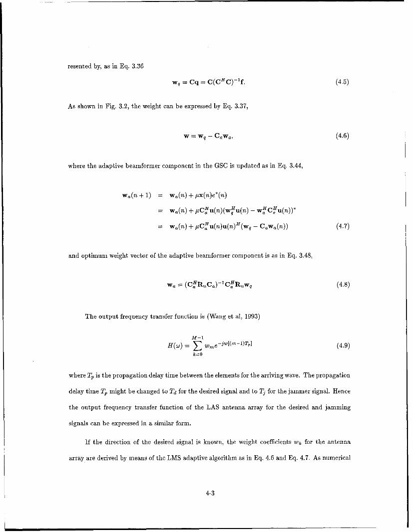
resented by, as in Eq. 3.36

Wq = Cq= C(CHC)-lf. (4.5)

As shown in Fig. 3.2, the weight can be expressed by Eq. 3.37,

W = Wq - CaWa, (4.6)

where the adaptive beamformer component in the GSC is updated as in Eq. 3.44,

Wa(f-+1) wa(Tn)+-tx(n)e*(n)

= Wa(n) + IC'u(n)(w'u(n) -

= Wa(n) + tLC. u(n)u(n)H(Wq - CaWa(n)) (4.7)

and optimum weight vector of the adaptive beamformer component is as in Eq. 3.48,

=CH -1H

Wa a(C RuCa) C a Rwq (4.8)

The output frequency transfer function is (Wang et al, 1993)

M-1

H(w) => wme - j [(m ' )Tl (4.9)k=O

where Tp is the propagation delay time between the elements for the arriving wave. The propagation

delay time Tp might be changed to Td for the desired signal and to Tj for the jammer signal. Hence

the output frequency transfer function of the LAS antenna array for the desired and jamming

signals can be expressed in a similar form.

If the direction of the desired signal is known, the weight coefficients Wk for the antenna

array are derived by means of the LMS adaptive algorithm as in Eq. 4.6 and Eq. 4.7. As numerical

4-3

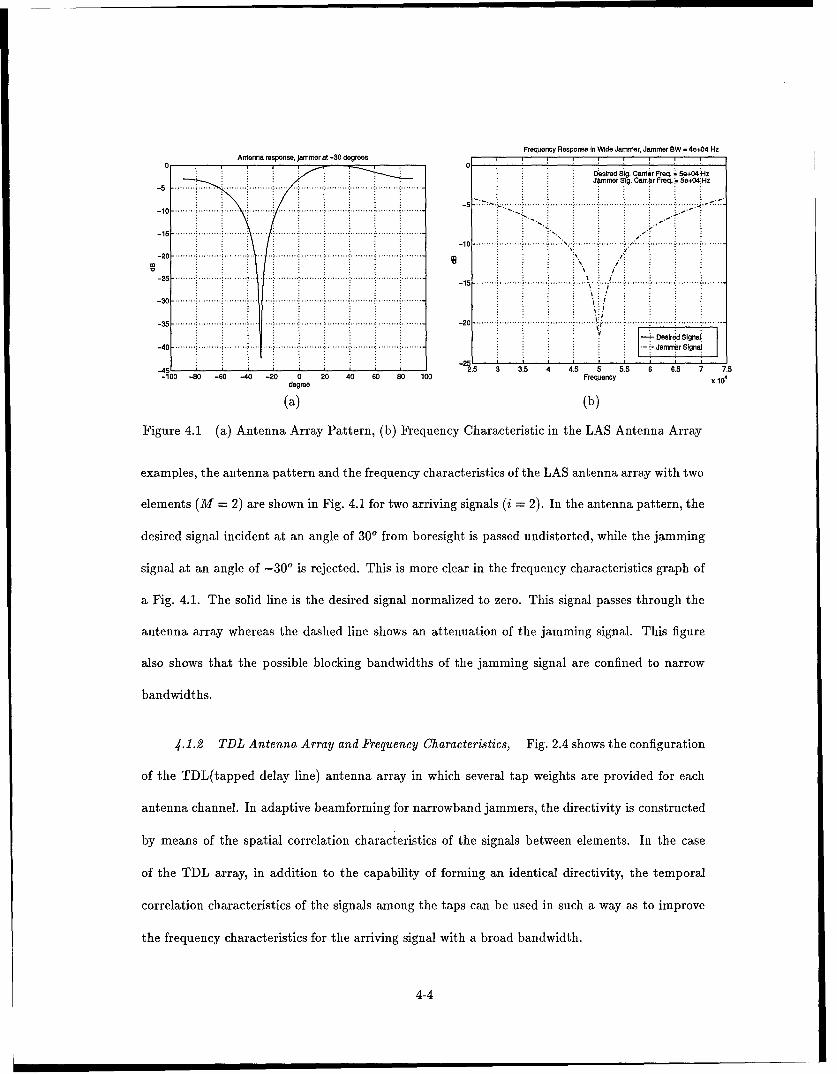
Frequency Response In Wide Jammer, Jammer BW - 4e+04 HzAntenna response, Jammer at -30 degrees - 7 - r - , , ,

Dieslred Sig. Carder Freq. 5 e+04 HzJammer Sig. Carribr Freq. 6 Se+04:Hz

-5 o -.-.., . .. ......... .. ... ............. .. .. .. .. .. .. .. .... .. .. ............... .. .......... .......--5 ..-10 ......... .... ...... ...... ......... .... .... .... : .... ... .........

-15 -.~ .. . .. . .. . .. . . .. . .. . .. . ....... '" ...... ..... ...................................... .. .....-1 0 ................ ............ ...... .................. ......... .........

.... .... I .. . . ... . . .

-20 .. . .........

-305.............. ............... ............................. .........

Desired Signet-40 ..... .... . .. . .. ............... ..... .. Jammen r Signal

-45 2.5 3 3.5 4 4. 6 6.5 7 7.5-100 -80 -60 -20 0 20 40 60 80 100 Frequency X 10,

degree

(a) (b)

Figure 4.1 (a) Antenna Array Pattern, (b) Frequency Characteristic in the LAS Antenna Array

examples, the antenna pattern and the frequency characteristics of the LAS antenna array with two

elements (M = 2) are shown in Fig. 4.1 for two arriving signals (i = 2). In the antenna pattern, the

desired signal incident at an angle of 300 from boresight is passed undistorted, while the jamming

signal at an angle of -30' is rejected. This is more clear in the frequency characteristics graph of

a Fig. 4.1. The solid line is the desired signal normalized to zero. This signal passes through the

antenna array whereas the dashed line shows an attenuation of the jamming signal. This figure

also shows that the possible blocking bandwidths of the jamming signal are confined to narrow

bandwidths.

4.1.2 TDL Antenna Array and Frequency Characteristics, Fig. 2.4 shows the configuration

of the TDL(tapped delay line) antenna array in which several tap weights are provided for each

antenna channel. In adaptive beamforming for narrowband jammers, the directivity is constructed

by means of the spatial correlation characteristics of the signals between elements. In the case

of the TDL array, in addition to the capability of forming an identical directivity, the temporal

correlation characteristics of the signals among the taps can be used in such a way as to improve

the frequency characteristics for the arriving signal with a broad bandwidth.

4-4

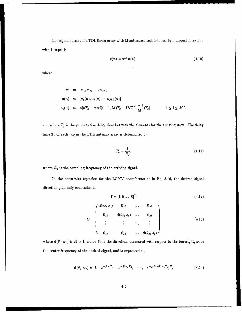
The signal output of a TDL linear array with M antennas, each followed by a tapped delay-line

with L taps, is

y(n) =wu(n). (4.10)

where

W = ['WlW2,-" ,WML]

u(n) = uj(n),U2 (n),.. UML(Th)I

ui(n) u(nT - mod(i - 1,M)T, - INT(--z-)T] 1 < i < ML

and where Tp is the propagation delay time between the elements for the arriving wave. The delay

time T of each tap in the TDL antenna array is determined by

1To = . -, (4.11)

where R8 is the sampling frequency of the arriving signal.

In the constraint equation for the LCMV beamformer as in Eq. 3.19, the desired signal

direction gain-only constraint is,

f = [1, 0... , 0]r (4.12)

d(Od, W,) OM ... OM

OM d(Od, w,) ... OMC j (4.13)

Om 0M ... d(Od, c

where d(Od, W,) is M x 1, where Od is the direction, measured with respect to the boresight, U;, is

the center frequency of the desired signal, and is expressed as,

d(Od,W,)=[1, e- j -CTd, e -j 2 cTd, ... , e-(M-)1Td]H, (4.14)

4-5

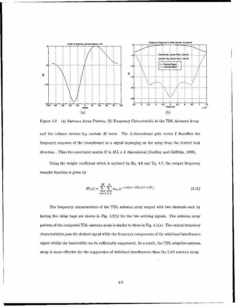
Antenna response, jammer degree -30 0 Frequency Response In Wide Jammer, RJ -2e+04

......... ......... Dasired Sig. ariarPreq .. p+04.... ......... .......

Jamrn er Sig Carrier Freq. 5,+04

'10 .. Desired Signal . . .

-l F ...... .. " " ......... ........... .................... :. ...... ... ...... ... " : ". .. .......

-10 . " "-0 .... . .. . .. .... ... ... .. . ... .. .... ...... .. ... ... .. .. .. .. .. .. ................................ ..........

-2 s ... ... .... ... i .... ... ... .... i ... ... i .... .... ...... .... ..... ........ .. .... ...20 ... ..... .. ...

-25....

-15L I - - -i

-100 -80 60 40 -20 0 20 40 60 80 100 2.5 3 3.5 4 4.5 5 5.5 6 6.5 7 7.5degree Frequency X 10'

(a) (b)

Figure 4.2 (a) Antenna Array Pattern, (b) Frequency Characteristic in the TDL Antenna Array

and the column vectors OM contain M zeros. The L-dimensional gain vector f describes the

frequency response of the beamformer to a signal impinging on the array from the desired look

direction . Thus the constraint matrix C is ML x L dimensional (Buckley and Griffiths, 1988).

Using the weight coefficient which is updated by Eq. 4.6 and Eq. 4.7, the output frequency

transfer function is given by

M L

H(w) = : w,ze - j [( ' -1)T+( - 1)T°] . (4.15)m-=--1 I

The frequency characteristics of the TDL antenna array output with two elements each by

having five delay taps are shown in Fig. 4.2(b) for the two arriving signals. The antenna array

pattern of the computed TDL antenna array is similar to those in Fig. 4.1(a). The output frequency

characteristics pass the desired signal while the frequency components of the wideband interference

signal within the bandwidth can be sufficiently suppressed. As a result, the TDL adaptive antenna

array is more effective for the suppression of wideband interferences than the LAS antenna array.

4-6

Item Desired Signal Jamming SignalDirection at Arrival 300 -300Carrier Frequency 15 x 104 (Hz) 15 x 10 4 (Hz)

Bandwidth 6 x 103 (Hz) 6 x 10Sampling Frequency 12 x 10' Hz

No. of TDL array elements 8No. of TDL tap elements 10, 20

TDL array tap delay 1/Rs

Table 4.1 Specification for First Computer Simulation

4.1.3 Comparison of Two Antennas. In the previous section, the output frequency

characteristics of the LAS and TDL adaptive antenna array were studied. In this section, the

performance of two antenna arrays is compared using output signal to jammer ratio (SJR) in

the presence of wideband jammers. The wideband signals shown in Table 4.1 were used for this

simulation. Their fractional bandwidth is a A = 0.04. Fractional bandwidth larger than 0.02 are

defined as wideband signals [section 3.1.3].

The performance of this system is demonstrated by exploring the input and output SJR and

improvement defined as,

SoSJRo - 7

J.

SJR, - j (4.16)i

SJRoIMP - SJR, (4.17)

where Si and S, is the desired signal input and output power, and Ji and J, is the jamming signal

power, respectively.

The LMS weight estimate is updated at each time n by Eq. 4.6 and Eq. 4.7. Fig. 4.3 shows

the IMP of the LAS and TDL antenna array as the function of iteration. Both systems have a

good convergence characteristic. IMP of the TDL antenna array converges to higher value than

IMP of the LAS antenna array. In order to see this more clearly, the IMP is separated into the

4-7

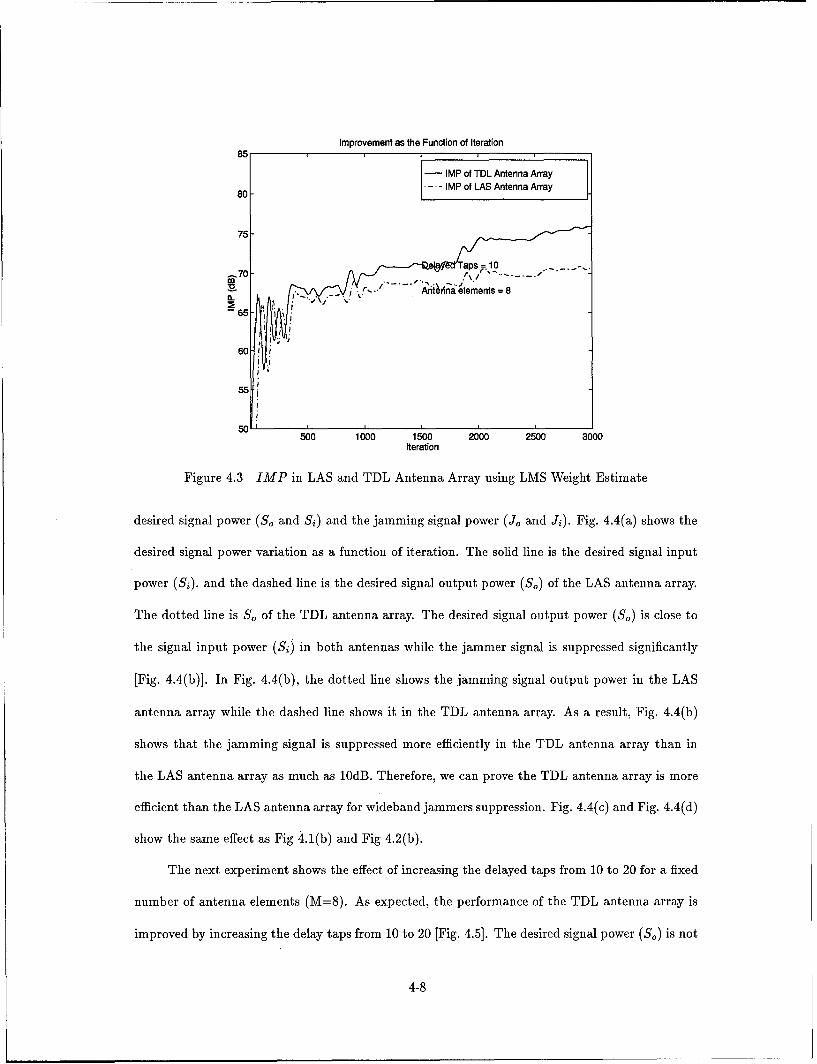
Improvement as the Function of Iteration

85 1..

- IMP of TDL Antenna Array

80 4.3 MPIMP of LAS Antenna Array

75-

_70 eas-1

Afi~na~i'eements =8

55

50'500 1000 1500 2000 2500 3000

Iteration

Figure 4.3 IMP in LAS and TDL Antenna Array using LMS Weight Estimate

desired signal power (S. and Si) and the jamming signal power (J, and Ji). Fig. 4.4(a) shows the

desired signal power variation as a function of iteration. The solid line is the desired signal input

power (Si), and the dashed line is the desired signal output power (So) of the LAS antenna array.

The dotted line is So, of the TDL antenna array. The desired signal output power (So) is close to

the signal input power (Si) in both antennas while the jammer signal is suppressed significantly

[Fig. 4.4(b)]. In Fig. 4.4(b), the dotted line shows the jamming signal output power in the LAS

antenna array while the dashed line shows it in the TDL antenna array. As a result, Fig. 4.4(b)

shows that the jamming signal is suppressed more efficiently in the TDL antenna array than in

the LAS antenna array as much as 10dB. Therefore, we can prove the TDL antenna array is more

efficient than the LAS antenna array for wideband jammers suppression. Fig. 4.4(c) and Fig. 4.4(d)

show the same effect as Fig 4.1(b) and Fig 4.2(b).

The next experiment shows the effect of increasing the delayed taps from 10 to 20 for a fixed

number of antenna elements (M=8). As expected, the performance of the TDL antenna array is

improved by increasing the delay taps from 10 to 20 [Fig. 4.5]. The desired signal power (S,) is not

4-8

Input and Output Desired Signal Power In Iteration

Input and Output Jamtmer Signel Power In Iteration

10

05-1

-2

0.u -40-

S-0

-- 60

-Var. of Desired Sig. Input -70-. ...

-2a.o55g Otu I O Var. at Jammer Output In TDL-... Var. ot Sig. Output In LAS -0~ wedme~lui A

500 1000 1500 2000 2500 3000 -0 1n 0oo 15oo zooo 2WO 3000iteration Iteration

(a) (b)Frequency Response In Wide Jammer, Jammer BW .6000 Frequency Response In Wide Jammer, Jammer SW .6000

0.DDeaired Signa

i - Jammer Signai-10 .. .. .. .. . .. .. ... .. . .. .. .. 0 ...

- 1 .... ....... . .... ....... ...... ....... ...... .....

250 -.-............... 40............... ......... ........ D sr d S g a

-60l~n 50.e

-70... . . .. .-6 0 .. ................ .. . .. .. .

A0 14 149....... 15.... 151....... 152.153.1.7.14..148.51.152.1.5

..re......en...... .... ..re..quen.......

(c).. (d) .. .... ... ...Figur 4..4.. nput and.. Output Poe .fT adLSAtnaAras()DsrdSga at

(b) Jamming. Signal...... Part Frqec Chrateisic.o.().ASAnena.rry.n

(d) TDL...... Antenna Array...... Respectively..................... ......... ....

........ ....... .. .. . 40 ......4 9..

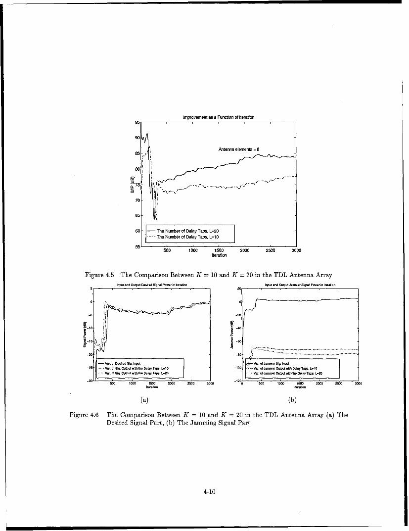
Improvement as a Function of Iteration

90

Antenna elements =8

5-,

500 100 150 200 200 30

56

10 00 10 20 50 30

5 20

-20- -40

Var. of Desired Sig. Input <eL- Ve. of Jamomer Sig. Input-25- Var. of Sig. Output with tihe Delay Teps, L 10 -100 Vea, of Jemmer Output with Deiay Tape, L1t

Var. of Sig. Output with the Delay Taps, WO.2 Var. of Jamner Output with the Delay Tap, L.20

-30--12C500 1000 1000 2000 2000 300 500 1000o to 1000 2000 2500 3000

Iteraion Iteraion

(a) (b)

Figure 4.6 The Comparison Between K = 10 and K =20 in the TDL Antenna Array (a) TheDesired Signal Part, (b) The Jamming Signal Part

4-10

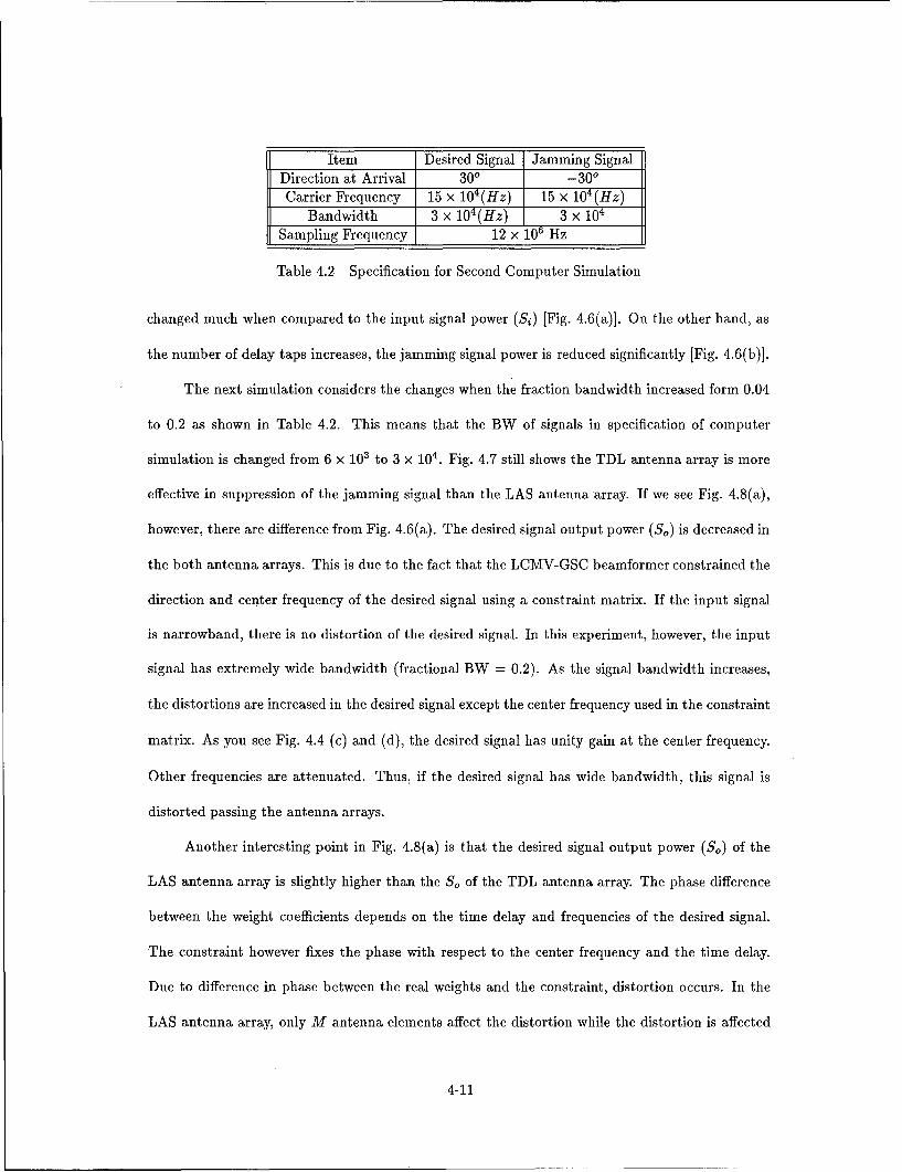
Item Desired Signal Jamming SignalDirection at Arrival 300 -300

Carrier Frequency 15 x 104 (Hz) 15 x 104 (Hz)Bandwidth 3 x 10 (Hz) 3 x 101

Sampling Frequency 12 x 106 Hz

Table 4.2 Specification for Second Computer Simulation

changed much when compared to the input signal power (Si) [Fig. 4.6(a)]. On the other hand, as

the number of delay taps increases, the jamming signal power is reduced significantly [Fig. 4.6(b)].

The next simulation considers the changes when the fraction bandwidth increased form 0.04

to 0.2 as shown in Table 4.2. This means that the BW of signals in specification of computer

simulation is changed from 6 x 103 to 3 x 101. Fig. 4.7 still shows the TDL antenna array is more

effective in suppression of the jamming signal than the LAS antenna array. If we see Fig. 4.8(a),

however, there are difference from Fig. 4.6(a). The desired signal output power (So) is decreased in

the both antenna arrays. This is due to the fact that the LCMV-GSC beamformer constrained the

direction and center frequency of the desired signal using a constraint matrix. If the input signal

is narrowband, there is no distortion of the desired signal. In this experiment, however, the input

signal has extremely wide bandwidth (fractional BW = 0.2). As the signal bandwidth increases,

the distortions are increased in the desired signal except the center frequency used in the constraint

matrix. As you see Fig. 4.4 (c) and (d), the desired signal has unity gain at the center frequency.

Other frequencies are attenuated. Thus, if the desired signal has wide bandwidth, this signal is

distorted passing the antenna arrays.

Another interesting point in Fig. 4.8(a) is that the desired signal output power (So) of the

LAS antenna array is slightly higher than the So of the TDL antenna array. The phase difference

between the weight coefficients depends on the time delay and frequencies of the desired signal.

The constraint however fixes the phase with respect to the center frequency and the time delay.

Due to difference in phase between the real weights and the constraint, distortion occurs. In the

LAS antenna array, only M antenna elements affect the distortion while the distortion is affected

4-11

Improvement as the Function of Iteration60

|8-- IMP of TDL Antenna Array* -54 IMP of LAS Antenna Array

56

54-

750

42

40500 1000 1500 2000 2500 3000

Iteration

Figure 4.7 IMP in LAS and TDL Antenna Array using LMS Weight Estimate

by not only M antenna elements but also (M - 1)L delayed taps in the TDL antenna array.

Fig. 4.8(b) indicates the jamming signal input and output powers as a function of iteration.

Both systems show the good convergence for jamming signal suppression. As the number of the

iteration increases, the TDL antenna array suppresses the jamming signal more than the LAS

antenna array.

The next experiment shows the performance effect by increasing the delayed taps from 10 to

20 in the extreme wideband signals. The IMP of the TDL antenna array decreases even though

the number of delayed taps increases, as shown in Fig. 4.9. The reason is that the desired signal

distortion was more serious with the larger number of delayed taps [Fig 4.10(a)]. Furthermore the

capability of the jamming signal suppression is not even changed [Fig 4.10(b)].

4-12

Input and Output Desired Signal Powar In Iteration Input and Output Jammer Signal Power In Iteration

0 -

-20-

_1-40

V-20 -4 - V

-Var. of Desirad Sig. Input-.- Var. of Sig. Oatput In MOL -6----------l~utarDL -~~~~~~~:x Var. ofi. attinLS* V.t Jammer Output In LAS

5 00 150 2() 50 3000 1500 2000 2000 3000Iteration Itercan

(a) (b)Fraquancy Resaponse In Wide Jammer Fraquency Rlesponae In Wide Jamnmer

0 ...

-20 30..... .... ...

-30 .. ......... ... ...

~~~~~~~~~~~~~~~~~Jamm Signal FeunyCaatrsiso c A nen ra n d DA nt nn A rra Respectively. ............... ... ...... .............

'o 20 ........ ..... ..........I ....... 4 -1 3 .

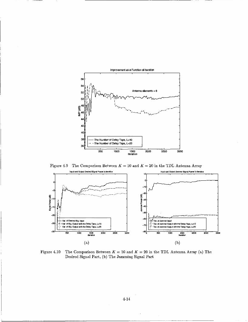
Improvement as a Function of Iteration

56-

52 i it .-. Antenna elements =8

52. . -~

11.7-

385 TeNmbr0 eayTpL1

400

38 Te Nubero~ela~aps-L10

500 1000 1500 -00 250 30

5 0

-0.-

-60-

-50I

VrofDesired Signal Part, (o) Theme JamigpinauPr

-2 - a. f i. utu wthte elyTasL10Vr.ofJmmr upu wt te4-14Tas L1

4.2 Jamming Suppression in Frequency-Hopped Environment

This section examines the output S JR performance of adaptive arrays in a Frequency-Hopped

(FH) environment. The combined effects of the arrays interference nulling ability and the interfer-

ence protection of FH signals result in a more robust interference rejection communication system.

As concluded in the previous section, the TDL antenna array should be more effective than the

LAS antenna array for frequency-hopped jamming signal suppression, because FH signals also have

wide bandwidths.

In the next example, two different techniques are used for frequency hopped jamming sup-

pression in the TDL antenna array. The first conventional technique is the same as the method of

section 4.1.2, which uses the center frequency in the constraint matrix. The second method uses a

hopping frequency in the constraint matrix.

4.2.1 Conventional Technique for Frequency-Hopped Environment. For the experiment,

the TDL(tapped delay line) antenna array is used. With M antenna elements spaced a half wave-

length apart at the center frequency of the FH band, w, = 2irf . A desired signal is incident on

the array from direction 0 d and with hopping frequencies wh = 2lrfh, and an jamming signal from

direction Oj and at its hopping frequencies wj = 2rfj. The input signal vector, u(n) can be written

as,

u(n) = ud(n) + u3 (n), (4.18)

where ud(n) and ug(n) are vectors containing the desired and interference signals respectively. Ud

and uj(n) are assumed to be uncorrelated.

The delay time T, of each tap in the TDL antenna array is determined by

1

T. = 7-1 (4.19)

4-15

where f, is the carrier frequency of the arriving signal. R.T Compton shows the coefficient -y in his

journal (Compton, 1988) as

1< < (4.20)

B B1

where B is determined as the normalized jammer bandwidth, B

The form of the desired signal vector and interference signal vector are

u(n) = u(n)e(h), Th-I :_ n < Th, (4.21)

where Th-1 < n < Th is the time duration of the hth hop interval, and the signal arrival vector is,

ei(h) = exp[-j{mod(i - 1, M)¢p(h) - INT( - )¢p(h)}]. (4.22)

Here, qd(h) is the desired signal interelement phase shift during hop h and Oj is the interference

signal interelement phase shift during hop j, i.e,

¢d(h) = WhTd

Oj(h) = wjTj,

and 00(h) is the phase shift due to taps delay time To, so,

00(h) = WhT

¢b?(h) = wjTo.

The constraint matrix and the weight coefficient of the TDL antenna array is the same as the

section 4.1.2. The frequency characteristics of the frequency hopped signals and the comparison

between the LAS antenna array and the TDL antenna array are very similar to Fig. 4.2 and Fig. 4.3,

respectively since frequency hopped signals belong to the wideband signals.

4-16

4.2.2 New Technique for Frequency-Hopped Environment. The signal output of the TDL

linear array with M antennas, each followed by a tapped delay-line with L taps, is

y(n) = wH u, (4.23)

where

w = [W1,W 2 , WML]

u = u(n)e(h), Th- n < Th.

The signal arrival vector is

ej(h) = exp[-j{mod(i - 1,M)Ob(h) - INT( iM 1 )Th(h)}]. (4.24)

Here, Od(h) is the desired signal interelement phase shift during hop h, and Oi is the interference

signal interelement phase shift. And 00(h) is the phase shift due to delay time T.

In the constraint equation, the desired signal direction gain-only constraint is,

f = [1, 0..., O]T , (4.25)

andd(Od, Wh) OK ... OM

OM d(Od, Wh) ... MC =(4.26)

OM 0M ... d(Od, Wh)

4-17

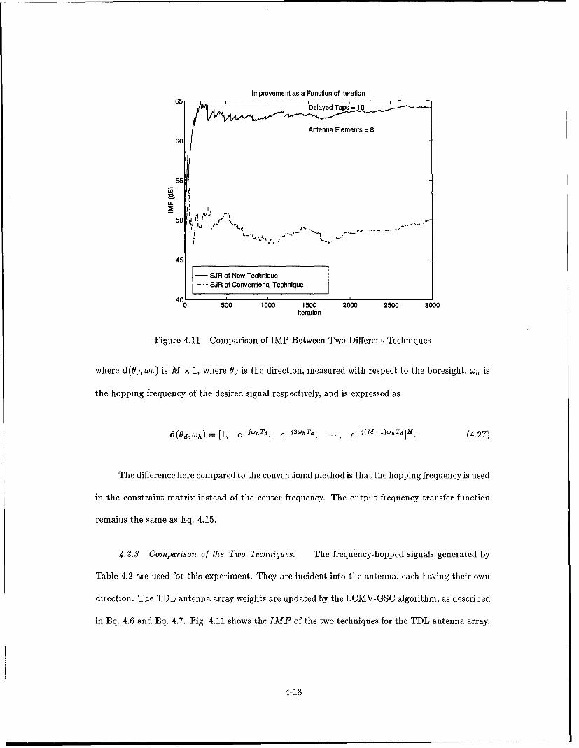
Improvement as a Function of Iteration65, , , Delayed Taps' = 1 '

Antenna Elements =8

6-

55

50 i ,.

45-

- SJR of New Technique. SJR of Conventional Technique

0 500 1000 1500 2000 2500 3000Iteration

Figure 4.11 Comparison of IMP Between Two Different Techniques

where d(9d, Wh) is M X 1, where Od is the direction, measured with respect to the boresight, Wh is

the hopping frequency of the desired signal respectively, and is expressed as

d(Od,wh) = [1, e-

jwhTd, e - 2whTd, ., ej(M1)whTd]H. (4.27)

The difference here compared to the conventional method is that the hopping frequency is used

in the constraint matrix instead of the center frequency. The output frequency transfer function

remains the same as Eq. 4.15.

4.2.3 Comparison of the Two Techniques. The frequency-hopped signals generated by

Table 4.2 are used for this experiment. They are incident into the antenna, each having their own

direction. The TDL antenna array weights are updated by the LCMV-GSC algorithm, as described

in Eq. 4.6 and Eq. 4.7. Fig. 4.11 shows the IMP of the two techniques for the TDL antenna array.

4-18

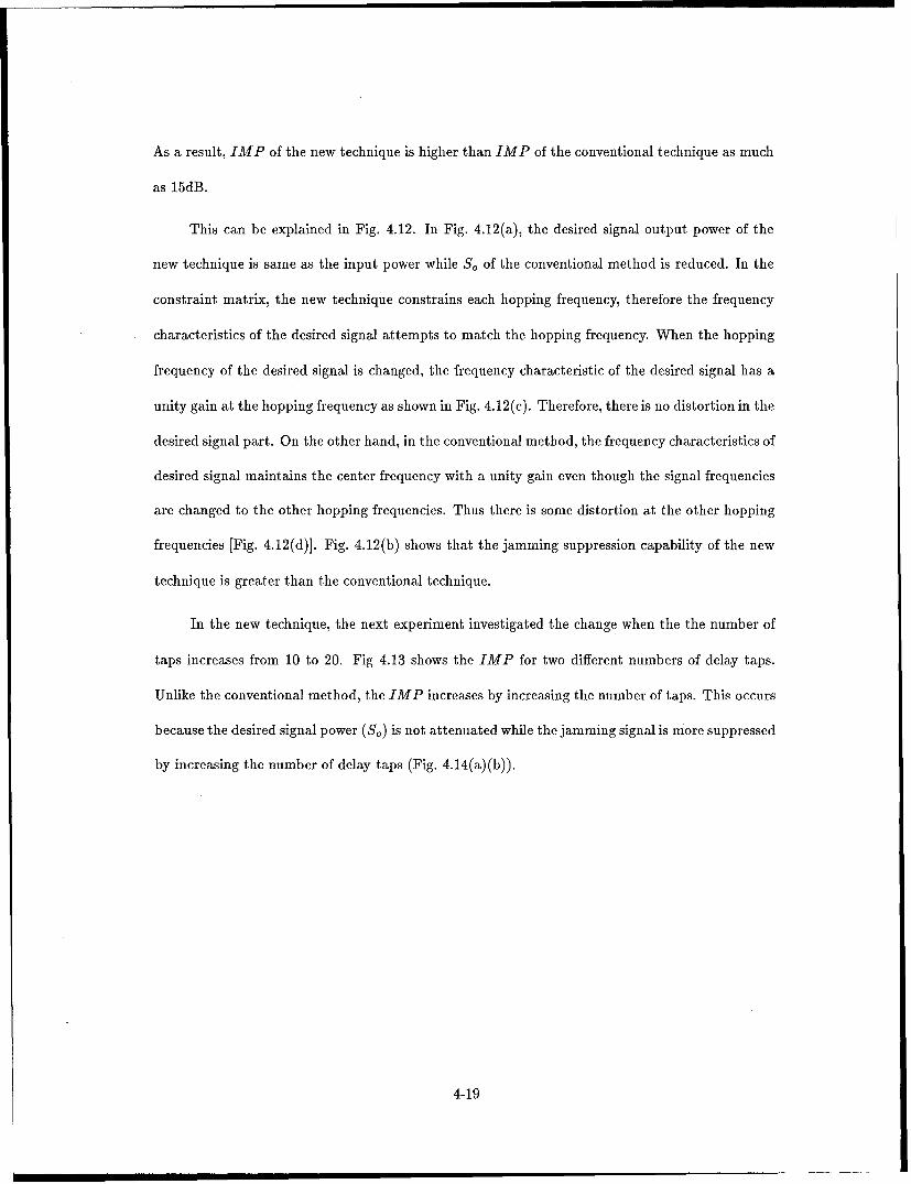
As a result, IMP of the new technique is higher than IMP of the conventional technique as much

as 15dB.

This can be explained in Fig. 4.12. In Fig. 4.12(a), the desired signal output power of the

new technique is same as the input power while S0 of the conventional method is reduced. In the

constraint matrix, the new technique constrains each hopping frequency, therefore the frequency

characteristics of the desired signal attempts to match the hopping frequency. When the hopping

frequency of the desired signal is changed, the frequency characteristic of the desired signal has a

unity gain at the hopping frequency as shown in Fig. 4.12(c). Therefore, there is no distortion in the

desired signal part. On the other hand, in the conventional method, the frequency characteristics of

desired signal maintains the center frequency with a unity gain even though the signal frequencies

are changed to the other hopping frequencies. Thus there is some distortion at the other hopping

frequencies [Fig. 4.12(d)]. Fig. 4.12(b) shows that the jamming suppression capability of the new

technique is greater than the conventional technique.

In the new technique, the next experiment investigated the change when the the number of

taps increases from 10 to 20. Fig 4.13 shows the IMP for two different numbers of delay taps.

Unlike the conventional method, the IMP increases by increasing the number of taps. This occurs

because the desired signal power (S,) is not attenuated while the jamming signal is more suppressed

by increasing the number of delay taps (Fig. 4.14(a)(b)).

4-19

Input and Output Desired Signat Power In Iteration Input and Output Jammer Signal Power as a Funtion of Iteration2 10

Signals BW -4e+04

00

-10-

-20-

Z5- 6 ~-40

-8

-1.*.VroSgOtu e~cnqe-0. of Desired Sig. Input -'otnte nu......... ..... .........

.V. of Sig. Output In Corivenflonal Technique .Va. of Jammar Output In OConventions! Technique

0 00 100 100 2000 200 000500 1000 1000 2000 2500 2000Iteration Iteration

(a) (b)Frequency Response In Wide Jemnmer Frequency Response In Wide Jamimer

0

-10- Jarnner hopping treq. - 1.694e+05 -10 aromer hopping freq. - 1.694e+05Sig. hopping treq. 1 .428e+05Si.hpngfe..142e0

-20- 2

--- -- - - ...........-

to -40 -

-50- -50

-60 I-ardSga Desired Signal 1

1.2 1.3 1.4 1.5 1.6 1.7 1.0 1.3 1.30 1.4 1.42 1.5 1.55 1.6 1.60 1,7Frequency 0 Frequencyx10

(c) (d)

Figure 4.12 Input and Output Power of New and Conventional Technique (a) Desired Signal Part(b) Jamming Signal Part, Frequency Characteristics of (c) New Technique and (d)Conventional Technique Respectively

4-20

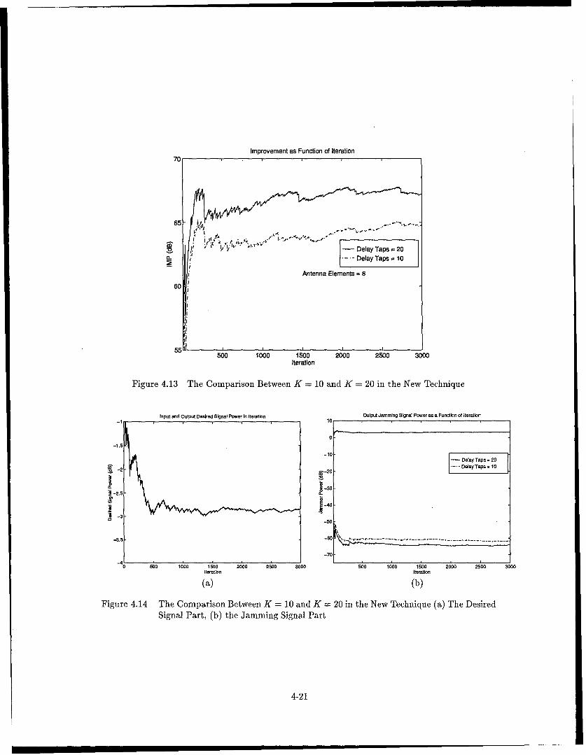
Improvement as Function of Iteration

L',. -Delay Taps =20

Delay Taps = 10

Antenna Elements =8

500 1000 1500 2000 2500 3000Iteration

Figure 4.13 The Comparison Between K =10 and K =20 in the New Technique

Input and Output Desired Signal Power In Iteration Output Jamming Signal Power as a Function of Iteration-i 10

0-

-10--Delay Taps . 20

-2---Delayraps .10

;3 -2

-4-2.5-

-3,5 -80 -- -- - ------.- -- -- - -- -- - -- -

0 S00 1000 1500 2000 2500 3000 500 1000 1500 2000 2500 3000Iteration Iteration

(a) (b)

Figure 4.14 The Comparison Between K = 10 and K = 20 in the New Technique (a) The DesiredSignal Part, (b) the Jamming Signal Part

4-21

4.3 The Performance of a Spatial Smoothing Technique for Correlated Signals

This section presents an example case in which the desired signal and the jamming signal are

correlated. The simulation uses the GSC adaptive weights, using the method which is described

in section 3.4. Both signals have wide bandwidths, and the correlation coefficient between desired

signal and jammer signal is 1,

SR--- 3 -1 , (4.28)P=RRj

where R3 j is the cross correlation between the desired signal and the jamming signal and R,,Rj

are the autocorrelation of the desired signal, the jamming signal respectively.

For this experiment, the LCMV beamformer with the TDL antenna array is used as in the

previous section. The input signals and the weight vectors are the same as in Section 4.1. The only

difference from section 4.1 is that the signals are correlated with each other.

The correlation matrix used for updating the weights is, as in Eq. 3.66,

K

R= KE R,. (4.29)k=I

The sub-array size M was fixed at 4 and the number of delayed taps is 10. The number

of smoothing steps K is 5. The desired signal input power and the jamming signal input power

are equal. Fig. 4.15 shows the SJR of three different cases as a function of iterations . The

solid line shows the SJRo when the signals are uncorrelated, while the dashed line and the dot-

and-dashed line show the correlated signals case. The dashed line displays before decorrelation,

which means K = 1. At that time, the SJRo is reduced significantly, because the antenna can't

put a null to the direction of the jamming signal as shown in Fig. 4.16(c). The jamming signal

is a replica of the desired signal. The antenna array accepts the jamming signal as the desired

signal. This fact shows that the adaptive antenna array is useless in the case of smart jammers

and multipath signals because those jamming signals and multipath signals are highly correlated

4-22

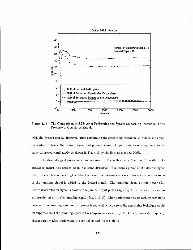
Output SJR in iteration

45

40 Number of Smoothing Steps = 5Delayed Taps = 10

35 . ,

30

n25-

S20

15

10 - SJR of Uncorrelated Signals

5- -- R of Correlated Signals after Decorrelation- - SJR o 6omeated Signals before Decorrelation

0 -- tnput-Sj ........................ ...

0 500 1000 1500 2000 2500 3000iteration

Figure 4.15 The Comparison of SJR After Performing the Spatial Smoothing Technique in thePresence of Correlated Signals

with the desired signal. However, after performing the smoothing technique to reduce the cross-

correlation between the desired signal and jammer signal, the performance of adaptive antenna

array improved significantly as shown in Fig. 4.15 by the lines as much as 20dB.

The desired signal power variation is shown in Fig. 4.16(a) as a function of iteration. As

explained earlier, the desired signal has some distortion. The output power of the desired signal

before decorrelation has a higher value than even the uncorrelated case. This occurs because some

of the jamming signal is added to the desired signal. The jamming signal output power (Jo)

before decorrelation signal is close to the jammer input power (Ji) (Fig. 4.16(b)), which shows no

suppression at all in the jamming signal (Fig. 4.16(c)). After performing the smoothing technique

however, the jamming signal output power is reduced, which shows the smoothing technique works

for suppression of the jamming signal in the adaptive antenna array. Fig 4.16(d) shows the frequency

characteristics after performing the spatial smoothing technique.

4-23

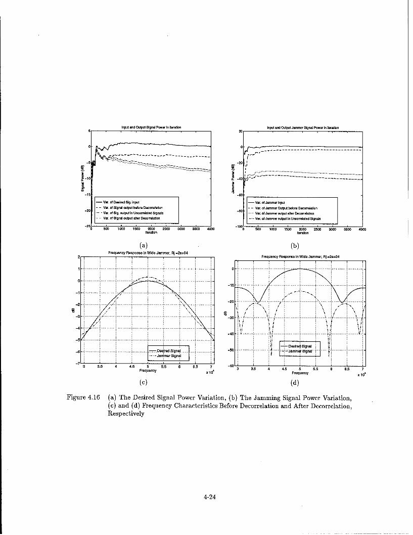
Input end Output Signal Power In Iteration Input saut Output Jammer Signal Power In Iteration

5 20

20

-g6

Var1. of Desired Sig. Input - Va. of Jammer Input

-20 Var. of Signal output before Decoeeton 80- - 'a. of Jammer Output before Decorralation*--Var. of Sig. output In Unconealeted Signals ...1Va. of Jammrer output atter Decerrelation

.Var. of Signal output after Decorrelftion - ar'1. of Jammer output In Uncorrelated Signals

0 0 10 15 100 5100 3000 3500 4000 DOC 50 100 10 2000 25300 3000 3500 4000Iteration ntration

(a) (b)Frequency Response in Wide Jammer, Rj -29+04 FeunyRsos nWd amr ].e0

-40 ...... ..........

-2 ...... ................ % DurdSga.......................... ..... ~-~ ~ ~ c I eierSga

-3 3.. . . . . . . . . . . .. .. . .. . ... . ... .5.....5.5 6 . . . . .5 7.. .. . _30 .. . .. . ....... __ .. . . . . . . .. .. . . . . . . . . . . .Frequency~~~~" 01 w"T4 . .5 6 6

Respectively

4-2

4.4 Adaptive Filter for Narrowband Interference Suppression

The desired signal used here is the same as that which is generated in Section 4.1. The desired

signal is assumed to be known in the receiver. The jamming signal is a single tone jammer. The

number of taps is 12. The input signal vector, u and weight vector w are,

u = [u(n),u(n- 1) ..... u(n- M± 1)]T

w = [W1,w2 ..... WMT,

where M = 12 is the number of taps.

The instantaneous estimated value of the tap-weight vector at time n ± 1 is computed by

using the simple recursive relation as in Eq. 3.11,

*(n + 1) = *(n) + ,u(n)[d*(n) - uH(n)*]. (4.30)

where d(n) is the desired signal, and pi . is the step size parameter. Amax is the largest

eigenvalue of correlation matrix R.

The performance of this adaptive filter is demonstrated by exploring the SJR improvement.

Fig. 4.17(a) shows the SJR improvement as a function of iterations. Fig. 4.17(b) shows the frequency

characteristics of the adaptive filter. This system inserts the notch filter at the jammer carrier

frequency at the cost suppressing that frequency in the desired signal. Therefore this system only

works for narrowband jamming signal suppression. The jamming signal is suppressed well after

just a few first iterations [Fig. 4.17(d)]. On the other hand, the desired signal is also suppressed at

the first iterations. However as the number of iterations increases, the desired signal recovers its

input power [Fig. 4.17(c)]. This means the notch filter is narrowing in order to avoid suppressing

the desired signal. Eventually, the desired signal output power approaches the input power. Thus

the SJR improvement of this system reaches the amount of jamming signal suppression.

4-25

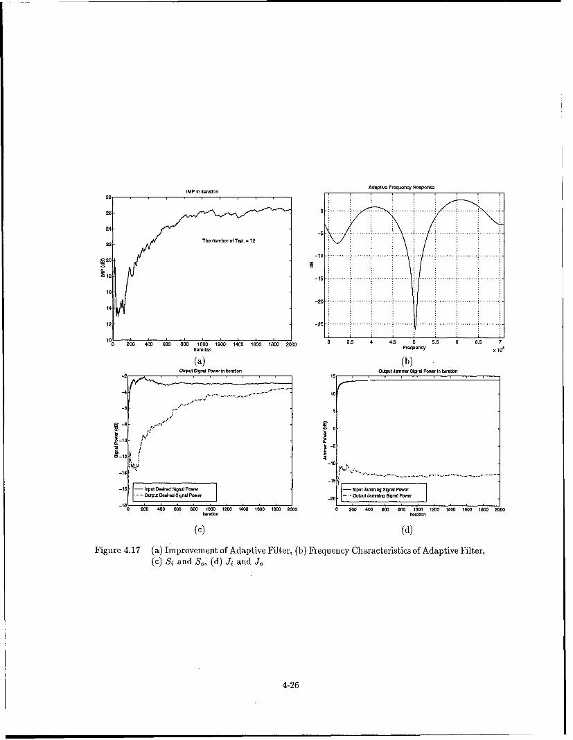
IMP In Relation Adaptive Frequency Response

26

24-

22

g20

-15

0 240 600 800 1000 1200 1400 1600 1800 200 3. 4.5 5 5 6 6.5 70 2 Iteration 2DOFrequency X14

(a) (b)Output Signal Power In Iteration Output Jamnmer Signal Fewer In Iteraton

-2 15

e~~~ -5 -

I IN II

J. -10

-10

-16 - Input Desired Signal Power I nput Jamming Signal Powe-.- Output Desired Signal Fewer -20- Output Jamming Signal Fewer

0 0 40 600 800 1000 1200 1400 1600 1800 2000 0 200 400 600 800 1000 1200 1400 1600 1800 2000Iteration fterallon

(c) (d)

Figure 4.17 (a) Improvement of Adaptive Filter, (b) Frequency Characteristics of Adaptive Filter,(c) Si and S,,, (d) Ji and J,,

4-26

4.5 Conclusion

This chapter considered the simulation of jamming signal suppression. The TDL antenna

array is more effective than the LAS antenna array to suppress the wideband interference in the

LCMV-GSC beamformer. In the frequency-hopped environment, a new technique, which the hop-

ping frequencies are used in the desired signal direction gain-only constraint matrix, suppressed

wideband jamming signal more efficiently than the conventional method. The smoothing technique

was demonstrated to reduce the cross-correlation of the desired and jamming signal. After perform-

ing this technique, the jamming signal was suppressed significantly. Finally, the performance of

the adaptive filter was shown for suppression of the narrowband jamming signal. The next chapter

will conclude this research and recommend research topics for future study.

4-27

V. Conclusion and Recommendations for Future Research

5.1 Conclusion

Interference(s) is a significant problem in military communication operations. This thesis

examined the suppression of interference using the SJR as a metric for comparing the adaptive

temporal filter and adaptive spatial filter (i.e. adaptive beamforming). In these systems, the opti-

mum weights are selected to optimize the response based on the statistics of the data. The data

statistics are often unknown and may change with time so adaptive algorithms are used to obtain

weights that converge to the statistically optimum solution. Here, the most well-known and simple

algorithm, LMS algorithm was used.

For the class of beamformer, a procedure was presented for the design and implementation of

a LCMV beamformer for wideband interference suppression. This beamformer attempts to achieve

the minimum output variance subject to the constraint on the gain in the desired signal direction.

The structure used extends the GSC to implement and to analyze the LCMV beamformer. The

GSC separates the weight vector with constrained and unconstrained components. The constrained

components represent the gain and phase of the desired signal and its direction. The unconstrained

components are adjusted using the LMS adaptive algorithm. Using the LCMV-GSC beamformer,

it was shown that the TDL adaptive antenna array is more effective for the suppression of wideband

jammer suppression than the LAS adaptive antenna array.

Further, in the frequency-hopped environment, the new technique was introduced which used

each hopping frequency for the desired signal direction gain-only constraint in the LCMV beam-

former. This new technique improved the capability of wideband interference suppression over the

conventional technique which used only the center frequency in the constraint matrix. The reason

is that the new technique does not distort the desired signal, while the conventional technique

severely distorts the desired signal.

Then the effect of the spatial smoothing in the presence of the correlated signals was ana-

5-1

lyzed. When the desired signal was correlated with the jamming signal, the LCMV beamforming

performed poorly because the adaptive antenna array accepted the jamming signal as the desired

signal. Therefore it couldn't put a null in the direction of the jamming signal. After performing

the spatial smoothing technique, however, the adaptive antenna array inserted a deep null for sup-

pression of the jamming signal.

Finally, the adaptive temporal filter was shown to adequately suppress narrowband jammers.

The drawback of this system however, is that it can not be used to suppress wideband interference.

5.2 Recommendation for Future Study

There are three main areas of research that can be derived from this thesis effort. These three

areas are,

* Adaptive Beamforming for Wideband Interference.

* Spatial Smoothing in the Presence of Correlated Signals.

* Adaptive Filter for Narrowband Interference.

In the first of these areas, there are the desired signal distortions when using the conventional

technique. Future study is recommended to investigate a way to decrease this distortion. Since the

desired signal is distorted, the SJR decreases even though the number of delayed taps increases.

Thus it is recommended to study the optimum number of delayed taps and antenna elements. This

thesis was limited to a single jammer and jamming signal direction. The performance of interfer-

ence suppression needs to be observed for a larger number of jammers and for changing directions.

Because of the computational consideration, the partially adaptive beamformer with array com-

posed of large numbers of sensors has been investigated and remained as a good topic.

Another area for possible research is suppression of the jamming signal correlated with the

desired signal. This area arises due to multipath propagation or smart jamming and creates a

serious problem for conventional adaptive beamformer. The spatial smoothing technique is based

5-2

on averaging to destroy the correlation between the signal and interference. However, correlated

interference suppression still remains an important research topic.

A final recommended area for future research regards temporal adaptive filters. It is recom-

mended to compare the performance of interference suppression of the time domain adaptive filter

with the transform domain adaptive filter and the transform domain excisor.

5-3

Appendix A. Constrained Optimization

The typical constraints optimization problem has the form

minf(x), subject to g(x)=O, (A.1)x

where f(.) is the scalar-valued objective function and g(.) is the vector-valued constaint function.

The classical approach to solving a constrained optimization problem is the method of Lagrange

multipliers, A. The Lagrangian of a constrained optimization problem is defined to be the scalar-

valued function

L(x, A) = f(x) + Ag(x). (A.2)

In the case at hand one minimize wHRw subject to the linear constraint CHw = f. w is weight

vector and R. is autocorrelation vector of input vector, x. The constraint g(x) = CHw - f is a

scalar-valued one where C is the constraint matrix and f is response vector. The Lagrangian is

L(w, A) = WHRw + A(CHw - f). (A.3)

Its gradient is 2Rw + AC with a solution,

Wopt = -A 0ptR-l . (A.4)2

To find the value of the Lagrange multiplier, this solution must satisfy the constraint. Imposing

the constraint,

A "ptCH R-lC = -2f. (A.5)

By solving with A pt,2f

A0p - CHR_ C (A.6)

A-1

The total solution is

wot=fR-' C (A.7)CHR-1C

A-2

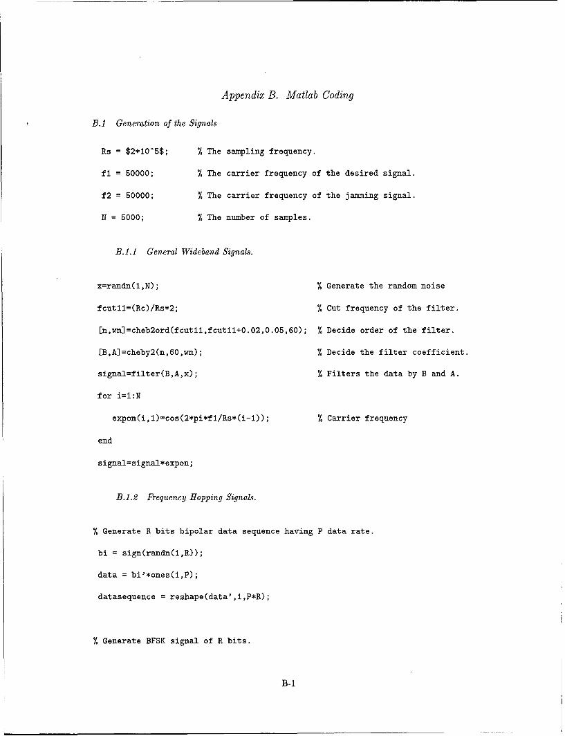
Appendix B. Matlab Coding

B.1 Generation of the Signals

Rs = $2*10^5$; % The sampling frequency.

fl = 50000; % The carrier frequency of the desired signal.

f2 = 50000; % The carrier frequency of the jamming signal.

N = 5000; % The number of samples.

B.1.1 General Wideband Signals.

x=randn(l,N); % Generate the random noise

fcutll=(Rc)/Rs*2; % Cut frequency of the filter.

[n,wn]=cheb2ord(fcutll,fcutil+0.02,0.05,60); % Decide order of the filter.

EB,A]=cheby2(n,60,wn); % Decide the filter coefficient.

signal=filter(B,A,x); % Filters the data by B and A.

for i=l:N

expon(i,1)=cos(2*pi*fl/Rs*(i-1)); % Carrier frequency

end

signal=signal*expon;

B.I.2 Frequency Hopping Signals.

% Generate R bits bipolar data sequence having P data rate.

bi = sign(randn(i,R));

data = bi'*ones(1,P);

datasequence = reshape(data',l,P*R);

% Generate BFSK signal of R bits.

B-I

bfsk=zeros(M,length(n)); % Initial value of BFSK signal.

w1=1000; % The first frequency of BFSK signal.

w2=2000; % The second frequency of BFSK signal.

n=1:20;

bfskl=cos(2*pi*wl.*n./fsim); % The data sequence of the first BFSK signal.

bfsk2=cos(2*pi*w2/fsim.*n); %. The data sequence of the second BFSK signal.

for i1l:R % Decide the bipolar data sequence

if bi(i)==l % using BFSK sequences.

bfsk(i, :)=bfskl;

else

bfsk(i, :)=bfsk2;

end

end

databfsk=reshape(bfsk',l,M*length(n)); % Generate the BFSK signal.

% Generate hopping signal.

hzeros(pg,N); % Initial value of hopping signal.

for i=1:pg

num(i)=round(rand(1,1)*pg);

end

for i1l:pg;

ffl(i)=fh*num(i)+fi; % Decide the hopping frequency.

for n=1:N;

h(i,n)=cos(2*pi*ffl(i)*n/fsim); % Make the hopping sequence.

end

end

h=reshape(h' ,l,N*pg);

B-2

% Generate the FH (Frequency Hopping) signal.

signal=databfsk. *h;

B.2 LCMV Adaptive Beamforming

M = 12; % The number of antenna elements.

K = 5; % The number of delayed Taps.

mul = 0.0002; % The step size parameter.

thd = 30*pi/180; % The desired signal direction.

thi = -30*pi/180; % The jamming signal direction.

Td = 2/fl*sin(thd); % Propagation delay by signal.

Ti = 2/fl*sin(thi); % Propagation delay by jammer.

ffl % The signal hopping frequency.

% Generate the constraint matrix for the LMS adaptive array antenna.

for ii=:M

d(ii,1)=exp(-sqrt(-l)*2*pi*(fc)/2/(fc)*sin(thd)*(ii-1));

end

C=d; % Constraint matrix for desired direction gain-only.

g=; % The response of the beamformer.

Wq=C*inv(C'*C)*g; % Wq is the quiescent weight vector.

% The blocking Matrix.

Em,n] = size(C);

C = zeros(m,m);

EQ,R] = qr(C);

Ca = Q(:,n+l:m); % The blocking matrix.

B-3

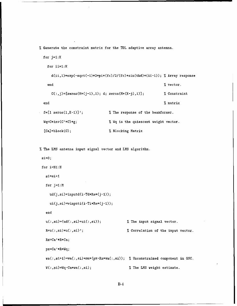
% Generate the constraint matrix for the TDL adaptive array antenna.

for j=I:K

for ii=l:M

d(ii,l)=exp(-sqrt(-l)*2*pi*(fc)/2/(fc)*sin(thd)*(ii-)); % Array response

end % vector.

C(:,j)=[zeros(M*(j-i),l); d; zeros(M*(K-j),i)J; % Constraint

end % matrix

f=[1 zeros(l,K-i)]'; % The response of the beamformer.

Wq=C*inv(C'*C)*g; % Wq is the quiescent weight vector.

[Cal=block(C); % Blocking Matrix

% The LMS antenna input signal vector and LMS algorithm.

si=O;

for i=NI:N

si=si+l

for j=I:M

ud(j,si)=inputd(i-Td*Rs*(j-l));

ui(j,si)=winputi(i-Ti*Rs*(j-l));

end

u(:,si)=(ud(:,si)+ui(:,si)); % The input signal vector.

R=u(:,si)*u(:,si)'; % Correlation of the input vector.

Rx=Ca'*R*Ca;

px=Ca'*R*Wq;

wa(:,si+l)=wa(:,si)+mu*(px-Rx*wa(:,si)); % Unconstrained component in GSC.

W(:,si)=Wq-Ca*wa(:,si); % The LMS weight estimate.

B-4

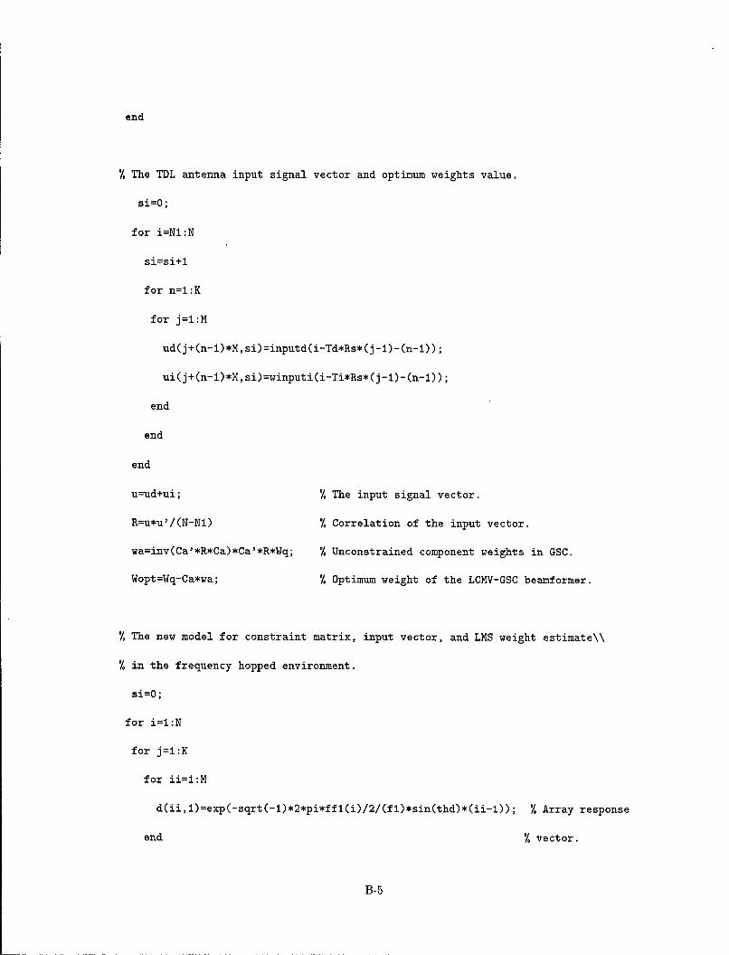
end

% The TDL antenna input signal vector and optimum weights value.

si=O;

for i=Nl:N

si=si+i

for n=1:K

for j=I:M

ud(j+(n-l)*M,si)=inputd(i-Td*Rs*(j-l)-(n-1));

ui(j+(n-1)*M,si)=winputi(i-Ti*Rs*(j-1)-(n-1));

end

end

end

u=ud+ui; % The input signal vector.

R=u*u'/(N-Nl) % Correlation of the input vector.

wa=inv(Ca'*R*Ca)*Ca'*R*Wq; % Unconstrained component weights in GSC.

Wopt=Wq-Ca*wa; % Optimum weight of the LCMV-GSC beamformer.

% The new model for constraint matrix, input vector, and LMS weight estimate\\

% in the frequency hopped environment.

si=O;

for i=:N

for j=I:K

for ii=l:M

d(ii,1)=exp(-sqrt(-1)*2*pi*ffl(i)/2/(fl)*sin(thd)*(ii-1)); % Array response

end % vector.

B-5

C(:,j)=[zeros(M*(j-i),1); d; zeros(M*(K-j),i)J; % The constraint

end % matrix

f=[1 zeros(1,K-1)]'; % The response of the beamformer.

Wq=C*inv(C'*C)*g; % Wq is the quiescent weight vector.

[Calblock(C); % Blocking Matrix

for n1l:K

for j=I:M

ud(j+(n-l)*M, i)=inputd(i)*exp(-sqrt(-1)*2*pi*ffl(i)*(j-l)/2/(fl)\\

*sin(thd))*exp(-sqrt(-1)*2*pi*To*(ff(i))*(n-1));

ui(j+(n-l)*M,i)winputi(i)*exp(-sqrt(-l)*2*pi*ff2(i)*(j-i)/2/(fi)\\

*sin(thi))*exp(-sqrt(-1)*2*pi*To*(ff2(i))*(n-1));

end

end

u(:,si)=(ud(:,si)+ui(:,si)); % The input signal vector.

R=u(:,si)*u(:,si)'; % Correlation of the input vector.

Rx=Ca' *R*Ca;

px=Ca'*R*Wq;

wa(: ,si+1)=wa(: ,si)+mu*Cpx-Rx*waC: ,si)); % Unconstrained component in GSC.

W(:,si)=Wq-Ca*waC:,si); % The LMS weight estimate.

end

B.3 Spatial Smoothing Technique

% Add the decorrelation factor in the LCMV-GSC beainformer.

R=zeros(M*K); % Initial value of correlation.

si-O;

for i=N1:N

B-6

KI= 5; % The smoothing steps

for MN=I:Kl

for j=I:K

ti=O;

for ii=MN:M+Mn-1

titi+i;

d(ti,i)=exp(-sqrt(-l)*2*pi*fl/2/(fl)*sin(thd)*(ii-1));

end

C(:,j)=[zeros(M*(j-1),I); d; zeros(M*(K-j),IXI; % The constraint

end %. matrix

f=[1 zeros(i,K-1)J'; % The response of the beamformer.

Wq--C*inv(C'*C)*g; %. Wq is the quiescent weight vector.

[Calhblock(C); %. Blocking Matrix

for n=1:K

tt=O;

for j=MN:M+MN-1

tttt+i;

ud(tt+(n-i)*M,si)=inputd(i-Td*Rs*(j-i)-(n-1));

ui(tt+(n-l)*M,si)=winputi(i-Ti*Rs*(j-i)-(n-1));

end

end

u(:,si)=(ud(:,si)+ui(:,si)); % The input signal vector.

R=R+u(:,si)*u(:,si)'; % Correlation of the input vector.

end

R-R/K;

Rx=Ca'*R*Ca;

B-7

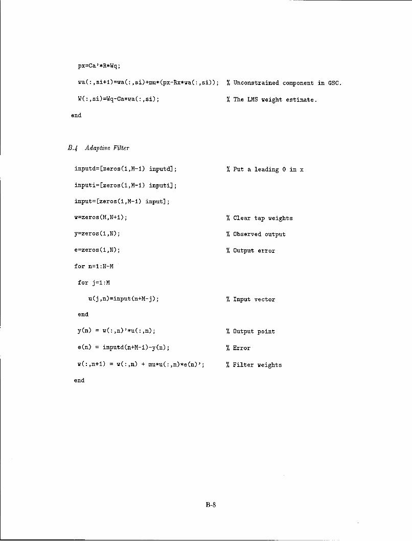
px=Ca'*R*Wq;

waC: ,si+i)=wa(: ,si)+mu*(px-Rx*wa(: ,si)); % Unconstrained component in GSC.

W(:,si)=Wq-Ca*wa(:,si); % The LMS weight estimate.

end

B.4 Adaptive Filter

inputd=[zeros(I,M-1) inputd]; % Put a leading 0 inx

inputi=[zeros(l,M-1) inputi];

input=Ezeros(1,M-1) input];

w=zeros(M,N+1); %~ Clear tap weights

yzeros(1 ,N); %A Observed output

e=zeros(1 ,N); %A Output error

for n1l:N-M

for j1l:M

u~j,n)=input(n+M-j); %A Input vector

end

y(n) = w(:,n)'*u(:,n); %A Output point

e(n) = inputd(n+M-1)-y(n); %A Error

wC:,n+i) = w(:,n) +' mu*u(:,n)*e(n)'; %A Filter weights

end

B-8

Bibliography

1. Bakhru, K. and D. Torrieri (1984), "The Maximin Algorithm for Adaptive Arrays and Fre-quency Hopped Communication," IEEE Trans. on Antennas and Propagation, vol. AP-32, no.9, pp. 919-928, Sep. 1984.

2. Buckley, M. Kevin and Lloyd J. Griffiths (1986), "An Adaptive Generalized Sidelobe Cancellerwith Derivative Constraints," IEEE Trans. on Antennas and Propagation, vol. AP-34, No. 3,March 1986.

3. Capon, J. (1969) "High-Resolution frequency-wavenumber spectrum analysis," Proc. IEEE,vol. 57, pp. 1408-1418.

4. Compton, R. T. (1985) "The Performance of an LMS Adaptive Array with Frequency HoppedSignals," IEEE Trans. on Aerospace and Electronic Systems, vol. AES-32, no. 9, pp. 360-371,Jan. 1988.

5. Compton, R. T. (1988) "The bandwidth performance of a two-element adaptive array withtapped delay-line processing," IEEE Trans. on Antennas and Propagation, vol. 36, no. 1, pp.5-14, Jan. 1988.

6. Compton, R. T. (1988) "The relationship between tapped delay line and FFT processing inAdaptive arrays," IEEE Trans. on Antennas and Propagation, vol. 36, no. 1, pp. 15-26, Jan.1988.

7. Davidovici, Sorin and Emmanuel G. Kanterakis, (1989) Narrowband interference rejectionusing real-time Fourier Transforms, IEEE Trans. on Comm., vol. 37, no. 7, pp. 713-722, July1989.

8. Frost, 0. (1972) "An algorithm for linearly constrained adaptive array processing," Proc.IEEE, vol. 60, 1972.

9. Gevargiz, J., Milstein, Laurence B., and P. K. Das Adaptive narrowband interference rejectionin a DSSS intercept receiver using transform domain signal processing techniques, IEEE Trans.on Comm. vol. 37, no. 12, pp. 1359-1366, Dec. 1989.

10. Godard, D. N. (1974) "Channel equalization using a Kalman filter for fast data transmission,"IBM K. Res. Dev., vol. 18, pp. 267-273.

11. Griffiths, L. J. and C. W. Jim, (1982) "An alternative approach to linearly constrained adaptivebeamforming," IEEE Trans. on Antennas and Propagation, vol. 30, Jan. 1982.

12. Haykin, S., and Allan Steinhardt, (1992) Adatptive Radar Detective and Estimation WileySeries in Remote Sensing, chapter 4, New York.

13. Howells, P.W. (1976). "Explorations in fixed and adaptive resolution at GE and SURC," IEEETrans. on Antennas and Propagation, vol. AP-24, Special Issue on Adpative Antennas, pp.575-584.

14. Hsu, F. M. and Arthur A, Giordano, (1978) "Digital Whitening Techniques for ImprovingSpread Spectrum Communications Performance in the presence of Narrowband Jamming andInterference," IEEE Trans. on Comm. vol. COM-26, no. 2, pp. 209-216, Feb. 1978.

15. Ketchum, John W. and John G. Proakis (1982) "Adaptive Algorithms for Estimating andsuppressing narrowband interference in PN SS systems," IEEE Trans. on Comm., vol. COM-32, no, 5, pp. 913-928, May 1982.

16. Levinson, N. (1947). "The Wiener RMS error criterion in filter design and prediction," J. MathPhys., vol. 25, pp. 261-278

BIB-1

17. Mayhan, J. T., A. J. Simmons and W. C. Summings, (1981) "Wideband adaptive antennanulling using tapped delay-lines," IEEE Trans. on Antennas and Propagation, vol. AP-20, no.6, pp. 923-936, Nov. 1981.

18. Mikulanicz, George S., (1990) Performance of an Acoustic Charge Transport (ACT)Programable Tapped delay line (PTDL) fo signal processing Applications. MS Thesis,AFIT/GE/EE90D-40. School of Engineering, Air Force Institute of Technology, Wright-Patterson AFB OH, DEC. 1990.

19. Milstein, Laurence B. and P. K. Das (1980) "An analysis of a real time transform domainfiltering digital comm. system-Part I: Narrowband interference rejection," IEEE Trans. onComm., vol. COM-28, no. 6, pp. 816-824, June 1980.

20. Milstein, Laurence B. (1988) "Interference Rejection Techniques in Spread Spectrum Commu-nication," Proc. of the IEEE, vol. 76, no. 6, pp. 657-671, June 1988.

21. Najar, M., and M. A. Lagunas (1995) "High Resolution Adpative Arrays Based on RandomProcessing Techniques : Frequency Hopping Modulation," IEEE ISACS pp. 1737-1740,

22. Nordholm, S., I. Claesson, and P. Eriksson, (1992) "The Broadband Wiener solution forGriffiths-Jim beamformers," IEEE Trans. on Signal Processing, vol. 40, no. 2, Feb. 1992.

23. Peterson, L. R., Ziemer, E. R. and D. E. Borth (1995) Introduction to Spread Spectrum Com-munications, Prentice Hall Englewood Cliffs, NJ.

24. Plackett, R. L. (1950). "Some theorems in least squares," Biometrika, Vol. 37, p. 14 9 .

25. Reddy, V. U., A. Paulraj, and T. Kailath (1987), "Performance Analysis of the OptimumBeamformer in the Presence of Correlated Sources and its Behavior Under Spatial Smoothing,"IEEE Trans. on Acoustics Speech and Signal Processing, vol. ASSP-35, pp. 927-936, July, 1987.

26. Reed, Francis A. and Paul L. Feintuch (1981) "A comparison of LMS adaptive cancellersimplemented in the Frequency domain and the Time domain," IEEE Trans. on AcousticsSpeech and Signal Processing, vol. ASSP-29, No. 3, pp. 770-775, June 1981.

27. Rodgers, W. E. and R. T. Compton, Jr., (1979) "Adaptive array bandwidth with tappeddelay-line processing," IEEE Trans. on Aerspace and Electronic Systems, vol. AES-15, no. 1,pp. 21-27, Jan. 1979.

28. Saulnier, Gary J., P. K. Das, and Laurence B. Milstein, (1984) "Suppression of narrowbandinterference rejection techniques in DSSS systems," IEEE Trans. on Comm., vol. COM-32,no. 11, pp. 1227-1232, Nov. 1984.

29. Saulnier, Gary J., P. K. Das, and Laurence B. Milstein, (1985) "An adaptive digital suppressionfilter for DSSS communications," IEEE Journal on Selective Areas in Comm., vol. SAC-3, no.5, pp. 676-685, Sep. 1985.

30. Saulnier, Gary J. (1990) "Interference suppression using a SAW-based adaptive filter," IEEEMILCOM '90, Monterey, CA, Sep30-Oct 3, 1990, pp. 970-974.

31. Saulnier, Gary J. (1992) "Supperssion of narrowband jammers in a SS receiver using transformdomain adaptive filtering," IEEE J. on Sel. Areas in Comm., vol. SAC-10, No. 4, pp. 742-749,May 1992.

32. Shephard, Michael M. (1982) The performance of a PN SS Receiver preceded by an adaptiveinterference suppression filter, MS Thesis, AFIT/GE/EE/82-62. School of Engineering, AirForce Institute of Technology, Wright-Patterson AFB OH, DEC. 1982.

33. Skolnik, M. I. (1982), Introduction to Radar Systems, Second Edition, McGraw-Hill, New York.

BIB-2

34. Torrieri, D. and K. Bakhru (1987), "Frequency Compensation in an Adaptive Antenna Systemfor Frequency Hopping Frequency," IEEE Trans. on Aerospace and Electronic Systems, vol.AES-23, no. 4, pp. 448-467, July 1987.

35. Wang, Hefeng, Ryuji Kohno, and Hideki Imai (1993) "Adaptive Array Antenna Combinedwith Tapped Delay Line Using Processing Gain for Direct Sequence/Spread Spectrum MultipleAccess System," Electronics and Communications in Japan, Part 1, Vol. 76, No. 5, 1993.

36. Way, John R. (1984) The performance of a new adaptive filter for digital communications,MS Thesis, AFIT/GE/EE84s-12, School of Engineering, Air Force Institute of Technology,Wright-Patterson AFB OH, June 1984.

37. White, W. D. (1983) "Wideband interference cancelllation in adatptive sidelobe cancellers,"IEEE Trans. on Aerospace and Electronic System, vol. 19, no. 6, pp. 915-925, Nov. 1983.

38. Widrow, B., P. E. Mantey, L. J. Griffiths, and B. B. Goode, (1967) "Adaptive antenna sys-tems," Proc. IEEE, vol. 55, no. 12, pp. 2143-2159, Dec. 1967.

39. Widrow, B. (1970). "Adaptive filters," in Aspects of Network and System Theory, ed. R. E.Kalman and N. DeClaris, Holt, Rinehart and Winston, New York.

40. Widrow, B., K. M. Duvall, R. P. Gooch, and W. C. Newman (1982), "Signal CancellationPhenomena in Adaptive Antennas: Causes and Cures," IEEE Trans. on Antennas and Prop-agation, vol. AP-30 pp. 469-478, May, 1982.

41. Widrow, B. and S. D. Stearns (1985), Adaptive Signal Processing Prentice Hall, EnglewoodCliffs, NJ.

42. Wiener, N., and E. Hopf (1931). "On a class of singular integral equations," Proc. PrussianAcad. Math Phys. Ser., p.696.

BIB-3

Vita

Wonjin Park ... .. . T -a. He completed high school at

SeoKang High School in Kwangju, Korea. In 1088, Wonjin attended the Korean Military Academy

(KMA). In April 1902, he graduated KMA with a Bachelor of Science Degree in Electrical Engi-

neering and was commissioned a Second Lieutenant in the Republic of Korean Army (ROKA). He

was then asuigned as a Platoon Leader to 7 Division Reconnaissance company. In 1994, Wonjin

was sponsored by the ROKA to complete a Master of Science Degree in Electrical Engineering at

the Air Force Institute of Technology, Dayton, OH.

VITA. 1

Form ApprovedREPORT DOCUMENTATION PAGE OMB No. 0704-0188

Public reporting burden for this collection of information is estimated to average 1 hour per response, including the time for reviewing instructions, searching existing data sources,gathering and maintaining the data needed, and completing and reviewing the collection of information. Send comments regarding this burden estimate or any other aspect of thiscollection of information, including suggestions for reducing this burden, to Washington Headquarters Services, Directorate for Information Operations and Reports, 1215 JeffersonDavis Highway, Suite 1204, Arlington, VA 22202-4302, and to the Office of Management and Budget, Paperwork Reduction Project (0704-0188), Washington, DC 20503.

1. AGENCY USE ONLY (Leave blank) 2. REPORT DATE 3. REPORT TYPE AND DATES COVEREDI December 1996 Master's Thesis

4. TITLE AND SUBTITLE 5. FUNDING NUMBERSInterference Suppression for Spread Spectrum SignalsUsing Adaptive Beamforming and Adaptive Temporal Filter

6. AUTHOR(S)Wonjin Park

7. PERFORMING ORGANIZATION NAME(S) AND ADDRESS(ES) 8. PERFORMING ORGANIZATION

Air Force Institute of Technology, WPAFB OH 45433-6583 REPORT NUMBERAFIT/GE/ENG/96D-14

9. SPONSORING/MONITORING AGENCY NAME(S) AND ADDRESS(ES) 10. SPONSORING/MONITORING

Lawrence L. Gutman AGENCY REPORT NUMBER

WL/AAMI

11. SUPPLEMENTARY NOTES

12a. DISTRIBUTION /AVAILABILITY STATEMENT 12b. DISTRIBUTION CODEApproved for Public release; Distribution Unlimited

13. ABSTRACT (Maximum 200 words)Interference and jamming signals are a serious concern in an operational military communication environment.This thesis examines the utility and performance of combining adaptive temporal filtering with adaptive spatialfiltering (i.e. adaptive beamforming) to improve the signal-to-jammer ratio (SJR) in the presence of narrowbandand wideband interference. Adaptive temporal filters are used for narrowband interference suppression whileadaptive beamforming is used to suppress wideband interference signals. A procedure is presented for thedesign and implementation of a linear constraints minimum variance generalized sidelobe canceler (LCMV-GSC)beamformer. The adaptive beamformer processes the desired signal with unity gain while simultaneously andadaptively minimizing the output due to any undesired signal. Using the LCMV-GSC beamformer with a leastmean squares (LMS) adaptive algorithm, it was shown that the tapped delay line (TDL) adaptive antenna arrayis more effective for the suppression of wideband jammer suppression than the linear array sensors (LAS) adaptiveantenna array. Also a new technique for adaptive beamforming is presented which improves wideband interferencesuppression in a frequency-hopped environment. The output SJR improvement for the new technique comparedto the conventional technique is as much as 15dB. Sometimes, multipath signals and jammers generated by asmart enemy are correlated with the desired signal which destroys the traditional beamformer's performance.After performing a spatial smoothing technique, adaptive beamforming can also be effective in suppressing thejamming signals that are highly correlated with the desired signal.

14. SUBJECT TERMS 15. NUMBER OF PAGES

Adaptive Beamforming, Frequency Hopping, Adaptive Temporal Filter, LMS Adap- 97

tive Algorithm 16. PRICE CODE

17. SECURITY CLASSIFICATION 18. SECURITY CLASSIFICATION 19. SECURITY CLASSIFICATION 20. LIMITATION OF ABSTRACT

OF REPORT OF THIS PAGE OF ABSTRACT

UNCLASSIFIED UNCLASSIFIED UNCLASSIFIED UL

NSN 7540-01-280-5500 Standard Form 298 (Rev. 2-89)Prescribed by ANSI Std. Z39-18298-102

GENERAL INSTRUCTIONS FOR COMPLETING SF 298

The Report Documentation Page (RDP) is used in announcing and cataloging reports. It is importantthat this information be consistent with the rest of the report, particularly the cover and title page.Instructions for filling in each block of the form follow. It is important to stay within the lines to meetoptical scanning requirements.

Block 1. Agency Use Only (Leave blank). Block 12a. Distribution/Availability Statement.Denotes public availability or limitations. Cite any

Block 2. Report Date. Full publication date availability to the public. Enter additionalincluding day, month, and year, if available (e.g. 1 limitations or special markings in all capitals (e.g.Jan 88). Must cite at least the year. NOFORN, REL, ITAR).

Block 3. Type of Report and Dates Covered. DOD - See DoDD 5230.24, "DistributionState whether report is interim, final, etc. If Statements on Technicalapplicable, enter inclusive report dates (e.g. 10 Documents."Jun 87 - 30 Jun 88). DOE - See authorities.

Block 4. Title and Subtitle. A title is taken from NASA - See Handbook NHB 2200.2.the part of the report that provides the most NTIS - Leave blank.meaningful and complete information. When areport is prepared in more than one volume, Block 12b. Distribution Code.repeat the primary title, add volume number, andinclude subtitle for the specific volume. Onclassified documents enter the title classification DOD - Eae blank.in parentheses. DOE - Enter DOE distribution categories

from the Standard Distribution for

Block 5. Funding Numbers. To include contract Unclassified Scientific and Technical

and grant numbers; may include program Reports.

element number(s), project number(s), task NASA - Leave blank.number(s), and work unit number(s). Use the NTIS - Leave blank.

following labels:

C - Contract PR - Project Block 13. Abstract. Include a brief(MaximumG - Grant TA - Task 200 words)factual summary of the mostPE - Program WU - Work Unit significant information contained in the report.

Element Accession No.

Block 6. Author(s). Name(s) of person(s) Block 14. Subiect Terms. Keywords or phrasesresponsible for writing the report, performing identifying major subjects in the report.the research, or credited with the content of thereport. If editor or compiler, this should followthe name(s). Block 15. Number of Pages. Enter the total

number of pages.Block7. Performing Organization Name(s) andAdd ress(es). Self-explanatory. Block 16. Price Code. Enter appropriate price

Block 8. Performing Organization Report code (NTIS only).Number. Enter the unique alphanumeric reportnumber(s) assigned by the organization Blocks 17.- 19. Security Classifications. Self-perform ing the report. explanatory. Enter U.S. Security Classification in

Block 9. Sponsoring/Monitoring Agency Name(s) accordance with U.S. Security Regulations (i.e.,and Address(es). Self-explanatory. UNCLASSIFIED). If form contains classified

information, stamp classification on the top andBlock 10. Sponsoring/Monitoring Agency bottom of the page.Report Number. (if known)

Block 11. Supplementary Notes. Enter Block 20. Limitation of Abstract. This block mustinformation not included elsewhere such as: be completed to assign a limitation to thePrepared in cooperation with...; Trans. of...; To be abstract. Enter either U L (unlimited) or SAR (samepublished in.... When a report is revised, include as report). An entry in this block is necessary ifa statement whether the new report supersedes the abstract is to be limited. If blank, the abstractor supplements the older report. is assumed to be unlimited.

*U.S.GPO:1 993-0-336-043 Standard Form 298 Back (Rev. 2-89)