AIM_To_study_and_plot_the_radiation_patt.pdf

Name: ____________________________

Enrollment No.: _____________________

Government Engineering College, Rajkot

LABORATORY MANUAL

[ANTENNA & WAVE PROPAGATION]

Government Engineering College, Rajkot 2

CertiFiCate

this is to CertiFy that miss/ mr. _______________________,

oF 6thsem – e.C.,

e.no.:_________________________ has satisFaCtorily CompleteD her / his

laboratory work in the AntennA And WAve propAgAtioN subjeCt

as per g.t.u. guiDelines. ____________

H.O.D.

___________

Faculty

Antenna and wave propagation / /2012


.

INDEX Sr.

No. Name of the Experiment Page No.

1. To study different types of antenna.

2. To study the phenomenon of linear, circular and elliptical polarization.

3. To find out the Beam Area of antenna using MATLAB.

4. To find out the Directivity (normal value and dB value) of antenna

using MATLAB.

5. To plot the 2-Dimensional and 3-Dimensional radiation pattern of

the omni- 6. To plot the2-Dimensional and 3-Dimensional radiation pattern of

the directional antenna using MATLAB.

7. To study and plot the array pattern and power pattern of the linear

arrays using MATLAB.

8. To study and plot the radiation pattern of an End-fire array using

MATLAB.

9. To study and plot the radiation pattern of a Broad-side array using

MATLAB.

10. To study and compare the radiation pattern of uniform linear

arrays and non-uniform (binomial) array antenna using MATLAB

11. To study loop antenna.

12. To design of Yagi-Uda antenna.



Experiment No. 1

Aim: To study different types of antenna. 1. Wire antenna

This is the oldest, simplest, cheapest and most versatile type of antenna for

many applications. It may have a linear, loop or some complicated shape like helix.

a. Linear wire antenna

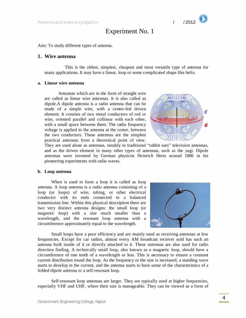
Antennas which are in the form of straight wire are called as linear wire antennas. It is also called as dipole.A dipole antenna is a radio antenna that can be made of a simple wire, with a center-fed driven element. It consists of two metal conductors of rod or wire, oriented parallel and collinear with each other, with a small space between them. The radio frequency voltage is applied to the antenna at the center, between the two conductors. These antennas are the simplest practical antennas from a theoretical point of view. They are used alone as antennas, notably in traditional “rabbit ears” television antennas, and as the driven element in many other types of antennas, such as the yagi. Dipole antennas were invented by German physicist Heinrich Hertz around 1886 in his pioneering experiments with radio waves.

b. Loop antenna

When is used to form a loop it is called as loop antenna. A loop antenna is a radio antenna consisting of a loop (or loops) of wire, tubing, or other electrical conductor with its ends connected to a balanced transmission line. Within this physical description there are two very distinct antenna designs: the small loop (or magnetic loop) with a size much smaller than a wavelength, and the resonant loop antenna with a circumference approximately equal to the wavelength.

Small loops have a poor efficiency and are mainly used as receiving antennas at low frequencies. Except for car radios, almost every AM broadcast receiver sold has such an antenna built inside of it or directly attached to it. These antennas are also used for radio direction finding. A technically small loop, also known as a magnetic loop, should have a circumference of one tenth of a wavelength or less. This is necessary to ensure a constant current distribution round the loop. As the frequency or the size is increased, a standing wave starts to develop in the current, and the antenna starts to have some of the characteristics of a folded dipole antenna or a self-resonant loop.

Self-resonant loop antennas are larger. They are typically used at higher frequencies, especially VHF and UHF, where their size is manageable. They can be viewed as a form of



folded dipole and have somewhat similar characteristics. The radiation efficiency is also high and similar to that of a dipole.

c. Helical antenna

A helical antenna is an antenna consisting of a conducting wire wound in the form of a helix. In most cases, helical antennas are mounted over a ground plane. The feed line is connected between the bottom of the helix and the ground plane. Helical antennas can operate in one of two principal modes: normal mode or axial mode.

In the normal mode or broadside helix, the dimensions of the helix (the diameter and the pitch) are small compared with the wavelength. The antenna acts similarly to an electrically short dipole or monopole, and the radiation pattern, similar to these antennas is omnidirectional, with maximum radiation at right angles to the helix axis. The radiation is linearly polarized parallel to the helix axis.

In the axial mode or end-fire helix, the dimensions of the helix are comparable to a wavelength. The antenna functions as a directional antenna radiating a beam off the ends of the helix, along the antenna's axis. It radiates circularly polarized radio waves.

2. Aperture antenna A waveguide is basically hollow metallic tube through which waves travel depending

upon the cross-section it is either rectangular or circular wave guide. A horn as shown in the figure below is an example of an aperture antenna. These types of antennas are used in aircraft and spacecraft. When one end of the tube is tapered (flared) to a large opening, the structure waves like antenna. These antennas are referred as aperture antennas. Due to its horn shape they are also called as horn antennas. The type of horn, direction and amount of taper can have significant effect on overall performance of these horns as a radiator.

3. Microstrip antenna

A patch antenna is a narrowband, wide-beam antenna fabricated by etching the antenna element pattern in metal trace bonded to an insulating dielectric substrate, such as a printed circuit board, with a continuous metal layer bonded to the opposite side of the substrate which forms a ground plane. Common microstrip antenna shapes are square, rectangular, circular and elliptical, but any continuous shape is possible. Some patch antennas do not use a dielectric substrate and instead made of a metal patch mounted above a ground plane using dielectric spacers; the resulting structure is less rugged but has a wider bandwidth. Because such antennas have a very low profile, are mechanically rugged and can be shaped to conform to the curving skin of a vehicle, they are often mounted on the exterior of aircraft and spacecraft, or are incorporated into mobile radio communications devices.



Microstrip antennas are relatively inexpensive to manufacture and design because of the simple 2-dimensional physical geometry. They are usually employed at UHF and higher frequencies because the size of the antenna is directly tied to the wavelength at the resonant frequency. A single patch antenna provides a maximum directive gain of around 6-9 dBi. It is relatively easy to print an array of patches on a single (large) substrate using lithographic techniques. Patch arrays can provide much higher gains than a single patch at little additional cost; matching and phase adjustment can be performed with printed microstrip feed structures, again in the same operations that form the radiating patches. The ability to create high gain arrays in a low-profile antenna is one reason that patch arrays are common on airplanes and in other military applications. Such an array of patch antennas is an easy way to make a phased array of antennas with dynamic beam forming ability.

An advantage inherent to patch antennas is the ability to have polarization diversity. Patch antennas can easily be designed to have vertical, horizontal, right hand circular (RHCP) or left hand circular (LHCP) polarizations, using multiple feed points, or a single feedpoint with asymmetric patch structures. This unique property allows patch antennas to be used in many types of communications links that may have varied requirements.

4. Array antenna

Antenna array (electromagnetic) a group of isotropic radiators such that the currents running through them are of different amplitudes and phases. Interferometric array of radio telescopes used in radio astronomy. Phased array, also known as a smart antenna, an electronically steerable directional antenna typically used in Radar and in wireless communication systems, in view to achieve beam forming, multiple-input and multiple-output (MIMO) communication or space-time coding. Directional array refers to multiple antennas arranged such that the superposition of the electromagnetic waves produce a predictable electromagnetic field. Watson-Watt / Adcock antenna array the Watson-Watt technique uses two Adcock antenna pairs to perform an amplitude comparison on the incoming signal.

Microstrip patch array antenna



5. Reflector antenna

An antenna reflector is a device that reflects electromagnetic waves. It is often a part of an antenna assembly. A passive element slightly longer than and located behind a radiating dipole element that absorbs and re-radiates the signal in a directional way as in a Yagi antenna array. Corner reflector which reflects the incoming signal back to the direction it came from parabolic reflector which focuses a beam signal into one point, or directs a radiating signal into a beam. Flat reflector which just reflects the signal like a mirror and is often used as a passive repeater.

6. Lens antenna

A lens is an optical device with perfect or approximate axial symmetry which transmits and refracts light, converging or diverging the beam. A simple lens consists of a single optical element. A compound lens is an array of simple lenses (elements) with a common axis; the use of multiple elements allows more optical aberrations to be corrected than is possible with a single element. Lenses are typically made of glass or transparent plastic. Elements which refract electromagnetic radiation outside the visual spectrum are also called lenses: for instance, a microwave lens can be made from paraffin wax.

Lenses are classified by the curvature of the two optical surfaces. A lens is biconvex (or double convex, or just convex) if both surfaces are convex. If both surfaces have the same radius of curvature, the lens is equiconvex. A lens with two concave surfaces is biconcave (or just concave). If one of the surfaces is flat, the lens is plano-convex or plano-concave depending on the curvature of the other surface. A lens with one convex and one concave side is convex-concave or meniscus. It is this type of lens that is most commonly used in corrective lenses.

If the lens is biconvex or plano-convex, a collimated beam of light travelling parallel to the lens axis and passing through the lens will be converged (or focused) to a spot on the axis, at a certain distance behind the lens (known as the focal length). In this case, the lens is called a positive or converging lens.



Experiment No. 2

Aim: To study the phenomenon of linear, circular and elliptical polarization.

Definition:

Polarization of a wave refers to the time varying behavior of the electric field strength vector at some fixed point in space.

Let us consider the wave travelling in +z direction and hence it has 퐸 and 퐸 components as

퐸 = 퐸 cos(휔푡 − 퐾푧)

퐸 = 퐸 cos(휔푡 − 퐾푧 − 훿)

Where

퐸 = 푎푚푝푙푖푡푢푑푒표푓푤푎푣푒푖푛푥 − 푑푖푟푒푐푡푖표푛

퐸 = 푎푚푝푙푖푡푢푑푒표푓푤푎푣푒푖푛푦 − 푑푖푟푒푐푡푖표푛

훿 = 푃ℎ푎푠푒푎푛푔푙푒푏푒푡푤푒푒푛퐸 푎푛푑퐸

There are three types of polarization:

1. Linear Polarization:

A plane electromagnetic wave is said to be linearly polarized. The transverse electric field wave is accompanied by a magnetic field wave as illustrated.



(a) Consider for a wave only 퐸 component is present and 퐸 = 0. Then the total electric field is consisting of only 퐸 component given by

퐸 = 퐸 cos(휔푡 − 퐾푧)푎

(b) Consider for a wave only 퐸 component is present and 퐸 = 0. Then the total electric field is consisting of only 퐸 component given by

퐸 = 퐸 cos(휔푡 − 퐾푧 − 훿)푎

2. Circular Polarization :

Circularly polarized light consists of two perpendicular electromagnetic plane waves of equal amplitude and 90° difference in phase. The light illustrated is right- circularly polarized. 푬ퟏ = 푬ퟐ풂풏풅휹 = ퟗퟎ°

If light is composed of two plane waves of equal amplitude but differing in phase by 90°, then the light is said to be circularly polarized. If you could see the tip of the electric field vector, it would appear to be moving in a circle as it approached you. If while looking at the source, the electric vector of the light coming toward you appears to be rotating counterclockwise, the light is said to be right-circularly polarized. If clockwise, then left-circularly polarized light. The electric field vector makes one complete revolution as the light advances one wavelength toward you. Another way of saying it is that if the thumb of your right hand were pointing in the direction of propagation of the light, the electric vector would be rotating in the direction of your fingers.

Circularly polarized light may be produced by passing linearly polarized light through a quarter-wave plate at an angle of 45° to the optic axis of the plate.



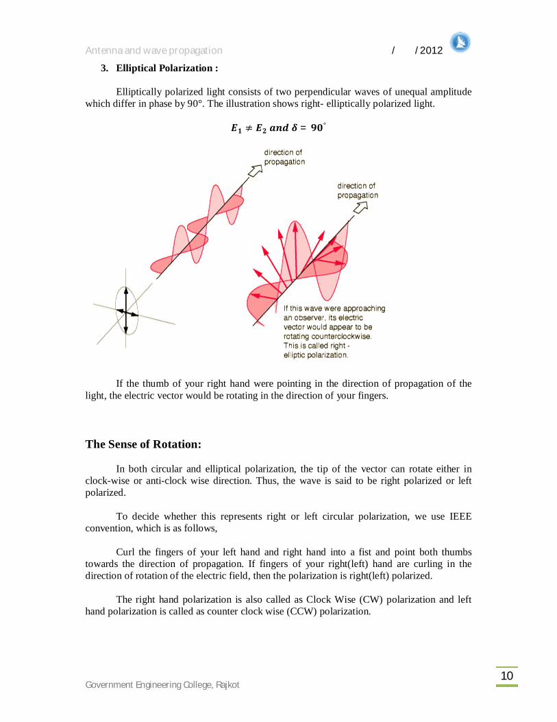
3. Elliptical Polarization :

Elliptically polarized light consists of two perpendicular waves of unequal amplitude which differ in phase by 90°. The illustration shows right- elliptically polarized light.

푬ퟏ ≠ 푬ퟐ풂풏풅휹 = ퟗퟎ°

If the thumb of your right hand were pointing in the direction of propagation of the light, the electric vector would be rotating in the direction of your fingers.

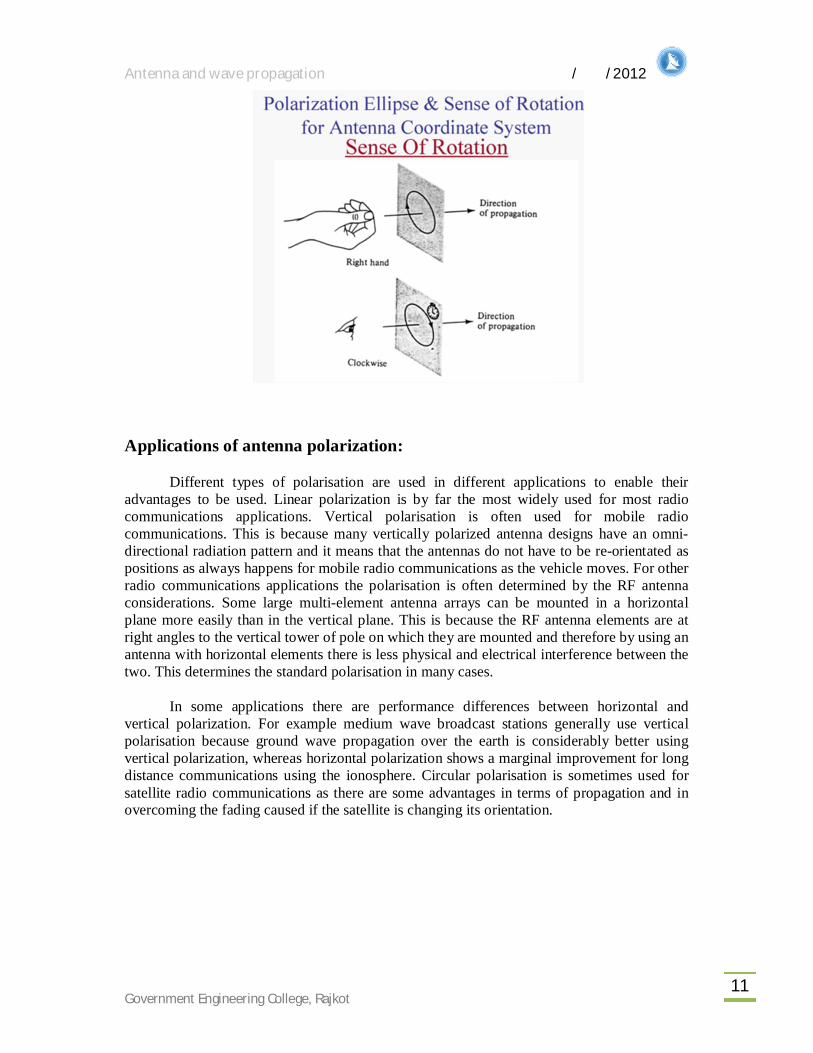
The Sense of Rotation:

In both circular and elliptical polarization, the tip of the vector can rotate either in clock-wise or anti-clock wise direction. Thus, the wave is said to be right polarized or left polarized.

To decide whether this represents right or left circular polarization, we use IEEE convention, which is as follows,

Curl the fingers of your left hand and right hand into a fist and point both thumbs towards the direction of propagation. If fingers of your right(left) hand are curling in the direction of rotation of the electric field, then the polarization is right(left) polarized.

The right hand polarization is also called as Clock Wise (CW) polarization and left hand polarization is called as counter clock wise (CCW) polarization.



Applications of antenna polarization:

Different types of polarisation are used in different applications to enable their advantages to be used. Linear polarization is by far the most widely used for most radio communications applications. Vertical polarisation is often used for mobile radio communications. This is because many vertically polarized antenna designs have an omni-directional radiation pattern and it means that the antennas do not have to be re-orientated as positions as always happens for mobile radio communications as the vehicle moves. For other radio communications applications the polarisation is often determined by the RF antenna considerations. Some large multi-element antenna arrays can be mounted in a horizontal plane more easily than in the vertical plane. This is because the RF antenna elements are at right angles to the vertical tower of pole on which they are mounted and therefore by using an antenna with horizontal elements there is less physical and electrical interference between the two. This determines the standard polarisation in many cases.

In some applications there are performance differences between horizontal and vertical polarization. For example medium wave broadcast stations generally use vertical polarisation because ground wave propagation over the earth is considerably better using vertical polarization, whereas horizontal polarization shows a marginal improvement for long distance communications using the ionosphere. Circular polarisation is sometimes used for satellite radio communications as there are some advantages in terms of propagation and in overcoming the fading caused if the satellite is changing its orientation.



Experiment No. 3

Aim: To find out the Beam Area of antenna using MATLAB.

DEFINITION:

The beam area or beam solid angle or ΩA of an antenna is given by the integral of the normalized power pattern over sphere (4π sr).

Where 푑훺 = 푠푖푛휃푑휃푑휑

The Beam Area of an antenna can often be describe approximately in terms of the angles subtended by the half-power points of the main lobe in the two principal planes.

Are the HPBW in the two principal planes, minor lobes being neglected.

PROGRAM:

clc;

close all;

clear all;

tmin=input('The lower bound of theta in degree=');

tmax=input('The upper bound of theta in degree=');

pmin=input('The lower bound of phi in degree=');

pmax=input('The upper bound of phi in degree=');

theta=(tmin:tmax)*pi/180;

phi=(pmin:pmax)*pi/180;

dth=theta(2)-theta(1);

dph=phi(2)-phi(1);

[THETA,PHI]=meshgrid(theta,phi);

x=input('The field pattern : E(THETA,PHI)=');

v=input('The power pattern: P(THETA,PHI)=','s');



Prad=sum(sum((x.^2).*sin(THETA)*dth*dph));

fprintf('\n Input Parameters: \n-------------------- ');

fprintf('\n Theta =%2.0f',tmin);

fprintf(' : %2.0f',dth*180/pi);

fprintf(' : %2.0f',tmax);

fprintf('\n Phi =%2.0f',pmin);

fprintf(' : %2.0f',dph*180/pi);

fprintf(' : %2.0f',pmax);

fprintf('\n POWER PATTERN : %s',v)

fprintf('\n \n Output Parameters: \n-------------------- ');

fprintf('\nBEAM AREA (steradians)=%3.2f',Prad);

Output:



Experiment No. 4

AIM: To find out the Directivity (normal value and dB value) of antenna using MATLAB.

DEFINITION:

The directivity of an antenna is equal to the ratio of the maximum power density to its average value over a sphere as observed in the far field of an antenna.

Directivity from pattern :

The directivity is also the ratio of the area of a sphere (4π sr) to the beam area ΩA of the antenna.

Directivity from beam area:

The smaller the beam area, the larger the directivity D.

PROGRAM:

clc;

close all;

clear all;

tmin=input('The lower bound of theta in degree=');

tmax=input('The upper bound of theta in degree=');

pmin=input('The lower bound of phi in degree=');

pmax=input('The upper bound of phi in degree=');

theta=(tmin:tmax)*(pi/180);

phi=(pmin:pmax)*(pi/180);

dth=theta(2)-theta(1);

dph=phi(2)-phi(1);


x=input('The field pattern : E(THETA,PHI)=');

v=input('The power pattern: P(THETA,PHI)=','s');



Prad=sum(sum((x.^2).*sin(THETA)*dth*dph));

D=4*pi*max(max(x.^2))/(Prad);

Ddb=10*log10(D);

D1=((D));



fprintf(' : %2.0f',dth*180/pi);



fprintf(' : %2.0f',dph*180/pi);


fprintf('\n POWER PATTERN : %s',v)

fprintf('\n \n Output Parameters: \n-------------------- ');

fprintf('\nBEAM AREA (steradians)=%3.2f',Prad);

fprintf('\nDIRECTIVITY (Dimensionless)=%3.0f',D);

fprintf('\nDIRECTIVITY (dB)=%6.4f',Ddb);

fprintf('\n');

OUTPUT:



Experiment No. 5

AIM: To plot the 2-Dimensional and 3-Dimensional radiation pattern of the omni-directional antenna using MATLAB.

PROGRAM:

clc; clear all; close all; tmin=input('The Lower Range of Theta in Degree= '); tmax=input('The Upper Range of Theta in Degree= '); pmin=input('The Lower Range of Phi in Degree= '); pmax=input('The Upper Range of Phi in Degree= '); tinc=2; pinc=4; rad=pi/180; theta1=(tmin:tinc:tmax); phi1=(pmin:pinc:pmax); theta=theta1.*rad; phi=phi1.*rad; [THETA,PHI]=meshgrid(theta,phi); y1=input('The field pattern: E(THETA,PHI)='); v=input('The field pattern: P(THETA,PHI)=','s'); y=abs(y1); ratio=max(max(y)); [X,Y,Z]=sph2cart(THETA,PHI,y); mesh(X,Y,Z); title('3 D Pattern','Color','b','FontName','Helvetica','FontSize',12,'FontWeight','demi'); fprintf('\n Input Parameters: \n-------------------- '); fprintf('\n Theta =%2.0f',tmin); fprintf(' : %2.0f',tinc); fprintf(' : %2.0f',tmax); fprintf('\n Phi =%2.0f',pmin); fprintf(' : %2.0f',pinc); fprintf(' : %2.0f',pmax); fprintf('\n FIELD PATTERN : %s',v) fprintf('\n \n Output is shown in the figure below----------- '); fprintf('\n');



OUTPUT:

Program for 2 D Pattern:

clc; close all; clear all; theta=0:0.1:2*pi; r=1; [T,R]=meshgrid(theta,r); polar(T,R,'*r')



2 D Pattern

Output :



Experiment No. 6

Aim: To plot the2-Dimensional and 3-Dimensional radiation pattern of the directional antenna using MATLAB.

PROGRAM: clc;

clear all;

close all;

tmin=input('The Lower Range of Theta in Degree= ');

tmax=input('The Upper Range of Theta in Degree= ');

pmin=input('The Lower Range of Phi in Degree= ');

pmax=input('The Upper Range of Phi in Degree= ');

tinc=2; pinc=4;

rad=pi/180;

theta1=(tmin:tinc:tmax);

phi1=(pmin:pinc:pmax);

theta=theta1.*rad;

phi=phi1.*rad;


y1=input('The field pattern: E(THETA,PHI)=');

v=input('The field pattern: P(THETA,PHI)=','s');

y=abs(y1);

ratio=max(max(y));

[X,Y,Z]=sph2cart(THETA,PHI,y);

mesh(X,Y,Z);

title('3 D Pattern','Color','b','FontName','Helvetica','FontSize',12,'FontWeight','demi');





fprintf(' : %2.0f',tinc);



fprintf(' : %2.0f',pinc);


fprintf('\n FIELD PATTERN : %s',v)

fprintf('\n \n Output is shown in the figure below----------- ');

fprintf('\n');

OUTPUT:



2 D Pattern

For Sin(Ø) :

Program :

clc; close all; clear all; phi=0:0.1:2*pi; e=abs(sin(phi)); polar(phi,e)



For Cos(ϴ) :

Program :

clc; close all; clear all; theta=0:0.1:2*pi; e=abs(cos(theta)); polar(theta,e) Output:



Experiment No. 7 AIM : To study and plot the array pattern and power pattern of the linear arrays using MATLAB.

Definition: For linear array: 퐸 = ( )

( )

PROGRAM:

clc close all clear all phi=0:.1:2*pi; d=input('give value of d:'); c=3*(10^8); f=input('enter frequency of signal:'); l=c/f; D=input('enter the distance between two antennas:'); B=2*pi/l Dr=B*D n=input('enter no. of point sources:') si=abs(Dr*cos(phi)+d); Eo=abs((1/n).*sin(n.*si./2)./sin(si./2)); polar(phi,Eo) OUTPUT:

Input Parameters :

give value of d:0

enter frequency of signal:1e9

enter the distance between two antennas:l/2

B =20.9440

Dr =3.1416

enter no. of point sources:4



Output parameters:

n =4

Field Pattern :

Power Pattern :

0.2

0.4

0.6

0.8

1

30

210

60

240

90

270

120

300

150

330

180 0



Experiment No. 8

AIM : To study and plot the radiation pattern of an End-fire array using MATLAB.

DEFINITION : An array is said to be end fire array if the phase angle is such that it makes maximum radiation in the direction of line of array i.e. 0°& 180°.

PROGRAM :

clc close all clear all phi=0:.1:2*pi; c=3*(10^8); f=input('enter frequency of signal:'); l=c/f; D=input('enter the distance between two antennas:'); B=2*pi/l Dr=B*D d=input('give value of d:'); n=input('enter no. of point sources:') si=abs(Dr*cos(phi)+d); Eo=abs((sin(n*si/2))./sin(si/2)); polar(phi,Eo)

OUTPUT:

Input parameters :

enter frequency of signal:1e9


B =20.9440

Dr =3.1416

give value of d:-Dr


Output :



n =4

Field Pattern :

1

2

3

4

30

210

60

240

90

270

120

300

150

330

180 0



Experiment No. 9 AIM: To study and plot the radiation pattern of a Broad-side array using MATLAB

DEFINITION:

An array is said to be broad side array if phase angle is such that it makes maximum radiation perpendicular to the line of array i.e. 90˚ & 270˚.

PROGRAM:

clc close all clear all phi=0:.1:2*pi; c=3*(10^8); f=input('enter frequency of signal:'); l=c/f; D=input('enter the distance between two antennas:'); B=2*pi/l Dr=B*D d=input('give value of d:'); n=input('enter no. of point sources:') si=abs(Dr*cos(phi)+d); Eo=abs((sin(n*si/2))./sin(si/2)); polar(phi,Eo)

OUTPUT: Input parameters : enter frequency of signal:1e9


B =20.9440

Dr =3.1416

give value of d:0




Output parameters : n =4

Field Pattern :



Experiment No. 10 AIM: To study and compare the radiation pattern of uniform linear arrays and non uniform linear (binomial) arrays antenna using MATLAB.

Definition:

For linear array: 퐸 = ( )

( )

For binomial array:퐸 =푐표푠 ( Ø)

Program:

clc; clear all; close all; theta=0:0.1:2*pi; n=input('enter no of sources:') si=pi*cos(theta); e=abs((1/n).*sin(n*si/2)./sin(si/2)); b=cos(pi*cos(theta)/2).^(n-1); polar(theta,b,'r');hold on polar(theta,e,'--b');hold off Output:



Experiment No. 11 Aim: To study loop antenna.

Loop Antenna :

Small Loop:

The field pattern of a small circular loop of radius a may be determined very simply by considering a square loop of the same area, i.e

푑 = 휋푎 d = side length of square loop

Assumption : loop dimensions < ( wavelength)

To prove : Far field patterns of circular & square loops of same area are same when the loops are small but different when they are large compared to wavelength.

If the loop in oriented as shown in fig. 2, its fare electric field has only an 퐸∅ component.To find the far- field pattern in the yz – plane, it is only necessary to consider two of the four small linear loops ( 2 & 4)

Assumptions: 1. The square loop in fig.2 is placed in the co – ordinate system such that center of

the loop is at origin & sides parallel to x & y axis.

1 & 3 parallel to Y– axis 2 & 4 parallel to X – axis

2. The current through the loop has constant amplitude 퐼 & zero phase around the

loop. 퐼 = 퐼 , δ=0

3. The analysis is restricted within far – field region.



4. Each side of the square loop is a short uniform electric current segment which is modeled as an ideal dipole.

A point P in far field region the field due to dipole 1 & 3 will get cancel. The total field at P is due to dipole 2 & 3 only.

When dipole is placed along Z axis it gives 퐸 & 퐻∅ componends from dipoles 2 & 4.



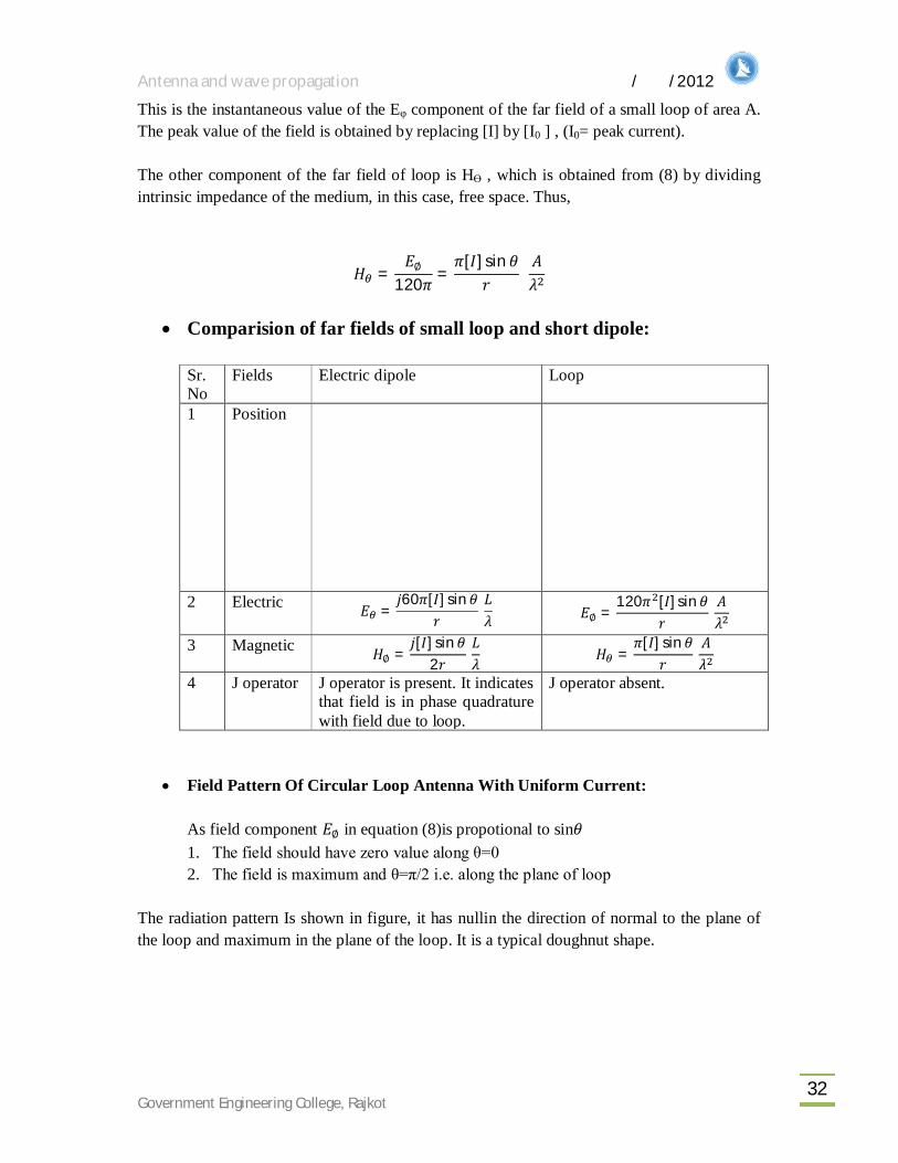
This is the instantaneous value of the Eφ component of the far field of a small loop of area A. The peak value of the field is obtained by replacing [I] by [I0 ] , (I0= peak current).

The other component of the far field of loop is Hϴ , which is obtained from (8) by dividing intrinsic impedance of the medium, in this case, free space. Thus,

퐻 =퐸∅

120휋 =휋[퐼] sin 휃

푟 퐴휆

Comparision of far fields of small loop and short dipole:

Sr. No

Fields Electric dipole Loop

1 Position

2 Electric 퐸 =푗60휋[퐼] sin 휃

푟퐿휆

퐸∅ =120휋 [퐼] sin 휃

푟퐴휆

3 Magnetic 퐻∅ =푗[퐼] sin 휃

2푟퐿휆

퐻 =휋[퐼] sin 휃

푟퐴휆

4 J operator J operator is present. It indicates that field is in phase quadrature with field due to loop.

J operator absent.

Field Pattern Of Circular Loop Antenna With Uniform Current: As field component 퐸∅ in equation (8)is propotional to sin휃 1. The field should have zero value along θ=0 2. The field is maximum and θ=π/2 i.e. along the plane of loop

The radiation pattern Is shown in figure, it has nullin the direction of normal to the plane of the loop and maximum in the plane of the loop. It is a typical doughnut shape.



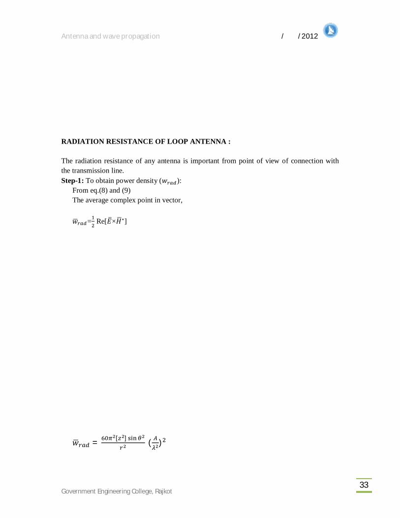
RADIATION RESISTANCE OF LOOP ANTENNA : The radiation resistance of any antenna is important from point of view of connection with the transmission line. Step-1: To obtain power density (푤 ):

From eq.(8) and (9) The average complex point in vector, 푤 = Re[퐸×퐻∗]

푤 = [ ] ( )



Step-2: To obtain radiated power(푃 ): 푃 = ∮푊 푑푠

4∏

푃 = 160휋 [퐼] ( ) Step-3: To obtain 푅 푃 = 퐼 푅

푅 ≅ 31200( ) 훺 For N number of turms in the loop ,total resistance is

For small loop antenna : 푅 ≅ 31200 훺



For large loop antenna : 푅 = 3720( ) ;a=radius , A=area

The radiation due to dipole 2 & 4 is non-directional in y-z plane and can be consider as isotropic sources.

퐸∅ = −2푗퐸∅ sin(푑푟2 sin 휃)

The j term in 퐸∅ indicates it is in phase quadrature with the individual fields due to dipoles.



퐸∅ = −푗퐸∅ 푑푟 sin 휃 In developing dipole formula, the dipole was in the z direction. Here angle θ is measured from axis of the dipole, which is along z axis. But in present case , the dipole axis is parallel to x axis, resulting in.…

퐸∅= [ ] [I]=Retarded current on dipole , r=distance from the dipole.

퐸∅= [ ] Directivity of circular loop antenna:

Directivity, D=

Where,푈 =Maximum radiation intensity (w/sr) 푃 =Power radiated

U=푟 푤

푈 =



Small loop, D=

Large loop, D=. ∗ ; c= circumference=2πa



Experiment No. 12

Aim : To design of Yagi-Uda antenna.

Introduction: A Yagi-Uda array, commonly known simply as a Yagi antenna, is a directional antenna consisting of a driven element (typically a dipole or folded dipole) and additional parasitic elements (usually a so-called reflector and one or more directors). The reflector element is slightly longer (typically 5% longer) than the driven dipole, whereas the so-called directors are a little bit shorter. This design achieves a very substantial increase in the antenna's directionality andgain compared to a simple dipole.

Description :

Yagi-Uda antenna. Viewed left to right: reflector, driven element,director. Exact spacings and element lengths

vary somewhat according to specific designs.

Yagi-Uda antennas are directional along the axis perpendicular to the dipole in the plane of the elements, from the reflector toward the driven element and the director(s). Typical spacings between elements vary from about 1/10 to 1/4 of a wavelength, depending on the specific design. The lengths of the directors are smaller than that of the driven element, which is smaller than that of the reflector(s) according to an elaborate design procedure. These elements are usually parallel in one plane, supported on a single crossbar known as a boom.

Improvement in basic yagi-uda antenna: The directivity of 9 db for basic three element yagi-uda can further be increased by increasing the no of elements.practically it is found that

1) Only one reflector need be used , as the addition of second and third reflector adds practically nothing to the directivity of the structure.

2) The directivity increased considerably by the addition of more directors. It increase from 9 db for a three element yagi to about 15 db for a five element yagi.



3) The no of directors can be increased up to 13 and after this there is no much improvement in the directivity.

4) The length of directors goes on decreasing as it goes away from the driven element .so the whole structure tapers in the direction of propagation .

5) All the element are electrically fastened to the conducting , grounded central support road .

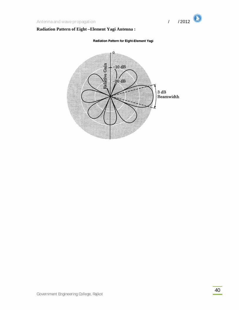
6) The radiation pattern consist of one main lobe lying in the forward direction along the axis of the array, with several very minor lobes in other direction.

7) Polarization in the direction of the element axes.

Application & Coast :

• Because of directivity & more antenna gain these antenna is widely used for the reception of T.V. signals.

• However the Yagi-Uda design only achieves this high gain over a rather narrow bandwidth, making it more useful for various communications bands (including amateur radio) but less suitable for traditional radio and television broadcast bands.

• Amateur radio operators ("hams") frequently employ these for communication on HF, VHF, and UHF bands.

• Wideband antennas used for VHF/UHF broadcast bands include the lower-gain log-periodic dipole array, which is often confused with the Yagi-Uda array due to its superficially similar appearance.

• For designing yagi antenna aluminium metal is used. Hence cost of this antenna is approximately 100 to 150 rs.

Design of 6 – Element Yagi-Uda Antenna:

For 6 element Yagi-Uda to have a gain of 12dBi at the operating frequency (f) or wavelength (λ), the design equations are as follows :

Length of reflector : LR = 0.475 λ Length of active (driven) element : La = 0.46 λ Length of directors : LD1 = 0.44 λ = LD2 LD3 = 0.43 λ LD4 = 0.40 λ Spacing between reflector and active element = SR = 0.25 λ Spacing between director and driving element = SD2 = SD3 = SD4 Spacing between directors : SD1 = 0.25 λ Diameter of elements ,d = 0.01 λ The length of Yagi-array : L = 1.5 λ



Radiation Pattern of Eight –Element Yagi Antenna :

AIM_To_study_and_plot_the_radiation_patt.pdf

Documents