AI Simulation 2011 GetStart

Autodesk Inventor Simulation 2011

Getting Started

January 2010

© 2010 Autodesk, Inc. All Rights Reserved. Except as otherwise permitted by Autodesk, Inc., this publication, or parts thereof, may not bereproduced in any form, by any method, for any purpose. Certain materials included in this publication are reprinted with the permission of the copyright holder. TrademarksThe following are registered trademarks or trademarks of Autodesk, Inc., and/or its subsidiaries and/or affiliates in the USA and other countries:3DEC (design/logo), 3December, 3December.com, 3ds Max, Algor, Alias, Alias (swirl design/logo), AliasStudio, Alias|Wavefront (design/logo),ATC, AUGI, AutoCAD, AutoCAD Learning Assistance, AutoCAD LT, AutoCAD Simulator, AutoCAD SQL Extension, AutoCAD SQL Interface,Autodesk, Autodesk Envision, Autodesk Intent, Autodesk Inventor, Autodesk Map, Autodesk MapGuide, Autodesk Streamline, AutoLISP, AutoSnap,AutoSketch, AutoTrack, Backburner, Backdraft, Built with ObjectARX (logo), Burn, Buzzsaw, CAiCE, Civil 3D, Cleaner, Cleaner Central, ClearScale,Colour Warper, Combustion, Communication Specification, Constructware, Content Explorer, Dancing Baby (image), DesignCenter, DesignDoctor, Designer's Toolkit, DesignKids, DesignProf, DesignServer, DesignStudio, Design Web Format, Discreet, DWF, DWG, DWG (logo), DWGExtreme, DWG TrueConvert, DWG TrueView, DXF, Ecotect, Exposure, Extending the Design Team, Face Robot, FBX, Fempro, Fire, Flame, Flare,Flint, FMDesktop, Freewheel, GDX Driver, Green Building Studio, Heads-up Design, Heidi, HumanIK, IDEA Server, i-drop, ImageModeler, iMOUT,Incinerator, Inferno, Inventor, Inventor LT, Kaydara, Kaydara (design/logo), Kynapse, Kynogon, LandXplorer, Lustre, MatchMover, Maya,Mechanical Desktop, Moldflow, Moonbox, MotionBuilder, Movimento, MPA, MPA (design/logo), Moldflow Plastics Advisers, MPI, MoldflowPlastics Insight, MPX, MPX (design/logo), Moldflow Plastics Xpert, Mudbox, Multi-Master Editing, Navisworks, ObjectARX, ObjectDBX, OpenReality, Opticore, Opticore Opus, Pipeplus, PolarSnap, PortfolioWall, Powered with Autodesk Technology, Productstream, ProjectPoint, ProMaterials,RasterDWG, RealDWG, Real-time Roto, Recognize, Render Queue, Retimer,Reveal, Revit, Showcase, ShowMotion, SketchBook, Smoke, Softimage,Softimage|XSI (design/logo), Sparks, SteeringWheels, Stitcher, Stone, StudioTools, ToolClip, Topobase, Toxik, TrustedDWG, ViewCube, Visual,Visual LISP, Volo, Vtour, Wire, Wiretap, WiretapCentral, XSI, and XSI (design/logo). All other brand names, product names or trademarks belong to their respective holders. DisclaimerTHIS PUBLICATION AND THE INFORMATION CONTAINED HEREIN IS MADE AVAILABLE BY AUTODESK, INC. "AS IS." AUTODESK, INC. DISCLAIMSALL WARRANTIES, EITHER EXPRESS OR IMPLIED, INCLUDING BUT NOT LIMITED TO ANY IMPLIED WARRANTIES OF MERCHANTABILITY ORFITNESS FOR A PARTICULAR PURPOSE REGARDING THESE MATERIALS. Published by:Autodesk, Inc.111 McInnis ParkwaySan Rafael, CA 94903, USA

Contents

Stress Analysis . . . . . . . . . . . . . . . . . . . . . . . . 1

Chapter 1 Stress Analysis . . . . . . . . . . . . . . . . . . . . . . . . . . . 3Features in Stress Analysis . . . . . . . . . . . . . . . . . . . . . . . . . 3Learn Autodesk Inventor Simulation . . . . . . . . . . . . . . . . . . . . 3Use Help . . . . . . . . . . . . . . . . . . . . . . . . . . . . . . . . . . 4Use the Simulation Guide . . . . . . . . . . . . . . . . . . . . . . . . . 5Use Stress Analysis Commands . . . . . . . . . . . . . . . . . . . . . . . 5Understand the Value of Stress Analysis . . . . . . . . . . . . . . . . . . 6Understand How Stress Analysis Works . . . . . . . . . . . . . . . . . . 7

Analysis Assumptions . . . . . . . . . . . . . . . . . . . . . . . . 7Interpret Results of Stress Analysis . . . . . . . . . . . . . . . . . . . . . 9

Equivalent or Von Mises Stress . . . . . . . . . . . . . . . . . . . . 9Maximum and Minimum Principal Stresses . . . . . . . . . . . . . 9Deformation . . . . . . . . . . . . . . . . . . . . . . . . . . . . . 10Safety Factor . . . . . . . . . . . . . . . . . . . . . . . . . . . . . 10Frequency Modes . . . . . . . . . . . . . . . . . . . . . . . . . . 10

Chapter 2 Analyze Models . . . . . . . . . . . . . . . . . . . . . . . . . . 13Do a Static Stress Analysis . . . . . . . . . . . . . . . . . . . . . . . . . 13

Enter Environment and Create a Simulation . . . . . . . . . . . . 14Specify Material . . . . . . . . . . . . . . . . . . . . . . . . . . . 15Add Constraints . . . . . . . . . . . . . . . . . . . . . . . . . . . 16

iii

Add Loads . . . . . . . . . . . . . . . . . . . . . . . . . . . . . . 17Add Contact Conditions . . . . . . . . . . . . . . . . . . . . . . 18Generate a Mesh . . . . . . . . . . . . . . . . . . . . . . . . . . 19Run the Simulation . . . . . . . . . . . . . . . . . . . . . . . . . 20

Run Modal Analysis . . . . . . . . . . . . . . . . . . . . . . . . . . . . 20

Chapter 3 View Results . . . . . . . . . . . . . . . . . . . . . . . . . . . . 23Use Results Visualization . . . . . . . . . . . . . . . . . . . . . . . . . 23Edit the Color Bar . . . . . . . . . . . . . . . . . . . . . . . . . . . . . 25Read Stress Analysis Results . . . . . . . . . . . . . . . . . . . . . . . . 26

Interpret Results Contours . . . . . . . . . . . . . . . . . . . . . 26Animate Results . . . . . . . . . . . . . . . . . . . . . . . . . . . 28Set Results Display Options . . . . . . . . . . . . . . . . . . . . . 28

Chapter 4 Revise Models and Stress Analyses . . . . . . . . . . . . . . . . 31Change Model Geometry . . . . . . . . . . . . . . . . . . . . . . . . . 31Change Solution Conditions . . . . . . . . . . . . . . . . . . . . . . . 32Update Results of Stress Analysis . . . . . . . . . . . . . . . . . . . . . 34

Chapter 5 Generate Reports . . . . . . . . . . . . . . . . . . . . . . . . . 35Run Reports . . . . . . . . . . . . . . . . . . . . . . . . . . . . . . . . 35Interpret Reports . . . . . . . . . . . . . . . . . . . . . . . . . . . . . 36

Model Information . . . . . . . . . . . . . . . . . . . . . . . . . 36Project Info . . . . . . . . . . . . . . . . . . . . . . . . . . . . . 36Simulation . . . . . . . . . . . . . . . . . . . . . . . . . . . . . . 36

Save and Distribute Reports . . . . . . . . . . . . . . . . . . . . . . . . 37Saved Reports . . . . . . . . . . . . . . . . . . . . . . . . . . . . 38Print Reports . . . . . . . . . . . . . . . . . . . . . . . . . . . . . 38Distribute Reports . . . . . . . . . . . . . . . . . . . . . . . . . . 38

Chapter 6 Manage Stress Analysis Files . . . . . . . . . . . . . . . . . . . 39Create and Use Analysis Files . . . . . . . . . . . . . . . . . . . . . . . 39

Understand File Relationships . . . . . . . . . . . . . . . . . . . 39Resolve Missing Files . . . . . . . . . . . . . . . . . . . . . . . . . . . 40

Dynamic Simulation . . . . . . . . . . . . . . . . . . . . 41

Chapter 7 Dynamic Simulation . . . . . . . . . . . . . . . . . . . . . . . . 43Features in Dynamic Simulation . . . . . . . . . . . . . . . . . . . . . 43Learning Autodesk Inventor Simulation . . . . . . . . . . . . . . . . . 44Use Help . . . . . . . . . . . . . . . . . . . . . . . . . . . . . . . . . . 44Understand Simulation Commands . . . . . . . . . . . . . . . . . . . 45

iv | Contents

Simulation Assumptions . . . . . . . . . . . . . . . . . . . . . . . . . 45Interpret Simulation Results . . . . . . . . . . . . . . . . . . . . . . . 45

Relative Parameters . . . . . . . . . . . . . . . . . . . . . . . . . 45Coherent Masses and Inertia . . . . . . . . . . . . . . . . . . . . 46Continuity of Laws . . . . . . . . . . . . . . . . . . . . . . . . . 46

Chapter 8 Simulate Motion . . . . . . . . . . . . . . . . . . . . . . . . . . 47Understand Degrees of Freedom . . . . . . . . . . . . . . . . . . . . . 47Understand Constraints . . . . . . . . . . . . . . . . . . . . . . . . . . 48Convert Assembly Constraints . . . . . . . . . . . . . . . . . . . . . . 49Run Simulations . . . . . . . . . . . . . . . . . . . . . . . . . . . . . . 52

Chapter 9 Construct Moving Assemblies . . . . . . . . . . . . . . . . . . 55Retain Degrees of Freedom . . . . . . . . . . . . . . . . . . . . . . . . 55Add Joints . . . . . . . . . . . . . . . . . . . . . . . . . . . . . . . . . 57Impose Motion on Joints . . . . . . . . . . . . . . . . . . . . . . . . . 58Run Simulations . . . . . . . . . . . . . . . . . . . . . . . . . . . . . . 59

Chapter 10 Construct Operating Conditions . . . . . . . . . . . . . . . . . 61Complete the Assembly . . . . . . . . . . . . . . . . . . . . . . . . . . 61Add Friction . . . . . . . . . . . . . . . . . . . . . . . . . . . . . . . . 63Add a Sliding Joint . . . . . . . . . . . . . . . . . . . . . . . . . . . . 64

Chapter 11 Simulation Commands . . . . . . . . . . . . . . . . . . . . . . 67Input Grapher . . . . . . . . . . . . . . . . . . . . . . . . . . . . . . . 67Output Grapher . . . . . . . . . . . . . . . . . . . . . . . . . . . . . . 70Publish Output in Inventor Studio . . . . . . . . . . . . . . . . . . . . 76

Index . . . . . . . . . . . . . . . . . . . . . . . . . . . . . . . . 79

Contents | v

vi

Stress Analysis

Part 1 of this manual presents the getting started information for Stress Analysis in theAutodesk® Inventor® Simulation software. This add-on to the Autodesk Inventor assembly,part, and sheet metal environments provides the capability to analyze the static stress andnatural frequency responses of mechanical designs.

1

2

Stress Analysis

Autodesk® Inventor® Simulation software provides a combination of industry-specificcommands. It extends the capabilities of Autodesk Inventor® for completing complexmachinery and other product designs.

This manual provides basic conceptual information to help get you started. It providesexamples that introduce you to the capabilities of Stress and Modal Analysis in AutodeskInventor Simulation.

Built on the Autodesk Inventor application, Autodesk Inventor Simulation includes severaldifferent modules. The first module included in this manual is Stress Analysis. It providesfunctionality for Structural Static and Modal analysis of mechanical product designs.

This chapter provides basic information about the stress analysis environment and theworkflow processes necessary to analyze loads and constraints placed on a part or assembly.

Features in Stress AnalysisStress Analysis in Autodesk Inventor Simulation is an add-on to the AutodeskInventor assembly, part, and sheet metal environments.

Static Analysis provides the means to simulate stress, strain, and deformation.

Modal Analysis provides means to find natural frequencies of vibration andmode shapes of mechanical designs.

You can visualize the effects in 3D volume plots, create reports for any results,and perform parametric studies to refine your design.

Learn Autodesk Inventor SimulationWe assume that you have a working knowledge of the Autodesk InventorSimulation interface and commands. If you do not, use Help for access to online

1

3

documentation and tutorials, and complete the exercises in the AutodeskInventor Simulation Getting Started manual.

At a minimum, we recommend that you understand how to:

■ Use the assembly, part modeling, and sketch environments and browsers.

■ Edit a component in place.

■ Create, constrain, and manipulate work points and work features.

■ Set color styles.

Be more productive with Autodesk® software. Get trained at an AutodeskAuthorized Training Center (ATC®) with hands-on, instructor-led classes tohelp you get the most from your Autodesk products. Enhance your productivitywith proven training from over 1,400 ATC sites in more than 75 countries.For more information about training centers, email [email protected],or visit the online ATC locator at http://www.autodesk.com/atc.

We also recommend that you have a working knowledge of Microsoft®

Windows® XP or Windows Vista®. It is desirable, but not required, to have aworking knowledge of concepts for stress analysis of mechanical assemblydesigns.

Use HelpAs you work, you can access information about your tasks. The Help systemprovides detailed concepts, procedures, and reference information about everyfeature in Autodesk Inventor Simulation.

To access the Help system, use one of the following methods:

■ Click Help ➤ Help Topics, and then use the Table of Contents to navigateto Stress Analysis topics.

■ Press F1 for Help with the active operation.

■ In any dialog box, click .

■ In the graphics window, right-click, and then click How To. The How Totopic for the current command is displayed.

4 | Chapter 1 Stress Analysis

http://www.autodesk.com/atc

Use the Simulation GuideUse the Simulation Guide to assist in preparation of your model andinterpretation of simulation results. The Guide provides interactive assistancefor navigating proper simulation workflows. The Guide compliments otherlearning resource material such as Help, tutorials, and Skill Builders, and hasthe following attributes

■ Initial content is context aware. For example, if you access the Guide whileapplying loads to your model, the Guide opens to display content relatedto load definition.

■ Content is presented in decision-tree fashion, reflective of proper simulationworkflows. The Guide queries your intent, and you click the appropriatelinks in response.

■ Contains expandable content sections, links to pages within the Guide,and clickable text to launch commands.

■ The Guide window is navigable and dockable.

Use Stress Analysis CommandsAutodesk Inventor Simulation Stress Analysis provides commands to determinestructural design performance directly on your Autodesk Inventor Simulationmodel. Autodesk Inventor Simulation Stress Analysis includes tools to placeloads and constraints on a part or assembly. It calculates the resulting stress,deformation, safety factor, and resonant frequency modes.

Enter the stress analysis environment in Autodesk Inventor Simulation withan active part or assembly.

With the stress analysis commands, you can:

■ Perform a structural static or modal analysis of a part or assembly.

■ Apply a force, pressure, bearing load, moment, or body load to vertices,faces, or edges of the model, or import a motion load from dynamicsimulation.

■ Apply fixed or non-zero displacement constraints to the model.

■ Model various mechanical contact conditions between adjacent parts.

■ Evaluate the impact of multiple parametric design changes.

Use the Simulation Guide | 5

■ View the analysis results in terms of equivalent stress, minimum andmaximum principal stresses, deformation, safety factor, or modal frequency.

■ Add or suppress features such as gussets, fillets or ribs, re-evaluate thedesign, and update the solution.

■ Animate the model through various stages of deformation, stress, safetyfactor, and frequencies.

■ Generate a complete and automatic engineering design report in HTMLformat.

Understand the Value of Stress AnalysisPerforming an analysis of a mechanical part or assembly in the design phasecan help you bring a better product to market in less time. Autodesk InventorSimulation Stress Analysis helps you:

■ Determine if the part or assembly is strong enough to withstand expectedloads or vibrations without breaking or deforming inappropriately.

■ Gain valuable insight at an early stage when the cost of redesign is small.

■ Determine if the part can be redesigned in a more cost-effective mannerand still perform satisfactorily under expected use.

Stress analysis, for this discussion, is a tool to understand how a designperforms under certain conditions. A highly trained specialist can take a greatdeal of time with a detailed analysis to obtain an exact answer about reality.You can often predict and improve a design with the trending and behavioralinformation you obtain from a basic or fundamental analysis. If you performthis basic analysis early in the design phase, you can substantially improvethe overall engineering process.

Here is an example of stress analysis use: When designing bracketry or singlepiece weldments, the deformation of your part can greatly affect the alignmentof critical components causing forces that induce accelerated wear. Whenevaluating vibration effects, geometry plays a critical role in the naturalfrequency of a part or assembly. Avoiding, or in some cases targeting criticalfrequencies, can be the difference between failure and expected performance.

For any analysis, detailed or fundamental, it is vital to keep in mind the natureof approximations, study the results, and test the final design. Proper use ofstress analysis greatly reduces the number of physical tests required. You canexperiment on a wider variety of design options and improve the end product.


To learn more about the capabilities of Autodesk Inventor Simulation StressAnalysis, view the online demonstrations and tutorials.

Understand How Stress Analysis WorksStress analysis is done using a mathematical representation of a physical systemcomposed of:

■ A part or assembly (model).

■ Material properties.

■ Applicable boundary conditions (loads, supports), contact conditions, andmesh, referred to as preprocessing.

■ The solution of that mathematical representation (solving).To find a result, the part is divided into smaller elements. The solver addsup the individual behaviors of each element. It predicts the behavior ofthe entire physical system by resolving a set of simultaneous algebraicequations.

■ The study of the results of that solution is referred to as post-processing.

Analysis AssumptionsA simulation depends on accurate information. It is important that you modelaccurately and specify the actual physical conditions (constraints, loads,materials, contact conditions). The accuracy of these conditions directlyinfluences the quality of your results.

The stress analysis that Autodesk Inventor Simulation provides is appropriateonly for linear material properties. These properties are where the stress isdirectly proportional to the strain in the material (meaning no permanentyielding of the material). Linear behavior results when the slope of the materialstress-strain curve in the elastic region (measured as the Modulus of Elasticity)is constant.

The total deformation is assumed to be small in comparison to the partthickness. For example, if studying the deflection of a beam, the calculateddisplacement must be less than the minimum cross-section of the beam.

The results are temperature-independent. The temperature is assumed not toaffect the material properties.

Understand How Stress Analysis Works | 7

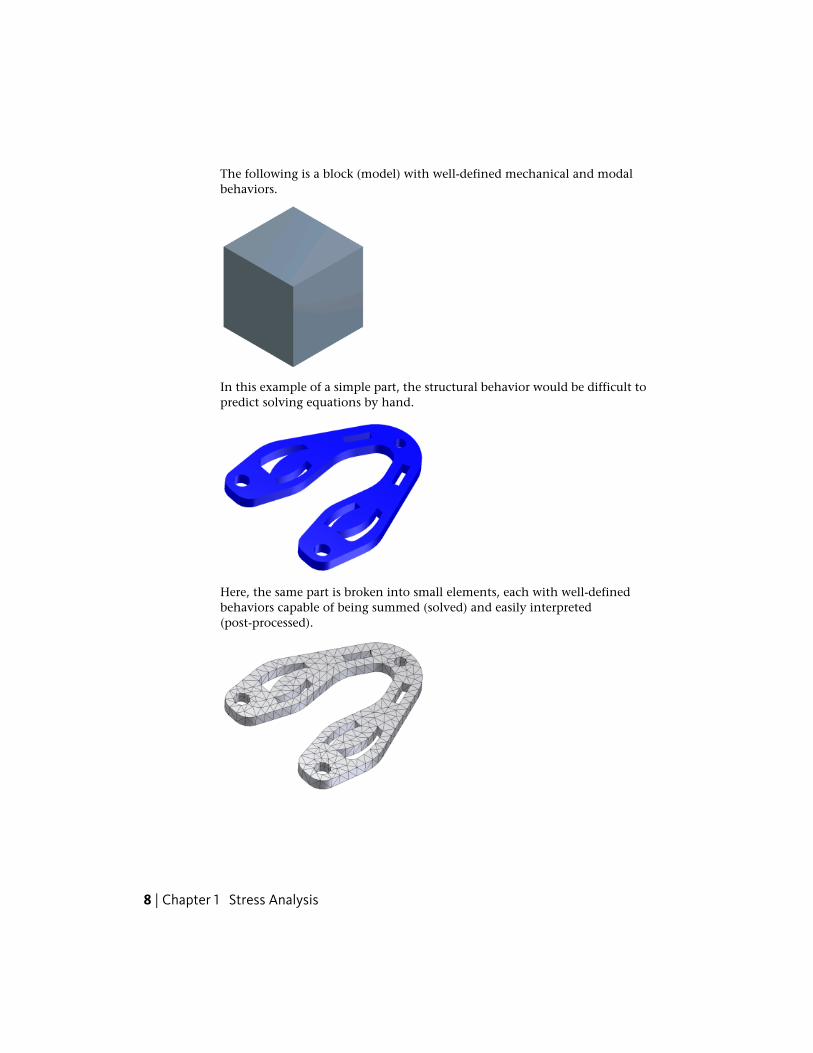
The following is a block (model) with well-defined mechanical and modalbehaviors.

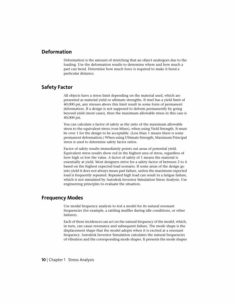
In this example of a simple part, the structural behavior would be difficult topredict solving equations by hand.

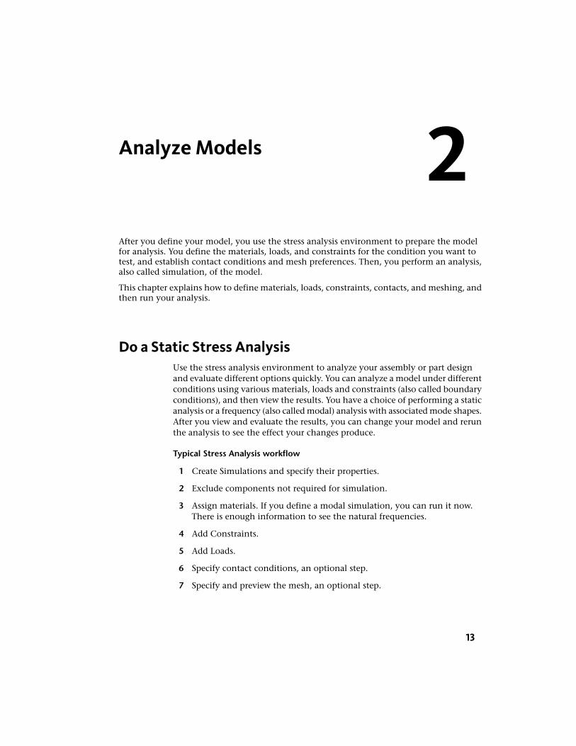
Here, the same part is broken into small elements, each with well-definedbehaviors capable of being summed (solved) and easily interpreted(post-processed).


Interpret Results of Stress AnalysisThe output of a mathematical solver is generally a substantial quantity of rawdata. This quantity of raw data would normally be difficult and tedious tointerpret without the data sorting and graphical representation traditionallyreferred to as post-processing. Post-processing is used to create graphicaldisplays that show the distribution of stresses, deformations, and other aspectsof the model. Interpretation of these post-processed results is the key toidentifying:

■ Areas of potential concern as in weak areas in a model.

■ Areas of material waste as in areas of the model bearing little or no load.

■ Valuable information about other model performance characteristics, suchas vibration, that otherwise would not be known until a physical modelis built and tested (prototyped).

The results interpretation phase is where the most critical thinking must takeplace. You compare the results (such as the numbers versus color contours,movements) with what is expected. You determine if the results make sense,and explain the results based on engineering principles. If the results are otherthan expected, evaluate the analysis conditions and determine what is causingthe discrepancy.

Equivalent or Von Mises StressThree-dimensional stresses and strains build up in many directions. A commonway to express these multidirectional stresses is to summarize them into anEquivalent stress, also known as the von-Mises stress. A three-dimensionalsolid has six stress components. Sometimes an uniaxial stress test finds materialproperties experimentally. In that case, the combination of the six stresscomponents to a single equivalent stress relates the real stress system.

Maximum and Minimum Principal StressesAccording to elasticity theory, an infinitesimal volume of material at anarbitrary point on or inside the solid body can rotate so that only normalstresses remain and all shear stresses are zero. When the normal vector of asurface and the stress vector acting on that surface are collinear, the directionof the normal vector is called principal stress direction. The magnitude of thestress vector on the surface is called the principal stress value.

Interpret Results of Stress Analysis | 9

DeformationDeformation is the amount of stretching that an object undergoes due to theloading. Use the deformation results to determine where and how much apart can bend. Determine how much force is required to make it bend aparticular distance.

Safety FactorAll objects have a stress limit depending on the material used, which arepresented as material yield or ultimate strengths. If steel has a yield limit of40,000 psi, any stresses above this limit result in some form of permanentdeformation. If a design is not supposed to deform permanently by goingbeyond yield (most cases), then the maximum allowable stress in this case is40,000 psi.

You can calculate a factor of safety as the ratio of the maximum allowablestress to the equivalent stress (von-Mises), when using Yield Strength. It mustbe over 1 for the design to be acceptable. (Less than 1 means there is somepermanent deformation.) When using Ultimate Strength, Maximum Principalstress is used to determine safety factor ratios.

Factor of safety results immediately points out areas of potential yield.Equivalent stress results show red in the highest area of stress, regardless ofhow high or low the value. A factor of safety of 1 means the material isessentially at yield. Most designers strive for a safety factor of between 2 to 4based on the highest expected load scenario. If some areas of the design gointo yield it does not always mean part failure, unless the maximum expectedload is frequently repeated. Repeated high load can result in a fatigue failure,which is not simulated by Autodesk Inventor Simulation Stress Analysis. Useengineering principles to evaluate the situation.

Frequency ModesUse modal frequency analysis to test a model for its natural resonantfrequencies (for example, a rattling muffler during idle conditions, or otherfailures).

Each of these incidences can act on the natural frequency of the model, which,in turn, can cause resonance and subsequent failure. The mode shape is thedisplacement shape that the model adopts when it is excited at a resonantfrequency. Autodesk Inventor Simulation calculates the natural frequenciesof vibration and the corresponding mode shapes. It presents the mode shapes


as results that you can view and animate. Dynamic response analysis is notoffered at this time.

LocationFor more information

Simulation - Stress AnalysisTutorial

Frequency Modes | 11

12

Analyze Models

After you define your model, you use the stress analysis environment to prepare the modelfor analysis. You define the materials, loads, and constraints for the condition you want totest, and establish contact conditions and mesh preferences. Then, you perform an analysis,also called simulation, of the model.

This chapter explains how to define materials, loads, constraints, contacts, and meshing, andthen run your analysis.

Do a Static Stress AnalysisUse the stress analysis environment to analyze your assembly or part designand evaluate different options quickly. You can analyze a model under differentconditions using various materials, loads and constraints (also called boundaryconditions), and then view the results. You have a choice of performing a staticanalysis or a frequency (also called modal) analysis with associated mode shapes.After you view and evaluate the results, you can change your model and rerunthe analysis to see the effect your changes produce.

Typical Stress Analysis workflow

1 Create Simulations and specify their properties.

2 Exclude components not required for simulation.

3 Assign materials. If you define a modal simulation, you can run it now.There is enough information to see the natural frequencies.

4 Add Constraints.

5 Add Loads.

6 Specify contact conditions, an optional step.

7 Specify and preview the mesh, an optional step.

2

13

8 Run the simulation.

9 View and Interpret the Results

When you modify the model or various inputs for the simulation, it can benecessary to update the mesh or other analysis parameters. A red lightningbolt icon next to the browser node indicates areas that need an update.Right-click the node and click Update to make them current with respect tothe modifications. For the Results node, run the Simulate command to updateresults.

Enter Environment and Create a SimulationYou enter the Stress Analysis environment from the assembly, part, or sheetmetal environments.

Enter the environment and create a simulation:

1 Open the model you want to analyze. By default you are in the modelingenvironment.

2 On the ribbon, click Environments tab ➤ Begin panel ➤ Stress Analysis.

The Stress Analysis tab displays.

3 On the ribbon, in the Manage panel ➤ Create Simulation.

You can create multiple simulations within the same document. Eachsimulation can use different materials, constraints, and loads.

4 Specify the simulation properties. Specify a name, type of simulation,and on the Model State tab, the model representation to use for thesimulation.

14 | Chapter 2 Analyze Models

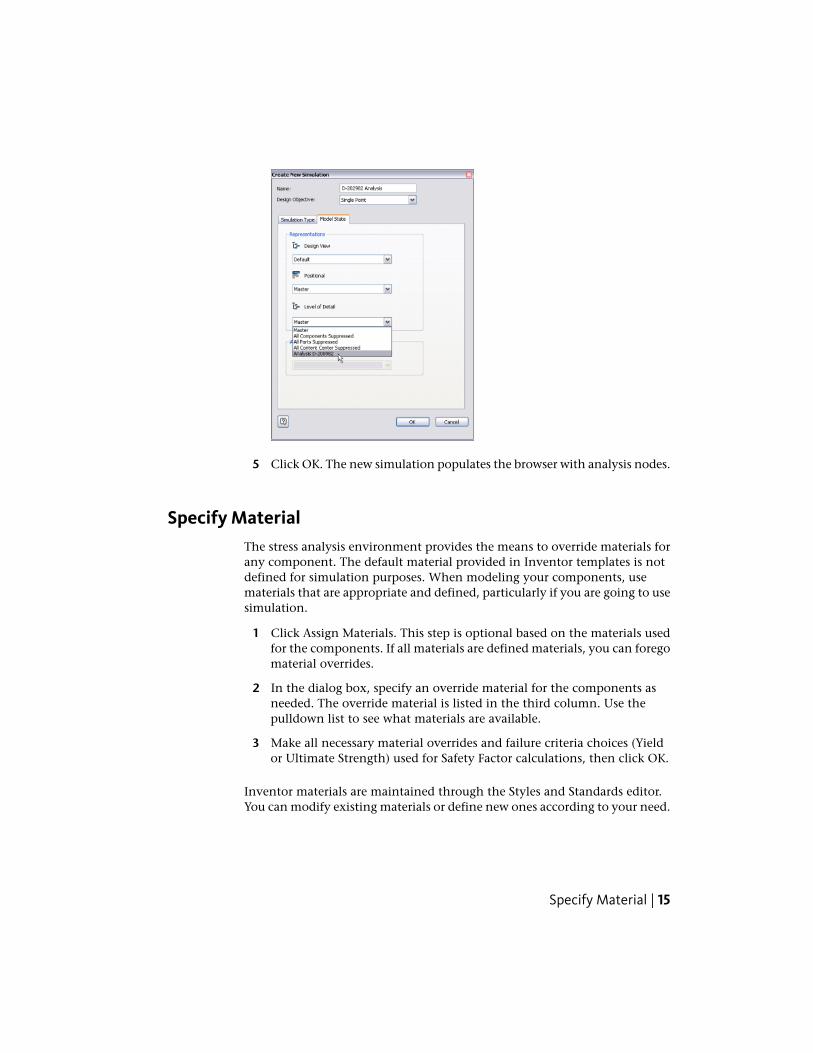
5 Click OK. The new simulation populates the browser with analysis nodes.

Specify MaterialThe stress analysis environment provides the means to override materials forany component. The default material provided in Inventor templates is notdefined for simulation purposes. When modeling your components, usematerials that are appropriate and defined, particularly if you are going to usesimulation.

1 Click Assign Materials. This step is optional based on the materials usedfor the components. If all materials are defined materials, you can foregomaterial overrides.

2 In the dialog box, specify an override material for the components asneeded. The override material is listed in the third column. Use thepulldown list to see what materials are available.

3 Make all necessary material overrides and failure criteria choices (Yieldor Ultimate Strength) used for Safety Factor calculations, then click OK.

Inventor materials are maintained through the Styles and Standards editor.You can modify existing materials or define new ones according to your need.

Specify Material | 15

You can access the editor from the Assign Materials dialog box or by clickingManage tab ➤ Styles and Standards panel ➤ Styles Editor.

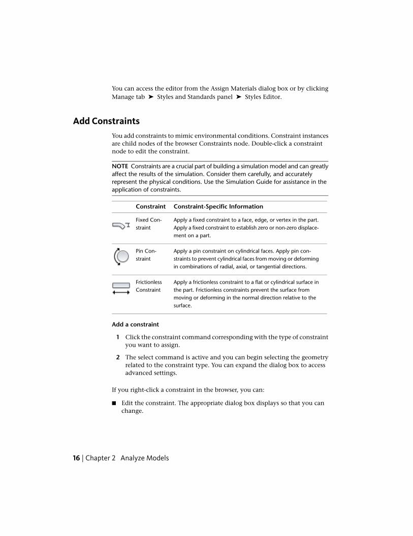
Add ConstraintsYou add constraints to mimic environmental conditions. Constraint instancesare child nodes of the browser Constraints node. Double-click a constraintnode to edit the constraint.

NOTE Constraints are a crucial part of building a simulation model and can greatlyaffect the results of the simulation. Consider them carefully, and accuratelyrepresent the physical conditions. Use the Simulation Guide for assistance in theapplication of constraints.

Constraint-Specific InformationConstraint

Apply a fixed constraint to a face, edge, or vertex in the part.Apply a fixed constraint to establish zero or non-zero displace-ment on a part.

Fixed Con-straint

Apply a pin constraint on cylindrical faces. Apply pin con-straints to prevent cylindrical faces from moving or deformingin combinations of radial, axial, or tangential directions.

Pin Con-straint

Apply a frictionless constraint to a flat or cylindrical surface inthe part. Frictionless constraints prevent the surface from

FrictionlessConstraint

moving or deforming in the normal direction relative to thesurface.

Add a constraint

1 Click the constraint command corresponding with the type of constraintyou want to assign.

2 The select command is active and you can begin selecting the geometryrelated to the constraint type. You can expand the dialog box to accessadvanced settings.

If you right-click a constraint in the browser, you can:

■ Edit the constraint. The appropriate dialog box displays so that you canchange.


■ View reaction forces. Values are zero until a simulation is run.

■ Suppress the constraint.

■ Copy and Paste between simulations within the same document.

■ Delete the constraint.

To rename an item in the browser, click it, pause, click it a second time, entera new name, and then press ENTER.

NOTE For some types of simulations you define, constraints are not required.

Add Loads

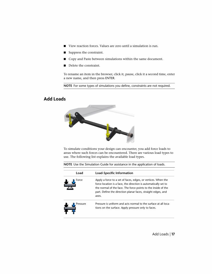
To simulate conditions your design can encounter, you add force loads toareas where such forces can be encountered. There are various load types touse. The following list explains the available load types.

NOTE Use the Simulation Guide for assistance in the application of loads.

Load-Specific InformationLoad

Apply a force to a set of faces, edges, or vertices. When theforce location is a face, the direction is automatically set to

Force

the normal of the face. The force points to the inside of thepart. Define the direction planar faces, straight edges, andaxes.

Pressure is uniform and acts normal to the surface at all loca-tions on the surface. Apply pressure only to faces.

Pressure

Add Loads | 17

Load-Specific InformationLoad

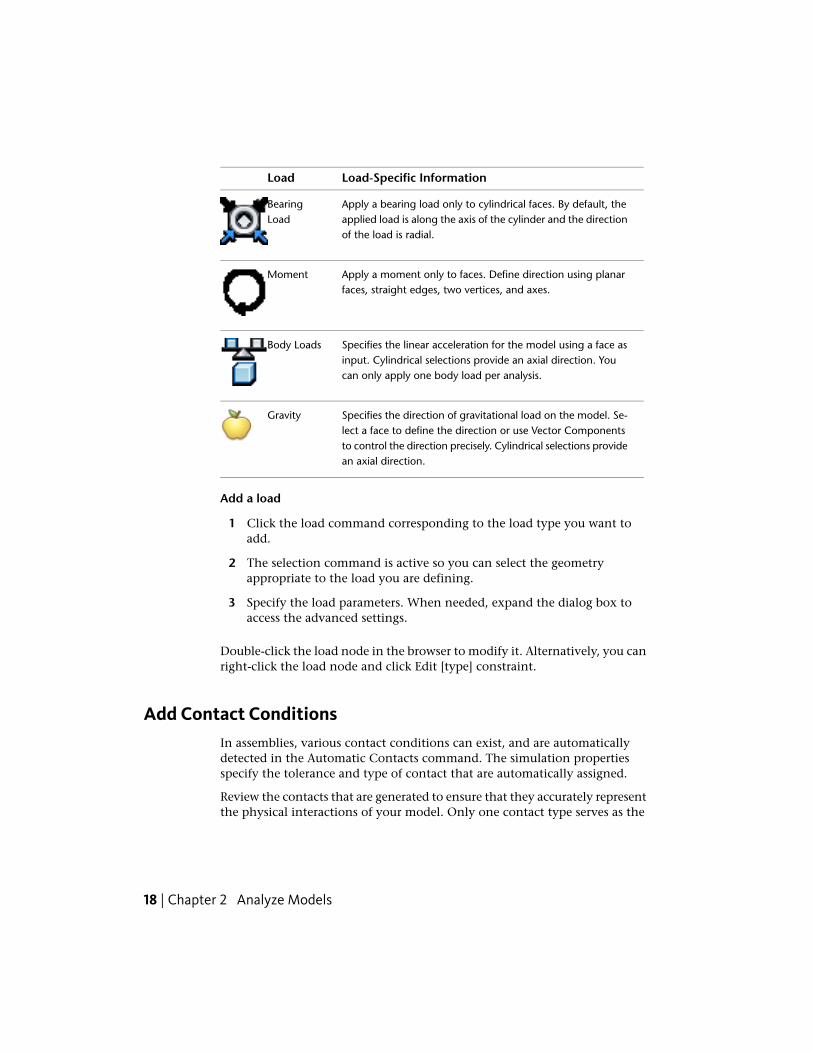
Apply a bearing load only to cylindrical faces. By default, theapplied load is along the axis of the cylinder and the directionof the load is radial.

BearingLoad

Apply a moment only to faces. Define direction using planarfaces, straight edges, two vertices, and axes.

Moment

Specifies the linear acceleration for the model using a face asinput. Cylindrical selections provide an axial direction. Youcan only apply one body load per analysis.

Body Loads

Specifies the direction of gravitational load on the model. Se-lect a face to define the direction or use Vector Components

Gravity

to control the direction precisely. Cylindrical selections providean axial direction.

Add a load

1 Click the load command corresponding to the load type you want toadd.

2 The selection command is active so you can select the geometryappropriate to the load you are defining.

3 Specify the load parameters. When needed, expand the dialog box toaccess the advanced settings.

Double-click the load node in the browser to modify it. Alternatively, you canright-click the load node and click Edit [type] constraint.

Add Contact ConditionsIn assemblies, various contact conditions can exist, and are automaticallydetected in the Automatic Contacts command. The simulation propertiesspecify the tolerance and type of contact that are automatically assigned.

Review the contacts that are generated to ensure that they accurately representthe physical interactions of your model. Only one contact type serves as the


default for automatically inferred contacts, so some modification afterwardcan be necessary.

NOTE Use the Simulation Guide for assistance in the application of contacts.

Automatic Contacts

To add contact conditions automatically, click the Automatic Contactscommand. Alternatively, right-click the Contact node and click AutomaticContacts.

Manual Contacts

At times, it is necessary to add contacts manually.

Add contact conditions manually

1 On the ribbon, click Stress Analysis tab ➤ Contacts panel ➤ Manual.

2 Specify the contact type.

3 Select the appropriate entities for the contact type. If other componentsare obscuring the component you want to select use Part selection optionto select the part first, then refine your selection thereafter.

Generate a MeshYou can accept the default mesh settings and proceed right to the simulation.At times, there are areas where you would like a mesh with greater density.You can adjust the mesh settings or use a local mesh control.

If you want to view the mesh settings, click the Mesh Settings command inthe Prepare panel. You can specify the mesh settings you want for thesimulation.

After you define the meshes, click Mesh View to produce the mesh. The meshis generated as an overlay atop the model geometry.

Generate a Mesh | 19

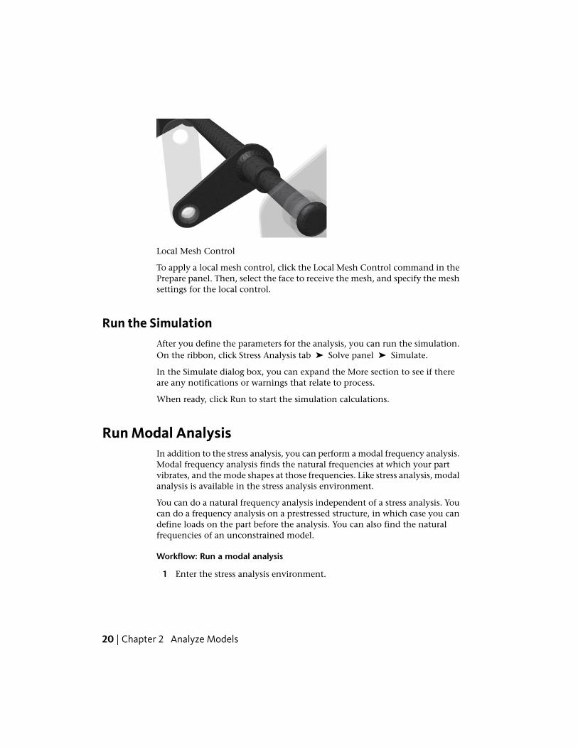
Local Mesh Control

To apply a local mesh control, click the Local Mesh Control command in thePrepare panel. Then, select the face to receive the mesh, and specify the meshsettings for the local control.

Run the SimulationAfter you define the parameters for the analysis, you can run the simulation.On the ribbon, click Stress Analysis tab ➤ Solve panel ➤ Simulate.

In the Simulate dialog box, you can expand the More section to see if thereare any notifications or warnings that relate to process.

When ready, click Run to start the simulation calculations.

Run Modal AnalysisIn addition to the stress analysis, you can perform a modal frequency analysis.Modal frequency analysis finds the natural frequencies at which your partvibrates, and the mode shapes at those frequencies. Like stress analysis, modalanalysis is available in the stress analysis environment.

You can do a natural frequency analysis independent of a stress analysis. Youcan do a frequency analysis on a prestressed structure, in which case you candefine loads on the part before the analysis. You can also find the naturalfrequencies of an unconstrained model.

Workflow: Run a modal analysis

1 Enter the stress analysis environment.


2 Start a new simulation, specifying Modal Analysis as the simulation type.

3 Verify that the material used for the part is suitable, or override theunsuitable with appropriate materials.

4 Apply the necessary constraints (optional).

5 Apply any loads (optional).

6 Adjust the mesh settings and preview the mesh (optional).

7 Click Simulate and in the dialog box, click Run.

The results for the first eight frequency modes are inserted under theResults folder in the browser. For an unconstrained part, the first sixfrequencies are essentially zero.

8 To change the number of frequencies displayed right click the Simulationnode (near the top of the browser), and select Edit Simulation Properties.

In the dialog box specify the number of modes to find.

After you complete all the required steps, the Update notification isdisplayed in the browser beside those sections that need updates.Right-click the node and click Update. On the Results node, right-clickthe node and click Simulate.

Run Modal Analysis | 21

22

View Results

After you analyze your model under the stress analysis conditions that you defined, you canvisually observe the results of the solution.

This chapter describes how to interpret the visual results of your stress analyses.

Use Results VisualizationWhen the simulation completes its computations, the graphics region updatesto show:

■ 3D Volume plot and result type.

■ Smooth Shading showing the distribution of stresses.

■ Color bar indicating the stress range.

■ Mesh Information including the number of nodes and elements.

■ Unit information.

■ Result browser node is populated with child nodes for the various resultsbased on the analysis type.

For Static Analysis, the default result is Von Mises Stress and for Modal Analysis,the default is Frequency 1. View the results by using the display commands andthe Results nodes in the browser. These tools help you visualize the magnitudeof the stresses that occur throughout the component, the deformation of thecomponent, and the stress safety factor. For modal analysis, you visualize thenatural frequency modes.

NOTE Use the Simulation Guide for assistance in displaying results.

3

23

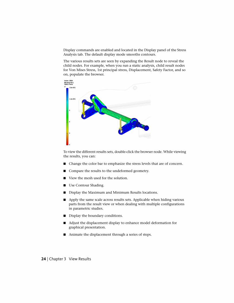
Display commands are enabled and located in the Display panel of the StressAnalysis tab. The default display mode smooths contours.

The various results sets are seen by expanding the Result node to reveal thechild nodes. For example, when you run a static analysis, child result nodesfor Von Mises Stress, 1st principal stress, Displacement, Safety Factor, and soon, populate the browser.

To view the different results sets, double-click the browser node. While viewingthe results, you can:

■ Change the color bar to emphasize the stress levels that are of concern.

■ Compare the results to the undeformed geometry.

■ View the mesh used for the solution.

■ Use Contour Shading.

■ Display the Maximum and Minimum Results locations.

■ Apply the same scale across results sets. Applicable when hiding variousparts from the result view or when dealing with multiple configurationsin parametric studies.

■ Display the boundary conditions.

■ Adjust the displacement display to enhance model deformation forgraphical presentation.

■ Animate the displacement through a series of steps.

24 | Chapter 3 View Results

■ Create a video of the displacement animation.

■ View 2D Convergence Plots (result accuracy curve).

■ Probe for values at specific points.

Edit the Color BarThe color bar shows you how the contour colors correspond to the stressvalues or displacements calculated in the solution. You can edit the color barto set up the color contours so that the stress/displacement is displayed in away that is meaningful to you.

Edit the color bar

1 On the ribbon, click Stress Analysis tab ➤ Display panel ➤ Color Bar.

By default, the maximum and minimum values shown on the color barare the maximum and minimum result values from the solution. Youcan edit the maximum and minimum values to adjust the way the bandsappear.

2 To edit the maximum and minimum critical threshold values, clear thecheck box next to the item you want to modify. Edit the values in thetext box. Click OK to complete the change.

To restore the default maximum and minimum critical threshold values,check the corresponding box next to the item.

The levels are initially divided into seven equivalent sections, with defaultcolors assigned to each section. You can select the number of contourcolors in the range of 2 to 12.

When using smooth shading, only five colors are used and these controlsare disabled.

3 To increase or decrease the number of colors, click Increase Colorsand Decrease Colors. You can also enter the number of colors you wantin the text box.

4 You can view the result contours in different colors or in shadesof gray. To view result contours on the grayscale, click Grayscale underColor Type.

Edit the Color Bar | 25

NOTE It does not work for safety factor.

5 By default, the color bar is positioned in the upper-left corner. Select anappropriate option under Position to place the color bar at a differentlocation.

6 For Size, select an appropriate option to resize the color bar, and thenclick OK.

The color bar settings are applied on a per result basis.

Read Stress Analysis ResultsWhen the analysis is complete, you see the results of your solution. If you dida stress analysis, the Von Mises Stress results set displays. If your initial analysisis a natural frequency analysis, the results set for the first mode displays. Toview a different results set, double-click that results set in the browser pane.The currently viewed results set has a check mark next to it in the browser.You always see the undeformed wireframe of the part when you are viewingresults.

Interpret Results ContoursThe contour colors display in the results corresponds to the value ranges shownin the legend. In most cases, results that display in red are of most interest.They represent high stress or high deformation, or a low factor of safety. Eachresults set gives you different information about the effect of the load on yourpart.

Von Mises StressVon Mises stress results use color contours to show you the stresses calculatedduring the solution for your model. The deformed model is displayed. Thecolor contours correspond to the values defined by the color bar.


1st Principal StressThe 1st principal stress gives you the value of stress that is normal to the planein which the shear stress is zero. The 1st principal stress helps you understandthe maximum tensile stress induced in the part due to the loading conditions.

3rd Principal StressThe 3rd principal stress acts normal to the plane in which shear stress is zero.It helps you understand the maximum compressive stress induced in the partdue to the loading conditions.

DisplacementThe Displacement results show you the deformed shape of your model afterthe solution. The color contours show you the magnitude of deformationfrom the original shape. The color contours correspond to the values definedby the color bar.

Safety FactorSafety factor shows you the areas of the model that are likely to fail underload. The color contours correspond to the values defined by the color bar.

Stress FolderContains normal and shear stress results for your simulation.

Displacement FolderContains normal and shear stress results for your simulation.

NOTE For modal analyses, the displacement results are modal deformations. Thedisplacement magnitude is relative and cannot be taken as actual deformation.

Interpret Results Contours | 27

Strain FolderContains strain results for your simulation.

Contact Pressure FolderContains contact pressure results for your simulation. Contact pressure is thepressure at contact interfaces. Includes contact pressure components and theresultant value.

Modal Frequency FolderYou can view the mode plots for the number of natural frequencies that youspecified in the solution. The modal results appear under the Results node inthe browser. When you double-click a frequency mode, the mode shapedisplays. The color contours show you the magnitude of deformation fromthe original shape. These deformations are modal, and their magnitude isrelative and cannot be taken as the actual deformation. The frequency of themode shows in the legend. It is also available as a parameter.

Animate ResultsUse Animate Displacement to visualize the part through various stages ofdeformation. You can also animate stress, safety factor, and deformation underfrequencies.

Set Results Display OptionsThe following commands are located on the Result and Display panels. Whileviewing your results, use the commands to modify the features of the resultsdisplay for your model.

Used toCommand

Maintains the same scale while viewing differentresults.

Same Scale


Used toCommand

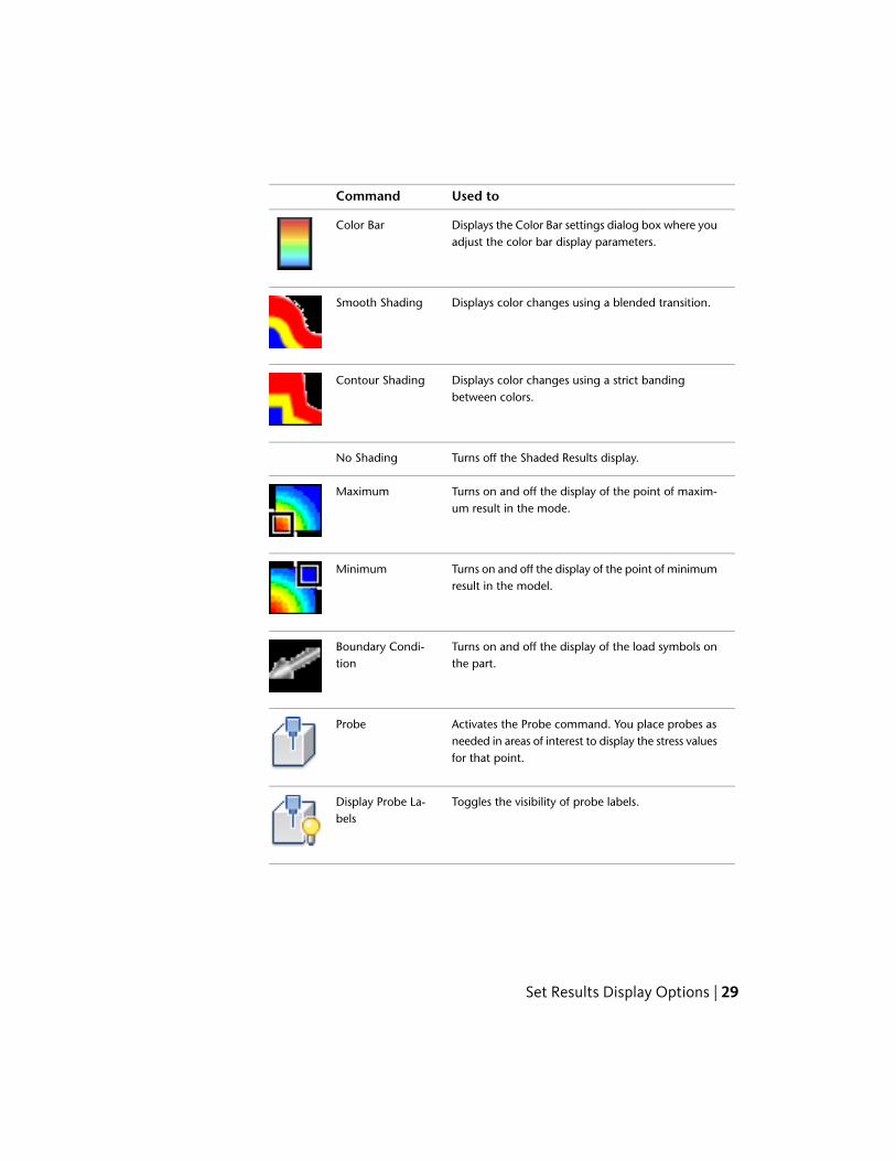
Displays the Color Bar settings dialog box where youadjust the color bar display parameters.

Color Bar

Displays color changes using a blended transition.Smooth Shading

Displays color changes using a strict bandingbetween colors.

Contour Shading

Turns off the Shaded Results display.No Shading

Turns on and off the display of the point of maxim-um result in the mode.

Maximum

Turns on and off the display of the point of minimumresult in the model.

Minimum

Turns on and off the display of the load symbols onthe part.

Boundary Condi-tion

Activates the Probe command. You place probes asneeded in areas of interest to display the stress valuesfor that point.

Probe

Toggles the visibility of probe labels.Display Probe La-bels

Set Results Display Options | 29

Used toCommand

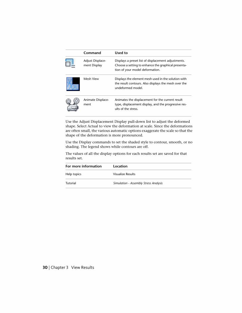
Displays a preset list of displacement adjustments.Choose a setting to enhance the graphical presenta-tion of your model deformation.

Adjust Displace-ment Display

Displays the element mesh used in the solution withthe result contours. Also displays the mesh over theundeformed model.

Mesh View

Animates the displacement for the current resulttype, displacement display, and the progressive res-ults of the stress.

Animate Displace-ment

Use the Adjust Displacement Display pull-down list to adjust the deformedshape. Select Actual to view the deformation at scale. Since the deformationsare often small, the various automatic options exaggerate the scale so that theshape of the deformation is more pronounced.

Use the Display commands to set the shaded style to contour, smooth, or noshading. The legend shows while contours are off.

The values of all the display options for each results set are saved for thatresults set.


Visualize ResultsHelp topics

Simulation - Assembly Stress AnalysisTutorial


Revise Models and StressAnalyses

After you run a simulation for your model, you can evaluate how changes to the model oranalysis conditions affect the results of the simulation.

This chapter explains how to change simulation conditions for the model and rerun thesimulation.

Change Model GeometryAfter you run an analysis on your model, you can change the design of yourmodel. Rerun the analysis to see the effects of the changes.

Edit a design and rerun analysis

1 In the browser, right-click the part or assembly you want to edit and clickOpen.

The component opens in another window where you can change. At thebottom of the window near the status bar, there is a tab for each opendocument. For the purposes of this discussion, we talk about a part edit.

2 In the browser, expand the feature node that you want to edit.

3 In the browser, right-click the feature that you want to edit and click ShowDimensions. The dimensions for that feature display over the model.

4 Double-click the dimension that you want to change, enter the new valuein the text box, and then click the green check mark. The sketch updates.

5 In the Quick Access Toolbar (QAT), click the Update model command.

4

31

6 At the bottom of the window, click the assembly tab. Your componentis updated.

7 Some portions of the simulation can now be out of date with the change.If an update is necessary to have current analysis data, right-click theContacts node, and click Update.

8 Repeat step 7 for each area that requires it. Then click Simulate to updatethe results.

After you update the simulation, the load glyphs relocate if the feature thatthey were associated with moved as a result of the geometry change. Thedirection of the load does not change, even if the feature associated with theload changes orientation.

Change Solution ConditionsAfter you run an analysis on your model, you can change the conditions underwhich the results were obtained. Rerun the analysis to see effects of thechanges. You can edit the loads and constraints you defined, add new loadsand constraints, or delete loads and constraints. To change your simulationconditions, enter the stress analysis environment if you are not already in it.

Delete a load or constraint

■ In the browser, right-click a load or constraint, and then select Delete fromthe menu.

Add a load or constraint

■ On the Stress Analysis tab, select the command and follow the sameprocedure you used to create your initial loads and constraints.

Edit a load or constraint

1 In the browser, right-click a load or constraint, and then select Edit fromthe menu.

The same dialog box you used to create the load or constraint displays.The values on the dialog box are the current values for that load orconstraint.

2 Click the selection arrow on the left side of the dialog box to enablefeature picking.

32 | Chapter 4 Revise Models and Stress Analyses

You are initially limited to selecting the same type of feature (face, edge,or vertex) that is currently used for the load or constraint.

To remove any of the current features, CTRL-click them. If you removeall of the current features, your new selections can be of any type.

3 Click the Direction Selection arrow to specify the change of directionusing model geometry.

4 Click Flip Direction to reverse the direction, if needed.

5 Change any values associated with the load or constraint.

6 Click OK to apply the load or constraint changes.

Hide a load symbol

■ On the ribbon, click Stress Analysis tab ➤ Display panel ➤

Boundary Conditions.The load symbols are hidden.

Redisplay a load symbol

■ On the Stress Analysis tab, click Boundary Conditions again.The load symbols redisplay.

Temporarily display load location

■ In the browser, pause the cursor over the Load or Constraint node. Theassociated face where the load or constraint is applied highlights.

Change the analysis type

1 In the browser, right-click the simulation and click Edit SimulationProperties.

2 On the Simulation Properties dialog box, Simulation Type tab, select thenew analysis type.

Change Solution Conditions | 33

Update Results of Stress AnalysisAfter you change any of the simulation conditions, or if you edit the partgeometry, the current results are invalid. A lightning bolt symbol next to theresults node indicates the invalid status. The Update command is located inthe node context menu and is enabled.

Update stress analysis results

■ Right-click the node that needs an update, and click Update.New results generate based on your revised solution conditions.


Simulation - Assembly Stress AnalysisTutorialSimulation - Part Modal and Stress Analysis

34 | Chapter 4 Revise Models and Stress Analyses

Generate Reports

After you run an analysis on a part or assembly, you can generate a report that provides arecord of the analysis environment and results.

This chapter tells you how to generate and interpret a report for an analysis, and how to saveand distribute the report.

Run ReportsAfter you run a simulation on a part or assembly, you can save the details ofthat analysis for future reference. Use the Report command to save all theanalysis conditions and results in HTML, MIME HTML, or Rich Text Format,for easy viewing and storage.

Generate a report

1 Set up and run an analysis for your part.

2 Orient the view in the graphics region the way you want to see it in thereport.

3 On the ribbon, click Stress Analysis tab ➤ Report panel ➤ Report to createa report for the current analysis.

4 Specify the report parameters in the dialog box. You control the reporttitle, filename, file location, file format, image size, properties reported,and so on. The report generates various image orientations based on theview orientation you established.

5 The report is then generated, presented in an internet browser, and savedfor your viewing and distribution.

5

35

Interpret ReportsThe report contains model information, project information, and simulationresults.

Model InformationThe Model information contains the model name, version of Inventor, andthe creation date.

Project InfoThe Project Info includes the following:

■ Summary, which includes the Author property.

■ Project properties, which includes part number, designer, cost, and datecreated.

■ Status property

■ Physical properties

SimulationThe simulation section gives details about the simulation conditions.

General objective and settingsThis section contains:

■ The design objective

■ Simulation Type

■ Last Modification date

■ Setting for Detect and Eliminate Rigid body modes

36 | Chapter 5 Generate Reports

Advanced settingsThis section contains:

■ Average Element size

■ Minimum element size

■ Grading Factor

■ Maximum Turn Angle

■ Create Curved Mesh Elements setting value

Material(s)■ Material name

■ General properties

■ Stress properties

■ Part names, if an assembly report

Operating conditions■ Each force by type and magnitude, with images

■ Each constraint by type with images.

Results■ Reaction force and moment on constraints

■ Images for each result type as seen in the reports section of the browser

The document path is listed last of all.

Save and Distribute ReportsYou select from the default HTML, MIME HTML, or Rich Text Format as thefile format for your report. You can accept the default settings for your report

Save and Distribute Reports | 37

generation or customize how information is output to your reports and wherethe reports are stored.

Saved ReportsBy default reports are saved in the same location as the model being analyzed.The report images are saved in a directory name Images in the same locationas the model being analyzed.

Be careful when you name a report. If the file name and location are the sameas the previous report, it is possible to overwrite the file without warning. Toavoid confusion, it is best to use a different name for each version of a report,or to delete the previous report.

Print ReportsUse your Web browser Print command to print the report as you would anyWeb page.

Distribute ReportsTo make the report available from a Web site, move all the files associatedwith the report to your Web site. Distribute a URL that points to the report.

38 | Chapter 5 Generate Reports

Manage Stress AnalysisFiles

Running a stress analysis in Autodesk® Inventor® Simulation creates separate files that containthe stress analysis information. In addition, the model file is modified to indicate the presenceof the stress files and the name of the files.

This chapter explains how the files are interdependent, and what to do if the files becomeseparated.

Create and Use Analysis FilesAfter you set up stress analysis information in Autodesk Inventor Simulation,you save the part or assembly. This action also saves the stress analysisinformation in the model file. Stress Analysis input and results information,including loads, constraints, and all results are also saved in separate files.

Simulation files are stored in a dedicated folder of the same name as the modelfile. By default, OLE links are created to each of these files. You can turn off thelinks by changing the option.

Understand File RelationshipsThe simulation files are unique to a given model and simulation. Inventormaintains file relationships as needed. There is no reason to work with or modifythe simulation files outside of Inventor.

The Save As and Save Copy As commands copy all Simulation files.

6

39

Resolve Missing FilesUnder certain circumstances, simulation files can be relocated or missing whenworking with a model. When you first open a model file, the Resolve Linkdialog box displays. You can browse to the location of the simulation files, oryou can choose to skip them.

If you skip the files, the Simulation environment can recompute the files ifnecessary.

40 | Chapter 6 Manage Stress Analysis Files

Dynamic Simulation

Part 2 of this manual presents the getting started information for Dynamic Simulation in theAutodesk® Inventor® Simulation software. This application environment provides commandsto predict dynamic performance and peak stresses before building prototypes.

41

42

Dynamic Simulation

Autodesk® Inventor® Simulation provides commands to simulate and analyze the dynamiccharacteristics of an assembly in motion under various load conditions. You can export loadconditions at any motion state to Stress Analysis in Autodesk Inventor Simulation. Thesimulation reveals how parts respond from a structural point of view to dynamic loads at anypoint in the range of motion of the assembly.

Features in Dynamic SimulationThe dynamic simulation environment works only with Autodesk Inventor®

assembly (.iam) files.

With the dynamic simulation, you can:

■ Have the software automatically convert all mate and insert constraints intostandard joints.

■ Access a large library of motion joints.

■ Define external forces and moments.

■ Create motion simulations based on position, velocity, acceleration, andtorque as functions of time in joints, in addition to external loads.

■ Visualize 3D motion using traces.

■ Export full output graphing and charts to Microsoft® Excel®.

■ Transfer dynamic and static joints and inertial forces to Autodesk InventorSimulation Stress Analysis or ANSYS Workbench.

■ Calculate the force required to keep a dynamic simulation in staticequilibrium.

■ Convert assembly constraints to motion joints.

7

43

■ Use friction, damping, stiffness, and elasticity as functions of time whendefining joints.

■ Use dynamic part motion interactively to apply dynamic force to thejointed simulation.

■ Use Inventor Studio to output realistic or illustrative video of yoursimulation.

Learning Autodesk Inventor SimulationWe assume that you have a working knowledge of the Autodesk InventorSimulation interface and commands. If you do not, use the integrated Helpfor access to online documentation and tutorials, and complete the exercisesin this manual.

At a minimum, we recommend that you understand how to:

■ Use the assembly, part modeling, and sketch environments and browsers.

■ Edit a component in place.

We recommend that you have a working knowledge of Microsoft® Windows®

XP or Windows Vista®, and concepts for stressing and analyzing mechanicalassembly designs.

Use HelpAs you perform tasks, you can get additional information in the Help system.It provides detailed concepts, procedures, and reference information aboutevery feature in the Autodesk Inventor Simulation modules and AutodeskInventor Simulation.

To access Help, use one of the following methods:

■ Click Help ➤ Help Topics. On the Contents tab, click Dynamic Simulation.

■ In any dialog box, click the ? icon.

44 | Chapter 7 Dynamic Simulation

Understand Simulation CommandsLarge and complex moving assemblies coupled with hundreds of articulatedmoving parts can be simulated. Dynamic Simulation provides:

■ Interactive, simultaneous, and associative visualization of 3D animationswith trajectories; velocity, acceleration, and force vectors; and deformablesprings.

■ Graphic generation command for representing and post-processing thesimulation output data.

Simulation AssumptionsThe dynamic simulation commands provided in Autodesk Inventor Simulationare invaluable in the conception and development steps and in reducing thenumber of prototypes. However, due to the hypothesis used in the simulation,it provides only an approximation of the behavior seen in real-life mechanisms.

Interpret Simulation ResultsSome computations can lead to a misinterpretation of the results or incompletemodels that cause unusual behavior. In some cases, a simulation can beimpossible to compute. To avoid these situations, be aware of the rules thatapply to:

■ Relative parameters

■ Continuity of laws

■ Coherent masses and inertia

Relative ParametersDynamic Simulation uses relative parameters. For example, the positionvariables, velocity, and acceleration give a direct description of the motion ofa child part. The motion is according to a parent part through the degree offreedom (DOF) of the joint that links them. As a result, select the initial velocityof a degree of freedom carefully.

Understand Simulation Commands | 45

Coherent Masses and InertiaEnsure that the mechanism is well-conditioned. For example, ensure that themass and inertia of the mechanism is in the same order of magnitude. Themost common error is a bad definition of density or volume of the CAD parts.

Continuity of LawsNumerical computing is sensitive toward incontinuities in imposed laws. Thus,while a velocity law defines a series of linear ramps, the acceleration isnecessarily discontinuous. Similarly, when using contact joints, it is better toavoid profiles or outlines with straight edges.

NOTE Using little fillets eases the computation by breaking the edge.


Simulation - Fundamentals - Part 1Tutorial

46 | Chapter 7 Dynamic Simulation

Simulate Motion

With the dynamic simulation or the assembly environment, the intent is to build a functionalmechanism. Dynamic simulation adds to that functional mechanism the dynamic, real-worldinfluences of various kinds of loads to create a true kinematic chain.

Understand Degrees of FreedomThough both have to do with creating mechanisms, there are some criticaldifferences between the dynamic simulation and the assembly environment.The most basic and important difference has to do with degrees of freedom.

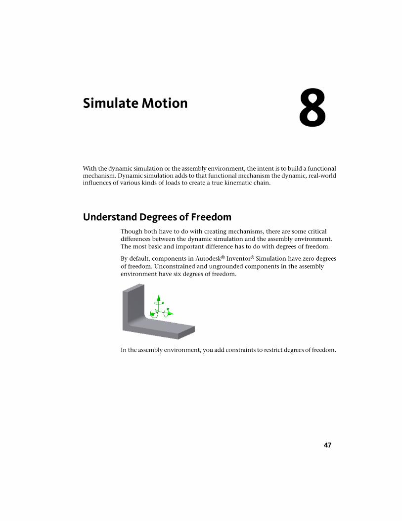
By default, components in Autodesk® Inventor® Simulation have zero degreesof freedom. Unconstrained and ungrounded components in the assemblyenvironment have six degrees of freedom.

In the assembly environment, you add constraints to restrict degrees of freedom.

8

47

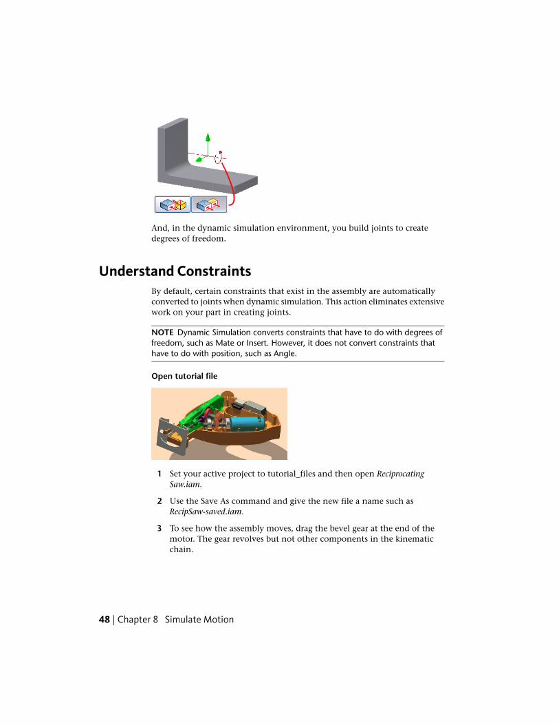
And, in the dynamic simulation environment, you build joints to createdegrees of freedom.

Understand ConstraintsBy default, certain constraints that exist in the assembly are automaticallyconverted to joints when dynamic simulation. This action eliminates extensivework on your part in creating joints.

NOTE Dynamic Simulation converts constraints that have to do with degrees offreedom, such as Mate or Insert. However, it does not convert constraints thathave to do with position, such as Angle.

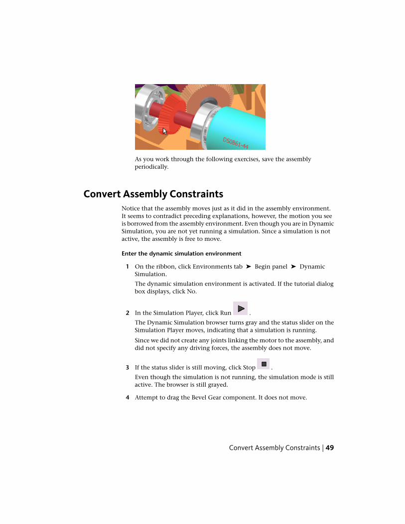
Open tutorial file

1 Set your active project to tutorial_files and then open ReciprocatingSaw.iam.

2 Use the Save As command and give the new file a name such asRecipSaw-saved.iam.

3 To see how the assembly moves, drag the bevel gear at the end of themotor. The gear revolves but not other components in the kinematicchain.

48 | Chapter 8 Simulate Motion

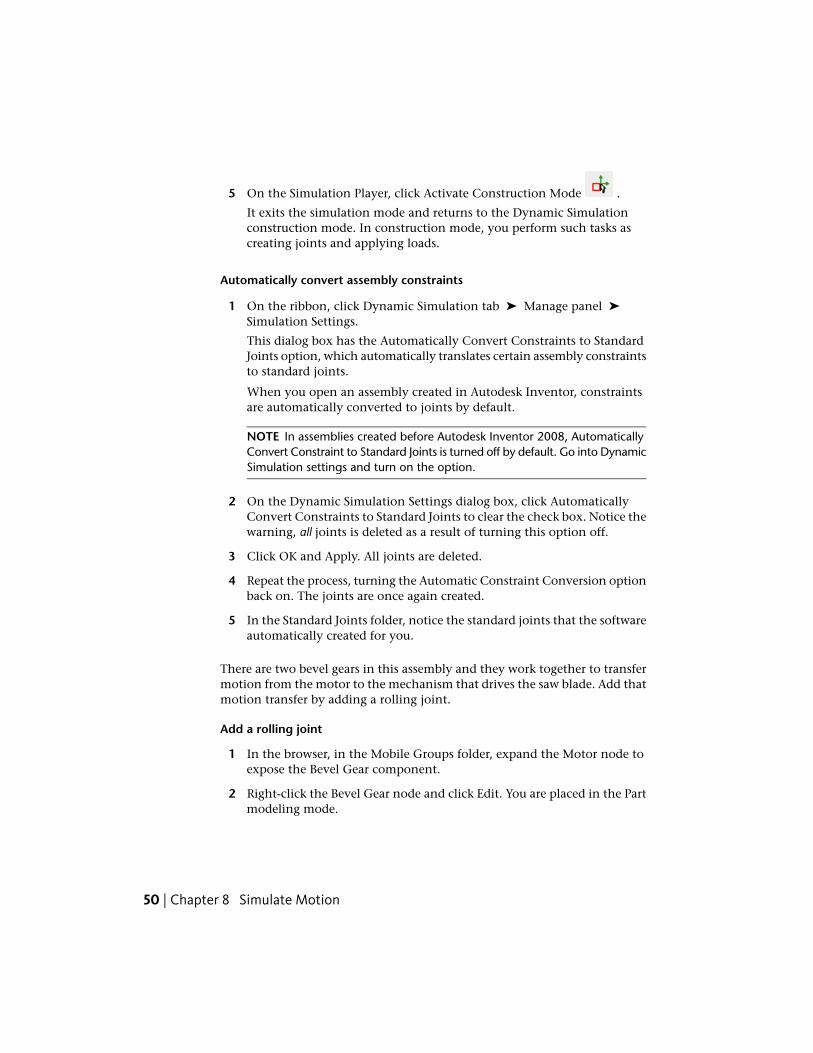
As you work through the following exercises, save the assemblyperiodically.

Convert Assembly ConstraintsNotice that the assembly moves just as it did in the assembly environment.It seems to contradict preceding explanations, however, the motion you seeis borrowed from the assembly environment. Even though you are in DynamicSimulation, you are not yet running a simulation. Since a simulation is notactive, the assembly is free to move.

Enter the dynamic simulation environment

1 On the ribbon, click Environments tab ➤ Begin panel ➤ DynamicSimulation.

The dynamic simulation environment is activated. If the tutorial dialogbox displays, click No.

2 In the Simulation Player, click Run .

The Dynamic Simulation browser turns gray and the status slider on theSimulation Player moves, indicating that a simulation is running.

Since we did not create any joints linking the motor to the assembly, anddid not specify any driving forces, the assembly does not move.

3 If the status slider is still moving, click Stop .

Even though the simulation is not running, the simulation mode is stillactive. The browser is still grayed.

4 Attempt to drag the Bevel Gear component. It does not move.

Convert Assembly Constraints | 49

5 On the Simulation Player, click Activate Construction Mode .

It exits the simulation mode and returns to the Dynamic Simulationconstruction mode. In construction mode, you perform such tasks ascreating joints and applying loads.

Automatically convert assembly constraints

1 On the ribbon, click Dynamic Simulation tab ➤ Manage panel ➤

Simulation Settings.

This dialog box has the Automatically Convert Constraints to StandardJoints option, which automatically translates certain assembly constraintsto standard joints.

When you open an assembly created in Autodesk Inventor, constraintsare automatically converted to joints by default.

NOTE In assemblies created before Autodesk Inventor 2008, AutomaticallyConvert Constraint to Standard Joints is turned off by default. Go into DynamicSimulation settings and turn on the option.

2 On the Dynamic Simulation Settings dialog box, click AutomaticallyConvert Constraints to Standard Joints to clear the check box. Notice thewarning, all joints is deleted as a result of turning this option off.

3 Click OK and Apply. All joints are deleted.

4 Repeat the process, turning the Automatic Constraint Conversion optionback on. The joints are once again created.

5 In the Standard Joints folder, notice the standard joints that the softwareautomatically created for you.

There are two bevel gears in this assembly and they work together to transfermotion from the motor to the mechanism that drives the saw blade. Add thatmotion transfer by adding a rolling joint.

Add a rolling joint

1 In the browser, in the Mobile Groups folder, expand the Motor node toexpose the Bevel Gear component.

2 Right-click the Bevel Gear node and click Edit. You are placed in the Partmodeling mode.


3 Right-click the Srf1 node and click Visibility. The Bevel Gear constructionsurface displays. We use this surface to help define the gear relationship.

4 At the right end of the ribbon panel, click Return. You are placed backin the simulation environment.

5 On the ribbon, click Dynamic Simulation tab ➤ Joint panel ➤ Insert

Joint .

6 In the pull down list, select Rolling: Cone on Cone.

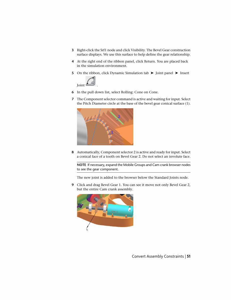
7 The Component selector command is active and waiting for input. Selectthe Pitch Diameter circle at the base of the bevel gear conical surface (1).

8 Automatically, Component selector 2 is active and ready for input. Selecta conical face of a tooth on Bevel Gear 2. Do not select an involute face.

NOTE If necessary, expand the Mobile Groups and Cam crank browser nodesto see the gear component.

The new joint is added to the browser below the Standard Joints node.

9 Click and drag Bevel Gear 1. You can see it move not only Bevel Gear 2,but the entire Cam crank assembly.

Convert Assembly Constraints | 51

Run SimulationsThe Simulation Player contains several fields including:

1 Final Time

2 Images

3 Filter

4 Simulation Time

5 Percent of Realized Simulation

6 Real Time of Computation

Simulation Panel

Controls the total time available for simulation.Final Time field

Controls the number of image frames available for asimulation.

Images field

Controls the frame display step. If the value is set to1, all frames play. If the value is set to 5, every fifth

Filter field

frame displays, and so on. This field is editable whensimulation mode is active, but a simulation is notrunning.

Shows the duration of the motion of the mechanismas would be witnessed with the physical model.

Simulation TimeValue

Shows the percentage complete of a simulation.Percent value

Shows the actual time it takes to run the simulation.The complexity of the model and the resources of yourcomputer affect the time.

Real Time of Compu-tation value


TIP Click the Screen Refresh command to turn off screen refresh during thesimulation. The simulation runs, but there is no graphic representation.

Before you run the simulation, make the following adjustments.

Set up a simulation

1 On the Simulation Player, in the Final Time field, enter 0.5 s.

TIP Use the tooltips to see the names of the fields in the Simulation Player.

2 In the Images field, enter 200. Increasing the image count improves theresults when viewed using the Output Grapher.

3 On the Simulation Panel, click Run.

As the Motor component moves, the other components making up thekinematic chain respond.

NOTE Because we did not yet specify any frictional or damping forces, themechanism is lossless. There is no friction automatically created betweencomponents.

4 If the simulation is still running, on the simulation panel, click Stop.

5 Click Activate construction mode.

As you can see, running the simulation did not result in motion because thekinematic chain is incomplete. In the following chapter, you complete theconstruction and enable motion.



Run Simulations | 53

54

Construct MovingAssemblies

To simulate the dynamic motion in an assembly, define mechanical joints between the parts.

This chapter provides basic workflows for constructing joints.

Retain Degrees of FreedomIn some cases, it is appropriate that certain parts move as a rigid body and ajoint is not required. As far as the movement of these parts is concerned, thewelded body functions like a subassembly moving in a constraint chain withina parent assembly. Similarly, at other times, components making up a weldedgroup need degrees of freedom for movement within the simulation. Such isthe case with the welded group in the Saw model.

Create a 2D contact

1 In the browser, expand Mobile Groups.

2 Right-click the Follower Roller, and click Retain DOF. The roller retains itsmotion characteristics.

3 In the graphics region, click and drag the Follower away from the Camcrank assembly.

4 On the ribbon, click Dynamic Simulation tab ➤ Joint panel ➤ InsertJoint and from the list, select 2D Contact.

5 Select the Cam profile edge (1).

9

55

6 Select circular sketch (2) on the roller component.

7 Click Apply. As you can see, sketch geometry can be used to help definethe simulation.

8 Drag the Follower until the roller contacts the cam. Notice it does notpenetrate. The 2D contact established a mechanical relationship betweenthe two components.

9 Set the properties for the 2D contact and display the force vector. In thebrowser, right-click the 2D Contact joint and click Properties.

10 Set the Restitution values to 0.0.

11 Expand the dialog box to access the lower section. Check the Normalbox and set the Scale to 0.003.

56 | Chapter 9 Construct Moving Assemblies

Add JointsThe Follower is designed to slide through a portion of the Guide component.However, to hold the Follower Roller against the Cam, specify a spring betweenthe Follower and Guide components. Dynamic Simulation has a joint fordoing that and more, the Spring/Damper/Jack joint.

1 On the ribbon, click Dynamic Simulation tab ➤ Joint panel ➤ InsertJoint and in the list, select Spring / Damper / Jack joint.

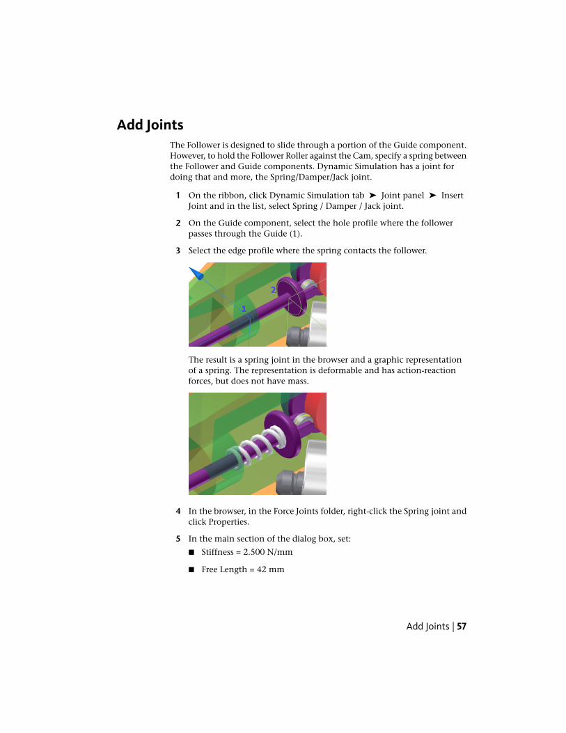
2 On the Guide component, select the hole profile where the followerpasses through the Guide (1).

3 Select the edge profile where the spring contacts the follower.

The result is a spring joint in the browser and a graphic representationof a spring. The representation is deformable and has action-reactionforces, but does not have mass.

4 In the browser, in the Force Joints folder, right-click the Spring joint andclick Properties.

5 In the main section of the dialog box, set:

■ Stiffness = 2.500 N/mm

■ Free Length = 42 mm

Add Joints | 57

Expand the dialog box and set:

■ Radius = 5.2 mm

■ Turns = 10

■ Wire Radius = .800 mm

6 Click OK. The spring properties and graphical display update.

Define gravity

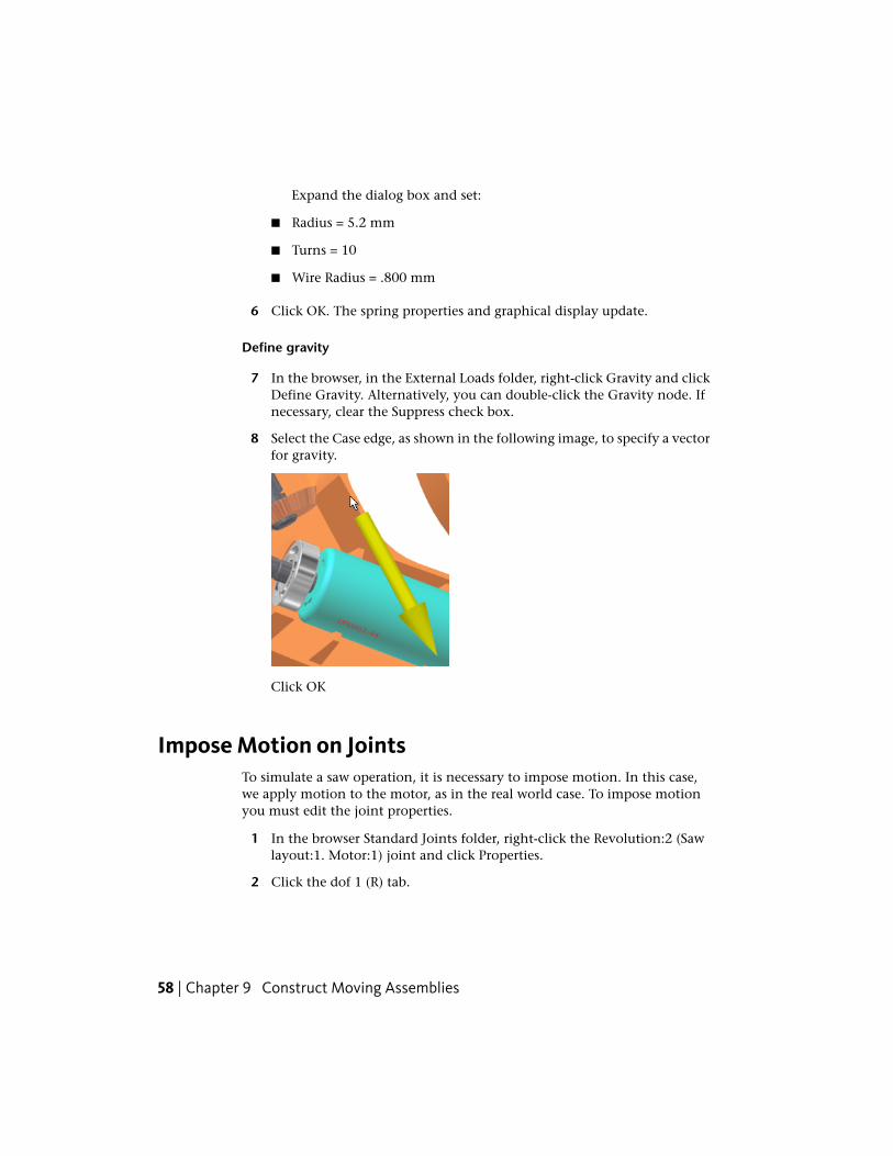
7 In the browser, in the External Loads folder, right-click Gravity and clickDefine Gravity. Alternatively, you can double-click the Gravity node. Ifnecessary, clear the Suppress check box.

8 Select the Case edge, as shown in the following image, to specify a vectorfor gravity.

Click OK

Impose Motion on JointsTo simulate a saw operation, it is necessary to impose motion. In this case,we apply motion to the motor, as in the real world case. To impose motionyou must edit the joint properties.

1 In the browser Standard Joints folder, right-click the Revolution:2 (Sawlayout:1. Motor:1) joint and click Properties.

2 Click the dof 1 (R) tab.


3 Click Edit Joint Motion , and check Enable imposed motion.

4 Verify that Velocity is the selected Driving option.

5 In the input field, click the arrow to expand the input choices and clickConstant Value. Specify 10,000 deg/s

6 Click OK.

Run SimulationsBecause the simulation is of a high speed device, modify the simulationproperties.

TIP Use the tooltips to see the names of the fields on the Simulation Player

Set simulation options

1 On the Simulation Player, Final Time field, enter .5 s, which is sufficientto demonstrate the mechanism.

NOTE The software automatically increases the value in the Images fieldproportionally to the change in the Final Time field. Press the Tab key tomove the cursor out of the Final Time field to update the Images field.

2 In the images field, enter 200. Increasing the image count improves theresults you view in the Output Grapher.

3 Click Run on the Simulation Player.

As the Motor component drives the bevel gear, the remaining parts inthe kinematic chain respond.

The direction of gravity has nothing to do with any external notion of"up" or "down," but is set according to the vector you specified.

Also, because we have not yet specified any frictional or damping forces,the mechanism is lossless. There is no friction between components,regardless of how long the simulation runs.

Run Simulations | 59

4 If the simulation is still running, click Stop on the Simulation Player.


Simulation - Assembly Motion and LoadsSimulation - FEA using Motion Loads

Tutorial


Construct OperatingConditions

This chapter demonstrates how to complete the motion definitions so that the simulationreflects operating conditions.

Complete the AssemblyIf the RecipSaw-saved.iam assembly is not open, open the file to continue. Asyou can see, though we have the saw body, we do not have the bladecomponents. To add the blade components it is not necessary to leave thesimulation environment.:

1 Click the Assemble tab to display the assembly ribbon.

2 In the Component panel, click Place Component. Select Blade set.iam andclick Open.

3 Position the Blade set assembly near where you plan to assemble it.

10

61

4 In the browser, expand the Blade set assembly node to expose thecomponents.

5 Select the Scottish Yoke component. On the Quick Access Toolbar, changethe color to Chrome.

NOTE If you receive a Design View Representation message about colorassociativity, select Remove associativity and click OK.

6 Add a mate constraint between the Scottish Yoke and Guide to positionthe yoke on top of the guide.

62 | Chapter 10 Construct Operating Conditions

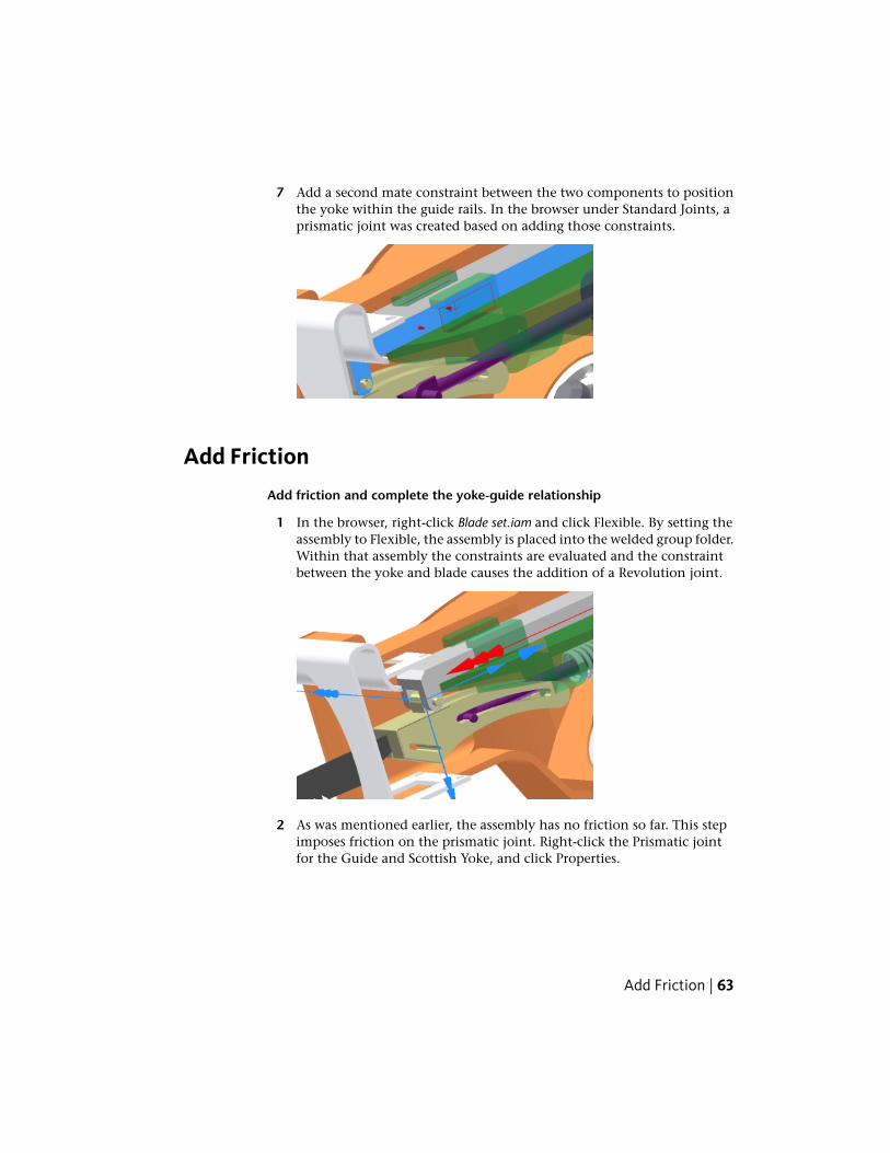
7 Add a second mate constraint between the two components to positionthe yoke within the guide rails. In the browser under Standard Joints, aprismatic joint was created based on adding those constraints.

Add Friction

Add friction and complete the yoke-guide relationship

1 In the browser, right-click Blade set.iam and click Flexible. By setting theassembly to Flexible, the assembly is placed into the welded group folder.Within that assembly the constraints are evaluated and the constraintbetween the yoke and blade causes the addition of a Revolution joint.

2 As was mentioned earlier, the assembly has no friction so far. This stepimposes friction on the prismatic joint. Right-click the Prismatic jointfor the Guide and Scottish Yoke, and click Properties.

Add Friction | 63

3 Click the dof 1 tab. Click the joint forces command . Click Enablejoint force. Enter a Dry Friction coefficient of 0.1 and click OK.

4 Add a constraint to position the Scottish Yoke with respect to the crankassembly. Set the browser view to Model and expand the Blade set.iamnode.

5 Expand the Scottish Yoke node and click the Constraint command.

6 In the browser, select Work Plane3 under the Scottish Yoke component.

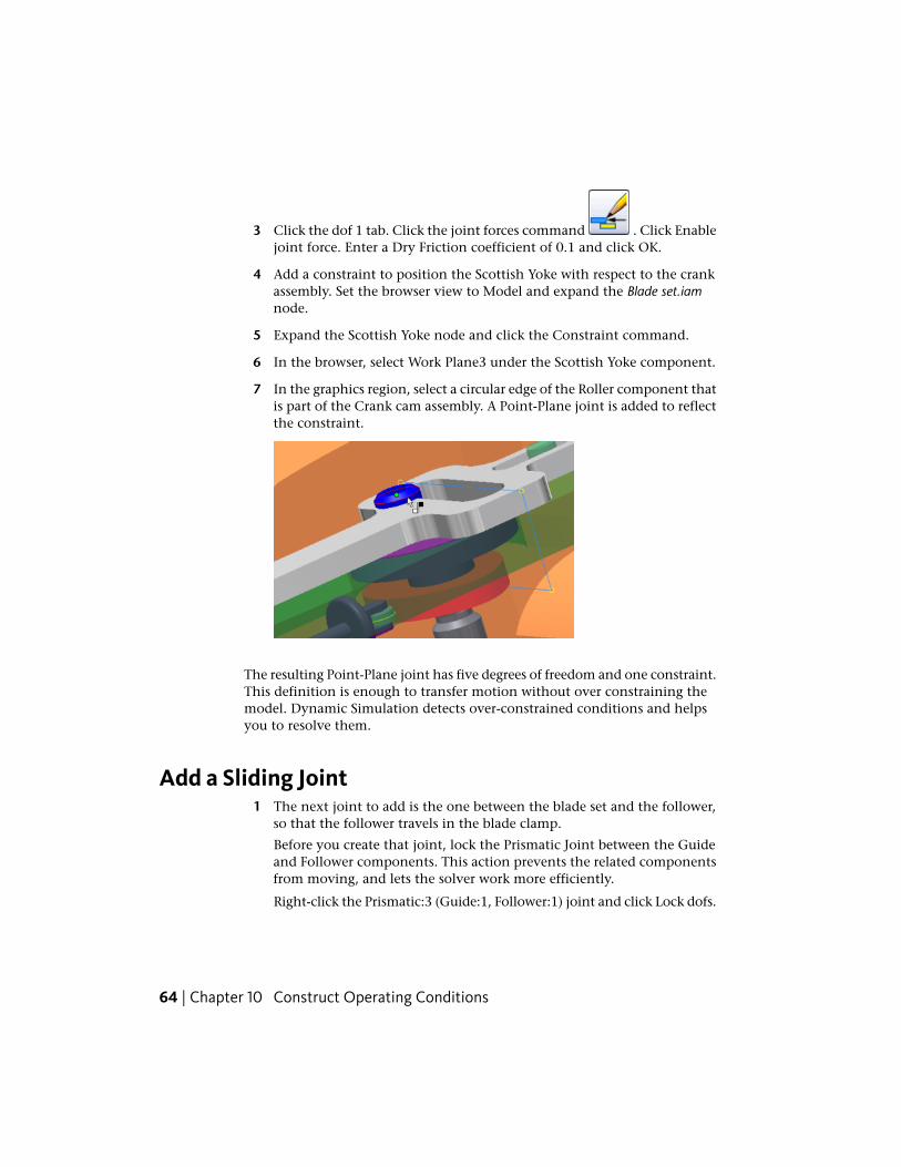
7 In the graphics region, select a circular edge of the Roller component thatis part of the Crank cam assembly. A Point-Plane joint is added to reflectthe constraint.

The resulting Point-Plane joint has five degrees of freedom and one constraint.This definition is enough to transfer motion without over constraining themodel. Dynamic Simulation detects over-constrained conditions and helpsyou to resolve them.

Add a Sliding Joint1 The next joint to add is the one between the blade set and the follower,

so that the follower travels in the blade clamp.

Before you create that joint, lock the Prismatic Joint between the Guideand Follower components. This action prevents the related componentsfrom moving, and lets the solver work more efficiently.

Right-click the Prismatic:3 (Guide:1, Follower:1) joint and click Lock dofs.

64 | Chapter 10 Construct Operating Conditions

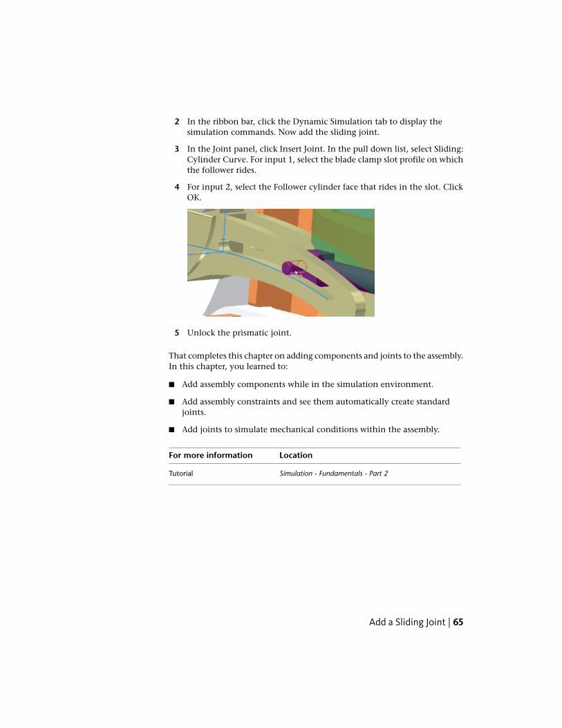
2 In the ribbon bar, click the Dynamic Simulation tab to display thesimulation commands. Now add the sliding joint.

3 In the Joint panel, click Insert Joint. In the pull down list, select Sliding:Cylinder Curve. For input 1, select the blade clamp slot profile on whichthe follower rides.

4 For input 2, select the Follower cylinder face that rides in the slot. ClickOK.

5 Unlock the prismatic joint.

That completes this chapter on adding components and joints to the assembly.In this chapter, you learned to:

■ Add assembly components while in the simulation environment.

■ Add assembly constraints and see them automatically create standardjoints.

■ Add joints to simulate mechanical conditions within the assembly.



Add a Sliding Joint | 65

66

Simulation Commands

This chapter explains how to use the Input Grapher, and how to export a load to Stress Analysisin Autodesk® Inventor® Simulation.

Input GrapherThe Input Grapher provides a means of adding forces and torques that changeduring the simulation based on other independent variables.

Add an external force that is dependent on the velocity in the prismatic jointbetween the Guide and Scottish Yoke. To provide a sense of the velocity we use+ or - values to define an opposite force.

1 In the browser, in Standard Joints, select the joint Prismatic (Guide:1,Scottish Yoke:1). Notice, in the reference frames, when the velocity ispositive, the reference frames point away from the blade end. If thereference frames point toward the saw blade, you can edit the joint andflip, or reverse, the direction.

11

67

2 In the Load panel, click Force. Select a vertex on one of the saw teeth.

3 The Direction Selector becomes active. Select the top edge of the sawblade that is parallel with the blade motion.

4 In the dialog box, click the arrow on the Magnitude input control todisplay the list options. Click Input Grapher.

The Magnitude dialog box displays.

5 In the Magnitude dialog box, click the Reference selector.

6 In the Select Reference dialog box, expand Standard Joints > Prismatic(Guide:1, Scottish Yoke:1) to reveal the velocities folder and contents.Click V(1) to specify velocity as variable for the graph X axis.

68 | Chapter 11 Simulation Commands

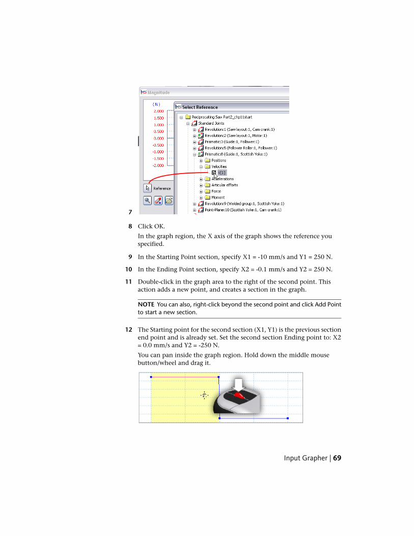
7

8 Click OK.

In the graph region, the X axis of the graph shows the reference youspecified.

9 In the Starting Point section, specify X1 = -10 mm/s and Y1 = 250 N.

10 In the Ending Point section, specify X2 = -0.1 mm/s and Y2 = 250 N.

11 Double-click in the graph area to the right of the second point. Thisaction adds a new point, and creates a section in the graph.

NOTE You can also, right-click beyond the second point and click Add Pointto start a new section.

12 The Starting point for the second section (X1, Y1) is the previous sectionend point and is already set. Set the second section Ending point to: X2= 0.0 mm/s and Y2 = -250 N.

You can pan inside the graph region. Hold down the middle mousebutton/wheel and drag it.

Input Grapher | 69

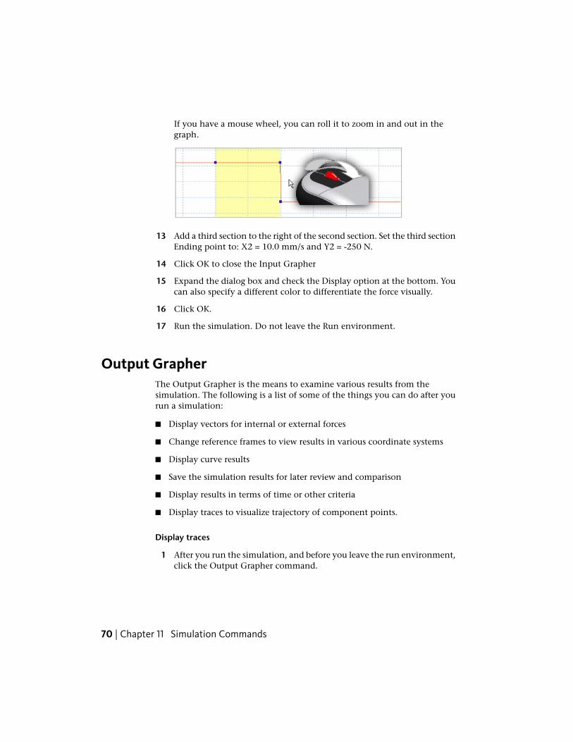
If you have a mouse wheel, you can roll it to zoom in and out in thegraph.

13 Add a third section to the right of the second section. Set the third sectionEnding point to: X2 = 10.0 mm/s and Y2 = -250 N.

14 Click OK to close the Input Grapher

15 Expand the dialog box and check the Display option at the bottom. Youcan also specify a different color to differentiate the force visually.

16 Click OK.

17 Run the simulation. Do not leave the Run environment.

Output GrapherThe Output Grapher is the means to examine various results from thesimulation. The following is a list of some of the things you can do after yourun a simulation:

■ Display vectors for internal or external forces

■ Change reference frames to view results in various coordinate systems

■ Display curve results

■ Save the simulation results for later review and comparison

■ Display results in terms of time or other criteria

■ Display traces to visualize trajectory of component points.

Display traces

1 After you run the simulation, and before you leave the run environment,click the Output Grapher command.


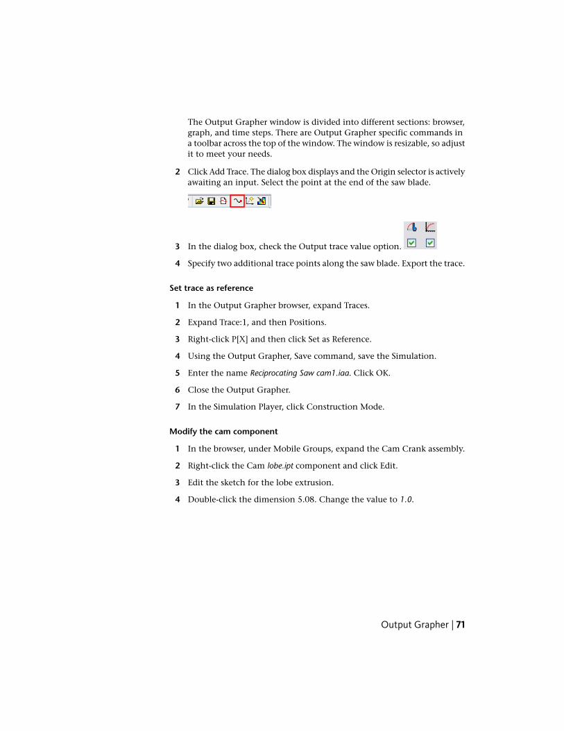
The Output Grapher window is divided into different sections: browser,graph, and time steps. There are Output Grapher specific commands ina toolbar across the top of the window. The window is resizable, so adjustit to meet your needs.

2 Click Add Trace. The dialog box displays and the Origin selector is activelyawaiting an input. Select the point at the end of the saw blade.

3 In the dialog box, check the Output trace value option.

4 Specify two additional trace points along the saw blade. Export the trace.

Set trace as reference

1 In the Output Grapher browser, expand Traces.

2 Expand Trace:1, and then Positions.

3 Right-click P[X] and then click Set as Reference.

4 Using the Output Grapher, Save command, save the Simulation.

5 Enter the name Reciprocating Saw cam1.iaa. Click OK.

6 Close the Output Grapher.

7 In the Simulation Player, click Construction Mode.

Modify the cam component

1 In the browser, under Mobile Groups, expand the Cam Crank assembly.

2 Right-click the Cam lobe.ipt component and click Edit.

3 Edit the sketch for the lobe extrusion.

4 Double-click the dimension 5.08. Change the value to 1.0.

Output Grapher | 71

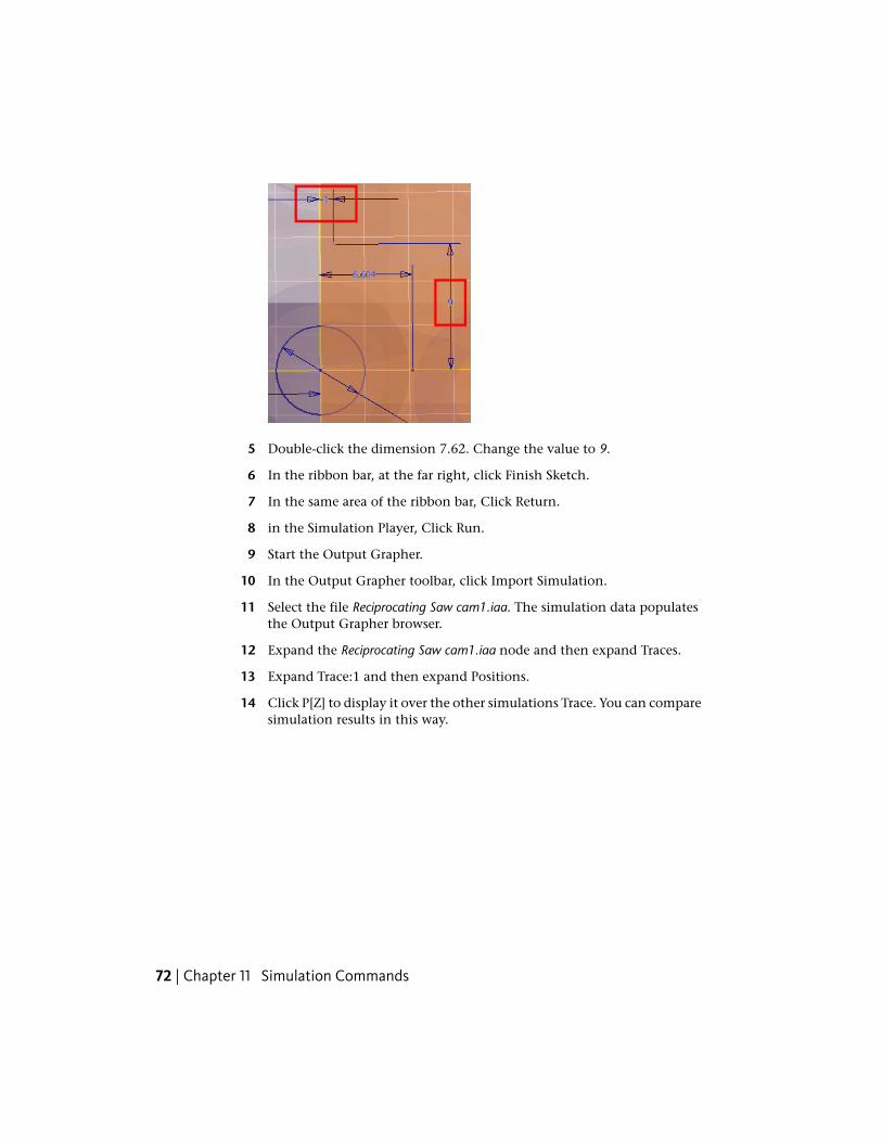
5 Double-click the dimension 7.62. Change the value to 9.

6 In the ribbon bar, at the far right, click Finish Sketch.

7 In the same area of the ribbon bar, Click Return.

8 in the Simulation Player, Click Run.

9 Start the Output Grapher.

10 In the Output Grapher toolbar, click Import Simulation.

11 Select the file Reciprocating Saw cam1.iaa. The simulation data populatesthe Output Grapher browser.

12 Expand the Reciprocating Saw cam1.iaa node and then expand Traces.

13 Expand Trace:1 and then expand Positions.

14 Click P[Z] to display it over the other simulations Trace. You can comparesimulation results in this way.


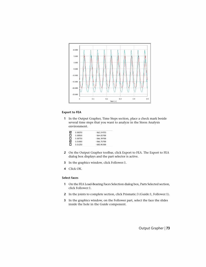
Export to FEA

1 In the Output Grapher, Time Steps section, place a check mark besideseveral time steps that you want to analyze in the Stress Analysisenvironment.

2 On the Output Grapher toolbar, click Export to FEA. The Export to FEAdialog box displays and the part selector is active.

3 In the graphics window, click Follower:1.

4 Click OK.

Select faces

1 On the FEA Load-Bearing Faces Selection dialog box, Parts Selected section,click Follower:1.

2 In the joints to complete section, click Prismatic:3 (Guide:1, Follower:1).

3 In the graphics window, on the Follower part, select the face the slidesinside the hole in the Guide component.

Output Grapher | 73

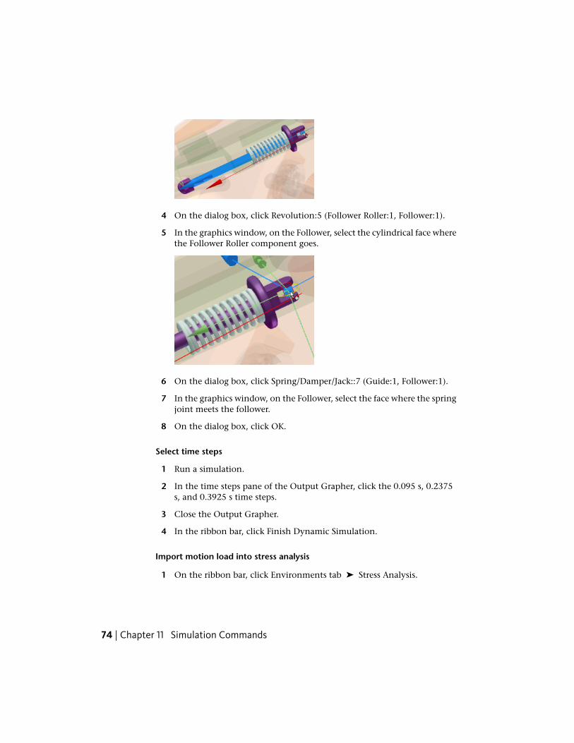
4 On the dialog box, click Revolution:5 (Follower Roller:1, Follower:1).

5 In the graphics window, on the Follower, select the cylindrical face wherethe Follower Roller component goes.

6 On the dialog box, click Spring/Damper/Jack::7 (Guide:1, Follower:1).

7 In the graphics window, on the Follower, select the face where the springjoint meets the follower.

8 On the dialog box, click OK.

Select time steps

1 Run a simulation.

2 In the time steps pane of the Output Grapher, click the 0.095 s, 0.2375s, and 0.3925 s time steps.

3 Close the Output Grapher.

4 In the ribbon bar, click Finish Dynamic Simulation.

Import motion load into stress analysis

1 On the ribbon bar, click Environments tab ➤ Stress Analysis.


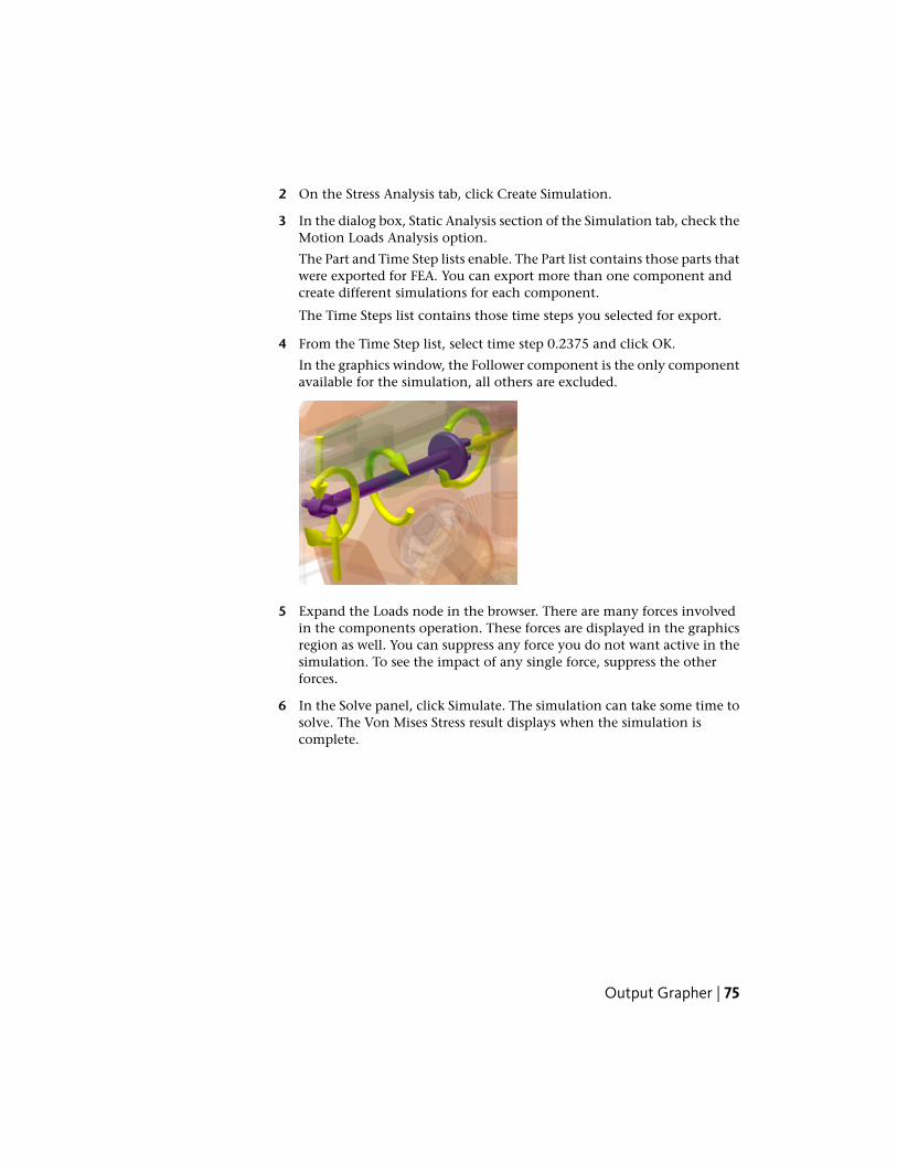
2 On the Stress Analysis tab, click Create Simulation.

3 In the dialog box, Static Analysis section of the Simulation tab, check theMotion Loads Analysis option.

The Part and Time Step lists enable. The Part list contains those parts thatwere exported for FEA. You can export more than one component andcreate different simulations for each component.

The Time Steps list contains those time steps you selected for export.

4 From the Time Step list, select time step 0.2375 and click OK.

In the graphics window, the Follower component is the only componentavailable for the simulation, all others are excluded.

5 Expand the Loads node in the browser. There are many forces involvedin the components operation. These forces are displayed in the graphicsregion as well. You can suppress any force you do not want active in thesimulation. To see the impact of any single force, suppress the otherforces.

6 In the Solve panel, click Simulate. The simulation can take some time tosolve. The Von Mises Stress result displays when the simulation iscomplete.

Output Grapher | 75

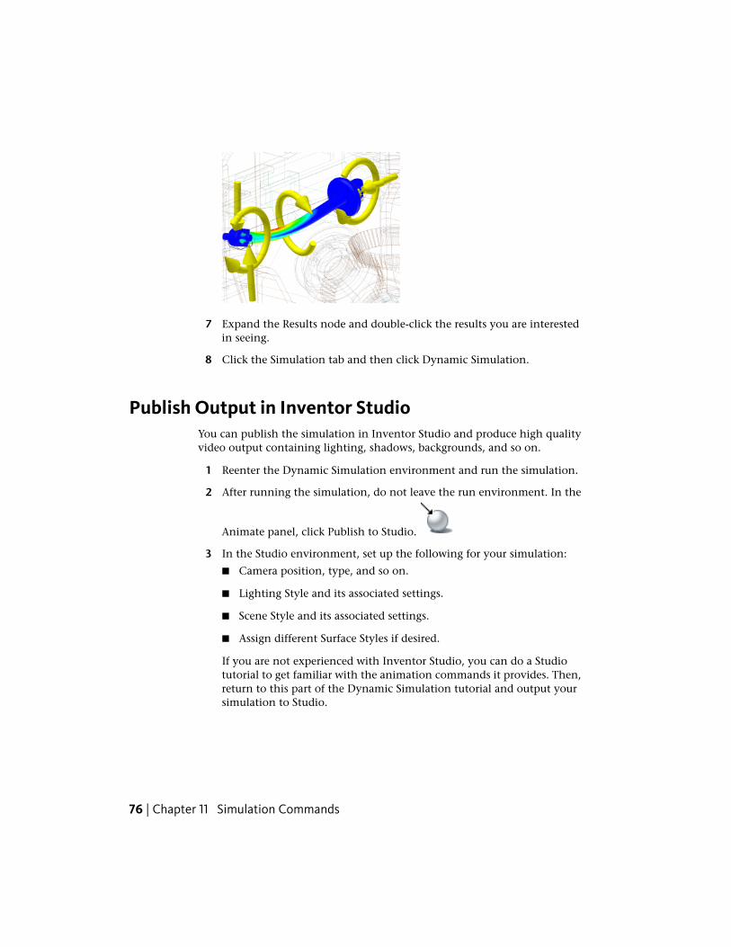
7 Expand the Results node and double-click the results you are interestedin seeing.

8 Click the Simulation tab and then click Dynamic Simulation.

Publish Output in Inventor StudioYou can publish the simulation in Inventor Studio and produce high qualityvideo output containing lighting, shadows, backgrounds, and so on.

1 Reenter the Dynamic Simulation environment and run the simulation.

2 After running the simulation, do not leave the run environment. In the

Animate panel, click Publish to Studio.

3 In the Studio environment, set up the following for your simulation:

■ Camera position, type, and so on.

■ Lighting Style and its associated settings.

■ Scene Style and its associated settings.

■ Assign different Surface Styles if desired.

If you are not experienced with Inventor Studio, you can do a Studiotutorial to get familiar with the animation commands it provides. Then,return to this part of the Dynamic Simulation tutorial and output yoursimulation to Studio.


4 Click Animation Timeline to display the timeline.

5 Set the timeline slider to the time you want for the animation action toend, such as, 2 seconds.

6 In the browser, expand the Animation Favorites folder. Right-click the

Simulation Timeline parameter, and click Animate Parameters .

7 Set the Action End value to 200 ul.

8 Click OK.

9 Click Render Animation .

10 On the General tab, the styles you set up are the active ones. If they arenot, select them from the various lists.

11 On the Output tab, click the box next to Preview No Render. This selectionproduces a test render so you can see if the animation action is what youwant. Click OK to render a preview.

12 Once you confirm the animation is playing like you want, clear thePreview option and render the simulation final animation with lightingand scene styles. Click OK to render a realistic looking simulation.

NOTE You can render images at a few different time positions to ensure thelighting and scene styles look like you expect, then render the animation.



Publish Output in Inventor Studio | 77

78

Index

A

analysesmeshing 7modal 20post processing 9reports 35rerunning on edited designs 31results, reading 23, 26solving 7types, setting 33updating 34vibration 10

analysis (.ipa) filesrepairing disassociated 40

ANSYS WorkBench 43

B

Boundary Condition command 29browser, Stress Analysis 13

C

coherent masses and inertia 46color bar 24commands, stress analysis 13constraints

assembly 49browser display 16converting assembly 50deleting, adding, and editing 32

contact pressure results folder 28continuity of laws 46contour colors 26

D

deformation results 10, 27displaying 30

degree of freedom 47

dialog boxesFrequency Options 21Simulation Panel 52

displacement results folder 27dynamic simulation 43

assumptions 45coherent masses and inertia 46continuity of laws 46relative parameters 45results 45

E

Element Visibility command 30equivalent stresses 9, 26exercises, prerequisites 4Export to FEA dialog box 73

F

factor of safety results 10FEA Load-Bearing Faces Selection dialog

box 73files, analysis

reassociating 40frequency modes 10Frequency Options dialog box 21frequency results options 21

G

geometry, editing 31

H

Help system 4, 44

J

joints 57

Index | 79

K

kinematic chains 47

L

load symbols 32displaying 29, 33

loadsbrowser display 16deleting, adding, and editing 32

M

meshescreating 7displaying 30

Minimum command 29modal analyses 10, 20modal frequency results folder 28model geometry, editing 31modes

frequency 10result options 21

N

natural resonant frequencies 10

O

Output Grapher 61, 70

P

post processing analyses 9preprocessing 7prerequisites for exercises 4

R

relative parameters 45Report command 35

reportsprinting and distributing 38saving 35

resonant frequency analyses 20resonant frequency results 28results

animate 28deformation 10display options 28equivalent stresses 9frequency options 21resonant frequency 28reviewing 9safety factor 10stress analysis, reading 26updating 34viewing analyses 23

rigid bodies, creating 55

S

safety factor results 10, 27Simulation Guide 5Simulation Panel 52

dialog box 52filter 52final time 52images 52percent value 52real time of compuation values 52simulation time value 52

solutionsmethods 7rerunning 32

strain results folder 28stress analysis

assumptions 7commands 5environment 13functionality 6results 26

Stress Analysis Update command 34stress results folder 27stresses, equivalent 9

80 | Index

T

tab, Stress Analysis 13

U

update analyses 34

V

vibration frequency analyses 20von Mises stress 9

W

welded bodies 55workflows

running modal analyses 20

Index | 81

82

AI Simulation 2011 GetStart

Documents

sheet metal environments

microsoft windows xp

image count improves

construct operating conditions

rich text format

kinematic chain respond

color contours correspond

construct moving assemblies