aguer

Methods and Tehniques in Surface Science

Prof. Dumitru LUCA

“Alexandru Ion Cuza” University, Iasi, Romania

• Auger Electron Spectroscopy (AES) – short historic and physical background,

• How AES measurements are performed,

• Information derived from Auger spectra:

• Methodology

• Data analysis

• Experimental considerations

Outline

Short historic of the Auger spectroscopyShort historic of the Auger spectroscopy

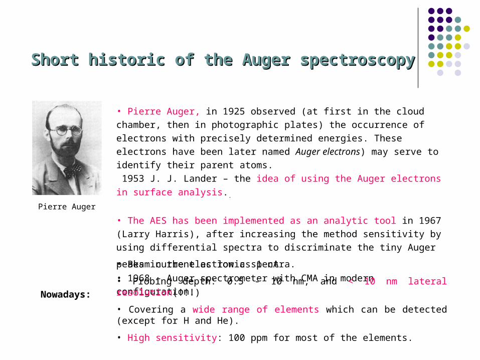
• Pierre Auger, in 1925 observed (at first in the cloud chamber, then in

photographic plates) the occurrence of electrons with precisely determined

energies. These electrons have been later named Auger electrons) may serve

to identify their parent atoms.

1953 J. J. Lander – the idea of using the Auger electrons in surface analysis..

• The AES has been implemented as an analytic tool in 1967 (Larry Harris),

after increasing the method sensitivity by using differential spectra to

discriminate the tiny Auger peaks in the electronic spectra. • 1968 – Auger spectrometer with CMA in modern configuration.

Pierre Auger

• Beam current as low as 1 nA

• Probing depth: 0.5 - 10 nm, and < 10 nm lateral resolution(!!!)

• Covering a wide range of elements which can be detected (except for H and He).

• High sensitivity: 100 ppm for most of the elements.

Nowadays:

Auger spectra. Expanation of the Auger effect in free atoms

1. The occurrence of an electron vacancy in a core level (K, L) (core level), by incident electron, X – ray photons, or ions.

Little information is available for the energy of

the primary and ejected electrons, due to complex cascade of successive collisions with the matrix. Therefore the complex picture in Fig. 1

2. The vacancy is filled by a second electron coming from an upper energy

level.

3. The energy of the emitted electron can serve for:

- the emission of a X photon (Z > 30) - ejection of a 3-rd (Auger) electron via a

non-radiative process.

4. The net result: an atom in a double-ionized state + 2 emitted electrons emisi (the K core level electron and the Auger electron).

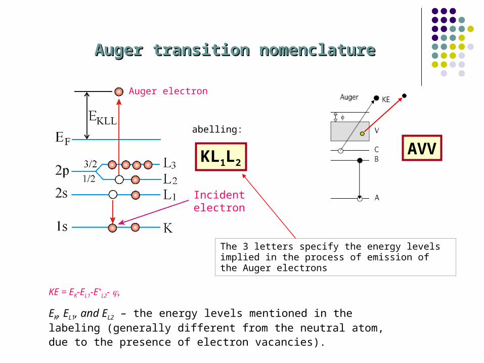
Auger transition nomenclatureAuger transition nomenclature

KL1L2

Labelling:

The 3 letters specify the energy levels implied in the process of emission of the Auger electrons

Auger electron

Incident electron

KE = EK-EL1-E*L2- ,

EK, EL1, and EL2 – the energy levels mentioned in the labeling (generally

different from the neutral atom, due to the presence of electron vacancies).

AVV

Factors influencing the Auger peak areaFactors influencing the Auger peak area

1. Ionisation cross section

10 keV incident electron beam

3keV incident

electron beam

KLL

LMM MNN

2. The Auger yield

3. Backscattering

• Competition between the Auger process and the X-ray fluorescence.

• The probability of occurrence of the Auger electrons increases with the decreasing of the differences between the energy levels involved in such transitions.

Factors influencing the Auger peak areaFactors influencing the Auger peak area(cont’d)(cont’d)

Auger electron spectraAuger electron spectra

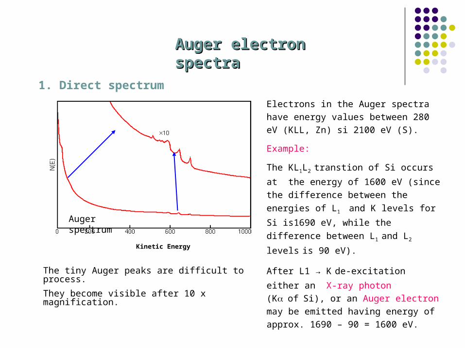
Auger spectrum

Kinetic Energy

The tiny Auger peaks are difficult to process.

They become visible after 10 x magnification.

Electrons in the Auger spectra have

energy values between 280 eV (KLL, Zn)

si 2100 eV (S).

Example:

The KL1L2 transtion of Si occurs at the

energy of 1600 eV (since the difference

between the energies of L1 and K levels

for Si is1690 eV, while the difference

between L1 and L2 levels is 90 eV).

After L1 → K de-excitation either an X-ray

photon (KofSi), or an Auger electron

may be emitted having energy of approx.

1690 – 90 = 1600 eV.

1. Direct spectrum

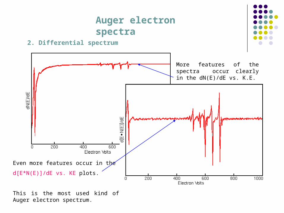
Even more features occur in the

d[E*N(E)]/dE vs. KE plots.

This is the most used kind of Auger electron spectrum.

More features of the spectra occur clearly in the dN(E)/dE vs. K.E.

Auger electron spectra

2. Differential spectrum

Auger spectra of light elementsAuger spectra of light elements

(the y-axis differs for different elements)

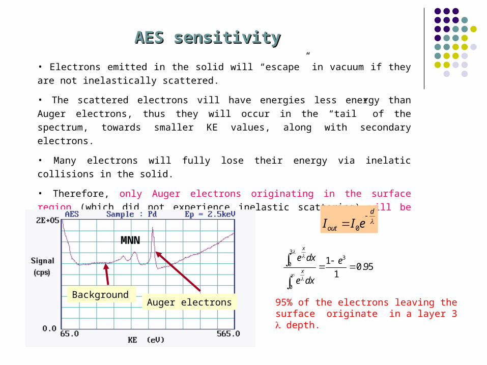
AES sensitivityAES sensitivity

• Electrons emitted in the solid will “escape” in vacuum if they are not inelastically

scattered.

• The scattered electrons vill have energies less energy than Auger electrons, thus they

will occur in the “tail” of the spectrum, towards smaller KE values, along with secondary

electrons.

• Many electrons will fully lose their energy via inelatic collisions in the solid.

• Therefore, only Auger electrons originating in the surface region (which did not

experience inelastic scattering) will be collected by the analyser.

Auger electronsBackground

MNN0

d

outI I e

33

0

0

10.95

1

x

x

e dx e

e dx

95% of the electrons leaving the surface originate in a layer 3 depth.

Experimental arrangementExperimental arrangement

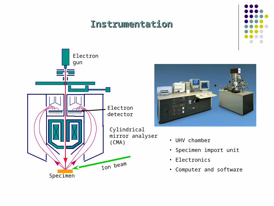
InstrumentationInstrumentation

Specimen

Electron gun

Cylindrical mirror analyser (CMA)

Ion beam

• UHV chamber

• Specimen import unit

• Electronics

• Computer and software

Electron detector

Scanning Auger Microscopy (SAM)Scanning Auger Microscopy (SAM)

AES Auger Electron Spectroscopy

SAM Scanning Auger Microscopy: Same instrument can provide SEM imaging, Auger spectra and chemical Auger mapping.

Specimen

Focussing & scanning system of the incident e-beam

Ion beam

ApplicationsApplications

• 1keV incident electron beam → penetration depth of about 15 Å.

• Verification of surface contamination freshly prepared in UHV.

• Investigation of the thin film growth process + elemental analysis.

• Depth profiling of concentration of chemical elements.

Qualitative analysisQualitative analysis

1. First, the main Auger peak positions are identified.

2. These values are correlated with the listed values in the Auger spectra book or standard tables. The main chemical elements are thus identified.

3. The identified element and transition are labelled in the spectrum (close to the negative jump in the differential spectrum).

4. The procedure is repeated for so-far unidentified peaks. The Auger spectrum of a sample

under investigation

E0 = 3keV

Elemental identification procedure

Example:

From the differential AES spectrum Ni, Fe and Cr have been identified.

NiFeCr

Qualitative analysis

Information concerning chemical composition

• Peak shape and the energy values, corresponding to maxima contain information on the nature of the environment, due to addition relaxation effects during the Auger process

• A full theoretical model is difficult to construct.

• In practice, Auger spectra of standard samples are used and the results are drawn from spectra comparison.

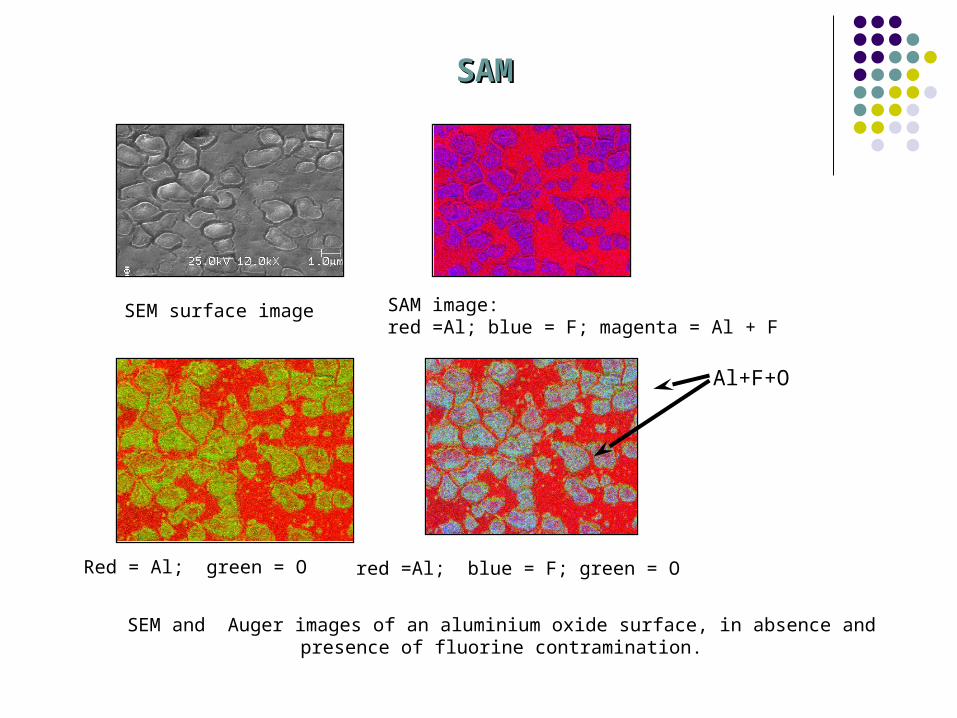
SAM image: red =Al; blue = F; magenta = Al + F

Red = Al; green = O red =Al; blue = F; green = O

SEM surface image

Al+F+O

SAMSAM

SEM and Auger images of an aluminium oxide surface, in absence and presence of fluorine contramination.

1. Measuring the peak-to-peak height

dEN(E)/dE vs. E

N(E) vs. E

2. Measuring the peak area

(after background subtraction)

Quntitative analysisQuntitative analysis

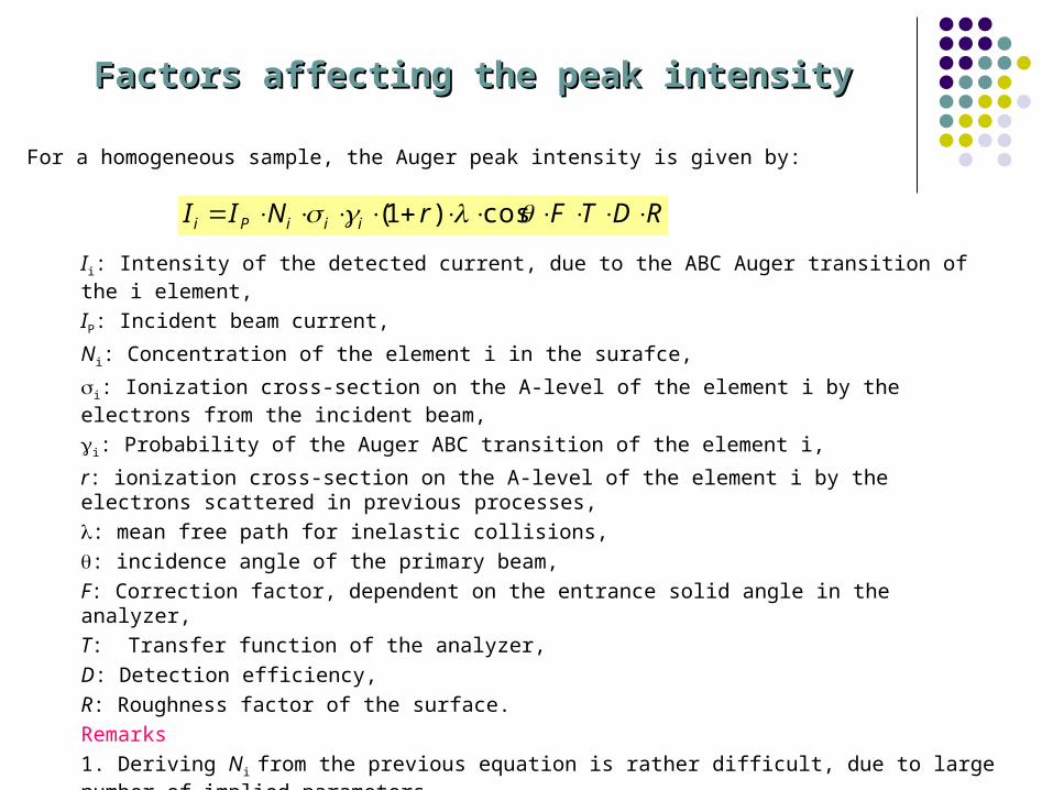
RDTFrNII iiiPi cos)1(

For a homogeneous sample, the Auger peak intensity is given by:

Ii: Intensity of the detected current, due to the ABC Auger transition of the i element,

IP: Incident beam current,

Ni: Concentration of the element i in the surafce,

i: Ionization cross-section on the A-level of the element i by the electrons from the incident beam,

i: Probability of the Auger ABC transition of the element i,

r: ionization cross-section on the A-level of the element i by the electrons scattered in previous processes,

: mean free path for inelastic collisions,

: incidence angle of the primary beam,

F: Correction factor, dependent on the entrance solid angle in the analyzer,

T: Transfer function of the analyzer,

D: Detection efficiency,

R: Roughness factor of the surface.

Remarks

1. Deriving Ni from the previous equation is rather difficult, due to large number of implied parameters,

2. In applications, empirical methods are used, which leave from: (a) utilization of standard specimens; (b) utilization of sensitivity factors.

Factors affecting the peak intensityFactors affecting the peak intensity

Quantitative analysis using standard specimensQuantitative analysis using standard specimens

Advantages:

No need to know “obscure” physical quantities:

• ionization cross-section, i on the A-level of the element i by the electrons in the primary beam,

• the Auger yield,

• backscattering cross-section and electron escape depth values.

Drawbacks:

• Necessity to prepare standard samples,• Valid only for homogeneous samples,• Quite low accuracy.

Quantitative analysis using sensitivity factorsQuantitative analysis using sensitivity factors

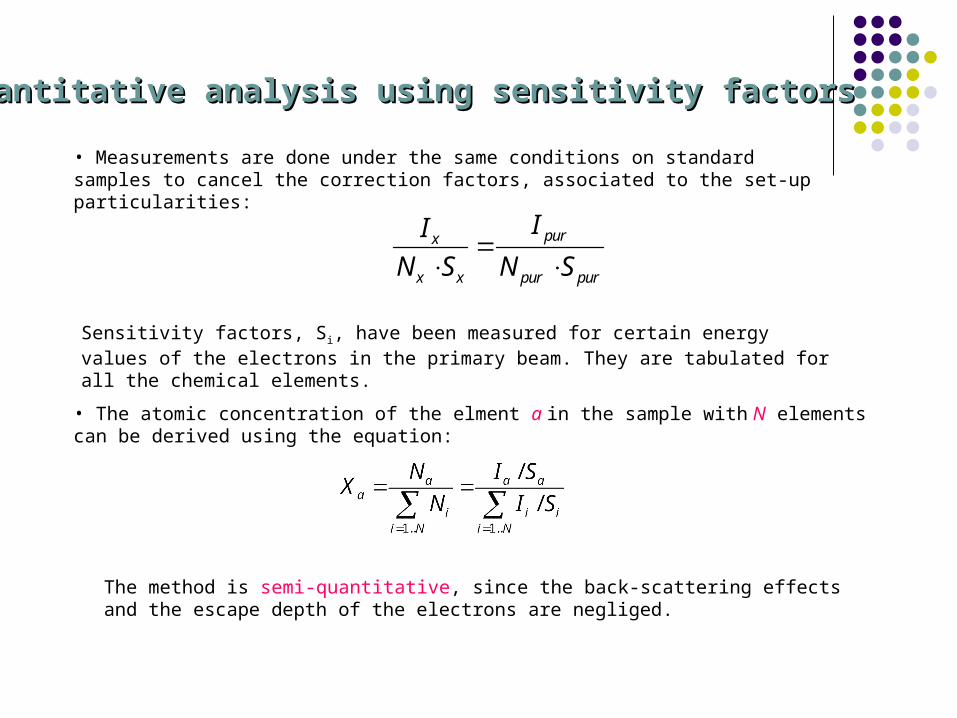
• Measurements are done under the same conditions on standard samples to cancel the correction factors, associated to the set-up particularities:

purx

x x pur pur

II

N S N S

Sensitivity factors, Si, have been measured for certain energy values of the electrons in the primary beam. They are tabulated for all the chemical elements.

• The atomic concentration of the elment a in the sample with N elements can be derived using the equation:

The method is semi-quantitative, since the back-scattering effects and the escape depth of the electrons are negliged.

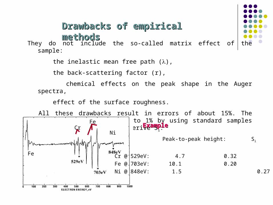
They do not include the so-called matrix effect of the sample:

the inelastic mean free path (),

the back-scattering factor (r),

chemical effects on the peak shape in the Auger spectra,

effect of the surface roughness.

All these drawbacks result in errors of about 15%. The errors can be diminished to 1% by using standard samples with the same matrix, to derive S i.

Fe

CrFe

Ni Peak-to-peak height: Si

Cr @ 529eV: 4.7 0.32

Fe @ 703eV: 10.1 0.20

Ni @ 848eV: 1.5 0.27

ExampleExample

Drawbacks of empirical methodsDrawbacks of empirical methods