Agronomy Research Established in 2003 by the Faculty of Agronomy, Estonian Agricultural University Aims and Scope: Agronomy Research is a peer-reviewed international Journal intended for publication of broad- spectrum original articles, reviews and short communications on actual problems of modern biosystems engineering incl. crop and animal science, genetics, economics, farm- and production engineering, environmental aspects, agro-ecology, renewable energy and bioenergy etc. in the temperate regions of the world. Copyright & Licensing: This is an open access journal distributed under the Creative Commons Attribution- NonCommercial-NoDerivatives 4.0 International (CC BY-NC-ND 4.0). Authors keep copyright and publishing rights without restrictions. Agronomy Research online: Agronomy Research is available online at: https://agronomy.emu.ee/ Acknowledgement to Referees: The Editors of Agronomy Research would like to thank the many scientists who gave so generously of their time and expertise to referee papers submitted to the Journal. Abstracted and indexed: SCOPUS, EBSCO, DOAJ, CABI Full Paper and Clarivate Analytics database: (Zoological Records, Biological Abstracts and Biosis Previews, AGRIS, ISPI, CAB Abstracts, AGRICOLA (NAL; USA), VINITI, INIST-PASCAL.) Subscription information: Institute of Technology, EMU Fr.R. Kreutzwaldi 56, 51006 Tartu, ESTONIA e-mail: [email protected] Journal Policies: Estonian University of Life Sciences, Latvia University of Life Sciences and Technologies, Vytautas Magnus University Agriculture Academy, Lithuanian Research Centre for Agriculture and Forestry, and Editors of Agronomy Research assume no responsibility for views, statements and opinions expressed by contributors. Any reference to a pesticide, fertiliser, cultivar or other commercial or proprietary product does not constitute a recommendation or an endorsement of its use by the author(s), their institution or any person connected with preparation, publication or distribution of this Journal. ISSN 1406-894X

Welcome message from author
This document is posted to help you gain knowledge. Please leave a comment to let me know what you think about it! Share it to your friends and learn new things together.
Transcript
Agronomy Research
Established in 2003 by the Faculty of Agronomy, Estonian Agricultural University Aims and Scope: Agronomy Research is a peer-reviewed international Journal intended for publication of broad-spectrum original articles, reviews and short communications on actual problems of modern biosystems engineering incl. crop and animal science, genetics, economics, farm- and production engineering, environmental aspects, agro-ecology, renewable energy and bioenergy etc. in the temperate regions of the world. Copyright & Licensing: This is an open access journal distributed under the Creative Commons Attribution-NonCommercial-NoDerivatives 4.0 International (CC BY-NC-ND 4.0). Authors keep copyright and publishing rights without restrictions.
Agronomy Research online: Agronomy Research is available online at: https://agronomy.emu.ee/ Acknowledgement to Referees: The Editors of Agronomy Research would like to thank the many scientists who gave so generously of their time and expertise to referee papers submitted to the Journal. Abstracted and indexed: SCOPUS, EBSCO, DOAJ, CABI Full Paper and Clarivate Analytics database: (Zoological Records, Biological Abstracts and Biosis Previews, AGRIS, ISPI, CAB Abstracts, AGRICOLA (NAL; USA), VINITI, INIST-PASCAL.) Subscription information: Institute of Technology, EMU Fr.R. Kreutzwaldi 56, 51006 Tartu, ESTONIA e-mail: [email protected] Journal Policies: Estonian University of Life Sciences, Latvia University of Life Sciences and Technologies, Vytautas Magnus University Agriculture Academy, Lithuanian Research Centre for Agriculture and Forestry, and Editors of Agronomy Research assume no responsibility for views, statements and opinions expressed by contributors. Any reference to a pesticide, fertiliser, cultivar or other commercial or proprietary product does not constitute a recommendation or an endorsement of its use by the author(s), their institution or any person connected with preparation, publication or distribution of this Journal. ISSN 1406-894X
662
CONTENTS
D. Berjoza, I. Jurgena and D. Bergspics Solar electric tricycle development and research .................................................... 665
V. Bulgakov, O. Adamchuk, S. Pascuzzi, F. Santoro and J. Olt Research into engineering and operation parameters of mineral fertiliser application machine with new fertiliser spreading tools ......................................... 676
K. Bumbiere, A. Gancone, J. Pubule and D. Blumberga Carbon balance of biogas production from maize in Latvian conditions ................ 687
N. Castrillón, V. Gonzalez and J.A. Osorio Approach to a classification of construction typologies of pig facilities: case study Antioquia – Colombia ............................................................................ 698
O. Chernikova, Yu. Mazhaysky, S. Buryak, T. Seregina and L. Ampleeva Comparative analysis of the use of biostimulants on the main types of soil ........... 711
R.C.B. Correia, F.C. Silva, M.M. Barros, A.C.L. Maria, D. Cecchin, L.A. Souza and D.F. Carmo
Productive efficiency and density and viscosity studies of biodiesels from vegetable oil mixtures .............................................................................................. 721
J. Galins, V. Osadcuks and A. Pecka Evaluation of passive cooling system in plywood enclosure for agricultural robot prototype ........................................................................................................ 739
M. Hissa, S. Niemi, T. Ovaska and A. Niemi Waste fish oil as an alternative renewable fuel for IC engines ................................ 749
L. Honchar, B. Mazurenko, O. Shutyi, V. Pylypenko, D. Rakhmetov Effect of pre-seed and foliar treatment with nano-particle solutions on seedling development of tiger nut (Cyperus Esculentus L.) plants ......................... 767

663
M. Hossain and J. Lellep Thermo mechanical vibration of single wall carbon nanotube partially embedded into soil medium ..................................................................................... 777
K. Jõgi, D. Malenica, I. Jõudu and R. Bhat Compositional evaluation of hot-pressed rapeseed cake for the purpose of bioplastic production ........................................................................................... 788
S. Kalenska, N. Novytska, T. Stolyarchuk, V. Kalenskyi, L. Garbar, M. Sadko, O. Shutiy and R. Sonko
Nanopreparations in technologies of plants growing .............................................. 795
V. Komasilovs, N. Bumanis, A. Kviesis, J. Anhorn and A. Zacepins Development of the Digital Matchmaking Platform for international cooperation in the biogas sector .............................................................................. 809
Z. Kusnere, K. Spalvins, D. Blumberga and I. Veidenbergs Packing materials for biotrickling filters used in biogas upgrading – biomethanation .................................................................................... 819
A. Martinovs, L. Mezule, R. Revalds, V. Pizica, V. Denisova, A. Skudra, G. Kolcs, E. Zaicevs and T. Juhna
New device for air disinfection with a shielded UV radiation and ozone ............... 834
C.L. Mendoza Martinez, E. Sermyagina, M. Silva de Jesus and E. Vakkilainen Use of principal component analysis to evaluate thermal properties and combustibility of coffee-pine wood briquettes ........................................................ 847
C. Nuortila, S. Heikkilä, R. Help, H. Suopanki, K. Sirviö and S. Niemi Effects of storage on the properties of rapeseed oil and alcohol blends .................. 868
S. Raita, K. Spalvins and D. Blumberga Prospect on agro-industrial residues usage for biobutanol production .................... 877
J. Rédl and P. Findura Improving ecological safety of agricultural off-road machines operating of sloped ground ...................................................................................................... 896

664
D.L. Rocha, A.R.G. Azevedo, M.T. Marvila, D. Cecchin, J. Alexandre, D.F. Carmo, Ferraz, P.F.P., Conti, L. and Rossi, G.
Influence of different methods of treating natural açai fibre for mortar in rural construction ................................................................................................. 910
J. Šafránková, T. Petrík, M. Libra, V. Beránek, V. Poulek, R. Belza and J. Sedláček
Operation of the photovoltaic system in Prague and data evaluation ...................... 922
E. Sermyagina, C. Mendoza and I. Deviatkin Effect of hydrothermal carbonization and torrefaction on spent coffee grounds .... 928
N. Shabbir, L. Kütt, M. Jarkovoi, M.N. Iqbal, A. Rassõlkin and K. Daniel An overview of measurement standards for power quality ..................................... 944
S. Zhao, V. Altmann, L. Richterova and V. Vitkova Comparison of physical composition of municipal solid waste in Czech municipalities and their potential in separation ....................................................... 961

665
Agronomy Research 19(S1), 665–675, 2021 https://doi.org/10.15159/AR.21.076
Solar electric tricycle development and research
D. Berjoza1,*, I. Jurgena2 and D. Bergspics1
1Latvia University of Life Sciences and Technologies, Faculty of Engineering, Motor vehicle institute, J. Cakstes blv. 5, LV-3001 Jelgava, Latvia 2Latvia University of Life Sciences and Technologies, Faculty of Economics and Social Development, Institute of Business and Management Science, Svetes street 18, LV-3001 Jelgava, Latvia *Correspondence: [email protected] Received: February 2nd, 2021; Accepted: May 8th, 2021; Published: May 13th, 2021 Abstract. Due to the fact that the world's energy resources are declining, various alternative energy sources are being sought. One such source of energy is solar energy. However, due to the large size of solar photovoltaic panels, solar energy is not widely used in mobile vehicles. In some electric automobiles, solar energy is used as an additional energy source, yet usually the sun is not able to provide more than 15–20% of the energy needed for their propulsion. There are some experimental design solutions for water vessels that are propelled by solar energy only. A recumbent electric tricycle was designed, constructed and tested within the present research. The recumbent electric tricycle used a 330 W solar battery, which was designed as a tricycle roof. During the tests with the solar battery, the electric tricycle reached a maximum speed of 32 km h-1. On a sunny day in May under the conditions in Latvia, a distance of 50.20 km was experimentally covered without battery recharging, compared with a distance of 17.14 km covered without the use of a solar battery. By skilfully operating the solar electric tricycle and limiting the speed to 20 km h-1 on a sunny day, the expected distance covered could be unlimited. The acceleration and braking parameters of the solar electric tricycle were identified by using a scientific radar Stalker ATS. Key words: acceleration, distance, range, solar tricycle, solar energy.
INTRODUCTION There are many known solutions for internal combustion engines that use fossil
fuels. In recent years, however, there has been a trend towards the development of vehicle propulsion technologies relying less on fossil fuels or replacing them with other forms of energy such as electrical energy. In the last decade, the use of electric automobiles has become more widespread, and now almost every auto manufacturer supplies electric or hybrid automobiles. Electric drive technology significantly reduces harmful emissions at the place of exploitation of the vehicles; however, the total emission balance depends on the way electricity is produced from renewable or fossil energy sources. The introduction of electric automobiles can reduce CO2, CnHm, NOx, CO and other exhaust components of internal combustion engines. The main advantages
666
of using electric drive are the quiet emission-free operation, yet the disadvantages are the relatively long charging time and the high price.
When introducing electric automobiles, scientists have also considered using alternative energy sources to charge the electric automobiles, e. g. solar and wind power. The first experimental solar charging station in Latvia, designed to charge electric automobile batteries, was opened in 2011. After successfully testing the solar station, experiments were done on the use of a solar battery in slow-moving vehicles for shopping, placing the solar battery on the roof of the electric automobile for shopping. On a sunny day, such an electric automobile can travel at a speed of 7 km h-1, and a 180 W solar battery provides a practically unlimited operating time on a sunny summer day (Berjoza & Misjuro, 2014). However, the vehicles of this design reach a low speed, which limits their use.
Solar energy is widely used in water vessels. Design solutions have been found both for the development of water vessels for scientific research purposes and for commercial uses. The requirements and operational characteristics for water vessels (maximum speed, weights of engine and batteries, area occupied by solar panels and their weight) are usually not as high as for automobiles. Therefore, solar-powered commercial and experimental boats are found in latitudes closer to the equator. The solar energy available is enough to propel such boats (Kurjakov et al., 2012; Nobrega & Rossling 2012; Mahmud et al., 2014; Kurniawan, 2016; Rodrigues et al., 2016; Sunaryo & Ramadhani, 2018). In some countries, e.g. the Netherlands, solar boat races involving several student teams are held. (Sutherlanda et al., 2017).
It is difficult for ground vehicles, i. e. electric automobiles, to create a sufficiently powerful solar battery for propelling them well. With the current technologies, it is difficult to achieve it because even the most modern solar cells have only a 24% efficiency factor. By fully covering the entire useful surface of an electric automobile with solar panels, it is usually possible to generate no more than 1,500 W of electricity, which is not enough to reach high speeds. Even a small electric automobile needs a 1.5 kW power supply to ensure smooth propulsion at a speed of 50 km h-1. The solar batteries of this capacity could not be placed on an electric vehicle. Accordingly, in modern solar electric automobiles, solar energy is usually used as a partial energy source to increase the distance covered by the traditional electric automobiles. In 2016, Toyota tested the solar hybrid car Prius, which aimed to generate 1,000 W of energy from solar panels located throughout the car’s horizontal body. The best solar cells are expected to have an efficiency factor of up to 34%. Solar panels not only charge the electric car batteries in stationary conditions but also increase the driving range by 45 km (Future car; Casey, 2019; Bellini, 2020). Some prototypes of solar energy use have also been developed by the automobile manufacturer Tesla.
The angle of sunlight falling on the ground can significantly affect the efficiency of non-adjustable angle photovoltaic panels, which makes solar electric automobiles more suitable for operation in countries closer to the equator. To popularize solar energy uses, Australia holds international car races for student-designed solar electric cars that travel 3,022 km, crossing Australia from north to south. The average speed of such cars specially designed for the race exceeds 80 km h-1.
The prototypes of solar-propelled vehicles are studied by scientists from various countries. During a sunny day, solar electric vehicles have no driving range restrictions and dependence on charging infrastructure. Hydrogen fuel cells could also be used as an
667
additional source of energy. The efficiency of a solar electric vehicle could be affected by several road infrastructure factors, e. g. trees, the height of buildings and other elements that obscure sunlight. In their research studies, scientists have developed an optimal route planning model, which takes into account both electric vehicle operating parameters and environmental parameters. The accuracy of the model was tested on a slow-moving electric automobile at a campus. The electric automobile used a 270 W solar battery placed on its roof solar and a 2.2 kW electric motor. The experiments were done at a 41.75-degree latitude. The experiments were carried out both in sunny conditions when the solar battery power supply reached 180−210 W and in cloudy conditions when the solar battery power supply was only 60 W.
In the countries where bicycles are popular, e. g. the Netherlands (almost 1 million bicycles are exploited), it has been found that the use of solar energy can significantly reduce CO2 emissions from energy production, as almost a quarter of the bicycles were electric ones. The prototypes of solar electric bicycles were also developed, with a small-capacity solar battery (66−72 W) mounted on the front wheel. The solar battery charged the bicycle when it was not ridden. An experiment involving 79 individuals working at two universities was carried out, in which 5 test bicycles were used; the average distance covered was 10.3 km, while the largest distance covered was 56 km (a total of 327 experimental rides were made), and the average speed was 17.3 km h-1 (Apostolou et al., 2018).
The total surface area of a car that could be covered with solar panels is quite large. For a middle-class car, the area of the bonnet is about 1.6 m2, the total area of the right and left doors is about 3.4 m2, the area of the roof is about 2 m2, the area of the boot lid is about 0.6 m2. If solar panels are installed on all the mentioned places, there might be a problem with energy flow management because in a particular position of the car, the solar panels are exposed to different, even very different intensities of solar radiation and also generate very different energy amounts (Kim et al., 2014). In order for an electric car equipped with solar photovoltaic panels to operate in several modes, e. g. solar electric car mode in combination with battery mode, charging mode during the day and night and regenerative braking mode, the development of a complex control algorithm with a superboost converter is required (Kumar et al., 2019). In most modern electric cars, the prototypes of which use photovoltaic panels experimentally, the panels can provide only a part of the energy required for their propulsion. Therefore, scientists propose to employ mathematical models for optimizing the energy flow, which manage the flow in different operating modes of the electric car and also while stopping at a charging station (Hu et al., 2016).
There are available many research studies on the use of solar energy to charge electric automobiles, which reduces CO2 emissions. No additional energy transmission is required at such charging stations. Simulations were performed for Italy, the Netherlands, Norway, Brazil and Australia (Longo et al., 2015; Rodriguez et al., 2019).
With the emergence of technologies for the use of solar panels on automobile roofs, it is also necessary to consider the standardization of these technological devices. Testing electric vehicle solar panels should include an alternating voltage tests, a temperature change test, a temperature-humidity change test, a dew test, a vibration test, an impact test, a water jet-moisture insulation test, a salt water test, a dust and oil resistance test to determine solar panel readiness for real operating conditions in vehicles (Araki et al., 2018).

668
At latitudes greater than 55 degrees, the use of solar energy to propel mobile vehicles might be constrained, especially the use of solar energy for full propulsion. Therefore, a solar electric tricycle prototype was developed to experimentally identify the possibility of using solar energy in latitudes exceeding 55. The aim of the research is to develop a workable, environment-friendly solar electric tricycle, which could operate autonomously, and to experimentally identify its key operating characteristics.
MATERIALS AND METHODS
Research object and experimental equipment For the experimental examination of solar energy used in mobile vehicles, a three-
wheeled recumbent tricycle was constructed, which was the main object of the present research. For the electric tricycle conversion, a standard set of components was used,
21.3×2 round tubes, as well as 20×20×2 square tubes. The key technical parameters of the electric tricycle are summarized in Table 1. Laser cutting technology was used to make the components made of sheet steel.
The solar battery frame was designed to be easily removed from the tricycle, and the frame was designed to be disassembled for easy storage. The electronics related to the solar control were mounted on the solar battery frame. The solar electric tricycle was equipped with a battery Canadian Solar Mono Cs1h-330MS and a controller Epever MPPT.
A Stalker ATS scientific radar was used to measure the acceleration and braking parameters. The key technical characteristics of the radar are as follows:
accuracy ± 0.1 km h-1; speed range 1–480 km h-1; data logging frequency 0.03 s; range up to 2,500 m; weight 1.45 kg.
which included a rear-wheel drive electric motor, front and rear brake levers with built-in switches, an accelerator handle, a controller and a control panel with a speedometer and an odometer. Two 20-inch front wheels and a 26-inch rear wheel were used to construct it (Fig. 1).
The tricycle is equipped with 3 lead gel batteries with a capacity of 12 Ah each. The batteries are connected in series, providing a nominal voltage of 36 V. The front and rear lamps with a nominal voltage of 6 V are used for lighting; the voltage is provided by a voltage converter 36 to 6 V. The frame of the tricycle was made of 33.7×3.2 and
Figure 1. Solar energy-powered recumbent tricycle: 1 – solar panel; 2 – rear wheel; 3 – electric motor; 4 – battery box; 5 – seat; 6 – front wheel; 7 – electric tricycle controller; 8 – pedals; 9 – steering handle; 10 – solar controller.
1
8
7 6 4
9 5
2
3
10
669
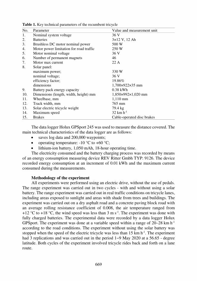
Table 1. Key technical parameters of the recumbent tricycle
No. Parameter Value and measurement unit 1. Nominal system voltage 36 V 2. Batteries 3×12 V, 12 Ah 3. Brushless DC motor nominal power 500 W 4. 5. 6. 7.
Motor power limitation for road traffic Motor nominal voltage Number of permanent magnets Motor max current
250 W 36 V 46 22 A
8. Solar panel: maximum power; nominal voltage; efficiency factor; dimensions
330 W 36 V 19.86% 1,700×922×35 mm
9. Battery pack energy capacity 0.38 kWh 10. Dimensions (length, width, height) mm 1,850×992×1,020 mm 11. Wheelbase, mm 1,110 mm 12. Track width, mm 765 mm 13. Solar electric tricycle weight 79.4 kg 14. Maximum speed 32 km h-1 15. Brakes Cable-operated disc brakes
The data logger Holux GPSport 245 was used to measure the distance covered. The
main technical characteristics of the data logger are as follows: saves log data and 200,000 waypoints; operating temperature: -10 °C to +60 °C; lithium-ion battery, 1,050 mAh, 18-hour operating time. The electricity consumed and the battery charging process was recorded by means
of an energy consumption measuring device REV Ritter Gmbh TYP: 9126. The device recorded energy consumption at an increment of 0.01 kWh and the maximum current consumed during the measurements.
Methodology of the experiment All experiments were performed using an electric drive, without the use of pedals.
The range experiment was carried out in two cycles - with and without using a solar battery. The range experiment was carried out in real traffic conditions on tricycle lanes, including areas exposed to sunlight and areas with shade from trees and buildings. The experiment was carried out on a dry asphalt road and a concrete paving block road with an average rolling resistance coefficient of 0.008, the air temperature ranged from +12 °C to +18 °C, the wind speed was less than 3 m s-1. The experiment was done with fully charged batteries. The experimental data were recorded by a data logger Holux GPSport. The experiment was done at a variable speed within a range of 20–28 km h-1 according to the road conditions. The experiment without using the solar battery was stopped when the speed of the electric tricycle was less than 15 km h-1. The experiment had 3 replications and was carried out in the period 1−9 May 2020 at a 56.65 - degree latitude. Both cycles of the experiment involved tricycle rides back and forth on a lane route.
670
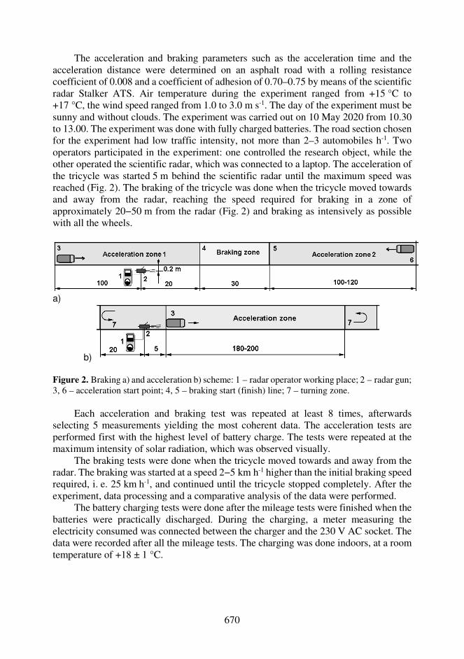
The acceleration and braking parameters such as the acceleration time and the acceleration distance were determined on an asphalt road with a rolling resistance coefficient of 0.008 and a coefficient of adhesion of 0.70–0.75 by means of the scientific radar Stalker ATS. Air temperature during the experiment ranged from +15 °C to +17 °C, the wind speed ranged from 1.0 to 3.0 m s-1. The day of the experiment must be sunny and without clouds. The experiment was carried out on 10 May 2020 from 10.30 to 13.00. The experiment was done with fully charged batteries. The road section chosen for the experiment had low traffic intensity, not more than 2–3 automobiles h-1. Two operators participated in the experiment: one controlled the research object, while the other operated the scientific radar, which was connected to a laptop. The acceleration of the tricycle was started 5 m behind the scientific radar until the maximum speed was reached (Fig. 2). The braking of the tricycle was done when the tricycle moved towards and away from the radar, reaching the speed required for braking in a zone of approximately 20−50 m from the radar (Fig. 2) and braking as intensively as possible with all the wheels.
a)
b)
Figure 2. Braking a) and acceleration b) scheme: 1 – radar operator working place; 2 – radar gun; 3, 6 – acceleration start point; 4, 5 – braking start (finish) line; 7 – turning zone.
Each acceleration and braking test was repeated at least 8 times, afterwards
selecting 5 measurements yielding the most coherent data. The acceleration tests are performed first with the highest level of battery charge. The tests were repeated at the maximum intensity of solar radiation, which was observed visually.
The braking tests were done when the tricycle moved towards and away from the radar. The braking was started at a speed 2−5 km h-1 higher than the initial braking speed required, i. e. 25 km h-1, and continued until the tricycle stopped completely. After the experiment, data processing and a comparative analysis of the data were performed.
The battery charging tests were done after the mileage tests were finished when the batteries were practically discharged. During the charging, a meter measuring the electricity consumed was connected between the charger and the 230 V AC socket. The data were recorded after all the mileage tests. The charging was done indoors, at a room temperature of +18 ± 1 °C.
671
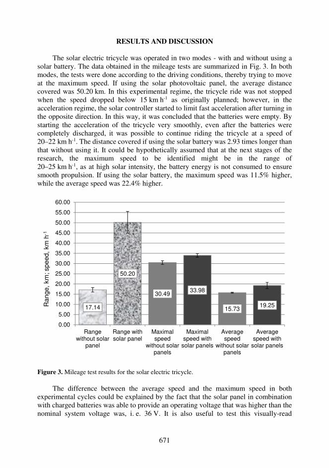
RESULTS AND DISCUSSION The solar electric tricycle was operated in two modes - with and without using a
solar battery. The data obtained in the mileage tests are summarized in Fig. 3. In both modes, the tests were done according to the driving conditions, thereby trying to move at the maximum speed. If using the solar photovoltaic panel, the average distance covered was 50.20 km. In this experimental regime, the tricycle ride was not stopped when the speed dropped below 15 km h-1 as originally planned; however, in the acceleration regime, the solar controller started to limit fast acceleration after turning in the opposite direction. In this way, it was concluded that the batteries were empty. By starting the acceleration of the tricycle very smoothly, even after the batteries were completely discharged, it was possible to continue riding the tricycle at a speed of 20–22 km h-1. The distance covered if using the solar battery was 2.93 times longer than that without using it. It could be hypothetically assumed that at the next stages of the research, the maximum speed to be identified might be in the range of 20–25 km h-1, as at high solar intensity, the battery energy is not consumed to ensure smooth propulsion. If using the solar battery, the maximum speed was 11.5% higher, while the average speed was 22.4% higher.
Figure 3. Mileage test results for the solar electric tricycle. The difference between the average speed and the maximum speed in both
experimental cycles could be explained by the fact that the solar panel in combination with charged batteries was able to provide an operating voltage that was higher than the nominal system voltage was, i. e. 36 V. It is also useful to test this visually-read
17.14
50.20
30.4933.98
15.7319.25
0.00
5.00
10.00
15.00
20.00
25.00
30.00
35.00
40.00
45.00
50.00
55.00
60.00
Rangewithout solar
panel
Range withsolar panel
Maximalspeed
without solarpanels
Maximalspeed with
solar panels
Averagespeed
without solarpanels
Averagespeed with
solar panels
Range,
km
; speed,
km
h-1
672
measurement at the next stages of the research by installing data logger equipment for measuring voltage and current changes.
New batteries were used in the experiment. Typically, battery performance and capacity reach nominal parameters after 2–3 charge cycles. For this reason, the distance covered in the first tests (without using the solar panel) with batteries that had several charge cycles could be longer.
The standard error for the mileage test data ranged (chosen confidence level 95%) are from 0.22% to 5.30%.
After each mileage test, the batteries were charged and the charge data were recorded. To prevent the solar panel from charging the battery during the transport of the electric tricycle, the storage batteries were disconnected from the solar panel immediately after each mileage test. The experiment had five replications, which allowed us to determine that the electricity consumed was in the range from 0.38 to 0.41 kW h, with the average energy consumption being 0.394 kW h. The experiment was conducted using a new battery pack; therefore, the first charge cycle required the largest amount of energy.
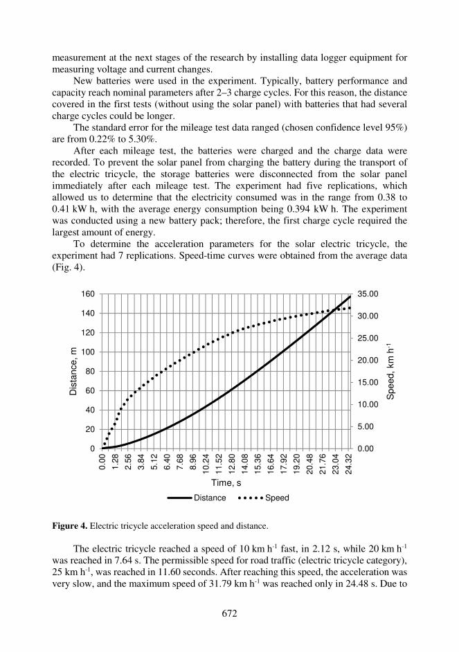
To determine the acceleration parameters for the solar electric tricycle, the experiment had 7 replications. Speed-time curves were obtained from the average data (Fig. 4).
Figure 4. Electric tricycle acceleration speed and distance. The electric tricycle reached a speed of 10 km h-1 fast, in 2.12 s, while 20 km h-1
was reached in 7.64 s. The permissible speed for road traffic (electric tricycle category), 25 km h-1, was reached in 11.60 seconds. After reaching this speed, the acceleration was very slow, and the maximum speed of 31.79 km h-1 was reached only in 24.48 s. Due to
0.00
5.00
10.00
15.00
20.00
25.00
30.00
35.00
0
20
40
60
80
100
120
140
160
0.0
0
1.2
8
2.5
6
3.8
4
5.1
2
6.4
0
7.6
8
8.9
6
10.2
4
11.5
2
12.8
0
14.0
8
15.3
6
16.6
4
17.9
2
19.2
0
20.4
8
21.7
6
23.0
4
24.3
2
Speed,
km
h-1
Dis
tance,
m
Time, s
Distance Speed

673
the fact that after reaching the speed of 25 km h-1, the acceleration curve also had a bend point, which indicated additional energy was consumed at higher speeds and the depletion of electricity reserves. Therefore, the cruise speed of 25 km h-1 could be considered to be an optimal operating speed for this kind of solar electric tricycles.
An analysis of the acceleration of the tricycle revealed that a speed of 10 km h-1 was reached after covering a distance of 4.05 m, while 25 km h-1 after 52.90 m. Based on the acceleration characteristics of such a recumbent tricycle, it is recommended to operate it only on tricycle paths or general roads, while sidewalks should be avoided. The maximum speed was reached after covering a relatively long distance of 157.21 m.
The braking of the tricycle was started at a speed of 25 km h-1 and finished when it came to a complete stop. In these tests, data were collected from 3 replications. It took 1.99 seconds to stop the solar electric tricycle (Fig. 5). During the braking, the average deceleration was 3.50 m s-2. Taking into account the relatively large weight of the solar electric tricycle used for the experiment, i. e. 155 kg, the braking parameters could be considered to be good.
Figure 5. Electric tricycle braking speed and distance.
When braking from a speed of 25 km h-1 until the tricycle came to a complete stop, the braking distance was 7.26 meters. When braking from 15 km h-1, the electric tricycle could be stopped in a distance of 2.34 meters, while from 20 km h-1– in 4.23 meters. In terms of braking distance, very good performance was demonstrated by the tricycle. If doing exploitational tests, braking is not recommended with the rear wheel brakes alone, as the wheel might slip under low-adhesion conditions.
The present experiment determined the primary operating parameters of the solar electric tricycle, yet at the next stages of the research, it is planned to carry out experiments using a data logger recording battery charge-discharge parameters and the
0.00
1.00
2.00
3.00
4.00
5.00
6.00
7.00
8.00
0.00
5.00
10.00
15.00
20.00
25.00
30.00
0 0.16 0.32 0.48 0.64 0.8 0.96 1.12 1.28 1.44 1.6 1.76 1.92
Bra
kin
g d
ista
nce,
m
Speed,
km
h-1
Time, s
Speed Distance
674
electricity consumed by the electric motor operated in different modes. It is also intended to determine the maximum speed of a solar electric tricycle at different solar intensities and at different angles of sunlight falling on the ground, with the battery not being discharged.
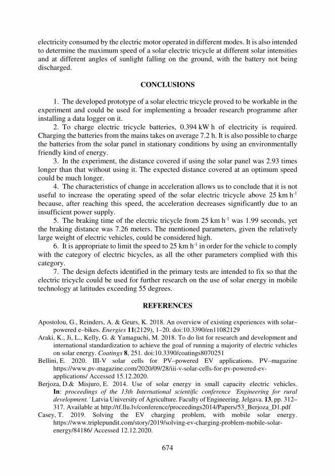
CONCLUSIONS
1. The developed prototype of a solar electric tricycle proved to be workable in the
experiment and could be used for implementing a broader research programme after installing a data logger on it.
2. To charge electric tricycle batteries, 0.394 kW h of electricity is required. Charging the batteries from the mains takes on average 7.2 h. It is also possible to charge the batteries from the solar panel in stationary conditions by using an environmentally friendly kind of energy.
3. In the experiment, the distance covered if using the solar panel was 2.93 times longer than that without using it. The expected distance covered at an optimum speed could be much longer.
4. The characteristics of change in acceleration allows us to conclude that it is not useful to increase the operating speed of the solar electric tricycle above 25 km h-1 because, after reaching this speed, the acceleration decreases significantly due to an insufficient power supply.
5. The braking time of the electric tricycle from 25 km h-1 was 1.99 seconds, yet the braking distance was 7.26 meters. The mentioned parameters, given the relatively large weight of electric vehicles, could be considered high.
6. It is appropriate to limit the speed to 25 km h-1 in order for the vehicle to comply with the category of electric bicycles, as all the other parameters complied with this category.
7. The design defects identified in the primary tests are intended to fix so that the electric tricycle could be used for further research on the use of solar energy in mobile technology at latitudes exceeding 55 degrees.
REFERENCES
Apostolou, G., Reinders, A. & Geurs, K. 2018. An overview of existing experiences with solar–
powered e–bikes. Energies 11(2129), 1–20. doi:10.3390/en11082129 Araki, K., Ji, L., Kelly, G. & Yamaguchi, M. 2018. To do list for research and development and
international standardization to achieve the goal of running a majority of electric vehicles on solar energy. Coatings 8, 251. doi:10.3390/coatings8070251
Bellini, E. 2020. III-V solar cells for PV–powered EV applications. PV–magazine https://www.pv-magazine.com/2020/09/28/iii-v-solar-cells-for-pv-powered-ev-applications/ Accessed 15.12.2020.
Berjoza, D.& Misjuro, E. 2014. Use of solar energy in small capacity electric vehicles. In: proceedings of the 13th International scientific conference ´Engineering for rural development.´ Latvia University of Agriculture. Faculty of Engineering. Jelgava. 13, pp. 312–317. Available at http://tf.llu.lv/conference/proceedings2014/Papers/53_Berjoza_D1.pdf
Casey, T. 2019. Solving the EV charging problem, with mobile solar energy. https://www.triplepundit.com/story/2019/solving-ev-charging-problem-mobile-solar-energy/84186/ Accessed 12.12.2020.

675
Future car. Toyota testing new solar panels to increase EV range. Available at https://m.futurecar.com/3341/Toyota-Testing-New-Solar-Panels-to-Increase-EV-Range
Hu, Y., Gan, C., Cao, W., Fang, Y. & Finney, S. 2016. Solar PV–powered SRM drive for EVs with flexible energy control functions. IEEE Transactions on Industry applications 52(4), 3357–3366. doi: 10.1109/TIA.2016.2533604
Kim, J., Wang, Y., Pedram, M. & Chang, N. 2014. Fast photovoltaic array reconfiguration for partial solar powered vehicles. In ISLPED '14: proceedings of the 2014 international symposium on Low power electronics and design. La Jolla, CA USA https://doi.org/10.1145/2627369.2627623
Kumar, G.G., Sundaramoorthy, K., Athikkal, S. & Karthikeyan, V. 2019. Dual input superboost DC–DC converter for solar powered electric vehicle. IET Power Electronics 12(9), 2276–2284. doi: 10.1049/iet-pel.2018.5255
Kurjakov, A., Kurjakov, M., Miškovic, D. & Caric, M. 2012. Electrical characteristics of thin film solar panels on a river boat under different microclimatic conditions. Electronics and Energetics 25(2), 151–160, Facta Universitatis. doi: 10.2298/FUEE1202151K
Kurniawan, A. 2016. A review of solar-powered boat development. IPTEK, The Journal for Technology and Science 27(1), 1–8.
Longo, M., Viola, F., Miceli, R., Zaninelli, D. & Romano, P. 2015. Replacement of vehicle fleet with EVs using PV energy. International Journal of Renewable Energy Research 5 (4).
Mahmud, K., Morsalin, S. & Khan, Md. I. 2014. Design and fabrication of an automated solar boat. International Journal of Advanced Science and Technology 64, 31–42. doi: 10.14257/ijast.2014.64.04
Nobrega, J. & Rossling, A. 2012. Development of solar powered boat for maximum energy efficiency. In: proceedings of the International Conference on Renewable Energies and Power Quality. Santiago de Compostela, Spain, pp. 302–307. Available at http://doi.org/10.24084/repqj10.299
Rodrigues, E.G., Bindu, S.J. & Chandran, V. 2016. Design and fabrication of solar boat. International Journal of Electrical Engineering & Technology (IJEET) 7(6), 01–10. Available at http://www.iaeme.com/IJEET/issues.asp?JType=IJEET&VType=7&IType=6
Rodriguez, A.S., Santana, T., MacGill, I., Ekins‐Daukes, N.J. & Reinders, A. 2019. A feasibility study of solar PV–powered electric cars using an interdisciplinary modeling approach for the electricity balance, CO2 emissions, and economic aspects: The cases of The Netherlands, Norway, Brazil, and Australia. Progress in photovoltaics 28, 517–532. doi: 10.1002/pip.3202
Sunaryo, S. & Ramadhani, A.W. 2018. Electrical system design of solar powered electrical recreational boat for Indonesian waters. In Kusrini, E., Juwono, F.H., Yatim, A. & Setiawan, E.A. (eds.): proceedings of the 3rd International Tropical Renewable Energy Conference ‘Sustainable Development of Tropical Renewable Energy’, pp. 1–5. Available at https://doi.org/10.1051/e3sconf/20186704011
Sutherlanda, J., Saladob, A., Oizumia, K. & Aoyamaa, K. 2017. Implementing value-driven design in modelica for a racing solar boat. In Madni, A.M., Boehm, B., Erwin, D.A., Ghanem, R. (ed.): proceeding of the 15th Annual Conference on Systems Engineering Research. University of Southern California, San Diego, USA, pp. 1–10.
676
Agronomy Research 19(S1), 676–686, 2021 https://doi.org/10.15159/AR.21.040
Research into engineering and operation parameters of mineral fertiliser application machine with new fertiliser spreading tools
V. Bulgakov1, O. Adamchuk2, S. Pascuzzi3, F. Santoro3 and J. Olt4,*
1National University of Life and Environmental Sciences of Ukraine, 15 Heroyiv Oborony Str., Kyiv UA 03041, Ukraine 2National Scientific Centre, Institute for Agricultural Engineering and Electrification, 11 Vokzalna Str., Glevakcha 1, Vasylkiv District, UA 08631 Kyiv Region, Ukraine 3University of Bari Aldo Moro, Department of Agricultural and Environmental Science, Via Amendola, 165/A, IT 70125 Bari, Italy 4Estonian University of Life Sciences, Institute of Technology, 56 Kreutzwaldi Str., EE 51006 Tartu, , Estonia *Correspondence: [email protected] Received: February 13th, 2021; Accepted: April 15th, 2021; Published: April 19th, 2021 Abstract. The output capacity of the machine for top spreading the soil with solid mineral fertilisers can be raised by means of increasing its working width. The authors have carried out field trials and field experiment investigations with the MVU-8 granulated mineral fertilizer spreading machine equipped with two prototype units of the centrifugal fertiliser spreading tool, in which the axis can be tilted at different angles to the vertical line. In accordance with the results of the completed investigations, it has been established that setting the axial tilt angle of the centrifugal operating device in the fertiliser spreading tool within the range of 25–30° provides for achieving a productivity of the combined tractor-implement unit for applying mineral fertilisers at a level of 35–40 ha per working shift hour. The best performance in the fertiliser application with regard to both the working width and the fertiliser placing distribution uniformity is ensured at angles of inclination of the disc in the fertiliser spreading tool with respect to the horizontal plane within the range of 25–30°. At these angles, the uneven distribution of the fertiliser over the working width is equal to 19.2%, the uneven distribution of the fertiliser along the unit’s line of travel is equal to 8.9%, while the deviation in the dosage of the applied fertilisers from the set value is equal to 7.5%. Key words: distribution uniformity, inclination angle, fertiliser, spreading disc, uneven distribution.
INTRODUCTION
As is known, the output capacity of the machine for top spreading the soil with mineral fertilisers and chemical soil improvers equipped with centrifugal fertiliser spreading tools depends on its working width, the tractor-implement unit’s operating rate of travel and the shift time utilisation rate (Adamchuk, 2002). In view of the fact that the resource for improving the productivity by increasing the unit’s operating travel rate as
677
well as the shift time utilisation rate has been used up, the only reserve for its improvement is the increase of the working width. That said, the working width of the mineral fertiliser top dressing machine, in its turn, depends on the absolute velocity of the departure of mineral fertiliser particles from the fertiliser spreading tool and the angle between its vector and the horizontal plane as well as the height above the field surface level, at which the fertiliser spreading tool is installed (Villette et al., 2005; 2007).
At the same time, the following circumstances have to be taken into account, when analysing the possible ways to design new fertiliser spreading tools for the purpose of increasing the mineral fertiliser spreading range and, accordingly, the working width of the machine:
– physical and mechanical properties of the mineral fertilisers supplied by the chemical industry currently to both the Ukrainian market and the international one, have for the last decades remained unchanged. Therefore, it can be forecasted that in the decade to come the physical and mechanical properties of mineral fertilisers, such as the dimensions and strength of the granules, the coefficient of friction for fertiliser particles on the vane surfaces, which have an effect on the spreading distance, will not change (Grift et al., 2006; Van Liedekerke et al., 2009; Biocca et al., 2013);
– spreading disc vanes manufactured with the use of polymer parts or state-of-the-art composite materials, on the surfaces of which the mineral fertilisers particles slide, have relatively small coefficients of friction, which results in the increased absolute velocity of the fertiliser particle departure from the fertiliser spreading tool. However, that has already been widely implemented in the engineering of new agricultural machinery and, therefore, hardly can be of great importance specifically with regard to the mineral fertiliser top dressing (Yildirim, 2006; 2008);
– raising the absolute velocity of the fertiliser particle departure from the fertiliser spreading tool by means of increasing the outer diameter of its spreading disc is in practice impossible, since this way, the same as in the preceding item, has been used up and the further augmentation of the disc diameter in the tool under consideration is restricted by the design layouts of mineral fertiliser top dressing machines (Adamchuk, 2006; Villette et al., 2008; 2010);
– raising the absolute velocity of the fertiliser particle departure from the fertiliser spreading tool by means of increasing its spreading disc rotation frequency is, again, not possible for practical purposes. The research carried out in the recent years has shown that the vanes of fertiliser spreading tools, which entrain the mineral fertiliser particles, apply to them impact force, which results in the disintegration of the granules and production of powder fractions (Adamchuk, 2006). It is to be taken into account that at higher rotation frequencies in the fertiliser spreading tool a considerable mass of dust and fine fraction is produced, which has a significantly reduced “tossing” property when spread in the air. That results in spreading the fertiliser within a much shorter range, than in case of spreading intact granules;
– way of increasing the angle between the vector of the absolute velocity, with which mineral fertiliser particles depart from the fertiliser spreading tool, and the horizontal plane, by means of increasing the vane setting angle in the horizontal plane, has also been used up by now in the existing tools with vertical rotation axes;
– as regards the height above the field surface, at which the fertiliser spreading tool is positioned, it is not much appropriate for two reasons. Firstly, it has no significant effect on the increase of the working width in mineral fertiliser top dressing machines.

678
Secondly, the height, at which such fertiliser spreading tools can be installed, is limited by the elevation of the process bin’s bottom, which cannot be positioned much higher.
On the assumption of the above-mentioned limiting factors and after the analysis of the above-said, it can be stated that increasing the working width is a topical problem in the design of new models of solid mineral fertiliser top dressing machines, which can be equipped with centrifugal disc-type fertiliser spreading tools. This problem has to be solved by way of carrying out the necessary scientific research.
The topical issues of raising the efficiency in the application of mineral fertilisers and the work processes of their placing in the soil have until now been subjects of study for many scientists. For example, in the studies by Scheufle & Bolwin (1991), Frode & Lorenzo (2001), Rainer (2001), Yasenetsky & Sheychenko (2002), Lawrence et al. (2007, White et al. (2007), Šima et al. (2013), Bulgakov et al. (2017), Marinello et al. (2017), Virro et al. (2020), it has been established that the efficiency of using mineral fertilisers depends not only on the fertilisers themselves, but also on the methods of their placing in the soil. The principal factor that limits the efficiency in the spreading application of mineral fertilisers is the uniformity in their distribution over the area of the field. This factor has a material effect on the ripening of the plants, the variation of the yield within the limits of one field and, overall, its decline.
Such scientists as Adjetey et al. (1999), Yasenetsky & Sheychenko (2002), White et al. (2007), Ma et al. (2009) have proved that the applied mineral fertilisers must be the direct source of nutrients for the plants, therefore, during their application they have to be placed in the soil in such a way that they become readily available for the active parts of the plants’ root systems. Placing mineral fertilisers close to the roots of agricultural plants creates the increased nutrient concentration zone for the roots. That facilitates the absorption of the fertilisers and improves their application efficiency. Fertilisers need be placed as in the top layers of the soil, so in the deeper ones, their concentration being in proportion to the development of the plants’ root systems.
The research carried out by various scientists has also greatly contributed to the elaboration of the fundamental principles for modelling the mineral fertiliser spreading by centrifugal tools. In particular, Yasenetsky & Sheychenko (2002), Aphale et al., (2003), Dintwa et al. (2004), Villette et al. (2007), Jones et al. (2008), Olt & Heinloo (2009), Hijazi et al. (2010), Antille et al. (2015), Lü et al. (2016), Kobets et al. (2017), Liu et al. (2018), Bulgakov et al. (2020) have carried out in-depth studies on the development of the fundamental principles for modelling both the process of top dressing with mineral fertilisers and the equipment for its implementation. However, the models generated in these studies are based on certain assumptions, which makes their practical application problematic. Those deficiencies have been eliminated by Adamchuk (2006) in the simulation model that he developed for the mineral fertiliser spreading process stipulating that its implementation requires carrying out separate experimental investigations. However, his approach did not cover such issues as the schematic model of the centrifugal spreading tool, in which the working axis is set with tilt with respect to the vertical line.
Meanwhile, in accordance with the working hypothesis developed by the authors, that is exactly the feature that will provide for increasing the mineral fertiliser particle spreading range and, accordingly, expanding the working width and improving the output capacity of the machines for top dressing with mineral fertilisers.

679
The aim of the paper was to improve the output capacity of the machines for top dressing with solid mineral fertilisers by means of increasing their working widths through the implementation of new fertiliser spreading tools with tilted axes.
MATERIALS AND METHODS
For the purpose of carrying out field tests and field experiment investigations, the
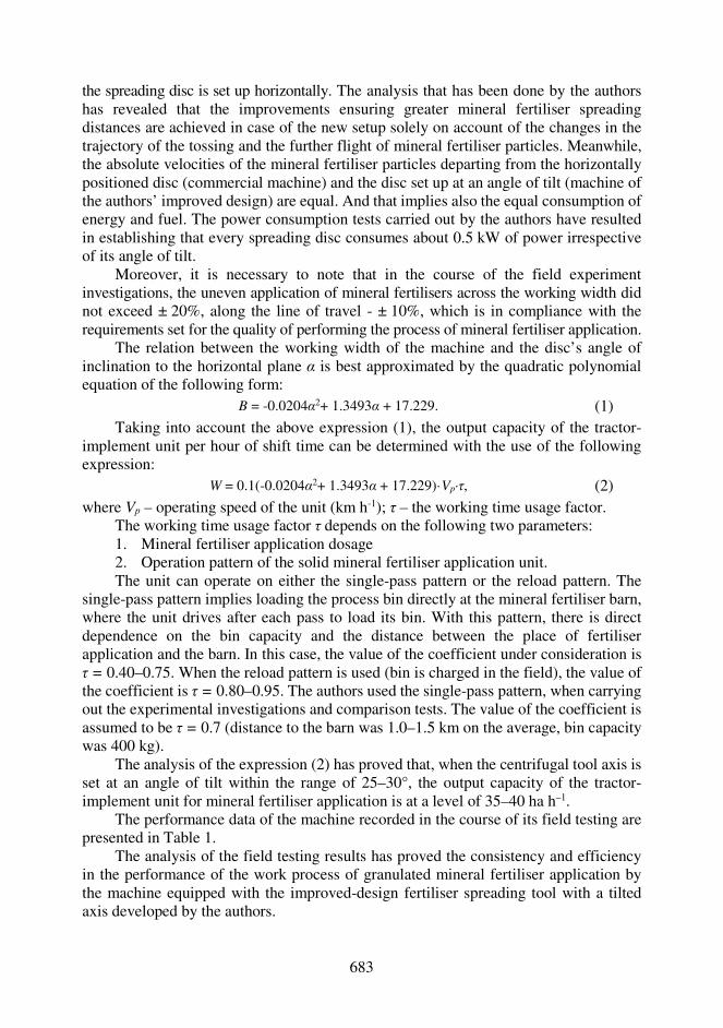
authors used the MVU-8 machine for the application of granulated mineral fertilisers and chemical soil improvers, which was equipped with two new prototype centrifugal fertiliser spreading tools developed by the authors (Bulgakov et al., 2021), the axes of which could be set at different angles of tilt with respect to the vertical line (Fig. 1).
Figure 1. General appearance of improved-design machine for top dressing with mineral fertilisers, lime and gypsum equipped with two fertiliser spreading tools with tilted axes during its field testing and field experiment investigation: a – side view; b – rear view.
During the field testing of the above-mentioned machine for top dressing with
mineral fertilisers, it was equipped with fertiliser spreading tools, the axes of which were
under consideration travelled forward, the rolling wheels of the machine’s running gear drove the closed loop of the fertiliser feeder, the top run of which entrained fertilisers
tilted at an angle of 30° with respect to the vertical line (Fig. 2).
Both the fertiliser spreading tools with tilted axes were kinematically linked with the power take-off shaft of the carrying tractor, while the fertiliser feeder - with the transport wheel of the machine. The powering on and off of the fertiliser feeder drive was controlled by the tractor operator remotely with the use of the tractor’s hydraulic system.
The operation of the machine equipped with the fertiliser spreading tools with tilted axes proceeded as follows. As the tractor-implement unit
Figure 2. General appearance of prototype fertiliser spreading tools with tilted axes installed in improved-design machine for top dressing with mineral fertilisers.

680
and brought them out from the body through the outlet slot in the form of a layer of a certain height. From the feeder the mineral fertilisers arrived to the fertilizer guides, which divided them into two equal flows and also forwarded them into the feed zones of the fertiliser spreading tools with tilted axes. When the fertilisers departed from the fertilizer guides, they were entrained by the vanes of the discs in the fertiliser spreading tools with tilted axes that performed rotary motion. Under the action of the centrifugal force the fertiliser granules accelerated moving along the vanes in the direction from the centre of the fertiliser spreading tool to the peripheral ends of the vanes. After reaching the vane ends, the fertilisers departed from the fertiliser spreading tools and flew in the set directions. The presence of two fertiliser spreading tools with tilted axes provided for the generation of two mineral fertiliser particle seeding fans, each in the form of a sector with an angle at centre of 90°. On account of the received reserve of kinetic energy and under the action of the gravity force, the fertiliser granules moved in the air in the direction from the fertiliser spreading tools to the field surface. The machine propelled
operations of the basic application of granulated superphosphate and nitroammophoska. During the experimental investigations, the following application dosages were
assumed for the above-mentioned mineral fertilisers: in case of granulated superphosphate, the application rate was equal to 400 kg ha-1, in case of nitroammophoska - 300 kg ha-1.
Prior to carrying out field experiment investigations, the authors performed the assessment of the properties of the process material, i.e. the above-mentioned mineral fertilisers. During the application, they had the following grain-size compositions:
– granulated superphosphate: ≤ 1 mm – 5.0%; ≥ 1 – ≤ 2 mm – 20.3%; ≥ 2 – ≤ 3 mm – 40.7%; ≥ 3 – ≤ 4 mm – 23.4%;
by the carrying tractor travelled linearly forward, therefore, the mineral fertiliser granules falling on the soil surface formed its continuous sheet cover.
The distribution uniformity in the spreading with fertiliser across the machine’s working width and along the line of the unit’s travel was determined as the coefficient of variation of the fertiliser mass distribution over the standard trays (GOST 28714-2007) that were placed in a horizontal area of the field in accordance with the layout presented in Fig. 3. During the experiment, the wind velocity did not exceed 2 m s–1, its value was determined with the use of the MS-13 cup anemometer.
The machine equipped with the fertiliser spreading tools with tilted axes developed by the authors and carried by the tractor was tested with its use for the
Figure 3. Layout of placing trays in single replication for determining values of distribution uniformity in spreading with mineral fertilisers.
Working Width
5 m
5 m

681
≥ 4 mm – 10.6%; – nitroammophoska:
≤ 1 mm – 2.1%; ≥ 1– ≤ 2 mm – 32.3%; ≥ 2– ≤ 3 mm – 59.1%; ≥ 3 mm – 6.5%.
The investigation of the performance figures of the mineral fertiliser top dressing machine with the new fertiliser spreading tools with tilted axes was carried out in field conditions in the fields of the Olenevskoye Experimental Farm under the National Research Centre of Institute of Agricultural Engineering and Electrification, where the machine performed the operation of top dressing the soil with mineral fertilisers before its cultivation.
The mineral fertiliser application machine travelled at a process speed of 12.5 km h-1.
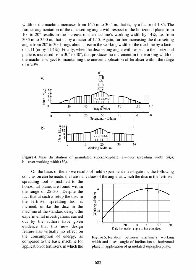
RESULTS AND DISCUSSION Fig. 4а represents the results obtained when determining how granulated
superphosphate distributed over the trays placed in accordance with the layout shown in Fig. 3. In the course of the field experiment investigations, the total range of the effective seeding of granulated superphosphate, that is, the spreading width provided by the machine equipped with two fertiliser spreading tools with tilted axes was equal to 58 m. At the same time, within the spreading width of 58 m, the uneven application of granulated superphosphate was equal to ± 65.4%, which did not meet the agricultural engineering requirements to the top dressing of the soil with mineral fertilisers. In view of that fact, in order to find out the working width of the machine, it was necessary to determine first the size of the overlap between the adjacent runs of the unit, which had to be selected so as to ensure that the uneven application of granulated superphosphate over the working width did not exceed ± 20%. As is seen in Fig. 4b, the above-mentioned condition was met at a working width of 39 m. In that case, the uneven application of granulated superphosphate over the working width was equal to ± 18.5%.
Apart from that, a large series of experiments has been carried out in order to investigate the effect of the angle of inclination of the disc in the fertiliser spreading tool with a tilted axis with respect to the horizontal plane on the working width of the machine.
In accordance with the design of the multifactorial experiment, the authors have carried out such an amount of tests, when each separate test (with one dosage and one type of mineral fertiliser) is repeated in three replicates. The triple replication of each test is in compliance with the requirements to the accuracy and validity of experimental investigations established in this branch of agricultural engineering.
As a result of the completed research, it has been established (Fig. 5) that increasing the angle of the discs’ inclination to the horizontal plane results in the expansion of the machine’s working width. However, the above-mentioned relation follows a special pattern, that is, increasing the said angle of inclination by the same amounts, but at different values of the angle produces different increments in the working width.
The analysis of the diagram presented in Fig. 5 indicates that the most intensive growth of the machine’s working width (84.8%) takes place, when the disc’s angle of inclination to the horizontal plane increases from 0 to 10°. In that interval, the working
682
width of the machine increases from 16.5 m to 30.5 m, that is, by a factor of 1.85. The further augmentation of the disc setting angle with respect to the horizontal plane from 10° to 20° results in the increase of the machine’s working width by 14%, i.e. from 30.5 m to 35.0 m, that is, by a factor of 1.15. Again, further increasing the disc setting angle from 20° to 30° brings about a rise in the working width of the machine by a factor of 1.11 (or by 11.4%). Finally, when the disc setting angle with respect to the horizontal plane is increased from 30° to 40°, that produces no increment in the working width of the machine subject to maintaining the uneven application of fertiliser within the range of ± 20%.
Figure 4. Mass distribution of granulated superphosphate: a – over spreading width (Мd); b – over working width (Мz).
On the basis of the above results of field experiment investigations, the following
conclusion can be made: the rational values of the angle, at which the disc in the fertiliser
spreading tool is inclined to the horizontal plane, are found within the range of 25–30°. Despite the fact that at such a setup the disc in the fertiliser spreading tool is inclined, unlike the disc in the machine of the standard design, the experimental investigations carried out by the authors have given evidence that this new design feature has virtually no effect on the consumption of energy, as compared to the basic machine for application of fertilisers, in which the
Figure 5. Relation between machine’s working width and discs’ angle of inclination to horizontal plane in application of granulated superphosphate.
v = ± 65.4%
v = ± 18.5%
a)
b)
683
the spreading disc is set up horizontally. The analysis that has been done by the authors has revealed that the improvements ensuring greater mineral fertiliser spreading distances are achieved in case of the new setup solely on account of the changes in the trajectory of the tossing and the further flight of mineral fertiliser particles. Meanwhile, the absolute velocities of the mineral fertiliser particles departing from the horizontally positioned disc (commercial machine) and the disc set up at an angle of tilt (machine of the authors’ improved design) are equal. And that implies also the equal consumption of energy and fuel. The power consumption tests carried out by the authors have resulted in establishing that every spreading disc consumes about 0.5 kW of power irrespective of its angle of tilt.
Moreover, it is necessary to note that in the course of the field experiment investigations, the uneven application of mineral fertilisers across the working width did not exceed ± 20%, along the line of travel - ± 10%, which is in compliance with the requirements set for the quality of performing the process of mineral fertiliser application.
The relation between the working width of the machine and the disc’s angle of inclination to the horizontal plane α is best approximated by the quadratic polynomial equation of the following form:
B = -0.0204α2+ 1.3493α + 17.229. (1) Taking into account the above expression (1), the output capacity of the tractor-
implement unit per hour of shift time can be determined with the use of the following expression:
W = 0.1(-0.0204α2+ 1.3493α + 17.229)·Vp·τ, (2) where Vр – operating speed of the unit (km h-1); τ – the working time usage factor.
The working time usage factor τ depends on the following two parameters: 1. Mineral fertiliser application dosage 2. Operation pattern of the solid mineral fertiliser application unit. The unit can operate on either the single-pass pattern or the reload pattern. The
single-pass pattern implies loading the process bin directly at the mineral fertiliser barn, where the unit drives after each pass to load its bin. With this pattern, there is direct dependence on the bin capacity and the distance between the place of fertiliser application and the barn. In this case, the value of the coefficient under consideration is τ = 0.40–0.75. When the reload pattern is used (bin is charged in the field), the value of the coefficient is τ = 0.80–0.95. The authors used the single-pass pattern, when carrying out the experimental investigations and comparison tests. The value of the coefficient is assumed to be τ = 0.7 (distance to the barn was 1.0–1.5 km on the average, bin capacity was 400 kg).
The analysis of the expression (2) has proved that, when the centrifugal tool axis is set at an angle of tilt within the range of 25–30°, the output capacity of the tractor-implement unit for mineral fertiliser application is at a level of 35–40 ha h–1.
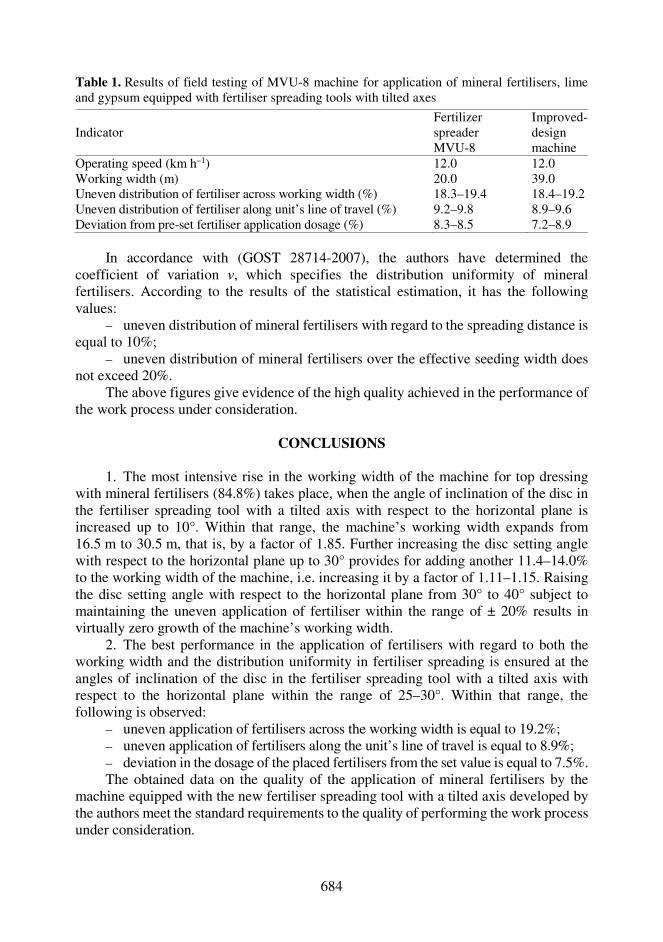
The performance data of the machine recorded in the course of its field testing are presented in Table 1.
The analysis of the field testing results has proved the consistency and efficiency in the performance of the work process of granulated mineral fertiliser application by the machine equipped with the improved-design fertiliser spreading tool with a tilted axis developed by the authors.
684
Table 1. Results of field testing of MVU-8 machine for application of mineral fertilisers, lime and gypsum equipped with fertiliser spreading tools with tilted axes
Indicator Fertilizer spreader MVU-8
Improved-design machine
Operating speed (km h–1) 12.0 12.0 Working width (m) 20.0 39.0 Uneven distribution of fertiliser across working width (%) 18.3–19.4 18.4–19.2 Uneven distribution of fertiliser along unit’s line of travel (%) 9.2–9.8 8.9–9.6 Deviation from pre-set fertiliser application dosage (%) 8.3–8.5 7.2–8.9
In accordance with (GOST 28714-2007), the authors have determined the coefficient of variation ν, which specifies the distribution uniformity of mineral fertilisers. According to the results of the statistical estimation, it has the following values:
– uneven distribution of mineral fertilisers with regard to the spreading distance is equal to 10%;
– uneven distribution of mineral fertilisers over the effective seeding width does not exceed 20%.
The above figures give evidence of the high quality achieved in the performance of the work process under consideration.
CONCLUSIONS
1. The most intensive rise in the working width of the machine for top dressing
with mineral fertilisers (84.8%) takes place, when the angle of inclination of the disc in the fertiliser spreading tool with a tilted axis with respect to the horizontal plane is increased up to 10°. Within that range, the machine’s working width expands from 16.5 m to 30.5 m, that is, by a factor of 1.85. Further increasing the disc setting angle with respect to the horizontal plane up to 30° provides for adding another 11.4–14.0% to the working width of the machine, i.e. increasing it by a factor of 1.11–1.15. Raising the disc setting angle with respect to the horizontal plane from 30° to 40° subject to maintaining the uneven application of fertiliser within the range of ± 20% results in virtually zero growth of the machine’s working width.
2. The best performance in the application of fertilisers with regard to both the working width and the distribution uniformity in fertiliser spreading is ensured at the angles of inclination of the disc in the fertiliser spreading tool with a tilted axis with respect to the horizontal plane within the range of 25–30°. Within that range, the following is observed:
– uneven application of fertilisers across the working width is equal to 19.2%; – uneven application of fertilisers along the unit’s line of travel is equal to 8.9%; – deviation in the dosage of the placed fertilisers from the set value is equal to 7.5%. The obtained data on the quality of the application of mineral fertilisers by the
machine equipped with the new fertiliser spreading tool with a tilted axis developed by the authors meet the standard requirements to the quality of performing the work process under consideration.
685
REFERENCES
Adamchuk, V. 2006. Mechanical-technological and technical bases of increase of efficiency of introduction of firm mineral fertilizers and chemical fertilizers. The Abstract of the Dissertation of the Doctor of Technical Sciences. National Agrarian University. Kyiv, 40 pp. (in Ukrainian).
Adamchuk, V. 2002. Substantiation of the model of application of mineral fertilizers. Interagency thematic scientific collection. Mechanization and electrification of agriculture 86, 90–99 (in Ukrainian).
Adjetey, J.A., Campbell, L.C., Searle, P.G.E. & Saffigna, P. 1999. Studies on depth of placement of urea on nitrogen recovery in wheat grown on a red-brown earth in Australia. Nutrient Cycling in Agroecosystems 54(3), 227–232. doi: 10.1023/A:1009775622609
Antille, D.L., Gallar, L., Miller, P.C.H. & Godwin, R.J. 2015. An investigation into the fertilizer particle dynamics off the disc. Applied Engineering in Agriculture 31(1), 49–60.
Aphale, A., Bolander, N., Park, J., Shaw, L., Svec, J. & Wassgren, C. 2003. Granular fertiliser particle dynamics on and off a spinner spreader. Biosystems Engineering 85(3), 319–329. doi: 10.1016/S1537-5110(03)00062-X
Biocca, M., Gallo, P. & Menesatti, P. 2013. Aerodynamic properties of six organo-mineral fertilizer particles. Journal of Agricultural Engineering 44, Art. E83, 411–414.
Bulgakov, V., Adamchuk, V., Arak. M., Petrychenko, I. & Olt, J. 2017. Theoretical research into the motion of combined fertilizing and sowing tractor-implement unit. Agronomy Research 15(4). 1498–1516. doi: 10.15159/AR.17.059
Bulgakov, V., Adamchuk, V., Kuvachov, V., Shymko, L. & Olt, J. 2020. A theoretical and experimental study of combined agricultural gantry unit with a mineral fertilizer spreader. Agraarteadus/Journal of Agricultural Science 31(2), 139–146. doi: 10.15159/jas.20.15
Bulgakov, V., Adamchuk, O., Pascuzzi, S., Santoro, F. & Olt, J. 2021. Experimental research into uniformity in spreading mineral fertilizers with fertilizer spreader disc with tilted axis. Agronomy Research 19(1), 28–41. doi: 10.15159/AR.21.025
Dintwa, E., Van Liedekerke, P., Olieslagers, R., Tijskens, E. & Ramon, H. 2004. Model forsimulation of particle flow on a centrifugal fertiliser spreader. Biosystems Engineering 87(4), 407–415. doi: 10.1016/j.biosystemseng.2004.01.001
Frode, B. & Lorenzo, H. 2001. The nutritional control of root development. Plant and Soil 232(1–2), 51–68. doi: 10.1023/A:1010329902165
GOST 28714-2007. 2020. Machines for spreading solid mineral fertilisers. Test methods. Standardinform, 45 pp.
Grift, T.E., Kweon, G., Hofstee, J.W., Piron, E. & Villette, S. 2006. Dynamic Friction Coefficient Measurement of Granular Fertiliser Particles. Biosystems Engineering 95(4), 507–515. doi: 10.1016/j.biosystemseng.2006.08.006
Hijazi, B., Baert, J., Cointault, F., Dubois, J., Paindavoine, M., Pieters, J. & Vangeyte, J. 2010. A device for extracting 3d information of fertilizer trajectories. In: XVIIth World Congress of the International Commission of Agricultural and Biosystems Engineering (CIGR), Québec City, Canada June 13–17, 8 pp.
Jones, J.R., Lawremce, H.G. & Yule, I.J. 2008. A statistical comparison of international fertiliser spreader test methods – Confidence in bout width calculations. Powder Technology 184(3), 337–351. doi: 10.1016/j.powtec.2007.09.004
Kobets, A.S., Naumenko, M.M., Ponomarenko, N.O., Kharytonov, M.M.,Velychko, O.P. & Yaropud, V.M. 2017. Design substantiation of the three-tier centrifugan type mineral feritlizers spreader. INMATEH, Agricultural Engineering 53(3), 13–20.
Lawrence, H.G., Yule, I.J. & Coetzee, M.G. 2007. Development of an image-processing method to assess spreader performance. Transactions of the ASABBE 50(2), 397–407.
686
Liu, C., Song, J., Zhang, J., Du, X. & Zheng, F. 2018. Design and performance experiment on centrifugal fertilizer spreader with a cone disc. International Agricultural Engineering Journal 27(1), 44–52.
Lü, J., Shang, Q., Yang, Y., Li, J. & Liu, Z. 2016. Performance analysis and experiment on granular fertilizer spreader with cone disc. Nongye Gongcheng Xuebao/Transactions of the Chinese Society of Agricultural Engineering 32(11), 16–24. doi: 10.11975/j.issn.1002-6819.2016.11.003
Ma, Q., Rengel, Z. & Rose, T. 2009. The effectiveness of deep placement of fertilisers is determined by crop species and adaphic conditions in Mediterranean-type environments:A reviw. Australian Journal og Soil Research 47(1), 19–32. doi: 10.1071/SR08105
Marinello, F., Pezzuolo, A., Gasparini, F. & Sartori, L. 2017. Integrated approach for prediction of centrifugal fertilizer spread patterns. Agricultural Engineering International: CIGR Journal 19(3), 1–6.
Olt, J. & Heinloo, M. 2009. On the formula for computation of flying distance of fertilizer´s particle under air resistance. Agraarteadus/Journal of Agricultural Science 20(2), 22–25.
Rainer, F. 2001. Ergbnisse der Umfrage. Schweiz. Landtechnik, 63(6), pp. 4–6. Scheufle, B. & Bolwin, H. 1991. Einsatzempfehllungen für die Mineraldüngung unter
Grossflächenbedingungen. Aqrartechnik. 41(3). pp. 114–116. Šima, T., Krupi©ka, J. & Nozdrovický, L. 2013. Effect of nitrification inhibitors on fertiliser
particle size distribution of the DASA ® 26/13 andf ENSIN ®fertilisers. Argronomy Research 11(1), 111–116.
Van Liedekerke, P., Tijskens, E. & Ramon, H. 2009. Discrete element simulations of the influence of fertiliser physical properties on the spread pattern from spinning disc spreaders. Biosystems Engineering 102, 392–405. doi: 10.1016/j.biosystemseng.2009.01.006
Virro, I., Arak, M., Maksarov, V.V & Olt, J. 2020. Precision fertilisation technologies for berry plantation. Agronomy Research 18(S4), 2797–2810. doi: 10.15159/AR.20.207
Villette, S., Cointault, F., Piron, E. & Chopinrt, B. 2005. Centrifugal Spreading: an Analytical Model for the Motion of Fertiliser Particles on a Spinning Disc. Biosystems Engineering 92(2), 157–164. doi: 10.1016/j.biosystemeng.2005.06.013
Villette, S., Cointault, F., Zwaenepoel, P., Chopinrt, B. & Paindavoine, M. 2007. Velosity measurement using motion blurred images to improve the quality of fertiliser spreading in agriculture. In: Proceedings of SPIE – The International Society for Optical Engineering, 6356, Art. 635601.
Villette, S., Gée, C., Piron, E., R. Martin, R., Miclet, D. & Paindavoine, M. 2010. Centrifugal fertiliser spreading: velocity and mass flow distribution measurement by image processing. In: Proceedings of AgEng 2010, International Conference on Agricultural Engineering, Clermont Ferrand, France, 10 pp.
Villette, S., Piron, E., Cointault, F. & Chopinet, B. 2008. Centrifugal spreading of fertiliser: Deducing three-dimensional velocities from horizontal outlet angles using computer vision. Biosystems Engineering 99(4), 496–507. doi: 10.1016/j.biosystemseng.2017.12.001
White, P.J., Wheatley, R.E., Hammond, J.P. & Zhang, K. 2007. Minerals, soils and roots. Potato Biology and Biotechnology: Advances and Perspectives, 739–752. doi: 10.1016/B978-044451018-1/50076-2
Yasenetsky, V. & Sheychenko, V. 2002. Mineral spreaders for farms of all forms of ownership. APK technique 12, 16–17 (in Ukrainian).
Yildirim, Y. 2006. Effect on vane number on distribution uniformity in single disc rotary fertilizer spreaders. Applied Engineering in Agriculture 22(5), 659–663.
Yildirim, Y. 2008. Effect of vane shape on fertilizer distribution uniformity in single disc rotary fertilizer spreaders. Applied Engineering in Agriculture 24(2), 159–163.

687
Agronomy Research 19(S1), 687–697, 2021 https://doi.org/10.15159/AR.21.085
Carbon balance of biogas production from maize in Latvian conditions
K. Bumbiere, A. Gancone, J. Pubule* and D. Blumberga
Riga Technical University, Institute of Energy Systems and Environment, Faculty of Electrical and Environmental Engineering, Azenes 12-K1, LV-1048 Riga, Latvia *Correspondence: [email protected] Received: January 31st, 2021; Accepted: March 28th, 2021; Published: May 19th, 2021 Abstract. Production of biogas using bioresources of agricultural origin plays an important role in Europe’s energy transition to sustainability. However, many substrates have been denounced in the last years as a result of differences of opinion on its impact on the environment, while finding new resources for renewable energy is a global issue. The aim of the study is to use a carbon balance method to evaluate the real impact on the atmosphere by carrying out a carbon balance to objectively quantify naturally or anthropogenically added or removed carbon dioxide from the atmosphere. This study uses Latvian data to determine the environmental impact of biogas production depending on the choice of substrate, in this case from specially grown maize silage. GHG emissions from specially grown maize use and cultivation (including the use of diesel fuel, crop residue and nitrogen fertilizer incorporation, photosynthesis), biogas production leaks, as well as digestate emissions (including digestate emissions and also saved nitrogen emissions by the use of digestate) are taken into account when compiling the carbon balance of maize. The results showed that biogas production from specially grown maize can save 1.86 kgCO2eq emissions per 1 m3 of produced biogas. Key words: agriculture, bioenergy, biofuels, multicriteria analysis, sustainability.
INTRODUCTION The European Union is the most progressive global leader on the path to climate
change mitigation, therefore The European Commission presented the vision for climate-neutral economy by 2050 to keep global temperature increase below 2 °C above the pre-industrial level (Bereiter et al., 2015), with decarbonising the energy sector as one of the key points (European Council, 2019). Production of biogas using bioresources of agricultural origin plays an important role in Europe’s energy transition to sustainability (European Council, 2014; European Council, 2019) due to the possibilities to use it for different purposes - transportation fuel, heat and electricity generation (Meyer et al., 2018).
The biogas production process integrates production (Chen et al., 2015), processing and recycling of degradable by-products (Li et al., 2019). Not only does the biogas produced by anaerobic digestion prevent greenhouse gas emissions and produce renewable energy, but also provides for the production of processed fertilizers,
688
improving nutrient self-sufficiency in the agricultural sector (Timonen et al., 2019). The productivity of a biogas plant depends on different aspects, like the type of biomass (Melvere et al., 2017; Krištof & Gaduš, 2018; Bumbiere et al., 2020), digestion (Meiramkulova et al., 2018; Mano Esteves et al., 2019), availability of biomass, impurities that may harm microorganisms (Mehryar et al., 2017; Muizniece et al., 2019) and lignin content (Lauka et al., 2019).
The most important element of the biogas production system, is the choice of a substrate, because by knowing the composition of biomass, it is possible to predict the yield of biogas and its ratio of methane (Ugwu et al., 2020). Almost any organic material can be used for the biogas production, for example, paper, grass, animal waste, domestic or manufacturing sewage, food waste, agricultural products (Ugwu et al., 2020), but whereas finding new sources of renewable energy production is a global issue (Sauthoff et al., 2016; Siddique & Wahid, 2018) at the same time specially grown substrates are being rejected for the production of biogas (Schulz et al., 2018).
One of the substrates being rejected is the use of maize as a result of differences of opinion on its impact on the environment (Schulz et al., 2018), even though maize biogas yields and characteristics are far superior to other crops for biogas production (Pimentel, 2003; Gowik & Westhoff, 2011). Not only does maize have a high carbon fixation and assimilation capacity (Crafts-Brandner & Salvucci, 2002), but it can also be grown worldwide due to its high photosynthesis and resource utilization (Arodudu et al., 2017), even in conditions of drought, high temperatures and lack of various nutrients (Patzek, 2004). In addition, in the process of anaerobic digestion it is very important to use co-digestion, which allows to increase the productivity of produced biogas from 25 to 400% over mono-digestion (Cavinato et al., 2010; Shah et al., 2015). Co-digestion is often used for the very reason that the optimal carbon-nitrogen ratio on biogas production is in the rage of 20:1 to 30:1, but in general, manure has very low carbon ratio and it is important to mix it with other substrates that are carbon-rich like maize to increase the biogas yield.
Therefore, in this case, a carbon balance was developed and carried out to objectively quantify naturally or anthropogenically added or removed carbon dioxide from the atmosphere in order to determine the environmental impact of biogas production from specially grown substrates, in this case - maize silage.
Although many authors have acknowledged that, when analyzing biomass life cycle analysis, the range of results is quite wide (Murphy et al., 2014) due to the differences in various factors and system boundaries (Muench & Guenther, 2013), it is considered to be the best method for calculating Greenhouse gas (GHG) balance (Cherubini, 2010).
In this study carbon balance was carried out to determine the environmental impact in terms of greenhouse gas emissions by biogas production from specially grown maize.
The methodology was based on life cycle analysis, which included calculations of: emissions from maize silage cultivation due to tillage, mineral nitrogen fertilizers and fuel use in heavy machinery (both in the process of growing maize, in the process of preparing the substrate for biogas production, and in the process of incorporating digestate into the soil); emissions collected due to the photosynthesis process; emission leaks from biogas production process; emissions from the use of maize digestate fertilizer; emissions saved from the mineral fertilizer replacement with digestate.
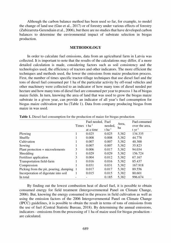
689
Although the carbon balance method has been used so far, for example, to model the change of land use (Guo et al., 2017) or of forestry under various effects of forestry (Zubizarreta-Gerendiain et al., 2006), but there are no studies that have developed carbon balances to determine the environmental impact of substrate selection in biogas production.
METHODOLOGY
In order to calculate fuel emissions, data from an agricultural farm in Latvia was
collected. It is important to note that the results of the calculations may differ, if a more detailed calculation is made, considering factors such as soil consistency and the technologies used, the efficiency of tractors and other indicators. The more efficient the techniques and methods used, the lower the emissions from maize production process. First, the number of times specific tractor-tillage techniques that use diesel fuel and the tons of diesel fuel consumed per 1 ha of the particular activity by off-road vehicles and other machinery were collected to an indicator of how many tons of diesel needed per hectare and how many tons of diesel fuel are consumed per year to process 1 ha of biogas maize fields. In turn, knowing the area of land that was used to grow the biogas maize substrate in a given year, can provide an indicator of all year’s fuel consumption for biogas maize cultivation per ha (Table 1). Data from company producing biogas from maize in was used.
Table 1. Diesel fuel consumption for the production of maize for biogas production
Times
Fuel needed, t ha-1 at a time
Fuel needed, t ha-1
Area, ha
Fuel consumed over the area, t yr-1
Plowing 1 0.025 0.025 5,382 134.335 Shuffle 1 0.008 0.008 5,382 44.778 Cultivation 1 0.007 0.007 5,382 40.300 Sowing 1 0.007 0.007 5,382 35.823 Plant protection + microelements 3 0.006 0.017 5,382 94.034 Shredding 1 0.029 0.029 5,382 156.724 Fertilizer application 3 0.004 0.012 5,382 67.167 Transportation field-farm 1 0.016 0.016 5,382 85.437 Compression 1 0.031 0.031 5,382 167.918 Picking from the pit, pouring, dumping 1 0.017 0.017 5,382 89.556 Incorporation of digestate into soil 1 0.015 0.015 5,382 80.601 In total - - 0.185 5,382 996.674
By finding out the lowest combustion heat of diesel fuel, it is possible to obtain consumed energy for field treatment (Intergovernmental Panel on Climate Change, 2006). But, knowing the energy consumed in the process in field cultivation as well as using the emission factors of the 2006 Intergovernmental Panel on Climate Change (IPCC) guidelines, it is possible to obtain the result in terms of tons of emissions from the use of fuel (Central Statistic Bureau, 2018). By determining the annual emissions, indicators - emissions from the processing of 1 ha of maize used for biogas production - are calculated.
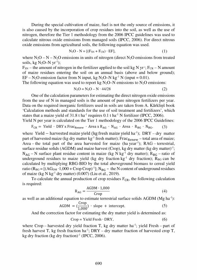
690
During the special cultivation of maize, fuel is not the only source of emissions, it is also caused by the incorporation of crop residues into the soil, as well as the use of nitrogen, therefore the Tier 1 methodology from the 2006 IPCC guidelines was used to calculate nitrous oxide emissions from managed soils (IPCC, 2006). For direct nitrous oxide emissions from agricultural soils, the following equation was used.
N2O - N = [(FSN + FCR) ∙ EF], (1)
where N2O – N – N2O emissions in units of nitrogen (direct N2O emissions from treated soils, kg N2O–N yr-1); FSN – the amount of nitrogen in the fertilizer applied to the soil kg N yr-1; FCR – N amount of maize residues entering the soil on an annual basis (above and below ground); EF – N2O emission factor from N input, kg N2O–N kg-1 N (input = 0.01). The following equation was used to report kg N2O–N emissions to N2O emissions:
N2O = N2O – N ∙ 44/28 (2)
One of the calculation parameters for estimating the direct nitrogen oxide emissions from the use of N in managed soils is the amount of pure nitrogen fertilizers per year. Data on the required inorganic fertilizers used in soils are taken from A. Kārkliņš book ‘Calculation methods and standards for the use of soil treatment and fertilizers’, which states that a maize yield of 31.8 t ha-1 requires 0.1 t ha-1 N fertilizer (IPCC, 2006). Yield N per year is calculated on the Tier 1 methodology of the 2006 IPCC Guidelines: F�� = Yield ∙ DRY x Frac����� ∙ Area x R�� ∙ N�� ∙ Area ∙ R�� ∙ N��, (3)
where Yield − harvested maize yield (kg fresh maize yield ha-1); DRY – dry matter part of harvested maize (kg dry matter kg-1 fresh matter); Frac����� – total area of maize; Area – the total part of the area harvested for maize (ha year-1); RAG – terrestrial, surface residue solids (AGDM) and maize harvest (Crop), kg dry matter (kg dry matter)-1; N�� – N surface plant residue content in maize (kg N kg-1 dry matter); R�� – ratio of underground residues to maize yield (kg dry fraction kg-1 dry fraction); RBG can be calculated by multiplying RBG-BIO by the total aboveground biomass to cereal yield ratio (RBG = [(AGDM ∙1,000 + Crop Crop)-1]; N�� – the N content of underground residues of maize (kg N kg-1 dry matter) (0.007) (Liu et al., 2019).
To calculate the annual production of crop residues F��, the following calculation is required: R�� = AGDM ∙ 1,000Crop (4)
as well as an additional equation to estimate terrestrial surface solids AGDM (Mg ha-1): AGDM = ( Crop1,000) ∙ slope + intercept. (5)
And the correction factor for estimating the dry matter yield is determined as: Crop = Yield Fresh ∙ DRY, (6)
where Crop – harvested dry yield fraction T, kg dry matter ha-1; yield Fresh – part of fresh harvest T, kg fresh fraction ha-1; DRY – dry matter fraction of harvested crop T, kg dry fraction (kg dry fraction)-1 (IPCC, 2006).
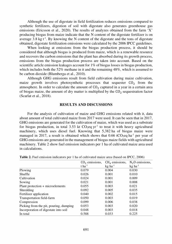
691
Although the use of digestate in field fertilization reduces emissions compared to synthetic fertilizers, digestion of soil with digestate also generates greenhouse gas emissions (Ericsson et al., 2020). The results of analyzes obtained from the farm ‘X’ producing biogas from maize indicate that the N content of the digestate fertilizer is on average 3.8 kg t-1. By knowing the N content of the digestate and the tons of digestate obtained, digestate fertilization emissions were calculated by the 2006 IPCC guidelines.
When looking at emissions from the biogas production process, it should be considered that although biogas is produced from maize, which is a renewable resource and recovers the carbon emissions that the plant has absorbed during its growth process, emissions from the biogas production process are taken into account. Based on the scientific article emission leakages account for 1% of biogas losses in biogas production, which includes both the 52% methane in it and the remaining 48%, which is assumed to be carbon dioxide (Blumberga et al., 2010).
Although GHG emissions result from field cultivation during maize cultivation, maize growth involves photosynthetic processes that sequester CO4 from the atmosphere. In order to calculate the amount of CO4 captured in a year in a certain area of biogas maize, the amount of dry matter is multiplied by the CO4 sequestration factor (Scarlat et al., 2018).
RESULTS AND DISCUSSIONS
For the analysis of cultivation of maize and GHG emissions related with it, data
about amount of total cultivated maize from 2017 were used. It can be seen that in 2017, GHG emissions are generated for the cultivation of maize, which was used as a substrate for biogas production, in total 3.53 kt CO2eq yr-1 to treat it with heavy agricultural machinery, which uses diesel fuel. Knowing that 5,382 ha of biogas maize were managed in 2017, a result is obtained which shows that 0.66 tCO2eq ha-1 per year of GHG emissions are generated in the management of biogas maize fields with agricultural machinery. Table 2 show fuel emission indicators per 1 ha of cultivated maize area used in calculations.
Table 2. Fuel emission indicators per 1 ha of cultivated maize area (based on IPCC, 2006)
CO4 emissions, t ha-1
CH6 emissions, kg ha-1
N4O emissions, kg ha-1
Plowing 0.079 0.004 0.030 Shuffle 0.026 0.001 0.010 Cultivation 0.024 0.001 0.009 Sowing 0.021 0.001 0.008 Plant protection + microelements 0.055 0.003 0.021 Shredding 0.092 0.005 0.035 Fertilizer application 0.040 0.002 0.015 Transportation field-farm 0.050 0.003 0.019 Compression 0.099 0.006 0.038 Picking from the pit, pouring, dumping 0.053 0.003 0.020 Incorporation of digestate into soil 0.048 0.003 0.018 In total 0.588 0.033 0.225

692
In order to objectively determine the total greenhouse gas emissions from fuel use, it is necessary to convert them into a single unit of measurement - CO2 equivalents. As the global warming potential (GWP) of 1 ton of CH4 equals 25 tons of C2 and 1 ton to N2O equals 298 tons of CO2, these values are used to produce total greenhouse gas emissions (IPCC, 2006). Table 3 shows CO2eq emission indicators per 1 ha of biogas produced from specially cultivated maize.
Table 3. Fuel CO2eq emission indicators per 1 ha of biogas produced from specially cultivated maize (based on IPCC, 2006)
CO4 emissions, kgCO4eq ha-1
CH6 emissions, kgCO4 eq ha-1
N4O emissions, kgCO4 eq ha-1
Total emissions, tCO4 eq ha-1
Plowing 79.28 0.11 9.04 0.09 Shuffle 26.43 0.04 3.01 0.03 Cultivation 23.78 0.03 2.71 0.03 Sowing 21.14 0.03 2.41 0.02 Plant protection + microelements 55.49 0.08 6.33 0.06 Shredding 92.49 0.13 10.55 0.10 Fertilizer application 39.64 0.06 4.52 0.04 Transportation field-farm 50.42 0.07 5.75 0.06 Compression 99.09 0.14 11.30 0.11 Picking from the pit, pouring, dumping 52.85 0.07 6.03 0.06 Incorporation of digestate into soil 47.57 0.07 5.42 0.05 In total 588.16 0.82 67.06 0.66
The obtained data show that the highest emissions per ha occur per year due to harvesting and shredding to prepare maize for placing in the bioreactor, as well as due to compaction. The lowest emissions occur during sowing. Total indicative emissions
relatively similar, amounting to 0.468 tCO2 eq ha-1 and 0.443 tCO2 eq ha-1. In total indicative emissions from biogas production from specially grown maize creates 1.567 t CO2 eq ha-1.
The biogas production process produces a very valuable by-product – digestate. It contains significant amounts of nutrients that are suitable for enriching the soil (Brown et al., 2010; Pereira et al., 2018). The dry weight of digestate from biogas production using only maize is approximately 58.22% (Tambone et al., 2019). Digestion of fields with digestate can indirectly reduce greenhouse gas emissions, for example, digestate from 1 ha of maize green matter with a yield of 30 t ha-1 fully provides the required
from biogas production from specially grown maize per ha shown in Table 4.
As a result, it can be seen that the highest emissions per ha are caused by the use of fuel to perform all the necessary treatment operations with heavy machinery, which is almost 0.66 tCO2eq ha-1. Emissions from tillage with nitrogen fertilizers and crop residue incorporation in soil after harvest are
Table 4. Total indicative emissions from biogas production from specially grown maize per ha (based on IPCC, 2006)
Indicative emissions tCO4eq ha-1
Fuel emissions 0.656 Crop residue emissions 0.443 N fertilizer emissions 0.468 In total 1.567
693
amount of potassium fertilizer and saves 31% phosphorus and 44–45% nitrogen fertilizer (Naglis-Liepa et al., 2014; Slepetiene et al., 2020).
Accordingly, using a maize yield of 31.8 t ha-1, it is possible to provide fertilizer for 1.06 ha of maize. As a total of 25,700 ha of maize was grown in Latvia in 2017, the use of digestate is topical, as well as interviews with farmers conducted within the framework of this study revealed that unfortunately digestate for field fertilization is a shortage product, which is why additional synthetic fertilizers are used (Iocoli et al., 2019; Verdi et al., 2019).
Using digestate fertilizer in tillage, 1.19 ktCO2eq emissions were saved in 2017, while indicative emissions show a reduction of 0.22 tCO2eq ha-1.
Although the use of digestate in field fertilization reduces emissions compared to synthetic fertilizers, digestion of soil with digestate also generates GHG emissions. The results of analyzes obtained from a farm producing biogas from maize indicate that the N content of the digestate fertilizer is on average 3.8 kg t-1. Assuming that the maize harvest in 2017 is 171,147.6 tons and that the amount of digestate from the amount of mass fed to the bioreactor usually ranges from 90 to 95%, in 2017 158,311.53 tons of maize digestate were obtained, while knowing the N content of digestate per 1 ton, it is obtained that the total N per 5,382 ha of the whole maize area was 0.60 kt (Central Statistic Bureau, 2021). Based on the level 1 methodology of the 2006 IPCC guidelines, it is estimated that digestate fertilization caused 2.82 ktCO2eq emissions in 2017 indicating on indicative emissions - 0.0005 tCO2eq ha-1.
The methane content of biogas produced exclusively from maize silage is known to be 52%, and the biogas yield per ton of maize is 202 cubic meters, which allows to calculate both the total amount of biogas produced from maize harvested in Latvia, which is 34,571,815.2 m3 from 171,147.6 t maize (Latvia's National Inventory Report, 1990).
At a 1% biogas leak in its production process in 2017, 2.63 ktCO4 eq GHG emissions were released into the atmosphere.
CONCLUSIONS The research proves that carrying out carbon balance by the methodology based on
life cycle analysis for assessment of the impact of biogas production from maize, it is possible to determine the environmental impact in terms of greenhouse gas emissions on the atmosphere. Despite the consumption of diesel fuel and emissions from the maize production process, maize absorbs much more carbon than is produced during photosynthesis, thus, if 1% of biogas leakage is assumed in its production process, as well as knowing by previous calculations that 34,571,815.2 m3 of biogas can be obtained from 5,382 ha specially grown maize, its production from specially grown maize can save 1.86 kg CO2 eq emissions per 1 m3 of produced biogas (in normal conditions, pressure 760 mm Hg).
The carbon balance can be further improved by reducing emissions from the agricultural process by growing the substrate, for example, using zero-emission electric tractors for soil tillage, could reduce total biogas maize growing emissions by 43%. But there are also processes that would not be desirable to reduce emissions, for example, the tractor driving frequency reduction in the field - the fertilization process can theoretically be carried out immediately and at once, but fertilization is divided into

694
several stages in order to gradually spread the substances for a favorable plant vegetation process, as well as not to promote pollution of water due to drainage that leads to erosion (Oshunsanya et al., 2019). After harvest, 28% of total emissions come from nitrogen emissions from crop residues (above and below ground). Unfortunately, these are emissions that cannot be reduced because, although these residues could theoretically be used for biogas production, the removal of crop residues from maize fields would have a negative impact on the environment and soil quality (Industrial Vehicle Technology International, 2021).
It is essential to combine efficiency in agriculture in order to reduce atmospheric emissions without losing sight of sustainable farming, so as not to have a negative impact on soil, water and the environment as a whole.
Results of this study demonstrates that using the carbon balance methodology developed in this work, it is possible to calculate the impact of biogas production and how the environment is affected as a result of substrate selection. Such calculations can be applied to any country or company in the world and it can be an excellent tool for political decision making, based not on discussion, but on quantitative calculations.
ACKNOWLEDGEMENTS. This research is funded by the Ministry of Economics of the Republic of Latvia, project ‘Sustainable and renewable transport policy formulation in Latvia’, project No. VPP-EM-2018/AER_2_0003.
REFERENCES
Arodudu, O.T., Helming, K., Voinov, A. & Wiggering, H. 2017. Integrating agronomic factors
into energy efficiency assessment of agro-bioenergy production – A case study of ethanol and biogas production from maize feedstock. Applied Energy 198, 426–439. https://doi.org/10.1016/j.apenergy.2017.02.017
Bereiter, B., Eggleston, S., Schmitt, J., Nehrbass-Ahles, C., Stocker, T.F., Fischer, H., Kipfstuhl, S. & Chappellaz, J. 2015. Revision of the EPICA Dome C CO2 record from 800 to 600-kyr before present. Geophysical Research Letters 42, 542–549. https://doi.org/10.1002/2014GL061957
Blumberga, D., Dzene, I., Al Seadi, T., Rutz, D., Prassl, H., Kottner, M., Finsterwalder, T., Volk, S. & Janssen, R. 2010. Biogas HANDBOOK. https://docplayer.org/69439281-D-blumberga-i-dzene-t-al-sedi-d-rucs-h-prasls-m-ketners-t-finstervalders-s-folka-r-jansens-biogaze-rokasgramata.html. Accessed 05.01.2021
Brown, S., Beecher, N. & Carpenter, A. 2010. Calculator tool for determining greenhouse gas emissions for biosolids processing and end use. Environmental Science & Technology 44, 9509–9515. https://doi.org/10.1021/es101210k
Bumbiere, K., Gancone, A., Pubule, J., Kirsanovs, V., Vasarevicius, S. & Blumberga, D. 2020. Ranking of Bioresources for Biogas Production. Environmental and Climate Technologies 24(1), 368–377. https://doi.org/10.2478/rtuect-2020-0021
Cavinato, C., Fatone, F., Bolzonella, D. & Pavan, P. 2010. Thermophilic anaerobic co-digestion of cattle manure with agro-wastes and energy crops: Comparison of pilot and full scale experiences. Bioresource Technology 101, 545–550. https://doi.org/10.1016/j.biortech.2009.08.043
695
Central Statistic Bureau, CSB database, (n.d.). https://www.csb.gov.lv/lv/statistika/db. Accessed 05.01.2021.
Central Statistic Bureau, Latvian energy balance in 2017. 2018. https://www.csb.gov.lv/lv/statistika/statistikas-temas/vide-energetika/energetika/meklet-tema/332-energobilance-2017-gada
Chen, X.Y., Vinh-Thang, H., Ramirez, A.A., Rodrigue, D. & Kaliaguine, S. 2015. Membrane gas separation technologies for biogas upgrading. RSC Advances 5, 24399–24448. https://doi.org/10.1039/c5ra00666j
Cherubini, F. 2010. GHG balances of bioenergy systems - Overview of key steps in the production chain and methodological concerns. Renewable Energy 35, 1565–1573. https://doi.org/10.1016/j.renene.2009.11.035
Crafts-Brandner, S.J. & Salvucci, M.E. 2002. Sensitivity of photosynthesis in a C4 plant, maize, to heat stress. Plant Physiology 129, 1773–1780. https://doi.org/10.1104/pp.002170.
European Council | European Commission. 2014. Communication from the Commission to the European Parliament, the Council, the European Economic and Social Committee and the Committee of the regions. A policy framework for Climate and Energy in the period from 2020 to 2030. https://ec.europa.eu/clima/policies/strategies/2030_en. Accessed 04.01.2021.
European Council, European Commission. 2018. 2050 long-term strategy. Going climate-neutral by 2050. https://ec.europa.eu/clima/policies/strategies/2050_en. Accessed 04.01.2021.
European Council, A European Green Deal | European Commission. https://ec.europa.eu/info/strategy/priorities-2019-2024/european-green-deal_en. Accessed 04.01.2021.
Ericsson, N., Nordberg, Å. & Berglund, M. 2020. Biogas plant management decision support - A temperature and time-dependent dynamic methane emission model for digestate storages. Bioresource Technology Reports 11, 100454. https://doi.org/10.1016/j.biteb.2020.100454
Gowik, U.& Westhoff, P. 2011. The Path from C3 to C4 photosynthesis. Plant Physiology 155, 56–63. https://doi.org/10.1104/pp.110.165308
Guo, R., Zhao, Y., Shi, Y., Li, F., Hu, J. & Yang, H. 2017. Low carbon development and local sustainability from a carbon balance perspective. Resources, Conservation & Recycling 122, 270–279. https://doi.org/10.1016/j.resconrec.2017.02.019.
Industrial Vehicle Technology International, John Deere develops fully electric, autonomous tractor, (n.d.). https://www.ivtinternational.com/news/agriculture/john-deere-develops-fully-electric-autonomous-tractor.html. Accessed 05.01.2021.
Iocoli, G.A., Zabaloy, M.C., Pasdevicelli, G. & Gómez, M.A. 2019. Use of biogas digestates obtained by anaerobic digestion and co-digestion as fertilizers: Characterization, soil biological activity and growth dynamic of Lactuca sativa L. Science of the Total Environment 647, 11–19. https://doi.org/10.1016/j.scitotenv.2018.07.444
IPCC - Task Force on National Greenhouse Gas Inventories. 2006. 2. https://www.ipcc-nggip.iges.or.jp/public/2006gl/ Accessed 05.01.2021.
Krištof, K. & Gaduš, J. 2018. Effect of alternative sources of input substrates on biogas production and its quality from anaerobic digestion by using wet fermentation. Agronomy Research 16(3), 769–783. https://doi.org/10.15159/AR.18.146
Latvia's National Inventory Report. 1990. http://www.meteo.lv/. Accessed 05.01.2021. Lauka, D., Slisane, D., Ievina, L., Muizniece, I. & Blumberga, D. 2019. When Bioeconomy
Development Becomes a Biomass Energy Competitor. Environmental and Climate Technologies 23, 347–359. https://doi.org/10.2478/rtuect-2019-0100
Li., Y., Wen, Z., Li, J., Cai, L. & Wang, H. 2019. Feasibility of utilizing by-product biogas in breweries after being decarbonized for refrigeration chiller and related primary energy efficiency analysis. Sustainable Energy Technologies and Assessments 31, 390–400. https://doi.org/10.1016/j.seta.2019.01.001

696
Liu, Z., Gao, J., Gao, F., Liu, P., Zhao, B. & Zhang, J. 2019. Late harvest improves yield and nitrogen utilization efficiency of summer maize. Field Crops Research 232, 88–94. https://doi.org/10.1016/j.fcr.2018.12.014
Mano Esteves, E.M., Naranjo Herrera, A.M., Pecanha Esteves, V.P. & Vaz Morgado, C.R. 2019. Life cycle assessment of manure biogas production: A review. Journal of Cleaner Production 219, 411–423. https://doi.org/10.1016/j.jclepro.2019.02.091
Meiramkulova, K., Bayanov, A., Ivanova, T., Havrland, B., Kára, J. & Hanzlíková, I. 2018. Effect of different compositions on anaerobic co-digestion of cattle manure and agro-industrial by-products. Agronomy Research 16(1), 176–187. https://doi.org/10.15159/AR.18.008
Melvere, M., Ivanovs, K., Pubule, J. & Blumberga, D. 2017. Use of round goby (Neogobius melanostomus) processing waste in bioeconomy. Energy Procedia 128, 484–490. https://doi.org/10.1016/j.egypro.2017.09.064
Mehryar, E., Ding, W.M., Hemmat, A., Hassan, M., Bi, J.H., Huang, H.Y. & Kafashan, J. 2017. Anaerobic co-digestion of oil refinery wastewater and chicken manure to produce biogas, and kinetic parameters determination in batch reactors. Agronomy Research 15(5), 1983–1996. https://doi.org/10.15159/AR.17.072.
Meyer, A.K.P., Ehimen, E.A. & Holm-Nielsen, J.B. 2018. Future European biogas: Animal manure, straw and grass potentials for a sustainable European biogas production. Biomass and Bioenergy 111, 154–164. https://doi.org/10.1016/j.biombioe.2017.05.013
Muench, S. & Guenther, E. 2013. A systematic review of bioenergy life cycle assessments. Applied Energy 112, 257–273. https://doi.org/10.1016/j.apenergy.2013.06.001.
Muizniece, I., Zihare, L., Pubule, J. & Blumberga, D. 2019. Circular Economy and Bioeconomy Interaction Development as Future for Rural Regions. Case Study of Aizkraukle Region in Latvia. Environmental and Climate Technologies 23, 129–146. https://doi.org/10.2478/rtuect-2019-0084
Murphy, F., Devlin, G. & McDonnell, K. 2014. Forest biomass supply chains in Ireland: A life cycle assessment of GHG emissions and primary energy balances. Applied Energy 116, 1–8. https://doi.org/10.1016/j.apenergy.2013.11.041
Naglis-Liepa, K. & Pelse, M. 2014. Biogas production from agricultural raw materials. https://llufb.llu.lv/conference/economic_science_rural/2014/ESRD_34_2014_Productions-172-179.pdf
Oshunsanya, S.O., Li, Y. & Yu, H. 2019. Vetiver grass hedgerows significantly reduce nitrogen and phosphorus losses from fertilized sloping lands. Science of the Total Environment 661, 86–94. https://doi.org/10.1016/j.scitotenv.2019.01.129
Patzek, T.W. 2004. Thermodynamics of the corn-ethanol biofuel cycle, CRC. Critical Reviews in Plant Sciences 23, 519–567. https://doi.org/10.1080/07352680490886905.
Pereira Domingues Martinho, V.J. 2018. Interrelationships between renewable energy and agricultural economics: An overview. Energy Strategy Reviews 22, 396–409. https://doi.org/10.1016/j.esr.2018.11.002
Pimentel, D. 2003. Ethanol fuels: Energy balance, economics, and environmental impacts are negative. Natural Resources Research 12, 127–134. https://doi.org/10.1023/A:1024214812527
Sauthoff, S., Musshoff, O., Danne, M. & Anastassiadis, F. 2016. Sugar beet as a biogas substrate? A discrete choice experiment for the design of substrate supply contracts for German farmers. Biomass and Bioenergy 90, 163–172. https://doi.org/10.1016/j.biombioe.2016.04.005
Scarlat, N., Dallemand, J.F. & Fahl, F. 2018. Biogas: Developments and perspectives in Europe. Renewable Energy 129, 457–472. https://doi.org/10.1016/j.renene.2018.03.006
Schulz, V.S., Munz, S., Stolzenburg, K., Hartung, J., Weisenburger, S., Mastel, K., Möller, K., Claupein, W. & Graeff-Hönninger, S. 2018. Biomass and biogas yield of maize (Zea mays l.) grown under artificial shading. Agriculture 8. https://doi.org/10.3390/agriculture8110178
697
Shah, F.A., Mahmood, Q., Rashid, N., Pervez, A., Raja, I.A. & Shah, M.M. 2015. Co-digestion, pretreatment and digester design for enhanced methanogenesis. Renewable & Sustainable Energy Reviews 42, 627–642. https://doi.org/10.1016/j.rser.2014.10.053
Siddique, M.N.I. & Wahid, Z.A. 2018. Achievements and perspectives of anaerobic co-digestion: A review. Journal of Cleaner Production 194, 359–371. https://doi.org/10.1016/j.jclepro.2018.05.155
Slepetiene, A., Volungevicius, J., Jurgutis, L., Liaudanskiene, I., Amaleviciute-Volunge, K., Slepetys, J. & Ceseviciene, J. 2020. The potential of digestate as a biofertilizer in eroded soils of Lithuania. Waste Management 102, 441–451. https://doi.org/10.1016/j.wasman.2019.11.008.
Tambone, F., Orzi, V., Zilio, M. & Adani, F. 2019. Measuring the organic amendment properties of the liquid fraction of digestate. https://doi.org/10.1016/j.wasman.2019.03.024
Timonen, K., Sinkko, T., Luostarinen, S., Tampio, E. & Joensuu, K. 2019. LCA of anaerobic digestion: Emission allocation for energy and digestate. Journal of Cleaner Production 235, 1567–1579. https://doi.org/10.1016/j.jclepro.2019.06.085
Ugwu, S.N., Biscoff, R.K. & Enweremadu, C.C. 2020. A meta-analysis of iron-based additives on enhancements of biogas yields during anaerobic digestion of organic wastes. Journal of Cleaner Production 269, 122449. https://doi.org/10.1016/j.jclepro.2020.122449
Verdi, L., Kuikman, P.J., Orlandini, S., Mancini, M., Napoli, M. & Dalla Marta, A. 2019. Does the use of digestate to replace mineral fertilizers have less emissions of N2O and NH 3? Agricultural and Forest Meteorology 269–270, 112–118. https://doi.org/10.1016/j.agrformet.2019.02.004
Zubizarreta-Gerendiain, A., Pukkala, T. & Peltola, H. 2016. Effects of wood harvesting and utilisation policies on the carbon balance of forestry under changing climate: A Finnish case study. Forest Policy and Economics 62, 168–176. https://doi.org/10.1016/j.forpol.2015.08.007
698
Agronomy Research 19(S1), 698–710, 2021 https://doi.org/10.15159/AR.21.058
Approach to a classification of construction typologies of pig facilities: case study Antioquia – Colombia
N. Castrillón2,3,*, V. Gonzalez1,3 and J.A. Osorio1
1Universidad Nacional de Colombia, sede Medellín, Facultad de Ciencias Agrarias, Carrera 65 #59A-110, Código postal 050034 Medellín, Colombia 2Universidad Nacional de Colombia, sede Medellín, Facultad de Minas, AV 80 #65-223, Código postal 050034 Medellín, Colombia 3Grupo de Investigación en Biodiversidad y Genética Molecular (BIOGEM), Departamento de Producción Animal, Universidad Nacional de Colombia, Sede Medellín, Carrera 65 No. 59 A-110, Código postal 050034, Colombia *Correspondence: [email protected] Received: January 31th, 2021; Accepted: March 27th, 2021; Published: April 30th, 2021 Abstract. Pig facilities foro confined production in tropical countries such as Colombia does not specify, in the present moment a typological classification that allows researchers to carry out evaluations related to animal comfort and environmental impacts according to the type of accommodation. To achieve the objective of this research were developed a survey to a panel of experts, a decision sensitivity analysis and the hierarchical analytical method AHP. Parameters that allowed to describe the concept of a technified pig farm were obteined, where the most relevant were: biosecurity measures, measurement of zootechnical parameters, training for workers and legal fulfilment. Additionally, ranges were defined to establish the production size in small, medium and large according to the number of animals. The results obtained per group were: 1) breeding small (50–200), medium (201–1,000) and large (1,001–5,000); 2) growth small (60–200), medium (201–800) and large (801–5000); and 3) finishing stage small (50–500), medium (501–1,000) and large (2,001–5,000). A total of 948 typological combinations were initially determined. Finally, the construction characteristics with the greatest technical and operational feasibility were prioritized for each group achieving 36 typologies that can represent the typological pig facilities not only in the state of Antioquia but also in many others states in Colombia. Key words: tropical country, natural ventilation, swine production, animal comfort.
INTRODUCTION Pork is the second most consumed meat in the world, representing 43% of the
world's meat production for human consumption (OCDE/FAO, 2013), the worldwide distribution is mainly concentrated in Asia 59%, Europe 22% and North and Central America with 11%. China, the European Union and the United States produce more than 86% of pig cattle (USDA, 2011). In America, the highest production occurs in countries such as the United States, Canada, Brazil and Mexico. Colombia only produces 1% of
699
the meat in the American continent (Porkcolombia & PigCHAMP, 2015) with 14,000 pig farms (Departamento Administrativo Nacional de Estadística (DANE), 2016). The steady growth of the productive sector has aroused keen interest worldwide on issues of animal welfare and environmental impact assessment, both widely studied for pig production systems, to find better management practices at commercial level (Rhodes et al., 2005).
Most of the production systems of northern and southern countries are developed in closed buildings (Reimert et al., 2014). In a multidisciplinary review developed by CIGR (2006) regarding the differences in constructive characteristics of greater relevance for animal comfort between zones with very marked seasons and subtropical or tropical countries, it was found that for countries with seasons is easy to find climate control systems to maintain the interior temperature and relative humidity, however, for hot summer days, the acclimatization problems are identical to the problems in equatorial areas (Jackson et al., 2018), where the main cause of thermal discomfort is due to the amount of heat, from solar energy, absorbed by the facilities. This is the reason why most of the facilities are equipped with natural ventilation and open systems in side walls and ceilings, and in few cases hybrid systems that combine natural and mechanical ventilation, searching lower operating costs and less greenhouse gas emissions (Reckmann et al., 2013 and Osorio et al., 2017). Due to the above, thermal stress should be the first attribute to take into account in a bioclimatic design, together with the gas emission (Pietrosemoli & Tang, 2020).
Regarding environmental impacts, those associated with manure management have been extensively studied. Contamination of soil, water and generation of atmospheric emissions were mainly evaluated. The latter in relation to toxicity in the biotic environment and contribution of gases with global warming potential GWP (Castrillón et al., 2020). However, there are other sources of impact related to accommodation. The most relevant of which are water management, feeding, energy consumption, management of liquid and solid manure, management of other waste, infrastructure design and thermal comfort characteristics (Reckmann et al., 2013).
The advantage that climate control systems have for research and legal policy management is that they have detailed definitions and defined typological classifications allowing efficient comparisons between the different systems. (Jackson et al., 2018). On the contrary, in tropical countries, the confined production of pigs does not have a specific classification in terms of its construction type, farm size, or a specific definition that allows identifying when a farm is technified.
Resolution 2640 of 2007 of the Colombian Agricultural Institute (ICA), is the only tool that provides criteria to evaluate production facilities at the national level. However, this standard does not have the necessary guidelines for the design and classification of accommodation with essential criteria such as animal welfare (Cecchin et al., 2019) and efficient management of natural resources (Reckmann et al., 2013). The foregoing leads to the need to generate a classification of these typologies based on their constructive characteristics, thermal floor, size and level of technification, which responds to the lack that researchers currently have to reference their work and determine the behaviour of different structures based on general welfare, animal comfort, impact on the environment, among others.
700
Given the above, this research is aimed to make a proposal for the classification of construction typologies for pig facilities of different age groups and according to the thermal floor. The research was developed in the department of Antioquia - Colombia and will serve for future research at the national level model.
MATERIALS AND METHODS
Data collection: The methodology for collecting the primary information to perform the qualitative
and quantitative analysis was divided into three stages. In the first stage, the concept of a technified pig farm was defined for a tropical country with productive levels such as Colombia. In the second, the farm size according to the age group and the most used construction characteristics in the department of Antioquia in relation to thermal comfort; generation, concentration and distribution of gases within the accommodation. And in the third, the criteria for categorizing the most feasible construction typologies of each age group were established, according to the thermal floor.
Determination of the panel of experts: The panel of experts consulted for this work was constituted by an interdisciplinary
group of 8 professionals from the branches of civil engineering, veterinary science, zootechnics, and agricultural engineering, among others, with experience in the construction, research, and management of pig housing in confined production, thermal comfort and animal welfare. The experts gave their concepts focused on developing typological classification guidelines according to the characteristics stated in each phase of production. The information was compiled and delivered again to the group of experts to carry out a first purge according to the criteria of age, thermal floor and degree of technification.
Finally, the expert panel were summoned to a group work to establish the construction and maintenance costs per square meter of each of the listed structures and define an evaluation relating to the effectiveness in keeping thermal comfort and animal welfare, in order to identify viable typological combinations. The construction characteristics used were: floor material (flat concrete, plastics and concrete slatteds, deep bed, mixed (flat and slatted)), manure storage or conveyance systems (flat floor, flooded pit, pit not flooded, pool or sump), lateral ventilation systems (100% open, low wall open between 50–80% and high wall with side windows openings between 30–50%), ventilation system on the roof (gable roof with or without laternim, gable roof with over-roof). Criteria such as the size of the facility were also taken into account based on the number of animals, age group and the respective thermal floors.
Determination of thermal floors: To determine the thermal floors, the 2014 national agricultural survey developed
by the ICA was used. It stated that Antioquia has 2,038 farms, located between 200 and 2,800 meters above sea level. Table 1 shows the classification of the facilities based on the height above sea level under the Caldas - Lang classification (Instituto Colombiano de Hidrología Meteorología y Estudios Ambientales - IDEAM, 2005, Gobernación de Antioquia, 2014). It was found that the largest number of farms in the department are located between 1,900 and 2,800 meters above sea level, represented by a cold, mild and

701
Determination of farm size: With the ranges of each of the respondents and the use of descriptive statistics tools,
the confidence intervals were determined to categorize the farms according to their size and age group between small, medium or large.
Determination of the total combinations of construction typologies: The quantity of all possible existing facilities, age groups and thermal floors were
subjected to a calculation of the possible number of combinations using the R statistical software. With the result, an initial filtration of the combinations that had mutually exclusive structures was carried out. Subsequently, the refined list of combinations was presented to the experts and they were asked to eliminate those combinations without feasibility according to the thermal floor and age group. Finally, the results were presented through a decision sensitivity analysis according to the thermal floor in which the mutually exclusive structures and those that are not appropriate for the climate were taken into account, the viable relationships were marked with 1 and those that had no feasibility with 0.
The results of the structures with the highest feasibility for each age group were analyzed through a descriptive statistical process to allow an organized display of them. The constructive characteristics with the highest weighing were established as selection criteria, to develop an analysis of all the possible combinations according to each age group.
Selection of the most representative typologies:
for the evaluation of the different constructive alternatives (constructive cost, maintenance cost, and efficiency in maintaining thermal comfort). The characteristics to
warm thermal floor. No technified farms are registered over 2,800 meters above sea level.
Definition of a technified farm: Different descriptive factors were
developed to establish the definition of a technified farm with the information obtained in the first panel of experts. They were valued according to the number of mentions made by each of the experts.
Table 1. Location of the farms in Antioquia according to the thermal floor (Departamento Administrativo Nacional de Estadística (DANE), 2016, Gobernación de Antioquia, 2014)
Number of farms
Height above sea level
Thermal Floor
63 0–900 Warm 539 900–1,900 Mild 1,436 1,900–2,800 Cold 0 2,800–3,700 Very cold 0 3,700–4,700 Extremely cold 0 > 4,700 Nival
In order to obtain the most viable typologies by age group and thermal floor, a weighting was used based on the consensus of experts on the priority of the factors that are typically used to add scores when working with multiple dimensions called the analytical hierarchy process (AHP) (Ameen & Mourshed, 2019). Three criteria were selected
Table 2. Characteristics to be evaluated to obtain the construction typologies
Age group Construction Features Thermal
floor Gestation Floor material Cold Breeding Manure storage or
conveyance system Mild
Growth Side ventilation structure Warm Fattening Roof ventilation structure
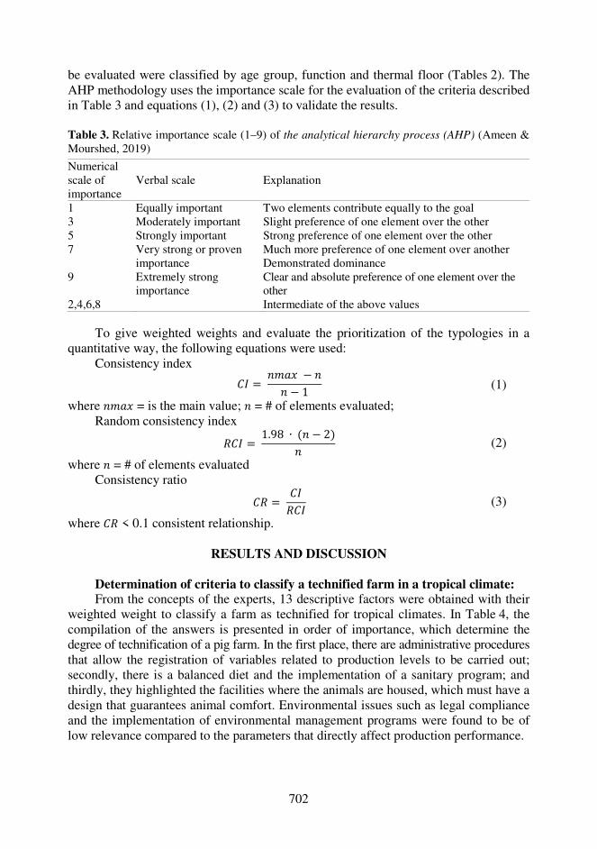
702
be evaluated were classified by age group, function and thermal floor (Tables 2). The AHP methodology uses the importance scale for the evaluation of the criteria described in Table 3 and equations (1), (2) and (3) to validate the results.
Table 3. Relative importance scale (1–9) of the analytical hierarchy process (AHP) (Ameen & Mourshed, 2019)
Numerical scale of importance
Verbal scale Explanation
1 Equally important Two elements contribute equally to the goal 3 Moderately important Slight preference of one element over the other 5 Strongly important Strong preference of one element over the other 7 Very strong or proven
importance Much more preference of one element over another Demonstrated dominance
9 Extremely strong importance
Clear and absolute preference of one element over the other
2,4,6,8 Intermediate of the above values
To give weighted weights and evaluate the prioritization of the typologies in a quantitative way, the following equations were used:
Consistency index 78 = 9:;< − 99 − 1 (1)
where 9:;< = is the main value; 9 = # of elements evaluated; Random consistency index =78 = 1.98 ∙ (9 − 2)9 (2)
where 9 = # of elements evaluated Consistency ratio 7= = 78=78 (3)
where 7= < 0.1 consistent relationship.
RESULTS AND DISCUSSION Determination of criteria to classify a technified farm in a tropical climate: From the concepts of the experts, 13 descriptive factors were obtained with their
weighted weight to classify a farm as technified for tropical climates. In Table 4, the compilation of the answers is presented in order of importance, which determine the degree of technification of a pig farm. In the first place, there are administrative procedures that allow the registration of variables related to production levels to be carried out; secondly, there is a balanced diet and the implementation of a sanitary program; and thirdly, they highlighted the facilities where the animals are housed, which must have a design that guarantees animal comfort. Environmental issues such as legal compliance and the implementation of environmental management programs were found to be of low relevance compared to the parameters that directly affect production performance.
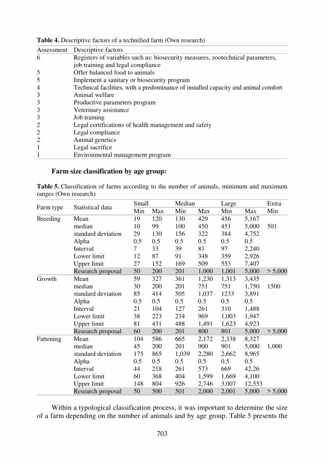
703
Table 4. Descriptive factors of a technified farm (Own research)
Assessment Descriptive factors 6 Registers of variables such as: biosecurity measures, zootechnical parameters,
job training and legal compliance 5 Offer balanced food to animals 5 Implement a sanitary or biosecurity program 4 Technical facilities, with a predominance of installed capacity and animal comfort 3 Animal welfare 3 Productive parameters program 3 Veterinary assistance 3 Job training 2 Legal certifications of health management and safety 2 Legal compliance 2 Animal genetics 1 Legal sacrifice 1 Environmental management program
Farm size classification by age group:
Table 5. Classification of farms according to the number of animals, minimum and maximum ranges (Own research)
Farm type Statistical data Small Median Large Extra Min Max Min Max Min Max Min
Breeding Mean 19 120 130 429 456 5,167 median 10 99 100 450 451 5,000 501 standard deviation 29 130 156 322 384 4,752 Alpha 0.5 0.5 0.5 0.5 0.5 0.5 Interval 7 33 39 81 97 2,240 Lower limit 12 87 91 348 359 2,926 Upper limit 27 152 169 509 553 7,407 Research proposal 50 200 201 1,000 1,001 5,000 > 5,000
Growth Mean 59 327 361 1,230 1,313 3,435 median 30 200 201 751 751 1,750 1500 standard deviation 85 414 505 1,037 1233 3,891 Alpha 0.5 0.5 0.5 0.5 0.5 0.5 Interval 21 104 127 261 310 1,488 Lower limit 38 223 234 969 1,003 1,947 Upper limit 81 431 488 1,491 1,623 4,923 Research proposal 60 200 201 800 801 5,000 > 5,000
Fattening Mean 104 586 665 2,172 2,338 8,327 median 45 200 201 900 901 5,000 1,000 standard deviation 175 865 1,039 2,280 2,662 8,965 Alpha 0.5 0.5 0.5 0.5 0.5 0.5 Interval 44 218 261 573 669 42,26 Lower limit 60 368 404 1,599 1,669 4,100 Upper limit 148 804 926 2,746 3,007 12,553 Research proposal 50 500 501 2,000 2,001 5,000 > 5,000
Within a typological classification process, it was important to determine the size
of a farm depending on the number of animals and by age group. Table 5 presents the
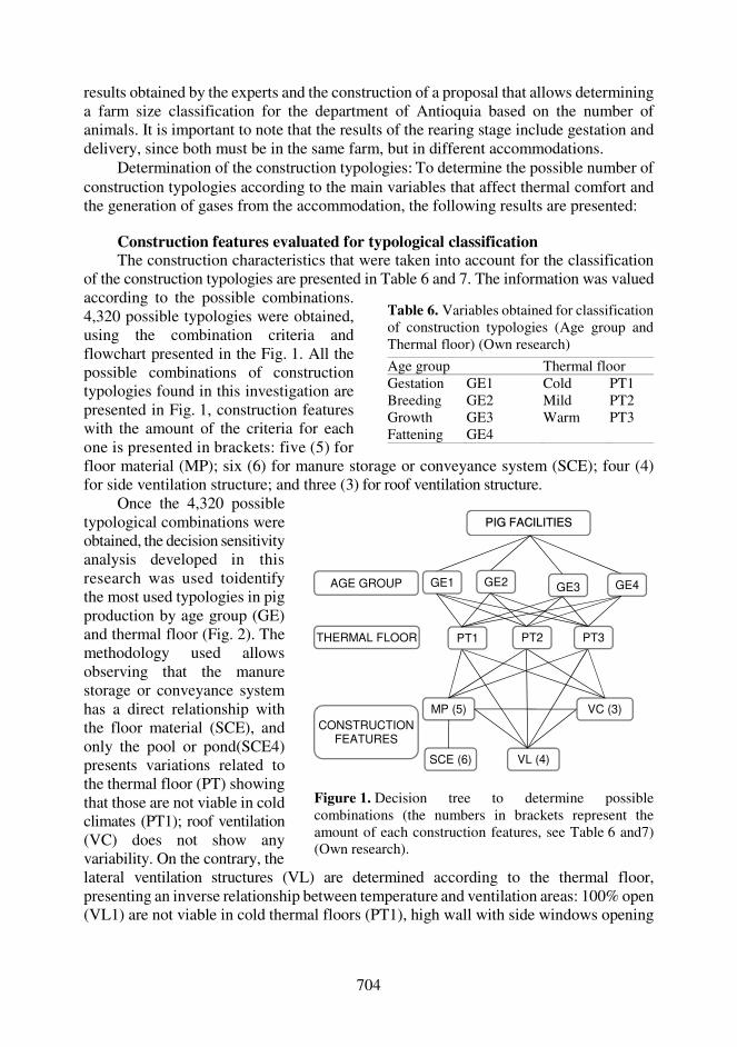
704
results obtained by the experts and the construction of a proposal that allows determining a farm size classification for the department of Antioquia based on the number of animals. It is important to note that the results of the rearing stage include gestation and delivery, since both must be in the same farm, but in different accommodations.
Determination of the construction typologies: To determine the possible number of construction typologies according to the main variables that affect thermal comfort and the generation of gases from the accommodation, the following results are presented:
Construction features evaluated for typological classification The construction characteristics that were taken into account for the classification
of the construction typologies are presented in Table 6 and 7. The information was valued
floor material (MP); six (6) for manure storage or conveyance system (SCE); four (4) for side ventilation structure; and three (3) for roof ventilation structure.
lateral ventilation structures (VL) are determined according to the thermal floor, presenting an inverse relationship between temperature and ventilation areas: 100% open (VL1) are not viable in cold thermal floors (PT1), high wall with side windows opening
according to the possible combinations. 4,320 possible typologies were obtained, using the combination criteria and flowchart presented in the Fig. 1. All the possible combinations of construction typologies found in this investigation are presented in Fig. 1, construction features with the amount of the criteria for each one is presented in brackets: five (5) for
Table 6. Variables obtained for classification of construction typologies (Age group and Thermal floor) (Own research)
Age group Thermal floor Gestation GE1 Cold PT1 Breeding GE2 Mild PT2 Growth GE3 Warm PT3 Fattening GE4
Once the 4,320 possible typological combinations were obtained, the decision sensitivity analysis developed in this research was used toidentify the most used typologies in pig production by age group (GE) and thermal floor (Fig. 2). The methodology used allows observing that the manure storage or conveyance system has a direct relationship with the floor material (SCE), and only the pool or pond(SCE4) presents variations related to the thermal floor (PT) showing that those are not viable in cold climates (PT1); roof ventilation (VC) does not show any variability. On the contrary, the
Figure 1. Decision tree to determine possible combinations (the numbers in brackets represent the amount of each construction features, see Table 6 and7) (Own research).
SCE (6)
MP (5)
VL (4)
VC (3)
PT1 PT2 PT3
PIG FACILITIES
GE1 GE2 GE3 GE4 AGE GROUP
THERMAL FLOOR
CONSTRUCTION FEATURES
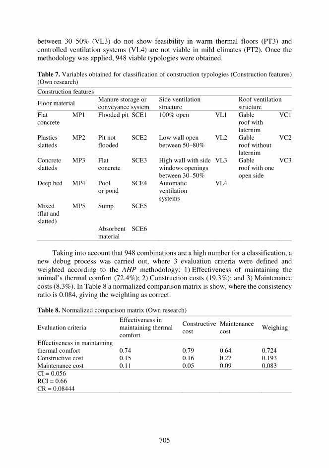
705
between 30–50% (VL3) do not show feasibility in warm thermal floors (PT3) and controlled ventilation systems (VL4) are not viable in mild climates (PT2). Once the methodology was applied, 948 viable typologies were obtained.
Table 7. Variables obtained for classification of construction typologies (Construction features) (Own research)
Construction features
Floor material Manure storage or conveyance system
Side ventilation structure
Roof ventilation structure
Flat concrete
MP1 Flooded pit SCE1 100% open VL1 Gable roof with laternim
VC1
Plastics slatteds
MP2 Pit not flooded
SCE2 Low wall open between 50–80%
VL2 Gable roof without laternim
VC2
Concrete slatteds
MP3 Flat concrete
SCE3 High wall with side windows openings between 30–50%
VL3 Gable roof with one open side
VC3
Deep bed MP4 Pool or pond
SCE4 Automatic ventilation systems
VL4
Mixed (flat and slatted)
MP5 Sump SCE5
Absorbent material
SCE6
Taking into account that 948 combinations are a high number for a classification, a
new debug process was carried out, where 3 evaluation criteria were defined and weighted according to the AHP methodology: 1) Effectiveness of maintaining the animal’s thermal comfort (72.4%); 2) Construction costs (19.3%); and 3) Maintenance costs (8.3%). In Table 8 a normalized comparison matrix is show, where the consistency ratio is 0.084, giving the weighting as correct.
Table 8. Normalized comparison matrix (Own research)
Evaluation criteria Effectiveness in maintaining thermal comfort
Constructive cost
Maintenance cost Weighing
Effectiveness in maintaining thermal comfort 0.74 0.79 0.64 0.724 Constructive cost 0.15 0.16 0.27 0.193 Maintenance cost 0.11 0.05 0.09 0.083 CI = 0.056 RCI = 0.66 CR = 0.08444
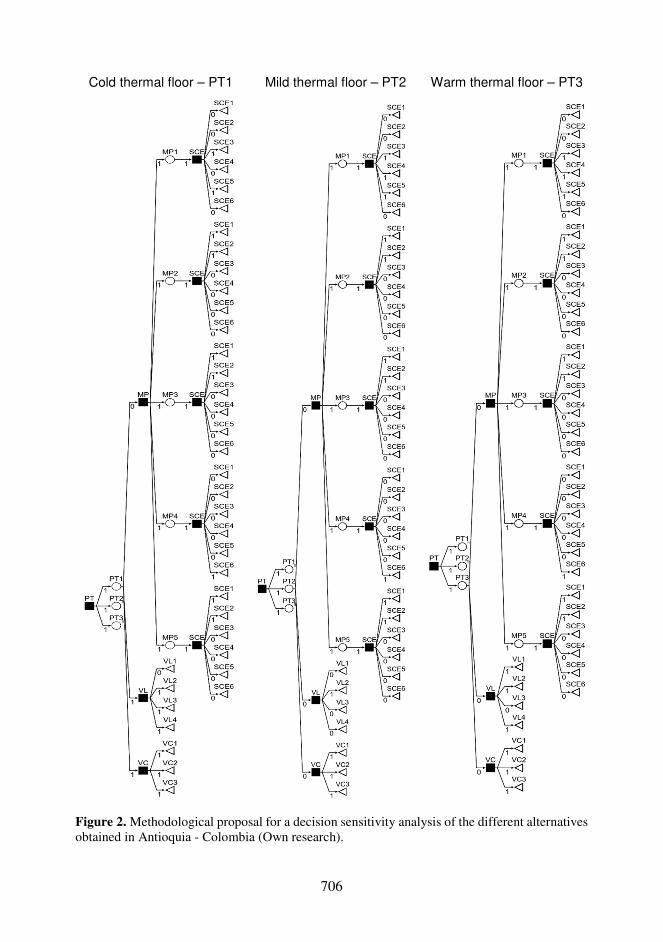
706
Cold thermal floor – PT1 Mild thermal floor – PT2 Warm thermal floor – PT3
Figure 2. Methodological proposal for a decision sensitivity analysis of the different alternatives obtained in Antioquia - Colombia (Own research).

707
Table 9. Ranking results of the alternatives (Own research)
Age group Evaluation criteria Construction Features Alternatives Weighing, % Gestation (GE1)
Effectiveness in maintaining thermal comfort
Floor material (MP) Flat concrete (MP1) Plastics slatteds (MP2) Mixed (flat and slatted) (MP5)
42.5 30 26.4
Constructive cost Manure storage or conveyance system (SCE)
Flooded pit (SCE1) Sump (SCE5)
39.4 59.6
Maintenance cost Side ventilation structure (VL)
100% open (VL1) Low wall open between 50–80% (VL2) High wall with side windows Openings between 30–50% (VL3)
10 61.9 27.5
Roof ventilation structure (VC)
Gable roof with laternim (VC1) Gable roof with one open side (VC3)
73.5 25.5
Breeding (GE2)
Effectiveness in maintaining thermal comfort
Floor material (MP) Flat concrete (MP1) Plastics slatteds (MP2) Mixed (flat and slatted) (MP5)
6.2 54.1 38.7
Constructive cost Manure storage or conveyance system (SCE)
Flat concrete (MP1) Plastics slatteds (MP2) Mixed (flat and slatted) (MP5)
67.9 31.1
Maintenance cost Side ventilation structure (VL)
Low wall open between 50–80% (VL2) High wall with side windows openings between 30–50% (VL3)
72.3 26.7
Roof ventilation structure (VC)
Gable roof with laternim (VC1) Gable roof with one open side (VC3)
73.5 25.5
Growth (GE3)
Effectiveness in maintaining thermal comfort
Floor material (MP) Plastics slatteds (MP2) Deep bed (MP4)
80.8 18.2
Constructive cost Manure storage or conveyance system (SCE)
Flooded pit (SCE1) Pit not flooded (SCE2) Absorbent material (SCE6)
58.5 24.6 15.9
Maintenance cost Side ventilation structure (VL)
Low wall open between 50–80% (VL2) High wall with side windows openings Between 30–50% (VL3)
72.3 26.7
Roof ventilation structure (VC)
Gable roof with laternim (VC1) Gable roof with one open side (VC3)
73.5 25.5
Table 9 shows the ranking results of the alternatives of the construction features.
Floor materials such as concrete was prioritized for the gestation and fattening groups, in contrast to breeding and growth where plastic had a greater weighing; manure storage or conveyance system for fattening was the only group where structures flooded with water (pool or pond (SCE4)), that allow animals to cool off, were taken into account, however, according to Table 1, 70% of the farms in Antioquia are located in cold
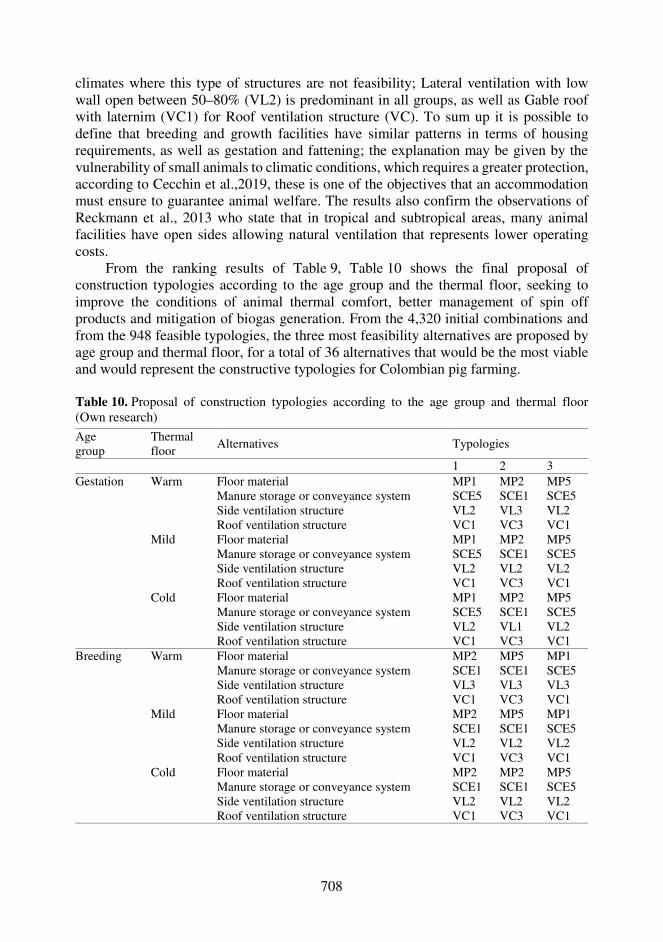
708
climates where this type of structures are not feasibility; Lateral ventilation with low wall open between 50–80% (VL2) is predominant in all groups, as well as Gable roof with laternim (VC1) for Roof ventilation structure (VC). To sum up it is possible to define that breeding and growth facilities have similar patterns in terms of housing requirements, as well as gestation and fattening; the explanation may be given by the vulnerability of small animals to climatic conditions, which requires a greater protection, according to Cecchin et al.,2019, these is one of the objectives that an accommodation must ensure to guarantee animal welfare. The results also confirm the observations of Reckmann et al., 2013 who state that in tropical and subtropical areas, many animal facilities have open sides allowing natural ventilation that represents lower operating costs.
From the ranking results of Table 9, Table 10 shows the final proposal of construction typologies according to the age group and the thermal floor, seeking to improve the conditions of animal thermal comfort, better management of spin off products and mitigation of biogas generation. From the 4,320 initial combinations and from the 948 feasible typologies, the three most feasibility alternatives are proposed by age group and thermal floor, for a total of 36 alternatives that would be the most viable and would represent the constructive typologies for Colombian pig farming.
Table 10. Proposal of construction typologies according to the age group and thermal floor (Own research) Age group
Thermal floor
Alternatives Typologies
1 2 3 Gestation Warm Floor material
Manure storage or conveyance system Side ventilation structure Roof ventilation structure
MP1 SCE5 VL2 VC1
MP2 SCE1 VL3 VC3
MP5 SCE5 VL2 VC1
Mild Floor material Manure storage or conveyance system Side ventilation structure Roof ventilation structure
MP1 SCE5 VL2 VC1
MP2 SCE1 VL2 VC3
MP5 SCE5 VL2 VC1
Cold Floor material Manure storage or conveyance system Side ventilation structure Roof ventilation structure
MP1 SCE5 VL2 VC1
MP2 SCE1 VL1 VC3
MP5 SCE5 VL2 VC1
Breeding Warm Floor material Manure storage or conveyance system Side ventilation structure Roof ventilation structure
MP2 SCE1 VL3 VC1
MP5 SCE1 VL3 VC3
MP1 SCE5 VL3 VC1
Mild Floor material Manure storage or conveyance system Side ventilation structure Roof ventilation structure
MP2 SCE1 VL2 VC1
MP5 SCE1 VL2 VC3
MP1 SCE5 VL2 VC1
Cold Floor material Manure storage or conveyance system Side ventilation structure Roof ventilation structure
MP2 SCE1 VL2 VC1
MP2 SCE1 VL2 VC3
MP5 SCE5 VL2 VC1
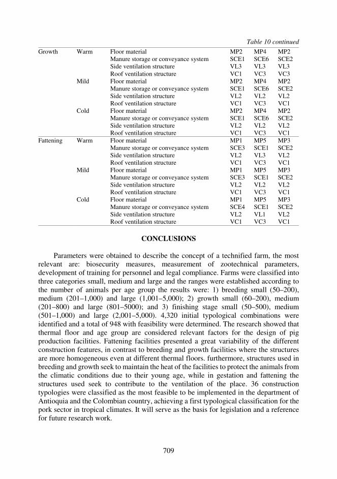
709
Table 10 continued
Growth Warm Floor material Manure storage or conveyance system Side ventilation structure Roof ventilation structure
MP2 SCE1 VL3 VC1
MP4 SCE6 VL3 VC3
MP2 SCE2 VL3 VC3
Mild Floor material Manure storage or conveyance system Side ventilation structure Roof ventilation structure
MP2 SCE1 VL2 VC1
MP4 SCE6 VL2 VC3
MP2 SCE2 VL2 VC1
Cold Floor material Manure storage or conveyance system Side ventilation structure Roof ventilation structure
MP2 SCE1 VL2 VC1
MP4 SCE6 VL2 VC3
MP2 SCE2 VL2 VC1
Fattening Warm Floor material Manure storage or conveyance system Side ventilation structure Roof ventilation structure
MP1 SCE3 VL2 VC1
MP5 SCE1 VL3 VC3
MP3 SCE2 VL2 VC1
Mild Floor material Manure storage or conveyance system Side ventilation structure Roof ventilation structure
MP1 SCE3 VL2 VC1
MP5 SCE1 VL2 VC3
MP3 SCE2 VL2 VC1
Cold Floor material Manure storage or conveyance system Side ventilation structure Roof ventilation structure
MP1 SCE4 VL2 VC1
MP5 SCE1 VL1 VC3
MP3 SCE2 VL2 VC1
CONCLUSIONS
Parameters were obtained to describe the concept of a technified farm, the most
relevant are: biosecurity measures, measurement of zootechnical parameters, development of training for personnel and legal compliance. Farms were classified into three categories small, medium and large and the ranges were established according to the number of animals per age group the results were: 1) breeding small (50–200), medium (201–1,000) and large (1,001–5,000); 2) growth small (60–200), medium (201–800) and large (801–5000); and 3) finishing stage small (50–500), medium (501–1,000) and large (2,001–5,000). 4,320 initial typological combinations were identified and a total of 948 with feasibility were determined. The research showed that thermal floor and age group are considered relevant factors for the design of pig production facilities. Fattening facilities presented a great variability of the different construction features, in contrast to breeding and growth facilities where the structures are more homogeneous even at different thermal floors. furthermore, structures used in breeding and growth seek to maintain the heat of the facilities to protect the animals from the climatic conditions due to their young age, while in gestation and fattening the structures used seek to contribute to the ventilation of the place. 36 construction typologies were classified as the most feasible to be implemented in the department of Antioquia and the Colombian country, achieving a first typological classification for the pork sector in tropical climates. It will serve as the basis for legislation and a reference for future research work.
710
ACKNOWLEDGEMENTS. This report is a result of a collaboration between The National University of Colombia Faculty of Agricultural Sciences and the Laboratory of Bioclimatic Applied to Agroindustry of the National University of Colombia.
REFERENCES Ameen, R.F.M. & Mourshed, M. 2019. Urban sustainability assessment framework
development: The ranking and weighting of sustainability indicators using analytic hierarchy process. Sustainable Cities and Society 44(October 2018), 356–366. https://doi.org/10.1016/j.scs.2018.10.020
Castrillón, N., González, V., Osorio, J.A., Montoya, A.P. & Correa, G. 2020. Assessment of the methane emission for different typologies of fattening swine facilities in the department of Antioquia Colombia. Agronomy Research 18(S2), 1189–1202. https://doi.org/10.15159/AR.20.108
Cecchin, D., Pereira, C.R., Campos, A.T., Ferraz, P.F.P., Amaral, P.I.S., Sousa, F.A., Hüther, C.M. & Cruz, V.M.F. 2019. Behavior of swine hosted in facilities with different construction typologies. Journal of Animal Behaviour and Biometeorology 7(1), 6–10. https://doi.org/10.31893/2318-1265jabb.v7n1p6-10
CIGR Section II Working Group in cooperation with EurAgEng. 2006. Animal housing in hot climates: A multidisciplinary view (I. de A. Nääs & D. J. Moura (eds.)). CIGR.
Departamento Administrativo Nacional de Estadística (DANE). 2016. 3rd National Agricultural Survey, Colombia.
Gobernación de Antioquia. 2014. Anuario estadístico del sector agropecuario en el departamento de Antioquia.
Instituto Colombiano de Hidrología Meteorología y Estudios Ambientales - IDEAM. 2005. Atlas climatológico de Colombia. Atlas Climatológico de Colombia, 219. http://www.ideam.gov.co/
Jackson, P., Guy, J.H., Sturm, B., Bull, S. & Edwards, S.A. 2018. An innovative concept building design incorporating passive technology to improve resource efficiency and welfare of finishing pigs. Biosystems Engineering 174, 190–203. https://doi.org/10.1016/j.biosystemseng.2018.07.008
OCDE/FAO. 2013. OCDE-FAO Perspectivas Agrícolas 2013-2022. Universidad Autónoma Chapingo.
Osorio, J.A., Zapata, O.L., Arango, J.C., Cardozo, C.J.M., Hernandez, R.O., Damasceno, F.A. & Oliveira, K.S. 2017. An approach to the ammonia inventory in the poultry production in Colombia: Antioquia case. Chemical Engineering Transactions 58(August), 799–804. https://doi.org/10.3303/CET1758134
Pietrosemoli, S. & Tang, C. 2020. Animal welfare and production challenges associated with pasture pig systems: A review. Agriculture (Switzerland) 10(6), 1–34. https://doi.org/10.3390/agriculture10060223
Porkcolombia, & PigCHAMP. 2015. Guia de mejores técnicas disponibles para el sector porcícola en Colombia. p. 34).
Reckmann, K., Traulsen, I. & Krieter, J. 2013. Life Cycle Assessment of pork production: A data inventory for the case of Germany. Livestock Science 157(2–3), 586–596. https://doi.org/10.1016/j.livsci.2013.09.001
Reimert, I., Rodenburg, T.B., Ursinus, W.W., Kemp, B. & Bolhuis, J.E. 2014. Selection based on indirect genetic effects for growth, environmental enrichment and coping style affect the immune status of pigs. PLoS ONE 9(10). https://doi.org/10.1371/journal.pone.0108700
Rhodes, T., Appleby, M., Chinn, K., Douglas, L., Firkins, L., Houpt, K., Irwin, C., McGlone, J., Dundberg, P., Tokach, L. & Wills, R. 2005. A comprehensive review of housing for pregnant sows Members - Task Force Report. Javma 227(10), 1580–1590.
USDA. 2011. Department of agriculture national agricultural statistics service agricultural - Agricultural Statistics 2010. 1–9.
711
Agronomy Research 19(S1), 711–720, 2021 https://doi.org/10.15159/AR.21.075
Comparative analysis of the use of biostimulants on the main types of soil
O. Chernikova1,*, Yu. Mazhaysky2, S. Buryak2, T. Seregina1 and L. Ampleeva2
1Academy of law management of the federal penal service of Russia, Sennaya street 1, RU390036 Ryazan, Russia 2Ryazan State Agrotechnological University named after P.A. Kostychev, Kostychev street 1, RU390044 Ryazan, Russia *Correspondence: [email protected] Received: February 6th, 2020; Accepted: April 14th, 2021; Published: May 13th, 2021 Abstract. A plant requires certain physiological conditions for normal and productive development. The determining vital factor is the nutritional status of the soil and the environment. At present, the biologization of agriculture is becoming increasingly important. The use of biostimulants is one of the rapidly developing areas in the world practice of crop production and, in the cultivation of agricultural crops, contributes to the production of environmentally friendly products and the improvement of the environment.Such substances can be metal nanoparticles, as well as preparations with a high level of biogenicity, nutritional value and physiology,they are used to improve the growth and development of plants, as well as to activate soil-microbiological processes, which is a liquid-phase biological product (LPBP). The purpose of this work is to identify the effectiveness of the use of a liquid-phase biological product and cobalt nanoparticles in pre-sowing seed treatment against the background of a minimum dose of organic fertilizers, the effect on the productivity and quality indicators of green mass when growing a grass mixture with over-sowing oats on three main types of soil: sod-podzolic, gray forest and black soil. Used cobalt nanoparticles have the following characteristics 40–60 nm, phase composition - Co - 100%. A suspension of nanoparticles was obtained by dispersing with ultrasound in an aqueous solution. LPBP is a dark brown liquid with a specific odor, pH =6.5–7.5, contains N, C, P, K, Ca, Mg, tryptophan, microorganisms. Cobalt nanopowder in solution contained 0.01 g per hectare seeding rate; LPBP concentration was 1%. The seeds were soaked 30 min before sowing in double distilled water (control), in a suspension of nanoparticles and LPBP. The research was carried out according to generally accepted methods. Presowing seed treatment in combination with organic fertilizers in minimal doses provided an increase in yield on soddy-podzolic soil - by 5.69–21.71%, gray forest soil - 2.64–7.50%, black soil - 9.18–18.28%, while no decrease in nutritional value was observed: metabolizable energy, feed units, digestible protein. It is noted that the use of cobalt nanoparticles leads to an increase in the carotene content. Key words: cobalt nanoparticles, liquid-phase biological product, grass mixture, oats, sod-podzolic soil, gray forest soil, chernozem.
712
INTRODUCTION The increase in crop yields and the production of grain, fodder and other crop
products is carried out through intensive production methods. They provide for the widespread use of balanced doses of organic and mineral fertilizers, chemical agents for protecting plants from weeds, diseases and pests, and the use of super-heavy means of complex mechanization in the implementation of technological operations. All this increases the anthropogenic load on the ecological environment, leads to the pollution of soil and products by heavy metals, pesticides and nitrates (Matyuk et al., 2011).
The development of modern crop production in conditions of limited financial and material resources requires the improvement of the applied technologies to increase the yield and quality of the products, reduce the costs of its production, as well as ensure the restoration and preservation of soil fertility. One of the ways to solve these problems is the use of growth biostimulants (Efremova, 2016). The production and use of biostimulants is one of the most dynamic segments of agricultural products. Annually the segment is growing by 13%.
In order to improve the efficiency of agricultural production by increasing the yield and quality of grown products, nanotechnologies have been obtained in recent years, as well as technologies with using biological products (Sabirova & Sabirov, 2018).
The elucidation of the biological basis of biostimulant function is a prerequisite for the development of science-based biostimulant industry and sound regulations governing these compounds (Yakhin et al., 2017). Many applied studies have been devoted to the study of the use of biological products and metal nanoparticles as biostimulants, which show the effectiveness and expediency of their use (Ruzzi & Aroca, 2015; Arora et al., 2016; Madbouly, 2018; Youssef & Colla, 2020). At the same time, it should be noted that there is still a need for further research on this issue.
Control of biological processes in agrocenoses is possible through the introduction of agronomically valuable strains of microorganisms into the rhizosphere of plants, enhances the beneficial or weakens the negative impact of undesirable phenomena for the realization of their potential. Today, on the basis of numerous experiments, it can be argued that the symbiosis and association of microorganisms with plants is the basis of the latter's vital activity.
The main mechanisms of the beneficial effect of microorganisms on plants include: improving plant nutrition (increasing the utilization of nutrients from fertilizers and soil); optimization of phosphorus nutrition of plants; fixation of atmospheric nitrogen (improvement of nitrogen nutrition); stimulation of plant growth and development (faster plant development and crop maturation); suppression of the development of phytopathogens (control over the development of diseases and reduction of plant infestation by them, improvement of product storage); increasing plant resistance to stressful conditions (the possibility of increasing plant productivity against the background of water deficit, unfavorable temperatures, high acidity, salinity or soil pollution) (Zavalin, 2005). Unlike chemical preparations, biological preparations have a more pronounced selectivity of action, they are also recognized as harmless to humans and animals, and rapidly decompose in the soil.
All-Russian Research Institute of Reclaimed Lands has developed a fermentation-extraction technology for obtaining various liquid-phase biological products, including a liquid-phase biological product LPBP for plant growing and agriculture. LPBP
713
production includes the stage of fermentation of a peat-manure mixture to obtain a solid-phase fermentation product, then its extraction by a saline solution, followed by filtration. The number of microorganisms (ammonifying, amylolytic, phosphate-mobilizing, amino-synthesizing, etc.) in a fresh biological product reaches n 109 – n 1012CFU mL-1, which makes it possible to refer it to microbial biological products. It lacks pathogenic microflora and parasites. In LPBP, the total nitrogen content is 0.2–0.5 g L-1, mobile forms of potassium (K2О) and phosphorus (Р2O5) - 9.5 and 10 g L-1, respectively. Also, it contains trace elements (copper, zinc, manganese, iron) and various metabolites of microorganisms (sugars, enzymes, amino acid tryptophan) (Rabinovich et al., 2009, 2015).
Nanosized micronutrient fertilizers are used as biostimulants to increase plant productivity in the direction of sustainable development of the environment. In this case, nanostructured plant trace elements such as Cu, Fe, Ni, Mn, Si, Co, Se and Zn play a crucial role in plant disease resistance by activating enzymes and in increasing the efficiency of energy production by photosynthetic processes for defense mechanisms (Vuong, 2019; Chernikova et al., 2019; Churilov et al., 2020; Seregina et al., 2020).
In plants, cobalt is necessary for fixing molecular nitrogen; it promotes the formation of bacteria in the nodules and leaves of legumes. Cobalt accumulates in pollen and accelerates its germination, participates in auxin metabolism, i.e. stimulates plant growth processes (incl. promotes stretching of cell membranes). This metal is involved in cell reproduction of leaves (an increase in the thickness and volume of the mesophyll, the size and number of cells in the columnar and spongy leaf parenchyma). In addition, cobalt increases the total water content of plants, thereby increasing the drought tolerance of crops.
The influence of cobalt on the formation and functioning of the photosynthetic apparatus of plants through the concentration of chloroplasts and pigments in the leaves was established. And although the amount of this microelement required for plants is very small (up to 12 mg kg-1of dry weight), and its indispensability for plants has not been strictly proven, cobalt fertilizers still contribute to an increase in crop yields and improve product quality (Polishchuk et al., 2015).
Thus, under the influence of cobalt, the development of plant tissues containing bacteroids is stimulated, the number of ribosomes in both plant and bacteroid cells increases, and the mobility of bacteroids in the nodules of leguminous plants increases.
The purpose of this work is to determine the effectiveness of the use of a liquid-phase biological product and cobalt nanoparticles in the pre-sowing treatment of seeds against the background of a minimum dose of organic fertilizers, the effect on the productivity and quality indicators of green mass when growing a grass mixture with over-sowing of oats on three main types of soil: sod-podzolic, gray forest and black soil.
MATERIALS AND METHODS
The research was carried out in lysimeters in four replicates (Dospekhov, 2012) on
three types of soil. The soil was characterized by the following agrochemical indicators: – sod-podzolic: рНКСl 6.0; humus content - 2.3%, Р2О5 - 200 mg kg-1, K2О -
198 mg kg-1 of soil; – gray forest: рНКСl 6.2; humus content - 2.6%, Р2О5 - 204 mg kg-1, K2О -
219 mg kg-1 of soil;
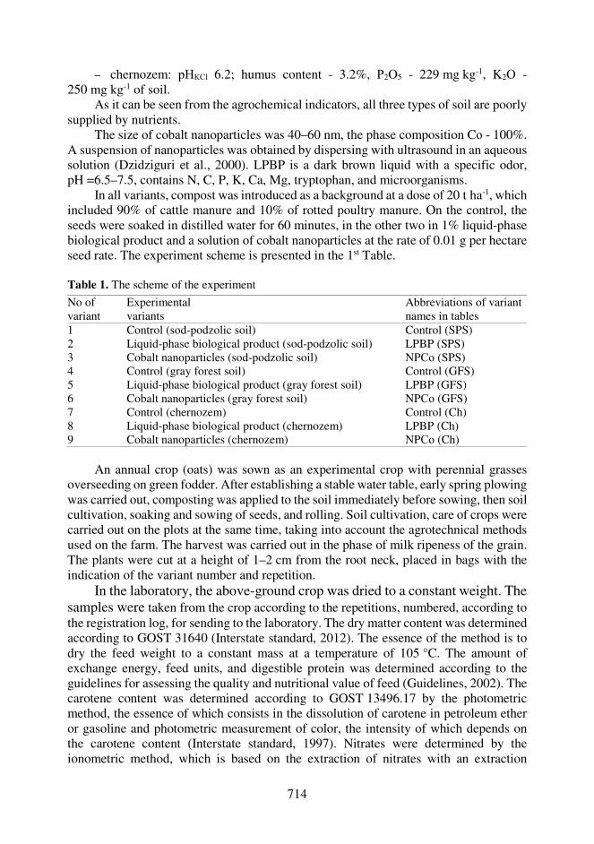
714
– chernozem: рНКСl 6.2; humus content - 3.2%, Р2О5 - 229 mg kg-1, K2О - 250 mg kg-1 of soil.
As it can be seen from the agrochemical indicators, all three types of soil are poorly supplied by nutrients.
The size of cobalt nanoparticles was 40–60 nm, the phase composition Cо - 100%. A suspension of nanoparticles was obtained by dispersing with ultrasound in an aqueous solution (Dzidziguri et al., 2000). LPBP is a dark brown liquid with a specific odor, pH =6.5–7.5, contains N, C, P, K, Ca, Mg, tryptophan, and microorganisms.
In all variants, compost was introduced as a background at a dose of 20 t ha-1, which included 90% of cattle manure and 10% of rotted poultry manure. On the control, the seeds were soaked in distilled water for 60 minutes, in the other two in 1% liquid-phase biological product and a solution of cobalt nanoparticles at the rate of 0.01 g per hectare seed rate. The experiment scheme is presented in the 1st Table.
Table 1. The scheme of the experiment
No of variant
Experimental variants
Abbreviations of variant names in tables
1 Control (sod-podzolic soil) Control (SPS) 2 Liquid-phase biological product (sod-podzolic soil) LPBP (SPS) 3 Cobalt nanoparticles (sod-podzolic soil) NPСо (SPS) 4 Control (gray forest soil) Control (GFS) 5 Liquid-phase biological product (gray forest soil) LPBP (GFS) 6 Cobalt nanoparticles (gray forest soil) NPСо (GFS) 7 Control (chernozem) Control (Ch) 8 Liquid-phase biological product (chernozem) LPBP (Ch) 9 Cobalt nanoparticles (chernozem) NPСо (Ch)
An annual crop (oats) was sown as an experimental crop with perennial grasses
overseeding on green fodder. After establishing a stable water table, early spring plowing was carried out, composting was applied to the soil immediately before sowing, then soil cultivation, soaking and sowing of seeds, and rolling. Soil cultivation, care of crops were carried out on the plots at the same time, taking into account the agrotechnical methods used on the farm. The harvest was carried out in the phase of milk ripeness of the grain. The plants were cut at a height of 1–2 cm from the root neck, placed in bags with the indication of the variant number and repetition.
In the laboratory, the above-ground crop was dried to a constant weight. The samples were taken from the crop according to the repetitions, numbered, according to the registration log, for sending to the laboratory. The dry matter content was determined according to GOST 31640 (Interstate standard, 2012). The essence of the method is to dry the feed weight to a constant mass at a temperature of 105 °C. The amount of exchange energy, feed units, and digestible protein was determined according to the guidelines for assessing the quality and nutritional value of feed (Guidelines, 2002). The carotene content was determined according to GOST 13496.17 by the photometric method, the essence of which consists in the dissolution of carotene in petroleum ether or gasoline and photometric measurement of color, the intensity of which depends on the carotene content (Interstate standard, 1997). Nitrates were determined by the ionometric method, which is based on the extraction of nitrates with an extraction
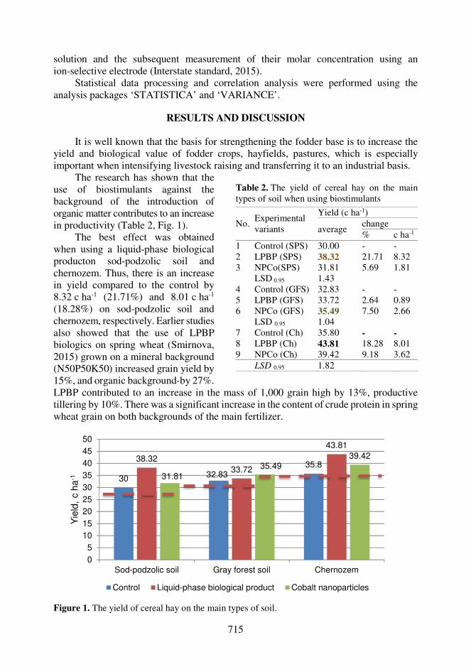
715
solution and the subsequent measurement of their molar concentration using an ion-selective electrode (Interstate standard, 2015).
Statistical data processing and correlation analysis were performed using the analysis packages ‘STATISTICA’ and ‘VARIANCE’.
RESULTS AND DISCUSSION
It is well known that the basis for strengthening the fodder base is to increase the
yield and biological value of fodder crops, hayfields, pastures, which is especially important when intensifying livestock raising and transferring it to an industrial basis.
LPBP contributed to an increase in the mass of 1,000 grain high by 13%, productive tillering by 10%. There was a significant increase in the content of crude protein in spring wheat grain on both backgrounds of the main fertilizer.
Figure 1. The yield of cereal hay on the main types of soil.
30 32.8335.8
38.32
33.72
43.81
31.81
35.4939.42
0
5
10
15
20
25
30
35
40
45
50
Sod-podzolic soil Gray forest soil Chernozem
Yie
ld,
cha
-1
Control Liquid-phase biological product Cobalt nanoparticles
The research has shown that the use of biostimulants against the background of the introduction of organic matter contributes to an increase in productivity (Table 2, Fig. 1).
The best effect was obtained when using a liquid-phase biological producton sod-podzolic soil and chernozem. Thus, there is an increase in yield compared to the control by 8.32 c ha-1 (21.71%) and 8.01 c ha-1 (18.28%) on sod-podzolic soil and chernozem, respectively. Earlier studies also showed that the use of LPBP biologics on spring wheat (Smirnova, 2015) grown on a mineral background (N50P50K50) increased grain yield by 15%, and organic background-by 27%.
Table 2. The yield of cereal hay on the main types of soil when using biostimulants
No. Experimental variants
Yield (c ha-1)
average change % c ha-1
1 Control (SPS) 30.00 - - 2 LPBP (SPS) 38.32 21.71 8.32 3 NPСо(SPS) 31.81 5.69 1.81 LSD 0.95 1.43 4 Control (GFS) 32.83 - - 5 LPBP (GFS) 33.72 2.64 0.89 6 NPСо (GFS) 35.49 7.50 2.66 LSD 0.95 1.04 7 Control (Ch) 35.80 - - 8 LPBP (Ch) 43.81 18.28 8.01 9 NPСо (Ch) 39.42 9.18 3.62 LSD 0.95 1.82
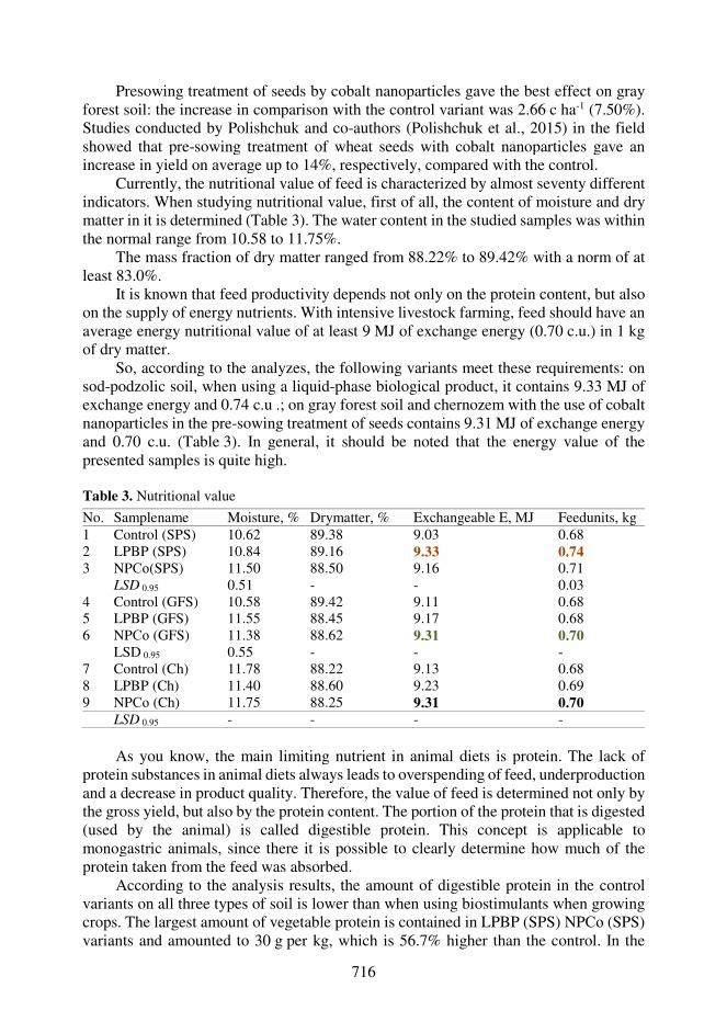
716
Presowing treatment of seeds by cobalt nanoparticles gave the best effect on gray forest soil: the increase in comparison with the control variant was 2.66 c ha-1 (7.50%). Studies conducted by Polishchuk and co-authors (Polishchuk et al., 2015) in the field showed that pre-sowing treatment of wheat seeds with cobalt nanoparticles gave an increase in yield on average up to 14%, respectively, compared with the control.
Currently, the nutritional value of feed is characterized by almost seventy different indicators. When studying nutritional value, first of all, the content of moisture and dry matter in it is determined (Table 3). The water content in the studied samples was within the normal range from 10.58 to 11.75%.
The mass fraction of dry matter ranged from 88.22% to 89.42% with a norm of at least 83.0%.
It is known that feed productivity depends not only on the protein content, but also on the supply of energy nutrients. With intensive livestock farming, feed should have an average energy nutritional value of at least 9 MJ of exchange energy (0.70 c.u.) in 1 kg of dry matter.
So, according to the analyzes, the following variants meet these requirements: on sod-podzolic soil, when using a liquid-phase biological product, it contains 9.33 MJ of exchange energy and 0.74 c.u .; on gray forest soil and chernozem with the use of cobalt nanoparticles in the pre-sowing treatment of seeds contains 9.31 MJ of exchange energy and 0.70 c.u. (Table 3). In general, it should be noted that the energy value of the presented samples is quite high.
Table 3. Nutritional value
No. Samplename Moisture, % Drymatter, % Exchangeable E, MJ Feedunits, kg 1 Control (SPS) 10.62 89.38 9.03 0.68 2 LPBP (SPS) 10.84 89.16 9.33 0.74 3 NPСо(SPS) 11.50 88.50 9.16 0.71 LSD 0.95 0.51 - - 0.03 4 Control (GFS) 10.58 89.42 9.11 0.68 5 LPBP (GFS) 11.55 88.45 9.17 0.68 6 NPСо (GFS) 11.38 88.62 9.31 0.70 LSD 0.95 0.55 - - - 7 Control (Ch) 11.78 88.22 9.13 0.68 8 LPBP (Ch) 11.40 88.60 9.23 0.69 9 NPСо (Ch) 11.75 88.25 9.31 0.70 LSD 0.95 - - - -
As you know, the main limiting nutrient in animal diets is protein. The lack of
protein substances in animal diets always leads to overspending of feed, underproduction and a decrease in product quality. Therefore, the value of feed is determined not only by the gross yield, but also by the protein content. The portion of the protein that is digested (used by the animal) is called digestible protein. This concept is applicable to monogastric animals, since there it is possible to clearly determine how much of the protein taken from the feed was absorbed.
According to the analysis results, the amount of digestible protein in the control variants on all three types of soil is lower than when using biostimulants when growing crops. The largest amount of vegetable protein is contained in LPBP (SPS) NPСо (SPS) variants and amounted to 30 g per kg, which is 56.7% higher than the control. In the
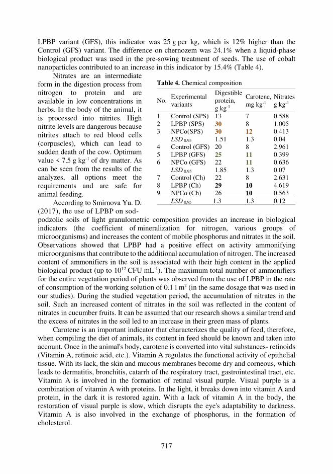
717
LPBP variant (GFS), this indicator was 25 g per kg, which is 12% higher than the Control (GFS) variant. The difference on chernozem was 24.1% when a liquid-phase biological product was used in the pre-sowing treatment of seeds. The use of cobalt nanoparticles contributed to an increase in this indicator by 15.4% (Table 4).
podzolic soils of light granulometric composition provides an increase in biological indicators (the coefficient of mineralization for nitrogen, various groups of microorganisms) and increases the content of mobile phosphorus and nitrates in the soil. Observations showed that LPBP had a positive effect on activity ammonifying microorganisms that contribute to the additional accumulation of nitrogen. The increased content of ammonifiers in the soil is associated with their high content in the applied biological product (up to 1012 CFU mL-1). The maximum total number of ammonifiers for the entire vegetation period of plants was observed from the use of LPBP in the rate of consumption of the working solution of 0.1 l m2 (in the same dosage that was used in our studies). During the studied vegetation period, the accumulation of nitrates in the soil. Such an increased content of nitrates in the soil was reflected in the content of nitrates in cucumber fruits. It can be assumed that our research shows a similar trend and the excess of nitrates in the soil led to an increase in their green mass of plants.
Carotene is an important indicator that characterizes the quality of feed, therefore, when compiling the diet of animals, its content in feed should be known and taken into account. Once in the animal's body, carotene is converted into vital substances- retinoids (Vitamin A, retinoic acid, etc.). Vitamin A regulates the functional activity of epithelial tissue. With its lack, the skin and mucous membranes become dry and corneous, which leads to dermatitis, bronchitis, catarrh of the respiratory tract, gastrointestinal tract, etc. Vitamin A is involved in the formation of retinal visual purple. Visual purple is a combination of vitamin A with proteins. In the light, it breaks down into vitamin A and protein, in the dark it is restored again. With a lack of vitamin A in the body, the restoration of visual purple is slow, which disrupts the eye's adaptability to darkness. Vitamin A is also involved in the exchange of phosphorus, in the formation of cholesterol.
Nitrates are an intermediate form in the digestion process from nitrogen to protein and are available in low concentrations in herbs. In the body of the animal, it is processed into nitrites. High nitrite levels are dangerous because nitrites attach to red blood cells (corpuscles), which can lead to sudden death of the cow. Optimum value < 7.5 g kg-1 of dry matter. As can be seen from the results of the analyzes, all options meet the requirements and are safe for animal feeding.
According to Smirnova Yu. D. (2017), the use of LPBP on sod-
Table 4. Chemical composition
No. Experimental variants
Digestible protein, g kg-1
Carotene, mg kg-1
Nitrates, g kg-1
1 Control (SPS) 13 7 0.588 2 LPBP (SPS) 30 8 1.005 3 NPСо(SPS) 30 12 0.413 LSD 0.95 1.51 1.3 0.04 4 Control (GFS) 20 8 2.961 5 LPBP (GFS) 25 11 0.399 6 NPСо (GFS) 22 11 0.636 LSD 0.95 1.85 1.3 0.07 7 Control (Ch) 22 8 2.631 8 LPBP (Ch) 29 10 4.619 9 NPСо (Ch) 26 10 0.563 LSD 0.95 1.3 1.3 0.12
718
The research has shown that the use of cobalt nanoparticles in pre-sowing seed treatment contributes to an increase in carotene in all three types of soil. The content of this provitamin was higher in comparison with the control variant on sod-podzolic soil by 41.7%, on gray forest soil - 27.3%, on chernozem - 20%.
Cobalt in plant tissues is found in ionic and complexes compounds. In optimal concentrations, this trace element contributes to an increase in the thickness and volume of the mesophyll in the leaves. Cobalt affects the formation and functioning of the photosynthetic apparatus of plants. This trace element contributes to the concentration of chloroplasts and pigments in the leaves, which is associated with an increase in the volume of the plastid apparatus due to the replication and growth of organelles. Carotenoids are a widespread class of structurally and functionally distinct natural pigments, usually yellow, orange, and red. They are synthesized in yeast, fungi, and all photosynthetic organisms, from bacteria and microalgae to higher plants (Armstrong, 1994; Eds Britton et al., 1998). The influence of cobalt on the formation and functioning of the photosynthetic apparatus of plants by the concentration of chloroplasts and pigments in the leaves was established (Bityutsky, 1999). This is due to an increase in the volume of the plastid apparatus due to the growth of organelles. Cobalt can activate the biosynthesis of chlorophyll by stimulating the synthesis of cytoplasmic protein and chloroplasts. Under the influence of chloroplasts, the protein content increases in parallel with the increase in them. The binding of cobalt to protein synthesis can be carried out by regulating the structure and stability of ribosomes, as well as the functioning of RNA. Ultrasonic action on the powder of cobalt nanoparticles and the aqueous medium leads to the creation of a disordered system, in which the presence of many free active reagents is detected, entering into direct reactions occurring in the cell, or serving as catalysts for some of them. In addition, due to the high diffuse mobility of the particles, unsaturated metal valences and the formation of a large set of chelated compounds, it provides high biological efficiency. Thus, it can be assumed that cobalt nanoparticles contributed to the activation of carotene synthesis processes in the green mass of perennial grasses.
CONCLUSIONS
Growth biostimulants used in pre-sowing seed treatment (liquid-phase biological
product or cobalt nanoparticles) against the background of a minimum dose of organic fertilizers provide an increase in yield on sod-podzolic soil by 5.69–21.71%, gray forest soil - 2.64–7.50%, black soil - 9.18–18.28%. A liquid-phase biological product works better on sod-podzolic soil and chernozem, and treatment by cobalt nanoparticles works on gray forest soil.At the same time, there is no decrease in nutritional and energy value: exchange energy, feed units, digestible protein, and the products themselves are safe. The use of cobalt nanoparticles leads to an increase in the carotene content, regardless of the type of soil, from 20.0% to 41.7%, then the liquid-phase biological product has the best effect in the accumulation of provitamin on gray forest and sod-podzolic soil.

719
REFERENCES Armstrong, G.A. 1994. Eubacteria show their true colors: Genetics of carotenoid pigment
biosynthesis from microbes to plants. J. Bacteriol. 176(16), 4795–4802. Arora, P., Mehta, C., Srivastava, R., Arora, S. & Sharma, A. 2016. Impact assessment of silver
nanoparticles on plant growth and soil bacterial diversity. 3 Biotech. 6. 254. doi.org/6.10.1007/s13205-016-0567-7
Bityutsky, N.P. 1999. Trace elements and the plant. Training manual. St. Petersburg University Press, 232 pp. (in Russian).
Chernikova, O., Mazhayskiy, Y. & Ampleeva, L. 2019. Selenium in nanosized form as an alternative to microfertilizers. Agronomy Research 17(1), 974–981. doi: 10.15159/AR.19.010
Churilov, D.G., Polischuk, S.D., Churilov, G.I., Churilova, V.V. & Byshova, D.N. 2020. Investigation of the long-term toxic effect of nanoparticles of different physical-chemical characteristics. Agronomy Research 18(3), 1973–1991. doi: 10.15159/AR.20.186
Dospekhov, B.A. 2012. Methodology of field experience (with the basics of statistical processing of research results). Moscow: Book on Demand. 352 pp. (in Russian).
Dzidziguri, E.L., Kuznetsov, D.V., Lyovina, V.V. & Sidorova, E.N. 2000. Perspective materials 6 Forestry 2019 IOP Conf. Series: Earth and Environmental Science, pp. 7–92.
Eds Britton, G., Liaaen-Jensen, S. & Pfander, H.1998. Basel Carotenoids in chemosystematics. Carotenoids: Biosynthesis and Metabolism. 3. 217–247.
Efremova, Y.V.2016. Growth stimulators as part of sustainable agriculture. Russian Journal of Agricultural and Socio-Economic Sciences 4(52), 86–91. doi: 10.18551/rjoas.2016-04.10
Interstate standard. Feed. Methods for determining the dry matter content. GOST 31640-2012 Interstate standard. Forage. Methods for determining carotene. GOST 13496.17-1997 Interstate standard. Feed, mixed feed and raw materials. Methods for the determination of nitrates
and nitrites. GOST 13496.19-2015 Guidelines for assessing the quality and nutritional value of feed. 2002. Moscow: TSINAO.
76 pp. (in Russian). Madbouly, A.K. 2018. Nanoparticles as novel plant growth promoters. Novel Research in
Microbiology Journal. doi.org/ 2. 10.21608/NRMJ.2018.12547. Matyuk, N.S., Belenkov, A.I., Mazirov, M.A., Polin, V.D., Rassadin, A.Ya. & Abrashkina, E.D.
2011. Ecological agriculture with the basics of soil science and agrochemistry. Textbook / N.S. Matyuk, A.I. Belenkov, M.A. Mazirov, V.D. Polin, A. Ya. Rassadin, E. D. Abrashkina. Publishing house of the Russian State Agricultural University named after K.A. Moscow, 189 pp. (in Russian).
Polishchuk, S., Nazarova, A., Kutskir, M., Churilov, D., Ivanycheva, Y., Kiryshin, V. & Churilov, G.2015. Ecologic-Biological Effects of Cobalt, Cuprum, Copper Oxide Nano-Powders and Humic Acids on Wheat Seeds. Modern Applied Science 9(6), 354–364. doi.org/10.5539/mas.v9n6p354.
Rabinovich, G.Yu., Fomicheva, N.V. & Smirnova, Yu.D. 2009. A method of obtaining a liquid-phase biological agent for plant growing and agriculture. RF Patent No. 2365568. (in Russian).
Rabinovich, G.Yu., Smirnova, Yu.D., Vasilyeva, E.A. & Fomicheva, N.V. 2015. Innovative technology for solving problems of agroecology. Regional ecology 6(41), 7–15 (in Russian).
Ruzzi, M. & Aroca, R. 2015. Plant growth-promoting rhizobacteria act as biostimulants in horticulture. Sci. Hortic. 196, 124–134. doi.org/ 10.1016/j.scienta.2015.08.042
Sabirova, T.P. & Sabirov, R.A. 2018.The influence of biological products on the productivity of agricultural crops. Bulletin of the agro-industrial complex of the Upper Volgaregion 3(43). 18–22 (in Russian).
720
Seregina, T., Chernikova, O., Mazhayskiy, Y. & Ampleeva, L. 2020. Features of the influence of copper nanoparticles and copper oxide on the formation of barley crop. Agronomy Research 18(1), 1010–1017. doi: 10.15159/AR.20.025
Smirnova, Yu.D. 2017. The effect of LPBP biologics on crop yield and quality. Dissertation for the degree of Candidate of Biological Sciences. Moscow, 166 pp.
Smirnova, Yu. D. & Rabinovich, G.Yu. 2015. The effect of the new biological product LPBP on the productivity of spring wheat and the state of the soil under it. Young scientist. 9.2 (89.2). 142–143 (in Russian).
Vuong, L.D. Nanoparticles for the Improved Crop Production.2019. In: Panpatte D., Jhala Y. (eds) Nanotechnology for Agriculture: Crop Production & Protection. Springer, Singapore. doi: 10.1007/978-981-32-9374-8_5
Yakhin, O., Lubyanov, A., Yakhin, I. & Brown, P. 2017. Biostimulants in Plant Science: A Global Perspective. Frontiers in Plant Science, 32 pp. doi: org/7. 10.3389/fpls.2016.02049
Youssef, R. & Colla, G. 2020. Editorial: Biostimulants in Agriculture. Front. Plant Sci. doi: org/10.3389/fpls.2020.00040
Zavalin, A.A. Biologicals, fertilizers and crops. 2005. All-Russian Research Institute of Automation, pp. 302. (in Russian).

721
Agronomy Research 19(S1), 721–738, 2021 https://doi.org/10.15159/AR.21.050
Productive efficiency and density and viscosity studies of biodiesels from vegetable oil mixtures
R.C.B. Correia1, F.C. Silva1,*, M.M. Barros2, A.C.L. Maria1
, D. Cecchin1, L.A. Souza1 and D.F. Carmo1
1Federal Fluminense University, Agricultural and Environmental Engineering Department, 156 Rua Passos da Pátria 156, bloco D, sala 235, BR24210-240 Niterói, Brasil 2Federal Rural University of Rio de Janeiro, Engineering Department, Rodovia BR 465, Km 07, s/n Zona Rural, 23890-000, Seropédica, Brasil *Correspondence: [email protected] Received: January 31st, 2021; Accepted: April 10th, 2021; Published: April 29th, 2021 Abstract. Currently in Brazil the minimum content of biodiesel in mixtures is 11% and, according to Brazilian laws, the goal is to reach 15% in volume in diesel fuel available for final consumers by 2023. Therefore, studies about different matrices of biodiesel and distinct mixtures are essential. The present work had two goals, the first one was to analyse physico-chemical properties of 16 biofuels produced from soybean and cotton oils, using S10 diesel, in mixtures B8, B10, B20 and B30. The second goal was to verify the vantages and disadvantages of biodiesel production through prior mixing of the oils, before and after the transesterification process. All biofuels produced presented results of specific mass values at 20 °C and kinematic viscosity at 40 °C within the limits established by ANP Resolution no 30/2016 and International Resolutions. The soybean B20 biofuel showed the best overall results, with the second highest production yield of 65.36%, the fifth lowest kinematic viscosity with 3.48 mm s-1. The mixture of soybean and cotton oils before the transesterification process presented the highest production yield when compared with the production from a single oil or biodiesel mixtures. The results found proved to be satisfactory and corroborate to continue with the increase of biodiesel in the mixture with diesel to B15 until 2023 and support the possibility of planning for a gradual increase of this mixture in the following years. Key words: transesterification, biodiesel, physical characterization, yield, mechanical performance.
INTRODUCTION
The energy produced for human consumption on the planet is largely dependent on fossil fuels that have limited sources of raw material and are considered to be the main causes of the increase in global warming and emissions of gases harmful to our health during their burning (Abed et al., 2019). According to Manaf et al. (2019), among the worst consequences of global warming, it is possible to highlight the increase in the concentration of CO2 in the atmosphere, the increase in the acidity of sea water and the
722
temperature of the sea surface, which generate serious consequences for society and reinforce that one of the ways to reduce these harmful emissions is using renewable energies.
According to Dantas et al. (2016), the use of biomass has been gaining relevance in the world scenario because it can be applied to the use in the production of heat for industrial thermal use or even for the generation of electric energy. Among the alternative energy sources, biodiesel, as it is a derivative of renewable materials, has become an increasingly used and studied substitute for diesel oil. Among the raw materials that can be used to produce biodiesel, vegetable oils and animal fats can be highlighted and they both result in a biofuel presenting mainly low emission of polluting gases, promoting a more sustainable energy production (Ambat et al., 2018).
According to Knothe et al. (2006), biodiesel can be obtained through different technologies, namely transesterification, esterification and cracking. The transesterification process occurs naturally when you mix vegetable oil with alcohol. In order to accelerate the process, in addition to the use of catalysts, which can be basic or acidic, magnetic stirrers and sonifiers are generally used at laboratory level, helping to reaction speed and minimizing the total time of the transesterification process as highlighted by Rockembach et al. (2014).
The biofuel manufacturing route is related to the type of alcohol used during the production process, which may be the methyl or ethyl route, the first being used due to its lower cost (Knothe et al., 2006). According to Meneghetti et al. (2013) in transesterification, basic or acid catalysts can be used, however the difference occurs when opting to use acid catalysts and we can see that there is an increase in corrosion of industrial equipment during the biodiesel production process and lower rates of reaction conversion. The basic catalysts, most used in the transesterification process, are sodium and potassium hydroxides.
When assessing the environmental impact of burning fuels, it can be said that when using biodiesel, lower amounts of carbon dioxide (CO2), sulfur dioxide (SO2), carbon monoxide (CO) and hydrocarbons are released compared to when using diesel, and that these emissions are proportional and lower the higher the percentage of biodiesel in the mixture (Perin et al., 2015).
For Silva et al. (2019) assessing the emission of exhaust gases from different biodiesel mixtures, concluded that the lowest SO2 emissions were obtained with fuels containing higher biodiesel percentages and operating at higher rotation speeds and nitrous oxides and carbon dioxide emissions decrease with higher engine rotation speed. Overall, higher percentages of biodiesel in the fuel mixture result in a less polluting fuel.
According to ANP (2019) Brazil, together with the United States, leads the world ranking of the largest biodiesel producers nowadays. The biodiesel production capacity in Brazil reached 8.76 billion liters in 2019 and a total of 5.89 billion liters were produced. Among the raw materials used to produce biodiesel in Brazil, soybean stands out, which in 2019 was responsible for approximately 70% of all production.
According to Knothe (2006), the physical-chemical characterization of biodiesel is an essential process to qualify and evaluate the biofuel, to ensure that it presents a complete combustion, and helps in the proper functioning of the engine, guaranteeing its useful life. The characteristics usually calculated and addressed in didactic studies are the specific mass at 20 °C and the kinematic viscosity at 40 °C. This mass must be in accordance with the norms established by the ANP in its resolution 30/2016, where limit
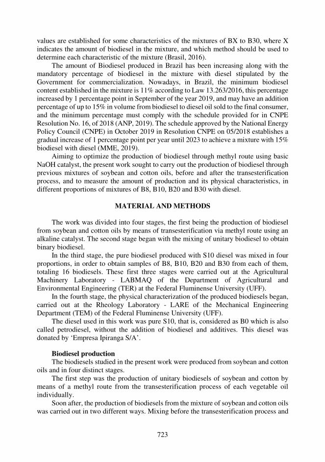
723
values are established for some characteristics of the mixtures of BX to B30, where X indicates the amount of biodiesel in the mixture, and which method should be used to determine each characteristic of the mixture (Brasil, 2016).
The amount of Biodiesel produced in Brazil has been increasing along with the mandatory percentage of biodiesel in the mixture with diesel stipulated by the Government for commercialization. Nowadays, in Brazil, the minimum biodiesel content established in the mixture is 11% according to Law 13.263/2016, this percentage increased by 1 percentage point in September of the year 2019, and may have an addition percentage of up to 15% in volume from biodiesel to diesel oil sold to the final consumer, and the minimum percentage must comply with the schedule provided for in CNPE Resolution No. 16, of 2018 (ANP, 2019). The schedule approved by the National Energy Policy Council (CNPE) in October 2019 in Resolution CNPE on 05/2018 establishes a gradual increase of 1 percentage point per year until 2023 to achieve a mixture with 15% biodiesel with diesel (MME, 2019).
Aiming to optimize the production of biodiesel through methyl route using basic NaOH catalyst, the present work sought to carry out the production of biodiesel through previous mixtures of soybean and cotton oils, before and after the transesterification process, and to measure the amount of production and its physical characteristics, in different proportions of mixtures of B8, B10, B20 and B30 with diesel.
MATERIAL AND METHODS
The work was divided into four stages, the first being the production of biodiesel
from soybean and cotton oils by means of transesterification via methyl route using an alkaline catalyst. The second stage began with the mixing of unitary biodiesel to obtain binary biodiesel.
In the third stage, the pure biodiesel produced with S10 diesel was mixed in four proportions, in order to obtain samples of B8, B10, B20 and B30 from each of them, totaling 16 biodiesels. These first three stages were carried out at the Agricultural Machinery Laboratory - LABMAQ of the Department of Agricultural and Environmental Engineering (TER) at the Federal Fluminense University (UFF).
In the fourth stage, the physical characterization of the produced biodiesels began, carried out at the Rheology Laboratory - LARE of the Mechanical Engineering Department (TEM) of the Federal Fluminense University (UFF).
The diesel used in this work was pure S10, that is, considered as B0 which is also called petrodiesel, without the addition of biodiesel and additives. This diesel was donated by ‘Empresa Ipiranga S/A’.
Biodiesel production The biodiesels studied in the present work were produced from soybean and cotton
oils and in four distinct stages. The first step was the production of unitary biodiesels of soybean and cotton by
means of a methyl route from the transesterification process of each vegetable oil individually.
Soon after, the production of biodiesels from the mixture of soybean and cotton oils was carried out in two different ways. Mixing before the transesterification process and
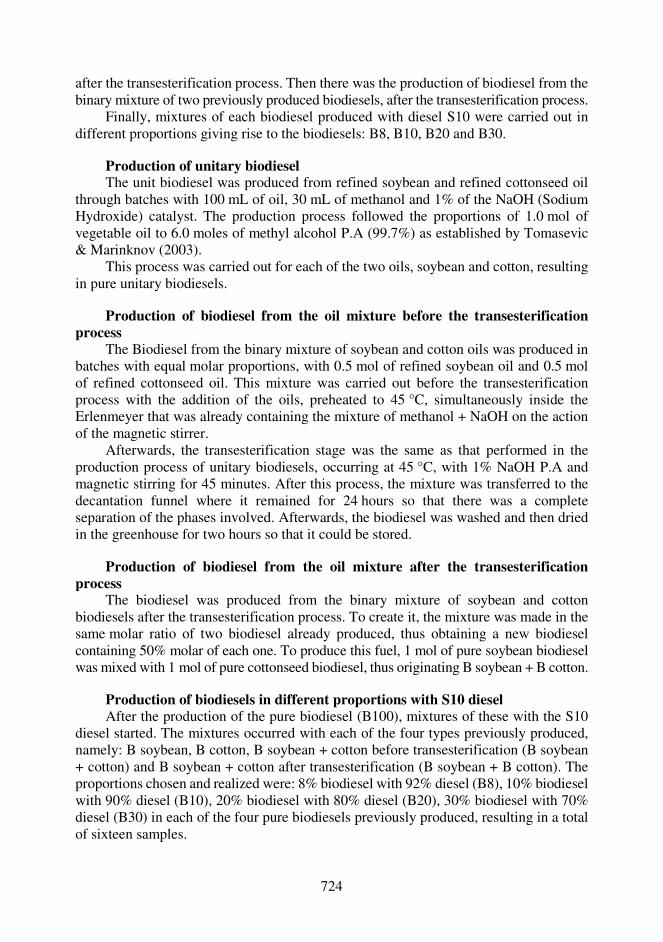
724
after the transesterification process. Then there was the production of biodiesel from the binary mixture of two previously produced biodiesels, after the transesterification process.
Finally, mixtures of each biodiesel produced with diesel S10 were carried out in different proportions giving rise to the biodiesels: B8, B10, B20 and B30.
Production of unitary biodiesel The unit biodiesel was produced from refined soybean and refined cottonseed oil
through batches with 100 mL of oil, 30 mL of methanol and 1% of the NaOH (Sodium Hydroxide) catalyst. The production process followed the proportions of 1.0 mol of vegetable oil to 6.0 moles of methyl alcohol P.A (99.7%) as established by Tomasevic & Marinknov (2003).
This process was carried out for each of the two oils, soybean and cotton, resulting in pure unitary biodiesels.
Production of biodiesel from the oil mixture before the transesterification
process The Biodiesel from the binary mixture of soybean and cotton oils was produced in
batches with equal molar proportions, with 0.5 mol of refined soybean oil and 0.5 mol of refined cottonseed oil. This mixture was carried out before the transesterification process with the addition of the oils, preheated to 45 °C, simultaneously inside the Erlenmeyer that was already containing the mixture of methanol + NaOH on the action of the magnetic stirrer.
Afterwards, the transesterification stage was the same as that performed in the production process of unitary biodiesels, occurring at 45 °C, with 1% NaOH P.A and magnetic stirring for 45 minutes. After this process, the mixture was transferred to the decantation funnel where it remained for 24 hours so that there was a complete separation of the phases involved. Afterwards, the biodiesel was washed and then dried in the greenhouse for two hours so that it could be stored.
Production of biodiesel from the oil mixture after the transesterification
process The biodiesel was produced from the binary mixture of soybean and cotton
biodiesels after the transesterification process. To create it, the mixture was made in the same molar ratio of two biodiesel already produced, thus obtaining a new biodiesel containing 50% molar of each one. To produce this fuel, 1 mol of pure soybean biodiesel was mixed with 1 mol of pure cottonseed biodiesel, thus originating B soybean + B cotton.
Production of biodiesels in different proportions with S10 diesel After the production of the pure biodiesel (B100), mixtures of these with the S10
diesel started. The mixtures occurred with each of the four types previously produced, namely: B soybean, B cotton, B soybean + cotton before transesterification (B soybean + cotton) and B soybean + cotton after transesterification (B soybean + B cotton). The proportions chosen and realized were: 8% biodiesel with 92% diesel (B8), 10% biodiesel with 90% diesel (B10), 20% biodiesel with 80% diesel (B20), 30% biodiesel with 70% diesel (B30) in each of the four pure biodiesels previously produced, resulting in a total of sixteen samples.
725
It is important to note that after the records the biodiesels were kept in opaque glassware and protected from heat and sunlight.
Production yield The yield of each treatment was obtained through Equation 1, used by Ambat et al.
(2018), just evaluating the values of the oil mass and the clean biodiesel mass produced in each batch.
Yield = ABCDBEFEG HIFFFCJAEIK HIFF (1)
Physical characterization
Specific Mass The specific mass was determined by the pycnometer and the thermostatic bath that
was used to maintain the temperature of the biodiesel analyzed at 20 °C. The pycnometer used to measure the specific mass was previously calibrated by analyzing the distilled water at 20 °C before the tests with the biodiesels were started.
To measure the specific mass, the pycnometer was initially weighed on an analytical balance. Subsequently, 50 mL of biodiesel was added to the pycnometer, which was fixed to a support that left it submerged in a thermostatic bath, thus ensuring that the sample contained in it stabilized its temperature at 20 °C. With the aid of a digital thermometer, you can have precise control of the temperature of the thermostatic bath.
In addition to the biofuel present in the pycnometer, the fuel that was being characterized was placed together with the other samples of biodiesel, which would then be analyzed in 100 mL beakers in the same thermostatic bath in which the pycnometer was located. This situation facilitated the measurement of the temperature of each biofuel and ensured that the samples stabilized at 20 °C. After stabilizing the pycnometer's interior temperature, it was removed from the thermostatic bath and weighed on the analytical balance with the biodiesel sample inside.
With the weight of the empty pycnometer, and then the measurement when it was filled with biodiesel, it was possible to calculate the specific mass of the sample using Eq. 2:
The physical characterization process took place in four different parts, namely: analysis of the specific mass at 20 °C and, later, at 40 °C with the use of pycnometer; verification of dynamic viscosity using a rheometer and calculation of the kinematic viscosity from the data found in the previous steps.
Table 1 identifies the physical-chemical properties that were used as a reference in this work to characterize and compare the biodiesel produced. Table 1 shows the standards for each characteristic, according to ANP No. 45/2014 resolution.
Table 1. Chemical physical property and corresponding pattern
Chemical physical property Pattern
Kinematic viscosity at 40 °C NBR 10.441 ASTM D 445 EN/ISO 3.104
Specific mass at 20 °C NBR 7.148 NBR 14.065 ASTM D 1.298 ASTM D 4.052 EN/ISO 3.675 EN/ISO 12.185
Source: Resolution adaptation nº 45/2014 of ANP.
726
L = MN\P – MNQN ∙ 1,000 (2)
where ρ – specific mass of biodiesel (kg m-3); Pp\b – weight of the pycnometer-biodiesel set (g); Pp – weight of the pycnometer (g); Vp – volume of the pycnometer (mL).
The specific mass was calculated for all biodiesel samples, five repetitions were performed for each one. With the average of the five repetitions, it was possible to find the most precise value of the specific mass of each biodiesel sample.
After the specific mass at 20 °C was found, the test was carried out again with the temperature of the biodiesel stabilized at 40 °C. This new measurement was necessary so that the kinematic viscosity at 40 °C could be found from the dynamic viscosity calculated with the same temperature.
Dynamic viscosity To determine the dynamic viscosity at 40 °C, the RS 50 RheoStress rheometer from
Precitech Instrumental LTDA was used with the coupled thermostatic bath to ensure that the experiment was carried out at a constant temperature previously established. The DG41Ti concentric cylinder was used for the measurement of biofuels because it ensures that during the experiment there is no loss of the sample and that it can be reused afterwards. The rheology tests were carried out at the Rheology Laboratory (LARE) of the Mechanical Engineering Department (TEM) of the Federal Fluminense University (UFF).
For the sake of carrying out the analysis on the rheometer, the data that was intended to be obtained through the equipment's RheoWin Pro 2.97 software, previously installed on the computer and attached to the rheometer, were previously inserted. A constant temperature of 40 °C was established for the execution of the experiment. The software itself creates a graph based on the data collected, which were previously selected to be measured, they are: dynamic viscosity versus shear rate (flow curve) and shear rate versus shear stress, both with temperature constant of 40 °C.
The rheometer test consists of turning the upper cup inside the lower one, applying a shear stress to the biodiesel present internally. This applied stress varied and increased over time, generating a shear rate corresponding to this variation.
This analysis was performed twice for each sample, with the results being tabulated and displayed graphically, to minimize possible errors.
The dynamic viscosity found was used to obtain the kinematic viscosity of biodiesel, a technical characteristic regulated by ANP standards.
In a rheological study, the fundamental parameter that must be investigated is viscosity. In these studies, the flow properties are usually illustrated by using graphs indicating the shear stress and viscosity as a function of the shear rate. These graphical representations of the flow and viscosity curves help to verify the behavior of the fluid to analyze whether it is considered a Newtonian fluid, since the functional relationship between the shear rate and the deformation rate is a line whose extension passes through the source.
Kinematic viscosity - Direct method To determine the kinematic viscosity at 40 °C, the values found for the specific
mass and dynamic viscosity at the same temperature were used. From these values, Eq. 3 was used to find the kinematic viscosity of each sample.
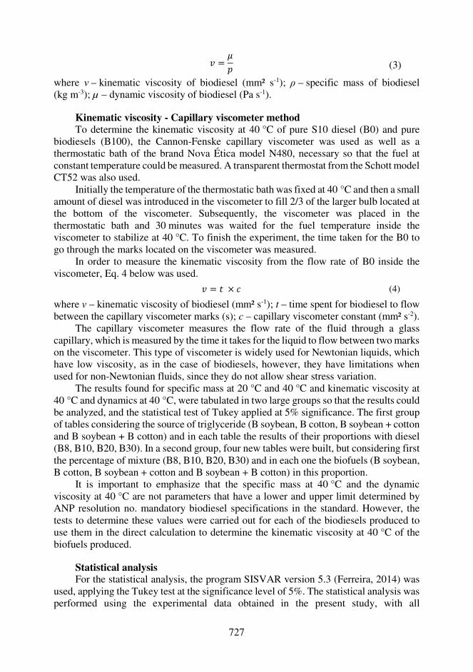
727
R = SN (3)
where ν – kinematic viscosity of biodiesel (mm² s-1); ρ – specific mass of biodiesel (kg m-3); µ – dynamic viscosity of biodiesel (Pa s-1).
Kinematic viscosity - Capillary viscometer method To determine the kinematic viscosity at 40 °C of pure S10 diesel (B0) and pure
biodiesels (B100), the Cannon-Fenske capillary viscometer was used as well as a thermostatic bath of the brand Nova Ética model N480, necessary so that the fuel at constant temperature could be measured. A transparent thermostat from the Schott model CT52 was also used.
Initially the temperature of the thermostatic bath was fixed at 40 °C and then a small amount of diesel was introduced in the viscometer to fill 2/3 of the larger bulb located at the bottom of the viscometer. Subsequently, the viscometer was placed in the thermostatic bath and 30 minutes was waited for the fuel temperature inside the viscometer to stabilize at 40 °C. To finish the experiment, the time taken for the B0 to go through the marks located on the viscometer was measured.
In order to measure the kinematic viscosity from the flow rate of B0 inside the viscometer, Eq. 4 below was used. R = T × V (4)
where v – kinematic viscosity of biodiesel (mm² s-1); t – time spent for biodiesel to flow between the capillary viscometer marks (s); c – capillary viscometer constant (mm² s-2).
The capillary viscometer measures the flow rate of the fluid through a glass capillary, which is measured by the time it takes for the liquid to flow between two marks on the viscometer. This type of viscometer is widely used for Newtonian liquids, which have low viscosity, as in the case of biodiesels, however, they have limitations when used for non-Newtonian fluids, since they do not allow shear stress variation.
The results found for specific mass at 20 °C and 40 °C and kinematic viscosity at 40 °C and dynamics at 40 °C, were tabulated in two large groups so that the results could be analyzed, and the statistical test of Tukey applied at 5% significance. The first group of tables considering the source of triglyceride (B soybean, B cotton, B soybean + cotton and B soybean + B cotton) and in each table the results of their proportions with diesel (B8, B10, B20, B30). In a second group, four new tables were built, but considering first the percentage of mixture (B8, B10, B20, B30) and in each one the biofuels (B soybean, B cotton, B soybean + cotton and B soybean + B cotton) in this proportion.
It is important to emphasize that the specific mass at 40 °C and the dynamic viscosity at 40 °C are not parameters that have a lower and upper limit determined by ANP resolution no. mandatory biodiesel specifications in the standard. However, the tests to determine these values were carried out for each of the biodiesels produced to use them in the direct calculation to determine the kinematic viscosity at 40 °C of the biofuels produced.
Statistical analysis For the statistical analysis, the program SISVAR version 5.3 (Ferreira, 2014) was
used, applying the Tukey test at the significance level of 5%. The statistical analysis was performed using the experimental data obtained in the present study, with all
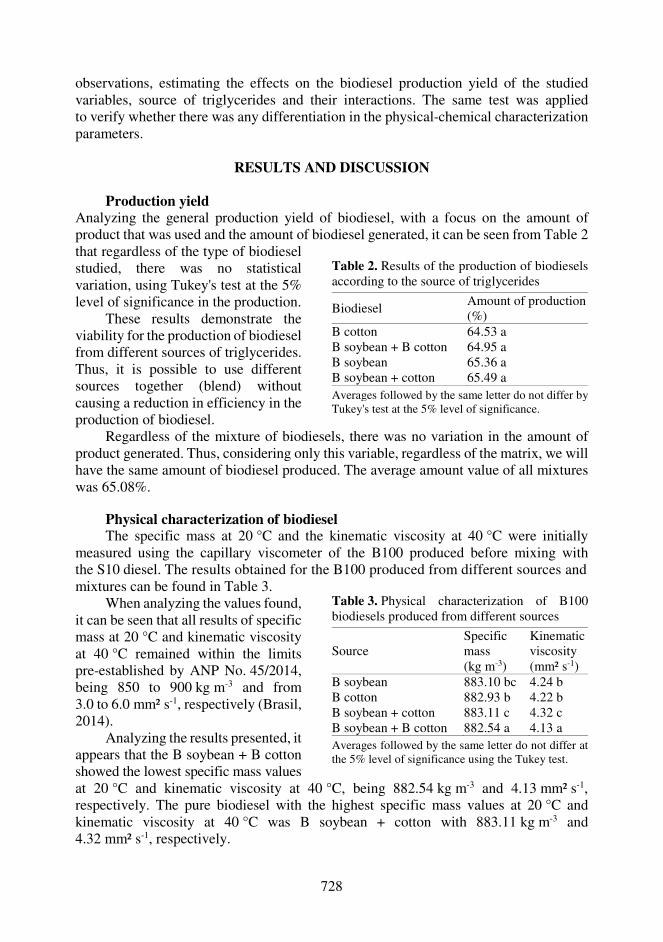
728
observations, estimating the effects on the biodiesel production yield of the studied variables, source of triglycerides and their interactions. The same test was applied to verify whether there was any differentiation in the physical-chemical characterization parameters.
RESULTS AND DISCUSSION
Production yield
Analyzing the general production yield of biodiesel, with a focus on the amount of product that was used and the amount of biodiesel generated, it can be seen from Table 2
Regardless of the mixture of biodiesels, there was no variation in the amount of product generated. Thus, considering only this variable, regardless of the matrix, we will have the same amount of biodiesel produced. The average amount value of all mixtures was 65.08%.
Physical characterization of biodiesel The specific mass at 20 °C and the kinematic viscosity at 40 °C were initially
measured using the capillary viscometer of the B100 produced before mixing with the S10 diesel. The results obtained for the B100 produced from different sources and
at 20 °C and kinematic viscosity at 40 °C, being 882.54 kg m-3 and 4.13 mm² s-1, respectively. The pure biodiesel with the highest specific mass values at 20 °C and kinematic viscosity at 40 °C was B soybean + cotton with 883.11 kg m-3 and 4.32 mm² s-1, respectively.
that regardless of the type of biodiesel studied, there was no statistical variation, using Tukey's test at the 5% level of significance in the production.
These results demonstrate the viability for the production of biodiesel from different sources of triglycerides. Thus, it is possible to use different sources together (blend) without causing a reduction in efficiency in the production of biodiesel.
Table 2. Results of the production of biodiesels according to the source of triglycerides
Biodiesel Amount of production (%)
B cotton 64.53 a B soybean + B cotton 64.95 a B soybean 65.36 a B soybean + cotton 65.49 a Averages followed by the same letter do not differ by Tukey's test at the 5% level of significance.
mixtures can be found in Table 3. When analyzing the values found,
it can be seen that all results of specific mass at 20 °C and kinematic viscosity at 40 °C remained within the limits pre-established by ANP No. 45/2014, being 850 to 900 kg m-3 and from 3.0 to 6.0 mm² s-1, respectively (Brasil, 2014).
Analyzing the results presented, it appears that the B soybean + B cotton showed the lowest specific mass values
Table 3. Physical characterization of B100 biodiesels produced from different sources
Source Specific mass (kg m-3)
Kinematic viscosity (mm² s-1)
B soybean 883.10 bc 4.24 b B cotton 882.93 b 4.22 b B soybean + cotton 883.11 c 4.32 c B soybean + B cotton 882.54 a 4.13 a Averages followed by the same letter do not differ at the 5% level of significance using the Tukey test.

729
For the kinematic viscosity at 40 °C the biofuels B soybean and B cotton did not vary significantly by the Tukey test at the level of 5% significance, unlike B soybean + cotton and B soybean + B cotton which varied significantly between them by the applied statistical test. For the specific mass at 20 °C, all the biofuels analyzed varied significantly between themselves by the Tukey test at the level of 5% of significance.
These physical variations are related to the composition of each oil (source of triglycerides) used in the transesterification process, as described by Gonçalves et al., (2019).
The specific mass at 20 °C and the kinematic viscosity at 40 °C were also measured using the capillary viscometer of the S10 diesel used to produce the biofuels B8, B10, B20 and B30. The results found for B0 can be seen in Table 4 and it can be noted that
2014), being 820.00 to 850.00 kg m-3 and 2.0 to 4.5 mm² s-1, respectively. Note that the specific mass and kinematic viscosity measured for B0 are lower than the values found for pure biodiesels (B100).
According to ANP Resolution No. 30/2016, which determines the lower and upper limits for BX to B30 biodiesel, the value calculated for specific mass at 20 °C must be between 817.80 and 865.00 kg m-3 when used diesel S10 in mixtures. For the kinematic viscosity at 40 °C, the regulation determines that the value must be within the range of 1.9 to 4.1 mm² s-1 (Brasil, 2016).
Table 5 below shows the results of kinematic Viscosity (.10-3 mm² s-1) at 40 °C according to ANP Resolution No. 30/2016. It can be observed that the biofuel that showed the highest value of kinematic viscosity at 40 °C, among all the tested samples, was the B 30 of B soybean + B cotton with a value of 3.94 mm² s-1 and that showed a significant difference when compared to the values of other biofuels from other sources of triglycerides in the same proportion (B30), in addition it differs significantly when comparing with other proportions from the same source. This value is 15.88% higher than the lowest result of kinematic viscosity at 40 °C found in the analyzes. The lowest value calculated was for B10 of cotton biodiesel, with a value of 3.40 mm² s-1.
Table 5. Kinematic viscosity (.10-3 mm² s-1) at 40 °C of biodiesels produced from different sources of triglycerides
Source Biodiesel B8 B10 B20 B30
Soybean 3.44 Ab 3.41 Ba 3.48 Ac 3.54 Ad Cotton 3.55 Db 3.40 Aa 3.67 Cc 3.72 Cd B soybean + cotton 3.54 Cb 3.42 Ca 3.91 Dd 3.61 Bc B soybean + B cotton 3.50 Ba 3.58 Db 3.64 Bc 3.94 Dd Averages followed by the same letter, uppercase in the column and lowercase in the row, do not differ at the 5% level of significance by the Tukey test.
the values found for specific mass at 20 °C and kinematic viscosity at 40 °C remained within the lower and upper limits established by Resolution 46/2012 of the ANP that regulates the characteristics of the S10 diesel (BRASIL,
Table 4. Physical characterization of B0 S10
Fuel Specific mass (kg m-3)
Kinematic viscosity (mm² s-1)
B0 830.28 2.85
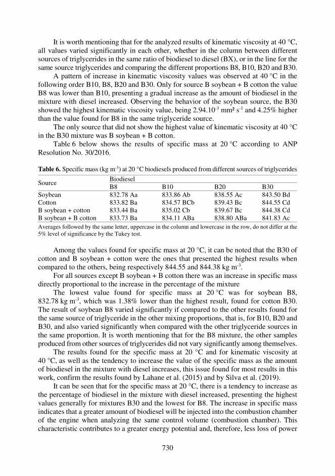
730
It is worth mentioning that for the analyzed results of kinematic viscosity at 40 °C, all values varied significantly in each other, whether in the column between different sources of triglycerides in the same ratio of biodiesel to diesel (BX), or in the line for the same source triglycerides and comparing the different proportions B8, B10, B20 and B30.
A pattern of increase in kinematic viscosity values was observed at 40 °C in the following order B10, B8, B20 and B30. Only for source B soybean + B cotton the value B8 was lower than B10, presenting a gradual increase as the amount of biodiesel in the mixture with diesel increased. Observing the behavior of the soybean source, the B30 showed the highest kinematic viscosity value, being 2.94.10-3 mm² s-1 and 4.25% higher than the value found for B8 in the same triglyceride source.
The only source that did not show the highest value of kinematic viscosity at 40 °C in the B30 mixture was B soybean + B cotton.
Table 6 below shows the results of specific mass at 20 °C according to ANP Resolution No. 30/2016.
Table 6. Specific mass (kg m-3) at 20 °C biodiesels produced from different sources of triglycerides
Source Biodiesel B8 B10 B20 B30
Soybean 832.78 Aa 833.86 Ab 838.55 Ac 843.50 Bd Cotton 833.82 Ba 834.57 BCb 839.43 Bc 844.55 Cd B soybean + cotton 833.44 Ba 835.02 Cb 839.67 Bc 844.38 Cd B soybean + B cotton 833.73 Ba 834.11 ABa 838.80 ABa 841.83 Ac Averages followed by the same letter, uppercase in the column and lowercase in the row, do not differ at the 5% level of significance by the Tukey test.
Among the values found for specific mass at 20 °C, it can be noted that the B30 of
cotton and B soybean + cotton were the ones that presented the highest results when compared to the others, being respectively 844.55 and 844.38 kg m-3.
For all sources except B soybean + B cotton there was an increase in specific mass directly proportional to the increase in the percentage of the mixture
The lowest value found for specific mass at 20 °C was for soybean B8, 832.78 kg m-3, which was 1.38% lower than the highest result, found for cotton B30. The result of soybean B8 varied significantly if compared to the other results found for the same source of triglyceride in the other mixing proportions, that is, for B10, B20 and B30, and also varied significantly when compared with the other triglyceride sources in the same proportion. It is worth mentioning that for the B8 mixture, the other samples produced from other sources of triglycerides did not vary significantly among themselves.
The results found for the specific mass at 20 °C and for kinematic viscosity at 40 °C, as well as the tendency to increase the value of the specific mass as the amount of biodiesel in the mixture with diesel increases, this issue found for most results in this work, confirm the results found by Lahane et al. (2015) and by Silva et al. (2019).
It can be seen that for the specific mass at 20 °C, there is a tendency to increase as the percentage of biodiesel in the mixture with diesel increased, presenting the highest values generally for mixtures B30 and the lowest for B8. The increase in specific mass indicates that a greater amount of biodiesel will be injected into the combustion chamber of the engine when analyzing the same control volume (combustion chamber). This characteristic contributes to a greater energy potential and, therefore, less loss of power
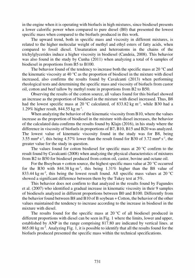
731
in the engine when it is operating with biofuels in high mixtures, since biodiesel presents a lower calorific power when compared to pure diesel (B0) that presented the lowest specific mass when compared to the biofuels produced in this work.
The upward trend, both in specific mass and viscosity in different mixtures, is related to the higher molecular weight of methyl and ethyl esters of fatty acids, when compared to fossil diesel. Unsaturation and heteroatoms in the chains of the trichylglycerides induce a higher viscosity in biodiesel (Candeia, 2008). This behavior was also found in the study by Cunha (2011) when analyzing a total of 6 samples of biodiesel in proportions from B5 to B100.
The behavior found of the tendency to increase both the specific mass at 20 °C and the kinematic viscosity at 40 °C as the proportion of biodiesel in the mixture with diesel increased, also confirms the results found by Cavalcanti (2013) when performing rheological tests and determining the specific mass and viscosity of biofuels from castor oil, cotton and beef tallow by methyl route in proportions from B2 to B50.
Observing the results of the cotton source, all values found for this biofuel showed an increase as the proportion of biodiesel in the mixture with diesel increased. Thus, B8 had the lowest specific mass at 20 °C calculated, of 833.82 kg m-3, while B30 had a 1.29% higher result, 844.55 kg m-3.
When analyzing the behavior of the kinematic viscosity from B10, where the values increase as the proportion of biodiesel in the mixture with diesel increases, the behavior of the calculated data confirms the results found by Klajn (2016), in his study where the difference in viscosity of biofuels in proportions of B7, B10, B15 and B20 was analyzed. The lowest value of kinematic viscosity found in the study was for B8, being 3.55 mm² s-1, this being 4.57% lower than the result found for B30 of 3.72 mm² s-1, the greater value for the study in question.
The values found for cotton biodiesel for specific mass at 20 °C confirm to the result found by Cavalcanti (2008) when analyzing the physical characteristics of mixtures from B2 to B50 for biodiesel produced from cotton oil, castor, bovine and octane oil.
For the Bsoybean + cotton source, the highest specific mass value at 20 °C occurred for the B30 with 844.38 kg m-3, this being 1.31% higher than the B8 value of 833.44 kg m-3, this being the lowest result found. All specific mass values at 20 °C showed a significant difference between them by the Tukey test at 5%.
This behavior does not confirm to that analyzed in the results found by Fagundes et al. (2007) who identified a gradual increase in kinematic viscosity in their 9 samples of biodiesels analyzed in different proportions between B0 and B100. Differently from the behavior found between B8 and B10 of B soybean + Cotton, the behavior of the other values maintained the tendency to increase according to the increase in biodiesel in the mixture with diesel.
The results found for the specific mass at 20 °C of all biodiesel produced in different proportions with diesel can be seen in Fig. 1 where the limits, lower and upper, established by ANP in the range comprising 817.80 are indicated by vertical lines. at 865.00 kg m-3. Analyzing Fig. 1, it is possible to identify that all the results found for the biofuels produced presented the specific mass within the technical specifications.
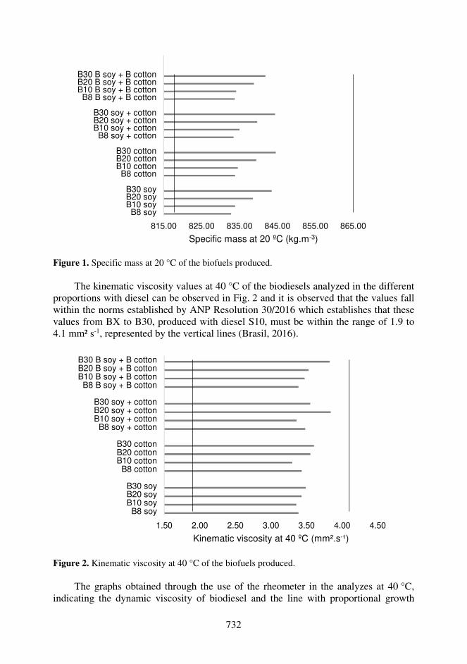
732
Figure 1. Specific mass at 20 °C of the biofuels produced.
The kinematic viscosity values at 40 °C of the biodiesels analyzed in the different proportions with diesel can be observed in Fig. 2 and it is observed that the values fall within the norms established by ANP Resolution 30/2016 which establishes that these values from BX to B30, produced with diesel S10, must be within the range of 1.9 to 4.1 mm² s-1, represented by the vertical lines (Brasil, 2016).
Figure 2. Kinematic viscosity at 40 °C of the biofuels produced. The graphs obtained through the use of the rheometer in the analyzes at 40 °C,
indicating the dynamic viscosity of biodiesel and the line with proportional growth
815.00 825.00 835.00 845.00 855.00 865.00
B8 soyB10 soyB20 soyB30 soy
B8 cottonB10 cottonB20 cottonB30 cotton
B8 soy + cottonB10 soy + cottonB20 soy + cottonB30 soy + cotton
B8 B soy + B cottonB10 B soy + B cottonB20 B soy + B cottonB30 B soy + B cotton
Specific mass at 20 ºC (kg.m-3)
1.50 2.00 2.50 3.00 3.50 4.00 4.50
B8 soyB10 soyB20 soyB30 soy
B8 cottonB10 cottonB20 cottonB30 cotton
B8 soy + cottonB10 soy + cottonB20 soy + cottonB30 soy + cotton
B8 B soy + B cottonB10 B soy + B cottonB20 B soy + B cottonB30 B soy + B cotton
Kinematic viscosity at 40 ºC (mm².s-¹)
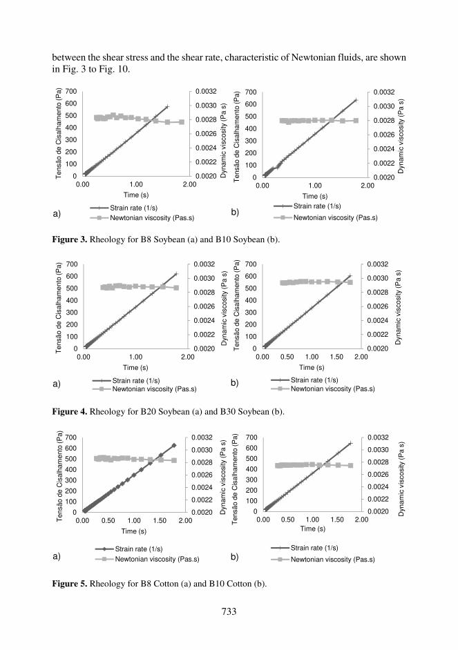
733
between the shear stress and the shear rate, characteristic of Newtonian fluids, are shown in Fig. 3 to Fig. 10.
Figure 3. Rheology for B8 Soybean (a) and B10 Soybean (b).
Figure 4. Rheology for B20 Soybean (a) and B30 Soybean (b).
Figure 5. Rheology for B8 Cotton (a) and B10 Cotton (b).
0.0020
0.0022
0.0024
0.0026
0.0028
0.0030
0.0032
0
100
200
300
400
500
600
700
0.00 1.00 2.00
Dynam
ic v
iscosity (
Pa s
)
Tensão d
e C
isalh
am
ento
(P
a)
Time (s)
Strain rate (1/s)
Newtonian viscosity (Pas.s)
0.0020
0.0022
0.0024
0.0026
0.0028
0.0030
0.0032
0
100
200
300
400
500
600
700
0.00 1.00 2.00
Dynam
ic v
iscosity (
Pa s
)
Tensão d
e C
isalh
am
ento
(P
a)
Time (s)
Strain rate (1/s)
Newtonian viscosity (Pas.s)
0.0020
0.0022
0.0024
0.0026
0.0028
0.0030
0.0032
0
100
200
300
400
500
600
700
0.00 1.00 2.00
Dynam
ic v
iscosity (
Pa s
)
Tensão d
e C
isalh
am
ento
(P
a)
Time (s)
Strain rate (1/s)Newtonian viscosity (Pas.s)
0.0020
0.0022
0.0024
0.0026
0.0028
0.0030
0.0032
0
100
200
300
400
500
600
700
0.00 0.50 1.00 1.50 2.00
Dynam
ic v
iscosity (
Pa s
)
Tensão d
e C
isalh
am
ento
(P
a)
Time (s)
Strain rate (1/s)
Newtonian viscosity (Pas.s)
0.0020
0.0022
0.0024
0.0026
0.0028
0.0030
0.0032
0
100
200
300
400
500
600
700
0.00 0.50 1.00 1.50 2.00
Dynam
ic v
iscosity (
Pa s
)
Tensão d
e C
isalh
am
ento
(P
a)
Time (s)
Strain rate (1/s)
Newtonian viscosity (Pas.s)
0.0020
0.0022
0.0024
0.0026
0.0028
0.0030
0.0032
0
100
200
300
400
500
600
700
0.00 0.50 1.00 1.50 2.00
Dynam
ic v
iscosity (
Pa s
)
Tensão d
e C
isalh
am
ento
(P
a)
Time (s)
Strain rate (1/s)
Newtonian viscosity (Pas.s)
a)
a)
a)
b)
b)
b)
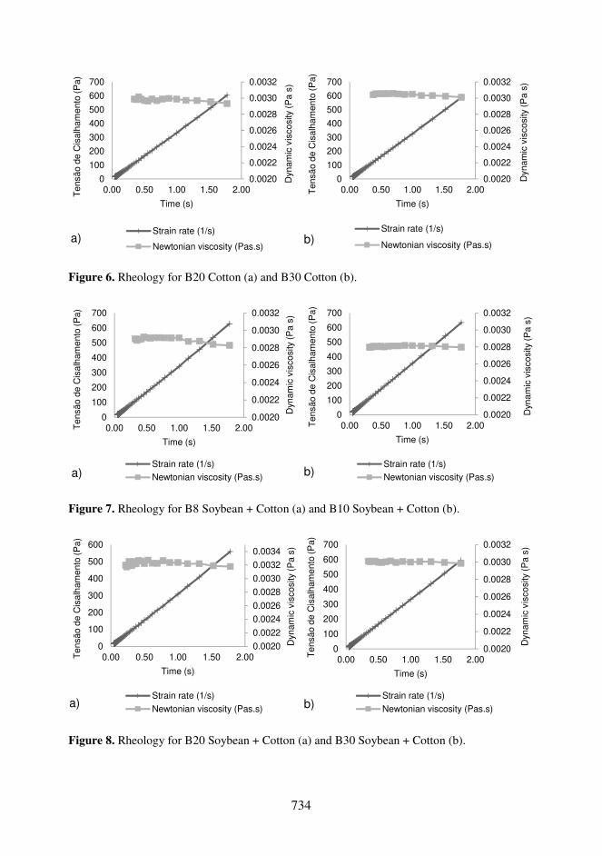
734
Figure 6. Rheology for B20 Cotton (a) and B30 Cotton (b).
Figure 7. Rheology for B8 Soybean + Cotton (a) and B10 Soybean + Cotton (b).
Figure 8. Rheology for B20 Soybean + Cotton (a) and B30 Soybean + Cotton (b).
0.0020
0.0022
0.0024
0.0026
0.0028
0.0030
0.0032
0
100
200
300
400
500
600
700
0.00 0.50 1.00 1.50 2.00
Dynam
ic v
iscosity (
Pa s
)
Tensão d
e C
isalh
am
ento
(P
a)
Time (s)
Strain rate (1/s)
Newtonian viscosity (Pas.s)
0.0020
0.0022
0.0024
0.0026
0.0028
0.0030
0.0032
0
100
200
300
400
500
600
700
0.00 0.50 1.00 1.50 2.00
Dynam
ic v
iscosity (
Pa s
)
Tensão d
e C
isalh
am
ento
(P
a)
Time (s)
Strain rate (1/s)
Newtonian viscosity (Pas.s)
0.0020
0.0022
0.0024
0.0026
0.0028
0.0030
0.0032
0
100
200
300
400
500
600
700
0.00 0.50 1.00 1.50 2.00
Dynam
ic v
iscosity (
Pa s
)
Tensão d
e C
isalh
am
ento
(P
a)
Time (s)
Strain rate (1/s)
Newtonian viscosity (Pas.s)
0.0020
0.0022
0.0024
0.0026
0.0028
0.0030
0.0032
0
100
200
300
400
500
600
700
0.00 0.50 1.00 1.50 2.00
Dynam
ic v
iscosity (
Pa s
)
Tensão d
e C
isalh
am
ento
(P
a)
Time (s)
Strain rate (1/s)
Newtonian viscosity (Pas.s)
0.0020
0.0022
0.0024
0.0026
0.0028
0.0030
0.0032
0.0034
0
100
200
300
400
500
600
0.00 0.50 1.00 1.50 2.00
Dynam
ic v
iscosity (
Pa s
)
Tensão d
e C
isalh
am
ento
(P
a)
Time (s)
Strain rate (1/s)
Newtonian viscosity (Pas.s)
0.0020
0.0022
0.0024
0.0026
0.0028
0.0030
0.0032
0
100
200
300
400
500
600
700
0.00 0.50 1.00 1.50 2.00
Dynam
ic v
iscosity (
Pa s
)
Tensão d
e C
isalh
am
ento
(P
a)
Time (s)
Strain rate (1/s)
Newtonian viscosity (Pas.s)
a)
a)
a)
b)
b)
b)
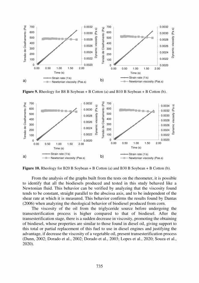
735
Figure 9. Rheology for B8 B Soybean + B Cotton (a) and B10 B Soybean + B Cotton (b).
Figure 10. Rheology for B20 B Soybean + B Cotton (a) and B30 B Soybean + B Cotton (b).
From the analysis of the graphs built from the tests on the rheometer, it is possible
to identify that all the biodiesels produced and tested in this study behaved like a Newtonian fluid. This behavior can be verified by analyzing that the viscosity found tends to be constant, straight parallel to the abscissa axis, and to be independent of the shear rate at which it is measured. This behavior confirms the results found by Dantas (2006) when analyzing the rheological behavior of biodiesel produced from corn.
The viscosity of the oil from the triglyceride source before undergoing the transesterification process is higher compared to that of biodiesel. After the transesterification stage, there is a sudden decrease in viscosity, promoting the obtaining of biodiesel, whose properties are similar to those found in diesel oil, giving support to this total or partial replacement of this fuel to use in diesel engines and justifying the advantage, if decrease the viscosity of a vegetable oil, present transesterification process (Dunn, 2002; Dorado et al., 2002; Dorado et al., 2003; Lopes et al., 2020; Souza et al., 2020).
0.0020
0.0022
0.0024
0.0026
0.0028
0.0030
0.0032
0
100
200
300
400
500
600
700
0.00 0.50 1.00 1.50 2.00
Dyn
am
ic v
iscosity
(Pa s
)
Tensão d
e C
isalh
am
ento
(P
a)
Time (s)
Strain rate (1/s)
Newtonian viscosity (Pas.s)
0.0020
0.0022
0.0024
0.0026
0.0028
0.0030
0.0032
0
100
200
300
400
500
600
700
0.00 0.50 1.00 1.50 2.00
Dyn
am
ic v
iscosity
(Pa s
)
Tensão d
e C
isalh
am
ento
(P
a)
Time (s)
Strain rate (1/s)
Newtonian viscosity (Pas.s)
0.0020
0.0022
0.0024
0.0026
0.0028
0.0030
0.0032
0
100
200
300
400
500
600
700
0.00 0.50 1.00 1.50 2.00
Dyn
am
ic v
iscosity
(Pa s
)
Tensão d
e C
isalh
am
ento
(P
a)
Time (s)
Strain rate (1/s)
Newtonian viscosity (Pas.s)
0.0020
0.0022
0.0024
0.0026
0.0028
0.0030
0.0032
0.0034
0
100
200
300
400
500
600
700
0.00 0.50 1.00 1.50 2.00
Dyn
am
ic v
iscosity
(Pa s
)
Tensão d
e C
isalh
am
ento
(P
a)
Time (s)
Strain rate (1/s)
Newtonian viscosity (Pas.s)
a)
a) b)
b)

736
It can be noted that the analyzed biodiesels present a Newtonian fluid behavior since the functional relationship between the shear stress and the strain rate is a line whose extension passes through the origin. This behavior found confirms the results found by Cavalcanti (2013) and Cavalcanti (2008) in their study with biodiesels and several BX mixtures. The same behavior was found for Dantas (2006).
According to Cavalcanti (2013), the lines that were constructed from the relationship between the deformation rate and shear stress have angular coefficients that are functions of the temperature and the composition of the components of the mixture, in this case the temperature has an inverse relationship with viscosity. The author also states that the apparent viscosity of the material at a given temperature and the range of strain rate is constant depending only on the temperature and composition of the material, so it can be considered as the dynamic viscosity of the material at that temperature.
CONCLUSIONS
This research investigated the production of biodiesel by the methyl route carrying
out the production through mixtures of soybean and cotton, before and after the transesterification process. Therefore, the work was carried out with the objective of optimizing and measuring the production volume, as well as physically characterizing the different proportions of biodiesel mixtures used. The assessment of the values observed in the production of the different types of biodiesel mixtures of soybean and cotton in the different proportions of mixtures indicated efficacy. Thus, they demonstrated its potential for use in internal combustion engines. All biofuels showed specific mass values at 20 °C and kinematic viscosity at 40 °C within the limits established by ANP Resolution 30/2016.
The mixture of soybean and cotton vegetable oils before the transesterification process showed the highest efficiency when compared to the production from only one vegetable oil or from the mixtures of biodiesels.
In general, the results showed an increase in specific mass at 20°C due to the increase in the percentage of Biodiesels, this factor is recommended, since it allows the increase of the biodiesel injected into the combustion chamber, compensating for the lower calorific power presented in biofuels.
The tests with B30 biodiesel showed satisfactory results that support the possibility of continuing to increase the amount of biodiesel in the mixture with diesel for the next years in Brazil, which is higher than the target stipulated throughout the national territory until 2023, the B15 mixture.
REFERENCES
Abed, K.A., Gad, M.S., El Morsi, A.K., Sayed, M.M. & Abu Elyazeed, S. 2019. Effect of
biodiesel fuels on diesel engine emissions. Egyptian Journal of Petroleum 28(2),183–188. https://doi.org/10.1016/j.ejpe.2019.03.001
Agência Nacional de Petróleo E Gás - ANP. 2019. Diesel oil will contain a minimum of 11 biodiesel as of September 1st. 2019. Available in: < http://www.anp.gov.br/noticias/5298-oleo-diesel-passa-a-conter-minimo-de-11-de-biodiesel-a-partir-de-1-de-setembro>. Accessed in: 15/12/2019 (in Portuguese).
737
Ambat, I., Srivastava, V. & Sillanpää, M. 2018. Recent advancement in biodiesel production methodologies using various feedstock: A review. Renewable and Sustainable Energy Reviews 90, 356–369. doi: https://doi.org/10.1016/j.rser.2018.03.069
Brasil. 2016. ANP Resolution No. 30, of June 24, 2016. Establishes the specification of diesel oil BX to B30, in an authoritative manner, under the terms of items I, II and III of art. 1 of CNPE Resolution No. 03, of September 21, 2015 (in Portuguese).
Brasil. 2014. ANP Resolution 45, of August 26, 2014. Establishes the biodiesel specification contained in ANP Technical Regulation No. 3/2014. Available in: <http://nxt.anp.gov.br/NXT/gateway.dll/leg/resolucoes_anp/2014/agosto /ranp%2045%20-%202014.xml?f=templates&fn=document-frameset.htm> Accessed in: 02/03/2019 (in Portuguese).
Candeia, R.A. 2008. Soybean Biodiesel: Synthesis, Degradation and Binary Mixtures. Tese de Doutorado. Universidade Federal da Paraíba. Centro de Ciências Exatas e da Natureza Departamento de Química. Programa de Pós-Graduação em Química, João Pessoa. 132 pp. (in Portuguese).
Cavalcanti, L.A.P. 2008. Rheology of biodiesel from different sources and of diesel/biodiesel mixtures. Programa de pós-graduação em engenharia química. Universidade Federal de Pernambuco. Recife, pp. 1–193 (in Portuguese).
Cavalcanti, L.A.P. 2013. Reology and improvement of flow properties cold biodiesel from various origins and their bx mixtures. Universidade Federal de Pernambuco. Centro de Tecnologia e Geociências. Programa de Pós-Graduação em Engenharia Química. Recife, pp. 1–193 (in Portuguese).
Cunha, J.P.B. 2011. Effects of different biodiesel concentrations in the performance of a tractor in operation of tillage. Tese de Mestrado. Universidade Estadual de Goiás. Unidade Universitária de Ciências Exatas e Tecnológica. Engenharia Agrícola, Anápolis, pp. 1–63 (in Portuguese).
Dantas, J., Leal, E., Mapossa, A.B., Silva, A.S. & CostA, A.C.F.M.C. 2016. Synthesis, characterization and catalytic performance of mixed nanoferrites submitted to transesterification and esterification reaction using methyl and ethyl route for biodiesel production. Revista Materia. 21, 1080–1093.
Dantas, M.B. 2006. Attainment, characterizing and thermoanalytic study of corn biodiesel. Universidade Federal de Paraíba. Centro de Ciências Exatas e da Natureza. Departamento de Química. Programa de Pós Graduação. João Pessoa. 115 pp. (in Portuguese).
Dorado, M.P., Arnal, J.M., Gomez, J., Gil, A. & Lopez, F.J. 2002. The effect of waste vegetable oil blend with diesel fuel on engine performance. Trans. ASAE 45, 525–529. https://doi.org/10.13031/2013.8820
Dorado, M.P., Ballesteros, E., Arnal, J.M., Gómez, J. & Giménez, F.J.L. 2003. Testing waste olive oil methyl ester as a fuel in a diesel engine. Energy Fuels 17, 1560–1565. https://doi.org/10.1021/ef0202485
Dunn, R.O. 2002. Effect of oxidation under accelerated conditions on fuel properties of methyl soyate (biodiesel). Journal of the American Oil Chemists' Society 79, 915–920. https://doi.org/10.1007/s11746-002-0579-2
Fagundes, F.P., Silva, A.S., Souto, C.R.O., Garcia, R. B. & Costa, M. 2007. Use of spectroscopic techniques to determine the percentage of biodiesel in binary mixtures with diesel. In 4º PDPETRO, Campinas, SP., pp. 1–9 (in Portuguese).
Ferreira, D.F. 2014. Sisvar: a Guide for its Bootstrap procedures in multiple comparisons. Ciência e Agrotecnologia. Ciência e Agrotecnologia [online]. 38(2), 109–112. doi: http://dx.doi.org/10.1590/S1413-70542014000200001
738
Goncalves, M.D., Silva, F.C., Maria, A.C.L., Souza, L.A. & Oliveira, P.C.O. 2019. Production and characterization of biodiesel produced from unitary oils and binary mixtures. Revista Brasileira de Ciências Ambientais (Impressa), v. 1, pp. 33–50. https://doi.org/10.5327/Z2176-947820190426 (in Portuguese).
Klajn, F.F. 2016. Comparative evaluation of different proportions of diesel-biodiesel-ethanol and diesel-biodiesel blends in comparison with type A Diesel: Physical-Chemical analysis and Moto-Generator performance. Universidade Estadual do Oeste do Paraná. Pós-Graduação em Engenharia de Energia na Agricultura. Cascavel, pp. 1–95. (in Portuguese).
Knothe, G., Gerpen, J.V., Krahl, J. & Ramos, L.P. 2006. Manual de Biodiesel. São Paulo: Edgard Blucher, p.1–340. https://doi.org/10.1201/9781439822357
Lahane, S. & Subramanian, K.A. 2015. Effect of different percentages of biodiesel-diesel blends on injection, spray, combustion, performance, and emission characteristics of a diesel engine. Fuel 139, 537–545. https://doi.org/10.1016/j.fuel.2014.09.036 (in Portuguese).
Lopes, L., Silva, F., Simões, R., Pontual, L., Souza, L., Nascimento, L. & Santos, C. M. 2020. Methylic route based on factorial design. Brazilian Journal of Environmental Sciences (Online), 55(2), 226–241. https://doi.org/10.5327/Z2176-947820200600
Manaf, I.S.A., Embong, N.H., Khazaai, S.N.M., Rahim, M.H.A., Yusoff, M.M., Lee, K.T. & Maniam, G.P.A. 2019. Review for key challenges of the development of biodiesel industry. Energy Conversion and Management 185, 508–517. https://doi.org/10.1016/j.enconman.2019.02.019
Meneghetti, S.M.P., Meneghetti, M.R. & Brito, Y.C. 2013. Transesterification, Some Applications and Biodiesel Production. Revista Virtual Química v. 5(1). 63–73. https://doi.org/10.5935/1984-6835.20130007 (in Portuguese).
Ministério de Minas e Energia - MME. 2019. Public Hearing on the definition of the timetable for the evolution of the percentage of mandatory addition of biodiesel to diesel oil, . Available in: <http://www.mme.gov.br/c/document_library/get_file?uuid=4016b267-261b-605f-4d67-29a3302a6278&groupId=36112>. Publicado em 25/11/2019. Accessed in: 10/01/2020 (in Portuguese).
Perin, G.F., Schlosser, J.F., Farias, M.S., Estrada, J.S., Treichel, H. & Galon, L. 2015. Emissions of agricultural engine using different diesel types and biodiesel concentrations in the fuel mixture. Pesq. Agropec, Bras. 50(12), 1168–1176. http://dx.doi.org/10.1590/S0100-204X2015001200006 (in Portuguese).
Rockembach, C.T., Dias, D., Vieira, B.M., Ritter, M., Santos, M.A.Z., Oliveira, D.M., Fontoura, L.A.M., Crizel, M. G., Mesko, M.F., Santos, V.O.B. & Pereira, C.M.P. 2014. Synthesis of Biodiesel from Grape Seed Oil Using Ultrasound Irradiation. Revista Virtual de Quimica, v. fev., pp. 884–897. https://doi.org/10.5935/1984-6835.20140054 (in Portuguese).
Silva, Flávio C. da, Aranha, Felipe N., Angelkorte, Gerd B., Guardiola, Juan F.H., Teixeira, Luciana P. & Correia, Ricardo C. de B. 2019. Quantification and qualification of exhaust gases in agricultural diesel engine operating with biodiesel mixtures. Revista Brasileira de Engenharia Agrícola e Ambiental 23(10), 794–799. https://dx.doi.org/10.1590/1807-1929/agriambi.v23n10p794-799
Souza, L.A., Silva, F.C., Maria, A.C.L., Belem, A.L., Cecchin, D. & Barros, M.M. 2020. Response surface for biodiesel production from soybean oil by ethylic route. Agronomy Research 18(S2), 1498–1515. https://doi.org/10.15159/ar.20.065
Tomasevic, A.V. & Marinkovic, S.S. 2003. Methanolysis of used frying oils. Fuel Process Technol. 81, pp. 1–6. https://doi.org/10.1016/s0378-3820(02)00096-6
739
Agronomy Research 19(S1), 739–748, 2021 https://doi.org/10.15159/AR.21.054
Evaluation of passive cooling system in plywood enclosure for agricultural robot prototype
J. Galins, V. Osadcuks and A. Pecka
Latvia University of Life Sciences and Technologies, Faculty of Engineering, Institute of Energetics, Jana Cakstes boulevard 5, LV-3001 Jelgava, Latvia *Correspondence: [email protected] Received: February 1st, 2021; Accepted: March 27th, 2021; Published: April 29th, 2021 Abstract. The use of autonomous robots in agriculture has been increasing rapidly in recent years, but is hampered by the complexity of data recording and processing. The prototyping process involves many changes to the housing design during development. Using laser cutting to make a housing is more convenient, faster and cheaper than milling or casting if only one body needs to be made. To speed up the production of autonomous robot prototypes, the body was made of birch plywood using laser-cut parts. The study analyses the efficiency of passive cooling to make sure that birch wood plywood is suitable for the production of a robotic body for outdoor use in agriculture. Under laboratory conditions, temperature measurements were made inside and outside the housing to determine how the heat released by the electronic components dissipates into the environment. An exponential model with a static coefficient and a time constant can be used to determine the recommended operating time at different ambient temperatures when the allowable operating temperature of the component is known. Air flow and heat transfer simulations were performed to represent heat dissipation. Birch plywood can be used for the production of prototype enclosures for agricultural robots, but the design must provide technological solutions for heat dissipation to prevent overheating of electronic components. Key words: cooling system, heat transfer, modelling, thermal management.
INTRODUCTION
In the 21st century, the level of human welfare has increased significantly, leading to rising labour costs. In order to reduce production costs, entrepreneurs are forced to use robots to make their products competitive (Marinoudi et al., 2019). Robotic hands are widely used to perform monotonous work, changing the placement of the object. It is much more difficult to create an autonomous robot that collects data and makes decisions itself. Autonomous robots are needed for various agricultural tasks, such as getting rid of the weeds (Xiong et al., 2017; McAllister et al., 2019). The computer vision is associated with the collection and processing of environmental data. Cameras record large amounts of data that are processed by a powerful computer (Malavazi et al., 2018; Le et al., 2019; Raja et al., 2019; Kim et al., 2021). Prototyping of such a robot is associated with many problems:

740
Change of location of components during development. Data recording and processing emits a significant amount of heat. The robot must be waterproof to withstand agricultural conditions such as rain,
snow, humidity, temperature fluctuations, UV radiation and aggressive gases. Data recording needs to be synchronized before it can be combined. The position of each camera must be calibrated before data can be recorded. Passive cooling without moving parts works more reliably than active cooling.
Using a fan for cooling can create additional risks such as dust and dirt getting on the electronics and camera lenses (Lanzerstorfer et al., 2016). Passive and active cooling solutions were compared by Galins et al. (2019) in another study.
3D printers are often used to make prototype housings, but they are not always convenient, fast, or cost-effective. Fused deposition modeling is cheaper and more affordable but the dimensional accuracy of 3D printed part is worse than by stereolithography and selective laser sintering (Minetola & Galati, 2018; Solomon et al., 2020; Zharylkassyn et al., 2020). 3D printing with thermoplastics is very popular in robot prototyping but the use of thermoplastic or plywood impairs heat dissipation in the environment (Flaata et al., 2017; Navarrete & Caldeira, 2019). For larger enclosures, laser-cut acrylic or plywood parts could be used. The mounting platform can be made by CNC milling machine to ensure accurate positioning of the cameras. The study uses thermography, experimental temperature measurements and Solidworks flow simulations to ensure that plywood enclosure is suitable for a prototype of agricultural robot. It is planned to place a bundle of sensors with a computer in a plywood box and to study the heat dissipation in the surrounding environment. The aim of the work is to determine the maximum ambient temperature up to which the equipment can safely operate as well as to determine weak spots of design from thermal point of view.
MATERIALS AND METHODS
The study was developed at the
Latvia University of Life Sciences and Technologies, laboratory of the Faculty of Engineering. A prototype agricultural robot was developed that can be used to record and process environmental data (Fig. 1).
The lower body of the robot is used to allow the robot to move on various agricultural road surfaces, as well as in agricultural facilities. Brushed DC motors allow the wheels to move back and forth. The upper part of the body is sensor bundle for environmental data recording and processing (Fig. 2). The sensor bundle should operate in various environmental conditions, including light rain, snow,
Figure 1. Experimental prototype of an agricultural robot: 1 – sensor bundle; 2 – lithium batteries for lower body; 3 – lithium batteries for sensor bundle; 4 – brushed DC motors; 5 – chassis; 6 – wheels.
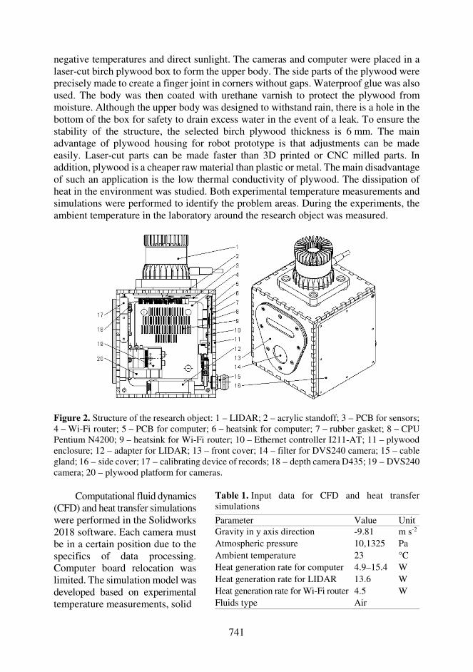
741
negative temperatures and direct sunlight. The cameras and computer were placed in a laser-cut birch plywood box to form the upper body. The side parts of the plywood were precisely made to create a finger joint in corners without gaps. Waterproof glue was also used. The body was then coated with urethane varnish to protect the plywood from moisture. Although the upper body was designed to withstand rain, there is a hole in the bottom of the box for safety to drain excess water in the event of a leak. To ensure the stability of the structure, the selected birch plywood thickness is 6 mm. The main advantage of plywood housing for robot prototype is that adjustments can be made easily. Laser-cut parts can be made faster than 3D printed or CNC milled parts. In addition, plywood is a cheaper raw material than plastic or metal. The main disadvantage of such an application is the low thermal conductivity of plywood. The dissipation of heat in the environment was studied. Both experimental temperature measurements and simulations were performed to identify the problem areas. During the experiments, the ambient temperature in the laboratory around the research object was measured.
Figure 2. Structure of the research object: 1 – LIDAR; 2 – acrylic standoff; 3 – PCB for sensors; 4 – Wi-Fi router; 5 – PCB for computer; 6 – heatsink for computer; 7 – rubber gasket; 8 – CPU Pentium N4200; 9 – heatsink for Wi-Fi router; 10 – Ethernet controller I211-AT; 11 – plywood enclosure; 12 – adapter for LIDAR; 13 – front cover; 14 – filter for DVS240 camera; 15 – cable gland; 16 – side cover; 17 – calibrating device of records; 18 – depth camera D435; 19 – DVS240 camera; 20 – plywood platform for cameras.
Computational fluid dynamics
(CFD) and heat transfer simulations were performed in the Solidworks 2018 software. Each camera must be in a certain position due to the specifics of data processing. Computer board relocation was limited. The simulation model was developed based on experimental temperature measurements, solid
Table 1. Input data for CFD and heat transfer simulations
Parameter Value Unit Gravity in y axis direction -9.81 m s-2 Atmospheric pressure 10,1325 Pa Ambient temperature 23 °C Heat generation rate for computer 4.9–15.4 W Heat generation rate for LIDAR 13.6 W Heat generation rate for Wi-Fi router 4.5 W Fluids type Air
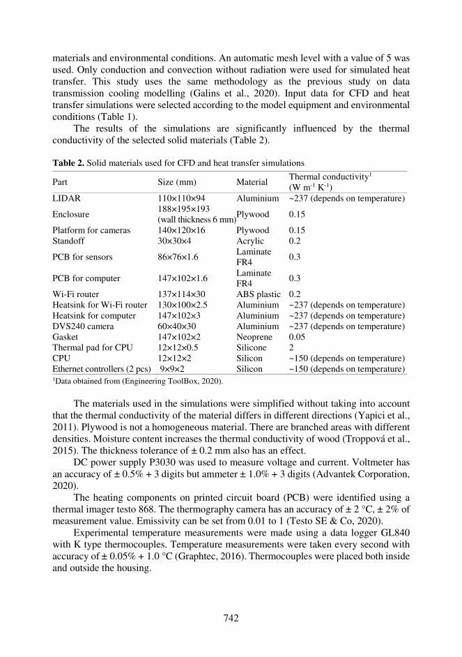
742
materials and environmental conditions. An automatic mesh level with a value of 5 was used. Only conduction and convection without radiation were used for simulated heat transfer. This study uses the same methodology as the previous study on data transmission cooling modelling (Galins et al., 2020). Input data for CFD and heat transfer simulations were selected according to the model equipment and environmental conditions (Table 1).
The results of the simulations are significantly influenced by the thermal conductivity of the selected solid materials (Table 2).
Table 2. Solid materials used for CFD and heat transfer simulations
Part Size (mm) Material Thermal conductivity1 (W m-1 K-1)
LIDAR 110×110×94 Aluminium ~237 (depends on temperature)
Enclosure 188×195×193 (wall thickness 6 mm)Plywood 0.15
Platform for cameras 140×120×16 Plywood 0.15 Standoff 30×30×4 Acrylic 0.2
PCB for sensors 86×76×1.6 Laminate FR4 0.3
PCB for computer 147×102×1.6 Laminate FR4 0.3
Wi-Fi router 137×114×30 ABS plastic 0.2 Heatsink for Wi-Fi router 130×100×2.5 Aluminium ~237 (depends on temperature) Heatsink for computer 147×102×3 Aluminium ~237 (depends on temperature) DVS240 camera 60×40×30 Aluminium ~237 (depends on temperature) Gasket 147×102×2 Neoprene 0.05 Thermal pad for CPU 12×12×0.5 Silicone 2 CPU 12×12×2 Silicon ~150 (depends on temperature) Ethernet controllers (2 pcs) 9×9×2 Silicon ~150 (depends on temperature) 1Data obtained from (Engineering ToolBox, 2020).
The materials used in the simulations were simplified without taking into account
that the thermal conductivity of the material differs in different directions (Yapici et al., 2011). Plywood is not a homogeneous material. There are branched areas with different densities. Moisture content increases the thermal conductivity of wood (Troppová et al., 2015). The thickness tolerance of ± 0.2 mm also has an effect.
DC power supply P3030 was used to measure voltage and current. Voltmeter has an accuracy of ± 0.5% + 3 digits but ammeter ± 1.0% + 3 digits (Advantek Corporation, 2020).
The heating components on printed circuit board (PCB) were identified using a thermal imager testo 868. The thermography camera has an accuracy of ± 2 °C, ± 2% of measurement value. Emissivity can be set from 0.01 to 1 (Testo SE & Co, 2020).
Experimental temperature measurements were made using a data logger GL840 with K type thermocouples. Temperature measurements were taken every second with accuracy of ± 0.05% + 1.0 °C (Graphtec, 2016). Thermocouples were placed both inside and outside the housing.
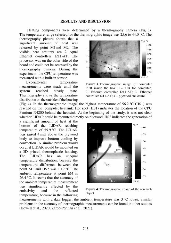
743
RESULTS AND DISCUSSION Heating components were determined by a thermography camera (Fig. 3).
The temperature range selected for the thermographic image was 25.6 to 44.0 °C. The
(Fig. 4). In the thermographic image, the highest temperature of 56.2 °C (HS1) was reached on the computer heatsink. Hot spot (HS1) indicates the location of the CPU Pentium N4200 behind the heatsink. At the beginning of the study, it was not clear whether LIDAR could be mounted directly on plywood. HS2 indicates the generation of
measurements with a data logger, the ambient temperature was 3 °C lower. Similar problems in the accuracy of thermographic measurements can be found in other studies (Howell et al., 2020; Zarco-Periñán et al., 2021).
thermography picture shows that a significant amount of heat was released by point M1and M2. The visible heat emitters are 2 equal Ethernet controllers I211-AT. The processor was on the other side of the board and could not be accessed by the thermography camera. During the experiment, the CPU temperature was measured with a built-in sensor.
Experimental temperature measurements were made until the system reached steady state. Thermography shows the temperature distribution on the outside of the housing
Figure 3. Thermographic image of computer PCB inside the box: 1 – PCB for computer; 2 – Ethernet controller I211-AT; 3 – Ethernet controller I211-AT; 4 – plywood enclosure.
a significant amount of heat at the bottom of the LIDAR reaching temperature of 55.9 °C. The LIDAR was raised 4 mm above the plywood body to improve bottom cooling by convection. A similar problem would occur if LIDAR would be mounted on a 3D printed thermoplastic housing. The LIDAR has an unequal temperature distribution, because the temperature difference between the point M1 and HS2 was 10.9 °C. The ambient temperature at point M4 is 26.4 °C. It seems that the accuracy of the ambient temperature measurement was significantly affected by the emissivity and the reflected temperature, because in the following
Figure 4. Thermographic image of the research object.
42.5 40.0
37.5 35.0
32.5 30.0
27.5
1
2
3
4
44.0 °C
25.6 °C
60 °C
23 °C
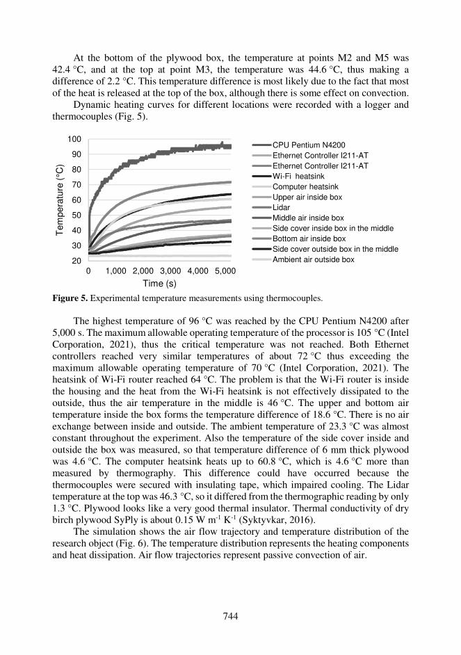
744
At the bottom of the plywood box, the temperature at points M2 and M5 was 42.4 °C, and at the top at point M3, the temperature was 44.6 °C, thus making a difference of 2.2 °C. This temperature difference is most likely due to the fact that most of the heat is released at the top of the box, although there is some effect on convection.
Dynamic heating curves for different locations were recorded with a logger and thermocouples (Fig. 5).
Figure 5. Experimental temperature measurements using thermocouples.
The highest temperature of 96 °C was reached by the CPU Pentium N4200 after
5,000 s. The maximum allowable operating temperature of the processor is 105 °C (Intel Corporation, 2021), thus the critical temperature was not reached. Both Ethernet controllers reached very similar temperatures of about 72 °C thus exceeding the maximum allowable operating temperature of 70 °C (Intel Corporation, 2021). The heatsink of Wi-Fi router reached 64 °C. The problem is that the Wi-Fi router is inside the housing and the heat from the Wi-Fi heatsink is not effectively dissipated to the outside, thus the air temperature in the middle is 46 °C. The upper and bottom air temperature inside the box forms the temperature difference of 18.6 °C. There is no air exchange between inside and outside. The ambient temperature of 23.3 °C was almost constant throughout the experiment. Also the temperature of the side cover inside and outside the box was measured, so that temperature difference of 6 mm thick plywood was 4.6 °C. The computer heatsink heats up to 60.8 °C, which is 4.6 °C more than measured by thermography. This difference could have occurred because the thermocouples were secured with insulating tape, which impaired cooling. The Lidar temperature at the top was 46.3 °C, so it differed from the thermographic reading by only 1.3 °C. Plywood looks like a very good thermal insulator. Thermal conductivity of dry birch plywood SyPly is about 0.15 W m-1 K-1 (Syktyvkar, 2016).
The simulation shows the air flow trajectory and temperature distribution of the research object (Fig. 6). The temperature distribution represents the heating components and heat dissipation. Air flow trajectories represent passive convection of air.
20
30
40
50
60
70
80
90
100
0 1,000 2,000 3,000 4,000 5,000
Tem
pera
ture
(°C
)
Time (s)
CPU Pentium N4200
Ethernet Controller I211-AT
Ethernet Controller I211-AT
Wi-Fi heatsink
Computer heatsink
Upper air inside box
Lidar
Middle air inside box
Side cover inside box in the middle
Bottom air inside box
Side cover outside box in the middle
Ambient air outside box
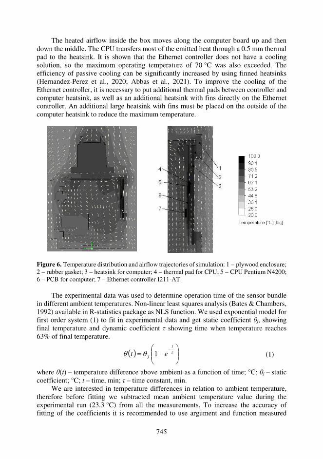
745
The heated airflow inside the box moves along the computer board up and then down the middle. The CPU transfers most of the emitted heat through a 0.5 mm thermal pad to the heatsink. It is shown that the Ethernet controller does not have a cooling solution, so the maximum operating temperature of 70 °C was also exceeded. The efficiency of passive cooling can be significantly increased by using finned heatsinks (Hernandez-Perez et al., 2020; Abbas et al., 2021). To improve the cooling of the Ethernet controller, it is necessary to put additional thermal pads between controller and computer heatsink, as well as an additional heatsink with fins directly on the Ethernet controller. An additional large heatsink with fins must be placed on the outside of the computer heatsink to reduce the maximum temperature.
Figure 6. Temperature distribution and airflow trajectories of simulation: 1 – plywood enclosure; 2 – rubber gasket; 3 – heatsink for computer; 4 – thermal pad for CPU; 5 – CPU Pentium N4200; 6 – PCB for computer; 7 – Ethernet controller I211-AT.
The experimental data was used to determine operation time of the sensor bundle
in different ambient temperatures. Non-linear least squares analysis (Bates & Chambers, 1992) available in R-statistics package as NLS function. We used exponential model for first order system (1) to fit in experimental data and get static coefficient θf, showing final temperature and dynamic coefficient τ showing time when temperature reaches 63% of final temperature.
t
f et 1 (1)
where θ(t) – temperature difference above ambient as a function of time; °C; θf – static coefficient; °C; t – time, min; τ – time constant, min.
We are interested in temperature differences in relation to ambient temperature, therefore before fitting we subtracted mean ambient temperature value during the experimental run (23.3 °C) from all the measurements. To increase the accuracy of fitting of the coefficients it is recommended to use argument and function measured

746
numerical values in close magnitudes, so we expressed time in minutes instead of seconds.
Table 3 shows the summary of NLS analysis results. Column θf shows static coefficients for different measurement points. Table 3. Fitted values of coefficients for different measurement points
Measurement point θf, °C τ, min Residual standrad error Lidar 22.3 13.2 0.8929 Ethernet Controller I211-AT 6.7 13.8 1.6680 Ethernet Controller I211-AT 46.5 13.6 1.7760 Wi-Fi heatsink 39.2 19.0 1.5110 Computer heatsink 36.9 17.0 0.4400 Bottom air inside box 17.9 68.1 0.3023 Upper air inside box 32.2 24.2 0.5006 Side cover inside box in the middle 16.2 46.1 0.2628 Side cover outside box in the middle 10.9 45.3 0.3065 Middle air inside box 24.1 34.2 0.2591 CPU Pentium N4200 68.4 7.6 4.8280
Using the Table 3, Eq. 1 and allowable operating temperatures of different
components it is possible to determine recommended operation time of the sensor bundle for a given ambient temperature. The best fit was achieved for sensors positioned in air or on large thermal mass objects (LIDAR, large heatsinks), where temperature change was less affected by multiple internal heat sources.
CONCLUSIONS
The study revealed that the current cooling solution is not efficient enough for the unit to operate for a long time at an ambient temperature above 23 °C. Ethernet controller I211-AT exceeded the maximum allowable temperature per 2 °C thus cooling solution needs improvement. The highest temperature of 96 °C was reached by the CPU Pentium N4200 thus not exceeding the maximum allowable operating temperature of 105 °C.
Thermography can be used effectively to identify hot spots where significant amounts of heat are released, but thermocouples should be used for more accurate measurements.
Birch plywood can be used for the production of prototype housings for agricultural robots, but the design must provide technological solutions for heat dissipation to prevent overheating of electronic components.
An exponential model with a static coefficient and a time constant can be used to determine the recommended operating time at different ambient temperatures when the allowable operating temperature of the component is known.
ACKNOWLEDGEMENTS. This research is funded by the Latvian Council of Science, Funding Number: lzp-2018/1-0482.

747
REFERENCES
Abbas, A., Muneeshwaran, M. & Wang, C.C. 2021. Performance of displaced fin heatsink in natural convection subject to upward and downward arrangement. International Journal of Thermal Sciences 162. doi: 10.1016/j.ijthermalsci.2020.106797
Advantek Corporation. 2020. P3030 manual. Available at http://www.advanteks.com/manual_for_P.pdf
Bates, D.M. & Chambers, J.M. 1992. Nonlinear models. Chapter 10 of Statistical Models in S eds J. M. Chambers and T. J. Hastie, Wadsworth & Brooks/Cole.
Engineering ToolBox. 2020. Available at https://www.engineeringtoolbox.com/ Flaata, T., Michna, G.J. & Letcher, T. 2017. Thermal conductivity testing apparatus for 3d
printed materials. ASME. doi: 10.1115/HT2017-4856 Galins, J., Laizans, A. & Galins, A. 2020. Modelling of heat processes for data transmission
equipment for operation at high temperature. Engineering for Rural Development 19, 1437–1443. doi: 10.22616/ERDev.2020.19.TF361
Galins, J., Laizans, A. & Galins, A. 2019. Review of cooling solutions for compact electronic devices. Research for Rural Development 1, 201–208. doi: 10.22616/rrd.25.2019.030
Graphtec. 2016. GL840 Manual. Hernandez-Perez, J.G., Carrillo, J.G., Bassam, A., Flota-Banuelos, M. & Patino-Lopez, L.D.
2020. Thermal performance of a discontinuous finned heatsink profile for PV passive cooling. Applied Thermal Engineering 184. doi: 10.1016/j.applthermaleng.2020.116238
Howell, K., Dudek, K. & Soroko, M. 2020. Thermal camera performance and image analysis repeatability in equine thermography. Infrared Physics and Technology 110. doi: 10.1016/j.infrared.2020.103447
Intel Corporation. 2021. Intel Pentium Processor N4200. Available at https://ark.intel.com/content/www/us/en/ark/products/95592/intel-pentium-processor-n4200-2m-cache-up-to-2-5-ghz.html?wapkw=CPU%20Pentium%20N4200%20
Intel Corporation. 2021. Intel Ethernet Controller I211-AT. Available at https://ark.intel.com/content/www/us/en/ark/products/64404/intel-ethernet-controller-i211-at.html
Kim, W.S., Lee, D.H., Kim, Y.J., Kim, T., Lee, W.S. & Choi, C.H. 2021. Stereo-vision-based crop height estimation for agricultural robots. Computers and Electronics in Agriculture 181. doi: 10.1016/j.compag.2020.105937
Lanzerstorfer, C., Neder, F. & Schmied, R. 2016. Constant design air flow industrial ventilation systems with regenerative dust filters: Economic comparison of fan speed-controlled, air damper controlled and uncontrolled operation. Energy and Buildings 128, 503–510. doi: 10.1016/j.enbuild.2016.07.032
Le, T., Omholt-Gjevestad, J.G. & From, P.J. 2019. Online 3D Mapping and Localization System for Agricultural Robots. IFAC-PapersOnLine 52(30), 167–172. doi: 10.1016/j.ifacol.2019.12.516
Malavazi, F.B.P., Guyonneau, R., Fasquel, J.B., Lagrange, S. & Mercier, F. 2018. LiDAR-only based navigation algorithm for an autonomous agricultural robot. Computers and Electronics in Agriculture 154, 71–79. doi: 10.1016/j.compag.2018.08.034
Marinoudi, V., Sørensen, C.G., Pearson, S. & Bochtis, D. 2019. Robotics and labour in agriculture. A context consideration. Biosystems Engineering 184, 111–121. doi: 10.1016/j.biosystemseng.2019.06.013
McAllister, W., Osipychev, D., Davis, A. & Chowdhary, G. 2019. Agbots: Weeding a field with a team of autonomous robots. Computers and Electronics in Agriculture 163. doi: 10.1016/j.compag.2019.05.036
748
Minetola, P. & Galati, M. 2018. A challenge for enhancing the dimensional accuracy of a low-cost 3D printer by means of self-replicated parts. Additive Manufacturing 22, 256–264. doi: 10.1016/j.addma.2018.05.028
Navarrete, M.J.I. & Caldeira, T. 2019. Smart Manufacturing of 3D Printed Robots. Advances in Science and Engineering Technology, 1–5 doi: 10.1109/ICASET.2019.8714537
Raja, R., Slaughter, D.C., Fennimore, S.A., Nguyen, T.T., Vuong, V.L., Sinha, N. & Siemens, M.C. 2019. Crop signalling: A novel crop recognition technique for robotic weed control. Biosystems Engineering 187, 278–291. doi: 10.1016/j.biosystemseng.2019.09.011
Solomon, I.J., Sevvel, P. & Gunasekaran, J. 2020. A review on the various processing parameters in FDM. Materials Today: Proceedings, pp. 10–15. doi: 10.1016/j.matpr.2020.05.484
Syktyvkar Plywood Mill. 2016. Handbook SyPly. Available at https://hanson-plywood.co.uk/wp-content/uploads/2017/07/SyPly_handbook_ENG2016.pdf
Testo SE & Co. 2020. Data Sheet Testo 868, pp. 4. Troppová, E., Švehlík, M., Tippner, J. & Wimmer, R. 2015. Influence of temperature and
moisture content on the thermal conductivity of wood-based fibreboards. Materials and Structures/Materiaux et Constructions 48(12), 4077–4083. doi: 10.1617/s11527-014-0467-4
Xiong, Y., Ge, Y., Liang, Y. & Blackmore, S. 2017. Development of a prototype robot and fast path-planning algorithm for static laser weeding. Computers and Electronics in Agriculture 142, 494–503. doi: 10.1016/j.compag.2017.11.023
Yapici, F., Ozcifci, A., Esen, R. & Kurt, S. 2011. The effect of grain angle and species on thermal conductivity of some selected wood species. BioResources 6(3), 2757–2762. doi: 10.15376/biores.6.3.2757-2762
Zarco-Periñán, P.J., Martínez-Ramos, J.L. & Zarco-Soto, F.J. 2021. A novel method to correct temperature problems revealed by infrared thermography in electrical substations. Infrared Physics and Technology 113. doi: 10.1016/j.infrared.2020.103623
Zharylkassyn, B., Perveen, A. & Talamona, D. 2020. Effect of process parameters and materials on the dimensional accuracy of FDM parts. Materials Today: Proceedings. doi: 10.1016/j.matpr.2020.11.332
749
Agronomy Research 19(S1), 749–766, 2021 https://doi.org/10.15159/AR.21.057
Waste fish oil as an alternative renewable fuel for IC engines
M. Hissa*, S. Niemi, T. Ovaska and A. Niemi
University of Vaasa, School of Technology and Innovations, P.O. Box 700, FI-65101 Vaasa, Finland *Correspondence: [email protected] Received: January 31st, 2021; Accepted: April 10th, 2021; Published: April 30th, 2021 Abstract. Bio-oils are potential fuels for internal combustion engines because of they have advantageous properties such as biodegradability, renewability, high oxygen content and low sulphur. However, the high viscosity, surface tension, and density of crude bio-oils pose challenges for engine use. Those properties affect fuel spray characteristics, mixture formation and combustion. In turn, these impact engine, efficiency, power and emissions. This study investigated the use of crude fish oil (FO) at medium and low engine-loads at two engine speeds in an off-road engine. The injectors had 6-hole high flow rate tips. The results were compared with those of fossil diesel fuel oil (DFO). Fish oil increased hydrocarbon (HC), carbon monoxide (CO) and partly oxides of nitrogen (NOx) emissions. Smoke number, however, decreased. Crude fish oil also showed lowered total particle number (TPN) at low load at low engine-speed compared with DFO. Key words: diesel engine, bio-oil, combustion, gaseous emissions, particle number.
INTRODUCTION
Bio-based fuels can provoke economic, social, and environmental issues, especially
if the raw material used in their production is edible. Consequently, the focus for biofuel production is switching to alternative raw materials such as non-edible vegetable oils, used cooking oils, fatty acids from algae, and animal fats (Sirviö, 2018; Ching-Velasquez et al., 2020).
According to its 2019 Government Programme, Finland will be carbon-neutral by 2035 (Ministry of the Environment, 2019). The already standardised blends of biodiesel and fatty acid methyl ester (FAME) fuels are one realistic way to increase the share of renewables to fulfil Finnish government and European Union targets (Sirviö, 2018). Many Finnish farms and factories are willing to increase the self-sufficiency of their energy production by utilising waste materials like crude fish oil as a fuel feedstock (Niemi et al., 2009; Niemi et al., 2011).
The crude oil extracted from discarded parts of marine fish may provide an abundant, cheap and stable source of raw oil to allow maritime countries to produce biodiesel and help to reduce pollutant emissions (Lin & Li, 2009; de Almeida et al., 2015). However, diesel engines can burn even unrefined bio-oils, such as animal fats, vegetable oils, and waste oils. This increases the interest in crude bio-oils (Niemi et al.,

750
2009; Niemi et al., 2011; Hoang, 2019). The use of straight bio-oils with minimal refining should even be preferable since refining always consumes energy and adds carbon dioxide (CO2) emissions (Niemi et al., 2009; Esteban et al., 2012). Power plants with medium-speed engines fuelled by neat bio-oil are already in operation around the world (Ollus & Juoperi, 2007; Niemi et al., 2011).
World fish production in 2018 was around 179 million tonnes, of which 12% was used for non-food purposes (Food and Agriculture Organization of the United Nations, FAO, 2020). More efficient and sustainable use of fisheries and aquaculture production must be implemented since a large proportion - as much as 35% - of production is either lost or wasted. Improvements can be achieved through appropriate policies, regulatory frameworks, capacity building, services and infrastructure, as well as physical access to markets. (FAO, 2020).
Most of the fish oil is used in the cosmetic, pharmaceutical, and human dietary complement industries (Bruun, 2019). If the fish oil degrades during storage or handling it can be used in marine or stationary diesel engines (Bruun, 2019). The oil can be also processed further to produce biodiesel. Thus, there is already large potential to also use fish wastes for fuel production.
Crude bio-oils have shown several advantages as fuels in IC engines. Compared with DFO, many studies report a significant reduction of toxic emissions and noise; small or insignificant generation of greenhouse gas (GHG) emissions; and lower emissions of NOx, polycyclic aromatic hydrocarbons (PAHs), particulate matter (PM) and smoke (How et al., 2012; Satyanarayana & Muraleedharan, 2012; Hoang, 2019).
Although liquid biofuels are a good alternative to fossil fuel oil, there are challenges associated with their use. For example, studies by, Niemi et al. (2011), Deshmukh et al. (2012), Fan et al. (2014), and Sirviö (2018) conclude that the high viscosity of neat bio-oils affects fuel atomisation and efficient combustion. They point to specific issues of large droplet size, long spray penetration, formation of deposits, injector coking, ring sticking, piston seize-up, lube oil dilution, filter choking etc. Other limiting factors for the use of pure bio-oils are their lower heating value and cetane number, higher density and surface tension when compared to DFO, as well as their acidic and corrosive properties, plus their water and oxygen (How et al., 2012; Bruun, 2019; Hoang, 2019). Studies by Hoang, (2019), Rakopoulos et al. (2014) and Chauhan et al. (2010) report that crude bio-oils give reduced power output but more deposit formation in the combustion chamber and injector holes, resulting in increased carbon monoxide (CO) and unburnt hydrocarbon (HC) emissions.
Unlike FAME biodiesels, crude bio-oils do not have common quality specifications. Some producers have their own specifications that set limits for viscosity, density, water content, acid number, sulphur content etc. These limits are based on the experiences of using bio-oils in diesel engines (Bruun, 2019). For example, according to Ollus & Juoperi (2007), the acid number of crude bio-oils should be below 5.0 mg KOH g-1; the water content less than 0.20% (V V-1); the sulphur content less than 500 ppm; and phosphorus content below 100 ppm.
The main research question of the current study was whether fish oil from left-over fish trimmings could be used as an alternative fuel in the local fishermen's vessels. The study was part of a project that investigated the potential to make more efficient use of fish trimmings and by-catches in Ostrobothnia, Finland (Skog et al., 2013). The present study investigated the use of crude fish oil in a high-speed, common-rail diesel engine
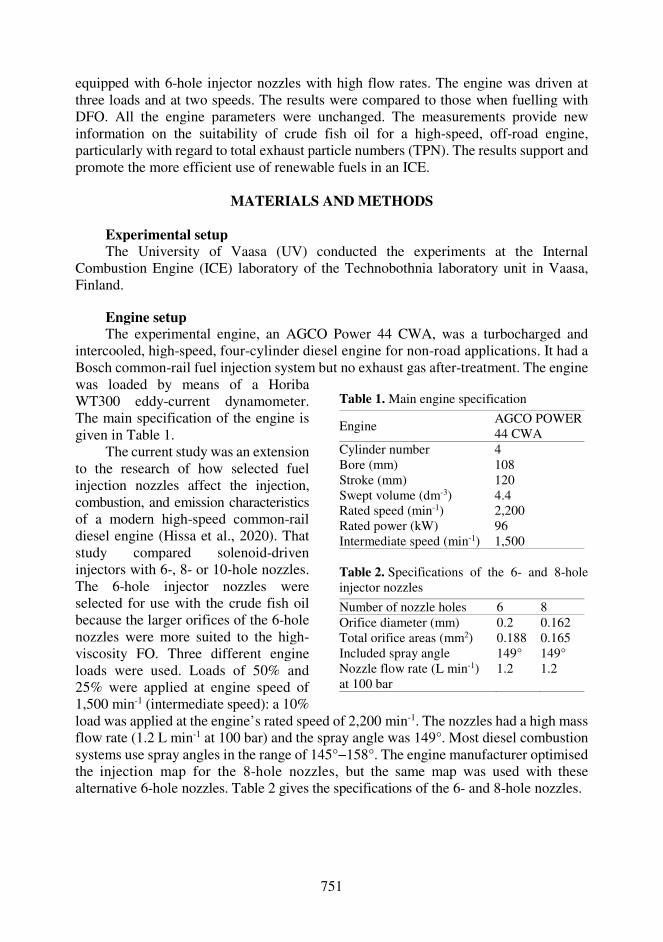
751
equipped with 6-hole injector nozzles with high flow rates. The engine was driven at three loads and at two speeds. The results were compared to those when fuelling with DFO. All the engine parameters were unchanged. The measurements provide new information on the suitability of crude fish oil for a high-speed, off-road engine, particularly with regard to total exhaust particle numbers (TPN). The results support and promote the more efficient use of renewable fuels in an ICE.
MATERIALS AND METHODS
Experimental setup The University of Vaasa (UV) conducted the experiments at the Internal
Combustion Engine (ICE) laboratory of the Technobothnia laboratory unit in Vaasa, Finland.
Engine setup The experimental engine, an AGCO Power 44 CWA, was a turbocharged and
intercooled, high-speed, four-cylinder diesel engine for non-road applications. It had a Bosch common-rail fuel injection system but no exhaust gas after-treatment. The engine
load was applied at the engine’s rated speed of 2,200 min-1. The nozzles had a high mass flow rate (1.2 L min-1 at 100 bar) and the spray angle was 149°. Most diesel combustion systems use spray angles in the range of 145°−158°. The engine manufacturer optimised the injection map for the 8-hole nozzles, but the same map was used with these alternative 6-hole nozzles. Table 2 gives the specifications of the 6- and 8-hole nozzles.
was loaded by means of a Horiba WT300 eddy-current dynamometer. The main specification of the engine is given in Table 1.
The current study was an extension to the research of how selected fuel injection nozzles affect the injection, combustion, and emission characteristics of a modern high-speed common-rail diesel engine (Hissa et al., 2020). That study compared solenoid-driven injectors with 6-, 8- or 10-hole nozzles. The 6-hole injector nozzles were selected for use with the crude fish oil because the larger orifices of the 6-hole nozzles were more suited to the high-viscosity FO. Three different engine loads were used. Loads of 50% and 25% were applied at engine speed of 1,500 min-1 (intermediate speed): a 10%
Table 1. Main engine specification
Engine AGCO POWER 44 CWA
Cylinder number 4 Bore (mm) 108 Stroke (mm) 120 Swept volume (dm-3) 4.4 Rated speed (min-1) 2,200 Rated power (kW) 96 Intermediate speed (min-1) 1,500 Table 2. Specifications of the 6- and 8-hole injector nozzles
Number of nozzle holes 6 8 Orifice diameter (mm) 0.2 0.162 Total orifice areas (mm2) 0.188 0.165 Included spray angle 149° 149° Nozzle flow rate (L min-1) at 100 bar
1.2 1.2
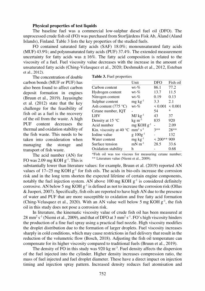
752
Physical properties of test liquids The baseline fuel was a commercial low-sulphur diesel fuel oil (DFO). The
unprocessed crude fish oil (FO) was purchased from Storfjärdens Fisk Ab, Åland (Aland Islands), Finland. Table 3 lists the key properties of the studied fuels.
FO contained saturated fatty acids (SAF) 18.0%; monounsaturated fatty acids (MUF) 43.9%; and polyunsaturated fatty acids (PUF) 37.4%. The extended measurement uncertainty for fatty acids was ± 16%. The fatty acid composition is related to the viscosity of a fuel. Fuel viscosity value decreases with the increase in the amount of unsaturated fatty acids (Ching-Velasquez et al., 2020; Deshmukh et al., 2012, Esteban
substantially lower than literature values: for example, Bruun et al. (2019) reported AN values of 17−25 mg KOH g-1 for fish oils. The acids in bio-oils increase the corrosion risk and in the long term shorten the expected lifetime of certain engine components, notably the fuel injection system. AN above 100 mg KOH g-1 is considered definitely corrosive. AN below 5 mg KOH g-1 is defined as not to increase the corrosion risk (Ollus & Juoperi, 2007). Specifically, fish oils are reported to have high AN due to the presence of water and PUF that are more susceptible to oxidation and free fatty acid formation (Ching-Velasquez et al., 2020). With an AN value well below 5 mg KOH g-1, the fish oil in this study does not pose a corrosion risk.
In literature, the kinematic viscosity value of crude fish oil has been measured at 28 mm2 s-1 (Niemi et al., 2009), and that of DFO at 3 mm2 s-1. FO’s high viscosity hinders the production of a fine fuel spray using a practical fuel nozzle. High viscosity modifies the droplet distribution due to the formation of larger droplets. Fuel viscosity increases sharply in cold conditions, which may cause restrictions in fuel delivery that result in the reduction of the volumetric flow (Bosch, 2018). Adjusting the fish oil temperature can compensate for its higher viscosity compared to traditional fuels (Bruun et al., 2019).
The density of FO in this study was 920 kg m-3. Fuel density affects the dispersion of the fuel injected into the cylinder. Higher density increases compression ratio, the mass of fuel injected and fuel droplet diameter. These have a direct impact on injection timing and injection spray pattern. Increased density reduces fuel atomisation and
et al., 2012). The concentration of double
carbon bonds (MUF or PUF) has also been found to affect carbon deposit formation in engines (Bruun et al., 2019). Jayasinghe et al. (2012) state that the key challenge for the feasibility of fish oil as a fuel is the recovery of the oil from the waste. A high PUF content decreases the thermal and oxidation stability of the fish waste. This needs to be taken into consideration when managing the storage and transport of fish waste.
The acid number (AN) for FO was 2.09 mg KOH g-1. This is
Table 3. Fuel properties
Unit DFO Fish oil Carbon content wt-% 86.1 77.2 Hydrogen content wt-% 13.7 11.5 Nitrogen content wt-% 0.19 0.13 Sulphur content mg kg-1 3.3 2.1 Ash content (775 °C) wt-% < 0.001 < 0.001 Cetane number, IQT - 54 * LHV MJ kg-1 43 37 Density at 15 °C kg m-3 835 920 Acid number mg KOH g-1 - 2.09 Kin. viscosity at 40 °C mm2 s-1 3** 28** Iodine value g 100g-1 - 132 Water content mg kg-1 < 200** 909 Surface tension mN m-1 28.5 33.6 Oxidation stability h - 0.68 *Fish oil was too viscous for measuring cetane number; ** Literature value (Niemi et al., 2009).

753
mixing with air: this reduction is associated with higher PM and NOx emissions. According to a manufacturer of marine diesel engines, the density of liquid biofuel should be lower than 991 kg m-3 for four-stroke engines (Juoperi & Ollus, 2008; Jayasinghe et al., 2012).
FO was too viscous to measure its cetane number (CN) by an ignition quality tester (IQT). In the study of Niemi et al. (2011) CN for crude fish oil was 49, i.e., not very low. In the current study, DFO had a CN of 54. CN has an impact on the ignition delay (ID). A low CN increases ID, resulting in poorer combustion and leading to noise and smoke emissions (Hissa et al., 2018).
The LHV (lower heating value) of FO (37 MJ kg-1) is substantially less than that of the DFO (43 MJ kg-1), thus increasing the required fuelling rate to achieve the same engine power output (Drenth et al., 2014). The presence of water in fish oil decreases its heating value. FO had high water content: over 900 mg kg-1. In engine use, water in oil may cause corrosion of the equipment and containers (Adeoti & Hawboldt, 2015; Bruun et al., 2019).
If the same volume of two fuels, with different fuel densities, are injected to an engine, the fuel with higher density provides higher engine output. However, this occurs only if lower heating values (LHV) do not differ greatly. (Murtonen, 2004) Since in this study, the density of fish oil is significantly greater than that of diesel, the energy per injection is actually more similar than based on LHV alone.
The surface tension of FO was 18% higher than that of diesel. Surface tension has a direct impact on the size of fuel droplets, so FO’s higher surface tension might also contribute to an increase in its droplet diameters (Heywood, 2018).
Analytical instruments LabVIEW system-design software was used to collect the sensor data from the
engine. The recorded variables were engine speed and torque, cylinder pressure and injection timing, duration, and quantity. A WinEEM3 program provided by the engine manufacturer, AGCO Power, controlled fuel injection according to load-speed requests. The basic settings of WinEEM3 were the same for all nozzles and fuels. Fig. 1 is a schematic of the test bench setup.
A piezoelectric Kistler 6125C pressure sensor measured the in-cylinder pressure. The sensor was mounted on the head of the fourth cylinder. A charge amplifier filtered and amplified the signal, which was then transmitted to a Kistler KIBOX combustion analyser. The crankshaft position was recorded by a crank-angle encoder (Kistler 2614B1), which can output a crank-angle signal with a resolution of 0.1 °CA by means of an optical sensor. The cylinder-pressure data was averaged over 100 consecutive cycles to smooth irregular combustion. The averaged data were used to calculate the heat release rate (HRR).
The HRR and mass fraction burned (MFB) were calculated via AVL Concerto's data-processing platform, using the Thermodynamics2 macro. The macro used a calculation resolution of 0.2 °CA. The start of the calculation was set at -30 °CA. The data were filtered with the DigitalFilter macro and a frequency of 2000 Hz. For the HRR results, the average values of in-cylinder pressure were calculated first. Thereafter, the macro was used to calculate HRR values. Finally, the HRR curve was filtered. In contrast, for the MFB results, pressure values were first filtered, and then the macro was
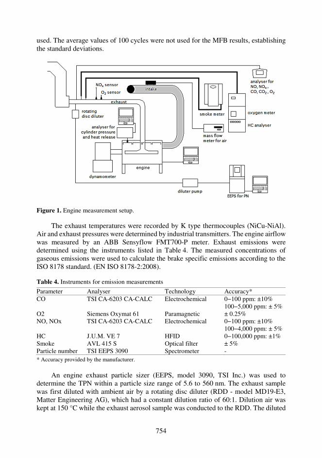
754
used. The average values of 100 cycles were not used for the MFB results, establishing the standard deviations.
Figure 1. Engine measurement setup.
The exhaust temperatures were recorded by K type thermocouples (NiCu-NiAl). Air and exhaust pressures were determined by industrial transmitters. The engine airflow was measured by an ABB Sensyflow FMT700-P meter. Exhaust emissions were determined using the instruments listed in Table 4. The measured concentrations of gaseous emissions were used to calculate the brake specific emissions according to the ISO 8178 standard. (EN ISO 8178-2:2008). Table 4. Instruments for emission measurements
Parameter Analyser Technology Accuracy* CO TSI CA-6203 CA-CALC Electrochemical 0−100 ppm: ±10%
100−5,000 ppm: ± 5% O2 Siemens Oxymat 61 Paramagnetic ± 0.25% NO, NOx TSI CA-6203 CA-CALC Electrochemical 0−100 ppm: ±10%
100−4,000 ppm: ± 5% HC J.U.M. VE 7 HFID 0−100,000 ppm: ±1% Smoke AVL 415 S Optical filter ± 5% Particle number TSI EEPS 3090 Spectrometer - * Accuracy provided by the manufacturer.
An engine exhaust particle sizer (EEPS, model 3090, TSI Inc.) was used to
determine the TPN within a particle size range of 5.6 to 560 nm. The exhaust sample was first diluted with ambient air by a rotating disc diluter (RDD - model MD19-E3, Matter Engineering AG), which had a constant dilution ratio of 60:1. Dilution air was kept at 150 °C while the exhaust aerosol sample was conducted to the RDD. The diluted
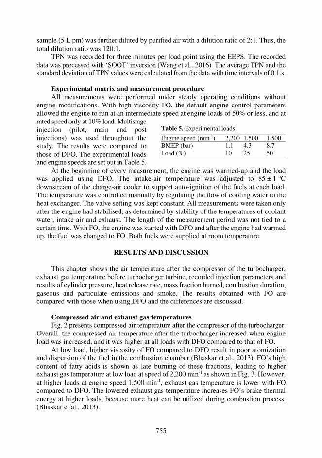
755
sample (5 L pm) was further diluted by purified air with a dilution ratio of 2:1. Thus, the total dilution ratio was 120:1.
TPN was recorded for three minutes per load point using the EEPS. The recorded data was processed with ‘SOOT’ inversion (Wang et al., 2016). The average TPN and the standard deviation of TPN values were calculated from the data with time intervals of 0.1 s.
Experimental matrix and measurement procedure All measurements were performed under steady operating conditions without
engine modifications. With high-viscosity FO, the default engine control parameters allowed the engine to run at an intermediate speed at engine loads of 50% or less, and at
At the beginning of every measurement, the engine was warmed-up and the load was applied using DFO. The intake-air temperature was adjusted to 85 ± 1 °C downstream of the charge-air cooler to support auto-ignition of the fuels at each load. The temperature was controlled manually by regulating the flow of cooling water to the heat exchanger. The valve setting was kept constant. All measurements were taken only after the engine had stabilised, as determined by stability of the temperatures of coolant water, intake air and exhaust. The length of the measurement period was not tied to a certain time. With FO, the engine was started with DFO and after the engine had warmed up, the fuel was changed to FO. Both fuels were supplied at room temperature.
RESULTS AND DISCUSSION
This chapter shows the air temperature after the compressor of the turbocharger,
exhaust gas temperature before turbocharger turbine, recorded injection parameters and results of cylinder pressure, heat release rate, mass fraction burned, combustion duration, gaseous and particulate emissions and smoke. The results obtained with FO are compared with those when using DFO and the differences are discussed.
Compressed air and exhaust gas temperatures Fig. 2 presents compressed air temperature after the compressor of the turbocharger.
Overall, the compressed air temperature after the turbocharger increased when engine load was increased, and it was higher at all loads with DFO compared to that of FO.
At low load, higher viscosity of FO compared to DFO result in poor atomization and dispersion of the fuel in the combustion chamber (Bhaskar et al., 2013). FO’s high content of fatty acids is shown as late burning of these fractions, leading to higher exhaust gas temperature at low load at speed of 2,200 min-1 as shown in Fig. 3. However, at higher loads at engine speed 1,500 min-1, exhaust gas temperature is lower with FO compared to DFO. The lowered exhaust gas temperature increases FO’s brake thermal energy at higher loads, because more heat can be utilized during combustion process. (Bhaskar et al., 2013).
rated speed only at 10% load. Multistage injection (pilot, main and post injections) was used throughout the study. The results were compared to those of DFO. The experimental loads and engine speeds are set out in Table 5.
Table 5. Experimental loads
Engine speed (min-1) 2,200 1,500 1,500 BMEP (bar) 1.1 4.3 8.7 Load (%) 10 25 50

756
Figure 2. Air temperature after the compressor of the turbocharger.
Figure 3. Exhaust gas temperature before the turbocharger turbine.
Injection parameters For all test conditions, pilot and main injections were set before top dead centre
(BTDC) and post injections occurred after top dead centre (ATDC). Exact timings and durations are shown in Table 6.
Table 6. Injection parameters for DFO and FO
Fuel Speed BMEP/ Load
Pilot Injection (ATDC)
Main injection (ATDC)
Post injection (ATDC)
Start Duration Start Duration Start Duration min-1 bar/% °CA °CA °CA °CA °CA °CA
DFO 2,200 1.1/10 -18 4.6 -8 6.9 13 0 FO -18 4.6 -8 7.6 13 0 DFO 1,500 4.3/25 -12 3.9 -4.5 8.2 13 4.7 FO -11 3.9 -4.4 9.6 15 4.7 DFO 1,500 8.7/50 -8.7 3.5 -2.1 13 21 4.5 FO -9.4 3.8 -2.5 16 22 3.4
Injection timings and durations were broadly similar with both fuels at 2,200 min-1,
but the duration of the main injection was longer for FO because its lower heating value is less than DFO’s.
At the load of 4.3 bar BMEP and engine speed 1,500 min-1, pilot injection started 1 °CA earlier with DFO compared to FO. The main injection started at the same time with both fuels but injection duration with FO was again longer than with DFO. FO's post injection started 2 °CA later than with DFO, most probably delayed due to FO’s longer main injection duration. The duration of post injection was still similar for both fuels.
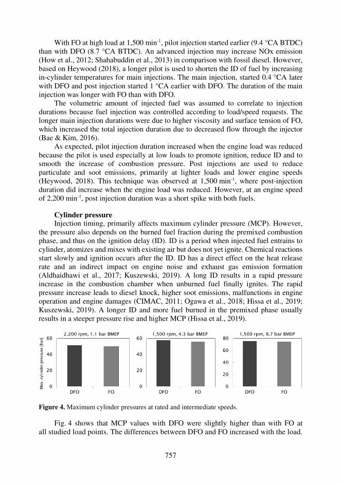
757
With FO at high load at 1,500 min-1, pilot injection started earlier (9.4 °CA BTDC) than with DFO (8.7 °CA BTDC). An advanced injection may increase NOx emission (How et al., 2012; Shahabuddin et al., 2013) in comparison with fossil diesel. However, based on Heywood (2018), a longer pilot is used to shorten the ID of fuel by increasing in-cylinder temperatures for main injections. The main injection, started 0.4 °CA later with DFO and post injection started 1 °CA earlier with DFO. The duration of the main injection was longer with FO than with DFO.
The volumetric amount of injected fuel was assumed to correlate to injection durations because fuel injection was controlled according to load/speed requests. The longer main injection durations were due to higher viscosity and surface tension of FO, which increased the total injection duration due to decreased flow through the injector (Bae & Kim, 2016).
As expected, pilot injection duration increased when the engine load was reduced because the pilot is used especially at low loads to promote ignition, reduce ID and to smooth the increase of combustion pressure. Post injections are used to reduce particulate and soot emissions, primarily at lighter loads and lower engine speeds (Heywood, 2018). This technique was observed at 1,500 min-1, where post-injection duration did increase when the engine load was reduced. However, at an engine speed of 2,200 min-1, post injection duration was a short spike with both fuels.
Cylinder pressure Injection timing, primarily affects maximum cylinder pressure (MCP). However,
the pressure also depends on the burned fuel fraction during the premixed combustion phase, and thus on the ignition delay (ID). ID is a period when injected fuel entrains to cylinder, atomizes and mixes with existing air but does not yet ignite. Chemical reactions start slowly and ignition occurs after the ID. ID has a direct effect on the heat release rate and an indirect impact on engine noise and exhaust gas emission formation (Aldhaidhawi et al., 2017; Kuszewski, 2019). A long ID results in a rapid pressure increase in the combustion chamber when unburned fuel finally ignites. The rapid pressure increase leads to diesel knock, higher soot emissions, malfunctions in engine operation and engine damages (CIMAC, 2011; Ogawa et al., 2018; Hissa et al., 2019; Kuszewski, 2019). A longer ID and more fuel burned in the premixed phase usually results in a steeper pressure rise and higher MCP (Hissa et al., 2019).
Figure 4. Maximum cylinder pressures at rated and intermediate speeds.
Fig. 4 shows that MCP values with DFO were slightly higher than with FO at all studied load points. The differences between DFO and FO increased with the load.

758
more rounded profile. The tail of the HRR curve is the remainder of the fuel's chemical energy released when burned gases mix with excess air that was not involved in the main combustion. (Heywood, 2018) Figs 5−7 show HRR curves for the studied fuels. A slight loss observed at the beginning of each HRR curve is due to the heat transfer into the liquid fuel for vaporising and heating (Heywood, 2018).
Fig. 5 illustrates the HRR of two fuels at 2,200 min-1 and 1.1 bar BMEP. The FO curve indicates that its pilot did not ignite properly, so FO had a higher peak HRR compared to DFO. FO's peak also occurred a few crank angle degrees later than DFO's.
Fig. 6 depicts the two HRR curves at 1,500 min-1 and 4.3 bar BMEP. The HRR of
DFO again shows a clear initial HRR peak and even an increase in the HRR at post-injection. In contrast, the FO curve shows no clear HRR peaks from either pilot or post injections, and its general profile is more rounded than DFO curve. Most likely, the high viscosity and surface tension of FO increased the droplet size of the fuel spray, impairing ignition. FO’s lower CN would also increase ignition delay leading, to retarded combustion (Bae & Kim, 2016; Heywood, 2018; Hissa et al., 2019). However, the lower compressibility and higher oxygen content of FO may have accelerated the HRR of FO (Shahabuddin et al., 2013).
The averaged MCP values and their standard deviations of 100 consecutive cycles are given in Table 7.
Heat release rate (HRR) Combustion starts with a rapid
burning phase that lasts only a few CA degrees and produces the first spike in the HRR curve. It is followed by the main heat-release period with a longer duration and a
Table 7. Maximum cylinder pressures and standard deviations
Fuel
Speed min-1
BMEP/ Load
Max. cylinder pressure (avg) StDev
(filtered) bar, % bar DFO 2,200 1.1/10 51 0.08 FO 50 0.05 DFO 1,500 4.3/25 58 0.12 FO 56 0.07 DFO 1,500 8.7/50 76 0.13 FO 75 0.06
Figure 5. Heat release rate curves with FO and DFO at 2,200 min-1 and 1.1 bar BMEP.
Figure 6. Heat release rate curves with FO and DFO at 1,500 min-1 and 4.3 bar BMEP.
759
Mass fraction burned (MFB) In the current study, the maximum compression pressure was at two degrees CA
before the top dead centre at an engine speed of 1,000 min-1. This had no effect on measured results but must be taken into consideration when the results are examined.
Table 8 presents mass fraction burned (MFB) values with their standard deviations. MFB values were very similar with both fuels. Only at MFB 90% at 2,200 min-1 was there more than 1 °CA of difference between them. Both fuels showed MFB 50% at between 24 to 26 °CA at lower loads and at 29 °CA at higher load. Most probably, FO burned slightly more rapidly due to its oxygen content after a shade slower ignition.
Table 8. Mass fraction burned and standard deviations
Fuel
BMEP/Speed MFB 10% StDev MFB 50% StDev MFB 90% StDev bar min-1 °CA °CA °CA
DFO 1.1/2,200 12 0.41 24 0.75 65 4.3 FO 13 0.46 25 0.78 69 4.3 DFO 4.3/1,500 13 0.21 25 0.31 59 1.5 FO 14 0.17 26 0.24 58 1.4 DFO 8.7/1,500 18 0.17 29 0.26 58 1.2 FO 18 0.13 29 0.24 59 1.3
Combustion duration Combustion duration (CD) can be defined either as the time interval between
MFB 5% and MBF 90% (Fig. 8) or the time interval between MFB 10% and MFB 50% (Fig. 9).
The high viscosity and surface tension of FO generated larger droplets. Larger droplets, again, require more time to evaporate and burn (Heywood, 2018). Fig. 8 shows that at 1.1 BMEP at 2,200 min-1 and at 8.7 bar BMEP at 1,500 min-1, CD 5−90% was longer with FO than with DFO. However, FO’s high oxygen content may have improved combustion by decreasing combustion duration since CD 10−50% was shorter or equal with FO compared to DFO (Fig. 9).
Fig. 7 shows the two HRR curves when the load at 1,500 min-1 increased to 8.7 bar BMEP. Now, the FO’s HRR peak from the pilot injection is clearly evident but is still seen later than that of DFO. FO shows no post-injection peak but seemed to burn slightly faster than DFO in the later phase of combustion. Again, the high viscosity and surface tension of FO increased the size of fuel droplets, and the time required to evaporate the fuel droplets also increased.
Figure 7. Heat release rate curves with FO and DFO at 1,500 min-1 and 8.7 bar BMEP.
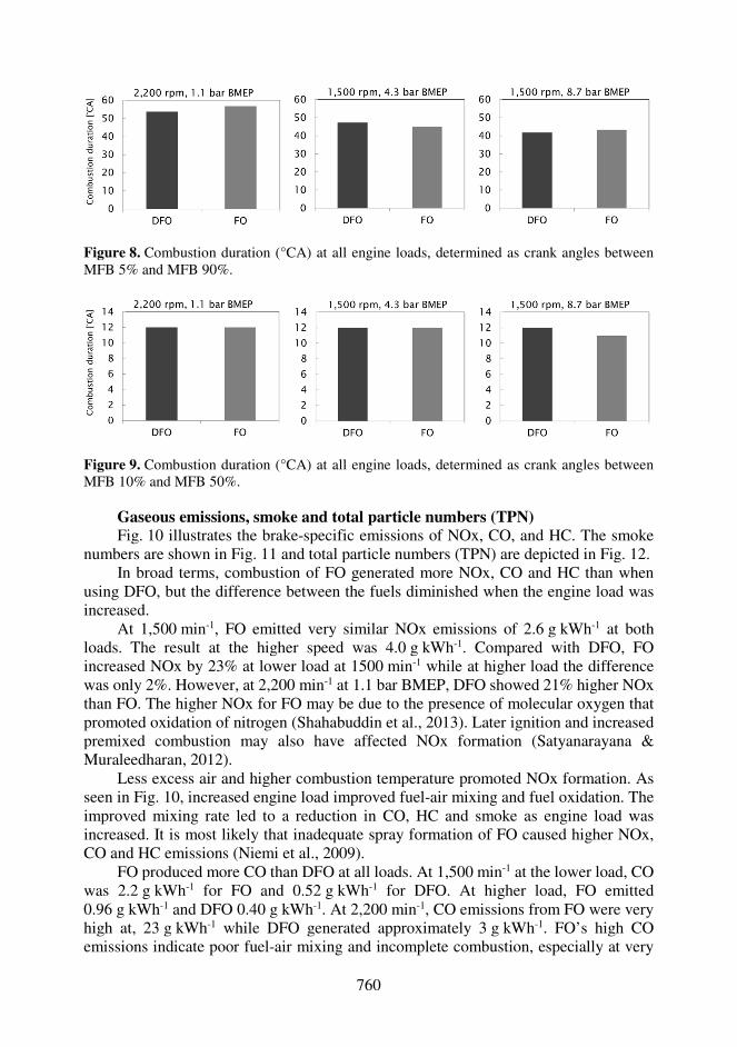
760
Figure 8. Combustion duration (°CA) at all engine loads, determined as crank angles between MFB 5% and MFB 90%.
Figure 9. Combustion duration (°CA) at all engine loads, determined as crank angles between MFB 10% and MFB 50%.
Gaseous emissions, smoke and total particle numbers (TPN) Fig. 10 illustrates the brake-specific emissions of NOx, CO, and HC. The smoke
numbers are shown in Fig. 11 and total particle numbers (TPN) are depicted in Fig. 12. In broad terms, combustion of FO generated more NOx, CO and HC than when
using DFO, but the difference between the fuels diminished when the engine load was increased.
At 1,500 min-1, FO emitted very similar NOx emissions of 2.6 g kWh-1 at both loads. The result at the higher speed was 4.0 g kWh-1. Compared with DFO, FO increased NOx by 23% at lower load at 1500 min-1 while at higher load the difference was only 2%. However, at 2,200 min-1 at 1.1 bar BMEP, DFO showed 21% higher NOx than FO. The higher NOx for FO may be due to the presence of molecular oxygen that promoted oxidation of nitrogen (Shahabuddin et al., 2013). Later ignition and increased premixed combustion may also have affected NOx formation (Satyanarayana & Muraleedharan, 2012).
Less excess air and higher combustion temperature promoted NOx formation. As seen in Fig. 10, increased engine load improved fuel-air mixing and fuel oxidation. The improved mixing rate led to a reduction in CO, HC and smoke as engine load was increased. It is most likely that inadequate spray formation of FO caused higher NOx, CO and HC emissions (Niemi et al., 2009).
FO produced more CO than DFO at all loads. At 1,500 min-1 at the lower load, CO was 2.2 g kWh-1 for FO and 0.52 g kWh-1 for DFO. At higher load, FO emitted 0.96 g kWh-1 and DFO 0.40 g kWh-1. At 2,200 min-1, CO emissions from FO were very high at, 23 g kWh-1 while DFO generated approximately 3 g kWh-1. FO’s high CO emissions indicate poor fuel-air mixing and incomplete combustion, especially at very
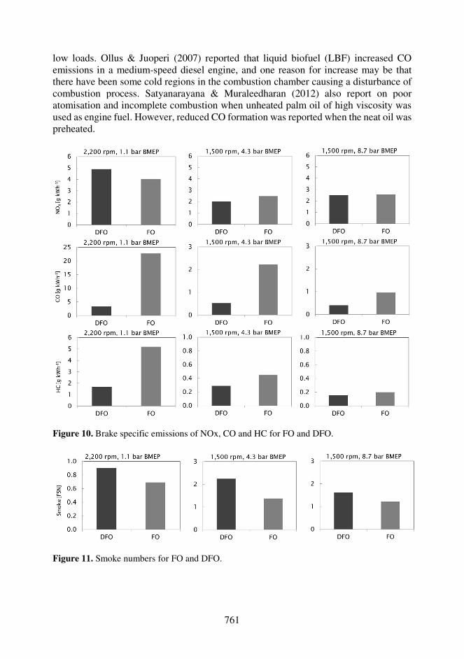
761
low loads. Ollus & Juoperi (2007) reported that liquid biofuel (LBF) increased CO emissions in a medium-speed diesel engine, and one reason for increase may be that there have been some cold regions in the combustion chamber causing a disturbance of combustion process. Satyanarayana & Muraleedharan (2012) also report on poor atomisation and incomplete combustion when unheated palm oil of high viscosity was used as engine fuel. However, reduced CO formation was reported when the neat oil was preheated.
Figure 10. Brake specific emissions of NOx, CO and HC for FO and DFO.
Figure 11. Smoke numbers for FO and DFO.
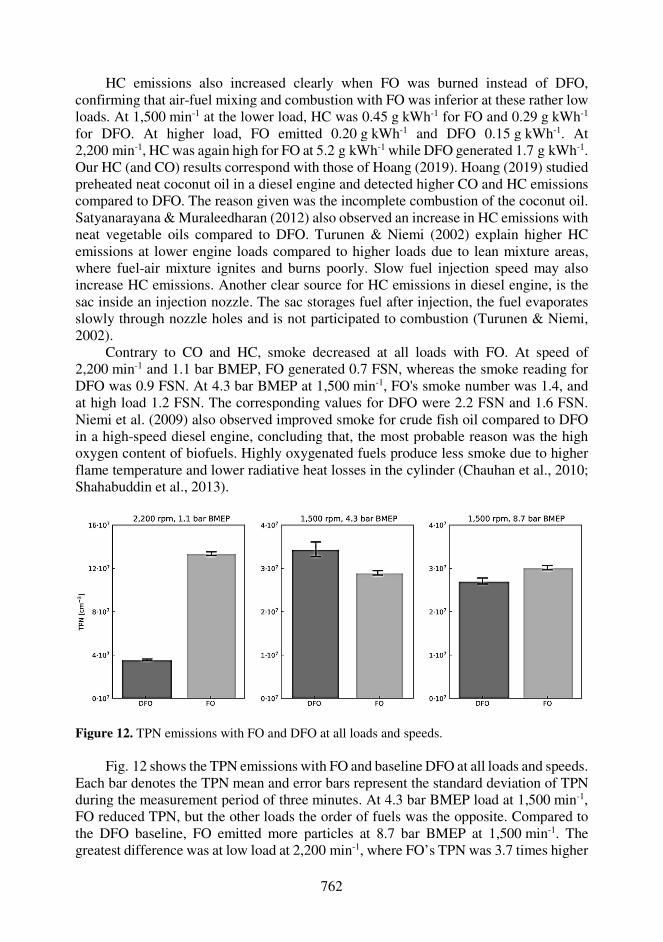
762
HC emissions also increased clearly when FO was burned instead of DFO, confirming that air-fuel mixing and combustion with FO was inferior at these rather low loads. At 1,500 min-1 at the lower load, HC was 0.45 g kWh-1 for FO and 0.29 g kWh-1 for DFO. At higher load, FO emitted 0.20 g kWh-1 and DFO 0.15 g kWh-1. At 2,200 min-1, HC was again high for FO at 5.2 g kWh-1 while DFO generated 1.7 g kWh-1. Our HC (and CO) results correspond with those of Hoang (2019). Hoang (2019) studied preheated neat coconut oil in a diesel engine and detected higher CO and HC emissions compared to DFO. The reason given was the incomplete combustion of the coconut oil. Satyanarayana & Muraleedharan (2012) also observed an increase in HC emissions with neat vegetable oils compared to DFO. Turunen & Niemi (2002) explain higher HC emissions at lower engine loads compared to higher loads due to lean mixture areas, where fuel-air mixture ignites and burns poorly. Slow fuel injection speed may also increase HC emissions. Another clear source for HC emissions in diesel engine, is the sac inside an injection nozzle. The sac storages fuel after injection, the fuel evaporates slowly through nozzle holes and is not participated to combustion (Turunen & Niemi, 2002).
Contrary to CO and HC, smoke decreased at all loads with FO. At speed of 2,200 min-1 and 1.1 bar BMEP, FO generated 0.7 FSN, whereas the smoke reading for DFO was 0.9 FSN. At 4.3 bar BMEP at 1,500 min-1, FO's smoke number was 1.4, and at high load 1.2 FSN. The corresponding values for DFO were 2.2 FSN and 1.6 FSN. Niemi et al. (2009) also observed improved smoke for crude fish oil compared to DFO in a high-speed diesel engine, concluding that, the most probable reason was the high oxygen content of biofuels. Highly oxygenated fuels produce less smoke due to higher flame temperature and lower radiative heat losses in the cylinder (Chauhan et al., 2010; Shahabuddin et al., 2013).
Figure 12. TPN emissions with FO and DFO at all loads and speeds.
Fig. 12 shows the TPN emissions with FO and baseline DFO at all loads and speeds.
Each bar denotes the TPN mean and error bars represent the standard deviation of TPN during the measurement period of three minutes. At 4.3 bar BMEP load at 1,500 min-1, FO reduced TPN, but the other loads the order of fuels was the opposite. Compared to the DFO baseline, FO emitted more particles at 8.7 bar BMEP at 1,500 min-1. The greatest difference was at low load at 2,200 min-1, where FO’s TPN was 3.7 times higher
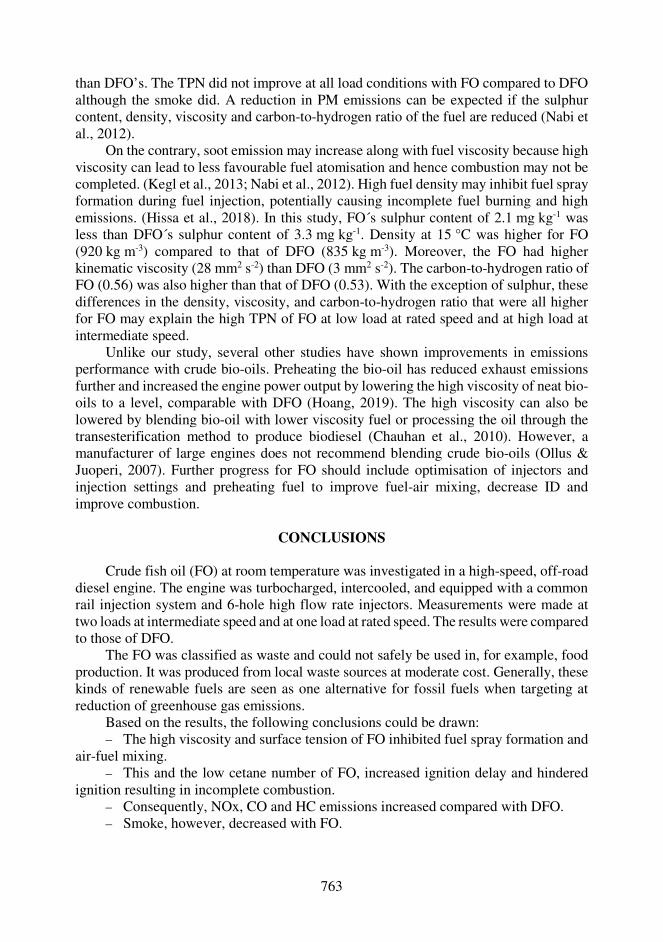
763
than DFO’s. The TPN did not improve at all load conditions with FO compared to DFO although the smoke did. A reduction in PM emissions can be expected if the sulphur content, density, viscosity and carbon-to-hydrogen ratio of the fuel are reduced (Nabi et al., 2012).
On the contrary, soot emission may increase along with fuel viscosity because high viscosity can lead to less favourable fuel atomisation and hence combustion may not be completed. (Kegl et al., 2013; Nabi et al., 2012). High fuel density may inhibit fuel spray formation during fuel injection, potentially causing incomplete fuel burning and high emissions. (Hissa et al., 2018). In this study, FO´s sulphur content of 2.1 mg kg-1 was less than DFO´s sulphur content of 3.3 mg kg-1. Density at 15 °C was higher for FO (920 kg m-3) compared to that of DFO (835 kg m-3). Moreover, the FO had higher kinematic viscosity (28 mm2 s-2) than DFO (3 mm2 s-2). The carbon-to-hydrogen ratio of FO (0.56) was also higher than that of DFO (0.53). With the exception of sulphur, these differences in the density, viscosity, and carbon-to-hydrogen ratio that were all higher for FO may explain the high TPN of FO at low load at rated speed and at high load at intermediate speed.
Unlike our study, several other studies have shown improvements in emissions performance with crude bio-oils. Preheating the bio-oil has reduced exhaust emissions further and increased the engine power output by lowering the high viscosity of neat bio-oils to a level, comparable with DFO (Hoang, 2019). The high viscosity can also be lowered by blending bio-oil with lower viscosity fuel or processing the oil through the transesterification method to produce biodiesel (Chauhan et al., 2010). However, a manufacturer of large engines does not recommend blending crude bio-oils (Ollus & Juoperi, 2007). Further progress for FO should include optimisation of injectors and injection settings and preheating fuel to improve fuel-air mixing, decrease ID and improve combustion.
CONCLUSIONS
Crude fish oil (FO) at room temperature was investigated in a high-speed, off-road
diesel engine. The engine was turbocharged, intercooled, and equipped with a common rail injection system and 6-hole high flow rate injectors. Measurements were made at two loads at intermediate speed and at one load at rated speed. The results were compared to those of DFO.
The FO was classified as waste and could not safely be used in, for example, food production. It was produced from local waste sources at moderate cost. Generally, these kinds of renewable fuels are seen as one alternative for fossil fuels when targeting at reduction of greenhouse gas emissions.
Based on the results, the following conclusions could be drawn: – The high viscosity and surface tension of FO inhibited fuel spray formation and
air-fuel mixing. – This and the low cetane number of FO, increased ignition delay and hindered
ignition resulting in incomplete combustion. – Consequently, NOx, CO and HC emissions increased compared with DFO. – Smoke, however, decreased with FO.

764
– Except at low load at 1,500 min-1, the TPN did not improve with FO compared to DFO. Density, viscosity, and carbon-to-hydrogen ratio were all higher for FO, so these differences may explain the high TPN with FO.
– Optimisation of the injection system and preheating the fuel are the main avenues towards improving engine performance and emissions with FO. Operation at very low loads most probably should also be avoided when using FO.
ACKNOWLEDGEMENTS. This project was one part of the national Future Combustion Engine Power Plant research program (grant number: 2804/31/2009). The authors wish to thank Business Finland for the financial support of the program. The authors offer their appreciation to Ms. Katriina Sirviö, Mr. Olav Nilsson, Mr. Markus Uuppo Mr. Henri Huusko and Mr. Marko Vallinmäki for their kind assistance in the measurements.
REFERENCES Adeoti, I.A. & Hawboldt, K. 2015. Comparison of biofuel quality of waste derived oils as a
function of oil extraction methods. Fuel 158, 183−190. Aldhaidhawi, M., Chiriac, R. & Badescu, V. 2017. Ignition delay, combustion and emission
characteristics of Diesel engine fueled with rapeseed biodiesel -A literature review. Renewable and Sustainable Energy Review 73, 178−186.
Bae, C. & Kim, J. 2016. Alternative fuels for internal combustion engines. Proceedings of the Combustion Institute 0000, 1−5.
Bhaskar, K., Nagarajan, G. & Sampath, S. 2013. Optimization of FOME (fish oil methyl esters) blend and EGR (exhaust gas recirculation) for simultaneous control of NOx and particulate matter emissions in diesel engines. Energy 62, 224−234.
Bosch GmbH. 2018. Automotive Handbook. 10th Edition, Robert Bosch GmbH, Karlsruhe, Germany. ISBN 978-1-119-53081-7, 1750 pp.
Bruun, N., Shoulaifar, T.K., Hemming, J., Willför, S & Hupa, L. 2019. Characterization of waste bio-oil as an alternate source of renewable fuel for marine engines. Biofuels. ISSN: 1759-7269. doi: 10.1080/17597269.2019.1628481
Chauhan, B.S., Kumar, N., Du Jun, Y. & Lee, K.B. 2010. Performance and emission study of preheated Jatropha oil on medium capacity diesel engine. Energy 35, 2484−2492.
Ching-Velasquez, J., Fernández-Lafuente, R., Rodrigues, R.C., Plata, V., Rosales-Quintero, A., Torrestiana-Sánchez, B. & Tacias-Pascacio, V.G. 2020. Production and characterization of biodiesel from oil of fish waste by enzymatic catalysis. Renewable Energy 153, 1346–1354.
CIMAC, The International Council on Combustion Engines. 2011. Fuel quality guide – Ignition and combustion. 27 pp.
de Almeida, V.F., García-Moreno, P.J., Guadix, A. & Guadix, E.M. 2015. Biodiesel production from mixtures of waste fish oil, palm oil and waste frying oil: Optimization of fuel properties. Fuel Processing Technology 133, 152−160.
Deshmukh, D., Madan Mohan, A., Anand, T.N.C. & Ravikrishna, R.V. 2012. Spray characterization of straight vegetable oils at high injection pressures. Fuel 97, 879−883.
Drenth, A.C., Olsen, D.B., Cabot, P.E. & Johnson, J.J. 2014. Compression ignition engine performance and emission evaluation of industrial oilseed biofuel feedstocks camelina, carinata, and pennycress across three fuel pathways. Fuel 136, 143−155.
EN ISO, 8178-2:2008. Reciprocating Internal Combustion Engines. Exhaust Emission Measurement; Part 2: Measurement of Gaseous and Particulate Exhaust Emissions under Feld Conditions; ISO: Geneva, Switzerland, 2008.
Esteban, B., Riba, J-R., Baquero, G., Rius, A. & Ruig, R. 2012. Temperature depence of density and viscosity of vegetable oils. Biomass and Bioenergy 42, 164−171.
765
Fan, Y., Hashimoto, N., Nishida, H & Ozawa, Y. 2014. Spray characterization of an air-assist pressure-swirl atomizer injectiong high-visocity Jatropha oils. Fuel 121, 271−283.
FAO. 2020. The State of World Fisheries and Aquaculture 2020. Sustainability in action. Rome. 244 pp. https://doi.org/10.4060/ca9229en
Heywood, J.B. 2018. Internal Combustion Engine Fundamentals, 2nd Edition, McGraw-Hill Education, USA. ISBN 978-1-260-11610-6. 1056 pp.
Hissa, M., Niemi, S.& Sirviö, K. 2018. Combustion property analyses with variable liquid marine fuels in combustion research unit. Agronomy Research 16(S1), 1032–1045.
Hissa, M., Niemi, S. & Sirviö, K. 2019. Ignition Studies of Liquid Marine Fuels with Different Ignition Analyzers. In the 29th CIMAC World Congress, Vancouver, Canada. Paper 121. 11 pp.
Hissa, M., Niemi, S. & Niemi, A. 2020. Combustion and emission studies of a common-rail direct injection diesel engine with various injector nozzles. Agronomy Research 18(3), 2033–2048. https://doi.org/10.15159/ AR.20.165
Hoang, A.T. 2019. Experimental study on spray and emission characteristics of a diesel engine fueled with preheated bio-oils and diesel fuel. Energy 171, 795−808.
How, H.G., Teoh, Y.H., Masjuki, H.H. & Kalam, M.A. 2012. Impact of coconut oil blends on particulate-phase PAHs and regulated emissions from a light duty diesel engine. Energy 48, 500−509.
Jayasinghe, P. & Hawboldt, K. 2012. A review of bio-oils from waste biomass: Focus on fish processing waste. Renewable and Sustainable Energy Reviews 16, 798–821.
Juoperi, K. & Ollus, R. 2008. Alternative fuels for medium-speed diesel engines. Wärtsilä Tech. J. 1, 24−28.
Kegl, B., Kegl, M. & Pehan, S. 2013. Green diesel engine. Biodiesel usage in diesel engines. London: Springer-Verlag. 263 pp. ISBN 978-1-4471-5324-5
Kuszewski, H. 2019. Experimental investigation of the autoignition properties of ethanol-biodiesel fuel blends. Fuel 235, 1301−1308.
Lin, C-Y & Li, R-J. 2009. Engine performance and emission characteristics of marine fish-oil biodiesel produced from the discarded parts of marine fish. Fuel Processing Technology 90, 883−888.
Nabi, M.N., Brown, R.J., Ristovski, Z. & Hustad, J.E. 2012. A comparative study of the number and mass of fine particles emitted with diesel fuel and marine gas oil (MGO). Atmos. Environ. 57, 22–28.
Niemi, S., Uuppo, M., Virtanen, S., Karhu, T., Ekman, K., Svahn, A., Vauhkonen, V., Agrawal, A. & Hiltunen, E. 2011. Animal Fat Based Raw Bio-Oils in a Non-Road Diesel Engine Equipped with a Diesel Particulate Filter. In Bartz, W.J. (ed) (2011): 8th International Colloquium Fuels; Conventional and Future Energy for Automobiles. Ostfildern, Germany: Technische Akademie Esslingen, pp. 517–528.
Niemi, S., Vauhkonen, V., Hiltunen, E., Virtanen, S., Karhu, T., Ekman, K., Salminen, H. & Appelberg, S. 2009. Results of an Off-Road Diesel Engine Driven with Different Animal Fat Based Biofuels. In ASME Internal Combustion Engine Division 2009 Fall Technical Conference. Lucerne, Switzerland. ASME Paper ICEF2009-14010
Ministry of the Environment, Finland. 2019. Government’s climate policy: carbon-neutral Finland by 2035. Available in: https://ym.fi/en/carbon-neutral-finland-2035.
Murtonen, T. 2004. Fuel quality effects on fuel consumption in a heavy-duty diesel engine. Project report PRO3/P5115/04. VTT Technical Research Centre of Finland Ltd. pp. 7. (in Finnish).
Ogawa, H., Morita, A., Futagami, K. & Shibata, G. 2018. Ignition delay in diesel combustion and intake gas conditions. International Journal of Engine Research 19(8), 805−812.

766
Ollus, R. & Juoperi, K. 2007. Alternative fuels experiences for medium-speed diesel engines. In The 25th CIMAC World Congress 2007, Vienna, Austria. Paper 234, 15 pp.
Rakopoulos, D.C., Rakopoulos, C.D., Giakoumis, E.G., Papagiannakis, R.G. & Kyritsis, D.C. 2014. Influence of properties of various common bio-fuels on the combustion and emission characteristics of high-speed DI (direct injection) diesel engine: Vegetable oil, bio-diesel, ethanol, n-butanol, diethyl eter. Energy 73, 354–366.
Satyanarayana, M. & Muraleedharan, C. 2012. Experimental Studies on Performance and Emission Characteristics of Neat Preheated Vegetable Oils in a DI Diesel Engine. Energy Sources, Part A: Recovery, Utilization, and Environmental Effects 34, 1710–1722.
Shahabuddin, M., Liaquat, A.M., Masjuki, H.H., Kalam, M.A. & Mofijur, M. 2013. Ignition delay, combustion and emission characteristics of diesel engine fueled with biodiesel. Renewable and Sustainable Energy Reviews 21, 623−632.
Sirviö, K. 2018. Issues of various alternative fuel blends for off-road, marine and power plant diesel engines. Dissertation, Acta Wasaensia 400, University of Vaasa, Finland. ISBN 978-952-476-805-4, 138 pp.
Skog, S-F., Nilsson, O. & Stam, U. 2013. Biofuels at fisheries industry – project report, serie R: Report 7/2013. Novia University of Applied Sciences, Finland. ISBN: 978-952-5839-78-4, pp. 38 (in Swedish).
Turunen, R & Niemi, S. 2002. Chapter 21 – Polttomoottorit, In Raiko, R., Saastamoinen, J., Hupa, M & Kurki-Suoni, I. (eds), Poltto ja palaminen, 2nd Edition. International Flame Research Foundation, Teknillistieteelliset akatemiat, Helsinki, Finland. ISBN 951-666-604-3, pp. 614−620.
Wang, X., Grose, M.A., Caldow, R., Osmondson, B.L., Swanson, J.J., Chow, J.C., Watson, J. G., Kittelson, D.B., Li, Y., Xue, J., Jung, H. & Hu, S. 2016. Improvement of Engine Exhaust Particle Sizer (EEPS) Size Distribution Measurement – II. Engine Exhaust Particles. J. Aerosol Sci. 92, 83–94.

767
Agronomy Research 19(S1), 767–776, 2021 https://doi.org/10.15159/AR.21.021
Effect of pre-seed and foliar treatment with nano-particle solutions on seedling development of tiger nut
(Cyperus Esculentus L.) plants
L. Honchar1, B. Mazurenko1,*, O. Shutyi1, V. Pylypenko1, D. Rakhmetov2
1National University of Life and Environmental Science, Department of Plant Science, Heroiv Oborony street 15, UA03041 Kyiv, Ukraine 2Gryshko National Botanic Garden, National Academy of Sciences of Ukraine, Timiryazevska street 1, UA01014 Kyiv, Ukraine *Correspondence: [email protected] Received: December 28th, 2020; Accepted: March 28th, 2021; Published: April 5th, 2021 Abstract. Micronutrients are part of enzymes and play an important role in plant germination. Purpose of our study was to establish the effect of pre-seed treatment of chufa tubers with metal nanoparticles on the growth of the root system and seedlings in the early stages of development. Laboratory tests were performed on seed of tiger nut cultivar Pharaoh. Experiment involved two methods of treatment: pre-sowing treatment of seeds with nano-particles solutions of manganese, zinc, copper and iron with a concentration of 60 ppm and re-application of these solutions after seedling emergence. The weight of seedlings and roots was determined at 3rd and 10th days after emergence in treated and untreated variants. Pre-sowing treatment of chufa tubers with all forms of micronutrients significantly increased the weight of the plant (excluding the weight of seeds), and the most effective were treatments with copper and iron. Treatment with copper colloidal solution increases in root weight at 3rd day on 156% compared to control without treatment and this dynamic stayed at 10th day. Most affective treatment is iron colloidal solution. This treatment gives +99% of root weight at 3rd day and 194% at 10th day after germination compared to control in same time. Colloidal forms of manganese, copper and iron also significantly increased the weight of the shoot. Increase in the mass of roots, shoots and plants is observed in plants with foliar fertilizing, but a few variants have an insignificant difference or inhibit the assimilation processes of plants. Pre-sowing treatment with zinc citrate at 60 ppm decreased root and shoot weight in chufa.
Key words: citrate, chufa, colloidal, copper, iron, manganese, solution, zinc.
INTRODUCTION Tiger nut or chufa (Cyperus Esculentus L.) is a highly productive crop that
accumulates nutrients in the tubers (Mokady & Dolev, 1970). Tubers are used for planting, so the content of nutrients in the tuber significantly affects the initial growth and formation of plant productivity. Accumulation of dry matter in chufa occurs exponentially up to 90 days, while in the initial stages the leaves and roots grow. Formation and accumulation of dry matter in the tubers of chufa occurs only

768
1.5–2 months after germination (Pascual-Seva et al., 2009). Stimulation of root and leaf surface growth at the initial stages of development will allow to form a more efficient photosynthetic system (leaf) with increased drought resistance (root).
Requirement for macro- and micro-nutrients in plants is fully covered by the reserves of tubers in the first 15 days. Content of micronutrients in the tubers varies significantly and depends on the region of cultivation. iron content in the tubers can be from 2.00 mg per 100 g (Arafat et al., 2009) till 6.18 mg per 100 g of tuber (Salama et al., 2013), but a greater extent Fe is concentrated in the inner part of the tuber (Ekeanyanwu & Ononogbu, 2010). Zinc content is 2 times lower than iron and is on a par with copper, and the manganese content differs significantly from the place of cultivation and the method of establishing the content (Arafat et al., 2009, Ekeanyanwu & Ononogbu, 2010). Copper content in the tubers is on average 4 times lower than iron and varies much less (Suleiman et al., 2018).
Soil factors can complicate the absorption of zinc and other trace elements from the salts contained in fertilizers (Alloway, 2009). ‘Controlled release’ property of nanoparticles allows them to include in physiological cicles in 'right dose' at the 'right time' (Kumar et al., 2014), however not all materials have this property (Deshpande et al., 2017). Main advantages of nanoparticle solution for fertilizations are control deliverey of nutrients, increase it bioavailability and reduce loss rate of nutrients (Zulfiqar et al., 2019). On the other hand, there is a risk to food safety because micronutrients are heavy metals and can accumulate in edible parts (López-Moreno et al., 2018).
Trace elements stimulate the awakening of tubers, as well as the growth of roots and stems in the initial stages (Farooq et al., 2012; Taran et al., 2016). Growth of shoots in chufa after germination is slow, so the greater the vegetative mass is formed in the initial stages, the more shoots and dry matter will accumulate in the active phase (Kelley, 1990). Effect of different micronutrients on the formation of the vegetative organs of the chufa under pre-sowing treatment with micronutrients (Mn, Cu, Zn, Fe) is poorly understood, and the effect may vary because sowing material of chufa is a tuber. Chufa tubers contain a lot of carbohydrates and fats (Pascual et al., 2000; Makareviciene et al., 2013), so their breakdown and use for the formation of roots and seedlings will depend on the enzyme system, which includes trace elements.
MATERIALS AND METHODS
Experimental conditions Laboratory tests were performed on tubers of tiger nut variety Pharaoh. All tubers
were aligned in size and shape, the weight of 1,000 tubers was 1.14 ± 0.02 g. Tubers on the day of planting were treated with solutions of nanoparticles with a concentration of 60 ppm. Tubers of chufa had planted in perlite (Fe free). Air temperature was + 22 ℃. Tiger nut plants cultivated on a 12-hour light/12-hour dark cycle.
Experiment design Scheme of research included two factors (Table 1). Factor A is nanoparticle
solution: water (control, without nanoparticles), manganese citrate (Mn citrate), colloidal solution of manganese (Mn colloidal - MnO, MnCO3), zinc citrate (Zn citrate), colloidal solution of zinc (Zn colloidal - Zn, ZnO), copper citrate (Cu citrate), colloidal solution

769
of copper (Cu colloidal - Cu, CuO), iron (II) citrate (Fe citrate), colloidal solution of iron (Fe colloidal - Fe, Fe3O4, FeO). Factor B was treatment time. There were pre-sowing tuber treatment and pre-sowing tuber treatment + foliar fertilizing (3rd day after emergency) in treatment time. Pre-sowing treatment (spraying of tubers) was carried out at 1 hours before sowing. Rate of consumption of the solution to pre-sowing treatment was 1.2 L t-1 (500 mg L-1 of nanometal solution) of tuber and 0.2 L ha-1 (500 mg L-1 of nanoparticles) to foliar fertilizing (density is 150,000 plants ha-1). Working solution to pre-sowing treatment was 10 L t-1 (concentration of nanoparticles is 60 ppm) of tuber and 100 L ha-1 (concentration of nanoparticles is 1 ppm) to foliar fertilizing. Solutions were prepared based on application rate of 100 mg ha-1 Mn, Cu, Zn or Fe in pre-sowing treatment and foliar fertilizing.
Colloidal nanoparticle solution
Table 1. Scheme of research
Factor A – nanoparticle solution
Size, nm
Factor B – Treatment time
Water (control) – B1. Pre-sowing treatment of tuber (PST) B2. Pre-sowing treatment of tuber + Foliar fertilizing (PST + FT)
Mn colloidal 53 Mn citrate – Zn colloidal 45 Zn citrate – Cu colloidal 78 Cu citrate – Fe colloidal 25–60 Fe citrate –
‘–‘ size is not established.
was produced by method of metal dispersion by electric current pulses with an amplitude of 100 to 2,000 A in water (Lopatko et al., 2009). Size and other properties of nanoparticles in the experimental colloidal solution obtained by X-ray diffraction and the diffraction patterns of the specimens (Batsmanova et al., 2020). Size of nanoparticles that was obtained by physical method is showed in Table 1. Citrate forms (nanoaquachelates) was obtained by erosive-explosive method at LLC ‘Nanomatherials and Nanotechnologies’ (Ukraine). Citrate forms (Mn, Zn, Cu, Fe) of fertilizers are characterized by a much smaller particle size (Cao et al., 2013; Huliaieva et al., 2018).
Calculation was performed so that the rate of solution for foliar fertilizing was similar to pre-sowing treatment on one plant/tuber. Foliar fertilizing was performed on 3rd day after emergence so results on 3rd day do not include root and leaf weight by foliar treatment variants.
Sampling Mass of roots and leaves was
determined on the 3rd and 10th day after emergence. Ten plants (n = 10) from each variant were selected. Root system and leaf surface were weighed separately, the weight of the tuber was not taken into account (Fig. 1).
Figure 1. Chufa plant on 3rd day after emergence.

770
Statistical analysis Suitability of the sample for statistical analysis was evaluated according to the
Shapiro-Wilk test. Effect power on 3rd day was assessed by one-factor ANOVA, and on 10th day by two-factor ANOVA. Difference between the variants was assessed by Tukey post-hoc test.
RESULTS AND DISCUSSION
Effect of pre-sowing treatment on 3rd day after germination Root weight Colloidal forms of micro elements had a significant effect on the mass of the root
system on day 3 after germination (Fig. 2). The highest mass of roots was formed by pre-sowing treatment of tubers with a colloidal solution of copper. Pre-sowing treatment with copper citrate did not differ significantly from the control variant. Effect of treatment with manganese solutions on the growth of the root system differed significantly from the type of the solution. Treatment with a colloidal solution of manganese allowed to form 0.282 g of roots. which did not differ significantly from the value of treatment with colloidal solution of iron and iron citrate. Iron citrate was more effective than colloidal solution, but only on 8.8%. Treatment with colloidal zinc solution had the least effect among colloidal solutions, but gave a significant increase compared to control variant.
Figure 2. Raw mass of chufa plant components (n = 10) on 3rd day after emergency depends on pre-sowing seed treatments with nanoparticle solutions of metals (different superscripts denote statistical significance at p ≤ 0.05 by Tukey`s post-hoc test; leaf and root weight were analysed separately).
Leaf weight Effect of seed treatment with trace elements was manifested on the leaf surface
differently than on the roots. The largest raw mass of leaves was in the variants by treatment of tubers with colloidal solution of iron, iron citrate and colloidal solution of
a
bc
a
a
bc
cc
bcc
ab
d
a
dd
0
0.05
0.1
0.15
0.2
0.25
0.3
0.35
Wa
ter
(c)
Mn
colo
ida
l
Mn
citra
te
Zn
co
loid
al
Zn
citra
te
Cu
co
loid
al
Cu
citra
te
Fe
co
loid
al
Fe
citra
te
Wa
ter
(c)
Mn
colo
ida
l
Mn
citra
te
Zn
co
loid
al
Zn
citra
te
Cu
co
loid
al
Cu
citra
te
Fe
co
loid
al
Fe
citra
te
Roots Leaves
Raw
mass, g

771
copper. Pre-sowing treatment of tubers with manganese solutions and colloidal zinc solution did not significantly affect the weight of seedlings compared to control variant. Variants by treatment with zinc citrate and copper citrate formed a significantly lower mass of seedlings than without treatment, because phytotoxicity may occur. These variants also formed the root system at the level of control variant, therefore the total weight of the plant was less than in the control.
Pre-sowing treatment with solutions of iron (colloidal and citrate form) and colloidal solution of copper were the most effective in assessing the weight of roots and leaves on 3rd day after germination. Mass of roots and leaves at the initial stages of development in chufa allows us to assess the effectiveness of the use of spare substances of tubers and their utilization for the formation of vegetative organs.
Greater efficiency of colloidal forms than conventional fertilizers may be due to the size of nanoparticles and their neutrality to the environment (Batsmanova et al., 2020). At the same time, the particle size depends on the form of nanoparticle, and therefore their permeability to the tuber will be different (Wong et al., 2016). High effect of iron treatments may indicate the favour of chufa to this element because a similar effect was observed in other plants (Cifuentes et al., 2010). Effect of iron citrate on the growth of vegetative mass in Chlorella vulgaris was manifested on the second day, and the effectiveness depended on the concentration, therefore its effect in plants may be similar, but with a slower manifestation (Golub et al., 2018).
Effect of pre-sowing treatment on 10th day after germination Root weight Mass of the root system on 7th day after the previous sampling (10th day after
germination) increased, and the effect of pre-sowing treatment of tubers and foliar fertilizing (3rd day after germination) had a significant effect on the variation of this parameter (Fig. 3).
Figure 3. Raw mass of chufa plant components (n = 10) on 10 day after germination; PST – pre-sowing treatment; PST + FT – pre-sowing treatment+ foliar treatment (3rd day after emergence); different superscripts denote statistical significance at p ≤ 0.05 by Tukey`s post-hoc test; leaf and root weight were analysed separately.
b
gbc cd
a
gef
a abc a abc
ef
abd
bc
f de a
h h hde de
abc c
f
abc
e
0
0.2
0.4
0.6
0.8
1
1.2
Wa
ter
(c)
Mn
colo
ida
l
Mn
citra
te
Zn
co
loid
al
Zn
citra
te
Cu
co
loid
al
Cu
citra
te
Fe
co
loid
al
Fe
citra
te
Wa
ter
(c)
Mn
colo
ida
l
Mn
citra
te
Zn
co
loid
al
Zn
citra
te
Cu
co
loid
al
Cu
citra
te
Fe
co
loid
al
Fe
citra
te
Roots Leaves
Raw
mass, g
PST PST+FT
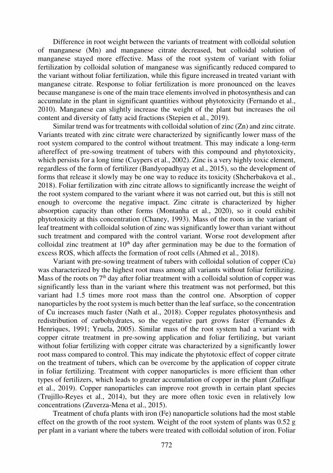
772
Difference in root weight between the variants of treatment with colloidal solution of manganese (Mn) and manganese citrate decreased, but colloidal solution of manganese stayed more effective. Mass of the root system of variant with foliar fertilization by colloidal solution of manganese was significantly reduced compared to the variant without foliar fertilization, while this figure increased in treated variant with manganese citrate. Response to foliar fertilization is more pronounced on the leaves because manganese is one of the main trace elements involved in photosynthesis and can accumulate in the plant in significant quantities without phytotoxicity (Fernando et al., 2010). Manganese can slightly increase the weight of the plant but increases the oil content and diversity of fatty acid fractions (Stepien et al., 2019).
Similar trend was for treatments with colloidal solution of zinc (Zn) and zinc citrate. Variants treated with zinc citrate were characterized by significantly lower mass of the root system compared to the control without treatment. This may indicate a long-term aftereffect of pre-sowing treatment of tubers with this compound and phytotoxicity, which persists for a long time (Cuypers et al., 2002). Zinc is a very highly toxic element, regardless of the form of fertilizer (Bandyopadhyay et al., 2015), so the development of forms that release it slowly may be one way to reduce its toxicity (Shcherbakova et al., 2018). Foliar fertilization with zinc citrate allows to significantly increase the weight of the root system compared to the variant where it was not carried out, but this is still not enough to overcome the negative impact. Zinc citrate is characterized by higher absorption capacity than other forms (Montanha et al., 2020), so it could exhibit phytotoxicity at this concentration (Chaney, 1993). Mass of the roots in the variant of leaf treatment with colloidal solution of zinc was significantly lower than variant without such treatment and compared with the control variant. Worse root development after colloidal zinc treatment at 10th day after germination may be due to the formation of excess ROS, which affects the formation of root cells (Ahmed et al., 2018).
Variant with pre-sowing treatment of tubers with colloidal solution of copper (Cu) was characterized by the highest root mass among all variants without foliar fertilizing. Mass of the roots on 7th day after foliar treatment with a colloidal solution of copper was significantly less than in the variant where this treatment was not performed, but this variant had 1.5 times more root mass than the control one. Absorption of copper nanoparticles by the root system is much better than the leaf surface, so the concentration of Cu increases much faster (Nath et al., 2018). Copper regulates photosynthesis and redistribution of carbohydrates, so the vegetative part grows faster (Fernandes & Henriques, 1991; Yruela, 2005). Similar mass of the root system had a variant with copper citrate treatment in pre-sowing application and foliar fertilizing, but variant without foliar fertilizing with copper citrate was characterized by a significantly lower root mass compared to control. This may indicate the phytotoxic effect of copper citrate on the treatment of tubers, which can be overcome by the application of copper citrate in foliar fertilizing. Treatment with copper nanoparticles is more efficient than other types of fertilizers, which leads to greater accumulation of copper in the plant (Zulfiqar et al., 2019). Copper nanoparticles can improve root growth in certain plant species (Trujillo-Reyes et al., 2014), but they are more often toxic even in relatively low concentrations (Zuverza-Mena et al., 2015).
Treatment of chufa plants with iron (Fe) nanoparticle solutions had the most stable effect on the growth of the root system. Weight of the root system of plants was 0.52 g per plant in a variant where the tubers were treated with colloidal solution of iron. Foliar
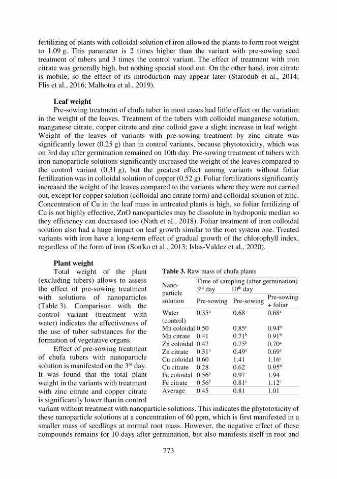
773
fertilizing of plants with colloidal solution of iron allowed the plants to form root weight to 1.09 g. This parameter is 2 times higher than the variant with pre-sowing seed treatment of tubers and 3 times the control variant. The effect of treatment with iron citrate was generally high, but nothing special stood out. On the other hand, iron citrate is mobile, so the effect of its introduction may appear later (Starodub et al., 2014; Flis et al., 2016; Malhotra et al., 2019).
Leaf weight Pre-sowing treatment of chufa tuber in most cases had little effect on the variation
in the weight of the leaves. Treatment of the tubers with colloidal manganese solution, manganese citrate, copper citrate and zinc colloid gave a slight increase in leaf weight. Weight of the leaves of variants with pre-sowing treatment by zinc citrate was significantly lower (0.25 g) than in control variants, because phytotoxicity, which was on 3rd day after germination remained on 10th day. Pre-sowing treatment of tubers with iron nanoparticle solutions significantly increased the weight of the leaves compared to the control variant (0.31 g), but the greatest effect among variants without foliar fertilization was in colloidal solution of copper (0.52 g). Foliar fertilizations significantly increased the weight of the leaves compared to the variants where they were not carried out, except for copper solution (colloidal and citrate form) and colloidal solution of zinc. Concentration of Cu in the leaf mass in untreated plants is high, so foliar fertilizing of Cu is not highly effective, ZnO nanoparticles may be dissolute in hydroponic median so they efficiency can decreased too (Nath et al., 2018). Foliar treatment of iron colloidal solution also had a huge impact on leaf growth similar to the root system one. Treated variants with iron have a long-term effect of gradual growth of the chlorophyll index, regardless of the form of iron (Son'ko et al., 2013; Islas‐Valdez et al., 2020).
Plant weight Total weight of the plant
(excluding tubers) allows to assess the effect of pre-sowing treatment with solutions of nanoparticles (Table 3). Comparison with the control variant (treatment with water) indicates the effectiveness of the use of tuber substances for the formation of vegetative organs.
Effect of pre-sowing treatment of chufa tubers with nanoparticle solution is manifested on the 3rd day. It was found that the total plant weight in the variants with treatment with zinc citrate and copper citrate is significantly lower than in control
Table 3. Raw mass of chufa plants
Nano-particle solution
Time of sampling (after germination) 3rd day 10th day
Pre-sowing Pre-sowing Pre-sowing + foliar
Water (control)
0.35a 0.68 0.68a
Mn coloidal 0.50 0.85c 0.94b
Mn citrate 0.41 0.71b 0.91b
Zn coloidal 0.47 0.75b 0.70a
Zn citrate 0.31a 0.49a 0.69a
Cu coloidal 0.60 1.41 1.16c
Cu citrate 0.28 0.62 0.95b
Fe coloidal 0.56b 0.97 1.94 Fe citrate 0.56b 0.81c 1.12c
Average 0.45 0.81 1.01
variant without treatment with nanoparticle solutions. This indicates the phytotoxicity of these nanoparticle solutions at a concentration of 60 ppm, which is first manifested in a smaller mass of seedlings at normal root mass. However, the negative effect of these compounds remains for 10 days after germination, but also manifests itself in root and
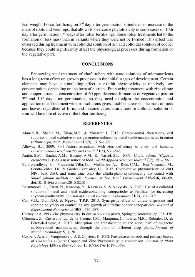
774
leaf weight. Foliar fertilizing on 3rd day after germination stimulates an increase in the mass of roots and seedlings, that allows to overcome phytotoxicity in some cases on 10th day after germination (7th days after foliar fertilizing). Some foliar treatments led to the formation of less mass than in variants where they were not performed. This effect was observed during treatment with colloidal solution of zin and colloidal solution of copper because they could significantly affect the physiological processes during formation of the vegetative part.
CONCLUSIONS
Pre-sowing seed treatment of chufa tubers with nano solutions of micronutrients
has a long-term effect on growth processes in the initial stages of development. Certain elements may have a stimulating effect or exhibit phytotoxicity at relatively low concentrations depending on the form of nutrient. Pre-sowing treatment with zinc citrate and copper citrate at concentration of 60 ppm decrease formation of vegetative part on 3rd and 10th day after germination, so they need to adjust the concentration and application rate. Treatment with iron solutions gives a stable increase in the mass of roots and leaves, regardless of form, and in some cases, iron citrate or colloidal solution of iron will be more effective if the foliar fertilizing.
REFERENCES
Ahmed, B., Shahid, M., Khan, M.S. & Musarrat, J. 2018. Chromosomal aberrations, cell
suppression and oxidative stress generation induced by metal oxide nanoparticles in onion (Allium cepa) bulb. Metallomics 10(9), 1315–1327.
Alloway, B.J. 2009. Soil factors associated with zinc deficiency in crops and humans. Environmental Geochemistry and Health 31(5), 537–548.
Arafat, S.M., Gaafar, A.M., Basuny, A.M. & Nassef, S.L. 2009. Chufa tubers (Cyperus esculentus L.): As a new source of food. World Applied Sciences Journal 7(2), 151–156.
Bandyopadhyay, S., Plascencia-Villa, G., Mukherjee, A., Rico, C.M., José-Yacamán, M., Peralta-Videa, J.R. & Gardea-Torresdey, J.L. 2015. Comparative phytotoxicity of ZnO NPs, bulk ZnO, and ionic zinc onto the alfalfa plants symbiotically associated with Sinorhizobium meliloti in soil. Science of The Total Environment 515–516, 60–69. doi:10.1016/j.scitotenv.2015.02.014
Batsmanova, L., Taran, N., Konotop, Y., Kalenska, S. & Novytska, N. 2020. Use of a colloidal solution of metal and metal oxide-containing nanoparticles as fertilizer for increasing soybean productivity. Journal of Central European Agriculture 21(2), 311–319.
Cao, V.D., Tran, N.Q. & Nguyen, T.P.P. 2013. Synergistic effect of citrate dispersant and capping polymers on controlling size growth of ultrafine copper nanoparticles. Journal of Experimental Nanoscience 10(8), 576–587.
Chaney, R.Á. 1993. Zinc phytotoxicity. In Zinc in soils and plants, Springer, Dordrecht, pp. 135–150. Cifuentes, Z., Custardoy, L., de la Fuente, J.M., Marquina, C., Ibarra, M.R., Rubiales, D. &
Pérez-de-Luque, A. 2010. Absorption and translocation to the aerial part of magnetic carbon-coated nanoparticles through the root of different crop plants. Journal of Nanobiotechnology 8(1), 26.
Cuypers, A. n. n., Vangronsveld, J. & Clijsters, H. 2002. Peroxidases in roots and primary leaves of Phaseolus vulgaris Copper and Zinc Phytotoxicity: a comparison. Journal of Plant Physiology 159(8), 869–876. doi:10.1078/0176-1617-00676
775
Deshpande, P., Dapkekar, A., Oak, M.D., Paknikar, K.M. & Rajwade, J.M. 2017. Zinc complexed chitosan/TPP nanoparticles: A promising micronutrient nanocarrier suited for foliar application. Carbohydrate Polymers 165, 394–401.
Ekeanyanwu, R.C. & Ononogbu, C.I. 2010. Nutritive value of Nigerian tigernut (Cyperus esculentus L.). Agricultural Journal 5(5), 297–302.
Farooq, M., Wahid, A. & Siddique, K.H. 2012. Micronutrient application through seed treatments: a review. Journal of Soil Science and Plant Nutrition 12(1), 125–142.
Fernandes, J.C. & Henriques, F.S. 1991. Biochemical, physiological, and structural effects of excess copper in plants. The Botanical Review 57(3), 246–273.
Fernando, D.R., Mizuno, T., Woodrow, I.E., Baker, A.J.M. & Collins, R.N. 2010. Characterization of foliar manganese (Mn) in Mn (hyper) accumulators using X-ray absorption spectroscopy. New Phytologist, 1014–1027.
Flis, P., Ouerdane, L., Grillet, L., Curie, C., Mari, S. & Lobinski, R. 2016. Inventory of metal complexes circulating in plant fluids: a reliable method based on HPLC coupled with dual elemental and high‐resolution molecular mass spectrometric detection. New Phytologist 211(3), 1129–1141.
Golub, N.B., Tsvetkovych, M., Levtun, I.I. & Maksyn, V.I. 2018. Nanostructured ferric citrate effect on Chlorella vulgaris development. Biotechnologia Acta 11(6). https://doi.org/10.15407/biotech11.06.047
Huliaieva, H., Tokovenko, I., Maksin, V., Kaplunenko, V. & Kalinichenko, A. 2018. Effect of nanoaquacitrates on physiological parameters of Fodder Galega infected with phytoplasma. Ecological Chemistry and Engineering S 25(1), 153–168.
Islas‐Valdez, S., López‐Rayo, S., Arcos, J., Menéndez, N. & Lucena, J.J. 2020. Effect of Fe: ligand ratios on hydroponic conditions and calcareous soil in Solanum lycopersicum L. and Glycine max L. fertilized with heptagluconate and gluconate. Journal of the Science of Food and Agriculture 100(3), 1106–1117.
Kelley, J.R. 1990. Biomass production of chufa (Cyperus esculentus) in a seasonally flooded wetland. Wetlands 10(1), 61–67. doi:10.1007/bf03160823
Kumar, S., Bhanjana, G., Sharma, A., Sidhu, M.C. & Dilbaghi, N. 2014. Synthesis, characterization and on field evaluation of pesticide loaded sodium alginate nanoparticles. Carbohydrate Polymers 101, 1061–1067.
Lopatko, K.G., Aftandilyants, E.H., Kalenska, S.M. & Tonkha, O.L. 2009. Mother colloidal solution of metals. Ukraine: B01J 13/00 Patent of Ukraine (No. 38459 12 January 2009). [Online] Available at: http://uapatents.com/4-38459-matochnijj-kolodnijj-rozchin-metaliv.html
López-Moreno, M.L., Cassé, C. & Correa-Torres, S.N. 2018. Engineered NanoMaterials interactions with living plants: Benefits, hazards and regulatory policies. Current Opinion in Environmental Science & Health 6, 36–41.
Makareviciene, V., Gumbyte, M., Yunik, A., Kalenska, S., Kalenskii, V., Rachmetov, D. & Sendzikiene, E. 2013. Opportunities for the use of chufa sedge in biodiesel production. Industrial Crops and Products 50, 633–637. doi:10.1016/j.indcrop.2013.08.036
Malhotra, H., Pandey, R., Sharma, S. & Bindraban, P.S. 2019. Foliar fertilization: possible routes of iron transport from leaf surface to cell organelles. Archives of Agronomy and Soil Science 66(3), 279–300. doi:10.1080/03650340.2019.1616288
Mokady, S.H. & Dolev, A. 1970. Nutritional evaluation of tubers of Cyperus esculentus L. Journal of the Science of Food and Agriculture 21(4), 211–214.
Montanha, G.S., Rodrigues, E.S., Romeu, S.L., de Almeida, E., Reis, A.R., Lavres, Jr,J. & de Carvalho, H.W.P. 2020. Zinc uptake from ZnSO4 (aq) and Zn-EDTA (aq) and its root-to-shoot transport in soybean plants (Glycine max) probed by time-resolved in vivo X-ray spectroscopy. Plant Science 292, 110370.

776
Nath, J., Dror, I., Landa, P., Vanek, T., Kaplan-Ashiri, I. & Berkowitz, B. 2018. Synthesis and characterization of isotopically-labeled silver, copper and zinc oxide nanoparticles for tracing studies in plants. Environmental Pollution 242, 1827–1837.
Pascual, B., Maroto, J.V., López-Galarza, S., Sanbautista, A. & Alagarda, J. 2000. Chufa (Cyperus esculentus L. var. sativus Boeck.): an unconventional crop. Studies related to applications and cultivation. Economic Botany 54(4), 439–448.
Pascual-Seva, N., Pascual, B., San Bautista, A., López-Galarza, S. & Maroto, J.V. 2009. Growth and nutrient absorption in chufa (Cyperus esculentus L. var. sativus Boeck.) in soilless culture. The Journal of Horticultural Science and Biotechnology 84(4), 393–398. doi:10.1080/14620316.2009.11512538
Salama, M.A., Osman, M.F., Owon, M.A. & Esmail, A.I. 2013. Chemical and technological characterization of tigernut (Cyperus esculentus L.) tubers. Journal of Food and Dairy Sciences 4(6), 323–332.
Shcherbakova, E.N., Rots, P.Y., Mulina, S.A., Shcherbakov, A.V., Lactionov, Y.V., Yahina, L.M., Gonchar, L.N. & Chebotar, V.K. 2018. Inoculation technology for legumes based on alginate encapsulation. Agronomy research 16(5), 2156–2168. https://doi.org/10.15159/AR.18.186
Son'ko, R.V., Starodub, N.F., Trach, V.V. & Lopat’ko, K.G. 2013. Effect of colloidal metals on the induced chlorophyll fluorescence at the different lupin state. In Biophotonics—Riga 2013. Vol. 9032, p. 90320Z.
Starodub, N.F., Shavanova, K.E., Taran, M.V., Katsev, A.M., Safronyuk, S.L., Son’ko, R.V., Bisio, C. & Guidotti, M. 2014. Nanomaterials: biological effects and some aspects of applications in ecology and agriculture. In Eighth International Conference on Advanced Optical Materials and Devices (AOMD-8). Vol. 9421, p. 942106.
Stepien, A., Wojtkowiak, K., Pietrzak-Fiecko, R., Zalewska, M. & Grzywinska-Rapca, M. 2019. Effect of manganese and nitrogen fertilization on the content of some essential micronutrients and composition of fatty acids in winter wheat grain. Chilean Journal of Agricultural Research 79(4), 616–627.
Suleiman, M.S., Olajide, J.E., Omale, J.A., Abbah, O.C. & Ejembi, D.O. 2018. Proximate composition, mineral and some vitamin contents of tigernut (Cyperus esculentus). Clinical Investigation 8(4), 161–165.
Taran, N., Batsmanova, L., Kosyk, O., Smirnov, O., Kovalenko, M., Honchar, L. & Okanenko, A. 2016. Colloidal nanomolybdenum influence upon the antioxidative reaction of chickpea plants (Cicer arietinum L.). Nanoscale research letters 11(1), 1–5.
Trujillo-Reyes, J., Majumdar, S., Botez, C.E., Peralta-Videa, J.R. & Gardea-Torresdey, J.L. 2014. Exposure studies of core–shell Fe/Fe3O4 and Cu/CuO NPs to lettuce (Lactuca sativa) plants: are they a potential physiological and nutritional hazard?. Journal of Hazardous Materials 267, 255–263.
Wong, M.H., Misra, R.P., Giraldo, J.P., Kwak, S.Y., Son, Y., Landry, M.P., ... & Strano, M.S. 2016. Lipid exchange envelope penetration (LEEP) of nanoparticles for plant engineering: a universal localization mechanism. Nano Letters 16(2), 1161–1172.
Yruela, I. 2005. Copper in plants. Brazilian Journal of Plant Physiology 17(1), 145–156. Zulfiqar, F., Navarro, M., Ashraf, M., Akram, N. A. & Munné-Bosch, S. 2019. Nanofertilizer use
for sustainable agriculture: advantages and limitations. Plant Science 289, 110270. Zuverza-Mena, N., Medina-Velo, I.A., Barrios, A.C., Tan, W., Peralta-Videa, J.R. & Gardea-
Torresdey, J.L. 2015. Copper nanoparticles/compounds impact agronomic and physiological parameters in cilantro (Coriandrum sativum). Environmental Science: Processes & Impacts 17(10), 1783–1793.
777
Agronomy Research 19(S1), 777–787, 2021 https://doi.org/10.15159/AR.21.027
Thermo mechanical vibration of single wall carbon nanotube partially embedded into soil medium
M. Hossain* and J. Lellep
University of Tartu, Faculty of Science and Technology, Institute of mathematics and statistics, Narva mnt 18, EE51009 Tartu, Estonia *Correspondence: [email protected] Received: January 2nd, 2021; Accepted: April 2nd, 2021; Published: April 7th, 2021 Abstract. Single wall carbon nanotube is one of the promising forms of carbon nanocomposite. Due to its high strength and stiffness, carbon nanotube is potentially used in various nanoscale structures. In this paper, dynamic behaviour of single wall carbon nanotube partially embedded into elastic soil medium is modelled by the Euler-Bernoulli beam theory and nonlocal theory of elasticity. Analytical solution technique is employed to solve these governing differential equations of nanotube. Analysing the effects of temperature, nonlocal parameter, coefficients of elastic medium on dynamic behaviour of nanotube are our main concern. The results reveal that the effects of temperature, nonlocal parameter and coefficients of elastic medium are very significant on the natural frequency of nanotube. Key words: carbon nanotube, partially embedded, elastic soil medium, temperature effect, exact solution technique.
INTRODUCTION
Carbon nanotube is very promising and effective element that has been used for developing high-performance composites. The main advantages of the carbon nanotube are its high chemical stability as well as its strong mechanical properties. In this paper, thermal effects on the dynamic behaviour of nanotube embedded into the soil (Haldar & Basu, 2013; Zhao et al., 2016; Zhang et al., 2018; Elhuni & Basu, 2019; Falope et al., 2020) or elastic medium are investigated. Soil can be considered as an elastic foundation. Basically, Winkler’s model is used to simulate the soil foundation. According to Winkler’s model, foundation is demonstrated by a series of discrete infinitesimal and mutually independent, closely spaced, linearly elastic lateral springs which provide resistance in direct proportion to its deflection. This model is very simple and popular among researchers. However, this model is unable to include the soil cohesive force or shear force. That is why Winkler’s model is not sufficient for evaluating the mechanical behaviour of soil. To overcome the limitation of Winkler’s model, Pasternak proposed two parameters model which included the transverse shear deformation. The advantages of this model are considering compressive stiffness and shear resistance which simulate the soil as a continuum. Moreover, surrounding temperature effects (Askari &

778
Esmailzadeh, 2017; Jiang & Wang, 2017; Lai & Zhang, 2018; Aria et al., 2019) on nanotube are also very important. Sometimes, researchers ignore the thermal effects. Whereas, the thermal effects on dynamic behaviour of nanostructure are very significant for designing nanostructure effectively. Dynamic characteristic of structure is significantly affected by the thermal load induced from temperature variation. Specially, lightweight structure such as nanotube is crucially affected by temperature where this element is extensively used in different nanocomposites. The end restrictions of the structural element are very important to induce the thermal effect. If the structure is restrained on the boundaries, it can’t elongate freely that induces thermal stress inside the restrained structure. This thermal stress is very critical for nanomaterial and can be the cause of failure. Nevertheless, the temperature can change material properties. For instance, Young’s modulus, density of nanotube can be significantly reduced by the rise of temperature.
Researchers extensively investigated the single wall carbon nanotube due to its high demand in material and technology. The nanotube is modelled based on various theories such as Timoshenko beam theory (Jiang et al., 2017), Shear deformation theory (Malikan et al., 2018), and Euler beam theory (Ehteshami & Hajabasi, 2011). Dynamic behaviour of nanotube is also very popular topic among researchers. Chang (2017) investigated nonlinear vibration of single-walled carbon nanotubes under the longitudinal magnetic field. He concluded that the nonlinear damping tended to reduce the amplitude and increase the oscillation frequency of the nonlinear vibration response. Similarly, Holubowski et al. (2019) investigated transverse vibration analysis of single wall carbon nanotube under a random load. They described the relationship between stochastic loads and the applied loads. In addition, some researchers showed their interest in single wall carbon nanotube under elastic medium. Rahmanian et al. (2016) and Fernandes et al. (2017) investigated single walled carbon nanotube on elastic foundation. They considered single parameter Winkler’s foundation. They described the effects of mechanical properties and foundation stiffness on natural frequency of nanotube. Similarly, Rosa & Lippiello (2016) analysed the vibration of single wall carbon nanotube surrounded by two parameters elastic foundation. Their results showed that the influence of the nonlocal effect could be ignored in the case of specific boundary conditions. It is clear from the above discussion that the nanotube partially embedded into elastic medium under thermal load is rare in available literature.
In this paper, single wall carbon nanotube is modelled by Euler-Bernoulli beam theory and nonlocal theory of elasticity. The nanotube is partially embedded into the soil where soil is simulated by two parameters Pasternak theory. The effects of temperature on the dynamic behaviour of nanotube are analysed in different support systems. An analytical solution technique is used to solve this problem. The results obtained from this analysis are compared with the results in available literature. The results show that the natural frequency is significantly affected by the position of embedded soil and the temperature variation.
PROBLEM SETTINGS
A schematic shape of a single wall carbon nanotube is included in Fig. 1. The origin
of the coordinate system is considered at the left corner point of the tube. The axis of the

779
MATHEMATICAL FORMULATION
Eringen (2002) proposed the theory of nonlocal elasticity which is very effective
for nanomaterial. According to his theory, the constitutive relation of nonlocal elasticity can be presented in the partial differential form as follow: W1 − (XY;)4 ∇4[\B] = E_B] (1)
where \, _, XY, ; are the stress field, strain, material constant, internal characteristic length respectively. XY; is the scale coefficient which is also called nonlocal parameter. In one-dimensional stress state, the nonlocal continuum theory with Hook’s law can be presented as:
\`` − (XY;)4 a4\``a<4 = E_`` (2)
where b is Young’s modulus. The displacement field can be described as: cd = e(<, T) − f aga< ; c4 = g(<, T) (3)
where e and g are the axial and transverse displacements respectively. According to the Euler-Bernoulli equations, dynamic behaviour of nanotube on elastic medium can be expressed as: −:Y a4gaT4 + :4 a4ga<4aT4 + a4ia<4 − jkg + jl a4ga<4 − m a4ga<4 = 0 (4)
where :Y, :4 are mass moments of inertia, jk , jl are spring constants for compression and shear respectively. In terms of bending moment i, the nonlocal equation can be written as:
i − (XY;)4 a4ia<4 = b8 n− a4ga<4 o (5)
Combining Eq. (4) and Eq. (5) can be presented as: b8 a6ga<6 − (XY;)4 a4a<4 njkg − jl a4ga<4 + m a4ga<4 + :Y a4gaT4 − :4 a6ga<4aT4o + jkg− jl a4ga<4 + m a4ga<4 + :Y a4gaT4 − :4 a6ga<4aT4 = 0 (6)
tube coincides with the <-axis and radius along the f-axis. The length of the tube is p and density of the material is L. Tube is partially supported by the elastic medium at a distance ; where 0 q ; q p. Here, jl and jk represent spring constants for shear and compression respectively. Thermal load m is applied laterally. The main concern is to scrutinize the dynamic behaviour of nanotube.
Figure 1. Nanotube partially embedded into elastic soil.
p ;
jl jk

780
Deflection can be presented as the following function: g(<, T) = gr (<)XBstu (7)
Using this transformation (7), partial differential Eq. (6) can be transformed in the ordinary form: b8 v6grv<6 − (XY;)4 njk v4grv<4 − jl v6grv<6 + m v6grv<6 − Lwxy4 v4grv<4 + L8xy4 v6grv<6 o
+ jkgr − jl v4grv<4 + m v4grv<4 − Lwxy4gr + L8xy4 v4grv<4 = 0 (8)
Introducing some dimensionless parameters as follows: z = <p , { = grp , S = XY;p , |k = jkp6b8 , |l = jlp4b8 , x4 = xy4p6 Lwb8 = xr6, }4 = 8wp4= 1~4 , 9 = − mp4b8 = �u�}4 (9)
Applying the dimensionless parameters, Eq. (8) can be written as: �Y v6{vz6 + �Y v4{vz4 − �Y { = 0 (10)
where �Y, �Y, �Y can be expressed as follows: �Y = �1 + S4|l − S49 − S4}4x4�, �Y = �S4x4−S4|k − |l + 9 + }4x4�, �Y= (x4 − |k) (11)
Similarly, the equation of nanotube which is out of soil or elastic medium can be presented as: �d v6{vz6 + �d v4{vz4 − �d { = 0 (12)
where �d, �d, �d can be expressed as follows: �d = (1 − S49 − S4}4x4), �d = (S4x4 + 9 + }4x4), �d = x4 (13)
Eqs (10) and (12) are the set of governing equations for embedded nanotube and exposed nanotube respectively.
SOLUTION TECHNIQUE
In this section, an analytical technique is described for solving this problem. Elastic foundation is placed from left corner to distance ;. So, the tube is divided into two segments at a distance ; and two ordinary differential Eqs (10), (12) represent the behaviour of these two segments. To determine the characteristic equations, one can consider this function {(z) = XB�� as a transformation. Let consider the solution of Eq. (10) for the first segment (0 q < q ;) as follow: { = wd��9(�Yz) + w4V��(�Yz) + w���9ℎ(�Yz) + w6V��ℎ(�Yz) (14)
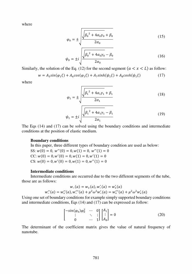
781
where
�Y = ±���Y4 + 4�Y�Y + �Y2�Y (15)
�Y = ±����Y4 + 4�Y�Y − �Y2�Y (16)
Similarly, the solution of the Eq. (12) for the second segment (; q < q p) as follow: { = w���9(�dz) + w�V��(�dz) + w���9ℎ(�dz) + w�V��ℎ(�dz) (17)
where
�d = ±���d4 + 4�d�d + �d2�d (18)
�d = ±����d4 + 4�d�d − �d2�d (19)
The Eqs (14) and (17) can be solved using the boundary conditions and intermediate conditions at the position of elastic medium.
Boundary conditions In this paper, three different types of boundary condition are used as below: SS: {(0) = 0, {��(0) = 0, {(1) = 0, {��(1) = 0 CC: {(0) = 0, {�(0) = 0, {(1) = 0, {�(1) = 0 CS: {(0) = 0, {�(0) = 0, {(1) = 0, {��(1) = 0 Intermediate conditions Intermediate conditions are occurred due to the two different segments of the tube,
those are as follows: {�(;) = {�(;), {�� (;) = {�� (;) {���(;) = {���(;), {����(;) + S4x4{�� (;) = {����(;) + S4x4{�� (;) Using one set of boundary conditions for example simply supported boundary conditions and intermediate conditions, Eqs (14) and (17) can be expressed as follow:
�−��9(�Y)�Y4 ⋯ 0⋮ ⋱ ⋮0 ⋯ 1� �wd⋮w�� = 0 (20)
The determinant of the coefficient matrix gives the value of natural frequency of nanotube.
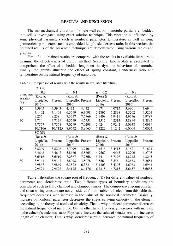
782
RESULTS AND DISCUSSION Thermo mechanical vibration of single wall carbon nanotube partially embedded
into soil is investigated using exact solution technique. This vibration is influenced by some physical parameters such as nonlocal parameter, temperature as well as some geometrical parameters such as embedded length, slenderness ratio. In this section, the obtained results of the presented technique are demonstrated using various tables and graphs.
First of all, obtained results are compared with the results in available literature to examine the effectiveness of current method. Secondly, tabular data is presented to comprehend the effect of embedded length on the dynamic behaviour of nanotube. Finally, the graphs illustrate the effect of spring constant, slenderness ratio and temperature on the natural frequency of nanotube.
Table 1. Comparison of results with the results in available literature
CC (xr)
Slenderness ratio (~)
S = 0.0 S = 0.1 S = 0.2 S = 0.3 (Rosa & Lippiello, 2016)
Present (Rosa & Lippiello, 2016)
Present (Rosa & Lippiello, 2016)
Present (Rosa & Lippiello, 2016)
Present
10 4.5945 4.5943 4.432 4.432 4.0714 4.0715 3.6901 3.69 7.1402 7.1401 6.3699 6.3698 5.2897 5.2898 4.5202 4.5201 9.256 9.258 7.5757 7.5769 5.9408 5.9419 4.9776 4.9787
30 4.714 4.7139 4.5749 4.5751 4.2512 4.2513 3.8894 3.8895 7.7557 7.7558 7.0299 7.0298 5.924 5.9242 5.0938 5.0939 10.7106 10.7125 8.9642 8.9665 7.1222 7.1242 6.0004 6.0024
SC (xr) (Rosa &
Lippiello, 2016)
Present (Rosa & Lippiello, 2016)
Present (Rosa & Lippiello, 2016)
Present (Rosa & Lippiello, 2016)
Present
10 3.8209 3.8208 3.7099 3.7101 3.4516 3.4515 3.1621 3.1621 6.4648 6.4647 5.8666 5.8665 4.9562 4.9563 4.2706 4.2705 8.6516 8.6519 7.2367 7.2368 5.74 5.7396 4.8245 4.8245
30 3.9141 3.9142 3.8078 3.8078 3.556 3.556 3.2683 3.2681 6.9867 6.9869 6.3822 6.382 5.4303 5.4305 4.6963 4.6964 9.9591 9.9597 8.4175 8.4176 6.7218 6.7213 5.6657 5.6653
Table 1 describes the square root of frequency (xr) for different values of nonlocal
parameter and slenderness ratio. Two different types of boundary conditions are considered such as fully clamped and clamped simply. The compressive spring constant and shear spring constant are not considered for this table. It is clear from this table that frequency decreases with increase in the value of the nonlocal parameter. Basically, increase of nonlocal parameter decreases the stress carrying capacity of the element according to the theory of nonlocal elasticity. That is why nonlocal parameter decreases the natural frequency of nanotube. On the other hand, frequency increases with increase in the value of slenderness ratio. Physically, increase the value of slenderness ratio increases length of the element. That is why, slenderness ratio increases the natural frequency of

783
nanotube. Obtained results are compared with the paper (Rosa & Lippiello, 2016) in available literature. The results show good agreement with the results of that paper. Table 2. Frequency of simply supported nanotube partially embedded into soil SS Nonlocal parameter (S = 0) Nonlocal parameter (S = 0.2) Spring constant
Embedded length
(x)d (x)4 (x)� (x)d (x)4 (x)� |l = 0, |k = 50 ; = 0 9.4155 33.4277 64.6445 7.9726 20.8141 30.2949 ; = 0.5 10.5419 33.6972 64.7461 9.2456 21.2559 30.5098 ; = 1 11.5831 33.9589 64.8476 10.4443 21.6582 30.7285 |l = 50, |k = 0 ; = 0 9.4155 33.4277 64.6445 7.9731 20.8144 30.2949 ; = 0.5 15.3349 42.8321 72.4336 11.7803 29.2324 38.4902 ; = 1 23.1895 50.3242 80.8047 22.6426 42.9961 57.1836 |l = 50, |k = 50 ; = 0 9.4155 33.4277 64.6445 7.9731 20.8144 30.2949 ; = 0.5 15.7509 43.1133 72.5195 12.0225 29.3809 38.6231 ; = 1 24.1504 50.6836 80.9766 23.6269 43.4102 57.4102
Table 3. Frequency of fully clamped supported nanotube partially embedded into soil. CC Nonlocal parameter (S = 0) Nonlocal parameter (S = 0.2) Spring constant
Embedded length
(x)d (x)4 (x)� (x)d (x)4 (x)� |l = 0, |k = 50 ; = 0 21.1074 50.9805 85.7109 16.5771 27.9824 35.3066 ; = 0.5 21.6269 51.1523 85.7891 17.1728 28.2481 35.4551 ; = 1 22.1387 51.3154 85.8672 17.7725 28.5059 35.5996 |l = 50, |k = 0 ; = 0 21.1074 50.9804 85.7109 16.5771 27.9824 35.3066 ; = 0.5 25.8339 58.1992 92.1641 20.4512 34.6231 42.4961 ; = 1 31.3769 64.6523 99.1641 34.1465 53.2148 64.4258 |l = 50, |k = 50 ; = 0 21.1074 50.9805 85.7109 16.5771 27.9824 35.3066 ; = 0.5 26.1465 58.3789 92.2266 20.5645 34.6738 42.5195 ; = 1 32.0801 64.9179 99.2891 34.7441 53.4961 64.5820
Tables 2, 3, 4 illustrate the three different modes of natural frequency for different
values of nonlocal parameter, spring constants and different embedded lengths of nanotube. Each table is considered for specific type of boundary condition. The results describe that the frequency increases with the increase of spring constant value.
Table 4. Frequency of simply clamped supported nanotube partially embedded into soil SC Nonlocal parameter (S = 0) Nonlocal parameter (S = 0.2) Spring constant
Embedded length
(x)d (x)4 (x)� (x)d (x)4 (x)� |l = 0, |k = 50 ; = 0 14.5986 41.7929 74.8555 11.9131 24.5645 32.9434 ; = 0.5 15.5791 41.9726 74.9414 13.1455 24.8574 33.1387 ; = 1 16.0615 42.2148 75.0273 13.6240 25.2246 33.3027 |l = 50, |k = 0 ; = 0 14.5986 41.7929 74.8555 11.9131 24.5644 32.9434 ; = 0.5 23.0254 50.2852 83.3516 18.6709 32.9863 41.3398 ; = 1 26.7949 56.9883 89.5703 27.7676 48.2227 60.9883 |l = 50, |k = 50 ; = 0 14.5986 41.7929 74.8555 11.9131 24.5645 32.9434 ; = 0.5 23.4746 50.4961 83.4141 18.9072 33.1309 41.4961 ; = 1 27.6230 57.2929 89.7266 28.5449 48.5664 61.1836

784
Spring provides extra support as a foundation for nanotube. Increase the value of spring constant increases overall stiffness of the system. Similarly, the frequency increases with the increase of embedded length of the nanotube. Basically, an increase in embedded length increases the surface area covered by elastic medium or soil that increases the stiffness of the nanotube.
Figs 2, 3 illustrate the relationship between frequency ratio and spring constants for different values of nonlocal parameter. Two different types of end support such as fully clamped and simply supported are considered. It is clear that the frequency ratio increases with the increase of spring constant. The shear spring is more effective than the compressive spring to increase the value of frequency ratio. The frequency ratio increases rapidly at the high value of nonlocal parameter. Another way, the effect of spring constant is very significant at the high value of nonlocal parameter. The shear spring layer resists the bending moment. On the other hand, the compressive spring layer resists the deflection of the nanotube.
Figure 2. Frequency ratio versus compressive spring constant (|k) for different values of nonlocal parameter (S) in fully clamped and simply supported nanotubes.
Figure 3. Frequency ratio versus shear spring constant �|l� for different values of nonlocal parameter (S) in fully clamped and simply supported nanotubes.
Fig. 4 demonstrates frequency for different values of slenderness ratio and temperature. Thermal expansion coefficient �u = 1.9 × 10�� j�d and nonlocal parameter S = 0.1 are considered. Frequency increases with the increase of slenderness ratio.
1
1.2
1.4
0 20 40 60 80 100
xxY
|k
S = 0.5
S = 0.25S = 0
1
1.4
1.8
2.2
0 50 100
xxY
|k
S = 0.5S = 0.25
S = 0
1
3.5
6
0 50 100
xxY
|l
S = 0.5S = 0.25
S = 01
3.5
6
0 25 50 75 100
xxY
|l
S = 0.5S = 0.25
S = 0
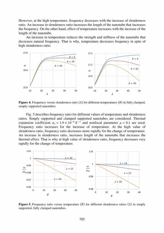
785
However, at the high temperature, frequency decreases with the increase of slenderness ratio. An increase in slenderness ratio increases the length of the nanotube that increases the frequency. On the other hand, effect of temperature increases with the increase of the length of the nanotube.
An increase in temperature reduces the strength and stiffness of the nanotube that decreases natural frequency. That is why, temperature decreases frequency in spite of high slenderness ratio.
Figure 4. Frequency versus slenderness ratio (~) for different temperatures (�) in fully clamped, simply supported nanotubes.
Fig. 5 describes frequency ratio for different values of temperature and slenderness ratios. Simply supported and clamped supported nanotubes are considered. Thermal expansion coefficient �u = 1.9 × 10�� j�d and nonlocal parameter S = 0.1 are used. Frequency ratio increases for the increase of temperature. At the high value of slenderness ratio, frequency ratio decreases more rapidly for the change of temperature. An increase in slenderness ratio, increases length of the nanotube that increases the thermal effect. That is why at high value of slenderness ratio, frequency decreases very rapidly for the change of temperature.
Figure 5. Frequency ratio versus temperature (�) for different slenderness ratios (~) in simply supported, fully clamped nanotubes.
25.8
26.8
27.8
10 20 30 40 50
x
~
� = 50 � = 20� = 0
16.6
16.9
17.2
17.5
10 20 30 40 50
x
~� = 50
� = 20� = 0
0.96
0.97
0.98
0.99
1
1.01
0 10 20 30 40
xxY
�~ = 50
~ = 25~ = 10
0.98
0.99
1
1.01
0 10 20 30 40
xxY
�~ = 50
~ = 25~ = 10

786
Figure 6. Frequency ratio versus embedded length (;) for different modes of frequency in simply supported, fully clamped nanotubes.
Fig. 6 illustrates the frequency ratio versus embedded length for different modes of
frequency. Simply supported and clamped supported nanotubes are considered. Spring constants |k = 50, |l = 50 and nonlocal parameter S = 0.1 are used. Frequency increases with the increase of embedded length. First mode of frequency is more influenced by the embedded length than the other modes of frequency. An increase in embedded length increases the stiffness of the nanotube where the embedded length is covered by the soil which is simulated by two types of spring.
CONCLUSIONS
In the present work, analytical solution technique is introduced to analyse the
dynamic behaviour of nanotube partially embedded into soil with thermal load. Soil is simulated by the two spring constants such as compressive spring and shear spring. It is clear from this analysis that the effects of nonlocal parameter, embedded length of nanotube, spring constants and temperature on dynamic behaviour of embedded nanotube are significant. At low temperature, frequency increases with the increase of slenderness ratio. On the other hand, at high temperature, frequency decreases at high value of slenderness ratio. The results of this analysis show good agreement with the results of other researchers.
REFERENCES
Aria, A.I., Friswell, M.I. & Rabczuk, T. 2019. Thermal vibration analysis of cracked nanobeams
embedded in an elastic matrix using finite element analysis. Composite Structures 212, 118–128.
Askari, H. & Esmailzadeh, E. 2017. Forced vibration of fluid conveying carbon nanotubes considering thermal effect and nonlinear foundations, Composites Part B 113, 31–43.
Chang, T.P. 2017. Nonlinear vibration of single-walled carbon nanotubes with nonlinear damping and random material properties under magnetic field, Composites Part B 114, 69–79.
Elhuni, H. & Basu, D. 2019. Dynamic soil structure interaction model for beams on viscoelastic foundations subjected to oscillatory and moving loads. Computers and Geotechnics 115, 103157.
0
0.5
1
1.5
2
2.5
3
0 0.2 0.4 0.6 0.8 1
xxY
1st Mode
2nd Mode
3rd Mode
; 0.9
1.2
1.5
1.8
0 0.25 0.5 0.75 1
1st Mode
2nd Mode
3rd Mode
xxY
;
787
Eringen, A.C. 2002. Nonlocal Continuum Field Theories, Springer-Verlag New York, Inc., pp. 82–86.
Falope, F.O., Lanzoni, L. & Radi, E. 2020. Buckling of a Timoshenko beam bonded to an elastic half-plane: Effects of sharp and smooth beam edges. International Journal of Solids and Structures 185–186, 222–239.
Fernandes, R., Borgi, S.E., Mousavi, S.M., Reddy, J.N. & Mechmoum, A. 2017. Nonlinear size-dependent longitudinal vibration of carbon nanotubes embedded in an elastic medium. Physica E 88, 18–25.
Haldar, S. & Basu, D. 2013. Response of Euler–Bernoulli beam on spatially random elastic soil. Computers and Geotechnics 50, 110–128.
Holubowski, R., Glabisz, W. & Jarczewska, K. 2019. Transverse vibration analysis of a single-walled carbon nanotube under a random load action. Physica E: Low-dimensional Systems and Nanostructures 109, 242–247.
Jiang, J. & Wang, L. 2017. Analytical solutions for thermal vibration of nanobeams with elastic boundary conditions. Acta mechanica solida sinica 30, 474–483.
Jiang, J., Wang, L. & Zhang, Y. 2017. Vibration of single-walled carbon nanotubes with elastic boundary conditions. International Journal of Mechanical Sciences 122, 156–166.
Lai, S.K. & Zhang, L.H. 2018. Thermal effect on vibration and buckling analysis of thin isotropic/orthotropic rectangular plates with crack defects. Engineering Structures 177, 444–458.
Malikan, M., Nguyen, V.B. & Tornabene, F. 2018. Damped forced vibration analysis of single-walled carbon nanotubes resting on viscoelastic foundation in thermal environment using nonlocal strain gradient theory Engineering Science and Technology, an International Journal 21, 778–786.
Rahmanian, M., Asadi, M.A.T., Abadi, R.D.F. & Kouchakzadeh, M.A. 2016. Free vibrations analysis of carbon nanotubes resting on Winkler foundations based on nonlocal models. Physica B 484, 83–94.
Rosa, M.A.D. & Lippiello, M. 2016. Nonlocal frequency analysis of embedded single-walled carbon nanotube using the Differential Quadrature Method. Composites Part B 84, 41–51.
Zhang, Z., Huang, M., Xu, C., Jiang, Y. & Wang, W. 2018. Simplified solution for tunnel-soil-pile interaction in Pasternak’s foundation model. Tunnelling and Underground Space Technology 78, 146–158.
Zhao, L.S., Zhou, W.H., Fatahi, B., Li, X.B. & Yuen, K.V. 2016. A dual beam model for geosynthetic-reinforced granular fill on an elastic foundation. Applied Mathematical Modelling 40, 9254–9268.

788
Agronomy Research 19(S1), 788–794, 2021 https://doi.org/10.15159/AR.21.033
Compositional evaluation of hot-pressed rapeseed cake for the purpose of bioplastic production
K. Jõgi1,*, D. Malenica1, I. Jõudu1,2 and R. Bhat1
1ERA-Chair for Food (By-) Products Valorisation Technologies of the Estonian University of Life Sciences (VALORTECH), Estonian University of Life Sciences, Fr.R. Kreutzwaldi 1, EE51006 Tartu, Estonia 2Chair of Food Science and Technology, Institute of Veterinary Medicine and Animal Sciences, Estonian, University of Life Science, Fr.R. Kreutzwaldi 56/5, EE51006 Tartu, Estonia *Correspondence: [email protected] Received: January 29th, 2021; Accepted: April 10th, 2021; Published: April 13th, 2021 Abstract. Rapeseed is widely cultivated for biodiesel or food-grade oil production. As the oil production process generates huge amounts of wastes and by-products (e.g. oil press cake and meal) that have relatively high crude protein content, valorisation as input material for protein-based bioplastics has a lot of potential. There is a limited number of studies undertaken on using rapeseed cake directly (without prior protein extraction) for biomaterial production, but the initial results have been very promising. As rape and turnip rapeseeds are also some of the most harvested crops in Estonia, the rapeseed oil press cake as a by-product is also available from local food-grade rapeseed oil production. In this regard, we investigated locally available rapeseed oil press cake for chemical composition and explored suitability for bioplastic production. The results indicate suitability for direct biomaterial production, meaning properties for biomaterial formation could be further explored. Key words: biomaterial, bioplastic, by-product, rapeseed cake, valorisation.
INTRODUCTION
According to European Bioplastics market development update for 2020, currently bioplastics represent only 1% of all the globally produced plastic materials (European Bioplastics, 2020). As concerns on plastic pollution are rising, demand for alternative materials for conventional petrochemical plastics is growing. Increasing the market share of bioplastics would support the circular economy concept by reducing also dependency on fossil resources (Geueke et al., 2018; Imre et al., 2019). Currently the industrial expenses to produce bioplastics are still higher than for petroleum-derived plastics (Raza et al., 2018). One option to reduce dependency on fossil resources and manufacturing costs of bioplastics would be to use wastes and by-products as input materials (Saharan & Sharma, 2012), and in this way the amount of wastes is reduced and new value-added products can be produced (Pagliaccia et al., 2019; Tsang et al., 2019).
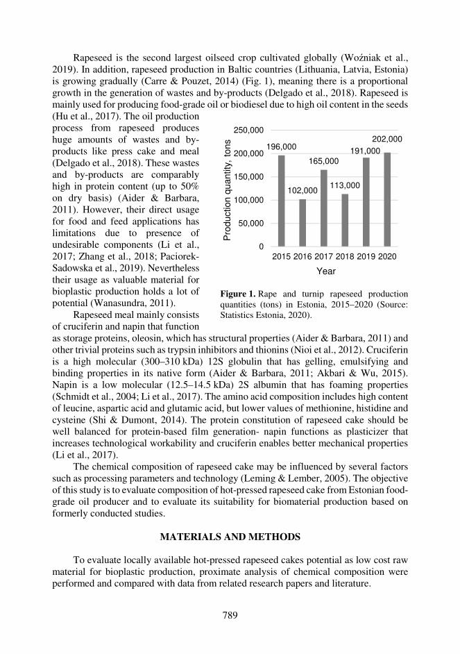
789
Rapeseed is the second largest oilseed crop cultivated globally (Woźniak et al., 2019). In addition, rapeseed production in Baltic countries (Lithuania, Latvia, Estonia) is growing gradually (Carre & Pouzet, 2014) (Fig. 1), meaning there is a proportional growth in the generation of wastes and by-products (Delgado et al., 2018). Rapeseed is mainly used for producing food-grade oil or biodiesel due to high oil content in the seeds
as storage proteins, oleosin, which has structural properties (Aider & Barbara, 2011) and other trivial proteins such as trypsin inhibitors and thionins (Nioi et al., 2012). Cruciferin is a high molecular (300–310 kDa) 12S globulin that has gelling, emulsifying and binding properties in its native form (Aider & Barbara, 2011; Akbari & Wu, 2015). Napin is a low molecular (12.5–14.5 kDa) 2S albumin that has foaming properties (Schmidt et al., 2004; Li et al., 2017). The amino acid composition includes high content of leucine, aspartic acid and glutamic acid, but lower values of methionine, histidine and cysteine (Shi & Dumont, 2014). The protein constitution of rapeseed cake should be well balanced for protein-based film generation- napin functions as plasticizer that increases technological workability and cruciferin enables better mechanical properties (Li et al., 2017).
The chemical composition of rapeseed cake may be influenced by several factors such as processing parameters and technology (Leming & Lember, 2005). The objective of this study is to evaluate composition of hot-pressed rapeseed cake from Estonian food-grade oil producer and to evaluate its suitability for biomaterial production based on formerly conducted studies.
MATERIALS AND METHODS
To evaluate locally available hot-pressed rapeseed cakes potential as low cost raw
material for bioplastic production, proximate analysis of chemical composition were performed and compared with data from related research papers and literature.
(Hu et al., 2017). The oil production process from rapeseed produces huge amounts of wastes and by-products like press cake and meal (Delgado et al., 2018). These wastes and by-products are comparably high in protein content (up to 50% on dry basis) (Aider & Barbara, 2011). However, their direct usage for food and feed applications has limitations due to presence of undesirable components (Li et al., 2017; Zhang et al., 2018; Paciorek-Sadowska et al., 2019). Nevertheless their usage as valuable material for bioplastic production holds a lot of potential (Wanasundra, 2011).
Rapeseed meal mainly consists of cruciferin and napin that function
Figure 1. Rape and turnip rapeseed production quantities (tons) in Estonia, 2015–2020 (Source: Statistics Estonia, 2020).
196,000
102,000
165,000
113,000
191,000
202,000
0
50,000
100,000
150,000
200,000
250,000
2015 2016 2017 2018 2019 2020
Pro
duction q
uantity
, to
ns
Year
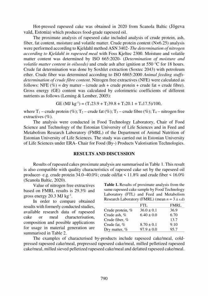
790
Hot-pressed rapeseed cake was obtained in 2020 from Scanola Baltic (Jõgeva vald, Estonia) which produces food-grade rapeseed oil.
The proximate analysis of rapeseed cake included analysis of crude protein, ash, fiber, fat content, moisture and volatile matter. Crude protein content (N×6.25) analysis were performed according to Kjeldahl method ASN 3402- The determination of nitrogen according to Kjeldahl in rapeseed meal with Foss Kjeltec 2300. Moisture and volatile matter content was determined by ISO 665:2020- (Determination of moisture and volatile matter content in oilseeds) and crude ash after ignition at 550 °C for 18 hours. Crude fat determination was done by Soxhlet extraction (Soxtec 2043) with petroleum ether. Crude fiber was determined according to ISO 6865:2000 Animal feeding stuffs- determination of crude fibre content. Nitrogen free extractives (NFE) were calculated as follows: NFE (%) = dry matter – (crude ash + crude protein + crude fat + crude fibre). Gross energy (GE) content was calculated by colorimetric coefficients of different nutrients as follows (Leming & Lember, 2005):
GE (MJ kg-1) = (T123.9 + T239.8 + T320.1 + T417.5)/100,
where T1 – crude protein (%); T2 – crude fat (%); T3 – crude fibre (%); T4 – nitrogen free extractives (%).
The analysis were conducted in Food Technology Laboratory, Chair of Food Science and Technology of the Estonian University of Life Sciences and in Feed and Metabolism Research Laboratory (FMRL) of the Department of Animal Nutrition of Estonian University of Life Sciences. The study was carried out in Estonian University of Life Sciences under ERA- Chair for Food (By-) Products Valorisation Technologies.
RESULTS AND DISCUSSION
Results of rapeseed cakes proximate analysis are summarised in Table 1. This result
is also compatible with quality characteristics of rapeseed cake set by the rapeseed oil producer- e.g. crude protein 34.0–40.0%; crude oil/fat < 11.8% and crude fiber < 16.0%
The examples of characterised by-products include rapeseed cake/meal, cold-pressed rapeseed cake/meal, prepressed rapeseed cake/meal, milled pelletized rapeseed cake/meal, milled sieved pelletized rapeseed cake/meal and defatted rapeseed cake/meal.
(Scanola Baltic, 2020). Value of nitrogen free extractives
based on FMRL results is 29.3% and gross energy 20.3 MJ kg-1.
In order to compare obtained results with formerly conducted studies, available research data of rapeseed cake or meal characterisation, composition and possible applications for usage in material generation are summarised in Table 2.
Table 1. Results of proximate analysis from the same rapeseed cake sample by Food Technology Laboratory (FTL) and Feed and Metabolism Research Laboratory (FMRL) (mean n = 3 ± s.d)
FTL FMRL Crude protein, % 36.0 ± 0.1 36.9 Crude ash, % 6.40 ± 0.0 6.70 Crude fiber, % 13.7 Crude fat, % 8.70 ± 0.1 9.10 Dry matter, % 97.9 ± 0.0 95.7
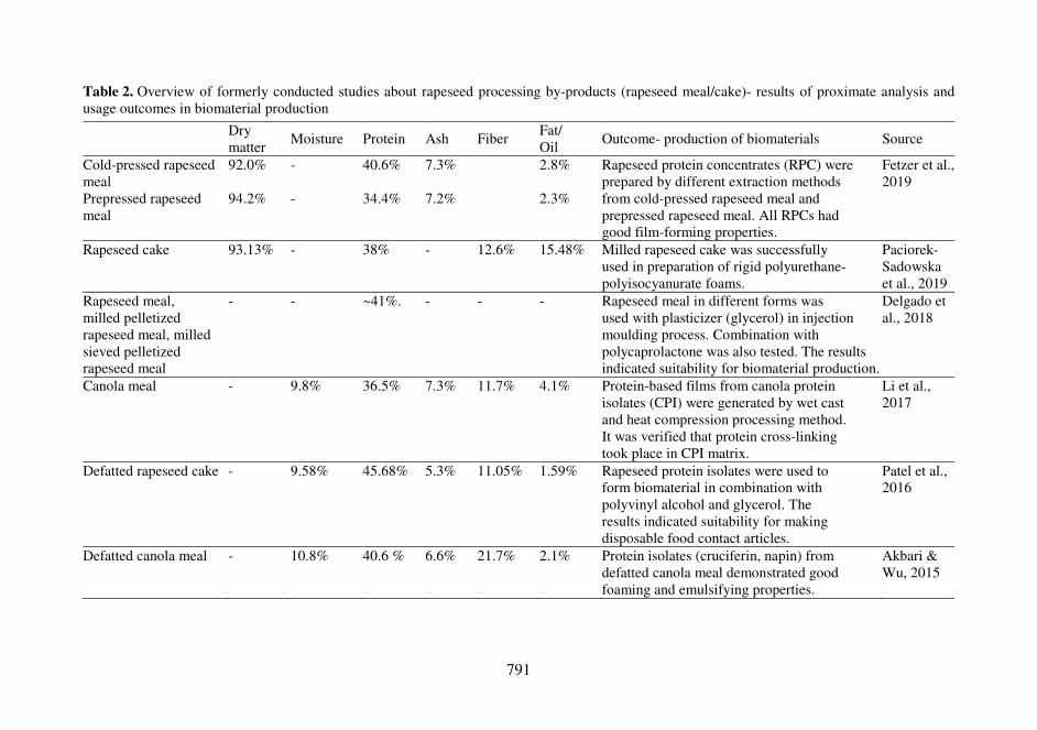
791
Table 2. Overview of formerly conducted studies about rapeseed processing by-products (rapeseed meal/cake)- results of proximate analysis and usage outcomes in biomaterial production
Dry matter Moisture Protein Ash Fiber Fat/
Oil Outcome- production of biomaterials Source
Cold-pressed rapeseed meal
92.0% - 40.6% 7.3% 2.8% Rapeseed protein concentrates (RPC) were prepared by different extraction methods from cold-pressed rapeseed meal and prepressed rapeseed meal. All RPCs had good film-forming properties.
Fetzer et al., 2019
Prepressed rapeseed meal
94.2% - 34.4% 7.2% 2.3%
Rapeseed cake 93.13% - 38% - 12.6% 15.48% Milled rapeseed cake was successfully used in preparation of rigid polyurethane-polyisocyanurate foams.
Paciorek-Sadowska et al., 2019
Rapeseed meal, milled pelletized rapeseed meal, milled sieved pelletized rapeseed meal
- - ~41%. - - - Rapeseed meal in different forms was used with plasticizer (glycerol) in injection moulding process. Combination with polycaprolactone was also tested. The results indicated suitability for biomaterial production.
Delgado et al., 2018
Canola meal - 9.8% 36.5% 7.3% 11.7% 4.1% Protein-based films from canola protein isolates (CPI) were generated by wet cast and heat compression processing method. It was verified that protein cross-linking took place in CPI matrix.
Li et al., 2017
Defatted rapeseed cake - 9.58% 45.68% 5.3% 11.05% 1.59% Rapeseed protein isolates were used to form biomaterial in combination with polyvinyl alcohol and glycerol. The results indicated suitability for making disposable food contact articles.
Patel et al., 2016
Defatted canola meal - 10.8% 40.6 % 6.6% 21.7% 2.1% Protein isolates (cruciferin, napin) from defatted canola meal demonstrated good foaming and emulsifying properties.
Akbari & Wu, 2015
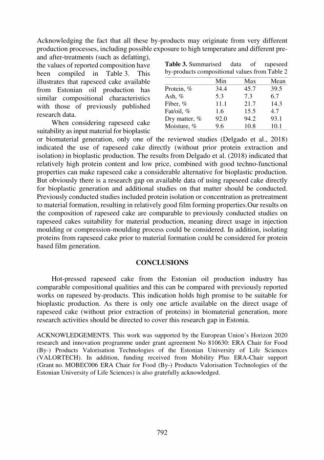
792
Acknowledging the fact that all these by-products may originate from very different production processes, including possible exposure to high temperature and different pre-
or biomaterial generation, only one of the reviewed studies (Delgado et al., 2018) indicated the use of rapeseed cake directly (without prior protein extraction and isolation) in bioplastic production. The results from Delgado et al. (2018) indicated that relatively high protein content and low price, combined with good techno-functional properties can make rapeseed cake a considerable alternative for bioplastic production. But obviously there is a research gap on available data of using rapeseed cake directly for bioplastic generation and additional studies on that matter should be conducted. Previously conducted studies included protein isolation or concentration as pretreatment to material formation, resulting in relatively good film forming properties.Our results on the composition of rapeseed cake are comparable to previously conducted studies on rapeseed cakes suitability for material production, meaning direct usage in injection moulding or compression-moulding process could be considered. In addition, isolating proteins from rapeseed cake prior to material formation could be considered for protein based film generation.
CONCLUSIONS
Hot-pressed rapeseed cake from the Estonian oil production industry has
comparable compositional qualities and this can be compared with previously reported works on rapeseed by-products. This indication holds high promise to be suitable for bioplastic production. As there is only one article available on the direct usage of rapeseed cake (without prior extraction of proteins) in biomaterial generation, more research activities should be directed to cover this research gap in Estonia.
ACKNOWLEDGEMENTS. This work was supported by the European Union’s Horizon 2020 research and innovation programme under grant agreement No 810630: ERA Chair for Food (By-) Products Valorisation Technologies of the Estonian University of Life Sciences (VALORTECH). In addition, funding received from Mobility Plus ERA-Chair support (Grant no. MOBEC006 ERA Chair for Food (By-) Products Valorisation Technologies of the Estonian University of Life Sciences) is also gratefully acknowledged.
and after-treatments (such as defatting), the values of reported composition have been compiled in Table 3. This illustrates that rapeseed cake available from Estonian oil production has similar compositional characteristics with those of previously published research data.
When considering rapeseed cake suitability as input material for bioplastic
Table 3. Summarised data of rapeseed by-products compositional values from Table 2
Min Max Mean Protein, % 34.4 45.7 39.5 Ash, % 5.3 7.3 6.7 Fiber, % 11.1 21.7 14.3 Fat/oil, % 1.6 15.5 4.7 Dry matter, % 92.0 94.2 93.1 Moisture, % 9.6 10.8 10.1

793
REFERENCES Aider, M. & Barbana, C. 2011. Canola proteins: Composition, extraction, functional properties,
bioactivity, applications as a food ingredient and allergenicity - A practical and critical review. Trends in Food Science & Technology 22, 21–39.
Akbari, A. & Wu, J. 2015. An integrated method of isolating napin and cruciferin from defatted canola meal. LWT - Food Science and Technology 64, 308–315.
Carre, P. & Pouzet, A. 2014. Rapeseed market, worldwide and in Europe. OCL 21(1). Delgado, M., Felix, M. & Bengoechea, C. 2018. Development of bioplastic materials: From
rapeseed oil industry by products to added-value biodegradable biocomposite materials. Industrial Crops & Products 125, 401–407.
European Bioplastics. 2020. Available at: https://docs.european-bioplastics.org/conference/Report_Bioplastics_Market_Data_2020_short_version.pdf Accessed 10.12.2020.
Fetzer, A., Herfellner, T. & Eisner, P. 2019. Rapeseed protein concentrates for non-food applications prepared from prepressed and cold-pressed press cake via acidic precipitation and ultrafiltration. Industrial Crops & Products 132, 396–406.
Geueke, B., Groh, K. & Muncke, J. 2018. Food packaging in the circular economy: Overview of chemical safety aspects for commonly used materials. Journal of Cleaner Production 193, 491–505.
Hu, Q., Hua, W., Yin, Y., Zhang, X., Liu, L., Shi, J., Zhao, Y., Qin, L., Chen, C. & Wang, H. 2017. Rapeseed research and production in China. The Crop Journal 5(2), 127–135.
Imre, B., Garcia, L., Puglia, D. & Vilaplana, F. 2019. Reactive compatibilization of plant polysaccharides and biobased polymers: review on current strategies, expectations and reality. Carbohydrate Polymers 209, 20–37.
Leming, R. & Lember, A. 2005. Chemical composition of expeller-extracted and cold-pressed rapeseed cake. Agraarteadus 16(2), 96−109.
Li, S., Donner, E., Thompson, M., Zhang, Y., Rempel, C. & Liu, Q. 2017. Preparation and characterization of cross-linked canola protein isolate films. European Polymer Journal 89, 419–430.
Nioi, C., Kapel, R., Rondags, E. & Marc, I. 2012. Selective extraction, structural characterisation and antifungal activity assessment of napins from an industrial rapeseed meal. Food Chemistry 134, 2149–2155.
Paciorek-Sadowska, J., Borowicz, M., Isbrandt, M., Czupryński, B. & Apiecionek, L. 2019. The Use of Waste from the Production of Rapeseed Oil for Obtaining of New Polyurethane Composites. Polymers 11, 1431.
Pagliaccia, P., Gallipoli, A., Gianico, A., Gironi, F., Montecchino, D., Pastore, C., di Bitonto, L. & Braguglia, C.M. 2019. Variability of food waste chemical composition: Impact of thermal pretreatment on lignocellulosic matrix and anaerobic biodegradability. Journal of Environmental Management 236, 100–107.
Patel, A.V., Panchal, T.M., Rudakiya, D., Gupte, A. & Patel, J.V. 2016. Fabrication of bio-plastics from protein isolates and its biodegradation studies. International Journal of Chemical Sciences and Technology 1(3).
Raza, Z.A., Abid, S. & Banat, I.M. 2018. Polyhydroxyalkanoates: Characteristics, production, recent developments and applications. International Biodeterioration & Biodegradation 126, 45–56.
794
Saharan, B. & Sharma, D. 2012. Bioplastics-For Sustainable Development: A Review. International Journal of Microbial Resource Technology 1(1), 11–23.
Scanola Baltic, 2020. Rapsikook. Available at: https://scanolabaltic.ee/en/content/42-rapsikook Accessed 16.12.2020.
Schmidt, I., Renard, D., Rondeau, D., Richomme, P., Popineau, Y. & Axelos, M.A. 2004. Detailed physicochemical characterization of the 2S storage protein from rape (Brassica napus L.). J. Agric. Food Chem. 52, 5995–6001.
Shi, W. & Dumont, M.J. 2014. Processing and physical properties of canola protein isolate-based films. Industrial Crops and Products 52, 269–277.
Statistics Estonia, 2020. Agriculture. Available at: https://www.stat.ee/en/find-statistics/statistics-theme/agriculture-fisheries-and-hunting/agriculture Accessed 16.12.2020.
Tsang, Y.F., Kumar, V., Samadar, P., Yang, Y., Lee, J., Ok, Y.S., Song, H., Kim, K.H., Kwon, E.E. & Jeon, Y.J. 2019. Production of bioplastic through food waste valorization. Environment International 127, 625–644.
Wanasundra, J.P.D. 2011. Proteins of Brassicaceae Oilseeds and their Potential as a Plant Protein Source. Critical Reviews in Food Science and Nutrition 51(7).
Woźniak, E., Waszkowska, E., Zimny, T., Sowa, S. & Twardowski, T. 2019. The Rapeseed Potential in Poland and Germany in the Context of Production, Legislation, and Intellectual Property Rights. Frontiers in plant science 10, 1423.
Zhang, Y., Liu, Q. & Rempel, C. 2018. Processing and characteristics of canola protein-based biodegradable packaging: A review. Critical Reviews in Food Science and Nutrition 58(3), 475–485.
795
Agronomy Research 19(S1), 795–808, 2021 https://doi.org/10.15159/AR.21.017
Nanopreparations in technologies of plants growing
S. Kalenska1,*, N. Novytska1, T. Stolyarchuk1, V. Kalenskyi2, L. Garbar1, M. Sadko3, O. Shutiy1 and R. Sonko1
1National University of Life and Environmental Science, Department of Plant Science, Heroiv Oborony str., no 15, UA03041 Kyiv, Ukraine 2National University of Life and Environmental Science, Department of Agrochemistry and Quality of Plant Production, Heroiv Oborony str., no 15, UA03041 Kyiv, Ukraine 3National University of Life and Environmental Science, Department of Information Systems and Technologies, Heroiv Oborony str., no 15, UA03041 Kyiv, Ukraine *Correspondence: [email protected] Received: December 1st, 2020; Accepted: March 25th, 2021; Published: March 30th, 2021 Abstract. The use of engineered nanomaterials in sustainable agriculture has demonstrated a completely new way of food production that can potentially overcome uncertainty in the agricultural sector with limited available resources. Nanoparticle engineering is one of the latest technological innovations which demonstrate unique target characteristics. During 2013–2020, research on the directions and effectiveness of nanopreparations in plant growing: nutrient source, activation of photosynthesis, immunocorrectors, stimulators of seed germination, plant growth and development, multivalent drugs for increasing plant resistance to stress was conducted. Monoparticles, nanoparticle combinations, and chelate complex of nano fertilizers on crops of soybean were tested. Field research was conducted in a stationary field experiment of the Plant Science Department of the National University of Life and Environmental Sciences of Ukraine. The soil of the stationary experiment is typical chernozem. In research was used soybean (Glycine max (L.) Merr.) of early-ripening variety Horol. Over the years of research, weather conditions varied, but were within the typical for zone of research. Average monthly temperatures were close or higher the perennial average indicators. The purpose of the research is to find out the influence of pre-sowing seed treatment and fertilizing of crops by nano-preparations Avatar (microfertilizer of carboxylates of natural acids), Iodis-concentrate (immunomodulator - stimulator of growth processes), and Super Micro Plus (nanochelate fertilizer) on leaf formation - rate, the activity of symbiotic nitrogen fixation and yield of soybean variety Horol. Nanopreparations were used for pre-sowing seed treatment and fertilizing - spraying during the growing season in several doses. The use of nanopreparations, as seed treatment in combination with inoculation and as fertilizer, intensified formation of the leaf surface area, symbiotic apparatus activity of soybean plants. The introduction of nanofertilizers complex in the top-dressing helped to increase yields and change the functional quality of crop products which indicates their unconditional effectiveness. Soybean yield significantly depended on weather conditions, varying from 1.23 to 3.48 t ha-1 depending on the weather conditions and the combination of seed inoculation and nanofertilizer. Soybean yield under favourable weather conditions in 2016, depending on the use of preparation combination ranged from 2.27 to 3.48 t ha-1.
796
As a result of the research, it was found that the use of nanopreparations Avatar, Jodis-concentrate and Super Micro Plus for seed treatment and fertilizing intensified leaf surface formation and symbiotic apparatus activity of soybean plants. The obtained results confirm that application of nanofertilizers complex Jodis-concentrate, Avatar and nano chelate fertilizer Super Micro Plus in the soybean fertilizing helped to increase the yield, which testifies to their unconditional effectiveness. The highest efficiency of nanofertilizers was shown by inoculation and seed treatment by Avatar and fertilizing by Avatar + nano chelate fertilizer Super Micro Plus, providing the formation of 52.4 thousand m2 ha-1 of leaf surface area of soybean varieties Horol, 69.7 pcs per plant of root nodules, 785 mg per plant of their weight and yield at the level of 2.79 t ha-1 an average of five years. Key words: nano fertilizers, forms of fertilizers, soybean, yields.
INTRODUCTION
To decide the growing challenges of sustainable production and food security,
significant technological advances and innovations have been achieved in recent years (Dijk & Meijerink, 2014; Kou et al., 2018). The growing demand for food in the world causes an increase in the intensity of production in plant growing, which leads to a chain of negative consequences – soil depletion, reduced crop yields, a significant increase in economic and energy costs (Kirchmann et al., 2020). About 40% of agricultural land in the world, due to intensive production, degraded, this led to significant losses of soil fertility (Kale & Gawade, 2016).
Sustainable agriculture involves the minimal use of agrochemicals, which has a positive impact on the environment, conservation of species from extinction, improving management tactics and conservation by reducing the cost of agricultural resources (Dubey & Mailapalli, 2016; Dwivedi et al., 2016). Energy use in agricultural production has been increasing faster than in many other sectors of the world economy. Owing to high energy consumption during the production of agricultural inputs, with mineral nitrogen fertilizers in particular, it is often questioned as to whether agricultural production is still energy efficient. The compared systems differed in nitrogen fertilization rates and the level of fungicide protection. The highest output/input ratio was noticed growing winter triticale in low-input production system. The most energy-consuming operation during winter triticale production in the compared systems was mineral fertilization. The high-input production system was significantly lower energy efficiency than the other systems (6.21, medium-input 5.95, low-input 8.19) (Bielski et al., 2019).
Nanotechnology could become a key technology in the twenty-first century. Over the last two decades, a significant amount of research on nanotechnology and their use in agriculture has been conducted (Khan & Rizvi, 2014; Chen et al., 2016; Kozyrskyi et al., 2019). One of the ways to achieve food security can be the development of innovative technologies for plants growing (Makarenko et al., 2015; Eremenko et al., 2019).
Advances in the production of nanomaterials of various sizes and shapes have given a wide range of applications in medicine, ecology, agriculture and food industry (Godfray et al., 2010; Panpatte et al., 2016; Worrall et al., 2018). The use of engineered nanomaterials has shown a completely new way of food production that can potentially overcome uncertainty in the agricultural sector with limited available resources (Lopatko et al., 2009; Godfray et al., 2010). Nanotechnologies have many promising areas of use in crop production: nutrient source, activation and growth of photosynthesis,

797
immunocorrectors, antistressors, nanopesticides, specific root effectors for rooting shoots and tissue crops, multivalent drugs to increase plant resistance to stress (Kwak et al., 2017; Prasad et al., 2017).
An important role is given to nanofertilizers and growth-stimulating complexes (Kou et al., 2018.). It is estimated that at least a third of crop productivity is accounted for by fertilizers, and the rest depends on the efficiency of other agricultural resources (Dubey & Mailapalli, 2016). However, the efficiency of nutrient use from traditional fertilizers does not exceed 30–40% (Dijk & Meijerink, 2014) and largely depends on the final concentration fertilizer that reaches the target place (Solanki et al., 2015). And reaches much lower than the minimum required concentration, due to the loss of chemicals during leaching, application, runoff, hydrolysis, evaporation, degradation (Sabir et al., 2014; Miao et al., 2015; Wang et al., 2015). Repeated use of excessive amounts of fertilizers negatively affects the inherent balance of soil nutrients, water purity, drinking water pollution, development of flora and fauna (Makarenko et al., 2015).
Nanofertilizers synthesized specifically for the controlled release of nutrients depending on the crops needs, minimizing differential losses, have great potential (Sabir et al., 2014; Solanki et al., 2015; Batsmanova et al., 2020). Controlled released nanoparticles improve plant growth and development, increase yields and improve product quality (Vermeulen et al., 2012; Kale & Gawade, 2016; Shcherbakova et al., 2017). The approach to targeted delivery of nutrients based on nanosized particles is used to optimize the production process, aimed at changing its passage, through certain areas of their functional efficiency (Sabir et al., 2014; Wang et al., 2015; Gogos et al., 2020).
Fertilizer nanoformulas synchronize the ‘emission’ of nanoparticles with the demand of the culture, which prevents nutrient loss through direct use by plants, avoiding the interaction of nutrients with soil, water, air and microorganisms (Miao et al., 2015; Dubey & Mailapalli, 2016).
An important problem in the growing crops efficiency is the use of high quality seeds. The search for ways of reducing seed injury during harvesting and post-harvest cleaning of crop seeds is quite relevant (Bulgakov et al., 2020). There are ongoing studies on ways to reduce seed injury and increase its sowing properties, which may also be associated with the use of nanopreparations or monoelements for pre-sowing seed treatment (Shcherbakova et al, 2017).
MATERIALS AND METHODS
Field research was conducted in 2016–2020 in a stationary field experiment at the
‘Agronomic Research Station’ of NULES of Ukraine in a 10-field field crop rotation and on the basis of educational and scientific laboratory ‘Demonstration collection field of agricultural crops’ of the Plant Science Department of NULES of Ukraine. The soil of the experimental site is typical low-humus chernozem, coarse-dusty-medium-loamy in granulometric composition. The humus content is 4.39–4.53%; pH of salt extract - 6.9–7.3; absorption capacity - 30.7–32 mg-eq. per 100 g of soil. The content of total nitrogen (according to Keldal) is 0.27–0.31%, total phosphorus is 0.15–0.25%, and potassium is 2.3–2.5%. The content of mobile phosphorus (according to Machigin) is 4.5–5.5 mg per 100 g of soil, and of exchangeable potassium is 9.8–10.3.
In research was used soybean (Glycine max (L.) Merr.) variety Horol. It’s early ripening variety of grain direction of use. Yield: 3.0–3.3 t ha-1. Resistance to diseases -

798
up to 1 point. Plant is 75–85 cm height with flower purple and yellow seeds. The weight of 1,000 seeds is 180–190 g, oil content - 19–20%.
Soybean was sown with soil warming at the depth of seeding to +8 ℃. In all years of research, the calendar date of sowing corresponded to the first decade of May.
In accordance with the set goal, research program and field experiment scheme were developed, which included options for seed treatment (Table 1).
Table 1. The effectiveness of nanopreparations and pre-sowing seed treatments (scheme of the experiment)
Pre-sowing treatment factorА
Designation of a variant
Drugs use factor В
Designation of a variant
Seed inoculation (control) А1 Seed treatment by water (control) В1 Seed inoculation + Iodis concentrate
А2 Iodis concentrate В2
Seed inoculation + Avatar А3 Nano Chelate fertilizer Super Micro Plus
В3
Avatar В4 Avatar + Jodis concentrate В5 Avatar + Nano Chelate fertilizer Super MicroPlus
В6
Seeds before sowing were treated by wet method according to the developed scheme. The area of the accounting plot is 50 m2, repetitions is quadruple. The placement of
plots is systematic. Seeds sowing rate is 600 thousand seeds ha-1. HighStik (4 kg per 1 ton of seeds) was used as inoculum. Preparative form is sterilized peat. Active substance is Bradyrhizobium japonicum (strain 532 C).
Over the years of research, weather conditions varied, but were within the typical for zone of research. Average monthly temperatures were close or higher the perennial average indicators, except May 2020, which is was colder (Fig. 1). In general, years of research characterized by the warm spring and hot summer.
Figure 1. The average monthly temperature for the years of research during the growing season, °C.
12
.4
15
.5
20
.6 22
.4
21
.1
10
.4
15
.2
20
.0
20
.9
22
.4
13
.1
18
.8 20
.6
21
.4
22
.5
10
.2
16
.8
22
.7
21
.2
21
.6
9.2
12
.5
21
.2
20
.5
20
.1
8.4
15.3
18.519.6 20.2
0.0
5.0
10.0
15.0
20.0
25.0
April May June July August
2016 2017 2018 2019 2020 Perennial averages

799
During the vegetations of 2016–2020, precipitation was unevenly distributed (Fig. 2).
Figure 2. The average monthly precipitation during the growing season, mm.
During the spring months of 2016, the plants were sufficiently provided with
moisture, and in May, even in excess. Index of precipitation was much higher average perennial. The similar situations were observed in June and July 2018 and in May 2019.
These conditions had both positive and negative effects on the development of soybean plants.
Next preparations were used in our research: Complex microfertilizer Avatar (Co - 0.0001–0.0025%, Cu - 0.01–0.08,
Zn - 0.001–0.007, Fe - 0.0015–0.008, Mn - 0.0005–0.005, Mo - 0.00001–0.0025, Mg - 0.01–0.08%), contains a complex of citrate chelates obtained from colloidal solutions of metals of such important trace elements as zinc, magnesium, copper, manganese, iron, cobalt, molybdenum. The complex microfertilizer contains microelements chelated by natural organic acids - carboxylates, necessary for plant growth and development.
Iodis concentrate is an immunomodulatory drug. Aqueous solution containing biologically active iodine (70 mg dm-3). The total mineralization is not more than 1,000 mg per dm3. Chemical composition, mg per dm3 (not more): Na + K - 10–100; Ca - 50–150; Mg - 10–100; chlorides - < 50; hydrocarbons -300–600.
Nanochelate fertilizer Super Micro Plus contains Fe - 4.5% (FeO), (FeS) - 9% of the total quantity), Zn - 8% (ZnO), (ZnS) - 13% of total), Mn - 0.8% (MnO), (MnS) - 3.2% of the total), K - 3% (KO) - 5% of the total), Mg - 6% (MgO), (MgS) - 9.5% of the total), Cu - 0.65% (CuO) - 2.7% of the total), N - 5% (NO), (N₂H₄O₃) - 10.3% of the total), P - 3% ( PO) - 5% of the total), P - 3% (P O) - 5% of the total), Mo - 0.1% (MoO) - 2.1% of the total), Ca - 6% (CaO), (CaS) - 10.5% of the total), B - 0.65% (BO) - 2.7% of the total).
The leaf surface area was determined by scanning the leaf surface and determined their area using the computer program IpSquare, yield by accounting method, statistical data processing was performed using the program SAS 9.4 and IBM SPSS.
68
14
3
15
46
27
25 3
3
28
62
58
8
39
11
1
87
22
48
82
57
73
22
2
15
13
31
17
46 48
64
83
59
0
20
40
60
80
100
120
140
160
April May June July August
2016 2017 2018 2019 2020 Perennial averages

800
RESULTS AND DISCUSSION
Soybean is extremely demanding to environmental factors during the growth and development of plants and especially to weather conditions, nutrient supply. Weather conditions during the years of research differed significantly in both temperature and rainfall. The most favorable conditions for plant growth and development were in 2016 and 2018 - sufficient rainfall and optimal temperatures. Weather conditions in 2017 and 2019 were characterized by a deficit of moisture in certain periods of plants' growth and development at relatively high average daily air temperatures. At the same time, the weather conditions in 2020 were extremely unfavorable and close to extreme conditions for moisture supply in combination with critically high air temperatures, which negatively affected the growth and development of plants.
The leaf area of soybean crops significantly depended on the weather conditions of the year (Figs 3, 4). Pre-sowing seeds inoculation in combination with nano preparation used for seed treatment and fertilizing during the growing season provided differentiation of plants in terms of growth and development, which could primarily be identified by the intensity of leaf surface area formation.
Figure 3. The leaf surface area of soybean crops in the flowering phase (BBCH 65-70) depending on the plants and seeds treatment by nano preparations, thousand m2 ha-1.
The advantage of foliar feeding by the liquid complex of nano fertilizers in comparison with the variant without fertilizing in terms of leaf surface area is obvious.
The use of nano preparation for seed treatment and fertilizing intensified leaf surface area formation of soybean plants. The maximum leaf surface area - 50.4 thousand m2 ha-1 was formed by seeds inoculation, seed treatment, and fertilizing by Avatar + Nano Chelate fertilizer Super Micro Plus.
Soybeans, unlike many field crops, continue to actively form the leaf surface after the flowering phase. The determination of leaf area confirmed that the maximum size of the leaf surface of soybean crops was formed at 78–82 microstages on the BBCH scale (Fig. 4). The maximum area of the leaf surface of the crop was formed by the combined treatment of seeds by inoculant and Avatar, and fertilizing plants by solution of Avatar
0
5
10
15
20
25
30
35
40
45
2016 2017 2018 2019 2020
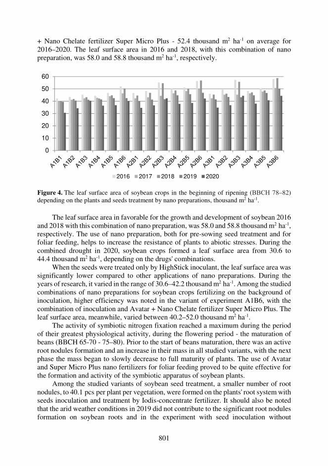
801
+ Nano Chelate fertilizer Super Micro Plus - 52.4 thousand m2 ha-1 on average for 2016–2020. The leaf surface area in 2016 and 2018, with this combination of nano preparation, was 58.0 and 58.8 thousand m2 ha-1, respectively.
Figure 4. The leaf surface area of soybean crops in the beginning of ripening (ВВСН 78–82) depending on the plants and seeds treatment by nano preparations, thousand m2 ha-1.
The leaf surface area in favorable for the growth and development of soybean 2016 and 2018 with this combination of nano preparation, was 58.0 and 58.8 thousand m2 ha-1, respectively. The use of nano preparation, both for pre-sowing seed treatment and for foliar feeding, helps to increase the resistance of plants to abiotic stresses. During the combined drought in 2020, soybean crops formed a leaf surface area from 30.6 to 44.4 thousand m2 ha-1, depending on the drugs' combinations.
When the seeds were treated only by HighStick inoculant, the leaf surface area was significantly lower compared to other applications of nano preparations. During the years of research, it varied in the range of 30.6–42.2 thousand m2 ha-1. Among the studied combinations of nano preparations for soybean crops fertilizing on the background of inoculation, higher efficiency was noted in the variant of experiment A1B6, with the combination of inoculation and Avatar + Nano Chelate fertilizer Super Micro Plus. The leaf surface area, meanwhile, varied between 40.2–52.0 thousand m2 ha-1.
The activity of symbiotic nitrogen fixation reached a maximum during the period of their greatest physiological activity, during the flowering period - the maturation of beans (BBCH 65-70 - 75–80). Prior to the start of beans maturation, there was an active root nodules formation and an increase in their mass in all studied variants, with the next phase the mass began to slowly decrease to full maturity of plants. The use of Avatar and Super Micro Plus nano fertilizers for foliar feeding proved to be quite effective for the formation and activity of the symbiotic apparatus of soybean plants.
Among the studied variants of soybean seed treatment, a smaller number of root nodules, to 40.1 pcs per plant per vegetation, were formed on the plants' root system with seeds inoculation and treatment by Iodis-concentrate fertilizer. It should also be noted that the arid weather conditions in 2019 did not contribute to the significant root nodules formation on soybean roots and in the experiment with seed inoculation without
0
10
20
30
40
50
60
2016 2017 2018 2019 2020

802
additional fertilizing of crops, the number of root nodules per growing season did not exceed 12.0 pcs per plant.
Seed treatment by Avatar and Iodis-concentrate nano fertilizers in combination with inoculation and without additional fertilizing of crops increased the number of root nodules during the growing season by 7–11%. Foliar application of Avatar micro fertilizer and Super Micro Plus nanochelate fertilizer contributed to the growth of the root nodules number by 11–18%.
The main criteria for evaluating the efficiency of photosynthesis, biological nitrogen fixation, and plant productivity formation are indicators of individual plant productivity and soybean yield. The results of the research made it possible to establish the positive effect of the use of Avatar fertilizer, Jodis-concentrate, and Nano Chelate fertilizer Super Micro Plus in the formation of individual productivity indicators. Soybean yield significantly depended on weather conditions, varying from 1.23 to 3.48 t ha-1depending on weather conditions and the combined use of seed inoculation and nano fertilizer. The most favorable conditions for the growth and development of soybeans were in 2016. Yields, depending on the use of drugs combination ranged from 2.27 to 3.48 t ha-1 (Fig. 5).
Figure 5. Soybean yield depending on the combined use of nano preparations, t ha-1.
The yield of soybean in the control variant without fertilizing(control) and seed treatment by inoculant only on average for 2016–2020 amounted to 1.93. Pre-sowing treatment of seeds by Iodis-concentrate or Avatar, in addition to inoculation, increased yield by 0.10–0.19 t ha-1. At the same time, the effectiveness of nano preparations increased with the combined use of Avatar and Nano Chelate fertilizer Super Micro Plus. The soybean yield in the control variant (A1B1) in 2019 was 1.71 t ha-1, and in the variants with fertilizing during vegetation and combined pre-sowing seed treatment (A2B1; A3B1) the yield varied from 1.86 to 2.36 t ha-1. The use of Avatar + Nano Chelate fertilizer Super Micro Plus for fertilizing increased the crop yield to 2.18 (on background of A1B1); 2.37 (at background A2B1); 2.39 t ha-1(on background of A3B1).
0
0.5
1
1.5
2
2.5
3
3.5
2016 2017 2018 2019 2020 Average 2016-2020
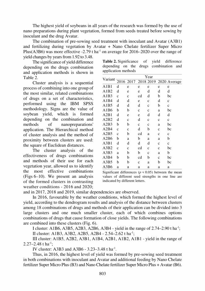
803
The highest yield of soybeans in all years of the research was formed by the use of nano preparations during plant vegetation, formed from seeds treated before sowing by inoculant and the drug Avatar.
The combination of pre-sowing seed treatment with inoculant and Avatar (A3B1) and fertilizing during vegetation by Avatar + Nano Chelate fertilizer Super Micro Plus(A3B6) was more effective -2.79 t ha-1 on average for 2016–2020 over the range of yield changes by years from 1.92 to 3.48.
The significance of yield difference depending on the drugs combination and application methods is shown in Table 2.
Cluster analysis is a sequential process of combining into one group of the most similar, related combinations of drugs on a set of characteristics, performed using the IBM SPSS methodology. Signs are the value of soybean yield, which is formed depending on the combination and methods of nanopreparations' application. The Hierarchical method of cluster analysis and the method of proximity between clusters are used: the square of Euclidean distances.
The cluster analysis of the effectiveness of drugs combinations and methods of their use for each vegetation year, allowed us to identify the most effective combinations (Figs 6–10). We present an analysis of the formed clusters in contrasting weather conditions - 2016 and 2020;
Table 2. Significance of yield difference depending on the drugs combination and application methods
Variant Year
2016 2017 2018 2019 2020 Average А1В1 d e e e e e А1В2 d e e d d d А1В3 c c cd d b bc А1В4 d d e c d c А1В5 d d d c b c А1В6 b b c c a bc А2В1 d e e d d d А2В2 d c d c c c А2В3 b b c c a bc А2В4 c c d b c bc А2В5 c b cd a c c А2В6 b a b a a b А3В1 d d d d c c А3В2 c c cd c c bc А3В3 a b b c a b А3В4 b b cd b c bc А3В5 b b c a b bc А3В6 a а a a a a Significant differences (p < 0.05) between the mean values of different seed strengths in one line are indicated by different letters.
and in 2017, 2018 and 2019, similar dependencies are observed. In 2016, favourable by the weather conditions, which formed the highest level of
yield, according to the dendrogram results and analysis of the distance between clusters among 18 combinations of drugs and methods of their application can be divided into 3 large clusters and one much smaller cluster, each of which combines options combinations of drugs that cause formation of close yields. The following combinations are combined into these clusters (Fig. 6).
I cluster: A1B6, A3B5, A2B3, A2B6, A3B4 - yield in the range of 2.74–2.90 t ha-1; II cluster: A1B3, A3B2, A2B5, A2B4 - 2.54–2.62 t ha-1; III cluster: A1B5, A2B2, A3B1, A1B4, A2B1, A1B2, A1B1 - yield in the range of
2.27–2.48 t ha-1; IV cluster: A3B3 and A3B6 - 3.23–3.48 t ha-1. Thus, in 2016, the highest level of yield was formed by pre-sowing seed treatment
in both combinations with inoculant and Avatar and additional feeding by Nano Chelate fertilizer Super Micro Plus (B3) and Nano Chelate fertilizer Super Micro Plus + Avatar (B6).

804
Figure 6. Dendrogram of yield using the method of intergroup connections (year of research 2016).
Figure 7. Dendrogram of yield using the method of intergroup connections (year of research 2017).
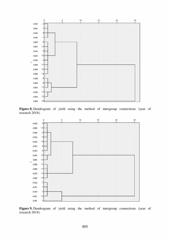
805
Figure 8. Dendrogram of yield using the method of intergroup connections (year of research 2018).
Figure 9. Dendrogram of yield using the method of intergroup connections (year of research 2019).

806
In 2020, due to extremely unfavourable weather conditions because of lack of moisture, the lowest level of yield was formed. According to the results of cluster analysis, the following clusters and yield levels were identified (Fig. 10):
I cluster: A2B5, A3B4, A3B2, A2B4, A3B1, A2B2 – 1.45–1.53 t ha-1; II cluster: A1B2, A1B4, A2B1 - 1.36–1.42 t ha-1; III cluster: A1B3, A1B5, A3B5 - 1.60–1.65 t ha-1; IV cluster: A2B6, A3B3, A3B6, A2B3 - 1.84–1.90 t ha-1.
Figure 10. Dendrogram of yield using the method of intergroup connections (year of research 2020).
Analysis of the formed clusters shows that the highest level of yield (cluster IV) is
also formed by combined pre-sowing treatment of seeds by inoculant and Iodis concentrate (A2) or Avatar (A3), and fertilizing by Nano Chelate fertilizer Super Micro Plus (B3) or combination of Nano Chelate fertilizer Super Micro Plus + Avatar (B6).
Feeding of soybean crops by nanofertilizer in combination with the drug Avatar with using for sowing seeds, inoculated and treated by the Avatar, and in adverse weather conditions and by Jodis concentrate, provide a significant increase in yield, which is observed in groups of formed clusters.
CONCLUSIONS
Based on the research, it was found that the use of nano preparations Avatar, Jodis-concentrate, and Super Micro Plus for seed treatment and fertilizing intensified the formation of the leaf surface area and the activity of the symbiotic apparatus of soybean plants. The obtained results confirm that application of the complex of nano fertilizers
807
Jodis-concentrate, Avatar, and Nano Chelate fertilizer Super Micro Plus in the soybean fertilizing helped to increase the yield, which testifies to their unconditional effectiveness. The highest efficiency of nano fertilizers was shown by inoculation and seed treatment by Avatar and co-fertilization Avatar + Nano Chelate fertilizer Super Micro Plus, ensuring the formation of 52.4 thousand m2 ha-1 of leaf surface area of soybean varieties Horol, 69.7 pcs plant-1 root nodules, 785 mg plant-1 of root nodules weight and yield at the level of 2.79 t ha-1.
REFERENCES
Batsmanova, L., Taran, N., Konotop, Y., Kalenska, S. & Novytska, N. 2020. Use of a colloidal solution of metal and metal oxide-containing nanoparticles as fertilizer for increasing soybean productivity. Journal of Central European Agriculture 21(2), 311–319. https://doi.org/10.5513/JCEA01/21.2.2414
Bielski, S., Romaneckas, K., Novikova, A. & Šarauskis, E. 2019. Are Higher Input Levels to Triticale Growing Technologies Effective in Biofuel Production System. Sustainability 11, 5915. doi:10.3390/su11215915
Bulgakov, V., Nikolaenko, S., Holovach, I., Adamchuk, V., Kiurchev, S., Ivanovs, S. & Olt, J. 2020. Theory of grain mixture particle motion during aspiration separation. Agronomy Research 18(1), 18–37.
Chen, Y.W., Lee, H.V., Juan, J.C. & Phang, S.M. 2016. Production of new cellulose nanomaterial from red algae marine biomass Gelidium elegans. Carbohydrate Polymers 151, 1210–1219. doi: http:// doi:10.1016/j.carbpol.2016.06.083
Dijk, V.M., Meijerink, G.W. 2014. A review of food security scenario studies: Gaps and ways forward. In: Achterbosch T.J., Dorp M., van Driel W.F., van Groot J.J., Lee J., van der Verhagen A., Bezlepkina I., editors. The Food Puzzle: Pathways to Securing Food for All. Wageningen UR; Wageningen, The Netherlands, pp. 30–32.
Dubey, A. & Mailapalli, D.R. 2016. Nanofertilisers, nanopesticides, nanosensors of pest and nanotoxicity in agriculture. Sustainable Agriculture Reviews 19, 307–330.
Dwivedi, S., Saquib, Q., Al-Khedhairy, A.A. & Musarrat, J. 2016. Understanding the role of nanomaterials in agriculture. Microbial Inoculants in Sustainable Agricultural Productivity. Springer; New Delhi, India. March, pp. 271–288.
Eremenko, O., Kalenska, S., Pokoptseva, L. & Todorova, L. 2019. The inffluence of AKM Growth Regulator on Photosynthetic Activity of Oilseed Flax Plants in the Conditions of Insufficient Humidification of the Southern Stepp of Ukraine. Modern Development Paths of agricultural production. 03 July: 703–807. doi: https://doi. org/10.1007/978-3-030-14918-5_78
Godfray, H.C.J., Beddington, J.R., Crute, R., Haddad, L., Lawrence, D., Muir, J.F., Pretty, J., Robinson, S., Thomas, S. & Toulmin, C. 2010. Food security: The challenge of feeding 9 billion people. Science. Vol. 327(5967), 812–818. doi: https://doi:10.1126/ science.1185383
Gogos, A., Knauer, K. & Bucheli, T.D. 2012. Nanomaterials in plant protection and fertilization: Current state, foreseen applications, and research priorities. Agriculture. Food Chem. 60, 9781–9792. doi: 10.1021/jf302154y
Kale, A.P. & Gawade, S.N. 2016. Studies on nanoparticle induced nutrient use efficiency of fertilizer and crop productivity. Green Chem. Technol. 2, 88–92. doi: https:// doi:10.18510/gctl.2016.226
Kirchmann, H., Börjesson, G., Bolinde, M., Katterer, T. & Djodjic, F. 2020. Soil properties currently limiting crop yields in Swedish agriculture – An analysis of 90 yield survey districts and 10 long-term field experiments. European Journal of Agronomy 120, 126–132 doi: https://doi.org/10.1016/j. eja.2020.126132
808
Khan, M.R. & Rizvi, T.F. 2014. Nanotechnology: Scope and application in plant disease management. Plant Patholоgy 13, 214–231. doi: https://doi: 10.3923/ ppj.2014.214.231
Kozyrskyi, V., Zablodskiy, M., Savchenko, V., Sinyavsky, O., Yuldashev, R., Kalenska, S. & Podlaski, S.Z. 2019. The Magnetic Treatment of Water Solutions and Seeds of Agricultural Crops. Advanced Agro-Engineering Technologies for Rural Business Development. 37 pp. doi: http://dx.doi.org/10,4018/978- 1-5225-7573-3.ch010
Kou, T.J., Yu, W.W., Lam, S.K., Chen, D.-L., How, Y.-P. & Li, Z.-Y. 2018. Differential root responses in two cultivars of winter wheat (Triticum aestivum L.) to elevated ozone concentration under fully open-air field conditions. Agron. Crop Sci. 204, 325–332. doi: https://doi:10.1111/jac.12257
Kwak, S.-Y., Wong, M.H., Lew, T.T.S., Bisker, G., Lee, M.A., Kaplan, A., Dong, J., Liu, A. T., Koman, V.B., Sinclair, R., Hamann, C. & Strano, M.S. 2017. Nanosensor technology applied to living plant systems. Annu. Rev. Anal. Chem. 10, 113–140. doi: https://doi:10.1146/annurev-anchem-061516-045310
Lopatko, K.H., Aftandiliants, E.H, Kalenska, S.M. & Tonkha, O.L. 2009. Mother colloidal solution of metals. Patent of Ukraine for useful model. No 38459, No 1. (in Ukrainian).
Makarenko, N.А., Kalenska, S.M. & Rudnitska, L.V. 2015. The biological efficacy and еnvironmental safety of nanoagrochemicals. Naukovyi visnyk NUBIP Ukrainy. Seriia: Ahronomiia [Scientific Bulletin of NULES of Ukraine. Series: Agronomy]. 210, 91–96 (in Ukrainian).
Miao, Y.F., Wang, Z.H. & Li, S.X. 2015. Relation of nitrate N accumulation in dryland soil with wheat response to N fertilizer. Field Crops Res. 170, 119–130. doi: https:// doi:10.1016/j.fcr.2014.09.016
Panpatte, D.G., Jhala, Y.K., Shelat H.N. & Vyas, R.V. 2016. Microbial Inoculants in Sustainable Agricultural Productivity. Nanoparticles: The next generation technology for sustainable agriculture, Springer; New Delhi, India, pp. 289–300.
Prasad, R., Bhattacharyya, A. & Nguyen, Q.D. 2017. Nanotechnology in sustainable agriculture: Recent developments, challenges, and perspectives. Front. Microbiol. 8, 1014. doi: https://doi:10.3389/fmicb.2017.01014
Sabir, A., Yazar, K., Sabir, F., Kara, Z., Yazici, M.A. & Goksu, N. 2014. Vine growth, yield, berry quality attributes and leaf nutrient content of grapevines as influenced by seaweed extract (Ascophyllum nodosum) and nanosize fertilizer pulverizations. Sci. Hortic. 175, 1–8. doi: https://doi:10.1016/j.scienta.2014.05.021
Shcherbakova, E.N., Shcherbakov, A.V., Andronov, E.E., Gonchar, L.N., Kalenskaya, S.M. & Chebotar, V.K. 2017. Combined pre seed treatment with microbial inoculants and Mo nanoparticles changes composition of root exudates and rhizosphere microbiome structure of chickpea (Cicer arietinum L.) plants. Biology. Symbiosis 73(1), 57–69. doi: https://doi.org/10.1007/ s13199-016-0472-1
Solanki, P., Bhargava, A., Chhipa, H., Jain, N. & Panwar, J. 2015. Nano-fertilizers and their smart delivery system. In: Rai, M., Ribeiro, C., Mattoso, L., Duran, N., editors. Nanotechnologies in Food and Agriculture. Springer; Cham, Switzerland, pp, 81–101.
Vermeulen, S. J., Aggarwal, P. K., Ainslie, A., Angelone, S., Campbel, B. M., Challinor, A. J., Hansen, J. W., Ingram, J. S. L., Jarvis, A., Kristjanson, P., Lau, C., Nelson, G.C., Thornton, P.K. & Wollenberg, E. 2012. Options for support to agriculture and food security under climate change. Environ. Sci. Policy 15, 136–144. doi: https://doi:10.1016/j.envs- ci.2011.09.003
Wang, Z.H., Miao, Y.F. & Li, S.X. 2015. Effect of ammonium and nitrate nitrogen fertilizers on wheat yield in relation to accumulated nitrate at different depths of soil in drylands of China. Field Crops Res. 183, 211–224. doi: https://doi:10.1016/j. fcr.2015.07.019
Worrall, E., Hamid, A., Mody, K., Mitterm, N. & Pappu, H. 2018. Nanotechnology for plant disease management. Agronomy 8, 285. doi: https://doi:10.3390/agronomy8120285
809
Agronomy Research 19(S1), 809–818, 2021 https://doi.org/10.15159/AR.21.018
Development of the Digital Matchmaking Platform for international cooperation in the biogas sector
V. Komasilovs1, N. Bumanis1, A. Kviesis1, J. Anhorn2 and A. Zacepins1,*
1Latvia University of Life Sciences and Technologies, Faculty of Information Technologies, Department of Computer Systems, Lielā iela 2, LV-3001 Jelgava, Latvia 2Deutsche Gesellschaft für Internationale Zusammenarbeit (GIZ) GmbH, Friedrich-Ebert-Allee 32 + 36, DE 53113 Bonn, Germany *Correspondence: [email protected] Received: January 12th, 2021; Accepted: March 27th, 2021; Published: March 31st, 2021 Abstract. The demand for sustainable, renewable and clean energy sources has been increasing in the past decade in order to combat global warming by reducing greenhouse gas emissions. Biogas has proven to be a versatile energy carrier which can be used for heating purposes, power and fuel. Having acknowledged the high potential for the use of biogas energy and having researched the demand and supply markets, the Digital Global Biogas Cooperation (DiBiCoo) project aims to link European biogas and biomethane technology providers with emerging and developing markets. To achieve this goal the development and application of innovative digital support tools is necessary - a digital matchmaking platform (DMP) with bi-directional partnership architecture. DMP can be used as means to build trust-based business relationships, share information on available European technologies and serve as an additional marketing option for EU and non-EU companies and industries. This article presents the developed platform prototype and demonstrates its basic functionality and the development process. Basic business and functional requirements were defined and then refined into functional, user-interface and performance requirements for implementation. User requirements were defined using user centred design approach in collaboration with potential platform end-users, considering their specific needs. During the development process Agile methodology was used. In the future digital platform functionality will be extended based on discussions and feedback of the stakeholders and end-users during local workshops and other events, where the DiBiCoo platform will be presented. Key words: DiBiCoo, biogas, international cooperation, matchmaking, IT platform.
INTRODUCTION Building trustworthy partnerships in the business sector are crucial for successful
expansion of businesses geographically and economically. Different approaches can be applied to address the commencing of business partnerships, such as matchmaking. Its scope in the context of business collaboration is to find suitable colleagues or business partners for mutual inspiration and support, ideally resulting in innovation (Kopplin, 2020). However, matchmaking is not something new and previously it was used mostly

810
for the marriage purposes (Wu et al., 2018). As well in some cultures, the role of the matchmaker was and is quite professionalised. Nowadays, matchmaking platforms and information and communication technology (ICT) solutions allow to apply it in other ways as well, for example, finding right events, doing networking in an efficient way, finding the right candidates, investors (Afuah & Tucci, 2012), finding organ donors or supplier selection (McCutcheon & Stuart, 2000), improving the quality of university-industry collaborations (Bjurström et al., 2020) etc. The main idea behind matchmaking is linking people or companies according to their values, goals and specific needs. In essence, the matchmaking process can be defined as searching for suitable agents that have complementary information, skills or other capabilities that you require. To achieve beneficial matching a digital platform can be used. A Matchmaking platform is a system where different people, groups of people and organisations can identify and connect with corresponding parties. There are various matchmaking platforms available online for different purposes like dating, tourism (Moreno et al., 2013; Grün et al., 2017), multiplayer games, e-commerce systems, medicine matchmaking system (Han et al., 2019) and systems for different services like hotels, restaurants, car sharing, etc. In addition, such platforms become available for Business-to-Business (B2B) matchmaking. Some examples of matchmaking platforms are described in different scientific articles (Keijzer-Broers et al., 2013; Montuschi et al., 2014; Rabhi & Pal, 2019). In the B2B sector, matchmaking platforms may have a great impact whether for a big corporation or a new start-up. In some regions digital innovation hubs were developed to reshape the regional bioeconomy to enable regional cooperation between biomass suppliers and technology providers (Macias Aragones et al., 2020).
DIBICOO PROJECT
DiBiCoo1 is a cooperation project between biogas technology exporting and
importing countries, with the overall objective to support the European biogas/biomethane industry by preparing markets for the export of sustainable biogas/biomethane technologies from Europe to developing and emerging countries like Indonesia, Argentina, Ethiopia, Ghana, South Africa (Rutz et al., 2020). The fast depleting supply of fossil fuels and growing environmental degradation by potent greenhouse gases is pushing the World´s economies towards the usage of alternative energy sources (Roubík et., 2017). In so-called developing countries, pollution and access to energy sources still represent a significant challenge, especially in connection with human and environmental health and with economic development (Shane et al., 2015). Access to energy influences living standards and overall development (Demirbas & Demirbas, 2007). Therefore, bioenergy production by fermentation reaction is gaining popularity due to its easy operation and a wide availability of organic wastes (Priekulis et al., 2015). Biogas production and use have increased rapidly in many countries over the last 20 years, augmenting its importance as a renewable energy source (Scarlat et al., 2018). The production of biogas is one of the most nature’s friendly alternative energy technologies and its demand is increasing (Dubrovskis & Plume, 2017). Biogas energy comes from biomass, which is the biodegradable fraction of products, waste and residues
1 http://dibicoo.org
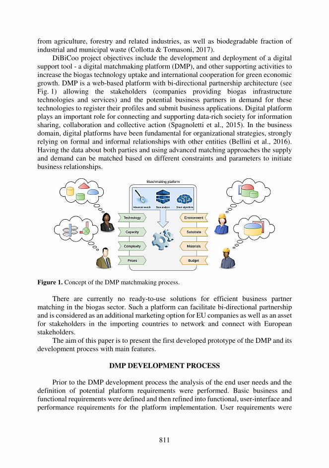
811
from agriculture, forestry and related industries, as well as biodegradable fraction of industrial and municipal waste (Collotta & Tomasoni, 2017).
DiBiCoo project objectives include the development and deployment of a digital support tool - a digital matchmaking platform (DMP), and other supporting activities to increase the biogas technology uptake and international cooperation for green economic growth. DMP is a web-based platform with bi-directional partnership architecture (see Fig. 1) allowing the stakeholders (companies providing biogas infrastructure technologies and services) and the potential business partners in demand for these technologies to register their profiles and submit business applications. Digital platform plays an important role for connecting and supporting data-rich society for information sharing, collaboration and collective action (Spagnoletti et al., 2015). In the business domain, digital platforms have been fundamental for organizational strategies, strongly relying on formal and informal relationships with other entities (Bellini et al., 2016). Having the data about both parties and using advanced matching approaches the supply and demand can be matched based on different constraints and parameters to initiate business relationships.
Figure 1. Concept of the DMP matchmaking process. There are currently no ready-to-use solutions for efficient business partner
matching in the biogas sector. Such a platform can facilitate bi-directional partnership and is considered as an additional marketing option for EU companies as well as an asset for stakeholders in the importing countries to network and connect with European stakeholders.
The aim of this paper is to present the first developed prototype of the DMP and its development process with main features.
DMP DEVELOPMENT PROCESS
Prior to the DMP development process the analysis of the end user needs and the
definition of potential platform requirements were performed. Basic business and functional requirements were defined and then refined into functional, user-interface and performance requirements for the platform implementation. User requirements were
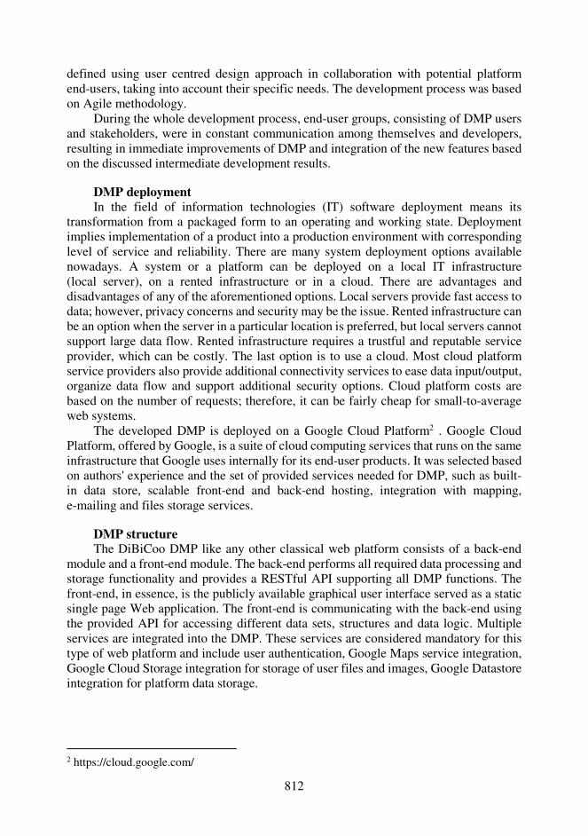
812
defined using user centred design approach in collaboration with potential platform end-users, taking into account their specific needs. The development process was based on Agile methodology.
During the whole development process, end-user groups, consisting of DMP users and stakeholders, were in constant communication among themselves and developers, resulting in immediate improvements of DMP and integration of the new features based on the discussed intermediate development results.
DMP deployment In the field of information technologies (IT) software deployment means its
transformation from a packaged form to an operating and working state. Deployment implies implementation of a product into a production environment with corresponding level of service and reliability. There are many system deployment options available nowadays. A system or a platform can be deployed on a local IT infrastructure (local server), on a rented infrastructure or in a cloud. There are advantages and disadvantages of any of the aforementioned options. Local servers provide fast access to data; however, privacy concerns and security may be the issue. Rented infrastructure can be an option when the server in a particular location is preferred, but local servers cannot support large data flow. Rented infrastructure requires a trustful and reputable service provider, which can be costly. The last option is to use a cloud. Most cloud platform service providers also provide additional connectivity services to ease data input/output, organize data flow and support additional security options. Cloud platform costs are based on the number of requests; therefore, it can be fairly cheap for small-to-average web systems.
The developed DMP is deployed on a Google Cloud Platform2 . Google Cloud Platform, offered by Google, is a suite of cloud computing services that runs on the same infrastructure that Google uses internally for its end-user products. It was selected based on authors' experience and the set of provided services needed for DMP, such as built-in data store, scalable front-end and back-end hosting, integration with mapping, e-mailing and files storage services.
DMP structure The DiBiCoo DMP like any other classical web platform consists of a back-end
module and a front-end module. The back-end performs all required data processing and storage functionality and provides a RESTful API supporting all DMP functions. The front-end, in essence, is the publicly available graphical user interface served as a static single page Web application. The front-end is communicating with the back-end using the provided API for accessing different data sets, structures and data logic. Multiple services are integrated into the DMP. These services are considered mandatory for this type of web platform and include user authentication, Google Maps service integration, Google Cloud Storage integration for storage of user files and images, Google Datastore integration for platform data storage.
2 https://cloud.google.com/
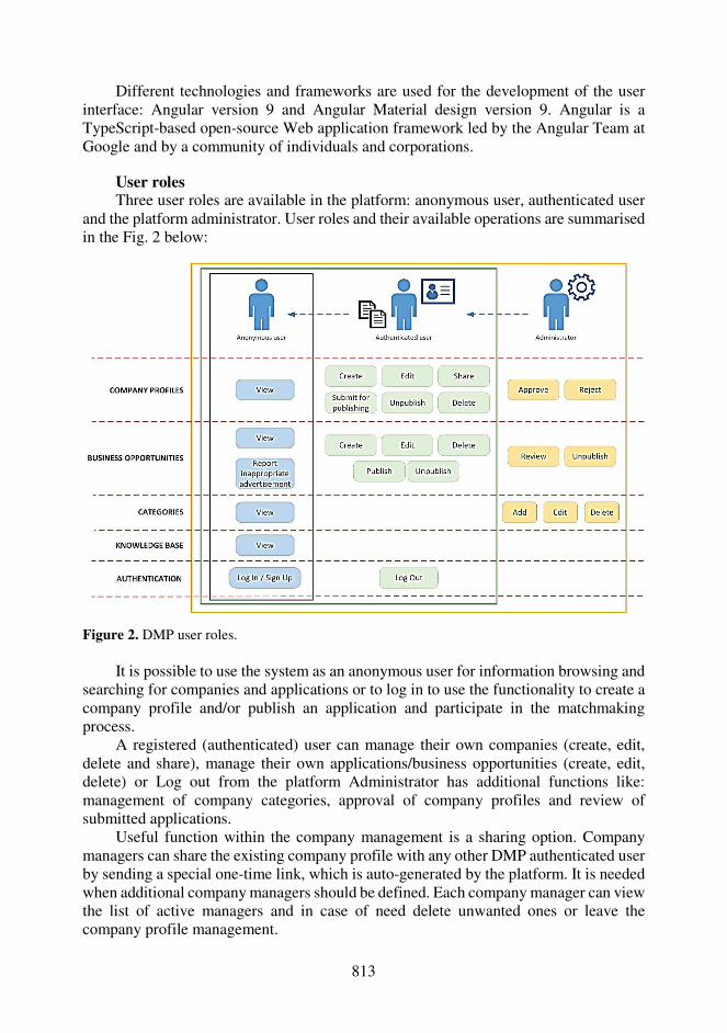
813
Different technologies and frameworks are used for the development of the user interface: Angular version 9 and Angular Material design version 9. Angular is a TypeScript-based open-source Web application framework led by the Angular Team at Google and by a community of individuals and corporations.
User roles Three user roles are available in the platform: anonymous user, authenticated user
and the platform administrator. User roles and their available operations are summarised in the Fig. 2 below:
Figure 2. DMP user roles.
It is possible to use the system as an anonymous user for information browsing and
searching for companies and applications or to log in to use the functionality to create a company profile and/or publish an application and participate in the matchmaking process.
A registered (authenticated) user can manage their own companies (create, edit, delete and share), manage their own applications/business opportunities (create, edit, delete) or Log out from the platform Administrator has additional functions like: management of company categories, approval of company profiles and review of submitted applications.
Useful function within the company management is a sharing option. Company managers can share the existing company profile with any other DMP authenticated user by sending a special one-time link, which is auto-generated by the platform. It is needed when additional company managers should be defined. Each company manager can view the list of active managers and in case of need delete unwanted ones or leave the company profile management.
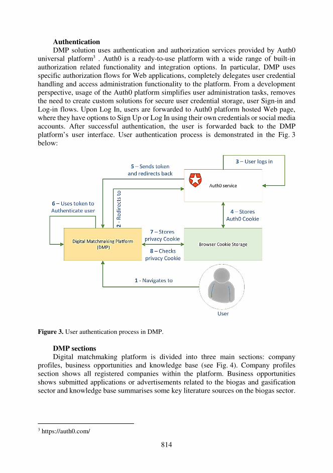
814
Authentication DMP solution uses authentication and authorization services provided by Auth0
universal platform3 . Auth0 is a ready-to-use platform with a wide range of built-in authorization related functionality and integration options. In particular, DMP uses specific authorization flows for Web applications, completely delegates user credential handling and access administration functionality to the platform. From a development perspective, usage of the Auth0 platform simplifies user administration tasks, removes the need to create custom solutions for secure user credential storage, user Sign-in and Log-in flows. Upon Log In, users are forwarded to Auth0 platform hosted Web page, where they have options to Sign Up or Log In using their own credentials or social media accounts. After successful authentication, the user is forwarded back to the DMP platform’s user interface. User authentication process is demonstrated in the Fig. 3 below:
Figure 3. User authentication process in DMP. DMP sections Digital matchmaking platform is divided into three main sections: company
profiles, business opportunities and knowledge base (see Fig. 4). Company profiles section shows all registered companies within the platform. Business opportunities shows submitted applications or advertisements related to the biogas and gasification sector and knowledge base summarises some key literature sources on the biogas sector.
3 https://auth0.com/

815
Figure 4. Front page of the DiBiCoo DMP. Company profile management One of the main authenticated user functions is creation and publishing of the
company profile. Company profile creation is necessary for a successful matchmaking process in the future. A digital company profile is like a business card with primary information and data about the company which takes part in the digital matchmaking process. This company registration form is divided into several sections with one or several input fields. The company profile is published online only after the DMP administrator reviews and accepts it. The company profile life cycle statuses include: draft, pending, published, rejected (see Fig. 5 below):
Figure 1. Company profile status changes.
816
Business opportunities section Within this section, authenticated users can submit advertisements or business
opportunities describing particular services, products or a biogas project they are interested in or offering.
Advertisements are not being reviewed by the DMP administrators and published without any content/liability check, but if any issues are found they can be unpublished by the advertisement creators or by the platform administrators afterwards. Furthermore, any user can file a report to the platform administrators by clicking the Report button.
Knowledge base section Within the knowledge base section, informative materials (factsheets) and links to
various sources about the biogas production and biogas related topics are summarised. In the future it is planned to also include information about the upcoming biogas events and conferences.
DISCUSSION
Digital matchmaking platform described within this article have been developed
also to address ICT sector acceleration for attaining the sustainability goals of the Green Deal (European Commission, 2019). Green Deal is an integral part of the European Commission’s strategy to implement the United Nation’s 2030 Agenda and the sustainable development goals. It is a new socio-economic growth strategy that aims to transform the EU into a fair and prosperous society, with a modern, resource-efficient and competitive economy, with no net emissions of greenhouse gases in 2050 and where economic growth is decoupled from resource use. ‘Mobilising industry for a clean and circular economy’ is one of the major objectives of the Green Deal, which includes two challenges concerning digitisation of biomass value chains. Developed platform can be considered as one of the industrial mobilising structures showing the capacity to accelerate and maximise the impact of digital technologies on the implementation of the Green Deal.
By focusing on digitisation of key actors within the biogas sector, effectively engaging and building networks between stakeholders involved in biogas industry development from different geographical location, a contribution to sustainability acceleration can be reached by the developed digital matchmaking platform.
Within the platform company profiles are organised by the categories which are formulated based on business processes within the biogas industry.
Companies matchmaking at this moment can be done in manual way by selecting several filtering options and searching for the target stakeholder by region or country of origin, company business field, company reference project location or company profile update time. In the future it will be possible to save matchmaking preferences and DiBiCoo platform will automatically notify the user when new matches will be found.
Developed DiBiCoo digital matchmaking platform can act as a main source of stakeholder information involved in biogas sector development with some additional features for actor matchmaking for successful business project development.
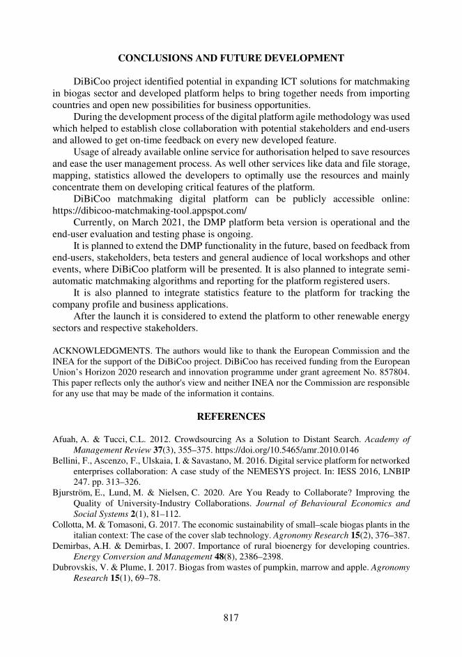
817
CONCLUSIONS AND FUTURE DEVELOPMENT
DiBiCoo project identified potential in expanding ICT solutions for matchmaking in biogas sector and developed platform helps to bring together needs from importing countries and open new possibilities for business opportunities.
During the development process of the digital platform agile methodology was used which helped to establish close collaboration with potential stakeholders and end-users and allowed to get on-time feedback on every new developed feature.
Usage of already available online service for authorisation helped to save resources and ease the user management process. As well other services like data and file storage, mapping, statistics allowed the developers to optimally use the resources and mainly concentrate them on developing critical features of the platform.
DiBiCoo matchmaking digital platform can be publicly accessible online: https://dibicoo-matchmaking-tool.appspot.com/
Currently, on March 2021, the DMP platform beta version is operational and the end-user evaluation and testing phase is ongoing.
It is planned to extend the DMP functionality in the future, based on feedback from end-users, stakeholders, beta testers and general audience of local workshops and other events, where DiBiCoo platform will be presented. It is also planned to integrate semi-automatic matchmaking algorithms and reporting for the platform registered users.
It is also planned to integrate statistics feature to the platform for tracking the company profile and business applications.
After the launch it is considered to extend the platform to other renewable energy sectors and respective stakeholders.
ACKNOWLEDGMENTS. The authors would like to thank the European Commission and the INEA for the support of the DiBiCoo project. DiBiCoo has received funding from the European Union’s Horizon 2020 research and innovation programme under grant agreement No. 857804. This paper reflects only the author's view and neither INEA nor the Commission are responsible for any use that may be made of the information it contains.
REFERENCES
Afuah, A. & Tucci, C.L. 2012. Crowdsourcing As a Solution to Distant Search. Academy of
Management Review 37(3), 355–375. https://doi.org/10.5465/amr.2010.0146 Bellini, F., Ascenzo, F., Ulskaia, I. & Savastano, M. 2016. Digital service platform for networked
enterprises collaboration: A case study of the NEMESYS project. In: IESS 2016, LNBIP 247. pp. 313–326.
Bjurström, E., Lund, M. & Nielsen, C. 2020. Are You Ready to Collaborate? Improving the Quality of University-Industry Collaborations. Journal of Behavioural Economics and Social Systems 2(1), 81–112.
Collotta, M. & Tomasoni, G. 2017. The economic sustainability of small–scale biogas plants in the italian context: The case of the cover slab technology. Agronomy Research 15(2), 376–387.
Demirbas, A.H. & Demirbas, I. 2007. Importance of rural bioenergy for developing countries. Energy Conversion and Management 48(8), 2386–2398.
Dubrovskis, V. & Plume, I. 2017. Biogas from wastes of pumpkin, marrow and apple. Agronomy Research 15(1), 69–78.
818
European Commission. The European Green Deal. Communication from the Commission to the European Parliament, the European Council, the Council, the European Economic and Social Committee and the Committee of the regions. Brussels, 11.12.2019 COM (2019) 640 Final, Brussels. 11 December 2019. Available online: https://ec.europa.eu/info/sites/info/files/european-green-deal-communication_en.pdf (accessed on 08 March 2021).
Grün, C., Neidhardt, J. & Werthner, H. 2017. Ontology-Based Matchmaking to Provide Personalized Recommendations for Tourists. In Information and Communication Technologies in Tourism 2017, 3–16. https://doi.org/10.1007/978-3-319-51168-9_1
Han, Q., Ji, M., Martinez De Rituerto De Troya, I., Gaur, M. & Zejnilovic, L. 2019. A hybrid recommender system for patient-doctor matchmaking in primary care. Proceedings - 2018 IEEE 5th International Conference on Data Science and Advanced Analytics, DSAA 2018, 481–490. https://doi.org/10.1109/DSAA.2018.00062
Keijzer-Broers, W.J.W., De Reuver, M. & Guldemond, N.A. 2013. Designing a matchmaking platform for smart living services. Lecture Notes in Computer Science (Including Subseries Lecture Notes in Artificial Intelligence and Lecture Notes in Bioinformatics), 7910 LNCS, 224–229. https://doi.org/10.1007/978-3-642-39470-6-28
Kopplin, C.S. 2020. Two heads are better than one: matchmaking tools in coworking spaces. Review of Managerial Science. https://doi.org/10.1007/s11846-020-00382-4
Macias Aragonés, M., de la Viña Nieto, G., Nieto Fajardo, M., Páez Rodríguez, D., Gaffey, J., Attard, J., McMahon, H., Doody, P., Anda Ugarte, J., Pérez-Camacho, M. & Cuenca Martín, M. 2020. Digital Innovation Hubs as a Tool for Boosting Biomass Valorisation in Regional Bioeconomies: Andalusian and South-East Irish Case Studies. Journal of Open Innovation: Technology, Market, and Complexity 6(4), pp.115.
McCutcheon, D. & Stuart, F.I. 2000. Issues in the choice of supplier alliance partners. Journal of Operations Management 18(3), 279–301. https://doi.org/10.1016/S0272-6963(99)00026-1
Montuschi, P., Gatteschi, V., Lamberti, F., Sanna, A. & Demartini, C. 2014. Job Recruitment and Job Seeking Processes: How Technology Can Help. IT Professional 16(5), 41–49. https://doi.org/10.1109/MITP.2013.62
Moreno, A., Valls, A., Isern, D., Marin, L. & Borràs, J. 2013. SigTur/E-Destination: Ontology-based personalized recommendation of Tourism and Leisure Activities. Engineering Applications of Artificial Intelligence 26(1), 633–651. https://doi.org/10.1016/j.engappai.2012.02.014
Priekulis, J., Aboltins, A. & Laurs, A. 2015. Amount of manure used for biogas production. Agronomy Research 13(2), 396–404.
Rabhi, A. & Pal, P. 2019. Japan–India Technology Matchmaking Platform: Approach to Promote Japanese Low Carbon Technologies in Indian Industries. Journal of Resources, Energy and Development 16(1), 9–18. https://doi.org/10.3233/red-160102
Roubík, H., Mazancová, J., Phung, L.D. & Dung, D.V. 2017. Quantification of biogas potential from livestock waste in Vietnam. Agronomy Research 15(2), 540–552.
Rutz, D., Gue, O., Colmorgen, F., Janssen, R., Anhorn, J., van Laere, A., … & Salie, Y. 2020. Biogas - Global Challenges, Markets and Cooperation Opportunities. 28th European Biomass Conference and Exibition, pp. 755–757.
Scarlat, N., Dallemand, J.F. & Fahl, F. 2018. Biogas: Developments and perspectives in Europe. Renewable energy 129,.457–472.
Shane, A., Gheewala, S.H. & Kasali, G. 2015. Potential, Barriers and Prospects of Biogas Production in Zambia. Journal of Sustainable Energy & Environment 6(January 2015), 21–27.
Spagnoletti, P., Resca, A. & Lee, G. 2015. A design theory for digital platforms supporting online communities: A multiple case study. J. Inf. Technol. 30, 364–380. Wu, Y., Zhang, K. & Padmanabhan, V. 2018. Matchmaker Competition and Technology Provision.
Journal of Marketing Research 55(3), 396–413. https://doi.org/10.1509/jmr.16.0423
819
Agronomy Research 19(S1), 819–833, 2021 https://doi.org/10.15159/AR.21.082
Packing materials for biotrickling filters used in biogas upgrading – biomethanation
Z. Kusnere*, K. Spalvins, D. Blumberga and I. Veidenbergs
Riga Technical University, Institute of Energy Systems and Environment Azenes street 12/1, LV 1048 Riga, Latvia *Correspondence: [email protected] Received: February 1st, 2021; Accepted: May 2nd, 2021; Published: May 18th, 2021 Abstract. One of the promising methods of biogas upgrading is biological methanation (biomethanation). During biomethanation process hydrogenotrophic microorganisms use carbon dioxide from biogas and added hydrogen to generate biomethane. Application of biotrickling filter reactors is one of the prospective biotechnologies for methanation where hydrogenotrophic methanogens are immobilized over a material that is used in reactor. Packing materials for biomethanation are critical in terms of hydrogenotrophic methanogens immobilization on the surface of packing material. It acts as support for biofilm growth. Therefore, characteristics of filter material are important parameters that influence the growth of microorganisms and methane production. Factors, such as optimal specific surface area and porosity are important to sustain growth and activity of microorganisms. Optimal particle size and capability to mechanically resist compaction ensures avoiding high pressure drop. Optimal particle size also ensures uniform gas flow as gases distribute through the packing material. This review paper summarizes and compare the characteristics of different packing materials important for biomethanation through ex-situ biotrickling filter reactor systems. Key words: biogas upgrading; biomethanation; biotrickling filter; biofilm; packing materials.
INTRODUCTION
Biogas production is an important process for dealing with different types of waste. It is particularly difficult for farms to live without a biogas station. If there were no biogas plants, the surrounding population would have problems with both smell and local environmental. Biogas production is one of the technological components of agriculture. Waste recycling produces heat and energy, as well as digestates (material remaining after anaerobic digestion), which is a much more valuable fertilizer for soil than fossil fertilizers.
Biogas is a product of anaerobic digestion - a renewable fuel which can be produced from different organic waste materials. In raw biogas methane content is about 50–70%, while carbon dioxide content is 30–50% (Baena-Moreno et al., 2019; Witte et al., 2019). Therefore, upgrading biogas by increasing methane concentration is a way to increase its usefulness. Upgraded biogas with methane content up to 96% can be directly added into the grid of natural gas (Dupnock & Deshusses, 2019; Witte et al., 2019). Unlimited
820
biogas injection into the gas grid can be achieved by removing carbon dioxide to acquire biomethane. The main advantage of biological biogas upgrading technologies is conversion of carbon dioxide into high value products under light operational conditions, which significantly promote to a sustainable bio economy and life cycle economy (Angelidaki et al., 2018). One of the promising methods of biogas upgrading is biological methanation (biomethanation). During biomethanation process hydrogenotrophic microorganisms use carbon dioxide from biogas and added hydrogen to generate biomethane. This method of biogas upgrading is energy intensive as it requires hydrogen as a material input (Mehrpooya et al., 2020). To ensure this method is sustainable, the hydrogen for the required reaction should come from a renewable source. Hydrogen can be produced via electrolysis using electricity from off-peak electricity surplus from solar or wind energy power systems (Akhlaghi & Najafpour-Darzi, 2020; Mehrpooya et al., 2020). Although in this system the cost of biomethane is determined of the cost of hydrogen used for biomethanation (Vo et al., 2018). If there is surplus renewable power, it can be utilized for biogas upgrading and make biomethanation as an energy storage solution (De Vrieze et al., 2020). This kind of system is known as ‘Power to Gas’ concept (Bensmann et al., 2013).
The biological hydrogen methanation using methanogens is possible to be applied in two different systems. First one is in-situ system (Luo & Angelidaki, 2012) where biomethanation is performed within anaerobic digester system. In this process organic matters are transformed into biogas under specific conditions (Holm-Nielsen et al., 2009). Second is an ex-situ system, where a separate external reactor for biomethanation is used (Lecker et al., 2017). Main reaction for the biomethanaion process is known as Sabatier reaction (Eq. 1),
CO2 + 4·H2 ↔ CH4 + 2·H2O (1)
where methane is converted from molecular hydrogen and carbon dioxide (Leonzio 2016). Carbon dioxide is used as a waste gas in this reaction to produce methane. Therefore, raw biogas which contents 30–50% of carbon dioxide can be upgraded to biometane. Methanogens are able to metabolize hydrogen into methane. These microorganisms are called hydrogenotrophic methanogens and they are often already present in anaerobic cultures that carry on the reaction. (Zabranska & Pokorna, 2018).
Various reactor types can be outfitted for ex-situ biomethanation, such as biotrickling filter reactors (Burkhardt et al., 2015; Rachbauer et al., 2016), continuously stirred tank reactors (Thema et al., 2019), fixed bed reactors (Alitalo et al., 2015), biofilm plug-flow reactors (Savvas et al., 2017) and other bioreactors (Dupnock & Deshusses 2019; Germec et al., 2020). There are several advantages for ex-situ systems. Industrial carbon dioxide can be easily added from external sources, if the biomethanation is carried out in ex-situ reactor by hydrogenotrophic methanogenesis. In this system CO2 can be used in biogas upgrading by conversion into biomethane (Michailos et al., 2020). But in external bioreactor systems only gases (H2 and CO2) can be used as substrates and added to fermentation liquid as energy source (I. Bassani et al., 2016). Therefore, efficient gas diffusion systems and different biofilter configurations are important for increasing gas-liquid contact time and enhancing biofilm growth. By increasing biofilm growth more efficient methane production can be achieved (C.L. Bassani et al., 2017).

821
Application of biotrickling filter reactors is one of the prospective biotechnology for methanation where hydrogenotrophic methanogens are immobilized over a material that is used in reactor (Ashraf et al., 2020). By immobilizing microorganism cells it is possible to increase efficiency of the substrate conversion, shorten retention times and minimalize microbial contaminations. Microorganisms are more protected from shear stress compared to stirring reactors and can be reused. Therefore, the costs of process can be reduced (Sekoai et al., 2018). If cells are not immobilized, microorganisms are prone to washout which causes instability in process and reduces biomethane yield (Kourkoutas et al., 2004). Packing materials and characteristics of the materials within biotrickling filter reactor system play a large role. (Sekoai et al., 2018). Defined characteristics of materials can facilitate bioreactors setup configurations for biomethanation process.
Biological trickling filter reactors Biological trickling filter (BTF) reactor is the most promising technology for
biomethanation, based on recent research studies on the ex-situ biomethanation design (Rachbauer et al., 2016; Strübing et al., 2018; Sieborg et al., 2020). The main and most important reason is that biotrickling filter is equipped with large surface area available to form biofilm and this means that methane production per unit volume is higher than in most other reactor types (Ashraf et al., 2020). In the biotrickling filter packing material supports the biofilm and generally offer more valuable gas to liquid mass transfer. Because of larger surface area of biofilter between liquid and gaseous substrates, low gas and liquid flow rates are maintained. Fermentation liquid can be recirculated to maintain efficient CH4 production. Liquid biofilm on the packaging materials as well as rate of recirculation has been studied by Burkhardt et al., 2015. Results show that biomethanation of hydrogen and carbon dioxide in biotrickling filter was successful and productive using anaerobic sewage sludge as inoculum (Burkhardt et al., 2015).
Biotrickling filter reactors have been studied in different conditions within biometnanation using hydrogen as energy source. By using trickle bed reactor, biomethane concentration successfully reached more than 98% in the output product (Rachbauer et al., 2016). This type of reactor was also used for syngas biomethanation and was successful at being very productive and having efficient conversion rates (Grimalt-Alemany et al., 2018). Tests are made to research appropriate conditions such as flow rate, pH rate, pressure, gas-liquid mass transfer, duration of reaction (Rachbauer et al., 2016; Porté et al., 2019) and also, best reactor setup for biomethanation efficiency. In the last few years many research works have been published where biotrickle filter reactor technology was used for biomethanation (Dupnock & Deshusses 2019; Porté et al., 2019; Dahl Jønson et al., 2020; Germec et al., 2020), making this one of the most promising novel technology for biogas upgrading. Using biotrickling filters, the energy demand is substantially lower as there is no need for stirring and dispersing liquid phase. Energy is used to pump the fermentation liquid to the top of the filter column where it is sprinkled over the packing material (Thema et al., 2019). The filter consists of packing material and microorganisms - hydrogenotrophic methanogens. Packing material act as support for biofilm growth, therefore characteristics of filter material are important parameters that influence the growth of microorganisms and, therefore, methane production. Packing materials could be examined as one of the main factors of the biotrickling filter reactor systems (Wu et al., 2018). Choosing an effective packing

822
material in a biotrickling filter for hydrogenotrophic methanogens to grow biofilm may be major design variable for the biotrickling filter reactor. However, testing the packing in a continuously operating biotrickling filter reactor is costly both in time and resources (Ashraf et al., 2020).
The main function for packing material in biotrickling filter reactor is to ensure contact between microorganisms and substrate to allow production of high concentration methane (Wu et al., 2018; Maegaard et al., 2019). Surface on packing materials of biofilter is larger for microorganisms to attach. Therefore, using biotrickling filter reactors the speed of the methanation process is significantly increased. Immobilizing microorganisms in biomethane production stabilizes the pH of the medium, prevents microorganism washout and extends microbial activity providing continuous methanation process (Sekoai et al., 2018).
CHARACTERISTICS OF PACKING MATERIALS
Packing materials used as biotrickling filters can normally be classified into three
categories: organic, inorganic, and mixed materials. Organic materials, such as soil, peat, and wood chips were being used in biotrickling filters at the beginning. Inorganic packing materials normally come directly from natural sources, such as lava and perlite. All these natural packing materials have good surface properties, but their shape may be irregular (Wu et al., 2018). With time a variety or inorganic packing materials were sythethized and used for biotrickling filters (or other systems), such as ceramic, plastic Pall rings, Rasching rings or rubber particles, clear polyvinyl chloride (PVC), polyurethane foam (PUF) and other materials (Park et al., 2011). Synthesized materials as packing materials sometimes have improved porosity and larger surface area. These materials have smoother surface, and specific made shape and strength that ensures good conditions for microorganisms. The escalated area of synthetized materials improves biotrickling filters performance. Most inorganic materials have advantage of uniform size and structure. These characteristics ensure better gas flow and reduce the compaction of materials (Ortiz et al., 2003). Mixed materials are combination of organic and inorganic packing materials.
Packing materials for biomethanation are critical in terms of hydrogenotrophic methanogens immobilization on the surface of a material. Efficient contact time between added gas bubbles and liquid inoculum ensure effective gas retention but also allows sufficient gas flow. In a biotrickling filter the packing filter can be either filled with packing materials randomly or with specifically designed structured packing materials.
Packing material should have following requirements in order to be suitable for immobilization of biomethane producing microorganisms (Freeman, 1984; Sekoai et al., 2018):
• Adequate surface area. • Optimal particle size. • Mechanically robust. • Chemical and thermal stability. • Non-toxic for biomethane producing microorganisms. • Able to resist compaction. • Able to resist plugging. • Reusable, inexpensive.

823
These are one of the core factors in BTF reactor systems. Packing materials must comply with some requirements such as optimal specific surface area to sustain growth and activity of microorganisms, optimal environmental conditions for activity of methanogens, optimal particle size and capability to mechanically resist compaction therefore avoiding high pressure drop. Particle size also is important to prevent high pressure drop and ensure uniform gas flow as gases distribute through the packing material (Dorado et al., 2010). Pressure drop is the difference of pressure between the inlet and the outlet of a biotrickling filter and is essential operating parameter as it is connected to the energy demands to drive gases through the reactor. Materials should be able to resist plugging and provide adequate homogeneity within a bioreactor. These requirements are defined by several physicochemical properties of materials, such as high porosity (%), high specific surface area (m2 m-3), density (kg m-3), water retention capacity, etc. Microorganisms should be evenly distributed on the surface of the carrying packing material, and gas flow should be unrestricted through the packing material. Materials used for microbial adhesion should not be toxic for hydrogenotrophic methanogens but also be chemical and thermal stable to ensure reusability and sustainability. An advantage is low cost of material. Sustainability of packing materials should be considered when biotrickling filter system is set up and when selecting packing materials.
Specific surface area Specific surface area is one of the main factor of packing material in methanation
within biotrickling filters. The larger the surface area of packing material is, the more biofilm can grow on material and increase methane production speed. Microbial populations are adhered to a filter packing material within trickling reactor achieving maximum surface area.
Using packing materials is one of a methods how volumetric gas-liquid mass transfer in methanation process can be increased. The coefficient kLa (volumetric mass transfer coefficient) indicates systems ability to diffuse specific gases into liquid. It can be unique for different reactor types and can be adjusted by changing parameters, such as hydrogen diffusion devices, gas recirculation and mixing. These parameters are being tested in biogas upgrading systems (Díaz et al., 2015; Rusmanis et al., 2019; Voelklein et al., 2019; Díaz et al., 2020). As for packing materials, cost of time and resources would be too large to test different packing materials in constantly operating biotrickling filter reactors.
Gas-liquid contact time mostly is not enough for all added hydrogen to dissolve. One way to deal with this matter is by recirculation of the gaseous substances (Zabranska & Pokorna, 2018). Some reactor configurations can influence the gas-liquid contact time. For example, the type of diffuser in the reactor and size of bubbles can be adjusted by the size of pores, as well as the ascending bubbles velocity (Bassani et al., 2017). Gas liquid contact time also can be increased by larger surface area of the packing material over which the hydrogen gas bubbles flow, thereby they are being separated into smaller bubbles. The gas-liquid mass transfer rate is increasing when surface area is larger. Bassani et al., 2016 performed an experiment, where packing material was replaced with one that had larger surface area. In the experiments within hydrogen injection chamber alumina ceramic sponge with higher surface area was used instead of ceramic rashing rings as a packing material. As a result, 67% of input hydrogen was utilized and the
824
output methane content using ceramic sponge was higher than with ceramic rashing rings. Also, H2 in output gas was reduced to smaller amount, which means that it was consumed by hydrogenotrophic microorganisms (Bassani et al., 2016).
The surface area may be the most important factor in the biomethanation. Therefore, any aspect of the material surface is important. By applying materials with crumpled surfaces (Germec et al., 2020), the surface area can be expanded, and more bacteria can be attached and applied to the process.
Porosity and particle size Packing material particles vary in size, which affects important media
characteristics, such as the resistance to gas flow and the effective biofilm surface area. If the size of the particles is small, large specific surface areas essential for mass transfer, are provided. However, smaller sizes also create a larger resistance to gas flow and, thus, larger operating costs due to the electrical power consumption of the gas pump. Conversely, large-size particles favours gas flows but reduce the number of potential sites for the microbial activity. (Dorado et al., 2010). Optimal particle size ensures uniform gas flow as gases distribute through the packing material and high pressure drop can be avoided.
Porosity also provides larger surface area for microorganism to attach. Synthesized inorganic materials sometimes have improved porosity and larger surface area as packing materials. Sometimes addition of foaming agent is used to increase porosity of packing materials (Lee et al., 2013). But if pores are too small, then they can be cluttered, and porosity would not be a core factor for methanation.
The porous matrix of the materials enables the microorganisms to be placed in a suitable sheltered place against the hydraulic shear forces (Massol-Deyá et al., 1995; Ho et al., 1997). In porous materials, biofilm is formed not only on the surface but also in the pores. By using materials with large pores, some problems can be eliminated, such as accumulation of metabolites in pores and lack of nutrient diffusion to the cluttered pores (Germec et al., 2020). Some research work shows the importance of the distribution of gases for an efficient utilization of hydrogen by bacteria. The upgrading performances showed that the influence of pore size and porosity of the packing material demonstrates on efficient utilization of hydrogen (Muffler et al., 2014; Yang et al., 2014; Liu et al., 2015; Sekoai et al., 2018). Many materials that can be used as packing materials have high specific area and porosity. Liu et al., 2015 performed an experiment, where ceramic saddles as a random packing material had the largest porosity on the surface between other materials but the specific surface area is comparatively low. On the other hand, upon closer examination of the saddles showed even smaller pores on the surface of the material, which was assumed not to be considered when the particular surface area was provided by supplier (Liu et al., 2015).
Porosity and particle size of material are quite important factors for microbial growth. In comparison with mammalian cells, the bacteria widely show no limitations in regarding growth inhibition by cell-with-cell contact. If pore size is too big, then distribution on the liquid within the reactors filter can be uneven (Grimalt-Alemany et al., 2018). If the particle size of the support material is smaller, then provided surface area will be larger accordingly. However, a crucial point to acknowledge is the variation of particle size of the packing material as support for microorganisms to retention

825
strategy. Therefore, to meet specific requirements of the microbial growth, an adjustment between the surface area and particle size is an important factor (Germec et al., 2020).
Physical and mechanical properties One of the features a packing material should have is mechanical resistance. In the
mechanics of all materials, the physical strength of a packing material is its capability to resist an adjusted load without any plastic damage and failure. Mechanical resistance of any packing material is identified by some physical factors such as density, hydrophobicity, surface charge and roughness. They also influence the adhesion of microbiological cells and following attachment onto them (Cheng et al., 2010; Germec et al., 2020). Density is one of the characteristics of materials that can be easily defined in studies for different kind of packing materials. Density can be known for most typical materials that are used or it is easy to measure using variety of methods, for example with graduated cylinder or analytically calculated (Haoran et al., 2013). Usually organic materials have less density than inorganic materials (Muffler et al., 2014). Biofilm should also be adapted to the specific conditions and have the required high cell density (Fortuny et al., 2008). Packing materials should be robust towards fermentative by-products (Sekoai et al., 2018). Compaction of material and water accumulation in it can be indirectly measured by pressure drop. This parameter is a consequential part of the costs operating bioreactor and also the majority of energy costs in bioreactors (Dorado et al., 2010). Compacted material increases she shear strength of the filter, but if it is too compacted than gas flow is lowered. Therefore, gas-liquid mass transfer decreases and there may be high pressure drop.
Other characteristics of packing materials in bioreactors should be considered os, such as, good environment of the growth of microorganisms. It can depend on water holding capacity, nutrient content that can be inorganic or high organic, and water retentively of materials. All these parameters are involved in keeping the optimal productivity of the microorganisms that are immobilized on the surface of the packing material inside biotrickling filter reactor. It is important to test new materials that could be used for biomethanation and provide better results in methane content of the final product, but testing packing materials in the operating bioreactors costs too much time and money. There have been small scale experiments, where an assay of testing packing materials for ex-situ biomethanation was demonstrated by Ashraf et. al., where small amount of materials were put in laboratory bottles as mini reactors and tested for biomethane production between different configurations. Laboratory methods like this can be used to predict production of methane and overall gas composition in the reactor (Ashraf et al., 2020).
PACKAGING MATERIALS FOR BIOMETHANATION
Mostly experimental biotrickling filter reactor setups are made with inorganic
packing materials that have been used in industry before and are easily available. Those materials are silica, ceramic, and plastic, polypropylene materials in different shapes. Materials that are mentioned in literature as applicable for use in bioreactors as packing materials are shown in Table 1. In some cases, there are data on many characteristics of materials that are used in bioreactors, in other cases materials are just mentioned, but no additional information about them is given. Therefore, data is collected from various

826
sources about materials in general to display average values of product specifications that are available. Also, some organic materials are included, though these are not commonly used in biotrickling filters nowadays. Table 1. Packing materials for biomethanation
Packaging material
Spec
ific
surf
ace
area
(m
2 m-3
) Po
rosi
ty/
Pore
siz
e (%
)/(µm
)
Den
sity
(k
g m
-3)
Parti
cle
size
(m
m)
Est
imat
ed
dura
bilit
y (y
ears
)
Cos
t (€)
References
Ceramic (Rashing rings), ceramic saddles
338 75/- 94 - 10 €€€ (Liu et al., 2015) (Bassani et al., 2016) (Ashraf et al., 2020) (Kougias et al., 2020) (Jiangxi Kelley, n.d.) (Wu et al., 2018)
Ceramic balls 504 - - 80–110 10 €€€ (Daglioglu et al., 2020) Silica ceramic sponge
- 79.9/100 - - - (Jee et al. 1987) (Bassani et al., 2016)
Glass tubes 111 - - - 10 €€€ (Daglioglu et al., 2020) Polypropylene packing rings, saddles
313 91/- - 15 €€ (Liu et al., 2015) (Rachbauer et al., 2016) (Jiangxi Kelley, n.d.)
Polyfoam – plastic matrix material
600 - - - 15 €€ (Baransi-Karkaby et al., 2020)
Polyurethane foam 600 97/20–30 35 - 15 €€ (Sakuma et al., 2006) (Fortuny et al., 2008) (Ashraf et al., 2020) (Sieborg et al., 2020)
Polypropylene HD Q-PACO
430 88/4 - - - €€ (Fortuny et al., 2008)
Lantec HD Q-PAC®
650 87.8/- 120 - 15 - (Daglioglu et al., 2019)
Lava Rock 458 57/80–160 96 8–16 15 €€ (Liu et al., 2015) Leca, clay pelets 372 91/- 25 80–100 5 € (Jee et al.1988)
(Liu et al., 2015) (Ashraf et al., 2020) (Jiangxi Kelley, n.d.)
Perlite 3.2 40 30–150 4 - € (Sakuma et al., 2006) (Alitalo et al., 2015)
Porcelite 35 85 4 15 €€ (Sakuma et al., 2006) Vermiculite 30 70 172 0.1–4 15 € (Séguin et al., 2005)
(Alitalo et al., 2015) Cellulose 383 98 2 - 1–2 € (Liu et al., 2015) Woodchips 532 58 21 - 1–2 € (Hernández et al., 2013)
(Liu et al., 2015) Cattle bone porcelite 300 35 81 1–2 € (Sakuma et al., 2006) Fish bone 33 78 1–2 € (Dorado et al., 2010)
(Voelklein et al., 2019)

827
Ceramic random materials Ceramic random shape materials are often mentioned within biogas industry.
Ceramic packing material are with acid resistance and heat resistance (Jiangxi Kelley, n.d.), which is great for reactor configurations that include thermophilic microorganisms. They can resist corrosion of different organic solvents. These characteristics ensure longer biomethane production without change of packing material. Ceramic packing materials come in various shapes and sizes. Ceramic materials have quite large surface area ranging from 300 to 500 m2 m-3. Also porosity or void fraction is considerably high - up to 79.7%.
Many researchers have used ceramic packing materials in biomethanation tests, for example, back in 1988 experiments in thermophilic reactor with ceramic material particles size of 2–3 mm. The achieved conversation efficiency was 80% and volumetric content of biomethane was 5.2 L/L/h (Jee et al., 1988). In recent biomethanation experiments slightly larger ceramic pellets (4–5 mm) were used in in biotrickling filter reactor as packing material (Zhang et al., 2020). Though, biomethane production rate is not comparable, because other reactor configurations and fermentation parameters are not similar.
Ceramic material is also used as a diffuser for biotrickling filter reactor. Small holes in diffuser provide good gas flow and breaks bubbles (Daglioglu et al., 2020) to enhance gas-liquid contact time on biofilm.
Plastic random materials Plastic packing materials are the most often used materials in biomethanation
experiments in recent years. Most plastic packing materials, such as plastic saddles, rings, or other shape polypropylene materials are heat and chemical resistant, therefore the durability is much longer than organic materials (Dorado et al., 2010; Jiangxi Kelley, n.d.). These can be made in different sizes and shapes as it is commercially available material and also price is affordable (Dorado et al., 2010). These materials are cheaper than other materials except when compared to some organic packing materials. But durability of plastic materials compared to organic materials outstands the costs, because plastic materials can be used in biotrickling filters for 10 to 15 years (Dorado et al., 2010). Various forms of plastic (polyurethane) packing materials have very large specific surface area reaching up to 650 m2 m-3 (Daglioglu et al., 2019). Porosity is also very high from 85 to 97%.
There have been many research studies with these plastic materials in context of biomethanation (Cheng et al., 2010; Hernández et al., 2013; Lee et al., 2013; Sieborg et al., 2020). Biomethane production in biotrickling filter with polyurethane foam (PUF) as packing material was mentioned in several studies (Sakuma et al., 2006; Fortuny et al., 2008; Zabranska & Pokorna, 2018; Sieborg et al., 2020). Although, results of methane conversion rate are quite high, they are not comparable between the studies, as different fermentation setups were used. There is one experiment, where identical lab batch reactors were set up and used to compare how packing materials perform in context of biomethanation. Between three materials (PUF, cley pellets and plastic rasching rings) the measured CH4 production potential was the largest using polyurethane foam (Ashraf et al., 2020). Porosity is the highest (97%) with such type of foam and surface area is very large, up to 600 m2 m-3. Daglioglu et al., 2020 used polyurethane foam in biotrickling reactor system and similar fed gas H2/CO2 ratio (ratio of 4:1) as

828
Ashraf et al., 2020 in his experiments (Ashraf et al., 2020; Daglioglu et al., 2020). The results showed high methane content in the product (80–89%) (Baransi-Karkaby et al., 2020; Daglioglu et al., 2020). Hydrogen consumption was increased by increasing circulation speed, therefore increasing methane production. With high circulation speed the biomass was not washout from reactor and immobilized polyurethane foam material provided stability. In another experiment plastic material was cubic form with grid openings 4 cm × 4 cm. With such packing material void fraction was 87.8% (Puhulwella et al., 2014). Main disadvantage of plastic materials is they are not sustainable.
Volcanic materials Volcanic packing materials, such as perlite, vermiculite, zeolite. They are valid for
biomethanation, because of mechanical and thermal stability, non-toxicity and resistance against organic solvents and fermentation by-products. These materials are used for different purposes and one of them is within filter materials. Such material as perlite is commonly used in biotechnological applications. It provides very good support for immobilization microorganisms and enzymes (Torabi et al., 2007). In a research within fixed bed reactor a vermiculite and perlite were used as packing materials for thermophilic methanogens to produce biomethane. In result hydrogen was completely converted, but only when liquid nutrition was recirculated. Only 3% liquid nutrition of reactor total volume was recirculated (Zabranska & Pokorna, 2018). Perlite, zeolite, vermiculite, and other packing materials were used for hydrogenotrophic biomethanation in different reactor types, such as fixed bed reactors and biotrickling filter reactors (Daglioglu et al., 2020). Costs of volcanic materials vary, but are similar to ceramic packing materials.
Soil materials Soil materials are also considered as packing materials for biomethanation. These
are typically Leca or clay pellets. Clay pellets are a lightweight and expand, when soaked in liquids. Some research work was made for testing clay pellets as packing material for ex-situ biomethanation (Ashraf et al., 2020, Liu et al., 2015). The surface area and porosity of material was not known. The amount of produced methane using clay pellets was almost half on an amount compared to polyurethane foam and 40% less then with plastic rings as packing materials. Clay pellets are very light, and they do not compact. Soil materials cost less than ceramic or plastic materials but are not so durable as volcanic, plastic, or ceramic materials.
Organic materials Least popular materials for packing bioreactors are organic materials, such as
cellulose, woodchips, cattle and fish bones or other materials. These materials are rich with nutrition that can cause an early degradation within fermentation reactors. Different organic materials vary in specific surface area and porosity. The use of organic materials would be most sustainable option for biogas upgrading if choosing amongst other materials. Moreover, if agricultural farm has its own biogas production system, and also some of these organic materials to use as packing materials, biogas upgrading can be efficiently done in one system. These also are the cheapest of all materials mentioned above (Dorado et al., 2010).
829
CONCLUSIONS Biomethanation is a prospective method to integrate renewable solar or wind power
grid with biogas grid, where excess energy can be used to produce hydrogen for biomethanation of the biogas and produce biomethane. Application of biotrickling filter reactors with suitable packing materials for biomethanation are critical in terms of hydrogenotrophic methanogens immobilization on the surface of packing material. It acts as support for biofilm growth. Therefore, characteristics of filter material are important parameters that influence the growth of microorganisms and methane production. Moreover, the combination of surface area of material, porosity, pore size and mechanical resistance together is important in context of biomethane production and testing their correlation would be great input for further development of biogas upgrading.
Testing of packing materials in constantly operating biotrickling filter reactors would be costing time and resources, considering different characteristics of materials and configurations. Therefore, smaller experiments, data reviews, modelling and simulations options for testing suitability of different packing materials in context of ex-situ biomethanation should be done. Testing packing materials in smaller laboratory setups is one step closer to adjust existing technologies as biotrickling filter reactor systems for more efficient biogas upgrading.
Non-traditional and new - more sustainable packing materials can be tested in laboratory scale tests and then new biotrickling filter reactor systems can be configured to increase biomethane production.
REFERENCES Akhlaghi, N. & Najafpour-Darzi, G. 2020. A Comprehensive Review on Biological Hydrogen
Production. International Journal of Hydrogen Energy 45(43), Elsevier Ltd, pp. 22492–512. doi: 10.1016/j.ijhydene.2020.06.182
Alitalo, A., Niskanen, M. & Aura, E. 2015.Biocatalytic Methanation of Hydrogen and Carbon Dioxide in a Fixed Bed Bioreactor. Bioresource Technology 196, Elsevier Ltd, pp. 600–05. doi: 10.1016/j.biortech.2015.08.021
Angelidaki, I., Treu, L., Tsapekos, P., Luo, G., Campanaro, S., Wenzel, H. & Kougias, P.G. 2018. Biogas Upgrading and Utilization: Current Status and Perspectives. Biotechnology Advances 36(2), Elsevier, pp. 452–66. doi: 10.1016/j.biotechadv.2018.01.011
Ashraf, M.T., Triolo, J.M. & Yde, L. 2020. Assay for Testingpacking Materials for Ex-Situ Biomethanation. 28th European Biomass Conference and Exhibition, 6-9 July 2020, Virtual 3, pp. 6–9.
Baena-Moreno, F.M., Rodríguez-Galán, M., Vega, F., Vilches, L.F. & Navarrete, B. 2019. Review: Recent Advances in Biogas Purifying Technologies. International Journal of Green Energy 16(5), Taylor & Francis, Apr., pp. 401–12. doi: 10.1080/15435075.2019.1572610
Baransi-Karkaby, K., Hassanin, M., Muhsein, S., Massalha, N. & Sabbah, I. 2020. Innovative Ex-Situ Biological Biogas Upgrading Using Immobilized Biomethanation Bioreactor (IBBR). Water Science and Technology : A Journal of the International Association on Water Pollution Research 81(6), 1319–28. doi: 10.2166/wst.2020.234
Bassani, C.L., Barbuto, F.A.A., Sum, A.K. & Morales, R.E.M. 2017. Modeling the Effects of Hydrate Wall Deposition on Slug Flow Hydrodynamics and Heat Transfer. Applied Thermal Engineering 114, pp. 245–54. doi: https://doi.org/10.1016/j.applthermaleng.2016.11.175

830
Bassani, I., Kougias, P.G. & Angelidaki, I. 2016. In-Situ Biogas Upgrading in Thermophilic Granular UASB Reactor: Key Factors Affecting the Hydrogen Mass Transfer Rate. Bioresource Technology 221, Elsevier Ltd, pp. 485–91. doi: 10.1016/j.biortech.2016.09.083
Bensmann, B., Hanke-Rauschenbach, R., Peña Arias, I.K. & Sundmacher, K. 2013. Energetic Evaluation of High Pressure PEM Electrolyzer Systems for Intermediate Storage of Renewable Energies. Electrochimica Acta 110, 570–80. doi: https://doi.org/10.1016/j.electacta.2013.05.102
Burkhardt, M., Koschack, T. & Busch, G. 2015. Biocatalytic Methanation of Hydrogen and Carbon Dioxide in an Anaerobic Three-Phase System. Bioresource Technology 178, Elsevier Ltd, pp. 330–33. doi: 10.1016/j.biortech.2014.08.023
Cheng, K.C., Demirci, A. & Catchmark, J.M. 2010. Advances in Biofilm Reactors for Production of Value-Added Products. Applied Microbiology and Biotechnology 87(2), 445–56. doi: 10.1007/s00253-010-2622-3
Daglioglu, S.T., Karabey, B., Ozdemir, G. & Azbar, N. 2019. ch4 Utilization via a Novel Anaerobic Bioprocess Configuration with Simulated Gas Mixture and Real Stack Gas Samples. Environmental Technology (United Kingdom) 40(6), 742–48. doi: 10.1080/09593330.2017.1406537
Daglioglu, S.T., Ogut, T.C., Ozdemir, G. & Azbar, N. 2020. Comparative Evaluation of Two Packing Materials (Glass Pipe and Ceramic Ball) for Hydrogenothrophic Biomethanation (BHM) of CO2. Waste and Biomass Valorization. doi: 10.1007/s12649-020-01242-8
De Vrieze, J., Verbeeck, K., Pikaar, I., Boere, J., Van Wijk, A., Rabaey, K. & Verstraete, W. 2020. The Hydrogen Gas Bio-Based Economy and the Production of Renewable Building Block Chemicals, Food and Energy. New Biotechnology 55, Elsevier B.V., pp. 12–18. doi: 10.1016/j.nbt.2019.09.004
Díaz, I., Pérez, C., Alfaro, N. & Fdz-Polanco, F. 2015. A Feasibility Study on the Bioconversion of CO2 and H2 to Biomethane by Gas Sparging through Polymeric Membranes. Bioresource Technology 185, 246–53. doi: 10.1016/j.biortech.2015.02.114
Díaz, I., Fdz-Polanco, F., Mutsvene, B. & Fdz-Polanco, M. 2020. Effect of Operating Pressure on Direct Biomethane Production from Carbon Dioxide and Exogenous Hydrogen in the Anaerobic Digestion of Sewage Sludge. Applied Energy 280(May), Elsevier Ltd, p. 115915. doi: 10.1016/j.apenergy.2020.115915
Dorado, A.D., Lafuente, F.J., Gabriel, D. & Gamisans, X. 2010. A Comparative Study Based on Physical Characteristics of Suitable Packing Materials in Biofiltration. Environmental Technology 31(2), 193–204. doi: 10.1080/09593330903426687
Dupnock, T.L. & Deshusses, M.A. 2019. Detailed Investigations of Dissolved Hydrogen and Hydrogen Mass Transfer in a Biotrickling Filter for Upgrading Biogas. Bioresource Technology 290(July), Elsevier, p. 121780. doi: 10.1016/j.biortech.2019.121780
Dupnock, T.L. & Deshusses, M.A. 2020. Development and Validation of a Comprehensive Model for Biotrickling Filters Upgrading Biogas. Chemical Engineering Journal 405(June), 126614. https://doi.org/10.1016/j.cej.2020.126614
Fortuny, M., Baeza, J.A., Gamisans, X., Casas, C., Lafuente, J., Deshusses, M.A. & Gabriel, D. 2008. Biological Sweetening of Energy Gases Mimics in Biotrickling Filters. Chemosphere 71(1), 10–17. doi: 10.1016/j.chemosphere.2007.10.072
Freeman, A. 1984. Gel Entrapment of Whole Cells and Enzymes in Crosslinked, Prepolymerized Polyacrylamide Hydrazide. Annals of the New York Academy of Sciences 434(1), Dec., pp. 418–26. doi: 10.1111/j.1749-6632.1984.tb29863.x.
Germec, M., Demirci, A. & Turhan, I. 2020. Biofilm Reactors for Value-Added Products Production: An in-Depth Review. Biocatalysis and Agricultural Biotechnology 27(April), Elsevier Ltd, p. 101662. doi: 10.1016/j.bcab.2020.101662
Grimalt-Alemany, A., Skiadas, I.V. & Gavala, H.N. 2018. Syngas Biomethanation: State-of-the-Art Review and Perspectives. Biofuels, Bioproducts and Biorefining 12(1), 139–58. doi: 10.1002/bbb.1826

831
Haoran, P., Valérie, L., Etienne, P. & Gilles, H. 2013. The Influence of Porous Structure and Biofilm on the Hydrodynamics of Two Types of Trickle Filters. Chemical Engineering Journal 231, Elsevier B.V., pp. 163–71. doi: 10.1016/j.cej.2013.06.115
Hernández, J., Lafuente, J., Prado, Ó.J. & Gabriel, D. 2013. Startup and Long-Term Performance of Biotrickling Filters Packed with Polyurethane Foam and Poplar Wood Chips Treating a Mixture of Ethylmercaptan, H2S, and NH3. Journal of the Air and Waste Management Association 63(4), 462–71. doi: 10.1080/10962247.2013.763305
Ho, K.L., Pometto, A.L. & Hinz, P.N. 1997. Optimization of L-(+)-Lactic Acid Production by Ring and Disc Plastic Composite Supports through Repeated-Batch Biofilm Fermentation. Applied and Environmental Microbiology 63(7), 2533–42. doi: 10.1128/aem.63.7.2533-2542.1997
Holm-Nielsen, J.B., Al Seadi, T. & Oleskowicz-Popiel, P. 2009. The Future of Anaerobic Digestion and Biogas Utilization. Bioresource Technology 100(22), Elsevier Ltd, pp. 5478–84. doi: 10.1016/j.biortech.2008.12.046
Jee, H.S., Nishio, N. & Nagai, S. 1988. Biomethanation of H2 and CO2 by Methanobacterium Thermoautotrophicum in Membrane and Ceramic Bioreactors. Journal of Fermentation Technology 65, 413–18.
Jee, H.S., Yano, T., Nishio, N. & Nagai, S. 1987. Continuous CH4 Production from H2 and CO2 by Methanobacterium Thermoautotrophicum in a Fixed-Bed Reactor. Journal of Fermentation Technology 66(2), 235–38. doi: 10.1016/0385-6380(88)90054-4
Jiangxi, K. Chemical Packagin. http://www.kelley-chempacking.net/2-ceramic-random-packing.html.
Jønson, D.B., Sieborg, U.M., Ashraf, T.M., Yde, L., Shin, J., Shin, S.G. & Mi Triolo, J. 2020. Direct Inoculation of a Biotrickling Filter for Hydrogenotrophic Methanogenesis. Bioresource Technology 318(July), Elsevier, p. 124098. doi: 10.1016/j.biortech.2020.124098
Kougias, P.G., Tsapekos, P., Treu, L., Kostoula, M., Campanaro, S., Lyberatos, G. & Angelidaki, I. 2020. Biological CO2 Fixation in Up-Flow Reactors via Exogenous H2 Addition. Journal of Biotechnology 319(March), pp. 1–7. doi: 10.1016/j.jbiotec.2020.05.012
Kourkoutas, Y., Bekatorou, A., Banat, I., Marchant, R. & Koutinas, A. 2004. Immobilization Technologies and Support Materials Suitable in Alcohol Beverages Production: A Review. Food Microbiology 21, Aug., pp. 377–97. doi: 10.1016/j.fm.2003.10.005
Lecker, B., Illi, L., Lemmer, A. & Oechsner, H. 2017. Biological Hydrogen Methanation – A Review. Bioresource Technology 245(August), Elsevier Ltd, pp. 1220–28. doi: 10.1016/j.biortech.2017.08.176
Lee, S., Li, C., Heber, A.J., Ni, J. & Huang, H. 2013. Biofiltration of a Mixture of Ethylene, Ammonia, n-Butanol, and Acetone Gases. Bioresource Technology 127, 366–77. doi: https://doi.org/10.1016/j.biortech.2012.09.110
Leonzio, G. 2016. Process Analysis of Biological Sabatier Reaction for Bio-Methane Production. Chemical Engineering Journal 290, Elsevier B.V., pp. 490–98. doi: 10.1016/j.cej.2016.01.068
Liu, D., Andreasen, R.R., Poulsen, T.G. & Feilberg, A. 2015. A Comparative Study of Mass Transfer Coefficients of Reduced Volatile Sulfur Compounds for Biotrickling Filter Packing Materials. Chemical Engineering Journal 260, Elsevier B.V., pp. 209–21. doi: 10.1016/j.cej.2014.08.070
Luo, G. & Angelidaki, I. 2012. Integrated Biogas Upgrading and Hydrogen Utilization in an Anaerobic Reactor Containing Enriched Hydrogenotrophic Methanogenic Culture. Biotechnology and Bioengineering 109(11), 2729–36. doi: 10.1002/bit.24557
Maegaard, K., Garcia-Robledo, E., Kofoed, M.V.W., Agneessens, L.M., de Jonge, N., Nielsen, J.L., Ottosen, L.D.M., Nielsen, L.P. & Revsbech, N.P. 2019. Biogas Upgrading with Hydrogenotrophic Methanogenic Biofilms. Bioresource Technology 287(March), Elsevier, p. 121422. doi: 10.1016/j.biortech.2019.121422

832
Massol-Deyá, A.A., Whallon, J., Hickey, R.F. & Tiedje, J.M. 1995. Channel Structures in Aerobic Biofilms of Fixed-Film Reactors Treating Contaminated Groundwater. Applied and Environmental Microbiology 61(2), Feb. pp. 769–77. doi: 10.1128/AEM.61.2.769-777.1995
Mehrpooya, M., Ghorbani, B. & Manizadeh, A. 2020. Cryogenic Biogas Upgrading Process Using Solar Energy (Process Integration, Development, and Energy Analysis). Energy 203, Elsevier Ltd, p. 117834. doi: 10.1016/j.energy.2020.117834
Michailos, S., Walker, M., Moody, A., Poggio, D. & Pourkashanian, M. 2020. Biomethane Production Using an Integrated Anaerobic Digestion, Gasification and CO2 Biomethanation Process in a Real Waste Water Treatment Plant: A Techno-Economic Assessment. Energy Conversion and Management 209(December), Elsevier, 2020, p. 112663. doi: 10.1016/j.enconman.2020.112663
Muffler, K., Lakatos, M., Schlegel, C., Strieth, D., Kuhne, S. & Ulber, R. 2014. Application of Biofilm Bioreactors in White Biotechnology. Advances in Biochemical Engineering/Biotechnology 146, 123–61. doi: 10.1007/10_2013_267
Ortiz, I., Revah, S. & Auria, R. 2003. Effects of Packing Material on the Biofiltration of Benzene, Toluene and Xylene Vapours. Environmental Technology 24(3), Taylor & Francis, Mar., pp. 265–75. doi: 10.1080/09593330309385559
Park, J., Evans, E.A. & Ellis, T.G. 2011. Development of a Biofilter with Tire-Derived Rubber Particle Media for Hydrogen Sulfide Odor Removal. Water, Air, & Soil Pollution 215(1), 145–53. doi: 10.1007/s11270-010-0466-1
Porté, H., Kougias, P.G., Alfaro, N., Treu, L., Campanaro, S. & Angelidaki, I. 2019. Process Performance and Microbial Community Structure in Thermophilic Trickling Biofilter Reactors for Biogas Upgrading. Science of the Total Environment 655, Elsevier B.V., pp. 529–38. doi: 10.1016/j.scitotenv.2018.11.289
Puhulwella, R.G., Beckers, L., Delvigne, F., Grigorescu, A.S., Thonart, P. & Hiligsmann, S. 2014. Mesophilic Biohydrogen Production by Clostridium Butyricum CWBI1009 in Trickling Biofilter Reactor. International Journal of Hydrogen Energy 39(30), Elsevier Ltd, pp. 16902–13. doi: 10.1016/j.ijhydene.2014.08.087
Rachbauer, L., Voitl, G., Bochmann, G. & Fuchs, W. 2016. Biological Biogas Upgrading Capacity of a Hydrogenotrophic Community in a Trickle-Bed Reactor. Applied Energy 180, Elsevier Ltd, pp. 483–90. doi: 10.1016/j.apenergy.2016.07.109
Rusmanis, D., O’Shea, R., Wall, D.M. & Murphy, J.D. 2019. Biological Hydrogen Methanation Systems–an Overview of Design and Efficiency. Bioengineered 10(1), Taylor & Francis, pp. 604–34. doi: 10.1080/21655979.2019.1684607
Sakuma, T., Hattori, T. & Deshusses, M.A. 2006. Comparison of Different Packing Materials for the Biofiltration of Air Toxics. Journal of the Air and Waste Management Association 56(11), 1567–75. doi: 10.1080/10473289.2006.10464564
Savvas, S., Donnelly, J., Patterson, T., Chong, Z.S., Esteves, S.R. 2017. Biological Methanation of CO2 in a Novel Biofilm Plug-Flow Reactor: A High Rate and Low Parasitic Energy Process. Applied Energy 202, Elsevier Ltd, pp. 238–47. doi: 10.1016/j.apenergy.2017.05.134
Séguin, V., Courchesne, F., Gagnon, C., Martin, R.R., Naftel, S.J. & Skinner, W. 2005. Chapter 2 - Mineral Weathering in the Rhizosphere of Forested Soils. Edited by P M Huang and G R B T - Biogeochemistry of Trace Elements in the Rhizosphere Gobran, Elsevier, pp. 29–55. doi: https://doi.org/10.1016/B978-044451997-9/50004-0
Sekoai, P.T., Awosusi, A.A., Yoro, K.O., Singo, M., Oloye, O., Ayeni, A.O., Bodunrin, M. & Daramola, M.O. 2018. Microbial Cell Immobilization in Biohydrogen Production: A Short Overview. Critical Reviews in Biotechnology 38(2), Informa Healthcare USA, Inc, pp. 157–71. doi: 10.1080/07388551.2017.1312274
833
Sieborg, M.U., Jønson, B.D., Ashraf, M.T., Yde, L. & Triolo, J.M. 2020. Biomethanation in a Thermophilic Biotrickling Filter Using Cattle Manure as Nutrient Media. Bioresource Technology Reports 9(January), Elsevier, p. 100391. doi: 10.1016/j.biteb.2020.100391
Strübing, D., Moeller, A.B., Mößnang, B., Lebuhn, M., Drewes, J.E. & Koch, K. 2018. Anaerobic Thermophilic Trickle Bed Reactor as a Promising Technology for Flexible and Demand-Oriented H2/CO2 Biomethanation. Applied Energy 232(July), Elsevier, pp. 543–54. doi: 10.1016/j.apenergy.2018.09.225
Thema, M., Weidlich, T., Hörl, M., Bellack, A., Mörs, F., Hackl, F., Kohlmayer, M., Gleich, J., Stabenau, C., Trabold, T., Neubert, M., Ortlo, F., Brotsack, R., Schmack, D., Huber, H., Hafenbradl, D., Karl, J. & Sterner, M. 2019. Biological CO 2 -Methanation : An Approach. Energies 12(1670), pp. 1–32.
Torabi, S.-F., Khajeh, K., Ghasempur, S., Ghaemi, N. & Siadat, S.-O.R. 2007. Covalent Attachment of Cholesterol Oxidase and Horseradish Peroxidase on Perlite through Silanization: Activity, Stability and Co-Immobilization. Journal of Biotechnology 131(2), 111–20. doi: https://doi.org/10.1016/j.jbiotec.2007.04.015
Trisha, L., Dupnock M.A., Deshusses. 2020. Development and Validation of a Comprehensive Model for Biotrickling Filters Upgrading Biogas. Chemical Engineering Journal 405(June), Elsevier, p. 126614. doi: 10.1016/j.cej.2020.126614
Vo, T.T.Q., Wall, D.M., Ring, D., Rajendran, K. & Murphy, J.D. 2018. Techno-Economic Analysis of Biogas Upgrading via Amine Scrubber, Carbon Capture and Ex-Situ Methanation. Applied Energy 212, 1191–202. doi: https://doi.org/10.1016/j.apenergy.2017.12.099
Voelklein, M.A., Rusmanis, D. & Murphy, J.D. 2019. Biological Methanation: Strategies for in-Situ and Ex-Situ Upgrading in Anaerobic Digestion. Applied Energy 235(October) 2018, Elsevier, pp. 1061–71. doi: 10.1016/j.apenergy.2018.11.006
Witte, J., Calbry-Muzyka, A., Wieseler, T., Hottinger, P., Biollaz, S.M.A. & Schildhauer, T.J. 2019. Demonstrating Direct Methanation of Real Biogas in a Fluidised Bed Reactor. Applied Energy 240, pp. 359–71. doi: https://doi.org/10.1016/j.apenergy.2019.01.230
Wu, H., Yan, H., Quan, Y., Zhao, H., Jiang, N. & Yin, C. 2018. Recent Progress and Perspectives in Biotrickling Filters for VOCs and Odorous Gases Treatment. Journal of Environmental Management 222(May), Elsevier, pp. 409–19. doi: 10.1016/j.jenvman.2018.06.001
Zabranska, J. & Pokorna, D. 2018. Bioconversion of Carbon Dioxide to Methane Using Hydrogen and Hydrogenotrophic Methanogens. Biotechnology Advances 36(3), Elsevier, pp. 707–20. doi: 10.1016/j.biotechadv.2017.12.003
Zhang, Y., Liu, J. & Li, J. 2020. Comparison of Four Methods to Solve Clogging Issues in a Fungi-Based Bio- Trickling Fi Lter. Biochemical Engineering Journal 153(September) 2019, Elsevier, p. 107401. doi: 10.1016/j.bej.2019.107401
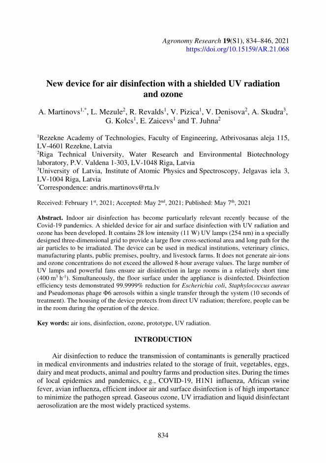
834
Agronomy Research 19(S1), 834–846, 2021 https://doi.org/10.15159/AR.21.068
New device for air disinfection with a shielded UV radiation and ozone
A. Martinovs1,*, L. Mezule2, R. Revalds1, V. Pizica1, V. Denisova2, A. Skudra3,
G. Kolcs1, E. Zaicevs1 and T. Juhna2
1Rezekne Academy of Technologies, Faculty of Engineering, Atbrivosanas aleja 115, LV-4601 Rezekne, Latvia 2Riga Technical University, Water Research and Environmental Biotechnology laboratory, P.V. Valdena 1-303, LV-1048 Riga, Latvia 3University of Latvia, Institute of Atomic Physics and Spectroscopy, Jelgavas iela 3, LV-1004 Riga, Latvia *Correspondence: [email protected] Received: February 1st, 2021; Accepted: May 2nd, 2021; Published: May 7th, 2021 Abstract. Indoor air disinfection has become particularly relevant recently because of the Covid-19 pandemics. A shielded device for air and surface disinfection with UV radiation and ozone has been developed. It contains 28 low intensity (11 W) UV lamps (254 nm) in a specially designed three-dimensional grid to provide a large flow cross-sectional area and long path for the air particles to be irradiated. The device can be used in medical institutions, veterinary clinics, manufacturing plants, public premises, poultry, and livestock farms. It does not generate air-ions and ozone concentrations do not exceed the allowed 8-hour average values. The large number of UV lamps and powerful fans ensure air disinfection in large rooms in a relatively short time (400 m3 h-1). Simultaneously, the floor surface under the appliance is disinfected. Disinfection efficiency tests demonstrated 99.9999% reduction for Escherichia coli, Staphylococcus aureus and Pseudomonas phage Φ6 aerosols within a single transfer through the system (10 seconds of treatment). The housing of the device protects from direct UV radiation; therefore, people can be in the room during the operation of the device. Key words: air ions, disinfection, ozone, prototype, UV radiation.
INTRODUCTION
Air disinfection to reduce the transmission of contaminants is generally practiced in medical environments and industries related to the storage of fruit, vegetables, eggs, dairy and meat products, animal and poultry farms and production sites. During the times of local epidemics and pandemics, e.g., COVID-19, H1N1 influenza, African swine fever, avian influenza, efficient indoor air and surface disinfection is of high importance to minimize the pathogen spread. Gaseous ozone, UV irradiation and liquid disinfectant aerosolization are the most widely practiced systems.
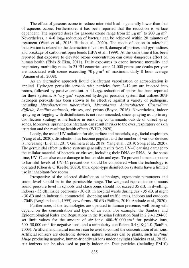
835
The effect of gaseous ozone to reduce microbial load is generally lower than that of aqueous ozone. Furthermore, it has been reported that the reduction is surface dependent. The reported doses for gaseous ozone range from 25 µg m-3 to 200 µg m-3. Nevertheless, a 4–6 log10 reduction of bacteria can be achieved within 20 minutes of treatment (Wani et al., 2015; Hutla et al., 2020). The mode of action in microbial inactivation is related to the destruction of cell wall, damage of purines and pyrimidines and breakage of carbon-nitrogen bonds (EPA et al., 1999). At the same time it has been reported that exposure to elevated ozone concentration can cause dangerous effect on human health (Elvis & Ekta, 2011). Daily exposures to ozone increase mortality and respiratory morbidity rates. In 25 EU countries some 21,000 premature deaths per year are associated with ozone exceeding 70 µg m-3 of maximum daily 8–hour average (Amann et al., 2008).
As an alternative approach liquid disinfectant vaporization or aerosolization is applied. Hydrogen peroxide aerosols with particles from 2–12 µm are injected into rooms, followed by passive aeration. A 4 Log10 reduction of spores has been reported for these systems. A ‘dry gas’ vaporized hydrogen peroxide system that utilizes 30% hydrogen peroxide has been shown to be effective against a variety of pathogens, including Mycobacterium tuberculosis, Mycoplasma, Acinetobacter, Clostridium difficile, Bacillus anthracis, viruses, and prions (Boyce, 2016). Nevertheless, indoor spraying or fogging with disinfectants is not recommended, since spraying as a primary disinfection strategy is ineffective in removing contaminants outside of direct spray zones. Moreover, spraying disinfectants can result in risks to the eyes, respiratory or skin irritation and the resulting health effects (WHO, 2020).
Lately, the use of UV radiation for air, surface and materials, e.g., facial respirators (Yang et al., 2020), disinfection has become popular, and the number of various devices is increasing (Li et al., 2017; Guimera et al., 2018; Yang et al., 2019; Song et al., 2020). The germicidal effect in these systems generally results from UV–C causing damage to the cellular material of bacteria or viruses, including their DNA or RNA. At the same time, UV–C can also cause damage to human skin and eyes. To prevent human exposure to harmful levels of UV–C, precautions should be considered when the technology is operated (Chen & O`Keeffe, 2020), thus, open-type disinfection systems have a limited use in inhabitant-free rooms.
Irrespective of the selected disinfection technology, ergonomic parameters and sound level should be in the permissible range. The weighted equivalent continuous sound pressure level in schools and classrooms should not exceed 35 dB, in dwelling, indoors - 35 dB, inside bedrooms - 30 dB, in hospital wards during day - 35 dB, at night - 30 dB and in industrial, commercial, shopping and traffic areas, indoors and outdoors - 70dB (Berglund et al., 1999), cow farms - 90 dB (Phillips, 2010; Andrade et al., 2020).
Furthermore, if the technologies are operated in human presence, well-being will depend on the concentration and type of air ions. For example, the Sanitary and Epidemiological Rules and Regulations in the Russian Federation SanPin 2.2.4.1294-03 set limit values for the amount of air ions: 400–50,000 cm-3 for positive ions, 600–50,000 cm-3 for negative ions, and a unipolarity coefficient 0.4 ≤ K≤ 1.0 (SanPin, 2003). Artificial and natural ionizers can be used to control the concentration of air ions. Artificial ionizers are electronic devices, natural ionizers can be plants, such as Pinus Mugo producing negative, human-friendly air ions under daylight (Sinicina et al., 2015). Air ionizers can be also used to purify indoor air. Dust particles (including PM10)
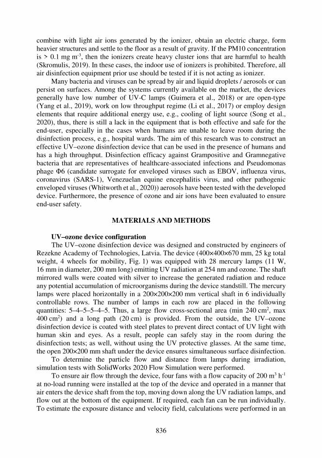
836
combine with light air ions generated by the ionizer, obtain an electric charge, form heavier structures and settle to the floor as a result of gravity. If the PM10 concentration is > 0.1 mg m-3, then the ionizers create heavy cluster ions that are harmful to health (Skromulis, 2019). In these cases, the indoor use of ionizers is prohibited. Therefore, all air disinfection equipment prior use should be tested if it is not acting as ionizer.
Many bacteria and viruses can be spread by air and liquid droplets / aerosols or can persist on surfaces. Among the systems currently available on the market, the devices generally have low number of UV-C lamps (Guimera et al., 2018) or are open-type (Yang et al., 2019), work on low throughput regime (Li et al., 2017) or employ design elements that require additional energy use, e.g., cooling of light source (Song et al., 2020), thus, there is still a lack in the equipment that is both effective and safe for the end-user, especially in the cases when humans are unable to leave room during the disinfection process, e.g., hospital wards. The aim of this research was to construct an effective UV–ozone disinfection device that can be used in the presence of humans and has a high throughput. Disinfection efficacy against Grampositive and Gramnegative bacteria that are representatives of healthcare-associated infections and Pseudomonas phage Φ6 (candidate surrogate for enveloped viruses such as EBOV, influenza virus, coronavirus (SARS-1), Venezuelan equine encephalitis virus, and other pathogenic enveloped viruses (Whitworth et al., 2020)) aerosols have been tested with the developed device. Furthermore, the presence of ozone and air ions have been evaluated to ensure end-user safety.
MATERIALS AND METHODS
UV–ozone device configuration The UV–ozone disinfection device was designed and constructed by engineers of
Rezekne Academy of Technologies, Latvia. The device (400×400×670 mm, 25 kg total weight, 4 wheels for mobility, Fig. 1) was equipped with 28 mercury lamps (11 W, 16 mm in diameter, 200 mm long) emitting UV radiation at 254 nm and ozone. The shaft mirrored walls were coated with silver to increase the generated radiation and reduce any potential accumulation of microorganisms during the device standstill. The mercury lamps were placed horizontally in a 200×200×200 mm vertical shaft in 6 individually controllable rows. The number of lamps in each row are placed in the following quantities: 5–4–5–5–4–5. Thus, a large flow cross-sectional area (min 240 cm2, max 400 cm2) and a long path (20 cm) is provided. From the outside, the UV–ozone disinfection device is coated with steel plates to prevent direct contact of UV light with human skin and eyes. As a result, people can safely stay in the room during the disinfection tests; as well, without using the UV protective glasses. At the same time, the open 200×200 mm shaft under the device ensures simultaneous surface disinfection.
To determine the particle flow and distance from lamps during irradiation, simulation tests with SolidWorks 2020 Flow Simulation were performed.
To ensure air flow through the device, four fans with a flow capacity of 200 m3 h-1 at no-load running were installed at the top of the device and operated in a manner that air enters the device shaft from the top, moving down along the UV radiation lamps, and flow out at the bottom of the equipment. If required, each fan can be run individually. To estimate the exposure distance and velocity field, calculations were performed in an
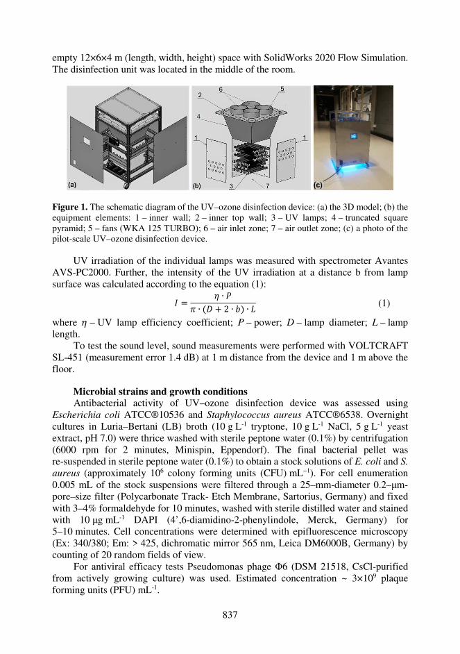
837
empty 12×6×4 m (length, width, height) space with SolidWorks 2020 Flow Simulation. The disinfection unit was located in the middle of the room.
Figure 1. The schematic diagram of the UV–ozone disinfection device: (a) the 3D model; (b) the equipment elements: 1 – inner wall; 2 – inner top wall; 3 – UV lamps; 4 – truncated square pyramid; 5 – fans (WKA 125 TURBO); 6 – air inlet zone; 7 – air outlet zone; (c) a photo of the pilot-scale UV–ozone disinfection device.
UV irradiation of the individual lamps was measured with spectrometer Avantes AVS-PC2000. Further, the intensity of the UV irradiation at a distance b from lamp surface was calculated according to the equation (1): 8 = ∙ M¡ ∙ (¢ + 2 ∙ P) ∙ p (1)
where – UV lamp efficiency coefficient; P – power; D – lamp diameter; L – lamp length.
To test the sound level, sound measurements were performed with VOLTCRAFT SL-451 (measurement error 1.4 dB) at 1 m distance from the device and 1 m above the floor.
Microbial strains and growth conditions Antibacterial activity of UV–ozone disinfection device was assessed using
Escherichia coli ATCC®10536 and Staphylococcus aureus ATCC®6538. Overnight cultures in Luria–Bertani (LB) broth (10 g L-1 tryptone, 10 g L-1 NaCl, 5 g L-1 yeast extract, pH 7.0) were thrice washed with sterile peptone water (0.1%) by centrifugation (6000 rpm for 2 minutes, Minispin, Eppendorf). The final bacterial pellet was re-suspended in sterile peptone water (0.1%) to obtain a stock solutions of E. coli and S. aureus (approximately 106 colony forming units (CFU) mL−1). For cell enumeration 0.005 mL of the stock suspensions were filtered through a 25–mm-diameter 0.2–μm-pore–size filter (Polycarbonate Track- Etch Membrane, Sartorius, Germany) and fixed with 3–4% formaldehyde for 10 minutes, washed with sterile distilled water and stained with 10 μg mL-1 DAPI (4’,6-diamidino-2-phenylindole, Merck, Germany) for 5–10 minutes. Cell concentrations were determined with epifluorescence microscopy (Ex: 340/380; Em: > 425, dichromatic mirror 565 nm, Leica DM6000B, Germany) by counting of 20 random fields of view.
For antiviral efficacy tests Pseudomonas phage Φ6 (DSM 21518, CsCl-purified from actively growing culture) was used. Estimated concentration ~ 3×10⁹ plaque forming units (PFU) mL-1.
838
Disinfection efficiency tests To test the disinfection efficiency E. coli, S. aureus or Pseudomonas phage Φ6
suspensions were sprayed into 2 or 4 air inlets (before the ventilators). Each spray dose contained 0.13–0.15 mL of the microbial suspension, thus, ~ 106 CFU of bacteria and ~ 109 PFU of bacteriophage was introduced in each run. To measure the amount of organisms released from the system, simultaneously four 90 mm diameter Petri dishes of Tryptone soya agar (TSA, Oxoid Ltd) were placed at an air outlet zone of each side of the device (Fig. 1, b. 7). For surface disinfection one 140 mm diameter Petri dish representing ~ 39% of the treated surface was placed under the system. All samplings were performed for 10 or 30 sec by holding the dish exposed at the respective air or surface zone. Each run was repeated 4 times, each time placing the Plates at different sides of the device air outlet zone or at the surface exposure zone. Directly after the contact time the dish was removed. In-between the runs, the system was operated for 5 minutes at full regime to exclude cross-contamination from previous runs. Tests have been performed for 1) 4 ventilator and 28 UV lamp regime; 2) 2 ventilator (suspensions were sprayed twice to ensure the same concentration) and 28 UV lamp regime, and 3) 4 ventilator and 16 UV lamp regime. After the treatment, the plates from bacterial tests were directly incubated at 37ºC for 24 hours. Plates with Pseudomonas phage Φ6 were covered with top agar and Pseudomonas spp. overnight culture, gently mixed and solidified, then the plates were incubated in an upright position for 24 h at 25 °C. The results are expressed as log reduction of CFU or PFU.
Direct plating of suspensions prior tests was performed to obtain suspension controls (initial viability). Negative controls were obtained by running the device with 4 ventilators and switched-off UV lamps and collecting air and surface samples after 60 sec of exposure. All test results that were used for efficacy calculations had no growth in prior negative control tests.
Ozone concentration measurements Ozone concentration was measured with ‘Gas Detector PLT300-O3’ (measurement
error ± 10 mg m-3) in an auditorium (12×6×4 m) with forced ventilation. The UV-ozone disinfection device was placed in the middle. The measurements were performed for 2 h before the device is switched on and during 4 h of operation (4 ventilators and 28 UV lamps).
Air ion concentration measurements To determine air ion concentration bipolar light air ion counter Sapfir-3M was used.
All measurements were performed in an auditorium (12 m × 6 m × 4 m; 18 °C room temperature; 55% humidity) with no forced ventilation. Two days before the measurements all windows were closed with tight blinds. Overall test time (100 min) was divided into 6 steps. First air ion counters were placed on 2 tables at 1 m distance from the UV–ozone disinfection device and 1.5 m apart from each other (1, 2, 4–6 measurement steps). In 3rd measurement step air ion counters were placed on the floor 60 cm apart from the UV–ozone disinfection device at different sides. During the experiment steps 1–5 the measurements were performed in the dark, at step 6 – under artificial daylight (16 luminescent bulbs). During the test time there was 1 person in the room at a distance of 3 m from the experimental stand, except when it was necessary to turn on / off the UV–ozone disinfection device or place the air ion counters on the floor
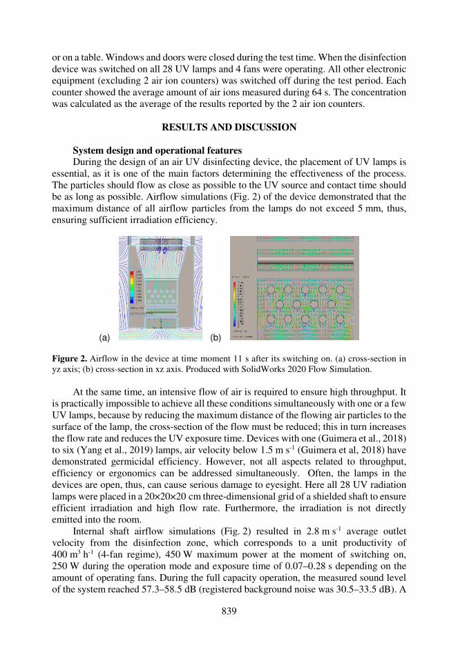
839
or on a table. Windows and doors were closed during the test time. When the disinfection device was switched on all 28 UV lamps and 4 fans were operating. All other electronic equipment (excluding 2 air ion counters) was switched off during the test period. Each counter showed the average amount of air ions measured during 64 s. The concentration was calculated as the average of the results reported by the 2 air ion counters.
RESULTS AND DISCUSSION
System design and operational features During the design of an air UV disinfecting device, the placement of UV lamps is
essential, as it is one of the main factors determining the effectiveness of the process. The particles should flow as close as possible to the UV source and contact time should be as long as possible. Airflow simulations (Fig. 2) of the device demonstrated that the maximum distance of all airflow particles from the lamps do not exceed 5 mm, thus, ensuring sufficient irradiation efficiency.
(a) (b) Figure 2. Airflow in the device at time moment 11 s after its switching on. (a) cross-section in yz axis; (b) cross-section in xz axis. Produced with SolidWorks 2020 Flow Simulation.
At the same time, an intensive flow of air is required to ensure high throughput. It
is practically impossible to achieve all these conditions simultaneously with one or a few UV lamps, because by reducing the maximum distance of the flowing air particles to the surface of the lamp, the cross-section of the flow must be reduced; this in turn increases the flow rate and reduces the UV exposure time. Devices with one (Guimera et al., 2018) to six (Yang et al., 2019) lamps, air velocity below 1.5 m s-1 (Guimera et al, 2018) have demonstrated germicidal efficiency. However, not all aspects related to throughput, efficiency or ergonomics can be addressed simultaneously. Often, the lamps in the devices are open, thus, can cause serious damage to eyesight. Here all 28 UV radiation lamps were placed in a 20×20×20 cm three-dimensional grid of a shielded shaft to ensure efficient irradiation and high flow rate. Furthermore, the irradiation is not directly emitted into the room.
Internal shaft airflow simulations (Fig. 2) resulted in 2.8 m s-1 average outlet velocity from the disinfection zone, which corresponds to a unit productivity of 400 m3 h-1 (4-fan regime), 450 W maximum power at the moment of switching on, 250 W during the operation mode and exposure time of 0.07–0.28 s depending on the amount of operating fans. During the full capacity operation, the measured sound level of the system reached 57.3–58.5 dB (registered background noise was 30.5–33.5 dB). A
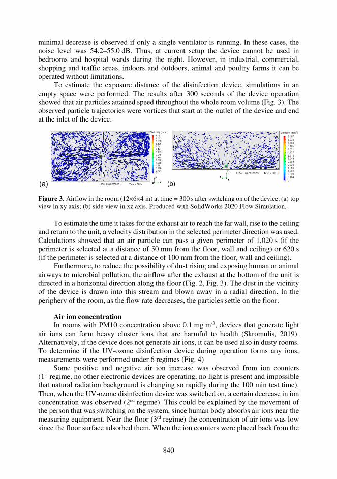
840
minimal decrease is observed if only a single ventilator is running. In these cases, the noise level was 54.2–55.0 dB. Thus, at current setup the device cannot be used in bedrooms and hospital wards during the night. However, in industrial, commercial, shopping and traffic areas, indoors and outdoors, animal and poultry farms it can be operated without limitations.
To estimate the exposure distance of the disinfection device, simulations in an empty space were performed. The results after 300 seconds of the device operation showed that air particles attained speed throughout the whole room volume (Fig. 3). The observed particle trajectories were vortices that start at the outlet of the device and end at the inlet of the device.
(a)
Figure 3. Airflow in the room (12×6×4 m) at time = 300 s after switching on of the device. (a) top view in xy axis; (b) side view in xz axis. Produced with SolidWorks 2020 Flow Simulation.
To estimate the time it takes for the exhaust air to reach the far wall, rise to the ceiling and return to the unit, a velocity distribution in the selected perimeter direction was used. Calculations showed that an air particle can pass a given perimeter of 1,020 s (if the perimeter is selected at a distance of 50 mm from the floor, wall and ceiling) or 620 s (if the perimeter is selected at a distance of 100 mm from the floor, wall and ceiling).
Furthermore, to reduce the possibility of dust rising and exposing human or animal airways to microbial pollution, the airflow after the exhaust at the bottom of the unit is directed in a horizontal direction along the floor (Fig. 2, Fig. 3). The dust in the vicinity of the device is drawn into this stream and blown away in a radial direction. In the periphery of the room, as the flow rate decreases, the particles settle on the floor.
Air ion concentration In rooms with PM10 concentration above 0.1 mg m-3, devices that generate light
air ions can form heavy cluster ions that are harmful to health (Skromulis, 2019). Alternatively, if the device does not generate air ions, it can be used also in dusty rooms. To determine if the UV-ozone disinfection device during operation forms any ions, measurements were performed under 6 regimes (Fig. 4)
Some positive and negative air ion increase was observed from ion counters (1st regime, no other electronic devices are operating, no light is present and impossible that natural radiation background is changing so rapidly during the 100 min test time). Then, when the UV-ozone disinfection device was switched on, a certain decrease in ion concentration was observed (2nd regime). This could be explained by the movement of the person that was switching on the system, since human body absorbs air ions near the measuring equipment. Near the floor (3rd regime) the concentration of air ions was low since the floor surface adsorbed them. When the ion counters were placed back from the
Velocity (m s-1) Velocity (m s-1)
(b)
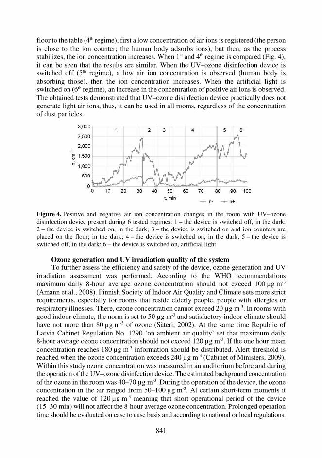
841
floor to the table (4th regime), first a low concentration of air ions is registered (the person is close to the ion counter; the human body adsorbs ions), but then, as the process stabilizes, the ion concentration increases. When 1st and 4th regime is compared (Fig. 4), it can be seen that the results are similar. When the UV–ozone disinfection device is switched off (5th regime), a low air ion concentration is observed (human body is absorbing those), then the ion concentration increases. When the artificial light is switched on (6th regime), an increase in the concentration of positive air ions is observed. The obtained tests demonstrated that UV–ozone disinfection device practically does not generate light air ions, thus, it can be used in all rooms, regardless of the concentration of dust particles.
Figure 4. Positive and negative air ion concentration changes in the room with UV–ozone disinfection device present during 6 tested regimes: 1 – the device is switched off, in the dark; 2 – the device is switched on, in the dark; 3 – the device is switched on and ion counters are placed on the floor; in the dark; 4 – the device is switched on, in the dark; 5 – the device is switched off, in the dark; 6 – the device is switched on, artificial light.
Ozone generation and UV irradiation quality of the system To further assess the efficiency and safety of the device, ozone generation and UV
irradiation assessment was performed. According to the WHO recommendations maximum daily 8-hour average ozone concentration should not exceed 100 µg m-3 (Amann et al., 2008). Finnish Society of Indoor Air Quality and Climate sets more strict requirements, especially for rooms that reside elderly people, people with allergies or respiratory illnesses. There, ozone concentration cannot exceed 20 µg m-3. In rooms with good indoor climate, the norm is set to 50 µg m-3 and satisfactory indoor climate should have not more than 80 µg m-3 of ozone (Säteri, 2002). At the same time Republic of Latvia Cabinet Regulation No. 1290 ‘on ambient air quality’ set that maximum daily 8-hour average ozone concentration should not exceed 120 µg m-3. If the one hour mean concentration reaches 180 µg m-3 information should be distributed. Alert threshold is reached when the ozone concentration exceeds 240 µg m-3 (Cabinet of Ministers, 2009). Within this study ozone concentration was measured in an auditorium before and during the operation of the UV–ozone disinfection device. The estimated background concentration of the ozone in the room was 40–70 µg m-3. During the operation of the device, the ozone concentration in the air ranged from 50–100 µg m-3. At certain short-term moments it reached the value of 120 µg m-3 meaning that short operational period of the device (15–30 min) will not affect the 8-hour average ozone concentration. Prolonged operation time should be evaluated on case to case basis and according to national or local regulations.
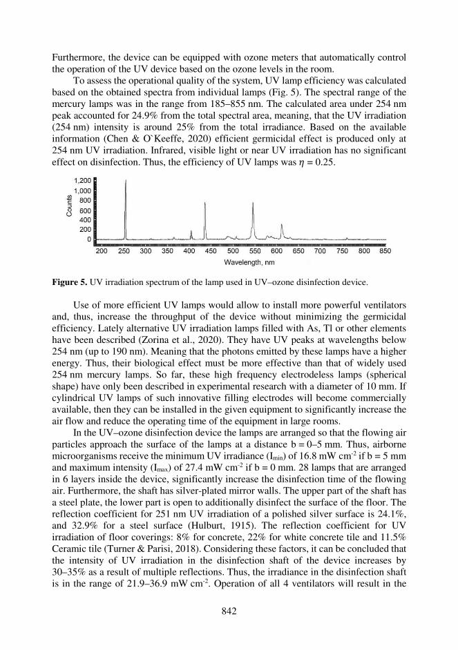
842
Furthermore, the device can be equipped with ozone meters that automatically control the operation of the UV device based on the ozone levels in the room.
To assess the operational quality of the system, UV lamp efficiency was calculated based on the obtained spectra from individual lamps (Fig. 5). The spectral range of the mercury lamps was in the range from 185–855 nm. The calculated area under 254 nm peak accounted for 24.9% from the total spectral area, meaning, that the UV irradiation (254 nm) intensity is around 25% from the total irradiance. Based on the available information (Chen & O`Keeffe, 2020) efficient germicidal effect is produced only at 254 nm UV irradiation. Infrared, visible light or near UV irradiation has no significant effect on disinfection. Thus, the efficiency of UV lamps was = 0.25.
Figure 5. UV irradiation spectrum of the lamp used in UV–ozone disinfection device.
Use of more efficient UV lamps would allow to install more powerful ventilators and, thus, increase the throughput of the device without minimizing the germicidal efficiency. Lately alternative UV irradiation lamps filled with As, Tl or other elements have been described (Zorina et al., 2020). They have UV peaks at wavelengths below 254 nm (up to 190 nm). Meaning that the photons emitted by these lamps have a higher energy. Thus, their biological effect must be more effective than that of widely used 254 nm mercury lamps. So far, these high frequency electrodeless lamps (spherical shape) have only been described in experimental research with a diameter of 10 mm. If cylindrical UV lamps of such innovative filling electrodes will become commercially available, then they can be installed in the given equipment to significantly increase the air flow and reduce the operating time of the equipment in large rooms.
In the UV–ozone disinfection device the lamps are arranged so that the flowing air particles approach the surface of the lamps at a distance b = 0–5 mm. Thus, airborne microorganisms receive the minimum UV irradiance (Imin) of 16.8 mW cm-2 if b = 5 mm and maximum intensity (Imax) of 27.4 mW cm-2 if b = 0 mm. 28 lamps that are arranged in 6 layers inside the device, significantly increase the disinfection time of the flowing air. Furthermore, the shaft has silver-plated mirror walls. The upper part of the shaft has a steel plate, the lower part is open to additionally disinfect the surface of the floor. The reflection coefficient for 251 nm UV irradiation of a polished silver surface is 24.1%, and 32.9% for a steel surface (Hulburt, 1915). The reflection coefficient for UV irradiation of floor coverings: 8% for concrete, 22% for white concrete tile and 11.5% Ceramic tile (Turner & Parisi, 2018). Considering these factors, it can be concluded that the intensity of UV irradiation in the disinfection shaft of the device increases by 30–35% as a result of multiple reflections. Thus, the irradiance in the disinfection shaft is in the range of 21.9–36.9 mW cm-2. Operation of all 4 ventilators will result in the

843
flow of 2.8 m s-1 and exposure time of 0.07 s. This will result in the irradiance dose of 1.5–2.6 mJ cm-2. Similar doses have been reported for 90 % reduction of SARS-CoV-2 (Sabino et al., 2020).
Disinfection efficacy tests Similar research with disinfection equipment (Heimbuch et al., 2011) has shown
that 254 nm UV irradiation from one 80 W lamp with total intensity of 1.6–2.2 mW cm-2 can reduce 4 log10 of viable H1N1 virus within 15 minutes. Alternatively, UVC irradiation for 120 seconds demonstrated ≥ 99.95% bacterial CFU decrease in simulated healthcare surface disinfection tests (Guridi et al., 2019). In the UV–ozone disinfection device designed within this study UV irradiance is around 15 times higher. The increase in power and irradiance results in the increased efficiency of the system. The disinfection time is reduced significantly and 5 log10 reduction can be obtained for both bacteria and virus within 10 seconds of contact time (Fig. 6.) in air quality tests. Only minor increase in the efficiency is observed if the sample contact time is increased to 30 seconds. However, the reduced counts could more account to certain UV irradiation at the air exit zones than efficiency as such. Higher efficiency in bacterial neutralisation was observed for 28 lamp regime than for 16 lamps (Fig. 6, a, b).
(a) (b)
(c)
Figure 6. The antimicrobial effect of UV-ozone disinfection device against aerosols of E. coli, S. aureus and Pseudomonas phage Φ6 when operated atA) 4 ventilator and 16 UV lamp regime; B) 4 ventilator and 28 UV lamp regime; C) 2 ventilator and 28 UV lamp regime. Standard deviation represents the average value from 2 individual experimental runs.
844
Surface disinfection tests demonstrated no growth (> 6 log10) of either E. coli or S. aureus at the exposed area of the device irrespective of the amount of lamps used. Some viral particles were detectable after 10 sec treatment, however, it still accounted for more than (> 7 log10) reduction.
No significant impact of the lamp quantity was observed for the neutralisation of Pseudomonas phage Φ6. Nevertheless, more than 5 log10 reduction was observed after 10 seconds.
Use of 2 ventilators decreased the air flow rate and resulted in an increased contact time of the particles in the system, thus higher efficiencies were observed (Fig, 6, c).
The observed decrease is sufficient for a system to perform air-disinfection. A mere 6 log10 reduction can be obtained under simulated conditions with high aerosol doses of healthcare-associated microorganisms. To a large extent, the high increase in disinfection efficiency can be associated with the use of many but smaller UV lamps, their correct placement (the air flow is as close as possible to the surface of the lamps) and installed mirror walls.
CONCLUSIONS
The shielded UV-ozone disinfection device with 28 UV lamps demonstrated high
efficiency to reduce aerosols of Grampositive and Gramnegative bacteria and virus. More than 99.999% CFU or PFU were neutralized within 10 seconds of system operation.
At the same time the system causes ozone concentration increase only for 10–50 g m-3 from the background level and practically does not produce light air ions, so it can be used in dusty rooms with PM10 concentration above 0.1 mg m-3.
Slight increase in operational noise, excludes the use of the equipment during the night, at the same time it operates at 400 m3 h-1 throughput to efficiently treat the air at 6 m distance (empty room).
The shielded construction allows to operate the equipment in human presence.
ACKNOWLEDGEMENTS. This research was funded by the Ministry of Education and Science, Republic of Latvia, National Research Programme ‘for Covid-19 mitigation’ Project ‘Integration of reliable technologies for protection against Covid-19 in healthcare and high-risk areas’ Project No. VPP-COVID-2020/1-0004. We thank Mr. Ralfs Vevers and Ms. Jelena Dzjubenko for technical assistance in efficacy tests.
REFERENCES
Amann, M., Derwent, D., Forsberg, B., Hänninen, O., Hurley, F., Krzyzanowski, M., De
Leeuw, F., Liu, S.J., Mandin, C., Schneider, J., Schwarze, P. & Simpson, D. 2008. Health risks of ozone from long-range transboundary air pollution. World Health Organization, Regional Office for Europe, Copenhagen, pp. 111.
Andrade, R.R., Tinôco, I.F.F., Damasceno, F.A., Barbari, M., Valente, D.A., Vilela, M.O., Souza, C.F., Conti, L. & Rossi, G. 2020. Lighting and noise levels in compost dairy barns with natural and forced ventilation. Agronomy Research 18(S1), 689–698.
Berglund, B. Lindvall, T. & Schwela, D.H. 1999. Guidelines for Community Noise. World Health Organization, Geneva, pp. 21.

845
Boyce, J.M. 2016. Modern technologies for improving cleaning and disinfection of environmental surfaces in hospitals. Antimicrobial Resistance & Infection Control 5, 10.
Cabinet of Ministers, Republic of Latvia. Cabinet Regulation No. 1290 “Regulations Regarding Ambient Air Quality”, Latvijas Vēstnesis, 182, 17.11.2009.
Chen, T. & O`Keeffe, J. COVID-19 in indoor environments – Air and surface disinfection measures. National Collaborating Centre for Environmental Health. 2020. Available at: https://ncceh.ca/documents/guide/covid-19-indoor-environments-air-and-surface-disinfection-measures
Elvis, A.M. & Ekta, J.S. 2011. Ozone therapy: A clinical review. Journal of Natural Science, Biology and Medicine 2(Issue 1), pp. 66–70.
Guimera, D., Pharm, J.T., Joyner, J. & Hysmith, N.D. 2018. Effectiveness of a shielded ultraviolet C air disinfection system in an inpatient pharmacy of a tertiary care children’s hospital. American Journal of Infection Control 46, 223–225.
Guridi, A., Sevillano, E., de la Fuente, I., Mateo, E., Eraso, E. & Quindos, G. 2019. Disinfectant activity of a portable ultraviolet C equipment. International Journal of Environmental Research and Public Health 16, 4747.
Heimbuch, B.K., Wallace, W.H., Kinney, K., Lumley, A.E., Wu, Chang-Yu, Woo Myung-Heui & Wander, J.D. 2011. A pandemic influenza preparedness study: Use of energetic methods to decontaminate filtering facepiece respirators contaminated with H1N1 aerosols and droplets. American Journal of Infection Control. Volume 39, Issue 1, pp. e1–e9
Hulburt, E.O. 1915. The Reflecting Power of Metals in the Ultraviolet Region of the Spectrum. Astrophys. J. 42, 205–230.
Hutla, P., Kolaříková, M., Hájek, D., Doležal, P., Hausvater, E. & Petráčková, B. 2020. Ozone treatment of stored potato tubers. Agronomy Research 18(1), 100–112.
Li, Y., Wang, M., Guan, D., Lv, H., Zhao, J., Yu, X., Yang, X. & Wu, C. 2017. A Study on the Decontaminated Efficiency of Ultraviolet Device on the Indoor Airborne Bacteria. Procedia Engineering 205, 1376–1380.
Phillips, C.J.C. 2010. Principles of Cattle Production Systems. 2ª ed. CABI, Wallingford, UK, pp. 256.
Sabino, C.P., Sellera, F.P., Sales-Medina, D.F., Guaragna Machado, R.R., Durigon, E.L., Freitas-Junior, L.H. & Ribeiro, M.S. 2020. UV-C (254 nm) lethal doses for SARS-CoV-2. Photodiagnosis and Photodynamic Therapy 32, 101995.
SanPin, 2003. Sanitary and Epidemiological Rules and Regulations in the Russian Federation SanPin 2.2.4.1294-03. Санитарно-эпидемиологические правила и нормативы "Гигиенические требования к аэроионному составу воздуха производственных и общественных помещений СанПиН 2.2.4 1294-03" (in Russian)
Säteri, J. Finnish classification of indoor climate 2000: revised target values. 2002. In: Proc. Indoor Air, pp. 643–648.
Sinicina, N., Skromulis, A. & Martinovs, A. 2015. Amount of air ions depending on indoor plant activity. In: Proc. Environment, Technology, Resources, V2, 267–273.
Skromulis, A. 2019. Impact of cluster ions and air pollution on human health. In: Proc. Environment, Technology, Resources. V1, 267–271.
Song, L., Li, W., He, J., Li, L., Li, T., Gu, D. & Tang, H. 2020. Development of a Pulsed Xenon Ultraviolet Disinfection Device for Real-Time Air Disinfection in Ambulances. Hindawi, Journal of Healthcare Engineering, Article ID 6053065, 1–5.
Turner, J. & Parisi, A.V. 2018. Ultraviolet Radiation Albedo and Reflectance in Review: The Influence to Ultraviolet Exposure in Occupational Settings. Int. J. Environ. Res. Public Health 15, 1507, pp.21.
US Environmental Protection Agency. Wastewater Technology Fact Sheet. Ozone disinfection, EPA 832-F-99-063, 1999.
846
Yang, H., Hu, J., Li, P. & Zhang, C. 2020. Ultraviolet germicidal irradiation for filtering facepiece respirators disinfection to facilitate reuse during COVID-19 pandemic: A review. Photodiagnosis and Photodynamic Therapy 31, 101943, pp.4.
Yang, J.H., Wu, U.I., Tai, H.M. & Sheng, W.H. 2019. Effectiveness of an ultraviolet-C disinfection system for reduction of healthcare associated pathogens. Journal of Microbiology, Immunology and Infection 52, 487–493.
Wani, S.J., Maker, K., Thompson, J., Barnes, J. & Singleton, I. 2015. Effect of ozone treatment on inactivation of Escherichia coli and listeria sp. on spinach. Agriculture 5, 155–169.
WHO Cleaning and disinfection of environmental surfaces in the context of COVID-19; Interim guidance 15 May 2020. https://apps.who.int/iris/rest/bitstreams/1277966/retrieve
Whitworth, C., Mu, Y., Houston, H., Martinez-Smith, M., Noble-Wang, J., Coulliette-Salmond A. & Rose, L. 2020. Persistence of Bacteriophage Phi 6 on Porous and Nonporous Surfaces and the Potential for Its Use as an Ebola Virus or Coronavirus Surrogate. Applied and Environmental Microbiology 86(17), 1–11.
Zorina, N., Skudra, A., Revalde, G. & Abola, A. 2020. Study of As and Tl high-frequency electrodeless lamps for Zeeman absorption spectroscopy. In: Proc. SPIE 11585, Biophotonics–Riga 2020.

847
Agronomy Research 19(S1), 847–867, 2021 https://doi.org/10.15159/AR.21.098
Use of principal component analysis to evaluate thermal properties and combustibility of coffee-pine wood briquettes
C.L. Mendoza Martinez1,2,3,*, E. Sermyagina1, M. Silva de Jesus3 and
E. Vakkilainen1
1LUT University, School of Energy Systems, Yliopistonkatu 34, FI-53850 Lappeenranta, Finland 2Federal University of minas Gerais, Department of Chemical Engineering, Av. Antônio Carlos 6627, MG 31270-901 Belo Horizonte, Brazil 3Federal University of Viçosa, Department of Forest Engineering, Av. Peter Henry Rolfs, s/n - University Campus, MG 36570-900 Viçosa, Brazil *Correspondence: [email protected] Received: February 1st, 2021; Accepted: March 30th, 2021; Published: May 21st, 2021 Abstract. The coffee production chain is a potential source of residual biomass inherent to the high productivity that can contribute to the generation of value-added products. The residues from the coffee sector are typically disposed to landfill without treatment causing potential environmental inconveniences. Briquetting presents an alternative process to produce a uniform fuel with high energy density. Briquettes facilitates easy transportation, enables better handling and storage of biomass residues. Properties such as low equilibrium moisture content, high energy density and compressive strength were reported for different coffee-pine wood briquettes treatments. Moreover, understanding of the thermal properties of the briquettes during combustion is crucial to evaluate their final application. This research is the first study that investigates the combustibility properties and kinetic parameters of the thermal decomposition of briquettes from coffee-pine wood using differential and integral thermal analysis under non-isothermal conditions. Multivariate analysis of the collected parameters through principal components analysis (PCA), was implemented to reduce the dimensionality of the data. The desired profile in the combustibility is directly related to high temperatures and long burning times, thus, the tested briquettes displayed a significant combustibility potential, reporting peak temperatures and burnout times around 600 °C and 27 minutes, respectively. Activation energy kinetic parameter in the range of 12–42 kJ mol-1 and average reactivity of 0.14–0.22 min-1, were also found. The results revealed the not thermally hard material to degrade when compared to biomasses typically used for combustion. Key words: briquette, chemometrics, combustion rate, reactivity, solid biofuels.
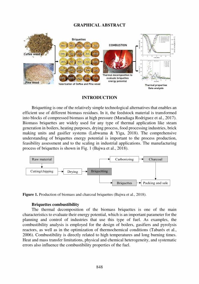
848
GRAPHICAL ABSTRACT
INTRODUCTION Briquetting is one of the relatively simple technological alternatives that enables an
efficient use of different biomass residues. In it, the feedstock material is transformed into blocks of compressed biomass at high pressure (Maradiaga Rodriguez et al., 2017). Biomass briquettes are widely used for any type of thermal application like steam generation in boilers, heating purposes, drying process, food processing industries, brick making units and gasifier systems (Lubwama & Yiga, 2018). The comprehensive understanding of briquettes energy potential is important to the process production, feasibility assessment and to the scaling in industrial applications. The manufacturing process of briquettes is shown in Fig. 1 (Bajwa et al., 2018).
Figure 1. Production of biomass and charcoal briquettes (Bajwa et al., 2018). Briquettes combustibility The thermal decomposition of the biomass briquettes is one of the main
characteristics to evaluate their energy potential, which is an important parameter for the planning and control of industries that use this type of fuel. As examples, the combustibility analysis is employed for the design of boilers, gasifiers and pyrolysis reactors, as well as in the optimization of thermochemical conditions (Tabarés et al., 2006). Combustibility is directly related to high temperatures and long burning times. Heat and mass transfer limitations, physical and chemical heterogeneity, and systematic errors also influence the combustibility properties of the fuel.
Cutting/chipping
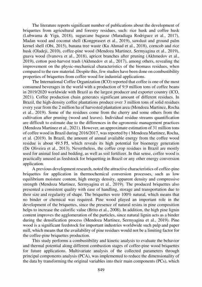
849
The literature reports significant number of publications about the development of briquettes from agricultural and forestry residues, such: rice husk and coffee husk (Lubwama & Yiga, 2018), sugarcane bagasse (Maradiaga Rodriguez et al., 2017), Madan wood and coconut shell (Kongprasert et al., 2019), sawdust and ground palm kernel shell (Obi, 2015), banana tree waste (Ku Ahmad et al., 2018), corncob and rice husk (Oladeji, 2010), coffee-pine wood (Mendoza Martinez, Sermyagina et al., 2019), guava wood (Ivanova et al., 2018), apricot branches after pruning (Akhmedov et al., 2019), cotton post-harvest trash (Akhmedov et al., 2017), among others, revealing the improvement on the physic-mechanical characteristics of the biomass residues, when compared to the raw material. Despite this, few studies have been done on combustibility properties of briquettes from coffee wood for industrial applications.
The International Coffee Organization (ICO) reported that coffee is one of the most consumed beverages in the world with a production of 9.9 million tons of coffee beans in 2019/2020 worldwide with Brazil as the largest producer and exporter country (ICO, 2021). Coffee production chain generates significant amount of different residues. In Brazil, the high-density coffee plantations produce over 3 million tons of solid residues every year from the 2 million ha of harvested plantation area (Mendoza Martinez, Rocha et al., 2019). Some of the residues come from the cherry and some others from the cultivation after pruning (wood and leaves). Individual residue streams quantification are difficult to estimate due to the differences in the agronomic management practices (Mendoza Martinez et al., 2021). However, an approximate estimation of 31 million tons of coffee wood in Brazil during 2016/2017, was reported by ( Mendoza Martinez, Rocha, et al. (2019). In Brazil, the amount of annual available energy from the coffee wood residue is about 49.5 PJ, which reveals its high potential for bioenergy generation (De Oliveira et al., 2013). Nevertheless, the coffee crop residues in Brazil are mostly used for animal feed and bedding, as well as soil fertilizer. In that sense, coffee wood is practically unused as feedstock for briquetting in Brazil or any other energy conversion application.
A previous development research, noted the attractive characteristics of coffee-pine briquettes for application in thermochemical conversion processes, such as low equilibrium moisture content, high energy density, apparent density and compressive strength (Mendoza Martinez, Sermyagina et al., 2019). The produced briquettes also presented a consistent quality with ease of handling, storage and transportation due to their size and regularity of shape. The briquettes were 100% natural, which means that no binder or chemical was required. Pine wood played an important role in the development of the briquettes, since the presence of natural resins in pine composition helps to increase the calorific value (Brito et al., 2008). In addition, the high pine lignin content improves the agglomeration of the particles, since natural lignin acts as a binder during the densification process (Mendoza Martinez, Sermyagina et al., 2019). Pine wood is a significant feedstock for important industries worldwide such pulp and paper mill, which means that the availability of pine residues would not be a limiting factor for the coffee-pine briquettes production.
This study performs a combustibility and kinetic analysis to evaluate the behavior and thermal potential along different combustion stages of coffee-pine wood briquettes for future applications. Multivariate analysis of the collected parameters through principal components analysis (PCA), was implemented to reduce the dimensionality of the data by transforming the original variables into their main components (PCs), which
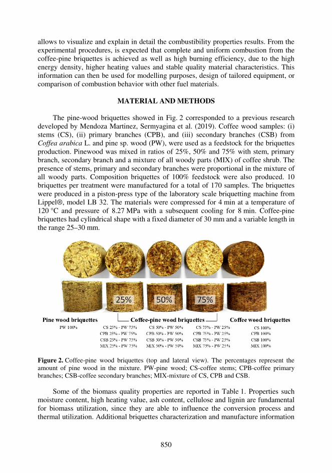
850
allows to visualize and explain in detail the combustibility properties results. From the experimental procedures, is expected that complete and uniform combustion from the coffee-pine briquettes is achieved as well as high burning efficiency, due to the high energy density, higher heating values and stable quality material characteristics. This information can then be used for modelling purposes, design of tailored equipment, or comparison of combustion behavior with other fuel materials.
MATERIAL AND METHODS
The pine-wood briquettes showed in Fig. 2 corresponded to a previous research
developed by Mendoza Martinez, Sermyagina et al. (2019). Coffee wood samples: (i) stems (CS), (ii) primary branches (CPB), and (iii) secondary branches (CSB) from Coffea arabica L. and pine sp. wood (PW), were used as a feedstock for the briquettes production. Pinewood was mixed in ratios of 25%, 50% and 75% with stem, primary branch, secondary branch and a mixture of all woody parts (MIX) of coffee shrub. The presence of stems, primary and secondary branches were proportional in the mixture of all woody parts. Composition briquettes of 100% feedstock were also produced. 10 briquettes per treatment were manufactured for a total of 170 samples. The briquettes were produced in a piston-press type of the laboratory scale briquetting machine from Lippel®, model LB 32. The materials were compressed for 4 min at a temperature of 120 °C and pressure of 8.27 MPa with a subsequent cooling for 8 min. Coffee-pine briquettes had cylindrical shape with a fixed diameter of 30 mm and a variable length in the range 25–30 mm.
Figure 2. Coffee-pine wood briquettes (top and lateral view). The percentages represent the amount of pine wood in the mixture. PW-pine wood; CS-coffee stems; CPB-coffee primary branches; CSB-coffee secondary branches; MIX-mixture of CS, CPB and CSB.
Some of the biomass quality properties are reported in Table 1. Properties such
moisture content, high heating value, ash content, cellulose and lignin are fundamental for biomass utilization, since they are able to influence the conversion process and thermal utilization. Additional briquettes characterization and manufacture information

851
can be found in an available article reported by Mendoza Martinez, Sermyagina et al. (2019).
Table 1. Literature report characterization of feedstocks.
***(Mendoza Martinez, Sermyagina et al., 2019); **(Mendoza Martinez, Rocha et al., 2019); *(Carvalho et al.,. 2015); aDry basis; bStandard deviation; MC – Moisture content; VM – Volatile matter; FC – Fixed carbon content; AC – Ash content; HHV– Higher heating value; Holocellulose (hemicelluloses + cellulose).
Experimental set-up
Mass and temperature variations The measurements of weight loss and temperature variation during the combustion
process were collected with the balance and the thermocouple, respectively. The time required for the complete combustion of the briquette (i.e., immediately before its final
Biomass Proximate analysis*** (wt%) HHV***
(MJ·kg-1) Chemical composition (wt%)
MC VMa ACa FCa Holocellulose Lignin Extractive
Cof
fee
woo
d Stem 11.0 79.8 2.1 18.1 20.1 52.7** 29.6** 10.6** Primary branch
8.7 80.7 2.3 17.0 19.8 54.1** 29.8** 13.1**
Secondary branch
9.3 76.5 4.1 19.4 19.7 50.1** 32.2** 13.9**
Pine wood 12.2 82.5 0.7 16.8 20.7 65.9* 32.3* 1.82*
SDb 1.6 2.5 1.4 1.2 0.5 6.9 1.5 4.8
Fig. 3 depicts the combustion system used to evaluate the behavior of the briquettes during combustion (Quirino & Brito, 1991). The device consists of: cylindrical aluminum combustor covered by a combustor bulkhead that protect the equipment of excess of oxygen; laboratory scales with a precision of ± 0.005 g; wooden base for thermal insulation; temperature recorder coupled with a thermocouple, and compensation cables. The briquettes were loaded onto the burner grate using approximately 60 ± 10 g solid mass for every treatment, with two replicates. The ignition occurred by the combustion of 10 g of ethyl alcohol in a crucible located under the grate. The experimental assays were performed at room temperature (~25–28 °C), with selected time of 30 minutes per treatment.
Figure 3. Scheme of the combustion system (dimensions in mm): 1 – digital balance; 2 – wooden base; 3 – ignition chamber; 4 – grate; 5 – briquettes; 6 – combustor; 7 – combustor bulkhead; 8 – thermocouple; 9 – compensation cables; and 10 – temperature recorder.
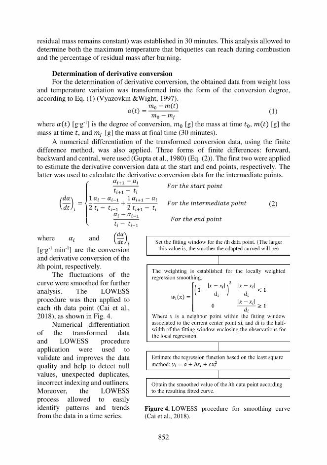
852
residual mass remains constant) was established in 30 minutes. This analysis allowed to determine both the maximum temperature that briquettes can reach during combustion and the percentage of residual mass after burning.
Determination of derivative conversion For the determination of derivative conversion, the obtained data from weight loss
and temperature variation was transformed into the form of the conversion degree, according to Eq. (1) (Vyazovkin &Wight, 1997). �(T) = :Y − :(T):Y − :£ (1)
where �(T) [g∙g-1] is the degree of conversion, :Y [g] the mass at time TY, :(T) [g] the mass at time T, and :£ [g] the mass at final time (30 minutes).
A numerical differentiation of the transformed conversion data, using the finite difference method, was also applied. Three forms of finite differences: forward, backward and central, were used (Gupta et al., 1980) (Eq. (2)). The first two were applied to estimate the derivative conversion data at the start and end points, respectively. The latter was used to calculate the derivative conversion data for the intermediate points.
¤v�vT ¥B =⎩⎪⎨⎪⎧ �B�d − �BTB�d − TB ª�} TℎX �T;}T N��9T12 �B − �B�dTB − TB�d + 12 �B�d − �BTB�d − TB ª�} TℎX �9TX}:Xv�;TX N��9T�B − �B�dTB − TB�d ª�} TℎX X9v N��9T
(2)
where �B and «D¬Du B [g∙g-1 min-1] are the conversion and derivative conversion of the ith point, respectively.
The fluctuations of the curve were smoothed for further analysis. The LOWESS procedure was then applied to each ith data point (Cai et al., 2018), as shown in Fig. 4.
Numerical differentiation of the transformed data and LOWESS procedure application were used to validate and improves the data quality and help to detect null values, unexpected duplicates, incorrect indexing and outliners. Moreover, the LOWESS process allowed to easily identify patterns and trends from the data in a time series.
Figure 4. LOWESS procedure for smoothing curve (Cai et al., 2018).
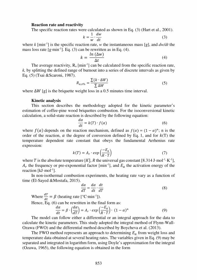
853
Reaction rate and reactivity The specific reaction rates were calculated as shown in Eq. (3) (Hart et al., 2001). | = 1{ ∙ v{vT (3)
where k [min-1] is the specific reaction rate, w the instantaneous mass [g], and dw/dt the mass loss rate [g∙min-1]. Eq. (3) can be rewritten as in Eq. (4). | = ®9 (∆{)∆T (4)
The average reactivity, Ra [min-1] can be calculated from the specific reaction rate, k, by splitting the defined range of burnout into a series of discrete intervals as given by Eq. (5) (Tsai &Scaroni, 1987). =I,`% = ∑(| ∙ ∆g)∑ ∆g (5)
where ∆g [g] is the briquette weight loss in a 0.5 minutes time interval. Kinetic analysis This section describes the methodology adopted for the kinetic parameter’s
estimation of coffee-pine wood briquettes combustion. For the isoconversional kinetic calculation, a solid-state reaction is described by the following equation: v�vT = |(²) ∙ ³(�) (6)
where ³(�) depends on the reaction mechanism, defined as ³(� = (1 − � K; n is the order of the reaction, � the degree of conversion defined by Eq. 1, and for |(T) the temperature dependent rate constant that obeys the fundamental Arrhenius rate expression: |(²) = w´ ∙ X<N ¤−bI= ∙ ²¥ (7)
where ² is the absolute temperature [j[, = the universal gas constant [8.314 J·mol-1·K-1], w´ the frequency or pre-exponential factor [min-1], and bI the activation energy of the reaction [kJ·mol-1].
In non-isothermal combustion experiments, the heating rate vary as a function of time (El-Sayed &Mostafa, 2015). v�v² = v�vT ∙ vTv² (8)
Where DµDu = � (heating rate [°C∙min-1]).
Hence, Eq. (6) can be rewritten in the final form as: v�vT = � ∙ ¤v�v²¥ = w´ ∙ X<N ¤−bI= ∙ ²¥ ∙ (1 − �)K (9)
The model can follow either a differential or an integral approach for the data to calculate the kinetic parameters. This study adopted the integral method of Flynn-Wall-Ozawa (FWO) and the differential method described by Boycheva et al. (2013).
The FWO method represents an approach to determining bI from weight loss and temperature data obtained at several heating rates. The variables given in Eq. (9) may be separated and integrated in logarithm form, using Doyle’s approximation for the integral (Ozawa, 1965), the following equation is obtained in the form

854
log(�) = log ¤w´ ∙ bI= ¥ − log (³(�)) − 2.315 − 0.4567 bI= ∙ ² (10)
The activation energy can therefore be obtained from a plot of log(�) vs ²B�d for a fixed degree of conversion.
The activation energy can be calculated by the following kinetic equation (Boycheva et al., 2013): 1² = w´ − ¤ =bI¥ ∙ ln (�) (11)
Principal Component Analysis (PCA) The PCA analysis facilitates visualization, and hence process understanding. In
brief, the principal components are the axes of a new coordinate system given by the rotation of the original one. These new directions are defined in order to explain most of the variance in the original data through a smaller number of dimensions (Jolliffe, 2003). The components are linear combinations of the original variables. In this study, the features were combustibility properties measured for all briquette treatments. The original variables were initially standardized (zero mean and unit variance) to avoid the scale problem caused by the discrepant standard deviations among them, to obtain the PCA model using MATLAB R2019a. After obtaining the PCA model, the resulting score (the coordinates of the original data in the new coordinate system) were used for a cluster analysis to evaluate similarities and dissimilarities among the briquettes treatments. Python 3.8.0 was used for the analysis.
RESULTS AND DISCUSSION
Thermal analysis results Weight loss and temperature variation analysis as well-known as thermal
gravimetric analysis (TGA) is the most commonly applied thermo-analytical technique in solid-phase thermal degradation studies (White et al., 2011). This technique can be implement for different purposes, for example, prediction of higher heating values (HHVs) though the thermal mass coefficients of samples composition (Li et al., 2017), determination of less combustible constituents in coals (Shu et al., 2002), combustion, kinetics and thermal behavior of lignocellulosic fuels for energy applications (Mishra & Mohanty, 2018). This article used the combustor instead of TGA analysis as a tool to obtain the weight loss curves along with their derived parameters and the temperature profile during devolatilization of the briquettes. The results are presented in Fig. 5.
The briquettes chemical composition consists principally of cellulose, hemicelluloses, lignin and extractives, which have different thermal behavior during combustion. The chemical composition regarding lignin and holocellulose (hemicelluloses + cellulose) content of the feedstock is tabulated in Table 1. The degradation process of the lignocellulosic briquettes can be divided into three main sections (Janković et al., 2020):
(i) moisture and very light volatiles components removal (< 120 °C). From Fig. 5 (right) a slightly inclined weight loss curve with 10% average weight loss was reported during the first 5–6 minutes of the experiment, due to the appearance of endothermic reaction. The initial moisture content of the briquettes was between 9.5–10.1 wt%
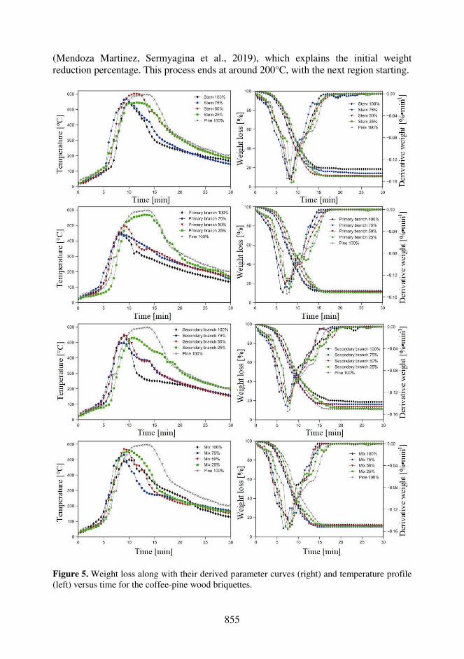
855
(Mendoza Martinez, Sermyagina et al., 2019), which explains the initial weight reduction percentage. This process ends at around 200°C, with the next region starting.
Figure 5. Weight loss along with their derived parameter curves (right) and temperature profile (left) versus time for the coffee-pine wood briquettes.
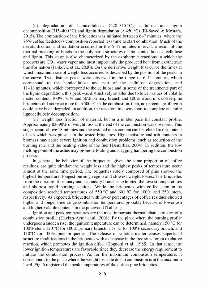
856
(ii) degradation of hemicelluloses (220–315 °C), cellulose and lignin decomposition (315–400 °C) and lignin degradation (> 450 °C) (El-Sayed & Mostafa, 2015). The combustion of the briquettes was initiated between 6–7 minutes, where the 75% coffee feedstocks composition reported less time to start combustion. Much of the devolatilization and oxidation occurred in the 6–17 minutes interval, a result of the thermal breaking of bonds in the polymeric structures of the hemicelluloses, cellulose and lignin. This stage is also characterized by the exothermic reactions in which the products are CO2, water vapor and most importantly the produced heat from exothermic transformation (Janković et al., 2020). On the derivative weight loss curve the times at which maximum rate of weight loss occurred is described by the position of the peaks in the curve. Two distinct peaks were observed in the range of 6–11 minutes, which correspond to the hemicellulose and part of the cellulose degradation, and 11–18 minutes, which correspond to the cellulose and in some of the treatments part of the lignin degradation, this peak was distinctively smaller due to lower values of volatile matter content. 100%, 75% and 50% primary branch and 100% wood mix coffee-pine briquettes did not react more than 500 °C in the combustion, then, no percentage of lignin could have been degraded, in addition, the reaction time was short to complete an entire lignocellulosic decomposition.
(iii) weight loss fraction of material, but in a milder pace till constant profile. Approximately 83–90% of weight loss at the end of the combustion was observed. This stage occurs above 18 minutes and the residual mass content can be related to the content of ash which was present in the tested briquettes. High moisture and ash contents in biomass may cause severe ignition and combustion problems, such as reduction of the burning rate and the heating value of the fuel (Demirbas, 2004). In addition, the low melting point of the ashes may promote fouling and slagging hampering the combustion process.
In general, the behavior of the briquettes, given the same proportion of coffee residues, are quite similar: the weight loss and the highest peaks of temperature occur almost at the same time period. The briquettes solely composed of pine showed the highest temperature, longest burning region and slowest weight losses. The briquettes from the mixture of primary and secondary branches exhibited the lowest temperatures and shortest rapid burning sections. While the briquettes with coffee stem in its composition reached temperatures of 550 °C and 601 °C for 100% and 25% stem, respectively. As expected, briquettes with lower percentages of coffee residues showed higher and longer time range combustion temperatures probably because of lower ash and higher volatile contents in the pinewood (Table 1).
Ignition and peak temperatures are the most important thermal characteristics of a combustion profile (Haykırı-Açma et al., 2001). By the place where the burning profile undergoes a sudden rise, the ignition temperature can be determined, namely 150 °C for 100% stem, 120 °C for 100% primary branch, 117 °C for 100% secondary branch, and 110°C for 100% pine briquettes. The release of volatile matter causes superficial structure modifications in the briquettes with a decrease in the free sites for an oxidative reaction, which promotes the ignition effect (Tognotti et al., 1985). In that sense, the lower ignition temperatures are favorable since they decrease the energy requirement to initiate the combustion process. As for the maximum combustion temperature, it corresponds to the place where the weight loss rate due to combustion is at the maximum level. Fig. 6 registered the peak temperatures of the coffee-pine briquettes.

857
Figure 6. Maximum combustion temperature of the coffee-pine wood briquettes. Total biomass burnout was also studied in this work based on weight losses, this
property includes the heating up, devolatilization and the oxidation time (Li et al., 2016). The burnout occurred at the range of temperature where the rate of weight loss consistently decreases to less than 1%∙min-1 (El-Sayed & Mostafa, 2015). Fig. 6 also shows that the burnout time of the briquettes increases with an increase in the pine content. For instance, it takes about 27.5 minutes and between 20–25.3, 16.5–17.3, 23.5–26.5 and 13–17 minutes to completely burn a 100% pinewood and steam, primary branch, secondary branch and wood mix present in the briquette composition, respectively. The maximum temperatures reveal that higher temperatures increases the devolatilization and the briquettes burnout process.
The residual mass after the combustion process is composed mainly of inorganic material, originally contained in the fuel. The percentages of residual mass are shown in Fig. 7. The reduction of the residual mass among the treatments is due to the decrease of the coffee residues content in the mixture. Briquettes of 100% secondary branch displayed the highest residual mass percentage, mainly because of the high ash content. They present values approximately 83% higher than pinewood, which reported the lowest ash content.
Nevertheless, high residual mass may also be attributed to the differences in composition and also to the strength of the molecular structure of the coffee residues in comparison to pinewood. The amount of structural polymers (holocellulose (lignin + cellulose) and hemicellulose) and their characteristics differ between softwood (pinewood) and hardwood (coffee wood) materials. Schutyser et al. (2017) reported content in the range of 46–50 wt%, 19–22 wt% and 21–29 wt% of cellulose, hemicellulose and lignin respectively for softwoods, and content in the range of 40–46 wt%, 17–23 wt% and 18–25 wt% of cellulose, hemicellulose and lignin respectively for hardwoods, in accordance of the data found in this study. For instance, the lignin and holocellulose content was 32.3 wt% and 65.9 wt% and between 29.6–32.2 wt% and 50.1–54.1 wt% for pinewood and coffee residues, respectively (Table 1). Lignin is the major plant cell wall component and has the ability to resist thermal degradation due to its chemically

858
complex structure (Cesarino et al., 2013). Consequently, the composition and the bonds that link the macromolecular structure of the briquettes with high content of coffee residues are less resistant to heat.
Figure 7. Percentage of the residual mass of the coffee-pine wood briquettes. Reactivity of coffee-pine briquettes The average reactivity of the briquettes is illustrated in Fig. 8. It was calculated
using the specific reaction rate (|). The | [min-1] property showed a similar behavior as the temperature profile, where a distinctively increase started from approximately 6 minutes and reported | high values in the range of 6–18 minutes. Right after this interval, the | values decrease steadily due to the briquettes burnout, in that way, the combustion reaction rate depends on the velocity gradient of the mass of the unburnt combustible material remaining in the fuel.
Figure 8. Average reactivity of coffee-pine wood briquettes.
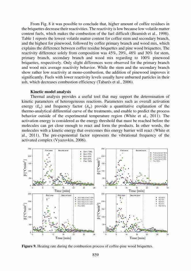
859
From Fig. 8 it was possible to conclude that, higher amount of coffee residues in the briquettes decrease their reactivities. The reactivity is low because low volatile matter content fuels, which makes the combustion of the fuel difficult (Beamish et al., 1998). Table 1 reports the lowest volatile matter content for coffee stem and secondary branch, and the highest for pinewood, followed by coffee primary branch and wood mix, which explains the difference between coffee residue briquettes and pine wood briquettes. The reactivity difference solely from composition was 45%, 29%, 48% and 30% for stem, primary branch, secondary branch and wood mix regarding to 100% pinewood briquettes, respectively. Only slight differences were observed for the primary branch and wood mix average reactivity behavior. While the stem and the secondary branch show rather low reactivity at mono-combustion, the addition of pinewood improves it significantly. Fuels with lower reactivity levels usually have unburned particles in their ash, which decreases combustion efficiency (Tabarés et al., 2006).
Kinetic model analysis Thermal analysis provides a useful tool that may support the determination of
kinetic parameters of heterogeneous reactions. Parameters such as overall activation energy (bI) and frequency factor (w¬) provide a quantitative explanation of the thermo-analytical differential curve of the treatments, and enable to predict the process behavior outside of the experimental temperature region (White et al., 2011). The activation energy is considered as the energy threshold that must be reached before the molecules can get close enough to react and form the products. In other words, the molecules with a kinetic energy that overcomes this energy barrier will react (White et al., 2011). The pre-exponential factor represents the vibrational frequency of the activated complex (Vyazovkin, 2006).
Figure 9. Heating rate during the combustion process of coffee-pine wood briquettes.
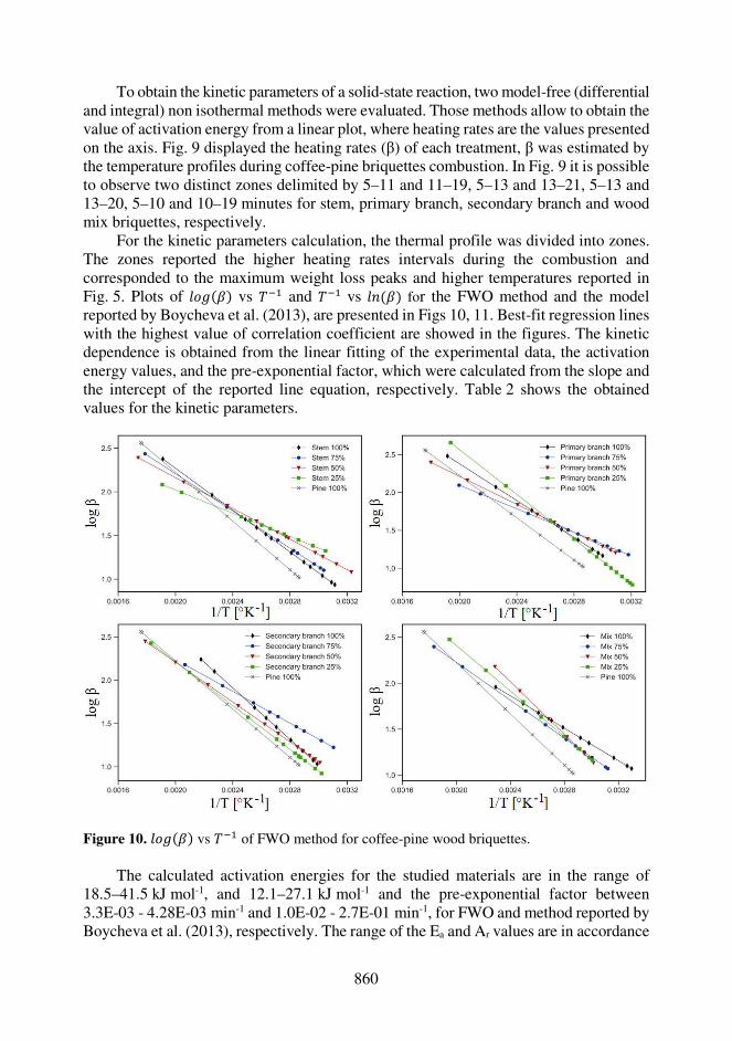
860
To obtain the kinetic parameters of a solid-state reaction, two model-free (differential and integral) non isothermal methods were evaluated. Those methods allow to obtain the value of activation energy from a linear plot, where heating rates are the values presented on the axis. Fig. 9 displayed the heating rates (β) of each treatment, β was estimated by the temperature profiles during coffee-pine briquettes combustion. In Fig. 9 it is possible to observe two distinct zones delimited by 5–11 and 11–19, 5–13 and 13–21, 5–13 and 13–20, 5–10 and 10–19 minutes for stem, primary branch, secondary branch and wood mix briquettes, respectively.
For the kinetic parameters calculation, the thermal profile was divided into zones. The zones reported the higher heating rates intervals during the combustion and corresponded to the maximum weight loss peaks and higher temperatures reported in Fig. 5. Plots of ®�¸(�) vs ²�d and ²�d vs ®9(�) for the FWO method and the model reported by Boycheva et al. (2013), are presented in Figs 10, 11. Best-fit regression lines with the highest value of correlation coefficient are showed in the figures. The kinetic dependence is obtained from the linear fitting of the experimental data, the activation energy values, and the pre-exponential factor, which were calculated from the slope and the intercept of the reported line equation, respectively. Table 2 shows the obtained values for the kinetic parameters.
Figure 10. ®�¸(�) vs ²�d of FWO method for coffee-pine wood briquettes.
The calculated activation energies for the studied materials are in the range of
18.5–41.5 kJ mol-1, and 12.1–27.1 kJ mol-1 and the pre-exponential factor between 3.3E-03 - 4.28E-03 min-1 and 1.0E-02 - 2.7E-01 min-1, for FWO and method reported by Boycheva et al. (2013), respectively. The range of the Ea and Ar values are in accordance
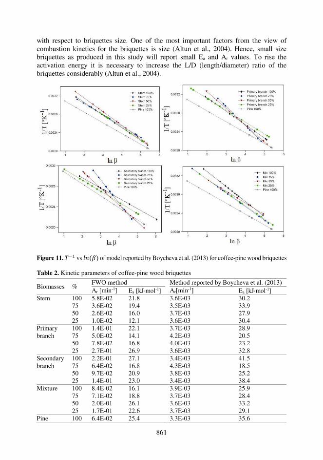
861
with respect to briquettes size. One of the most important factors from the view of combustion kinetics for the briquettes is size (Altun et al., 2004). Hence, small size briquettes as produced in this study will report small Ea and Ar values. To rise the activation energy it is necessary to increase the L/D (length/diameter) ratio of the briquettes considerably (Altun et al., 2004).
Figure 11. ²�d vs ®9(�) of model reported by Boycheva et al. (2013) for coffee-pine wood briquettes
Table 2. Kinetic parameters of coffee-pine wood briquettes
Biomasses % FWO method Method reported by Boycheva et al. (2013) Ar [min-1] Ea [kJmol-1] Ar[min-1] Ea [kJmol-1]
Stem 100 5.8E-02 21.8 3.6E-03 30.2 75 3.6E-02 19.4 3.5E-03 33.9 50 2.6E-02 16.0 3.7E-03 27.9 25 1.0E-02 12.1 3.6E-03 30.4
Primary branch
100 1.4E-01 22.1 3.7E-03 28.9 75 5.0E-02 14.1 4.2E-03 20.5 50 7.8E-02 16.8 4.0E-03 23.2 25 2.7E-01 26.9 3.6E-03 32.8
Secondary branch
100 2.2E-01 27.1 3.4E-03 41.5 75 6.4E-02 16.8 4.3E-03 18.5 50 9.7E-02 20.9 3.8E-03 25.2 25 1.4E-01 23.0 3.4E-03 38.4
Mixture 100 8.4E-02 16.1 3.9E-03 25.9 75 7.1E-02 18.8 3.7E-03 28.4 50 2.0E-01 26.1 3.6E-03 33.2 25 1.7E-01 22.6 3.7E-03 29.1
Pine 100 6.4E-02 25.4 3.3E-03 35.6
862
The values found for different percentages of pinewood in the mixtures are not following any visible pattern of behavior for all biomass mixtures. However, the presence of pinewood in the mixtures yields higher activation energies and pre-exponential factors through most of the treatments. The results, to some extent, are in agreement with the data obtained by integral and derivate methods and also matched with values calculated by literature report for coal briquettes using similar kinetic models analysis (Altun et al., 2004; Boycheva et al., 2013; Idris et al., 2017). However slightly difference among the results were observed. These variations are probably caused by the difference in both physicochemical composition and metal concentration (Mendoza Martinez, Rocha et al., 2019). The presence of alkali (Na and K) and alkaline earth metals (Mg and Ca) on the feedstock tends to decrease the activation energy.
Principal component and cluster analysis PCA analysis was used to investigate the effects of the process conditions, given
by the briquette treatments over the combustibility properties. All briquette samples were used for a cluster analysis by PCA. The seven autoscaled features used are the residual mass, maximum heating rate, burnout time, activation energy, pre-exponential factor, maximum temperature and average reactivity. The first two principal components (PCs), preserved 44.1% and 29% of the total variance, respectively. In that way, it was feasible to carry out the study using only two PCs rather than seven (given by the original space of properties) dimensions. The analysis of the relationships between treatments and properties in the PC1-PC2 plane was performed through the bi-plot graph, as shown in Fig. 12. This graph plots scores (points) and loads (represented by lines) simultaneously. The scores are the coordinates of each point in the original space in the new coordinate system defined by the principal components, and the loads are the weights associated to the original features in a component (each component is a linear combination of the original variables). This way, they can be used to characterize the strength of the original variables in each principal component.
Samples build a relative diverse behavior. Generally, briquettes with high content of pine wood are centered in the cluster represented by squares. From PC1, it can be observed that the largest positive loads are related to the activation energy and the maximum heating rate, equal to 0.46 and 0.41, respectively. On the other hand, the most significant negative loads refer to pre-exponential factor and the average reactivity, equal to -0.44 and -0.27, respectively. Therefore, the greater the value (score) of this first component, the higher the energy consumed for briquette ignition, but higher temperatures and longer burning time will also be reached. Regarding PC2, it can be observed that the most significant negative load (-0.58) refers to average reactivity. In the opposite direction, higher values of residual mass, with loads equal to 0.58, result in more positive PC2. Therefore, the higher the scores of this second component, the more propitious will the briquettes be for ash production and the briquette will produce less energy. It can also be observed that the features that reveal poor briquette combustibility, remain in the upper left quadrant, with positive values for PC1 and PC2, since high residual mass means high tar content and less energy generated. High content of coffee residues in briquettes showed the highest residual mass values in each set of treatments of the same biomass. This indicates that the briquettes with pinewood in its composition are better for combustion.

863
Figure 12. Bi-plot for the PCA analysis of coffee-pine wood briquette treatments. The circle and square symbol denote the clustering groups centered in the X symbol. CS-coffee stems; CPB-coffee primary branches; CSB-coffee secondary branches; MIX-mixture of CS, CPB and CSB; PW-pine wood. Subscript represent the percentage of pinewood in the mixture.
The previous load analysis was then coupled with the scores analysis. Higher
pre-exponential values contribute significantly for negative PC1-scores and positive PC2-scores. This condition resides on the upper right quadrant, where briquettes treatments are represented by the cluster (circles). In brief, it means that these treatments yield to combustibility processes that present higher pre-exponential factors. This may be explained by the high molecular collision frequency during the combustion process. It means that the influence of temperature into the reactant molecules is higher for CSB75 and CPB75 treatments. The relation between the variables that affect the combustibility and the most energy-attractive briquette treatments can be determined.
Other subsets of treatments can be observed. Treatments located in the lower right quadrant are related to higher activation energies and burnout time and can reach higher temperatures. This combination increases the potential of combustibility. Such behavior is given by positive PC1 scores and negative PC2 scores. In this region is possible to observe briquettes with higher content of pinewood in its composition. Other group is given by coffee wood mixture treatment, which presents the highest average reactivity during combustion. The last group is given by the CSB100, CS100 and CSB50 treatments. It is characterized by positive scores of both PC1 and PC2. This region is strongly
CS100 CSB100
CSB 50
75CS
CSB25
50CS
50CS
25CPBMIX50
MIX25
100PW
MIX75
100CPB50CPB
MIX100
75CPB
Preexponential factor
Residual mass
CSB 75
Max heating rate
Burnout time
Activation energy
Max temperature
Average reactivity
Principal component 1
Pri
nci
pa
l co
mp
on
en
t 2
-0.4 -0.2 0 0.2 0.4 0.6
-0.6
-0.4
-0.2
0
0.2
0.4
0.6

864
associated with the residual mass obtained during the combustion process. The higher quantity of residual mass in these treatments may be explained by the high content of ash in final composition. Therefore, it can be verified that the composition of the briquettes, and more specifically the wood coffee residues, change considerably the combustibility behavior. The briquettes centered in the cluster represented with squares, displayed the highest combustibility potential, once they provide significant peak temperatures and burn out times.
CONCLUSIONS
Coffee wood from varied parts of the shrub mixed with pinewood were used to
produce coffee-pine wood briquettes. The combustibility analysis of the produced briquettes was evaluated in this work. It was possible to observed by means of the mass loss and temperature behavior, small difference between the sample’s combustibility properties, acknowledge that all produced briquettes are an alternative solution to maximize the thermochemical properties of coffee-pine-based biomass residues. However, coffee-pine briquettes composed of coffee stem and secondary branch displayed the highest combustibility potential, given their peak temperatures over 550 °C and burnout times over 20 minutes. Properties such as high volatiles matter (82.5 wt%) and low ash content (0.7 wt%) in pinewood favor the combustion process and the energy potential of the briquettes. The kinetic analysis provided useful parameters for optimization of the combustion of the briquettes improving the burning stage in domestic and industrial applications. The presence of coffee wood in the mixture, yields to higher values of activation energy and pre-exponential factor in relation to 100% pine wood briquette. Lastly, the PCA analysis made the similarity and dissimilarity analysis among the briquette treatments easier favoring the selection of those most energy attractive, which again point the coffee-pine briquettes composed of coffee stem and secondary branch. PCA chemometric technique presents a great potential for a better understanding of combustion processes in general, and more specifically with respect to the use of coffee residues wood in briquettes should be more explored, due to its high energetic potential.
ACKNOWLEDGEMENTS. This work was kindly supported by the Brazilian Research Foundation CAPES (Coordenação de aperfeiçoamento de pessoal de nivel superior).
REFERENCES
Akhmedov, S., Ivanova, T., Abdulloeva, S., Muntean, A. & Krepl, V. 2019. Contribution to the
Energy Situation in Tajikistan by Using Residual Apricot Branches after Pruning as an Alternative Fuel. Energies 12(16), 3169. doi: 10.3390/en12163169
Akhmedov, S., Krepl, V., Muntean, A. & Ivanova, T. 2017. Research on solid biofuels from cotton waste biomass–alternative for Tajikistan’s energy sector development. Agronomy Research 15(5), 1846–1855. doi: 10.15159/ar.17.056
Altun, N.E., Hicyilmaz, C. &, Bagci A.S. 2004. Influence of coal briquette size on the combustion kinetics. Fuel Process Technol. 85(11), 1345–1357. doi: 10.1016/j.fuproc.2003.09.010

865
Bajwa, D.S., Peterson, T., Sharma, N., Shojaeiarani, J. & Bajwa, S.G. 2018. A review of densified solid biomass for energy production. Renew. Sustain. Energy Rev. 96, 296–305.
Beamish, B.B., Shaw, K.J., Rodgers, K.A. & Newman, J. 1998. Thermogravimetric determination of the carbon dioxide reactivity of char from some new zealand coals and its association with the inorganic geochemistry of the parent coal. Fuel Process Technol. 53(3), 243–253. doi: 10.1016/S0378-3820(97)00073-8
Boycheva, S, Zgureva, D. & Vassilev, V. 2013. Kinetic and thermodynamic studies on the thermal behaviour of fly ash from lignite coals. Fuel 108, 639–646. doi: 10.1016/j.fuel.2013.02.042
Brito, J.O., Silva, F.G., Leão, M.M. & Almeida, G. 2008. Chemical composition changes in eucalyptus and pinus woods submitted to heat treatment. Bioresour Technol. 99, 8545–8548. doi: 10.1016/j.biortech.2008.03.069
Cai, J., Xu, D., Dong, Z., Yu, X., Yang, Y., Banks, S.W. & Bridgwater, A.B. 2018. Processing thermogravimetric analysis data for isoconversional kinetic analysis of lignocellulosic biomass pyrolysis: case study of corn stalk. Renew. Sustain. Energy Rev. 82, 2705–2715.
Carvalho, A.G., Donato, B.D., Zanuncio, A.J.V., Carneiro, A.D.C.O., Vital, B.R. & de Freitas, F.P. 2015. Collage of heat treated Pinus wood. Rev Ciência da Madeira (Brazilian Journal of Wood Science). 6(3), 217–222 (in Portugues). doi: 10.12953/2177-6830/rcm.v6n3p217-222
Cesarino, I., Araújo, P., Domingues, J.A.P. & Mazzafera, P. 2013. An overview of lignin metabolism and its effect on biomass recalcitrance. Brazilian J Bot. 35(4), 303–311. doi: 10.1590/s0100-84042012000400003
de Oliveira, J.L., da Silva, J.N., Pereira, E.G., Oliveira Filho, D., Carvalho, D.R. 2013. Characterization and mapping of waste from coffee and eucalyptus production in brazil for thermochemical conversion of energy via gasification. Renew. Sustain. Energy Rev. 21, 52–58. doi: 10.1016/j.rser.2012.12.025
Demirbas, A. 2004. Combustion characteristics of different biomass fuels. Prog. Energy Combust. Sci. 30(2), 219–230. doi: 10.1016/j.pecs.2003.10.004
El-Sayed, S.A. & Mostafa, M.E. 2015. Kinetic parameters determination of biomass pyrolysis fuels using tga and dta techniques. Waste and Biomass Valorization 6(3), 401–415. doi: 10.1007/s12649-015-9354-7
Gupta, P.P., Gupta, S. & Malik, G.S. 1980. Calculus of finite difference & numerical analysis. Krishna Prakashan Media.
Hart, S., Ward, J. & Biffes, M. 2001. Development of a method to asses the reactivity of multi component solid fuel briquette. Frf Combust. Journal 1.
Haykırı-Açma, H. 2003. Combustion characteristics of different biomass materials. Energy Conversion and Management 44(1), 155–162. doi: 10.1016/S0196–8904(01)00200–X
ICO-International Coffee Organization. 2021. http://www.ico.org/. Accessed 01–04–2021. Idris, Y.R., Bayu, H.T., Wintoko, J., Murachman, B., Yuliansyah, A.T., & Purwono, S. 2017.
Kinetic Modelling of the Pyrolysis of Biomass for the Development of Charcoal Briquette. in: IOP Conference Series: Materials Science and Engineering 206(1), 012063. doi: 10.1088/1757-899X/206/1/012063
Ivanova, T., Mendoza Hernández, A.H., Bradna, J., Fernández Cusimamani, E., García Montoya, J.C. & Armas Espinel, D.A. 2018. Assessment of Guava (Psidium guajava L.) wood biomass for briquettes’ production. Forests 9(10), 613. doi: 10.3390/f9100613
Janković, B., Manić, M., Stojiljković, D. & Jovanović, V. 2020. The assessment of spontaneous ignition potential of coals using TGA–DTG technique. Combust Flame 211, 32–43. doi: 10.1016/j.combustflame.2019.09.020

866
Jesus, M.S., Napoli, A., Trugilho, P.F, Abreu Júnior, Á.A., Martinez, C.L.M. & Freitas, T.P. 2018. Energy and mass balance in the pyrolysis process of eucalyptus wood. CERNE. 24(3), 288–294. doi: 10.1590/01047760201824032561
Jolliffe, IT. 2003. Principal component analysis. Technometrics 45(3), 276. Kongprasert, N., Wangphanich, P. & Jutilarptavorn, A. 2019. Charcoal briquettes from madan
wood waste as an alternative energy in thailand. in: Procedia Manufacturing 30:128–135. Ku Ahmad, K., Sazali, K. & Kamarolzaman, A.A. 2018. Characterization of fuel briquettes from
banana tree waste. in: Materials Today Proceedings 5(1), 21744–21752. Li, J., Paul, M.C., Younger, P.L., Watson, I., Hossain, M., & Welch, S. 2016. Prediction of
high-temperature rapid combustion behaviour of woody biomass particles. Fuel. 165, 205–214. doi: 10.1016/j.fuel.2015.10.061
Li, Q., Long, Y., Zhou, H., Meng, A., Tan, Z., & Zhang, Y. 2017. Prediction of higher heating values of combustible solid wastes by pseudo-components and thermal mass coefficients. Thermochimica Acta 658, 93–100. doi: 10.1016/j.tca.2017.10.013
Lubwama, M & Yiga, V.A. 2018. Characteristics of briquettes developed from rice and coffee husks for domestic cooking applications in uganda. Renew. Energy 118, 43–55. doi: 10.1016/j.renene.2017.11.003
Maradiaga Rodriguez, W.D., Wagner, A.E., Sette, C.R.J, Alves, J.J. & da Silva, M.F. 2017. Production of briquettes with Jatropha curcas shell and sugar cane bagasse. Bosque (valdivia). 38(3), 527–533. (in portuguese) doi: 10.4067/S0717-92002017000300010
Mendoza Martinez, C.L., Rocha, E.P.A, Carneiro, A.D.C.O., Gomes, F.J.B., Batalha, L.A.R., Vakkilainen, E. & Cardoso, M.. 2019. Characterization of residual biomasses from the coffee production chain and assessment the potential for energy purposes. Biomass and Bioenergy 120, 68–76. doi: 10.1016/j.biombioe.2018.11.003
Mendoza Martinez, C. L., Saari, J., Melo, Y., Cardoso, M., de Almeida, G.M. & Vakkilainen, E. 2021. Evaluation of thermochemical routes for the valorization of solid coffee residues to produce biofuels: A Brazilian case. Renewable and Sustainable Energy Reviews 137, 110585. doi:10.1016/j.rser.2020.110585
Mendoza Martinez, C.L., Sermyagina, E., Carneiro, A.D.C.O., Vakkilainen, E. & Cardoso, M. 2019. Production and cha acterization of coffee-pine wood residues briquettes as an alternative fuel for local firing systems in brazil. Biomass and Bioenergy 123, 70–77. doi: 10.1016/j.biombioe.2019.02.013
Mishra, R.K. & Mohanty, K. 2018. Pyrolysis kinetics and thermal behavior of waste sawdust biomass using thermogravimetric analysis. Bioresource technology 251, 63–74. doi: 10.1016/j.biortech.2017.12.029
Obi, O.F. 2015. Evaluation of the effect of palm oil mill sludge on the properties of sawdust briquette. Renew. Sustain. Energy Rev. 52, 1749–1758. doi: 10.1016/j.rser.2015.08.001
Oladeji, J. 2010. Fuel characterization of briquettes produced from corncob and rice husk resides. Pacific. J. Sci. Technol. 11, 1 1–106.
Ozawa, T. 1965. A new method of analyzing thermogravimetric data. Bull. Chem Soc. Jpn. 38(11), 1881–1886. doi: 10.1246/bcsj.38.1881
Quirino, W.F. & Brito, J.O. 1991. Characteristics and combustion index of charcoal briquettes. IBAMA, laboratório de produtos florestais. (in portuguese)
Shu, X., Xu, X., Fan, H., Wang, S. & Yan, D. 2002. Application of TG–DTG analysis and centrifugal separation in the investigation of less combustible constituents in coals. Thermochimica acta 381(1), 73–81. doi: 10.1016/S0040–6031(01)00647–5

867
Schutyser, W., Renders, T., Van den Bossche, G., Van den Bosch, S., Koelewijn, S.F., Ennaert, T. & Sels, B.F. 2017. Catalysis in lignocellulosic biorefineries: the case of lignin conversion. Nanotechnology in catalysis, 537–584. doi: 10.1002/9783527699827.ch23
Tabarés J.M., Granada E., Moran J., Porteiro J., Murillo S. & González L.L. 2006. Combustion behavior of spanish lignocellulosic briquettes. Energy Sources, Part A, 8(6), 501–515. doi: 10.1080/009083190913647
Tognotti, L, Malotti, A., Petarca, L. & Zanelli, S. 1985. Measurement of ignition temperature of coal particles using a thermogravimetric technique. Combust Sci Technol. 44(1–2), 15–28. doi: 10.1080/00102208508960290
Tsai, C.Y. & Scaroni, A.W. 1987. eactivity of bituminous coal chars during the initial stage of pulverised-coal combustion. Fuel 66, 1400–1406.
Vyazovkin, S. & Wight, C.A. 1997. Kinetics in solids. Annu Rev Phys Chem. 48(1), 125–149. doi: 10.1146/annurev.physchem.48.1.125
White, J.E., Catallo, W.J. & Legendre, B.L. 2011. Biomass pyrolysis kinetics: a comparative critical review with relevant agricultural residue case studies. J. Anal. Appl. Pyrolysis 91(1), 1–33. doi: 10.1016/j.jaap.2011.01.004
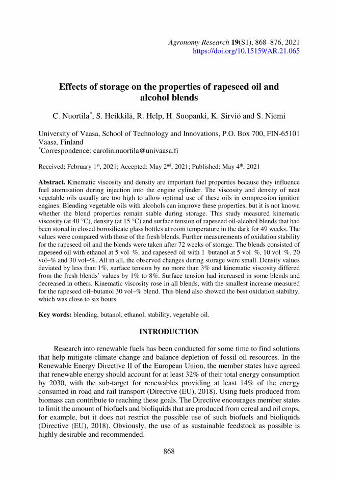
868
Agronomy Research 19(S1), 868–876, 2021 https://doi.org/10.15159/AR.21.065
Effects of storage on the properties of rapeseed oil and alcohol blends
C. Nuortila*, S. Heikkilä, R. Help, H. Suopanki, K. Sirviö and S. Niemi
University of Vaasa, School of Technology and Innovations, P.O. Box 700, FIN-65101 Vaasa, Finland *Correspondence: [email protected] Received: February 1st, 2021; Accepted: May 2nd, 2021; Published: May 4th, 2021 Abstract. Kinematic viscosity and density are important fuel properties because they influence fuel atomisation during injection into the engine cylinder. The viscosity and density of neat vegetable oils usually are too high to allow optimal use of these oils in compression ignition engines. Blending vegetable oils with alcohols can improve these properties, but it is not known whether the blend properties remain stable during storage. This study measured kinematic viscosity (at 40 °C), density (at 15 °C) and surface tension of rapeseed oil-alcohol blends that had been stored in closed borosilicate glass bottles at room temperature in the dark for 49 weeks. The values were compared with those of the fresh blends. Further measurements of oxidation stability for the rapeseed oil and the blends were taken after 72 weeks of storage. The blends consisted of rapeseed oil with ethanol at 5 vol–%, and rapeseed oil with 1–butanol at 5 vol–%, 10 vol–%, 20 vol–% and 30 vol–%. All in all, the observed changes during storage were small. Density values deviated by less than 1%, surface tension by no more than 3% and kinematic viscosity differed from the fresh blends’ values by 1% to 8%. Surface tension had increased in some blends and decreased in others. Kinematic viscosity rose in all blends, with the smallest increase measured for the rapeseed oil–butanol 30 vol–% blend. This blend also showed the best oxidation stability, which was close to six hours. Key words: blending, butanol, ethanol, stability, vegetable oil.
INTRODUCTION
Research into renewable fuels has been conducted for some time to find solutions that help mitigate climate change and balance depletion of fossil oil resources. In the Renewable Energy Directive II of the European Union, the member states have agreed that renewable energy should account for at least 32% of their total energy consumption by 2030, with the sub-target for renewables providing at least 14% of the energy consumed in road and rail transport (Directive (EU), 2018). Using fuels produced from biomass can contribute to reaching these goals. The Directive encourages member states to limit the amount of biofuels and bioliquids that are produced from cereal and oil crops, for example, but it does not restrict the possible use of such biofuels and bioliquids (Directive (EU), 2018). Obviously, the use of as sustainable feedstock as possible is highly desirable and recommended.

869
Alternative renewable fuels must have properties suitable for combustion in existing technologies and they also need to be stable. Viscosity, density and surface tension are all important fuel characteristics because they affect fuel injection, drop formation and atomisation (Guibet, 1999). Vegetable oils are a renewable source and have been used as neat material or in blends with fossil diesel in compression ignition engines (D’Alessandro et al., 2016; Čedik et al., 2018; Mat et al., 2018). Two of the critical properties for use of vegetable oils in combustion engines are density and viscosity: both usually are too high in neat vegetable oils to work optimally. Transesterification of oil triglycerides into fatty methyl esters can profoundly reduce viscosity of oils or fats (Kralova & Sjöblom, 2010). Blending vegetable oil with alcohols can also reduce viscosity and density of vegetable oil (Laza & Bereczky, 2011).
Another challenge with vegetable oils is their propensity to degrade when in contact with oxygen. All vegetable oils, animal fats and biodiesels are susceptible to oxidative degradation and this is related to the occurrence and the amount of unsaturated fatty acids in the material (Dunn, 2005). In turn, oxidative degradation of biodiesel can lead to an increase in viscosity due to the formation of high molecular weight molecules (Pölczmann et al., 2014).
When developing and testing new fuels or fuel blends, it is important to study properties over time to evaluate fuel stability. One way of investigation is to store fuels for an appropriate time under defined conditions.
This study investigates some selected fuel properties of rapeseed oil-alcohol blends after having stored the blends in closed borosilicate glass bottles in the dark at room temperature for almost one year. Kinematic viscosity, density and surface tension were measured and compared with results reported for the fresh blends before storage. Data from the initial measurements of fresh rapeseed oil and rapeseed oil-alcohol blends were presented in Nuortila et al. (2020). The current study also used a Rancimat test to measure oxidation stability of the neat rapeseed oil and its blends with ethanol and butanol after storage for over one year. This study presents results from investigating the stability of rapeseed oil-alcohol blends as a contribution to exploring potential alternative renewable fuels for compression ignition technology.
MATERIALS AND METHODS
Blends of rapeseed oil and ethanol at 5 vol–% and rapeseed oil and 1–butanol at 5,
10, 20, and 30 vol–% were prepared to a final volume of 200 mL. The blending ratios and abbreviations used for the blends are shown in Table 1. In pre-tests, the blends had proven to be stable at these blending ratios for a couple of weeks prior to the initial measurements. The blend components were commercial products: ethanol (denatured, 91.2% Etax A12) from Altia, Finland; *butanol (1–Butanol ≥ 98.5%, GPR RECTAPUR®) from VWR International, France; and rapeseed oil (100% rapeseed oil) containing vitamin E from Avena Kantvik Oy, Finland.
Table 1. Blending ratios and abbreviations of rapeseed oil and alcohol blends
Blending ratio (v–v%) Blend abbreviation
Rapeseed oil Alcohol
RSO 100% no alcohol BU5–RSO 95% 1–Butanol 5% BU10–RSO 90% 1–Butanol 10% BU20–RSO 80% 1–Butanol 20% BU30–RSO 70% 1–Butanol 30% E5–RSO 95% Ethanol 5%

870
The kinematic viscosity at 40 °C, density at 15 °C and surface tension at room temperature were measured for the fresh blends and the original rapeseed oil. The blends and the rapeseed oil (RSO) were then stored in closed borosilicate glass bottles in a dark chemical safety cabinet in the laboratory at room temperature. After 49 weeks, kinematic viscosity at 40 °C, density at 15 °C and surface tension of the blends and the rapeseed oil were measured again. In addition, oxidation stability was measured after 72 weeks of storage. A visual inspection of the blends and the RSO was made after storage before mixing the batches prior to analyses.
Kinematic viscosity and density Kinematic viscosity and density were measured with a Stabinger SVM 3000
rotational viscometer (Anton Paar GmbH, Austria). The measurements follow standard EN ISO 3104 for kinematic viscosity at 40 °C and EN ISO 12185 for density at 15 °C.
Surface tension Surface tension was measured with a Lauda tensiometer TD 2 (Lauda Dr. R. Wobser
GmbH & CO.KG). Measurements were made according to the manufacturer’s instructions (Tensiometer TD 2 Operating Instructions).
Oxidation stability In order to evaluate the blends’ susceptibility to oxidation, samples were
investigated in an accelerated aging test. Samples of three grams of each were measured at 110 °C in a Biodiesel Rancimat 873 (Metrohm AG, Herisau, Switzerland). The method is used for measurement of biodiesels and is based on change of conductivity in ionised water when degradation products are vented from the heated sample into the water. The induction time is recorded, i.e. the time that passes until secondary reaction products are formed. This analysis had not been done with the fresh blends.
Two replicate measurements were made to determine kinematic viscosity, density and oxidation stability for each blend and the rapeseed oil. The results are shown as the arithmetic mean of the two measurements. Single measurements were made to determine surface tension of the samples.
The analysis methods had been previously validated in the laboratory using validation samples. The relative standard deviation (RSD) for both kinematic viscosity and density was < 1%; RSD for oxidation stability was 2.10% (validated for bio–oils). The RSD was not measured for surface tension.
RESULTS AND DISCUSSION
There was no phase separation in any of the rapeseed oil-butanol blends. In the
BU20–RSO and BU30-RSO blends there was some slight deposit at the bottom of the bottles. The E5-RSO blend had separated into three phases of which the lowermost and biggest phase was slightly turbid. A clear phase had formed about 5 mm thick beneath the surface, and a third phase was distinguished just at the surface, slightly oscillating in colour. Phases disappeared after mixing the blend batch.
Rapeseed oil-alcohol blends showed only relatively small changes in kinematic viscosity and surface tension during storage. Essentially, there were no changes in density when compared to the values for the fresh blends and rapeseed oil. All of the
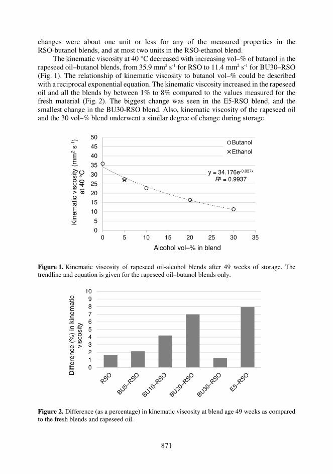
871
changes were about one unit or less for any of the measured properties in the RSO-butanol blends, and at most two units in the RSO-ethanol blend.
The kinematic viscosity at 40 °C decreased with increasing vol–% of butanol in the rapeseed oil–butanol blends, from 35.9 mm2 s-1 for RSO to 11.4 mm2 s-1 for BU30–RSO (Fig. 1). The relationship of kinematic viscosity to butanol vol–% could be described with a reciprocal exponential equation. The kinematic viscosity increased in the rapeseed oil and all the blends by between 1% to 8% compared to the values measured for the fresh material (Fig. 2). The biggest change was seen in the E5-RSO blend, and the smallest change in the BU30-RSO blend. Also, kinematic viscosity of the rapeseed oil and the 30 vol–% blend underwent a similar degree of change during storage.
Figure 1. Kinematic viscosity of rapeseed oil-alcohol blends after 49 weeks of storage. The trendline and equation is given for the rapeseed oil–butanol blends only.
Figure 2. Difference (as a percentage) in kinematic viscosity at blend age 49 weeks as compared to the fresh blends and rapeseed oil.
y = 34.176e-0.037x
R² = 0.9937
0
5
10
15
20
25
30
35
40
45
50
0 5 10 15 20 25 30 35
Kin
em
atic v
iscosity
(mm
2s
-1)
at
40 °
C
Alcohol vol–% in blend
Butanol
Ethanol
0
1
2
3
4
5
6
7
8
9
10
Diffe
rence (
%)
in k
inem
atic
vis
cosity

872
Density at 15 °C decreased with increasing vol–% of butanol in the blends, from 920 g cm-3 for RSO to 888 g cm-3 for BU30-RSO (Fig. 3). The relationship was linear between density and the increasing vol–% of butanol in the blends. The density of the E5-RSO blend was 914 g cm-3, the same as the BU5-RSO blend. Over the storage time of almost one year, the density of the RSO and all the rapeseed oil-alcohol blends changed only minimally, by less than 0.2% (Fig. 4).
Figure 3. Density of rapeseed oil-alcohol blends after 49 weeks of storage. The trendline and equation is given for the rapeseed oil-butanol blends only. Note the y-axis scale starts at 870 g cm-3.
Figure 4. Difference (as a percentage) in density at 15 °C at blend age 49 weeks as compared to the fresh blends and rapeseed oil.
The surface tension decreased with increasing vol–% of butanol in the blends, from
33 mN m-1 for RSO to 26 mN m-1 for BU30-RSO (Fig. 5). The relationship could be described with a linear equation. The surface tension was 28 mN m-1 for E5-RSO, almost identical to the value for BU20-RSO. Surface tension had changed by between 1% and 3% during storage (Fig. 6). While kinematic viscosity had slightly increased, surface
y = -1.0647x + 919.91R² = 0.9995
870
880
890
900
910
920
930
940
0 5 10 15 20 25 30 35
Density
(g c
m-3
) at 15 °
C
Alcohol vol–% in blend
Butanol
Ethanol
-1.0
-0.5
0.0
0.5
1.0
1.5
2.0
Diffe
rence (
%)
in d
ensity
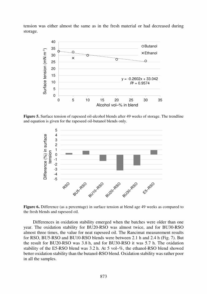
873
tension was either almost the same as in the fresh material or had decreased during storage.
Figure 5. Surface tension of rapeseed oil-alcohol blends after 49 weeks of storage. The trendline and equation is given for the rapeseed oil-butanol blends only.
Figure 6. Difference (as a percentage) in surface tension at blend age 49 weeks as compared to the fresh blends and rapeseed oil.
Differences in oxidation stability emerged when the batches were older than one
year. The oxidation stability for BU20-RSO was almost twice, and for BU30-RSO almost three times, the value for neat rapeseed oil. The Rancimat measurement results for RSO, BU5-RSO and BU10-RSO blends were between 2.1 h and 2.4 h (Fig. 7). But the result for BU20-RSO was 3.8 h, and for BU30-RSO it was 5.7 h. The oxidation stability of the E5-RSO blend was 3.2 h. At 5 vol–%, the ethanol-RSO blend showed better oxidation stability than the butanol-RSO blend. Oxidation stability was rather poor in all the samples.
y = -0.2602x + 33.042R² = 0.9574
0
5
10
15
20
25
30
35
40
0 5 10 15 20 25 30 35
Surf
ace tensio
n (
mN
m-1
)
Alcohol vol–% in blend
Butanol
Ethanol
-5
-4
-3
-2
-1
0
1
2
3
4
5
Diffe
rence (
%)
in s
urf
ace
tensio
n

874
At present, there is no information available in the scientific literature reporting effects of storage on vegetable oil-alcohol blends. Therefore, the results from this study will be compared to results from storage studies with vegetable oils and biodiesel.
Figure 7. Oxidation stability measured as induction time in a Rancimat for rapeseed oil-alcohol blends after 72 weeks of storage. The trendline and equation is given for the rapeseed oil-butanol blends only.
Kreivaitis et al. (2013) reported an increase of approximately 5% in kinematic
viscosity of rapeseed oil after 70 days of storage at 70 °C. Bezergianni & Chrysikou (2012) investigated oxidative stability of waste cooking oil and white diesel stored in air–tight bottles in the dark at room temperature for a year. They reported that density of the waste cooking oil did not change noticeably, but viscosity increased slightly by approximately 2%. In a study by Pattamaprom et al. (2012), kinematic viscosity of palm stearin and palm olein biodiesel did not increase during six months of storage in dark and closed containers at room temperature, but density increased by 5–6%. The authors noticed that viscosities dropped slightly and argued that this was possibly caused by chain scission of biodiesel into smaller molecules. Palm-oil diesel without antioxidants showed an increase in kinematic viscosity, from approximately 6 cSt to approximately 7 cSt (i.e. approximately 6 mm2 s-1 to 7 mm2 s-1, equalling a change of about 16%) when stored at 20 °C for 125 days (Lin & Chiu, 2009). Bouaid et al. (2009) reported an increase in viscosity from 5.1 to 6.9 mm2 s-1 (equalling an increase of 35%) for biodiesel made from Brassica carinata and ethanol after 12 months storage. The samples had been stored under argon in a closed glass bottle at room temperature and exposed to daylight. These literature results indicate that kinematic viscosity of oils and biodiesel can vary in response to different materials and storage conditions.
Biodiesels vary also in oxidation stability depending on their constituent materials (reviewed in Jain & Sharma, 2010). A neat animal fat methyl ester without antioxidant showed an oxidation stability of only 2.2 h (Sirviö et al., 2018). The oxidation stability of biodiesel made from rapeseed oil and used cooking oil decreased from 5–6 h to approximately 1 h over the course of 136 weeks (Pölczmann et al., 2014). Laza & Bereczky (2011) measured oxidation stability of rapeseed oil and propanol, and of rapeseed oil and butanol blends with alcohol volume percentages from 5% to 20% at
y = 1.9282e0.0345x
R² = 0.9431
0
1
2
3
4
5
6
7
8
0 5 10 15 20 25 30 35
Oxid
ation s
tabili
ty(induction t
ime, h)
Alcohol vol-% in blend
Butanol
Ethanol
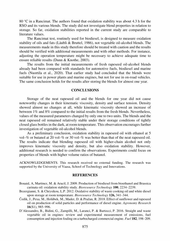
875
80 °C in a Rancimat. The authors found that oxidation stability was about 4.3 h for the RSO and its various blends. The study did not investigate blend properties in relation to storage. So far, oxidation stabilities reported in the current study are comparable to literature values.
The Rancimat test, routinely used for biodiesel, is designed to measure oxidation stability of oils and fats (Läubli & Bruttel, 1986), not vegetable oil-alcohol blends. The measurements made in this study therefore should be treated with caution and the results should be verified with additional measurements and with other methods. For instance, adjusting the operation temperature might be necessary to achieve adequate time to ensure reliable results (Dunn & Knothe, 2003).
The results from the initial measurements of fresh rapeseed oil-alcohol blends already had been compared with standards for automotive fuels, biodiesel and marine fuels (Nuortila et al., 2020). That earlier study had concluded that the blends were suitable for use in power plants and marine engines, but not for use in on-road vehicles. The same conclusion holds for the results after storing the blends for almost one year.
CONCLUSIONS
Storage of the neat rapeseed oil and the blends for one year did not cause
noteworthy changes in their kinematic viscosity, density and surface tension. Density showed almost no changes at all, while kinematic viscosity showed an increase of between 1% and 8% compared to the initial results from the fresh blends. Nevertheless, values of the measured parameters changed by only one to two units. The blends and the neat rapeseed oil remained relatively stable under their storage conditions of tightly closed glass bottles in the dark, at room temperature. This observation encourages further investigation of vegetable oil-alcohol blends.
As a preliminary conclusion, oxidation stability in rapeseed oil with ethanol at 5 vol–% or butanol at 20 vol–% or 30 vol–% was better than that of the neat rapeseed oil. The results indicate that blending rapeseed oil with higher-chain alcohol not only improves kinematic viscosity and density, but also oxidation stability. However, additional research is needed to confirm the observations. Experiments could focus on properties of blends with higher volume ratios of butanol.
ACKNOWLEDGEMENTS. This research received no external funding. The research was supported by the University of Vaasa, School of Technology and Innovations.
REFERENCES
Bouaid, A, Martinez, M. & Aracil, J. 2009. Production of biodiesel from bioethanol and Brassica
carinata oil: oxidation stability study. Bioresource Technology 100, 2234‒2239. Bezergianni, S. & Chrysikou, L.P. 2012. Oxidative stability of waste cooking oil and white diesel
upon storage at room temperature. Bioresource Technology 126, 341‒344. Čedik, J., Pexa, M., Holúbek, M., Mader, D. & Pražan, R. 2018. Effect of sunflower and rapeseed
oil on production of solid particles and performance of diesel engine. Agronomy Research 16(S1), 985‒996.
D’Alessandro, B., Bidini, G., Zampilli, M., Laranci, P. & Bartocci, P. 2016. Straight and waste vegetable oil in engines: review and experimental measurement of emissions, fuel consumption and injection fouling on a turbocharged commercial engine. Fuel 182, 198‒209.

876
Directive (EU). 2018. Directive (EU) 2018/2001 of the European Parliament and of the Council of 11 December 2018 on the promotion of the use of energy from renewable sources. https://eur-lex.europa.eu/legal-content/EN/TXT/?uri=uriserv:OJ.L_.2018.328.01.0082.01.ENG&toc=OJ:L:2018:328:TOC. Accessed 21.3.2021.
Dunn, R.O. 2005. Oxidative stability of soybean oil fatty acid methyl esters by oil stability index (OSI). Journal of the American Oil Chemists Society 82, 381‒387.
Dunn, R.O. & Knothe, G. 2003. Oxidative stability of biodiesel in blends with jet fuel by analysis of oil stability index. Journal of the American Oil Chemists’ Society 80, 1047‒1048.
Guibet, 1999. Fuels and Engines. Institut Français du Pétrole Publications. Éditions Technip, Paris. 786 pp.
Jain, S. & Sharma, M.P. 2010. Stability of biodiesel and its blends: a review. Renewable and Sustainable Energy Reviews 14, 667‒678.
Kralova, I. & Sjöblom, J. 2010. Biofuels‒renewable energy sources: a review. Journal of Dispersion Science and Technology 31, 409‒425.
Kreivaitis, R., Gumbytė, M., Kazancev, K., Padgurskas, J. & Makarevičienė, V. 2013. A comparison of pure and natural antioxidant modified rapeseed oil storage properties. Industrial Crops and Products 43, 511‒516.
Laza, T. & Bereczky, Á. 2011. Basic fuel properties of rapeseed oil-higher alcohols blends. Fuel 90, 803‒810.
Läubli, M.W. & Bruttel, P.A. 1986. Determination of the oxidative stability of fats and oils: comparison between the active oxygen method (AOCS Cd 12‒57) and the Rancimat method. JAOCS 63, 792‒795.
Lin, C.-Y. & Chiu, C.-C. 2009. Effects of oxidation during long-term storage on the fuel properties of palm oil-based biodiesel. Energy & Fuels 23, 3285‒3289.
Mat, S.C., Idroas, M.Y., Hamid, M.F. & Zainal, Z.A. 2018. Performance and emissions of straight vegetable oils and its blends as a fuel in diesel engine: A review. Renewable and Sustainable Energy Reviews 82, 808‒823.
Nuortila, C., Help, R., Sirviö, K., Suopanki, H., Heikkilä, S. & Niemi, S. 2020. Selected fuel properties of alcohol and rapeseed oil blends. Energies 13, 3821.
Pattamaprom, C., Pakdee, W. & Ngamjaroen, S. 2012. Storage degradation of palm‒derived biodiesels: its effects on chemical properties and engine performance. Renewable Energy 37, 412‒418.
Pölczmann, G., Tóth, O., Beck, Á. & Hancsók, J. 2014. Storage stability of gas oil containing waste originated biocomponent. Periocida Polytechnica Chemical Engineering 58, 157‒163. doi:10.3311/PPch.7205
Sirviö, K., Heikkilä, S., Help, R., Niemi, S. & Hiltunen, E. 2018. Properties of local produced animal-fat based biodiesel and its blend with fossil fuel. Agronomy Research 16(S1), 1237‒1246.

877
Agronomy Research 19(S1), 877–895, 2021 https://doi.org/10.15159/AR.21.084
Prospect on agro-industrial residues usage for biobutanol production
S. Raita*, K. Spalvins and D. Blumberga
Riga Technical University, Institute of Energy Systems and Environment, Azenes street 12/1, LV 1048 Riga, Latvia *Correspondence: [email protected] Received: February 13th, 2021; Accepted: May 2nd, 2021; Published: May 18th, 2021 Abstract. Climate changes, environmental pollution and resource depletion are one of the numerous major problems humanity faces. United Nations sustainable development goals are aimed at solving these problems. The requirement for affordable, renewable, sustainable, biodegradable and environmentally friendly fossil fuel alternative sources is prompted by the development and advancement of biofuel production technologies. Of the various biofuel alternatives, biobutanol has increased the interests of researchers due to its desirable characteristics such as hydrophobicity, relatively high heating value and energy density, relatively low vapour pressure, etc. Nowadays, sustainable production of the biobutanol depends on the used feedstock source and its pre-treatment method, selected enhancing microorganism strain, acetone–butanol–ethanol fermentation effectiveness and titer of biobutanol. The main research challenges in biobutanol production are an improvement of production efficiency and increasing the financial viability of the technology. This review summarizes the latest results of lignocellulosic components content and fermentable sugars composition in different agro-industrial residues; biobutanol production depending on the Clostridium enhancing strategy, process optimization and selection of substrate. Such analysis provides a better perception of the capability of using agro-industrial residues for biobutanol production efficiency. Key words: ABE fermentation, agricultural residues, biobutanol, Clostridium, lignocellulosic.
INTRODUCTION
The awareness of harmful impacts over global warming, environmental pollution and limitation of fossil fuels creates a need to find an alternate source for renewable energy resources (Anandharaj et al., 2020) Consequently, a variety of sustainable potent biofuels have been explored such as biodiesel, bioethanol, biobutanol, biomethanol, biogas etc. (Rathour et al., 2018). Butanol is a four-carbon straight-chained alcohol with a formula of C4H9OH (Lv et al., 2021). It is a promising alternative biofuel, owing to its appropriate physical properties. Compared to bioethanol it has a greater heating value and 25% higher energy content, higher viscosity, lower heat of vaporization and lower corrosivity (Jiang et al., 2018; Anandharaj et al., 2020). Butanol has better intersolubility than that of ethanol fuel, it is hydrophobic, can be blended in any concentration with gasoline without any modification of current vehicle engines, and can be transported in existing

878
infrastructure (Rathour et al., 2018; Lv et al., 2021). To assess the profitability of biofuels, including biobutanol, the important criteria is energy return on investment (EROI) defined as the ratio of the total energy output to the energy input. Because of relatively high energy density of butanol, biobutanol production process has the potential to have higher EROI than it is for corn-based ethanol (EROI ranges from 0.8 to 1.6) (Tao et al., 2013; Rezaei et al., 2021). Research by Tao et al. (2013) shows that cellulosic n-butanol lower than that of ethanol, by-product appearance during the butanol production process eventually compensate and increase the EROI of butanol (Tao et al., 2013).
Selection of the feedstock is other important factor affecting EROI of the butanol production. Shift from first to the second generation biofuels by utilizing lignocellulose, instead of edible resources - is accompanied by the increase of EROI (Rezaei et al., 2021). Compared with the first generation of biofuels production using starch-based feedstock, the second generation of biofuels is suitable for acetone-butanol-ethanol (ABE) fermentation, because does not compete with food market (Li et al., 2019; Jiang et al., 2019; Tsai et al., 2020). Utilizing lignocellulosic biomass seems to be the best alternative for biobutanol production since it is a renewable and widely available low cost resource (Huzir et al., 2018). Additionally, utilizing lignocellulosic biomass helps to properly manage the waste generation (Huzir et al., 2018).
The selection of biomass of feedstock for butanol production should be considered is the variety of cultivated agricultural crops available in each country, its growth time, the request for each crop for other purposes, and harvesting, transportation and pre-treatment costs (Procentese et al., 2017). Lignocellulosic biomass from agricultural residues like rice straw, sugarcane bagasse, wheat straw, corn cob and corn stover are potential sources for bioethanol and biobutanol production. These crops have a short-harvest rotation, thus allowing greater availability of these residues throughout the year (Sindhu et al., 2016; Araújo et al., 2018). Very interesting lignocellulosic by-product of the mushroom industry is the spent mushroom substrate. Food and Agriculture Organization have estimated, that in 2019 year world production of spent mushroom substrate was about 12 million tons. For every ton of mushroom produced, about 5 tons of spent mushroom substrate is generated (FAO, 2019) As a kind of lignocellulosic materials, it could be a source of reducing sugars for producing biofuels (Rajavat et al., 2019).
Many lignocellulosic biomasses with high cellulose and hemicellulose content and low lignin content are the ideal substrate for biobutanol production (Galbe & Wallberg, 2019). However, lignocellulosic biomass cannot be converted into biofuels directly and has to be pre–treated to release the fermentable sugars for solventogenic Clostridium sp., which produce butanol via ABE fermentation (Jiang et al., 2018; Kolesinska et al., 2019). Lignocellulosic biomass feedstock selection, ABE fermentation time and biobutanol yield were some of the major factors which predominantly affect the cost and sustainability of the butanol production process. The production cost of biobutanol can be reduced by various Clostridium strain metabolic engineering and fermentation process optimization strategies (Tian et al., 2019b; Gao et al., 2020).
In recent years, a numerous researchers has reviewed the potential of agricultural feedstock, lignocellulose pre-treatment methods and process optimization for sustainable production of biobutanol, for example, Ravindran & Jaiswal (2016), Araújo et al. (2018), Kolesinska et al. (2019), Vivek et al. (2019). In this study the latest results for lignocellulosic components content and fermentable sugars composition in different
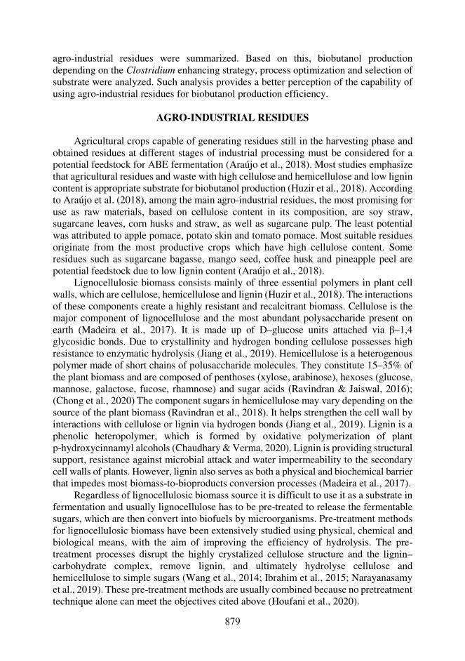
879
agro-industrial residues were summarized. Based on this, biobutanol production depending on the Clostridium enhancing strategy, process optimization and selection of substrate were analyzed. Such analysis provides a better perception of the capability of using agro-industrial residues for biobutanol production efficiency.
AGRO-INDUSTRIAL RESIDUES
Agricultural crops capable of generating residues still in the harvesting phase and
obtained residues at different stages of industrial processing must be considered for a potential feedstock for ABE fermentation (Araújo et al., 2018). Most studies emphasize that agricultural residues and waste with high cellulose and hemicellulose and low lignin content is appropriate substrate for biobutanol production (Huzir et al., 2018). According to Araújo et al. (2018), among the main agro-industrial residues, the most promising for use as raw materials, based on cellulose content in its composition, are soy straw, sugarcane leaves, corn husks and straw, as well as sugarcane pulp. The least potential was attributed to apple pomace, potato skin and tomato pomace. Most suitable residues originate from the most productive crops which have high cellulose content. Some residues such as sugarcane bagasse, mango seed, coffee husk and pineapple peel are potential feedstock due to low lignin content (Araújo et al., 2018).
Lignocellulosic biomass consists mainly of three essential polymers in plant cell walls, which are cellulose, hemicellulose and lignin (Huzir et al., 2018). The interactions of these components create a highly resistant and recalcitrant biomass. Cellulose is the major component of lignocellulose and the most abundant polysaccharide present on earth (Madeira et al., 2017). It is made up of D–glucose units attached via β–1,4 glycosidic bonds. Due to crystallinity and hydrogen bonding cellulose possesses high resistance to enzymatic hydrolysis (Jiang et al., 2019). Hemicellulose is a heterogenous polymer made of short chains of polusaccharide molecules. They constitute 15–35% of the plant biomass and are composed of penthoses (xylose, arabinose), hexoses (glucose, mannose, galactose, fucose, rhamnose) and sugar acids (Ravindran & Jaiswal, 2016); (Chong et al., 2020) The component sugars in hemicellulose may vary depending on the source of the plant biomass (Ravindran et al., 2018). It helps strengthen the cell wall by interactions with cellulose or lignin via hydrogen bonds (Jiang et al., 2019). Lignin is a phenolic heteropolymer, which is formed by oxidative polymerization of plant p-hydroxycinnamyl alcohols (Chaudhary & Verma, 2020). Lignin is providing structural support, resistance against microbial attack and water impermeability to the secondary cell walls of plants. However, lignin also serves as both a physical and biochemical barrier that impedes most biomass-to-bioproducts conversion processes (Madeira et al., 2017).
Regardless of lignocellulosic biomass source it is difficult to use it as a substrate in fermentation and usually lignocellulose has to be pre-treated to release the fermentable sugars, which are then convert into biofuels by microorganisms. Pre-treatment methods for lignocellulosic biomass have been extensively studied using physical, chemical and biological means, with the aim of improving the efficiency of hydrolysis. The pre-treatment processes disrupt the highly crystalized cellulose structure and the lignin–carbohydrate complex, remove lignin, and ultimately hydrolyse cellulose and hemicellulose to simple sugars (Wang et al., 2014; Ibrahim et al., 2015; Narayanasamy et al., 2019). These pre-treatment methods are usually combined because no pretreatment technique alone can meet the objectives cited above (Houfani et al., 2020).
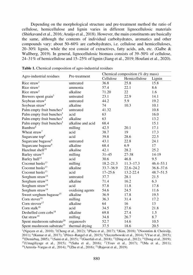
880
Depending on the morphological structure and pre-treatment method the ratio of cellulose, hemicellulose and lignin varies in different lignocellulosic materials (Shirkavand et al., 2016; Araújo et al., 2018). However, the main constituents are basically the same, although the contents of individual carbohydrates, aromatics and other compounds vary: about 50–60% are carbohydrates, i.e. cellulose and hemicelluloses, 20–30% lignin, while the rest consist of extractives, fatty acids, ash, etc. (Galbe & Wallberg, 2019). In general, lignocellulosic biomass consists of 39–50% of cellulose, 24–31% of hemicellulose and 15–25% of lignin (Jiang et al., 2019; Houfani et al., 2020).
Table 1. Chemical composition of agro-industrial residues
Agro-industrial residues Pre-treatment Chemical composition (% dry mass) Cellulose Hemicellulose Lignin
Rice straw1 untreated 36.8 25.8 15.8 Rice straw1 ammonia 57.4 22.1 8.6 Rice straw2 alkaline 71.20 22 1.6 Brewers spent grain3 untreated 23.1 22.9 14.1 Soybean straw4 untreated 44.2 5.9 19.2 Soybean straw4 alkaline 74 10.3 10.1 Palm empty fruit bunches5 untreated 41.32 10.8 Palm empty fruit bunches5 acid 63 16.0 Palm empty fruit bunches5 alkaline 63 13.2 Palm empty fruit bunches5 alkaline and acid 68.4 15.1 Bamboo6 milling 42.5 20.1 17.1 Wheat straw7 acid 38.7 19 17.3 Sugarcane top8 acid 39.8 28.6 22.5 Sugarcane bagasse9 untreated 43.1 22.8 24.1 Sugarcane bagasse9 alkaline 68.4 6.9 17 Hazelnut shell10 alkaline 42.1 28.2 25.2 Barley straw11 milling 31–45 27-38 14-19 Barley hull12 acid 30.6 46.8 9.5 Coconut husks13 milling 18.2–21.3 11.3–17.3 46.4–53.1 Coconut husks13 alkaline 33.7–36.9 22.6–24.2 36.8–37.6 Coconut husks13 acid 17–25.6 13.2-22.4 48.7–51.5 Sorghum straw14 untreated 37.7 28.1 21.5 Sorghum straw14 alkaline 71.4 16.2 6.3 Sorghum straw14 acid 57.8 11.8 17.8 Sorghum straw14 oxidising agents 54.6 24.5 11.6 Sweet sorghum bagasse15 alkaline 36.9 17.8 19.5 Corn stover16 milling 36.3 31.4 17.2 Corn strover17 alkaline 64 16 13 Corn stalk18 acid 34.5 27.6 21.8 Deshelled corn cobs18 alkaline 69.8 27.4 1.5 Oat straw19 milling 34.8 26.7 8.7 Spent mushroom substrate20 organosolv 52.7 14.6 10.5 Spent mushroom substrate21 thermal drying 37.5 18.6 20.5 1(Nguyen et al., 2010); 2(Cheng et al., 2012); 3(Plaza et al., 2017); 4(Kim, 2018); 5(Noomtim & Cheirsilp, 2011); 6(Kumar et al., 2017); 7(Pérez–Rangel et al., 2015); 8(Szczerbowski et al., 2014); 9(Yue et al., 2015); 10(Demirbaş, 2005); 11(Saini et al., 2015); 12(Guerfali et al., 2018); 13(Ding et al., 2012); 14(Dong et al., 2019); 15(Umagiliyage et al., 2015); 16(Saha et al., 2016); 17(Yoav et al., 2017); 18(Ma et al., 2011); 19(Arreola–Vargas et al., 2014); 20(Zhu et al., 2016); 21(Rajavat et al., 2019).
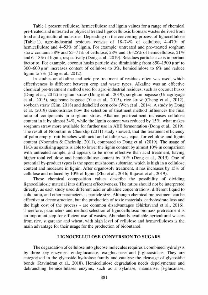
881
Table 1 present cellulose, hemicellulose and lignin values for a range of chemical pre-treated and untreated or physical treated lignocellulosic biomass wastes derived from food and agricultural industries. Depending on the converting process of lignocellulose (Table 1), agro-industrial residues consist of 18–74% of cellulose, 4–47% of hemicellulose and 4–53% of lignin. For example, untreated and pre–treated sorghum straw contains 38% and 55–71% of cellulose, 28% and 16–25% of hemicellulose, 21% and 6–18% of lignin, respectively (Dong et al., 2019). Residues particle size is important factor to. For example, coconut husks particle size diminishing from 850–1500 µm2 to 300–600 µm2 increases content of cellulose to 3%, hemicellulose to 6% and reduce lignin to 7% (Ding et al., 2012).
In studies an alkaline and acid pre-treatment of residues often was used, which effectiveness is different between crop and waste types. Alkaline was an effective chemical pre-treatment method used for agro-industrial residues, such as coconut husks (Ding et al., 2012) sorghum straw (Dong et al., 2019), sorghum bagasse (Umagiliyage et al., 2015), sugarcane bagasse (Yue et al., 2015), rice straw (Cheng et al., 2012), soybean straw (Kim, 2018) and deshelled corn cobs (Wen et al., 2014). A study by Dong et al. (2019) demonstrates how the selection of treatment method influences the final ratio of components in sorghum straw. Alkaline pre-treatment increases cellulose content in it by almost 34%, while the lignin content was reduced by 15%, what makes sorghum straw more available for further use in ABE fermentation (Dong et al., 2019). The result of Noomtim & Cheirslip (2011) study showed, that the treatment efficiency of palm empty fruit bunches with acid and alkaline was equal for cellulose and lignin content (Noomtim & Cheirsilp, 2011), compared to Dong et al. (2019). The usage of H2O2 as oxidising agents is able to lower the lignin content by almost 10% in comparison with untreated sample, and appears to be more effective than acid treatment, having higher total cellulose and hemicellulose content by 10% (Dong et al., 2019). One of potential by-product types is the spent mushroom substrate, which is high in a cellulose content and moderate in lignin. After organosolv treatment, it has increases by 15% of cellulose and reduced by 10% of lignin (Zhu et al., 2016; Rajavat et al., 2019).
These chemical composition values describe the possibility of dividing lignocellulosic material into different effectiveness. The ratios should not be interpreted directly, as each study used different acid or alkaline concentrations, different liquid to solid ratio, and other parameters as particle size. Although chemical pretreatment can be effective at deconstruction, but the production of toxic materials, carbohydrate loss and the high cost of the process - are common disadvantages (Shirkavand et al., 2016). Therefore, parameters and method selection of lignocellulosic biomass pretreatment is an important step for efficient use of wastes. Abundantly available agricultural wastes from rice, sugarcane and wheat, with high level of cellulose and hemicelluloses is the main advantage for their usage for the production of biobutanol.
LIGNOCELLULOSE CONVERSION TO SUGARS
The degradation of cellulose into glucose molecules requires a combined hydrolysis
by three key enzymes: endoglucanase, exoglucanase and β-glucosidase. They are categorized in the glycoside hydrolase family and catalyse the cleavage of glycosidic bonds (Ravindran et al., 2018). Hemicellulose degradation needs depolymerase and debranching hemicellulases enzyms, such as a xylanase, mannanse, β-glucanase,
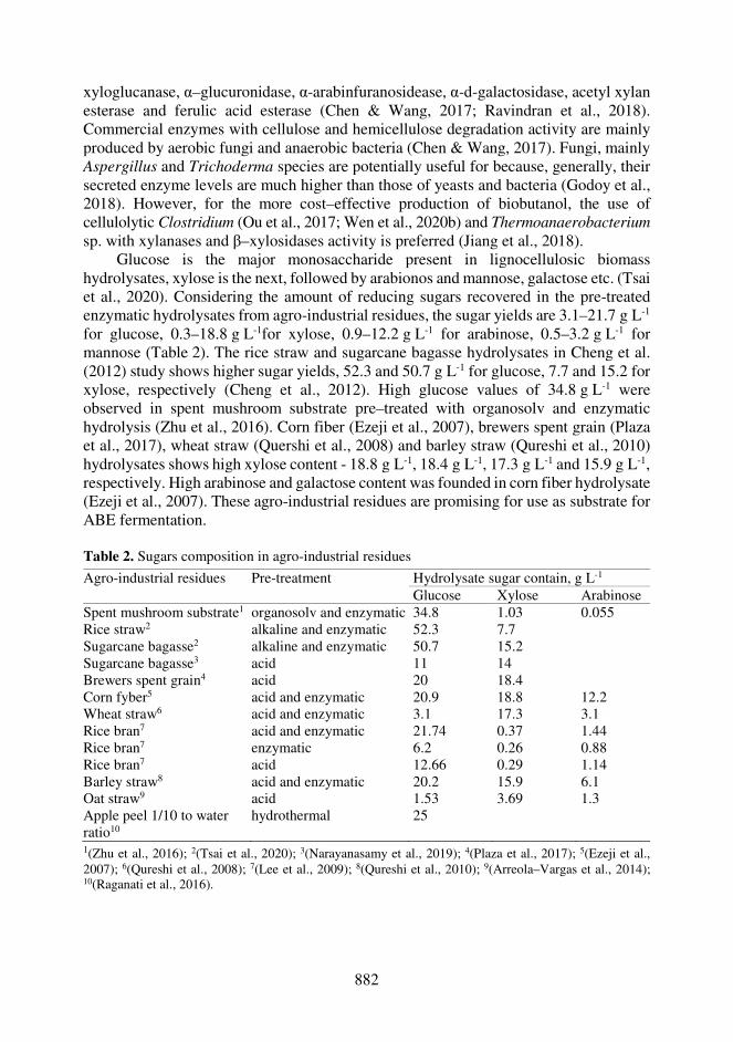
882
xyloglucanase, α–glucuronidase, α-arabinfuranosidease, α-d-galactosidase, acetyl xylan esterase and ferulic acid esterase (Chen & Wang, 2017; Ravindran et al., 2018). Commercial enzymes with cellulose and hemicellulose degradation activity are mainly produced by aerobic fungi and anaerobic bacteria (Chen & Wang, 2017). Fungi, mainly Aspergillus and Trichoderma species are potentially useful for because, generally, their secreted enzyme levels are much higher than those of yeasts and bacteria (Godoy et al., 2018). However, for the more cost–effective production of biobutanol, the use of cellulolytic Clostridium (Ou et al., 2017; Wen et al., 2020b) and Thermoanaerobacterium sp. with xylanases and β–xylosidases activity is preferred (Jiang et al., 2018).
Glucose is the major monosaccharide present in lignocellulosic biomass hydrolysates, xylose is the next, followed by arabionos and mannose, galactose etc. (Tsai et al., 2020). Considering the amount of reducing sugars recovered in the pre-treated enzymatic hydrolysates from agro-industrial residues, the sugar yields are 3.1–21.7 g L-1 for glucose, 0.3–18.8 g L-1for xylose, 0.9–12.2 g L-1 for arabinose, 0.5–3.2 g L-1 for mannose (Table 2). The rice straw and sugarcane bagasse hydrolysates in Cheng et al. (2012) study shows higher sugar yields, 52.3 and 50.7 g L-1 for glucose, 7.7 and 15.2 for xylose, respectively (Cheng et al., 2012). High glucose values of 34.8 g L-1 were observed in spent mushroom substrate pre–treated with organosolv and enzymatic hydrolysis (Zhu et al., 2016). Corn fiber (Ezeji et al., 2007), brewers spent grain (Plaza et al., 2017), wheat straw (Quershi et al., 2008) and barley straw (Qureshi et al., 2010) hydrolysates shows high xylose content - 18.8 g L-1, 18.4 g L-1, 17.3 g L-1 and 15.9 g L-1, respectively. High arabinose and galactose content was founded in corn fiber hydrolysate (Ezeji et al., 2007). These agro-industrial residues are promising for use as substrate for ABE fermentation.
Table 2. Sugars composition in agro-industrial residues
Agro-industrial residues Pre-treatment Hydrolysate sugar contain, g L-1 Glucose Xylose Arabinose
Spent mushroom substrate1 organosolv and enzymatic 34.8 1.03 0.055 Rice straw2 alkaline and enzymatic 52.3 7.7 Sugarcane bagasse2 alkaline and enzymatic 50.7 15.2 Sugarcane bagasse3 acid 11 14 Brewers spent grain4 acid 20 18.4 Corn fyber5 acid and enzymatic 20.9 18.8 12.2 Wheat straw6 acid and enzymatic 3.1 17.3 3.1 Rice bran7 acid and enzymatic 21.74 0.37 1.44 Rice bran7 enzymatic 6.2 0.26 0.88 Rice bran7 acid 12.66 0.29 1.14 Barley straw8 acid and enzymatic 20.2 15.9 6.1 Oat straw9 acid 1.53 3.69 1.3 Apple peel 1/10 to water ratio10
hydrothermal 25
1(Zhu et al., 2016); 2(Tsai et al., 2020); 3(Narayanasamy et al., 2019); 4(Plaza et al., 2017); 5(Ezeji et al., 2007); 6(Qureshi et al., 2008); 7(Lee et al., 2009); 8(Qureshi et al., 2010); 9(Arreola–Vargas et al., 2014); 10(Raganati et al., 2016).
883
POTENTIAL CLOSTRIDIUM SP. FOR PRODUCTION OF BIOBUTANOL
Biobutanol production is usually done by solventogenic bacteria from Clostridium genus, such as C. acetobutylicum (Ibrahim et al., 2015), C. beijerinckii (Plaza et al., 2017), C. saccharoperbutylacetonicum (Zetty–Arenas et al., 2019) and C. pasteurianum (Lipovsky et al., 2016). These bacteria produce biobutanol by fermenting sugars through acetone, butanol and ethanol fermentation (Zetty–Arenas et al., 2019; Ashani et al., 2020). ABE fermentation can be divided into two phases: acidogenic phase, where cell growth occurs and acids (butyric acid, acetic acid) are the main metabolites; and solventogenic phase, where acids are reassimilated and solvents are produced. Later, fermentation ceases and cells form endospores (Birgen et al., 2019; Xue & Cheng, 2019);
Butanol producing Clostridium sp. are able to use a wide variety of carbohydrates such as starch, cellobiose, sucrose, glucose, fructose, mannose, dextrin, galactose, xylose and arabinose (Plaza et al., 2017). Glucose is the most preferred carbon source for Clostridium sp., and all the central carbon metabolic pathways are expressed constitutively enabling efficient and rapid glucose utilization. (Jang et al., 2013; Ibrahim et al., 2015; Tsai et al., 2020). Other simple sugars, such as xylose, could not be consumed by bacteria in the presence of higher concentrations of glucose, due to a phenomenon called carbon catabolite repression, which might reduce butanol yield from the lignocellulosic biomass (Wen et al., 2020b). Bacteria have developed sophisticated mechanisms to adapt to environmental changes. For example, carbon catabolite repression allows bacteria the assimilation of a preferred (i.e. rapidly metabolisable) carbon source when they are exposed to more than one carbohydrate (Deutscher, 2008). Improvement of either native or genetically engineered strains for simultaneous utilization of hexoses and pentoses without carbon catabolite repression, could improve the biobutanol production efficiency, resulting in a more economicaly feasible process (Vivek et al., 2019).
Acidogenic Clostridium such as C. tyrobutyricum, C. thermocellum, C. cellulolyticum and C. cellulovorans produces butyric and acetic acids as the main metabolic product, but not butanol, because of lacking some key enzymes, including CoA transferase (ctfAB), acetoacetate decarboxylase (adc), and aldehyde dehydrogenase (ald), in the pathways leading to ABE production (Yu et al., 2015; Xue & Cheng, 2019); (Bao et al., 2019). These strains have had evolving interest of researchers, due to the possibility of engineering their metabolic pathways in benefit for butanol production. Especially, C. thermocellum, C. cellulolyticum and C. cellulovorans with cellulolytic activity, because they natively secrete cellulases and consume cellulose, xylan and mannan (Yang et al., 2015; Ou et al., 2017; Wen et al., 2020b).
ENHANCING PRODUCTIVITY OF BIOBUTANOL
Solvent producing Clostridium strains rarely tolerate more than 10–20 g L-1 butanol in fermentation broth (Yang et al., 2015; Amiri & Karimi 2018; LV et al., 2020). Depending on the species, 10–20 g L-1 butanol concentration induces an adverse change in phospholipid and fatty acid composition in cell membrane (LV et al., 2020). Which induces bacteria sporulation, that results in, viable cell metabolism and end of solvent biosynthesis (Kumar & Gayen, 2011; Cheng et al., 2019). Most solventogenic Clostridium sp. share similar central carbon metabolic pathway and may encounter
884
similar problems, including low butanol yield (g of butanol from g of consumed sugar) and final titer (g butanol in L of fermentation broth), in the fermentation (Cheng et al., 2019).
To improve Clostridium sp. biobutanol yield and titer various strategies have been explored, such as genetic modification, metabolic engineering, randomly induced mutation by UV light, irradiation and chemical mutagenesis (Jang et al., 2013; Schwarz et al., 2017; Tian et al., 2019b; Gao et al., 2020). These strategies have been used to engineer (1) solventogenic Clostridium with improved biobutanol tolerance and productivity, (2) acidogenic Clostridium to produce butanol, (3) cellulolytic Clostridium to produce butanol and improve cellulases activity (Wen et al., 2017; Xin et al., 2018; Cheng et al., 2019).
Metabolic engineered Clostridium sp. Metabolic engineering (ME) has been widely applied for Clostridium strain
improvement for enhanced production of butanol (Raganati, 2016; Zhang et al., 2018b; Bao et al., 2019; Wen, 2020b). In study by Jang et al. (2012) butanol production in engineered C. acetobutylicum BKW increased by 60% from 11.8 g L-1 to 18.9 g L-1, compared with a wild strain (Jang et al., 2012). By using ME to enhance solvent tolerance of C. acetobutylicum strain an increase of 61% butanol titer from 12.6 to 20.3 g L-1 with increase in yield from 0.20 to 0.23 g/g was observed (Xu et al., 2015). In another study, Tian et al. (2019b) have reported significant increase in butanol tolerance by C. thermocellum of 15 g L-1, which is up to 300% higher, compared to wild strain (Tian et al., 2019b). In Wen et al. (2020b) study, metabolic engineered C. cellulovorans was metabolic engineered, resulting in 4.96 g L-1 butanol titer from alkali extracted corn cob xylose (Wen et al., 2020b). Some Clostridium wild type strains and engineered strains are able to convert acetone to isopropanol, producing a mixture of isopropanol, butanol and ethanol, all of which can be used as biofuels without purification (Youn et al., 2016). Youn et al. (2016) reported on an effective isopropanol and butanol (IB) fermentation using a newly isolated Clostridium sp. A1424 capable 13.92 g L-1 of IB and 9.43 g L-1 of butanol producing from glucose with a small amounts of residual acetone (Youn et al., 2016). Zhang et al. (2018a) engineered C. tyrobutyricum and these recombinant bacteria produced 26.2 g L-1 butanol and 38.2 g L-1 butanol and ethanol mixture without acetone, which is the highest value when cultivated on glucose based batch fermentations using natural butanol–ethanol producers (Zhang et al., 2018a).
Table 3 summarizes the highest butanol titer results from 24 studies, depending on the choice of Clostridium specie, substrate, fermentation process and enhancing strategy. The highest titer results showed the ME C. tyrobutyricum 26.2 g L-1 (Zhang et al., 2018a), ME C. acetobutylicum 20.3 g L-1 (Xu, 2014), chemical mutant C. acetobutylicum 17.6 g L-1, which have used glucose as substrate (Jang et al., 2013) and ME C. cellulovarans 15.8 g L-1 from fructose (Wen et al., 2020b). It should be noted that such high titer values are observed in experiments, where sugar content in batch was more than 60 g L-1. Rather well butanol titer rates of 7.6–11.8 g L-1 were obtained from other carbon sources as mannitol, xylose, mannose, arabinose and crude glycerol (Raganati 2016; Xin 2017; Wen et al., 2020a). Sugarcane bagasse showed good results as substrate, resulting in 14.5 g L-1 of butanol, fermented by C. saccharoperbutylacetonicum (Zetty-Arenas 2019). Although not large, but optimistic results have ME C. cellulovarans that consumes cellulose, with butanol titer of
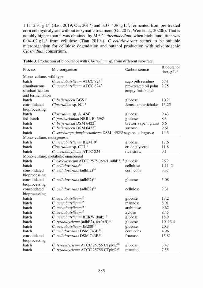
885
1.11–2.31 g L-1 (Bao, 2019; Ou, 2017) and 3.37–4.96 g L-1, fermented from pre-treated corn cob hydrolysate without enzymatic treatment (Ou 2017; Wen et al., 2020b). That is notably higher than it was obtained by ME C. thermocellum, when biobutanol titer was 0.04–02 g L-1 from cellulose (Tian 2019a). C. cellulovarans seems to be suitable microorganism for cellulose degradation and butanol production with solventogenic Clostridium consortium. Table 3. Production of biobutanol with Clostridium sp. from different substrate
Process Microorganism Carbon source Biobutanol titer, g L-1
Mono–culture, wild type batch C. acetobutylicum ATCC 8241 sago pith residues 5.41 simultaneous saccharification and fermentation
C. acetobutylicum ATCC 8242 pre–treated oil palm empty fruit bunch
2.75
batch C. beijerinckii BGS13 glucose 10.21 consolidated bioprocessing
Clostridium sp. NJ44 Jerusalem artichoke 13.25
batch Clostridium sp. A14245 glucose 9.43 fed–batch C. pasteurianum NRRL B–5986 glucose 8.3 batch C. beijerinckii DSM 64227 brewer’s spent grains 6.6 batch C. beijerinckii DSM 64227 sucrose 9.61 batch C. saccharoperbutylacetonicum DSM 149238 sugarcane bagasse 14.5 Mono–culture, mutagenesis batch C. acetobutylicum BKM199 glucose 17.6 batch Clostridium sp. CT710 crude glycerol 11.8 batch C. acetobutylicum ATTC 82411 rice straw 9.1 Mono–culture, metabolic engineered batch C. tyrobutyricum ATCC 2575 (Δcat1, adhE2)12 glucose 26.2 batch C. cellulovarans13 cellulose 1.11–2 consolidated bioprocessing
C. cellulovarans (adhE2)14 corn cobs 3.37
consolidated bioprocessing
C. cellulovarans (adhE2)14 glucose 3.08
consolidated bioprocessing
C. cellulovarans (adhE2)14 cellulose 2.31
batch C. acetobutylicum15 glucose 13.2 batch C. acetobutylicum15 mannose 8.91 batch C. acetobutylicum15 arabinose 9.62 batch C. acetobutylicum15 xylose 8.45 batch C. acetobutylicum BEKW (buk)16 glucose 18.9 batch C. tyrobutyricum (adhE2), (ctfAB)17 glucose 10–13.4 batch C. acetobutylicum JB20018 glucose 20.3 batch C. cellulovorans DSM 743B19 corn cobs 4.96 consolidated bioprocessing
C. cellulovorans DSM 743B19 fructose 15.81
batch C. tyrobutyricum ATCC 25755 CTpM220 glucose 3.47 batch C. tyrobutyricum ATCC 25755 CTpM220 mannitol 7.55
886
Table 3 continued
Co–culture consolidated bioprocessing
Phlebia sp. & C. saccharoperbutylacetonicum21
cellulose 3.2
consolidated bioprocessing
C. cellulovorans DSM 743B & C. beijerinckii 805222
extracted corn cob 11.5
consolidated bioprocessing
C. thermocellum NBRC 103400 & C. saccharoperbutylacetonium N1–423
rice straw 5.5
consolidated bioprocessing
Thermoanaerobacterium sp. M5 & C. acetobutylicum NJ424
xylan 8.34
consolidated bioprocessing
Thermoanaerobacterium sp. M5 & C. acetobutylicum NJ425
xylan 13.25
1(Linggang et al., 2013) 2(Ibrahim et al., 2015); 3(Zhang et al., 2018b); 4(Jiang et al., 2020a); 5(Youn et al., 2016); 6(Lipovsky et al., 2016); 7(Plaza et al., 2017); 8(Zetty–Arenas et al., 2019); 9(Jang et al., 2013); 10(Xin et al., 2017); 11(Tsai et al., 2020); 12(Zhang et al., 2018a); 13(Bao et al., 2019); 14(Ou et al., 2017);15(Raganati et al., 2016); 16(Jang et al., 2012); 17(Yu et al., 2015); 18(Xu et al., 2015); 19(Wen et al., 2020b); 20(Yu et al., 2012) 21(Tri & Kamei, 2020); 22(Wen et al., 2017); 23(Kiyoshi et al., 2015); 24(Jiang et al., 2018); 25(Jiang et al., 2020b).
Process optimization It should also be noted that with optimization in the medium composition,
fermentation conditions and process integrations, higher butanol productivity and titer can also be achieved (Yang et al., 2015). Supplementation of micronutrients and chemical compounds has been proven to be an effective (Xin et al., 2017). For example, supplementation of zinc and iron could enhance butanol titer production to 12.8 g L-1 compared to 4.5 g L-1 of butanol (Wu et al., 2016). Calcium carbonate had ability to enhance Clostridium tolerance to butanol by stabilizing cell membrane (Zhang et al., 2018b). In Raganati et al. (2016) study, the highest butanol titer was obtained from glucose, mannose, arabinose and xylose, when added 5 g L-1 and 10 g L-1 calcium carbonate in fermentation broth, respectively (Raganati et al., 2016). Yang et al., 2015 reported on synergistic effect of surfant PEG 4000 with xylanase on saccharification process efficiency, when used glucose and xylose yield increased from 53.2% to 86.0% and from 36.2% to 70.2%, respectively (Yang et al., 2015.) The influence of pH has been recognized as an important factor in determining the outcome of ABE fermentation, that the initiation of solvent production occurred only after the medium pH had decreased between 4.5 and 5.5 (Xin et al., 2017; Wen et al., 2020b). Generally, cultures at high pH values mainly produce acids, whereas in cultures maintained at a low pH, solvent production usually predominates. However, the pH range, over which solvent formation may occur, appears to vary quite widely depending on the particular strain and applied culture conditions (Xin et al., 2017).
In the last decade, to reduce the butanol toxicity during the fermentation process, various in situ solvent recovery techniques were successfully employed. These recovery techniques are integrated into the fermentation process for simultaneous production of solvents and its removal, which leads to increase in consumption of fermentable sugars by solventogenic Clostridium, prolongs the time of solventogenic phase and improves fermentation productivity and biobutanol yield (Jiménez-Bonilla & Wang, 2018; Azimi et al., 2019). Solvents removal methods, that have been studied and optimized all the time, are liquid–liquid extraction (Díaz & Tost, 2018), pervaporation (Zhu et al., 2020),

887
perstraction (Merlet et al., 2017), adsorption (Raganati et al., 2020), gas stripping (Naidoo et al., 2018), vacuum fermentation (Mariano et al., 2012) and other. These methods are admitted to have numerous advantages and disadvantages, that are reviewed in detail by Jiménez-Bonilla & Wang, (2018), Outram et al. (2017), Xue et al. (2017), Cai et al. (2018), Azimi et al. (2019).
Co-cultivation In recent years, co-cultivation of cellulolytic and solventogenic Clostridium, by
means of consolidated bioprocessing, has been actively studied (Jiang et al., 2018; Xin et al., 2019; Wen et al., 2020a). Consolidated bioprocessing (CBP), which combines hydrolytic enzymes production, cellulose and hemicellulose hydrolysis and sugars fermentation through ABE production, has a promising potential (Ou et al., 2017). The combination of cellulose saccharification and fermentation in CBP shows numerous advantages, including reduction of contamination risk, increased overall production yield and ability to reduce the reactor and enzyme costs (Vivek et al., 2019; Olguin–Maciel et al., 2020; Tri & Kamei, 2020). A co–culture system will also increase the substrate utilization rate when both bacteria can use the substrate to produce the target product (Du et al., 2020).
However, such consolidated bioprocessing implementation strongly depends on pH regulation (Wen et al., 2020b). Solventogenic Clostridium usually produce solvents after acidogenesis, when the culture pH decreases to 4.5–5.5 (Wen et al., 2020b), which, however, would inhibit growth and hamper cellulose degradation by cellulolytic Clostridium (Cheng et al., 2019). The change of pH during ABE fermentation by C. acetobutylicum could initiate the switch from acidogenesis to solventogenesis (Ou et al., 2017). Ou et al. (2017) study showed, that cell growth of the C. cellulovorans stopped when the culture pH dropped below 5.5, but high fermentation pH could reduce the production and selectivity of butanol. Therefore, the pH of 6.5 was identified as the optimal cellulosic fermentation pH in CBP using C. cellulovorans, resulting in 3.07 g L-1 butanol production. Higher pH value reduces titer 1.82 g L-1 and 1.33 g L-1 at pH of 7.0 and 7.5, respectively (Ou et al., 2017).
Recently, metabolic engineered strains with tolerance to butanol and low pH, or with higher butanol production capability, was studied towards Clostridium species, Clostridium sp. & bacteria, Clostridium sp. & fungi co-cultivation (Table 3) (Kiyoshi et al., 2015; Jiang et al., 2018; Wen et al., 2017; Jiang et al., 2020b; Tri & Kamei, 2020). In Jiang et al. (2018) study, thermophilic Thermoanaerobacterium sp. M5 was used, which possesses the indigenous capability of butanol production (1.17 g L-1). Optimization of co-cultivation process of mesofilic C. acetobutylicum NJ4 has increased butanol titer to 8.34 g L-1 from xylan (Jiang et al., 2018). In the other study, thermophilic C. thermocellum and mesophilic C. saccharoperbutylacetonicum was co–cultivated, resulting in 5.5 g L-1 of butanol synthesis from 40 g L-1 of cellulose, indicating the highest butanol biosynthesis from cellulose (Kiyoshi et al., 2015). High result was obtained from engineered C. cellulovorans with C. beijerinckii in consortium, where butanol titer was 11.5 g L-1 from alkali pre-treated corn cobs (Wen et al., 2017). Interesting results were obtained in the Tri & Kamei (2020) study, where the synergistic effect of the white–rot fungus Phlebia sp. KO77 and C. saccharoperbutylacetonicum co-culture was successful in terms of both butanol production and enhancement of

888
saccharification, resulting in 3.2 g L-1 production of butanol from cellulose (Tri & Kamei, 2020).
CONCLUSIONS
Although intense research and development have been made in the field of
production of biobutanol using a lignocellulosic substrate, it is necessary to select the best pre-treatment method for each type of lignocellulosic feedstock for efficient biomass conversion to sugars. The most promising feedstock from agro-industrial residues are rice straw, rice bagasse, soybean straw, sorgum straw, corn strover and spent mushroom substrate. Due to the high results of metabolic engineering strains, it is possible to use lignocellulosic biomass more efficiently. Cellulolytic C. cellulovorans shows sufficient enzyme activity for cellulose degradation to fermentable sugars, which allows cost–effective lignocellulose conversion for ABE fermentation with C. acetobutylicum, C. beijerinckii or C. saccharoperbutylacetonicum co–cultivation. Further research is needed on co-cultivation optimization of solventogenic with cellulolytic engineered Clostridium or with other potential microorganisms capable of degrading lignocellulosic biomass for technically feasible and simplified strategy to produce butanol from agro-industrial residues. A consolidated bioprocessing is well suited for these purpose, because it increases substrate utilization rate from lignocellulosic wastes through co-cultivation process. At the moment, there are not many studies on the production of butanol by co-cultivation of bacteria using CBP, and further research is needed.
REFERENCES
Amiri, H. & Karimi, K. 2018. Pretreatment and Hydrolysis of Lignocellulosic Wastes for Butanol
Production: Challenges and Perspectives. Bioresource Technology 270, pp. 66. Elsevier Ltd. doi: 10.1016/j.biortech.2018.08.117
Anandharaj, S.J., Gunasekaran, J., Udayakumar, G.P., Meganathan, Y. & Sivarajasekar, N. 2020. Biobutanol: Insight, Production and Challenges. Sustainable Development in Energy and Environment: Select Proceedings of ICSDEE 2019, Book, pp. 25–37. Singapore. https://books.google.co.in/books?id=k69tzQEACAAJ
Araújo, D.J.C., Machado, A.V. & Vilarinho, M.C.L.G. 2018. Availability and Suitability of Agroindustrial Residues as Feedstock for Cellulose–Based Materials: Brazil Case Study. Waste and Biomass Valorization 10(10), 2863–2878. doi.: 10.1007/s12649-018-0291-0
Arreola–Vargas, J., Razo–Flores, E., Celis, L.B. & Alatriste–Mondragón, F. 2014. Sequential Hydrolysis of Oat Straw and Hydrogen Production from Hydrolysates: Role of Hydrolysates Constituents. International Journal of Hydrogen Energy 40(34), 10756–10765. doi: 10.1016/j.ijhydene.2015.05.200
Ashani, P.N., Shafiei, M. & Karimi, K. 2020. Biobutanol Production from Municipal Solid Waste: Technical and Economic Analysis. Bioresource Technology 308(January), pp. 9. 123267. doi: 10.1016/j.biortech.2020
Azimi, H., Tezel, H. & Thibault, J. 2019. Optimization of the in Situ Recovery of Butanol from ABE Fermentation Broth via Membrane Pervaporation. Chemical Engineering Research and Design 150, 49–64. doi.: 10.1016/j.cherd.2019.07.012

889
Bao, T., Zhao, J., Li, J., Liu, X. & Yang, S.T. 2019. N-butanol and Ethanol Production from Cellulose by Clostridium Cellulovorans Overexpressing Heterologous Aldehyde/Alcohol Dehydrogenases. Bioresource Technology 285(April), pp. 9. doi: 10.1016/j.biortech.2019.121316
Birgen, C., Dürre, P., Preisig, H.A. & Wentzel, A. 2019. Butanol Production from Lignocellulosic Biomass: Revisiting Fermentation Performance Indicators with Exploratory Data Analysis. Biotechnology for Biofuels 12(1), 1–15. doi: 10.1186/s13068-019-1508-6
Cai, D., Hu, S., Qin, P. & Tan, T. 2018. Separation of Butanol, Acetone, and Ethanol. Emerging Areas in Bioengineering, 255–285. doi.: 10.1002/9783527803293.ch14
Chaudhary, I. & Verma, S.R. 2020. Ligninolysis: Roles of Microbes and Their Extracellular Enzymes. In Microbial Bioremediation & Biodegradation, Book. pp. 393–407. Singapore: Springer. doi: 10.1007/978-981-15-1812-6_14
Chen, H. & Wang, L. 2017. Enzymatic Hydrolysis of Pretreated Biomass. Technologies for Biochemical Conversion of Biomass, Book. Elsevier, pp. 65–99. doi: 10.1016/b978-0-12-802417-1.00004-1
Cheng, C., Bao, T. & Yang, S.T. 2019. Engineering Clostridium for Improved Solvent Production: Recent Progress and Perspective. Applied Microbiology and Biotechnology 103(14), 5549–5566. doi: 10.1007/s00253-019-09916-7
Cheng, C.L., Che, P.Y., Chen, B.Y., Lee, W.J., Lin, C.Y. & Chang, J.S. 2012. Biobutanol Production from Agricultural Waste by an Acclimated Mixed Bacterial Microflora. Applied Energy 100, 3–9. doi: 10.1016/j.apenergy.2012.05.042
Chong, T.Y., Law, M.C. & Chan, Y.S. 2020. The Potentials of Corn Waste Lignocellulosic Fibre as an Improved Reinforced Bioplastic Composites. Journal of Polymers and the Environment 29(2), 363–381. doi:10.1007/s10924-020-01888-4
Demirbaş, A. 2005. Thermochemical Conversion of Biomass to Liquid Products in the Aqueous Medium. Energy Sources 27(13), 1235–1243. doi: 10.1080/009083190519357
Deutscher, J. 2008. The Mechanisms of Carbon Catabolite Repression in Bacteria. Current Opinion in Microbiology 11(2), 87–93. doi: 10.1016/j.mib.2008.02.007
Díaz, V.H.G. & Tost, G.O. 2018. Economic Optimization of in Situ Extraction of Inhibitors in Acetone-Ethanol-Butanol (ABE) Fermentation from Lignocellulose. Process Biochemistry 70, 1–8. doi.: 10.1016/j.procbio.2018.04.014
Ding, T.Y., Hii, S.L. & Ong, L.G.A. 2012. Comparison of Pretreatment Strategies for Conversion of Coconut Husk Fiber to Fermentable Sugars. BioResources 7(2), 1540–1547. doi: 10.15376/biores.7.2.1540-1547
Dong, M., Wang, S., Xu, F., Wang, J., Yang, N., Li, Q., Chen, J. & Li, W. 2019. Pretreatment of Sweet Sorghum Straw and Its Enzymatic Digestion: Insight into the Structural Changes and Visualization of Hydrolysis Process. Biotechnology for Biofuels 12(1), 1–11. doi: 10.1186/s13068-019-1613-6
Du, Y., Zou, W., Zhang, K., Ye, G. & Yang, J. 2020. Advances and Applications of Clostridium Co-Culture Systems in Biotechnology. Frontiers in Microbiology 11(November), 1–22. doi: 10.3389/fmicb.2020.560223
Ezeji, T., Qureshi, N. & Blaschek, H.P. 2007. Butanol Production From Agricultural Residues: Impact of Degradation Products on Clostridium Beijerinckii Growth and Butanol Fermentation. Biotechnology and Bioengineering 97(6), 1460–1469. doi: 10.1002/bit.21373
FAO. 2019. Production/Yield Quantities of Mushrooms and Truffles in World. 2019. http://www.fao.org/faostat/en/#data/QC/visualize. Accesssed 08.02.2020.
Galbe, M. & Wallberg, O. 2019. Pretreatment for Biorefineries: A Review of Common Methods for Efficient Utilisation of Lignocellulosic Materials. Biotechnology for Biofuels 12(1), 1–26. doi: 10.1186/s13068-019-1634-1
890
Gao, Y., Zhang, M., Zhou, X., Guo, X., Lei, C., Li, W. & Lu, D. 2020. Effects of Carbon Ion Beam Irradiation on Butanol Tolerance and Production of Clostridium Acetobutylicum. Frontiers in Microbiology 11(December), 1–13. doi: 10.3389/fmicb.2020.602774
Godoy, M.G., Amorim, G.M., Barreto, M.S. & Freire, D.M.G. 2018. Agricultural Residues as Animal Feed: Protein Enrichment and Detoxification Using Solid–State Fermentation. Current Developments in Biotechnology and Bioengineering, Book. Elsevier. pp. 235–256. doi: 10.1016/b978-0-444-63990-5.00012-8
Guerfali, M., Ayadi, I., Belhassen, A., Gargouri, A. & Belghith, H. 2018. Single Cell Oil Production by Trichosporon Cutaneum and Lignocellulosic Residues Bioconversion for Biodiesel Synthesis. Process Safety and Environmental Protection, Book. 113. 292–304. Institution of Chemical Engineers. doi: 10.1016/j.psep.2017.11.002
Houfani, A.A., Anders, N., Spiess, A.C., Baldrian, P. & Benallaoua, S. 2020. Insights from Enzymatic Degradation of Cellulose and Hemicellulose to Fermentable Sugars. Biomass and Bioenergy 134(February), pp. 13. doi: 10.1016/j.biombioe.2020.105481
Huzir, N.M., Aziz, M.M.A., Ismail, S.B., Abdullah, B., Mahmood, N.A.N., Umor, N.A. & Syed Muhammad, S.A.F. ad. 2018. Agro-Industrial Waste to Biobutanol Production: Eco-Friendly Biofuels for next Generation. Renewable and Sustainable Energy Reviews, Book. 476–485. Elsevier. doi: 10.1016/j.rser.2018.06.036
Ibrahim, M.F., Abd-Aziz, S., Yusoff, M.E.M., Phang, L.Y. & Hassan, M.A. 2015. Simultaneous Enzymatic Saccharification and ABE Fermentation Using Pretreated Oil Palm Empty Fruit Bunch as Substrate to Produce Butanol and Hydrogen as Biofuel. Renewable Energy 77, 447–455. doi: 10.1016/j.renene.2014.12.047
Jang, Y.S., Lee, J.Y., Lee, J., Park, J.H., Im, J.A., Eom, M.H., Lee, J., Lee, S.H., Song, H., Cho, J.H., Seung, D.Y.,& Lee, S.Y. 2012. Enhanced Butanol Production Obtained by Reinforcing the Direct Butanol-Forming Route in Clostridium Acetobutylicum. MBio 3(5), pp. 9. doi: 10.1128/mBio.00314-12
Jang, Y.S., Malaviya, A. & Lee, S.Y. 2013. Acetone-Butanol-Ethanol Production with High Productivity Using Clostridium Acetobutylicum BKM19. Biotechnology and Bioengineering 110(6), 1646–1653. doi: 10.1002/bit.24843
Jiang, Y., Guo, D., Lu, J., Dürre, P., Dong, W., Yan, W., Zhang, W., Ma, J., Jiang, M. & Xin, F. 2018. Consolidated Bioprocessing of Butanol Production from Xylan by a Thermophilic and Butanologenic Thermoanaerobacterium Sp. M5. Biotechnology for Biofuels 11(1), 1–14. doi: 10.1186/s13068-018-1092-1
Jiang, Y., Lv, Y., Michenfelder, R., Chen, T., Wu, R., Xin, F. & Jiang, M. 2020a. Clostridium Sp. Strain NJ4: A Promising Solventogenic Strain for Butanol Production from Jerusalem Artichoke through Consolidated Bioprocessin. Energy & Fuels 34(3), 3406–3411. doi: 10.1021/acs.energyfuels.0c00123
Jiang, Y., Lv, Y., Wu, R., Lu, J., Dong, W., Zhou, J., Zhang, W., Xin, F. & Jiang, M. 2020b. Consolidated Bioprocessing Performance of a Two-Species Microbial Consortium for Butanol Production from Lignocellulosic Biomass. Biotechnology and Bioengineering 117(10), 2985–2995. doi: /10.1002/bit.27464
Jiang, Y., Lv, Y., Wu, R., Sui, Y., Chen, C., Xin, F., Zhou, J., Dong, W. & Jiang, M. 2019. Current Status and Perspectives on Biobutanol Production Using Lignocellulosic Feedstocks. Bioresource Technology Reports 7(March), pp. 6. doi: 10.1016/j.biteb.2019.100245
Jiménez-Bonilla, P. & Wang, Y. 2018. In Situ Biobutanol Recovery from Clostridial Fermentations: A Critical Review. Critical Reviews in Biotechnology 38(3), 469–482. doi: 10.1080/07388551.2017.1376308
Kim, S. 2018. Evaluation of Alkali-Pretreated Soybean Straw for Lignocellulosic Bioethanol Production. International Journal of Polymer Science 2018, pp. 7. doi: 10.1155/2018/5241748
891
Kiyoshi, K., Furukawa, M., Seyama, T., Kadokura, T., Nakazato, A. & Nakayama, S. 2015. Butanol Production from Alkali-Pretreated Rice Straw by Co-Culture of Clostridium Thermocellum and Clostridium Saccharoperbutylacetonicum. Bioresource Technology 186, 325–328. doi: 10.1016/j.biortech.2015.03.061
Kolesinska, B., Fraczyk, J., Binczarski, M., Modelska, M., Berlowska, J., Dziugan, P., Antolak, H., Kaminski, Z.J., Witonska, I.A. & Kregiel, D. 2019. Butanol Synthesis Routes for Biofuel Production: Trends and Perspectives. Materials 12(3), pp. 22. doi: 10.3390/ma12030350
Kumar, M. & Gayen, K. 2011. Developments in Biobutanol Production: New Insights. Applied Energy 88(6), 1999–2012. doi.org/10.1016/j.apenergy.2010.12.055
Kumar, S., Gujjala, L.K.S. & Banerjee, R. 2017. Simultaneous Pretreatment and Saccharification of Bamboo for Biobutanol Production. Industrial Crops and Products 101, 21–28. doi: 10.1016/j.indcrop.2017.02.028
Lee, J.E., Seo, E., Kweon, D.H., Park, K.M. & Jin, Y.S. 2009. Fermentation of Rice Bran and Defatted Rice Bran for Butanol Production Using Clostridium Beijerinckii NCIMB 8052. Journal of Microbiology and Biotechnology 19(5), 482–490. doi: 10.14014/jmb.0804.275
Li, Y., Tang, W., Chen, Y., Liu, J. & Lee, C. fon F. 2019. Potential of Acetone-Butanol-Ethanol (ABE) as a Biofuel. Fuel. 242, 637–686. doi: 10.1016/j.fuel.2019.01.063
Linggang, S., Phang, L.Y., Wasoh, H. & Abd-Aziz, S. 2013. Acetone-Butanol-Ethanol Production by Clostridium Acetobutylicum ATCC 824 Using Sago Pith Residues Hydrolysate. Bioenergy Research 6(1), 321–328. doi: 10.1007/s12155-012-9260-9.
Lipovsky, J., Patakova, P., Paulova, L., Pokorny, T., Rychtera, M. & Melzoch, K. 2016. Butanol Production by Clostridium Pasteurianum NRRL B-598 in Continuous Culture Compared to Batch and Fed–Batch Systems. Fuel Processing Technology 144, 139–144. doi: 10.1016/j.fuproc.2015.12.020
Lv, Y., Jiang, Y., Peng, W., Fang, Y., Dong, W., Zhou, J., Zhang, W., Xin, F. & Jiang, M. 2021. Genetic Manipulation of Non–Solvent–Producing Microbial Species for Effective Butanol Production. Biofuels, Bioproducts and Biorefining 15(1), 119–130. doi: 10.1002/bbb.2152
Ma, S., Wang, H., Wang, Y., Bu, H. & Bai, J. 2011. Bio-Hydrogen Production from Cornstalk Wastes by Orthogonal Design Method. Renewable Energy 36(2), 709–713. doi: 10.1016/j.renene.2010.08.019
Madeira, J.V., Contesini, F.J., Calzado, F., Rubio, M.V., Zubieta, M.P., Lopes, D.B. & Melo, R.R. de. 2017. Agro-Industrial Residues and Microbial Enzymes: An Overview on the Eco–Friendly Bioconversion into High Value–Added Products. Biotechnology of Microbial Enzymes: Production, Biocatalysis and Industrial Applications, Book, 475–511, Elsevier doi: 10.1016/B978-0-12-803725-6.00018-2
Mariano, A.P., Qureshi, N., Maciel Filho, R. & Ezeji, T.C. 2012. Assessment of in Situ Butanol Recovery by Vacuum during Acetone Butanol Ethanol (ABE) Fermentation. Journal of Chemical Technology and Biotechnology 87(3), 334–340. doi.: 10.1002/jctb.2717
Merlet, G., Uribe, F., Aravena, C., Rodríguez, M., Cabezas, R., Quijada-Maldonado, E. & Romero, J. 2017. Separation of Fermentation Products from ABE Mixtures by Perstraction Using Hydrophobic Ionic Liquids as Extractants. Journal of Membrane Science 537(May), 337–343. doi.: 10.1016/j.memsci.2017.05.045
Naidoo, M., Tai, S.L. & Harrison, S.T.L. 2018. Energy Requirements for the In-Situ Recovery of Biobutanol via Gas Stripping. Biochemical Engineering Journal 139, 74–84. doi: 10.1016/j.bej.2018.07.022
Narayanasamy, S., Chan, K.L., Cai, H., Hilman, A., Abdul, B., Tay, B.K. & Miao, H. 2019. Biobutanol Production from Sugarcane Bagasse by Clostridium Beijerinckii Strains. Biotechnology and Applied Biochemistry 67(5), 732–737. doi: 10.1002/bab.1865
892
Nguyen, T.A.D., Kim, K.R., Han, S.J., Cho, H.Y., Kim, J.W., Park, S.M., Park, J.C. & Sim, S.J. 2010. Pretreatment of Rice Straw with Ammonia and Ionic Liquid for Lignocellulose Conversion to Fermentable Sugars. Bioresource Technology 101(19), 7432–7438. doi: 10.1016/j.biortech.2010.04.053
Noomtim, P. & Cheirsilp, B. 2011. Production of Butanol from Palm Empty Fruit Bunches Hydrolyzate by Clostridium Acetobutylicum. Energy Procedia 9, 140–146. doi: 10.1016/j.egypro.2011.09.015
Olguin–Maciel, E., Singh, A., Chable–Villacis, R., Tapia–Tussell, R. & Ruiz, H.A. 2020. Consolidated Bioprocessing, an Innovative Strategy towards Sustainability for Biofuels Production from Crop Residues: An Overview. Agronomy 10(11), pp. 20. doi: 10.3390/agronomy10111834
Ou, J., Xu, N., Ernst, P., Ma, C., Bush, M., Goh, K.Y., Zhao, J., Zhou, L., Yang, S.T. & Liu, X. 2017. Process Engineering of Cellulosic N-butanol Production from Corn–Based Biomass Using Clostridium Cellulovorans. Process Biochemistry 62(May), 144–150. doi: /10.1016/j.procbio.2017.07.009
Outram, V., Lalander, C.A., Lee, J.G.M., Davies, E.T. & Harvey, A.P. 2017. Applied in Situ Product Recovery in ABE Fermentation. Biotechnology Progress 33(3), 563–579. doi: 10.1002/btpr.2446
Pérez–Rangel, M., Quiroz–Figueroa, F.R., González–Castañeda, J. & Valdez–Vazquez, I. 2015. Microscopic Analysis of Wheat Straw Cell Wall Degradation by Microbial Consortia for Hydrogen Production. International Journal of Hydrogen Energy 40(1), 151–160. doi: 10.1016/j.ijhydene.2014.10.050
Plaza, P.E., Gallego–Morales, L.J., Peñuela–Vásquez, M., Lucas, S., García–Cubero, M.T. & Coca, M. 2017. Biobutanol Production from Brewer’s Spent Grain Hydrolysates by Clostridium Beijerinckii. Bioresource Technology 244(July), 166–174. doi: 10.1016/j.biortech.2017.07.139
Procentese, A., Raganati, F., Olivieri, G., Russo, M.E., la Feld, M. de, & Marzocchella, A. 2017. Renewable Feedstocks for Biobutanol Production by Fermentation. New Biotechnology 39, 135–140. doi: 10.1016/j.nbt.2016.10.010
Qureshi, N., Saha, B.C., Dien, B., Hector, R.E. & Cotta, M.A. 2010. Production of Butanol (a Biofuel) from Agricultural Residues: Part I - Use of Barley Straw Hydrolysate. Biomass and Bioenergy 34(4), 559–565. doi: 10.1016/j.biombioe.2009.12.024
Qureshi, N., Saha, B.C., Hector, R.E., Hughes, S.R. & Cotta, M.A. 2008. Butanol Production from Wheat Straw by Simultaneous Saccharification and Fermentation Using Clostridium Beijerinckii: Part I-Batch Fermentation. Biomass and Bioenergy 32(2), 168–175. doi: 10.1016/j.biombioe.2007.07.004
Raganati, F., Procentese, A., Olivieri, G., Russo, M.E. & Marzocchella, A. 2016. Butanol Production by Fermentation of Fruit Residues. Chemical Engineering Transactions 49(November), 229–234. doi: 10.3303/CET1649039
Raganati, F., Procentese, A., Olivieri, G., Russo, M.E., Salatino, P. & Marzocchella, A. 2020. Bio-Butanol Recovery by Adsorption/Desorption Processes. Separation and Purification Technology 235(September), 116145. doi.: 10.1016/j.seppur.2019.116145
Rajavat, A.S., Rai, S., Pandiyan, K., Kushwaha, P., Choudhary, P., Kumar, M., Chakdar, H., … & Saxena, A.K. 2019. Sustainable Use of the Spent Mushroom Substrate of Pleurotus Florida for Production of Lignocellulolytic Enzymes. Journal of Basic Microbiology. 60(2), 173–184. doi: 10.1002/jobm.201900382
Rathour, R.K., Ahuja, V., Bhatia, R.K. & Bhatt, A.K. 2018. Biobutanol: New Era of Biofuels. International Journal of Energy Research. 42(15), 4532–4545. doi: 10.1002/er.4180
Ravindran, R., Hassan, S.S., Williams, G.A. & Jaiswal, A.K. 2018. A Review on Bioconversion of Agro-Industrial Wastes to Industrially Important Enzymes. Bioengineering 5(4), 1–20. doi: 10.3390/bioengineering5040093
893
Ravindran, R. & Jaiswal, A.K. 2016. A Comprehensive Review on Pre-treatment Strategy for Lignocellulosic Food Industry Waste: Challenges and Opportunities. Bioresource Technology. 199, 92–102. doi: 10.1016/j.biortech.2015.07.106
Rezaei, M., Amiri, H., Shafiei M. 2021. Aqueous pretreatment of triticale straw for integrated production of hemicellulosic methane and cellulosic butanol. Renewable Energy 171(6), 971–980. doi.: 10.1016/j.renene.2021.02.159
Saha, B.C., Qureshi, N., Kennedy, G.J. & Cotta, M.A. 2016. Biological Pretreatment of Corn Stover with White-Rot Fungus for Improved Enzymatic Hydrolysis. International Biodeterioration and Biodegradation 109, 29–35. doi: 10.1016/j.ibiod.2015.12.020
Saini, J.K., Saini, R. & Tewari, L. 2015. Lignocellulosic Agriculture Wastes as Biomass Feedstocks for Second Generation Bioethanol Production: Concepts and Recent Developments. 3 Biotech 5(4), 337–353. doi: 10.1007/s13205-014-0246-5
Shirkavand, E., Baroutian, S., Gapes, D.J. & Young, B.R. 2016. Combination of Fungal and Physicochemical Processes for Lignocellulosic Biomass Pretreatment – A Review. Renewable and Sustainable Energy Reviews 54, 217–234. doi: 10.1016/j.rser.2015.10.003
Sindhu, R., Binod, P. & Pandey, A. 2016. Biological Pretreatment of Lignocellulosic Biomass - An Overview. Bioresource Technology. 199, 76–82. doi: 10.1016/j.biortech.2015.08.030
Szczerbowski, D., Pitarelo, A.P., Zandoná Filho, A. & Ramos, L.P. 2014. Sugarcane Biomass for Biorefineries: Comparative Composition of Carbohydrate and Non-Carbohydrate Components of Bagasse and Straw. Carbohydrate Polymers 114, 95–101. doi: 10.1016/j.carbpol.2014.07.052
Tao, L., Tan, E.C.D., McCormick, R., Zhang, M., Aden, A., He, X. & Zigler, B.T. 2013. Perspective: Jatropha Cultivation in Southern India: Assessing Farmers’ Experiences. Biofuels, Bioproducts and Biorefining 6(3), 246–256. doi.: 10.1002/bbb
Tian, L., Cervenka, N.D., Low, A.M., Olsin, D.G. & Lynd, L.R. 2019a. A mutation in the Adhe alcohol dehydrogenase of Clostridium thermocellum increases tolerance to several primary alcohols, including isobutanol, n-butanol and ethanol. Scientific Reports 9(1), 1–7. doi: 10.1038/s41598-018-37979-5
Tian, L., Conway, P.M., Cervenka, N.D., Cui, J., Maloney, M., Olson, D.G. & Lynd, L.R. 2019b. Metabolic Engineering of Clostridium Thermocellum for N-Butanol Production from Cellulose. Biotechnology for Biofuels 12(1), 1–13. doi: 10.1186/s13068-019-1524-6
Tri, C.L. & Kamei, I. 2020. Butanol Production from Cellulosic Material by Anaerobic Co-Culture of White-Rot Fungus Phlebia and Bacterium Clostridium in Consolidated Bioprocessing. Bioresource Technology 305(February), pp. 6. doi: 10.1016/j.biortech.2020.123065
Tsai, T.Y., Lo, Y.C., Dong, C. Di, Nagarajan, D., Chang, J.S. & Lee, D.J. 2020. Biobutanol Production from Lignocellulosic Biomass Using Immobilized Clostridium Acetobutylicum. Applied Energy 277(November), pp. 10. doi: 10.1016/j.apenergy.2020.115531
Umagiliyage, A.L., Choudhary, R., Liang, Y., Haddock, J. & Watson, D.G. 2015. Laboratory Scale Optimization of Alkali Pretreatment for Improving Enzymatic Hydrolysis of Sweet Sorghum Bagasse. Industrial Crops and Products 74, 977–986. doi: 10.1016/j.indcrop.2015.05.044
Vivek, N., Nair, L.M., Mohan, B., Nair, S.C., Sindhu, R., Pandey, A., Shurpali, N. & Binod, P. 2019. Bio-Butanol Production from Rice Straw – Recent Trends, Possibilities, and Challenges. Bioresource Technology Reports 7(September), pp. 14. doi: 10.1016/j.biteb.2019.100224
Wang, J., Yang, X., Chen, C.C. & Yang, S.T. 2014. Engineering Clostridia for Butanol Production from Biorenewable Resources: From Cells to Process Integration. Current Opinion in Chemical Engineering 6, 43–54. doi: 10.1016/j.coche.2014.09.003
894
Wen, Z., Ledesma–Amaro, R., Lu, M., Jin, M. & Yang, S. 2020b. Metabolic Engineering of Clostridium Cellulovorans to Improve Butanol Production by Consolidated Bioprocessing. ACS Synthetic Biology 9(2), 304–315. doi: 10.1021/acssynbio.9b00331
Wen, Z., Minton, N.P., Zhang, Y., Li, Q., Liu, J., Jiang, Y. & Yang, S. 2017. Enhanced Solvent Production by Metabolic Engineering of a Twin–Clostridial Consortium. Metabolic Engineering 39, 38–48. doi: 10.1016/j.ymben.2016.10.013
Wen, Z., Ledesma–Amaro, R., Lu, M., Jiang, Y., Gao, S., Jin, M. & Yang, S. 2020a. Combined evolutionary engineering and genetic manipulation improve low pH tolerance and butanol production in a synthetic microbial Clostridium community. Biotechnology and Bioengineering 117(7), 2008–2022. doi: 10.1002/bit.27333
Wen, Z., Wu, M., Lin, Y., Yang, L., Lin, J. & Cen, P. 2014. Artificial Symbiosis for Acetone-Butanol-Ethanol (ABE) Fermentation from Alkali Extracted Deshelled Corn Cobs by Co-Culture of Clostridium Beijerinckii and Clostridium Cellulovorans. Microbial Cell Factories. 13(1), 1–11. doi: 10.1186/s12934-014-0092-5
Wu, Y.D., Xue, C., Chen, L.J. & Bai, F.W. 2016. Impact of Zinc Supplementation on the Improved Fructose/Xylose Utilization and Butanol Production during Acetone-Butanol-Ethanol Fermentation. Journal of Bioscience and Bioengineering 121(1), 66–72. doi:10.1016/j.jbiosc.2015.05.003
Xin, F., Chen, T., Jiang, Y., Lu, J., Dong, W., Zhang, W., Ma, J., Zhang, M. & Jiang, M. 2017. Enhanced Biobutanol Production with High Yield from Crude Glycerol by Acetone Uncoupled Clostridium Sp. Strain CT7. Bioresource Technology 244, 575–581. doi: 10.1016/j.biortech.2017.08.002
Xin, F., Dong, W., Zhang, W., Ma, J. & Jiang, M. 2018. Biobutanol Production from Crystalline Cellulose through Consolidated Bioprocessing. Trends in Biotechnology 37(2), 167–180. doi: 10.1016/j.tibtech.2018.08.007
Xu, M., Zhao, J., Yu, L., Tang, I.C., Xue, C. & Yang, S.T. 2015. Engineering Clostridium Acetobutylicum with a Histidine Kinase Knockout for Enhanced N-butanol Tolerance and Production. Applied Microbiology and Biotechnology 99(2), 1011–1122. doi: 10.1007/s00253-014-6249-7
Xue, C., Zhao, J., Chen, L., Yang, S.T. & Bai, F. 2017. Recent Advances and State-of-the-Art Strategies in Strain and Process Engineering for Biobutanol Production by Clostridium Acetobutylicum. Biotechnology Advances 35(2), 310–322. doi: 10.1016/j.biotechadv.2017.01.007
Xue, C. & Cheng, C. 2019. Butanol Production by Clostridium. Advances in Bioenergy, Book. 1st ed. 4, 35–77. Elsevier Inc. doi:10.1016/bs.aibe.2018.12.001
Yang, X., Xu, M. & Yang, S.T. 2015. Metabolic and Process Engineering of Clostridium Cellulovorans for Biofuel Production from Cellulose. Metabolic Engineering 32, 39–48. doi: 10.1016/j.ymben.2015.09.001
Yoav, S., Barak, Y., Shamshoum, M., Borovok, I., Lamed, R., Dassa, B., Hadar, Y., Morag, E. & Bayer, E.A. 2017. How Does Cellulosome Composition Influence Deconstruction of Lignocellulosic Substrates in Clostridium (Ruminiclostridium) Thermocellum DSM 1313? Biotechnology for Biofuels 10(1), 1–16. doi: 10.1186/s13068-017-0909-7
Youn, S.H., Lee, K.M., Kim, K.Y., Lee, S.M., Woo, H.M. & Um, Y. 2016. Effective Isopropanol–Butanol (IB) Fermentation with High Butanol Content Using a Newly Isolated Clostridium Sp. A1424. Biotechnology for Biofuels 9(1), 1–15. doi: 10.1186/s13068-016-0650-7
Yu, L., Zhao, J., Xu, M., Dong, J., Varghese, S., Yu, M., Tang, I.C. & Yang, S.T. 2015. Metabolic Engineering of Clostridium Tyrobutyricum for N-butanol Production: Effects of CoA Transferase. Applied Microbiology and Biotechnology 99(11), 4917–4930. doi: 10.1007/s00253-015-6566-5
895
Yu, M., Du, Y., Jiang, W., Chang, W.L., Yang, S.T. & Tang, I.C. 2012. Effects of Different Replicons in Conjugative Plasmids on Transformation Efficiency, Plasmid Stability, Gene Expression and n-Butanol Biosynthesis in Clostridium Tyrobutyricum. Applied Microbiology and Biotechnology 93(2), 881–889. doi: 10.1007/s00253-011-3736-y
Yue, Y., Han, J., Han, G., Aita, G.M. & Wu, Q. 2015. Cellulose Fibers Isolated from Energycane Bagasse Using Alkaline and Sodium Chlorite Treatments: Structural, Chemical and Thermal Properties. Industrial Crops and Products 76, 355–363. doi: 10.1016/j.indcrop.2015.07.006
Zetty–Arenas, A.M., Alves, R.F., Portela, C.A.F., Mariano, A.P., Basso, T.O., Tovar, L.P., Maciel Filho, R. & Freitas, S. 2019. Towards Enhanced N-butanol Production from Sugarcane Bagasse Hemicellulosic Hydrolysate: Strain Screening, and the Effects of Sugar Concentration and Butanol Tolerance. Biomass and Bioenergy 126(2019), 190–198. doi: 10.1016/j.biombioe.2019.05.011
Zhang, C., Li, T. & He, J. 2018b. Characterization and Genome Analysis of a Butanol-Isopropanol–Producing Clostridium Beijerinckii Strain BGS1 06 Biological Sciences 0605 Microbiology 06 Biological Sciences 0604 Genetics. Biotechnology for Biofuels 11(1), 1–11. doi: 10.1186/s13068-018-1274-x
Zhang, J., Zong, W., Hong, W., Zhang, Z.T. & Wang, Y. 2018a. Exploiting Endogenous CRISPR–Cas System for Multiplex Genome Editing in Clostridium Tyrobutyricum and Engineer the Strain for High–Level Butanol Production. Metabolic Engineering 47(March), 49–59. doi: 10.1016/j.ymben.2018.03.007
Zhu, Y., Chang, Y., Guan, J., Shanguan, G. & Xin, F. 2016. Butanol Production from Organosolv Treated Spent Mushroom Substrate Integrated with in Situ Biodiesel Extraction. Renewable Energy 96, 656–661. doi: 10.1016/j.renene.2016.04.048
Zhu, H., Li, X., Pan, Y., Liu, G., Wu, H., Jiang, M. & Jin, W. 2020. Fluorinated PDMS Membrane with Anti-Biofouling Property for in-Situ Biobutanol Recovery from Fermentation-Pervaporation Coupled Process. Journal of Membrane Science 609(May), 118225. doi.: 10.1016/j.memsci.2020.118225
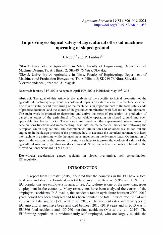
896
Agronomy Research 19(S1), 896–909, 2021 https://doi.org/10.15159/AR.21.088
Improving ecological safety of agricultural off-road machines operating of sloped ground
J. Rédl1,* and P. Findura2
1Slovak University of Agriculture in Nitra, Faculty of Engineering, Department of Machine Design, Tr. A. Hlinku 2, SK949 76 Nitra, Slovakia 2Slovak University of Agriculture in Nitra, Faculty of Engineering, Department of Machines and Production Biosystems, Tr. A. Hlinku 2, SK949 76 Nitra, Slovakia *Correspondence: [email protected] Received: January 31st, 2021; Accepted: April 10th, 2021; Published: May 19th, 2021 Abstract. The goal of this article is the analysis of the specific technical properties of the agricultural machinery to prevent the ecological impacts on nature in case of a machine accident. The loss of stability and overturning of the machine is an important part of the farm safety code of practice document and the source of the ground contamination with fuel and no-bio lubricants. The main work is oriented to determine and derive the steps of prevention or prediction of dangerous states of the agricultural off-road vehicle operating on sloped ground and even applicable for heavy trucks. These steps are based on the experimental measurement of accelerations functions and implementing these into the mathematical model and following the European Union Regulations. The recommended simulation and obtained results can tell the engineers in the design process of the prototype how to accurate the technical parameters to keep the machine in a safe state while the machine is under acting the dynamic loads. Optimization of specific dimensions in the process of design can help to improve the ecological safety of the agricultural machines operating on sloped ground. Some theoretical methods are based on the Slovak National Standard STN 47 0170. Key words: acceleration gauge, accident on slope, overturning, soil contamination, EU regulation.
INTRODUCTION A report from Eurostat (2019) declared that the countries in the EU have a total
land area and share of farmland in total land area in 2016 year 39.9% and 4.1% from EU populations are employers in agriculture. Agriculture is one of the most dangerous employment in the economy. Many researchers have been analyzed the causes of the employer’s accidents. In Slovakia, the accidents rate in agriculture between 2000–2012 years period has been analyzed and has been counted the total injuries rate 12,874 and 90 was the fatal injuries (Váliková et al., 2013). The accident rates and their types in EU agricultural area have been analyzed between 2013–2019 years and in 2013 was in EU 366 fatal accidents and 135,260 non-fatal accidents (Merisalu et al., 2019). The EU farming population is predominantly self-employed, who are largely outside the

897
scope of EU occupational safety and health (OSH) legislation. Utilizing effective communications approaches to transmit clear messages is a possible way of motivating farmer OSH adoption. The Public Health Model (PHM) of accident causation conceptualizes an accident as occurring due to multiple interacting physical and human factors while the Social-Ecologic Framework enhances the PHM by defining various levels of the social environment, which are influential on persons’ OSH actions (Mc Namara et al., 2019). The national bodies for control of employer’s accidents record all occurred cases. The National Labour Inspectorate in Slovakia in the 2010–2019 years period recorded 23 deadly cases, 9 hard injuries, and 2 soft injuries, and these data were processed by the Statistical Office of the Slovak Republic (2019). As a representative unit of EU we were chosen the analysis of the Estonian accident provided by Enn & Merisalu (2019). Their study aimed to analyze the dynamics of work accidents (WA) incidence by severity, gender, and lost workdays in Estonian agriculture in 2008–2017. They found in total 13 fatal work accidents have occurred, which accounts 0.8% of all the WAs (n = 1,696). The published results from the analyses about accident rates, causes, and levels of injuries were analyzed very well, but the analyses do not tell us the detailed scenes and backgrounds of accidents or possibly raised environmental damages. Several accidents arise as a consequence of agricultural machine overturns. These machines operating on sloped ground or operating on rough terrain in forestry. Wide analysis about the causes of tractors overturns and accidents from past to 2010 year has been done by Abubakar et al. (2010). A similar analysis about fatal accidents due to tractors' overturns has been published by Antunes et al. (2018). Garland (2018) published that, the harvesting machines are now being used on slopes over 100 percent (i.e. greater than 45 degrees) in varying site conditions. This should also be considered in accident reporting and analysis. As defined by Visser & Stampfer (2015) the dynamic factor reduces the slope limit where a rollover can occur. As such, loss of traction can become a significant factor and it can be deduced that most rollover accidents result from an initial loss of traction. It results in an uncontrolled gain in momentum and if followed by hitting an object, such as a stump, or a change in terrain slope, can readily result in a rollover. The basic physics with regard to retaining traction on a slope is that the gravity force pulling the machine down should not exceed the traction force that the machine can develop on the ground. Another study published by Issa et al. (2019) analyzed the influence of agricultural engineering development on the occurrences of fatal accidents in agriculture-related to farm machinery in USA. The mentioned review of accidents shows, that the fatal and other injuries of employers are the cause of the agricultural machines accidents, especially tractors overturn. To prevent machinery accidents the wide research of the operating stability is in progress. Nowadays is running intensive research, which evidence are several published research papers. The serious research has been published by Bulgakov et al. (2016), where the aim of their study was to the elaboration of the theoretical basis for the process of vertical oscillation of the combined plowing and chopping tractor-implement unit and the validation of its dynamic stability in the longitudinal and vertical plane. The research has been performed with the use of the methods of designing the analytical mathematical models of functioning of agricultural machines and machine assembly units based on the theory of tractor, the vibration theory, the theory of automatic control and dynamic stability, and the methods of computer program construction and PC-assisted numerical computation. The next research of Bulgakov et al. (2017) has been aimed on substantiate the set-up and
898
parameters of the plowing unit with a front-mounted plow basing on the theoretical investigation of the stability of its motion in the horizontal plane. Another research published by Bulgakov et al. (2019) dealt by the investigation is a detailed examination of criteria for the stability assessment of a mechanical system used in agriculture, enabling their wide application to study the performance of the system in the case when it is affected by random forces that were not taken into account in the original model. The considered calculation methods and examples of their application make it possible to evaluate the performance of complex dynamic systems without numerical solution of complicated differential equations of the movement in the presence of external disturbances.
To prevent the possible accidental cases the European Union Commission released regulation No 167/20133, where says: ‘point 11: To ensure a high level of functional safety, occupational safety, and environmental protection, the technical requirements and environmental standards applicable to vehicles, systems, components, and separate technical units concerning type-approval should be harmonized. Point 12: It is appropriate to establish the principle that vehicles must be designed, constructed, and assembled to minimize the risk of injury to the vehicle occupants and other road users.’ For that purpose, manufacturers must ensure that vehicles comply with the relevant requirements set out in this Regulation. Those provisions should include, but not be limited to, requirements relating to vehicle structural integrity, systems to aid the driver’s control of the vehicle, systems to provide the driver with visibility and information on the state of the vehicle and the surrounding area, vehicle lighting systems, vehicle occupant protection systems, the vehicle exterior and accessories, vehicle masses and dimensions and vehicle tires. In Chapter, I, Article 3 ‘Definitions’, point 24, defines: ‘functional safety’ means the absence of unacceptable risk of physical injury or damage to the health of persons or property owing to hazards caused by mal-functional behavior of mechanical, hydraulic, pneumatic, electrical or electronic systems, components or separate technical units. The meaning of this regulation justifies the research of static and dynamic stability of agricultural off-road vehicles.
The important field of reduction of the possibilities of agricultural machinery accidents and consecutive ecological impacts is standardization. The International Organization for Standardization (ISO) released a few standards and technical reports, which deal with the safety of machinery and risk assessment. The ISO 12100 (2010) deals with the determination of the limits of machinery. Risk assessment begins with the determination of the limits of the machinery, taking into account all the phases of the machinery life. This means that the characteristics and performances of the machine or a series of machines in an integrated process, and the related people, environment, and products, should be identified in terms of the limits of machinery. Recommendations for machine manufacturers say about the inherently safe design measures. Machines shall be designed so that they have sufficient stability to allow them to be used safely in their specified conditions of use. Factors to be taken into account include:
the geometry of the base, the weight distribution, including loading, the dynamic forces due to movements of parts of the machine, of the machine
itself, or of elements held by the machine which can result in an overturning moment, vibration, oscillations of the center of gravity.
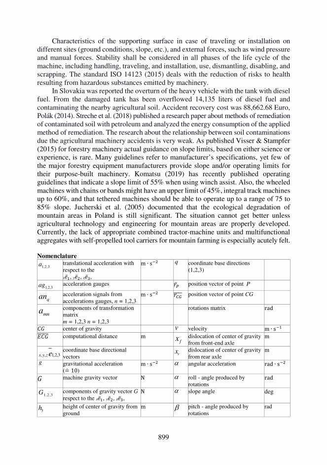
899
Characteristics of the supporting surface in case of traveling or installation on different sites (ground conditions, slope, etc.), and external forces, such as wind pressure and manual forces. Stability shall be considered in all phases of the life cycle of the machine, including handling, traveling, and installation, use, dismantling, disabling, and scrapping. The standard ISO 14123 (2015) deals with the reduction of risks to health resulting from hazardous substances emitted by machinery.
In Slovakia was reported the overturn of the heavy vehicle with the tank with diesel fuel. From the damaged tank has been overflowed 14,135 liters of diesel fuel and contaminating the nearby agricultural soil. Accident recovery cost was 88,662.68 Euro, Polák (2014). Streche et al. (2018) published a research paper about methods of remediation of contaminated soil with petroleum and analyzed the energy consumption of the applied method of remediation. The research about the relationship between soil contaminations due the agricultural machinery accidents is very weak. As published Visser & Stampfer (2015) for forestry machinery actual guidance on slope limits, based on either science or experience, is rare. Many guidelines refer to manufacturer’s specifications, yet few of the major forestry equipment manufacturers provide slope and/or operating limits for their purpose-built machinery. Komatsu (2019) has recently published operating guidelines that indicate a slope limit of 55% when using winch assist. Also, the wheeled machines with chains or bands might have an upper limit of 45%, integral track machines up to 60%, and that tethered machines should be able to operate up to a range of 75 to 85% slope. Jucherski et al. (2005) documented that the ecological degradation of mountain areas in Poland is still significant. The situation cannot get better unless agricultural technology and engineering for mountain areas are properly developed. Currently, the lack of appropriate combined tractor-machine units and multifunctional aggregates with self-propelled tool carriers for mountain farming is especially acutely felt.
Nomenclature
1 2 3, ,a translational acceleration with respect to the xX̅d, yX̅4, zX̅�,
m ∙ s�4 q coordinate base directions (1,2,3)
1 2 3, ,ag acceleration gauges }̅º position vector of point P
qan acceleration signals from accelerations gauges, n = 1,2,3
m ∙ s�4 }»¼½½½½ position vector of point CG
mna components of transformation matrix m = 1,2,3 n = 1,2,3
rotations matrix rad
7¾ center of gravity v velocity m ∙ s�d b7¾½½½½½½ computational distance m fx dislocation of center of gravity
from front-end axle m
1 2 3x,y,z , ,e coordinate base directional vectors
rx dislocation of center of gravity
from rear axle m
g gravitational acceleration (=¿ 10)
m ∙ s�4 angular acceleration rad ∙ s�4 ¾ machine gravity vector N roll - angle produced by rotations
rad
1 2 3, ,G components of gravity vector G respect to the xX̅d, yX̅4, zX̅�,
N slope angle deg
3h height of center of gravity from ground
m pitch - angle produced by rotations
rad
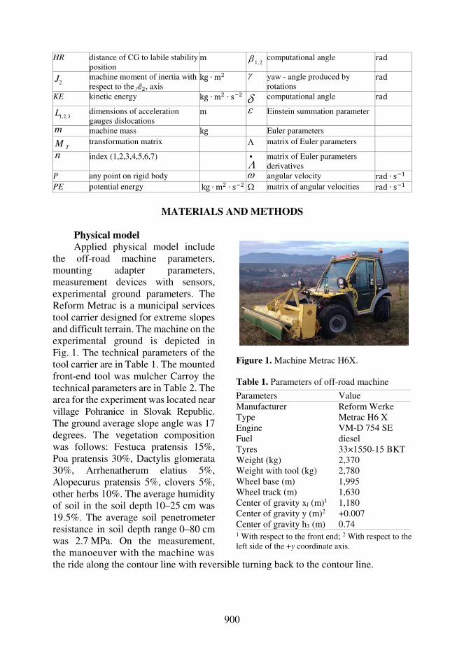
900
HR distance of CG to labile stability position
m 1 2, computational angle rad
2J machine moment of inertia with respect to the yX̅4, axis
kg ∙ m4 yaw - angle produced by rotations
rad
KE kinetic energy kg ∙ m4 ∙ s�4 computational angle rad
1 2 3, ,L dimensions of acceleration gauges dislocations
m Einstein summation parameter
m machine mass kg Euler parameters
TM transformation matrix matrix of Euler parameters
n index (1,2,3,4,5,6,7)
matrix of Euler parameters derivatives
M any point on rigid body angular velocity rad ∙ s�d PE potential energy kg ∙ m4 ∙ s�4 matrix of angular velocities rad ∙ s�d
MATERIALS AND METHODS
Physical model
the ride along the contour line with reversible turning back to the contour line.
Applied physical model include the off-road machine parameters, mounting adapter parameters, measurement devices with sensors, experimental ground parameters. The Reform Metrac is a municipal services tool carrier designed for extreme slopes and difficult terrain. The machine on the experimental ground is depicted in Fig. 1. The technical parameters of the tool carrier are in Table 1. The mounted front-end tool was mulcher Carroy the technical parameters are in Table 2. The area for the experiment was located near village Pohranice in Slovak Republic. The ground average slope angle was 17 degrees. The vegetation composition was follows: Festuca pratensis 15%, Poa pratensis 30%, Dactylis glomerata 30%, Arrhenatherum elatius 5%, Alopecurus pratensis 5%, clovers 5%, other herbs 10%. The average humidity of soil in the soil depth 10–25 cm was 19.5%. The average soil penetrometer resistance in soil depth range 0–80 cm was 2.7 MPa. On the measurement, the manoeuver with the machine was
Figure 1. Machine Metrac H6X. Table 1. Parameters of off-road machine
Parameters Value Manufacturer Reform Werke Type Metrac H6 X Engine VM-D 754 SE Fuel diesel Tyres 33×1550-15 BKT Weight (kg) 2,370 Weight with tool (kg) 2,780 Wheel base (m) 1,995 Wheel track (m) 1,630 Center of gravity xf (m)1 1,180 Center of gravity y (m)2 +0.007 Center of gravity h3 (m) 0.74 1 With respect to the front end; 2 With respect to the left side of the +y coordinate axis.

901
Measurement devices were set up for experimental measurement in-situ. For this purpose we are used the Adlink data acquisition devices which have been connected to PC through USB port. The data recording was realized in real-time. The used acceleration gauge ADXL 325EB is depicted in Fig. 2 and mounted on the machine in Fig. 3. The ADXL325 is a small, low power, complete 3-axis accelerometer with signal conditioned voltage outputs. The product measures acceleration with a minimum full-scale range of ± 5 g. It can measure the static acceleration of gravity in tilt-sensing applications, as well as dynamic acceleration, resulting from motion, shock, or vibration. The user selects the bandwidth of the accelerometer using the CX, CY, and CZ capacitors at the XOUT, YOUT, and ZOUT pins. Bandwidths can be selected to suit the application with a range of 0.5 Hz to 1,600 Hz for X and Y axes and a range of 0.5 Hz to 550 Hz for the Z axis. The detailed technical parameters are available at www.analog.com. The dislocations of mounted accelerations gauges are depicted on the picture 4.
On Fig. 4 the accelerations gauges are signed as ag1, ag2, ag3, ag4, where the
measured accelerations with respect to the coordinate axes directions is ;9À which means a – acclereation, n – number index for moving euquations, q – coordinate directions x,y,z X̅1,2,3 axis with respect to the coordinate base ov machine with origin in center of gravity of machine. The determinantion of center of gravity and weigth deistribution on the machine were published by Rédl & Páleš (2017).
Table 2. Parameters of mounted tool
Parameters Value Manufacturer Dsp Production Sas Mark Carroy Type GF 2072 RE7F C6 2S Description mulch-laying adapter Weight (kg) 410 Length (m) 1.0 Width (m) 2.27 Height (m) 1.10
Figure 2 ADXL gauge.
Figure 3. Dislocations of sensors of acceleration on machine (is the same on the hidden part of machine).
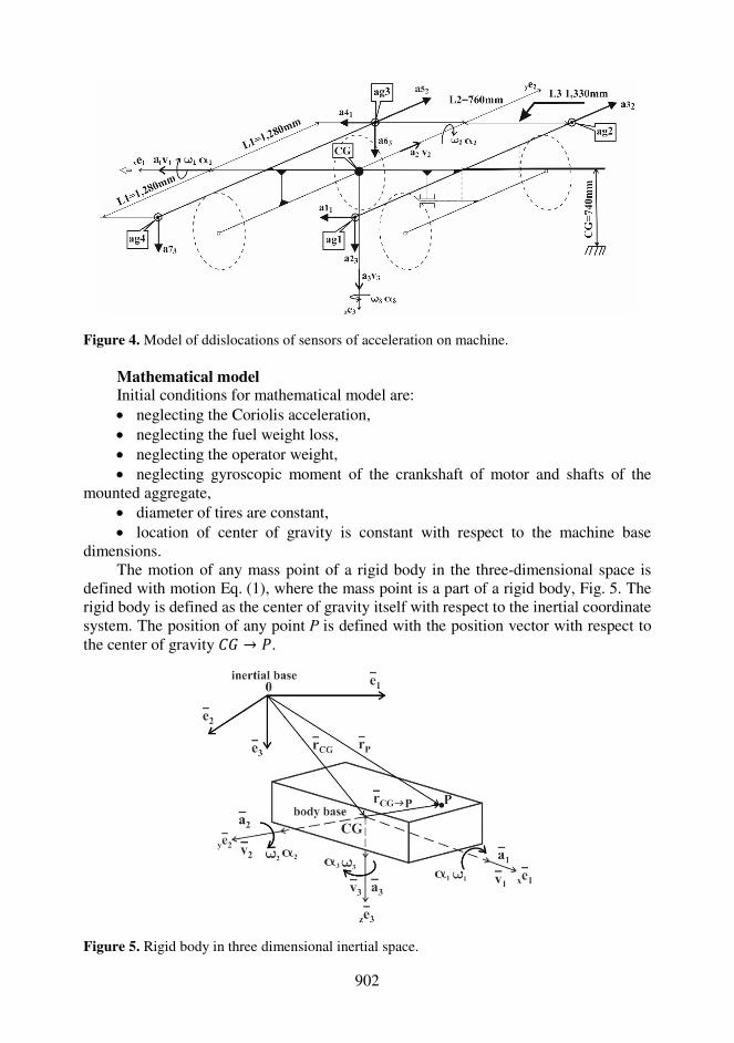
902
Figure 4. Model of ddislocations of sensors of acceleration on machine.
Mathematical model Initial conditions for mathematical model are: neglecting the Coriolis acceleration, neglecting the fuel weight loss, neglecting the operator weight, neglecting gyroscopic moment of the crankshaft of motor and shafts of the
mounted aggregate, diameter of tires are constant, location of center of gravity is constant with respect to the machine base
dimensions. The motion of any mass point of a rigid body in the three-dimensional space is
defined with motion Eq. (1), where the mass point is a part of a rigid body, Fig. 5. The rigid body is defined as the center of gravity itself with respect to the inertial coordinate system. The position of any point P is defined with the position vector with respect to the center of gravity 7¾ → M.
Figure 5. Rigid body in three dimensional inertial space.

903
2
1 2 3
i i i j k i i k i ii i jk i jk q i mn jk n j
CG PP CG
k i j kq i jk q i
CG P CG P
e v e v v e r e
r e r e ,
where i, j ,k , , ; q x, y,z
(1)
Where ie is a unit vector with components 1 2 3e e ,e ,e of inertial base,
1 2 3q x y ze e , e , e is a unit vector of body base. For all vectors ie , q e , parameters ijk
and all remained components of the Eq. (1) we used the Einstein summation convention where v is a velocity, r is a position vector, is an angular velocity. The point sign above the some components indicates its differentiation. Neglecting the Coriolis
acceleration 2i j kjk q i
CG Pr e
and decomposition of elements with Einstein
summation to its components, we got the moving equations of center of gravity with respect to the inertial base as follows:
2 21 1 2 3 3 2 2 3 1 2 3 1 3 2a v v v x y z
,
2 22 2 3 1 1 3 1 2 3 1 3 2 3 1a v v v x y z
,
2 23 3 1 2 2 1 1 3 2 2 3 1 1 2a v v v x y z
.
(2)
The Eqs (2) could be rewrite for six degrees of freedom where the accelerations �d − �� are obtained from experimental measurement from accelerations gauges. The dislocation of accelerations gauges are mounted on steel frame, oriented in horizontal plane of center of gravity, with dislocations depicted on Fig. 4. For the spatial identification of rigid body with respect to the inertial base we were used the Euler parameters expressed in the matrix form as follows:
12
, (3)
where is a matrix of Euler parameters derivatives, WΩ[ is the matrix of angular
velocities obtained from experiment. Solving the Eq. (3) we got the transformation
matrix parameters ija where 1 2 3 1 2 3i , , ; j , , . We were created the transformation
matrix as follows:
11 12 13
21 22 231 2 3
31 32 33
T
n
T ii , , ,..
i
a a a
M a a a
a a a
, (4)
where the T in matrix superscript position indicates the matrix transposition on each steps i t on . For parameters transformation from body base to inertial base the transformation matrix Wiµ[ has been used as follows:
gravity acceleration vector in initial position 0 1 2 3, ,G T G , (5)

904
gravity acceleration vector 0i T ( i )G M G , (6)
angular velocity Ts T TM , (7)
The differential Eqs (2) and (3) were solved numerically with application the Runge-Kutta numerical method of fourth degree as published by Rédl et al. (2015).
Figure 6. Machine center of gravity accelerations.
Solving the Eq. (3) we got the components of transformation matrix (4) as follows:
a11 02
12
22
32 , 12 1 2 0 32a , 13 1 3 0 22a ,
21 1 2 0 32a , a22 02
22
32
12 , 23 2 3 0 12a ,
31 3 1 0 22a , 32 2 3 0 12a , a33 02
32
12
22 ,
(8)
Rotation matrix 1 2 3, ,T has the next form:
1 2 3
1 0 0 0 0
0 0 1 0 0
0 0 0 0 1, ,
cos sin cos sin
T cos sin sin cos
sin cos sin cos
(9)
To derive the stability factor of machine which is operating on slope we had to determine the gravity mass vector and its components during the experiment. In the start position the machine gravity acceleration force has the form:
1 0
2 0 1 2 3
3 0
0
0( )
( ) , ,
( )
G
G T
G G
, (10)
For the determination of the stable state of the machine during the maneuver on the slope we designed the model of the vehicle overturn. The geometrical interpretation of
-0.5
-0.4
-0.3
-0.2
-0.1
0
0.1
0.2
0.3
0.4
0.5
0 5 10 15 20 25
Accele
ration,
ms
-2
Time, s
Translational acceleration a3 Angular acceleration 23
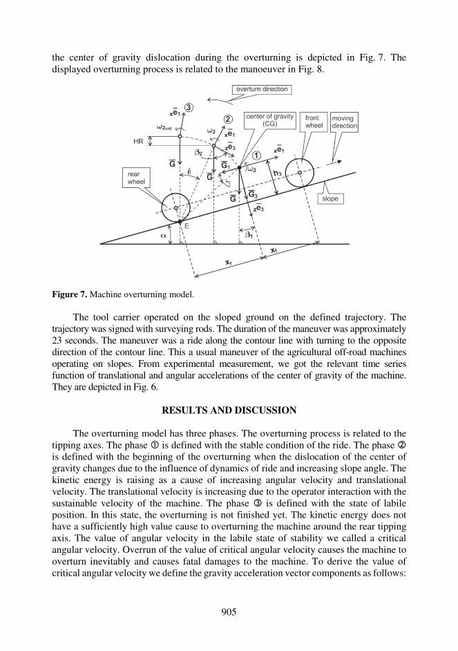
905
the center of gravity dislocation during the overturning is depicted in Fig. 7. The displayed overturning process is related to the manoeuver in Fig. 8.
Figure 7. Machine overturning model. The tool carrier operated on the sloped ground on the defined trajectory. The
trajectory was signed with surveying rods. The duration of the maneuver was approximately 23 seconds. The maneuver was a ride along the contour line with turning to the opposite direction of the contour line. This a usual maneuver of the agricultural off-road machines operating on slopes. From experimental measurement, we got the relevant time series function of translational and angular accelerations of the center of gravity of the machine. They are depicted in Fig. 6.
RESULTS AND DISCUSSION
The overturning model has three phases. The overturning process is related to the
tipping axes. The phase is defined with the stable condition of the ride. The phase is defined with the beginning of the overturning when the dislocation of the center of gravity changes due to the influence of dynamics of ride and increasing slope angle. The kinetic energy is raising as a cause of increasing angular velocity and translational velocity. The translational velocity is increasing due to the operator interaction with the sustainable velocity of the machine. The phase is defined with the state of labile position. In this state, the overturning is not finished yet. The kinetic energy does not have a sufficiently high value cause to overturning the machine around the rear tipping axis. The value of angular velocity in the labile state of stability we called a critical angular velocity. Overrun of the value of critical angular velocity causes the machine to overturn inevitably and causes fatal damages to the machine. To derive the value of critical angular velocity we define the gravity acceleration vector components as follows:
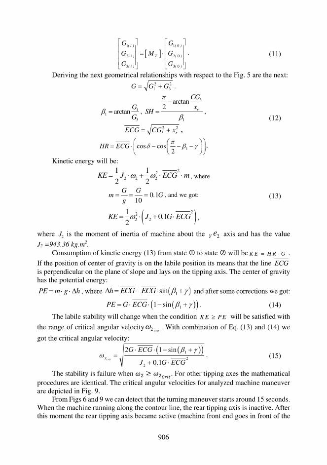
906
1 1 0
2 2 0
3 3 0
( i ) ( )
( i ) T ( )
( i ) ( )
G G
G M G
G G
. (11)
Deriving the next geometrical relationships with respect to the Fig. 5 are the next: 2 2
1 3G G G .
11
3
arctanG
G ,
3
1
arctan2 r
CG
xSH
,
2 23 rECG CG x ,
1cos cos2
HR ECG
,
(12)
Kinetic energy will be: 22
2 2 2
1 12 2
KE J ECG m , where
0 110
G Gm . G
g , and we got:
222 2
10.1
2KE J G ECG ,
(13)
where 2J is the moment of inertia of machine about the 2Y e axis and has the value J2 =943.36 kg.m2.
Consumption of kinetic energy (13) from state to state will be K E H R G . If the position of center of gravity is on the labile position its means that the line ECGis perpendicular on the plane of slope and lays on the tipping axis. The center of gravity has the potential energy:
PE m g h , where 1sinh ECG ECG and after some corrections we got:
11 sinPE G ECG . (14)
The labile stability will change when the condition K E P E will be satisfied with
the range of critical angular velocity 2 Crit . With combination of Eq. (13) and (14) we
got the critical angular velocity:
1
2
2
2 1 sin
0.1crity
G ECG
J G ECG
. (15)
The stability is failure when x4 ≥ x4ÄÅÆÇ. For other tipping axes the mathematical procedures are identical. The critical angular velocities for analyzed machine maneuver are depicted in Fig. 9.
From Figs 6 and 9 we can detect that the turning maneuver starts around 15 seconds. When the machine running along the contour line, the rear tipping axis is inactive. After this moment the rear tipping axis became active (machine front end goes in front of the

907
slope) and lateral tipping axes became active. The machine starts turning. The dynamic forces acting on the vehicle on rounding especially the inertial centrifugal force. Between 15 seconds and 20 seconds, the rear tipping axis became active. In this position of the machine is a high risk of overturning around the rear overturning axis. Also, the left and right tipping axes are activated as is shown in Fig. 8. The most dangerous state occurs in the critical angular velocity of lateral tipping axes. The critical angular velocity reaches
Prediction of the tractor overturn is the serious problem in the agricultural machinery. The mathematical models created by Previati et al (2014) are able to estimate the rollover limit of a farm tractor. The rollover phenomenon is investigated by considering the static stability of the farm tractor on a sloped surface. The authors derived three mathematical models to understand the basic features of the rollover mechanism. The models are able to predict the (static) rollover limit for any orientation of the farm tractor with respect to the slope. The effects of tyre stiffness (vertical and lateral) and nonsymmetrical implement positioning are analyzed also. The limitation of presented model is fact that the models did not actuated by real technical function. From this point of view is usable for prediction of static states of overturns.
Figure 9. Critical angular velocity.
Bietresato & Mazzetto (2018) stated that unstopped overturning must be avoided at all to prevent serious damages to people and things near the facility, due to the dangerous condition of having a relevant mass in a not-controlled motion within an enclosed area. Reporting of the agricultural damages and the outflow of the fuel or other
0
0.5
1
1.5
2
2.5
3
3.5
4
4.5
0 5 10 15 20 25
Critical angula
r velo
city,
ra
ds
-1
Time, s
Frontend axis
Rear axis
Lateral axes
the value when the angular velocity reaches this value the possibility of overturning around the lateral axis very high. If the active stability control device is mounted on the machine, the pitch angular velocity is indicated the possible risk of overturning as published by Rédl et al. (2014). Eliminating the risk of the overturning of the machine will increase the operating and ecological safety of agricultural machines.
Figure 8. Maneuver.

908
technical liquid due to machine accident is very lack. Kogler et al. (2015) determined that the information content of accident reports, because of insufficient information about the accident-causing human-machine interaction, does not suffice to derive or develop further sustainable preventive measures. The reporting of the soil contamination is missing.
The Slovak standard STN 47 0170 defines the mathematical background of determination of allowed operating slope angle for agricultural machines. The developed mathematical model based on the Slovak standard enables the prediction of the dangerous states of the machine during the maneuver.
CONCLUSION
The study presenting the nowadays actual problems about the dangerous consequences of agricultural machines overturn and the ecological impact on the agricultural soil. We designed the mathematical model for the determination of critical angular velocity which has a major influence on the dynamic stability of the agricultural machine operating on sloped ground. The mathematical model is based on the Slovak national standard STN 47 0170. We realized the experimental measurement with an agricultural machine on defined land parameters and slope. Designed mathematical model processed the measured technical function of the acceleration of the center of gravity of the machine. The derived geometrical relationship of the center of gravity dislocation allows determining the critical angular velocity related to the active tipping axis. Carrying out the experimental measurements for certain maneuvers for certain operating conditions we able to implement the boundary ranges of critical angular velocities into the active stability control devices and eliminated the machine accidents. That improve also the ecological safety of agricultural machines operating on the sloped ground.
REFERENCES
Abubakar, M.S., Ahmad, D. & Akande, F.B. 2010. A Review of Farm Tractor Overturning
Accidents and Safety. Pertanika J. Sci. & Technol. 18(2), 377–385. Antunes, S.M., Cordeiro, C. & Teixeira, H.M. 2018. Analysis of fatal accidents with tractors in
the Centre of Portugal: Ten Years Analysis. Forensic Science International Volume 287, June 2018, Pages 74–80. https://doi.org/10.1016/j.forsciint.2018.03.048
Analog.com ADXL 325 Data Sheet [Internet 25.03.2021], available from: https://www.analog.com/media/en/technical-documentation/data-sheets/ADXL325.pdf Bietresato, M. & Mazzetto, F. 2018. Increasing the safety of agricultural machinery operating on
sloping grounds by performing static and dynamic tests of stability on a new-concept facility. Int. J. of Safety and Security Eng. 8(1), 77–89 . DOI: 10.2495/SAFE-V8-N1-77-89
Bulgakov, V., Adamchuk, V. -Arak, M., Nadykto, V., Kyurchev, V. & Olt, J. 2016. Theory of vertical oscillations and dynamic stability of combined tractor-implement unit. Agronomy Research 14(3), 689–710.
Bulgakov, V., Adamchuk, V., Nadykto, V., Kistechok, O. & Olt, J. 2017. Theoretical research into the stability of motion of the ploughing tractor. Agronomy Research 15(4), 1517–1529, 2017. https://doi.org/10.15159/AR.17.069
Bulgakov, V., Kaletnik, H., Goncharuk, T., Rucins, A., Dukulis, I. & Pascuzzi, S. 2019. Research of the movement of agricultural aggregates using the methods of the movement stability theory. Agronomy Research 17(5), 1846–1860. https://doi.org/10.15159/AR.19.189

909
Enn, A. & Merisalu, E. 2019. Dynamics of work accidents incidence by severity, gender and lost workdays in Estonian agricultural sector and sub-sectors in 2008–2017. Agronomy Research 17(4), 1617–1629. https://doi.org/10.15159/AR.19.169
Eurostat. 2019. Agriculture, forestry and fishery statistics 2019 edition, Luxembourg: Publications Office of the European Union, 2019 ISBN 978-92-76-13193-9, https://doi:10.2785/798761, KS-FK-19-001-EN-N
Garland, J.J. 2018. Accident reporting and analysis in forestry: guidance on increasing the safety of forest work. Forestry Working Paper No. 2. Rome, FAO.
Issa, S.F., Patrick, K., Thomson, S. & Rein, B. 2019. Estimating the Number of Agricultural Fatal Injuries Prevented by Agricultural Engineering Developments in the United States. Safety 5(63). doi:10.3390/safety5040063
ISO 12100. 2010 Safety of machinery - General principles for design - Risk assessment and risk reduction.
Jucherski, A., Golka, W. & Eymontt, A. 2005. Agricultural engineering in the ecological mountian farms. Rural Areas and Development 3(2005).
Kogler, R., Quendler, E. & Boxberger, J. 2015. Analysis of occupational accidents with agricultural machinery in the period 2008–2010 in Austria. Safety Science 72, 319–328.
Komatsu report 2019. www.komatsu.com. Available at: https://home.komatsu/en/ir/library/annual/pdf/KMT_AR19E_spread.pdf. Accessed 08.10.2020.
Mc Namara, J., Griffin, P., Phelan, J., Field, W.E. & Kinsella, J. 2019. Farm health and safety adoption through engineering and behaviour change. Agronomy Research 17(5), 1953–1959. https://doi.org/10.15159/AR.19.151
Merisalu, E., Leppälä, J., Jakob, M. & Rautiainen, R.H. 2019. Variation in Eurostat and national statistics of accidents in agriculture. Agronomy Research 17(5), 1969–1983. https://doi.org/10.15159/AR.19.190
Polák, R. 2014. Report on the extraordinary deterioration of water quality on the locality Dolné Saliby on 12.3.2014 no. 3368-8818/326/2014 Dom. Hydropol, Rudolf Polák s.r.o. Rajská l, 81108 Bratislava.
Previati, G., Gobbi, M. & Mastinu, G. 2014. Mathematical models for farm tractor rollover prediction. Int. J. Vehicle Design, Vol. 64, Nos. 2/3/4.
Rédl, J. & Páleš, D. 2017. Algorithm of determination of centre of gravity of agricultural machine with error estimation. Mathematics in Education, Research and Applications 3(2), 95–103.
doi: https://doi.org/10.15414/meraa.2017.03.02.95-103 Rédl, J.-Váliková, V. & Antl, J. 2014. Design of active stability control system of agricultural
off-road vehicles. Research in agricultural engineering 60, 77–84. ISSN 1212-9151 Rédl, J., Váliková, V., Páleš, D. & Antl, J. 2015. Application of numerical integration in technical
practice. Math. Educ. Res. Appl. 1(1). doi: http://dx.doi.org/10.15414/meraa.2015.01.01.12-17 Regulation (EU) No 167/2013 of the European Parliament and of the Council of 5 February 2013
on the approval and market surveillance of agricultural and forestry vehicles. Váliková, V., Rédl, J. & Antl, J. 2013. Analysis of Accidents Rate of Agricultural Off-Road Vehicles.
Journal of Central European Agriculture 14(4), 1303–1316. doi: 10.5513/JCEA01/14.4.1348 Visser, R. & Stampfer, K. 2015. Expanding Ground-based Harvesting onto Steep Terrain: A
Review. Croatian Journal of Forest Engineering 36(2), 321–331. Statistical Office Of The Slovak Republic, 2019, https://slovak.statistics.sk/ STN 47 0170. 2001. Agricultural tractors and machinery. Gradeability test metods. Safety of
work. Slovak office for standardization 2001. Poľnohospodárske stroje a traktory. Stanovenie svahovej dostupnosti. Bezpečnosť práce. (in Slovak).
Streche, C., Cocârţă, D.M, Istrate, I. & Badea, A.A. 2018. Decontamination of Petroleum-Contaminated Soils Using the Electrochemical Technique: Remediation Degree and Energy Consumption. Sci. Rep. 8(1), 3272. doi: 10.1038/s41598-018-21606-4
910
Agronomy Research 19(S1), 910–921, 2021 https://doi.org/10.15159/AR.21.062
Influence of different methods of treating natural açai fibre for mortar in rural construction
D.L. Rocha1, A.R.G. Azevedo2, M.T. Marvila2, D. Cecchin3,*, J. Alexandre2,
D.F. Carmo3, Ferraz, P.F.P.4, Conti, L.5 and Rossi, G.5
1UENF - State University of the Northern Rio de Janeiro, LAMAV - Advanced Materials Laboratory; Av. Alberto Lamego, 2000, PO Box 28013-602, Campos dos Goytacazes, Brazil 2UENF - State University of the Northern Rio de Janeiro, LECIV - Civil Engineering Laboratory; Av. Alberto Lamego, 2000, PO Box 28013-602, Campos dos Goytacazes, Brazil 3UFF - Federal Fluminense University, TER - Department of Agricultural and Environmental Engineering; Rua Passo da Pátria, 156, PO Box 21065-230, Niterói, Brazil 4UFLA - Federal University of Lavras, Department of Agricultural Engineering, Campus Universitário, PO Box 3037, Lavras, Minas Gerais, Brazil 5University of Firenze, Department of Agriculture, Food, Environment and Forestry (DAGRI), Via San Bonaventura 13, IT50145 Firenze, Italy *Correspondence: [email protected] Received: January 20th, 2021; Accepted: April 15th, 2021; Published: May 4th, 2021 Abstract. Açai is a typical Amazonian fruit that has enormous potential for use in medicines and foods, whose consumption has been growing year after year. One of the major environmental impacts related to Açai is the generation of agro-industrial wastes, which are disposed of in landfills. One of the major problems related to the reuse of natural fibres in cementitious materials is related to their durability due to the alkalinity of the matrix. Thus, the objective of this work was to evaluate three different methodologies for surface treatment of Açai fibre, by immersion in NaOH, KOH and Ca(OH)2 solution to mortar application in rural construction. After the treatments, the fibres were added in a proportion of 2.5 and 5.0% in relation to the cement mass, in addition to the reference mortar (without fibre) in the making of the prismatic specimens (40×40×160 mm) and cured for 28 days in room temperature. Right after the curing period, the specimens were evaluated according to the mechanical strength of flexion and compression, workability, water absorption by capillarity and mass density in the hardened state of each methodology. The results showed that the best treatment methodology is with NaOH solution, with the addition of 5% Açai fibre in relation to the cement mass, producing a suitable mortar for use in rural buildings. Key words: agro-industrial wastes, açai, reuse, rural constructions, sustainability.
911
INTRODUCTION
The Açai is a small fruit with a rounded shape, usually dark in colour, with a small lump and its pulp (Sato et al., 2019). The fruit is found predominantly in the Amazon region, which spreads to countries like Brazil (predominantly), Peru, Colombia and Venezuela, but also in other regions of Brazil, spreading its cultivation in several places due to the constant increase of its added value in all world (Sato et al., 2020).
The most traditional açaí is the fruit of the açaizeiro (Euterpe oleracea), which is native to the amazon region, and in some cases is also called juçara, being a tree that can reach up to 30 meters in height, predominantly in the humid regions, favouring its growth in amazon region and coastal locations. The fruit's productivity is high, since in one hectare the production can reach 12 tons a year, when the appropriate management techniques are used (De Azevedo et al., 2021).
According to the Brazilian Institute of Geography and Statistics (IBGE) and the Municipal Agricultural Production (MAP) survey, Brazil produced more than 1.5 million tons of the fruit in 2018, a figure that has been growing day by day, reaching a projection of almost 2 million tons in 2021, due to the greater dissemination of this fruit internationally, which enhances exports, and research aimed at its application for medicinal purposes and uses in food (IBGE, 2019).
In Brazil, the state of Para is the main producer with 95% of the production of açaí in Brazil (Cruz et al., 2019). Currently, 90% of açaí production in Brazil is destined for the domestic market and 10% for export to about 40 countries, with the United States receiving the largest amount (Sato et al., 2020). Of the processed foods that contain açaí and launched on the world market in the last 5 years, 22% are represented by juices, 12% energy and sports drinks, 9% snacks, 7% desserts and ice cream, 5% in the dairy category and 3% in sweets and bullets, with the United States (30%), Brazil (19%) and Canada (8%) the most representative countries in the launch of these products (Virmond et al., 2012). The açaí market had a turnover of around 1.5 billion dollars in 2020 (De Azevedo et al., 2021).
All the growing production and processing of fruit for the manufacturing of its derived products generate great environmental impacts, whether in the matter of soil management, use of agricultural pesticides, increase in areas cultivated as a result of illegal deforestation in the Amazon region and the large generation of waste solids during the processing step (Silva et al., 2018). The açaí fruit has a round shape and weighs about two grams. For the production of fruit-based products, a processing process must be carried out that results in the açaí lump, since only 17% of the fruit is edible (pulp and peel), requiring about 2 kilos of fruit for a litter of juice (Virmond et al., 2012). The core is covered with small natural fibres, which are currently a major environmental liability since they are discarded in landfills or disposed of in open land, contaminating the environment (De Azevedo et al., 2021). Thus, in view of the constant growth of açaí production and its popularization in Brazil and worldwide, the concern with sustainable practices for the generated agro-industrial solid waste is constant.
Some research has been developed around the world in relation to the use of açaí lump and fibre, evaluating the potential of its reuse for medicinal purposes or even in the reuse in the development of alternative construction materials and energy generation. There are studies that assess the potential of energy generation, through açaí, as a source of biomass, mainly in remote regions that use generators, such as in the Amazon region,
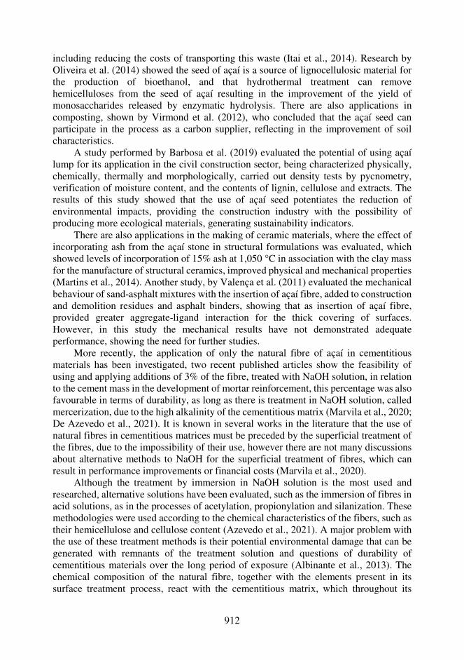
912
including reducing the costs of transporting this waste (Itai et al., 2014). Research by Oliveira et al. (2014) showed the seed of açaí is a source of lignocellulosic material for the production of bioethanol, and that hydrothermal treatment can remove hemicelluloses from the seed of açaí resulting in the improvement of the yield of monosaccharides released by enzymatic hydrolysis. There are also applications in composting, shown by Virmond et al. (2012), who concluded that the açaí seed can participate in the process as a carbon supplier, reflecting in the improvement of soil characteristics.
A study performed by Barbosa et al. (2019) evaluated the potential of using açaí lump for its application in the civil construction sector, being characterized physically, chemically, thermally and morphologically, carried out density tests by pycnometry, verification of moisture content, and the contents of lignin, cellulose and extracts. The results of this study showed that the use of açaí seed potentiates the reduction of environmental impacts, providing the construction industry with the possibility of producing more ecological materials, generating sustainability indicators.
There are also applications in the making of ceramic materials, where the effect of incorporating ash from the açaí stone in structural formulations was evaluated, which showed levels of incorporation of 15% ash at 1,050 °C in association with the clay mass for the manufacture of structural ceramics, improved physical and mechanical properties (Martins et al., 2014). Another study, by Valença et al. (2011) evaluated the mechanical behaviour of sand-asphalt mixtures with the insertion of açaí fibre, added to construction and demolition residues and asphalt binders, showing that as insertion of açaí fibre, provided greater aggregate-ligand interaction for the thick covering of surfaces. However, in this study the mechanical results have not demonstrated adequate performance, showing the need for further studies.
More recently, the application of only the natural fibre of açaí in cementitious materials has been investigated, two recent published articles show the feasibility of using and applying additions of 3% of the fibre, treated with NaOH solution, in relation to the cement mass in the development of mortar reinforcement, this percentage was also favourable in terms of durability, as long as there is treatment in NaOH solution, called mercerization, due to the high alkalinity of the cementitious matrix (Marvila et al., 2020; De Azevedo et al., 2021). It is known in several works in the literature that the use of natural fibres in cementitious matrices must be preceded by the superficial treatment of the fibres, due to the impossibility of their use, however there are not many discussions about alternative methods to NaOH for the superficial treatment of fibres, which can result in performance improvements or financial costs (Marvila et al., 2020).
Although the treatment by immersion in NaOH solution is the most used and researched, alternative solutions have been evaluated, such as the immersion of fibres in acid solutions, as in the processes of acetylation, propionylation and silanization. These methodologies were used according to the chemical characteristics of the fibers, such as their hemicellulose and cellulose content (Azevedo et al., 2021). A major problem with the use of these treatment methods is their potential environmental damage that can be generated with remnants of the treatment solution and questions of durability of cementitious materials over the long period of exposure (Albinante et al., 2013). The chemical composition of the natural fibre, together with the elements present in its surface treatment process, react with the cementitious matrix, which throughout its
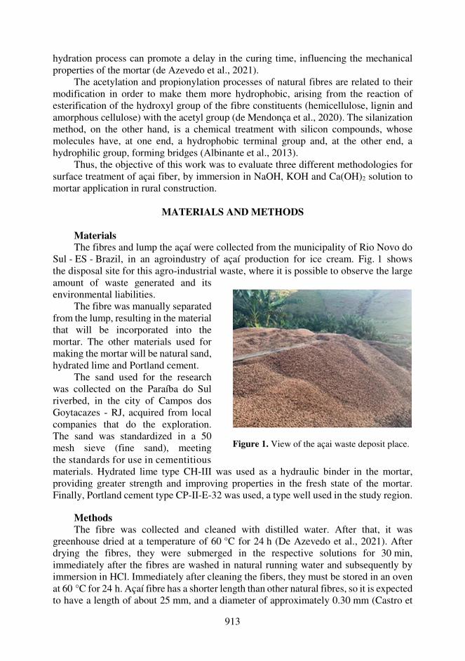
913
hydration process can promote a delay in the curing time, influencing the mechanical properties of the mortar (de Azevedo et al., 2021).
The acetylation and propionylation processes of natural fibres are related to their modification in order to make them more hydrophobic, arising from the reaction of esterification of the hydroxyl group of the fibre constituents (hemicellulose, lignin and amorphous cellulose) with the acetyl group (de Mendonça et al., 2020). The silanization method, on the other hand, is a chemical treatment with silicon compounds, whose molecules have, at one end, a hydrophobic terminal group and, at the other end, a hydrophilic group, forming bridges (Albinante et al., 2013).
Thus, the objective of this work was to evaluate three different methodologies for surface treatment of açai fiber, by immersion in NaOH, KOH and Ca(OH)2 solution to mortar application in rural construction.
MATERIALS AND METHODS
Materials The fibres and lump the açaí were collected from the municipality of Rio Novo do
Sul - ES - Brazil, in an agroindustry of açaí production for ice cream. Fig. 1 shows the disposal site for this agro-industrial waste, where it is possible to observe the large
materials. Hydrated lime type CH-III was used as a hydraulic binder in the mortar, providing greater strength and improving properties in the fresh state of the mortar. Finally, Portland cement type CP-II-E-32 was used, a type well used in the study region.
Methods The fibre was collected and cleaned with distilled water. After that, it was
greenhouse dried at a temperature of 60 °C for 24 h (De Azevedo et al., 2021). After drying the fibres, they were submerged in the respective solutions for 30 min, immediately after the fibres are washed in natural running water and subsequently by immersion in HCl. Immediately after cleaning the fibers, they must be stored in an oven at 60 °C for 24 h. Açaí fibre has a shorter length than other natural fibres, so it is expected to have a length of about 25 mm, and a diameter of approximately 0.30 mm (Castro et
amount of waste generated and its environmental liabilities.
The fibre was manually separated from the lump, resulting in the material that will be incorporated into the mortar. The other materials used for making the mortar will be natural sand, hydrated lime and Portland cement.
The sand used for the research was collected on the Paraíba do Sul riverbed, in the city of Campos dos Goytacazes - RJ, acquired from local companies that do the exploration. The sand was standardized in a 50 mesh sieve (fine sand), meeting the standards for use in cementitious
Figure 1. View of the açai waste deposit place.
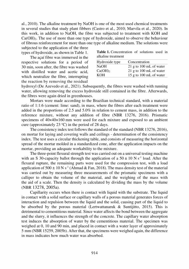
914
al., 2010). The alkaline treatment by NaOH is one of the most used chemical treatments in several studies that study plant fibbers (Castro et al., 2010; Marvila et al., 2020). In this work, in addition to NaOH, the fibre was subjected to treatment with KOH and Ca(OH)2. The use of more than one type of hydroxide, aimed to observe the behaviour of fibrous reinforcement for more than one type of alkaline medium. The solutions were
hydroxyl (De Azevedo et al., 2021). Subsequently, the fibres were washed with running water, allowing removing the excess hydroxide still contained in the fibre. Afterwards, the fibres were again dried in greenhouses.
Mortars were made according to the Brazilian technical standard, with a material ratio of 1:1:6 (cement: lime: sand), in mass, where the fibres after each treatment were added in the proportions of 2.5 and 5.0% in relation to cement mass, in addition to the reference mixture, without any addition of fibre (NBR 13276, 2016). Prismatic specimens of 40×40×160 mm were used for each mixture and exposed to an ambient cure (approximately 23 oC) in the period of 28 days.
The consistency index test follows the standard of the standard (NBR 13276, 2016), on mortar for laying and covering walls and ceilings - determination of the consistency index. The test uses a circular thickening table, and consists of measuring the horizontal spread of the mortar molded in a standardized cone, after the application impacts on the mortar, providing an adequate workability to the mixture.
The three-point flexural strength test was carried out on a universal testing machine with an S 30-capacity ballot through the application of a 50 ± 10 N s-1 load. After the flexural rupture, the remaining parts were used for the compression test, with a load application of 500 ± 10 N s-1 (Ahmad & Fan, 2018). The mass density test of the material was carried out by measuring three measurements of the prismatic specimens with a calliper to obtain the volume of the material, and the weighing of the mass with the aid of a scale. Then the density is calculated by dividing the mass by the volume (NBR 13278, 2005a).
Capillarity occurs when there is contact with liquid with the substrate. The liquid in contact with a solid surface or capillary walls of a porous material generates forces of interaction and repulsion between the liquid and the solid, causing part of the liquid to be absorbed by the porous material (Lertwattanaruk & Suntijitto, 2015). This is detrimental to cementitious material. Since water affects the bond between the aggregate and the slurry, it influences the strength of the concrete. The capillary water absorption test induces the absorption of water by the cementitious material. The specimen was weighed at 0, 10 and 90 min, and placed in contact with a water layer of approximately 5 mm (NBR 15259, 2005b). After that, the specimens were weighed again, the difference in mass indicates how much water was absorbed.
subjected to the application of the three types of hydroxide, as shown in Table 1.
The açaí fibre was immersed in the respective solutions for a period of 30 min, soon after, the fibre was washed with distilled water and acetic acid, which neutralize the fibre, interrupting the reaction by removing the residual
Table 1. Concentration of solutions used in alkaline treatment
Hydroxide type Concentration NaOH 21 g to 100 mL of water Ca(OH)2 21 g to 100 mL of water KOH 15 g to 100 mL of water
915
RESULTS AND DISCUSSION The Table 2 shows the results related to the mixing of the materials, such as the
proportion, in mass, of the constituents for making the mortar. It is observed that for each type of treatment methodology, the fibres were added proportionally to the cement mass, without changing the quantity of the other materials, such as cement, lime and sand.
Table 2. Workability properties of mortars and mixtures
Treatment Type
Cement (g)
Lime (g)
Sand (g)
Water (g)
Fibre (g)
water/ cement
Horizontal spreading (mm)
NaOH 100 100 600 45 2.5 0.45 259 ± 14 100 100 600 45 5.0 0.45 257 ± 12
Ca(OH)2 100 100 600 45 2.5 0.45 277 ± 10 100 100 600 45 5.0 0.45 264 ± 6
KOH 100 100 600 45 2.5 0.45 278 ± 11 100 100 600 45 5.0 0.45 262 ± 18
It can be seen in Table 2 that the water/cement ratio was kept constant, at 0.45,
which is a value widely used in the literature on cementitious composites for reinforcement with natural fibres (Candamano et al., 2020; Morón Barrios et al., 2021), another point is that when choosing to keep this parameter fixed, the comparison ratio between mixtures and the evaluated treatment methods is better.
When we evaluate the horizontal spreading, which is a property directly related to the workability of the mixture, we have that the literature speaks of values around 260 ± 5 mm, which is the same as that adopted in the Brazilian technical standard for applications in coating mortars (NBR 13276, 2016; De Azevedo et al., 2021). Therefore, it was decided to use this reference value, and the treatment with NaOH (mercerization), was be showed with the most stable values and within the acceptable range, keeping a mortar with good workability.
In the Ca(OH)2 and KOH treatments for the 2.5% fibre content, the nominal average spreading exceeded the maximum limit, even within the standard deviation values, this can be attributed to the lower adhesion that the fibre had, with these treatment methodologies, along with the cementitious matrix, resulting in more fluid mortars (Marvila et al., 2020). With higher levels, such as 5%, both treatments obtained nominal values within the acceptable range (260 ± 5 mm), but still very close to maximun limit, which may denote not being a significant and acceptable result for the application in rural construction (García-Esparza et al., 2018).
Thus, the treatment with NaOH was the one that showed the greatest stability regarding the horizontal spreading of the mortar, showing an acceptable workability according to the literature values (Marvila et al., 2020). Another important point is that for applications in rural constructions, the workforce want at a mortar with workability, since the buildings present a facades greater irregularity to application surface and greater exposure to heat, which can influence the final durability of the coating in the environment rural (García-Esparza et al., 2018; Marvila et al., 2020).
Fig. 2 shows the results of the mass density of the specimens in the hardened state, that is, after the curing period.

916
Fig. 2 shows the result of the mass density in the hardened state, where comparatively the reference mixture (without the addition of any fibre), the treatment
Barrios et al., 2021). The results of the literature itself indicate that mortars for use as external cladding
of facades should have a mass density around 1.7 to 1.9 g cm-2, which shows that the treatments of the fibres with KOH and Ca(OH)2 do not are recommended for this
with NaOH was the one that showed the best behaviour, with reduced density in all two levels of incorporation, which is beneficial for mortars in general, as it reduces the load on masonry in rural constructions (De Azevedo et al., 2021). This reduction with the treatment of NaOH can be justified due to the greater impermeability that the surface treatment caused in the fibres, reducing the effect of the alkaline medium in the matrix in the reinforcement (Asim et al., 2020). The treatments with KOH and Ca(OH)2 were less efficient since there was a dissipation of part of the formed film, which in the case of Ca(OH)2 was influenced by the hydration of the cement (Morón
Figure 2. Results of mass density in the hardened state of each methodology of treatment.
property (Marvila et al., 2020; De Azevedo et al., 2021). Obviously, the amount of fibre addition also influenced, since greater proportions indicated a possible increase in density, which corroborates with other studies in the literature on the use of natural fibres in mortars for coating (Asim et al., 2020).
Fig. 3 shows the result of water absorption by capillarity for the different fiber treatment methodologies.
The absorption of water by capillarity is a phenomenon that evaluates the interconnection potential of the internal pores, which culminates in the transfer of fluids, such as water or external gases, into the cementitious matrix, affecting its behaviour and durability (Nadelman & Kurtis, 2019).
Figure 3. Results of water absorption by capillarity of each methodology of treatment.
1.761.73
1.8
1.92
2.12
1.93
2.24
1.5
1.6
1.7
1.8
1.9
2
2.1
2.2
2.3
2.50% 5% Referencemortar
Mass d
ensity
in t
he h
ard
ened
sta
te (
gcm
-2)
NaOH treatment
KOH treatment
Ca(OH)2 treatment
0.7
0.98
1.2
0.96
1.12
1.341.43
0.6
0.7
0.8
0.9
1
1.1
1.2
1.3
1.4
1.5
2.50% 5% Referencemortar
Wate
r absorp
tion
by
capill
arity
(%
)
NaOH treatment
KOH treatment
Ca(OH)2 treatment

917
It was observed in Fig. 3 that the treatment with Ca(OH)2 induced an increase in this water absorption by capillarity due to the fact that this treatment, which is based on hydrated lime dissolved in the aqueous solution, participates in the hydration process of cement matrix, together with existing cement, reducing the protection efficiency, which helps in the hydrophilic power of natural fibres, in this case more exposed (Marvila et al., 2020).
In the case of treatment with NaOH and KOH what was observed was a reduction, mainly with NaOH, which is justified by the fact of the actual superficial impregnation of the treatment in the fibre, which reduces its effect of formation of capillary veins. In addition, there is a greater internal compactness of matrices with Açai type fibres, as they are shorter and less thick, which corroborates their internal filling effect, in addition to the reinforcement, thus reducing the capillary absorption effect, as observed in results of Fig. 3 (Nadelman & Kurtis, 2019).
Rural buildings are highly susceptible to exposure to the effects of heavy rains, and depending on the region with high temperature rates, a positive point of these environments is the lower exposure to gases, such as atmospheric CO2, which reduces the incidence of pathologies in this sense in these areas buildings (García-Esparza et al.,
test pieces with NaOH treatment presented, in the rupture region, greater shortening of the fibres that were left out in the test pieces, due to the greater resistance that they imposed on these samples. In the other treatments, the fibres were severely broken, showing the greatest fragility of these samples.
The results observed in Fig, 4 indicate that the reference mortar (without adding natural fibers in its mixture), presented a mechanical resistance to flexion of 3.64 MPa, this value is consistent with the main applications that relate the coatings, which according to the study from the literature, it must present at least 3 MPa for medium
2018). Figs 4 and 5 show the results of
mechanical strength flexion and compression, respectively, in the different treatment methodologies analysed. All results of mechanical strength are preceded by the respective standard deviations, as a result of the samples of the specimens used in this study. It can be seen visually that the specimens before the execution of the tests, in all treatment conditions, presented a good consolidation of the mortar, without occurrence of voids due to failure of the density of the dough in the moulds and the occurrence some small parts of these fibres for the external side. After the execution of the tests of mechanical strength to compression and flexion, it was observed that the
Figure 4. Results of mechanical strength of flexion of each methodology of treatment.
3.96
4.1
3.64
3.23
3.76
3.45
3.32
3
3.2
3.4
3.6
3.8
4
4.2
4.4
2.50% 5% Referencemortar
Mechanic
al str
ength
of
flexio
n (
MP
a)
NaOH treatment
KOH treatment
Ca(OH)2 treatment
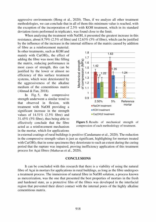
918
aggressive environments (Hong et al., 2020). Thus, if we analyze all other treatment methodologies, we can conclude that in all of them this minimum value is reached, with the exception of the incorporation of 2.5% with KOH treatment, which in its standard deviation (tests performed in triplicate), was found close to the limit.
When analysing the treatment with NaOH, it presented the greatest increase in this resistance, about 8.79% (2.5% of fibre) and 12.63% (5% of fibre), which can be justified by the influence of the increase in the internal stiffness of the matrix caused by addition
in external coatings of rural buildings is positive (Candamano et al., 2020). The reduction in the compressive strength values is just as significant, highlighting for mortars treated with Ca(OH)2 that in some specimens they deteriorate to such an extent during the curing period that the rupture was impaired, proving inefficiency application of this treatment process for Açai fibres (Mathavan et al., 2020).
CONCLUSIONS It can be concluded with this research that there is a viability of using the natural
fibre of Açai in mortars for applications in rural buildings, as long as the fibre undergoes a treatment process. The immersion of natural fibre in NaOH solution, a process known as mercerization, was the one that presented the best properties of mortars in the fresh and hardened state, as a protective film of the fibres was developed in the interfacial region that prevented their direct contact with the internal pores of the highly alkaline cementitious matrix.
of fibre as a reinforcement material. In other treatments, such as KOH and mainly with Ca(OH)2, the effect of adding the fibre was more like filling the matrix, reducing performance in most cases of strength, this can be justified by the lower or almost no efficiency of this surface treatment systems, which were deteriorated by the aggressiveness of the alkaline medium of the cementitious matrix (Ahmad & Fan, 2018).
In Fig. 5, the compressive strength underwent a similar trend to that observed in flexion, with treatment with NaOH providing a significant increase in the strength values of 14.51% (2.5% fibre) and 31.45% (5% fibre), thus being able to effectively conclude that the fibre acted as a reinforcement mechanism in the mortar, which for applications
Figure 5. Results of mechanical strength of compression of each methodology of treatment.
1.42
1.63
1.241.2
1.35
1.22
1
0.9
1
1.1
1.2
1.3
1.4
1.5
1.6
1.7
1.8
2.50% 5% Referencemortar
Mechanic
al str
ength
of
com
pre
ssio
n (
MP
a)
NaOH treatment
KOH treatment
Ca(OH)2 treatment
919
Other methodologies for the treatment of the natural fibre of Açai, such as immersion in KOH and Ca(OH)2 solution, were not as efficient, in these cases the fibre behaved as a filler in the matrix, while in the treatment with NaOH it provided that the Açaí fibre behaved as a reinforcement of the matrix, which was verified in the results of mechanical strength.
As for the percentages of addition of natural fibre, it was observed that values of 5% in relation to the cement mass have adequate behaviour and within the normative standards and the literature of the area. Although higher percentages are not evaluated, other studies related to the use of natural fibres in cementitious matrices have shown that these higher values are harmful. Thus, treatment by immersion in NaOH solution with the addition of 5% Açaí fibre is possible for making mortars for use in cladding and stabbing in rural buildings.
As a suggestion for other works, it is possible to verify the influence of the orientation and arrangement of the fibres in the molding process of the specimens, in addition to other intermediate additions to those already evaluated.
ACKNOWLEDGEMENTS. The authors thank the Brazilian agencies: CNPq, an FAPERJ, proc. No. E-26/210.150/2019 and E-26/010.001953/2019, for supporting this investigation.
REFERENCES
Ahmad, H. & Fan, M. 2018. Interfacial properties and structural performance of resin-coated
natural fibre rebars within cementitious matrices. Cement Concrete Composite 45(5), 167–137. doi:10.1016/j.cemconcomp.2017.12.002
Albinante, S.R., Pacheco, E.B.A.V. & Visconte, L.L.Y. 2013. A review on chemical treatment of natural fiber for mixing with polyolefins. Química Nova 36 (1), 59–65. doi: 10.1590/S0100-40422013000100021 (in Portuguese).
Asim, M., Uddin, G.M., Jamshaid, H., Raza, A., Tahir, Z.U.R., Hussain, U., Satti, A.N., Hayat, N. & Arafat, S.M. 2020. Comparative experimental investigation of natural fibers reinforced light weight concrete as thermally efficient building materials. Journal of Building Engineering 31(3), 101–123. doi: 10.1016/j.jobe.2020.101411
Azevedo, A., de Matos, P., Marvila, M., Sakata, R., Silvestro, L., Gleize, P. & Brito, J. 2021. Rheology, Hydration, and Microstructure of Portland Cement Pastes Produced with Ground Açaí Fibers. Applied Sciences 11(1), 30–36. doi: https://doi.org/10.3390/app11073036.
Barbosa, A.M., Rebelo, V.S.M., Martorano, L.G. & Giacon, V.M. 2019. Characterization of acai waste particles for civil construction use. Matéria 24(3), 16–25. doi: 10.1590/s1517-707620190003.0750 (in Portuguese).
Candamano, S., Crea, F., Coppola, L., De Luca, P. & CoffettI, D. 2020. Influence of acrylic latex and pre-treated hemp fibers on cement based mortar properties. Construction and Building Materials 59(3), 121–720. doi:10.1016/j.conbuildmat.2020.121720
Castro, C.D.P.C., Dias, C.G.B.T. & Faria, J.A.F. 2010. Production and evaluation of recycled polymers from açaí fibers. Materials Research 23(2), 17–25. doi: 10.1590/s1516-14392010000200007
Cruz, T.M.S., Lisboa, C.R., Correa, N.C.F. & Santos, G.R. 2019. Use of solid waste from açaí agroindustry: A review. The production of Knowledge in Science Agrarian and Environmental. 23(2), 60–74. doi:10.22533/at.ed.8451926049

920
de Azevedo, A.R.G., Marvila, M.T., Tayeh, B.A., Cecchin, D., Pereira, A.C. & Monteiro, S.N. 2021. Technological performance of açaí natural fibre reinforced cement-based mortars. Journal of Building Engineering 33(1), 12–22. doi: 10.1016/j.jobe.2020.101675
de Mendonça, N.L., Pereira Junio, R.F., Ribeiro, M.P., Souza, A.T., de Sousa Lima, E., Garcia Filho, F.C., Figueiredo, A.B.H.S., Braga, F.O., Azevedo, A.R.G. & Monteiro, S.N. 2020. Promising Mechanical, Thermal, and Ballistic Properties of Novel Epoxy Composites Reinforced with Cyperus malaccensis Sedge Fiber. Polymers 12(8), 17–46. doi: https://doi.org/10.3390/polym12081776
García-Esparza, J.A., Pardo, F. & Palmero, L.M. 2018. A multi-analysis characterization of medieval and vernacular coating mortars in rural Valencia (Spain): An experimental study for a Heritage Action Plan. Journal of Cultural Heritage 31(2), 83–96. doi: 10.1016/j.culher.2017.10.013
Hong, L., Chen, Y.D., Li, T.D., Gao, P. & Sun, L.Z. 2020. Microstructure and bonding behavior of fiber-mortar interface in fiber-reinforced concrete. Construction and Building Materials 232(30), 117–123. doi: /10.1016/j.conbuildmat.2019.117235
IBGE 2019. Brazilian Institute of Geography and Statistics. Data Yearbook. https:// https://sidra.ibge.gov.br/pesquisa/pam/tabelas. Accessed 16.01.2021. (in Portuguese)
Itai, Y., Santos, R., Branquinho, M., Malico, I., Ghesti, G.F. & Brasil, A.M. 2014. Numerical and experimental assessment of a downdraft gasifier for electric power in Amazon using açaí seed (Euterpe oleracea Mart.) as a fuel. Renewable energy 66(5), 662–669. doi: 10.1016/J.RENENE.2014.01.007
Lertwattanaruk, P. & Suntijitto, A. 2015. Properties of natural fiber cement materials containing coconut coir and oil palm fibers for residential building applications. Construction and Building Materials 56(3), 234–245. doi:10.1016/j.conbuildmat.2015.07.154
Martins, M.A., Mattoso, L.H.C. & Pessoa, J.D.C. 2014. Thermal behavior and morphological characterization of mesocarp fibers and açaí kernel (Euterpe oleracea Mart.). Journal of Brazilian Fruit 31(4), 1150–1157. doi: 10.1590/S0100-29452009000400032
Marvila, M.T., Azevedo, A.R.G., Cecchin, D., Costa, J.M., Xavier, G.C., Carmo, D.F. & Monteiro, S.N. 2020. Durability of coating mortars containing açaí fibers. Case Studies in Construction Materials 13 (3), 234 – 252. doi:10.1016/j.cscm.2020.e00406
Mathavan, M., Sakthieswaran, N. & Babu, G. 2020. Experimental investigation on strength and properties of natural fibre reinforced cement mortar. Materials Proceedings doi: 10.1016/j.matpr.2020.06.295
Morón Barrios, A., Ferrández Vega, D., Saiz Martínez, P., Atanes-Sánchez, E. & Morón Fernández, C. 2021. Study of the properties of lime and cement mortars made from recycled ceramic aggregate and reinforced with fibers. Journal of Building Engineering 35(3), 102–197. doi:10.1016/j.jobe.2020.102097
Nadelman, E.I. & Kurtis, K.E. 2019. Durability of Portland-limestone cement-based materials to physical salt attack. Cement and Concrete Research 125(1), 123–145. doi: 10.1016/j.cemconres.2019.105859
NBR 13276. 2016. Mortar for laying and cladding walls and ceilings - Determination of the consistency index, Brazilian Association of Technical Standards. (in Portuguese)
NBR 13278a. 2005. Mortar for laying and cladding walls and ceilings - Determination of mass density and incorporated air content, Brazilian Association of Technical Standards (in Portuguese).
NBR 15259b. 2005. Mortar for laying and cladding walls and ceilings - Determination of water absorption by capillarity and capillarity coefficient, Brazilian Association of Technical Standards (in Portuguese).
921
Oliveira, J.A.R., Komesu, A. & Maciel Filho, R. 2014. Hydrothermal pretreatment for enhancing enzymatic hydrolysis of seeds of açaí (Euterpe oleracea) and sugar recovery. Chemical Engineering Transactions 37(7), 787–792. doi:1 0.3303/CET1437132
Sato, M.K., de Lima, H.V., Costa, A.N., Rodrigues, S., Mooney, S.J., Clarke, M., Pedroso, A.J.S. & Maia, C.M.B.F. 2020. Biochar as a sustainable alternative to açaí waste disposal in Amazon, Brazil. Process Safety and Environmental Protection 139(4), 36–46. doi: 10.1016/j.psep.2020.04.001
Sato, M.K., de Lima, H.V., Costa, A.N., Rodrigues, S., Pedroso, A.J.S. & de Freitas Maia, C.M.B. 2019. Biochar from Acai agroindustry waste: Study of pyrolysis conditions. Waste Management 28(2), 123–135. doi:10.1016/j.wasman.2019.07.022
Silva, R.C., Batista, A., Costa, D.C.F., Da Moura-Nunes, N., Koury, J.C., Costa, C.A., Resende, Â.C. & Daleprane, J.B. 2018 Açaí (Euterpe oleracea Mart.) seed flour prevents obesityinduced hepatic steatosis regulating lipid metabolism by increasing cholesterol excretion in high-fat diet-fed mice. Food Research International 111(13), 408–415. doi: 10.1016/J.FOODRES.2018.05.043
Valença, P.M.A., Frota, C.A., Bertoldo, R.A. & Cunha, T.M.F. 2011. Study of sand asphalt mixtures with construction and demolition waste sand, açaí fiber and polymers for the city of Manaus, AM. Ciência & Engenharia 20(2), 11–19. doi: 10.18540/24469416030420170627
Virmond, E., De Sena, R.F., Albrecht, W., Althoff, C.A., Moreira, R.F.P.M. & José, H.J. 2012. Characterisation of agroindustrial solid residues as biofuels and potential application in thermochemical processes. Waste Management 32(10), 1952–1961. doi: 10.1016/j.wasman.2012.05.014
922
Agronomy Research 19(S1), 922–927, 2021 https://doi.org/10.15159/AR.21.030
Operation of the photovoltaic system in Prague and data evaluation
J. Šafránková1,*, T. Petrík1, M. Libra1, V. Beránek2, V. Poulek1, R. Belza1 and
J. Sedláček1
1Czech University of Life Sciences Prague, Kamýcká 129, CZ16500 Prague, Czech Republic 2Solarmonitoring, Ltd., U Zátiší 545/3, CZ14700 Prague Prague, Czech Republic *Correspondence: [email protected] Received: January 6th, 2021; Accepted: April 7th, 2021; Published: April 12th, 2021 Abstract. The on-grid photovoltaic system was installed at the Faculty of Engineering in 2015. The monitoring system developed in our laboratory monitors data and can also detect failure and type of failure. The evaluation of the data shows that the amount of electricity produced slightly exceeds the expected values predicted by the internationally used internet application PVGIS. The effect of the aging of PV panels has so far had a minimal effect on the electricity produced. Immediate output power is affected by multiple parameters. Higher temperatures reduce the efficiency of energy conversion, so in summer the instantaneous power may be lower even at higher radiation intensity and smaller angle of incidence. Key words: solar energy conversion, photovoltaic generators, Solar panels, data monitoring.
INTRODUCTION
The efficiency of a photovoltaic (PV) system depends on many parameters. In our previous article (Daneček et al., 2020), we compared PV systems with different constructions located in very different and distant locations in the Czech Republic in Central Europe and in Chile in South America. We compared mainly the amount of electricity produced.
In this article we will focus on only one PV system located at the Faculty of Engineering, CULS Prague and in addition to the total amount of electricity produced, we will monitor in more detail the distribution of output power during selected sunny days and we will compare measured values with expected values according to theoretical calculations. To monitor the data, we used the Solarmon (2.0) monitoring system (Beránek et al., 2018) developed in our laboratory. This monitoring system is already successfully working on a number of PV systems in the Czech Republic and abroad, and similar monitoring systems have been described in the papers (Ayompe et al., 2011, Madeti & Singh, 2017, Øgaard et al., 2020). Data monitoring can also predict failures of PV systems and the types of such failures. We have also dealt with this in previous works and for example, works (Spertino et al., 2015, Bilčík et al., 2019) also dealt with it. The

923
cracked PV cells in the PV panel and broken contacts are the ordinary faults, but there are many types of faults. If the PV system or part of it reduces the output power, the monitoring system will report a suspected failure. The monitoring system thus helps operators with the management of the PV system.
The widely used internet application (Photovoltaic Geographical Information System, 2020) provided us with the expected values of the amount of electricity produced for a PV system of a given construction and location. We could compare the expected values with our measured values. A similar comparison of expected and measured values was performed in the work (Baena et al., 2020). During operation, a decrease in the values of the produced electricity can also be expected due to the aging of the PV system. Our observation is also given below. Similar observations have been addressed in the work (Kazem et al., 2020).
MATERIALS AND METHODS
Fig. 1 shows the PV system installed at the Faculty of Engineering in Prague
(50.13° north, 14.37° east). 40 PV panels (Renesola, GmbH, type JC 260M-24/Bb, nominal nominal output power 260 Wp) based on polycrystaline silicon are divided into two independent sections. In each section, 20 PV panels are connected in a series and they are connected to the distribution network via inverters. PV panels are installed on a fixed stand, they are oriented nearly to the south with an inclination of 35°. (Azimuth 5° to the east is given by the building orientation.) The nominal output power is cca 10 kWp. Solar conditions correspond to the temperate climate zone in Central Europe.
Figure 1. On-grid PV system installed at the Faculty of Engineering, Czech University of Life Sciences Prague (nominal output power 10 kWp).
Fig. 2 shows the scheme of the PV system showing the angle of incidence of direct solar radiation at noon on two selected days in different seasons. Below, we will compare data from our monitoring system during two selected sunny days (1st June 2017 and 25th February 2018). Several factors affect the resulting amount of electricity produced (especially temperature of PV panels, intensity of solar radiation and angle of incidence).

924
Figure 2. Scheme of the PV system showing the angle of incidence of direct solar radiation at noon on selected days.
RESULTS AND DISCUSSION
Table 1. Estimated amount of electricity produced per year
Month Jan Feb Mar Apr Mar Jun Jul Aug Sep Oct Nov Dec Total Electricity (kWh.kWp-1.year-1) 37.4 54.9 90.8 122.2 128.8 128.4 130.4 121.4 105.2 72.6 39.3 36.3 1,067.7
Fig. 3 shows the amount of electricity produced during 4 years of operation. Typical annual energy production in this region is about 1,100 kWh.kWp
-1 year-1. In 2019, production was several percent higher due to better climatic conditions. Table 1 shows the estimated amount of electricity produced per year according to an internationally used application (Photovoltaic Geographical Information System, 2020). It can be seen that our PV system has produced a little more electricity in all years than the expected value. (The year 2018 cannot be compared because there was a longer failure of the monitoring system and data are not available.) We have previously convinced that PV panels do not show significant defects by monitoring defects with a drone and we published the results (Libra et al., 2019).
Figure 3. Monthly values of electricity produced in the years 2016–2019 calculated to 1 kWp of installed power.
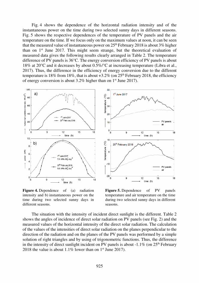
925
Fig. 4 shows the dependence of the horizontal radiation intensity and of the instantaneous power on the time during two selected sunny days in different seasons. Fig. 5 shows the respective dependences of the temperature of PV panels and the air temperature on the time. If we focus only on the maximum values at noon, it can be seen that the measured value of instantaneous power on 25th February 2018 is about 3% higher than on 1st June 2017. This might seem strange, but the theoretical evaluation of measured data gives the following results clearly arranged in Table 2. The temperature difference of PV panels is 36°C. The energy conversion efficiency of PV panels is about 18% at 20°C and it decreases by about 0.5%/°C at increasing temperature (Libra et al., 2017). Thus, the difference in the efficiency of energy conversion due to the different temperature is 18% from 18%, that is about +3.2% (on 25th February 2018, the efficiency of energy conversion is about 3.2% higher than on 1st June 2017).
Figure 4. Dependence of (a) radiation intensity and b) instantaneous power on the time during two selected sunny days in different seasons.
Figure 5. Dependence of PV panels temperature and air temperature on the time during two selected sunny days in different seasons.
The situation with the intensity of incident direct sunlight is the different. Table 2
shows the angles of incidence of direct solar radiation on PV panels (see Fig. 2) and the measured values of the horizontal intensity of the direct solar radiation. The calculation of the values of the intensities of direct solar radiation on the planes perpendicular to the direction of the radiation and on the planes of the PV panels was performed by a simple solution of right triangles and by using of trigonometric functions. Thus, the difference in the intensity of direct sunlight incident on PV panels is about -1.1% (on 25th February 2018 the value is about 1.1% lower than on 1st June 2017).
a)
b)
6 9 12 15 18
6 9 12 15 18
10
8
6
4
2
0
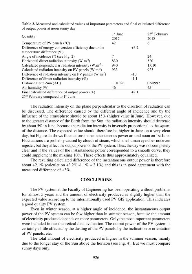
926
Table 2. Measured and calculated values of important parameters and final calculated difference of output power at noon sunny day
Quantity 1st June 2017
25th February 2018
Temperature of PV panels (°C) 42 6 Difference of energy conversion efficiency due to the temperature difference (%)
+3.2
Angle of incidence (°) (see Fig. 2) 7 24 Horizontal direct radiation intensity (W.m-2) 830 520 Calculated perpendicular radiation intensity (W.m-2) 940 1,010 Calculated radiation intensity on PV panels (W.m-2) 933 923 Difference of radiation intensity on PV panels (W.m-2) -10 Difference of direct radiation intensity (%) -1.1 Distance Earth-Sun (AU) 1.01396 0.98992 Air humidity (%) 46 45 Final calculated difference of output power (%) 25th February compared to 1st June
+2.1
The radiation intensity on the plane perpendicular to the direction of radiation can
be discussed. The difference caused by the different angle of incidence and by the influence of the atmosphere should be about 15% (higher value in June). However, due to the greater distance of the Earth from the Sun, the radiation intensity should decrease by about 5% in June, because the radiation intensity is inversely proportional to the square of the distance. The expected value should therefore be higher in June on a very clear day, but Figure 4a shows fluctuations in the instantaneous power around noon on 1st June. Fluctuations are probably caused by clouds of steam, which the human eye does not even register, but they affect the output power of the PV system. Thus, the day was not completely clear and if the values of the instantaneous power corresponded to a smooth curve, they could supplement the missing 10%. These effects thus approximately equalized.
The resulting calculated difference of the instantaneous output power is therefore about +2.1% (calculation +3.2% -1.1% = 2.1%) and this is in good agreement with the measured difference of +3%.
CONCLUSIONS
The PV system at the Faculty of Engineering has been operating without problems
for almost 5 years and the amount of electricity produced is slightly higher than the expected value according to the internationally used PV GIS application. This indicates a good quality PV system.
Even in winter season, at a higher angle of incidence, the instantaneous output power of the PV system can be few higher than in summer season, because the amount of electricity produced depends on more parameters. Only the most important parameters were included in our theoretical data evaluation. The output power of the PV system is certainly a little affected by the dusting of the PV panels, by the inclination or orientation of PV panels, etc.
The total amount of electricity produced is higher in the summer season, mainly due to the longer stay of the Sun above the horizon (see Fig. 4). But we must compare sunny days only.
927
The amount of electricity produced could be increased by cooling the PV panels especially in summer season, because at lower temperatures the efficiency of photovoltaic energy conversion is higher (Libra et al., 2017). However, this would require a more complicated design of hybrid photovoltaic-photothermal panels and cooling water circulation. This problem has already been studied and such hybrid panels exist, see for example (Zagorska et al., 2012, Matuška et al., 2015).
ACKNOWLEDGEMENTS. The work was supported by the internal research project of the Faculty of Engineering IGA 2021.
REFERENCES
Ayompe, L.M., Duffy, A., McCormack, S.J. & Conlon, M., 2011. Measured performance of a
1.72 kW rooftop grid connected photovoltaic system in Ireland. Energy Conversion and Management 52(2), 816–825. doi: 10.1016/j.enconman.2010.08.007
Baena, F., Muñoz-Rodriguez, F.J., Vidal, P.G. & Almonacid, G. 2020. A New Approach to Estimate from Monitored Demand Data the Limit of the Coverage of Electricity Demand through Photovoltaics in Large Electricity Grids. Sensors 20(16), 4390. doi: 10.3390/s20164390
Beránek, V., Olšan, T., Libra, M., Poulek, V., Sedláček, J., Dang, M.Q. & Tyukhov, I. 2018. New Monitoring System for Photovoltaic Power Plants’ Management. Energies 11(10), Article ID 2495. doi: 10.3390/en11102495
Bilčík, M., Božiková, M. & Malínek, M. 2019. The Influence of Selected External Factors on Temperature of Photovoltaic Modules. Acta Technologica Agriculturae 22(4), 122–127. doi: 10.2478/ata-2019-0022
Daneček, M., Havrlík, M., Beránek, V., Šafránková, J., Libra, M., Poulek, V., Sedláček, J. & Belza, R. 2020. Design and data comparison of the photovoltaic power plants in the southern and northern hemispheres. Agronomy Research 18(S1), 755–761. doi: 10.15159/AR.20.096
Kazem, H.A., Chaichan, M.T., Al-Waeli, A.H.A. & Sopian, K., 2020. Evaluation of aging and performance of grid-connected photovoltaic system northern Oman: Seven years’ experimental study. Solar Energy, 207, 1247–1258. doi: 10.1016/j.solener.2020.07.061
Libra, M., Poulek, V. & Kouřím, P. 2017. Temperature changes of I-V characteristics of photovoltaic cells as a consequence of the Fermi energy level shift. Research in Agricultural Engineering 63(1), 10–15. doi: 10.17221/38/2015-RAE
Libra, M., Daneček, M., Lešetický, J., Poulek, V., Sedláček, J. & Beránek, V. 2019. Monitoring of Defects of a Photovoltaic Power Plant Using a Drone. Energies 12(5), Article No. 795. doi: 10.3390/en12050795
Madeti, S.R. & Singh, S.N., 2017. Monitoring system for photovoltaic plants: A review. Renewable and Sustainable Energy Reviews 67, 1180–1207. doi: 10.1016/j.rser.2016.09.088
Matuška, T., Sourek, B., Jirka, V. & Pokorny, N. 2015. Glazed PVT collector with polysiloxane encapsulation of PV cells: Performance and economic analysis. International Journal of Photoenergy 2015, article number 718316. doi: 10.1155/2015/718316
Øgaard, M.B., Riise, H.N., Haug, H., Sartori, S. & Selj, J.H., 2020. Photovoltaic system monitoring for high latitude locations. Solar Energy 207, 1045–1054. doi: 10.1016/j.solener.2020.07.043
Photovoltaic Geographical Information System (PVGIS) [online], 2020. Available from: https://re.jrc.ec.europa.eu/pvg_tools/en/tools.html. Accessed 26.10.2020.
Spertino, F., Ciocia, A., Di Leo, P., Tommasini, R., Berardone, I., Corrado, M., Infuso, A. & Paggi, M. 2015. A power and energy procedure in operating photovoltaic systems to quantify the losses according to the causes. Solar Energy 118, 313–326. doi: 10.1016/j.solener.2015.05.033
Zagorska, V., Ziemelis, I., Kancevica, L. & Putans, H., 2012. Experimental investigation of photovoltaic-thermal hybrid solar collector. Agronomy Research 10(S1), 227–234.
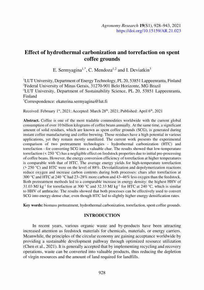
928
Agronomy Research 19(S1), 928–943, 2021 https://doi.org/10.15159/AR.21.023
Effect of hydrothermal carbonization and torrefaction on spent coffee grounds
E. Sermyagina1,*, C. Mendoza1,2 and I. Deviatkin3
1LUT University, Department of Energy Technology, PL 20, 53851 Lappeenranta, Finland 2Federal University of Minas Gerais, 31270-901 Belo Horizonte, MG Brazil 3LUT University, Department of Sustainability Science, PL 20, 53851 Lappeenranta, Finland *Correspondence: [email protected] Received: February 1st, 2021; Accepted: March 28th, 2021; Published: April 6th, 2021 Abstract. Coffee is one of the most tradable commodities worldwide with the current global consumption of over 10 billion kilograms of coffee beans annually. At the same time, a significant amount of solid residues, which are known as spent coffee grounds (SCG), is generated during instant coffee manufacturing and coffee brewing. Those residues have a high potential in various applications, yet they remain mostly unutilized. The current work presents the experimental comparison of two pretreatment technologies - hydrothermal carbonization (HTC) and torrefaction - for converting SCG into a valuable char. The results showed that low-temperature torrefaction (< 250 °C) has a negligible effect on feedstock properties due to initial pre-processing of coffee beans. However, the energy conversion efficiency of torrefaction at higher temperatures is comparable with that of HTC. The average energy yields for high-temperature torrefaction (> 250 °C) and HTC were on the level of 88%. Devolatilization and depolymerization reactions reduce oxygen and increase carbon contents during both processes: chars after torrefaction at 300 °C and HTC at 240 °C had 23–28% more carbon and 43–46% less oxygen than the feedstock. Both pretreatment methods led to a comparable increase in energy density: the highest HHV of 31.03 MJ kg-1 for torrefaction at 300 °C and 32.33 MJ kg-1 for HTC at 240 °C, which is similar to HHV of anthracite. The results showed that both processes can be effectively used to convert SCG into energy-dense char, even though HTC led to slightly higher energy densification rates. Key words: biomass pretreatment, hydrothermal carbonization, torrefaction, spent coffee grounds.
INTRODUCTION
In recent years, various organic waste and by-products have been attracting increased attention as feedstock materials for chemicals, materials, or energy carriers. Meanwhile, the principles of the circular economy are gaining acceptance worldwide by providing a sustainable development pathway through optimized resource utilization (Chen et al., 2021). It is generally accepted that by implementing recycling and recovery operations, waste can be converted into valuable products, thus reducing the depletion of virgin resources and the amount of land required for landfills.
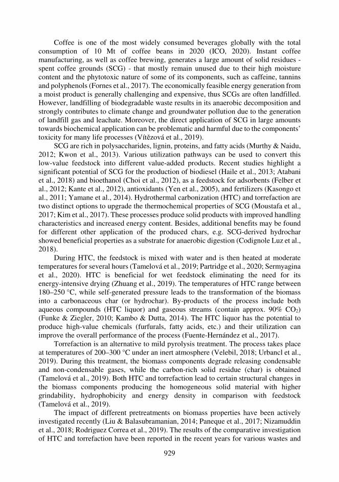
929
Coffee is one of the most widely consumed beverages globally with the total consumption of 10 Mt of coffee beans in 2020 (ICO, 2020). Instant coffee manufacturing, as well as coffee brewing, generates a large amount of solid residues - spent coffee grounds (SCG) - that mostly remain unused due to their high moisture content and the phytotoxic nature of some of its components, such as caffeine, tannins and polyphenols (Fornes et al., 2017). The economically feasible energy generation from a moist product is generally challenging and expensive, thus SCGs are often landfilled. However, landfilling of biodegradable waste results in its anaerobic decomposition and strongly contributes to climate change and groundwater pollution due to the generation of landfill gas and leachate. Moreover, the direct application of SCG in large amounts towards biochemical application can be problematic and harmful due to the components’ toxicity for many life processes (Vítězová et al., 2019).
SCG are rich in polysaccharides, lignin, proteins, and fatty acids (Murthy & Naidu, 2012; Kwon et al., 2013). Various utilization pathways can be used to convert this low-value feedstock into different value-added products. Recent studies highlight a significant potential of SCG for the production of biodiesel (Haile et al., 2013; Atabani et al., 2018) and bioethanol (Choi et al., 2012), as a feedstock for adsorbents (Felber et al., 2012; Kante et al., 2012), antioxidants (Yen et al., 2005), and fertilizers (Kasongo et al., 2011; Yamane et al., 2014). Hydrothermal carbonization (HTC) and torrefaction are two distinct options to upgrade the thermochemical properties of SCG (Moustafa et al., 2017; Kim et al., 2017). These processes produce solid products with improved handling characteristics and increased energy content. Besides, additional benefits may be found for different other application of the produced chars, e.g. SCG-derived hydrochar showed beneficial properties as a substrate for anaerobic digestion (Codignole Luz et al., 2018).
During HTC, the feedstock is mixed with water and is then heated at moderate temperatures for several hours (Tamelová et al., 2019; Partridge et al., 2020; Sermyagina et al., 2020). HTC is beneficial for wet feedstock eliminating the need for its energy-intensive drying (Zhuang et al., 2019). The temperatures of HTC range between 180–250 °C, while self-generated pressure leads to the transformation of the biomass into a carbonaceous char (or hydrochar). By-products of the process include both aqueous compounds (HTC liquor) and gaseous streams (contain approx. 90% CO2) (Funke & Ziegler, 2010; Kambo & Dutta, 2014). The HTC liquor has the potential to produce high-value chemicals (furfurals, fatty acids, etc.) and their utilization can improve the overall performance of the process (Fuente-Hernández et al., 2017).
Torrefaction is an alternative to mild pyrolysis treatment. The process takes place at temperatures of 200–300 °C under an inert atmosphere (Velebil, 2018; Urbancl et al., 2019). During this treatment, the biomass components degrade releasing condensable and non-condensable gases, while the carbon-rich solid residue (char) is obtained (Tamelová et al., 2019). Both HTC and torrefaction lead to certain structural changes in the biomass components producing the homogeneous solid material with higher grindability, hydrophobicity and energy density in comparison with feedstock (Tamelová et al., 2019).
The impact of different pretreatments on biomass properties have been actively investigated recently (Liu & Balasubramanian, 2014; Paneque et al., 2017; Nizamuddin et al., 2018; Rodriguez Correa et al., 2019). The results of the comparative investigation of HTC and torrefaction have been reported in the recent years for various wastes and
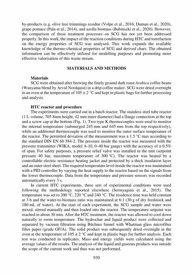
930
by-products (e.g. olive tree trimmings residue (Volpe et al., 2016; Duman et al., 2020), grape pomace (Pala et al., 2014), and azolla biomass (Babinszki et al., 2020). However, the comparison of these treatment processes on SCG has not yet been addressed properly. In this work, the impact of the reaction conditions during HTC and torrefaction on the energy properties of SCG was analysed. This work expands the available knowledge of the thermo-chemical properties of SCG and derived chars. The obtained information can be effectively utilized for modelling purposes and promoting more effective valorisation of this waste stream.
MATERIALS AND METHODS
Materials SCG were obtained after brewing the finely ground dark roast Arabica coffee beans
(Wanyama blend by Arvid Nordquist) in a drip coffee maker. SCG were dried overnight in an oven at the temperature of 105 ± 2 °C and kept in plastic bags for further processing and analysis.
HTC reactor and procedure The experiments were carried out in a batch reactor. The stainless steel tube reactor
(1 L volume, 705 8mm height, 42 mm inner diameter) had a flange connection at the top and a screw cap at the bottom (Fig. 1). Two type K thermocouples were used to monitor the internal temperature (submerged 245 mm and 645 mm from the top respectively), while an additional thermocouple was used to monitor the outer surface temperature of the reactor. The permitted deviation of the measurement was ± 1.5 °C max according to the standard DIN EN 60 584-2. The pressure inside the reactor was measured with the pressure transmitter (WIKA, model A-10, 0–40 bar gauge) with the accuracy of ± 0.5% of span. For safety purposes, a pressure relief valve was installed in the unit (setpoint pressure 40 bar, maximum temperature of 300 °C). The reactor was heated by a controllable electric resistance heating jacket and protected by a thick insulation layer and an outer steel sheet. The required temperature level inside the reactor was maintained with a PID controller by varying the heat supply to the reactor based on the signals from the lower thermocouple. Data from the temperature and pressure sensors was recorded automatically every 3 s.
In current HTC experiments, three sets of experimental conditions were used following the methodology reported elsewhere (Sermyagina et al., 2015). The temperature was set to 200 °C, 220 °C and 240 °C. The residence time was held constant at 3 h and the water-to-biomass ratio was maintained at 6:1 (30 g of dry feedstock and 180 mL of water). At the start of each experiment, the SCG sample and water were mixed, stirred manually and then loaded into the reactor. The temperature setpoint was reached in about 30 min. After the HTC treatment, the reactor was allowed to cool down naturally to room temperature. The hydrochar and liquid product were collected and separated by vacuum filtration using Büchner funnel with Whatman glass microfiber filter paper (grade GF/A). The solid product was subsequently dried overnight in the oven at the temperature of 105 ± 2 °C and kept in plastic bags for further analysis. Each test was conducted in replicates. Mass and energy yields were calculated using the average values of the results. The analysis of the liquid and gaseous products was outside the scope of the current work and thus was not performed.
931
Figure 1. HTC experimental unit and experimental procedure. Hydrochar samples were named following the process temperature as HTC-t,
where t denotes the reaction temperature in °C. Torrefaction reactor and procedur For the torrefaction experiments,
a vertical quartz tube (780 mm length, 45 mm diameter) was used with the previously described electric resistance heating jacket (Fig. 2). The feedstock was placed onto the sintered quartz glass grid in the reactor and the constant gas flow of nitrogen of 0.5 L min-1 was introduced and maintained by Bronkhorst mass flow controllers to obtain an inert atmosphere. The gas inlet was at the bottom part of the reactor and the outlet at the top. Two type K thermocouples were used to measure the temperature below and above the grid. The temperature inside the reactor was controlled with a PID controller by varying the heat supply on the basis of the signals from upper thermocouple. The data from temperature sensors and mass flow controllers were recorded automatically every 3 s.
Figure 2. Bench-scale torrefaction unit.
932
For each torrefaction test, about 9 g of SCG were introduced into the reactor and the nitrogen was used to purge the air from the system for several minutes before the start of the heating. The temperature setpoints varied between 200 °C and 300 °C with 20 °C incremental steps. The heating rate was set on the level 10 °C min-1. The residence time was held constant at 60 min. After each test, the reactor and the samples were allowed to cool down naturally to room temperature. The char was then collected and kept in plastic bags for further analysis. Torrefied char samples were named according to the process parameters as Torre-t, where t denotes the reaction temperature in °C. The analysis of the gaseous products was outside the scope of the current work.
Analytical methods Both the SCG and the produced char samples were characterized using the standard
procedures. Characterization was performed at least twice for each reaction condition, and the average value was reported.
For the proximate analysis, the samples were first dried in a laboratory oven at the temperature of 105 ± 2 °C until a constant mass was reached to determine the moisture content with the simplified oven-dry method EN 14774-2 (SFS, 2009a). The ash content was determined according to EN 14775 (SFS, 2009b) by gradually heating the sample to 550 °C and maintaining it at a constant temperature for at least 2 h. The volatile matter was measured by calculating the mass lost at the temperature of 900 ± 10 °C after 7 min without contact with air as described by EN 15148 (SFS, 2012). Fixed carbon content was determined by reducing the mass of ash and volatiles from the initial mass of the dry sample.
The elemental composition, i.e. carbon, hydrogen, nitrogen, oxygen, and sulphur, of the samples was determined following ISO 16948 (SFS, 2015) and ISO 16994 (SFS, 2016). The elemental analysis was performed with a LECO CHN628 Series Elemental Determinator coupled with a 628S Sulphur Add-On Module. Prior to the analysis, the standard samples (ethylenediaminetetraacetic acid for CHN and coal for S measurements) were first analysed to verify the experimental error within ± 1% for the elements. For CHN analysis, approximately 30 mg of oven-dry material were fed in the combustion chamber. The sulphur content was determined by using approximately 50 mg of dried material which was combusted in the sulphur module at 1,350 °C. The results are presented on a dry basis as the mean of replicates. The oxygen content was approximated as the difference between 100% and the weight percentages of the major elements and ash on a dry basis.
Thermogravimetric analysis (TGA) was performed with STA 449C thermogravimetric analyzer (Netzsch Instruments, Germany). About 10 mg of the sample were placed inside Al2O3 sample holder. The furnace was sealed and purged with high purity (99.9995 %) nitrogen flow to remove air. The sample was heated from room temperature to 900 °C at rate of 20 °C min-1. Two different gas atmospheres were applied: high purity nitrogen for pyrolysis conditions and compressed air for combustion conditions. In both cases, a constant gas flow rate of 250 mL min-1 was maintained.
The morphology of the samples was examined by scanning electron microscopy (SEM) using a Hitachi SU3500 microscope.

933
The mass yield (MY, %) was calculated on a dry basis (d.b.) as follows: iÈ = :CÉu :BK ∙ 100% (1)
where min – the initial mass of feedstock (d.b.), g; mout – the solid mass output (d.b.), g. The energy densification ratio (ER) was calculated as follows: b= = ÊÊQl´CDÊÊQ£F (2)
The energy yield (EY, %), was calculated as follows: bÈ = iÈ ∙ b= (3)
The higher heating values on dry basis (HHV, d.b.) of the samples were calculated with Eq. (4) from Reed & Gaur (1994): ÊÊQ, v. P. = 0.3491 ∙ Ë» + 1.1783 ∙ ËÌ + 0.1005 ∙ ËÍ − 0.0151 ∙ ËÎ − 0.1034 ∙ ËÏ − 0.0211 ∙ Ëл (4)
where HHV in MJ kg-1 (d.b.); XÒ - concentrations of carbon (C), hydrogen (H), oxygen (O), sulphur (S), nitrogen (N) and ash content in wt.% (d.b.). HHVprod is higher heating value of the product char, MJ kg-1 and HHVfs is higher heating value of the feedstock, MJ kg-1.
RESULTS AND DISCUSSION
Mass and energy yields The mass yield was calculated with Eq. (1). Fig. 3 presents the results of
torrefaction and HTC together with the correlation curves for the char mass yield. The equations for the correlations are given between reaction temperature, T, in °C, and the mass yield values in the percentage points. The solid yield decreased with the reaction temperature for both treatment methods. In the case of torrefaction, low-degree processing (< 250 °C) had a limited effect on the SCG decomposition which can be seen from the negligible mass loss. This result could be attributed to the structural modifications that have already happened during initial roasting of coffee beans. The typical roasting temperatures are in the range of 220–240 °C, the roasting process can be compared to a low-temperature torrefaction that results limited devolatilization of SCG components. Such pre-processing explains the limited changes in the feedstock during low-degree torrefaction. At the same time, higher temperatures led to the mass loss intensification with the maximum value of 32% at 300 °C. Overall, the obtained values fit well with the polynomial correlation (R2 = 0.999). As for the HTC tests, the reaction temperature increase led to a steady decrease in the mass yield from 81% at 200 °C to 72% at 240 °C. The HTC conditions resulted in a higher mass loss at the lower temperature limit in comparison with torrefaction. Water during this treatment acts as a catalyst and a reactant for organic compounds of the feedstock, thus making them more reactive (Román et al., 2012). Linear regression was fitted to the individual HTC runs with an R2 value of 0.961.
The higher heating values were calculated with Eq. (4). The impact of the reaction temperature on the HHV of the products is presented in Fig. 4. The values for the coal grades are from (Donahue & Rais, 2009).The rapid increase of the heating values can be seen for the torrefied samples treated at 260 °C and higher, while low temperatures result
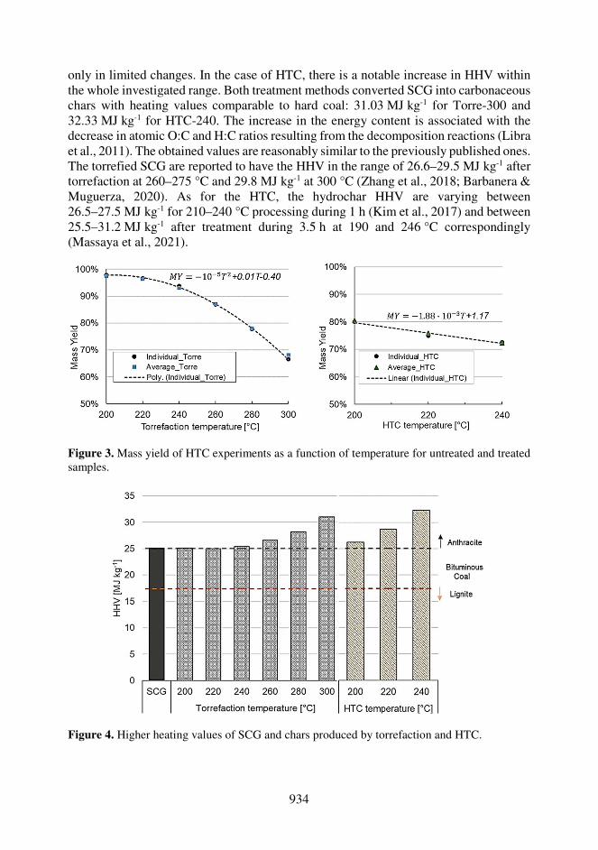
934
only in limited changes. In the case of HTC, there is a notable increase in HHV within the whole investigated range. Both treatment methods converted SCG into carbonaceous chars with heating values comparable to hard coal: 31.03 MJ kg-1 for Torre-300 and 32.33 MJ kg-1 for HTC-240. The increase in the energy content is associated with the decrease in atomic O:C and H:C ratios resulting from the decomposition reactions (Libra et al., 2011). The obtained values are reasonably similar to the previously published ones. The torrefied SCG are reported to have the HHV in the range of 26.6–29.5 MJ kg-1 after torrefaction at 260–275 °C and 29.8 MJ kg-1 at 300 °C (Zhang et al., 2018; Barbanera & Muguerza, 2020). As for the HTC, the hydrochar HHV are varying between 26.5–27.5 MJ kg-1 for 210–240 °C processing during 1 h (Kim et al., 2017) and between 25.5–31.2 MJ kg-1 after treatment during 3.5 h at 190 and 246 °C correspondingly (Massaya et al., 2021).
Figure 3. Mass yield of HTC experiments as a function of temperature for untreated and treated samples.
Figure 4. Higher heating values of SCG and chars produced by torrefaction and HTC.
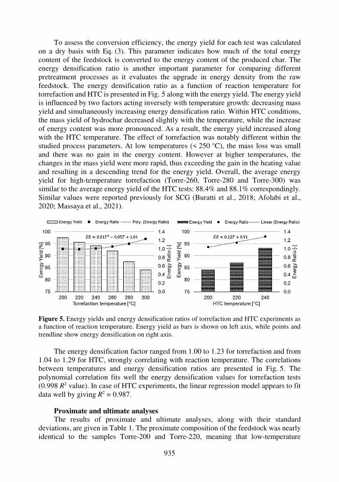
935
To assess the conversion efficiency, the energy yield for each test was calculated on a dry basis with Eq. (3). This parameter indicates how much of the total energy content of the feedstock is converted to the energy content of the produced char. The energy densification ratio is another important parameter for comparing different pretreatment processes as it evaluates the upgrade in energy density from the raw feedstock. The energy densification ratio as a function of reaction temperature for torrefaction and HTC is presented in Fig. 5 along with the energy yield. The energy yield is influenced by two factors acting inversely with temperature growth: decreasing mass yield and simultaneously increasing energy densification ratio. Within HTC conditions, the mass yield of hydrochar decreased slightly with the temperature, while the increase of energy content was more pronounced. As a result, the energy yield increased along with the HTC temperature. The effect of torrefaction was notably different within the studied process parameters. At low temperatures (< 250 °C), the mass loss was small and there was no gain in the energy content. However at higher temperatures, the changes in the mass yield were more rapid, thus exceeding the gain in the heating value and resulting in a descending trend for the energy yield. Overall, the average energy yield for high-temperature torrefaction (Torre-260, Torre-280 and Torre-300) was similar to the average energy yield of the HTC tests: 88.4% and 88.1% correspondingly. Similar values were reported previously for SCG (Buratti et al., 2018; Afolabi et al., 2020; Massaya et al., 2021).
Figure 5. Energy yields and energy densification ratios of torrefaction and HTC experiments as a function of reaction temperature. Energy yield as bars is shown on left axis, while points and trendline show energy densification on right axis.
The energy densification factor ranged from 1.00 to 1.23 for torrefaction and from
1.04 to 1.29 for HTC, strongly correlating with reaction temperature. The correlations between temperatures and energy densification ratios are presented in Fig. 5. The polynomial correlation fits well the energy densification values for torrefaction tests (0.998 R2 value). In case of HTC experiments, the linear regression model appears to fit data well by giving R2 = 0.987.
Proximate and ultimate analyses The results of proximate and ultimate analyses, along with their standard
deviations, are given in Table 1. The proximate composition of the feedstock was nearly identical to the samples Torre-200 and Torre-220, meaning that low-temperature
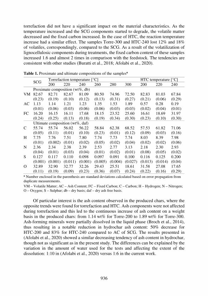
936
torrefaction did not have a significant impact on the material characteristics. As the temperature increased and the SCG components started to degrade, the volatile matter decreased and the fixed carbon increased. In the case of HTC, the reaction temperature increase had a similar effect. The samples Torre-300 and HTC-240 lost 12% and 18% of volatiles, correspondingly, compared to the SCG. As a result of the volatilization of lignocellulosic components during treatments, the fixed carbon content of these samples increased 1.6 and almost 2 times in comparison with the feedstock. The tendencies are consistent with other studies (Buratti et al., 2018; Afolabi et al., 2020).
Table 1. Proximate and ultimate compositions of the samplesα
SCG
Torrefaction temperature [°C] HTC temperature [°C] 200 220 240 260 280 300 200 220 240
Proximate composition (wt%, db) VM 82.67
(0.23) 82.71 (0.19)
82.67 (0.10)
81.09 (0.12)
80.50 (0.13)
74.96 (0.31)
72.50 (0.27)
82.83 (0.21)
81.03 (0.06)
67.84 (0.29)
AC 1.13 (0.01)
1.14 (0.06)
1.21 (0.03)
1.23 (0.06)
1.35 (0.06)
1.53 (0.03)
1.89 (0.03)
0.57 (0.02)
0.28 (0.04)
0.19 (0.01)
FC 16.20 (0.24)
16.15 (0.25)
16.11 (0.13)
17.68 (0.18)
18.15 (0.19)
23.52 (0.34)
25.60 (0.30)
16.61 (0.23)
18.69 (0.10)
31.97 (0.30)
Ultimate composition (wt%, daf) C 55.74
(0.05) 55.74 (0.11)
56.02 (0.01)
56.22 (0.10)
58.84 (0.23)
62.38 (0.01)
68.52 (0.12)
57.53 (0.09)
61.82 (0.03)
71.06 (0.16)
H 7.75 (0.01)
7.76 (0.002)
7.51 (0.01)
7.80 (0.02)
7.74 (0.05)
7.73 (0.02)
7.74 (0.04)
8.03 (0.02)
8.39 (0.02)
7.98 (0.06)
N 2.36 (0.04)
2.34 (0.01)
2.38 (0.03)
2.39 (0.04)
2.53 (0.01)
2.77 (0.02)
3.13 (0.01)
2.18 (0.08)
2.30 (0.05)
2.93 (0.02)
S 0.127 (0.001)
0.117 (0.001)
0.110 (0.011)
0.098 (0.001)
0.097 (0.005)
0.091 (0.004)
0.100 (0.027)
0.116 (0.013)
0.125 (0.014)
0.200 (0.04)
O 32.89 (0.11)
32.90 (0.19)
32.77 (0.09)
32.26 (0.23)
29.43 (0.36)
25.51 (0.07)
18.61 (0.24)
31.58 (0.22)
27.08 (0.16)
17.65 (0.29)
α Number enclosed in the parenthesis are standard deviations calculated based on error propagation from duplicate measurements. VM – Volatile Matter; AC – Ash Content; FC – Fixed Carbon; C – Carbon; H – Hydrogen; N – Nitrogen; O – Oxygen; S – Sulphur; db – dry basis; daf – dry ash free basis.
Of particular interest is the ash content observed in the produced chars, where the
opposite trends were found for torrefaction and HTC. Ash components were not affected during torrefaction and this led to the continuous increase of ash content on a weight basis in the produced chars: from 1.14 wt% for Torre-200 to 1.89 wt% for Torre-300. Ash-forming minerals were partially dissolved in the liquid phase (Broch et al., 2014), thus resulting in a notable reduction in hydrochar ash content: 50% decrease for HTC-200 and 83% for HTC-240 compared to AC of SCG. The results presented in (Afolabi et al., 2020) showed a similar decreasing tendency of ash content in hydrochar, though not as significant as in the present study. The differences can be explained by the variation in the amount of water used for the tests and affecting the extent of the dissolution: 1:10 in (Afolabi et al., 2020) versus 1:6 in the current work.
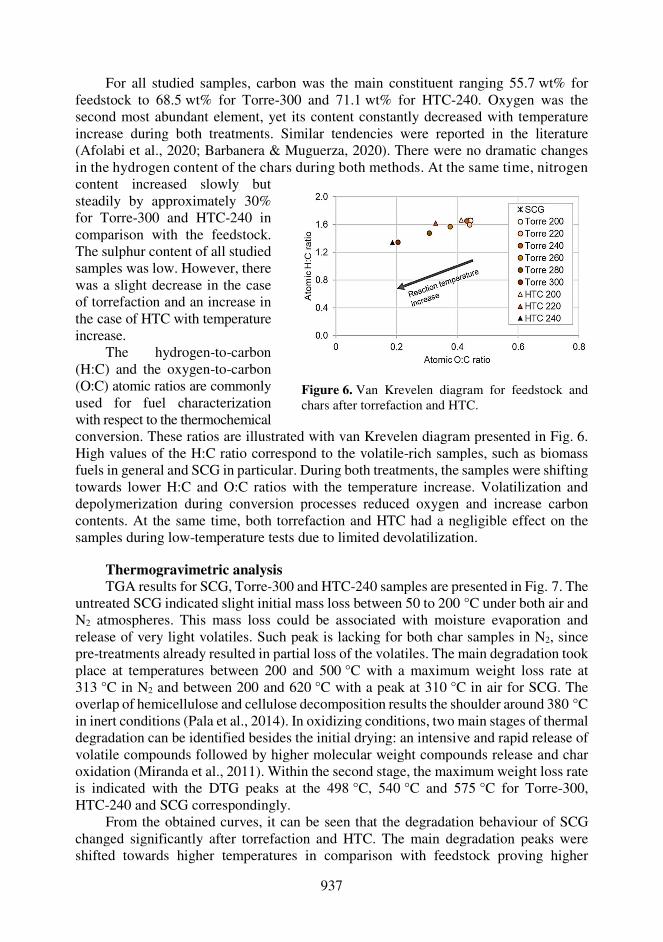
937
For all studied samples, carbon was the main constituent ranging 55.7 wt% for feedstock to 68.5 wt% for Torre-300 and 71.1 wt% for HTC-240. Oxygen was the second most abundant element, yet its content constantly decreased with temperature increase during both treatments. Similar tendencies were reported in the literature (Afolabi et al., 2020; Barbanera & Muguerza, 2020). There were no dramatic changes in the hydrogen content of the chars during both methods. At the same time, nitrogen
conversion. These ratios are illustrated with van Krevelen diagram presented in Fig. 6. High values of the H:C ratio correspond to the volatile-rich samples, such as biomass fuels in general and SCG in particular. During both treatments, the samples were shifting towards lower H:C and O:C ratios with the temperature increase. Volatilization and depolymerization during conversion processes reduced oxygen and increase carbon contents. At the same time, both torrefaction and HTC had a negligible effect on the samples during low-temperature tests due to limited devolatilization.
Thermogravimetric analysis TGA results for SCG, Torre-300 and HTC-240 samples are presented in Fig. 7. The
untreated SCG indicated slight initial mass loss between 50 to 200 °C under both air and N2 atmospheres. This mass loss could be associated with moisture evaporation and release of very light volatiles. Such peak is lacking for both char samples in N2, since pre-treatments already resulted in partial loss of the volatiles. The main degradation took place at temperatures between 200 and 500 °C with a maximum weight loss rate at 313 °C in N2 and between 200 and 620 °C with a peak at 310 °C in air for SCG. The overlap of hemicellulose and cellulose decomposition results the shoulder around 380 °C in inert conditions (Pala et al., 2014). In oxidizing conditions, two main stages of thermal degradation can be identified besides the initial drying: an intensive and rapid release of volatile compounds followed by higher molecular weight compounds release and char oxidation (Miranda et al., 2011). Within the second stage, the maximum weight loss rate is indicated with the DTG peaks at the 498 °C, 540 °C and 575 °C for Torre-300, HTC-240 and SCG correspondingly.
From the obtained curves, it can be seen that the degradation behaviour of SCG changed significantly after torrefaction and HTC. The main degradation peaks were shifted towards higher temperatures in comparison with feedstock proving higher
content increased slowly but steadily by approximately 30% for Torre-300 and HTC-240 in comparison with the feedstock. The sulphur content of all studied samples was low. However, there was a slight decrease in the case of torrefaction and an increase in the case of HTC with temperature increase.
The hydrogen-to-carbon (H:C) and the oxygen-to-carbon (O:C) atomic ratios are commonly used for fuel characterization with respect to the thermochemical
Figure 6. Van Krevelen diagram for feedstock and chars after torrefaction and HTC.
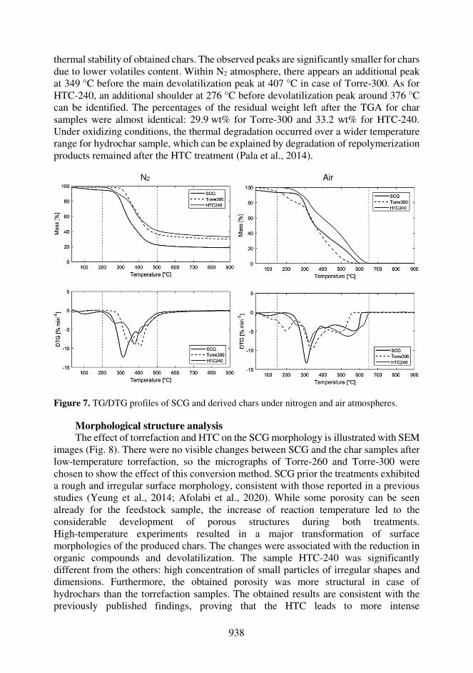
938
thermal stability of obtained chars. The observed peaks are significantly smaller for chars due to lower volatiles content. Within N2 atmosphere, there appears an additional peak at 349 °C before the main devolatilization peak at 407 °C in case of Torre-300. As for HTC-240, an additional shoulder at 276 °C before devolatilization peak around 376 °C can be identified. The percentages of the residual weight left after the TGA for char samples were almost identical: 29.9 wt% for Torre-300 and 33.2 wt% for HTC-240. Under oxidizing conditions, the thermal degradation occurred over a wider temperature range for hydrochar sample, which can be explained by degradation of repolymerization products remained after the HTC treatment (Pala et al., 2014).
N2 Air
Figure 7. TG/DTG profiles of SCG and derived chars under nitrogen and air atmospheres. Morphological structure analysis The effect of torrefaction and HTC on the SCG morphology is illustrated with SEM
images (Fig. 8). There were no visible changes between SCG and the char samples after low-temperature torrefaction, so the micrographs of Torre-260 and Torre-300 were chosen to show the effect of this conversion method. SCG prior the treatments exhibited a rough and irregular surface morphology, consistent with those reported in a previous studies (Yeung et al., 2014; Afolabi et al., 2020). While some porosity can be seen already for the feedstock sample, the increase of reaction temperature led to the considerable development of porous structures during both treatments. High-temperature experiments resulted in a major transformation of surface morphologies of the produced chars. The changes were associated with the reduction in organic compounds and devolatilization. The sample HTC-240 was significantly different from the others: high concentration of small particles of irregular shapes and dimensions. Furthermore, the obtained porosity was more structural in case of hydrochars than the torrefaction samples. The obtained results are consistent with the previously published findings, proving that the HTC leads to more intense
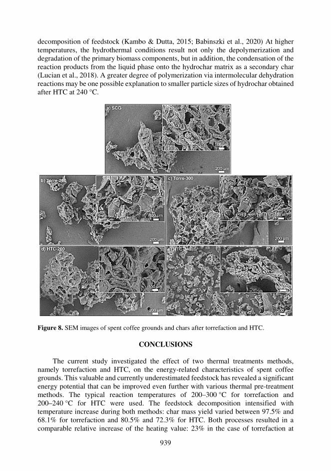
939
decomposition of feedstock (Kambo & Dutta, 2015; Babinszki et al., 2020) At higher temperatures, the hydrothermal conditions result not only the depolymerization and degradation of the primary biomass components, but in addition, the condensation of the reaction products from the liquid phase onto the hydrochar matrix as a secondary char (Lucian et al., 2018). A greater degree of polymerization via intermolecular dehydration reactions may be one possible explanation to smaller particle sizes of hydrochar obtained after HTC at 240 °C.
Figure 8. SEM images of spent coffee grounds and chars after torrefaction and HTC.
CONCLUSIONS
The current study investigated the effect of two thermal treatments methods, namely torrefaction and HTC, on the energy-related characteristics of spent coffee grounds. This valuable and currently underestimated feedstock has revealed a significant energy potential that can be improved even further with various thermal pre-treatment methods. The typical reaction temperatures of 200–300 °C for torrefaction and 200–240 °C for HTC were used. The feedstock decomposition intensified with temperature increase during both methods: char mass yield varied between 97.5% and 68.1% for torrefaction and 80.5% and 72.3% for HTC. Both processes resulted in a comparable relative increase of the heating value: 23% in the case of torrefaction at

940
300 °C and 29% in the case of HTC at 240 °C. The energy yield of HTC increased with temperature from 84.1% for HTC-200 to 93.0% for HTC-240. Alternatively, in the case of torrefaction, higher mass losses resulted in a descending trend for energy yield with temperature from 97.5% for Torre-200 to 84.1% for Torre-300. However, the energy yields for HTC and high-temperature torrefaction (> 250 °C) averaged over the temperature were 87.8% and 87.9% correspondingly. It means that both treatments had relatively similar energy conversion efficiencies.
The release of the volatile compounds and increase of the fixed carbon of SCG during both treatments intensified with temperature. The ash content of the chars produced with torrefaction grew from 1.13 wt% (SCG) to 1.89% (Torre-300). An opposite tendency was in the case of HTC: hydrothermal conditions led to the dissolving of ash forming minerals and ash content decreased to 0.19 wt% (HTC-240). As for the elemental composition, devolatilization and depolymerization reduced oxygen and increased carbon contents during both conversion processes. At the highest temperatures, produced chars indicated 23–28% more carbon and 43–46% less oxygen for torrefaction and HTC correspondingly. The untreated SCG sample was noticeably more reactive during TGA analysis in comparison with the tested char samples. The samples Torre-300 and HTC-240 were more stable under both inert and oxidizing conditions.
The obtained results confirmed that both hydrothermal carbonization and torrefaction could considerably increase the energy content of spent coffee grounds and convert it to highly carbonaceous char with increased energy content. Within the limits of selected reaction parameters, HTC showed slightly higher energy densification rates and more intensive decomposition of feedstock in comparison with torrefaction. An optimal selection of reaction settings affects the efficiency of the treatment and product characteristics. The overall efficiency of the process will be influenced by the heat supply method and subsequent utilization of the char and should be further investigated.
ACKNOWLEDGEMENTS. Authors highly appreciated the help of Toni Väkiparta, D.Sc., in making SEM images of the samples. Special thanks to Jussi Saari, D.Sc., for his valuable input of the coffee feedstock for the current experiments.
REFERENCES
Afolabi, O.O.D., Sohail, M. & Cheng, Y.L. 2020. Optimisation and characterisation of hydrochar
production from spent coffee grounds by hydrothermal carbonisation. Renew. Energy 147, 1380–1391. doi: 10.1016/j.renene.2019.09.098
Atabani, A.E., Mercimek, S.M., Arvindnarayan, S., Shobana, S., Kumar, G., Cadir, M. & Al-Muhatseb, A.H. 2018. Valorization of spent coffee grounds recycling as a potential alternative fuel resource in Turkey: An experimental study. J. Air Waste Manag. Assoc. 68(3), 196–214. doi: 10.1080/10962247.2017.1367738
Babinszki, B., Jakab, E., Sebestyén, Z., Blazsó, M., Berényi,B., Kumar, J., Krishna, B.B., Bhaskar, T. & Czégény, Z. 2020. Comparison of hydrothermal carbonization and torrefaction of azolla biomass: Analysis of the solid products. J. Anal. Appl. Pyrolysis 149, 104844. doi: 10.1016/j.jaap.2020.104844
Barbanera, M. & Muguerza, I.F. 2020. Effect of the temperature on the spent coffee grounds torrefaction process in a continuous pilot-scale reactor. Fuel 262, 116493. doi: 10.1016/j.fuel.2019.116493
941
Broch, A., Jena, U., Hoekman, S.K. & Langford, J. 2014. Analysis of solid and aqueous phase products from hydrothermal carbonization of whole and lipid-extracted algae. Energies 7(1), 62–79. doi: 10.3390/en7010062
Buratti, C., Barbanera, M., Lascaro, E. & Cotana, F. 2018. Optimization of torrefaction conditions of coffee industry residues using desirability function approach. Waste Manag. 73, 523–534. doi: 10.1016/j.wasman.2017.04.012
Chen, W.H., Lin, B.J., Lin, Y.Y., Chu, Y.S., Ubando, A.T., Show, P.L., Ong, H.C., Chang, J.-S., Ho, S.-H., Culaba, A.B., Pétrissans, A. & Pétrissans, M. 2021. Progress in biomass torrefaction: Principles, applications and challenges. Prog. Energy Combust. Sci. 82, 100887. doi: 10.1016/j.pecs.2020.100887
Choi, I.S., Wi, S.G., Kim, S.B. & Bae, H.J. 2012. Conversion of coffee residue waste into bioethanol with using popping pretreatment. Bioresour. Technol. 125, 132–137. doi: 10.1016/j.biortech.2012.08.080
Donahue, C.J., & Rais, E.A. 2009. Proximate analysis of coal. J. Chem. Educ. 86(2), 222–224. doi: 10.1021/ed086p222
Duman, G., Balmuk, G., Cay, H., Kantarli, I.C. & Yanik, J. 2020. Comparative Evaluation of Torrefaction and Hydrothermal Carbonization: Effect on Fuel Properties and Combustion Behavior of Agricultural Wastes. Energy and Fuels 34(9), 11175–11185. doi: 10.1021/acs.energyfuels.0c02255
Felber, R., Hüppi, R., Leifeld, J. & Neftel, A. 2012. Nitrous oxide emission reduction in temperate biochar-amended soils. Biogeosciences Discuss. 9(1), 151–189. doi: 10.5194/bgd-9-151-2012
Fornes, F., Belda, R.M., Fernández de Córdova, P. & Cebolla-Cornejo, J. 2017. Assessment of biochar and hydrochar as minor to major constituents of growing media for containerized tomato production. J. Sci. Food Agric. 97(11), 3675–3684. doi: 10.1002/jsfa.8227
Fuente-Hernández, A., Lee, R., Béland, N., Zamboni, I. & Lavoie, J.M. 2017. Reduction of furfural to furfuryl alcohol in liquid phase over a biochar-supported platinum catalyst. Energies 10(3). doi: 10.3390/en10030286
Funke, A. & Ziegler, F. 2010. Hydrothermal carbonization of biomass: A summary and discussion of chemical mechanisms for process engineering. Biofuels, Bioprod. Biorefining 4(2), 160–177. doi: 10.1002/bbb.198
Haile, M., Asfaw, A. & Asfaw, N. 2013. Investigation of waste coffee ground as a potential raw material for biodiesel production. Int. J. Renew. Energy Res. 3(4), 854–860. doi: 10.20508/ijrer.23113
ICO. 2020. International Coffee Organization - What’s New. http://www.ico.org/ (accessed 4 September 2020).
Kambo, H.S & Dutta, A. 2014. Strength, storage, and combustion characteristics of densified lignocellulosic biomass produced via torrefaction and hydrothermal carbonization. Appl. Energy 135: 182–191. doi: 10.1016/j.apenergy.2014.08.094
Kambo, H.S. & Dutta, A. 2015. Comparative evaluation of torrefaction and hydrothermal carbonization of lignocellulosic biomass for the production of solid biofuel. Energy Convers. Manag. 105, 746–755. doi: 10.1016/j.enconman.2015.08.031
Kante, K., Nieto-Delgado, C., Rangel-Mendez, J.R. & Bandosz, T.J. 2012. Spent coffee-based activated carbon: Specific surface features and their importance for H 2S separation process. J. Hazard. Mater. 201–202, 141–147. doi: 10.1016/j.jhazmat.2011.11.053
Kasongo, R.K., Verdoodt, A., Kanyankagote, P., Baert, G. & Ranst, E.V. 2011. Coffee waste as an alternative fertilizer with soil improving properties for sandy soils in humid tropical environments. Soil Use Manag. 27(1), 94–102. doi: 10.1111/j.1475-2743.2010.00315.x
Kim, D., Lee, K., Bae, D. & Park, K.Y. 2017. Characterizations of biochar from hydrothermal carbonization of exhausted coffee residue. J. Mater. Cycles Waste Manag. 19(3), 1036–1043. doi: 10.1007/s10163-016-0572-2
942
Kwon, E.E., Yi, H. & Jeon, Y.J. 2013. Sequential co-production of biodiesel and bioethanol with spent coffee grounds. Bioresour. Technol. 136, 475–480. doi: 10.1016/j.biortech.2013.03.052
Libra, J.A., Ro, K.S., Kammann, C., Funke, A., Berge, N.D., Neubauer, Y., Titirici, M.M., Fühner, C., Bens, O., Kern, J. & Emmerich, K.H. 2011. Hydrothermal carbonization of biomass residuals: A comparative review of the chemistry, processes and applications of wet and dry pyrolysis. Biofuels 2(1), 71–106. doi: 10.4155/bfs.10.81
Liu, Z. & Balasubramanian, R. 2014. Upgrading of waste biomass by hydrothermal carbonization (HTC) and low temperature pyrolysis (LTP): A comparative evaluation. Appl. Energy 114, 857–864. doi: 10.1016/j.apenergy.2013.06.027
Lucian, M., Volpe, M., Gao, L., Piro, G., Goldfarb, J.L. & Fiori, L. 2018. Impact of hydrothermal carbonization conditions on the formation of hydrochars and secondary chars from the organic fraction of municipal solid waste. Fuel 233, 257–268. doi: 10.1016/j.fuel.2018.06.060
Massaya, J., Chan, K.H., Mills-Lamptey, B. & Chuck, C.J. 2021. Developing a biorefinery from spent coffee grounds using subcritical water and hydrothermal carbonisation. Biomass Convers. Biorefinery 1–17. doi: 10.1007/s13399-020-01231-w
Miranda, M.T., Arranz, J.I., Román, S., Rojas, S., Montero, I., López, M. & Cruz, J.A. 2011. Characterization of grape pomace and pyrenean oak pellets. Fuel Processing Technology. Elsevier. p. 278–283.
Moustafa, H., Guizani, C., Dupont, C., Martin, V., Jeguirim, M. & Dufresne, A. 2017. Utilization of torrefied coffee grounds as reinforcing agent to produce high-quality biodegradable PBAT composites for food packaging applications. ACS Sustain. Chem. Eng. 5(2), 1906–1916. doi: 10.1021/acssuschemeng.6b02633
Murthy, P.S. & Naidu, M.M. 2012. Recovery of Phenolic Antioxidants and Functional Compounds from Coffee Industry By-Products. Food Bioprocess Technol. 5(3), 897–903. doi: 10.1007/s11947-010-0363-z
Nizamuddin, S., Baloch, H.A., Siddiqui, M.T.H., Mubarak, N.M., Tunio, M.M., Bhutto, A.W. & Srinivasan, M.P. 2018. An overview of microwave hydrothermal carbonization and microwave pyrolysis of biomass. Rev. Environ. Sci. Biotechnol. 17(4), 813–837. doi: 10.1007/s11157-018-9476-z
Pala, M., Kantarli, I.C., Buyukisik, H.B. & Yanik, J. 2014. Hydrothermal carbonization and torrefaction of grape pomace: A comparative evaluation. Bioresour. Technol. 161, 255–262. doi: 10.1016/j.biortech.2014.03.052
Paneque, M., De la Rosa, J.M., Kern, J., Reza, M.T. & Knicker, H. 2017. Hydrothermal carbonization and pyrolysis of sewage sludges: What happen to carbon and nitrogen? J. Anal. Appl. Pyrolysis 128, 314–323. doi: 10.1016/j.jaap.2017.09.019
Partridge, A., Sermyagina, E. & Vakkilainen, E. 2020. Impact of pretreatment on hydrothermally carbonized spruce. Energies 13(11). doi: 10.3390/en13112984
Reed, T.B. & Gaur, S. 1994. Atlas of thermal data of biomass and other fuels-a report on the forthcoming book. Pergamon.
Rodriguez Correa, C., Hehr, T., Voglhuber-Slavinsky, A., Rauscher, Y. & Kruse, A. 2019. Pyrolysis vs. hydrothermal carbonization: Understanding the effect of biomass structural components and inorganic compounds on the char properties. J. Anal. Appl. Pyrolysis 140, 137–147. doi: 10.1016/j.jaap.2019.03.007
Román, S., Nabais, J.M.V, Laginhas, C., Ledesma, B. & González, J.F. 2012. Hydrothermal carbonization as an effective way of densifying the energy content of biomass. Fuel Process. Technol. 103, 78–83. doi: 10.1016/j.fuproc.2011.11.009
Sermyagina, E., Saari, J., Kaikko, J. & Vakkilainen, E. 2015. Hydrothermal carbonization of coniferous biomass: Effect of process parameters on mass and energy yields. J. Anal. Appl. Pyrolysis 113, 551–556. doi: 10.1016/j.jaap.2015.03.012

943
Sermyagina, E., Murashko, K., Nevstrueva, D. & Vakkilainen, E. 2020. Conversion of cellulose to activated carbons for high-performance supercapacitors. Agron. Res. 18(3), 2197–2210. doi: 10.15159/AR.20.163
SFS, 2009a. EN 14774-2 Solid biofuels - Determination of moisture content - Oven dry method - Part 2: Total moisture - Simplified method.
SFS, 2009b. SFS-EN 14775:en Solid biofuels. Determination of ash content. SFS, 2012. EN 15148 Solid biofuels - Determination of the content of volatile matter. SFS, 2015. ISO 16948 Solid biofuels. Determination of total content of carbon, hydrogen and
nitrogen. SFS, 2016. ISO 16994 Solid biofuels. Determination of total content of sulfur and chlorine. Tamelová, B., Malaťák, J. & Velebil, J. 2019. Hydrothermal carbonization and torrefaction of
cabbage waste. Agron. Res. 17(3), 862–871. doi: 10.15159/AR.19.098 Urbancl, D., Krope, J. & Goričanec, D. 2019. Torrefaction-the process for biofuels production by
using different biomasses. Agron. Res. 17(4), 1800–1807. doi: 10.15159/AR.19.176. Velebil, J. 2018. Energy valorisation of citrus peel waste by torrefaction treatment. Agron. Res.
16(1), 276. doi: 10.15159/AR.18.029 Vítězová, M., Jančiková, S., Dordević, D., Vítěz, T., Elbl, J., Hanišáková, N., Jampílek, J. &
Kushkevych, I. 2019. The Possibility of Using Spent Coffee Grounds to Improve Wastewater Treatment Due to Respiration Activity of Microorganisms. Appl. Sci. 9(15), 3155. doi: 10.3390/app9153155
Yamane, K., Kono, M., Fukunaga, T., Iwai, K., Sekine, R., Watanabe, Y. & Iijima, M. 2014. Field evaluation of coffee grounds application for crop growth enhancement, weed control, and soil improvement. Plant Prod. Sci. 17(1), 93–102. doi: 10.1626/pps.17.93
Yen, W.J., Wang, B.S., Chang, L.W. & Duh, P.D. 2005. Antioxidant properties of roasted coffee residues. J. Agric. Food Chem. doi: 10.1021/jf0402429
Yeung, P.T., Chung, P.Y., Tsang, H.C., Cheuk-On Tang, J., Yin-Ming Cheng, G., Gambari, R. & Lam, K.H. 2014. Preparation and characterization of bio-safe activated charcoal derived from coffee waste residue and its application for removal of lead and copper ions. RSC Adv. 4(73), 38839–38847. doi: 10.1039/c4ra05082g
Zhang, C., Ho, S.H., Chen, W.H., Xie, Y., Liu, Z. & Chang, J.S. 2018. Torrefaction performance and energy usage of biomass wastes and their correlations with torrefaction severity index. Appl. Energy 220, 598–604. doi: 10.1016/j.apenergy.2018.03.129
Zhuang, X., Zhan, H., Song, Y., He, C., Huang, Y., Yin, X. & Wu, C. 2019. Insights into the evolution of chemical structures in lignocellulose and non-lignocellulose biowastes during hydrothermal carbonization (HTC). Fuel 236, 960–974. doi: 10.1016/j.fuel.2018.09.019
944
Agronomy Research 19(S1), 944–960, 2021 https://doi.org/10.15159/AR.21.074
An overview of measurement standards for power quality
N. Shabbir*, L. Kütt, M. Jarkovoi, M.N. Iqbal, A. Rassõlkin and K. Daniel
Tallinn University of Technology, School of Engineering, Department of Electrical Power Engineering & Mechatronics, Ehitajate tee 5, EE19086 Tallinn, Estonia *Correspondence: [email protected] Received: December 7th, 2020; Accepted: April 7th, 2021; Published: May 13th, 2021 Abstract. Power Quality (PQ) is a vital aspect of electrical power systems, which cannot be neglected anymore, as an ample PQ guarantees the essential compatibility between consumer equipment and the electricity network. The analysis of electrical parameters related to distributing electricity is recognized as a complex engineering problem. It remains a critical task to maintain and improve PQ in modern evolving networks as the overall system performance highly depends on it. Future smart grids will also require a further increase in PQ levels in terms of observability, affordability, data exchange, flexibility, and net metering, thus making the network much more complex as it will be featuring a large amount of variable renewable-based distributed generation. This will further require the need for the introduction of novel, efficient and intelligent monitoring, control, and communication systems with various demand manageable resources. In this paper, a review and comparisons have been made for different IEEE and IEC measurement standards that are used for PQ with a specific focus on harmonic distortion as it is one of the most important parameters in PQ and some guidelines have been suggested for future electricity networks. Key words: power quality, measurement standards, voltage harmonics, current harmonics, distortions.
INTRODUCTION
The growing demand for service quality, safety, reliability, and efficiency, as well as the inclusion of increasingly environmental and sustainable energy sources, is making the management of electricity networks more complex ( Lizana et al., 2018; Khalid et al., 2019; Nolasco et al., 2019a; Stanisvavljevis & Kati, 2019). Now a more flexible and efficient electricity system is needed, which is mostly referred to as Smart Grid (SG). To achieve this milestone, a combination of new technologies including Distributed Generation (DG), Renewable Energy Sources (RES) with storage capacity, and the latest Information and Communication Technologies (ICT) is needed (CIGRE 719, 2018; Gandoman et al., 2018; Rodrigues Junior et al., 2019). However, the installation of these new devices will also increase Power Quality (PQ) issues (Marais et al., 2018). Two major causes of issues related to PQ and Electromagnetic Compatibility (EMC) have been identified, first at the consumer equipment end (load) and second at the distribution and transmission systems end (Rönnberg & Bollen, 2016). The emissions by these new
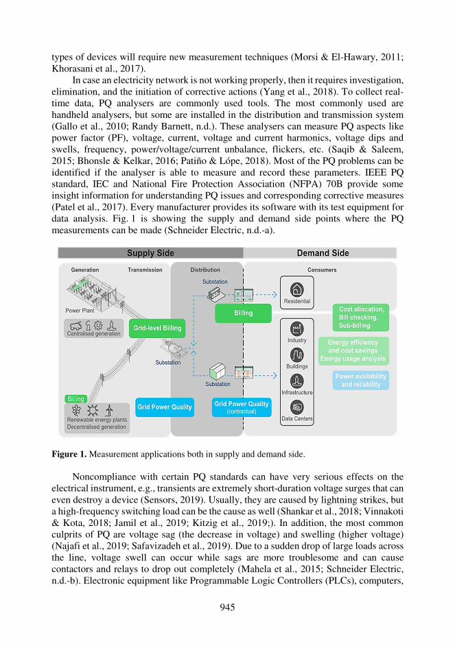
945
types of devices will require new measurement techniques (Morsi & El-Hawary, 2011; Khorasani et al., 2017).
In case an electricity network is not working properly, then it requires investigation, elimination, and the initiation of corrective actions (Yang et al., 2018). To collect real-time data, PQ analysers are commonly used tools. The most commonly used are handheld analysers, but some are installed in the distribution and transmission system (Gallo et al., 2010; Randy Barnett, n.d.). These analysers can measure PQ aspects like power factor (PF), voltage, current, voltage and current harmonics, voltage dips and swells, frequency, power/voltage/current unbalance, flickers, etc. (Saqib & Saleem, 2015; Bhonsle & Kelkar, 2016; Patiño & Lópe, 2018). Most of the PQ problems can be identified if the analyser is able to measure and record these parameters. IEEE PQ standard, IEC and National Fire Protection Association (NFPA) 70B provide some insight information for understanding PQ issues and corresponding corrective measures (Patel et al., 2017). Every manufacturer provides its software with its test equipment for data analysis. Fig. 1 is showing the supply and demand side points where the PQ measurements can be made (Schneider Electric, n.d.-a).
Figure 1. Measurement applications both in supply and demand side.
Noncompliance with certain PQ standards can have very serious effects on the electrical instrument, e.g., transients are extremely short-duration voltage surges that can even destroy a device (Sensors, 2019). Usually, they are caused by lightning strikes, but a high-frequency switching load can be the cause as well (Shankar et al., 2018; Vinnakoti & Kota, 2018; Jamil et al., 2019; Kitzig et al., 2019;). In addition, the most common culprits of PQ are voltage sag (the decrease in voltage) and swelling (higher voltage) (Najafi et al., 2019; Safavizadeh et al., 2019). Due to a sudden drop of large loads across the line, voltage swell can occur while sags are more troublesome and can cause contactors and relays to drop out completely (Mahela et al., 2015; Schneider Electric, n.d.-b). Electronic equipment like Programmable Logic Controllers (PLCs), computers,
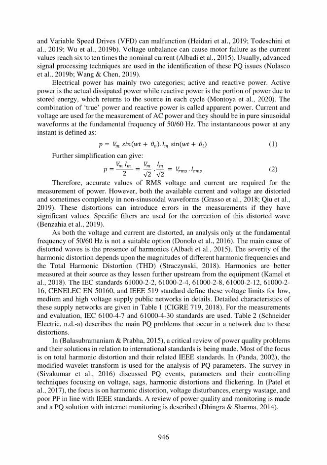
946
and Variable Speed Drives (VFD) can malfunction (Heidari et al., 2019; Todeschini et al., 2019; Wu et al., 2019b). Voltage unbalance can cause motor failure as the current values reach six to ten times the nominal current (Albadi et al., 2015). Usually, advanced signal processing techniques are used in the identification of these PQ issues (Nolasco et al., 2019b; Wang & Chen, 2019).
Electrical power has mainly two categories; active and reactive power. Active power is the actual dissipated power while reactive power is the portion of power due to stored energy, which returns to the source in each cycle (Montoya et al., 2020). The combination of ‘true’ power and reactive power is called apparent power. Current and voltage are used for the measurement of AC power and they should be in pure sinusoidal waveforms at the fundamental frequency of 50/60 Hz. The instantaneous power at any instant is defined as: N = QH ��9({T + �Ó). 8H sin({T + �B) (1)
Further simplification can give: N = QH 8H 2 = QH√2 . 8H√2 = Q́ HF . 8́ HF (2)
Therefore, accurate values of RMS voltage and current are required for the measurement of power. However, both the available current and voltage are distorted and sometimes completely in non-sinusoidal waveforms (Grasso et al., 2018; Qiu et al., 2019). These distortions can introduce errors in the measurements if they have significant values. Specific filters are used for the correction of this distorted wave (Benzahia et al., 2019).
As both the voltage and current are distorted, an analysis only at the fundamental frequency of 50/60 Hz is not a suitable option (Donolo et al., 2016). The main cause of distorted waves is the presence of harmonics (Albadi et al., 2015). The severity of the harmonic distortion depends upon the magnitudes of different harmonic frequencies and the Total Harmonic Distortion (THD) (Straczynski, 2018). Harmonics are better measured at their source as they lessen further upstream from the equipment (Kamel et al., 2018). The IEC standards 61000-2-2, 61000-2-4, 61000-2-8, 61000-2-12, 61000-2-16, CENELEC EN 50160, and IEEE 519 standard define these voltage limits for low, medium and high voltage supply public networks in details. Detailed characteristics of these supply networks are given in Table 1 (CIGRE 719, 2018). For the measurements and evaluation, IEC 6100-4-7 and 61000-4-30 standards are used. Table 2 (Schneider Electric, n.d.-a) describes the main PQ problems that occur in a network due to these distortions.
In (Balasubramaniam & Prabha, 2015), a critical review of power quality problems and their solutions in relation to international standards is being made. Most of the focus is on total harmonic distortion and their related IEEE standards. In (Panda, 2002), the modified wavelet transform is used for the analysis of PQ parameters. The survey in (Sivakumar et al., 2016) discussed PQ events, parameters and their controlling techniques focusing on voltage, sags, harmonic distortions and flickering. In (Patel et al., 2017), the focus is on harmonic distortion, voltage disturbances, energy wastage, and poor PF in line with IEEE standards. A review of power quality and monitoring is made and a PQ solution with internet monitoring is described (Dhingra & Sharma, 2014).

947
Table 1. Characteristics of different voltage supply systems
Parameter Low Voltage Supply (up to 1 kV)
Medium Voltage Supply (1 kV to 36 kV)
High Voltage Supply (36 kV to 150 kV)
Voltage variations
10 and - 15% range and the same apply for all 10 min RMS values
should not exceed ± 10%. -
Voltage unbalance
95% of the 10 min mean RMS value of the negative phase sequence component should be in range of 0 to 2% of positive phase.
95% of the 10 min mean RMS value of the negative phase sequence component should be in range of 0 to 2% of positive phase.
95% of the 10 min mean RMS value of the negative phase sequence component should be in the range of 0 to 2% of positive phase.
Harmonics and THD
THD ≤ 8% while individual harmonics should be 95% of the 10 min mean RMS value for one week.
THD ≤ 8% while individual harmonics should be 95% of the 10 min mean RMS value for one week.
Individual harmonics should be 95% of the 10 min mean RMS value for one week while THD is still under consideration.
Table 2. Problems in the electrical network and their consequences
The paper (Barros & Diego, 2016) gives an extensive overview of power quality
issues in ships. Power quality issues, instrumentation, and standards are also discussed. In (Albadi et al., 2015), a case study and literature review about unbalancing in power systems in Oman is discussed. The study showed that unbalance levels are below 1% of the specified limit. A survey of harmonic distortion and power quality measurements has been made in (Gopalakrishnan et al., 2002), in accordance with IEEE 519 standards. Simulation has also been carried out that shows the improvement in PF from 0.74 to 0.9 and a reduction in current THD as well. In (Smith, 2008), a detailed review of CELEC EN 50160 standards is made with a focus on voltage and frequency characteristics and their limits. Some measurement requirements and applications of these standards are also discussed.
Many studies have focused on the review of power quality issues and standards applied to electric motors (Gnacinski & Tarasiuk, 2016), photovoltaic power generation (Seme et al., 2017; Hacke et al., 2018; Elkholy, 2019; Smadi et al., 2019), microgrids (Senthil Kumar et al., 2015; Van den Broeck et al., 2018; Wu et al., 2019a), electric
Parameter Measurement Influence on installation Influence on performance Power Factor PF Low PF generates additional
losses in the installation. Energy provider is charging penalties to the customer
Cable heating (cables need to be oversized)
Voltage and current harmonics
THDv THDi
Negative sequence harmonics (V2) are slowing the motors down. Harmonics generates extra losses in the installation
Early failure of some devices, mainly motors.
Permanent or frequent deviations of voltage
V Devices may work outside their specified range, and they may consume mainly motors
Early failure of some devices, mainly motors
Voltage sunbalance
Vimb Voltage unbalance generates extra losses in motors.
Early failure of some devices, mainly motors
948
vehicles (Khalid et al., 2019; Khan et al., 2019), energy storage (Das et al., 2018) and shipboard power systems (Barros & Diego, 2016; Rodrigues et al., 2018). In Table 3, a detailed comparison of our paper with other papers on power quality standards is shown. In most of the studies, the focus is only on one standard and a review is made highlighting the pros and cons. Our study comprises of five different standards and covers a broader prospect. Most of the eariler studies focused on one parameter and there has not been a single review study in terms of PQ measurments and their impact. Accurate PQ measurements are extremely important for the monotoring and smooth oprtaion of any grid and for that these standrads needs to be followed.
Table 3. Comparison of our survey with other surveys
Surveys IEC 61000-4-7
IEC 61000-4-13
IEC 61000-4-30
CIGRE JWG C4.24
IEEE 519- 2014
(Balasubramaniam & Prabha, 2015)
× × × × √
(Sivakumar et al., 2016) × × × × √ (Patel et al., 2017) × × × × √ (Dhingra & Sharma, 2014) × × × × × (Barros & Diego, 2016) √ × √ × √ (Albadi et al., 2015) × × √ × × (Gopalakrishnan et al., 2002) × × × × √ (Smith, 2008) × × × × × Our Article √ √ √ √ √
The rest of the article is as follows: harmonic distortions are discussed in detail in
the next section. In Section 3, an overview of different PQ standards is given. Finally, the conclusion and recommendations are given in Section 4.
HARMONIC DISTORTIONS
One of the most important factors in PQ are harmonic distortions, if experiencing
distorted sinewave, blown fuses, overheating (transformers, motors, neutral), unusual audible noise and tripping of circuit breakers in larger distribution equipment, then these are the indication of harmonics (Lu, 2018; Rabehi et al., 2018; Montoya et al., 2019). The indication of harmonics in electrical systems is a distorted sine wave for voltage and current (Mustafa et al., 2019). In distribution systems, nonlinear loads are the major cause of harmonic currents (D. Wang et al., 2019). A nonlinear load will draw a current that has a different waveform compared to the supply voltage waveform. The supply voltage is then distorted by the flow of these harmonic currents through impedances that in the results generates voltage harmonics (Tokic et al., 2018). Mainly inverter drives and power electronics circuits with higher switching frequencies as they create variations in amplitude and/or phase angle and the harmonic components of the fundamental frequency cause inter-harmonics (Pérez Vallés & Salmerón Revuelta, 2019), (Xu et al., 2019). Harmonics values can be analysed using Fourier series, which will give:
Fundamental sinusoidal frequency (50 or 60 Hz), integer multiples of the fundamental frequency (harmonics), DC component at zero frequency (if applicable).

949
The hth order harmonic is the component having ‘h’ times the fundamental frequency. Recently, a new term has been introduced which is called super harmonics that refers to the distortion of voltage or current in the frequency range from 2 to 150 kHz (Moussa et al., 2019). Active power electronics converters connected to the grid are responsible for much higher frequencies (Chattopadhyay et al., 2014; Prieto T.J. et al., 2016). A description of harmonic distortions effecting the fundamental signal is given in Fig. 2. The equation for the harmonic expansion Õ(T) is presented below:
Õ(T) = ÈY + Ö È× √2 ��9(|xT − ∅× )Ù×Úd (3)
where ÈY – DC components, mostly considered zero; È| – RMS value of kth harmonic; x – angular frequency; Ø| – Harmonic component displacement at zero time. THD is an indicator of the distortion in a signal. For a signal Õ, it is defined as:
²Ê¢ = ÜÈ44 + È�4 + ⋯ È×4 Èd (4)
THD is the ratio of the RMS value of all the harmonic components of the signal Õ, to the fundamental È1. It is generally expressed in percentage. For current harmonics, it is:
²Ê¢B = �Ö(�×�d)4Ý×Úd (5)
Figure 2. Harmonics distortions.
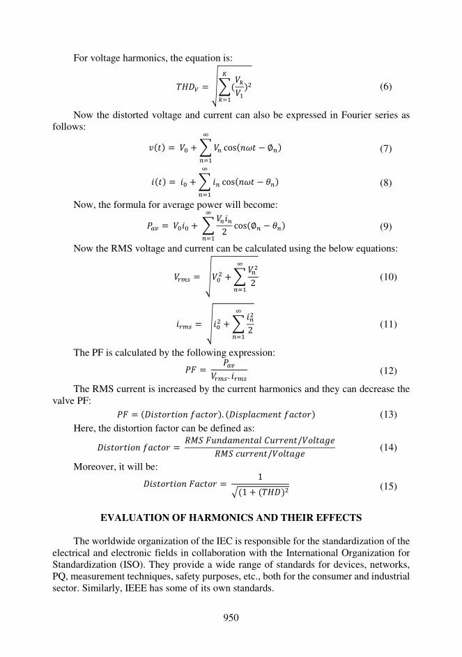
950
For voltage harmonics, the equation is:
²Ê¢Þ = �Ö(Q×Qd)4Ý×Úd (6)
Now the distorted voltage and current can also be expressed in Fourier series as follows:
R(T) = QY + Ö QK cos(9xT − ∅K) ÙKÚd (7)
�(T) = �Y + Ö �K cos(9xT − �K) ÙKÚd (8)
Now, the formula for average power will become:
MIÓ = QY�Y + Ö QK�K2ÙKÚd cos(∅K − �K) (9)
Now the RMS voltage and current can be calculated using the below equations:
Q́ HF = �QY4 + Ö QK 42ÙKÚd (10)
�´HF = ��Y4 + Ö �K42ÙKÚd (11)
The PF is calculated by the following expression: Mª = MIÓQ́ HF . �´HF (12)
The RMS current is increased by the current harmonics and they can decrease the valve PF: Mª = (¢��T�}T��9 ³;VT�}). (¢��N®;V:X9T ³;VT�}) (13)
Here, the distortion factor can be defined as: ¢��T�}T��9 ³;VT�} = =iß ªc9v;:X9T;® 7c}}X9T/Q�®T;¸X=iß Vc}}X9T/Q�®T;¸X (14)
Moreover, it will be: ¢��T�}T��9 ª;VT�} = 1Ü(1 + (²Ê¢)4 (15)
EVALUATION OF HARMONICS AND THEIR EFFECTS
The worldwide organization of the IEC is responsible for the standardization of the
electrical and electronic fields in collaboration with the International Organization for Standardization (ISO). They provide a wide range of standards for devices, networks, PQ, measurement techniques, safety purposes, etc., both for the consumer and industrial sector. Similarly, IEEE has some of its own standards.
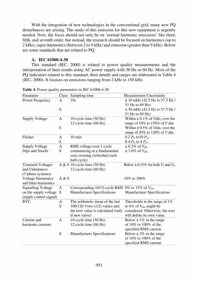
951
With the integration of new technologies in the conventional grid, many new PQ disturbances are arising. The study of this emission for this new equipment is urgently needed. Now, the focus should not only be on ‘normal harmonic emissions’ like third, fifth, and seventh order, but instead, the research should be focused on harmonics (up to 2 kHz), super-harmonics (between 2 to 9 kHz) and emission (greater than 9 kHz). Below are some standards that are related to PQ:
A. IEC 61000-4-30 This standard (IEC, 2000) is related to power quality measurements and the
interpretation of their results using AC power supply with 50 Hz or 60 Hz. Most of the PQ indicators related to this standard, their details and ranges are elaborated in Table 4 (IEC, 2000). It focuses on emissions ranging from 2 kHz to 150 kHz.
Table 4. Power quality parameters in IEC 61000-4-30
Parameter Class Sampling time Measurement Uncertainty Power Frequency A 10s
± 10 mHz (42.5 Hz to 57.5 Hz / 51 Hz to 69 Hz)
S ± 50 mHz (42.5 Hz to 57.5 Hz / 51 Hz to 69 Hz)
Supply Voltage A 10-cycle time (50 Hz) 12-cycle time (60 Hz)
Within ± 0.1% of Vdin, over the range of 10% to 150% of V din.
S Within ± 0.5% of Vdin, over the range of 20% to 120% of V din.
Flicker A 10 min 0.2 Pst to10 Pst. S 0.4 Pst to 4 Pst.
Supply Voltage Dips and Swells
A RMS voltage over 1 cycle commencing at a fundamental zero crossing (refreshed each half-cycle)
± 0.2% of Vdin S ± 1.0% of Vdin
Transient Voltages and Unbalances (3-phase systems)
A & S 10-cycle time (50 Hz) 12-cycle time (60 Hz)
Below ± 0.15% for both V2 and V0.
Voltage Harmonics and Inter-harmonics
A & S 10% to 200%
Signalling Voltage on the supply voltage (ripple control signal)
A Corresponding 10/12-cycle RMS 0% to 15% of Vdin. S Manufacturer Specifications Manufacturer Specifications
RVC A The arithmetic mean of the last 100/120 Vrms (1/2) values and the new value is calculated (only if new valve)
Thresholds in the range of 1% to 6% of Vdin might be considered. Otherwise, the user will define its own value.
S
Current and harmonic currents
A 10-cycle time (50 Hz) 12-cycle time (60 Hz)
Below ± 1% in the range of 10% to 100% of the specified RMS current.
S Manufacturer Specifications Below ± 2% in the range of 10% to 100% of the specified RMS current.

952
As described in the Tables 5, two classes are defined in this standard, Class A (precision measurements are required) and class S (for statistical surveys or power quality assessment). Both classes have different measurement incertainty for different PQ parameters. The reference measurement unit for this standard is shown in Fig. 3. The measurement unit contains a transducer unit that converts the signal from one from one energy to another. Then the value of the signal is measured, and results are display. For further evaluation of the signal, there can be some additional options like FFT, spectrum analysis etc.
(Optional)
Figure 3. Block Diagram of a measuring unit. The range of 2 kHz to 9 kHz can also be found in IEC 61000-4-7:2002, while
Comité International Spécial des Perturbations Radioélectriques (CISPR 16) covers disturbances from 9 kHz to 150 kHz. The measurement methods in CISPR 16 may be complex or expensive to implement, due to their gapless measurement and accuracy requirements, and it provides a large amount of data (IEC, 2000).
B. IEC 61000-4-7 This standard (IEC 61000-4-7 Standard, 2002) deals with the measurement
instrument envisioned for quantifying spectral disturbances up to 9 kHz. As shown in Fig. 4 (IEC 61000-4-7 Standard, 2002), the measurement unit consists of an anti-aliasing filter, A/D-converter, a synchronizer, and, if needed, a window-shaping unit with a Discrete Fourier Transform (DFT) based processor output coefficients am and bm. Then there are special parts related to current and voltage assessment. Frequencies above the measuring shall be attenuated. To obtain the appropriate attenuation, the instrument may sample the input signal at a frequency much higher than the measuring frequency.
Figure 4. The general structure of the measuring unit.
Transducers
Unit Measuremnet
Unit
Measuremnt
Results
Evaluation
Unit
Measurement Unit
I/P Current
I/P Voltage Output
Sampling Frequency
DFT
+Grouping Output 2a +Smoothing Output 2b +Check for Compliance Output 3
I/P
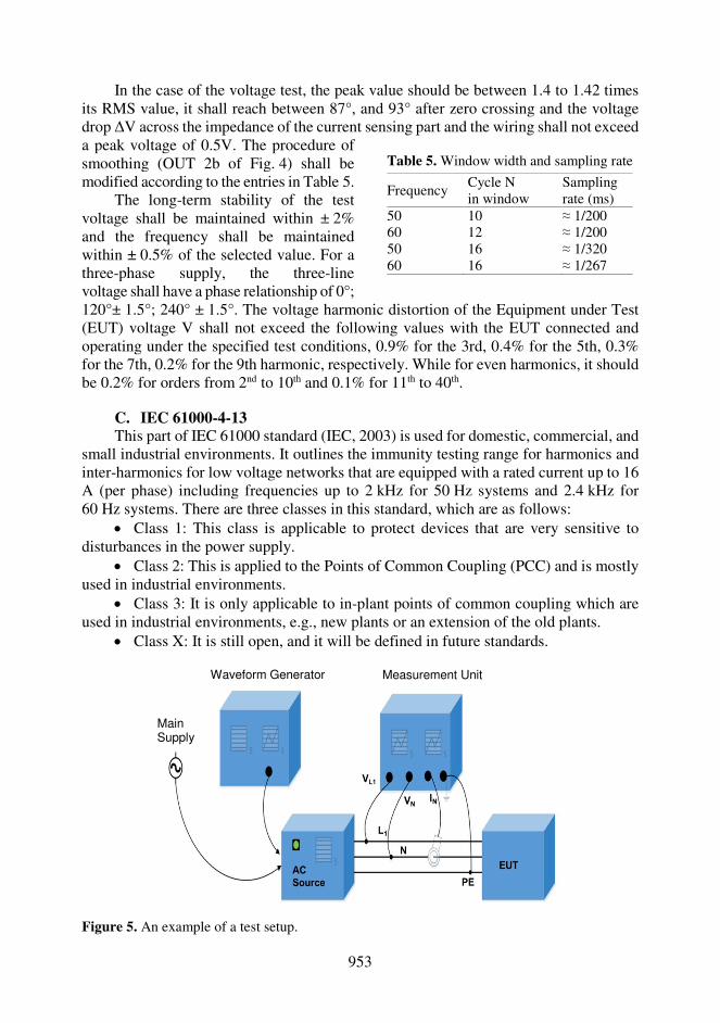
953
In the case of the voltage test, the peak value should be between 1.4 to 1.42 times its RMS value, it shall reach between 87°, and 93° after zero crossing and the voltage drop ΔV across the impedance of the current sensing part and the wiring shall not exceed
120°± 1.5°; 240° ± 1.5°. The voltage harmonic distortion of the Equipment under Test (EUT) voltage V shall not exceed the following values with the EUT connected and operating under the specified test conditions, 0.9% for the 3rd, 0.4% for the 5th, 0.3% for the 7th, 0.2% for the 9th harmonic, respectively. While for even harmonics, it should be 0.2% for orders from 2nd to 10th and 0.1% for 11th to 40th.
C. IEC 61000-4-13 This part of IEC 61000 standard (IEC, 2003) is used for domestic, commercial, and
small industrial environments. It outlines the immunity testing range for harmonics and inter-harmonics for low voltage networks that are equipped with a rated current up to 16 A (per phase) including frequencies up to 2 kHz for 50 Hz systems and 2.4 kHz for 60 Hz systems. There are three classes in this standard, which are as follows:
Class 1: This class is applicable to protect devices that are very sensitive to disturbances in the power supply.
Class 2: This is applied to the Points of Common Coupling (PCC) and is mostly used in industrial environments.
Class 3: It is only applicable to in-plant points of common coupling which are used in industrial environments, e.g., new plants or an extension of the old plants.
Class X: It is still open, and it will be defined in future standards.
Figure 5. An example of a test setup.
a peak voltage of 0.5V. The procedure of smoothing (OUT 2b of Fig. 4) shall be modified according to the entries in Table 5.
The long-term stability of the test voltage shall be maintained within ± 2% and the frequency shall be maintained within ± 0.5% of the selected value. For a three-phase supply, the three-line voltage shall have a phase relationship of 0°;
Table 5. Window width and sampling rate
Frequency Cycle N in window
Sampling rate (ms)
50 10 ≈ 1/200 60 12 ≈ 1/200 50 16 ≈ 1/320 60 16 ≈ 1/267
Waveform Generator Measurement Unit
Main Supply
954
The test generator for this standard must have the ability to generate a 50 Hz or 60 Hz signal frequency to superimpose the required frequencies, e.g., harmonics and frequencies between harmonics. The analyser for harmonics and inter-harmonics must be according to IEC 61000-4-7 for voltage test verification. The example test setup is shown in Fig. 5 (IEC, 2003).
D. CIGRE JWG C4.24 CIGRÉ Study Committee C4 and CIRED established the Joint Working Group
(JWG) C4.24: PQ and EMC Issues associated with future electricity networks” in late 2013 to address future power quality issues (CIGRE 719, 2018). In normal practice, the utility companies including transmission and distribution only measure the power quality either in substations or at the Point of Common Coupling (PCC). The future trends will require additional monitoring at the point of connection of renewable energy sources due to their distributed generation and storage along with distribution feeders. Nowadays, the trend of Low Voltage (LV) and High Voltage (HV) side are to measure at every location, both in the control side and revenue side using advanced metering systems. Mostly, these devices do not store data, but there is a need in the future and the potential is already there. Although, the main question is when and what to measure, then its storage and further utilization.
This monitoring requires Intelligent Electronic Devices (IEDs) based on transducers and sensors for current, voltage, temperature, and humidity. Classical transduces work effectively at the fundamental frequency, but they are not suitable for higher frequency ranges (Arrillaga & Watson, 2003). These sensors are quite useful for current and voltage measurements in LV, MV, and HV for protection, operation and monitoring, fault diagnostics, and PQ measurements. Sensors are based on several different phenomena or effects (F. Zavoda, 2009). They have different current and voltage ranges with the possibility of data acquisition, storage, and transmission. Mostly they are used to measure currents and line to ground voltages. However, some of them are compatible with IEC 61000-4-30 and they are used to measure harmonics.
The future devices must be capable of measuring PQ issues like harmonics, inter-harmonics, voltage unbalance, voltage flicker and dip, voltage sag and swell, interruptions, and RVC. There are several proposals for a combination of transducers and IEDs for PQ measurements. Due to the increase of distributed generation and integration, the problems associated with it are also increasing (McDermott & Dugan, 2003). A new set of indices is proposed for a better understanding of these issues (Chicco et al. (n.d.)).
E. IEEE 519-2014 Standard The standard IEEE 519-2014 (IEEE Power and Energy Society, 2014) is a revision
in the previous IEEE 519-1992 standard. The prime goal of these standards is to protect consumers and utilities from the adverse effect of harmonics by keeping the THD in a limit at PCC. In this standard, the individual current limit is 5%, THD is 8% with a new PCC value for voltage (V ≤ 1.0 kV), and it also defines a new maximum individual value for the 35th to 50th harmonic (Wallace, 2014). The measurement window in this standard, for 60 Hz is 12 cycles (~ 200 ms), and for 50, Hz is 10 cycles on the instrument using DFT. Three statistical limits are defined in this standard, which are as follows:

955
For 3 secs, the harmonic current should be less than two times the current distortion limit of the daily 99th percentile.
For 10 min, the harmonic current should be less one and a half times than the current distortion of the weekly 99th percentile.
For 10 min, the harmonic current should be less than the current distortion of the weekly 95th percentile
CONCLUSIONS
The advancement in technology has allowed measuring, monitoring, and analysing
PQ parameters at higher frequencies and their transmission via wireless technology for accurate evaluation. New sensing equipment is replacing the old one, as we are moving towards higher frequencies, up to 150 kHz or even beyond. This change requires a critical revision of the existing limits and the possibility of their graduation, e.g., super-harmonics, phase angles, and voltage unbalance. Due to the increase in energy-efficient lighting, the harmonics in the system will increase. With the ever-growing measurement data, new system models including both software and hardware are required to get as much information as possible. The live status of the system should be visualized, monitored with the help of flexible and convenient methods.
In future power systems, a balance will be required between conventional PQ analysers, with unconventional devices like controllers and relays, and Advance Metering Interfaces (AMI) with PQ measurement capabilities. The measurement of distortion is a bit tricky; it will require a novel sensor for MV, HV, and EHV systems and it should be done in the planning phase of any new substation. New measurement standards with a new set of parameters are urgently required for the range of 2 kHz to 150 kHz. This must also include both time and frequency domain analysis of these parameters due to special signal characteristics in this range. On the consumer side, the analysis of emissions should also include the monitoring of the contribution of consumer installed devices to voltage quality, rather than only considering current-based measurement methods.
The PQ indices used today were introduced decades ago, but the electricity networks have changed very rapidly. This evolving network needs a new evolving set of PQ indices. The main documents providing information about PQ are IEC 61000-4-30 and IEEE 1159. The currently used measurement units only cover harmonics up to the 50th and calculate the THD and that is not enough. It does not include super-harmonics, so that must be included in future solutions.
ACKNOWLEDGEMENTS. This work was supported by the Estonian Research Council grants PSG142, PUT1680, Estonian Centre of Excellence in Zero Energy and Resource Efficient Smart Buildings and Districts ZEBE, grant 2014-2020.4.01.15-0016 funded by European Regional Development Fund.

956
REFERENCES
Albadi, M.H., Al Hinai, A.S., Al-Badi, A.H., Al Riyami, M.S., Al Hinai, S.M. & Al Abri, R.S. 2015. Unbalance in power systems: Case study. Proceedings of the IEEE International Conference on Industrial Technology, 2015-June(June), 1407–1411. https://doi.org/10.1109/ICIT.2015.7125294
Arrillaga, J. & Watson, N.R. 2003. Power System Harmonics (Second). John Wiley & Sons, Ltd. Balasubramaniam, P.M. & Prabha, S.U. 2015. Power quality issues, solutions and standards: A
technology review. Journal of Applied Science and Engineering 18(4), 371–380. https://doi.org/10.6180/jase.2015.18.4.08
Barros, J. & Diego, R.I. 2016. A review of measurement and analysis of electric power quality on shipboard power system networks. Renewable and Sustainable Energy Reviews 62, 665–672. https://doi.org/10.1016/j.rser.2016.05.043
Benzahia, A., Boualaga, R., Moussi, A., Zellouma, L. & Meriem, M. 2019. A PV powered shunt active power filter for power quality improvement. Global Energy Interconnection 2(2), 143–149. https://doi.org/10.1016/j.gloei.2019.07.001
Bhonsle, D.C. & Kelkar, R.B. 2016. Analyzing power quality issues in electric arc furnace by modeling. Energy 115, 830–839. https://doi.org/10.1016/j.energy.2016.09.043
Chattopadhyay, S., Chattopadhyaya, A. & Sengupta, S. 2014. Harmonic power distortion measurement in Park Plane. Measurement: Journal of the International Measurement Confederation 51(1), 197–205. https://doi.org/10.1016/j.measurement.2014.02.021
Chicco, G., Corona, F., Porumb, R. & Spertino, F. (n.d.). Experimental Indicators of Current Unbalance in Building-Integrated Photovoltaic Systems. IEEE J. Photovolt 4(3), 924–934.
CIGRE 719. 2018. Power Quality and EMC issues with Future Electricity Networks (Issue March). Das, C.K., Bass, O., Kothapalli, G., Mahmoud, T.S. & Habibi, D. 2018. Overview of energy
storage systems in distribution networks: Placement, sizing, operation, and power quality. Renewable and Sustainable Energy Reviews 91(March 2018), 1205–1230. https://doi.org/10.1016/j.rser.2018.03.068
Dhingra, A. & Sharma, A.K. 2014. Power Quality Issues : Monitoring & Measurement 7(10), 1049–1056.
Donolo, P., Bossio, G., De Angelo, C., García, G. & Donolo, M. 2016. Voltage unbalance and harmonic distortion effects on induction motor power, torque and vibrations. Electric Power Systems Research 140, 866–873. https://doi.org/10.1016/j.epsr.2016.04.018
McDermott, T.E. & Dugan, R.C. & 2003. PQ, reliability and DG. IEEE Industry Applications Magazine, 9(5), 17–23.
Elkholy, A. 2019. Harmonics assessment and mathematical modeling of power quality parameters for low voltage grid connected photovoltaic systems. Solar Energy 183(June 2018), 315–326. https://doi.org/10.1016/j.solener.2019.03.009
Gallo, D., Landi, C. & Luiso, M. 2010. Issues in the characterization of power quality instruments. Measurement: Journal of the International Measurement Confederation 43(8), 1069–1076. https://doi.org/10.1016/j.measurement.2010.03.010
Gandoman, F.H., Ahmadi, A., Sharaf, A.M., Siano, P., Pou, J., Hredzak, B. & Agelidis, V.G. 2018. Review of FACTS technologies and applications for power quality in smart grids with renewable energy systems. Renewable and Sustainable Energy Reviews 82(October 2017), 502–514. https://doi.org/10.1016/j.rser.2017.09.062
Gnacinski, P. & Tarasiuk, T. 2016. Energy-efficient operation of induction motors and power quality standards. Electric Power Systems Research 135, 10–17. https://doi.org/10.1016/j.epsr.2016.03.022
957
Gopalakrishnan, C., Udayakumar, K. & Raghavendiran, T.A. 2002. Survey of harmonic distortion from power quality measurements and the application of standards including simulation. IEEE/PES Transmission and Distribution Conference and Exhibition 2, 1054–1058. https://doi.org/10.1109/TDC.2002.1177623
Grasso, F., Luchetta, A. & Manetti, S. 2018. Measurement of Electric Power Quantities and Efficiency in Nonsinusoidal Conditions. 2018 AEIT International Annual Conference, Bari, Italy, 2018, pp. 1–6, doi: 10.23919/AEIT.2018.8577454
Hacke, P., Lokanath, S., Williams, P., Vasan, A., Sochor, P., TamizhMani, G.S., Shinohara, H. & Kurtz, S. 2018. A status review of photovoltaic power conversion equipment reliability, safety, and quality assurance protocols. Renewable and Sustainable Energy Reviews 82(October 2017), 1097–1112. https://doi.org/10.1016/j.rser.2017.07.043
Heidari, H., Rassõlkin, A., Vaimann, T., Kallaste, A., Taheri, A., Holakooie, M.H. & Belahcen, A. 2019. A novel vector control strategy for a six-phase induction motor with low torque ripples and harmonic currents. Energies 12(6). https://doi.org/10.3390/en12061102
IEC. 2000. IEC 61000-4-30 Electromagnetic compatibility (EMC) – Part 4-30: Testing and measurement techniques – Power quality measurement methods. 134.
IEC. 2003. IEC 61000-4-13 Electromagnetic compatibility (EMC) – Part 4-13: Testing and measurement techniques - Harmonics and interharmonics including mains signalling at a.c. power port, low frequency immunity tests. 6–8. https://doi.org/10.16309/j.cnki.issn.1007-1776.2003.03.004
IEC. (2002). IEC 61000-4-7 Electromagnetic compatibility (EMC) – Part 4-7: Testing and measurement techniques - General guide on harmonics and interharmonics measurements and instrumentation, for power supply systems and equipment connected (IEC 61000-4-7:2002).
IEC. 2019. Static meters for AC measurements (Issue Clc). IEEE Power and Energy Society. 2014. IEEE Recommended Practice and Requirements for
Harmonic Control in Electric Power Systems IEEE Power and Energy Society. IEEE Standard 519–2014, 2014. https://doi.org/10.1109/IEEESTD.2014.6826459
Jamil, E., Hameed, S., Jamil, B. & Qurratulain. 2019. Power quality improvement of distribution system with photovoltaic and permanent magnet synchronous generator based renewable energy farm using static synchronous compensator. Sustainable Energy Technologies and Assessments 35(March), 98–116. https://doi.org/10.1016/j.seta.2019.06.006
Kamel, K., Laid, Z. & Abdallah, K. 2018. Control Algorithms Of Shunt Active Power Filter For Non-Linear Loads. 2018 International Conference on Applied Smart Systems (ICASS), November, 1–4.
Khalid, M.R., Alam, M.S., Sarwar, A. & Jamil Asghar, M.S. 2019. A Comprehensive review on electric vehicles charging infrastructures and their impacts on power-quality of the utility grid. ETransportation 1, 100006. https://doi.org/10.1016/j.etran.2019.100006
Khan, W., Ahmad, F. & Alam, M.S. 2019. Fast EV charging station integration with grid ensuring optimal and quality power exchange. Engineering Science and Technology, an International Journal 22(1), 143–152. https://doi.org/10.1016/j.jestch.2018.08.005
Khorasani, P.G., Joorabian, M. & Seifossadat, S.G. 2017. Smart grid realization with introducing unified power quality conditioner integrated with DC microgrid. Electric Power Systems Research 151, 68–85. https://doi.org/10.1016/j.epsr.2017.05.023
Kitzig, J., Schlaghecke, S. & Bumiller, G. 2019. Power Quality Measurement System With PMU Functionality Based on Interpolated Sampling. IEEE Transactions on Instrumentation and Measurement 68(4), 1014–1025. https://doi.org/10.1109/TIM.2018.2863458
Lizana, J., Friedrich, D., Renaldi, R. & Chacartegui, R. 2018. Energy flexible building through smart demand-side management and latent heat storage. Applied Energy 230(July), 471–485. https://doi.org/10.1016/j.apenergy.2018.08.065
958
Lu, J. 2018. Harmonic Balance Methods used in Power Electronics and Distributed Energy System. Proceedings - 2018 IEEE International Power Electronics and Application Conference and Exposition, PEAC 2018, 1–6. https://doi.org/10.1109/PEAC.2018.8590473
Mahela, O.P., Shaik, A.G. & Gupta, N. 2015. A critical review of detection and classification of power quality events. Renewable and Sustainable Energy Reviews 41, 495–505. https://doi.org/10.1016/j.rser.2014.08.070
Marais, Z., Rens, J., Peterson, B. & Botha, G. 2018. Measurement uncertainty of current harmonics during the assessment of compliance to grid code requirements. 2018 IEEE 9th International Workshop on Applied Measurements for Power Systems (AMPS), 1–6.
Montoya, F.G., Baños, R., Alcayde, A. & Arrabal-Campos, F.M. 2019. Analysis of power flow under non-sinusoidal conditions in the presence of harmonics and interharmonics using geometric algebra. International Journal of Electrical Power and Energy Systems 111(April), 486–492. https://doi.org/10.1016/j.ijepes.2019.04.032
Montoya, F.G., Baños, R., Alcayde, A., Arrabal-Campos, F.M. & Viciana, E. 2020. Analysis of non-active power in non-sinusoidal circuits using geometric algebra. International Journal of Electrical Power & Energy Systems 116(September 2019), 105541. https://doi.org/10.1016/j.ijepes.2019.105541
Morsi, W.G. & El-Hawary, M.E. 2011. Power quality evaluation in smart grids considering modern distortion in electric power systems. Electric Power Systems Research 81(5), 1117–1123. https://doi.org/10.1016/j.epsr.2010.12.013
Moussa, H., Martin, J.P., Pierfederici, S., Meibody-Tabar, F. & Moubayed, N. 2019. Voltage harmonic distortion compensation with non-linear load power sharing in low-voltage islanded microgrid. Mathematics and Computers in Simulation 158, 32–48. https://doi.org/10.1016/j.matcom.2018.05.007
Mustafa, T.I.A.H., Cabral, S.H., Almaguer, H.D., Meyer, L.H., Puchale, L.H.B., Cereja, J.E.M. & Vier, G.B. 2019. Analysis of the Behavior of the 3rd Harmonic over Power Transmission Lines. 2019 IEEE PES GTD Grand International Conference and Exposition Asia, GTD Asia 2019, 310–313. https://doi.org/10.1109/GTDAsia.2019.8715919
Najafi, E., Yatim, A.H.M. & Mirzaei, A. 2019. An improved sag detection approach based on modified Goertzel algorithm An improved sag detection approach based on modi fi ed Goertzel algorithm. International Journal of Electronics 106(1), 36–47. https://doi.org/10.1080/00207217.2018.1501612
Nolasco, D.H.S., Costa, F.B., Palmeira, E.S., Alves, D.K., Bedregal, B.R.C., Rocha, T.O.A., Ribeiro, R.L.A. & Silva, J.C.L. 2019. Wavelet-fuzzy power quality diagnosis system with inference method based on overlap functions: Case study in an AC microgrid. Engineering Applications of Artificial Intelligence 85(February), 284–294. https://doi.org/10.1016/j.engappai.2019.05.016
Nolasco, D.H.S., Palmeira, E.S. & Costa, F.B. 2019. A cascade-type hierarchical fuzzy system with additional defuzzification of layers for the automatic power quality diagnosis. Applied Soft Computing Journal 80, 657–671. https://doi.org/10.1016/j.asoc.2019.02.007
Panda, G. 2002. Power Quality Analysis Using S-Transform. IEEE Power Engineering Review, 22(7), 60. https://doi.org/10.1109/MPER.2002.4312414
Patel, N., Gandhi, K., Mahida, D. & Chudasama, P. 2017. A Review On Power Quality Issues and Standards. International Research Journal of Engineering and Technology 4(2), 247–250.
Patiño, .A.S. & López, Y.U. 2018 Analysis power quality of a photovoltaic system connected to the grid-tie, 2018 IEEE ANDESCON, Santiago de Cali, Colombia, 2018, pp. 1–6, doi: 10.1109/ANDESCON.2018.8564564
Pérez, V.A. & Salmerón, R.P. 2019. A new distributed measurement index for the identification of harmonic distortion and/or unbalance sources based on the IEEE Std. 1459 framework. Electric Power Systems Research 172(March), 96–104. https://doi.org/10.1016/j.epsr.2019.03.007

959
Prieto, T. J., Revuelta, P,S., Pérez, V.A. & Pérez, S.L. 2016. Practical evaluation of unbalance and harmonic distortion in power conditioning. Electric Power Systems Research 141, 487–499. https://doi.org/10.1016/j.epsr.2016.08.012
Qiu, W., Tang, Q., Liu, J., Teng, Z. & Yao, W. 2019. Power Quality Disturbances Recognition Using Modified S Transform and Parallel Stack Sparse Auto-encoder. Electric Power Systems Research 174(October 2018), 105876. https://doi.org/10.1016/j.epsr.2019.105876
Rabehi, R., Kouzou, A., Saadi, S., Hafaifa, A. & Nail, B. 2018. Harmonics and inter-harmonics estimation of voltage/current based on least error squares algorithm. 2018 15th International Multi-Conference on Systems, Signals and Devices, SSD 2018, 1, 324–327. https://doi.org/10.1109/SSD.2018.8570614
Randy Barnett. (n.d.). Power Quality Measurement and Analysis Basics | Electrical Construction & Maintenance (EC&M) Magazine. Retrieved December 14, 2018, from https://www.ecmweb.com/power-quality/power-quality-measurement-and-analysis-basics
Rodrigues Junior, W.L., Borges, F.A.S., Veloso, A.F. da S., Rabêlo, R. de A.L. & Rodrigues, J.J.P.C. 2019. Low voltage smart meter for monitoring of power quality disturbances applied in smart grid. Measurement 147, 106890. https://doi.org/10.1016/j.measurement.2019.106890
Rodrigues, T.A., Neves, G.S., Gouveia, L.C.S., Abi-Ramia, M.A., Fortes, M.Z. & Gomes, S. 2018. Impact of electric propulsion on the electric power quality of vessels. Electric Power Systems Research 155, 350–362. https://doi.org/10.1016/j.epsr.2017.11.006
Rönnberg, S. & Bollen, M. 2016. Power quality issues in the electric power system of the future. Electricity Journal 29(10), 49–61. https://doi.org/10.1016/j.tej.2016.11.006
Safavizadeh, A., Member, S., Yousefi, G.R. & Karshenas, H.R. 2019. Voltage Variation Mitigation Using Reactive Power Management of Distributed Energy Resources in a Smart Distribution System. IEEE Transactions on Smart Grid 10(2), 1907–1915. https://doi.org/10.1109/TSG.2017.2781690
Saqib, M.A. & Saleem, A.Z. 2015. Power-quality issues and the need for reactive-power compensation in the grid integration of wind power. Renewable and Sustainable Energy Reviews 43, 51–64. https://doi.org/10.1016/j.rser.2014.11.035
Schneider Electric. (n.d.-a). Measurement applications - Electrical Installation Guide. Retrieved December 14, 2018, from http://www.electrical-installation.org/enwiki/Measurement_applications
Schneider Electric. (n.d.-b). Measurement for Power availability and reliability - Electrical Installation Guide. Retrieved December 14, 2018, from http://www.electrical-installation.org/enwiki/Measurement_for_Power_availability_and_reliability
Seme, S., Lukač, N., Štumberger, B. & Hadžiselimović, M. 2017. Power quality experimental analysis of grid-connected photovoltaic systems in urban distribution networks. Energy 139, 1261–1266. https://doi.org/10.1016/j.energy.2017.05.088
Sensors, E.F. 2019. Transient Voltage Measurements for Overhead Transmission Lines and Substations by Metal-Free and Contactless Integrated. IEEE Transactions on Industrial Electronics 66(1), 571–579. https://doi.org/10.1109/TIE.2018.2826455
Senthil Kumar, A., Rajasekar, S. & Raj, P.A.-D.-V. 2015. Power Quality Profile Enhancement of Utility Connected Microgrid System Using ANFIS-UPQC. Procedia Technology 21, 112–119. https://doi.org/10.1016/j.protcy.2015.10.017
Shankar, V.K.A., Umashankar, S., Sanjeevikumar, P., Viliam, F., Ramachandaramurthy, V.K. & Mihet-Popa, L. 2018. Investigations of power quality disturbances in a variable speed parallel pumping system with grid tied solar PV. Energy Procedia 145, 490–496. https://doi.org/10.1016/j.egypro.2018.04.097
Sivakumar, D., Srividhya, J.P. & Shanmathi, T. 2016. A Review on Power Quality Monitoring and Its Controlling Techniques. 8th International Conference on Latest Trends in Engineering and Technology 1(1), 3–9. https://doi.org/10.15662/IJAREEIE.2015.0503143
960
Smadi, I.A., Albatran, S. & Alsyouf, M.A. 2019. Power quality improvement of a class of reduced device count inverter. Simulation Modelling Practice and Theory 96(January), 101939. https://doi.org/10.1016/j.simpat.2019.101939
Smith, V. 2008. A review of the new CELEC STANDARD EN 50160. Syst. Biol. 57(4), 660–663. http://www.informaworld.com/10.1080/10635150802303508
Straczynski, P. 2018. Higher Harmonics and Power in Circuits with LED Light Sources. 5–9. https://doi.org/10.1109/EPMCCS.2018.8596561
Stanisvavljevis, A.M. & Kati, V.A. (2019). Magnitude of Voltage Sags Prediction Based on the Harmonic Footprint for Application in DG Control System. IEEE Transcations on Industrial Electronics 66(11), 8902–8912. https://doi.org/10.1109/TIE.2018.2881934
Todeschini, G., Lewis, M., Mcnaughton, J., Concha, M., Togneri, M., Masters, I., Allmark, M., Stallard, T., Neill, S., Goward-brown, A. & Robins, P. 2019. Power variability of tidal-stream energy and implications for electricity supply 183, 1061–1074. https://doi.org/10.1016/j.energy.2019.06.181
Tokic, A., Jukan, A., Uglesic, I. & Mustafic, D. 2018. Nonlinear Model of Fluorescent Lamp in Harmonic Studies. Proceedings - 2018 IEEE PES Innovative Smart Grid Technologies Conference Europe, ISGT-Europe 2018, 1–6. https://doi.org/10.1109/ISGTEurope.2018.8571760
Van den Broeck, G., Stuyts, J. & Driesen, J. 2018. A critical review of power quality standards and definitions applied to DC microgrids. Applied Energy 229(July), 281–288. https://doi.org/10.1016/j.apenergy.2018.07.058
Vinnakoti, S. & Kota, V.R. 2018. ANN based control scheme for a three-level converter based unified power quality conditioner. Journal of Electrical Systems and Information Technology 5(3), 526–541. https://doi.org/10.1016/j.jesit.2017.11.001
Wallace, I. 2014. Key Changes and Differences between the New IEEE 519- 2014 Standard and IEEE 519-1992. In Alcatel Telecommunications Review (Vol. 11, Issue 1).
Wang, D., Nahid-Mobarakeh, B. & Emadi, A. 2019. Second Harmonic Current Reduction for a Battery-Driven Grid Interface with Three-Phase Dual Active Bridge DC/DC Converter. IEEE Transactions on Industrial Electronics 66(11), 1–1. https://doi.org/10.1109/tie.2019.2899563
Wang, S. & Chen, H. 2019. A novel deep learning method for the classification of power quality disturbances using deep convolutional neural network. Applied Energy 235(March 2018), 1126–1140. https://doi.org/10.1016/j.apenergy.2018.09.160
Wu, M., Niu, X., Gao, S. & Wu, J. 2019a. Power quality assessment for AC/DC hybrid micro grid based on on-site measurements. Energy Procedia 156(2018), 396–400. https://doi.org/10.1016/j.egypro.2018.11.105
Wu, M., Niu, X., Gao, S. & Wu, J. 2019b. ScienceDirect ScienceDirect ScienceDirect Power Quality Assessment for AC / DC Hybrid Micro Grid Based on Power Quality Assessment for AC / DC Hybrid Micro Grid Based on On-Site Measurements On-Site Measurements Assessing the using the heat temperature fu. Energy Procedia 156(2018), 396–400. https://doi.org/10.1016/j.egypro.2018.11.105
Xu, J., Qian, Q., Zhang, B. & Xie, S. 2019. Harmonics and Stability Analysis of Single-Phase Grid-Connected Inverters in Distributed Power Generation Systems Considering Phase-Locked Loop Impact. IEEE Transactions on Sustainable Energy 10(3), 1470–1480. https://doi.org/10.1109/TSTE.2019.2893679
Yang, L., Peng, J., Wang, T., Li, Y., Deng, Z., Liu, Y. & Tan, M. 2018. Compliance verification and probabilistic analysis of state-wide power quality monitoring data. Global Energy Interconnection 1(3), 391–395. https://doi.org/10.14171/j.2096-5117.gei.2018.03.011
Zavoda, F. 2009. State of the art sensors suitable for distribution automation application. CEATI T074700-1539.
961
Agronomy Research 19(S1), 961–974, 2021 https://doi.org/10.15159/AR.21.081
Comparison of physical composition of municipal solid waste in Czech municipalities and their potential in separation
S. Zhao1,*, V. Altmann1, L. Richterova2 and V. Vitkova1
1Czech University of Life Sciences Prague (CZU), Faculty of Engineering, Department of Machinery Utilization, Kamýcká 129, CZ165 00 Praha 6 – Suchdol, Czech Republic 2Institut Cirkulární Ekonomiky, z.ú., Hybernská 998/4, CZ110 00 Prague, Czech Republic *Correspondence: [email protected] Received: February 23rd, 2021; Accepted: May 2nd, 2021; Published: May 17th, 2021 Abstract. Czech Republic has been moving from landfill-based waste system toward resource-based waste management system with an increasing rate of recyclable waste in the last years (38.6% of recycling by material and 11.7% of energy recovery in 2018). However, landfill is still a popular way of mixed municipal solid waste (MMSW) disposal due to the low tax. In the Czech Republic, MMSW is collected from households by door-to-door system or recovery operations (Household Waste Recycling Centre) and only should consists of everyday items, which are further non-recyclable and non-reusable. However, a significant amount of recyclable waste can still be found in MMSW. Therefore, a good knowledge of the physical composition of MMSW is required to define strategy plans and improve waste management in municipalities. This work is aimed at comparing the physical composition of MMSW in the Czech Republic with small municipalities up to 2,999 inhabitants and big municipalities from 3,000 inhabitants to recognize the share of recyclable and non-recyclable waste in MSW and designate the potential of separation at source. Composition of MMSW was determined by a physical evaluation of waste collected from households in target municipalities which consists in a detailed manual sorting of waste into 13 specific groups according to their types, and weighting by a scale. We found that the real proportion of MMSW that could no longer be reused or recycled was much less than the amount disposed of in the municipal waste bins. A large part of MMSW consisted of organic waste together with food waste. This type of waste is especially useful when people turn it into compost to prevent the production of waste and it returns the nutrients back to the soil, closing the circle. The rate of recyclable waste was also high in many municipalities covered by our analyses, which indicated a lower rate of separation and reflected an insufficient sorting system in municipality and insufficient education of inhabitants. On the other hand, it points to the larger space of separation potential in households. In conclusion the evaluation emphasizes the improper proportion of MMSW in Czech municipalities. A lot of waste can be recycled but once it is thrown into black bins as MMSW, there is no chance that it will be reused/recycled. It therefore calls for measures to improve sorting at source, which will benefit municipal authorities in term of increasing recycle rates in order to comply with regulations and make a profit. We found the analysis of the physical composition of MMSW as a fundamental method for municipalities to verify the separation rate at the source, and it is recommended to conduct this analysis regularly and monitor developments. Key words: physical analysis, waste composition, municipal solid waste, separation at source, Czech Republic.
962
INTRODUCTION In 2018, the Czech Republic produced 5,782 thousand tons of mixed municipal
solid waste (MMSW) which represents 544 kg of MMSW per person, about 52 kg more than the European average (492 kg). In this year Denmark generated the most municipal waste per capita among the EU Member States, on the other hand they are also front runner in diverting waste from landfilling, mainly through incineration with energy recovery (European Commission, 2020a). In the Czech Republic, only 38.6% of municipal waste was recycled by material and 11.7% for energy recovery, 46% was landfilled (Ministry of the Environment, 2019). Thanks to one of the lowest landfill tax in Europe (€20 in CZE, the tax in EU varies from €5 to more than €100) (CEWEP, 2020), landfilling as a way of waste disposal is still popular in Czech municipalities, especially in small municipalities with a low budget.
However, a number of European legislations pushes their members into transition to a circular economy. A new Circular Economy Action Plan presents key elements including a target of recycling 65% of municipal waste by 2030 and reducing landfill to a maximum of 10% of municipal waste in the same year. In addition, there is a strict ban on landfilling separately collected waste, for example paper, plastics, organic waste, metals, etc. (European Commission, 2020b). This is a strong message for the Czech Republic to set up higher strategy targets for waste recycling, recovery and diversion from landfill. The Czech Waste Management Plan 2015–2024 has stipulated that a landfill tax should be adjusted so that waste is redirected higher up the hierarchy (Ministry of the Environment, 2014). The increase in the landfill tax from €20 to €74 per ton to be applied in 2030 should shift more waste treatment to recycling and reuse instead of landfilling. This step would have a significant impact on the municipality’s budget and would force small municipalities to focus on waste treatment and try to find a new way of waste disposal produced in their region. Thorough understanding the quantity and composition of a waste production is important in improving quantities of potentially recyclable materials and to forecast future waste generation (Parfitt & Flowerdew, 1997; Parizeau et al., 2006). The composition and variation of waste is also important in the design and implementation of appropriate sorting and recycling technologies (Burnley, 2007).
The composition of the produced waste is extremely variable and depends on multiple seasonal and cultural factors, dietary habits and socio–economic and legal impacts. This variability makes the definition and measurement of waste composition both more difficult and necessary (Kreith, 1999; Dehghani et al., 2009; Diaz et al., 2020). Accurate information on the quantities and characteristics of solid waste can then be used for the design, implementation and operation of the best practice in waste management as well as resource control and saving, recycling, waste collection planning, transport, and disposal system ultimately leading to environmental protection against such harmful effects (Heravi et al., 2013; Erami et al., 2015). Assessing the composition of waste provides a detailed view of the municipal waste produced by citizens every day and inspires authorities to make further improvements. To study the quantity and composition of municipal waste, there is no adopted international standard but various working standards on national level (Dahlen & Lagerkvist, 2008), even though there is an up-to-date document providing methodology for solid waste composition analysis from 2014 called SWA-Tool for European countries, it is not obligatory and does not

963
meet current requirements (Kropáč et al., 2020). Therefore, each member of EU has developed its own methods based on the individual waste background with varying numbers of material fractions and sorting objectives (Edjabou et al., 2015). The method used in this project has its base in national method and inspired most by French MODECOM methodology characterized by at least 2 tons of MMSW, from which 500 kg for sampling (Montejo et al., 2011). In Austria and Germany, there are methodologies at the level of individual Lands and regions (Vogel et al., 2009; Kern & Aiwpwnkorhwn, 2010). From the other continent, American Society for Testing and Materials (ASTM) evolved a number of methods for local governments or industrial plants including Standard Test Method for Determination of the Composition of Unprocessed Municipal Solid Waste, suitable not only for US, but worldwide (Dahlen & Lagerkvist, 2008).
To this end, the non-governmental organization Institut Cirkulární Ekonomiky z. ú. (INCIEN) in cooperation with JRK Czech Republic s.r.o. (JRK) conducted analyses of the physical composition of the MMSW to help municipalities gain better knowledge of their waste. Thanks to their work and the data collected, this paper could emerge.
This study investigates the physical composition of a mixed municipal solid waste material. The primary objective is to evaluate all obtained data of selected municipalities and provide an initial overview on waste composition in the Czech Republic. It includes using various statistical tools focusing on the qualitative and quantitative characteristics of the MMSW and comparing the municipalities for recognising the composition differences. Then, the factors affecting composition of the MMSW are identified and lastly, the potential trends for reducing waste and increasing recycling are determined for guiding prospective steps in planning and environmental assessment of waste management.
MATERIALS AND METHODS All analyses of physical composition were completed by the Institut Cirkulární
Ekonomiky, z.ú in cooperation with JRK Czech Republic, s.r.o., whose main objective is to transform and implement the circular economy in the Czech Republic.
The aim of the field analysis was to evaluate the mixed municipal solid waste and its physical composition of recyclable and non-recyclable compounds, to determine their percentage and to identify the potential for improving recycling rates. The methodology was designed according to the Waste Sampling Methodological Guideline (Ministry of the Environment, 2008) and adjusted to meet the waste analysis objective. The assessment of the physical composition of the MMSW was carried out in a total of 35 Czech municipalities grouped into 2 categories: small municipalities (SM) with a population up to 2,999 citizens and big municipalities (BM) with a population of more than 3,000 citizens. Some analyses were repeated upon request to monitor changes in the composition of municipal waste over a four-year testing period.
Waste samples were collected from households (both urban centres and family houses) randomly distributed among selected municipalities during each field analysis. All analyses were carried out in cooperation with the municipal authorities who provided samples of MMSW collected from households. For analysis, a sample of approx. 500 kg of randomly picked municipal waste was taken and analysed. Protective equipment (suits, gloves, goggles, respirators, etc.) was used throughout the analysis. Each sample
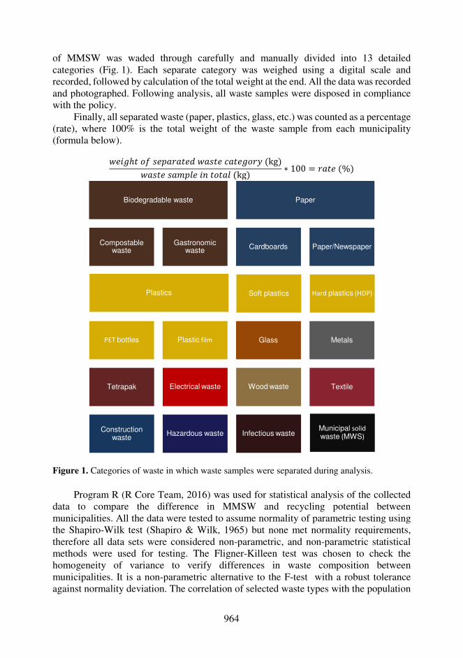
964
of MMSW was waded through carefully and manually divided into 13 detailed categories (Fig. 1). Each separate category was weighed using a digital scale and recorded, followed by calculation of the total weight at the end. All the data was recorded and photographed. Following analysis, all waste samples were disposed in compliance with the policy.
Finally, all separated waste (paper, plastics, glass, etc.) was counted as a percentage (rate), where 100% is the total weight of the waste sample from each municipality (formula below).
{X�¸ℎT �³ �XN;};TXv {;�TX V;TX¸�}Õ (kg){;�TX �;:N®X �9 T�T;® (kg) ∗ 100 = };TX (%)
Figure 1. Categories of waste in which waste samples were separated during analysis.
Program R (R Core Team, 2016) was used for statistical analysis of the collected data to compare the difference in MMSW and recycling potential between municipalities. All the data were tested to assume normality of parametric testing using the Shapiro-Wilk test (Shapiro & Wilk, 1965) but none met normality requirements, therefore all data sets were considered non-parametric, and non-parametric statistical methods were used for testing. The Fligner-Killeen test was chosen to check the homogeneity of variance to verify differences in waste composition between municipalities. It is a non-parametric alternative to the F-test with a robust tolerance against normality deviation. The correlation of selected waste types with the population
Biodegradable waste Paper
Compostable waste
Gastronomic waste
Cardboards Paper/Newspaper
Plastics Soft plastics Hard plastics (HDP)
PET bottles Plastic film Glass Metals
Tetrapak Electrical waste Wood waste Textile
Constructionwaste
Hazardous waste Infectious wasteMunicipal solid
waste (MWS)
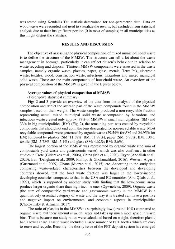
965
was tested using Kendall's Tau statistic determined for non-parametric data. Data on wood waste were recorded and used to visualize the results, but excluded from statistical analysis due to their insignificant portion (0 in most of samples) in all municipalities as this might distort the statistics.
RESULTS AND DISCUSSION
The objective of assessing the physical composition of mixed municipal solid waste
is to define the structure of the MMSW. The structure can tell a lot about the waste management in borough, particularly it can reflect citizen’s behaviour in relation to waste recycling and disposal. Thirteen MMSW components were assessed in the waste samples, namely organic waste, plastics, paper, glass, metals, Tetra-Pak, electronic waste, textiles, wood, construction waste, infectious, hazardous and mixed municipal solid waste. These are the main components of household waste. An overview of the physical composition of the MMSW is given in the figures below.
Average values of physical composition of MMSW (Descriptive statistical summary) Figs 2 and 3 provide an overview of the data from the analysis of the physical
composition and depict the average part of the waste compounds found in the MMSW samples based on their weight. The waste samples produced a non-recyclable fraction representing actual mixed municipal solid waste accompanied by hazardous and infectious waste created only approx. 37% of MMSW in small municipalities (SM) and 33% in big municipalities (BM) (Fig. 2), the remaining part was created by recyclable compounds that should not end up in the bins designated for non-recyclable waste. Most recyclable compounds were generated by organic waste (29.54% for SM and 24.95% for BM) followed by plastics (SM: 11.38%; BM: 11.99%), paper (SM: 5.93%; BM: 10%), textile (SM: 5.78%; BM: 5.1%) and glass (SM: 4.62%; BM: 5.6%).
The largest portion of the MMSW was represented by organic waste (the sum of compostable yard–waste and gastronomic waste), which was also confirmed in other studies in Crete (Gidarakos et al., 2006), China (Ma et al., 2020), Egypt (Abdallah et al., 2020), Iran (Dehghani et al., 2009; Phillips & Gholamalifard, 2016), Western Algeria (Guermoud et al., 2009), Ghana (Miezah et al., 2015), etc. According to the study data comparing waste–related characteristics between the developed and developing countries showed, that the food waste fraction was larger in the lower-income developing countries compared to that in the USA and EU countries (Abu Qdais et al., 1997), which is supported by another study with finding that the low-income areas produce larger organic share than high-income ones (Ogwueleka, 2009). Organic waste (the sum of compostable yard-waste and gastronomic waste) in the MMSW is a quantitatively essential category of waste and the way it is treated can have a positive and negative impact on environmental and economic aspects in municipalities (Chotovinský & Altmann, 2017).
The ratio of plastics in the MMSW is surprisingly low (around 10%) compared to organic waste, but their amount is much larger and takes up much more space in waste bins. That is because our study ratios were calculated based on weight, therefore plastic had a lower share. Plastic waste included a large number of PET bottles which are easy to reuse and recycle. Recently, the thorny issue of the PET deposit system has emerged

966
in the Czech Republic. The main objective of operating the deposit system will be to save bottles from landfilling, which will also guarantee the good quality of bottles returning back to producers. In addition to the PET bottles, plastic films, soft and hard plastics were also found in the waste sample.
a)
b)
Figure 2. Average physical composition of municipal solid waste in the selected municipalities of this study: a): small municipalities; b) big municipalities. Abbreviations: BIO – organic waste; EEW – electrical and electronic waste; WW – wood waste; CW – construction waste; HW – hazardous waste; IW – infectious waste; MMSW – mixed municipal solid waste.
967
Unlike plastics, paper waste had an unequal proportional rate in small and big municipalities. While in small municipalities paper had only 5,93% share in the MMSW, big municipalities had almost twice the share than SM (10%). But both plastic and paper waste has similar properties in terms of volume. Large uncompressed packages may take up much more volume but their weight in MMSW is much lower. Pressing can help to reduce the volume of paper packaging to 20% of its original volume and achieve substantial savings in logistics costs (Chotovinský & Altmann, 2018).
Figure 3. Average fraction of recyclable and non-recyclable waste divided according to their type: a) small municipalities; b) big municipalities. Municipal solid waste is a type of waste that no further use but is destined for incineration (energy recovery) and landfill. According to this figure, more than fifty percent of usable/recyclable waste still existed but ended up in mixed waste bins.
Construction waste was present in less significant quantities in the MMSW, but still accounted for more than 3% of the MMSW. Sometimes electric waste could also be found in MMSW, accounting for approx. 1% of the waste sample, similar to the Tetra Pak (liquid packaging board). Clearly, non-recyclable MMSW produced by households were actually much smaller than those thrown in the municipal waste bins.
As it represents a significant amount in the MMSW, organic waste and plastics were specifically tested between municipalities. Plastic waste had a small range from 3% to 16% of the MMSW, while organic waste was more variable; one municipality had even more than 50% of the MMSW generated by organic waste, another 4 had over 40% and the average rate is 29.5% of the total MMSW for small municipalities and 25.8% for big municipalities. These results showed that plastic and organic waste from kitchens and horticulture is often thrown in the municipal waste bin instead of being recycled. On the other hand, this signals the potential for improving recycling at source.
a) b)
Composition of mixed MSW-SM Composition of mixed MSW-BM
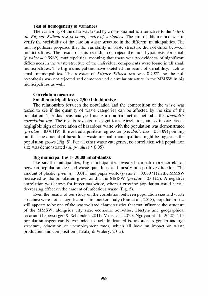
968
Test of homogeneity of variances The variability of the data was tested by a non-parametric alternative to the F-test:
the Fligner–Killeen test of homogeneity of variances. The aim of this method was to verify the variability of the date on waste structure in the different municipalities. The null hypothesis proposed that the variability in waste structure did not differ between municipalities. The result of this test did not reject the null hypothesis for small (p-value = 0.9989) municipalities, meaning that there was no evidence of significant differences in the waste structure of the individual components were found in all small municipalities. The big municipalities have sketched the result of variability, such as small municipalities. The p-value of Fligner–Killeen test was 0.7922, so the null hypothesis was not rejected and demonstrated a similar structure in the MMSW in big municipalities as well.
Correlation measure Small municipalities (< 2,900 inhabitants): The relationship between the population and the composition of the waste was
tested to see if the quantity of waste categories can be affected by the size of the population. The data was analysed using a non-parametric method - the Kendall’s correlation tau. The results revealed no significant correlation, unless in one case a negligible sign of correlation of hazardous waste with the population was demonstrated (p-value = 0.08419). It revealed a positive regression (Kendall’s tau = 0.3109) pointing out that the amount of hazardous waste in small municipalities might be bigger as the population grows (Fig. 5). For all other waste categories, no correlation with population size was demonstrated (all p-values > 0.05).
Big municipalities (> 30,00 inhabitants): like small municipalities, big municipalities revealed a much more correlation
between population size and waste quantities, and mostly in a positive direction. The amount of plastic (p-value = 0.011) and paper waste (p-value = 0.00071) in the MMSW increased as the population grew, as did the MMSW (p-value = 0.0165). A negative correlation was shown for infectious waste, where a growing population could have a decreasing effect on the amount of infectious waste (Fig. 5).
Even the results of our study on the correlation between population size and waste structure were not as significant as in another study (Han et al., 2018), population size still appears to be one of the waste-elated characteristics that can influence the structure of the MMSW, alongside city size, economic activities, lifestyle and geographical location (Lebersorger & Schneider, 2011; Ma et al., 2020; Nguyen et al., 2020). The population aspect can be expanded to include detailed issues such as gender and age structure, education or unemployment rates, which all have an impact on waste production and composition (Talalaj & Walery, 2015).
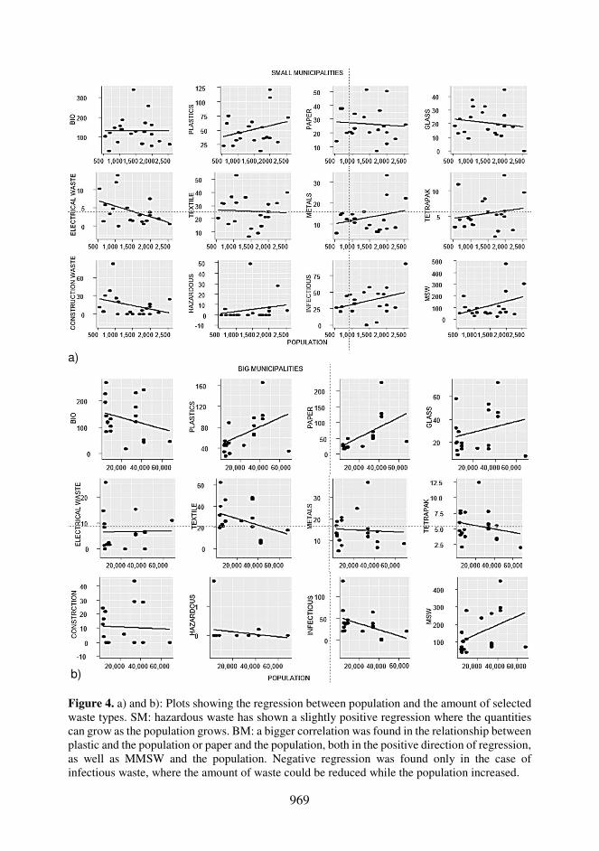
969
a)
Figure 4. a) and b): Plots showing the regression between population and the amount of selected waste types. SM: hazardous waste has shown a slightly positive regression where the quantities can grow as the population grows. BM: a bigger correlation was found in the relationship between plastic and the population or paper and the population, both in the positive direction of regression, as well as MMSW and the population. Negative regression was found only in the case of infectious waste, where the amount of waste could be reduced while the population increased.
b)
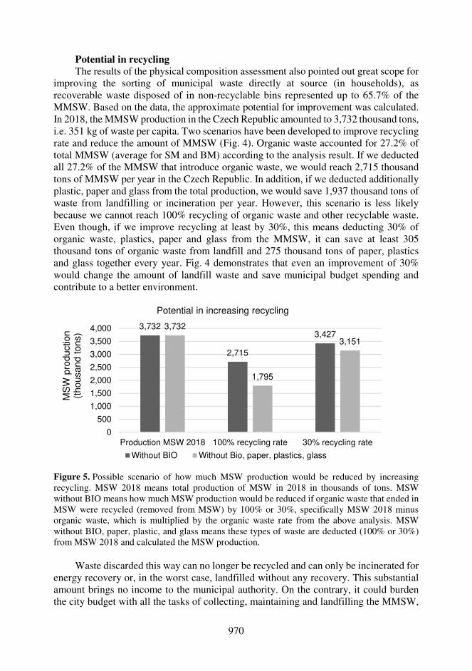
970
Potential in recycling The results of the physical composition assessment also pointed out great scope for
improving the sorting of municipal waste directly at source (in households), as recoverable waste disposed of in non-recyclable bins represented up to 65.7% of the MMSW. Based on the data, the approximate potential for improvement was calculated. In 2018, the MMSW production in the Czech Republic amounted to 3,732 thousand tons, i.e. 351 kg of waste per capita. Two scenarios have been developed to improve recycling rate and reduce the amount of MMSW (Fig. 4). Organic waste accounted for 27.2% of total MMSW (average for SM and BM) according to the analysis result. If we deducted all 27.2% of the MMSW that introduce organic waste, we would reach 2,715 thousand tons of MMSW per year in the Czech Republic. In addition, if we deducted additionally plastic, paper and glass from the total production, we would save 1,937 thousand tons of waste from landfilling or incineration per year. However, this scenario is less likely because we cannot reach 100% recycling of organic waste and other recyclable waste. Even though, if we improve recycling at least by 30%, this means deducting 30% of organic waste, plastics, paper and glass from the MMSW, it can save at least 305 thousand tons of organic waste from landfill and 275 thousand tons of paper, plastics and glass together every year. Fig. 4 demonstrates that even an improvement of 30% would change the amount of landfill waste and save municipal budget spending and contribute to a better environment.
Figure 5. Possible scenario of how much MSW production would be reduced by increasing recycling. MSW 2018 means total production of MSW in 2018 in thousands of tons. MSW without BIO means how much MSW production would be reduced if organic waste that ended in MSW were recycled (removed from MSW) by 100% or 30%, specifically MSW 2018 minus organic waste, which is multiplied by the organic waste rate from the above analysis. MSW without BIO, paper, plastic, and glass means these types of waste are deducted (100% or 30%) from MSW 2018 and calculated the MSW production.
Waste discarded this way can no longer be recycled and can only be incinerated for energy recovery or, in the worst case, landfilled without any recovery. This substantial amount brings no income to the municipal authority. On the contrary, it could burden the city budget with all the tasks of collecting, maintaining and landfilling the MMSW,
3,732
2,715
3,4273,732
1,795
3,151
0
500
1,000
1,500
2,000
2,500
3,000
3,500
4,000
Production MSW 2018 100% recycling rate 30% recycling rate
MS
W p
roduction
(thousand t
ons)
Potential in increasing recycling
Without BIO Without Bio, paper, plastics, glass
971
which means that the more MMSW it produces the higher the tax has to be paid. Therefore, the priority is to keep MMSW volume low by applying the 6R strategy: Refuse, Reduce, Reuse, Recycle, Rot and Rethink. This strategy is fundamental in the circular economy and aligns with the waste hierarchy in waste management: preventing waste generation at source (households), reusing and recycling waste treated as material and trading it means additional income to the city budget. Moreover, there is an exceptional reason calling for increased recycling at national level. Many obligations such as compulsory collection of compostable organic waste and metal waste (since 2015) and collection of gastronomic oil waste (since 2020) were introduced to municipal authorities. Czech legislation has a clear message aimed at a circular economy and waste production reduction. This seems necessary and essential to make changes not only at the municipal level, but also with the private sector. On the other hand, it is very easy to reduce the MMSW and associated costs when we have found out that there is a striking amount of recyclable waste waiting to be separated. If we redirect it, it can be saved. Study of Chotovinský et al. (2018) showed a direct impact on the amount of organic waste and paper in the MMSW. The amount of recyclable compounds in the MMSW can be easily regulated by the frequency of separate waste collection and the different collection types. In addition, the waste reduction is highly depended on the activities of the population. There are many socio-economic-technical factors that influence their behaviour and disabling them in recycling. Barrier to basic recycling are, for example, the distance and availability of recycling bins, the volume and repletion of waste bins, lack of information and education, low levels of technology and innovation, etc. (Lane & Wagner, 2013) while financial stimulus is the major motivating factor for their active participation. The good side is that it can be easily changed by the motivation and efforts of the municipal authority (Kattoua et al., 2019). The link between them and citizens needs to be strengthened. Hence, possible activities for residents must focus on the following areas: awareness raising for residents, special education activities for children and schools, organisation of recycling awareness events and overall support for reuse and recycling of waste.
Revaluing the waste collection system opens up new opportunities for the municipality. A good way is to check the data from the collection companies. Other unpublished study from INCIEN showed that many waste bins were collected practically empty or half-empty, but municipalities have to pay companies for each collection regardless of whether the bin was empty or full. Based on this information, optimizing the number of containers comes in handy and can deliver further significant budget savings that can be invested in technology, for instance. In addition, the education and motivation system can enhance public participation in many phases of waste management and help municipalities turn waste into resources.
CONCLUSIONS
Although the analysis of physical composition of MMSW is a basic tool for
verifying the efficiency of sorting at source, there is a lack of comprehensive study at composition of municipal waste production in Czech municipalities. This paper executed an extensive analysis in over 30 municipalities to provide an overview on waste composition in the Czech Republic. Beside it, the study highlighted an inappropriate content in MMSW and addressed to insufficient sorting at source in households. The
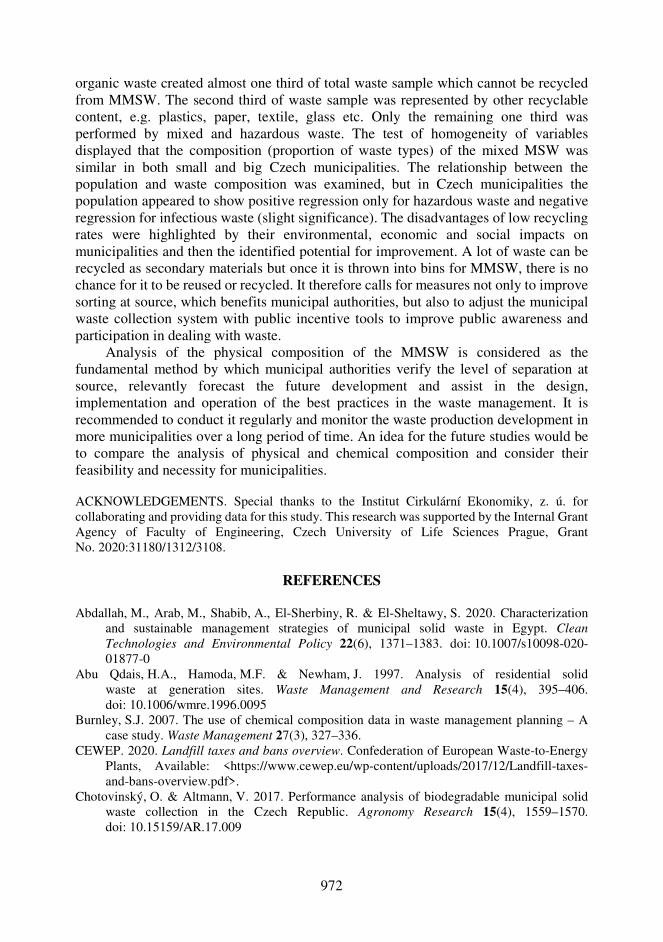
972
organic waste created almost one third of total waste sample which cannot be recycled from MMSW. The second third of waste sample was represented by other recyclable content, e.g. plastics, paper, textile, glass etc. Only the remaining one third was performed by mixed and hazardous waste. The test of homogeneity of variables displayed that the composition (proportion of waste types) of the mixed MSW was similar in both small and big Czech municipalities. The relationship between the population and waste composition was examined, but in Czech municipalities the population appeared to show positive regression only for hazardous waste and negative regression for infectious waste (slight significance). The disadvantages of low recycling rates were highlighted by their environmental, economic and social impacts on municipalities and then the identified potential for improvement. A lot of waste can be recycled as secondary materials but once it is thrown into bins for MMSW, there is no chance for it to be reused or recycled. It therefore calls for measures not only to improve sorting at source, which benefits municipal authorities, but also to adjust the municipal waste collection system with public incentive tools to improve public awareness and participation in dealing with waste.
Analysis of the physical composition of the MMSW is considered as the fundamental method by which municipal authorities verify the level of separation at source, relevantly forecast the future development and assist in the design, implementation and operation of the best practices in the waste management. It is recommended to conduct it regularly and monitor the waste production development in more municipalities over a long period of time. An idea for the future studies would be to compare the analysis of physical and chemical composition and consider their feasibility and necessity for municipalities. ACKNOWLEDGEMENTS. Special thanks to the Institut Cirkulární Ekonomiky, z. ú. for collaborating and providing data for this study. This research was supported by the Internal Grant Agency of Faculty of Engineering, Czech University of Life Sciences Prague, Grant No. 2020:31180/1312/3108.
REFERENCES
Abdallah, M., Arab, M., Shabib, A., El-Sherbiny, R. & El-Sheltawy, S. 2020. Characterization
and sustainable management strategies of municipal solid waste in Egypt. Clean Technologies and Environmental Policy 22(6), 1371–1383. doi: 10.1007/s10098-020-01877-0
Abu Qdais, H.A., Hamoda, M.F. & Newham, J. 1997. Analysis of residential solid waste at generation sites. Waste Management and Research 15(4), 395–406. doi: 10.1006/wmre.1996.0095
Burnley, S.J. 2007. The use of chemical composition data in waste management planning – A case study. Waste Management 27(3), 327–336.
CEWEP. 2020. Landfill taxes and bans overview. Confederation of European Waste-to-Energy Plants, Available: <https://www.cewep.eu/wp-content/uploads/2017/12/Landfill-taxes-and-bans-overview.pdf>.
Chotovinský, O. & Altmann, V. 2017. Performance analysis of biodegradable municipal solid waste collection in the Czech Republic. Agronomy Research 15(4), 1559–1570. doi: 10.15159/AR.17.009

973
Chotovinský, O. & Altmann, V. 2018. A comparative case study of the efficiency of collection systems for paper and biodegradable municipal solid waste. Agronomy Research 16(S1), 997–1009. https://doi.org/10.15159/AR.18.106
Dahlen, L. & Lagerkvist, A. 2008. Methods for household waste composition studies. Waste Management 28, 13.
Dehghani, M.H., Dehghanifard, E., Azam, K., Asgari, A.R. & Baneshi, M.M. 2009. A Quantitative and Qualitative Investigation of Tehran Solid Waste Recycling Potential. Knowledge & Health Journal 4(1), 40–44, Iran, doi: 10.22100/jkh.v4i1.186
Diaz, L.F., Golueke, C.G., Savage, G.M. & Eggerth, L.L. 2020. Composting and recycling municipal solid waste. CRC Press, 318 pp. Available: <https://books.google.com/books?hl=cs&lr=&id=_i_gDwAAQBAJ&oi=fnd&pg=PT18&ots=JBvaoF7Qnl&sig=26mYnEN7C8iIW8p3Rpex1CkAKL4 https://books.google.com/books?hl=en&lr=&id=_i_gDwAAQBAJ&oi=fnd&pg=PT18&dq=municipal+solid+waste+calorific&ots=JBv6nz-Opl&sig=x_GvtduUeB>.
Edjabou, M.E., Jensen, M.B., Götze, R., Pivnenko, K., Petersen, C., Scheutz, C. & Astrup, T.F. 2015. Municipal solid waste composition: Sampling methodology, statistical analyses, and case study evaluation. Waste Management 36, 12–23. doi: 10.1016/j.wasman.2014.11.009
Erami, S., Maleki, A. & Shahmoradi, B. 2015. Municipal Solid Waste Management in Mahabad Town, Iran. ournal of Environmental Science and Technology, 1–9.
European Commission. 2020a. 492 kg of municipal waste generated per person in the EU. Eurostat, Available: <https://ec.europa.eu/eurostat/web/products-eurostat-news/-/ddn-20200318-1>, [Consulted: April 9, 2021].
European Commission, 2020b. Circular Economy Action Plan for a cleaner and more competitive Europe, 28, Brussels.
Gidarakos, E., Havas, G. & Ntzamilis, P. 2006. Municipal solid waste composition determination supporting the integrated solid waste management system in the island of Crete. Waste Management 26(6), 668–679. doi: https://doi.org/10.1016/j.wasman.2005.07.018.
Guermoud, N., Ouadjnia, F., Abdelmalek, F., Taleb, F. & Addou, A. 2009. Municipal solid waste in Mostaganem city (Western Algeria). Waste Management 29(2), 896–902. doi: https://doi.org/10.1016/j.wasman.2008.03.027
Han, Z., Liu, Y., Zhong, M., Shi, G., Li, Q., Zeng, D., Zhang, Y., Fei, Y. & Xie, Y. 2018. Influencing factors of domestic waste characteristics in rural areas of developing countries. Waste Management 72, 45–54. doi: 10.1016/j.wasman.2017.11.039
Heravi, H.M., Sabour, M.R. & Mahvi, A.H. 2013. Municipal Solid Waste Characterization, Tehran-Iran. Pakistan Journal of Biological Sciences 16(16), 759–769. doi: 10.3923/pjbs.2013.759.769
Kattoua, M.G., Al-Khatib, I.A. & Kontogianni, S. 2019. Barriers on the propagation of household solid waste recycling practices in developing countries: State of Palestine example. Journal of Material Cycles and Waste Management 21(4), 774–785. doi: 10.1007/s10163-019-00833-5
Kern, M. & Aiwpwnkorhwn, H.-J. 2010. Restabfallanalysen für die AWSH Abfallwitschaft Südholstein GmbH. Available: <https://www.awsh.de/fileadmin/media/PDFs/AWK/Abfallanalyse_AWSH.pdf>
Kreith, F. 1999. Handbook of solid waste management. New York: McGraw-Hill, ISBN: 0070358761.
Kropáč, J., Gregor, J. & Pavlas, M. 2020. Municipal Waste Composition Analysis – Approaches to and Solutions for Czech Waste Management. In: 2nd International Conference on : Technologies & Business Models for Circular Economy: Conference Proceedings, International Conference on Technologies & Business Models for Circular Economy, 21 May, University of Maribor, University Press, pp. 85–94, ISBN: 978-961-286-353-1, doi: 10.18690/978-961-286-353-1.8. Available: <https://press.um.si/index.php/ump/catalog/book/472>, [Consulted: April 10, 2021].
974
Lane, G.W.S. & Wagner, T.P. 2013. Examining recycling container attributes and household recycling practices. Resources, Conservation and Recycling 75, 32–40. doi: https://doi.org/10.1016/j.resconrec.2013.03.005
Lebersorger, S. & Schneider, F. 2011. Discussion on the methodology for determining food waste in household waste composition studies. Waste Managemen 31(9–10), 1924–1933. doi: 10.1016/j.wasman.2011.05.023.
Ma, S., Zhou, C., Chi, C., Liu, Y. & Yang, G. 2020. Estimating Physical Composition of Municipal Solid Waste in China by Applying Artificial Neural Network Method. Environmental Science and Technology 54(15), 9609–9617. doi: 10.1021/acs.est.0c01802
Miezah, K., Obiri-Danso, K., Kádár, Z., Fei-Baffoe, B. & Mensah, M. Y. 2015. Municipal solid waste characterization and quantification as a measure towards effective waste management in Ghana. Waste Management 46, 15–27. doi: https://doi.org/10.1016/j.wasman.2015.09.009
Ministry of the Environment. 2008. Metodický pokyn ke vzorkování odpadů. Available: <https://www.mzp.cz/web/edice.nsf/8B372EC499E277D2C125746B002F3A2A/$file/17708196.pdf>.
Ministry of the Environment. 2014. Waste Management Plan of the Czech Republic for the period 2015-2024. Prague: Ministry of the Environment, 189 pp., Available: <https://www.mzp.cz/C1257458002F0DC7/cz/plan_odpadoveho_hospodarstvi_aj/$FILE/OODP-WMP_CZ_translation-20151008.pdf>.
Ministry of the Environment. Produkce a nakládání s odpady v roce 2019, pp. 2019, Available: <https://www.mzp.cz/C1257458002F0DC7/cz/odpady_podrubrika/$FILE/OODP-Produkce_a_nakladani_2018-20191025.pdf>.
Montejo, C., Costa, C., Ramos, P. & Márquez, M. del C. 2011. Analysis and comparison of municipal solid waste and reject fraction as fuels for incineration plants. Applied Thermal Engineering 31(13), 2135–2140. doi: 10.1016/j.applthermaleng.2011.03.041
Nguyen, K.L.P., Chuang, Y.H., Chen, H.W. & Chang, C.C. 2020. Impacts of socioeconomic changes on municipal solid waste characteristics in Taiwan. Resources, Conservation and Recycling 161, 104931. doi: 10.1016/j.resconrec.2020.104931
Ogwueleka, T.C. 2009. Municipal solid waste characteristics and management in Nigeria. Iranian Journal of Environmental Health Science & Engineering 6(3), Available: <https://www.researchgate.net/publication/40542918_Municipal_solid_waste_characteristics_and_management_in_Nigeria>.
Parfitt, J.P. & Flowerdew, R. 1997. Methodological problems in the generation of household waste statistics: An analysis of the United Kingdom’s National Household Waste Analysis Programme. Applied Geography 17(3), 231–244. doi: 10.1016/S0143-6228(96)00031-8
Parizeau, K., Maclaren, V. & Chanthy, L. 2006. Waste characterization as an element of waste management planning: Lessons learned from a study in Siem Reap, Cambodia. Resources, Conservation and Recycling 49(2), 110–128. Idoi: 10.1016/j.resconrec.2006.03.006
Phillips, J. & Gholamalifard, M. 2016. Quantitative evaluation of the sustainability or unsustainability of municipal solid waste options in Tabriz, Iran. International Journal of Environmental Science and Technology 13(6), 1615–1624. doi: 10.1007/s13762-016-0997-0
R Core Team, 2016. R: A Language and Environment for Statistical Computing. The R Foundation for Statistical Computing, Vienna, Austria, Vienna, Available: <http://www.r-project.org/>.
Shapiro, S. & Wilk, M. 1965. An analysis of variance test for normality (complete samples). Biometrika 52(3–4), 591–611.
Talalaj, I.A. & Walery, M. 2015. The effect of gender and age structure on municipal waste generation in Poland. Waste Management 40, 3–8. doi: 10.1016/j.wasman.2015.03.020
Vogel, E., Steiner, M. & Quickert, A. 2009. Siebgestützte Restmüllanalysen im Land Steiermark. Available: <<http://www.abfallwirtschaft.steiermark.at/cms/dokumente/10168259_4336659/4dfe9a05 /Endbericht%20Steiermark_2008.pdf>
975
INSTRUCTIONS TO AUTHORS Papers must be in English (British spelling). English will be revised by a proofreader, but authors are strongly urged to have their manuscripts reviewed linguistically prior to submission. Contributions should be sent electronically. Papers are considered by referees before acceptance. The manuscript should follow the instructions below. Structure: Title, Authors (initials & surname; an asterisk indicates the corresponding author), Authors’ affiliation with postal address (each on a separate line) and e-mail of the corresponding author, Abstract (up to 250 words), Key words (not repeating words in the title), Introduction, Materials and methods, Results and discussion, Conclusions, Acknowledgements (optional), References. Layout, page size and font Use preferably the latest version of Microsoft Word, doc., docx. format. Set page size to ISO B5 (17.6×25 cm), all margins at 2 cm. All text, tables, and figures
must fit within the text margins. Use single line spacing and justify the text. Do not use page numbering. Use indent 0.8 cm
(do not use tab or spaces instead). Use font Times New Roman, point size for the title of article 14 (Bold), author's names
12, core text 11; Abstract, Key words, Acknowledgements, References, tables, and figure captions 10.
Use italics for Latin biological names, mathematical variables and statistical terms. Use single (‘…’) instead of double quotation marks (“…”). Tables All tables must be referred to in the text (Table 1; Tables 1, 3; Tables 2–3). Use font Times New Roman, regular, 10 pt. Insert tables by Word's ‘Insert’ menu. Do not use vertical lines as dividers; only horizontal lines (1/2 pt) are allowed. Primary
column and row headings should start with an initial capital. Figures All figures must be referred to in the text (Fig. 1; Fig. 1 A; Figs 1, 3; Figs 1–3). Use only
black and white or greyscale for figures. Avoid 3D charts, background shading, gridlines and excessive symbols. Use font Arial, 10 pt within the figures. Make sure that thickness of the lines is greater than 0.3 pt.
Do not put caption in the frame of the figure. The preferred graphic format is Excel object; for diagrams and charts EPS; for half-tones
please use TIFF. MS Office files are also acceptable. Please include these files in your submission.
Check and double-check spelling in figures and graphs. Proof-readers may not be able to change mistakes in a different program.
References
Within the text In case of two authors, use ‘&’, if more than two authors, provide first author ‘et al.’:
Smith & Jones (1996); (Smith & Jones, 1996);

976
Brown et al. (1997); (Brown et al., 1997) When referring to more than one publication, arrange them by following keys: 1. year of publication (ascending), 2. alphabetical order for the same year of publication:
(Smith & Jones, 1996; Brown et al., 1997; Adams, 1998; Smith, 1998)
For whole books Name(s) and initials of the author(s). Year of publication. Title of the book (in italics). Publisher, place of publication, number of pages.
Shiyatov, S.G. 1986. Dendrochronology of the upper timberline in the Urals. Nauka, Moscow, 350 pp. (in Russian).
For articles in a journal
Name(s) and initials of the author(s). Year of publication. Title of the article. Abbreviated journal title (in italic) volume (in bold), page numbers. Titles of papers published in languages other than English, should be replaced by an English translation, with an explanatory note at the end, e.g., (in Russian, English abstr.).
Karube, I. & Tamiyra, M.Y. 1987. Biosensors for environmental control. Pure Appl. Chem. 59, 545–554.
Frey, R. 1958. Zur Kenntnis der Diptera brachycera p.p. der Kapverdischen Inseln. Commentat.Biol. 18(4), 1–61.
Danielyan, S.G. & Nabaldiyan, K.M. 1971. The causal agents of meloids in bees. Veterinariya 8, 64–65 (in Russian).
For articles in collections:
Name(s) and initials of the author(s). Year of publication. Title of the article. Name(s) and initials of the editor(s) (preceded by In:) Title of the collection (in italics), publisher, place of publication, page numbers.
Yurtsev, B.A., Tolmachev, A.I. & Rebristaya, O.V. 1978. The floristic delimitation and subdivisions of the Arctic. In: Yurtsev, B. A. (ed.) The Arctic Floristic Region. Nauka, Leningrad, pp. 9–104 (in Russian).
For conference proceedings:
Name(s) and initials of the author(s). Year of publication. Name(s) and initials of the editor(s) (preceded by In:) Proceedings name (in italics), publisher, place of publishing, page numbers.
Ritchie, M.E. & Olff, H. 1999. Herbivore diversity and plant dynamics: compensatory and additive effects. In: Olff, H., Brown, V.K. & Drent R.H. (eds) Herbivores between plants and predators. Proc. Int. Conf. The 38th Symposium of the British Ecological Society, Blackwell Science, Oxford, UK, pp. 175–204.
Please note Use ‘.’ ( not ‘,’) for decimal point: 0.6 0.2; Use ‘,’ for thousands – 1,230.4; Use ‘–’ (not ‘-’) and without space: pp. 27–36, 1998–2000, 4–6 min, 3–5 kg With spaces: 5 h, 5 kg, 5 m, 5 °C, C : D = 0.6 0.2; p < 0.001 Without space: 55°, 5% (not 55 °, 5 %) Use ‘kg ha–1’ (not ‘kg/ha’); Use degree sign ‘ ° ’ : 5 °C (not 5 OC).
Related Documents