Agricultural and resource economics discussion paper

Estimating input allocation for farm supply models

A. Gocht

Institute for Food and Resource Economics ILR, Bonn University, Germany

Contact: [email protected]

Paper prepared for presentation at the 107th EAAE Seminar "Modelling of Agricultural and Ru-

ral Development Policies". Sevilla, Spain, January 29th -February 1st, 2008 Copyright 2007 by A. Gocht. All rights reserved. Readers may make verbatim copies of this document for non-commercial purposes by any means, provided that this copyright notice appears on all such copies.

Abstract

When building an economic model for supply analysis the aim is to model a decision making proc-ess of one or more agents which fits the observed practice as good as possible. Hereby the model-ler is often confronted with incomplete information about the production process; particular crop specific input data are rarely available. The problem of defining activity related technology inputs coefficients is not new. A good deal of literature comes from the mathematical programming per-spective, where input coefficients were estimated using a standard linear regression function to fully represent the mathematical program. However this approach is a pure technical device and may result in an inconsistent model. The author of the paper wants to investigate whether it is possible, employing proper estimation techniques, to simultaneously estimate all unknown coefficients of a mathematical farm supply model. This includes the estimation of parameters of the non linear cost function, used to calibrate and catch the simulation behaviour and the crop specific input coefficients. It is shown that a si-multaneous estimation of all parameters improves the goodness of fit of the estimated parameters and that such an approach is technically feasible.

Key words: farm supply model, input allocation, entropy, HDP

1. Introduction

The decision-making problem of an agricultural firm or sector in empirical analysis is often speci-fied using multiple-output and constraint mathematical programming models. Here two trends can be discovered in the last decade. The first comprehends the issue of “How parameters of a programming supply model are derived”. In that area progress can be identified in a development away from pure normative programming models - where the model structure did not take historical data into account- towards supply models, where the advantages of econometric estimation and mathematical program-ming are combined. This enhancement was mainly possible due to ill-posed estimation methods pro-posed by Golan et al. (1997) or related techniques such as the highest posterior density (HPD) estima-tion Heckelei et al. (2005). The distinctive advantage of these estimation techniques is the possibility to overcome the ill-posedness by incorporating prior information and offered the practitioners the pos-sibility to make full use of the available information. Recent “real-life” application from Buysse et al. (2007) and Jansson (2007) illustrate the use of the estimation methods and unambiguously depict the development away from calibration methods - such as positive mathematical programming (PMP, see e.g. Howitt (1995)) - towards econometric related type of estimated supply model using prior informa-tion.

The second tendency is the linkage of agricultural supply programmes with spatial related bio-physical models. These types of model interact with supply models over policy provoked land and input intensity changes, which requires that the supply model explicitly define technologies and it brings the coefficients of those technologies - fertilizer and pesticides per crop - into sharper focus.

These two tendencies gave impetus to raise the question; whether it is feasible to use the new esti-mation methods to further improve the explanatory power of the technology coefficients of the supply model. In this context particular the parameter of the input technology comes into focus, due to the linkage to environmental and bio-physical models. Unfortunately these input coefficients are often not directly observable and the information is often restricted to total farm or sector purchases of various input categories. Hence information about crop specific inputs are not collected during surveys but are often derived using engineering knowledge about the physiology of the crop and are estimated before the actual model is set up. Combining these two trends, the authors of the paper want to show that it is possible using proper estimation techniques to simultaneous estimate the coefficients of a farm supply model and the coefficient of the input allocation. We argue that this approach provides better estimates for input coefficients in an economically consistent theory formulation due to the first order condition applied in the input allocation model.

In order to develop our approach the paper is structured as following: In chapter one publication in the field of input-output and linear production coefficients estimation are reviewed. The second chap-ter will introduce the simultaneous model which is applied against a time series of German FADN data in North Rhine-Westphalia. The data aggregation and preparation steps are discussed in a subsequent chapter.

2. Production coefficients estimation

The term input allocation describes how aggregated input demand is “distributed” to production ac-tivities Britz (2005). The resulting activity input is called input coefficients. There is a long history of allocating inputs to production activities in agricultural analysis and the literature provides different approaches depending on the demand of the simulation model and the scope of the analysis. Ad hoc approach which infers the allocation based on information relying on sources such as published ‘in-dustry standards’, agronomic field trials and expert opinions will not be further discussed.

1.1 Linear multiple regression function

The larger the regional coverage of a supply model becomes the lesser the manageable of ad-hoc determination of input coefficients. To overcome that and to keep the possibility to express regional or farm type variation of the production process several specifications of a linear multiple regression function were proposed, where total input use is treaded as dependent variable and the output of a firm as explanatory variable. b Ax=

Herby, A is a n x m matrix of technological coefficients with its elements ija representing the amount of input i required per unit of output j . x is a 1n x vector of activity level. b is the available resource vector.

1

nf f f

i i ij j ij

b c a x u=

= + +∑ Equation 1

Errington (1989) proposed a multiple regression or OLS technique applied to a system of derived

demand as shown in Equation 1. He extended Equation 1 by adding a constant and an error term to account for deviation within the sample. He found very high 2R for most of the inputs whereas the constant for many of the inputs were not significant. However, through the OLS estimation he ob-tained negative estimates and in some cases the input coefficients sum up to greater than one, where the author concluded negative profits. Ray (1985) discussed several alternative estimation procedures based on mathematical programming. He emphasis that in view of the non-negativity demand for the input coefficients least square methods may lead to unacceptable estimates and outlined three alterna-tive methods of inequality – constrained parameter estimation namely: inequality constraint least square, minimum mean absolute deviation and maximum absolute deviation. Midmore (1990) re-viewed the findings by Errington and discussed the underlying technical assumptions and pointed out that if the commodity technology assumption1 is implied and a correction for heteroscedasticity is applied, resulting from the size effect in production, the farm specific input coefficients can be esti-mated from regional farm business survey data. Further he noticed that using OLS techniques for (Equation 1) causes problems because the disturbance terms are not independent due to the accounting constraint involved, which dedicates that the columns of the coefficients matrix sum up to unity.

1 Commodity technology assumption implies that the input structure of a commodity is the same, regardless of the industry (farm type in the context of agriculture) where it is produced Midmore (1990).

Dixon et al. (1992) viewed the estimation of linear programming model’s technology coefficients as an application of random coefficients regression (RCR) and proposed an estimator, which restricts the predicted coefficient values to be non-negative.

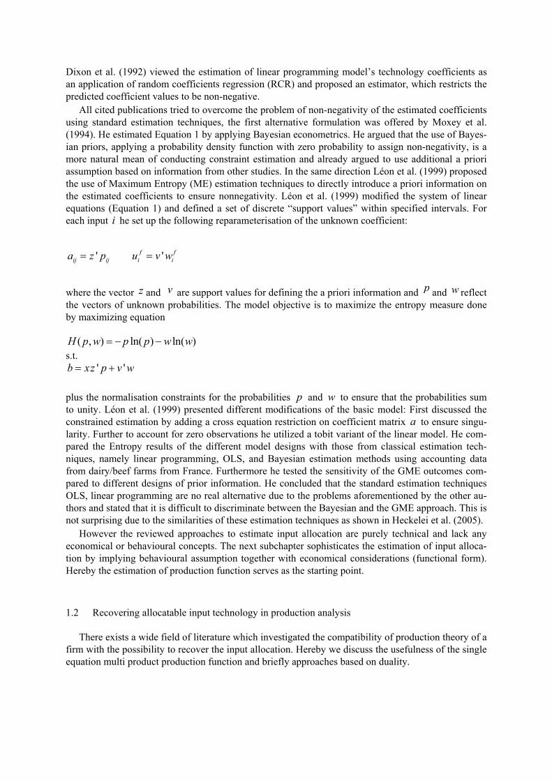
All cited publications tried to overcome the problem of non-negativity of the estimated coefficients using standard estimation techniques, the first alternative formulation was offered by Moxey et al. (1994). He estimated Equation 1 by applying Bayesian econometrics. He argued that the use of Bayes-ian priors, applying a probability density function with zero probability to assign non-negativity, is a more natural mean of conducting constraint estimation and already argued to use additional a priori assumption based on information from other studies. In the same direction Léon et al. (1999) proposed the use of Maximum Entropy (ME) estimation techniques to directly introduce a priori information on the estimated coefficients to ensure nonnegativity. Léon et al. (1999) modified the system of linear equations (Equation 1) and defined a set of discrete “support values” within specified intervals. For each input i he set up the following reparameterisation of the unknown coefficient:

' 'f fij ij i ia z p u v w= =

where the vector z and v are support values for defining the a priori information and p and w reflect the vectors of unknown probabilities. The model objective is to maximize the entropy measure done by maximizing equation

( , ) ln( ) ln( )H p w p p w w= − − s.t.

' 'b xz p v w= + plus the normalisation constraints for the probabilities p and w to ensure that the probabilities sum to unity. Léon et al. (1999) presented different modifications of the basic model: First discussed the constrained estimation by adding a cross equation restriction on coefficient matrix a to ensure singu-larity. Further to account for zero observations he utilized a tobit variant of the linear model. He com-pared the Entropy results of the different model designs with those from classical estimation tech-niques, namely linear programming, OLS, and Bayesian estimation methods using accounting data from dairy/beef farms from France. Furthermore he tested the sensitivity of the GME outcomes com-pared to different designs of prior information. He concluded that the standard estimation techniques OLS, linear programming are no real alternative due to the problems aforementioned by the other au-thors and stated that it is difficult to discriminate between the Bayesian and the GME approach. This is not surprising due to the similarities of these estimation techniques as shown in Heckelei et al. (2005).

However the reviewed approaches to estimate input allocation are purely technical and lack any economical or behavioural concepts. The next subchapter sophisticates the estimation of input alloca-tion by implying behavioural assumption together with economical considerations (functional form). Hereby the estimation of production function serves as the starting point.

1.2 Recovering allocatable input technology in production analysis

There exists a wide field of literature which investigated the compatibility of production theory of a firm with the possibility to recover the input allocation. Hereby we discuss the usefulness of the single equation multi product production function and briefly approaches based on duality.

1.2.1 Single equation multi-product production function

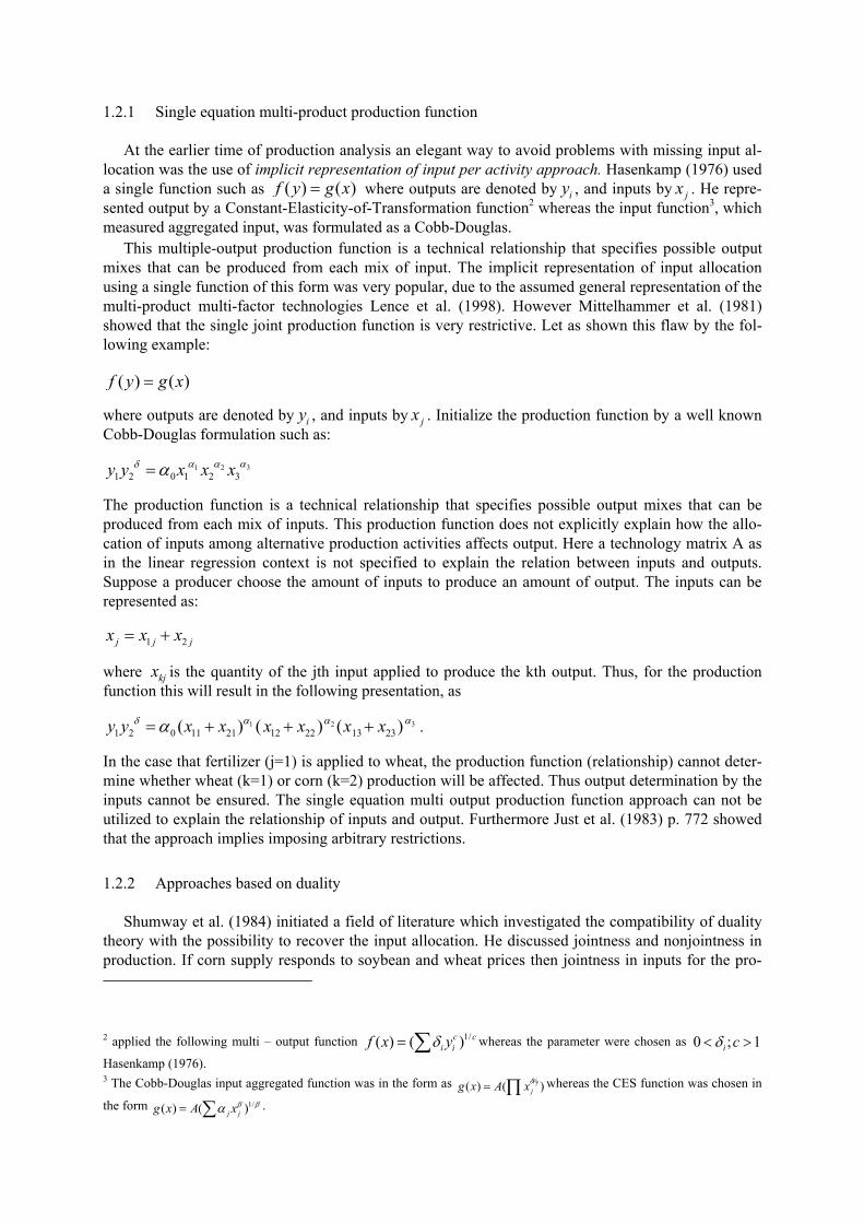
At the earlier time of production analysis an elegant way to avoid problems with missing input al-location was the use of implicit representation of input per activity approach. Hasenkamp (1976) used a single function such as ( ) ( )f y g x= where outputs are denoted by iy , and inputs by jx . He repre-sented output by a Constant-Elasticity-of-Transformation function2 whereas the input function3, which measured aggregated input, was formulated as a Cobb-Douglas.

This multiple-output production function is a technical relationship that specifies possible output mixes that can be produced from each mix of input. The implicit representation of input allocation using a single function of this form was very popular, due to the assumed general representation of the multi-product multi-factor technologies Lence et al. (1998). However Mittelhammer et al. (1981) showed that the single joint production function is very restrictive. Let as shown this flaw by the fol-lowing example:

( ) ( )f y g x=

where outputs are denoted by iy , and inputs by jx . Initialize the production function by a well known Cobb-Douglas formulation such as:

31 21 2 0 1 2 3y y x x x αα αδ α=

The production function is a technical relationship that specifies possible output mixes that can be produced from each mix of inputs. This production function does not explicitly explain how the allo-cation of inputs among alternative production activities affects output. Here a technology matrix A as in the linear regression context is not specified to explain the relation between inputs and outputs. Suppose a producer choose the amount of inputs to produce an amount of output. The inputs can be represented as:

1 2j j jx x x= +

where kjx is the quantity of the jth input applied to produce the kth output. Thus, for the production function this will result in the following presentation, as

31 21 2 0 11 21 12 22 13 23( ) ( ) ( )y y x x x x x x αα αδ α= + + + .

In the case that fertilizer (j=1) is applied to wheat, the production function (relationship) cannot deter-mine whether wheat (k=1) or corn (k=2) production will be affected. Thus output determination by the inputs cannot be ensured. The single equation multi output production function approach can not be utilized to explain the relationship of inputs and output. Furthermore Just et al. (1983) p. 772 showed that the approach implies imposing arbitrary restrictions.

1.2.2 Approaches based on duality

Shumway et al. (1984) initiated a field of literature which investigated the compatibility of duality theory with the possibility to recover the input allocation. He discussed jointness and nonjointness in production. If corn supply responds to soybean and wheat prices then jointness in inputs for the pro- 2 applied the following multi – output function 1/( ) ( )c c

i if x yδ= ∑ whereas the parameter were chosen as 0 ; 1i cδ< >

Hasenkamp (1976). 3 The Cobb-Douglas input aggregated function was in the form as ( ) ( )j

jg x A xα= ∏ % whereas the CES function was chosen in

the form 1/( ) ( )j jg x A xβ βα= ∑ .

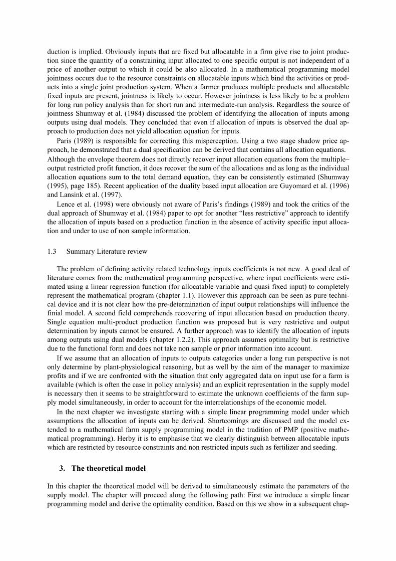
duction is implied. Obviously inputs that are fixed but allocatable in a firm give rise to joint produc-tion since the quantity of a constraining input allocated to one specific output is not independent of a price of another output to which it could be also allocated. In a mathematical programming model jointness occurs due to the resource constraints on allocatable inputs which bind the activities or prod-ucts into a single joint production system. When a farmer produces multiple products and allocatable fixed inputs are present, jointness is likely to occur. However jointness is less likely to be a problem for long run policy analysis than for short run and intermediate-run analysis. Regardless the source of jointness Shumway et al. (1984) discussed the problem of identifying the allocation of inputs among outputs using dual models. They concluded that even if allocation of inputs is observed the dual ap-proach to production does not yield allocation equation for inputs.

Paris (1989) is responsible for correcting this misperception. Using a two stage shadow price ap-proach, he demonstrated that a dual specification can be derived that contains all allocation equations. Although the envelope theorem does not directly recover input allocation equations from the multiple–output restricted profit function, it does recover the sum of the allocations and as long as the individual allocation equations sum to the total demand equation, they can be consistently estimated (Shumway (1995), page 185). Recent application of the duality based input allocation are Guyomard et al. (1996) and Lansink et al. (1997).

Lence et al. (1998) were obviously not aware of Paris’s findings (1989) and took the critics of the dual approach of Shumway et al. (1984) paper to opt for another “less restrictive” approach to identify the allocation of inputs based on a production function in the absence of activity specific input alloca-tion and under to use of non sample information.

1.3 Summary Literature review

The problem of defining activity related technology inputs coefficients is not new. A good deal of literature comes from the mathematical programming perspective, where input coefficients were esti-mated using a linear regression function (for allocatable variable and quasi fixed input) to completely represent the mathematical program (chapter 1.1). However this approach can be seen as pure techni-cal device and it is not clear how the pre-determination of input output relationships will influence the finial model. A second field comprehends recovering of input allocation based on production theory. Single equation multi-product production function was proposed but is very restrictive and output determination by inputs cannot be ensured. A further approach was to identify the allocation of inputs among outputs using dual models (chapter 1.2.2). This approach assumes optimality but is restrictive due to the functional form and does not take non sample or prior information into account.

If we assume that an allocation of inputs to outputs categories under a long run perspective is not only determine by plant-physiological reasoning, but as well by the aim of the manager to maximize profits and if we are confronted with the situation that only aggregated data on input use for a farm is available (which is often the case in policy analysis) and an explicit representation in the supply model is necessary then it seems to be straightforward to estimate the unknown coefficients of the farm sup-ply model simultaneously, in order to account for the interrelationships of the economic model.

In the next chapter we investigate starting with a simple linear programming model under which assumptions the allocation of inputs can be derived. Shortcomings are discussed and the model ex-tended to a mathematical farm supply programming model in the tradition of PMP (positive mathe-matical programming). Herby it is to emphasise that we clearly distinguish between allocatable inputs which are restricted by resource constraints and non restricted inputs such as fertilizer and seeding.

3. The theoretical model

In this chapter the theoretical model will be derived to simultaneously estimate the parameters of the supply model. The chapter will proceed along the following path: First we introduce a simple linear programming model and derive the optimality condition. Based on this we show in a subsequent chap-

ter under which conditions a linear model can be estimated using an information theoretic approach. Hereby it is always the aim to estimate the model parameters of a supply model in such a way that

• the economic assumption “profit maximization” holds • that the model fits as best as possible to the observed data and • available non-sample information are considered.

Afterwards, we discuss the shortcoming of the linear formulation and modify the model in a way that it fits to the requirements of a regional farm supply model.

1.4 Linear model

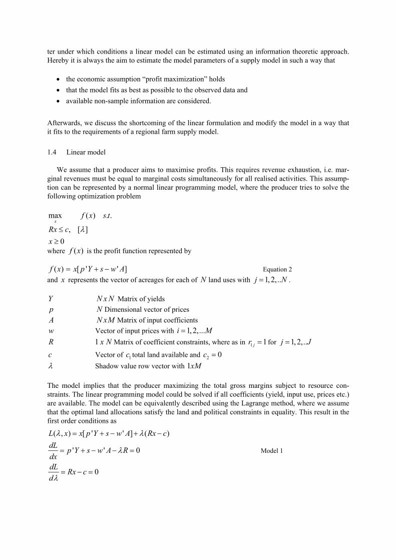
We assume that a producer aims to maximise profits. This requires revenue exhaustion, i.e. mar-ginal revenues must be equal to marginal costs simultaneously for all realised activities. This assump-tion can be represented by a normal linear programming model, where the producer tries to solve the following optimization problem

max ( ) . .

xf x s t

, [ ]

0Rx cx

λ≤≥

where ( )f x is the profit function represented by

( ) [ ' ' ]f x x p Y s w A= + − Equation 2 and x represents the vector of acreages for each of N land uses with 1,2,..j N= . Y N x N Matrix of yields p N Dimensional vector of prices A N xM Matrix of input coefficients w Vector of input prices with 1,2,...i M= R 1 x N Matrix of coefficient constraints, where as in 1 1jr = for 1, 2,..j J=

c Vector of 1c total land available and 2 0c = λ Shadow value row vector with 1xM

The model implies that the producer maximizing the total gross margins subject to resource con-straints. The linear programming model could be solved if all coefficients (yield, input use, prices etc.) are available. The model can be equivalently described using the Lagrange method, where we assume that the optimal land allocations satisfy the land and political constraints in equality. This result in the first order conditions as

( , ) [ ' ' ] ( )

' ' 0

0

L x x p Y s w A Rx cdL p Y s w A RdxdL Rx cd

λ λ

λ

λ

= + − + −

= + − − =

= − =

Model 1

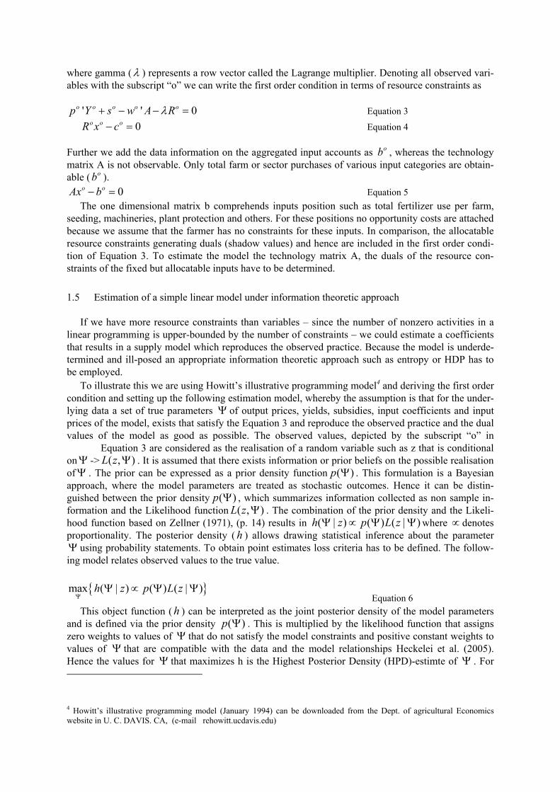
where gamma (λ ) represents a row vector called the Lagrange multiplier. Denoting all observed vari-ables with the subscript “o” we can write the first order condition in terms of resource constraints as

' ' 0o o o o op Y s w A Rλ+ − − = Equation 3

0o o oR x c− = Equation 4 Further we add the data information on the aggregated input accounts as ob , whereas the technology matrix A is not observable. Only total farm or sector purchases of various input categories are obtain-able ( ob ).

0o oAx b− = Equation 5 The one dimensional matrix b comprehends inputs position such as total fertilizer use per farm,

seeding, machineries, plant protection and others. For these positions no opportunity costs are attached because we assume that the farmer has no constraints for these inputs. In comparison, the allocatable resource constraints generating duals (shadow values) and hence are included in the first order condi-tion of Equation 3. To estimate the model the technology matrix A, the duals of the resource con-straints of the fixed but allocatable inputs have to be determined.

1.5 Estimation of a simple linear model under information theoretic approach

If we have more resource constraints than variables – since the number of nonzero activities in a linear programming is upper-bounded by the number of constraints – we could estimate a coefficients that results in a supply model which reproduces the observed practice. Because the model is underde-termined and ill-posed an appropriate information theoretic approach such as entropy or HDP has to be employed.

To illustrate this we are using Howitt’s illustrative programming model4 and deriving the first order condition and setting up the following estimation model, whereby the assumption is that for the under-lying data a set of true parameters Ψ of output prices, yields, subsidies, input coefficients and input prices of the model, exists that satisfy the Equation 3 and reproduce the observed practice and the dual values of the model as good as possible. The observed values, depicted by the subscript “o” in Equation 3 are considered as the realisation of a random variable such as z that is conditional onΨ -> ( , )L z Ψ . It is assumed that there exists information or prior beliefs on the possible realisation ofΨ . The prior can be expressed as a prior density function ( )p Ψ . This formulation is a Bayesian approach, where the model parameters are treated as stochastic outcomes. Hence it can be distin-guished between the prior density ( )p Ψ , which summarizes information collected as non sample in-formation and the Likelihood function ( , )L z Ψ . The combination of the prior density and the Likeli-hood function based on Zellner (1971), (p. 14) results in ( | ) ( ) ( | )h z p L zΨ ∝ Ψ Ψ where ∝ denotes proportionality. The posterior density ( h ) allows drawing statistical inference about the parameter Ψ using probability statements. To obtain point estimates loss criteria has to be defined. The follow-ing model relates observed values to the true value.

{ }max ( | ) ( ) ( | )h z p L z

ΨΨ ∝ Ψ Ψ

Equation 6 This object function ( h ) can be interpreted as the joint posterior density of the model parameters

and is defined via the prior density ( )p Ψ . This is multiplied by the likelihood function that assigns zero weights to values of Ψ that do not satisfy the model constraints and positive constant weights to values of Ψ that are compatible with the data and the model relationships Heckelei et al. (2005). Hence the values for Ψ that maximizes h is the Highest Posterior Density (HPD)-estimte of Ψ . For 4 Howitt’s illustrative programming model (January 1994) can be downloaded from the Dept. of agricultural Economics website in U. C. DAVIS. CA, (e-mail rehowitt.ucdavis.edu)

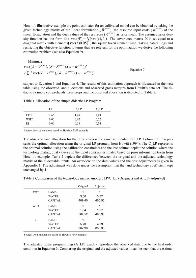
Howitt’s illustrative example the point estimates for an calibrated model can be obtained by taking the given technology matrix of the linear formulation ( priorR ), the resource input costs ( priorw ) of the linear formulation and the dual values of the resources ( priorλ ) as prior mean. The assumed prior den-sity function has the form like ( ) ~ ( ( ), )vec N vec zΨ ∑ . The covariance matrix ∑ is set equal to a diagonal matrix with elements ( )2( )0.05vec z , the square taken element wise. Taking natural logs and restricting the objective function to terms that are relevant for the optimization we derive the following estimation problem (see also Equation 9).

Minimize

1

(( ), ( ), ( )) '(( ), ( ), ( ))

prior prior prior

prior prior prior

vec R R w wvec R R w wλ λ

λ λ−

− − −

× ∑ − − − Equation 7

subject to Equation 3 and Equation 4. The results of this estimation approach is illustrated in the next table using the observed land allocations and observed gross margins from Howitt’s data set. The di-dactic example comprehends three crops and the observed allocation is depicted in Table 1.

Table 1 Allocation of the simple didactic LP Program

LP C_LP A_LP

COT 2,65 1,49 1,49WHT 0,00 0,62 0,62RI 0,00 0,54 0,54

Source: Own calculations based on Howitt's PMP example The observed land allocation for the three crops is the same as in column C_LP. Column “LP” repre-sents the optimal allocation using the original LP program from Howitt (1994). The C_LP represents the optimal solution using the calibration constraints and the last column depict the solution where the technology matrix, dual values and the input costs are estimated based on prior information taken from Howitt’s example. Table 2 depicts the differences between the original and the adjusted technology matrix of the allocatable inputs. An overview on the dual values and the cost adjustments is given in Appendix 1. The adjustment was done under the assumption that the land technology coefficient kept unchanged by 1.

Table 2 Comparison of the technology matrix amongst LP/C_LP (Original) and A_LP (Adjusted)

Original Adjusted

COT LAND 1 1WATER 3,00 3,37CAPITAL 409,40 465,55

WHT LAND 1 1WATER 1,84 1,67CAPITAL 564,52 495,98

RI LAND 1 1WATER 5,70 4,89CAPITAL 962,96 886,36

Source: Own calculations based on Howitt's PMP example The adjusted linear programming (A_LP) exactly reproduce the observed data due to the first order condition in Equation 3. Comparing the original and the adjusted values it can be seen that the estima-

tion framework tries to minimize the quadratic deviation of the posterior and the prior settings. Even although the model could be estimated in such a way that it exactly reproduces the observed practice such a simple LP calibration approach has some unattractive properties that it rarely meets the re-quirements for applied policy analysis.

i. Often a suitable number of empirical justified constraints are rarely available. Particular in farm group models which represents a greater population of farms.

ii. Further the adjustment of the crop allocation to price and policy changes will be discontinuous and consequently does not realistically represent the behaviour of an aggregated production model. A continuously adjustment would be more suitable.

iii. Economical concepts such as return to scale or diminishing costs are not considered5.

iv. The LP formulation does not allow a concept for catching the supply response estimated from time series or multiple observations. No behaviour parameters are included. For instance pri-ory believes on elasticities are not possible to include.

The small linear sample showed that allocatable input use could be adjusted in order to reproduce the observed practice. It should be emphasised here, that the differences of the priors versus the poste-rior point estimates of the technology matrix will increase when the input cost and dual are taken as certain outcomes. Nevertheless, the exercise demonstrated that as long as data can be seen as outcome of a random variable the model parameters can be estimated when taking relevant non-sample infor-mation into account. In the next chapter this small example will be extended that it meets the require-ments of a farm supply model appropriate for policy analysis.

1.6 Farm supply model

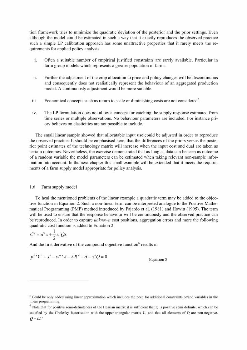
To heal the mentioned problems of the linear example a quadratic term may be added to the objec-tive function in Equation 2. Such a non-linear term can be interpreted analogue to the Positive Mathe-matical Programming (PMP) method introduced by Fajardo et al. (1981) and Howitt (1995). The term will be used to ensure that the response behaviour will be continuously and the observed practice can be reproduced. In order to capture unknown cost positions, aggregation errors and more the following quadratic cost function is added to Equation 2.

1' '2

vC d x x Qx= +

And the first derivative of the compound objective function6 results in ' ' ' 0o o o o o op Y s w A R d x Qλ+ − − − − = Equation 8

5 Could be only added using linear approximation which includes the need for additional constraints or/and variables in the linear programming. 6 Note that for positive semi-definiteness of the Hessian matrix it is sufficient that Q is positive semi definite, which can be satisfied by the Cholesky factorisation with the upper triangular matrix U, and that all elements of Q are non-negative.

'Q LL=

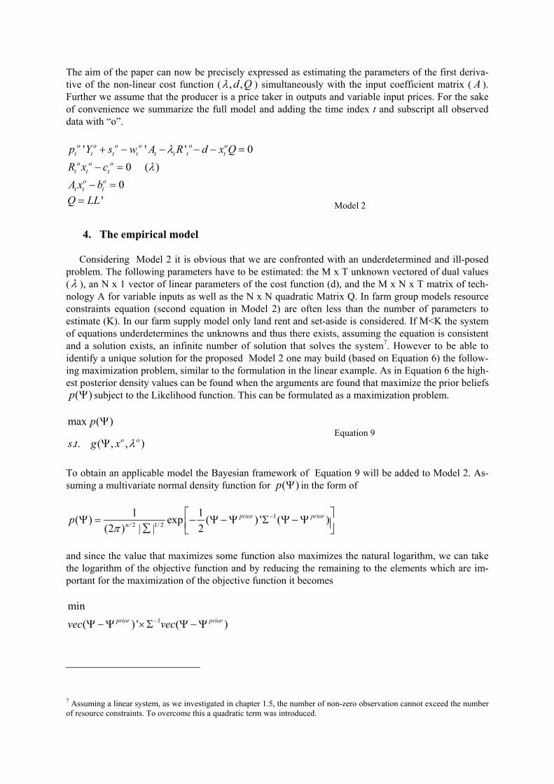
The aim of the paper can now be precisely expressed as estimating the parameters of the first deriva-tive of the non-linear cost function ( , ,d Qλ ) simultaneously with the input coefficient matrix ( A ). Further we assume that the producer is a price taker in outputs and variable input prices. For the sake of convenience we summarize the full model and adding the time index t and subscript all observed data with “o”.

' ' ' 0o o o o o o

t t t t t t t tp Y s w A R d x Qλ+ − − − − = 0 ( )o o o

t t tR x c λ− =

0o ot t tA x b− =

'Q LL= Model 2

4. The empirical model

Considering Model 2 it is obvious that we are confronted with an underdetermined and ill-posed problem. The following parameters have to be estimated: the M x T unknown vectored of dual values (λ ), an N x 1 vector of linear parameters of the cost function (d), and the M x N x T matrix of tech-nology A for variable inputs as well as the N x N quadratic Matrix Q. In farm group models resource constraints equation (second equation in Model 2) are often less than the number of parameters to estimate (K). In our farm supply model only land rent and set-aside is considered. If M<K the system of equations underdetermines the unknowns and thus there exists, assuming the equation is consistent and a solution exists, an infinite number of solution that solves the system7. However to be able to identify a unique solution for the proposed Model 2 one may build (based on Equation 6) the follow-ing maximization problem, similar to the formulation in the linear example. As in Equation 6 the high-est posterior density values can be found when the arguments are found that maximize the prior beliefs

( )p Ψ subject to the Likelihood function. This can be formulated as a maximization problem.

max ( )

. . ( , , )o o

p

s t g x λ

Ψ

Ψ Equation 9

To obtain an applicable model the Bayesian framework of Equation 9 will be added to Model 2. As-suming a multivariate normal density function for ( )p Ψ in the form of

1

/ 2 1/ 2

1 1( ) exp ( ) ' ( )(2 ) | | 2

prior priornp

π−⎡ ⎤Ψ = − Ψ −Ψ Σ Ψ −Ψ⎢ ⎥∑ ⎣ ⎦

and since the value that maximizes some function also maximizes the natural logarithm, we can take the logarithm of the objective function and by reducing the remaining to the elements which are im-portant for the maximization of the objective function it becomes

1

min( ) ' ( )prior priorvec vec−Ψ −Ψ ×Σ Ψ −Ψ

7 Assuming a linear system, as we investigated in chapter 1.5, the number of non-zero observation cannot exceed the number of resource constraints. To overcome this a quadratic term was introduced.

where 1−Σ is the covariance metrics and Ψ are the true values of the data generating process. The observed values ( , , , )o o o oz x p Y w= (crop allocation, output prices, yield, input prices are outcomes of a random variable and hence an error term is added to this observation. Assuming there exist a set of true parameters ( , , , , , )p Y A w d QΨ that satisfy the first order condition. It is further assumed that subsidies ( s ), price index, set-aside rate, and the total land constrain are known with certainty and that the producer has naïve price expectations for output and input prices ( ,p w ) and that yield is modelled over time via a linear trend. This prepositions leads to the following model8.

1

min( 0, 0, 0, ( ), ( )) '

( 0, 0, 0, ( ), ( )). .

x Y w prior priort t t t t t t

x Y w prior priort t t t t t t

vec A A

vec A As t

ε ε ε λ λ

ε ε ε λ λ−

− − − − −

× Σ − − − − −

all equations from Model 2

0 1

1

o xt t to Y

t t t

o pt t t

x x

Y T

p p

ε

β β ε

ε−

= +

= + +

= +

Model 3

Model 3 is estimated using Conopt4 which is part of the mathematical software package GAMS. The prior information for land duals was taken, where available, from the farm accounting network, the prior for the coefficient matrix A were taken from management handbooks.

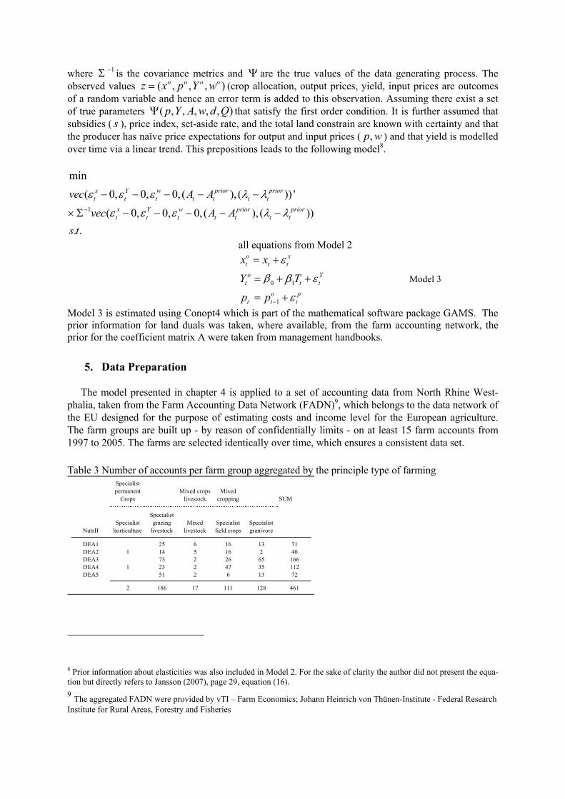
5. Data Preparation

The model presented in chapter 4 is applied to a set of accounting data from North Rhine West-phalia, taken from the Farm Accounting Data Network (FADN)9, which belongs to the data network of the EU designed for the purpose of estimating costs and income level for the European agriculture. The farm groups are built up - by reason of confidentially limits - on at least 15 farm accounts from 1997 to 2005. The farms are selected identically over time, which ensures a consistent data set.

Table 3 Number of accounts per farm group aggregated by the principle type of farming

Specialist permanent

CropsMixed crops-

livestockMixed

cropping SUM

NutsIISpecialist

horticulture

Specialist grazing

livestockMixed

livestockSpecialist field crops

Specialist granivore

DEA1 25 6 16 13 71DEA2 1 14 5 16 2 40DEA3 73 2 26 65 166DEA4 1 23 2 47 35 112DEA5 51 2 6 13 72

2 186 17 111 128 461

8 Prior information about elasticities was also included in Model 2. For the sake of clarity the author did not present the equa-tion but directly refers to Jansson (2007), page 29, equation (16). 9 The aggregated FADN were provided by vTI – Farm Economics; Johann Heinrich von Thünen-Institute - Federal Research Institute for Rural Areas, Forestry and Fisheries

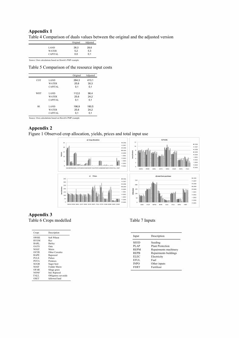
The specialized field crop farms in region DEA4 are selected to simulate and present the proposed input allocation for chapter 6. This particular farm group was chosen, because it is well represented during the simulation years from 1997 to 2005. Based on the information of each single farm account the production structure, prices, costs were mapped into the positions presented in the Appendix 3. Built up on the farms an average group was aggregated. Some production data of the selected farm group DEA4 is given in Appendix 2.

6. Results

In order to compare the effect of a simultaneously estimation of the input allocation two models were estimated and compared in this chapter. The first model is Model , for the remainder of the text indicated by “fixed model”, where the input allocation was pre-estimated and enters the model with the condition prior

t tA A= . In the second model (“sim model”) tA is determined by the objective and the Likelihood function (constraints of Model ). The hypothesis for the simulation is that due to the opti-mality condition the simultaneously estimated input allocation (“sim model”) will be less restrictive than its counterpart. Furthermore we assume that the “sim model” produces better estimates regarding the observed values (crop allocation, prices and yields).

Table 4 shows the share of explained variation for crop allocation, prices and yields. In the most cases the simultaneous model specification considerably improved the goodness of fit for land alloca-tion and prices. The fit for yields is in general lower due to the linear trend in both model specifica-tions.

Table4: R² measure for the “fixed” and “sim” model - prior versus posterior fit

R2

Crop allocation

Output prices Yields

Crop allocation Output prices Yields

SWHE 0,58 0,30 0,76 0,83 0,44 0,77RYEM 1,00 0,69 0,45 1,00 0,69 0,46BARL 0,46 0,25 0,71 0,63 1,00 0,71OATS 0,97 0,13 0,80 1,00 0,31 0,80MAIZ 0,75 0,77 0,53 1,00 0,81 0,52OCER 0,87 0,51 0,79 1,00 0,63 0,79RAPE 0,70 0,94 0,56 0,99 0,97 0,56PULS 1,00 0,96 0,34 1,00 0,97 0,33POTA 0,30 0,96 0,48 1,00 0,96 0,45SUGB 0,54 0,12 0,63 0,75 0,16 0,62MAIF 1,00 0,19 0,76 1,00 0,40 0,80OFAR 1,00 0,52 0,85 1,00 0,80 0,85NONF 0,99 0,63 0,51 1,00 0,74 0,51FALL 0,99 0,00 0,00 1,00 0,00 0,00OSET 1,00 0,00 0,00 1,00 0,00 0,00

Source: Own calculations

fixed model sim model

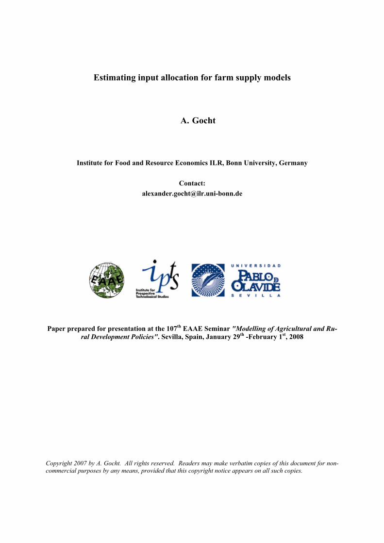
Figure 1 depicts the prior versus posterior values for soft wheat allocation. It can be seen that the

“sim” model outrange the “fixed” model estimates due to the possibility to adjust the input allocation between the crops within the total input constraints.

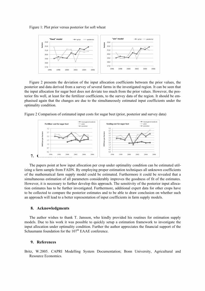
Figure 1: Plot prior versus posterior for soft wheat

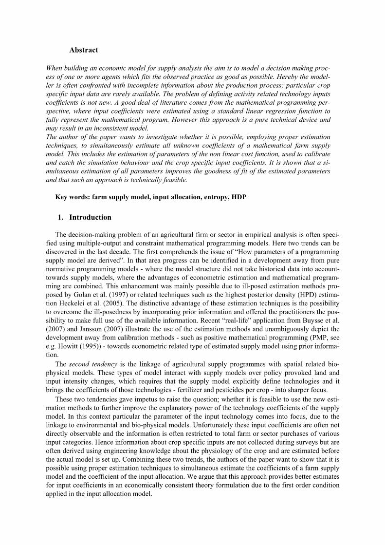
Figure 2 presents the deviation of the input allocation coefficients between the prior values, the

posterior and data derived from a survey of several farms in the investigated region. It can be seen that the input allocation for sugar beet does not deviate too much from the prior values. However, the pos-terior fits well, at least for the fertilizer coefficients, to the survey data of the region. It should be em-phasised again that the changes are due to the simultaneously estimated input coefficients under the optimality condition.

Figure 2 Comparison of estimated input costs for sugar beet (prior, posterior and survey data)

7. Conclusive remarks

The papers point at how input allocation per crop under optimality condition can be estimated util-izing a farm sample from FADN. By employing proper estimation techniques all unknown coefficients of the mathematical farm supply model could be estimated. Furthermore it could be revealed that a simultaneous estimation of all parameters considerably improves the goodness of fit of the estimates. However, it is necessary to further develop this approach. The sensitivity of the posterior input alloca-tion estimates has to be further investigated. Furthermore, additional expert data for other crops have to be collected to compare the posterior estimates and to be able to draw conclusion on whether such an approach will lead to a better representation of input coefficients in farm supply models.

8. Acknowledgments

The author wishes to thank T. Jansson, who kindly provided his routines for estimation supply models. Due to his work it was possible to quickly setup a estimation framework to investigate the input allocation under optimality condition. Further the author appreciates the financial support of the Schaumann foundation for the 107th EAAE conference.

9. References

Britz, W.2005. CAPRI Modelling System Documentation; Bonn University, Agricultural and Resource Economics.

17,0

18,0

19,0

20,0

21,0

22,0

23,0

1996 1998 2000 2002 2004 2006

hect

are

"fixed" model prior posterior

17,0

18,0

19,0

20,0

21,0

22,0

23,0

1996 1998 2000 2002 2004 2006

hect

are

"sim" model prior posterior

0,20,71,21,72,22,73,23,74,24,75,2

1996 1998 2000 2002 2004 2006

100

Eur

o pe

r he

ctar

e

Seeding cost for sugar beetmanagment analysispriorposterior

0,2

0,7

1,2

1,7

2,2

2,7

3,2

1996 1998 2000 2002 2004 2006

100

Eur

o pe

r he

ctar

e

Fertilizer cost for sugar beetmanagment analysispriorposterior

Buysse, J., Fernagut Bruno Harmignie, O., Frahan, d., Henry, B., Lauwers, L., Polome Philippe Van Huylenbroeck, G., Meensel, V., and Jef,. 2007. Farm-based modelling of the EU sugar reform: impact on Belgian sugar beet suppliers. Eur Rev Agric Econ 34: 21-52.

Chambers, R.G., and Just, R.E. 1989. Estimating Multioutput Technologies. American Journal of

Agricultural Economics 71: 980-995. Dixon, B.L., and Hornbaker, R.H. 1992. Estimating the technology coefficient in linear programming

models. American journal of agricultural economics 74: 1029-1039. Errington, A. 1989. Estimating Enterprise Input-Output Coefficients from Regional Farm Data.

Journal of Agricultural Economics 40: 52-56. Fajardo, D., B. A. McCarl; R. L. Thompson, and R. L. Thompson,. 1981. A Multicommodity Analysis

of Trade Policy Effects: The Case of Nicaraguan Agriculture. American Journal of Agricultural Economics 23-31.

Golan, A., Judge, G., and Miller, D. 1997. Maximum entropy econometrics Wiley,Chichester [u.a.]. Guyomard, H., Baudry, M., and Carpentier, A. 1996. Estimating crop supply response in the presents

of farm programmes: application to the CAP. European Review of Agricultural Economics 23: 401-420.

Hasenkamp, G. 1976. A Study of Multiple-Output Production Functions. Journal of Econometrics 4:

253-262. Heckelei, T., Mittelhammer, R., and Britz, W. 2005. A Bayesian Alternative to Generalized Cross

Entropy Parma : Monte Universita Parma Editore,Italy, Parma. Howitt, R.E. 1995. Positive Mathematical Programming. American Journal of Agricultural Economics

77: 329-342. Jansson, T. 2007. Estimation of supply response in CAPRI; Bonn University, Agricultural and

Resource Economics, Discussion Paper 2007:2 Just, R.E., Zilbermann, D., and Hochman, E. 1983. Estimation od Multicrop Production Function.

American Journal of Agricultural Economics 65: 770-780. Lansink, A.O., and Peerlings, J. 1997. Effects of N-Surplus Taxes: Combining Technical and

Historical Information. European Review of Agricultural Economics 24: 231-47. Lence, S.H., and Miller, D.J. 1998. Estimation of multi-output production functions with incomplete

data: A generalised maximum entropy approach. European Review of Agricultural Economics 25: 188-209.

Léon, Y., Peeters, L., Quinqu, M., and Surry, Y. 1999. The Use of Maximum Entropy to Estimate

Input-Output Coefficients From Regional Farm Accounting Data. Journal of agricultural Economics 50: 425-439.

Midmore, P. 1990. Estimating Input-Output Coefficients from Regional Farm Data. Journal of

Agricultural Economics 41: 108-111.

Mittelhammer, R.C., Scott C. Matulich; Bushaw, and Bushaw, D. 1981. On implicit Forms of Multiproduct-Multifactor Production Functions. American Journal of Agricultural Economics 63: 164-168.

Moxey, A., and Tiffin, R. 1994. Estimating linear production coefficients from farm business survey

data: A Note. Journal of Agricultural Economics 45: 381-385. Paris, Q. 1989. A Sure Bet on Symmetry. American Journal of Agricultural Economics 71: 344-351. Ray, S.C. 1985. Methods of estimating the input coefficient for linear programming models. American

journal of agricultural economics 67: 660-665. Shumway, C.R. 1995. Recent Duality Contributions in Production Economics. American Journal of

Agricultural Economics 20: 178-194. Shumway, C.R., Pope, R.D., and Nash, E.K. 1984. Allocatable Fixed Inputs and Jointness in

Agricultural Production: Implications for Economic Modeling. American Journal of Agricultural Economics 66: 72-78.

Zellner, A. 1971. An introduction to Bayesian inference in econometrics Wiley, New York

0

5

10

15

20

25

SWHERYEMBARL OATSMAIZ OCERRAPE PULS POTA SUGBNONFMAIF OFAR FALL OSET

Hect

are

a) Crop allocation

1996

1997

1998

1999

2000

2001

2002

2003

2004

2005 0

2

4

6

8

10

12

SWHE RYEM BARL OATS MAIZ OCER RAPE PULS

tone

s/he

ctar

e

b) Yields

1996

1997

1998

1999

2000

2001

2002

2003

2004

2005

0

50

100

150

200

250

300

350

SWHE RYEM BARL OATS MAIZ OCER RAPE PULS POTA SUGB NONF MAIF OFAR

Euro

/hec

tare

c) Prices

1996

1997

1998

1999

2000

2001

2002

2003

2004

2005 0

50

100

150

200

250

SEED PLAP REPM REPB ELEC EFUL INPO FERT

€/he

ctar

e

d) total farm purchase1996

1997

1998

1999

2000

2001

2002

2003

2004

2005

Appendix 1 Table 4 Comparison of duals values between the original and the adjusted version

Original Adjusted

LAND 28,3 28,6WATER 5,2 5,3CAPITAL 0,0 0,1

Source: Own calculations based on Howitt's PMP example

Table 5 Comparison of the resource input costs

Original Adjusted

COT LAND 264,3 413,1WATER 25,6 30,3CAPITAL 0,1 0,1

WHT LAND 112,0 96,4WATER 25,6 24,2CAPITAL 0,1 0,1

RI LAND 196,9 180,5WATER 25,6 24,2CAPITAL 0,1 0,1

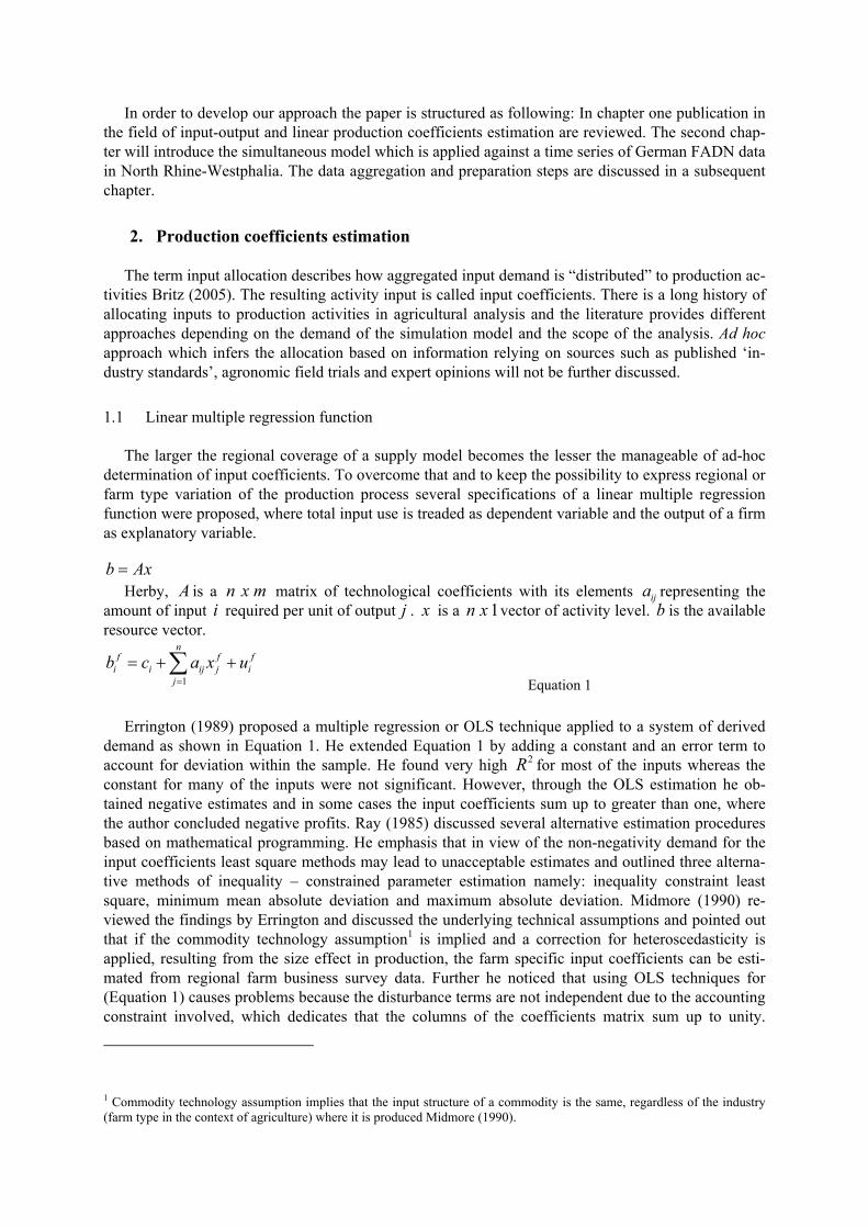
Source: Own calculations based on Howitt's PMP example Appendix 2 Figure 1 Observed crop allocation, yields, prices and total input use

Appendix 3 Table 6 Crops modelled Table 7 Inputs

Crops Description

SWHE Soft WheatRYEM RyeBARL BarleyOATS OatsMAIZ MaizeOCER Other CerealesRAPE RapeseedPULS PulsesPOTA PotatoesSUGB Suger beetMAIF Fodder MaizeOFAR Silage grassNONF Ind. RapseedFALL Obligatory set-asideOSET fallowed land

Input Description

SEED SeedingPLAP Plant ProtectionREPM Repairments machineryREPB Repairments buildingsELEC ElectricityEFUL FuelINPO Other inputsFERT Fertilizer