GUIDE TO ROAD DESIGN Part 3: Geometric Design

AGRD03-10
Oct 27, 2015
road handbook
Welcome message from author
This document is posted to help you gain knowledge. Please leave a comment to let me know what you think about it! Share it to your friends and learn new things together.
Transcript
GUIDE TO ROAD DESIGN
Part 3: Geometric Design
Guide to Road Design Part 3: Geometric Design

Guide to Road Design Part 3: Geometric Design Summary The Guide to Road Design – Part 3: Geometric Design contains guidance that provides road designers and other practitioners with information that is common to the geometric design of road alignments.
Road designers have to consider many factors and disciplines that may affect, or be affected by, the design of roads and intersections. Therefore, reference should also be made to the other parts of the Austroads Guide to Road Design are shown in Section 1 of this guide.
Part 3 covers topics that are common to geometric design such as operating speed, sight distance, horizontal and vertical geometry, including the coordination of those two elements and consideration of cross-section element. It also provides relevant information relating to the design of on-road cyclist and parking facilities.
The information in this guide generally replaces that which was previously provided in the Austroads Urban and Rural Road Design Guides (Austroads 2002b and Austroads 2003). Keywords Geometric road design, operating speed, cross-section, traffic lanes, shoulders, verge, batters, roadside drainage, medians, bicycle lanes, HOV lanes, on-street parking, service roads, outer separators, footpaths, bus stops, sight distance, stopping sight distance, sight distance on horizontal curves, overtaking sight distance, manoeuvre sight distance, intermediate sight distance, headlight sight distance, horizontal curve perception sight distance, horizontal alignment, vertical alignment, side friction factor, superelevation, adverse crossfall, grades, auxiliary lanes and bridge considerations First Published November 2009 Second edition October 2010 - References to Commentaries have been updated. © Austroads Ltd. 2010 This work is copyright. Apart from any use as permitted under the Copyright Act 1968, no part may be reproduced by any process without the prior written permission of Austroads. ISBN 978-1-921551-90-1 Austroads Project No. TP1566 Austroads Publication No. AGRD03/10 Project Manager David Hubner, DTMR Qld Prepared by David Barton, VicRoads Published by Austroads Ltd Level 9, Robell House 287 Elizabeth Street Sydney NSW 2000 Australia Phone: +61 2 9264 7088 Fax: +61 2 9264 1657 Email: [email protected]

www.austroads.com.au This guide is produced by Austroads as a general guide. Its application is discretionary. Road authorities may vary their practice according to local circumstances and policies. Austroads believes this publication to be correct at the time of printing and does not accept responsibility for any consequences arising from the use of information herein. Readers should rely on their own skill and judgement to apply information to particular issues.

Guide to Road Design Part 3: Geometric Design
Sydney 2010
Austroads profile Austroads purpose is to contribute to improved Australian and New Zealand transport outcomes by:
providing expert advice to SCOT and ATC on road and road transport issues facilitating collaboration between road agencies promoting harmonisation, consistency and uniformity in road and related operations undertaking strategic research on behalf of road agencies and communicating outcomes promoting improved and consistent practice by road agencies.
Austroads membership Austroads membership comprises the six state and two territory road transport and traffic authorities, the Commonwealth Department of Infrastructure, Transport, Regional Development and Local Government in Australia, the Australian Local Government Association, and New Zealand Transport Agency. It is governed by a council consisting of the chief executive officer (or an alternative senior executive officer) of each of its 11 member organisations:
Roads and Traffic Authority New South Wales Roads Corporation Victoria Department of Transport and Main Roads Queensland Main Roads Western Australia Department for Transport, Energy and Infrastructure South Australia Department of Infrastructure, Energy and Resources Tasmania Department of Planning and Infrastructure Northern Territory Department of Territory and Municipal Services Australian Capital Territory Department of Infrastructure, Transport, Regional Development and Local Government Australian Local Government Association New Zealand Transport Agency. The success of Austroads is derived from the collaboration of member organisations and others in the road industry. It aims to be the Australasian leader in providing high quality information, advice and fostering research in the road sector.

GUI DE TO RO A D DE SIG N P ART 3 : GEO MET RI C D ESI G N
A u s t r o a d s 2 0 1 0
— i —
ACKNOWLEDGEMENTS The key authors acknowledge the role and contribution of the Austroads Road Design Reference Panel in providing guidance and information during the preparation of this guide. The panel comprised the following members:
Mr Pat Kenny Roads and Traffic Authority, New South Wales Mr David Barton Roads Corporation, Victoria Dr Owen Arndt Department of Transport and Main Roads, Queensland Mr Rob Grove Main Roads Western Australia Mr Noel O’Callaghan Department for Transport, Energy and Infrastructure, South Australia Mr Graeme Nichols Department of Infrastructure, Energy and Resources, Tasmania Mr Peter Toll Department of Planning and Infrastructure, Northern Territory Mr Ken Marshall ACT Department of Territory and Municipal Services Mr Peter Aumann Australian Local Government Association Mr James Hughes NZ Transport Agency Mr Tom Brock The Association of Consulting Engineers Australia Mr Anthony Barton Australian Bicycle Council Mr Michael Tziotis ARRB Group Ltd It is also acknowledged that much of the material presented was derived or reproduced from the superseded Austroads Guide to the Geometric Design of Rural Roads (2003) and Austroads Guide to the Geometric Design of Major Urban Roads (2002).
GUI DE TO RO A D DE SIG N P ART 3 : GEO MET RI C D ESI G N
A u s t r o a d s 2 0 1 0
— i i —
CONTENTS 1 INTRODUCTION .......................................................................................................... 1 1.1 Purpose ........................................................................................................................ 1 1.2 Scope of this Part ......................................................................................................... 2 1.3 Design Criteria in Part 3 ................................................................................................ 2 1.4 Objectives of Geometric Design .................................................................................... 3 1.5 Road Safety .................................................................................................................. 4
1.5.1 Providing for a Safe System ............................................................................ 4 1.6 Design Process ............................................................................................................. 5 2 FUNDAMENTAL CONSIDERATIONS ......................................................................... 6 2.1 General ......................................................................................................................... 6 2.2 Design Parameters ....................................................................................................... 6
2.2.1 Location .......................................................................................................... 6 2.2.2 Road Classification ......................................................................................... 6 2.2.3 Traffic Volume and Composition ..................................................................... 6 2.2.4 Design Speed (Operating Speed) ................................................................... 7 2.2.5 Design Vehicle ................................................................................................ 7 2.2.6 Environmental Considerations ......................................................................... 8 2.2.7 Access Management ....................................................................................... 8 2.2.8 Drainage ......................................................................................................... 8 2.2.9 Utility Services................................................................................................. 9 2.2.10 Topography/Geology ....................................................................................... 9
3 SPEED PARAMETERS .............................................................................................. 10 3.1 General ....................................................................................................................... 10 3.2 Terminology ................................................................................................................ 11
3.2.1 Operating Speed (85th Percentile Speed) ..................................................... 11 3.2.2 Desired Speed .............................................................................................. 11 3.2.3 Design Speed ............................................................................................... 11 3.2.4 Vehicle Speeds on Roads ............................................................................. 11
3.3 Operating Speeds on Urban Roads ............................................................................ 12 3.3.1 Freeways (Access Controlled Roads) ........................................................... 12 3.3.2 High Standard Urban Arterial and Sub-arterial Roads ................................... 13 3.3.3 Urban Roads with Varying Standard Horizontal Curvature ............................ 13 3.3.4 Local Urban Roads ....................................................................................... 14
3.4 Operating Speeds on Rural Roads ............................................................................. 14 3.4.1 High Speed Rural Roads ............................................................................... 14 3.4.2 Intermediate Speed Rural Roads .................................................................. 15 3.4.3 Low Speed Rural Roads ............................................................................... 16
3.5 Determining Operating Speeds using the Operating Speed Model ............................. 17 3.5.1 General ......................................................................................................... 17 3.5.2 Driver Behaviour ........................................................................................... 17 3.5.3 Road Characteristics ..................................................................................... 17 3.5.4 Vehicle Characteristics .................................................................................. 18 3.5.5 Operating Speed Estimation Model ............................................................... 18 3.5.6 Car Acceleration on Straights Graph ............................................................. 18 3.5.7 Car Deceleration on Curves Graph ............................................................... 19 3.5.8 Section Operating Speeds ............................................................................ 20 3.5.9 Use of Operating Speed in the Design of Rural Roads .................................. 23
3.6 Operating Speed of Trucks ......................................................................................... 24 3.7 Operating Speeds for Temporary Works (including Sidetracks) .................................. 25
GUI DE TO RO A D DE SIG N P ART 3 : GEO MET RI C D ESI G N
A u s t r o a d s 2 0 1 0
— i i i —
4 CROSS-SECTION ...................................................................................................... 27 4.1 General ....................................................................................................................... 27
4.1.1 Functional Classification of Road Network .................................................... 28 4.1.2 Consideration of Staged Development .......................................................... 29
4.2 Traffic Lanes ............................................................................................................... 30 4.2.1 General ......................................................................................................... 30 4.2.2 Road Crossfall............................................................................................... 31 4.2.3 Crown Lines .................................................................................................. 31 4.2.4 Traffic Lane Widths ....................................................................................... 32 4.2.5 Urban Road Widths ....................................................................................... 33 4.2.6 Rural Road Widths ........................................................................................ 34
4.3 Shoulders ................................................................................................................... 36 4.3.1 Function ........................................................................................................ 36 4.3.2 Width ............................................................................................................. 36 4.3.3 Shoulder Sealing ........................................................................................... 37 4.3.4 Shoulder Crossfalls ....................................................................................... 38
4.4 Verge .......................................................................................................................... 39 4.4.1 Verge Widths ................................................................................................ 39 4.4.2 Verge Rounding ............................................................................................ 40 4.4.3 Verge Slopes ................................................................................................ 41
4.5 Batters ........................................................................................................................ 41 4.5.1 Benches ........................................................................................................ 43 4.5.2 Batter Rounding ............................................................................................ 45
4.6 Roadside Drainage ..................................................................................................... 46 4.6.1 Table Drains .................................................................................................. 46 4.6.2 Catch Drains ................................................................................................. 46 4.6.3 Median Drains ............................................................................................... 47 4.6.4 Kerb and Channel ......................................................................................... 50
4.7 Medians ...................................................................................................................... 52 4.7.1 Median Width ................................................................................................ 53 4.7.2 Median Slopes .............................................................................................. 55 4.7.3 Median Transitions ........................................................................................ 56 4.7.4 Median Openings .......................................................................................... 56
4.8 Bicycle Lanes.............................................................................................................. 60 4.8.1 General ......................................................................................................... 60 4.8.2 Road Geometry ............................................................................................. 61 4.8.3 Gradients ...................................................................................................... 61 4.8.4 Cross-section and Clearances ...................................................................... 61 4.8.5 Separated Bicycle Lanes ............................................................................... 63 4.8.6 Contra-flow Bicycle Lanes ............................................................................. 66 4.8.7 Exclusive Bicycle Lanes ................................................................................ 67 4.8.8 ‘Peak Period’ Exclusive Bicycle Lanes .......................................................... 71 4.8.9 Sealed Shoulders .......................................................................................... 71 4.8.10 Bicycle/Car Parking Lanes ............................................................................ 71 4.8.11 Wide Kerbside Lanes .................................................................................... 74 4.8.12 Supplementary Treatments ........................................................................... 75
4.9 High Occupancy Vehicle (HOV) Lanes ....................................................................... 76 4.9.1 General ......................................................................................................... 76 4.9.2 Bus Lanes ..................................................................................................... 77 4.9.3 Tram/Light Rail Vehicle (LRV) Lanes ............................................................ 81
4.10 On-street Parking ........................................................................................................ 83 4.10.1 General ......................................................................................................... 83 4.10.2 Parallel Parking ............................................................................................. 84
GUI DE TO RO A D DE SIG N P ART 3 : GEO MET RI C D ESI G N
A u s t r o a d s 2 0 1 0
— i v —
4.10.3 Angle Parking ................................................................................................ 85 4.10.4 Centre-of-road Parking .................................................................................. 85 4.10.5 Parking for Motorcycles ................................................................................. 88 4.10.6 Parking for People with Disabilities ................................................................ 89
4.11 Service Roads, Outer Separators and Footpaths ........................................................ 90 4.11.1 Service Roads ............................................................................................... 90 4.11.2 Outer Separator ............................................................................................ 91 4.11.3 Urban Border ................................................................................................ 92
4.12 Bus Stops ................................................................................................................... 94 4.12.1 General ......................................................................................................... 94 4.12.2 Urban ............................................................................................................ 95 4.12.3 Rural ............................................................................................................. 96
5 SIGHT DISTANCE...................................................................................................... 99 5.1 General ....................................................................................................................... 99 5.2 Sight Distance Parameters ......................................................................................... 99
5.2.1 Driver Eye Height ........................................................................................ 100 5.2.2 Driver Reaction Time................................................................................... 101 5.2.3 Longitudinal Deceleration ............................................................................ 102
5.3 Stopping Sight Distance (SSD) ................................................................................. 104 5.3.1 Car Stopping Sight Distance ....................................................................... 104 5.3.2 Truck Stopping Sight Distance .................................................................... 107
5.4 Sight Distance on Horizontal Curves ......................................................................... 109 5.4.1 Benching for Visibility on Horizontal Curves ................................................ 110
5.5 Sight Distance Requirements on Horizontal Curves with Roadside Barriers / Wall / Bridge Structures .................................................................................................... 112 5.5.1 Requirements where Sighting over Roadside Barriers is Possible............... 112 5.5.2 Requirements where there is no Line of Sight over Roadside ..................... 113
5.6 Overtaking Sight Distance......................................................................................... 113 5.6.1 General ....................................................................................................... 113 5.6.2 Overtaking Model ........................................................................................ 114 5.6.3 Determination of Overtaking Provision ........................................................ 115 5.6.4 Determination of Percentage of Road Providing Overtaking ........................ 116
5.7 Manoeuvre Sight Distance ........................................................................................ 117 5.8 Intermediate Sight Distance ...................................................................................... 118 5.9 Headlight Sight Distance ........................................................................................... 118 5.10 Horizontal Curve Perception Sight Distance ............................................................. 120 5.11 Other Restrictions to Visibility ................................................................................... 121 6 COORDINATION OF HORIZONTAL AND VERTICAL ALIGNMENT....................... 122 6.1 Principles .................................................................................................................. 122 6.2 Safety Considerations ............................................................................................... 122 6.3 Aesthetic Considerations .......................................................................................... 128
6.3.1 Coincident Horizontal and Vertical Curves .................................................. 128 6.3.2 Horizontal Curves ........................................................................................ 130 6.3.3 Vertical Curves ............................................................................................ 131
6.4 Drainage Considerations .......................................................................................... 132 7 HORIZONTAL ALIGNMENT .................................................................................... 133 7.1 General ..................................................................................................................... 133 7.2 Horizontal Alignment Design Procedure .................................................................... 135 7.3 Tangents ................................................................................................................... 136 7.4 Circular Curves ......................................................................................................... 136
GUI DE TO RO A D DE SIG N P ART 3 : GEO MET RI C D ESI G N
A u s t r o a d s 2 0 1 0
— v —
7.4.1 Horizontal Curve Equation .......................................................................... 136 7.5 Types of Horizontal Curves ....................................................................................... 137
7.5.1 Compound Curves ...................................................................................... 137 7.5.2 Broken Back Curves ................................................................................... 137 7.5.3 Reverse Curves .......................................................................................... 139 7.5.4 Transition Curves ........................................................................................ 139
7.6 Side Friction and Minimum Curve Size ..................................................................... 143 7.6.1 Minimum Radius Values .............................................................................. 144 7.6.2 Minimum Horizontal Curve Lengths and Deflection Angles not Requiring
Curves ........................................................................................................ 145 7.7 Superelevation .......................................................................................................... 146
7.7.1 Linear Method ............................................................................................. 147 7.7.2 Maximum Values of Superelevation ............................................................ 150 7.7.3 Minimum Values of Superelevation ............................................................. 150 7.7.4 Application of Superelevation ...................................................................... 150 7.7.5 Length of Superelevation Development ....................................................... 151 7.7.6 Rate of Rotation .......................................................................................... 153 7.7.7 Relative Grade ............................................................................................ 153 7.7.8 Design Superelevation Development Lengths ............................................. 155 7.7.9 Positioning of Superelevation Runoff without Transitions ............................ 156 7.7.10 Positioning of Superelevation Runoff with Transitions ................................. 157
7.8 Curves with Adverse Crossfall .................................................................................. 158 7.9 Pavement Widening on Horizontal Curves ................................................................ 159 7.10 Curvilinear Alignment Design in Flat Terrain ............................................................. 161
7.10.1 Theoretical Considerations .......................................................................... 162 7.10.2 Advantages of Curvilinear Alignment ........................................................... 162
8 VERTICAL ALIGNMENT .......................................................................................... 164 8.1 General ..................................................................................................................... 164 8.2 Vertical Controls ....................................................................................................... 164
8.2.1 Flood Levels or Water Table ....................................................................... 165 8.2.2 Vertical Clearances ..................................................................................... 166 8.2.3 Underground Services ................................................................................. 166 8.2.4 Other Vertical Clearance Considerations..................................................... 167 8.2.5 Vehicle Clearances ..................................................................................... 168
8.3 Grading Procedure ................................................................................................... 169 8.4 Grading Point ............................................................................................................ 170
8.4.1 Two-lane – Two-way Roads ........................................................................ 170 8.4.2 Divided Roads ............................................................................................. 171
8.5 Grades ...................................................................................................................... 172 8.5.1 General ....................................................................................................... 172 8.5.2 Vehicle Operation on Grades ...................................................................... 173 8.5.3 Maximum Grades ........................................................................................ 174 8.5.4 Length of Steep Grades .............................................................................. 175 8.5.5 Steep Grade Considerations ....................................................................... 176 8.5.6 Minimum Grades ......................................................................................... 176
8.6 Vertical Curves ......................................................................................................... 177 8.6.1 General ....................................................................................................... 177 8.6.2 Forms and Types of Vertical Curves ........................................................... 177 8.6.3 Crest Vertical Curves .................................................................................. 179 8.6.4 Sag Vertical Curves .................................................................................... 183 8.6.5 Sight Distance Criteria (Sag) ....................................................................... 184 8.6.6 Reverse/Compound/Broken Back Vertical Curves ...................................... 187
GUI DE TO RO A D DE SIG N P ART 3 : GEO MET RI C D ESI G N
A u s t r o a d s 2 0 1 0
— v i —
8.6.7 Minimum Length of Vertical Curves ............................................................. 187 8.6.8 Maximum Grade Change without a Vertical Curve ...................................... 188
8.7 Earthworks ................................................................................................................ 188 8.7.1 Earthworks Balance .................................................................................... 188 8.7.2 Earthworks Quantities ................................................................................. 189
9 AUXILIARY LANES ................................................................................................. 191 9.1 General ..................................................................................................................... 191 9.2 Types of Auxiliary Lanes ........................................................................................... 191 9.3 Speed Change Lanes ............................................................................................... 192
9.3.1 Acceleration Lanes ...................................................................................... 192 9.3.2 Deceleration Lanes ..................................................................................... 192
9.4 Overtaking Lanes ...................................................................................................... 192 9.4.1 General ....................................................................................................... 192
9.5 Climbing Lanes ......................................................................................................... 199 9.5.1 General ....................................................................................................... 199 9.5.2 Warrants ..................................................................................................... 199 9.5.3 Length ......................................................................................................... 200
9.6 Slow Vehicle Turnouts .............................................................................................. 206 9.6.1 Partial Climbing Lanes ................................................................................ 206 9.6.2 Slow Vehicle Turnouts ................................................................................. 206
9.7 Descending Lanes .................................................................................................... 207 9.8 Carriageway Requirements ....................................................................................... 207 9.9 Geometric Requirements .......................................................................................... 208
9.9.1 Starting and Termination Points .................................................................. 208 9.9.2 Tapers ......................................................................................................... 209 9.9.3 Cross-section .............................................................................................. 210
10 BRIDGE CONSIDERATIONS ................................................................................... 211 10.1 General ..................................................................................................................... 211 10.2 Cross Section ........................................................................................................... 211 10.3 Horizontal Geometry ................................................................................................. 212
10.3.1 Superelevation ............................................................................................ 212 10.4 Vertical Geometry ..................................................................................................... 212 REFERENCES .................................................................................................................. 213 APPENDIX A EXTENDED DESIGN DOMAIN (EDD) FOR GEOMETRIC
ROAD DESIGN ............................................................................. 219 APPENDIX B SPEED PARAMETER TERMINOLOGY ........................................ 240 APPENDIX C EXAMPLE CALCULATION OF THE OPERATING SPEED
MODEL ......................................................................................... 242 APPENDIX D THEORY OF MOVEMENT IN A CIRCULAR PATH ...................... 252 APPENDIX E REVERSE CURVES ..................................................................... 259 APPENDIX F TRANSITION CURVES (SPIRALS) .............................................. 266 APPENDIX G VERTICAL CURVE CURVATURE FORMULAE ........................... 272
GUI DE TO RO A D DE SIG N P ART 3 : GEO MET RI C D ESI G N
A u s t r o a d s 2 0 1 0
— v i i —
TABLES Table 3.1: Typical urban operating speeds (km/h) ......................................................... 12 Table 3.2: Typical desired speed (for rural roads on which vehicle speeds are
influenced by the horizontal alignment) ......................................................... 16 Table 3.3: Section operating speeds .............................................................................. 21 Table 3.4: Car/truck speed relationship .......................................................................... 24 Table 4.1: Suggested design life .................................................................................... 30 Table 4.2: Typical pavement crossfall on straights ......................................................... 31 Table 4.3: Urban arterial road widths ............................................................................. 33 Table 4.4: Urban freeway widths .................................................................................... 34 Table 4.5: Single carriageway rural road widths (m)....................................................... 35 Table 4.6: Divided carriageway rural road widths ........................................................... 35 Table 4.7: Shoulder width .............................................................................................. 38 Table 4.8: Shoulder crossfalls ........................................................................................ 39 Table 4.9: Verge width ................................................................................................... 39 Table 4.10: Verge rounding.............................................................................................. 41 Table 4.11: Verge slopes ................................................................................................. 41 Table 4.12: Typical design batter slopes .......................................................................... 43 Table 4.13: Clearances from line of kerb to traffic lane .................................................... 51 Table 4.14: Median widths ............................................................................................... 53 Table 4.15: Median slopes ............................................................................................... 56 Table 4.16: Clearance to cyclist envelope from adjacent truck ......................................... 61 Table 4.17: Exclusive bicycle lane dimensions in urban areas ......................................... 68 Table 4.18: Bicycle/car parking lane dimensions (parallel parking) .................................. 72 Table 4.19: Bicycle/car parking lane dimensions (angle parking) ..................................... 73 Table 4.20: Wide kerbside lane dimensions ..................................................................... 75 Table 4.21: Widths of bus travel lanes on new roads ....................................................... 77 Table 4.22: Width of kerbside bus lanes .......................................................................... 80 Table 4.23: Light rail vehicle critical dimensions for straight track .................................... 82 Table 4.24: Centre of road parking – minimum roadway width ......................................... 86 Table 4.25: Minimum service road lane widths for roads with low traffic volumes ............ 90 Table 4.26: Typical minimum service road carriageway widths for roads with low
traffic volumes and low parking demand........................................................ 91 Table 4.27: Typical widths of outer separators ................................................................. 92 Table 4.28: Typical urban border widths .......................................................................... 93 Table 4.29: Typical urban border slopes .......................................................................... 93 Table 4.30: Typical clearances to ROW boundary ........................................................... 94 Table 5.1: Vertical height parameters .......................................................................... 101 Table 5.2: Driver reaction times ................................................................................... 102 Table 5.3: Design domain for coefficient of deceleration .............................................. 103 Table 5.4: Stopping sight distances for cars on sealed roads ....................................... 106 Table 5.5: Truck stopping sight distances .................................................................... 109
GUI DE TO RO A D DE SIG N P ART 3 : GEO MET RI C D ESI G N
A u s t r o a d s 2 0 1 0
— v i i i —
Table 5.6: Minimum shoulder widths and manoeuvre times for sight distances over roadside safety barriers on horizontal curves .............................................. 113
Table 5.7: Overtaking sight distances for determining overtaking zones on MCV routes when MCV speeds are 10 km/h less than the operating speed ....... 117
Table 5.8: Overtaking sight distances for determining overtaking zones on MCV routes when MCV speeds are equal to the operating speed........................ 117
Table 7.1: Maximum decrease in speed value between geometric elements for low and intermediate speed rural roads ............................................................. 134
Table 7.2: Maximum radius requiring a spiral ............................................................... 141 Table 7.3: Minimum spiral lengths ................................................................................ 142 Table 7.4: Recommended side friction factors for cars and trucks ............................... 144 Table 7.5: Minimum radii of horizontal curves based on superelevation and side
friction at maximum values .......................................................................... 144 Table 7.6: Maximum deflection angles not requiring horizontal curves and minimum
horizontal curve lengths .............................................................................. 146 Table 7.7: Maximum values of superelevation to be used for different road types ........ 150 Table 7.8: Maximum relative grade between edge of carriageway and axis of
rotation in superelevation development ....................................................... 154 Table 7.9: Design superelevation development lengths (le) satisfying both rate of
rotation and relative grade criteria ............................................................... 156 Table 7.10: Minimum radii with adverse crossfall ........................................................... 159 Table 7.11: Curve widening per lane for current Austroads design vehicles ................... 161 Table 8.1: Typical minimum vertical clearances over roadways and
pedestrian/cycle paths ................................................................................. 167 Table 8.2: Effect of grade on vehicle type .................................................................... 174 Table 8.3: General maximum grades (%) ..................................................................... 174 Table 8.4: Desirable maximum lengths of grades ........................................................ 176 Table 8.5: Minimum grades .......................................................................................... 177 Table 8.6: Length of crest vertical curves – appearance criterion when S < L .............. 180 Table 8.7: Minimum size crest vertical curve (K value) for sealed roads (S<L) ............. 181 Table 8.8: Minimum size crest vertical curve (K value) for sealed roads to satisfy
intermediate sight distance (S<L) ................................................................ 182 Table 8.9: Minimum lengths of vertical curves for new construction ............................. 188 Table 8.10: Maximum grade change without a vertical curve ......................................... 188 Table 9.1: Traffic volume guidelines for providing overtaking lanes .............................. 194 Table 9.2: Overtaking lane lengths ............................................................................... 198 Table 9.3: Merge sight distance at end of overtaking lane for cars overtaking MCVs ... 198 Table 9.4: Volume guidelines for partial climbing lanes ................................................ 200 Table 9.5: Grade/distance warrant (lengths (m) to reduce truck vehicle speed to 40
km/h) ........................................................................................................... 201 Table 9.6: Merge sight distance at end of climbing lane for cars overtaking MCVs ...... 201 Table 9.7: Sight distance to the start of an auxiliary lane ............................................. 208 Table 9.8: Tapers for diverges and merges .................................................................. 210
GUI DE TO RO A D DE SIG N P ART 3 : GEO MET RI C D ESI G N
A u s t r o a d s 2 0 1 0
— i x —
FIGURES Figure 1.1: Flowchart of the Guide to Road Design ........................................................... 1 Figure 1.2: Flow chart for alignment design ....................................................................... 5 Figure 3.1: High speed .................................................................................................... 15 Figure 3.2: Intermediate speed ....................................................................................... 15 Figure 3.3: Low speed roads ........................................................................................... 16 Figure 3.4: Acceleration on straights ............................................................................... 19 Figure 3.5: Deceleration on curves .................................................................................. 20 Figure 3.6: Road study length ......................................................................................... 21 Figure 3.7: Single curve disparity .................................................................................... 22 Figure 3.8: Road length sections ..................................................................................... 23 Figure 3.9: Determination of truck speeds on grade, 19 m semi-trailer (33 t), 12 l
diesel carrying an average load (9.7 kW/t) .................................................... 26 Figure 4.1: Cross-section design flowchart ...................................................................... 28 Figure 4.2: Cross-section terminology ............................................................................. 29 Figure 4.3: 2 m rounding across crown line ..................................................................... 31 Figure 4.4: Kerb and channel components ...................................................................... 32 Figure 4.5: Minimum verge width under structures .......................................................... 40 Figure 4.6: Verge rounding.............................................................................................. 41 Figure 4.7: Benches (elevation and cross-section) .......................................................... 45 Figure 4.8: Typical table drain shape and location .......................................................... 47 Figure 4.9: Typical catch drains and banks ..................................................................... 47 Figure 4.10: Desirable V-drain cross-sections ................................................................... 48 Figure 4.11: Desirable table drain cross-sections .............................................................. 49 Figure 4.12: Typical kerb profile shapes ............................................................................ 50 Figure 4.13: Typical median cross-sections ...................................................................... 53 Figure 4.14: Example of kerbed medians on divided urban roads ..................................... 54 Figure 4.15: Median slope treatment (road reserve 30 – 50 m wide) ................................. 57 Figure 4.16: Median slope treatment (road reserves greater than 50 m wide) ................... 58 Figure 4.17: Typical median terminal treatments ............................................................... 59 Figure 4.18: Cyclist envelope ............................................................................................ 62 Figure 4.19: Road clearances ........................................................................................... 63 Figure 4.20: Location and typical cross-section of kerb separated bicycle lane ................. 64 Figure 4.21: Kerb separated bicycle lane .......................................................................... 65 Figure 4.22: Typical cross-section of a protected bicycle lane ........................................... 66 Figure 4.23: Contra-flow bicycle lane – layout ................................................................... 67 Figure 4.24: Exclusive bicycle lane ................................................................................... 68 Figure 4.25: Low and high speed exit and entry ramps ..................................................... 70 Figure 4.26: During and outside clearway times ................................................................ 71 Figure 4.27: Typical bicycle/car parking lanes layout (parallel parking) ............................. 73 Figure 4.28: Typical bicycle/car parking lanes layout (angle parking) ................................ 74 Figure 4.29: Wide kerbside lane ........................................................................................ 74
GUI DE TO RO A D DE SIG N P ART 3 : GEO MET RI C D ESI G N
A u s t r o a d s 2 0 1 0
— x —
Figure 4.30: Camera systems to record illegal use of bus lanes ........................................ 77 Figure 4.31: Example diagram showing a full-time/part-time bus lane with signage .......... 81 Figure 4.32: Layouts for angle parking spaces .................................................................. 87 Figure 4.33: Minimum width for on-street parking .............................................................. 88 Figure 4.34: Conversion of a car parking space to motorcycle spaces .............................. 89 Figure 4.35: Example of a parallel disabled parking space with access ramps to the
footpath ......................................................................................................... 90 Figure 4.36: Outer separators ........................................................................................... 91 Figure 4.37: Urban border ................................................................................................. 93 Figure 4.38: Example bus stop layout for roadside width > 4.0 m ...................................... 96 Figure 4.39: Typical indented bus bay layout .................................................................... 96 Figure 5.1: Sight distance ............................................................................................... 99 Figure 5.2: Car stopping sight distance ......................................................................... 105 Figure 5.3: Truck stopping sight distance ...................................................................... 107 Figure 5.4: Line of sight on horizontal curves ................................................................ 111 Figure 5.5: Overtaking manoeuvre ................................................................................ 115 Figure 5.6: Car headlight sight distance on sag vertical curves ..................................... 119 Figure 5.7: Headlights shine tangentially off horizontal curves ...................................... 119 Figure 6.1: Lateral shifts on crests (poor design practice) ............................................. 123 Figure 6.2: Alignment change behind crest (poor design practice) ................................ 124 Figure 6.3: Horizontal curve longer than vertical curve (good design practice) .............. 124 Figure 6.4: Intersection hidden behind a crest (poor design practice) ............................ 124 Figure 6.5: Hidden dip (poor design practice) ................................................................ 125 Figure 6.6: Shallow dip (poor design practice)............................................................... 125 Figure 6.7: Measures to correct dips in long uniform grades ......................................... 125 Figure 6.8: Poor coordination of horizontal and vertical alignments ............................... 126 Figure 6.9: Roller coaster grading resulting in hidden dips ............................................ 128 Figure 6.10: Acceptable coordination of horizontal and vertical alignments ..................... 129 Figure 6.11: A road well fitted to the terrain ..................................................................... 130 Figure 6.12: A road that is not well fitted to the terrain..................................................... 130 Figure 6.13: Comparison of short and long horizontal curves .......................................... 131 Figure 6.14: Short horizontal curves in series ................................................................. 131 Figure 6.15: Short sag curve appears kinked .................................................................. 132 Figure 7.1: Identification of roadways on long, steep grades ......................................... 134 Figure 7.2: Types of broken back curves ....................................................................... 138 Figure 7.3: Drivers’ view of broken back curves ............................................................ 138 Figure 7.4: Mathematical spiral ..................................................................................... 140 Figure 7.5: Rural Roads: Relationship between speed, radius and superelevation
(V ≥ 80 km/h) and Urban Roads: Relationship between speed, radius and superelevation (V ≥ 90 km/h) ................................................................ 148
Figure 7.6: Rural Roads: Relationship between speed, radius and superelevation (V < 80 km/h) .............................................................................................. 149
Figure 7.7: Urban Roads: Relationship between speed, radius and superelevation (V < 90 km/h) .............................................................................................. 149
GUI DE TO RO A D DE SIG N P ART 3 : GEO MET RI C D ESI G N
A u s t r o a d s 2 0 1 0
— x i —
Figure 7.8: Typical superelevation development profile on two lane roads (tangent to transition curve to circular curve) ................................................................. 152
Figure 7.9: Typical superelevation development profile (tangent to circular curve) ........ 157 Figure 8.1: Less clearance for long vehicles ................................................................. 165 Figure 8.2: Driveway gradient profile beam ................................................................... 168 Figure 8.3: Typical grading point on two-lane – two-way roads ..................................... 171 Figure 8.4: Typical grading points on urban freeways ................................................... 171 Figure 8.5: Typical grading points on rural freeways ..................................................... 172 Figure 8.6: Types of vertical curves ............................................................................... 178 Figure 8.7: K values for sag curves ............................................................................... 186 Figure 9.1: Example overtaking lane configurations ...................................................... 195 Figure 9.2: Typical development and termination of overtaking lanes ........................... 196 Figure 9.3: Determination of truck speeds on grade, 19 m semi-trailer (42.5 t), 12 l
diesel carrying a maximum load (7.5 kW/t) .................................................. 202 Figure 9.4: Determination of truck speeds on grade, B-double (62.4 t), 12 l diesel
carrying a maximum load (5.4 kW/t) ............................................................ 203 Figure 9.5: Determination of truck speeds on grade, Type 1 road train (89.8 t), 12 l
diesel carrying a maximum load (3.8 kW/t) .................................................. 204 Figure 9.6: Determination of truck speeds on grade, Type 2 road train (140 t), 16.4 l
diesel carrying a maximum load (3.1 kW/t) .................................................. 205 Figure 9.7: Examples of the development of slow vehicle turnouts ................................ 207
GUI DE TO RO A D DE SIG N P ART 3 : GEO MET RI C D ESI G N
A u s t r o a d s 2 0 1 0
— 1 —
1 INTRODUCTION
1.1 Purpose The Austroads Guide to Road Design seeks to capture the contemporary road design practice of member organisations (refer to the Austroads Guide to Road Design – Part 1: Introduction to Road Design, Austroads (2006b). In doing so, it provides valuable guidance to designers in the production of safe, economical and efficient road designs.
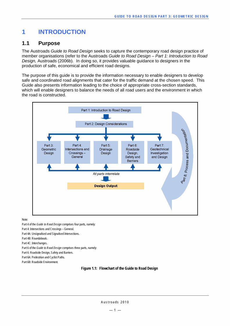
The purpose of this guide is to provide the information necessary to enable designers to develop safe and coordinated road alignments that cater for the traffic demand at the chosen speed. This Guide also presents information leading to the choice of appropriate cross-section standards, which will enable designers to balance the needs of all road users and the environment in which the road is constructed.
Note: Part 4 of the Guide to Road Design comprises four parts, namely: Part 4: Intersections and Crossings – General. Part 4A: Unsignalised and Signalised Intersections. Part 4B: Roundabouts. Part 4C: Interchanges. Part 6 of the Guide to Road Design comprises three parts, namely: Part 6: Roadside Design, Safety and Barriers. Part 6A: Pedestrian and Cyclist Paths. Part 6B: Roadside Environment.
Figure 1.1: Flowchart of the Guide to Road Design
GUI DE TO RO A D DE SIG N P ART 3 : GEO MET RI C D ESI G N
A u s t r o a d s 2 0 1 0
— 2 —
As shown in Figure 1.1, Part 3 is one of eight guides that comprise the Austroads Guide to Road Design and provide information on a range of disciplines including intersection design, drainage, roadside design and geotechnical design, all of which may influence the location and design of a road. Outputs from the geometric design process must be considered in the broader context of the overall design task as they may impact on other elements of the design. Whilst Figure 1.1 outlines the structure of the Guide to Road Design, designers should be aware that there are nine other subject areas spanning the range of Austroads publications that may also be relevant to geometric road design (www.austroads.com.au).
1.2 Scope of this Part The Austroads Guide to Road Design provides the designer with a framework that is intended to promote efficiency in design, construction and maintenance of a length of roadway. Part 3 is concerned primarily with the horizontal and vertical geometric design, along with the cross-section standards that are appropriate for the functional class of the road. Part 3 also provides information relating to cycling, public transport and parking facilities as they apply in an on-road situation. Reference should be made to Guide to Road Design – Part 6A: Pedestrian and Cyclist Paths (Austroads 2009e) for information regarding off-road facilities for cyclists and Part 6B: Roadside Environmental (Austroads 2009f). Designers should also consult Guide to Road Design – Part 4: Intersections and Crossings – General (Austroads 2009a) for information about the appropriate placement and design of all forms of intersections, interchanges and railway level crossings.
This guide must be applied sensibly and flexibly in conjunction with the skill and judgement of the designer. The designer should have regard for the particular circumstances in each case, including the importance of the road, the nature and amount of traffic expected to use it now and in the future, and the cost and implications of alternatives.
Compliance with these guidelines does not relieve designers of the responsibility for establishing that their design was suitable, appropriate and adequate for the purpose stated in the project requirements. In selecting design criteria based on the guidelines, the designer should take care to ensure that the selection of minimum criteria does not lead to an unsatisfactory or unsafe design overall.
Design values that are not within the limits recommended by this guide do not necessarily result in unacceptable designs and values that are within those limits do not necessarily guarantee an acceptable design. In assessing the quality of a design, it is not appropriate to simply consider a checklist of recommended limits. The design has to be developed with sound, professional judgement and guidelines assist the designer in making those judgements. In general, minimum standards should only be used where they are considered necessary to meet one or more of the design objectives listed in Section 1.4. Generally, if a minimum is used for any particular design element, it is preferable to avoid using a minimum for another element in the same location, for the road to be able to still provide an appropriate factor of safety to the road user.
1.3 Design Criteria in Part 3 The Guide to Road Design – Part 2: Design Considerations (Austroads 2006c) discusses the concept of Normal Design Domain (NDD) and Extended Design Domain (EDD). Guidance on the application of this concept to road geometry is provided in Appendix A of this guide.
In the context of road design:
A greenfield site is a location on which a new road is being built where there is no development that prevents the use of design values within the guidelines relating to NDD.
GUI DE TO RO A D DE SIG N P ART 3 : GEO MET RI C D ESI G N
A u s t r o a d s 2 0 1 0
— 3 —
A brownfield site is a location where development (e.g. roads and buildings) exists and may influence the design to the extent that use of values outside the NDD and EDD for one or more elements of the design may be necessary.
The body of this guide contains NDD values. These are road design values suitable for the design development of the cross-section and geometry for new roads (greenfield sites). In most cases, these design values will also be suitable for modifications and upgrades to existing roads (brownfield sites).
In constrained locations (particularly at brownfield sites), it may not always be practical or possible to achieve all of the relevant NDD values. In these constrained locations, road authorities may consider the use of values outside of the NDD.
Appendix A contains Extended Design Domain (EDD) values. These are values outside of the NDD that through research and/or operating experience, particular road authorities have found to provide a suitable solution in constrained situations. EDD values have only been developed for particular parameters, where considerable latitude exists within the NDD values.
Guidance on the use of values outside of the design domain (i.e. outside of the NDD and EDD) is not provided in this guide. Designers should consult the delegated representative from the relevant road authority for advice and direction with respect to an appropriate standard when values within the design domain are not achievable.
In applying this guide:
1. NDD values given in the body of this guide should be used wherever practical.
2. Design values outside of the NDD are only to be used if approved in writing by the delegated representative from the relevant road authority. The relevant road authority may be a state road authority, municipal council or private road owner.
3. If using EDD values, the reduction in standard associated with their use should be appropriate for the prevailing local conditions. Generally, EDD should be used for only one parameter in any application and not be used in combination with any other minimum or EDD value for any related or associated parameters.
1.4 Objectives of Geometric Design Road projects are developed to meet increasing travel demand, address crash problems, and rehabilitate existing infrastructure or a combination of any of these reasons. A balanced approach towards road planning and design can improve operational efficiency, road safety and public amenity whilst minimising the environmental impacts of noise, vibration, pollution and visual intrusion.
The objectives of new and existing road projects should be carefully considered to achieve the desired balance between the level of traffic service provided, safety, whole-of-life costs, flexibility for future upgrading or rehabilitation and environmental impact. These issues are discussed further in the Guide to Road Design – Part 2: Design Considerations (Austroads 2006c). It is incumbent upon the designer to consider the issues listed and apply them as needed to the geometric design of a road project.
Specific objectives related to geometric design are listed below:
provision of a road that is safe to travel on for all road users at the appropriate travel speeds, and a roadside that reduces the incidence and severity of crashes
GUI DE TO RO A D DE SIG N P ART 3 : GEO MET RI C D ESI G N
A u s t r o a d s 2 0 1 0
— 4 —
maintenance of a degree of uniformity, particularly across administrative boundaries to provide a consistent and operationally effective driving experience relative to the functional class of road
development of economically efficient designs to maximise the limited funds available for road construction and maintenance
adequately provision for the future requirements of the road network
cater for the types of vehicles expected to use the road
mitigation of environmental impacts (during construction and operation) both in the immediate vicinity of the road and over a wider area.
Section 2 of this guide provides further information regarding the fundamental design parameters that should be considered in the development of any road project.
1.5 Road Safety The Guide to Road Design – Part 3: Geometric Design should be considered in the context of road safety and the contribution that the guide can make to the design of safer roads.
1.5.1 Providing for a Safe System Adopting a safe system approach to road safety recognises that humans, as road users are fallible and will continue to make mistakes, and that the community should not penalise people with death or serious injury when they do make mistakes. In a safe system, therefore, roads (and vehicles) should be designed to reduce the incidence and severity of crashes when they inevitably occur.
The safe system approach requires, in part (Australian Transport Council 2006):
Designing, constructing and maintaining a road system (roads, vehicles and operating requirements) so that forces on the human body generated in crashes are generally less than those resulting in fatal or debilitating injury.
Improving roads and roadsides to reduce the risk of crashes and minimise harm: measures for higher speed roads including dividing traffic, designing ‘forgiving’ roadsides, and providing clear driver guidance. In areas with large numbers of vulnerable road users or substantial collision risk, speed management supplemented by road and roadside treatments is a key strategy for limiting crashes.
Managing speeds, taking into account the risks on different parts of the road system.
Safer road user behaviour, safer speeds, safer roads and safer vehicles are the four key elements that make a safe system. In relation to speed the Australian Transport Council (2006) reported that the chances of surviving a crash decrease markedly above certain speeds, depending on the type of crash i.e.:
pedestrian struck by vehicle: 20 to 30 km/h
motorcyclist struck by vehicle (or falling off): 20 to 30 km/h
side impact vehicle striking a pole or tree: 30 to 40 km/h
side impact vehicle-to-vehicle crash: 50 km/h
head-on vehicle-to-vehicle (equal mass) crash: 70 km/h.
In New Zealand, practical steps have been taken to give effect to similar guiding principles through a Safety Management Systems (SMS) approach.
GUI DE TO RO A D DE SIG N P ART 3 : GEO MET RI C D ESI G N
A u s t r o a d s 2 0 1 0
— 5 —
Road designers should be aware of, and through the design process actively support, the philosophy and road safety objectives covered in the Austroads Guide to Road Safety.
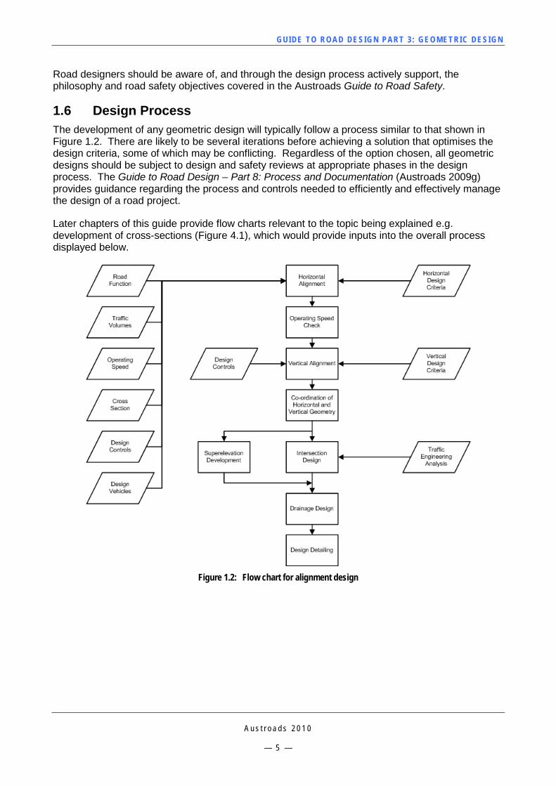
1.6 Design Process The development of any geometric design will typically follow a process similar to that shown in Figure 1.2. There are likely to be several iterations before achieving a solution that optimises the design criteria, some of which may be conflicting. Regardless of the option chosen, all geometric designs should be subject to design and safety reviews at appropriate phases in the design process. The Guide to Road Design – Part 8: Process and Documentation (Austroads 2009g) provides guidance regarding the process and controls needed to efficiently and effectively manage the design of a road project.
Later chapters of this guide provide flow charts relevant to the topic being explained e.g. development of cross-sections (Figure 4.1), which would provide inputs into the overall process displayed below.
Figure 1.2: Flow chart for alignment design
GUI DE TO RO A D DE SIG N P ART 3 : GEO MET RI C D ESI G N
A u s t r o a d s 2 0 1 0
— 6 —
2 FUNDAMENTAL CONSIDERATIONS
2.1 General Roads need to provide for the safe, convenient, effective and efficient movement of persons and goods. The design of roads should be based on the capabilities and behaviour of all road users, including pedestrians, cyclists, motorcyclists, and on the performance and physical characteristics of vehicles (including road based public transport). At the same time, consideration must also be given to the whole range of economic, social, environmental and other factors that may be involved.
While Part 3 of the Guide to Road Design provides information relating to alignment geometry and cross-section, designers should familiarise themselves with the basic parameters that define an appropriate design solution. These are detailed in the following sections along with references to other parts of the Guide to Road Design and other Austroads Guides.
2.2 Design Parameters 2.2.1 Location The basic premise of whether a road is located in an urban or rural area will to a certain extent impact on the attributes that it is designed for. Rural roads generally carry lower traffic volumes and are not subject to as many constraints as urban roads. Public expectation also differs in relation to operating speeds, abutting access, geometry and cross-section.
2.2.2 Road Classification Most road authorities in Australia have developed a functional hierarchy for their road networks. This hierarchy enables each authority to systematically plan and develop their network to meet the needs for local access, cross town/city travel, intrastate and interstate travel. Further information about this topic can be found in the Guide to Road Design – Part 2: Design Considerations (Austroads 2006c).
2.2.3 Traffic Volume and Composition The development of the cross-section and geometry of a road are generally based on the expected traffic volumes and composition of that traffic, e.g. number or percentage of trucks. Various methods have been established internationally to measure existing volumes and determine the likely future use of a facility.
The Guide to Traffic Management – Part 3: Traffic Studies and Analysis (Austroads 2009h), provides specific information regarding the analysis required to determine the capacity requirements for a length of roadway.
Designers need to consider future traffic demands for a road section to determine the required cross-sectional configuration. Consideration should be given to the staged construction or widening of roads over this period.
Design requirements for roads are typically assessed by reference to forecasts of Annual Average Daily Traffic (AADT). Design hour volumes may be derived by consideration of the flow pattern across hours of the year. A 30th highest hourly volume is often adopted as a design volume. In areas of high peak or seasonal demands, such as recreational or harvest routes, special consideration may be required. In the absence of such information, refer to Table 4.1 for suggested values for the design life of particular road elements or treatments.
GUI DE TO RO A D DE SIG N P ART 3 : GEO MET RI C D ESI G N
A u s t r o a d s 2 0 1 0
— 7 —
In addition to capacity considerations, traffic volume and composition is a key input to the structural design of pavements, culverts and bridges.
2.2.4 Design Speed (Operating Speed) Identification of the design speed of the vehicles travelling along the roadway will determine the geometric parameters to be adopted for the design. Section 3 of this guide describes the process to be used for identifying the operating speed of both an existing and planned length of road. Identification of the operating speed is fundamental to the development of any roadway facility.
2.2.5 Design Vehicle The physical and operating characteristics of vehicles using the road, control specific elements in the geometric design, e.g. tracking of large vehicles on small radius horizontal curves. The classification and function of the road may determine the type of vehicle operating on a length of road.
Information regarding the choice and application of design vehicles can be found in the Guide to Road Design – Part 4: Intersections and Crossings – General (Austroads 2009a).
The design vehicle is a hypothetical vehicle whose dimensions and operating characteristics are typically used to establish traffic lane widths, intersection layout and road geometry. Historically, four general classes of vehicles have been selected for design purposes, namely:
design prime mover and semi-trailer (19.0 m)
design single unit truck/bus (12.5 m)
service vehicle (8.8 m)
design car (5.0 m).
Other larger vehicles such as B-doubles or Type 1 and 2 road trains can be regularly found in some rural (and increasingly urban) areas of Australia. Each road authority has specific practices regarding their use and should be consulted when evaluating the choice of the design vehicle for any road project. Designers should also consider the implications of seasonal cartage routes where larger vehicles may be required in large numbers for relatively short time periods. Designers should consult the Austroads Design Vehicles and Turning Path Templates (Austroads 2006a) or the New Zealand Transport Agency On-road Tracking Curves for Heavy Vehicles (NZTA 2007) for specific details regarding vehicle turn paths of these standard design vehicles.
Recent initiatives to improve freight productivity in Australia have seen the development of vehicles using ‘performance based standards’ (PBS). Rather than being prescriptive in the dimensions, masses and turning paths, like for the design vehicles listed above, PBS vehicles must only meet minimum design criteria that are specified by the National Transport Commission. These criteria have been developed to meet the needs of the existing road network, e.g. lane widths or the space generally available for turns within intersections. Designers should note that whilst specific turning templates are not typically available for PBS vehicles (although they can be developed for specific vehicles), one of the performance standards for these vehicles is that they should have a swept path whilst turning, which is roughly equivalent to a B-double or Type 1 or 2 Road Train. Designers should consult the National Transport Commission PBS vehicle guidelines for further information (www.ntc.gov.au).
GUI DE TO RO A D DE SIG N P ART 3 : GEO MET RI C D ESI G N
A u s t r o a d s 2 0 1 0
— 8 —
2.2.6 Environmental Considerations The various impacts of roads are of growing concern to individuals and communities. It is important to fully consider the impact of these issues in any road design. Reduction of adverse environmental impact should be one of the main objectives of any road project both during construction and operation.
Careful design of roads can incorporate the means to ameliorate the environmental intrusion of road infrastructure and associated traffic. In particular, consideration should be given to visual amenity through the use of landscaping and creativity with structures and noise barriers. Traffic related intrusions perceived by people include:
visual
noise
vibration
pedestrian delay and severance
air pollution
erosion
risk of accidents and intimidation of vulnerable road users
deterioration of water quality and the increase in water quantity from urbanisation
adverse effect on environmentally sensitive areas
clearing.
Further information about these issues can be found in the Guide to Road Design – Part 6B: Roadside Environment (Austroads 2009f).
2.2.7 Access Management Access management is the process of controlling the movement of traffic between a road and adjacent land. The purpose of access management is to protect the safety and efficiency of the traffic function of the road, while acknowledging the needs and amenable use of adjacent land, through the provision of safe and appropriate access.
Some road authorities may have well-developed access management policies and designers should consult the relevant authority when considering this issue.
Designers should consult the Guide to Traffic Management – Part 5: Road Management (Austroads 2008d) and any relevant road authority guidelines for further guidance.
2.2.8 Drainage Consideration of issues associated with drainage of the road and surrounding land can significantly affect the geometry and cross-section of the road. Provision of drainage structures at watercourses affects the grading of the road, the choice of drainage system can affect the cross-section or formation width, maintenance requirements and cost of the project, especially if underground piped drainage networks are considered. Surface flows along the pavement are especially important in the context of minimising the chances of vehicles aquaplaning through the appropriate combinations of crossfall and grade.
Information relating to the design of drainage for roads can be found in the Guide to Road Design – Part 5: Drainage Design (Austroads 2008b). Drainage related considerations are also noted in specific sections of this guide.
GUI DE TO RO A D DE SIG N P ART 3 : GEO MET RI C D ESI G N
A u s t r o a d s 2 0 1 0
— 9 —
2.2.9 Utility Services The location of utility services should be considered early in the design process as they can have a significant impact on design decisions, construction and maintenance costs. Road improvement or upgrade projects will generally involve service relocations that may provide physical or economic constraints to the design. The provision of utility services adjacent to or across greenfield road developments should consider the future role of the transport corridor to minimise or avoid future service relocations associated with construction or upgrading of the facility.
Consolidated services to assist in the identification and location of underground public utilities are now available for most urban areas. These services are an efficient initial interface between the designer and service authorities to enable the early consideration of services to occur.
2.2.10 Topography/Geology Site-specific features have a large impact on the cost of road projects, which may influence the extent of the road project that gets constructed or how much funding remains available to fund other road improvements across the network.
To ensure that limited funds are effectively spent on appropriate designs, due regard must be given to designing with the terrain rather than against it. For example:
balanced earthworks limit the cost of importing additional fill materials or disposing it off-site
ensuring that the grade line stays above non-rippable rock, negates the need for blasting
keeping the grade line above the water table will limit moisture ingress to the pavement and could avoid the need for drainage blankets.
The Guide to Road Design – Part 7: Geotechnical Investigation and Design (Austroads 2008c) provides further information about geotechnical issues that should be considered by the road designer.
GUI DE TO RO A D DE SIG N P ART 3 : GEO MET RI C D ESI G N
A u s t r o a d s 2 0 1 0
— 1 0 —
3 SPEED PARAMETERS
3.1 General One of the first requirements in developing a new geometric design is to establish the appropriate operating speed or speeds to use for design. The speed to be adopted, which typically provides some margin over the proposed posted speed limit, directly influences the principal parameters used in road design which include:
sight distance
stopping distance
horizontal curve radii
pavement superelevation
traffic lane width.
Designers should also consider the potential increase in vehicle operating speeds, after the completion of rehabilitation or restoration type projects, as these may change the driver’s perception of the road. Some existing geometric features may not conform to current design criteria for the higher operating speeds and the geometric assessment included in the Operating Speed Model described below, will highlight these elements.
When determining the choice of design speed for a road, designers are required to obtain rigorous estimates of the 85th percentile vehicle operating speeds for each element of the road. These can either be measured or estimated. Designers need to ensure that the design speed of every element is either equal to, or greater than, the 85th percentile operating speed on that element at times of light traffic conditions, to maintain geometric consistency. This means that if the combination of alignment and operating environment cause the operating speed to vary, the design speed has to vary accordingly. At the same time, the design must ensure that where drivers have to slow down for a horizontal curve, the speed reduction must be consistent with normal driver capability and expectations. Wherever possible, operating speeds should be measured for both cars and trucks, in both directions of travel. As this is not possible with new road proposals, operating speeds have to be obtained by other means including measurement of vehicle speeds on similar roads, or estimation of speeds using the Operating Speed Model, described in Section 3.5. See Commentary 1.
The Operating Speed Model lends itself to rural roads where the design features of the road tend to dominate the operating speed of vehicles. For urban areas, current practice has been to adopt a design speed 10 km/h higher than the posted speed limit. This practice is valid provided all horizontal curves are suitable for that speed. As far as practicable, the operating speed chosen should be consistent with driver expectations in urban areas during both peak and low traffic times.
Where the operating speed cannot be determined through speed measurement or by the Operating Speed Model, designers shall adopt an operating speed 10 km/h higher than the legal (posted) speed limit. Designers shall refer to Section 3.6 for guidance regarding the estimation of truck operating speeds. Section 3.7 provides issues to be considered when determining the operating speed for temporary works.
The operating speed estimation procedure shown in Section 3.5 was developed to simulate or model the actual behaviour of vehicles on the road. This correlation between the mathematical model and actual vehicle operation in the field enables designers to visualise themselves in the position of a driver negotiating the road. Use of this procedure can help designers to identify features that could influence the operating speed; it is also a useful technique for identifying other potential geometric inconsistencies with the design.
GUI DE TO RO A D DE SIG N P ART 3 : GEO MET RI C D ESI G N
A u s t r o a d s 2 0 1 0
— 1 1 —
In addition to simulating vehicle behaviour on curves, the estimation model has the following built-in safety factors:
The model identifies the use of lateral friction factors that exceed minimum specified values.
The model identifies the development of excessive speed inconsistencies along the alignment. The model restricts speed differences between design elements to less than 10 km/h, (where designers are using the desirable section on the chart) and in most cases the difference is significantly less than this.
3.2 Terminology Appendix B provides definitions for the terms used with the Operating Speed Model, however key terms are listed below.
3.2.1 Operating Speed (85th Percentile Speed) The term Operating Speed in this guide refers to the 85th percentile speed of cars at a time when traffic volumes are low, and drivers are free to choose the speed at which they travel. In effect, this means that designs based on the 85th percentile speed will cater for the majority of drivers.
In New Zealand, Operating Speed is considered to be the highest overall speed, exclusive of stops, at which a driver can safely travel on a given section of road under the prevailing traffic conditions.
3.2.2 Desired Speed The term ‘Desired Speed’ in this guide refers to the operating speed that drivers will adopt on the less constrained alignment elements, i.e. longer straights and large radius horizontal curves of a reasonably uniform section of road when not constrained by other vehicles. In other words, it is the operating speed that drivers build up to and are then happy to settle at.
3.2.3 Design Speed A speed fixed for the design and correlation of those geometric features of a carriageway that influence vehicle operation. Design speed should not be less than the intended operating (85th percentile) speed. If the operating speed varies along the road, the design speed must vary accordingly.
3.2.4 Vehicle Speeds on Roads For design purposes, the following definitions of high, intermediate and low vehicle speeds will apply for both urban and rural areas:
High speed: 90 km/h or greater
Intermediate: 70 km/h to 89 km/h
Low speed: 69 km/h or less.
Driver operating speeds are not only constrained by the geometry of the road but by a number of other factors, which include:
the degree of risk the drivers are prepared to accept
speed limits and the level of policing/enforcement of these limits
vehicle performance (e.g. cars vs trucks on grades).
See Commentary 2.
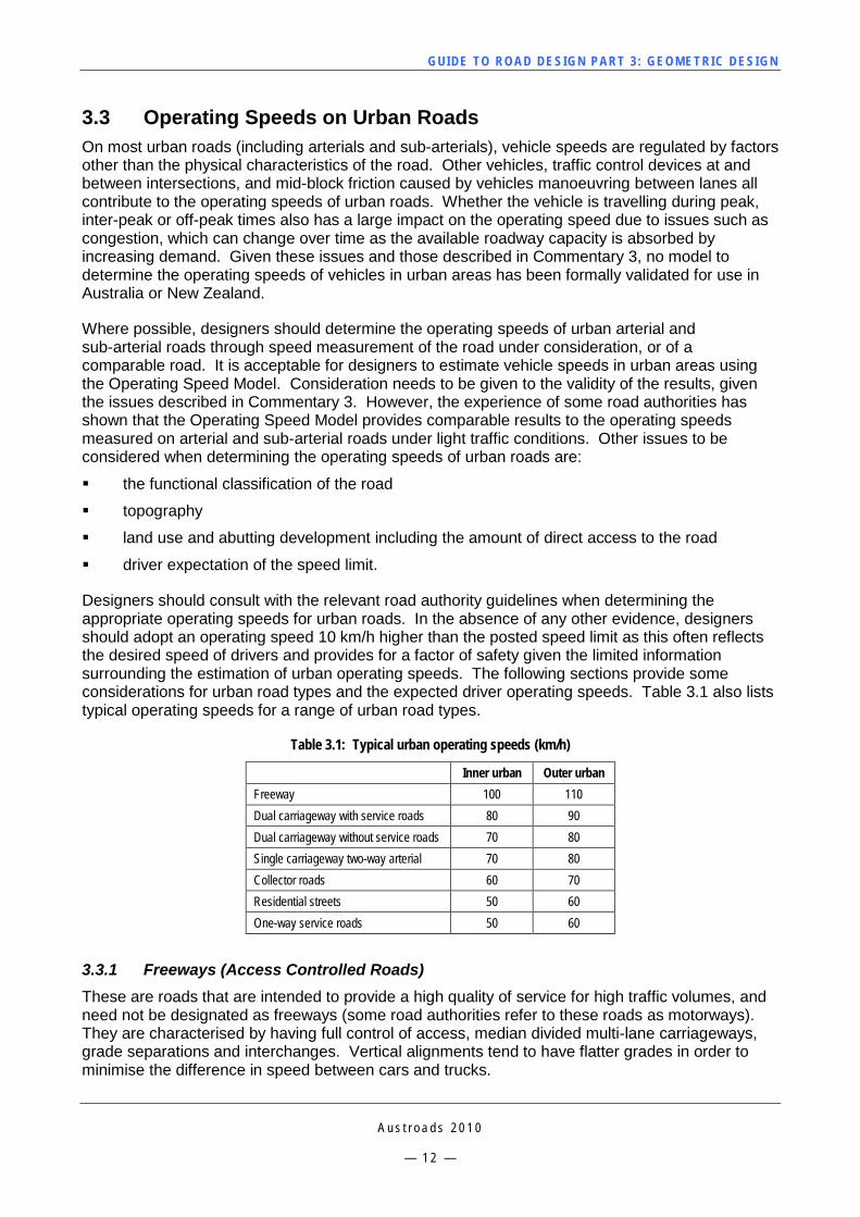
GUI DE TO RO A D DE SIG N P ART 3 : GEO MET RI C D ESI G N
A u s t r o a d s 2 0 1 0
— 1 2 —
3.3 Operating Speeds on Urban Roads On most urban roads (including arterials and sub-arterials), vehicle speeds are regulated by factors other than the physical characteristics of the road. Other vehicles, traffic control devices at and between intersections, and mid-block friction caused by vehicles manoeuvring between lanes all contribute to the operating speeds of urban roads. Whether the vehicle is travelling during peak, inter-peak or off-peak times also has a large impact on the operating speed due to issues such as congestion, which can change over time as the available roadway capacity is absorbed by increasing demand. Given these issues and those described in Commentary 3, no model to determine the operating speeds of vehicles in urban areas has been formally validated for use in Australia or New Zealand.
Where possible, designers should determine the operating speeds of urban arterial and sub-arterial roads through speed measurement of the road under consideration, or of a comparable road. It is acceptable for designers to estimate vehicle speeds in urban areas using the Operating Speed Model. Consideration needs to be given to the validity of the results, given the issues described in Commentary 3. However, the experience of some road authorities has shown that the Operating Speed Model provides comparable results to the operating speeds measured on arterial and sub-arterial roads under light traffic conditions. Other issues to be considered when determining the operating speeds of urban roads are:
the functional classification of the road
topography
land use and abutting development including the amount of direct access to the road
driver expectation of the speed limit.
Designers should consult with the relevant road authority guidelines when determining the appropriate operating speeds for urban roads. In the absence of any other evidence, designers should adopt an operating speed 10 km/h higher than the posted speed limit as this often reflects the desired speed of drivers and provides for a factor of safety given the limited information surrounding the estimation of urban operating speeds. The following sections provide some considerations for urban road types and the expected driver operating speeds. Table 3.1 also lists typical operating speeds for a range of urban road types.
Table 3.1: Typical urban operating speeds (km/h)
Inner urban Outer urban Freeway 100 110 Dual carriageway with service roads 80 90 Dual carriageway without service roads 70 80 Single carriageway two-way arterial 70 80 Collector roads 60 70 Residential streets 50 60 One-way service roads 50 60
3.3.1 Freeways (Access Controlled Roads) These are roads that are intended to provide a high quality of service for high traffic volumes, and need not be designated as freeways (some road authorities refer to these roads as motorways). They are characterised by having full control of access, median divided multi-lane carriageways, grade separations and interchanges. Vertical alignments tend to have flatter grades in order to minimise the difference in speed between cars and trucks.
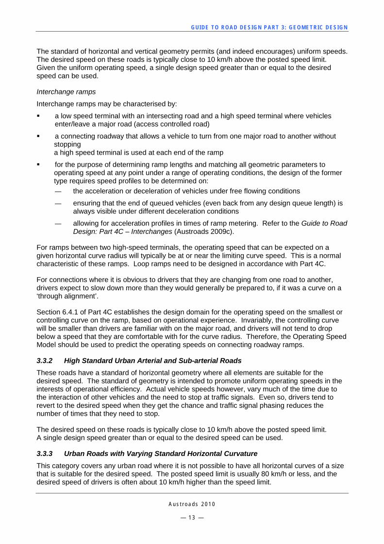
GUI DE TO RO A D DE SIG N P ART 3 : GEO MET RI C D ESI G N
A u s t r o a d s 2 0 1 0
— 1 3 —
The standard of horizontal and vertical geometry permits (and indeed encourages) uniform speeds. The desired speed on these roads is typically close to 10 km/h above the posted speed limit. Given the uniform operating speed, a single design speed greater than or equal to the desired speed can be used.
Interchange ramps
Interchange ramps may be characterised by:
a low speed terminal with an intersecting road and a high speed terminal where vehicles enter/leave a major road (access controlled road)
a connecting roadway that allows a vehicle to turn from one major road to another without stopping a high speed terminal is used at each end of the ramp
for the purpose of determining ramp lengths and matching all geometric parameters to operating speed at any point under a range of operating conditions, the design of the former type requires speed profiles to be determined on: — the acceleration or deceleration of vehicles under free flowing conditions
— ensuring that the end of queued vehicles (even back from any design queue length) is always visible under different deceleration conditions
— allowing for acceleration profiles in times of ramp metering. Refer to the Guide to Road Design: Part 4C – Interchanges (Austroads 2009c).
For ramps between two high-speed terminals, the operating speed that can be expected on a given horizontal curve radius will typically be at or near the limiting curve speed. This is a normal characteristic of these ramps. Loop ramps need to be designed in accordance with Part 4C.
For connections where it is obvious to drivers that they are changing from one road to another, drivers expect to slow down more than they would generally be prepared to, if it was a curve on a ‘through alignment’.
Section 6.4.1 of Part 4C establishes the design domain for the operating speed on the smallest or controlling curve on the ramp, based on operational experience. Invariably, the controlling curve will be smaller than drivers are familiar with on the major road, and drivers will not tend to drop below a speed that they are comfortable with for the curve radius. Therefore, the Operating Speed Model should be used to predict the operating speeds on connecting roadway ramps.
3.3.2 High Standard Urban Arterial and Sub-arterial Roads These roads have a standard of horizontal geometry where all elements are suitable for the desired speed. The standard of geometry is intended to promote uniform operating speeds in the interests of operational efficiency. Actual vehicle speeds however, vary much of the time due to the interaction of other vehicles and the need to stop at traffic signals. Even so, drivers tend to revert to the desired speed when they get the chance and traffic signal phasing reduces the number of times that they need to stop.
The desired speed on these roads is typically close to 10 km/h above the posted speed limit. A single design speed greater than or equal to the desired speed can be used.
3.3.3 Urban Roads with Varying Standard Horizontal Curvature This category covers any urban road where it is not possible to have all horizontal curves of a size that is suitable for the desired speed. The posted speed limit is usually 80 km/h or less, and the desired speed of drivers is often about 10 km/h higher than the speed limit.
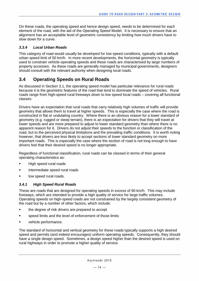
GUI DE TO RO A D DE SIG N P ART 3 : GEO MET RI C D ESI G N
A u s t r o a d s 2 0 1 0
— 1 4 —
On these roads, the operating speed and hence design speed, needs to be determined for each element of the road, with the aid of the Operating Speed Model. It is necessary to ensure that an alignment has an acceptable level of geometric consistency by limiting how much drivers have to slow down for a curve.
3.3.4 Local Urban Roads This category of road would usually be developed for low speed conditions, typically with a default urban speed limit of 50 km/h. In more recent developments, the horizontal geometry is typically used to constrain vehicle-operating speeds and these roads are characterised by large numbers of property accesses. As these roads are generally managed by municipal governments, designers should consult with the relevant authority when designing local roads.
3.4 Operating Speeds on Rural Roads As discussed in Section 3.1, the operating speed model has particular relevance for rural roads because it is the geometric features of the road that tend to dominate the speed of vehicles. Rural roads range from high-speed rural freeways down to low speed local roads – covering all functional classes.
Drivers have an expectation that rural roads that carry relatively high volumes of traffic will provide geometry that allows them to travel at higher speeds. This is especially the case where the road is constructed in flat or undulating country. Where there is an obvious reason for a lower standard of geometry (e.g. rugged or steep terrain), there is an expectation for drivers that they will travel at lower speeds and are more prepared to adjust to lower standard geometry than where there is no apparent reason for it. Drivers do not adjust their speeds to the function or classification of the road, but to the perceived physical limitations and the prevailing traffic conditions. It is worth noting however, that drivers are less likely to accept sections of lower standard geometry on more important roads. This is especially the case where the section of road is not long enough to have drivers feel that their desired speed is no longer appropriate.
Regardless of functional classification, rural roads can be classed in terms of their general operating characteristics as:
High speed rural roads
intermediate speed rural roads
low speed rural roads.
3.4.1 High Speed Rural Roads These are roads that are designed for operating speeds in excess of 90 km/h. This may include freeways, which are intended to provide a high quality of service for large traffic volumes. Operating speeds on high-speed roads are not constrained by the largely consistent geometry of the road but by a number of other factors, which include:
the degree of risk drivers are prepared to accept
speed limits and the level of enforcement of those limits
vehicle performance.
The standard of horizontal and vertical geometry for these roads typically supports a high desired speed and permits (and indeed encourages) uniform operating speeds. Consequently, they should have a single design speed. Sometimes, a design speed higher than the desired speed is used on rural highways in order to promote a higher quality of service.
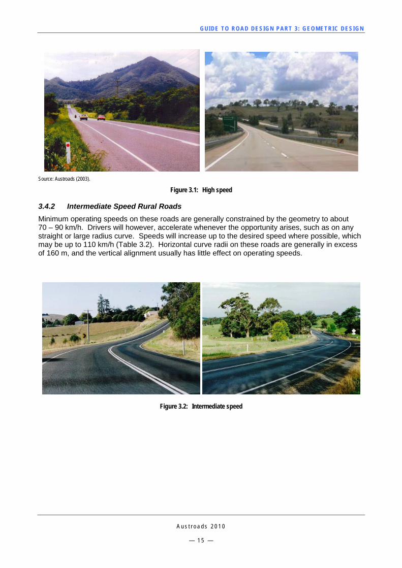
GUI DE TO RO A D DE SIG N P ART 3 : GEO MET RI C D ESI G N
A u s t r o a d s 2 0 1 0
— 1 5 —
Source: Austroads (2003).
Figure 3.1: High speed
3.4.2 Intermediate Speed Rural Roads Minimum operating speeds on these roads are generally constrained by the geometry to about 70 – 90 km/h. Drivers will however, accelerate whenever the opportunity arises, such as on any straight or large radius curve. Speeds will increase up to the desired speed where possible, which may be up to 110 km/h (Table 3.2). Horizontal curve radii on these roads are generally in excess of 160 m, and the vertical alignment usually has little effect on operating speeds.
Figure 3.2: Intermediate speed
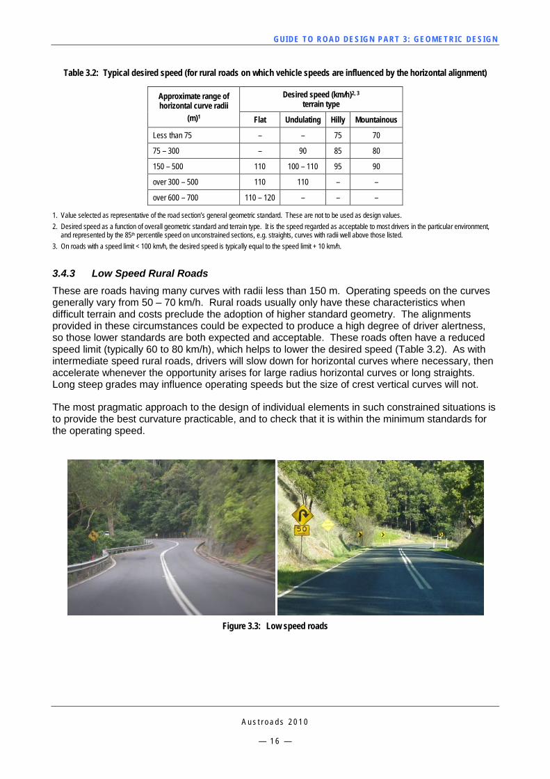
GUI DE TO RO A D DE SIG N P ART 3 : GEO MET RI C D ESI G N
A u s t r o a d s 2 0 1 0
— 1 6 —
Table 3.2: Typical desired speed (for rural roads on which vehicle speeds are influenced by the horizontal alignment)
Approximate range of horizontal curve radii
(m)1
Desired speed (km/h)2, 3
terrain type
Flat Undulating Hilly Mountainous
Less than 75 – – 75 70
75 – 300 – 90 85 80
150 – 500 110 100 – 110 95 90
over 300 – 500 110 110 – –
over 600 – 700 110 – 120 – – –
1. Value selected as representative of the road section’s general geometric standard. These are not to be used as design values. 2. Desired speed as a function of overall geometric standard and terrain type. It is the speed regarded as acceptable to most drivers in the particular environment,
and represented by the 85th percentile speed on unconstrained sections, e.g. straights, curves with radii well above those listed. 3. On roads with a speed limit < 100 km/h, the desired speed is typically equal to the speed limit + 10 km/h.
3.4.3 Low Speed Rural Roads These are roads having many curves with radii less than 150 m. Operating speeds on the curves generally vary from 50 – 70 km/h. Rural roads usually only have these characteristics when difficult terrain and costs preclude the adoption of higher standard geometry. The alignments provided in these circumstances could be expected to produce a high degree of driver alertness, so those lower standards are both expected and acceptable. These roads often have a reduced speed limit (typically 60 to 80 km/h), which helps to lower the desired speed (Table 3.2). As with intermediate speed rural roads, drivers will slow down for horizontal curves where necessary, then accelerate whenever the opportunity arises for large radius horizontal curves or long straights. Long steep grades may influence operating speeds but the size of crest vertical curves will not.
The most pragmatic approach to the design of individual elements in such constrained situations is to provide the best curvature practicable, and to check that it is within the minimum standards for the operating speed.
Figure 3.3: Low speed roads
GUI DE TO RO A D DE SIG N P ART 3 : GEO MET RI C D ESI G N
A u s t r o a d s 2 0 1 0
— 1 7 —
3.5 Determining Operating Speeds using the Operating Speed Model 3.5.1 General The Operating Speed Model is used to predict the operating speeds of cars in each direction along the road, where speeds are largely controlled by the horizontal curvature, so that the operating speed varies.
The methodology for the geometric design of rural roads has moved toward the use of a ‘section operating speed’ model, which provides realistic speeds on the curves and straights of a road section. This approach is founded on the understanding of driver behavior for rural conditions. The Australian Road Research Board (now ARRB Group) has verified that the operating speed model appears to successfully model most of the essential features of driver behavior on rural roads and provides a sound basis for geometric road design (McLean 1988).
The following procedure will enable designers to consider the behaviour of a typical 85th percentile driver. There are three basic elements: the driver, the road and the vehicle.
3.5.2 Driver Behaviour Consider first a typical driver approaching a straight section of road, which is followed by a series of curves at the end of the straight.
The driver's initial response will depend on the speed at this time and the length of straight. If the straight is too short, the driver is likely to continue at the same speed. On longer straights, the driver will accelerate until terminal speed is reached, which is related to the length of straight and the initial speed. They will then continue at this speed to within approximately 75 m of the curve. The driver then decelerates to a speed, which is considered safe for the curve ahead. Truck drivers will generally decelerate to the appropriate speed for the curve by the start of the curve (unlike car drivers going into the curve) because of the dangers associated with trucks braking on curves. Car drivers are likely to enter at a speed that is high for the curve as indicated by some further deceleration, which commonly occurs within the first 80 m of the curve. Speeds remain at this level until the driver has a clear view of the curve or straight ahead. If it is a straight, the driver will accelerate out of the curve; if another relatively low radius curve follows, the driver is likely to reduce speed further. This loss of speed continues until the driver of the vehicle reaches a comfortable speed. This is the section operating speed for the series of curves. This speed is then maintained until the end of the section.
3.5.3 Road Characteristics The operating speed of the road can be affected by the following characteristics, especially for different vehicle classes:
road grade
cross-section
surface conditions.
There has been insufficient research to accurately understand their impact but it is important to be aware of their characteristics. Commentary 4 provides some limited guidance on parameters that could be taken into consideration when calibrating the operating speed model for observed conditions.
GUI DE TO RO A D DE SIG N P ART 3 : GEO MET RI C D ESI G N
A u s t r o a d s 2 0 1 0
— 1 8 —
When choosing to adjust the operating speed with the parameters listed above, designers should consider that future maintenance/reconstruction operations can remedy formation width and poor surfacing conditions, which may result in higher operating speeds. Further assessments of operating speeds may need to be undertaken again at that time.
3.5.4 Vehicle Characteristics Two design vehicles are considered: cars and the truck (design semi-trailer 19.0 m). Speeds are determined first for cars, then trucks. Truck speeds are obtained using Table 3.4; unless other sources such as measured speeds or vehicle performance simulation software is available. For specific roads/projects, designers may also need to consider some of the other design vehicles listed in Section 2 that may have specific performance attributes.
3.5.5 Operating Speed Estimation Model The operating speed model is based on observed driver behaviour on Australian roads. There are three key components of the model:
section operating speeds
acceleration on straights
deceleration on curves.
The model used to estimate operating speeds is based on a large number of observations of the behaviour of traffic. The operating speed of vehicles is estimated by establishing the approach speed of the vehicle for the direction of traffic flow being considered. The approach speed is then applied to the first curve and an operating speed is read. This speed then becomes the approach speed for the subsequent curves and separating straights. The operating speed estimating graphs are:
acceleration on straights (Figure 3.4)
deceleration on curves (Figure 3.5).
3.5.6 Car Acceleration on Straights Graph The car Acceleration on Straights graph (Figure 3.4), allows the designer to estimate the speed at which a vehicle can accelerate over a given length. Large radius curves may be considered as straights, as depicted on Figure 3.5, where the operating speed from 50 to 120 km/h is no longer influenced by a further increase in the radius. The change in speed, read from Figure 3.4 assumes that the terrain is constant.
An increase of 1 km/h for every 5 m of travel is possible when:
accelerating on steeper downgrades on straights with good visibility
accelerating from stop such as starting off from an intersection
accelerating from speeds below about 70 km/h and up to about 80 km/h, except in mountainous terrain.
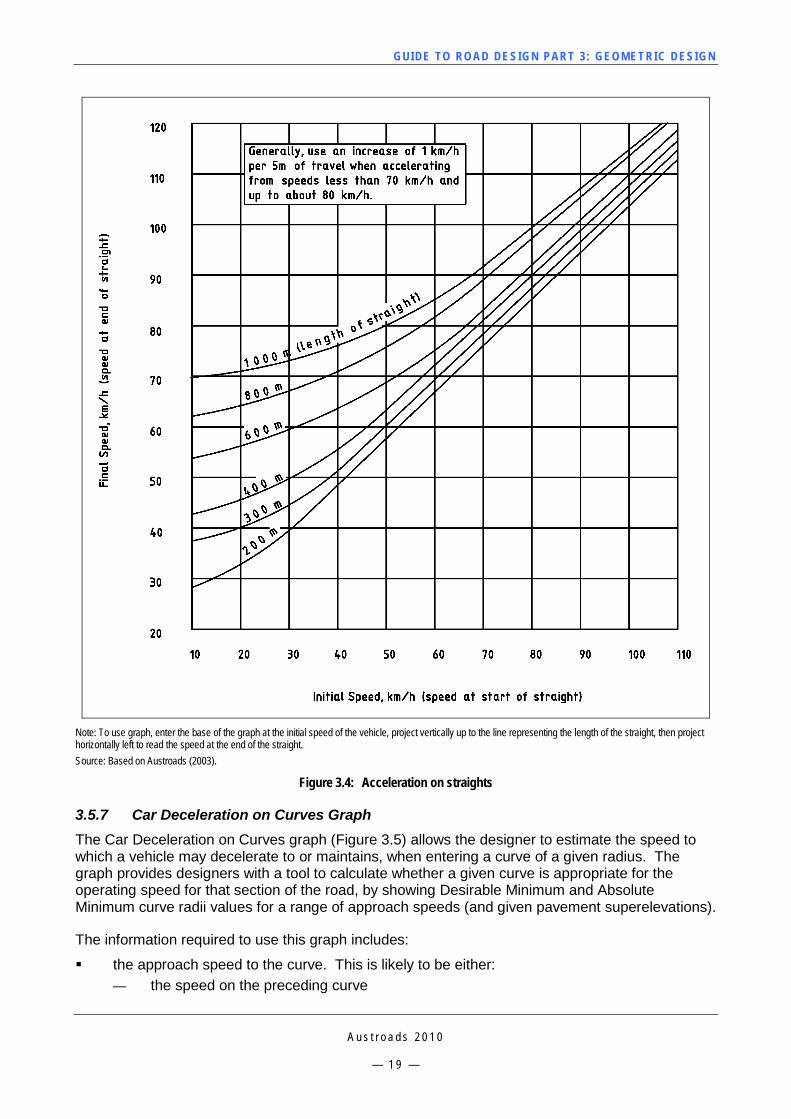
GUI DE TO RO A D DE SIG N P ART 3 : GEO MET RI C D ESI G N
A u s t r o a d s 2 0 1 0
— 1 9 —
Note: To use graph, enter the base of the graph at the initial speed of the vehicle, project vertically up to the line representing the length of the straight, then project horizontally left to read the speed at the end of the straight. Source: Based on Austroads (2003).
Figure 3.4: Acceleration on straights
3.5.7 Car Deceleration on Curves Graph The Car Deceleration on Curves graph (Figure 3.5) allows the designer to estimate the speed to which a vehicle may decelerate to or maintains, when entering a curve of a given radius. The graph provides designers with a tool to calculate whether a given curve is appropriate for the operating speed for that section of the road, by showing Desirable Minimum and Absolute Minimum curve radii values for a range of approach speeds (and given pavement superelevations).
The information required to use this graph includes:
the approach speed to the curve. This is likely to be either: — the speed on the preceding curve
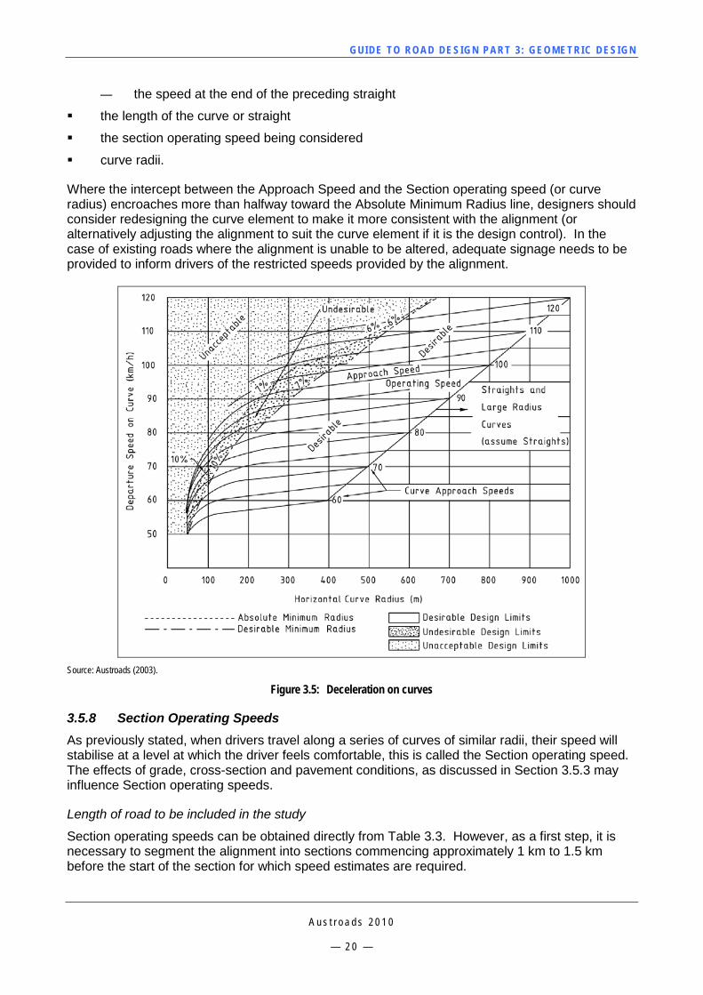
GUI DE TO RO A D DE SIG N P ART 3 : GEO MET RI C D ESI G N
A u s t r o a d s 2 0 1 0
— 2 0 —
— the speed at the end of the preceding straight
the length of the curve or straight
the section operating speed being considered
curve radii.
Where the intercept between the Approach Speed and the Section operating speed (or curve radius) encroaches more than halfway toward the Absolute Minimum Radius line, designers should consider redesigning the curve element to make it more consistent with the alignment (or alternatively adjusting the alignment to suit the curve element if it is the design control). In the case of existing roads where the alignment is unable to be altered, adequate signage needs to be provided to inform drivers of the restricted speeds provided by the alignment.
Source: Austroads (2003).
Figure 3.5: Deceleration on curves
3.5.8 Section Operating Speeds As previously stated, when drivers travel along a series of curves of similar radii, their speed will stabilise at a level at which the driver feels comfortable, this is called the Section operating speed. The effects of grade, cross-section and pavement conditions, as discussed in Section 3.5.3 may influence Section operating speeds.
Length of road to be included in the study
Section operating speeds can be obtained directly from Table 3.3. However, as a first step, it is necessary to segment the alignment into sections commencing approximately 1 km to 1.5 km before the start of the section for which speed estimates are required.
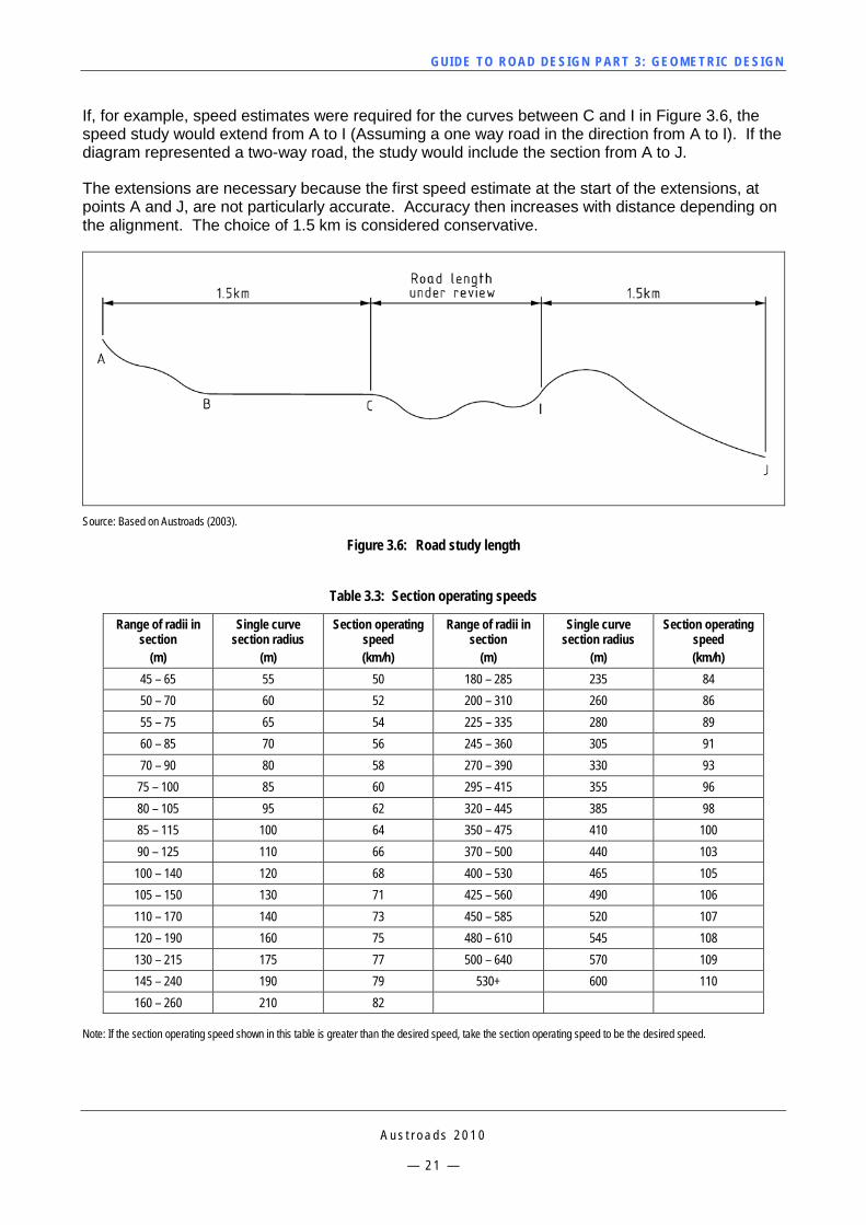
GUI DE TO RO A D DE SIG N P ART 3 : GEO MET RI C D ESI G N
A u s t r o a d s 2 0 1 0
— 2 1 —
If, for example, speed estimates were required for the curves between C and I in Figure 3.6, the speed study would extend from A to I (Assuming a one way road in the direction from A to I). If the diagram represented a two-way road, the study would include the section from A to J.
The extensions are necessary because the first speed estimate at the start of the extensions, at points A and J, are not particularly accurate. Accuracy then increases with distance depending on the alignment. The choice of 1.5 km is considered conservative.
Source: Based on Austroads (2003).
Figure 3.6: Road study length
Table 3.3: Section operating speeds
Range of radii in section
(m)
Single curve section radius
(m)
Section operating speed (km/h)
Range of radii in section
(m)
Single curve section radius
(m)
Section operating speed (km/h)
45 – 65 55 50 180 – 285 235 84 50 – 70 60 52 200 – 310 260 86 55 – 75 65 54 225 – 335 280 89 60 – 85 70 56 245 – 360 305 91 70 – 90 80 58 270 – 390 330 93 75 – 100 85 60 295 – 415 355 96 80 – 105 95 62 320 – 445 385 98 85 – 115 100 64 350 – 475 410 100 90 – 125 110 66 370 – 500 440 103 100 – 140 120 68 400 – 530 465 105 105 – 150 130 71 425 – 560 490 106 110 – 170 140 73 450 – 585 520 107 120 – 190 160 75 480 – 610 545 108 130 – 215 175 77 500 – 640 570 109 145 – 240 190 79 530+ 600 110 160 – 260 210 82
Note: If the section operating speed shown in this table is greater than the desired speed, take the section operating speed to be the desired speed.
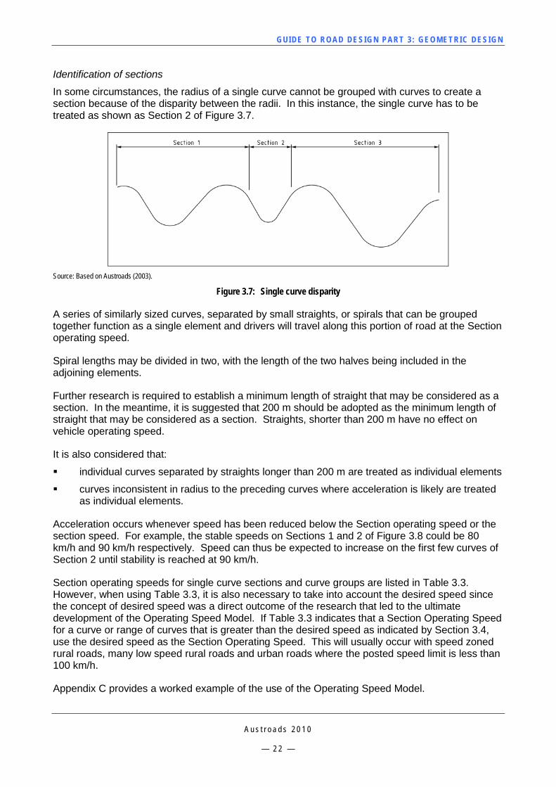
GUI DE TO RO A D DE SIG N P ART 3 : GEO MET RI C D ESI G N
A u s t r o a d s 2 0 1 0
— 2 2 —
Identification of sections
In some circumstances, the radius of a single curve cannot be grouped with curves to create a section because of the disparity between the radii. In this instance, the single curve has to be treated as shown as Section 2 of Figure 3.7.
Source: Based on Austroads (2003).
Figure 3.7: Single curve disparity
A series of similarly sized curves, separated by small straights, or spirals that can be grouped together function as a single element and drivers will travel along this portion of road at the Section operating speed.
Spiral lengths may be divided in two, with the length of the two halves being included in the adjoining elements.
Further research is required to establish a minimum length of straight that may be considered as a section. In the meantime, it is suggested that 200 m should be adopted as the minimum length of straight that may be considered as a section. Straights, shorter than 200 m have no effect on vehicle operating speed.
It is also considered that:
individual curves separated by straights longer than 200 m are treated as individual elements
curves inconsistent in radius to the preceding curves where acceleration is likely are treated as individual elements.
Acceleration occurs whenever speed has been reduced below the Section operating speed or the section speed. For example, the stable speeds on Sections 1 and 2 of Figure 3.8 could be 80 km/h and 90 km/h respectively. Speed can thus be expected to increase on the first few curves of Section 2 until stability is reached at 90 km/h.
Section operating speeds for single curve sections and curve groups are listed in Table 3.3. However, when using Table 3.3, it is also necessary to take into account the desired speed since the concept of desired speed was a direct outcome of the research that led to the ultimate development of the Operating Speed Model. If Table 3.3 indicates that a Section Operating Speed for a curve or range of curves that is greater than the desired speed as indicated by Section 3.4, use the desired speed as the Section Operating Speed. This will usually occur with speed zoned rural roads, many low speed rural roads and urban roads where the posted speed limit is less than 100 km/h.
Appendix C provides a worked example of the use of the Operating Speed Model.
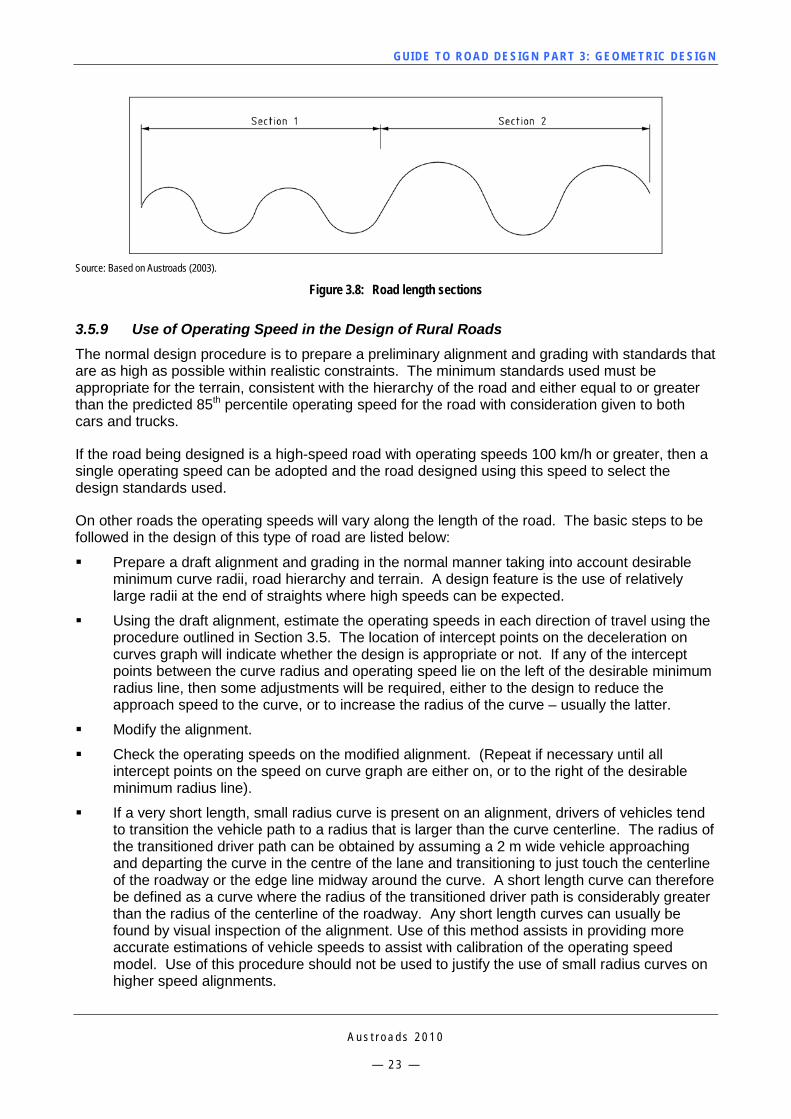
GUI DE TO RO A D DE SIG N P ART 3 : GEO MET RI C D ESI G N
A u s t r o a d s 2 0 1 0
— 2 3 —
Source: Based on Austroads (2003).
Figure 3.8: Road length sections
3.5.9 Use of Operating Speed in the Design of Rural Roads The normal design procedure is to prepare a preliminary alignment and grading with standards that are as high as possible within realistic constraints. The minimum standards used must be appropriate for the terrain, consistent with the hierarchy of the road and either equal to or greater than the predicted 85th percentile operating speed for the road with consideration given to both cars and trucks.
If the road being designed is a high-speed road with operating speeds 100 km/h or greater, then a single operating speed can be adopted and the road designed using this speed to select the design standards used.
On other roads the operating speeds will vary along the length of the road. The basic steps to be followed in the design of this type of road are listed below:
Prepare a draft alignment and grading in the normal manner taking into account desirable minimum curve radii, road hierarchy and terrain. A design feature is the use of relatively large radii at the end of straights where high speeds can be expected.
Using the draft alignment, estimate the operating speeds in each direction of travel using the procedure outlined in Section 3.5. The location of intercept points on the deceleration on curves graph will indicate whether the design is appropriate or not. If any of the intercept points between the curve radius and operating speed lie on the left of the desirable minimum radius line, then some adjustments will be required, either to the design to reduce the approach speed to the curve, or to increase the radius of the curve – usually the latter.
Modify the alignment.
Check the operating speeds on the modified alignment. (Repeat if necessary until all intercept points on the speed on curve graph are either on, or to the right of the desirable minimum radius line).
If a very short length, small radius curve is present on an alignment, drivers of vehicles tend to transition the vehicle path to a radius that is larger than the curve centerline. The radius of the transitioned driver path can be obtained by assuming a 2 m wide vehicle approaching and departing the curve in the centre of the lane and transitioning to just touch the centerline of the roadway or the edge line midway around the curve. A short length curve can therefore be defined as a curve where the radius of the transitioned driver path is considerably greater than the radius of the centerline of the roadway. Any short length curves can usually be found by visual inspection of the alignment. Use of this method assists in providing more accurate estimations of vehicle speeds to assist with calibration of the operating speed model. Use of this procedure should not be used to justify the use of small radius curves on higher speed alignments.
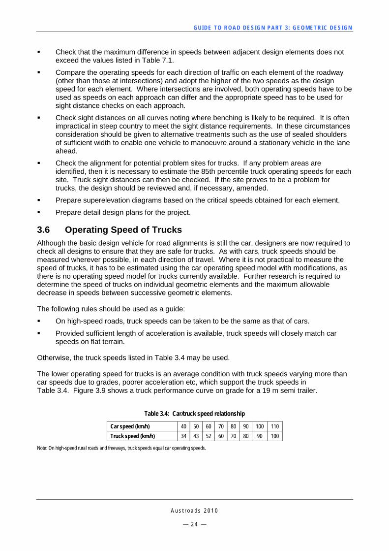
GUI DE TO RO A D DE SIG N P ART 3 : GEO MET RI C D ESI G N
A u s t r o a d s 2 0 1 0
— 2 4 —
Check that the maximum difference in speeds between adjacent design elements does not exceed the values listed in Table 7.1.
Compare the operating speeds for each direction of traffic on each element of the roadway (other than those at intersections) and adopt the higher of the two speeds as the design speed for each element. Where intersections are involved, both operating speeds have to be used as speeds on each approach can differ and the appropriate speed has to be used for sight distance checks on each approach.
Check sight distances on all curves noting where benching is likely to be required. It is often impractical in steep country to meet the sight distance requirements. In these circumstances consideration should be given to alternative treatments such as the use of sealed shoulders of sufficient width to enable one vehicle to manoeuvre around a stationary vehicle in the lane ahead.
Check the alignment for potential problem sites for trucks. If any problem areas are identified, then it is necessary to estimate the 85th percentile truck operating speeds for each site. Truck sight distances can then be checked. If the site proves to be a problem for trucks, the design should be reviewed and, if necessary, amended.
Prepare superelevation diagrams based on the critical speeds obtained for each element.
Prepare detail design plans for the project.
3.6 Operating Speed of Trucks Although the basic design vehicle for road alignments is still the car, designers are now required to check all designs to ensure that they are safe for trucks. As with cars, truck speeds should be measured wherever possible, in each direction of travel. Where it is not practical to measure the speed of trucks, it has to be estimated using the car operating speed model with modifications, as there is no operating speed model for trucks currently available. Further research is required to determine the speed of trucks on individual geometric elements and the maximum allowable decrease in speeds between successive geometric elements.
The following rules should be used as a guide:
On high-speed roads, truck speeds can be taken to be the same as that of cars.
Provided sufficient length of acceleration is available, truck speeds will closely match car speeds on flat terrain.
Otherwise, the truck speeds listed in Table 3.4 may be used.
The lower operating speed for trucks is an average condition with truck speeds varying more than car speeds due to grades, poorer acceleration etc, which support the truck speeds in Table 3.4. Figure 3.9 shows a truck performance curve on grade for a 19 m semi trailer.
Table 3.4: Car/truck speed relationship
Car speed (km/h) 40 50 60 70 80 90 100 110 Truck speed (km/h) 34 43 52 60 70 80 90 100
Note: On high-speed rural roads and freeways, truck speeds equal car operating speeds.
GUI DE TO RO A D DE SIG N P ART 3 : GEO MET RI C D ESI G N
A u s t r o a d s 2 0 1 0
— 2 5 —
3.7 Operating Speeds for Temporary Works (including Sidetracks) As with other road types, the design of temporary roads has to suit the operating speeds that occur in practice. Compared with permanent works, there will be markedly different tradeoffs between cost, construction safety, operational safety and operational efficiency. During the development of a project, road authorities typically specify the operational requirements for temporary works. Designers need to consider these requirements when producing their designs, but the following issues are provided as a guide to assist in the development of temporary works:
safe operation of the road for road users, construction and maintenance personnel, despite the necessary tradeoffs inherent with temporary works
appropriate design standard, with provision for all relevant road users
ensuring that operating speeds and speed zoning are seen as appropriate by drivers
control of operating speeds, including provision of suitable transition sections between the temporary works and existing road, and retention of sight distances with safety barriers typically in close proximity to the road
proximity of the temporary works to the permanent works
the need to accommodate temporary intersections and in some cases, temporary ramps or ramp terminals at interchanges.
It is usually desirable and necessary for the operating speeds on temporary roads to be less than the operating speed on the approach section. Where the temporary road is short (e.g. less than 1 km long), the desired speed of the driver is unlikely to reduce significantly, even with the support of appropriate speed zoning. The addition of visible cues however, will highlight the need for a reduced operating speed to the driver, and the speed zoning. This may be achieved by a combination of:
signage, safety barriers and anti-gawking screens that reinforce the presence of the road works
narrower cross-section elements where practical to give the appearance of lower standard of road
different pavement surfacing appearance and/or type
active traffic management, including temporary traffic signals and stop/go traffic control.
Common operational experience has shown that the vehicle operating speed through temporary works is typically 10 km/h higher than the posted speed limit and the choice of design speed should incorporate this. Assuming a design speed equal to the posted speed limit should not be considered without supporting data.
Where possible, the horizontal curvature should be used to control operating speeds through a transition section, since horizontal curvature has the greatest effect on operating speed. Designers should develop this horizontal geometry with the aid of the Operating Speed Model, and check the geometric consistency of the design. Besides the transition section, it is good practice to use horizontal curvature to control the operating speed on the temporary road proper. The most common design problems occur where the alignment of the temporary road is controlled by the permanent works or existing roadway, thus limiting the amount of curvature that can be introduced. Sight distance constraints are also prevalent around curves where safety barriers are installed and where the temporary roadway has to cross over from one part of the existing roadway to another.
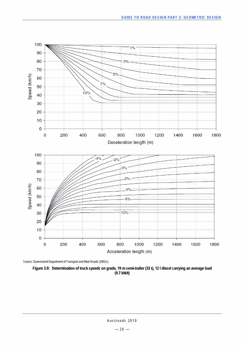
GUI DE TO RO A D DE SIG N P ART 3 : GEO MET RI C D ESI G N
A u s t r o a d s 2 0 1 0
— 2 6 —
Source: Queensland Department of Transport and Main Roads (2002c).
Figure 3.9: Determination of truck speeds on grade, 19 m semi-trailer (33 t), 12 l diesel carrying an average load (9.7 kW/t)
GUI DE TO RO A D DE SIG N P ART 3 : GEO MET RI C D ESI G N
A u s t r o a d s 2 0 1 0
— 2 7 —
4 CROSS-SECTION
4.1 General The type of cross-section to be used in the development of any road project depends on:
urban or rural location
the functions of the road: for example, through route or local access
new road or treatment of an existing road
traffic volume and mixture
number (and type) of trucks
provision for public transport
environmental constraints: for example, topography, existing public utility services, existing road reserve widths, significant vegetation, geology
local road-making materials available.
Having defined the functions required and the design traffic volume, the desirable widths of each element may be selected from Section 4.2 to 4.11. In many cases the selection of cross-section elements will exceed the available width and an iterative process is followed to optimise function, safety, environmental impact, economy and aesthetics.
A flow chart of the design process for cross-section elements is shown on Figure 4.1. The terminology discussed throughout this section is illustrated in Figure 4.2.
A key consideration in determining the appropriate cross-section of a road is to understand the type and mix of traffic expected to use the road. With a growing public awareness of sustainability and the impact that congestion and pollution has on the environment and well-being of people, road designers need to be conscious of the effort that various road authorities are expending to provide road space for all types of transport, including:
bicycles
motorcycles
road based public transport (buses and trams)
cars
trucks (including high productivity freight vehicles).
In most urban areas, there is limited space to provide for all of the above mentioned road users. However, consideration can be given to not just the spatial separation of different road users but also to the temporal separation of road users through the use of time restricted exclusive bus lanes, and bicycle lanes in clearways etc., during peak hours. Methods such as these provide priority to more efficient modes of transport (compared with individual car use) to encourage their use and assist in combating congestion. The effective management of cars on road networks will assist in managing the increasing freight task that Australia and New Zealand are facing.
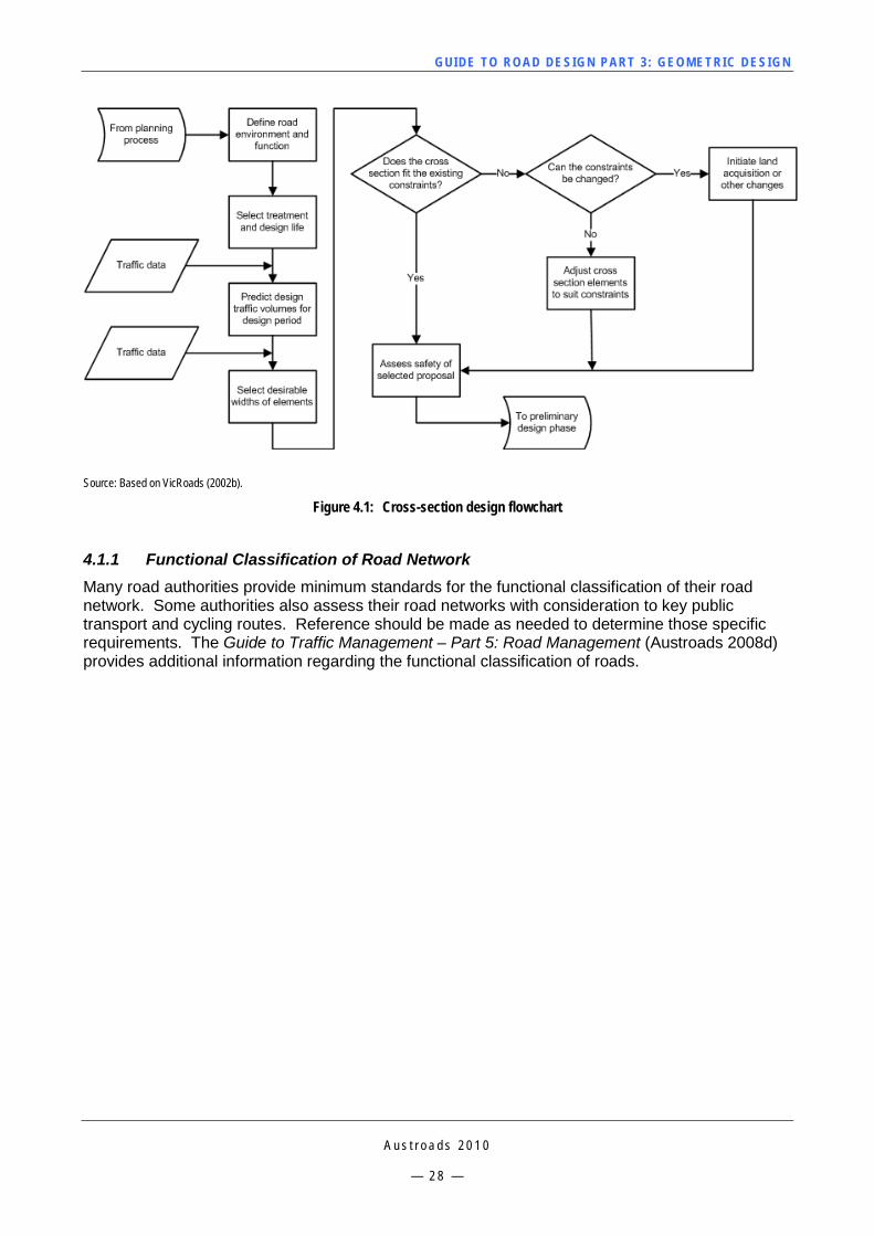
GUI DE TO RO A D DE SIG N P ART 3 : GEO MET RI C D ESI G N
A u s t r o a d s 2 0 1 0
— 2 8 —
Source: Based on VicRoads (2002b).
Figure 4.1: Cross-section design flowchart
4.1.1 Functional Classification of Road Network Many road authorities provide minimum standards for the functional classification of their road network. Some authorities also assess their road networks with consideration to key public transport and cycling routes. Reference should be made as needed to determine those specific requirements. The Guide to Traffic Management – Part 5: Road Management (Austroads 2008d) provides additional information regarding the functional classification of roads.
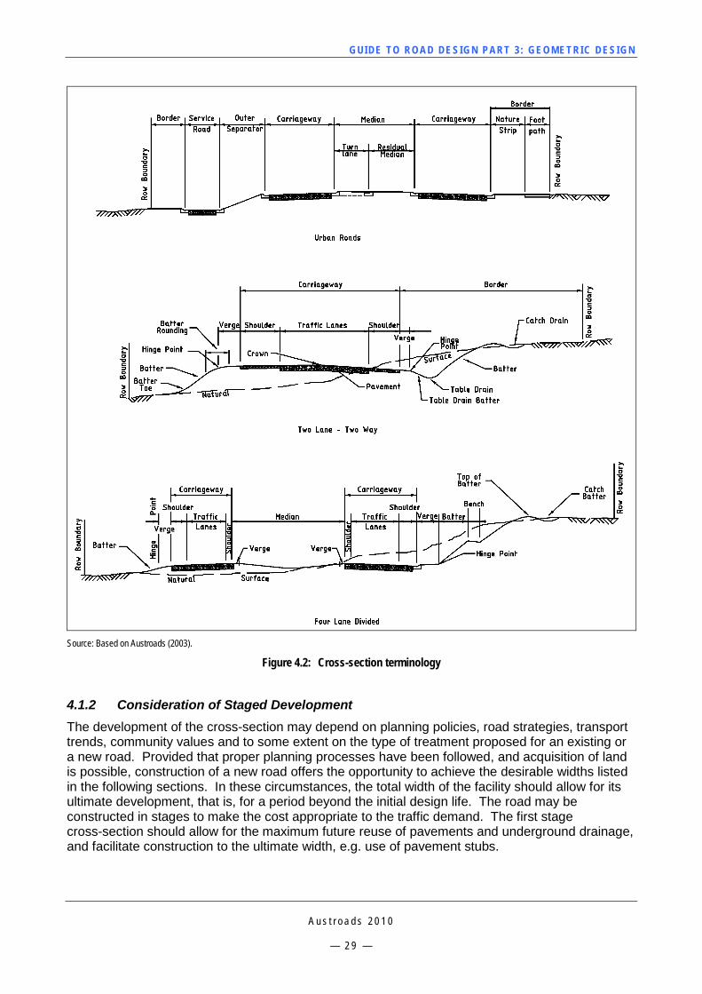
GUI DE TO RO A D DE SIG N P ART 3 : GEO MET RI C D ESI G N
A u s t r o a d s 2 0 1 0
— 2 9 —
Source: Based on Austroads (2003).
Figure 4.2: Cross-section terminology
4.1.2 Consideration of Staged Development The development of the cross-section may depend on planning policies, road strategies, transport trends, community values and to some extent on the type of treatment proposed for an existing or a new road. Provided that proper planning processes have been followed, and acquisition of land is possible, construction of a new road offers the opportunity to achieve the desirable widths listed in the following sections. In these circumstances, the total width of the facility should allow for its ultimate development, that is, for a period beyond the initial design life. The road may be constructed in stages to make the cost appropriate to the traffic demand. The first stage cross-section should allow for the maximum future reuse of pavements and underground drainage, and facilitate construction to the ultimate width, e.g. use of pavement stubs.
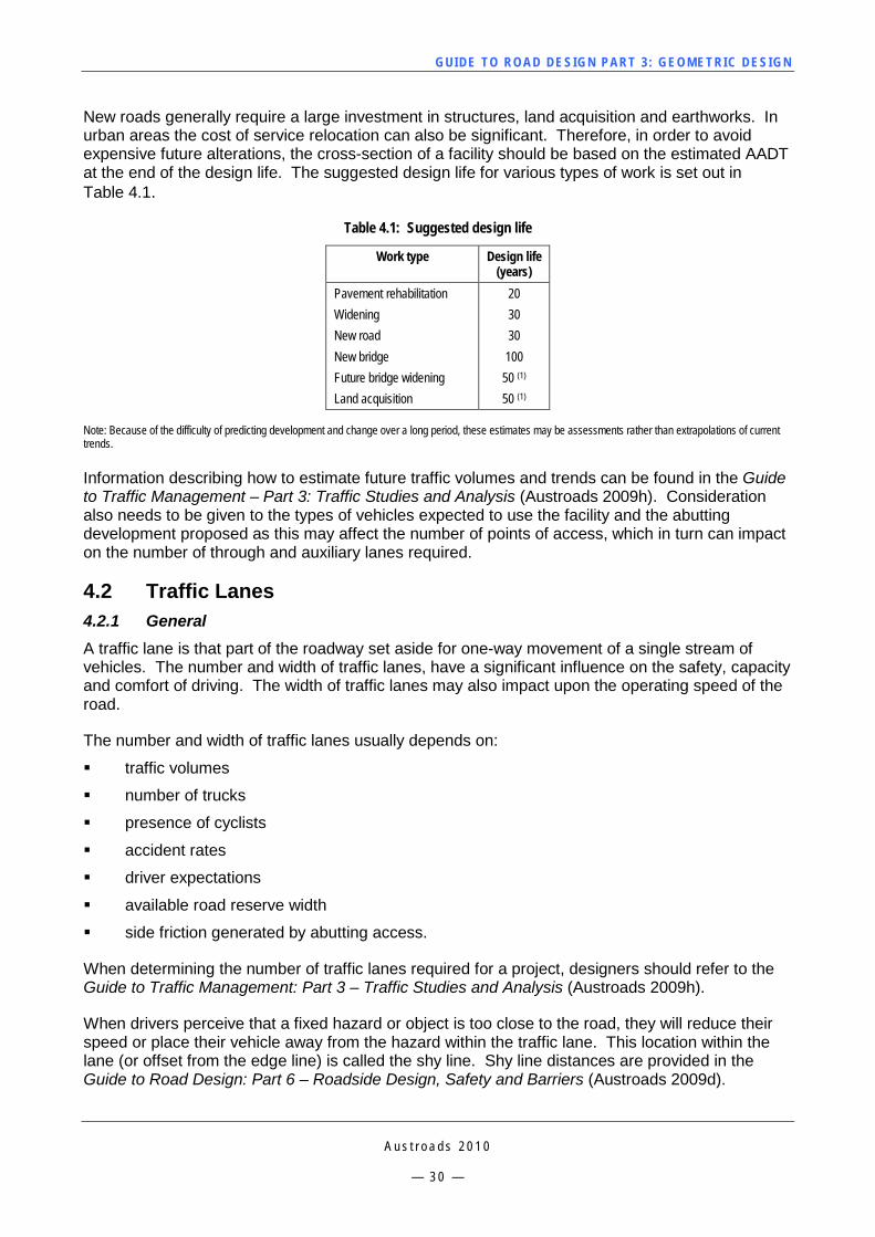
GUI DE TO RO A D DE SIG N P ART 3 : GEO MET RI C D ESI G N
A u s t r o a d s 2 0 1 0
— 3 0 —
New roads generally require a large investment in structures, land acquisition and earthworks. In urban areas the cost of service relocation can also be significant. Therefore, in order to avoid expensive future alterations, the cross-section of a facility should be based on the estimated AADT at the end of the design life. The suggested design life for various types of work is set out in Table 4.1.
Table 4.1: Suggested design life
Work type Design life (years)
Pavement rehabilitation 20 Widening 30 New road 30 New bridge 100 Future bridge widening 50 (1) Land acquisition 50 (1)
Note: Because of the difficulty of predicting development and change over a long period, these estimates may be assessments rather than extrapolations of current trends. Information describing how to estimate future traffic volumes and trends can be found in the Guide to Traffic Management – Part 3: Traffic Studies and Analysis (Austroads 2009h). Consideration also needs to be given to the types of vehicles expected to use the facility and the abutting development proposed as this may affect the number of points of access, which in turn can impact on the number of through and auxiliary lanes required.
4.2 Traffic Lanes 4.2.1 General A traffic lane is that part of the roadway set aside for one-way movement of a single stream of vehicles. The number and width of traffic lanes, have a significant influence on the safety, capacity and comfort of driving. The width of traffic lanes may also impact upon the operating speed of the road.
The number and width of traffic lanes usually depends on:
traffic volumes
number of trucks
presence of cyclists
accident rates
driver expectations
available road reserve width
side friction generated by abutting access.
When determining the number of traffic lanes required for a project, designers should refer to the Guide to Traffic Management: Part 3 – Traffic Studies and Analysis (Austroads 2009h).
When drivers perceive that a fixed hazard or object is too close to the road, they will reduce their speed or place their vehicle away from the hazard within the traffic lane. This location within the lane (or offset from the edge line) is called the shy line. Shy line distances are provided in the Guide to Road Design: Part 6 – Roadside Design, Safety and Barriers (Austroads 2009d).
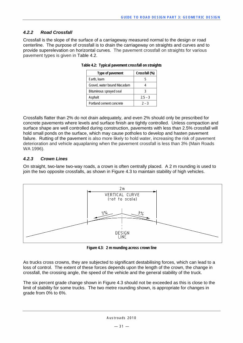
GUI DE TO RO A D DE SIG N P ART 3 : GEO MET RI C D ESI G N
A u s t r o a d s 2 0 1 0
— 3 1 —
4.2.2 Road Crossfall Crossfall is the slope of the surface of a carriageway measured normal to the design or road centerline. The purpose of crossfall is to drain the carriageway on straights and curves and to provide superelevation on horizontal curves. The pavement crossfall on straights for various pavement types is given in Table 4.2.
Table 4.2: Typical pavement crossfall on straights
Type of pavement Crossfall (%) Earth, loam 5 Gravel, water bound Macadam 4 Bituminous sprayed seal 3 Asphalt 2.5 – 3 Portland cement concrete 2 – 3
Crossfalls flatter than 2% do not drain adequately, and even 2% should only be prescribed for concrete pavements where levels and surface finish are tightly controlled. Unless compaction and surface shape are well controlled during construction, pavements with less than 2.5% crossfall will hold small ponds on the surface, which may cause potholes to develop and hasten pavement failure. Rutting of the pavement is also more likely to hold water, increasing the risk of pavement deterioration and vehicle aquaplaning when the pavement crossfall is less than 3% (Main Roads WA 1996).
4.2.3 Crown Lines On straight, two-lane two-way roads, a crown is often centrally placed. A 2 m rounding is used to join the two opposite crossfalls, as shown in Figure 4.3 to maintain stability of high vehicles.
Figure 4.3: 2 m rounding across crown line
As trucks cross crowns, they are subjected to significant destabilising forces, which can lead to a loss of control. The extent of these forces depends upon the length of the crown, the change in crossfall, the crossing angle, the speed of the vehicle and the general stability of the truck.
The six percent grade change shown in Figure 4.3 should not be exceeded as this is close to the limit of stability for some trucks. The two metre rounding shown, is appropriate for changes in grade from 0% to 6%.
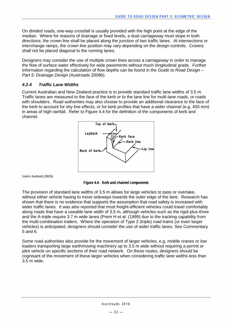
GUI DE TO RO A D DE SIG N P ART 3 : GEO MET RI C D ESI G N
A u s t r o a d s 2 0 1 0
— 3 2 —
On divided roads, one-way crossfall is usually provided with the high point at the edge of the median. Where for reasons of drainage or fixed levels, a dual carriageway must slope in both directions; the crown line shall be placed along the junction of two traffic lanes. At intersections or interchange ramps, the crown line position may vary depending on the design controls. Crowns shall not be placed diagonal to the running lanes.
Designers may consider the use of multiple crown lines across a carriageway in order to manage the flow of surface water effectively for wide pavements without much longitudinal grade. Further information regarding the calculation of flow depths can be found in the Guide to Road Design – Part 5: Drainage Design (Austroads 2008b).
4.2.4 Traffic Lane Widths Current Australian and New Zealand practice is to provide standard traffic lane widths of 3.5 m. Traffic lanes are measured to the face of the kerb or to the lane line for multi-lane roads, or roads with shoulders. Road authorities may also choose to provide an additional clearance to the face of the kerb to account for shy line effects, or for kerb profiles that have a wider channel (e.g. 450 mm) in areas of high rainfall. Refer to Figure 4.4 for the definition of the components of kerb and channel.
Source: Austroads (2002b).
Figure 4.4: Kerb and channel components
The provision of standard lane widths of 3.5 m allows for large vehicles to pass or overtake, without either vehicle having to move sideways towards the outer edge of the lane. Research has shown that there is no evidence that supports the assumption that road safety is increased with wider traffic lanes. It was also reported that most freight-efficient vehicles could travel comfortably along roads that have a useable lane width of 3.5 m, although vehicles such as the rigid-plus-three and the A-triple require 3.7 m wide lanes (Prem H et al. (1999) due to the tracking capability from the multi-combination trailers. Where the operation of Type 2 (triple) road trains (or even larger vehicles) is anticipated, designers should consider the use of wider traffic lanes. See Commentary 5 and 6.
Some road authorities also provide for the movement of larger vehicles, e.g. mobile cranes or low loaders transporting large earthmoving machinery up to 3.5 m wide without requiring a permit or pilot vehicle on specific sections of their road network. On these routes, designers should be cognisant of the movement of these larger vehicles when considering traffic lane widths less than 3.5 m wide.
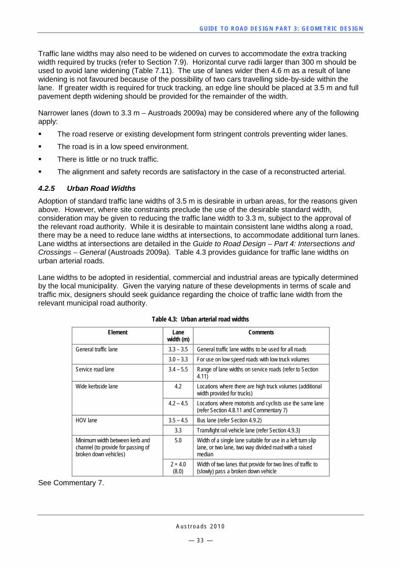
GUI DE TO RO A D DE SIG N P ART 3 : GEO MET RI C D ESI G N
A u s t r o a d s 2 0 1 0
— 3 3 —
Traffic lane widths may also need to be widened on curves to accommodate the extra tracking width required by trucks (refer to Section 7.9). Horizontal curve radii larger than 300 m should be used to avoid lane widening (Table 7.11). The use of lanes wider then 4.6 m as a result of lane widening is not favoured because of the possibility of two cars travelling side-by-side within the lane. If greater width is required for truck tracking, an edge line should be placed at 3.5 m and full pavement depth widening should be provided for the remainder of the width.
Narrower lanes (down to 3.3 m – Austroads 2009a) may be considered where any of the following apply:
The road reserve or existing development form stringent controls preventing wider lanes.
The road is in a low speed environment.
There is little or no truck traffic.
The alignment and safety records are satisfactory in the case of a reconstructed arterial.
4.2.5 Urban Road Widths Adoption of standard traffic lane widths of 3.5 m is desirable in urban areas, for the reasons given above. However, where site constraints preclude the use of the desirable standard width, consideration may be given to reducing the traffic lane width to 3.3 m, subject to the approval of the relevant road authority. While it is desirable to maintain consistent lane widths along a road, there may be a need to reduce lane widths at intersections, to accommodate additional turn lanes. Lane widths at intersections are detailed in the Guide to Road Design – Part 4: Intersections and Crossings – General (Austroads 2009a). Table 4.3 provides guidance for traffic lane widths on urban arterial roads.
Lane widths to be adopted in residential, commercial and industrial areas are typically determined by the local municipality. Given the varying nature of these developments in terms of scale and traffic mix, designers should seek guidance regarding the choice of traffic lane width from the relevant municipal road authority.
Table 4.3: Urban arterial road widths
Element Lane width (m)
Comments
General traffic lane 3.3 – 3.5 General traffic lane widths to be used for all roads 3.0 – 3.3 For use on low speed roads with low truck volumes
Service road lane 3.4 – 5.5 Range of lane widths on service roads (refer to Section 4.11)
Wide kerbside lane 4.2 Locations where there are high truck volumes (additional width provided for trucks)
4.2 – 4.5 Locations where motorists and cyclists use the same lane (refer Section 4.8.11 and Commentary 7)
HOV lane 3.5 – 4.5 Bus lane (refer Section 4.9.2) 3.3 Tram/light rail vehicle lane (refer Section 4.9.3)
Minimum width between kerb and channel (to provide for passing of broken down vehicles)
5.0 Width of a single lane suitable for use in a left turn slip lane, or two lane, two way divided road with a raised median
2 × 4.0 (8.0)
Width of two lanes that provide for two lines of traffic to (slowly) pass a broken down vehicle
See Commentary 7.
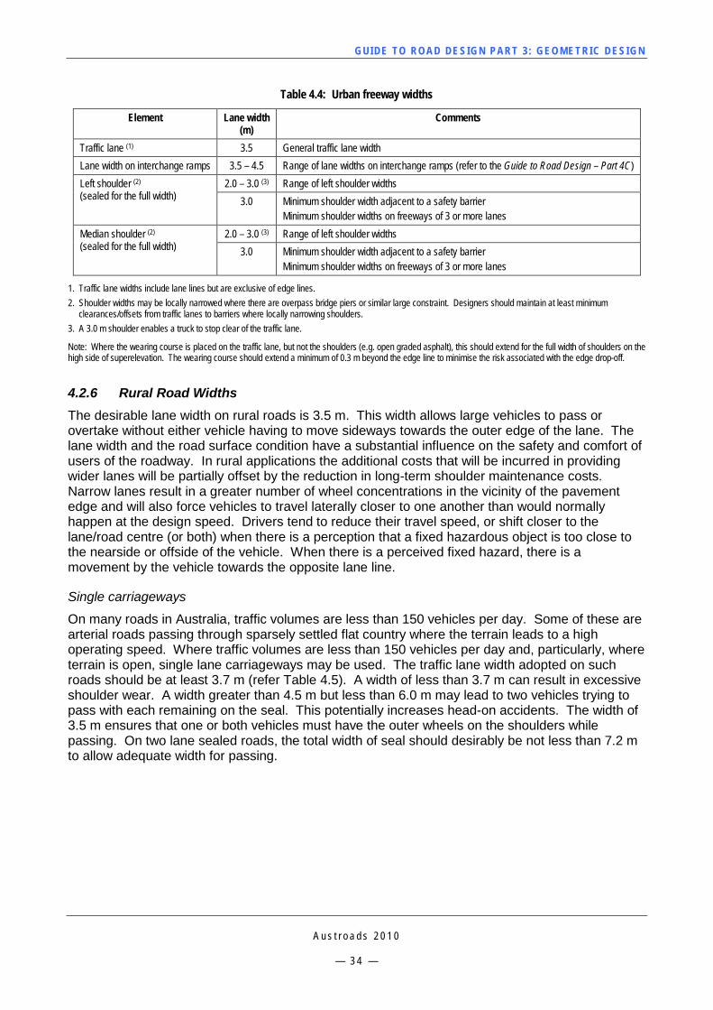
GUI DE TO RO A D DE SIG N P ART 3 : GEO MET RI C D ESI G N
A u s t r o a d s 2 0 1 0
— 3 4 —
Table 4.4: Urban freeway widths
Element Lane width (m)
Comments
Traffic lane (1) 3.5 General traffic lane width Lane width on interchange ramps 3.5 – 4.5 Range of lane widths on interchange ramps (refer to the Guide to Road Design – Part 4C) Left shoulder (2)
(sealed for the full width) 2.0 – 3.0 (3) Range of left shoulder widths
3.0 Minimum shoulder width adjacent to a safety barrier Minimum shoulder widths on freeways of 3 or more lanes
Median shoulder (2)
(sealed for the full width) 2.0 – 3.0 (3) Range of left shoulder widths
3.0 Minimum shoulder width adjacent to a safety barrier Minimum shoulder widths on freeways of 3 or more lanes
1. Traffic lane widths include lane lines but are exclusive of edge lines. 2. Shoulder widths may be locally narrowed where there are overpass bridge piers or similar large constraint. Designers should maintain at least minimum
clearances/offsets from traffic lanes to barriers where locally narrowing shoulders. 3. A 3.0 m shoulder enables a truck to stop clear of the traffic lane.
Note: Where the wearing course is placed on the traffic lane, but not the shoulders (e.g. open graded asphalt), this should extend for the full width of shoulders on the high side of superelevation. The wearing course should extend a minimum of 0.3 m beyond the edge line to minimise the risk associated with the edge drop-off.
4.2.6 Rural Road Widths The desirable lane width on rural roads is 3.5 m. This width allows large vehicles to pass or overtake without either vehicle having to move sideways towards the outer edge of the lane. The lane width and the road surface condition have a substantial influence on the safety and comfort of users of the roadway. In rural applications the additional costs that will be incurred in providing wider lanes will be partially offset by the reduction in long-term shoulder maintenance costs. Narrow lanes result in a greater number of wheel concentrations in the vicinity of the pavement edge and will also force vehicles to travel laterally closer to one another than would normally happen at the design speed. Drivers tend to reduce their travel speed, or shift closer to the lane/road centre (or both) when there is a perception that a fixed hazardous object is too close to the nearside or offside of the vehicle. When there is a perceived fixed hazard, there is a movement by the vehicle towards the opposite lane line.
Single carriageways
On many roads in Australia, traffic volumes are less than 150 vehicles per day. Some of these are arterial roads passing through sparsely settled flat country where the terrain leads to a high operating speed. Where traffic volumes are less than 150 vehicles per day and, particularly, where terrain is open, single lane carriageways may be used. The traffic lane width adopted on such roads should be at least 3.7 m (refer Table 4.5). A width of less than 3.7 m can result in excessive shoulder wear. A width greater than 4.5 m but less than 6.0 m may lead to two vehicles trying to pass with each remaining on the seal. This potentially increases head-on accidents. The width of 3.5 m ensures that one or both vehicles must have the outer wheels on the shoulders while passing. On two lane sealed roads, the total width of seal should desirably be not less than 7.2 m to allow adequate width for passing.
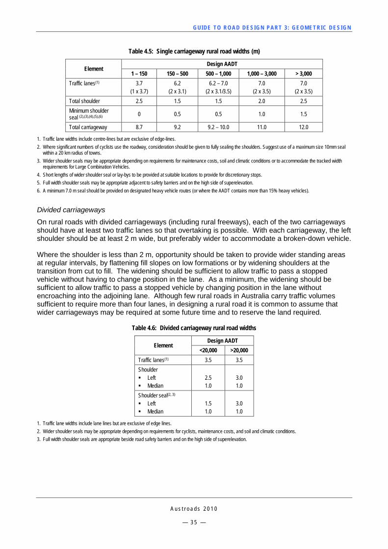
GUI DE TO RO A D DE SIG N P ART 3 : GEO MET RI C D ESI G N
A u s t r o a d s 2 0 1 0
— 3 5 —
Table 4.5: Single carriageway rural road widths (m)
Element Design AADT
1 – 150 150 – 500 500 – 1,000 1,000 – 3,000 > 3,000 Traffic lanes(1) 3.7
(1 x 3.7) 6.2
(2 x 3.1) 6.2 – 7.0
(2 x 3.1/3.5) 7.0
(2 x 3.5) 7.0
(2 x 3.5) Total shoulder 2.5 1.5 1.5 2.0 2.5 Minimum shoulder seal (2),(3),(4),(5),(6) 0 0.5 0.5 1.0 1.5
Total carriageway 8.7 9.2 9.2 – 10.0 11.0 12.0
1. Traffic lane widths include centre-lines but are exclusive of edge-lines. 2. Where significant numbers of cyclists use the roadway, consideration should be given to fully sealing the shoulders. Suggest use of a maximum size 10mm seal
within a 20 km radius of towns. 3. Wider shoulder seals may be appropriate depending on requirements for maintenance costs, soil and climatic conditions or to accommodate the tracked width
requirements for Large Combination Vehicles. 4. Short lengths of wider shoulder seal or lay-bys to be provided at suitable locations to provide for discretionary stops. 5. Full width shoulder seals may be appropriate adjacent to safety barriers and on the high side of superelevation. 6. A minimum 7.0 m seal should be provided on designated heavy vehicle routes (or where the AADT contains more than 15% heavy vehicles).
Divided carriageways
On rural roads with divided carriageways (including rural freeways), each of the two carriageways should have at least two traffic lanes so that overtaking is possible. With each carriageway, the left shoulder should be at least 2 m wide, but preferably wider to accommodate a broken-down vehicle.
Where the shoulder is less than 2 m, opportunity should be taken to provide wider standing areas at regular intervals, by flattening fill slopes on low formations or by widening shoulders at the transition from cut to fill. The widening should be sufficient to allow traffic to pass a stopped vehicle without having to change position in the lane. As a minimum, the widening should be sufficient to allow traffic to pass a stopped vehicle by changing position in the lane without encroaching into the adjoining lane. Although few rural roads in Australia carry traffic volumes sufficient to require more than four lanes, in designing a rural road it is common to assume that wider carriageways may be required at some future time and to reserve the land required.
Table 4.6: Divided carriageway rural road widths
Element Design AADT
<20,000 >20,000 Traffic lanes(1) 3.5 3.5 Shoulder Left Median
2.5 1.0
3.0 1.0
Shoulder seal(2, 3)
Left Median
1.5 1.0
3.0 1.0
1. Traffic lane widths include lane lines but are exclusive of edge lines. 2. Wider shoulder seals may be appropriate depending on requirements for cyclists, maintenance costs, and soil and climatic conditions. 3. Full width shoulder seals are appropriate beside road safety barriers and on the high side of superelevation.
GUI DE TO RO A D DE SIG N P ART 3 : GEO MET RI C D ESI G N
A u s t r o a d s 2 0 1 0
— 3 6 —
4.3 Shoulders 4.3.1 Function Road shoulders are provided to carry out two functions; structural and traffic. The structural function of the shoulder is to provide lateral support to the road pavement layers.
The traffic functions of the shoulder are:
an initial recovery area for any errant vehicle
a refuge for stopped vehicles on a firm surface at a safe distance from traffic lanes
a trafficable area for emergency use
space for cyclists
clearance to lateral obstructions
provision of additional width for tracking of large vehicles (Section 7.9).
4.3.2 Width Shoulder width is measured from the outer edge of the traffic lane to the edge of usable carriageway and excludes any berm, verge, rounding or extra width provided to accommodate guideposts and guard fencing. Wide shoulders have the following advantages:
Space is available for a stationary vehicle to stand clear of the traffic lanes; a vehicle standing partly on a shoulder and partly on a traffic lane may be a hazard.
Space is available on which vehicles may deviate to avoid colliding with other vehicles and on which a driver may regain control of an errant vehicle.
The resulting wider formations increase driver comfort and the quality of service of the road.
They contribute to improved sight distance across the inside of horizontal curves.
Table 4.3 to Table 4.6 list shoulder width values for both urban and rural roads based on AADT volumes or functional classification. These widths allow a vehicle to stop, or a maintenance vehicle to operate, with only partial or no obstruction of the traffic lanes. Provided volumes are not high or sight distances are sufficiently long, partial obstruction of the traffic lane will not present an undue hazard to traffic.
A width of 2.5 m is needed to allow a passenger vehicle to stop clear of the traffic lanes. A width of 3.0 m allows a passenger vehicle to stop clear of the traffic lanes and provides an additional clearance to passing traffic. It also allows a truck to stop clear of the traffic lanes.
The cost of maintaining road shoulders does not rise in proportion to their width. However, the cost of the initial construction involves additional earthwork and pavement construction costs. In reconstruction of older pavements, the provision of wider shoulders may increase the costs extensively. Therefore, an economic balance must be achieved in shoulder width, and in the case of upgrading work this element can be very significant.
The aim should be to provide shoulders of 1.5 m to 2.0 m wherever possible, and up to 2.5 to 3 m on higher volume roads. Because most vehicles standing on road shoulders exercise some choice as to the stopping place, it is desirable to take every opportunity to provide areas at intervals where vehicles can stop completely clear of the traffic lanes, such as on low fills where flattening the slopes automatically provides this, or at the transition from cut to fill where minor additional earthworks involved can be made at low cost. The choice of shoulder width should also consider the installation of road furniture and safety barriers as these will constrain the distance that a vehicle can stop clear of the traffic lane. See Commentary 8.
GUI DE TO RO A D DE SIG N P ART 3 : GEO MET RI C D ESI G N
A u s t r o a d s 2 0 1 0
— 3 7 —
On a divided road with two lanes in each direction, it is desirable to provide shoulders at least 2.5 m wide on the left side of each carriageway and 1.0 m wide on the median side of each carriageway. If the divided road has three or more lanes in each direction, it is preferable to have wide shoulders on both sides of both carriageways, especially where there is a median barrier adjacent to the shoulder. This limits the number of lanes a vehicle may have to cross in the event of breakdowns to stop clear of the traffic lanes, allows for the provision of emergency telephone points and for the operation of emergency services, tow trucks or maintenance vehicles.
A shoulder is not usually provided on urban local roads or arterials where kerb and channel has been constructed. Shoulders may be provided on major urban roads to perform a similar function to those on rural roads, particularly for drainage, on-road cyclists and to store (or partly store) a broken down vehicle so that the road does not become completely blocked when a breakdown occurs. Shoulders may be used during interim stages of road construction, with the width determined by the future cross-section.
4.3.3 Shoulder Sealing Shoulders may be wholly or partially sealed. Sealing of shoulders is frequently done to reduce maintenance costs and to improve moisture conditions under pavements, especially under the outer wheel path.
However, from the geometric design point of view, the shoulder is regarded as being usable by traffic. Partial sealing ensures this by protecting the lane edge against the development of the broken edges or ‘drop offs’ that occur adjacent to the traffic lanes and results in the whole shoulder width remaining usable to traffic up to 2.5 m wide. For a marginally greater cost, full shoulder sealing provides an even better result than partial shoulder sealing.
The desirable width of sealed shoulder depends on many factors including:
traffic composition
AADT
access
operating speed
rainfall
shoulder pavement.
While 0.5 m wide seals on the shoulders should be considered the minimum when the predicted AADT is less than 1000, more sealed width is often warranted. In some instances, partial shoulder sealing is widened to full width adjacent to concrete gutters and on the high side of super-elevated curves. In wetter areas where moisture control is required, shoulder seal widths of 0.5 m are desirable and 1.0 m is preferable. In the case of full or partial sealing of shoulders, longitudinal edge lines are desirable at the edge of the traffic lanes. Otherwise, in the case of narrow partial sealing, usage of the additional seal as part of the traffic lanes merely transfers the problem to the new edge.
To minimise the effect of wind erosion on shoulder material, a 1.0 m sealed shoulder is often used on roads carrying AADT over 2000 vpd (with 10% heavy vehicles (RTA 1989).
The widths required for the various functions are set out in Table 4.7.
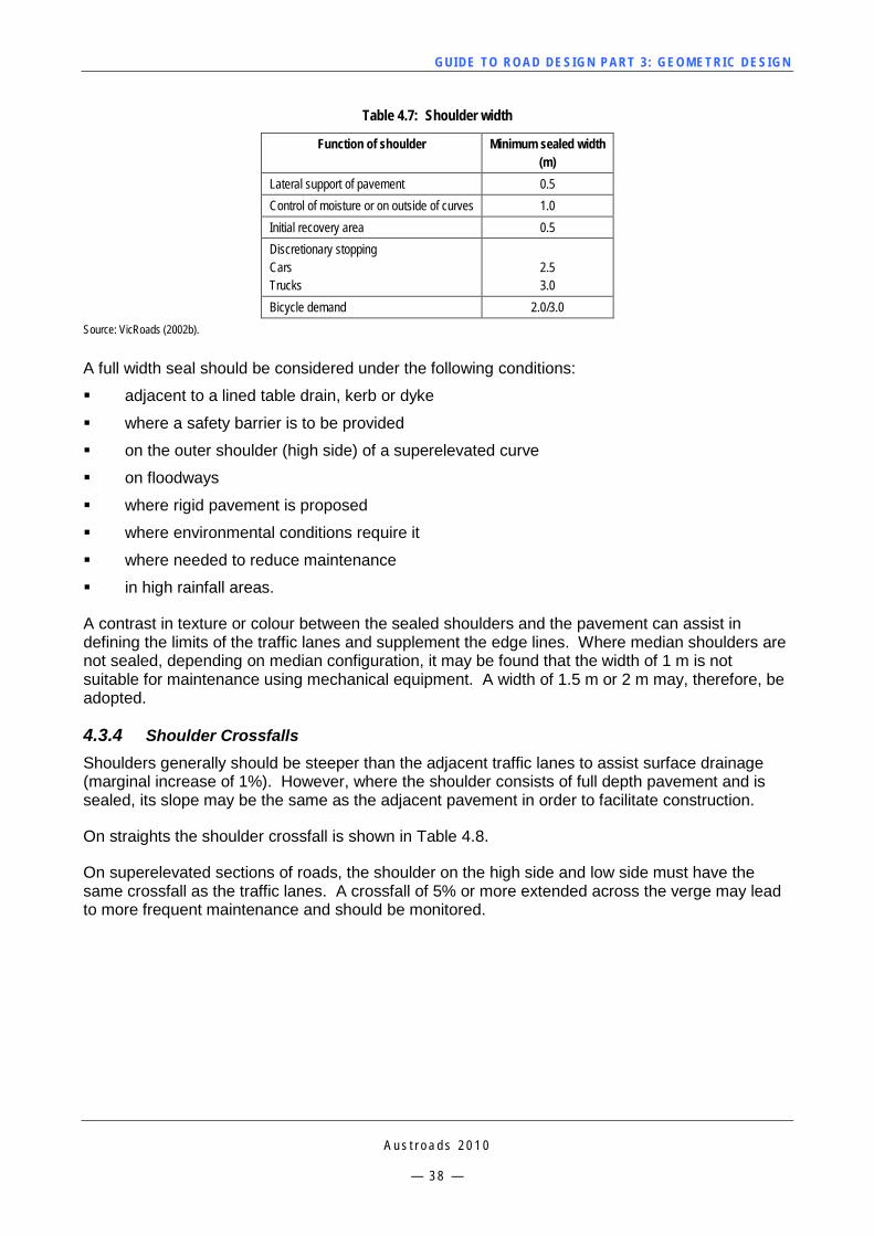
GUI DE TO RO A D DE SIG N P ART 3 : GEO MET RI C D ESI G N
A u s t r o a d s 2 0 1 0
— 3 8 —
Table 4.7: Shoulder width
Function of shoulder Minimum sealed width (m)
Lateral support of pavement 0.5 Control of moisture or on outside of curves 1.0 Initial recovery area 0.5 Discretionary stopping Cars Trucks
2.5 3.0
Bicycle demand 2.0/3.0 Source: VicRoads (2002b).
A full width seal should be considered under the following conditions:
adjacent to a lined table drain, kerb or dyke
where a safety barrier is to be provided
on the outer shoulder (high side) of a superelevated curve
on floodways
where rigid pavement is proposed
where environmental conditions require it
where needed to reduce maintenance
in high rainfall areas.
A contrast in texture or colour between the sealed shoulders and the pavement can assist in defining the limits of the traffic lanes and supplement the edge lines. Where median shoulders are not sealed, depending on median configuration, it may be found that the width of 1 m is not suitable for maintenance using mechanical equipment. A width of 1.5 m or 2 m may, therefore, be adopted.
4.3.4 Shoulder Crossfalls Shoulders generally should be steeper than the adjacent traffic lanes to assist surface drainage (marginal increase of 1%). However, where the shoulder consists of full depth pavement and is sealed, its slope may be the same as the adjacent pavement in order to facilitate construction.
On straights the shoulder crossfall is shown in Table 4.8.
On superelevated sections of roads, the shoulder on the high side and low side must have the same crossfall as the traffic lanes. A crossfall of 5% or more extended across the verge may lead to more frequent maintenance and should be monitored.
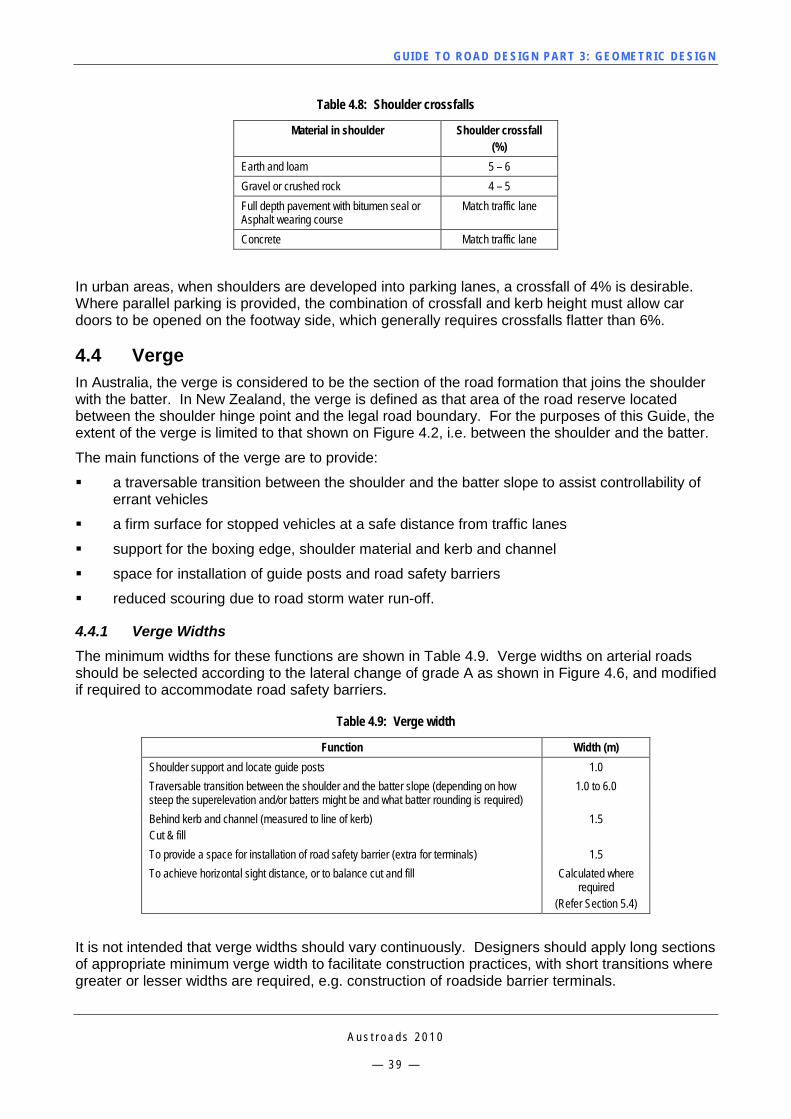
GUI DE TO RO A D DE SIG N P ART 3 : GEO MET RI C D ESI G N
A u s t r o a d s 2 0 1 0
— 3 9 —
Table 4.8: Shoulder crossfalls
Material in shoulder Shoulder crossfall (%)
Earth and loam 5 – 6 Gravel or crushed rock 4 – 5 Full depth pavement with bitumen seal or Asphalt wearing course
Match traffic lane
Concrete Match traffic lane In urban areas, when shoulders are developed into parking lanes, a crossfall of 4% is desirable. Where parallel parking is provided, the combination of crossfall and kerb height must allow car doors to be opened on the footway side, which generally requires crossfalls flatter than 6%.
4.4 Verge In Australia, the verge is considered to be the section of the road formation that joins the shoulder with the batter. In New Zealand, the verge is defined as that area of the road reserve located between the shoulder hinge point and the legal road boundary. For the purposes of this Guide, the extent of the verge is limited to that shown on Figure 4.2, i.e. between the shoulder and the batter.
The main functions of the verge are to provide:
a traversable transition between the shoulder and the batter slope to assist controllability of errant vehicles
a firm surface for stopped vehicles at a safe distance from traffic lanes
support for the boxing edge, shoulder material and kerb and channel
space for installation of guide posts and road safety barriers
reduced scouring due to road storm water run-off.
4.4.1 Verge Widths The minimum widths for these functions are shown in Table 4.9. Verge widths on arterial roads should be selected according to the lateral change of grade A as shown in Figure 4.6, and modified if required to accommodate road safety barriers.
Table 4.9: Verge width
Function Width (m) Shoulder support and locate guide posts 1.0 Traversable transition between the shoulder and the batter slope (depending on how steep the superelevation and/or batters might be and what batter rounding is required)
1.0 to 6.0
Behind kerb and channel (measured to line of kerb) Cut & fill
1.5
To provide a space for installation of road safety barrier (extra for terminals) 1.5 To achieve horizontal sight distance, or to balance cut and fill Calculated where
required (Refer Section 5.4)
It is not intended that verge widths should vary continuously. Designers should apply long sections of appropriate minimum verge width to facilitate construction practices, with short transitions where greater or lesser widths are required, e.g. construction of roadside barrier terminals.
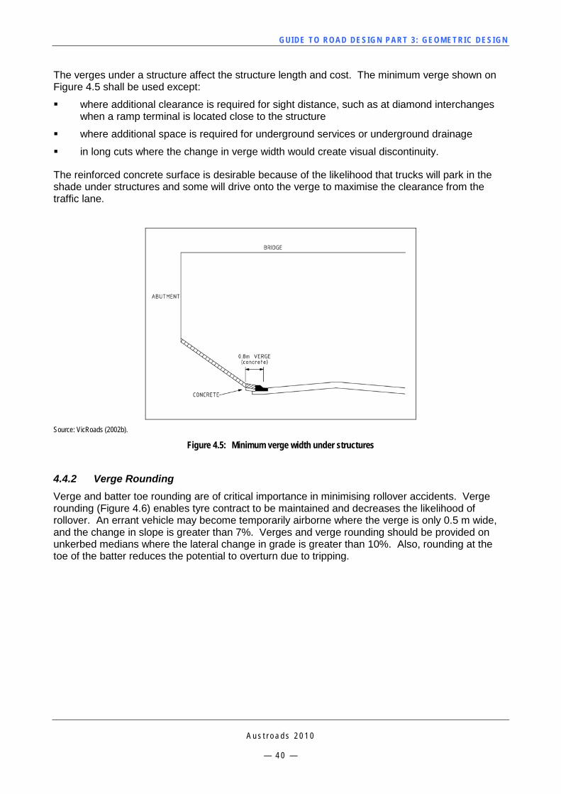
GUI DE TO RO A D DE SIG N P ART 3 : GEO MET RI C D ESI G N
A u s t r o a d s 2 0 1 0
— 4 0 —
The verges under a structure affect the structure length and cost. The minimum verge shown on Figure 4.5 shall be used except:
where additional clearance is required for sight distance, such as at diamond interchanges when a ramp terminal is located close to the structure
where additional space is required for underground services or underground drainage
in long cuts where the change in verge width would create visual discontinuity.
The reinforced concrete surface is desirable because of the likelihood that trucks will park in the shade under structures and some will drive onto the verge to maximise the clearance from the traffic lane.
Source: VicRoads (2002b).
Figure 4.5: Minimum verge width under structures
4.4.2 Verge Rounding Verge and batter toe rounding are of critical importance in minimising rollover accidents. Verge rounding (Figure 4.6) enables tyre contract to be maintained and decreases the likelihood of rollover. An errant vehicle may become temporarily airborne where the verge is only 0.5 m wide, and the change in slope is greater than 7%. Verges and verge rounding should be provided on unkerbed medians where the lateral change in grade is greater than 10%. Also, rounding at the toe of the batter reduces the potential to overturn due to tripping.
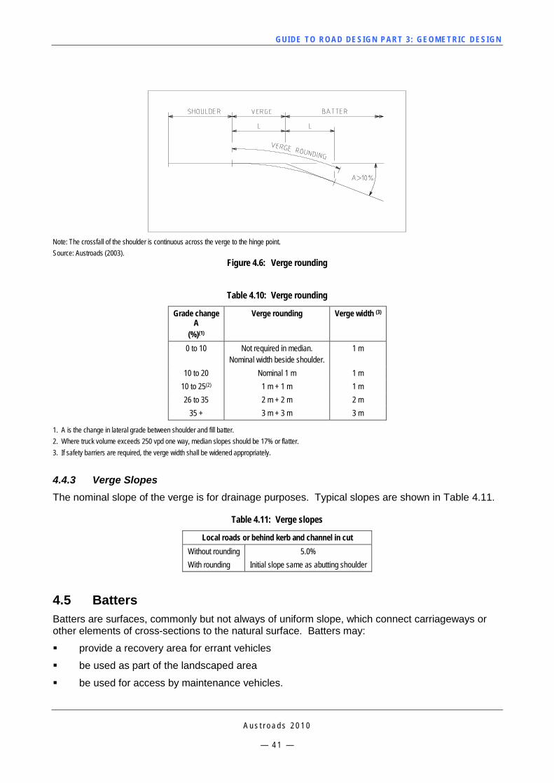
GUI DE TO RO A D DE SIG N P ART 3 : GEO MET RI C D ESI G N
A u s t r o a d s 2 0 1 0
— 4 1 —
Note: The crossfall of the shoulder is continuous across the verge to the hinge point. Source: Austroads (2003).
Figure 4.6: Verge rounding
Table 4.10: Verge rounding
Grade change A
(%)(1)
Verge rounding Verge width (3)
0 to 10 Not required in median. Nominal width beside shoulder.
1 m
10 to 20 Nominal 1 m 1 m 10 to 25(2) 1 m + 1 m 1 m 26 to 35 2 m + 2 m 2 m
35 + 3 m + 3 m 3 m
1. A is the change in lateral grade between shoulder and fill batter. 2. Where truck volume exceeds 250 vpd one way, median slopes should be 17% or flatter. 3. If safety barriers are required, the verge width shall be widened appropriately.
4.4.3 Verge Slopes The nominal slope of the verge is for drainage purposes. Typical slopes are shown in Table 4.11.
Table 4.11: Verge slopes
Local roads or behind kerb and channel in cut Without rounding 5.0% With rounding Initial slope same as abutting shoulder
4.5 Batters Batters are surfaces, commonly but not always of uniform slope, which connect carriageways or other elements of cross-sections to the natural surface. Batters may:
provide a recovery area for errant vehicles
be used as part of the landscaped area
be used for access by maintenance vehicles.
GUI DE TO RO A D DE SIG N P ART 3 : GEO MET RI C D ESI G N
A u s t r o a d s 2 0 1 0
— 4 2 —
Batter slopes are usually defined as the ratio of ‘x’ horizontal to one vertical and are shown as, for example, 6:1.
The following factors should be considered when selecting batter slopes:
the results and recommendations of geotechnical investigation
batter stability
batter safety (economics of eliminating safety barriers, e.g. maintaining a smooth face for rock cuttings which will not snag a vehicle)
Fill batters with the following slopes can be considered to be: — recoverable for cars with 4:1 or flatter batter slopes — non-recoverable for cars with batter slopes from 3:1 to 4:1, but they are considered to
be traversable. Cars are likely to continue to the bottom of the slope — non-recoverable (and non-traversable) for cars with batter slopes steeper than 3:1 — recoverable for trucks with batter slopes of 10:1
future costs of maintaining the adopted slope and accessibility requirements considering occupational health and safety issues
appearance and environmental effects
earthworks balance
available width of road reserve
landscaping requirements.
Slopes flatter than the desirable maximum (Table 4.12) should be used where possible. Where steeper slopes are unavoidable and barriers are required, designers shall consult the Guide to Road Design – Part 6: Roadside Design, Safety and Barriers (Austroads 2009d).
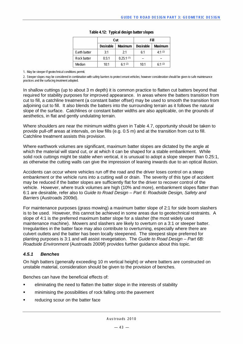
GUI DE TO RO A D DE SIG N P ART 3 : GEO MET RI C D ESI G N
A u s t r o a d s 2 0 1 0
— 4 3 —
Table 4.12: Typical design batter slopes
Cut Fill Desirable Maximum Desirable Maximum
Earth batter 3:1 2:1 6:1 4:1 (2) Rock batter 0.5:1 0.25:1 (1) – – Median 10:1 6:1 (2) 10:1 6:1 (2)
1. May be steeper if geotechnical conditions permit. 2. Steeper slopes may be considered in combination with safety barriers to protect errant vehicles; however consideration should be given to safe maintenance practices and the surfacing treatment adopted. In shallow cuttings (up to about 3 m depth) it is common practice to flatten cut batters beyond that required for stability purposes for improved appearance. In areas where the batters transition from cut to fill, a catchline treatment (a constant batter offset) may be used to smooth the transition from adjoining cut to fill. It also blends the batters into the surrounding terrain as it follows the natural slope of the surface. Catchlines or constant batter widths are also applicable, on the grounds of aesthetics, in flat and gently undulating terrain.
Where shoulders are near the minimum widths given in Table 4.7, opportunity should be taken to provide pull-off areas at intervals, on low fills (e.g. 0.5 m) and at the transition from cut to fill. Catchline treatment assists this provision.
Where earthwork volumes are significant, maximum batter slopes are dictated by the angle at which the material will stand cut, or at which it can be shaped for a stable embankment. While solid rock cuttings might be stable when vertical, it is unusual to adopt a slope steeper than 0.25:1, as otherwise the cutting walls can give the impression of leaning inwards due to an optical illusion.
Accidents can occur where vehicles run off the road and the driver loses control on a steep embankment or the vehicle runs into a cutting wall or drain. The severity of this type of accident may be reduced if the batter slopes are sufficiently flat for the driver to recover control of the vehicle. However, where truck volumes are high (10% and more), embankment slopes flatter than 6:1 are desirable, refer also to Guide to Road Design – Part 6: Roadside Design, Safety and Barriers (Austroads 2009d).
For maintenance purposes (grass mowing) a maximum batter slope of 2:1 for side boom slashers is to be used. However, this cannot be achieved in some areas due to geotechnical restraints. A slope of 4:1 is the preferred maximum batter slope for a slasher (the most widely used maintenance machine). Mowers and slashers are likely to overturn on a 3:1 or steeper batter. Irregularities in the batter face may also contribute to overturning, especially where there are culvert outlets and the batter has been locally steepened. The steepest slope preferred for planting purposes is 3:1 and will assist revegetation. The Guide to Road Design – Part 6B: Roadside Environment (Austroads 2009f) provides further guidance about this topic.
4.5.1 Benches On high batters (generally exceeding 10 m vertical height) or where batters are constructed on unstable material, consideration should be given to the provision of benches.
Benches can have the beneficial effects of:
eliminating the need to flatten the batter slope in the interests of stability
minimising the possibilities of rock falling onto the pavement
reducing scour on the batter face

GUI DE TO RO A D DE SIG N P ART 3 : GEO MET RI C D ESI G N
A u s t r o a d s 2 0 1 0
— 4 4 —
reducing the amount of water in cuttings to be carried by the table drain
providing easier access for maintenance of the batter face
improving the appearance of the cutting
assisting the re-establishment of vegetation
improving sight distance on horizontal curves.
Benches should be sloped away from the roadway and longitudinally so that stormwater can be drained towards the ends of the bench and discharged on to the natural ground. In some instances, the invert so formed may require lining.
The minimum width of bench should be 3 m (Figure 4.7) with a maximum crossfall of 10%. The desirable width of bench to meet the requirements of road authority safe work and maintenance practices and drainage purposes is 5 m.
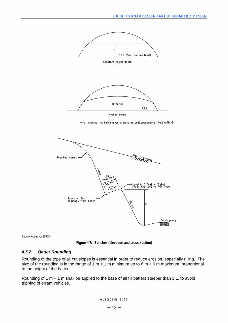
GUI DE TO RO A D DE SIG N P ART 3 : GEO MET RI C D ESI G N
A u s t r o a d s 2 0 1 0
— 4 5 —
Source: Austroads (2003).
Figure 4.7: Benches (elevation and cross-section)
4.5.2 Batter Rounding Rounding of the tops of all cut slopes is essential in order to reduce erosion, especially rilling. The size of the rounding is in the range of 1 m + 1 m minimum up to 6 m + 6 m maximum, proportional to the height of the batter.
Rounding of 1 m + 1 m shall be applied to the base of all fill batters steeper than 3:1, to avoid tripping of errant vehicles.
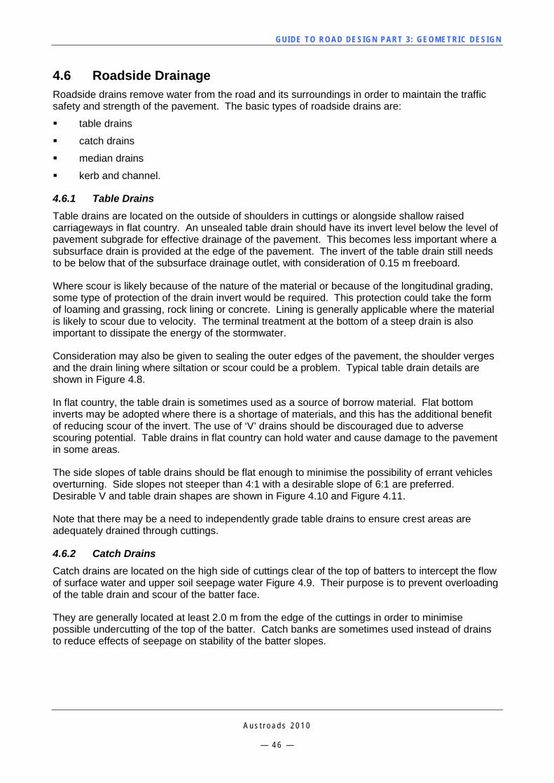
GUI DE TO RO A D DE SIG N P ART 3 : GEO MET RI C D ESI G N
A u s t r o a d s 2 0 1 0
— 4 6 —
4.6 Roadside Drainage Roadside drains remove water from the road and its surroundings in order to maintain the traffic safety and strength of the pavement. The basic types of roadside drains are:
table drains
catch drains
median drains
kerb and channel.
4.6.1 Table Drains Table drains are located on the outside of shoulders in cuttings or alongside shallow raised carriageways in flat country. An unsealed table drain should have its invert level below the level of pavement subgrade for effective drainage of the pavement. This becomes less important where a subsurface drain is provided at the edge of the pavement. The invert of the table drain still needs to be below that of the subsurface drainage outlet, with consideration of 0.15 m freeboard.
Where scour is likely because of the nature of the material or because of the longitudinal grading, some type of protection of the drain invert would be required. This protection could take the form of loaming and grassing, rock lining or concrete. Lining is generally applicable where the material is likely to scour due to velocity. The terminal treatment at the bottom of a steep drain is also important to dissipate the energy of the stormwater.
Consideration may also be given to sealing the outer edges of the pavement, the shoulder verges and the drain lining where siltation or scour could be a problem. Typical table drain details are shown in Figure 4.8.
In flat country, the table drain is sometimes used as a source of borrow material. Flat bottom inverts may be adopted where there is a shortage of materials, and this has the additional benefit of reducing scour of the invert. The use of ‘V’ drains should be discouraged due to adverse scouring potential. Table drains in flat country can hold water and cause damage to the pavement in some areas.
The side slopes of table drains should be flat enough to minimise the possibility of errant vehicles overturning. Side slopes not steeper than 4:1 with a desirable slope of 6:1 are preferred. Desirable V and table drain shapes are shown in Figure 4.10 and Figure 4.11.
Note that there may be a need to independently grade table drains to ensure crest areas are adequately drained through cuttings.
4.6.2 Catch Drains Catch drains are located on the high side of cuttings clear of the top of batters to intercept the flow of surface water and upper soil seepage water Figure 4.9. Their purpose is to prevent overloading of the table drain and scour of the batter face.
They are generally located at least 2.0 m from the edge of the cuttings in order to minimise possible undercutting of the top of the batter. Catch banks are sometimes used instead of drains to reduce effects of seepage on stability of the batter slopes.
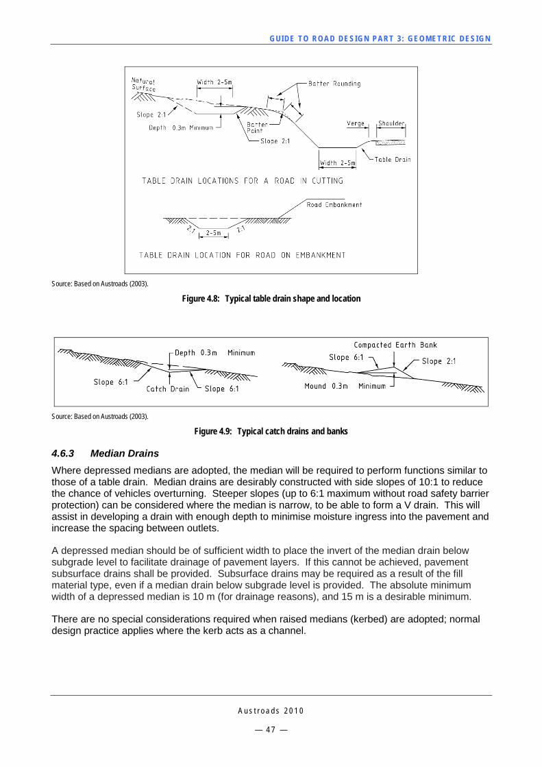
GUI DE TO RO A D DE SIG N P ART 3 : GEO MET RI C D ESI G N
A u s t r o a d s 2 0 1 0
— 4 7 —
Source: Based on Austroads (2003).
Figure 4.8: Typical table drain shape and location
Source: Based on Austroads (2003).
Figure 4.9: Typical catch drains and banks
4.6.3 Median Drains Where depressed medians are adopted, the median will be required to perform functions similar to those of a table drain. Median drains are desirably constructed with side slopes of 10:1 to reduce the chance of vehicles overturning. Steeper slopes (up to 6:1 maximum without road safety barrier protection) can be considered where the median is narrow, to be able to form a V drain. This will assist in developing a drain with enough depth to minimise moisture ingress into the pavement and increase the spacing between outlets.
A depressed median should be of sufficient width to place the invert of the median drain below subgrade level to facilitate drainage of pavement layers. If this cannot be achieved, pavement subsurface drains shall be provided. Subsurface drains may be required as a result of the fill material type, even if a median drain below subgrade level is provided. The absolute minimum width of a depressed median is 10 m (for drainage reasons), and 15 m is a desirable minimum.
There are no special considerations required when raised medians (kerbed) are adopted; normal design practice applies where the kerb acts as a channel.
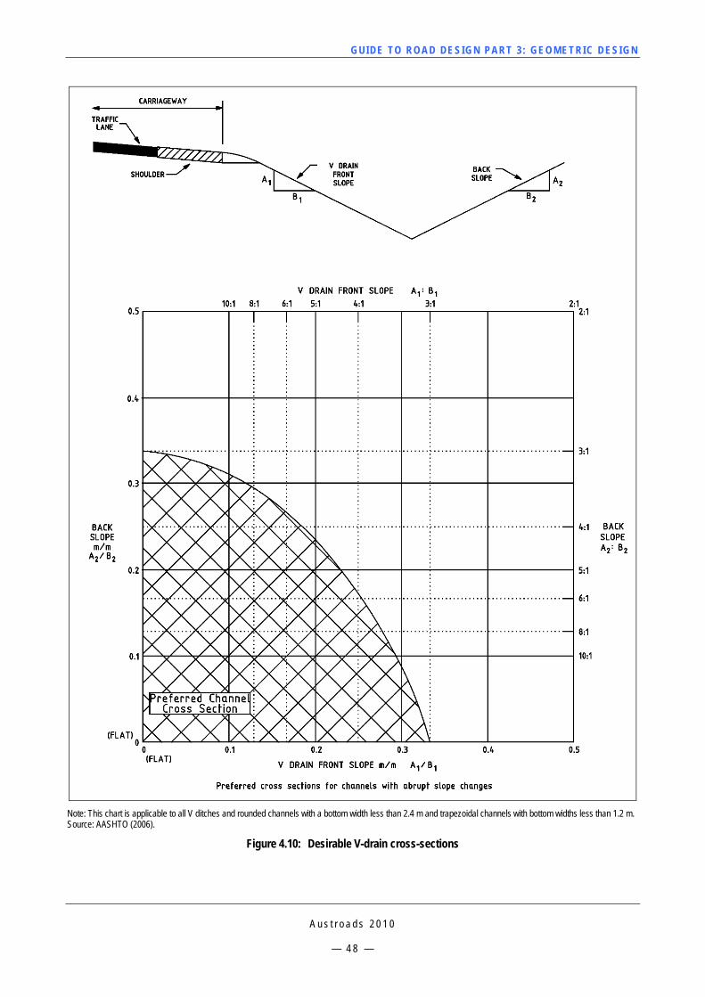
GUI DE TO RO A D DE SIG N P ART 3 : GEO MET RI C D ESI G N
A u s t r o a d s 2 0 1 0
— 4 8 —
Note: This chart is applicable to all V ditches and rounded channels with a bottom width less than 2.4 m and trapezoidal channels with bottom widths less than 1.2 m. Source: AASHTO (2006).
Figure 4.10: Desirable V-drain cross-sections
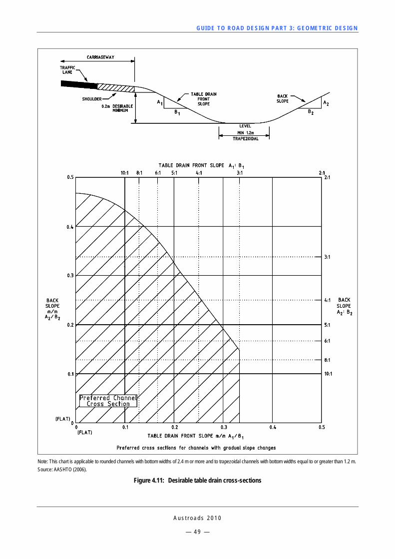
GUI DE TO RO A D DE SIG N P ART 3 : GEO MET RI C D ESI G N
A u s t r o a d s 2 0 1 0
— 4 9 —
Note: This chart is applicable to rounded channels with bottom widths of 2.4 m or more and to trapezoidal channels with bottom widths equal to or greater than 1.2 m. Source: AASHTO (2006).
Figure 4.11: Desirable table drain cross-sections
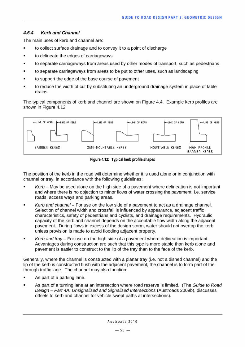
GUI DE TO RO A D DE SIG N P ART 3 : GEO MET RI C D ESI G N
A u s t r o a d s 2 0 1 0
— 5 0 —
4.6.4 Kerb and Channel The main uses of kerb and channel are:
to collect surface drainage and to convey it to a point of discharge
to delineate the edges of carriageways
to separate carriageways from areas used by other modes of transport, such as pedestrians
to separate carriageways from areas to be put to other uses, such as landscaping
to support the edge of the base course of pavement
to reduce the width of cut by substituting an underground drainage system in place of table drains.
The typical components of kerb and channel are shown on Figure 4.4. Example kerb profiles are shown in Figure 4.12.
Figure 4.12: Typical kerb profile shapes
The position of the kerb in the road will determine whether it is used alone or in conjunction with channel or tray, in accordance with the following guidelines:
Kerb – May be used alone on the high side of a pavement where delineation is not important and where there is no objection to minor flows of water crossing the pavement, i.e. service roads, access ways and parking areas.
Kerb and channel – For use on the low side of a pavement to act as a drainage channel. Selection of channel width and crossfall is influenced by appearance, adjacent traffic characteristics, safety of pedestrians and cyclists, and drainage requirements. Hydraulic capacity of the kerb and channel depends on the acceptable flow width along the adjacent pavement. During flows in excess of the design storm, water should not overtop the kerb unless provision is made to avoid flooding adjacent property.
Kerb and tray – For use on the high side of a pavement where delineation is important. Advantages during construction are such that this type is more stable than kerb alone and pavement is easier to construct to the lip of the tray than to the face of the kerb.
Generally, where the channel is constructed with a planar tray (i.e. not a dished channel) and the lip of the kerb is constructed flush with the adjacent pavement, the channel is to form part of the through traffic lane. The channel may also function:
As part of a parking lane.
As part of a turning lane at an intersection where road reserve is limited. (The Guide to Road Design – Part 4A: Unsignalised and Signalised Intersections (Austroads 2009b), discusses offsets to kerb and channel for vehicle swept paths at intersections).
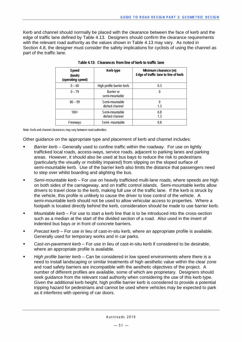
GUI DE TO RO A D DE SIG N P ART 3 : GEO MET RI C D ESI G N
A u s t r o a d s 2 0 1 0
— 5 1 —
Kerb and channel should normally be placed with the clearance between the face of kerb and the edge of traffic lane defined by Table 4.13. Designers should confirm the clearance requirements with the relevant road authority as the values shown in Table 4.13 may vary. As noted in Section 4.8, the designer must consider the safety implications for cyclists of using the channel as part of the traffic lane.
Table 4.13: Clearances from line of kerb to traffic lane
Speed (km/h)
(operating speed)
Kerb type Minimum clearance (m) Edge of traffic lane to line of kerb
0 – 60 High profile barrier kerb 0.3 0 – 79 Barrier or
semi-mountable 0
80 – 99 Semi-mountable dished channel
0 1.3
100+ Semi-mountable dished channel
0.8 1.3
Freeways Semi- mountable 0.8
Note: Kerb and channel clearances may vary between road authorities. Other guidance on the appropriate type and placement of kerb and channel includes:
Barrier kerb – Generally used to confine traffic within the roadway. For use on lightly trafficked local roads, access-ways, service roads, adjacent to parking lanes and parking areas. However, it should also be used at bus bays to reduce the risk to pedestrians (particularly the visually or mobility impaired) from slipping on the sloped surface of semi-mountable kerb. Use of the barrier kerb also limits the distance that passengers need to step over whilst boarding and alighting the bus.
Semi-mountable kerb – For use on heavily trafficked multi-lane roads, where speeds are high on both sides of the carriageway, and on traffic control islands. Semi-mountable kerbs allow drivers to travel close to the kerb, making full use of the traffic lane. If the kerb is struck by the vehicle, this profile is unlikely to cause the driver to lose control of the vehicle. A semi-mountable kerb should not be used to allow vehicular access to properties. Where a footpath is located directly behind the kerb, consideration should be made to use barrier kerb.
Mountable kerb – For use to start a kerb line that is to be introduced into the cross-section such as a median at the start of the divided section of a road. Also used in the invert of indented bus bays or in front of concrete barriers.
Precast kerb – For use in lieu of cast-in-situ kerb, where an appropriate profile is available. Generally used for temporary works and in car parks.
Cast-on-pavement kerb – For use in lieu of cast-in-situ kerb if considered to be desirable, where an appropriate profile is available.
High profile barrier kerb – Can be considered in low speed environments where there is a need to install landscaping or similar treatments of high aesthetic value within the clear zone and road safety barriers are incompatible with the aesthetic objectives of the project. A number of different profiles are available, some of which are proprietary. Designers should seek guidance from the relevant road authority when considering the use of this kerb type. Given the additional kerb height, high profile barrier kerb is considered to provide a potential tripping hazard for pedestrians and cannot be used where vehicles may be expected to park as it interferes with opening of car doors.
GUI DE TO RO A D DE SIG N P ART 3 : GEO MET RI C D ESI G N
A u s t r o a d s 2 0 1 0
— 5 2 —
Layback kerb – For use on minor roads to allow for off-road parking and for continuous access to property. This profile can be traversed more readily than a semi-mountable kerb and has greater hydraulic capacity to top of kerb than mountable kerb.
The use of kerb should be avoided within the swept path of trucks on the outer edge of low radius curves as it can contribute to truck rollovers. Kerbs can also be hazardous to turning motorcyclists.
Kerb and channel should be offset from safety barriers, as discussed in the Austroads Guide to Road Design – Part 6: Roadside Design, Safety and Barriers (Austroads 2009d).
It is noted that there is variability in kerb profiles in different regions. Reference should be made to local guidelines and AS 2876 (2000) for further information.
4.7 Medians A median is commonly provided to improve the safety and operation of major urban and rural roads with multiple lanes in each direction. Medians may be raised or depressed as shown in Figure 4.13. The main functions of medians are:
to separate and reduce conflict between opposing traffic flows, effectively reducing the possibility of head-on collisions
to prevent indiscriminate crossing and turning movements
to shelter right-turning and crossing vehicles at intersections
to shelter road furniture and traffic control devices, such as signs, traffic signals and street lighting
to provide a pedestrian refuge which enables pedestrians to cross the road one carriageway at a time
to reduce the impact of headlight glare and air turbulence from opposing streams of traffic
to provide scope for improvement of visual amenity by landscaping
to accommodate level differences between carriageways
to provide a safety barrier
to provide an emergency stopping area on multi-lane roads
to provide a recovery area for errant vehicles.
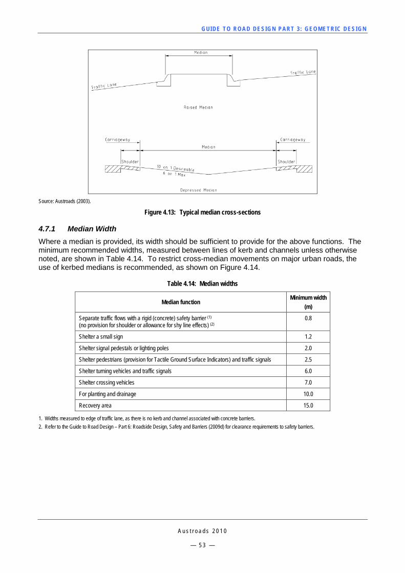
GUI DE TO RO A D DE SIG N P ART 3 : GEO MET RI C D ESI G N
A u s t r o a d s 2 0 1 0
— 5 3 —
Source: Austroads (2003).
Figure 4.13: Typical median cross-sections
4.7.1 Median Width Where a median is provided, its width should be sufficient to provide for the above functions. The minimum recommended widths, measured between lines of kerb and channels unless otherwise noted, are shown in Table 4.14. To restrict cross-median movements on major urban roads, the use of kerbed medians is recommended, as shown on Figure 4.14.
Table 4.14: Median widths
Median function Minimum width
(m)
Separate traffic flows with a rigid (concrete) safety barrier (1)
(no provision for shoulder or allowance for shy line effects) (2) 0.8
Shelter a small sign 1.2
Shelter signal pedestals or lighting poles 2.0
Shelter pedestrians (provision for Tactile Ground Surface Indicators) and traffic signals 2.5
Shelter turning vehicles and traffic signals 6.0
Shelter crossing vehicles 7.0
For planting and drainage 10.0
Recovery area 15.0
1. Widths measured to edge of traffic lane, as there is no kerb and channel associated with concrete barriers. 2. Refer to the Guide to Road Design – Part 6: Roadside Design, Safety and Barriers (2009d) for clearance requirements to safety barriers.
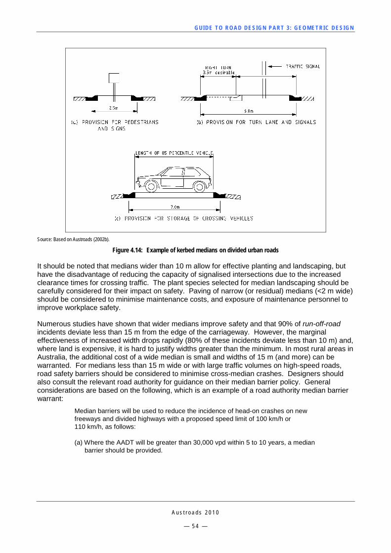
GUI DE TO RO A D DE SIG N P ART 3 : GEO MET RI C D ESI G N
A u s t r o a d s 2 0 1 0
— 5 4 —
Source: Based on Austroads (2002b).
Figure 4.14: Example of kerbed medians on divided urban roads
It should be noted that medians wider than 10 m allow for effective planting and landscaping, but have the disadvantage of reducing the capacity of signalised intersections due to the increased clearance times for crossing traffic. The plant species selected for median landscaping should be carefully considered for their impact on safety. Paving of narrow (or residual) medians (<2 m wide) should be considered to minimise maintenance costs, and exposure of maintenance personnel to improve workplace safety.
Numerous studies have shown that wider medians improve safety and that 90% of run-off-road incidents deviate less than 15 m from the edge of the carriageway. However, the marginal effectiveness of increased width drops rapidly (80% of these incidents deviate less than 10 m) and, where land is expensive, it is hard to justify widths greater than the minimum. In most rural areas in Australia, the additional cost of a wide median is small and widths of 15 m (and more) can be warranted. For medians less than 15 m wide or with large traffic volumes on high-speed roads, road safety barriers should be considered to minimise cross-median crashes. Designers should also consult the relevant road authority for guidance on their median barrier policy. General considerations are based on the following, which is an example of a road authority median barrier warrant:
Median barriers will be used to reduce the incidence of head-on crashes on new freeways and divided highways with a proposed speed limit of 100 km/h or 110 km/h, as follows:
(a) Where the AADT will be greater than 30,000 vpd within 5 to 10 years, a median barrier should be provided.
GUI DE TO RO A D DE SIG N P ART 3 : GEO MET RI C D ESI G N
A u s t r o a d s 2 0 1 0
— 5 5 —
(b) Where the AADT will be less than 30,000 vpd within 5 to 10 years, a risk assessment should be carried out to evaluate the safety implications and need for a median barrier. The risk assessment should include consideration of traffic volume and median width. Where the AADT will be between 20,000 and 30,000 within 5 to 10 years, a median barrier should be provided if the width between inner traffic lanes is less than 6 metres.
Medians should be designed so that there are minimal hazards, and where hazards cannot be avoided - e.g. bridge piers, large sign supports or trees - barrier treatment should be installed in addition to the requirements in (a) or (b) (VicRoads 2003).
The risk assessment to evaluate the need for a median barrier could consider the following parameters. Median width has not been included as it is assumed that for a cross-median crash to occur, the errant vehicle has already crossed the median:
traffic volume
lane width
number of lanes on each carriageway
road geometry
proportion of trucks in vehicle stream.
Raised medians are sometimes used on rural roads in cuttings, and have some advantages with headlight glare and a reduction in earthwork costs; however, the cost advantage is somewhat mitigated by additional drainage and safety barrier costs.
The width of a median need not be constant and independently aligned and graded carriageways have much to commend, provided that the opposing carriageway is not out of sight for extended periods. Local widening at intersections may be necessary to accommodate crossing or turning trucks. When stage constructing a project (e.g. a freeway), the usual practice is to widen the carriageways into the median. As such, it is typical to construct a wide median in the initial stages of a project. It is beneficial to widen into the median as this removes the need to modify interchange ramps and other intersection treatments with side roads or longitudinal drainage systems constructed along the verge.
4.7.2 Median Slopes The slopes in the median are influenced by the selected width, terrain, drainage and safety. Median slopes preferably should be driveable. Recommended median slopes are set out in Table 4.15. When considering the slope to be constructed on depressed medians, designers shall consider the following needs:
Drainage – the median should be wide enough to provide a driveable batter, yet deep enough to construct a drain that will carry the design volume of storm water whilst providing freeboard to the road pavement. Narrow medians (less than 10 m wide) result in shallow drains, which require regular outlets to manage the volume of storm water.
Safety barriers – designers should consider the appropriate median slopes to be used in conjunction with safety barriers, for traffic on both carriageways. Refer to the Guide to Road Design: Part 6 – Roadside Design, Safety and Barriers (Austroads 2009d) for guidance on the appropriate batter slopes for alternative barrier systems.
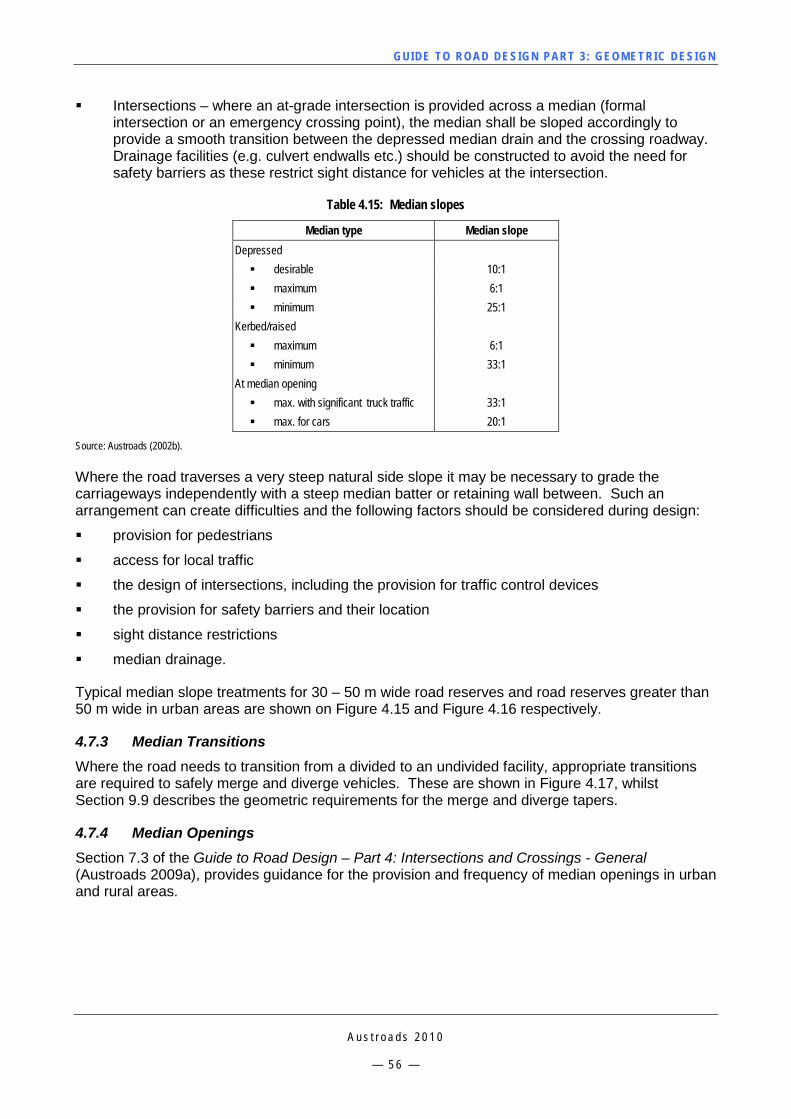
GUI DE TO RO A D DE SIG N P ART 3 : GEO MET RI C D ESI G N
A u s t r o a d s 2 0 1 0
— 5 6 —
Intersections – where an at-grade intersection is provided across a median (formal intersection or an emergency crossing point), the median shall be sloped accordingly to provide a smooth transition between the depressed median drain and the crossing roadway. Drainage facilities (e.g. culvert endwalls etc.) should be constructed to avoid the need for safety barriers as these restrict sight distance for vehicles at the intersection.
Table 4.15: Median slopes
Median type Median slope Depressed desirable 10:1 maximum 6:1 minimum 25:1
Kerbed/raised maximum 6:1 minimum 33:1
At median opening max. with significant truck traffic 33:1 max. for cars 20:1
Source: Austroads (2002b). Where the road traverses a very steep natural side slope it may be necessary to grade the carriageways independently with a steep median batter or retaining wall between. Such an arrangement can create difficulties and the following factors should be considered during design:
provision for pedestrians
access for local traffic
the design of intersections, including the provision for traffic control devices
the provision for safety barriers and their location
sight distance restrictions
median drainage.
Typical median slope treatments for 30 – 50 m wide road reserves and road reserves greater than 50 m wide in urban areas are shown on Figure 4.15 and Figure 4.16 respectively.
4.7.3 Median Transitions Where the road needs to transition from a divided to an undivided facility, appropriate transitions are required to safely merge and diverge vehicles. These are shown in Figure 4.17, whilst Section 9.9 describes the geometric requirements for the merge and diverge tapers.
4.7.4 Median Openings Section 7.3 of the Guide to Road Design – Part 4: Intersections and Crossings - General (Austroads 2009a), provides guidance for the provision and frequency of median openings in urban and rural areas.
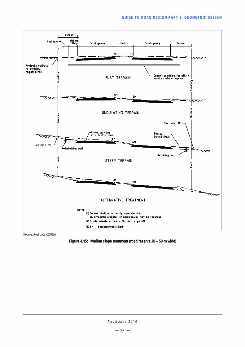
GUI DE TO RO A D DE SIG N P ART 3 : GEO MET RI C D ESI G N
A u s t r o a d s 2 0 1 0
— 5 7 —
Source: Austroads (2002b).
Figure 4.15: Median slope treatment (road reserve 30 – 50 m wide)
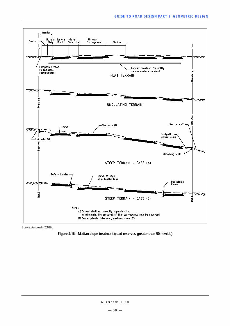
GUI DE TO RO A D DE SIG N P ART 3 : GEO MET RI C D ESI G N
A u s t r o a d s 2 0 1 0
— 5 8 —
Source: Austroads (2002b).
Figure 4.16: Median slope treatment (road reserves greater than 50 m wide)
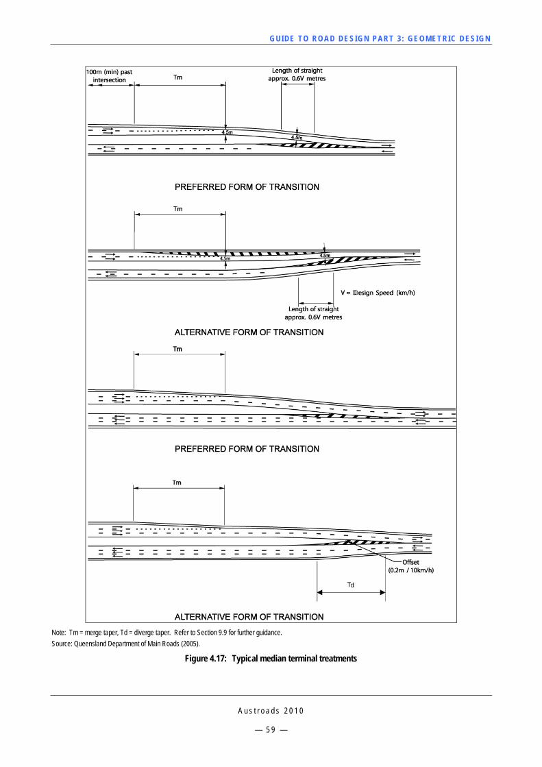
GUI DE TO RO A D DE SIG N P ART 3 : GEO MET RI C D ESI G N
A u s t r o a d s 2 0 1 0
— 5 9 —
Note: Tm = merge taper, Td = diverge taper. Refer to Section 9.9 for further guidance. Source: Queensland Department of Main Roads (2005).
Figure 4.17: Typical median terminal treatments
GUI DE TO RO A D DE SIG N P ART 3 : GEO MET RI C D ESI G N
A u s t r o a d s 2 0 1 0
— 6 0 —
4.8 Bicycle Lanes 4.8.1 General The provision of cyclist facilities should be based on the hierarchy of needs, delivered in order of level of safety and priority:
1. Off-road exclusive bicycle path (within the road corridor)
2. On-road segregated bicycle lanes – median or similar separation
3. On-road exclusive bicycle lane
4. On-road peak period exclusive bicycle lane
5. On-road bicycle/car parking lane
6. Wide kerbside lane
7. Narrow kerbside lane.
Provision for cyclists on roads should be considered in all aspects of road management, including:
choice of cross-section for all roads during the design process
development of traffic management programs
maintenance programs where opportunities exist to provide space for cyclists by altering lane markings.
Information regarding bicycle rider requirements can be found in Commentary 9.
The warrants for the type of facility to be provided for cyclists in New Zealand is provided in Commentary C9.6. This figure is applicable to both urban and rural roads.
In local streets it is usually not necessary to make special provision for cyclists, as the lower speed of motor traffic should enable cyclists to safely share the road with other users. On arterial roads and collector streets it is usually necessary to ensure that adequate space exists for cyclists to share the road safely and comfortably, particularly when the road forms part of a principal or regional bicycle network. It may be possible to reduce the widths of other lanes in order to allocate additional space to the left hand lane for joint use by cyclists.
Depending on the nature of the road, abutting land use, the function of the road in bicycle networks, and the number of cyclists using the road, provision of the special on-road facilities described in this section may be appropriate.
The facilities described in this section are those applied within the carriageway of new roads or within the established road carriageway in the case of existing roads.
On-road bicycle facilities may take the form of:
dedicated bicycle lanes
road shoulders
widened lanes for joint use by bicycles and moving or parked vehicles
separated bicycle lanes.
Off-road bicycle facilities typically take the form of shared pathways for use by both cyclists and pedestrians, and these are described in more detail in the Guide to Road Design – Part 6A: Pedestrian and Cyclist Paths (Austroads 2009e).
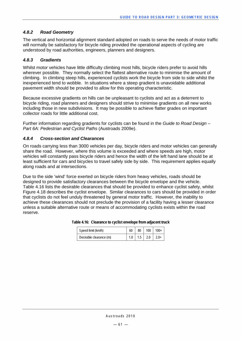
GUI DE TO RO A D DE SIG N P ART 3 : GEO MET RI C D ESI G N
A u s t r o a d s 2 0 1 0
— 6 1 —
4.8.2 Road Geometry The vertical and horizontal alignment standard adopted on roads to serve the needs of motor traffic will normally be satisfactory for bicycle riding provided the operational aspects of cycling are understood by road authorities, engineers, planners and designers.
4.8.3 Gradients Whilst motor vehicles have little difficulty climbing most hills, bicycle riders prefer to avoid hills wherever possible. They normally select the flattest alternative route to minimise the amount of climbing. In climbing steep hills, experienced cyclists work the bicycle from side to side whilst the inexperienced tend to wobble. In situations where a steep gradient is unavoidable additional pavement width should be provided to allow for this operating characteristic.
Because excessive gradients on hills can be unpleasant to cyclists and act as a deterrent to bicycle riding, road planners and designers should strive to minimise gradients on all new works including those in new subdivisions. It may be possible to achieve flatter grades on important collector roads for little additional cost.
Further information regarding gradients for cyclists can be found in the Guide to Road Design – Part 6A: Pedestrian and Cyclist Paths (Austroads 2009e).
4.8.4 Cross-section and Clearances On roads carrying less than 3000 vehicles per day, bicycle riders and motor vehicles can generally share the road. However, where this volume is exceeded and where speeds are high, motor vehicles will constantly pass bicycle riders and hence the width of the left hand lane should be at least sufficient for cars and bicycles to travel safely side by side. This requirement applies equally along roads and at intersections.
Due to the side ‘wind’ force exerted on bicycle riders from heavy vehicles, roads should be designed to provide satisfactory clearances between the bicycle envelope and the vehicle. Table 4.16 lists the desirable clearances that should be provided to enhance cyclist safety, whilst Figure 4.18 describes the cyclist envelope. Similar clearances to cars should be provided in order that cyclists do not feel unduly threatened by general motor traffic. However, the inability to achieve these clearances should not preclude the provision of a facility having a lesser clearance unless a suitable alternative route or means of accommodating cyclists exists within the road reserve.
Table 4.16: Clearance to cyclist envelope from adjacent truck
Speed limit (km/h) 60 80 100 100+
Desirable clearance (m) 1.0 1.5 2.0 2.0+
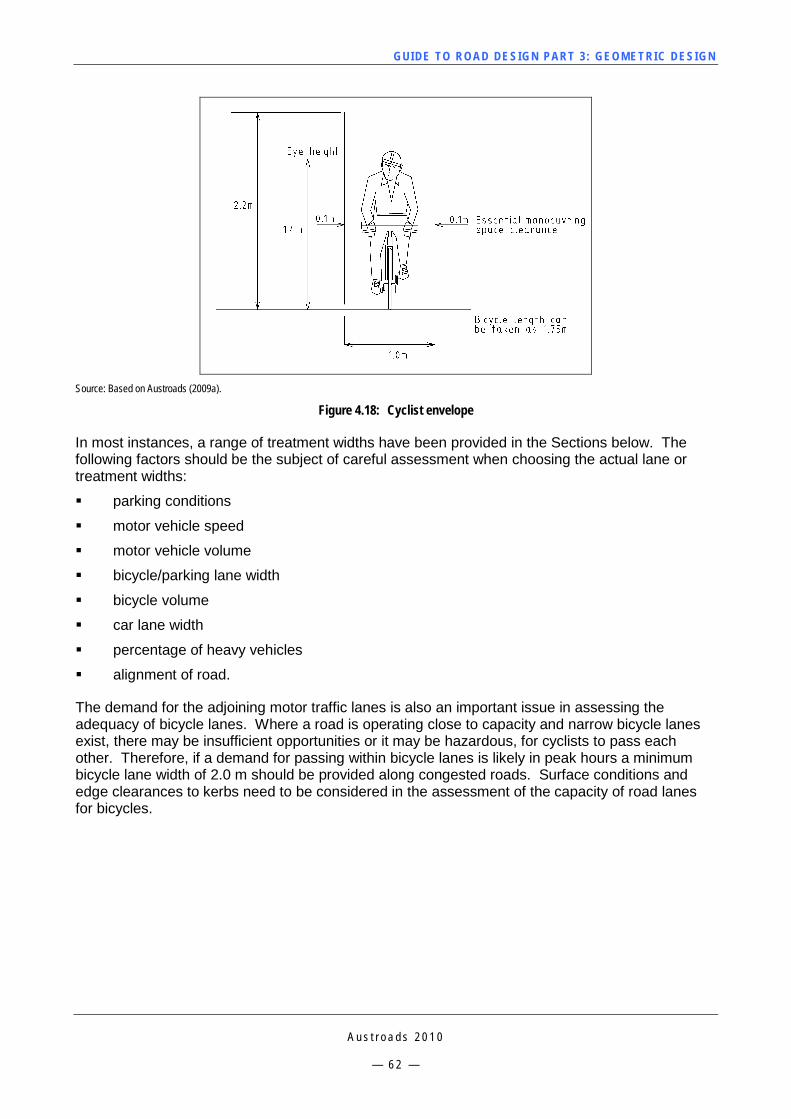
GUI DE TO RO A D DE SIG N P ART 3 : GEO MET RI C D ESI G N
A u s t r o a d s 2 0 1 0
— 6 2 —
Source: Based on Austroads (2009a).
Figure 4.18: Cyclist envelope
In most instances, a range of treatment widths have been provided in the Sections below. The following factors should be the subject of careful assessment when choosing the actual lane or treatment widths:
parking conditions
motor vehicle speed
motor vehicle volume
bicycle/parking lane width
bicycle volume
car lane width
percentage of heavy vehicles
alignment of road.
The demand for the adjoining motor traffic lanes is also an important issue in assessing the adequacy of bicycle lanes. Where a road is operating close to capacity and narrow bicycle lanes exist, there may be insufficient opportunities or it may be hazardous, for cyclists to pass each other. Therefore, if a demand for passing within bicycle lanes is likely in peak hours a minimum bicycle lane width of 2.0 m should be provided along congested roads. Surface conditions and edge clearances to kerbs need to be considered in the assessment of the capacity of road lanes for bicycles.
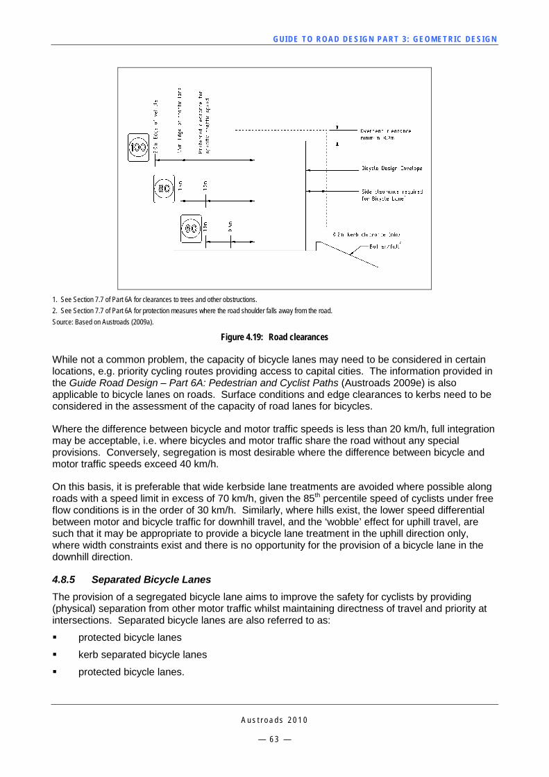
GUI DE TO RO A D DE SIG N P ART 3 : GEO MET RI C D ESI G N
A u s t r o a d s 2 0 1 0
— 6 3 —
1. See Section 7.7 of Part 6A for clearances to trees and other obstructions. 2. See Section 7.7 of Part 6A for protection measures where the road shoulder falls away from the road. Source: Based on Austroads (2009a).
Figure 4.19: Road clearances
While not a common problem, the capacity of bicycle lanes may need to be considered in certain locations, e.g. priority cycling routes providing access to capital cities. The information provided in the Guide Road Design – Part 6A: Pedestrian and Cyclist Paths (Austroads 2009e) is also applicable to bicycle lanes on roads. Surface conditions and edge clearances to kerbs need to be considered in the assessment of the capacity of road lanes for bicycles.
Where the difference between bicycle and motor traffic speeds is less than 20 km/h, full integration may be acceptable, i.e. where bicycles and motor traffic share the road without any special provisions. Conversely, segregation is most desirable where the difference between bicycle and motor traffic speeds exceed 40 km/h.
On this basis, it is preferable that wide kerbside lane treatments are avoided where possible along roads with a speed limit in excess of 70 km/h, given the 85th percentile speed of cyclists under free flow conditions is in the order of 30 km/h. Similarly, where hills exist, the lower speed differential between motor and bicycle traffic for downhill travel, and the ‘wobble’ effect for uphill travel, are such that it may be appropriate to provide a bicycle lane treatment in the uphill direction only, where width constraints exist and there is no opportunity for the provision of a bicycle lane in the downhill direction.
4.8.5 Separated Bicycle Lanes The provision of a segregated bicycle lane aims to improve the safety for cyclists by providing (physical) separation from other motor traffic whilst maintaining directness of travel and priority at intersections. Separated bicycle lanes are also referred to as:
protected bicycle lanes
kerb separated bicycle lanes
protected bicycle lanes.
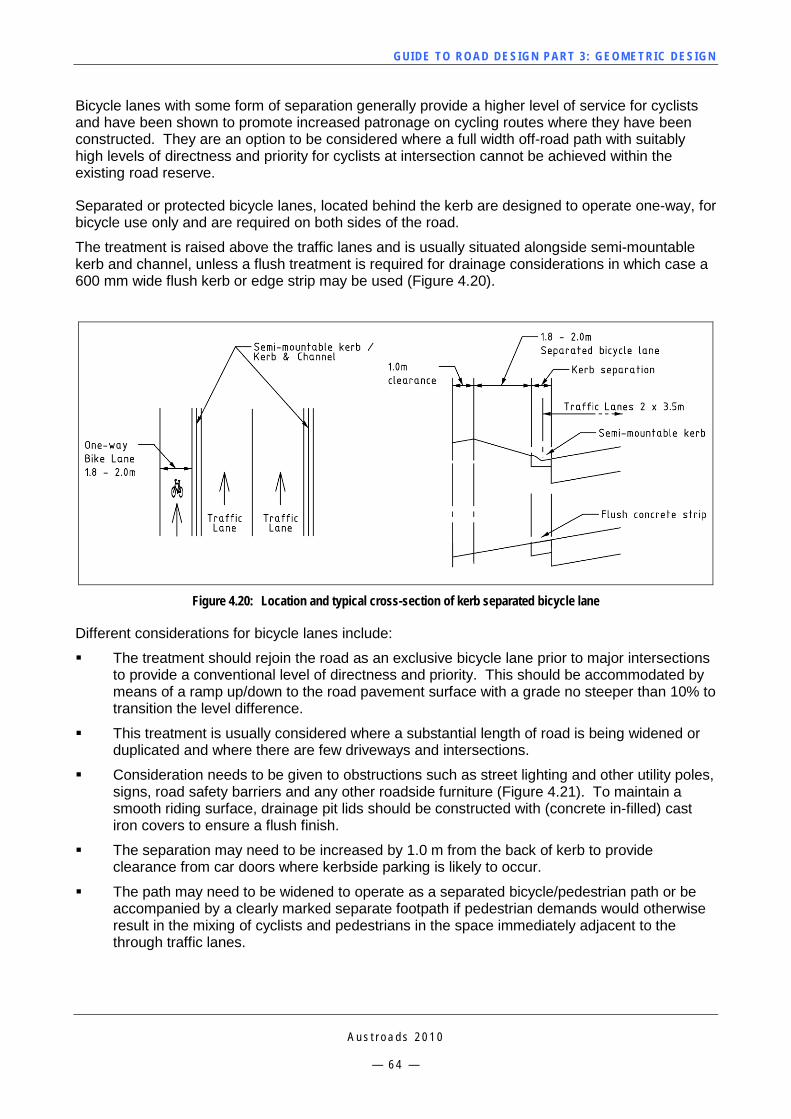
GUI DE TO RO A D DE SIG N P ART 3 : GEO MET RI C D ESI G N
A u s t r o a d s 2 0 1 0
— 6 4 —
Bicycle lanes with some form of separation generally provide a higher level of service for cyclists and have been shown to promote increased patronage on cycling routes where they have been constructed. They are an option to be considered where a full width off-road path with suitably high levels of directness and priority for cyclists at intersection cannot be achieved within the existing road reserve.
Separated or protected bicycle lanes, located behind the kerb are designed to operate one-way, for bicycle use only and are required on both sides of the road.
The treatment is raised above the traffic lanes and is usually situated alongside semi-mountable kerb and channel, unless a flush treatment is required for drainage considerations in which case a 600 mm wide flush kerb or edge strip may be used (Figure 4.20).
Figure 4.20: Location and typical cross-section of kerb separated bicycle lane
Different considerations for bicycle lanes include:
The treatment should rejoin the road as an exclusive bicycle lane prior to major intersections to provide a conventional level of directness and priority. This should be accommodated by means of a ramp up/down to the road pavement surface with a grade no steeper than 10% to transition the level difference.
This treatment is usually considered where a substantial length of road is being widened or duplicated and where there are few driveways and intersections.
Consideration needs to be given to obstructions such as street lighting and other utility poles, signs, road safety barriers and any other roadside furniture (Figure 4.21). To maintain a smooth riding surface, drainage pit lids should be constructed with (concrete in-filled) cast iron covers to ensure a flush finish.
The separation may need to be increased by 1.0 m from the back of kerb to provide clearance from car doors where kerbside parking is likely to occur.
The path may need to be widened to operate as a separated bicycle/pedestrian path or be accompanied by a clearly marked separate footpath if pedestrian demands would otherwise result in the mixing of cyclists and pedestrians in the space immediately adjacent to the through traffic lanes.
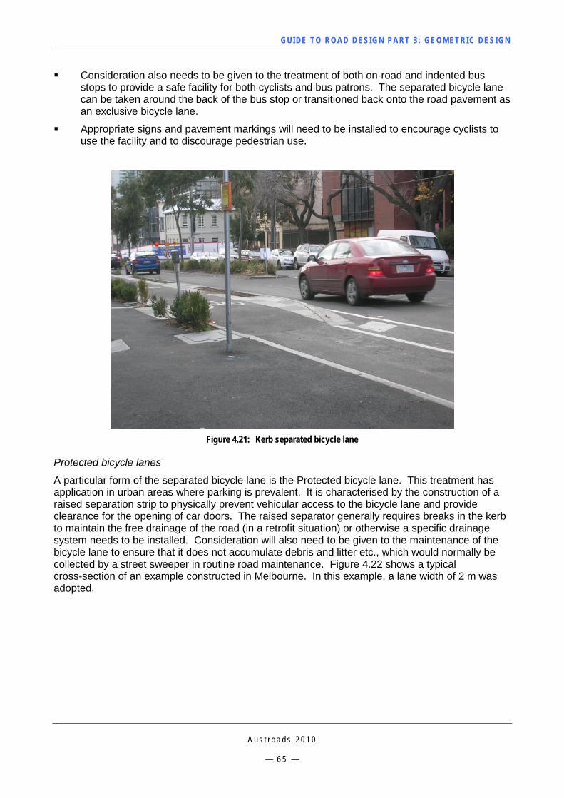
GUI DE TO RO A D DE SIG N P ART 3 : GEO MET RI C D ESI G N
A u s t r o a d s 2 0 1 0
— 6 5 —
Consideration also needs to be given to the treatment of both on-road and indented bus stops to provide a safe facility for both cyclists and bus patrons. The separated bicycle lane can be taken around the back of the bus stop or transitioned back onto the road pavement as an exclusive bicycle lane.
Appropriate signs and pavement markings will need to be installed to encourage cyclists to use the facility and to discourage pedestrian use.
Figure 4.21: Kerb separated bicycle lane
Protected bicycle lanes
A particular form of the separated bicycle lane is the Protected bicycle lane. This treatment has application in urban areas where parking is prevalent. It is characterised by the construction of a raised separation strip to physically prevent vehicular access to the bicycle lane and provide clearance for the opening of car doors. The raised separator generally requires breaks in the kerb to maintain the free drainage of the road (in a retrofit situation) or otherwise a specific drainage system needs to be installed. Consideration will also need to be given to the maintenance of the bicycle lane to ensure that it does not accumulate debris and litter etc., which would normally be collected by a street sweeper in routine road maintenance. Figure 4.22 shows a typical cross-section of an example constructed in Melbourne. In this example, a lane width of 2 m was adopted.
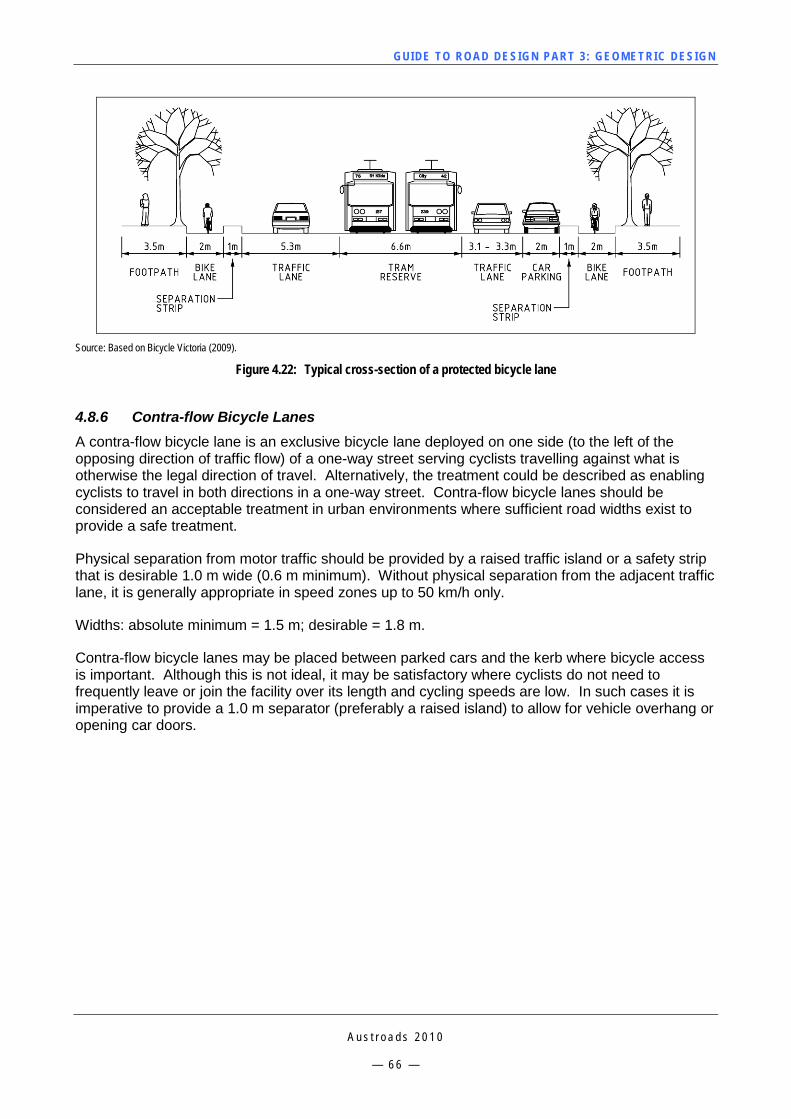
GUI DE TO RO A D DE SIG N P ART 3 : GEO MET RI C D ESI G N
A u s t r o a d s 2 0 1 0
— 6 6 —
Source: Based on Bicycle Victoria (2009).
Figure 4.22: Typical cross-section of a protected bicycle lane
4.8.6 Contra-flow Bicycle Lanes A contra-flow bicycle lane is an exclusive bicycle lane deployed on one side (to the left of the opposing direction of traffic flow) of a one-way street serving cyclists travelling against what is otherwise the legal direction of travel. Alternatively, the treatment could be described as enabling cyclists to travel in both directions in a one-way street. Contra-flow bicycle lanes should be considered an acceptable treatment in urban environments where sufficient road widths exist to provide a safe treatment.
Physical separation from motor traffic should be provided by a raised traffic island or a safety strip that is desirable 1.0 m wide (0.6 m minimum). Without physical separation from the adjacent traffic lane, it is generally appropriate in speed zones up to 50 km/h only.
Widths: absolute minimum = 1.5 m; desirable = 1.8 m.
Contra-flow bicycle lanes may be placed between parked cars and the kerb where bicycle access is important. Although this is not ideal, it may be satisfactory where cyclists do not need to frequently leave or join the facility over its length and cycling speeds are low. In such cases it is imperative to provide a 1.0 m separator (preferably a raised island) to allow for vehicle overhang or opening car doors.
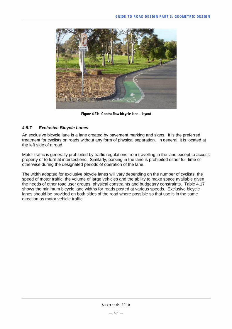
GUI DE TO RO A D DE SIG N P ART 3 : GEO MET RI C D ESI G N
A u s t r o a d s 2 0 1 0
— 6 7 —
Figure 4.23: Contra-flow bicycle lane – layout
4.8.7 Exclusive Bicycle Lanes An exclusive bicycle lane is a lane created by pavement marking and signs. It is the preferred treatment for cyclists on roads without any form of physical separation. In general, it is located at the left side of a road.
Motor traffic is generally prohibited by traffic regulations from travelling in the lane except to access property or to turn at intersections. Similarly, parking in the lane is prohibited either full-time or otherwise during the designated periods of operation of the lane.
The width adopted for exclusive bicycle lanes will vary depending on the number of cyclists, the speed of motor traffic, the volume of large vehicles and the ability to make space available given the needs of other road user groups, physical constraints and budgetary constraints. Table 4.17 shows the minimum bicycle lane widths for roads posted at various speeds. Exclusive bicycle lanes should be provided on both sides of the road where possible so that use is in the same direction as motor vehicle traffic.
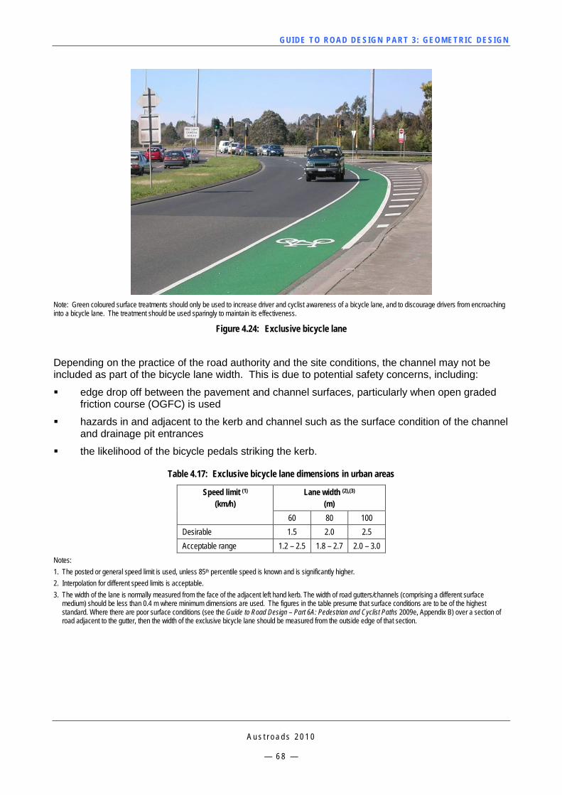
GUI DE TO RO A D DE SIG N P ART 3 : GEO MET RI C D ESI G N
A u s t r o a d s 2 0 1 0
— 6 8 —
Note: Green coloured surface treatments should only be used to increase driver and cyclist awareness of a bicycle lane, and to discourage drivers from encroaching into a bicycle lane. The treatment should be used sparingly to maintain its effectiveness.
Figure 4.24: Exclusive bicycle lane
Depending on the practice of the road authority and the site conditions, the channel may not be included as part of the bicycle lane width. This is due to potential safety concerns, including:
edge drop off between the pavement and channel surfaces, particularly when open graded friction course (OGFC) is used
hazards in and adjacent to the kerb and channel such as the surface condition of the channel and drainage pit entrances
the likelihood of the bicycle pedals striking the kerb.
Table 4.17: Exclusive bicycle lane dimensions in urban areas
Speed limit (1) (km/h)
Lane width (2),(3) (m)
60 80 100 Desirable 1.5 2.0 2.5 Acceptable range 1.2 – 2.5 1.8 – 2.7 2.0 – 3.0
Notes: 1. The posted or general speed limit is used, unless 85th percentile speed is known and is significantly higher. 2. Interpolation for different speed limits is acceptable. 3. The width of the lane is normally measured from the face of the adjacent left hand kerb. The width of road gutters/channels (comprising a different surface
medium) should be less than 0.4 m where minimum dimensions are used. The figures in the table presume that surface conditions are to be of the highest standard. Where there are poor surface conditions (see the Guide to Road Design – Part 6A: Pedestrian and Cyclist Paths 2009e, Appendix B) over a section of road adjacent to the gutter, then the width of the exclusive bicycle lane should be measured from the outside edge of that section.
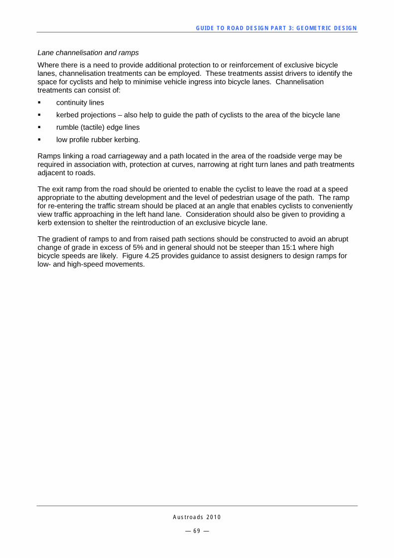
GUI DE TO RO A D DE SIG N P ART 3 : GEO MET RI C D ESI G N
A u s t r o a d s 2 0 1 0
— 6 9 —
Lane channelisation and ramps
Where there is a need to provide additional protection to or reinforcement of exclusive bicycle lanes, channelisation treatments can be employed. These treatments assist drivers to identify the space for cyclists and help to minimise vehicle ingress into bicycle lanes. Channelisation treatments can consist of:
continuity lines
kerbed projections – also help to guide the path of cyclists to the area of the bicycle lane
rumble (tactile) edge lines
low profile rubber kerbing.
Ramps linking a road carriageway and a path located in the area of the roadside verge may be required in association with, protection at curves, narrowing at right turn lanes and path treatments adjacent to roads.
The exit ramp from the road should be oriented to enable the cyclist to leave the road at a speed appropriate to the abutting development and the level of pedestrian usage of the path. The ramp for re-entering the traffic stream should be placed at an angle that enables cyclists to conveniently view traffic approaching in the left hand lane. Consideration should also be given to providing a kerb extension to shelter the reintroduction of an exclusive bicycle lane.
The gradient of ramps to and from raised path sections should be constructed to avoid an abrupt change of grade in excess of 5% and in general should not be steeper than 15:1 where high bicycle speeds are likely. Figure 4.25 provides guidance to assist designers to design ramps for low- and high-speed movements.
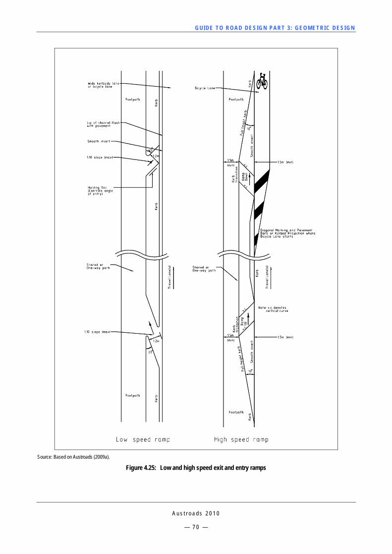
GUI DE TO RO A D DE SIG N P ART 3 : GEO MET RI C D ESI G N
A u s t r o a d s 2 0 1 0
— 7 0 —
Source: Based on Austroads (2009a).
Figure 4.25: Low and high speed exit and entry ramps
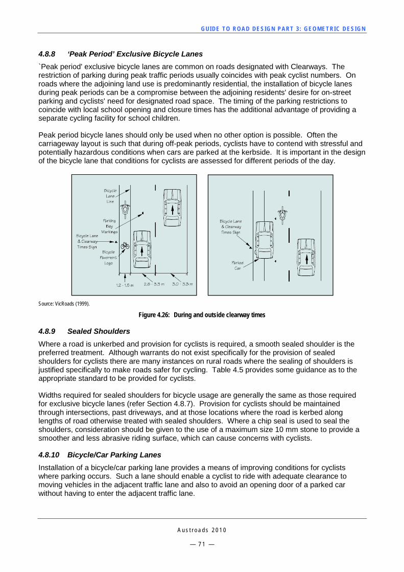
GUI DE TO RO A D DE SIG N P ART 3 : GEO MET RI C D ESI G N
A u s t r o a d s 2 0 1 0
— 7 1 —
4.8.8 ‘Peak Period’ Exclusive Bicycle Lanes `Peak period' exclusive bicycle lanes are common on roads designated with Clearways. The restriction of parking during peak traffic periods usually coincides with peak cyclist numbers. On roads where the adjoining land use is predominantly residential, the installation of bicycle lanes during peak periods can be a compromise between the adjoining residents' desire for on-street parking and cyclists' need for designated road space. The timing of the parking restrictions to coincide with local school opening and closure times has the additional advantage of providing a separate cycling facility for school children.
Peak period bicycle lanes should only be used when no other option is possible. Often the carriageway layout is such that during off-peak periods, cyclists have to contend with stressful and potentially hazardous conditions when cars are parked at the kerbside. It is important in the design of the bicycle lane that conditions for cyclists are assessed for different periods of the day.
Source: VicRoads (1999).
Figure 4.26: During and outside clearway times
4.8.9 Sealed Shoulders Where a road is unkerbed and provision for cyclists is required, a smooth sealed shoulder is the preferred treatment. Although warrants do not exist specifically for the provision of sealed shoulders for cyclists there are many instances on rural roads where the sealing of shoulders is justified specifically to make roads safer for cycling. Table 4.5 provides some guidance as to the appropriate standard to be provided for cyclists.
Widths required for sealed shoulders for bicycle usage are generally the same as those required for exclusive bicycle lanes (refer Section 4.8.7). Provision for cyclists should be maintained through intersections, past driveways, and at those locations where the road is kerbed along lengths of road otherwise treated with sealed shoulders. Where a chip seal is used to seal the shoulders, consideration should be given to the use of a maximum size 10 mm stone to provide a smoother and less abrasive riding surface, which can cause concerns with cyclists.
4.8.10 Bicycle/Car Parking Lanes Installation of a bicycle/car parking lane provides a means of improving conditions for cyclists where parking occurs. Such a lane should enable a cyclist to ride with adequate clearance to moving vehicles in the adjacent traffic lane and also to avoid an opening door of a parked car without having to enter the adjacent traffic lane.
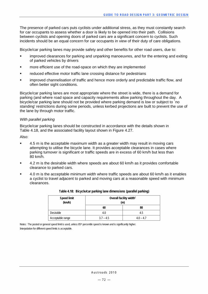
GUI DE TO RO A D DE SIG N P ART 3 : GEO MET RI C D ESI G N
A u s t r o a d s 2 0 1 0
— 7 2 —
The presence of parked cars puts cyclists under additional stress, as they must constantly search for car occupants to assess whether a door is likely to be opened into their path. Collisions between cyclists and opening doors of parked cars are a significant concern to cyclists. Such incidents should be an equal concern for car occupants in view of their duty of care obligations.
Bicycle/car parking lanes may provide safety and other benefits for other road users, due to:
improved clearances for parking and unparking manoeuvres, and for the entering and exiting of parked vehicles by drivers
more efficient use of the road-space on which they are implemented
reduced effective motor traffic lane crossing distance for pedestrians
improved channelisation of traffic and hence more orderly and predictable traffic flow, and often better sight conditions.
Bicycle/car parking lanes are most appropriate where the street is wide, there is a demand for parking (and where road space and capacity requirements allow parking throughout the day. A bicycle/car parking lane should not be provided where parking demand is low or subject to `no standing' restrictions during some periods, unless kerbed projections are built to prevent the use of the lane by through motor traffic.
With parallel parking
Bicycle/car parking lanes should be constructed in accordance with the details shown in Table 4.18, and the associated facility layout shown in Figure 4.27.
Also:
4.5 m is the acceptable maximum width as a greater width may result in moving cars attempting to utilise the bicycle lane. It provides acceptable clearances in cases where parking turnover is significant or traffic speeds are in excess of 60 km/h but less than 80 km/h.
4.2 m is the desirable width where speeds are about 60 km/h as it provides comfortable clearance to parked cars.
4.0 m is the acceptable minimum width where traffic speeds are about 60 km/h as it enables a cyclist to travel adjacent to parked and moving cars at a reasonable speed with minimum clearances.
Table 4.18: Bicycle/car parking lane dimensions (parallel parking)
Speed limit (km/h)
Overall facility widthC
(m) 60 80
Desirable 4.0 4.5 Acceptable range 3.7 – 4.5 4.0 – 4.7
Notes: The posted or general speed limit is used, unless 85th percentile speed is known and is significantly higher. Interpolation for different speed limits is acceptable.
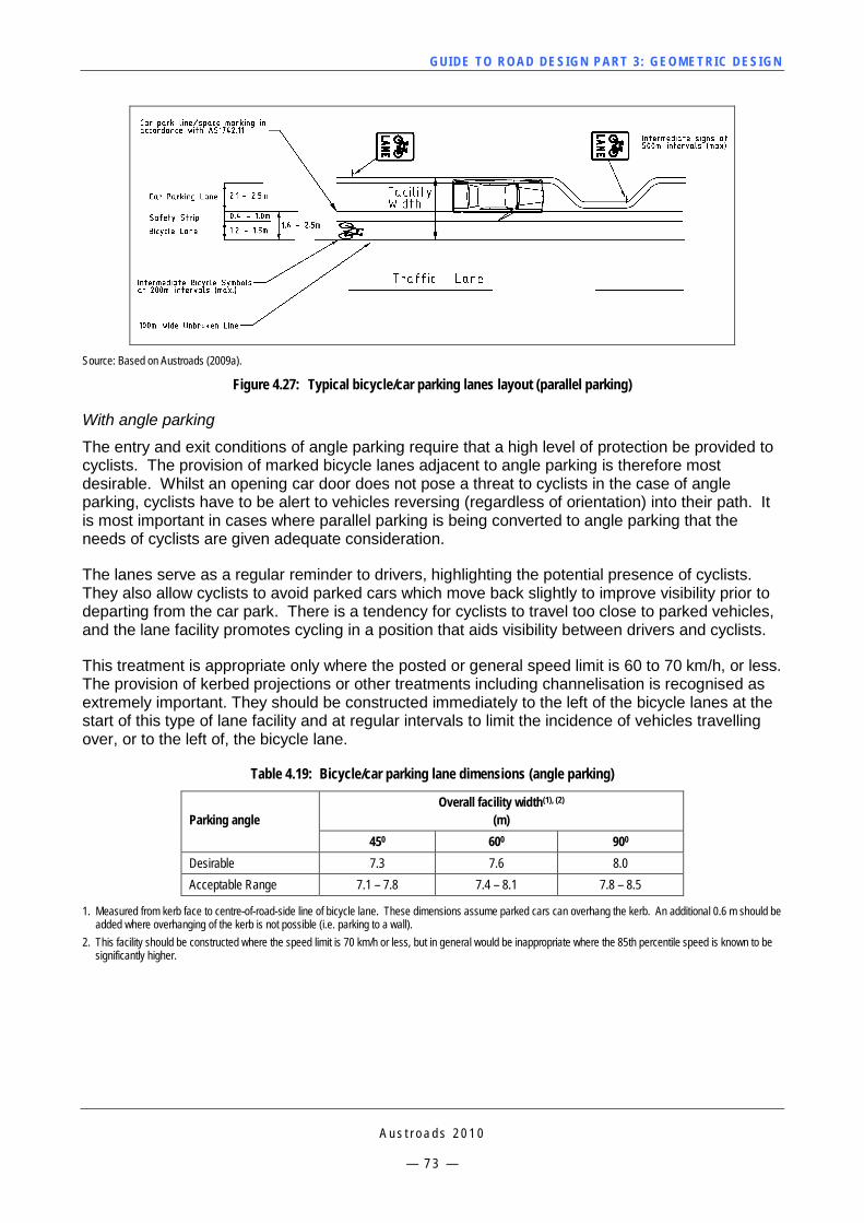
GUI DE TO RO A D DE SIG N P ART 3 : GEO MET RI C D ESI G N
A u s t r o a d s 2 0 1 0
— 7 3 —
Source: Based on Austroads (2009a).
Figure 4.27: Typical bicycle/car parking lanes layout (parallel parking)
With angle parking
The entry and exit conditions of angle parking require that a high level of protection be provided to cyclists. The provision of marked bicycle lanes adjacent to angle parking is therefore most desirable. Whilst an opening car door does not pose a threat to cyclists in the case of angle parking, cyclists have to be alert to vehicles reversing (regardless of orientation) into their path. It is most important in cases where parallel parking is being converted to angle parking that the needs of cyclists are given adequate consideration.
The lanes serve as a regular reminder to drivers, highlighting the potential presence of cyclists. They also allow cyclists to avoid parked cars which move back slightly to improve visibility prior to departing from the car park. There is a tendency for cyclists to travel too close to parked vehicles, and the lane facility promotes cycling in a position that aids visibility between drivers and cyclists.
This treatment is appropriate only where the posted or general speed limit is 60 to 70 km/h, or less. The provision of kerbed projections or other treatments including channelisation is recognised as extremely important. They should be constructed immediately to the left of the bicycle lanes at the start of this type of lane facility and at regular intervals to limit the incidence of vehicles travelling over, or to the left of, the bicycle lane.
Table 4.19: Bicycle/car parking lane dimensions (angle parking)
Parking angle
Overall facility width(1), (2)
(m) 450 600 900
Desirable 7.3 7.6 8.0 Acceptable Range 7.1 – 7.8 7.4 – 8.1 7.8 – 8.5
1. Measured from kerb face to centre-of-road-side line of bicycle lane. These dimensions assume parked cars can overhang the kerb. An additional 0.6 m should be added where overhanging of the kerb is not possible (i.e. parking to a wall).
2. This facility should be constructed where the speed limit is 70 km/h or less, but in general would be inappropriate where the 85th percentile speed is known to be significantly higher.
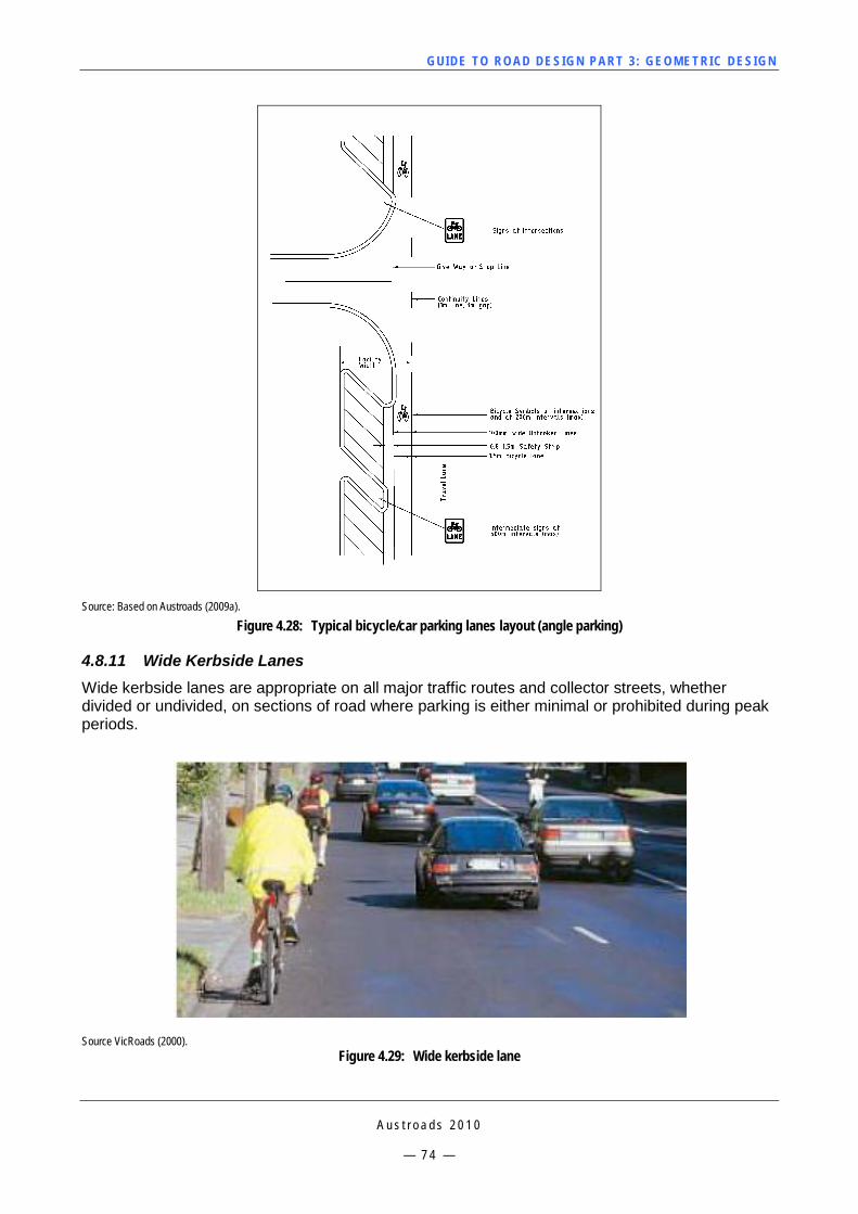
GUI DE TO RO A D DE SIG N P ART 3 : GEO MET RI C D ESI G N
A u s t r o a d s 2 0 1 0
— 7 4 —
Source: Based on Austroads (2009a).
Figure 4.28: Typical bicycle/car parking lanes layout (angle parking)
4.8.11 Wide Kerbside Lanes Wide kerbside lanes are appropriate on all major traffic routes and collector streets, whether divided or undivided, on sections of road where parking is either minimal or prohibited during peak periods.
Source VicRoads (2000). Figure 4.29: Wide kerbside lane
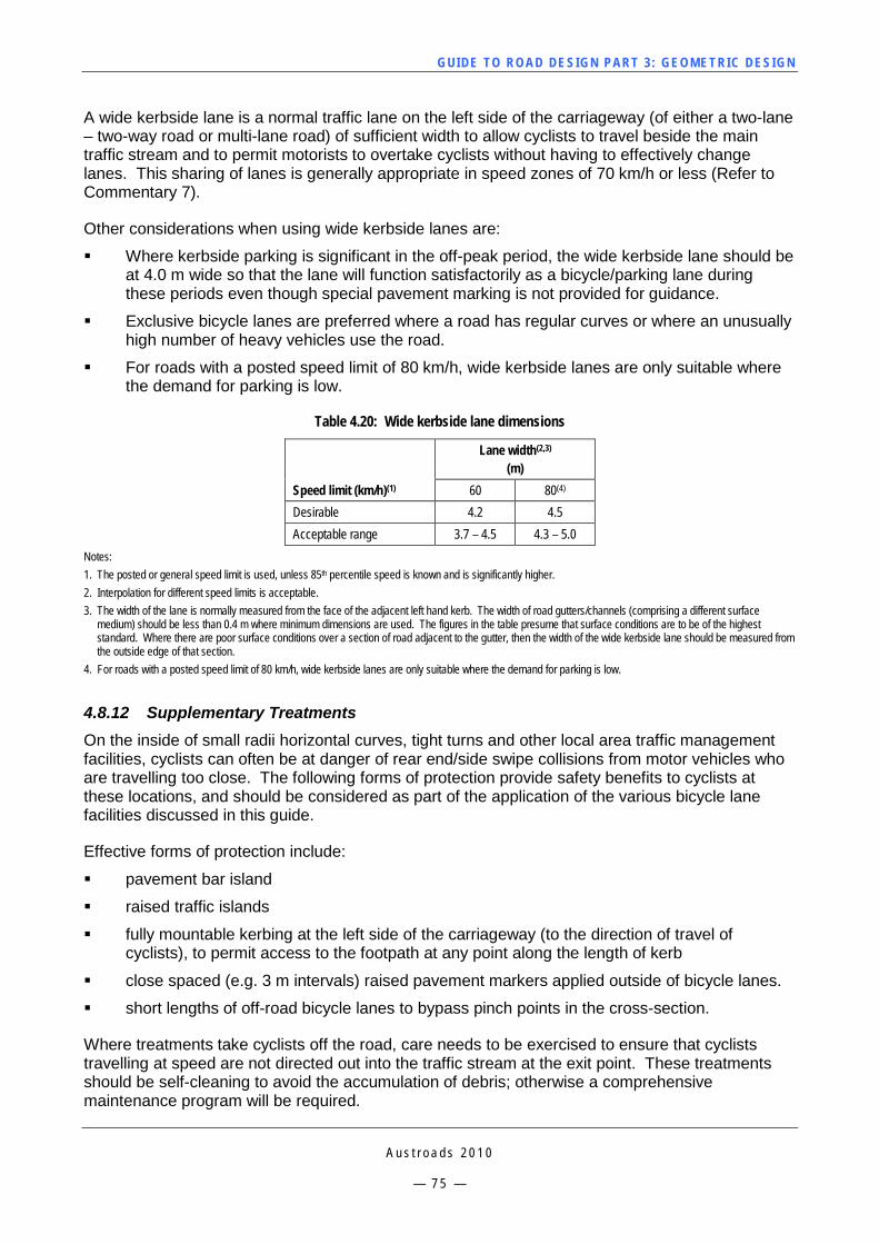
GUI DE TO RO A D DE SIG N P ART 3 : GEO MET RI C D ESI G N
A u s t r o a d s 2 0 1 0
— 7 5 —
A wide kerbside lane is a normal traffic lane on the left side of the carriageway (of either a two-lane – two-way road or multi-lane road) of sufficient width to allow cyclists to travel beside the main traffic stream and to permit motorists to overtake cyclists without having to effectively change lanes. This sharing of lanes is generally appropriate in speed zones of 70 km/h or less (Refer to Commentary 7).
Other considerations when using wide kerbside lanes are:
Where kerbside parking is significant in the off-peak period, the wide kerbside lane should be at 4.0 m wide so that the lane will function satisfactorily as a bicycle/parking lane during these periods even though special pavement marking is not provided for guidance.
Exclusive bicycle lanes are preferred where a road has regular curves or where an unusually high number of heavy vehicles use the road.
For roads with a posted speed limit of 80 km/h, wide kerbside lanes are only suitable where the demand for parking is low.
Table 4.20: Wide kerbside lane dimensions
Speed limit (km/h)(1)
Lane width(2,3) (m)
60 80(4) Desirable 4.2 4.5 Acceptable range 3.7 – 4.5 4.3 – 5.0
Notes: 1. The posted or general speed limit is used, unless 85th percentile speed is known and is significantly higher. 2. Interpolation for different speed limits is acceptable. 3. The width of the lane is normally measured from the face of the adjacent left hand kerb. The width of road gutters/channels (comprising a different surface
medium) should be less than 0.4 m where minimum dimensions are used. The figures in the table presume that surface conditions are to be of the highest standard. Where there are poor surface conditions over a section of road adjacent to the gutter, then the width of the wide kerbside lane should be measured from the outside edge of that section.
4. For roads with a posted speed limit of 80 km/h, wide kerbside lanes are only suitable where the demand for parking is low.
4.8.12 Supplementary Treatments On the inside of small radii horizontal curves, tight turns and other local area traffic management facilities, cyclists can often be at danger of rear end/side swipe collisions from motor vehicles who are travelling too close. The following forms of protection provide safety benefits to cyclists at these locations, and should be considered as part of the application of the various bicycle lane facilities discussed in this guide.
Effective forms of protection include:
pavement bar island
raised traffic islands
fully mountable kerbing at the left side of the carriageway (to the direction of travel of cyclists), to permit access to the footpath at any point along the length of kerb
close spaced (e.g. 3 m intervals) raised pavement markers applied outside of bicycle lanes.
short lengths of off-road bicycle lanes to bypass pinch points in the cross-section.
Where treatments take cyclists off the road, care needs to be exercised to ensure that cyclists travelling at speed are not directed out into the traffic stream at the exit point. These treatments should be self-cleaning to avoid the accumulation of debris; otherwise a comprehensive maintenance program will be required.
GUI DE TO RO A D DE SIG N P ART 3 : GEO MET RI C D ESI G N
A u s t r o a d s 2 0 1 0
— 7 6 —
Designers will also need to ensure that the safety and needs of pedestrians are provided for, wherever off-road cycling treatments are proposed.
4.9 High Occupancy Vehicle (HOV) Lanes 4.9.1 General High Occupancy Vehicle (HOV) lanes are lanes that provide priority for road based public transport – buses and trams (i.e. Bus Lanes and Tram Lanes) and other vehicles with more than one occupant (T2 or T3 Transit Lanes). In some States/Territories, taxis, hire cars, motor bikes and bicycles may also use these lanes.
When designing road layouts, it is important that designers appreciate that public transport is not simply another set of vehicles operating independently on the road network. Public transport is a comprehensive service system that involves vehicles, infrastructure, systematically planned strategic routes and schedules, operational systems and most importantly, passengers.
Passengers travelling on road based public transport are usually unrestrained and are often standing, resulting in passengers being more susceptible to dynamic forces than the occupants of cars. Accordingly, roads and special public transport facilities must not only be designed to physically accommodate the types of vehicles that are intended to use them, but also to ensure that passengers using the service (particularly those standing) are not subjected to excessive forces as the vehicle moves through the system.
When developing new roads, designers should establish whether there are any public transport services proposed for the route. If so, the road alignment should be designed to provide acceptable ride quality for passengers and minimal delay to the progress of the bus or tram. This applies equally to horizontal and vertical alignments, intersection layouts, and to mid-block curves and gradients.
Inappropriate use of HOV lanes will occur where there is high demand for road space. Consideration of enforcement will provide scope to retain the priority for the intended vehicles. This can be employed through the use of:
3.5 m wide shoulders (lesser widths are not useable)
Intermittent bays that are constructed long enough with appropriate length tapers to provide for the safe movement of vehicles. Acceleration calculations shall assume that vehicles are starting from a stationary position at the end of the bay.
Installation of camera systems to record illegal use (Figure 4.30).
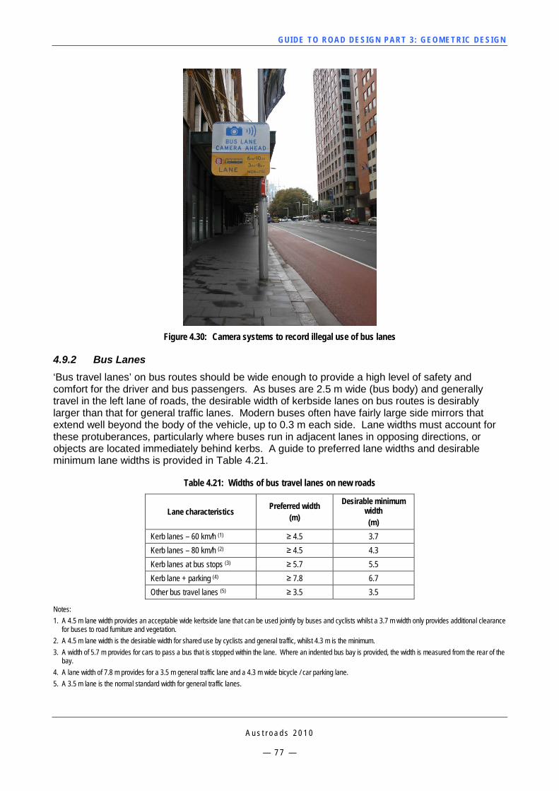
GUI DE TO RO A D DE SIG N P ART 3 : GEO MET RI C D ESI G N
A u s t r o a d s 2 0 1 0
— 7 7 —
Figure 4.30: Camera systems to record illegal use of bus lanes
4.9.2 Bus Lanes ‘Bus travel lanes’ on bus routes should be wide enough to provide a high level of safety and comfort for the driver and bus passengers. As buses are 2.5 m wide (bus body) and generally travel in the left lane of roads, the desirable width of kerbside lanes on bus routes is desirably larger than that for general traffic lanes. Modern buses often have fairly large side mirrors that extend well beyond the body of the vehicle, up to 0.3 m each side. Lane widths must account for these protuberances, particularly where buses run in adjacent lanes in opposing directions, or objects are located immediately behind kerbs. A guide to preferred lane widths and desirable minimum lane widths is provided in Table 4.21.
Table 4.21: Widths of bus travel lanes on new roads
Lane characteristics Preferred width (m)
Desirable minimum width (m)
Kerb lanes – 60 km/h (1) ≥ 4.5 3.7 Kerb lanes – 80 km/h (2) ≥ 4.5 4.3 Kerb lanes at bus stops (3) ≥ 5.7 5.5 Kerb lane + parking (4) ≥ 7.8 6.7 Other bus travel lanes (5) ≥ 3.5 3.5
Notes: 1. A 4.5 m lane width provides an acceptable wide kerbside lane that can be used jointly by buses and cyclists whilst a 3.7 m width only provides additional clearance
for buses to road furniture and vegetation. 2. A 4.5 m lane width is the desirable width for shared use by cyclists and general traffic, whilst 4.3 m is the minimum. 3. A width of 5.7 m provides for cars to pass a bus that is stopped within the lane. Where an indented bus bay is provided, the width is measured from the rear of the
bay. 4. A lane width of 7.8 m provides for a 3.5 m general traffic lane and a 4.3 m wide bicycle / car parking lane. 5. A 3.5 m lane is the normal standard width for general traffic lanes.
GUI DE TO RO A D DE SIG N P ART 3 : GEO MET RI C D ESI G N
A u s t r o a d s 2 0 1 0
— 7 8 —
During periods when parking is permitted, the lane adjacent to the kerb lane will generally be used by buses. The lane widths in Table 4.21 provide:
satisfactory clearance to trees, public utility poles and other objects in the nature strip, and also to pedestrians standing behind the kerb
a wider kerbside lane for cyclists
space for a following car to pass a bus that is stationary at a bus stop.
The widths in Table 4.21 also apply to dedicated bus lanes that are signed and marked in accordance with AS1742.12 – Manual of uniform traffic control advices: Bus, Transit, Tram and Truck Lanes (2000).
Special bus facilities are not normally provided in the medians of normal arterial roads because of the space required to:
accommodate bus stops and allow buses to overtake
provide a safe clearance between buses travelling at substantial speeds in opposite directions.
There are also operational consequences in catering for the bus movements at major intersections.
Guidance for bus stop facilities in both urban and rural areas is provided in Section 4.12.
Undivided roads
Undivided roads used by buses include both local collector/distributor roads and arterial roads.
Collector/distributor roads provide access into residential, commercial or industrial areas. They usually provide one traffic lane in each direction and space for on-street parking. These roads may carry a bus route in which case bus stops are accommodated in the space that is generally used for parking. It is desirable that bicycle lanes are provided, particularly through residential and commercial areas. Where bicycle lanes are to be provided a minimum width of 15 m (two 3.5 m traffic lanes, and two 4 m bicycle/car parking lanes) is required between kerbs. Where a bicycle lane is unable to be provided, a minimum width of 11.6 m (two 3.5 m traffic lanes and two 2.3 m parking lanes) is required.
New undivided arterial roads may eventuate from the:
need to serve commercial centres in towns where a road with four through lanes would provide sufficient capacity
upgrading of a two-lane two-way road to a four lane undivided road in order to improve traffic capacity in an existing 20 m road reservation
provision of a new road link in fully developed areas where the opportunity to acquire space is limited.
In these situations space is restricted and buses will have to use the normal traffic lanes, either the kerbside lane if parking is prohibited, or the lane adjacent to parked vehicles. While it may be desirable to provide special bus facilities or indented bus bays in these situations it is often not practicable.
GUI DE TO RO A D DE SIG N P ART 3 : GEO MET RI C D ESI G N
A u s t r o a d s 2 0 1 0
— 7 9 —
Divided roads
Bus services on divided roads normally use the left lane and hence the desirable lane widths in Table 4.22 apply. Where a bus facility is provided in a median, the residual median width should be adequate to accommodate bus stops, stage pedestrians crossing at mid-block locations, and to accommodate all necessary road furniture with adequate clearance to traffic lanes. Where service roads are to be provided, the outer separator width should be adequate to enable satisfactory openings to be designed and to accommodate indented bus bays.
Medians
The provision of bus facilities in medians is usually restricted to:
express services on freeways
medians on large bridges at critical river crossings
queue jump facilities over relatively short lengths
a separate right turn facility where a bus route turns at a major intersection
provision of a ‘centre of the road’ bus stop where this is advantageous to bus services.
The median width will vary in accordance with the service required and site constraints.
Providing for cyclists within bus lanes
While it is desirable that bicycles are accommodated in a separate bicycle lane, examples exist where bicycles have successfully shared in the use of bus lanes. In most circumstances, cyclists may be permitted to use bus lanes when they are located next to the kerb on arterial or local roads. Considerations for provision of bicycles within bus lanes should be based on:
the number of cyclists
frequency of bus services
the number of bus stops
time required to set down and pick up passengers.
Generally, buses will overtake cyclists between bus stops and cyclists will catch up and overtake buses at bus stops. This process can lead to ‘leap-frogging’ along the bus lane.
The key to managing the impact of this process on the level of service to buses and cyclists is to provide a bus lane that is wide enough to accommodate these movements. Alternatively, it may be possible to provide a separate on-road bicycle lane or off-road bicycle path adjacent to the bus lane and at bus stops.
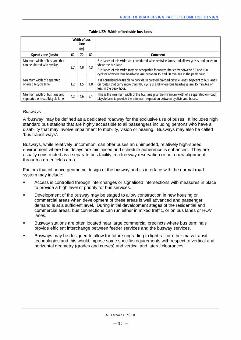
GUI DE TO RO A D DE SIG N P ART 3 : GEO MET RI C D ESI G N
A u s t r o a d s 2 0 1 0
— 8 0 —
Table 4.22: Width of kerbside bus lanes
Width of bus lane (m)
Speed zone (km/h) 60 70 80 Comment Minimum width of bus lane that can be shared with cyclists 3.7 4.0 4.3
Bus lanes of this width are considered wide kerbside lanes and allow cyclists and buses to share the bus lane. Bus lanes of this width may be acceptable for routes that carry between 50 and 100 cyclists or where bus headways are between 15 and 30 minutes in the peak hour.
Minimum width of separated on-road bicycle lane 1.2 1.5 1.8
It is considered desirable to provide separated on-road bicycle lanes adjacent to bus lanes on routes that carry more than 100 cyclists and where bus headways are 15 minutes or less in the peak hour.
Minimum width of bus lane and separated on-road bicycle lane 4.2 4.6 5.1 This is the minimum width of the bus lane plus the minimum width of a separated on-road
bicycle lane to provide the minimum separation between cyclists and buses.
Busways
A ‘busway’ may be defined as a dedicated roadway for the exclusive use of buses. It includes high standard bus stations that are highly accessible to all passengers including persons who have a disability that may involve impairment to mobility, vision or hearing. Busways may also be called ‘bus transit ways’.
Busways, while relatively uncommon, can offer buses an unimpeded, relatively high-speed environment where bus delays are minimised and schedule adherence is enhanced. They are usually constructed as a separate bus facility in a freeway reservation or on a new alignment through a greenfields area.
Factors that influence geometric design of the busway and its interface with the normal road system may include:
Access is controlled through interchanges or signalised intersections with measures in place to provide a high level of priority for bus services.
Development of the busway may be staged to allow construction in new housing or commercial areas when development of these areas is well advanced and passenger demand is at a sufficient level. During initial development stages of the residential and commercial areas, bus connections can run either in mixed traffic, or on bus lanes or HOV lanes.
Busway stations are often located near large commercial precincts where bus terminals provide efficient interchange between feeder services and the busway services.
Busways may be designed to allow for future upgrading to light rail or other mass transit technologies and this would impose some specific requirements with respect to vertical and horizontal geometry (grades and curves) and vertical and lateral clearances.
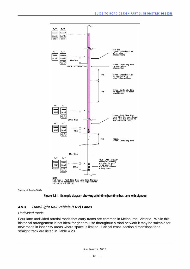
GUI DE TO RO A D DE SIG N P ART 3 : GEO MET RI C D ESI G N
A u s t r o a d s 2 0 1 0
— 8 1 —
Source: VicRoads (2009).
Figure 4.31: Example diagram showing a full-time/part-time bus lane with signage
4.9.3 Tram/Light Rail Vehicle (LRV) Lanes Undivided roads
Four lane undivided arterial roads that carry trams are common in Melbourne, Victoria. While this historical arrangement is not ideal for general use throughout a road network it may be suitable for new roads in inner city areas where space is limited. Critical cross-section dimensions for a straight track are listed in Table 4.23.
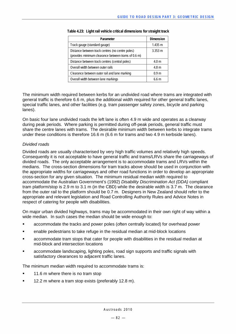
GUI DE TO RO A D DE SIG N P ART 3 : GEO MET RI C D ESI G N
A u s t r o a d s 2 0 1 0
— 8 2 —
Table 4.23: Light rail vehicle critical dimensions for straight track
Parameter Dimension Track gauge (standard gauge) 1.435 m Distance between track centres (no centre poles) (provides minimum clearance between trams of 0.6 m)
3.353 m
Distance between track centres (central poles) 4.0 m Overall width between outer rails 4.8 m Clearance between outer rail and lane marking 0.9 m Overall width between lane markings 6.6 m
The minimum width required between kerbs for an undivided road where trams are integrated with general traffic is therefore 6.6 m, plus the additional width required for other general traffic lanes, special traffic lanes, and other facilities (e.g. tram passenger safety zones, bicycle and parking lanes).
On basic four lane undivided roads the left lane is often 4.9 m wide and operates as a clearway during peak periods. Where parking is permitted during off-peak periods, general traffic must share the centre lanes with trams. The desirable minimum width between kerbs to integrate trams under these conditions is therefore 16.6 m (6.6 m for trams and two 4.9 m kerbside lanes).
Divided roads
Divided roads are usually characterised by very high traffic volumes and relatively high speeds. Consequently it is not acceptable to have general traffic and trams/LRVs share the carriageways of divided roads. The only acceptable arrangement is to accommodate trams and LRVs within the medians. The cross-section dimensions for tram tracks above should be used in conjunction with the appropriate widths for carriageways and other road functions in order to develop an appropriate cross-section for any given situation. The minimum residual median width required to accommodate the Australian Government’s (1992) Disability Discrimination Act (DDA) compliant tram platform/stop is 2.9 m to 3.1 m (in the CBD) while the desirable width is 3.7 m. The clearance from the outer rail to the platform should be 0.7 m. Designers in New Zealand should refer to the appropriate and relevant legislation and Road Controlling Authority Rules and Advice Notes in respect of catering for people with disabilities.
On major urban divided highways, trams may be accommodated in their own right of way within a wide median. In such cases the median should be wide enough to:
accommodate the tracks and power poles (often centrally located) for overhead power
enable pedestrians to take refuge in the residual median at mid-block locations
accommodate tram stops that cater for people with disabilities in the residual median at mid-block and intersection locations
accommodate landscaping, lighting poles, road sign supports and traffic signals with satisfactory clearances to adjacent traffic lanes.
The minimum median width required to accommodate trams is:
11.6 m where there is no tram stop
12.2 m where a tram stop exists (preferably 12.8 m).

GUI DE TO RO A D DE SIG N P ART 3 : GEO MET RI C D ESI G N
A u s t r o a d s 2 0 1 0
— 8 3 —
Delineation between the tram/LRV reservation or lane and adjacent general traffic lanes may be achieved by providing an unbroken line and raised pavement markers. The lane should have legal status through signs to discourage its use by general traffic. Where non-compliance is a concern, low profile concrete ‘safety bars’ may be installed, in which case an additional 0.5 m wide strip is required to accommodate this separator. This type of treatment may not be suitable where high numbers of pedestrians cross the road as pedestrians may trip over the bars.
For safety considerations it is necessary to maintain minimum clearances between trams and other trams, other vehicles and structures.
Clearance to other vehicles is provided by a 100 mm broken yellow fairway line at 0.9 m offset, measured from running edge of rail to the outside edge of the line.
Tram stops
Accessible tram stops fall into two main categories, platform stops and kerbside stops.
Platform stops should be at least 33 m in length, to accommodate the new generation of articulated trams. A single-facing platform should be 2.4 m wide. The minimum clear width along the platform to comply with the Australian Government (2002) Disability Standards for Accessible Public Transport, disability access standards is 1.8 m. Platform facilities such as shelter(s), audio and real-time traveller information will also need to be accommodated. Platform stops can be located at intersections or mid-block between intersections. Mid-block platform stops may also be configured as a central island platform. The central platform width should be 4.5 m, though high patronage stops may require greater widths for safety.
Kerbside stops are located on the footpath and typically form the vast majority of stops on a tram network. There are three options to build platforms in these environments:
kerb access stops
trafficable platform stops with one traffic lane
trafficable platform stops with two traffic lanes.
Tram track design standards
When considering the current or future provision of light rail vehicles, road designers should consult with the tram track design standards of the relevant authority for further information regarding design clearances and horizontal and vertical geometry requirements.
4.10 On-street Parking 4.10.1 General On-street parking for cars generally comprises the following:
parallel kerbside parking
angle kerbside parking
centre-of-road parking.
Facilities are also provided for trucks (e.g. loading zones), motorcycles, buses, taxis, bicycles and other special users.
Designers are encouraged to consult the following references regarding the provision of parking:
AS2890 Parking Facilities (2004) is the principal source of information regarding parking in Australia.
GUI DE TO RO A D DE SIG N P ART 3 : GEO MET RI C D ESI G N
A u s t r o a d s 2 0 1 0
— 8 4 —
Austroads Guide to Traffic Management – Part 11: Parking (Austroads 2008e).
Austroads Guide to Road Design – Part 6B: Roadside Environment (Austroads 2009f), for the design of off-street parking facilities and rest areas. See Commentary 10.
The high demand for on-street parking in many urban locations will often put pressure on authorities to try to provide more parking than is environmentally reasonable. Consideration needs to be given to the following factors when locating on-road parking:
provision of adequate end clearances to intersections and driveways — regulatory ‘no-stopping’ distance at an intersection — preservation of adequate intersection sight distances — prohibition of parking to accommodate queues on the approach to intersections — provision of left turn lanes at intersections — pedestrian crossings, bus/tram stops, railway level crossings, fire hydrants, road
bridges.
preservation of safe and convenient pedestrian access — wheelstops to prevent angle parked vehicles intruding on narrow footpaths (less than
2 m wide).
protection of through traffic — kerbside parking part way around a left-hand curve with limited sight distance across
the curve — parking just beyond a crest — a parking area which starts just beyond a roadway narrowing or lane reduction — parking on the right-hand side of a one-way roadway — any other location where a parking zone protrudes an unexpectedly large distance into
a roadway, or where parking manoeuvres may encroach into a high speed traffic lane
unsafe parking locations — on the inside of sharp curves — within a T-junction — on islands and reservations including the central island of a roundabout
Provision of disabled parking and access to the destination, e.g. kerb ramps.
4.10.2 Parallel Parking Parallel kerbside parking in the direction of traffic flow is the basic method of parking provided for in regulations. It presents, under properly controlled conditions, the least impediment to the orderly and regular flow of traffic along the road. Parallel parking limits the number of vehicles parked along the kerb (compared with angle parking), but has the advantage of minimising crashes associated with parking and unparking manoeuvres. Parallel parking is also the best system for use where parking must be provided and street capacity must be kept to a maximum, because it requires a lesser width of roadway for parking and manoeuvring.
Parallel parking is generally applicable where traffic speeds past the site do not generally exceed 60 km/h. Where this is the case, there should desirably be 0.5 m clearance from the nearest moving traffic lane. This clearance should be increased by 1.0 m for each 10 km/h by which traffic speeds exceed 60 km/h, up to a maximum of 3.0 m.
GUI DE TO RO A D DE SIG N P ART 3 : GEO MET RI C D ESI G N
A u s t r o a d s 2 0 1 0
— 8 5 —
4.10.3 Angle Parking Angle parking can generally accommodate up to twice as many vehicles per unit length of kerb as parallel parking. Small angles (30 degrees or less) give little advantage over parallel parking, especially where there are frequent driveways or other kerb interruptions. The maximum advantage occurs at 90 degrees.
However, all forms of angle kerbside parking present a greater hazard to road users than parallel parking. Studies show that when parking is changed from angle to parallel kerbside parking, the accident rate along a length of road decreases substantially and the traffic capacity is greatly increased.
The parking manoeuvre is generally more easily accomplished with angle parking than with parallel parking, and is easier with small angles than with large. As the angle of parking increases so does the width of roadway that is required for parking and unparking manoeuvres. Ninety degrees is the only angle suitable for access from both approach directions.
Angle parking may be either ‘front-in’ or ‘reverse-in’. Any town or city applying angle parking should be consistent in adopting one form or the other. Designers should note that reverse-in angle parking is prohibited by some road authorities. Consideration should also be made of the effects of exhaust fumes on pedestrian traffic.
Figure 4.32 shows the relevant dimensions required when setting out angle parking.
Long vehicles are usually unable to make use of angle parking spaces. In commercial areas, for example, adequate parallel loading spaces should also be provided to cater for long vehicles and commercial vehicles.
Wheelstops may be required to control encroachment onto pedestrian paths by excess kerb overhang, where the footpath is 2 m or less in width.
Figure 4.3 indicates the minimum widths between the separation line or median, and the kerb, for parking angles 30, 45, 60 and 90 degrees respectively that should be available before parking is permitted.
4.10.4 Centre-of-road Parking Unprotected centre-of-road parking should be considered only in streets with little through traffic and where all traffic moves slowly. The central line of parked vehicles separates opposing traffic flows and provides a continuous refuge for pedestrians, but this type of parking generates additional pedestrian movements across the road.
It is essential that adequate visibility be preserved at intersections. Hazardous conditions would be brought about by permitting centre-of-road parking too close to the cross-street traffic lanes.
A combination of kerbside parking and centre-of-road parking provides a large number of street parking spaces per unit length of street. Angle kerbside parking is rarely possible where centre-of-road parking is permitted.
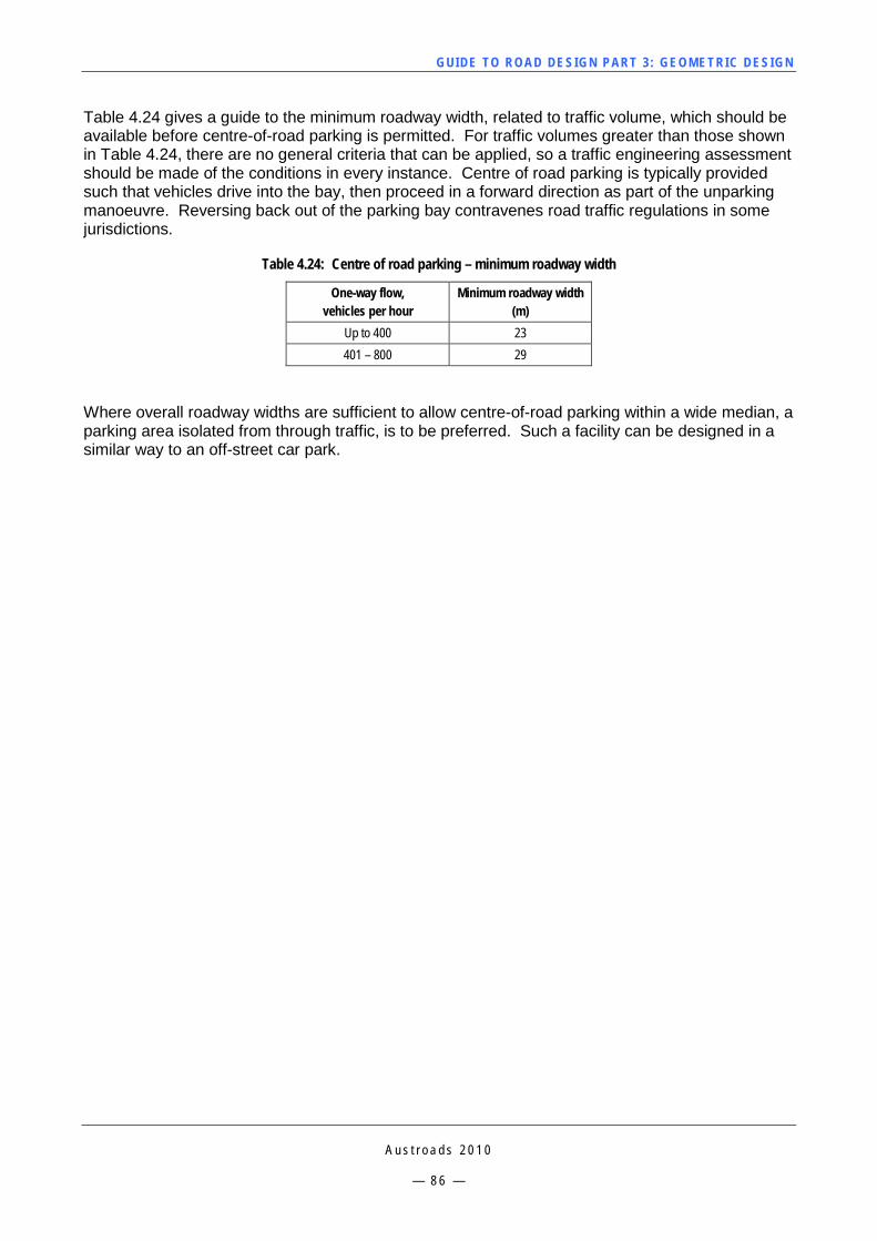
GUI DE TO RO A D DE SIG N P ART 3 : GEO MET RI C D ESI G N
A u s t r o a d s 2 0 1 0
— 8 6 —
Table 4.24 gives a guide to the minimum roadway width, related to traffic volume, which should be available before centre-of-road parking is permitted. For traffic volumes greater than those shown in Table 4.24, there are no general criteria that can be applied, so a traffic engineering assessment should be made of the conditions in every instance. Centre of road parking is typically provided such that vehicles drive into the bay, then proceed in a forward direction as part of the unparking manoeuvre. Reversing back out of the parking bay contravenes road traffic regulations in some jurisdictions.
Table 4.24: Centre of road parking – minimum roadway width
One-way flow, vehicles per hour
Minimum roadway width (m)
Up to 400 23 401 – 800 29
Where overall roadway widths are sufficient to allow centre-of-road parking within a wide median, a parking area isolated from through traffic, is to be preferred. Such a facility can be designed in a similar way to an off-street car park.
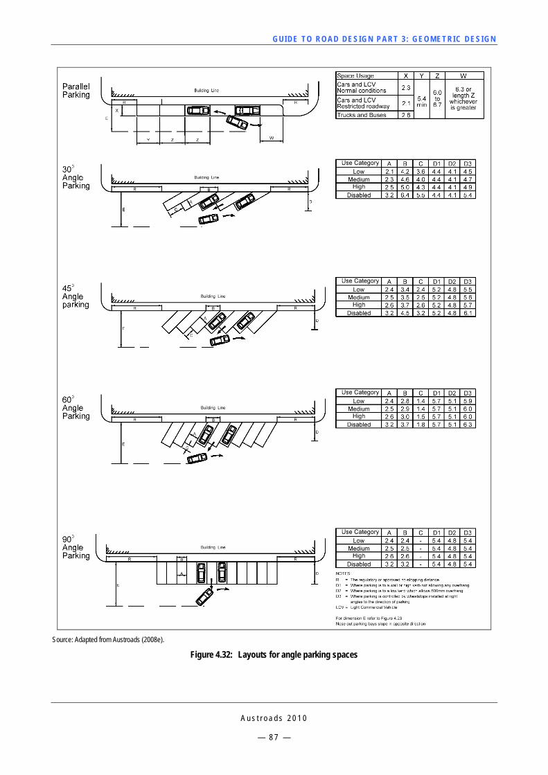
GUI DE TO RO A D DE SIG N P ART 3 : GEO MET RI C D ESI G N
A u s t r o a d s 2 0 1 0
— 8 7 —
Source: Adapted from Austroads (2008e).
Figure 4.32: Layouts for angle parking spaces
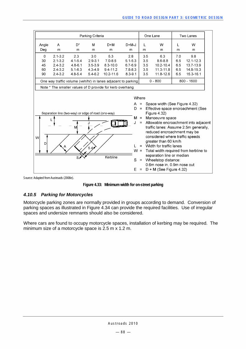
GUI DE TO RO A D DE SIG N P ART 3 : GEO MET RI C D ESI G N
A u s t r o a d s 2 0 1 0
— 8 8 —
Source: Adapted from Austroads (2008e).
Figure 4.33: Minimum width for on-street parking
4.10.5 Parking for Motorcycles Motorcycle parking zones are normally provided in groups according to demand. Conversion of parking spaces as illustrated in Figure 4.34 can provide the required facilities. Use of irregular spaces and undersize remnants should also be considered.
Where cars are found to occupy motorcycle spaces, installation of kerbing may be required. The minimum size of a motorcycle space is 2.5 m x 1.2 m.
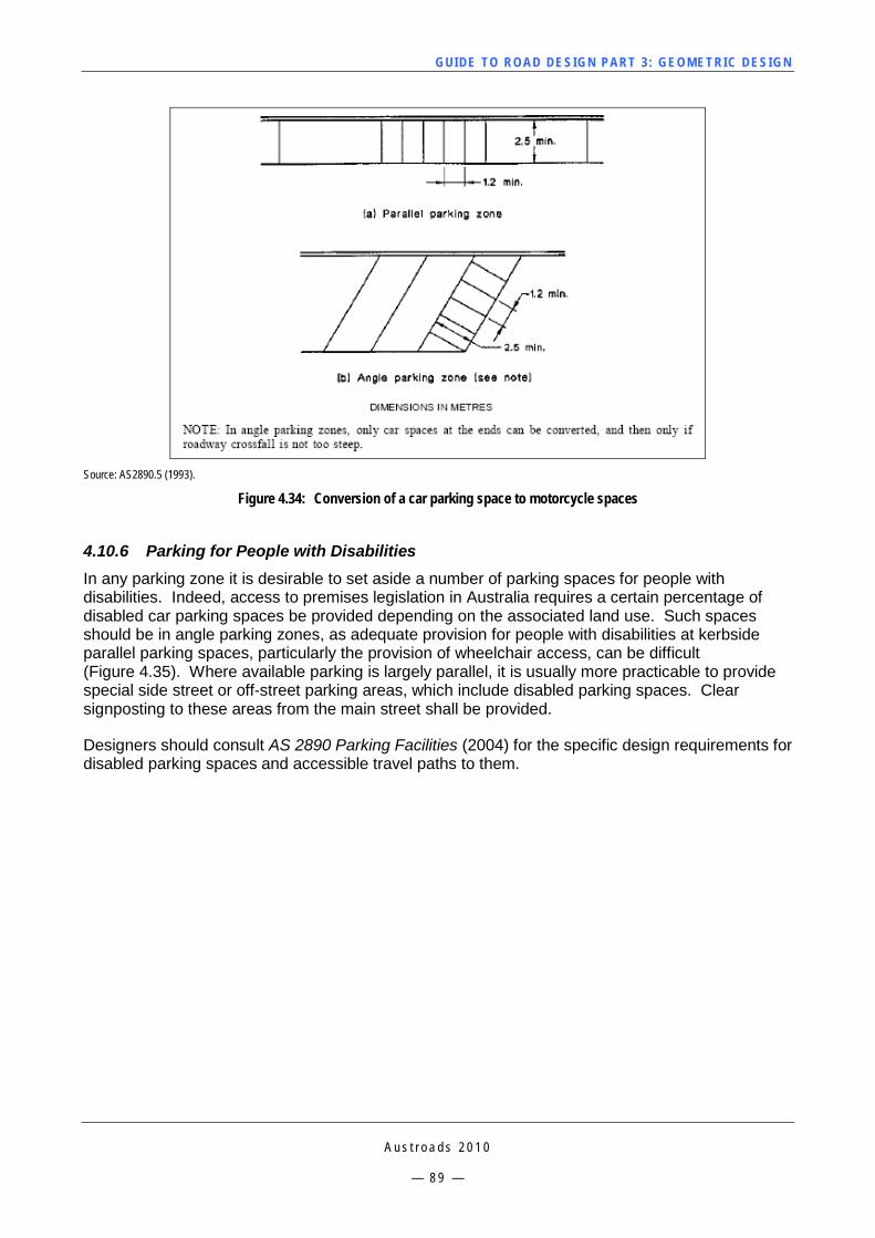
GUI DE TO RO A D DE SIG N P ART 3 : GEO MET RI C D ESI G N
A u s t r o a d s 2 0 1 0
— 8 9 —
Source: AS2890.5 (1993).
Figure 4.34: Conversion of a car parking space to motorcycle spaces
4.10.6 Parking for People with Disabilities In any parking zone it is desirable to set aside a number of parking spaces for people with disabilities. Indeed, access to premises legislation in Australia requires a certain percentage of disabled car parking spaces be provided depending on the associated land use. Such spaces should be in angle parking zones, as adequate provision for people with disabilities at kerbside parallel parking spaces, particularly the provision of wheelchair access, can be difficult (Figure 4.35). Where available parking is largely parallel, it is usually more practicable to provide special side street or off-street parking areas, which include disabled parking spaces. Clear signposting to these areas from the main street shall be provided.
Designers should consult AS 2890 Parking Facilities (2004) for the specific design requirements for disabled parking spaces and accessible travel paths to them.
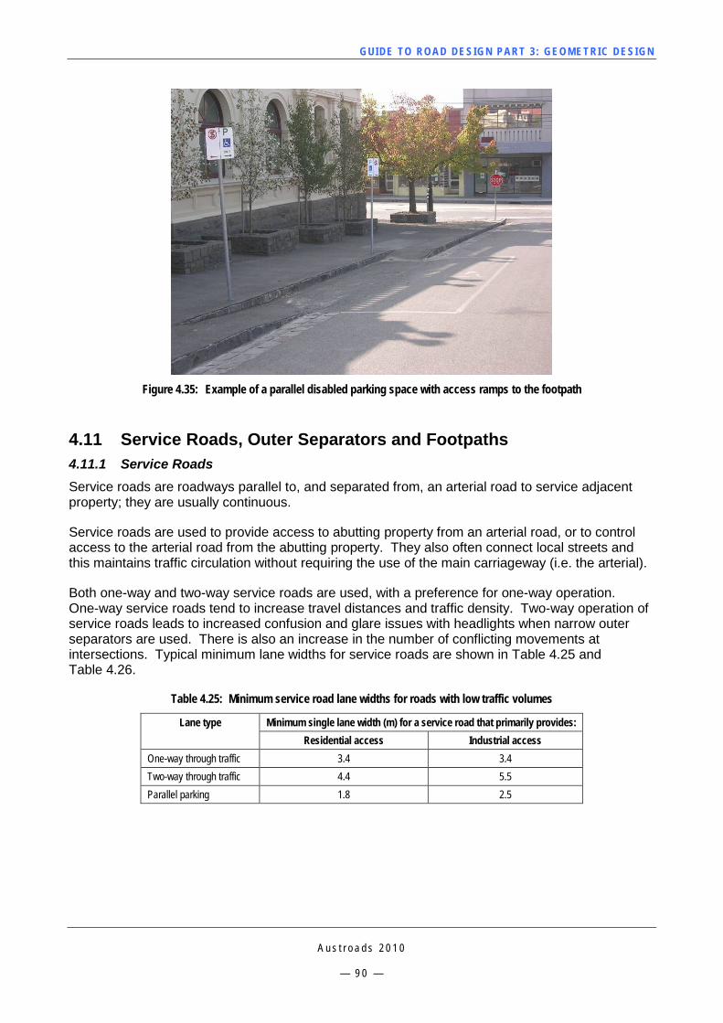
GUI DE TO RO A D DE SIG N P ART 3 : GEO MET RI C D ESI G N
A u s t r o a d s 2 0 1 0
— 9 0 —
Figure 4.35: Example of a parallel disabled parking space with access ramps to the footpath
4.11 Service Roads, Outer Separators and Footpaths 4.11.1 Service Roads Service roads are roadways parallel to, and separated from, an arterial road to service adjacent property; they are usually continuous.
Service roads are used to provide access to abutting property from an arterial road, or to control access to the arterial road from the abutting property. They also often connect local streets and this maintains traffic circulation without requiring the use of the main carriageway (i.e. the arterial).
Both one-way and two-way service roads are used, with a preference for one-way operation. One-way service roads tend to increase travel distances and traffic density. Two-way operation of service roads leads to increased confusion and glare issues with headlights when narrow outer separators are used. There is also an increase in the number of conflicting movements at intersections. Typical minimum lane widths for service roads are shown in Table 4.25 and Table 4.26.
Table 4.25: Minimum service road lane widths for roads with low traffic volumes
Lane type Minimum single lane width (m) for a service road that primarily provides: Residential access Industrial access
One-way through traffic 3.4 3.4 Two-way through traffic 4.4 5.5 Parallel parking 1.8 2.5
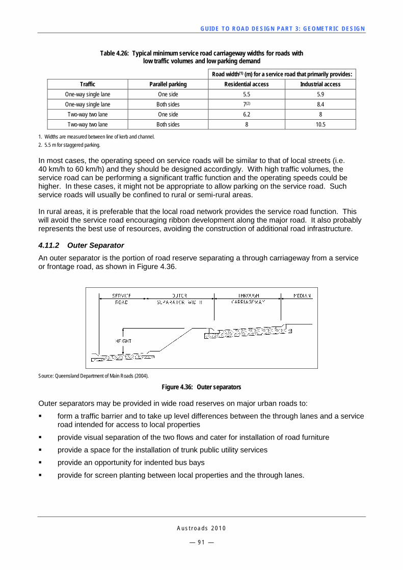
GUI DE TO RO A D DE SIG N P ART 3 : GEO MET RI C D ESI G N
A u s t r o a d s 2 0 1 0
— 9 1 —
Table 4.26: Typical minimum service road carriageway widths for roads with low traffic volumes and low parking demand
Road width(1) (m) for a service road that primarily provides: Traffic Parallel parking Residential access Industrial access
One-way single lane One side 5.5 5.9 One-way single lane Both sides 7(2) 8.4 Two-way two lane One side 6.2 8 Two-way two lane Both sides 8 10.5
1. Widths are measured between line of kerb and channel. 2. 5.5 m for staggered parking.
In most cases, the operating speed on service roads will be similar to that of local streets (i.e. 40 km/h to 60 km/h) and they should be designed accordingly. With high traffic volumes, the service road can be performing a significant traffic function and the operating speeds could be higher. In these cases, it might not be appropriate to allow parking on the service road. Such service roads will usually be confined to rural or semi-rural areas.
In rural areas, it is preferable that the local road network provides the service road function. This will avoid the service road encouraging ribbon development along the major road. It also probably represents the best use of resources, avoiding the construction of additional road infrastructure.
4.11.2 Outer Separator An outer separator is the portion of road reserve separating a through carriageway from a service or frontage road, as shown in Figure 4.36.
Source: Queensland Department of Main Roads (2004).
Figure 4.36: Outer separators
Outer separators may be provided in wide road reserves on major urban roads to:
form a traffic barrier and to take up level differences between the through lanes and a service road intended for access to local properties
provide visual separation of the two flows and cater for installation of road furniture
provide a space for the installation of trunk public utility services
provide an opportunity for indented bus bays
provide for screen planting between local properties and the through lanes.
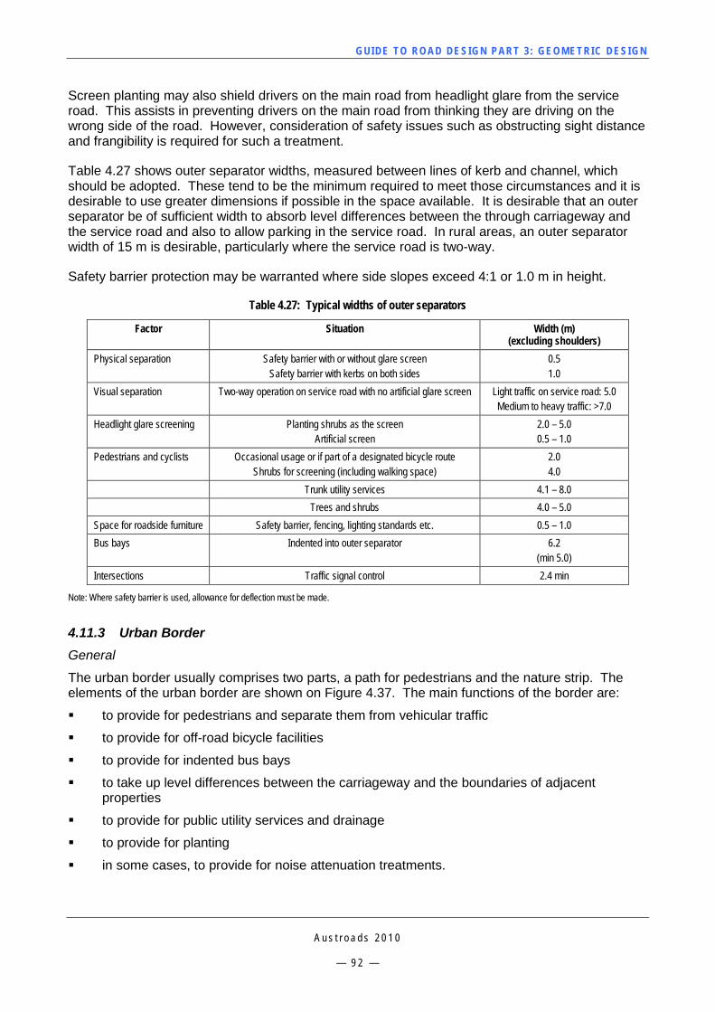
GUI DE TO RO A D DE SIG N P ART 3 : GEO MET RI C D ESI G N
A u s t r o a d s 2 0 1 0
— 9 2 —
Screen planting may also shield drivers on the main road from headlight glare from the service road. This assists in preventing drivers on the main road from thinking they are driving on the wrong side of the road. However, consideration of safety issues such as obstructing sight distance and frangibility is required for such a treatment.
Table 4.27 shows outer separator widths, measured between lines of kerb and channel, which should be adopted. These tend to be the minimum required to meet those circumstances and it is desirable to use greater dimensions if possible in the space available. It is desirable that an outer separator be of sufficient width to absorb level differences between the through carriageway and the service road and also to allow parking in the service road. In rural areas, an outer separator width of 15 m is desirable, particularly where the service road is two-way.
Safety barrier protection may be warranted where side slopes exceed 4:1 or 1.0 m in height.
Table 4.27: Typical widths of outer separators
Factor Situation Width (m) (excluding shoulders)
Physical separation Safety barrier with or without glare screen Safety barrier with kerbs on both sides
0.5 1.0
Visual separation Two-way operation on service road with no artificial glare screen Light traffic on service road: 5.0 Medium to heavy traffic: >7.0
Headlight glare screening Planting shrubs as the screen Artificial screen
2.0 – 5.0 0.5 – 1.0
Pedestrians and cyclists Occasional usage or if part of a designated bicycle route Shrubs for screening (including walking space)
2.0 4.0
Trunk utility services 4.1 – 8.0 Trees and shrubs 4.0 – 5.0 Space for roadside furniture Safety barrier, fencing, lighting standards etc. 0.5 – 1.0 Bus bays Indented into outer separator 6.2
(min 5.0) Intersections Traffic signal control 2.4 min
Note: Where safety barrier is used, allowance for deflection must be made.
4.11.3 Urban Border General
The urban border usually comprises two parts, a path for pedestrians and the nature strip. The elements of the urban border are shown on Figure 4.37. The main functions of the border are:
to provide for pedestrians and separate them from vehicular traffic
to provide for off-road bicycle facilities
to provide for indented bus bays
to take up level differences between the carriageway and the boundaries of adjacent properties
to provide for public utility services and drainage
to provide for planting
in some cases, to provide for noise attenuation treatments.
GUI DE TO RO A D DE SIG N P ART 3 : GEO MET RI C D ESI G N
A u s t r o a d s 2 0 1 0
— 9 3 —
Source: VicRoads (2002b).
Figure 4.37: Urban border
Table 4.28: Typical urban border widths
Border function Desirable minimum width (m)
Footpath Light volume Disabilities Bus stop At shops
General min.1.2
Absolute min. 0.9 1.0 – 1.8
3.4 2.4
Pedestrians plus public utility services Local road or service road Collector Arterial with service road Arterial
Measured to line of kerb 4.6 5.1 7.3 4.3
Pedestrians plus fully indented bays 5.4
The minimum slope on the urban border is determined by drainage. The maximum slope depends on the terrain and provision of access at driveways.
Table 4.29: Typical urban border slopes
Location Slope Footpath:
Desirable Maximum
1%
2.5% Nature Strip:
Grassed Soil
4% to 10% Note: Refer to AS 1428 for further details.
Clearances to road boundaries
Where a new road reservation is to be acquired, or an existing reservation is to be widened, the desirable clearances to the right-of-way (ROW) boundary are shown in Table 4.30. Where these clearances cannot be achieved, satisfactory arrangements shall be negotiated to provide for stormwater drainage and location of public utility services within the space available, having due regard to the safety of motorists and pedestrians. Provision should be made for access by maintenance vehicles.
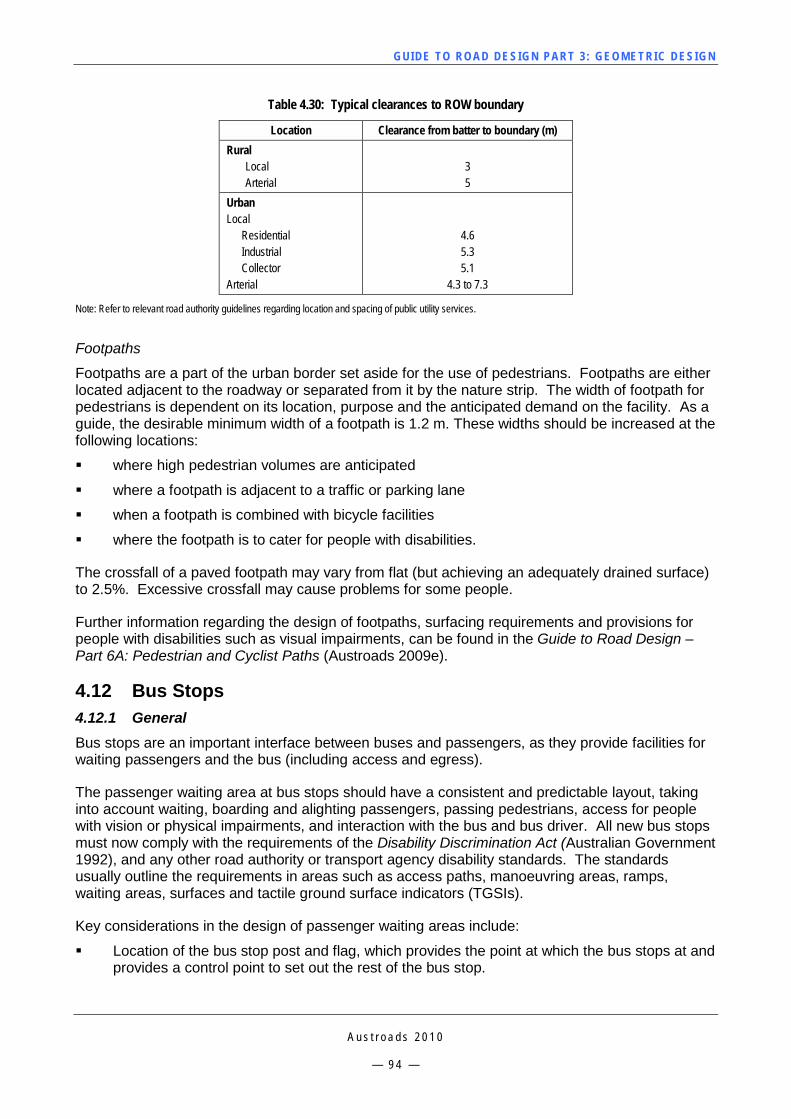
GUI DE TO RO A D DE SIG N P ART 3 : GEO MET RI C D ESI G N
A u s t r o a d s 2 0 1 0
— 9 4 —
Table 4.30: Typical clearances to ROW boundary
Location Clearance from batter to boundary (m) Rural
Local Arterial
3 5
Urban Local
Residential Industrial Collector
Arterial
4.6 5.3 5.1
4.3 to 7.3
Note: Refer to relevant road authority guidelines regarding location and spacing of public utility services.
Footpaths
Footpaths are a part of the urban border set aside for the use of pedestrians. Footpaths are either located adjacent to the roadway or separated from it by the nature strip. The width of footpath for pedestrians is dependent on its location, purpose and the anticipated demand on the facility. As a guide, the desirable minimum width of a footpath is 1.2 m. These widths should be increased at the following locations:
where high pedestrian volumes are anticipated
where a footpath is adjacent to a traffic or parking lane
when a footpath is combined with bicycle facilities
where the footpath is to cater for people with disabilities.
The crossfall of a paved footpath may vary from flat (but achieving an adequately drained surface) to 2.5%. Excessive crossfall may cause problems for some people.
Further information regarding the design of footpaths, surfacing requirements and provisions for people with disabilities such as visual impairments, can be found in the Guide to Road Design – Part 6A: Pedestrian and Cyclist Paths (Austroads 2009e).
4.12 Bus Stops 4.12.1 General Bus stops are an important interface between buses and passengers, as they provide facilities for waiting passengers and the bus (including access and egress).
The passenger waiting area at bus stops should have a consistent and predictable layout, taking into account waiting, boarding and alighting passengers, passing pedestrians, access for people with vision or physical impairments, and interaction with the bus and bus driver. All new bus stops must now comply with the requirements of the Disability Discrimination Act (Australian Government 1992), and any other road authority or transport agency disability standards. The standards usually outline the requirements in areas such as access paths, manoeuvring areas, ramps, waiting areas, surfaces and tactile ground surface indicators (TGSIs).
Key considerations in the design of passenger waiting areas include:
Location of the bus stop post and flag, which provides the point at which the bus stops at and provides a control point to set out the rest of the bus stop.
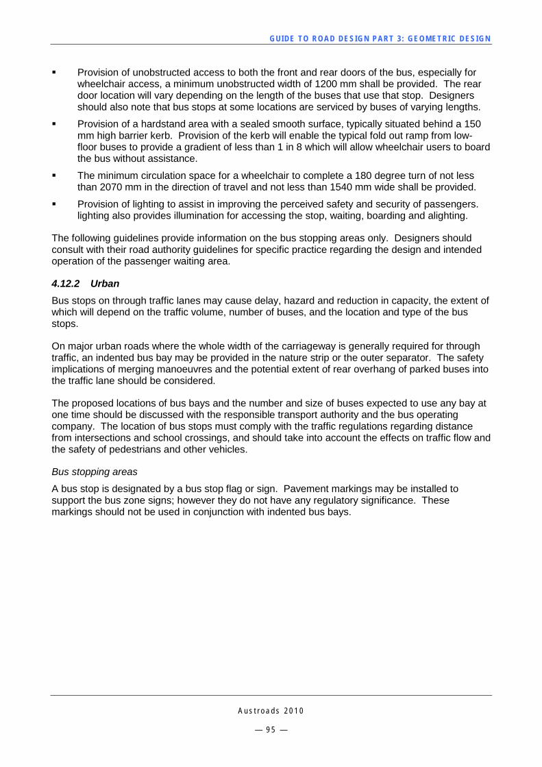
GUI DE TO RO A D DE SIG N P ART 3 : GEO MET RI C D ESI G N
A u s t r o a d s 2 0 1 0
— 9 5 —
Provision of unobstructed access to both the front and rear doors of the bus, especially for wheelchair access, a minimum unobstructed width of 1200 mm shall be provided. The rear door location will vary depending on the length of the buses that use that stop. Designers should also note that bus stops at some locations are serviced by buses of varying lengths.
Provision of a hardstand area with a sealed smooth surface, typically situated behind a 150 mm high barrier kerb. Provision of the kerb will enable the typical fold out ramp from low-floor buses to provide a gradient of less than 1 in 8 which will allow wheelchair users to board the bus without assistance.
The minimum circulation space for a wheelchair to complete a 180 degree turn of not less than 2070 mm in the direction of travel and not less than 1540 mm wide shall be provided.
Provision of lighting to assist in improving the perceived safety and security of passengers. lighting also provides illumination for accessing the stop, waiting, boarding and alighting.
The following guidelines provide information on the bus stopping areas only. Designers should consult with their road authority guidelines for specific practice regarding the design and intended operation of the passenger waiting area.
4.12.2 Urban Bus stops on through traffic lanes may cause delay, hazard and reduction in capacity, the extent of which will depend on the traffic volume, number of buses, and the location and type of the bus stops.
On major urban roads where the whole width of the carriageway is generally required for through traffic, an indented bus bay may be provided in the nature strip or the outer separator. The safety implications of merging manoeuvres and the potential extent of rear overhang of parked buses into the traffic lane should be considered.
The proposed locations of bus bays and the number and size of buses expected to use any bay at one time should be discussed with the responsible transport authority and the bus operating company. The location of bus stops must comply with the traffic regulations regarding distance from intersections and school crossings, and should take into account the effects on traffic flow and the safety of pedestrians and other vehicles.
Bus stopping areas
A bus stop is designated by a bus stop flag or sign. Pavement markings may be installed to support the bus zone signs; however they do not have any regulatory significance. These markings should not be used in conjunction with indented bus bays.
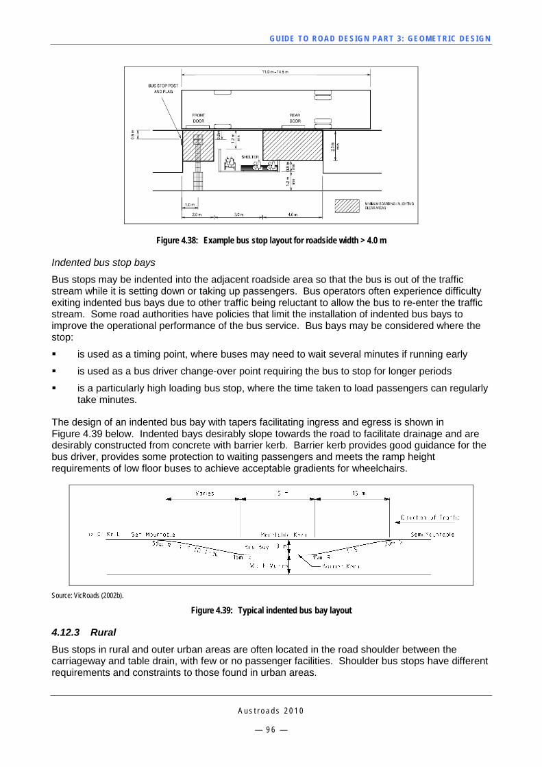
GUI DE TO RO A D DE SIG N P ART 3 : GEO MET RI C D ESI G N
A u s t r o a d s 2 0 1 0
— 9 6 —
Figure 4.38: Example bus stop layout for roadside width > 4.0 m
Indented bus stop bays
Bus stops may be indented into the adjacent roadside area so that the bus is out of the traffic stream while it is setting down or taking up passengers. Bus operators often experience difficulty exiting indented bus bays due to other traffic being reluctant to allow the bus to re-enter the traffic stream. Some road authorities have policies that limit the installation of indented bus bays to improve the operational performance of the bus service. Bus bays may be considered where the stop:
is used as a timing point, where buses may need to wait several minutes if running early
is used as a bus driver change-over point requiring the bus to stop for longer periods
is a particularly high loading bus stop, where the time taken to load passengers can regularly take minutes.
The design of an indented bus bay with tapers facilitating ingress and egress is shown in Figure 4.39 below. Indented bays desirably slope towards the road to facilitate drainage and are desirably constructed from concrete with barrier kerb. Barrier kerb provides good guidance for the bus driver, provides some protection to waiting passengers and meets the ramp height requirements of low floor buses to achieve acceptable gradients for wheelchairs.
Source: VicRoads (2002b).
Figure 4.39: Typical indented bus bay layout
4.12.3 Rural Bus stops in rural and outer urban areas are often located in the road shoulder between the carriageway and table drain, with few or no passenger facilities. Shoulder bus stops have different requirements and constraints to those found in urban areas.
GUI DE TO RO A D DE SIG N P ART 3 : GEO MET RI C D ESI G N
A u s t r o a d s 2 0 1 0
— 9 7 —
The careful selection and assessment of locations for shoulder bus stops can assist in meeting the needs of various stakeholders effectively. When the opportunity arises to site a new stop or review the site of an existing bus stop, the following should be considered:
Bus stops and stopping areas should not be located near or on curves along a road. These locations may not provide sufficient sight distance for bus drivers to identify and stop at the bus stop, or adequate view of approaching vehicles when pulling out of the shoulder. Further, it may not provide sufficient sight distance to allow motorists to stop behind the stationary bus.
Locating adjacent to a table drain should be avoided if possible as it becomes an obstacle for passengers boarding the bus, especially for disabled passengers.
The bus stop should be located near an existing footpath to provide access to the bus stop and to minimise the cost of providing access.
Bus stops should not be located where there is insufficient area for installation of hardstand for passengers to wait safely. The bus stop should be located with greater roadside width. Where there is no other option, consideration should be given to not installing the bus stop.
Bus stopping areas should be ideally located on sealed shoulders as this minimises the cost of maintenance.
The provision of a hardstand area is considered to be a basic requirement for all new or upgraded bus stops in accordance with the Disability Discrimination Act (Australian Government (1992). It provides passengers with a stable and even surface to wait for and board a bus, especially for disabled passengers. It assists bus drivers to maintain a clean bus interior and minimises the potential slip hazards in the bus for other passengers. The provision of a hardstand area should be sufficient to allow all passengers adequate room to stand without overcrowding.
Bus shelters should be considered at locations where there is a high level of passenger patronage. The shelter should be located such that the bus driver is able to see waiting passengers. The speed environment and physical features should be considered in the location of the shelter in relation to the traffic lanes. Desirably, the shelter should be located beyond the clear zone so as not to become a hazard to road users.
The minimum shoulder width required for a bus stopping area is 3 m, which allows the bus to stop without delaying traffic. Where insufficient shoulder width is available, designers should extend the width of the shoulder locally, to allow the bus to fully pull into the bus stopping area. This may also involve drainage works for any table drain present. Alternatively, another location for the bus stop should be considered.
The length of a bus stopping area should be sufficient to allow the bus to start moving before re-entering traffic lanes. Compared to a standing start, providing a short length for acceleration reduces bus driver and motorist frustration, with less disruption to the flow of traffic. The minimum length recommended is 15 m consistent with a taper on a bus bay. Where possible, a longer sealed distance may be provided (e.g. say up to 30 – 50 m in intermediate speed environments) to cater for bus acceleration, especially in higher speed zones.
Ideally, bus stops should not be located on unsealed shoulders, as the frequent repeated heavy vehicle loading and braking cause greater wear, requiring frequent maintenance intervention to repair rutting and potholes. Where bus stops are proposed on roads with unsealed shoulders, consideration should be given to locally sealing the bus stopping area with a similar surface treatment as the rest of the road. In some situations, the existing shoulder material may not support the increased loadings and will require reconstruction/strengthening. Similar treatments should also be applied to the acceleration and deceleration tapers of the bus stopping area.
GUI DE TO RO A D DE SIG N P ART 3 : GEO MET RI C D ESI G N
A u s t r o a d s 2 0 1 0
— 9 8 —
School bus stops
School bus stops are slightly different to normal rural bus stops in that they are only available for use by school children. These stops are only active at two times in the day (pick-up in the morning and drop-off in the afternoon) and can move location to suit the needs of passengers (a stop may not be required once a child has completed school). The needs of school children using these bus stops are similar to those of normal rural bus stops with regard to the location and facilities that they provide, however designers should be cognisant of the age and behaviours of children. Designers should consult relevant road authority guidelines (where available) for further information on this topic.
Depending mainly on the number of school children using a bus stop, consideration should be given to providing the following facilities. (For safety, all facilities for children should be on the side of the bus stop furthest from the road).
Waiting Areas – Where needed, waiting areas should be provided at school bus stops for school children to assemble and disperse. These areas should be level, well drained and free from tripping hazards and may be gravelled and sealed. It is desirable to provide shade.
Parking Facilities – Providing safe parking facilities should be considered at school bus stops where parents with vehicles assemble to drop-off/collect children. Adequate area should be available to permit parents to park their vehicle, drop-off the children and collect them safely with minimum disruption to the children and traffic.
Travel Paths for Pedestrians – Safe travel paths should be available for children to walk to and from the school bus stop (e.g. from a separate parking area). The need for children to walk along the edge of a vehicle carriageway should be avoided where possible, especially on roads where the traffic speed, volume and proportion of heavy vehicles are high. Preferably, paths at the maximum distance from the traffic lanes should be provided for children to use. In some cases, facilities for bicycles on off-road paths and storage for bicycles should be considered.
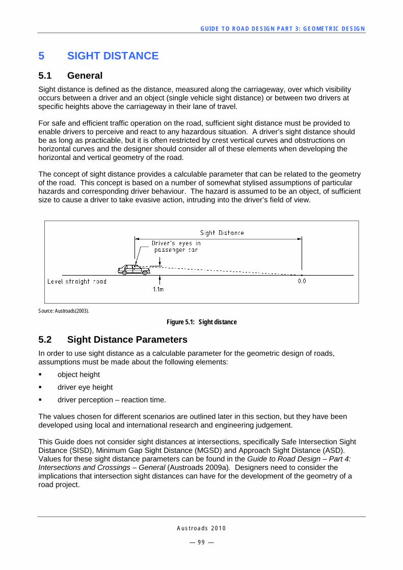
GUI DE TO RO A D DE SIG N P ART 3 : GEO MET RI C D ESI G N
A u s t r o a d s 2 0 1 0
— 9 9 —
5 SIGHT DISTANCE
5.1 General Sight distance is defined as the distance, measured along the carriageway, over which visibility occurs between a driver and an object (single vehicle sight distance) or between two drivers at specific heights above the carriageway in their lane of travel.
For safe and efficient traffic operation on the road, sufficient sight distance must be provided to enable drivers to perceive and react to any hazardous situation. A driver’s sight distance should be as long as practicable, but it is often restricted by crest vertical curves and obstructions on horizontal curves and the designer should consider all of these elements when developing the horizontal and vertical geometry of the road.
The concept of sight distance provides a calculable parameter that can be related to the geometry of the road. This concept is based on a number of somewhat stylised assumptions of particular hazards and corresponding driver behaviour. The hazard is assumed to be an object, of sufficient size to cause a driver to take evasive action, intruding into the driver’s field of view.
Source: Austroads(2003).
Figure 5.1: Sight distance
5.2 Sight Distance Parameters In order to use sight distance as a calculable parameter for the geometric design of roads, assumptions must be made about the following elements:
object height
driver eye height
driver perception – reaction time.
The values chosen for different scenarios are outlined later in this section, but they have been developed using local and international research and engineering judgement.
This Guide does not consider sight distances at intersections, specifically Safe Intersection Sight Distance (SISD), Minimum Gap Sight Distance (MGSD) and Approach Sight Distance (ASD). Values for these sight distance parameters can be found in the Guide to Road Design – Part 4: Intersections and Crossings – General (Austroads 2009a). Designers need to consider the implications that intersection sight distances can have for the development of the geometry of a road project.
GUI DE TO RO A D DE SIG N P ART 3 : GEO MET RI C D ESI G N
A u s t r o a d s 2 0 1 0
— 1 0 0 —
Object height
The object height to be used in the calculation of sight distance is a compromise between the length of sight distance and the cost of construction. Stopping is generally in response to another vehicle or large hazard in the roadway. For example, to recognise a vehicle as a hazard at night, a line of sight to its headlights or taillights would be necessary. Larger objects would be visible sooner and provide longer stopping distances. To perceive a very small hazard, such as a surface defect, a zero object height would be necessary. However, at the required stopping sight distances for high speeds, small pavement variations and small objects (especially at night) may not be visible to most drivers. Thus, most drivers travelling at high speeds would have difficulty in stopping before reaching such a small obstruction.
The length of crest vertical curves increases significantly as the object height approaches zero.
For the geometric design of all roads, the object heights shown in Table 5.1 are to be used.
5.2.1 Driver Eye Height Driver eye height is a combination of the height of driver stature and driver seat height. Based upon recent research and consideration of the characteristics of the vehicle fleet, a car driver eye height of 1.10 m is to be used for the geometric design of all roads.
For commercial vehicles, a driver eye height of 2.40 m is to be used. The 2.40 m truck driver eye height for sag curves is particularly important for checking the effect of overhead structures on sight distance.
When designing facilities for buses, the driver eye height is 1.80 m.
The driver eye heights and typical applications are listed in Table 5.1.
The change of car driver eye height will have implications for geometric design elements (such as length of vertical curves) used in other road design publications, which should be considered by the designer when this guide is used in conjunction with previously published guides. See Commentary 11.
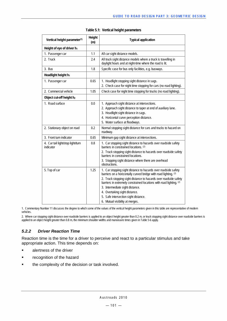
GUI DE TO RO A D DE SIG N P ART 3 : GEO MET RI C D ESI G N
A u s t r o a d s 2 0 1 0
— 1 0 1 —
Table 5.1: Vertical height parameters
Vertical height parameter(1) Height (m) Typical application
Height of eye of driver h1 1. Passenger car 1.1 All car sight distance models. 2. Truck 2.4 All truck sight distance models where a truck is travelling in
daylight hours and at night-time where the road is lit. 3. Bus 1.8 Specific case for bus only facilities, e.g. busways.
Headlight height h1 1. Passenger car 0.65 1. Headlight stopping sight distance in sags.
2. Check case for night time stopping for cars (no road lighting). 2. Commercial vehicle 1.05 Check case for night time stopping for trucks (no road lighting).
Object cut-off height h2 1. Road surface 0.0 1. Approach sight distance at intersections.
2. Approach sight distance to taper at end of auxiliary lane. 3. Headlight sight distance in sags. 4. Horizontal curve perception distance. 5. Water surface at floodways.
2. Stationary object on road 0.2 Normal stopping sight distance for cars and trucks to hazard on roadway.
3. Front turn indicator 0.65 Minimum gap sight distance at intersections. 4. Car tail light/stop light/turn indicator
0.8 1. Car stopping sight distance to hazards over roadside safety barriers in constrained locations. (2) 2. Truck stopping sight distance to hazards over roadside safety barriers in constrained locations. 3. Stopping sight distance where there are overhead obstructions.
5. Top of car 1.25 1. Car stopping sight distance to hazards over roadside safety barriers on a horizontally curved bridge with road lighting. (2) 2. Truck stopping sight distance to hazards over roadside safety barriers in extremely constrained locations with road lighting. (2) 3. Intermediate sight distance. 4. Overtaking sight distance. 5. Safe intersection sight distance. 6. Mutual visibility at merges.
1. Commentary Number 11 discusses the degree to which some of the values of the vertical height parameters given in this table are representative of modern vehicles. 2. Where car stopping sight distance over roadside barriers is applied to an object height greater than 0.2 m, or truck stopping sight distance over roadside barriers is applied to an object height greater than 0.8 m, the minimum shoulder widths and manoeuvre times given in Table 5-6 apply.
5.2.2 Driver Reaction Time Reaction time is the time for a driver to perceive and react to a particular stimulus and take appropriate action. This time depends on:
alertness of the driver
recognition of the hazard
the complexity of the decision or task involved.
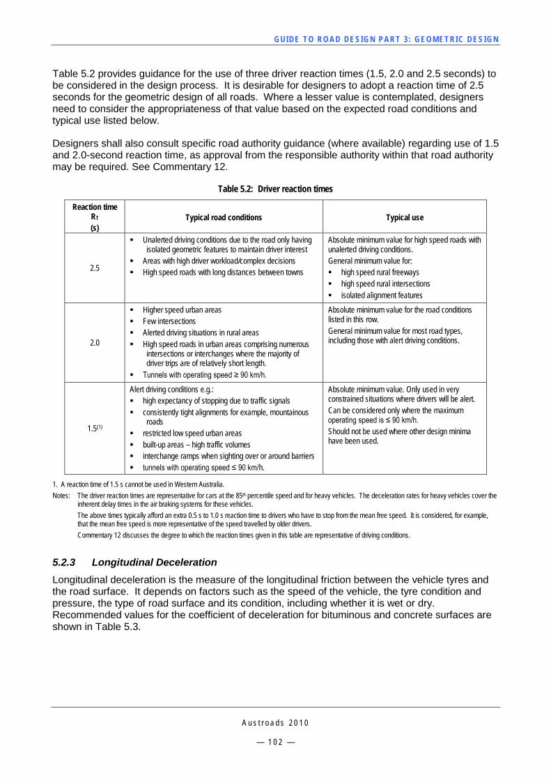
GUI DE TO RO A D DE SIG N P ART 3 : GEO MET RI C D ESI G N
A u s t r o a d s 2 0 1 0
— 1 0 2 —
Table 5.2 provides guidance for the use of three driver reaction times (1.5, 2.0 and 2.5 seconds) to be considered in the design process. It is desirable for designers to adopt a reaction time of 2.5 seconds for the geometric design of all roads. Where a lesser value is contemplated, designers need to consider the appropriateness of that value based on the expected road conditions and typical use listed below.
Designers shall also consult specific road authority guidance (where available) regarding use of 1.5 and 2.0-second reaction time, as approval from the responsible authority within that road authority may be required. See Commentary 12.
Table 5.2: Driver reaction times
Reaction time RT (s)
Typical road conditions Typical use
2.5
Unalerted driving conditions due to the road only having isolated geometric features to maintain driver interest
Areas with high driver workload/complex decisions High speed roads with long distances between towns
Absolute minimum value for high speed roads with unalerted driving conditions. General minimum value for: high speed rural freeways high speed rural intersections isolated alignment features
2.0
Higher speed urban areas Few intersections Alerted driving situations in rural areas High speed roads in urban areas comprising numerous
intersections or interchanges where the majority of driver trips are of relatively short length.
Tunnels with operating speed ≥ 90 km/h.
Absolute minimum value for the road conditions listed in this row. General minimum value for most road types, including those with alert driving conditions.
1.5(1)
Alert driving conditions e.g.: high expectancy of stopping due to traffic signals consistently tight alignments for example, mountainous
roads restricted low speed urban areas built-up areas – high traffic volumes interchange ramps when sighting over or around barriers tunnels with operating speed ≤ 90 km/h.
Absolute minimum value. Only used in very constrained situations where drivers will be alert. Can be considered only where the maximum operating speed is ≤ 90 km/h. Should not be used where other design minima have been used.
1. A reaction time of 1.5 s cannot be used in Western Australia. Notes: The driver reaction times are representative for cars at the 85th percentile speed and for heavy vehicles. The deceleration rates for heavy vehicles cover the
inherent delay times in the air braking systems for these vehicles. The above times typically afford an extra 0.5 s to 1.0 s reaction time to drivers who have to stop from the mean free speed. It is considered, for example,
that the mean free speed is more representative of the speed travelled by older drivers. Commentary 12 discusses the degree to which the reaction times given in this table are representative of driving conditions.
5.2.3 Longitudinal Deceleration Longitudinal deceleration is the measure of the longitudinal friction between the vehicle tyres and the road surface. It depends on factors such as the speed of the vehicle, the tyre condition and pressure, the type of road surface and its condition, including whether it is wet or dry. Recommended values for the coefficient of deceleration for bituminous and concrete surfaces are shown in Table 5.3.
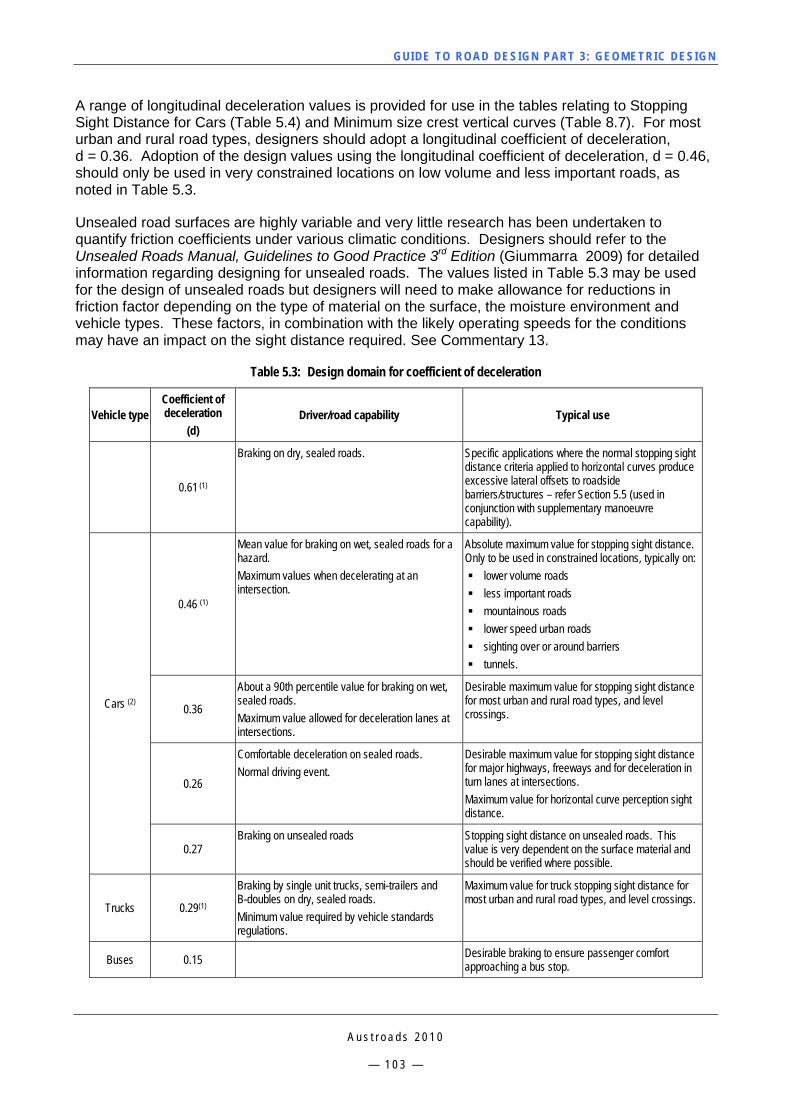
GUI DE TO RO A D DE SIG N P ART 3 : GEO MET RI C D ESI G N
A u s t r o a d s 2 0 1 0
— 1 0 3 —
A range of longitudinal deceleration values is provided for use in the tables relating to Stopping Sight Distance for Cars (Table 5.4) and Minimum size crest vertical curves (Table 8.7). For most urban and rural road types, designers should adopt a longitudinal coefficient of deceleration, d = 0.36. Adoption of the design values using the longitudinal coefficient of deceleration, d = 0.46, should only be used in very constrained locations on low volume and less important roads, as noted in Table 5.3.
Unsealed road surfaces are highly variable and very little research has been undertaken to quantify friction coefficients under various climatic conditions. Designers should refer to the Unsealed Roads Manual, Guidelines to Good Practice 3rd Edition (Giummarra 2009) for detailed information regarding designing for unsealed roads. The values listed in Table 5.3 may be used for the design of unsealed roads but designers will need to make allowance for reductions in friction factor depending on the type of material on the surface, the moisture environment and vehicle types. These factors, in combination with the likely operating speeds for the conditions may have an impact on the sight distance required. See Commentary 13.
Table 5.3: Design domain for coefficient of deceleration
Vehicle type Coefficient of deceleration
(d) Driver/road capability Typical use
0.61 (1)
Braking on dry, sealed roads. Specific applications where the normal stopping sight distance criteria applied to horizontal curves produce excessive lateral offsets to roadside barriers/structures – refer Section 5.5 (used in conjunction with supplementary manoeuvre capability).
Cars (2)
0.46 (1)
Mean value for braking on wet, sealed roads for a hazard. Maximum values when decelerating at an intersection.
Absolute maximum value for stopping sight distance. Only to be used in constrained locations, typically on: lower volume roads less important roads mountainous roads lower speed urban roads sighting over or around barriers tunnels.
0.36
About a 90th percentile value for braking on wet, sealed roads. Maximum value allowed for deceleration lanes at intersections.
Desirable maximum value for stopping sight distance for most urban and rural road types, and level crossings.
0.26
Comfortable deceleration on sealed roads. Normal driving event.
Desirable maximum value for stopping sight distance for major highways, freeways and for deceleration in turn lanes at intersections. Maximum value for horizontal curve perception sight distance.
0.27 Braking on unsealed roads Stopping sight distance on unsealed roads. This
value is very dependent on the surface material and should be verified where possible.
Trucks 0.29(1)
Braking by single unit trucks, semi-trailers and B-doubles on dry, sealed roads. Minimum value required by vehicle standards regulations.
Maximum value for truck stopping sight distance for most urban and rural road types, and level crossings.
Buses 0.15 Desirable braking to ensure passenger comfort approaching a bus stop.
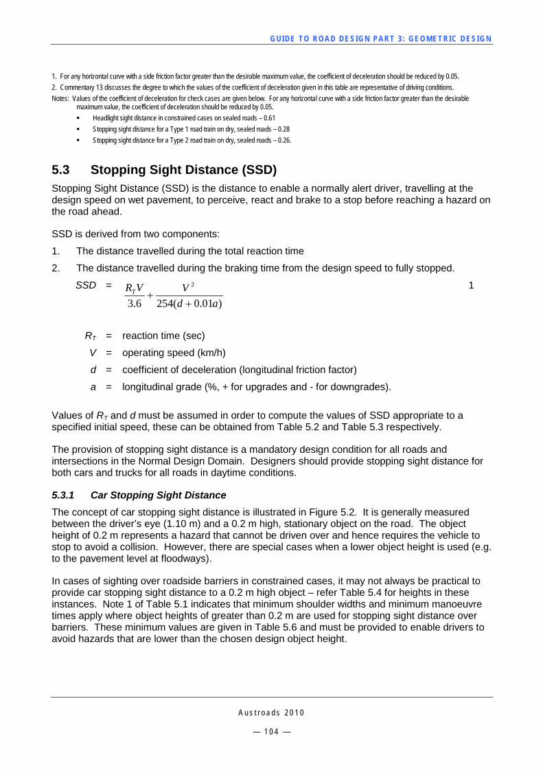
GUI DE TO RO A D DE SIG N P ART 3 : GEO MET RI C D ESI G N
A u s t r o a d s 2 0 1 0
— 1 0 4 —
1. For any horizontal curve with a side friction factor greater than the desirable maximum value, the coefficient of deceleration should be reduced by 0.05. 2. Commentary 13 discusses the degree to which the values of the coefficient of deceleration given in this table are representative of driving conditions. Notes: Values of the coefficient of deceleration for check cases are given below. For any horizontal curve with a side friction factor greater than the desirable
maximum value, the coefficient of deceleration should be reduced by 0.05. Headlight sight distance in constrained cases on sealed roads – 0.61 Stopping sight distance for a Type 1 road train on dry, sealed roads – 0.28 Stopping sight distance for a Type 2 road train on dry, sealed roads – 0.26.
5.3 Stopping Sight Distance (SSD) Stopping Sight Distance (SSD) is the distance to enable a normally alert driver, travelling at the design speed on wet pavement, to perceive, react and brake to a stop before reaching a hazard on the road ahead.
SSD is derived from two components:
1. The distance travelled during the total reaction time
2. The distance travelled during the braking time from the design speed to fully stopped.
SSD =
)01.0(2546.3
2
adVVRT
++
1
RT = reaction time (sec)
V = operating speed (km/h)
d = coefficient of deceleration (longitudinal friction factor)
a = longitudinal grade (%, + for upgrades and - for downgrades).
Values of RT and d must be assumed in order to compute the values of SSD appropriate to a specified initial speed, these can be obtained from Table 5.2 and Table 5.3 respectively.
The provision of stopping sight distance is a mandatory design condition for all roads and intersections in the Normal Design Domain. Designers should provide stopping sight distance for both cars and trucks for all roads in daytime conditions.
5.3.1 Car Stopping Sight Distance The concept of car stopping sight distance is illustrated in Figure 5.2. It is generally measured between the driver’s eye (1.10 m) and a 0.2 m high, stationary object on the road. The object height of 0.2 m represents a hazard that cannot be driven over and hence requires the vehicle to stop to avoid a collision. However, there are special cases when a lower object height is used (e.g. to the pavement level at floodways).
In cases of sighting over roadside barriers in constrained cases, it may not always be practical to provide car stopping sight distance to a 0.2 m high object – refer Table 5.4 for heights in these instances. Note 1 of Table 5.1 indicates that minimum shoulder widths and minimum manoeuvre times apply where object heights of greater than 0.2 m are used for stopping sight distance over barriers. These minimum values are given in Table 5.6 and must be provided to enable drivers to avoid hazards that are lower than the chosen design object height.
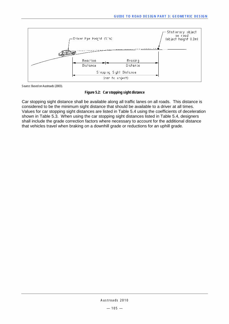
GUI DE TO RO A D DE SIG N P ART 3 : GEO MET RI C D ESI G N
A u s t r o a d s 2 0 1 0
— 1 0 5 —
Source: Based on Austroads (2003).
Figure 5.2: Car stopping sight distance
Car stopping sight distance shall be available along all traffic lanes on all roads. This distance is considered to be the minimum sight distance that should be available to a driver at all times. Values for car stopping sight distances are listed in Table 5.4 using the coefficients of deceleration shown in Table 5.3. When using the car stopping sight distances listed in Table 5.4, designers shall include the grade correction factors where necessary to account for the additional distance that vehicles travel when braking on a downhill grade or reductions for an uphill grade.

GUI DE TO RO A D DE SIG N P ART 3 : GEO MET RI C D ESI G N
A u s t r o a d s 2 0 1 0
— 1 0 6 —
Table 5.4: Stopping sight distances for cars on sealed roads
Design speed (km/h)
Absolute minimum values Only for specific road types and
situations(1)
based on d = 0.46 (2), (3)
Desirable minimum values for most urban and rural road types
based on d = 0.36
Desirable values for major highways and
freeways based on d = 0.26
RT = 1.5s(4) RT = 2.0 s(4) RT = 2.5s RT = 1.5 s(4) RT = 2.0 s(4) RT = 2.5 s RT = 2.0s RT = 2.5 s 40 30 36 – 34 40 45 – – 50 42 49 – 48 55 62 – – 60 56 64 – 64 73 81 – – 70 71 81 – 83 92 102 113 123 80 88 99 – 103 114 126 141 152 90 107 119 132 126 139 151 173 185 100 – 141 155 – 165 179 207 221 110 – 165 180 – 193 209 244 260 120 – 190 207 – 224 241 285 301 130 – 217 235 – 257 275 328 346
Corrections due to grade
(5) (6) -8 -6 -4 -2 2 4 6 8
40 5 3 2 1 -1 -2 -2 -3 50 8 5 3 2 -1 -3 -4 -5 60 11 8 5 2 -2 -4 -6 -7 70 15 11 7 3 -3 -5 -8 -10 80 20 14 9 4 -4 -7 -10 -13 90 25 18 11 5 -5 -9 -13 -16 100 31 22 14 6 -6 -11 -16 -20 110 38 26 17 8 -7 -13 -19 -24 120 45 31 20 9 -8 -16 -22 -29 130 53 37 23 11 -10 -18 -26 -34
1. These values are only suitable for use in very constrained locations. Examples of this in Australia are: lower volume roads mountainous roads lower speed urban roads sighting over or around barriers tunnels.
2. On any horizontal curve with a side friction factor greater than the desirable maximum value, reduce the coefficient of deceleration by 0.05 and calculate the stopping distance according to Equation 1
3. Where deceleration values greater than 0.36 are used, minimum seal widths for supplementary manoeuvre capability should be provided. For two-lane, two-way roads, a desirable minimum width of 12 m and a minimum of 9 m is applicable. This is especially important on horizontal curves with a side friction demand greater than the desirable maximum in Table 7.4.
4. Reaction times of 1.5 s cannot be used in Western Australia. A 1.5 s reaction time is only to be used in constrained situations where drivers will be alert. Typical situations are given in Table 5.2. The general minimum reaction time is 2.0 s.
5. If the roadway is on a grade, designers shall adjust stopping sight distance values by applying these grade corrections derived with d=0.36. Downhill grades are shown as negative, with uphill listed as positive. The grade adopted is determined using the average grade over the braking length. Grade correction for d = 0.46 should be calculated separately using Equation 1. Generally, grade corrections are not necessary when using d=0.26 because the deceleration value is conservative and because steep grades are not usually applied to roadways utilising d = 0.26.
6. Corrected stopping sight distances should be rounded conservatively to the nearest 5 m. Note: Combinations of design speed and reaction times not shown in this table are generally not used. Either the resulting stopping distances are similar to other
combinations of the parameters for the design speed, or they fall outside the realistic design speed for the road.
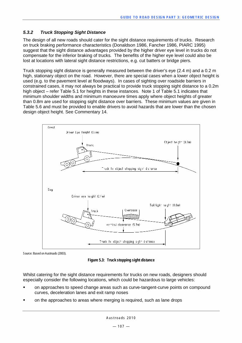
GUI DE TO RO A D DE SIG N P ART 3 : GEO MET RI C D ESI G N
A u s t r o a d s 2 0 1 0
— 1 0 7 —
5.3.2 Truck Stopping Sight Distance The design of all new roads should cater for the sight distance requirements of trucks. Research on truck braking performance characteristics (Donaldson 1986, Fancher 1986, PIARC 1995) suggest that the sight distance advantages provided by the higher driver eye level in trucks do not compensate for the inferior braking of trucks. The benefits of the higher eye level could also be lost at locations with lateral sight distance restrictions, e.g. cut batters or bridge piers.
Truck stopping sight distance is generally measured between the driver’s eye (2.4 m) and a 0.2 m high, stationary object on the road. However, there are special cases when a lower object height is used (e.g. to the pavement level at floodways). In cases of sighting over roadside barriers in constrained cases, it may not always be practical to provide truck stopping sight distance to a 0.2m high object – refer Table 5.1 for heights in these instances. Note 1 of Table 5.1 indicates that minimum shoulder widths and minimum manoeuvre times apply where object heights of greater than 0.8m are used for stopping sight distance over barriers. These minimum values are given in Table 5.6 and must be provided to enable drivers to avoid hazards that are lower than the chosen design object height. See Commentary 14.
Source: Based on Austroads (2003).
Figure 5.3: Truck stopping sight distance
Whilst catering for the sight distance requirements for trucks on new roads, designers should especially consider the following locations, which could be hazardous to large vehicles:
on approaches to speed change areas such as curve-tangent-curve points on compound curves, deceleration lanes and exit ramp noses
on the approaches to areas where merging is required, such as lane drops
GUI DE TO RO A D DE SIG N P ART 3 : GEO MET RI C D ESI G N
A u s t r o a d s 2 0 1 0
— 1 0 8 —
on the approaches to construction zones, especially where the surface changes from sealed to unsealed
sight distance through underpasses where the critical case is truck driver eye height (2.4 m) to car taillight (0.8 m)
bus lanes on freeways adjacent to safety barriers
areas where large vehicles are required to brake on low radius horizontal curves, e.g. at intersections, as large vehicles require additional distance for braking, especially when considering truck stability during turns within intersections – see below.
Designers are referred to the Guide to Road Design – Part 4: Intersections and Crossings – General (Austroads 2009a) for further information regarding Truck SSD at intersections. However, consideration should be given to providing Truck SSD at the following potentially hazardous locations:
On the approaches to railway level crossings.
Intersections with lateral sight distance restrictions. For example, intersections in hilly terrain or near bridge piers.
Intersections on or near crest vertical curves.
On intersection approaches where truck speeds are close or equal to car speeds.
At crest and sag points, truck stopping sight distance is measured as shown on Figure 5.3.
The designer should consider measures such as additional signs and line marking to improve safety if stopping sight distance is found to be inadequate for trucks and it is not possible to improve the geometric design. However, it is emphasised that signage and line marking are not substitutes for achieving standard design practices.
SSD values for trucks have been calculated using the coefficient of longitudinal deceleration shown in Table 5.3.
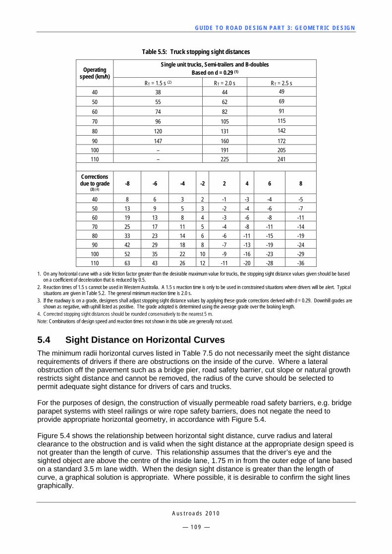
GUI DE TO RO A D DE SIG N P ART 3 : GEO MET RI C D ESI G N
A u s t r o a d s 2 0 1 0
— 1 0 9 —
Table 5.5: Truck stopping sight distances
Operating speed (km/h)
Single unit trucks, Semi-trailers and B-doubles Based on d = 0.29 (1)
RT = 1.5 s (2) RT = 2.0 s RT = 2.5 s 40 38 44 49
50 55 62 69
60 74 82 91
70 96 105 115
80 120 131 142
90 147 160 172 100 – 191 205 110 – 225 241
Corrections due to grade
(3) (4) -8 -6 -4 -2 2 4 6 8
40 8 6 3 2 -1 -3 -4 -5 50 13 9 5 3 -2 -4 -6 -7 60 19 13 8 4 -3 -6 -8 -11 70 25 17 11 5 -4 -8 -11 -14 80 33 23 14 6 -6 -11 -15 -19 90 42 29 18 8 -7 -13 -19 -24
100 52 35 22 10 -9 -16 -23 -29 110 63 43 26 12 -11 -20 -28 -36
1. On any horizontal curve with a side friction factor greater than the desirable maximum value for trucks, the stopping sight distance values given should be based on a coefficient of deceleration that is reduced by 0.5.
2. Reaction times of 1.5 s cannot be used in Western Australia. A 1.5 s reaction time is only to be used in constrained situations where drivers will be alert. Typical situations are given in Table 5.2. The general minimum reaction time is 2.0 s.
3. If the roadway is on a grade, designers shall adjust stopping sight distance values by applying these grade corrections derived with d = 0.29. Downhill grades are shown as negative, with uphill listed as positive. The grade adopted is determined using the average grade over the braking length.
4. Corrected stopping sight distances should be rounded conservatively to the nearest 5 m. Note: Combinations of design speed and reaction times not shown in this table are generally not used.
5.4 Sight Distance on Horizontal Curves The minimum radii horizontal curves listed in Table 7.5 do not necessarily meet the sight distance requirements of drivers if there are obstructions on the inside of the curve. Where a lateral obstruction off the pavement such as a bridge pier, road safety barrier, cut slope or natural growth restricts sight distance and cannot be removed, the radius of the curve should be selected to permit adequate sight distance for drivers of cars and trucks.
For the purposes of design, the construction of visually permeable road safety barriers, e.g. bridge parapet systems with steel railings or wire rope safety barriers, does not negate the need to provide appropriate horizontal geometry, in accordance with Figure 5.4.
Figure 5.4 shows the relationship between horizontal sight distance, curve radius and lateral clearance to the obstruction and is valid when the sight distance at the appropriate design speed is not greater than the length of curve. This relationship assumes that the driver’s eye and the sighted object are above the centre of the inside lane, 1.75 m in from the outer edge of lane based on a standard 3.5 m lane width. When the design sight distance is greater than the length of curve, a graphical solution is appropriate. Where possible, it is desirable to confirm the sight lines graphically.

GUI DE TO RO A D DE SIG N P ART 3 : GEO MET RI C D ESI G N
A u s t r o a d s 2 0 1 0
— 1 1 0 —
5.4.1 Benching for Visibility on Horizontal Curves Where sight benches in side cuttings are required on horizontal curves or a combination of horizontal and vertical curves, the horizontal and vertical limits of the benching are determined graphically or by modeling.
Benching is the widening of the cutting on the inside of a curve to obtain the specified sight distance. It usually takes the form of a flat table or bench over which a driver can see an approaching vehicle or an object on the road. In plan view, the envelope formed by the lines of sight fixes the benching. The driver and the object are assumed to be in the centre of the inner lane and the sight distance is measured around the centerline of the lane, the path the vehicle would follow in braking. Benching adequate for inner lane traffic more than meets requirements for the outer lane.
Where a horizontal and crest vertical curve overlap, the line of sight between approaching vehicles may not be over the top of the crest but to one side and may be partly off the formation. Cutting down the crest on the pavement will not increase visibility if the line of sight is clear of the pavement, and the bottom of the bench may be lower than the shoulder level. In these cases, as well as in the case of sharp horizontal curves, a better solution may be to use a larger radius curve so that the line of sight remains within the formation. However, this will tend to increase the operating speed, which in turn will increase the sight distance required.
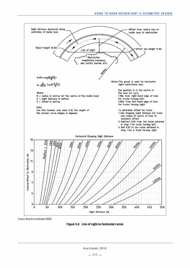
GUI DE TO RO A D DE SIG N P ART 3 : GEO MET RI C D ESI G N
A u s t r o a d s 2 0 1 0
— 1 1 1 —
Source: Based on Austroads (2003).
Figure 5.4: Line of sight on horizontal curves
GUI DE TO RO A D DE SIG N P ART 3 : GEO MET RI C D ESI G N
A u s t r o a d s 2 0 1 0
— 1 1 2 —
5.5 Sight Distance Requirements on Horizontal Curves with Roadside Barriers / Wall / Bridge Structures
Application of the normal stopping sight distance requirements over/around roadside barriers and structures on horizontal curves can produce excessive lateral offsets in particular circumstances. This can have the following adverse operational effects:
cars and trucks parking in the widened area, reducing sight distance
errant vehicles potentially impacting the barrier at a greater angle, increasing the severity of these types of accidents
cost of providing the widened area becomes prohibitively expensive.
Experience shows that the criteria in this section provide acceptable sight distance for these circumstances. This supersedes the previous common practice of dismissing sight distance criteria altogether based on the grounds of being uneconomic.
5.5.1 Requirements where Sighting over Roadside Barriers is Possible Minimum shoulder widths and minimum manoeuvre times apply where object heights of greater than 0.2 m for cars and 0.8 m for trucks are used for stopping sight distance over barriers (refer Note 1 in Table 5.1). These minimum values are given in Table 5.6 and must be provided to enable drivers to avoid hazards that are lower than the design object height/s. This is provided through adequate width to manoeuvre around smaller objects and an adequate time in which to undertake the manoeuvre.
No supplementary manoeuvre capability needs to be provided where object heights of 0.2 m for car stopping and 0.8 m for truck stopping are used. This is because objects lower than these in the majority of circumstances are assumed not to be major hazards to the vehicles. Also, the latitude available under the design condition usually affords some stopping capability for the smaller hazards.
Additional manoeuvre time is required where drivers have to undertake evasive action on the inside of a tight horizontal curve. This is a difficult manoeuvre because of the high degree of side friction already being utilised.
The minimum manoeuvre time criteria are applied as follows:
Calculate the distance travelled at the design speed for the minimum manoeuvre time listed in Table 5.6.
For car stopping, this distance must be provided as a minimum from a 1.1 m passenger car eye height to a 0.2 m high object.
For truck stopping, this distance must be provided as a minimum from a 2.4 m truck eye height to a 0.8 m high object.
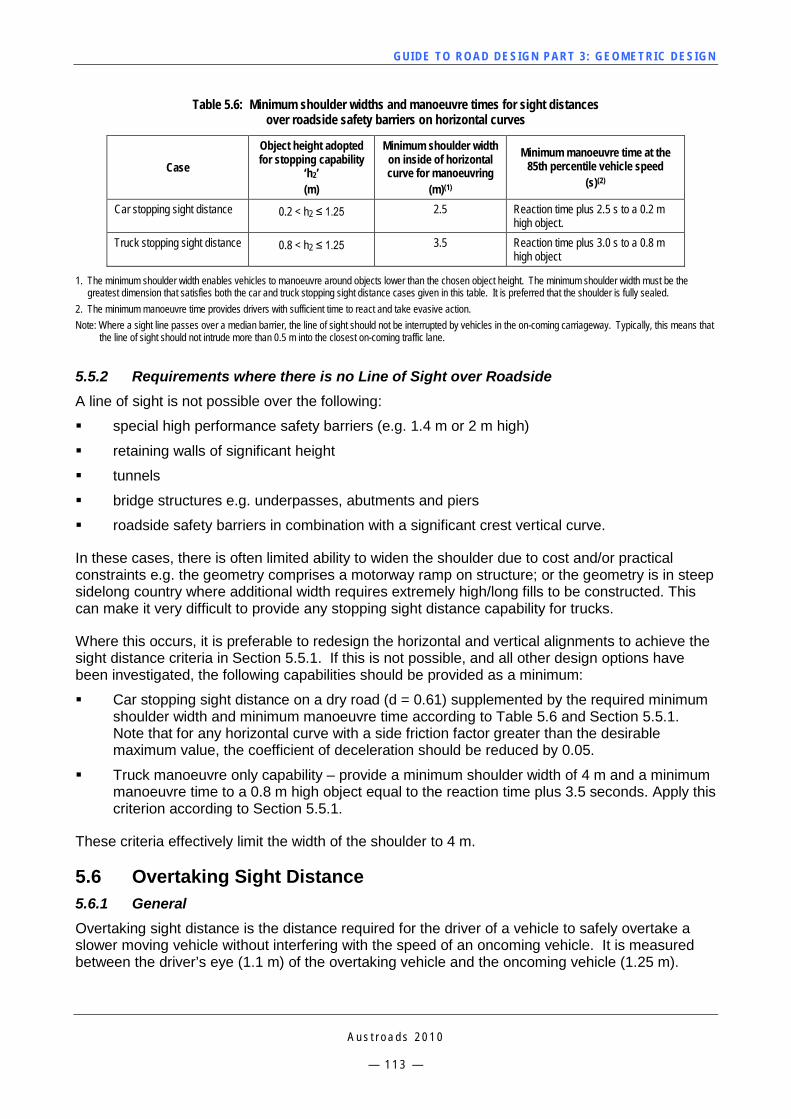
GUI DE TO RO A D DE SIG N P ART 3 : GEO MET RI C D ESI G N
A u s t r o a d s 2 0 1 0
— 1 1 3 —
Table 5.6: Minimum shoulder widths and manoeuvre times for sight distances over roadside safety barriers on horizontal curves
Case
Object height adopted for stopping capability
‘h2’ (m)
Minimum shoulder width on inside of horizontal curve for manoeuvring
(m)(1)
Minimum manoeuvre time at the 85th percentile vehicle speed
(s)(2)
Car stopping sight distance 0.2 < h2 ≤ 1.25 2.5 Reaction time plus 2.5 s to a 0.2 m high object.
Truck stopping sight distance 0.8 < h2 ≤ 1.25 3.5 Reaction time plus 3.0 s to a 0.8 m high object
1. The minimum shoulder width enables vehicles to manoeuvre around objects lower than the chosen object height. The minimum shoulder width must be the greatest dimension that satisfies both the car and truck stopping sight distance cases given in this table. It is preferred that the shoulder is fully sealed.
2. The minimum manoeuvre time provides drivers with sufficient time to react and take evasive action. Note: Where a sight line passes over a median barrier, the line of sight should not be interrupted by vehicles in the on-coming carriageway. Typically, this means that
the line of sight should not intrude more than 0.5 m into the closest on-coming traffic lane.
5.5.2 Requirements where there is no Line of Sight over Roadside A line of sight is not possible over the following:
special high performance safety barriers (e.g. 1.4 m or 2 m high)
retaining walls of significant height
tunnels
bridge structures e.g. underpasses, abutments and piers
roadside safety barriers in combination with a significant crest vertical curve.
In these cases, there is often limited ability to widen the shoulder due to cost and/or practical constraints e.g. the geometry comprises a motorway ramp on structure; or the geometry is in steep sidelong country where additional width requires extremely high/long fills to be constructed. This can make it very difficult to provide any stopping sight distance capability for trucks.
Where this occurs, it is preferable to redesign the horizontal and vertical alignments to achieve the sight distance criteria in Section 5.5.1. If this is not possible, and all other design options have been investigated, the following capabilities should be provided as a minimum:
Car stopping sight distance on a dry road (d = 0.61) supplemented by the required minimum shoulder width and minimum manoeuvre time according to Table 5.6 and Section 5.5.1. Note that for any horizontal curve with a side friction factor greater than the desirable maximum value, the coefficient of deceleration should be reduced by 0.05.
Truck manoeuvre only capability – provide a minimum shoulder width of 4 m and a minimum manoeuvre time to a 0.8 m high object equal to the reaction time plus 3.5 seconds. Apply this criterion according to Section 5.5.1.
These criteria effectively limit the width of the shoulder to 4 m.
5.6 Overtaking Sight Distance 5.6.1 General Overtaking sight distance is the distance required for the driver of a vehicle to safely overtake a slower moving vehicle without interfering with the speed of an oncoming vehicle. It is measured between the driver’s eye (1.1 m) of the overtaking vehicle and the oncoming vehicle (1.25 m).
GUI DE TO RO A D DE SIG N P ART 3 : GEO MET RI C D ESI G N
A u s t r o a d s 2 0 1 0
— 1 1 4 —
Overtaking sight distance is considered only on high-speed, two-lane two-way roads. On these roads, the overtaking of slower moving vehicles is only possible when there is a suitable gap in the oncoming traffic accompanied by sufficient sight distance and appropriate line marking. Sections with adequate overtaking sight distance should be provided as frequently as possible, as they are an essential safety measure by reducing driver frustration and risk taking. The desirable frequency is related to the operating speed, traffic volume and composition, terrain and construction cost. Overtaking demand increases rapidly as traffic volume increases, while overtaking capacity in the opposing lane decreases as volume increases. As a general rule, if overtaking sight distance cannot be economically provided at least once in each 5 km of road or the operating speed divided by 20 (km) which is three to five minutes of driving time apart, (Troutbeck 1981), consideration should be given to the construction of overtaking lanes (Section 9.4).
In practice, overtaking zones will usually be the fortuitous result of road alignment and cross-section. Because of the large sight distances involved, it is often not practical to achieve overtaking zones through design alone (costly to provide). However, good design practice will include a check on the overtaking zones that are provided and may result in cases where an overtaking zone can be achieved through a practical refinement of the design. More commonly though, the proportion of road that provides overtaking is used in conjunction with traffic volumes to assess the level of service provided by a section of road and hence determine whether overtaking lanes are warranted.
The Austroads parameters for determining the start and finish of overtaking zones dictate that there are few passing opportunities on New Zealand roads. The New Zealand practice to provide a desirable minimum overtaking sight distance for vertical curve design is to double safe stopping sight distance.
5.6.2 Overtaking Model The overtaking manoeuvre has a large number of variables, such as:
the judgement of the overtaking driver and the risks the driver is prepared to take
the speed and size of vehicles to be overtaken
the speed of the overtaking vehicle
the speed of a potential on coming vehicle
the evasive action or braking undertaken by the vehicle or the overtaken vehicle.
Since the sixth edition of the Austroads Rural Road Design Guide (NAASRA 1980), overtaking has been assessed by means of a model that was derived from research into overtaking on Australian rural roads (Troutbeck 1981). There are two main considerations with the overtaking model: (Figure 5.5).
Establishment: A minimum sight distance that is adequate to encourage a given proportion of drivers to commence an overtaking manoeuvre. This is called the Overtaking Establishment Sight Distance (OED) as it establishes a length of road as a potential overtaking zone. OED is the sight distance required for most drivers of passenger cars to overtake other vehicles.
Continuation: A critical sight distance, which if maintained for some length of road after the OED has become available, will enable an overtaking driver to either complete or abandon a manoeuvre already commenced with safety. This is called the Overtaking Continuation Sight Distance (OCD). After the establishment sight distance first becomes available, an overtaking zone is assumed to extend as long as this shorter distance remains available, subject to the constraint in the next paragraph.
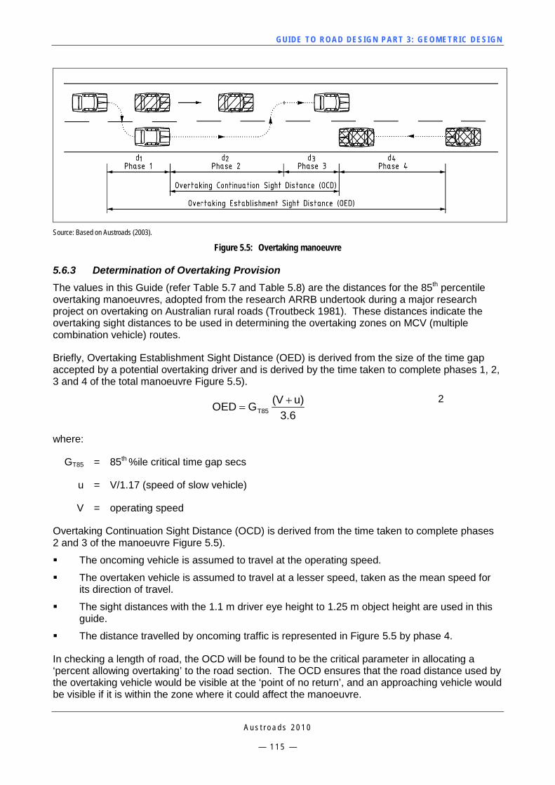
GUI DE TO RO A D DE SIG N P ART 3 : GEO MET RI C D ESI G N
A u s t r o a d s 2 0 1 0
— 1 1 5 —
Source: Based on Austroads (2003).
Figure 5.5: Overtaking manoeuvre
5.6.3 Determination of Overtaking Provision The values in this Guide (refer Table 5.7 and Table 5.8) are the distances for the 85th percentile overtaking manoeuvres, adopted from the research ARRB undertook during a major research project on overtaking on Australian rural roads (Troutbeck 1981). These distances indicate the overtaking sight distances to be used in determining the overtaking zones on MCV (multiple combination vehicle) routes.
Briefly, Overtaking Establishment Sight Distance (OED) is derived from the size of the time gap accepted by a potential overtaking driver and is derived by the time taken to complete phases 1, 2, 3 and 4 of the total manoeuvre Figure 5.5).
3.6
u)(VGOED T85+
= 2
where:
GT85 = 85th %ile critical time gap secs
u = V/1.17 (speed of slow vehicle)
V = operating speed
Overtaking Continuation Sight Distance (OCD) is derived from the time taken to complete phases 2 and 3 of the manoeuvre Figure 5.5).
The oncoming vehicle is assumed to travel at the operating speed.
The overtaken vehicle is assumed to travel at a lesser speed, taken as the mean speed for its direction of travel.
The sight distances with the 1.1 m driver eye height to 1.25 m object height are used in this guide.
The distance travelled by oncoming traffic is represented in Figure 5.5 by phase 4.
In checking a length of road, the OCD will be found to be the critical parameter in allocating a ‘percent allowing overtaking’ to the road section. The OCD ensures that the road distance used by the overtaking vehicle would be visible at the ‘point of no return’, and an approaching vehicle would be visible if it is within the zone where it could affect the manoeuvre.
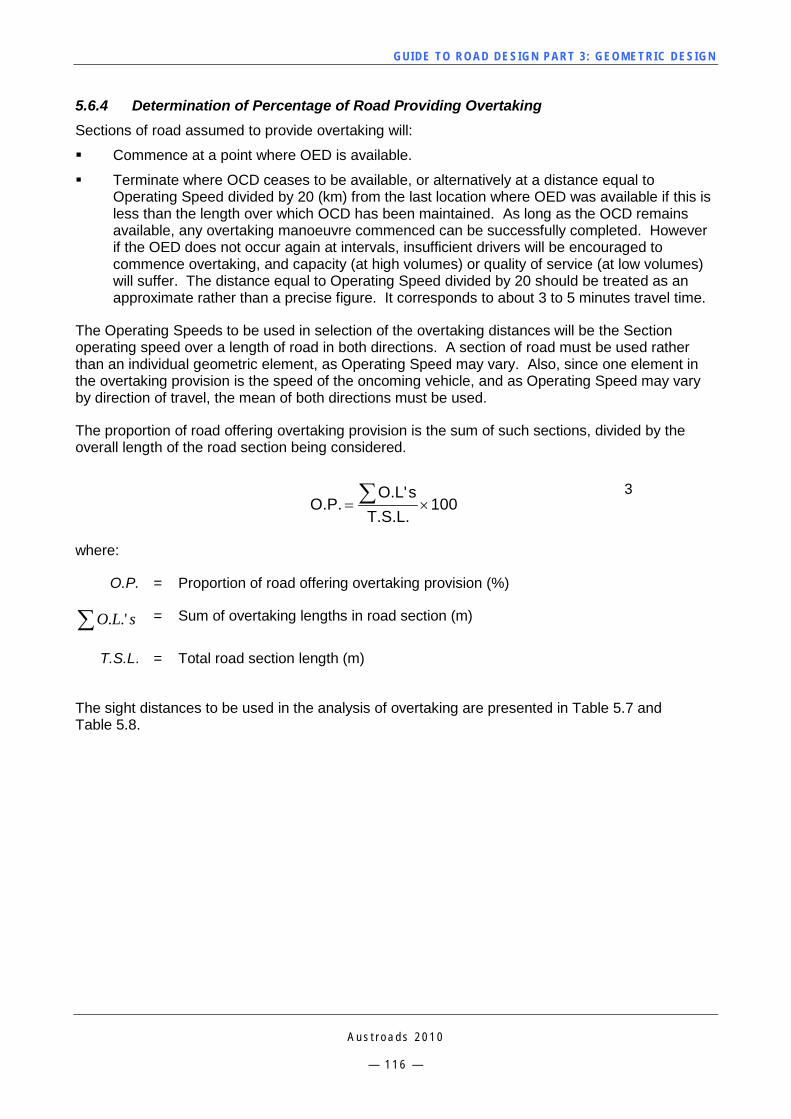
GUI DE TO RO A D DE SIG N P ART 3 : GEO MET RI C D ESI G N
A u s t r o a d s 2 0 1 0
— 1 1 6 —
5.6.4 Determination of Percentage of Road Providing Overtaking Sections of road assumed to provide overtaking will:
Commence at a point where OED is available.
Terminate where OCD ceases to be available, or alternatively at a distance equal to Operating Speed divided by 20 (km) from the last location where OED was available if this is less than the length over which OCD has been maintained. As long as the OCD remains available, any overtaking manoeuvre commenced can be successfully completed. However if the OED does not occur again at intervals, insufficient drivers will be encouraged to commence overtaking, and capacity (at high volumes) or quality of service (at low volumes) will suffer. The distance equal to Operating Speed divided by 20 should be treated as an approximate rather than a precise figure. It corresponds to about 3 to 5 minutes travel time.
The Operating Speeds to be used in selection of the overtaking distances will be the Section operating speed over a length of road in both directions. A section of road must be used rather than an individual geometric element, as Operating Speed may vary. Also, since one element in the overtaking provision is the speed of the oncoming vehicle, and as Operating Speed may vary by direction of travel, the mean of both directions must be used.
The proportion of road offering overtaking provision is the sum of such sections, divided by the overall length of the road section being considered.
100
T.S.L.sO.L'
O.P. ×= ∑ 3
where:
O.P. = Proportion of road offering overtaking provision (%)
∑ sLO .'. = Sum of overtaking lengths in road section (m)
T.S.L. = Total road section length (m)
The sight distances to be used in the analysis of overtaking are presented in Table 5.7 and Table 5.8.
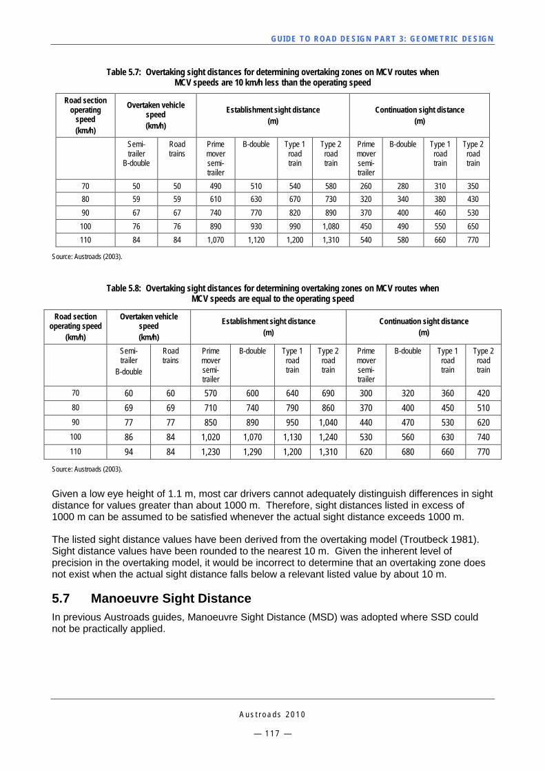
GUI DE TO RO A D DE SIG N P ART 3 : GEO MET RI C D ESI G N
A u s t r o a d s 2 0 1 0
— 1 1 7 —
Table 5.7: Overtaking sight distances for determining overtaking zones on MCV routes when MCV speeds are 10 km/h less than the operating speed
Road section operating
speed (km/h)
Overtaken vehicle speed (km/h)
Establishment sight distance (m)
Continuation sight distance (m)
Semi-trailer
B-double
Road trains
Prime mover semi-trailer
B-double Type 1 road train
Type 2 road train
Prime mover semi-trailer
B-double Type 1 road train
Type 2 road train
70 50 50 490 510 540 580 260 280 310 350 80 59 59 610 630 670 730 320 340 380 430 90 67 67 740 770 820 890 370 400 460 530 100 76 76 890 930 990 1,080 450 490 550 650 110 84 84 1,070 1,120 1,200 1,310 540 580 660 770
Source: Austroads (2003).
Table 5.8: Overtaking sight distances for determining overtaking zones on MCV routes when MCV speeds are equal to the operating speed
Road section operating speed
(km/h)
Overtaken vehicle speed (km/h)
Establishment sight distance (m)
Continuation sight distance (m)
Semi-trailer
B-double
Road trains
Prime mover semi-trailer
B-double Type 1 road train
Type 2 road train
Prime mover semi-trailer
B-double Type 1 road train
Type 2 road train
70 60 60 570 600 640 690 300 320 360 420 80 69 69 710 740 790 860 370 400 450 510 90 77 77 850 890 950 1,040 440 470 530 620
100 86 84 1,020 1,070 1,130 1,240 530 560 630 740 110 94 84 1,230 1,290 1,200 1,310 620 680 660 770
Source: Austroads (2003).
Given a low eye height of 1.1 m, most car drivers cannot adequately distinguish differences in sight distance for values greater than about 1000 m. Therefore, sight distances listed in excess of 1000 m can be assumed to be satisfied whenever the actual sight distance exceeds 1000 m.
The listed sight distance values have been derived from the overtaking model (Troutbeck 1981). Sight distance values have been rounded to the nearest 10 m. Given the inherent level of precision in the overtaking model, it would be incorrect to determine that an overtaking zone does not exist when the actual sight distance falls below a relevant listed value by about 10 m.
5.7 Manoeuvre Sight Distance In previous Austroads guides, Manoeuvre Sight Distance (MSD) was adopted where SSD could not be practically applied.
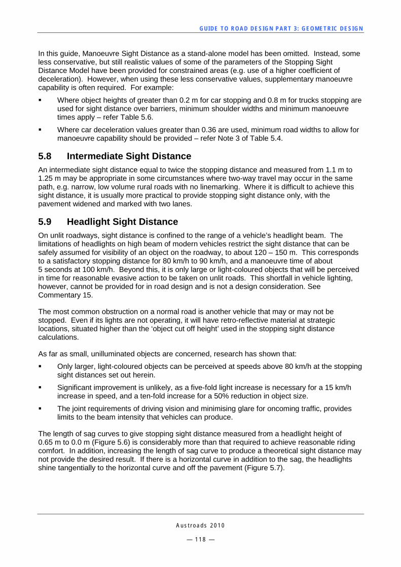
GUI DE TO RO A D DE SIG N P ART 3 : GEO MET RI C D ESI G N
A u s t r o a d s 2 0 1 0
— 1 1 8 —
In this guide, Manoeuvre Sight Distance as a stand-alone model has been omitted. Instead, some less conservative, but still realistic values of some of the parameters of the Stopping Sight Distance Model have been provided for constrained areas (e.g. use of a higher coefficient of deceleration). However, when using these less conservative values, supplementary manoeuvre capability is often required. For example:
Where object heights of greater than 0.2 m for car stopping and 0.8 m for trucks stopping are used for sight distance over barriers, minimum shoulder widths and minimum manoeuvre times apply – refer Table 5.6.
Where car deceleration values greater than 0.36 are used, minimum road widths to allow for manoeuvre capability should be provided – refer Note 3 of Table 5.4.
5.8 Intermediate Sight Distance An intermediate sight distance equal to twice the stopping distance and measured from 1.1 m to 1.25 m may be appropriate in some circumstances where two-way travel may occur in the same path, e.g. narrow, low volume rural roads with no linemarking. Where it is difficult to achieve this sight distance, it is usually more practical to provide stopping sight distance only, with the pavement widened and marked with two lanes.
5.9 Headlight Sight Distance On unlit roadways, sight distance is confined to the range of a vehicle’s headlight beam. The limitations of headlights on high beam of modern vehicles restrict the sight distance that can be safely assumed for visibility of an object on the roadway, to about 120 – 150 m. This corresponds to a satisfactory stopping distance for 80 km/h to 90 km/h, and a manoeuvre time of about 5 seconds at 100 km/h. Beyond this, it is only large or light-coloured objects that will be perceived in time for reasonable evasive action to be taken on unlit roads. This shortfall in vehicle lighting, however, cannot be provided for in road design and is not a design consideration. See Commentary 15.
The most common obstruction on a normal road is another vehicle that may or may not be stopped. Even if its lights are not operating, it will have retro-reflective material at strategic locations, situated higher than the ‘object cut off height’ used in the stopping sight distance calculations.
As far as small, unilluminated objects are concerned, research has shown that:
Only larger, light-coloured objects can be perceived at speeds above 80 km/h at the stopping sight distances set out herein.
Significant improvement is unlikely, as a five-fold light increase is necessary for a 15 km/h increase in speed, and a ten-fold increase for a 50% reduction in object size.
The joint requirements of driving vision and minimising glare for oncoming traffic, provides limits to the beam intensity that vehicles can produce.
The length of sag curves to give stopping sight distance measured from a headlight height of 0.65 m to 0.0 m (Figure 5.6) is considerably more than that required to achieve reasonable riding comfort. In addition, increasing the length of sag curve to produce a theoretical sight distance may not provide the desired result. If there is a horizontal curve in addition to the sag, the headlights shine tangentially to the horizontal curve and off the pavement (Figure 5.7).
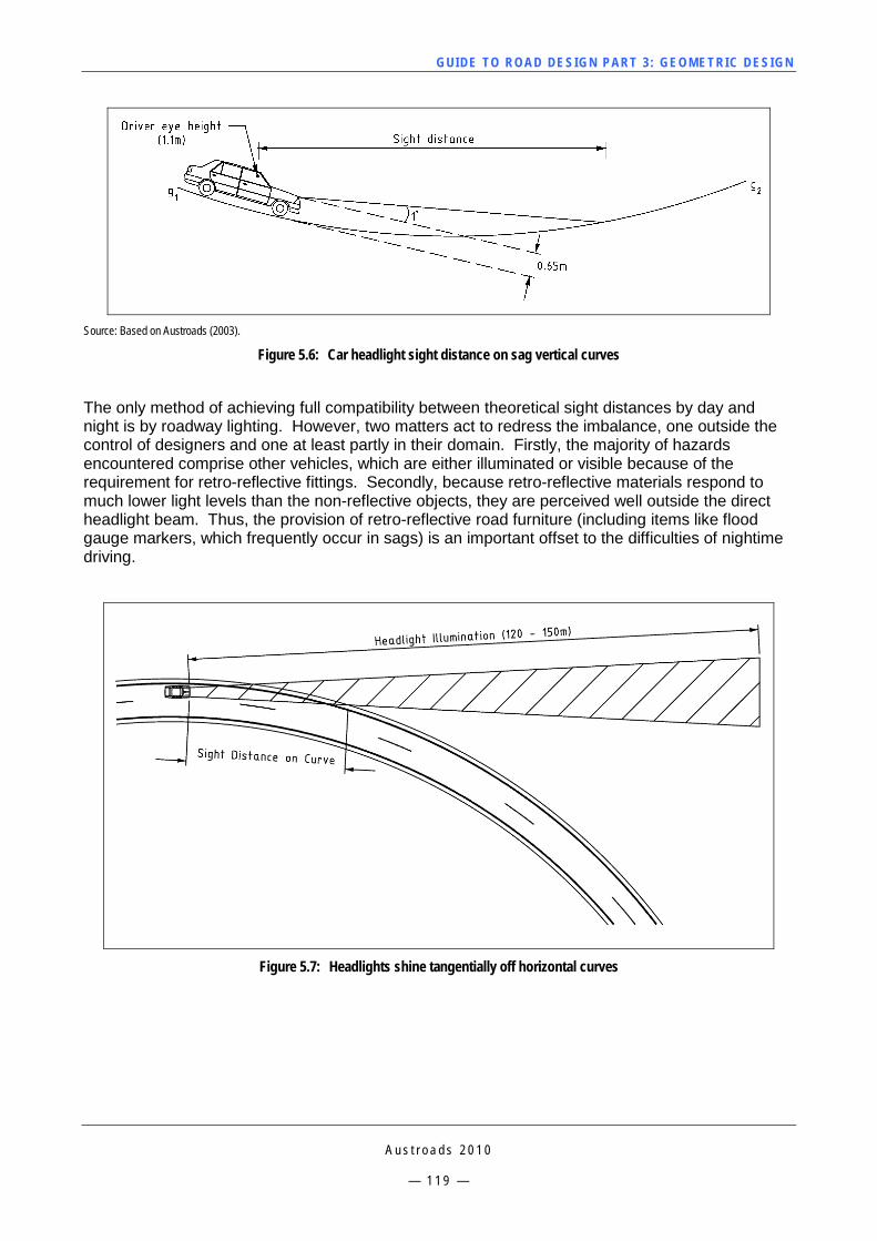
GUI DE TO RO A D DE SIG N P ART 3 : GEO MET RI C D ESI G N
A u s t r o a d s 2 0 1 0
— 1 1 9 —
Source: Based on Austroads (2003).
Figure 5.6: Car headlight sight distance on sag vertical curves
The only method of achieving full compatibility between theoretical sight distances by day and night is by roadway lighting. However, two matters act to redress the imbalance, one outside the control of designers and one at least partly in their domain. Firstly, the majority of hazards encountered comprise other vehicles, which are either illuminated or visible because of the requirement for retro-reflective fittings. Secondly, because retro-reflective materials respond to much lower light levels than the non-reflective objects, they are perceived well outside the direct headlight beam. Thus, the provision of retro-reflective road furniture (including items like flood gauge markers, which frequently occur in sags) is an important offset to the difficulties of nightime driving.
Figure 5.7: Headlights shine tangentially off horizontal curves
GUI DE TO RO A D DE SIG N P ART 3 : GEO MET RI C D ESI G N
A u s t r o a d s 2 0 1 0
— 1 2 0 —
5.10 Horizontal Curve Perception Sight Distance A major characteristic of low speed roads and intermediate speed roads is the way drivers will speed up on longer straights and through larger radius horizontal curves then slow down where necessary for smaller radius curves. Since the sixth edition of the NAASRA Interim Guide to the Geometric Design of Rural Roads (NAASRA 1980), such roads have been designed so that the geometric elements matched the operating speeds along the road. This means that when vehicles have to slow down for a horizontal curve, drivers must see a sufficient amount of the curve in order to perceive its curvature, react and slow down appropriately for the curve.
If drivers are unable to perceive the curvature of the road, they may not slow down to an appropriate speed, which increases the risk of a single vehicle crash. Therefore, curves constructed on these types of alignments should only be used when the curve operating speed is no more than 5 km/h less than the operating speed on the approach to the curve.
Normally, sufficient sight distance for a horizontal curve is provided through the practice of not having a horizontal curve start over a crest. Designers should also consider the locations of cut batters or other visual obstruction on the inside of a left turning horizontal curve, which can hide the degree of curvature of the road ahead, especially if the horizontal curve is used in conjunction with a spiral. However, there are times where this cannot be avoided and the following criteria should be applied in order to check that sufficient visibility is provided for the curve:
A driver eye height of 1.1 m
A zero object height because the driver needs to see the road surface in order to perceive the curvature Road edge guide posts and cut batters can only be considered as supplementary aids
A driver needs to see sufficient length of the curve in order to judge its curvature The driver must be able to see the minimum of: — 5 degrees of arc — about 80 m of arc — the whole curve.
If the curve is transitioned however, at least 80% of the transition length and desirably all of the transition needs to be seen by the driver.
The length of arc that needs to be perceived must be seen from a point that allows the driver to react then decelerate – refer Section 5.2.2 for guidance on the choice of reaction time. The deceleration should only require comfortable braking by drivers, therefore, a maximum deceleration rate of 2.5 m/s/s should be used. Typically, this means a distance of 25 m will accommodate a 10 km/h speed reduction from 90 km/h and 40 m will accommodate a 15 km/h speed reduction. Deceleration distances should be adjusted for the effect of grade.
The sight distance is the sum of the reaction distance, arc length for perception and deceleration distance. If the curve is transitioned, it is possible for the deceleration distance to coincide with up to the first half of the transition. If the curve is untransitioned, deceleration up to the curve tangent point can be assumed.
Provision of horizontal curve perception distance may require a larger crest than is required for stopping sight distance.

GUI DE TO RO A D DE SIG N P ART 3 : GEO MET RI C D ESI G N
A u s t r o a d s 2 0 1 0
— 1 2 1 —
5.11 Other Restrictions to Visibility There are other minor constraints on sight distance that must be mitigated for by the designer:
In avenues of trees, visibility can be reduced at a sag owing to the line of sight being interrupted by the foliage. The same may happen where a bridge crosses a sag and the line of sight is obstructed.
Road safety barriers, bridge handrails, median kerbs and similar obstructions can restrict the visibility available at horizontal and vertical curves.
There is a sizeable difference between the length of sight distance available to a driver depending on whether the curve ahead is to the left or the right.
GUI DE TO RO A D DE SIG N P ART 3 : GEO MET RI C D ESI G N
A u s t r o a d s 2 0 1 0
— 1 2 2 —
6 COORDINATION OF HORIZONTAL AND VERTICAL ALIGNMENT
6.1 Principles In engineering terms, road alignments have to service traffic in terms of providing a route that meets the constraints imposed by vehicle dynamics, occupant comfort, and topography. This means that most road alignments are in fact complex three-dimensional splines that do not have a simple mathematical definition. This problem has historically been addressed by reducing the three-dimensional alignment to two, two-dimensional alignments. In each case, the alignments are made up of geometric elements that are convenient to calculate and construct yet still ensure that vehicle dynamic constraints are met. Even with the advent of computers, this approach has still proven to be the most convenient for both design and construction. To use complex three-dimensional models would introduce unnecessary complexity into the process but it is necessary to ensure that the two alignments are properly coordinated and complement each other.
The interrelationship of horizontal and vertical alignment is best addressed in the concept and preliminary design phases of the project. At this stage, appropriate trade-offs and balances between design speed and the character of the road – traffic volume, topography and existing development – can be made. Because they must be complementary, horizontal and vertical geometry can ruin the best parts and accentuate the weak points of each element. Excellence in the combination of their designs increases efficiency and safety, encourages uniform speed, and improves appearance – almost always without additional cost.
Where possible, horizontal and vertical geometry should be coordinated for appearance and safety. In principle, co-ordination means that horizontal and vertical curves should either be completely superimposed or completely separated. The related horizontal and vertical elements should be of similar lengths, with the vertical curve contained within the horizontal curve. This arrangement should produce the most pleasing, flowing three-dimensional result, which is more likely to be in harmony with the natural landform.
In urban situations it is frequently the case that such aesthetic considerations will be very difficult or expensive to apply. Many major urban roads are developed by widening established streets, or by intermittent alignment improvements. In consequence, the existing street locations and levels, and abutting development, will exert a strong influence on the alignment of major urban roads.
6.2 Safety Considerations The following relationships between horizontal and vertical alignment should be applied to the design wherever possible for safety, aesthetic and drainage reasons:
A crest can obscure the horizontal alignment and the severity of a horizontal curve. Minimum radius horizontal curves should not, therefore, be used with crest vertical curves. Lateral shifts in the alignment on crests can lead to confusion and accidents. Lateral shifts of approximately one lane width are particularly hazardous as shown on Figure 6.1.
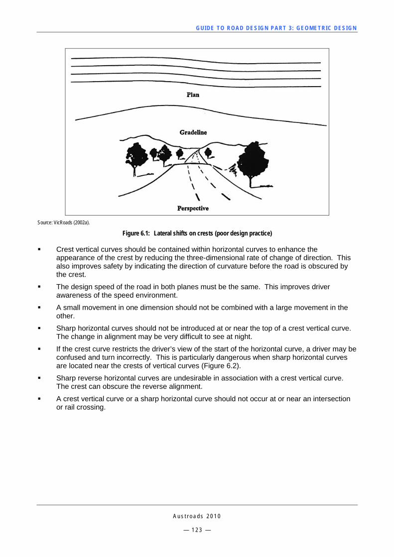
GUI DE TO RO A D DE SIG N P ART 3 : GEO MET RI C D ESI G N
A u s t r o a d s 2 0 1 0
— 1 2 3 —
Source: VicRoads (2002a).
Figure 6.1: Lateral shifts on crests (poor design practice)
Crest vertical curves should be contained within horizontal curves to enhance the appearance of the crest by reducing the three-dimensional rate of change of direction. This also improves safety by indicating the direction of curvature before the road is obscured by the crest.
The design speed of the road in both planes must be the same. This improves driver awareness of the speed environment.
A small movement in one dimension should not be combined with a large movement in the other.
Sharp horizontal curves should not be introduced at or near the top of a crest vertical curve. The change in alignment may be very difficult to see at night.
If the crest curve restricts the driver’s view of the start of the horizontal curve, a driver may be confused and turn incorrectly. This is particularly dangerous when sharp horizontal curves are located near the crests of vertical curves (Figure 6.2).
Sharp reverse horizontal curves are undesirable in association with a crest vertical curve. The crest can obscure the reverse alignment.
A crest vertical curve or a sharp horizontal curve should not occur at or near an intersection or rail crossing.
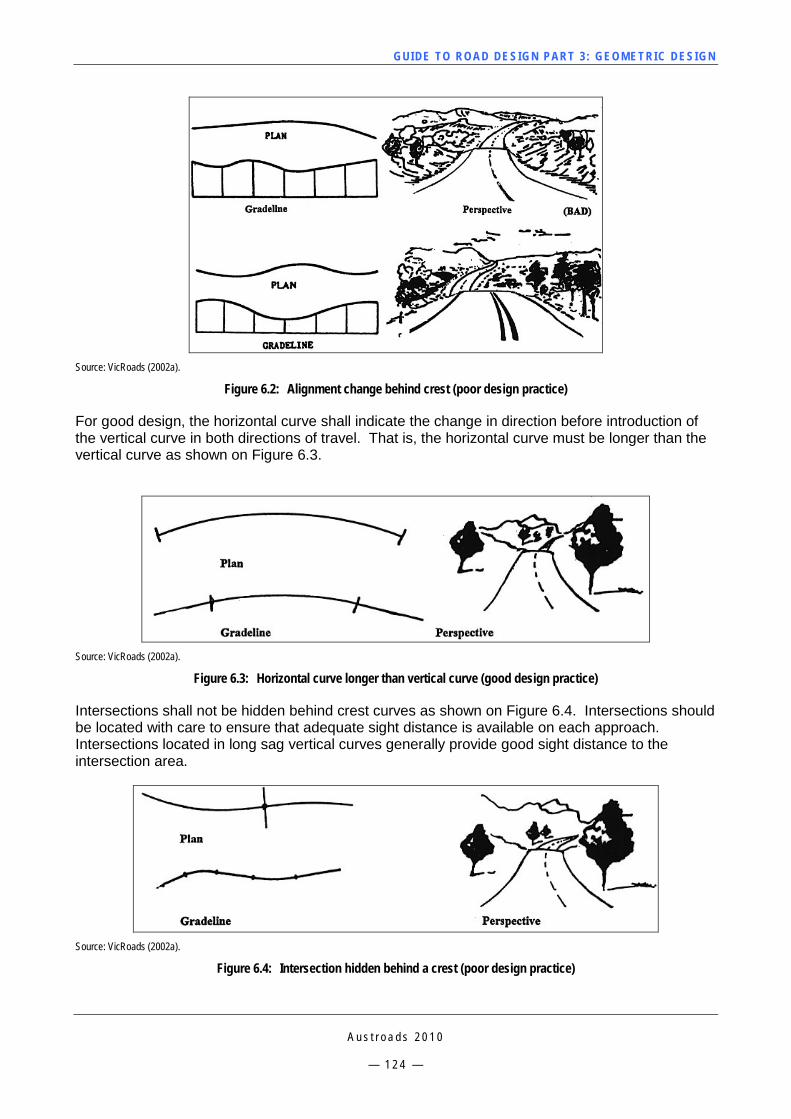
GUI DE TO RO A D DE SIG N P ART 3 : GEO MET RI C D ESI G N
A u s t r o a d s 2 0 1 0
— 1 2 4 —
Source: VicRoads (2002a).
Figure 6.2: Alignment change behind crest (poor design practice)
For good design, the horizontal curve shall indicate the change in direction before introduction of the vertical curve in both directions of travel. That is, the horizontal curve must be longer than the vertical curve as shown on Figure 6.3.
Source: VicRoads (2002a).
Figure 6.3: Horizontal curve longer than vertical curve (good design practice)
Intersections shall not be hidden behind crest curves as shown on Figure 6.4. Intersections should be located with care to ensure that adequate sight distance is available on each approach. Intersections located in long sag vertical curves generally provide good sight distance to the intersection area.
Source: VicRoads (2002a).
Figure 6.4: Intersection hidden behind a crest (poor design practice)
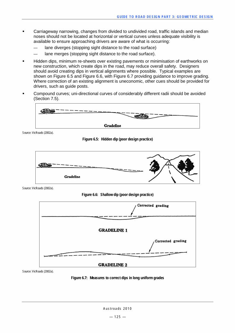
GUI DE TO RO A D DE SIG N P ART 3 : GEO MET RI C D ESI G N
A u s t r o a d s 2 0 1 0
— 1 2 5 —
Carriageway narrowing, changes from divided to undivided road, traffic islands and median noses should not be located at horizontal or vertical curves unless adequate visibility is available to ensure approaching drivers are aware of what is occurring: — lane diverges (stopping sight distance to the road surface) — lane merges (stopping sight distance to the road surface).
Hidden dips, minimum re-sheets over existing pavements or minimisation of earthworks on new construction, which create dips in the road, may reduce overall safety. Designers should avoid creating dips in vertical alignments where possible. Typical examples are shown on Figure 6.5 and Figure 6.6, with Figure 6.7 providing guidance to improve grading. Where correction of an existing alignment is uneconomic, other cues should be provided for drivers, such as guide posts.
Compound curves; uni-directional curves of considerably different radii should be avoided (Section 7.5).
Source: VicRoads (2002a).
Figure 6.5: Hidden dip (poor design practice)
Source: VicRoads (2002a).
Figure 6.6: Shallow dip (poor design practice)
Source: VicRoads (2002a).
Figure 6.7: Measures to correct dips in long uniform grades
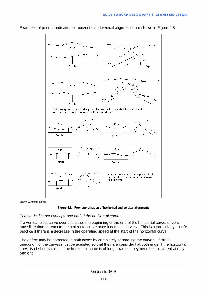
GUI DE TO RO A D DE SIG N P ART 3 : GEO MET RI C D ESI G N
A u s t r o a d s 2 0 1 0
— 1 2 6 —
Examples of poor coordination of horizontal and vertical alignments are shown in Figure 6.8.
Source: Austroads (2003).
Figure 6.8: Poor coordination of horizontal and vertical alignments
The vertical curve overlaps one end of the horizontal curve
If a vertical crest curve overlaps either the beginning or the end of the horizontal curve, drivers have little time to react to the horizontal curve once it comes into view. This is a particularly unsafe practice if there is a decrease in the operating speed at the start of the horizontal curve.
The defect may be corrected in both cases by completely separating the curves. If this is uneconomic, the curves must be adjusted so that they are coincident at both ends, if the horizontal curve is of short radius. If the horizontal curve is of longer radius, they need be coincident at only one end.
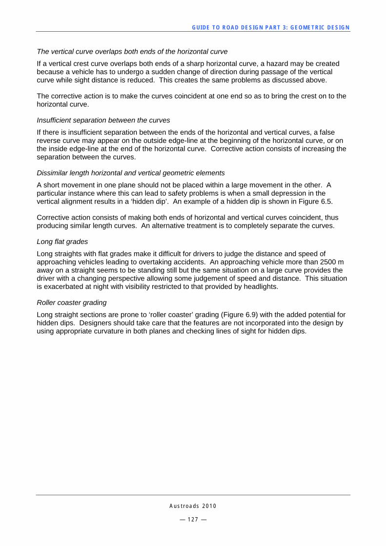
GUI DE TO RO A D DE SIG N P ART 3 : GEO MET RI C D ESI G N
A u s t r o a d s 2 0 1 0
— 1 2 7 —
The vertical curve overlaps both ends of the horizontal curve
If a vertical crest curve overlaps both ends of a sharp horizontal curve, a hazard may be created because a vehicle has to undergo a sudden change of direction during passage of the vertical curve while sight distance is reduced. This creates the same problems as discussed above.
The corrective action is to make the curves coincident at one end so as to bring the crest on to the horizontal curve.
Insufficient separation between the curves
If there is insufficient separation between the ends of the horizontal and vertical curves, a false reverse curve may appear on the outside edge-line at the beginning of the horizontal curve, or on the inside edge-line at the end of the horizontal curve. Corrective action consists of increasing the separation between the curves.
Dissimilar length horizontal and vertical geometric elements
A short movement in one plane should not be placed within a large movement in the other. A particular instance where this can lead to safety problems is when a small depression in the vertical alignment results in a ‘hidden dip’. An example of a hidden dip is shown in Figure 6.5.
Corrective action consists of making both ends of horizontal and vertical curves coincident, thus producing similar length curves. An alternative treatment is to completely separate the curves.
Long flat grades
Long straights with flat grades make it difficult for drivers to judge the distance and speed of approaching vehicles leading to overtaking accidents. An approaching vehicle more than 2500 m away on a straight seems to be standing still but the same situation on a large curve provides the driver with a changing perspective allowing some judgement of speed and distance. This situation is exacerbated at night with visibility restricted to that provided by headlights.
Roller coaster grading
Long straight sections are prone to ‘roller coaster’ grading (Figure 6.9) with the added potential for hidden dips. Designers should take care that the features are not incorporated into the design by using appropriate curvature in both planes and checking lines of sight for hidden dips.
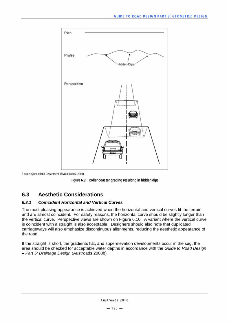
GUI DE TO RO A D DE SIG N P ART 3 : GEO MET RI C D ESI G N
A u s t r o a d s 2 0 1 0
— 1 2 8 —
Source: Queensland Department of Main Roads (2001).
Figure 6.9: Roller coaster grading resulting in hidden dips
6.3 Aesthetic Considerations 6.3.1 Coincident Horizontal and Vertical Curves The most pleasing appearance is achieved when the horizontal and vertical curves fit the terrain, and are almost coincident. For safety reasons, the horizontal curve should be slightly longer than the vertical curve. Perspective views are shown on Figure 6.10. A variant where the vertical curve is coincident with a straight is also acceptable. Designers should also note that duplicated carriageways will also emphasize discontinuous alignments, reducing the aesthetic appearance of the road.
If the straight is short, the gradients flat, and superelevation developments occur in the sag, the area should be checked for acceptable water depths in accordance with the Guide to Road Design – Part 5: Drainage Design (Austroads 2008b).
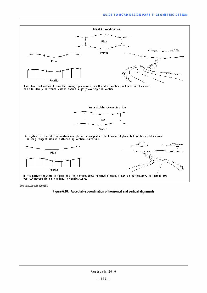
GUI DE TO RO A D DE SIG N P ART 3 : GEO MET RI C D ESI G N
A u s t r o a d s 2 0 1 0
— 1 2 9 —
Source: Austroads (2002b).
Figure 6.10: Acceptable coordination of horizontal and vertical alignments
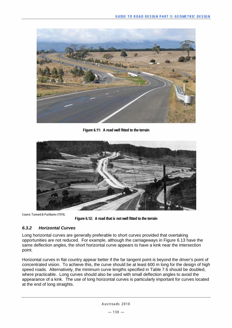
GUI DE TO RO A D DE SIG N P ART 3 : GEO MET RI C D ESI G N
A u s t r o a d s 2 0 1 0
— 1 3 0 —
Figure 6.11: A road well fitted to the terrain
Source: Tunnard & Pushkarev (1974).
Figure 6.12: A road that is not well fitted to the terrain
6.3.2 Horizontal Curves Long horizontal curves are generally preferable to short curves provided that overtaking opportunities are not reduced. For example, although the carriageways in Figure 6.13 have the same deflection angles, the short horizontal curve appears to have a kink near the intersection point.
Horizontal curves in flat country appear better if the far tangent point is beyond the driver’s point of concentrated vision. To achieve this, the curve should be at least 600 m long for the design of high speed roads. Alternatively, the minimum curve lengths specified in Table 7.6 should be doubled, where practicable. Long curves should also be used with small deflection angles to avoid the appearance of a kink. The use of long horizontal curves is particularly important for curves located at the end of long straights.
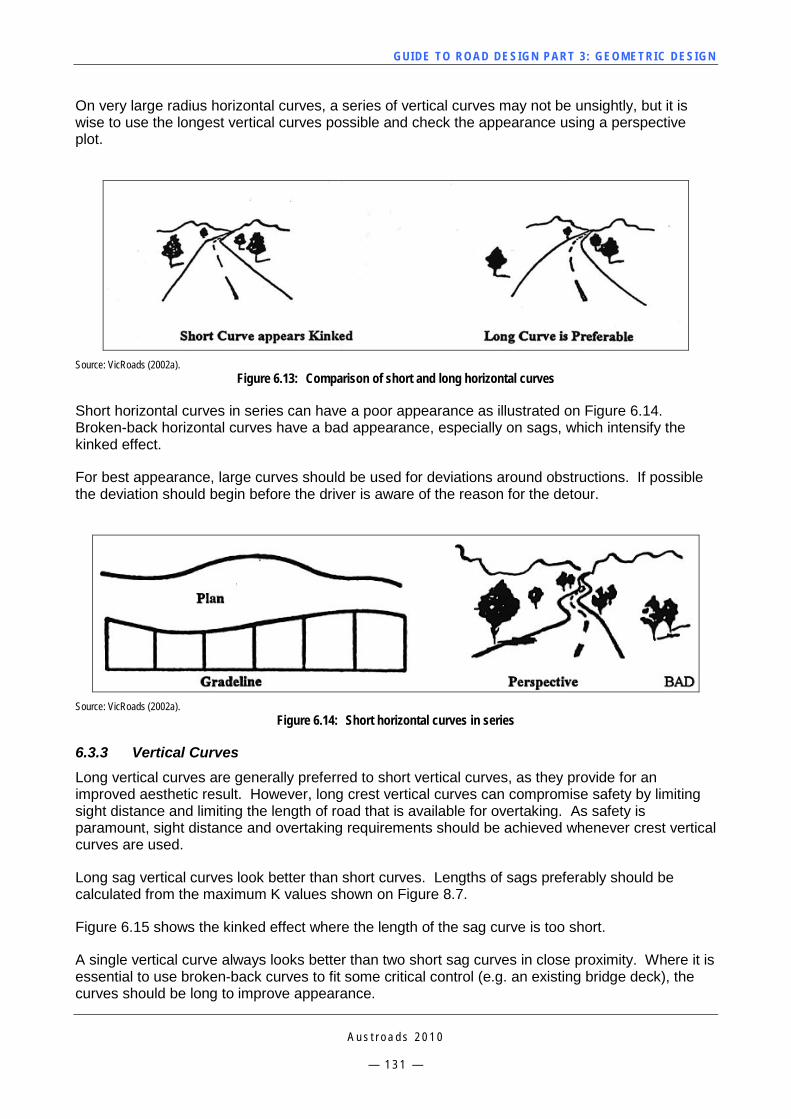
GUI DE TO RO A D DE SIG N P ART 3 : GEO MET RI C D ESI G N
A u s t r o a d s 2 0 1 0
— 1 3 1 —
On very large radius horizontal curves, a series of vertical curves may not be unsightly, but it is wise to use the longest vertical curves possible and check the appearance using a perspective plot.
Source: VicRoads (2002a).
Figure 6.13: Comparison of short and long horizontal curves
Short horizontal curves in series can have a poor appearance as illustrated on Figure 6.14. Broken-back horizontal curves have a bad appearance, especially on sags, which intensify the kinked effect.
For best appearance, large curves should be used for deviations around obstructions. If possible the deviation should begin before the driver is aware of the reason for the detour.
Source: VicRoads (2002a).
Figure 6.14: Short horizontal curves in series
6.3.3 Vertical Curves Long vertical curves are generally preferred to short vertical curves, as they provide for an improved aesthetic result. However, long crest vertical curves can compromise safety by limiting sight distance and limiting the length of road that is available for overtaking. As safety is paramount, sight distance and overtaking requirements should be achieved whenever crest vertical curves are used.
Long sag vertical curves look better than short curves. Lengths of sags preferably should be calculated from the maximum K values shown on Figure 8.7.
Figure 6.15 shows the kinked effect where the length of the sag curve is too short.
A single vertical curve always looks better than two short sag curves in close proximity. Where it is essential to use broken-back curves to fit some critical control (e.g. an existing bridge deck), the curves should be long to improve appearance.
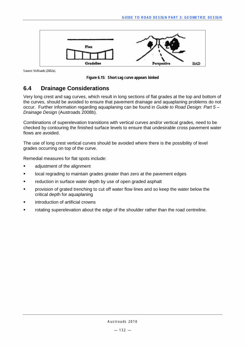
GUI DE TO RO A D DE SIG N P ART 3 : GEO MET RI C D ESI G N
A u s t r o a d s 2 0 1 0
— 1 3 2 —
Source: VicRoads (2002a).
Figure 6.15: Short sag curve appears kinked
6.4 Drainage Considerations Very long crest and sag curves, which result in long sections of flat grades at the top and bottom of the curves, should be avoided to ensure that pavement drainage and aquaplaning problems do not occur. Further information regarding aquaplaning can be found in Guide to Road Design: Part 5 – Drainage Design (Austroads 2008b).
Combinations of superelevation transitions with vertical curves and/or vertical grades, need to be checked by contouring the finished surface levels to ensure that undesirable cross pavement water flows are avoided.
The use of long crest vertical curves should be avoided where there is the possibility of level grades occurring on top of the curve.
Remedial measures for flat spots include:
adjustment of the alignment
local regrading to maintain grades greater than zero at the pavement edges
reduction in surface water depth by use of open graded asphalt
provision of grated trenching to cut off water flow lines and so keep the water below the critical depth for aquaplaning
introduction of artificial crowns
rotating superelevation about the edge of the shoulder rather than the road centreline.
GUI DE TO RO A D DE SIG N P ART 3 : GEO MET RI C D ESI G N
A u s t r o a d s 2 0 1 0
— 1 3 3 —
7 HORIZONTAL ALIGNMENT
7.1 General The horizontal alignment of a road is usually a series of straights (tangents) and circular curves that may or may not be connected by transition curves. The following sections outline various design criteria that are to be considered when developing a horizontal road alignment.
The speed adopted on an open road is affected more by the driver’s perception of the horizontal alignment of the road than by any other single design feature. For this reason, whenever curves are used to change the direction of travel or to suit the topography, the radii must be large enough to permit travel speeds commensurate with those expected on adjoining straights or along the whole of the section being designed. Generally, the adopted alignment should be as direct as possible, with curve radii as large as practicable. Given the importance of horizontal geometry determining the operating speed of vehicles, provision of horizontal curve perception sight distance (Section 5.10) should desirably be provided to enable drivers to perceive the curvature of the road and adjust their speed accordingly.
As with other elements of design, horizontal alignment should generally provide for safe and continuous operation at a uniform travel speed. Sudden reductions in standard, such as isolated curves of small radius (particularly at the end of long straights), introduce an element of surprise to the driver and should be avoided. The result of drivers not recognising the required action for these geometric features greatly increases the chance of a single vehicle accident occurring. The provision of geometric consistency is a fundamental requirement in geometric road design and in the application of the operating speed model.
Where physical restrictions on curve radii cannot be overcome and it becomes necessary to introduce curvature of lower standard than the design speed of the project (normally only applicable to low and intermediate speed rural roads and minor urban roads), the differences in design speeds of successive geometric elements should be less than or equal to the values shown on Table 7.1. On two-way roads, both directions of travel need to be considered. During the design of major roads, such as freeways, major rural highways and major urban roads, the same speed value should be used for the design of each horizontal element, to provide a consistent driving environment.
Designers should avoid locating features that are likely to require large/special vehicles to brake on curves, such as intersections where the major road is on a small radius curve. Note that the extra braking distances required on horizontal curves are not compensated by the higher driver eye height of trucks.
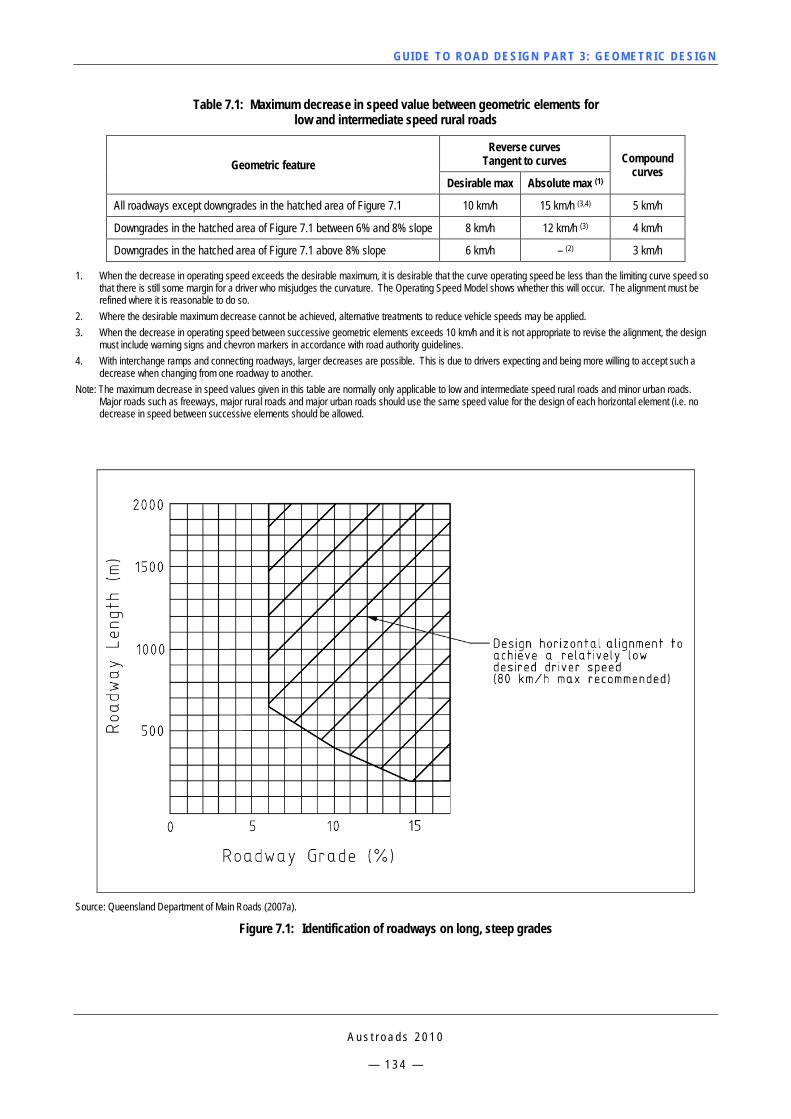
GUI DE TO RO A D DE SIG N P ART 3 : GEO MET RI C D ESI G N
A u s t r o a d s 2 0 1 0
— 1 3 4 —
Table 7.1: Maximum decrease in speed value between geometric elements for low and intermediate speed rural roads
Geometric feature Reverse curves
Tangent to curves Compound curves
Desirable max Absolute max (1)
All roadways except downgrades in the hatched area of Figure 7.1 10 km/h 15 km/h (3,4) 5 km/h
Downgrades in the hatched area of Figure 7.1 between 6% and 8% slope 8 km/h 12 km/h (3) 4 km/h
Downgrades in the hatched area of Figure 7.1 above 8% slope 6 km/h – (2) 3 km/h
1. When the decrease in operating speed exceeds the desirable maximum, it is desirable that the curve operating speed be less than the limiting curve speed so that there is still some margin for a driver who misjudges the curvature. The Operating Speed Model shows whether this will occur. The alignment must be refined where it is reasonable to do so.
2. Where the desirable maximum decrease cannot be achieved, alternative treatments to reduce vehicle speeds may be applied. 3. When the decrease in operating speed between successive geometric elements exceeds 10 km/h and it is not appropriate to revise the alignment, the design
must include warning signs and chevron markers in accordance with road authority guidelines. 4. With interchange ramps and connecting roadways, larger decreases are possible. This is due to drivers expecting and being more willing to accept such a
decrease when changing from one roadway to another. Note: The maximum decrease in speed values given in this table are normally only applicable to low and intermediate speed rural roads and minor urban roads.
Major roads such as freeways, major rural roads and major urban roads should use the same speed value for the design of each horizontal element (i.e. no decrease in speed between successive elements should be allowed.
Source: Queensland Department of Main Roads (2007a).
Figure 7.1: Identification of roadways on long, steep grades
GUI DE TO RO A D DE SIG N P ART 3 : GEO MET RI C D ESI G N
A u s t r o a d s 2 0 1 0
— 1 3 5 —
7.2 Horizontal Alignment Design Procedure Step 1
Identify all major controls on the alignment and categorise them as mandatory or discretionary.
Step 2
Decide upon an operating speed (Refer Section 3) that is appropriate both for the class of road and for the terrain. Minimum radii for these operating speeds are then obtained from Table 7.5. Radii used are chosen to fit the terrain and desirably should exceed the minimum. Refer to Figure 7.5 to Figure 7.7 for guidance on the relationship between speed, curve radii and superelevation.
Step 3
Prepare a trial alignment using a series of straights and curves, using the radii determined in Step 2. On low and intermediate speed alignments, curves used should generally be consistent. Special care must be taken with curves at the end of straights because of the high speeds that can be developed at these locations. Designers should also avoid locating floodways or floodway approaches on curved sections of road.
When developing a horizontal alignment, the following symbols are typically chosen to describe the various individual components. They are then combined to identify the intersection points, e.g. TC.
T = Tangent 7.3
C = Circular curve Section 7.4
S = Spiral or transition curve Section 7.5.4
Step 4
Prepare a trial gradeline, taking into account vertical controls and drainage aspects. Co-ordinate horizontal and vertical alignments as described in Section 6.
On downgrades, minimum curve radii should be increased by 10% for each 1% increase in grade over 3%. Refer Section 7.6.1.
Step 5
Check that all radii are compatible with estimated vehicle operating speeds using the procedure described in Section 3.
Step 6
Adjust the alignment so that:
all mandatory controls are met
discretionary controls are met as far as possible
curve radii are consistent with operating speeds at all locations
other controlling criteria are satisfied with special consideration given to the location of intersections and points of access to ensure that minimum sight distances and critical crossfall controls are met
earthworks are minimised.
GUI DE TO RO A D DE SIG N P ART 3 : GEO MET RI C D ESI G N
A u s t r o a d s 2 0 1 0
— 1 3 6 —
7.3 Tangents The tangent or straight section is the most common element of the horizontal alignment. It provides clear orientation, but at the same time is visually uninteresting, unless aimed at some landmark. Being totally predictable, with a view that appears static, it causes driver monotony and encourages the undesirable combination of fatigue and excessive speed in rural areas. At night, opposing headlights can cause glare problems for drivers. It is worth noting however, that these problems are only generally a problem on very long tangents.
Tangents of suitable length are desirable on two-lane, two-way roads to facilitate overtaking manoeuvres and should be provided as frequently as the terrain permits. Straight sections are too long (e.g. 1,000 m) if they encourage drivers to travel well in excess of the design speed and should therefore be avoided if practicable. Tangents that are too short to provide adequate separation between adjoining curves to enable a desirable rate of rotation of the pavement, should also be avoided as they have the potential to destabilise vehicles.
In flat topography, long straights on roads may have to be accepted. If curves are deliberately introduced into the design to break the monotony, they should have long arc lengths or else they will look like kinks. Unless the change in alignment is considerable, oncoming headlights will remain a nuisance to drivers. Further information about curvilinear alignment design can be found in Section 7.10.
7.4 Circular Curves 7.4.1 Horizontal Curve Equation The basic principle of horizontal curve design is derived from application of the kinematics equation, according to which the total lateral acceleration, applied through pavement superelevation and tyre pavement friction on a vehicle negotiating a circular curve, should be equal to the centripetal acceleration (CA) due to vehicle movement:
CA = gfe
Rv )(
2
+= 4
therefore:
R =
)(127)(
22
feV
gfev
+=
+
5
where
v = vehicle speed (m/s)
V = vehicle speed (km/h)
R = curve radius (m)
e = pavement superelevation (m/m)
f = side friction factor (between the tyre and the pavement)
g = acceleration due to gravity (9.81 m/s2).

GUI DE TO RO A D DE SIG N P ART 3 : GEO MET RI C D ESI G N
A u s t r o a d s 2 0 1 0
— 1 3 7 —
Application of the design for a horizontal curve involves the determination of a vehicle speed. For that speed, a corresponding side-friction factor value is also specified which is commonly a decreasing function of speed. The designer may select from different possible pairs of values for R and e that satisfy the equation above, subject to a number of constraints. The most important constraint is that superelevation should fall within a desirable/maximum range (Appendix D).
7.5 Types of Horizontal Curves 7.5.1 Compound Curves Compound curves are horizontal curves of different radii turning in the same direction with a common tangent point. In general, the use of compound curves is not favoured as they may cause operational problems due to drivers not perceiving the change in curvature and not anticipating a change in side friction demand. Where practicable, designers should try and replace compound curves with a single circular curve. Where it is found necessary to use compound curves, the following guidelines apply to their use:
Radii less than 1,000 m are undesirable.
Where radii less than 1,000 m are unavoidable, the design speed for each curve should desirably be within 5 km/h, as noted in Table 7.1 and remain above the minimum operating speed for the section of road.
There should be no more than two curves of diminishing radii.
Diminishing radii should be avoided on steep downgrades.
On a one-way roadway, a smaller curve preceding a larger curve is preferable.
The change in friction demand between the curves of different radii can cause instability problems for motorcycles and trucks (or any other vehicle with a high centre of gravity). Riders of motorcycles are not able to anticipate the change in friction if they are unable to perceive the change in curve radii, which is common with compound curves. If deceleration is likely to be required for trucks, allow sufficient distance for drivers to react and decelerate.
7.5.2 Broken Back Curves Broken back curves are horizontal curves turning in the same direction joined by a short length of straight or two relatively small unidirectional curves connected by a large radius curve. Broken back curves should be avoided if possible, as it is virtually impossible to provide the correct amount of superelevation throughout, and it is equally difficult to produce a pleasing grading of pavement edges.
There are two general cases of broken back curves, and these are shown in Figure 7.2 and Figure 7.3.
Case 1
Where the length of straight is less than about 0.6V (based on about two seconds of travel time), the separation of the curves is usually small enough so that there is no visual complication or problems with superelevation. Such curvature may be tolerated in urban areas if there is a need to maintain existing pavement and kerbing. However, it is often possible and preferable to substitute a single curve depending on the difference in the curve radii.
If a single curve cannot be substituted, the short length of straight and the difference in curve radii can cause instability for motorcycles and trucks due to the change in friction demand and result in similar operational problems encountered with compound curves.
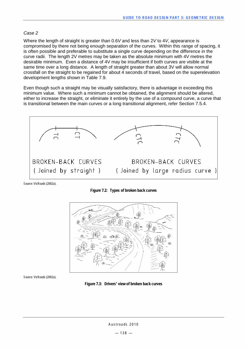
GUI DE TO RO A D DE SIG N P ART 3 : GEO MET RI C D ESI G N
A u s t r o a d s 2 0 1 0
— 1 3 8 —
Case 2
Where the length of straight is greater than 0.6V and less than 2V to 4V, appearance is compromised by there not being enough separation of the curves. Within this range of spacing, it is often possible and preferable to substitute a single curve depending on the difference in the curve radii. The length 2V metres may be taken as the absolute minimum with 4V metres the desirable minimum. Even a distance of 4V may be insufficient if both curves are visible at the same time over a long distance. A length of straight greater than about 3V will allow normal crossfall on the straight to be regained for about 4 seconds of travel, based on the superelevation development lengths shown in Table 7.9.
Even though such a straight may be visually satisfactory, there is advantage in exceeding this minimum value. Where such a minimum cannot be obtained, the alignment should be altered, either to increase the straight, or eliminate it entirely by the use of a compound curve, a curve that is transitional between the main curves or a long transitional alignment, refer Section 7.5.4.
Source: VicRoads (2002a).
Figure 7.2: Types of broken back curves
Source: VicRoads (2002a).
Figure 7.3: Drivers’ view of broken back curves
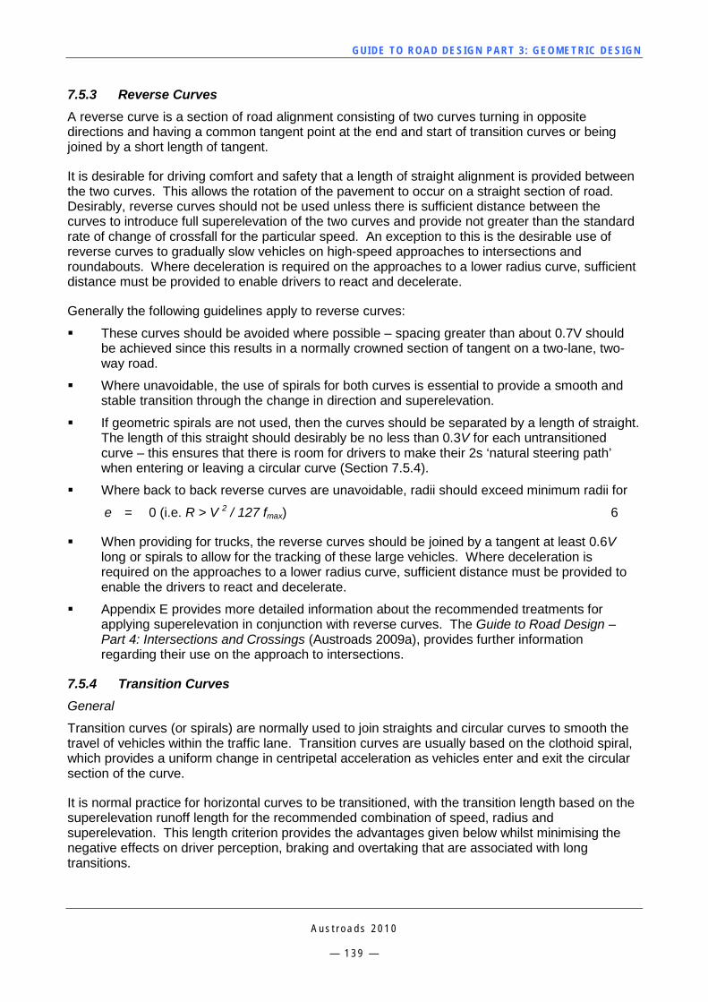
GUI DE TO RO A D DE SIG N P ART 3 : GEO MET RI C D ESI G N
A u s t r o a d s 2 0 1 0
— 1 3 9 —
7.5.3 Reverse Curves A reverse curve is a section of road alignment consisting of two curves turning in opposite directions and having a common tangent point at the end and start of transition curves or being joined by a short length of tangent.
It is desirable for driving comfort and safety that a length of straight alignment is provided between the two curves. This allows the rotation of the pavement to occur on a straight section of road. Desirably, reverse curves should not be used unless there is sufficient distance between the curves to introduce full superelevation of the two curves and provide not greater than the standard rate of change of crossfall for the particular speed. An exception to this is the desirable use of reverse curves to gradually slow vehicles on high-speed approaches to intersections and roundabouts. Where deceleration is required on the approaches to a lower radius curve, sufficient distance must be provided to enable drivers to react and decelerate.
Generally the following guidelines apply to reverse curves:
These curves should be avoided where possible – spacing greater than about 0.7V should be achieved since this results in a normally crowned section of tangent on a two-lane, two-way road.
Where unavoidable, the use of spirals for both curves is essential to provide a smooth and stable transition through the change in direction and superelevation.
If geometric spirals are not used, then the curves should be separated by a length of straight. The length of this straight should desirably be no less than 0.3V for each untransitioned curve – this ensures that there is room for drivers to make their 2s ‘natural steering path’ when entering or leaving a circular curve (Section 7.5.4).
Where back to back reverse curves are unavoidable, radii should exceed minimum radii for
e = 0 (i.e. R > V 2 / 127 fmax) 6
When providing for trucks, the reverse curves should be joined by a tangent at least 0.6V long or spirals to allow for the tracking of these large vehicles. Where deceleration is required on the approaches to a lower radius curve, sufficient distance must be provided to enable the drivers to react and decelerate.
Appendix E provides more detailed information about the recommended treatments for applying superelevation in conjunction with reverse curves. The Guide to Road Design – Part 4: Intersections and Crossings (Austroads 2009a), provides further information regarding their use on the approach to intersections.
7.5.4 Transition Curves General
Transition curves (or spirals) are normally used to join straights and circular curves to smooth the travel of vehicles within the traffic lane. Transition curves are usually based on the clothoid spiral, which provides a uniform change in centripetal acceleration as vehicles enter and exit the circular section of the curve.
It is normal practice for horizontal curves to be transitioned, with the transition length based on the superelevation runoff length for the recommended combination of speed, radius and superelevation. This length criterion provides the advantages given below whilst minimising the negative effects on driver perception, braking and overtaking that are associated with long transitions.
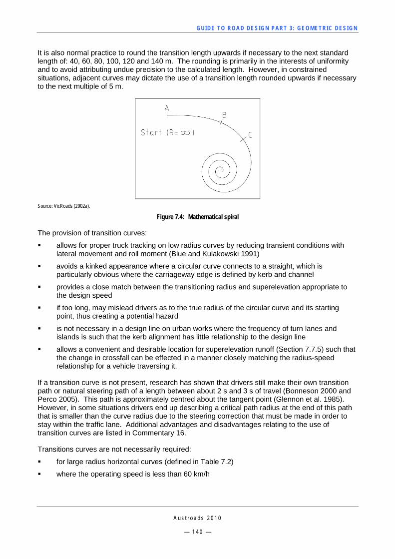
GUI DE TO RO A D DE SIG N P ART 3 : GEO MET RI C D ESI G N
A u s t r o a d s 2 0 1 0
— 1 4 0 —
It is also normal practice to round the transition length upwards if necessary to the next standard length of: 40, 60, 80, 100, 120 and 140 m. The rounding is primarily in the interests of uniformity and to avoid attributing undue precision to the calculated length. However, in constrained situations, adjacent curves may dictate the use of a transition length rounded upwards if necessary to the next multiple of 5 m.
Source: VicRoads (2002a).
Figure 7.4: Mathematical spiral
The provision of transition curves:
allows for proper truck tracking on low radius curves by reducing transient conditions with lateral movement and roll moment (Blue and Kulakowski 1991)
avoids a kinked appearance where a circular curve connects to a straight, which is particularly obvious where the carriageway edge is defined by kerb and channel
provides a close match between the transitioning radius and superelevation appropriate to the design speed
if too long, may mislead drivers as to the true radius of the circular curve and its starting point, thus creating a potential hazard
is not necessary in a design line on urban works where the frequency of turn lanes and islands is such that the kerb alignment has little relationship to the design line
allows a convenient and desirable location for superelevation runoff (Section 7.7.5) such that the change in crossfall can be effected in a manner closely matching the radius-speed relationship for a vehicle traversing it.
If a transition curve is not present, research has shown that drivers still make their own transition path or natural steering path of a length between about 2 s and 3 s of travel (Bonneson 2000 and Perco 2005). This path is approximately centred about the tangent point (Glennon et al. 1985). However, in some situations drivers end up describing a critical path radius at the end of this path that is smaller than the curve radius due to the steering correction that must be made in order to stay within the traffic lane. Additional advantages and disadvantages relating to the use of transition curves are listed in Commentary 16.
Transitions curves are not necessarily required:
for large radius horizontal curves (defined in Table 7.2)
where the operating speed is less than 60 km/h
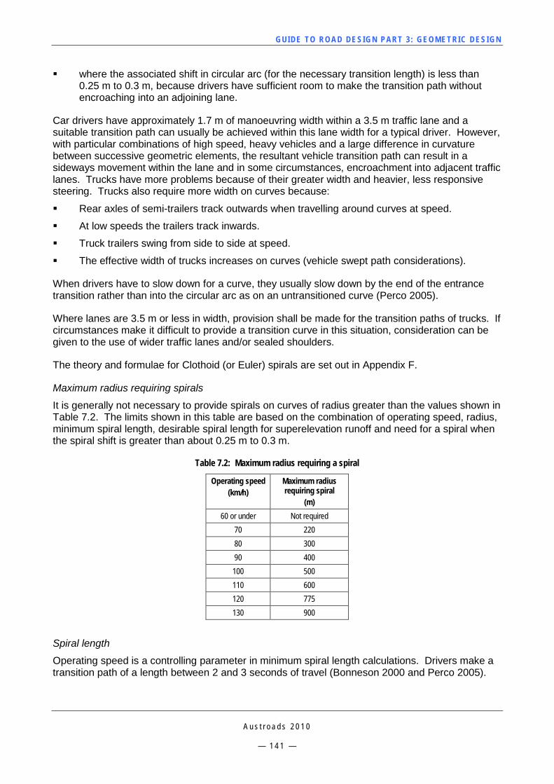
GUI DE TO RO A D DE SIG N P ART 3 : GEO MET RI C D ESI G N
A u s t r o a d s 2 0 1 0
— 1 4 1 —
where the associated shift in circular arc (for the necessary transition length) is less than 0.25 m to 0.3 m, because drivers have sufficient room to make the transition path without encroaching into an adjoining lane.
Car drivers have approximately 1.7 m of manoeuvring width within a 3.5 m traffic lane and a suitable transition path can usually be achieved within this lane width for a typical driver. However, with particular combinations of high speed, heavy vehicles and a large difference in curvature between successive geometric elements, the resultant vehicle transition path can result in a sideways movement within the lane and in some circumstances, encroachment into adjacent traffic lanes. Trucks have more problems because of their greater width and heavier, less responsive steering. Trucks also require more width on curves because:
Rear axles of semi-trailers track outwards when travelling around curves at speed.
At low speeds the trailers track inwards.
Truck trailers swing from side to side at speed.
The effective width of trucks increases on curves (vehicle swept path considerations).
When drivers have to slow down for a curve, they usually slow down by the end of the entrance transition rather than into the circular arc as on an untransitioned curve (Perco 2005).
Where lanes are 3.5 m or less in width, provision shall be made for the transition paths of trucks. If circumstances make it difficult to provide a transition curve in this situation, consideration can be given to the use of wider traffic lanes and/or sealed shoulders.
The theory and formulae for Clothoid (or Euler) spirals are set out in Appendix F.
Maximum radius requiring spirals
It is generally not necessary to provide spirals on curves of radius greater than the values shown in Table 7.2. The limits shown in this table are based on the combination of operating speed, radius, minimum spiral length, desirable spiral length for superelevation runoff and need for a spiral when the spiral shift is greater than about 0.25 m to 0.3 m.
Table 7.2: Maximum radius requiring a spiral
Operating speed (km/h)
Maximum radius requiring spiral
(m) 60 or under Not required
70 220 80 300 90 400 100 500 110 600 120 775 130 900
Spiral length
Operating speed is a controlling parameter in minimum spiral length calculations. Drivers make a transition path of a length between 2 and 3 seconds of travel (Bonneson 2000 and Perco 2005).
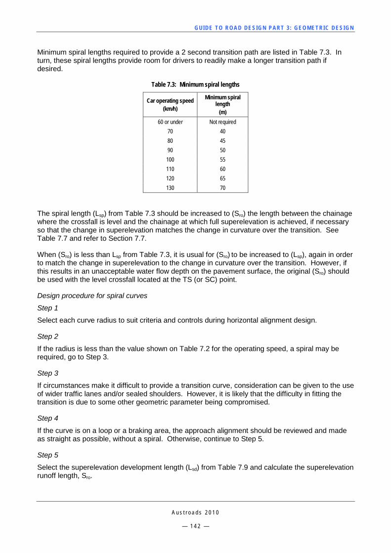
GUI DE TO RO A D DE SIG N P ART 3 : GEO MET RI C D ESI G N
A u s t r o a d s 2 0 1 0
— 1 4 2 —
Minimum spiral lengths required to provide a 2 second transition path are listed in Table 7.3. In turn, these spiral lengths provide room for drivers to readily make a longer transition path if desired.
Table 7.3: Minimum spiral lengths
Car operating speed (km/h)
Minimum spiral length
(m) 60 or under Not required
70 40 80 45 90 50 100 55 110 60 120 65 130 70
The spiral length (Lsp) from Table 7.3 should be increased to (Sro) the length between the chainage where the crossfall is level and the chainage at which full superelevation is achieved, if necessary so that the change in superelevation matches the change in curvature over the transition. See Table 7.7 and refer to Section 7.7.
When (Sro) is less than Lsp from Table 7.3, it is usual for (Sro) to be increased to (Lsp), again in order to match the change in superelevation to the change in curvature over the transition. However, if this results in an unacceptable water flow depth on the pavement surface, the original (Sro) should be used with the level crossfall located at the TS (or SC) point.
Design procedure for spiral curves
Step 1
Select each curve radius to suit criteria and controls during horizontal alignment design.
Step 2
If the radius is less than the value shown on Table 7.2 for the operating speed, a spiral may be required, go to Step 3.
Step 3
If circumstances make it difficult to provide a transition curve, consideration can be given to the use of wider traffic lanes and/or sealed shoulders. However, it is likely that the difficulty in fitting the transition is due to some other geometric parameter being compromised.
Step 4
If the curve is on a loop or a braking area, the approach alignment should be reviewed and made as straight as possible, without a spiral. Otherwise, continue to Step 5.
Step 5
Select the superelevation development length (Lsd) from Table 7.9 and calculate the superelevation runoff length, Sro.
GUI DE TO RO A D DE SIG N P ART 3 : GEO MET RI C D ESI G N
A u s t r o a d s 2 0 1 0
— 1 4 3 —
Step 6
Use the greater of Sro or length Lsp from Table 7.3 as the spiral length.
Step 7
Calculate the spiral shift from the formula in Appendix F (Equation A 20). If the shift is less than 0.3 m (desirably 0.25 m for operating speeds >100 km/h), no transition is necessary.
Step 8
If convenient, round the spiral length up to the next 5 or 10 m. Calculate set out points for the horizontal alignment at the required chainages.
7.6 Side Friction and Minimum Curve Size A vehicle travelling around a circular horizontal curve requires a radial force that tends to effect the change in direction and consequent centripetal acceleration. This force is provided by side friction between the tyres and the road surface. If there is insufficient force provided by side friction, the vehicle will tend to slide tangentially to the road alignment.
The side friction factor (f) is a measure of the frictional force between the pavement and the vehicle tyre. Based on the review of side friction factor values used by Australian and international authorities, the desirable and absolute values of f recommended for design are shown in Table 7.4.
The value of the side friction factor depends on the type and condition of the road surface, driver behaviour and the type and condition of the tyres. Therefore, it is variable.
The desirable maximum values should be used on intermediate and high-speed roads with uniform traffic flow, on which drivers are not tolerant of discomfort. Where possible, these values should be adopted to allow vehicles to maintain their lateral position within a traffic lane and to be able to comfortably change lanes if necessary. Figure 7.5 to Figure 7.7 provide the relationship between speed, radius and superelevation using the desirable maximum values of side friction, for both urban and rural roads.
On low speed roads with non-uniform traffic flow, which are typical in urban areas or mountainous terrain, drivers are more tolerant of discomfort. This permits the absolute maximum values of side friction to be safely used in the design of horizontal curves, although the designer should endeavour to adopt desirable maximum values where possible. The minimum radii curves listed in Table 7.5 are suitable in constrained urban areas but their use in rural areas will result in a poor alignment and associated road safety issues.
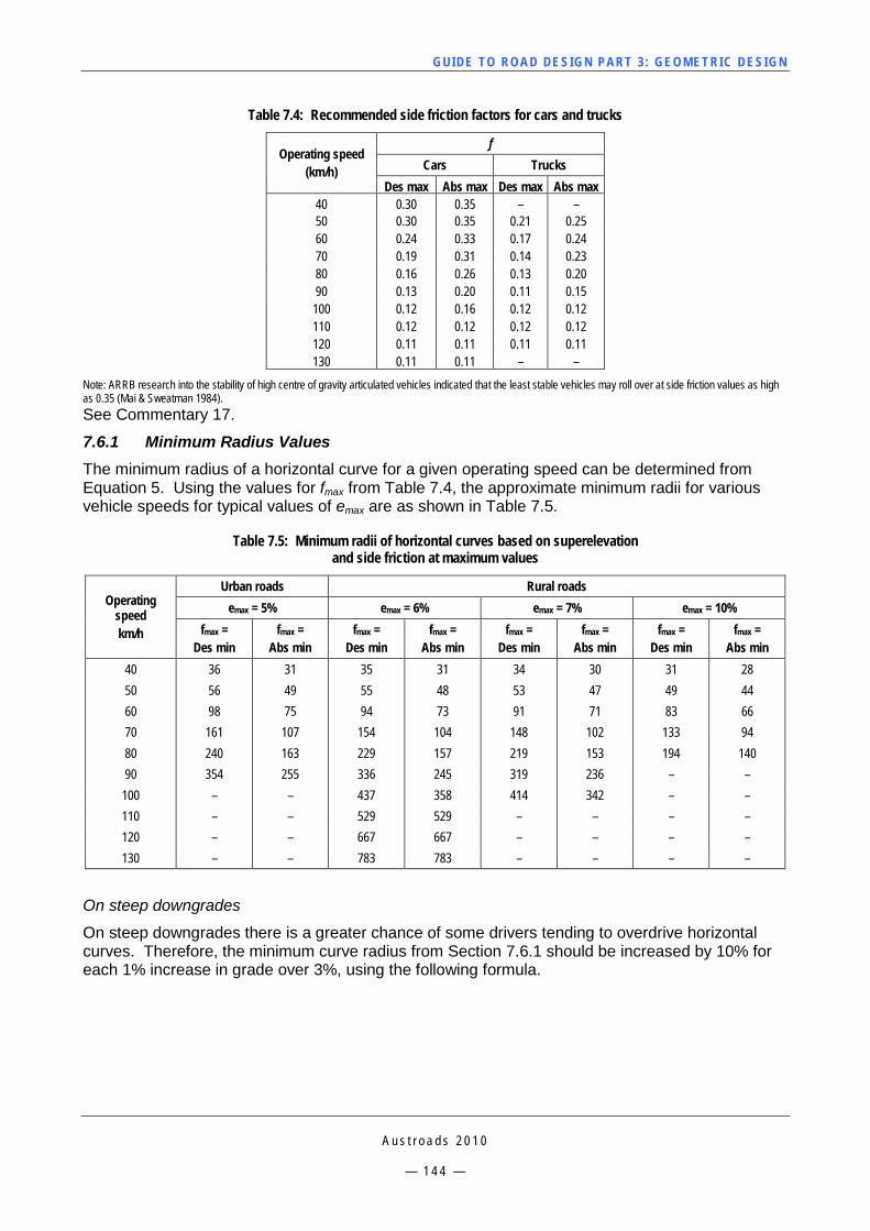
GUI DE TO RO A D DE SIG N P ART 3 : GEO MET RI C D ESI G N
A u s t r o a d s 2 0 1 0
— 1 4 4 —
Table 7.4: Recommended side friction factors for cars and trucks
Operating speed (km/h)
f Cars Trucks
Des max Abs max Des max Abs max 40 0.30 0.35 – – 50 0.30 0.35 0.21 0.25 60 0.24 0.33 0.17 0.24 70 0.19 0.31 0.14 0.23 80 0.16 0.26 0.13 0.20 90 0.13 0.20 0.11 0.15 100 0.12 0.16 0.12 0.12 110 0.12 0.12 0.12 0.12 120 0.11 0.11 0.11 0.11 130 0.11 0.11 – –
Note: ARRB research into the stability of high centre of gravity articulated vehicles indicated that the least stable vehicles may roll over at side friction values as high as 0.35 (Mai & Sweatman 1984). See Commentary 17.
7.6.1 Minimum Radius Values The minimum radius of a horizontal curve for a given operating speed can be determined from Equation 5. Using the values for fmax from Table 7.4, the approximate minimum radii for various vehicle speeds for typical values of emax are as shown in Table 7.5.
Table 7.5: Minimum radii of horizontal curves based on superelevation and side friction at maximum values
Operating speed km/h
Urban roads Rural roads emax = 5% emax = 6% emax = 7% emax = 10%
fmax = Des min
fmax = Abs min
fmax = Des min
fmax = Abs min
fmax = Des min
fmax = Abs min
fmax = Des min
fmax = Abs min
40 36 31 35 31 34 30 31 28 50 56 49 55 48 53 47 49 44 60 98 75 94 73 91 71 83 66 70 161 107 154 104 148 102 133 94 80 240 163 229 157 219 153 194 140 90 354 255 336 245 319 236 – –
100 – – 437 358 414 342 – – 110 – – 529 529 – – – – 120 – – 667 667 – – – – 130 – – 783 783 – – – –
On steep downgrades
On steep downgrades there is a greater chance of some drivers tending to overdrive horizontal curves. Therefore, the minimum curve radius from Section 7.6.1 should be increased by 10% for each 1% increase in grade over 3%, using the following formula.
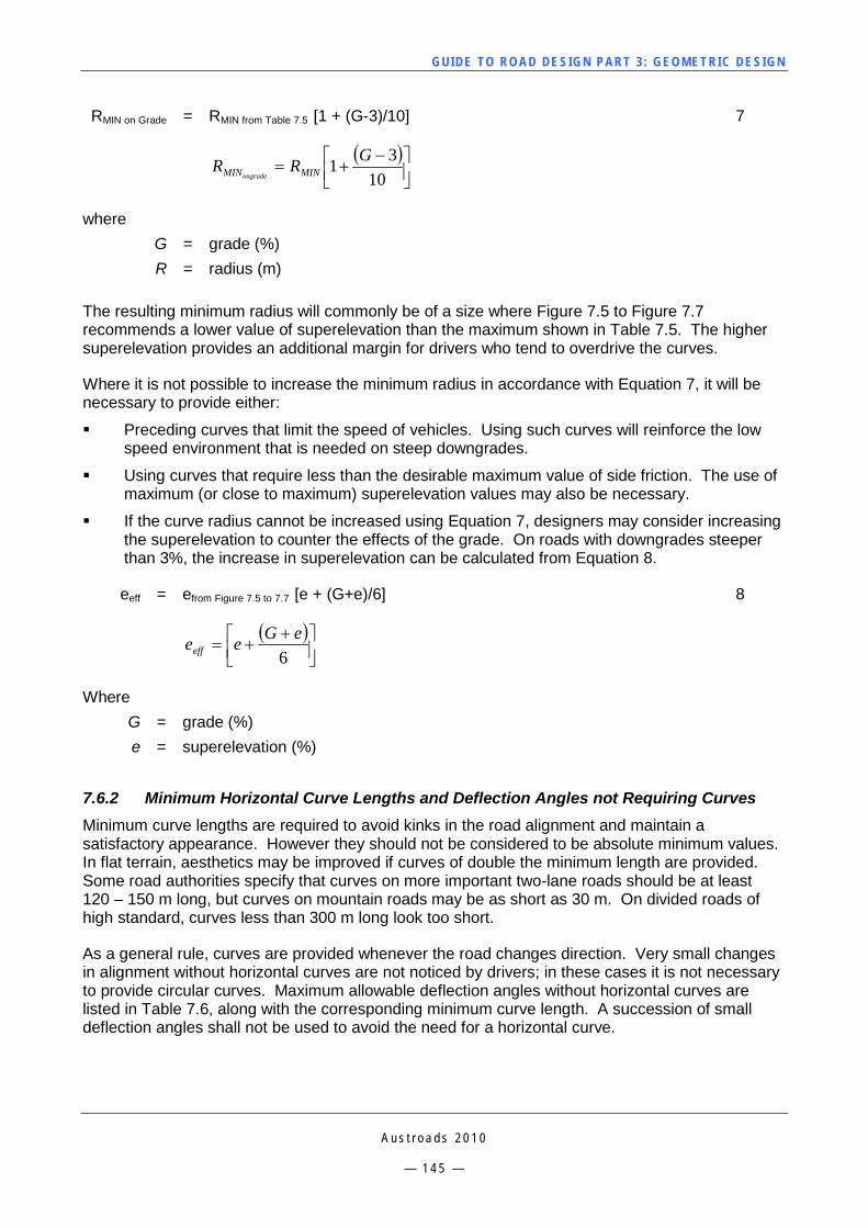
GUI DE TO RO A D DE SIG N P ART 3 : GEO MET RI C D ESI G N
A u s t r o a d s 2 0 1 0
— 1 4 5 —
RMIN on Grade = RMIN from Table 7.5 [1 + (G-3)/10] 7
( )
−+=
1031 GRR MINMINongrade
where G = grade (%) R = radius (m)
The resulting minimum radius will commonly be of a size where Figure 7.5 to Figure 7.7 recommends a lower value of superelevation than the maximum shown in Table 7.5. The higher superelevation provides an additional margin for drivers who tend to overdrive the curves.
Where it is not possible to increase the minimum radius in accordance with Equation 7, it will be necessary to provide either:
Preceding curves that limit the speed of vehicles. Using such curves will reinforce the low speed environment that is needed on steep downgrades.
Using curves that require less than the desirable maximum value of side friction. The use of maximum (or close to maximum) superelevation values may also be necessary.
If the curve radius cannot be increased using Equation 7, designers may consider increasing the superelevation to counter the effects of the grade. On roads with downgrades steeper than 3%, the increase in superelevation can be calculated from Equation 8.
eeff = efrom Figure 7.5 to 7.7 [e + (G+e)/6] 8
( )
++=
6eGeeeff
Where G = grade (%) e = superelevation (%)
7.6.2 Minimum Horizontal Curve Lengths and Deflection Angles not Requiring Curves Minimum curve lengths are required to avoid kinks in the road alignment and maintain a satisfactory appearance. However they should not be considered to be absolute minimum values. In flat terrain, aesthetics may be improved if curves of double the minimum length are provided. Some road authorities specify that curves on more important two-lane roads should be at least 120 – 150 m long, but curves on mountain roads may be as short as 30 m. On divided roads of high standard, curves less than 300 m long look too short.
As a general rule, curves are provided whenever the road changes direction. Very small changes in alignment without horizontal curves are not noticed by drivers; in these cases it is not necessary to provide circular curves. Maximum allowable deflection angles without horizontal curves are listed in Table 7.6, along with the corresponding minimum curve length. A succession of small deflection angles shall not be used to avoid the need for a horizontal curve.
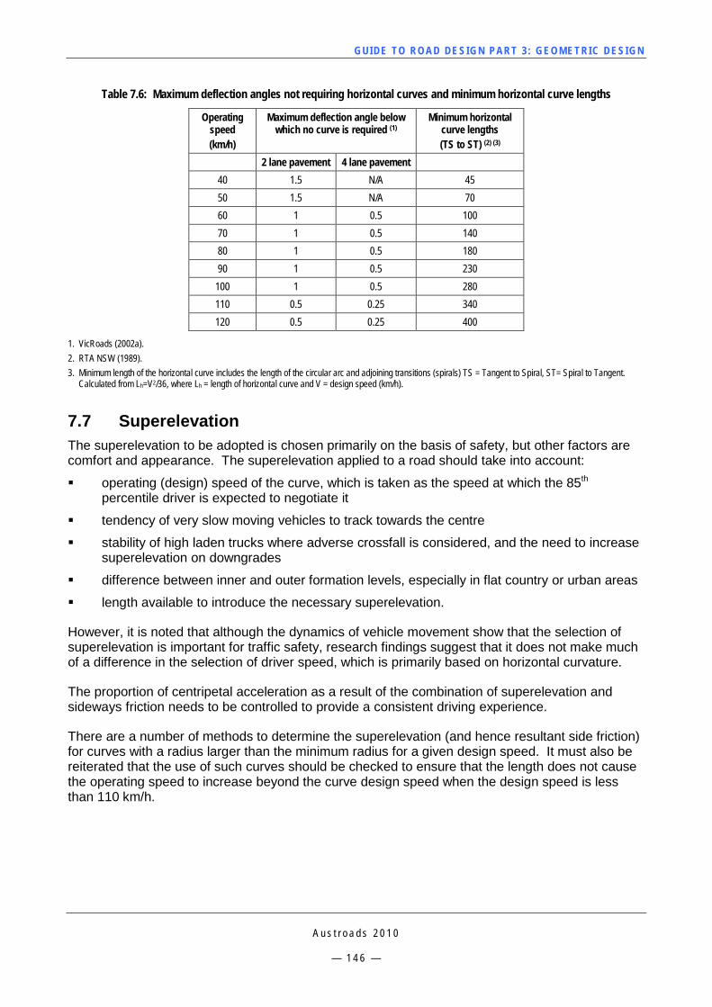
GUI DE TO RO A D DE SIG N P ART 3 : GEO MET RI C D ESI G N
A u s t r o a d s 2 0 1 0
— 1 4 6 —
Table 7.6: Maximum deflection angles not requiring horizontal curves and minimum horizontal curve lengths
Operating speed (km/h)
Maximum deflection angle below which no curve is required (1)
Minimum horizontal curve lengths (TS to ST) (2) (3)
2 lane pavement 4 lane pavement 40 1.5 N/A 45 50 1.5 N/A 70 60 1 0.5 100 70 1 0.5 140 80 1 0.5 180 90 1 0.5 230
100 1 0.5 280 110 0.5 0.25 340 120 0.5 0.25 400
1. VicRoads (2002a). 2. RTA NSW (1989). 3. Minimum length of the horizontal curve includes the length of the circular arc and adjoining transitions (spirals) TS = Tangent to Spiral, ST= Spiral to Tangent. Calculated from Lh=V2/36, where Lh = length of horizontal curve and V = design speed (km/h).
7.7 Superelevation The superelevation to be adopted is chosen primarily on the basis of safety, but other factors are comfort and appearance. The superelevation applied to a road should take into account:
operating (design) speed of the curve, which is taken as the speed at which the 85th percentile driver is expected to negotiate it
tendency of very slow moving vehicles to track towards the centre
stability of high laden trucks where adverse crossfall is considered, and the need to increase superelevation on downgrades
difference between inner and outer formation levels, especially in flat country or urban areas
length available to introduce the necessary superelevation.
However, it is noted that although the dynamics of vehicle movement show that the selection of superelevation is important for traffic safety, research findings suggest that it does not make much of a difference in the selection of driver speed, which is primarily based on horizontal curvature.
The proportion of centripetal acceleration as a result of the combination of superelevation and sideways friction needs to be controlled to provide a consistent driving experience.
There are a number of methods to determine the superelevation (and hence resultant side friction) for curves with a radius larger than the minimum radius for a given design speed. It must also be reiterated that the use of such curves should be checked to ensure that the length does not cause the operating speed to increase beyond the curve design speed when the design speed is less than 110 km/h.
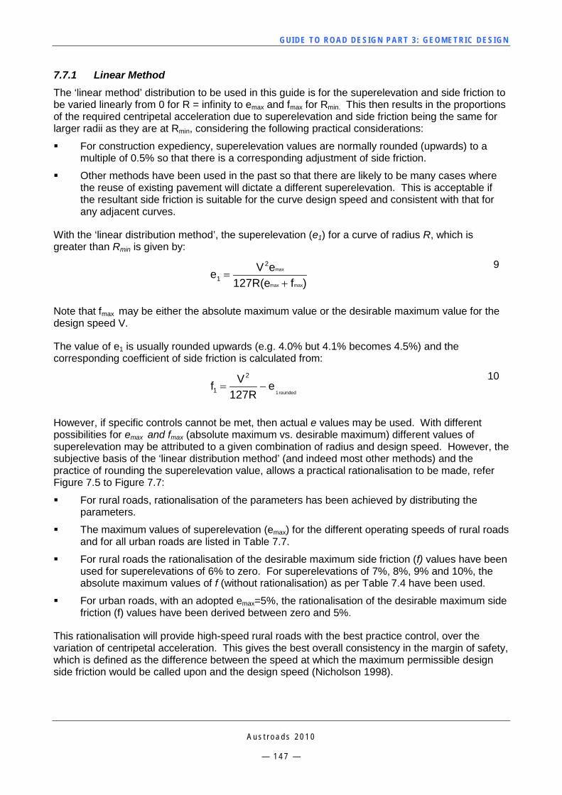
GUI DE TO RO A D DE SIG N P ART 3 : GEO MET RI C D ESI G N
A u s t r o a d s 2 0 1 0
— 1 4 7 —
7.7.1 Linear Method The ‘linear method’ distribution to be used in this guide is for the superelevation and side friction to be varied linearly from 0 for R = infinity to emax and fmax for Rmin. This then results in the proportions of the required centripetal acceleration due to superelevation and side friction being the same for larger radii as they are at Rmin, considering the following practical considerations:
For construction expediency, superelevation values are normally rounded (upwards) to a multiple of 0.5% so that there is a corresponding adjustment of side friction.
Other methods have been used in the past so that there are likely to be many cases where the reuse of existing pavement will dictate a different superelevation. This is acceptable if the resultant side friction is suitable for the curve design speed and consistent with that for any adjacent curves.
With the ‘linear distribution method’, the superelevation (e1) for a curve of radius R, which is greater than Rmin is given by:
)f127R(eeVe
maxmax
max2
1 +=
9
Note that fmax may be either the absolute maximum value or the desirable maximum value for the design speed V.
The value of e1 is usually rounded upwards (e.g. 4.0% but 4.1% becomes 4.5%) and the corresponding coefficient of side friction is calculated from:
rounded1
e127R
Vf2
1 −= 10
However, if specific controls cannot be met, then actual e values may be used. With different possibilities for emax and fmax (absolute maximum vs. desirable maximum) different values of superelevation may be attributed to a given combination of radius and design speed. However, the subjective basis of the ‘linear distribution method’ (and indeed most other methods) and the practice of rounding the superelevation value, allows a practical rationalisation to be made, refer Figure 7.5 to Figure 7.7:
For rural roads, rationalisation of the parameters has been achieved by distributing the parameters.
The maximum values of superelevation (emax) for the different operating speeds of rural roads and for all urban roads are listed in Table 7.7.
For rural roads the rationalisation of the desirable maximum side friction (f) values have been used for superelevations of 6% to zero. For superelevations of 7%, 8%, 9% and 10%, the absolute maximum values of f (without rationalisation) as per Table 7.4 have been used.
For urban roads, with an adopted emax=5%, the rationalisation of the desirable maximum side friction (f) values have been derived between zero and 5%.
This rationalisation will provide high-speed rural roads with the best practice control, over the variation of centripetal acceleration. This gives the best overall consistency in the margin of safety, which is defined as the difference between the speed at which the maximum permissible design side friction would be called upon and the design speed (Nicholson 1998).
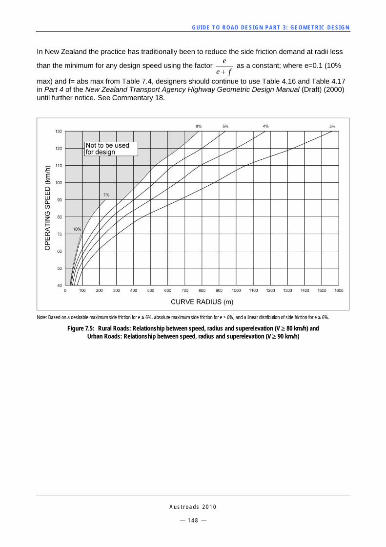
GUI DE TO RO A D DE SIG N P ART 3 : GEO MET RI C D ESI G N
A u s t r o a d s 2 0 1 0
— 1 4 8 —
In New Zealand the practice has traditionally been to reduce the side friction demand at radii less
than the minimum for any design speed using the factor fe
e+
as a constant; where e=0.1 (10%
max) and f= abs max from Table 7.4, designers should continue to use Table 4.16 and Table 4.17 in Part 4 of the New Zealand Transport Agency Highway Geometric Design Manual (Draft) (2000) until further notice. See Commentary 18.
Note: Based on a desirable maximum side friction for e ≤ 6%, absolute maximum side friction for e > 6%, and a linear distribution of side friction for e ≤ 6%.
Figure 7.5: Rural Roads: Relationship between speed, radius and superelevation (V ≥ 80 km/h) and Urban Roads: Relationship between speed, radius and superelevation (V ≥ 90 km/h)
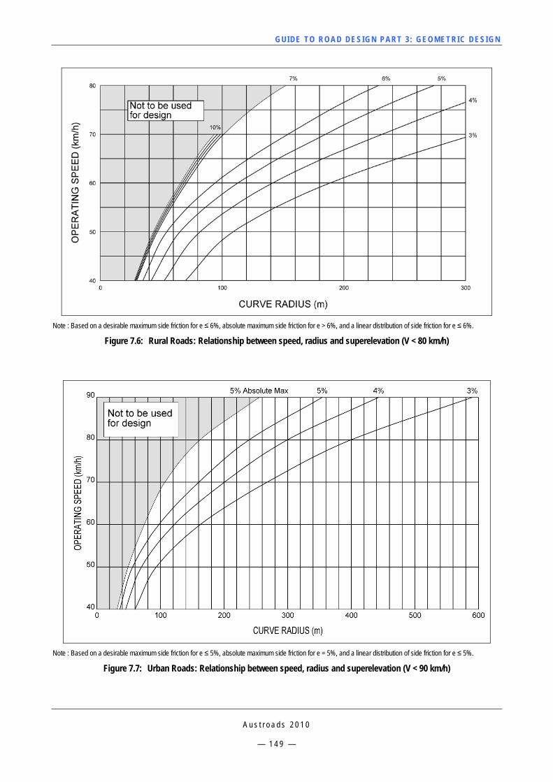
GUI DE TO RO A D DE SIG N P ART 3 : GEO MET RI C D ESI G N
A u s t r o a d s 2 0 1 0
— 1 4 9 —
Note : Based on a desirable maximum side friction for e ≤ 6%, absolute maximum side friction for e > 6%, and a linear distribution of side friction for e ≤ 6%.
Figure 7.6: Rural Roads: Relationship between speed, radius and superelevation (V < 80 km/h)
Note : Based on a desirable maximum side friction for e ≤ 5%, absolute maximum side friction for e = 5%, and a linear distribution of side friction for e ≤ 5%.
Figure 7.7: Urban Roads: Relationship between speed, radius and superelevation (V < 90 km/h)
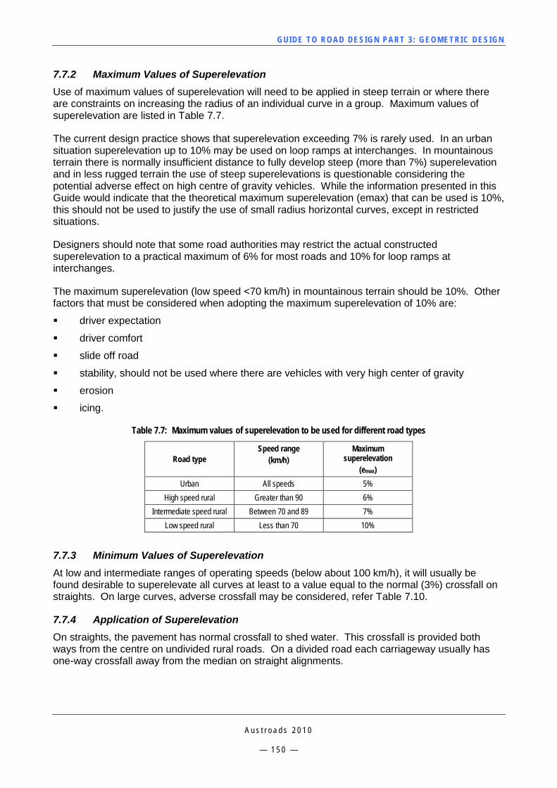
GUI DE TO RO A D DE SIG N P ART 3 : GEO MET RI C D ESI G N
A u s t r o a d s 2 0 1 0
— 1 5 0 —
7.7.2 Maximum Values of Superelevation Use of maximum values of superelevation will need to be applied in steep terrain or where there are constraints on increasing the radius of an individual curve in a group. Maximum values of superelevation are listed in Table 7.7.
The current design practice shows that superelevation exceeding 7% is rarely used. In an urban situation superelevation up to 10% may be used on loop ramps at interchanges. In mountainous terrain there is normally insufficient distance to fully develop steep (more than 7%) superelevation and in less rugged terrain the use of steep superelevations is questionable considering the potential adverse effect on high centre of gravity vehicles. While the information presented in this Guide would indicate that the theoretical maximum superelevation (emax) that can be used is 10%, this should not be used to justify the use of small radius horizontal curves, except in restricted situations.
Designers should note that some road authorities may restrict the actual constructed superelevation to a practical maximum of 6% for most roads and 10% for loop ramps at interchanges.
The maximum superelevation (low speed <70 km/h) in mountainous terrain should be 10%. Other factors that must be considered when adopting the maximum superelevation of 10% are:
driver expectation
driver comfort
slide off road
stability, should not be used where there are vehicles with very high center of gravity
erosion
icing.
Table 7.7: Maximum values of superelevation to be used for different road types
Road type Speed range
(km/h) Maximum
superelevation (emax)
Urban All speeds 5% High speed rural Greater than 90 6%
Intermediate speed rural Between 70 and 89 7% Low speed rural Less than 70 10%
7.7.3 Minimum Values of Superelevation At low and intermediate ranges of operating speeds (below about 100 km/h), it will usually be found desirable to superelevate all curves at least to a value equal to the normal (3%) crossfall on straights. On large curves, adverse crossfall may be considered, refer Table 7.10.
7.7.4 Application of Superelevation On straights, the pavement has normal crossfall to shed water. This crossfall is provided both ways from the centre on undivided rural roads. On a divided road each carriageway usually has one-way crossfall away from the median on straight alignments.
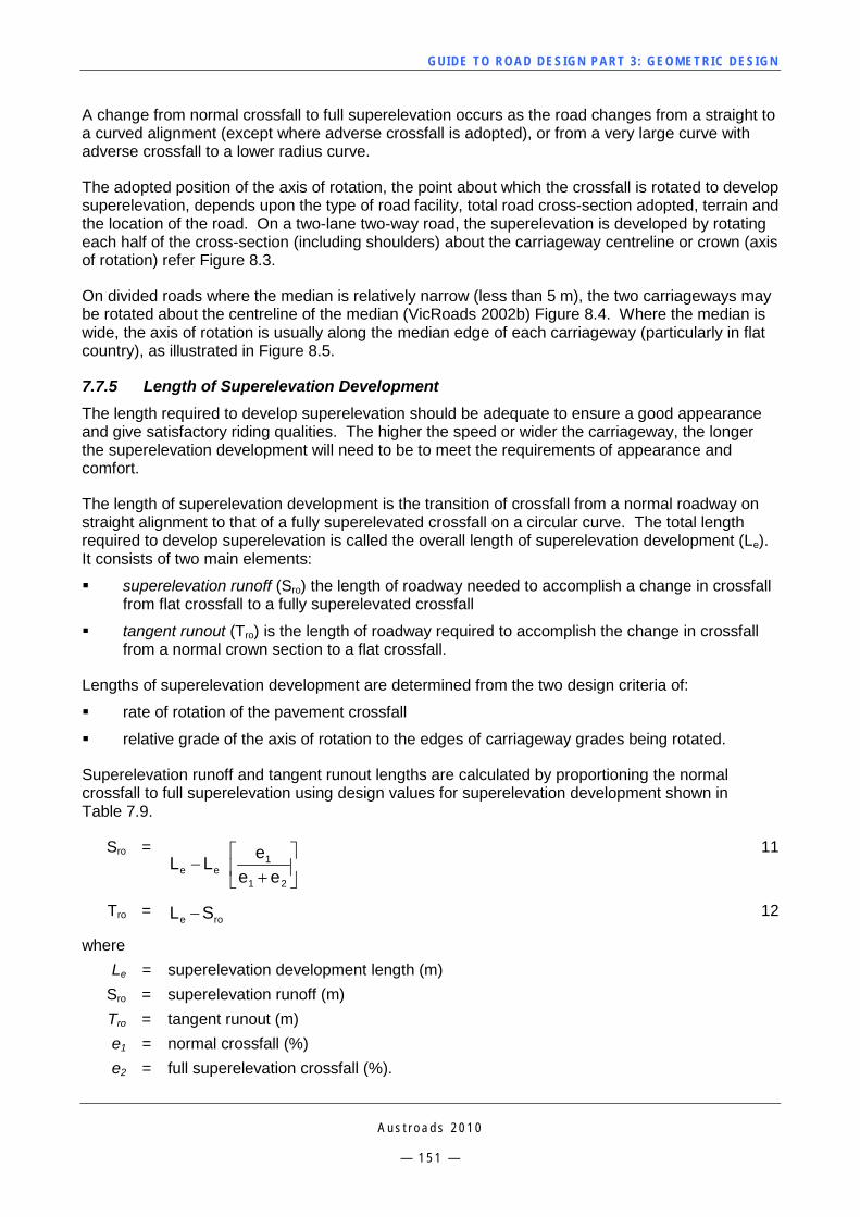
GUI DE TO RO A D DE SIG N P ART 3 : GEO MET RI C D ESI G N
A u s t r o a d s 2 0 1 0
— 1 5 1 —
A change from normal crossfall to full superelevation occurs as the road changes from a straight to a curved alignment (except where adverse crossfall is adopted), or from a very large curve with adverse crossfall to a lower radius curve.
The adopted position of the axis of rotation, the point about which the crossfall is rotated to develop superelevation, depends upon the type of road facility, total road cross-section adopted, terrain and the location of the road. On a two-lane two-way road, the superelevation is developed by rotating each half of the cross-section (including shoulders) about the carriageway centreline or crown (axis of rotation) refer Figure 8.3.
On divided roads where the median is relatively narrow (less than 5 m), the two carriageways may be rotated about the centreline of the median (VicRoads 2002b) Figure 8.4. Where the median is wide, the axis of rotation is usually along the median edge of each carriageway (particularly in flat country), as illustrated in Figure 8.5.
7.7.5 Length of Superelevation Development The length required to develop superelevation should be adequate to ensure a good appearance and give satisfactory riding qualities. The higher the speed or wider the carriageway, the longer the superelevation development will need to be to meet the requirements of appearance and comfort.
The length of superelevation development is the transition of crossfall from a normal roadway on straight alignment to that of a fully superelevated crossfall on a circular curve. The total length required to develop superelevation is called the overall length of superelevation development (Le). It consists of two main elements:
superelevation runoff (Sro) the length of roadway needed to accomplish a change in crossfall from flat crossfall to a fully superelevated crossfall
tangent runout (Tro) is the length of roadway required to accomplish the change in crossfall from a normal crown section to a flat crossfall.
Lengths of superelevation development are determined from the two design criteria of:
rate of rotation of the pavement crossfall
relative grade of the axis of rotation to the edges of carriageway grades being rotated.
Superelevation runoff and tangent runout lengths are calculated by proportioning the normal crossfall to full superelevation using design values for superelevation development shown in Table 7.9.
Sro = ee LL −
+ 21
1
eee
11
Tro = roe SL − 12
where Le = superelevation development length (m)
Sro = superelevation runoff (m) Tro = tangent runout (m) e1 = normal crossfall (%) e2 = full superelevation crossfall (%).
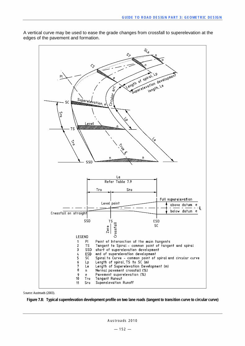
GUI DE TO RO A D DE SIG N P ART 3 : GEO MET RI C D ESI G N
A u s t r o a d s 2 0 1 0
— 1 5 2 —
A vertical curve may be used to ease the grade changes from crossfall to superelevation at the edges of the pavement and formation.
Source: Austroads (2003).
Figure 7.8: Typical superelevation development profile on two lane roads (tangent to transition curve to circular curve)
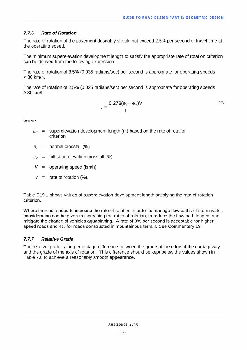
GUI DE TO RO A D DE SIG N P ART 3 : GEO MET RI C D ESI G N
A u s t r o a d s 2 0 1 0
— 1 5 3 —
7.7.6 Rate of Rotation The rate of rotation of the pavement desirably should not exceed 2.5% per second of travel time at the operating speed.
The minimum superelevation development length to satisfy the appropriate rate of rotation criterion can be derived from the following expression.
The rate of rotation of 3.5% (0.035 radians/sec) per second is appropriate for operating speeds < 80 km/h.
The rate of rotation of 2.5% (0.025 radians/sec) per second is appropriate for operating speeds ≥ 80 km/h.
r
)Ve0.278(eL 21rr
−=
13
where
Lrr = superelevation development length (m) based on the rate of rotation criterion
e1 = normal crossfall (%)
e2 = full superelevation crossfall (%)
V = operating speed (km/h)
r = rate of rotation (%).
Table C19 1 shows values of superelevation development length satisfying the rate of rotation criterion.
Where there is a need to increase the rate of rotation in order to manage flow paths of storm water, consideration can be given to increasing the rates of rotation, to reduce the flow path lengths and mitigate the chance of vehicles aquaplaning. A rate of 3% per second is acceptable for higher speed roads and 4% for roads constructed in mountainous terrain. See Commentary 19.
7.7.7 Relative Grade The relative grade is the percentage difference between the grade at the edge of the carriageway and the grade of the axis of rotation. This difference should be kept below the values shown in Table 7.8 to achieve a reasonably smooth appearance.
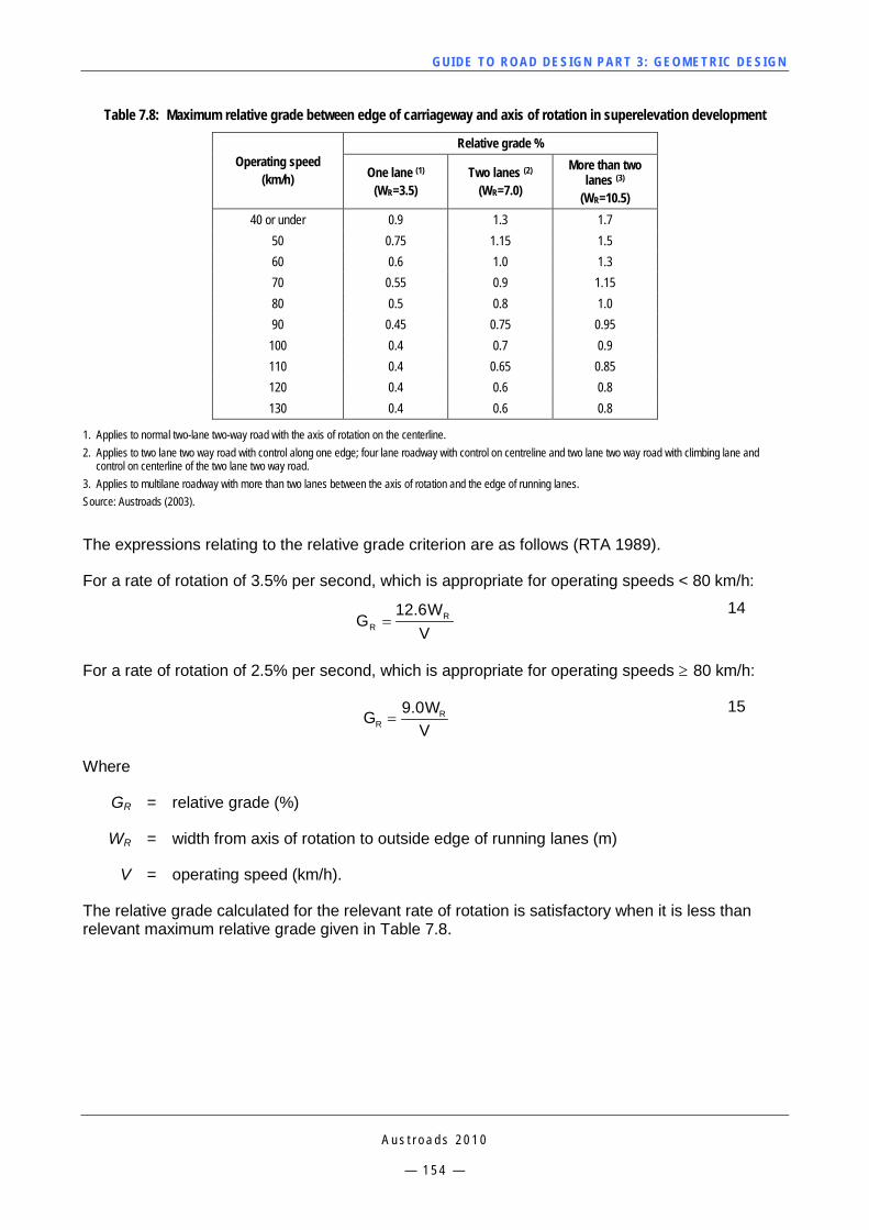
GUI DE TO RO A D DE SIG N P ART 3 : GEO MET RI C D ESI G N
A u s t r o a d s 2 0 1 0
— 1 5 4 —
Table 7.8: Maximum relative grade between edge of carriageway and axis of rotation in superelevation development
Operating speed (km/h)
Relative grade %
One lane (1)
(WR=3.5) Two lanes (2)
(WR=7.0)
More than two lanes (3)
(WR=10.5) 40 or under 0.9 1.3 1.7
50 0.75 1.15 1.5 60 0.6 1.0 1.3 70 0.55 0.9 1.15 80 0.5 0.8 1.0 90 0.45 0.75 0.95 100 0.4 0.7 0.9 110 0.4 0.65 0.85 120 0.4 0.6 0.8 130 0.4 0.6 0.8
1. Applies to normal two-lane two-way road with the axis of rotation on the centerline. 2. Applies to two lane two way road with control along one edge; four lane roadway with control on centreline and two lane two way road with climbing lane and
control on centerline of the two lane two way road. 3. Applies to multilane roadway with more than two lanes between the axis of rotation and the edge of running lanes. Source: Austroads (2003).
The expressions relating to the relative grade criterion are as follows (RTA 1989).
For a rate of rotation of 3.5% per second, which is appropriate for operating speeds < 80 km/h:
VW6.12
G RR =
14
For a rate of rotation of 2.5% per second, which is appropriate for operating speeds ≥ 80 km/h:
VW0.9G R
R = 15
Where
GR = relative grade (%)
WR = width from axis of rotation to outside edge of running lanes (m)
V = operating speed (km/h).
The relative grade calculated for the relevant rate of rotation is satisfactory when it is less than relevant maximum relative grade given in Table 7.8.
GUI DE TO RO A D DE SIG N P ART 3 : GEO MET RI C D ESI G N
A u s t r o a d s 2 0 1 0
— 1 5 5 —
The length of superelevation development to satisfy the relative grade criterion is derived from the following formula:
R
21Rrg G
)e(eWL −=
16
where
Lrg = length of superelevation development (m) based on the relative grade criterion
e1 = normal crossfall (%)
e2 = full superelevation (%)
GR = relative grade (%), from Table 7.8
Use calculated values for GR if they are < Table 7.8 values
WR = width from axis of rotation to outside edge of running lanes (m).
Table C19 2 shows values of superelevation development lengths satisfying the relative grade criterion. These lengths have been calculated using GR values from Table 7.8. The designer may consider using the calculated values of GR where they are less than the tabulated values (See Commentary 19).
7.7.8 Design Superelevation Development Lengths Designers shall adopt superelevation development lengths (Le) that satisfy both the rate of rotation and relative grade criteria. These values are shown in Table 7.9 and combine the tables provided in Commentary 19.
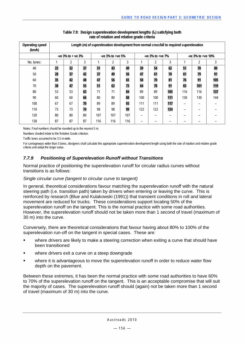
GUI DE TO RO A D DE SIG N P ART 3 : GEO MET RI C D ESI G N
A u s t r o a d s 2 0 1 0
— 1 5 6 —
Table 7.9: Design superelevation development lengths (le) satisfying both rate of rotation and relative grade criteria
Operating speed (km/h)
Length (m) of superelevation development from normal crossfall to required superelevation
-ve 3% to + ve 3% -ve 3% to +ve 5% -ve 3% to +ve 7% -ve 3% to +ve 10% No. lanes: 1 2 3 1 2 3 1 2 3 1 2 3
40 23 32 37 31 43 49 39 54 62 51 70 80 50 28 37 42 37 49 56 47 61 70 61 79 91 60 35 42 48 47 56 65 58 70 81 76 91 105 70 38 47 55 51 62 73 64 78 91 83 101 119 80 53 53 63 71 71 84 89 89 105 116 116 137 90 60 60 66 80 80 88 100 100 111 130 130 144 100 67 67 70 89 89 93 111 111 117 – – – 110 73 73 74 98 98 99 122 122 124 – – – 120 80 80 80 107 107 107 – – – – – – 130 87 87 87 116 116 116 – – – – – –
Notes: Final numbers should be rounded up to the nearest 5 m. Numbers shaded relate to the Relative Grade criterion. Traffic lanes assumed to be 3.5 m wide. For carriageways wider than 3 lanes, designers shall calculate the appropriate superelevation development length using both the rate of rotation and relative grade criteria and adopt the larger value.
7.7.9 Positioning of Superelevation Runoff without Transitions Normal practice of positioning the superelevation runoff for circular radius curves without transitions is as follows:
Single circular curve (tangent to circular curve to tangent)
In general, theoretical considerations favour matching the superelevation runoff with the natural steering path (i.e. transition path) taken by drivers when entering or leaving the curve. This is reinforced by research (Blue and Kulakowski (1991)) that transient conditions in roll and lateral movement are reduced for trucks. These considerations support locating 50% of the superelevation runoff on the tangent. This is the normal practice with some road authorities. However, the superelevation runoff should not be taken more than 1 second of travel (maximum of 30 m) into the curve.
Conversely, there are theoretical considerations that favour having about 80% to 100% of the superelevation run-off on the tangent in special cases. These are:
where drivers are likely to make a steering correction when exiting a curve that should have been transitioned
where drivers exit a curve on a steep downgrade
where it is advantageous to move the superelevation runoff in order to reduce water flow depth on the pavement.
Between these extremes, it has been the normal practice with some road authorities to have 60% to 70% of the superelevation runoff on the tangent. This is an acceptable compromise that will suit the majority of cases. The superelevation runoff should (again) not be taken more than 1 second of travel (maximum of 30 m) into the curve.
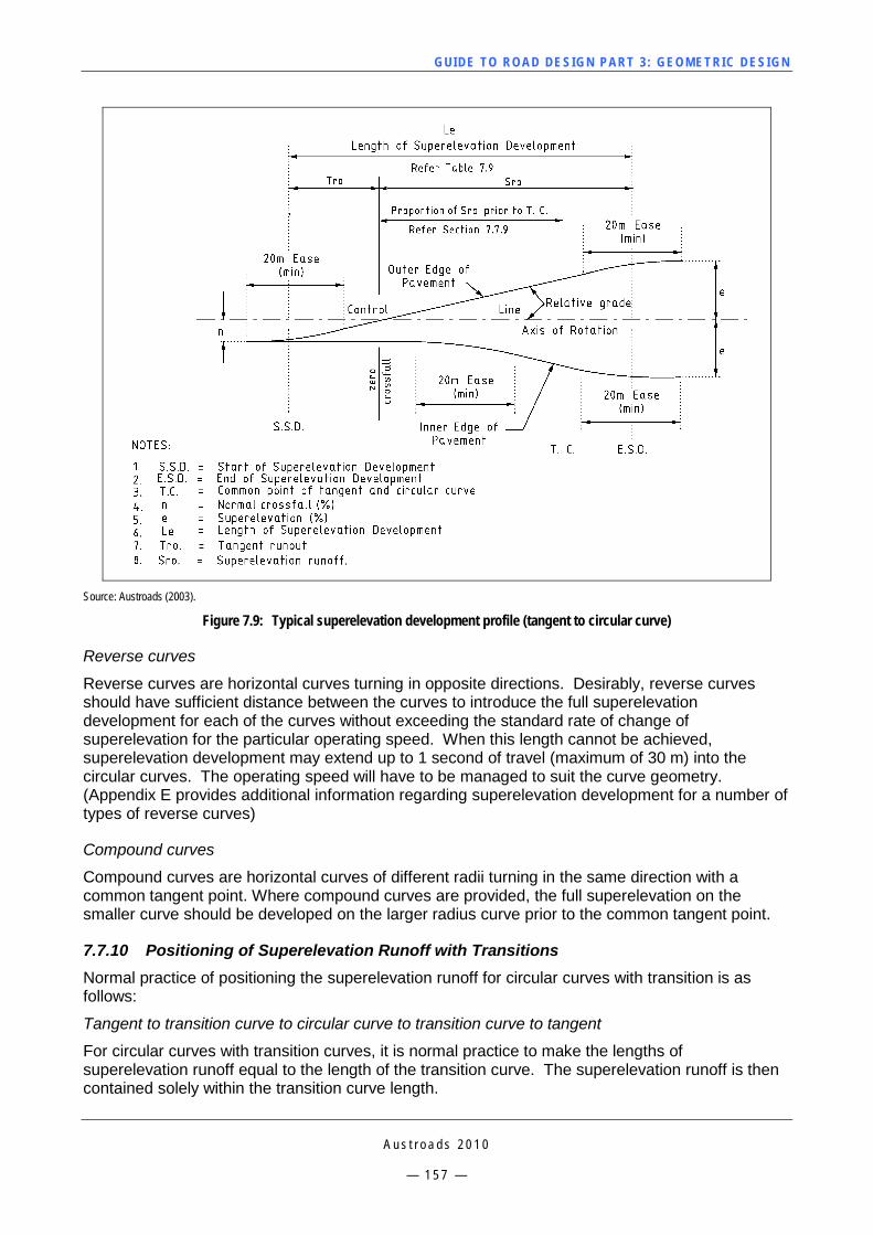
GUI DE TO RO A D DE SIG N P ART 3 : GEO MET RI C D ESI G N
A u s t r o a d s 2 0 1 0
— 1 5 7 —
Source: Austroads (2003).
Figure 7.9: Typical superelevation development profile (tangent to circular curve)
Reverse curves
Reverse curves are horizontal curves turning in opposite directions. Desirably, reverse curves should have sufficient distance between the curves to introduce the full superelevation development for each of the curves without exceeding the standard rate of change of superelevation for the particular operating speed. When this length cannot be achieved, superelevation development may extend up to 1 second of travel (maximum of 30 m) into the circular curves. The operating speed will have to be managed to suit the curve geometry. (Appendix E provides additional information regarding superelevation development for a number of types of reverse curves)
Compound curves
Compound curves are horizontal curves of different radii turning in the same direction with a common tangent point. Where compound curves are provided, the full superelevation on the smaller curve should be developed on the larger radius curve prior to the common tangent point.
7.7.10 Positioning of Superelevation Runoff with Transitions Normal practice of positioning the superelevation runoff for circular curves with transition is as follows:
Tangent to transition curve to circular curve to transition curve to tangent
For circular curves with transition curves, it is normal practice to make the lengths of superelevation runoff equal to the length of the transition curve. The superelevation runoff is then contained solely within the transition curve length.
GUI DE TO RO A D DE SIG N P ART 3 : GEO MET RI C D ESI G N
A u s t r o a d s 2 0 1 0
— 1 5 8 —
A typical example of the development of superelevation on horizontally transitioned curves on two-lane roads is shown in Figure 7.8. The superelevation runoff commences at the tangent to spiral point (flat cross fall) along the straight and ends at the spiral to circular curve point.
Reverse transitioned curves
On reverse transitioned curves, the reversal of superelevation is implemented uniformly and linearly.
However, in the case of long transition curves and small superelevations, it is necessary to increase the rotation rate in the vicinity of the point of zero superelevation to promote improved pavement surface drainage and minimise flow path lengths. Reference should be made to Austroads Guide to Road Design – Part 5: Drainage Design (Austroads 2008b) for further information.
It is undesirable to use long transition curves in other than high-speed curvilinear alignments because of the potential to mislead drivers as to the radius of the following circular curve.
7.8 Curves with Adverse Crossfall Adverse crossfall on curves should normally be avoided except on curves of large radius that can be regarded as straights. Table 7.10 gives minimum radius curves for various operating speeds for which adverse crossfall may be considered.
Adverse crossfall should not exceed 3%, except for curves in urban areas with an operating speed less than or equal to 70 km/h in constrained areas, and for intersection turns and roundabouts. It is common practice throughout the world to limit the maximum side friction factor to about half (or two thirds if the resulting factor < 0.08) that allowed on a superelevated curve.
Use of adverse superelevation should be limited on rural roads and freeways to:
situations where water depths on the pavement surface can be reduced
temporary roadways and temporary connections
side tracks.
Adverse crossfall should be avoided in the following circumstances:
On the approach to intersections or other braking areas
Areas subject to aquaplaning or icing
High speed roads with downhill grades in excess of 4%.
On urban roads, adverse superelevation can be tolerated more than on rural roads. This is mainly due to lower vehicle speeds and driver familiarity with the road. In addition to the situations that may require adverse superelevation on rural roads, common urban situations that may require the use of adverse superelevation are:
property access controls
channel drainage controls
grading restrictions
the need to maintain visibility of the road surface, especially near intersections.
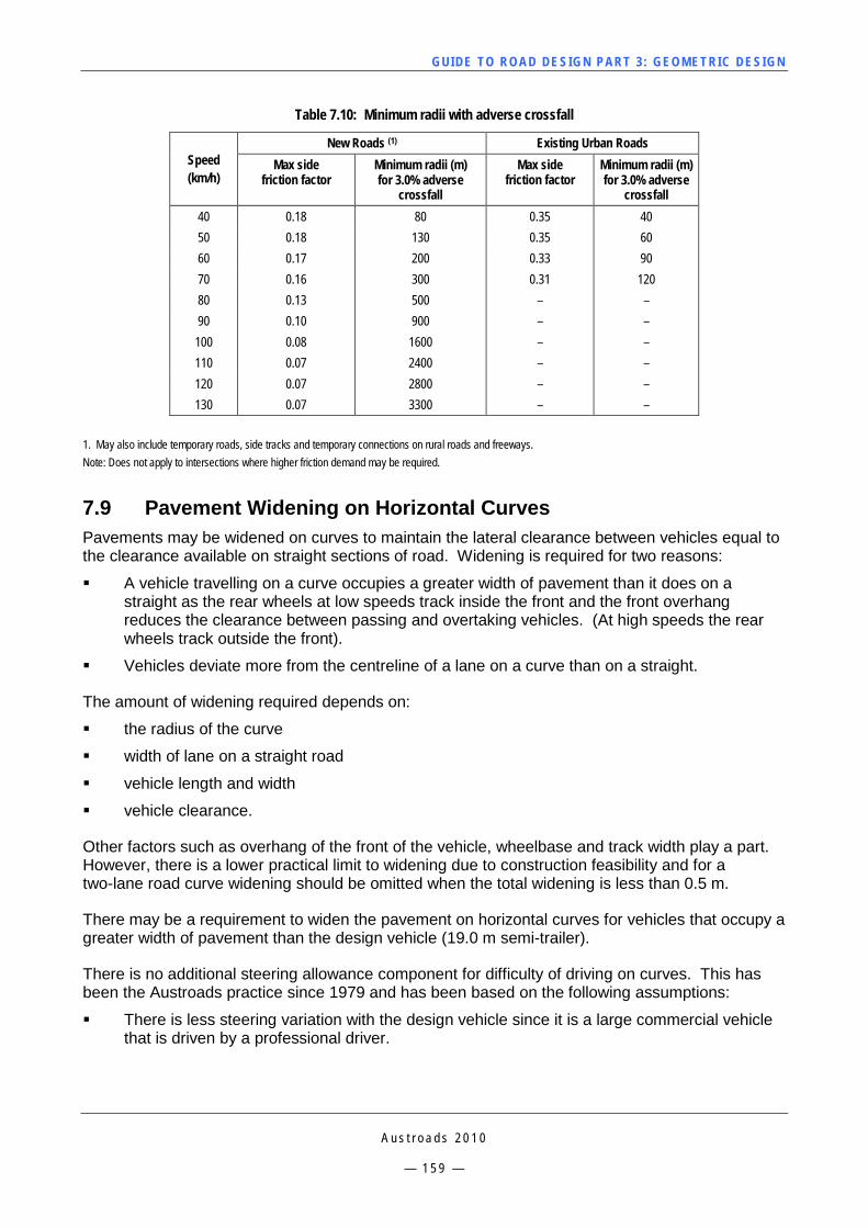
GUI DE TO RO A D DE SIG N P ART 3 : GEO MET RI C D ESI G N
A u s t r o a d s 2 0 1 0
— 1 5 9 —
Table 7.10: Minimum radii with adverse crossfall
Speed (km/h)
New Roads (1) Existing Urban Roads Max side
friction factor Minimum radii (m) for 3.0% adverse
crossfall
Max side friction factor
Minimum radii (m) for 3.0% adverse
crossfall 40 0.18 80 0.35 40 50 0.18 130 0.35 60 60 0.17 200 0.33 90 70 0.16 300 0.31 120 80 0.13 500 – – 90 0.10 900 – – 100 0.08 1600 – – 110 0.07 2400 – – 120 0.07 2800 – – 130 0.07 3300 – –
1. May also include temporary roads, side tracks and temporary connections on rural roads and freeways. Note: Does not apply to intersections where higher friction demand may be required.
7.9 Pavement Widening on Horizontal Curves Pavements may be widened on curves to maintain the lateral clearance between vehicles equal to the clearance available on straight sections of road. Widening is required for two reasons:
A vehicle travelling on a curve occupies a greater width of pavement than it does on a straight as the rear wheels at low speeds track inside the front and the front overhang reduces the clearance between passing and overtaking vehicles. (At high speeds the rear wheels track outside the front).
Vehicles deviate more from the centreline of a lane on a curve than on a straight.
The amount of widening required depends on:
the radius of the curve
width of lane on a straight road
vehicle length and width
vehicle clearance.
Other factors such as overhang of the front of the vehicle, wheelbase and track width play a part. However, there is a lower practical limit to widening due to construction feasibility and for a two-lane road curve widening should be omitted when the total widening is less than 0.5 m.
There may be a requirement to widen the pavement on horizontal curves for vehicles that occupy a greater width of pavement than the design vehicle (19.0 m semi-trailer).
There is no additional steering allowance component for difficulty of driving on curves. This has been the Austroads practice since 1979 and has been based on the following assumptions:
There is less steering variation with the design vehicle since it is a large commercial vehicle that is driven by a professional driver.
GUI DE TO RO A D DE SIG N P ART 3 : GEO MET RI C D ESI G N
A u s t r o a d s 2 0 1 0
— 1 6 0 —
The swept path width of the design vehicle accommodates the swept path width of smaller vehicles plus provides room for steering variation (and driver skill variation) with the smaller vehicles.
The now common use of full width or part width paved and sealed shoulders compensates for not having a steering allowance component for the design vehicle.
Table 7.11 shows the widening for a range of circular curve radii and design vehicles.
For lane widening with transitioned curves, it is normal practice to apply half of the curve widening to each side of the road. However, this means that the shift associated with the transition
(R
Lshift p
24
2
= , where LP is the length of transition curve, and R is the radius of the circular arc) must
be greater than the curve widening that is applied to the outer side of the curve so that the design vehicle will make use of the widening and for appearance. This will usually only be a problem when the curve widening has to suit a road train and a greater proportion of the total widening will have to be applied on the inside of the curve. The painted centreline will then be offset from the control line in order to provide equal lane widths.
For untransitioned curves, it is normal practice to apply all the curve widening to the inside of the curve with the painted centreline then being offset from the control line in order to provide equal lane widths. This practice aids drivers in making their own transition.
The need for widening of existing roads ceases when the widening per lane is less than 0.25 m (i.e. tabulated lane widths of less than 3.8 m, to fit the minimum practical widening for a two-lane road of 0.5 m). Small radius curves should be designed with the aid of turning templates or computer turn path simulation programs. This is because the angle of turn starts to affect the swept path width and the application of the curve widening will have to be checked against the swept path.
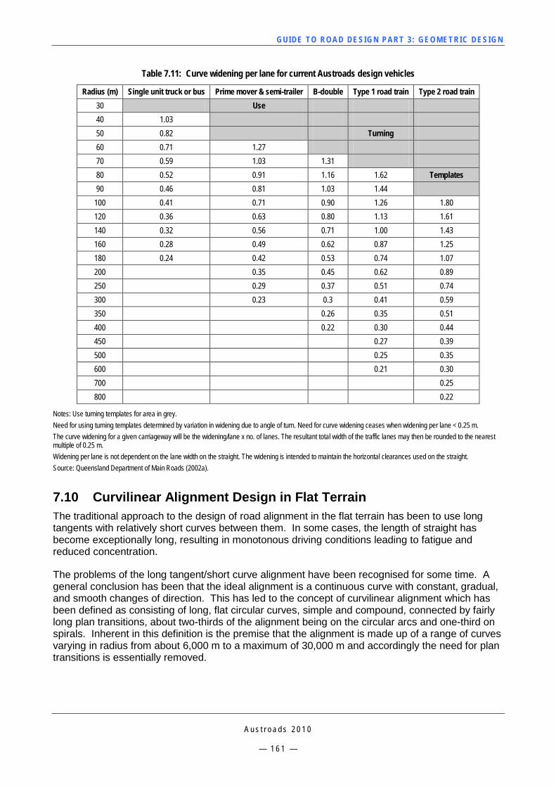
GUI DE TO RO A D DE SIG N P ART 3 : GEO MET RI C D ESI G N
A u s t r o a d s 2 0 1 0
— 1 6 1 —
Table 7.11: Curve widening per lane for current Austroads design vehicles
Radius (m) Single unit truck or bus Prime mover & semi-trailer B-double Type 1 road train Type 2 road train 30 Use 40 1.03 50 0.82 Turning 60 0.71 1.27 70 0.59 1.03 1.31 80 0.52 0.91 1.16 1.62 Templates 90 0.46 0.81 1.03 1.44
100 0.41 0.71 0.90 1.26 1.80 120 0.36 0.63 0.80 1.13 1.61 140 0.32 0.56 0.71 1.00 1.43 160 0.28 0.49 0.62 0.87 1.25 180 0.24 0.42 0.53 0.74 1.07 200 0.35 0.45 0.62 0.89 250 0.29 0.37 0.51 0.74 300 0.23 0.3 0.41 0.59 350 0.26 0.35 0.51 400 0.22 0.30 0.44 450 0.27 0.39 500 0.25 0.35 600 0.21 0.30 700 0.25 800 0.22
Notes: Use turning templates for area in grey. Need for using turning templates determined by variation in widening due to angle of turn. Need for curve widening ceases when widening per lane < 0.25 m. The curve widening for a given carriageway will be the widening/lane x no. of lanes. The resultant total width of the traffic lanes may then be rounded to the nearest multiple of 0.25 m. Widening per lane is not dependent on the lane width on the straight. The widening is intended to maintain the horizontal clearances used on the straight. Source: Queensland Department of Main Roads (2002a).
7.10 Curvilinear Alignment Design in Flat Terrain The traditional approach to the design of road alignment in the flat terrain has been to use long tangents with relatively short curves between them. In some cases, the length of straight has become exceptionally long, resulting in monotonous driving conditions leading to fatigue and reduced concentration.
The problems of the long tangent/short curve alignment have been recognised for some time. A general conclusion has been that the ideal alignment is a continuous curve with constant, gradual, and smooth changes of direction. This has led to the concept of curvilinear alignment which has been defined as consisting of long, flat circular curves, simple and compound, connected by fairly long plan transitions, about two-thirds of the alignment being on the circular arcs and one-third on spirals. Inherent in this definition is the premise that the alignment is made up of a range of curves varying in radius from about 6,000 m to a maximum of 30,000 m and accordingly the need for plan transitions is essentially removed.
GUI DE TO RO A D DE SIG N P ART 3 : GEO MET RI C D ESI G N
A u s t r o a d s 2 0 1 0
— 1 6 2 —
7.10.1 Theoretical Considerations The basis for using curvilinear alignment is found in the consideration of visual requirements and the effect of speed on perception and vision. As speed increases:
concentration increases
the point of concentration recedes
peripheral vision diminishes
foreground detail begins to fade
space perception becomes impaired.
Thus, the higher the speed, the further ahead the driver focuses vision and the more concentrated the angle of vision becomes. This restriction of vision (called ‘tunnel view’ by some) may induce fatigue unless the point of concentration is made to move around laterally by means of a curvilinear layout of the road.
Space perception is achieved with the help of memory, and by assessing relative changes in the size and position of objects. It is therefore necessary to have a lateral component to enable a driver to discern movement and its direction. This lateral component is provided on curves, the rate of such movement depending on the radius of the curve.
The radius that should be adopted depends on several factors including the type of topography and the expected speed of travel, the desired radius depending on how far ahead the driver can see the road. At high speeds, a driver looks from 300 m to 600 m ahead and a curve should be at least this long to be visually significant when the driver is on it.
It is desirable to design on the basis of at least 30 degrees of deflection angle as a minimum, which will result in the adoption of curve radii of from 3,000 to 30,000 m depending on how far ahead the road can be seen. A further consideration is the requirement of overtaking sight distance. It is desirable that overtaking sight distance be provided if possible and in flat country this can easily be achieved. A 15,000 m radius curve allows overtaking sight distance for 120 km/h to be achieved. The optimum radius range is about 16,000 to 18,000 m.
The larger the radius, however, the closer the alignment comes to a straight line and the less the advantages become and in this respect further consideration may need to be given to the desirable maximum length of curve in one direction. There is no point in using radii larger than 30,000 m for this reason.
7.10.2 Advantages of Curvilinear Alignment A road with curvilinear alignment is much more pleasant to drive on than one with long straight tangents since it unfolds itself smoothly with no unexpected checks. The driver is more able to judge the distance to an approaching vehicle, and to assess its rate of approach since the driver sees it to one side, the lateral component of its movement providing the necessary information for the driver assessment. Judgements on the safety of overtaking manoeuvres are easier to make under these circumstances.
Because of the continuously curving alignment, the view ahead is constantly changing and it is also possible to direct the road towards interesting features of the countryside for short periods. This removes much of the monotony of the long straight alignment and can create a sense of anticipation in the driver for what is beyond.
GUI DE TO RO A D DE SIG N P ART 3 : GEO MET RI C D ESI G N
A u s t r o a d s 2 0 1 0
— 1 6 3 —
At night, curvilinear alignment removes much of the approaching headlight glare problem common to long straight roads in flat country. On long straights, headlights become visible from a very long distance away and can be annoying and distracting from a distance of over 3 kilometres. Where vehicles approach each other on curvilinear alignment, the glow of the approaching vehicle headlamps can be seen well before the lamps become visible, and the rate of approach of the vehicle can be assessed.
In the daytime when driving in the direction of the sun, curvilinear alignment removes much of the approaching glare problem caused by the sun’s rays common to long straight roads running in a westerly/easterly direction in flat country.
Conditions for both day and night driving are therefore much more comfortable on a road with curvilinear alignment.
On treeless plains, some of the effect of the curvilinear alignment is lost. It may be that in such circumstances, the smaller (optimum) radii would be more effective in that it will increase the driver’s perception of relative change.
The principles of curvilinear alignment can be applied in a wide range of conditions using a wide range of curve radii together with spirals. Considerable improvements in the quality of the road system can be achieved at no extra cost by the application of these principles.
GUI DE TO RO A D DE SIG N P ART 3 : GEO MET RI C D ESI G N
A u s t r o a d s 2 0 1 0
— 1 6 4 —
8 VERTICAL ALIGNMENT
8.1 General Vertical alignment is the longitudinal profile along the centreline of a road. It is made up of a series of grades and vertical curves. The profile is determined by a consideration of the planning, access, topographic, geological, design controls, earthworks and other economic aspects.
The grades are generally expressed as a percentage of the vertical component divided by the horizontal component.
The vertical curves are usually parabolic in shape and are expressed as a K Value. The K Value is the vertical curve constant, used to define the size of a parabola. It is the length (m) required for a 1% change of grade.
For design purposes the K value concept also has the advantage of easily determining the radius at the apex of a parabolic vertical curve: R = 100K. Within the range of grades used for road design there is little variation between the parabola and the extended arc of the apex radius. Therefore, the apex radius value yields a suitable equivalent radius and an alternative vertical curve constant that can be used to define the size of a parabolic vertical curve.
Some road authorities use the radius to define the crest curve instead of the K value, using the relationship noted above. For the purposes of consistency across the Austroads Guide to Road Design, all issues relating to vertical curves are only described using K values.
The vertical alignment is typically displayed on a longitudinal section (profile) with an exaggerated vertical scale of 10:1. The gradeline shown relates to a reference point (or physical attribute) on the cross-section.
8.2 Vertical Controls The level of a road at any point along its route, and therefore its vertical alignment, is usually controlled to a large extent by features that the road passes through. The following are typical controls for vertical geometry:
existing topography
geotechnical conditions
existing intersections
property entrances
overpasses and underpasses
pedestrian accesses
service utility assets (and their protection requirements)
median openings.
The road will have to match, within appropriate limits, the levels that these controls dictate.
Designers should also not underestimate the impact that carriageway crossfalls from adjacent or intersecting roads can impact on the design of the vertical geometry, especially when considering drainage of surface flows.
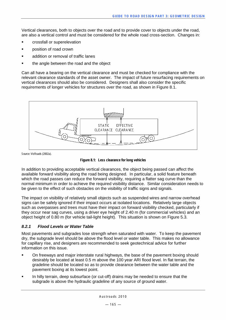
GUI DE TO RO A D DE SIG N P ART 3 : GEO MET RI C D ESI G N
A u s t r o a d s 2 0 1 0
— 1 6 5 —
Vertical clearances, both to objects over the road and to provide cover to objects under the road, are also a vertical control and must be considered for the whole road cross-section. Changes in:
crossfall or superelevation
position of road crown
addition or removal of traffic lanes
the angle between the road and the object
Can all have a bearing on the vertical clearance and must be checked for compliance with the relevant clearance standards of the asset owner. The impact of future resurfacing requirements on vertical clearances should also be considered. Designers shall also consider the specific requirements of longer vehicles for structures over the road, as shown in Figure 8.1.
Source: VicRoads (2002a).
Figure 8.1: Less clearance for long vehicles
In addition to providing acceptable vertical clearances, the object being passed can affect the available forward visibility along the road being designed. In particular, a solid feature beneath which the road passes can reduce the forward visibility, requiring a flatter sag curve than the normal minimum in order to achieve the required visibility distance. Similar consideration needs to be given to the effect of such obstacles on the visibility of traffic signs and signals.
The impact on visibility of relatively small objects such as suspended wires and narrow overhead signs can be safely ignored if their impact occurs at isolated locations. Relatively large objects such as overpasses and trees must have their impact on forward visibility checked, particularly if they occur near sag curves, using a driver eye height of 2.40 m (for commercial vehicles) and an object height of 0.80 m (for vehicle tail-light height). This situation is shown on Figure 5.3.
8.2.1 Flood Levels or Water Table Most pavements and subgrades lose strength when saturated with water. To keep the pavement dry, the subgrade level should be above the flood level or water table. This makes no allowance for capillary rise, and designers are recommended to seek geotechnical advice for further information on this issue.
On freeways and major interstate rural highways, the base of the pavement boxing should desirably be located at least 0.5 m above the 100 year ARI flood level. In flat terrain, the gradeline should be located so as to provide clearance between the water table and the pavement boxing at its lowest point.
In hilly terrain, deep subsurface (or cut-off) drains may be needed to ensure that the subgrade is above the hydraulic gradeline of any source of ground water.
GUI DE TO RO A D DE SIG N P ART 3 : GEO MET RI C D ESI G N
A u s t r o a d s 2 0 1 0
— 1 6 6 —
On other roads it may be desirable, for economic reasons, to adopt reduced clearances above the water table. Although arterial roads should remain flood free, it is occasionally necessary to accept some water on the pavement for the design storm. For details of design Average Recurrence Intervals and acceptable water levels, refer to the Guide to Road Design – Part 5: Drainage Design (Austroads 2008b). Further guidance is also provided on the recommended freeboard for culverts and bridges.
For all road projects, minimum clearances above flood levels and water tables shall be defined by the relevant road authority.
8.2.2 Vertical Clearances Typical vertical clearances for objects constructed over a road are listed in Table 8.1. In all cases, it is the responsibility of designers to confirm these clearances from the following sources and if required, the order of precedence where there is a conflict:
The policies of the road owning authority.
AS5100 Set-2007, Bridge Design Set or the New Zealand Bridge Design Manual, Transit New Zealand (2003).
The requirements of the authority that owns the object. e.g. rail authority. See Commentary 20.
8.2.3 Underground Services All underground services in the vicinity of the roadworks shall be identified and located to ensure that minimum clearance requirements of the responsible authority are satisfied. Services commonly involved include:
gas mains
water mains
stormwater drains
sewer outfalls
telecommunication cables
underground electrical cables
road authority assets for ITS, traffic signals and street lighting.
In each case, designers shall consult with the relevant authority to determine the minimum clearances. With gas pipes, for example, clearances depend on the pressure within the pipe. The age of the service can also be relevant, particularly when lead joints have been used for water supply pipes.
It is sometimes possible to obtain agreement to the use of a reduced clearance together with some form of special protection for the service such as encasement of the service in a box culvert, encasement in mass concrete or the provision of a concrete slab over the service.
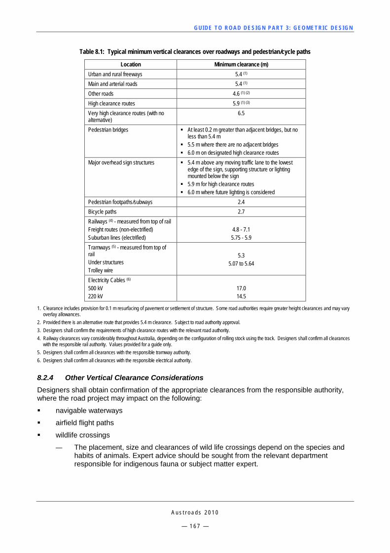
GUI DE TO RO A D DE SIG N P ART 3 : GEO MET RI C D ESI G N
A u s t r o a d s 2 0 1 0
— 1 6 7 —
Table 8.1: Typical minimum vertical clearances over roadways and pedestrian/cycle paths
Location Minimum clearance (m) Urban and rural freeways 5.4 (1) Main and arterial roads 5.4 (1) Other roads 4.6 (1) (2) High clearance routes 5.9 (1) (3) Very high clearance routes (with no alternative)
6.5
Pedestrian bridges At least 0.2 m greater than adjacent bridges, but no less than 5.4 m
5.5 m where there are no adjacent bridges 6.0 m on designated high clearance routes
Major overhead sign structures 5.4 m above any moving traffic lane to the lowest edge of the sign, supporting structure or lighting mounted below the sign
5.9 m for high clearance routes 6.0 m where future lighting is considered
Pedestrian footpaths/subways 2.4 Bicycle paths 2.7 Railways (4) - measured from top of rail Freight routes (non-electrified) Suburban lines (electrified)
4.8 - 7.1 5.75 - 5.9
Tramways (5) - measured from top of rail Under structures Trolley wire
5.3
5.07 to 5.64
Electricity Cables (6) 500 kV 220 kV
17.0 14.5
1. Clearance includes provision for 0.1 m resurfacing of pavement or settlement of structure. Some road authorities require greater height clearances and may vary overlay allowances.
2. Provided there is an alternative route that provides 5.4 m clearance. Subject to road authority approval. 3. Designers shall confirm the requirements of high clearance routes with the relevant road authority. 4. Railway clearances vary considerably throughout Australia, depending on the configuration of rolling stock using the track. Designers shall confirm all clearances
with the responsible rail authority. Values provided for a guide only. 5. Designers shall confirm all clearances with the responsible tramway authority. 6. Designers shall confirm all clearances with the responsible electrical authority.
8.2.4 Other Vertical Clearance Considerations Designers shall obtain confirmation of the appropriate clearances from the responsible authority, where the road project may impact on the following:
navigable waterways
airfield flight paths
wildlife crossings
— The placement, size and clearances of wild life crossings depend on the species and habits of animals. Expert advice should be sought from the relevant department responsible for indigenous fauna or subject matter expert.
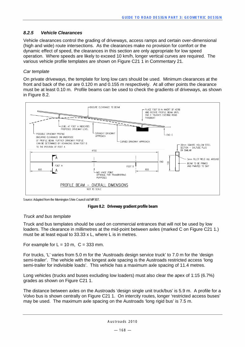
GUI DE TO RO A D DE SIG N P ART 3 : GEO MET RI C D ESI G N
A u s t r o a d s 2 0 1 0
— 1 6 8 —
8.2.5 Vehicle Clearances Vehicle clearances control the grading of driveways, access ramps and certain over-dimensional (high and wide) route intersections. As the clearances make no provision for comfort or the dynamic effect of speed, the clearances in this section are only appropriate for low speed operation. Where speeds are likely to exceed 10 km/h, longer vertical curves are required. The various vehicle profile templates are shown on Figure C21 1 in Commentary 21.
Car template
On private driveways, the template for long low cars should be used. Minimum clearances at the front and back of the car are 0.120 m and 0.155 m respectively. At all other points the clearance must be at least 0.10 m. Profile beams can be used to check the gradients of driveways, as shown in Figure 8.2.
Source: Adapted from the Mornington Shire Council std MP307.
Figure 8.2: Driveway gradient profile beam
Truck and bus template
Truck and bus templates should be used on commercial entrances that will not be used by low loaders. The clearance in millimetres at the mid-point between axles (marked C on Figure C21 1.) must be at least equal to 33.33 x L, where L is in metres.
For example for L = 10 m, C = 333 mm.
For trucks, ‘L’ varies from 5.0 m for the ‘Austroads design service truck’ to 7.0 m for the ‘design semi-trailer’. The vehicle with the longest axle spacing is the Austroads restricted access ‘long semi-trailer for indivisible loads’. This vehicle has a maximum axle spacing of 11.4 metres.
Long vehicles (trucks and buses excluding low loaders) must also clear the apex of 1:15 (6.7%) grades as shown on Figure C21 1.
The distance between axles on the Austroads ‘design single unit truck/bus’ is 5.9 m. A profile for a Volvo bus is shown centrally on Figure C21 1. On intercity routes, longer ‘restricted access buses’ may be used. The maximum axle spacing on the Austroads ‘long rigid bus’ is 7.5 m.
GUI DE TO RO A D DE SIG N P ART 3 : GEO MET RI C D ESI G N
A u s t r o a d s 2 0 1 0
— 1 6 9 —
If the provision of these standards is difficult, designers should determine the critical axle spacing for the buses that are likely to use the route (Department of Transport and Communications 1986).
Note that angular templates such as these are only appropriate for low speed operation i.e. 1 to 5 km/h. The provision of a vertical curve at the apex increases the clearance available and provides a smoother ride. Desirably vertical curves should be at least 1.5 to 2 m long for speeds of 0 to 5 km/h and 2 to 5 m long for speeds of 6 to 15 km/h. For speeds from 16 to 30 km/h, the vertical curve should be at least 10 metres long. Vertical curves for higher speeds are tabulated on Table 8.9.
Low loaders
At intersections on designated over-dimensional routes and all railway crossings, the low loader template (Figure C21 1, bottom) shall be used. For through roads that are likely to be used by low loaders, the clearance diagram for low loaders should be used.
The maximum grade change without a vertical curve at level crossings and intersections on through routes should not exceed 4.6%, to avoid snagging low loaders.
Designers should consult the Guide to Road Design – Part 4: Intersections and Crossings – General (Austroads 2009a) for further advice on grading controls at intersections and railway level crossings.
8.3 Grading Procedure Step 1
In collaboration with the client, identify all major controls on the alignment (Section 8.2), and categorise them as mandatory or discretionary.
Other controls that could be considered include:
operating speed (Section 3)
providing appropriate sight distance (Section 5)
providing overtaking opportunities (Section 9)
drainage culverts (Guide to Road Design – Part 5: Drainage Design (Austroads 2008b))
achieving earthworks balance (Section 8.7)
environmentally sensitive sites
costs
aesthetics (Section 6).
Step 2
Prepare a horizontal alignment in accordance with Section7 of this guide.
Step 3
Select appropriate grading points (Section 8.4).
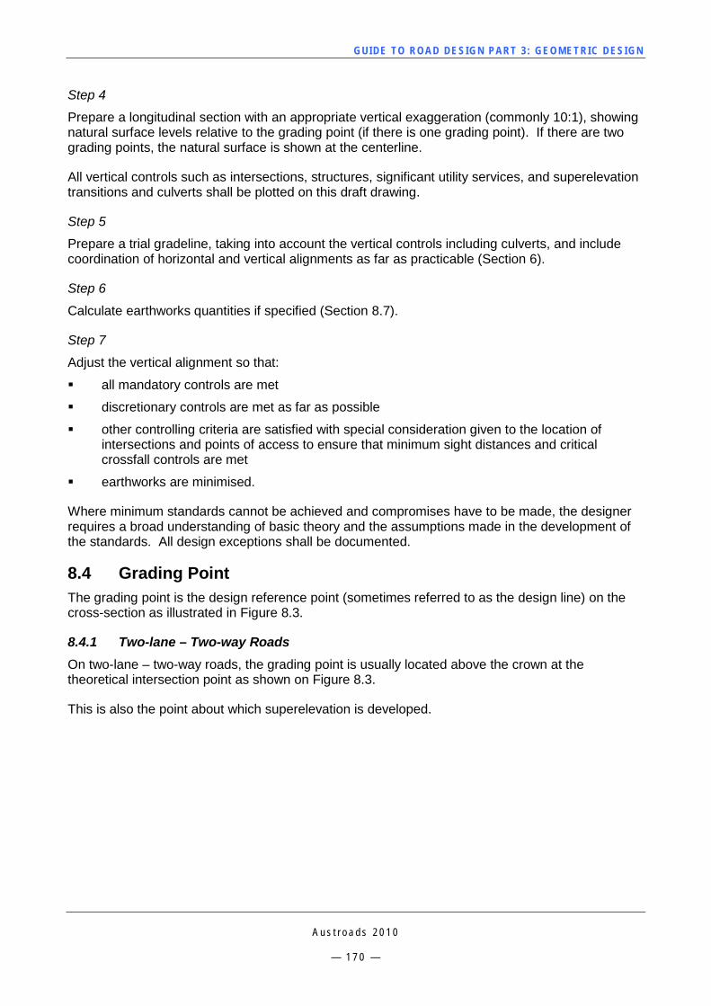
GUI DE TO RO A D DE SIG N P ART 3 : GEO MET RI C D ESI G N
A u s t r o a d s 2 0 1 0
— 1 7 0 —
Step 4
Prepare a longitudinal section with an appropriate vertical exaggeration (commonly 10:1), showing natural surface levels relative to the grading point (if there is one grading point). If there are two grading points, the natural surface is shown at the centerline.
All vertical controls such as intersections, structures, significant utility services, and superelevation transitions and culverts shall be plotted on this draft drawing.
Step 5
Prepare a trial gradeline, taking into account the vertical controls including culverts, and include coordination of horizontal and vertical alignments as far as practicable (Section 6).
Step 6
Calculate earthworks quantities if specified (Section 8.7).
Step 7
Adjust the vertical alignment so that:
all mandatory controls are met
discretionary controls are met as far as possible
other controlling criteria are satisfied with special consideration given to the location of intersections and points of access to ensure that minimum sight distances and critical crossfall controls are met
earthworks are minimised.
Where minimum standards cannot be achieved and compromises have to be made, the designer requires a broad understanding of basic theory and the assumptions made in the development of the standards. All design exceptions shall be documented.
8.4 Grading Point The grading point is the design reference point (sometimes referred to as the design line) on the cross-section as illustrated in Figure 8.3.
8.4.1 Two-lane – Two-way Roads On two-lane – two-way roads, the grading point is usually located above the crown at the theoretical intersection point as shown on Figure 8.3.
This is also the point about which superelevation is developed.
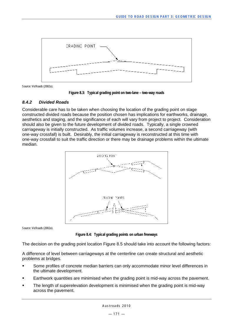
GUI DE TO RO A D DE SIG N P ART 3 : GEO MET RI C D ESI G N
A u s t r o a d s 2 0 1 0
— 1 7 1 —
Source: VicRoads (2002a).
Figure 8.3: Typical grading point on two-lane – two-way roads
8.4.2 Divided Roads Considerable care has to be taken when choosing the location of the grading point on stage constructed divided roads because the position chosen has implications for earthworks, drainage, aesthetics and staging, and the significance of each will vary from project to project. Consideration should also be given to the future development of divided roads. Typically, a single crowned carriageway is initially constructed. As traffic volumes increase, a second carriageway (with one-way crossfall) is built. Desirably, the initial carriageway is reconstructed at this time with one-way crossfall to suit the traffic direction or there may be drainage problems within the ultimate median.
Source: VicRoads (2002a).
Figure 8.4: Typical grading points on urban freeways
The decision on the grading point location Figure 8.5 should take into account the following factors:
A difference of level between carriageways at the centerline can create structural and aesthetic problems at bridges.
Some profiles of concrete median barriers can only accommodate minor level differences in the ultimate development.
Earthwork quantities are minimised when the grading point is mid-way across the pavement.
The length of superelevation development is minimised when the grading point is mid-way across the pavement.
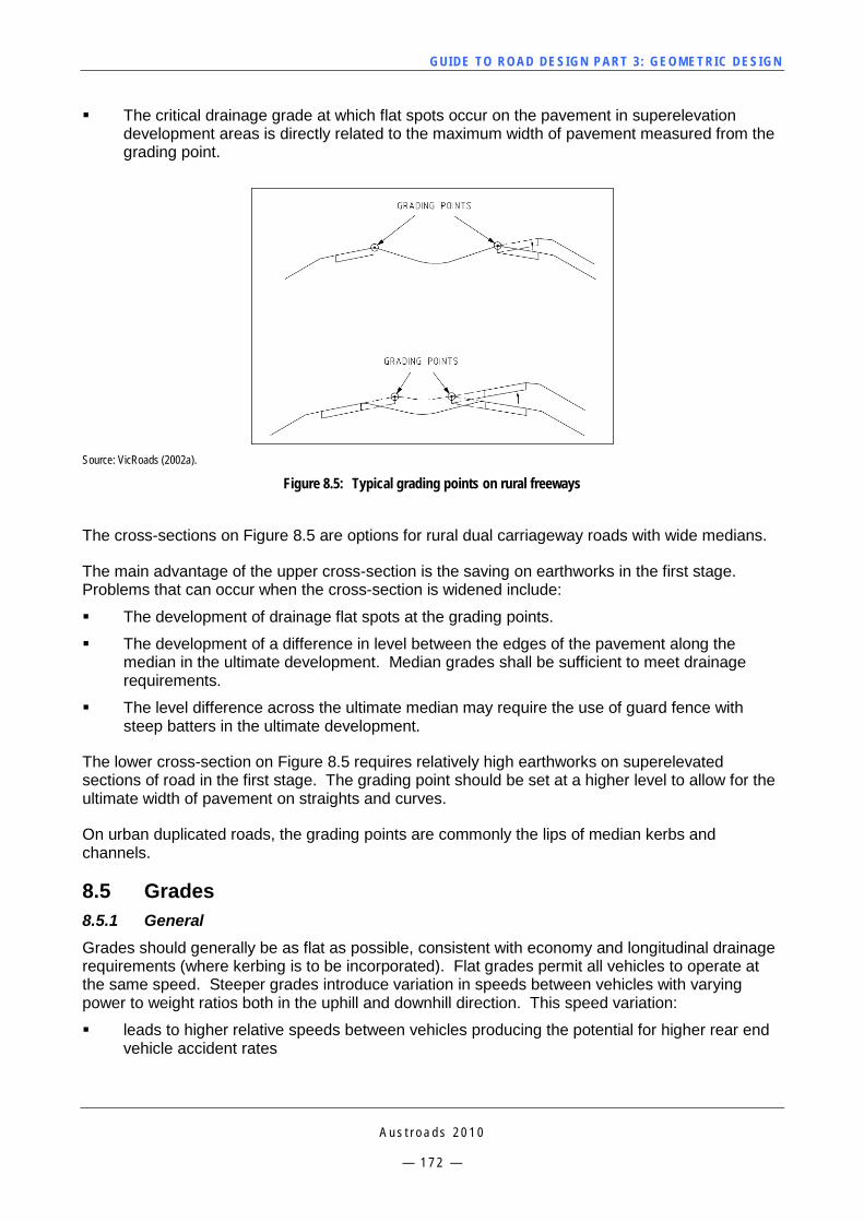
GUI DE TO RO A D DE SIG N P ART 3 : GEO MET RI C D ESI G N
A u s t r o a d s 2 0 1 0
— 1 7 2 —
The critical drainage grade at which flat spots occur on the pavement in superelevation development areas is directly related to the maximum width of pavement measured from the grading point.
Source: VicRoads (2002a).
Figure 8.5: Typical grading points on rural freeways
The cross-sections on Figure 8.5 are options for rural dual carriageway roads with wide medians.
The main advantage of the upper cross-section is the saving on earthworks in the first stage. Problems that can occur when the cross-section is widened include:
The development of drainage flat spots at the grading points.
The development of a difference in level between the edges of the pavement along the median in the ultimate development. Median grades shall be sufficient to meet drainage requirements.
The level difference across the ultimate median may require the use of guard fence with steep batters in the ultimate development.
The lower cross-section on Figure 8.5 requires relatively high earthworks on superelevated sections of road in the first stage. The grading point should be set at a higher level to allow for the ultimate width of pavement on straights and curves.
On urban duplicated roads, the grading points are commonly the lips of median kerbs and channels.
8.5 Grades 8.5.1 General Grades should generally be as flat as possible, consistent with economy and longitudinal drainage requirements (where kerbing is to be incorporated). Flat grades permit all vehicles to operate at the same speed. Steeper grades introduce variation in speeds between vehicles with varying power to weight ratios both in the uphill and downhill direction. This speed variation:
leads to higher relative speeds between vehicles producing the potential for higher rear end vehicle accident rates
GUI DE TO RO A D DE SIG N P ART 3 : GEO MET RI C D ESI G N
A u s t r o a d s 2 0 1 0
— 1 7 3 —
results in increased queuing and overtaking requirements which gives rise to further safety problems, particularly at higher traffic volumes.
In addition, freight costs are increased due to the increased fuel consumption and slower speed of heavy vehicles. From an environmental perspective, steeper grades also result in higher vehicle emissions.
Table 8.2 shows the effect of grade on vehicle performance and lists road types that would be suitable for these grades. Vehicles can tolerate relatively short lengths of steeper grades better than longer lengths of less steep grades.
Grades above 5% can create drainage problems because the length of drainage flow paths increase with grade. Conversely, flat grades create drainage problems on roads with kerb and channel and may require the use of independently graded, grated trenches. Further information about this topic can be found in the Guide to Road Design – Part 5: Drainage Design (Austroads 2008b).
Designers need to also consider the effect of steep downhill grades for trucks and ensure that adequate signage is provided to warn drivers. Adequate sight distance is also required for drivers on the approaches to curves on steep downhill grades. Section 7 in the Guide to Road Design – Part 6: Roadside Design, Safety and Barriers (Austroads 2009d), provides guidance regarding the provision of arrester beds and other facilities to reduce the risk of brake failure on steep grades.
8.5.2 Vehicle Operation on Grades There are three aspects to the design of grades that can be adopted in difficult terrain:
The poorer performing vehicles using the road (generally trucks in the lower power ranges) must be able to climb the grade. This limits the maximum grade that can be considered for roads open to the public. It only becomes an acceptable limit in low volume situations, or for special purpose roads, e.g. to a specific tourist vantage point.
Grades cause the need for speed variations, gear changes and braking for all vehicles. This is a quality of service consideration. Flatter grades, which enable a more consistent travel speed, make fewer demands on both vehicle and driver and generally reduce vehicle operating costs.
Grades cause speed disparities between vehicle types, leading to increased queuing and overtaking requirements. This is a level of service problem. The increased overtaking requirements and reduced service volumes can give rise to operational and safety problems at higher traffic flows. The problem can arise from cars towing caravans and trailers as well as from heavy commercial vehicles.
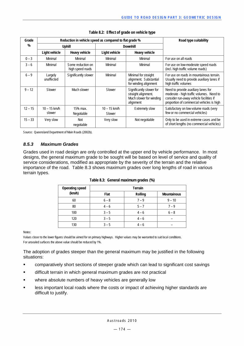
GUI DE TO RO A D DE SIG N P ART 3 : GEO MET RI C D ESI G N
A u s t r o a d s 2 0 1 0
— 1 7 4 —
Table 8.2: Effect of grade on vehicle type
Grade %
Reduction in vehicle speed as compared to flat grade % Road type suitability Uphill Downhill
Light vehicle Heavy vehicle Light vehicle Heavy vehicle 0 – 3 Minimal Minimal Minimal Minimal For use on all roads 3 – 6 Minimal Some reduction on
high speed roads Minimal Minimal For use on low-moderate speed roads
(incl. high traffic volume roads) 6 – 9 Largely
unaffected Significantly slower Minimal Minimal for straight
alignment. Substantial for winding alignment
For use on roads in mountainous terrain. Usually need to provide auxiliary lanes if high traffic volumes
9 – 12 Slower Much slower Slower Significantly slower for straight alignment. Much slower for winding alignment
Need to provide auxiliary lanes for moderate - high traffic volumes. Need to consider run-away vehicle facilities if proportion of commercial vehicles is high
12 – 15 10 – 15 km/h slower
15% max. Negotiable
10 – 15 km/h Slower
Extremely slow Satisfactory on low volume roads (very few or no commercial vehicles)
15 – 33 Very slow Not negotiable
Very slow Not negotiable Only to be used in extreme cases and be of short lengths (no commercial vehicles)
Source: Queensland Department of Main Roads (2002b).
8.5.3 Maximum Grades Grades used in road design are only controlled at the upper end by vehicle performance. In most designs, the general maximum grade to be sought will be based on level of service and quality of service considerations, modified as appropriate by the severity of the terrain and the relative importance of the road. Table 8.3 shows maximum grades over long lengths of road in various terrain types.
Table 8.3: General maximum grades (%)
Operating speed (km/h)
Terrain Flat Rolling Mountainous
60 6 – 8 7 – 9 9 – 10 80 4 – 6 5 – 7 7 – 9 100 3 – 5 4 – 6 6 – 8 120 3 – 5 4 – 6 – 130 3 – 5 4 – 6 –
Notes: Values closer to the lower figures should be aimed for on primary highways. Higher values may be warranted to suit local conditions. For unsealed surfaces the above value should be reduced by 1%. The adoption of grades steeper than the general maximum may be justified in the following situations:
comparatively short sections of steeper grade which can lead to significant cost savings
difficult terrain in which general maximum grades are not practical
where absolute numbers of heavy vehicles are generally low
less important local roads where the costs or impact of achieving higher standards are difficult to justify.
GUI DE TO RO A D DE SIG N P ART 3 : GEO MET RI C D ESI G N
A u s t r o a d s 2 0 1 0
— 1 7 5 —
Design options for managing steep grades include, flattening the grade, or alternatively provision of auxiliary lanes and/or special facilities for safely controlling runaway vehicles on downgrades (refer Section 9 and the Guide to Road Design – Part 6: Roadside Design, Safety and Barriers (Austroads 2009d)).
When adopting maximum grades, side drains need to be considered in respect of the maximum velocity of flow for scour protection. Special lining of open drains may be required to limit damage to the drain and the environment.
Maximum grades at intersections
Designers should refer to the Guide to Road Design – Part 4: Intersections and Crossings – General (Austroads 2009a) for information relating to the control of grades at intersections and railway level crossings.
8.5.4 Length of Steep Grades Maximum grade in itself is not a complete design control, as designers need to also consider what impact the length of the grade has on vehicle performance. Most standards do not explicitly limit the length of grades, but suggest that it is desirable to limit the length of sections with maximum grades. AASHTO (2004) discusses the term ‘critical length of grade’ which is used to indicate the maximum length of a designated upgrade on which a loaded truck can operate without an unreasonable reduction in speed. AASHTO notes that to establish design values for critical lengths of grade for which gradeability of trucks is the determining factor, the following needs to be considered:
Size and power of a representative truck or truck combination to be used as a design vehicle along with the gradeability data for that vehicle. AASHTO propose adoption of a weight/power ratio of about 120 kg/KW. This is roughly equivalent to a 19 m semi-trailer carrying an average load.
Figure 3.9 provides truck performance curves for this vehicle. Designers should refer to Figure 9.3 to Figure 9.6 for the performance curves of alternative truck combinations.
Speed of the truck at the entrance to the critical length of grade.
Minimum speed on the grade below which the interference to following vehicles is unreasonable. AASHTO propose a maximum speed reduction of 15 km/h be adopted for the determination of critical lengths of grade as the likelihood of the truck being involved in a crash increases significantly beyond this speed.
However, it must be remembered that length of grade can affect both safety and capacity. Studies show that, regardless of the average speed on the highway, the more a vehicle deviates from the average speed, the greater are its chances of becoming involved in a crash. On both the upgrade and downgrade, the lower operating speed of trucks may cause inconvenience to cars. Long gradients, for example 5 km at 4%, could result in a high risk of serious accidents involving descending vehicles as a result of brake failure. Such gradients could also cause climbing vehicles to slow down to well below the 85th percentile speed. Current vehicle standards require multi-combination vehicles to be able to maintain a speed of 70 km/h on a 1% grade. The length of grade plays an important factor in the performance of those vehicles. For sections of road with grades greater than those given in Table 8.4, a risk analysis to identify operational and safety effects should be undertaken to determine the most appropriate treatment.
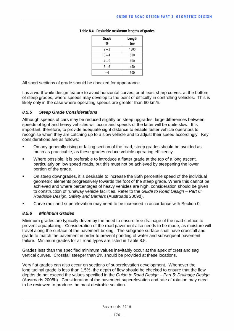
GUI DE TO RO A D DE SIG N P ART 3 : GEO MET RI C D ESI G N
A u s t r o a d s 2 0 1 0
— 1 7 6 —
Table 8.4: Desirable maximum lengths of grades
Grade %
Length (m)
2 – 3 1800 3 – 4 900 4 – 5 600 5 – 6 450 > 6 300
All short sections of grade should be checked for appearance.
It is a worthwhile design feature to avoid horizontal curves, or at least sharp curves, at the bottom of steep grades, where speeds may develop to the point of difficulty in controlling vehicles. This is likely only in the case where operating speeds are greater than 60 km/h.
8.5.5 Steep Grade Considerations Although speeds of cars may be reduced slightly on steep upgrades, large differences between speeds of light and heavy vehicles will occur and speeds of the latter will be quite slow. It is important, therefore, to provide adequate sight distance to enable faster vehicle operators to recognise when they are catching up to a slow vehicle and to adjust their speed accordingly. Key considerations are as follows:
On any generally rising or falling section of the road, steep grades should be avoided as much as practicable, as these grades reduce vehicle operating efficiency.
Where possible, it is preferable to introduce a flatter grade at the top of a long ascent, particularly on low speed roads, but this must not be achieved by steepening the lower portion of the grade.
On steep downgrades, it is desirable to increase the 85th percentile speed of the individual geometric elements progressively towards the foot of the steep grade. Where this cannot be achieved and where percentages of heavy vehicles are high, consideration should be given to construction of runaway vehicle facilities. Refer to the Guide to Road Design – Part 6: Roadside Design, Safety and Barriers (Austroads 2009d).
Curve radii and superelevation may need to be increased in accordance with Section 0.
8.5.6 Minimum Grades Minimum grades are typically driven by the need to ensure free drainage of the road surface to prevent aquaplaning. Consideration of the road pavement also needs to be made, as moisture will travel along the surface of the pavement boxing. The subgrade surface shall have crossfall and grade to match the pavement in order to prevent ponding of water and subsequent pavement failure. Minimum grades for all road types are listed in Table 8.5.
Grades less than the specified minimum values inevitably occur at the apex of crest and sag vertical curves. Crossfall steeper than 2% should be provided at these locations.
Very flat grades can also occur on sections of superelevation development. Whenever the longitudinal grade is less than 1.5%, the depth of flow should be checked to ensure that the flow depths do not exceed the values specified in the Guide to Road Design – Part 5: Drainage Design (Austroads 2008b). Consideration of the pavement superelevation and rate of rotation may need to be reviewed to produce the most desirable solution.
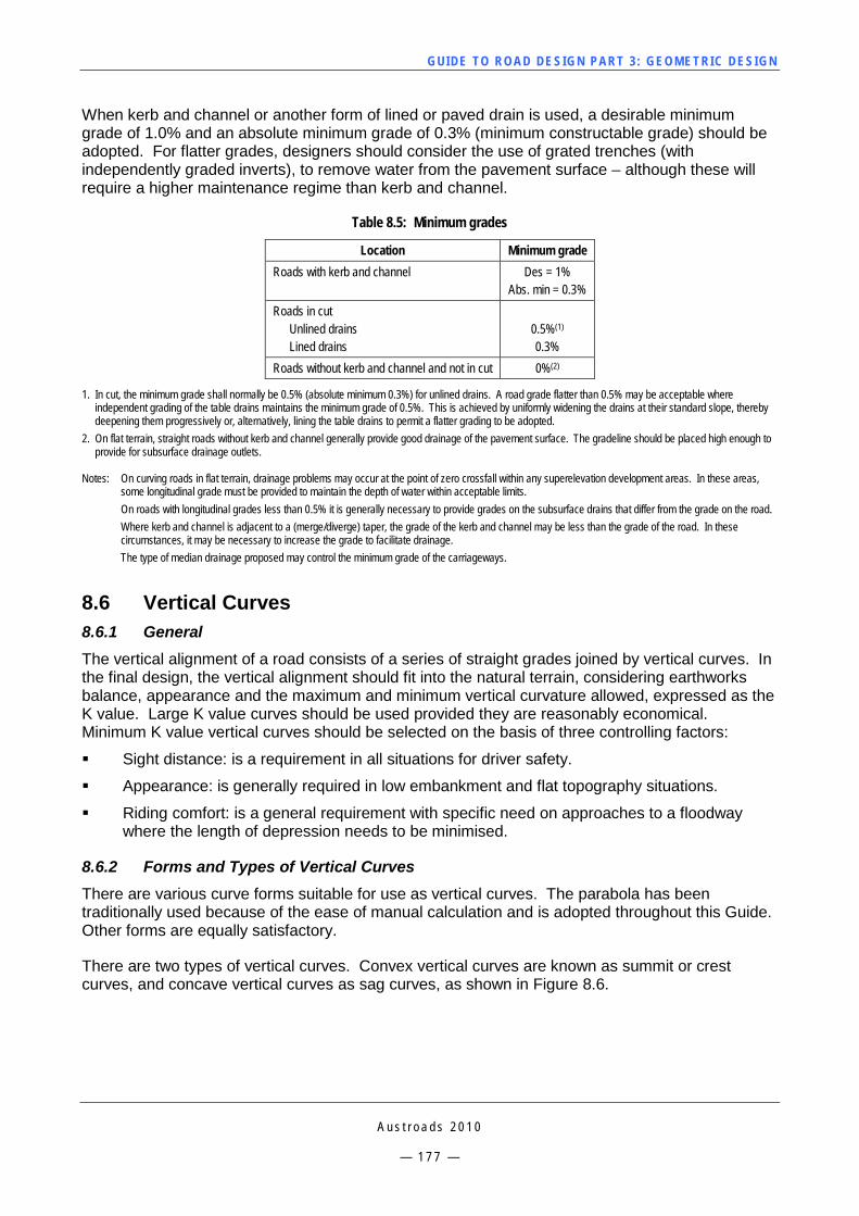
GUI DE TO RO A D DE SIG N P ART 3 : GEO MET RI C D ESI G N
A u s t r o a d s 2 0 1 0
— 1 7 7 —
When kerb and channel or another form of lined or paved drain is used, a desirable minimum grade of 1.0% and an absolute minimum grade of 0.3% (minimum constructable grade) should be adopted. For flatter grades, designers should consider the use of grated trenches (with independently graded inverts), to remove water from the pavement surface – although these will require a higher maintenance regime than kerb and channel.
Table 8.5: Minimum grades
Location Minimum grade Roads with kerb and channel Des = 1%
Abs. min = 0.3% Roads in cut
Unlined drains Lined drains
0.5%(1) 0.3%
Roads without kerb and channel and not in cut 0%(2)
1. In cut, the minimum grade shall normally be 0.5% (absolute minimum 0.3%) for unlined drains. A road grade flatter than 0.5% may be acceptable where independent grading of the table drains maintains the minimum grade of 0.5%. This is achieved by uniformly widening the drains at their standard slope, thereby deepening them progressively or, alternatively, lining the table drains to permit a flatter grading to be adopted.
2. On flat terrain, straight roads without kerb and channel generally provide good drainage of the pavement surface. The gradeline should be placed high enough to provide for subsurface drainage outlets.
Notes: On curving roads in flat terrain, drainage problems may occur at the point of zero crossfall within any superelevation development areas. In these areas,
some longitudinal grade must be provided to maintain the depth of water within acceptable limits. On roads with longitudinal grades less than 0.5% it is generally necessary to provide grades on the subsurface drains that differ from the grade on the road. Where kerb and channel is adjacent to a (merge/diverge) taper, the grade of the kerb and channel may be less than the grade of the road. In these circumstances, it may be necessary to increase the grade to facilitate drainage. The type of median drainage proposed may control the minimum grade of the carriageways.
8.6 Vertical Curves 8.6.1 General The vertical alignment of a road consists of a series of straight grades joined by vertical curves. In the final design, the vertical alignment should fit into the natural terrain, considering earthworks balance, appearance and the maximum and minimum vertical curvature allowed, expressed as the K value. Large K value curves should be used provided they are reasonably economical. Minimum K value vertical curves should be selected on the basis of three controlling factors:
Sight distance: is a requirement in all situations for driver safety.
Appearance: is generally required in low embankment and flat topography situations.
Riding comfort: is a general requirement with specific need on approaches to a floodway where the length of depression needs to be minimised.
8.6.2 Forms and Types of Vertical Curves There are various curve forms suitable for use as vertical curves. The parabola has been traditionally used because of the ease of manual calculation and is adopted throughout this Guide. Other forms are equally satisfactory.
There are two types of vertical curves. Convex vertical curves are known as summit or crest curves, and concave vertical curves as sag curves, as shown in Figure 8.6.
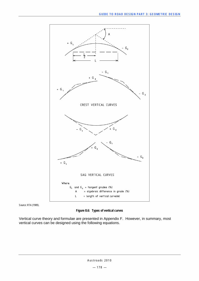
GUI DE TO RO A D DE SIG N P ART 3 : GEO MET RI C D ESI G N
A u s t r o a d s 2 0 1 0
— 1 7 8 —
Source: RTA (1989).
Figure 8.6: Types of vertical curves
Vertical curve theory and formulae are presented in Appendix F. However, in summary, most vertical curves can be designed using the following equations.
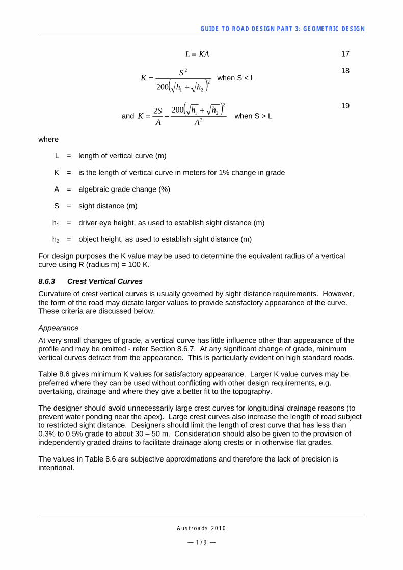
GUI DE TO RO A D DE SIG N P ART 3 : GEO MET RI C D ESI G N
A u s t r o a d s 2 0 1 0
— 1 7 9 —
KAL = 17
( )221
2
200 hh
SK+
= when S < L 18
and
( )2
2
212002A
hhASK
+−= when S > L
19
where
L = length of vertical curve (m)
K = is the length of vertical curve in meters for 1% change in grade
A = algebraic grade change (%)
S = sight distance (m)
h1 = driver eye height, as used to establish sight distance (m)
h2 = object height, as used to establish sight distance (m)
For design purposes the K value may be used to determine the equivalent radius of a vertical curve using R (radius m) = 100 K.
8.6.3 Crest Vertical Curves Curvature of crest vertical curves is usually governed by sight distance requirements. However, the form of the road may dictate larger values to provide satisfactory appearance of the curve. These criteria are discussed below.
Appearance
At very small changes of grade, a vertical curve has little influence other than appearance of the profile and may be omitted - refer Section 8.6.7. At any significant change of grade, minimum vertical curves detract from the appearance. This is particularly evident on high standard roads.
Table 8.6 gives minimum K values for satisfactory appearance. Larger K value curves may be preferred where they can be used without conflicting with other design requirements, e.g. overtaking, drainage and where they give a better fit to the topography.
The designer should avoid unnecessarily large crest curves for longitudinal drainage reasons (to prevent water ponding near the apex). Large crest curves also increase the length of road subject to restricted sight distance. Designers should limit the length of crest curve that has less than 0.3% to 0.5% grade to about 30 – 50 m. Consideration should also be given to the provision of independently graded drains to facilitate drainage along crests or in otherwise flat grades.
The values in Table 8.6 are subjective approximations and therefore the lack of precision is intentional.
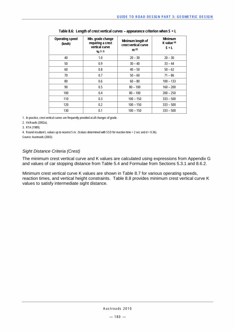
GUI DE TO RO A D DE SIG N P ART 3 : GEO MET RI C D ESI G N
A u s t r o a d s 2 0 1 0
— 1 8 0 —
Table 8.6: Length of crest vertical curves – appearance criterion when S < L
Operating speed (km/h)
Min. grade change requiring a crest
vertical curve % (1, 2)
Minimum length of crest vertical curve
m (3)
Minimum K value (4)
S < L
40 1.0 20 – 30 20 – 30 50 0.9 30 – 40 33 – 44 60 0.8 40 – 50 50 – 62 70 0.7 50 – 60 71 – 86 80 0.6 60 – 80 100 – 133 90 0.5 80 – 100 160 – 200 100 0.4 80 – 100 200 – 250 110 0.3 100 – 150 333 – 500 120 0.2 100 – 150 333 – 500 130 0.1 100 – 150 333 – 500
1. In practice, crest vertical curves are frequently provided at all changes of grade. 2. VicRoads (2002a). 3. RTA (1989). 4. Round resultant L values up to nearest 5 m. (Values determined with SSD for reaction time = 2 sec and d = 0.36). Source: Austroads (2003).
Sight Distance Criteria (Crest)
The minimum crest vertical curve and K values are calculated using expressions from Appendix G and values of car stopping distance from Table 5.4 and Formulae from Sections 5.3.1 and 8.6.2.
Minimum crest vertical curve K values are shown in Table 8.7 for various operating speeds, reaction times, and vertical height constraints. Table 8.8 provides minimum crest vertical curve K values to satisfy intermediate sight distance.
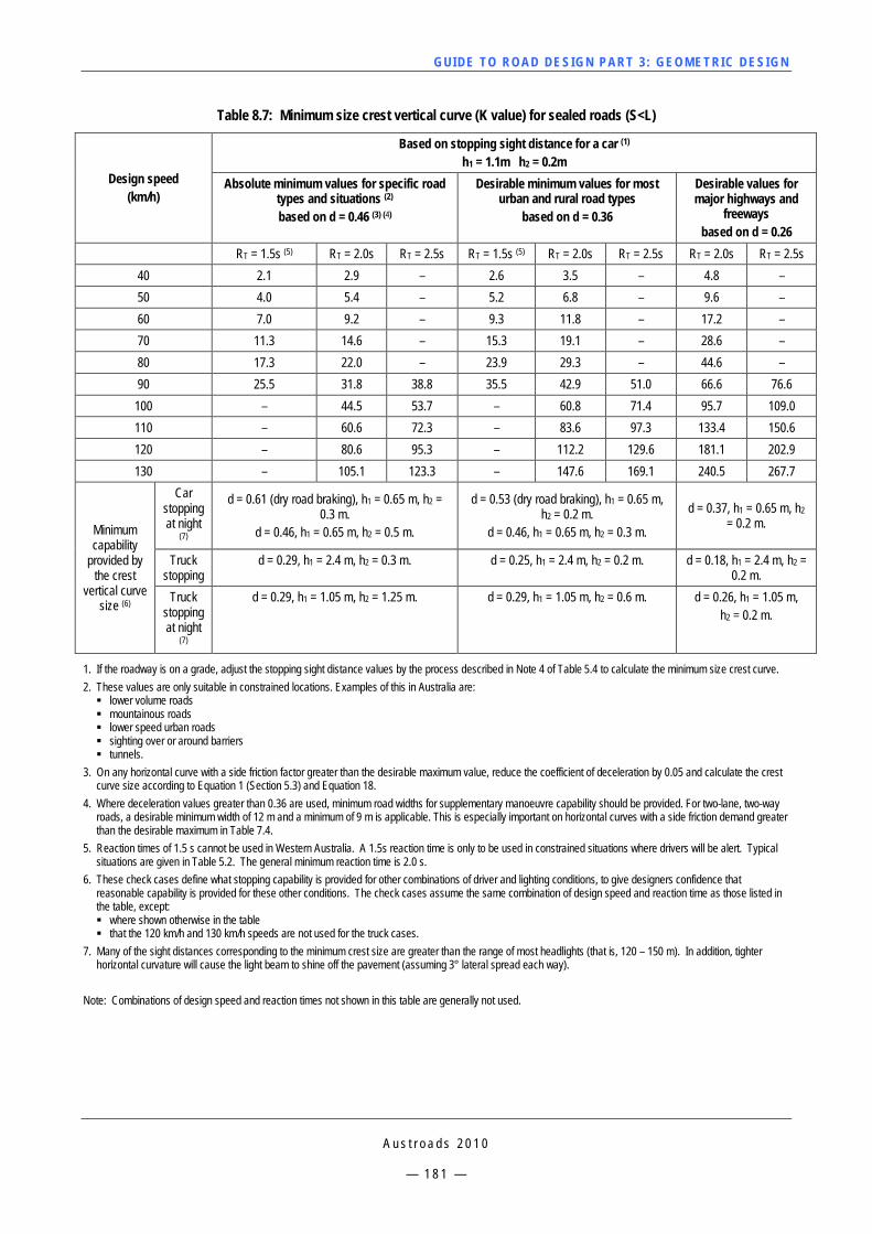
GUI DE TO RO A D DE SIG N P ART 3 : GEO MET RI C D ESI G N
A u s t r o a d s 2 0 1 0
— 1 8 1 —
Table 8.7: Minimum size crest vertical curve (K value) for sealed roads (S<L)
Design speed (km/h)
Based on stopping sight distance for a car (1) h1 = 1.1m h2 = 0.2m
Absolute minimum values for specific road types and situations (2) based on d = 0.46 (3) (4)
Desirable minimum values for most urban and rural road types
based on d = 0.36
Desirable values for major highways and
freeways based on d = 0.26
RT = 1.5s (5) RT = 2.0s RT = 2.5s RT = 1.5s (5) RT = 2.0s RT = 2.5s RT = 2.0s RT = 2.5s 40 2.1 2.9 – 2.6 3.5 – 4.8 – 50 4.0 5.4 – 5.2 6.8 – 9.6 – 60 7.0 9.2 – 9.3 11.8 – 17.2 – 70 11.3 14.6 – 15.3 19.1 – 28.6 – 80 17.3 22.0 – 23.9 29.3 – 44.6 – 90 25.5 31.8 38.8 35.5 42.9 51.0 66.6 76.6 100 – 44.5 53.7 – 60.8 71.4 95.7 109.0 110 – 60.6 72.3 – 83.6 97.3 133.4 150.6 120 – 80.6 95.3 – 112.2 129.6 181.1 202.9 130 – 105.1 123.3 – 147.6 169.1 240.5 267.7
Minimum capability
provided by the crest
vertical curve size (6)
Car stopping at night
(7)
d = 0.61 (dry road braking), h1 = 0.65 m, h2 = 0.3 m.
d = 0.46, h1 = 0.65 m, h2 = 0.5 m.
d = 0.53 (dry road braking), h1 = 0.65 m, h2 = 0.2 m.
d = 0.46, h1 = 0.65 m, h2 = 0.3 m.
d = 0.37, h1 = 0.65 m, h2 = 0.2 m.
Truck stopping
d = 0.29, h1 = 2.4 m, h2 = 0.3 m. d = 0.25, h1 = 2.4 m, h2 = 0.2 m. d = 0.18, h1 = 2.4 m, h2 = 0.2 m.
Truck stopping at night
(7)
d = 0.29, h1 = 1.05 m, h2 = 1.25 m. d = 0.29, h1 = 1.05 m, h2 = 0.6 m. d = 0.26, h1 = 1.05 m, h2 = 0.2 m.
1. If the roadway is on a grade, adjust the stopping sight distance values by the process described in Note 4 of Table 5.4 to calculate the minimum size crest curve. 2. These values are only suitable in constrained locations. Examples of this in Australia are: lower volume roads mountainous roads lower speed urban roads sighting over or around barriers tunnels.
3. On any horizontal curve with a side friction factor greater than the desirable maximum value, reduce the coefficient of deceleration by 0.05 and calculate the crest curve size according to Equation 1 (Section 5.3) and Equation 18.
4. Where deceleration values greater than 0.36 are used, minimum road widths for supplementary manoeuvre capability should be provided. For two-lane, two-way roads, a desirable minimum width of 12 m and a minimum of 9 m is applicable. This is especially important on horizontal curves with a side friction demand greater than the desirable maximum in Table 7.4.
5. Reaction times of 1.5 s cannot be used in Western Australia. A 1.5s reaction time is only to be used in constrained situations where drivers will be alert. Typical situations are given in Table 5.2. The general minimum reaction time is 2.0 s.
6. These check cases define what stopping capability is provided for other combinations of driver and lighting conditions, to give designers confidence that reasonable capability is provided for these other conditions. The check cases assume the same combination of design speed and reaction time as those listed in the table, except: where shown otherwise in the table that the 120 km/h and 130 km/h speeds are not used for the truck cases.
7. Many of the sight distances corresponding to the minimum crest size are greater than the range of most headlights (that is, 120 – 150 m). In addition, tighter horizontal curvature will cause the light beam to shine off the pavement (assuming 3° lateral spread each way).
Note: Combinations of design speed and reaction times not shown in this table are generally not used.

GUI DE TO RO A D DE SIG N P ART 3 : GEO MET RI C D ESI G N
A u s t r o a d s 2 0 1 0
— 1 8 2 —
Table 8.8: Minimum size crest vertical curve (K value) for sealed roads to satisfy intermediate sight distance (S<L)
Design speed (km/h)
Based on intermediate sight Distance for cars (1)
h1 = 1.1 m h2 = 1.25 m d = 0.36 (2)
RT = 2.0s RT = 2.5s 50 - - 60 - - 70 36.4 - 80 55.8 - 90 81.8 97.2 100 115.9 136.2 110 159.4 185.6 120 214.0 247.0 130 281.4 322.4
Minimum capability
provided by the crest vertical curve size (3)
Car stopping at night Drivers will see the glow from
oncoming headlights well before they need to start braking.
Truck stopping d = 0.23, h1 = 2.4 m, h2 = 2.4 m.
Truck stopping at night Drivers will see the glow from
oncoming headlights well before they need to start braking.
1. If the roadway is on a grade, adjust the stopping sight distance values by the process described in Note 4 of Table 5.4 to calculate the minimum size crest curve. 2. In constrained locations on one-lane, two-way roads, a coefficient of deceleration of 0.46 may be used. For any horizontal curve with a side friction factor greater
than the desirable maximum value for cars (in constrained locations on one-lane, two-way roads), use a coefficient of deceleration of 0.41. The resultant crest curve size can then be calculated according to Equation 1 (Section 5.3) and Equation 18.
3. These check cases define what stopping capability is provided for other combinations of driver and lighting conditions, to give designers confidence that reasonable capability is provided for these other conditions. The check cases assume the same combination of design speed and reaction time as those listed in the table, except that the 120 km/h and 130 km/h speeds are not used for the truck cases.
Note: Combinations of design speed and reaction times not shown in this table are generally not used.
Hidden dip grading
On long lengths of straight alignment, particularly in slightly rolling country, hidden dips should be avoided wherever possible. At times, in periods of high glare or poor visibility, and because of the foreshortening effect due to the level of the eye, an illusion of apparent continuity of pavement omitting the dip is sometimes created.
Hidden dips contribute to overtaking manoeuvre crashes, the overtaking driver being deceived by the view of highway beyond the dip free of opposing vehicles. Even with shallow dips, this type of road profile is disconcerting because the driver cannot be sure whether or not there is an oncoming vehicle or obstacles on the road (such as stock) hidden beyond the crest. This type of profile can be avoided by appropriate horizontal curvature or by more gradual grades made possible by heavier cuts and fills.
It is preferred that the entire pavement surface is visible in these cases. However, if there is no alternative, a maximum depression of 60 mm below the driver’s line of sight may be tolerated. Guidance on the limited depth of depression gives confidence to drivers, and road edge guide posts at close intervals provide an acceptable method.
GUI DE TO RO A D DE SIG N P ART 3 : GEO MET RI C D ESI G N
A u s t r o a d s 2 0 1 0
— 1 8 3 —
Floodways
The longitudinal grade on the approach to floodways must be carefully designed to:
avoid discomfort to the occupants of vehicles
provide stopping sight distance to the pavement level in a short floodway
ensure that drivers are not mislead regarding the extent and depth of the floodway.
The vertical curves should be designed in accordance with the comfort criteria described in Section 8.6.4. For floodways, it is important that drivers can see the presence of water on the road and the sight distance should be checked to ensure that stopping sight distance is achieved to the road pavement (object height = 0.0 m) to enable drivers to see debris on the road or washouts.
In flat country, the presence of the floodway must be obvious to the driver and a relatively short, sharp entrance to the floodway section (within the comfort criterion) should be provided. It is also essential to avoid more than one level in a floodway. That is, once the driver has entered the floodway with water across it, there must be no deeper water at some point further along the floodway. This type of design is misleading to drivers and can result in a dangerous situation.
8.6.4 Sag Vertical Curves Appearance and comfort
Appearance is important when considering small and larger changes in grade (the same as for crest curves).
Sag vertical curves are generally designed to achieve the comfort criterion as a minimum. For unlit rural and urban roads, sag curves should desirably be designed for headlight criteria. Higher standard roads (highways and freeways) are typically designed with sag curves that exceed headlight sight distance criteria.
On two lane roads, long sag curves in excess of 750 m long should be avoided for drainage reasons. For kerbed roads, the maximum length of sag curve with less than 0.3% grade should be limited to 30 m.
A person subjected to rapid changes in vertical acceleration feels discomfort. To minimise such discomfort when passing from one grade to another, it is usual to limit the vertical acceleration generated on the vertical curve to a value less than 0.05g where g is the acceleration due to gravity.
GUI DE TO RO A D DE SIG N P ART 3 : GEO MET RI C D ESI G N
A u s t r o a d s 2 0 1 0
— 1 8 4 —
The minimum sag vertical curve K value for comfort criteria can be calculated by the following equation.
aVK
1296
2
= 20
where
K = length of vertical curve in metres for 1% change in grade
a = vertical acceleration (m/sec2) = 0.05g (max)
V = speed of the vehicle (km/h)
g = gravitation force m/sec2 = 9.81 m/sec2.
8.6.5 Sight Distance Criteria (Sag) Headlight sight distance
Sight distance on sag curves is not restricted by the vertical geometry in daylight conditions or at night with full roadway lighting, unless overhead obstructions are present. Under night conditions on unlit roads, limitations of vehicle headlights restrict sight distance to between 120 m and 150 m on crest curves. On high-speed roads not likely to be provided with roadway lighting, consideration should be given to providing headlight sight distance. Nevertheless, horizontal curvature would cause the light beam to shine off the pavement (assuming 3o lateral spread each way), and little is gained by increasing the K value of the sag curve Figure 5.7.
( )qShSK
tan200
2
+= when S < L
21
and ( )2
tan2002A
qshASK +−= when S > L
22
where
h = mounting height of headlights (m)
S = stopping sight distance (m), Table 5.4
q = elevation angle of beam 10 (+ upwards) (tan 10 = 0.01746)
A = algebraic grade change (%)
L = length of curve (m)
The minimum acceptable sag curve K values for a headlight mounting height of 0.65 m and one degree of light beam elevation are presented in Figure 8.7.
GUI DE TO RO A D DE SIG N P ART 3 : GEO MET RI C D ESI G N
A u s t r o a d s 2 0 1 0
— 1 8 5 —
Overhead obstructions
Overhead obstructions such as road or rail overpasses, sign gantries or even overhanging trees may limit the sight distance available on sag vertical curves, especially for trucks with their higher driver eye height. With the minimum overhead clearances normally specified for roads, these obstructions would not interfere with minimum stopping sight distance. They may, however, need to be considered with the upper limit of stopping distance (including sight distance to intersections) and overtaking provision Figure 8.1.
For overhead obstruction sight distance:
( )221
2
200 hHhH
SK−+−
= when S> L 23
where:
H = height of overhead obstruction (m)
h1 = truck driver eye height (2.4 m)
h2 = object height (0.60 m)
S = stopping sight distance (m), Table 5.4.
L = length of curve (m)
K Values for sag curve design
The minimum size sag curves for different categories of roads using both comfort criteria and headlight sight distance are listed in Figure 8.7.
The graph was developed using the following criteria to determine the lower bounds:
1. Low Standard Roads – comfort criteria with a = 0.1g
2. Other Urban and Rural Roads with street lighting – comfort criteria with a = 0.05g
3. Other Urban and Rural Roads without street lighting – headlight sight distance with reaction time = 2.0s and coefficient of deceleration = 0.61
4. Highways and freeways:
Minimum – headlight Sight Distance with reaction time = 2.5s and coefficient of deceleration = 0.36
Desirable – crest curve stopping sight distance with reaction time = 2.0s and coefficient of deceleration = 0.36.
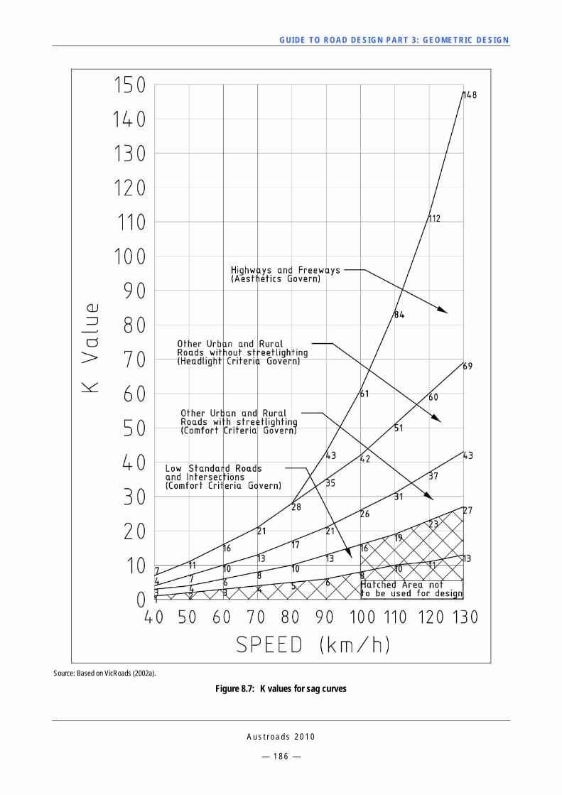
GUI DE TO RO A D DE SIG N P ART 3 : GEO MET RI C D ESI G N
A u s t r o a d s 2 0 1 0
— 1 8 6 —
Source: Based on VicRoads (2002a).
Figure 8.7: K values for sag curves
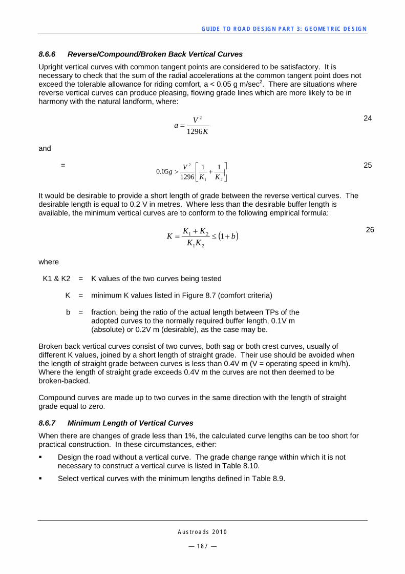
GUI DE TO RO A D DE SIG N P ART 3 : GEO MET RI C D ESI G N
A u s t r o a d s 2 0 1 0
— 1 8 7 —
8.6.6 Reverse/Compound/Broken Back Vertical Curves Upright vertical curves with common tangent points are considered to be satisfactory. It is necessary to check that the sum of the radial accelerations at the common tangent point does not exceed the tolerable allowance for riding comfort, a < 0.05 g m/sec2. There are situations where reverse vertical curves can produce pleasing, flowing grade lines which are more likely to be in harmony with the natural landform, where:
KVa
1296
2
= 24
and
=
+>
21
2 111296
05.0KK
Vg 25
It would be desirable to provide a short length of grade between the reverse vertical curves. The desirable length is equal to 0.2 V in metres. Where less than the desirable buffer length is available, the minimum vertical curves are to conform to the following empirical formula:
( )bKK
KKK +≤+
= 121
21 26
where
K1 & K2 = K values of the two curves being tested
K = minimum K values listed in Figure 8.7 (comfort criteria)
b = fraction, being the ratio of the actual length between TPs of the adopted curves to the normally required buffer length, 0.1V m (absolute) or 0.2V m (desirable), as the case may be.
Broken back vertical curves consist of two curves, both sag or both crest curves, usually of different K values, joined by a short length of straight grade. Their use should be avoided when the length of straight grade between curves is less than 0.4V m (V = operating speed in km/h). Where the length of straight grade exceeds 0.4V m the curves are not then deemed to be broken-backed.
Compound curves are made up to two curves in the same direction with the length of straight grade equal to zero.
8.6.7 Minimum Length of Vertical Curves When there are changes of grade less than 1%, the calculated curve lengths can be too short for practical construction. In these circumstances, either:
Design the road without a vertical curve. The grade change range within which it is not necessary to construct a vertical curve is listed in Table 8.10.
Select vertical curves with the minimum lengths defined in Table 8.9.
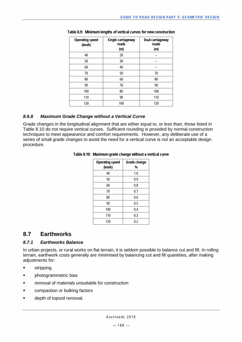
GUI DE TO RO A D DE SIG N P ART 3 : GEO MET RI C D ESI G N
A u s t r o a d s 2 0 1 0
— 1 8 8 —
Table 8.9: Minimum lengths of vertical curves for new construction
Operating speed (km/h)
Single carriageway roads
(m)
Dual carriageway roads
(m) 40 20 – 50 30 – 60 40 – 70 50 70 80 60 80 90 70 90
100 80 100 110 90 110 120 100 120
8.6.8 Maximum Grade Change without a Vertical Curve Grade changes in the longitudinal alignment that are either equal to, or less than, those listed in Table 8.10 do not require vertical curves. Sufficient rounding is provided by normal construction techniques to meet appearance and comfort requirements. However, any deliberate use of a series of small grade changes to avoid the need for a vertical curve is not an acceptable design procedure.
Table 8.10: Maximum grade change without a vertical curve
Operating speed (km/h)
Grade change %
40 1.0 50 0.9 60 0.8 70 0.7 80 0.6 90 0.5
100 0.4 110 0.3 120 0.2
8.7 Earthworks 8.7.1 Earthworks Balance In urban projects, or rural works on flat terrain, it is seldom possible to balance cut and fill. In rolling terrain, earthwork costs generally are minimised by balancing cut and fill quantities, after making adjustments for:
stripping
photogrammetric bias
removal of materials unsuitable for construction
compaction or bulking factors
depth of topsoil removal.
GUI DE TO RO A D DE SIG N P ART 3 : GEO MET RI C D ESI G N
A u s t r o a d s 2 0 1 0
— 1 8 9 —
No general rules can be made for the adjustment factors, which should be discussed and agreed with the construction engineer, in consultation with the surveyor and the geotechnical engineer.
The first option for achieving earthworks balance is to adjust the gradeline. The second option can be to shift the alignment. Minor changes can be achieved by altering verge widths or batter slopes. The optimum solution usually involves adjustments both to the horizontal and the vertical alignment.
The limits of the balance area have to be chosen with care to ensure that total project costs are minimised. For example, earthworks from the hills could be used as fill within the flat plains, but the limit will depend on the on site costs of fill material from other sources, including the costs of cartage. If material won from cuts is suitable for pavement material, it must be deducted from common earthworks and added to the pavement material quantity.
For large road projects a comprehensive geotechnical investigation should be undertaken before the gradeline is fixed. The materials report includes advice on the suitability of fill materials, batter stability and possible sources of imported fill.
Designers should seek to gain agreement to the proposed use of fill materials from the construction project manager prior to fixing the gradeline.
8.7.2 Earthworks Quantities Earthworks quantities are usually extracted using the average end area method. Designers should be aware of the intrinsic limits of accuracy due to variations of the terrain between surveyed cross-sections, and variations from a truly prismoidal shape. The calculated volume may vary from the actual volume by 5% to 10% from these factors alone.
Where the alignment lies on a small radius curve, further quantity adjustments are required because the ends of the prism are not parallel. No adjustments are required for those computer programs that extract volumes using vertical triangular prismoids.
Factors that affect earthwork quantities include: Depth of topsoil to be removed prior to placement of fill (the stripping depth).
Quantity of material that has to be removed to provide a stable base for the pavement or embankment.
The compaction factor, that is, the ratio in volume between one cubic metre of in situ material and the same material after placement and compaction. Cohesive materials commonly occupy less volume after compaction, while rock may occupy more volume after excavation and placement.
Material which is unsuitable for embankment construction including:
— topsoil and other material with organic content — large boulders — excavated hard rock which may be uneconomical to crush to a size which can be
compacted — any unstable or expansive material to be carted to waste
Flattening of embankment batter slopes outside stability limits to provide for safety and maintenance requirements.
Photogrammetric bias. It is preferable that ground survey be used for detailed design, in order to eliminate this factor and improve accuracy.

GUI DE TO RO A D DE SIG N P ART 3 : GEO MET RI C D ESI G N
A u s t r o a d s 2 0 1 0
— 1 9 0 —
Subject to the construction specification, possible use of material otherwise classed as unsuitable material in noise attenuation mounds or other land forming.
When calculating earthwork quantities, designers shall document all factors that have been taken into account in the computations.
GUI DE TO RO A D DE SIG N P ART 3 : GEO MET RI C D ESI G N
A u s t r o a d s 2 0 1 0
— 1 9 1 —
9 AUXILIARY LANES
9.1 General Auxiliary lanes are those lanes which are added adjacent to the through traffic lanes to enhance traffic flow and maintain the required level of service on the road.
Auxiliary lanes are used to remove traffic that is causing disruption to the smooth flow of traffic in the through lanes to a separate lane to allow the through traffic to proceed relatively unhindered by the disruption. They are a means of separating the elements of the traffic stream on the basis of the speed difference between them, thereby improving the safety of the road as well as its capacity and level of service provided.
9.2 Types of Auxiliary Lanes Traffic speed and congestion on rural arterial roads are largely determined by two factors:
Alignment and standard of a road affects the magnitude and the spread of operating speeds.
Interactions between faster and slower vehicles determine the extent of traffic delay and congestion. The effect of these interactions is greatest when the spread of speeds (the difference between the operating speeds of the fastest and slowest vehicles) is largest.
Of these two, traffic interactions have an increasingly dominant effect on delay and congestion as traffic flows increase. Overtaking opportunities, therefore, have a large effect on traffic operations on rural roads. These can be improved in varying degrees by the following methods:
speed change lanes
improved overtaking sight distance
overtaking and climbing lanes
wide full depth paved shoulders
four lane wide cross-sections
dual carriageway cross-sections
slow vehicle turnouts
descending lanes.
The types of auxiliary lanes discussed in this section are as follows:
speed change lanes (acceleration and deceleration)
overtaking lanes/climbing lanes
slow vehicle turnouts
descending lanes.
In this guide, weaving lanes are not treated as auxiliary lanes but as part of the required cross-section of a freeway where weaving conditions occur.
GUI DE TO RO A D DE SIG N P ART 3 : GEO MET RI C D ESI G N
A u s t r o a d s 2 0 1 0
— 1 9 2 —
9.3 Speed Change Lanes 9.3.1 Acceleration Lanes Acceleration lanes are provided at intersections and interchanges to allow an entering vehicle to access the traffic stream at a speed approaching or equal to the 85th percentile speed of the through traffic. They are usually parallel to and contiguous with the through lane with appropriate tapers at the entering point. The warrants for this type of auxiliary lane and the desirable road layouts are discussed in the Guide to Road Design – Part 4: Intersections and Crossings – General (Austroads 2009a).
9.3.2 Deceleration Lanes Deceleration lanes are provided at intersections and interchanges to allow an exiting vehicle to depart from the through lanes at the 85th percentile speed of the through lanes and decelerate to a stop or to the 85th percentile speed of the intersecting road, whichever is appropriate for the circumstances. These lanes are usually parallel to and contiguous with the through lanes with appropriate tapers at the departure point on the through lane.
At intersections, the deceleration lane can be placed on either the right or the left of the through lanes, depending on the type of turn being effected. At interchanges, it is preferred that the exit be from the left side for most ramps and the deceleration lane will therefore be on the left in most cases.
Details of the requirements for deceleration lanes are given in the Guide to Road Design – Part 4: Intersections and Crossings – General (Austroads 2009a).
9.4 Overtaking Lanes 9.4.1 General On two lane two-way carriageways, examples of overtaking lane configurations are shown on Figure 9.1. These overtaking lanes are provided to break up bunches of traffic and improve traffic flow over a section of road. They provide a positive overtaking opportunity and are sometimes the only real chance for overtaking to occur. In New Zealand, overtaking lanes are referred to as passing lanes. Reference must be made to the Transport Agency’s Policy and Planning Manual for the applicable Passing Lane Policy. The layout and signing of Passing Lanes is covered in Manual of Traffic Signs and Markings (MOTSAM) Part 1 (2007) and part 2 (2008).
The desirable layout is based on the start or end of the lane merge location being separated by a three second distance of travel time. This distance is to minimise the possibility of conflict between opposing merging vehicles.
An acceptable layout, when the geometric conditions do not provide for an alternative is to allow the start of the merges to be opposite one another.
Figure 9.1 also shows the undesirable and unacceptable configurations of the merge area at the end of overtaking lanes. These are shown to highlight the possible conflict areas of late merging vehicles and are not to be used.
Overtaking demand
The demand for overtaking occurs each time a vehicle catches up with another and the driver wishes to maintain the speed of travel. Provided there is no approaching traffic, this manoeuvre can occur where there is adequate sight distance.
GUI DE TO RO A D DE SIG N P ART 3 : GEO MET RI C D ESI G N
A u s t r o a d s 2 0 1 0
— 1 9 3 —
As traffic volume increases, the approaching traffic will restrict the available places where overtaking can occur and these will be further limited by the road geometry.
If demand is not met the results are:
enforced following
the growth of traffic bunches
driver delay and frustration.
In extreme no-overtaking situations, very long queues can develop behind the slowest vehicles in the traffic stream. The delay and frustration experienced on grades may be greater due to the slow speed of travel. The proportion of the journey time spent following in bunches is a useful measure of quality of service as seen by the driver.
The type of slow vehicle influences the nature of overtaking demand. Some vehicles can be overtaken easily anywhere along a route, while for others an upgraded overtaking opportunity is desirable. In evaluating the need for auxiliary lanes, attention should be given to the type of slow vehicles involved and whether the overtaking demand is continuous along a route or confined to specific problem locations.
Types of slow vehicles are:
vehicles with fairly high speeds, that slow down markedly on grades
vehicles with low speeds, not affected by grades
vehicles with average speeds that are seen as slow by those wishing to travel faster.
Overtaking opportunities
On two-lane two way roads, the availability of overtaking opportunities depends on sight distance and gaps in the opposing traffic stream. As opposing traffic volume increases, overtaking opportunities become restricted even if sight distance is adequate. Sight distance that appears adequate may also be unusable on occasions due to the size of the vehicle in front, particularly on left-hand curves.
On an existing road, overtaking opportunities can be increased either by improved alignment or the provision of overtaking lanes. Of the two options, overtaking lanes will generally prove to be the most cost-effective in reducing the level of traffic bunching. This is because realignment to provide overtaking opportunities is likely to be a much more expensive option, and even then the opportunities are only available when opposing traffic permits. This has been demonstrated by ARRB simulation studies, which showed that the provision of overtaking lanes at regular spacings often led to greater improvements in overall traffic operations than even major alignment improvements (Hoban 1983).
A two-lane two way road with overtaking lanes at regular intervals provides an intermediate level of service between two-lane two way roads and four lane roads, undivided and divided. The overtaking lanes may delay the need for the provision of dual carriageways. Where a four-lane road has already been provided, and traffic volumes are consistently high, the need for auxiliary lanes on grades may still arise when there is a high proportion of heavy vehicles.
Warrants
In deciding whether an overtaking lane is warranted, the evaluation needs to be carried out over a significant route length and not be isolated to the particular length over which the additional lane may be constructed.

GUI DE TO RO A D DE SIG N P ART 3 : GEO MET RI C D ESI G N
A u s t r o a d s 2 0 1 0
— 1 9 4 —
Overtaking opportunities outside the particular length can affect the result considerably. On multi-lane roads, this may not apply since the reason for the extra lane will usually be confined to a specific location.
The following guidelines are based on initial ARRB research using traffic simulation and benefit-cost analysis (Hoban & Morrall (1986)). Alternatively, the need for an additional lane can be evaluated in terms of level of service. In special circumstances, a more detailed evaluation may be undertaken using traffic simulation or the results of prior ARRB research (Hoban 1983).
The basis for adopting an overtaking lane is the traffic volume, the percentage of slow vehicles including light trucks and cars towing, and the availability of overtaking opportunities on adjoining sections. The percentage of road allowing overtaking is described in Section 5.6 of this Guide.
Table 9.1 gives the current-year design volumes (AADT) at which overtaking lanes would normally be justified. These guidelines apply for short low-cost overtaking lanes at spacings of 10 to 15 km or more along a road in a given direction. If spacing is less than this, a specific cost benefit analysis will be needed to justify the construction at the shorter spacing.
Development and termination of an overtaking lane is shown in Figure 9.2.
Table 9.1: Traffic volume guidelines for providing overtaking lanes
Overtaking opportunities over the preceding 5 km (1) Current-year design volume (AADT)
Description Percent length providing overtaking (2)
Percentage of slow vehicles (3)
5 10 20 Excellent 70 – 100 5,670 5,000 4,330
Good 30 – 70 4,330 3,670 3,330 Moderate 10 – 30 3,130 2,800 2,470
Occasional 5 – 10 2,270 2,000 1,730 Restricted 0 – 5 1,530 1,330 1,130
Very Restricted (4) 0 930 800 670
1. Depending on road length being evaluated, this distance could range from 3 to 10 km. 2. See Section 5.6.4. 3. Including light trucks and cars towing trailers, caravans and boats. 4. No overtaking for 3 km in each direction. Source: Austroads (2003).
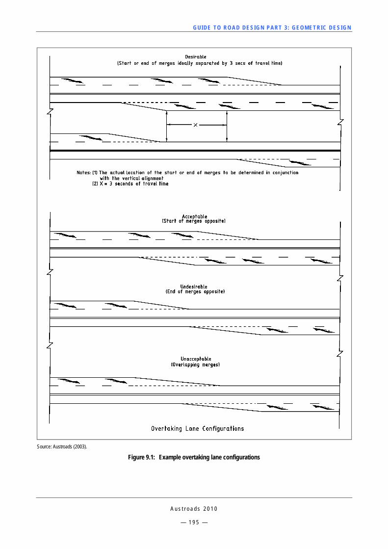
GUI DE TO RO A D DE SIG N P ART 3 : GEO MET RI C D ESI G N
A u s t r o a d s 2 0 1 0
— 1 9 5 —
Source: Austroads (2003).
Figure 9.1: Example overtaking lane configurations
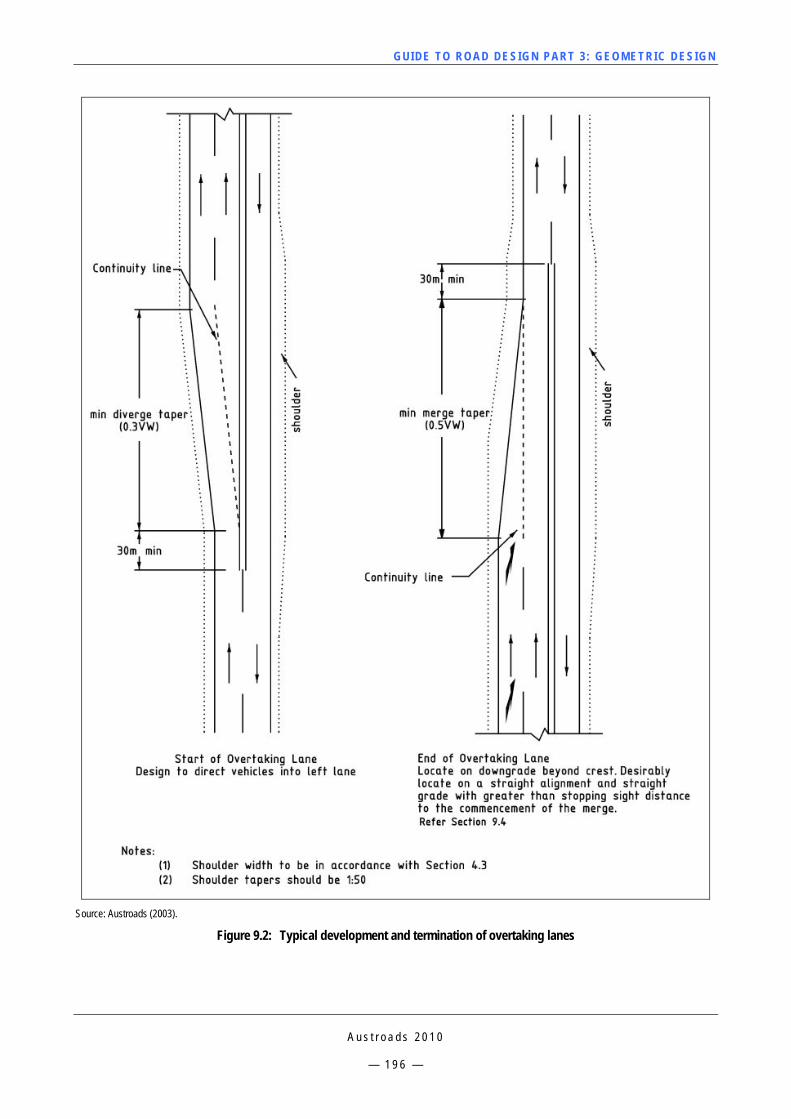
GUI DE TO RO A D DE SIG N P ART 3 : GEO MET RI C D ESI G N
A u s t r o a d s 2 0 1 0
— 1 9 6 —
Source: Austroads (2003).
Figure 9.2: Typical development and termination of overtaking lanes
GUI DE TO RO A D DE SIG N P ART 3 : GEO MET RI C D ESI G N
A u s t r o a d s 2 0 1 0
— 1 9 7 —
Length
Table 9.2 presents the adopted lengths of overtaking lane lengths that are appropriate for both grades and level terrain. On long grades, the values for a lower operating speed should be used. The minimum lengths provide for the majority of movements as single overtakings, but may not allow many multiple overtakings, or overtakings between vehicles with only a small difference in speed. Minimum lengths are generally only appropriate for lower operating speeds or constrained situations.
Overtaking lanes may be extended beyond the desirable length to allow start and termination points to fit within the terrain. This additional length may not be well utilised as bunches generally break up in the first section of the overtaking lane. Some road authority practice as shown there to be merit in the provision of overtaking lanes up to 1500m long (including tapers), which provides additional overtaking opportunities where there is a long queue behind slow moving vehicles
The length of an overtaking lane on a grade is largely constrained by the choice of appropriate locations for start and termination points. These should be clearly visible to approaching drivers, and be located to minimise speed differences between slow and fast vehicles. These constraints, however, sometimes lead to quite long and/or expensive climbing lane proposals.
The sight distance to the termination of the overtaking lane is based on the distance for the vehicle in the fast lane to complete or abandon the overtaking manoeuvre. The sight distances required to overtake the various types of MCVs are shown in Table 9.3. Further information regarding the termination of overtaking lanes can be found in Section 9.9.1.
Situations may exist however, where an overtaking lane might end where the sight distance is less than that required to complete an overtaking. In such cases, drivers will have to rely on adequate signage of the termination.
Location
The location of overtaking sites should be determined after considering the following:
Strategic planning of the road in question and the long-term objectives of that link – the spacing and consequently, expenditure, must be in accord with the strategy to obtain the best use of funds over the whole network.
Nature of traffic on the section of road – if queuing occurs all along the route, then overtaking lanes at any location will be useful; if they occur at specific locations where slow vehicles cause the queue, then specific locations should be chosen.
Location of grades – may be more effective to take advantage of the slower moving vehicles.
Costs of construction of the alternative sites – may get a more cost-effective solution by locating on the sites where construction is cheapest.
Geometry of the road – when the sites are not on grades, sections with curved alignment and restricted sight distances are generally preferable to long straight sections. These locations will make the location appear appropriate to the driver. However, sections with curves with reduced safe speeds are not suitable for overtaking lanes.
Intersections should be avoided, especially property accesses on the right hand side of the road.
If the conclusion is that the overtaking lane should be located on a grade, the length will be tailored to fit the grade. If the costs of the lane on the grade outweigh the benefits of being on the grade, the lane should be located to minimise the costs. Alternatively, a partial climbing lane could be considered (Section 9.5).
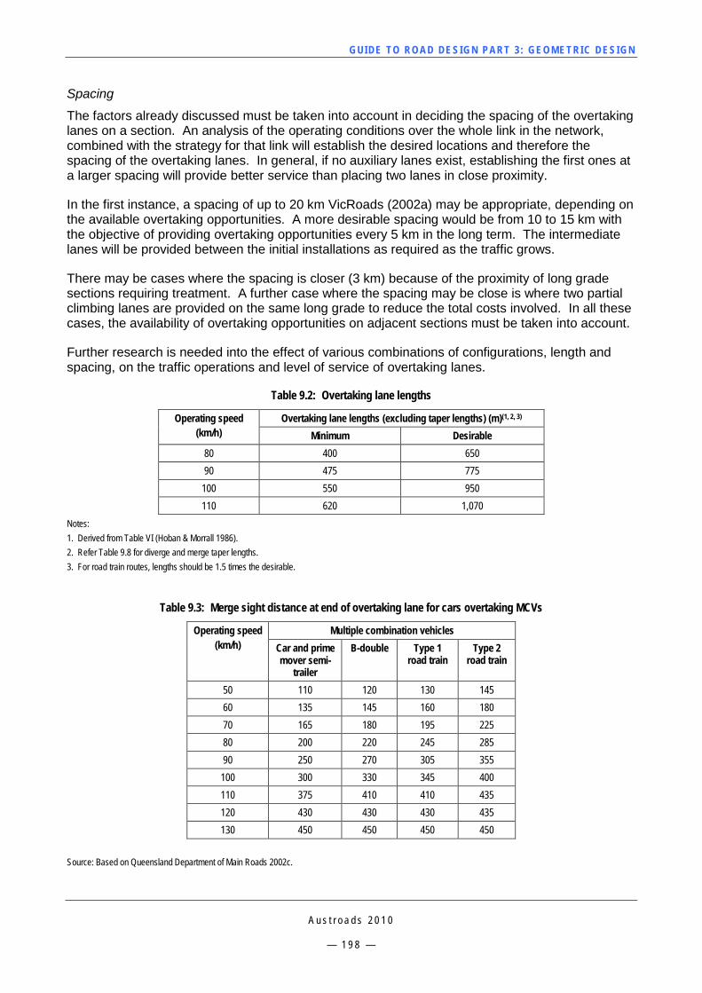
GUI DE TO RO A D DE SIG N P ART 3 : GEO MET RI C D ESI G N
A u s t r o a d s 2 0 1 0
— 1 9 8 —
Spacing
The factors already discussed must be taken into account in deciding the spacing of the overtaking lanes on a section. An analysis of the operating conditions over the whole link in the network, combined with the strategy for that link will establish the desired locations and therefore the spacing of the overtaking lanes. In general, if no auxiliary lanes exist, establishing the first ones at a larger spacing will provide better service than placing two lanes in close proximity.
In the first instance, a spacing of up to 20 km VicRoads (2002a) may be appropriate, depending on the available overtaking opportunities. A more desirable spacing would be from 10 to 15 km with the objective of providing overtaking opportunities every 5 km in the long term. The intermediate lanes will be provided between the initial installations as required as the traffic grows.
There may be cases where the spacing is closer (3 km) because of the proximity of long grade sections requiring treatment. A further case where the spacing may be close is where two partial climbing lanes are provided on the same long grade to reduce the total costs involved. In all these cases, the availability of overtaking opportunities on adjacent sections must be taken into account.
Further research is needed into the effect of various combinations of configurations, length and spacing, on the traffic operations and level of service of overtaking lanes.
Table 9.2: Overtaking lane lengths
Operating speed (km/h)
Overtaking lane lengths (excluding taper lengths) (m)(1, 2, 3) Minimum Desirable
80 400 650 90 475 775
100 550 950 110 620 1,070
Notes: 1. Derived from Table VI (Hoban & Morrall 1986). 2. Refer Table 9.8 for diverge and merge taper lengths. 3. For road train routes, lengths should be 1.5 times the desirable.
Table 9.3: Merge sight distance at end of overtaking lane for cars overtaking MCVs
Operating speed (km/h)
Multiple combination vehicles Car and prime mover semi-
trailer
B-double Type 1 road train
Type 2 road train
50 110 120 130 145 60 135 145 160 180 70 165 180 195 225 80 200 220 245 285 90 250 270 305 355 100 300 330 345 400 110 375 410 410 435 120 430 430 430 435 130 450 450 450 450
Source: Based on Queensland Department of Main Roads 2002c.
GUI DE TO RO A D DE SIG N P ART 3 : GEO MET RI C D ESI G N
A u s t r o a d s 2 0 1 0
— 1 9 9 —
Improvement strategy for overtaking lanes
The goal of any improvement strategy is to identify and plan for staged development that will keep pace with increases in traffic demand, ensuring the availability of overtaking opportunities at regular intervals. A strategy for improving operational performance of two-lane two-way rural roads should consider overtaking lane strategy in the context of potential future road duplication.
With an overtaking lane strategy, overtaking lanes should be provided to maintain the desired level of service. Full duplication of the road will not normally be anticipated during the economic life of these improvements. This period of time, typically 20 years, will be used to recover the cost of the improvements. This strategy should be applied when there are no existing overtaking lanes. The proposed spacing (for each direction) will typically be 3 to 10 km.
The upper limit for an overtaking lane strategy is 800 veh/h, if the desired level of service is C. If the desired level of service were B, 500 veh/h, would be the upper limit (Queensland Department of Main Roads, 2002c).
For hourly traffic volumes above the suggested limits, a strategy that is compatible with future road duplication should be adopted. In this situation, full duplication will normally occur within the economic life of the overtaking lane pavement. Sections of duplication 2 km long and at 5 km spacings are usually warranted. This strategy does not necessarily preclude the use of some overtaking lanes, particularly at the initial stages. However, it is highly desirable to use all improvements in the final road duplication.
Further analysis of a particular section of road will be required to determine the optimum combination of overtaking lane length and spacing.
9.5 Climbing Lanes 9.5.1 General Climbing lanes can be considered as a special form of overtaking lane but they are only provided on inclines. Where they are provided, they form part of the network of overtaking opportunities and will therefore have an effect on decisions on the location of other overtaking lanes.
On multi-lane roads, there is no need to take account of the overall overtaking situation, as the effect is limited to the specific location of the grade in question. The decision on whether to add a climbing lane is based on level of service considerations only. Climbing lanes on multilane roads are specifically provided for slow moving vehicles and are therefore treated differently for signing and line marking.
9.5.2 Warrants Climbing lanes are warranted where:
truck speeds fall to 40 km/h or less
traffic volumes equal or exceed those in Table 9.4.
In addition, climbing lanes should be considered where:
long grades over 8% occur
accidents attributable to the effects of the slow moving trucks are significant
heavy trucks from an adjacent industry enter the traffic stream on the up grade
the level of service on the grade falls two levels below that on the approach on the up grade or to level ‘e’ AASHTO (2004).
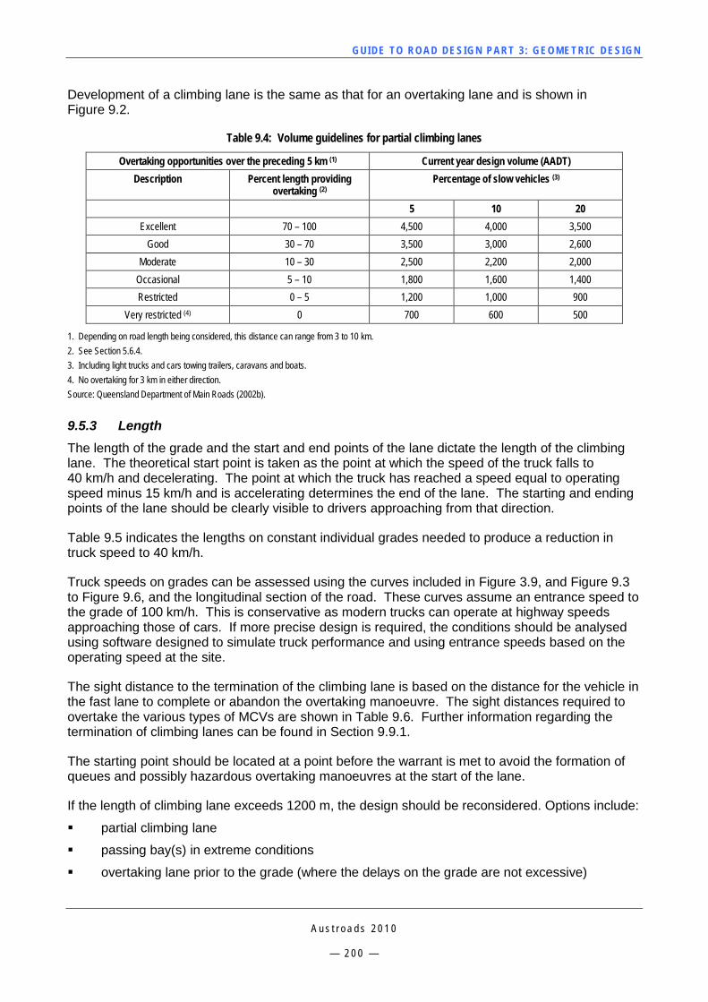
GUI DE TO RO A D DE SIG N P ART 3 : GEO MET RI C D ESI G N
A u s t r o a d s 2 0 1 0
— 2 0 0 —
Development of a climbing lane is the same as that for an overtaking lane and is shown in Figure 9.2.
Table 9.4: Volume guidelines for partial climbing lanes
Overtaking opportunities over the preceding 5 km (1) Current year design volume (AADT) Description Percent length providing
overtaking (2) Percentage of slow vehicles (3)
5 10 20 Excellent 70 – 100 4,500 4,000 3,500
Good 30 – 70 3,500 3,000 2,600 Moderate 10 – 30 2,500 2,200 2,000
Occasional 5 – 10 1,800 1,600 1,400 Restricted 0 – 5 1,200 1,000 900
Very restricted (4) 0 700 600 500
1. Depending on road length being considered, this distance can range from 3 to 10 km. 2. See Section 5.6.4. 3. Including light trucks and cars towing trailers, caravans and boats. 4. No overtaking for 3 km in either direction. Source: Queensland Department of Main Roads (2002b).
9.5.3 Length The length of the grade and the start and end points of the lane dictate the length of the climbing lane. The theoretical start point is taken as the point at which the speed of the truck falls to 40 km/h and decelerating. The point at which the truck has reached a speed equal to operating speed minus 15 km/h and is accelerating determines the end of the lane. The starting and ending points of the lane should be clearly visible to drivers approaching from that direction.
Table 9.5 indicates the lengths on constant individual grades needed to produce a reduction in truck speed to 40 km/h.
Truck speeds on grades can be assessed using the curves included in Figure 3.9, and Figure 9.3 to Figure 9.6, and the longitudinal section of the road. These curves assume an entrance speed to the grade of 100 km/h. This is conservative as modern trucks can operate at highway speeds approaching those of cars. If more precise design is required, the conditions should be analysed using software designed to simulate truck performance and using entrance speeds based on the operating speed at the site.
The sight distance to the termination of the climbing lane is based on the distance for the vehicle in the fast lane to complete or abandon the overtaking manoeuvre. The sight distances required to overtake the various types of MCVs are shown in Table 9.6. Further information regarding the termination of climbing lanes can be found in Section 9.9.1.
The starting point should be located at a point before the warrant is met to avoid the formation of queues and possibly hazardous overtaking manoeuvres at the start of the lane.
If the length of climbing lane exceeds 1200 m, the design should be reconsidered. Options include:
partial climbing lane
passing bay(s) in extreme conditions
overtaking lane prior to the grade (where the delays on the grade are not excessive)
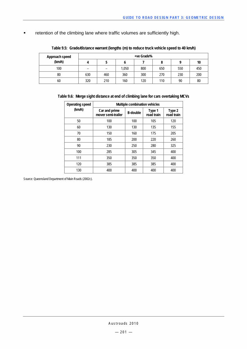
GUI DE TO RO A D DE SIG N P ART 3 : GEO MET RI C D ESI G N
A u s t r o a d s 2 0 1 0
— 2 0 1 —
retention of the climbing lane where traffic volumes are sufficiently high.
Table 9.5: Grade/distance warrant (lengths (m) to reduce truck vehicle speed to 40 km/h)
Approach speed (km/h)
+ve Grade% 4 5 6 7 8 9 10
100 – – 1,050 800 650 550 450 80 630 460 360 300 270 230 200 60 320 210 160 120 110 90 80
Table 9.6: Merge sight distance at end of climbing lane for cars overtaking MCVs
Operating speed (km/h)
Multiple combination vehicles Car and prime
mover semi-trailer B-double Type 1 road train
Type 2 road train
50 100 100 105 120 60 130 130 135 155 70 150 160 175 205 80 185 200 220 260 90 230 250 280 325 100 285 305 345 400 111 350 350 350 400 120 385 385 385 400 130 400 400 400 400
Source: Queensland Department of Main Roads (2002c).
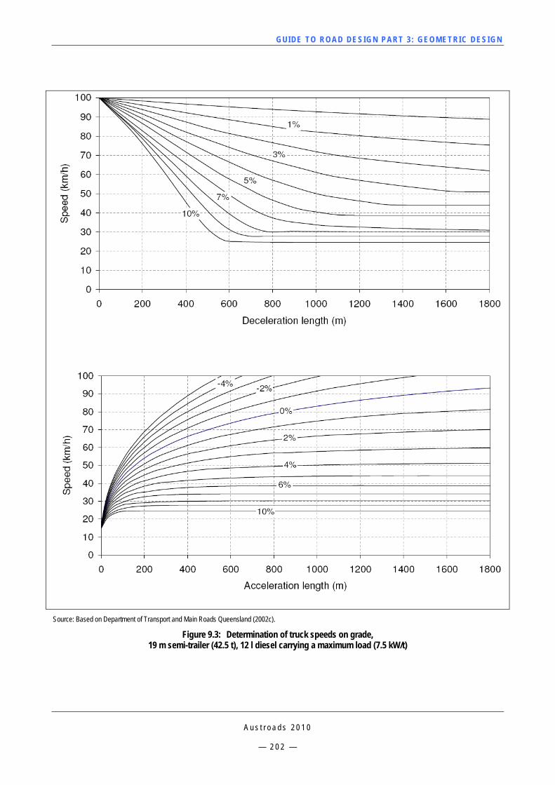
GUI DE TO RO A D DE SIG N P ART 3 : GEO MET RI C D ESI G N
A u s t r o a d s 2 0 1 0
— 2 0 2 —
Source: Based on Department of Transport and Main Roads Queensland (2002c).
Figure 9.3: Determination of truck speeds on grade, 19 m semi-trailer (42.5 t), 12 l diesel carrying a maximum load (7.5 kW/t)
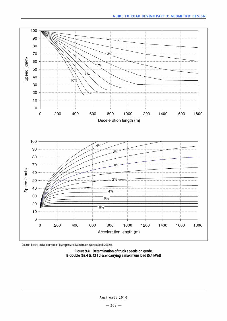
GUI DE TO RO A D DE SIG N P ART 3 : GEO MET RI C D ESI G N
A u s t r o a d s 2 0 1 0
— 2 0 3 —
Source: Based on Department of Transport and Main Roads Queensland (2002c).
Figure 9.4: Determination of truck speeds on grade, B-double (62.4 t), 12 l diesel carrying a maximum load (5.4 kW/t)
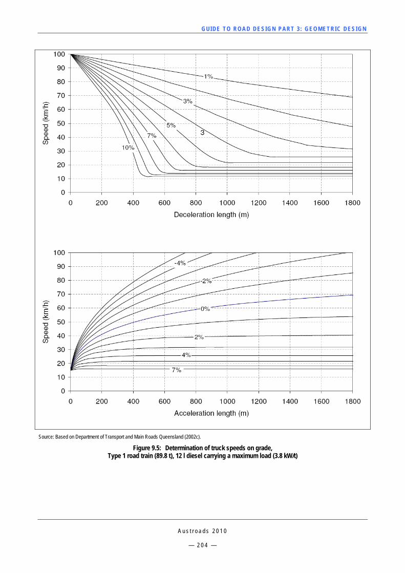
GUI DE TO RO A D DE SIG N P ART 3 : GEO MET RI C D ESI G N
A u s t r o a d s 2 0 1 0
— 2 0 4 —
Source: Based on Department of Transport and Main Roads Queensland (2002c).
Figure 9.5: Determination of truck speeds on grade, Type 1 road train (89.8 t), 12 l diesel carrying a maximum load (3.8 kW/t)
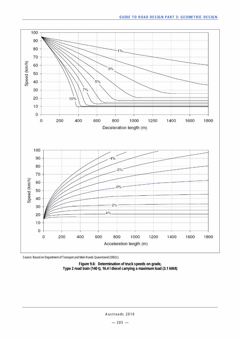
GUI DE TO RO A D DE SIG N P ART 3 : GEO MET RI C D ESI G N
A u s t r o a d s 2 0 1 0
— 2 0 5 —
Source: Based on Department of Transport and Main Roads Queensland (2002c).
Figure 9.6: Determination of truck speeds on grade, Type 2 road train (140 t), 16.4 l diesel carrying a maximum load (3.1 kW/t)
GUI DE TO RO A D DE SIG N P ART 3 : GEO MET RI C D ESI G N
A u s t r o a d s 2 0 1 0
— 2 0 6 —
9.6 Slow Vehicle Turnouts 9.6.1 Partial Climbing Lanes A turnout is a very short section of paved shoulder or added lane that is provided to allow slow vehicles to pull aside and be overtaken. It differs from an overtaking lane in its short length, different signing, and the fact that the majority of vehicles are not encouraged to travel in the left lane.
On dual carriageways a partial climbing lane for slow vehicles can be provided as shown on Figure 9.7.
While climbing lanes should preferably be designed to span the full length of the grade, there may be circumstances where it will be satisfactory to use a turnout on part of the up grade. A turnout may be appropriate if traffic volumes are low or construction costs are very high.
Turnout lengths of 60 to 160 m for average approach speeds of 30 to 90 km/h respectively and a width of 3.7 m is to be used.
If a turnout is used, care must be taken to provide adequate sight distance. Signing at the start and merge points are required to better indicate diverge and merge locations. The minimum sight distance available should be stopping sight distance for the operating speed of the road.
9.6.2 Slow Vehicle Turnouts In New Zealand, the layout and signing of Slow Vehicle Bays is covered in Manual of Traffic Signs and Markings (MOTSAM) Part 1 (2007) and Part 2 (2008).
On two-lane two-way roads a passing bay may be provided as shown on Figure 9.7, for slow vehicle turnouts.
On steep grades where truck speeds can reduce to a ‘crawl’ speed less than 20 km/h and a full climbing lane can not be provided, passing bays may provide an improvement to traffic flow. A passing bay is a very short auxiliary lane (of the order of 100 m, but not more than 160 m plus tapers) that allows a slow vehicle to pull aside to allow a following vehicle to pass. The passing bay provides for the overtaking of the slowest vehicles and is only appropriate if all of the following conditions are met:
long grades over 8%
high proportion of heavy vehicles
low overall traffic volumes
construction costs are too high or the environmental amenity of the area precludes development of full climbing lanes.
Slow vehicle bays must be properly signed to ensure their effectiveness. Normally, 300 m advance warning of the location of the bay is required to allow heavy vehicle drivers to prepare for the overtaking manoeuvre and to alert other drivers to the approaching facility.
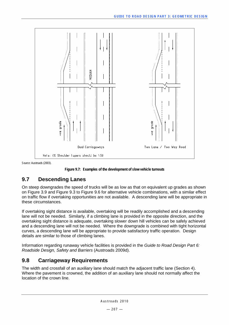
GUI DE TO RO A D DE SIG N P ART 3 : GEO MET RI C D ESI G N
A u s t r o a d s 2 0 1 0
— 2 0 7 —
Source: Austroads (2003).
Figure 9.7: Examples of the development of slow vehicle turnouts
9.7 Descending Lanes On steep downgrades the speed of trucks will be as low as that on equivalent up grades as shown on Figure 3.9 and Figure 9.3 to Figure 9.6 for alternative vehicle combinations, with a similar effect on traffic flow if overtaking opportunities are not available. A descending lane will be appropriate in these circumstances.
If overtaking sight distance is available, overtaking will be readily accomplished and a descending lane will not be needed. Similarly, if a climbing lane is provided in the opposite direction, and the overtaking sight distance is adequate, overtaking slower down hill vehicles can be safely achieved and a descending lane will not be needed. Where the downgrade is combined with tight horizontal curves, a descending lane will be appropriate to provide satisfactory traffic operation. Design details are similar to those of climbing lanes.
Information regarding runaway vehicle facilities is provided in the Guide to Road Design Part 6: Roadside Design, Safety and Barriers (Austroads 2009d).
9.8 Carriageway Requirements The width and crossfall of an auxiliary lane should match the adjacent traffic lane (Section 4). Where the pavement is crowned, the addition of an auxiliary lane should not normally affect the location of the crown line.
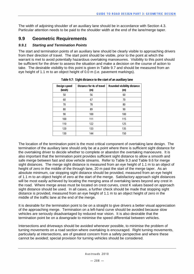
GUI DE TO RO A D DE SIG N P ART 3 : GEO MET RI C D ESI G N
A u s t r o a d s 2 0 1 0
— 2 0 8 —
The width of adjoining shoulder of an auxiliary lane should be in accordance with Section 4.3. Particular attention needs to be paid to the shoulder width at the end of the lane/merge taper.
9.9 Geometric Requirements 9.9.1 Starting and Termination Points The start and termination points of an auxiliary lane should be clearly visible to approaching drivers from their direction of travel. The start point should be visible, prior to the point at which the warrant is met to avoid potentially hazardous overtaking manoeuvres. Visibility to this point should be sufficient for the driver to assess the situation and make a decision on the course of action to take. The desirable visibility to this point is given in Table 9.7 and should be measured from an eye height of 1.1 m to an object height of 0.0 m (i.e. pavement markings).
Table 9.7: Sight distance to the start of an auxiliary lane
Design speed (km/h)
Distance for 4s of travel (m)
Rounded visibility distance (m)
50 56 60 60 67 70 70 78 80 80 89 90 90 100 100 100 111 115 110 122 125 120 133 135 130 144 150
The location of the termination point is the most critical component of overtaking lane design. The termination of the auxiliary lane should only be at a point where there is sufficient sight distance for the overtaking driver to decide whether to complete or abandon the overtaking manoeuvre. It is also important that the termination point provides sufficient sight distance to allow a smooth and safe merge between fast and slow vehicle streams. Refer to Table 9.3 and Table 9.6 for merge sight distances. The merge sight distance is measured from an eye height of 1.1 m to an object of height of zero in the middle of the through lane, 20 m past the start of the merge taper. As an absolute minimum, car stopping sight distance should be provided, measured from an eye height of 1.1 m to an object height of zero at the start of the merge. Satisfactory approach sight distances will be most easily achieved by locating the merging area of overtaking lanes beyond any crest in the road. Where merge areas must be located on crest curves, crest K values based on approach sight distance should be used. In all cases, a further check should be made that stopping sight distance is provided, measured from an eye height of 1.1 m to an object height of zero in the middle of the traffic lane at the end of the merge.
It is desirable for the termination point to be on a straight to give drivers a better visual appreciation of the approaching merge. Termination on a left-hand curve should be avoided because slow vehicles are seriously disadvantaged by reduced rear vision. It is also desirable that the termination point be on a downgrade to minimise the speed differential between vehicles.
Intersections and driveways should be avoided whenever possible, to minimise the problem of turning movements on a road section where overtaking is encouraged. Right turning movements, particularly at intersections, are of greatest concern from a safety perspective and where these cannot be avoided; special provision for turning vehicles should be considered.
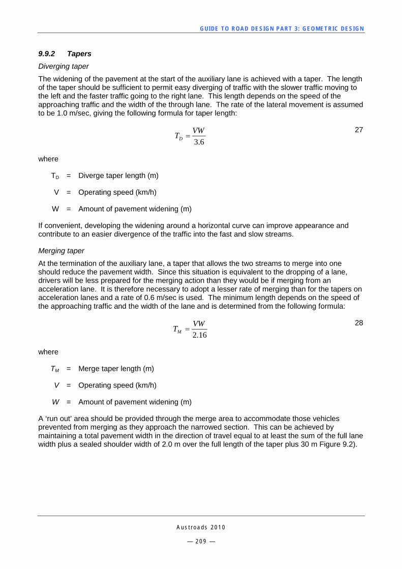
GUI DE TO RO A D DE SIG N P ART 3 : GEO MET RI C D ESI G N
A u s t r o a d s 2 0 1 0
— 2 0 9 —
9.9.2 Tapers Diverging taper
The widening of the pavement at the start of the auxiliary lane is achieved with a taper. The length of the taper should be sufficient to permit easy diverging of traffic with the slower traffic moving to the left and the faster traffic going to the right lane. This length depends on the speed of the approaching traffic and the width of the through lane. The rate of the lateral movement is assumed to be 1.0 m/sec, giving the following formula for taper length:
6.3
VWTD = 27
where
TD = Diverge taper length (m)
V = Operating speed (km/h)
W = Amount of pavement widening (m)
If convenient, developing the widening around a horizontal curve can improve appearance and contribute to an easier divergence of the traffic into the fast and slow streams.
Merging taper
At the termination of the auxiliary lane, a taper that allows the two streams to merge into one should reduce the pavement width. Since this situation is equivalent to the dropping of a lane, drivers will be less prepared for the merging action than they would be if merging from an acceleration lane. It is therefore necessary to adopt a lesser rate of merging than for the tapers on acceleration lanes and a rate of 0.6 m/sec is used. The minimum length depends on the speed of the approaching traffic and the width of the lane and is determined from the following formula:
16.2
VWTM = 28
where
TM = Merge taper length (m)
V = Operating speed (km/h)
W = Amount of pavement widening (m)
A ‘run out’ area should be provided through the merge area to accommodate those vehicles prevented from merging as they approach the narrowed section. This can be achieved by maintaining a total pavement width in the direction of travel equal to at least the sum of the full lane width plus a sealed shoulder width of 2.0 m over the full length of the taper plus 30 m Figure 9.2).
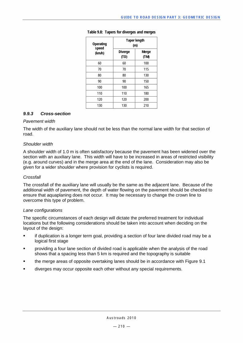
GUI DE TO RO A D DE SIG N P ART 3 : GEO MET RI C D ESI G N
A u s t r o a d s 2 0 1 0
— 2 1 0 —
Table 9.8: Tapers for diverges and merges
Operating speed (km/h)
Taper length (m)
Diverge (TD)
Merge (TM)
60 60 100 70 70 115 80 80 130 90 90 150 100 100 165 110 110 180 120 120 200 130 130 210
9.9.3 Cross-section Pavement width
The width of the auxiliary lane should not be less than the normal lane width for that section of road.
Shoulder width
A shoulder width of 1.0 m is often satisfactory because the pavement has been widened over the section with an auxiliary lane. This width will have to be increased in areas of restricted visibility (e.g. around curves) and in the merge area at the end of the lane. Consideration may also be given for a wider shoulder where provision for cyclists is required.
Crossfall
The crossfall of the auxiliary lane will usually be the same as the adjacent lane. Because of the additional width of pavement, the depth of water flowing on the pavement should be checked to ensure that aquaplaning does not occur. It may be necessary to change the crown line to overcome this type of problem.
Lane configurations
The specific circumstances of each design will dictate the preferred treatment for individual locations but the following considerations should be taken into account when deciding on the layout of the design:
if duplication is a longer term goal, providing a section of four lane divided road may be a logical first stage
providing a four lane section of divided road is applicable when the analysis of the road shows that a spacing less than 5 km is required and the topography is suitable
the merge areas of opposite overtaking lanes should be in accordance with Figure 9.1
diverges may occur opposite each other without any special requirements.
GUI DE TO RO A D DE SIG N P ART 3 : GEO MET RI C D ESI G N
A u s t r o a d s 2 0 1 0
— 2 1 1 —
10 BRIDGE CONSIDERATIONS
10.1 General The provision of structures on road alignments generally forms a significant cost element to any project. Road designers should be cognisant of the geometric complexity particular road elements can have on the design of structures. The following information provides general guidance that should be considered in the preparation of a road design that will interface with a bridge.
When developing the road alignment, the road designer should consult with a bridge designer or engineer with regard to construction economies, span lengths and arrangement, provision for future duplication etc.
Further consideration of geometric requirements for bridges is set out in:
AS5100 Set-2007, Bridge Design Set.
The New Zealand Bridge Design Manual, Transit New Zealand (2003).
10.2 Cross Section Designers should aim to provide a consistent cross section on the bridge and approach roadways, as this will provide a consistent level of service along that section of the road.
The following factors should be considered:
road geometry and lane widths
traffic volumes and composition
terrain
climatic conditions
bridge location.
The traffic lane and shoulder widths provided on the bridge should not be less than the widths provided on the approach roadway. Designers should refer to the Bridge Design Code AS 5100 Set-2007, Bridge Design Set or New Zealand Bridge Design Manual, Transit New Zealand (2003) and road authority guidelines regarding the provision of full width shoulders on bridges. Designers shall consider the safety of all road users (especially cyclists) when determining the appropriate cross-section.
Where necessary, additional bridge width should be provided:
to carry a kerbed footway on the bridge and on the approaches
on bridges constructed with horizontal curves where additional width is required on the inside of the curve to allow for horizontal sight distance clear of the barrier
to achieve satisfactory curve widening on small radius horizontal curves.
Auxiliary lane lengths and, in particular, tapers should not be reduced in order to avoid widening on bridges. If possible, it may be preferable to relocate the auxiliary lane or extend the lane across the structure.
GUI DE TO RO A D DE SIG N P ART 3 : GEO MET RI C D ESI G N
A u s t r o a d s 2 0 1 0
— 2 1 2 —
10.3 Horizontal Geometry The following principles are to be adopted for the horizontal alignment of the road where it crosses a structure:
avoid multiple and varying geometrics on the structure, including superelevation transitions, where possible
skew angle should desirably not exceed 35o
avoid curve radii below 500 m
avoid short end spans on bridges
if curvature is unavoidable, the bridge should lie fully within the circular arc and the radius should be as large as possible with a maximum superelevation of 6%
transition curves (spirals) on or leading into the structure should be avoided
the road designer should seek advice from bridge engineers in relation to the location of tangent points.
10.3.1 Superelevation Where practicable, designers should try to provide constant superelevation on bridges. Special conditions for superelevation that apply to bridges include:
The maximum superelevation shall not exceed 6%.
The absolute minimum crossfall on structures shall be 2% (drainage requirement).
The maximum grade on the structure, taking the vectorial sum of longitudinal grade and crossfall into account, shall not exceed 8%.
Changes in crossfall on the structure create difficulties both for design and construction of bridges and increased costs. Where varying crossfall or superelevation on the bridge is unavoidable, the changes should occur uniformly from one end of the bridge to the other. This also applies with changes from two-way to one-way crossfall.
Where parallel bridges are in close proximity, superelevation changes on the structures need to allow for any future widening and the possibility that the space between structures may be bridged in the future.
10.4 Vertical Geometry The vertical geometry can have a large effect on the design complexity of structures, especially if combined with tight horizontal geometry. The following principles should be considered:
Sag curves on the structure should be avoided. This will create a low point that will need to be drained, resulting in provision of a piped network to discharge the stormwater.
Minimum grades appropriate for kerb and channel are typically required to provide for a free draining structure, where there are solid bridge barriers (parapets).
GUI DE TO RO A D DE SIG N P ART 3 : GEO MET RI C D ESI G N
A u s t r o a d s 2 0 1 0
— 2 1 3 —
REFERENCES AASHTO 1994, A policy on geometric design of highways and streets 1994, 3rd edn, American Association
of State Highway and Transportation Officials, Washington DC, USA.
AASHTO 2001, A policy on geometric design of highways and streets 2001, 4th edn, American Association of State Highway and Transportation Officials, Washington DC, USA.
AASHTO 2004, A policy on geometric design of highways and streets, 5th edn, American Association of State Highway and Transportation Officials, Washington DC, USA.
AASHTO 2006. Roadside design guide, 3rd edn, American Association of State Highway and Transportation Officials, Washington, DC USA.
Anderson, GM 1969, ‘Driver eye height study 1969’, Australian Road Research, vol. 4, no. 4, pp. 9-14.
Armour, M 1976, The reaction times of drivers to roadside objects, AIR 217-2, Australian Road Research Board, Vermont South, Vic.
Australian Transport Council 2006, National road safety action plan 2007 and 2008, Australian Transport Council, Canberra, ACT.
Austroads 1989, Rural Road Design: Guide to the Geometric Design of Rural Roads, AP-1/89, Austroads, Sydney, NSW.
Austroads, 2000, Road Safety Environment and Design for Older Drivers, by B Fildes, G Corben, A Morris, J Oxley, N Prouk, L Brown & M Fitzharris M, AP-R169/00, Austroads, Sydney, NSW.
Austroads 2002a, Geometric Design for Trucks: When, Where and How?, by J McLean, M Tziotis, and T Gunatillake, AP-R211/02, Austroads, Sydney, NSW.
Austroads 2002b, Urban Road Design: A Guide to the Geometric Design of Major Urban Roads, AP-G69/02, Austroads, Sydney, NSW.
Austroads 2003, Rural Road Design: A Guide to the Geometric Design of Rural Roads, AP-G1/03, Austroads, Sydney, NSW.
Austroads 2006a, Austroads Design Vehicles and Turning Path Templates, by R George, AP-G34/06, Austroads, Sydney, NSW.
Austroads 2006b, Guide to Road Design: Part 1: Introduction to Road Design, by G Veith & D Bennett, AGRD01/06, Austroads, Sydney, NSW.
Austroads 2006c, Guide to Road Design: Part 2: Design Considerations, by G Veith, D Bennett & A Armistead, AGRD02/06, Austroads, Sydney, NSW.
Austroads 2006d, Guide to Road Safety – Part 5: Safety for Rural and Remote Areas, by M Tziotis, P Roper, Colin Edmonston and Prof M Sheehan, AGRS05/06, Austroads, Sydney, NSW.
Austroads 2008a, Glossary of Austroads Terms; 3rd edn, AP-C87/08 Austroads, Sydney, NSW.
Austroads 2008b, Guide to Road Design: Part 5: Drainage Design, by A Armistead, A Woollard, D Bennett & J Barff, AGRD05/08, Austroads, Sydney, NSW.
Austroads 2008c, Guide to Road Design: Part 7: Geotechnical Investigation and Design, by R Paul & R Grove, AGRD07/08, Austroads, Sydney, NSW.
GUI DE TO RO A D DE SIG N P ART 3 : GEO MET RI C D ESI G N
A u s t r o a d s 2 0 1 0
— 2 1 4 —
Austroads 2008d, Guide to Traffic Management: Part 5: Road Management, by D Bennett, G Veith, P Freeman, M Prodanovic & J Bliss, AGTM05/08, Austroads, Sydney, NSW.
Austroads 2008e, Guide to Traffic Management: Part 11: Parking, by P Damen & A Huband, AGTM11/08, Austroads, Sydney, NSW.
Austroads 2009a, Guide to Road Design: Part 4: Intersections and Crossings - General, by G Vieth & O Ardnt, Austroads, Sydney, NSW
Austroads 2009b, Guide to Road Design: Part 4A: Unsignalised and Signalised Intersections, by G Vieth, Austroads, Sydney, NSW.
Austroads 2009c, Guide to Road Design: Part 4C: Interchanges, by G Veith & L Louis Austroads, Sydney, NSW.
Austroads 2009d, Guide to Road Design: Part 6: Roadside Design, Safety and Barrier, by G Veith, Austroads, Sydney, NSW.
Austroads 2009e, Guide to Road Design: Part 6A: Pedestrians and Cyclist Paths, by G Veith, Austroads, Sydney, NSW.
Austroads 2009f, Guide to Road Design: Part 6B: Roadside Environment, by L Louis & G Veith, Austroads, Sydney, NSW.
Austroads 2009g, Guide to Road Design: Part 8: Process and Documentation, by B Hammonds, D Hicks and J McLean, Austroads, Sydney, NSW.
Austroads 2009h, Guide to Traffic Management: Part 3: Traffic Studies and Analysis, by D Bennett, R Troutbeck, P Croft, D McTiernan and A Shah, Austroads, Sydney, NSW.
Barker, DJ 1987, ‘The distribution of driver eye heights on the approaches to intersections’, Australian Road Research, vol 17, no 4, pp. 265-8.
Blue, DW & Kulakowski, BT 1991, ‘Effects of horizontal curve transition design on truck roll stability’, Journal of Transportation Engineering, vol. 117, no.1, pp.91-102.
Bonneson, RJ 2000, Superelevation distribution methods and transition designs, National Cooperative Highway Research Program, report 439, Transportation Research Board, Washington DC.
Botterill, R 1994, ‘Validation of operating speed model’, contract report CRTE 94/004, Australian Road Research Board, Vermont South, Vic.
Bovy, PHL & Bradley, MA 1985, ‘Route choice analyzed with stated-preference approaches’, Transportation Research Record, no. 1037, pp.11-20.
Bicycle Victoria 2009, Bicycle Victoria, Bicycle Victoria Incorporated, Melbourne, Vic, viewed 12 June 2009, <www.bv.com.au>.
Brundell-Freij, K & Ericsson, E 2005, ‘Influence of street characteristics, driver category and car performance on urban driving patterns’, Transportation Research, Part D - Transport and Environment, vol.10D, pp. 213-29.
Cox, RL 2003, ‘The impact of eye height on road design:the low-down on driver eye height’, 2003 Planners and designers symposium, Brisbane, Queensland, Queensland Department of Main Roads, Brisbane, Qld.
GUI DE TO RO A D DE SIG N P ART 3 : GEO MET RI C D ESI G N
A u s t r o a d s 2 0 1 0
— 2 1 5 —
Cox, RL & Arndt, OK 2005, ‘Using an extended design domain concept for road restoration projects’, 3rd international symposium of geometric design practice, Chicago, USA, Transportation Research Board, Washington, DC, 20p.
Di Cristoforo, R, Hood, C & Sweatman PF 2004, Acceleration and deceleration testing of combination vehicles, report RUS-04-1075-01-05, Main Roads Western Australia, Perth, WA.
Donaldson, GA 1986, ‘Safety of large trucks and geometric design of two-lane two-way roads’, Transportation Research Record, no.1052, pp.10-14.
Durth, W & Bernhard, M 2000, ‘Revised design parameters for stopping sight distance’, International symposium on highway geometric design, 2nd, June 2000, Mainz, Germany, Road and Transport Research Association, Cologne, Germany, pp. 410-21.
R Ervin, M Barnes, C MacAdam and R Scott 1986 ‘Impact of specific geometric features on truck operations and safety at interchanges’. University of Michigan, Ann Arbour, Transport Research Insitute, USA.
Fambro, DB, Fitzpatrick, K& Koppa, RJ 1997, Determination of stopping sight distances, National Cooperative Highway Research Program (NHCRP) report 400, Transportation Research Board,Washington DC, USA.
Fancher, PS 1986, ‘Sight distance problems related to large trucks’, Transportation Research Record, no. 1052, pp.29-35,7.
Farber, EI 1982, ‘Driver eye height trends and sight distance on vertical curves’, Transportation Research Record, no. 855, pp. 27-33.
Fitzpatrick, K, Carlson, P, Brewer, M., Wooldridge, M., 2001. ‘Design Factors That Affect Driver Speed on Suburban Streets’. Transportation Research Record: Journal of the Transportation Research Board 1751, 18-24.
Garber, N J & Hoel, LA 1988, Traffic and highway engineering, West Publishing Co., St. Paul, MN, USA.
Glennon, JC, TR Neumann & Leisch, JE 1985, Safety and operational characteristics for design of rural highway curves, report FHWA-RD-86, Federal Highway Administration, Washington, DC, USA.
Green, M 2000, ‘"How long does it take to stop?" - a methodological analysis of driver perception-brake times’, Transportation Human Factors, vol.2, no.3, pp.195-216.
Giummarra, G 2009, Unsealed roads manual: guidelines to good practice, 3rd edn., ARRB Group, Vermont South, Vic.
Harwood DW, Fambro DB, Fishburn B, Joubert H, Lamm R & Psarianos, B 1998, ‘International sight distance design practices’, International symposium on highway geometric design practices, 1995, Boston, Massachusetts, Transportation Research Board, Washington, DC, USA, 23 pp.
Hoban, CJ 1983, Guidelines for rural road improvements: a simulation study, AIR 359-10, Australian Road Research Board, Vermont South, Vic.
Hoban, CJ & Morrall, FJ 1986, Overtaking lane practice in Canada and Australia, ARR 144, Australian Road Research Board, Vermont South, Vic.
Kanellaidis, G 1999, ‘Road curve superelevation design: current practices and proposed approach’, Road and Transport Research, vol.8, no. 2, pp. 27-38.
GUI DE TO RO A D DE SIG N P ART 3 : GEO MET RI C D ESI G N
A u s t r o a d s 2 0 1 0
— 2 1 6 —
Krammes, RA, Brackett, et al 1993, State of the practice geometric design consistency, contract no. DTFH61-91-C-00050, Federal Highway Administration, McLean, Virginia, USA.
Land Transport New Zealand 2007, New Zealand on road tracking curves for heavy vehicles, RTS 18, LTNZ, Wellington, NZ.
Land Transport Safety Authority 2004, Cycle network and rout planning guide, LTSA, Wellington, NZ.
Lay, MG 1998, Handbook of road technology: volume 2: traffic and transport, 3rd edn., Gordon and Breach Science Publishers, Sydney, NSW.
Lennie, SC, Arndt, OK & Cox, RL 2008, 2008 Measurement of passenger cars: head light height, tail light height & vehicle height, Queensland Department of Main Roads. Brisbane, QLD.
Main Roads, Western Australia 1996, Technical standards, item 2.3.14, volume 1: part 1: geometric road design standards and practice guidelines, roadways document no. 67-08-6, MRWA, Perth, WA.
Mai, L & Sweatman, P 1984, Articulated vehicle stability: phase 2: tilt tests and computer model, AIR 323-2, Australian Road Research Board, Vermont South, Vic.
McCormack, EM & Sanders, MS 1982, Human factors in engineering and design , 5th edn., McGraw Hill, New York, USA.
McLean, J 1978, ‘Review of the design speed concept’, Australian Road Research Board, vol. 8, no. 1, pp. 3-15.
McLean, JR 1988, Speeds, friction factors and alignment design standards, ARR 154, Australian Road Research Board, Vermont South, Vic.
NAASRA 1980, Interim guide to the geometric design of rural roads, RDC-6, National Association of Australian State Road Authorities (NAASRA), Sydney, NSW.
Nicholson A 1998, ‘Superelevation, side friction and roadway consistency’, Journal of Transportation Engineering, vol. 124, no. 5, pp.411-8.
National Transport Commission 2009, Transport efficiency and supply chain revenue: PBS standards, NTC, Melbourne, Vic, viewed 15 June 2009, <http://www.ntc.gov.au/viewpage.aspx?documentid=1230>
Perco, P 2005, ’Comparison between vehicle paths along transition sections with and without spiral curves’, International symposium on highway geometric design, 3rd, June 2005, Chicago, Illinois, Transportation Research Board, Washington, DC, USA, 23 pp.
PIARC 1995, ‘Interurban roads: report of the committee C4’, PIARC world road congress, 20th, Montreal, Canada, Permanent International Association of Road Congresses (PIARC), Paris, France.
Poe, CM, Tarris, JP & Mason, JM 1995, ‘Operating speed approach to geometric design of low-speed urban streets’, Proceedings of the international symposium on highway geometric design practices, Boston, MA, Transportation Research Board, Washington DC, USA.
Prem, H, Ramsay, E, Fletcher, C, George, R & Gleeson, B, 1999, Estimation of lane width requirements for heavy vehicles on straight paths, ARR 342, ARRB Transport Research, Vermont South, Vic
Queensland Department of Main Roads 2001, Road planning and design manual: chapter 10: alignment design, Queensland Department of Main Roads, Brisbane, Qld.
GUI DE TO RO A D DE SIG N P ART 3 : GEO MET RI C D ESI G N
A u s t r o a d s 2 0 1 0
— 2 1 7 —
Queensland Department of Main Roads 2002a, Road planning and design manual: chapter 11: horizontal alignment, Queensland Department of Main Roads, Brisbane, Qld.
Queensland Department of Main Roads 2002b, Road planning and design manual: chapter 12: vertical alignment, Queensland Department of Main Roads, Brisbane, Qld.
Queensland Department of Main Roads 2002c, Road planning and design manual: chapter 15: auxiliary lanes. Queensland Department of Main Roads, Brisbane, Qld.
Queensland Department of Main Roads 2004, Road planning and design manual: chapter 7: cross section, Queensland Department of Main Roads, Brisbane, Qld.
Queensland Department of Main Roads 2005, Road planning and design manual: chapter 4: application of design principles and guidelines, Queensland Department of Main Roads, Brisbane, QLD.
Queensland Department of Main Roads 2007a, Road design and planning manual: chapter 6: speed parameters, Queensland Department of Transport, Brisbane, Qld.
RTA 1989, Road Design Guide, Roads and Traffic Authority, Sydney, NSW..
Summala, H 2002, ‘Behavioural adaptation and drivers' task control’, in R Fuller & JA Santos, (eds), Human factors for highway engineers, Pergamon, Amsterdam, Netherlands.
Transit New Zealand 2000, State highway geometric design manual (draft). Transit New Zealand, Wellington, New Zealand.
Transit New Zealand 2003, Bridge Manual, 2nd edn,Transit New Zealand, Wellington, New Zealand.
Transit New Zealand 2007, MOTSAM: manual of traffic signs and markings: part 1: traffic signs, Transit New Zealand, Wellington, NZ.
Transit New Zealand 2008 ,MOTSAM: manual of traffic signs and markings: part 2: markings, Transit New Zealand, Wellington, NZ.
Triggs, TJ & Harris, WG 1982, Reaction time of drivers to road stimuli, human factors report no. HFR-12, Monash University, Clayton, Vic.
Troutbeck, RJ 1981, Overtaking behaviour on Australian two-lane rural highways, special report 20, Australian Road Research Board, Vermont South, Vic.
Tunnard, E & Pushkarev, B 1974, Man-made America: chaos or control?: an enquiry into selected problems of design in the urbanized landscape, Yale University Press, New Haven, CT, USA.
VicRoads 1999, Clearway bicycle lanes, cycle notes, no. 4, September, 1999.
VicRoads 2000, On-road arterial bicycle routes, cycle notes, no. 7, August 2000.
VicRoads 2002a, Road design guidelines: part 2: horizontal and vertical geometry, revision 2.6. VicRoads, Kew, Vic.
VicRoads 2002b, Road design guidelines: part 3: cross sectional elements, revision 3.7. VicRoads, Kew, Vic.
VicRoads 2003, ‘Median barrier warrant policy’, internal document, VicRoads, Kew, Vic.
VicRoads forthcoming 2009, Bus priority guidelines no. 2, bus lanes, signs and lines, VicRoads, Kew, Vic.
GUI DE TO RO A D DE SIG N P ART 3 : GEO MET RI C D ESI G N
A u s t r o a d s 2 0 1 0
— 2 1 8 —
Wang, J, Dixon, KK, Li, H, & Hunter, M 2006, ‘Operating-speed model for low-speed urban tangent streets based on in-vehicle global positioning system data’, Transportation Research Record, no. 1961, pp. 24-33.
Zegeer, CV, Deen, RC & Mayes, JG 1981, ‘Effect of lane and shoulder widths on accident reduction on rural, two lane roads, Transportation Research Record, no 806, pp. 33-43
Australian Standards
AS 1428 Set – 2003, Design for access and mobility.
AS 1742.12:2000, Manual of uniform traffic control devices part 12: bus, transit, tram and truck lane.
AS 2876: 2000, Concrete kerbs and channels (gutters): manually or machine placed.
AS/NZS 2890.1: 2004, Parking facilities: off-street car parking.
AS/NZS 2890.5: 1993, Parking facilities: on street parking.
AS/NZS 2890 (set): 2004, Parking facilities set.
AS 5100 (set): 2007, Bridge design set.

GUI DE TO RO A D DE SIG N P ART 3 : GEO MET RI C D ESI G N
A u s t r o a d s 2 0 1 0
— 2 1 9 —
APPENDIX A EXTENDED DESIGN DOMAIN (EDD) FOR GEOMETRIC ROAD DESIGN
A.1 General This section provides extended design domain (EDD) values for geometric road design. These are values outside of the normal design domain (NDD) that through research and/or operating experience, particular road authorities have found to provide a suitable solution in constrained situations (typically at brownfield sites).
Examples of when EDD may be considered are as follows:
reviewing the geometry of existing roads
realignment of a few geometric elements on existing roads in constrained locations
improving the standard of existing roads in constrained locations
building temporary roads.
Application of the EDD involves identification and documentation of driver capability. Ultimately, the capabilities that are accepted may have to pass the test of what is reasonable capability (the capability that a court decides a motorist can reasonably be expected to have when they are taking reasonable care for their own safety). The decision to use EDD should not be taken lightly.
In applying this Guide:
1. NDD values given in the body of this Guide should be used wherever practical.
2. Design values outside of the NDD are only to be used if approved in writing by the delegated representative from the relevant road authority. The relevant road authority may be a state road authority, municipal council or private road owner.
3. If using EDD values, the reduction in standard associated with their use should be appropriate for the prevailing local conditions. Generally, EDD should be used for only one parameter in any application and not be used in combination with any other minimum or EDD value for any related or associated parameters.
Through collective experience it has been accepted for a very long time that the use of minimum values for several parameters at the same location does not constitute good practice and generally leads to an inferior or unsafe design.
Designers may refer to the Guide to Road Design Australian Government (1992). Part 2: Design Considerations (Austroads 2006c) and Cox and Arndt (2005) for further information on EDD. The following sections deal with EDD for specific road design parameters and situations.
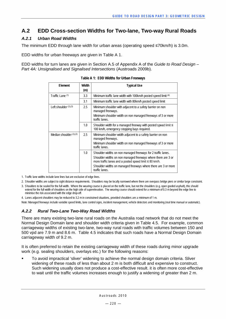
GUI DE TO RO A D DE SIG N P ART 3 : GEO MET RI C D ESI G N
A u s t r o a d s 2 0 1 0
— 2 2 0 —
A.2 EDD Cross-section Widths for Two-lane, Two-way Rural Roads A.2.1 Urban Road Widths The minimum EDD through lane width for urban areas (operating speed ≤70km/h) is 3.0m.
EDD widths for urban freeways are given in Table A 1.
EDD widths for turn lanes are given in Section A.5 of Appendix A of the Guide to Road Design – Part 4A: Unsignalised and Signalised Intersections (Austroads 2009b).
Table A 1: EDD Widths for Urban Freeways
Element Width (m)
Typical Use
Traffic Lane (1) 3.3 Minimum traffic lane width with 100km/h posted speed limit (4) 3.1 Minimum traffic lane width with 80km/h posted speed limit
Left shoulder (2),(3) 2.5 Minimum shoulder with adjacent to a safety barrier on non managed freeways. Minimum shoulder width on non managed freeways of 3 or more traffic lanes.
1.0 Shoulder width for a managed freeway with posted speed limit ≤ 100 km/h, emergency stopping bays required.
Median shoulder (2),(3) 2.5 Minimum shoulder width adjacent to a safety barrier on non managed freeways. Minimum shoulder width on non managed freeways of 3 or more traffic lanes.
1.0 Shoulder widths on non managed freeways for 2 traffic lanes. Shoulder widths on non managed freeways where there are 3 or more traffic lanes and a posted speed limit ≤ 80 km/h. Shoulder widths on managed freeways where there are 3 or more traffic lanes.
1. Traffic lane widths include lane lines but are exclusive of edge lines. 2. Shoulder widths are subject to sight distance requirements. Shoulders may be locally narrowed where there are overpass bridge piers or similar large constraint. 3. Shoulders to be sealed for the full width. Where the wearing course is placed on the traffic lane, but not the shoulders (e.g. open graded asphalt), this should
extend for the full width of shoulders on the high side of superelevation. The wearing course should extend for a minimum of 0.3 m beyond the edge line to minimise the risk associated with the edge drop-off.
4. Lanes adjacent shoulders may be reduced to 3.2 m in constrained situations, provided shoulders are a minimum of 1 m. Note: Managed freeways include variable speed limits, lane control signs, incident management, vehicle detectors and monitoring (real time manual or automatic).
A.2.2 Rural Two-Lane Two-Way Road Widths There are many existing two-lane rural roads on the Australia road network that do not meet the Normal Design Domain lane and shoulder width criteria given in Table 4.5. For example, common carriageway widths of existing two-lane, two-way rural roads with traffic volumes between 150 and 500 vpd are 7.9 m and 8.6 m. Table 4.5 indicates that such roads have a Normal Design Domain carriageway width of 9.2 m.
It is often preferred to retain the existing carriageway width of these roads during minor upgrade work (e.g. sealing shoulders, overlays etc.) for the following reasons:
To avoid impractical ‘sliver’ widening to achieve the normal design domain criteria. Sliver widening of these roads of less than about 2 m is both difficult and expensive to construct. Such widening usually does not produce a cost-effective result. it is often more cost-effective to wait until the traffic volumes increases enough to justify a widening of greater than 2 m.
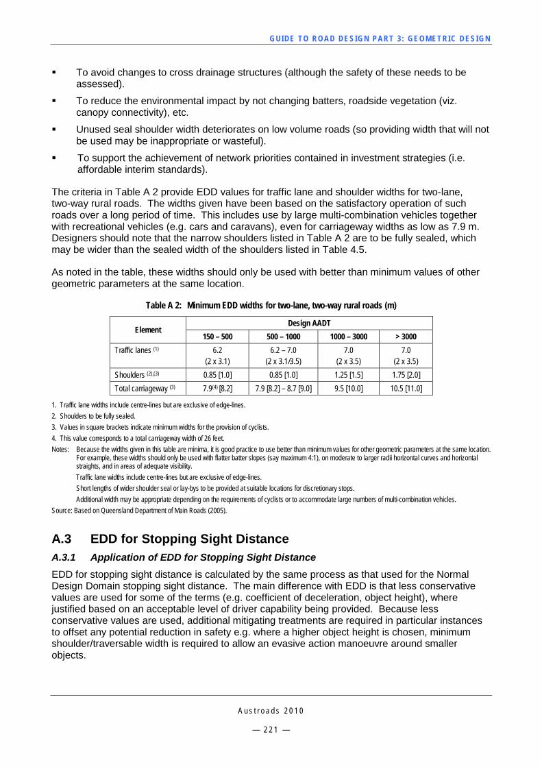
GUI DE TO RO A D DE SIG N P ART 3 : GEO MET RI C D ESI G N
A u s t r o a d s 2 0 1 0
— 2 2 1 —
To avoid changes to cross drainage structures (although the safety of these needs to be assessed).
To reduce the environmental impact by not changing batters, roadside vegetation (viz. canopy connectivity), etc.
Unused seal shoulder width deteriorates on low volume roads (so providing width that will not be used may be inappropriate or wasteful).
To support the achievement of network priorities contained in investment strategies (i.e. affordable interim standards).
The criteria in Table A 2 provide EDD values for traffic lane and shoulder widths for two-lane, two-way rural roads. The widths given have been based on the satisfactory operation of such roads over a long period of time. This includes use by large multi-combination vehicles together with recreational vehicles (e.g. cars and caravans), even for carriageway widths as low as 7.9 m. Designers should note that the narrow shoulders listed in Table A 2 are to be fully sealed, which may be wider than the sealed width of the shoulders listed in Table 4.5.
As noted in the table, these widths should only be used with better than minimum values of other geometric parameters at the same location.
Table A 2: Minimum EDD widths for two-lane, two-way rural roads (m)
Element Design AADT
150 – 500 500 – 1000 1000 – 3000 > 3000 Traffic lanes (1) 6.2
(2 x 3.1) 6.2 – 7.0
(2 x 3.1/3.5) 7.0
(2 x 3.5) 7.0
(2 x 3.5) Shoulders (2),(3) 0.85 [1.0] 0.85 [1.0] 1.25 [1.5] 1.75 [2.0] Total carriageway (3) 7.9(4) [8.2] 7.9 [8.2] – 8.7 [9.0] 9.5 [10.0] 10.5 [11.0]
1. Traffic lane widths include centre-lines but are exclusive of edge-lines. 2. Shoulders to be fully sealed. 3. Values in square brackets indicate minimum widths for the provision of cyclists. 4. This value corresponds to a total carriageway width of 26 feet. Notes: Because the widths given in this table are minima, it is good practice to use better than minimum values for other geometric parameters at the same location.
For example, these widths should only be used with flatter batter slopes (say maximum 4:1), on moderate to larger radii horizontal curves and horizontal straights, and in areas of adequate visibility.
Traffic lane widths include centre-lines but are exclusive of edge-lines. Short lengths of wider shoulder seal or lay-bys to be provided at suitable locations for discretionary stops. Additional width may be appropriate depending on the requirements of cyclists or to accommodate large numbers of multi-combination vehicles. Source: Based on Queensland Department of Main Roads (2005).
A.3 EDD for Stopping Sight Distance A.3.1 Application of EDD for Stopping Sight Distance EDD for stopping sight distance is calculated by the same process as that used for the Normal Design Domain stopping sight distance. The main difference with EDD is that less conservative values are used for some of the terms (e.g. coefficient of deceleration, object height), where justified based on an acceptable level of driver capability being provided. Because less conservative values are used, additional mitigating treatments are required in particular instances to offset any potential reduction in safety e.g. where a higher object height is chosen, minimum shoulder/traversable width is required to allow an evasive action manoeuvre around smaller objects.
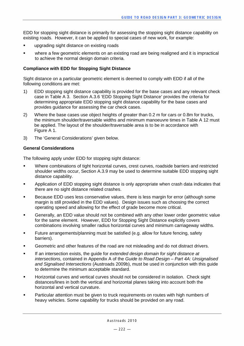
GUI DE TO RO A D DE SIG N P ART 3 : GEO MET RI C D ESI G N
A u s t r o a d s 2 0 1 0
— 2 2 2 —
EDD for stopping sight distance is primarily for assessing the stopping sight distance capability on existing roads. However, it can be applied to special cases of new work, for example:
upgrading sight distance on existing roads
where a few geometric elements on an existing road are being realigned and it is impractical to achieve the normal design domain criteria.
Compliance with EDD for Stopping Sight Distance
Sight distance on a particular geometric element is deemed to comply with EDD if all of the following conditions are met:
1) EDD stopping sight distance capability is provided for the base cases and any relevant check case in Table A 3. Section A.3.6 ‘EDD Stopping Sight Distance’ provides the criteria for determining appropriate EDD stopping sight distance capability for the base cases and provides guidance for assessing the car check cases.
2) Where the base cases use object heights of greater than 0.2 m for cars or 0.8m for trucks, the minimum shoulder/traversable widths and minimum manoeuvre times in Table A 12 must be applied. The layout of the shoulder/traversable area is to be in accordance with Figure A 1.
3) The ‘General Considerations’ given below.
General Considerations
The following apply under EDD for stopping sight distance:
Where combinations of tight horizontal curves, crest curves, roadside barriers and restricted shoulder widths occur, Section A.3.9 may be used to determine suitable EDD stopping sight distance capability.
Application of EDD stopping sight distance is only appropriate when crash data indicates that there are no sight distance related crashes.
Because EDD uses less conservative values, there is less margin for error (although some margin is still provided in the EDD values). Design issues such as choosing the correct operating speed and allowing for the effect of grade become more critical.
Generally, an EDD value should not be combined with any other lower order geometric value for the same element. However, EDD for Stopping Sight Distance explicitly covers combinations involving smaller radius horizontal curves and minimum carriageway widths.
Future arrangements/planning must be satisfied (e.g. allow for future fencing, safety barriers).
Geometric and other features of the road are not misleading and do not distract drivers.
If an intersection exists, the guide for extended design domain for sight distance at intersections, contained in Appendix A of the Guide to Road Design – Part 4A: Unsignalised and Signalised Intersections (Austroads 2009b), must be used in conjunction with this guide to determine the minimum acceptable standard.
Horizontal curves and vertical curves should not be considered in isolation. Check sight distances/lines in both the vertical and horizontal planes taking into account both the horizontal and vertical curvature.
Particular attention must be given to truck requirements on routes with high numbers of heavy vehicles. Some capability for trucks should be provided on any road.
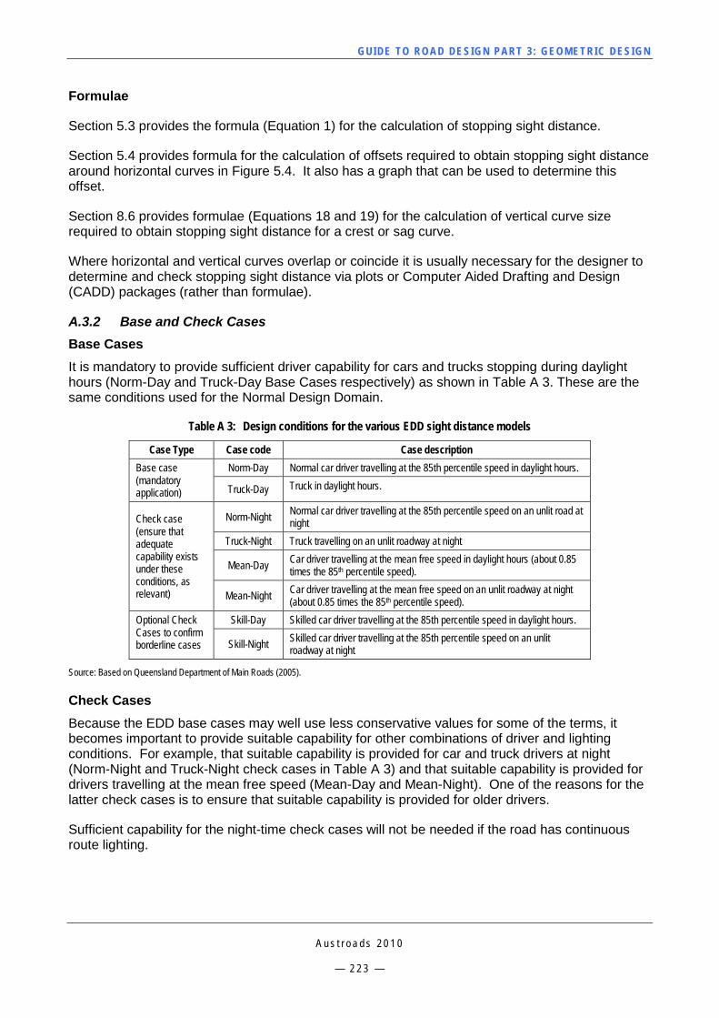
GUI DE TO RO A D DE SIG N P ART 3 : GEO MET RI C D ESI G N
A u s t r o a d s 2 0 1 0
— 2 2 3 —
Formulae
Section 5.3 provides the formula (Equation 1) for the calculation of stopping sight distance.
Section 5.4 provides formula for the calculation of offsets required to obtain stopping sight distance around horizontal curves in Figure 5.4. It also has a graph that can be used to determine this offset.
Section 8.6 provides formulae (Equations 18 and 19) for the calculation of vertical curve size required to obtain stopping sight distance for a crest or sag curve.
Where horizontal and vertical curves overlap or coincide it is usually necessary for the designer to determine and check stopping sight distance via plots or Computer Aided Drafting and Design (CADD) packages (rather than formulae).
A.3.2 Base and Check Cases Base Cases It is mandatory to provide sufficient driver capability for cars and trucks stopping during daylight hours (Norm-Day and Truck-Day Base Cases respectively) as shown in Table A 3. These are the same conditions used for the Normal Design Domain.
Table A 3: Design conditions for the various EDD sight distance models
Case Type Case code Case description Base case (mandatory application)
Norm-Day Normal car driver travelling at the 85th percentile speed in daylight hours.
Truck-Day Truck in daylight hours.
Check case (ensure that adequate capability exists under these conditions, as relevant)
Norm-Night Normal car driver travelling at the 85th percentile speed on an unlit road at night
Truck-Night Truck travelling on an unlit roadway at night
Mean-Day Car driver travelling at the mean free speed in daylight hours (about 0.85 times the 85th percentile speed).
Mean-Night Car driver travelling at the mean free speed on an unlit roadway at night (about 0.85 times the 85th percentile speed).
Optional Check Cases to confirm borderline cases
Skill-Day Skilled car driver travelling at the 85th percentile speed in daylight hours.
Skill-Night Skilled car driver travelling at the 85th percentile speed on an unlit roadway at night
Source: Based on Queensland Department of Main Roads (2005). Check Cases Because the EDD base cases may well use less conservative values for some of the terms, it becomes important to provide suitable capability for other combinations of driver and lighting conditions. For example, that suitable capability is provided for car and truck drivers at night (Norm-Night and Truck-Night check cases in Table A 3) and that suitable capability is provided for drivers travelling at the mean free speed (Mean-Day and Mean-Night). One of the reasons for the latter check cases is to ensure that suitable capability is provided for older drivers.
Sufficient capability for the night-time check cases will not be needed if the road has continuous route lighting.
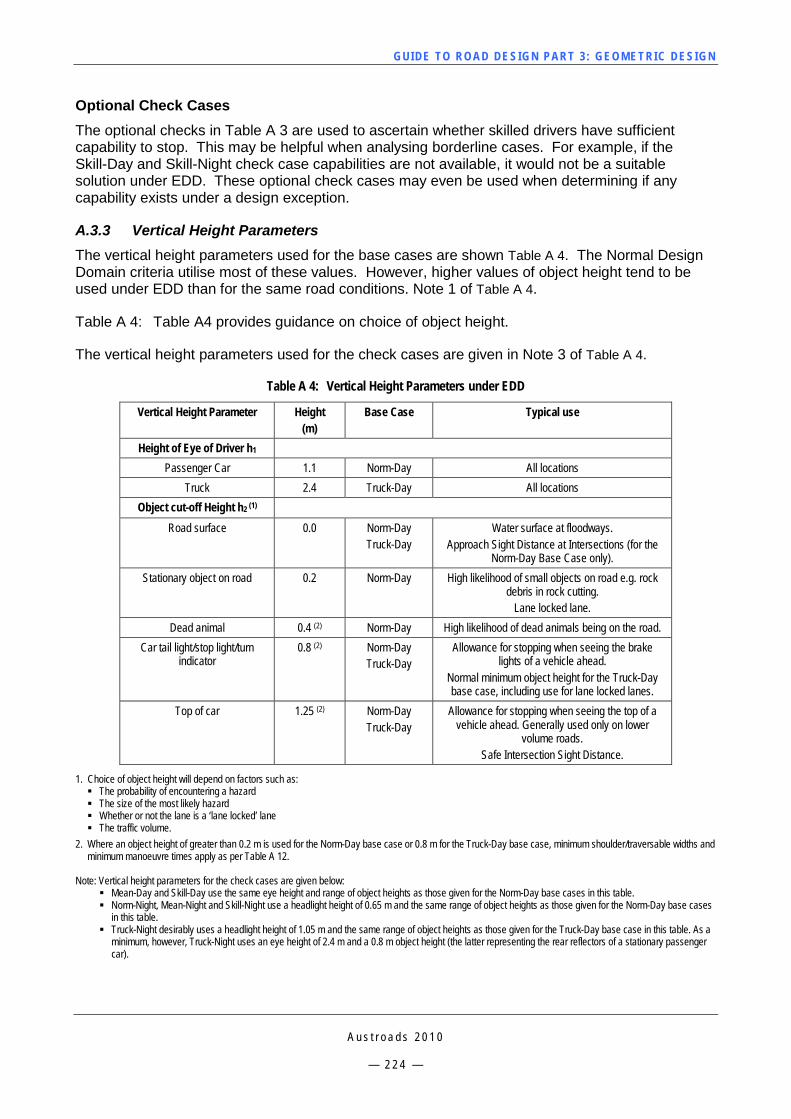
GUI DE TO RO A D DE SIG N P ART 3 : GEO MET RI C D ESI G N
A u s t r o a d s 2 0 1 0
— 2 2 4 —
Optional Check Cases The optional checks in Table A 3 are used to ascertain whether skilled drivers have sufficient capability to stop. This may be helpful when analysing borderline cases. For example, if the Skill-Day and Skill-Night check case capabilities are not available, it would not be a suitable solution under EDD. These optional check cases may even be used when determining if any capability exists under a design exception.
A.3.3 Vertical Height Parameters The vertical height parameters used for the base cases are shown Table A 4. The Normal Design Domain criteria utilise most of these values. However, higher values of object height tend to be used under EDD than for the same road conditions. Note 1 of Table A 4.
Table A 4: Table A4 provides guidance on choice of object height.
The vertical height parameters used for the check cases are given in Note 3 of Table A 4.
Table A 4: Vertical Height Parameters under EDD
Vertical Height Parameter Height (m)
Base Case Typical use
Height of Eye of Driver h1 Passenger Car 1.1 Norm-Day All locations
Truck 2.4 Truck-Day All locations Object cut-off Height h2 (1)
Road surface 0.0 Norm-Day Truck-Day
Water surface at floodways. Approach Sight Distance at Intersections (for the
Norm-Day Base Case only). Stationary object on road 0.2 Norm-Day High likelihood of small objects on road e.g. rock
debris in rock cutting. Lane locked lane.
Dead animal 0.4 (2) Norm-Day High likelihood of dead animals being on the road. Car tail light/stop light/turn
indicator 0.8 (2) Norm-Day
Truck-Day Allowance for stopping when seeing the brake
lights of a vehicle ahead. Normal minimum object height for the Truck-Day base case, including use for lane locked lanes.
Top of car 1.25 (2) Norm-Day Truck-Day
Allowance for stopping when seeing the top of a vehicle ahead. Generally used only on lower
volume roads. Safe Intersection Sight Distance.
1. Choice of object height will depend on factors such as: The probability of encountering a hazard The size of the most likely hazard Whether or not the lane is a ‘lane locked’ lane The traffic volume.
2. Where an object height of greater than 0.2 m is used for the Norm-Day base case or 0.8 m for the Truck-Day base case, minimum shoulder/traversable widths and minimum manoeuvre times apply as per Table A 12.
Note: Vertical height parameters for the check cases are given below:
Mean-Day and Skill-Day use the same eye height and range of object heights as those given for the Norm-Day base cases in this table. Norm-Night, Mean-Night and Skill-Night use a headlight height of 0.65 m and the same range of object heights as those given for the Norm-Day base cases
in this table. Truck-Night desirably uses a headlight height of 1.05 m and the same range of object heights as those given for the Truck-Day base case in this table. As a
minimum, however, Truck-Night uses an eye height of 2.4 m and a 0.8 m object height (the latter representing the rear reflectors of a stationary passenger car).
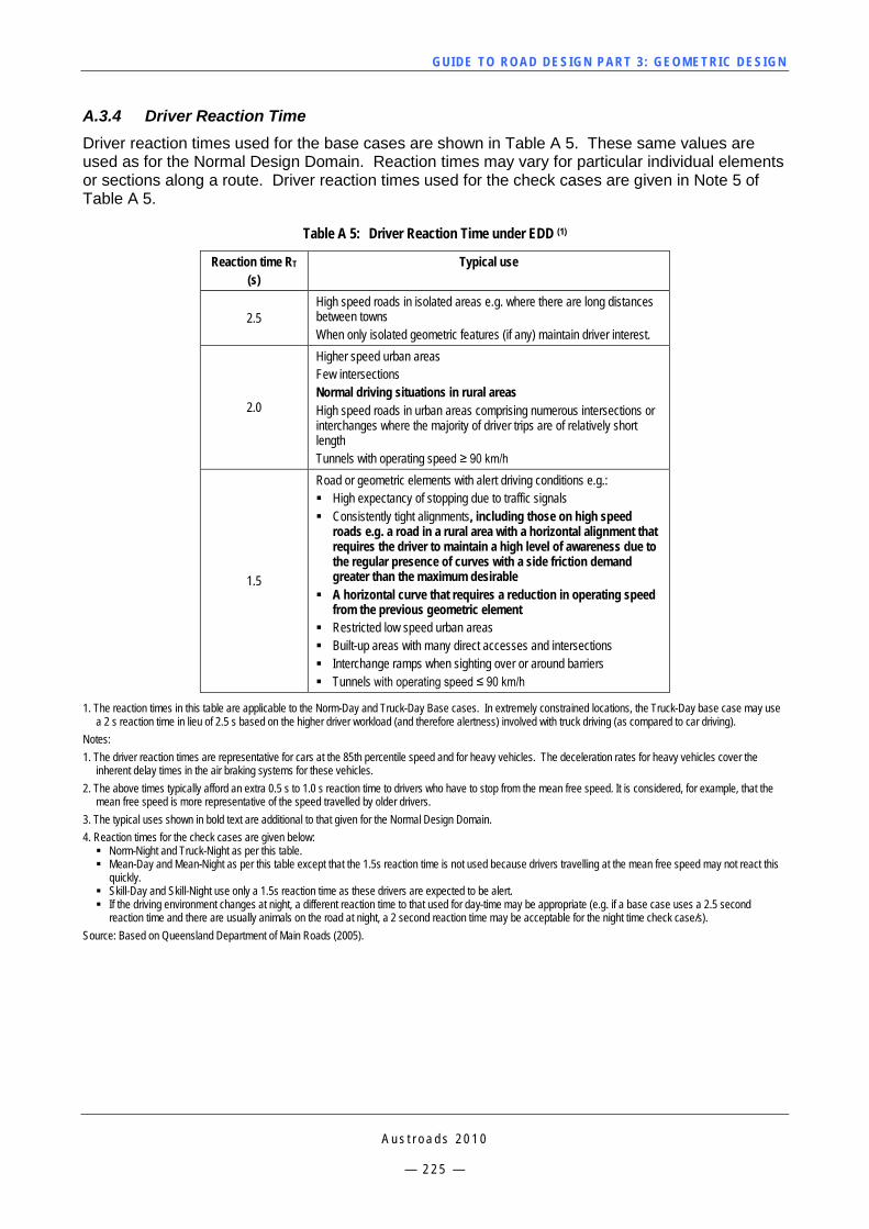
GUI DE TO RO A D DE SIG N P ART 3 : GEO MET RI C D ESI G N
A u s t r o a d s 2 0 1 0
— 2 2 5 —
A.3.4 Driver Reaction Time Driver reaction times used for the base cases are shown in Table A 5. These same values are used as for the Normal Design Domain. Reaction times may vary for particular individual elements or sections along a route. Driver reaction times used for the check cases are given in Note 5 of Table A 5.
Table A 5: Driver Reaction Time under EDD (1)
Reaction time RT (s)
Typical use
2.5 High speed roads in isolated areas e.g. where there are long distances between towns When only isolated geometric features (if any) maintain driver interest.
2.0
Higher speed urban areas Few intersections Normal driving situations in rural areas High speed roads in urban areas comprising numerous intersections or interchanges where the majority of driver trips are of relatively short length Tunnels with operating speed ≥ 90 km/h
1.5
Road or geometric elements with alert driving conditions e.g.: High expectancy of stopping due to traffic signals Consistently tight alignments, including those on high speed
roads e.g. a road in a rural area with a horizontal alignment that requires the driver to maintain a high level of awareness due to the regular presence of curves with a side friction demand greater than the maximum desirable
A horizontal curve that requires a reduction in operating speed from the previous geometric element
Restricted low speed urban areas Built-up areas with many direct accesses and intersections Interchange ramps when sighting over or around barriers Tunnels with operating speed ≤ 90 km/h
1. The reaction times in this table are applicable to the Norm-Day and Truck-Day Base cases. In extremely constrained locations, the Truck-Day base case may use a 2 s reaction time in lieu of 2.5 s based on the higher driver workload (and therefore alertness) involved with truck driving (as compared to car driving).
Notes: 1. The driver reaction times are representative for cars at the 85th percentile speed and for heavy vehicles. The deceleration rates for heavy vehicles cover the
inherent delay times in the air braking systems for these vehicles. 2. The above times typically afford an extra 0.5 s to 1.0 s reaction time to drivers who have to stop from the mean free speed. It is considered, for example, that the
mean free speed is more representative of the speed travelled by older drivers. 3. The typical uses shown in bold text are additional to that given for the Normal Design Domain. 4. Reaction times for the check cases are given below: Norm-Night and Truck-Night as per this table. Mean-Day and Mean-Night as per this table except that the 1.5s reaction time is not used because drivers travelling at the mean free speed may not react this
quickly. Skill-Day and Skill-Night use only a 1.5s reaction time as these drivers are expected to be alert. If the driving environment changes at night, a different reaction time to that used for day-time may be appropriate (e.g. if a base case uses a 2.5 second
reaction time and there are usually animals on the road at night, a 2 second reaction time may be acceptable for the night time check case/s). Source: Based on Queensland Department of Main Roads (2005).
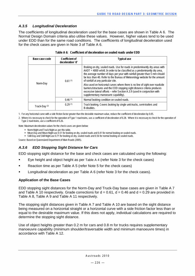
GUI DE TO RO A D DE SIG N P ART 3 : GEO MET RI C D ESI G N
A u s t r o a d s 2 0 1 0
— 2 2 6 —
A.3.5 Longitudinal Deceleration The coefficients of longitudinal deceleration used for the base cases are shown in Table A 6. The Normal Design Domain criteria also utilise these values. However, higher values tend to be used under EDD than for the same road conditions. The coefficients of longitudinal deceleration used for the check cases are given in Note 3 of Table A 6.
Table A 6: Coefficient of deceleration on sealed roads under EDD
Base case code Coefficient of deceleration ‘d’
Typical use
Norm-Day 0.61 (1)
Braking on dry, sealed roads. Use for roads in predominantly dry areas with AADT < 4000 veh/d. In order to be classified as a predominantly dry area, the average number of days per year with rainfall greater than 5 mm should be less than 40. Refer to the Bureau of Meteorology website for the amount of rainfall at any particular site. Also used on horizontal curves where there is no line of sight over roadside barriers/structures and the EDD stopping sight distance criteria produces excessive lateral offsets – refer Section A.3.9 (used in conjunction with supplementary manoeuvre capability).
0.46 (1) Normal braking condition on sealed roads.
Truck-Day (2) 0.29 (1) Truck braking. Covers braking by single unit trucks, semi-trailers and B-doubles.
1. For any horizontal curve with a side friction factor greater than the desirable maximum value, reduce the coefficient of deceleration by 0.05. 2. Where it is necessary to check for the operation of Type 1 road-trains, use a coefficient of deceleration of 0.28. Where it is necessary to check for the operation of
Type 2 road-trains, use a coefficient of 0.26.
Note: Maximum deceleration values for the check cases are given below: Norm-Night and Truck-Night as per this table. Mean-Day and Mean-Night use 0.51 for braking on dry, sealed roads and 0.41 for normal braking on sealed roads. Skill-Day and Skill-Night use 0.71 for braking on dry, sealed roads and 0.56 for normal braking on sealed roads.
Source: Based on Queensland Department of Main Roads (2005).
A.3.6 EDD Stopping Sight Distance for Cars EDD stopping sight distance for the base and check cases are calculated using the following:
Eye height and object height as per Table A 4 (refer Note 3 for the check cases)
Reaction time as per Table A 5 (refer Note 5 for the check cases)
Longitudinal deceleration as per Table A 6 (refer Note 3 for the check cases).
Application of the Base Cases
EDD stopping sight distances for the Norm-Day and Truck-Day base cases are given in Table A 7 and Table A 10 respectively. Grade corrections for d = 0.61, d = 0.46 and d = 0.29 are provided in Table A 8, Table A 9 and Table A 11 respectively.
The stopping sight distances given in Table A 7 and Table A 10 are based on the sight distance being measured on a horizontal straight or a horizontal curve with a side friction factor less than or equal to the desirable maximum value. If this does not apply, individual calculations are required to determine the stopping sight distance.
Use of object heights greater than 0.2 m for cars and 0.8 m for trucks requires supplementary manoeuvre capability (minimum shoulder/traversable width and minimum manoeuvre times) in accordance with Table A 12.
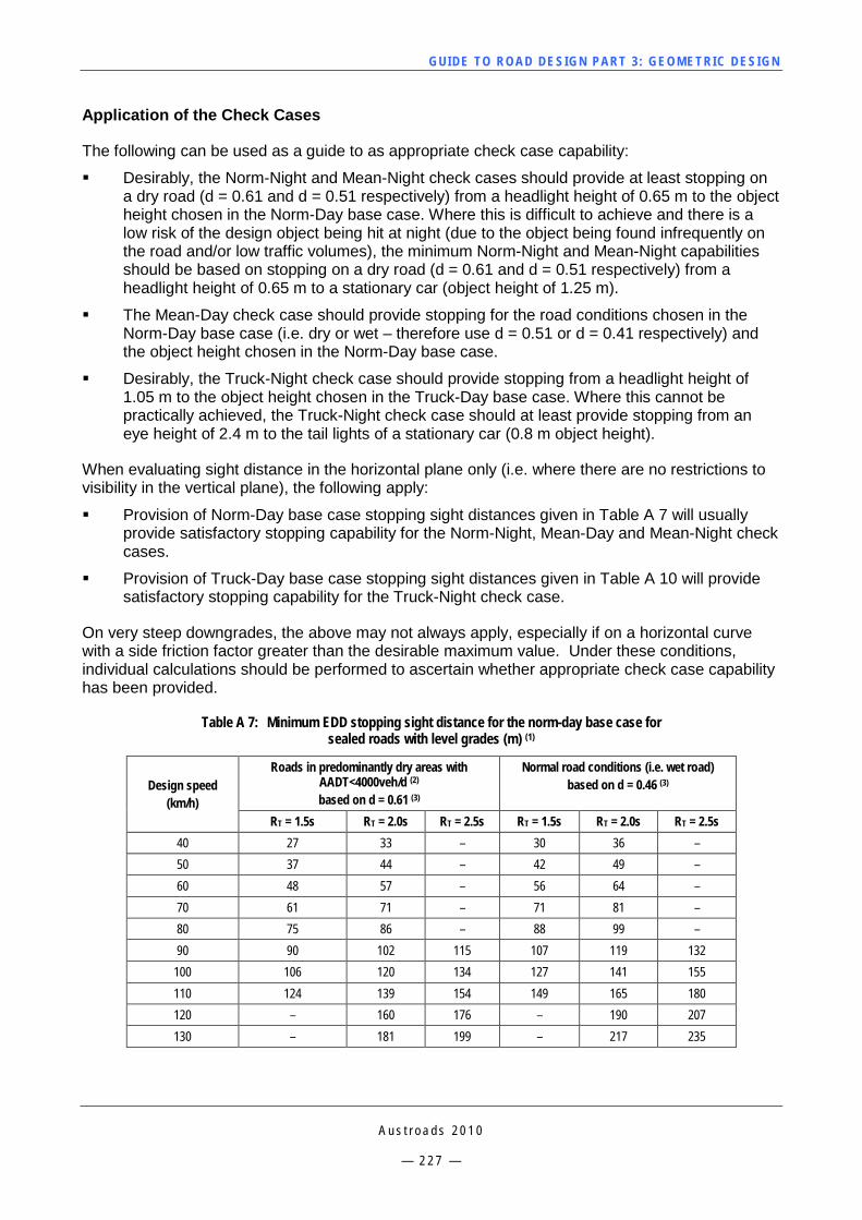
GUI DE TO RO A D DE SIG N P ART 3 : GEO MET RI C D ESI G N
A u s t r o a d s 2 0 1 0
— 2 2 7 —
Application of the Check Cases
The following can be used as a guide to as appropriate check case capability:
Desirably, the Norm-Night and Mean-Night check cases should provide at least stopping on a dry road (d = 0.61 and d = 0.51 respectively) from a headlight height of 0.65 m to the object height chosen in the Norm-Day base case. Where this is difficult to achieve and there is a low risk of the design object being hit at night (due to the object being found infrequently on the road and/or low traffic volumes), the minimum Norm-Night and Mean-Night capabilities should be based on stopping on a dry road (d = 0.61 and d = 0.51 respectively) from a headlight height of 0.65 m to a stationary car (object height of 1.25 m).
The Mean-Day check case should provide stopping for the road conditions chosen in the Norm-Day base case (i.e. dry or wet – therefore use d = 0.51 or d = 0.41 respectively) and the object height chosen in the Norm-Day base case.
Desirably, the Truck-Night check case should provide stopping from a headlight height of 1.05 m to the object height chosen in the Truck-Day base case. Where this cannot be practically achieved, the Truck-Night check case should at least provide stopping from an eye height of 2.4 m to the tail lights of a stationary car (0.8 m object height).
When evaluating sight distance in the horizontal plane only (i.e. where there are no restrictions to visibility in the vertical plane), the following apply:
Provision of Norm-Day base case stopping sight distances given in Table A 7 will usually provide satisfactory stopping capability for the Norm-Night, Mean-Day and Mean-Night check cases.
Provision of Truck-Day base case stopping sight distances given in Table A 10 will provide satisfactory stopping capability for the Truck-Night check case.
On very steep downgrades, the above may not always apply, especially if on a horizontal curve with a side friction factor greater than the desirable maximum value. Under these conditions, individual calculations should be performed to ascertain whether appropriate check case capability has been provided.
Table A 7: Minimum EDD stopping sight distance for the norm-day base case for sealed roads with level grades (m) (1)
Design speed (km/h)
Roads in predominantly dry areas with AADT<4000veh/d (2) based on d = 0.61 (3)
Normal road conditions (i.e. wet road) based on d = 0.46 (3)
RT = 1.5s RT = 2.0s RT = 2.5s RT = 1.5s RT = 2.0s RT = 2.5s 40 27 33 – 30 36 – 50 37 44 – 42 49 – 60 48 57 – 56 64 – 70 61 71 – 71 81 – 80 75 86 – 88 99 – 90 90 102 115 107 119 132
100 106 120 134 127 141 155 110 124 139 154 149 165 180 120 – 160 176 – 190 207 130 – 181 199 – 217 235
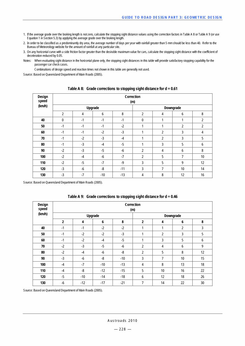
GUI DE TO RO A D DE SIG N P ART 3 : GEO MET RI C D ESI G N
A u s t r o a d s 2 0 1 0
— 2 2 8 —
1. If the average grade over the braking length is not zero, calculate the stopping sight distance values using the correction factors in Table A 8 or Table A 9 (or use Equation 1 in Section 5.3) by applying the average grade over the braking length.
2. In order to be classified as a predominantly dry area, the average number of days per year with rainfall greater than 5 mm should be less than 40. Refer to the Bureau of Meteorology website for the amount of rainfall at any particular site.
3. On any horizontal curve with a side friction factor greater than the desirable maximum value for cars, calculate the stopping sight distance with the coefficient of deceleration reduced by 0.05.
Notes: When evaluating sight distance in the horizontal plane only, the stopping sight distances in this table will provide satisfactory stopping capability for the passenger car check cases. Combinations of design speed and reaction times not shown in this table are generally not used.
Source: Based on Queensland Department of Main Roads (2005).
Table A 8: Grade corrections to stopping sight distance for d = 0.61
Design speed (km/h)
Correction (m)
Upgrade Downgrade 2 4 6 8 2 4 6 8
40 0 -1 -1 -1 0 1 1 2 50 -1 -1 -1 -2 1 1 2 2 60 -1 -1 -2 -3 1 2 3 4 70 -1 -2 -3 -4 1 2 3 5 80 -1 -3 -4 -5 1 3 5 6 90 -2 -3 -5 -6 2 4 6 8 100 -2 -4 -6 -7 2 5 7 10 110 -2 -5 -7 -9 3 5 9 12 120 -3 -6 -8 -11 3 7 10 14 130 -3 -7 -10 -13 4 8 12 16
Source: Based on Queensland Department of Main Roads (2005).
Table A 9: Grade corrections to stopping sight distance for d = 0.46
Design speed (km/h)
Correction (m)
Upgrade Downgrade 2 4 6 8 2 4 6 8
40 -1 -1 -2 -2 1 1 2 3 50 -1 -2 -2 -3 1 2 3 5 60 -1 -2 -4 -5 1 3 5 6 70 -2 -3 -5 -6 2 4 6 9 80 -2 -4 -6 -8 2 5 8 12 90 -3 -6 -8 -10 3 7 10 15
100 -4 -7 -10 -13 4 8 13 18 110 -4 -8 -12 -15 5 10 16 22 120 -5 -10 -14 -18 6 12 18 26 130 -6 -12 -17 -21 7 14 22 30
Source: Based on Queensland Department of Main Roads (2005).
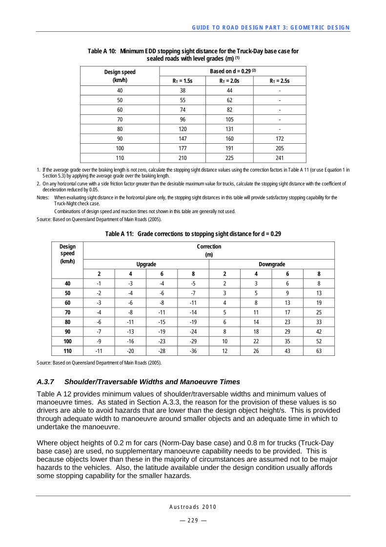
GUI DE TO RO A D DE SIG N P ART 3 : GEO MET RI C D ESI G N
A u s t r o a d s 2 0 1 0
— 2 2 9 —
Table A 10: Minimum EDD stopping sight distance for the Truck-Day base case for sealed roads with level grades (m) (1)
Design speed (km/h)
Based on d = 0.29 (2) RT = 1.5s RT = 2.0s RT = 2.5s
40 38 44 - 50 55 62 - 60 74 82 - 70 96 105 - 80 120 131 - 90 147 160 172 100 177 191 205 110 210 225 241
1. If the average grade over the braking length is not zero, calculate the stopping sight distance values using the correction factors in Table A 11 (or use Equation 1 in Section 5.3) by applying the average grade over the braking length.
2. On any horizontal curve with a side friction factor greater than the desirable maximum value for trucks, calculate the stopping sight distance with the coefficient of deceleration reduced by 0.05.
Notes: When evaluating sight distance in the horizontal plane only, the stopping sight distances in this table will provide satisfactory stopping capability for the Truck-Night check case. Combinations of design speed and reaction times not shown in this table are generally not used.
Source: Based on Queensland Department of Main Roads (2005).
Table A 11: Grade corrections to stopping sight distance for d = 0.29
Design speed (km/h)
Correction (m)
Upgrade Downgrade 2 4 6 8 2 4 6 8
40 -1 -3 -4 -5 2 3 6 8 50 -2 -4 -6 -7 3 5 9 13 60 -3 -6 -8 -11 4 8 13 19 70 -4 -8 -11 -14 5 11 17 25 80 -6 -11 -15 -19 6 14 23 33 90 -7 -13 -19 -24 8 18 29 42
100 -9 -16 -23 -29 10 22 35 52 110 -11 -20 -28 -36 12 26 43 63
Source: Based on Queensland Department of Main Roads (2005).
A.3.7 Shoulder/Traversable Widths and Manoeuvre Times Table A 12 provides minimum values of shoulder/traversable widths and minimum values of manoeuvre times. As stated in Section A.3.3, the reason for the provision of these values is so drivers are able to avoid hazards that are lower than the design object height/s. This is provided through adequate width to manoeuvre around smaller objects and an adequate time in which to undertake the manoeuvre.
Where object heights of 0.2 m for cars (Norm-Day base case) and 0.8 m for trucks (Truck-Day base case) are used, no supplementary manoeuvre capability needs to be provided. This is because objects lower than these in the majority of circumstances are assumed not to be major hazards to the vehicles. Also, the latitude available under the design condition usually affords some stopping capability for the smaller hazards.
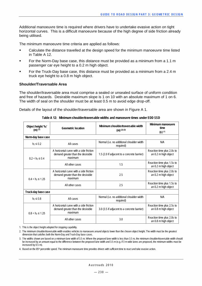
GUI DE TO RO A D DE SIG N P ART 3 : GEO MET RI C D ESI G N
A u s t r o a d s 2 0 1 0
— 2 3 0 —
Additional manoeuvre time is required where drivers have to undertake evasive action on tight horizontal curves. This is a difficult manoeuvre because of the high degree of side friction already being utilised.
The minimum manoeuvre time criteria are applied as follows:
Calculate the distance travelled at the design speed for the minimum manoeuvre time listed in Table A 12.
For the Norm-Day base case, this distance must be provided as a minimum from a 1.1 m passenger car eye height to a 0.2 m high object.
For the Truck-Day base case, this distance must be provided as a minimum from a 2.4 m truck eye height to a 0.8 m high object.
Shoulder/Traversable Area
The shoulder/traversable area must comprise a sealed or unsealed surface of uniform condition and free of hazards. Desirable maximum slope is 1 on 10 with an absolute maximum of 1 on 6. The width of seal on the shoulder must be at least 0.5 m to avoid edge drop-off.
Details of the layout of the shoulder/traversable area are shown in Figure A 1.
Table A 12: Minimum shoulder/traversable widths and manoeuvre times under EDD SSD
Object height ‘h2’ (m) (1) Geometric location Minimum shoulder/traversable width
(m) (2) (3)
Minimum manoeuvre time (s) (4)
Norm-day base case
h2 ≤ 0.2 All cases Normal (i.e. no additional shoulder width required)
N/A
0.2 < h2 ≤ 0.4
A horizontal curve with a side friction demand greater than the desirable
maximum 1.5 (2.0 if adjacent to a concrete barrier)
Reaction time plus 2.0s to an 0.2 m high object
All other cases 1.5 Reaction time plus 1.5s to an 0.2 m high object
0.4 < h2 ≤ 1.25
A horizontal curve with a side friction demand greater than the desirable
maximum 2.5
Reaction time plus 2.0s to an 0.2 m high object
All other cases 2.5 Reaction time plus 1.5s to an 0.2 m high object
Truck-day base case
h2 ≤ 0.8 All cases Normal (i.e. no additional shoulder width required)
N/A
0.8 < h2 ≤ 1.25
A horizontal curve with a side friction demand greater than the desirable
maximum 3.0 (3.5 if adjacent to a concrete barrier)
Reaction time plus 2.5s to an 0.8 m high object
All other cases 3.0 Reaction time plus 2.0s to an 0.8 m high object
1. This is the object height adopted for stopping capability. 2. The minimum shoulder/traversable width enables vehicles to manoeuvre around objects lower than the chosen object height. The width must be the greatest
dimension that satisfies both the Norm-Day and Truck-Day base cases. 3. The widths shown are based on a minimum lane width of 3.5 m. Where the proposed lane width is less than 3.5 m, the minimum shoulder/traversable width should
be increased by an amount equal to the difference between the proposed lane width and 3.5 m (e.g. if 3 m wide lanes are proposed, the minimum widths must be increased by 0.5 m).
4. Based on the 85th percentile speed. The minimum manoeuvre time provides drivers with sufficient time to react and take evasive action.
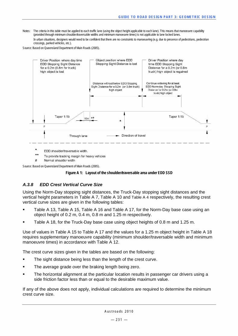
GUI DE TO RO A D DE SIG N P ART 3 : GEO MET RI C D ESI G N
A u s t r o a d s 2 0 1 0
— 2 3 1 —
Notes: The criteria in this table must be applied to each traffic lane (using the object height applicable to each lane). This means that manoeuvre capability (provided through minimum shoulder/traversable widths and minimum manoeuvre times) is not applicable to lane locked lanes.
In urban situations, designers would need to be confident that there are no constraints to manoeuvring (e.g. due to presence of pedestrians, pedestrian crossings, parked vehicles, etc.).
Source: Based on Queensland Department of Main Roads (2005).
Source: Based on Queensland Department of Main Roads (2005).
Figure A 1: Layout of the shoulder/traversable area under EDD SSD
A.3.8 EDD Crest Vertical Curve Size Using the Norm-Day stopping sight distances, the Truck-Day stopping sight distances and the vertical height parameters in Table A 7, Table A 10 and Table A 4 respectively, the resulting crest vertical curve sizes are given in the following tables:
Table A 13, Table A 15, Table A 16 and Table A 17, for the Norm-Day base case using an object height of 0.2 m, 0.4 m, 0.8 m and 1.25 m respectively.
Table A 18, for the Truck-Day base case using object heights of 0.8 m and 1.25 m.
Use of values in Table A 15 to Table A 17 and the values for a 1.25 m object height in Table A 18 requires supplementary manoeuvre capability (minimum shoulder/traversable width and minimum manoeuvre times) in accordance with Table A 12.
The crest curve sizes given in the tables are based on the following:
The sight distance being less than the length of the crest curve.
The average grade over the braking length being zero.
The horizontal alignment at the particular location results in passenger car drivers using a side friction factor less than or equal to the desirable maximum value.
If any of the above does not apply, individual calculations are required to determine the minimum crest curve size.

GUI DE TO RO A D DE SIG N P ART 3 : GEO MET RI C D ESI G N
A u s t r o a d s 2 0 1 0
— 2 3 2 —
Table A 13 to Table A 18 list whether check case capability has been provided in accordance with Section A.3.6, subsection ‘Application of the Check Cases’. Particular combinations of speeds and reaction times in the tables will produce greater check case capability than that shown. If unsure whether sufficient capability is provided for a particular check case, individual calculations should be performed.
Crest curves smaller than the EDD lower bound are Design Exceptions and must be treated accordingly. Crests larger than the EDD lower bound (those within EDD or NDD) will obviously provide better capability.
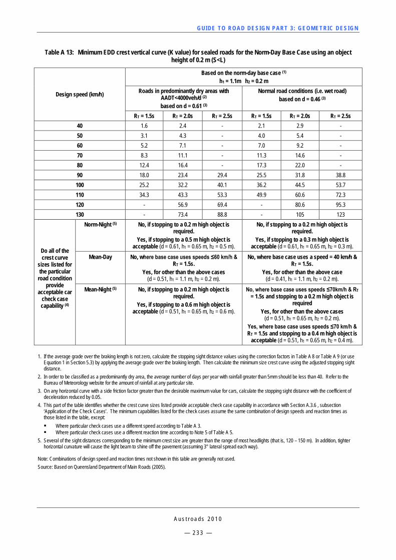
GUI DE TO RO A D DE SIG N P ART 3 : GEO MET RI C D ESI G N
A u s t r o a d s 2 0 1 0
— 2 3 3 —
Table A 13: Minimum EDD crest vertical curve (K value) for sealed roads for the Norm-Day Base Case using an object height of 0.2 m (S<L)
Design speed (km/h)
Based on the norm-day base case (1) h1 = 1.1m h2 = 0.2 m
Roads in predominantly dry areas with AADT<4000veh/d (2) based on d = 0.61 (3)
Normal road conditions (i.e. wet road) based on d = 0.46 (3)
RT = 1.5s RT = 2.0s RT = 2.5s RT = 1.5s RT = 2.0s RT = 2.5s 40 1.6 2.4 - 2.1 2.9 - 50 3.1 4.3 - 4.0 5.4 - 60 5.2 7.1 - 7.0 9.2 - 70 8.3 11.1 - 11.3 14.6 - 80 12.4 16.4 - 17.3 22.0 - 90 18.0 23.4 29.4 25.5 31.8 38.8 100 25.2 32.2 40.1 36.2 44.5 53.7 110 34.3 43.3 53.3 49.9 60.6 72.3 120 - 56.9 69.4 - 80.6 95.3 130 - 73.4 88.8 - 105 123
Do all of the crest curve
sizes listed for the particular
road condition provide
acceptable car check case capability (4)
Norm-Night (5) No, if stopping to a 0.2 m high object is required.
Yes, if stopping to a 0.5 m high object is acceptable (d = 0.61, h1 = 0.65 m, h2 = 0.5 m).
No, if stopping to a 0.2 m high object is required.
Yes, if stopping to a 0.3 m high object is acceptable (d = 0.61, h1 = 0.65 m, h2 = 0.3 m).
Mean-Day No, where base case uses speeds ≤60 km/h & RT = 1.5s.
Yes, for other than the above cases (d = 0.51, h1 = 1.1 m, h2 = 0.2 m).
No, where base case uses a speed = 40 km/h & RT = 1.5s.
Yes, for other than the above case (d = 0.41, h1 = 1.1 m, h2 = 0.2 m).
Mean-Night (5) No, if stopping to a 0.2 m high object is required.
Yes, if stopping to a 0.6 m high object is acceptable (d = 0.51, h1 = 0.65 m, h2 = 0.6 m).
No, where base case uses speeds ≤70km/h & RT = 1.5s and stopping to a 0.2 m high object is
required Yes, for other than the above cases
(d = 0.51, h1 = 0.65 m, h2 = 0.2 m). Yes, where base case uses speeds ≤70 km/h & RT = 1.5s and stopping to a 0.4 m high object is
acceptable (d = 0.51, h1 = 0.65 m, h2 = 0.4 m). 1. If the average grade over the braking length is not zero, calculate the stopping sight distance values using the correction factors in Table A 8 or Table A 9 (or use
Equation 1 in Section 5.3) by applying the average grade over the braking length. Then calculate the minimum size crest curve using the adjusted stopping sight distance.
2. In order to be classified as a predominantly dry area, the average number of days per year with rainfall greater than 5mm should be less than 40. Refer to the Bureau of Meteorology website for the amount of rainfall at any particular site.
3. On any horizontal curve with a side friction factor greater than the desirable maximum value for cars, calculate the stopping sight distance with the coefficient of deceleration reduced by 0.05.
4. This part of the table identifies whether the crest curve sizes listed provide acceptable check case capability in accordance with Section A.3.6 , subsection ‘Application of the Check Cases’. The minimum capabilities listed for the check cases assume the same combination of design speeds and reaction times as those listed in the table, except: Where particular check cases use a different speed according to Table A 3. Where particular check cases use a different reaction time according to Note 5 of Table A 5.
5. Several of the sight distances corresponding to the minimum crest size are greater than the range of most headlights (that is, 120 – 150 m). In addition, tighter horizontal curvature will cause the light beam to shine off the pavement (assuming 3° lateral spread each way).
Note: Combinations of design speed and reaction times not shown in this table are generally not used. Source: Based on Queensland Department of Main Roads (2005).
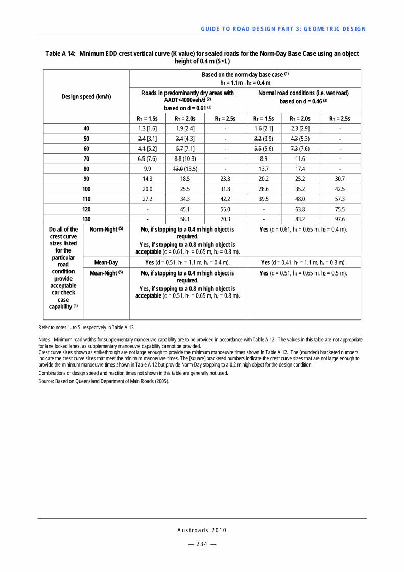
GUI DE TO RO A D DE SIG N P ART 3 : GEO MET RI C D ESI G N
A u s t r o a d s 2 0 1 0
— 2 3 4 —
Table A 14: Minimum EDD crest vertical curve (K value) for sealed roads for the Norm-Day Base Case using an object height of 0.4 m (S<L)
Design speed (km/h)
Based on the norm-day base case (1) h1 = 1.1m h2 = 0.4 m
Roads in predominantly dry areas with AADT<4000veh/d (2) based on d = 0.61 (3)
Normal road conditions (i.e. wet road) based on d = 0.46 (3)
RT = 1.5s RT = 2.0s RT = 2.5s RT = 1.5s RT = 2.0s RT = 2.5s 40 1.3 [1.6] 1.9 [2.4] - 1.6 [2.1] 2.3 [2.9] - 50 2.4 [3.1] 3.4 [4.3] - 3.2 (3.9) 4.3 (5.3) - 60 4.1 [5.2] 5.7 [7.1] - 5.5 (5.6) 7.3 (7.6) - 70 6.5 (7.6) 8.8 (10.3) - 8.9 11.6 - 80 9.9 13.0 (13.5) - 13.7 17.4 - 90 14.3 18.5 23.3 20.2 25.2 30.7
100 20.0 25.5 31.8 28.6 35.2 42.5 110 27.2 34.3 42.2 39.5 48.0 57.3 120 - 45.1 55.0 - 63.8 75.5 130 - 58.1 70.3 - 83.2 97.6
Do all of the crest curve sizes listed
for the particular
road condition provide
acceptable car check
case capability (4)
Norm-Night (5) No, if stopping to a 0.4 m high object is required.
Yes, if stopping to a 0.8 m high object is acceptable (d = 0.61, h1 = 0.65 m, h2 = 0.8 m).
Yes (d = 0.61, h1 = 0.65 m, h2 = 0.4 m).
Mean-Day Yes (d = 0.51, h1 = 1.1 m, h2 = 0.4 m). Yes (d = 0.41, h1 = 1.1 m, h2 = 0.3 m).
Mean-Night (5) No, if stopping to a 0.4 m high object is required.
Yes, if stopping to a 0.8 m high object is acceptable (d = 0.51, h1 = 0.65 m, h2 = 0.8 m).
Yes (d = 0.51, h1 = 0.65 m, h2 = 0.5 m).
Refer to notes 1. to 5. respectively in Table A 13. Notes: Minimum road widths for supplementary manoeuvre capability are to be provided in accordance with Table A 12. The values in this table are not appropriate for lane locked lanes, as supplementary manoeuvre capability cannot be provided. Crest curve sizes shown as strikethrough are not large enough to provide the minimum manoeuvre times shown in Table A 12. The (rounded) bracketed numbers indicate the crest curve sizes that meet the minimum manoeuvre times. The [square] bracketed numbers indicate the crest curve sizes that are not large enough to provide the minimum manoeuvre times shown in Table A 12 but provide Norm-Day stopping to a 0.2 m high object for the design condition. Combinations of design speed and reaction times not shown in this table are generally not used. Source: Based on Queensland Department of Main Roads (2005).
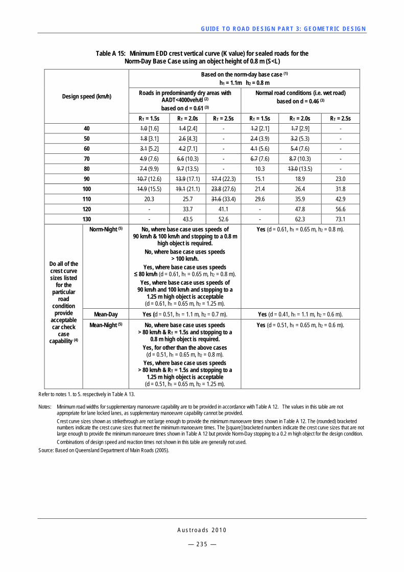
GUI DE TO RO A D DE SIG N P ART 3 : GEO MET RI C D ESI G N
A u s t r o a d s 2 0 1 0
— 2 3 5 —
Table A 15: Minimum EDD crest vertical curve (K value) for sealed roads for the Norm-Day Base Case using an object height of 0.8 m (S<L)
Design speed (km/h)
Based on the norm-day base case (1) h1 = 1.1m h2 = 0.8 m
Roads in predominantly dry areas with AADT<4000veh/d (2) based on d = 0.61 (3)
Normal road conditions (i.e. wet road) based on d = 0.46 (3)
RT = 1.5s RT = 2.0s RT = 2.5s RT = 1.5s RT = 2.0s RT = 2.5s 40 1.0 [1.6] 1.4 [2.4] - 1.2 [2.1] 1.7 [2.9] - 50 1.8 [3.1] 2.6 [4.3] - 2.4 (3.9) 3.2 (5.3) - 60 3.1 [5.2] 4.2 [7.1] - 4.1 (5.6) 5.4 (7.6) - 70 4.9 (7.6) 6.6 (10.3) - 6.7 (7.6) 8.7 (10.3) - 80 7.4 (9.9) 9.7 (13.5) - 10.3 13.0 (13.5) - 90 10.7 (12.6) 13.9 (17.1) 17.4 (22.3) 15.1 18.9 23.0
100 14.9 (15.5) 19.1 (21.1) 23.8 (27.6) 21.4 26.4 31.8 110 20.3 25.7 31.6 (33.4) 29.6 35.9 42.9 120 - 33.7 41.1 - 47.8 56.6 130 - 43.5 52.6 - 62.3 73.1
Do all of the crest curve sizes listed
for the particular
road condition provide
acceptable car check
case capability (4)
Norm-Night (5) No, where base case uses speeds of 90 km/h & 100 km/h and stopping to a 0.8 m
high object is required. No, where base case uses speeds
> 100 km/h. Yes, where base case uses speeds
≤ 80 km/h (d = 0.61, h1 = 0.65 m, h2 = 0.8 m). Yes, where base case uses speeds of
90 km/h and 100 km/h and stopping to a 1.25 m high object is acceptable
(d = 0.61, h1 = 0.65 m, h2 = 1.25 m).
Yes (d = 0.61, h1 = 0.65 m, h2 = 0.8 m).
Mean-Day Yes (d = 0.51, h1 = 1.1 m, h2 = 0.7 m). Yes (d = 0.41, h1 = 1.1 m, h2 = 0.6 m).
Mean-Night (5) No, where base case uses speeds > 80 km/h & RT = 1.5s and stopping to a
0.8 m high object is required. Yes, for other than the above cases
(d = 0.51, h1 = 0.65 m, h2 = 0.8 m). Yes, where base case uses speeds
> 80 km/h & RT = 1.5s and stopping to a 1.25 m high object is acceptable
(d = 0.51, h1 = 0.65 m, h2 = 1.25 m).
Yes (d = 0.51, h1 = 0.65 m, h2 = 0.6 m).
Refer to notes 1. to 5. respectively in Table A 13. Notes: Minimum road widths for supplementary manoeuvre capability are to be provided in accordance with Table A 12. The values in this table are not
appropriate for lane locked lanes, as supplementary manoeuvre capability cannot be provided. Crest curve sizes shown as strikethrough are not large enough to provide the minimum manoeuvre times shown in Table A 12. The (rounded) bracketed
numbers indicate the crest curve sizes that meet the minimum manoeuvre times. The [square] bracketed numbers indicate the crest curve sizes that are not large enough to provide the minimum manoeuvre times shown in Table A 12 but provide Norm-Day stopping to a 0.2 m high object for the design condition.
Combinations of design speed and reaction times not shown in this table are generally not used. Source: Based on Queensland Department of Main Roads (2005).
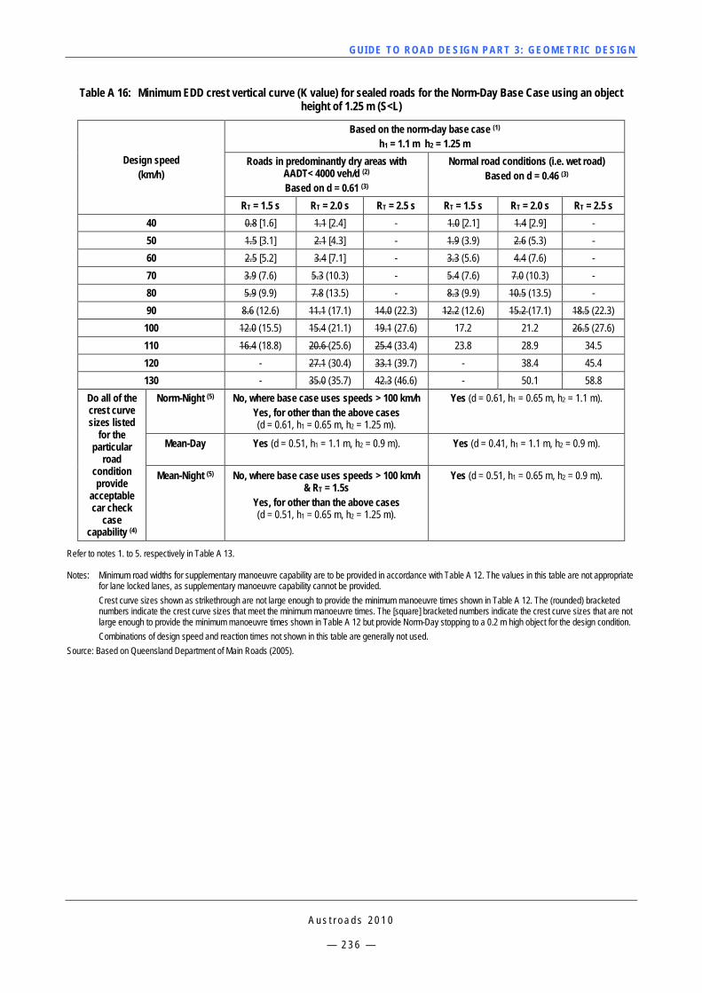
GUI DE TO RO A D DE SIG N P ART 3 : GEO MET RI C D ESI G N
A u s t r o a d s 2 0 1 0
— 2 3 6 —
Table A 16: Minimum EDD crest vertical curve (K value) for sealed roads for the Norm-Day Base Case using an object height of 1.25 m (S<L)
Design speed (km/h)
Based on the norm-day base case (1) h1 = 1.1 m h2 = 1.25 m
Roads in predominantly dry areas with AADT< 4000 veh/d (2) Based on d = 0.61 (3)
Normal road conditions (i.e. wet road) Based on d = 0.46 (3)
RT = 1.5 s RT = 2.0 s RT = 2.5 s RT = 1.5 s RT = 2.0 s RT = 2.5 s 40 0.8 [1.6] 1.1 [2.4] - 1.0 [2.1] 1.4 [2.9] - 50 1.5 [3.1] 2.1 [4.3] - 1.9 (3.9) 2.6 (5.3) - 60 2.5 [5.2] 3.4 [7.1] - 3.3 (5.6) 4.4 (7.6) - 70 3.9 (7.6) 5.3 (10.3) - 5.4 (7.6) 7.0 (10.3) - 80 5.9 (9.9) 7.8 (13.5) - 8.3 (9.9) 10.5 (13.5) - 90 8.6 (12.6) 11.1 (17.1) 14.0 (22.3) 12.2 (12.6) 15.2 (17.1) 18.5 (22.3)
100 12.0 (15.5) 15.4 (21.1) 19.1 (27.6) 17.2 21.2 26.5 (27.6) 110 16.4 (18.8) 20.6 (25.6) 25.4 (33.4) 23.8 28.9 34.5 120 - 27.1 (30.4) 33.1 (39.7) - 38.4 45.4 130 - 35.0 (35.7) 42.3 (46.6) - 50.1 58.8
Do all of the crest curve sizes listed
for the particular
road condition provide
acceptable car check
case capability (4)
Norm-Night (5) No, where base case uses speeds > 100 km/h Yes, for other than the above cases (d = 0.61, h1 = 0.65 m, h2 = 1.25 m).
Yes (d = 0.61, h1 = 0.65 m, h2 = 1.1 m).
Mean-Day Yes (d = 0.51, h1 = 1.1 m, h2 = 0.9 m). Yes (d = 0.41, h1 = 1.1 m, h2 = 0.9 m).
Mean-Night (5) No, where base case uses speeds > 100 km/h & RT = 1.5s
Yes, for other than the above cases (d = 0.51, h1 = 0.65 m, h2 = 1.25 m).
Yes (d = 0.51, h1 = 0.65 m, h2 = 0.9 m).
Refer to notes 1. to 5. respectively in Table A 13. Notes: Minimum road widths for supplementary manoeuvre capability are to be provided in accordance with Table A 12. The values in this table are not appropriate
for lane locked lanes, as supplementary manoeuvre capability cannot be provided. Crest curve sizes shown as strikethrough are not large enough to provide the minimum manoeuvre times shown in Table A 12. The (rounded) bracketed
numbers indicate the crest curve sizes that meet the minimum manoeuvre times. The [square] bracketed numbers indicate the crest curve sizes that are not large enough to provide the minimum manoeuvre times shown in Table A 12 but provide Norm-Day stopping to a 0.2 m high object for the design condition.
Combinations of design speed and reaction times not shown in this table are generally not used. Source: Based on Queensland Department of Main Roads (2005).
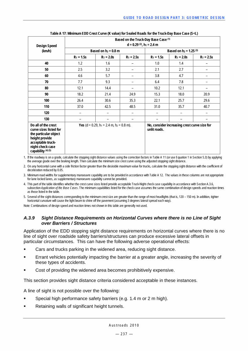
GUI DE TO RO A D DE SIG N P ART 3 : GEO MET RI C D ESI G N
A u s t r o a d s 2 0 1 0
— 2 3 7 —
Table A 17: Minimum EDD Crest Curve (K value) for Sealed Roads for the Truck-Day Base Case (S<L)
Design Speed (km/h)
Based on the Truck-Day Base Case (1) d = 0.29 (2), h1 = 2.4 m
Based on h2 = 0.8 m Based on h2 = 1.25 (3) RT = 1.5s RT = 2.0s RT = 2.5s RT = 1.5s RT = 2.0s RT = 2.5s
40 1.2 1.6 – 1.0 1.4 – 50 2.5 3.2 – 2.1 2.7 – 60 4.6 5.7 – 3.8 4.7 – 70 7.7 9.3 – 6.4 7.8 – 80 12.1 14.4 – 10.2 12.1 – 90 18.2 21.4 24.9 15.3 18.0 20.9 100 26.4 30.6 35.3 22.1 25.7 29.6 110 37.0 42.5 48.5 31.0 35.7 40.7 120 – – – – – – 130 – – – – – –
Do all of the crest curve sizes listed for the particular object height provide acceptable truck-night check case capability (4) (5)
Yes (d = 0.29, h1 = 2.4 m, h2 = 0.8 m). No, consider increasing crest curve size for unlit roads.
1. If the roadway is on a grade, calculate the stopping sight distance values using the correction factors in Table A 11 (or use Equation 1 in Section 5.3) by applying the average grade over the braking length. Then calculate the minimum size crest curve using the adjusted stopping sight distance.
2. On any horizontal curve with a side friction factor greater than the desirable maximum value for trucks, calculate the stopping sight distance with the coefficient of deceleration reduced by 0.05.
3. Minimum road widths for supplementary manoeuvre capability are to be provided in accordance with Table A 12. The values in these columns are not appropriate for lane locked lanes, as supplementary manoeuvre capability cannot be provided.
4. This part of the table identifies whether the crest curve sizes listed provide acceptable Truck-Night check case capability in accordance with Section A.3.6, subsection Application of the Base Cases. The minimum capabilities listed for the check case assumes the same combination of design speeds and reaction times as those listed in the table.
5. Several of the sight distances corresponding to the minimum crest size are greater than the range of most headlights (that is, 120 – 150 m). In addition, tighter horizontal curvature will cause the light beam to shine off the pavement (assuming 3 degrees lateral spread each way).
Note: Combinations of design speed and reaction times not shown in this table are generally not used.
A.3.9 Sight Distance Requirements on Horizontal Curves where there is no Line of Sight over Barriers / Structures
Application of the EDD stopping sight distance requirements on horizontal curves where there is no line of sight over roadside safety barriers/structures can produce excessive lateral offsets in particular circumstances. This can have the following adverse operational effects:
Cars and trucks parking in the widened area, reducing sight distance.
Errant vehicles potentially impacting the barrier at a greater angle, increasing the severity of these types of accidents.
Cost of providing the widened area becomes prohibitively expensive.
This section provides sight distance criteria considered acceptable in these instances.
A line of sight is not possible over the following:
Special high performance safety barriers (e.g. 1.4 m or 2 m high).
Retaining walls of significant height tunnels.
GUI DE TO RO A D DE SIG N P ART 3 : GEO MET RI C D ESI G N
A u s t r o a d s 2 0 1 0
— 2 3 8 —
Bridge structures e.g. underpasses, abutments and piers.
Roadside safety barriers in combination with a significant crest vertical curve.
In these cases, there is often limited ability to widen the shoulder due to cost and/or practical constraints e.g. the geometry comprises a motorway ramp on structure; or the geometry is in steep sidelong country where additional width requires extremely high/long fills to be constructed. This can make it very difficult to provide any stopping sight distance capability for trucks. Where this occurs, it is preferable to redesign the horizontal and vertical alignments to achieve the sight distance criteria in Section A.3.7. If this is not possible, and all other design options have been investigated, the following capabilities should be provided as a minimum:
Car stopping sight distance on a dry road (d = 0.61) supplemented by the required minimum shoulder width and minimum manoeuvre time according to Table A 12 and Section A.3.7. Note that for any horizontal curve with a side friction factor greater than the desirable maximum value, the coefficient of deceleration should be reduced by 0.05.
Truck manoeuvre only capability – provide a minimum shoulder width of 3.5m and a minimum manoeuvre time to a 0.8m high object equal to the reaction time plus 3 seconds. Apply this criterion according to Section A.3.7.
A.4 EDD for Horizontal Curves with Adverse Superelevation This section contains guidance on application of EDD to horizontal curves with adverse superelevation.
Under Normal Design Domain, the practice of limiting the side friction demand on adverse horizontal curves to half the relevant absolute maximum of side friction factor (given in Table 7.10) is considered to be ‘good working practice’ rather than a reflection of what side friction drivers use in practice. Limiting the side friction demand on a curve in this way means that it is less likely the curve will be overdriven.
When negotiating a curve, drivers can, and often do, use a side friction factor up to the design maximum for their speed of travel irrespective of the superelevation. EDD on horizontal curves with adverse superelevation is based on this practice. It uses the maximum side friction factors in accordance with the Normal Design Domain values (refer Table 7.4) on horizontal curves with adverse superelevation, subject to the following:
It is only applicable to a restoration or widening project on an existing road in an urban area.
It is only applicable to geometric elements where the operating speed (85th percentile speed) is less than or equal to 80 km/h. Note that this would preclude it from being used on most roads with a speed limit of 80 km/h or higher.
Side friction demand on the geometric element concerned does not exceed the absolute maximum value of side friction for cars (refer to Section 7.6) at the operating speed of cars (refer to Section 3).
Its use must support truck operating speeds. That is, the side friction demand on the geometric element concerned is not excessive for trucks (refer to Section 7) at the operating speed of trucks (refer to Section 3). Note also that the static roll threshold for trucks is 0.35 and that this is numerically equivalent to the co-efficient of side friction. This means the side friction demand must not exceed 0.35 for trucks when tested at, say, the truck operating speed plus 10 km/h, and preferably should not exceed the absolute maximum side friction value for trucks given in Section 7.
The road surface must be capable of providing a high degree of skid resistance.

GUI DE TO RO A D DE SIG N P ART 3 : GEO MET RI C D ESI G N
A u s t r o a d s 2 0 1 0
— 2 3 9 —
The adverse superelevation must not exceed 3% and preferably not exceed 2.5%.
Its use must be supported by crash data at the site and possibly other similar sites. This review would have to show an absence of crashes related to the presence of adverse superelevation, particularly single vehicle crashes.
It should not be used in conjunction with other minima (e.g. with a vertical curve that provides for EDD stopping sight distance) or undesirable geometric features (e.g. compound curves).
It should be noted the presence or use of adverse superelevation can be problematic for some road users (e.g. motorcyclists).and those who are unfamiliar with the road.
GUI DE TO RO A D DE SIG N P ART 3 : GEO MET RI C D ESI G N
A u s t r o a d s 2 0 1 0
— 2 4 0 —
APPENDIX B SPEED PARAMETER TERMINOLOGY For further definitions of terms reference should be made to the Austroads Glossary of Austroads Terms, Austroads (2008a).
B.1 Design Speed Value The Operating Speed is the value adopted for the design of each element of the road.
On roads designed for high-speed travel, speeds remain relatively constant permitting the use of a single design value for the road. Designers should note that although operating speeds are relatively constant, they can differ significantly from the design value.
On roads with operating speeds less than 100 km/h, operating speeds vary along the length of the road depending on the road geometry and, to some extent on other factors such as speed limits and the level of speed enforcement. For the design of rural roads, most weight is given to the effects of the geometry of the road as speed limits and the level of enforcement can change. On these roads, operating speed needs to be determined for each element of the road.
For design purposes on two-way carriageways, operating speeds are either measured or estimated for each element of the road and for each direction of travel. In many cases the higher of the two values will be adopted as the design value of the curve. There will be some circumstances where each direction has to be considered separately, such as on the approaches to intersections. At intersections, the stopping distance on each approach should be based on the operating speed for that approach. Operating speeds can be affected by the frequency of intersections.
B.2 Desired Speed The term ‘Desired Speed’ in this Guide refers to the operating speed that drivers will adopt on the less constrained alignment elements, i.e. longer straights and large radius horizontal curves of a reasonably uniform section of road when not constrained by other vehicles. In other words, it is the operating speed that drivers build up to and are then happy to settle at.
The concept of desired speed is fundamental to understanding the operating characteristics of any road since the desired speed is influenced by:
roadside environment – topography in rural areas, development density and type (i.e. built environments) in urban areas
road characteristics – geometric standard (predominantly horizontal alignment; to a lesser extent, vertical alignment and lane widths), frequency of intersections and accesses, sight distance, parking provisions etc.
speed limit
road function – to the extent that on important roads such as freeways and highways, drivers are less willing to accept reductions in desired speed.
Desired speed does not vary over a section of roadway that has a similar roadside environment, road characteristics and speed limit even if the section still has isolated geometric features inconsistent with the desired speed. Isolated geometric features can include the following:
a ‘tight’ horizontal curve (or a short section of road containing a few ‘tight’ curves)
an intersection controlled by a stop or give-way sign or roundabout
an overtaking lane / climbing lane.
GUI DE TO RO A D DE SIG N P ART 3 : GEO MET RI C D ESI G N
A u s t r o a d s 2 0 1 0
— 2 4 1 —
In the case of an overtaking lane, it is possible that the operating speed of the overtaking lane will exceed the desired speed for the section of road.
If the roadside environment, road characteristics and speed limit of the roadway are similar before and after the isolated feature, the desired speed will remain the same. The desired speed will only change if the roadside environment or road characteristics change over a significant length of roadway.
Typically, reduction in desired speed takes longer to come into effect than increases in desired speed. Therefore, on two-way roads, there may be locations where the desired speed is different for each direction of travel.
The concept of desired speed is closely related to the concept of speed environment that was used in earlier design guides and is still used in associated references. This relationship is explained in Commentary 1 since the term is likely to remain in general usage for some time.
B.3 Limiting Curve Speed The limiting curve speed is the speed at which a vehicle travelling on a curve of given radius and superelevation, will have a side friction demand equal to the absolute maximum recommended value given in Table 7.5 for that speed. The operating speed on a particular horizontal curve should not exceed the limiting curve speed for that curve. It may not be possible to apply this criterion, for horizontal curves on the minor roads at intersections, intersection turns and on roundabouts. On some interchange off-ramps and connecting ramps, it will be common for some curves to be driven at close to the limiting curve speed. This is due to general driver behaviour, expectations and familiarity with these facilities.
B.4 Operating Speed of Trucks The term ‘Operating Speed of Trucks’ is the 85th percentile speed of trucks at a time when traffic volumes are low. In many places, the operating speeds of cars and trucks will be different due to their performance characteristics, especially on grades.
B.5 Section Operating Speed Vehicle speeds on a series of curves and short straights tend to stabilise at a value related to the range of curve radii. This speed is called the ‘Section operating speed’.
B.6 Speed Environment The operating speed that drivers will adopt on the less constrained elements, i.e. straights and large radius horizontal curves of a more or less uniform section of road when not constrained by other vehicles. It is numerically equal to the 85th percentile desired driver speed.
GUI DE TO RO A D DE SIG N P ART 3 : GEO MET RI C D ESI G N
A u s t r o a d s 2 0 1 0
— 2 4 2 —
APPENDIX C EXAMPLE CALCULATION OF THE OPERATING SPEED MODEL
C.1 Using the Operating Speed Model The best way to explain the use of the Operating Speed Model is by working through a simple example. Figure C 1, Figure C 2 and Figure C 3 help explain some basic concepts when using the model as well as giving details of the road to be analysed. Figure C 4, Figure C 6 and Figure C 6 show specific cases of using the Car Deceleration on Curves graph (Figure 3.5). This example involves a 1.4 km length of tight alignment that is being realigned. Figure C 7 shows the predicted operating speeds along the road.
C.1.1 Details of Example For the road section under consideration:
It is in flat to undulating terrain.
The link strategy has set a target speed of 110 km/hr for the link, but recognises that a lower operating speed will be likely over this section because of local topographic constraints.
It has horizontal curve radii ranging between 165 m and 320 m.
It has a posted speed limit of 100 km/h.
The pavement conditions are constant.
The type cross section is the same for the entire length.
C.1.2 Determination of Desired Speed Given a combination of flat to undulating terrain and horizontal curve radii ranging between 165 m and 320 m, Table 3.2 indicates a desired speed of 110 km/h. This is reinforced by note 3 in the table, which indicates a desired speed of 110 km/h for the 100 km/h speed limit in this example.
C.1.3 Length of Road to be Analysed As a first step, it is necessary to include segments that are approximately 1 to 1.5 km at each end of the length of road for which speed estimates are required. This helps ensure more accurate approach speeds for the alignment that is being assessed. It also helps ensure that there are no problems created downstream due to increases in operating speed. If the adjoining 1 to 1.5 km lengths are likely to be upgraded in the future, the analysis of speeds should also cover the short term and long term scenarios.
If, for example, speed estimates were required for the curves between C and I in Figure C 1, the speed study would extend from A to L, with speeds being assessed in each direction of travel on a two-way road.
The extensions are necessary because the first speed estimate at the start of the extensions, at points A and L, are not likely to be particularly accurate without measured speed data. Accuracy then increases with distance depending on the alignment. The choice of 1.5 km is considered conservative.
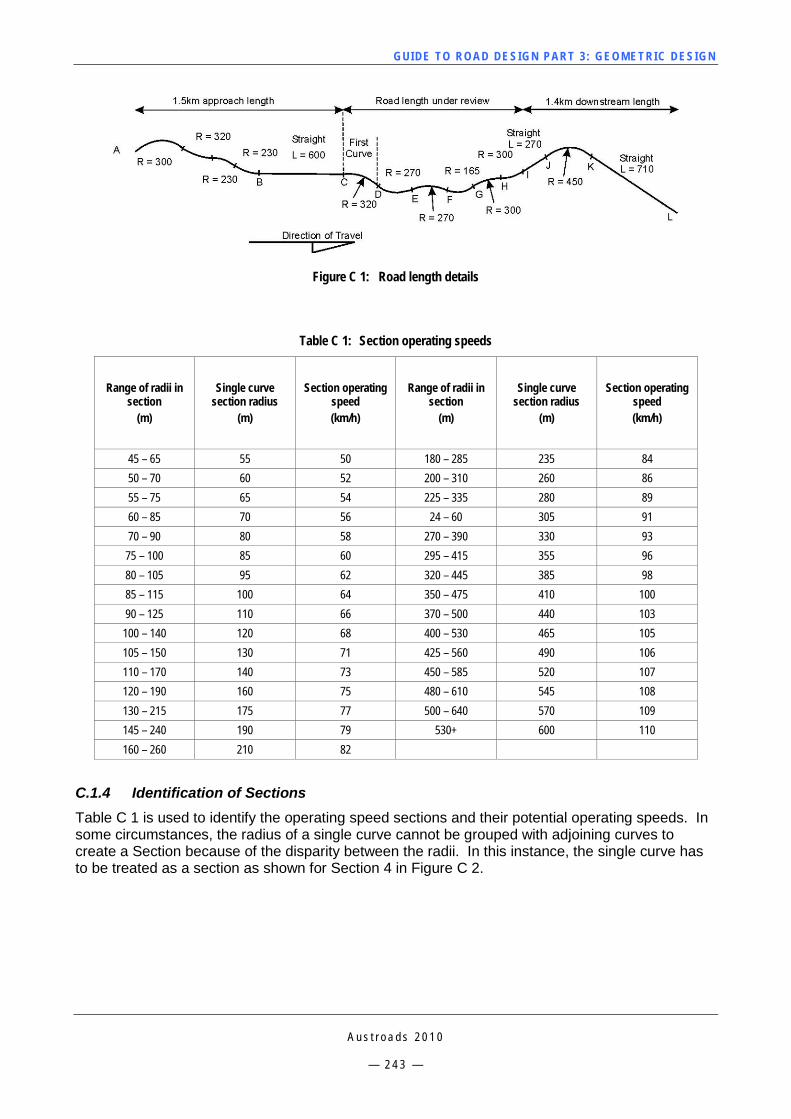
GUI DE TO RO A D DE SIG N P ART 3 : GEO MET RI C D ESI G N
A u s t r o a d s 2 0 1 0
— 2 4 3 —
Figure C 1: Road length details
Table C 1: Section operating speeds
Range of radii in section
(m)
Single curve section radius
(m)
Section operating speed (km/h)
Range of radii in section
(m)
Single curve section radius
(m)
Section operating speed (km/h)
45 – 65 55 50 180 – 285 235 84 50 – 70 60 52 200 – 310 260 86 55 – 75 65 54 225 – 335 280 89 60 – 85 70 56 24 – 60 305 91 70 – 90 80 58 270 – 390 330 93 75 – 100 85 60 295 – 415 355 96 80 – 105 95 62 320 – 445 385 98 85 – 115 100 64 350 – 475 410 100 90 – 125 110 66 370 – 500 440 103 100 – 140 120 68 400 – 530 465 105 105 – 150 130 71 425 – 560 490 106 110 – 170 140 73 450 – 585 520 107 120 – 190 160 75 480 – 610 545 108 130 – 215 175 77 500 – 640 570 109 145 – 240 190 79 530+ 600 110 160 – 260 210 82
C.1.4 Identification of Sections Table C 1 is used to identify the operating speed sections and their potential operating speeds. In some circumstances, the radius of a single curve cannot be grouped with adjoining curves to create a Section because of the disparity between the radii. In this instance, the single curve has to be treated as a section as shown for Section 4 in Figure C 2.
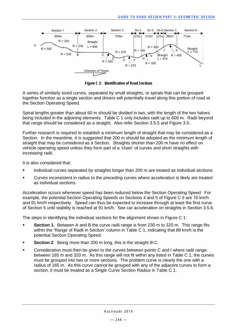
GUI DE TO RO A D DE SIG N P ART 3 : GEO MET RI C D ESI G N
A u s t r o a d s 2 0 1 0
— 2 4 4 —
Figure C 2: Identification of Road Sections
A series of similarly sized curves, separated by small straights, or spirals that can be grouped together function as a single section and drivers will potentially travel along this portion of road at the Section Operating Speed.
Spiral lengths greater than about 60 m should be divided in two, with the length of the two halves being included in the adjoining elements. Table C 1 only includes radii up to 600 m. Radii beyond that range should be considered as a straight. Also refer Section 3.5.5 and Figure 3.5.
Further research is required to establish a minimum length of straight that may be considered as a Section. In the meantime, it is suggested that 200 m should be adopted as the minimum length of straight that may be considered as a Section. Straights shorter than 200 m have no effect on vehicle operating speed unless they form part of a ‘chain’ of curves and short straights with increasing radii.
It is also considered that:
Individual curves separated by straights longer than 200 m are treated as individual sections.
Curves inconsistent in radius to the preceding curves where acceleration is likely are treated as individual sections.
Acceleration occurs whenever speed has been reduced below the Section Operating Speed. For example, the potential Section Operating Speeds on Sections 4 and 5 of Figure C 3 are 76 km/h and 91 km/h respectively. Speed can thus be expected to increase through at least the first curve of Section 5 until stability is reached at 91 km/h. See car acceleration on straights in Section 3.5.6.
The steps in identifying the individual sections for the alignment shown in Figure C 1:
Section 1. Between A and B the curve radii range is from 230 m to 320 m. This range fits within the ‘Range of Radii in Section’ column in Table C 1, indicating that 89 km/h is the potential Section Operating Speed.
Section 2. Being more than 200 m long, this is the straight B-C.
Consideration must then be given to the curves between points C and I where radii range between 165 m and 320 m. As this range will not fit within any listed in Table C 1, the curves must be grouped into two or more sections. The problem curve is clearly the one with a radius of 165 m. As this curve cannot be grouped with any of the adjacent curves to form a section, it must be treated as a Single Curve Section Radius in Table C 1.
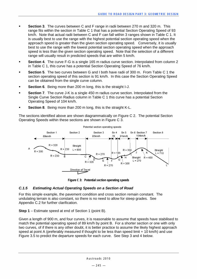
GUI DE TO RO A D DE SIG N P ART 3 : GEO MET RI C D ESI G N
A u s t r o a d s 2 0 1 0
— 2 4 5 —
Section 3. The curves between C and F range in radii between 270 m and 320 m. This range fits within the section in Table C 1 that has a potential Section Operating Speed of 93 km/h. Note that actual radii between C and F can fall within 3 ranges shown in Table C 1. It is usually best to use the range with the highest potential section operating speed when the approach speed is greater than the given section operating speed. Conversely, it is usually best to use the range with the lowest potential section operating speed when the approach speed is less than the given section operating speed. Note that the selection of a different range will usually result in predicted speeds that are within 5 km/h.
Section 4. The curve F-G is a single 165 m radius curve section. Interpolated from column 2 in Table C 1, this curve has a potential Section Operating Speed of 76 km/h.
Section 5. The two curves between G and I both have radii of 300 m. From Table C 1 the section operating speed of this section is 91 km/h. In this case the Section Operating Speed can be obtained from the single curve column.
Section 6. Being more than 200 m long, this is the straight I-J.
Section 7. The curve J-K is a single 450 m radius curve section. Interpolated from the Single Curve Section Radius column in Table C 1 this curve has a potential Section Operating Speed of 104 km/h.
Section 8. Being more than 200 m long, this is the straight K-L.
The sections identified above are shown diagrammatically on Figure C 2. The potential Section Operating Speeds within these sections are shown in Figure C 3.
Figure C 3: Potential section operating speeds
C.1.5 Estimating Actual Operating Speeds on a Section of Road For this simple example, the pavement condition and cross section remain constant. The undulating terrain is also constant, so there is no need to allow for steep grades. See Appendix C.2 for further clarification.
Step 1 – Estimate speed at end of Section 1 (point B).
Given a length of 900 m, and four curves, it is reasonable to assume that speeds have stabilised to match the potential operating speed of 89 km/h by point B. For a shorter section or one with only two curves, of if there is any other doubt, it is better practice to assume the likely highest approach speed at point A (preferably measured if thought to be less than speed limit + 10 km/h) and use Figure 3.5 to predict the departure speeds for each curve. See Step 3 and 4 below.
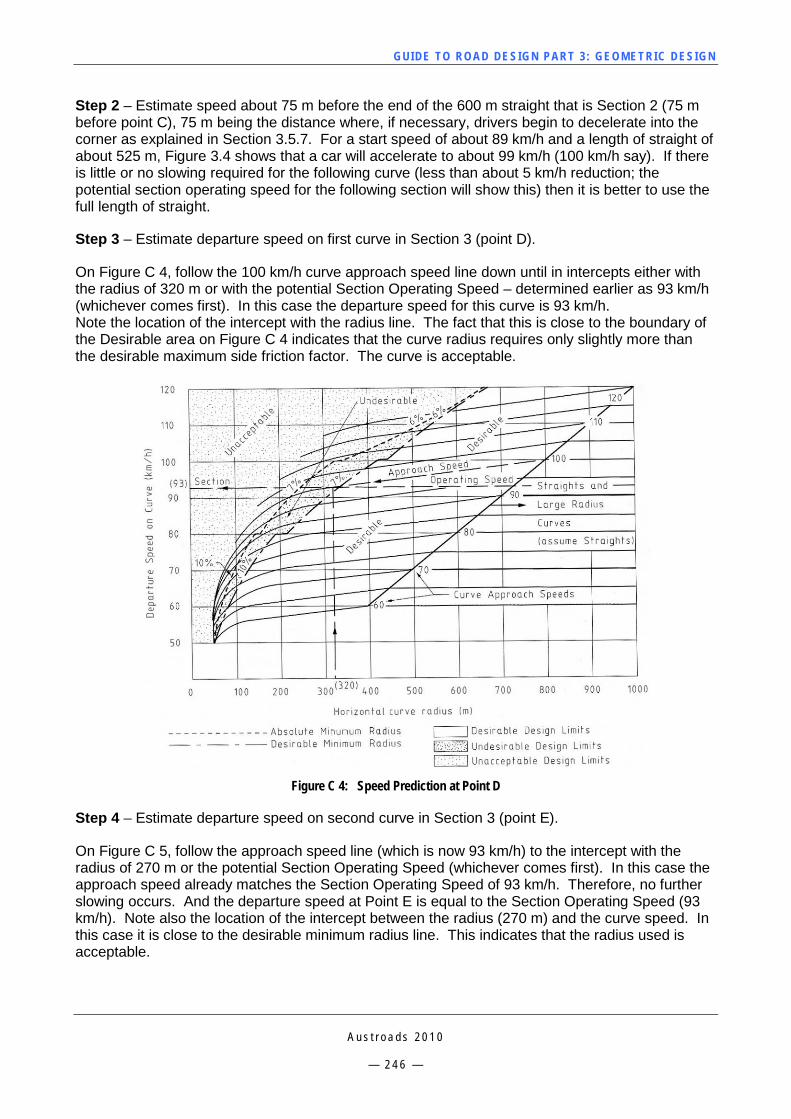
GUI DE TO RO A D DE SIG N P ART 3 : GEO MET RI C D ESI G N
A u s t r o a d s 2 0 1 0
— 2 4 6 —
Step 2 – Estimate speed about 75 m before the end of the 600 m straight that is Section 2 (75 m before point C), 75 m being the distance where, if necessary, drivers begin to decelerate into the corner as explained in Section 3.5.7. For a start speed of about 89 km/h and a length of straight of about 525 m, Figure 3.4 shows that a car will accelerate to about 99 km/h (100 km/h say). If there is little or no slowing required for the following curve (less than about 5 km/h reduction; the potential section operating speed for the following section will show this) then it is better to use the full length of straight.
Step 3 – Estimate departure speed on first curve in Section 3 (point D).
On Figure C 4, follow the 100 km/h curve approach speed line down until in intercepts either with the radius of 320 m or with the potential Section Operating Speed – determined earlier as 93 km/h (whichever comes first). In this case the departure speed for this curve is 93 km/h. Note the location of the intercept with the radius line. The fact that this is close to the boundary of the Desirable area on Figure C 4 indicates that the curve radius requires only slightly more than the desirable maximum side friction factor. The curve is acceptable.
Figure C 4: Speed Prediction at Point D
Step 4 – Estimate departure speed on second curve in Section 3 (point E).
On Figure C 5, follow the approach speed line (which is now 93 km/h) to the intercept with the radius of 270 m or the potential Section Operating Speed (whichever comes first). In this case the approach speed already matches the Section Operating Speed of 93 km/h. Therefore, no further slowing occurs. And the departure speed at Point E is equal to the Section Operating Speed (93 km/h). Note also the location of the intercept between the radius (270 m) and the curve speed. In this case it is close to the desirable minimum radius line. This indicates that the radius used is acceptable.
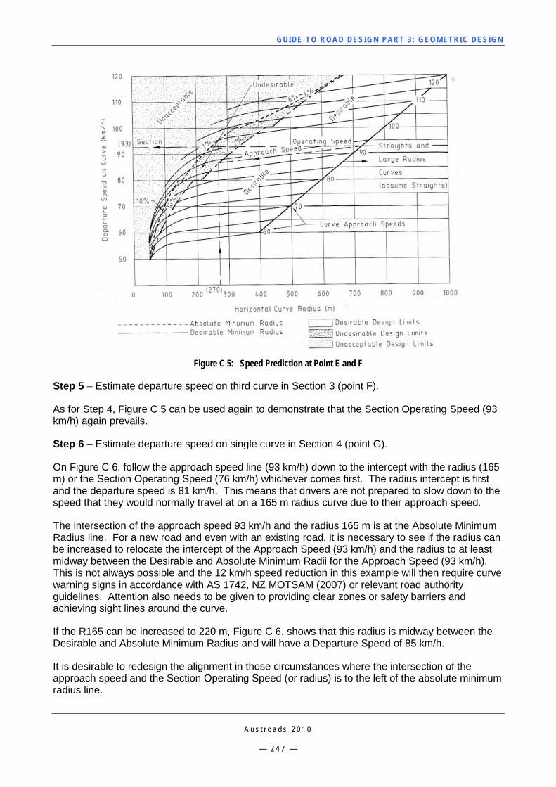
GUI DE TO RO A D DE SIG N P ART 3 : GEO MET RI C D ESI G N
A u s t r o a d s 2 0 1 0
— 2 4 7 —
Figure C 5: Speed Prediction at Point E and F
Step 5 – Estimate departure speed on third curve in Section 3 (point F).
As for Step 4, Figure C 5 can be used again to demonstrate that the Section Operating Speed (93 km/h) again prevails.
Step 6 – Estimate departure speed on single curve in Section 4 (point G).
On Figure C 6, follow the approach speed line (93 km/h) down to the intercept with the radius (165 m) or the Section Operating Speed (76 km/h) whichever comes first. The radius intercept is first and the departure speed is 81 km/h. This means that drivers are not prepared to slow down to the speed that they would normally travel at on a 165 m radius curve due to their approach speed.
The intersection of the approach speed 93 km/h and the radius 165 m is at the Absolute Minimum Radius line. For a new road and even with an existing road, it is necessary to see if the radius can be increased to relocate the intercept of the Approach Speed (93 km/h) and the radius to at least midway between the Desirable and Absolute Minimum Radii for the Approach Speed (93 km/h). This is not always possible and the 12 km/h speed reduction in this example will then require curve warning signs in accordance with AS 1742, NZ MOTSAM (2007) or relevant road authority guidelines. Attention also needs to be given to providing clear zones or safety barriers and achieving sight lines around the curve.
If the R165 can be increased to 220 m, Figure C 6. shows that this radius is midway between the Desirable and Absolute Minimum Radius and will have a Departure Speed of 85 km/h.
It is desirable to redesign the alignment in those circumstances where the intersection of the approach speed and the Section Operating Speed (or radius) is to the left of the absolute minimum radius line.
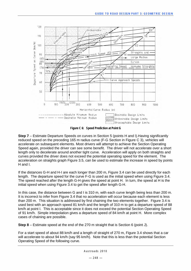
GUI DE TO RO A D DE SIG N P ART 3 : GEO MET RI C D ESI G N
A u s t r o a d s 2 0 1 0
— 2 4 8 —
Figure C 6: Speed Prediction at Point G
Step 7 – Estimate Departure Speeds on curves in Section 5 (points H and I).Having significantly reduced speed on the preceding 165 m radius curve (F-G Section in Figure C 3), vehicles will accelerate on subsequent elements. Most drivers will attempt to achieve the Section Operating Speed again, provided the driver can see some benefit. The driver will not accelerate over a short length only to decelerate around another tight curve. Acceleration will apply on both straights and curves provided the driver does not exceed the potential operating speed for the element. The acceleration on straights graph Figure 3.5, can be used to estimate the increase in speed by points H and I.
If the distances G-H and H-I are each longer than 200 m, Figure 3.4 can be used directly for each length. The departure speed for the curve F-G is used as the initial speed when using Figure 3.4. The speed reached after the length G-H gives the speed at point H. In turn, the speed at H is the initial speed when using Figure 3.4 to get the speed after length G-H.
In this case, the distance between G and I is 310 m, with each curve length being less than 200 m. It is incorrect to infer from Figure 3.4 that no acceleration will occur because each element is less than 200 m. This situation is addressed by first chaining the two elements together. Figure 3.4 is used best with an approach speed 81 km/h and the length of 310 m to get a departure speed of 88 km/h at point I. This is acceptable since it does not exceed the potential Section Operating Speed of 91 km/h. Simple interpolation gives a departure speed of 84 km/h at point H. More complex cases of chaining are possible.
Step 8 – Estimate speed at the end of the 270 m straight that is Section 6 (point J).
For a start speed of about 88 km/h and a length of straight of 270 m, Figure 3.4 shows that a car will accelerate to about 94 km/h (say 95 km/h). Note that this is less than the potential Section Operating Speed of the following curve.
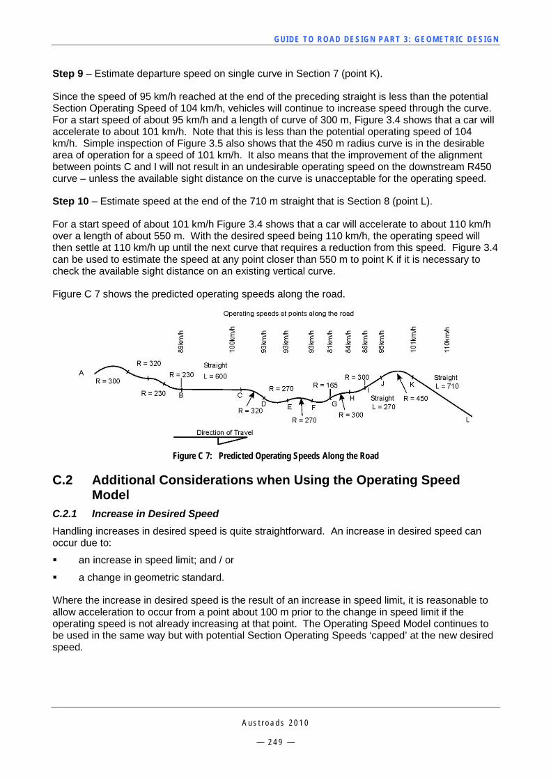
GUI DE TO RO A D DE SIG N P ART 3 : GEO MET RI C D ESI G N
A u s t r o a d s 2 0 1 0
— 2 4 9 —
Step 9 – Estimate departure speed on single curve in Section 7 (point K).
Since the speed of 95 km/h reached at the end of the preceding straight is less than the potential Section Operating Speed of 104 km/h, vehicles will continue to increase speed through the curve. For a start speed of about 95 km/h and a length of curve of 300 m, Figure 3.4 shows that a car will accelerate to about 101 km/h. Note that this is less than the potential operating speed of 104 km/h. Simple inspection of Figure 3.5 also shows that the 450 m radius curve is in the desirable area of operation for a speed of 101 km/h. It also means that the improvement of the alignment between points C and I will not result in an undesirable operating speed on the downstream R450 curve – unless the available sight distance on the curve is unacceptable for the operating speed.
Step 10 – Estimate speed at the end of the 710 m straight that is Section 8 (point L).
For a start speed of about 101 km/h Figure 3.4 shows that a car will accelerate to about 110 km/h over a length of about 550 m. With the desired speed being 110 km/h, the operating speed will then settle at 110 km/h up until the next curve that requires a reduction from this speed. Figure 3.4 can be used to estimate the speed at any point closer than 550 m to point K if it is necessary to check the available sight distance on an existing vertical curve.
Figure C 7 shows the predicted operating speeds along the road.
Figure C 7: Predicted Operating Speeds Along the Road
C.2 Additional Considerations when Using the Operating Speed Model
C.2.1 Increase in Desired Speed Handling increases in desired speed is quite straightforward. An increase in desired speed can occur due to:
an increase in speed limit; and / or
a change in geometric standard.
Where the increase in desired speed is the result of an increase in speed limit, it is reasonable to allow acceleration to occur from a point about 100 m prior to the change in speed limit if the operating speed is not already increasing at that point. The Operating Speed Model continues to be used in the same way but with potential Section Operating Speeds ‘capped’ at the new desired speed.
GUI DE TO RO A D DE SIG N P ART 3 : GEO MET RI C D ESI G N
A u s t r o a d s 2 0 1 0
— 2 5 0 —
Where the increase in desired speed is the result of a change in geometric standard, the Operating Speed Model continues to be used in the same way but with potential Section Operating Speeds ‘capped’ at the new desired speed. A possible increase in desired speed should be considered whenever Figure 3.4 indicates that it is possible to increase speed beyond the current desired speed.
C.2.2 Decrease in Desired Speed Simple driving experience is sufficient to show that it usually takes some time and distance to achieve a reduction in desired speed, even when it is due to a reduction in speed limit. Therefore, implementing a reduction in desired speed with the Operating Speed Model will be subjective when the road alignment itself does not lead to a reduction in operating speed. When the road alignment causes a reduction in operating speed, it is then only necessary to decide if the alignment and terrain conditions then exist for a sufficient distance to cause a reduction in desired speed. Otherwise, operating speeds will tend to increase towards the original desired speed and the model will show this.
If the road alignment does not cause a reduction in operating speed (e.g. a reduction in speed limit on a straight), the key issue is to decide over what length the reduction in desired speed occurs. Drivers’ perception of the need for a speed reduction due to the change in roadside environment, level of speed limit enforcement and so on, all comes into play. It is suggested that a distance based on a 1 to 2 km/h speed reduction for every 30 m of travel be assumed, depending upon drivers’ perception of the need for a speed reduction.
C.2.3 Increase in Speed on a Chain of ‘Short’ Elements Predicting the increase in speed through a combination of increasing curve radii with short intervening straights (each with a length < 200 m) involves chaining a number of straights and curves together to determine the increase in operating speed. It is not correct to infer from Figure 3.4 that no speed increase will occur because each element is less than 200 m long. A chain is terminated by the following conditions, whichever occurs first:
A straight at least 200 m long. The speed at the end of the straight (or 75 m before the end if slowing for a curve at the end is involved) is then calculated for the length of the chain. Operating speeds at the end of the preceding elements in the chain are interpolated over the length of the chain.
The operating speed on an element in the chain reaches the desired speed. Operating speeds at the end of the preceding elements in the chain are interpolated over the length of the chain to this point. Speed on the following elements will stay at the desired speed until it is necessary to slow for a later section.
Speed on an element in the chain reaches the potential Section Operating Speed. Operating speeds at the end of the preceding elements in the chain are interpolated over the length of the chain to this point. However, the process may have to repeat for another chain after this point.
Sometimes, when the end of an element in a chain is more than about 400 m from the start of the chain, experience shows that it may be more convenient to end the chain at that point and to repeat the process for another chain after this point.
C.2.4 Effects of Grades Insufficient information is available to provide firm guidelines on the effect of grades. However, designers are expected to consider the grading and make adjustments to speed estimates. Section 8.4 provides guidance for cars on longer sections of grade.
GUI DE TO RO A D DE SIG N P ART 3 : GEO MET RI C D ESI G N
A u s t r o a d s 2 0 1 0
— 2 5 1 —
The following assumptions can also be made for each element of the road as the speed estimate is made:
The operating speed of cars may be reduced on up-hill grades longer than 200 m and steeper than about 8%.
The operating speed of laden trucks will be significantly reduced on long up hill grades. Where possible, use a vehicle performance simulation program to predict truck speeds using an average laden prime-mover and semi-trailer.
Car operating speeds can be assumed to be unaffected by ‘shorter’ (less than 200 m) down-hill grades less than about 9%. However, some increase should be expected toward the end of a ‘longer’ grade.
Car operating speeds can be assumed to be 5 to 10 km/h lower on down-hill grades steeper than about 9%, than for flatter grades. However, some increase should be expected toward the end of the grade.
For grades steeper than 12%, see Table 8.2.
Trucks may be required to significantly reduce their speed prior to steep (more than 8%) down-hill grades or even long grades as flat as 5%. Where possible, use a vehicle performance simulation program or assume a speed 5 to 10 km/h greater than the up-hill speed.
Corrections for grade should be considered for each element of the road. This is particularly necessary when there is a significant change in topography.
C.2.5 Effect of Cross-Section Typically, operating speeds are reduced by about 3 km/h when traffic lanes widths are 3 m or less. The operating speed model assumes that the traffic lanes are 3.5 m wide. This is because the horizontal alignment design should always be suitable for any future lane widening even if 3 m wide lanes are being used initially.
The only time speed reduction due to narrow lane width should be used is when using speed data on an existing road to ‘tune’ the results from the operating speed model.
C.2.6 Effect of Pavement Condition On roads with a high roughness or poor or broken surfaces, speeds can be reduced by 5 to 10 km/h. The operating speed model assumes that the pavement is in good condition. This is because the horizontal alignment design should always be based on operating speeds when the pavement is in good condition.
The only time speed reduction due to pavement condition should be used is when using speed data on an existing road to ‘tune’ the results from the operating speed model.
GUI DE TO RO A D DE SIG N P ART 3 : GEO MET RI C D ESI G N
A u s t r o a d s 2 0 1 0
— 2 5 2 —
APPENDIX D THEORY OF MOVEMENT IN A CIRCULAR PATH
D.1 Movement in a Circular Path Symbols Used:
a = acceleration (m/sec2)
e = superelevation (m/m)
f = side (lateral) friction factor
ff = side friction force down the plane (N)
fg = gravity force down the plane (N)
g = gravitational acceleration (m/sec2)
m = vehicle mass (kg)
R = radius of circular curve (m)
Re = reaction force perpendicular to the plane (N)
u = coefficient of sliding friction
V = speed (km/h)
v = speed (m/s)
Θ = angle of inclination of the plane (radians)
A body will travel at constant velocity in a straight line unless a force acts on it to change its velocity.
Consider a particle travelling on a circular path with constant velocity v,
t
RtLv
∆∆
=∆∆
=α
A 1
Rearranging,
Rtv∆
=∆α A 2
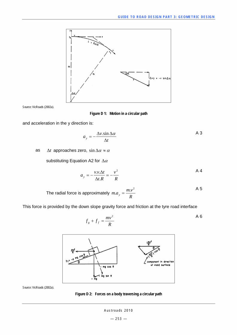
GUI DE TO RO A D DE SIG N P ART 3 : GEO MET RI C D ESI G N
A u s t r o a d s 2 0 1 0
— 2 5 3 —
Source: VicRoads (2002a).
Figure D 1: Motion in a circular path
and acceleration in the y direction is:
t
vay ∆∆∆
−=αsin.
A 3
as t∆ approaches zero, αα ≈∆sin
substituting Equation A2 for α∆
Rv
Rttvvay
2
...
−=∆∆
−= A 4
The radial force is approximately
Rvmam y
2.. = A 5
This force is provided by the down slope gravity force and friction at the tyre road interface
Rmvff fg
2
=+ A 6
Source: VicRoads (2002a).
Figure D 2: Forces on a body traversing a circular path
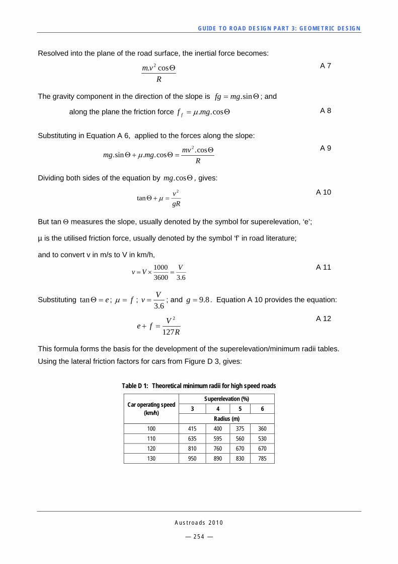
GUI DE TO RO A D DE SIG N P ART 3 : GEO MET RI C D ESI G N
A u s t r o a d s 2 0 1 0
— 2 5 4 —
Resolved into the plane of the road surface, the inertial force becomes:
Rvm Θcos. 2
A 7
The gravity component in the direction of the slope is Θ= sin.mgfg ; and
along the plane the friction force Θ= cos..mgf f µ A 8
Substituting in Equation A 6, applied to the forces along the slope:
Rmvmgmg Θ
=Θ+Θcos.cos..sin.
2
µ A 9
Dividing both sides of the equation by Θcos.mg , gives:
gRv 2
tan =+Θ µ A 10
But tan Θ measures the slope, usually denoted by the symbol for superelevation, ‘e’;
µ is the utilised friction force, usually denoted by the symbol ‘f’ in road literature;
and to convert v in m/s to V in km/h,
6.33600
1000 VVv =×= A 11
Substituting e=Θtan ; f=µ ; 6.3
Vv = ; and 8.9=g . Equation A 10 provides the equation:
RVfe
127
2
=+ A 12
This formula forms the basis for the development of the superelevation/minimum radii tables.
Using the lateral friction factors for cars from Figure D 3, gives:
Table D 1: Theoretical minimum radii for high speed roads
Car operating speed (km/h)
Superelevation (%) 3 4 5 6
Radius (m) 100 415 400 375 360 110 635 595 560 530 120 810 760 670 670 130 950 890 830 785
GUI DE TO RO A D DE SIG N P ART 3 : GEO MET RI C D ESI G N
A u s t r o a d s 2 0 1 0
— 2 5 5 —
These radii are not recommended for practical use on high speed roads, because the formula applies to a theoretical point mass, and does not allow for body roll and other dynamic and aerodynamic effects. The formula cannot be reliably applied to adverse crossfall, because other factors such as the high centre of mass of trucks and other factors set out below can significantly influence vehicle stability and safety.
D.2 Side Friction Force on Vehicle Equation A 12 shows that the lateral friction developed at the tyre/road interface as vehicles turn is directly related to the square of the vehicle speed. A speed can be reached at which the force required to maintain a circular path exceeds the force which can be developed by friction and superelevation. At this point, the vehicle starts to slide in a spiral path away from the alignment of the road.
D.2.1 Sliding For design purposes, friction factors have to be defined which are less than the maximum at which a vehicles lose control. The design friction factors for cars and trucks on sealed roads are shown on Figure D 3. These friction factors were calculated from field measurements of speeds and superelevations on dry sealed rural roads. Eighty-fifth percentile speeds were obtained from these measurements and then the lateral friction factors were calculated (McLean 1988). These factors are therefore more a measure of the driver comfort than the friction at the tyre/road interface. The figures remain valid for wet roads unless the driver’s view is obscured by heavy rain or fog (Botterill 1994).
On wet surfaces, trucks tend to lose stability by sliding. On dry, low radius curves, high trucks are more likely to roll. Figure D 3 specifies the lateral friction that is used for design in order to avoid truck instability. In most cases it is not necessary to know whether this instability is caused by sliding or by rolling.
D.2.2 Overturning When a truck travels around an unsuperelevated curve, sufficient lateral friction usually develops at the tyre/road interface to force the truck to turn in a circular path. Without this force, the truck would travel in a straight line.
If for analysis purposes, the moving truck is deemed to be a static point mass located at the centre of mass and the horizontal component of the force at the tyre/road interface is f = mv2/R, there is a moment that tends to overturn the truck (Figure D 4).
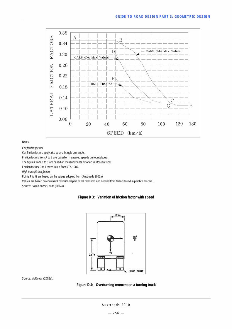
GUI DE TO RO A D DE SIG N P ART 3 : GEO MET RI C D ESI G N
A u s t r o a d s 2 0 1 0
— 2 5 6 —
Notes:
Car friction factors Car friction factors apply also to small single unit trucks. Friction factors from A to B are based on measured speeds on roundabouts. The figures from B to C are based on measurements reported in McLean 1998 Friction factors D to E were taken from RTA 1989. High truck friction factors Points F to G are based on the values adopted from (Austroads 2002a) Values are based on equivalent risk with respect to roll threshold and derived from factors found in practice for cars. Source: Based on VicRoads (2002a).
Figure D 3: Variation of friction factor with speed
Source: VicRoads (2002a).
Figure D 4: Overturning moment on a turning truck
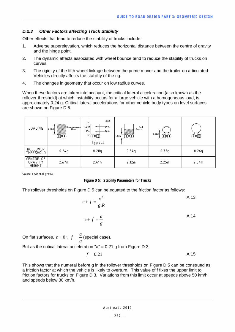
GUI DE TO RO A D DE SIG N P ART 3 : GEO MET RI C D ESI G N
A u s t r o a d s 2 0 1 0
— 2 5 7 —
D.2.3 Other Factors affecting Truck Stability Other effects that tend to reduce the stability of trucks include:
1. Adverse superelevation, which reduces the horizontal distance between the centre of gravity and the hinge point.
2. The dynamic affects associated with wheel bounce tend to reduce the stability of trucks on curves.
3. The rigidity of the fifth wheel linkage between the prime mover and the trailer on articulated Vehicles directly affects the stability of the rig.
4. The changes in geometry that occur on low radius curves.
When these factors are taken into account, the critical lateral acceleration (also known as the rollover threshold) at which instability occurs for a large vehicle with a homogeneous load, is approximately 0.24 g. Critical lateral accelerations for other vehicle body types on level surfaces are shown on Figure D 5.
Source: Ervin et al. (1986).
Figure D 5: Stability Parameters for Trucks
The rollover thresholds on Figure D 5 can be equated to the friction factor as follows:
Rgvfe.
2
=+ A 13
gafe =+
A 14
On flat surfaces, gafe =∴= 0 (special case).
But as the critical lateral acceleration "a" = 0.21 g from Figure D 3,
21.0=f A 15
This shows that the numeral before g in the rollover thresholds on Figure D 5 can be construed as a friction factor at which the vehicle is likely to overturn. This value of f fixes the upper limit to friction factors for trucks on Figure D 3. Variations from this limit occur at speeds above 50 km/h and speeds below 30 km/h.
GUI DE TO RO A D DE SIG N P ART 3 : GEO MET RI C D ESI G N
A u s t r o a d s 2 0 1 0
— 2 5 8 —
The reduction in friction factors above 50 km/h are consistent with observed operating speeds in the field , that is, truck speeds should be approximately 10 km/h below car speeds. This speed range above 50 km/h is also the range where instability is generally initiated by sliding.
The deviation from the friction factor of 0.24 value below 30 km/h is necessary to match limiting speeds shown on the Austroads templates. In the speed range involved, curve radii are sufficiently low to influence the geometry of articulated vehicles and this effect could explain the low stability of trucks at low speeds.
Use of the truck friction factors on Figure D 3 provides for the majority of trucks. There have been some trucks that have rolled at lower friction factors. Rollovers at low speed can be initiated by a range of factors, including:
Tripping: Vehicles sliding sideways can overturn at speeds below 10 km/h when tripped by a kerb or pothole. For this reason road surfaces must be kept in good condition where critical turning movements occur.
Loading: Small lateral offsets of the centre of gravity of the load significantly reduce the lateral stability of the truck. Uneven longitudinal loading also reduces the vehicle's stability.
Load shift: For example, liquid in tankers or cattle on high trucks.
Dynamic forces: Associated with tyre and suspension bounce. These forces are related to the speed of the vehicle and the condition of the pavement.
Aquaplaning: Leading to loss of control and rollover.
Braking: As the brakes are applied, the friction available in the radial direction decreases. If the wheels lock, lateral stability and steering is lost.
Rearward Amplification: A ‘whiplash’ effect. Specifically it is the ratio of the maximum lateral acceleration at the rear axle over the lateral acceleration on the prime mover.
Speed: The indications are that critical lateral accelerations (or friction forces) are speed dependent as shown by Figure D 3.
The least stable truck on Figure D 5 was used as a basis for design friction factors for trucks and the critical turning radii for trucks in intersections.
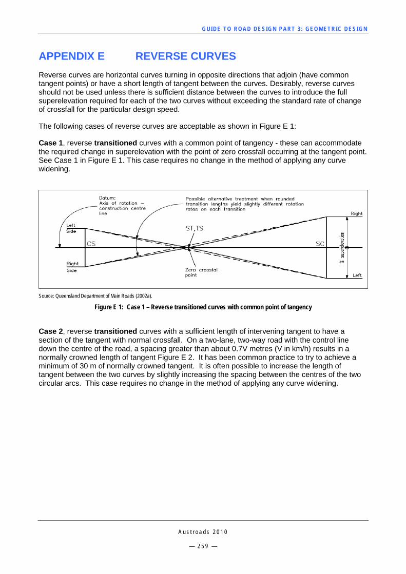
GUI DE TO RO A D DE SIG N P ART 3 : GEO MET RI C D ESI G N
A u s t r o a d s 2 0 1 0
— 2 5 9 —
APPENDIX E REVERSE CURVES Reverse curves are horizontal curves turning in opposite directions that adjoin (have common tangent points) or have a short length of tangent between the curves. Desirably, reverse curves should not be used unless there is sufficient distance between the curves to introduce the full superelevation required for each of the two curves without exceeding the standard rate of change of crossfall for the particular design speed.
The following cases of reverse curves are acceptable as shown in Figure E 1:
Case 1, reverse transitioned curves with a common point of tangency - these can accommodate the required change in superelevation with the point of zero crossfall occurring at the tangent point. See Case 1 in Figure E 1. This case requires no change in the method of applying any curve widening.
Source: Queensland Department of Main Roads (2002a).
Figure E 1: Case 1 – Reverse transitioned curves with common point of tangency
Case 2, reverse transitioned curves with a sufficient length of intervening tangent to have a section of the tangent with normal crossfall. On a two-lane, two-way road with the control line down the centre of the road, a spacing greater than about 0.7V metres (V in km/h) results in a normally crowned length of tangent Figure E 2. It has been common practice to try to achieve a minimum of 30 m of normally crowned tangent. It is often possible to increase the length of tangent between the two curves by slightly increasing the spacing between the centres of the two circular arcs. This case requires no change in the method of applying any curve widening.

GUI DE TO RO A D DE SIG N P ART 3 : GEO MET RI C D ESI G N
A u s t r o a d s 2 0 1 0
— 2 6 0 —
Source: Queensland Department of Main Roads (2002a).
Figure E 2: Case 2 – Reverse transitioned curves with length of intervening tangent > 0.7V
Case 3A, reverse circular curves with a common point of tangency are possible for operating speeds less than or equal to 80 km/h if the superelevation on each curve does not exceed 3% and a nominal rotation rate of 0.025 rad/s is used. This allows the superelevation to change from zero crossfall at the common tangent point to 3% in 25 m (or less) in line with established practice of attaining full superelevation 25 m into an untransitioned curve Figure E 3. However, the need to switch curve widening from one side of the road to the other will require the treatment shown in Figure E 9. For lower operating speeds, the acceptable rate of pavement rotation (0.035 rad/s or 0.04 rad/s) may allow more than 3% superelevation to be achieved over the 25 m length. Case 3A represents an acceptable compromise of the location of the superelevation runoff.
Source: Queensland Department of Main Roads (2002a).
Figure E 3: Case 3A – Reverse circular curves with common tangent point
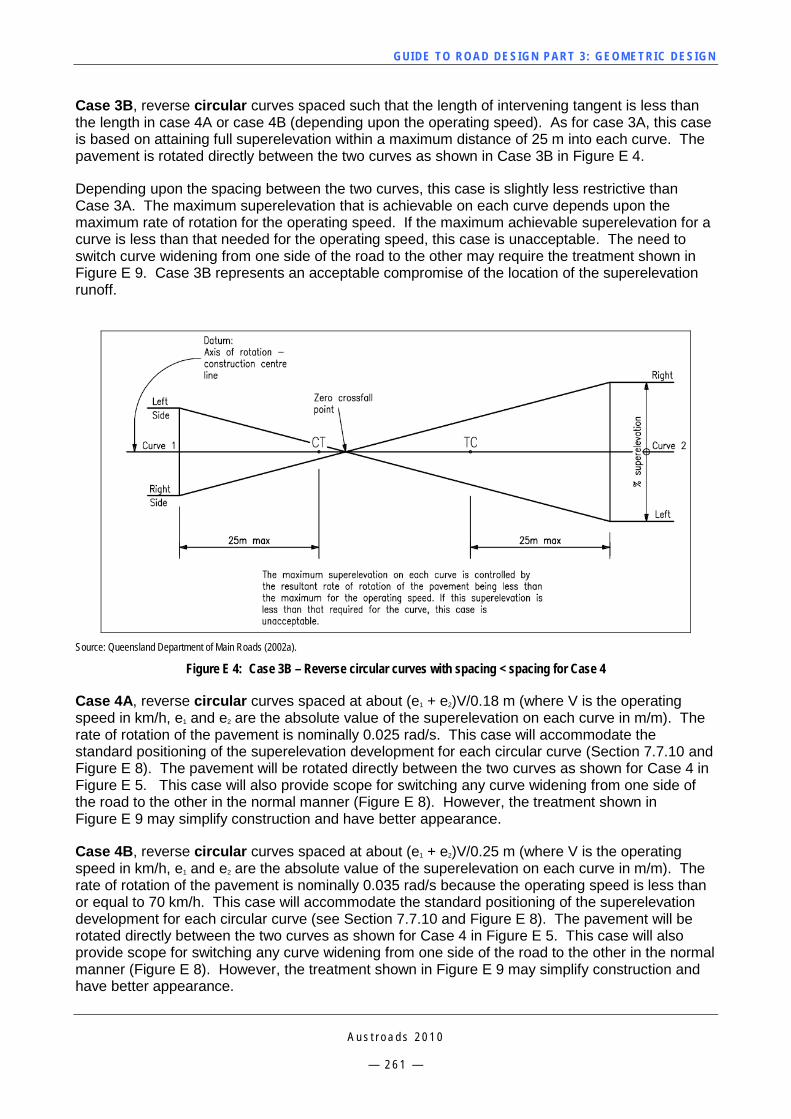
GUI DE TO RO A D DE SIG N P ART 3 : GEO MET RI C D ESI G N
A u s t r o a d s 2 0 1 0
— 2 6 1 —
Case 3B, reverse circular curves spaced such that the length of intervening tangent is less than the length in case 4A or case 4B (depending upon the operating speed). As for case 3A, this case is based on attaining full superelevation within a maximum distance of 25 m into each curve. The pavement is rotated directly between the two curves as shown in Case 3B in Figure E 4.
Depending upon the spacing between the two curves, this case is slightly less restrictive than Case 3A. The maximum superelevation that is achievable on each curve depends upon the maximum rate of rotation for the operating speed. If the maximum achievable superelevation for a curve is less than that needed for the operating speed, this case is unacceptable. The need to switch curve widening from one side of the road to the other may require the treatment shown in Figure E 9. Case 3B represents an acceptable compromise of the location of the superelevation runoff.
Source: Queensland Department of Main Roads (2002a).
Figure E 4: Case 3B – Reverse circular curves with spacing < spacing for Case 4
Case 4A, reverse circular curves spaced at about (e1 + e2)V/0.18 m (where V is the operating speed in km/h, e1 and e2 are the absolute value of the superelevation on each curve in m/m). The rate of rotation of the pavement is nominally 0.025 rad/s. This case will accommodate the standard positioning of the superelevation development for each circular curve (Section 7.7.10 and Figure E 8). The pavement will be rotated directly between the two curves as shown for Case 4 in Figure E 5. This case will also provide scope for switching any curve widening from one side of the road to the other in the normal manner (Figure E 8). However, the treatment shown in Figure E 9 may simplify construction and have better appearance.
Case 4B, reverse circular curves spaced at about (e1 + e2)V/0.25 m (where V is the operating speed in km/h, e1 and e2 are the absolute value of the superelevation on each curve in m/m). The rate of rotation of the pavement is nominally 0.035 rad/s because the operating speed is less than or equal to 70 km/h. This case will accommodate the standard positioning of the superelevation development for each circular curve (see Section 7.7.10 and Figure E 8). The pavement will be rotated directly between the two curves as shown for Case 4 in Figure E 5. This case will also provide scope for switching any curve widening from one side of the road to the other in the normal manner (Figure E 8). However, the treatment shown in Figure E 9 may simplify construction and have better appearance.
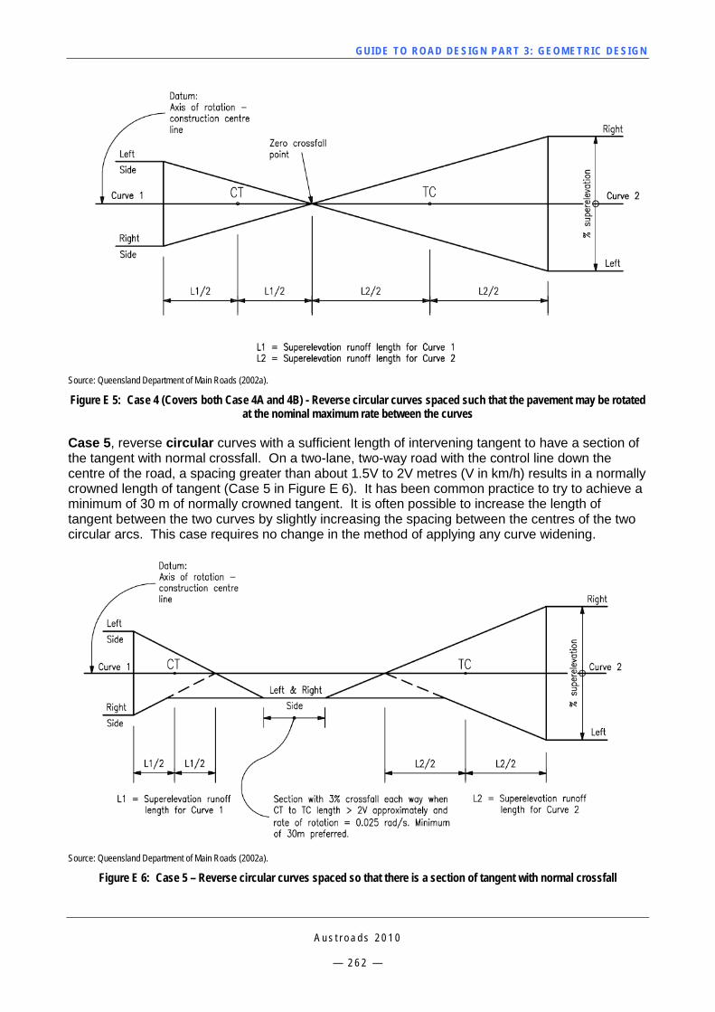
GUI DE TO RO A D DE SIG N P ART 3 : GEO MET RI C D ESI G N
A u s t r o a d s 2 0 1 0
— 2 6 2 —
Source: Queensland Department of Main Roads (2002a).
Figure E 5: Case 4 (Covers both Case 4A and 4B) - Reverse circular curves spaced such that the pavement may be rotated at the nominal maximum rate between the curves
Case 5, reverse circular curves with a sufficient length of intervening tangent to have a section of the tangent with normal crossfall. On a two-lane, two-way road with the control line down the centre of the road, a spacing greater than about 1.5V to 2V metres (V in km/h) results in a normally crowned length of tangent (Case 5 in Figure E 6). It has been common practice to try to achieve a minimum of 30 m of normally crowned tangent. It is often possible to increase the length of tangent between the two curves by slightly increasing the spacing between the centres of the two circular arcs. This case requires no change in the method of applying any curve widening.
Source: Queensland Department of Main Roads (2002a).
Figure E 6: Case 5 – Reverse circular curves spaced so that there is a section of tangent with normal crossfall
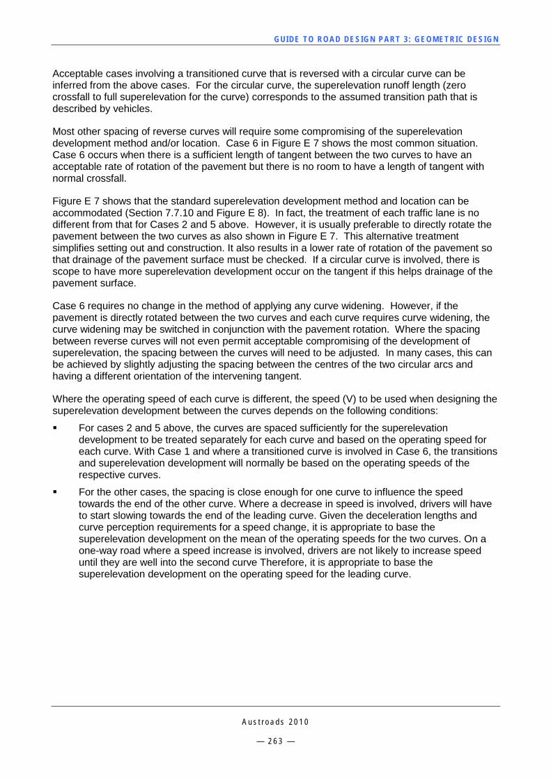
GUI DE TO RO A D DE SIG N P ART 3 : GEO MET RI C D ESI G N
A u s t r o a d s 2 0 1 0
— 2 6 3 —
Acceptable cases involving a transitioned curve that is reversed with a circular curve can be inferred from the above cases. For the circular curve, the superelevation runoff length (zero crossfall to full superelevation for the curve) corresponds to the assumed transition path that is described by vehicles.
Most other spacing of reverse curves will require some compromising of the superelevation development method and/or location. Case 6 in Figure E 7 shows the most common situation. Case 6 occurs when there is a sufficient length of tangent between the two curves to have an acceptable rate of rotation of the pavement but there is no room to have a length of tangent with normal crossfall.
Figure E 7 shows that the standard superelevation development method and location can be accommodated (Section 7.7.10 and Figure E 8). In fact, the treatment of each traffic lane is no different from that for Cases 2 and 5 above. However, it is usually preferable to directly rotate the pavement between the two curves as also shown in Figure E 7. This alternative treatment simplifies setting out and construction. It also results in a lower rate of rotation of the pavement so that drainage of the pavement surface must be checked. If a circular curve is involved, there is scope to have more superelevation development occur on the tangent if this helps drainage of the pavement surface.
Case 6 requires no change in the method of applying any curve widening. However, if the pavement is directly rotated between the two curves and each curve requires curve widening, the curve widening may be switched in conjunction with the pavement rotation. Where the spacing between reverse curves will not even permit acceptable compromising of the development of superelevation, the spacing between the curves will need to be adjusted. In many cases, this can be achieved by slightly adjusting the spacing between the centres of the two circular arcs and having a different orientation of the intervening tangent.
Where the operating speed of each curve is different, the speed (V) to be used when designing the superelevation development between the curves depends on the following conditions:
For cases 2 and 5 above, the curves are spaced sufficiently for the superelevation development to be treated separately for each curve and based on the operating speed for each curve. With Case 1 and where a transitioned curve is involved in Case 6, the transitions and superelevation development will normally be based on the operating speeds of the respective curves.
For the other cases, the spacing is close enough for one curve to influence the speed towards the end of the other curve. Where a decrease in speed is involved, drivers will have to start slowing towards the end of the leading curve. Given the deceleration lengths and curve perception requirements for a speed change, it is appropriate to base the superelevation development on the mean of the operating speeds for the two curves. On a one-way road where a speed increase is involved, drivers are not likely to increase speed until they are well into the second curve Therefore, it is appropriate to base the superelevation development on the operating speed for the leading curve.
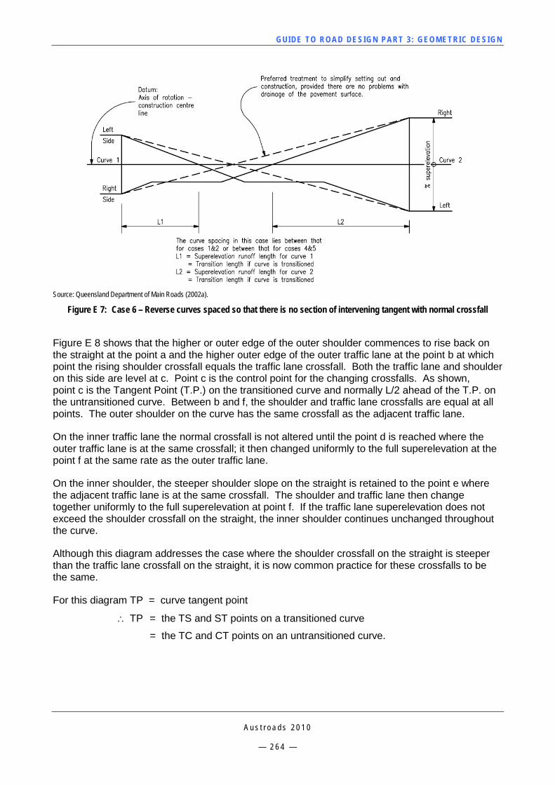
GUI DE TO RO A D DE SIG N P ART 3 : GEO MET RI C D ESI G N
A u s t r o a d s 2 0 1 0
— 2 6 4 —
Source: Queensland Department of Main Roads (2002a).
Figure E 7: Case 6 – Reverse curves spaced so that there is no section of intervening tangent with normal crossfall
Figure E 8 shows that the higher or outer edge of the outer shoulder commences to rise back on the straight at the point a and the higher outer edge of the outer traffic lane at the point b at which point the rising shoulder crossfall equals the traffic lane crossfall. Both the traffic lane and shoulder on this side are level at c. Point c is the control point for the changing crossfalls. As shown, point c is the Tangent Point (T.P.) on the transitioned curve and normally L/2 ahead of the T.P. on the untransitioned curve. Between b and f, the shoulder and traffic lane crossfalls are equal at all points. The outer shoulder on the curve has the same crossfall as the adjacent traffic lane.
On the inner traffic lane the normal crossfall is not altered until the point d is reached where the outer traffic lane is at the same crossfall; it then changed uniformly to the full superelevation at the point f at the same rate as the outer traffic lane.
On the inner shoulder, the steeper shoulder slope on the straight is retained to the point e where the adjacent traffic lane is at the same crossfall. The shoulder and traffic lane then change together uniformly to the full superelevation at point f. If the traffic lane superelevation does not exceed the shoulder crossfall on the straight, the inner shoulder continues unchanged throughout the curve.
Although this diagram addresses the case where the shoulder crossfall on the straight is steeper than the traffic lane crossfall on the straight, it is now common practice for these crossfalls to be the same.
For this diagram TP = curve tangent point
∴ TP = the TS and ST points on a transitioned curve
= the TC and CT points on an untransitioned curve.
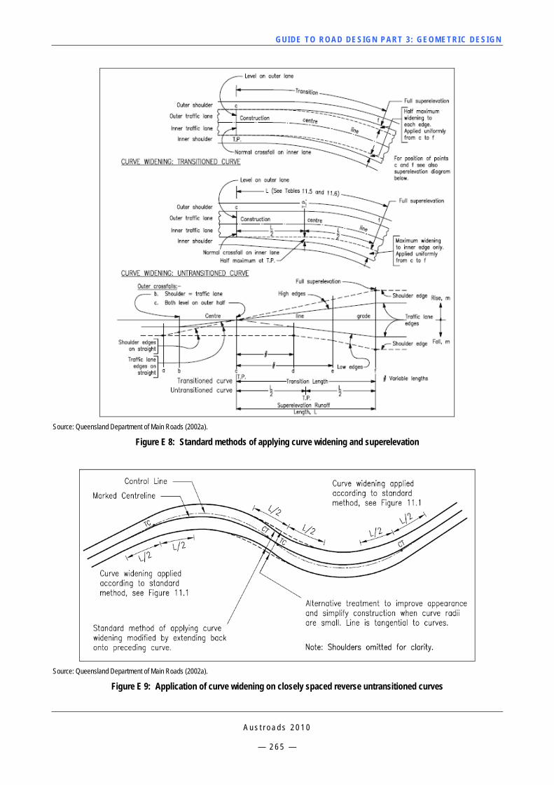
GUI DE TO RO A D DE SIG N P ART 3 : GEO MET RI C D ESI G N
A u s t r o a d s 2 0 1 0
— 2 6 5 —
Source: Queensland Department of Main Roads (2002a).
Figure E 8: Standard methods of applying curve widening and superelevation
Source: Queensland Department of Main Roads (2002a).
Figure E 9: Application of curve widening on closely spaced reverse untransitioned curves
GUI DE TO RO A D DE SIG N P ART 3 : GEO MET RI C D ESI G N
A u s t r o a d s 2 0 1 0
— 2 6 6 —
APPENDIX F TRANSITION CURVES (SPIRALS)
F.1 General Any motor vehicle describes a transition path as it changes from a straight to a circular horizontal curve and vice versa, or between the elements of a compound curve. The way drivers, in general, steer a vehicle at speed results in a path that provides a reasonably uniform attainment of centripetal acceleration. For most curves, the average car driver can achieve a suitable transition path within the limits of normal lane width. However, with particular combinations of high speed, heavy vehicles and a large difference in curvature between successive geometric elements, the resultant vehicle transition path can result in encroachment into adjoining lanes. Trucks have more problems because of their greater width, longer wheel base and heavier, less responsive steering. Also, trucks have a greater swept path width on curves as explained in Section 7.9 on Curve Widening.
In cases where the combination of lane width, vehicle speed and curve radius do not allow sufficient space for a vehicle to describe a suitable transition path, it is necessary to provide a transition curve between the tangent and the circular arc. The need for such transition curves was learned from the early days of railway building when problems were encountered with passenger comfort and track wear due to the sudden application of curvature with untransitioned curves. However, the fact that road vehicles are not rigidly confined to a specific path together with the characteristics of road vehicle steering mean that shorter transition lengths are more appropriate than those used for railways. This is why it is current road design practice to base transition lengths on driver steering characteristics and on superelevation runoff length instead of a comfort criterion that was once used.
Transition curves provide the following advantages:
A properly designed transition curve allows the vehicle's centripetal acceleration to increase or decrease gradually as the vehicle enters or leaves a circular curve. This transition curve minimises encroachment on adjoining traffic lanes.
The transition curve length provides a convenient desirable arrangement for superelevation runoff. The change in the crossfall can be effected along the length of the transition curve in a manner closely fitting the radius-speed relation for the vehicle traversing it.
A transition facilitates the change in width where the pavement section is to be widened around a circular curve. Use of transitions provides flexibility in the widening on sharp curves.
The appearance of the highway or street is enhanced by the application of transitions. On multilane divided roads where the curve operating speeds are consistent with the operating speeds on the straights (typically, greater than 100 km/h), there is scope to improve the appearance by using longer transitions.
Transitioned curves simplify the application of curve widening on closely spaced curves in constrained mountainous situations because they avoid having to switch the widening from one side of the road to the other.
The use of longer transitions than those in Section 7.5.4 should be avoided when curve operating speeds are such that drivers have to reduce speed for the curve. Long transitions should only be considered in high-speed curvilinear alignments (Section 7.10) that are designed for a uniform speed of travel.
GUI DE TO RO A D DE SIG N P ART 3 : GEO MET RI C D ESI G N
A u s t r o a d s 2 0 1 0
— 2 6 7 —
F.1.1 Effect on Braking When drivers brake on curves, a combination of forces applies on the tyres, effectively reducing the maximum force that can be developed for braking or cornering. Articulated trucks also have problems with braking on curves because of the tendency of these vehicles to jack-knife. On transitioned curves where the operating speed is such that drivers are expected to reduce speed prior to the curve, there is a likelihood of braking on the transition if a long transition is used. This is because the change in curvature is not sufficient to identify the approximate start of the transition.
F.1.2 Effect on Overtaking Transitions can reduce the length of straights between curves, effectively reducing the length of possible overtaking opportunities.
F.1.3 Effect on Design Transitions involve additional work both in design and construction. Transitions that are longer than the superelevation runoff length for the curve design speed, but still have the superelevation runoff matched with the longer transition length, are more likely to have problems with drainage of the pavement surface. If this occurs, it will be necessary to compromise the application of the superelevation.
F.2 Use of Transitions It is normal practice for horizontal curves to be transitioned, with the transition length based on the superelevation runoff length for the recommended combination of speed, radius and superelevation. Section 7.5.4 sets out the requirements for transition curves including transition lengths. The lengths in Section 7.5.4 provide the advantages given previously while minimising the negative effects on driver perception, braking and overtaking that are associated with long transitions. It is also normal practice to round the transition length upwards if necessary to the next standard length of: 40, 60, 80, 100, 120 and 140 m. The rounding is primarily in the interests of uniformity and to avoid attributing undue precision to the calculated length.
Due to the characteristics of vehicle steering geometry, there is a transient state (or distance) where it is possible for the front (steered) wheels of a vehicle travelling at slow speed to follow a circular path while the steering angle is changed from straight ahead to the maximum angle needed to describe the turn. This is a major reason why transitions are not needed for intersection turns and most curves with a design speed below 60 km/h.
F.3 Types of Transitions The standard form of transition curve is the clothoid spiral. Other curves have been used in the past such as the cubic parabola, combination of cubic parabola and cubic spiral, lemniscate and a suitably large radius compound curve. All of these alternatives were advocated on the basis that they closely matched the shape of the clothoid spiral but were simpler to calculate. The disadvantage of the first three alternatives was that there were points of discontinuity that were conveniently 'smoothed out' during construction. Furthermore, for simplifying calculations, arc lengths were assumed to equal the tangent length of the transition curve. Restoration type projects on existing roads may encounter one of these alternative forms of transitions. However, it will be possible to fit a control line that contains clothoid spirals instead.
The clothoid spiral was adopted because the simplifications that were assumed for the alternative forms could not be conveniently incorporated into computer programs that came to be used for design calculations. Furthermore, electronic calculators and portable computers made field calculations feasible.

GUI DE TO RO A D DE SIG N P ART 3 : GEO MET RI C D ESI G N
A u s t r o a d s 2 0 1 0
— 2 6 8 —
With a defining property of the clothoid spiral being that curvature (reciprocal of the radius) varies uniformly along the spiral (rather than the tangent), other convenient properties can be derived:
If vehicles travel at a uniform speed and follow the transition curve closely enough, they will experience a uniform change in centripetal acceleration as they enter and exit the circular section of the curve.
In turn, by matching superelevation runoff to the transition, the uniform rate of application of the superelevation then results in a uniform attainment of side friction force.
The properties of transition curves that are relevant to road design and the derivation of equations for use in design calculations are given in Section F.4 below.
F.4 Characteristics of the Euler Spiral (Clothoid) Transition curves connecting a circular curve to two straights are shown in Figure F 1. Typical standard notation for transition curves is as follows (Figure F 1):
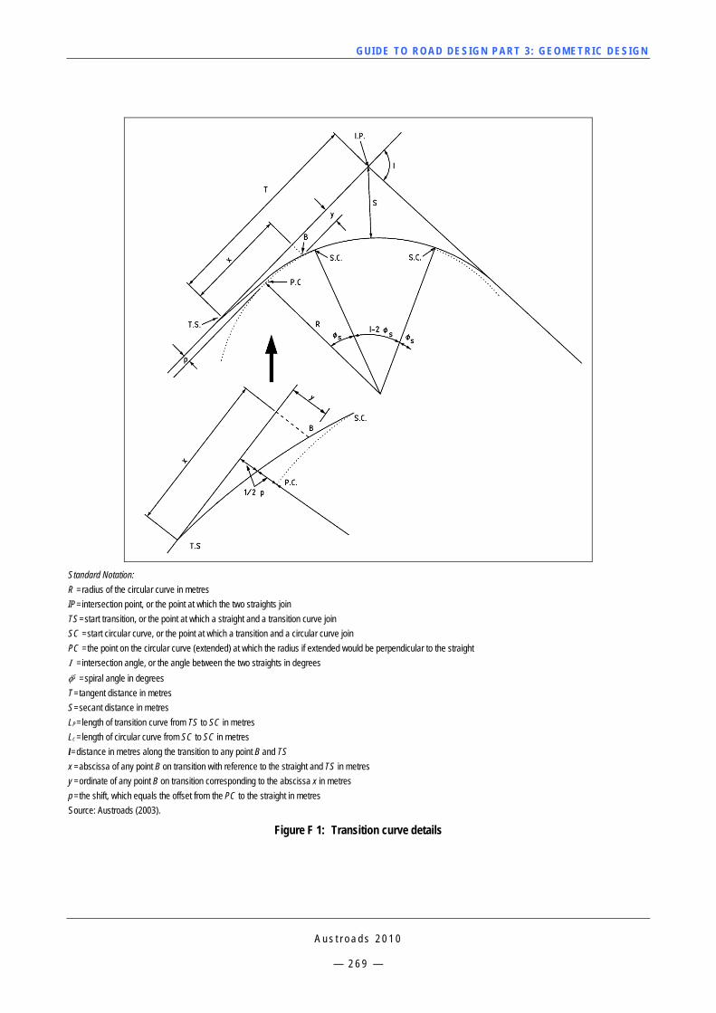
GUI DE TO RO A D DE SIG N P ART 3 : GEO MET RI C D ESI G N
A u s t r o a d s 2 0 1 0
— 2 6 9 —
Standard Notation: R = radius of the circular curve in metres IP = intersection point, or the point at which the two straights join TS = start transition, or the point at which a straight and a transition curve join SC = start circular curve, or the point at which a transition and a circular curve join PC = the point on the circular curve (extended) at which the radius if extended would be perpendicular to the straight I = intersection angle, or the angle between the two straights in degrees φS = spiral angle in degrees T = tangent distance in metres S = secant distance in metres LP = length of transition curve from TS to SC in metres Lc = length of circular curve from SC to SC in metres l= distance in metres along the transition to any point B and TS x = abscissa of any point B on transition with reference to the straight and TS in metres y = ordinate of any point B on transition corresponding to the abscissa x in metres p = the shift, which equals the offset from the PC to the straight in metres Source: Austroads (2003).
Figure F 1: Transition curve details
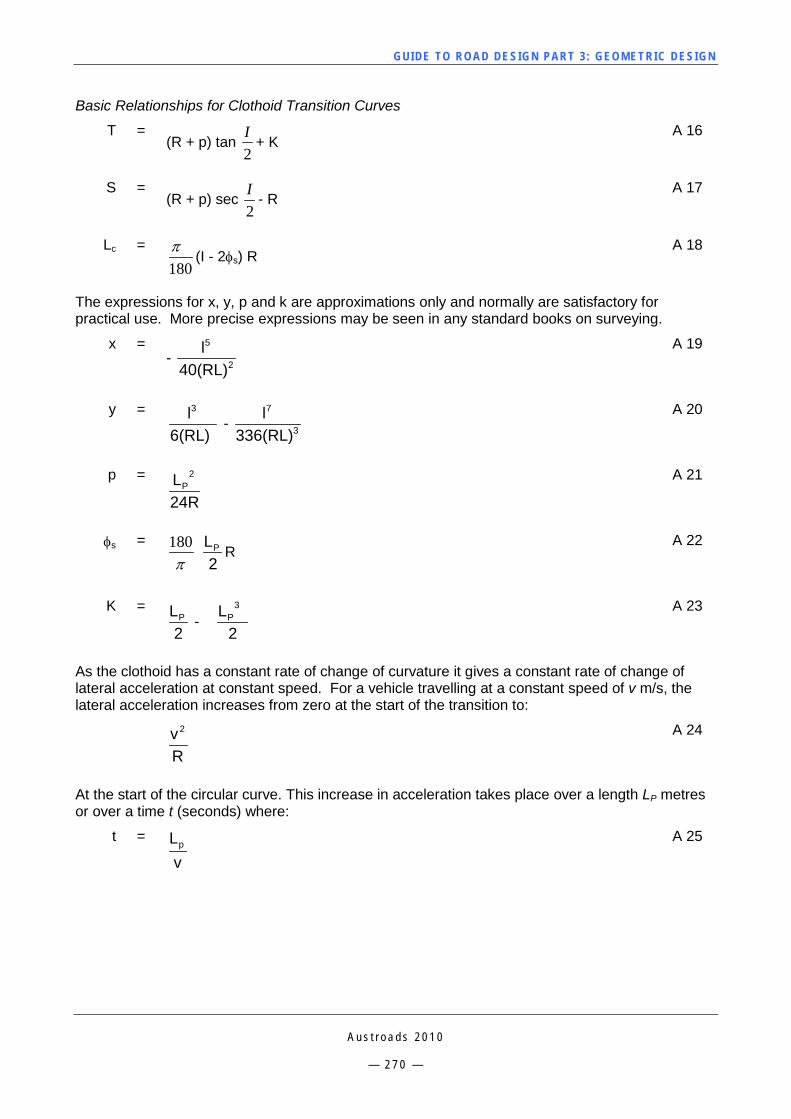
GUI DE TO RO A D DE SIG N P ART 3 : GEO MET RI C D ESI G N
A u s t r o a d s 2 0 1 0
— 2 7 0 —
Basic Relationships for Clothoid Transition Curves
T = (R + p) tan
2I
+ K A 16
S = (R + p) sec
2I
- R A 17
Lc = 180π
(I - 2φs) R A 18
The expressions for x, y, p and k are approximations only and normally are satisfactory for practical use. More precise expressions may be seen in any standard books on surveying.
x = - 2
5
40(RL)l
A 19
y =
6(RL)l3
- 3
7
336(RL)l
A 20
p =
24RL 2
P A 21
φs = π
180
2LP R
A 22
K =
2LP -
2L 3
P A 23
As the clothoid has a constant rate of change of curvature it gives a constant rate of change of lateral acceleration at constant speed. For a vehicle travelling at a constant speed of v m/s, the lateral acceleration increases from zero at the start of the transition to:
Rv2
A 24
At the start of the circular curve. This increase in acceleration takes place over a length LP metres or over a time t (seconds) where:
t =
vLp
A 25

GUI DE TO RO A D DE SIG N P ART 3 : GEO MET RI C D ESI G N
A u s t r o a d s 2 0 1 0
— 2 7 1 —
Thus, the rate of change of lateral acceleration, A m/s3
=
Rv2
/ v
LP A 26
=
P
3
RLv m/s3
A 27
If v m/s is converted to V km/h, this equation becomes: A m/s3 =
P
3
RLV 0.0214
where V is in km/h A 28
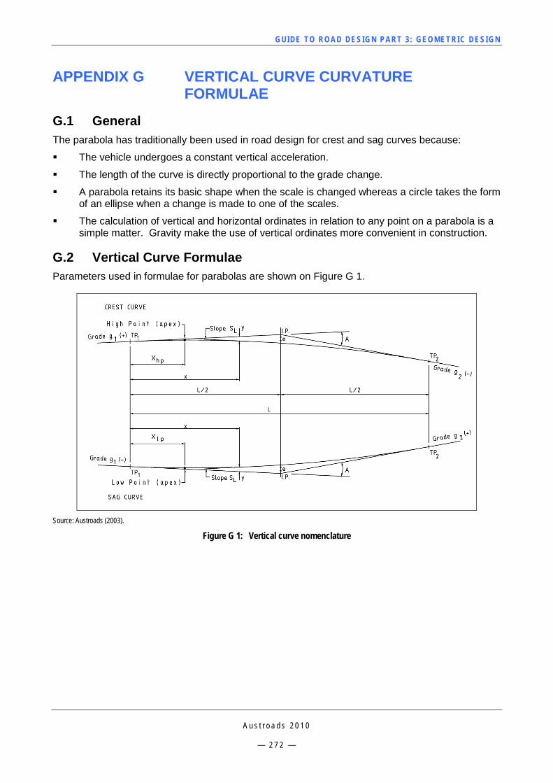
GUI DE TO RO A D DE SIG N P ART 3 : GEO MET RI C D ESI G N
A u s t r o a d s 2 0 1 0
— 2 7 2 —
APPENDIX G VERTICAL CURVE CURVATURE FORMULAE
G.1 General The parabola has traditionally been used in road design for crest and sag curves because:
The vehicle undergoes a constant vertical acceleration.
The length of the curve is directly proportional to the grade change.
A parabola retains its basic shape when the scale is changed whereas a circle takes the form of an ellipse when a change is made to one of the scales.
The calculation of vertical and horizontal ordinates in relation to any point on a parabola is a simple matter. Gravity make the use of vertical ordinates more convenient in construction.
G.2 Vertical Curve Formulae Parameters used in formulae for parabolas are shown on Figure G 1.
Source: Austroads (2003).
Figure G 1: Vertical curve nomenclature
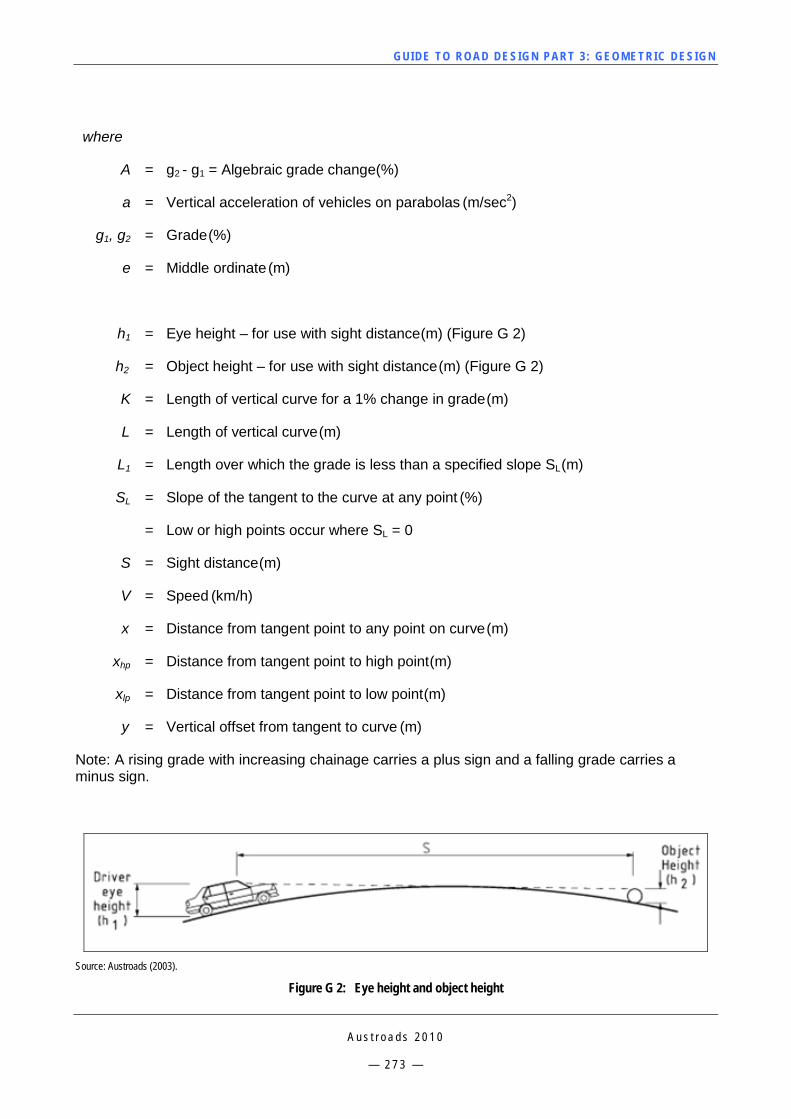
GUI DE TO RO A D DE SIG N P ART 3 : GEO MET RI C D ESI G N
A u s t r o a d s 2 0 1 0
— 2 7 3 —
where
A = g2 - g1 = Algebraic grade change (%)
a = Vertical acceleration of vehicles on parabolas (m/sec2)
g1, g2 = Grade (%)
e = Middle ordinate (m)
h1 = Eye height – for use with sight distance (m) (Figure G 2)
h2 = Object height – for use with sight distance (m) (Figure G 2)
K = Length of vertical curve for a 1% change in grade (m)
L = Length of vertical curve (m)
L1 = Length over which the grade is less than a specified slope SL (m)
SL = Slope of the tangent to the curve at any point (%)
= Low or high points occur where SL = 0
S = Sight distance (m)
V = Speed (km/h)
x = Distance from tangent point to any point on curve (m)
xhp = Distance from tangent point to high point (m)
xlp = Distance from tangent point to low point (m)
y = Vertical offset from tangent to curve (m)
Note: A rising grade with increasing chainage carries a plus sign and a falling grade carries a minus sign.
Source: Austroads (2003).
Figure G 2: Eye height and object height
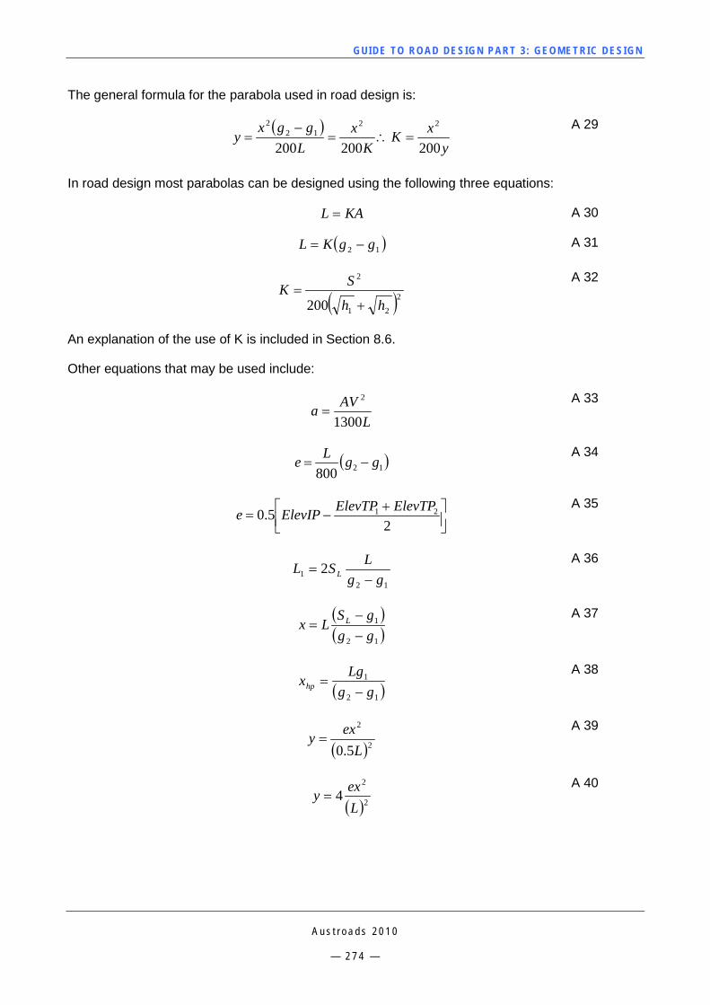
GUI DE TO RO A D DE SIG N P ART 3 : GEO MET RI C D ESI G N
A u s t r o a d s 2 0 1 0
— 2 7 4 —
The general formula for the parabola used in road design is:
( )y
xKK
xL
ggxy200200200
2212
2
=∴=−
= A 29
In road design most parabolas can be designed using the following three equations:
KAL = A 30
( )12 ggKL −= A 31
( )221
2
200 hh
SK+
= A 32
An explanation of the use of K is included in Section 8.6.
Other equations that may be used include:
LAVa
1300
2
= A 33
( )12800ggLe −=
A 34
+
−=2
5.0 21 ElevTPElevTPElevIPe A 35
121 2
ggLSL L −
= A 36
( )( )12
1
gggSLx L
−−
= A 37
( )12
1
ggLgxhp −
= A 38
( )2
2
5.0 Lexy =
A 39
( )2
2
4Lexy =
A 40
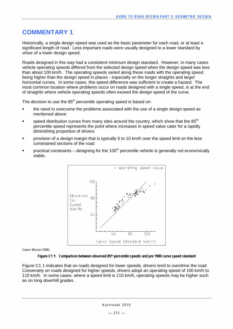
GUI DE TO RO A D DE SIG N P ART 3 : GEO MET RI C D ESI G N
A u s t r o a d s 2 0 1 0
— 2 7 5 —
COMMENTARY 1 Historically, a single design speed was used as the basic parameter for each road, or at least a significant length of road. Less important roads were usually designed to a lower standard by virtue of a lower design speed.
Roads designed in this way had a consistent minimum design standard. However, in many cases vehicle operating speeds differed from the selected design speed when the design speed was less than about 100 km/h. The operating speeds varied along these roads with the operating speed being higher than the design speed in places - especially on the longer straights and larger horizontal curves. In some cases, this speed difference was sufficient to create a hazard. The most common location where problems occur on roads designed with a single speed, is at the end of straights where vehicle operating speeds often exceed the design speed of the curve.
The decision to use the 85th percentile operating speed is based on:
the need to overcome the problems associated with the use of a single design speed as mentioned above
speed distribution curves from many sites around the country, which show that the 85th percentile speed represents the point where increases in speed value cater for a rapidly diminishing proportion of drivers
provision of a design margin that is typically 6 to 10 km/h over the speed limit on the less constrained sections of the road
practical constraints – designing for the 100th percentile vehicle is generally not economically viable.
Source: McLean (1988).
Figure C1 1: Comparison between observed 85th percentile speeds and pre 1980 curve speed standard
Figure C1 1 indicates that on roads designed for lower speeds, drivers tend to overdrive the road. Conversely on roads designed for higher speeds, drivers adopt an operating speed of 100 km/h to 110 km/h. In some cases, where a speed limit is 110 km/h, operating speeds may be higher such as on long downhill grades.
GUI DE TO RO A D DE SIG N P ART 3 : GEO MET RI C D ESI G N
A u s t r o a d s 2 0 1 0
— 2 7 6 —
Previous studies (Krammes et al. 1993 and McLean 1978) have documented a noticeable disparity between design and operating speeds. Results indicated that horizontal curves with design speeds less than 90 km/h had 85th percentile speeds that were consistently faster than the design speed, whereas curves with design speeds greater than 90 km/h had 85th percentile speeds that were consistently slower than the design speed. The observed relationship between design and operating speed is shown in Figure C1 1.
COMMENTARY 2 Studies have shown that drivers select their speeds based on what they perceive to be a safe speed for the road environment. Research has also shown that drivers are not very good at assessing the level of risk posed by the road environment, e.g. trees close to the road don’t typically slow drivers down. Designers should refer to the Guide to Road Safety – Part 5: Safety for Rural and Remote Areas (Austroads 2006d).
COMMENTARY 3 While it is considered desirable that an operating speed model be adopted for the design of urban roads, further research is required to validate the model for use on these roads. Additional factors relevant to the development of an operating speed model for urban roads (when compared with the model for rural roads) requiring investigation, include:
the impact of intersections and traffic control devices accident prevention factors (radius tracking, curve width) several unresolved areas of driver behavior (excess speed, increasing speed in curves,
acceleration factors in straights, effect of enforcement).
A literature review was undertaken by the NSW RTA in an effort to determine the physical factors that influence vehicle operating speeds in urban areas. The review identified the following modifiers to behaviour:
geometric road design
street type, cross-section and function, for example: — more lanes will generally lead to higher speeds — kerb and channel present will generally lead to higher speeds
speed limit
surrounding environment (CBD, residential, commercial etc.) — commercial (e.g. strip shopping centre will tend to lead to slower speeds)
interaction with vulnerable road users (pedestrians, cyclists etc.) — footpaths present may lead to slower speeds
density of roadside objects — more objects (utility poles, roadside furniture etc.) will reduce speeds
parked vehicles — vehicles parked on the road will lead to slower speeds
GUI DE TO RO A D DE SIG N P ART 3 : GEO MET RI C D ESI G N
A u s t r o a d s 2 0 1 0
— 2 7 7 —
bus stops will reduce speeds
number of entries/exits to the main flow (driveways, intersections with minor roads etc.) — more driveways/intersections will likely lead to slower speeds
traffic flow measures, including intensity, directional distribution, rate of through traffic).
For further information, refer to Wang et al. 2006, Fitzpatrick et al. 2001, Brundell-Freij & Ericsson, 2005, Poe, Tarris & Mason, Jr., 1995.
Other factors may also influence operating speed. These factors are generally based in behavioural science principles, and rely on inference from psychological knowledge in areas outside of road safety and design to predict the changes to driver behaviour through the perception of the roadway and the surrounding environment. Some potential behaviour modifiers are presented below:
Increased external information or stimuli, or, a ‘busy’ environment may distract people, or may overload their cognitive resources. This may lead to a higher perceived level of risk, which may lead to a lower overall speed. Once the section is passed, the speed may actually be higher than average, as drivers attempt to make up for lost time.
Poorer road conditions may lead to a higher risk perception, which could lower speeds.
Transit or bus lanes may also affect speed. This could be because of a reduction in lane width, a change in the traffic composition or dynamics, an increased perception of risk in the area because of the likelihood of pedestrians, or because of the loss of capacity on the road through the addition of the bus or transit lane.
A higher level of pedestrian activity may lead to a higher level of risk perception, which could lower speeds.
Smoother (meaning less vibration and noise in the cabin of the vehicle) roads can reduce the physical stimuli that drivers receive and may contribute to higher speeds.
For night driving, a well-lit road could lead to higher speeds as drivers have a lower perception of risk in the area.
A high truck composition in the general traffic stream may contribute to a higher risk perception, which could lower vehicle speeds.
A greater cleared area adjacent to the road may provide a lower risk perception, which may lead to higher speeds.
Increased enforcement levels or perception of high enforcement may lead to slower speeds.
Roads that are familiar to the users may lower risk perception and potentially increase speeds.
Easier navigation within an area could lower risk perception and increase speeds.
Roads that present a perceived significant risk at all times, or are adjacent to significant social areas can attract sensation seekers who will take risks in order to demonstrate their ‘prowess’.
The above factors, as stated above, are based upon inference from other areas of psychological knowledge. They are yet to be formally studied and accepted by the academic community as behaviour modifiers.
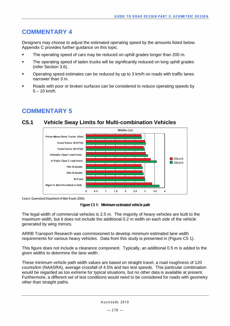
GUI DE TO RO A D DE SIG N P ART 3 : GEO MET RI C D ESI G N
A u s t r o a d s 2 0 1 0
— 2 7 8 —
COMMENTARY 4 Designers may choose to adjust the estimated operating speed by the amounts listed below. Appendix C provides further guidance on this topic.
The operating speed of cars may be reduced on uphill grades longer than 200 m.
The operating speed of laden trucks will be significantly reduced on long uphill grades (refer Section 3.6).
Operating speed estimates can be reduced by up to 3 km/h on roads with traffic lanes narrower than 3 m.
Roads with poor or broken surfaces can be considered to reduce operating speeds by 5 – 10 km/h.
COMMENTARY 5
C5.1 Vehicle Sway Limits for Multi-combination Vehicles
Source: Queensland Department of Main Roads (2004).
Figure C5 1: Minimum estimated vehicle path
The legal width of commercial vehicles is 2.5 m. The majority of heavy vehicles are built to the maximum width, but it does not include the additional 0.2 m width on each side of the vehicle generated by wing mirrors.
ARRB Transport Research was commissioned to develop minimum estimated lane width requirements for various heavy vehicles. Data from this study is presented in (Figure C5 1).
This figure does not include a clearance component. Typically, an additional 0.5 m is added to the given widths to determine the lane width.
These minimum vehicle path width values are based on straight travel, a road roughness of 120 counts/km (NAASRA), average crossfall of 4.5% and two test speeds. This particular combination would be regarded as too extreme for typical situations, but no other data is available at present. Furthermore, a different set of test conditions would need to be considered for roads with geometry other than straight paths.
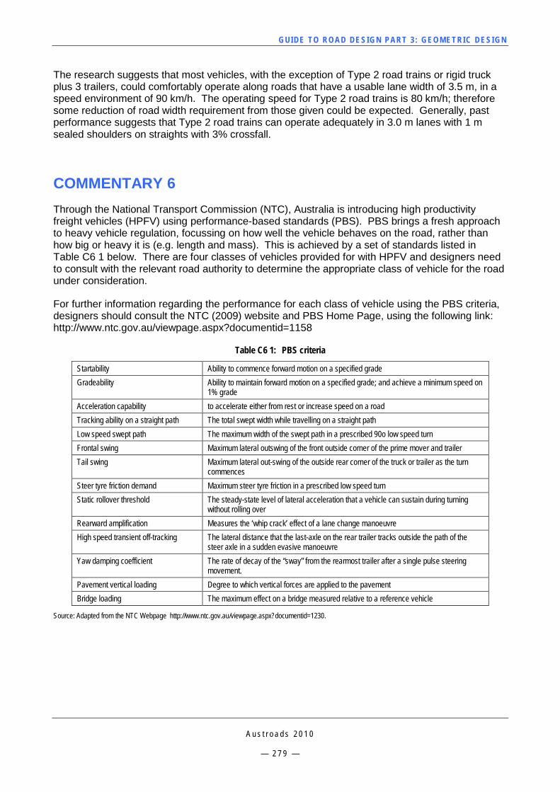
GUI DE TO RO A D DE SIG N P ART 3 : GEO MET RI C D ESI G N
A u s t r o a d s 2 0 1 0
— 2 7 9 —
The research suggests that most vehicles, with the exception of Type 2 road trains or rigid truck plus 3 trailers, could comfortably operate along roads that have a usable lane width of 3.5 m, in a speed environment of 90 km/h. The operating speed for Type 2 road trains is 80 km/h; therefore some reduction of road width requirement from those given could be expected. Generally, past performance suggests that Type 2 road trains can operate adequately in 3.0 m lanes with 1 m sealed shoulders on straights with 3% crossfall.
COMMENTARY 6 Through the National Transport Commission (NTC), Australia is introducing high productivity freight vehicles (HPFV) using performance-based standards (PBS). PBS brings a fresh approach to heavy vehicle regulation, focussing on how well the vehicle behaves on the road, rather than how big or heavy it is (e.g. length and mass). This is achieved by a set of standards listed in Table C6 1 below. There are four classes of vehicles provided for with HPFV and designers need to consult with the relevant road authority to determine the appropriate class of vehicle for the road under consideration.
For further information regarding the performance for each class of vehicle using the PBS criteria, designers should consult the NTC (2009) website and PBS Home Page, using the following link: http://www.ntc.gov.au/viewpage.aspx?documentid=1158
Table C6 1: PBS criteria
Startability Ability to commence forward motion on a specified grade Gradeability Ability to maintain forward motion on a specified grade; and achieve a minimum speed on
1% grade Acceleration capability to accelerate either from rest or increase speed on a road Tracking ability on a straight path The total swept width while travelling on a straight path Low speed swept path The maximum width of the swept path in a prescribed 90o low speed turn Frontal swing Maximum lateral outswing of the front outside corner of the prime mover and trailer Tail swing Maximum lateral out-swing of the outside rear corner of the truck or trailer as the turn
commences Steer tyre friction demand Maximum steer tyre friction in a prescribed low speed turn Static rollover threshold The steady-state level of lateral acceleration that a vehicle can sustain during turning
without rolling over Rearward amplification Measures the ‘whip crack’ effect of a lane change manoeuvre High speed transient off-tracking The lateral distance that the last-axle on the rear trailer tracks outside the path of the
steer axle in a sudden evasive manoeuvre Yaw damping coefficient The rate of decay of the “sway” from the rearmost trailer after a single pulse steering
movement. Pavement vertical loading Degree to which vertical forces are applied to the pavement Bridge loading The maximum effect on a bridge measured relative to a reference vehicle
Source: Adapted from the NTC Webpage http://www.ntc.gov.au/viewpage.aspx?documentid=1230.
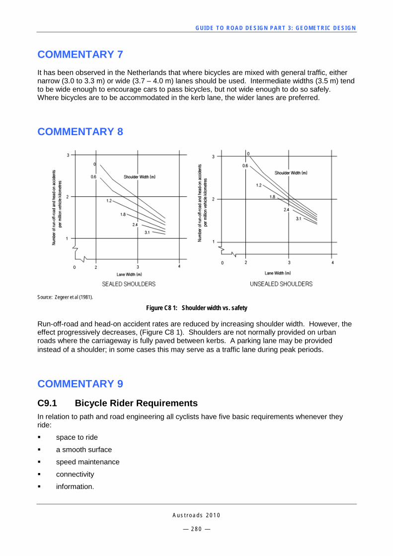
GUI DE TO RO A D DE SIG N P ART 3 : GEO MET RI C D ESI G N
A u s t r o a d s 2 0 1 0
— 2 8 0 —
COMMENTARY 7 It has been observed in the Netherlands that where bicycles are mixed with general traffic, either narrow (3.0 to 3.3 m) or wide (3.7 – 4.0 m) lanes should be used. Intermediate widths (3.5 m) tend to be wide enough to encourage cars to pass bicycles, but not wide enough to do so safely. Where bicycles are to be accommodated in the kerb lane, the wider lanes are preferred.
COMMENTARY 8
Source: Zegeer et al (1981).
Figure C8 1: Shoulder width vs. safety
Run-off-road and head-on accident rates are reduced by increasing shoulder width. However, the effect progressively decreases, (Figure C8 1). Shoulders are not normally provided on urban roads where the carriageway is fully paved between kerbs. A parking lane may be provided instead of a shoulder; in some cases this may serve as a traffic lane during peak periods.
COMMENTARY 9
C9.1 Bicycle Rider Requirements In relation to path and road engineering all cyclists have five basic requirements whenever they ride:
space to ride
a smooth surface
speed maintenance
connectivity
information.
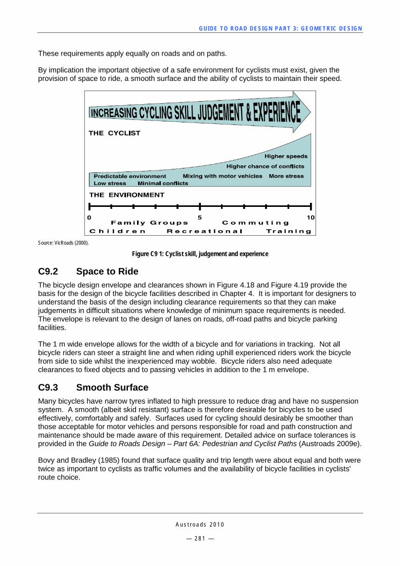
GUI DE TO RO A D DE SIG N P ART 3 : GEO MET RI C D ESI G N
A u s t r o a d s 2 0 1 0
— 2 8 1 —
These requirements apply equally on roads and on paths.
By implication the important objective of a safe environment for cyclists must exist, given the provision of space to ride, a smooth surface and the ability of cyclists to maintain their speed.
Source: VicRoads (2000).
Figure C9 1: Cyclist skill, judgement and experience
C9.2 Space to Ride The bicycle design envelope and clearances shown in Figure 4.18 and Figure 4.19 provide the basis for the design of the bicycle facilities described in Chapter 4. It is important for designers to understand the basis of the design including clearance requirements so that they can make judgements in difficult situations where knowledge of minimum space requirements is needed. The envelope is relevant to the design of lanes on roads, off-road paths and bicycle parking facilities.
The 1 m wide envelope allows for the width of a bicycle and for variations in tracking. Not all bicycle riders can steer a straight line and when riding uphill experienced riders work the bicycle from side to side whilst the inexperienced may wobble. Bicycle riders also need adequate clearances to fixed objects and to passing vehicles in addition to the 1 m envelope.
C9.3 Smooth Surface Many bicycles have narrow tyres inflated to high pressure to reduce drag and have no suspension system. A smooth (albeit skid resistant) surface is therefore desirable for bicycles to be used effectively, comfortably and safely. Surfaces used for cycling should desirably be smoother than those acceptable for motor vehicles and persons responsible for road and path construction and maintenance should be made aware of this requirement. Detailed advice on surface tolerances is provided in the Guide to Roads Design – Part 6A: Pedestrian and Cyclist Paths (Austroads 2009e).
Bovy and Bradley (1985) found that surface quality and trip length were about equal and both were twice as important to cyclists as traffic volumes and the availability of bicycle facilities in cyclists' route choice.
GUI DE TO RO A D DE SIG N P ART 3 : GEO MET RI C D ESI G N
A u s t r o a d s 2 0 1 0
— 2 8 2 —
C9.4 Speed Maintenance For bicycles to be most effective as a means of transport cyclists must be able to maintain speed without having to slow or stop often. Cyclists typically travel at speeds between 20 km/h and 30 km/h although they may reach in excess of 50 km/h down hills. Once slowed or stopped it takes considerable time and effort to regain the desired operating speed.
Bicycle routes, especially off-road, should be designed for continuous riding, minimising the need to slow or stop for any reason including steep gradients, rough surfaces, sharp corners, obscured sight lines, intersections, or to give way to other people because the width available is too narrow. On many roads cyclists are confined to the extreme lefthand side by motor vehicles and a rough surface prevents cyclists from maintaining an acceptable speed.
C9.5 Connectivity Connectivity is that quality of a bicycle route or route network, describing the continuous nature of facilities or of the continuous nature of desired conditions.
Cyclists need to be able to undertake and complete meaningful trips by bicycle. For recreation it may be from a residential area to a picnic spot, for a specific purpose trip from home to work or the shops. Bicycle routes comprising roads and paths should combine to form an effective, convenient and safe network.
Connectivity is an important aspect of the construction of effective bicycle routes. Before a route is constructed the purpose of the route should be identified as well as the routes which cyclists are likely to use in travelling to and from the paths, bicycle lanes and roads forming the network.
A route for cyclists which starts and ends abruptly is undesirable and may be hazardous as it may lure inexperienced cyclists to a point where they are at risk, perhaps having to ride along or across busy roads to complete their intended trip.
On road bicycle facilities may take the form of:
dedicated bicycle lanes
road shoulders
widened lanes for joint use by bicycles and moving or parked vehicles
separated bicycle lanes, e.g. ‘Copenhagen bicycle lanes’ or ‘Kerb-separated bicycle lanes’.
Off-road bicycle facilities typically take the form of shared pathways for use by both cyclists and pedestrians, and these are described in more detail in the Guide to Road Design – Part 6A: Pedestrian and Cyclist Paths (Austroads 2009e).
The potential safety concerns of including the channel as part of the bicycle lane width include:
edge drop off between the pavement and channel surfaces, particularly when open graded friction course (OGFC) is used
hazards in and adjacent to the kerb and channel such as the surface condition of the channel and drainage pit entrances
the likelihood of the bicycle pedals striking the kerb.
In constrained locations the designer shall determine whether it is safe to include the channel as part of the bicycle lane width by considering factors such as those listed above.
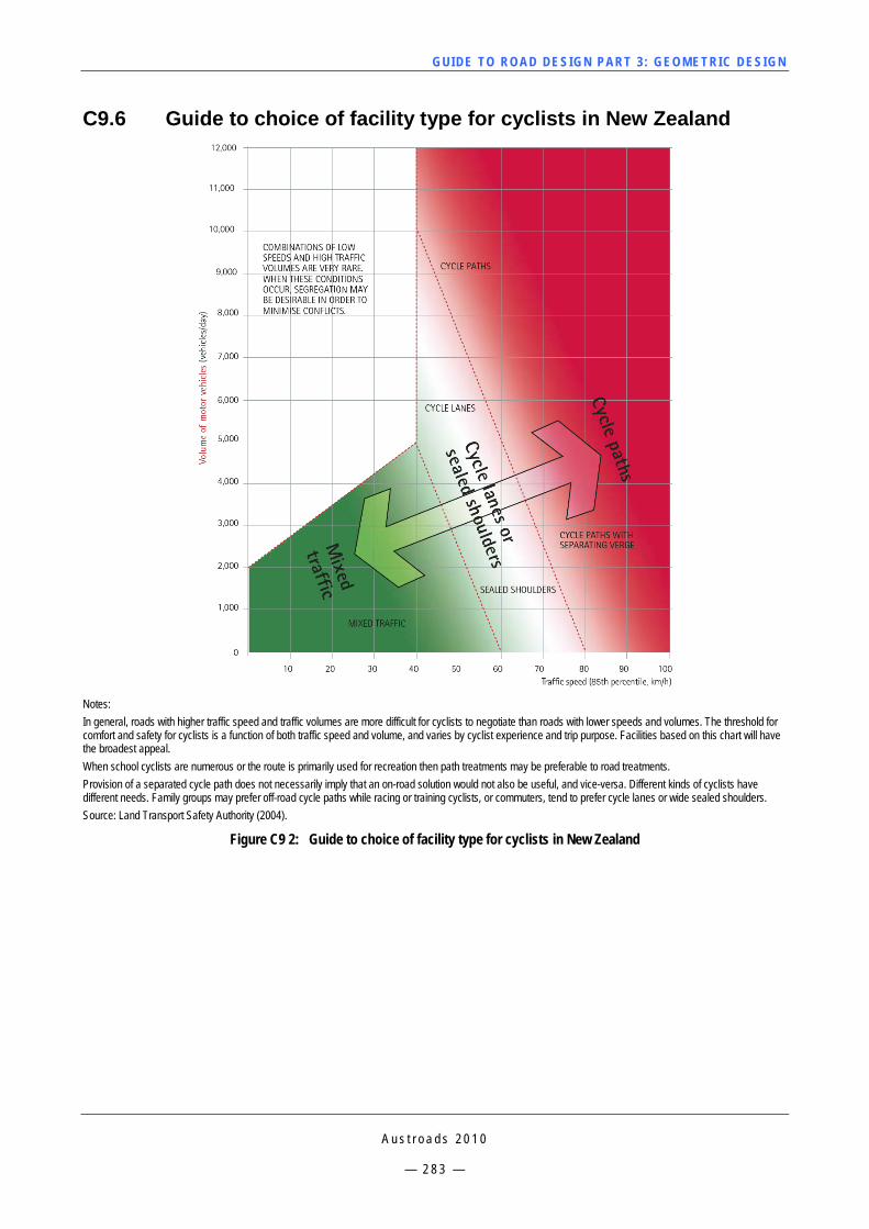
GUI DE TO RO A D DE SIG N P ART 3 : GEO MET RI C D ESI G N
A u s t r o a d s 2 0 1 0
— 2 8 3 —
C9.6 Guide to choice of facility type for cyclists in New Zealand
Notes: In general, roads with higher traffic speed and traffic volumes are more difficult for cyclists to negotiate than roads with lower speeds and volumes. The threshold for comfort and safety for cyclists is a function of both traffic speed and volume, and varies by cyclist experience and trip purpose. Facilities based on this chart will have the broadest appeal. When school cyclists are numerous or the route is primarily used for recreation then path treatments may be preferable to road treatments. Provision of a separated cycle path does not necessarily imply that an on-road solution would not also be useful, and vice-versa. Different kinds of cyclists have different needs. Family groups may prefer off-road cycle paths while racing or training cyclists, or commuters, tend to prefer cycle lanes or wide sealed shoulders. Source: Land Transport Safety Authority (2004).
Figure C9 2: Guide to choice of facility type for cyclists in New Zealand
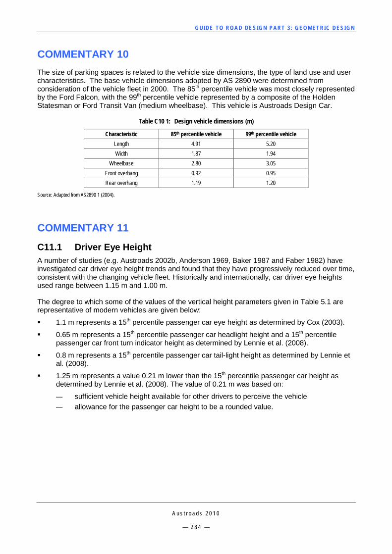
GUI DE TO RO A D DE SIG N P ART 3 : GEO MET RI C D ESI G N
A u s t r o a d s 2 0 1 0
— 2 8 4 —
COMMENTARY 10 The size of parking spaces is related to the vehicle size dimensions, the type of land use and user characteristics. The base vehicle dimensions adopted by AS 2890 were determined from consideration of the vehicle fleet in 2000. The 85th percentile vehicle was most closely represented by the Ford Falcon, with the 99th percentile vehicle represented by a composite of the Holden Statesman or Ford Transit Van (medium wheelbase). This vehicle is Austroads Design Car.
Table C10 1: Design vehicle dimensions (m)
Characteristic 85th percentile vehicle 99th percentile vehicle Length 4.91 5.20 Width 1.87 1.94
Wheelbase 2.80 3.05 Front overhang 0.92 0.95 Rear overhang 1.19 1.20
Source: Adapted from AS2890 1 (2004).
COMMENTARY 11
C11.1 Driver Eye Height A number of studies (e.g. Austroads 2002b, Anderson 1969, Baker 1987 and Faber 1982) have investigated car driver eye height trends and found that they have progressively reduced over time, consistent with the changing vehicle fleet. Historically and internationally, car driver eye heights used range between 1.15 m and 1.00 m.
The degree to which some of the values of the vertical height parameters given in Table 5.1 are representative of modern vehicles are given below:
1.1 m represents a 15th percentile passenger car eye height as determined by Cox (2003).
0.65 m represents a 15th percentile passenger car headlight height and a 15th percentile passenger car front turn indicator height as determined by Lennie et al. (2008).
0.8 m represents a 15th percentile passenger car tail-light height as determined by Lennie et al. (2008).
1.25 m represents a value 0.21 m lower than the 15th percentile passenger car height as determined by Lennie et al. (2008). The value of 0.21 m was based on:
— sufficient vehicle height available for other drivers to perceive the vehicle — allowance for the passenger car height to be a rounded value.
GUI DE TO RO A D DE SIG N P ART 3 : GEO MET RI C D ESI G N
A u s t r o a d s 2 0 1 0
— 2 8 5 —
COMMENTARY 12
C12.1 Driver Reaction Time Research studies have shown that an average reaction time of 2.5 seconds is typical although the variance of the distribution of reaction times is very high (Armour 1976, Garber and Hoel (1988), McCormick and Sanders (1982), Triggs and Harris (1982), Austroads 2000)). Values of up to 7 seconds have been recorded at one extreme, and, at the other extreme, 1.0 second times have been measured with forced stops (Armour 1976). One reason for the large variability is that reaction time depends on a driver’s level of alertness at the time. Similarly, anticipation or pre-signalling of an event, the absence of uncertainty on multiple choices, and the familiarity with the task can each lower reaction time.
Consequently, the reaction time of 2.5 seconds is a commonly adopted value, although a number of European countries specify a value of 2.0 seconds.
A recent study investigating road safety and design for older drivers (Austroads 2000) recommended a minimum reaction time of 2.5 seconds at intersections. For mid-block sections it recommended a desirable minimum reaction time of 2.5 seconds and an absolute minimum of 2.0 seconds. The aging of drivers emphasises the importance of these recommendations.
As people age, they experience decreasing physical and mental capabilities and become more susceptible to injury and shock. Human functions subject to deterioration due to ageing include:
visual acuity
attention capacity
reaction time
contrast sensitivity.
As a group, older drivers do not currently represent a major road safety problem in most Western societies when compared with other age groups. However, older drivers are involved in significantly more serious injury and casualty crashes per kilometre travelled. Furthermore, as the proportion of older people in Australia is expected to roughly double over the next 40 years, older drivers are likely to become a more significant problem in the years ahead (Austroads 2000).
Recent research (Austroads 2000) indicates that a number of road design elements may be associated with older driver crashes in Australasia. In particular, it was concluded that improvements to intersection sight distances, provision for separate turn phases at traffic signals, more conspicuous traffic signal lanterns and more clearly defined vehicle paths have the potential to reduce crash and injury risk for older drivers. The research includes a detailed description of measures that should be implemented immediately in Australia to increase the safety of older road users.
The degrees to which the reaction times given in Table 5.2 are representative of driving conditions are given below:
1.5s represents at least a mean value for surprise stopping for all drivers from a number of tests around the world – refer pages 24 and 32 of Fambro et al. (1997), Summala (2002), Green (2000) and Exhibit 2-26 in AASHTO (2001). The data in Summala (2002) suggests that ‘urgency’ ensures that 1.5s may be an 85th percentile value or better (in good conditions at least) for drivers travelling at the 85th percentile speed. This is further supported by Figure 4 in Durth and Bernhard (2000).
GUI DE TO RO A D DE SIG N P ART 3 : GEO MET RI C D ESI G N
A u s t r o a d s 2 0 1 0
— 2 8 6 —
2.0s represents at least an 85th percentile value and possibly a 95th percentile value for all car drivers – refer Fambro et al. (1997) (see pages 32 and 74).
2.5s represents better than a 90th percentile value and possibly better than a 95th percentile value for all drivers – refer Fambro et al. (1997) (see page 74).
COMMENTARY 13 C13.1 Longitudinal Deceleration (Longitudinal Friction Factor) McLean 1988 noted that the limiting values for longitudinal friction factor were based on producing stopping sight distance requirements which would lead to what was considered to be an appropriate balance between horizontal and crest vertical curve standards. The balance achieved appears to be generally consistent with international practice, although, relative to North America and earlier Australian practice, minimum sight distance requirements are a little high.
The degrees to which the values of the coefficient of deceleration given in Table 5.3 are representative of driving conditions are given below:
0.61 represents the average braking capability in dry conditions – refer Fambro et al. (1997).
0.46 represents the average braking capability in wet conditions – refer Fambro et al. (1997).
0.36 represents about a 90th percentile value for braking on wet, sealed roads – refer Fambro et al. (1997). This value continues to be used in Austroads guides as the maximum coefficient of deceleration for the design of deceleration lanes at intersections.
0.26 represents comfortable deceleration. This value continues to be used in Austroads guides as the maximum desirable coefficient of deceleration for the design of deceleration lanes at intersections.
0.29 represents braking by single unit trucks, semi-trailers and B-doubles on dry roads – refer Di Cristoforo et al. (2004).
0.28 represents braking by Type 1 road trains on dry roads – value derived from Di Cristoforo et al. (2004).
0.26 represents braking by Type 2 road trains on dry roads – value derived from Di Cristoforo et al. (2004).
For the purposes of relating the values of the coefficient of deceleration above to actual driving conditions, the following is provided. Passengers find that 3m/s2 (d = 0.31) is comfortable deceleration – refer Table 27.1 in Lay (1998). Lay also states that about 4m/s2 (d = 0.41) is the maximum deceleration that drivers will use when a traffic signal changes. Otherwise, they will continue through. Exhibit 2-25 in AASHTO (2001) uses 4.2m/s2 (d = 0.43) as the maximum rate for cars approaching an intersection in wet conditions. Exhibit 2-25 in AASHTO (2001) uses 5.7m/s2 (d = 0.58) as the maximum rate for cars approaching an intersection in dry conditions. Lay explains that deceleration of 6m/s2 (d = 0.61) is consciously used by only a few drivers. In other words, this rate is in the domain of emergency situations – which is the intent of the stopping sight distance model.
GUI DE TO RO A D DE SIG N P ART 3 : GEO MET RI C D ESI G N
A u s t r o a d s 2 0 1 0
— 2 8 7 —
COMMENTARY 14
C14.1 Truck Stopping Sight Distance A comparison of international sight distance design practices (Harwood et al. 1998) noted that SSD only refers to cars. Truck stopping sight distance is not considered by most of the countries reviewed. A typical reason for this can be found in AASHTO 1994:
The derived minimum stopping sight distances directly reflect passenger car operation and might be questioned for use in design for truck operations. Trucks as a whole, especially the larger and heavier units, require longer stopping distances for a given speed than passenger vehicles do. However, there is one factor that tends to balance the additional braking lengths for trucks for given speeds with those for passenger cars. The truck operator is able to see the vertical features of the obstruction substantially farther because of the higher position of the seat in the vehicle. Separate stopping sight distances for trucks and passenger cars, therefore, are not used in highway design standards.
However, this is quite contrary to the findings of a review of references on truck performance characteristics (Donaldson 1986, Fancher 1986 and PIARC 1995), which suggest that the sight distance advantages provided by the higher driver eye level in trucks do not compensate for the inferior braking of trucks. Particularly at locations with lateral sight distance restrictions, the benefits of the higher eye level could be lost and provision of longer SSD or other remedial measures, such as signing and higher friction surfaces would be needed.
The reasons for the longer truck braking distances include:
Poor braking characteristics of empty trucks – Empty trucks have poor braking characteristics and this is reflected in comparatively high crash rates. The problem relates to the suspension and tyres, which are designed for maximum efficiency under load.
Uneven load between axles – When the load is not evenly distributed between axles, one axle can slip sideways and create instability in others (up to 15% of braking efficiencies can be lost).
Inefficient brakes of articulated trucks – Fifty percent of trucks tested on the roads in the US could not meet the required braking standards. Many drivers immobilise their front brakes to reduce the possibility of jack-knifing.
Effect of road curvature – Trucks require longer SSD on curves than on straights because some of the friction available at the road/tyre interface is used to hold the vehicle in a circular path.
The braking of articulated vehicles must be in the form of controlled braking without wheel locking in order to avoid jack-knifing if wheels lock at different times. Without the aid of antilock braking systems, the friction coefficient used in controlled braking is usually less than that for locked wheel braking. The coefficients of deceleration for cars in Table 5.3 involve locked wheel braking.
Truck tyres are designed primarily for wear resistance. Consequently, they tend to have lower wet friction coefficients than cars.
GUI DE TO RO A D DE SIG N P ART 3 : GEO MET RI C D ESI G N
A u s t r o a d s 2 0 1 0
— 2 8 8 —
In situations where driver eye height provides no advantage, the only parameter that offsets the poorer braking performance of trucks is the assumed lower operating speed as per Table 3.4. Therefore, some further justification or basis of the truck operating speeds should be given. For example:
The lower operating speed for trucks is an average condition with truck speeds varying more than car speeds due to grades, poorer acceleration, etc.
When checking braking and stopping sight distance provision for trucks, it is acceptable to use the lower truck operating speed for a corresponding car operating speed. This is because an acceptable level of safety is provided through the assumptions of: — wet conditions — unladen state — no antilock braking system — there is no additional assumption of a reduction in operating speed due to wet
conditions.
COMMENTARY 15 The relatively small number of accidents involving objects on the roadway at night is probably due to the factor of safety implicit in the various assumptions in sight distance calculations and the low exposure (i.e. likelihood of objects being on the road).
In addition to the problem of beam illumination, the question of the angle of the beam is relevant in sags. It is inappropriate for the beam to be aimed above the horizontal position because of glare to opposing drivers and a figure of 0.5° depression is an appropriate assumption. A headlight aiming angle of 0.5o depressed will allow an effective 1° elevation of the beam to be used in design due to vertical spread.
COMMENTARY 16 Transition curves have been applied to obtain the following advantages:
Provide a natural path for vehicles moving from a straight to a circular curve and enable centripetal acceleration to increase gradually from zero at the start of the transition to their maximum value at the start of the circular curve. If a transition curve is not provided some drivers will encroach on adjoining lanes when entering and leaving the curve.
The transition curve length provides a convenient desirable arrangement for superelevation runoff. The transition between the crossfall on the straight and the fully superelevated section on the curve can be effected along the length of the transition curve in a manner closely fitting the speed-radius relation for the vehicle traversing it.
Where superelevation runoff is affected without a transition curve, it has been common practice to match the superelevation runoff with the likely transition path the vehicles take when entering or leaving the circular curve.
A transition facilitates the change in width where the pavement section is to be widened around a circular curve. Use of transitions provides flexibility in the widening on sharp curves.
Improve the appearance of the curve ahead.
GUI DE TO RO A D DE SIG N P ART 3 : GEO MET RI C D ESI G N
A u s t r o a d s 2 0 1 0
— 2 8 9 —
Despite the advantages of using transition curves, there are also possible adverse effects associated with transitions. Some research studies undertaken indicate the following disadvantages:
Transitions at the start of horizontal curves give the impression of magnifying the radius of the curve ahead. This may encourage drivers to approach the curve too quickly; drivers regulate their speed from the apparent curvature of the road ahead and in practice, there is some variation in curve entry speeds. In these circumstances, longer transitions may cause drivers to perceive a higher standard of curvature than there is, with consequent increased speed and friction demand on the circular section of the curve.
Transitions hide the tangent-to-curve point making it difficult to identify the start of the curve. This results in drivers reducing speed on the approach to curves so that they can judge when to commence braking.
Transition curves at the start of circular curves are reported to lead to a higher single vehicle accident rate than circular curves without transitions, for the above reasons. However, other studies indicate that single vehicle accident rates on circular curves with transitions are similar to those for circular curves without transitions (Krammes & Brackett, et al. 1993). Overseas studies have found that there have been higher accident rates on some curves with a combination of long transition (typically with more than twice the length based on superelevation development) and small to medium radii.
When drivers brake on curves, a combination of forces applies on the tyres, effectively reducing the maximum force that can be developed for braking or cornering. Articulated trucks also have problems with braking on curves because of the tendency of these vehicles to jack-knife. On curves with transition approaches, braking occurs on the spiral. This could create a problem if the driver does not commence braking sufficiently early.
Transitions can read like small radius circular curves at the end of long straights with long transitions.
COMMENTARY 17 Side friction factor f is the friction force divided by the weight perpendicular to the pavement and is expressed as the following formula:
e
127RVf
2
−= C 1
where
V = operating speed, km/h
R = radius of horizontal curve, m
e = superelevation, m/m.
The upper limit of this factor is that at which the tyre is skidding or at the point of impending skid (AASHTO 1994). The side friction factor at which side skidding is imminent depends on:
vehicle operating speed
the type and condition of the roadway surface
the type and condition of the tyres.
GUI DE TO RO A D DE SIG N P ART 3 : GEO MET RI C D ESI G N
A u s t r o a d s 2 0 1 0
— 2 9 0 —
If the vehicle speed was less than the permissible operating speed V, the side friction factor being called upon would be less than the design maximum side friction factor f max, and as the travel speed approaches V, then f will approach f max. The speed at which f just equals f max can be considered as a limiting (safe) speed Vs and if a vehicle is travelling in excess of Vs, then the side friction factor being called upon will exceed f max. Vs, is called the Limiting Curve Speed Standard.
The amount by which Vs exceeds V can be considered to indicate a lower bound for the margin of safety against the friction being demanded exceeding the friction that is available. That is, the quantity Vs – V can be considered a design margin of safety.
The available friction can vary both spatially (from one curve to another, at the same time) and temporally (from one time to another time at the same curve). Temporal variations in the available side friction factor are often due to changes in weather and are inevitable, and the most practicable way to minimise the total variation is to minimise the spatial variations by providing a spatially uniform road surface.
Variation in the margin of safety arises from both variations in the available friction (friction supply) and the friction demanded (friction demand) by drivers. The geometric design will have little (if any) effect on the available friction, but it can influence the behaviour of drivers (and particularly their choice of speed) (Nicholson 1998).
The values of side friction factor f for use in geometric design are shown in Table 7.4.
It is important to note that the absolute maximum values for f given in Table 7.4 assume construction and maintenance techniques that will ensure an adequate factor of safety against skidding. The susceptibility of the wearing surface to polishing, the macro-texture of the surface and the amount of bitumen used, evident at wearing surface, are all important matters in the initial construction of a pavement contributing to skid resistance. Freedom from contamination by oil spillage or loose aggregate and resealing when surface texture becomes too smooth are important aspects in maintenance of skid resistance. Normally, a pavement, which is properly maintained, will retain adequate resistance to skidding under all but extreme conditions of driver behaviour or weather.
The desirable maximum values should be used on intermediate and high-speed roads with uniform traffic flow, on which drivers are not tolerant of discomfort. These values should be adopted, if possible, to allow vehicles to maintain their lateral positions within a traffic lane and be able to comfortably change lanes if necessary.
On low speed roads with non-uniform traffic flow, drivers are more tolerant of discomfort, thus permitting employment of absolute maximum amount of side friction for use in design of horizontal curves (AASHTO 1994).
The f values given in Table 7.4, which apply only to sealed pavements, have been derived from observations of driver speed behaviour on rural road curves and revised by Botterill R (1994). Giummarra (2009) provides guidance on the friction values to be used when designing roads with unsealed pavements.
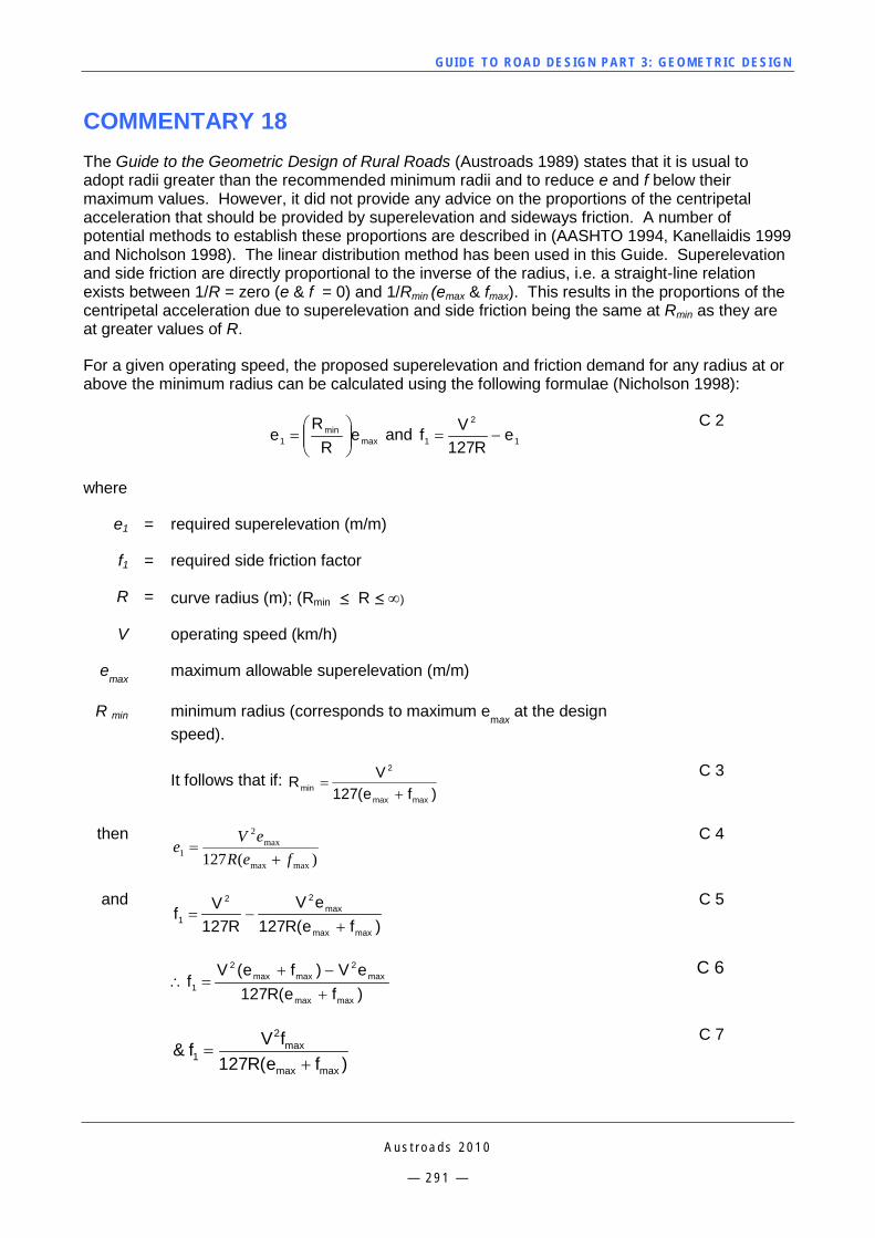
GUI DE TO RO A D DE SIG N P ART 3 : GEO MET RI C D ESI G N
A u s t r o a d s 2 0 1 0
— 2 9 1 —
COMMENTARY 18 The Guide to the Geometric Design of Rural Roads (Austroads 1989) states that it is usual to adopt radii greater than the recommended minimum radii and to reduce e and f below their maximum values. However, it did not provide any advice on the proportions of the centripetal acceleration that should be provided by superelevation and sideways friction. A number of potential methods to establish these proportions are described in (AASHTO 1994, Kanellaidis 1999 and Nicholson 1998). The linear distribution method has been used in this Guide. Superelevation and side friction are directly proportional to the inverse of the radius, i.e. a straight-line relation exists between 1/R = zero (e & f = 0) and 1/Rmin (emax & fmax). This results in the proportions of the centripetal acceleration due to superelevation and side friction being the same at Rmin as they are at greater values of R.
For a given operating speed, the proposed superelevation and friction demand for any radius at or above the minimum radius can be calculated using the following formulae (Nicholson 1998):
max
min1 e
RR
e
= and 1
2
1 eR127
Vf −= C 2
where
e1 = required superelevation (m/m)
f1 = required side friction factor
R = curve radius (m); (Rmin ≤ R ≤ ∞)
V operating speed (km/h)
emax maximum allowable superelevation (m/m)
R min minimum radius (corresponds to maximum emax at the design speed).
It follows that if: )fe(127
VRmaxmax
2
min += C 3
then )(127 maxmax
max2
1 feReV
e+
= C 4
and
)fe(R127eV
R127Vf
maxmax
max22
1 +−=
C 5
)fe(R127eV)fe(V
fmaxmax
max2
maxmax2
1 +−+
=∴ C 6
)fe(R127fVf&
maxmax
max2
1 +=
C 7
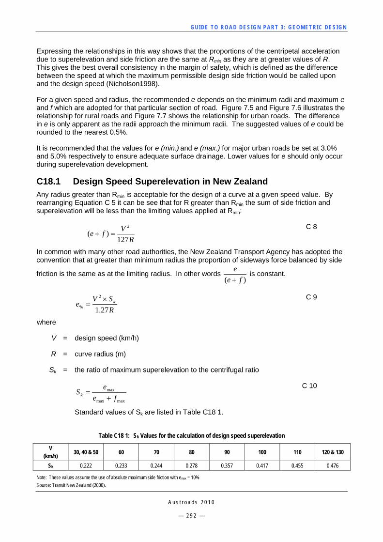
GUI DE TO RO A D DE SIG N P ART 3 : GEO MET RI C D ESI G N
A u s t r o a d s 2 0 1 0
— 2 9 2 —
Expressing the relationships in this way shows that the proportions of the centripetal acceleration due to superelevation and side friction are the same at Rmin as they are at greater values of R. This gives the best overall consistency in the margin of safety, which is defined as the difference between the speed at which the maximum permissible design side friction would be called upon and the design speed (Nicholson1998).
For a given speed and radius, the recommended e depends on the minimum radii and maximum e and f which are adopted for that particular section of road. Figure 7.5 and Figure 7.6 illustrates the relationship for rural roads and Figure 7.7 shows the relationship for urban roads. The difference in e is only apparent as the radii approach the minimum radii. The suggested values of e could be rounded to the nearest 0.5%.
It is recommended that the values for e (min.) and e (max.) for major urban roads be set at 3.0% and 5.0% respectively to ensure adequate surface drainage. Lower values for e should only occur during superelevation development.
C18.1 Design Speed Superelevation in New Zealand Any radius greater than Rmin is acceptable for the design of a curve at a given speed value. By rearranging Equation C 5 it can be see that for R greater than Rmin the sum of side friction and superelevation will be less than the limiting values applied at Rmin:
RVfe
127)(
2
=+ C 8
In common with many other road authorities, the New Zealand Transport Agency has adopted the convention that at greater than minimum radius the proportion of sideways force balanced by side
friction is the same as at the limiting radius. In other words )( fe
e+
is constant.
RSV
e k
27.1
2
%×
= C 9
where
V = design speed (km/h)
R = curve radius (m)
Sk = the ratio of maximum superelevation to the centrifugal ratio
maxmax
max
fee
Sk +=
C 10
Standard values of Sk are listed in Table C18 1.
Table C18 1: Sk Values for the calculation of design speed superelevation
V (km/h) 30, 40 & 50 60 70 80 90 100 110 120 & 130
Sk 0.222 0.233 0.244 0.278 0.357 0.417 0.455 0.476
Note: These values assume the use of absolute maximum side friction with emax = 10% Source: Transit New Zealand (2000).
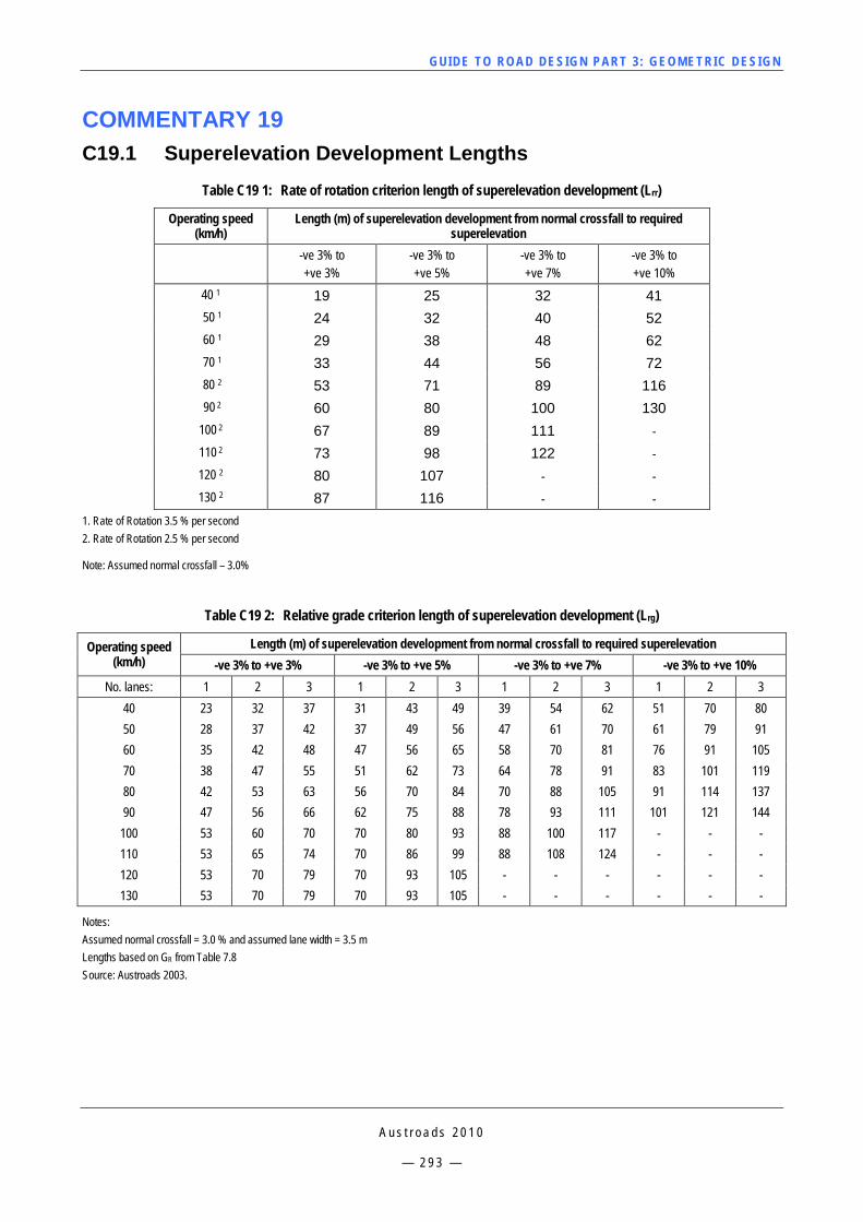
GUI DE TO RO A D DE SIG N P ART 3 : GEO MET RI C D ESI G N
A u s t r o a d s 2 0 1 0
— 2 9 3 —
COMMENTARY 19 C19.1 Superelevation Development Lengths
Table C19 1: Rate of rotation criterion length of superelevation development (Lrr)
Operating speed (km/h)
Length (m) of superelevation development from normal crossfall to required superelevation
-ve 3% to +ve 3%
-ve 3% to +ve 5%
-ve 3% to +ve 7%
-ve 3% to +ve 10%
40 1 19 25 32 41 50 1 24 32 40 52 60 1 29 38 48 62 70 1 33 44 56 72 80 2 53 71 89 116 90 2 60 80 100 130 100 2 67 89 111 - 110 2 73 98 122 - 120 2 80 107 - - 130 2 87 116 - -
1. Rate of Rotation 3.5 % per second 2. Rate of Rotation 2.5 % per second Note: Assumed normal crossfall – 3.0%
Table C19 2: Relative grade criterion length of superelevation development (Lrg)
Operating speed (km/h)
Length (m) of superelevation development from normal crossfall to required superelevation -ve 3% to +ve 3% -ve 3% to +ve 5% -ve 3% to +ve 7% -ve 3% to +ve 10%
No. lanes: 1 2 3 1 2 3 1 2 3 1 2 3 40 23 32 37 31 43 49 39 54 62 51 70 80 50 28 37 42 37 49 56 47 61 70 61 79 91 60 35 42 48 47 56 65 58 70 81 76 91 105 70 38 47 55 51 62 73 64 78 91 83 101 119 80 42 53 63 56 70 84 70 88 105 91 114 137 90 47 56 66 62 75 88 78 93 111 101 121 144
100 53 60 70 70 80 93 88 100 117 - - - 110 53 65 74 70 86 99 88 108 124 - - - 120 53 70 79 70 93 105 - - - - - - 130 53 70 79 70 93 105 - - - - - -
Notes: Assumed normal crossfall = 3.0 % and assumed lane width = 3.5 m Lengths based on GR from Table 7.8 Source: Austroads 2003.

GUI DE TO RO A D DE SIG N P ART 3 : GEO MET RI C D ESI G N
A u s t r o a d s 2 0 1 0
— 2 9 4 —
COMMENTARY 20
C20.1 Clearances to Electricity Transmission Cables Clearances should always be based on an accurate survey of existing electric cables because levels differ daily from those shown on the transmission line design plans. At the time of the survey, measurements must be taken of the temperature, the time of day and the approximate wind speed and direction. The electricity authority will use this information to calculate minimum design levels for the cable taking into account the change in height associated with ambient temperature variations, the change in height associated with temperature variations created by increased current, and swing effects.
Designers should note that clearances to transmission lines (or other overhead electrical cables) can also vary depending on the structure, the material it is made from and how often it is likely to be accessed for maintenance, e.g. a noise mound and street light poles will have separate clearance requirements.
Clearance requirements to all overhead services must be obtained from the owner of the service involved.
Table C20 1: Typical minimum vertical clearance to high voltage transmission cables
220 kV 500 kV Pedestrian overpass, floor level 6.8 m 9.8 m Earth noise mound, top 7.6 m 15 m Top of concrete or timber noise barriers on which a person could not normally stand.
3.7 m 6.4 m
Top of concrete or timber noise barriers on which a person could easily stand. 7.6 m 15 m Light poles, top 3.7 m 6.4 m Road surface, minimum 11.5 m 14.0 m Road surface, desirable 14.5 m 17.0 m
Notes: 1. For detailed design purposes, clearances shall be confirmed in writing by the responsible electricity authority. 2. Clearances to other overhead services must be obtained in writing from the owner of the service involved. Source: VicRoads (2002a).
Table C20 2: Horizontal clearance requirements to high voltage transmission cables and towers (1) 220 kV 500 kV
Centreline between towers to easement boundary 18.3 m 32.5 m Tower steel to metallic services and fences 20 m 30 m Minimum access requirements around base of tower 5 m(2) 5 m(2)
1. All clearances are to be confirmed with the authority responsible for the transmission lines (PowerNet). 2. The design of barriers provided to protect towers shall be approved by PowerNet. Note: Induced currents can be significant. Advice should be obtained from the responsible electricity transmission authority for all long or high fences within 50 m of transmission lines.
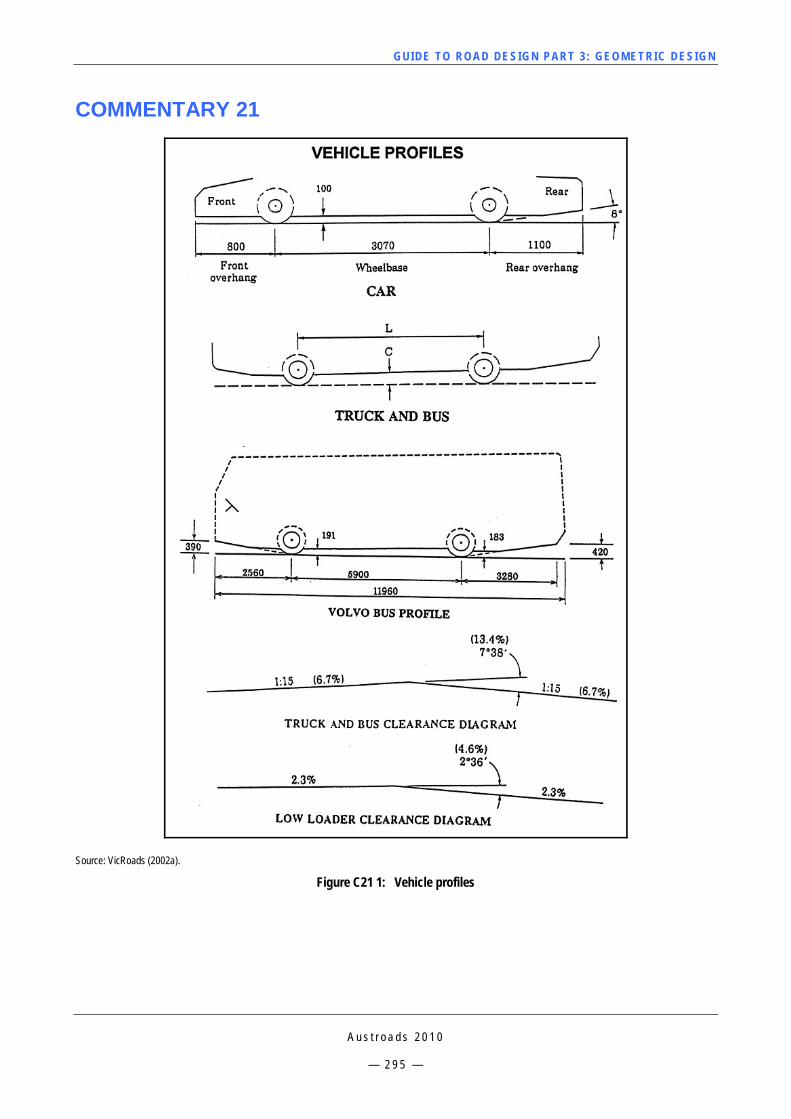
GUI DE TO RO A D DE SIG N P ART 3 : GEO MET RI C D ESI G N
A u s t r o a d s 2 0 1 0
— 2 9 5 —
COMMENTARY 21
Source: VicRoads (2002a).
Figure C21 1: Vehicle profiles
Related Documents