AGGREGATE PRODUCTION PLANNING FOR BATCH- ORIENTED …

AGGREGATE PRODUCTION PLANNING FOR BATCH-ORIENTED DISCRETE MANUFACTURING SYSTEM

INTEGRATION WITH FORECASTING

CHITRA LEKHA KARMAKER

DEPARTMENT OF INDUSTRIAL AND PRODUCTION ENGINEERING (IPE)

BANGLADESH UNIVERSITY OF ENGINEERING AND TECHNOLOGY (BUET) DHAKA, BANGLADESH

11 December, 2017

i

AGGREGATE PRODUCTION PLANNING FOR BATCH-ORIENTED DISCRETE MANUFACTURING SYSTEM

INTEGRATION WITH FORECASTING

By

CHITRA LEKHA KARMAKER

A Thesis Submitted to the Department of Industrial and Production Engineering, Bangladesh University of Engineering and Technology

in Partial Fulfillment of the requirements for the Degree of

MASTER OF SCIENCE IN INDUSTRIAL and PRODUCTION ENGINEERING

DEPARTMENT OF INDUSTRIAL AND PRODUCTION ENGINEERING (IPE)

BANGLADESH UNIVERSITY OF ENGINEERING AND TECHNOLOGY (BUET) DHAKA, BANGLADESH

11 December, 2017

ii

CERTIFICATE OF APPROVAL

The thesis entitled as “Aggregate Production Planning For Batch-Oriented Discrete

Manufacturing System Integration With Forecasting” submitted by Chitra Lekha Karmaker,

Student No. 1015082002, Session- October 2015, has been accepted as satisfactory in partial

fulfillment of the requirement for the degree of M.Sc. in Industrial and Production Engineering

on December 11, 2017.

BOARD OF EXAMINERS

----------------------------------------------- Dr. M. Ahsan Akhtar Hasin Chairman (Supervisor) Professor Department of IPE, BUET, Dhaka ---------------------------------------------- Dr. AKM Kais Bin Zaman Member (Ex-Officio) Professor and Head Department of IPE, BUET, Dhaka ------------------------------------------- Dr. Shuva Ghosh Member Assistant Professor Department of IPE, BUET, Dhaka ------------------------------------------------ Dr. Md. Nazrul Islam Member (External) Former Director, National Productivity Organization (NPO) Ministry of Industries, GOB

iii

CANDIDATE’S DECLARATION

It is hereby declared that this thesis or any part of it has not been submitted elsewhere for the

award of any degree or diploma.

Chitra Lekha Karmaker

iv

THIS WORK IS DEDICATED TO MY PARENTS AND MY FAMILY

v

ACKNOWLEDGEMENT

At first, the author wants to convey her deepest gratefulness to the almighty God, the beneficial,

the merciful for granting me to bring this research work into light. The author would like to

express her sincere respect & gratitude to honorable teacher & thesis supervisor, Dr. M. Ahsan

Akhtar Hasin, Professor, Department of Industrial and Production Engineering (IPE),

Bangladesh University of Engineering and Technology (BUET), Dhaka, for his thoughtful

suggestions, constant guidance and encouragement throughout the progress of this research

work. The author also expressed her sincere gratitude to Dr. AKM Kais Bin Zaman, Professor

and Head, Department of IPE, BUET, Dr. Shuva Ghosh, Assistant Professor, Department of IPE,

BUET and Dr. Md. Nazrul Islam, Former Director, National Productivity Organization (NPO)

Ministry of Industries, GOB for their constructive remarks and for kindly evaluating this

research.

The author is especially thankful to Bulbul Ahmed, Project Manager, Magpie Knit Wear Limited

(MKWL) for his cordial encouragement and sincere help during the data collection phase and

permitting me to have accessed to his company.

The author is grateful to all the writers and publishers of the books and journal papers that have

taken as references while conducting this research. With a very special recognition, the author

would like to thanks her parents as well as all the members of her families, who provided their

continuous inspiration, sacrifice and support encouraged me to complete the research work

successfully.

vi

ABSTRACT

Aggregate Production Planning (APP) involves the determination of company’s optimal

production, inventory and employment levels with a given set of resources and constraints.

Forecasted demand of products is one of the important inputs of APP and a more justified as well

as realistic forecasting technique for prediction of market demand is very crucial for reducing

unnecessary inventories, smoothing the production plan etc. Usually in APP process, economic

planners of most of the manufacturing companies in Bangladesh use subjective and intuitive

judgments to estimate future demand which leads the result to infeasibility or decreased

performance. Nevertheless, aggregate plan is the basis of subsequent plan, and thus, accuracy in

it leads to proportionate accuracy in master production schedule (MPS) and material

requirements plan (MRP).

This study develops a decision support model for multi-period multi-product aggregate

production planning integration with forecasting technique aiming at minimizing the total

relevant cost considering projected demand, production capacity and work forces, inventory

control, backorder, and wastage reduction. In this study, different time series forecasting models

are applied on the historical data of two product groups (Hooded jacket, Ladies cardigan). Then,

error levels are compared with those obtained by subjective and intuitive judgements (company’s

current practice). It is found that winter’s additive method and Holt’s method provide lower

forecast errors for hooded jacket and ladies cardigan respectively. A multi-period multi-product

mathematical model for APP problem is formulated which is solved by Linear Programming

(LP) and Genetic Algorithm (GA) approaches. Finally, the results drawn from two different

approaches are compared with company’s current production plan in terms of total cost to

evaluate the best one for a situational APP decision. According to cost minimization objective of

APP, linear programming seems to be satisfactory than genetic algorithm and company’s current

practice. Practically, for simple linear optimization problems, linear programming (LP) approach

is suitable to provide better result.

The proposed framework is effective and easy to implement in practical management and supply

chain systems. So, this study can be the roadmap for manufacturers as well as planners to

minimize total cost.

vii

TABLE OF CONTENTS

Topic Page No.

Certificate of Approval ii

Candidate’s Declaration iii

Dedication iv

Acknowledgement v

Abstract vi

Table of Contents vii-x

List of Tables xi

List of Figures xii

List of Abbreviations xiii

Chapter 1 Introduction 01-05

1.1 General Introduction 01

1.2 Rationale Of The Study 02

1.3 Objectives Of The Study 03

1.4 Outline Of Methodology 03

1.5 Organization Of The Report 04

Chapter 2 Literature Review 06-12

2.1 Introduction 06

2.2 Forecasting In APP 06

2.3 Different Techniques For Optimizing APP 08

Chapter 3 Theoretical Framework 13-31

3.1 Forecasting 13

3.2 Types Of Forecasting Methods 13

3.2.1 Qualitative Methods 13

3.2.2 Quantitative Methods 14

3.2.3 Time Series Analysis 14

3.2.4 Associative Model 18

viii

3.2.4 Simulation Model 18

3.3 Measures Of Forecasting Accuracy 18

3.4 Aggregate Production Planning 20

3.4.1 Importance Of Aggregate Planning 20

3.4.2 Inputs To Aggregate Planning 21

3.4.3 General Aggregate Planning Strategies 21

3.5 Linear Programming (LP) approach 22

3.5.1 Common Terminologies 22

3.5.2 Outline Of Linear Programming 22

3.5.3 Solving Methods Of Linear Programming 23

3.5.4 Applications Of Linear Programming 24

3.6 Genetic Algorithm 24

3.6.1 Biological Background 24

3.6.1.1 The Cell 25

3.6.1.2 Chromosomes 25

3.6.1.3 Genetics 25

3.6.1.4 Reproduction 25

3.6.1.5 Selection 26

3.6.2 Working Principle 26

3.6.3 GA Parameters 27

3.6.3.1 Key Elements 27

3.6.3.2 Genes 27

3.6.3.3 Fitness 27

3.6.3.4 Encoding 28

3.6.3.5 Breeding 28

3.6.4 Termination 29

3.6.5 Outline of Genetic Algorithm 29

3.6.6 Advantages and Limitations Of Genetic

Algorithm

30

Chapter 4 Company Overview 32

4.1 Company Profile 32

ix

Chapter 5 Forecasting Method Selection 33-40

5.1 Methodology 33

5.2 Time Series Analysis Of Hooded Jacket 33

5.2.1 Comparison of current & proposed models 38

5.3 Time Series Analysis Of Ladies Cardigan 39

5.3.1 Comparison between current & proposed models 39

5.4 Calculation of Forecasted Demand of Product Groups 40

Chapter 6 Model Description 41-48

6.1 Problem Formulation 41

6.2 Model Development 42

6.3 Develop Objective Function 43

6.3.1 Regular Time Production Cost 43

6.3.2 Overtime Production Cost 44

6.3.3 Subcontracting Cost 44

6.3.4 Inventory Cost 44

6.3.5 Backorder/ Penalty Cost 44

6.3.6 Wastage Cost 44

6.3.7 Labor Hiring Cost 44

6.3.8 Labor Firing Cost 45

6.3.9 Objectives 45

6.4 Setting Constraints 46

6.5 Decision Variables 47

6.6 Outline Of LP Approach 47

6.7 Outline Of The Basic GA Model 48

Chapter 7 Model Implementation-A Case Study 49-53

7.1 Case Description 49

7.2 Data Description 49

7.3 Applying Linear Programming (LP) 50

7.4 Applying Genetic Algorithm (GA) 51

Chapter 8 Results And Findings 54-59

x

Chapter 9 Conclusions And Recommendations 60-61

9.1 Conclusions 60

9.2 Future Recommendations 61

References 62

Appendices 68

xi

LIST OF TABLES

Table No. Title Page No.

Table 5.1 Forecasting Errors Under SMA Method 34

Table 5.2 Forecasting Errors Under SES Method 35

Table 5.3 Forecasting Errors Under Holt’s Method 35

Table 5.4 Forecasting Errors Under Winter’s Method 37

Table 5.5 Summary Of Decomposition Methods 38

Table 5.6 Comparison Of The Forecasting Methods (Product-1) 38

Table 5.7 Comparison Of The Forecasting Methods (Product-2) 40

Table 5.8 Forecasted Demand Of Product Groups 40

Table 7.1 Forecasted Demand Data For The MKWL Case 50

Table 7.2 Related Operating Cost Data For The MKWL Case 50

Table 7.3 Values Of Related Other Parameters 50

Table 7.4 Values Of Decision Variables For The MKWL Case (Product 1) 51


Table 7.6 Labor Parameters For The APP Plan Of MKWL Case 51

Table 7.7 Objective Values For The APP Plan of MKWL Case 51



Table 7.10 Labor Parameters For The APP Plan Of MKWL Case 53

Table 7.11 Objective Values For The APP Plan Of MKWL Case 53

Table 8.1 Demand Forecast Errors Of Hooded Jacket 54

Table 8.2 Demand Forecast Errors Of Ladies Cardigan 56

Table 8.3 Total Cost Comparison Of Existing & LP Approach 58

Table 8.4 Total Cost Comparison Of Existing And Genetic Algorithm Approach

59

Table 8.5 Total Cost Comparison of Different Approaches For APP Problem 59

xii

LIST OF FIGURES Figure No. Figure Title Page No.

Figure 3.1 Outline Of Genetic Algorithm 30

Figure 5.1 Time Series Plot Of Hooded Jacket Demand 34

Figure 5.2 Linear Trend Equation For Hooded Jacket 36

Figure 5.3 Time Series Plot Of Ladies Cardigan 39

Figure 8.1 A Comparative Study Of MAPE For Hooded Jacket 55

Figure 8.2 A Comparative Study Of MAD For Hooded Jacket 55

Figure 8.3 A Comparative Study Of MSD For Hooded Jacket 56

Figure 8.4 A Comparative Study Of MAPE For Ladies Cardigan 57

Figure 8.5 A Comparative Study Of MAD For Ladies Cardigan 57

Figure 8.6 A Comparative Study Of MSD For Ladies Cardigan 57

Figure 8.7 Demand Comparisons Between Proposed And Current

Approaches

58

xiii

LIST OF ABBREVIATIONS

APP : Aggregate Production Planning

MRP : Material Requirements Planning

MPS : Master Production Schedule

GA : Genetic Algorithm

LP : Linear Programming

MATLAB : Matrix Laboratory

SMA : Simple Moving Average

SES : Simple Exponential Smoothing

MAPE : Mean Absolute Percentage Error

MAD : Mean Absolute Deviation

MSE : Mean Squared Error

-1-

CHAPTER 1 INTRODUCTION

1.1 GENERAL INTRODUCTION Aggregate production planning (APP), which might also be called macro production planning, is such an activity that addresses the problem of deciding how many employees the company should retain and, for a manufacturing company, the optimal quantity and the mix of products to be produced with a given set of resources & constraints. This methodology is planned to translate demand forecasts in to a blueprint for planning staffing and production levels for the firm over a predetermined planning horizon. The planning horizon is often divided into periods. For example, a one year planning horizon may be composed of two six-month periods or one six month period plus two three-month periods. APP is widely used today in manufacturing environment but it was first formulated in the 1950s. Generally, aggregate production planning problem involves matching capacity to fulfill the demand of forecasted, fluctuating customer orders in such a way that overall cost is minimized. However, other strategic issues may be more important than low cost. These strategies may be to smooth employment levels, to drive down inventory levels, or to meet a high level of service. To meet customer uncertain requirements in the most efficient and effective way, manufacturing planning and control address decisions on the acquisition, utilization and allocation of production resources. Typical decisions include determination of inventory level, work force level, production lot sizes, subcontracting units, backorder items, assignment of overtime and sequencing of production runs. To cope up with the highly competitive and constantly changing market environment, it is even more important to have a high degree of coordination between all the planning activities. It is widely recognized that efficient aggregate planning methods have much potential for reducing costs in many areas since the process harmonizes the system in its entirety. During the planning horizon of interest, the physical resources of the associated organizations are assumed to be fixed and the planning effort is oriented toward the best utilization of those resources, given the external demand requirements. Since it is usually impossible to consider every fine detail associated with the production process while maintaining such a long planning horizon, it is mandatory to aggregate the information being processed. Normally, capacity planning is based on aggregate demand for one or more aggregate items. Once the aggregate production plan is generated, constraints are imposed on the detailed production scheduling process which decides the specific quantities to be produced of each individual item. APP usually covers a time period ranging from 4 to 12 months. In the aggregate plan, data are usually based on monthly or quarterly data. The most important input data for an APP problem are demand forecast of products because the main aim of APP is to respond to demand fluctuations in a proper manner. Usually in APP process, planners use conventional

-2-

distinct forecasting methods, more specifically subjective & intuitive judgments, to estimate uncertain demand which lead the result to infeasibility or lower performance. Ultimately, this sort of action leads to increase total cost of the supply chain network. Hence to reduce the gap between the estimated demand and capacity requirements throughout the entire period of planning, a more justified and realistic forecasting method should be adopted in optimization of APP problems. However, these observations result in the need for developing a decision support model for aggregate production planning and improving the forecasting technique to improve customer service level as well as reduce total cost. In this study, time series forecasting models are applied in order to determine the forecasted demand. Then, the projected demand will be used as the input of APP model. 1.2 RATIONALE OF THE STUDY Forecasted demand of products is one of the inputs in APP process. An accurate prediction of market demand is very crucial in case of reducing unnecessary inventories, smoothing the production plan, maintaining supply chain effectiveness & responsiveness which finally results in increasing profit (Tuzkaya et. al. 2009; Sultana et. al. 2014; Mirzapouur-al-hashem et. al. 2011). But, economic planners of most of the manufacturing companies in Bangladesh use subjective & intuitive judgments to organize a firm's life to respond to the inevitable changes of the broader economy. This type of activity leads the result to infeasibility or lower performance (Price and Sharp 1984; Yenradee et. al. 2001). Hence to reduce the gap between the production quantities and market demand throughout the entire period of planning, a more justified and realistic forecasting method should be adopted in optimization of APP problems. However, these observations result in the need for developing a decision support model for aggregate production planning and improving the forecasting technique to improve customer service level. Here in this study, a multi-product & multi period aggregate planning along with proper forecasting technique has been targeted. Multi criteria encompasses inventory costs, product purchasing costs, manufacturing costs, manpower maintain costs, extra subcontracting or backordering costs etc. Researches reveal that the complex task of preparing an aggregate production plan, under varied constraints, is very difficult, and often leads to NP-hardness. Nevertheless, it is the basis of subsequent plan, and thus, accuracy in aggregate plan leads to proportionate accuracy in master production schedule (MPS) and material requirements plan (MRP). So proper planning is mandatory by any means. Here, aggregate production planning problem has been formulated as a linear programming model and later solved by both LP approach and Genetic Algorithm optimization engine. Genetic algorithm approach is vastly used in this recent time by several researchers. The proposed model is validated with the real data collected from an export oriented garments manufacturer company in Bangladesh. The real case demonstration and the obvious necessity of having perfect aggregate production planning will help the researchers as well as manufacturers which will certainly increase the value of this thesis work.

-3-

1.3 OBJECTIVES OF THE STUDY The specific objectives of this research work are as follows:

➢ To understand the current forecasting practice of any batch-oriented discrete

manufacturing system (specifically the Garments sector).

➢ To recommend an improved and effective forecasting technique among different time

series forecasting models by comparing their level of accuracy.

➢ Using the best fitting forecasting approach, demand values of products are projected.

➢ To develop a model of multi-period and multi-product Aggregate Production Planning

considering wastage cost to minimize total cost.

➢ To formulate aggregate production planning problem as a linear programming model

and solve it by both LP and Genetic Algorithm in Matlab R2012a.

➢ To obtain the results drawn from two different approaches and compare it with

company’s current production plan in terms of total cost to evaluate the best one for a

situational APP decision.

1.4 OUTLINE of METHODOLOGY In order to carry out the proposed research work, required steps that have been adopted are stated below:-

➢ Study of different production process characteristics and existing demand forecasting

technique of a renowned Bangladeshi Garments company named Magpie Knit Wear

Limited (MKWL).

➢ Identify the parameters & factors which affect the company’s overall aggregate

planning.

➢ Apply different time series forecasting models like decomposition, Holt’s method,

winter’s method etc. to predict future values of products.

➢ Different forecasting errors like mean absolute deviation (MAD), mean squared error

(MSE), mean absolute percent error (MAPE) etc. under applied forecasting methods

as well as company’s current practice are calculated using MINITAB Release 13.32

package program.

➢ After comparing the level of accuracy, the most suitable forecasting technique is

selected and compared it with the company’s current forecasting practice.

-4-

➢ In the next step, the aggregate demand of products is projected using the proposed

forecasting techniques which are used as inputs to determine the production plan.

➢ To develop the APP model, different data such as regular time production cost,

overtime production cost, hiring & firing opportunities, subcontracting &

backordering information, total manpower used, wastage cost etc. are accumulated.

➢ The main objective function (minimizing total cost) and all the constraints on carrying

inventory, labor levels, machine and warehouse space, wastage cost, non-negativity

etc. are developed.

➢ Later step, the model is formulated as Linear Programming (LP) model & solved by

LP approach in Matlab software using practical data from Magpie Knit Wear Limited

(MKWL).

➢ Another meta-heuristic algorithm named Genetic Algorithm is also employed.

➢ Finally, a detailed comparison among all this aforementioned approaches and

company’s current practice is generated.

1.5 ORGANIZATION OF THE REPORT The thesis paper is structured into nine chapters along with a list of references & appendices. Chapter 1 entitled as “Introduction” which consists general introduction, background of the study, research objectives, and research methodologies. Under introduction section, general concepts on Aggregate Production Planning problems are discussed. Proper reason for the research work has been demonstrated. The research objectives are also outlined here with some guideline of research methodologies. Recent research works on aggregate production planning, demand management in context of supply chain management etc. are summarized in the following Chapter 2 termed as “Literature Review”. Evolution of different approaches for solving APP problem was also explained. Under Chapter 3 entitled as “Theoretical Framework”, details of forecasting, Linear Programming (LP) approach, Genetic algorithm approach are outlined. Different Genetic algorithm parameters, basic information regarding GA, crossover, mutation, reproduction, creation, selection functions etc are also focused on this chapter. Here, a detail of time series forecasting models and measures of forecasting accuracy is presented. Chapter 4 describes the selected company in where the proposed framework is applied. In Chapter 5, selection of appropriate forecasting technique for selected products is outlined. In the later portion of this thesis paper, the targeted problem with its detailed formulation is discussed in Chapter 6. In Chapter 7, how the models are implemented is discussed there. A

-5-

numerical example is given with the practical data from an export oriented readymade garments manufacture named as Magpie Knit Wear Limited (MKWL). In the later Chapter 8, the calculated results & important findings are presented with different contrasting features. At the bottom, a detailed comparison among all this aforementioned approaches and company’s current practice is generated. And finally, in Section 9, conclusions with further research recommendations for the manufacturers, practitioners, future researchers are portrayed following a list of references and appendices focused on the programming languages. This section wraps up the study.

-6-

CHAPTER 2 LITERATURE REVIEW

2.1 INTRODUCTION Nowadays, increased product complexity in combination with amplified customer service orientation are two pivotal factors that lead to challenging production planning problems faced by most of the manufacturing companies. Also shortenings of product life cycles, ongoing market instabilities, increasing fragmentation of supply chain’s ownership, and demand uncertainties ask for a high level of production edibility. In this situation of constantly increasing complexity, supply chain management (SCM) can play a vital role as it covers overall production planning for entire supply chain from the raw material supplier to the end customer. According to several researchers, supply chain management, a more matured discipline, has a tremendous impact on organizational performance in terms of competing based on price, quality, dependability, responsiveness, and flexibility and helps different organizations to enhance their competitiveness in the global market (Dolgui and Ould-Louly, 2002; Wang and Liang, 2005; Gunnarsson and Ronnqvist, 2008; Lodree and Uzochukwu, 2008; Gebennini et. al., 2009). It has shifted the attention of managers as well as planners from only manufacturing plant to entities plants interact with; for example, suppliers, distributors, warehouses, and customers. To exploit the full potential of supply chain management, companies require a more defined organizational structure, performance measures, etc. In this scope, one of the problems that managers and analysts should address is aggregate production planning (APP), which is focused in this paper. Aggregate Production Planning (APP) is such an activity that deals with the determination of optimal production level, work force, inventory levels to meet fluctuating demand needs of products with a given set of resources and constraints. Operation managers try to determine the best way to meet forecasted demand in a cost effective manner by adjusting production rates, labor levels, inventory levels, overtime work, subcontracting rates, and other controllable variables for each period of planning horizon. The planning horizon ranges from six months up to a year. During the planning horizon of interest, planners consider the fixed value for the physical resources and try to make the best utilization of those resources with respect to demand values of products. It is necessary to aggregate the information being processed while maintaining such a long planning horizon. 2.2 FORECASTING IN APP Forecasted demand of items is one among several critical inputs of a production planning process. The accuracy of production plan highly depends on the accuracy of forecasted demand and this accuracy leads to proportionate accuracy in master production schedule (MPS) and material requirements plan (MRP) (Chakraborty and Hasin, 2013; Chakraborty and Hasin, 2013). But unfortunately, it is very obvious that most manufacturing companies in

-7-

developing countries define product demand forecasts and production plans using subjective and intuitive judgments instead of comparing forecasting techniques. When the demand is highly seasonal, an accurate forecast cannot be obtained without the help of appropriate forecasting method. Inappropriate forecasting technique provides unreliable production plan, may result over-stock or under stock situation which ultimately hampers customer service level (CSL). When demand is not anticipated properly, unnecessary inventory will result in an increased inventory holding costs. Moreover, the accuracy of aggregate production plan leads to proportionate accuracy in master production schedule (MPS) and material requirements plan (MRP) as it is the basis of two. So, to struggle with these kinds of problems, the implementation of sound forecasting techniques in production planning process is decisive and therefore addressed by a number of researchers (Price and Sharp, 1984; Ho and Ireland, 1998; Enns, 2002; Xie et al., 2004; Kerkkänen et al., 2009; Gansterer, 2015). In the research work of Price and Sharp in 1984, the importance of the selection of appropriate demand forecasting method in the aggregate capacity planning of the UK electric supply industry was investigated. The authors applied some extrapolative forecasting methods and found them to perform surprisingly well than the current practice over a six year time horizon. For the selection of reliable forecasting technique, financial performance measures instead of using conventional measures of accuracy were used. Ho and Ireland (1998) observed the impact of forecasting errors on the scheduling instability in an MRP operating environment. The effects of demand uncertainty and forecast bias in a batch production environment are investigated by Enns (2002). As stated earlier, improper forecasting leads to production inefficiency, increase unnecessary inventory that raise the holding cost. Xie et al. (2004) investigated the impact of forecasting error on the performance of capacitated multi-item production systems, total cost, schedule instability and system service level. Similar type of research was performed by Kerkkänen et al. (2009) who assessed the impacts of sales forecast errors in a supply chain through a case study. Yenradeeet al. (2001) emphasized on the improvements of the forecasting techniques for capacity planning in a pressure container factory in Thailand. The authors investigated factory’s current practice and then, applied three forecasting models, namely, winter’s, decomposition, and Auto-Regressive Integrated Moving Average (ARIMA) to forecast the product demands. The results were compared with the subjective and intuitive judgments (current practice) and found that decomposition and ARIMA models provide lower forecast errors in all product groups. The results revealed that the total costs could be reduced by 13.2% when appropriate forecasting models are applied in place of the current practice. Researchers mostly discuss cases with seasonal demand which are obviously supposed to be the most challenging ones. The reason is the high variation in capacity requirements. Vörös (1999) demonstrated a model for risk-based aggregate planning for seasonal products. Dobos (1996) addressed aggregate planning with continuous time. In the paper, a simple forward algorithm was presented based on the solution of the optimal control problem. But also recent studies are investigating this topic. Inspiring with that Yenradee et al. (2001) proposed a new framework that incorporated selection of appropriate forecasting technique with capacity planning problem.

-8-

2.3 DIFFERENT TECHNIQUES FOR OPTIMIZING APP APP has attracted considerable interest from both practitioners and academics (Shi and Haase, 1996). The APP is considered as the combination of several classical production planning problems which have been modeled in the form of different mathematical programming like scheduling problems (Buxey, 1993; Foote et al., 1998), work force planning problems (Mazzola et al., 1998), long set up time problems (Porkka et al., 2003) etc. Numerous APP models with varying degree of sophistication have been introduced in the literature during the last decades. Holt et al (1955) proposed the approach of aggregate production planning problem for the first time. Later, different scholars have proposed numerous models for solving APP problems. Hanssman and Hess (1960) developed a linear programming model to production and employment scheduling using linear cost structure of decision variables. Previous model was extended by another researcher Haehling (1970) for multi-period, multi-stage production systems. Haehling (1970) proposed the new model in which optimal disaggregation decisions can be made under capacity constraints. Masud and Hwang (1980) used three MCDM methods namely goal programming, step method, sequential multi-objective problem for solving APP problem. The objective of the study was to maximize the profit, minimize changes in workforce level, minimize backorders and inventory investment. A set of data consisting of two products, a single production plant and eight planning periods was generated and results obtained from three MCDM approaches were compared. Baykasoglu (2001) made an extension of Masud and Hwang’s (1980) model by adding constraints such as subcontractor selection, setup decisions etc. and solved the model using a tabu search algorithm. Goodman (1974) proposed a framework for aggregate planning of production and work forces using goal programming method that approximates original non-linear cost terms of the Holt’s model by linear terms. A variant of the simplex method was used to solve the model.In 1992, Nam and Logendram conducted a survey on APP models and methodologies .They reviewed about 140 journal articles and 14 books to classify models and classified them into optimal and near optimal classifications. Hsieh and Wu (2000) proposed a possibilistic linear programming model for demand and cost forecast error sensitivity analyses in aggregate production planning. Different meta-heuristic methods are used to solve NP-hard problems and due to NP-hard class of aggregate production planning, these approaches have been used for solving APP. Baykasogluy (2006) proposed a meta-heuristic approach by Tabu search algorithm for solving APP problems with multiple objectives, multi-product, multi-periods. Ramazanian and Modares (2011) showed the application of particle swarm optimization algorithm for a multi-product multi-step multi-period APP problem in the cement industry. The model was reformulated as a single objective nonlinear programming model. It was solved by using the expended objective function method and a propose PSO variant whose inertia weighted was set as a function. The simulation comparing with GA in the final showed that PSO gains satisfactory result then GA. Several researchers have proposed a solution for integrated

-9-

production and distribution planning in complicated environments where the objective is to maximize the total profit (Jung and Jeong, 2005; Park, 2005; Silva et al.2006). Bakar et al. (2016) suggested multi objective linear programming model for APP and optimized by modified simulated annealing (MSA). To enhance efficiency as well as alleviate the deficiencies in the traditional SA, modified SA was proposed. Here, the authors attempted to augment the search space by n+1 solutions instead of one solution and compared the performance of MSA with the standard SA and harmony search (HS).The result showed that compared to SA and HS approaches, MSA offers better quality solutions with regard to convergence and accuracy. Kavehand and Dalfard (2014) used simulated annealing for solving aggregate planning. While APP modeling techniques are constantly enhanced, there are also authors pointing out the fruitful use of genetic algorithm for solving the capacity planning problem. Genetic Algorithm (GA) normally provides a series of alternative solutions for various GA parameter values. The decision-maker can find alternative optimal solutions from a series of alternative values (Sharma and Jana, 2009). In order for GAs to surpass their more traditional cousins in the quest for robustness, they must vary in some very fundamental ways (Goldberg, 1989). Ioannis (2009) proposed a novel genetic algorithm approach for solving constrained optimization problems. His model was a modified version of the genetic operators namely crossover and mutation. These new version preserve the feasibility of the trial solutions of the constrained problem that are encoded in the chromosomes. Bunnag and Sun (2005) described a robust optimization model using Genetic Algorithm (GA) for constrained global optimization in continuous variables. In the research, the constraints were treated through a repair operator and solved the model using real coded GA, which converges in probability to the optimal solution. Another important contribution of the study was the inclusion of a specific repair operator for linear inequality constraints. Due to NP-hard class of aggregate production planning, Fahimnia et al. (2006) presented a decision support system for modeling and optimization of aggregate production planning via Genetic Algorithm approach. Jiang et al. (2008) applied genetic algorithm approach to determine the optimum production level in production line of iron & steel enterprise. Savsani et al. (2016) presented a Genetic Algorithm approach for solving aggregate production planning with different selection methods and various crossover phenomenon. Here, combination of four selection methods and five crossover phenomenon were considered and compared to choose the best combination for solving APP in this present work. The result showed the outstanding performance of uniform selection procedure and two point crossover combination. Chakrabortty and Hasin (2013) described an interactive Multi-Objective Genetic Algorithm (MOGA) approach for solving APP problem having multi-product, multi-period parameters. The objective of the work was to determine the optimum production level by adjusting inventory levels, labor levels, overtime, subcontracting and backordering levels, and labor, machine and warehouse capacity. Here, several genetic algorithm parameters were

-10-

considered and the obtained results were compared to select the most favorable combination with the lowest total cost. Hossain et al. (2015) presented an extension version of previous work for solving multi-period multi-product aggregate planning. The proposed approach differs from the research of Chakrabortty and Hasin (2013) because it attempts to evaluate the impact of escalating factor under uncertain demand. Another point was the consideration of wastage cost and incentive cost. In paper Hashem et al. (2013), wastage cost was considered for transportation but here wastage cost was considered for total production cost which had an impact on minimizing total cost. Several researchers have combined genetic algorithm with other optimization approaches for obtaining much better solution. The combination of GA with other optimization methods seems to be quite efficient. Generally, GA is quite good method for finding global solutions, but quite inefficient at locating the last few mutations to determine the absolute optimum. Mohan and Noorul (2005) presented hybrid genetic-ant colony algorithms in order to determine the optimum production level by adjusting inventory, backorder, subcontracting levels. The study reported that combined genetic algorithm approach makes the production plan smoother. Ganesh and Punniyamoorthy (2005) also applied hybrid Genetic Algorithms with Simulated Annealing for optimization of continuous-time production planning. Ramezanian et al. (2012) concentrated on multi-period, multi-product and multi-machine systems with setup decisions. In their study, they developed a mixed integer linear programming (MILP) model for general two-phase aggregate production planning systems. Due to NP-hard class of APP, they implemented a genetic algorithm and Tabu search for solving this problem. Yeh and Chuang (2011) concentrated on using multi objective genetic algorithm for partner selection in green supply chain problems. In manufacturing environments, aggregate production planning model is developed based on some parameters having uncertain values. Uncertainty may come from market demands and capacities in production environment, imprecise process times, and other factors. That’s why numerous researchers have proposed robust approaches to deal with the real life planning problem having noisy, incomplete, erroneous data. For solving the multi-product APP decision problem in a fuzzy environment, Wang and Liang (2004) demonstrated a fuzzy based multi-objective linear programming (FMOLP) model whose objective was to optimum total production costs, carrying and backordering costs and rates of changes in labor levels considering inventory level, labor levels, capacity, warehouse space and the time value of money. In the study of Ninget et al. (2006), a fuzzy random APP model was formulated in which different factors like market demand, production cost, subcontracting cost, inventory carrying cost, backorder cost, product capacity, sales revenue, maximum labor level, maximum capital level etc. were represented as fuzzy random variables. The model was solved via a hybrid optimization approach combining fuzzy random simulation, genetic algorithm (GA), neural network (NN) and simultaneous perturbation stochastic approximation (SPSA) algorithm. Aliev et al. (2007) developed a fuzzy integrated multi-period and multi-product production and distribution model in supply chain where the model was modeled in terms of fuzzy

-11-

programming and the solution was provided by genetic optimization. Liang (2007) formulated an imprecise multi-objective APP model using possibilistic linear programming (i-PLP) approach and the prime objective of the research was to minimize the total production costs and changes in work-force level with reference to imprecise demand, cost coefficients, available resources and capacity. Moreover, the proposed approach helps decision making process to solve fuzzy multi-objective APP problems effectively, enabling decision makers to interactively modify the imprecise data and parameters until a set of satisfactory solutions is derived. Sharma and Jana (2009) developed a model using genetic algorithm approach under fuzzy environment for obtaining better rice crop planning. Sakallı et al. (2010) proposed a possibilistic aggregate production planning model for brass casting industry. Abass and Elsayed (2012) presented APP model under uncertain environment with a view to maximizing the revenues net of the production, inventory and lost sales costs. In this research, the author formulated proposed model based linear programming (LP) which was solved by using software named Win QSB. Mirzapour Al-e-hashem et al. (2012) presented a multi-objective model to deal with a multi-period multi-product multi-site APP problem under uncertainty and used an efficient algorithm that is a combination of a modified ε-constraint method and genetic algorithm to solve their problem. Chakrabortty and Hasin (2013) developed an interactive model using genetic algorithm under fuzzy environment for solving aggregate production plan. Ait-Alla et al. (2014) presented a mathematical model for robust production planning at fashion apparel industry considering conditional value at risk (CVaR) as the risk measure. The researchers considered several factors such as the stochastic nature of customer demand, differences in production and transport costs and transport times between production plants in different regions. The main objective of the study was to achieve minimal production cost and minimal tardiness. Chakrabortty et al. (2015) also used Particle Swarm Optimization under uncertain environment for solving aggregate production planning in the garment industry in Bangladesh. Abbas et al. (2015) presented a fuzzy multi-objective linear programming model for solving aggregate production planning problems with multiple products and multiple periods. The contribution of the study was to present a new model based on Zimmermans approach to determine the tolerance and aspiration levels. Islam and Hossain (2016) developed a robust aggregate production planning model considering uncertain input value. In this study, random value is considered from specific data range of each parameter of a specific automobile factory and finally, result was compared with the company’s existing approach. Khalili-Damghani et al. (2015) proposed a multi-period multi-product multi-objective aggregate production planning (APP) model for an uncertain multi-echelon supply chain considering financial risk, customer satisfaction, and human resource training. The researchers considered three conflictive objective functions and several sets of real constraints in the proposed APP model. Some parameters of the proposed model were assumed to be uncertain and handled through a two-stage stochastic programming (TSSP) approach. The proposed TSSP was solved using three multi-objective

-12-

solution procedures, i.e., the goal attainment technique, the modified ε-constraint method, and STEM method. The results revealed that the efficacy and applicability of the proposed approaches were much higher than existing experimental production planning method. The increased concern about the environmental impact of manufacturing activities has urged researchers to include environmental aspects in production planning. Aggregate production planning has recently been addressed in conjunction with environmental aspects in green supply chains (Entezaminia et al. 2016). Entezaminia et al. (2016) developed a multi-objective APP model to investigate economic and environmental performance in a green supply chain. Due to the increased concern about the depletion of natural resources and the calls for sustainable manufacturing, recent research work concentrated on energy-efficiency in manufacturing. Mirzapour Al-e-hashem et al., (2013) developed a stochastic APP approach in a green supply chain. Biel and Glock (2016) conducted a review which considered the role of medium and short-term production planning in saving energy consumption. A multi-objective linear programming model was developed in (Modarres and Izadpanahi, 2016) to integrate the energy consumption in the classical aggregate production planning formulation. Three objectives were considered: minimizing operation cost, energy cost, and CO2 emissions. The model further addressed uncertainty in objective function parameters (operational cost, energy, and carbon), maximum capacity, and demand. Robust optimization approach has been used to deal with uncertainty. Nour et al (2017) presented a case study for developing an energy-based aggregate production plan for a porcelain tableware manufacturer in Egypt. The mathematical model used is a mixed integer linear programming model targeting the maximization of the profit while explicitly using the energy cost as one of the cost elements. Throughout the review, it is obvious that there have been a long phase for aggregate production planning problem and the author has become optimistic enough after reviewing all the literatures since there are good opportunities for future contributions. All the previous works described in the above section gives descriptive knowledge on aggregate production planning study and all are relevant to real world problem. The proposed approach is oriented to understand the existing forecasting method of batch-oriented discrete manufacturing system in Bangladesh and to recommend an improved and effective forecasting technique among different time series forecasting models by comparing their level of accuracy. Incorporation of demand forecasting process in aggregate production plan will help decision makers to minimize the overall forecast variability and inventory holding cost. In previous work (Hashem et al. 2013), wastage cost was considered for transportation but in this study, wastage cost has been included for calculating total production cost which has an impact on minimizing total cost in terms of inventory levels, labor levels, overtime, subcontracting and backordering levels, wastage cost, and labor, machine and warehouse capacity. Here, the production planning problem has been formulated as a linear programming model which is solved using computer aided LP approach and genetic algorithm method. Finally, the optimum solution is determined from comparing the described approaches and company’s existing practice.

-13-

CHAPTER 3 THEORITICAL FRAMEWORK

3.1 FORECASTING Forecasting refers to the technique to probe the future event or occurrence. An event may be demand of a product, price of a commodity, unemployment rate etc. Generally it is carried out in order to provide some guidelines for decision making process and in better planning the future. To stay competitive in the global business environment, effective planning regarding scheduling, inventory, production, distribution, purchasing and so on is very important as it is considered as the backbone of fruitful operations. History reveals that many organizations have failed due to faulty forecasting on which whole planning was made. In today’s competitive business environment, satisfying customer’s demand at right time at right quantity is the main driving force for generating profit for any business. So, to ensure product availability with the lowest possible cost, forecasting with as much accuracy as possible is very crucial. As forecasting is an uncertain process, it is not so much easy task to predict consistently what will happen in future. Product diversification, short life cycle of product, rapid technological advances etc. make forecasting product demand more difficult and too much challenging. Some of its applications are listed below:

➢ Inventory control/production planning: To control the stock of raw materials, finished

goods or to plan the aggregate production properly, forecasting the demand of a

product is required.

➢ Investment policy: This area indicates the forecasting of financial information such as

interest rates, exchange rates, share price, the price of gold, etc. The research work in

this area is very limited.

➢ Economic policy: It covers the forecasting of economic information such as the

growth in the economy, unemployment, the inflation rate, etc. which is vital both to

government and business in planning for the future.

3.2 TYPES OF FORECASTING METHODS Generally, forecasting techniques can be divided into two basic groups. They are qualitative and quantitative methods. Further, they are categorized into different groups which are discussed below: 3.2.1 Qualitative Methods

-14-

These types of forecasting methods are based on judgments, opinions, intuition, emotions, or personal experiences and are subjective in nature. They do not rely on any rigorous mathematical computations. Some qualitative types of forecasting are presented below:

➢ Executive opinion: Approach in which a group of managers meet in order to develop

a forecast.

➢ Market survey: This method uses individual interviews as well as market surveys to

evaluate preferences of customer. Based on customers’ judgments, demand is

forecasted.

➢ Sales force composite: Under this approach, each salesperson estimates sales in his or

her region.

➢ Historical analysis: Tics what is being forecast to a similar item. Important in

planning new products where forecast t may be derived by using the history of a

similar product.

➢ Delphi method: Approach in which consensus agreement is reached among a group of

experts.

3.2.2 Quantitative Methods These types of forecasting methods are objective in nature. They make forecast based on mathematical (quantitative) models. Unlike qualitative approach, they rely heavily on mathematical computations. Quantitative methods can be divided into three groups which are Time-Series Models, Associative Models and Simulation Models. 3.2.3 Time Series Analysis Time series analysis can be defined as a statistical technique that deals with time series data, or trend analysis. Time series data means a series of data points which is indexed (or listed or graphed) in time order. Most precisely, it is a sequence taken at successive equally spaced points in time. This method takes into account possible internal structure in the data. In the literature, several types of time series forecasting approach are found. The detailed description of time series analysis methods are given below.

1. Naive Approach It is the simplest estimating technique which uses last period’s actual value as the period’s forecast without adjusting the values or trying to develop causal factors. The main idea of this technique is that ‘tomorrow will be like today’.

2. Simple Moving Average (SMA) Method

-15-

Simple moving average (SMA) or rolling average is the arithmetic mean of observations of the full data set and uses the arithmetic mean as the predictor of the future period. This method is used to smooth out short-term deviations of time series data and indicate long-term trends or cycles. The equation of SMA is as follow:

nDMAFn

i

int /1

Where,

tF = Forecast for time period t

tD Demand in period t n= Number of periods in the moving average

3. Weighted Moving Average (WMA) Method

Weighted moving average method is another type of simple moving average technique. But in moving average technique, each of the observations is given equal weight. On the other hand, when using weighted moving average method, different weights are given to different observations. Generally, more weight is put on the observations that are closer to the time period being forecast.

4. Single Exponential Smoothing (SES) Method

This sophisticated method is a kind of weighted averaging method which estimates based on previous forecast plus a percentage of the forecasted error. It is easy to implement and compute as it needs not maintaining the history of previous input data. It fades uniformly the effect of unusual data. The equation of SES is as follow:

111 tttt AFFF Where,

tF = Forecast for time period t

1tF = Forecast for the previous period

1tA =Actual demand for the previous period

5. Double Exponential Smoothing (Holt’s method) Double exponential smoothing or Holt’s method by Holt (1957) is used to forecast data having linear trend. It is an extension of simple exponential smoothing. Holt’s method smoothes both trend and slope in the time series using two different smoothing constants

-16-

(alpha for the level & gamma for the trend). Necessary equations for Holt’s method are as follows: Forecast equation ttht hbly

Level equation ))(1( 11 tttt blyl

Trend equation 11 )1()( tttt bllb

6. Winter’s Method When both trend & seasonality are present in data set, this procedure can be used. It is used to smooth data employing a level component, a trend component, and a seasonal component at each period and provides short to medium-range forecasting. There are two types of model: Multiplicative and Additive. Multiplicative model is used when the magnitude of the seasonal pattern varies with the size of the data. Additive model is just opposite to multiplicative model.

Smoothing equation for multiplicative model:

Forecast equation ptttt STLy )( 11

Trend equation 11 )1()( tttt TLLT

Level equation ))(1()( 11 ttpttt TLSyL

Seasonal equation ptttt SLyS )1()(

Smoothing equation for additive model:

Forecast equation ptttt STLy 11

Level equation ))(1()( 11 ttpttt TLSyL

Trend equation 11 )1()( tttt TLLT

Seasonal equation ptttt SLyS )1()(

-17-

7. Trend Analysis

Trend analysis fits a general model to multiple time series data having trend pattern and provides idea to traders what will happen in the future based on historical data. Trend can be linear, quadratic or S-curve. A general linear type trend equation has the following form:

btaFt

22 )(

ttn

yttynb

n

tbya

Where,

tF = forecast for time period t t= specified number of time periods a= Intercept of the trend line b= Slope of the line n= number of periods y= Value of the time series

8. Decomposition Model Decomposition technique is used to separate the time series into linear trend and seasonal components, as well as error. Seasonal component can be additive or multiplicative with the trend. When seasonal component is present in time series, it is used to examine the nature of the component parts.

9. Box Jenkins Technique

Box Jenkins method applies either autoregressive moving average (ARMA) or autoregressive integrated moving average (ARIMA) models to find the best fit of a time-series model to past values of a time series. This technique requires iterative three-stage modeling approaches which are model identification and model selection, model estimation using computational algorithms and model validation. It is quite flexible due to the inclusion of both autoregressive and moving average terms. For effective fitting of Box-Jenkins models, at least a moderately long series of data are required. At least 50 or more observations lead to the model accuracy.

-18-

3.2.4 Associative Model Associative techniques depend on identification of related variables which can be used to predict values of the variable of interest. For example, sales of chicken may be related to the price per pound charged for chicken. The essence of associative models is the development of an equation that is used to summarize the effects of predictor variables. Predictor variables are those that can be used to predict values of the variable of interest. 3.2.5 Simulation Model Simulation model refers to dynamic models usually computer driven models which allow the user to make assumptions about the internal variables and external environment in the model. Based on variables of the model, the forecaster asks such questions such as: What would happen to my forecast if price increased or decreased by 10 percent. 3.3 MEASURES OF FORECASTING ACCURACY Forecasting accuracy plays a vital role when deciding among several forecasting alternatives. Here, accuracy refers to forecasting error which is the deviation between the actual value and forecasted value of a given period. In simple word, the accuracy of forecast is the degree of closeness of the statement of quantity to that quantity’s actual (true) value. In the literature, different types of measures of forecasting accuracy such as mean forecast error (MFE), mean absolute deviation (MAD), tracking signal (TS), mean squared error (MSE), and root mean squared error (RMSE), and mean absolute percent error (MAPE) etc. have been presented. In this study, three forecasting error determinants are used: mean absolute deviation (MAD), the mean squared error (MSE), and the mean absolute percent error (MAPE).

1. Mean Forecast Error (MFE) Mean forecast error is the average difference between actual value and value that was predicted for n given periods.

n

FDMFE

tt

)(

2. Mean Absolute Deviation (MAD) MAD is the average absolute difference between actual value and value that was predicted for n given periods.

n

FDMAD

tt

)(

3. Tracking Signal (TS)

-19-

Tracking signal is used to pinpoint forecasting models that need adjustment. When actual demand, forecast demand and mean absolute deviation (MAD) are known, this parameter can be obtained using following equation.

MAD

FDTS

tt

)(

4. Mean Squared Error (MSE)

MSE is the average of squared errors for n time periods.

1)(

n

FDMSE

tt

5. Root Mean Squared Error (RMSE)

RMSE is the root value of average of squared errors for n time periods.

]1

)([

2

n

FDRMSE

tt

6. Mean Absolute Percent Error (MAPE)

MAPE is the average of absolute percent error.

100*n

D

e

MAPEt

t

Where,

tD = Actual demand for time period t

tF = Forecast demand for time period t n = Specified number of time periods

te = Forecast error= )( tt FD 3.4 AGGREGATE PRODUCTION PLANNING Aggregate Production Planning (APP) is a game plan that deals with the determination of optimal production level, staffing requirements, budget costs etc. of a specified product with a given set of resources & constraints. This general approach is used to altering a company's

-20-

production schedule for proper respond to forecasted changes in demand. Generally, it is a forecasting technique that a company uses to predict the demand and supply of its products and services. The ultimate purpose of the mid-range planning is to reduce unnecessary costs, streamline operations and increase overall productivity. Aggregate planning is the baseline for any further planning and formulating the master production scheduling, resources, capacity and raw material planning. A good APP has the capacity to positively influence the bottom line and also permit a long-term view of the organization performance. Proper planning helps to avoid short-term decisions and fire-fight problems which lead to adversely affect the company’s reputation. In practice, organizations finalize their business plans on the anticipated demand. During planning horizon, they face major constraints in the number of workers, facilities and plant capacity to fulfill the demand. So, not only all the demand must be met in each planning period (month/week), but costs have to be minimized. 3.4.1 Importance Of Aggregate Planning There are many advantages of aggregate planning. The importance of it in achieving long-term objectives of the organization is very crucial. The importances are given below:

➢ Provide an idea to management as to what quantity of materials and other resources

are to be procured and when.

➢ Achieving competitive advantage by keeping total cost of operation of the

organization minimum over that period.

➢ The quantity of outsourcing, subcontracting of items, wastage level, backorders,

amount of inventory, overtime of labor, numbers to be hired and fired in each period

are decided.

➢ Maximum utilization of the available production facility and improving the bottom

line.

➢ Provide customer delight by matching demand and reducing wait time for customers.

➢ Reduce investment in unnecessary inventory stocking.

➢ Able to meet scheduling goals there by creating a happy and satisfied work force.

3.4.2 Inputs To Aggregate Planning Aggregate planning is an operational activity critical to the organization as it looks to balance long-term strategic planning with short term production success. It starts with a forecast of average demand for the relevant period. An accurate prediction of market demand is very crucial in this context to reduce unnecessary inventories, smoothing the production plan which finally results in increasing profit. An accuracy in forecast demand leads to proportionate accuracy in aggregate production plan as well as master production schedule. Necessary information of workforce (number, skill set, etc.), inventory level, production

-21-

efficiency, subcontracting volume, wastage level, back order units are important inputs of APP.

➢ Effective aggregate planning requires good information. Before starting an aggregate

planning process, following factors are critical.

➢ Complete information is required about available production facility and raw

materials.

➢ A solid demand forecast covering the medium-range period.

➢ Financial planning surrounding the production cost which includes raw material,

labor, inventory planning, etc.

➢ Organization policy around labor management, quality management, etc.

3.4.3 General Aggregate Planning Strategies Aggregate planners may employ several strategies to meet expected customer demand like:

1. Level Production Strategy As the name suggests, level production strategy aims to set production and workforce level at a fixed rate to meet average demand. In this strategy, organization requires a robust forecast demand and uses inventory to absorb variations in demand. During periods of low demand, excess production is stored as inventory which is to be depleted in periods of high demand. The cost of this strategy is the cost of holding inventory, including the cost of obsolete or perishable items that may have to be discarded. A level strategy allows a firm to maintain a constant level of output and still meets demand. Negative results of the level strategy would include the cost of excess inventory, subcontracting or overtime costs, and backorder costs, which typically are the cost of expediting orders and the loss of customer goodwill.

2. Chase Demand Strategy As the name suggests, chase strategy aims to match demand and capacity period by period. This could result in a considerable amount of hiring, firing or laying off of employees; insecure and unhappy employees; increased inventory carrying costs; problems with labor unions; and erratic utilization of plant and equipment. The cost of this strategy is the cost of hiring and firing workers. The major advantage of a chase strategy is lower inventory levels and back logs which is a considerable savings for some firms.

3. Mixed Strategy As the name suggests, hybrid or mixed strategy is the combination of the level and chase strategy. A combination strategy can be found to better meet organizational goals and policies and achieve lower costs than either of the pure strategies used independently.

-22-

3.5 LINEAR PROGRAMMING (LP) APPROACH Linear programming (LP) is one of the simplest ways to perform optimization. Linear programming (LP, also called linear optimization) is a method to achieve the best outcome (such as maximum profit or lowest cost) in a mathematical model whose requirements are represented by linear relationships. This method helps to solve some very complex optimization problems by making a few simplifying assumptions. It involves an objective function, linear inequalities with subject to constraints. 3.5.1 Common Terminologies The following terminologies are used in Linear Programming approach which is discussed below:

➢ Decision Variables: The decision variables are the variables which will decide the

desired output. They represent the ultimate solution. To solve any problem, decision

variables need to be identified at first.

➢ Objective Function: It is defined as the objective of making decisions. The objective

function may be maximizing profit or minimizing total cost, total travel distance etc.

➢ Constraints: The constraints are the restrictions or limitations on the decision

variables. They usually limit the value of the decision variables.

➢ Non-negativity Restriction: For all linear programs, the decision variables should

always take non-negative values. Which means the values for decision variables

should be greater than or equal to 0.

3.5.2 Outline Of Linear Programming The necessary steps for defining a Linear Programming problem generically are presented below:

1. Identify the decision variables 2. Write the objective function 3. Mention the constraints 4. Explicitly state the non-negativity restriction

For a problem to be a linear programming problem, the decision variables, objective function and constraints all have to be linear functions. 3.5.3 Solving Methods Of Linear Programming A linear program can be solved by multiple methods such as:

1. Graphical Method

-23-

This method is used to solve a two variable linear program. If you have only two decision variables, you should use the graphical method to find the optimal solution. A graphical method involves formulating a set of linear inequalities subject to the constraints. Then the inequalities are plotted on a X-Y plane. Once all the inequalities are plotted on a graph the intersecting region gives us a feasible region. The feasible region explains what all values our model can take. And it also gives us the optimal solution.

2. Open Solver In reality, a linear program can contain 30 to 1000 variables and solving it either graphically or algebraically is next to impossible. Companies generally use Open Solver to tackle these real-world problems. Open Solver is an open source linear and optimizer for Microsoft Excel. It is an advanced version of built-in excels Solver.

3. Simplex Method Simplex Method is one of the most powerful and popular methods for linear programming. Simplex method is an iterative procedure for getting the most feasible solution. In this method, we keep transforming the value of basic variables to get maximum value for the objective function.

4. Northwest Corner Method Northwest corner method is a special type method used for transportation problems in linear programming. It is used to calculate the feasible solution for transporting commodities from one place to another. This method is suitable whenever you are given a real-world problem, which involves supply and demand from one source of different source. The data model includes the following:

• The level of supply and demand at each source is given.

• The unit transportation of a commodity from each source to each destination.

The model assumes that there is only one commodity. The demand for which can come from different sources. The objective is to fulfill the total demand with minimum transportation cost. The model is based on the hypothesis that the total demand is equal to the total supply, i.e the model is balanced.

5. Least Cost Method Least Cost method is another method to calculate the most feasible solution for a linear programming problem. This method derives more accurate result than Northwest corner method. It is used for transportation and manufacturing problems. 3.5.4 Applications Of Linear Programming Linear programming and Optimization are used in various industries. Manufacturing and service industry uses linear programming on a regular basis. Some of them are given below:

-24-

➢ Manufacturing industries use linear programming for analyzing their supply chain

operations. Their motive is to maximize efficiency with minimum operation cost.

➢ Linear programming is also used in organized retail for shelf space optimization.

Since the number of products in the market have increased in leaps and bounds, it is

important to understand what the customer wants.

➢ Optimization is also used for optimizing delivery routes. This is an extension of the

popular traveling salesman problem. Service industry uses optimization for finding

the best route for multiple salesmen traveling to multiple cities.

➢ Optimization is also used in Machine Learning. Supervised Learning works on the

fundamental of linear programming.

3.6 GENETIC ALGORITHM In the computer science field of artificial intelligence, a Genetic Algorithm (GA) is a search heuristic that mimics the process of natural evolution. This heuristic is routinely used to generate useful solutions to optimization and search problems. Genetic algorithms belong to the larger class of evolutionary algorithms (EA), which generate solutions to optimization problems using techniques inspired by natural evolution, such as inheritance, mutation, selection, and crossover. Professor John Holland in 1975 proposed an attractive class of computational models, called Genetic Algorithms (GA), that mimic the biological evolution process for solving problems in a wide domain. The mechanisms under GA have been analyzed and explained later by Goldberg, De Jong, Davis, Muehlenbein, Chakraborti, Fogel, Vose and many others. Genetic algorithms have three major applications, namely, intelligent search, optimization and machine learning. Holland‘s theory has been further developed and now Genetic Algorithms (GAs) stand up as a powerful tool for solving search and optimization problems. 3.6.1 Biological Background The science that deals with the mechanisms responsible for similarities and differences in a species is called Genetics, the science which helps to differentiate between heredity and variations. The concepts of Genetic Algorithms are directly derived from natural evolution or genetics. The main terminologies involved in the biological background of species are as follows: 3.6.1.1 The Cell Every animal/human cell is a complex of many small factories that work together. The center of all this is the cell nucleus. The genetic information is contained in the cell nucleus.

-25-

3.6.1.2 Chromosomes All the genetic information gets stored in the chromosomes. The chromosomes are divided into several parts called genes. Genes code the properties of species i.e., the characteristics of an individual. The possibilities of the genes for one property are called allele and a gene can take different alleles. For example, there is a gene for eye color, and all the different possible alleles are black, brown, blue and green (since no one has red or violet eyes). The set of all possible alleles present in a particular population forms a gene pool. This gene pool can determine all the different possible variations for the future generations. The size of the gene pool helps in determining the diversity of the individuals in the population. The set of all the genes of a specific species is called genome. Each and every gene has a unique position on the genome called locus. In fact, most living organisms store their genome on several chromosomes, but in the Genetic Algorithms (GAs), all the genes are usually stored on the same chromosomes (Goldberg, 1989). Thus chromosomes and genomes are synonyms with one other in GAs. 3.6.1.3 Genetics For a particular individual, the entire combination of genes is called genotype. The phenotype describes the physical aspect of decoding a genotype to produce the phenotype. One interesting point of evolution is that selection is always done on the phenotype whereas the reproduction recombines genotype. Thus morphogenesis plays a key role between selection and reproduction. 3.6.1.4 Reproduction Reproduction of species via genetic information is carried out by, Mitosis and Meiosis. In Mitosis the same genetic information is copied to new offspring. There is no exchange of information. This is a normal way of growing of multi cell structures, like organs. When meiotic division takes place genetic information is shared between the parents in order to create new offspring. 3.6.1.5 Selection The origin of species is based on Preservation of favorable variations and rejection of unfavorable variations‖. The variation refers to the differences shown by the individual of a species and also by offspring‘s of the same parents. There are more individuals born than can survive, so there is a continuous struggle for life. Individuals with an advantage have a greater chance for survive i.e., the survival of the fittest. As a result, natural selection plays a major role in this survival process. A Genetic Algorithms operates through a simple cycle of stages:

1. Creation of a “population” of strings. 2. Evaluation of each string.

-26-

3. Selection of best strings and 4. Genetic manipulation to create new population of strings.

3.6.2 Working Principle In a genetic algorithm, a population of strings (called chromosomes or the genotype of the genome), which encode candidate solutions (called individuals, creatures, or phenotypes) to an optimization problem, evolves toward better solutions. Traditionally, solutions are represented in binary as strings of 0 s and 1s, but other encodings are also possible. The evolution usually starts from a population of randomly generated individuals and happens in generations. In each generation, the fitness of every individual in the population is evaluated, multiple individuals are stochastically selected from the current population (based on their fitness), and modified (recombined and possibly randomly mutated) to form a new population. The new population is then used in the next iteration of the algorithm. Commonly, the algorithm terminates when either a maximum number of generations has been produced, or a satisfactory fitness level has been reached for the population. If the algorithm has terminated due to a maximum number of generations, a satisfactory solution may or may not have been reached. A typical genetic algorithm requires a genetic representation of the solution domain and a fitness function to evaluate the solution domain. A standard representation of the solution is as an array of bits. Arrays of other types and structures can be used in essentially the same way. The main property that makes these genetic representations convenient is that their parts are easily aligned due to their fixed size, which facilitates simple crossover operations. Variable length representations may also be used, but crossover implementation is more complex in this case. Tree-like representations are explored in genetic programming and graph-form representations are explored in evolutionary programming; a mix of both linear chromosomes and trees is explored in gene expression programming. The fitness function is defined over the genetic representation and measures the quality of the represented solution. The fitness function is always problem dependent. For instance, in the knapsack problem one wants to maximize the total value of objects that can be put in a knapsack of some fixed capacity. A representation of a solution might be an array of bits, where each bit represents a different object, and the value of the bit (0 or 1) represents whether or not the object is in the knapsack. Not every such representation is valid, as the size of objects may exceed the capacity of the knapsack. The fitness of the solution is the sum of values of all objects in the knapsack if the representation is valid or 0 otherwise. In some problems, it is hard or even impossible to define the fitness expression; in these cases, interactive genetic algorithms are used. Once the genetic representation and the fitness function are defined, a GA proceeds to initialize a population of solutions (usually randomly) and then to improve it through repetitive application of the mutation, crossover, inversion and selection operators. Each cycle in Genetic Algorithms produces a new generation of possible solutions for a given

http://en.wikipedia.org/wiki/Population

http://en.wikipedia.org/wiki/Chromosome_%28genetic_algorithm%29

http://en.wikipedia.org/wiki/Genotype

http://en.wikipedia.org/wiki/Genome

http://en.wikipedia.org/wiki/Candidate_solution

http://en.wikipedia.org/wiki/Phenotype

http://en.wikipedia.org/wiki/Stochastics

http://en.wikipedia.org/wiki/Algorithm

http://en.wikipedia.org/wiki/Genetic_representation

http://en.wikipedia.org/wiki/Fitness_function

http://en.wikipedia.org/wiki/Bit_array

http://en.wikipedia.org/wiki/Genetic_programming

http://en.wikipedia.org/wiki/Evolutionary_programming

http://en.wikipedia.org/wiki/Gene_expression_programming

http://en.wikipedia.org/wiki/Knapsack_problem

http://en.wikipedia.org/wiki/Interactive_evolutionary_computation

-27-

problem. In the first phase, an initial population, describing representatives of the potential solution, is created to initiate the search process. The elements of the population are encoded into bit-strings, called chromosomes. The performance of the strings, often called fitness, is then evaluated with the help of some functions, representing the constraints of the problem. Depending on the fitness of the chromosomes, they are selected for a subsequent genetic manipulation process. It should be noted that the selection process is mainly responsible for assuring survival of the best-fit individuals. 3.6.3 GA Parameters This section discusses different genetic algorithm parameters. 3.6.3.1 Key Elements The two distinct elements in the GA are individuals and populations. An individual is a single solution while the population is the set of individuals currently involved in the search process. 3.6.3.2 Genes Genes are the basic instructions for building a Generic Algorithms. A chromosome is a sequence of genes. Genes may describe a possible solution to a problem, without actually being the solution. A gene is a bit string of arbitrary lengths. 3.6.3.3 Fitness The fitness of an individual in a genetic algorithm is the value of an objective function for its phenotype. For calculating fitness, the chromosome has to be first decoded and the objective function has to be evaluated. The fitness not only indicates how good the solution is, but also corresponds to how close the chromosome is to the optimal one. 3.6.3.4 Encoding Encoding is a process of representing individual genes. The process can be performed using bits, numbers, trees, arrays, lists or any other objects. The encoding depends mainly on solving the problem. For example, one can encode directly real or integer numbers. There are different types of encoding such as binary encoding, octal encoding, hexadecimal encoding, permutation encoding, value encoding etc. 3.6.3.5 Breeding

-28-

The breeding process is the heart of the genetic algorithm. It is in this process, the search process creates new and hopefully fitter individuals (Sivanandam and Deepa, 2008). The breeding cycle consists of following steps:

1. Selecting parents. 2. Crossing the parents to create new individuals (offspring or children).

3. Mutation of the off strings. 4. Migration. 5. Replace old individuals in the population with the new ones.

1. Selection Options Selection is the process of choosing two parents from the population for crossing. After deciding on an encoding, the next step is to decide how to perform selection. The purpose of selection is to emphasize fitter individuals in the population in hopes that their off springs have higher fitness. Chromosomes are selected from the initial population to be parents for reproduction. Selection is a method that randomly picks chromosomes out of the population according to their evaluation function. The higher the fitness function, the more chance an individual has to be selected. 2. Cross Over Crossover is the process of taking two parent solutions and producing from them a child. After the selection (reproduction) process, the population is enriched with better individuals. Crossover operator is applied to the mating pool with the hope that it creates a better offspring. 3. Mutation Options After crossover, the strings are subjected to mutation. Mutation options specify how the genetic algorithm makes small random changes in the individuals in the population to create mutation children. Mutation option provides genetic diversity and enables the genetic algorithm to search a broader space. It introduces new genetic structures in the population by randomly modifying some of its building blocks. There are several types of mutation such as Constraint dependent mutation, Adapt feasible mutation options etc. for the different kinds of representation. 4. Migration Options Migration options specify how individuals move between subpopulations. Migration occurs if you set Population size to be a vector of length greater than 1. When migration occurs, the best individuals from one subpopulation replace the worst individuals in another

-29-

subpopulation. Individuals that migrate from one subpopulation to another are copied. They are not removed from the source subpopulation. 5. Replacement Replacement is the last stage of any breeding cycle. Basically, there are two kinds of methods for maintaining the population: generational updates and steady state updates. The basic generational update scheme consists in producing N children from a population of size N to form the population at the next time step (generation), and this new population of children completely replaces the parent selection. In a steady state update, new individuals are inserted in the population as soon as they are created, as opposed to the generational update where an entire new generation is produced at each time step. 3.6.4 Termination This generational process is repeated until a termination condition has been reached. Common terminating conditions are:

➢ A solution is found that satisfies minimum criteria

➢ Fixed number of generations reached

➢ Allocated budget (computation time/money) reached

➢ The highest ranking solution's fitness is reaching or has reached a plateau such that

successive iterations no longer produce better results

➢ Manual inspection

➢ Combinations of the above

3.6.5 Outline Of Genetic Algorithm The working principle of genetic algorithm can be described as follows:

-30-

Figure 3.1: Outline of Genetic Algorithm

3.6.6 Advantages And Limitations Of Genetic Algorithm The advantages of genetic algorithm include:

➢ Solution space is wider.

➢ Easy to discover global optimum.

➢ Can be used for solving problems having multi objective functions.

➢ Easily modified for different problems.

➢ Handles noisy functions well.

➢ Handles large search spaces easily.

➢ They are resistant to becoming trapped in local optima.

➢ They perform very well for large-scale optimization problems.

➢ Can be employed for a wide variety of optimization problems.

There are limitations of the use of a genetic algorithm compared to alternative optimization algorithms:

-31-

➢ The problem of identifying repeated fitness function evaluation. Finding the optimal

solution to complex high-dimensional, multimodal problems often requires very

expensive fitness function evaluations.

➢ In many problems, GAs may have a tendency to converge towards local optima or

even arbitrary points rather than the global optimum of the problem.

➢ The problem of choosing the various parameters like the size of the population,

mutation rate, cross over rate, the selection method and its strength.

https://en.wikipedia.org/wiki/Fitness_function

https://en.wikipedia.org/wiki/Fitness_function

-32-

CHAPTER 4 COMPANY OVERVIEW

4.1 ABOUT COMPANY Magpie Knit Wear Limited (MKWL) is a 100% export oriented quality readymade garments industry established with the commitment to cater the Global needs for knit and casual clothing. The company is specialized in the production of fashionable Sweaters, Mufflers, and Scarfs etc. It utilizes knitted fabrics and has been exporting quality goods to renowned companies in European countries like France, Germany, Sweden, UK since 2003. They also work with reputed brand in USA and Canada. The factory is located at Zirabo of Savar, 25 km from Dhaka International Airport (Hazrat Shahjalal International Airport). It has a good position to deliver garments with excellent quality and be on time. They have skilled designers and provide opportunities for bringing in any designs and patterns. The industry has more than ten years of experience, well-equipped testing and strong technical force including professional designers, high level technicians, as well as skilled and well-trained working staffs. In the industry, Production items are inspected at warehouse to ensure that they are indeed first quality and damage-free. It is the largest computerized sweater factory in Bangladesh. The selected factory is well organized by efficient merchandisers, skilled quality controllers and high technical persons from home and abroad. The quality assurance policies strengthen their bond with their valued buyers and made them work with us repeatedly. It made them more committed to ensure the delivery in due time with high quality product only. Magpie Knit Wear Limited (MKWL) has some special qualities which are described below:

➢ Able to produce all type of Jacquard and intarsia garments

➢ Strong source and accessories of any kind of imported Yarn

➢ Short time delivery System

➢ In house Technical Facilities with national & international human resources

➢ Fully complied

➢ Full Social / Ethical compliance

➢ Well educated workforce capable of running and managing advanced technology

-33-

CHAPTER 5 FORECASTING METHOD SELECTION

5.1 METHODOLOGY The purpose of this study is to develop a framework for the future researchers as well as Bangladeshi manufacturers that can help identify an appropriate forecasting approach. The Magpie Knit Wear Limited (MKWL) Company is now using subjective and intuitive judgments to forecasting the demand of all types of product without considering any trend or seasonal effect in sales pattern which is not very feasible for all types of product. So, to make the forecasting system more effective and efficient and for better customer satisfaction and overall improvement of inventory management and control, it is strongly recommended to conduct time series analysis and select the best one. In this study, different time series forecasting models such as simple moving average, single exponential smoothing, double exponential method (Holt’s), winter’s method, decomposition, linear trend analysis etc. have been applied on the historical data of two types of products. Then, different forecasting errors, in terms of MAD, MSE, and MAPE are calculated and the results are compared with those obtained by subjective and intuitive judgment (which is the current practice). For real case demonstration, a practical case study on Magpie Knit Wear Limited (MKWL) was conducted. The company’s historical data includes monthly demand values of two products (Hooded jacket, and Ladies cardigan) for 7 years (January 2010 to December 2016). By using these data, demand forecast is realized for next (8th) year’s months. By using MINITAB Release 13.32 package program, mostly known forecasting methods are run and compared with each other considering minimum MAPE, MAD and MSD statistical measures. 5.2 TIME SERIES ANALYSIS OF HOODED JACKET Time series plot of 84 months demand data of hooded jacket (Product 1) is portrayed in Figure 5.1. It indicates that demand fluctuates over period to period.

-34-

JanNovSepJulMayMarJan

1500

1250

1000

750

500

Months

Actu

al d

em

an

d o

f h

oo

de

d j

acke

t

2010

2011

2012

2013

2014

2015

2016

Variable

Demand pattern of hooded jacket

Figure 5.1: Time Series Plot of Hooded Jacket Demand

From the time series plot of hooded jacket, it is quite obvious that there is a rise of demand from October to December month periods. The values also increase in January month which continues to month March. Demands of remaining months are steady. The analysis also reveals that the demand of jacket is increasing with respect to time. In Year-2010, the highest demand was only 757 units and lowest value was 420 units. But in Year 2016, the lowest demand was seen in month June (1200 units) which is larger than highest value of Year 2010. The highest demand in Year 2016 is 1525 jackets. In simple moving average (SMA) method, nine trials were taken through putting different values of periods (n) and nine sets of error determinants were measured. The least values of MAD, MAPE, and MSE were obtained when value of forecasting period (n) is 2 months. Table 5.1 Forecasting Errors Under SMA Method

Length of average (n) MAPE MAD MSD

2MA 4.49 36.61 1480.73

3MA 4.50 39.05 2694.63

4MA 4.54 41.14 2769.75

5MA 6.77 62.45 6284.76

6MA 6.66 61.94 6106.69

7MA 8.38 78.20 9333.83

8MA 8.04 75.17 8878.07

9MA 8.50 81.6 10636.8

10MA 7.76 77.17 9605.00

To determine optimal smoothing constant (α) in single exponential smoothing (SES) method, nine trials (varying α from 0.1 to 0.9) were conducted and least forecasting errors were

-35-

obtained at higher value of smoothing constant. Different values of forecasting errors with varying smoothing constant are shown in Table 5.2. Following table shows that minimum errors occurred at optimum smoothing constant (α=0.9). Table 5.2 Forecasting Errors Under SES Method

Value of smoothing constant (alpha)

MAPE MAD MSD

0.1 10.80 101.70 16361.30 0.2 8.60 78.40 10347.50 0.3 8.00 71.94 8445.17 0.4 7.47 66.95 7289.56 0.5 6.94 62.12 6414.29 0.6 6.47 57.79 5734.56 0.7 6.07 54.11 5220.85 0.8 5.69 50.68 4848.20 0.9 5.42 48.22 4594.12

In Holt’s method, nine trials were performed varying smoothing constants (both level & trend) from 0.1 to 0.3 and lowest values of errors were achieved at α=0.3 & γ=0.1 which is shown in following Table. Table 5.3 Forecasting Errors Under Holt’s Method

Smoothing constant alpha

(Level)

Smoothing constant Gamma (Trend)

MAPE MAD MSD

0.1 0.1 9.35 81.41 9946.63 0.1 0.2 9.34 80.08 9947.65 0.1 0.3 9.50 80.20 10280.70 0.2 0.1 9.06 78.11 8926.38 0.2 0.2 9.57 82.19 9845.14 0.2 0.3 10.30 89.00 11098.90 0.3 0.1 8.88 76.97 8407.56 0.3 0.2 9.55 83.28 9617.25 0.3 0.3 10.20 89.40 11113.90

From trend analysis on hooded jacket demand data of 84 months, obtained trend equation is

Level equation tYt *18.99.565 which is shown in Figure 5.2. Figure shows the

forecasting errors as well as forecasted values with respect to the actual demand.

-36-

80726456484032241681

1500

1250

1000

750

500

Index

Actu

al d

em

an

dMAPE 9.03

MAD 78.52

MSD 9222.47

Accuracy Measures

Actual

Fits

Variable

Trend Analysis Plot for Actual demandLinear Trend Model

Yt = 565.9 + 9.18*t

Figure 5.2 Linear Trend Equation for Hooded Jacket

In this research, two types of winter’s model (multiplicative & additive model) were used to determine the errors. Total 27 trials have been conducted by varying the values of three smoothing constants (α, γ, and ) values ranging from 0.1 to 0.3. For both cases, seasonal length was 12 months. 27 sets of forecasting errors for 27 trials were obtained and optimum smoothing constants for additive & multiplicative models and corresponding MAD, MAPE, and MSE were obtained for both models at α=0.3, γ=0.1, and But Winters’ additive model provides satisfactory result than multiplicative model.

-37-

Table 5.4 Forecasting Errors Under Winter Method

Smoothing constant

alpha (Level)

Smoothing constant Gamma (Trend)

Smoothing constant

Delta (Seasonal)

Winters' additive model Winters' multiplicative model

MAPE

MAD

MSD

MAPE

MAD

MSD

0.1 0.1 0.1 6.64 60.47 5752.55 7.58 67.65 7247.04

0.1 0.1 0.2 6.58 59.80 5666.27 7.6 67.67 7079.95

0.1 0.1 0.3 6.57 59.60 5594.22 7.56 67.19 6910.43

0.1 0.2 0.1 6.26 55.48 4642.73 7.49 66.17 6326.58

0.1 0.2 0.2 6.31 55.92 4672.28 7.54 66.20 6221.93

0.1 0.2 0.3 6.34 56.25 4715.76 7.54 66.20 6221.93

0.1 0.3 0.1 6.09 53.43 4125.02 7.38 64.51 5922.16

0.1 0.3 0.2 6.18 54.41 4268.67 7.46 64.87 5909.29

0.1 0.3 0.3 6.26 55.15 4409.73 7.53 65.25 5980.37

0.2 0.1 0.1 6.38 56.92 4919.18 6.38 56.92 4919.18

0.2 0.1 0.2 6.49 57.76 4972.08 6.49 57.76 4972.08

0.2 0.1 0.3 6.53 57.87 5017.69 6.53 57.87 5017.69

0.2 0.2 0.1 4.89 43.16 2890.13 6.39 57.01 5001.04

0.2 0.2 0.2 5.00 44.42 3014.40 6.49 57.61 5110.90

0.2 0.2 0.3 5.09 45.47 3134.60 6.51 57.59 5228.31

0.2 0.3 0.1 4.78 42.86 2850.23 6.51 58.19 5364.42

0.2 0.3 0.2 4.89 44.11 2998.61 6.56 58.33 5593.07

0.2 0.3 0.3 4.96 45.07 3149.73 6.62 58.75 5828.49

0.3 0.1 0.1 4.43 39.32 2549.38 5.89 53.17 4452.23

0.3 0.1 0.2 4.53 40.43 2653.17 6.05 54.60 4621.97

0.3 0.1 0.3 4.63 41.51 2750.42 6.19 55.76 4753.26

0.3 0.2 0.1 4.38 39.43 2516.12 6.16 55.69 4835.62

0.3 0.2 0.2 4.48 40.52 2638.66 6.27 56.64 5144.37

0.3 0.2 0.3 4.57 41.59 2759.48 6.45 58.33 5404.62

0.3 0.3 0.1 4.36 39.62 2591.16 6.52 59.06 5406.03

0.3 0.3 0.2 4.49 40.91 2738.68 6.76 61.39 5983.24

0.3 0.3 0.3 4.62 42.32 2894.32 6.96 63.34 6521.59

Multiplicative & additive decomposition models considering both seasonal plus trend & only seasonal pattern were used to calculate measures of accuracy. Table 5.5 summarizes the results of both models & indicates that multiplicative decomposition model with trend & seasonal effect has minimum errors. Additive model having trend & seasonal effect also provides least error values.

-38-

Table 5.5 Summary Of Decomposition Methods

Measures

Decomposition Multiplicative Additive

Trend & Seasonal

Only Seasonal

Trend & Seasonal

Only Seasonal

MAPE 6.00 22.20 5.56 22.20 MAD 54.48 187.50 51.43 187.40 MSD 4974.72 55653.40 4326.68 55486.20

5.2.1 Comparison Of Current & Proposed Models The comparison of the demand forecast errors obtained from six forecasting models and those from the current practice of the marketing department is summarized in Table 5.6. Results show that differences are present among applied techniques. MAD values vary from 39.62 to 287.02, MAPE values of different forecasting methods vary from 4.36 to 30.42. The maximum value of MSD is 12403.08 whereas lowest value is 480.73. Results reveal that the error levels in the applied forecasting techniques are lower than those obtained by company’s existing practice (subjective and intuitive judgments). Comparing the performance of anticipated methods, winter’s additive model displays the minimum forecasting error values which indicates the greatest accuracy and implies the suitability of this method for predicting demand of hooded jacket. Table 5.6 Comparison Of The Forecasting Methods Pro

duct

M

ea

sur

es

Decomposition Movi

ng

aver

age

Single

Exp.

smoot

hing

Double

Exp.

smoot

hing

Tre

nd

anal

ysis

Winters'

multiplic

ative

model

Winter

s'

additiv

e

model

Cu

rre

nt

pr

ac

tic

e

Multiplicati

ve

Additive

Tren

d &

Seas

onal

Onl

y

seas

onal

Tren

d &

Seas

onal

Onl

y

seas

onal

Hoo

ded

jack

et

M

AP

E

6.00 22.2 5.56 22.2 4.49 5.42 8.88 9.03 5.89 4.36 30

.4

2

M

AD

54.4

8

187.

5

51.4

3

187.

4

46.6

1

48.22 76.97 78.5

2

53.17 39.62 28

7.

02

M

SD

4974

.72

556

53.4

4326

.68

554

86.2

480.

73

4594.1

2

8407.5

6

922

2.47

4452.23 2591.1

6

12

40

3.

08

-39-

5.3 TIME SERIES ANALYSIS OF LADIES CARDIGAN Time series plot of 84 months demand data of ladies cardigan (Product 2) is portrayed in Figure 5.3. It indicates that demand fluctuates over period to period. The trends of demand from year 2010-2016 are quite similar with little fluctuations. Demand was steady from month April to October, and then sharply increased at month November. It continued to month March for all seven years. From November to March, the trend of demand was highest for all seven years and here the seasonality found. Average demand has increased sharply from year 2010 to year 2016.

121110987654321

1750

1500

1250

1000

750

500

Month

Actu

al d

em

an

d o

f la

die

s k

ard

iga

n

2010

2011

2012

2013

2014

2015

2016

Variable

Demand pattern of ladies kardigan

Figure 5.3 Time Series Plot of Ladies Cardigan

5.3.1 Comparison Of Current & Proposed Models Like product 1, different time series forecasting models were run varying different parameters by using MINITAB Release 13.32 package program. The comparison of the demand forecast errors obtained from the forecasting models and those from the current practice of the marketing department (as presented in Table 5.7) indicates that the errors of the forecasting models are substantially lower than those of the current practice. From the table, it is quite obvious that the appropriate forecasting method for product 2 is double exponential smoothing (α=0.3, γ=0.1).

-40-

Table 5.7 Comparison Of The Forecasting Methods Product Meas

ures

Decomposition Mov

ing

aver

age

Single

Exp.

smoo

thing

Doubl

e Exp.

smoo

thing

Tre

nd

anal

ysis

Winter

s'

multipli

cative

model

Win

ters'

addi

tive

mod

el

Curr

ent

prac

tice

Multiplicati

ve

Additive

Tren

d &

Seas

onal

Only

seas

onal

Tren

d &

Seas

onal

Only

seas

onal

Ladies

cardigan

MAP

E

15.6 32.5 15.9 32.4 11.1 11.7 10.8 16.6 15 15.1 20.1

MAD 128.

7

264.

1

131.

7

262.

9

136.

7

182.3 116.8 139.

2

133.1 134.

8

188.

5

MSD 363

40.1

915

90.6

364

33.1

915

05.2

193

42.3

2942

1

2225

5

387

36

30543.

8

298

75.4

682

59.6

5.4 Calculation OF Forecasted Demand OF Product Groups The forecasted demand for two products using two month moving average and single exponential smoothing approaches respectively are calculated for further using as input of aggregate production plan. Demand values along with company’s estimated demand using current practice are presented in Table 5.8. Table 5.8 Forecasted Demand Of Product Groups

Product type, n

Period, t

Proposed approach Current practice

Demand, (Units)

Demand, (Units)

1

1 1600 3000 2 1619 2800

2

1 1400 2500 2 1286 1850

The estimated demand (Table 5.8) values show that there is a huge difference between company’s current approach and proposed technique. In period 1, the demand values of product “Hooded jacket” and “Ladies cardigan” are 1600, 3000; and 1400, 2500 units for current approach and proposed model respectively. In period 2, the values are 1619, 2800; and 1286, 1850 respectively. Table 5.8 also reveals that the demand of ladies cardigan is lower than hooded jacket for both periods.

-41-

CHAPTER 6 MODEL DEVELOPMENT

6.1 PROBLEM FORMULATION The multi-product multi-period APP problem can be explained as follows. Assume that a company manufactures N types of products to satisfy the market demand over a planning horizon T. Generally, in the deterministic model, there is a peril that demand might not be met with the right products. During the planning horizon, some critical parameters such as customer demand, labor and machine capacity etc. are not known with certainty. So, there is a pressing need for a robust production planning model to meet the uncertain demand. Otherwise, the performance of an improper production planning could be devastating for all kinds of enterprises. This APP problem focuses on developing a single objective innovative approach to develop the optimum production plan to fulfill forecast demand by adjusting regular and overtime production rates, inventory levels, labor levels, subcontracting and backordering rates, and other controllable variables. Based on the above characteristics of the considered APP problem, the proposed model has the following assumptions:

➢ The objective function and all constraints of the proposed model are linear.

➢ It is assumed that the values of all parameters are considered certain over the planning

horizon of the next time period T.

➢ Actual labor levels, machine capacity, wastage level and warehouse space in each

period cannot exceed their respective maximum levels.

➢ The forecasted demand over a particular period can be either satisfied or backordered,

but the backorder must be fulfilled in the next period.

Assumptions 1 and 2 imply that both the linearity and certainty properties must be technically satisfied in order to represent an optimization problem as a LP problem. Assumption 3 represents the limits on the work force level, maximum machine and warehouse space capacity in a normal business operation. Assumption 4 concerns that the portion of market demands that must be satisfied during any period. As demand is uncertain, so the rest of the market demand can be backordered. However, backorders should not be carried over for more than one period in a practical situation. In the proposed model, following notations are used after reviewing the literature as well as considering practical situations of Chakrabortty and Hasin (2013), Tuzkaya et al. (2009) etc.

-42-

Notations n Product type t Period

D

ntp Forecasted demand for nth product in period t (units) rt

ntc Regular time production cost per unit for nth product in period t (Tk. /unit) ot

ntc Overtime production cost per unit for nth product in period t (Tk. /unit) sc

ntc Subcontracting cost per unit of nth product in period t (Tk. /unit) in

ntc Inventory carrying cost per unit of nth product in period t (Tk. /unit) bo

ntc Backorder cost per unit of nth product in period t (Tk. /unit) wa

ntc Wastage cost per unit of nth product in period t (Tk. /unit)

w

tc Worker’s payment in period t (Tk. /man-our) h

tc Cost to hire one worker in period t (Tk. /man-hour) h

tc Cost to layoff one worker in period t (Tk. /man-hour) in

ntp min Minimum inventory level available of nth product in period t (units) bo

ntp max Maximum backorder level available of nth product in period t (units) sc

ntp max Maximum subcontracted volume available of nth product in period t (units) wa

ntp max Maximum wastage volume available of nth product in period t (units)

ntn Hours of labor per unit of nth product in period t (man-hour/unit)

bW Labor level available at the beginning (man-hour)

maxtW Maximum labor level available in period t (man-hour) h

tw Worker hired in period t (man-hour) lo

tw Workers laid off in period t (man-hour)

ntm Hours of machine usage per unit of nth product in period t (machine-hour/unit)

maxtM Maximum machine capacity available in period t (machine-hour)

ntv Warehouse spaces per unit of nth product in period t (ft2/unit)

maxtV Maximum warehouse space available in period t (ft2) 6.2 MODEL DEVELOPMENT In order to determine the optimum production plan aiming reduction of total cost, a step by step procedure is adopted which is as follows:

➢ Apply different time series forecasting models like decomposition, Holt’s method,

winter’s method etc. to predict future values of products.

-43-

➢ Estimate different forecasting errors like mean absolute deviation (MAD), mean

square error (MSE), mean absolute percent error (MAPE) using Minitab software.

➢ Compare the estimated errors and select the best fitting forecasting approach.

➢ Project the aggregate demand of products using the proposed forecasting techniques

and company’s existing approach.

➢ Accumulate different data such as machine limit, maximum warehouse space, factory

manpower data, hiring and firing opportunities, subcontracting & backordering

information, total manpower used, wastage cost etc.

➢ Setting objective function considering relevant cost parameters.

➢ Setting all the constraints on carrying inventory, backorder units, labor levels,

machine and warehouse space, wastage cost, non-negativity etc.

➢ Formulate the model as Linear Programming (LP) model & solved by Linear

Programming (LP) approach using practical data from the selected company.

➢ Apply another heuristic algorithm named Genetic Algorithm.

➢ To obtain the results drawn from two different approaches and compare it with

company’s current production plan in terms of total cost to evaluate the best one for a

situational APP decision.

6.3 DEVELOP OBJECTIVE FUNCTIONS In order to determine the optimum production level through aggregate production planning (APP), the one of the important steps is to set the objective function. The main objective of the proposed model is to reduce the total cost. The logic works here if the total costs are lowered, then automatically the optimum level of production will be achieved as to maintain a lower cost each factor causing costs will be reduced (Masud and Hwang, 1980; Saad, 1982; Wang and Fang, 2001). Here, total cost is made of two components which are production costs and the costs of changes in labor levels over the planning horizon T. Production costs have different components such as regular time production, overtime, and subcontracts, carrying inventory, backordering cost, wastage cost, lost sale cost etc. In this study, first six components are considered. Different types of cost are described details in below: 6.3.1 Regular Time Production Cost Regular time production cost refers to the cost incurred by a business when manufacturing a good or providing a service in firm’s scheduled regular period. The formula for regular time production cost is,

-44-

Regular time production cost, rt

nt

rt

nt

rt

nt cpC

6.3.2 Overtime Production Cost Overtime production cost is a cost incurred by a company when it has to run production in overtime due to excess demand. Here, regular time production is insufficient to meet the anticipated demand. The formula for overtime production cost is,

Overtime production cost, ot

nt

ot

nt

ot

nt cpC

6.3.3 Subcontracting Cost

Subcontracting is the practice of assigning part of the obligations and tasks under a contract to another party known as a subcontractor. This action causes a cost which is known as subcontracting cost. The formula for subcontracting cost is,

Subcontracting cost, sc

nt

sc

nt

sc

nt cpC

6.3.4 Inventory Cost The cost of inventory includes all costs associated with holding or storing inventory for sale. This type of cost depends on inventory level. The formula for inventory cost is,

Inventory carrying cost, in

nt

in

nt

in

nt cpC 6.3.5 Backorder/ Penalty Cost Backorder cost is a penalty type cost incurred by a company when it is unable to fill an order and complete it later. It is a real and perceived cost of the inability to satisfy the demand from downstream members of the supply chain. The formula for backorder cost is,

Backorder cost, bo

nt

bo

nt

bo

nt cpC

6.3.6 Wastage Cost Wastage cost is occurred due several activities like spoilage, damages etc. The formula for backorder cost is,

Wastage cost, wa

nt

wa

nt

wa

nt cpC 6.3.7 Labor Hiring Cost

-45-

Labor hiring cost is a cost which is incurred due to hiring workforce so that required production can run smoothly. The formula for labor hiring cost is,

Hiring cost, h

t

h

t

h

t cwC

6.3.8 Labor Firing Cost This cost occurs when excess workforce is laid off during the planning horizon. The formula for labor firing cost is,

Firing cost, lo

t

lo

t

lo

t cwC

6.3.9 Objectives As the total cost consists of two parts, production cost and costs of changes in labor levels over the planning horizon T. To minimize the total cost, costs for each part should be reduced. So, the objectives of the proposed model are represented below:

i. Minimize the production cost over the planning horizon T:

Minimize wa

nt

bo

nt

in

nt

sc

nt

ot

nt

rt

nt CCCCCCtC )(1

wa

nt

wa

nt

bo

nt

bo

nt

in

nt

in

nt

sc

nt

sc

nt

ot

nt

ot

nt

rt

nt

rt

nt cpcpcpcpcpcp

ii. Minimize the costs of changes in labor levels over the planning horizon T:

Minimize b

lo

t

h

t

w

t

lo

t

h

t WwwCCCtC )()(2

b

lo

t

h

t

w

t

lo

t

lo

t

h

t

h

t Wwwccwcw )(

iii. Minimize the Total Cost (TC): TC is the sum of all costs involved in the overall planning. If the number of planning periods and product types are T, N then, the final objective of the proposed model is to minimize the following.

Minimize )()( 21 tCtCTC

Min

b

lo

t

h

t

t

w

t

lo

t

lo

t

h

t

h

t

t

N

n

T

t

wa

nt

wa

nt

bo

nt

bo

nt

in

nt

in

nt

sc

nt

sc

nt

ot

nt

ot

nt

rt

nt

rt

nt

Wwwccwcw

cpcpcpcpcpcpZ

)()(2

1

2

1

1 1 (1)

-46-

Here the first six terms are used to calculate production costs. The production costs include six components-regular time production, overtime, and subcontracts, carrying inventory, wastage and backordering cost. The later portion specifies the costs of change in labor levels, including the costs of hiring and lay off workers. 6.4 SETTING CONSTRAINTS

In this research, seven types of constraints are considered to develop the proposed model. They are as follows:

i. Constraints on carrying inventory

wa

nt

D

nt

sc

nt

ot

nt

rt

nt

bo

tn

in

tn

bo

nt

in

nt ppppppppp )1()1( (2)

in

nt

in

nt pp min (3)

bo

nt

bo

nt pp max (4) Where, D

ntp denotes the projected demand of the nth product in period t. In real-world APP

decision problems, the estimation of forecast demand D

ntp cannot be obtained precisely in a dynamic market. But in this study, the best fitting forecasting approaches are selected to forecast demand of selected products. The sum of regular and overtime production, inventory levels, wastage, subcontracting and backorder levels essentially should equal the market demand, as in first constraint Equation. It is assumed that demand over a particular period can be either met or backordered, but a backorder must be fulfilled in the subsequent period. The second & third constraints determine the level of inventory and the level of backorder.

ii. Constraints on labor levels

b

lo

t

h

t

ot

nt

rt

nt

N

n nt Wwwppn 1 (5)

max1 t

ot

nt

rt

nt

N

n nt Wppn (6)

Here in the fifth constraint equation represents a set of constraints in which the total of regular time and over time workforce level used for current period cannot exceed the total of available work force taking into account the number of workers laid off/hired in the current period t. Actual labor levels cannot exceed the maximum available labor levels in each period, as in sixth equation. Maximum available labor levels are imprecise, owing to uncertain labor market demand and supply.

iii. Constraints on Machine capacity & Warehouse space

-47-

max1 t

ot

nt

rt

nt

N

n nt Mppm (7)

max1 t

in

nt

N

n nt Vpv (8)

Above two equations represent the limits of actual machine and warehouse capacity in each period. iv. Constraints on Wastage

wa

nt

wa

nt pp max (9)

v. Constraints on Subcontracting volume

sc

nt

sc

nt pp max (10)

vi. Non-negativity Constraints on decision variables

0 , , , , , , , lo

t

h

t

in

nt

wa

nt

bo

nt

sc

nt

ot

nt

rt

nt wwpppppp (11) 6.5 DECISION VARIABLES In this study, eight types of decision variables are considered which are regular time production units, overtime units, subcontracting unit, inventory level, backorder units, wastage level, worker hired (man-hour), workers laid off (man-hour) for two products over two months planning horizon. Decision variables are as follows: Decision variables

rt

ntp Regular time production of nth product in period t (units) ot

ntp Overtime production of nth product in period t (units) sc

ntp Subcontracting volume of nth product in period t (units) in

ntp Inventory level of nth product in period t (units) bo

ntp Backorder level of nth product in period t (units) wa

ntp Wastage level of nth product in period t (units) h

tw Worker hired in period t (man-hour) lo

tw Workers laid off in period t (man-hour) 6.6 OUTLINE OF LP APPROACH

-48-

The algorithm of the proposed LP approach for solving the APP decision problem is as follows. Step 1: Develop objective function (minimize the total cost) for the multi-period multi-

product APP decision problem.

Step 2: Formulate all constraints and right-hand sides using estimated demand values &

necessary data collected from the company.

Step 3: Solve the model using MATLAB R2012a software.

6.7 OUTLINE OF THE BASIC GA MODEL Step 1: Develop objective function (minimize the total cost) for the multi-period multi-

product APP decision problem.

Step 2: Develop all related constraints using estimated demand values & necessary data

collected from the company.

Step 3: Solve the model using Genetic Algorithm.

-49-

CHAPTER 7 MODEL IMPLEMENTATION

-A CASE STUDY 7.1 CASE DESCRIPTION In order to validate the practicality of the proposed methodology, a real life example was taken as a case study in the context of Bangladeshi industries. The research was performed on the basis of collected data from Magpie Knit Ware Limited (MKWL), one of the renowned companies of Ready Made Garments (RMG) sector in Bangladesh. The Magpie Knit Ware Limited (MKWL) produces different knitwear items. Among the items, hooded jacket and special type of ladies cardigan are very demanding and most cost and time incurring manufacturing items. So, there is a pressing need for ensuring availability as well as perfect manufacturing practices of jacket items and ladies cardigan. Proper production plan of these products can help the company to catch up market share and to satisfy the buyers within specified lead time. In this research, detailed forecasting techniques and optimum level (production level, backorder, inventory, wastage etc.) are set to reduce the total costs through the interactive models. The model includes two particular products of Magpie Knit Wear Limited (MKWL) which are hooded jacket (product 1) and another special type of ladies cardigan (product 2). The planning horizon is two months long, including January and February in 2017. 7.2 DATA DESCRIPTION According to the preliminary environmental information, Tables 7.1, 7.2, and 7.3 summarize the demand values, related operating cost, and capacity data used in the MKWL case. The illustrative example has the following conditions and assumptions: 1. There is a two-period planning horizon. 2. Initial inventory in period 1 is 500 units of product 1 and 200 units of product 2. 3. Initial backorder in period 1 is 180 units of product 1 and 80 units of product 2. 4. Hours of labor per unit for any periods are fixed at 0.03 man-hour for product 1 and 0.05

man-hour for product 2. 5. Hours of machine usage per unit for each of the two planning periods are 0.1 machine-

hours for product 1 and 0.08 machine-hours for product 2. 6. Warehouse spaces required per unit are 1 square feet for product 1and 1.5 square feet for

product 2. 7. Initial fixed labor level is 225 man-hour. 8. The costs associated with hiring and layoffs are Tk. 22 and Tk. 8 per worker per hour,

respectively.

-50-

Table 7.1 Forecasted Demand Data For The MKWL Case

Product type, n

Period, t

Proposed approach Current practice

Demand (Units) Demand (Units)

1

1 1600 3000 2 1619 2800

2

1 1400 2500

2 1286 1850

Table 7.2 Related Operating Cost Data For The MKWL Case

Product crt

nt

(tk./unit) c

ot

nt (tk./unit)

csc

nt

(tk./unit) c

in

nt

(tk./unit) c

bo

nt

(tk./unit)

cwa

nt

(tk./unit)

1 22 40 27 3.5 42 32

2 20 40 30 4 47 30

Table 7.3 Values Of Related Other Parameters

Items Period 1 2

maxtW (man-hours) 350 350 maxtM (machine-hours) 400 500

maxtV (ft2) 1000 1000 in

tP min1 (units) 280 450 in

tP min2 (units) 160 200 bo

tP max1 (units) 200 600 bo

tP max2 (units) 150 100 sc

tP max1 (units) 200 300 sc

tP max2 (units) 100 100 wa

tP max1 (units) 40 80 wa

taxP2 (units) 30 25

7.3 LINEAR PROGRAMMING (LP) MODEL Here in this thesis paper, the author has applied an interactive LP approach for solving this aggregate production planning problem with respect to forecasted demand (proposed) & company’s estimated demand (current practice). MATLAB R2012a computer software is used to run this model & yield the results. The minimum fitness or objective values for LP

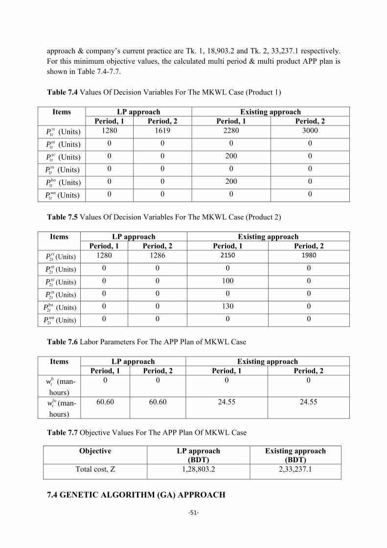
-51-

approach & company’s current practice are Tk. 1, 18,903.2 and Tk. 2, 33,237.1 respectively. For this minimum objective values, the calculated multi period & multi product APP plan is shown in Table 7.4-7.7. Table 7.4 Values Of Decision Variables For The MKWL Case (Product 1)

Items LP approach Existing approach Period, 1 Period, 2 Period, 1 Period, 2

rt

tP1 (Units) 1280 1619 2280 3000

ot

tP1 (Units) 0 0 0 0

sc

tP1 (Units) 0 0 200 0 in

tP1 (Units) 0 0 0 0

bo

tP1 (Units) 0 0 200 0 wa

tP1 (Units) 0 0 0 0 Table 7.5 Values Of Decision Variables For The MKWL Case (Product 2) Items LP approach Existing approach

Period, 1 Period, 2 Period, 1 Period, 2 rt

tP2 (Units) 1280 1286 2150 1980

ot

tP2 (Units) 0 0 0 0

sc

tP2 (Units) 0 0 100 0

in

tP2 (Units) 0 0 0 0 bo

tP2 (Units) 0 0 130 0 wa

tP2 (Units) 0 0 0 0

Table 7.6 Labor Parameters For The APP Plan of MKWL Case Items LP approach Existing approach

Period, 1 Period, 2 Period, 1 Period, 2 h

tw (man-hours)

0 0 0 0

lo

tw (man-hours)

60.60 60.60 24.55 24.55

Table 7.7 Objective Values For The APP Plan Of MKWL Case

Objective LP approach (BDT)

Existing approach (BDT)

Total cost, Z 1,28,803.2 2,33,237.1

7.4 GENETIC ALGORITHM (GA) APPROACH

-52-

The author has applied an interactive genetic algorithm approach for solving this aggregate production planning problem with respect to forecasted demand (proposed) and company’s estimated demand (current practice). Using MATLAB R2012a, the minimum fitness or objective values for genetic algorithm approach & company’s existing practice are Tk. 1, 35,140 and Tk. 2, 33,237.1 respectively. For this minimum objective values, the calculated multi period & multi product APP plan is shown in Table 7.8-7.11. Table 7.8 Values Of Decision Variables For The MKWL Case (Product 1)

Items GA approach Existing approach Period, 1 Period, 2 Period, 1 Period, 2

rt

tP1 (Units) 430.28 441.618

2280 3000

ot

tP1 (Units) 431.67

433.91

0 0

sc

tP1 (Units) 200.00

99.17

200 0

in

tP1 (Units) 280.09

552.26

0 0

bo

tP1 (Units) 3.46

439.62

200 0

wa

tP1 (Units) 0 0 0 0 Table 7.9 Values Of Decision Variables For The MKWL Case (Product 2)


rt

tP2 (Units) 494.07

400.74 2150 1980

ot

tP2 (Units) 495.06

399.80

0 0

sc

tP2 (Units) 84.83

0 100 0

in

tP2 (Units) 298.74

298.49

0 0

bo

tP2 (Units) 105.50

0 130 0

wa

tP2 (Units) 0 0 0 0

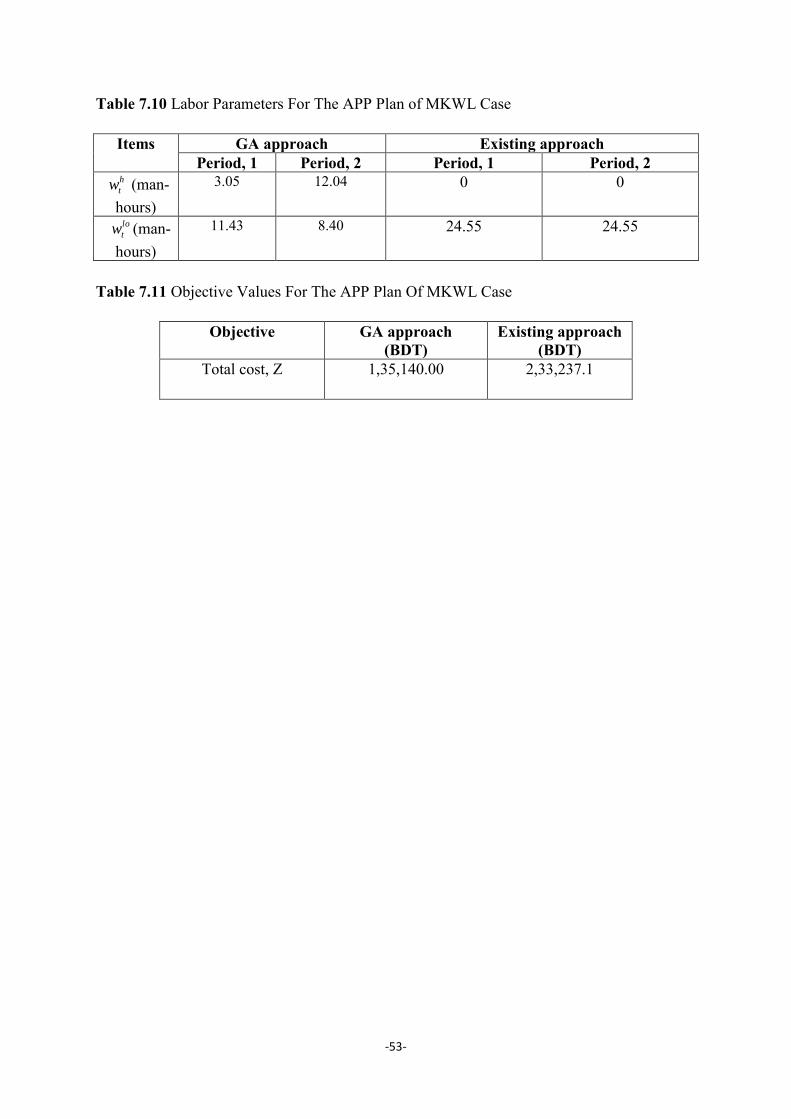
-53-

Table 7.10 Labor Parameters For The APP Plan of MKWL Case


h

tw (man-hours)

3.05

12.04

0 0

lo

tw (man-hours)

11.43

8.40

24.55 24.55

Table 7.11 Objective Values For The APP Plan Of MKWL Case

Objective GA approach (BDT)

Existing approach (BDT)

Total cost, Z 1,35,140.00

2,33,237.1

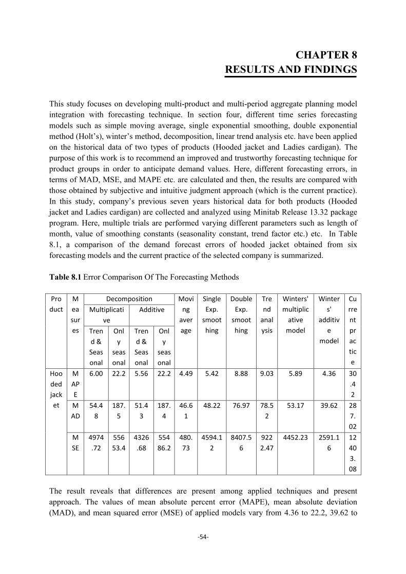
-54-

CHAPTER 8 RESULTS AND FINDINGS

This study focuses on developing multi-product and multi-period aggregate planning model integration with forecasting technique. In section four, different time series forecasting models such as simple moving average, single exponential smoothing, double exponential method (Holt’s), winter’s method, decomposition, linear trend analysis etc. have been applied on the historical data of two types of products (Hooded jacket and Ladies cardigan). The purpose of this work is to recommend an improved and trustworthy forecasting technique for product groups in order to anticipate demand values. Here, different forecasting errors, in terms of MAD, MSE, and MAPE etc. are calculated and then, the results are compared with those obtained by subjective and intuitive judgment approach (which is the current practice). In this study, company’s previous seven years historical data for both products (Hooded jacket and Ladies cardigan) are collected and analyzed using Minitab Release 13.32 package program. Here, multiple trials are performed varying different parameters such as length of month, value of smoothing constants (seasonality constant, trend factor etc.) etc. In Table 8.1, a comparison of the demand forecast errors of hooded jacket obtained from six forecasting models and the current practice of the selected company is summarized. Table 8.1 Error Comparison Of The Forecasting Methods Pro

duct

M

ea

sur

es

Decomposition Movi

ng

aver

age

Single

Exp.

smoot

hing

Double

Exp.

smoot

hing

Tre

nd

anal

ysis

Winters'

multiplic

ative

model

Winter

s'

additiv

e

model

Cu

rre

nt

pr

ac

tic

e

Multiplicati

ve

Additive

Tren

d &

Seas

onal

Onl

y

seas

onal

Tren

d &

Seas

onal

Onl

y

seas

onal

Hoo

ded

jack

et

M

AP

E

6.00 22.2 5.56 22.2 4.49 5.42 8.88 9.03 5.89 4.36 30

.4

2

M

AD

54.4

8

187.

5

51.4

3

187.

4

46.6

1

48.22 76.97 78.5

2

53.17 39.62 28

7.

02

M

SE

4974

.72

556

53.4

4326

.68

554

86.2

480.

73

4594.1

2

8407.5

6

922

2.47

4452.23 2591.1

6

12

40

3.

08

The result reveals that differences are present among applied techniques and present approach. The values of mean absolute percent error (MAPE), mean absolute deviation (MAD), and mean squared error (MSE) of applied models vary from 4.36 to 22.2, 39.62 to

-55-

187.5, and 480.732 to 8407.56 respectively. The values of MAPE, MAD, and MSD in current approach are 30.42, 287.02, and 12403.08 respectively. Results reveal that the errors of the forecasting models are substantially lower than values obtained from the company’s current practice (subjective and intuitive judgments). Among several methods, winter’s additive method shows the lowest forecasting errors which indicates the greatest accuracy and implies the suitability of this method for predicting demand of hooded jacket. A graphical presentation of different forecasting error’s in terms of MAPE, MAD, MSD is shown in Figure 8.1, 8.2, and 8.3.

Figure 8.1 A Comparative Study of MAPE for Hooded Jacket

Figure 8.2 A Comparative Study of MAD for Hooded Jacket

-56-

Figure 8.3 A Comparative Study of MSD for Hooded Jacket

Similarly, different time series forecasting models were run on the historical data of product ‘Ladies cardigan’ varying different parameters (length of month, smoothing constant etc.) by using MINITAB Release 13.32 package program. The comparison of the demand forecast errors obtained from the forecasting models and those from the current practice of the marketing department (as presented in Table 8.2) indicates that the errors of the forecasting models are substantially lower than those of the current practice. From the table, it is quite obvious that the appropriate forecasting method for product ‘Ladies cardigan’ is Holt’s method. Table 8.2 Comparison of the Forecasting Methods Product Meas

ures

Decomposition Mov

ing

aver

age

Single

Exp.

smoo

thing

Doubl

e Exp.

smoo

thing

Tre

nd

anal

ysis

Winter

s'

multipli

cative

model

Win

ters'

addi

tive

mod

el

Curr

ent

prac

tice

Multiplicati

ve

Additive

Tren

d &

Seas

onal

Only

seas

onal

Tren

d &

Seas

onal

Only

seas

onal

Ladies

cardigan

MAP

E

15.6 32.5 15.9 32.4 11.1 11.7 10.8 16.6 15 15.1 20.1

MAD 128.

7

264.

1

131.

7

262.

9

100.

7

182.3 116.8 139.

2

133.1 134.

8

188.

5

MSD 363

40.1

915

90.6

364

33.1

915

05.2

223

42.3

2942

1

2225

5

387

36

30543.

8

298

75.4

682

59.6

A graphical presentation of different forecasting error’s in terms of MAPE, MAD, MSD is shown in Figure 8.4, 8.5, and 8.6.

-57-

Figure 8.4 A Comparative Study of MAPE for Ladies Cardigan

Figure 8.5 A Comparative Study of MAD for Ladies Cardigan

Figure 8.6 A Comparative Study of MSD for Ladies Cardigan

-58-

Finally, using the best fitting forecasting methods, demand values are projected for both products. Figure 8.7 shows the comparative study of projected demands between proposed approach and company’s current practice. The results reveal that projected demand values using company’s usual practice are much higher than proposed approaches for both products. At planning horizon 1, forecasted demands (units) of hooded jacket and Ladies cardigan under proposed and company’s current practice are 1515, 3000 & 1479, 2500 respectively. Again, at period 2, demand values are 1558, 2800 & 1048, 1850 for suggested approach and company’s current approach.

Figure 8.7 Demand Comparisons between Proposed & Current approaches

The LP and Genetic Algorithm (GA) approach for solving aggregate production planning decision problem through minimizing total cost is analyzed with a case study in the previous section. From the result of existing and applied approaches, it is clear that the proposed models can lower the total cost than existing practice. In the Table 8.3, the comparison of total cost (production & labor related cost) between existing and LP approach is presented. The objective value when applying company’s current practice to minimize the total costs, the value of fitness function is BDT 2,33,237.1. In contrast with the LP approach, the improved result is BDT 1,28,803.2. These figures reveal that the LP approach is an efficient compromise solution & minimizes the total cost, compared to the optimal goal value obtained by the company’s existing practice. Table 8.3 Total Cost Comparison of Existing & LP Approach

Item Existing approach LP approach

Objective function Min Z Min Z Z (Total cost) BDT 2,33,237.10 BDT 1,28,803.20

-59-

The LP approach is well suited for solving single objective problem having linear constraints. This approach constitutes a systematic framework that facilitates the decision-making process. In this research, another robust optimization tool which is genetic algorithm (GA) has been also applied to solve the same APP decision problem. This meta-heuristic approach can solve most real-world supply chain cost minimization problems through an interactive decision making process. Moreover, GA approach also can help to determine optimum solution even it is NP (nondeterministic polynomial) hard problems. The below Table 8.4 compares the solutions obtained from existing model with that from GA (Genetic Algorithm) model. Table 8.4 Total Cost Comparison of Existing and Genetic Algorithm Approach

Item Existing approach GA approach

Objective function Min Z Min Z Z (Total cost) BDT 2,33,237.10 BDT 1,35,140.00

Finally, the below Table 8.5 compares the solutions obtained from different approaches for APP problem. In this research, different approaches have been applied to provide a detailed comparison of results as well as to measure their effectiveness. From the table, it is quite obvious that the objective function obtained from company’s current practice is higher than those obtained from LP and GA approaches. Among three approaches, linear programming approach seems to be satisfactory because this technique gives the minimum value of objective function. Table 8.5 Total Cost Comparison of Different Approaches for APP Problem

Approaches Main Objective Value Z (BDT)

Existing practice 2,33,237.10 LP model 1,28,803.20 GA model 1, 35,140.00

-60-

CHAPTER 9 CONCLUSIONS AND RECOMMENDATIONS

9.1 CONCLUSIONS This research presents a novel decision support model for aggregate production planning and improving the forecasting technique as well as selecting the best one for predicting future demand. Forecasted demand of products is one of the important inputs in APP process. An accurate prediction of market demand is very crucial in case of reducing unnecessary inventories, smoothing the production plan, maintaining supply chain effectiveness and responsiveness which finally results in increasing profit. Improper capacity planning occurs due to lacking of justified and realistic forecasting method which implies to the wrong production quantities for the members of a supply chain. However, these observations result in the need for developing a decision support model for aggregate production planning and improving the forecasting technique to improve customer service level. Here in this study, a multi-product multi-period aggregate planning model along with proper forecasting technique selection has been targeted to minimize the overall cost. In this study, to select the best fitting forecasting approach, different types of time series forecasting models are used and errors in terms of MAD, MSE, and MAPE are calculated. For this purpose, Minitab software has been utilized to make a comparison of different approaches. This attempt can help to improve efficiency in the formulation of aggregate production planning model. The objective function used here is to minimize the total cost. In the objective function, seven types of cost like inventory holding costs, production costs (regular plus overtime production), extra subcontracting cost, backordering cost, wastage cost, labor cost have been considered in order to find out the optimal cost. Here, aggregate production planning problem has been formulated as a linear programming model and later solved by both Linear Programming (LP) approach and a meta-heuristic algorithm (Genetic Algorithm). The LP approach provides simplicity and helps to determine objective function easily. Actually, LP approach is suitable for solving simple linear problems. But, for solving NP (non-deterministic polynomial) hard problems, meta-heuristics algorithms provide global optima faster than exact algorithms. This type of algorithms has mechanisms to avoid getting caught by local optima. For example, GA uses crossover and mutation operators that make its population more diverse as well as more immune to be trapped in local optima. Since APP problem is often NP hard problem, in this case genetic algorithm can provide satisfactory result. From the last four decades, a lot of researches works are have been performed for optimization of APP problems and obtaining optimum quantities (production, back order etc.). But the researches focusing the incorporation of best fitting forecasting approach in

-61-

optimization of APP problems are very limited. This research distinctively uses the analysis of time series forecasting models for finding the best fitting forecasting approach and then, the projected demand from that selected approach is incorporated in APP model. Here, APP problem is solved by both LP & Genetic Algorithm (GA) and finally, a comparison is performed between those approaches & company’s existing practice. However, this research must also admit the limitations. In order to develop APP model as well as selecting appropriate technique in a batch oriented discrete manufacturing company, all the data are collected from real company. These collected data relied mostly on the management of the associated company. To find a more accurate optimum production level of specific products, precise data providing as input is very crucial. From the comparison section in the previous chapter, it is quite clear that, among three approaches, LP approach gives satisfactory result than existing practice of the selected company as well as meta-heuristic algorithm. 9.2 FUTURE RECOMMENDATIONS

➢ In this research, to find out the optimal production level of specific products, seven

types of cost functions were used to minimize the total cost. In future, some other cost

criteria like cost for lost sales, incentive cost etc. can be included to make the costs

more appropriate.

➢ For predicting demand, common types of forecasting techniques available in Minitab

software were applied in this study. But, there are many robust forecasting techniques

are available in literature. In future, more robust techniques like artificial neural

network (ANN) in fuzzy environment can be considered.

➢ In future, the proposed model can be applied in fuzzy based environment to address

uncertain situation. Here, demand and other cost related parameters were used as

exact numerical values. In future, they can be considered as fuzzy data to improve the

model.

➢ Here, only single objective (minimizing total cost) has been considered. In future,

multi-objective APP model can be formulated.

➢ In the research, genetic algorithm and Linear Programming were used to solve the

problem. For specific optimization problems and problem instances, other

optimization algorithms such as particle swarm optimization (PSO), ant colony

optimization (ACO), mixed integer linear programming (MILP), fuzzy multi-

objective linear programming (FMOLP) etc. may be used to solve and compare the

solutions with the proposed algorithm.

-62-

REFERENCES

[1] Aliev, R. A., Fazlollahi, B., Guirimov, B. G., & Aliev, R. R. (2007). Fuzzy-genetic

approach to aggregate production-distribution planning in supply chain management

Information Sciences, 177, pp. 4241–4255.

[2] Baykasogluy, A. (2006). Aggregate production planning using the multiple objective

tabu search. International Journal of Production Research, 39 (16), pp. 3685-3702.

[3] Bunnag, D., & Sun, M. (2005). Genetic Algorithm for constrained global optimization

in continuous variables. Applied Mathematics and Computation, 171, pp. 604–636.

[4] Buxey, G. (1993). Production planning and scheduling for seasonal demand.

International Journal of Operations and Production Management, 13(7), pp. 4–21.

[5] Chakraborty, R.K., & Hasin, M. A.A. (2013). Solving an aggregate production

planning problem by Fuzzy Genetic Algorithm (FBGA). International Journal of

Fuzzy Logic Systems, 3(1), pp. 1-16.

[6] Chakraborty, R.K., & Hasin, M. A.A. (2013). Solving an aggregate production

planning problem by multi-objective genetic algorithm (MOGA) approach.

International Journal of Industrial Engineering Computations, 5, pp. 1-12.

[7] Chakraborty, R.K., Hasin, M. A.A., Sarkar, R.A., & Essam, D.L. (2015). A

Possibilistic environment based Particle Swarm Optimization for aggregate

production planning. Computers and Industrial Engineering, Elsevier, 88, pp. 366-

377.

[8] Dobos, I. (1996). Aggregate planning with continuous time. Int. J. Prod. Econ. 43 (1),

pp. 1–9.

[9] Dolgui, A., & Ould-Louly, M.A. (2002). A model for supply planning under lead time

uncertainty. International Journal of Production Economics, 78(2), pp. 145–152.

[10] Enns, S.T. (2002). MRP performance effects due to forecast bias and demand

uncertainty. Eur. J. Oper. Res. 138, pp. 87–102.

[11] Fahimnia, L., & Marian, S. (2006). Modeling and optimization of aggregate

production planning- A Genetic Algorithm. In: Proceedings of World Academy of

Science, Engineering and Technology.

-63-

[12] Foote, B.L., Ravindran, A., & Lashine, S. (1998). Production planning and

scheduling: computational feasibility of multi-criteria models of production, planning

and scheduling. Computers and Industrial Engineering, 15(1), pp. 129–138.

[13] Ganesh, K., & Punniya Moorthy, M. (2005). Optimization of continuous-time

production planning using hybrid Genetic Algorithms- Simulated Annealing.

International Journal of Advance Manufacturing Technology, 26, pp. 148-154.

[14] Gansterer M. (2015).Aggregate planning and forecasting in make-to-order production

systems. International Journal of Production Economics, 170, pp. 521–528.

[15] Gebennini, E., Gamberini, R., & Manzini, R. (2009). An integrated production–

distribution model for the dynamic location and allocation problem with safety stock

optimization. International Journal of Production Economics, 122(1), pp. 286–304.

[16] Goldberg, D.E. (1989). Genetic Algorithms in Search, Optimization & Machine

Learning. Pearson Education Pvt. Ltd., Singapore.

[17] Gunnarsson, H., & Ronnqvist, M. (2008). Solving a multi-period supply chain

problem for a pulp company using heuristics—an application to Sodra Cell AB.

International Journal of Production Economics, 116(1), pp. 75–94.

[18] Ho, C., & Ireland, T.C. (1998). Correlating MRP system nervousness with forecast

errors. Int. J. Prod. Res., 36 (8), pp. 2285–2299.

[19] Hsieh, S., & Wu, M.S. (2000). Demand and cost forecast error sensitivity analyses in

aggregate production planning by possibilistic linear programming models. J. Intell.

Manuf., 11 (4), pp. 355–364.

[20] Ioannis, G.T. (2009). Solving constrained optimization problems using a novel

genetic algorithm. Applied Mathematics and Computation, 208, pp. 273–283.

[21] Jiang, Kong, & Li (2008). Aggregate production planning model of production line in

iron & steel enterprise based on Genetic Algorithm. Proceedings of the 7th World

Congress on Intelligent Control Automation, Chongqing, China.

[22] Jung, H., & Jeong, B. (2005). Decentralized production-distribution planning system

using collaborative agents in supply chain network. Int. J. Adv. Manuf. Technol.

Springer London 25 (1–2), pp. 167–173.

[23] Kerkkänen, A., Korpela, J., & Huiskonen, J. (2009). Demand forecasting errors in

industrial context: measurement and impacts. Int. J. Prod. Econ. 118, pp. 43–48.

[24] Liang, T. F. (2007). Application of interactive possibilistic linear programming to

aggregate production planning with multiple imprecise objectives. Production

Planning and Control, 18(7), pp. 548–560.

-64-

[25] Lodree Jr., E.J., & Uzochukwu, B.M. (2008). Production planning for a deteriorating

item with stochastic demand and consumer choice. International Journal of

Production Economics, 116(2), pp. 219–232.

[26] Mazzola, J.B., Neebe, A.W., & Rump, C.M. (1998). Multiproduct production

planning in the presence of work-force learning. European Journal of Operational

Research, 10(2–3), pp. 336–356.

[27] Mirzapouur-al-hashem S.M.J., Malekly H., & aryanezhad M. B. (2011). A multi-

objective robust optimization model for multi-product, multi-site aggregate

production planning in a supply chain under uncertainty. Int J Production Economics

134, pp. 28–42.

[28] Mohan Kumar, G., & Noorul Haq, A. (2005). Hybrid genetic-ant colony algorithms

for solving aggregate production plan. Journal of Advanced Manufacturing Systems,

1, pp. 103-111.

[29] Ning, Y., Tang, W., & Zhao, R. (2006). Multi-product aggregate production planning

in fuzzy random environments. World Journal of Modeling and Simulation, 2(2), pp.

312–321.

[30] Park, Y.B. (2005). An integrated approach for production and distribution planning in

supply chain management. Int. J. Prod. Res., 43 (6), pp. 1205–1224.

[31] Price D. H. R., & Sharp J. A. (1984). Demand forecasting and aggregate planning in

the electrical supply industry. International Journal of Operations & Production

Management, 4(4), pp. 48 – 56.

[32] Porkka, P., Vepsalainen, A.P.J., & Kuula, M. (2003). Multi-period production

planning carrying over set-up time. International Journal of Production Research,

41(6), pp. 1113–1148.

[33] Ramazanian & Modares (2011). Application of particle swarm optimization algorithm

to aggregate production planning. Asian Journal of Business Management Studies, 2,

pp. 44-54.

[34] Ramezanian, R., Rahmani, D., & Barzinpour, F. (2012). An aggregate production

planning model for two phase production systems: Solving with genetic algorithm and

tabu search. Expert Systems with Applications, 39, pp. 1256-1263.

[35] Sharma, D.K., & Jana R.K. (2009). Fuzzy goal programming based genetic algorithm

approach to nutrient management for rice crop planning. International Journal of

Production Economics, 121, pp. 224–232.

-65-

[36] Silva, Figureria, Lisboa & Barman (2006).An interactive decision support system for

an aggregate production planning model based on multiple criteria mixed integer

linear programming. Omega-International Journal of Management Science, 34, pp.

167-177.

[37] Sivanandam, S.N., & Deepa, S. N. (2008). Introduction to Genetic Algorithms, New

York: Springer Berlin Heidelberg.

[38] Vörös, J. (1999). On the risk-based aggregate planning for seasonal products. Int. J.

Prod. Econ., 59 (1), pp. 195–201.

[39] Wang, R. C., & Liang, T. F. (2004). Application of fuzzy multi-objective linear

programming to aggregate production planning. Computers & Industrial Engineering,

46, pp. 17–41.

[40] Wang, R.C., & Liang, T.F. (2005). Applying Possibilistic linear programming to

aggregate production planning. International Journal of Production Economics, 98,

pp. 328-341.

[41] Xie, J., Lee, T.S., & Zhao, X. (2004). Impact of forecasting error on the performance

of capacitated multi-item production systems. Computer Ind. Eng., 46, pp. 205–219.

[42] Yeh, W.C., & Chuang, M.C. (2011).Using multi-objective genetic algorithm for

partner selection in green supply chain problems. Expert Systems with Applications,

38, pp. 4244-4253.

[43] Yenradeea P., Pinnoib A., & Charoenthavornying A. (2001). Demand Forecasting and

Production Planning for Highly Seasonal Demand Situations: Case Study of a

Pressure Container Factory. Science Asia, 27, pp. 271-278.

[44] Wang, R.C., & Fang, H.H. (2001). Aggregate production planning with multiple

objectives in a fuzzy environment. European Journal of Operational Research, 133,

pp. 521–536.

[45] Wang, R.C., & Liang, T.F. (2004). Application of fuzzy multi-objective linear

programming to aggregate production planning. Computers and Industrial

Engineering, 46 (1), pp. 17–41.

[46] Masud, S.M., & Hwang, C.L. (1980). An aggregate production planning model and

application of three multiple objective decision methods. International Journal of

Production Research, 18, pp. 741–752.

[47] Islam, M.M., & Hossain, M.M. (2016). Multi product multi period aggregate

production planning in an uncertain environment. Global Science and Technology

Journal, 4(1), pp. 1-19.

-66-

[48] Kalaf, B. A., Bakar, R. A., Soon, L. L., Monsi, M. B., Bakheet, A. J. K., & Abbas, I.

T. (2015). A modified fuzzy multi-objective linear programming to solve aggregate

production planning. International Journal of Pure and Applied Mathematics, 104(3),

pp. 339-352.

[49] Abass, S. A., & Elsayed, M. S. (2012). Modeling and Solving Production Planning

Problem under Uncertainty: A Case Study. American Journal of Operational

Research, 2(5), pp. 60-65.

[50] Savsani, P., Banthia, G., Gupta, J., & Vyas, R. (2016). Optimal aggregate production

planning by using genetic algorithm. International Conference on Industrial

Engineering and Operations Management, pp. 863-874.

[51] Entezaminia, A., Heydari, M., & Rahmani, D. (2016). A multi-objective model for

multi-product multi-site aggregate production planning in a green supply chain:

Considering collection and recycling centers. Journal of Manufacturing Systems, 40,

pp. 63–75.

[52] Modarres, M., & Izadpanahi, E. (2016). Aggregate production planning by focusing

on energy saving: a robust optimization approach. Journal of Cleaner Production, 133,

pp. 1074–85.

[53] Biel, K., & Glock, C. H. (2016). Systematic literature review of decision support

models for energy-efficient production planning. Computers & Industrial

Engineering, 101, pp. 243-259.

[54] Nour, A., Galal, N. M., & El-Kilany, K. S. (2017). Energy-Based Aggregate

Production Planning For Porcelain Tableware Manufacturer in Egypt. International

Conference on Industrial Engineering and Operations Management, pp. 2351-2358.

[55] Khalili-Damghani, K., Shahrokhb, A., & Pakgoharc, A. (2017). Stochastic multi-

period multi-product multi-objective Aggregate Production Planning model in multi-

echelon supply chain. International Journal of Production Management and

Engineering, 5(2), pp. 85-106.

[56] Mirzapour Al-e-hashem, S.M.J., Baboli, A., & Sazvar, Z. (2013).A stochastic

aggregate production planning model in a green supply chain: Considering flexible

lead times, nonlinear purchase and shortage cost functions. European Journal of

Operational Research, 230, pp. 26–41.

[57] Mirzapour Al-e-Hashem, S.M.J., Aryanezhad, M.B., & Sadjadi, S.J. (2012).An

efficient algorithm to solve a multi-objective robust aggregate production planning in

-67-

an uncertain environment. International Journal of Advanced Manufacturing

Technology, 58, pp. 765–782.

[58] Sakallı, Ü.S., Baykoç, Ö.F., & Birgören, B. (2010). A possibilistic aggregate

production planning model for brass casting industry. Production Planning & Control:

The Management of Operations, 21(3), pp. 319-338.

[59] Ait-Alla, A., Teucke, M., Lütjen, M., Beheshti-Kashi, S., & Karimi, H. R. (2014).

Robust Production Planning in Fashion Apparel Industry under Demand Uncertainty

via Conditional Value at Risk. Mathematical Problems in Engineering, pp. 1-10.

[60] Bakar, M. R.A., Bakheet, A.J.K., Kamil, F., Kalaf, B.A., Abbas, I.T., & Soon, L. L.

(2016). Enhanced simulated annealing for solving aggregate production planning.

Mathematical Problems in Engineering, pp. 1-9.

[61] Luangpaiboon, P., & Aungkulanon, P. (2013). Integrated approaches to enhance

aggregate production planning with inventory uncertainty based on improved

harmony search algorithm. Proceedings of World Academy of Science, Engineering

and Technology, 73, pp. 243-250.

[62] Kavehand, M., & Dalfard, V.M. (2014). A simulated annealing algorithm for

aggregate production planning with considering of ancillary costs. International

Journal of Mathematics in Operational Research, 6(4), pp. 474–490.

-68-

APPENDIX-A

Code for the Linear Programming Model

(Software Used: MATLAB R2012a)

MATLAB commands for determining Z

%% Define the coefficient of the objective function f=[22 22 20 20 40 40 40 40 27 27 30 30 3.5 3.5 4 4 42 42 47 47 32 32 30 30

49 49 -19 -19];

%% Define the coefficients for equality constraints Aeq=[1 0 0 0 1 0 0 0 1 0 0 0 -1 0 0 0 1 0

0 0 -1 0 0 0 0 0 0 0 0 1 0 0 0 1 0 0 0 1 0 0 1 -1 0 0 -1 1 0

0 0 -1 0 0 0 0 0 0 0 0 1 0 0 0 1 0 0 0 1 0 0 0 -1 0 0 0 1

0 0 0 -1 0 0 0 0 0 0 0 0 1 0 0 0 1 0 0 0 1 0 0 1 -1 0 0 -1

1 0 0 0 -1 0 0 0 0];

%% Define the coefficients for equality constraints [R.H.S.] beq=[1280 1619 1280 1286];

%% %Define the coefficients for inequality constraints A=[0 0 0 0 0 0 0 0 0 0 0 0 1 0 0 0 0 0

0 0 0 0 0 0 0 0 0 0 0 0 0 0 0 0 0 0 0 0 0 0 0 1 0 0 0 0 0

0 0 0 0 0 0 0 0 0 0 0 0 0 0 0 0 0 0 0 0 0 0 0 1 0 0 0 0

0 0 0 0 0 0 0 0 0 0 0 0 0 0 0 0 0 0 0 0 0 0 0 0 1 0 0 0

0 0 0 0 0 0 0 0 0 0 0 0 0 0 0 0 0 0 0 0 0 0 0 0 0 1 0 0

0 0 0 0 0 0 0 0 0 0 0 0 0 0 0 0 0 0 0 0 0 0 0 0 0 0 1 0

0 0 0 0 0 0 0 0 0 0 0 0 0 0 0 0 0 0 0 0 0 0 0 0 0 0 0 1

0 0 0 0 0 0 0 0 0 0 0 0 0 0 0 0 0 0 0 0 0 0 0 0 0 0 0 0

1 0 0 0 0 0 0 0 0 0 0 0 0 0 0 0 0 1 0 0 0 0 0 0 0 0 0 0

0 0 0 0 0 0 0 0 0 0 0 0 0 0 0 0 0 0 1 0 0 0 0 0 0 0 0 0

0 0 0 0 0 0 0 0 0 0 0 0 0 0 0 0 0 0 0 1 0 0 0 0 0 0 0 0

0 0 0 0 0 0 0 0 0 0 0 0 0 0 0 0 0 0 0 0 1 0 0 0 0 0 0 0

0 0 0 0 0 0 0 0 0 0.1 0 0.08 0 0.1 0 0.08 0 0 0 0 0 0 0 0 0 0

0 0 0 0 0 0 0 0 0 0 0

-69-

0 0.1 0 0.08 0 0.1 0 0.08 0 0 0 0 0 0 0 0 0

0 0 0 0 0 0 0 0 0 0 0 0 0 0 0 0 0 0 0 0 0 0 0 1 0 1.5 0 0 0 0

0 0 0 0 0 0 0 0 0 0 0 0 0 0 0 0 0 0 0 0 0 0 1 0 1.5 0 0 0

0 0 0 0 0 0 0 0 0 0 0 0 0 0 0 0 0 0 0 0 0 0 0 0 0 0 0 0

0 1 0 0 0 0 0 0 0 0 0 0 0 0 0 0 0 0 0 0 0 0 0 0 0 0 0 0

0 0 1 0 0 0 0 0 0 0 0 0 0 0 0 0 0 0 0 0 0 0 0 0 0 0 0 0

0 0 0 1 0 0 0 0 0 0 0 0 0 0 0 0 0 0 0 0 0 0 0 0 0 0 0 0

0 0 0 0 1 0 0 0 0 0.03 0 0.05 0 0.03 0 0.05 0 0 0 0 0 0 0 0

0 0 0 0 0 0 0 0 0 0 0 0 0 0 0.03 0 0.05 0 0.03 0 0.05 0 0 0 0 0 0 0

0 0 0 0 0 0 0 0 0 0 0 0 0 0.03 0 0.05 0 0.03 0 0.05 0 0 0 0 0 0 0 0

0 0 0 0 0 0 0 0 0 -1 -1 1 1 0 0.03 0 0.05 0 0.03 0 0.05 0 0 0 0 0 0 0

0 0 0 0 0 0 0 0 0 0 0 0 0];

%% Define the coefficients for inequality constraints [R.H.S.] b=[280 450 160 200 200 600 150 100 200 300 100 100 400 500 1000 1000 40 80

30 25 350 350 225 225]; formatlong

%% Call MATLAB linprog solver x=linprog(f,A,b,Aeq,beq,zeros(28,1),[],[]); %% Calculate objective function value Min_cost=12150+f*x; fprintf('Minimized objective function value is %d\n',Min_cost) disp(x) format

-70-

APPENDIX-B

Code for the Single Objective Genetic Algorithm (GA) Approach

(Software Used: MATLAB R2012a)

Objective function y=simple_fitness(x) y=(22*x(1)+22*x(2)+20*x(3)+20*x(4)+40*x(5)+40*x(6)+40*x(7)+40*x(8)+27*x(9)+27*x(10)+30*x(11)+30*x(12)+3.5*x(13)+3.5*x(14)+4*x(15)+4*x(16)+42*x(17)+42*x(18)+47*x(19)+47*x(20)+32*x(21)+32*x(22)+30*x(23)+30*x(24)+49*x(25)+49*x(26)-19*x(27)-19*x(28)+12150); Constraints function [c,ceq]=simple_constraint(x) c=[280-x(13);450-x(14);160-x(15);200-x(16);-200+x(17);-600+x(18);-150+x(19);-100+x(20);-200+x(9);-300+x(10);-100+x(11);-100+x(12);-400+0.1*x(1)+0.1*x(5)+.08*x(3)+.08*x(7);-500+0.1*x(2)+0.1*x(6)+.08*x(4)+.08*x(8);-1000+1.0*x(13)+1.5*x(15);-1000+1.0*x(14)+1.5*x(16);-40+x(21);-80+x(22);-30+x(23);-25+x(24);-350+0.03*x(1)+0.03*x(5)+0.05*x(3)+0.05*x(7);-350+0.03*x(2)+0.03*x(6)+0.05*x(4)+0.05*x(8);-225+.03*x(1)+0.03*x(5)+0.05*x(3)+0.05*x(7)-x(25)+x(27);-225+.03*x(2)+0.03*x(6)+0.05*x(4)+0.05*x(8)-x(26)+x(28)]; ceq=[-1280+x(1)+x(5)+x(9)-x(21)-x(13)+x(17);-1619+x(2)+x(6)+x(10)-x(22)+x(13)-x(17)-x(14)+x(18);-1280+x(3)+x(7)+x(11)-x(23)-x(15)+x(19);-1286+x(4)+x(8)+x(12)-x(24)+x(15)-x(19)-x(16)+x(20)]; Function call ObjectiveFunction=@simple_fitness; nvars=28; lb=[0 0 0]; ub=[]; ConstraintFunction=@simple_constraint; [x,fval]=ga(ObjectiveFunction,nvars,[],[],[],[],lb,ub,ConstraintFunction)

AGGREGATE PRODUCTION PLANNING FOR BATCH- ORIENTED …

Documents