Agent performance in vehicle routing when the only thing certain is uncertainty

Agent Performance in Vehicle Routing when the OnlyThing Certain is Uncertainty

Tamas MahrDelft Technical University and Almende BV

Rotterdam, The [email protected]

Jordan SrourRSM Erasmus University

Rotterdam, The [email protected]

Mathijs de WeerdtDelft Technical University

Delft, The [email protected]

Rob ZuidwijkRSM Erasmus University

Rotterdam, The [email protected]

ABSTRACTWhile intermodal transport has the potential to introduceefficiency to the transport network, this transport environ-ment also suffers from a lot of uncertainty at the interface ofmodes. For example, trucks moving containers to and froma port terminal are often uncertain as to when exactly theircontainer will be released from the ship, from the stack, orfrom customs. This leads to much difficulty and inefficiencyin planning a profitable routing for multiple containers inone day.

In this paper, we examine agent-based solutions as a mech-anism to handle job arrival uncertainty in the context of adrayage case at the Port of Rotterdam. We compare ouragent-based solution approach to a well known on-line opti-mization approach and study the comparative performanceof both systems across four scenarios of varying job arrivaluncertainty. We conclude that when less than 50% of all jobsare known at the start of the day then an agent-based ap-proach performs competitively with an on-line optimizationapproach.

1. INTRODUCTIONScheduling the routes of trucks to pick-up and deliver con-

tainers is a complex problem. In general such Vehicle Rout-ing Problems (VRPs) [19] are known to be NP-complete,and therefore inherently hard and time consuming to solveto optimality. Fortunately, these problems have a structurethat can facilitate efficient derivation of feasible (if not op-timal) solutions. Specifically, the routes of different trucksare more or less independent. Such “locality” in a problemis a first sign that an agent-based approach may be viable.

Modeling and solving a VRP by coordinating a set ofagents can bring a number of advantages over more estab-lished approaches in the field of operations research evenwhen using state-of-the-art mixed integer solvers such asCPLEX [7]. Agent advantages include the possibility fordistributed computation, the ability to deal with propri-etary data from multiple companies, the possibility to reactCite as: Agent Performance in Vehicle Routing when the Only ThingCertain is Uncertainty, T. Mahr, J. Srour, M.M. de Weerdt, and R. Zuidwijk,Proc. of 7th Int. Conf. on Autonomous Agents and Multia-gent Systems (AAMAS 2008), Padgham, Parkes, Müller and Parsons(eds.), May, 12-16., 2008, Estoril, Portugal, pp. XXX-XXX.Copyright © 2008, International Foundation for Autonomous Agents andMultiagent Systems (www.ifaamas.org). All rights reserved.

quickly on local knowledge [5], and the capacity for mixed-initiative planning [1].

In particular, agents have been shown to perform well inuncertain domains. That is, in domains where the problemis continually evolving [5]. In the VRP, for example, a verybasic form of uncertainty is that of job arrivals over time.To the best of our knowledge, however, the effect of eventhis basic level of uncertainty on the performance of agent-based planning in a realistic logistics problem has never beenshown.

We think it is safe to assume, based on its long history,that current practice in operations research (OR) outper-forms agent-based approaches in settings where all infor-mation is known in advance (static settings). However, insituations with a lot of uncertainty, agent-based approachesare expected to outperform these traditional methods [8].

In this paper we investigate whether a distributed agent-based planning approach indeed suffers less from job arrivaluncertainty than a centralized optimization-based approach.Our main contribution is to determine at which level of jobarrival uncertainty agent-based planning outperforms on-line operations research methods. These results can helptransportation companies decide when to adopt an agent-based approach, and when to use an on-line optimizationtool, depending on the level of uncertainty job arrivals ex-hibit in their daily business.

In Section 2 we provide a survey of current work on agent-based approaches to logistics problems. In Section 3 we thenintroduce the case of a transportation company near theport of Rotterdam. Based on this literature review and thespecific nature of our case study VRP, we propose a state-of-the-art agent-based approach where orders are auctionedamong trucks in such a way that each order is assigned tothe truck that can most efficiently transport the container.Moreover, these trucks continuously negotiate among eachother to exchange orders as the routing situation evolves.This agent-based approach is the topic of Section 4. Inthe following section, Section 5, we describe the central-ized on-line optimization approach used in comparison toour distributed agent-based system. The structure of ourtest problems and the computational results are the topicsof Section 6. In our final section we discuss the consequencesof our results, summarize our advice to transportation com-panies, and give a direction for future work.

2. LITERATURE SURVEYIn their frequently cited 1995 paper, Fischer et al. ar-

gued that multi-agent models fit the transportation domainparticularly well [5]. Their main reasons were that (i) thedomain is inherently distributed (trucks, customers, compa-nies etc.); (ii) a distributed agent architecture can cope withmultiple dynamic events; (iii) commercial companies may bereluctant to provide proprietary data needed for global op-timization and agents can use local information; and (iv)inter-company cooperation can be more easily facilitated byagents. To illustrate the idea, the authors also provided adetailed agent architecture for transportation problems thatevolve over time thereby exhibiting uncertainty over time.This architecture makes a distinction between a higher anda lower architectural level. At the higher level, companyagents negotiate over transportation requests to eliminateill-fitting orders. On the lower level, truck agents (clusteredper company) participate in simulated market places, wherethey bid on offered transportation orders. Truck agents usesimple insertion heuristics to calculate their costs and usethose costs to bid on auctions implementing an extendedcontract net protocol [17]. Although the heuristics thatagents use to make decisions are rather crude, the authorssuggested that in dynamic problems (problems with high un-certainty), such methods survive better than sophisticatedoptimization methods.

Fischer et al.’s bi-level approach recognizes that one short-coming of a fully distributed system is that agents only haveaccess to local information [5]. The need to balance be-tween the omniscience of a centralized model and the agilityof a distributed model, was similarly recognized by Mes etal. [12]. They also introduce a higher level of agents, butwith a different role than the high-level agents of Fischer etal. Mes et al.’s two high-level agents (the planner and thecustomer agent) gather information from and provide infor-mation to agents assigned beneath them. The role of thehigher level agents is to centralize information essential forthe lower level agents to make the right decisions.

Some researchers have gone even further in proposing cen-tralized agent-based models. These researchers focused oncentralizing the problem information to be able of make bet-ter distributed decisions. In one of the few models that isactually applied in a commercial company, Dorer and Cal-isty cluster trucks geographically, using one agent per clus-ter [4]. This way, one agent plans for multiple trucks. Theyuse insertion heuristics to initially assign orders to trucks,and then use cyclic transfers [18] to enhance the solution.In an even more centralized model, Leong and Liu use afully centralized optimizer to initialize the agents [11]. Theagents’ role is then to change the plans as events are re-vealed. The authors analyze the performance of their modelon a selection of Solomon benchmark sets, and show that itperforms competitively.

As noted previously, however, the move towards central-ization can hinder the ability of the agents to react quicklyon local information. Given the uncertain environment ofour problem, we are interested in the competitiveness of asystem with fully distributed agents. One example of a fullydistributed agent approach in the transportation domainis that of Brückert et al. They proposed a more detailed(holonic) agent model [1]. They distinguished truck, driver,chassis, and container agents that have to form groups (calledholons) to serve orders. Already formed holons use the same

techniques to allocate tasks as Fischer et al., but the higheragent level is omitted, since they model only a single com-pany case. The main focus of their research is computer-human cooperative planning, and they do not test theirmodel extensively against other models.

Generally, the decision to use a distributed approach isbased on the expectation (included already in the reasons ofFischer et al.) that distributed models handle uncertaintybetter. The agent architecture in these fully distributedmodels is completely flat, the models avoid centralizing in-formation, and agents can use only local information whenmaking decisions. Having lost the power of using (partial)global information, distributed agents need other ways toenhance their performance.

In the model of Fischer et al., as well as in the modelsof many of their followers, agents use simple approximationtechniques to make decisions. In the related domain of pro-duction planning Persson et al. embed optimization in theagents to improve local decisions [13]. They show that op-timizing agents outperform the approximating agents, butthey also show that central optimization still outperformsthe optimizing, but distributed, agents.

While Persson et al. concentrated on making optimal de-cisions within agents, there is still a need to coordinate be-tween the distributed agents. For example, in the transportproblem context, when orders are assigned to trucks sequen-tially, at every assignment the truck with the cheapest in-sertion gets the order. Later, however, it might turn outthat it would be cheaper to assign the same order togetherwith newly arrived orders to another truck. From the truckpoint of view it means that trucks that bid early and winassignments might not be able to bid later on more benefi-cial (better fitting) orders. This problem is called ‘the eagerbidder problem’ [16], and several researchers proposed al-ternative techniques to solve it. Kohout and Erol introducean enhancement process that works between agents [9]. Theprocess mimics a well known enhancement technique called’swapping’ or two-exchange [2]. Kohout and Erol implementthis swapping process in a fully distributed way, and showthat it yields significant improvement.

Perugini et al. extend Fischer’s contract-net protocol toallow trucks to place multiple possibly-conflicting bids forpartial routes [14]. These bids are not binding, trucks arerequested to commit to them only when one of the bids isaccepted by an order agent. Since auctions are not neces-sarily cleared before other auctions are started, agents havea chance to “change their mind” if the situation changes.This extension helps to overcome the eager bidder problemto some extent and thereby produces better results. An-other possible way to tackle the same problem is to useleveled commitment contracts introduced by Sandholm andLesser [15]. Leveled commitment contracts represent agree-ments between agents that can be withdrawn. If a truckagent finds a new order that fits better, it can decommitan already committed order and take the new one. Hoenand La Poutré employ truck agents that bid for new ordersconsidering decommitting already assigned ones [6]. Theyshow that decommitment yields more optimal plans in asingle-company cooperative case.

Returning to Fischer’s reasoning, however, the primaryreason for using distributed agent models is that they areusually expected to outperform central optimization modelsin problem instances with high levels of uncertainty. Tak-

ing this for granted, researchers usually show that their dis-tributed algorithm is better than the distributed algorithmsof others. Experiments studying the behavior of distributedmethods over varying levels of uncertainty in comparison tocentralized optimization methods are generally absent fromthe literature.

If advanced swapping and decommitment techniques areused, can fully distributed agents perform competitively with(or better than) centralized optimization in highly uncer-tain settings? Can the time gained in doing local operationscompensate for the loss of not considering crucial global in-formation? In our opinion these questions have not beenfully answered. In this paper, we construct a distributedagent model using the most promising techniques as identi-fied in the agent literature and compare this approach viaexperiments on a real data set to a state-of-the-art central-ized on-line optimization approach. The lack of appropriatecomparisons between agent-based approaches and existingtechniques for transportation and logistics problems possiblyindicates a belief on the part of agent researchers that agent-based systems outperform traditional methods [3]. Our goalis to add credibility to this belief by studying a state-of-the-art agent-based system in comparison to a state-of-the-artcentralized optimization approach for a real-world dynamictransportation problem. In the following section we definein detail the exact VRP that we use to study both the dis-tributed agent-based and centralized optimization-based ap-proaches.

3. VEHICLE ROUTING PROBLEMMany of the agent-based approaches for vehicle routing

problems are tested on generated data-sets. These data-setsare usually constructed to test specific features of the agentsystem - often focusing on the extreme ends of the perfor-mance spectrum. We, however, want to understand the po-tential of agent solutions in the highly uncertain real world.To that end we are fortunate to have access to operationaldata from a mid-sized Dutch logistics service provider (LSP)engaged in the road transport of sea containers. While theLSP that we study is active in several sectors, we focus onlyon the container division which has a fleet of around 40trucks, handling an average of 65 customer orders each day.

The process of executing an order starts with receiving anorder, generally one day before execution is required. Whilethe orders are often called in one day early, the companydoes not generally use this information in planning routesor establishing schedules. This is due to the unreliable na-ture of the order information and the resulting uncertaintyencountered during execution. An order is a customer re-quest to the LSP for pickup and transport of a specific con-tainer from a container terminal (in the case of an importcontainer) to the customer, with delivery within a certaintime window. Arriving at the customer’s requested location,the container is then unloaded, and the empty container isbrought back to a container terminal or empty depot. Thisconcludes the order, and the truck is ready for its next or-der. The process is reversed for export containers. Whatadds uncertainty to this process is that not all containersare available at the time indicated in the received order: ei-ther they have not physically left the ship at the expectedtime or they are delayed for administrative reasons, e.g. anunsettled payment or customs clearing. The LSP can onlytransport containers that have been released, and are al-

lowed to leave the container terminal. For this reason it ishard to optimize the system in a traditional sense, since notall information is known beforehand, and will only becomeavailable at some point in time during the day.

The planning and control of operations is currently per-formed manually by a team of three human planners, whotake care of order intake, arrange the proper amount oftrucks based on the expected workload, and assign currentorders to trucks. Given the primarily manual method ofoperations, the addition of a computerized decision supportsystem may greatly enhance the profitability and scalabilityof the LSP’s operations.

To formalize the structure of this case study problem wemake several formal assumptions:

• Each demand is available for scheduling at the timeit is announced. The announcement of a demand in-cludes all information on: the pick-up location (zip-code), the customer location (zipcode), return drop-offlocation (zipcode), and the required time windows forarrival at each of these three locations.

• Loading and unloading at the terminals and customertakes time. Picking up a container requires 60 min-utes; servicing the container at the customer requires60 minutes; and returning a container to the final ter-minal takes 30 minutes.

• All travel times are measured according to data on theBenelux road network.

• No time window violations are allowed; if a job is goingto violate time windows then it is rejected at a penalty.

• The penalty for rejecting a job is equal to the loadedtime of the job. Given the problem structure definedhere, loaded time serves as a proxy for revenue.

• Given the demand structure, the truckload nature ofthe problem, and the fact that the truck must remainwith the container at the customer location, we bundlethe pick-up, drop-off, and return activities into one job.The loaded time of a job is then the time spanning thearrival at the pick-up terminal through the completionof service at the return terminal - including all loadingand unloading times.

• All trucks in the fleet are equivalent.

Given this context, the objective of this vehicle routingproblem is to derive a schedule in real-time that serves asmany jobs as possible at the least cost. Cost is defined herein terms of time, as the time spent traveling empty (i.e. non-revenue generating travel) to serve all jobs in addition to theloaded time penalty affiliated with rejecting jobs. By addinga penalty for rejecting jobs equal to the loaded distance (interms of time) of each job, the obvious cost-minimizing so-lution of rejecting all jobs is avoided. In this regard, it isimportant to note that in our setting the loaded distance ofan order is approximately four times as great as the emptydistance incurred in serving that job.

4. AGENT-BASED APPROACHBased on the agent-based modeling literature and the as-

sumptions related to our problem as introduced in Section

3, our goal is to design, using selected techniques from theliterature, a distributed agent model that can outperform acentralized optimization approach. Since we are primarilyinterested in distributed agent models, we use an uncompro-misingly flat architecture: no agents can concentrate infor-mation from a multitude of other agents. The global ideaof our agent-based planning system is to apply an advancedinsertion heuristic in a distributed setting and combine thiswith two heuristics for making (local) improvements: sub-stitution of orders, and random attempts for re-allocation oforders. The only two kinds of agents that participate in thisplanning system are truck agents and order (or container)agents.

Our order agents represent container orders. The partic-ularity of container orders is identical to the real-world caseof the previous section in that they are described by thethree stops required: a pick up at a sea-terminal, a deliv-ery at the customer’s, and a drop-off return at a possiblydifferent sea-terminal. With each of the three stops thereis a time window and a service time associated, which areobeyed by the trucks. Truck agents represent trucks witha single chassis, which means that they can transport onlyone order at a time. They make plans in order to transportas many containers as they can.

Order agents hold auctions in order of their arrival, andtruck agents bid in these auctions. This results in partiallyparallel sequential auctions. Trucks may bid on multipleorders at the same time; these bids are not binding. If atruck happens to win more than one order, it takes only thefirst one. All the other orders it won parallel to the firstone are rejected, which results in the rejected order agentsstarting a new auction. Truck agents ultimately accept onlyone winning bid on parallel auctions as all bids submittedin parallel are highly dependent on the order of previouslywon and accepted bids. In this way, in the end, the ordersare auctioned sequentially, even if they happen to arrive atthe same time.

To clear an auction, order agents choose the best bid aswinner, and respond positively to the winner and negativelyto the others. For this we chose a one-shot auction (andmore specifically, a Vickrey auction [20]) for its computa-tional efficiency, as in the model of Hoen and La Poutré [6].If the winner confirms the deal, a contract is made. Thesecontracts are semi-binding, so truck agents might break itin order to achieve a better allocation.

At the heart of the agent model are the decisions truckagents make. The most important decision they have tomake is the bid they submit for a given order. Every truckagent submits a bid that reflects its cost associated withtransporting the given order. This cost is a quantity in thetime domain. To calculate it, a truck considers inserting thenew order into its plan, or alternatively substituting one ofthe already contracted orders by the new one.

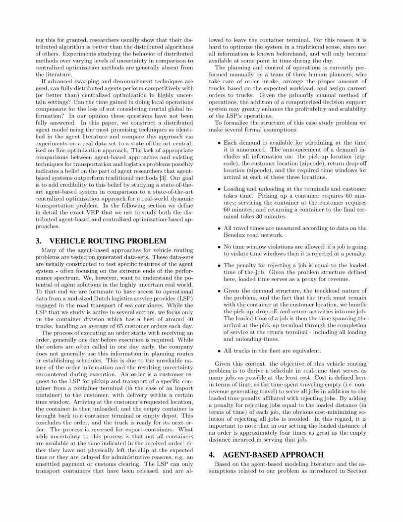
To calculate the cost of insertion, the truck agent tries toinsert the new order in-between every two adjacent orders intheir plan (see Figure 1), plus at the beginning and the end.At every position, it calculates the amount of extra emptytime it needs to drive if this order is inserted there. Supposethat an agent considers the position between container i andj, and calculates that the empty time the truck needs totravel to pick up j after returning i is dij . Here we use dij

to represent the distance (in time) between the two jobs iand j, and dii to denote the loaded distance of job i. The

RDP

P D R

P D R P D R P D R

?

Plan

−− time needed to travel from the return location−− return location−− delivery location−− pickup location

of one order to the pickup location of anotherdij

Order l

Order i Order j Order k

dij

Figure 1: Insertion

P D R

P D R P D R P D R

?

?

Plan

Order l

Order i Order j Order k

dij

Figure 2: Substitution

amount of extra empty time the truck would need to drivefor container l then equals insl

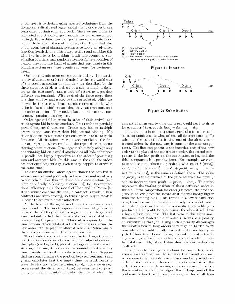
ij = dil + dlj − dij .In addition to insertion, a truck agent also considers sub-

stitution (analogous to what others call decommitment). Tocalculate the cost of substituting one of the already con-tracted orders by the new one, it sums up the cost compo-nents. The first component is the insertion cost of the neworder at the place of the substituted order, the second com-ponent is the lost profit on the substituted order, and thethird component is a penalty term. For example, we com-pute the cost of substituting order j with order l (subsl

j)in Figure 4. Here subsl

j = inslik + profitj + djj . The in-

sertion term inslik is the same as defined above. The value

of profitj is the difference of the price received for order j

and its insertion cost: profitj = pricej − insjik. This term

represents the market position of the substituted order inthe bid. If the competition for order j is fierce, the profit onj would be low (since the second-best bid was hardly higherthan the winning bid). This results in a low substitutioncost, therefore such orders are more likely to be substituted.An order that is well suited for a specific truck is likely toproduce a high profit for that truck, therefore it will havea high substitution cost. The last term in this expression,the amount of loaded time of order j, serves as a penaltyon substituting that job. Using such a penalty discouragesthe substitution of long orders that may be harder to fitsomewhere else. Additionally, the orders that are finally re-jected (those that do not manage to make a contract withany truck agents) will be shorter, which will result in a bet-ter total cost. Algorithm 1 describes how new orders aredealt with.

In addition to bidding on auctions for new orders, truckagents have another way to enhance the overall solution.At random time intervals, every truck randomly selects anorder in its plan and releases it. Trucks never select theorder they are currently serving and also not one, for whichthe execution is about to begin (the pick-up time of thecontainer is less than 10 seconds away – this small time

Algorithm 1 Insertion and substitution of orders

1. Compute the extra costs for every possible insertionand every possible substitution

2. Order the merged list of insertions and substitutionsin increasing order of these costs

3. Iterate over this list

(a) If the new order’s time windows are violated, con-tinue with the next alternative.

(b) If a time window of an order after the new one isviolated, continue with the next alternative.

(c) Else the cheapest feasible position is found. Re-turn this position.

buffer is selected to provide as much opportunity for routeimprovement as possible). Note, the same time limit is alsoapplied to the insertion and substitution decisions explainedearlier. An order agent that is released (just as those orderagents that are substituted) initiates a new auction to findanother place. In most cases, these auctions result in thevery same allocation as before the release. Nevertheless,sometimes they do manage to find a better place and makea contract with another truck.

Whenever an order agent finalizes a contract with a truckagent, it sends a message to all other order agents to notifythem about the changed plan of the given truck. This isimportant for order agents that do not have a contract yet.Any change in the trucks’ plans may be their chance tofind their place in a truck. Those order agents will start anauction in response to the notification message in the hopeof finally making a contract.

To summarize the agent-based approach, let us list themain techniques that characterize it:

• Orders are allocated to trucks via second-price auc-tions sequentially, at the time they become known tothe agent system.

• Truck agents consider insertion and substitution ofnew orders in their plan. Substituted orders are re-leased from the truck. Released order agents hold anew auction to find another place. If a truck cannotdeliver an order within the time windows, it rejects it.

• Truck agents randomly release contracted order agents.Randomly released order agents also hold a new auc-tion to find a place.

• Order agents notify each other whenever they changethe plan of a truck (make a contract). Rejected orders(without a contract) thereby get a chance to hold anew auction and find a truck.

To evaluate this approach, we implemented a real-timetruck simulator that we connected to the agent system. Ev-ery truck agent assumes responsibility for a simulated truck.In the coupled agent-truck-simulator system, agents sendplans to trucks for execution. Simulated trucks drive alongthe road network of the Benelux as the plans prescribe. Theyperiodically report their position as well as their activities tothe agents. This way truck agents can follow the execution

Figure 3: Cycles in the MIP solution structure.

of the plans and make decisions with the knowledge of whatis happening in the (simulated) world.

Finally, we have a third element in the system, whose roleis to monitor both the agents and the simulator, therebygathering all information necessary to evaluate the perfor-mance of the agents, and to calculate the total cost of therouting. Just as described in Section 3, the ultimate objec-tive of the agents is to minimize the total cost of the routingwhich is specified in terms of the time trucks travel emptyplus the loaded-travel-time penalty associated with rejectinga container. The next section describes the on-line optimiza-tion approach that is used in comparison to the agent-basedapproach, based on this total cost.

5. ON-LINE OPTIMIZATION APPROACHTo estimate the value of the agent-based solution ap-

proach (described in Section 4), we study it in comparison toan optimization-based solution approach, reflective of thosecurrently embedded in commercially available vehicle rout-ing decision support software (DSS). We therefore examinetwo optimization based solution approaches: (i) a mixed-integer program for solving the static a priori case in orderto provide a baseline benchmark, and (ii) an on-line opti-mization approach, comparable to the agent approach, anddesigned to represent current vehicle routing DSS.

At the core of both the static a priori solution and theon-line optimization is a mixed integer program (MIP) fora truck-load vehicle routing problem with time windows,which is given to CPLEX [7]. This MIP is based on theformulation put forth by Yang et al. [21]. The completedescription of our modifications to Yang et al.’s MIP is thefocus of this section. Before introducing the notation andmathematical formulation for this problem, we begin witha small example to illustrate exactly how Yang et al.’s MIPworks to exploit the structure of this truckload pick-up anddelivery problem with time windows.

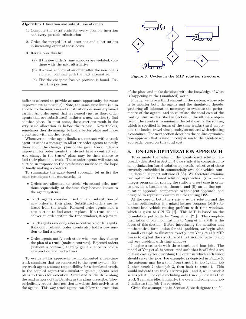
Imagine a scenario with three trucks and four jobs. Themodel of Yang et al. is constructed such that it will find a setof least cost cycles describing the order in which each truckshould serve the jobs. For example, as depicted in Figure 3,the outcome may be a tour from truck 1 to job 1, then job2, then truck 2, then job 3, then back to truck 1. Thiswould indicate that truck 1 serves job 1 and 2, while truck 2serves job 3. The cycle including only truck 3 indicates thattruck 3 remains idle. Similarly, the cycle including only job4 indicates that job 4 is rejected.

Given the assumptions in Section 3, we designate the fol-

lowing notation for the given information.K the total number of vehicles available in the fleet.N the total number of known demands.dij as introduced in 4, the travel time required to go

from demand i’s return terminal to the pick-up ter-minal of demand j. Note, if i = j then the traveltime dii represents the loaded distance of job i.

dk0i the travel time required to move from the location

where truck k started to the pick-up terminal of de-mand i.

dkiH the travel time from the return terminal of demand

i to the home terminal of vehicle k.vk the time vehicle k becomes available.li the loaded time required of job i (time from pick up

at originating terminal to completion of service atthe return terminal). Note, li = dii.

τ−i earliest possible arrival at demand i’s pick-up ter-minal.

τ+i latest possible arrival at demand i’s pick-up termi-

nal.M a large number set to be 2 ·maxi,j{dij}.Note: τ−i and τ+

i are calculated to ensure that all sub-sequent time windows (at the customer location and returnterminal) are respected. Given the problem of interest, wespecify the following two variables.xuv a binary variable indicating whether arc (u, v) is

used in the final routing; u, v = 1, . . . , K + N .δi a continuous variable designating the time of arrival

at the pick-up terminal of demand i.Using the notation described above, we formulate a MIP

that explicitly permits job rejections, based on the loadeddistance of a job.

minPK

k=1

PNi=1 dk

0ixk,K+i +PN

i=1

PNj=1 dijxK+i,K+j

+PN

i=1

PKk=1 dk

iHxK+i,k

(1)such that

K+NXv=1

xuv = 1 ∀u = 1, . . . , K + N (2)

K+NXv=1

xvu = 1 ∀u = 1, . . . , K + N (3)

δi −KX

k=1

(dk0i + vk)xk,K+i ≥ 0 ∀i = 1, . . . , N (4)

δj − δi −MxK+i,K+j+(li + dij)xK+i,K+i

≥ li + dij −M∀i, j = 1, . . . , N (5)

τ−i ≤ δi ≤ τ+i ∀i = 1, . . . , N (6)

δi ∈ R+ ∀i = 1, . . . , N (7)xuv ∈ {0, 1} ∀u, v = 1, . . . , K + N (8)

In words, the objective (1) of this model is to minimizethe total amount of time spent traveling without a profitgenerating load. This objective is subject to the followingseven constraints:

(2) Each demand and vehicle node must have one and onlyone arc entering.

(3) Each demand and vehicle node must have one and onlyone arc leaving.

(4) If demand i is the first demand assigned to vehicle k,then the start time of demand i (δi) must be later thanthe available time of vehicle k plus the time requiredto travel from the available location of vehicle k to thepick up location of demand i.

(5) If demand i follows demand j then the start time ofdemand j must be later than the start time of demandi plus the time required to serve demand i plus thetime required to travel between demand i and demandj; if however, demand i is rejected, then the pick uptime for job i is unconstrained.

(6) The arrival time at the pick up terminal of demand imust be within the specified time windows.

(7) δi is a positive real number.

(8) xuv is binary.

Mathematically this model specification serves to find theleast-cost (in terms of time) set of cycles that includes allnodes given in the set {1, . . . , K, K + 1, . . . , K + N}. Wedefine xuv, (u, v = 1, . . . , K + N) to indicate whether arc(u, v) is selected in one of the cycles. These tours requireinterpretation in terms of vehicle routing. This is done bynoting that node k, (1 ≤ k ≤ K) represents the vehicle kand node K + i, (1 ≤ i ≤ N) corresponds to demand i.Thus, each tour that is formed may be seen as a sequentialassignment of demands to vehicles respecting time windowconstraints.

The model described above is used to provide the optimal(yet realistically unattainable) lower bound for each day ofdata in each scenario. We denote this approach as the statica priori case. In this case, we obtain the route and scheduleas if all the jobs are known and we have hours to find theoptimal solution. Thus, not only is this lower bound real-istically unattainable due to a relaxation on the amount ofinformation available, but also due to a relaxation on theamount of time available to CPLEX for obtaining the opti-mal solution. In this way, because the problem instances arerelatively small (note, using this MIP structure CPLEX canhandle a maximum of about 100 jobs and about 50 Trucks,yet our instances are only 34 trucks and 65 jobs) we are ableto uncover the optimal solution for all 26 problem instancesacross all four uncertainty scenarios.

In order to provide a fair comparison with the agent-basedapproach, the MIP is then manipulated for use in on-lineoperations. In our on-line approach, this MIP is invokedat 30 second intervals. At each interval, the full and cur-rent state of the world is captured, and then encoded inthe MIP. This “snapshot” of the world includes informationof all jobs that are available and in need of scheduling, aswell as the forecasted next available location and time of alltrucks. The MIP is then solved via a call to CPLEX. Thedecision to use 30 second intervals was driven by the desireto be comparable to the agent-based approach while stillproviding CPLEX enough time to find a feasible solutionfor each snapshot problem. The solution given by CPLEXis parsed and any jobs that are within two intervals (i.e.60 seconds) of being late (i.e. missing the time specified byδi in the latest plan) are permanently assigned if travel isnot commenced in the next interval. Any jobs that weredesignated for rejection in the solution are rejected only ifthey are within two intervals of violating a time window;

otherwise they are considered available for scheduling in asubsequent interval. The procedure continues in this fashionuntil the end of the working day at which point all jobs havebeen served or rejected.

The test problems and the results from the static a prioribenchmark, the on-line optimization, and the agent-basedsolution approach as applied to these test problems are thetopic of the next section.

6. COMPUTATIONAL EXPERIMENTSIn this section we report the computational results on the

performance of the agent-based approach in comparison tothe optimization-based approach. The first subsection (6.1)describes how the test problems were generated and in sub-section 6.2 we present the results of these tests.

6.1 Test ProblemsThe data we used for our experiments was based on data

provided to us by the LSP described in Section 3. In all,we were given the execution data from January 2002 to Oc-tober 2005 as well as the data from January 2006 throughMarch 2006. We could not, however, simply use this datain its raw form. We first had to make multiple correctionsto the customer address fields as many addresses referred topostal boxes and not to the physical terminal locations. Af-ter cleaning the address fields, we then extracted a randomsample of jobs from the original data-set in order to generatea set of 26 days with 65 orders per day. The company fromwhich these data are taken serves between 50 and 80 jobsper day, thus 65 jobs per day represents the average dailyjob load.

Just as discussed before, each order consists of a pickuplocation, customer location, and return location. To stan-dardize the data for our experimental purposes we specifiedtime windows at all locations as follows: for the terminals(the pickup and return locations) the time windows span afull twelve hour work day from 6am to 6pm and the timewindows at the customer locations are always 2 hours. Thestart of the 65 customer time windows occurs throughout theworking day in accordance with the data provided by theLSP, which roughly follows a uniform distribution. Giventhe variation in customer locations, the workload per dayvaries similarly. On average each job requires approximately4.2 hours of loaded distance. When the routing is optimal inthe case that all jobs are known at the start of the day theaverage empty time per job is approximately 25 minutes.

Given our interest in determining how the agent solutionperforms on this pick-up and delivery problem with timewindows and order arrival uncertainty, we further renderedour 26 days of data into four separate scenarios with varyinglevels of order arrival uncertainty. This was done by alteringthe arrival times of the orders, i.e., the time at which theorder data is revealed to the LSP. We generated these pointsin times over the day using a uniform distribution. We usedsuch a uniform distribution as the original data did not showa fit with other distributions. The four different scenariosreflecting different levels of order arrival uncertainty were:

Scenario A: All orders (100%) are known at the start ofthe working day, 6AM.

Scenario B: About half of the orders (50%, selected ran-domly from the 65 jobs) are known at the start of the

Hours Traveling Empty + Job Rejection Penalty

24.0

26.0

28.0

30.0

32.0

34.0

36.0

38.0

40.0

42.0

Scenario A -100% Jobs at

Start

Scenario B -50% Jobs at

Start

Scenario C -10% Jobs at

Start

Scenario D - 0%Jobs at Start

Ho

urs

A Priori On-line Opt. Agents

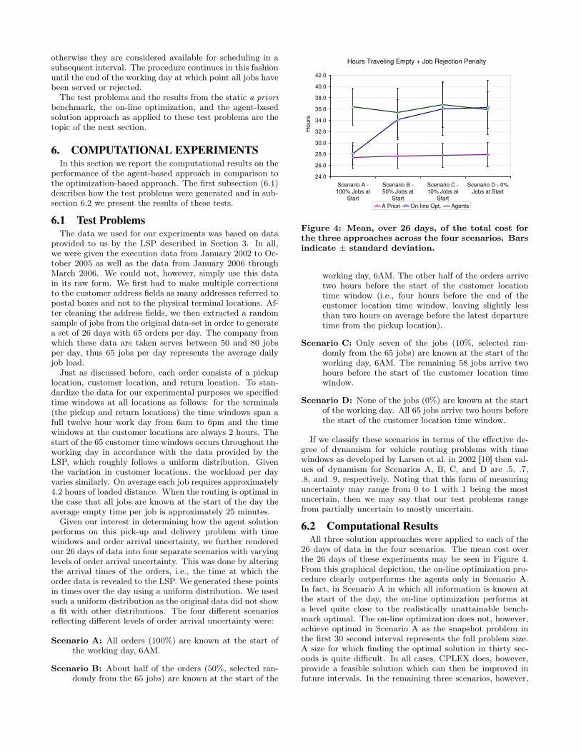
Figure 4: Mean, over 26 days, of the total cost forthe three approaches across the four scenarios. Barsindicate ± standard deviation.

working day, 6AM. The other half of the orders arrivetwo hours before the start of the customer locationtime window (i.e., four hours before the end of thecustomer location time window, leaving slightly lessthan two hours on average before the latest departuretime from the pickup location).

Scenario C: Only seven of the jobs (10%, selected ran-domly from the 65 jobs) are known at the start of theworking day, 6AM. The remaining 58 jobs arrive twohours before the start of the customer location timewindow.

Scenario D: None of the jobs (0%) are known at the startof the working day. All 65 jobs arrive two hours beforethe start of the customer location time window.

If we classify these scenarios in terms of the effective de-gree of dynamism for vehicle routing problems with timewindows as developed by Larsen et al. in 2002 [10] then val-ues of dynamism for Scenarios A, B, C, and D are .5, .7,.8, and .9, respectively. Noting that this form of measuringuncertainty may range from 0 to 1 with 1 being the mostuncertain, then we may say that our test problems rangefrom partially uncertain to mostly uncertain.

6.2 Computational ResultsAll three solution approaches were applied to each of the

26 days of data in the four scenarios. The mean cost overthe 26 days of these experiments may be seen in Figure 4.From this graphical depiction, the on-line optimization pro-cedure clearly outperforms the agents only in Scenario A.In fact, in Scenario A in which all information is known atthe start of the day, the on-line optimization performs ata level quite close to the realistically unattainable bench-mark optimal. The on-line optimization does not, however,achieve optimal in Scenario A as the snapshot problem inthe first 30 second interval represents the full problem size.A size for which finding the optimal solution in thirty sec-onds is quite difficult. In all cases, CPLEX does, however,provide a feasible solution which can then be improved infuture intervals. In the remaining three scenarios, however,

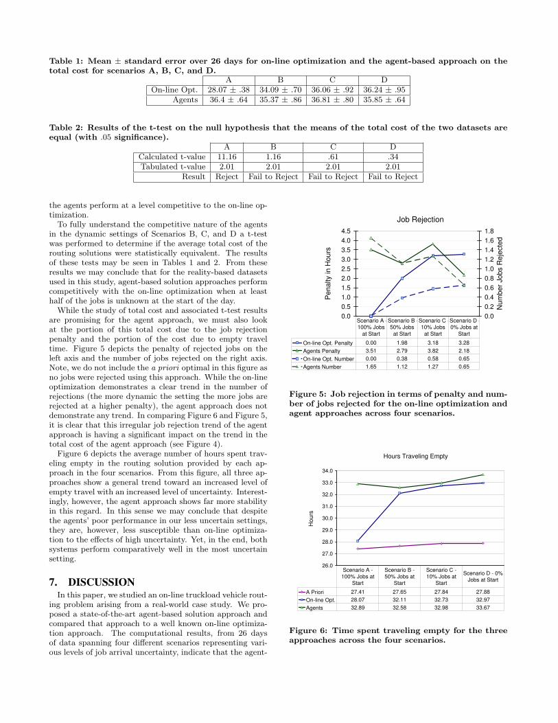
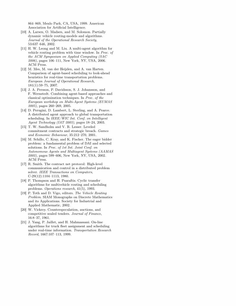
Table 1: Mean ± standard error over 26 days for on-line optimization and the agent-based approach on thetotal cost for scenarios A, B, C, and D.

A B C DOn-line Opt. 28.07 ± .38 34.09 ± .70 36.06 ± .92 36.24 ± .95

Agents 36.4 ± .64 35.37 ± .86 36.81 ± .80 35.85 ± .64

Table 2: Results of the t-test on the null hypothesis that the means of the total cost of the two datasets areequal (with .05 significance).

A B C DCalculated t-value 11.16 1.16 .61 .34Tabulated t-value 2.01 2.01 2.01 2.01

Result Reject Fail to Reject Fail to Reject Fail to Reject

the agents perform at a level competitive to the on-line op-timization.

To fully understand the competitive nature of the agentsin the dynamic settings of Scenarios B, C, and D a t-testwas performed to determine if the average total cost of therouting solutions were statistically equivalent. The resultsof these tests may be seen in Tables 1 and 2. From theseresults we may conclude that for the reality-based datasetsused in this study, agent-based solution approaches performcompetitively with the on-line optimization when at leasthalf of the jobs is unknown at the start of the day.

While the study of total cost and associated t-test resultsare promising for the agent approach, we must also lookat the portion of this total cost due to the job rejectionpenalty and the portion of the cost due to empty traveltime. Figure 5 depicts the penalty of rejected jobs on theleft axis and the number of jobs rejected on the right axis.Note, we do not include the a priori optimal in this figure asno jobs were rejected using this approach. While the on-lineoptimization demonstrates a clear trend in the number ofrejections (the more dynamic the setting the more jobs arerejected at a higher penalty), the agent approach does notdemonstrate any trend. In comparing Figure 6 and Figure 5,it is clear that this irregular job rejection trend of the agentapproach is having a significant impact on the trend in thetotal cost of the agent approach (see Figure 4).

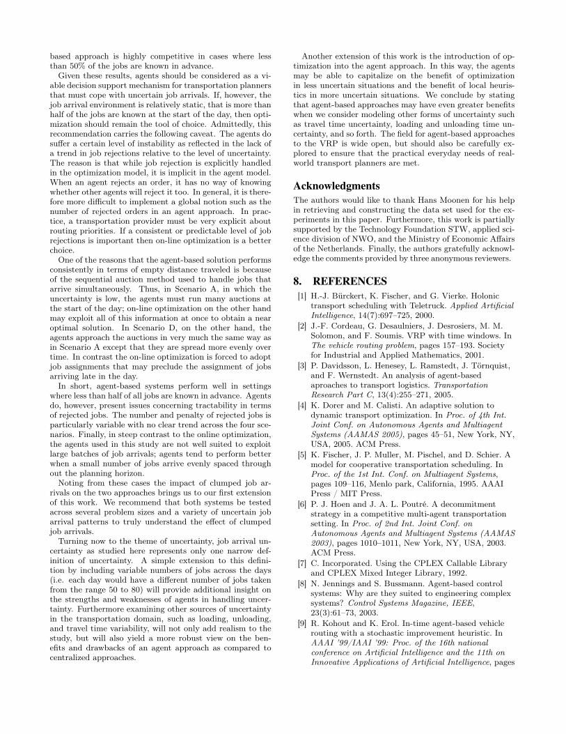
Figure 6 depicts the average number of hours spent trav-eling empty in the routing solution provided by each ap-proach in the four scenarios. From this figure, all three ap-proaches show a general trend toward an increased level ofempty travel with an increased level of uncertainty. Interest-ingly, however, the agent approach shows far more stabilityin this regard. In this sense we may conclude that despitethe agents’ poor performance in our less uncertain settings,they are, however, less susceptible than on-line optimiza-tion to the effects of high uncertainty. Yet, in the end, bothsystems perform comparatively well in the most uncertainsetting.

7. DISCUSSIONIn this paper, we studied an on-line truckload vehicle rout-

ing problem arising from a real-world case study. We pro-posed a state-of-the-art agent-based solution approach andcompared that approach to a well known on-line optimiza-tion approach. The computational results, from 26 daysof data spanning four different scenarios representing vari-ous levels of job arrival uncertainty, indicate that the agent-

Job Rejection

0.0

0.5

1.0

1.5

2.0

2.5

3.0

3.5

4.0

4.5

Penalty in H

ours

0.0

0.2

0.4

0.6

0.8

1.0

1.2

1.4

1.6

1.8

Num

ber

Jobs R

eje

cte

d

On-line Opt. Penalty 0.00 1.98 3.18 3.28

Agents Penalty 3.51 2.79 3.82 2.18

On-line Opt. Number 0.00 0.38 0.58 0.65

Agents Number 1.65 1.12 1.27 0.65

Scenario A -

100% Jobs

at Start

Scenario B -

50% Jobs

at Start

Scenario C -

10% Jobs

at Start

Scenario D -

0% Jobs at

Start

Figure 5: Job rejection in terms of penalty and num-ber of jobs rejected for the on-line optimization andagent approaches across four scenarios.

Hours Traveling Empty

26.0

27.0

28.0

29.0

30.0

31.0

32.0

33.0

34.0

Ho

urs

A Priori 27.41 27.65 27.84 27.88

On-line Opt. 28.07 32.11 32.73 32.97

Agents 32.89 32.58 32.98 33.67

Scenario A -

100% Jobs at

Start

Scenario B -

50% Jobs at

Start

Scenario C -

10% Jobs at

Start

Scenario D - 0%

Jobs at Start

Figure 6: Time spent traveling empty for the threeapproaches across the four scenarios.

based approach is highly competitive in cases where lessthan 50% of the jobs are known in advance.

Given these results, agents should be considered as a vi-able decision support mechanism for transportation plannersthat must cope with uncertain job arrivals. If, however, thejob arrival environment is relatively static, that is more thanhalf of the jobs are known at the start of the day, then opti-mization should remain the tool of choice. Admittedly, thisrecommendation carries the following caveat. The agents dosuffer a certain level of instability as reflected in the lack ofa trend in job rejections relative to the level of uncertainty.The reason is that while job rejection is explicitly handledin the optimization model, it is implicit in the agent model.When an agent rejects an order, it has no way of knowingwhether other agents will reject it too. In general, it is there-fore more difficult to implement a global notion such as thenumber of rejected orders in an agent approach. In prac-tice, a transportation provider must be very explicit aboutrouting priorities. If a consistent or predictable level of jobrejections is important then on-line optimization is a betterchoice.

One of the reasons that the agent-based solution performsconsistently in terms of empty distance traveled is becauseof the sequential auction method used to handle jobs thatarrive simultaneously. Thus, in Scenario A, in which theuncertainty is low, the agents must run many auctions atthe start of the day; on-line optimization on the other handmay exploit all of this information at once to obtain a nearoptimal solution. In Scenario D, on the other hand, theagents approach the auctions in very much the same way asin Scenario A except that they are spread more evenly overtime. In contrast the on-line optimization is forced to adoptjob assignments that may preclude the assignment of jobsarriving late in the day.

In short, agent-based systems perform well in settingswhere less than half of all jobs are known in advance. Agentsdo, however, present issues concerning tractability in termsof rejected jobs. The number and penalty of rejected jobs isparticularly variable with no clear trend across the four sce-narios. Finally, in steep contrast to the online optimization,the agents used in this study are not well suited to exploitlarge batches of job arrivals; agents tend to perform betterwhen a small number of jobs arrive evenly spaced throughout the planning horizon.

Noting from these cases the impact of clumped job ar-rivals on the two approaches brings us to our first extensionof this work. We recommend that both systems be testedacross several problem sizes and a variety of uncertain jobarrival patterns to truly understand the effect of clumpedjob arrivals.

Turning now to the theme of uncertainty, job arrival un-certainty as studied here represents only one narrow def-inition of uncertainty. A simple extension to this defini-tion by including variable numbers of jobs across the days(i.e. each day would have a different number of jobs takenfrom the range 50 to 80) will provide additional insight onthe strengths and weaknesses of agents in handling uncer-tainty. Furthermore examining other sources of uncertaintyin the transportation domain, such as loading, unloading,and travel time variability, will not only add realism to thestudy, but will also yield a more robust view on the ben-efits and drawbacks of an agent approach as compared tocentralized approaches.

Another extension of this work is the introduction of op-timization into the agent approach. In this way, the agentsmay be able to capitalize on the benefit of optimizationin less uncertain situations and the benefit of local heuris-tics in more uncertain situations. We conclude by statingthat agent-based approaches may have even greater benefitswhen we consider modeling other forms of uncertainty suchas travel time uncertainty, loading and unloading time un-certainty, and so forth. The field for agent-based approachesto the VRP is wide open, but should also be carefully ex-plored to ensure that the practical everyday needs of real-world transport planners are met.

AcknowledgmentsThe authors would like to thank Hans Moonen for his helpin retrieving and constructing the data set used for the ex-periments in this paper. Furthermore, this work is partiallysupported by the Technology Foundation STW, applied sci-ence division of NWO, and the Ministry of Economic Affairsof the Netherlands. Finally, the authors gratefully acknowl-edge the comments provided by three anonymous reviewers.

8. REFERENCES[1] H.-J. Bürckert, K. Fischer, and G. Vierke. Holonic

transport scheduling with Teletruck. Applied ArtificialIntelligence, 14(7):697–725, 2000.

[2] J.-F. Cordeau, G. Desaulniers, J. Desrosiers, M. M.Solomon, and F. Soumis. VRP with time windows. InThe vehicle routing problem, pages 157–193. Societyfor Industrial and Applied Mathematics, 2001.

[3] P. Davidsson, L. Henesey, L. Ramstedt, J. Törnquist,and F. Wernstedt. An analysis of agent-basedaproaches to transport logistics. TransportationResearch Part C, 13(4):255–271, 2005.

[4] K. Dorer and M. Calisti. An adaptive solution todynamic transport optimization. In Proc. of 4th Int.Joint Conf. on Autonomous Agents and MultiagentSystems (AAMAS 2005), pages 45–51, New York, NY,USA, 2005. ACM Press.

[5] K. Fischer, J. P. Muller, M. Pischel, and D. Schier. Amodel for cooperative transportation scheduling. InProc. of the 1st Int. Conf. on Multiagent Systems,pages 109–116, Menlo park, California, 1995. AAAIPress / MIT Press.

[6] P. J. Hoen and J. A. L. Poutré. A decommitmentstrategy in a competitive multi-agent transportationsetting. In Proc. of 2nd Int. Joint Conf. onAutonomous Agents and Multiagent Systems (AAMAS2003), pages 1010–1011, New York, NY, USA, 2003.ACM Press.

[7] C. Incorporated. Using the CPLEX Callable Libraryand CPLEX Mixed Integer Library, 1992.

[8] N. Jennings and S. Bussmann. Agent-based controlsystems: Why are they suited to engineering complexsystems? Control Systems Magazine, IEEE,23(3):61–73, 2003.

[9] R. Kohout and K. Erol. In-time agent-based vehiclerouting with a stochastic improvement heuristic. InAAAI ’99/IAAI ’99: Proc. of the 16th nationalconference on Artificial Intelligence and the 11th onInnovative Applications of Artificial Intelligence, pages

864–869, Menlo Park, CA, USA, 1999. AmericanAssociation for Artificial Intelligence.

[10] A. Larsen, O. Madsen, and M. Solomon. Partiallydynamic vehicle routing-models and algorithms.Journal of the Operational Research Society,53:637–646, 2002.

[11] H. W. Leong and M. Liu. A multi-agent algorithm forvehicle routing problem with time window. In Proc. ofthe ACM Symposium on Applied Computing (SAC2006), pages 106–111, New York, NY, USA, 2006.ACM Press.

[12] M. Mes, M. van der Heijden, and A. van Harten.Comparison of agent-based scheduling to look-aheadheuristics for real-time transportation problems.European Journal of Operational Research,181(1):59–75, 2007.

[13] J. A. Persson, P. Davidsson, S. J. Johansson, andF. Wernstedt. Combining agent-based approaches andclassical optimization techniques. In Proc. of theEuropean workshop on Multi-Agent Systems (EUMAS2005), pages 260–269, 2005.

[14] D. Perugini, D. Lambert, L. Sterling, and A. Pearce.A distributed agent approach to global transportationscheduling. In IEEE/WIC Int. Conf. on IntelligentAgent Technology (IAT 2003), pages 18–24, 2003.

[15] T. W. Sandholm and V. R. Lesser. Leveledcommitment contracts and strategic breach. Gamesand Economic Behaviour, 35:212–270, 2001.

[16] M. Schillo, C. Kray, and K. Fischer. The eager bidderproblem: a fundamental problem of DAI and selectedsolutions. In Proc. of 1st Int. Joint Conf. onAutonomous Agents and Multiagent Systems (AAMAS2002), pages 599–606, New York, NY, USA, 2002.ACM Press.

[17] R. Smith. The contract net protocol: High-levelcommunication and control in a distributed problemsolver. IEEE Transactions on Computers,C-29(12):1104–1113, 1980.

[18] P. Thompson and H. Psaraftis. Cyclic transferalgorithms for multivehicle routing and schedulingproblems. Operations research, 41(5), 1993.

[19] P. Toth and D. Vigo, editors. The Vehicle RoutingProblem. SIAM Monographs on Discrete Mathematicsand its Applications. Society for Industrial andApplied Mathematic, 2002.

[20] W. Vickrey. Counterspeculation, auctions, andcompetitive sealed tenders. Journal of Finance,16:8–37, 1961.

[21] J. Yang, P. Jaillet, and H. Mahmassani. On-linealgorithms for truck fleet assignment and schedulingunder real-time information. Transportation ResearchRecord, 1667:107–113, 1999.