Agent-Based Simulation of Episodic Criminal Behaviour

1

Agent-Based Simulation of

Episodic Criminal Behaviour∗∗∗∗

Tibor Bosse, Charlotte Gerritsen, and Jan Treur

Vrije Universiteit Amsterdam, Department of Artificial Intelligence

De Boelelaan 1081a, NL-1081 HV, Amsterdam, the Netherlands

E-mail:{tbosse, cg, treur}@few.vu.nl

URL: http://www.few.vu.nl/~{tbosse, cg, treur}

Abstract. Criminal behaviour often involves a combination of physical, mental,

social and environmental (multi-)agent aspects, such as neurological deviations,

hormones, arousal, (non)empathy, targets and social control. This paper contributes

a dynamical agent-based approach for analysis and simulation of criminal

behaviour, covering the above aspects, illustrated for the case of an Intermittent

Explosive Disorder. It involves dynamically generated desires and beliefs in

opportunities within the social environment, both based on literature on criminal

behaviour.

Keywords: Criminal Behaviour, Agent-Based Simulation, Analysis.

1 Introduction

Within Criminology the analysis of criminal behaviour addresses physical, mental,

environmental and social aspects; e.g., [5, 15, 22, 25, 30]. Only few contributions to the

literature address formalisation and computational modelling of criminal behaviour,

usually focussing only on some of the factors involved; e.g., [3, 20, 21]. This paper is part

of a large interdisciplinary research project (involving parties from computer science,

criminology, psychology and social science) that has as main goal to develop a modelling

approach for criminal behaviour, which integrates physical, mental, environmental and

social aspects. To this end, in this research project the standard BDI-model for action

preparation based on motivations [14, 26] is taken as a basis and is extended by specific

models for generation of desires and for generations of beliefs in opportunities. These

extensions are based on available literature on criminal behaviour and the underlying

aspects. For the generation of desires, dynamical models were incorporated involving

internal states, for example, for neurological, hormonal, and emotional aspects and their

interaction; e.g., [22, 25]. For the generation of beliefs in opportunities, a model was

∗ A shorter, preliminary version of this paper appeared in: Proceedings of the Sixth International

Joint Conference on Autonomous Agents and Multi-Agent Systems, AAMAS'07. ACM Press,

2007, pp. 367-374.

2

incorporated formalising the well-known Routine Activity Theory within Criminology;

e.g., [15]. This (informal) theory assumes motivation of the criminal and covers

environmental and social aspects such as the presence of targets and social control.

The overall modelling approach for criminal behaviour involves models at two different

levels. At the level of single agents, the decisions of individuals and the underlying

biological and psychological aspects are addressed. At the level of the multi-agent system,

the impact of such decisions on the society as a whole are addressed. The current article

focuses on the latter aspect, i.e., it presents an approach to study the dynamics of a group

of agents given certain assumptions about the behaviour of individuals and characteristics

of the environment. For example, it aims to answer questions such as “how are crime rates

influenced by the size of a city?”, or “how are crime rates influenced by the amount of

police?”. Since they involve the interaction of different types of agents over time and

space, such questions are usually not easy to answer analytically. Therefore, the current

paper presents an approach to explore the dynamics of crime via simulation and formal

techniques. As such, the main users of the approach are considered to be social scientists

and researchers in applications of modelling in criminology. However, in case it leads to

interesting results, these results may also be presented to policy makers.

Since this article focuses on the social aspects of crime, the description at the level of the

individual agents is kept abstract; these behaviours are modelled in terms of simple input-

output relationships. However, more information about the underlying

biological/psychological models in the context of the research project as a whole can be

found in [6], and the way that these models are connected to the BDI-model is explained

in [7].

To address the type of questions given above, an artificial society has been modelled,

where on a map (represented by a labeled graph) agents move around and meet each

other. Agents may be of four types: potential criminal, agent with negative appearance,

potential victim, and guardian. The models for the agents and their environment have been

formally specified in dynamical systems style [2, 24] by executable temporal/causal

logical relationships, extended by probabilities. To obtain these, knowledge from the

literature in Criminology, and the different disciplines underlying it, was exploited; e.g.,

[17, 22, 25, 30].

Although the model is generic, the current paper focuses on a specific type of crimes,

namely those that are performed by persons with Intermittent Explosive Disorder (IED), a

disorder of impulse control, characterised by short episodes of aggression. This is an

interesting case study, because these types of crimes on the one hand have a biological

background (the presence of the disorder highly increases the probability of these persons

to perform certain assaults), but on the other hand involve a social aspect (the episodes of

aggression are usually triggered by encounters with other people).

The challenge is to model the variety of physical, mental and social aspects as mentioned

above in an integrated manner. On the one hand, qualitative aspects have to be addressed,

3

such as epistemic and motivational states, certain brain deviations, and some aspects of

the environment such as the presence of certain agents. On the other hand, quantitative

aspects have to be addressed, such as testosterone and serotonin levels, and (in the

environment) distances and time durations. Furthermore, it should be possible to model on

a higher level of aggregation or abstraction, as it would not be feasible, for example, to

model the brain anatomy at the level of neurons. The modelling language LEADSTO [9]

fulfils these desiderata. It allows to model at higher levels of aggregation, and it integrates

qualitative, logical aspects and quantitative, numerical aspects; cf. [11]. In LEADSTO

direct temporal dependencies between two state properties in successive states are

modelled by executable dynamic properties. The format is briefly defined as follows. Let

α and β be state properties of the form ‘conjunction of ground atoms or negations of

ground atoms’. In the LEADSTO language the notation α →→e, f, g, h β, means: If state property α holds for a certain time interval with duration g,

then after some delay (between e and f) state property β will hold

for a certain time interval of length h.

Here atomic state properties can have a qualitative, logical format, such as an expression

desire(d), expressing that desire d occurs, or a quantitative, numerical format such as an

expression has_value(x, v) which expresses that variable x has value v. For more details of

the language LEADSTO, see [9].

Section 2 discusses a summary from the literature on criminals with Intermittent

Explosive Disorder. In Section 3 the simulation model is presented, and Section 4

discusses the results of the simulations by referring to an example simulation trace.

Section 5 presents a number of global dynamic properties of the society and their logical

formalisation and discusses automated verification of the simulation results against them.

Section 6 discusses a probability-based analysis of similar properties, also automatically

verified on a set of generated traces. Finally, Section 7 is a concluding discussion about

the approach.

2 Case Study: a Criminal with IED

An Intermittent Explosive Disorder (IED) is a disorder of impulse control, characterised

by several episodes (usually of 10 to 20 minutes each) in which aggressive impulses are

released and expressed in serious assault or destruction of property, although no such

impulsiveness or aggressiveness is shown in the periods (usually weeks or months)

between episodes. To evoke such episodes, often only a minor stimulus is sufficient, such

as an encounter with someone that has a negative, provoking, appearance or behaviour. It

is estimated that about 7% of the adult population in the US can be diagnosed as having

IED. Offences by persons with IED concern a disproportionate reaction, usually to an

acquaintance or family member. After the episode the offender has no recollection of his

actions and, when informed, has feelings of remorse [22]. The following sketch illustrates

4

the interplay of the physical, mental and social aspects involved. Suppose the criminal

meets somebody with negative, provoking behaviour (social aspect). This is interpreted by

the criminal (mental aspect), provokes stress, and leads to an episode with an epileptic

state of the brain (neurological, physical aspect). This state leads to changes in hormonal

(physical) and emotional (mental) states, which lead to a certain type of desire, providing

the motivation for some criminal action (mental aspect). As soon as an opportunity of a

suitable potential victim with not much social control (social aspect) is perceived (mental

aspect), the desire leads to the criminal action.

The scenario described above on the one hand involves epistemic and motivational

concepts (e.g., the desire to act aggressively, and the belief that certain actions can fulfil

this desire), but on the other hand biological concepts (e.g., disorders in the limbic system

and high levels of testosterone [22]). In order to integrate these notions within one agent-

based model, the standard BDI-model for rational reasoning (e.g., [14, 26]) has been

extended by a model that generates desires based on underlying biological and

psychological factors. Some of these factors, which are particularly important to model

the behaviour of a person with IED, are impulsiveness, aggressiveness, emotional

attitudes towards others, tendencies to become anxious or excited, and capabilities to

understand the mental states of others.

In order to convert these elements into complex desires, the physiological makeup of each

agent has been modelled via a number of numerical parameters (e.g., level of testosterone,

serotonin, and so on) are that combinations of these parameters result in an assignment of

values to the characteristics mentioned above (e.g., aggressiveness, impulsiveness), on a

qualitative scale. Eventually, these characteristics are combined into composed desires,

which play the role of regular desires in a BDI-model. This model is described in detail in

[6], and its integration within the BDI-model is described in [7]. The remainder of this

paper assumes these models as given, and focuses on the social/environmental aspect of

criminal behaviour by IED patients. To this end, in this paper the model to generate

complex desires is simply represented in terms of a (probabilistic) input-output

relationship, i.e., a relationship between incoming stimuli and the desires of the person.

3 The Simulation Model

In this section the overall simulation model as developed is described in more detail. The

combination of physical, mental and social aspects involved requires integration of

models for internal physical and mental functioning of an agent with a model at the social

level. To this end, as mentioned earlier, the simulation model has been composed from

submodels, integrating different aspects, including (but not limited to) a decision making

model based on beliefs, desires and intentions (BDI) and a model for the social

environment. The BDI-submodel describes how actions relate to desires and intentions,

when appropriate opportunities are there. It needs as input desires and beliefs in

5

opportunities. For these elements additional models have been developed. Thus the

simulation model is composed of four submodels:

1. a submodel for reasoning about beliefs, desires and intentions (BDI-model)

2. a submodel to determine desires needed as input for the BDI-model

3. a (small) submodel to determine how observations lead to beliefs in an opportunity as

needed as input for the BDI-model; this model is based on the Routine Activity Theory

4. a submodel for the society; this model has two aspects namely, a geographical aspect; this

is represented by a labeled graph of locations and connections and a multi-agent societal

aspect; this lets agents move in the world and determines the effects of actions performed.

Note that submodels 1. and 2. address physical and mental aspects, submodel 4. addresses

social and environmental aspects, and submodel 3. relates society aspects to mental

aspects.

Overview of the Simulation Model: Graphical Form

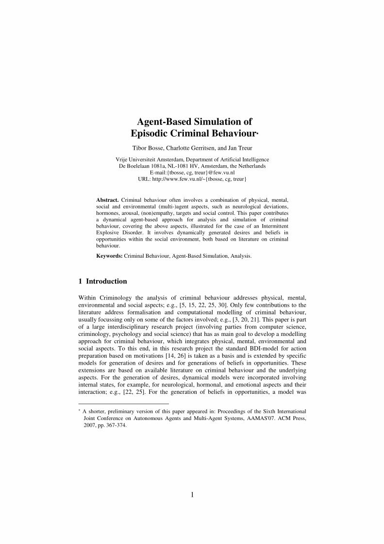
A visualisation of the simulation model is provided in Figure 1. The circles denote state

properties, and the arrows indicate local dynamic (LEADSTO) properties (LP’s). The

dotted box indicates the borders of the agent: all circles that are depicted inside the box

are internal state properties, all circles depicted outside the box are external world state

properties, and all circles depicted at the left (right) border of the box are input (output)

state properties. The solid boxes indicate submodels.

The BDI-submodel

The BDI-submodel bases preparation and performance of actions on beliefs, desires and

intentions, e.g. [14, 26]: an action is performed when the subject has the intention to do

this action and it has the belief that the opportunity to do the action is there. Beliefs are

created on the basis of stimuli that are observed. The intention to do a specific type of

action is created if there is a certain desire, and there is the belief that in the given world

state, performing this action will fulfil this desire. The generic rule to generate the action

performance from the intention and the belief in the opportunity is specified within the

BDI-submodel as:

LP33 The belief that there is an opportunity to perform a certain action combined with the intention to perform

that action will lead to the performance of that action. ∀a:ACTION belief(opportunity(a)) ∧ intention(a) →→ performed(a)

The effects of actions (e.g., the decrease of stimuli) are modelled in the submodel for the

society. For simplicity, we assume that actions always succeed. The intention is generated

by a desire and a belief in a good reason, according to the following rule:

LP32 Desire d combined with the belief that a certain action will lead to the fulfilment of that desire will lead

to the intention to perform that action. Here, d is a specific combined desire that consists of multiple

characteristics as described in Section 2 (see also the next submodel. ∀d:DESIRE ∀a:ACTION desire(d) ∧ belief(satisfies(a, d)) →→ intention(a)

6

Figure 1. Graphical Overview of the Simulation Model.

Within the BDI-submodel, for reasons of simplicity, per desire only one action that can

satisfy the desire is included. What remains to be generated are the desires and the beliefs

in opportunities. For desires, the standard BDI-model [26] does not prescribe a generic

way in which they are to be generated. Recent extensions of BDI models do comprise

models for generation of desires (e.g., [23]) ; this often depends on domain-specific

knowledge, which also seems to be the case for criminal behaviour. Therefore, a similar

approach is adopted here. In particular, for IED patients, a number of physical aspects

play a role, such as certain brain deviations and serotonin levels, as discussed below in

some further detail. For beliefs in opportunities, they are strongly dependent on the

(social) environment, which is another theme discussed below.

observes_ stimulus

desire(d)

SUBMODEL TO

GENERATE DESIRES

belief(satisfies(act, d))

intention(act)

stimulus

performed (act)

observes(a, passer-by)

not observes(a, criminal)

belief(opportunity(a))

is_at_location

(a,l)

performed(a, goto(l)) observes(a, self)

SUBMODEL

FOR THE SOCIETY

7

The Submodel to Determine Desires

To determine desires a rather complex submodel was built based on literature such as [5,

17, 22, 25], incorporating, for example, testosterone, serotonin, adrenalin, blood sugar

levels and brain configuration aspects. These physical aspects relate to mental aspects

such as arousal, aggressiveness, impulsiveness, risk-taking, thrill-seeking, understanding

others, and feeling for others. The aspects involved contain both qualitative aspects (e.g.,

the existence of certain brain deviations) and quantitative aspects (e.g., levels of

testosterone or serotonin). To model these, both causal and logical relations (as in

qualitative modelling) and numerical relations (as in differential equations) have to be

integrated in one modelling framework, using the LEADSTO language.

As mentioned earlier, this submodel is explained in detail in [6]. However, since the

current paper focuses on social/environmental aspects of crime, in the presented

simulations an abstraction of the submodel to determine desires has been made. To be

specific, it has been replaced by the following two rules:

LP30 When agent a1, who is an IED agent is at location l and observes a ‘negative’ agent at location l, then agent a1 will have an aggressive episode.

∀a1,a2:AGENT ∀l:LOCATION observes(a1,agent_of_type_at_location(a1,IED,l)) ∧ observes(a1,agent_of_type_at_location(a2, neg_agent,l))

→→ has_episode

LP42 An agent that has an aggressive episode has the desire to performs an aggressive action. has_episode →→ desire(aggressive_action))

The Submodel to Determine Opportunities

As another input for the BDI-model, the notion of opportunity is used. For the current

domain, this is modelled via a single rule, based on criteria indicated in the Routine

Activity Theory [15]: a suitable target and absence of a guardian. This was specified by:

LP41 When agent a1, who is an IED agent, is at location l and observes a passer-by at location l and does not observe a guardian at location l, then agent a1 believes that there is an opportunity to assault someone.

∀a1,a2:AGENT ∀l:LOCATION observes(a1,agent_of_type_at_location(a1,IED,l)) ∧ observes(a1,agent_of_type_at_location(a2,passer_by,l)) ∧

[∀a3:AGENT not observes(a1,agent_of_type_at_location(a3,guardian,l)) ] →→ belief(opportunity(assault))

In dynamic property LP32 shown earlier, the third criterion of the Routine Activity

Theory, the motivated offender, is represented by the intention to perform some action.

Note that LP41 is a domain-dependent rule. For other domains, the submodel can be filled

with rules that generate beliefs in opportunities for other actions than assaults. Also, the

perception process that generates beliefs based on observation can be modelled in more

detail. However, since the main goal of the current paper is to study the patterns that result

from the Routine Activity Theory, there is no need to further refine this submodel.

The Submodel for the Society

The social, multi-agent aspect is modelled by an environment, in which a number of

agents move around and sometimes meet at a location. One of the agents is the criminal

8

agent with IED, the others are guardian agents, potential victims (passers-by) and agents

with provoking behaviour (so that they may trigger an episode in the criminal when (s)he

encounters them), from now on referred to as negative agents1. The passers-by are

assumed to be suitable targets, for example, because they appear rich and/or weak.

However, as also the guardians are moving around, such targets may be protected,

whenever at the same location a guardian is observed by the criminal: formal control2.

Figure 2. Example World Geography (with an initial distribution of agents over locations; agent

1 is the agent with IED, agent 2 and 3 are guardians, agent 4, 5 and 6 are passers-by (potential

victims), and agent 7 and 8 are ‘negative’ agents.

The interaction between a specific agent and the environment is modelled by (1)

observation, which takes information on the environment as input for the agent (e.g., at

which location it is, where suitable targets are, and whether social control is present), and

(2) performing actions, which is an output of the agent affecting the state of the world

(e.g., going to a different location, or committing a crime). The geographical information

of the world is described by a labeled graph as depicted in Figure 2. Relevant locations are

indicated by nodes A, B,…, and routes connecting locations by edges E1, E2,… The

agents move from location to location via these edges. Edges have lengths; travelling

takes time, depending on these lengths.

To model the dynamics of an agent moving in the environment, the following cycle is

used: observe, determine next action, determine effects of this action. In some more detail,

1 According to Moir and Jessel (1995, pp. 184-194) an episode may be provoked by various types of

unpleasant encounters with other people. Examples are a certain negative look or an unfriendly

remark or question by someone. For simplicity, all these events are summarised here as

encounters with a negative agent. 2 For future work, it is planned to incorporate informal social control as well, e.g., by allowing a

group of passers-by to act as one guardian - and prevent crimes - as well.

E10

E9

E7 E8

E5

E4 E3 E2

E1

E6

B C

D E

H G

A F

1

2

3

4

5

6

7

8

9

the model is based on (1) properties expressing what is observed, for example, stimuli or

other agents: if another agent is present at the agent’s location, then the agent will observe

this, (2) properties expressing which next action is to be undertaken; for example, if the

agent has stayed at its location for duration s, and the next location to reach is l, then it

will move to this next location (probabilities are used to make random choices between

options), and (3) properties expressing the results of actions undertaken; for example, if

the agent starts to move to a next location over edge e and edge e has length d, then it will

arrive at the next location after duration d.

Settings for the Model

The model is initialised by setting the initial locations in the world of all agents: IED

agents, guardians, passers-by, and negative agents. These inputs are included in scenarios

for simulation. For the simulation trace explained in the following section, the settings

shown in Figure 2 were chosen, i.e., consisting of 8 locations that are populated by 1 IED

agent, 2 guardians, 3 passers-by, and 2 ‘negative’ agents.

4 Simulation Traces

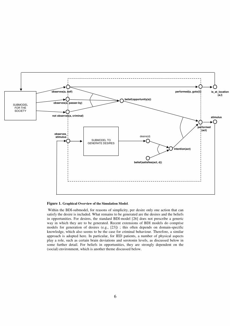
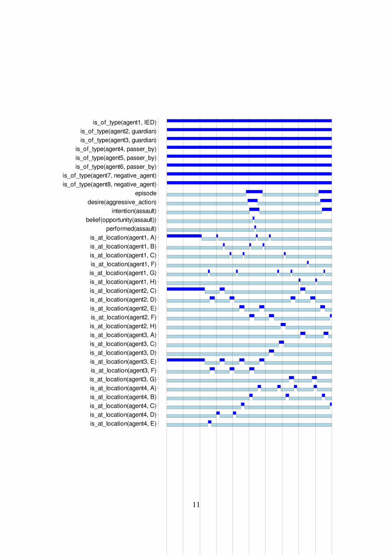
A large number of simulation traces (200 in total) have been generated for the behaviour

of the IED criminal under different circumstances using the simulation model. Below, an

example simulation trace is shown in Figure 3, which was generated using the simulation

model. In this picture, time is on the horizontal axis; state properties are on the vertical

axis. A dark box on top of the line indicates that the property is true during that time

period, and a lighter box below the line indicates that the property is false. The first eight

lines display the characteristics of the agents involved. The next 5 lines show the BDI-

based decision making process of agent 1, which is the agent with IED, and the rest of the

trace shows the movement of the different agents over the environment. For simplicity, all

other events, such as the generation of actions to move to another location (and the

physiological processes underlying agent 1´s behaviour) are not shown.

As shown by Figure 3, the example environment contains 8 agents and 8 locations. Agent

1, the agent with IED, initially does not have a desire to perform aggressive actions.

However, at time point 46 this agent is at location C, where he meets a negative agent

(agent 8). This causes an episode, which leads to the desire to perform an aggressive

action. This desire, combined with the belief that performing an assault leads to the

satisfaction of this desire3, leads to the intention to assault someone. At time point 51, the

IED agent is at location B, together with a passer by (agent 4) without a guardian present

(agents 2 and 3 are both on location F). This leads to the belief that there is an opportunity

3 Although the model allows multiple actions to fulfill a particular desire, the current paper only

addresses those desires for aggression that are so strong that assault is considered the best (and

most immediate) solution.

10

to assault agent 4. This belief combined with the intention leads to the performance of the

assault. Because of the assault, the stimuli of the world increase, which satisfies the

desires of agent 1. Later, at time point 91, agent 1 again generates an aggressive episode,

but because it does not encounter any opportunities, it does not perform any assaults.

As mentioned above, various similar simulation experiments have been performed.

Among the different experiments, several parameter settings were varied, in particular the

number of agents, the ratio between different types of agents, and the number of locations.

All in all, the generated traces indeed show the behaviour of crimes performed by IED

patients, as described in literature such as [17, 22, 25]. Moreover, these simulation

experiments may give insight into the impact of different types of populations or

geographical environments on crime rates. For example, is it better to invest in more

police at a particular location or to prevent passer-by from going to that location?

Obviously, when the number of simulations becomes large, it becomes impossible to

study all simulation traces by hand. Therefore, in the next sections it is explained how this

investigation process automated analysis techniques.

Furthermore, although the simulation examples as presented here involve only 8 agents, it

has been found that the model easily scales to a society of several hundreds of agents

(processing time staying within one hour). Nevertheless, complexity problems may arise

when populations of (more than) thousands of (heterogeneous) agents are considered.

These problems could be solved by translating the current simulation model to a

stochastic model, as is done, for example, in the analysis of epidemics [1]. To make such

a translation, the description of the dynamics of a population will shift from a “micro”

perspective (at the level of individual agents) to a “macro” perspective (at the level of

groups of agents). For example, the number of criminals, guardians, negative agents, and

passers-by at certain locations may be described by global variables, which are influenced

by probabilistic rules. The main advantage of these types of macro-level approaches is

that they can deal with larger populations. An inevitable drawback is however that they

imply a loss of detail at the individual agent level. In future work, the benefits of such

approaches will be explored.

11

is_of_type(agent1, IED)

is_of_type(agent2, guardian)

is_of_type(agent3, guardian)

is_of_type(agent4, passer_by)



is_of_type(agent7, negative_agent)

is_of_type(agent8, negative_agent)

episode

desire(aggressive_action)

intention(assault)

belief(opportunity(assault))

performed(assault)

is_at_location(agent1, A)

is_at_location(agent1, B)

is_at_location(agent1, C)

is_at_location(agent1, F)

is_at_location(agent1, G)

is_at_location(agent1, H)


is_at_location(agent2, D)

is_at_location(agent2, E)














12




























time 0 10 20 30 40 50 60 70 80 90 100

Figure 3. Example Simulation Trace.

5 Logical Analysis

When the number of simulation traces becomes large, automated support for analysis of

the traces becomes very useful. To this end, the TTL Checker tool [8] may be used. This

piece of software takes as input a number of simulation traces and a logical formula

13

(represented in the predicate logic-based language TTL), and verifies whether the

property holds for the traces. Moreover, in case a property does not hold, the software

automatically provides a counter example, i.e., a combination of traces, time points, and

variable instantiations for which the property fails. This allows the analyst to formulate

properties that (s)he expects to hold for a certain process, but also to study those situations

for which the property does not hold in more detail (e.g., by investigating those simulation

traces by hand), and explain what causes the unexpected behaviour.

Following this approach, a number of properties of criminal behaviour have been

identified and formalised. Some of these properties have a logical character and some

have a probabilistic character. Both types of properties have been automatically verified

for the simulation traces. In this section the logical properties are discussed, in the next

section the probabilistic ones. For a multi-agent system, dynamic properties can be

identified at different aggregation levels, roughly spoken (1) the level of the behaviour of

a single agent (external perspective), (2) the level of the internal functioning of an agent

(internal perspective), and (3) the level of the multi-agent system as a whole (society

behaviour). For each of these levels, relevant properties are identified and formalised.

Behavioural Properties of Agents

The properties that have been identified and formalised in the logical language TTL [8] to

characterise the behaviour of the criminal agent (from an external perspective) are as

follows (where f is the duration of the reaction time from observations to internal states or

from internal states to actions):

BP1 From Circumstances to Criminal Action If an IED agent meets a negative agent, and within duration e

an opportunity occurs, then an assault will be performed. ∀t ∀a1,a2:agent ∀l1:location

[ state(γ, t) |= observes(a1, agent_of_type_at_location(a1, IED, l1)) ∧ observes(a1, agent_of_type_at_location(a2, passer_by, l1)) &

∀a3:agent

state(γ, t) |≠ observes(a1, agent_of_type_at_location(a3, guardian, l1)) &

∃t1<t ∃a4:agent ∃l2:location t-e ≤ t1 &

state(γ, t1) |= observes(a1, agent_of_type_at_location(a4, neg_agent, l2)) ]

⇒ ∃t2≥t t2≤t+2f & state(γ, t2) |= performed(assault)

Here state(γ, t) |= X denotes that within the state state(γ, t) at time point t in trace γ state

property X holds (and with |≠ that it does not hold), with the infix predicate |= within the

language denoting the formalised satisfaction relation. See [8] for more details of TTL.

BP2 From Criminal Action to Circumstances If an assault is performed, then the opportunity was there and

earlier (at most e back in time) the IED agent encountered a negative agent. ∀t [state(γ, t) |= performed(assault)

⇒ ∃t1≤t ∃a1,a2:agent ∃l1:location [ t-2f≤t1 &

state(γ, t1) |= observes(a1, agent_of_type_at_location(a1, IED, l1)) ∧ observes(a1, agent_of_type_at_location(a2, passer_by, l1)) &

∀a3:agent

state(γ, t1) |≠ observes(a1, agent_of_type_at_location(a3, guardian, l1)) &

∃t2≤t1 ∃a4:agent ∃l2:location t-e≤t2 &

state(γ, t2) |= observes(a1, agent_of_type_at_location(a4, neg_agent, l2)) ]]

14

Notice that these properties summarise how the agent functions in the context of society,

abstracting from the internal mechanisms underlying this behaviour. Logical

consequences of these external agent behaviour properties include the following external

behavioural property:

BP3 No Opportunity No Crime If no opportunities are offered, then no criminal action occurs. [∀t ∀a1,a2:agent ∀l:location

¬ [ state(γ, t) |=observes(a1, agent_of_type_at_location(a1, IED, l)) ∧ observes(a1, agent_of_type_at_location(a2, passer_by, l)) &

∀a3:agent

state(γ, t) |≠observes(a1, agent_of_type_at_location(a3, guardian, l)) ] ]

⇒ [ ∀t state(γ, t) |≠ performed(assault) ]

Internal Properties of Agents

Although for an analysis at the level of the society as a whole, details of internal

mechanisms and processes are not needed, from the perspective of justifying,

understanding and explaining whether, how and when such behaviour can occur, still the

internal agent dynamics are interesting to formalise. Knowledge of these mechanisms may

also be useful as a basis for therapy and/or medication. The following internal behavioural

properties of the criminal agent were identified and formally specified4:

IP1a (Episode Provoking) If the IED agent observes an agent A which has a negative appearance, then from t

to t+e the IED agent will have an episode.

∀t [ state(γ, t) |= observes(negative_event, pos)

⇒ ∀t1≥t [ t1 ≤ t+e ⇒ state(γ, t1) |= has_episode ] ]

IP1b (Episode Grounding) If the IED agent has an episode, then at some time point between t-e and t the IED

agent observed an agent A which has a negative appearance.

∀t [ state(γ, t) |= has_episode

⇒ ∃t1≤t [ t-e ≤ t1 & state(γ, t1) |= observes(negative_event, pos) ] ]

IP2a (Crime Committing) If the IED agent has an episode, and it believes there is an opportunity to commit a

crime, then it will perform criminal action a.

∀t [ state(γ, t) |= belief(opportunity, pos) ∧ has_episode ]

⇒ ∃t1≥t t1≤t+f & state(γ, t1) |= performs_action(a)

IP2b (Crime Grounding) If the IED agent performs criminal action a, then it believes there is an opportunity

to commit a crime, and it has an episode.

∀t [state(γ, t) |= performs_action(a)

⇒ ∃t1≤t t-f≤t1 & state(γ, t1) |= belief(opportunity, pos) ∧ has_episode ]

IP3a (Belief Generation) If the IED agent observes X, then it will believe X.

∀t [state(γ, t) |= observes(X, S)

⇒ ∃t1≥t t1≤t+f & state(γ, t1) |= belief(X, S) ]

4 Note that, in case the whole underlying biological and cognitive model of the IED agent is

incorporated, these properties would rather be used to analyse given traces of behaviour, instead

of generating them. Moreover, also probabilistic variants of these properties may be defined (see

Section 6).

15

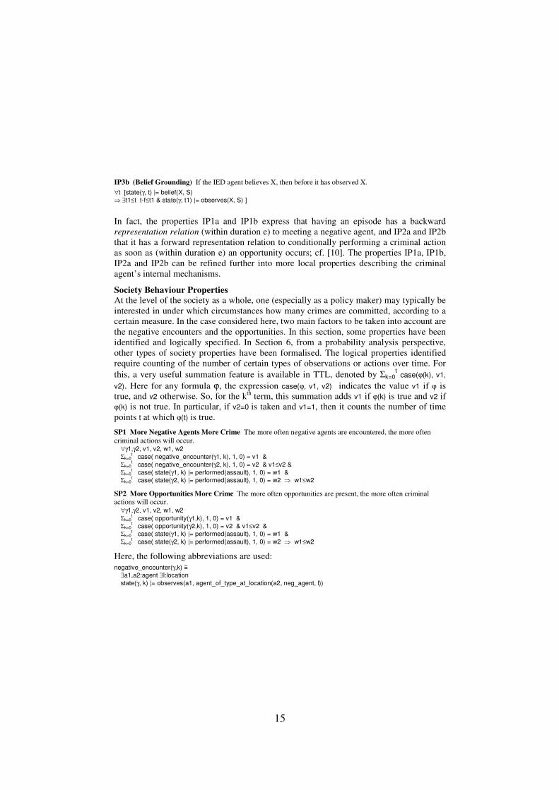
IP3b (Belief Grounding) If the IED agent believes X, then before it has observed X.

∀t [state(γ, t) |= belief(X, S)

⇒ ∃t1≤t t-f≤t1 & state(γ, t1) |= observes(X, S) ]

In fact, the properties IP1a and IP1b express that having an episode has a backward

representation relation (within duration e) to meeting a negative agent, and IP2a and IP2b

that it has a forward representation relation to conditionally performing a criminal action

as soon as (within duration e) an opportunity occurs; cf. [10]. The properties IP1a, IP1b,

IP2a and IP2b can be refined further into more local properties describing the criminal

agent’s internal mechanisms.

Society Behaviour Properties

At the level of the society as a whole, one (especially as a policy maker) may typically be

interested in under which circumstances how many crimes are committed, according to a

certain measure. In the case considered here, two main factors to be taken into account are

the negative encounters and the opportunities. In this section, some properties have been

identified and logically specified. In Section 6, from a probability analysis perspective,

other types of society properties have been formalised. The logical properties identified

require counting of the number of certain types of observations or actions over time. For

this, a very useful summation feature is available in TTL, denoted by Σk=0t case(ϕ(k), v1,

v2). Here for any formula ϕ, the expression case(ϕ, v1, v2) indicates the value v1 if ϕ is

true, and v2 otherwise. So, for the kth

term, this summation adds v1 if ϕ(k) is true and v2 if

ϕ(k) is not true. In particular, if v2=0 is taken and v1=1, then it counts the number of time

points t at which ϕ(t) is true.

SP1 More Negative Agents More Crime The more often negative agents are encountered, the more often

criminal actions will occur. ∀γ1,γ2, v1, v2, w1, w2

Σk=0t case( negative_encounter(γ1, k), 1, 0) = v1 &

Σk=0t case( negative_encounter(γ2, k), 1, 0) = v2 & v1≤v2 &

Σk=0t case( state(γ1, k) |= performed(assault), 1, 0) = w1 &

Σk=0t case( state(γ2, k) |= performed(assault), 1, 0) = w2 ⇒ w1≤w2

SP2 More Opportunities More Crime The more often opportunities are present, the more often criminal

actions will occur. ∀γ1,γ2, v1, v2, w1, w2

Σk=0t case( opportunity(γ1,k), 1, 0) = v1 &

Σk=0t case( opportunity(γ2,k), 1, 0) = v2 & v1≤v2 &

Σk=0t case( state(γ1, k) |= performed(assault), 1, 0) = w1 &

Σk=0t case( state(γ2, k) |= performed(assault), 1, 0) = w2 ⇒ w1≤w2

Here, the following abbreviations are used:

negative_encounter(γ,k) ≡

∃a1,a2:agent ∃l:location

state(γ, k) |= observes(a1, agent_of_type_at_location(a2, neg_agent, l))

16

opportunity(γ,k) ≡

∃a1,a2:agent ∃l:location

state(γ, k) |= observes(a1, agent_of_type_at_location(a1, IED, l)) ∧ observes(a1, agent_of_type_at_location(a2, passer_by, l)) &

∀a3:agent

state(γ, t) |≠ observes(a1, agent_of_type_at_location(a3, guardian, l))

Notice that the above properties compare two traces with each other. In the language TTL,

it is possible to express such properties, in contrast to, for example, modal temporal

logics.

Verification of the Logical Properties

Verification of properties at the three aggregation levels can be done in different ways.

One way is to check whether the properties hold in the different simulation traces that

have been generated, using the TTL Checker tool [8]. When compared to other

verification approaches such as model checking, this approach has as advantage that it is

relatively cheap (since basically one checks a formula against a limited set of traces

instead of ‘exhaustively’ against all possible traces of a model). As a result, the

verification process is quicker, and more expressive properties can be checked. In

practice, the duration of such checks usually varies from one second to a couple of

minutes, depending on the complexity of the formula and the traces under consideration.

With the increase of the number of traces, the checking time grows linearly. However, it

is polynomial in the number of isolated time range variables occurring in the formula

under analysis. Nevertheless, for the purpose presented in this paper, all properties could

be checked in a couple of seconds. For an extensive comparison between the different

verification approaches, see [8] and [12].

All of the properties as discussed have been checked automatically for all 200 simulation

traces using the TTL Checker. Using these checks, the behavioural and internal agent

properties were all found satisfied. However, the society properties turned out not to hold

for all combinations of traces. The reason for this is that, by chance, there are some traces

in which there is not much crime although many negative agents are encountered (for

example, because there are no opportunities). Likewise, there are some traces where there

is not much crime although many opportunities arise (e.g., because the criminals have no

episodes). These individual traces cannot be distinguished by checking properties such as

SP1 and SP2. For this reason, a probabilistic approach is sometimes more useful. Such a

probabilistic approach is worked out in the next section.

Another way of verification is by establishing interlevel relations between dynamic

properties. For example, the properties IP1a, IP2a and IP3a together (logically) imply

behaviour property BP1, and IP1b, IP2b and IP3b together imply BP2, by the following

interlevel relations:

IP1a & IP2a & IP3a ⇒ BP1

IP1b & IP2b & IP3b ⇒ BP2

These interlevel relations have been verified as well.

17

6 Probabilistic Analysis

In this section properties are analysed from a probability perspective. At the society level,

a main property is the parameterised global property below, addressing the expected

number of crimes occurring within a certain time interval.

GP1(t, d, EC) Crime Occurrence Expectation

The expected number of crimes that take place from t within duration d is EC.

Later on an expression will be shown for the expected number of crimes EC in this

property with the following parameters:

• M total number of locations that can be visited

• N total number of agents with negative appearance

• V total number of agents offering an opportunity (potential victims)

• G total number of guardian agents

To analyse property GP1 in more detail, it is related to two more refined properties:

• the probability that within a certain duration d1 (for the first time) a negative agent is met

• the probability that (after meeting a negative agent) within a duration e1 (for the first time) an

opportunity for crime is met

Here e is the assumed duration of the episode. GP2(t1, d1, p1) Provocation Occurrence Probability The probability that from t1 after duration d1 a negative agent is met is p1.

GP3(t2, e1, p2) Opportunity Occurrence Probability The probability that from t2 after duration e1 a first opportunity is met and in the meantime no negative agent is

met is p2.

A first step is to assume invariance over time, so that these probabilities do not depend on

the time parameters. Then these parameters will be left out. As a next step it is assumed

that meeting a negative agent before t1 and an opportunity after t1 are independent events.

Moreover, the behavioural properties IP1 and IP2 of the criminal agent are used.

Relating the probabilities and expected crimes

As a first step the probability p in GP1 will be related to the probabilities p1 and p2 in

GP2 and GP3. This is done by the following logical relation. IP1 & IP2 &

EC = Σ0≤d1≤d, p1 with GP2(d1, p1) Σ0≤e1≤e, p2 with GP3(e1, p2) p1* p2

⇒ GP1(d1+e, EC)

This relation collects all paths that can lead to a crime, indicated by the time that a

negative agent was met and the (first) time that an opportunity was met. A next step is to

find out what reasonable estimations are for the probabilities in GP2 and GP3. After this

18

step the relation above will be used to find an estimation for EC. First GP2 is addressed.

For convenience the following short notations are used: a = (1 – 1/M), b = 1 - (1 - aV)*aG.

Estimating the probability to meet a negative agent

A next assumption is that, by their moving, the agents will be present at locations

according to a uniform probability distribution, so for any agent A and location L, at any

point in time, the probability that agent A is at location L is 1/M. The probability that it is

not at L is 1 – 1/M = a. A further assumption is that agents move independently, and

hence their locations are independent. Therefore for a given location L at time point t, the

probability that there is no agent with negative appearance at L is given by p(no_negative_agent_at_L) = aN, and, the probability that there is at least one agent with

negative appearance at L is: p(at_least_one_negative_agent_at_L) = 1 – aN. This gives an

estimation of how the probability p1 in property GP2(d1, p1) depends on d1, or, expressed

differently, it has been found that by estimation it holds: GP2(d1, (1 – aN)).

Estimating the probability to meet an opportunity

The next step addresses the probability to meet an opportunity within duration e, as

indicated by property GP3. Here, the additional condition is that at e1, it is the first time

that in the interval e an opportunity is met, and that no further negative agents were met in

the meantime. Then the probabilities that at that location no victims and no guardians are

met are as follows (with a = 1 – 1/M):

p(no_victim_at_L) = aV

p(no_guardian_at_L) = aG

Therefore the

probability that an opportunity is met (i.e., a victim and no guardian present) is

(with b = 1 - (1 - aV)*aG):

p(opportunity_at_L) = (1 - aV)*aG = (1 - b)

The probability that no opportunities and no negative agents are met is:

p(no_opportunity_no_neg_at_L) = aN (1 - (1 - b)) = aN b

The probability that at e1 locations {0, …, e1-1} of a sequence no opportunities and no

negative agents are met is:

p(no_opportunity_met_up_to(e1-1)) = (aN b)e1

Based on this, the probability that in a sequence of e1 locations at the e1-th element a first

opportunity is met, whereas at all locations before e1 no opportunity and no negative

agent was met is given by:

p(first_opportunity_ met_after(e1)) = (aN b)e1* (1 - b)

19

This gives an estimation of how the probability p2 in property GP3(e1, p2) depends on e1,

or, expressed differently, it has been found that by estimation the following holds:

GP3(e1, (aN b)e1* (1 – b))

Estimating the Expected Number of Crimes

Now that estimations for the probabilities in GP2 and GP3 have been found, it is possible

to estimate the expected number of crimes in GP1, on the basis of the following

calculation for EC:

Σ0≤d1≤d and p1 with GP2(d1, p1) Σ0≤e1≤e and p2 with GP3(e1, p2) p1*p2

Substituting here the probabilities as specified by GP2 and GP3 in the form GP2(d1, (1 - aN))

and GP3(e1, (aN b)e1* (1 - b)) obtains the following for the probability in GP1 that a crime is

committed within duration d + e:

EC = Σ0≤d1≤d Σ0≤e1≤e (1 - aN) * (aN b)e1

* (1 - b)

= Σ0≤d1≤d (1 - aN) * Σ0≤e1≤e (a

N b)e1* (1 - b)

= Σ0≤d1≤d (1 - aN) * ((1- (aN b)(e+1)) /(1- (aN b))) * (1 - b)

= ( Σ0≤d1≤d (1 - aN) ) * ((1- (aN b)(e+1)) /(1- (aN b))) * (1 - b)

= d * (1 - aN) *

((1- (aN b)(e+1)) /(1- (aN b))) * (1 - b)

This implies that

GP1(d+e, d * (1 - a

N) *

((1- (a

N b)

(e+1)) /(1- (a

N b))) * (1 - b))

holds. Substituting b = 1 - (1 - aV)*aG and a = (1 - 1/M) provides for EC an expression in the

basic parameters. To evaluate the behaviour of this expression for the expected number of

crimes, depending on different parameter settings for the 6 basic parameters M, V, G, N,

d, e, the expression has been implemented in a spreadsheet5 (in Microsoft Excel).

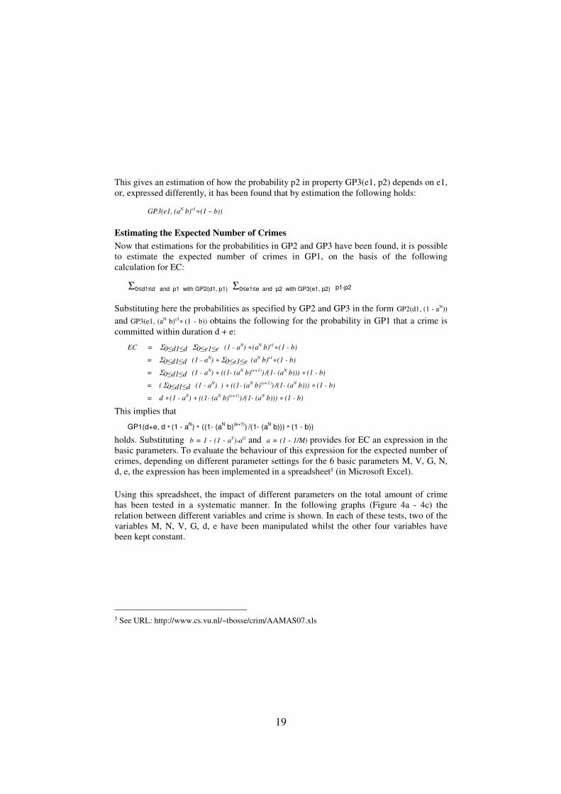
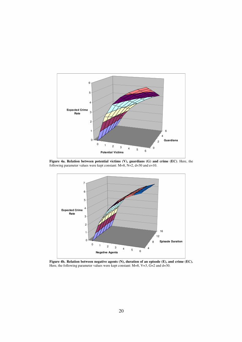
Using this spreadsheet, the impact of different parameters on the total amount of crime

has been tested in a systematic manner. In the following graphs (Figure 4a - 4c) the

relation between different variables and crime is shown. In each of these tests, two of the

variables M, N, V, G, d, e have been manipulated whilst the other four variables have

been kept constant.

5 See URL: http://www.cs.vu.nl/~tbosse/crim/AAMAS07.xls

20

0 1 2 3 4 5 60

2

4

6

0

1

2

3

4

5

6

Expected Crime

Rate

Potential Victims

Guardians

Figure 4a. Relation between potential victims (V), guardians (G) and crime (EC). Here, the

following parameter values were kept constant: M=8, N=2, d=30 and e=10.

0 1 2 3 4 5 64

8

12

16

0

1

2

3

4

5

6

7

Expected Crime

Rate

Negative Agents

Episode Duration

Figure 4b. Relation between negative agents (N), duration of an episode (E), and crime (EC). Here, the following parameter values were kept constant: M=8, V=3, G=2 and d=30.

21

5 6 7 8 9 10 1115

25

35

45

0

1

2

3

4

5

6

7

8

9

10

Expected Crime

Rate

Number of Locations

Time Window

Figure 4c. Relation between number of locations (M), time window (d) and crime (EC). Here,

the following parameter values were kept constant: N=2, V=3, G=2 and e=10.

Some observations that are plausible from the context are indeed shown by these tests, as

well as by the implementation. For example:

• EC is monotonically increasing in its dependence on each of N, V, d, e

• EC is monotonically decreasing in G

• for N=0 or V=0 or M very large, EC becomes 0

Furthermore, the expected number of crimes has been automatically verified against a set

of simulation traces. To this end, another set of n=200 simulation traces has been

generated. These traces were similar to the ones mentioned in Section 4, but used a fully

connected graph for the geographical model (because of the assumption that the location

of agents is independent of their previous location). For these traces, the following TTL

formula:

∃w [w = ∑k=1

n ∑t=0

d case(state(γ(k), t) |= performed(assault)), 1, 0) / n

& EC - δ < w & w < EC + δ ]

was checked with suitable values for parameters EC (given above) and δ. For the expected

number of crimes EC, the value of 4.14 was chosen, as predicted by the above

probabilistic analysis (with M=8, N=2, V=3, G=2, d=40, e=10). For δ, the value of 0.1

was chosen (i.e., about 2.5% of EC). Based on these parameter values, the TTL formula

22

mentioned above indeed succeeded (in a few minutes), since in the 200 traces under

investigation 809 crimes were performed. This is an average of 4.04 crimes per trace,

which lies just within δ from the number of 4.14 expected crimes. This is an indication

that the probabilistic analysis is an adequate alternative for the simulation-based approach,

as long as the analyst is interested in overall numbers, rather than in the local mechanisms

that cause certain types of criminal behaviour.

7 Discussion

This paper presents results from an interdisciplinary research project that is aimed at the

development of an agent-based modelling approach to analyse criminal behaviour in its

social context. Agent-based modelling approaches often either address the internal

functioning of an agent in an extensive manner but leave the social context limited, or

address the social interactions at the level of the multi-agent system as a whole, thereby

taking the internal models of the agents of limited complexity. As in many cases the

interaction of physical, mental and social aspects is crucial, a model covering both levels

is required. The proposed model adopts a general BDI-agent-model [14, 26] extended by

specific models to generate desires and beliefs in opportunities, exploiting literature on

criminal behaviour, in particular [17, 22, 25]. It involves both qualitative aspects (such as

the anatomy of brain deviations, and presence or absence of agents at a specific location

in the world), and quantitative aspects (such as distances and time durations in the world

and hormone and neurotransmitter levels).

One of the challenges met when designing an agent model for criminal behaviour, is the

large variety of different types of criminals and the amount of literature of different

scopes about them. Often knowledge is formulated in a manner that does not make it clear

how much certainty can be attached to it and/or in which context it would be valid. By

focussing on the Intermittent Explosive Disorder (IED) type of criminal and using

knowledge about this type of criminal that is confirmed in different sources in the

literature, this challenge was addressed. It has been found that the model indeed shows the

behaviour as known for this type of criminal within the given social context, as described

in criminological literature.

All in all, the presented approach involves models at two different levels: submodels at

the level of the biological/physiological aspects of single agents and submodels about the

multi-agent society as a whole. The current paper presents an approach to analyse the

dynamics of the latter. At this level, typical questions asked by criminologists are “how

are crime rates influenced by the size of a city?”, or “how are crime rates influenced by

the amount of police?”. Due to the high number of parameters and interactions involved,

these questions are difficult to be answered analytically. Therefore, this paper presents an

approach (based on simulation and formal analysis) that can be used as an experimental

tool to address such questions, by offering the analyst the possibility to predict crime rates

23

given various characteristics of the population and the environment (often called “what

if”-scenarios). As such, the tool can be used by researchers in modelling applied to

criminology, and social scientists, but (in the long term) also by policy makers. In future

work, the possibilities will be explored to apply these methods to real data, to be able to

make predictions about crime in existing cities.

In addition, to analyse the model in more detail, a number of dynamic properties have

been formalised in the TTL language, and (using an automated checker tool) have been

(successfully) verified against a large set of simulated traces. These dynamic properties,

both of logical and probabilistic type, comprise not only behavioural and internal

properties of the agents involved, but also properties that address the society as a whole.

Especially the latter type of properties may have a complex structure, e.g., because they

compare multiple traces with each other, or because of the probabilistic aspects involved.

The language TTL and its software environment turned out useful for these purposes.

In literature such as [14, 26], within standard BDI-models no general model for generation

of desires is included. In many cases desires are just assumed to be there, or even

communicated to the agent as goals it should adopt. Recently, extensions of BDI models

are being developed in which this is the case, e.g., in Jadex [23]. One aspect that is

addressed particularly here is the revision of desires as a result of undertaken actions that

fulfill them. Another aspect relevant for desire generation is the biological substrate of the

agent. Sometimes desires are just inherent to a certain biological makeup or state. The

project of which the current paper reports results, takes a similar approach, namely to

incorporate both biological and psychological factors into a submodel for generation of

desires, see [6, 7]. Within the project, a number of biological aspects as found in the

literature have been taken into account in the dynamic generation of desires, varying from

specific types of brain deviations, and serotonin and testosterone levels, to the extent to

which a substrate for theory of mind was developed. For the current paper, however, this

model has been abstracted to a more high-level behavioural model. Moreover, the

generation of beliefs in opportunities has been based on environmental and social aspects

involving two specific criteria (suitable target, presence of guardian) as indicated by the

Routine Activity Theory in [15]. Within the BDI-submodel, for reasons of simplicity, per

desire only one action that can satisfy the desire is included (and one intention for that

action). When a number of intentions are possible for one desire, then the model can be

extended by a more specific decision making approach, such as utility-based multi-

objective decision making; cf. [7, 16].

Agent models for human-like behaviour incorporating more cognitive and social aspects

(such as trust and theory of mind) are described in [27, 28, 29]. These references focus on

the internal architecture of an agent, and the applications aimed at are mainly in the area

of games and virtual reality. An interesting extension of the work reported in the current

paper would be to design more complex internal models for criminals (incorporating, for

example, aspects such as trust and theory of mind in a more detailed manner) and perform

social simulations with them. In such extensions the challenge how criminal agents come

24

to their decisions in the context of a large variety of internal aspects can be addressed in

more detail.

Although it is recognised that computer support in the area of crime investigation is an

interesting challenge, only few papers on simulation and formal analysis of criminal

behaviour can be found in the literature; they usually address a more limited number of

aspects than the approach presented in this paper. For example, Brantingham and

Brantingham [13] discuss the possible use of agent modelling approaches to criminal

behaviour in general, but do not report a specific model or case study. Moreover, in [3] a

model is presented with emphasis on the social network and the perceived sanctions.

However, this model leaves the mental and physical aspects largely unaddressed. The

same applies to the work reported in [21], where an emphasis is on the environment, and

police organisation. The contribution put forward in the current paper and its counterparts

[6, 7] shows that an agent-based modelling approach is possible where both a complex

internal agent model is involved (addressing physical and mental aspects) and a model for

the multi-agent society.

Further future work will address a number of extensions to the model. Among the factors

that will be added are attractiveness and reputations of locations, informal social control

by passers-by, adaptivity of individual agents, and different surveillance strategies (e.g.,

random, planning-based, or area-based) of the guardians.

Acknowledgements

The authors are grateful to Pieter van Baal, Martine F. Delfos, Henk Elffers, Elisabeth

Groff, Jasper van der Kemp, Mike Townsley, and Mireille M. Utshudi for fruitful

discussions and contributions about the subject. In addition, they with to thank the

anonymous reviewers for their constructive comments to an earlier version of this article.

References

1. Anderson, H., and Britton, T. (2000). Stochastic Epidemic Models and Their Statistical

Analysis. Springer-Verlag, NY.

2. Ashby, R. (1960). Design for a Brain. Second Edition. Chapman & Hall, London. First edition

1952.

3. Baal, P.H.M. van (2004). Computer Simulations of Criminal Deterrence. Ph.D. Thesis, Erasmus

University Rotterdam. Boom Juridische Uitgevers.

4. Baron-Cohen, S. (1995). Mindblindness. MIT Press.

5. Bartol, C.R. (2002). Criminal Behavior: a Psychosocial Approach. Sixth edition. Prentice Hall,

New Jersey.

25

6. Bosse, T., Gerritsen, C., and Treur, J. (2007). Grounding a Cognitive Modelling Approach for

Criminal Behaviour. In: Vosniadou, S., Kayser, D., and Protopapas, A. (eds.), Proceedings of

the Second European Cognitive Science Conference, EuroCogSci'07, 2007, pp. 776-781.

7. Bosse, T., Gerritsen, C., and Treur, J. (2007). Integrating Rational Choice and Subjective

Biological and Psychological Factors in Criminal Behaviour Models. In: Lewis, R.L., Polk,

T.A., and Laird, J.E. (eds.), Proceedings of the 8th International Conference on Cognitive Modeling, ICCM'07. Taylor and Francis, 2007, pp. 181-186.

8. Bosse, T., Jonker, C.M., Meij, L. van der, Sharpanskykh, A., and Treur, J., (2006).

Specification and Verification of Dynamics in Cognitive Agent Models. In: Proc. of the 6th Int.

Conf. on Intelligent Agent Technology, IAT'06. IEEE Computer Society Press, 2006, pp. 247-

254.

9. Bosse, T., Jonker, C.M., Meij, L. van der, and Treur, J. (2005). LEADSTO: a Language and

Environment for Analysis of Dynamics by SimulaTiOn. In: Eymann, T. et al. (eds.), Proc. of,

MATES'05. LNAI, vol. 3550. Springer Verlag, 2005, pp. 165-178. Extended version in

International Journal of Artificial Intelligence Tools. In press, 2007.

10. Bosse, T., Jonker, C.M., and Treur, J. (2005). Representational Content and the Reciprocal

Interplay of Agent and Environment. In: Leite, J., Omincini, A., Torroni, P., and Yolum, P.

(eds.), Proc. of the Second International Workshop on Declarative Agent Languages and

Technologies, DALT'04. Lecture Notes in Artificial Intelligence, vol. 3476. Springer Verlag,

2005, pp. 270-288.

11. Bosse, T., Jonker, C.M., and Treur, J., (2006). An Integrative Modelling Approach for

Simulation and Analysis of Adaptive Agents. In: Proc. of the 39th Annual Simulation

Symposium. IEEE Computer Society Press, 2006, pp. 312-319. Extended version to appear in: Advances in Complex Systems, vol. 10, 2007.

12. Bosse, T., Lam, D.N., and Barber, K.S. (2008). Tools for Analyzing Intelligent Agent Systems. Web Intelligence and Agent Systems: An International Journal, IOS Press. To appear.

13. Brantingham, P. L., & Brantingham, P. J. (2004). Computer Simulation as a Tool for

Environmental Criminologists. Security Journal, 17(1), 21-30.

14. Bratman, M.E., Israel, D.J., and Pollack, M.E. (1988). Plans and Resource-Bounded Practical

Reasoning. Computational Intelligence 4(3), 1988, pp.349-355.

15. Cohen, L.E. and Felson, M. (1979). Social change and crime rate trends: a routine activity

approach. American Sociological Review, vol. 44, pp. 588-608.

16. Cornish, D.B., and Clarke, R.V. (1986). The Reasoning Criminal: Rational Choice Perspectives

on Offending. Springer Verlag.

17. Delfos, M.F. (2004). Children and Behavioural Problems: Anxiety, Aggression, Depression and

ADHD; A Biopsychological Model with Guidelines for Diagnostics and Treatment. Harcourt

book publishers, Amsterdam.

18. Dennett, D.C. (1987). The Intentional Stance. MIT Press. Cambridge Massachusetts.

19. Humphrey, N. (1984). Consciousness Regained. Oxford University Press.

20. Liu, L., Wang, X., Eck, J., & Liang, J. (2005). Simulating Crime Events and Crime Patterns in

RA/CA Model. In F. Wang (ed.), Geographic Information Systems and Crime Analysis.

Singapore: Idea Group, pp. 197-213.

21. Melo, A., Belchior, M., and Furtado, V. (2005). Analyzing Police Patrol Routes by Simulating

the Physical Reorganisation of Agents. In: Sichman, J.S., and Antunes, L. (eds.), Multi-Agent-

26

Based Simulation VI, Proc. of the Sixth International Workshop, MABS'05. Lecture Notes in

AI, vol. 3891, Springer Verlag, 2006, pp. 99-114.

22. Moir, A., and Jessel, D. (1995). A Mind to Crime: the controversial link between the mind and

criminal behaviour. London: Michael Joseph Ltd; Penguin.

23. Pokahr, A., Braubach, L., and Lamersdorf, W. (2005). Jadex: A BDI reasoning engine. In:

Bordini, R.H., Dastani, M., Dix, J., and El Fallah Seghrouchni, A. (eds). Multi-Agent

Programming: Languages, Platforms and Applications. Springer Verlag, 2005, pp. 149–174.

24. Port, R.F., and Gelder, T. van (eds.). (1995). Mind as Motion: Explorations in the Dynamics of

Cognition. MIT Press, Cambridge, Mass.

25. Raine, A. (1993). The Psychopathology of Crime: Criminal Behaviors as a Clinical Disorder.

New York, NY: Guilford Publications.

26. Rao, A.S. & Georgeff, M.P. (1991). Modelling Rational Agents within a BDI-architecture. In:

Allen, J., et al. (eds.), Proc. 2nd Int. Conf. on Principles of Knowledge Representation and

Reasoning, (KR’91). Morgan Kaufmann, pp. 473-484.

27. Silverman, B.G. (2004). Toward Realism in Human Performance Simulation. In: Ness, Ritzer

and Tepe (eds), The Science and Simulation of Human Performance, Elsevier, 2004, pp 469-

498.

28. Silverman, B.G., Bharathy, G.K., O'Brien, K., and Cornwell, J. (2006). Human Behavior

Models for Agents in Simulators and Games: Part II Gamebot Engineering with PMFserv.

Presence: Teleoperators and Virtual Environments 15(2), 2006, 139-162.

29. Silverman, B.G., Johns, M., Cornwell, J., and O'Brien, K. (2006). Human Behavior Models for

Agents in Simulators and Games: Part I: Enabling Science with PMFserv. Presence:

Teleoperators and Virtual Environments 15(2), 2006, 139-162.

30. Towl, G.J., and Crighton, D.A. (1996). The Handbook of Psychology for Forensic

Practitioners. Routledge, London, New York.

31. Webster, C.D., and M.A. Jackson (eds.), (1997). Impulsivity: Theory, Assessment and

Treatment. Guilford, New York.

Agent-Based Simulation of Episodic Criminal Behaviour

Documents