Age, Wage and Productivity: Firm-Level Evidence

1

Age, Wage and Productivity: Firm-Level Evidence

Patrick Aubert (INSEE and CREST)1 and Bruno Crépon (CREST, CEPR and IZA)

November 20062

Abstract: In this paper, we estimate the profile of productivity by age through the estimation of production functions. ‘Productivity’ is defined as the average contribution of age groups to the productivity of firms. Our data are a matched employer-employee dataset covering about 70,000 firms in the late 1990’s in France. We find that productivity increases with age until age 40 and then remains stable after this age. Workers aged 40 and more are roughly 5% more productive than workers aged 35-39, while workers below 30 are 15% to 20% less productive. This result is moreover stable across sectors, since it holds in manufacturing, trading and services. Besides, the age-productivity profile is similar to the age-labor cost profile, which means that the hypothesis of a lower employability of older workers that would be explained by a significant wage-productivity gap seems rejected, at least before age 55. After this age, a slight decrease occurs, by 1 to 5 percentage point across sectors. Unfortunately, this decrease is not statistically significant and, due data and precision issues, the evidence for what happens after age 55 remains inconclusive.

Keywords: labor productivity, wage, demand for elder workers, production functions

JEL classification: J24, J31

1 Contact: INSEE - Département de l’emploi et des revenus d’activité - Section « Synthèse et conjoncture de

l’emploi » 18, Boulevard Adolphe Pinard - BP 100 – 75 Paris Cedex - Mail : [email protected]

2 A French version of this study (“La productivité des salariés âgés : une tentative d’estimation”) has been

published in Economie et Statistique, n°363 (2003), pp.95-119

2

Introduction ............................................................................................................................................. 3

The Model ............................................................................................................................................... 6

The Production Function ..................................................................................................................... 6

The Wage Equation ............................................................................................................................. 7

The Endogeneity Issue ........................................................................................................................ 8

The Data ................................................................................................................................................ 11

Results ................................................................................................................................................... 13

Estimation in the Between and Within Dimensions.......................................................................... 13

The Profile of Productivity by Age ................................................................................................... 17

Labor Cost Profile ............................................................................................................................. 19

Conclusion............................................................................................................................................. 23

References ............................................................................................................................................. 24

3

Introduction

A striking feature of the economic literature on older workers is the sharp asymmetry between the

number of studies addressing labor supply issues and those addressing labor demand issues. While

there is a large amount of studies dealing with retirement decisions and the incentives to cease activity

that are given to elder workers through the institutional framework, the literature on firms’ behavior

and strategies toward their elder labor-force is thinner by far. Although most authors emphasize the

fact that both supply-side and demand-side aspects are crucial when trying to understand the low

participation rate to the labor market of people aged more then 50, there are very few empirical

analyses of the firms’ demand for elder workers and of the fundamentals behind.

In particular, elder workers are frequently alleged to be less productive than younger ones and firms

are often claimed to avoid hiring and try to get rid of elder workers since such lower productivity is

not compensated by a lower wage due to rigidities. Nevertheless, such assertion of a decreasing

productivity after 50 often relies on interviews of managers or employers, or on psychometric tests

designed to assess the variation of cognitive abilities with age. Empirical evaluations of the link

between productivity and age are actually rare. This scarcity mainly stems from the difficulty to define

an appropriate measure of productivity and to find relevant data to estimate it. Earlier studies such as

Medoff and Abraham (1981) often rely on indirect measures of workers’ performance, such as

notation by superiors. Such a definition of productivity is actually questionable. Moreover this kind of

data is usually available on a small range of firms (Medoff and Abraham actually use data from two

firms only), which cast doubt on the possibility to generalize results inferred from them.

If we except early studies such as Medoff and Abraham the empirical estimation of the age-

productivity profile is actually a very recent issue. Recent studies trying to address this issue renounce

to the estimation of productivity at an individual level. Productivity is rather assessed at the group

level, where groups of workers are defined by common characteristics. It is defined as the

“contribution” of the group of workers to the firm’s production, which implies matching employee

4

data with firm data so as to get data on both the financial structure and the structure of the labor force

of firms.

This methodology was initially developed by Hellerstein, Neumark and Troske (1999, hereafter HNT).

From a panel covering more than 3 000 firms and 120 000 workers, they estimate production functions

so as to assess the relative marginal productivity of groups of workers defined by sex, age, race and

qualification. They also estimate wage equations in order to assess relative wages of those groups.

This joint estimation allows them to test the equality between wage and productivity. As far as age is

concerned, they find that higher wages given to elder workers correspond to a higher productivity,

which implies that American data give no support to the idea that elder workers are overpaid

according to their productivity.

HNT’s results are actually contradicted by two further studies. Both Haegeland and Klette (1999),

using Norwegian data, and Crépon, Deniau, Perez-Duarte (2001, hereafter CDPD), with French data,

find that elder workers are not substantially more productive than younger ones, unlike in HNT.

Moreover CDPD provide a new methodology to directly test the equality between relative productivity

and relative wage of groups of workers, through the direct estimation of a relative “markdown”. Their

estimation is run on a panel of more then 75 000 firms, observed from 1994 to 1997. They find that the

difference between elder workers’ and younger workers’ wage is higher than what it should be

according to differences in productivity, both in the manufacturing and non-manufacturing sectors.

Those results are confirmed by a series of estimations testing robustness along the time dimension,

sectors and identifying hypotheses.

However those results might still be questioned. Two kinds of problem arise while estimating

production functions, as it is done both in HNT and CDPD. First, there might be problem of precision

if the quality of data is not good enough. For instance shares of the labor force of each group of

workers in HNT is assessed as the share of a sample of this labor force in each firm. Such a problem

does not arise with CDPD’s data, since they use exhaustive data covering all private-sector firms. The

5

second source of difficulty is commonplace in the estimation of production function. As it is

thoroughly documented in Griliches and Mairesse (1997), such estimation is bound to be biased

because the same underlying forces determine both output and input variables simultaneously.

Moreover, the use of panel data estimation may not be enough to remove the bias in OLS estimation,

since there is also simultaneity between the variations of output and input levels along the time

dimension because of anticipations. If managers anticipate shocks on production, they will adjust

inputs at the same time, in such a way that the “true” production function will not be identifiable since

observations do not allow identifying whether a lower level of inputs causes a lower production, or

whether a decrease in demand induces managers to decrease the level of inputs. In particular this

simultaneity bias is likely to arise in the estimation of the marginal productivity of age groups, since

adjustments of the labor force are not homogeneous across age groups. For instance, firms facing a

low demand for their products will tend not to hire any worker. Since workers in those firms will get

older and since no hiring of younger workers can compensate for this ageing process, the

econometrician will observe both a low level of production and a higher share of older workers. On

the contrary, firms facing booming demand and steadily increasing their production tend to hire many

younger workers. This will thus lead to observations of high levels of production simultaneous to

higher share of younger workers. In both cases the econometrician will tend to conclude that elder

workers are less productive then younger ones. In other words, the essence of this causality problem

can be summed up by the following question: are firms less productive because they hire more elder

workers, or are elder workers more likely to be hired in less productive firms?

This paper starts off from CDPD and aims at addressing the endogeneity issue in the estimation of the

age-productivity profile with production functions. Expanding on their methodology, we use larger

data (firms are observed from 1994 to 2000 instead of 1994 to 1997) and consider a decomposition of

the labor force into thinner age groups to test several identifying hypotheses and estimation methods.

Our result is that the endogeneity bias is large. Different hypotheses on the form of the unobservable

individual component in the production function can lead to estimates of the age-productivity profile

6

with opposite slope. Using Arellano and Bond’s (1991) estimator, we estimate a profile of productivity

that is concave and increasing, productivity being almost constant after 50.

The paper proceeds as follows: in section II we present the model and discuss the endogeneity bias.

Section III introduces the data. Results are given in section IV. Section V concludes.

The Model

The Production Function

The model and methodology is the same as in Crépon et al. (2001) and Hellerstein et al. (1999). Let us

consider the following Cobb-Douglas production function

titititi LKAQ ,,,, ).ln(.)ln(.)ln()ln( ελαβ +++=

where « production » iQ , measured as firm i’s value-added, is linked to the level of capital iK and the

level of “productive labor” L.λ .

We aim at estimating relative productivities of some categories of workers. Assuming perfect

substitution among all kind of workers, ‘productive’ labor L.λ can be re-written as the sum of

productive labor of each category of workers. If jλ is group j’s marginal productivity:

{ } { })).1(1.(.).(..

0 00

0 0

00 ∑∑∑

−−

−+=+==j

jj

j

jj

jjj L

LL

LL

LLLLL

λλ

λλλ

λλλ

The production function now writes

{ }titi

j

jjtititi L

LLKconsQ ,,

0 0,,, )).1(1log(.)log(.)ln(.)ln( ε

λλ

ααβ +−++++= ∑−

or, after linearization

7

{ }ti

j ti

jjtititi L

LLKconsQ ,

0 ,0,,, )1.()log(.)ln(.)ln( ε

λλ

ααβ +⎟⎟⎠

⎞⎜⎜⎝

⎛−+++≈ ∑

−

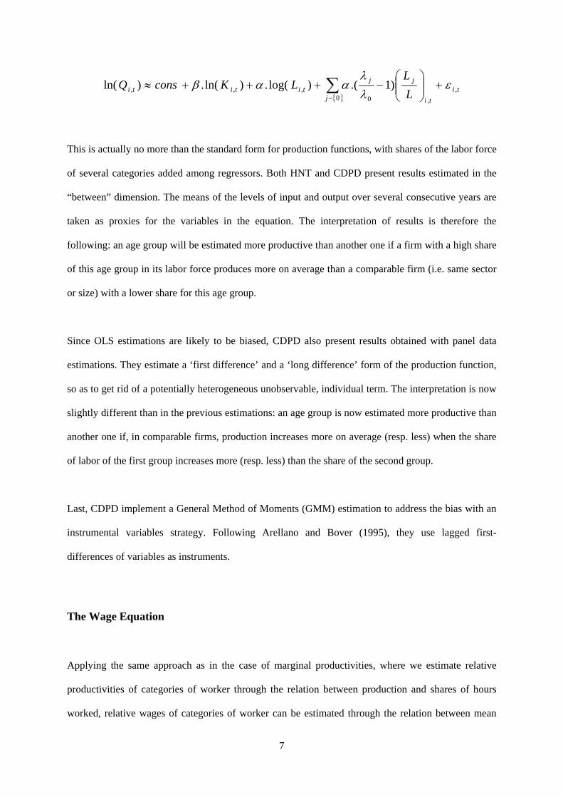
This is actually no more than the standard form for production functions, with shares of the labor force

of several categories added among regressors. Both HNT and CDPD present results estimated in the

“between” dimension. The means of the levels of input and output over several consecutive years are

taken as proxies for the variables in the equation. The interpretation of results is therefore the

following: an age group will be estimated more productive than another one if a firm with a high share

of this age group in its labor force produces more on average than a comparable firm (i.e. same sector

or size) with a lower share for this age group.

Since OLS estimations are likely to be biased, CDPD also present results obtained with panel data

estimations. They estimate a ‘first difference’ and a ‘long difference’ form of the production function,

so as to get rid of a potentially heterogeneous unobservable, individual term. The interpretation is now

slightly different than in the previous estimations: an age group is now estimated more productive than

another one if, in comparable firms, production increases more on average (resp. less) when the share

of labor of the first group increases more (resp. less) than the share of the second group.

Last, CDPD implement a General Method of Moments (GMM) estimation to address the bias with an

instrumental variables strategy. Following Arellano and Bover (1995), they use lagged first-

differences of variables as instruments.

The Wage Equation

Applying the same approach as in the case of marginal productivities, where we estimate relative

productivities of categories of worker through the relation between production and shares of hours

worked, relative wages of categories of worker can be estimated through the relation between mean

8

hourly wages and share of hours worked. Re-writing the aggregate labor cost as the sum of labor costs

for each category, the mean hourly cost of labor is

⎟⎟⎠

⎞⎜⎜⎝

⎛⎟⎟⎠

⎞⎜⎜⎝

⎛−+=⎟⎟

⎠

⎞⎜⎜⎝

⎛== ∑∑∑

∑−′ L

Lww

wLL

ww

wL

Lww j

j

jo

j

jjo

jj

jjj

}0 00

11...

Assuming constant relative labor costs across firms, it is possible to estimate them regressing the

following equation

{ }∑−

+⎟⎟⎠

⎞⎜⎜⎝

⎛−++=

0,

,0, )).1(1ln()ln(

jti

ti

jjti L

Lww

consw ϕ

or a linearized first-difference form of it

{ }∑−

+⎟⎟⎠

⎞⎜⎜⎝

⎛Δ−=Δ

0,

,0, ).1()ln(

jti

ti

jjti L

Lww

w ξ

The idea in HNT basically consisted in the joint estimation of the production equation and the wage

equation. Once such estimations are performed, equality between relative wage and relative

productivity can be tested through a test of the equality of estimated coefficients 0w

wj and 0λ

λ j .

The Endogeneity Issue

As it is documented in Griliches and Mairesse (1997), potentially large biases can arise in the

estimation of production functions, both in the between and within dimension. The ‘between’

estimation is biased in case of unobserved heterogeneity across firms. This is very likely to be the case

considering age groups, since the distribution of such groups over types of firms is known to be quite

different (Aubert, 2003; Aubert and Crépon, 2003). For instance, in France, the share of workers aged

more than 45 is 22% in the 25% of firms with the lower capital-labor ratio, whereas it is 34% in the

9

25% of firms with higher capital-labor ratio. This share equals 20% in 1995 in the 25% of firms that

had the highest rise in employment between 1995 and 2000, whereas it equals 32% in the 25% firms

with the sharpest decrease.

Estimation in the within-dimension is also biased in the case of simultaneity between unobserved

shocks on productivity and labor adjustments. This is also likely to be the case in France, since French

firms usually adjust their labor force on younger workers rather than older ones, due to lower

adjustment costs3. In the within dimension, a higher level of employment is correlated with a higher

share of workers aged less than 30, whereas a lower level then usual is correlated with a higher share

of workers aged 30 or more (Aubert and Crépon, 2003.

In this paper, we estimate production and wage equations using between-, within- and GMM-

estimations. Since we expect between- and within-estimations to be biased, results with those methods

are presented as a benchmark, in a way to compare with results of former studies.

The General Method of Moments (GMM) estimation is done according to Arellano and Bond (1991)

methodology. The production function is estimated in its first-difference specification, with variations

of the level of inputs as endogenous regressors and lagged values of those levels as instruments. The

underlying hypothesis is that the ‘innovation’ in the unobserved individual productivity term (which is

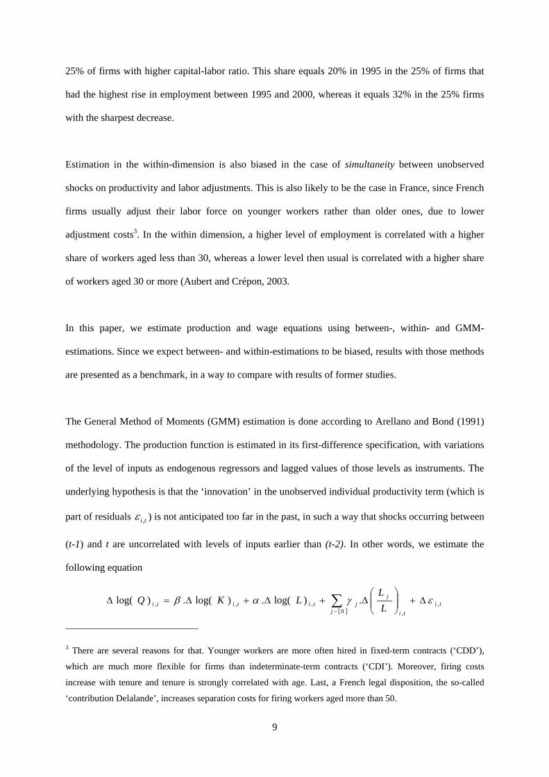
part of residuals ti,ε ) is not anticipated too far in the past, in such a way that shocks occurring between

(t-1) and t are uncorrelated with levels of inputs earlier than (t-2). In other words, we estimate the

following equation

{ }ti

j ti

jjtititi L

LLKQ ,

0 ,,,, .)log(.)log(.)log( εγαβ Δ+⎟⎟

⎠

⎞⎜⎜⎝

⎛Δ+Δ+Δ=Δ ∑

−

3 There are several reasons for that. Younger workers are more often hired in fixed-term contracts (‘CDD’),

which are much more flexible for firms than indeterminate-term contracts (‘CDI’). Moreover, firing costs

increase with tenure and tenure is strongly correlated with age. Last, a French legal disposition, the so-called

‘contribution Delalande’, increases separation costs for firing workers aged more than 50.

10

under the orthogonality conditions

( )( )

⎪⎪⎪⎪

⎩

⎪⎪⎪⎪

⎨

⎧

=⎟⎟

⎠

⎞

⎜⎜

⎝

⎛Δ⎟⎟

⎠

⎞⎜⎜⎝

⎛

=Δ

=Δ

−

−

−

0.

0.)ln(0.)ln(

,,

,,

,,

tisti

j

tisti

tisti

LL

E

LEKE

ε

εε

for all firm i at every time t and for all categories of worker j. We only consider lags s with s greater

than two. Besides, we include dummies for sector, year of observation and firm’s size.

A recurrent conclusion of simulations or studies implementing this method is that it frequently leads to

unsatisfactory results, mainly because of the weak correlation between endogenous variables and

instruments. As Griliches and Mairesse (1997) stress it, precautions against the endogeneity issue, i.e.

differencing transformation and use of instrumental variables strategy, lead to drastically reduce the

amount of identifying variance. Consequently, one might encounter small sample biases even with a

seemingly large sample, since other sources of bias, e.g. measurement errors, are exacerbated. The

situation is however slightly different in our case, at least as far as shares of hours worked by age

groups is concerned. Variations in the size of age categories do not only stem from taking-on and lay-

off. Ageing is an important source of variation of the share of hours worked by age groups which is

quite realistically a priori uncorrelated with shocks on the general productivity level of a firm. The

structure by age of a firm a few years ago will therefore provide good, exogenous instruments for the

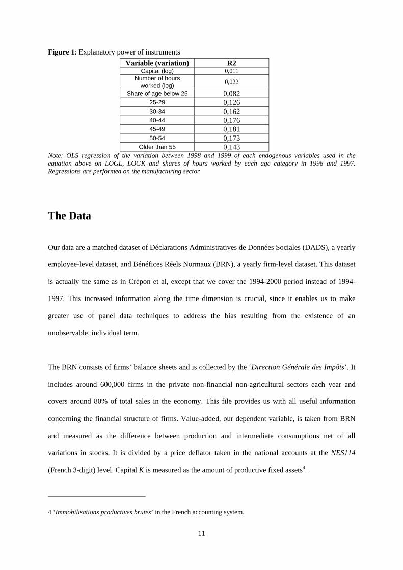
variations oh shares of the labor force. R2’s of the regressions of all endogenous variables on all levels

two and three years before are represented in figure 1 below. For most variables, the R2 is very low,

emphasizing the low correlation between instruments and endogenous variables, and the traditional

problems with Arellano and Bond’s method are likely to arise. However, instruments perform better in

the prediction of the variation of shares of hours worked by age groups.

11

Figure 1: Explanatory power of instruments Variable (variation) R2

Capital (log) 0,011 Number of hours

worked (log) 0,022

Share of age below 25 0,082 25-29 0,126 30-34 0,162 40-44 0,176 45-49 0,181 50-54 0,173

Older than 55 0,143 Note: OLS regression of the variation between 1998 and 1999 of each endogenous variables used in the equation above on LOGL, LOGK and shares of hours worked by each age category in 1996 and 1997. Regressions are performed on the manufacturing sector

The Data

Our data are a matched dataset of Déclarations Administratives de Données Sociales (DADS), a yearly

employee-level dataset, and Bénéfices Réels Normaux (BRN), a yearly firm-level dataset. This dataset

is actually the same as in Crépon et al, except that we cover the 1994-2000 period instead of 1994-

1997. This increased information along the time dimension is crucial, since it enables us to make

greater use of panel data techniques to address the bias resulting from the existence of an

unobservable, individual term.

The BRN consists of firms’ balance sheets and is collected by the ‘Direction Générale des Impôts’. It

includes around 600,000 firms in the private non-financial non-agricultural sectors each year and

covers around 80% of total sales in the economy. This file provides us with all useful information

concerning the financial structure of firms. Value-added, our dependent variable, is taken from BRN

and measured as the difference between production and intermediate consumptions net of all

variations in stocks. It is divided by a price deflator taken in the national accounts at the NES114

(French 3-digit) level. Capital K is measured as the amount of productive fixed assets4.

4 ‘Immobilisations productives brutes’ in the French accounting system.

12

DADS is an exhaustive dataset available since 1994, therefore covering all of the more than 1,000,000

private sector and state-owned firms in France. This file is both establishment- and employee-level,

thus it provides all relevant information on the workforce concerning gender, age, skills, number of

hours worked, wage, etc. Characteristics of groups of workers can be therefore easily computed from

the aggregation of information on all workers with similar characteristics. For each firm, we consider

9 age categories: less than 25, 25-29, 30-34, 35-39, 40-44, 45-49, 50-54, 55-59 and 60 and more. 35 to

39 year old workers are taken as references. Labor is measured as the total number of hours worked in

the firm during the year, excluding trainees and apprentices. The share of age groups in the workforce

are calculated as shares in the total number of hours worked. Aggregate labor cost is computed from

information on wages applying the payroll taxes rule.

The measure of the size of the workforce in DADS can be biased, since temporary workers (hired by

temporary-work agencies) are not registered in this file. This bias can be quite large, especially in

manufacturing, since such workers can represent a non-neglectable share of the total number of hours

worked (Gonzalez, 2002). In the production function, we therefore control for a temporary worker

ratio, which is proxied by the ratio of the firm’s payments to temporary-work agencies on the

aggregate wage bill of permanent workers (measured in BRN). Similarly, we also control for the ratio

of the number of hours worked by trainees to the total number of hours worked by permanent workers.

We also performed filtering on the matched dataset and applied the following rules. Firms had to be

present in both the DADS and the BRN files for each year between 1994 and 2000. All firms must

have at least 5 workers over the year. Workforce, value-added, fixed assets and labor cost had to be

strictly positive for each year of observation. The fishing, energy, construction, finance and

administration sectors were excluded. We also filtered extreme values and discarded from the dataset

all firms outside mean plus or minus 5 standard errors for the logarithm of mean hourly labor cost,

logarithm of mean number of hours worked per day, means from 1994 to 2000 of labor productivity

and of capital productivity, workforce growth, capital growth and production growth. Last, we

13

discarded observations with incoherent values for the size of the workforce in DADS and BRN

(workforce in the DADS outside 0.5-1.5 time the size of the workforce in the BRN). This requisite,

combined to the fact that firms had to exist from 1994 to 2000, are the two main restrictions, in the

sense that they led to the largest number of discarding observations.

Since each firm is identified by a single SIREN code, matching the two dataset is easy. Although

DADS are supposed to be exhaustive, we found firms that were present in BRN and not in DADS, in

such a way that, for unclear reasons, the match is not perfect. Anyhow, the imperfect match,

discarding of extreme values and the requisite that firms in the data should be present with strictly

positive production and employment for each year of observation (1994 to 2000) left us with 24,058

firms in the manufacturing sector, 28,690 in the trading sector and 19,764 in services.

Results

In what follows, productivity and labor cost profiles correspond to estimates associated with the share

of age groups in the production function and labor cost equations. Since labor is defined as the total

number of hours worked over the year and labor shares are defined within this number of hours,

results refer to hourly productivity and hourly labor costs.

Estimation in the Between and Within Dimensions

Figures 2 and 3 presents age-productivity profiles estimated by OLS in the ‘Between’ and ‘Within’

dimension. Those estimation methods are orthogonal one to the other. The Between estimation

compares firms. A given age group will be estimated more productive than an other if firms with a

higher share of this group are have on average a higher productivity than firms with a lower share of

the age group. On the contrary, deviation from the average on a long period are considered in the

14

Within estimation. Thus, a given age group will be estimated more productive than another if, on

average within each firm, this group represents a higher share of labor the years when the firm has a

higher productivity than its long-term average.

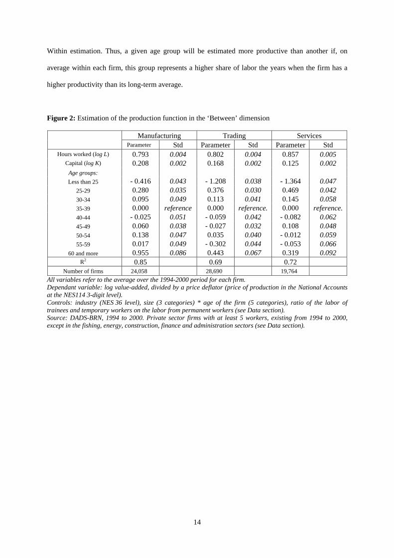
Figure 2: Estimation of the production function in the ‘Between’ dimension

Manufacturing Trading Services Parameter Std Parameter Std Parameter Std

Hours worked (log L) 0.793 0.004 0.802 0.004 0.857 0.005 Capital (log K) 0.208 0.002 0.168 0.002 0.125 0.002

Age groups: Less than 25 - 0.416 0.043 - 1.208 0.038 - 1.364 0.047

25-29 0.280 0.035 0.376 0.030 0.469 0.042 30-34 0.095 0.049 0.113 0.041 0.145 0.058 35-39 0.000 reference 0.000 reference. 0.000 reference. 40-44 - 0.025 0.051 - 0.059 0.042 - 0.082 0.062 45-49 0.060 0.038 - 0.027 0.032 0.108 0.048 50-54 0.138 0.047 0.035 0.040 - 0.012 0.059 55-59 0.017 0.049 - 0.302 0.044 - 0.053 0.066

60 and more 0.955 0.086 0.443 0.067 0.319 0.092 R2 0.85 0.69 0.72

Number of firms 24,058 28,690 19,764 All variables refer to the average over the 1994-2000 period for each firm. Dependant variable: log value-added, divided by a price deflator (price of production in the National Accounts at the NES114 3-digit level). Controls: industry (NES 36 level), size (3 categories) * age of the firm (5 categories), ratio of the labor of trainees and temporary workers on the labor from permanent workers (see Data section). Source: DADS-BRN, 1994 to 2000. Private sector firms with at least 5 workers, existing from 1994 to 2000, except in the fishing, energy, construction, finance and administration sectors (see Data section).

15

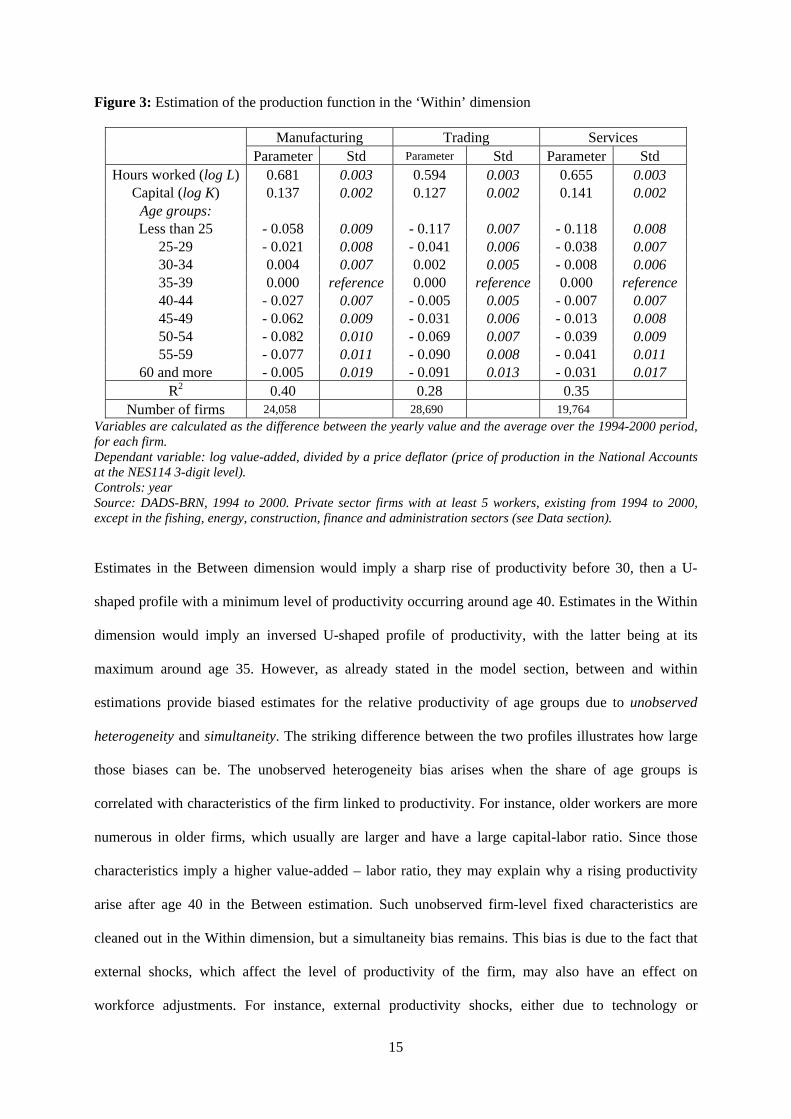
Figure 3: Estimation of the production function in the ‘Within’ dimension




25-29 - 0.021 0.008 - 0.041 0.006 - 0.038 0.007 30-34 0.004 0.007 0.002 0.005 - 0.008 0.006 35-39 0.000 reference 0.000 reference 0.000 reference 40-44 - 0.027 0.007 - 0.005 0.005 - 0.007 0.007 45-49 - 0.062 0.009 - 0.031 0.006 - 0.013 0.008 50-54 - 0.082 0.010 - 0.069 0.007 - 0.039 0.009 55-59 - 0.077 0.011 - 0.090 0.008 - 0.041 0.011

60 and more - 0.005 0.019 - 0.091 0.013 - 0.031 0.017 R2 0.40 0.28 0.35

Number of firms 24,058 28,690 19,764 Variables are calculated as the difference between the yearly value and the average over the 1994-2000 period, for each firm. Dependant variable: log value-added, divided by a price deflator (price of production in the National Accounts at the NES114 3-digit level). Controls: year Source: DADS-BRN, 1994 to 2000. Private sector firms with at least 5 workers, existing from 1994 to 2000, except in the fishing, energy, construction, finance and administration sectors (see Data section).

Estimates in the Between dimension would imply a sharp rise of productivity before 30, then a U-

shaped profile with a minimum level of productivity occurring around age 40. Estimates in the Within

dimension would imply an inversed U-shaped profile of productivity, with the latter being at its

maximum around age 35. However, as already stated in the model section, between and within

estimations provide biased estimates for the relative productivity of age groups due to unobserved

heterogeneity and simultaneity. The striking difference between the two profiles illustrates how large

those biases can be. The unobserved heterogeneity bias arises when the share of age groups is

correlated with characteristics of the firm linked to productivity. For instance, older workers are more

numerous in older firms, which usually are larger and have a large capital-labor ratio. Since those

characteristics imply a higher value-added – labor ratio, they may explain why a rising productivity

arise after age 40 in the Between estimation. Such unobserved firm-level fixed characteristics are

cleaned out in the Within dimension, but a simultaneity bias remains. This bias is due to the fact that

external shocks, which affect the level of productivity of the firm, may also have an effect on

workforce adjustments. For instance, external productivity shocks, either due to technology or

16

demand, will lead the firm to simultaneously adjust the size of its workforce. Since hirings and firings

are less costly when they imply younger workers (see Model section), this will result in changes in the

share of age groups occurring at the same time than productivity shocks occur, with the share of older

workers decreasing when the firms increase its workforce, and vice versa. An empirical consequence

of this is that part of the negative productivity shock can be erroneously attributed to a lower

productivity of older workers in the Within-dimension estimation.

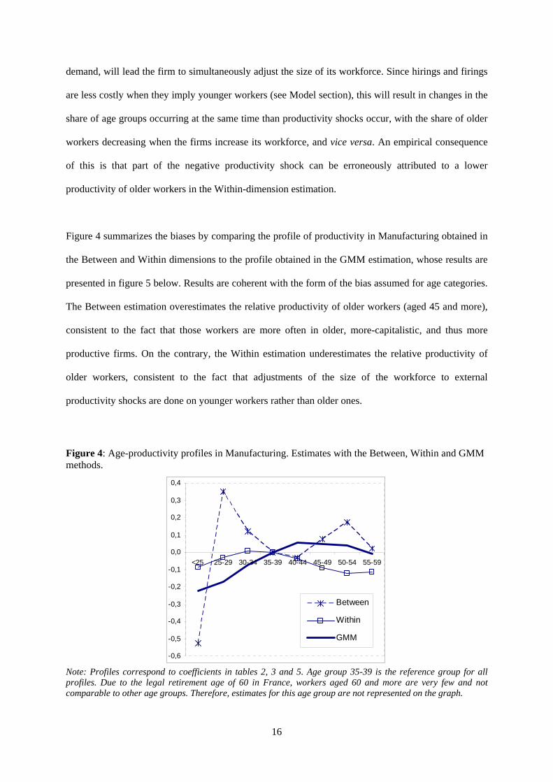
Figure 4 summarizes the biases by comparing the profile of productivity in Manufacturing obtained in

the Between and Within dimensions to the profile obtained in the GMM estimation, whose results are

presented in figure 5 below. Results are coherent with the form of the bias assumed for age categories.

The Between estimation overestimates the relative productivity of older workers (aged 45 and more),

consistent to the fact that those workers are more often in older, more-capitalistic, and thus more

productive firms. On the contrary, the Within estimation underestimates the relative productivity of

older workers, consistent to the fact that adjustments of the size of the workforce to external

productivity shocks are done on younger workers rather than older ones.

Figure 4: Age-productivity profiles in Manufacturing. Estimates with the Between, Within and GMM methods.

-0,6

-0,5

-0,4

-0,3

-0,2

-0,1

0,0

0,1

0,2

0,3

0,4

<25 25-29 30-34 35-39 40-44 45-49 50-54 55-59

Between

Within

GMM

Note: Profiles correspond to coefficients in tables 2, 3 and 5. Age group 35-39 is the reference group for all profiles. Due to the legal retirement age of 60 in France, workers aged 60 and more are very few and not comparable to other age groups. Therefore, estimates for this age group are not represented on the graph.

17

The Profile of Productivity by Age

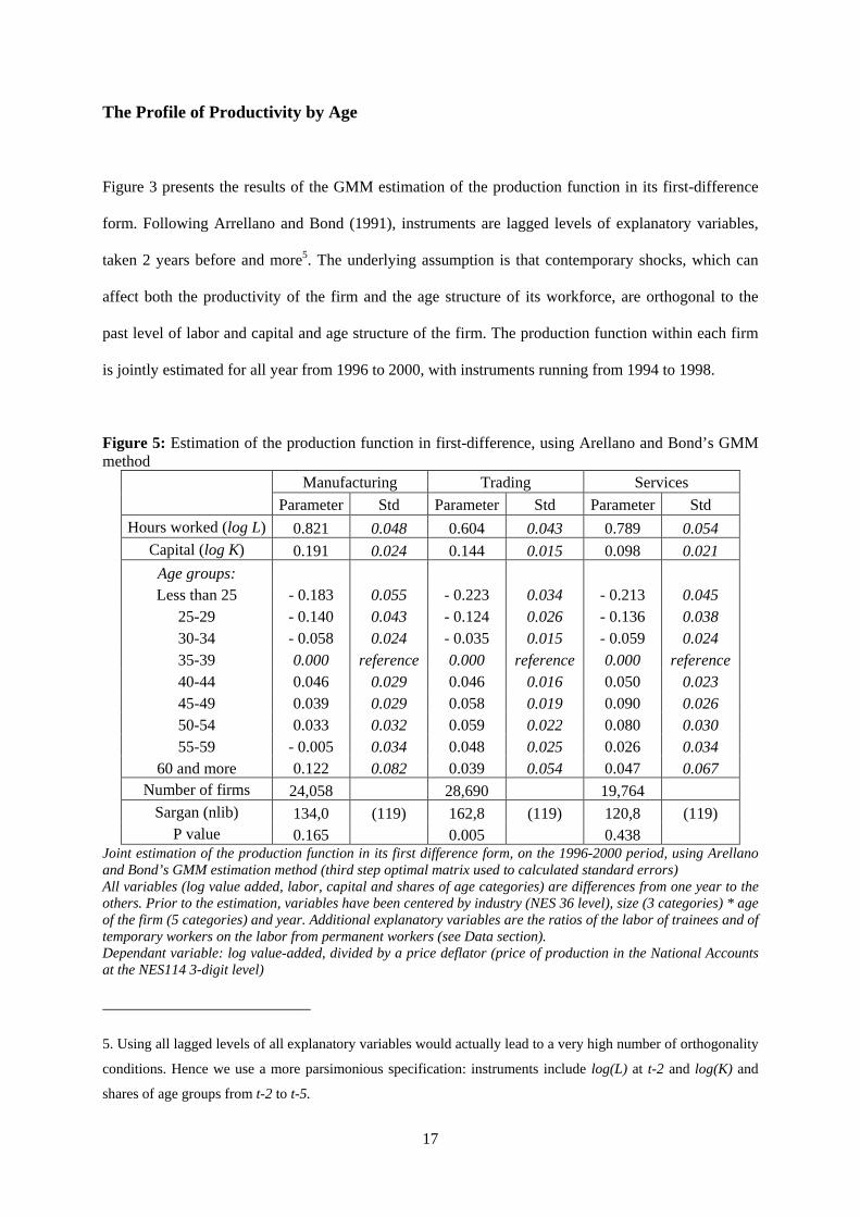
Figure 3 presents the results of the GMM estimation of the production function in its first-difference

form. Following Arrellano and Bond (1991), instruments are lagged levels of explanatory variables,

taken 2 years before and more5. The underlying assumption is that contemporary shocks, which can

affect both the productivity of the firm and the age structure of its workforce, are orthogonal to the

past level of labor and capital and age structure of the firm. The production function within each firm

is jointly estimated for all year from 1996 to 2000, with instruments running from 1994 to 1998.

Figure 5: Estimation of the production function in first-difference, using Arellano and Bond’s GMM method




25-29 - 0.140 0.043 - 0.124 0.026 - 0.136 0.038 30-34 - 0.058 0.024 - 0.035 0.015 - 0.059 0.024 35-39 0.000 reference 0.000 reference 0.000 reference 40-44 0.046 0.029 0.046 0.016 0.050 0.023 45-49 0.039 0.029 0.058 0.019 0.090 0.026 50-54 0.033 0.032 0.059 0.022 0.080 0.030 55-59 - 0.005 0.034 0.048 0.025 0.026 0.034

60 and more 0.122 0.082 0.039 0.054 0.047 0.067 Number of firms 24,058 28,690 19,764

Sargan (nlib) 134,0 (119) 162,8 (119) 120,8 (119) P value 0.165 0.005 0.438

Joint estimation of the production function in its first difference form, on the 1996-2000 period, using Arellano and Bond’s GMM estimation method (third step optimal matrix used to calculated standard errors) All variables (log value added, labor, capital and shares of age categories) are differences from one year to the others. Prior to the estimation, variables have been centered by industry (NES 36 level), size (3 categories) * age of the firm (5 categories) and year. Additional explanatory variables are the ratios of the labor of trainees and of temporary workers on the labor from permanent workers (see Data section). Dependant variable: log value-added, divided by a price deflator (price of production in the National Accounts at the NES114 3-digit level)

5. Using all lagged levels of all explanatory variables would actually lead to a very high number of orthogonality

conditions. Hence we use a more parsimonious specification: instruments include log(L) at t-2 and log(K) and

shares of age groups from t-2 to t-5.

18

Instruments are lagged level of log labor (in t - 2) and lagged levels of log capital and the share of age groups in the total number of hours worked (from (t - 2) to (t - 5)). Source: DADS-BRN, 1994 to 2000. Private sector firms with at least 5 workers, existing from 1994 to 2000, except in the fishing, energy, construction, finance and administration sectors (see Data section).

Estimates of marginal productivities of labor and of capital are quite unsatisfactory. They yield low

estimates for capital, from 0.098 in services to 0.191 in manufacturing, compared to the usual 0.3. This

estimates imply constant return to scale in one sector only (manufacturing) and decreasing return to

scale in the two other. However, such ‘attenuation’ of coefficients for labor and capital in difference

specifications are quite standard in the estimation of production functions (see Griliches and

Mairesse). As already discussed in the model section, they are due to the low explanatory power of

instruments on those two variables.

The same problem does not arise for shares of hours worked by age groups, since we saw that our

instruments are good predictors of those variables. This stems from the fact that many workers remain

in the firm several years. Since they are getting one year older each year, the past age structure of the

workforce is correlated to yearly changes from one age group to another.

We estimate quite similar age-productivity profiles in all three sectors. Productivity increases with age

in the first part of the economically active lifetime, up to age 40 to 45. Then it remains quite stable,

with a little decrease after age 55. Due to large standard error, differences between estimated marginal

productivity of age groups (compared to the reference group) are often statistically not significant. In

all three sectors younger workers (less than 35) have a statistically lower productivity than 35-39 age

old workers. In manufacturing, there is no statistically significant difference between the reference age

group and older workers. In trading, workers age 40 to 59 are significantly more productive than

workers aged 35-39, whereas in services only workers aged 45 to 54 are.

In all three sectors, productivity is lower for workers aged 55 to 59 compared to the preceding age

group (50-54), which would mean that there is a (small) decrease of productivity for older workers.

However, the difference between those two age groups is not statistically significant, due to our large

19

standard error. It is therefore difficult to conclude to a decrease of productivity after age 55, rather than

a stability. Lastly, productivity increases after age 60 in services and manufacturing, the rise being

very large in the latter sector. However, due to the legal retirement age at 60 in France, individuals

remaining at work after this age are very few and very particular. They are usually highly qualified

high wage workers, who choose to retire later than the normal retirement age. This selection issue can

explain why they are found much more productive than other age groups in manufacturing.

Labor Cost Profile

Similar to what is done for the production function, we jointly estimates our labor cost equation on the

1996-2000 period following Arellano and Bond’s GMM procedure. Note that, since labor costs by age

groups are observed, we could have directly plotted the age profile of such costs. However we intend

to compare this profile to the age-productivity profile. We therefore need to estimate it under the same

restrictions and specifications, e.g. log transformation, linearization, etc.

Results are presented in figure 6. In manufacturing, trading and services we estimate a rising and

concave profile of labor cost with age, which is consistent to what is known on this profile (see, for

instance, Aubert, 2003).

20

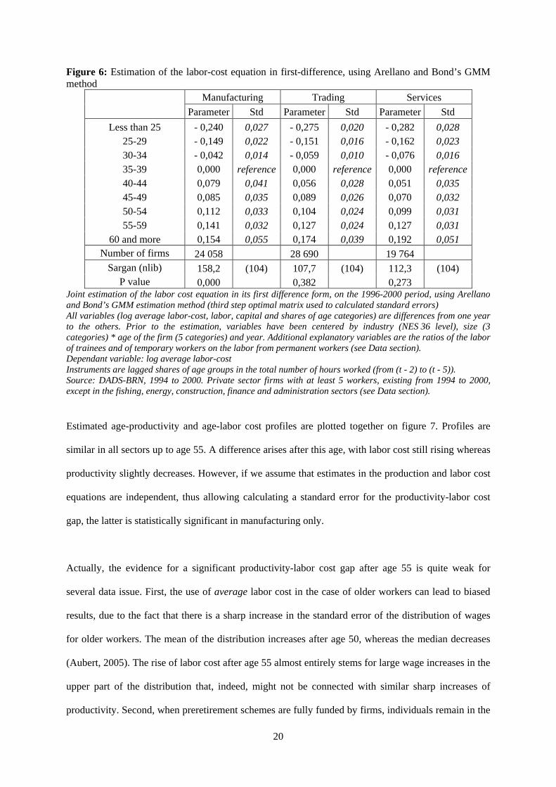
Figure 6: Estimation of the labor-cost equation in first-difference, using Arellano and Bond’s GMM method


Less than 25 - 0,240 0,027 - 0,275 0,020 - 0,282 0,028 25-29 - 0,149 0,022 - 0,151 0,016 - 0,162 0,023 30-34 - 0,042 0,014 - 0,059 0,010 - 0,076 0,016 35-39 0,000 reference 0,000 reference 0,000 reference40-44 0,079 0,041 0,056 0,028 0,051 0,035 45-49 0,085 0,035 0,089 0,026 0,070 0,032 50-54 0,112 0,033 0,104 0,024 0,099 0,031 55-59 0,141 0,032 0,127 0,024 0,127 0,031

60 and more 0,154 0,055 0,174 0,039 0,192 0,051 Number of firms 24 058 28 690 19 764

Sargan (nlib) 158,2 (104) 107,7 (104) 112,3 (104) P value 0,000 0,382 0,273

Joint estimation of the labor cost equation in its first difference form, on the 1996-2000 period, using Arellano and Bond’s GMM estimation method (third step optimal matrix used to calculated standard errors) All variables (log average labor-cost, labor, capital and shares of age categories) are differences from one year to the others. Prior to the estimation, variables have been centered by industry (NES 36 level), size (3 categories) * age of the firm (5 categories) and year. Additional explanatory variables are the ratios of the labor of trainees and of temporary workers on the labor from permanent workers (see Data section). Dependant variable: log average labor-cost Instruments are lagged shares of age groups in the total number of hours worked (from (t - 2) to (t - 5)). Source: DADS-BRN, 1994 to 2000. Private sector firms with at least 5 workers, existing from 1994 to 2000, except in the fishing, energy, construction, finance and administration sectors (see Data section).

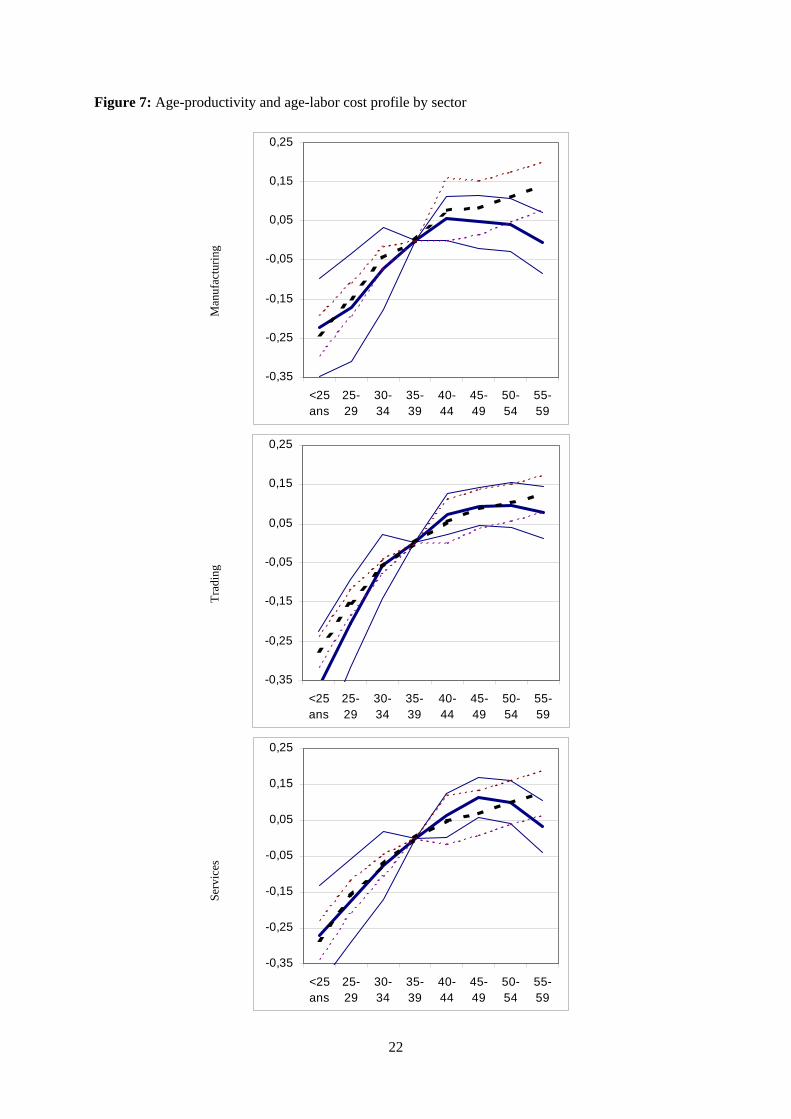
Estimated age-productivity and age-labor cost profiles are plotted together on figure 7. Profiles are

similar in all sectors up to age 55. A difference arises after this age, with labor cost still rising whereas

productivity slightly decreases. However, if we assume that estimates in the production and labor cost

equations are independent, thus allowing calculating a standard error for the productivity-labor cost

gap, the latter is statistically significant in manufacturing only.

Actually, the evidence for a significant productivity-labor cost gap after age 55 is quite weak for

several data issue. First, the use of average labor cost in the case of older workers can lead to biased

results, due to the fact that there is a sharp increase in the standard error of the distribution of wages

for older workers. The mean of the distribution increases after age 50, whereas the median decreases

(Aubert, 2005). The rise of labor cost after age 55 almost entirely stems for large wage increases in the

upper part of the distribution that, indeed, might not be connected with similar sharp increases of

productivity. Second, when preretirement schemes are fully funded by firms, individuals remain in the

21

wage bill of the firm until the legal retirement age in our data. Therefore, the lower productivity of

workers aged 55 or more may partly be explained by the fact that some of the ‘workers’ in this age

group are actually not working, thus decreasing the average productivity of the category.

22

Figure 7: Age-productivity and age-labor cost profile by sector

Man

ufac

turin

g

-0,35

-0,25

-0,15

-0,05

0,05

0,15

0,25

<25ans

25-29

30-34

35-39

40-44

45-49

50-54

55-59

Trad

ing

-0,35

-0,25

-0,15

-0,05

0,05

0,15

0,25

<25ans

25-29

30-34

35-39

40-44

45-49

50-54

55-59

Serv

ices

-0,35

-0,25

-0,15

-0,05

0,05

0,15

0,25

<25ans

25-29

30-34

35-39

40-44

45-49

50-54

55-59

23

Lecture: productivity and its confidence interval are represented by plain lines (thick line: productivity, thin lines: upper and lower bound of the 95 % confidence interval). Labor cost and its confidence interval are represented by dotted lines. Profiles correspond to estimates for each age group in the estimation of the

production function and labor cost equation (figures 5 and 6). Coefficients correspond to (1

0

−λλ j

) in the production function equation (see Model section). Workers aged 60 or more are particular and not represented on these graphs (see above). Source: DADS-BRN, 1994 to 2000. Private sector firms with at least 5 workers, existing from 1994 to 2000, except in the fishing, energy, construction, finance and administration sectors (see Data section).

Conclusion

In this paper, we estimate the profile of productivity by age through the estimation of production

functions, following a methodology that is similar to Hellerstein, Neumark, Troske (1999) and

Crépon, Deniau, Perez-Duarte (2003). In this methodology, ‘productivity’ is estimated as the average

contribution of age groups to the productivity of firms. Our data are a matched employer-employee

dataset covering about 70,000 firms in the late 1990’s in France.

We find that productivity increases with age until age 40 and then remains stable after this age.

Workers aged 40 and more are roughly 5% more productive than workers aged 35-39, while workers

below 30 are 15 to 20% less productive. This result is moreover stable across sectors, since it holds in

manufacturing, trading and services. Besides, the age-productivity profile is similar to the age-labor

cost profile, which means that the hypothesis of a lower employability of older workers that would be

explained by a significant wage-productivity gap seems rejected, at least before age 55. After this age,

a slight decrease occurs, by 1 to 5 percentage point across sectors. Unfortunately, this decrease is not

statistically significant, due to the large standard errors. The evidence for what happens after age 55

therefore remains inconclusive.

Another result is that standard estimations of the production function in the Between and Within

dimension lead to strongly biased estimations for the productivity of age groups. In particular, the

decrease of productivity after 35 in Crépon and al. (2003) is explained by simultaneity of productivity

24

shocks with adjustments of the age structure of the workforce, rather than a truly lower productivity of

older workers. The existence of these biases may stress the fact that there is a problem of allocation of

older workers, the latter ending up being more numerous in declining firms.

Our study however has several limits, which should be addressed in further works. First, we estimate

the average productivities of age categories for all workers in the category. The profile is therefore

different from the individual profile of productivity by age. There may be composition effects by

gender, skill, sector, etc. that may explain part of the productivity differences across age groups.

Second, we estimate a common profile of productivity for all types of workers in all types of firms.

There might be differences, though, for instance between high skill and low skill workers or between

technologically innovative or non innovative firms. Our study should be replicated on smaller

samples, although a problem of imprecision may arise. Third, we estimate the productivity of

employed workers. Therefore our estimation is not free from selection effects. For instance, if the

crowding-out from the labor market of unproductive workers is larger for elder workers than for

younger workers, the higher productivity of seniors may reflect the heterogeneous selection in the

labor market across ages. However, since the essence of the method is to define the productivity of an

age category as the average contribution of the category to the production of the firm, the productivity

of non-working individuals is simply not identifiable. Fourth, our estimation is run on a 5-year period

at the end of the 1990’s. Due to this short time dimension, we cannot separate age effects from cohort

effects. In particular, workers aged 55 or more in our sample were born before the baby-boom and

may be not comparable with younger workers. The estimation should be run on more recent data to

test whether results after age 55 still hold.

References

Arellano M. and Bond S. (1991), « Some Tests of Specification for Panel Data: Monte Carlo Evidence

and an Application to Employment Equations », Review of Economic Studies, 58: 277-97.

25

Aubert P. (2003), « Les quinquagénaires dans l’emploi salarié privé », Economie et Statistique, n°368,

pp.65-94

Aubert P. et Crépon B. (2003), « La productivité des salariés âgés : une tentative d’estimation »,

Economie et Statistique, n° 368, pp.95-119

Aubert P. (2005), “Comment interpréter l’évolution des salaire après 50 ans ?”, Insee miméo

Crépon B., Deniau N. et Perez-Duarte S. (2003), « Productivité et salaire des travailleurs âgés », Revue

française d’économie, vol. 18, n° 1, pp. 157-185.

Gonzalez L. (2002), « L’incidence du recours à l’intérim sur la mesure de la productivité du travail des

branches industrielles », Économie et Statistique, n° 357-358, pp. 103-133.

Griliches Z. and Mairesse J. (1997), « Production Functions: The Search for Identification », Working

paper 9730, Crest.

Hægeland T. and Klette T. (1999), « Do Higher Wages Reflect Higher Productivity? Education,

Gender and Experience Premiums in a Matched Plant-Worker Data Set », in The Creation and

Analysis of Employer-Employee Matched Data, edited by J. Haltiwanger, J. Lane, J.R. Spletzer,

J. Theeuwes and K. Troske, Amsterdam: North Holland.

Hellerstein J., Neumark D. and Troske K. (1999), « Wages, Productivity, and Worker Characteristics:

Evidence from Plant-Level Production Functions and Wage Equations », Journal of Labor Economics,

17, pp. 409–446.

Jolivet A., Molinié A. et Volkoff S. (2000), « Efficaces à tout âge ? Vieillissement démographique et

activités de travail », Dossier n° 16 du Centre d’Études sur l’Emploi.

Jovanovic B. (1979), « Job Matching and the Theory of Turnover », Journal of Political Economy, 87,

pp. 972-990.

Lazear E. (1979), « Why is there a Mandatory Retirement? », Journal of Political Economy, 87,

pp. 1261-1284.

26

Mac Donald G. (1982), « A Market Equilibrium Theory of Job Assignment and Sequential

Accumulation of Information », American Economic Review, 72, pp. 1038-1055.

Mincer J. (1974), Schooling, Experience and Earnings, N.Y., Columbia University Press.

Age, Wage and Productivity: Firm-Level Evidence

Documents