TLb® Ag® dfttlfo® A reconstruction for the states and territories, 1881-1961 r Sudhansu Bhusan Mukherjee East-West Center East-West Population Institute

Welcome message from author
This document is posted to help you gain knowledge. Please leave a comment to let me know what you think about it! Share it to your friends and learn new things together.
Transcript
TLb® Ag® d f t t l f o ®
A reconstruction for the states and territories, 1881-1961 r
Sudhansu Bhusan Mukherjee
East -West C e n t e r Eas t -Wes t P o p u l a t i o n Ins t i tu te
The Age Distribution of the Indian Population
A reconstruction for the states and territories, 1881-1961
Sudhansu Bhusan Mukherjee
East -West C e n t e r T Eas t -West P o p u l a t i o n I n s t i t u t e \ ^ \ ^
H o n o l u l u
.Library of Congress Cataloging in Publication Data
Mukherjee, Sudhansu Bhusan, 1923-The age distribution of the Indian population.
Bibliography:'p. 243—257. 1. Age distribution (Demography)-India.
2. Indian-Statistics, Vital. I. Title. HB1679.M84 312'.92'0954 76-28367 ISBN 0-8248-0518-6
©1976 East-West Center All rights reserved Printed in the United States of America Designed by Mary Connors Distributed by the University Press of Hawaii, Honolulu, Hawaii 96822
To my father
Sri Jyotish Chandra Mukherjee (1883-1967)
and my mother
Srimati Umasashi Devi (1894-1963)
Foreword xix
Acknowledgments xxi
H Introduction 1
Age composition as a demographic variable 2 Age composition as an economic variable 3 Age composition in development planning 6 l i v
Underutilization of age data from census tables 8
2 Regrouping age data from census tables 9
Changes in administrative divisions 9 Current administrative divisions 1 7 Strategy for regrouping age data 21 Variation in boundaries of age intervals 23 Decomposition of a broad age group into five-year age groups 25 Parent age distribution for different areas 27 Semismobthed age data for 1931 28 The unsmoothing method 30 Result of unsmoothing operations 32 Y-sampie tables and partially smoothed data: 1941 36 The displaced population: 1951 40
viii The age distribution of the Indian population
The reconstructed age tables 44 Broad features of the age composition 44 Errors in the reconstructed age tables 47 Age-ratio score and sex-ratio score 57 Age ratios and sex ratios computed by Indian census actuary Age ratios and sex ratios for other countries 62 Age-sex selectivity in underenumeration 62
Age distribution and the hypothesis of quasi stability 129 The L curve and indices of dissimilarity 131 Test of the indices 134 Computed distance measures for India 137 Distance measures for hypothetical quasi-stable populations Effect of differences in fertility on the index 145
Rate of natural increase and the hypothesis of quasi stability Two kinds of quasi stability 149 Components of population increase 150 Natural increase 155
Methodology used to estimate fertility and mortality 164 The OPR stable populations 165 The estimation technique 167 An alternative method 169 Age pattern of mortality in India 7 70 Comparative qx values 173 The U.N. model life tables 175 Using a period growth rate for estimation 7 76 7? elasticity Of the estimates 7 75 The need for correction 181 Methods for correction 184
Quasi-stable estimates of fertility and mortality 189
Mean of the female fertility schedule 189 Quasi-stable estimates of female birth rate and G R R 192
Contents ix
Estimates of female death rate and life expectancy 79 7 Estimates for the male population 200 Consistency of estimated birth rates for males and females 202 Consistency between female birth rate and G R R 204 A summing up 206
® Derivation of fertility and mortality by the forward projection method 208 The method 208 An illustrative estimation of mortality 209 Estimates of mortality for India and zones 275 Limitations of the FPM 275 Sensitivity of the estimates to differences in the age pattern of mortality 27 6 Examination of sensitivity using hypothetical populations 275
Final estimates and comparisons 220 Joint estimates 220 Estimates based on the sample registration system 227 Estimates based on survey data 226 Estimates based on census data 225 Comparison with some advanced countries 233
Appendix: the 1971 age distribution 236
References 243
References for basic tables 257
Text tables 2.1 States and union territories of India with area and population according to
1971 census 18 2.2 Percentage of population of dismembered districts incorporated into
separate states: 1951-1961 24 2.3 Percentage distribution of population within 20-year age groups, by region
and by religion: Bengal, male, 1911 27 2.4 Areas and religious groups used to estimate district age data for states
created from partitioned provinces 28 2.5 Smoothing formula used in 1931 census 29 2.6 Boundary of preliminary age groups according to two definitions
of age 31 2.7 Smoothed and unsmoothed 1931 age distributions: Uttar Pradesh,
male 32 2.8 K multipliers for unsmoothing 1931 census age data for five states 33 2.9 1931 census percentage age distribution for five states before and after
unsmoothing 35 2.10 Formula for smoothing 1941 age data for selected princely states 38 2.11 Percentage age distribution of displaced and nondisplaced male population
in four states and territories: 1951 42
3.1 Percentage age distribution in the common set of states and territories and in India as a whole: 1961 50
3.2 Age-ratio score, sex-ratio score, and joint score: India and zones, 1881-1961 60
Tables xi
3.3 Age-ratio score, sex-ratio score, and joint score calculated from original and reconstructed age data: India and selected areas, 1901 — 1921 61
3.4 Ratios of sex-age selectivity due to underenumeration: India, 1891-1961 63
4.1 Cumulative percentage of total population up to various ages: India, female (1901 and 1961), and United States, female (1950) 133
4.2 Matrix of distances between age distributions of different years: United States, 1900-1940 136
A3 Aggregate dissimilarity, concentration dissimilarity, and net concentration dissimilarity for six advanced countries: female 138
4.4 Matrix of distances between age distributions of census years: India, female, 1881-1961 139
4.5 Matrix of distances between age distributions of census years: India, male, 1881-1961 140
4.6 Aggregate dissimilarity between actual age distribution and simulated age distribution under assumptions of constant fertility and changing mortality 144
4.7 Aggregate dissimilarity between stable age distributions corresponding to proportionate differences in GRR underlying such age distributions, by mortality level 147
4.8 Computed values of coefficients a and b 147
5.1 Birthplace-enumeration place matrix for male and female population by zone: 1951 156
5.2 Birthplace-enumeration place matrix for male and female population by zone: 1961 157
5.3 Annual rate of natural increase: India and zones, 1881 —1961 159
6.1 Stable estimates of birth rate, death rate, gross reproduction rate, and life expectancy at birth: West Bengal, female, 1901 767
6.2 Estimates of birth rate and life expectancy at age 10 by alternative method: West Bengal, female, 1901 777
6.3 Stable estimates of birth rate, death rate, gross reproduction rate, and life expectancy at birth using regional model life tables and stable populations: India, female, 1911 7 72
6.4 Root-mean-square deviations of qx values in model life tables from qx
values in Indian census life tables with same el0: male and female, 1901-1961 775
6.5 Instantaneous and average growth rates in simulated projections assuming fluctuations in mortality similar to those in India, 1881 -1921 7 77
6.6 Instantaneous and average growth rates in simulated projections assuming GRR = 3.200 and a monotonic decline in mortality 177
xii The age distribution of the Indian population
6.7 Stable estimates of birth rate, gross reproduction rate, death rate, and life expectancy at birth derived from female age distribution of India (1961) with different assumed growth rates 180
6.8 Parameters of regression equation^ = a + bx and values of correlation coefficient (rXy) between growth rate (x) used as estimating parameter and derived estimates of birth rate, gross reproduction rate, and life expectancy at birth 181
6.9 Values of e0 under various mortality assumptions: 1911 — 1961 183 6.10 Ratios cqs(a)/cs(a) with GRR (29) = 3.000 and mortality assumptions A,
B , C , D 185
7.1 Proportion of currently married women among all women by age group: India and zones, 1901-1961 790
7.2 Mean age of fertility schedule: India and zones, 1901 — 1961 797 7.3 Lower and upper estimates of female birth rate: India and zones,
1901-1961 796 7.4 Lower and_upper estimates of female gross reproduction rate for respective
values of Af: India and zones, 1901-1961 796 7.5 Lower and upper estimates of female death rate: India and zones:
1901-1961 797 7.6 Stable estimates of female life expectancy at birth: India and zones,
1901-1961 198 7.7 Ranking of zones according to estimated birth rate, gross reproduction rate,
death rate, and life expectancy at birth: female, 1901—1961 799 7.8 Lower and upper estimates of male birth rate: India and zones,
1901-1961 200 7.9 Lower and upper estimates of male gross reproduction rate: India and
zones, 1901-1961 207 7.10 Lower and upper estimates of male death rate: India and zones:
1901-1961 207 7.11 Stable estimates of male life expectancy at birth: India and zones,
1901-1961 202 7.12 Sex ratio for India and zones: 1901-1961 203 7.13 Expected values of FBR/MBR on assumption of sex ratio at birth between
1.03 and 1.09: India and zones, 1901-1961 203 7.14 Observed values of FBR/MBR in quasi-stable estimates: India and zones,
1901-1961 204 7.15 Synthetic values of female gross reproduction rate obtained by relating
basic birth rate to quasi-stable estimate of birth rate: India and zones, 1901-1961 206
8.1 Areas and populations excluded for derivation of FPM estimates 213
Tables xiii
8.2 FPM estimates of death rate and life expectancy at age 5: India and zones, 1881-1891 to 1951-1961 214
8.3 Estimates of death rate and life expectancy at age 5 with five sets of model life tables: India, 1881-1891 to 1951-1961 277
8.4 FPM estimates of death rate and life expectancy at age 5 with five sets of model life tables for Demeny's projected population 279
9.1 Estimates of joint birth rate, death rate, and life expectancy: India and zones, 1901-1961 227
9.2 Estimates of birth rate and death rate based on sample registration system: India, 1969 225
9.3 Estimates of birth rate, death rate, and growth rate in rural areas of India from two interpenetrating samples: NSS 14th, 15th, and 18th rounds 226
9.4 Estimates of birth rate, death rate, and growth rate in rural areas of India: NSS 13th and 14th rounds 227
9.5 Upper estimates of birth rate for selected areas of India: 1951 census fertility inquiry 229
9.6 Estimates of birth rate and death rate by zone obtained by differencing method, reverse-survival method, and registration: Indian census actuary, 1951 230
9.7 Birth rates and death rates estimated by Davis: India, 1881 — 1891 to 1931-1941 231
9.8 Birth rates, death rates, life expectancy, and gross reproduction rates estimated by Visaria: India, 1941-1961 232
9.9 Demographic parameters for four industrialized countries and India: 1901,1941, and 1961 234
A . l Percentage age distribution of total, rural, and urban population: India, 1971 237
A.2 Percentage of population below age 15: India and zones, 1961 and 1971 237
A.3 Percentage of population in age groups 0—4, 5—9, and 10—14, based on 1 percent sample: India, 1961 and 1971 238
A.4 Percentage age distribution of rural and urban population, based on 1 percent sample, India, 1961 and 1971 239
A.5 Quasi-stable estimates of birth rate, death rate, gross reproduction rate, and life expectancy at birth: India, 1961 — 1971 240
xiv The age distribution of the Indian population
Basic tables 1. Population by age and sex: India and zones, states, and territories,
1881-1971 65 2. Population by age and sex: Goa, Daman, and Diu, 1900-1971 94 3. Population by age and sex: Dadra and Nagar Haveli, 1900-1971 95 4. Population by age and sex: Pondicherry and Laccadive, Minicoy, and
Amindivi Islands, 1961 and 1971 96 5. Percentage distribution of population by age and sex: India and states
and territories, 1881-1971 97 6. Percentage distribution of population by age and sex: Goa, Daman,
and Diu, 1900-1971 126 1. Percentage distribution of population by age and sex: Dadra and Nagar Haveli
1900-1971 127
8. Percentage distribution of population by age and sex: Pondicherry and Laccadive, Minicoy, and Amindivi Islands, 1961 and 1971 128
3.1 Male age distribution: India, 1901-1961 45 3.2 Female age distribution: India, 1901-1961 46 3.3 Comparative age structures for India, Japan, United States, and Europe:
1955-1961 48 3.4 Age structural changes in India and Great Britain: 1911-1961 49 3.5 Age ratios for India: 1881-1961 54 3.6 Age ratios for Eastern Zone: 1881 -1961 55 3.7 Age ratios for Central Zone: 1881-1961 56 3.8 Age ratios for Southern Zone: 1881-1961 57 3.9 Age ratios for Western Zone: 1881-1961 58 3.10 Age ratios for Northern Zone: 1881-1961 59
4.1 L curves showing age distribution of India females (1961) and United States females (1950) with India females (1901) as base 132
4.2 Values of \D\ for India and zones contrasted to those for some advanced countries: female, 1861-1961 141
4.3 Values of ICI for India and zones contrasted to those for some advanced countries: female, 1861-1961 142
4.4 Values of C for India and zones contrasted to those for some advanced countries: female, 1861-1961 143
4.5 Regression of A G R R / G R R on \D\, Dp, and C 146
5.1 Rate of natural increase: India and Eastern Zone, 1881-1891 to 1951-1961 160
xvi The age distribution of the Indian population
5.2 Rate of natural increase: Central and Southern Zones, 1881-1891 to 1951-1961 161
5.3 Rate of natural increase: Western and Northern Zones, 1881-1891 to 1951-1961 162
6.1 Regression of stable estimates on values of r as an estimating parameter with age segment 0—30 182
6.2 cqs(a)/cs(a) for GRR = 3.0 and mortality assumptions A, B, C, D 756
7.1 Corrected estimates of female birth rate: India and Eastern Zone, 1901-1961 193
7.2 Corrected estimates of female birth rate: Central and Southern Zones, 1901-1961 194
7.3 Corrected estimates of female birth rate: Western and Northern Zones, 1901-1961 195
9.1 Male, female, and joint birth rates, death rates, and life expectancy: India and zones, 1901-1961 222
Maps 2.1 Administrative units of India: 1911 14 2.2 Administrative units of the Indian Union: 1951 75 2.3 Administrative units of the Indian Union: 1961 76 2.4 Administrative units of the Indian Union: 1971 20 2.5 Districts and zones of the Indian Union: 1971 22
Worksheets 8.1 Estimates of survivors of 1901 census population in 1911 compared with
191 1 census population: India, male 270 8.2 Estimated values of e5 corresponding to reverse-cumulated population
of 1911 census for different age sectors 211 8.3 Estimating the number of male deaths: India, 1901-1911 272
Exhibit 2.1 Administrative units of the Indian subcontinent: 1872-1971 10
The unbroken series of the decennial population censuses of India, now spanning a century, provide an extraordinarily valuable storehouse of information for students of demography. The present monograph by S.B. Mukherjee represents an important entry in the long list of. demographic studies, marked by numerous notable achievements, that seek to analyze and interpret that record. The outstanding significance of Indian census statistics for demographers is easily understood if one considers the scarcity of comparable data sets. Of other large countries, only the United States and a number of European states possess census records that match the length and consistency of those available for India; and in Europe, and to a lesser exterit/in the United States, the existence of birth and death statistics makes the census a less important source of information for reconstructing demographic history. In what is called nowadays "the developing world," the Indian record is quite without parallel. The contrast to that other Asian giant, China, is of course particularly striking; and even among the countries of the Subcontinent, only India succeeded fully in preserving the decennial regularity of its census in the post-Independence period.
' The synergistic possibilities for demographic analysis inherent in successive census descriptions of the state of a population are truly remarkable. In the hands of the skilled analyst, cross-sectional observations can be transformed into reliable estimates of indices characterizing demographic dynamics. In particular, since the age distribution of a population is a reflection of past mortality, fertility, and migra-
xx The age distribution of the Indian population
tion processes, information on these phenomena can be distilled from census data alone, provided that censuses supply consistent records on the size and age composition of the population at successive dates. For India as a whole, such analyses have been performed with signal success by several investigators. Work on the subnational level has been hampered, however, by a multiplicity of problems affecting the availability and comparability of data on age distribution for smaller areas. Boundary changes, lack of uniformity in the methods of collecting and publishing age information, and errors in reporting age are the main sources of the difficulty encountered by the analyst.
By successfully constructing a uniform and consistent series of age and sex distributions covering the period 1881 — 1961 for the main territorial subdivisions of contemporary India, Mukherjee has eliminated most of these problems and, as a result, provides the basis for deepened understanding of Indian demographic history. His results, obtained through painstaking and ingenious adjustment of data gathered from virtually hundreds of publications of nine successive censuses, not only will be accepted as an authoritative description of a phenomenon that is of interest in its own right, but will also be utilized in future demographic analyses that require such data as raw material. Mukherjee's study itself provides the best illustration of how productive the mining of such data can be by developing a variety of new estimates of population dynamics for subnational units of India. While the bulk of his study treats phenomena that lie in the domain of demographic history, this hardly diminishes the timeliness of his contribution. Understanding the past is an indispensable first step toward understanding the present and the unfolding future. Mukherjee's work will not lose significance as modern India reaches and passes a demographic watershed, the historic significance of which will be fully visible only after the 1981 census results will have been collected and made available.
Readers and users of this book will be mostly demographers. This makes it unnecessary to dwell on what will be obvious to any practitioner of the trade: the truly monumental labor and the analytical virtuosity that went into this study. To persevere in the kind of task Mr. Mukherjee set for himself would have been impossible without his special mixture of professional skills and seemingly unlimited capacity for meticulous work. During the preparation of this volume, he cheerfully coped with difficulties that would have deterred lesser souls and carried the work to conclusion with a stubborn singleness of purpose. It gives me great pleasure to register here my admiration and appreciation for his accomplishment.
Paul Demeny
I wish to express my grateful thanks to the East-West Population Institute for the fellowship offered to me in 1970 which enabled me to complete this research by March 1972. The director of the Institute, Professor Paul Demeny, provided help, inspiration, and guidance at every stage of the work. He also very kindly contributed a foreword to this volume. I cannot thank him adequately for all this.
The high-level academic atmosphere in the Institute, the scholarly exchange among researchers, the superbly managed library, the unstinted cooperation of the secretarial staff, the all-pervading Yes attitude to the manifold problems faced by a foreign scholar doing research in the Institute-all were extremely helpful in my day-to-day progress of work. It is difficult to select names from among a large number of colleagues and friends. Any list would have to include Professors Lee-Jay Cho, James Palmore, Bradley Wells, and Johannes Overbeek, Executive Officer Keith Adamson, Librarian Alice Harris, and Administrative Assistant Virginia Dolan. My student assistants James O'Heron, Enamul Huq Chudhury, Steven Honda, Tan Chun Ling, and James Modecki helped in the collection and collation of the data, and I put on record my appreciation for their hard work.
While in Honolulu I received great encouragement and inspiration from eminent demographers who visited the Institute from time to
xxii The age distribution of the Indian population
time. Special thanks are due for this to Professors C. Chandrasekharan, Philip Hauser, Nathan Keyfitz, Charles Westoff, and the late lamented Irene Taeuber. Thanks are due also to the government of West Bengal and to the commissioner, Development and Planning (Town and Country Planning) Department, for kindly granting me study leave and enabling me to take up research at the East-West Population Institute.
When the question of publishing this book came up, I received invaluable help and cooperation from two persons—Sandra Ward of the East-West Population Institute and Professor Karol Krotki of the University of Alberta, who read the manuscript and suggested a number of modifications for improving the presentation as well as the content of the various chapters. Thanks are also due to Griffi th Feeney and Robert Gardner of the East-West Population Institute for their helpful comments on the manuscript, and to copyeditor Don Yoder, cartographer and graphic artist Gregory Chu, and compositor Lois Bender for their assistance in bringing the volume to press.
Last but most important, I would like to acknowledge my deep sense of gratitude to Professor Ansley J. Coale, who initiated me into the study of age distribution and has frequently provided guidance through personal correspondence. With regard to my training in demography, I consider the O'ffice of Population Research (Princeton University) to be my Alma Mater and regard Professor Coale as my guru in the truest traditional sense of the term.
S.B. Mukherjee
1 Introduction
There are two outstanding features of the Indian population: its massive growth and its static structure. During the 80-year period 1881 through 1961 the population of India* increased from 190 million to 440 million-revealing a growth of 130 percent. The period can be divided into two halves. During the first 40 years the population increased from 190 million to 250 million-at an approximate average annual rate of 0.6 percent. During the second 40 years it increased from 250 million to 440 million-at an average annual rate of about 1.6 percent. The preliminary results of the 1971 census indicate that the annual rate of increase has since shot up to 2.2 percent.
A l l these phenomena are fairly well known. What is not so well known is the fact that a nearly static age structure has been coexisting with such a vast growth in the size of the population. A n unchanging age composition accompanied by a rapid increase in the total population has important and interesting implications from the standpoint of future population increase and economic development in the country.
This treatise aims at a longitudinal study of the age distribution in India: its five zones, eighteen states, and eleven territories as defined
* Indian Union as defined since independence in 1947.
2 The age distribution of the Indian population
for the purpose of the 1971 census [32].* It attempts to compile the age-sex data from the nine decennial censuses of 1881 through 1961, to regroup the age data for the changes that occurred in the political divisions of the country from one census to another, and to recast these age data into a uniform set of quinquennial age intervals for a uniformly defined set of states and territories. It is only after such a reconstruction that the age compositions for the different years and for different zones and territories can be compared.
Age composition as a demographic variable
As a basic demographic variable, age composition is intertwined with all other demographic variables. Age composition affects and is affected by fertility, mortality, and migration. Births occur to women aged 15 to 50. Within this range the rate of childbearing usually rises slowly between ages 15 and 20, then sharply between ages 20 and 30, and thereafter declines first slowly and then rapidly [4, 35, 80].
Deaths occur to men and women of all ages. But here again there are typical age patterns in the incidence of mortality. Starting high during infancy, the incidence of mortality decreases in childhood years until ages 10 to 15 and then continues at a low level until about age 30. Thereafter it starts increasing, first gradually and then sharply [90, 105].
So far as migration is concerned, the effect of age is not so much a biological phenomenon as a sociological one. While people of all ages and both sexes can migrate, in many societies including the developing ones the incidence of migration is particularly high among men of early working age (15—29) and women around the age of marriage or birth of the first or second child (15-35).
So much for the effect of age composition on fertility, mortality, and migration. The cause-effect relationship could be viewed from the reverse side also. Age composition itself is determined by fertility, mortality, and migration. When a child is born, its age is invariably zero years. Hence an increase in the birth rate tends to increase the proportion of children in the population and make the population younger. The effects of a change in death rate depend on the age incidence of the change in the risks of dying. To the extent that the age composition of migrants differs from that of the general population, the age composition of a community undergoes changes because of migration.
* Throughout this study, numbers in brackets refer to the bibliographic references presented at the end of the book.
Introduction 3
The intricacies of these interrelationships may be further exemplified if one recalls that even with a moderate gross reproduction rate a high proportion of women in the age group 15—49 makes for a high birth rate. The high birth rate in turn results in a high proportion of children and consequently helps to keep the future birth rate high. A young age composition working via a high birth rate thus tends to perpetuate itself. When fertility-depressing factors are operating in such a population, the young age composition puts up a resistance against their effectiveness. If postponement of marriage, increasing practice of contraception, and legalization of abortion lead to a decrease in the number of live births per married woman, the high proportion of women in the reproductive ages tends to slow down the rate of decline in the resultant birth rate.*
Age composition as an economic variable
Age composition and per capita income are interdependent variables. Per capita income and the standard of living affect the level of fertility, mortality, and migration and through them the age composition of a population. A high per capita income is usually associated with a low birth rate, which leads to an aging of the population, and a low death rate, which has a slight rejuvenating effect on the age composition. A low per capita income is usually associated with a high birth rate, which generates a young age distribution, and a high death rate, which reduces the proportion of children in the population. Migration is usually age-selective and sex-selective and hence affects the age-sex composition of both the donor community and the receiving community.
Age distribution affects people both as producers and as consumers of wealth. Manpower is the most valuable economic resource in all societies^ and the share of the population belonging to the working ages is its only source. Definition of the working ages varies from country to country, but whatever the definition may be, the important element in manpower supply is the size of the population and its distribution by age and sex. It has been estimated that 89 percent of the net change in the world labor supply during the decade 1950—1960 was due to
* As Notestein [82:275 ] has observed, "the size and age composition of a population are heavily influenced by the size and age composition a quarter century earlier."
t Okazaki [83:94] has argued that "too little attention to the importance of human resources, and too much attention to physical capital, has been one of the mistakes made in discussions of development policies for developing countries."
4 The age distribution of the Indian population
changes in the population size and age-sex structure—the remaining 11 percent being due to socioeconomic, cultural, and other factors [ 1 ].
The size of the labor force in proportion to the total population is measured by the crude activity rate, which is determined by the age-specific activity rates of males and females together with the sex-age composition of the population [51 ]. It is worthwhile mentioning here that the proportion of population in the working age groups (15—59) is generally smaller in developing countries than in developed ones—a consequence of a lower level of fertility in the developed countries generally.
To measure the changes that occur in the labor force over time, it is not sufficient to compare the total figures at two different times. A meaningful picture of such changes emerges only when we know the number of new entrants into the labor force belonging to early adult ages and the number of withdrawals from the labor force belonging to ages 60 and above. If fertility declines, the number of new entrants will start declining 15 or 20 years after the onset of fertility decline. But the immediate effect may be a little increase in the number of job-seeking women—released from the burden of childbearing owing to • the decline in fertility.
It has been observed that the average age of entry into the labor force rises under the impact of urbanization, industrialization, and growth of education. On the other hand, i f mortality declines or the age of retirement is postponed, there are fewer withdrawals from employment by older people and the average age of workers tends to increase.
Young workers are. more responsive than older ones to the introduction of new methods of work, new technology, and new products, and they are more adaptable to work in new places. Modern economic development is characterized by rapid structural change, shifts in the relative" importance of industries, and shifts in their location within the country. Sluggish response of the labor force to such changes can be a serious obstacle to. economic growth and greater per capita product. A young or otherwise mobile group within the labor force is therefore strategically important [72]. A country with a high proportion of persons in early adult ages (like India or Pakistan) enjoys an advantage over a country with a high proportion of persons in late working ages (like France or Japan).
Looking at people as savers of wealth, we may, following Meade, introduce the concept of the dependency ratio: other things remaining the same, a high dependency ratio reduces the capacity to save, while
Introduction 5
a low dependency ratio releases a portion of the immediately consumable goods and services for investment purposes. Meade [79:121 ] has defined the dependency ratio as
The population measured in consuming units The population measured in producing units
where the population measured in consuming units is the sum of the populations in the different age and sex groups in the population, each weighed by its relevant specific need rate, and the population measured in working units is the sum of the numbers in the different age-sex groups in the population each weighed by its relevant specific work rate. If we assumed that the specific need rates and the specific work rates are fixed, regardless of the level of the standard of living, the dependency ratio will depend solely upon the age and sex composition of the population.
Because of the younger age distribution in India than in Japan, the dependency ratio in India (1.9) is higher than that in Japan (1.5). If the per earner income were the same in India and Japan, the per capita income would be 26 percent higher in Japan than in India. As facts' stand, the per earner income is much lower in India than in Japan. The adverse effect of a low per earner income is severely accentuated by a higher dependency ratio in India.
A high dependency ratio erodes the saving potential of the three sources of saving in a country: private household saving, the public sector's surplus on current accounts, and corporate saving. The link between a high dependency ratio and low household savings is direct. As taxes are supposed to be paid at least partly out of potential household savings, the connection between government revenues and surplus on the one hand and the rate of saving on the other is well established. A young age distribution compels the state to spend more for schools and hospitals, leaving less for the creation of the material base forvthe development of the economy in the state sector.
Taking people as consumers of wealth, one has to recall that the . consumption of goods and services is related to age and hence the dis- -aggregated components of the consumption function are correlated with changes in the age structure. If the proportion of children in a • population decreases and that of old people Increases, the nature and composition of the consumption needs in the society will undergo significant shifts, leading in their turn to changes in the pattern, of expenditure and investments both in the private and in the public sectors.
In a subsistence economy with low income and low level of living, the differentiated production for different age groups may not always be visible. The whole economy may have been geared to the produc-
6 The age distribution of the Indian population
tion of essential food items like grains and cereals and a minimum of clothes and shelter. Even in such a state of the economy, a careful observer discerns some differences in the product mix i f children constitute 35 percent of the population instead of 45 percent. When the economy starts developing and the per capita income and per capita consumption go up, the differentiation in the product mix will be more and more visible. In a developed economy every change in the age structure is carefully taken into account by industrialists and entrepreneurs in making investment decisions for producing goods and services for babies, children, schoolchildren, college students, housewives, working people, old people, and so forth.
Age composition in development planning
Development planning involves first a statement of goals and objectives, then the formulation of a strategy to achieve the objectives, and finally the preparation of programs and projects in the light of the strategy. The age composition enters into the decision-making process at each stage and with regard to each of these elements.
A declared goal of planning in developing countries like India is an expansion of employment opportunities, both for the purpose of wiping off the backlog of unemployment and also to provide employment to new entrants into the labor force [58]. Knowledge of the age distribution of the population is essential for making estimates of existing unemployment and the present and future size of the labor force. The rightful weight of the age composition has started to assert itself in the enunciation of plan objectives in recent years [98]. Maximization of productivity and maximization of employment per unit of capital are often incompatible and conflicting goals. The size of the labor force, depending on the age distribution of the population, is one of the criteria with which to judge the relative merits of the two goals.
Investment in physical capital and investment in human capital are often alternative strategies in developmental planning [61, 62] . Expenditures on education and health are regarded as investments made to improve the quality and adaptability of men as workers, to make them more productive, and in some cases to lengthen their working lives. Education is both an end itself as a component of the level of living and also a means to achieving higher domestic product through higher productivity. The developing countries lag behind in general education as well as vocational education. The objectives in the planning of education are twofold: to increase enrollment in primary and
Introduction 7
secondary levels of education and to increase facilities for vocational training. Current estimates and future projection of the number of persons aged 6—11, 12—14, 15—17, and so forth are needed for setting up programs for educational development. The spread of education keeps people in school and thus diminishes labor force participation at younger ages [46]. The age at entry into the labor force is deferred with education, and studies on the deferment effect are relevant to employment planning. This calls for joint planning of education, employment, and manpower—all based upon the data on age composition of the national, regional, and local populations [108].
Health planning is an essential component of welfare planning and is now recognized as an aspect of economic planning also, because health is a factor of high productivity. The causes and pattern of morbidity, the conditions of health, and the'kind of health services needed vary from age to age. Therefore the current and projected estimates of population by age and sex are essential ingredients also for efficient health planning [ 107].
Forecasting of consumer demand is an essential prerequisite for planning of agriculture and industries producing consumer goods and intermediate goods. The practice in most countries is to forecast demand with the help of a projected growth rate of the total population. But demand forecasts can be much more sophisticated and realistic, if changes in the age distribution of the population are taken into account along with the overall growth rate of the population. To estimate the marketable surplus or exportable surplus of food from a region, analysts need cross-tabulated data on farm size, family size, and age distribution.
Regional planning introduces a hew dimension in the planning process—the dimension of space. While sectoral planning is involved in questions like what to plan and how much to plan for, regional planning tries to find answers to questions like where to plan and where to locate specific investment projects. Data on the age distribution of the population are an essential ingredient for program planning and project planning at the regional level. The knowledge of the number of males and females in various age groups intercorrelated with household headship rates is necessary for the assessment of the need for housing and hence the planning of housing projects [101]. The priorities for employment-oriented projects or productivity-oriented projects in particular regions are determined according to the relative magnitudes of unemployed manpower and locally mobilizable resources both real and financial.
8 ' The age distribution of the Indian population
Urban planning is an important aspect of regional planning. The age composition of the urban population is often different from that of the rural population. As the working people belong to a particular age segment of the population, the planning of the spatial distribution of economic activities as well as the planning of traffic and transportation for carrying people to their places of work depend on information about age composition. Cultural needs, recreational habits, leisure-time pursuits-all are different for people belonging to different age groups. Hence the social planner, involved in planning a fuller life for citizens, must be well apprised of the age composition of the urban people who are the customers and recipients of these amenities.
Underutilization of age data from census tables
India is one of the few developing countries in which eleven consecutive decennial censuses have been undertaken. The census reports contain a vast amount of information on the sex and age composition o f ' the population at both the national and the subnational levels. It is somewhat surprising that this information has been inadequately utilized up till now. A crucial inhibiting element must have been that the data were not available in convenient form to the intended users-be-cause of frequent changes in the boundaries of administrative divisions and because the number and definition of age intervals vary from one census to the next.
The primary objective of this study is to make available to demographers, economists, and other social scientists a part of the census data on age and sex in a convenient and usable form. A secondary objective is to demonstrate how these reconstructed data can be used to derive estimates of the basic demographic parameters—birth rate, death rate, gross reproduction rate, and expectation of life at birth.
Regrouping age data from census tables
Changes in administrative divisions The task of reconstructing the age data in a common series of quinquennial age intervals for a set of uniformly defined states and territories in India over a period of 80 years involves three operations. First, the age data collected from census reports have to be recast and regrouped for changes in the political boundaries of these states and territories that occurred between 1881 and 1971. Second, interpolations have to be made for changes in the boundaries of age-intervals and also for those in the formats of the age tables from year to year.^ Third, adjustments have to be made for the special nature of the cen-sus age data for the years 1931, 1941, and 1951 so that the resultant . age distributions may be comparable with those for other years. . ; . :
To regroup the data to match the currently (1971) defined administrative divisions, we need to know how their definition changed from :
census to census. Then we must collect the age data for the lowest-'' level administrative units for which such data are available and recast these data for the states and territories according to their 1971 definition.
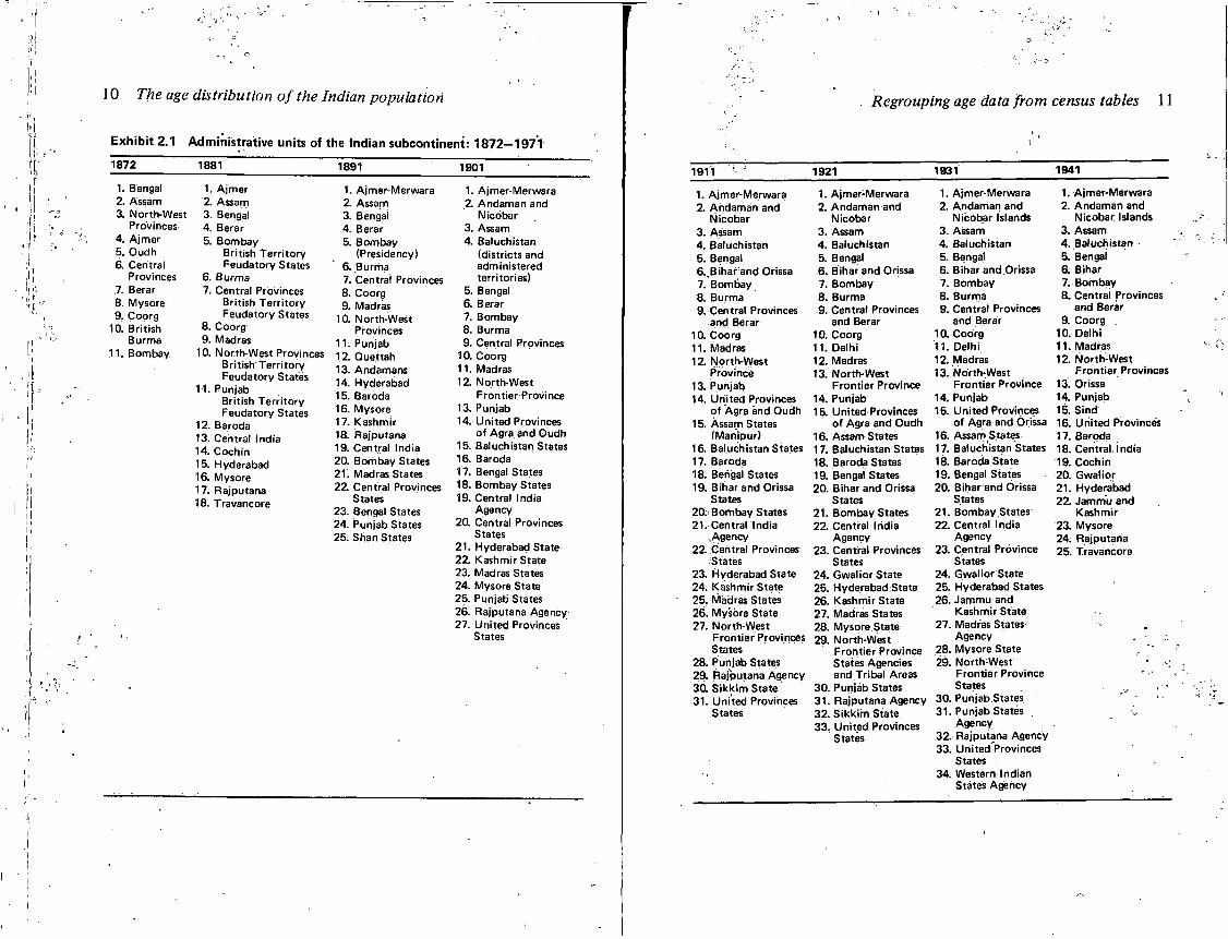
The political map of India and its administrative divisions has been undergoing continual change over the last hundred years. Exhibit s. 1 lists the constituent units of India in the 11 censuses during the period
10 The age distribution of the Indian population
Exhibit 2.1 Administrative units of the Indian subcontinent: 1872-197T
1872 1881 1891 1901
1. Bengal 2. Assam 3. North-West
Provinces 4. Ajmer 5. Oudh 6. Central
Provinces 7. Berar 8. Mysore 9. Coorg
10. British Burma
11. Bombay
1. Ajmer 2. Assam 3. Bengal 4. Berar 5. Bombay
British Territory Feudatory States
6. Burma 7. Central Provinces
British Territory Feudatory States
8. Coorg 9. Madras
10. North-West Provinces British Territory Feudatory States
11. Punjab British Territory Feudatory States
12. Baroda 13. Central India 14. Cochin 15. Hyderabad 16. Mysore 17. Rajputana 18. Travancore
1. Ajmer-Merwara 2. Assam 3. Bengal 4. Berar 5. Bombay
(Presidency) 6. Burma 7. Central Provinces 8. Coorg 9. Madras
10. North-West Provinces
11. Punjab 12. Quettah 13. Andamans 14. Hyderabad 15. Baroda 16. Mysore 17. Kashmir 18. Rajputana 19. Central India 20. Bombay States 21. Madras States 22. Central Provinces
States 23. Bengal States 24. Punjab States 25. Shan States
1. Ajmer-Merwara 2. Andaman and
Nicobar 3. Assam 4. Baluchistan
(districts and administered territories)
5. Bengal 6. Berar 7. Bombay 8. Burma 9. Central Provinces
10. Coorg 11. Madras 12. North-West
Frontier Province 13. Punjab 14. United Provinces
of Agra and Oudh 15. Baluchistan States 16. Baroda 17. Bengal States 18. Bombay States 19. Central India
Agency 20. Central Provinces
States 21. Hyderabad State 22. Kashmir State 23. Madras States 24. Mysore State 25. Punjab States 26. Rajputana Agency 27. United Provinces
States
Regrouping age data from census tables 11
i
1911 - * 1921 1931 1941
1. Ajmer-Merwara 2. Andaman and
Nicobar 3. Assam 4. Baluchistan 5. Bengal 6. Bihar and Orissa 7. Bombay 8. Burma 9. Central Provinces
and Berar 10. Coorg 11. Madras 1 2 North-West
Province 13. Punjab 14. United Provinces
of Agra and Oudh 15. Assam States
(Manipiir) 16. Baluchistan States 17. Baroda 18. Bengal States 19. Bihar and Orissa
States 20. Bombay States 21. Central India
.Agency 22. Central Provinces
States 23. Hyderabad State 24. Kashmir State 25. Madras States 26. Mysore State 27. North-West
Frontier Provinces States
28. Punjab States 29. Rajputana Agency 30. S ikk im State 31. United Provinces
States
1. Ajmer-Merwara 2. Andaman and
Nicobar 3. Assam 4. Baluchistan 5. Bengal 6. Bihar and Orissa 7. Bombay 8. Burma 9. Central Provinces
and Berar 10. Coorg 11. Delhi 12. Madras 13. North-West
Frontier Province 14. Punjab 15. United Provinces
of Agra and Oudh 16. Assam States 17. Baluchistan States 18. Baroda States 19. Bengal States 20. Bihar and Orissa
States 21. Bombay States 22. Central India
Agency 23. Central Provinces
States 24. Gwalior State 25. Hyderabad State 26. Kashmir State 27. Madras States 28. Mysore.State 29. North-West
Frontier Province States Agencies and Tribal Areas
30. Punjab States 31. Rajputana Agency 32. S ikk im State 33. United Provinces
States
1. Ajmer-Merwara 2. Andaman and
Nicobar Islands 3. Assam 4. Baluchistan 5. Bengal 6. Bihar and Orissa 7. Bombay 8. Burma 9. Central Provinces
and Berar 10. Coorg 11. Delhi 12. Madras 13. North-West
Frontier Province 14. Punjab 15. United Provinces
of Agra and Orissa 16. Assam States 17. Baluchistan States 18. Baroda State 19. Bengal States 20. Bihar and Orissa
States 21. Bombay States: 22. Central India
Agency 23. Central Province
States 24. Gwalior State 25. Hyderabad States 26. Jammu and
Kashmir State 27. Madras States
Agency 28. Mysore State 29. North :West
Frontier Province States
30. Punjab.States 31. Punjab States
Agency 32. Rajputana Agency 33. United Provinces
States 34. Western Indian
States Agency
1. Ajmer-Merwara 2. Andaman and
Nicobar Islands 3. Assam 4. Baluchistan 5. Bengal 6. Bihar 7. Bombay 8. Central Provinces
and Berar 9. Coorg
10. Delhi 11. Madras 12. North-West
Frontier Provinces 13. Orissa 14. Punjab 1 5 S i n d 16. United Provinces 17. Baroda 18. Central India 19. Cochin 20. Gwalior, 21. Hyderabad 22. Jammu and
Kashmir 23. Mysore 24. Rajputana 25. Travancore
. 12 The age distribution of the Indian population "
Exh ibit 2.1 (con tinued) .
1951 •' 1961 1971
1. Ajmer 1. Andhra Pradesh 1. Andhra Pradesh 2. Assam 2. Assam 2. Assam 3. B ilaspur 3. Bihar 3. Bihar 4. Bhopal 4. Gujarat 4. Gujarat 5. Bihar 5. Jammu and Kashmir 5. Haryana 6. Bombay 6. Kerala 6. Himachal Pradesh 7. Coorg 7. Madhya Pradesh 7. Jammu and Kashmir 8. Delhi 8. Madras 8. Kerala 9. Himachal Pradesh 9. Maharashtra 9. Madhya Pradesh
10. Hyderabad 10. Mysore 10. Maharashtra 11. Kutch 11. Orissa 11. Mysore 12. Madras 12. Punjab 12. Nagaland 13. Madhya Bharat 13. Rajasthan 13. Orissa 14. Madhya Pradesh 14. Uttar Pradesh 14. Punjab
•15. Mysore 15. West Bengal 15. Rajasthan 16. Orissa Union Territories 16. Tamil Nadu .17. Punjab and East Pun 16. Andaman and Nicobar 17. Uttar Pradesh
• jab States Union Islands 18. West Bengal Union Terri(PEPSU) 17. Delhi tories
18. Punjab 18. Himachal Pradesh 19. Andaman and Nicobar 19. Rajasthan 19. Laccadive, Minicoy, Islands 20. Saurastra Amindivi Islands 20. Chandigarh 21. Uttar Pradesh 20. Manipur 21. Dadra and Nagar Haveli 22. Vindhya Pradesh 21. Tripura 22. Delhi 23. West Bengal 22. Dadra and Nagar Haveli 23. Goa, Daman, Diu 24. Manipur 23. Goa, Daman, Diu 24. Laccadive; Minicoy, 25. Tripura 24. Pondicherry Amindivi Islands 26. S ikk im 25. North-East Frontier 25. Manipur 27. Travancore Agency 26. Meghalaya
and Cochin 26. Nagaland 27. Arunachal Pradesh 28. Andaman and 27. S ikk im 28. Pondicherry
Nicobar Islands 29. Tripura
S O U R C E S : 1872 [ 7 , 8 , 9 ] , 1881 [10] , 1891 [11], 1901 [12] , 1911 [13], 1921 [14] , 1931 [ 1 5 H 1941 [17] , 1951 [21], 1961 [29], 1971 [32] .
1872^ 1971. When the first all-India census was taken in 1872, India* was about twice as large as at present but was divided into only 11
. provinces. At the time of the second census in 1881 there were 18 administrative units, including British Indian provinces and princely states. This number increased to 25 in 1891, 27 in 1901, 31 in 1911, 33 in 1921, and 34 in 1931. Thereafter the number dropped to 25 in 1941. In 1951 the number of Part A, Part B, and Part C states was 27. The number of states and territories was again 27 in 1961 and 29 in 1971.
* Including territories now in Pakistan, Bangladesh, Sri Lanka, Burma.
Regrouping age data from census tables 13
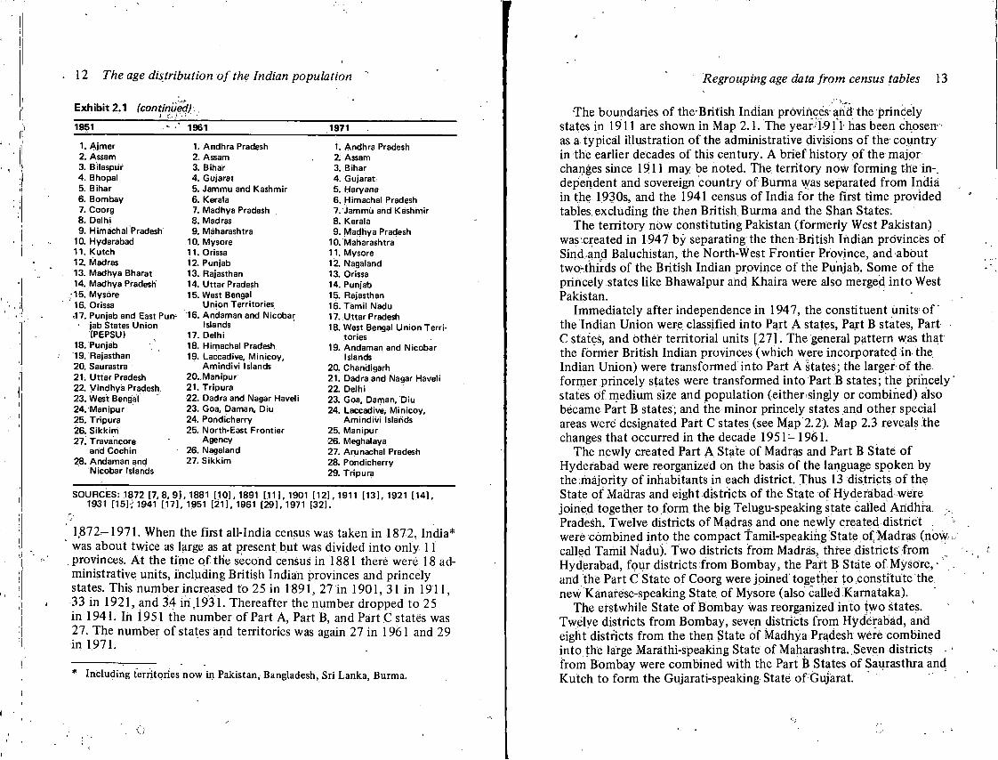
The boundaries of the British Indian provinces and the princely states in 1911 are shown in Map 2.1. The year-1911- has been chosen • as a typical illustration of the administrative divisions of the country in the earlier decades of this century. A brief history of the major changes since 1911 may be noted. The territory now forming the in-, dependent and sovereign country of Burma was separated from India in the 1930s, and the 1941 census of India for the first time provided tables excluding the then British Burma and the Shan States.
The territory how constituting Pakistan (formerly West Pakistan) was created in 1947 by separating the then British Indian provinces of Sind and Baluchistan, the North-West Frontier Province, and about two-thirds of the British Indian province of the Punjab. Some of the princely states like Bhawalpur and Khaira were also merged into West Pakistan.
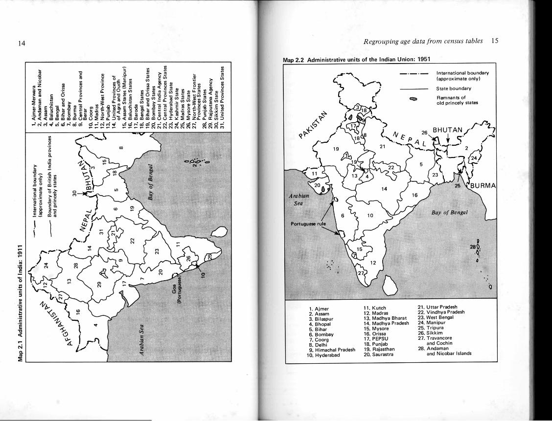
Immediately after independence in 1947, the constituent units o f ' the Indian Union were classified into Part A states, Part B states, Part C states, and other territorial units [27]. The general pattern was that the former British Indian provinces (which were incorporated in the Indian Union) were transformed into Part A states; the larger of the former princely states were transformed into Part B states; the princely states of medium size and population (either .singly or combined) also became Part B states; and the minor princely states and other special areas were designated Part C states (see Map 2.2). Map 2.3 reveals the changes that occurred in the decade 1951 —1961.
The newly created Part A State of Madras and Part B State of Hyderabad were reorganized on the basis of the language spoken by the majority of inhabitants in each district. Thus 13 districts of the State of Madras and eight districts of the State of Hyderabad were joined together to form the big Telugu-speaking state called Andhra x
Pradesh. Twelve districts of Madras and one newly created district . were combined into the compact Tamil-speaking State of] Madras (now called Tamil Nadu). Two districts from Madras, three districts from Hyderabad, four districts from Bombay, the Part B State of Mysore, • and the Part C State of Coorg were joined together to .constitute the new Kanarese-speaking State of Mysore (also called Karnataka).
The erstwhile State of Bombay was reorganized into two states. Twelve districts from Bombay, seven districts from Hyderabad, and eight districts from the then State of Madhya Pradesh were combined into the large Marathi-speaking State of Maharashtra. .Seven districts • from Bombay were combined with the Part B States of Saurasthra and Kutch to form the Gujarati-speaking State of Gujarat:
Regrouping age data from census tables 15
Map 2.2 Administrative units of the Indian Union: 1951
— — International boundary (approximate only)
State boundary
c^p Remnants of old princely states
B H U T A N / '
22
20, 14 B U R M A
Arabian Sea
Portuguese rule
16
10 Bay of Bengal
15 P
280. •V
12
1. Ajmer 2. Assam 3. Bilaspur 4. Bhopal 5. Bihar 6. Bombay 7. Coorg 8. Delhi 9. Himachal Pradesh
10. Hyderabad
11. Kutch 12. Madras 13. Madhya Bharat 14. Madhya Pradesh 15. Mysore 16. Orissa 17. PEPSU 18. Punjab 19. Rajasthan 20. Saurastra
21. Uttar Pradesh 22. Vindhya Pradesh 23. West Bengal 24. Manipur 25. Tripura 26. Sikkim 27. Travancore
and Cochin 28. Andaman
and Nicobar Islands
16 The age distribution of the Indian population
Map 2.3 Administrative units of the Indian Union: 1961
S
i o n u i
International boundary (approximate only)
State boundary
B H U T A N ^ - 2 5 *Jp
1 3 1 4
| Arabian Sea 11
23
21
flay of Bengal 22
23\ 1 0
16 ?.
19 : T24
1. Andhra Pradesh 2. Assam 3. Bihar 4. Gujarat 5. Jammu and Kashmir 6. Kerala 7. Madhya Pradesh 8. Madras 9. Maharashtra
10. Mysore
11. Orissa 12. Punjab 13. Rajasthan 14. Uttar Pradesh 15. West Bengal Union
Territories 16. Andaman and Nicobar
Islands 17. Delhi 18. Himachal Pradesh
19. Laccadive, Minicoy, Amindivi Islands
20. Manipur 21. Tripura 22. Dadra and Nagar Haveli 23. Goa, Daman, Diu 24. Pondicherry 25. North-East Frontier Agency 26. Nagaland 27. Sikkim
Regrouping age data from census tables 17
The twelve remaining districts of the State of Madhya Pradesh were combined with the Part B States of Vindhya Pradesh and Madhya Bharat and the Part C States of Rewa, Indore, and Bhopal to form the large but sparsely populated State of Madhya Pradesh. The Part B State of Rajasthan was joined with Ajmer to make the State of Rajasthan.
Among the other changes may be mentioned the transfer of the major part of Manbhum District from Bihar to West Bengal, the carving out of the territorial unit called the North-East Frontier Agency (now called Arunachal Pradesh) from the State of Assam, the creation of the new State of Nagaland by merging the two districts in the erstwhile State of Assam, the creation of the territorial unit called Goa, Daman, and Diu from areas previously under Portuguese colonial rule, the creation of the territorial unit of Pondicherry which had hitherto been under French rule, the creation of the territorial unit of Himachal Pradesh by combining some hilly areas earlier included among the princely states of the Punjab, and the creation of the State of Punjab by combining the Part A State of Punjab and Part B State of PEPSU.
Changes in territorial boundaries did not stop in the year 1961. Extensive reorganization of Punjab and Assam has taken place since then. The State of Haryana was formed by carving out seven districts from the State of Punjab. Three districts from the State of Punjab were ceded to the Union Territory of Himachal Pradesh, which now enjoys the full status of a state in the Indian Union. The erstwhile State of Punjab kept the remaining Punjabi-speaking districts. The city of Chandigarh, built as a capital of the larger Punjab, remained a separate unit. The status of the Union Territories of Nagaland, Tripura, and Manipur was raised to that of a state. Moreover, a new union territory called Meghalaya was created by combining the two hilly districts of Assam—United Khasi Jaintia Hills and Garo Hills. The present State of Assam is composed of the remaining nine districts.
Current administrative divisions
Table 2.1 and Map 2.4 show the 21 states and eight union territories as defined for the 1971 census. It is these administrative divisions for which the age composition has been reconstructed. Though the administrative divisions existing up to the year 1971 have been taken into account, the age data for the 1971 census are not yet available. Hence the reconstruction of the age data covers the period 1881-1961. (Partially tabulated age data for the 1971 census were available in November 1972. A note on 1971 age distribution appears in the appendix.)
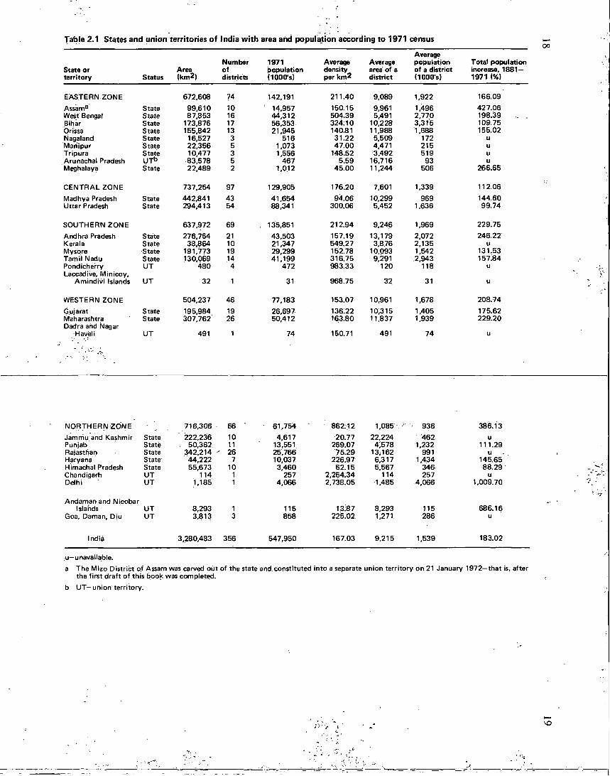
Table 2.1 States and union territories of India with area and population according to 1971 census
State or territory Status
Area (krr>2)
Number of districts
1971 population (1000/s)
Average density per krr)2
Average area of a district
Average population of a district (1000/s)
Total population increase, 1881 — 1971 (%)
E A S T E R N Z O N E 672,608 74 142,191 211.40 9,089 1,922 166.09
Assam 3 State 99,610 10 ' 14,957 150.15 9,961 1,496 427.06 West Bengal State 87,853 16 44,312 504.39 5,491 2,770 198.39 Bihar State 173,876 17 56,353 324:10 10,228 3,315 109.75 Orissa State 155,842 13 21,945 140.81 11,988 1,688 155.02 Nagaland State 16,527 3 516 31.22 5,509 172 u Manipur State 22,356 5 1,073 47.00 4,471 215 u Tripura State 10,477 3 1,556 148.52 3,492 519 u Arunachal Pradesh U T D 83,578 5 467 5.59 16,716 93 u Meghalaya State 22,489 2 1,012 45.00 11,244 506 266.65
C E N T R A L Z O N E 737,254 97 129,905 176.20 7,601 1,339 112.06
Madhya Pradesh State 442,841 43 41,654 94.06 10,299 969 144.60 Uttar Pradesh State 294,413 54 88,341 300.06 5,452 1,636 99.74
S O U T H E R N Z O N E 637,972 69 . 135,851 212.94 9,246 1,969 229.75
Andhra Pradesh State 276,754 21 43,503 157.19 13,179 2,072 246.22 Kerala State 38,864 10 21,347 549.27 3,876 2,135 u Mysore State 191,773 19 29,299 152.78 10,093 1,542 131.53 Tamil Nadu State 130,069 14 41,199 316.75 9,291 2,943 157:84 Pondicherry U T 480 4 472 983.33 120 118 u Laccadive, Minicoy,
Amindivi Islands U T 32 1 31 968.75 32 31 u
W E S T E R N Z O N E 504,237 46 77,183 153.07 10,961 1,678 208.74
Gujarat State 195,984 19 26,697 136.22 10,315 1,405 175.62 Maharashtra State 307,762 26 50,412 163.80 11,837 1,939 229.20 Dadra and Nagar
Haveli U T 491 1 74 150.71 491 74 u
N O R T H E R N Z O N E 716,306 66 61,754 862.12 1,085•-,•* , 936 386.13
Jammu and Kashmir State 222,236 10 4,617 20.77 22,224 462 u Punjab State . 50,362 11 13,551 269.07 4;578 1,232 111.29 Rajasthan State 342,214 ' 26 25,766 75.29 13,162 991 u Haryana State 44,222 7 10,037 226.97 6,317 1,434 145.65 Himachal Pradesh State 55,673 10 3,460 62.15 5,567 346 88.29 Chandigarh U T 114 1 257 2,254.34 114 257 u Delhi U T 1,185 1 4,066 2,738.05 1,485 4,066 1,009.70
Andaman and Nicobar Islands U T 8,293 1 115 13:87 8,293 115 686.16
Goa, Daman, Diu U T 3,813 3 858 225.02 1,271 286 u
India 3,280,483 356 547,950 167.03 9,215 1,539 183.02
u—unavailable. a The Mizo District of Assam was carved out of the state and constituted into a separate union territory on 21 January 1972—that is, after
the first draft of this book was completed.
b UT—union territory.
20 The age distribution of the Indian population
Map 2.4 Administrative units of the Indian Union: 1971
r
r
7 >
5 '20
:22
1 5
>
1 7
International boundary (approximate only)
Zonal boundary
State boundary
BHUTAN / i j / y T /
'25j*
S ' B U R M A I
Arabian Sea
1 3
1 0
23 2 1 Bay o/ Bengal
11 .0
19 P 0
728
24 1 6
.SRI LANKA
1. Andhra Pradesh 2. Assam 3. Bihar 4. Gujarat 5. Haryana 6. Himachal Pradesh 7. Jammu and Kashmir 8. Kerala 9. Madhya Pradesh
10. Maharashtra
11. Mysore 12. Nagaland 13. Orissa 14. Punjab 15. Rajasthan 16. Tamil Nadu 17. Uttar Pradesh 18. West Bengal Union Territories 19. Andaman and Nicobar Islands 20. Chandigarh
21. Dadra and Nagar Haveli 22. Delhi 23. Goa, Daman, Diu 24. Laccadive, Minicoy,
Amindivi Islands 25. Manipur 26. Meghalaya 27. Arunachal Pradesh 28. Pondicherry 29. Tripura
Regrouping age data from census tables 21
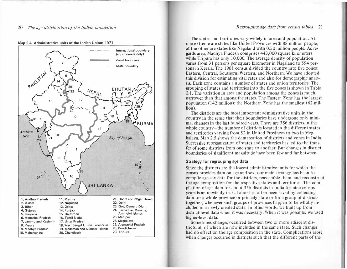
The states and territories vary widely in area and population. At one extreme are states like United Provinces with 88 million people; at the other are states like Nagaland with 0.50 million people. As regards area, Madhya Pradesh comprises 443,000 square kilometers while Tripura has only 10,000. The average density of population varies from 31 persons per square kilometer in Nagaland to 594 persons in Kerala. The 1961 census divided the country into five zones: Eastern, Central, Southern, Western, and Northern. We have adopted this division for estimating vital rates and also for demographic analysis. Each zone contains a number of states and union territories. The grouping of states and territories into the five zones is shown in Table 2.1. The variation in area and population among the zones is much narrower than that among the states. The Eastern Zone has the largest population (142 million); the Northern Zone has the smallest (62 million).
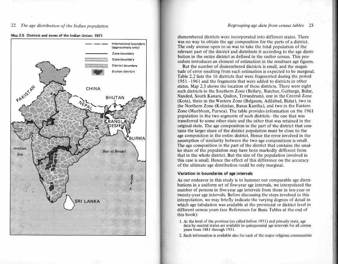
The districts are the most important administrative units in the country in the sense that their boundaries have undergone only minimal changes in the last hundred years. There are 356 districts in the whole country-the number of districts located in the different states and territories varying from 52 in United Provinces to two in Meghalaya. Map 2.5 shows the demarcation of districts and zones in India. Successive reorganization of states and territories has led to the transfer of some districts from one state to another. But changes in district boundaries of significant magnitude have been few and far between.
Strategy for regrouping age data
Since the districts are the lowest administrative units for which the census provides data on age and sex, our main strategy has been to compile age-sex data for the districts, reassemble them, and reconstruct the age composition for the respective states and territories. The compilation of age data for about 356 districts in India for nine census years is an unwieldy task. Labor has often been saved by collecting data for a whole province or princely state or for a group of districts together, whenever such groups of provinces happen to be wholly included in a newly created state. In other words, we built up from district-level data when it was necessary. When it was possible, we used higher-level data.
Sometimes changes occurred between two or more adjacent districts, all of which are now included in the same state. Such changes had no effect on the age composition in the state. Complications arose when changes occurred in districts such that the different parts of the
22 The age distribution of the Indian population
Map 2.5 Districts and zones of the Indian Union: 1971
Regrouping age data from census tables 23
dismembered districts were incorporated into different states. There was no way to obtain the age composition for the parts of a district. The only avenue open to us was to take the total population of the relevant part of the district and distribute it according to the age distribution in the entire district as defined in the earlier census. This procedure introduces an element of estimation in the resultant age figures.
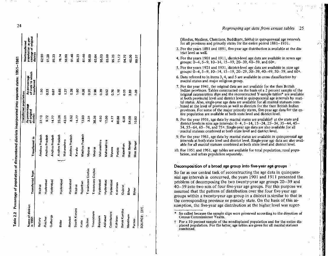
But the number of dismembered districts is small, and the magnitude of error resulting from such estimation is expected to be marginal. Table 2.2 lists the 16 districts that were fragmented during the period 1951 — 1961 and the fragments that were added to districts in other states. Map 2.5 shows the location of these districts. There were eight such districts in the Southern Zone (Bellary, Raichur, Gulbarga, Bidar, Nanded, South Kanara, Quilon, Trivandrum), one in the Central Zone (Kota), three in the Western Zone (Belgaum, Adilabad, Bidar), two in the Northern Zone (Kohistan, Banas Kantha), and two in the Eastern Zone (Manbhum, Purnea). The table provides information on the 1961 population in the two segments of such districts—the one that was transferred to some other state and the other that was retained in the original state. The age composition in the part of the district that contains the larger share of the district population must be close to the age composition in the entire district. Hence the error involved in the assumption of similarity between the two age compositions is small. The age composition in the part of the district that contains the smaller share of the population may have been markedly different from that in the whole district. But the size of the population involved in this case is small. Hence the effect of this difference on the accuracy of the ultimate age distribution could be only marginal.
Variation in boundaries of age intervals
As our endeavor in this study is to hammer out comparable age distributions in a uniform set of five-year age intervals, we interpolated the number of persons in five-year age intervals from those in ten-year or twenty-year age intervals. Before discussing the steps involved in this interpolation, we may briefly indicate the varying degrees of detail in which age tabulation was available at the provincial or district level in different census years (see References for Basic Tables at the end of this book):
1. At the level of the province (so called before 1951) and princely state, age data by marital status are available in quinquennial age intervals for all census years from 1881 through 1931.
2. Such information is available also for each of the major religious communities
24
L "re o c
"H a '5> £ » § S o * l i s , «-» 3 n • £ 2 »:
8>|
ra >
. *" E c J?-*- 2 8.
re c re a c S ? i
< O "D
o 00 n O)' 00 01 CN CN r» 01 CN in 10 CO r-
to cn CO r» LO en
o a> co co cn
o m in cn
CN CN o « ~ ' o o T ~ CO oi CO
o in
co r** cn co co co CN "- d o d T - "
oo o CN co d T -
co co 8 CN CD CO ID P- >-d
CO 05 CO CO
o i - d co <-' 8
CO i -CN O CO CO CN
CN in od
O T -
co co CN CO-
O O p~ 00 00 CO 00
00 CN to <T d
in T -
o o
.e "O
< < < •o C
<
> 8 8 2 2 £ i - i . re re T3 TJ TJ . C .c ra re nj ra ra
S' S' s s s
ra 2 .£> 5 O cn
" "c .2. 5 o. CC
5 5
o a
c
S a) >
X
8 £ •D •> I
"D >•
X ra E C 5 DC H
ai T> >• I
ra 2 T3 > I
XI >-
X £ .2. O 3
CJ
Regrouping age data from census tables 25
(Hindus, Muslims, Christians, Buddhists, Sikhs) in quinquennial age intervals for all provinces and princely states for the entire period 1881—1931.
3. For the years 1881 and 1891, five-year age distribution is available at the district level as well.
4. For the years 1901 and 1911, district-level age data are available in seven age groups: 0-4, 5-9, 10-14, 15-19, 20-39,40-59, and 60+.
5. For the years 1921 and 1931, district-level age data are available in nine age groups: 0-4, 5-9, 10-14, 15-19, 20-29,30-39,40-49, 50-59, and 60+.
6. Data referred to in items 3,4, and 5 are available in cross classification by marital status and major religious group.
7. For the year 1941, the original data are not available for the then British Indian provinces. Tables constructed on the basis of a 2 percent sample of the "original enumeration slips and the reconstructed Y-sample tables* are available at both provincial level and district level in quinquennial age intervals by marital status. Also, single-year age data are available for all marital statuses combined at the level of provinces as well as districts for the then British Indian provinces. For some of the major princely states, five-year age data for the entire population are available at both state level and district level.
8. For the year 1951, age data by marital status are available* at the state and district levels in nine age intervals: 0-4, 5-14, 15-24, 25-34, 35-44, 45-54, 55—64, 65-74, and 75+. Single-year age data are also available for all marital statuses combined at both state level and district level.
9. For the year 1961, age data by marital status are available in quinquennial age intervals at both state level and district level. Single-year age data are also available for all marital statuses combined at both state level and district level.
10. For 1951 and 1961, age tables are available for total population, rural population, and urban population separately.
Decomposition of a broad age group into five-year age groups '
So far as our central task of reconstructing the age data in quinquennial age intervals is concerned, the years 1901 and 1911 presented the problem of decomposing the two twenty-year age groups 20—39 and 40—59 into two sets of four five-year age groups. For this purpose we assumed that the pattern of distribution over the four five-year age groups within a twenty-year age group in a district is similar to that in the corresponding province or princely state. On the basis of this assumption, the five-year age distribution at the higher level was super-
* So called because the sample slips were preserved according to the direction of Census Commissioner Yeatts.
t For a 10 percent sample of the nondisplaced population and for the entire displaced population. For the latter, age tables are given for all maritahstatuses combined.
26 The age distribution of the Indian population
imposed on the twenty-year age distribution at the corresponding lower level to yield the five-year age distribution for the districts. To put it symbolically: let D P 2 0 _ 3 9 be the district population in the age interval 20-39; let H P 2 0 _ 3 9 be the population in the whole province in the age interval 20-39; let H P 2 0 _ 2 4 , H P 2 S _ 2 9 , H P 3 0 - 3 4 , and H P 3 S _ 3 9
be the populations in the province in the respective five-year age intervals; and let D P 2 0 _ 2 4 , D P 2 S _ 2 9 , D P 3 0 _ 3 4 , and D P 3 5 _ 3 9 be the required district populations in the same age intervals. Then
* l = HP 2 0 - 2 4 / H P 2 o - 39
k 2 = HP 2 S _ 2 9 / H P 2 0 - 39
*3 = HP 3 0 -34 / H P 2 0 - 39
k< = HP 3 5 - 3 9 / H P 2 o - 39
D P 2 0 - i 4 - *i (DP 2 0 - 39)
DP 2 5_ •29 — M D P a o - -39)
D P 3 0 - 34 ~ A:3(DP2 0-•39)
DP35-•39 ~ M D P 2 0 - •39)
Note that our purpose is not to interpolate the five-year age distribution within a twenty-year age distribution; it is to reclaim as far as possible the original age distribution along with whatever biases it might initially contain. We have not, therefore, adopted any sophisticated interpolation technique involving the neighboring age groups. We simply assume that the internal distribution within a twenty-year age group is the same in the provincial population as in the district population. To examine whether it is actually so, we scrutinized the age data for the districts incorporated into West Bengal vis-a-vis the age data for the then Province of Bengal as a whole. We discovered some interesting differences in age distribution between the group of districts located in West Bengal and those located in East Bengal (now Bangladesh). It may be recalled that the Province of Bengal was partitioned on the basis of religion-the Hindu majority districts were included in West Bengal and the Muslim majority districts in East Bengal. In this part of the Indian subcontinent the Muslims had a younger age distribution than the Hindus. Therefore, for the purpose of decomposing a broader age group into five-year age groups, the use of the five-year age distribution of the Hindu population in Bengal was thought to be more appropriate than that of the total population of Bengal.
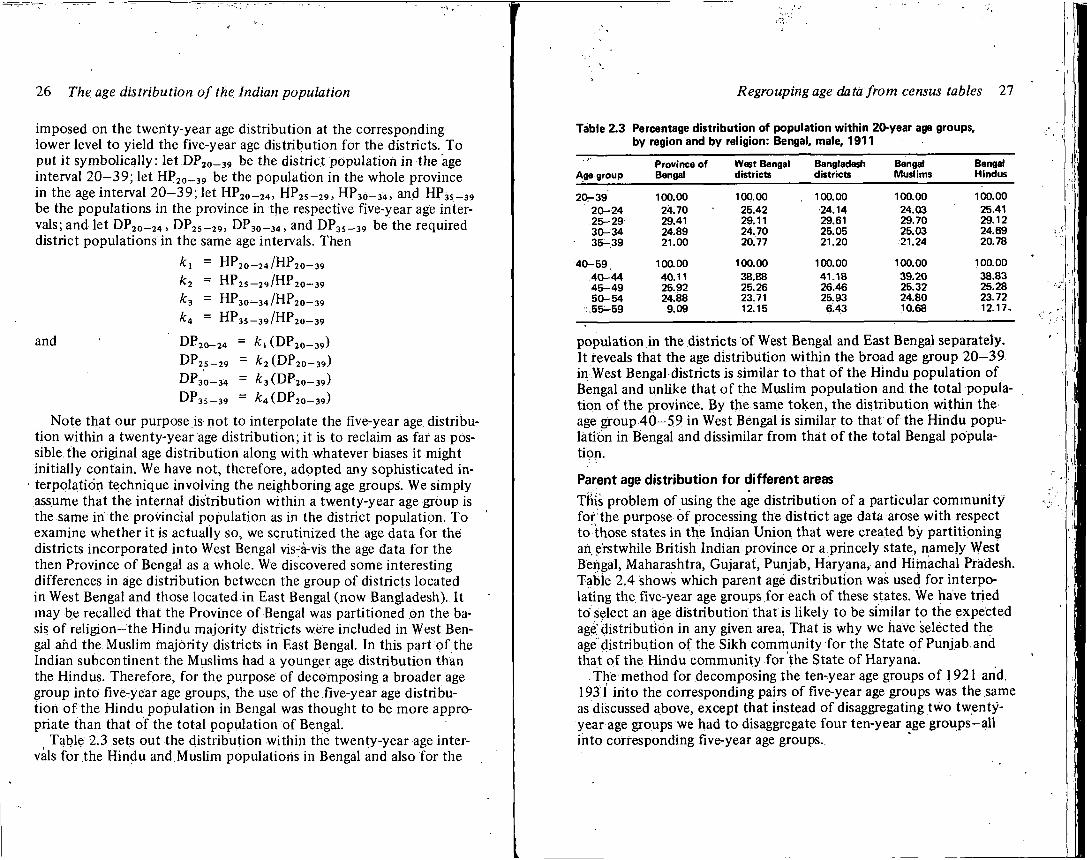
Table 2.3 sets out the distribution within the twenty-year age intervals for the Hindu and Muslim populations in Bengal and also for the
Regrouping age data from census tables 27
Table 2.3 Percentage distribution of population within 20-year age groups, by region and by religion: Bengal, male, 1911
Province of West Bengal Bangladesh Bengal Bengal Age group Bengal districts districts Muslims Hindus
2 0 - 3 9 100.00 100.00 100.00 100.00 100.00 2 0 - 2 4 24.70 25.42 24.14 24.03 25.41 2 5 - 2 9 29.41 29.11 29.61 29.70 29.12 3 0 - 3 4 24.89 24.70 25.05 25.03 24.69 3 5 - 3 9 21.00 20.77 21.20 21.24 20.78
4 0 - 5 9 , 100.00 100.00 100.00 100.00 100.00 4 0 - 4 4 40.11 38.88 41.18 39.20 38.83 4 5 - 4 9 25.92 25.26 26.46 25.32 25.28 5 0 - 5 4 24.88 23.71 25.93 24.80 23.72 . 55 -59 9.09 12.15 6.43 10.68 12.17,
population in the districts of West Bengal and East Bengal separately. It reveals that the age distribution within the broad age group 20-39 in West Bengal districts is similar to that of the Hindu population of Bengal and unlike that of the Muslim population and the total population of the province. By the same token, the distribution within the^ age group 40 -59 in West Bengalis similar to that of the Hindu population in Bengal and dissimilar from that of the total Bengal population.
Parent age distribution for different areas
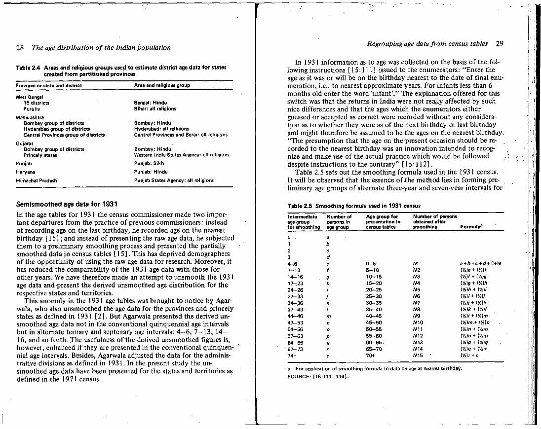
Triisi problem of using the age distribution of a particular community for the purpose of processing the district age data arose with respect to those states in the Indian Union that were created by partitioning an erstwhile British Indian province or a princely state, namely West Bengal, Maharashtra, Gujarat, Punjab, Haryana, and Himachal Pradesh. Table 2.4 shows which parent age distribution was used for interpolating the five-year age groups for each of these states. We have tried to select an age distribution that is likely to be similar to the expected age distribution in any given area. That is why we have selected the age distribution of the Sikh community for the State of Punjab and that of the Hindu community for the State of Haryana.
The method for decomposing the ten-year age groups of 1921 and. 1931 into the corresponding pairs of five-year age groups was the same as discussed above, except that instead of disaggregating two twenty-year age groups we had to disaggregate four ten-year age groups-all into corresponding five-year age groups.
28 The age distribution of the Indian population
Table 2.4 Areas and religious groups used to estimate district age data for states created from partitioned provinces
Province or state and district Area and religious group
West Bengal 15 districts Purulia
Maharashtra Bombay group of districts Hyderabad group of districts Central Provinces group of districts
Gujarat Bombay group of districts Princely states
Punjab
Haryana
Himachal Pradesh
Bengal: Hindu Bihar: all religions
Bombay: Hindu Hyderabad: all religions Central Provinces and Berar: all religions
Bombay: Hindu Western India States Agency: all religions
Punjab: Sikh
Punjab: Hindu
Punjab States Agency: all religions
Semismoothed age data for 1931
In the age tables for 1931 the census commissioner made two important departures from the practice of previous commissioners: instead of recording age on the last birthday, he recorded age on the nearest birthday [15]; and instead of presenting the raw age data, he subjected them to a preliminary smoothing process and presented the partially smoothed data in census tables [15]. This has deprived demographers of the opportunity of using the raw age data for research. Moreover, it has reduced the comparability of the 1931 age data with those for other years. We have therefore made an attempt to unsmooth the 1931 age data and present the derived unsmoothed age distribution for the respective states and territories.
This anomaly in the 1931 age tables was brought to notice by Agar-wala, who also unsmoothed the age data for the provinces and princely states as defined in 1931 [2] . But Agarwala presented the derived unsmoothed age data not in the conventional quinquennial age intervals but in alternate ternary and septenary age intervals: 4 - 6 , 7-13 , 14-16, and so forth. The usefulness of the derived unsmoothed figures is, however, enhanced if they are presented in the conventional quinquennial age intervals. Besides, Agarwala adjusted the data for the administrative divisions as defined in 1931. In the present study the unsmoothed age data have been presented for the states and territories as defined in the 1971 census.
Regrouping age da ta from census tables 29
In 1931 information as to age was collected on the basis of the following instructions [15:111] issued to the enumerators: "Enter the age as it was or will be on the birthday nearest to the date of final enumeration, i.e., to nearest approximate years. For infants less than 6 ' months old enter the word 'infant'." The explanation offered for this switch was that the returns in India were not really affected by such nice differences and that the ages which the enumerators either guessed or accepted as correct were recorded without any consideration as to whether they were as of the next birthday or last birthday and might therefore be assumed to be the ages on the nearest birthday. "The presumption that the age on the present occasion should be re- , corded to the nearest birthday was an innovation intended to recognize and make use of the actual practice which would be followed despite instructions to the contrary" [15:112].
Table 2.5 sets out the smoothing formula used in the 1931 census. It will be observed that the essence of the method lies in forming preliminary age groups of alternate three-year and seven-year intervals for
Table 2.5 Smoothing formula used in 1931 census
Intermediate Number of Age group for Number of persons age group persons in presentation in obtained after
Formula3 for smoothing age group census tables smoothing Formula3
0 1 2 3
a b c d
4 - 6 e 0 - 5 An a + D + c + d+(Vi)e 7 - 1 3 f 5 - 1 0 A/2 (Vi)e + iY,)f 1 4 - 1 6 9 1 0 - 1 5 A/3 <54)f + (y,)g 1 7 - 2 3 h 1 5 - 2 0 m (K)g + (54)/i 2 4 - 2 6 i 2 0 - 2 5 A/5 (V,)h + (54)/' 2 7 - 3 3 i 2 5 - 3 0 A/6 (%)/+ 0/4)/ 3 4 - 3 6 k 3 0 - 3 5 A/7 0,4)/' + (54)* 3 7 - 4 3 1 3 5 - 4 0 A/8 (54)* + (54)/ 4 4 - 4 6 m 4 0 - 4 5 A/9 (54)/ + (ya)n7 4 7 - 5 3 n 4 5 - 5 0 A/10 <54)/n-+.(54)n 5 4 - 5 6 0 5 0 - 5 5 A/11 (54)n + 0/4)o 5 7 - 6 3 P 5 5 - 6 0 A/12 0/4)6 + 0/4)p 6 4 - 6 6 Q 6 0 - 6 5 A/13 (54)p + (54)g 6 7 - 7 3 r 6 5 - 7 0 A/14 (72)0 + 0/4)r 74+ s 70+ A/15 C/j)r + s
a For application of smoothing formula to data on age at nearest birthday.
S O U R C E : [16 :111-114] .
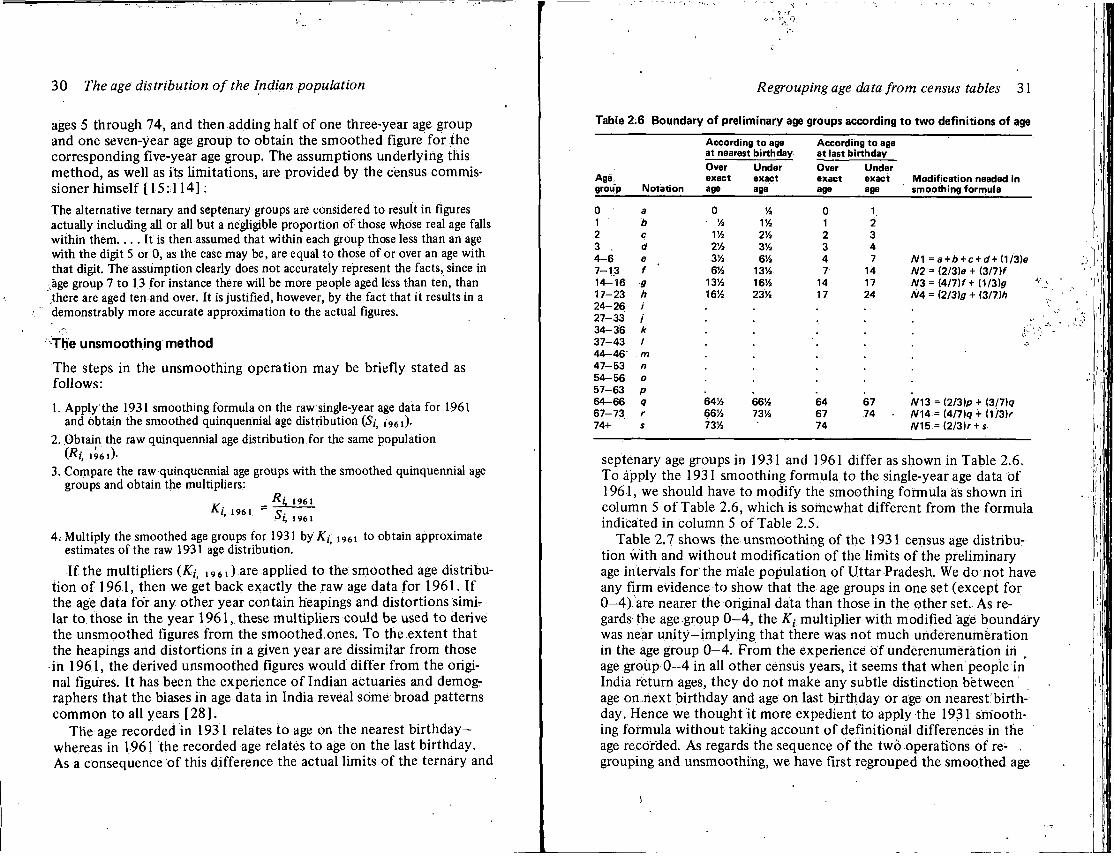
30 The age distribution of the Indian population
ages 5 through 74, and then adding half of one three-year age group and one seven-year age group to obtain the smoothed figure for the corresponding five-year age group. The assumptions underlying this method, as well as its limitations, are provided by the census commissioner himself [15:114]: The alternative ternary and septenary groups are considered to result in figures actually including all or all but a negligible proportion of those whose real age falls within them.... It is then assumed that within each group those less than an age with the digit 5 or 0, as the case may be, are equal to those of or over an age with that digit. The assumption clearly does not accurately represent the facts, since in
• age group 7 to 13 for instance there will be more people aged less than ten, than diere are aged ten and over. It is justified, however, by the fact that it results in a demonstrably more accurate approximation to the actual figures.
c "The unsmoothing method
The steps in the unsmoothing operation may be briefly stated as follows:
1. Apply the 1931 smoothing formula on the raw single-year age data for 1961 and obtain the smoothed quinquennial age distribution (S^ ig6i).
2. Obtain the raw quinquennial age distribution for the same population ( ^ / , 196 l ) -
3. Compare the raw quinquennial age groups with the smoothed quinquennial age groups and obtain the multipliers:
r - R i 1 9 6 1
A J , 1961 _ C . MZ, 1961
4. Multiply the smoothed age groups for 1931 by AT,; i 9 6 i to obtain approximate estimates of the raw 1931 age distribution.
If the multipliers , 9 6 , ) are applied to the smoothed age distribution of 1961, then we get back exactly the raw age data for 1961. If the age data for any other year contain heapirigs and distortions similar to those in the year 1961, these multipliers could be used to derive the unsmoothed figures from the smoothed ones. To the extent that the heapings and distortions in a given year are dissimilar from those in 1961, the derived unsmoothed figures would differ from the original figures. It has been the experience of Indian actuaries and demographers that the biases in age data in India reveal some broad patterns common to all years [28].
The age recorded In 1931 relates to age on the nearest birthday-whereas in 1961 the recorded age relates to age on the last birthday. As a consequence of this difference the actual limits of the ternary and
Regrouping age data from census tables 31
Table 2.6 Boundary of preliminary age groups according to two definitions of age
According to age According to age at nearest birthday at last birthday Over Under Over Under
Age, exact exact exact exact Modification needed in group Notation age age age age smoothing formula
0 a 0 54 0 1. 1 b % 154 1 2 2 c VA 2% 2 3 3 . d 2% 3y 2 3 4 4 - 6 e 3% 61/2 4 7 A/1 = a + 6 + c + d+(1/3)e 7 -13 f '6% 1354 7 14 N2 = (2/3)e + (3/7)/ 14 -16 9 1354 16V2 14 17 A/3 = (4/7)/+ (1/3)ff 17 -23 h 1654 2354 17 24 A/4 = <2/3)g + (3/7W 2 4 - 2 6 i 2 7 - 3 3 i 3 4 - 3 6 k .1-3 7 - 4 3 1 4 4 - 4 6 ' - m 4 7 - 5 3 n 5 4 - 5 6 o 5 7 - 6 3 P 6 4 - 6 6 Q 64V 3 66'/4 64 67 A/13 = (2/3)p + <3/7)o-6 7 - 7 3 r 66y2 731/* 67 74 A/14 = (4/7)<7+ (1/3)r 74+ s 73y 2 74 A/15 = (2/3)r + s
septenary age groups in 1931 and 1961 differ as shown in Table 2.6. To apply the 1931 smoothing formula to the single-year age data of 1961, we should have to modify the smoothing formula as shown in column 5 of Table 2.6, which is somewhat different from the formula indicated in column 5 of Table 2.5.
Table 2.7 shows the unsmoothing of the 1931 census age distribution with and without modification of the limits of the preliminary age intervals for the male population of Uttar Pradesh. We do not have any firm evidence to show that the age groups in one set (except for 0-4). are nearer the original data than those in the other set. As regards the age group 0-4 , the Kt multiplier with modified age boundary was near unity-implying that there was not much uriderenufneration in the age group 0—4. From the experience of underenumeration in age group 0—4 in all other census years, it seems that when people in India return ages, they do not make any subtle distinction between age on next birthday and age on last birthday or age on nearest birthday. Hence we thought i t more expedient to apply the 1931 smoothing formula without taking account of definitional differences in the age recorded. As regards the sequence of the two operations of re- . grouping and unsmoothing, we have first regrouped the smoothed age
)
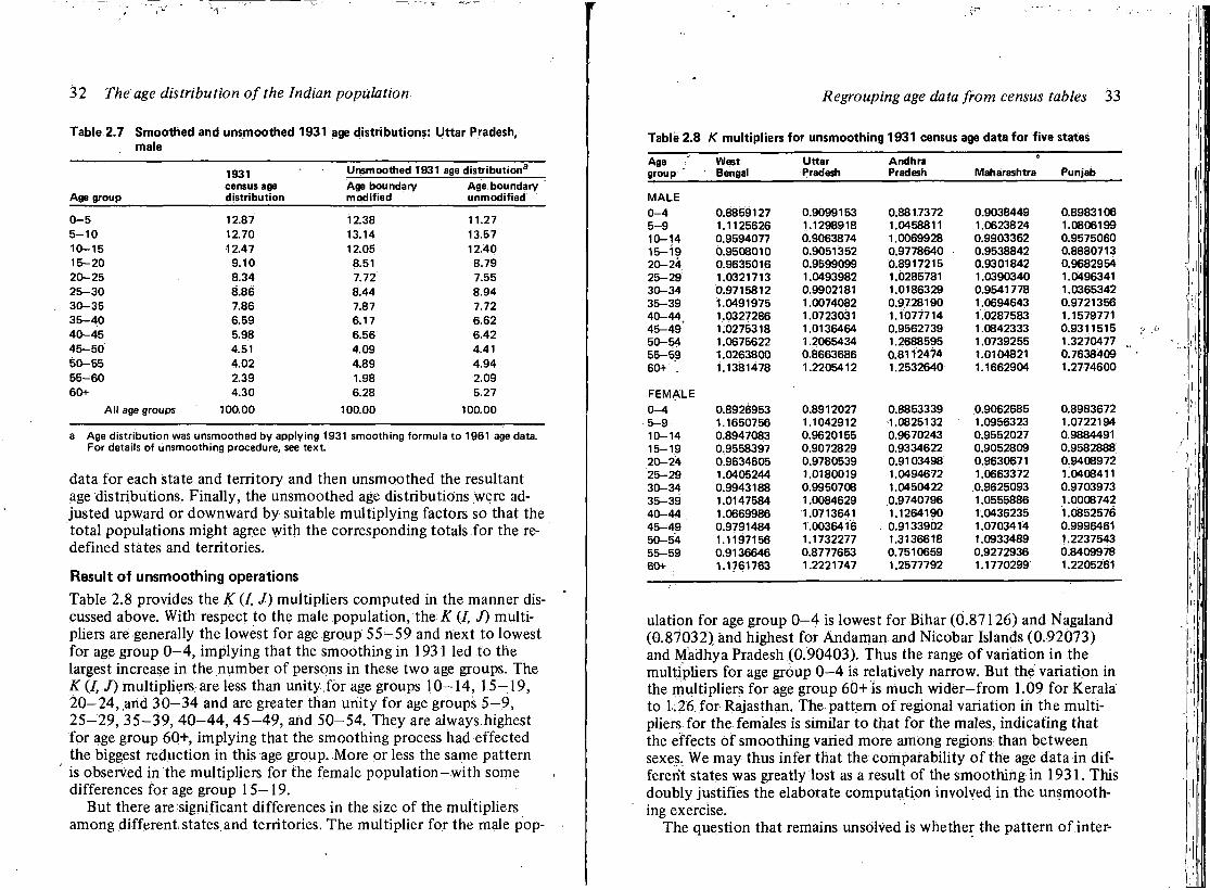
32 The age distribution of the Indian population
Table 2.7 Smoothed and unsmoothed 1931 age distributions: Uttar Pradesh, male
Age group
1931 census age distribution
Unsmoothed 1931 age distribution3
Age boundary Age boundary modified unmodified
0 - 5 12.87 12.38 11.27 5 - 1 0 12.70 13.14 13.57 1 0 - 1 5 12.47 12.05 12.40 1 5 - 2 0 9.10 8.51 8.79 2 0 - 2 5 8.34 7.72 7.55 2 5 - 3 0 8.86 8.44 8.94 3 0 - 3 5 7.86 7.87 7.72 3 5 - 4 0 6.59 6.17 6.62 4 0 - 4 5 5.98 6.56 6.42 4 5 - 5 0 4.51 4.09 4.41 5 0 - 5 5 4.02 4.89 4.94 5 5 - 6 0 2.39 1.98 2.09 60+ 4.30 6.28 5.27
All age groups 100.00 100.00 100.00
a Age distribution was unsmoothed by applying 1931 smoothing formula to 1961 age data. For details of unsmoothing procedure, see text.
data for each state and territory and then unsmoothed the resultant age distributions. Finally, the unsmoothed age distributions were adjusted upward or downward by suitable multiplying factors so that the total populations might agree with the corresponding totals for the redefined states and territories.
Result of unsmoothing operations
Table 2.8 provides the K (/, / ) multipliers computed in the manner discussed above. With respect to the male population, the K (I, J) multipliers are generally the lowest for age group 55—59 and next to lowest for age group 0—4, implying that the smoothing in 1931 led to the largest increase in the number of persons in these two age groups. The K (/, / ) multipliers are less than unity .for age groups 10—14, 15-19, 20—24, and 30—34 and are greater than unity for age groups 5—9, 25-29, 35-39, 40-44, 45-49, and 50-54. They are always.highest for age group 60+, implying that the smoothing process had effected the biggest reduction in this age group. More or less the same pattern is observed in the multipliers for the female population-with some differences for age group 15— 19.
But there are significant differences in the size of the multipliers among different states.and territories. The multiplier for the male pop-
Regrouping age data from census tables 33
Table 2.8 K multipliers for unsmoothing 1931 census age data for five states
Age West Uttar Andhra 4
group : ' Bengal Pradesh Pradesh Maharashtra Punjab
M A L E 0 - 4 0.8859127 0.9099153 0.8817372 0.9038449 0.8983106 5 - 9 1.1125626 1.1298918 1.0458811 1.0623824 1.0806199 10 -14 0.9594077 0.9063874 1.0069928 0.9903362 0.9575060 1 5 - 1 9 0.9508010 0.9051352 0.9778640 0.9538842 0.8880713 2 0 - 2 4 0.9635016 0.9599099 0.8917215 0.9301842 0.9682954 2 5 - 2 9 1.0321713 1.0493982 1.0285781 1.0390340 1.0496341 3 0 - 3 4 0.9715812 0.9902181 1.0186329 0.9541778 1.0365342 3 5 - 3 9 1.0491975 1.0074082 0.9728190 1.0694643 0.9721356 4 0 - 4 4 1.0327286 1.0723031 1.1077714 1.0287583 1.1579771 4 5 - 4 9 ' 1.0275318 1.0136464 0.9562739 1.0842333 0.9311515 5 0 - 5 4 1.0675622 1.2065434 1.2688595 1.0739255 1.3270477 5 5 - 5 9 1.0263800 0.8663686 0.8112474 1.0104821 0.7638409 60+ . 1.1381478 1.2205412 1.2532640 1.1662904 1.2774600
F E M A L E 0 - 4 0.8926953 0.8912027 0.8853339 0.9062685 0.8983672 5 - 9 1.1650756 1.1042912 1.0825132 1.0956323 1.0722194 10 -14 0.8947083 0.9620155 0.9670243 0.9552027 0.9884491 15 -19 0.9558397 0.9072829 0.9334622 0.9052809 0.9582888 2 0 - 2 4 0.9634605 0.9780539 0.9103498 0.9630671 0.9408972 2 5 - 2 9 1.0405244 1.0180019 1.0494672 1.0663372 1.0408411 3 0 - 3 4 0.9943188 0.9950708 1.0450422 0.9625093 0.9703973 3 5 - 3 9 1.0147584 1.0084629 0.9740796 1.0555886 1.0008742 4 0 - 4 4 1.0669986 1.0713641 1.1264190 1.0436235 1.0852576 4 5 - 4 9 0.9791484 1.0036416 . 0.9133902 1.0703414 0.9996461 5 0 - 5 4 1.1197156 1.1732277 1.3136618 1.0933489 1.2237543 5 5 - 5 9 0.9136646 0.8777653 0.7510659 0.9272936 0.8409978 60+ 1.1761763 1.2221747 1.2577792 1.1770299 1.2205261
ulation for age group 0—4 is lowest for Bihar (0.87126) and Nagaland (0.87032) and highest for Andaman and Nicobar Islands (0.92073) and Madhya Pradesh (0.90403). Thus the range of variation in the multipliers for age group 0—4 is relatively narrow. But the variation in the multipliers for age group 60+is much wider—from 1.09 for Kerala to 1.26 for Rajasthan. The pattern of regional variation in the multipliers for the females is similar to that for the males, indicating that the effects of smoothing varied more among regions than between sexes. We may thus infer that the comparability of the age data i n different states was greatly lost as a result of the smoothing in 1931. This doubly justifies the elaborate computation involved In the unsmoothing exercise.
The question that remains unsolved is whether the pattern of inter-
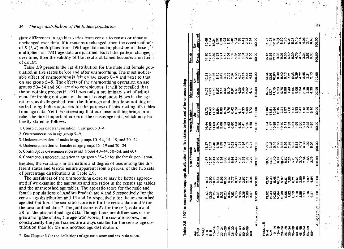
34 The age distribution of the Indian population
state differences in age bias varies from census to census or remains unchanged over time. If it remains unchanged, then the construction^ of K{I, J) multipliers from 1961 age data and application of.these \ ••: multipliers on 1931 age data are justified. But.if the pattern changes - • 1
over time, then the validity of the results obtained becomes a matter •/ of doubt.
Table 2.9 presents the age distribution for the male and female population in five states before and after unsmoothing. The most noticeable effect of unsmoothing is felt on age group 0—4 and next to that on age group 5-9. The effects of the unsmoothing operation on age groups 50—54 and 60+ are also conspicuous. It will be recalled that the smoothing process in 1931 was only a preliminary sort of adjustment for ironing out some of the most conspicuous biases in the age returns, as distinguished from the thorough and drastic smoothing resorted to by Indian actuaries for the purpose of constructing life tables from age data. Yet it is interesting that our unsmoothing brings into relief the most important errors in the census age data, which may be briefly stated as follows:
1. Conspicuous underenumeration in age group 0—4 2. Overenumeration in age group 5—9 3. Underenumeration of males in age groups 10—14, 15-19, and 20—24 4. Underenumeration of females in age groups 15—19 and 20—24 5. Conspicuous overenumeration in age groups 40—44, 50—54, and 60+ 6. Conspicuous underenumeration in age group 55—59 for the female population.
Besides, the variations in the nature and degree of bias among the different states and territories are apparent from a perusal of the two sets of percentage distributions in Table 2.9.
The usefulness of the unsmoothing exercise may be better appreciated i f we examine the age ratios and sex ratios in the census age tables and the unsmoothed age tables. The age-ratio score for the male and female populations of Andhra Pradesh are 4 and 5 respectively for the census age distribution and 14 and 16 respectively for the unsmoothed age distribution. The sex-ratio score is 6 for the census data and 9 for the unsmoothed data.* The joint score is 27 for the census data and 58 for the unsmoothed age data. Though there are differences of degree among the states, the age-ratio scores, the sex-ratio scores, and consequently the joint scores are always smaller for the census age distribution than for the unsmoothed age distribution.
See Chapter 3 for the definitions of age-ratio score and sex-ratio score.
35
1*1
Q.
•O o •6 o
L O
c
o L 9
o
\B p i
o
' ' t
cn * o cn co in co co co *- co ^- © •* co CN m co o r- ?F CN CN «r co CN q CN co rJ cri co co co in in ^-' * CN I~ O t- T- o
o r» o CO <- r- 3 cn CD co «- co Q o «- r-> co in CN q in co co cq q q * C N C N O ) W r ~ r - ^ l r i ^ ' ^ C O C N C D o
«-ocooencocNenco«-*r>5 ;co o C 5 C D P » l > * C O o co co co v-*t cn r-.
coco '^ ' cdcocor^ . 'S t r i^ 'CocN^j -
CN co *- CO CO CO I S- cb co>V * CN in
a
< col
i n c N C n o ^ ' - C 5 ' ? « - i n c n c N p » o r> oo * 1 0 <°. <*>. "J n . * * ° . ^ CN oti cri co' co co in ^ co CN * ' d »— .— •— o
r ~ * c o e n c o c N c o > - c o c o c o o - in o r- r» CN co o r- o
* co, q r» q in> q to to co * in in q •» ' CN co oi oci p» co in >» co' CN V d
p » r » o c n i n « C N C N CN . « - 3 en r» C N i n * r ~ q q r » q * ^ q q c N
co CN cn' r»' 00 r» co co * ' ^r CN in
r ~ o r » o * c o o p * S c N e n c n c o 00 I*;; »fr « - CO CO * CD * O OJ CN
CN CN CN cri 05 CO CO CD in "3- co' <-' CO
« - O c n m c D c o r » r » c o r » r - t - g co co r-» 00 cn in co 1-; co1 ID in «-; q 0 co'd co' 00 0 00 co V co' CN co"
S c o p o c o c o c o c o c o i n c o i n co r-CN CN co co CN q co co q *r
>-' CN «-'cri cri d 00' r»" co co' CN CO
o o d o
o o d o
c o r » p o < - o i n o o o o i n ^ - 00 ^- co o P» CN O O) ID 00 CN CO ; « r O r - *f O
. » ' CN" 00 00' r» co in IT) ^ * ' CN co d
CN co o r » o o o o r > c o c o * ^ , ' - c o
^ • e n ^ c n ^ ' c n ^ c n ^ c o r - T - c N C N c o c o f l ' t i n i n
Tci iAci inci inci iAci inci i n » - > - c N C N c o c o ^ , ^ , i n m c o
m c o r ^ c o c o o o c n c o c o ^ i n c o o ^- co CN co q ui ID co r". r - co q co q co co' CN cri cri cri co in >t * ' co" CN in d
S co co o o co co cn CN in «- co o q CO CO «T >- CN CO CN CN Tt CN i - O
V co d 00 cri cri r»" co in ^ co CN m' d
in 1- in co co co en 3 cp 3 co 00 in T - r« CN i-; in ^ q q en n n co CN •-" cri cri 00' r» io in co co' CN M-'
c o ^ - * i n ' - r » c o c N c o r » c o e n o o 00 in co i*^ CN in co P~ in q co co d 00i cri cri r> in in co' * ' «- co 0
S r ~ c n i ^ o « - c o r » i n o ^ , o o i n TT a> co q co q cq «-p rt zo
in CN 0 oi 0 a> r~ in <o" co CN" 't 8
C M c o f l ' i n o o r ^ c n c o c o c o e n c N ^ o c o S * c D o o c n e n c o c o « - c o c n o o
co co o en co CN * c o n o » co cn o 00 * » CN ID co CN CN «-|; in cq r-_ q
cri co *- cri d 00 r-' ID ^ co CN «-' CN d
co en co * 1 j - in >- o o r- 3 o o co 9 «-; q q 00 CN| in 00 o> en q CN ^ cri d cri d r>-' co in co co «-' ^ 0
CN cn co « 00 in CN co co en co in co co co co co en 00 q "- . CN co' CN d d d cri r*- co in co" co CN
a ^ a> t cn t cn 5 en «r o> ^ » - t - C N C N c o c o ' * T in m
m T "T ci J) ci in ci ID d ID d) J) $> i i - O i n > - « - C N C N C o co 1 * t invin co
36 The age distribution of the Indian population t
This is what is expected. Since the biases in the original census returns of 1931 had been somewhat reduced by the smoothing operation, the age-ratio scores and sex-ratio scores were reduced. Because the unsmoothing operation reversed the process, the resultant age dis-:, tributions regained some of the old biases in the original census age returns.
Y-sample tables and partially smoothed data: 1941
Two types of age data are available for 1941: 2 percent sample tables for the British Indian provinces and complete tabulation for a number of princely states. For the princely states, the age data were subjected to a preliminary smoothing operation before being presented in the census tables. We have attempted to regain the raw age figures from these two types of data.
Since 1941 was a war year, a drastic economy was effected in the tabulation and printing of the census information. Age data were tabulated for the then British Indian provinces on the basis of a 2 percent sample of the enumeration slips [ 17]. It was later discovered that these samples had not been drawn with an equal rigor for the different districts in the various provinces. After a few years the sample slips were used by the Indian Statistical Institute for correcting the errors of sampling and reconstructing the age data. These reconstructed age tables (called the Y-sample tables) are available for the following states Andhra Pradesh (excluding districts transferred from Nizam's Territory of Hyderabad), Madhya Pradesh (excluding districts transferred -from Centra] Provinces States and Central Indian Agency), Madras, West Bengal, Assam, Gujarat (excluding districts transferred from princely states of the West Indian Agency), Orissa, Bihar, Haryana, Punjab (excluding districts transferred from princely states of the Punjab States and Punjab States Agency), Maharashtra, Meghalaya, and Uttar Pradesh.
Three sets of figures are given in these reconstructed age tables. The first set shows the age distribution in five-year age groups by sex and marital status. The second set shows; the literacy standard by age and sex, under the categories Illiterate, Literate, and Literate in English. The third set presents the single-year age distribution. Since the five-year age distribution in the sample tables had been subjected to a preliminary smoothing operation, we preferred to use the reconstructed single-year age figures.and regrouped them into five-year age groups for our purpose.
The reader may profitably note in this connection the following
Regrouping age data from census tables 37
observations made in the census paper on Y-sample tables for West Bengal [17:1]. No uniform method of estimation can be used for all the dis tricts for two reasons. Firstly, owing largely to conditions created by the war, the 2% slips were not always properly extracted and sometimes properly stored after extraction and were partly destroyed or lost. In consequence, available district samples were defective, some of them being extremely so. Adjustments had therefore to be made to eliminate as far as possible, the effects of such defects.
In certain cases even tolerably satisfactory sample slips were not available. Adjustments had to be made therefore on the basis of the information contained in the Sample Tables already published in the Census Report.
On the basis of the adjustments noted above, "weights" or "multipliers" were determined to estimate from sample figures results for the whole population. The figures given in these tables are such estimates.
One could see some pitfalls in the drawing of the samples and in tracing and identifying the codes of some places. Nevertheless, it is believed that the sampling errors were to some extent counterbalanced by presumably higher quality of office work. Moreover, the use of the district data gave the additional benefit of stratification.
The population covered by the Y-sample tables constituted about half the total population of India in 1941. The remaining population belonged mainly to the princely states. Most of the major princely states, acting on the advice of the census commissioner, proceeded to a full tabulation at their own expense [25]. The existence of a full age record for Kashmir, Rajputana, Baroda, Gwalior, Mysore, Travancore, and Cochin served the additional purpose of enabling the statisticians, to test the results of estimation against the complete data.
The advantage was not, however, unqualified. The age data for the abovementioned areas had been presented not in raw form but after having been subjected to a preliminary process of smoothing (compare 1931). In pursuance of the suggestions of the census actuary of 1931, the census commissioner of 1941 advised the officers in charge in the princely states to apply a smoothing formula to the raw age data and then present them in the census tables. The formula used for smoothing was different from that used in 1931. The 1941 smoothing formula is given in Table 2.10 [19:130].
Such smoothing had been effected with respect to the states of Cochin, Baroda, and Gwalior. As for the other states, it was not mentioned whether smoothing had been done or not. But an examination of the census age tables strongly suggests that the age data for these other states also had been smoothed. We have therefore derived the
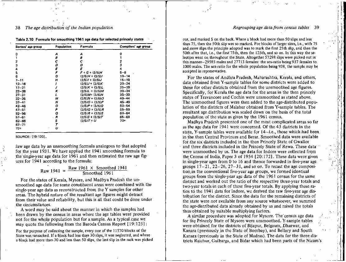
38 The age distribution of the Indian population
Table 2.10 Formula for smoothing 1941 age data for selected princely states
Sorters' ai je group Population Formula Compilers' age group
0 A A 0 1 B B 1 2 C C 2 3 D D 3 4 E E 4 5 F F + G + (3/5)H 5-9 6 G (2/5)W + (3/5)/ 10-14 7-11 H (2/5)/+ (3/5)7 15-19 12-16 1 (2/5)./+ (3/5)/C 20-24 17-21 J (2/51/C + (3/5)/. 25-29 22-26 K (2/5)/. + (3/5)M 30-34 27-31 L (2/5)/W+ (3/5J/V 35-39 32-36 M (2/5I/V+ (3/5)0 40-44 37-41 N (2/5)0+ (3/5)/» 45-49 42-46 O (2/5)/»+ (3/5)0 50-54 47-51 P (2/5IQ + (3/5)/? 55-59 52-56 Q (2/5)/? + (3/5)5 60-64 57-61 Ft (2/5 )S+ (3/5)7" 65-69 62-66 S (2/5)7+U 70+ 67-71 T 72+ U
SOURCE: [19:1301.
raw age data by an unsmoothing formula analogous to that adopted for the year 1931. We have applied the 1941 smoothing formula to the'single-year age data for 1961 and then estimated the raw age figr ures for 1941 according to the formula:
„ ' „, Raw 1961 X Smoothed 1941 R a w 1 9 4 1 = ~ Smoothed 1961 _
For the states of Kerala, Mysore, and Madhya Pradesh the unsmoothed age data for some constituent areas were combined with the single-year age data as reconstructed from the Y samples for other areas. The hybrid nature of the resultant age figures might detract from their value and reliability, but this is all that could be done under the circumstances.
A word may be said about the manner in which the samples had been drawn by the census in areas where the age tables were provided not for the whole population but for a sample. As a typical case we may quote the following from the Baroda Census Report [19:125]: For the purpose of collecting the sample, every one of the 11570 blocks of the State was ransacked. If a block had less than 30 slips, it was neglected, and where a block had more than 30 and less than 50 slips, the last slip in the rack was picked
Regrouping age data from census tables 39
out, and marked $ on the back. Where a block had more than 50 slips and less than 75, then the 50th slip was so marked. For blocks of larger sizes, i:e., with 75 and.more slips the principle adopted was to mark the first 25 th slip, and then the 50th.after that, i.e., the first 75th, then the 125th, and so on. In this way the selection went on throughout the State. Altogether 57298 slips were picked out in this,manner-29585 males and 27713 females: the sex-ratio being 937 females to 1000 males. The sex-ratio for the whole population being 938, the sample may be accepted as representative.
For the states of Andhra Pradesh, Maharashtra, Kerala, and others, data obtained from Y-sample tables for some districts were added to those for other districts obtained from the unsmoothed age figures. Specifically, for Kerala the age data for the areas in the then princely states of Travancore and Cochin were unsmoothed as stated above. The unsmoothed figures were then added to the age-distributed population of the districts of Malabar obtained from Y-sample tables. The resultant age distribution was scaled down on the basis of the total population of the state as given by the 1961 census.
Madhya Pradesh presented one of the most complicated areas so far as the age data for 1941 were concerned. Of the 43 districts in the state, Y-sample tables were available for 14—i.e., those which had been in the then Central Provinces and Berar. Smoothed data were available for the six districts included in the then Princely State of Gwalior and three districts included in the Princely State of Rewa. These data' were unsmoothed by us. The age data for Indore were collected from the Census of India, Paper 3 of 1954 [20:172]. These data were given in single-year ages from 0 to 16 and thence forwarded in five-year age groups 17—21, 22—26, 27-31, and so on. To recast the age composition, in the conventional five-year age groups, we formed identical groups from the single-year age data of the 1961 census for the same district and worked out the ratio of the respective three-year totals and two-year totals in each of these five-year totals. By applying these ratios to the 1941 data for Indore, we derived the raw five-year age distribution for the district. Since the data for the remaining districts of the state were not available from any source whatsoever, we summed the age-distributed data already obtained by us and raised the totals thus obtained by suitable multiplying factors.
A similar procedure was adopted for Mysore. The'census age data for the Princely State of Mysore were unsmoothed. Y-sample tables were obtained for the districts of Bijapur, Belgaum, Dharwar, and Kanara (previously in the State of Bombay), and Bellary and South Kanara (previously in the State of Madras). The data for the three, districts Raichur, Gulbarga, and Bidar which had been parts of the Nizam'
40 The age distribution of the Indian population
Territory of Hyderabad, were not available from any source. This leaves a big gap in the data for 1941.
A gap exists also in the age data for Punjab, Haryana, and Himachal Pradesh. Of the eleven districts in the Punjab, Y-sample tables were available for only six: Hoshiarpur, Jullundhur, Ludhiana, Ferozepur, Amritsar, and Gurudaspur. The small and medium-sized princely states included in what was then Punjab had not tabulated the age data. The only alternative left to us therefore was to add up the age figures for these six districts and scale up the resultant age distribution by a suitable multiplying factor. Evidently the multiplying factors were large in such cases. In the absence of relevant data this appears to be unavoidable.
As regards Haryana, Y-sample tables were available for five out of seven districts: Hissar, Rohtak, Kamal, Gurgaon, and Ambala. As regards Himachal Pradesh, Y-sample tables were available for two districts only (Simla and Kangra). No age data were available for the then princely states in the hills. We have constructed tables on the 1961 age data for the states of Madhya Pradesh, Andhra Pradesh, Maharashtra,. and Mysore showing the differences in their age composition with and
• without those districts for which no age data were available for 1941. Trie differences were small. Presumably, similar differences for 1941 also would be small. We hypothesize that though the gaps In data were real and substantial in some cases, the effects of such gaps were not-great.
The displaced population: 1951
The age data for 1951 were given in the census tables separately for the displaced population from Pakistan and the rest of the population (the nondisplaced or general population). For the nondisplaced population, age data are available for a 10 percent sample. (The sampling fraction was not strictly 10 percent in all cases; there are some variations from state to state.)
The registrar general's instruction [21 :iii] for taking the samples was as follows: Break each pad [of 100 enumeration slips] and stack the slips of the pad; and cut the stack as in a card game. Place the lower portion above the upper portion and then deal the slips into the pigeonholes. You should deal the slips into the pigeonholes in the order of 1, 2, 3, 4, 5, S, 6, 7,8 and 9 respectively. All the time you should watch the slips of displaced persons. If you come across any slip of a displaced person, deal it in the pigeonhole of "Displaced Persons."
A displaced person was defined [21:iii] as "any person who has en-
Regrouping age data from census tables 41
tered India having left or being compelled to leave his or her home In Western Pakistan on or after the first [of] March 1947 or his or her home in Eastern Pakistan on or after the 15th [of] October 1946 on account of civil disturbances or the fear of such disturbances or on account of the setting up of the two dominions of India and Pakistan."
With regard to the nondisplaced persons, the single-year age data of the sample population were grouped into the required series of quinquennial age intervals. The age figures thus obtained were expanded by suitable multiplying factors separately for the male and female population. The multiplying factors were obtained by relating the-nondisplaced population of each state by sex (adjusted for changes in the administrative boundaries) to the sample population for the re
number of nondisplaced persons adjusted for boundary changes effective sample size for area multiplying factor number of persons in age group (/) in sample ' \ number of persons in age group (/) in parent nondisplaced population :
N_ s . „ t; ' m [sp(0)
With regard to the displaced persons, the census age tables for 1951 provide five-year age distribution for age groups 0—4, 5—9, and 10-14 and ten-year age distribution thereafter (15-24, 25-34, and so on). We first decomposed the ten-year age groups into the corresponding pairs of five-year age groups on the basis of the assumption that the internal distribution.of two five-year age groups within a ten-year age group was the same for the displaced population as for the nondisplaced population in the particular state. Then the age-distributed displaced population was added to the age-distributed nondisplaced pop- -ulation of the respective states.
Of the 29 states and territories, separate account has been taken of the displaced population in seven: Assam, Meghalaya, West Bengal, Punjab, Haryana, Himachal Pradesh, and Delhi. For the remaining 22 states and territories, the entire population was assumed to have been
spective areas. If N =
S = m -
sp(i) =
pQ) =
theh m =
and p(i) =
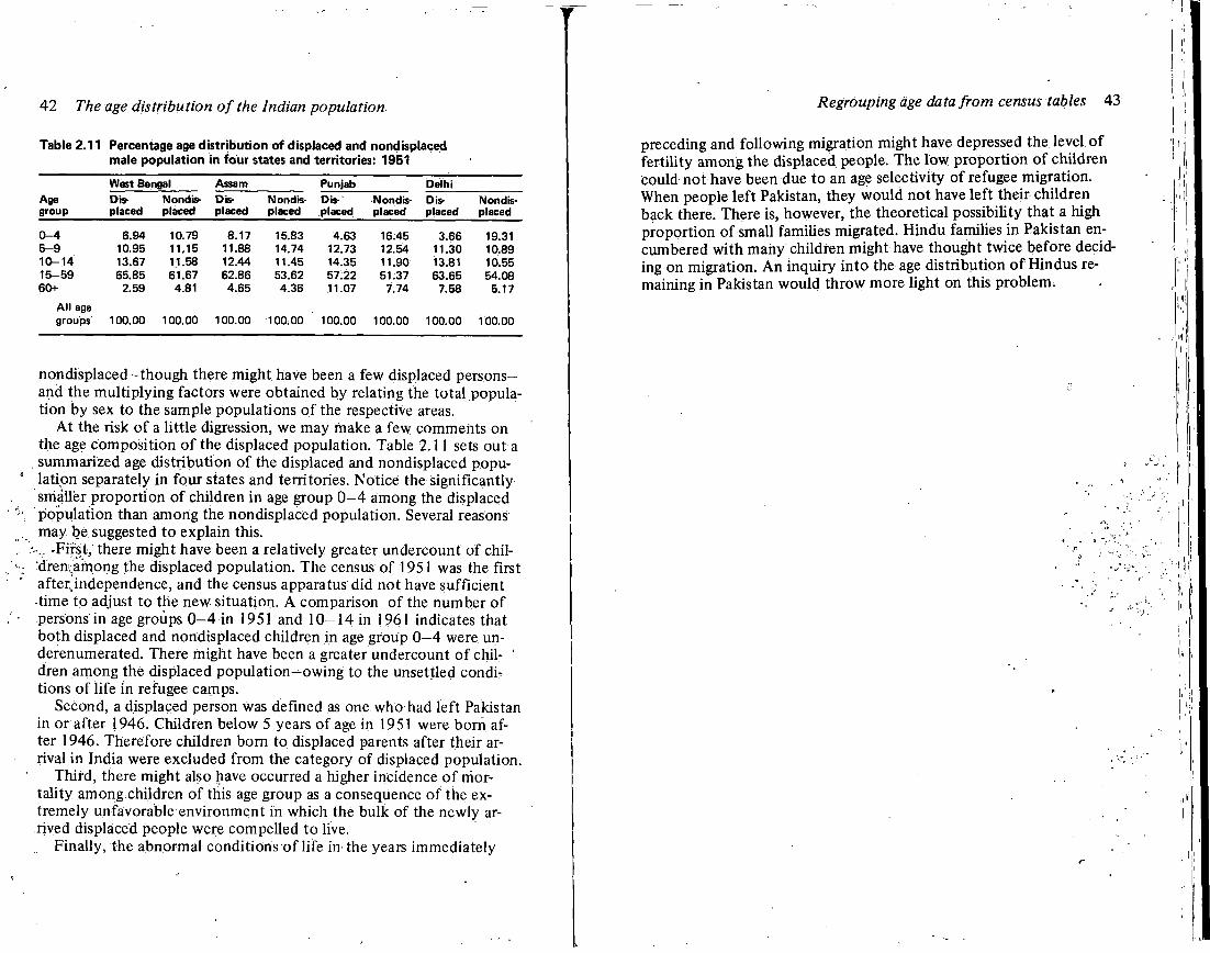
42 The age distribution of the Indian population
Table 2.11 Percentage age distribution of displaced and nondisplaced male population in four states and territories: 1951
West Bengal Assam Punjab Delhi Age Dis Nondis Dis Nondis Dis Nondis Dis Nondisgroup placed placed placed placed placed placed placed placed
0-4 6.94 10.79 8.17 15.83 4.63 16.45 3.66 19.31 5-9 10.95 11.15 11.88 14.74 12.73 12.54 11.30 10.89 10-14 13.67 11.58 12.44 11.45 14.35 11.90 13.81 10.55 15-59 65.85 61.67 62.86 53.62 57.22 51.37 63.65 54.08 60+ 2.59 4.81 4.65 4.36 11.07 7.74 7.58 5.17
All age groups 100.00 100.00 100.00 100.00 100.00 100.00 100.00 100.00
nondisplaced—though there might have been a few displaced persons-arid the multiplying factors were obtained by relating the total population by sex to the sample populations of the respective areas.
At the risk of a little digression, we may make a few comments on the age composition of the displaced population. Table 2.11 sets out a
. summarized age distribution of the displaced and nondisplaced population separately in four states and territories. Notice the significantly smaller proportion of children in age group 0—4 among the displaced population than among the nondisplaced population. Several reasons may be suggested to explain this,
.-•v -First,'there might have been a relatively greater undercount of chil-'dreniiamong the displaced population. The census of 1951 was the first after independence, and the census apparatus did not have sufficient time to adjust to the new situation. A comparison of the number of persons in age groups 0-4 in 1951 and 10-14 in 1961 indicates that both displaced and nondisplaced children in age group 0—4 were un-derenumerated. There might have been a greater undercount of chil- ' dren among the displaced population—owing to the unsettled condi tions of life in refugee camps.
Second, a displaced person was defined as one who had left Pakistan in or after 1946. Children below 5 years of age in 1951 were born after 1946. Therefore children born to displaced parents after their arrival in India were excluded from the category of displaced population.
Third, there might also have occurred a higher incidence of mortality among children of this age group as a consequence of the extremely unfavorable environment in which the bulk of the newly arrived displaced people were compelled to live.
Finally, the abnormal conditions of life in the years immediately
Regrouping age data from census tables 43
preceding and following migration might have depressed the level of fertility among the displaced people. The low proportion of children could not have been due to an age selectivity of refugee migration. When people left Pakistan, they would not have left their children back there. There is, however, the theoretical possibility that a high proportion of small families migrated. Hindu families in Pakistan encumbered with many children might have thought twice before deciding on migration. An inquiry into the age distribution of Hindus remaining in Pakistan would throw more light on this problem.
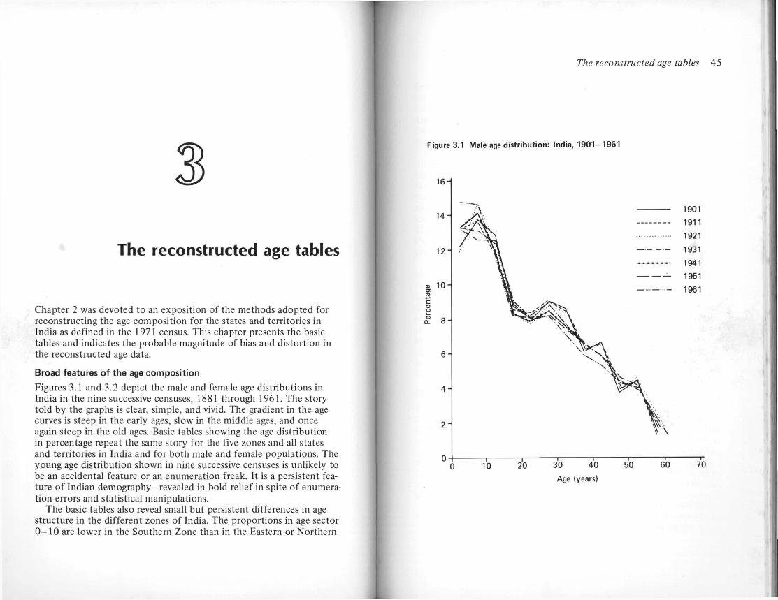
The reconstructed age tables
Chapter 2 was devoted to an exposition of the methods adopted for reconstructing the age composition for the states and territories in India as defined in the 1971 census. This chapter presents the basic tables and indicates the probable magnitude of bias and distortion in the reconstructed age data.
Broad features of the age composition
Figures 3.1 and 3.2 depict the male and female age distributions in India in the nine successive censuses, 1881 through 1961. The story told by the graphs is clear, simple, and vivid. The gradient in the age curves is steep in the early ages, slow in the middle ages, and once again steep in the old ages. Basic tables showing the age distribution in percentage repeat the same story for the five zones and all states and territories in India and for both male and female populations. The young age distribution shown in nine successive censuses is unlikely to be an accidental feature or an enumeration freak. It is a persistent feature of Indian demography-revealed in bold relief in spite of enumeration errors and statistical manipulations.
The basic tables also reveal small but persistent differences in age structure in the different zones of India. The proportions in age sector 0-10 are lower in the Southern Zone than in the Eastern or Northern
The reconstructed age tables 45
Figure 3.1 Male age distribution: India, 1901-1961
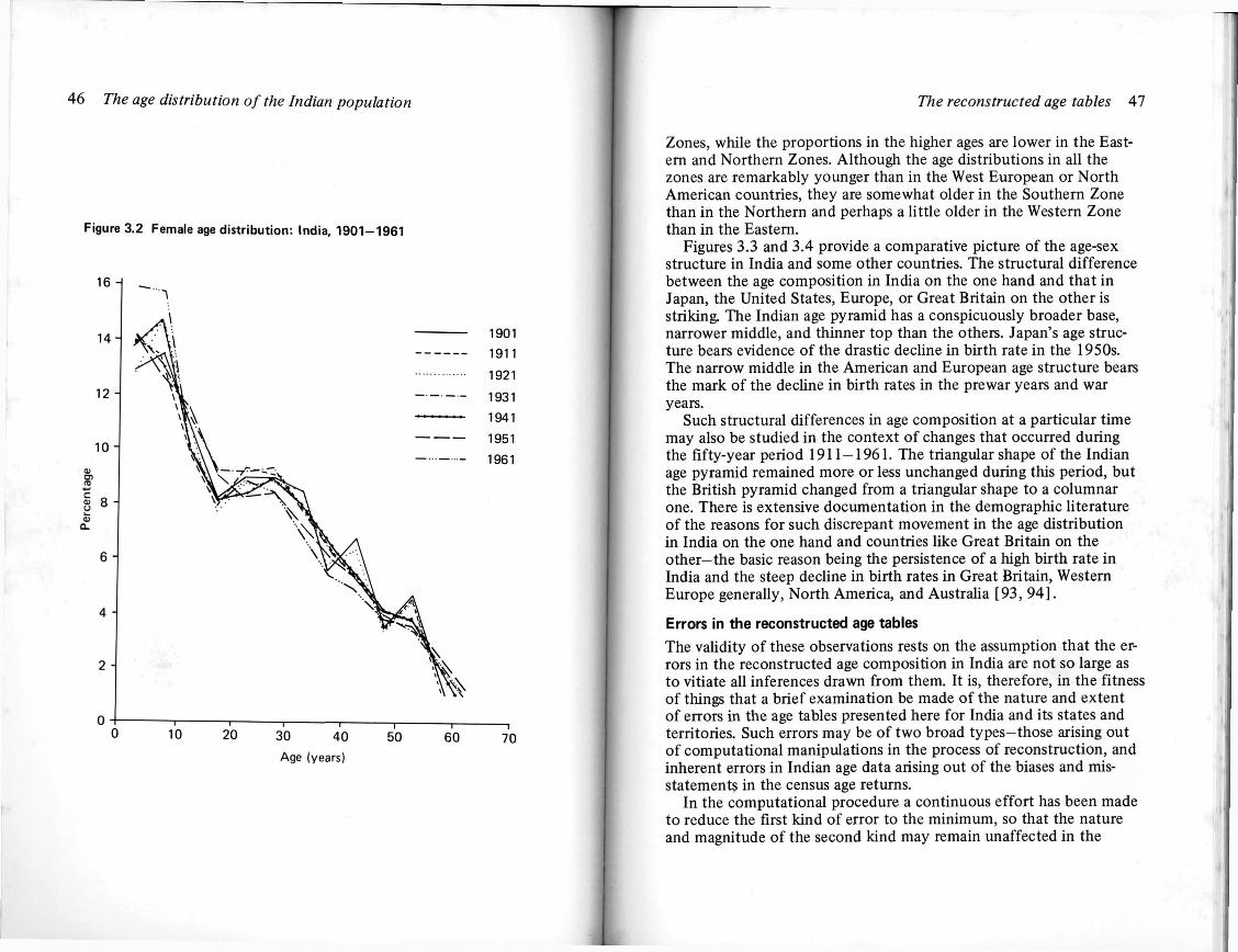
46 The age distribution of the Indian population
Figure 3.2 Female age distribution: India, 1901-1961
Age (years)
The reconstructed age tables 47
Zones, while the proportions in the higher ages are lower in the Eastern and Northern Zones. Although the age distributions in all the zones are remarkably younger than in the West European or North American countries, they are somewhat older in the Southern Zone than in the Northern and perhaps a little older in the Western Zone than in the Eastern.
Figures 3.3 and 3.4 provide a comparative picture of the age-sex structure in India and some other countries. The structural difference between the age composition in India on the one hand and that in Japan, the United States, Europe, or Great Britain on the other is striking. The Indian age pyramid has a conspicuously broader base, narrower middle, and thinner top than the others. Japan's age structure bears evidence of the drastic decline in birth rate in the 1950s. The narrow middle in the American and European age structure bears the mark of the decline in birth rates in the prewar years and war years.
Such structural differences in age composition at a particular time may also be studied in the context of changes that occurred during the fifty-year period 1911-1961. The triangular shape of the Indian age pyramid remained more or less unchanged during this period, but the British pyramid changed from a triangular shape to a columnar one. There is extensive documentation in the demographic literature of the reasons for such discrepant movement in the age distribution in India on the one hand and countries like Great Britain on the other—the basic reason being the persistence of a high birth rate in India and the steep decline in birth rates in Great Britain, Western Europe generally, North America, and Australia [93, 94].
Errors in the reconstructed age tables
The validity of these observations rests on the assumption that the errors in the reconstructed age composition in India are not so large as to vitiate all inferences drawn from them. It is, therefore, in the fitness of things that a brief examination be made of the nature and extent of errors in the age tables presented here for India and its states and territories. Such errors may be of two broad types—those arising out of computational manipulations in the process of reconstruction, and inherent errors in Indian age data arising out of the biases and misstatements in the census age returns.
In the computational procedure a continuous effort has been made to reduce the first kind of error to the minimum, so that the nature and magnitude of the second kind may remain unaffected in the
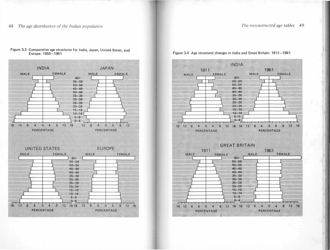
48 The age distribution of the Indian population
UNITED STATES EUROPE MALE FEMALE MALE FEMALE
1 60+ 1 1 I 55-59
50-54 1 45-49
40-44 35-39 30-34 25-29 20-24
1 15-19 1 10-14
1 I 5-9
1—1—1—1—I—I—I—I— H 0-4
—i—i—i—i—r-*T—i—i i — i — i — r — i — i — i — i — 1 1 1 j 1 1 1 1
PERCENTAGE PERCENTAGE
The reconstructed age tables 49
Figure 3.4 Age structural changes in India and Great Britain: 1911—1961
8 4 0 PERCENTAGE
8 4 0 PERCENTAGE
G R E A T BRITAIN
MALE FEMALE
- T - — i — i — i — i — i — I — i — i — i — i — i * — i — i — i i — i — i — r - i — i — i — i — I — i — i — i 1—i—i—i—i
16 12 8 4 0 4 8 12 16 16 12 8 4 0 4 8 12 16 PERCENTAGE PERCENTAGE
H H H H 9
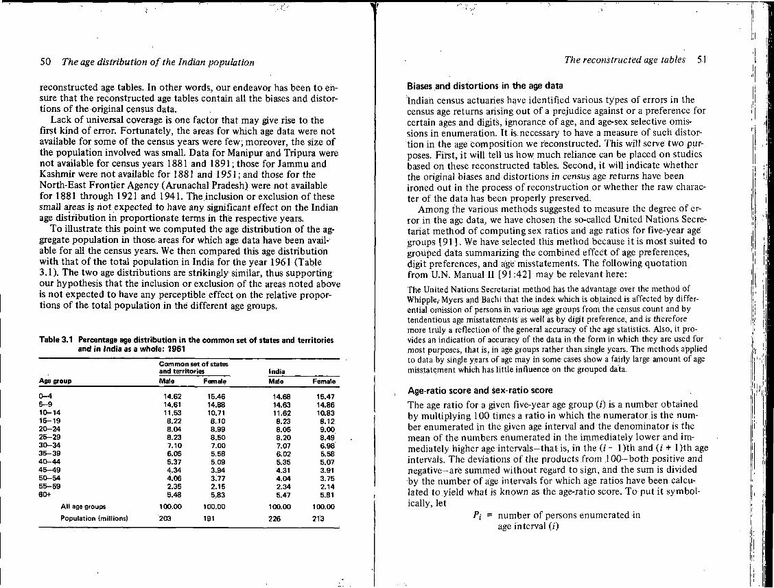
50 The age distribution of the Indian population
reconstructed age tables. In other words, our endeavor has been to ensure that the reconstructed age tables contain all the biases and distortions of the original census data.
Lack of universal coverage is one factor that may give rise to the first kind of error. Fortunately, the areas for which age data were not available for some of the census years were few; moreover, the size of the population involved was small. Data for Manipur and Tripura were not available for census years 1881 and 1891; those for Jammu and Kashmir were not available for 1881 and 1951; and those for the North-East Frontier Agency (Arunachal Pradesh) were not available for 1881 through 1921 and 1941. The inclusion or exclusion of these small areas is riot expected to have any significant effect on the Indian age distribution in proportionate terms in the respective years.
To illustrate this point we computed the age distribution of the aggregate population in those areas for which age data have been available for all the census years. We then compared this age distribution with that of the total population in India for the year 1961 (Table 3.1). The two age distributions are strikingly similar, thus supporting our hypothesis that the inclusion or exclusion of the areas noted above is not expected to have any perceptible effect on the relative proportions of the total population in the different age groups.
Table 3.1 Percentage age distribution in the common set of states and territories and in India as a whole: 1961
Common set of states and territories India
Age group Male Female Male Female
0-4 14.62 15.46 14.68 15.47 5-9 14.61 14.88 14.63 14.86 10-14 11.53 10.71 11.62 10.83 15-19 8.22 8.10 8.23 8.12 20-24 8.04 8.99 8.05 9.00 25-29 8.23 8.50 8.20 8.49 30-34 7.10 7.00 7.07 6.98 35-39 6.05 5.58 6.02 5.58 40-44 5.37 5.09 5.35 5.07 45-49 4.34 3.94 4.31 3.91 50-54 4.06 3.77 4.04 3.75 55-59 2.35 2.15 2.34 2.14 60+ 5.48 5.83 5.47 5.81
All age groups 100.00 100.00 100.00 100.00 Population (millions) 203 191 226 213
The reconstructed age tables 51
Biases and distortions in the age data
Indian census actuaries have identified various types of errors in the census age returns arising out of a prejudice against or a preference for certain ages and digits, ignorance of age, and age-sex selective omissions in enumeration. It is necessary to have a measure of such distortion in the age composition we reconstructed. This will serve two purposes. First, it will tell us how much reliance can be placed on studies based on these reconstructed tables. Second, it will indicate whether the original biases and distortions in census age returns have been ironed out in the process of reconstruction or whether the raw character of the data has been properly preserved.
Among the various methods suggested to measure the degree of error in the age data, we have chosen the so-called United Nations Secretariat method of computing sex ratios and age ratios for five-year age groups [91 ]. We have selected this method because it is most suited to grouped data summarizing the combined effect of age preferences, digit preferences, and age misstatements. The following quotation from U.N. Manual II [91:42] may be relevant here:
The United Nations Secretariat method has the advantage over the method of Whipple, Myers and Bachi that the index which is obtained is affected by differential omission of persons in various age groups from the census count and by tendentious age misstatements as well as by digit preference, and is therefore more truly a reflection of the general accuracy of the age statistics. Also, it provides an indication of accuracy of the data in the form in which they are used for most purposes, that is, in age groups rather than single years. The methods applied to data by single years of age may in some cases show a fairly large amount of age misstatement which has little influence on the grouped data.
Age-ratio score and sex-ratio score The age ratio for a given five-year age group (0 is a number obtained by multiplying 100 times a ratio in which the numerator is the number enumerated in the given age interval and the denominator is the mean of the numbers enumerated in the immediately lower and immediately higher age intervals-that is, in the (/ - l)th and (/ + ljth age intervals. The deviations of the products from 100-both positive and negative-are summed without regard to sign, and the sum is divided by the number of age intervals for which age ratios have been calculated to yield what is known as the age-ratio score. To put it symbolically, let
Pi = number of persons enumerated in age in terval (/)
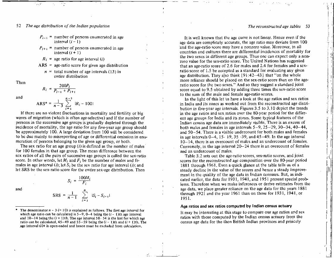
52 The age distribution of the Indian population
number of persons enumerated in age interval (/ - 1) number of persons enumerated in age interval (/' + 1) age ratio for age interval (0 age-ratio score for given age distribution total number of age intervals (13) in entire distribution
2 OOP, Pi-1 + P i + l
n-2
^ 2 "ft-1001 J = 2
If there are no violent fluctuations in mortality and fertility or big waves of migration (which is often age-selective) and if the number of persons in the successive age groups is gradually depleted through the incidence of mortality, the age ratio for any five-year age group should be approximately 100. A large deviation from 100 will be considered to be due mainly to misreporting of age or differential omission in enumeration of persons belonging to the given age group, or both.
The sex ratio for an age group (/) is defined as the number of males for 100 females in that age group. The mean difference between the sex ratios of all the pairs of successive age groups is called the sex-ratio score. In other words, let Mi and Fj be the number of males and females in age interval (/); let 5, be the sex ratio for age interval (/); and let SRS be the sex-ratio score for the entire sex-age distribution. Then
~ Ft
and „
SRS = - ^ j 2 15/-5,^,1 i = 2
* The denominator n - 3 (= 10) is explained as follows. The first age interval for which age ratio can be calculated is 5-9, 0-4 being the (z - l)th age interval and 10—14 being the (< + l)th. The age interval 50-54 is the last for which age ratio can be calculated, 45-49 and 55-59 being the (i - 1 )th and (V + l)th. The age interval 60+ is open-ended and hence must be excluded from calculation.
Then
and
Pi+i
Ri ARS
n
Ri =
ARS"
The reconstructed age tables 53
It is well known that the age curve is not linear. Hence even if the age data are completely accurate, the age ratio may deviate from 100 and the age-ratio score may have a nonzero value. Moreover, in all countries and cultures there are differential incidences of mortality for the two sexes in different age groups. Thus one can expect only a nonzero value for the sex-ratio score. The United Nations has suggested that an age-ratio score of 2.6 for males and 2.4 for females and a sex-ratio score of 1.5 be accepted as a standard for evaluating any given age distribution. They also think [91:42-43] that "on the whole more reliance should be placed on the sex-ratio score than on the age-ratio score for the two sexes." And so they suggest a standard joint score equal to 9.5 obtained by adding three times the sex-ratio score to the sum of the male and female age-ratio scores.
In the light of this let us have a look at the age ratios and sex ratios in India and its zones as worked out from the reconstructed age distribution in five-year age intervals. Figures 3.5 to 3.10 depict the trends in the age ratios and sex ratios over the 80-year period for the different age groups for India and its zones. Some typical features of the Indian census age data are immediately visible. There is an excess of both males and females in age intervals 5—9, 25—29, 30-34, 40-44, and 50-54. There is a visible undercount for both males and females in age intervals 0-4, 15-19, 35.-39, and 45-49. In the age interval 10-14, there is an overcount of males and an undercount of females. Conversely, in the age interval 20-24 there is an overcount of females and an undercount of males.
Table 3.2 sets out the age-ratio scores, sex-ratio scores, and joint scores for the reconstructed age composition over the 80-year period 1881 through 1961. Even a quick glance at the table tells us of a steady decline in the value of the scores and hence a steady improvement in the quality of the age data in Indian censuses. But, as indicated earlier, the data for 1931, 1941, and 1951 present special problems. Therefore when we make inferences or derive estimates from the age data, we place greater reliance on the age data for the years 1881 through 1921 and the year 1961 than on those for 193 1, 1941, or 1951.
Age ratios and sex ratios computed by Indian census actuary
It may be interesting at this stage to compare our age ratios and sex ratios with those computed by the Indian census actuary from the census age data for the then British Indian provinces and princely
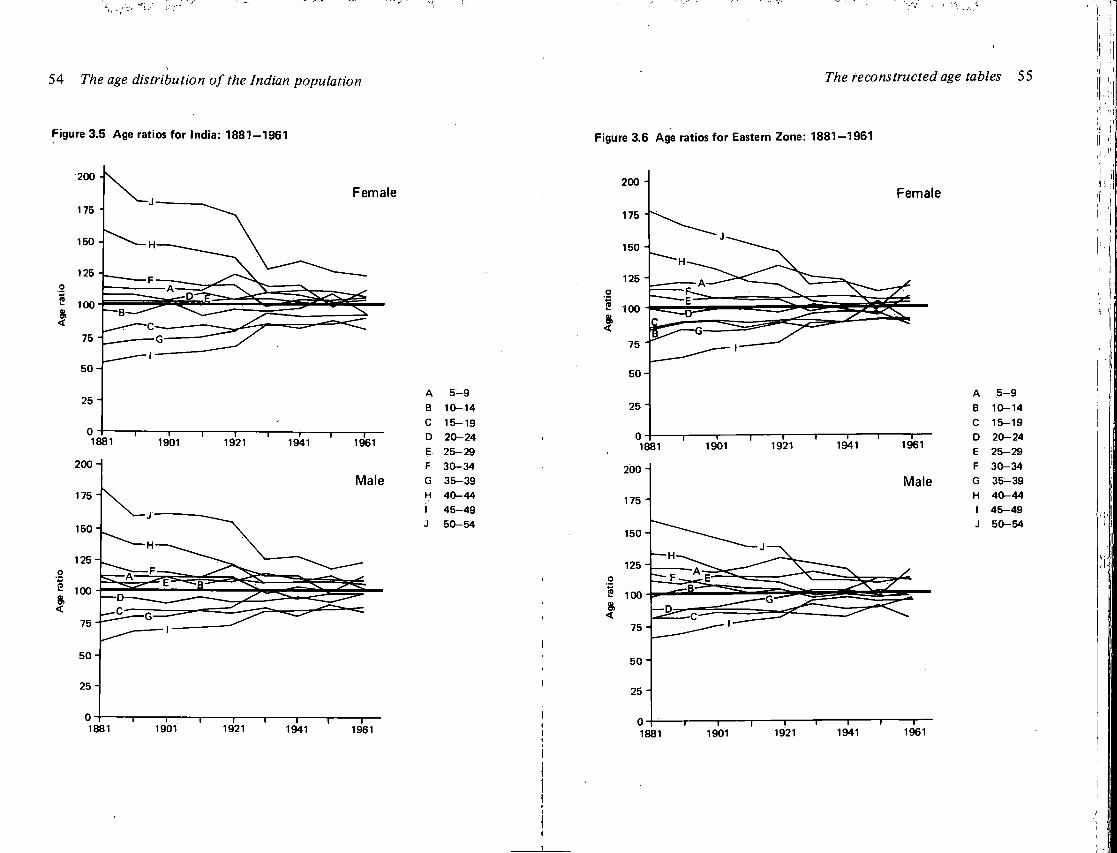
54 The age distribution of the Indian population
Figure 3.5 Age ratios for India: 1881-1961
The reconstructed age tables 55
Figure 3.6 Age ratios for Eastern Zone: 1881-1961
200 H Female
A 5-9 B 10-14 C 15-19 D 20-24 E 25-29 F 30-34 G 35-39 H 40-44 I 45-49 J 50-54
1881 1901 1921 1941 1961
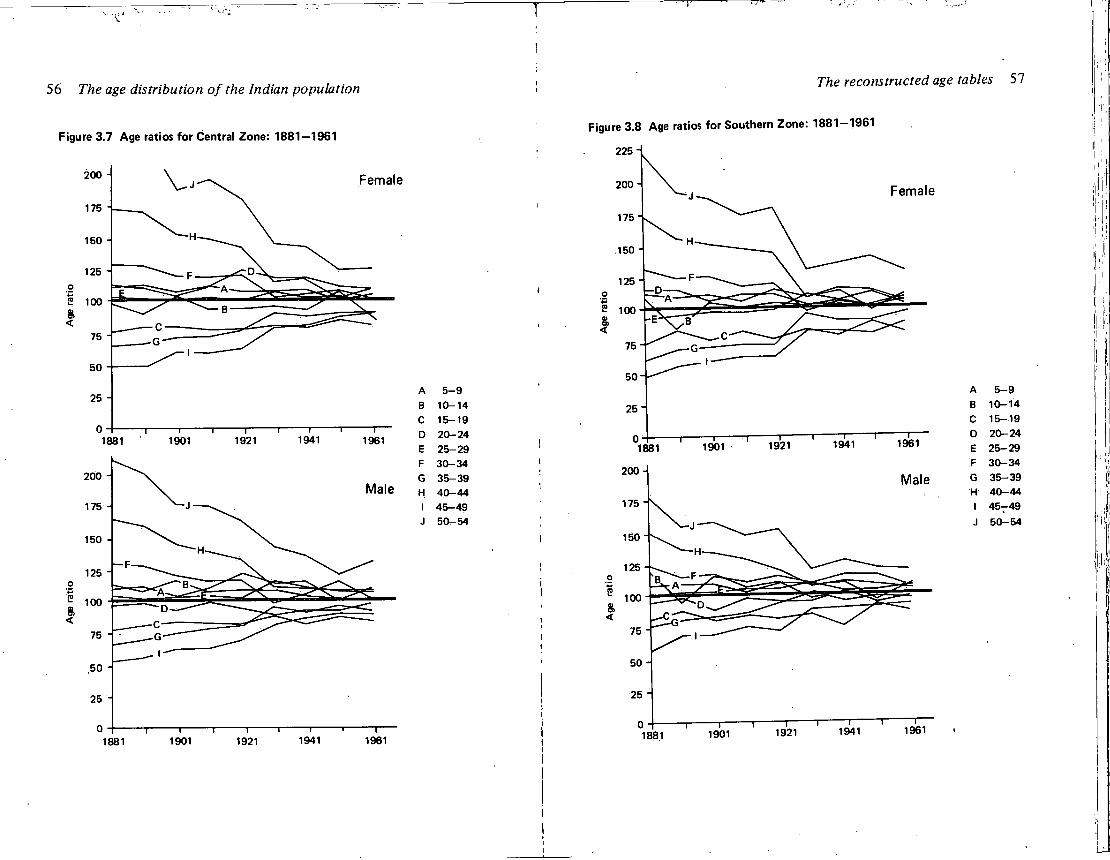
56 The age distribution of the Indian population
Figure 3.7 Age ratios for Central Zone: 1881-1961
o H 1 1 1 1 1 1 1 1— 1881 1901 1921 1941 1961
The reconstructed age tables 57
Figure 3.8 Age ratios for Southern Zone: 1881-1961
225 -\
A 5-9 B 10-14 C 15-19
D 20-24 E 25-29 F 30-34 G 35-39 H 40-44 I 45T49 J 50-54
25
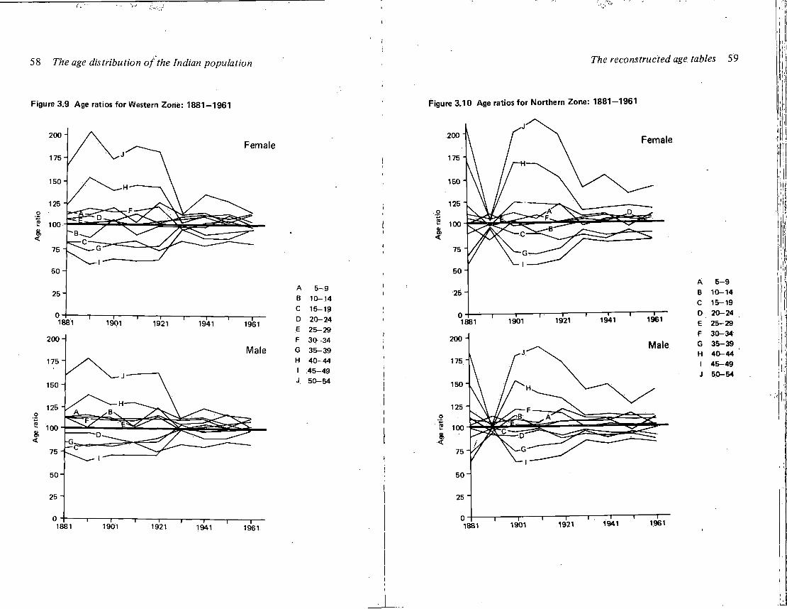
58 The age distribution of the Indian population
Figure 3.9 Age ratios for Western Zone: 1881-1961
25 i
1881 1901 1921 1941 1961
The reconstructed age tables 59
Figure 3.10 Age ratios for Northern Zone: 1881-1961
25 "
0 1 1 1 1 r~ i i r -
1881 1901 1921 1941 1961
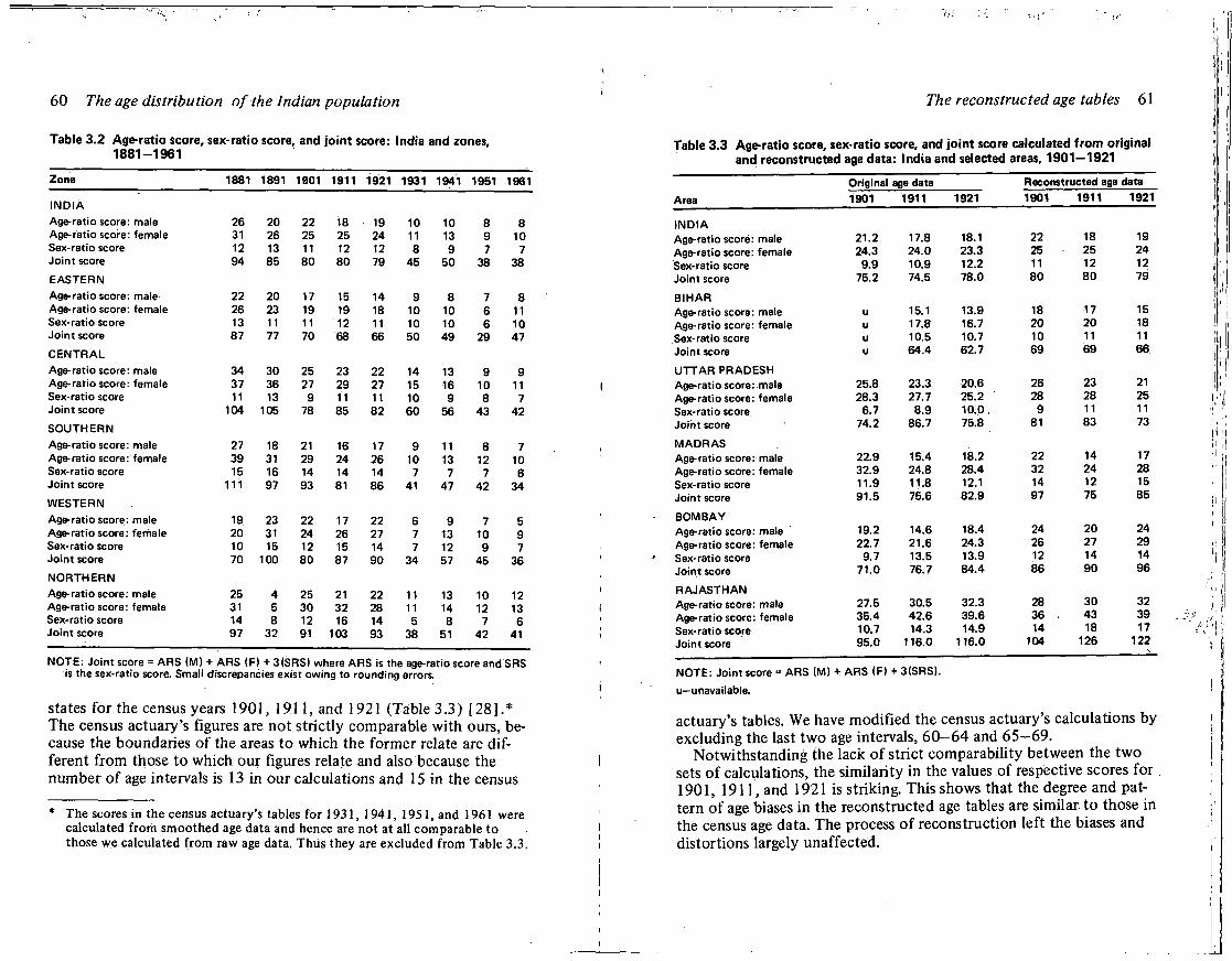
60 The age distribution of the Indian population
Table 3.2 Age-ratio score, sex-ratio score, and joint score: India and zones, 1881-1961
Zone 1881 1891 1901 1911 1921 1931 1941 1951 196
INDIA Age-ratio score: male 26 20 22 18 19 10 10 8 8 Age-ratio score: : female 31 26 25 25 24 11 13 9 10 Sex-ratio score 12 13 11 12 12 8 9 7 7 Joint score 94 85 80 80 79 45 50 38 38 EASTERN Age-ratio score: male 22 20 17 15 14 9 8 7 8 Age-ratio score: female 26 23 19 19 18 10 10 6 11 Sex-ratio score 13 11 11 12 11 10 10 6 10 Joint score 87 77 70 68 66 50 49 29 47 CENTRAL Age-ratio score: male 34 30 25 23 22 14 13 9 9 Age-ratio score: female 37 36 27 29 27 15 16 10 11 Sex-ratio score 11 13 9 11 11 10 9 8 7 Joint score 104 105 78 85 82 60 56 43 42 SOUTHERN Age-ratio score: male 27 18 21 16 17 9 11 8 7 Age-ratio score: female 39 31 29 24 26 10 13 12 10 Sex-ratio score 15 16 14 14 14 7 7 7 6 Joint score 111 97 93 81 86 41 47 42 34 WESTERN Age-ratio score: male 19 23 22 17 22 6 9 7 5 Age-ratio score: female 20 31 24 26 27 7 13 10 9 Sex-ratio score 10 15 12 15 14 7 12 9 7 Joint score 70 100 80 87 90 34 57 45 36 NORTHERN Age-ratio score: male 25 4 25 21 22 11 13 10 12 Age-ratio score: female 31 5 30 32 28 11 14 12 13 Sex-ratio score 14 8 12 16 14 5 8 7 6 Joint score 97 32 91 103 93 38 51 42 41
NOTE: Joint score = ARS (M) + ARS (F) + 3(SRS) where ARS is the age-ratio score and SRS is the sex-ratio score. Small discrepancies exist owing to rounding errors.
states for the census years 1901, 1911, and 1921 (Table 3.3) [28].* The census actuary's figures are not strictly comparable with ours, because the boundaries of the areas to which the former relate are different from those to which our figures relate and also because the number of age intervals is 13 in our calculations and 15 in the census
* The scores in the census actuary's tables for 1931, 1941, 1951, and 1961 were calculated from smoothed age data and hence are not at all comparable to those we calculated from raw age data. Thus they are excluded from Table 3.3.
The reconstructed age tables 61
Table 3.3 Age-ratio score, sex-ratio score, and joint score calculated from original and reconstructed age data: India and selected areas, 1901-1921
Original age data Reconstructed age data Area 1901 1911 1921 1901 1911 1921
INDIA Age-ratio score: male 21.2 17.8 18.1 22 18 19 Age-ratio score: female 24.3 24.0 23.3 25 25 24 Sex-ratio score 9.9 10.9 12.2 11 12 12 Joint score 75.2 74.5 78.0 80 80 79
BIHAR Age-ratio score: male u 15.1 13.9 18 17 15 Age-ratio score: female u 17.8 16.7 20 20 18 Sex-ratio score u 10.5 10.7 10 11 11 Joint score u 64.4 62.7 69 69 66 UTTAR PRADESH Age-ratio score: male 25.8 23.3 20.6 26 23 21 Age-ratio score: female 28.3 27.7 25.2 28 28 25 Sex-ratio score 6.7 8.9 10.0 . 9 11 11 Joint score 74.2 86.7 75.8 81 83 73
MADRAS Age-ratio score: male 22.9 15.4 18.2 22 14 17 Age-ratio score: female 32.9 24.8 28.4 32 24 28 Sex-ratip score 11.9 11.8 12.1 14 12 15 Joint score 91.5 75.6 82.9 97 75 85
BOMBAY Age-ratio score: male 19.2 14.6 18.4 24 20 24 Age-ratio score: female 22.7 21.6 24.3 26 27 29 Sex-ratio score 9.7 13.5 13.9 12 14 14 Joint score 71.0 76.7 84.4 86 90 96
RAJASTHAN Age-ratio score: male 27.5 30.5 32.3 28 30 32 Age-ratio score: female 35.4 42.6 39.6 36 . 43 39 Sex-ratio score 10.7 14.3 14.9 14 18 17 Joint score 95.0 116.0 116.0 104 126 122
NOTE: Joint score = ARS (M) + ARS (F) + 3(SRS). u—unavailable.
actuary's tables. We have modified the census actuary's calculations by excluding the last two age intervals, 60-64 and 65-69.
Notwithstanding the lack of strict comparability between the two sets of calculations, the similarity in the values of respective scores for 1901, 1911, and 1921 is striking. This shows that the degree and pattern of age biases in the reconstructed age tables are similar to those in the census age data. The process of reconstruction left the biases and distortions largely unaffected.
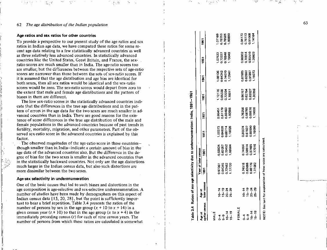
62 The age distribution of the Indian population
Age ratios and sex ratios for other countries
To provide a perspective to our present study of the age ratios and sex ratios in Indian age data, we have computed these ratios for some recent age data relating to a few statistically advanced countries as well as three relatively less advanced countries. In statistically advanced countries like the United States, Great Britain, and France, the sex-ratio scores are much smaller than in India. The age-ratio scores too are smaller; but the differences between the respective sets of age-ratio scores are narrower than those between the sets of sex-ratio scores. If it is assumed that the age distribution and age bias are identical for both sexes, then all sex ratios would be identical and the sex-ratio scores would be zero. The sex-ratio scores would depart from zero to the extent that male and female age distributions and the pattern of biases in them are different.
The low sex-ratio scores in the statistically advanced countries indicate that the differences in the true age distributions and in the pattern of errors in the age data for the two sexes are much smaller in advanced countries than in India. There are good reasons for the existence of some differences in the true age distribution of the male and female populations in the advanced countries because of past trends in fertility, mortality, migration, and other parameters. Part of the observed sex-ratio score in the advanced countries is explained by this factor.
The observed magnitudes of the age-ratio score in these countries— though smaller than in. India—indicate a certain amount of bias in the age data of the advanced countries also. But the difference in the degree of bias for the two sexes is smaller in the advanced countries than in the statistically backward countries. Not only are the age distortions much larger in the Indian census data, but also such distortions are more dissimilar between the two sexes.
Age-sex selectivity in underenumeration
One of the basic causes that led to such biases and distortions in the age composition is age-selective and sex-selective underenumeration. A number of studies have been made by demographers on this aspect of Indian census data [15, 20, 28], but the point is sufficiently important to bear a brief repetition. Table 3.4 presents the ratios of the number of persons by sex in the age group (x + 10 to x + 14) in a given census year (<*.+ 10) to that in the age group (* to jc + 4) in the immediately preceding census (r) for each of nine census years. The number of persons from which these ratios are calculated is somewhat
63
8
10 0 )
i s
a
CM 01
o en
~ s
< 2
o co i n o co in co cn T - CM S5 oo ro cn co c i o t» ro o — d d <-'
co ro op cn o n * J in co co o r - CN to cn o r - r-> *-r d d ^
to co o r->
" * s s M - CN
r - o o <-'
i- CO
3 3
co co s ro co co «-» - CO CN 05 CM i n CN co
co ro « -r O O r
T - cn co to in r - eg co ^ r - ? in i n «- co CM cn <o co o d 6 d ^
co co * co r~ CN T - CN co co r - o O « CO o O CO CO « -«-' d d •- '
cm f r> cs °° -CO CN O O) co -d d o <-
8 $ 8 " 8
T - i n CN o CO ^ CO CN co CN ^ ro r- CN ro O) to ro i -d d d '
* O) * o> i - i - CN CM
« U < c U T - CN CN
< S'l
LU
< 5
to co co i ro ro o cD
r- o «-« II) r * O) r» cn «-o d d . - -
CM rt o co o r- « - CN tn to in a CD O CM O en r- en CN d d o ^
in CN ro co co cn cn ro cn oo oo co r- CN ^ o> CO CO ffl »-d d d ^
P . ^ r - <o in in CN i n r~ i ~ o> co o CN co o O) co a) co d d d
co in co co io 00 r« CM CN r - co o co co co o r - in oo «-o d d '
^ r* o OJ ro co cn cn o co in o o o> o> oo co oo «-d d d <-
^ i n co in r ; co *-in oo ^ cn * cn ro ro ro in cn T -d d d ^
< UJ LL
A i o i J , r - ^ CM CN
nil
3 o
a >c
i i - ^ . . - . .
UJ K O z
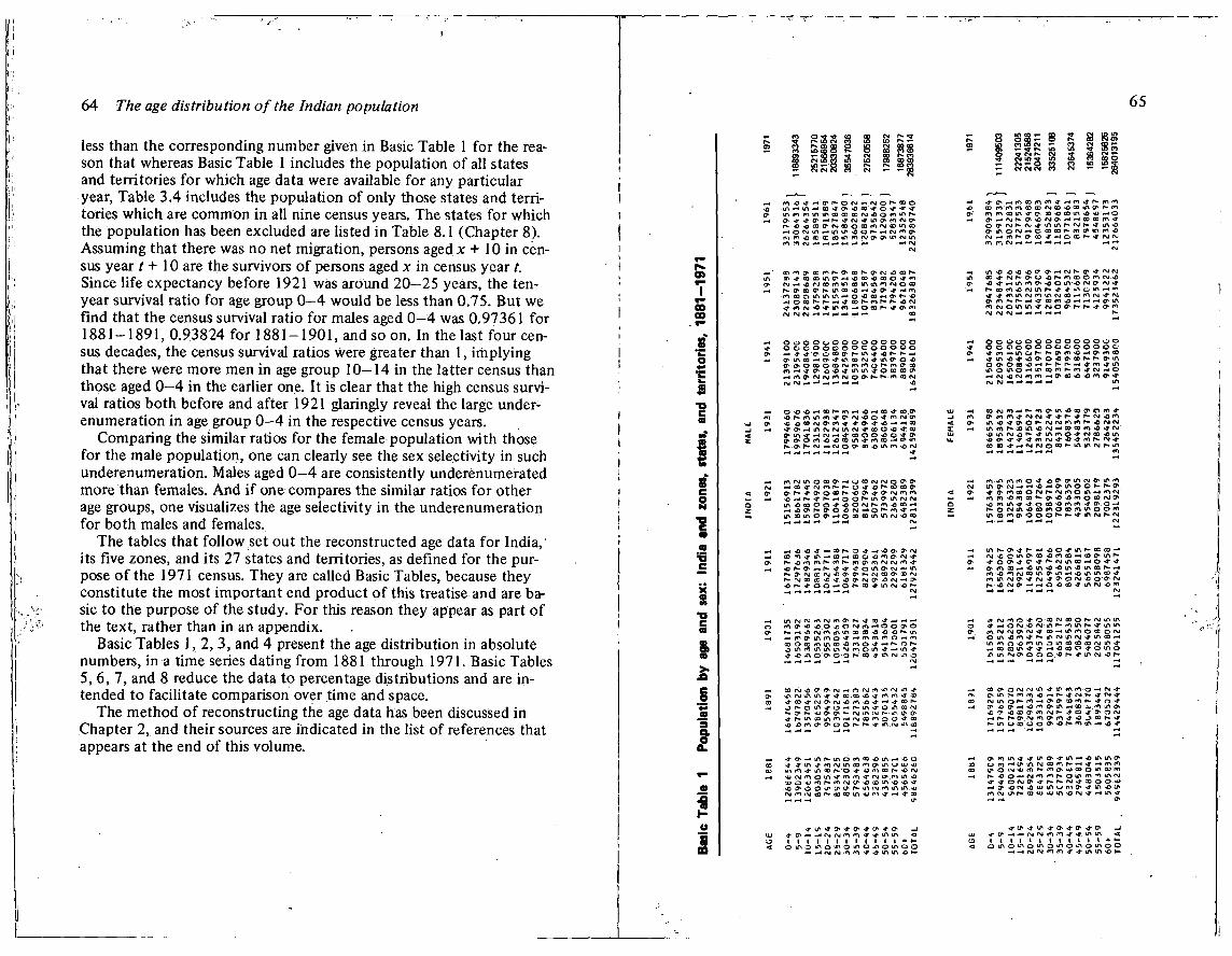
1
64 The age distribution of the Indian population
less than the corresponding number given in Basic Table 1 for the reason that whereas Basic Table 1 includes the population of all states and territories for which age data were available for any particular year, Table 3.4 includes the population of only those states and territories which are common in all nine census years. The states for which the population has been excluded are listed in Table 8.1 (Chapter 8). Assuming that there was no net migration, persons aged x + 10 in census year t + 10 are the survivors of persons aged x in census year t. Since life expectancy before 1921 was around 20—25 years, the ten-year survival ratio for age group 0—4 would be less than 0.75. But we find that the census survival ratio for males aged 0—4 was 0.97361 for 1881 -1891, 0.93824 for 1881 -1901, and so on. In the last four census decades, the census survival ratios were greater than 1, implying that there were more men in age group 10—14 in the latter census than those aged 0—4 in the earlier one. It is clear that the high census survival ratios both before and after 1921 glaringly reveal the large underenumeration in age group 0—4 in the respective census years.
Comparing the similar ratios for the female population with those for the male population, one can clearly see the sex selectivity in such underenumeration. Males aged 0—4 are consistently underenumerated more than females. And if one compares the similar ratios for other age groups, one visualizes the age selectivity in the underenumeration for both males and females.
The tables that follow set out the reconstructed age data for India, its five zones, and its 27 states and territories, as defined for the purpose of the 1971 census. They are called Basic Tables, because they constitute the most important end product of this treatise and are basic to the purpose of the study. For this reason they appear as part of the text, rather than in an appendix.
Basic Tables 1, 2, 3, and 4 present the age distribution in absolute numbers, in a time series dating from 1881 through 1971. Basic Tables 5, 6, 7, and 8 reduce the data to percentage distributions and are intended to facilitate comparison over time and space.
The method of reconstructing the age data has been discussed in Chapter 2, and their sources are indicated in the list of references that appears at the end of this volume.
LTi^in^CDJl>-0(D<r O *T oT >T
r- -O « CO ( M \ ( D O O r i i n j l D l n ( 0 O ^ ^ if1 ^ vO o r» »w t\j n>
m f n f y r H ^ ^ M F J H <-* eg
8 8 »- "C r-«r CM r» «<r CM in — — CM « -*- CN CM
r» tM
•r o » i H f n c D f n f n * ^ f n j , f > -<D m r«"i m co co IN co >o co *n tr m rn oo in >f to <o com <o « Q> ^ r\i N >C f\it7*-*-*cOco O Cf t \ | S N ^ i n i P M M h v * f r i n O f M ^ O O c O M T i r / i n f\j —< m r- o* co %r —• o cc r» *f (M (NJ
CD m t> en en* o> co s c w * <o r* r j ^<CNODi^ tn (Oi r i in rn rgocO N O > I O O , M n « ) 1 O H ^ O , ^ r t m m <D C J tf"\ UN m —< O IO 'CD 0> r- ~o
( N J f M t N l — c o
C 0 > T H i n f n t 7 ^ 0 in «0 fM rj* fM ^
& rn t*~ ~+ •& eoif\>o^r^—*tj*u\ m cNjO'^in>a kr\jOC7 ,l^r^>tC*' r i
I M < N J ( \ J - * - 4 ^ ^ " *
O O O O o O O O O O O O O O o o o o o o o o o o o o o o
0>t>0 D D i D M n K i O f- m O* CO m ~+ •? & -o <C •4* m m O oo ao rj« l\jr\|r4''H>'><>4 -O
— o o o o o o o o o o o o o o sT O O O o O O O O O O O O O C
O 0 , O e o ' O H f ^ r * r " - < i t m ^ i f i ifl O U^O IT CO r*~l P- m <t C\i 0 _< (M ^) '«M rf> —4 O CO NO •OCiC'T M t\ H r4 F4 m
NQ yfl 03 (M tT frt * t> • H 9 )
f— ff> p~ fM <\J o o* tr <j ^\ m *o fM
C D N ' n H N r n O ' i r i O t o ^ O r f i ' r o> mr^^fNjrsjvr-j-r-xtr-f\io f ,*> mmr*cokn4}'si-4coco«%o<<rt\i'
vO lA N 4 ^ ^ in m O ^ N CO -Cm
_ i p4 «4 m
0"i r— <r fji O CD -O 0* O r\i rr\ r*\
r-l 4 -4 .-t w* t-4 CVJ
rT| in (*1 CI O "d" ^ O O l f t M C l f l W ITi O (NJ ~* •£ -^ t>U*\OOr- - ro -0 *t Cr* m t s o i N i N N r r t O i n ^ r n f t j m m •o rn co N oNO.ornocofNiON O Ml <*.0 <D O fn C\ "t O O in CO ^ O 1 O O O N r > * ^ N N M
f» *Q rr\ f U M f l N PVQN m N i A j m ^ •o r-cr r- >r -a- -j-amo^cM-xm r*» r\j to oc *o -JT *o c* r\i 0" J3 INI -« a* O r - -4 -00—<Of- CO in eg -O r— „, ^ _ _t ^ ,4 fM
-4 m r— f- _4 •a o -J- u*\ r» ce CO -« (Ni •£ O in O* CO O fl CO H CO O in P*
cr- O OV* a «*• f*" (\J in co ^ o -o> co ^ 4 tn -43 «o tn o m a s »4 m *«1 r\j co in I X T I H 4} ITi in co «r
in fM 0* P O (M 4 O cr <NI O -O >t in <NJ
^ <-i <NI
in r\i (NJ f« (NI rr\ m *o sO.O •C 0(Mt*i -400<?tO -o <NI <n m m O" in m O co o CO ro tn CD m (*•) in in m M ni O m if -4 in N* o o o O N f f l ^ l T l M l A O
r - -4
rxj »*i O >* o cO(NicOOh-(NJinin o O (NI o (NJ
fM <NJ ON <Ni •* ee-H in m o tt O * N I o in •o m >* p» in I M U M M .f in CO >4 in «v Ci -o n in i3U>cOCOcOr\jin<t
CO co in •4- H o o o ^ o m o m m (NI O o o O . * P" <* if> N O S -H —* ^ —l
aifNivO<r'f>r«j^O(NjffiinrNiin^f (M ^ in «t ot CD CO -J rA ffl >f 30
-u o* o> r- <M in isj o m c Cr> >j- r- m J3 LO m ^ t\ to m o o M* to <| fi fl(f C7" O O N -7 m.fNi m CO
*-4 0 3 0 0 N < M i n v k i n f A ( n O ' 4 N * ^ asvn>.rrNr^^3^ro.j-(Njro.cfMot co r \ j inOf*rn-40>fj*c!>rni». '**0'* 1 ,
> CT' O O ' H ^ r n o ^ m ^ c o a/.<n u> ^
r<- m u o O O rj>>Of > »' r vm-^0>T -
y " 0 - 4 l f > M n O f | l D * m ^ -O o ut m ^ m co r- o fi ai i> vO r\i 4 j c M f n { j i n ^ , f n r n N " r M 0» ro m O 4 j O k O O u , o , c t | M n r M r f i i n m.va nj (*i »M as f* co co m <u nw H <t 3
tr*
35 U i ^ - ' O ' i A f M C O r A p - H ^ r t mrn CO C71 O rNivUfir*- C i o a i t D O ' n ' u r f l
N flO^>Nr^rtf,"0>nrn'n«riftl <T -T O (Ni CT» r-ro.ro«j-xoO>*^
0(>i4)oiiniJri*Clt>>'in<ou< rn r\i u>i»3)u) iuiA43iM«r-4in«i
- » ON
>r y1 v* (7> -r c NT cr- .a* j> O'H'^CMtNi'Oni^^rinin I I I I I I I I I I I I o i A o m o u 1 o m o m o m
•^-4(\if\ji'n>l"*inui
<i UJ j - cr-O O < o m
>r -j* y ^ o cr- >j- u1 _j H H OJ N m m s'-r in in < l 1 l 1 l l 1 l l l * fc-o m o m o i n o * n o m o o -4M(\j"j' fim-i;4-i/>if\c^
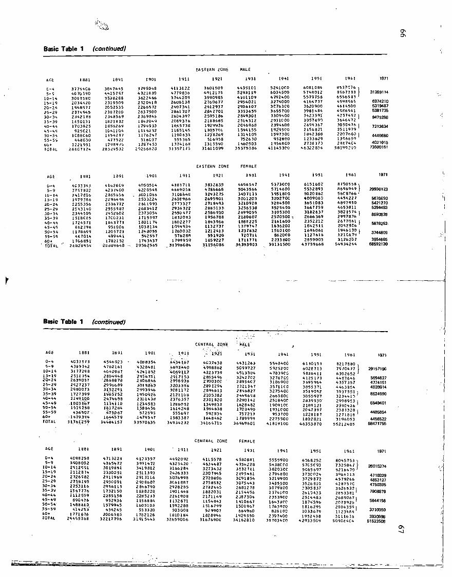
Basic Table 1 (continued)
EASTERN ZONE WALE
AGt 1881 1S91 1901 1911 1921 1931 19*1 1951 1961 1971
G - 4 37754C6 38*76*5 37950*8 *113122 3601509 **351C1 52*1000 608108* 8537076 < 5-9 40 70 590 4*15797 *321830 *779836 *912175 5293119 603*500 57*8012 8567383 } 31369114
10-14 3019580 3508288 3622*66 3 7**209 3990985 A101109 4792400 5579758 6556583 ' 6374210 15-19 2034420 2319509 2520*1 8 2606138 2760677 295*021 327*000 *16*737 *598565 6374210
2 0 - 2 * 154S577 2052535 2266572 2*073*1 2*12937 2906107 3C763C0 3620900 461*500 S319487 25-29 237*545 2387200 263 7500 2861707 28*2701 3353655 3655700 3981*8* * 5 e 6 5 * l 5381735 3 0 - 3 * 23*2188 23*8569 23698*6 260*397 2 595186 28*9301 3309*00 3*23591 *257452 1 9475286 3 5 - 3 9 1450131 1821 832 18*2049 2089376 2188*85 251*312 2931000 3357693 36*6*72
9475286
* 0 - * * 1703025 1056269 179*9 30 18*5730 1929926 20*6968 239*600 269*367 3050476 1 7212634 4 5 - 4 5 925C21 10*110* 1116232 11851*5 1305701 159*155 19295C0 2156821 2511979 50-54 1C88C60 115*287 11762*7 1190633 1238269 131*105 159730C 18*2388 2207680 1 4446680 55-5S 448C30 *77522 516037 555365 516958 752630 952B00 1233629 1396659
4021015 60* 1221951 1298975 1287*53 137*168 1315590 1*60503 1956800 2738373 2H674C4 4021015
TOTAL 266C7124 28529532 29266620 31357175 31611099 35575086 411*5300 *632283* 58199210 73600161
EASTERN ZONE FEMALE
AGE 1 881 1891 1901 1911 1921 1931 1941 1951 1961 1971
0-4 4033343 41628C9 4050514 4383711 3832635 4656547 53730C0 6151602 8 7 5 0 5 5 8 , 5-9 3757802 4237400 4220548 4669058 * 786668 5043566 5 714600 5532893 8696949 \ 29930123
10-14 2417806 2365356 . 3001066 3108640 3293275 340717 3 3951800 5020 862 56CB766 ' 15 -19 1579386 22964 96 2533224 2608966 2695901 3001203 3202700 4009060 4454227 5676690 20-24 2255356 2336772 2611993 2773327 2718493 3210928 3284500 36510B3 4897950 5421270 25-29 2543140 2555587 268 3412 2936322 2885133 3256538 3525400 3667759 4653811 5294493 30-34 234*505 2452602 2373054 2550477 2 586930 2699055 3105300 3182637 3B21574 I 8690828 35-39 1518C65 17CC231 1715397 1B32093 1956788 2180607 2570500 -. 2666 369 2997826 40-44 172*571 1B43773 1801174 1802277 1B43966 1888225 2161600 2352212 2677061 ) 5879252 4 5 - 4 9 £ 6 2 3 9 6 951006 1038134 109*93* 1132737 13797*7 1636200 1842511 2092506 50-54 1178699 1205723 1248055 1260032 1212*13 1237832 1510100 1696061 1946130 1 3744809 55-59 46701* 499441 542557 5762BB 551920 723711 8620C0 1127616 121C679 60» 1706851 1782152 1743437 1799959 1659227 1711771 2 233 800 2859003 3126207 3954665 TOTAL ' 26828954 2B38964B 29562565 3139608* 31156086 34393903 39131500 43759668 54934244 68592130
Basic Table 1 (continued)
AGE
0 -4 5-9
10-14 1 5 - 1 9 2 0 - 2 4 2 5 - 2 9 30-34 3 5 - 3 9 4 0 - 4 * * 5 - * 9 5 0 - 5 4 55-59 60» TOTAL
1881
4C33E73 4369742 3J77298 2518754 2639057 2S27237 2580073 1727399 2 249100 1003667 1519258 436507 .
1479394 31761259
1891
4546923 4762161 4040907 28049*8 2868878 29 966 89 3152291 1965 /52 2*74*88 113*1 10 161728*
4750 67 1644579
34484157
1901
4 08 83 54 4328*81 4241852 2956751 2806846 3019860 2993946 1950926 23114 38 1234583 1 58 64 56
572595 1479547
33570635
1911
4*3*167 4693 440 4069117 2917153 299893B 3203396 3081172 2121103 2376357 1286052 1614248
555697 1583387
34934232
CENTRAL ZONE
- 1921
4C3 7438 4998862 4223739 2 855496 270030C 2891294 2894613 2105382 2301820 1349837 1594638
592834 1648462
34164715
1931
4431263 5099727 4513304 3242702 28954C7 3321347 2846827 2449653 22901*2 162B482 1703490
757213 1789999
36569601
1941
5548400 592520C 47839C0 327670C 3186900 35711C0 32-75400 266380C 251840C 19091OC 1931CO0
953700 2275500
41819100
1951
6130153 6028713 5836*11 *125173 369596* 3855371 3519052 3055977 2839530 2189121 20*7397 1228187 18028.21
*6353870
1961
8217380 7570477 6302652 4457646 4357357 4463854 3937551 l 3234411 1
2998953 | 2390426 1
2383328 1 1271818 1
3196053 55212405
1971
29157196
5694627 4774151 4828014
8524990
6549401
4486854 4456522
68471755
CENTRAL ZONE
ACE 1881 1891 1901 ' 1911 1921
0-4 4C9B258 471322B 4133357 4492092 4115578 5-9 3508002 4365*72 3991472 4325420 ' 4634487
10-14 2512551 3019851 3419812 3166284 3273432 15-19 2112874 2330051 251 1393 2406333 2307945 20 -24 2 726582' 2911969 2913116 3076998 2720806 2 5 - 2 9 2758195 293C091 2908607 3061887 2758532 30 -34 2753116 2956115 2 84 6790 2928285 2732*45 3 5 - 3 9 1547776 1732150 1838228 1901448 1882031 4 0 - 4 4 2112 559 2285158 2285233 2261908 2171149 4 5 - 4 9 890476 952936 1156884 1132871 1154843 5 0 - 5 4 1488610 1579945 16051 03 1592288 1516799 5 5 - 5 9 414 253 434245 55 33 20 503OOB 529907 60* 1771676 2006585 1782128 1810184 1828946 TOTAL 25455768 32217796 31915443 32659006 316769D0
FEMALE
1931
4580881 4756228 3532761 2695461 3C91854 3075443 2681278 2154456 2J87304 1*10667 1501967
664960 1929550
34162810
1941
5555900 54380T-0 38203CC 2 794800 3219900 3435500 3079'BOO 23741(10 2353900 1643 30C 1763900
826100 2 397400
33703400
1951
6068252 5705093 5C65697 3730024 3729B72 3526810 3305837 2613433 251*483 1874596 1816295 1033679 1952*38
*2933509
1961
80*5753 l 73258*7 \ 5216*70 1
396*113 *579266 428757C 3 6 2 6 5 3 2 . 2853381 ' 2 6 6 9 0 6 7 l 2 0 7 8 9 2 6 ' 2 0 0 4 3 5 9 1 1123484 3111636
509064C4
26015274
4710329 4853127 4750395
7908879
5644158
3710350 3930996
61523508
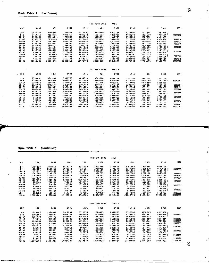
Basic Table 1 (continued} OS co
SOUTHERN ZONE KALE
AGE 1681 i s n 1901 1911 1921 1931 1941 1951 1961 1971
0 -4 2 4 1 9 3 i 3 376G2 60 3739931 411680C 3876849 4703186 5357500 5971148 7857848 , 5-9 2747667 351399b 4051367 4085253 4314023 4856789 575020C 5736479 7757479 \ 27456738
10-14 2724386 2 7 1 4 1 0 1 . 372 5 0 76 3B08924 4030 794 4340759 516 3000 5927912 6664805 ' 15-19 1783573 2133168 234 9 8 6 2 2728645 2699374 3376020 3128C0O 4 )23833 4656536 6287918 20 -24 17C4571 2142344 2069784 2580497 2569873 2517619 3211900 3904618 4501091 5649133 2 5 - 2 9 1792235 22059JI 2296835 2599000 2 708385 30434 36 312350C 37 774 70 4423050 4883510 30-34 188BC97 2149426 2374007 2390 278 2603407 2659848 287100C 3325760 3833381 i 3 5 - 3 9 1251739 1575665 1779388 1901003 2019943 2420773 2559CC0 2988097 3457586 ' 8532426 40 -44 1413902 1726000 1940462 2045466 1966635 2129591 2454700 2798447 3113953 l T rvicc cn 4 5 - 4 9 (34414 963011 112 7472 1296846 1259139 1567117 1894 7C0 2227023 24994C8 ' 7036560 50-54 B64757 1135745 13312B9 1431023 1474630 1431299 180750C 21G7003 23187CO i 5 5 - 5 9 233363 459289 567431 656430 688752 824902 972900 1248600 1368126 ' 4551422 60* 568251 1285920 1447156 1753334 1870081 1538731 2282800 2686723 321841B 4151918 TOTAL 20546288 2573185B 28830060 31393499 32081885 35910073 40576700 47221113 556707'81 68649625
SOUTHERN ZONE FEMALE
AGE 1881 1891 1901 1911 1921 1931 1941 1951 1561 1971
0-4 2556632 3965160 3938753 4299718 4063316 4914772 5332300 5993598 7 8 2 7 4 3 9 , 5-9 2783CC6 34 75 390 4057260 4130403 4446136 4 606547 5773300 581 9C69 7757713 \ 26947992
10-14 2389545 234 8662 3304911 3473 840 3672595 4023562 4757400 5775359 6 3 2 8 2 6 0 J
15-19 1639698 2062695 2211938 2694463 2548467 3093684 3222600 4429713 4581601 6036621 20 -24 2C16941 2523415 2479130 2981104 3006864 330 7C26 34527CC 42C5244 45C83C1 5707155
.25-29 1860481 2291 ICS 2448894 2682126 2829 740 3349756 3416800 3912622 4717292 5352008 30-34 1929322 226756C 2533046 2577206 2693933 2702029 3C38200 3447647 3847650i OCA Acna 35-39 1C31443 1342 363 1557107 1681266 1689618 2215203 2428900 2764727 3 1 8 6 9 1 2 ' 0044oUB 4 0 - 4 4 1387951 1677697 1924270 2060349 20 1 6 3 63 1935979 2351200 2670900 2823565 , 4 5 - 4 9 564CC0 801762 969216 1108315 11135C5 1379718 1644203 1915735 2 1 5 5 8 C 3 ' 6246038 50-54 '.8 8 504 1181824 1370203 1469090 152 9819 140 5 7 7 5 1667400 2123489 2 2 0 3 4 3 5 , A 1*1Q07C 55-59 319176 415988 49 7380 569970 586443 761698 827700 1122595 1225139 ' «* UMZ/O 60* 1184953 1560648 1677399 1901603 1950008 2012895 23543C0 2791569 3276163 4128461 TOTAL 20651852 25914272 2896 9507 31629453 32146807 35505644 40267C00 46962267 54883293 67202157
r Basic Table 1 (continued)
WESTERN ZONE MALE
AGE 1881 1891 1901 1911 1921 1931 1941 1951 1961 1971
0 -4 1655118 2049045 1536217 2274618 1923735 2406643 2751100 3329354 4658854 i 5-9 1800119 2039112 1979512 1975054 2368918 2531293 2873200 3250290 45320C1 \ 16664885
10-14 159395 7 1623830 195 5974 1646 542 1986874 2138913 2396500 3174939 3631446 1
15-15 1041288 1142951 1260512. 1262 686 1152725 1535263 1627300 2252166 2603807 3686266 20 -24 1062 748 1202517 1193425 1376569 1134597 1543037 1660700 2100915 2630379 3218960 25-29 1227739 1394554 1384071 1544554 1404162 1569161 18434C0 2094 890 2610333 2911691 30 -34 1137818 1313632 1302673 1397237 1402630 1354C94 1685700 1877076 2225123 . 3 5 - 3 9 800426 912883 943227 1042949 1053399 1244450 13700C0 1622459 1856690 ' 4 0 - 4 4 747351 588404 946351 1074228 1036437 103700B 1170500 1402620 16GC556 , 1Q1 usee 4 5 - 4 9 470645 5304 87 545735 633783 628334 849511 918700 1039582 1337968 ' OO1JODO 50 -54 545495 678308 617271 728267 744037 7CB705 868600 933771 1148454 . 5 5 - 5 9 221467 233626 246727 276530 291104 434801 518400 592429 710294 ' 60* 523953 681699 545309 727506 799375 859725 1145800 1153970 1505883 2129305 TOTAL 12828124 14791018 1445 7004 15960 523 15 926327 18212604 20B29900 24821961 31092308 39955809
WESTERN ZONE FEMALE
AGE 1881 1891 1901 1911 1921 1931 1941 1951 1961 1971
0 - 4 1728847 2176613 1617184 2379053 2026403 2498C05 2780600 327C045 4561038 l 5 -9 1701695 19364 77 1938147 1B94987 2309340 2425872 27B34C0 3163391 4365874 \ 15707323
10-14 1254422 1286162 1645089 1348949 1662730 18BC521 2 t93900 2880832 3205R21 ' 15-19 571231 1061875 1159405 1174923 1C39138 1450212 1504100 2063729 2347819 3128815 20 -24 1136485 13060 22 1290296 1490911 1217829 1618718 18219C0 2134061 2715372 3102391 25-29 115C593 1335372 132 7060 1453164 1324100 1509 1 96 1792100 1973141 2498272 2897955 30 -34 1041479 1227422 1252539 1363 308 1318624 1226C09 1504100 1747966 2010681 i 4750751 35-39 666929 768138 849916 899304 881306 1C85548 1148800 1378446 1643823 ' 4 0 - 4 4 682445 923824 93 6242 1024191 1000518 938232 1070CC0 1264755 1447820 i 3347733 4 5 - 4 9 439555 435612 494207 527775 528392 740122 792500 387786 1158431 ' 50 -54 542618 643371 628401 710991 692935 618995 810300 861085 999470 i 2130959 55-59 215622 195422 226665 233 906 236831 375360 414400 483978 593527 '
2130959
60 • 619548 7896 96 664236 819125 860182 369734 11914C0 1334045 1600778 2162144 TOTAL 12171309 14056053 14029387 15317.587 15098328 1 7236524 19704500 23443260 29152723 37228071
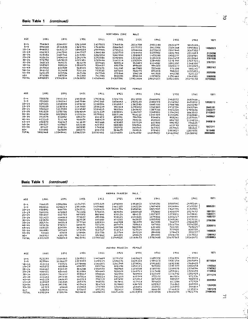
Basic Table 1 (continued) o
NORTHERN ZONE
AGE 1681 1891 1901 1911 1921 1931 1941 1951 1961
0 -4 758845 2266207 1521888 1837020 1746506 ,2016758 2501100 2622677 3865145 5-9 894038 2066520 182 1754 1763094 2066965 2177272 261230C 2324168 37908C6
10-14 848052 1683117 1844103 1559945 1754211 1946646 22726CC 22K7940 3067352 15-19 652343 146 7541 144 75C7 1366188 1235710 1 50 6 4 51 1675900 1691784 22116C3 20-24 619456 1327761 1215701 1262918 1087593 1358887 1473200 1432277 2056564 25-29 610626 1404143 1241576 1253586 1192404 1321403 1491 ICO 1443697 2015062 30-34 571798 12C-5093 1221401 1218446 1161114 1132834 1284400 1271797 17C7314 3 5 - 3 9 362C65 949171 814278 837464 829918 950809 1G1490C 1081050 1348330 40-44 448565 808124 1008375 926457 890754 899665 994300 1025577 1301865 4 5 - 4 9 24 78C6 654909 518545 522071 531240 667980 752400 771100 981141 50-54 341432 513498 701123 723720 687633 7022 75 8712CC 788222 1057203 55-59 124139 4C9726 26 74 36 247748 275346 3362 38 441900 4910 50 527112 60* 371560 587034 741360 741786 848186 894618 1229800 1291665 1543301 TOTAL 6890625 15342844 14365052 14260443 14307580 15911836 18615100 18523004 25473158
1971
14056321
3124556 2555598 2281508
3767331
2863163
2020558
32758023
NORTHERN ZONE FEMALE
AGE 1881 1891 1901 1911 1921 1931 1941 19 51 1561
0 -4 730578 2151114 144 0268 1783836 1724771 2013598 24626C0 2462072 3682466 5-9 755383 1781547 1627584 1542365 1856643 _ 1920120 2386000 2136542 3400202
10-14 625324 1248598 143 5152 1140594 1353557 1582580 1885700 1988786 2620292 15-19 518229 1230515 1147807 1036239 951818 1230640 1360 300 1512734 19C0784 20 -24 556463 1217995 1139582 1164035 983545 1245632 138 7000 1401226 1999636 2 5 - 2 9 531029 1250796 1089249 1121239 1009024 1154707 1349900 135424C 1863563 30 -34 5C4650 1025929 1130154 1079661 1007149 943112 1143 3C0 1172694 1522980 35-35 253474 832852 691373 641600 655991 7947C6 8546C0 903241 .1 157964 40-44 413165 711148 93 8 3 79 866439 80 40 42 758144 842600 881722 1114213 4 5 - 4 9 168679 546947 42 38 20 402663 403300 537729 601900 594752 776025 50-54 284527 437807 632188 622553 588388 558944 69540C 633C93 6C8351 55-59 87427 348334 205893 174830 192972 263765 307700 357913 384921 60* 323340 565859 690773 656193 703679 739915 9724CC 100382 7 1207555 TOTAL 5812468 13349441 12562219 12232452 12234879 13743592 162494C0 16412842 22438952
1971
12628212
2645181 2400277 2143842
3469667
2485810
1607211 1615466
28995666
Basic Table 1 (continued)
ANOHRA PRADESH MALE.
AGE 1881 1891 1901 1911 1921 1931 1941 1951 196 1
0-4 776535 1088866 1176795 1373329 1196345 15510C3 1749100 168554C 24 90164 5-9 858346 1092219 1351404 1439882 1461105 1642224 1987400 1914844 2535552
10-14 £ 5 5 8 9 1 889 7 95 1262211 1329425 1414754 1434C61 18275C0 1982774 2152314 15-19 518164 621865 741828 870235 865054 1040468 772800 1406 8 70 1517422 20 -24 554657 682712 68 5302 862 640 850126 984121 10573C0 12330C1 1422B61 2 5 - 2 9 521423 644849 779027 893 594 933121 1C70404 1075500 1244217 1478453 30-34 623878 708832 82.70 28 835683 877255 945937 1053700 1145161 1313111 3 5 - 3 9 30C576 383518 577740 630833 640928 781879 847200 946577 1066655 4 0 - 4 4 465236 596311 6846 74 727254 637674 759623 537400 1023716 1076330 4 5 - 4 5 153325 224586 363287 430062 40B780 500595 621400 722259 769025 50 -54 3C6889 367669 471394 512 767 516013 527514 7032CC 777925 838735 55-55 72463 87B33 17 8904 210 756 213764 247229 294900 379409 393237 60* 3637G7 4 39193 50 7497 652862 684301 698615 855000 1008272 1107812 TOTAL 6371910 7850268 9607091 10 769 322 10749220 12183673 13782400 15670565 18161671
1971
8895361
1891331 1680471 1598707
2796298
2289515
1468828 1388152
22008663
ANDHRA PRADESH
AGE 1631 1891 1901 1911 •1921 1931 1941 1951 1961 1971
0 -4 623193 1164065 1269510 1443669 1275152 1665609 16857CC 1916334 2513073 , 5-9 827964 1056627 1333859 1440015 1536576 1624333 1S841C0 1930158 2569395 \ 8715034
10-14 71 C 63 3 733721 1079990 1160203 1241749 1279041 ,1591800 1830582 15684 20 ' 15-19 483272 600966 696785 B45756 801198 1052121 9493CC 1390370 1462658 1780303 20-24 646162 808339 8162 88 1002 9 70 930965 1106538 1135700 1339571 1574094 1756382 25-29 494421 628460 811884 904643 928029 1149719 1147400 1255161 1524455 1730659 30-34 610G41 741457 85 8047 898066 922 353 520949 11221CC 1206792 1282925 , 2771274 35-39 221633 297233 48 7814 550028 541105 637749 772100 8670C4 97133o '
2771274
40 -44 44G123 563435 643318 708.330 697650 671017 B87200 980457 582932 l 2005954 4 5 - 4 9 116449 160564 239374 348531 347641 417418 504600 612286 671926 1
2005954
50 -54 226483 391591 457419 504793 519883 496749 628300 746 863 800244 l 1353420 55-55 62709 69660 143845 173798 176510 214851 232500 321893 3446C4 1
1353420
60 + 428053 522916 570697 697 291 702417 733806 866100 K-46823 1135214 1381019 TOTAL 6193166 7739J94 945 88 30 10678090 10671228 12C19900 13506900 15444654 17821776 21494045
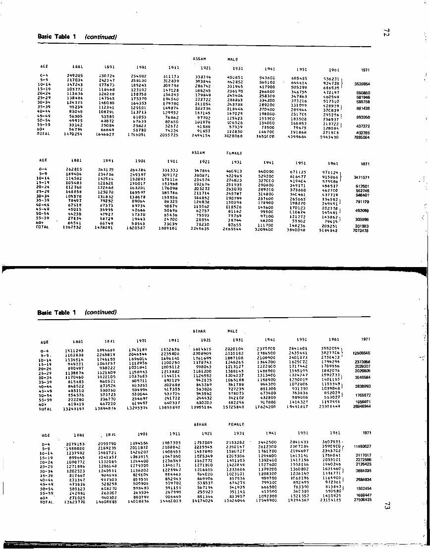
Basic Table 1 (continued)
AGE
c-4 5-9
10-14 15-19 2 0 i 2 4 2 5 - 2 9 30 -34 3 5 - 3 9 40 -44 4 5 - 4 9 5C-54 55-59 60* TOTAL
1881
249205 217034 147243 105772 113636 138486 124375
95239 83048 56305 49975 33142 56794
1470254
1891
£ 5 0 7 2 4 242347 177873 118468 1262 68 147545 1460 80 112341 108791
53585 68872 2 5084 66649
1646627
1901
254002 258030 18 5243 123192 138758 175370 164353 129101 113713 61053 67633 25823 58780
1755051
1911
311173 312 839 209758 147128 156243 194 560 17978C 149874 129952
76 862 80650 32672 74234
2055725
ASSAM
1921
338394 393844 286742 188245 179849 222722 211054 182734 157145
97702 101978 41888 91857
2494154
1931
450851 442852 331945 236170 245406 238863 243788 218446 167029 125423 106526 57939
112830 3028068
1941
543600 565100 417900 266800 258300 334200 289200 270400 198000 153300 134000
73500 14670C
3651C00
1951
685485 644414 505299 346755 347863 373216 331099 289944 2517C5 183508 168853
79675 191868
4399684
1961
5 3 6 2 3 1 • 924728 686935 472157 460549 517510 428929 1 37C839 1
295256 I 236937 213722 1 128084 2715C3
5943430
1971
3539854
660860 581946 586758
981439
693050
437372 403785
788S064
AGE 1881 1891 1901 1911 1921
0 -4 262815 26 3175 264784 331330 34 7844 5-9 189404 234736 249397 309172 380871
10-14 114.582 142964 152093 178116 234574 1 5 - 1 9 105483 121621 130017 153968 192674 20 -24 112768 122668 163201 176098 20 3 2 7 2 2 5 - 2 9 148858 1250 70 165597 185786 211714 30 -34 105576 131832 138678 155556 186852 3 5 - 3 9 78497 792 52 89064 86 32 5 126B38 40-4.4 67519 3 73 73 89734 98 8 79 115562 4 5 - 4 9 45015 35995 42666 50696 62757 5 0 - 5 4 44236 47927 57370 654 36 75593 5 5 - 5 9 27634 16729 19443 24700 28854 60* 64541 66749 58543 73C39 73230 TOTAL 1367532 1478091 1620587 1889101 2245635
FEMALE
1931
4o0913 422965 274823 251935 263070 245787 190799 150396 118526
81162 78769 3 8744 87655
2665544
1941 1951 1961 1971
540000 671125 971124 -, 529200 616477 915866 \ 3471571 3270CO 419404 579586 ' 290600 349171 456517 612501 2892C0 373668 4627C0 552749 314800 34C461 437719 546401 237600 265665 334592 , 791179 178900 198270 249451 1 791179 145600 170123 202338 i 492098 9950C 110674 1454 81 1 492098
97100 121272 143862 i 303996 48200 55502 79415 ' 303996 111700 148 236 205251 301983
320940C 3840048 5184342 7072478
Basic Table 1 (continued)
AGE
0 -4 5-9 .
10-14 15-19 20 -24 2 5 - 2 9 3 0 - 3 4 3 5 - 3 9 4 0 - 4 4 4 5 - 4 9 50 -54 55-59 60* TOTAL
1881
1511293 S1G2838 1534514
949331 890497
1138674 1170460
815483 946522 485110 554576 222260 619419
13243197
18)1
1894689 2265819 1746155 1063757
938222 1121609 1122105
860521 873526 530760 573723 236770 667220
13894876
1901
1743189 2046544 1696014 1112956 1001841 1158943 1037683
805711 803261 504994 53 0044 234697 619497
1329 5374
1911
1832636 2235808 1696 140 1100250 1005112 1213882 1144114
892129 602688 517355 533724 241722 640 33 7
13855897
1921
1614615 2308909 1761695 1178743
998043 1181200 1124552
942135 843269 533826 54 3 5 6 2 244432 630203
13955184
1931
2020104 2510182 1887108 1246265 1213127 1388143 1204237 1065188
861788 727235 578073 342102 682256
15725848
1941
23707C0 2 7865C0 2108900 1364700 1222 600 1438900 1313400 1198900
944300 851300 673400 432800 917800
17 624200
1951
2841601 2435441 2401873 1625072 1317442 1545195 1324247 1230019 1072606
931 350 763636 589008
1414327 19491817
1961
5 4 , C6 \ •>2 '
3552C54 38277C6 2736432 1794254 1709556 1882076 1592733 1401155 1153349 1039048
852029 563027
1197551 23301449
1971
12505545
2373066 2029307 2028806
3649584
2838993
1765572 1656071
28846944
AGE
0 - 4 5-9
10-14 15-19 20 -24 25-29 30-34 35-39 40 -44 4 5 - 4 9 50 -54 5 5 - 5 9 60* TOTAL
1881
2079153 1588020 1237582
899645 1080772 1271896 1202523
817667 673347 473636 585123 242981 671025
12623770
1BJ1
2095790 21892 35 1461721 104135? 1132085 1286148 1240511
904698 917503 52825B 6G82 70 263007 940 302
14608885
1901
1894586 2011872 1426207 1083915 1244400 1279300 1136202
B29104 859551 500906 59 8490 263504 890799
140188 36
BIHAR FEMALE
1911 1921 1931 1941 1951 1961 1971
1987305 1 757089 2153282 2442 500 2841433 3 6 0 7 9 3 1 i 2188842 2235545 2350147 2612300 2307084 35909C0 \ 11490527 1408453 1437890 1580727 1761700 2194697 2 3 4 3 7 0 2 ' 1047050 107 5 349 1203306 1294600 1613141 1756041 2117017 1236549 1162772 1401103 1392400 1412156 20331C1 2272586 1346171 1271 BOO 1422848 152760C 1553166 1940246 2126425 1225947 1216655 1233666 1379200 1360 802 1631460 , 3684035
884463 934C20 1023101 1208 300 1236140 1336771 ' 3684035
852943 869906 657536 959700 1063 196 1165900 i 2584934 519702 538537 674275 799300 892495 9 7 2 3 6 1 '
2584934
591155 567194 541935 666500 763390 8 1 3 8 4 3 i 1562454 267990 255923 351141 413500 560310 550580 '
1562454
904449 851344 83 3957 1092300 152135 7 1410925 1668447 14461019 14174024 15624044 17549900 19294367 23154161 27506425
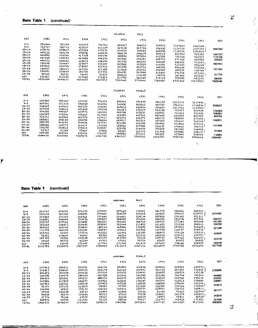
(
Basic Table 1 (continued)
GUJARAT
AGE
0-4 5-5
10-14 15-19 20 -24 25-29 30-34 3 5 - 3 9 40-44 ' 4 5 - 4 9 50 -54 55-59 60* TOTAL
iesi
596366 722 74 7 678572 469212 465802 467269 409553 2106 48 259262 18455 7 153491
89563 151407
4595689
1B91
75C359 782779 598847 465158 491546 499585 46B482 333 5 63 345796 182813 236645
81331 212040
5448675
1901
432409 625037 653363 49 05 96 417338 463288 42 84 75 320877 278007 167334 181730
76452 119969
46548 75
1911
761 914 611229 4792 76 448436 453494 496394 438439 340187 323715 2C1380 217354
90829 175205
5037852
1921 1931 1941 1951 1961
664817 769013 979700 1 147649 1660188 815430 857758 956500 1124730 1637145 676905 740584 802e00 1 118041 1300065 40613V 538679 5930 CO 812503 922382 360040 497854 612500 716 768 91C367 443962 470381 628700 671762 8353C5 431555 404244 540600 616252 712393 343068 372229 414100 523683 596249 321082 341016 368500 456693 532158 213868 270312 294900 309039 4397ee 236281 247888 315300 294758 4C3362 106612 134488 179700 180945 204545 213703 262160 374100 359099 481255
5233462 5506646 7060400 8331922 106339C2
5987260
1347737 1122166 959302
1667542
1221052
811738 685697
13802494
GUJARAT FEMALE
AGE 1881 1871 1901 1911 1921
0-4 604 505 780103 43 3783 776350 690919 5-9 667541 7213 15 593509 553054 760830
10-14 548505 4 696 56 545100 378691 56 8602 15-19 4C5530 3G8826 426 848 375258 34U6C3 20 -24 454550 499307 429772 484352 385095 2 5 - 2 9 434589 473352 434646 467462 410206 30-34 375352 441983 402279 432417 422293 3 5 - 3 9 285661 291C88 2864 90 296824 29 9917 40 -44 250159 341458 293656 319771 321385 4 5 - 4 5 180486 160775 163417 173729 189916 50 -54 156290 243018 19 5015 219507 225550 55-59 93312 72339 75922 77900 85325 60 » 189336 261765 162436 210420 240886 TOTAL 4686416 5141985 4439873 4765735 4941527
1931 1941 1951 1961 1971
791599 584100 1122273 1611950 , 803022 905700 1062141 1516834 \ 5508037 633634 704600 1311926 1 123003 ' 4764C7 541C00 743537 812538 1182959 523031 638500 741241 931583 1090961 445014 587600 652870 805555 942254 336371 482000 593699 6 7 7 2 3 4 ,
942254
342514 357300 456447 545345 ' 1568621 322288 355300 414842 515513 , 1141599 247960 26310C 276663 393773 1 1141599 216485 2953C0 281265 348558 , 741685 117733 141500 153982 178173 ' 741685 272403 3852C0 429849 538952 718865
5583182 664120C 7930735 9999448 12894981
Basic Table 1 (continued)
AGE 1881 1891 1901 1911 1921 1931 1941 19 51 1961 1971
0-4 261747 378759 2714 79 275987 297628 3192*1 381700 466834 666362 i 5-9 264478. 304 348 330100 273462 338075 344048 3831G0 370415 631951 J 2474265
10-14 273365 271723 314921 272893 274825 319C36 355800 374 342 501311 ' 15-19 212851 268446 243576 250827 20 8692 255244 286300 282378 357366 534122 20^24 212537 237562 215892 208 342 192104 208764 230500 237265 3094 89 401265 2 5 - 2 9 202222 2369C7 218450 203097 202469 211850 221600 231238 298942 330258 30-34 183122 163242 206867 182140 169964 173890 181000 201045 242429 , 531509 3 5 - 3 9 111278 166193 136184 126087 12 5413 14C980 141000 140097 198936 1
531509
40 -44 143331 81533 175516 142522 131443 1321B0 1568C0 153126 201515 ) 433030 4 5 - 4 9 78301 1186 67 90342 85706 86516 101530 1102C0 125471 1587C7 '
433030
50-54 1C9705 45556 120330 110270 10 7504 9932B 135C00 129422 162457 , 323103 5 5 - 5 9 39469 84772 42185 41913 47421 50724 65600 84857 84820 '
323103
60» 110299 63145 121485 111723 131365 130319 1674C0 23B160 2583 29 349706 TOTAL 2222 705 2420870 2487377 2284969 2313419 2487154 2816C0O 3030720 4072654 5377258
HARYANA FEMALE
AGE 1881 1891 1901 1911 1921 19 31 1941 1951 1961 1971
0 -4 227842 354311 256351 266116 290900 312896 3954C0 429905 625572 l 5 -9 241817 258651 29 2125 233178 301023 292991 351ICO 34150 2 552242 \ 2165899
10-14 201286 • 203238 246402 197933 221053 258492 3016C0 326075 433 138 ' 15-19 164 570 234579 188163 181930 161041 196990 22210G 246776 291243 444865 20-24 1B4927 203201 193212 180933 162674 189475 221600 232 565 296212 370191 2 5 - 2 9 165884 217509 186037 169962 162692 178187 199700 216013 278684 309967 30-34 162587 122761 185518 157925 147230 138729 168500 1794 74 2221C6 , 514810 3 5 - 3 9 51657 153152 113203 98987 97799 113089 126300 137426 175349 ' 40 -44 136140 62542 158172 128263 115512 105797 129900 138715 169917 , 381727 4 5 - 4 5 59532 108378 68713 63947 64840 79726 81400 92625 122748 ' 50-54 94039 30374 1366 24 90212 87533 75538 103800 101079 1200C5 , 240626 5 5 - 5 9 2 7 776 78186 29572 28421 32238 36919 33900 55801 58329 ' 60> 100974 4936 5 111531 92224 98046 9 5017 1167C0 142924 1718C1 231465 TOTAL- 1863231 2076247 2135623 18900 31 1942581 2072846 2457C0C 2643290 3517346 4659550
- J L/>
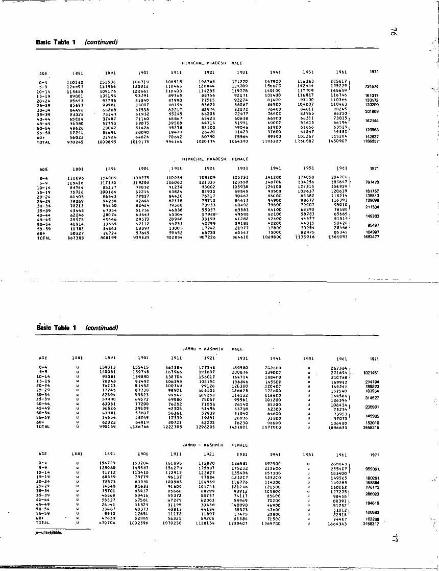
Basic Table 1 (continued) 0\
HIMACHAL PRADESH MALE
AGE
0-4 5-9
10-14 1 5 - 1 9 20 -24 2 5 - 2 9 30 -34 3 5 - 3 9 40 -44 45-49 50 -54 55-59 60* TOTAL
AGE
0-4 5-9
10-14 15-19 20 -24 2 5 - 2 9 30 -34 3 5 - 3 9 4 0 - 4 4 4 5 - 4 9 50 -54 5 5 - 5 9 60 » TOTAL
l e s i 1891 1901 1911 1921 1931 1941 1951 1961 1971
I10SC2 151536 106719 108515 106769 121220 147900 156263 2 0 5 6 1 7 i 124497 127956 120812 118463 128844 129709 1566CC 142444 195229 \ 724574 115655 109176 122661 110403 114235 119778 140CO0 137709 165659 J
89C01 105198 93791 89365 88756 92171 101400 116817 116746 161017 8565 3 92735 81340 87990 77515 92274 81400 93130 110364 130173 85657 99981 88007 88194 83625 86067 86500 104037 110463 120290 84498 68268 87538 82217 82974 82072 76400 84811 9B245 , 201859 53328 73149 61932 55245 68205 72477 764C0 83965 86220 ' 65C84 37487 71160 68867 65423 60638 66800 68311 73015 , 162144 34 380 52750 39875 39508 44718 51951 60000 58615 66194 1
49626 20042 51426 55278 52500 49046 62900 61666 6 3 5 2 9 , 123963 17241 38691 2 0090 19479 26420 31423 37600 41047 443B2 ' 56023 32926 64824 70642 80790 75564 99300 101267 115 204 142937
970245 10098 95 1010175 994 166 1020774 1C64390 1 193200 1 >5C 082 14509C7 1766957
HIMACHAL PRADESH FEMALE
1881 1891 1901 J 911 1921 1931 1941 1951 1961 1971
111896 154009 108275 110085 109509 125733 141200 174050 2047C6 , 115416 117140 ' 118203 116063 121833 123550 148700 134256 185647 \ 701478
89764 85317 198 32 91230 93002 105938 124100 122315 156929 ' 75728 100166 82214 83824 82930 89545 935CO 109637 120619 161757 81405 86343 77827 84430 76317 90467 86C00 88382 118214 139813 79269 942 58 82644 82118 79710 84417 94900 98677 116 39 2 129098 78212 54860 82424 79 300 73933 68492 79800 79007 95010 , 211534 43448 67354 51736 46838 55037 63883 64100 68 890 78180 1
62246 2 BO 74 63443 63304 5 7 9 8 8 - 49598 62100 58783 65665 | 149303 25978 45446 29573 28948 33193 41282 42400 44377 51514 1
41914. 13665 42112 44237 42799 39181 42200 44315 50426 , 95497 11782 34843 13897 1300 5 17242 21977 17800 30 254 28446 ' 50327 26724 5 7645 59 452 63733 60547 73000 B2975 85345 104997
867385 908199 909825 902634 907226 564610 1069800 1135918 1361093 1693477
Basic Table 1 (continued)
JAMMU - KASHMIR MALE
AGE 1881 1891 1901 1911 1921 1931 1941 1951
0-4 u 159013 155415 167384 177348 189580 200800 u 5-9 u 140051 159748 167966 191697 2008 76 23900C u
10-14 u 98081 139890 138 704 156017 164714 1BB4C0 u 1 5 - 1 9 u 78248 92452 106193 108150 136846 145500 u 2 0 - 2 4 u 76213 81452 100749 99126 120300 I2040C u 2 5 - 2 9 u 77745 87730 98901 106505 126628 122600 u 30-34 u 82394 99823 99547 109258 114132 1166C0 u 3 5 - 3 9 u 57990 69572 69880 75057 95561 101200 u 40 -44 u 63051 77200 76252 71558 76140 85200 u 4 5 - 4 9 u 36526 3 9109 42308 41496 53718 62300 u 50 -54 u 43981 5 3807 56361 57939 51040 64600 u 5 5 - 5 9 u 14554. 15749 17339 19851 26036 31800 u 60 » u 62322 64819 80721 82203 76230 98600 u TOTAL u 990169 1136766 1222305 1296205 1431801 15770C0 u
JAMMU - KASHMIR FEMALE
AGE 18B1 1891 1901 1911 1921 1931 1941 1951
0 -4 u 156729 153204 161898 172870 186581 192900 u 5 -9 u 125060 149587 156278 175887 175232 212600 u
10-14 u 71712 113410 112912 122827 135494 157300 u 1 5 - 1 9 u 68339 79779 96137 97584 1232C7 1232CO u 2 0 - 2 4 u 78573 830 31 1005B3 104959 116776 114200 u 2 5 - 2 9 u 74840 81633 91 600 101743 121246 121500 u 30-34 u 75701 83417 85666 88799 93913 105800 u 3 5 - 3 9 u 46868 53416 55372 55737 74117 85000 u 40 -44 u 55827 67581 67279 62003 59969 70200 u 4 5-45 u 26J41 31529 31195 30458 ' 4 0 0 9 0 46900 u 50-54 u 33467 40373 43813 44184 36323 47800 u 5 5 - 5 9 u 9910 12651 11172 11897 17475 23800 u 60* u. 47639 52985 56325 592C6 55584 71 500 u TOTAL u B707C6 1002596 1070230 1128154 12384C7 13697C0 u
1961
267364 , 271654 I 210768 > 169912 149241 157540 144564 i 126396 ' 106414 i
75234 ' 73953 I 37073 1
106480 1896633
1961
26064 3 i 2554C7 183400 • 149565 149285 160152 127275 j
9 84 5 6 ' 8 0 3 9 1 , 51752 ' 51012 i 22518 1
744E7 1664343
1971
1021461
214794 189823 182954
314527
235961
145985 153010
2458315
1971
959061
180251 168584 176112
286023
184615
100383 103288
2158317
u—unavailable. —J
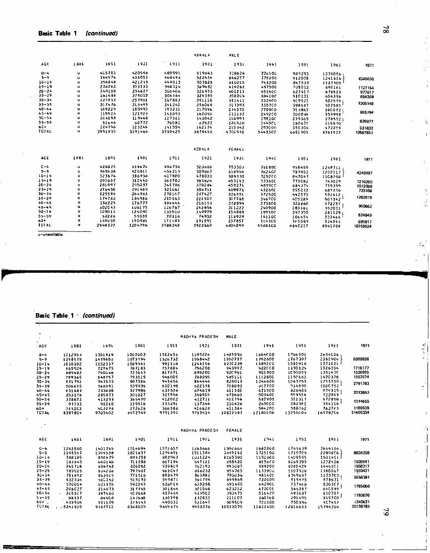
Basic Table 1 (continued) oo
KERALA KALE
AGE 1831 1651 1901 1911 1921 1931 1941 1951 1961
0-4 u 4G5703 42059d 489991 519843 7C8624 776100 983293 1279056 5-9 u 384974 433053 468493 522434 646277 775200 812008 1241616
10-14 u 356848 421215 449013 503828 610205 743 200 847539 1127300 15-19 u 273762 303133 348514 36 94 82 419261 457500 7JB012 690161 20-24 u 24B118 254627 306406 326970 40 2 2 1 3 451400 623417 678523 25-29 u 261463 275G02 306564 324385 3582C4 38410C 510131 604 356 30-34 u 2277 37 257961 ' 2 6 7 8 8 3 .291118 311411 3324C0 4C9521 522579 35-39 u 20 74 76 219495 241242 256069 313393 3307C0 398687 5075e5 40-44 u 169228 180993 193231 217096 234370 270900 313867 380022 45-49 u 118926 121923 143093 160090 211132 2492C0 300034 359958 5G-54 u 10 61 58 119448 127361 143042 156993 19810C 239365 278552 55-59 u 61o46 60772 76080 82927 120526 144 500 ' 180671 215 8 70 6C» u 124756 12 3246 141554 162174 210342 290000 35C306 472259 TOTAL u 2951855 3191466 3559425 3879458 4702551 5443300 6681901 8361927
KERALA FEMALE
AGE l eei 1891 1901 1911 1921 1931 1941 1 951 1961
C-4 u 428025 43 5674 496736 52 0 6 66 703300 761800 95B459 1 2 4 R 7 U 5-9 u 369638 420811 456213 509867 618954 762400 781952 1202117
10-14 u 3236 76 3B693d 417800 478030 589350 7252 CO 847047 11C8258 15-19 u 291637 312440 363702 3B5626 453143 533600 773C82 743029 20-24 u 281997 295057 345 786 378284 459271 483900 684 374 755359 25-29 u 2764 50 291469 321661 354751 409971 432600 555072 687226 30-34 u 225584 264363 278167 297427 326551 372500 442573 551412 3 5 - 3 9 u 174760 184986 210163 222507 30 7 7 6 8 3467CC 405289 50 3 34 2 40-44 u 158225 176777 194444 216153 222894 273BC0 323860 372257 4 5 - 4 9 u 102043 106175 126767 142 856 2C1222 240900 283161 352021 50-54 u 109011 124090 135510 149979 154889 199500 247305 281129 5 5 - 5 9 u 58226 5 5035 70116 74932 118929 141100 186454 222466 60* u 1490 50 150981 171183 191591 237857 314300 365589 514361 TOTAL u 2948322 3204796 3588248 3922669 4804099 5538300 6867217 8541788
4345630
1127154 977917 664398
1205148
995794
639977 631833
10587851
1971
4249997
1210250 1012068 723166
1282815
960662
624649 695917
10759524
u—unavailable.
Basic Table .1 " (continued)
MADHYA PRADESH
AGE 1881 1691 1901 1911 1921 1931 1941 1951 1961
0-4 1212953 1301319 1002002 1512656 1195224 1435596 1664000 1766 900 2654G26 5-9 1258578 1479652 1073794 1326732 1558442 1550737 1792600 1767397 2361904
10-14 1010182 1152337 1089541 991118 1243154 1270239 13892C0 1581913 1773121 15-15 665526 727475 737183 757 884 756208 943997 5220C0 1150624 1326354 20-24 685482 740046 723163 817671 695280 92C961 901900 1050055 1351430 2 5 - 2 9 789365 848757 793115 946005 788095 585101 1 112800 1150663 1470378 30-34 671792 943573 80 7386 943656 864446 828013 1346600 1063755 1253330 35-39 506655 56B591 539936 62019B 622358 718093 817700 914890 1000752 40-44 651687 733880 577986 633 534 674619 6115 81 671500 828483 R74319 4 5 - 4 5 253176 289973 301027 327956 348905 475663 503600 5<;9554 722865 5 0 - 5 4 378872 419293 365470 412002 412711 41C756 510900 512317 672858 55-59 93333 98210 139518 133291 137344 210426 2630C0 2 8 0 3 e i 3541C4 60 » 3C52C3 4C2296 272628 368588 416628 411384 584200 588062 762763 TOTAL 87878C4 9705402 847 2749 9791291 9713414 10622587 12180000 13255004 165782C4
1971
1716177 1526955 1552574
2791783
2013843
1314655 1169509
21455334
MADHYA PRADESH FEMALE
AGE 1881 1891 1901 1911 1921 1931 1941 1951 1961
C-4 1262580 14017b5 1014694 1572657 1263666 1550664 16B2eC0 1745639 2644114 5-9 1195557 1399538 1021837 1274691 1511386 1499142 1725100 1715704 22808C6
10-14 738185 8504 79 893758 802963 1011224 1C6 5 390 115030C 1409595 15014C1 15-19 583645 640140 711388 667194 647121 888420 8156C0 1069395 1232426 20-24 745718 836742 326282 939819 762193 993087 989200 1080429 14443C1 2 5 - 2 9 785525 8 i 4 2 8 6 79 7987 963047 810232 954765 1133900 1107328 1380067 33-34 7818J2 6635C5 771516 B93479 863882 793036 9814 CO 1349637 11237C3 35-39 432334 480142 515193 549871 5 b l 7 9 4 65986B 720100 319475 378631 40 -44 570054 621376 592243 626016 635288 591455 64290C 737466 8303C7 4 5 - 4 9 2C6C27 214673 317745 301844 301568 423212 470000 546387 64C599 50 -54 • 365507 387463 402B6B 437464 419502 393475 5164C0 493637 61C707 5 5-59 88537 86408 147665 1305O8 132833 211C07 260 110 291495 3197C0 60» . 435504 521178 375143 490031 531647 50 9 5 0 9 722300 7 50 396 9C7452 10TAL , , .e241B25 9169712 83U8019 9649 674 9458336 10533070 U 8 1 0 6 0 0 12816633 15794204
1971
8834258
1503641 1568317 1550431
2556381
1765080
1180076 1240621
20198785 - J
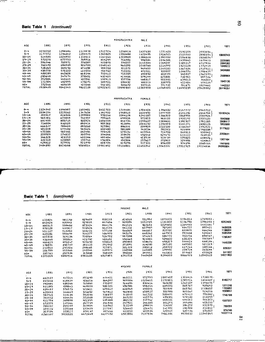
Basic Table 1 (continued) oo o
MAHARASHTRA
AGE 1881 1891 1901 1911 1921 19 31 1941 1951 19 6 1
0 -4 1C58752 12986B6 1133838 1512704 1258918 1637630 17714C0 2132205 2593654 5-9 1C 77 272 1256342 1354475 1363825 1553488 1673495 1916700 2125560 2890354
10-14 514985 1024953 1302611 1167266 1309969 1398329 1593700 2056 8)8 2328074 15-19 572C76 677753 769916 814250 746586 5965 84 1034300 1439663 16 754 13 20 -24 596946 710971 776087 923075 774557 1C45183 1C48 20C 1384147 1717916 25-29 76C4 70 8949 69 9 2 0 7 8 3 . 1048160 960200 U 5 8 7 8 0 1214700 1423128 1772719 30-34 728 255 645150 87 4198 958798 971075 949850 1145100 1260824 15 10511 35-39 489778 579320 O22350 702762 710331 872221 955900 1098775 1298437 40 -44 488C89 642608 668344 750513 715355 695992 8C2000 945927 1067370 4 5 - 4 9 285648 347674 378401 432 403 414466 579199 623800 730 543 99 7 7 26 50 -54 352004 441663 43 5541 510913 507756 460817 553300 639013 744C87 55-59 131504 152595 170275 185701 1844 92 300313 3387C0 411484 505120 60 • 372546 469659 42 5340 552301 585672 597545 77170C 791871 1023461 TOTAL 7828435 9342343 9802129 10922671 10692865 12305958 13769500 164900 39 20428882
1971
10660743
2335665 2094282 1949672
3404668
2588964
1640130 1442227
26116351
MAHARASHTRA FEMALE
AGE 1881 1891 1901 1911 1921 1931 1941 1951 1961
0 -4 1124342 1396507 118 3401 1602 703 1335484 17064C6 I 796500 2147772 2943712 5-9 1034154 1215162 1 34 7638 1341933 154B510 1622950 i e 7 7 7 0 0 2101250 2944799
10-14 705917 816506 1099989 970258 1094128 1241687 1386300 1868906 2083924 1 5 - 1 9 565 301 673049 732557 799665 698535 973805 963100 1320192 1533120 20-24 681935 8067 15 860524 1006559 832734 1C95637 1 183400 1392 620 1781185 2 5 - 2 9 716004 832020 892414 985702 913894 1064192 12045C0 132C271 1690123 30-34 666127 785439 850260 927891 896331 839938 1022100 1164267 1331521 3 5 - 3 9 401068 477100 563426 602 480 581389 743034 7915C0 921999 1056889 40 -44 432286 582 366 642 5 86 704420 679133 • 615944 714700 349913 930942 4 5 - 4 9 259509 274837 330790 354046 338476 492142 529400 61112 3 763539 50 -54 346328 403353 433386 491484 467385 4C2509 5150 00 579820 649 5 76 55-59 122310 123083 150743 156006 151506 257627 272900 329996 414843 60 » 429612 527931 50 IB 00 608705 619296 597331 806200 904196 1060 664 TOTAL 7484893 8914068 9589514 10551852 10156801 11653342 13063300 1 5512 525 19124836
10182424
1942909 2008417 1952988
3177622
2202691
1387184 1441649
24295884
Basic Table 1 (continued)
MYSORE
AGE 1881 1891 1901 1911 1921 1931 1941 1951 1961
0 -4 633824 881150 829609 838155 816316 931952 1073100 1296813 1749993 5-9 843425 8 20942 925995 847656 • 909994 103378 5 1131800 1236 790 1796154
10-14 880315 559488 873324 844174 841024 903653 1029 800 1265933 1451331 1 5 - 1 9 570128 48181f 522426 612C55 541332 63 7969 707300 934737 995421 20 -24 551127 513280 4662 36 577138 566389 598857 70770C 833975 964 246 2 5 - 2 9 623281 555699 5J6377 586970 592274 648232 667500 793458 534362 30 -34 607238 514138 530064 526702 ' 5 5 7 3 9 8 574265 5B47C0 702256 808017 35-39 431649 395869 421792 422691 456685 5C4885 529800 628104 73C545 4 0 - 4 4 466613 4002 47 43 56 90 454015 392840 4586 76 4982C0 564628 668164 4 5 - 4 9 1760 74 240737 28 1133 291942 271091 314280 387100 449550 521CC3 50-54 252013 250206 298085 317871 301723 330018 3597C0 417264 480144 55-59 101759 113365 145544 139973 150588 145885 179500 239728 263655 60» 235763 2579 78 315830 368459 39 6064 395951 440800 503687 677828 TOTAL 6373209 5992916 6582105 6B27801 6793718 7445458 8 294000 9866923 12040523
6252402
1406026 1198654 1026268
1796397
1445320
935331 911502
14971900
MYSORE FEMALE
AGE 1661 1891 1901 1911 1921 1931 1941 1951 1961 1971
0 -4 662427 517204 853290 875401 B63211 97 279 3 10876CC 1303415 17381 79 •, 6183717 5-9 655048 818639 926216 B64287 929306 1C25611 1170900 1285014 1814587 \ 6183717
10-14 792494 489349 763353 775097 764695 830416 965000 1262107 1393473 ' 1271318 1 5 - 1 9 511395 458843 46 9359 580 324 496984 598244 639000 868787 925052 1271318
2 0 - 2 4 629637 576573 522611 b29467 623765 6501CI 711900 065 761 It 08657 1155982 2 5 - 2 9 620645 548669 53 6652 567812 582850 658927 700700 600267 564216 1099851 3 0 - 3 4 587933 518135 542096 5 38 8 37 512055 561722 585600 675413 7 9 3 3 8 2 , 1745199 3 5 - 39 345532 334474 373508 353692 337100 415774 475C0C 529180 618359 1
40-44 421758 369898 422353 439389 382C32 397742 448000 494002 5663C0 , 1207207 4 5 - 4 9 153375 197344 2477 35 241536 237921 246385 3012C0 355694 4C5 210 ' 50-54 286237 264097 30 3934 316962 3122 89 299814 3141CC 384252 431575 , 789094 55-59 105172 105388 133405 117380 126463 126471 141900 1907OS 212812 1
874746 60* 3C7524 333007 378137 397266 410210 403534. 420400 520436 674007 874746
TOTAL 6281187 5931820 6472649 6697450 6583881 7187534 7561300 9535033 11545645 14327114 oo
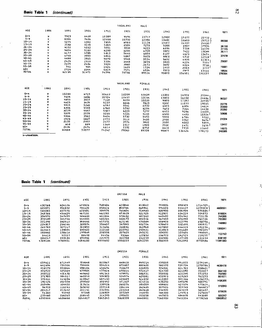
Basic Table 1 (continued)
AGE
0-4 5-9
10-14 15-19 20-24 25-29 30-34 3 5 - 3 9 40-44 4 5 - 4 9 50-54 55-59 60 + TOTAL
AG E
0 -4 5-9
10-14 15-19 2 0 - 2 4 25-29 30-34 35 -35 40 -44 4 5 - 4 9 50-54 55-59 60+ TOTAL
NAGAL AND MALE
1B81 1891 1901 1911 1921 1931 1941
u 99C5 6438 10389 9594 11717 12900 u 6391 7405 10558 10732 12351 13400 u 5274 4390 7855 8983 11138 133C0 u 35 82 3235 5205 6504 7203 8 200 u 4CC2 4162 5051 5010 6223 6200 u 5854 5183 6290 6204 6 700 5900 u 6177 4789 5813 5645 6859 6 ICC u b745 3993 4846 4887 5605 59C0 u 4498 3910 5670 5545 5554 560C u 2425 2313 3354 3448 3855 3900 u 2379 2426 3520 3980 3673 3500 u 741 9B4 1426 1635 1724 1400 u 2226 2244 4819 7571 6934 7500 u 621 99 51473 74796 79738 89536 936C0
NAGALAND FEMALE
1881 1891 1901 1911 1921 1931 1941
u 10289 6710 10633 10209 12439 13300 u 740 5 6806 10924 10457 12C94 13800 u 4853 3937 7110 8223 10220 9800 u 4605 34 79 5237 6666 7820 930C u 4915 5260 6597 5561 67 70 63 CO u 6306 5550 6 960 5792 6254 7600 li 6239 4547 5 82 7 6225 7277 64C0 u 5020 2579 3235 4 226 5103 6500 u 4366 3562 5404 5730 5493 5500 u 1826 1827 2770 3111 3435 2700 u 21 10 2357 3577 3976 3802 3500 u 600 839 1349 1517 1809 253C u 2134 2474 461 1 7370 6752 86( 0 u 60668 50077 74 242 79063 89308 958C0
1951
15 177 16653 14307
3937 7755 7422 6623 4732 6935 4226 4014 2063 7907
106551
1951
14909 16150 12397 11C77
6904 7364 9 296 4493 6784 3 762 40B2 1471 7735
136 424
1961
2 2 2 3 2 . 25713 24433 ' 17954 16170 15089 13654 , 12549 ' 113C3 i
7554 ' 7C38 i 3777 '
13464 191027
1961
2 3 3 4 4 , 24486 22755 ' 19015 14614 14430 13105 . 103341
9712 . 56 74 ' 5859 . 2179 I
11667 178173
1971
99368
26159 27145 25111
37479
25697
15581 19544
276084
1971
96337
23776 20580 20292
30666
21324
12417 14973
240365 u—unavailable.
Basic Table 1 (continued)
ORISSA MALE
AGE 1881 1891 1901 1911 1921 1931 1941 1951 1961 1971
0-4 63C568 626126 670326 768 406 62 0848 813022 7939C0 8983C9 12147C5 , 5-9 685671 751892 734120 853116 858784 869941 974C00 933439 1259308 \ 4669591
10-14 514883 657376 672401 709975 765824 714983 020900 834759 975884 > 15-19 348766 436655 467101 462253 47 3515 521523 512500 634228 704873 916824 20 -24 354 570 367455 3846B3 401804 378682 487360 460400 554942 705179 744268 2 5-29 372489 364716 445005 435264 448177 5535C6 567600 601858 761326 792280 30-34 371290 382513 398446 457372 415195 474089 5589C0 513795 658796 , i Aciaori 35-39 2248C7 264166 309374 356637 347845 402704 4 79 600 502835. 550971 ' iwrJoU 40 -44 265783 32714 7 302893 313656 318836 343948 427800 446315 431236 , i n o n i A 1 4 5 - 4 9 112663 139304 190423 232160 220742 255431 3120C0 334689 39C3E5 ' 50-54 183982 198618 199869 208558 207625 245231 30930C 327605 398065 , 55 -59 54615 57227 83498 94456 93366 127853 1567C0 182523 216220 1 722753 60 + 184C47 195436 19 49 61 221975 200 788 2322 59 332900 427595 451658 636146 TOTAL 4209134 4768331 505 8100 5535632 5350227 6C42255 6706500 7242892 6,770586 11041083
ORISSA FEMALE
AGE 1881 1851 1901 1911 1921 1931 1941 1951 1961 1971
0-4 659611 671549 70 364B 803867 648418 849214 e300C0 956533 1274164 5-9 641894 734501 734464 854214 873607 880620 582100 939 734 1278786 \ 4626478
10-14 418579 555864 590104 638674 710677 626555 724500 821703 8 5 8 6 3 1 ' 15 - 19 331522 425388 479905 477828 495014 571417 514700 614090 722607 864149 20-24 350522 430 4 70 449642 491343 479971 566731 555500 610395 772253 792002 2 5 - 2 9 371705 384317 462253 534903 524974 629381 653900 61B289 762253 861571 30-34 375111 413086 410547 487130 483689 521552 61220C 591366 6 3 6 1 7 3 , 1AOOOCfi 35-39 191424 242558 29 9582 351442 371327 414216 475200 495695 500791 ' 1428300 4 0 - 4 4 287494 334410 317616 339 9 26 365276 385009 4598C0 42 7 574 475624 , 4 5 - 4 9 567C0 118283 18 5092 207118 226134 262635 3075C0 339745 3646C3 ' 970090 50-54 204217 217657 221151 235594 233348 262618 334500 343 139 331657 , 55 -55 51360 55543 97368 106 809 105289 143595 164300 179913 207668 1 675529 60 + 275460 286265 208445 314395 290635 315258 4473C0 494878 543080 685347 TOTAL 4295599 4639883 5244817 5843 24 3 5338359 6448801 7C61500 7433054 6778260 10903532
oo
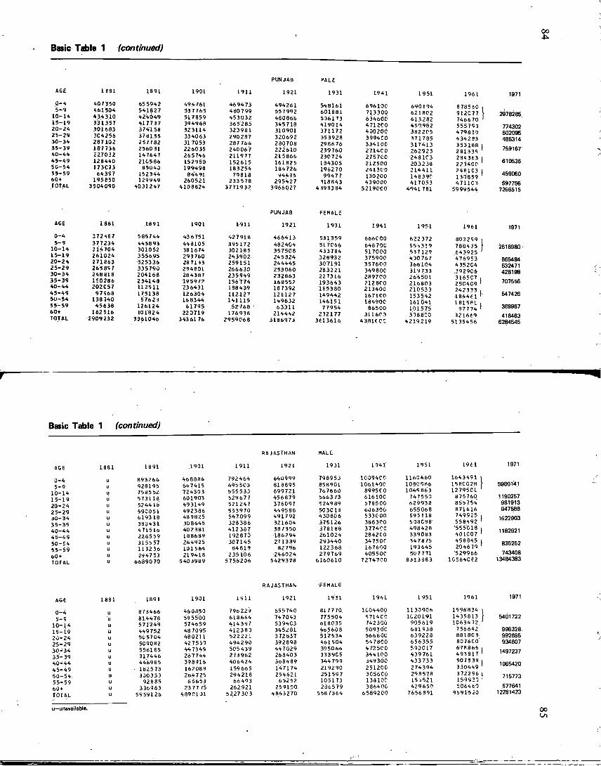
oo
Basic Table 1 (continued)
PALE
AGE
0 -4 5-9.
10-14 15-19 20-24 2 5 - 2 9 3 0 - 3 4 3 5 - 3 9 40 -44 4 5 - 4 9 50 -54 55-59 60* TOTAL
1 681
407350 461504 434310 331357 301683 3C4256 287102 187736 227032 128440 173C73
64357 195850
3504 090
1891 1901 1911 1921 1931
655942 494761 469473 494261 548161 541827 537755 480799 557992 601881 424049 517859 453032 480866 536173 417737 394968 365285 345718 419014 374158 323114 323981 310901 371172 378155 334063 290287 320692 353928 2 577 82 317053 287766 280708 298676 256031 226035 240067 222610 239760 147647 265746 211977 215866 230724 210586 152950 152 615 161825 194305
85040 199498 183254 184726 196270 152344 844 91 79818 94435 9947 7 129949 260521 233578 295427 318843
4031247 4108824 3771932 3966027 4399384
1941
696100 713300 634600 4712C0 400200 399400 334100 2714C0 27570C 212500 241300 130200 439000
5 2190 CO'
1951
690194 621802 613282 4509B2 382205 371785 317413 262923 248103 203238 214411 148390 417053
4941781
1961
978560 912077 746670 555753 4 79 810 4342e3 353188 281335 284363 223400 246103 1 130859 4711C3
5999544
1971
2978285
774302 602095 485314
759167
610536
459060 597756
7266515
AGE 1881 1891 1901 1911 1921
0-4 372467 585744 43 6751 427918 466413 5-9 377234 445893 443105 395172 48 2404
10-14 314704 301052 381674 302185 357508 15-19 261024 355695 293760 243902 245824 20 -24 271663 325336 28 7133 259151 244445 2 5 - 2 9 265857 335790 294801 266630 253060 3 0 - 3 4 248618 204168 284387 235949 232863 3 5 - 3 9 150286 234148 195972 156774 168552 40-44 202C57 112511 236431 168439 187392 4 5 - 4 9 97568 175138 126304 112127 121127 50 -54 138740 57623 168344 141115 149632 5 5 - 5 9 45638 126124 61795 52768 63311 60+ 162516 101824 220719 176938 214442 TOTAL 2909232 3361046 3436176 2959068 3186973
1931
531359 517066 433784 328932 307191 283221 227316 193643 165380 149442 146151 77954
232177 3613616
1941 1951 1961 1971
6660.00 622 372 803259 l 646700 5 5 i 3 1 9 788435 \ 2616980 517000 537129 .643925 ' 375900 430767 476953 665484 357600 366104 435204 532471 349800 319733 2929C6 428198 289700 264 501 316507 ,
707556 2128C0 216803 25C4C9 ' 707556 213400 210533 242333 ,
547426 167100 153542 1344 61 ' 547426 184900 161041 181581 ,
369967 86500 101575 97774 ' 369967 3 U 6 C 3 338800 321669 416463
4381CCC 4219219 51 35456 6284545
Basic Table 1 (continued)
AGE
3-4 5-9
10-14 15-19 20-24 25-29 3 0 - 3 4 35-39 4 0 - 4 4 4 5 - 4 5 50 -54 5 5 - 5 9 60 + TOTAL
AGE
0-4 5-9
10-14 15-19 2 0 - 2 4 25-29 3 0 - 3 4 35-39 40-44 4 5 - 4 9 50 -54 55-59 60 + TOTAL
RAJASTHAN MALE
1881 1891 1901 1911 1921 1931 1941 1951 196 1
u 893266 466886 792464 640999 798953 10094C0 1160460 1643491 u 928195 647415 695 503 818 89 5 858901 1061400 1080986 156CC28 u 758552 724333 555533 699721 767660 8995C0 1049 863 12795C1 u 5731 13 601903 529677 456879 5663 73 616100 747550 875760 u 524418 49 3149 521247 376097 524989 578500 629938 855754 u 590051 492386 553970 449588 503013 636300 655068 871616 u 619318 489825 547099 491792 433 806 533000 595118 7 499 2 5 u 383431 30 8645 328386 321604 375126 388300 538C93 558492 u 471516 402381 4123B7 387350 378188 3774C0 498428 555019 u 226559 188689 192870 186294 261024 2842CO 339083 401007 u 315557 264925 307145 271339 293440 34750C 347875 458845 u 113236 101564 84819 82796 122368 167600 193645 204679 u 29 47 53 219418 235106 246024 279769 40550C 507771 529966 u 6689070 5403989 5 755206 5429378 6160610 7274700 8313883 10564Ce2
RAJASTHAN FEMALE
1881 1891 1931 1911 1921 19 31 1941 1951 1961
873466 814478 571249 449752 50 5704 509082 558165 317446 4469 6 5
• 132578 3003 53
92885 336963
5959126
460853 59 5500 574659 48 7095 48 3211 427539 447345 267744 398916 162089 254725
85653 23 7 7 75
4890101
796229 618664 414397 412 3 83 522221 494 290 505439 273962 406424 159665 294218
66493 262921
5227303
655740 74 7043 5394C3 345281 372837 392898 447029 268403 368489 147174 254621
65252 259100
4863270
81T770 775504 618035 4O5603 512534 461504 39 50 66 3339C5 344799 219290 251557 105173 286579
5587364
1G04400 5714CC 742300 509300 566800 547800 472500 344100 349300 251200 305600 138100 386400
6589200
1130906 1020191
905 619 681938 639228 656355 590017 439761 433733 274394 298578 1 5 i 5 2 1 429650
7656891
1556834 • 1435613 10634 72, '
7 56642 8818C3 6076C0 678866 , 493617 1
507538 , 330449 1
372256 l 159523 1
506463 95915 20
1971
5980141
1190257 981913 947588
1622903
1182921
835252 743408
13484383
1971
5401722
996328 992695 934607
1497237
1065420
715773 677641
12281423
u—unavailable. 00
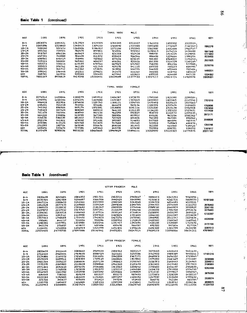
Basic Table 1 (continued)
TAMIL NADU
A G E 1 8 8 1 1 8 9 1 1 9 0 1 1 9 1 1 1 9 2 1 1 9 3 1 1 9 4 1 1 9 5 1 1 9 6 1
0 - 4 1 0 C 8 5 7 4 1 3 8 4 5 2 1 1 3 1 2 9 2 9 1 4 1 5 3 2 5 1 3 4 4 3 4 5 1 5 1 1 6 0 7 1 7 6 2 2 C 0 1 8 0 5 5 0 2 2 3 1 0 5 1 9 5 - 9 1 0 6 5 8 9 6 1 2 1 5 8 6 3 1 3 4 0 9 1 5 1 3 2 9 2 2 2 1 4 2 0 4 9 0 1 5 3 7 5 0 3 1 8 5 5 8 0 C 1 7 7 2 8 3 7 2 1 6 0 3 4 7
1 0 - 1 4 9 8 8 1 8 0 9 0 7 9 7 0 1 1 6 8 3 2 6 1 1 8 6 3 1 2 1 2 7 U 8 U 1 3 9 2 8 4 0 1 5 6 2 5 0 C 1 8 3 1 6 6 6 1 9 1 2 7 2 7 1 5 - 1 9 6 9 5 2 6 1 7 3 9 7 2 4 7 8 2 4 7 5 8 9 7 8 4 1 9 2 3 5 0 6 9 7 8 3 2 2 1 1 5 0 4 0 0 1 4 7 4 2 1 4 1 4 3 8 6 8 0 2 0 - 2 4 5 5 6 7 8 7 6 9 B 2 3 4 6 6 3 6 1 9 8 3 4 3 1 3 8 2 6 3 6 8 9 3 2 4 2 8 9 9 5 5 0 0 1 2 1 4 2 2 5 1 4 1 9 0 5 5 2 5 - 2 9 6 4 7 5 3 1 7 4 3 9 0 0 7 0 6 4 2 9 8 1 1 8 7 2 8 5 8 6 0 5 9 6 6 5 4 6 9 9 6 4 0 0 1 2 2 9 6 6 4 1 3 9 0 2 5 4 3 0 - 3 4 6 5 6 5 8 1 6 5 8 7 1 9 7 5 8 9 5 4 7 6 0 0 1 0 8 7 7 6 3 6 8 2 8 2 3 5 9 0 0 2 0 0 1 0 6 8 8 2 2 1 1 7 6 2 4 3 3 5 - 3 9 5 1 9 1 1 4 5 8 8 8 0 2 5 6 0 3 6 1 6 0 6 2 3 7 6 6 6 2 6 1 8 2 0 6 1 6 8 5 1 3 0 0 1 0 1 4 7 2 9 1 1 4 0 1 8 9 4 0 - 4 4 4 8 2 C 5 3 5 5 8 2 1 4 6 3 9 1 0 5 6 7 0 9 6 6 6 6 9 0 2 5 6 7 6 9 2 2 7 4 8 2 0 0 8 9 1 2 3 6 9 7 7 9 6 5 4 5 - 4 9 3 0 5 C 1 5 3 7 8 7 6 2 3 6 1 1 2 9 4 3 1 7 4 9 4 1 9 1 7 8 5 4 1 1 1 0 6 3 7 0 0 0 7 5 5 1 3 3 8 3 9 7 9 5 5 0 - 5 4 3 0 S 6 5 5 3 6 1 7 1 2 4 4 2 3 6 2 4 7 3 0 2 4 5 1 3 8 5 2 4 4 6 7 7 4 5 4 6 5 0 C 6 7 2 4 4 9 7 1 2 4 0 4 5 5 - 5 9 1 5 9 1 4 1 1 9 6 4 4 5 1 8 2 2 1 1 2 2 9 6 2 1 2 4 1 4 7 3 3 1 1 2 6 2 3 5 4 0 0 0 4 4 8 7 9 2 4 8 5 4 1 0 6 0 + 3 6 8 7 8 1 4 6 3 9 5 3 5 0 0 5 8 3 5 9 0 4 5 9 6 2 7 5 4 2 6 3 3 8 2 3 6 9 7 C 0 C 8 2 4 4 5 8 9 4 7 3 3 0 T O T A L 7 8 0 1 1 6 9 8 9 3 6 8 1 9 9 4 1 9 3 9 8 1 0 2 3 6 9 5 1 1 0 6 5 9 4 8 9 1 1 5 7 7 5 8 8 1 3 0 5 7 C C C 1 5 0 0 3 7 2 4 1 6 9 1 0 5 7 8
7862278
1841548 1771662 1576455
2801925
1204062 20828021
TAMIL NADU FEMALE
A G E 1 8 8 1 1 8 9 1 1 9 0 1 1 9 1 1 1 9 2 1 1 9 3 1 1 9 4 1 1 9 5 1 1 9 6 1
0 - 4 1 C 7 1 0 1 2 1 4 5 5 8 4 6 1 3 8 0 2 7 9 1 4 8 3 9 1 2 1 4 0 4 2 8 7 1 5 7 3 0 7 0 1 7 9 7 2 0 0 1 8 1 5 3 9 0 2 2 9 9 5 8 4 5 - 9 1 C 9 9 9 9 4 1 2 3 3 2 8 6 1 3 7 6 3 7 4 1 3 6 9 8 8 8 1 4 7 0 3 8 7 1 5 3 7 6 4 9 1 8 5 5 9 0 0 1 8 0 3 9 4 5 2 1 4 7 2 4 8
1 0 - 1 4 8 8 6 4 1 8 8 0 1 9 1 6 1 0 7 4 6 3 0 1 1 2 0 7 4 3 1 1 8 6 1 2 1 1 3 2 4 7 5 5 1 4 7 5 4 0 0 1 8 3 5 6 2 3 1 8 3 7 6 6 3 1 5 - 1 9 6 4 5 2 3 1 7 1 1 2 4 9 7 3 3 3 5 4 9 0 4 6 8 1 8 6 4 6 5 9 9 8 7 1 7 6 1 1 0 0 7 0 0 1 3 9 7 4 7 4 1 4 1 4 6 6 3 2 0 - 2 4 7 4 1 1 4 2 8 5 6 5 0 6 8 4 5 1 7 4 1 0 0 2 8 8 1 1 0 1 8 8 5 0 1 C 9 1 1 1 6 1 1 2 1 2 3 0 1 3 1 5 1 3 8 1 5 5 2 5 C 8 2 5 - 2 9 7 4 5 4 1 5 8 3 7 5 2 9 8 0 8 8 8 9 8 8 8 0 1 0 9 6 4 1 1 0 1 1 3 1 1 3 9 1 1 3 6 1 0 0 1 3 0 2 1 2 2 1 5 2 3 6 2 1 3 0 - 3 4 7 3 1 3 7 8 7 8 2 3 4 4 8 6 8 5 4 0 8 6 2 1 3 6 9 6 2 0 9 8 8 9 2 8 0 7 9 5 8 0 0 0 1 1 2 2 8 7 2 1 2 0 5 6 3 5 3 5 - 3 9 4 6 4 2 2 8 5 3 5 8 9 6 5 1 0 7 9 9 5 6 7 3 8 3 5 8 8 9 0 6 8 0 3 9 1 2 8 3 5 1 0 0 9 6 3 2 5 4 1 0 8 1 3 6 2 4 0 - 4 4 5 2 6 0 3 0 5 8 6 1 3 9 6 8 1 8 2 2 7 1 8 1 8 6 7 2 0 5 2 8 6 4 4 3 2 6 7 4 2 2 0 0 8 6 7 5 8 1 8 9 1 0 6 2 4 5 - 4 9 2 9 2 1 7 6 3 4 1 8 1 1 3 2 5 9 3 2 3 9 1 4 8 1 3 8 5 0 6 7 5 1 4 6 9 3 5 9 7 5 0 0 6 6 4 5 9 4 7 6 1 5 5 4 5 0 - 5 4 3 7 3 7 8 4 4 1 7 1 2 5 4 6 4 7 6 0 5 1 1 6 2 5 5 4 7 6 6 8 4 5 4 3 2 3 5 2 5 5 0 0 7 4 5 0 6 9 6 8 1 8 7 8 5 5 - 5 9 . 1 5 1 2 9 5 1 8 2 7 1 4 1 6 5 0 9 5 2 0 8 6 7 6 2 0 8 5 3 8 3 0 1 4 4 7 3 1 2 2 0 0 4 2 3 5 4 0 " 4 3 9 5 2 5 6 0 + 4 4 9 3 7 6 5 5 5 6 7 5 5 7 7 5 8 4 6 3 5 6 6 3 6 4 5 7 9 0 6 3 7 6 9 8 7 5 3 5 0 0 8 5 8 7 2 1 9 3 9 2 5 2 T O T A L 6 1 7 7 4 7 9 9 2 9 5 0 3 6 9 8 3 3 2 3 2 1 0 6 6 5 6 6 5 1 0 9 6 9 0 2 9 1 1 8 9 4 1 1 1 1 3 2 1 0 5 0 0 1 5 1 1 5 3 2 3 1 6 7 7 5 9 7 5
1971
7701010
1752698 1761650 1777409
2812171
2048826
1355766 '1161617 20371147
Basic Table 1 (continued)
U T T A R P R A D E S H M A L E
A G E 1 6 8 1 1 8 9 1 1 9 0 1 1 9 1 1 1 9 2 1 1 9 3 1 1 9 4 1 1 9 5 1 1 9 6 1 1971
0 - 4 2 6 2 0 6 2 0 3 2 4 5 6 0 4 3 0 8 6 3 5 2 2 9 2 1 5 1 1 2 8 1 2 2 1 4 2 9 4 5 6 6 7 3 8 8 4 4 C 0 4 3 6 3 2 5 3 5 5 6 3 6 5 4 i 5 - 9 3 0 7 0 7 6 4 3 2 8 2 5 0 9 3 2 5 4 6 8 7 3 3 6 6 7 0 8 3 4 4 0 4 2 0 3 5 4 8 9 9 0 4 1 3 2 6 0 0 4 2 6 1 3 1 6 5 6 0 8 5 7 3 \ 1 9 7 8 7 3 5 8
1 0 - 1 4 2 8 6 7 1 1 6 2 6 6 8 6 5 3 3 1 5 2 3 1 1 3 0 7 7 9 9 9 2 9 B 0 5 8 5 3 2 4 3 0 6 5 3 3 9 4 7 0 0 4 2 5 4 4 9 3 4 5 2 9 5 3 1 ' 1 5 - 1 9 1 8 5 2 8 2 6 2 0 7 7 4 7 3 2 1 6 9 5 6 8 2 1 5 9 2 6 9 2 0 9 9 2 8 8 2 2 9 8 7 0 5 2 3 5 4 7 0 0 2 9 7 4 5 4 9 3 1 6 1 2 5 2 3 9 7 8 4 5 0 2 0 - 2 4 1 9 4 9 5 7 5 2 1 2 8 8 3 2 2 3 8 3 6 8 3 2 1 8 1 2 6 7 2 0 0 5 0 2 0 1 9 7 4 4 4 6 2 2 8 5 C 0 0 2 6 4 5 9 0 9 3 0 0 5 9 2 7 3 2 4 7 1 9 6 2 5 - 2 9 2 1 3 7 6 7 2 2 1 4 7 9 3 2 2 2 2 5 7 4 5 2 2 5 7 3 9 1 2 1 0 3 1 9 9 2 3 3 6 2 4 6 2 4 5 8 3 0 0 2 7 0 4 7 0 8 2 9 9 3 4 7 6 3 2 7 5 4 4 0 3 0 - 3 4 . 2 1 0 6 2 8 1 2 2 C 8 7 1 8 2 1 8 6 5 6 3 2 1 3 7 5 1 6 2 0 3 0 1 6 7 2 C 1 8 8 1 4 2 2 2 8 8 0 0 2 4 5 5 2 9 7 2 6 8 4 2 2 1 . R71*l9n.7 3 5 - 3 9 1 2 2 0 5 4 4 1 3 9 7 1 6 1 1 4 1 0 9 9 0 1 5 0 0 9 1 0 1 4 8 3 0 2 4 1 7 3 1 6 0 5 1 8 4 6 1 0 0 2 1 4 1 0 8 7 2 2 3 3 6 5 6 , ' Of iM<U/
4 0 - 4 4 1 5 5 7 4 1 3 1 7 4 0 6 0 8 1 7 3 3 4 5 2 1 7 4 2 8 2 3 1 6 2 7 2 0 1 1 6 7 8 5 6 1 1 B 4 6 9 0 C 2 0 1 1 0 4 2 2 1 2 4 6 3 4 . 4 5 - 4 9 7 5 0 6 9 1 8 4 4 1 3 7 9 3 3 5 5 6 9 5 8 0 9 6 1 0 0 0 9 3 2 1 1 5 2 8 1 9 1 4 0 5 5 0 0 1 5 8 9 5 6 7 1 6 6 7 5 6 1 ' 5 0 - 5 4 1 1 4 0 3 8 6 1 1 9 7 9 9 1 1 2 2 0 9 8 5 1 2 0 2 2 4 6 1 1 3 1 9 2 7 1 2 9 2 6 9 4 1 4 2 0 1 0 0 1 5 3 5 0 8 0 1 7 1 0 4 7 0 , T 1 7 9 T Q Q 5 5 - 5 9 3 4 3 1 7 4 3 7 6 8 5 7 4 3 3 0 7 7 4 2 2 4 0 6 4 5 5 4 9 0 5 4 6 7 8 7 6 9 0 7 0 0 9 4 7 8 C O 9 1 7 7 1 4 ' J I / £ 199 6 0 + 1 1 1 4 1 9 1 1 2 4 2 2 8 3 1 2 0 6 9 1 9 1 2 1 4 7 9 9 1 2 3 1 8 3 4 1 3 7 8 6 1 5 1 6 9 1 3 0 0 1 2 1 4 7 5 9 2 4 3 3 2 9 0 3 2 8 7 0 1 3 T O T A L 2 2 5 7 3 4 5 5 2 4 7 7 8 7 5 5 2 5 0 9 7 8 8 6 2 5 1 4 2 9 4 1 2 4 4 5 1 3 0 1 2 6 1 4 7 0 1 4 2 9 6 3 9 1 C 0 3 3 3 9 8 8 6 6 3 8 6 3 4 2 C 1 4 7 0 1 6 4 2 1
U T T A R P R A D E S H F E M A L E
A G E 1 8 8 1 1 8 9 1 1 9 0 1 1 9 1 1 1 9 2 1 1 9 3 1 1 9 4 1 1 9 5 1 1 9 6 1 1971
0 - 4 2 6 3 5 6 7 8 3 3 1 1 4 4 3 3 0 8 8 6 6 3 2 9 1 9 4 3 5 2 8 5 1 9 1 2 3 0 3 0 2 1 7 3 8 7 3 1 0 0 4 3 2 2 6 1 3 5 4 0 1 6 3 9 5 - 9 2 7 1 2 4 4 5 2 9 6 5 9 3 4 2 9 6 9 6 3 5 3 0 5 0 7 2 9 3 1 2 3 1 0 1 3 2 5 7 C 8 6 3 7 1 2 9 0 0 3 9 8 9 3 8 9 5 0 4 5 C 4 1 \ 1 7 1 8 1 0 1 6
1 0 - 1 4 2 1 2 4 6 0 6 2 1 6 9 3 7 2 2 52 6 0 5 4 2 3 6 3 3 2 1 2 2 6 2 2 0 8 2 4 6 7 3 7 1 2 6 6 9 5 C 0 3 6 5 6 1 0 2 3 7 1 5 0 6 9 > 1 5 - 1 9 1 5 2 9 2 2 9 1 6 8 9 9 1 1 1 6 3 0 3 0 5 1 7 3 9 1 3 9 1 6 6 0 8 2 4 1 6 3 7 0 4 1 1 9 7 9 2 0 0 2 6 6 C 6 2 9 2 7 3 1 6 8 7 3 2 0 6 6 8 8 2 0 - 2 4 1 9 8 1 2 6 4 2 0 7 5 2 2 7 2 0 8 6 8 3 4 2 1 3 7 1 7 9 1 9 5 8 6 1 3 2 C 9 B 7 6 7 2 2 3 0 7 0 0 2 6 4 9 4 4 3 3 1 3 4 9 6 5 3 2 8 4 8 1 0 2 5 - 2 9 1 5 7 2 2 7 0 2 0 6 5 6 0 5 2 1 1 0 6 2 0 2 0 9 8 8 4 0 1 9 4 2 3 C 0 2 1 2 C 6 7 8 2 3 0 1 6 0 0 2 4 1 9 4 8 2 2 9 0 7 5 C 3 3 1 9 9 9 6 4 3 0 - 3 4 1 5 7 1 2 6 4 2 0 9 2 6 1 0 2 0 7 5 2 7 4 2 0 3 4 8 0 6 1 9 1 8 5 6 3 1 8 8 8 2 4 2 2 0 9 8 4 0 0 2 2 5 5 1 5 0 2 5 0 2 8 2 9 , 3 5 - 3 9 1 1 1 5 4 4 2 1 2 5 2 0 0 8 1 3 2 3 0 3 5 1 3 5 1 5 7 7 1 3 2 0 2 3 7 . 1 4 9 4 5 8 8 1 6 5 4 C 0 0 1 7 9 1 9 5 8 1 9 7 4 7 5 0 ' 4 0 - 4 4 1 5 4 2 5 0 5 1 6 6 3 7 6 2 1 6 9 2 9 9 0 1 6 3 5 8 9 2 1 5 3 5 8 6 1 1 4 9 5 8 0 9 1 7 1 1 0 0 0 1 7 7 7 0 1 7 1 8 5 6 7 6 0 , TH7QnQQ 4 5 - 4 9 6 8 4 4 4 9 7 3 8 2 6 3 8 3 9 1 3 9 8 3 1 0 2 7 8 5 3 2 7 5 9 8 7 4 5 5 1 1 7 3 8 C 0 1 3 2 8 2 0 9 1 4 3 8 3 3 7 1 JO f WHO
5 0 - 5 4 1 1 2 3 1 0 3 1 1 9 2 4 8 5 1 2 0 2 2 3 5 1 1 5 4 8 2 4 1 0 9 7 2 9 7 1 1 0 8 4 9 2 1 2 4 7 5 0 0 1 3 2 2 6 5 8 1 3 9 3 6 5 2 , 2 5 3 0 2 7 4
5 5 - 5 9 3 2 5 7 1 6 3 4 5 8 3 7 4 0 5 6 5 5 3 7 2 4 1 0 3 9 7 0 7 4 4 5 3 9 5 3 5 6 6 0 0 0 7 4 2 1 8 4 B 0 3 7 B 4 ' 6 0 + 1 3 3 5 7 7 2 1 4 8 5 4 0 7 1 4 3 6 9 8 5 1 3 2 0 1 5 3 1 2 9 7 2 9 9 1 4 2 3 0 4 1 1 6 7 5 1 0 0 1 2 0 2 0 4 2 2 2 0 4 1 6 4 2 6 9 0 3 7 5 T O T A L 2 1 2 5 3 9 4 3 2 3 0 4 8 0 6 4 2 3 5 2 7 4 2 4 2 3 0 0 9 3 3 2 2 2 2 1 8 5 6 4 2 3 6 2 9 7 4 0 2 6 8 9 2 8 0 0 3 0 1 1 6 8 7 6 3 5 1 1 2 2 0 0 4 1 3 2 4 7 2 3
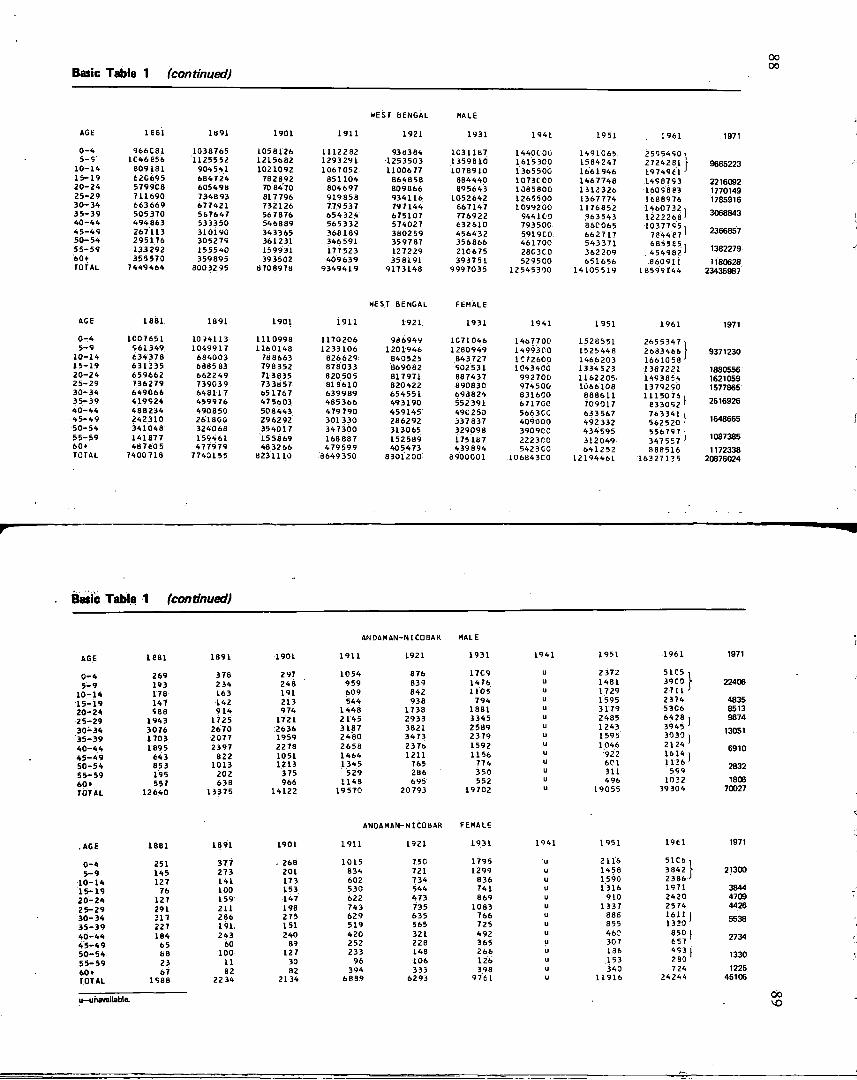
Basic Table 1 (continued) oo oo
WEST BENGAL MALE
AGE 1881 1891 1901 1911 1921 1931 1941 1951 1961
0-4 966C81 1038765 1058126 1112282 93B384 1031187 1440C00 1491065 2555450 5-5 1C46656 1125552 1215682 1293291 1253503 1359810 16153C0 1584247 2724281
10-14 809181 904541 1021092 1067052 11006 77 1078910 1365500 1661946 1974961 15-19 620695 684724 782892 851104 864858 884440 1073C00 1467748 1458793 20 -24 5799C8 605498 70 8 4 70 804697 809866 89 5643 1085800 1312326 16058 83 25-29 711690 734893 817 796 919858 934116 1052642 1265500 1367774 1688976 3 0 - 3 4 663669 677421 732126 779 537 797144 867147 1099200 1176852 1460732 3 5 - 3 9 505370 567647 56 7876 654324 675107 776922 944100 963543 1222268 40 -44 494863 533350 546889 565332 574027 632610 793500 86C065 1037755 4 5 - 4 5 267113 310190 343365 36B189 380259 456432 5919C0 662717 784487 50 -54 295176 305279 361231 346 591 359787 356866 461700 543371 6855e5 5 5 - 5 9 133292 155540 159931 177 523 127229 210675 2BO3C0 362209 . 454982 60* 355570 359895 393502 409 639 358191 393751 529500 651656 860511 TOTAL 7449464 80032 95 B70B9 78 9349419 9173148 9997035 12545300 14105519 18599144
1971
9665223
2216092 1770149 1785916
3068843
2366857
1382279 1180628
23435987
HEST BENGAL FEMALE
AGE 1881 1891 1901 1911 1921 1931 1941 1951 1961
0 -4 1007651 1094113 1110998 1170206 986949 1C71046 1467700 1528551 2655347 5-9 561349 1049917 1160148 1233106 1201946 1280949 14993C0 1525448 2683466
10-14 634378 684003 788663 826629 840525 843727 1C72600 1466203 1661058 15-19 631335 6885 83 798352 878033 869082 902 531 1043400 1334523 1387221 20-24 659662 662249 713835 620 505 817971 887437 992700 1162205 1493854 25-29 736279 739039 733857 818610 820422 890830 974500 1066108 1379250 30 -34 649066 648117 651767 639989 654551 698824 831600 888611 11150 7 6 3 5 - 3 9 419524 459976 475603 485366 493190 552391 671700 709017 633052 4 0 - 4 4 488234 490850 508443 479 790 459145 490 250 5663CC 633567 763341 4 5 - 4 9 242310 261800 296292 301330 286292 337837 409000 492332 562520 50-54 341048 32406B 354017 347300 313065 329098 390900 434595 556757 55-59 141877 155461 15 5869 166887 152589 175187 2223C0 312049 347 5 57 60* 487605 477979 48 32 66 479599 40 5 4 73 439694 542300 641252 888516 TOTAL 7400718 7740155 6231110 8649 350 8301200 8900001 106843C0 12194461 16327135
9371230
1880556 1621059 1577865
2516926
1648665
1087385 1172338
20876024
Basic Table 1 (continued)
ANDAMAN-NICOBAR
AGE
0 -4 5 -9
10-14 15-19 20-24 25-29 30-34 3 5 - 3 9 4 0 - 4 4 4 5 - 4 9 50 -54 5 5 - 5 9 60 * TOTAL
i e a i 1891 1901 1911 1921 1931 1941 1951
269 378 297 1054 876 17C9 u 2 372 193 234 248 959 839 1476 u 1481 178 163 191 609 642 1105 u 1729 147 142 213 544 938 794 u 1595 588 914 974 1448 1738 1881 u 3179
1943 1725 1721 2145 2933 3345 u 2485 3076 2670 2636 3187 3821 2589 u 1243 1703 2077 1959 2480 3473 23 79 u 1595 1895 2397 2278 2658 2376 1592 u 1046
(43 822 1051 1464 1211 1156 u 922 853 1013 1213 134 5 765 774 u 601 195 202 375 529 286 350 u 311 557 638 966 1148 695 552 u 496
12640 13375 14122 19570 20793 19702 u 19055
1961
5105 •, 39C0 \ 2711 ' 2374 5306 6428 , 3945 ' 3030 , 2124 ' 1614 , 1126 '
599 1032
39304
22406
4835 8513 9874
13051
6910
2832 1806
70027
ANDAMAN-NICOBAR FEMALE
. AGE
0-4 5-9
10-14 15-19 2 0 - 2 4 2 5 - 2 9 3 0 - 3 4 3 5 - 3 9 4 0 - 4 4 4 5 - 4 9 5 0 - 5 4 5 5 - 5 9 60 + TOTAL
1861
251 145 127
76 127 291 317 227 184
65 88 23 67
1588
1891 1901 1911 1921 1931. 1941 1951 1961
377 . 268 1015 750 1795 u 2116 51C6 273 201 834 721 1299 u 1458 3842 141 173 602 734 836 u 1590 2386 100 153 530 544 741 u 1 316 1971 159 147 622 473 869 u 910 2420 211 198 743 735 1083 u 1337 2574 266 275 629 635 766 u 888 1611 191 151 519 565 725 u 855 13 30 243 240 420 321 492 u 460 850
60 89 252 226 365 u 30 7 657 100 127 233 148 266 u 136 453
11 30 96 106 126 u 153 280 82 82 394 333 398 u 340 7 24
22 34 2134 5889 6293 9761 u . 11916 24244
1971
21300
3844 4709 4426
5538
1330
1225 45106
u—unavailable. 00
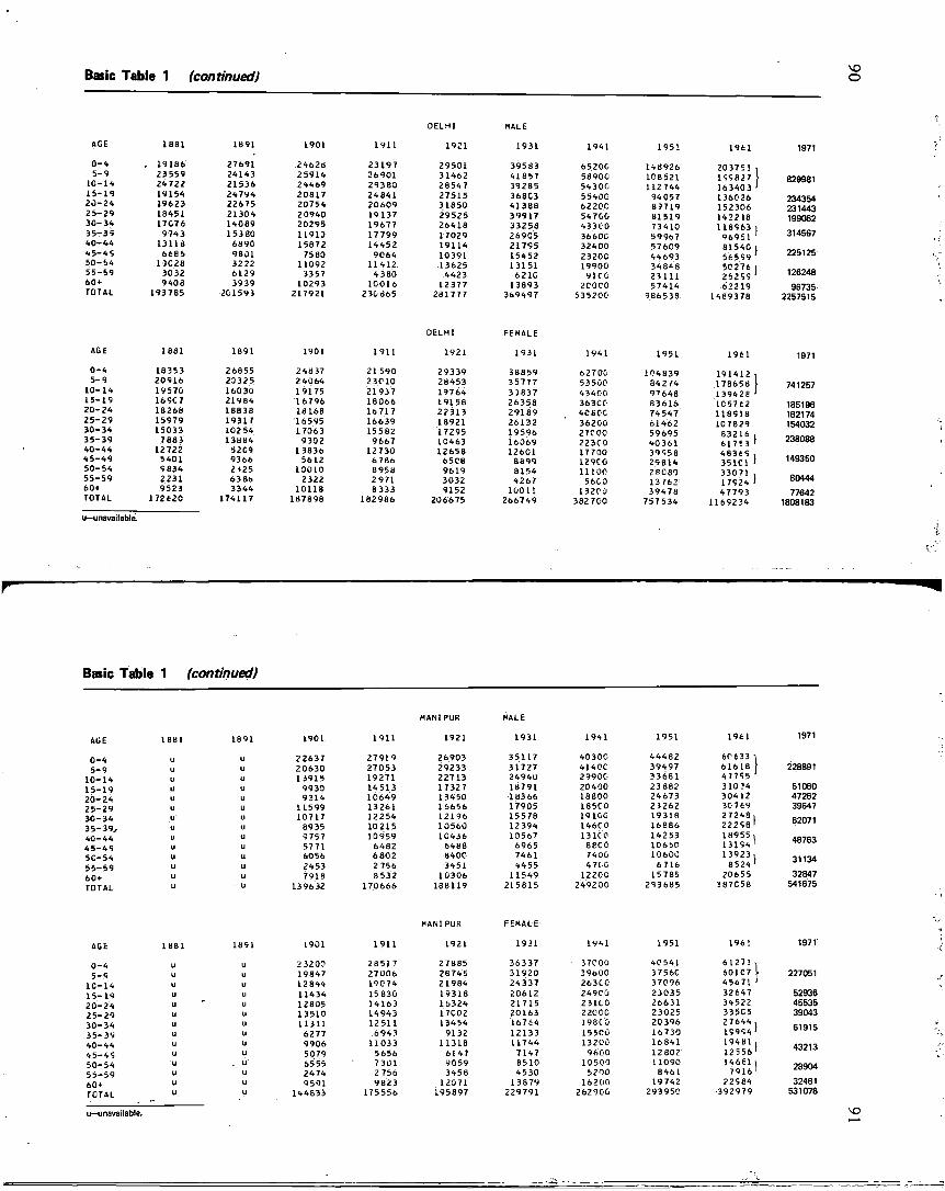
Basic Table 1 (continued)
DELHI MALE
AGE 18B1 1891 1901 1911 1921 1931 1941 1951
0-4 . 19186 27691 24628 23197 29501 39583 65200 148926 5-9 23559 24143 25914 26901 31462 41857 58900 108521
10-14 24722 21536 24469 29380 28547 39285 54300 112744 15-19 19154 24794 20817 24841 27515 368C3 55400 94057 20 -24 19623 22675 20754 20609 31850 41388 6220C BJ719 2 5 - 2 9 18451 21304 20940 19137 29525 39917 547GC 81519 30-34 17G76 14089 20295 19677 26413 33258 433C0 73410 35-35 974 3 153 80 11913 17799 17029 269C5 3660C 59 967 40-44 13118 6890 15872 14452 19114 21755 32400 57609 4 5 - 4 5 6685 9801 75 80 9064 10391 15452 2320C 44693 50-54 10C28 3222 11092 11412 13625 131 51 19900 34 84 8 55-59 3032 6129 3357 4380 4423 6210 91C0 23111 60* 940B 3939 10293 10016 12377 13893 2C0C0 57414 TOTAL 193785 201593 217921 230 865 281777 369497 535200 986538.
DELHI FEMALE
AGE 1881 1891 1901 1911 1921 1931 1941 1951
0-4 18353 26855 24837 21590 29339 38859 62700 104839 5-9 20916 23325 2 4064 23010 28453 35777 53500 84274
10-14 19570 16030 19175 21937 19764 33837 43400 97648 15-19 165C7 21984 16796 18066 19158 26358 363CC 83616 20 -24 18268 18838 13168 16717 22313 29189 4C60C 74547 2 5 - 2 9 15579 1931 1 16595 16639 18921 26132 36200 61462 30-34 15033 102 54 1 7063 15582 17295 19596 27000 59695 3 5 - 3 9 7883 13884 9302 9667 10463 16069 22300 40361 40 -44 12722 5209 1 3836 12730 12658 12601 17700 39558 4 5 - 4 9 5401 9366 5612 6786 65C8 8899 129C0 29B14 50-54 5834 2125 10010 8958 9619 8154 11100 28080 5 5 - 5 9 2231 6386 2322 2971 3032 4267 5600 13762 60» 9523 3344 10118 8333 9152 10011 13203 39478 TOTAL 172620 174117 18789B 182986 206675 266749 382 700 757534
203751 , 155827 } 1 6 3 4 0 3 ' 136026 152306 142218 118563 )
96951 ' 81540 l 56559 ' 50276 1 25255 1
62219 1489378
1961
191412 17865B 139428 • 105762 118518 107829
83216 1 61753 1
48365 , 351C1 I 33071 . 1 7524 I 47793
1165234
828981
234354 231443 199062
314567
225125
126248 96735
2257515
1971
741257
185196 182174 154032
238088
149350
80444 77642
1808183
u—unavailable:
r
Basic Table 1 (continued)
AGE
0-4 5-9
10-14 15-19 20 -24 25-29 30 -34 3 5 - 3 9 , 40-44 4 5 - 4 5 5C-54 55-59 60* TOTAL
AGE
0-4 5-9
10 -14 15-19 20 -24 25-29 30-34 35-39 40-44 4 5-4 5 50-54 55-59 60* TOTAL
1901
22637 20630 13915
99 30 9314
11599 13717
89 35 9757 5771 6056 2453 7918
13 96 32
1901
2 3200 19847 12844 11434 12805 13510 11311
6277 9906 5079 6555 2474 9591
144833
1911 1921 1931 1941
27919 26903 35117 40300 27053 29233 31727 41400 19271 22713 24940 2 99 00 14513 17327 18791 20400 10649 13450 18366 18800 13261 16656 17905 18500 12254 12196 15578 19100 10215 10560 12394 146C0 10959 10436 10567 13 100
6482 6488 6965 seoo 6802 8400 7461 7400 2 756 3451 4455 4 7C0 8 532 10306 11549 12200
170666 188119 215815 249200
HANI PUR FEMALE
1911 1921 1931 1941
2851 7 27885 36337 37000 2700b 28 745 31920 39600 19074 21984 24337 263C0 15 830 19318 20612 249C3 14163 16324 21715 231C0 14943 17002 20163 22000 12511 13454 16764 198C0
6943 9132 12133 15500 11033 11318 11744 13200
5656 6147 7147 9600 7301 9059 8510 10500 2 756 3458 4530 5200 9823 12071 13879 16200
175556 195897 229791 262900
1951
44482 39497 33681 23882 24673 23262 19318 16886 14253 10650 10600
6716 15785
293685
1951
40 541 3756C 37096 23035 26631 23025 20396 16730 16 841 12802 11090
8461 19742
293950
1961
60633 I 61618 47755 ' 31034 30412 3C769 2 7 2 4 8 , 22256 ' 1 8 9 5 5 , 13154 1 13923 ,
8 5 2 4 ' 20655
387C58
1961
6 1 2 7 1 , 60107 45671> 32647 34522 335C5 27644 , 1 9 9 5 4 1
1 9 4 8 1 , 1 2 5 5 6 1
1 4 6 6 1 , 7916 '
22564 392979
228891
51060 47262 39647
62071
48763
31134 32847
541675
227051
52936 45535 39043
61915
32481 531078
u—unavailable.
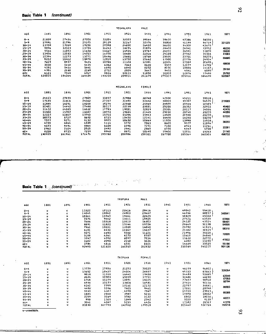
Basic Table 1 (continued}
MEGHALAYA MALE
AGE l t e i 1891 1901 1911 1921 1931 1941 1951 1961 1971
0 -4 21859 27436 2 7008 33204 32355 39064 396 00 47386 58550 I 5-9 17591 21796 25373 28 129 32267 32976 38800 41 155 54718 \ 221223
10-14 13759 1 T069 19250 20598 24890 26455 360CC 34 300 43675 ' 15 -19 9856 12323 1 3736 16243 18274 21874 284C0 26541 33702 46220 20 -24 9566 11093 11658 13467 14924 19787 242C0 26591 33839 39836
.25-29 13406 12583 14713 16770 18480 22316 25100 27542 34366 41069 30 -34 12394 12273 13771 15496 15881 18765 23500 23701 30209 i e o o o n 3 5 - 3 9 9232 10412 10878 12919 13750 15682 17500 20776 249C4 1 D o t u U 40-44 . 76C9 89 57 9436 10788 11358 12391 1230G 17559 2C695 i 4 5 - 4 9 3830 5140 5125 6382 7063 8620 83C0 12C77 14799 ' 48808 50-54 4351 5416 5641 6696 6 840 8252 80 00 10886 14 1671 55-59, 4701 2160 2169 2712 2809 3647 3400 4541 6595 ' 29169 60* 6121 7549 6767 9816 10123 11850 102C0 12876 17480 25762 TOTAL 1350J5 154204 165525 193220 209014 241679 2753C0 335931 384659 520967
MEGHALAYA FEMALE
AGE 1881 18 H 1901 1911 1921 1931 1941 1951 1961 1971
0-4 24113 27893 2 7809 33897 32988 38768 42500 45211 59028 l 5-9 17135 21606 24362 27357 31493 32442 383C0 39397 54575 \ 219589
10-14 11885 16251 18200 19274 22960 24989 29900 30 938 405C5 ' ' 15 -19 11401 14942 17498 20117 22739 23531 25200 28352 32933 45480 2 0 - 2 4 11632 14385 16102 17793 19031 22819 25300 28117 34586 42476 2 5 - 2 9 14402 14707 16407 18772 19821 21465 25C00 28040 35230 44286 3 0 - 3 4 12227 12817 13740 15710 15394 15953 18500 20558 26250 , 3 5 - 3 9 10573 8727 86 92 8723 10450 12141 14400 16260 18278 ' 57220 4 0 - 4 4 7577 9271 9132 9975 10630 10869 115C0 13998 16518 , 4 5 - 4 9 4735 4844 43 89 5114 5772 7063 B600 9C77 11096 1 38250 50-54 4073 5691 5866 6600 6396 7251 7100 8943 11261 , 55 -59 2962 2104 2020 2492 2441 2885 6000 4147 4738 ' 22291 60* 8220 8723 72 58 9948 8871 10145 154CC 12031 15263 21140 TOTAL 140935 161961 171475 195780 208986 230321 267700 285069 360301 490732
T
Basic Table 1 (continued) '
AGE
0 -4 5-9
10-14 15-19 20 -24 2 5 T 2 9 30-34 3 5 - 3 9 40 -44 4 5 - 4 5 50 -54 5 5 - 5 9 60 » TOTAL
1881 1901
13322 14045 10161
73 76 7686 8891 7961 6181 5071 3188 3347 14B2 3784
9 2495
1911
17113 19042 13563
9442 10318 11822 10031
8432 6693 4361 4092 2098 4816
121820
TRIPURA
1921
20416 24903 19461 13211 13113 15146 13519 11467
9310 6173 6097 2148 6551
161515
1931
29416 29687 22625 15925 16303 19728 16040 14637 11221
8587 7036 3626 8101
202932
1951
49342 46958 38828 27421 24120 29649 23792 25482 21956 15 600 11620 6392
14689 335589
1961
95410 • 88237 65388 • 43533 43524 50178 41515 | 38e25 1
30220 i 24846 1
22752 I 13260 1
33525 591237
1971
348541
67996 56401 54856
98316
72028
47802 55186
801126
AGE
0 -4 5-9
10-14 15-19 20-24 25-29 30-34 35-39 40-44 4 5 - 4 5 50-54 55-55 60* TOTAL
1681 1901
1 3779 13652
9018 8624 6748 69 38 6162 4496 3233 1883 2249
990 3061
80830
1911
17956 18437 11310 1C903 10279 10177
7799 5596 4327 2 548 3 069 1305 4087
107793
1921
21253 240C4 16442 15059 13591 13608 10110
76G5 6399
' 3987 3782 1849 5233
142922
1931
30025 28857 1943 8 17711 18225 16581 12132
9461 7567 5231 5122 2342 6426
179518
1951
46199 45 333 34489 31480 2 745 7 27414 22757 1 7661 13333 10598
8802 5335
1 2382 303440
1961
96812 • 87863 55885 • 462 60 50910 5C116 36661 : 28748 23913 | ,18042 1
18036 i 9135 1
2836 7 550763
1971
339264
63540 57050 58794
88983
60088
40221 47276
755216
u—unavailable.
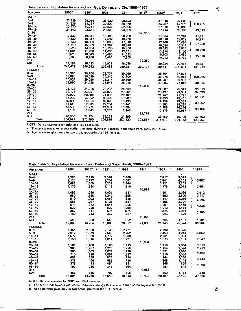
Basic Table 2 Population by age and sex: Goa, Daman, and Diu, 1900—1971 Age group 1900a 1910a 1921 1931 1941b 1950a 1961 1971 MALE 0-4 27,529 29,054 28,420 29,603 31,919 37,605 1 5-9 34,539 31,787 32,823 35.158 34,787 42,270 f 166,455 10-14 32,470 30,351 30,833 32,986 37,870 38,805 J
166,455
15-19 21,842 23,551 20,338 24,900 27,274 28,180 43,572 0-20
24,900 140,915
27,274 28,180 43,572
20-24 17,827 19,841 16,496 20,268 140,915
21,864 25,992 41,131 25-29 19,332 19,347 17,692 18,736 20,876 22,579 34,811 30-34 16,730 16,900 16,886 17,376 17,766 20,084 }
34,811
35-39 14,719 15,809 14,962 16,676 16,694 16,344 } 57,260 40-44 15,026 14,904 13,730 15,800 15,682 15,914 } 38,298 45-49 11,894 11,286 11,056 12,791 13,970 13,106 } 38,298 50-54 10,628 10,643 10,460 11,523 10,503 12,459
.} 25,556 55-59 6,706 6,956 6,455 7,508 10,012 8,739 .} 25,556 21+ 139,260
10,012 8,739
60+ 14,197 16,413 15,937 16,056 20,924 20,457 24,131 Total 243,439 246,842 236,088 259,381 280,175 280,141 302,534 431,214
FEMALE 0-4 28,385 30,150 28,774 30,040 35,804 37,024 ~) 5-9 33,596 30,689 32,240 33,700 38,078 40,913 \ 160,325 10-14 30,924 29,025 28,217 30,150 35,297 36,836 J
160,325
15-19 21,966 24,996 21,944 25,226 27,986 27,018 40,014 0-20 140,803
27,986 27,018 40,014
20-24 21,125 24,918 22,298 24,309 24,887 26,543 35,513 25-29 22,775 23,951 23,072 23,361 23,497 23,901 34,035 30-34 19,922 20,388 21,038 22,187 21,747 21,795 } 54,614 35-39 15,202 16,052 16,398 18,287 19,830 18,451 } 54,614 40-44 16,899 16,814 16,020 18,495 19,799 19,265 } 39,252 45-49 11,640 12,005 12,254 13,441 14,663 15,235 } 39,252 50-54 13,500 13,775 12,933 13,894 13,285 16,376 } 30,104 55-59 7,189 7,843 7,369 7,940 12,876 10,667 } 30,104 21 + 162,758
10,667
60+ 20,956 21,774 22,259 21,299 28,169 30,109 32,700 Total 264,079 272,380 264,816 282,329 303,561 315,918 324,133 426,557
NOTE: Data unavailable for 1881 and 1891 censuses. a The census was taken a year earlier than usual during this decade in the three Portuguese territories. b Age data were given only in two broad groups in the 1941 census.
Basic Table 3 Population by age and sex: Dadra and Nagar Haveli, 1900—1971 Age group 1900a 1910a
v . 1921 s "1931 1941b ' 1951 1961 1971 • MALE 0-4 1,360 2,219 2,026 2,600 2,817 5,012 5-9 2,123 2,177 2,754 3,007. 2,841 4,502 \ 16,882 10-14 1,687 1,509 2,237 2,544 2,731 3,307 J 15-19 1,176 1,224 1,112 1,510 1,775 2,012 2,864 0-20 10,989 20-24 1,096 1,246 1,007 1,537 1,581 2,096 2,512 25-29 980 1,338 1,240 1,698 1,892 2,609 2,717 30-34 870 1,092 1,059 1,325 1,547 2,219 } 4,594 35-39 888 1,097 1,128 1,657 1,595 2,004 } 4,594 40-44 671 872 1,045 1,206 1,291 1,468 } 3,649 45-49 539 728 822 1,098 1,019 1,454 } 3,649 50-54 367 441 576 676 825 1,045 } 2,365 55-59 180 243 357 507 526 629 } 2,365 21 + 10,020 60+ 449 568 645 652 905 1,167 1,381
Total 12.386 14,754 16,008 20,017 21,009 21,345 29,524 36,964 FEMALE 0-4 1,454 2,398 2,138 2,721 2,790 5,376 5-9 2,012 1,939 2,643 2,762 3,453 4,243 f 16362 10-14 1,577 1,333 1,772 1,969 2,201 2,894 J 15-19 1,150 1,376 1,011 1,791 1,676 2,161 2,947 0-20 10,364 20-24 1,101 1,486 1,100 1,735 1,716 2,604 3,013 25-29 905 1,237 1,275 1,758 1,754 2,594 2,713 30-34 906 1,063 1,022 1,256 1,391 1,926 } 4,508 35-39 715 896 1,057 1,327 1,210 1,586 } 4,508 40-44 658 739 822 794 1,144 1,366 } 3,443 45-49 378 466 689 710 868 1,119 } 3,443 50-54 376 412 464 551 645 895 } 2,090 55-59 197 285 345 364 487 514 } 2,090 21 + 9,068 60+ 465 636 702 505
9,068 852 1,161 1,630
Total 11,894 14,266 15,040 18,243 19,432 20,187 28,439 37,206
NOTE: Data unavailable for 1881 and 1891 censuses. a The census was taken a year earlier than usual during this decade in the two Portuguese territories, b Age data were given only in two broad groups in the 1941 census.
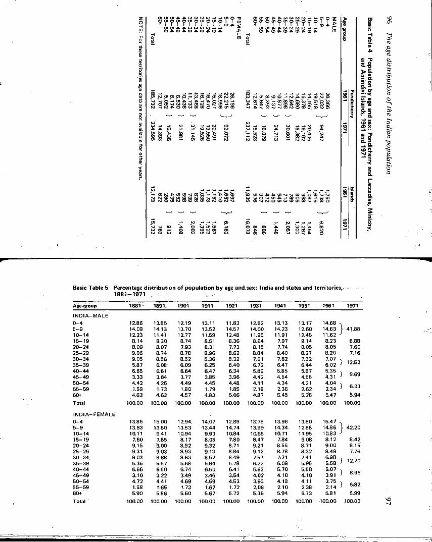
z o H m Tl o 3 "
a
01 Ol Ol A » U U MM Ul O n OlOlOlAAUUMM-'-'OlQ? OIUI J l i U U U M - ' - ' U I U I 6 « U U M M - > ^ r_ I O ^ I O ^ I O A I O ^ I O A J> co & co J> co co 4 co 4 rn
H r- n o m o Q) Q)
00 -.-.-.-.-.-.-.roro 01 ro ci 00 00 p to 01 pi cn co ro pi -J "%j b 01 * Vi £ V b co Vj CO O O l M U U U S I O v l K l I D —* co ro MM^OOlUOOOOONOlOlOl 10 01 co •*>' co co co 01 co 01
ro co —» —» ro _» -» co co p co "-• "01 ui J > 00 A 10 ui co -»• 01 c o o - 1
o -o 10
-» oiio4^uiui»jooo-'->^aia> M M 00 co 011 co ro o ui ro 1 ~j ro 00 couicouroco~jui-'Uico
- ~ I C O I O O O I U M O M > J
^ M I D co 01 -> ro co ro ro 01 b co ui ui o co 10 01 a> ro ui co -> ro
co -» -»-»-»_-*_» _> ro ro co ro ui 00 co p M A ui J > co ro o> co 01 "01 co 00 00 01 01 co 01 b co A ->j>coco jcoJ>oo~ja>->cooi «j ^>iusiviooMOCooiooroai
ro CO —FC —» •O Ul 0 1
ui b -> ro ~ J ro co co ro CO -» ro % 4* 0 01 CD 0 %
01 CO ro —> 0 00 01 0 CO —' ro 10 Ul •0
co c n u ^ ^ u i > i N i i O ( D o o i N i > j U N O N Ol A -» 00 o CD 00 -» CO Ul Ol Ol N M O Ul CO CO Ul CO —4 Ul 00 o
Ol "0 00 - J A 00 01
ro -» -» O) b co to J > 00 - 001 f"
O -o .
& 3 8 3 2 1 0
8.
CO 0 ) ut o" H 0 )
cr re J>
0 ) " D
a.-a > £ • 3 a> 5' o' a 3 <" cr _ . <
ut 09
f<8 CL S> </> 3 - a CD CD Ol X
°> 7? 3 9
- 5
0 ) 3 a.
0 ) o o
o o
N O
3 « >
R
S-
3'
04
ft 3
O
o
r
Basic Table 5 Percentage distribution of population by age and sex: India and,states.and territories,- . 1881-1971 , \ i
Age-group 1881 1891. 1901 1911 1921 1931 1941 1951 1961 1971
INDIA-MALE 0-4 12.86 13.85 12.19 13.11 11.83 12:62 13.13 13.17 14.68 5-9 14.09 14.13 13.70 13.52 14.57 14.00 14.23 12.60 14.63 } 41.88 10-14 12.23 11.41 12.77 11.59 12.48 11.95 11.91 12.45 11.62 J
15-19 8.14 8.30 8.74 8.51 •8.36 8.64 7.97 9.14 8.23 8.88 20-24 8.09 8.07 7.93 8.31 7.73 8.15 7.74 8.05 8.05 7.60 25-29 9.06 8.74 8.78 8.96 8.62 8.84 8.40 8.27 8.20 7.16 30-34 9.05 8.56 8.52 8.36 8.32 7.61 7.62 7.32 7.07 1 12:52 35-39 5.87 6.08 6.09 &25 6.40 6.72 6.47 6.44 6.02 1 12:52
40-44 6.65 6.61 6.64 6.47 6.34 5.89 5.85 5.87 5:35 l Q C Q
45-49 3.33 3.64 3.77 3.85 3.96 4.42 4.54 4.58 4.31 ; y.oy 50-^54 4.42 4.26 4.49 4.45 4.48 4.11 4.34 4.21 4.04 i 55-59 1.59 1.73 1.80 1.79 1.85 2.18 2.36 2.62 2.34 ; 6.33 60+ 4.63 4.63 4.57 4.83 5.06 4.87 5.45 5.28 5.47 5.94 Total 100.00 100.00 100.00 100.00 100.00 100.00 100.00 100.00 100.00 100.00
INDIA—FEMALE 0-4 13.85 15.00 12.94 14.07 12.89 13.78 13.96 13.80 15.47 5-9 13.63 13.80 13.53 13.44 14.74 13.99 14.34 12.88 14.86 ) 42.20 10-14 10.11 9.41 10.94 9.93 10.84 10.65 10.71 11.95 10.83 J 15^19 7.60 7.85 8.17 8.05 7.80 8.47 7.84 9.08 8.12 8.42 20-24 9.15 9.00 8.92 9.32 8.71 9.21 8.55 8.71 9.00 8.15 25-29 9.31 9.03 8.93 9.13 8.84 9.12 8.78 8.32 8.49 7.76 30-34 9.03 8.68 8.63 8.52 8.49 7.57 7; 71 7.41 6.98 t 35-39 5.35 5.57 5.68 5.64 5.78 6.22 6.09 5.95 5.58 ; 12.70 40-44 6.66 6.50 6.74 6.50 6.41 5.62 5.70 5.58 5.07 i 45-49 3.10 3.22 3.49 3.46 3.54 4.02 4.10 4.10 3.91 ; 8.96 50-54 4.72 4.41 4.69 4.59 4.53 3.93 4.18 4.11 3.75 i 55-59 1.58 1.65 1.73 1.67 1.72 2.06 2.10 2.38 2.14 ; 5.82 60+ 5.90 5.86 5.60 5.67 5.72 5.36 5.94 5.73 5.81 5.99 Total 100.00 100.00 100.00 100.00 10000 100.00 100.00 100.00 100.00 100.00
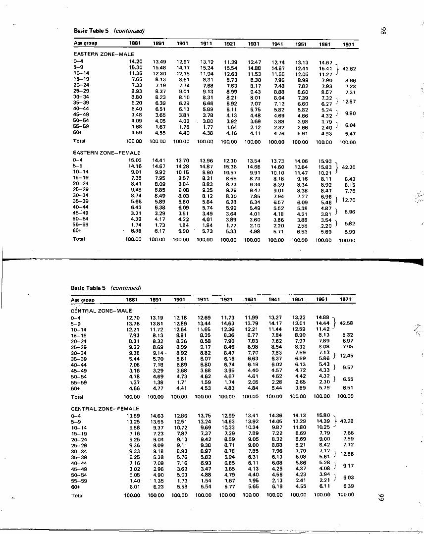
Basic Table 5 (continued) O O
Age group 1881 1891 1901 1911 1921 1931 1941 1951 1961 1971
EASTERN Z O N E -•MALE 0-4 14.20 13.49 12.97 13.12 11.39 12.47 1274 13.13 14.67 5-9 15.30 15.48 14.77 15.24 15.54 14.88 14.67 12.41 15.41 42.62 10-14 11.35 12.30 12.38 11.94 12.63 11.53 11.65 12.05 11.27 J 15-19 7.65 8.13 8.61 8.31 8.73 8.30 7.96 8.99 7.90 8.66 20-24 7.33 7.19 7.74 7.68 7.63 8.17 7.48 7.82 7.93 7.23 25-29 8.93 8.37 9.01 9.13 8.99 9.43 8.88 8.60 8.57 7.31 30-34 8.80 8.23 8.10 8.31 8.21 8.01 8.04 7.39 7.32
12.87 35-39 6.20 6.39 6.29 6.66 6.92 7.07 7.12 6.60 6.27 } 12.87 40-44 6.40 6.51 6.13 5.89 6.11 5.75 5.82 5.82 5.24
9.80 45-49 3.48 3.65 3.81 3.78 4.13 4.48 4.69 4.66 4.32 } 9.80 50-54 4.09 4.05 4.02 . 3.80 3.92 3.69 3.88 3.98 3.79
6.04 55-59 1.68 1.67 1.76 1.77 1.64 2.12 2.32 2.66 2.40 } 6.04 60+ 4.59 4.55 4.40 4.38 4.16 4.11 4.76 5.91 4.93 5.47 Total 100.00 100.00 100.00 100.00 100.00 100.00 100.00 100.00 100.00 100.00
EASTERN Z O N E - FEMALE 0-4 15.03 14.41 13.70 13.96 12.30 13.54 13.73 14.06 15.93 5-9 14.16 14.67 14.28 14.87 15.36 14.66 14.60 12.64 15.83 ] 42.20 10-14 9.01 9.92 10.15 9.90 1Q57 9.91 10.10 11.47 10.21 J 15-19 7.38 7.95 8.57 8.31 8.65 8.73 8.18 9.16 8.11 8.42 20-24 8.41 8.09 8.84 8.83 8.73 9.34 8.39 8.34 8.92 8.15 25-29 9.48 8.85 9.08 9.35 9.26 9.47 9.01 8.38 8.47 7.76 30-34 8.74 8.49 8.03 8.12 8.30 7.85 7.94 7.27 6.96 12.70 35-39 5.66 5.89 5.80 5.84 6.28 6.34 6.57 6.09 5.46 } 12.70 40-44 6.43 6.38 6.09 5.74 5.92 5.49 5.52 5.38 4.87
8.96 45-49 3.21 3.29 3.51 3.49 3.64 4.01 4.18 4.21 3.81 } 8.96 50-54 4.39 4.17 4.22 4.01 3.89 3.60 3.86 3.88 3.54 1 5.82 55-59 1.74 1.73 1.84 1.84 1.77 2.10 2.20 2.58 2.20 } 5.82 60+ 6.36 6.17 5.90 5.73 5.33 4.98 5.71 6.53 5.69 5.99 Total 100.00 100.00 100.00 100.00 100.00 100.00 100.00 100.00 100.00 100.00
Basic Table 5 (continued)
Age group 1881 1891 1901 1911 1921 .1931 1941 1951 1961 1971
CENTRAL Z O N E - MALE 0-4 12.70 13.19 12.18 12.69 11.73 11.99 13.27 13.22 14.88 5-9 13.76 13.81 12.89 13.44 14.63 13.79 14.17 13.01 14.44 } 42.58 10-14 12.21 11.72 12.64 11.65 12.36 12.21 11.44 12.59 11.42 j
15-19 7.93 8.13 8.81 8.35 8.36 8.77 7.84 8.90 8.13 8:32 20-24 8.31 8.32 8.36 8.58 7.90 7.83 7.62 7.97 7.89 6.97 25-29 9.22 8.69 8.99 9.17 8.46 8.98 8.54 8.32 8.08 7.05 30-34 9.38 9.14 • 8.92 8.82 8.47 7.70 7.83 7.59 7.13
1 O Ati 35-39 5.44 5.70 5.81 ao7 6.16 6.63 6.37 6.59 5.86 i
40-44 7.08 7.18 6.89 6.80 6.74 6.19 6.02 6.13 5.43 Q R7 45-49 3.16 3.29 3.68 3.68 3.95 4.40 4.57 4.72 4.33 s y.o / 50-54 4.78 4.69 4.73 4.62 4.67 4.61 4.62 4.42 4.32 \ R 55-59 1.37 1.38 1.71 1.59 1.74 2.05 2.28 2.65 2.30 1 O.OD
60+ 4.66 4.77 4.41 4.53 4.83 4.84 5.44 3.89 5.79 6.51
Total 100.00 100.00 100.00 100.00 100.00 100.00 100.00 100.00 100.00 100.00
CENTRAL ZONE--FEMALE 0-4 13.89 14.63 12.86 13.75 12.99 13.41 14.36 14.13 15.80 5-9 13.25 13.55 12.51 13.24 14.63 13.92 14.05 13.29 14.39 } 42.28 10-14 9.88 9.37 10.72 9.69 10.33 10.34 9.87 11.80 10.25 J
15-19 7.16 7.23 7.87 7.37 7.29 7.89 7.22 8.69 7.79 7.66 20-24 9.25 9.04 9.13 9.42 8.59 9.05 8.32 8.69 9.00 7.89 25-29 9.35 9.09 9.11 9.38 8.71 9.00 8.88 8.21 8.42 7.72 30-34 9.33 9.18 8.92 8.97 8.78 7.85 7.96 7.70 7.12 \ 1 *> Bfi
35-39 5.25 5.38 5.76 5.82 5.94 6.31 6.13 6.08 5.61 J I Z.OO
40-44 7.16 7.09 7.16 6.93 6.85 6.11 6.08 5.86 5.28 \ Q 1 7 45-49 3.02 2.96 3.62 3.47 3.65 4.13 4.25 4.37 4.08 i 9. 1 /
50-54 5.05 4.90 5.03 4.88 4.79 4.40 4.56 4.23 3.94 \ 55-59 1.40 • 1.35 1.73 1.54 1.67 1.95 2.13 2.41 2.21 J D.UJ
60+ 6.01 6.23 5.58 5.54 5.77 5.65 6.19 4.55 6.11 6.39
Total 100.00 100.00 100.00 100.00 100.00 100.00 100.00 100.00 100.00 100.00
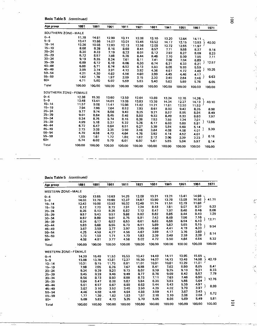
Basic Table 5 (continued)
Age group 1881
SOUTHERN Z O N E - M A L E 0-4 5-9 10-14 15-19 20-24 25-29 30-34 35-39 40-44 45-49 50-54 55-59 60+
Total
SOUTHERN ZONE-0-4 5-9 10-14 15-19 20-24 25-29 30-34 35-39 40-44 45-49 50-54 55-59 60+
Total
11.78 13.47 13.26 8.68 8.30 8.72 9.19 6.09 6.88 3.09 4.21 1.62 4.71
1891
14.61 13.66 10.55 8.28 8.33 8.57 8.35 6.12 6.71 3.74 4.30 1.78 5.00
1901
12.99 14.07 12.93 8.16 7.19 7.98 8.24 6.18 6.74 3.91 4.62 1.97 5.02
1911
13.11 13.01 12.13 8.69 8.22 8.28 7.61 6.06 6.52 4.13 4.56 2.09 5.59
1921
12.08 13.45 12.56 8.41 8.01 8.44 8.11 6.30 6.13 3.92 4.60 2.15 5.83
1931
13.10 13.52 12.09 8.57 8.12 8.48 7.41 6.74 5.93 4.36 3.99 2.30 5.40
1941
13.20 14.17 12.72 7.71 7.92 7.70 7.08 6.31 6.05 4.67 4.45 2.40 5.63
1951
12.64 12.15 12.55 9.58 8.27 8.00 7.04 6.33 5.93 4.72 4.46 2.64 5.69
1961
14.11 13.93 11.97 8.37 8.09 7.95 6.89 6.21 5.59 4.49 4.17 2.46 5.78
1971
} 40.00
9.16 8.23 7.11
12.57
10.25
6.63
6.05 100.00 100.00 100.00 100.00 100.00 100.00 100.00 100.00 100.00 100.00
FEMALE 12.38 15.30 13.60 13.59 12.64 13.69 13.24 12.76 14.26 -13.48 13.41 14.01 13.06 13.83 13.39 14.34 12.37 14.13 i 40.10 11.57 9.06 11.41 10.98 11.42 11.21 11.81 12.30 11.53 -J 7.94 7.96 7.64 8.52 7.93 8.61 8.00 9.43 8.35 8.98 9.77 9.74 8.56 9.43 9.35 9.21 8.57 8.95 8.94 8.49 9.01 8.84 8.45 8.48 8.80 9.33 8.49 8.33 8.60 7.97 9.34 8.75 8.74 8.15 8.38 7.53 7.55 7.34 7.01
} 12.86 4.99 5.18 5.37 5.32 5.26 6.17 6.03 5.89 5.81 } 12.86 6.72 6.47 6.64 6.51 6.27 5.39 5.84 5.69 5.14
} 9.30 2.73 3.09 3.35 3.50 3.46 3.84 4.08 4.08 4.01 } 9.30 4.79 4.56 4.73 4.64 4.76 3.92 4.14 4.52 4.01
} 6.16 1.55 1.61 1.72 1.80 1.82 2.12 2.06 2.39 2.23 } 6.16 5.74 6.02 5.79 6.01' 6.07 5.61 5.85 5.94 5.97 6.14
100.00 100.00 100.00 100.00 100.00 100.00 100.00 100.00 100.00 100.00
Basic Table 5 (continued)
' Age group 1881 1891 1901 1911 1921 1931 1941 1951 1961 1971
WESTERN Z O N E - M A L E
0-4 12.90 13.85 10.63 14.25 12.08 13.21 13.21 13.41 14.98 1 5-9 14.03 13.79 13.69 12.37 14.87 13.90 13.79 13.09 14.58 \ 41.71 10-14 12.43 10.98 13.53 10.32 12.48 11.74 11.51 12.79 11.68 J 15-19 8.12 7.73 8.72 7.91 7.24 8.43 7.81 9.07 8:37 9.23 20-24 8.28 8.13 8.25 8.62 7.12 8.47 7.97 8.46 8.46 8.06 25-29 9.57 9.43 9.57 9.68 8.82 8.62 8.85 8.44 8.40 7.29 30-34 8.87 8.88 9.01 8.75 8.81 7.43 8.09 7.56 7.16 } 12.71 35-39 6.24 6.17 6.52 6.53 6.61 6.83 6.58 6.54 6.10 40-44 5.83 6.68 6.55 6.73 6.51 5.69 5.62 5.65 5.15 } 9.54 45-49 3.67 3.59 3.77 3.97 3.95 4.66 4.41 4.19 4.30 50-54 4.25 4159 4.27 4.56 4.67 3.89 4.17 3.76 3.69 } 6.14 55-59 1.73 1.58 1.71 1.73 1.83 2.39 2.49 2.39 2.28 60+ 4.08 4.61 3.77 4.56 5.02 4.72 5.50 4.64 4.84 5.32
Total 100.00 100.00 100.00 100.00 100.00 100.00 100.00 100.00 100.00 100.00
WESTERN Z O N E - FEMALE
0-4 14.20 15.49 11.53 15.53 13.42 14.49 14.11 13.95 . 15.65 5-9 13.98 13.78 13.81 12.37 15.30 14.07 14.13 13.49 14.98 \ 42.19 10-14 10.31 9.15 11.73 8.81 11.01 10.91 10.61 12.29 11.01 J 15-19 7.98 7.55 8.26 7.67 6.88 8.41 7.63 8.80 8.05 8.41 20-24 9.34 9.29 9.20 9.73 8.07 9.39 9.25 9.10 9.31 8.33 25-29 9.45 9.29 9.46 9.49 8.77 8.76 9.09 8.42 8.57 7.79 30-34 8.56 8.73 8.93 8.88 8.73 7.11 7.63 7.46 6.90 } 12:76 35-39 5.64 5.47 6.06 5.87 5.84 6.30 5.83 5.88 5.64 40-44 5.61 6.57 6.67 6.69 6.63 5.44 5.43 5.39 4.97
} 8.99 45-49 3.62 3.10 3.52 3.45 3.50 4.29 4.02 3.79 3.97 50-54 4.46 4.58 4.48 4.64 4.59 3.59 4.11 3.67 3.43 } 5.72 55-59 1.77 1.39 . 1.62 1.53 1.57 2.18 2.10 2.06 2.04 60+ 5.09 5.62 4.73 5.35 5.70 5.05 6.05 5.69 5.49 5.81
Total 100.00 100.00 100.00 100.00 100.00 100.00 100.00 100.00 100.00 100.00
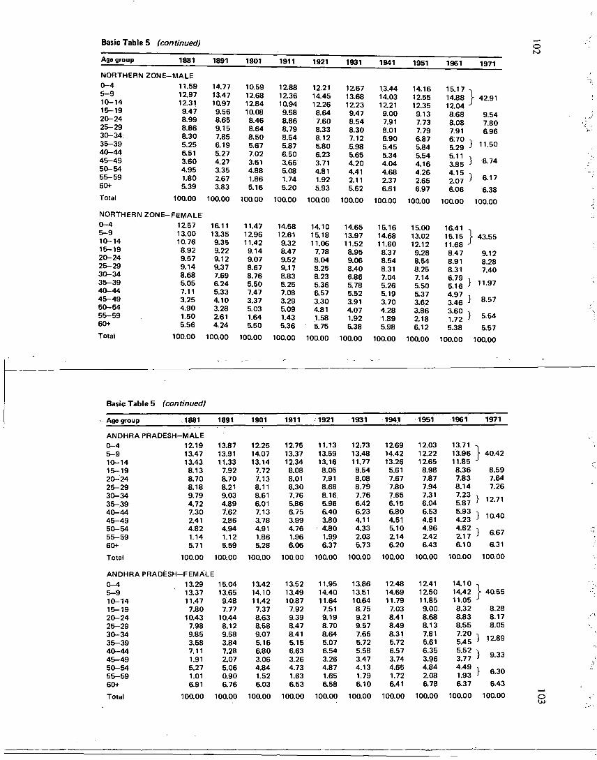
Basic Table 5 (continued)
Age group 1881
NORTHERN Z O N E - M A L E 0-4 5-9 10-14 15-19 20-24 25-29 30-34 35-39 40-44 45-49 50-54 55-59 60+
Total
NORTHERN ZONE-0-4 5-9 10-14 15-19 20-24 25-29 30-34 35-39 40-44 45-49 50-54 55-59 60+
Total
11.59 12.97 12.31 9.47 8.99 8.86 8.30 5.25 6.51 3.60 4.95 1.80 5.39
1891
14.77 13.47 10.97 9.56 8.65 9.15 7.85 6.19 5.27 4.27 3.35 2.67 3.83
1901
10.59 12.68 12.84 10.08 8.46 8.64 8.50 5.67 7.02 3.61 4.88 1.86 5.16
1911
12.88 12.36 10.94 9.58 8.86 8.79 8.54 5.87 6.50 3.66 5.08 1.74 5.20
1921
12.21 14.45 12.26 8.64 7.60 8.33 8.12 5.80 6.23 3.71 4.81 1.92 5.93
1931
12.67 13.68 12.23 9.47 8.54 8.30 7.12 5.98 5.65 4.20 4.41 2.11 5.62
1941
13.44 14.03 1221 9.00 7.91 8.01 6.90 5.45 5.34 4.04 4.68 2.37 6.61
1951
14.16 12.55 12.35 9.13 7.73 7.79 6.87 5.84 5.54 4.16 4.26 2.65 6.97
1961
15.17 14.88 12.04 8.68 8.08 7.91 6.70 5.29 5.11 3.85 4.15 2.07 6.06
1971
100.00 100.00 10000 100.00 100 00 100.00 100.00 100.00 100.00
FEMALE 12.57 16.11 11.47 14.58 14.10 14.65 15.16 15.00 16.41 13.00 13.35 12.96 1261 15.18 13.97 14.68 13.02 15.15 10.76 9.35 11.42 9.32 11.06 11.52 11.60 12.12 11.68 8.92 9.22 9.14 8.47 7.78 8.95 8.37 9.28 8.47 9.57 9.12 9.07 9.52 8.04 9.06 8.54 8.54 8.91 9.14 9.37 8.67 9.17 8.25 8.40 8.31 8.25 8.31 8.68 7.69 8.76 8.83 a23 6.86 7.04 7.14 6.79 5.05 6.24 5.50 5.25 5.36 5.78 5.26 5.50 5.16 7.11 5.33 7.47 7.08 a57 5.52 5.19 5.37 4.97 3.25 4.10 3.37 3.29 3.30 3.91 3.70 3.62 3.46 4.90 3.28 5.03 5.09 4.81 4.07 4.28 3.86 3.60 1.50 2.61 1.64 1.43 1.58 1.92 1.89 2.18 1.72 5.56 4.24 5.50 5.36 5.75 5.38 5.98 6.12 5.38
100.00 100.00 100.00 100.00 100.00 100.00 100.00 100.00 100.00
} 42.91
9.54 7.80 6.96
} 11.50
} 8.74
} 6.17
6.38
43.55
9.12 8.28 7.40
11.97
8.57
5.54
5.57
Basic Table 5 (continued)
Age group 1881 1891 1901 1911 1921 1931 1941 1951 1961 1971
ANDHRA PRADESH-- M A L E 0-4 12.19 13.87 12.25 12.75 11.13 12.73 12.69 12.03 13.71 -i
5-9 13.47 13.91 14.07 13.37 13.59 13.48 14.42 12.22 13.96 } 40.42 10-14 13.43 11.33 13.14 12.34 13.16 11.77 13.26 12.65 11.85 J
15-19 8.13 7.92 7.72 8.08 8.05 8.54 5.61 8.98 8.36 8.59 20-24 8.70 8.70 7.13 8.01 7.91 8.08 7.67 7.87 7.83 7.64 25-29 8.18 8.21 8.11 8.30 8.68 8.79 7.80 7.94 8.14 7.26 30-34 9.79 9.03 8.61 7.76 8.16 7.76 7.65 7.31 7.23 \ 1 1 1 1
35-39 4.72 4.89 6.01 5.86 5.96 6.42 6.15 6.04 5.87 i I z. / I
40-44 7.30 7.62 7.13 6.75 6.40 6.23 6.80 6.53 5.93 \ i n AC\
45-49 2.41 2.86 3.78 3.99 3.80 4.11 4.51 4.61 4.23 }
50-54 4.82 4.94 4.91 4.76 4:80 4.33 5.10 4.96 4.62 \ ft C I
55-59 1.14 1.12 1.86 1.96 1.99 2.03 214 2.42 2.17 1 D . O /
60+ 5.71 5.59 5.28 6.06 6.37 5.73 6.20 6.43 6.10 6.31
Total 100.00 100.00 100.00 100.00 100.00 100.00 100.00 100.00 100.00 100.00
ANDHRA PRADESH-- F E M A L E 0-4 13.29 15.04 13.42 13.52 11.95 13.86 12.48 1241 14.10 5-9 13.37 13.65 14.10 13.49 14.40 13.51 14.69 12.50 14.42 } 40.55 10-14 11.47 9.48 11.42 10.87 11.64 10.64 11.79 11.85 11.05 J
15-19 7.80 7.77 7.37 7.92 7.51 8.75 7.03 9.00 8.32 8.28 20-24 10.43 10.44 8.63 9.39 9.19 9.21 8.41 8.68 8.83 8.17 25-29 7.98 8.12 8.58 8.47 8.70 9.57 8.49 8.13 8.55 8.05 30-34 9.85 9.58 9.07 8.41 8.64 7.66 8.31 7.81 7.20 \ 1 O ftQ 35-39 3.58 3.84 5.16 5.15 5.07 5.72 5.72 5.61 5.45 i 1 Z . O J
40-44 7.11 7.28 6.80 6.63 6.54 5.58 6.57 6.35 5.52 \ Q H
45-49 1.91 207 3.06 3.26 3.26 3.47 3.74 3.96 3.77 J
50-54 5.27 5.06 4.84 4.73 4.87 4.13 4.65 4.84 4.49 \ c Ort
55-59 1.01 0.90 1.52 1.63 1.65 1.79 1.72 2.08 1.93 J D.oU
60+ 6.91 6.76 6.03 6.53 6.58 6.10 6.41 6.78 6.37 6.43
Total 100.00 100.00 100.00 100.00 100.00 100.00 100.00 100.00 100.00 100.00
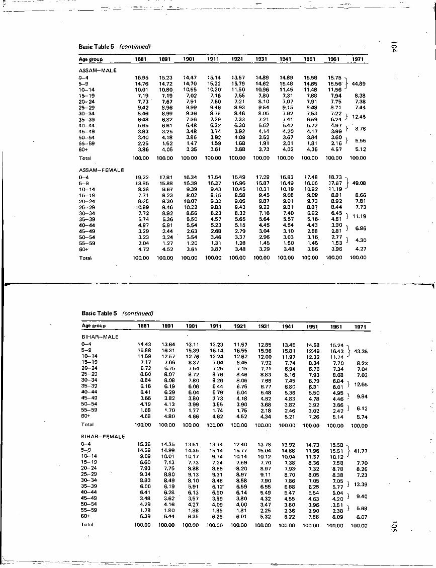
Basic Table 5 (continued) o
Age group 1881 1891 1901 1911 1921 1931 1941 1951 1961 1971
A S S A M - M A L E 0-4 16.95 15.23 14.47 15.14 13.57 14.89 14.89 15.58 15.75 5-9 14.76 14.72 14.70 15.22 15.79 14.62 15.48 14.65 15.56 } 44.89 10-14 10.01 10.80 10.55 10.20 11.50 10.96 11.45 11.48 11.56 J
15-19 7.19 7.19 7.02 7.16 7.55 7.80 7.31 7.88 7.94 8.38 20-24 7.73 7.67 7.91 7.60 7.21 8.10 7.07 7.91 7.75 7.38 25-29 9.42 8.96 9.99 9.46 8.93 9.54 9.15 8.48 8.71 7.44 30-34 8.46 8.99 9.36 8.75 8.46 8.05 7.92 7.53 7:22 1 1 1 A C 35-39 6.48 6.82 7.36 7.29 7.33 7.21 7.41 6.59 6.24 ; 12.. 4b
40-44 5.65 6.61 6.48 6.32 6.30 5.52 5.42 5.72 4.97 i
45-49 3.83 3.25 3.48 3.74 3.92 4.14 4.20 4.17 3.99 / o. to 50-54 3.40 4.18 3.85 3.92 4.09 3.52 3.67 3.84 3.60 i a cc 55-59 2.25 1.52 1.47 1.59 1.68 1.91 2.01 1.81 2.16 b.bb
60+ 3.86 4.05 3.35 3.61 3.68 3.73 4.02 4.36 4.57 5.12
Total 100.00 100.00 100.00 100.00 100.00 100.00 100.00 100.00 100.00 100.00
ASSAM—FEMALE 0-4 19.22 17.81 16.34 17.54 15.49 17:29 16.83 17.48 18.73 5-9 13.85 15.88 15.39 16.37 16.96 15.87 16.49 16.05 17.67 } 49.08 10-14 8.38 9.67 9.39 9.43 10.45 10.31 10.19 10.92 11.19 j
15-19 7.71 8.23 8.02 8.15 8.58 9.45 9.05 9.09 8.81 8.66 20-24 8.25 8.30 10.07 9.32 9.05 9.87 9.01 9.73 8.92 7.81 25-29 10.89 8.46 10.22 9.83 9.43 9.22 9.81 8.87 8.44 7.73 30-34 7.72 8.92 8.56 8.23' 8.32 7.16 7.40 6.92 6.45 i 1 1 in 35-39 5.74 5.36 5.50 4.57 5.65 5.64 5.57 5.16 4.81 5 i 1.1y
40-44 4.97 5.91 5.54 5.23 5.15 4.45 4.54 4.43 3.90 \ c Oc
45-49 3.29 2.44 2.63 2.68 2.79 3.04 3.10 2.88 2.81 5 D.sO
50-54 3.23 3.24 3.54 3.46 3.37 2.96 3.03 3.16 2.77 \ A i n 55-59 2.04 1.27 1.20 1.31 1.28 1.45 1.50 1.45 1.53 J 4.JU
60+ 4.72 4.52 3.61 3.87 3.48 3.29 3.48 3.86 3.96 4.27
Total 100.00 100.00 100.00 100.00 100.00 100.00 100.00 100.00 100.00 100.00
1
Basic Table 5 (continued)
Age group 1881 1891 1901 1911 1921 1931 1941 1951 1961 1971
BIHAR-•MALE 0-4 14.43 13.64 13.11 13.23 11.57 12.85 13.45 14.58 15.24 -1 5-9 15.88 16.31 15.39 16.14 16.55 15.96 15.81 12.49 16.43 \ 43.35 10-14 11.59 12.57 12.76 12.24 12.62 12.00 11.97 12.32 11.74 J 15-19 7.17 7.66 8.37 7.94 8.45 7.92 7.74 8.34 7.70 8.23 20-24 6.72 6.75 7.54 7.25 7.15 7.71 6.94 6.76 7.34 7.04 25-29 8.60 8.07 8.72 8.76 8.46 8.83 8.16 7.93 8.08 7.03 30-34 8.84 8.08 7.80 8.26 8.06 7.66 7.45 6.79 6.84 35-39 6.16 6.19 6.06 6.44 6.75 6.77 6.80 6.31 6.01 } 12.65 40-44 6.41 6.29 6.04 5.79 6.04 5.48 5.36 5.50 4.95
} 9.84 45-49 3.66 3.82 3.80 3.73 4.18 4.62 4.83 4.78 4.46 } 9.84 50-54 4.19 4.13 3.99 3.85 3.90 3.68 3.82 3.92 3.66
} 6.12 55-59 1.68 •".70 1.7.7 1.74 1.75 2.18 2.46 3.02 2.42 } 6.12 60+ 4.68 4.80 4.66 4.62 4.52 4.34 5.21 7.26 5.14 5.74 Total 100.00 100.00 100.00 100.00 100.00 100.00 100.00 100.00 100.00 100.00
BIHAR— FEMALE 0-4 15.26 14.35 13.51 13.74 12.40 13.78 13.92 14.73 15.58 5-9 14.59 14.99 14.35 15.14 15.77 15.04 14.88 11.96 15.51 \ 41.77 10-14 9.09 10.01 10.17 9.74 1tt14 10.12 10.04 11.37 10.12 J 15-19 6.60 7.13 7.73 7:24 7.59 7.70 7.38 8.36 7.58 7.70 20-24 7.93 7.75 8.88 8.55 8.20 8.97 7.93 7.32 8.78 8.26 25-29 9.34 8.80 9.13 9.31 8.97 9.11 8.70 8.05 8.38 7.23 30-34 8.83 8.49 8.10 8.48 8.58 7.90 7.86 7.05 7.05 } 13.39 35-39 6.00 6.19 5.91 6.12 6.59 6.55 6.88 R25 5.77 } 13.39 40-44 6.41 6.28 6.13 5.90 6.14 5.49 5.47 5:54 5.04
} 9.40 45-49 3.48 3.62 3.57 3.59 3.80 4.32 4.55 4.63 4.20 } 9.40 50-54 4.29 4.16 4.27 4.09 4.00 3.47 3.80 3.96 3.51 55-59 1.78 1.80 1.88 1.85 1.81 2.25 2.36 2.90 2.38 } 5.68 60+ 6.39 6.44 6.35 a25 6.01 5.32 6.22 7.88 6.09 6.07 Total 100.00 100.00 100.00 100.00 100.00 100.00 100.00 100.00 100.00 100.00
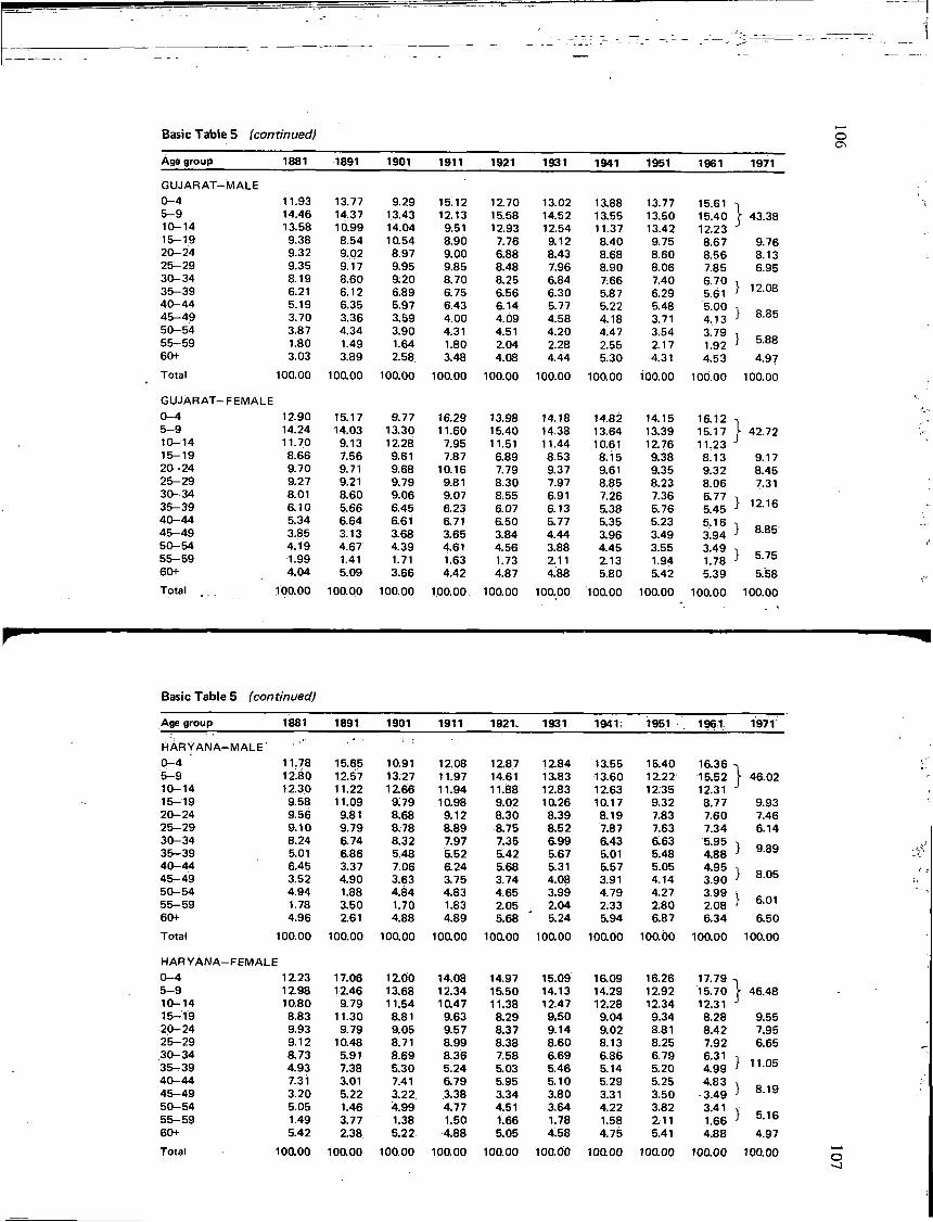
Basic Table 5 (continued) o Os
Age group 1881 1891 1901 1911 1921 1931 1941 1951 1961 1971
G U J A R A T - MALE 0-4 11.93 13.77 9.29 15J2 12.70 13.02 13.88 13.77 15.61 5-9 14.46 14.37 13.43 12.13 15.58 14.52 13.55 13.50 15.40 1 43.38 10-14 13.58 10.99 14.04 9.51 12.93 12.54 11.37 13.42 12.23 J 15-19 9.38 8.54 10.54 8.90 7.76 9.12 8.40 9.75 8.67 9.76 20-24 9.32 9.02 8.97 9.00 6.88 8.43 8.68 8.60 8.56 8.13 25-29 9.35 9.17 9.95 9.85 8.48 7.96 8.90 8.06 7.85 6.95 30-34 8.19 8.60 9.20 8.70 8.25 6.84 7.66 7.40 6.70 i 12.08 35-39 6.21 6.12 6.89 6.75 6.56 6.30 5.87 6.29 5.61 } 12.08 40-44 5.19 6.35 5.97 6.43 6.14 5.77 5.22 5.48 5.00
8.85 45-49 3.70 3.36 3.59 4.00 4.09 4.58 4.18 3.71 4.13 } 8.85 50-54 3.87 4.34 3.90 4.31 4.51 4.20 4.47 3.54 3.79
5.88 55-59 1.80 1.49 1.64 1.80 2.04 2.28 2.55 2.17 1.92 ) 5.88 60+ 3.03 3.89 2.58 3.48 4.08 4.44 5.30 4.31 4.53 4.97 Total 100.00 100.00 100.00 100.00 100.00 100.00 100.00 100.00 100.00 100.00
G U J A R A T - FEMALE 0-4 12.90 15.17 9.77 16.29 13.98 14.18 14.82 14.15 16.12 5-9 14.24 14.03 13.30 11.60 15.40 14.38 13.64 13.39 15.17 } 42.72 10-14 11.70 9.13 12.28 7.95 11.51 11.44 10.61 12.76 11.23 J 15-19 8.66 7.56 9.61 7.87 6.89 8.53 8.15 9.38 8.13 9.17 20-24 9.70 9.71 9.68 10.16 7.79 9.37 9.61 9.35 9.32 8.45 25-29 9.27 9.21 9.79 9.81 8.30 7.97 8.85 8.23 8.06 7.31 30-34 8.01 8.60 9.06 9.07 8.55 6.91 7.26 7.36 6.77 s 12.16 35-39 6.10 5.66 6.45 6.23 6.07 6.13 5.38 5.76 5.45 } 12.16 40-44 5.34 6.64 6.61 a71 6.50 5.77 5.35 5.23 5.16 1 8.85 45-49 3.85 3.13 3.68 3.65 3.84 4.44 3.96 3.49 3.94 i 8.85 50-54 4.19 4.67 4.39 4.61 4.56 3.88 4.45 3.55 3.49
5.75 55-59 1.99 1.41 1.71 1.63 1.73 2.11 2.13 1.94 1.78 } 5.75 60+ 4.04 5.09 3.66 4.42 4.87 4.88 5.80 5.42 5.39 5.58 Total 100.00 100.00 100.00 100.00 100.00 100.00 100.00 100.00 100.00 100.00
Basic Table 5 (continued)
Age group 1881 1891 1901 1911 1921. 1931 1941, 195,1 1961 1971
H A R Y A N A - •MALE' 0-4 11.78 15.65 10.91 12.08 12.87 12.84 13.55 15.40 16.36 5-9 12.80 12.57 13.27 11.97 14.61 13.83 13.60 12.22 15.52 [ 46.02 10-14 12.30 11.22 12.66 11.94 11.88 12.83 12.63 12.35 12.31 J 15-19 9.58 11.09 9.79 10.98 9.02 10.26 10.17 9.32 8.77 9.93 20-24 9.56 9.81 8.68 9.12 8.30 8.39 8.19 7.83 7.60 7.46 25-29 9.10 9.79 8.78 8.89 8.75 8.52 7.87 7.63 7.34 6.14 30-34 8.24 & 74 8.32 7.97 7.35 6.99 6.43 6.63 5.95 \ 35-39 5.01 6.86 5.48 5.52 5.42 5.67 5.01 5.48 4.88 i 9.89 40-44 6.45 3.37 7.06 a24 5.68 5.31 5.57 5.05 4.95 x 45-49 3.52 4.90 3.63 3.75 3.74 4.08 3.91 4.14 3.90 i 8.05 50-54 4.94 1.88 4.84 4.83 4.65 3.99 4.79 4.27 3.99 l 55-59 1.78 3.50 1.70 1.83 2.05 2.04 2.33 2.80 2.08 i 6.01 60+ 4.96 2.61 4.88 4.89 5.68 5.24 5.94 6.87 6.34 6.50
Total 100.00 100.00 100.00 100.00 100.00 100.00 100.00 100.00 100.00 100.00
H A R Y A N A - •FEMALE 0-4 1223 17.06 1200 14.08 14.97 15.09 iao9 16.26 17.79 5-9 12.98 12.46 13.68 12.34 iaso 14.13 14.29 12.92 15.70 ) 46.48 10-14 10.80 9.79 11.54 10.47 11.38 12.47 12.28 12.34 12.31 J 15—19 8.83 11.30 8.81 9.63 8.29 9.50 9.04 9.34 8.28 9.55 20-24 9.93 9.79 9.05 9.57 8.37 9.14 9.02 8.81 8.42 7.95 25-29 9.12 10.48 8.71 8.99 8.38 8.60 8.13 8.25 7.92 6.65 30-34 8.73 5.91 8.69 8.36 7.58 6.69 6.86 6.79 6.31 i 35-39 4.93 7.38 5.30 5.24 5.03 5.46 5.14 5.20 4.99 i 11.05 40-44 7.31 3.01 7.41 6.79 5.95 5.10 5.29 5.25 4.83 \ 45-49 3.20 5.22 3.22 3.38 3.34 3.80 3.31 3.50 •3.49 i 8.19 50-54 5.05 1.46 4.99 4.77 4.51 3.64 4.22 3.82 3.41 V 55-59 1.49 3.77 1.38 1.50 1.66 1.78 1.58 211 1.66 ; 5.16 60+ 5.42 2.38 5.22 4.88 5.05 4.58 4.75 5.41 4.88 4.97
Total 100.00 100.00 100.00 100.00 100.00 100.00 100.00 100.00 100.00 100.00 o —J
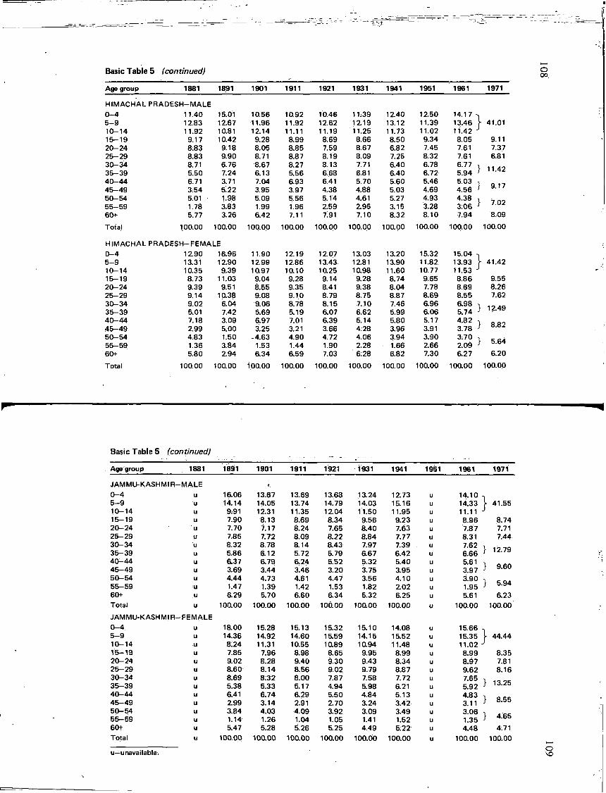
Basic Table 5 (continued)
Age group 1881 1891 1901 1911 1921 1931 1941 1951 1961 1971
HIMACHAL PRADESH-MALE 0-4 11.40 15.01 10.56 10.92 10.46 11.39 12.40 12.50 14.17 5-9 12.83 12.67 11.96 11.92 12.62 12.19 13.12 11.39 13.46 } 41.01 10-14 11.92 10.81 12.14 11.11 11.19 11.25 11.73 11.02 11.42 J
15-19 9-17 10.42 9.28 8.99 8.69 8.66 8.50 9.34 8.05 9.11 20-24 8.83 9.18 8.05 8.85 7.59 8.67 6.82 7.45 7.61 7.37 25-29 8.83 9.90 8.71 8.87 8.19 8.09 7.25 8.32 7.61 6.81 30-34 8.71 6.76 8.67 8.27 8.13 7.71 6.40 6.78 6.77 \ 1 1 A O 35-39 5.50 7.24 6.13 5.56 6.68 6.81 6.40 6.72 5.94 i \ 1.4z 40-44 6.71 3.71 7.04 6.93 6.41 5.70 5.60 5.46 5.03 1 0 1 1 45-49 3.54 5!22 3.95 3.97 4.38 4.88 5.03 4.69 4.56 ; y. 1 /
50-54 5.01 1.98 5.09 5.56 5.14 4.61 5.27 4.93 4.38 I •7 no 55-59 1.78 3.83 1.99 1.96 2.59 2.95 3.15 3.28 3.06 i /.UZ
60+ 5.77 3.26 6.42 7.11 7.91 7.10 8.32 8.10 7.94 8.09
Total 100.00 100.00 100.00 100.00 100.00 100.00 100.00 100.00 100.00 100.00
HIMACHAL PRADESH-FEMALE 0-4 12.90 16.96 11.90 12.19 12.07 13.03 13.20 15.32 15.04 -1 5-9 13.31 12.90 12.99 12.86 13.43 12.81 13.90 11.82 13.93 } 41.42 10-14 10.35 9.39 10.97 10.10 1025 10.98 11.60 10.77 11.53 j 15-19 8.73 11.03 9.04 9.28 9.14 9.28 8.74 9.65 8.86 9.55 20-24 9.39 9.51 8.55 9.35 8.41 9.38 8.04 7.78 8.69 8.26 25-29 9.14 1038 9.08 9.10 8.79 8.75 8.87 8.69 8.55 7.62 30-34 9.02 6.04 9.06 8.78 8.15 7.10 7.46 6.96 6.98 1 1 *5 AQ 35-39 5.01 7.42 5.69 5.19 6.07 6.62 5.99 6.06 5.74 ; 1 Z.HJi
40-44 7.18 3.09 6.97 7.01 6.39 5.14 5.80 5.17 4.82 45-49 2.99 5.00 3.25 3.21 3.66 4.28 3.96 3.91 3.78 / 0 . 0 /
50-54 4.83 1.50 -4.63 4.90 4.72 4.06 3.94 3.90 3.70 K CA 55-59 1.36 3.84 1.53 1.44 1.90 2.28 1.66 2.66 2.09 i
60+ 5.80 2.94 6.34 6.59 7.03 6.28 6.82 7.30 6.27 6.20
Total 100.00 100.00 100.00 100.00 100.00 100.00 100.00 100.00 100.00 100.00
Basic Table 5 (continued)
Age group 1881 1891 1901 1911 1921 1931 1941 1951 1961 1971
JAMMU-KASHMIR-•MALE 0-4 u 16.06 13.67 13.69 13.68 13.24 12.73 u 14.10 5-9 u 14.14 14.05 13.74 14.79 14.03 15.16 u 14.33 f 41.55 10-14 u 9.91 12.31 11.35 12.04 11.50 11.95 u 11.11 J 15-19 u 7.90 8.13 8.69 8.34 9.56 9.23 u 8.96 8.74 20-24 u 7.70 7.17 8.24 7.65 8.40 7.63 u 7.87 7.71 25-29 u 7.85 7.72 8.09 8.22 8.84 7.77 u 8.31 7.44 30-34 u 8.32 8.78 8.14 8.43 7.97 7.39 u 7.62 i 35-39 u 5.86 6.12 5.72 5.79 &67 6.42 u 6.66 ) 12.79 40-44 u 6.37 6.79 6.24 5.52 5.32 5.40 u 5.61 45-49 u 3.69 3.44 3.46 3.20 3.75 3.95 u 3.97 ; 9.60 50-54 u 4.44 4.73 4.61 4.47 3.56 4.10 u 3.90 1 55-59 u 1.47 1.39 1.42 1.53 1.82 2.02 u 1.95 i 5.94 60+ u 6.29 5.70 6.60 &34 5.32 6.25 u 5.61 6.23 Total u 100.00 100.00 100.00 100.00 100.00 100.00 u 100.00 100.00
JAMMU-KASHMIR-•FEMALE 0-4 u 18.00 15.28 15.13 15.32 15.10 14.08 u 15.66 5-9 u 14.36 14.92 14.60 15.59 14.15 15.52 u 15.35 } 44.44 10-14 u 8.24 11.31 10.55 10.89 10.94 11.48 u 11.02 J 15-19 u 7.85 7.96 8.98 8.65 9.95 8.99 u 8.99 8.35 20-24 u 9.02 8.28 9.40 9.30 9.43 8.34 u 8.97 7.81 25-29 u 8.60 8.14 8.56 9.02 9.79 8.87 u 9.62 8.16 30-34 u 8.69 8.32 8.00 7.87 7.58 7.72 u 7.65 35-39 u 5.38 5.33 5.17 4.94 5.98 6.21 u 5.92 13.25 40-44 u 6.41 6.74 6.29 5.50 4.84 5.13 u 4.83 45-49 u 2.99 3.14 2.91 2.70 3.24 3.42 u 3.11 ,} 8.55 50-54 u 3.84 4.03 4.09 3.92 3.09 3.49 u 3.06 i 55-59 u 1.14 1.26 1.04 1.05 1.41 1.52 u 1.35 j 4.65 60+ u 5.47 5.28 5.26 5.25 4.49 5.22 u 4.48 4.71 Total u 100.00 100.00 100.00 100.00 100.00 100.00 u 100.00 100.00
u—unavailable.
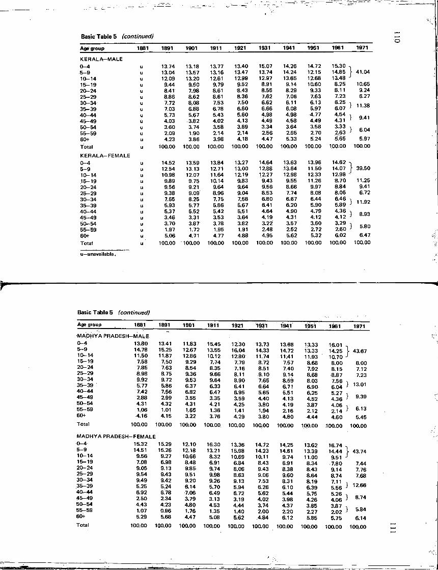
Basic Table 5 (continued)
Age group 1881 1891 1901 1911 1921 1931 1941 1951 1961 1971
KERALA—MALE 0-4 u 13.74 13.18 13.77 13.40 15.07 14.26 14.72 15.30 5-9 u 13.04 13.57 13.16 13.47 13.74 14.24 12.15 14.85 } 41.04 10-14 u 1209 13.20 12.61 12.99 12.97 13.65 12.68 13.48 J
15-19 u 9.44 9.50 9.79 9.52 8.91 9.14 10.60 8.25 10.65 20-24 u 8.41 7.98 8.61 8.43 8.55 8.29 9.33 8.11 9.24 25-29 u 8.86 8.62 8.61 8.36 7.62 7.06 7.63 7.23 6.27 30-34 u 7.72 8.08 7.53 7.50 6.62 6.11 6.13 6.25 \ 1 1 Ifi 35-39 u 7.03 6.88 6.78 6.60 6.66 6.08 5.97 6.07 5 1 1 .OO
40-44 u 5.73 5.67 5.43 5.60 4.98 4.98 4.77 4.54 X Q 4.1 45-49 u 4.03 3.82 4.02 4.13 4.49 4.58 4.49 4.31 J o.H 1
50-54 u 3.60 3.74 3.58 3.69 3.34 3.64 3.58 3.33 \ fi f\A 55-59 u 2.09 1.90 2.14 2.14 2.56 2.65 2.70 2.63 J
60+ u 4.23 3.86 3.98 4.18 4.47 5.33 5.24 5.65 5.97
Total u 100.00 100.00 100.00 100.00 100.00 100:00 100.00 100.00 100.00
K E R A L A - F E M A L E 0-4 u 14.52 13.59 13.84 13.27 14.64 13.63 13.96 14.62 5-9 u 12.54 13.13 12.71 13.00 12.88 13.64 11.50 14.07 j 39.50 10-14 u 10.98 12.07 11.64 12.19 12.27 12.98 1233 12.98 J
15-19 u 9.89 9.75 10.14 9.83 9.43 9.55 11.26 8.70 11.25 20-24 u 9.56 9.21 9.64 9.64 9.56 8.66 9.97 8.84 9.41 25-29 u 9.38 9.09 8.96 9.04 8.53 7.74 8.08 8.05 6.72 30-34 u 7.65 8.25 7.75 7.58 6.80 6.67 6.44 6.46 X 1 1 CkO 35-39 u 5.93 5.77 5.86 5.67 6.41 6.20 5.90 5.89 j 1
40-44 u 5.37 5.52 5.42 5.51 4.64 4.90 4.79 4.36 \ B Q1 45-49 u 3.46 3.31 3.53 3.64 4.19 4.31 4.12 4.12 1 0.90
50-54 u 3.70 3.87 3.78 3.82 3.22 3.57 3.60 3.29 X 55-59 u 1.97 1.72 1.95 1.91 2.48 2.52 2.72 2.60 i o.ou
60+ u 5.06 4.71 4.77 4.88 4.95 5.62 5.32 6.02 6.47 Total u 100.00 "100.00 100.00 100.00 100.00 100.00 100.00 100.00 100.00
u—unavailable.
Basic Table 5 (continued)
Age group 1881 1891 1901 1911 1921 i?31 1941 1951 1961 1971
-MADHYA PRADESH - M A L E 0-4 13.80 13.41 11.83 15.45 1230 13.73 13.66 13.33 16.01 5-9 14.78 15.25 12.67 13.55 16.04 14.33 14.72 13.33 14.25 \ 43.67 10-14 11.50 11.87 12.86 10.12 12.80 11.74 11.41 11.93 10.70 J 15-19 7.58 7.50 9.29 7.74 7.79 8.72 7.57 8.68 8.00 8.00 20-24 7.85 7.63 8.54 8.35 7.16 8.51 7.40 7.92 8.15 7.12 25-29 8.98 8.75 9.36 9.66 8.11 9.10 9.14 8.68 8.87 7.23 30-34 9.92 9.72 9.53 9.64 8.90 7.65 8.59 8.03 7.56
13.01 35-39 5.77 5.86 6.37 6.33 6.41 6.64 6.71 6.90 6.04 } 13.01 40-44 7.42 7.56 6.82 6.47 6.95 5.65 5.51 6.25 5.27
9.39 45-49 2.88 299 3.55 3.35 3.59 4.40 4.13 4.52 4.36 } 9.39 50-54 4.31 4.32 4.31 4.21 4.25 3.80 4.19 3.87 4.06 6.13 55-59 1.06 1.01 1.65 1.36 1.41 1.94 216 212 2.14 } 6.13 60+ 4.16 4.15 3.22 3.76 4.29 3.80 4.80 4.44 4.60 5.45 Total 100.00 100.00 100.00 100.00 100.00 100.00 100.00 100.00 100.00 100.00
MADHYA PRADESH-- F E M A L E 0-4 15.32 15.29 12.10 16.30 13.36 14.72 14.25 13.62 16.74 5-9 14.51 15.26 12.18 13.21 15.98 14.23 14.61 13.39 14.44 ) 43.74 10-14 9.56 9.27 10.66 8.32 10.69 10.11 9.74 11.00 9.51 J 15-19 7.08 6.98 8.48 6.91 6.84 8.43 6.91 8.34 7.80 7.44 20-24 9.05 9.13 9.85 9.74 8.06 9.43 8.38 8.43 9.14 7.76 25-29 9.54 9.43 9.51 9.98 8.63 9.06 9.60 8.64 8.74 7.68 30-34 9.49 9.42 9.20 9.26 9.13 7.53 8.31 8.19 7.11
12.66 35-39 5.25 5.24 6.14 5.70 5.94 6.26 6.10 6.39 5.56 } 12.66 40-44 6.92 6.78 7.06 6.49 6.72 5.62 5.44 5.75 5.26 8.74 45-49 250 2.34 3.79 3.13 3.19 4.02 3.98 4.26 4.06 } 8.74 50-54 4.43 4:23 4.80 4.53 4.44 3.74 4.37 3.85 3.87 5.84 55-59 1.07 0.96 1.76 1.35 1.40 2.00 2.20 2.27 2.02 } 5.84 60+ 5.29 5.68 4.47 5.08 5.62 4.84 6.12 5.85 5.75 6.14 Total 100.00 100.00 100.00 100.00 100.00 100.00 100.00 100.00 100.00 100.00
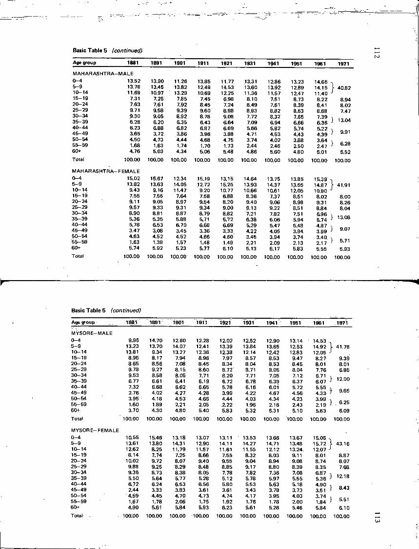
Basic Table 5 (continued)
Age group 1881 1891 1901 1911 1921 1931 1941 1951 1961 1971
MAHARASHTRA- -MALE 0-4 13.52 13.90 11.26 13.85 11.77 13.31 12.86 13.23 14.65 5-9 13.76 13.45 13.82 12.49 14.53 13.60 13.92 12.89 14.15 ) 40.82 10-14 11.69 10.97 13.29 10.69 12.25 11.36 11.57 12.47 11.40 J 15-19 7.31 7.25 7.85 7.45 6.98 8.10 7.51 8.73 8.22 8.94 20-24 7.63 7.61 7.92 8.45 7.24 8.49 7.61 8.39 8.41 8.02 25-29 9.71 9.58 9.39 9.60 8.98 8.93 8.82 8.63 8.68 7.47 30-34 9.30 9.05 8.92 8.78 9.08 7.72 8.32 7.65 7.39 \ 13.04 35-39 6.26 6.20 6.35 6.43 6.64 7.09 6.94 6.66 6.36 } 13.04 40-44 6.23 6.88 6.82 6.87 6.69 5.66 5.82 5.74 5.22 l 9.91 45-49 3.65 3.72 3.86 3.96 3.88 4.71 4.53 4.43 4.39 } 9.91 50-54 4.50 4.73 4.44 4.68 4.75 3.74 4.02 3.88 3.64
6.28 55-59 1.68 1.63 1.74 1.70 1.73 2.44 2.46 2.50 2.47 } 6.28 60+ 4.76 5.03 4.34 5.06 5.48 4.86 5.60 4.80 5.01 5.52 Total 100.00 100.00 100.00 100.00 100.00 100.00 100.00 100.00 100.00 100.00
MAHARASHTRA— FEMALE 0-4 15.02 15.67 12.34 15.19 13.15 14.64 13.75 13.85 15.39 5-9 13.82 13.63 14.05 12.72 15.25 13.93 14.37 13.55 14.87 ) 41.91 10-14 9.43 9.16 11.47 9.20 10.77 10.66 10.61 12.05 10.90 J 15-19 7.55 7.55 7.64 7.58 6.88 8.36 7.37 8.51 8.02 8.00 20-24 9.11 9.05 8.97 9.54 8.20 9.40 9.06 8.98 9.31 8.26 25-29 9.57 9.33 9.31 9.34 9.00 9.13 9.22 8.51 8.84 8.04 30-34 8.90 8.81 8.87 8.79 8.82 7.21 7.82 7.51 696
13.08 35-39 5.36 5.35 5.88 5.71 5.72 6.38 6.06 5.94 5.74 } 13.08 40-44 5.78 6.53 6.70 6.68 6.69 5.29 5.47 5.48 4.87
9.07 45-49 3.47 3.08 3.45 3.36 3.33 4.22 4.05 3.94 3.99 } 9.07 50-54 4.63 4.52 4.52 4.66 4.60 3.45 3.94 3.74 3.40 5.71 55-59 1.63 1.38 1.57 1.48 1.49 2.21 2.09 2.13 2.17 } 5.71 60+ 5.74 5.92 5.23 5.77 6.10 5.13 6.17 5.83 5.55 5.93 Total 100.00 100.00 100.00 100.00 100.00 100.00 100.00 100.00 100.00 100.00
Basic Table 5 (continued)
Age group 1881 1891 1901 1911 1921 1931 1941.'1 1951 1961 . 1971
MYSORE- MALE 0-4 9.95 14.70 12.60 12.28 12.02 12.52 12.90 13.14 14.53 5-9 13.23 13.70 14.07 12.41 13.39 13.84 13.65 12.53 14.92 } 41.76 10-14 13.81 9.34 13.27 12.36 12.38 12.14 12.42 12.83 12.05 J 15-19 8.95 8.17 7.94 8.96 7.97 8.57 8.53 9.47 8.27 9.39 20-24 8.65 8.56 7.08 8.45 8.34 8.04 8.53 8.45 8.01 8.01 25-29 9.78 9.27 8.15 8.60 8.72 8.71 8.05 8.04 7.76 6.85 30-34 9.53 8.58 8.05 7.71 8.20 7.71 7.05 7.12 6.71 35-39 6.77 6.61 6.41 6.19 6.72 6.78 6.39 6:37 6.07 ; 12.00 40-44 7.32 6.68 6.62 6.65 5.78 6.16 6.0 i 5.72 5.55
9.65 45-49 2.76 4.02 4.27 4.28 3.99 4.22 4.67 4.56 4.33 i 9.65 50-54 3.95 4.18 4.53 4.66 4.44 4.03 4.34 4.23 3.99 55-59 1.60 1.89 2.21 2.05 2.22 1.96 2.16 2.43 2.19 i 6.25 60+ 3.70 4.30 4.80 5.40 5.83 5.32 5.31 5.10 5.63 6.09 Total 100.00 100.00 100.00 100.00 100.00 100.00 100.00 100.00 100.00 100.00
MYSORE- FEMALE 0-4 10.55 15.46 13.18 13.07 13.11 13.53 13.66 13.67 15.05 5-9 13.61 13!80 14.31 12.90 14.11 14.27 14.71 13.48 15.72 } 43.16 10-14 12.62 8.25 11.79 11.57 11.61 11.55 12.12 13.24 12.07 J 15-19 8.14 7.74 7.25 8.66 7.55 8.32 8.03 9.11 8.01 8.87 20-24 10.02 9.72 8.07 9.40 9.55 9.04 8.94 9.08 8.74 8.07 25-29 9.88 9.25 8.29 8.48 8.85 9.17 8.80 8.39 8.35 7.68 30-34 9.36 8.73 8.38 8.05 7.78 7.82 7.36 7.08 6.87 35-39 5.50 5.64 5.77 5.28 5.12 5.78 5.97 5.55 5.36 ) 12.18 40-44 6.72 6.24 6.53 6.56 5.80 5.53 5.63 5.18 4.90 45-49 2.44 3.33 3.83 3.61 3.61 3.43 3.78 3.73 3.51 } 8.43 50-54 4.59 4.45 4.70 4.73 4.74 4.17 3.95 4.03 3.74
5.51 55-59 1.67 1.78 2.06 1.75 1.92 1.76 1.78 2.00 1.84 } 5.51 60+ 4.90 5.61 5.84 5.93 6.23 5.61 5.28 5.46 5.84 6.10 Total ioo;oo 100.00 100.00 100.00 100.00 100.00 100.00 100.00 100.00 100.00
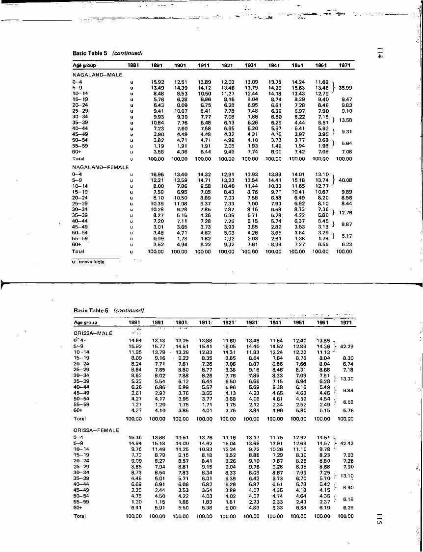
Basic Table 5 (continued)
Age group 1881 1891 1901 1911 1921 1931 1941 1951 1961
NAGALAND—MALE 0-4 u 15.92 1251 13.89 12.03 13.09 13.75 14.24 11.69 5-9 u 13.49 14.39 14.12 13.46 13.79 14.29 15.63 13.46 10-14 u 8.48 8.53 10.50 11.27 12.44 14.18 13.43 12.79 15-19 u 5.76 6.28 6.96 8.16 8.04 8.74 8.29 9.40 20-24 u 6.43 8.09 6.75 6.28 6.95 6.61 7.28 8.46 25-29 u 9.41 10.07 8.41 7.78 7.48 6.29 6.97 7.90 30-34 u 9.93 9.30 7.77 7.08 7.66 6.50 6.22 7.15 35-39 u 10.84 7.76 6.48 6.13 6.26 6.29 4.44 6.57 40-44 u 7.23 7.60 7.58 6.95 6.20 5.97 6.41 5.92 45-49 u 3.90 4.49 4.48 4.32 4.31 4.16 3.97 3.95 50-54 u 3.82 4.71 4.71 4.99 4.10 3.73 3.77 3:68 55-59 u 1.19 1.91 1.91 2.05 1.93 1.49 1.94 1.98 60+ u 3.58 4.36 6.44 9.49 7.74 8.00 7.42 7.05 Total u 100.00 100.00 100.00 100.00 100.00 100.00 100.00 100.00
N A G A L A N D - F E M A L E 0-4 u 16.96 13.40 14.32 12.91 13.93 13.88 14.01 13.10 5-9 u 12.21 13.59 14.71 13.23 13.54 14.41 15.18 13.74 10-14 u 8.00 7.86 9.58 10.40 11.44 10.23 11.65 12.77 15-19 u 7.59 6.95 7.05 8.43 8.76 9.71 10.41 10.67 20-24 u 8.10 10.50 8.89 7.03 7.58 6.58 6.49 8.20 25-29 u 10.39 11.08 9.37 7.33 7.00 7.93 6.92 8.10 30-34 u 10.28 9.28 7.85 7.87 8.15 6.68 8.73 7.36 35-39 u 8.27 5.15 4.36 5.35 5.71 6.78 4.22 5.80 40-44 u 7.20 7.11 7.28 7.25 6.15 5.74 6.37 5.45 45-49 u 3.01 3.65 3.73 3.93 3.85 2.82 3.53 3.18 50-54 u 3.48 4.71 4.82 5.03 4.26 3.65 3.84 3.29 55-59 u 0.99 1.78 1.82 1.92 2.03 2.61 1.38 1.78 60+ u 3.52 4.94 6.22 9.32 7.61 8.98 7.27 6.55 Total u 100.00 100.00 100.00 100.00 100.00 100.00 100.00 100.00
1971
u—unavailable.
35.99
9.47 9.83 9.10
13.58
9.31
5.64
7.08
} 40.08
9.89 8.56 8.44
} 12.76
8.87
5.17
6.23
Basic Table 5 (continued)
Age group 1881 1891 1901 1911/ 1921" 1931' 1941 1951 1961 1971
O.RISSA-MALE -. ^ 0^4'- 14.64 13.13 13.25 13.88 11.60 13.46 11.84 12.40 13.85 5^9 15.92 15.77 14.51 15.41 16.05 14.40 14.52 12.89 14.36 } 42.29 10-14 11.95 13.79 13.29 12.83 14.31 11.83 12.24 12.22 11.13 J 15-19 8.09 9.16 9.23 8.35 8.85 8.64 7.64 8.76 8.04 8.30 20-24 8.24 7.71 7.61 7.26 7.08 8.07 6.86 7.66 8.04 6.74 25-29 8.64 7.65 8.80 8.77 8.38 9.16 8.46 8.31 8.68 7.18 30-34 8.62 8.02 7.88 8.26 7.76 7.85 8.33 7.09 7.51 1
35-39 5.22 5.54 6.12 6.44 6.50 6.66 7.15 6.94 6.28 j 13.30 40-44 6.26 6.86 5.99 5.67 5.96 5.69 6.38 6.16 5.49 i O OQ 45-49 2.61 2.92 3.76 3.65 4.13 4.23 4.65 4.62 4.45 ; 9.00
50-54 4.27 4.17 3.95 3.77 3.88 4.06 4.61 4.52 4.54 i 55-59 1.27 1.20 1.75 1.71 1.75 2.12 2.34 2.52 2.49 s 6.55 60+ 4.27 4.10 3.85 4.01 3.75 3.84 4.96 5.90 5.15 5.76
Total 100.00 100.00 100.00 100.00 100.00 100.00 100.00 100.00 100.00 100.00
ORISSA—FEMALE 0-4 15.35 13.88 13.51 13.76 11.16 13.17 11.75 12.92 14.51 -) 5-9 14.94 15.18 14.00 14.62 15.04 13.66 13.91 12.69 14.57 } 42.43 10-14 9.75 11.49 11.25 10.93 12.24 9.72 10.26 11.10 9.78 J
15-19 7.72 8.79 9.15 8.18 8.52 8.86 7.29 8.30 8.23 7.93 20-24 9.09 8.27 8.57 8.41 8.26 9.10 7.87 8.25 8.80 7.26 25-29 8.65 7.94 8.81 9.15 9.04 9.76 9.26 8.35 8.68 7.90 30-34 8.73 8.54 7.83 8.34 8.33 8.09 8.67 7.99 7.25 x 35-39 4.46 5.01 5.71 6.01 6.39 6.42 6.73 6.70 5.70 i 13.10 40-44 6.69 6.91 6.06 5.82 6.29 5.97 6.51 5.78 5.42 i 45-49 2.25 2.44 3.53 3.54 3.89 4.07 4.35 4.18 4.15 8.90 50-54 4.75 4.50 4.22 4.03 4.02 4.07 4.74 4.64 4.35 i 55-59 1.20 1.15 1.86 1.83 1.81 2.23 2.33 2.43 2.37 ; 6.19 60+ 6.41 5.91 5.50 5.38 5.00 4.89 6.33 6.68 6.19 6.29
Total 100.00 100.00 100.00 100.00 100.00 100.00 100.00 100.00 100.00 100.00
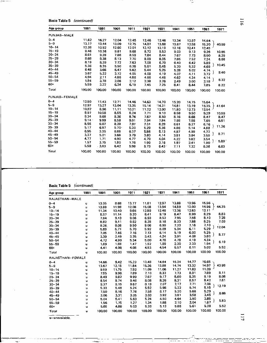
Basic Table 5 (continued)
Age group 1881 1891 1901 1911 1921 1931 1941 1951 1961 1971
PUNJAB—MALE 0-4 11.62 16.27 12.04 12.45 12.46 12.46 13.34 13.97 14.64 5-9 13.17 13.44 13.09 12.75 14.07 13.68 13.67 12.58 15.20 ) 40.99 10-14 12.39 10.52 12.60 12.01 12.12 12.19 12.16 12.41 12.45 J. 15-19 9.46 10.36 9.61 9.68 8.72 9.53 9.03 9.13 9.26 10.65 20-24 8.61 9.28 7.86 8.59 7.84 8.44 7.67 7.73 8.00 8.29 25-29 8.68 9.38 8.13 7.70 8.09 8.05 7.65 7.52 7.24 6.68 30-34 8.19 6.39 7.72 7.63 7.08 6.79 6.40 6.42 5.89
10.45 35-39 5.36 6.35 5.50 6.36 5.61 5.45 5.20 5.32 4.69 } 10.45 40-44 6.48 3.66 6.47 5.62 5.44 5.25 5.28 5.02 4.74
8.40 45-49 3.67 5.22 3.72 4.05 4.08 4.19 4.07 4.11 3.72 } 8.40 50-54 4.94 2.11 4.86 4.86 4.66 4.46 4.62 4.34 4.14
6.32 55-59 1.84 3.78 2.06 2.12 2.38 2.26 2.49 3.00 2:18 } 6.32 60+ 5.59 3.22 6.34 6.19 7.45 7.25 8.41 8.44 7.85 8.22 Total 100.00 100.00 100.00 100.00 100.00 100.00 100.00 100.00 100.00 100.00
PUNJAB—FEMALE 0-4 12.80 17.43 12.71 14.46 14.63 14.70 15.20 14.75 15.64 5-9 12.97 13.27 13.04 13.35 15.14 14.31 14.81 13.19 15.35 ) 41.64 10-14 10.82 8.96 11.11 10.21 11.22 12.00 11.80 12.73 12.54 J 15-19 8.97 10.58 8.55 8.24 7.71 9.10 8.58 9.50 9.29 10.59 20-24 9.34 9.68 8.36 8.76 7.67 8.50 8.16 8.68 8.47 8.47 25-29 9.14 9.99 8.58 9.01 7.94 7.84 7.98 7.58 7.65 6.81 30-34 8.55 6.07 8.28 7.97 7.31 6.29 6.61 6.27 6.16
11.26 35-39 5.17 6.97 5.70- 5.30 5.29 5.36 4.86 5.14 4.88 } 11.26 40-44 6.95 3.35 6.88 6.37 5.88 5.13 4.87 4.99 4.72
8.71 45-49 3.37 5.21 3.68 3.79 3.80 4.14 3.81 3.64 3.59 } 8.71 50-54 4.77 1.71 4.90 4.77 4.70 4.04 4.22 3.82 3.54
5.89' 55-59 1.57 3.75 1.80 1.78 1.99 2.16 1.97 2.41 1.90 } 5.89' 60+ 5.59 3.03 6.42 5.98 6.73 6.43 7.11 7.32 6.26 6.63 Total 100.00 100.00 100.00 100.00 100.00 100.00 100.00 100.00 100.00 100.00
Basic Table 5 (continued)
Age group 1881 1891 1901 1911 1921 1931 1941 1951 1961 1971
RAJASTHAN- •MALE 0-4 u 13.35 8.68 13.77 11.81 12.97 13.88 13.96 15.56 1 5-9 u 13.88 11.98 12.08 15.08 13.94 14.59 13.00 14.96 \ 44.35 10-14 u 11.34 13.40 9.65 12.89 12.46 12.36 12.63 12.11 J
15—19 u 8.57 11.14 9.20 8.41 9.19 8.47 8.99 8.29 8.83 20-24 u 7.84 9.13 9.06 6.93 8.52 7.95 7.58 8.10 7.28 25-29 u 8.82 9.11 9.62 8.28 8.16 8.33 7.88 8.25 7.03 30-34 u 9.26. 9.06 9.50 9.06 6.99 7.33 7.16 7.10 "l 1-1 C\A .
35^39 u 5.69 5.71 5.70 5.92 6.09 5.34 6.11 5.29 J 1 Z.U*t
40-44 u 7.05 7.46 7.16 7.13 6.14 5.19 6.00 5.25 ^ P 77
45-49 u 3.39 3.49 3.35 3.43 4.24 3.91 4.08 3.80 j O. / /
50-54 u 4.72 4.90 5.34 5.00 4.76 4.78 4.18 4.34 ^ R 1Q
55-59 u 1.69 1.88 1.47 1.52 1.99 2.30 2.33 1.94 j o. i y 60+ u 4.41 4.06 4.08 4.53 4.54 5.57 6.11 5.02 5.52
Total u 100.00 100.00 100.00 100.00 100.00 100.00 100.00 100.00 100.00
RAJASTHAN- •FEMALE 0-4 u 14.66 9.42 15.23 13.48 14.64 15.24 14.77 16.65 1 5-9 u 13.67 12.18 11.84 15.36 13.88 14.74 13.32 14.97 \ 43.98 10-14 u 9.59 11.75 7.93 11.09 11.06 11.27 11.83 11.09 J
15-19 u 7.55 9.96 7.89 7.10 8.33 7.73 8.91 7.89 8.11 20-24 u 8.49 9.82 9.99 7.67 9.17 8.60 8.35 9.19 8.08 25-29 u 8.54 8.74 9.46 8.08 8.26 8.31 8.57 8.42 7.61 30-34 u 9.37 9.15 9.67 9.19 7.07 7.17 7.71 7.08 1 1 O 1 Q 35-39 u 5.33 5.48 5.24 5.52 5.98 5.22 5.74 5.15 J IZ. 19
40-44 u 7.50 8.16 7.78 7.58 6.17 5.30 5.66 5.29 1 C C O
45-49 u 3.06 3.31 3.05 3.03 3.92 3.81 3.58 3.45 J O. DO
50-54 u 5.04 5.41 5.63 5.24 4.50 4.64 3.90 3.88 55-59 u 1.56 1.75 1.27 1.34 1.88 2.10 2.04 1.67 J O.oo
60+ u 5.65 4.86 5.03 5.33 5.13 5.86 5.61 5.28 5.52
Total u 100.00 100.00 100.00 100.00 100.00 100.00 100.00 100.00 100.00
u—unavailable.
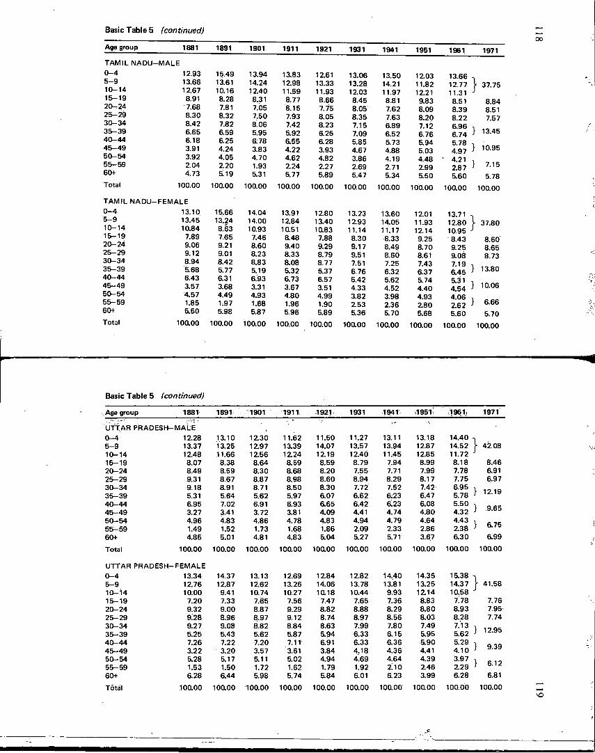
Basic Table 5 (continued)
Age group
TAMIL NADU—MALE 0-4 5-9 10-14 15-19 20-24 25-29 30-34 35-39 40-44 45-49 50-54 55-59 60+
Total
1881 1891 1901 1911 1921 1931 1941 1951 1961 1971
E 12.93 15.49 13.94 13.83 12.61 13.06 13.50 12.03 13.66 13.66 13.61 14.24 12.98 13.33 13.28 14.21 11.82 12.77 } 37.75 12.67 10.16 12.40 11.59 11.93 12.03 11.97 12.21 11.31 J
37.75
8.91 8.28 8.31 8.77 8.66 8.45 8.81 9.83 8.51 8.84 7.68 7.81 7.05 8.15 7.75 8.05 7.62 8.09 8.39 8.51 8.30 8.32 7.50 7.93 8.05 8.35 7.63 8.20 8.22 7.57 8.42 7.82 8.06 7.42 8.23 7.15 6.89 7.12 6.96
13.45 6.65 6.59 5.95 5.92 6.25 7.09 6.52 6.76 6.74 } 13.45 6.18 6.25 6.78 a55 6.28 5.85 5.73 5.94 5.78
10.95 3.91 4.24 3.83 4.22 3.93 4.67 4.88 5.03 4.97 } 10.95 3.92 4.05 4.70 4.62 4.82 3.86 4.19 4.48 • 4.21
7.15 2.04 2.20 1.93 2.24 2.27 2.69 2.71 2.99 2.87 } 7.15 4.73 5.19 5.31 5.77 5.89 5.47 5.34 5.50 5.60 5.78
100.00 100.00 100.00 100.00 100.00 100.00 100.00 100.00 100.00 100.00
TAMIL N A D U - F E M A L E 0-4 5-9 10-14 15-19 20-24 25-29 30-34 35-39 40-44 45-49 50-54 55-59 60+
Total
13.10 15.66 14.04 13.91 12.80 13.23 13.60 12.01 13.71 13.45 13.24 14.00 12.84 13.40 12.93 14.05 11.93 12.80 ) 37.80 10.84 8.63 10.93 10.51 10.83 11.14 11.17 12.14 10.95 J 7.89 7.65 7.46 8.48 7.88 8.30 8.33 9.25 8.43 8.60 9.06 9.21 8.60 9.40 9.29 9.17 8.49 8.70 9.25 8.65 9.12 9.01 8.23 8.33 8.79 9.51 8.60 8.61 9.08 8.73 8.94 8.42 8.83 8.08 8.77 7.51 7.25 7.43 7.19
13.80 5.68 5.77 5.19 5.32 5.37 6.76 6.32 6.37 6.45 } 13.80 6.43 6.31 6.93 6.73 6.57 5.42 5.62 5.74 5.31
10.06 3.57 3.68 3.31 3.67 3.51 4.33 4.52 4.40 4.54 } 10.06 4.57 4.49 4.93 4.80 4.99 3.82 3.98 4.93 4.06
6.66 1.85 1,97 1.68 1.96 1.90 2.53 2.36 280 2.62 } 6.66 5.50 5.98 5.87 5.96 5.89 5.36 5.70 5.68 5.60 5.70
100.00 100.00 100.00 100.00 100.00 100.00 100.00 100.00 100.00 100.00
Basic Table 5 (continued)
Age group 1881 1891 1901 1911; 1921. 1931 1941 si 951 1961, 1971
UTTAR PRADESH- MALE •'
0-4 12.28 13.10 12.30 11.62 11.50 11.27 13.11 13.18 14.40 5-9 13.37 13.25 12.97 13.39 14.07 13.57 13.94 12.87 14.52 [ 42.08 10-14 12.48 11.66 12.56 12.24 12.19 12.40 11.45 12.85 11.72 J 15-19 8.07 8.38 8.64 8.59 8.59 8.79 7.94 8.99 8.18 8.46 20-24 8.49 8.59 8.30 8.68 8.20 7.55 7.71 7.99 7.78 6.91 25-29 9.31 8.67 8.87 8.98 8.60 8.94 8.29 8.17 7.75 6.97 30-34 9.18 8.91 8.71 8.50 8.30 7.72 7.52 7.42 6.95
1 n in 35-39 5.31 5.64 5.62 5.97 6.07 6.62 6.23 6.47 5.78 j i z. i y
40-44 6.95 7.02 6.91 6.93 6.65 6.42 6.23 6.08 5.50 \ Q C C
45-49 3.27 3.41 3.72 3.81 4.09 4.41 4.74 4.80 4.32 j y . o D
50-54 4.96 4.83 4.86 4.78 4.83 4.94 4.79 4.64 4.43 X a *?c 55-59 1.49 1.52 1.73 1.68 1.86 2.09 2.33 2.86 2.38 J o . / o
60+ 4.85 5.01 4.81 4.83 5.04 5.27 5.71 3.67 6.30 6.99
Total 100.00 100.00 100.00 100.00 100.00 100.00 100.00 100.00 100.00 100.00
UTTAR PRADESH- FEMALE 0-4 13.34 14.37 13.13 12.69 12.84 12.82 14.40 14.35 15.38 5-9 12.76 12.87 12.62 13.26 14.06 13.78 13.81 13.25 14.37 \ 41.58 10-14 10.00 9.41 10.74 10.27 10.18 10.44 9.93 12.14 10.58 J 15-19 7.20 7.33 7.65 7.56 7.47 7.65 7.36 8.83 7.78 7.76 20-24 9.32 9.00 8.87 9.29 8.82 8.88 8.29 8.80 8.93 7.95 25-29 9.28 8.96 8.97 9.12 8.74 8.97 8.56 8.03 8.28 7.74 30-34 9.27 9.08 8.82 8.84 8.63 7.99 7.80 7.49 7.13 1 1*5 O K
35-39 5.25 5.43 5.62 5.87 5.94 6.33 6.15 5.95 5.62 j i z.yo 40-44 7.26 7.22 7.20 7.11 6.91 6.33 6.36 5.90 5.29 "I Q *JQ 45-49 3.22 3.20 3.57 3.61 3.84 4.18 4.36 4.41 4.10 j y . o y
50-54 5.28 5.17 5.11 5.02 4.94 4.69 4.64 4.39 3.97 X c n 55-59 1.53 1.50 1.72 1.62 1.79 1.92 2.10 246 229 J O . I Z
60+ 6.28 6.44 5.98 5.74 5.84 6.01 6.23 3.99 6.28 6.81
Total 100.00 100.00 100.00 100.00 100.00 100.00 100.00 100.00 100.00 100.00
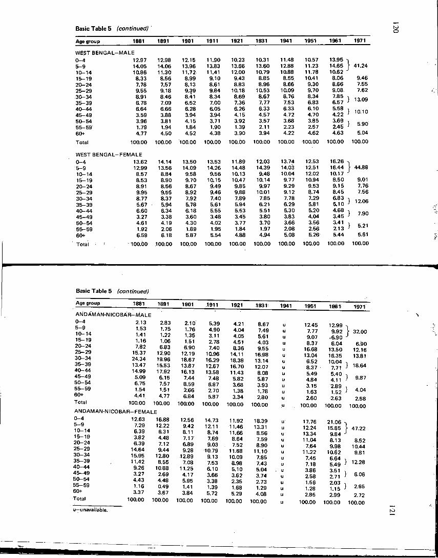
Basic Table 5 (continued)
Age group 1881 1891 1901 1911 1921 1931 1941 1951 1961 1971
WEST BENGAL— MALE 0-4 12.97 12.98 12.15 11.90 10.23 10.31 11.48 10.57 13.95 5-9 14.05 14.06 13.96 13.83 13.66 13.60 12.88 11.23 14.65 \ 41.24 10-14 10.86 11.30 11.72 11.41 12.00 10.79 10.88 11.78 10.62 J
15-19 8.33 8.56 8.99 9.10 9.43 8.85 8.55 10.41 8.06 9.46 20-24 7.78 7.57 8.13 8.61 8.83 8.96 8.66 9.30 8.66 7.55 25-29 9.55 9.18 9.39 9.84 10.18 10.53 10.09 9.70 9.08 7.62 30-34 8.91 8.46 8.41 8.34 8.69 8.67 8.76 8.34 7.85 \ 11 no 35-39 6.78 7.09 6.52 7.00 7.36 7.77 7.53 6.83 6.57 J 1 J . U 9
40-44 6.64 6.66 6.28 6.05 6.26 6.33 6.33 6.10 5.58 \ i f i ' in 45-49 3.59 3.88 3.94 3.94 4.15 4.57 4.72 4.70 4.22 j 1 U. 1 u
50-54 3.96 3.81 4.15 3.71 3.92 3.57 3.68 3.85 3.69 1- R on 55-59 1.79 1.94 1.84 1.90 1.39 2.11 2.23 2.57 2.45 j o.yu 60+ 4.77 4.50 4.52 4.38 3.90 3.94 4.22 4.62 4.63 5.04
Total 100.00 100.00 100.00 100.00 100.00 100.00 100.00 100.00 100.00 100.00
WEST BENGAL-•FEMALE 0-4 13.62 14.14 13.50 13.53 11.89 12.03 13.74 12.53 16.26 5-9 12.99 13.56 14.09 14.26 14.48 14.39 14.03 12.51 16.44 \ 44.88 10-14 8.57 8.84 9.58 9.56 10.13 9.48 10.04 12.02 10.17 J
15-19 8.53 8.90 9.70 10.15 10.47 10.14 9.77 10.94 8.50 9.01 20-24 8.91 8.56 8.67 9.49 9.85 9.97 9.29 9.53 9.15 7.76 25-29 9.95 9.55 8.92 9.46 9.88 10.01 9.12 8.74 8.45 7.56 30-34 8.77 8.37 7.92 7.40 7.89 7.85 7.78 7.29 6.83 35-39 5.67 5.94 5.78 5.61 5.94 6.21 6.29 5.81 5.10 J I z.vo 40-44 6.60 6.34 6.18 5.55 5:53 5.51 5.30 5.20 4.68
\ ~J on 45-49 3.27 3.38 3.60 3.48 3.45 3.80 3.83 4.04 3.45 J / .9U
50-54 4.61 4.19 4.30 4.02 3.77 3.70 3.66 3.56 3.41 \ K 01
55-59 1.92 2.06 1.89 1.95 1.84 1.97 2.08 2.56 2.13 J 0.«£ \
60+ 6.59 6.18 5.87 5.54 4.88 4.94 5.08 5.26 5.44 5.61
Total •- ; 100.00 100.00 100.00 100.00 100.00 100.00 100.00 100.00 100.00 100.00
Basic Table 5 (continued)
Age group 1881 1891 1901 ,1911 1921 1931- 1941 1951 1961 1971
ANDAMAN-NICOBAR-MALE 0-4 5-9 10-14 15-19 20-24 25-29 30-34 35-39 40-44 45-49 50-54 55-59 60+ Total
ANDAMAN-NICOBAR-FEMALE 0-4 5-9 10-14 15-19 20-24 25-29 30-34 35-39 40-44 45-49 50-54 55-59 60+ Total
2.13 2.83 2.10 5.39 4.21 8.67 u 12.45 12.99 1.53 1.75 1.76 4.90 4.04 7.49 u 7.77 9.92 1.41 1.22 1.35 3.11 4.05 5.61 u 9.07 .6.90 1.16 1.06 1.51 2.78 4.51 4.03 u 8.37 6.04 7.82 6.83 6.90 7.40 8.36 9.55 u 16.68 13.50
15.37 12.90 12.19 10.96 14.11 16.98 u 13.04 16.35 24.34 19.96 18.67 16.29 18.38 13.14 u 6.52 10.04 13.47 15.53 13.87 12.67 16.70 12.07 u 8.37 7.71 14.99 17.92 16.13 13.58 11.43 8.08 u 5.49 5.40 5.09 6.15 7.44 7.48 5.82 5.87 u 4.84 4.11 6.75 7.57 8.59 6.87 3.68 3.93 u 3.15 2.89 1.54 1.51 2.66 2.70 1.38 1.78 u 1.63 1.52 4.41 4.77 6.84 5.87 3.34 2.80 u 2.60 2.63
100.00 100.00 100.00 100.00 100.00 100.00 u 100.00 100.00
}
12.63 16.88 12.56 14.73 11.92 18.39 u 17.76 21.06 7.29 12.22 9.42 12.11 11.46 13.31 u 12.24 15.85 6.39 6.31 8.11 8.74 11.66 8.56 u 13.34 9.84 3.82 4.48 7.17 7.69 8.64 7.59 u 11.04 8.13 6.39 7.12 6.89 9.03 7.52 8.90 u 7.64 9.98
14.64 9.44 9.28 10.79 11.68 11.10 u 11.22 1062 15.95 12.80 12.89 9.13 10.09 7.85 u 7.45 6.64 11.42 8.55 7.08 7.53 8.98 7.43 u 7.18 5.49 9.26 10.88 11.25 6.10 5.10 5.04 . u 3.86 3.51 3.27 2.69 4.17 3.66 3.62 3.74 u 2.58 2.71 4.43 4.48 5.95 3.38 2.35 2.73 u 1.56 2.03 1.16 0.49 1.41 1.39 1.68 1.29 u 1.28 1.15 3.37 3.67 3.84 5.72 5.29 4.08 u 2.85 2.99
100.00 100.00 100.00 100.00 100.00 100.00 u 100.00 100.00
32.00
6.90 12.16 13.81
} 18.64
} 9.87
4.04 2.58
100.00
f 47.22
8.52 10.44 9.81
• 12.28
6.06
2.95 2.72
100.00 u—unavailable.
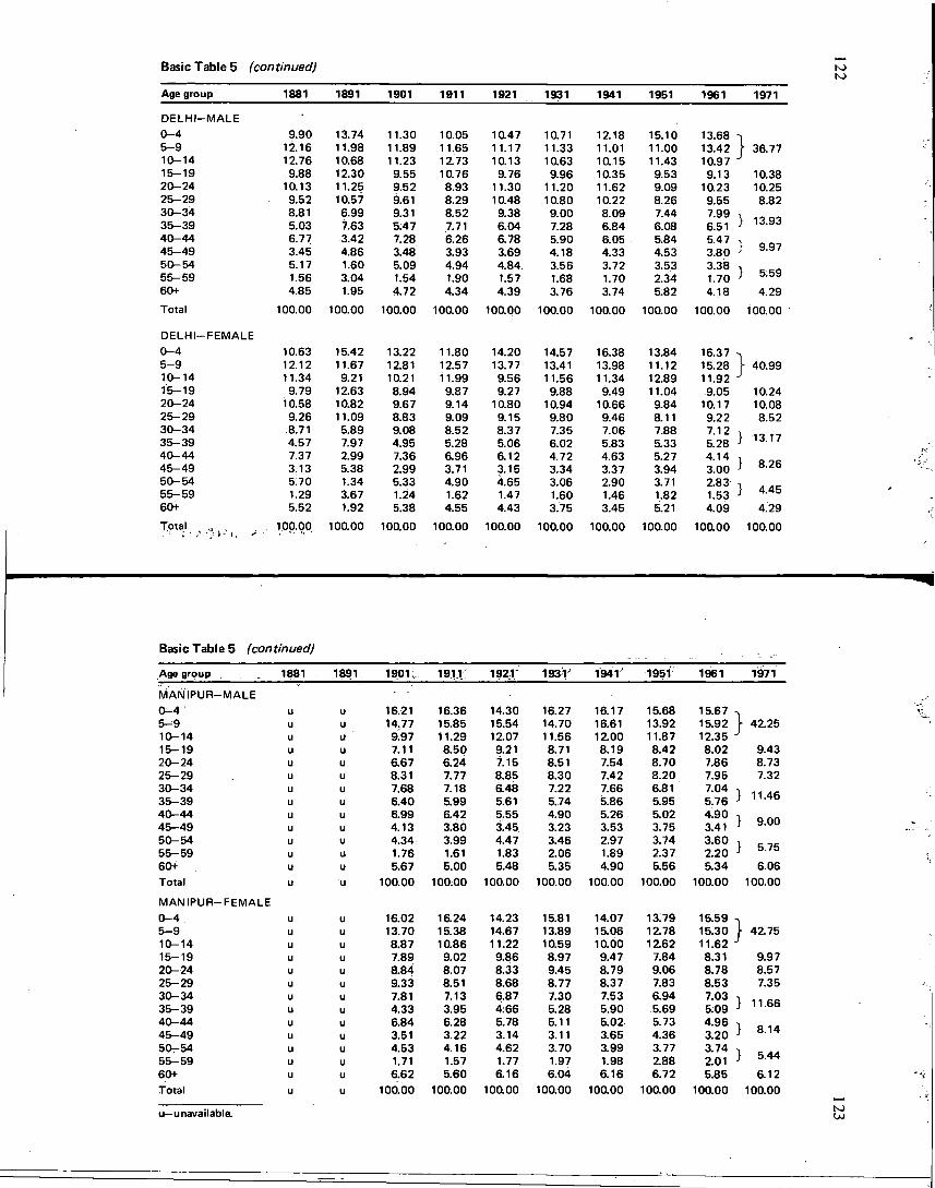
Basic Table 5 (continued) to to
Age group 1881 1891 1901 1911 1921 1931 1941 1951 1961 1971
DELHI -MALE 0-4 9.90 13.74 11.30 10.05 10.47 10.71 12.18 15.10 13.68 5-9 12.16 11.98 11.89 11.65 11.17 11.33 11.01 11.00 13.42 } 36.77 10-14 12.76 10.68 11.23 12.73 10.13 10.63 10.15 11.43 10.97 J
15-19 9.88 12.30 9.55 10.76 9.76 9.96 10.35 9.53 9.13 10.38 20-24 10.13 11.25 9.52 8.93 11.30 11.20 11.62 9.09 10.23 10.25 25-29 9.52 10.57 9.61 8.29 10.48 10.80 10.22 8.26 9.55 8.82 30-34 8.81 6.99 9.31 8.52 9.38 9.00 8.09 7.44 7.99 \ 35-39 5.03 7.63 5.47 7.71 6.04 7.28 6.84 6.08 6.51 1 13.93 40-44 6.77 3.42 7.28 6.26 6.78 5.90 6.05 5.84 5.47 \ 45-49 3.45 4.86 3.48 3.93 3.69 4.18 4.33 4.53 3.80 S 9.97 50-54 5.17 1.60 5.09 4.94 4.84 3.56 3.72 3.53 3.38 1
55-59 1.56 3.04 1.54 1.90 1.57 1.68 1.70 2.34 1.70 ; 5.59 60+ 4.85 1.95 4.72 4.34 4.39 3.76 3.74 5.82 4.18 4.29 Total 100.00 100.00 100.00 100.00 100.00 100.00 100.00 100.00 100.00 100.00
DELHI—FEMALE 0-4 10.63 15.42 13.22 11.80 14.20 14.57 16.38 13.84 16.37 5-9 12.12 11.67 12.81 12.57 13.77 13.41 13.98 11.12 15.28 } 40.99 10-14 11.34 9.21 10.21 11.99 9.56 11.56 11.34 12.89 11.92 J 15-19 9.79 12.63 8.94 9.87 9.27 9.88 9.49 11.04 9.05 10.24 20-24 10.58 10.82 9.67 9.14 10.80 10.94 10.66 9.84 10.17 10.08 25-29 9.26 11.09 8.83 9.09 9.15 9.80 9.46 8.11 9.22 8.52 30-34 8.71 5.89 9.08 8.52 8.37 7.35 7.06 7.88 7.12 35-39 4.57 7.97 4.95 5.28 5.06 6.02 5.83 5.33 5.28 s 13.17 40-44 7.37 2.99 7.36 6.96 6.12 4.72 4.63 5.27 4.14 i 45-49 3.13 5.38 2.99 3.71 3.15 3.34 3.37 3.94 3.00 ; 8.26 50-54 5.70 1.34 5.33 4.90 4.65 3.06 2.90 3.71 2.83 i 55-59 1.29 3.67 1.24 1.62 1.47 1.60 1.46 1.82 1.53 ) 4.45 60+ 5.52 1.92 5.38 4.55 4.43 3.75 3.45 5.21 4.09 4.29
Total 100.00. 100.00 100.00 100.00 100.00 100.00 100.00 100.00 100.00 100.00
Basic Table 5 (continued)
Age group 1881 1891, 1901;, 1911." 1921 193 V 1941" 1951 1961 1971
MANIPUR— MALE 0-4 u u 16.21 16.36 14.30 16.27 16.17 15.68 15.67 5-9 u u 14.77 15.85 15.54 14.70 16.61 13.92 15.92 } 42.25 10-14 u u 9.97 11.29 12.07 11.56 12.00 11.87 12.35 j
15-19 u u 7.11 8.50 9.21 8.71 8.19 8.42 8.02 9.43 20-24 u u &67 6.24 7.15 8.51 7.54 8.70 7.86 8.73 25-29 u u 8.31 7.77 8.85 8.30 7.42 8.20 7.95 7.32 30-34 u u 7.68 7.18 6.48 7.22 7.66 6.81 7.04 \ 35-39 u u 6.40 5.99 5.61 5.74 5.86 5.95 5.76 s 11.46 40-44 u u 6.99 6.42 5.55 4.90 5.26 5.02 4^90 1 0 nn 45-49 u u 4.13 3.80 £45. 3.23 3.53 3.75 3.41 ; 9.0U 50-54 u u 4.34 3.99 4.47 3.46 2.97 3.74 3.60 \ 55-59 u u 1.76 1.61 1.83 2.06 1.89 2.37 2.20 ; 5.75 60+ u u 5.67 5.00 5.48 5.35 4.90 5.56 5.34 6.06 Total u u 100.00 100.00 100.00 100.00 100.00 100.00 100.00 100.00
MANIPUR— FEMALE 0-4 u u 16.02 16.24 14.23 15.81 14.07 13.79 15.59 1
5-9 u u 13.70 15.38 14.67 13.89 15.06 12.78 15.30 } 42.75 10-14 u u 8.87 10.86 11.22 10.59 10.00 1262 11.62 j 15-19 u u 7.89 9.02 9.86 8.97 9.47 7.84 8.31 9.97 20-24 u u 8.84 8.07 8.33 9.45 8.79 9.06 8.78 8.57 25-29 u u 9.33 8.51 8.68 8.77 8.37 7.83 8.53 7.35 30-34 u u 7.81 7.13 6.87 7.30 7.53 6.94 7.03 1
35-39 u u 4.33 3.95 4:66 5.28 5.90 5.69 5.09 ; 11.66 40-44 u u 6.84 6.28 5.78 5.11 5.02 5.73 4.96 1
45-49 u u 3.51 3.22 3.14 3.11 3.65 4.36 3.20 ; 8.14 50-54 u u 4.53 4.16 4.62 3.70 3.99 3.77 3.74 1
55-59 u u 1.71 1.57 1.77 1.97 1.98 2.88 201 ; 5.44 60+ u u 6.62 5.60 6.16 6.04 6.16 6.72 5.85 6.12 Total u u 100.00 100.00 10a 00 100.00 100.00 100.00 100.00 100.00
u—unavailable. to
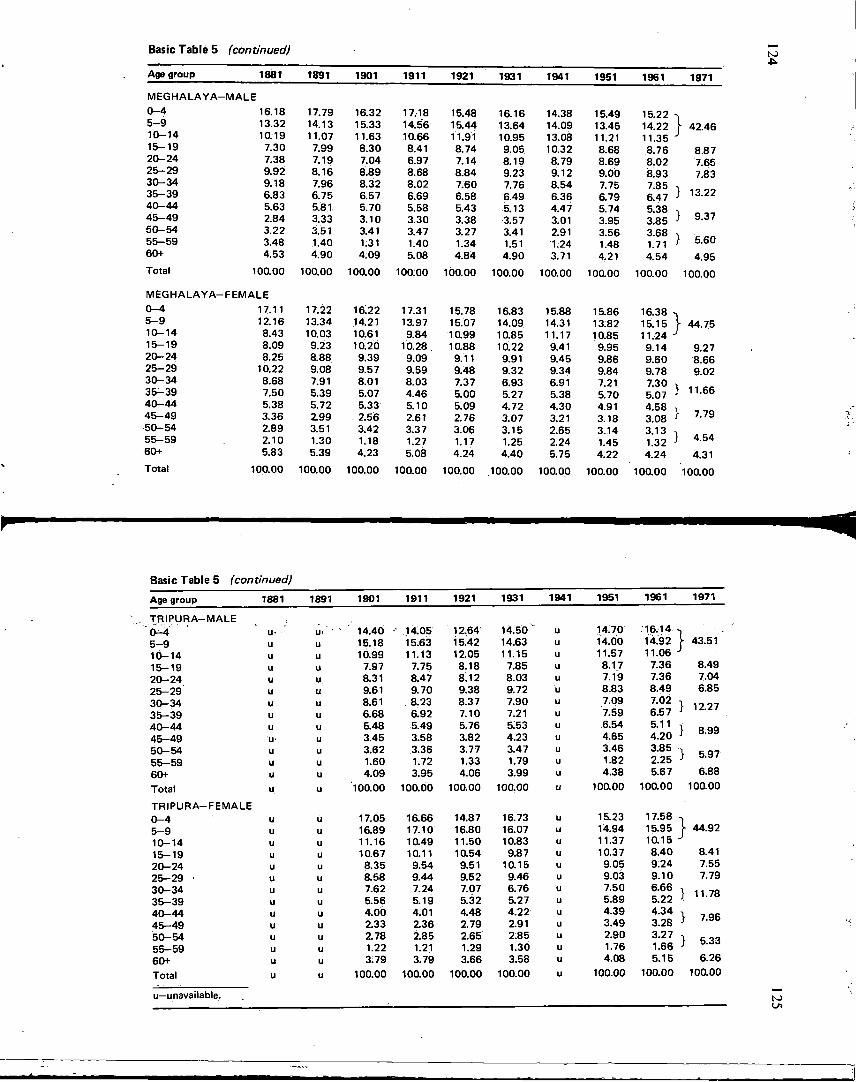
Basic Table 5 (continued)
Age group 1881 1891 1901 1911 1921 1931 1941 1951 1961 1971
MEGHALAYA- -MALE 0-4 16.18 17.79 16.32 17,18 15.48 16.16 14.38 15.49 15.22 5-9 13.32 14.13 15.33 14.56 15.44 13.64 14.09 13.45 14.22 \ 42.46 10-14 10.19 11.07 11.63 10.66 11.91 10.95 13.08 11.21 11.35 J 15-19 7.30 7.99 8.30 8.41 8.74 9.05 10.32 8.68 8.76 8.87 20-24 7.38 7.19 7.04 6.97 7.14 8.19 8.79 8.69 8.02 7.65 25-29 9.92 8.16 8.89 8.68 8.84 9.23 9.12 9.00 8.93 7.83 30-34 9.18 7.96 8.32 8.02 7.60 7.76 8.54 7.75 7.85
} 13.22 35-39 6.83 6.75 6.57 6.69 6.58 6.49 6.36 6.79 6.47 } 13.22 40-44 5.63 5.81 5.70 5.58 5.43 5.13 4.47 5.74 5.38 45-49 2.84 3.33 3.10 3.30 3.38 3.57 3.01 3.95 3.85 } 937 50-54 3.22 3.51 3.41 3.47 3.27 3.41 2.91 3.56 3.68
} 5.60 55-59 3.48 1.40 1.31 1.40 1.34 1.51 1.24 1.48 1.71 } 5.60 60+ 4.53 4.90 4.09 5.08 4.84 4.90 3.71 4.21 4.54 4.95 Total 100.00 100.00 100.00 100:00 100.00 100.00 100.00 100.00 100.00 100.00
M E G H A L A Y A - •FEMALE 0-4 17.11 17.22 16.22 17.31 15.78 16.83 15.88 15.86 16.38 - i 5-9 12.16 13.34 14.21 13.97 15.07 14.09 14.31 13.82 15.15 [ 44.75 10-14 8.43 10.03 10.61 9.84 10.99 10.85 11.17 10.85 11.24 J 15-19 8.09 9.23 10.20 10.28 . 10.88 10.22 9.41 9.95 9.14 9.27 20-24 8.25 8.88 9.39 9.09 9.11 9.91 9.45 9.86 9.60 8.66 25-29 10.22 9.08 9.57 9.59 9.48 9.32 9.34 9.84 9.78 9.02 30-34 8.68 7.91 8.01 8.03 7.37 6.93 6.91 7.21 7.30
} 11.66 35-39 7.50 5.39 5.07 4.46 5.00 5.27 5.38 5.70 5.07 } 11.66 40-44 5.38 5.72 5.33 5.10 5.09 4.72 4.30 4.91 4.58 45-49 3.36 2.99 2.56 2.61 2.76 3.07 3.21 3.18 3.08 } 7.79 50-54 2.89 3.51 3.42 3.37 3.06 3.15 2.65 3.14 3.13
} 4.54 55-59 2.10 1.30 1.18 1.27 1.17 1.25 2.24 1.45 1.32 } 4.54 60+ 5.83 5.39 4.23 5.08 4.24 4.40 5.75 4.22 4.24 4.31 Total 100.00 100.00 100.00 100.00 100.00 .100.00 100.00 100.00 100.00 100.00
r
Basic Table 5 (continued)
Age group 1881 1891 1901 1911 1921 1931 1941 1951 1961 1971
TRIPURA-MALE OM-4 TRIPURA-MALE OM-4 u. w - ' " 14.40 ,14.05 1264 14.50" u 14.70 .16.14 5-9 u u 15.18 15.63 15^42 14.63 u 14.00 14.92 ) 43.51 10-14 u u 10.99 11.13 1205 11.15 u 11.57 11.06 J
15-19 u u 7.97 7.75 8.18 7.85 u 8.17 7.36 8.49 20-24 u u 8.31 8.47 8.12 8.03 u 7.19 7.36 7.04 25-29 u u 9.61 9.70 9.38 9.72 u 8.83 8.49 6.85 30-34 u u 8.61 8.23 8.37 7.90 u 7.09 7.02
} 12.27 35-39 u u 6.68 6.92 7.10 7.21 u 7.59 6.57 } 12.27
40-44 u u 5.48 5.49 5.76 5.53 u 6.54 5.11 } 8.99
45-49 u- u 3.45 3.58 3.82 4.23 u 4.65 4.20 } 8.99
50-54 u u 3.62 3.36 3.77 3.47 u 3.46 3.85 } 5.97
55-59 u u 1.60 1.72 1.33 1.79 u 1.82 2.25 } 5.97
60+ u u 4.09 3.95 4.06 3.99 u 4.38 5.67 6.88
Total u u 100.00 100.00 100.00 100.00 u 100.00 100.00 100.00
TRIPURA-FEMALE -
0-4 u u 17.05 16.66 14.87 16.73 u 15.23 17.58 5-9 u u 16.89 17.10 16.80 16.07 u 14.94 15.95 j 44.92 10-14 u u 11.16 10.49 11.50 10.83 u 11.37 10.15 J
15-19 u u 10.67 10.11 10.54 9.87 u 10.37 8.40 8.41 20-24 u u 8.35 9.54 9.51 10.15 u 9.05 9.24 7.55 25-29 • u u 8.58 9.44 9.52 9.46 u 9.03 9.10 7.79 30-34 u u 7.62 7.24 7.07 6.76 u 7.50 6.66
} 11.78 35-39 u u 5.56 5.19 5.32 5.27 u 5.89 5.22 } 11.78
40-44 u u 4.00 4.01 4.48 4.22 u 4.39 4.34 } 7.96
45-49 u u 2.33 236 2.79 2.91 u 3.49 3.28 } 7.96
50-54 u u 2.78 2.85 2.65 2.85 u 2.90 3.27 } 5.33
55-59 u u 1.22 1.21 1.29 1.30 u 1.76 1.66 } 5.33
60+ u u 3.79 3.79 3.66 3.58 u 4.08 5.15 6.26
Total u u 100.00 100.00 100.00 100.00 u 100.00 100.00 100.00
u—unavailable.
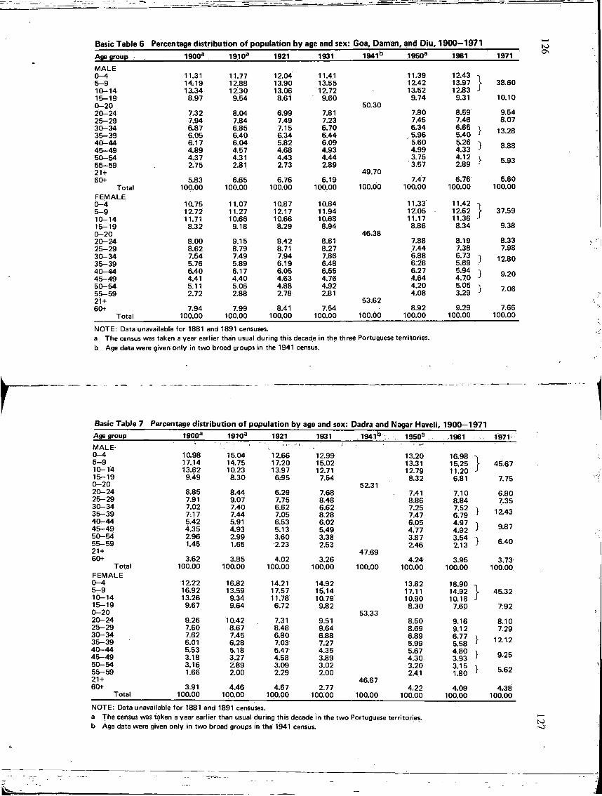
Basic Table 6 Percentage distribution of population by age and sex: Goa, Daman, and Diu, 1900—1971 Age group 1900a 1910a 1921 1931 1941° 1950a 1961 1971
MALE 0-4 11.31 11.77 12.04 11.41 11.39 12.43 5-9 14.19 12.88 13.90 13.55 12.42 13.97 [ 38.60 10-14 13.34 12.30 13.06 12.72 13.52 12.83 J 15-19 8.97 9.54 8.61 9.60 9.74 9.31 10.10 0-20 50.30 20-24 7.32 8.04 6.99 7.81 7.80 8.59 9.54 25-29 7.94 7.84 7.49 7.23 7.45 7.46 8.07 30-34 6.87 6.85 7.15 6.70 6.34 6.65 } 13.28 35-39 6.05 6.40 6.34 6.44 5.96 5.40 } 13.28
40-44 6.17 6.04 5.82 6.09 5.60 5.26 } 8.88 45-49 4.89 4.57 4.68 4.93 4.99 4.33 } 8.88
50-54 4.37 4.31 4.43 4.44 3.75 4.12 } 5.93 55-59 2.75 2.81 2.73 2.89 3.57 2.89 } 5.93
21+ 49.70 60+ 5.83 6.65 6.76 6.19 7.47 6.76 5.60
Total 100.00 100.00 100.00 100.00 100.00 100.00 100.00 100.00 FEMALE 0-4 10.75 11.07 10.87 10.64 11.33 11.42 1 5-9 12.72 11.27 12.17 11.94 12.05 12.62 \ 37.59 10-14 11.71 10.66 10.66 10.68 11.17 11.36 J 15-19 8.32 9.18 8.29 8.94 8.86 8.34 9.38 0-20 46.38 20-24 8.00 9.15 8.42 8.61 7.88 8.19 8.33 25-29 8.62 8.79 8.71 8.27 7.44 7.38 7.98 30-34 7.54 7.49 7.94 7.86 6.88 6.73 } 12.80 35-39 5.76 5.89 6.19 6.48 6.28 5.69 } 12.80
40-44 6.40 6.17 6.05 6.55 6.27 5.94 } 9.20 45-49 4.41 4.40 4.63 4.76 4.64 4.70 } 9.20
50-54 5.11 5.06 4.88 4.92 4.20 5.05 } 7.06 55-59 2.72 2.88 2.78 2.81 4.08 3.29 } 7.06
21 + 53.62 60+ 7.94 7.99 8.41 7.54 8.92 9.29 7.66
Total 100.00 100.00 100.00 100.00 100.00 100.00 100.00 100.00
NOTE: Data unavailable for 1881 and 1891 censuses. a The census was taken a year earlier than usual during this decade in the three Portuguese territories, b Age data were given only in two broad groups in the 1941 census.
Basic Table 7 Percentage distribution of population by age and sex: Dadra and Nagar Haveli, 1900—1971 Age group 1900a 1910a 1921 1931 . 1 9 4 1 ° : . 1950a ,1961 1971 MALE ' -f
0-4 10.98 15.04 12.66 12.99 13.20 16.98 5-9 17.14 14.75 17.20 15.02 13.31 15.25 1 45.67 10-14 13.62 10.23 13.97 12.71 12.79 11.20 J 15-19 9.49 8.30 6.95 7.54 8.32 6.81 7.75 0-20 52.31
6.81
20-24 8.85 8.44 6.29 7.68 7.41 7.10 6.80 25-29 7.91 9.07 7.75 8.48 8.86 8.84 7.35 30-34 7.02 7.40 6.62 6.62 7.25 7.52 } 12.43 35-39 7.17 7.44 7.05 8.28 7.47 6.79 } 12.43 40-44 5.42 5.91 6.53 6.02 6.05 4.97 } 9.87 45-49 4.35 4.93 5.13 5.49 4.77 4.92 } 9.87 50-54 2.96 2.99 3.60 3.38 3.87 3.54
.} 6.40 55-59 1.45 1.65 2.23 2.53 2.46 2.13 .} 6.40 21 + 47.69 60+ 3.62 3.85 4.02 3.26 4.24 3.95 3.73
Total 100.00 100.00 100.00 100.00 100.00 100.00 100.00 100.00 FEMALE 0-4 12.22 16.82 14.21 14.92 13.82 18.90 5-9 16.92 13.59 17.57 15.14 17.11 14.92 ) 45.32 10-14 13.26 9.34 11.78 10.79 10.90 10.18 J 15-19 9.67 9.64 6.72 9.82 8.30 7.60 7.92 0-20 53.33 20-24 9.26 10.42 7.31 9.51 8.50 9.16 8.10 25-29 7.60 8.67 8.48 9.64 8.69 9.12 7.29 30-34 7.62 7.45 6.80 6.88 6.89 6.77 } 12.12 35-39 6.01 6.28 7.03 7.27 5.99 5.58 } 12.12 40-44 5.53 5.18 5.47 4.35 5.67 4.80 } 9.25 45-49 3.18 3.27 4.58 359 4.30 3.93 } 9.25 50-54 3.16 2.89 3.09 3.02 3.20 3.15 } 5.62 55-59 1.66 2.00 2.29 2.00 2.41 1.80 } 5.62 21 + 46.67 60+ 3.91 4.46 4.67 2.77 4.22 4.09 4.38
Total 100.00 100.00 100.00 100.00 100.00 100.00 100.00 100.00
NOTE: Data unavailable for 1881 and 1891 censuses. a The census was taken a year earlier than usual during this decade in the two Portuguese territories, b Age data were given only in two broad groups in the 1941 census.
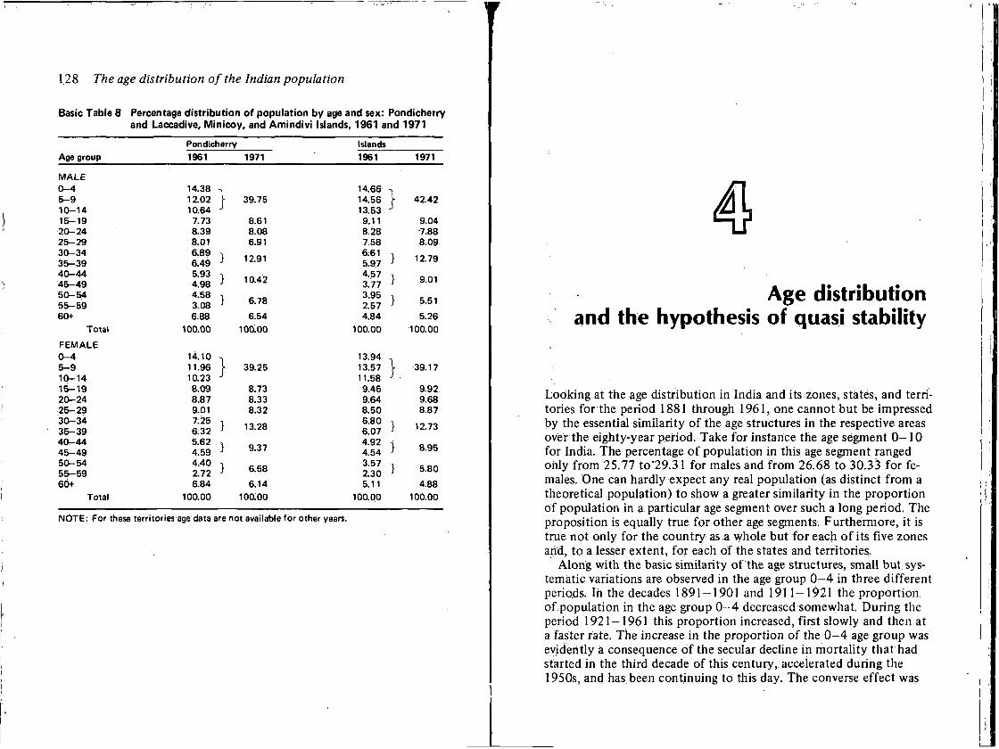
128 The age distribution of the Indian population
Basic Table 8 Percentage distribution of population by age and sex: Pondicherry and Laccadive, Minicoy, and Amindivi Islands, 1961 and 1971
Pondicherry Islands Age group 1961 1971 1961 1971
MALE 0-4 14.38 -> 14.66 5-9 12.02 \ 39.75 14.56 \ 42.42 10-14 10.64 J 13.53 J
15-19 7.73 8.61 9.11 9.04 20-24 8.39 8.08 8.28 7.88 25-29 8.01 6.91 7.58 8.09 30-34 35-39
6.89 ;
6.49 12.91 6.61 5.97 } 12.79
40-44 45-49
5.93 i 4.98 ; 10.42
4.57 3.77 } 9.01
50-54 55-59
4.58 3.08 ' 6.78 3.95
2.57 } 5.51
60+ 6.88 6.54 4.84 5.26 Total 100.00 100.00 100.00 100.00
FEMALE 0-4 14.10 13.94 5-9 11.96 \ 39.25 13.57 ) 39.17 10-14 10.23 J 11.58 J. . 15-19 8.09 8.73 9.46 9.92 20-24 8.87 8.33 9.64 9.68 25-29 9.01 8.32 8.50 8.87 30-34 35-39
7:25 , 6.32 ' 13.28 6.80
6.07 } 12.73
40-44 45-49
5.62 , 4.59 ' 9.37 4.92
4.54 } 8.95
50-54 55-59
4.40 i
2.72 6.58 3.57 2.30 } 5.80
60+ 6.84 6.14 5.11 4.88 Total 100.00 100.00 100.00 100.00
NOTE: For these territories age data are not available for other years.
4 Age distribution
and the hypothesis of quasi stability
Look ing at the age distr ibution in India and its zones, states, and territories for the period 1881 through 1961, one cannot but be impressed by the essential similarity o f the age structures in the respective areas over the eighty-year period. Take for instance the age segment 0—10 for India. The percentage of populat ion in this age segment ranged only f rom 25.77 to'29.31 for males and f rom 26.68 to 30.33 for females. One can hardly expect any real populat ion (as distinct f rom a theoretical populat ion) to show a greater similari ty in the proport ion of populat ion in a particular age segment over such a long period. The proposit ion is equally true for other age segments. Furthermore, it is true not only for the country as a whole but for each of its five zones and, to a lesser extent, for each of the states and territories.
A l o n g with the basic similarity o f the age structures, small but systematic variations are observed in the age group 0 - 4 in three different periods. In the decades 1891-1901 and 1911-1921 the proport ion of.populat ion in the age group 0—4 decreased somewhat. Dur ing the period 1921-1961 this proport ion increased, first slowly and then at a faster rate. The increase in the proport ion of the 0 - 4 age group was evidently a consequence of the secular decline in mortal i ty that had started in the third decade of this century, accelerated during the 1950s, and has been cont inuing to this day. The converse effect was
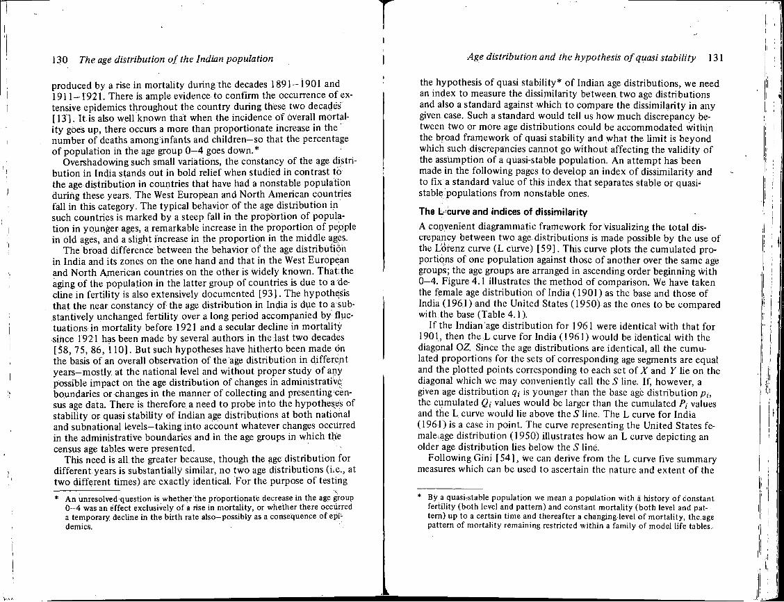
130 The age distribution of_ the Indian population
produced by a rise in mortal i ty during the decades 1891-1901 and 1 9 1 1 - 1 9 2 1 . There is ample evidence to conf i rm the occurrence of extensive epidemics throughout the country during these two decades [13 ] . It is also wel l known that when the incidence of overall mortali ty goes up, there occurs a more than proportionate increase in the number of deaths among infants and ch i ld ren-so that the percentage of populat ion in the age group 0 - 4 goes down. *
Overshadowing such small variations, the constancy of the age distribut ion in India stands out in bold relief when studied in contrast to the age distr ibution in countries that have had a nonstable populat ion during these years. The West European and Nor th Amer ican countries fall in this category. The typical behavior of the age distr ibut ion in such countries is marked by a steep fall in the proport ion of populat ion in younger ages, a remarkable increase in the proport ion of people in old ages, and a slight increase in the proport ion in the middle ages.
The broad difference between the behavior o f the age distr ibution in India and its zones on the one hand and that in the West European and Nor th Amer ican countries on the other is widely known. Tha t the aging of the populat ion in the latter group of countries is due to a decline in ferti l i ty is also extensively documented [93 ] . The hypothesis that the near constancy of the age distr ibution in India is due to a substantively unchanged ferti l ity over a long period accompanied by fluctuations in mortal i ty before 1921 and a secular decline in mortal i ty since 1921 has been made by several authors in the last two decades [58, 75, 86, 110] . But such hypotheses have hitherto been made on the basis of an overall observation of the age distr ibution in different years-most ly. at the national level and without proper study of any possible impact on the age distr ibution of changes in administrative boundaries or changes in the manner of collecting and presenting census age data. There is therefore a need to probe into the hypotheses of stabil i ty or quasi stabil i ty of Indian age distributions at both national and subnational leve ls- tak ing into account whatever changes occurred in the administrative boundaries and in the age groups in which the census age tables were presented.
This need is all the greater because, though the age distr ibut ion for different years is substantially similar, no two age distributions (i.e., at two different times) are exactly identical. F o r the purpose of testing
* An unresolved question is whether the proportionate decrease in the age group 0-4 was an effect exclusively of a rise in mortality, or whether there occurred a temporary decline in the birth rate also-possibly as a consequence of epidemics.
Age distribution and the hypothesis of quasi stability 131
the hypothesis o f quasi stabi l i ty* o f Indian age distr ibutions, we need an index to measure the dissimilarity between two age distr ibutions and also a standard against which to compare the dissimilarity in any given case. Such a standard would tell us how much discrepancy between two or more age distributions could be accommodated within the broad framework of quasi stabil i ty and what the l imit is beyond which such discrepancies cannot go without affecting the val idity o f the assumption of a quasi-stable populat ion. A n attempt has been made in the fol lowing pages to develop an index o f dissimilarity and to fix a standard value of this index that separates stable or quasi-stable populations from nonstable ones.
The L curve and indices of dissimilarity
A convenient diagrammatic framework for visualizing the total discrepancy between two age distributions is made possible by the use of the Lorenz curve (L curve) [59 ] . This curve plots the cumulated proportions of one populat ion against those o f another over the same age groups; the age groups are arranged in ascending order beginning with 0 - 4 . Figure 4.1 illustrates the method of comparison. We have taken the female age distr ibution of India (1901) as the base and those of India (1961) and the United States (1950) as the ones to be compared with, the base (Table 4.1).
If the Indian age distr ibution for 1961 were identical wi th that for 1901, then the L curve for India (1961) would be identical w i th the diagonal OZ. Since the age distributions are ident ical , all the cumulated proport ions for the sets of corresponding age segments are equal and the plotted points corresponding to each set o f X and Y lie on the diagonal which we may conveniently call the S line. If, however, a given age distr ibution m is younger than the base age distr ibut ion p,, the cumulated Q, values would be larger than the cumulated Pi values and the L curve would lie above the S line. The L curve for India (1961) is a case in point. The curve representing the Uni ted States fe-malcage distr ibution (1950) illustrates how an L curve depict ing an older age distr ibution lies below the S l ine.
Fo l lowing G in i [ 54 ] , we can derive from the L curve five summary measures which can be used to ascertain the nature and extent o f the
* By a quasi-stable population we mean a population with a history of constant fertility (both level and pattern) and constant mortality (both level and pattern) up to a certain time and thereafter a changing level of mortality, the age pattern of mortality remaining restricted within a family of model life tables.
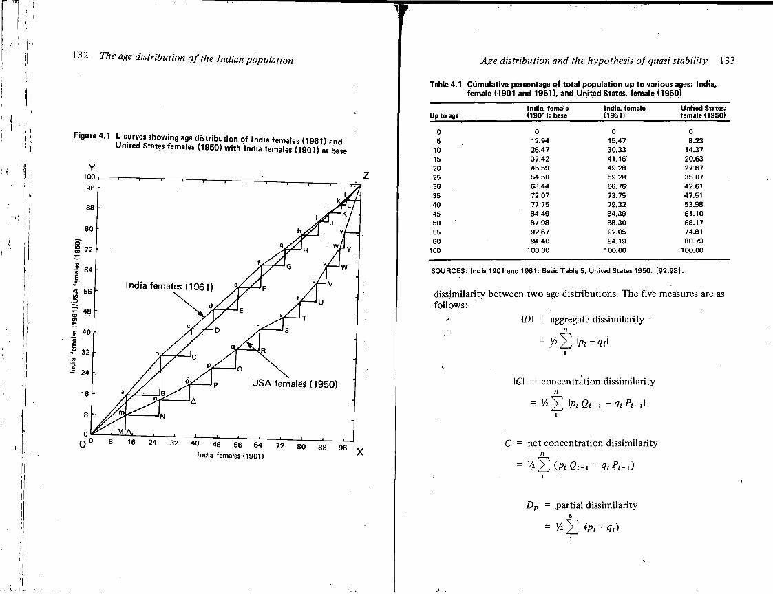
The age distribution of the Indian population
Age distribution and the hypothesis of quasi stability 133
Table 4.1 Cumulative percentage of total population up to various ages: India, female (1901 and 1961), and United States, female (1950)
India, female India, female United States; Up to age (1901): base (1961) female (1950)
0 0 0 0 5 12.94 15.47 8.23
10 26.47 30.33 14.37 15 37.42 41.16 20.63 20 45.59 49.28 27167 25 54.50 59.28 35.07 30 63.44 66.76 42.61 35 72.07 73.75 47.51 40 77.75 79.32 53.98 45 84.49 84.39 61.10 50 87.98 88.30 68.17 55 92.67 92.05 74.81 60 94.40 94.19 80.79
100 100.00 100.00 100.00
SOURCES: India 1901 and 1961: Basic Table 5; United States 1950: (92:981.
dissimilarity between two age distributions. The five measures are as
fol lows:
ID I = aggregate dissimilarity • n
ICI = concentrat ion dissimilarity n
= Vi^T \pi Qi-i ~qiPi-i\
C = net concentrat ion dissimilarity n
= V i ^ i P i Q i ^ - Q i P i - i )
Dp - partial dissimilarity 6
= V2 2 ( P i - Ri)
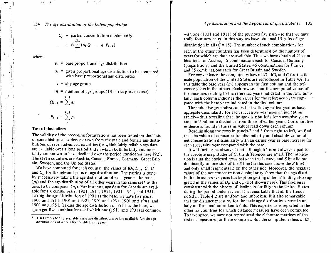
134 The age distribution of the Indian population
Cp = partial concentrat ion dissimilarity 6
= 1/2^(Pi Qi-i -qiPi-i) "\
where
Pi = base proport ional age distr ibution
qi = given proport ional age distr ibution to be compared with base proport ional age distr ibution
i = any age group
n = number o f age groups (13 in the present case) ; i - i
Qi-1 =
i
i-1
Pt-i = 2 > i
.i Test of the indices
The val idity o f the preceding formulations has been tested on the basis o f some historical evidence drawn from the male and female age distributions o f seven advanced countries for which fairly reliable age data are available over a long period and in which both ferti l i ty and mortality are known to have declined over the perjod considered here [92]. The seven countries are Austr ia, Canada, France, Germany, Great Britain, Sweden, and the Uni ted States.
We have computed for each country the values of ID I, Dp, ICI, Q and Cp for the relevant pairs of age distr ibut ion. The pairing is done by successively taking the age distr ibution of each year as the base (pi) and the age distr ibut ion of all other years in the same set* as the ones to be compared (qi). F o r instance, age data for Canada are available for six census years: 1901, 1911, 1921, 1931, 1941, and 1951. Taking the age distr ibut ion of 1901 as the base, we have five pairs: 1901 and 1911, 1901 and 1921, 1901 and 1931, 1901 and 1941, and 1901 and 1951. Taking the age distr ibution of 1911 as the base, we again get five comb ina t i ons -o f which one (1911 and 1901) is common
* A set refers to the available male age distributions or the available female age distributions of a country for different years.
Age distribution and the hypothesis of quasi stability 135
with one (1901 and 1911) of the previous five pa i rs -so that we have really four new pairs. In this way we have obtained 15 pairs o f age
distribution in all ( C =15) . The number o f such combinat ions for
each of the other countries has been determined by the number o f years for which age data are available. Thus we have obtained 21 combinations for Austr ia, 15 combinations each for Canada, Germany (prepartit ion), and the Uni ted States, 45 combinations for France, and 55 combinat ions each for Great Br i tain and Sweden.
For convenience the computed values o f LDI, ICI, and C for the female populat ion of the Uni ted States are reproduced in Table 4.2. In this table the base year (p,) appears in the first co lumn and the reference years in the others. Each row sets out the computed values o f the measures relating to the reference years indicated in the row. Similarly, each co lumn indicates the values for the reference years compared with the base years indicated in the first co lumn.
The inductive generalization is that wi th any earlier year as base, aggregate dissimilarity for each successive year goes on increasing rapidly—thus revealing that the age distr ibutions for successive years are more and more dissimilar from those of earlier years. Corroborat ive evidence is found in the same values read down each co lumn.
Reading along the rows in panels 2 and 3 from right to left, we find that the values o f concentrat ion dissimilarity and absolute values o f net concentrat ion dissimilarity wi th an earlier year as base increase for each successive year compared wi th the base.
It wi l l further be observed that although ICI is not always equal to the absolute magnitudes of C , the differences are small. The impl ication is that the enclosed areas between the L curve and S l ine lie predominantly on one side of the S l ine (in this case above the S line)— and only small fragments lie on the other side. Moreover, the negative values of the net concentrat ion dissimilarity show that the age distribution in successive years has kept on getting o l d e r - a finding also suggested in the values o f Dp and Cp (not shown here). This f inding is consistent wi th the history o f decline in fert i l i ty in the Uni ted States during the period under review. It is remarkable that all the trends noted in Table 4.2 are uni form and unbroken. It is also remarkable that the distance measures for the male age distr ibutions reveal similarly uni form and unbroken trends. This experience is repeated in the other six. countries for which distance measures have been computed. To save space, we have not reproduced the elaborate matrices of the distance measures for these countries. But the computed values o f ID I,
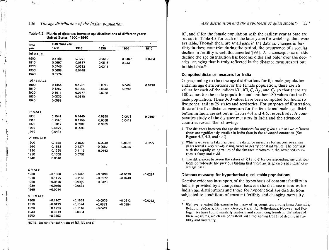
\
136 The age distribution of the Indian population
Table 4.2 Matrix of distances between age distributions of different years: United States, 1900-1940
Reference year year 1950 1940 1930 1920 1910
IDIMALE 1900 0.1166 0.1021 0.0680 0.0467 0.0264 1910 0.0997 0.0837 0.0516 0.0331 1920 0.0746 0.0682 0.0311 1930 0.0698 0.0445 1940 0.0574
IDI FEMALE 1900 0.1454 0.1201 0.0745 0.0458 0.0220 1910 0.1257 0.1004 0.0548 0.0261 1920 0.1011 0.0777 0.0348 1930 0.0829 0.0510 1940 0.0589
Id MALE 1900 0.1541 0.1440 0.0858 0.0571 0.0309 1910 0.1345 0.1156 0.0668 0.0411 1920 0.1017 0.0902 0.0365 1930 0.0827 . 0.0596 1940 0.0437
Id FEMALE 1900 0.1858 0.1629 0.0939 0.0532 0.0277 1910 0.1633 0.1374 0.0682 0.0349 1920 0.1365 0.1116 0.0442 1930 0.1058 0.0707 1940 0.0516
C MALE 1900 -0.1386 -0.1440 -0.0858 -0.0535 -0.0294 1910 -0.1125 -0.1156 -0.0572 -0.0248 1920 -0.0875 -0.0902 -0.0323 1930 -0.0566 -0.0583 1940 -0.0014
C FEMALE 1900 -0.1707 -0.1629 -0.0939 -0.0513 -0.0262 1910 -0.1473 -0.1374 -0.0682 -0.0254 1920 -0.1223 -0.1116 -0.0427 1930 -0.0819 -0.0694 1940 -0.0163
NOTE: See text for definitions of \D\ \C\. and C.
Age distribution and the hypothesis of quasi stability 137
ICI, and C for the female populat ion with the earliest year as base are set out in Table 4.3 for each of the later years for which age data were available. Though there are small gaps in the data on changes in fert i l i ty in these countries during the period, the occurrence of a secular decline in fert i l i ty is well documented [93 ]. As a consequence of this decline the age distr ibution has become older and older over the decades—an aging that is truly reflected in the distance measures set out in this table.*
Computed distance measures for India
Corresponding to the nine age distributions for the male populat ion and.nihe age distributions for the female populat ion, there are 36 values for each of the indices IDI, ICI, C,Dp, and Cp so that there are 180values for the male populat ion and another 180 values for the female populat ion. These 360 values have been computed for India, its five zones, and its 29 states and territories. F o r purposes of i l lustrat ion, three of the five distance measures for the female and male age distribution in India are set out in Tables 4.4 and 4.5 , respectively. A comparative study of the distance measures in India and the advanced countries reveals the fo l lowing:
1. The distances between the age distributions for any given state at two different times are significantly smaller in India than in the advanced countries. (See Figures 4.2, 4.3, and 4.4.)
2. Whichever year is taken as base, the distance measures for successive census years reveal a very slowly rising trend or nearly constant values. The contrast with the rapidly rising values of the distance measures in the advanced countries is sharp and vivid.
3. The differences between the values of ICI and C for corresponding age distributions corroborate the previous finding that there are large errors in Indian census age data.
Distance measures for hypothetical quasi-stable populations
Decisive evidence in support o f the hypothesis o f constant fert i l i ty in India is provided by a comparison between the distance measures for Indian age distributions and those for hypothet ical age distr ibutions subjected to condit ions of constant fert i l i ty and changing mortal i ty .
* We have repeated this exercise for many other countries, among them Australia, Belgium, Bulgaria, Denmark, Greece, Italy, the Netherlands, Norway, and Portugal. We have found similarly uniform and convincing trends in the values of these measures, which are consistent with the known trends of decline in fertility and mortality.
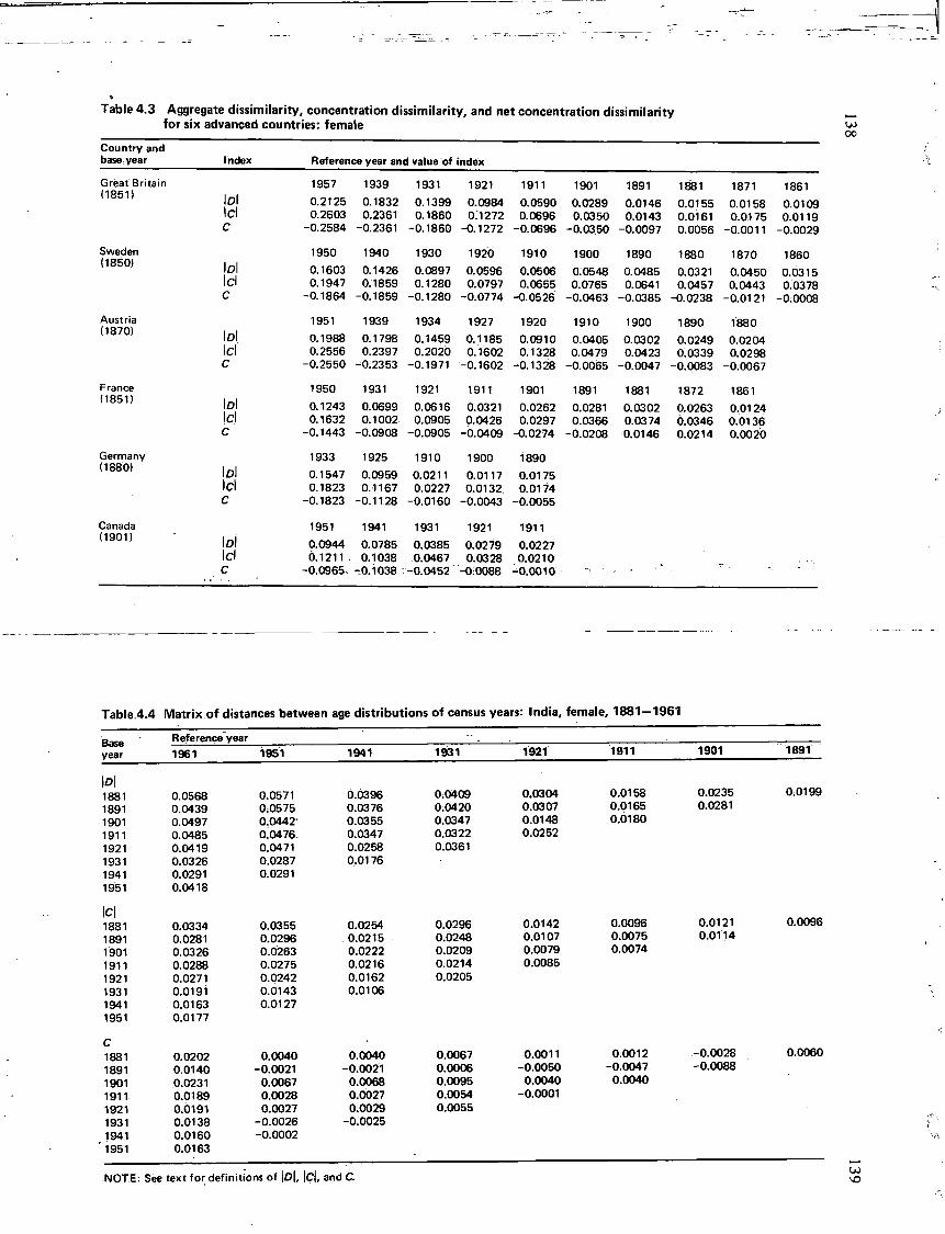
Table 4.3 Aggregate dissimilarity, concentration dissimilarity, and net concentration dissimilarity for six advanced countries: female
Country and base; year Index Reference year and value of index
Great Britain (1851) lol
Id C
1957
0.2125 0.2603
-0.2584
1939
0.1832 0.2361
-0.2361
1931
0.1399 0.1860
-0.1860
1921
0.0984 0.1272
-0.1272
1911
0.0590 0.0696
-0.0696
1901
0.0289 0.0350
-0.0350
1891
0.0146 0.0143
-0.0097
1881
0.0155 0.0161 0.0056
1871
0.0158 0.0175
-0.0011
1861
0.0109 0.0119
-0.0029
Sweden (1850)
1950 1940 1930 1920 1910 1900 1890 1880 1870 1860 Sweden (1850) lol
Id c
0.1603 0.1947
-0.1864
0.1426 0.1859
-0.1859
0.0897 0.1280
-0.1280
0.0596 0.0797
-0.0774
0.0506 0.0655
-0.0526
0.0548 0.0765
-0.0463
0.0485 0.0641
-0.0385
0.0321 0.0457
-0.0238
0.0450 0.0443
-0.0121
0.0315 0.0378
-0:0008
Austria (1870) lol
Id c
1951 1939 1934 1927 1920 1910 1900 1890 1880 Austria (1870) lol
Id c
0.1988 0.2556
-0.2550
0.1798 0.2397
-0.2353
0.1459 0.2020
-0.1971
0.1185 0.1602
-0.1602
0.0910 0.1328
-0.1328
0.0405 0.0479
-0.0065
0.0302 0.0423
-0.0047
0.0249 0.0339
-0.0083
0.0204 0.0298
-0.0067
France (1851)
1950 1931 1921 1911 1901 1891 1881 1872 1861 France (1851) lol
Id c
0.1243 0.1632
-0.1443
0.0699 0.1002
-0.0908
0.0616 0.0905
-0.0905
0.0321 0.0426
-0.0409
0.0262 0.0297
-0.0274
0.0281 0.0366
-0.0208
0.0302 0.0374 0.0146
0.0263 0.0346 0.0214
0.01 24 0.0136 0.0020
Germany (1880)
1933 1925 1910 1900 1890 Germany (1880) lol
Id c
0.1547 0.1823
-0.1823
0.0959 0.1167
-0.1128
0.0211 0.0227
-0.0160
0.0117 0.0132
-0.0043
0.0175 0.0174
-0.0055
Canada (1901)
1951 1941 1931 1921 1911 Canada (1901) lol
Id c
0.0944 6.1211 .
-0.0965-
0.0785 0.1038
T0.1038
0.0385 0.0467
-0.0452
0.0279 0.0328
-0i0088
0.0227 0.0210
-0.0010
Table 4.4 Matrix of distances between age distributions of census years: India, female, 1881-1961
Base year
Reference year Base year 1961 1951 1941 1931 1921 1911 1901 1891
lol. 1881 0.0568 0.0571 0.0396 0.0409 0.0304 0.0158 0.0235 0.0199
1891 0.0439 0.0575 0.0376 0.0420 0.0307 0.0165 0.0281 1901 0.0497 0.0442 0.0355 0.0347 0.0148 0.0180 1911 0.0485 0.0476 0.0347 0.0322 0.0252 1921 0.0419 0.0471 0.0258 0.0361 1931 0.0326 0.0287 0.0176 1941 0.0291 0.0291 1951 0.0418
lc| 0.0096 1881 0.0334 0.0355 0.0254 0.0296 0.0142 0.0096 0.0121 0.0096
1891 0.0281 0.0296 0.0215 0.0248 0.0107 0.0075 0.0114 1901 0.0326 0.0263 0.0222 0.0209 0.0079 0.0074 1911 0.0288 0.0275 0.0216 0.0214 0.0085 1921 0.0271 0.0242 0.0162 0.0205 1931 0.0191 0.0143 0.0106 1941 0.0163 0.0127 1951 0.0177
C 1881 0.0202 0.0040 0.0040 0.0067 0.0011 0.0012 -0.0028 0.0060
1891 0.0140 -0.0021 -0.0021 0.0006 -0.0050 -0.0047 -0.0088 1901 0.0231 0.0067 0.0068 0.0095 0.0040 0.0040 1911 0.0189 0.0028 0.0027 0.0054 -0.0001 1921 0.0191 0.0027 0.0029 0.0055 1931 0.0138 -0.0026 -0.0025 1941 0.0160 -0.0002 1951 0.0163
NOTE: See text for definitions of |D|, \C\, and C.
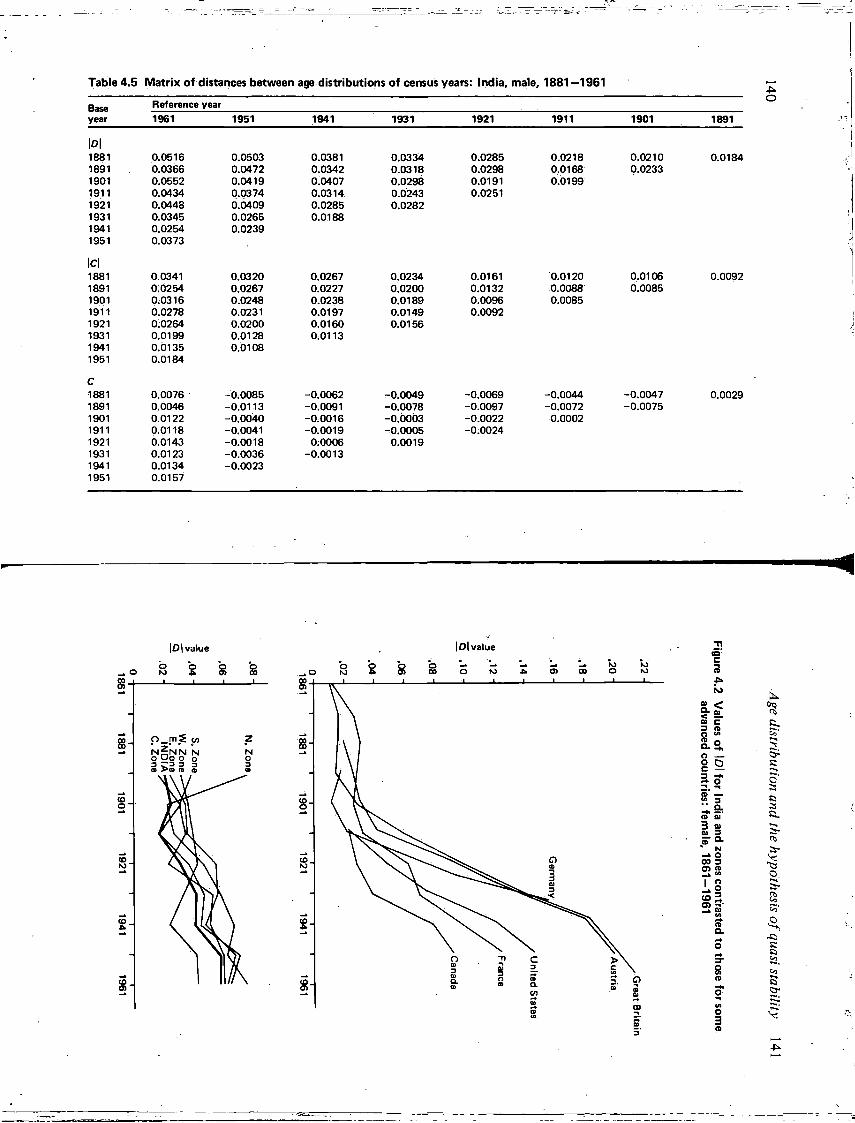
Table 4.5 Matrix of distances between age distributions of census years: India, male, 1881—1961
Base year
Reference year Base year 1961 1951 1941 1931 1921 1911 1901 1891
lol 1881 0.0516 0.0503 0.0381 0.0334 0.0285 0.0218 0.0210 0.0184 1891 0.0366 0.0472 0.0342 0.0318 0.0298 0.0168 0.0233 1901 0.0552 0.0419 0.0407 0.0298 0.0191 0.0199 1911 0.0434 0.0374 0.0314 o;0243 0.0251 1921 0.0448 6.0409 0.0285 0.0282 1931 0.0345 0.0265 0.0188 1941 0.0254 0.0239 1951 0.0373
\c\ 1881 0.0341 0.0320 0.0267 0.0234 0.0161 0.0120 0.0106 0.0092 1891 0.0254 0.0267 0.0227 0.0200 0.0132 0.0088 0.0085 1901 0.0316 0.0248 0.0238 0.0189 0.0096 0.0085 1911 0.0278 0.0231 0.0197 0.0149 0.0092 1921 0:0264 0.0200 0.0160 0.0156 1931 0.0199 0.0128 0.0113 1941 0.0135 0.0108 1951 0.0184
C
1881 0.0076 -0.0085 -0.0062 -0.0049 -0.0069 -0.0044 -0.0047 0.0029 1891 0.0046 -0.0113 -0.0091 -0.0078 -0.0097 -0.0072 -0.0075 1901 0.0122 -0.0040 -0.0016 -0.0003 -0.0022 0.0002 1911 0.0118 -0.0041 -0.0019 -0.0005 -0.0024 1921 6.0143 -0.0018 0:0006 0.0019 1931 0.0123 -0.0036 -0.0013 1941 0.0134 -0.0023 1951 0.0157
|D | value |D| value
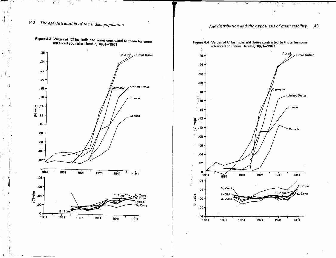
1 4 2 The age distribution of the Indian population
Figure 4.3 Values of Id for India and zones contrasted to those for some advanced countries: female, 1861-1961
Austria / Great Britaii
Germany / United States
188
1 .06 A
' ' i w i 1 i9bl 1 ^ 1 i r 1961
Age distribution and the hypothesis of quasi stability 143
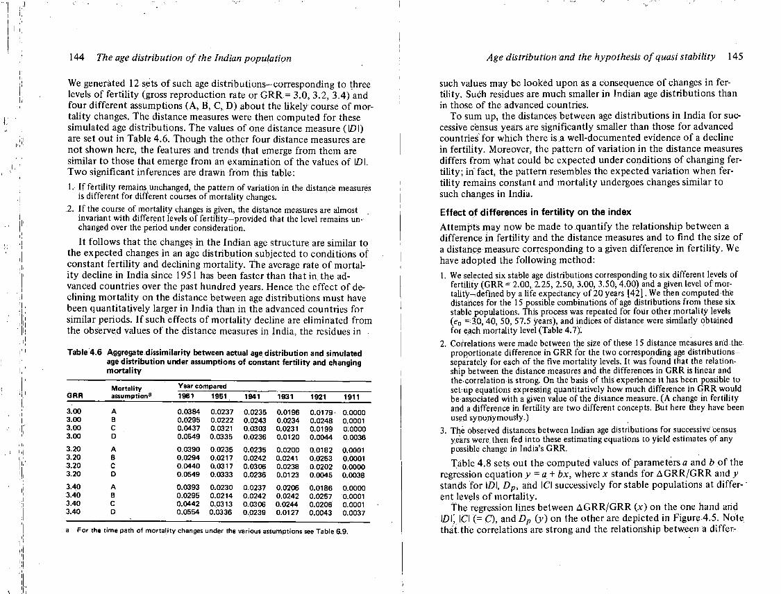
144 The age distribution of the Indian population
We generated 12 sets of such age d is t r ibut ions-corresponding to three levels o f fert i l i ty (gross reproduct ion rate or G R R - 3.0, 3.2, 3,4) and four different assumptions (A , B, C , D) about the l ikely course of mortality changes. The distance measures were then computed for these simulated age distributions. The values of one distance measure (IDJ) are set out in Table 4.6. Though the other four distance measures are not shown here, the features and trends that emerge from them are similar to those that emerge from an examination of the values of LDI. T w o significant inferences are drawn from this table:
1. If fertility remains unchanged, the pattern of variation in the distance measures is different for different courses of mortali ty changes.
2. If the course of mortality changes is given, the distance measures are almost invariant with different levels of fertility-provided that the level remains unchanged over the period under consideration.
It fol lows that the changes in the Indian age structure are similar to the expected changes in an age distr ibution subjected to condit ions of constant fert i l i ty and declining mortal i ty. The average rate of mortality decline in India since 1951 has been faster than that in the advanced countries over the past hundred years. Hence the effect o f decl ining mortal i ty on the distance between age distr ibutions must have been quantitatively larger in India than in the advanced countries for similar periods. If such effects o f mortal i ty decline are el iminated from the observed values o f the distance measures in India, the residues in .
Table 4.6 Aggregate dissimilarity between actual age distribution and simulated age distribution under assumptions of constant fertility and changing mortality
GRR Mortality assumption3
Year compared GRR
Mortality assumption3 1961 1951 1941 1931 1921 1911
3.00 A 0.0384 0.0237 0.0235 0.0196 0.0179 0.0000 3.00 B 0.0295 0.0222 0.0243 0.0234 0.0248 0.0001 3.00 c 0.0437 0.0321 0.0303 0.0231 0.0199 0.0000 3.00 D 0.0549 0.0335 0.0236 0.0120 0.0044 0.0036
3.20 A 0.0390 0.0235 0.0235 0.0200 0.0182 0.0001 3.20 B 0.0294 0.0217 0.0242 0.0241 0.0253 0.0001 3.20 c 0.0440 0.0317 0.0306 0.0238 0.0202 0.0000 3.20 D 0.0549 0.0333 0.0236 0.0123 0.0045 0.0038
3.40 A 0.0393 0.0230 0.0237 0.0206 0.0186 0.0000 3.40 B 0.0295 0.0214 0.0242 0.0242 0.0257 0.0001 3.40 c 0.0442 0.0313 0.0306 0.0244 0.0206 0.0001 3.40 D 0.0554 0.0336 0.0239 0.0127 0.0043 0.0037
a For the time path of mortality changes under the various assumptions see Table 6.9.
Age distribution and the hypothesis of quasi stability 145
such values may be looked upon as a consequence of changes in fertil ity. Such residues are much smaller in Indian age distr ibutions than in those of the advanced countries.
To sum up, the distances between age distr ibutions in India for successive census years are signif icantly smaller than those for advanced countries for which there is a well-documented evidence of a decline in ferti l i ty. Moreover, the pattern of variation in the distance measures differs f rom what could be expected under condit ions of changing fert i l i ty; in fact, the pattern resembles the expected variation when ferti l i ty remains constant and mortal i ty undergoes changes similar to such changes in India.
Effect of differences in fertility on the index Attempts may now be made to quanti fy the relationship between a difference in fert i l i ty and the distance measures and to find the size of a distance measure corresponding to a given difference in fert i l i ty. We have adopted the fol lowing method:
1. We selected six stable age distributions corresponding to six different levels of fertility (GRR = 2.00, 2.25, 2.50, 3.00, 3.50, 4.00) and a given level of mor-tality-:defined by a life expectancy of 20 years [42]. We then computed the distances for the 15 possible combinations of age distributions from these six stable populations. This process was repeated for four other mortality levels (e0 = 30,40, 50, 57.5 years), and indices of distance were similarly obtained for each mortality level (Table 4.7).
2. Correlations were made between the size of these 15 distance measures and the proportionate difference in GRR for the two corresponding age distributions— separately for each of the five mortality levels. It was found that the relationship between the distance measures and the differences in GRR is linear and the-correlation is strong. On the basis of this experience it has been possible to set up equations expressing quantitatively how much difference in GRR would be associated with a given value of the distance measure. (A change in fertility and a difference in fertility are two different concepts. But here they have been used synonymously.)
3. The observed distances between Indian age distributions for successive census years were then fed into these estimating equations to yield estimates of any possible change in India's GRR.
Table 4.8 sets out the computed values of parameters a and b o f the regression equation y = a. + bx, where x stands for A G R R / G R R and y stands for \D\, Dp, and ICI successively for stable populations at different levels o f mortal i ty.
The regression lines between A G R R / G R R (x) on the one hand and \D\] ICI (= O , and Dp (y) on the other are depicted in Figure 4.5. Note that the correlations are strong and the relationship between a differ-
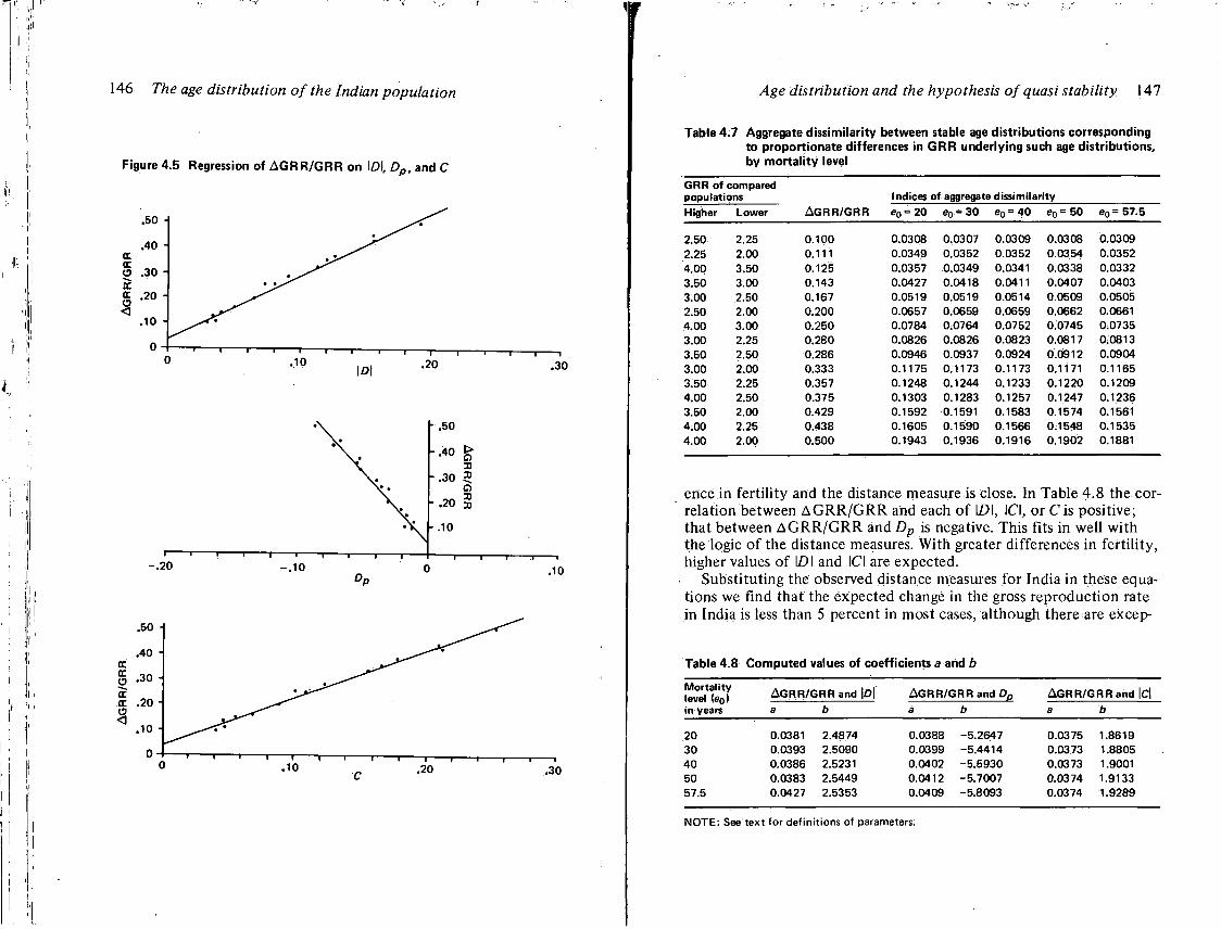
146 The age distribution of the Indian population
.10 .20
Age distribution and the hypothesis of quasi stability 147
Table 4.7 Aggregate dissimilarity between stable age distributions corresponding to proportionate differences in GRR underlying such age distributions, by mortality level
GRR of compared populations Indices of aggregate dissimilarity Higher Lower AGRR/GRR eo= 20 e0 = 30 <?o = 40 e 0 = 50 e 0 = 57.5
2.50 2.25 0.100 0.0308 0.0307 0.0309 0.0308 0.0309 2.25 2.00 0.111 0.0349 0.0352 0.0352 0.0354 0.0352 4.00 3.50 0.125 0.0357 0.0349 0.0341 0.0338 0.0332 3.50 3.00 0.143 0.0427 0.0418 0.0411 0.0407 0.0403 3.00 2.50 0.167 0.0519 0.0519 0.0514 0.0509 0.0505 2.50 2.00 0.200 0.0657 0.0659 0.0659 0.0662 0.0661 4.00 3.00 0.250 0.0784 0.0764 0.0752 0.0745 0.0735 3.00 2.25 0.280 0.0826 0.0826 0.0823 0.0817 0.0813 3.50 2.50 0.286 0.0946 0.0937 0.0924 0.0912 0.0904 3.00 2.00 0.333 0.1175 0.1173 0.1173 0.1171 0.1165 3.50 2.25 0.357 0.1248 0.1244 0.1233 0.1220 0.1209 4.00 2.50 0.375 0.1303 0.1283 0.1257 0.1247 0.1236 3.50 2.00 0.429 0.1592 0.1591 0.1583 0.1574 0.1561 4.00 2.25 0.438 0.1605 0.1590 0.1566 0.1548 0.1535 4.00 2.00 0.500 0.1943 0.1936 0.1916 0.1902 0.1881
ence in ferti l i ty and the distance measure is close. In Table 4-8 the cor
relation between A G R R / G R R and each of ID I, ICI, or C i s posit ive;
that between A G R R / G R R and D p is negative. This fits in well w i th
the logic of the distance measures. With greater differences in fert i l i ty,
higher values of LDI and ICI are expected.
Substitut ing the observed distance measures for India in these equa
tions we find that the expected change in the gross reproduct ion rate
in India is less than 5 percent in most cases, although there are excep-
Table 4.8 Computed values of coefficients a and b
Mortality level (e0) in years
AGRR/GRR and |0| a b
AGRR/GRR and D0
a b AGRR/GRR and \C\ a b
20 0.0381 2.4874 0.0388 -5.2647 0.0375 1.8619 30 0.0393 2.5090 0.0399 -5.4414 0.0373 1.8805 40 0.0386 2.5231 0.0402 -5.5930 0.0373 1.9001 50 0.0383 2.5449 0.0412 -5.7007 0.0374 1.9133 57.5 0.0427 2.5353 0.0409 -5.8093 0.0374 1.9289
NOTE: See text for definitions of parameters.
148 The age distribution of the Indian population
t ions here and there. With regard to the age distr ibut ion in 1961, the larger values o f the distance measures are possibly a consequence of the substantial decrease in mortal i ty during the period 1 9 5 1 - 1 9 6 1 .
Rate of natural increase and the hypothesis of quasi stability
In the last chapter, we found that the behavior of the age distr ibut ion in India over the 80-year period satisfies one necessary condi t ion o f quasi stabil i ty. In this chapter we investigate the rate o f natural increase in India and examine whether it is in keeping wi th the concept of quasi stabil i ty.
Two kinds of quasi stability
There are two distinct phases in the behavior of the rate o f natural increase. Pr ior to 1921 the rate f luctuated widely from one decade to the next. But since 1921 the rate has been monotonical ly increasing. This warrants a hypothesis of quasi stabil i ty in a somewhat broader . sense than that in which the term has been hitherto used. Un t i l now, the term quasi stabil i ty has been used to describe a situation in which fert i l i ty remains constant but mortal i ty declines monotonical ly [38, 4 9 ] . In the present study,, we do not restrict the concept to situations of decl ining mortal i ty only but extend it to situations of both rising mortal i ty and declining mor ta l i t y - fe r t i l i t y having remained the same. The natural increase in India reveals the characteristics of quasi stability of the first k ind in the decades after 1921 and those of the second k ind in the decades before 1921. The prevalence of a long period of cycl ical f luctuations in mortal i ty prior to the onset of a secular decline
150 The age distribution of the Indian population
in mortal i ty has probably been characteristic of all developing coun-t r i es - i f not o f developed countries also in earlier periods [48 ] . The long-term rate of populat ion growth must have been very low in almost all countries. Otherwise, the present populations would be much larger than they are. There are three different combinations of ferti l i ty and mortal i ty that would lead to a low growth rate in the long run:
1. Constant fertility and constant mortality-at levels conducive to a low rate of increase
•2. Constant fertility and fluctuating mortality-so that the high growth rates in some years combined with low or negative growth rates in others produce a low growth rate in the long run [85]
3. Fluctuating fertility and constant mortality-so that, here again, the positive and negative growth rates in successive periods jointly produce a low long-term growth rate
The recorded history o f India and of many other countries provides evidence of famines, epidemics, pestilences, and wars in different phases o f their development [22] . The hypothesis o f constant mortality is therefore untenable. In countries l ike India the nearly constant age distr ibut ion precludes the plausibi l i ty of the third alternative also. Hence the second alternative may be taken as the most general and l ike ly combinat ion of ferti l i ty and mortal i ty trends in the past. By broadening the concept of quasi stabil i ty as stated above, the analytical frame may be made more useful to handle both s i tuat ions- the monotonic decline in mortal i ty in the immediate past and fluctuations in mortal i ty pr ior to that.
Components of population increase
A comparison of the size o f populat ion in a state at the beginning and at the end of a decade gives the overall increase in populat ion in the state during the decade. This overall increase has four components: the increase due to greater accuracy in the census count; the increase due to boundary changes; the increase due to migration to and from the area; and the natural increase.* T o obtain the natural increase, we have to eliminate the other three components. These components and their quantitative impact on the census populat ion in India are discussed in the fol lowing paragraphs.
* Of course, the population of a state can stay the same size or decrease, and similarly any of the components can act in a neutral or negative manner.
Rate of natural increase and the hypothesis of quasi stability 151
Accuracy in census counts Census operations started in 1872 and improved in coverage and accuracy with each successive census. B y 1891 or 1901 coverage was almost universal. It is therefore assumed that the increase in the resident census populat ion over a decade may be taken as a tolerably good measure of the increase in actual populat ion [29 ] . It must be admitted, however, that improvement in enumeration f rom one census to the next is not inevitable. Moreover, i f there is a change i n the direction of enumeration errors between two consecutive censuses, the resulting error in the rate of populat ion increase may be large even though the absolute magnitude of error in each census is relatively small. This is exactly what happened in the 1941 census. A l though i n most years the census figures suffer f rom underenumeration, in 1941 there was an evident inf lat ion of the populat ion count for Punjab and Bengal. However, the fact that we have a series of populat ion figures for 11 consecutive decennial censuses at the national, provincial , distr ict, 'subdivision, police station, and village levels and that by and large the figures of total populat ion for different years at all these levels are consistent wi th one another lends a considerable degree of dependabil i ty to these data.
Increase due to boundary changes Changes in the boundaries of states and territories were discussed in Chapter 2. Such changes necessitate adjustment o f the total populat ion so that the rate o f increase of populat ion may be correct ly measured. Wi th regard to the total populat ion for the period 1901 - 1 9 6 1 , we did not make any adjustments on our own but depended entirely on the time-series data presented in the 1961 census [29 ] . Adjustment for the six census years 1901 through 1951 according to the newly defined areal unit was done by the Census of India (1961) wi th the actual census counts in the respective censuses at all levels—provinces, princely states, districts, subdivisions, police stations, unions, and vi llages. In the large majority of cases, changes in the boundary of a state or territory did not involve the parti t ion o f the lowest administrative unit; Therefore, in the reconstruction o f the total populat ion for the constituent areas, no element o f estimation was involved.* It was only
* Note the following quotation from the Census of India [27:4-5]: "Estimation of data Asa result of reorganization of States, Districts and Census tracts have sometimes been broken up and portions transferred from one State to another. Villages and towns, however, have not been affected. Since the data contained
152 The age distribution of the Indian population
with respect to a negligibly small number o f people that the boundary changes led to the parti t ion o f a village and the share of the populat ion in the fragmented areas had to be estimated.
The adjustment of populat ion in previous censuses had been done by the census commissioner carefully and thoroughly. The populat ion of a transferred area for any census year was estimated on the assumption that the proport ion of the populat ion in the area transferred to the total populat ion o f the relevant district ( in which it was situated at the time of the transfer) was the same in the particular year as it was in 1951 [29 ] .
We calculated the total populat ion for 1881 and for 1891 on the basis o f populat ion data given in the census for the provinces and princely states that constituted the respective zones in the two years. In the absence of a good base map showing the small administrative divisions in 1881 and 1891, it was d i f f icu l t to match the geographical area o f a new pol i t ical unit with that of an old one. Under the circumstances we used the total populat ion figures for the provinces and princely states reconstructed by the Census of India (190] ) for the years 1881 and 1891 [12 ] . Each zone contained a number of provinces and princely states as a whole and some fragmented areas. It was simple to ident i fy most of the provinces and princely states as belonging to one zone or another. We reconstructed the aggregate populat ion of those administrative units the locat ion of which could be f i rmly identi f ied i n a zone f rom the figures adjusted by the 1901 census. Then we assumed that the populat ion in the areas that could not be identi f ied had grown at a rate equal to that o f the populat ion in areas that could be identi f ied. On the basis o f this assumption the populat ion of the unidenti f ied areas was obtained by backward projection.
International migration
T o obtain the rate of natural increase for India as a whole, we treated the Indian populat ion as closed to international migration for the per iod 1881 to 1941. There had always been a slight foreign in f lux in the populat ion of India. There also occurred a small out f low o f persons born in India to foreign territories, mainly in A f r i ca and Asia. But as Kingsley Davis [47 ] has observed, whatever the economic and pol i t ical importance of such movements to and from India, their demographic significance was small. The situation changed considerably in
in the present table are available by individual villages and towns in the published census records, it has been possible to recast the figures of the original count without resorting to estimations except in a few cases."
Rate of natural increase and the hypothesis of quasi stability 153
1951 and 1961 because of the parti t ion of India and migration of displaced persons to and from Pakistan.
F o r the decade 1941-1951 the census commissioner estimated a net migration into India of about 600,000 to 800,000 persons or about one-sixth of 1 percent o f the total populat ion [22] . This conclusion was based on the fol lowing findings. The number of displaced persons f rom Pakistan enumerated in the 1951 census was 7.20 mi l l ion. F r o m the Pakistan Census Bul le t in , i t was found that nearly 7.15 mil l ion displaced persons f rom India were enumerated in Pakistan. Moreover, there were about 1.20 mi l l ion Pakistan-born persons in East India ,who were not registered as displaced persons. It is d i f f icu l t to ascertain the precise period of their migration to India. In addit ion to migrants to and f rom Pakistan, there was earlier in the decade an influx o f Indians returning to India who had earlier migrated to countries l ike Burma and Malaya. It is extremely di f f icul t to take all these factors in to proper account and provide any precise estimate o f net migration. We have therefore accepted the census commissioner's estimate and assumed that the net immigrat ion into India was 700,000 during the decade 1941 — 1951 [22 ] . T o obtain the sex composi t ion of the migrants, we processed the birthplace data of the male and female populat ion born outside India (but enumerated in India in the 1951 census [21 ]) and thus divided the net migrants by sex. It was observed that males and females constituted 55.20 percent and 44.80 percent respectively of all immigrants. O n this basis, 700,000 net migrants were divided in to 386,000 males and 314,000 females.
F o r the decade 1951 — 1961, our estimates of net international migration were prepared from the fol lowing data made available by the Census o f India ( 1 9 6 1 ) [ 3 1 ] : 1. The estimated number of net migrants (both sexes) in the census paper on age
tables, which puts the figures at 3.14 million [28] 2. Data on birthplace of the persons enumerated in various states and territories
3. Data on duration of stay of the migrant population in the place of enumeration classified into five groups: less than 1 year, 1—5 years, 6—10 years, 11—15 years, and 16 years and more [31 ]
We assumed that the sex composi t ion and zonal distr ibut ion of the net.international migrants are the same as those o f all in-migrants during the period. We then divided net migrants into three durat ion groups according to the proportionate division of all in-migrants during: the period. Then we applied the reverse survival method to the number of net in-migrants in each duration group and obtained the original cohort o f migrants. F ina l ly we estimated the net growth due
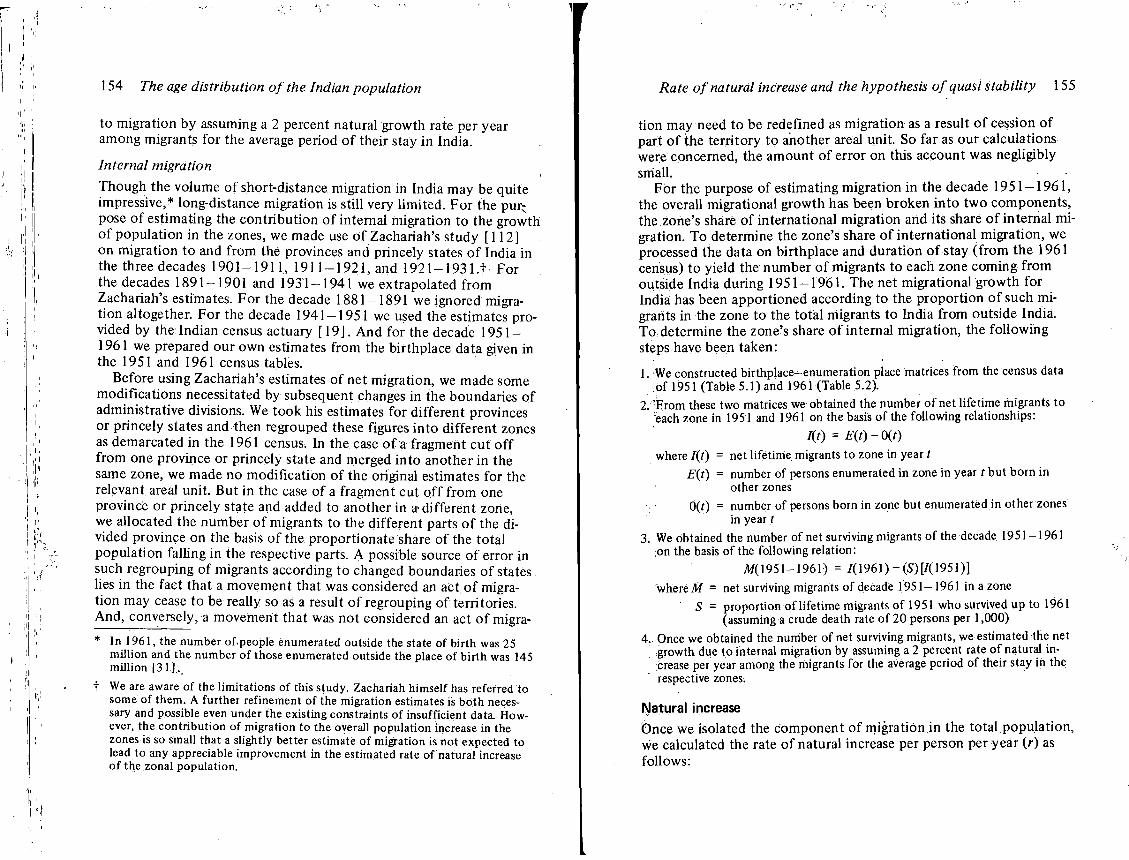
154 The age distribution of the Indian population
to migrat ion by assuming a 2 percent natural growth rate per year among migrants for the average period of their stay in India.
Internal migration
Though the volume of short-distance migration in India may be quite impressive,* long-distance migration is sti l l very l imi ted. F o r the pur; pose of estimating the contr ibut ion o f internal migration to the growth o f populat ion in the zones, we made use o f Zachariah's study [112] on migration to and f rom the provinces and princely states o f India in the three decades 1 9 0 1 - 1 9 1 1 , 1 9 1 1 - 1 9 2 1 , and 192 . l -1931 . f - F o r the decades 1891-1901 and 1931-1941 we extrapolated f rom Zachariah's estimates. F o r the decade 1881 -1891 we ignored migrat ion altogether. F o r the decade 1941-1951 we used the estimates provided by the Indian census actuary [19 ] . A n d for the decade 1951 -1961 we prepared our own estimates from the birthplace data given in the 1951 and 1961 census tables.
Before using Zachariah's estimates of net migrat ion, we made some modif icat ions necessitated by subsequent changes in the boundaries of administrative divisions. We took his estimates for different provinces or princely states and then regrouped these figures into different zones as demarcated in the 1961 census. In the case o f a fragment cut o f f f rom one province or princely state and merged into another in the same zone, we made no modi f icat ion of the original estimates for the relevant areal unit. But in the case of a fragment cut o f f f rom one province or princely state and added to another in a different zone, we allocated the number o f migrants to the different parts o f the divided province on the basis o f the proport ionate share of the total populat ion fall ing in the respective parts. A possible source o f error in such regrouping of migrants according to changed boundaries of states lies in the fact that a movement that was considered an act o f migrat ion may cease to be really so as a result o f regrouping of territories. A n d , conversely, a movement that was not considered an act o f migra-
* In 1961, the number of.people enumerated outside the state of birth was 25 million and the number of those enumerated outside the place of birth was 145 million [31]..
t We are aware of the limitations of this study. Zachariah himself has referred to some of them. A further refinement of the migration estimates is both necessary and possible even under the existing constraints of insufficient data. However, the contribution of migration to the overall population increase in the zones is so small that a slightly better estimate of migration is not expected to lead to any appreciable improvement in the estimated rate of natural increase of the zonal population.
Rate of natural increase and the hypothesis of quasi stability 155
t ion may need to be redefined as migration as a result o f cession of part o f the territory to another areal unit. So far as our calculations were concerned, the amount o f error on this account was negligibly sniall.
Fo r the purpose of estimating migration in the decade 1 9 5 1 - 1 9 6 1 , the overall migrational growth has been broken into two components, the zone's share of international migration and its share o f internal migration. To determine the zone's share o f international migrat ion, we processed the data on birthplace and durat ion of stay ( f rom the 1961 census) to yield the number o f migrants to each zone coming f rom outside India during 1 9 5 1 - 1 9 6 1 . The net migrational growth for India has been apport ioned according to the proport ion o f such migrants in the zone to the total migrants to India from outside India. To determine the zone's share of internal migration, the fo l lowing steps have been taken:
1. -We constructed birthplace-enumeration place matrices from the census data of 1951 (Table 5.1) and 1961 (Table 5.2).
2. ^From these two matrices we obtained the number of net lifetime migrants to each zone in 1951 and 1961 on the basis of the following relationships:
/(0 = f ( 0 -o« where I(t) = net lifetime migrants to zone in year t
E(t) = number of persons enumerated in zone in year t but born in other zones
0(0 = number of persons born in zone but enumerated in other zones in year t
3. We obtained the number of net surviving migrants of the decade 1951-1961 ;on the basis of the following relation:
M(1951-1961) = 7(1961) - (5) [/(1951)]
where M = net surviving migrants of decade 1951-1961 in a zone S = proportion of lifetime migrants of 1951 who survived up to 1961
(assuming a crude death rate of 20 persons per 1,000)
4.. Once we obtained the number of net surviving migrants, we estimated the net growth due to internal migration by assuming a 2 percent rate of natural increase per year among the migrants for the average period of their stay in the respective zones;
Natural increase Once we isolated the component o f migration in the total populat ion, we calculated the rate o f natural increase per person per year (r) as fol lows:
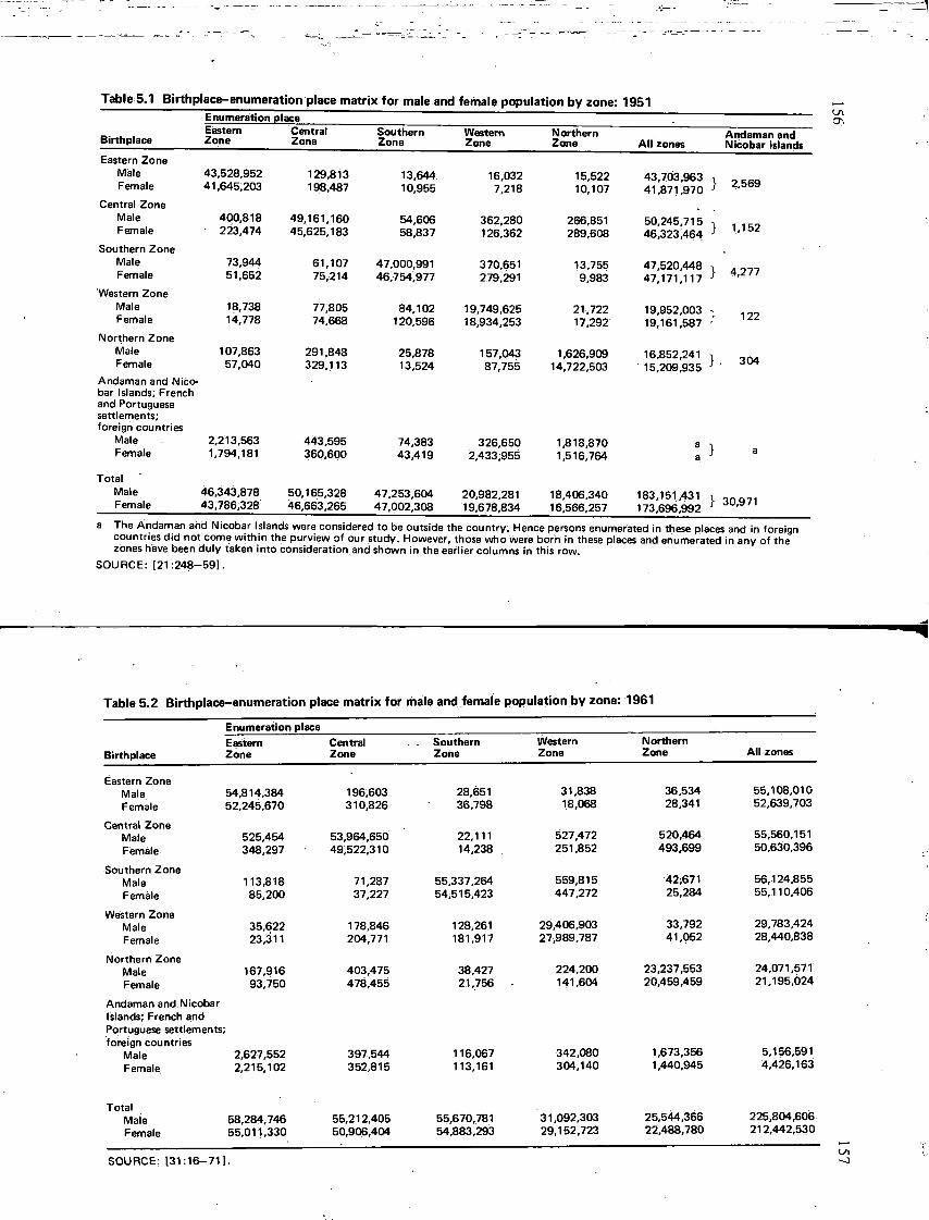
Table 5.1 Birthplace-enumeration place matrix for male and female population by zone: 1951
Birthplace
Enumeration pi ace
Birthplace Eastern Zone
Central Zone
Southern Zone
Western Zone
Northern Zone All zones
Eastern Zone Male 43,528,952 129,813 13,644 16,032 15,522 43,703,963 Female 41,645,203 198,487 10,955 7,218 10,107 41,871,970
Central Zone Male 400,818 49,161,160 54,606 362,280 266,851 50,245,715 Female 223,474 45,625,183 58,837 126,362 289,608 46,323,464
Southern Zone Male 73,944 61,107 47,000,991 370,651 13,755 47,520,448 Female 51,652 75,214 46,754,977 279,291 9,983 47,171,117
Western Zone Male 18,738 77,805 84,102 19,749,625 21,722 19,952,003 Female 14,778 74,668 120,596 18,934,253 17,292 19,161,587
Northern Zone Male 107,863 291,848 25,878 157,043 1,626,909 16,852,241 Female 57,040 329,113 13,524 87,755 14,722,503 15,209,935
Andaman and Nicobar Islands; French and Portuguese settlements; foreign countries
Male 2,213,563 443,595 74,383 326,650 1,818,870 a Female 1,794,181 360,600 43,419 2,433,955 1,516,764 a
Total Male 46,343,878 50,165,328 47,253,604 20,982,281 18,406,340 183,151,431 Female 43,786,328 46,663,265 47,002,308 19,678,834 16,566,257 173,696,992
Andaman and Nicobar Islands
} 2,569
} 1.152
122
304
} 30,971
a The Andaman and Nicobar Islands were considered to be outside the country. Hence persons enumerated in these places and in foreign countries did not come within the purview of our study. However, those who were born in these places and enumerated in any of the zones have been duly taken into consideration and shown in the earlier columns in this row.
SOURCE: [21:248-59].
Table 5.2 Birthplace-enumeration place matrix for male and female population by zone: 1961
Birthplace
Enumeration place Eastern Zone
Central Zone
Southern Zone
Western Zone
Northern Zone All zones
Eastern Zone Male Female
Central Zone Male Female
Southern Zone Male Female
Western Zone Male Female
Northern Zone Male Female
54,814,384 52,245,670
525,454 348,297
113,818 85,200
35,622 23,311
167,916 93,750
Andaman and Nicobar Islands; French and Portuguese settlements; foreign countries
Male Female
2,627,552 2,215,102
196,603 310,826
53,964,650 49,522,310
71,287 37,227
178,846 204,771
403,475 478,455
397,544 352,815
28,651 36,798
22,111 14,238
55,337,264 54,515,423
128,261 181,917
38,427 21,756
116,067 113,161
31,838 18,068
527,472 251,852
559,815 447,272
29,406,903 27,989,787
224,200 141,604
342,080 304,140
36,534 28,341
520,464 493,699
42;671 25,284
33,792 41,052
23,237,553 20,459,459
1,673,356 1,440,945
55,108,010 52,639,703
55,560,151 50,630,396
56,124,855 55,110,406
29,783,424 28,440,838
24,071,571 21,195,024
5,156,591 4,426,163
Total Male Female
58,284,746 55,011,330
55,212,405 50,906,404
55,670,781 54,883,293
31,092,303 29,152,723
25,544,366 22,488,780
225,804,606 212,442,530
SOURCE: [31:16-71].
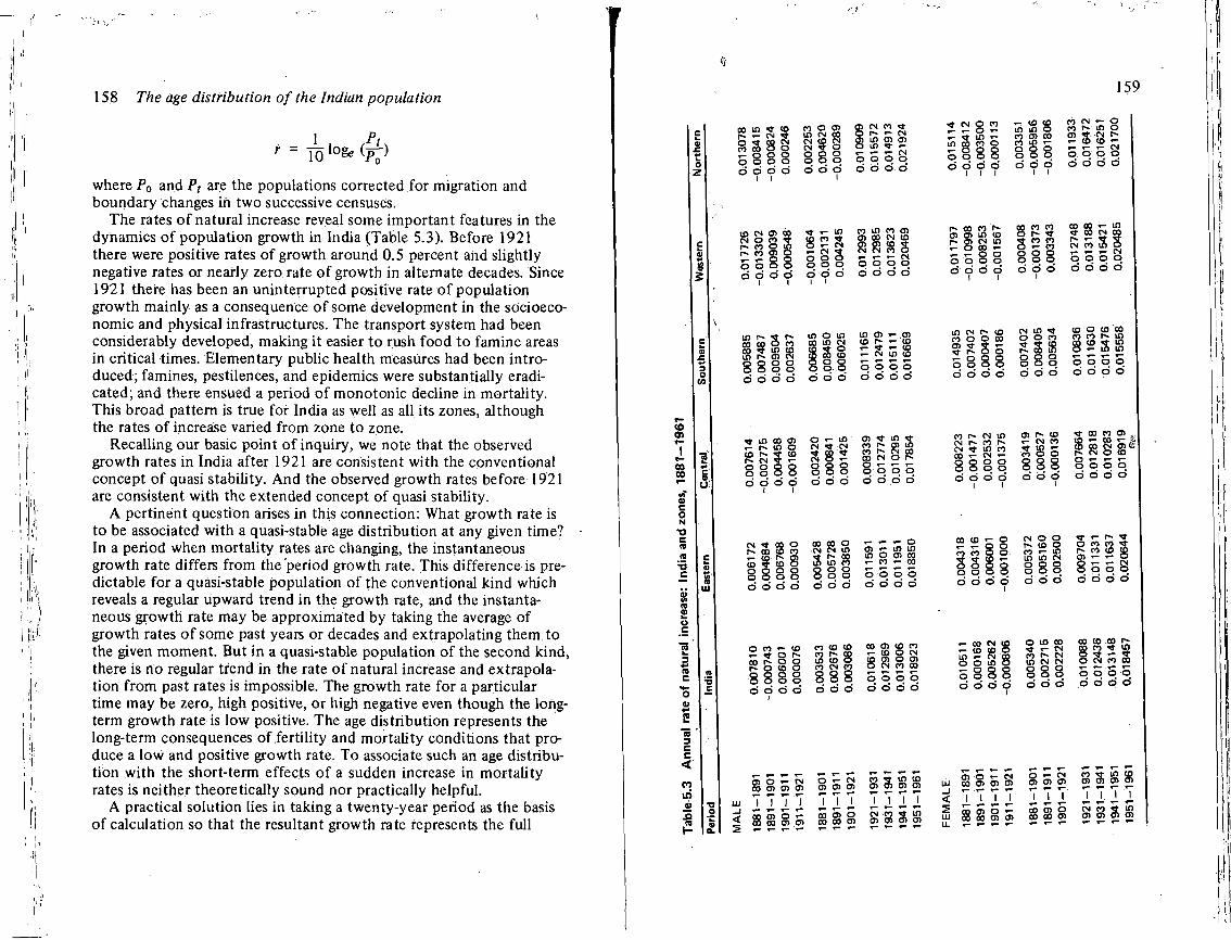
158 The age distribution of the Indian population
1 . As r = Tolofo(^)
where P0 and Pt are the populations corrected for migration and boundary changes in two successive censuses.
The rates of natural increase reveal some important features in the dynamics of population growth in India (Table 5.3). Before 1921 there were positive rates of growth around 0.5 percent and slightly negative rates or nearly zero rate of growth in alternate decades. Since 1921 there has been an uninterrupted positive rate of population growth mainly as a consequence of some development in the socioeconomic and physical infrastructures. The transport system had been considerably developed, making it easier to rush food to famine areas in critical times. Elementary public health measures had been introduced; famines, pestilences, and epidemics were substantially eradicated; and there ensued a period of monotonic decline in mortality. This broad pattern is true for India as well as all its zones, although the rates of increase varied from zone to zone.
Recalling our basic point of inquiry, we note that the observed growth rates in India after 1921 are consistent with the conventional concept of quasi stability. And the observed growth rates before 1921 are consistent with the extended concept of quasi stability.
A pertinent question arises in this connection: What growth rate is to be associated with a quasi-stable age distribution at any given time? In a period when mortality rates are changing, the instantaneous growth rate differs from the period growth rate. This difference is predictable for a quasi-stable population of the conventional kind which reveals a regular upward trend in the growth rate, and the instantaneous growth rate may be approximated by taking the average of growth rates of some past years or decades and extrapolating them to the given moment. But in a quasi-stable population of the second kind, there is no regular trend in the rate of natural increase and extrapolation from past rates is impossible. The growth rate for a particular time may be zero, high positive, or high negative even though the long-term growth rate is low positive. The age distribution represents the long-term consequences of fertility and mortality conditions that produce a low and positive growth rate. To associate such an age distribution with the short-term effects of a sudden increase in mortality rates is neither theoretically sound nor practically helpful.
A practical solution lies in taking a twenty-year period as the basis of calculation so that the resultant growth rate represents the full
159
co in * n 3 8 5 o o o d d
CO O O ) g N n J in CM co o r~ «- CN CN cp CN cn in cn cn CM *T O O tf) * r O O O ' r M o q o q q q q o d d d o d o
2 2 8 <* in in co co o a o o o o d d i i
r- CO CO in in o CO CD 00 co in «-o o o o o o o d d
i
CO CN CO f~ 2 3 5 3 d d
«- o m o CN r» co « - CN o o d d
co CN o> oo CN o co t r~ co o to
CO CD O T- «- O O o o q q d d d d i i
t •<-8 £ r- CM o o 0 o d d 1 i
co co co at at oo CN CD cn eft co a CN CN CO O t- « - CN O O O O o d d d
r- co co r-cn at in co r~ at CN m T - o oo <-•r- .r- O O o o o o d d d d
i i
oo co co o r- *r S co co
«- CO o o o o o o o d d
co co Tt 00 CN p» « - N " CN co in 5 o 5 o d d
3 S CO m co o> CM o o o o d d
m o m co in g 8 CO CD o o o o o o o d d
m at «- ,cxi co i— CO
£ CM In 8 o o o o d o d o
in CN i» co co o o co Ol » } r Tt O o ,- o o o o o q q d d d d
CM m ^ o o co co o co oo
w co co in S 5 8 8 2 3 8 O O O »-q o q q q q q o d d d d d o
^ in oo cn «- i-« m o co r- 5 co r» CM ^ «-o o o o o o q q d d d d
i.
o «- m
O Q O O O O o d d
rf m t r» cn m r» CN co CN o r» o o o d d d
co r . CM m CM r» co r> CM *r in eo oo t — CN i— o o o o o o q q d d d d
i I
enr^co ^-cococn . 5 S 2 8 5 8 5 < S | co o o CM o co o g o o r r T o
d d i
o d d q d d d d
CM ^ CO o I— CO CD CO
CD >? CD 8 ° S Q O o o o q d d d d
oo oo o CM CN m 3 En 8 o o o o o o o d d
r- t- o cn »- in in in o cn co i— co «— co o o o o d o d o
o co «- co T- * O r» co r*> o o ™ O 10 o o S S 2 o o o o d d d d
co co co co cn co co co co i- co o CM in to o cp at o at co CN co o CN eo oo 8 8 8 5 5 5 q o d d d d d d
COCOf-O rs o o S ~ ~ ?- o o r- co o o co co eo co o o co »- 10 rococo 5 ? co ^ in in CN a t ^ — -O O O O O O O O ^ ' N o o o o o o q o o o o d d d d odd o o o o
«- 00 CN CD T - CD CO O in <- CN co o o in o 5 8 8 8 d d d d
o in oo »— CN
co r- CN m CM CN o o o o o o o d d
co co co r-. S c o m
* ~ 3 o CN co co ^ T - ^ o o o o
d d d d
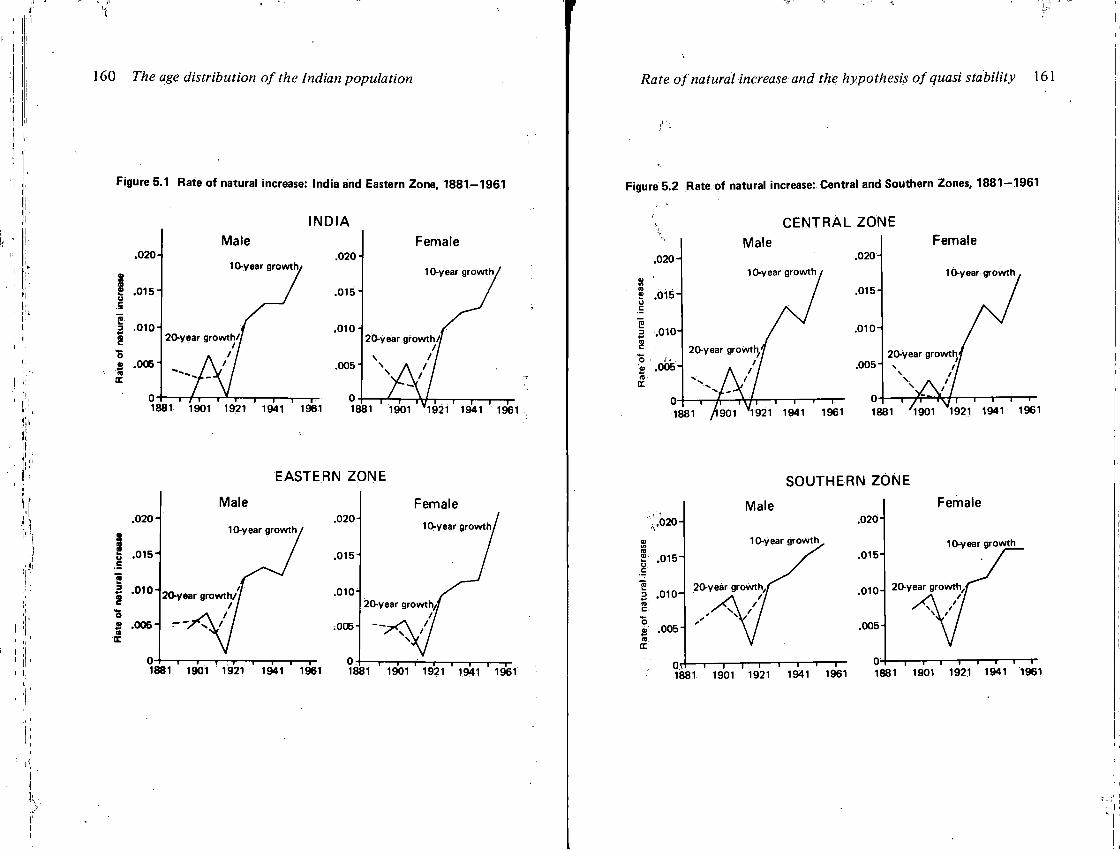
160 The age distribution of the Indian population
Figure 5.1 Rate of natural increase: India and Eastern Zone, 1881-1961
.020-1 Male
10-year growth/
INDIA
.020
.015
.010 H
.0051
Female
10-year growthV
1881 1901 1921 1941 1961 1881 1901 '^1921 ' 1941 ' 1961
20-year growth//
.020
.015H
3 .010
o S .005 H
.020
20-year growth/ /
EASTERN ZONE
Male
10-year growth r
.015
.010
;005H
Female
10-year growth/
1881 1901 1921 1941 1961 1881 ' 1901 ' 1921 ' 1941 ' 1961
Rate of natural increase and the hypothesis of quasi stability 161
Figure 5.2 Rate of natural increase: Central and Southern Zones, 1881-1961
C E N T R A L ZONE
.020-.020 H Male
10-year growth j
.015
.010
.005
-i 1 1 r 1881 /1901 V1921 1941 1961 1881 "1901 '1921 1941 1961
Female
10-year growth .
.020 H
£ .015-8: i .01 OH (0
c o u .005 m tr
OT
20-year growthj
SOUTHERN ZONE
.020
.015
.010
.005-1
-| 1 1 ! r
20-year growth
-i——i—i 1 1 1 i i 1881 1901 1921 1941 1961 1881 1901 1921 1941 1961
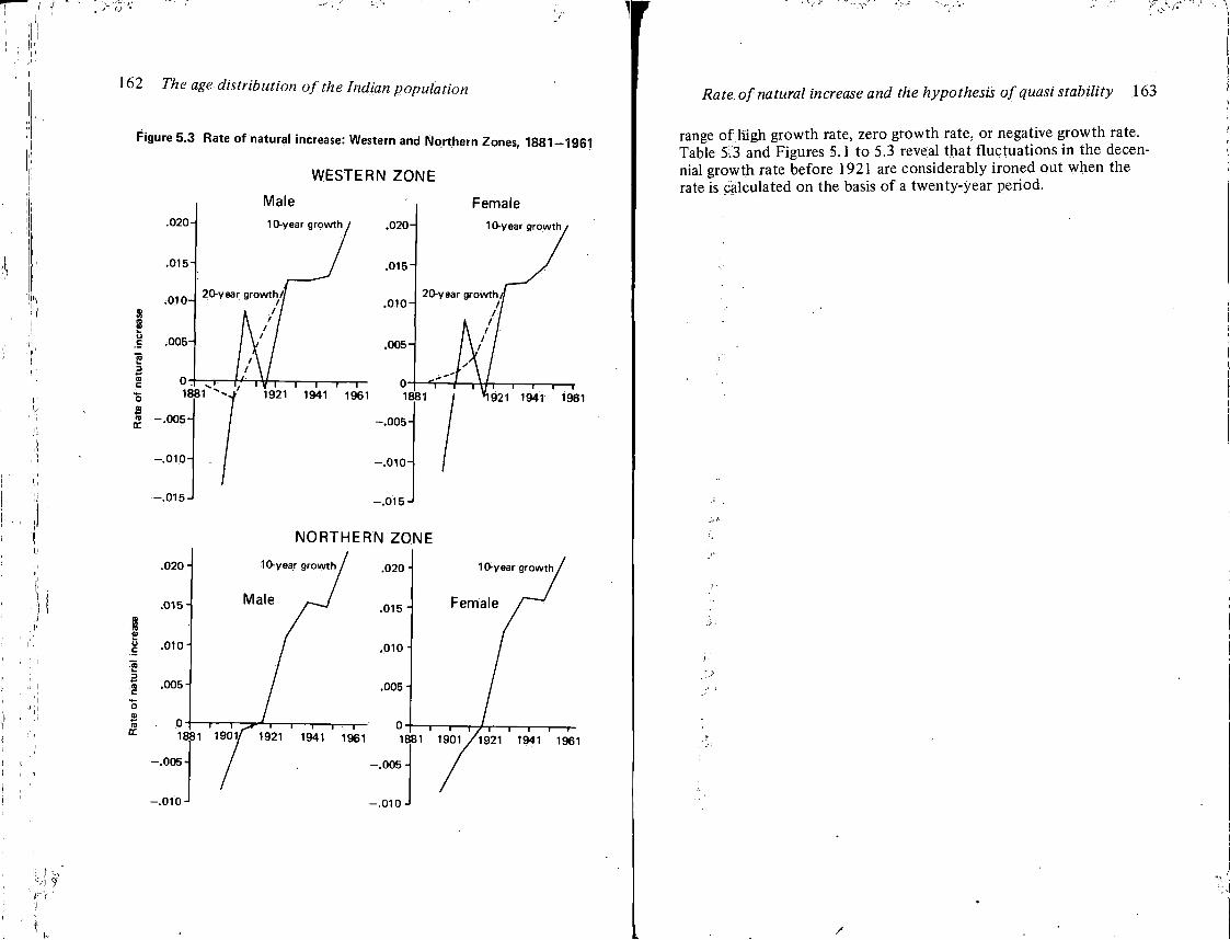
62 The age distribution of the Indian population
Figure 5.3 Rate of natural increase: Western and Northern Zones, 1881-1961
WESTERN ZONE
.020
.015
.010-
.005H
3 (0 c *-o • -.005-
Male 10-year growth , .020
20-year growth//
., • , ~ i 1 1 i — r -1881 ^ 1921 1941 1961
Female 10-year growth,
20-year growth
.01 OH
-.015
.010H
.015
T 1 1 1 r 921 1941 1961
.020
.015 H
.010
.005
NORTHERN ZONE
10-year growtr^ .0201
Male , .
.015 -
.010 •
.005--i 1 1 i
10-year growth /
Female
1881 1901/ 1921 1941 1961 1881 ' 1901 / l 9 2 1 ' 1941 ' 1961
.005
.010
.005 A
.010 J
Rate of natural increase and the hypothesis of quasi stability 163
range of high growth rate, zero growth rate, or negative growth rate. Table 5:3 and Figures 5.1 to 5.3 reveal that fluctuations in the decennial growth rate before 1921 are considerably ironed out when the rate is calculated on the basis of a twenty-year period.
Methodology used to estimate fertility and mortality
One of the stated objectives of this study is to derive estimates of fertility and mortality in India by using the reconstructed age distribution obtained from census data on age and.sex. United Nations Manual IV [99] lays down some new techniques for estimating the birth rate, death rate, gross reproduction rate, and life expectancy from incomplete data. (For a brief summary of these new methods see Coale [41 ].) From among a battery of new methods, we have selected two that are exclusively dependent on the information available in census tables: the method based on the quasi-stable population model and the method of forward projection.
The stable estimates are derived by drawing on the extensive tabulations of stable populations prepared by the Office of Population Research [42] and then correcting them for changes in mortality. Two observed parameters of the population for which estimates are re-quired-the decennial growth rate and the age distribution-are used to identify the exact stable population implied by them. Once the stable population is identified, it is just a routine computation to read off the ' other parameters relating to this population. If we had dependable data on other parameters-gross reproduction rate, expectation of life at birth, childhood mortality, mean age-we could use any two of them (two nonredundant parameters, of course) to locate the exact
Methodology used to estimate fertility and mortality 165
stable population by interpolation from the above tabulations and derive the other variables. But under existing conditions of data availability, the growth rate and age distribution obtained from the census data seem to be the best estimating parameters we can hope to use.
The OPFS stable populations Since the stable population tables prepared by the Office of Population Research (OPR) hold a key position in our process of estimation, a brief discussion of their construction may be useful. For a full discussion the reader is referred to the original text [41 ] . Each stable age distribution is a combination of a model life table and a rate of natural increase according to Lotka's first fundamental equation,
c(a) = be-rap{a) Since the age distributions are given in five-year intervals, the exact expression for the proportion in each age interval is
[a2c(a)da = b f2 e-rap(a)da
= be~rS (%(<?)<&
The birth rate has been evaluated according to the relation
e~rap(a)da ". J 0
The proportion of population in the age interval has been evaluated according to the relation
5
S
The death rate has been obtained by subtracting the growth rate from the birth rate according to the relation
d = b-r where b = birth rate of stable population
. c(a) - proportion of population at age a r = intrinsic rate of natural increase
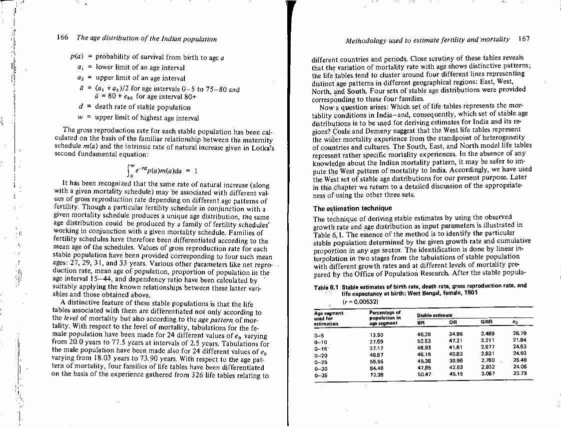
166 The age distribution of the Indian population
p(a) = probability of survival from birth to age a <2i = lower limit of an age interval a2 = upper limit of an age interval
a = (ai +a 2)/2 for age intervals 0—5 to 75—80 and a = 80 + eso for age interval 80+
d = death rate of stable population w = upper limit of highest age interval
The gross reproduction rate for each stable population has been calculated on the basis of the familiar relationship between the maternity schedule m(a) and the intrinsic rate of natural increase given in Lotka's second fundamental equation:
\We-rap(a)m(a)da = 1 Jo
It has been recognized that the same rate of natural increase (along with a given mortality schedule) may be associated with different values of gross reproduction rate depending on different age patterns of fertility. Though a particular fertility schedule in conjunction with a given mortality schedule produces a unique age distribution, the same age distribution could be produced by a family of fertility schedules' working in conjunction with a given mortality schedule. Families of fertility schedules have therefore been differentiated according to the mean age of the schedules. Values of gross reproduction rate for each stable population have been provided corresponding to four such mean ages: 27, 29, 31, and 33 years. Various other parameters like net reproduction rate, mean age of population, proportion of population in the age interval 15—44, and dependency ratio have been calculated by suitably applying the known relationships between these latter variables and those obtained above.
A distinctive feature of these stable populations is that the life tables associated with them are differentiated not only according to the level of mortality but also according to the age pattern of mortality. With respect to the level of mortality, tabulations for the female population have been made for 24 different values of e0 varying from 20.0 years to 77.5 years at intervals of 2.5 years. Tabulations for the male population have been made also for 24 different values of e0
varying from 18.03 years to 73.90 years. With respect to the age pattern of mortality, four families of life tables have been differentiated on the basis of the experience gathered from 326 life tables relating to
Methodology used to estimate fertility and mortality 167
different countries and periods. Close scrutiny of these tables reveals that the variation of mortality rate with age shows distinctive patterns; the life tables tend to cluster around four different lines representing distinct.age patterns in different geographical regions: East, West, North, and South. Four sets of stable age distributions were provided corresponding to these four families.
Now a question arises: Which set of life tables represents the mort a l i t y conditions in India-and, consequently, which set of stable age distributions is to be used for deriving estimates for India and its regions? Coale and Demeny suggest that the West life tables represent the wicier mortality experience from the standpoint of heterogeneity of countries and cultures. The South, East, and North model life tables represent rather specific mortality experiences. In the absence of any knowledge about the Indian mortality pattern, it may be safer to impute the West pattern of mortality to India. Accordingly, we have used the West set of stable age distributions for our present purpose. Later in this chapter we return to a detailed discussion of the appropriateness of using the other three sets.
The estimation technique The technique of deriving stable estimates by using the observed growth rate and age distribution as input parameters is illustrated in Table 6.1. The essence of the method is to identify the particular stable population determined by the given growth rate and cumulative proportion in any age sector. The identification is done by linear interpolation in two stages from the tabulations of stable population with different growth rates and at different levels of mortality prepared by the Office of Population Research. After the stable popula-
Table 6.1 Stable estimates of birth rate, death rate, gross reproduction rate, and ' life expectancy at birth: West Bengal, female, 1901
(r = 0.00532)
Age segment used for estimation
Percentage of population in age segment
Stable estimate Age segment used for estimation
Percentage of population in age segment BR DR GRR
0-5 13.50 40.28 34.96 2.489 28.79
0-10 27.59 52.53 47.21 3.211 21.84
0-15' 37.17 46.93 41.61 2.877 24.53
0-20 46.87 46.15 40.83 2.831 24.93
0-25 55.55 45.36 39.96 2.780 25.46
0-30 64.46 47.85 42.53 2.932 24.06
0-35 72.38 50.47 45.15 3.087 22.73
168 The age distribution of the Indian population
tion is identified, the various vital rates are read off from the relevant columns of the model stable populations.
Note that the estimates made from different age sectors vary considerably from one an other-a consequence of age distortions in Indian censuses, as well as past changes in mortality. Most of the differences in the estimated stable rates are due to biases in age data. If one wished to judge which stable estimates are nearer the true value, one would have to know the relative magnitude of enumeration error in the d i f - r
ferent age sectors. Valuable studies have been made on this subject by the Indian census actuaries and others. Special mention may be made of Vaidyanathan's study in the actuarial report of the 1931 census [109].
As these studies indicate, there is a considerable amount of regional variation and census-to-census variation in age preference and digital -preference in the age returns. This variation results in different patterns of movement of the age ratios and sex ratios over the quinquennial age groups. However, beyond these complex variations a broad -pattern of age bias does emerge for all the years and all the regions (summarized in Chapter 3). In considering the impact of age distribution on the stable estimates derived therefrom, one has to remember that the absolute number of persons in lower age groups is larger than in higher ones. This influences to a varying degree the quantitative effect of a proportionately equal deficit or excess in different age groups on the cumulative proportions of the population up to age 35.
Bringing all these factors to bear upon the stable estimates, we may hypothesize that the estimate based on the proportion of the popula--tion aged 0-5 is an underestimate whereas that based on the propor-' tion aged 0 -10 is an overestimate. The estimates based on proportions in the age groups 0-15, 0-30, and 0-35 are near the true values; those based on proportions in the age. groups 0-20 and 0-25 are possibly somewhat lower than the true values.
It should be appreciated that the age distortions affect our estimates only to the extent that they carry people across the upper boundary of any age sector-e.g., when people below 35 years of age are carried up to higher ages or when people above 35 years of age are carried down to ages below 35. Age distortions within the broad age span of 0-35 do not affect our estimates made on the basis of the population proportion therein. The sequence of estimates made from the successive age sectors suggests that the undercount of infants and children in age group 0 -5 results less from omissions than from an overstatement of their ages. If it were predominantly a case of omission, the estimated
Methodology used to estimate fertility and mortality 169
birth rate would tend to rise continuously in the successive age sectors. As the sum of the proportions in all age intervals is 100 in any case, the relative importance of the undercount in age group 0-5 would gradually diminish. If there were an undercount in higher age groups also, the effect of the undercount in age group 0 -5 on the stable estimate derived therefrom would be limited to the extent of the relatively greater undercount in this age group (i.e., 0-5). And this effect would similarly diminish in successive age sectors. However, the phenomenon observed here is that the estimates go up and down and then up again. Such a sequence lends support to the hypothesis that the true stable birth rate lies between the limits indicated.*
An alternative method A different method was used by the Indian census actuary (1961) for applying the stable technique to Indian age data. This method consists of deriving a life table from the reported age distribution and growth rate and then finding a birth rate consistent with this derived life table and growth rate. This method may be stated as follows. Starting from the stable age distribution,
; da) = be-rap(a)
we obtain c(a)era = bp(a)
That is, multiplying the reported age distribution by the factor era we get a life table with radix b. Since age group 0-5 is often severely mis-reported, we may use the expectation of life at age 10, instead of the expectation of life at age 0, for finding the mortality level. Once the level of mortality is found, we use the model life table for getting the detailed values of p(a). Then, by using the formula
* This method was suggested in the U.N. Population Studies No. 42 [92:12-28, 61-72]. The limitations of the method are recognized. The technique of using the cumulated age proportions takes care of the relative underenumeration in age group 0-4 and relative overenumeration in age group 5-9. But, when whole families are missed by the census enumerator, this method does not serve as a corrective. If there is proportionate underenumeration in all ages, only the growth rate is affected-not the age distribution This method tries to find a solution to the problem of age-selective underenumeration. To cope with the problem of sex-selective underenumeration, we constructed estimates separately for the male and the female population and examined their consistency. (See Chapter 7.)
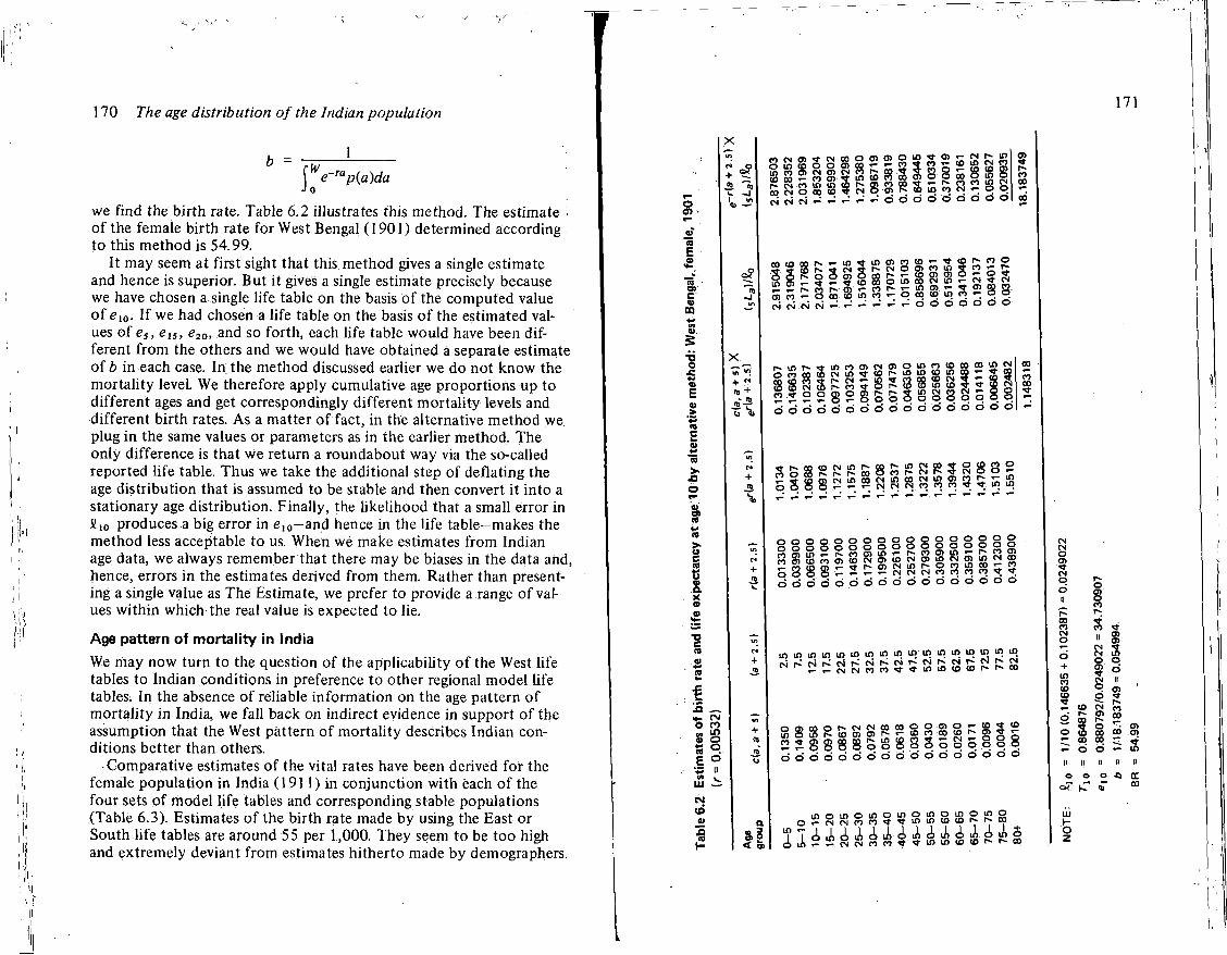
170 The age distribution of the Indian population
e-rap(a)da J 0
we find the birth rate. Table 6.2 illustrates this method. The estimate • of the female birth rate for West Bengal (1901) determined according to this method is 54.99.
It may seem at first sight that this method gives a single estimate and hence is superior. But it gives a single estimate precisely because we have chosen a single life table on the basis of the computed value of el0. If we had chosen a life table on the basis of the estimated values of es, e15, e20, and so forth, each life table would have been different from the others and we would have obtained a separate estimate of b in each case. In the method discussed earlier we do not know the mortality level. We therefore apply cumulative age proportions up to different ages and get correspondingly different mortality levels and different birth rates. As a matter of fact, in the alternative method we plug in the same values or parameters as in the earlier method. The only difference is that we return a roundabout way via the so-called reported life table. Thus we take the additional step of deflating the age distribution that is assumed to be stable and then convert it into a stationary age distribution. Finally, the likelihood that a small error in fi10 produces a big error in e , 0 -and hence in the life table—makes the method less acceptable to us. When we make estimates from Indian age data, we always remember that there may be biases in the data and, hence, errors in the estimates derived from them. Rather than presenting a single value as The Estimate, we prefer to provide a range of values within which the real value is expected to lie.
Age pattern of mortality in India
We may now turn to the question of the applicability of the West life tables to Indian conditions in preference to other regional model life tables. In the absence of reliable information on the age pattern of mortality in India, we fall back on indirect evidence in support of the assumption that the West pattern of mortality describes Indian conditions better than others.
Comparative estimates of the vital rates have been derived for the female population in India (191 1) in conjunction with each of the four sets of model life tables and corresponding stable populations (Table 6.3). Estimates of the birth rate made by using the East or South life tables are around 55 per 1,000. They seem to be too high and extremely deviant from estimates hitherto made by demographers.
171
o co <B O CD 9 E ° •a II
+ r CO + rtT —
a
« N C » * N C 0 O c t C 9 O I 5 * 0 ) r ; M r < l l l
CN co io in co CO CN q GO CD CN CN CN «-' *-
s 5 n o ? ' - ' v c , i n i f l r j S e c n S i o i D O C N ^ o q r r d d d c i d d d o o
oocD«f^^in*i«oicoco^'tfco^coO SSSr^acNjr-cNOcncoina^srj "S^nr^cn^coi^^incn^scj icbW 5 n ^ 8 o . S i n n ^ o c o i o i q n - S d CN CN CN CN - ^ - ~ O O O O O O O
3 innffiNOioionoooinN S S - c t c o t f i B S S S S S ^ o S S
n , ? o o g o g - - * l " I N , m r > " - 0 0
d d d d d d d c i c i > © o o o q q qi q d d d d d d d d
rt o eo £ S 12 £ 8 S P 8 fS 3 8 8 S ° CO o
o o o o o o o o o o o o o o o o o o o o o o o o o o o o o q o o o o c o f f i S c o S S c N c n c D C N c n B C N c n i n c N c o " c o c o S ^ ^ i ^ O ) e N i n r ~ o c o i o c O ' - c o O O O O v - ^ ^ ^ C N C N C N C O C O C O C O * ^ :
0 0 6 6 0 0 0 0 6 0 6 0 0 0 0 0 0
t n i n i o i n i n i n i n i n i n i o i n i o i n i o i o i r > l o tNi<CMi<N^CNr^CNr~CM^CMr»CNi>CN ^ ^ i J ^ S S c o c o ^ ' r i n i n c o c D i ^ r ^ c o
o o > » o r > c s N i » c o q o j | 0 ^ i D l J
2 2 8 8 8 8 S 8 8 8 S q S q 8 8 8 d o ' d d d d d d o d . d d d d o o o
i n o i n o i n o i n o i n o i n o i n o
T T ci J> o J> o J> A J. A J> A A A J, & o i A ° ™ S S n n « - * i B i o » » f - ' > « !
r» 00 co CN o 6 + in co to 2 CD
O CD •- d
o cn o co r-t" -co ^ II o> II cn
CM *r CM in o o ? ° CM II <=>. cn ' o
i— CN CO OJ CO o ^ o oo co cn co C -t O « - ID
II II II II II
UJ t-O z
o « to*
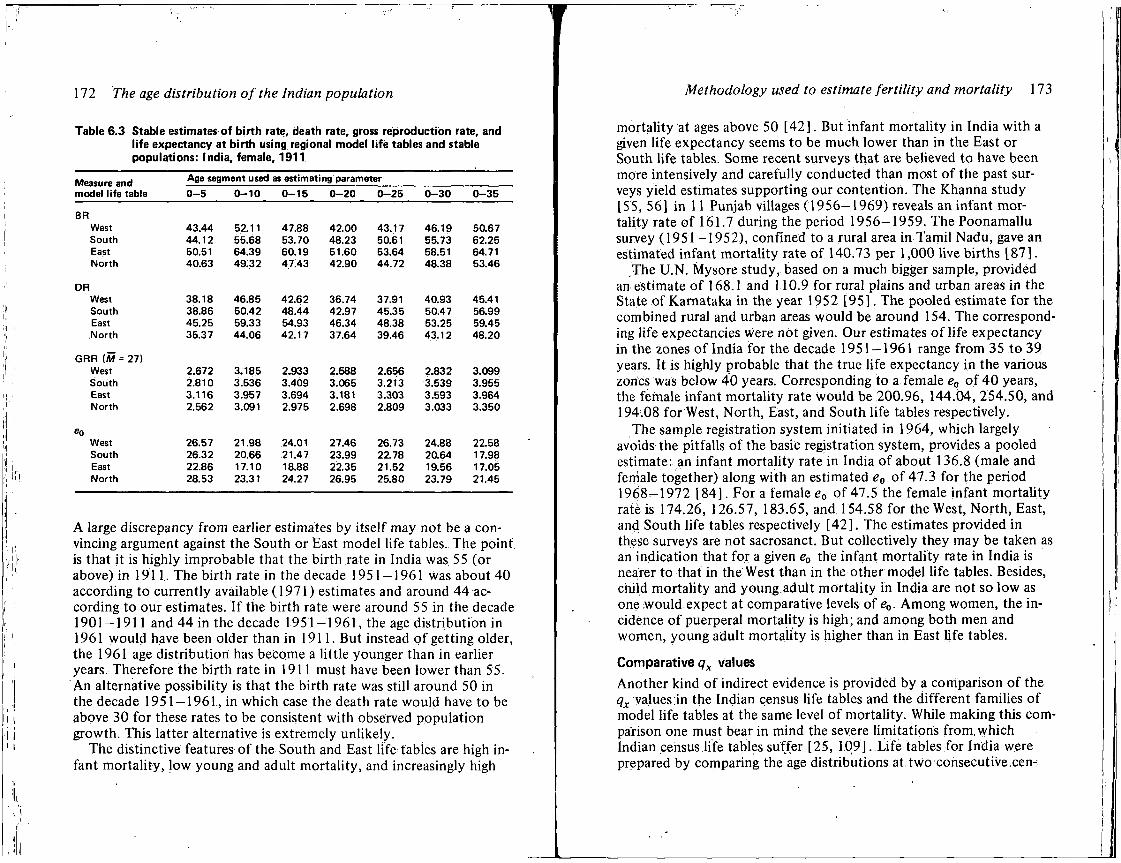
172 The age distribution of the Indian population
Table 6.3 Stable estimates of birth rate, death rate, gross reproduction rate, and life expectancy at birth using regional model life tables and stable populations: India, female, 1911
Measure and * f l B S B 9 m e n t u s e < * 8 5 estimating parameter
model life table 0-5 0-10 0-15 0-20 0-25 0-30 0-35
BR West 43.44 52.11 47.88 42.00 43.17 46.19 50.67 South 44.12 55.68 53.70 48.23 50.61 55.73 62.25 East 50.51 64.39 60.19 51.60 53.64 58.51 64.71 North 40.63 49.32 47.43 42.90 44.72 48.38 53.46
DR West 38.18 46.85 42.62 36.74 37.91 40.93 45.41 South 38.86 50.42 48.44 42.97 45.35 50.47 56.99 East 45.25 59.33 54.93 46.34 48.38 53.25 59.45 North 35.37 44.06 42.17 37.64 39.46 43.12 48.20
GRR (M = 27) West 2.672 3.185 2.933 2.588 2.656 2.832 3.099 South 2.810 3.536 3.409 3.065 3.213 3.539 3.955 East 3.116 3.957 3.694 3.181 3.303 3.593 3.964 North 2.562 3.091 2.975 2.698 2.809 3.033 3.350
West 26.57 21.98 24.01 27.46 26.73 24.88 22.58 South 26.32 20.66 21.47 23.99 22.78 20.64 17.98 East 22.86 17.10 18.88 22.35 21.52 19.56 17.05 North 28.53 23.31 24.27 26.95 25.80 23.79 21.45
A large discrepancy from earlier estimates by itself may not be a convincing argument against the South or East model life tables. The point, is that it is highly improbable that the birth rate in India was 55 (or above) in 1911. The birth rate in the decade 1951-1961 was about 40 according to currently available (1971) estimates and around 44 according to our estimates. If the birth rate were around 55 in the decade 1901-1911 and 44 in the decade 1951-1961, the age distribution in 1961 would have been older than in 1911. But instead of getting older, the 1961 age distribution has become a little younger than in earlier years. Therefore the birth rate in 1911 must have been lower than 55. An alternative possibility is that the birth rate was still around 50 in the decade 1951 — 1961., in which case the death rate would have to be above 30 for these rates to be consistent with observed population growth. This latter alternative is extremely unlikely.
The distinctive features of the South and East life tables are high infant mortality, low young and adult mortality, and increasingly high
Methodology used to estimate fertility and mortality 173
mortality at ages above 50 [42] . But infant mortality in India with a given life expectancy seems to be much lower than in the East or South life tables. Some recent surveys that are believed to have been more intensively and carefully conducted than most of the past surveys yield estimates supporting our contention. The Khanna study [55, 56] in 11 Punjab villages (1956-1969) reveals an infant mortality rate of 161.7 during the period 1956-1959. The Poonamallu survey (1951-1952), confined to a rural area in Tamil Nadu, gave an estimated infant mortality rate of 140.73 per 1,000 live births [87].
The U . N . Mysore study, based on a much bigger sample, provided an estimate of 168.1 and 110.9 for rural plains and urban areas in the State of Karnataka in the year 1952 [95]. The pooled estimate for the combined rural and urban areas would be around 154. The corresponding life expectancies were not given. Our estimates of life expectancy in the zones of India for the decade 1951 — 1961 range from 35 to 39 years. It is highly probable that the true life expectancy in the various zones was below 40 years. Corresponding to a female e0 of 40 years, the female infant mortality rate would be 200.96, 144.04, 254.50, and 194.08 for West, North, East, and South life tables respectively.
The sample registration system initiated in 1964, which largely avoids the pitfalls of the basic registration system, provides a pooled estimate: an infant mortality rate in India of about 136.8 (male and female together) along with an estimated e0 of 47.3 for the period 1968-1972 [84]. For a female e0 of 47.5 the female infant mortality rate is 174.26, 126.57, 183.65, and 154.58 for the West, North, East, and South life tables respectively [42]. The estimates provided in these surveys are not sacrosanct. But collectively they may be taken as an indication that for a given e0 the infant mortality rate in India is nearer to that in the West than in the other model hfe tables. Besides, child mortality and young adult mortality in India are not so low as one would expect at comparative levels of e0. Among women, the incidence of puerperal mortality is high; and among both men and women, young adult mortality is higher than in East life tables.
Comparative qx values
Another kind of indirect evidence is provided by a comparison of the qx values in the Indian census life tables and the different families of model life tables at the same level of mortality. While making this comparison one must bear in mind the severe limitations from, which Indian census life tables suffer [25, 1.09]. Life tables for India were prepared by comparing the age distributions at two consecutive cen-
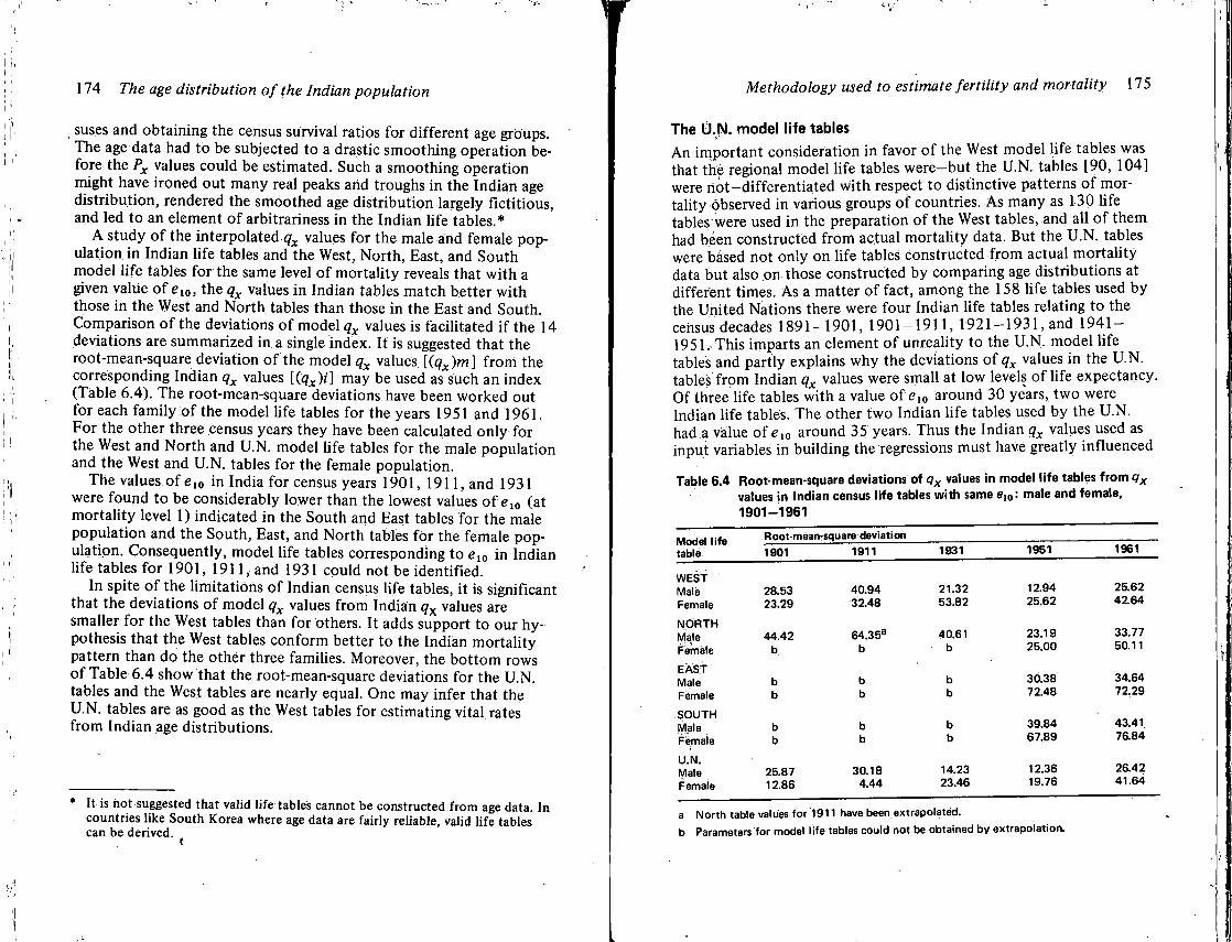
174 The age distribution of the Indian population
suses and obtaining the census survival ratios for different age groups. The age data had to be subjected to a drastic smoothing operation before the Px values could be estimated. Such a smoothing operation might have ironed out many real peaks and troughs in the Indian age distribution, rendered the smoothed age distribution largely fictitious, and led to an element of arbitrariness in the Indian life tables.*
A study of the interpolated qx values for the male and female population in Indian life tables and the West, North, East, and South model life tables for the same level of mortality reveals that with a given value of e l 0 , the qx values in Indian tables match better with those in the West and North tables than those in the East and South. Comparison of the deviations of model qx values is facilitated i f the 14 deviations are summarized in a single index. It is suggested that the root-mean-square deviation of the model qx values [(qx)m] from the corresponding Indian qx values Kqx)i] may be used as such an index (Table 6.4). The root-mean-square deviations have been worked out for each family of the model life tables for the years 1951 and 1961. For the other three census years they have been calculated only for the West and North and U.N. model life tables for the male population and the West and U . N . tables for the female population.
The values of e, 0 in India for census years 1901, 1911, and 1931 were found to be considerably lower than the lowest values of el0 (at mortality level 1) indicated in the South and East tables for the male population and the South, East, and North tables for the female population. Consequently, model life tables corresponding to e 1 0 in Indian life tables for 1901, 1911, and 1931 could not be identified.
In spite of the limitations of Indian census life tables, it is significant that the deviations of model qx values from Indian qx values are smaller for the West tables than for others. It adds support to our hypothesis that the West tables conform better to the Indian mortality pattern than do the other three families. Moreover, the bottom rows of Table 6.4 show that the root-mean-square deviations for the U.N. tables and the West tables are nearly equal. One may infer that the U.N. tables are as good as the West tables for estimating vital rates from Indian age distributions.
* It is not suggested that valid life tables cannot be constructed from age data. In countries like South Korea where age data are fairly reliable, valid life tables can be derived.
(
Methodology used to estimate fertility and mortality 175
The U.N. model life tables An important consideration in favor of the West model life tables was that the regional model life tables were—but the U.N. tables [90, 104] were hot—differentiated with respect to distinctive patterns of mortality observed in various groups of countries. As many as 130 life tables were used in the preparation of the West tables, and all of them had been constructed from actual mortality data. But the U . N . tables were based not only on life tables constructed from actual mortality data but also on those constructed by comparing age distributions at different times. As a matter of fact, among the 158 life tables used by the United Nations there were four Indian life tables relating to the census decades 1891-1901, 1901-1911, 1921-1931, and 1941-1951. This imparts an element of unreality to the U . N . model life tables and partly explains why the deviations of qx values in the U.N. tables from Indian qx values were small at low levels of life expectancy. Of three life tables with a value of el0 around 30 years, two were Indian life tables. The other two Indian life tables used by the U.N. had a value of e 1 0 around 35 years. Thus the Indian qx values used as input variables in building the regressions must have greatly influenced
Table 6.4 Root-mean-square deviations of qx values in model life tables from q x
values in Indian census life tables with same e 1 0 : male and female, 1901-1961
Model life table
Root-mean-square deviation Model life table 1901 1911 1931 1951 1961
WEST Male 28.53 40.94 21.32 12.94 25.62 Female 23.29 32.48 53.82 25.62 42.64
NORTH Male 44.42 64.35a 40.61 23.19 33.77 Female b b b 25.00 50.11
EAST Male b b b 30.38 34.64 Female b b b 72.48 72,29
SOUTH Male b b b 39.84 43.41 Female b b b 67.89 76.84
U.N. Male 25.87 30.18 14.23 12.36 26.42 Female 12.86 4.44 23.46 19.76 41.64
a North table values for 1911 have been extrapolated. b Parameters for model life tables could not be obtained by extrapolation.
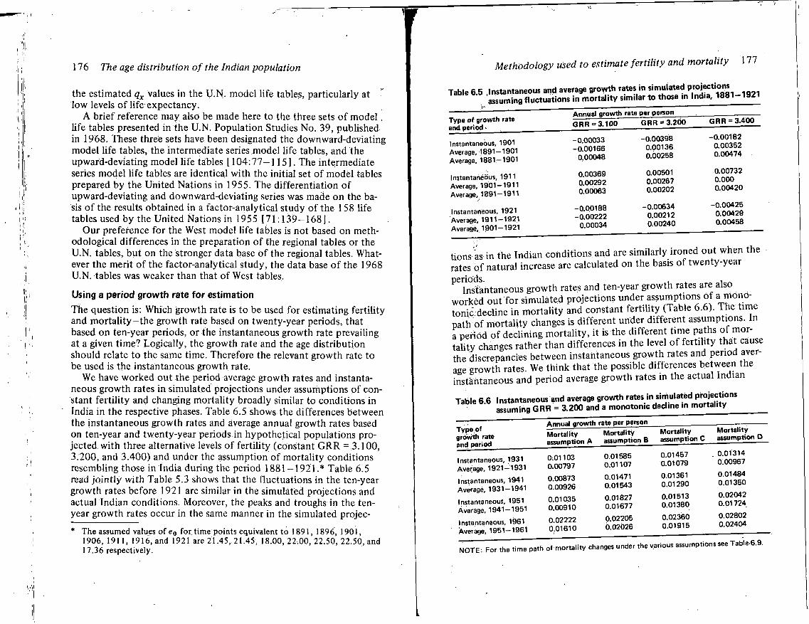
176 The age distribution of the Indian population
the estimated qx values in the U.N. model life tables, particularly at low levels of life expectancy.
A brief reference may also be made here to the three sets of model , life tables presented in the U.N. Population Studies No. 39, published in 1968. These three sets have been designated the downward-deviating model life tables, the intermediate series model life tables, and the upward-deviating model life tables [104:77—115]. The intermediate series model life tables are identical with the initial set of model tables prepared by the United Nations in 1955. The differentiation of upward-deviating and downward-deviating series was made on the basis of the results obtained in a factor-analytical study of the 158 life tables used by the United Nations in 1955 [71:139-168] .
Our preference for the West model life tables is not based on methodological differences in the preparation of the regional tables or the U.N. tables, but on the stronger data base of the regional tables. Whatever the merit of the factor-analytical study, the data base of the 1968 U.N. tables was weaker than that of West tables.
Using a period growth rate for estimation
The question is: Which growth rate is to be used for estimating fertility and mortality—the growth rate based on twenty-year periods, that based on ten-year periods, or the instantaneous growth rate prevailing at a given time? Logically, the growth rate and the age distribution should relate to the same time. Therefore the relevant growth rate to be used is the instantaneous growth rate.
We have worked out the period average growth rates and instantaneous growth rates in simulated projections under assumptions of constant fertility and changing mortality broadly similar to conditions in India in the respective phases. Table 6.5 shows the differences between the instantaneous growth rates and average annual growth rates based on ten-year and twenty-year periods in hypothetical populations projected with three alternative levels of fertility (constant G R R = 3.100, 3.200, and 3.400) and under the assumption of mortality conditions resembling those in India during the period 1881 —1921.* Table 6.5 read jointly with Table 5.3 shows that the fluctuations in the ten-year growth rates before 1921 are similar in the simulated projections and actual Indian conditions. Moreover, the peaks and troughs in the ten-year growth rates occur in the same manner in the simulated projec-
* The assumed values of e0 for time points equivalent to 1891, 1896, 1901, 1906, 191 1, 1916, and 1921 are 21.45, 21.45, 18.00, 22.00, 22.50, 22.50, and 17.36 respectively.
Methodology used to estimate fertility and mortality 177
Table 6.5 Instantaneous and average growth rates in simulated P W ^ ° ™ assumina fluctuations in mortality similar to those in India, 1881-1921
Type of growth rate Annual arowth rate per person
Type of growth rate GRR = 3.100 GRR = 3.200 GRR = 3.400
1 nctantanpntJS 190 1 -0.00033 -0.00398 -0.00182 1 ll> Lol i I O I icuuj) • w
Auoranp 1RQ1—1901 -0.00166 0.00136 0.00352
Average, 1881-1901 0.00048 0.00258 0.00474
1 liptnntononi ic 1Q1 1 0.00369 0.00501 0.00732 1 nsTanidneuuo, I ^ I • Avpraae 1901 — 1911
0.00292 0.00267 0.000 rtwci oyO( • +JV • • w • • Average.,1891-1911
0.00063 0.00202 0.00420
InctantanpnuS 1921 -0.00188 -0.00634 -0.00425 11 laldl I lot icuua(
1 *- • A , , . . ™ iQi 1—1921
-0.00222 0.00212 0.00429 Mveraye, ia i i i o*. • Average, 1901-1921
0.00034 0.00240 0.00458
tions as in the Indian conditions and are similarly ironed out when the • rates of natural increase are calculated on the basis of twenty-year periods.
Instantaneous growth rates and ten-year growth rates are also worked out for simulated projections under assumptions of a mono-tonic, decline in mortality and constant fertility (Table 6.6). The time path of mortality changes is different under different assumptions. In a period of declining mortality, it is the different time paths of mortality changes rather than differences in the level of fertility that cause the discrepancies between instantaneous growth rates and period average growth rates. We think that the possible differences between the instantaneous and period average growth rates in the actual Indian
Table 6.6 Instantaneous and average growth rates in simulated Projections assuming GRR = 3.200 and a monotonic decline in mortality
Type of growth rate
Annual nrnuith rate Der person Type of growth rate Mortality
assumption A Mortality assumption B
Mortality assumption C
Mortality assumption D
and period 0.01103 0.01585 0.01457 . 0.01314
l nsTanxancuua, i w • Average, 1921-1931
0.00797 0.01107 0.01079 0.00967
1 netantanpniK 1941 0.00873 0.01471 0.01361 0.01484 1 nSlonIdlHHJua, >«-»~ > Average, 1931-1941
0.00926 0.01543 0.01290 0.01350
1 nptonto noni l<I 1 Mfi 1 0.01035 0.01827 0.01513 0.02042 InsTanidiicuua, • ~* • Average, 1941-1951
0.00910 0.01677 0.01380 0.01724
1 net a ntarloni 1 1961 0.02222 0.02205 0.02360 0.02802 i nsidnidiicuua^ • • Average, 1951-1961
0.01610 0.02026 0.01915 0.02404
NOTE: For the time path of mortality changes under the various assumptions see Table 6.9.
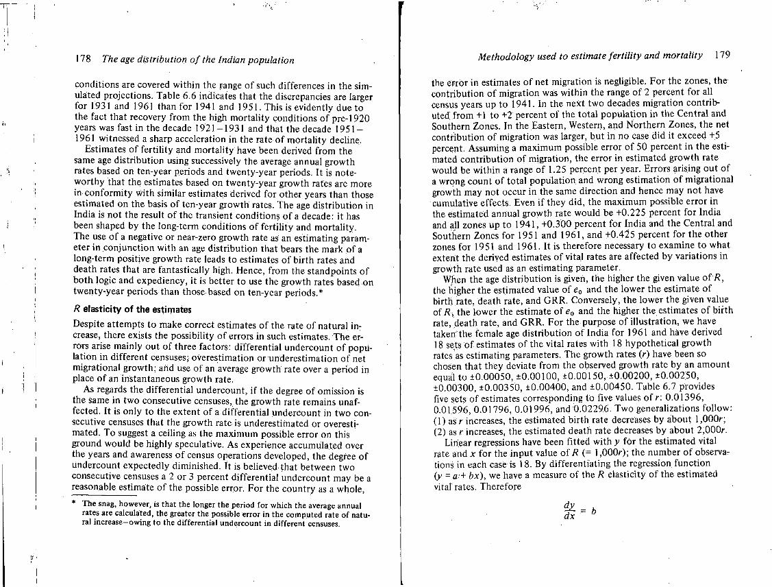
178 The age distribution of the Indian population
conditions are covered within the range of such differences in the simulated projections. Table 6.6 indicates that the discrepancies are larger for 1931 and 1961 than for 1941 and 1951. This is evidently due to the fact that recovery from the high mortality conditions of pre-1920 years was fast in the decade 1921-1931 and that the decade 1951-1961 witnessed a sharp acceleration in the rate of mortality decline.
Estimates of fertility and mortality have been derived from the same age distribution using successively the average annual growth rates based on ten-year periods and twenty-year periods. It is noteworthy that the estimates based on twenty-year growth rates are more in conformity with similar estimates derived for other years than those estimated on the basis of ten-year growth rates. The age distribution in India is not the result of the transient conditions of a decade: it has been shaped by the long-term conditions of fertility and mortality. The use of a negative or near-zero growth rate as an estimating parameter in conjunction with an age distribution that bears the mark of a long-term positive growth rate leads to estimates of birth rates and death rates that are fantastically high. Hence, from the standpoints of both logic and expediency, it is better to use the growth rates based on twenty-year periods than those based on ten-year periods.*
R elasticity of the estimates
Despite attempts to make correct estimates of the rate of natural increase, there exists the possibility of errors in such estimates. The errors arise mainly out of three factors: differential undercount of population in different censuses; overestimation or underestimation of net migrational growth; and use of an average growth rate over a period in place of an instantaneous growth rate.
As regards the differential undercount, if the degree of omission is the same in two consecutive censuses, the growth rate remains unaffected. It is only to the extent of a differential undercount in two consecutive censuses that the growth rate is underestimated or overestimated. To suggest a ceiling as the maximum possible error on this ground would be highly speculative. As experience accumulated over the years and awareness of census operations developed, the degree of undercount expectedly diminished. It is believed that between two consecutive censuses a 2 or 3 percent differential undercount may be a reasonable estimate of the possible error. For the country as a whole,
* The snag, however, is that the longer the period for which the average annual rates are calculated, the greater the possible error in the computed rate of natural increase-owing to the differential undercount in different censuses.
Methodology used to estimate fertility and mortality 179
the error in estimates of net migration is negligible. For the zones, the contribution of migration was within the range of 2 percent for all census years up to 1941. In the next two decades migration contributed.from +1 to +2 percent of the total population in the Central and Southern Zones. In the Eastern, Western, and Northern Zones, the net contribution of migration was larger, but in no case did it exceed +5 percent. Assuming a maximum possible error of 50 percent in the estimated contribution of migration, the error in estimated growth rate would be within a range of 1.25 percent per year. Errors arising out of a wrong count of total population and wrong estimation of migrational growth may not occur in the same direction and hence may not have cumulative effects. Even if they did, the maximum possible error in the estimated annual growth rate would be +0.225 percent for India and all zones up to 1941, +0.300 percent for India and the Central and Southern Zones for 1951 and 1961, and +0.425 percent for the other zones for 1951 and 1961. It is therefore necessary to examine to what extent the derived estimates of vital rates are affected by variations in growth rate used as an estimating parameter.
When the age distribution is given, the higher the given value o f / ? , the higher the estimated value of e0 and the lower the estimate of birth rate, death rate, and G R R . Conversely, the lower the given value of /? , the lower the estimate of e0 and the higher the estimates of birth rate, death rate, and G R R . For the purpose of illustration, we have taken the female age distribution of India for 1961 and have derived 18 sets of estimates of the vital rates with 18 hypothetical growth rates as estimating parameters. The growth rates (r) have been so chosen that they deviate from the observed growth rate by an amount equal to ±0.00050, ±0.00100, ±0.00150,-±0.00200, ±0.00250, ±0.00300, ±0.00350, ±0.00400, and ±0.00450. Table 6.7 provides five sets of estimates corresponding to five values of r: 0.01396, 0.01.596, 0.01796, 0.01996, and 0.02296. Two generalizations follow: (1) as r increases, the estimated birth rate decreases by about l,000r; (2) as r increases, the estimated death rate decreases by about 2,000r.
Linear regressions have been fitted with y for the estimated vital rate and x for the input value of R (= l,000r); the number of observations; in each case is 18. By differentiating the regression function O = a-+ bx), we have a measure of the R elasticity of the estimated vital rates. Therefore
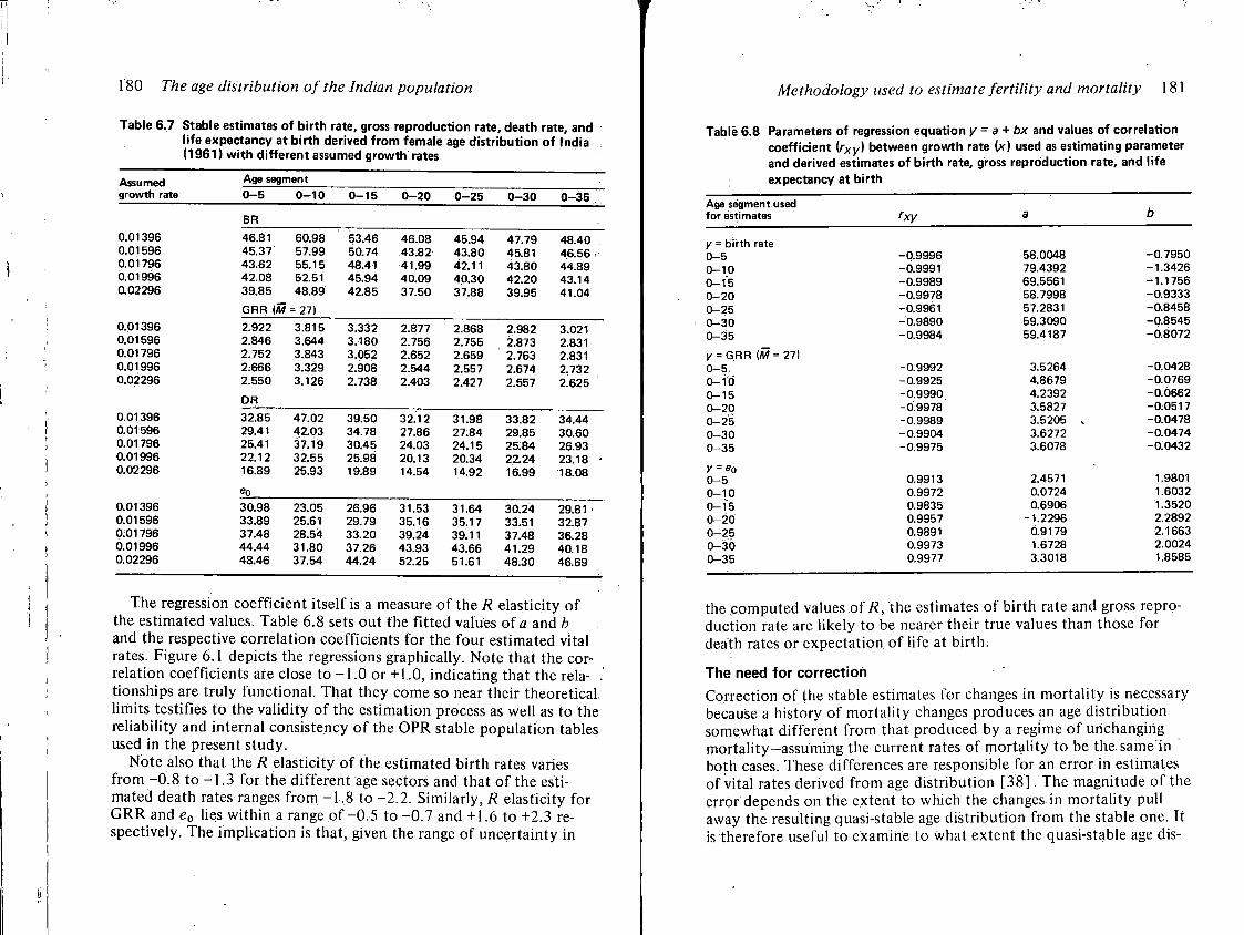
180 The age distribution of the Indian population
Table 6.7 Stable estimates of birth rate, gross reproduction rate, death rate, and life expectancy at birth derived from female age distribution of India (1961) with different assumed growth rates
Assumed Age segment growth rate 0-5 0-10 0-15 0-20 0-25 0-30 0-35
BR
0.01396 46.81 60.98 53.46 46.08 45.94 47.79 48.40 0.01596 45.37 57.99 50.74 43.82 43.80 45.81 46.56 0.01796 43.62 55.15 48.41 41.99 42.11 43.80 44.89 0.01996 42.08 52.51 45.94 40.09 40.30 42.20 43.14 0.02296 39.85 48.89 42.85 37.50 37.88 39.95 41.04
GRR (M = 27) 0.01396 2.922 3.815 3.332 2.877 2.868 2.982 3.021 0.01596 2.846 3.644 3.180 2.756 2.755 2.873 2.831 0.01796 2.752 3.843 3.052 2.652 2.659 2.763 2.831 0.01996 2.666 3.329 2.908 2.544 2.557 2.674 2.732 0.02296 2.550 3.126 2.738 2.403 2.427 2.557 2.625
DR 0.01396 32.85 47.02 39.50 32.12 31.98 33.82 34.44 0.01596 29.41 42.03 34.78 27.86 27.84 29.85 30.60 0.01796 25.41 37.19 30.45 24.03 24.15 25.84 26.93 0.01996 22.12 32.55 25.98 20.13 20.34 22.24 23.18 • 0.02296 16.89 25.93 19.89 14.54 14.92 16.99 18.08
0.01396 30.98 23.05 26.96 31.53 31.64 30.24 29.81 0.01596 33.89 25.61 29.79 35.16 35.17 33.51 32.87 0;01796 37.48 28.54 33.20 39.24 39.11 37.48 36.28 0.01996 44.44 31.80 37.26 43.93 43.66 41.29 40.18 0.02296 48.46 37.54 44.24 52.25 51.61 48.30 46.69
The regression coefficient itself is a measure of the R elasticity of the estimated values. Table 6.8 sets out the fitted values of a and b and the respective correlation coefficients for the four estimated vital rates. Figure 6.1 depicts the regressions graphically. Note that the correlation coefficients are close to -1.0 or +1.0, indicating that the rela- . tionships are truly functional. That they come so near their theoretical limits testifies to the validity of the estimation process as well as to the reliability and internal consistency of the OPR stable population tables used in the present study.
Note also that the R elasticity of the estimated birth rates varies from -0.8 to -1.3 for the different age sectors and that of the estimated death rates ranges from -1.8 to -2.2. Similarly, R elasticity for G R R and e0 lies within a range o f -0 .5 to -0.7 and +1.6 to +2.3 respectively. The implication is that, given the range of uncertainty in
Methodology used to estimate fertility and mortality 181
Table 6.8 Parameters of regression equation y = a + bx and values of correlation coefficient ( r X y ) between growth rate (x) used as estimating parameter and derived estimates of birth rate, gross reproduction rate, and life expectancy at birth
Age segment used for estimates rxy a b
y = birth rate 0-5 -0.9996 58.0048 -0.7950 0-10 -0.9991 79.4392 -1.3426 0-15 -0.9989 69.5561 -1.1756 0-20 -0.9978 58.7998 -0.9333 0-25 -0.9961 57.2831 -0.8458 0-30 -0.9890 59.3090 -0.8545 0-35 -0.9984 59.4187 -0.8072
y = G R R (M = 27) 0-5. -0.9992 3.5264 -0.0428 o-ib -0.9925 4.8679 -0.0769 0-15 -0.9990 4.2392 -0.0662 0-20 -0.9978 3.5827 -0.0517 0-25 -0.9989 3.5205 , -0.0478 0-30 -0.9904 3.6272 -0.0474 0-35 -0.9975 3.6078 -0.0432
Y = e 0
0-5 0.9913 2.4571 1.9801 0-10 0.9972 0.0724 1.6032 0-15 0.9835 0.6906 1.3520 0-20 0.9957 -1.2296 2.2892 0-25 0.9891 0.9179 2.1663 0-30 0.9973 1.6728 2.0024 0-35 0.9977 3.3018 1.8585
the computed values of R, the estimates of birth rate and gross reproduction rate are likely to be nearer their true values than those for death rates or expectation of life at birth.
The need for correction Correction of the stable estimates for changes in mortality is necessary because a history of mortality changes produces an age distribution somewhat different from that produced by a regime of unchanging mortality-assuming the current rates of mortality to be the same'in both cases. These differences are responsible for an error in estimates of vital rates derived from age distribution [38]. The magnitude of the error depends on the extent to which the changes in mortality pull away the resulting quasi-stable age distribution from the stable one. It is therefore useful to examine to what extent the quasi-stable age dis-
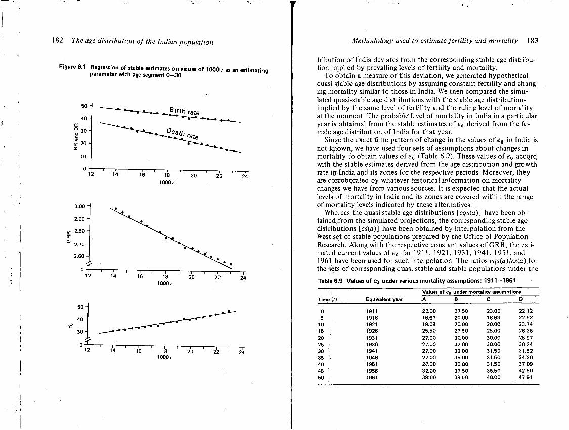
182 The age distribution of the Indian population
Methodology used to estimate fertility and mortality 183
tribution of India deviates from the corresponding stable age distribution implied by prevailing levels of fertility and mortality.
To obtain a measure of this deviation, we generated hypothetical quasi-stable age distributions by assuming constant fertility and changing mortality similar to those in India. We then compared the simulated quasi-stable age distributions with the stable age distributions implied by the same level of fertility and the ruling level of mortality at the moment. The probable level of mortality in India in a particular year is obtained from the stable estimates of e0 derived from the female age distribution of India for that year.
Since the exact time pattern of change in the values of eQ in India is not known, we have used four sets of assumptions about changes in mortality to obtain values of e0 (Table 6.9). These values of e0 accord with the stable estimates derived from the age distribution and growth rate in; India and its zones for the respective periods. Moreover, they are corroborated by whatever historical information on mortality changes we have from various sources. It is expected that the actual levels of mortality in India and its zones are covered within the range of mortality levels indicated by these alternatives.
Whereas the quasi-stable age distributions [cqs(a)] have been ob-tained .from the simulated projections, the corresponding stable age distributions [cs(a)] have been obtained by interpolation from the West set of stable populations prepared by the Office of Population Research. Along with the respective constant values of G R R , the estimated current values of e0 for 1911, 1921, 1931, 1941, 1951, and 1961 have been used for such interpolation. The ratios cqs{a)jcs(a) for the sets of corresponding quasi-stable and stable populations under the
Table 6.9 Values of e0 under various mortality assumptions: 1911—1961
Values of ep under mortality assumptions Time (r) Equivalent year A B C D
0 1911 22.00 27.50 23.00 22.12 5 1916 16.63 20.00 16.63 22.93
10 1921 19.08 20.00 20.00 23.74 15 1926 25.50 27.50 28.00 26.36 20 1931 27.00 30.00 30.00 28.97 25 1936 27.00 32.00 30.00 30.24 30 1941 27.00 32.00 31.50 31.52 35 1946 27.00 35.00 31.50 34.30 40 1951 27.00 35.00 31.50 37.09 45 1956 3200 37.50 35.50 42.50 50 1961 38.00 38.50 40.00 47.91
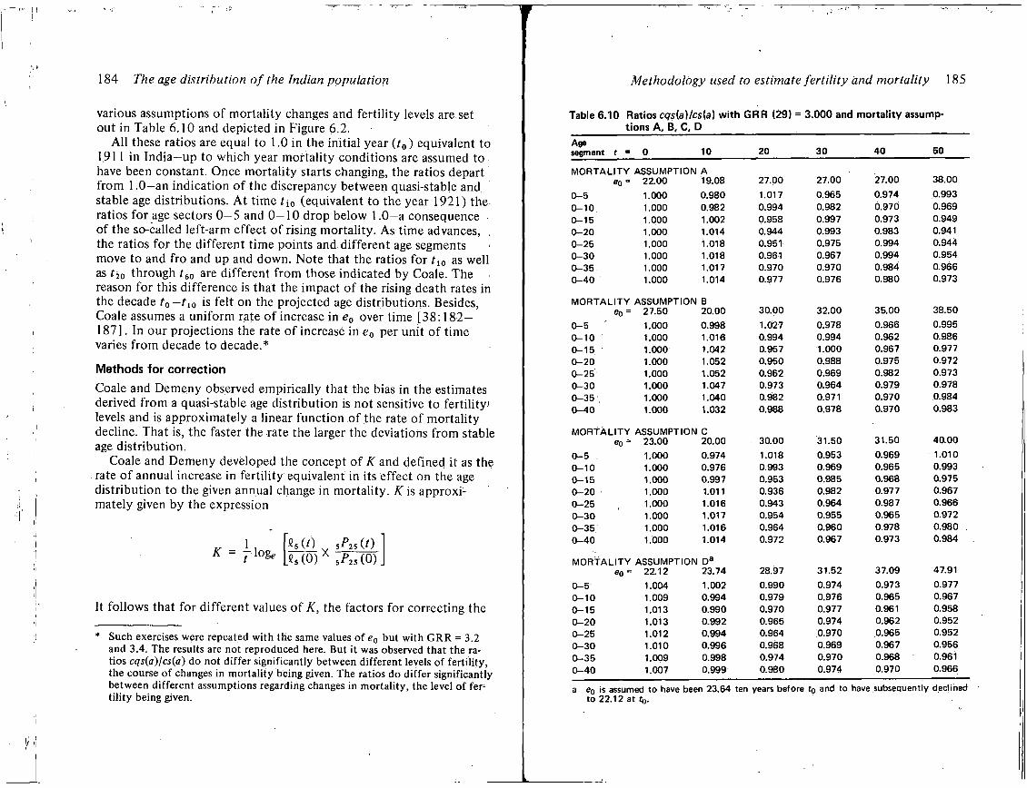
184 The age distribution of the Indian population
various assumptions of mortality changes and fertility levels are set out in Table 6.10 and depicted in Figure 6.2.
A l l these ratios are equal to 1.0 in the initial year (t0) equivalent to 1911 in India—up to which year mortality conditions are assumed to have been constant. Once mortality starts changing, the ratios depart from 1.0—an indication of the discrepancy between quasi-stable and stable age distributions. At time f 1 0 (equivalent to the year 1921) the ratios for age sectors 0—5 and 0—10 drop below 1.0—a consequence of the so-called left-arm effect of rising mortality. As time advances, ; the ratios for the different time points and different age segments move to and fro and up and down. Note that the ratios for r 1 0 as well as t 2 0 through t60 are different from those indicated by Coale. The reason for this difference is that the impact of the rising death rates in the decade t 0 - t l 0 is felt on the projected age distributions. Besides, Coale assumes a uniform rate of increase in e0 over time [38:182— 187]. In our projections the rate of increase in e0 per unit of time varies from decade to decade.*
Methods for correction
Coale and Demeny observed empirically that the bias in the estimates derived from a quasi-stable age distribution is not sensitive to fertility' levels and is approximately a linear function of the rate of mortality decline. That is, the faster the rate the larger the deviations from stable age distribution.
Coale and Demeny developed the concept of K and defined it as the rate of annual increase in fertility equivalent in its effect on the age distribution to the given annual change in mortality. K is approximately given by the expression
K = y-\oge
It follows that for different values of K, the factors for correcting the
* Such exercises were repeated with the same values of e0 but with GRR = 3.2 and 3.4. The results are not reproduced here. But it was observed that the ratios cqs(a)/cs(a) do not differ significantly between different levels of fertility, the course of changes in mortality being given. The ratios do differ significantly between different assumptions regarding changes in mortality, the level of fertility being given.
' M O v 5 25 (0 « S ( 0 ) X 5^25(0).
I
Methodology used to estimate fertility and mortality 185
Table 6.10 Ratios cqs(a)lcs(a) with GRR (29) = 3.000 and mortality assumptions A, B, C, D
Age segment f = 0 10 20 30 40 50
MORTALITY ASSUMPTION A e0= 22.00 19.08 27.00 27.00 27.00 38.00
0-5 1.000 0.980 1.017 0.965 0.974 0.993 0-10 1.000 0.982 0.994 0.982 0.970 0.969 0-15 1.000 1.002 0.958 0.997 0.973 0.949 0-20 1.000 1.014 0.944 0.993 0.983 0.941 0-25 1.000 1.018 0.951 0.975 0.994 0.944 0-30 1.000 1.018 0.961 0.967 0.994 0.954 0-35 1.000 1.017 0.970 0.970 0.984 0.966 0-40 1.000 1.014 0.977 0.976 0.980 0.973
MORTALITY ASSUMPTION B e 0 = 27.50 20.00 30.00 32.00 35.00 38.50
0-5 1.000 0.998 1.027 0.978 0.966 0.995 0-10 1.000 1.016 0.994 0.994 0.962 0.986 0-15 1.000 1.042 0.957 1.000 0.967 0.977 0-20 1.000 1.052 0.950 0.988 0.975 0.972 0-25 1.000 1.052 0.962 0.969 0.982 0.973 0-30 1.000 1.047 0.973 0.964 0.979 0.978 0-35 : 1.000 1.040 0.982 0.971 0.970 0.984 0-40 1.000 1.032 0.988 0.978 0.970 0.983
MORTALITY ASSUMPTION C e 0 = 23.00 20.00 30.00 31.50 31.50 40.00
0-5 . 1.000 0.974 1.018 0.953 0.969 1.010 0-10 1.000 0.976 0.993 0.969 0.965 0.993 0-15 1.000 0.997 0.953 0.985 0.968 0.975 0-20 1.000 1.011 0.936 0.982 0.977 0.967 0-25 1.000 1.016 0.943 0.964 0.987 0.966 0-30 1.000 1.017 0.954 0.955 0.965 0.972 0-35 1.000 1.016 0.964 0.960 0.978 0.980 . 0-40 1.000 1.014 0.972 0.967 0.973 0.984
MORTALITY ASSUMPTION D a
e 0 = 22.12 23.74 28.97 31.52 37.09 47.91
0-5 1.004 1.002 0.990 0.974 0.973 0.977 0-10 1.009 0.994 0.979 0.976 0.965 0.967 0-15 1.013 0.990 0.970 0.977 0.961 0.958 0-20 1.013 0.992 0.965 0.974 0.962 0.952 0-25 1.012 0.994 0.964 0.970 0.965 0.952 0-30 1.010 0.996 0.968 0.969 0.967 0.956 0-35 1.009 0.998 0.974 0.970 0.968 0.961 0-40 1.007 0.999 0.980 0.974 0.970 0.966
a e0 is assumed to have been 23.64 ten years before t0 and to have subsequently declined to 22.12 at f0.
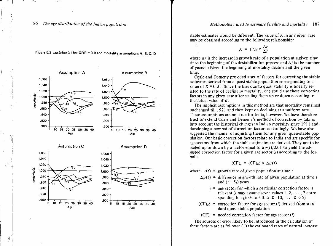
186 The age distribution of the Indian population
Figure 6.2 cqs(a)lcs(a) for GRR = 3.0 and mortality assumptions A, B, C, D
Assumption A Assumption B
~ i — i — i — i — r 10 15 20 25 30 35 40
Age
T 1 1 r 10 15 20 25 30 35 40
Age
Assumption C Assumption D
" i 1 " 1 — i — r 5 10 15 20 25 30 35 40
Age
1.060
1.040
1.020
1.000
.980
.960
.940
.920
.900 H 1 1 1 1 1 r 5 10 15 20 25 30 35 40
Age
Methodology used to estimate fertility and mortality 187
stable estimates would be different. The value of K in any given case may be obtained according to the following relationship:
Ar K = 17.8X
where Ar is the increase in growth rate of a population at a given time since the beginning of the destabilization process and At is the number of years between the beginning of mortality decline and the given time.
Coale and Demeny provided a set of factors for correcting the stable estimates derived from a quasi-stable population corresponding to a value of K = 0.01. Since the bias due to quasi stability is linearly related to the rate of decline in mortality, one could use these correcting factors in any given case after scaling them up or down according to the actual value of A". .
The implicit assumptions in this method are that mortality remained unchanged till 1921 and then kept on declining at a uniform rate. These assumptions are not true for India, however. We have therefore tried to extend Coale and Demeny's method of correction by taking into account the historical changes in Indian mortality since 1911 and developing a new set of correction factors accordingly. We have also suggested the manner of adjusting them for any given quasi-stable population. Our basic correction factors relate to India and are specific for age sectors from which the stable estimates are derived. They are to be scaled up or down by a factor equal to A,r(f)/0.01 to yield the adjusted correction factor for a given age sector (/) according to the formula
(CF),- = (CF)/6X Air(t)
where r(t) = growth rate of given population at time t Ajr(t) = difference in growth rate of given population at time t
and (t - 5/) years i = age sector for which a particular correction factor is
relevant (i may assume seven values 1, 2 , . . . , 7 corre-. sponding to age sectors 0 -5 , 0 - 1 0 , . . . , 0-35)
(CF),/> = correction factor for age sector (i) derived from standard quasi-stable population
(CF),- = needed correction factor for age sector (/) The sources of error likely to be introduced in the calculation of
these factors are as follows: (1) the estimated rates of natural increase
188 The age distribution of the Indian population
for India have their own uncertainties, particularly in the years prior to 1901; (2) the calculation of such rates for midcensus periods is based on the assumption of a uniform rate of change in mortality over the decade, which in reality might not have been the case.
Coale and Demeny's method of correction is more appropriate for age distributions having a history of monotonic decline in mortality. For age distributions with a history of fluctuating mortality as in India, our method seems to be more appropriate for correcting estimates relating to time points near the date when mortality decline started. For time points 40 or 50 years after the onset of mortality decline, the two methods yield similar results. Nevertheless there remains the need for a more general method of correcting stable estimates for past changes in mortality.
7 Quasi-stable estimates
of fertility and mortality
Chapter 6 discussed the method of preparing quasi-stable estimates of fertility and mortality. This chapter presents the estimates and examines their internal consistency. But before we discuss the estimated rates, a word on the estimates of G R R is in order.
Mean of the female fertility schedule Estimates of G R R are not fully defined'unless the respective means of fertility schedule (M) going with such estimates are indicated. To obtain values of M for the female population in India and its zones, we have elaborately processed the census data on marital status by age in a manner similar to that adopted for processing the age-sex composition (see Chapter 2). This gave us the proportion of currently married women in the various age groups for the seven censuses_1901 through 1961 (Table 7.1). The other ingredient for calculating M is the data on marital fertility by age. In the absence of such data in the required form, we used the National Sample Survey (NSS) data (14th round-rural) [65] on age-specific fertility rates. The underlying marital fertility rates have been abstracted from the specific marital status observed in the samples in the various states and territories in the respective zones. Assuming that the schedule of marital fertility rates in the respective zones remained constant during the period 1901 -1961 , we
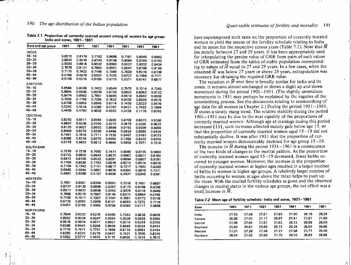
190 The age distribution of the Indian population
Table 7.1 Proportion of currently married women among all women by age group: India and zones, 1901—1961
Zone and age group 1901 1911 1921 1931 1941 1951 1961
INDIA 15-19 0.8015 0.8179 0.7762 0.8698 0.7181 0.6945 0.6962 20-24 0.8830 0.9018 0.8740 0.9156 0.9094 0.9160 0.9183 25-29 0.8593 0.8816 0.8532 0.8963 0.9027 0.9032 0.9424 30-34 0.7879 0:8137 0.7885 0.8551 0.8547 0.8768 0.9149 35-39 0.7175 0.7423 0.7196 0.7565 0.7639 0.8276 0.8708 40-44 0.5766 0.5970 0.5924 0.7035 0.6707 0.7386 0.7771 45-49 0.5190 0.5218 0.5199 0.5715 0.5371 0.6747 0.6977 EASTERN 15-19 0.8568 0.8338 0.7402 0.8549 0.7575 0.7214 0.7343 20-24 0.8854 0.8906 0.8239 0.8735 0.9032 0.8962 0.9122 25-29 0.8474 0.8562 0.7951 0.8695 0.8910 0.8942 0.9336 30-34 0.7595 0.7765 0.7364 0.7832 0.8338 0.8690 0.9075 35-39 0.6708 0.6905 0.6545 0.6714 0.7436 0.8323 0.8576 40-44 0.5240 0.5514 0.5385 0.5797 0.6421 0.7462 0.7689 45-49 0.4495 0.4760 0.4639 0.4332 0.5136 0.7176 0.6792 CENTRAL 15-19 0.8393 0.8817 0:8584 0.8935 0.8209 0.8073 0.8358 20-24 0.8897 0.9209 0.9100 0.9270 0.9479 0.9295 0.9623 25-29 0.8725 0.9021 0.8920 0.8899 0.9192 0.9209 0.9659 30-34 0.8060 0.8376 0.8258 0.8496 0.8659 0.8985 0.9424 35-39 0.7461 0.7816 0.7711 0.7328 0.8407 0.9181 0.9073 40-44 0.6068 0.6216 0.6270 0.6493 0.7264 0.8303 0.8205 45-49 . 0.5719 0.5632 0.5612 0.4804 0.5909 0.7071 0.7518 SOUTHERN 15-19 0.7079 0.7279 0.7002 0.7471 0.6048 0.5735 0.5693 20-24 0.8703 0.8802 0.8643 0.8670 0.8682 0.8827 0.8762 25-29 0.8473 0.8704 0.8523 0.8391 0.8694 0.8867 0.9181 30-34 0.7780 0.8036 0.7793 0.8078 0.8213 0.8514 0.8815 35-39 0.7104 0.7342 0.7141 0.6617 0.7217 0.7992 0.8329 40-44 0.5649 0.5944 0.5861 0.6076 0.6284 0.6919 0.7211 45-49 0.4991 0.5098 0.5157 0.4436 0.4937 0.6245 0.6391 WESTERN 15-19 0.7951 0.8561 0.8304 0.8591 0.7316 0.7051 0.6687 20-24 0.8737 0.9128 0.8898 0.9257 0.9173 0.9709 0.9208 25-29 0.8517 0.8922 0.8658 0.9250 0.9074 0.9118 0.9449 30-34 0.7866 0.8279 0.7967 0.8148 0.8573 0.8864 0.9186 35-39 0.7105 0.7517 0.7207 0.7397 0.7587 0.8172 0.8738 40-44 0.5729 0.6001 0.5909 0.6101 0.6550 0.7272 0.7776 45-49 0.5051 0.5155 0.5065 0.4756 0.5060 0.6117 0.6898 NORTHERN 15-19 0.7804 0.8232 0.8278 0.8488 0.7240 0.6836 0.6629 20-24 0.8953 0.9224 0.9247 0.9554 0.9339 0.9655 0.9363 25-29 0.8876 0.9074 0.8977 0.8921 0.9310 0.9234 0.9702 30-34 0.8268 08447 0.8208 0.8639 0.8945 0.9034 0.9491 35-39 0.7776 0.7871 0.7731 0.7469 0.8170 0.8662 0.9154 40-44 0.6289 0.6322 0.6376 0.6427 0.7421 0.7895 0.8345 45-49 0.5962 0.5777 0.5835 0.5175 0.6035 0.7614 0.7810
Quasi-stable estimates of fertility and mortality 191
have superimposed such rates on the proportion of currently married women to yield the means of the fertility schedule relating to India_ and its zones for the respective census years (Table 7.2). Note that M lies mostly between 27 and 29 years. It has been appropriately used for interpolating the precise value of G R R from pairs of such values of G R R estimated from the tables of stable population corresponding to values oiM equal to 27 and 29 years. In a few cases, when the observed M was below 27 years or above 29 years, extrapolation was necessary for obtaining the required G R R value.
The variation in M over time is broadly similar for India and its zones. It remains almost unchanged or shows a slight up and down movement during the period 1901-1931. (The slightly anomalous movements in 1931 may perhaps be explained by the vagaries of the unsmoothing process. See the discussions relating to unsmoothing of age data for all women in Chapter 2.) During the period 1931 — 1.961, M shows a slowly rising trend. The relative stability during the period 1901-1931 may be due to the near equality of the proportions of currently married women. Although age at marriage during this period increased [15], such increases affected mainly girls below age 15, so that the proportion of currently married women aged 15—19 did not substantially decline. It was after 1931 that the proportion of currently married women demonstrably declined for age group 15—19.
The increase in Af during the period 1931-1961 is a consequence of the; two kinds of changes in the marital pattern. As the proportion of currently married women aged 15—19 decreased, fewer births occurred to younger women. Moreover, the increase in the proportion of currently married women at higher ages resulted in a larger number of births to women in higher age groups. A relatively larger number of births occurring to women at ages above the mean helps to push up the mean. With the marital fertility schedules as given and the observed changes in marital_status in the various age groups, the net effect was a small increase in M.
Table 7.2 Mean age of fertility schedule: India and zones, 1901-1961
Zone 1901 1911 1921 1931 1941 1951 1961
India 27.53 27.56 27.61 27.63 27.90 28.19 28.24 Eastern 26.88 27.00 27.17 26.97 27.41 27.87 27.89 Central 27.96 27.94 27.97 27.82 28.23 28.58 28.50 Southern 25.83 25.87 25.89 25.72 26.24 26.53 26.66 Western 27.31 27.28 27.26 27.21 27.58 27.77 28.09 Northern 28.04 27.93 27.90 27.75 28.35 28.62 28.86
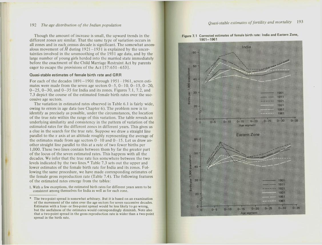
192 The age distribution of the Indian population
Though the amount of increase is small, the upward trends in the different zones are similar. That the same type of variation occurs in all zones and in each_census decade is significant. The somewhat anomalous movement of M during 1921 — 1931 is explained by the uncertainties involved in the unsmoothing of the 1931 age data, and by the large number of young girls herded into the married state immediately before the enactment of the Child Marriage Restraint Act by parents eager to escape the provisions of the Act [57:651—653].
Quasi-stable estimates of female birth rate and GRR For each of the decades 1891 -1901 through 1951 — 1961, seven estimates were made from the seven age sectors 0 -5 , 0—10, 0—15, 0—20, 0—25, 0—30, and 0—35 for India and its zones. Figures 7.1, 7.2, and 7.3 depict the course of the estimated female birth rates over the successive age sectors.
The variation in estimated rates observed in Table 6.1 is fairly wide, owing to errors in age data (see Chapter 6). The problem now is to identify as precisely as possible, under the circumstances, the location of the true rate within the range of this variation. The table reveals an underlying similarity and consistency in the pattern of variation of the estimated rates for the different zones in different years. This gives us a clue in the search for the true rate. Suppose we draw a straight line parallel to the x axis at an altitude roughly representing the average of the estimates made from age sectors 0—10 and 0—15. Let us draw another straight line parallel to this at a rate of two fewer births per 1,000. These two lines contain between them by far the greater part of the locus of the seven estimated rates. This happens with all the decades. We infer that the true rate lies somewhere between the two levels indicated by the two lines.* Table 7.3 sets out the upper and lower estimates of the female birth rate for India and its zones. Following the same procedure, we have made corresponding estimates of the female gross reproduction rate (Table 7.4). The following features of the estimated rates emerge from the tables:
1. With a few exceptions, the estimated birth rates for different years seem to be consistent among themselves for India as well as for each zone.
* The two-point spread is somewhat arbitrary. But it is based on an examination of the movement of the rates over the age sectors for seven successive decades. Estimates with a four- or five-point spread would be less likely to go wrong, but the usefulness of the estimates would correspondingly diminish. Note also that a two-point spread in the gross reproduction rate is wider than a two-point spread in the birth rate.
Quasi-stable estimates of fertility and mortality 193
Figure 7.1 Corrected estimates of female birth rate: India and Eastern Zone,
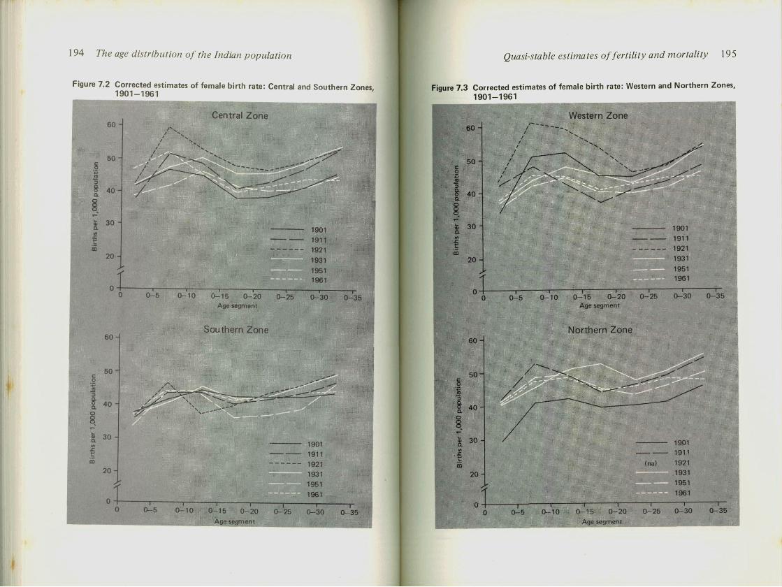
194 The age distribution of the Indian population
Quasi-stable estimates of fertility and mortality 195
Figure 7.3 Corrected estimates of female birth rate: Western and Northern Zones, 1901-1961
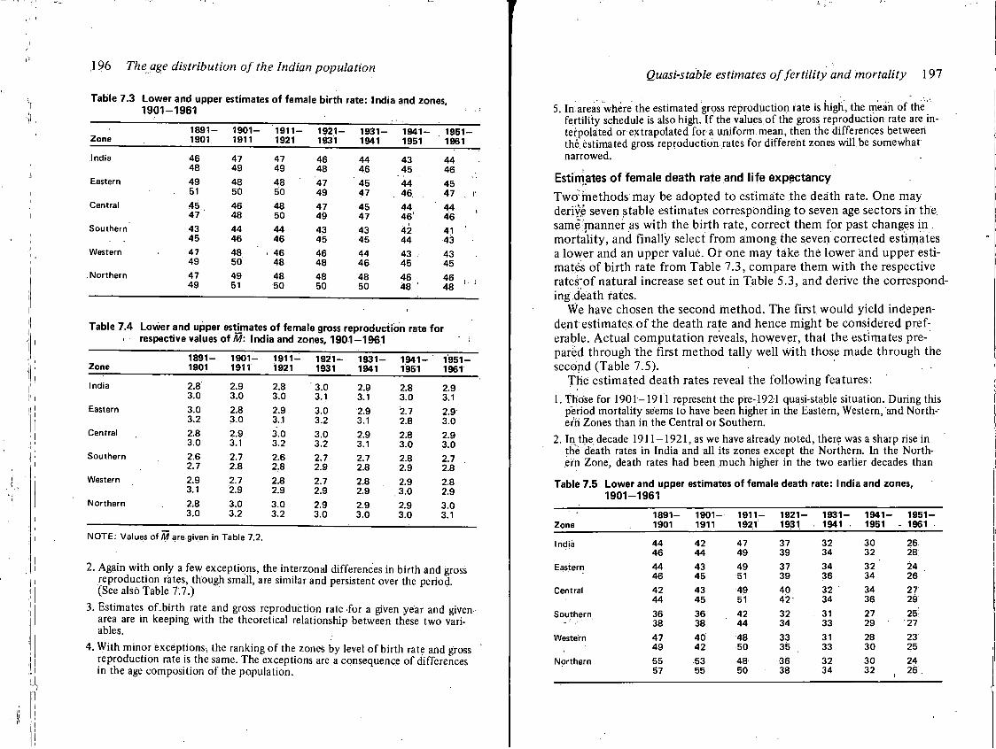
.196 The age distribution of the Indian population
Table 7.3 Lower and upper estimates of female birth rate: India and zones, 1901-1961
1891- 1901- 1911 — 1921- 1931- 1941- 1951-Zone 1901 1911 1921 1931 1941 1951 1961
India 46 47 47 46 44 43 44 48 49 49 48 46 45 46
Eastern 49 48 48 ' 47 45 44 45 51 50 50 49 47 . 46 47 i
Central 45. 46 48 47 45 44 44 47 48 50 49 47 46' 46 '
Southern 43 44 44 43 43 42 41 ' 45 46 46 45 45 44 43
Western 47 48 > 46 46 44 43 : 43 49 50 48 48 46 45 45
Northern 47 49 48 48 48 46 46 . . 49 51 50 50 50 48 ' 48 ' '
Table 7.4 Lower and upper estimates of female gross reproduction rate for * respective values of M: India and zones, 1901-1961
Zone 1891- 1901- 1911 — 1921- 1931- 1941- 1951-
Zone 1901 1911 1921 1931 1941 1951 1961
India 2.8 2.9 2.8 3.0 2.9 2.8 2.9 3.0 3.0 3.0 31 3.1 3.0 3.1
Eastern 3.0 2.8 2.9 3.0 2.9 2.7 2.9 3.2 3.0 3.1 3.2 3.1 2.8 3.0
Central 2.8 2.9 3.0 3.0 2.9 2.8 2.9 3.0 3.1 3.2 3.2 3.1 3.0 3.0
Southern 2.6 2.7 2.6 2.7 2.7 2.8 2.7 2.7 2.8 2.8 2.9 2.8 2.9 2.8
Western 2.9 2.7 2.8 2.7 2.8 2.9 2.8 3.1 2.9 2.9 2.9 2.9 .3.0 2.9
Northern 2.8 3.0 3.0 2.9 2.9 2.9 3.0 3.0 3.2 3.2 3.0 3.0 3.0 3.1
NOTE: Values of M are given in Table 7.2.
2. Again with only a few exceptions, the interzonal differences in birth and gross reproduction rates, though small, are similar and persistent over the period (See also Table 7.7.)
3. Estimates of.birth rate and gross reproduction rate for a given year and given area are in keeping with the theoretical relationship between these two variables.
4. With minor exceptions, the ranking of the zones by level of birth rate and gross reproduction rate is the same. The exceptions are a consequence of differences in the age composition of the population.
Quasi-stable estimates of fertility and mortality 197
5. In areas where the estimated gross reproduction rate is high, the mean of the fertility schedule is also high. If the values of the gross reproduction rate are interpolated or extrapolated for a uniform mean, then the differences between the.estimated gross reproduction rates for different zones will be somewhat narrowed.
Estimates of female death rate and life expectancy
Two'methods may be adopted to estimate the death rate. One may derive seven stable estimates corresponding to seven age sectors in the same manner as with the birth rate, correct them for past changes in . mortality, and finally select from among the seven corrected estimates a lower and an upper value. Or one may take the lower and upper estimates of birth rate from Table 7.3, compare them with the respective rate's'of natural increase set out in Table 5.3, and derive the corresponding death rates.
We have chosen the second method. The first would yield independent estimates of the death rate and hence might be considered preferable. Actual computation reveals, however, that the estimates prepared through the first method tally well with those made through the second (Table 7.5).
The estimated death rates reveal the following features: 1. Those for 1901-1911 represent the pre-1921 quasi-stable situation. During this
period mortality seems to have been higher in the Eastern, Western, and North-em Zones than in the Central or Southern.
2. In the decade 1911 — 1921, as we have already noted, there was a sharp rise in the death rates in India and all its zones except the Northern. In the Northern Zone, death rates had been much higher in the two earlier decades than
Table 7.5 Lower and upper estimates of female death rate: India and zones, 1901-1961
1891- 1901 — 1911— 1921- 1931- 1941- 1951-Zone 1901 1911 1921 1931 1941 1951 - 1961
India 44 42 47 37 32 30 26 46 44 49 39 34 32 28
Eastern 44 43 49 37 34 32 24 46 45 51 39 36 34 26
Central 42 43 49 40 32 34 27 44 45 51 42 34 36 29
Southern 36 36 42 32 . 31 27 25-38 38 44 34 33 29 ' 27
Western 47 40 48 33 31 28 23 49 42 50 35 33 30 25
Northern 55 53 48 36 32 30 24 57 55 50 38 34 32
I 26 .
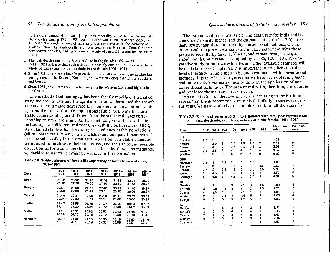
198 The age distribution of the Indian population
in the other zones. Moreover, the spurt in mortality witnessed in the rest of the country during 1911-1921 was not observed in the Northern Zone, although the absolute level of mortality was the same as in the country as a whole. Note that high death rates persisted in the Northern Zone for three consecutive decades, leading to a negative rate of natural increase for the entire period.
3. The high death rates in the Western Zone in the decades 1891-1901 and 1911-1921 indicate that such a situation possibly existed there too over the •. whole period except for an interlude in the decade 1901-1911.
4. Since 1921, death rates have kept on declining in all the zones. The decline has been greater in the Eastern, Northern, and Western Zones than in the Southern and Central.
5. Since 1951, death rates seem to be lowest in the Western Zone and highest in the Central.
The method of estimating e0 has been slightly modified. Instead of using the growth rate and the age distribution we have used the growth rate and the estimated death rate as parameters to derive estimates of eQ from the tables of stable populations (Table 7.6). Note that such stable estimates of e0 are different from the stable estimates corresponding to seven age segments. This method gives a single estimate instead of seven different estimates. As with the birth rate and G R R , ' we obtained stable estimates from projected quasi-stable populations (all the parameters of which are available) and compared them with " the true values of e0 in the simulated projection. The stable estimates were found to be close to their true values, and the size of any possible correction factor would therefore be small. Under these circumstances, we decided to use these estimates without further correction.
Table 7.6 Stable estimates of female life expectancy at birth: India and zones, 1901-1961
Zone 1891- 1901- 1911- 1921- 1931- 1941- 1951-
Zone 1901 1911 1921 1931 1941 1951 1961
India 22.50 23.90 21.70 28.46 31.86 33.34 38.63 21.00 22.96 20.00 27.15 30.30 31.68 36.73
Eastern 23.51 23.88 22.27 27.46 30.11. 31.16 38.97 -21.59 22.86 21.41 26.31 28.75 29.66 36.97
Central 24.40 23.31 19.69 26.09 31.40 29.97 36.07 23.34 22.29 18.74 24.91 29.88 28.60 33.25
Southern 28.47 28.56 26.48 31.27 31.96 36.54 37.62 27.11 27.20 25.24 29.72 30.38 34.62 35.63 '
Western 21.58 25.91 23.82 30.57 32.42 35.48 41.01 , 20.69 24.77 22.76 29.19 30.89 33.70 38.81
Northern 23.30 21.04 21.28 28.55 28.18 33.63 39.10 22.89 20.16 20.39 27.26 26;95 32.01 37.11
Quasi-stable estimates of fertility and mortality 199
The estimates of birth rate, G R R , and death rate for India and its zones are strikingly higher, and the estimates of eQ (Table 7.6) strikingly lower, than those prepared by conventional methods. On the other hand, the present estimates are in close agreement with those prepared recently by Saxena, Visaria, and others through the quasi-stable population method as adopted by us [86, 100, 110]. A comparative study of our own estimates and other available estimates will be made later (see Chapter 9). It is important to note, here that the level of fertility in India used to be underestimated with conventional methods. It is only in recent years that we have been obtaining higher and more realistic estimates, mostly through the application of non-conventional techniques. The present estimates, therefore, corroborate and reinforce those made in recent years.
An examination of the rows in Table 7.7 relating to the birth rate reveals that the different zones are ranked similarly in successive census years. We have worked out a combined rank for all the years for
Table;7.7 Ranking of zones according to estimated birth rate, gross reproduction rate, death rate, and life expectancy at birth: female, 1901—1961
Zone 1901 1911 1921 1931 1941 1951 1961 Mean rank value
Combined rank
2.5 1 2 1 1 1 1 1.35 1 1 2.5 2 2.5 2.5 2.5 2 2.14 2 4 4 2 2.5 2.5 2.5 3 2.93 3 2.5 2.5 4 4 4 4 4 3.57 4 5 5 5 5 5 5 5 5.00 5
3.5 1 1.5 3 2 1.5 1 1.93 1 1 3 3 1.5 2 5 2.5 2.57 3 3.5 2 1.5 1.5 2 3.5 2.5 2.36 2 2 4.5 4 4.5 4 1.5 4 3.50 4 5 4.5 5 4.5 5 3.5 5 4.64 5
1 1 3.5 3 2.5 3 3.5 2.50 3 3 2.5 1.5 2 1 2 3.5 2.21 2 4 2.5 1.5 1 2.5 1 1 1.93 1 2 4 3.5 4 4.5 5 5 4.00 4 5 5 5 5 4.5 5 2 4.36 5
4 5 4 3 5 3 2 3.71 5 3 3 3 4 4 4 3 3.43 4 2 4 5 3 5 5 5 3.43 3 5 2 2 2 1 2 1 2.14 2 1 1 1 1 2 1 4 1.57 1
BR Northern Eastern Central Western Southern
GRR Northern Eastern Central Western Southern
DR .'. Northern Eastern Central Western Southern eo ... Northern Eastern Central Western Southern
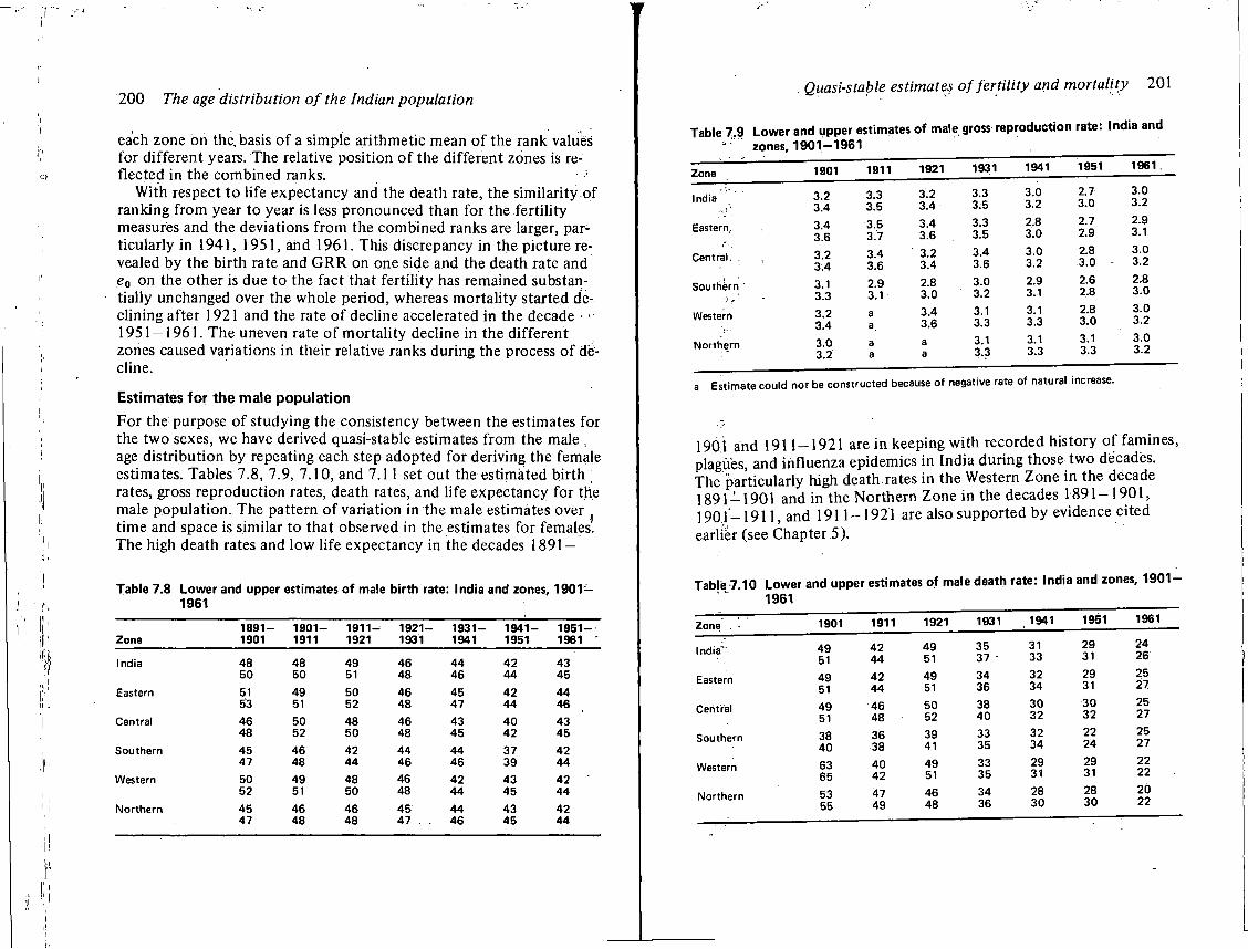
200 The age distribution of the Indian population
each zone on the. basis of a simple arithmetic mean of the rank values for different years. The relative position of the different zones is reflected in the combined ranks.
With respect to life expectancy and the death rate, the similarity,of ranking from year to year is less pronounced than for the fertility measures and the deviations from the combined ranks are larger, particularly in 1941, 1951, and 1961. This discrepancy in the picture revealed by the birth rate and G R R on one side and the death rate and e0 on the other is due to the fact that fertility has remained substantially unchanged over the whole period, whereas mortality started declining after 1921 and the rate of decline accelerated in the decade • • 1951 — 1961. The uneven rate of mortality decline in the different zones caused variations in their relative ranks during the process of decline.
Estimates for the male population
For the purpose of studying the consistency between the estimates for the two sexes, we have derived quasi-stable estimates from the male , age distribution by repeating each step adopted for deriving the female estimates. Tables 7.8, 7.9, 7.10, and 7.11 set out the estimated birth \ rates, gross reproduction rates, death rates, and life expectancy for the male population. The pattern of variation in the male estimates over time and space is similar to that observed in the estimates for females. The high death rates and low life expectancy in the decades 1891 —
Table 7.8 Lower and upper estimates of male birth rate: India and zones, 1901 — 1961
1891- 1901- 1911- 1921- 1931- 1941- 1951-Zone 1901 1911 1921 1931 1941 1951 1961 '
India 48 48 49 46 44 42 43 50 50 51 48 46 44 45
Eastern 51 49 50 46 45 42 44 S3 51 52 48 47 44 46
Central 46 50 48 46 43 40 43 48 52 50 48 45 42 45
Southern 45 46 42 44 44 37 42 47 48 44 46 46 39 44
Western 50 49 48 46 42 43 42 52 51 50 48 44 45 44
Northern 45 46 46 45 44 43 42 47 48 48 47 . . 46 45 44
Quasi-stable estimates of fertility and mortality 201
Table 7.9 Lower and upper estimates of male gross reproduction rate: India and zones, 1901-1961
1901 1911 1921 1931 1941 1951 1961.
India 3.2 3.3 3.2 3.3 3.0 2.7 3.0 India
3.4 3.5 3.4 3.5 3.2 3.0 3.2
Eastern. 3.4 3.6
3.5 3.7
3.4 3.6
3.3 3.5
2.8 3.0
2.7 2.9
2.9 3.1
Central. . , 3.2 3.4
3.4 3.6
3.2 3.4
3.4 3.6
3.0 3.2
2.8 3.0 -
3.0 3.2
Southern 3.1 3.3
2.9 3.1
2.8 3.0
3.0 3.2
2.9 3.1
2.6 2.8
2.8 3.0
Western 3.2 3.4
a a.
3.4 3.6
3.1 3.3
3.1 3.3
2.8 3.0
3.0 3.2
Northern 3.0 3.2
a a
a a
3.1 3.3
3.1 3.3
3.1 3.3
3.0 3.2
Estimate could not be constructed because of negative rate of natural ii
1901 and 1911-1921 are in keeping with recorded history of famines, plagues, and influenza epidemics in India during those two decades.. The particularly high death rates in the Western Zone in the decade 1891-1901 and in the Northern Zone in the decades 1891-1901, 1901 — 1911, and 1911-1921 are also supported by evidence cited earlier (see Chapter 5).
Table 7.10 Lower and upper estimates of male death rate: India and zones, 1901-1961
Zone . 1901 1911 1921 1931 1941 1951 1961
India- 49 51
42 44
49 51
35 37
31 33
29 31
24 26
Eastern 49 51
42 44
49 51
34 36
32 34
29 31
25 27
Central 49 51
46 48
50 52
38 40
30 32
30 32
25 27
Southern 38 40
36 38
39 41
33 35
32 34
22 24
25 27
Western 63 65
40 42
49 51
33 35
29 31
29 31
22 22
Northern 53 55
47 49
46 48
34 36
28 30
28 30
20 22
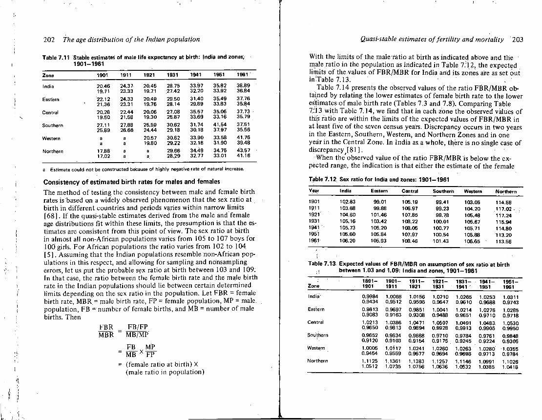
202 The age distribution of the Indian population
Table 7.11 Stable estimates of male life expectancy at birth: India and zones, 1901-1961
Zone 1901 1911 1921 1931 1941 1951 1961
India 20.46 24.37 20.45 28.75 33.97 35.82 38.89 19.71 23.33 19.71 27.42 32.20 33.92 36.84
Eastern 22.12 24.33 20.49 29.50 31.40 35.49 37.76 21.36 23.31 19.76 28.14 29.89 33.83 35.84
Central 20.28 22.44 20.06 27.08 35.57 35.06 37.73 19.50 21.58 19.30 25.87 33.69 33.16 35.79
Southern 27.11 27.88 25.59 30.62 31.74 41.54 37.51 25.89 26.66 24.44 29.18 30.18 37.97 35.56
Western a a 20.57 30.62 33.90 33.58 41.76 a a 19.80 29.22 32.16 31.90 39.48
Northern 17.88 a a 29.66 34.49 34.75 43.57 17.02 a a 28.29 32.77 33.01 41.16
a Estimate could not'be constructed because of highly negative rate of natural increase.
Consistency of estimated birth rates for males and females
The method of testing the consistency between male and female birth rates is based on a widely observed phenomenon that the sex ratio at birth in different countries and periods varies within narrow limits [68]. If the quasi-stable estimates derived from the male and female age distributions fit within these limits, the presumption is that the estimates are consistent from this point of view. The sex ratio at birth in almost all non-African populations varies from 105 to 107 boys for 100 girls. For African populations the ratio varies from 102 to 104 [5]. Assuming that the Indian populations resemble non-African populations in this respect, and allowing for sampling and nonsampling errors, let us put the probable sex ratio at birth between 103 and 109. In that case, the ratio between the female birth rate and the male birth rate in the Indian populations should lie between certain determined limits depending on the sex ratio in the population. Let F B R = female birth rate, MBR = male birth rate, FP = female population, MP = male population, FB - number of female births, and MB = number of male births. Then
FBR FB/FP M B R MB/MP
FB MP MB * FP
= (female ratio at birth) X (male ratio in population)
r
Quasi-stable estimates of fertility and mortality ' 203
With the limits of the male ratio at birth as indicated above and the male ratio in the population as indicated in Table 7.12, the expected limits of the values of F B R / M B R for India and its zones are as set out in Table 7.13. .
Table 7.14 presents the observed values of the ratio F B R / M B R obtained by relating the lower estimates of female birth rate to the lower estimates of male birth rate (Tables 7.3 and 7.8). Comparing Table 7:13 with Table 7.14, we find that in each zone the observed values of this ratio are within the limits of the expected values of F B R / M B R in at least five of the seven census years. Discrepancy occurs in two years in the Eastern, Southern, Western, and Northern Zones and in one year in the Central Zone. In India as a whole, there is no single case of discrepancy [81 ].
When the observed value of the ratio F B R / M B R is below the expected range, the indication is that either the estimate of the female
Table 7.12 Sex ratio for India and zones: 1901-1961
Year India Eastern Central Southern Western Northern
1901 102.83 99.01 105.19 99.41 103.05 114.58 1911 103.68 99.88 106.97 99.23 104.20 117.02 • 1921 104.60 101.46 107.85 99.78 105.48 117,24 1931 105.16 103.42 108.22 100.01 105.67 115.94 1941 105.73 105.20 108.05 100.77 105.71 114.80 1951 105.60 105.84 107.97 100.54 105.88 113.20 1961- 106.20 105.93 108.46 101.43 106.65 113.56
Table 7.13 Expected values of FBR/MBR on assumption of sex ratio at birth between 1.03 and 1.09: India and zones, 1901-1961
1891- 1901- 1911- 1921^ 1931- 1941- 1951-Zone 1901 1911 1921 1931 1941 1951 1961
India' 0.9984 0.9434
1.0066 0.9512
1.0156 0.9596
1.0210 0.9647
1.0265 0.9610
1.0253 0.9688
1.0311 0.9743
Eastern 0.9613 0.9083
0.9697 0.9163
0.9851 0.9308
1.0041 0.9488
1.0214 0.9651
1.0276 0.9710
1.0285 0.9718
Central 1.0213 0;9650
1.0386 0.9813
1.0471 0.9894
1.0507 0.9928
1.0491 0.9913
1.0483: 0.9905
1.0530 0.9950
Southern 0.9652 0.9120
0.9634 0.9103
0.9688 0.9154
0.9710 0.9175 ;
0.9784 0.9245
0.9761 0.9224
0.9848 0.9305
Western 1.0005 0.9454
1.0117 0.9559
1.0241 0.9677
1.0260 0.9694
1.0263 0.9698
1.0280 0.9713
1.0355 0.9784
Northern 1.1125 1.0512
1.1361 1.0735
1.1383 1.0756
1.1257 1.0636
1.1146 1.0532
1.0991 1.0385
1.1026 1.0418
1
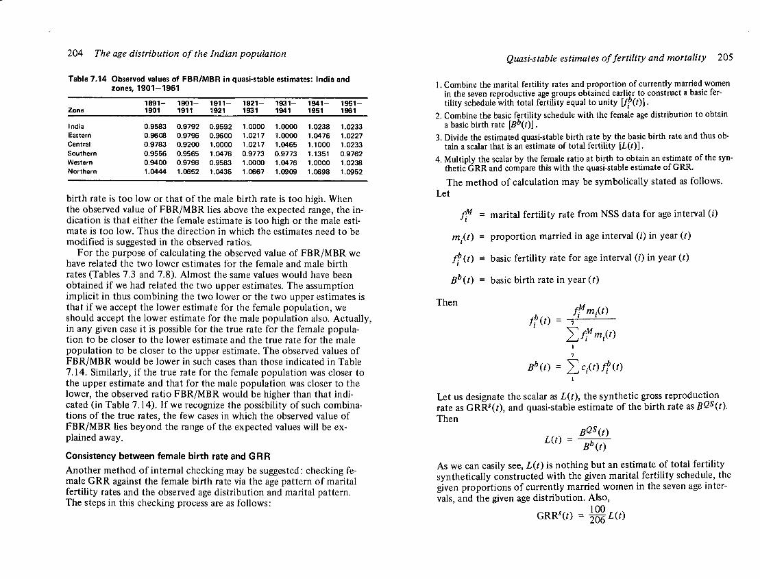
204 The age distribution of the Indian population
Table 7.14 Observed values of FBR/MBR in quasi-stable estimates: India and zones, 1901-1961
1891- 1901- 1911- 1921- 1931- 1941- 1951-Zone 1901 1911 1921 1931 1941 1951 1961
India 0.9583 0.9792 0.9592 1.0000 1.0000 1.0238 1.0233 Eastern 0.9608 0.9796 0.9600 1.0217 1.0000 1.0476 1.0227 Central 0.9783 0.9200 1.0000 1.0217 1.0465 1.1000 1.0233 Southern 0.9556 0.9565 1.0476 0.9773 0.9773 1.1351 0.9762 Western 0.9400 0.9796 0.9583 1.0000 1.0476 1.0000 1.0238 Northern 1.0444 1.0652 1.0435 1.0667 1.0909 1.0698 1.0952
birth rate is too low or that of the male birth rate is too high. When the observed value of F B R / M B R lies above the expected range, the indication is that either the female estimate is too high or the male estimate is too low. Thus the direction in which the estimates need to be modified is suggested in the observed ratios.
For the purpose of calculating the observed value of F B R / M B R we have related the two lower estimates for the female and male birth rates (Tables 7.3 and 7.8). Almost the same values would have been obtained if we had related the two upper estimates. The assumption implicit in thus combining the two lower or the two upper estimates is that i f we accept the lower estimate for the female population, we should accept the lower estimate for the male population also. Actually, in any given case it is possible for the true rate for the female population to be closer to the lower estimate and the true rate for the male population to be closer to the upper estimate. The observed values of F B R / M B R would be lower in such cases than those indicated in Table 7.14. Similarly, i f the true rate for the female population was closer to the upper estimate and that for the male population was closer to the lower, the observed ratio F B R / M B R would be higher than that indicated (in Table 7.14). If we recognize the possibility of such combinations of the true rates, the few cases in which the observed value of F B R / M B R lies beyond the range of the expected values will be explained away.
Consistency between female birth rate and GRR
Another method of internal checking may be suggested: checking female G R R against the female birth rate via the age pattern of marital fertility rates and the observed age distribution and marital pattern. The steps in this checking process are as follows:
Quasi-stable estimates of fertility and mortality 205
1. Combine the marital fertility rates and proportion of currently married women in the seven reproductive age groups obtained earlier to construct a basic fertility schedule with total fertility equal to unity \ f f ( t ) ] .
2. Combine the basic fertility schedule with the female age distribution to obtain a basic birth rate [Bb(t)].
3. Divide the estimated quasi-stable birth rate by the basic birth rate and thus obtain a scalar that is an estimate of total fertility [L(01 •
4. Multiply the scalar by the female ratio at birth to obtain an estimate of the synthetic GRR and compare this with the quasi-stable estimate of GRR.
The method of calculation may be symbolically stated as follows. Let
f f = marital fertility rate from NSS data for age interval (0
m f t ) = proportion married in age interval (/') in year (f)
fP(t) = basic fertility rate for age interval (/) in year (t)
Bb(t) = basic birth rate in year (t)
Then f f m . ( t )
f H t )
I 7
BbU) = J > . ( 0 / ? ( 0
Let us designate the scalar as L(t), the synthetic gross reproduction rate as G R R ^ f ) , and quasi-stable estimate of the birth rate as B<2s(t). Then
m = w
As we can easily see, L(t) is nothing but an estimate of total fertility synthetically constructed with the given marital fertility schedule, the given proportions of currently married women in the seven age intervals, and the given age distribution. Also,
G R R ' ( f ) = ^ W )
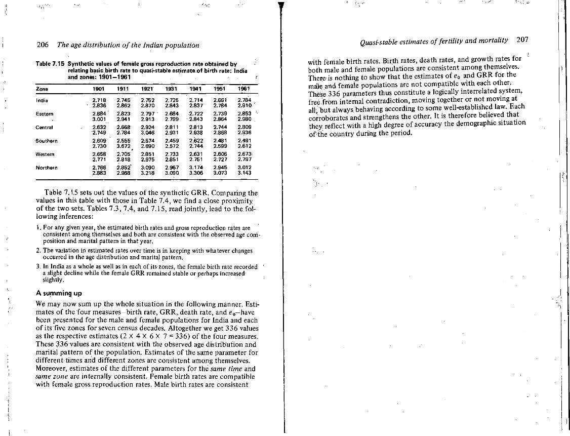
206 The age distribution of the Indian population
Table 7.15 Synthetic values of female gross reproduction rate obtained by relating basic birth rate to quasi-stable estimate of birth rate: India and zones: 1901-1961
Zone 1901 1911 1921 1931 1941 1951 1961
India 2.718 2.745 2.752 2.725 2.714 2.661 2.784 2.836 2.862 2.870 2.843 2.837 2.784 2.910
Eastern 2.884 2.823 2.797 2.684 2.722 2.739 2.853 :
3.001 2.941 2.913 2:799 2.843 2.864 2.980
Central 2.632 2.668 2.924 2.811 2.813 2.744 2.809 2.749 2.784 3.046 2.931 2.938 2.868 2.936
Southern 2.609 2.555 2.574 2.459 2.622 2.481 2.491 2.730 3.672 ^ 2.690 2.572 2.744 2.599 2.612
Western 2.658 2.705 2.851 2.733 2.631 2.606 2.673 2.771 2.818 2.975 2.851 2.751 2.727 2.797
Northern 2.766 2.852' 3.090 2.967 3.174 2.945 3.012 2:883 2.968 3.218 3.090 3.306 3.073 3.143
Table 7.1,5 sets out the values of the synthetic G R R . Comparing the values in this table with those in Table 7.4, we find a close proximity of the two sets. Tables 7.3, 7.4, and 7.15, read jointly, lead to the following inferences: 1. For any given year, the estimated birth rates and gross reproduction rates are
consistent among themselves and both are consistent with the observed age composition and marital pattern in that year.
2. The variation in estimated rates over time is in keeping with whatever changes occurred in the age distribution and marital pattern.
3. In India as a whole as well as in each of its zones, the female birth rate recorded a slight decline while the female GRR remained stable or perhaps increased slightly.
A summing up
We may now sum up the whole situation in the following manner. Estimates of the four measures-birth rate, GRR,, death rate, and e 0-have been presented for the male and female populations for India and each of its five zones for seven census decades. Altogether we get 336 values as the respective estimates (2 X 4 X 6 X 7 = 336) of the four measures. These 336 values are consistent with the observed age distribution and marital pattern of the population. Estimates of the same parameter for different times and different zones are consistent among themselves. Moreover, estimates of the different parameters for the same time and same zone are internally consistent. Female birth rates are compatible with female gross reproduction rates. Male birth rates are consistent
Quasi-stable estimates of fertility and mortality 207
with female birth rates. Birth rates, death rates, and growth rates for both male and female populations are consistent among themselves. There is nothing to show that the estimates of e0 and G R R for the male and female populations are not compatible with each other. These 336 parameters thus constitute a logically interrelated system, free from internal contradiction, moving together or not moving at all, but always behaving according to some well-established law. Each corroborates and strengthens the other. It is therefore believed that they, reflect with a high degree of accuracy the demographic situation of the country during the period.
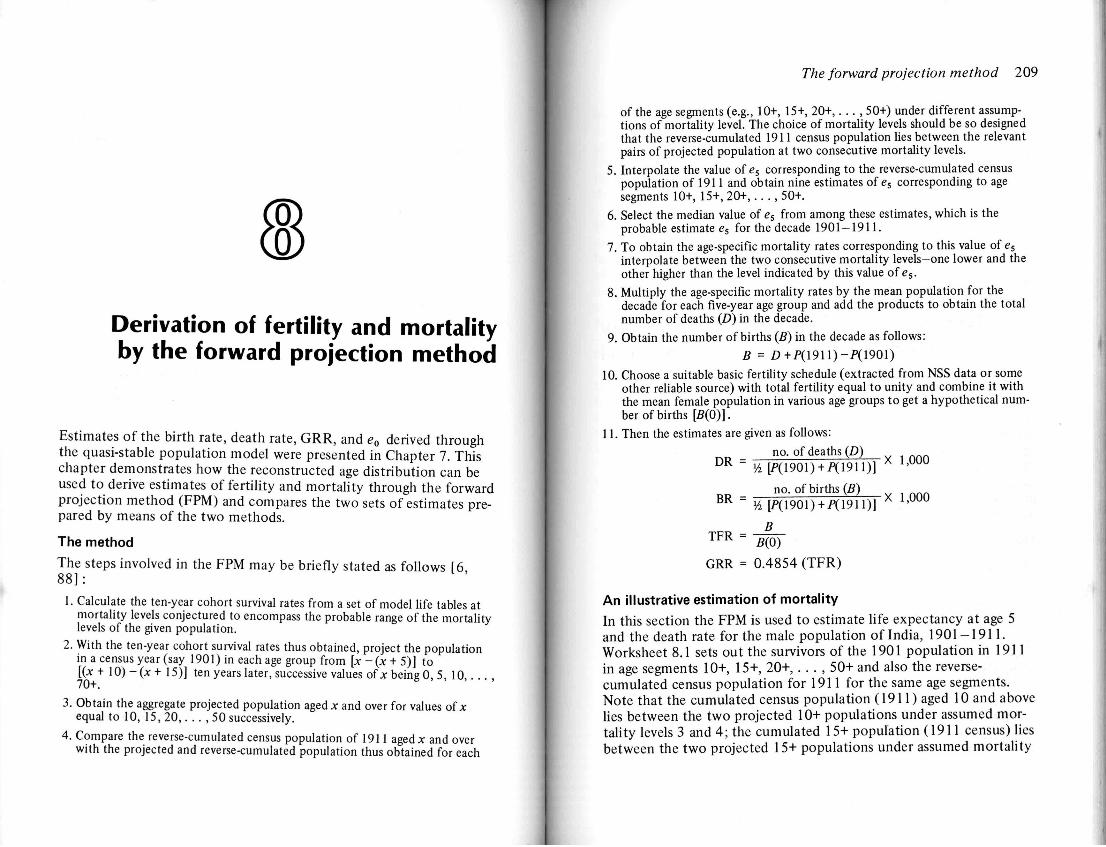
Derivation of fertility and mortality by the forward projection method
Estimates of the birth rate, death rate, G R R , and e0 derived through the quasi-stable population model were presented in Chapter 7. This chapter demonstrates how the reconstructed age distribution can be used to derive estimates of fertility and mortality through the forward projection method (FPM) and compares the two sets of estimates prepared by means of the two methods.
The method
The steps involved in the FPM may be briefly stated as follows \6 88] :
1. Calculate the ten-year cohort survival rates from a set of model life tables at mortality levels conjectured to encompass the probable range of the mortality levels of the given population.
2. With the ten-year cohort survival rates thus obtained, project the population in a census year (say 1901) in each age group from [x- (x + 5)] to [(x + 1 0 ) - ( x + 15)] ten years later, successive values of x being 0, 5, 1 0 , . . . , 70+.
3. Obtain the aggregate projected population aged x and over for values o f* equal to 10, 15, 20,. . . , 50 successively.
4. Compare the reverse-cumulated census population of 1911 aged* and over with the projected and reverse-cumulated population thus obtained for each
The forward projection method 209
of the age segments (e.g., 10+, 15+, 20+,. . . , 50+) under different assumptions of mortality level. The choice of mortality levels should be so designed that the reverse-cumulated 1911 census population lies between the relevant pairs of projected population at two consecutive mortality levels.
5. Interpolate the value of es corresponding to the reverse-cumulated census population of 1911 and obtain nine estimates of es corresponding to age segments 10+, 15+, 20+,.. . , 50+.
6. Select the median value of es from among these estimates, which is the probable estimate e s for the decade 1901-1911.
7. To obtain the age-specific mortality rates corresponding to this value of es
interpolate between the two consecutive mortality levels-one lower and the other higher than the level indicated by this value of e s.
8. Multiply the age-specific mortality rates by the mean population for the decade for each five-year age group and add the products to obtain the total number of deaths (D) in the decade.
9. Obtain the number of births (B) in the decade as follows: B = /J+P(1911)-/ >(1901)
10. Choose a suitable basic fertility schedule (extracted from NSS data or some other reliable source) with total fertility equal to unity and combine it with the mean female population in various age groups to get a hypothetical number of births [B(0)].
11. Then the estimates are given as follows: no. of deaths (D)
D R ~ M [P(\9Q\) + P(\9\\)] X 1 , U U U
no. of births (B) B R = V4 [P(1901) + JRC1911)] 1 , 0 0 0
TFR = B
B(0)
GRR = 0.4854 (TFR)
An illustrative estimation of mortality
In this section the FPM is used to estimate life expectancy at age 5 and the death rate for the male population of India, 1901-1911. Worksheet 8.1 sets out the survivors of the 1901 population in 1911 in age segments 10+, 15+, 20+, . . . , 50+ and also the reverse-cumulated census population for 1911 for the same age segments. Note that the cumulated census population (1911) aged 10 and above lies between the two projected 10+ populations under assumed mortality levels 3 and 4; the cumulated 15+ population (1911 census) lies between the two projected 15+ populations under assumed mortality
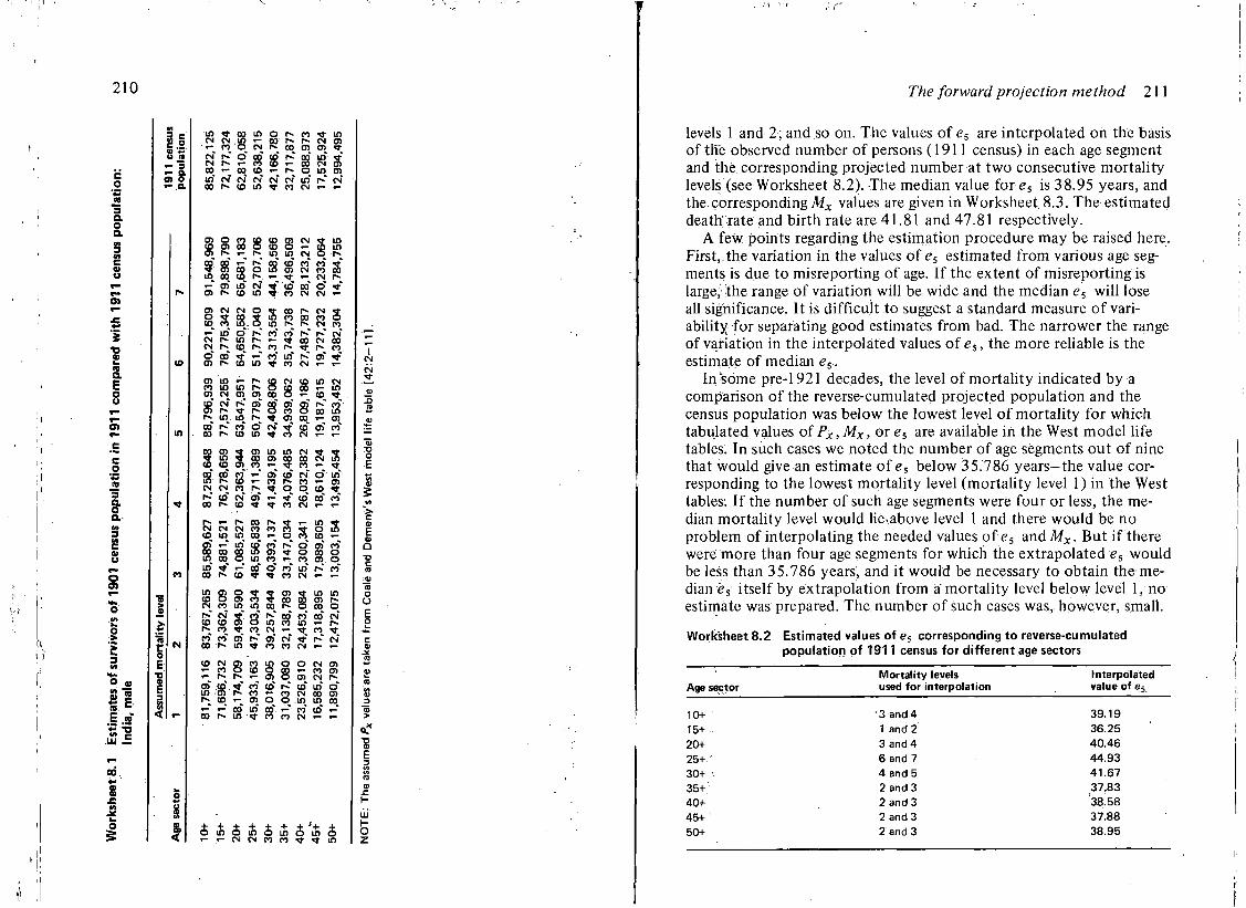
210
! § |
* ~ 3 i r- a. at o t- a
in *f 03 ifl o s w CN in «- co ro * in r- CN cn r n o ni N to oi oi »
in *" . . w • w CN cri
co cq to_ <- r- o in 0) in" CN CM* CM" CN" CN" in" r»* CN" o o r - c o i n ' j n c N T - ^
CM r« o co to K CN r-~ t - co co
c n o c o c p c o g > C N «
o > r ~ i - r ~ m i n c M O o> r~ r»_ in 58 99 £ <S co* co" co* ^ c n c o o i n o i C M c o in co «) p> — «- CM «-" o>" in" CM" «•" co* co" o" o i r - c o m v c o c M C M cn CM o -3-u> to <-* in" CM r-CM r* o* co" 0) r-
CM o » co r- CM 9 S j in co co co o o in r~ r~ CM co o r-~ in r -co r» 5 in
co co
co co" iri
1-s" CO CM
CO CM CO • l«. -of
CO T f "
C o E •o o E 3
o > i n » - r < c p c M c o i n c M r o i n i n r - « o c p c 0 " - m CO CN 0> O) CD O «- CD * co" CN" r»" cn" go" of of S " co" c n r ~ * r - » O c o o o o m r» in in r» oi co cn oo" r»" co" o" CM" co" of co" c o r - c o i n T t c o c N t - t -
c o o i ' J O i i n i n t N ^ * 4 in 4 m a op oo CN I A
CD 03 O l CO »-_ 9 CO « -
S* oo" co" <-" of co" CM" O " in r ^ c D " - f o r ~ c o T - c n '"i ^ °, °. 1 0 ^
r-" co" CM" of «-" ^" co" oo" co" c o r - v C D ^ r ^ c o C N i - t -
CM CM to
r» eg r- * t -CM co co co * in in oo
«-" in" co" co"
in . o CO CD
in gi o « « ID • oi n 4 CM co in in co
m m O)
S 8 8 « 3 G > S 3 ! 3 £ ci ^ n CN ^ co" co" of r»" of CN* ^ " co in * co co CM
CN*
<D CM gj co T - co o CD «- c~ r- «- cn
co" CD*
o o 8 o>
CN cn CO O) CN r»
r»" co" in" o" co CM oo cn co *-v oi o o AO in co
<-" *-" oo* in* oo* <-" co* co* «-* o o r ~ i n « * c o c o c N > - T -
C D i n c S i n S i n S i n i > - t - c M C N c o c o ^ - ^ r i n
The forward projection method 211
levels. 1 and 2 ; and so on. The values of e5 are interpolated on the basis of the observed number of persons (1911 census) in each age segment and the corresponding projected number at two consecutive mortality levels (see Worksheet 8.2). The median value for es is 38.95 years, and the.corresponding^ values are given in Worksheet 8.3. The estimated death' rate and birth rate are 41.81 and 47.81 respectively.
A few points regarding the estimation procedure may be raised here. First,.the variation in the values of e5 estimated from various age segments is due to misreporting of age. If the extent of misreporting is large," the range of variation will be wide and the median es will lose all significance. It is difficult to suggest a standard measure of variability for separating good estimates from bad. The narrower the range of variation in the interpolated values of es, the more reliable is the estimate of median es .
In "some pre-1921 decades, the level of mortality indicated by a comparison of the reverse-cumulated projected population and the census population was below the lowest level of mortality for which tabulated values of PX,MX, or e5 are available in the West model life tables. In such cases we noted the number of age segments out of nine that would give an estimate of e5 below 35.786 years-the value corresponding to the lowest mortality level (mortality level 1) in the West tables. If the number of such age segments were four or less, the median mortality level would lie.above level 1 and there would be no problem of interpolating the needed values of es ahd-M*. But i f there were more than four age segments for which the extrapolated es would be less than 35.786 years, and it would be necessary to obtain the median es' itself by extrapolation from a mortality level below level 1, no estimate was prepared. The number of such cases was, however, small.
Worksheet 8.2 Estimated values of e 5 corresponding to reverse-cumulated population of 1911 census for different age sectors
Age sector Mortality levels used for interpolation
Interpolated value of e 5
10+ • 3 and 4 39.19 15+ • 1 and 2 36.25 20+ 3 and 4 40.46 25+ 6 and 7 44.93 30+ 4 and 5 41.67 35+; 2 and 3 37.83 40+ 2 and 3 38.58 45+ 2 and 3 37.88 50+ 2 and 3 38.95
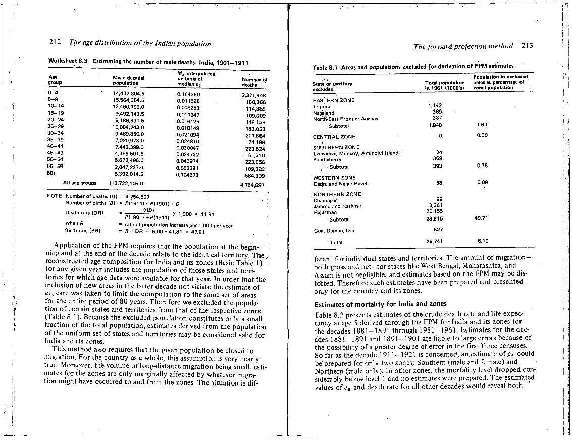
212 The age distribution of the Indian population
Worksheet 8.3 Estimating the number of male deaths: India, 1901-1911
Age group
Mean decadal population
Mx interpolated on basis of median e$
Number of deaths
0-4 14,432,304.5 0.164350 2,371,948 5-9 15,564,354.5 0.011588 180,366 10-14 13,460,199.0 0.008253 114,389 15-19 9,492,143.5 0.011247 109,009 20-24 9,186,890.5 0.016125 148,138 25-29 10,084,743.0 0.018149 183,023 30-34 9,469,850.0 0.021094 201,864 35-39 7,020,973.0 0.024810 174,188 40-44 7,442,399.0 0.030047 223,624 45-49 4,356,501.5 0.034732 151,310 50-54 5,672,496.0 0.043974 223,056 55-59 2,047,237.0 0.053381 109,283 60+ 5,392,014.5 0.104673 564,399
All age groups 113.722,106.0 4,754,597
NOTE: Number of deaths (O) = 4,754,597 , Number of births (fl) = P(1911) - P(1901) + D ]
Death rate (DR) = X 1,000 = 41.81 PI1901) +PI1911)
when R = rate of population increase per 1,000 per year Birth rate (BR) = R + DR = 6.00 + 41.81 = 47.81
Application of the F P M requires that the population at the beginning and at the end of the decade relate to the identical territory. The,, reconstructed age composition for India and its zones (Basic Table 1) for any given year includes the population of those states and territories for which age data were available for that year. In order that the inclusion of new areas in the latter decade not vitiate the estimate of e 5, care was taken to limit the computation to the same set of areas for the entire period of 80 years. Therefore we excluded the population of certain states and territories from that of the respective zones (Table 8.1). Because the excluded population constitutes only a small fraction of the total population, estimates derived from the population of the uniform set of states and territories may be considered valid for India and its zones.
This method also requires that the given population be closed to migration. For the country as a whole, this assumption is very nearly true. Moreover, the volume of long-distance migration being small, estimates for the zones are only marginally affected by whatever migration might have occurred to and from the zones. The situation is dif-
The forward projection method "213
Table 8.1 Areas and populations excluded for derivation of FPM estimates
Population in excluded State or territory Total population areas as percentage of excluded in 1961 (1000'sl tonal population
. 1 • EASTERN ZONE Tripura Nagaland NortlvEast Frontier Agency
Subtotal
1,142 369 337
1,848 1.63
CENTRAL ZONE 0 0.00
SOUTHERN ZONE Laccadive, Minicoy, Amindivi Islands Pondicherry
.Subtotal
24 369 393 0.36
WESTERN ZONE Dadra and Nagar Haveli 58 0.09
NORTHERN ZONE Chandigar Jammu and Kashmir Rajasthan
Subtotal
99 3,561
20,155 23,815 49.71
Goa, Daman, Diu 627
Total 26,741 6.10
fefent for individual states and territories. The amount of migration-both gross and net-for states like West Bengal, Maharashtra, and Assam is not negligible, and estimates based on the FPM may be distorted. Therefore such estimates have been prepared and presented only for the country and its zones.
Estimates of mortality for India and zones Table 8.2 presents estimates of the crude death rate and life expectancy at age 5 derived through the F P M for India and Its zones for the decades 1881-1891 through 1951-1961. Estimates for the decades 1881-1891 and 1891 — 1901 are liable to large errors because of the possibility of a greater degree of error in the first three censuses. So far as the decade 1911 — 1921 is concerned, an estimate of _es could be prepared for only two zones: Southern (male and female) and Northern (male only). In other zones, the mortality level dropped considerably below level 1 and no estimates were prepared. The estimated values of e s and death rate for all other decades would reveal both
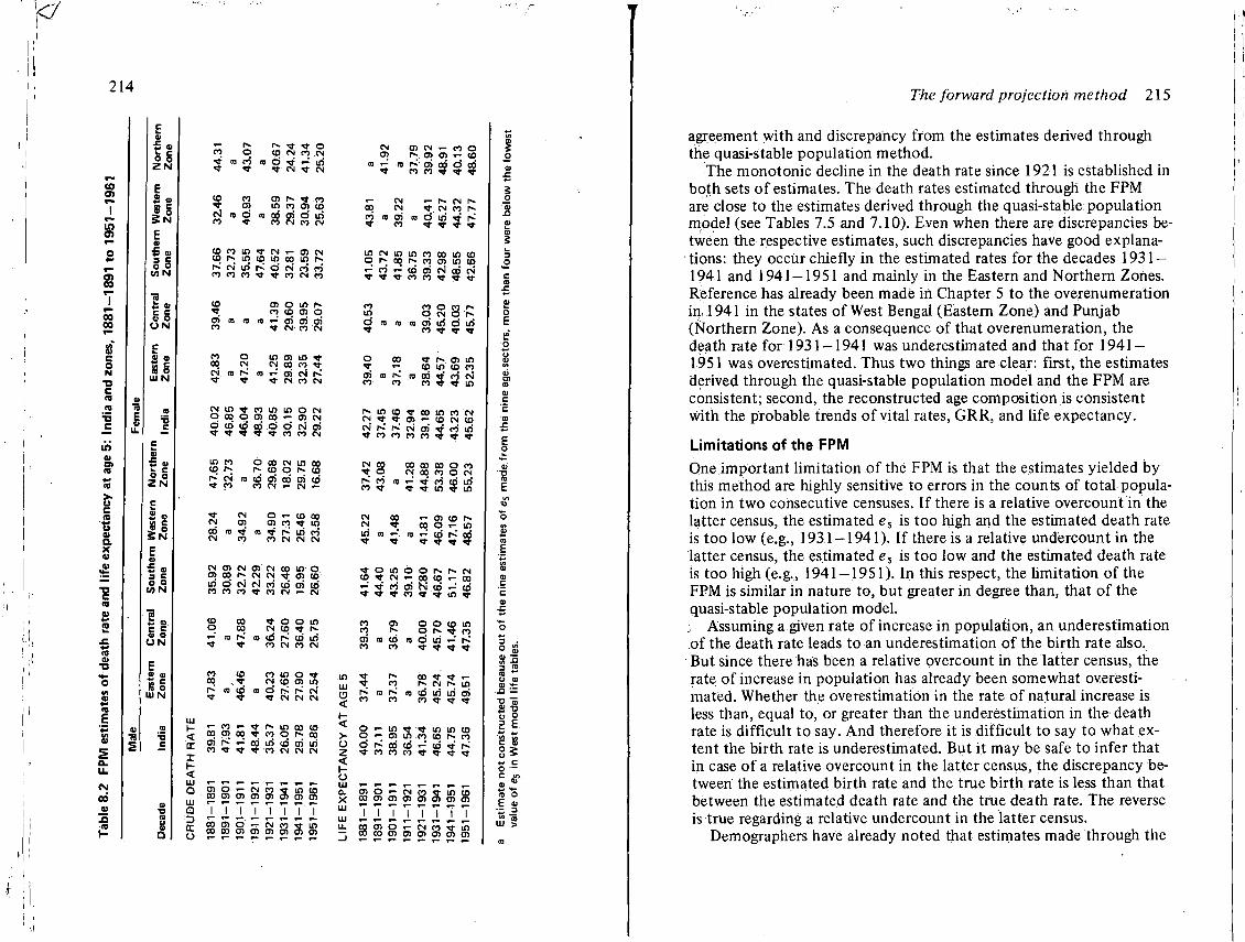
14
O o Z N
€ CO
s § in N
1 c £ « o
U N
£ S 2 8 o UJ N
u £ at o o
Z N
5 N
E 0}
£ CO
g§ C/5N
£ CO c c « o
U N
2 2 18 o
UI N
U J
< tr
CO •3-CN ro
ro O
ro co
1 ' J - TJ- o CO CN CO CM d * i-' iri
CN ^ CN
co O) ro TJ- .co cn i n co oj co o n co oi d i n * CO CN CO CN
I B t O i n V N ^ O l C N i o r > i n i o m c o i n N ro' CN iri r- ' o o i co' co r o c o c o > * ^ r r o c N c o
co
05
CO CN.
05 O 1/5 |o co co 05 q
to 05 05 05 <t CM CO CN
o in cn in *t CN CM CO CO Tiro ra oi c i h> ^ CM ro CN
C N i n ^ c o i o i n o c N p c q o o ) a 3 « - 0 ) C N d c o ' c r i c o d d c N ' o ) ' " a f ^ ^ ^ ^ c o c o c N
in co o co CN in co co ro ro co o ro co r * « ' c N ( o c d c j ) c d o > c o * CO CO CN v - CM «—
CN CM O T - CO 00 05 05 .CO ^" i n ^•' to ro' i n co CO CO CN CM CM
C N 0 5 C N 0 5 C M O O i n O Ci 00 Co CN CN «d" 05 CO' i r i d c N C N c o ' c o ' o i c o C O C O r O V C O C N > - C M
co o
00 « O O ID oo CN co ^ - r<. ro ro co* ro co i r i
CO CN CO CN
co 1;
S co cd 1- • *
oo co i n o ^ CN co o) i n d ro ro CM' ^ - CN CM CM
« - t o ^ ^ (o i f l CO (O cp 05 cq ^ co o ro co o i N ' ^ c d i r f c n ' o i i f i CO * »t ^ CO CM CN CM
< ^ C 0 O ) O 5 O ) O 5 O 5 O 5 O 5
Q T T T T T T T T 2 o o 0 5 , o » - C M c o ^ r t r ) j*j n c o o i o i o i c D o i o i
CN O)
tO
05 CN t— CO O ro 05 o) «- co ro* ' oo oo d oo n n rr ^ rt
>- CM 00 CM CO to 05 * CO
«- ro CN ro *r CN co ro d in « r^ »r * 3- *r
i n c N i n i n c o c o m c o q r o o p r o c o c j 5 i n c D
co «-' co oi CM od CN
co in d
o
05 CO
co o co ro O CM o ro
to cri i r i d i r i n » » *
oo ^ ro c) in >- co in co co ro to oo ri CN co co Tt m
r- in co v co m co CM CM * ^ o> <- co CM co C N r o f o ' c M o S ^ j / c o ' t r i ^ • c o c o c o c o ^ r ^ T f
CN CO O
ro' co co i -
CO 00 CO O CO CM cq co o CN «-' ^-' ro' co i r i
i n ^ i n
CN iri
00 .«- 05 co ro co O in r-' CO ro 00 •tf V <» *
^ • o i n o o r o r o c N C O T f C N * - C 0 C 0 * - C 0 »- * ' CO 05 N CD •-' CO » « » n » ^ i n »
05 ro
co co 05 (0 CO CO CO
o o co in o ro to
i d iri <-' ro * *
ro" CO
oo Tr i t « ~ ro CM ro m co i r i i n 05 n * <f *
in m
< h-<
O T - m t ^ m m c o > q ^ oo in co co ro co U d r^ to (d to' ^ ' io Z < r n e o o * M , « < r < r-O U J <-r-. i - t - r - r - i - , -
cu 0 ) 0 * - c N 0 9 i n c o X 0 0 0 5 0 5 0 ) 0 5 0 ) 0 5 0 5
tu I n I i i M U . C Q O O . t - C N C O ^ - i n — C 0 C 0 O 5 O 5 O 5 0 5 C 5 5 C 3 5
The forward projection method 215
agreement with and discrepancy from the estimates derived through the quasi-stable population method.
The monotonic decline in the death rate since 1921 is established in both sets of estimates. The death rates estimated through the FPM are close to the estimates derived through the quasi-stable population model (see Tables 7.5 and 7.10). Even when there are discrepancies between the respective estimates, such discrepancies have good explanations: they occur chiefly in the estimated rates for the decades .1931 — 1941 and 1941-1951 and mainly in the Eastern and Northern Zones. Reference has already been made in Chapter 5 to the overenumeration i n 1941 in the states of West Bengal (Eastern Zone) and Punjab (Northern Zone). As a consequence of that overenumeration, the death rate for 1931-1941 was underestimated and that for 1941-1951 was overestimated. Thus two things are clear: first, the estimates derived through the quasi-stable population model and the F P M are consistent; second, the reconstructed age composition is consistent with the probable trends of vital rates, G R R , and life expectancy.
Limitations of the FPM
One important limitation of the FPM is that the estimates yielded by this method are highly sensitive to errors in the counts of total population in two consecutive censuses. If there is a relative overcount in the latter census, the estimated es is too high and the estimated death rate is too low (e.g., 1931 — 1941). If there is a relative undercount in the latter census, the estimated e5 is too low and the estimated death rate is too high (e.g., 1941 — 1951). In this respect, the limitation of the FPM is similar in nature to, but greater in degree than, that of the quasi-stable population model. ;. Assuming a given rate of increase in population, an underestimation of the death rate leads to an underestimation of the birth rate also. But since there has been a relative overcount in the latter census, the rate of increase in population has already been somewhat overestimated. Whether the overestimation in the rate of natural increase is less than, equal to, or greater than the underestimation in the death rate is difficult to say. And therefore it is difficult to say to what extent the birth rate is underestimated. But it may be safe to infer that in case of a relative overcount in the latter census, the discrepancy between the estimated birth rate and the true birth rate is less than that between the estimated death rate and the true death rate. The reverse is true regarding a relative undercount in the latter census.
Demographers have already noted that estimates made through the
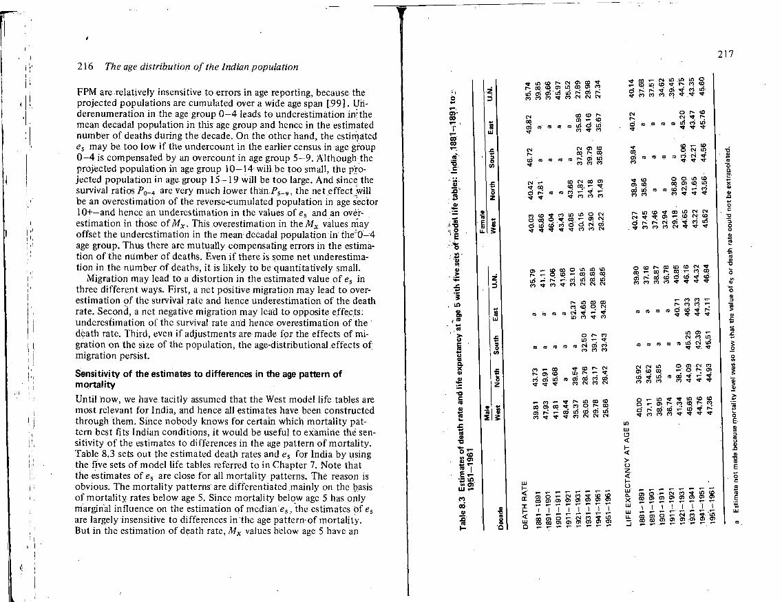
216 The age distribution of the Indian population
F P M are relatively insensitive to errors in age reporting, because the projected populations are cumulated over a wide age span [ 9 9 ] . Underenumeration in the age group 0 - 4 leads to underestimation in;the mean decadal populat ion i n this age group and hence in the estimated number o f deaths during the decade. O n the other hand, the estimated es may be too low i f the undercount in the earlier census in age group 0 - 4 is compensated by an overcount in age group 5—9. Al though the projected populat ion in age group 10—14 wi l l be too small, the projected populat ion in age group 15—19 wi l l be too large. A n d since the survival ratios / ,
0 - 4 are very much lower than P5-9, the net effect w i l l be an overestimation of the reverse-cumulated population in age sector 10+—and hence an underestimation in the values of es and an over-estimation in those o f M x . This overestimation in theMx values may offset the underestimation in the mean decadal population in the"0-4 age group. Thus there are mutual ly compensating errors in the estimat ion o f the number o f deaths. Even i f there is some net underestimation in the number o f deaths, it is l ikely to be quantitatively small.
Migrat ion may lead to a distortion in the estimated value o f es in three different ways. First , a net positive migration may lead to over-estimation of the survival rate and hence underestimation o f the death rate. Second, a net negative migration may lead to opposite effects: underestimation of the survival rate and hence overestimation o f the ' death rate. Th i rd , even i f adjustments are made for the effects of migration on the size of the populat ion, the age-distributional effects o f migration persist.
Sensitivity of the estimates to differences in the age pattern of mortality
U n t i l now, we have tacitly assumed that the West model l ife tables are most relevant for India, and hence all estimates have been constructed through them. Since nobody knows for certain which mortal i ty pattern best fits Indian conditions, it would be useful to examine the sensitivity o f the estimates to differences in the age pattern o f mortal i ty . Table 8.3 sets out the estimated death rates and es for India by using the five sets o f model l i fe tables referred to in Chapter 7. Note that the estimates o f e5 are close for all mortal i ty patterns. The reason is obvious. The mortal i ty patterns are differentiated mainly on the basis of mortal i ty rates below age 5. Since mortal i ty below age 5 has only marginal influence on the estimation of median es, the estimates of es
are largely insensitive to differences in the age pattern'of mortal i ty. But in the estimation o f death rate, Mx values below age 5 have an
217
"3, S I S
CO
S en
u t n
in CT) U l i -M CO
es
^ Ul ( O S N fj J" * f. co O cs I D co oi « iri oi oi iri in' r*- ci rj-m co co <t co CN CN C N
C N oo oi
co co r-cn co
co iri d iri ci »r co
co co CO co
CN CO CO
co r-; oo r-" cri iri co co co
CM * -•4 cp
CO CN CO O ) co op, ^
<o co «- n CO CO CO
c o c o t c o i n i n O C N ci co o •* oo en CM d I D <o co d d C N eg
ffli-IOCOOIO^IO r - , - o c o « - c p c p c q irf r» <-' co iri od iri CO^CO'tfCOCNCNCM
r- 10 oo oo co CD oI CN
n oi * '-' * I D CO * CO
o r> o in 1; CO CN oi CO
CO CO CO
CO r - co f co r- C N o co in r» *
co ci iri cooiodcocp 3 q: co CM co CM
i - c o ' - f ' ^ ' o c o c o c o o i c o f o o ^ a ) ci K cn iri co cn in Co !*V"tCOCMCMCM
LLI
5 5 o - S 2 S IS 2
° - 0 5 O > ( ! ) O 1 0 , * J 2
U J g § Q O f J 1 0 ) « 0 )
rf-co«-CNininino J c o i q c D ^ ^ c o i q d r - I ^ ^ ' o i ^ n S ^ co ro co co «t , f *
CN r~ d
oo oi
(O CO CO (o
O l» CD CM >» r-iri co in f
CD a> co co in co co
CD « - CD o C M in 10 co CM «t » f
o o in co co o> co in (0 CO CN ^ CO
CO t f *
r~ in co <r co I D CM CM c M * * c n « - « p c M c o d K r - CM oi co in I J c o c o c o c N f l - ' r
o CD co «- op oi co co co
co in co C N ^ r~ oo co op
co co o co CD n <f f "f f
co co co co
(0 CD (0 CD
«- CO CO »r-r-» co co d co i"-»t «t
in a> r-C N co in
co iri C M iri
CN CN in o 2 CN ro oo co oo o r-_ cn co <t iri ra cri 3 H S co co co ri ^ <f »
o « - i n « f f i o c o c D o *- oo r-# co <p r-_ co d r" co id «••. «t co co co *r * r->
in UJ
< I-< > o z < r-SI oi 5 - C N co s jg 56 ^ 0)0)0)010)0)0)0) L U * i " T 7 T 7 7 T 7 iH co 5 5 ^ 5 n s ss = ScTocncncncncfio)
o a
2 o
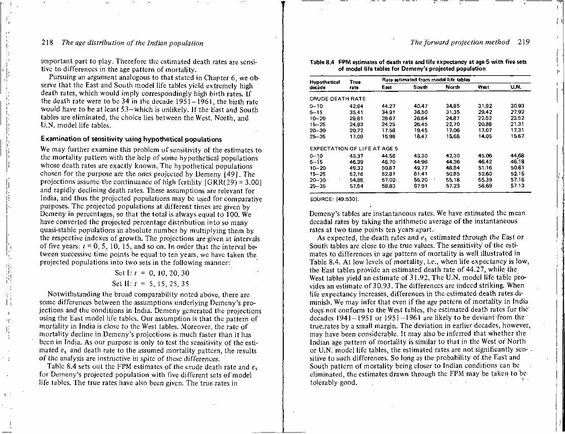
218 The age distribution of the Indian population
important part to play. Therefore the estimated death rates are sensitive to differences in the age pattern of mortal i ty.
Pursuing an argument analogous to that stated in Chapter 6, we observe that the East and South model l ife tables yield extremely high death rates, which would imply correspondingly high bir th rates. If the death rate were to be 34 in the decade 1 9 5 1 - 1 9 6 1 , the bir th rate would have to be at least 5 3 - w h i c h is unl ikely. If the East and South tables are eliminated, the choice lies between the West, Nor th , and U . N . model l i fe tables.
Examination of sensitivity using hypothetical populations
We may further examine this problem o f sensitivity of the estimates to the mortal i ty pattern wi th the help o f some hypothetical populations whose death rates are exactly known. The hypothetical populations chosen for the purpose are the ones projected by Demeny [ 4 9 ] . The projections assume the continuance o f high fert i l i ty [ G R R ( 2 9 ) = 3.00] and rapidly declining death rates. These assumptions are relevant for India, and thus the projected populations may be used for comparative purposes. The projected populations at different times are given by Demeny in percentages, so that the total is always equal to 100. We have converted the projected percentage distribution into so many quasi-stable populations in absolute number by mul t ip ly ing them by the respective indexes o f growth. The projections are given at intervals o f five years: t = 0, 5, 10, 15, and so on. In order that the interval be-tween successive time points be equal to ten years, we have taken the projected populations in to two sets in the fo l lowing manner:
Set I: t = 0, 10, 20, 30
Set II: t = 5, 1 5 , 2 5 , 3 5
Notwithstanding the broad comparabili ty noted above, there are some differences between the assumptions underlying Demeny's projections and the conditions in India. Demeny generated the projections using the East model l ife tables. Our assumption is that the pattern of mortal i ty in India is close to the West tables. Moreover, the rate o f mortal i ty decline in Demeny's projections is much faster than it has been in India. As our purpose is only to test the sensitivity o f the estimated e 5 and death rate to the assumed mortali ty pattern, the results o f the analysis are instructive in spite o f these differences.
Table 8.4 sets out the F P M estimates o f the crude death rate and es
for Demeny's projected population with five different sets o f model l ife tables. The true rates have also been given. The true rates in
The forward projection method 219
Table 8.4 FPM estimates of death rate and life expectancy at age 5 with five sets of model life tables for Demeny's projected population
Hypothetical True Rate estimated from model life tables decade rate East South North West U.N.
CRUDE DEATH RATE 0-10 42.64 44.27 40.47 34.85 31.92 30.93 5-15 35.41 34.91 36.50 31.35 29.42 27.92 10-20 29.81 28.67 28.64 24.87 22.52 23.52 15-25 24.93 24.25 26.45 22.70 20.88 21.31 20-30 20.72 17.58 19.45 17.06 17.07 17.31 25-35 17.09 15.96 18.47 15.68 14.05 15.67
EXPECTATION OF LIFE A T AGE 5 0-1.0 43.37 44.56 43.30 42.30 45.06 44.68 5-15 46.39 46.70 44.96 44.36 46.42 46:18 10-20 49.32 50.87 49.77 48.84 51.16 50.61 15-25 52.16 52.81 61.41 50.85 52.60 52.15 20-30 54.88 57.02 . 56.20 55.18 55.39 57.16 25-35 57.54 58.83 67.91 57.23 58.69 57.13
SOURCE: [49:530].
Demeny's tables are instantaneous rates. We have estimated the mean decadal rates by taking the arithmetic average o f the instantaneous rates at two time points ten years apart.
As expected, the death rates and es estimated through the East or South tables are close to the true values. The sensitivity o f the estimates to differences in age pattern of mortal i ty is well illustrated in Table 8.4. A t low levels of mortal i ty, i.e., when l ife expectancy is low, the East tables provide an estimated death rate o f 44.27, while the West tables yield an estimate of 31.92. The U . N . model l i fe table provides an estimate o f 30.93. The differences are indeed striking. When life expectancy increases, differences in the estimated death rates-diminish. We may infer that even i f the age pattern o f mortal i ty in India does, not Conform to the West tables, the estimated death rates for the' decades 1941-1951 or 1951-1961 are l ikely to be deviant f r o m the true.rates by a small margin. The deviation in earlier decades, however, may have been considerable. It may also be inferred that whether the Indian age pattern o f mortal i ty is similar to that in the West of Nor th or U . N . model l i fe tables, the estimated rates are not significantly sensitive to such differences. So long as the probabil i ty of the East and South pattern o f mortal i ty being closer to Indian conditions can be eliminated, the estimates drawn through the F P M may be taken to be tolerably good. . '
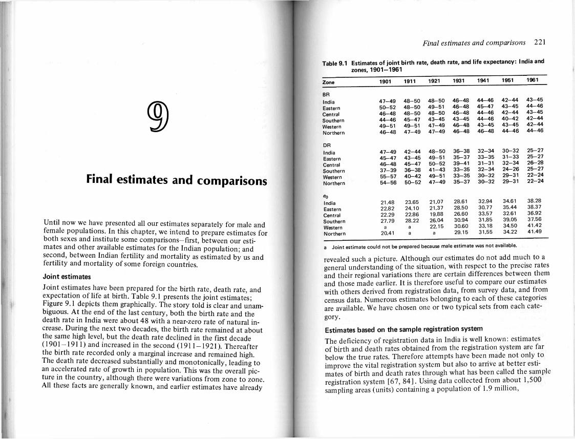
Final estimates and comparisons
U n t i l now we have presented all our estimates separately for male and female populations. In this chapter, we intend to prepare estimates for both sexes and institute some comparisons—first, between our estimates and other available estimates for the Indian populat ion; and second, between Indian ferti l i ty and mortali ty as estimated by us and fert i l i ty and mortali ty o f some foreign countries.
Joint estimates
Joint estimates have been prepared for the bir th rate, death rate, and expectation o f l ife at bir th. Table 9.1 presents the joint estimates; Figure 9.1 depicts them graphically. The story told is clear and unambiguous. A t the end o f the last century, both the birth rate and the death rate in India were about 48 with a near-zero rate of natural increase. Dur ing the next two decades, the b i r th rate remained at about the same high level, but the death rate declined in the first decade (1901 - 1 9 1 1 ) and increased in the second (1911-1921) . Thereafter the bir th rate recorded only a marginal increase and remained high. The death rate decreased substantially and monotonical ly , leading to an accelerated rate of growth in population. This was the overall picture in the country, although there were variations f rom zone to zone. A l l these facts are generally known, and earlier estimates have already
Final estimates and comparisons 221
Table 9.1 Estimates of joint birth rate, death rate, and life expectancy: India and zones, 1901-1961
Zone 1901 1911 1921 1931 1941 1951 1961
BR India 4 7 - 4 9 4 8 - 5 0 4 8 - 5 0 4 6 - 4 8 4 4 - 4 6 4 2 - 4 4 4 3 - 4 5
Eastern 5 0 - 5 2 4 8 - 5 0 4 9 - 5 1 4 6 - 4 8 4 5 - 4 7 4 3 - 4 5 4 4 - 4 6
Central 4 6 - 4 8 4 8 - 5 0 4 8 - 5 0 4 6 - 4 8 4 4 - 4 6 4 2 - 4 4 4 3 - 4 5 Southern 4 4 - 4 6 4 5 - 4 7 4 3 - 4 5 4 3 - 4 5 4 4 - 4 6 4 0 - 4 2 4 2 - 4 4 Western 4 9 - 5 1 4 9 - 5 1 4 7 - 4 9 4 6 - 4 8 4 3 - 4 5 4 3 - 4 5 4 2 - 4 4 Northern 4 6 - 4 8 4 7 - 4 9 4 7 - 4 9 4 6 - 4 8 4 6 - 4 8 4 4 - 4 6 4 4 - 4 6
DR India 4 7 - 4 9 4 2 - 4 4 4 8 - 5 0 3 6 - 3 8 3 2 - 3 4 3 0 - 3 2 2 5 - 2 7
Eastern 4 5 - 4 7 4 3 - 4 5 4 9 - 5 1 3 5 - 3 7 3 3 - 3 5 3 1 - 3 3 2 5 - 2 7
Central 4 6 - 4 8 4 5 - 4 7 5 0 - 5 2 3 9 - 4 1 3 1 - 3 1 3 2 - 3 4 2 6 - 2 8
Southern 3 7 - 3 9 3 6 - 3 8 4 1 - 4 3 3 3 - 3 5 3 2 - 3 4 2 4 - 2 6 2 5 - 2 7
Western 5 5 - 5 7 4 0 - 4 2 4 9 - 5 1 3 3 - 3 5 3 0 - 3 2 2 9 - 3 1 2 2 - 2 4
Northern 5 4 - 5 6 5 0 - 5 2 4 7 - 4 9 3 5 - 3 7 3 0 - 3 2 2 9 - 3 1 2 2 - 2 4
India 21.48 23.65 21.07 28.61 32.94 34.61 38.28
Eastern 22.82 24.10 21.37 28.50 30.77 35.44 38.37 Central 22.29 22.86 19.88 26.60 33.57 32.61 36.92 Southern 27.79 28.22 26.04 30.94 31.85 39.05 37.56 Western a a 22.15 30.60 33.18 34.50 41.42 Northern 20.41 a a 29.15 31.55 34.22 41.49
a Joint estimate could not be prepared because male estimate was not available.
revealed such a picture. Al though our estimates do not add much to a general understanding o f the situation, wi th respect to the precise rates and their regional variations there are certain differences between them and those made earlier. It is therefore useful to compare our estimates with others derived f rom registration data, f rom survey data, and f rom census data. Numerous estimates belonging to each of these categories are available. We have chosen one or two typical sets f rom each category.
Estimates based on the sample registration system
The deficiency o f registration data in India is well known: estimates o f bir th and death rates obtained f rom the registration system are far below the true rates. Therefore attempts have been made not only to improve the vital registration system but also to arrive at better estimates of birth and death rates through what has been called the sample registration system [67, 8 4 ] . Using data collected f rom about 1,500 sampling areas (units) containing a population o f 1.9 mi l l ion ,
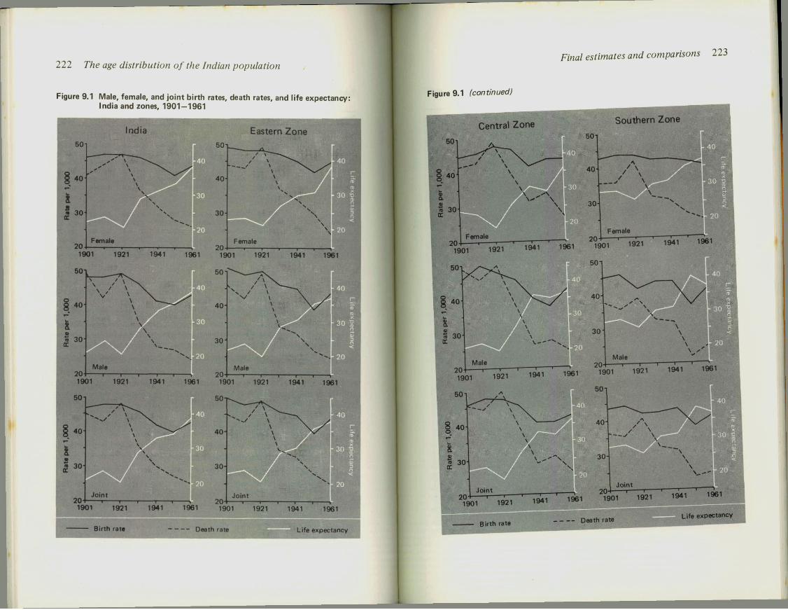
222 The age distribution of the Indian population
Final estimates and comparisons
Figure 9.1 (continued)
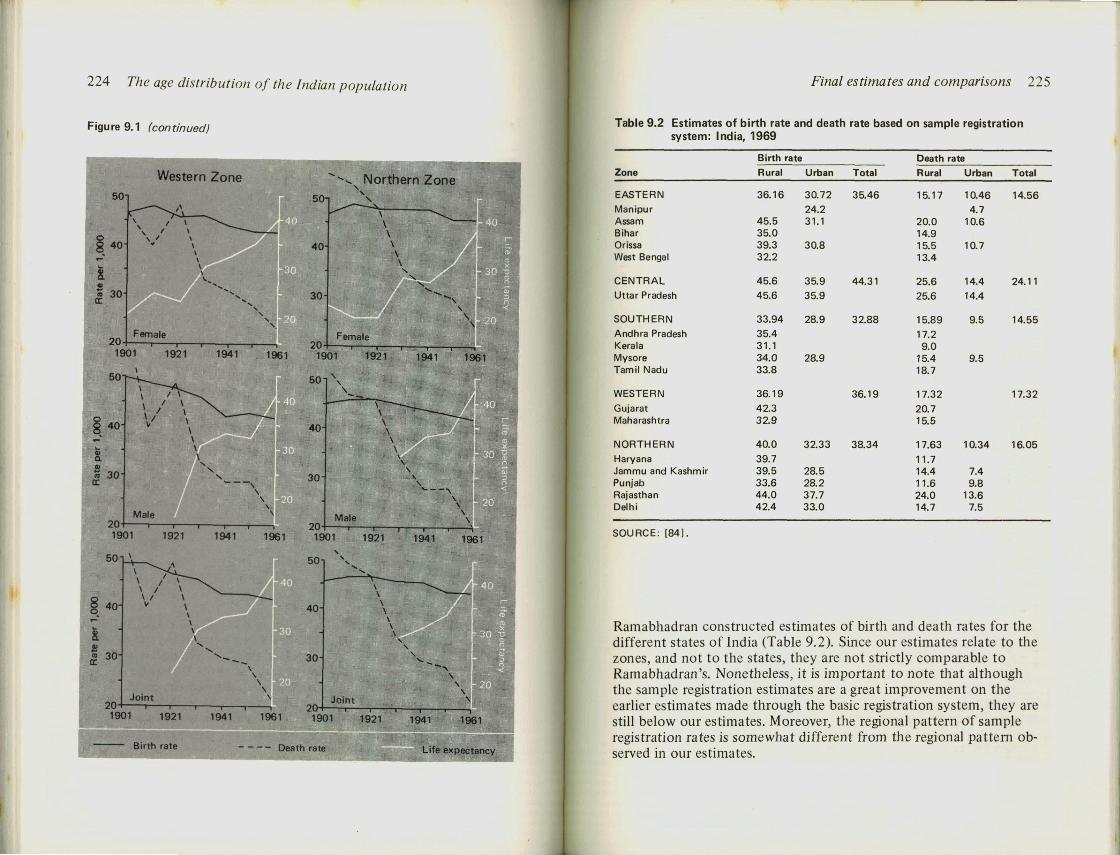
224 The age distribution of the Indian population
Figure 9.1 (continued)
Final estimates and comparisons 225
Table 9.2 Estimates of birth rate and death rate based on sample registration system: India, 1969
Birth rate Death rate Zone Rural Urban Total Rural Urban Total
E A S T E R N 36.16 30.72 35.46 15.17 10.46 14.56 Manipur 24.2 4.7 Assam 45.5 31.1 20.0 10.6 Bihar 35.0 14.9 Orissa 39.3 30.8 15.5 10.7 West Bengal 32.2 13.4
C E N T R A L 45.6 35.9 44.31 25.6 14.4 24.11 Uttar Pradesh 45.6 35.9 25.6 14.4
S O U T H E R N 33.94 28.9 32.88 15.89 9.5 14.55 Andhra Pradesh 35.4 17.2 Kerala 31.1 9.0 Mysore 34.0 28.9 15.4 9.5 Tamil Nadu 33.8 18.7
W E S T E R N 36.19 36.19 17.32 17.32 Gujarat 42.3 20.7 Maharashtra 32.9 15.5
N O R T H E R N 40.0 32.33 38.34 17.63 10.34 16.05 Haryana 39.7 11.7 Jammu and Kashmir 39.5 28.5 14.4 7.4 Punjab 33.6 28.2 11.6 9.8 Rajasthan 44.0 37.7 24.0 13.6 Delhi 42.4 33.0 14.7 7.5
S O U R C E : [84].
Ramabhadran constructed estimates of birth and death rates for the different states o f India (Table 9.2). Since our estimates relate to the zones, and not to the states, they are not strictly comparable to Ramabhadran's. Nonetheless, i t is important to note that although the sample registration estimates are a great improvement on the earlier estimates made through the basic registration system, they are still below our estimates. Moreover, the regional pattern o f sample registration rates is somewhat different f rom the regional pattern observed in our estimates.
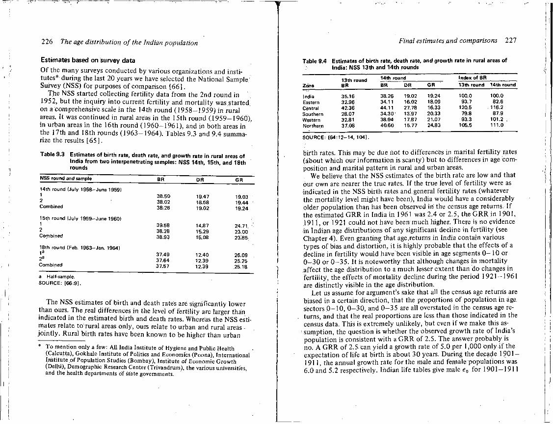
226 The age distribution of the Indian population
Estimates based on survey data
O f the many surveys conducted by various organizations and institutes* during the last 20 years we have selected the National Sample-Survey (NSS) for purposes o f comparison [ 6 6 ] .
The N S S started collecting fert i l i ty data f rom the 2nd round in 1952, but the inquiry into current fert i l i ty and mortali ty was started; on a comprehensive scale in the 14th round ( 1 9 5 8 - 1 9 5 9 ) in rural areas. It was continued in rural areas in the 15th round (1959 -1960) , in urban areas in the 16th round (1960 -1961) , and in both areas in the 17th and 18th rounds (1963 -1964) . Tables 9.3 and 9.4 summarize the results [65 ] .
Table 9.3 Estimates of birth rate, death rate, and growth rate in rural areas of India from two interpenetrating samples: NSS 14th, 15th, and 18th rounds
NSS round and sample BR DR GR
14th round (July 1958-June 1959) 1 38.50 19.47 19.03 2 38.02 18.58 19.44 Combined 38.26 19.02 19.24
15th round (July 1959-June 1960) 1 39.58 14.87 24.71. 2 38.28 15.29 23.00 Combined 38.93 15.08 23:85;
18th round (Feb. 1963-Jan. 1964) 1 a
37.49 12.40 25.09 , 2 a 37.64 12.39 25.25 Combined 37.57 12.39 25.18
a Half-sample. SOURCE: (66:9).
The NSS estimates o f birth and death rates are significantly lower than ours. The real differences in the level o f fert i l i ty are larger than indicated in the estimated birth and death rates. Whereas the N S S estimates relate to rural areas only, ours relate to urban and rural areas -jo in t ly . Rural birth rates have been known to be higher than urban
* To mention only a few: AH India Institute of Hygiene and Public Health (Calcutta), Gokhale Institute of Politics and Economics (Poona), International Institute of Population Studies (Bombay), Institute of Economic Growth (Delhi), Demographic Research Center (Trivandrum), the various universities, and the health departments of state governments.
Final estimates and comparisons 227
Table 9.4 Estimates of birth rate, death rate, and growth rate in rural areas of ; India: NSS 13th and 14th rounds
Zone 13th round BR
14th round Index of BR
Zone 13th round BR BR DR GR 13th round 14th round
India 35.16 38.26 19.02 19.24 100.0 100.0 Eastern 32.96 34.11 16.02 18.09 93.7 82.6 Central 42.36 44.11 27.78 16.33 120.5 116:2 Southern 28.07 34.30 13.97 20.33 79.8 87.9 Western 32.81 38.94 17.87 21.07 93.3 101.2 . Northern 37.08 40.60 15.77 24.83 105.5 111.0
SOURCE: [64:12-14, 104].
birth rates. This may be due hot to differences in marital fer t i l i ty rates (about which our informat ion is scanty) but to differences in age composition and marital pattern in rural and urban areas.
We believe that the N S S estimates of the bir th rate are low and that our own are nearer the true rates. If the true level of fert i l i ty were as indicated in the N S S bir th rates and general fert i l i ty rates (whatever the mortali ty level might have been), India would have a considerably older population than has been observed iri the census age returns. If the estimated G R R in India in 1961 was 2.4 or 2.5, the G R R in 1901, 1911, or 1921 could not have been much higher. There is no evidence in Indian age distributions of any significant decline in fert i l i ty (see Chapter 4). Even granting that age.returns in India contain various types of bias and distortion, i t is highly probable that the effects of a decline in fert i l i ty would have been visible in age segments 0 - 1 0 or 0 - 3 0 or 0 - 3 5 . It is noteworthy that although changes in mortal i ty affect the age distribution to a much lesser extent than do changes i n fer t i l i ty , the effects of mortali ty decline during the period 1921-1961 are distinctly visible in the age distribution.
Let us assume for argument's sake that all the census age returns are biased in a certain direction, that the proportions of population in age sectors .0 -10 , 0 - 3 0 , and 0 - 3 5 are all overstated in the census age returns, and that the real proportions are less than those indicated in the census data. This is extremely unl ikely, but even i f we make this as-
• sumption, the question is whether the observed growth rate of India's population is consistent wi th a G R R of 2.5. The answer probably is no. A G R R of 2.5 can yield a growth rate of 5.0 per 1,000 only i f the expectation of l ife at bir th is about 30 years. Dur ing the decade 1901 — 191 1, the annual growth rate fo r the male and female populations was 6.0 and 5.2 respectively. Indian l ife tables give male e0 for 1901-1911
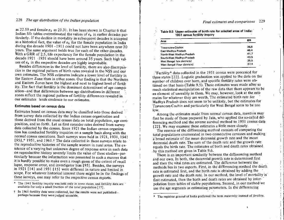
228 The age distribution of the Indian population
as 22.59 and female e0 as 23.31. It has been shown in Chapter 6 that Indian l i fe tables overestimated the values of e0 in earlier decades particularly. If the decline in mortali ty in subsequent decades is accepted as a historical fact, the value of e0 for the female population in India during the decade 1901-1911 could not have been anywhere near 30 years. The same argument holds true for each o f the other decades. Wi th a G R R of 2.5, l i fe expectancy for the female population in the decade 1921 - 1 9 3 1 should have been around 3 5 years. Such high values o f e0 in the respective decades are highly improbable.
Besides differences in the level o f fert i l i ty, there are also discrepancies in the regional pattern o f birth rates revealed in the N S S and our own estimates. The N S S estimates indicate a lower level o f fer t i l i ty in the Eastern Zone than in other zones. Our finding is that the Northern and Eastern Zones have the highest and next to highest level o f ferti li ty . The fact that fer t i l i ty is the dominant determinant o f age compo-s i t i o n - a n d that differences between age distributions in different ' zones reflect the regional pattern o f fert i l i ty differences revealed in . our estimates-lends credence to our estimates.
Estimates based on census data
Estimates based on census data may be classified into those derived f rom survey data collected by the Indian census organization and those derived f r o m the usual census data on total populat ion, age composit ion, and so for th . Let us first consider rates derived f rom survey data collected by the census. Since 1921 the Indian census organization has conducted fer t i l i ty Inquiries on a sample basis along with the normal census operations. Such surveys were held in 1921, 1931, 1941 [95;-],* 1951, and 1961 . f The data collected in these surveys relate to. the reproductive histories o f the sample women in rural areas. The existence o f a varying but unknown degree o f response error in such data on reproductive history severely limits the value o f these studies-par-ticularly because the informat ion was presented in such a manner that it is hardly possible* to make even a rough guess o f the extent o f recall lapse, response error, and investigator bias [95 ] . Besides, the surveys in 1921 [1.4] and 1931 [15] were different in nature and l imited in scope. F o r whatever historical interest there might be i n the findings o f these surveys, one may refer to the respective census reports.
* The 1941 fertility inquiry was held only in some states, and fertility data are • available for only a small fraction of the total population [17].
t In 1961 fertility data were collected, but the results were not published-perhaps because they were judged unusable.
Final estimates and comparisons 229
Table 9.5 Upper estimates of birth rate for selected areas of India: 1951 census fertility inquiry
Area BR
Travancore-Cochin East Madhya Pradesh North-West Madhya Pradesh South-West Madhya Pradesh West Bengal (six districts) West Bengal (four districts)
' Fe r t i l i ty* data collected in the 1951 census were processed for three states [22] . Logistic graduation was applied to the data on the number of children ever born, and specific fer t i l i ty rates were obtained on that basis (Table 9.5). These estimates were made after so much statistical manipulation o f the raw data that there appears to be an element of unreality in them. We may, however, look at the estimates for whatever they are wor th . The estimated birth rate fo r Madhya Pradesh does not seem to'be unl ikely , but the estimates for Travancore-Cochin and particularly for West Bengal seem to be too low. . A m o n g the estimates made f rom normal census data, mention may first be made of those prepared by Jain, who applied the so-called differencing method and the reverse survival method to 1951 census data [22 ] . We may examine these estimates a l i t t le more closely.
The essence o f the differencing method consists o f comparing the total populations enumerated in two consecutive censuses and making a broad estimate o f the mean decennial growth rate and the mean decennial death rate. The sum of the death rate and the growth rate equals the birth rate. The estimates o f bi r th and death rates obtained by this method are given in Table 9.6.
There is an important similarity between the differencing method and our own. In both, the decennial growth rate is determined first and then the vital rates are estimated. The difference between the methods lies in two aspects. First, in the differencing method the death rate is estimated first, and the bir th rate is obtained by adding the growth rate and the death rate. In our method, the level o f mortal i ty is' first estimated, then the birth and death rates are obtained by inter- ' polation f rom tables o f stable populations. Second, in our method we use the age segments as estimating parameters. In the differencing
* The registrar general of India preferred the term maternity instead of fertility.
36.8 46.4 41.7 43.5 35.5 37.4
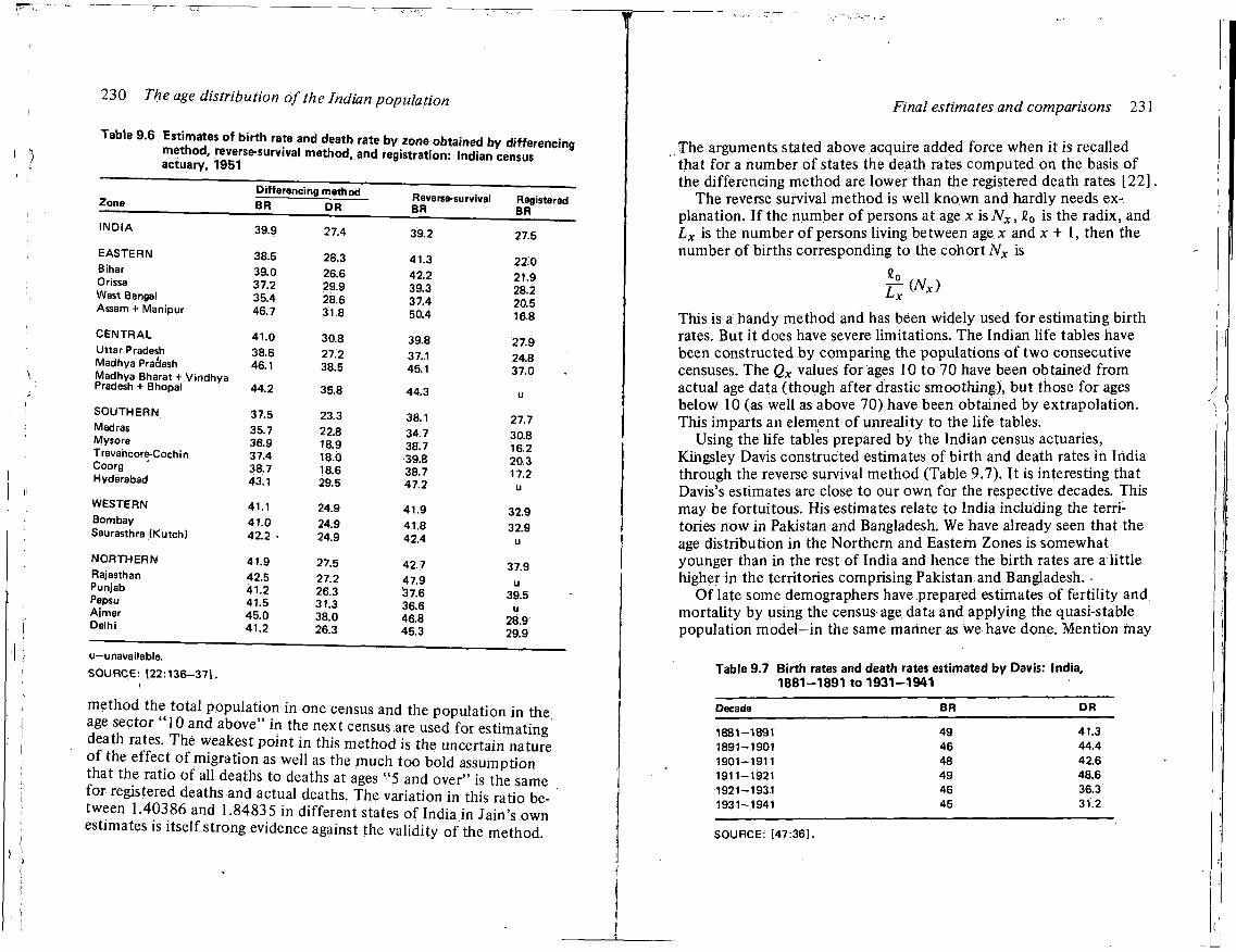
230 The age distribution of the Indian population
Table 9.6 Estimates of birth rate and death rate by zone obtained by differencing method, reverse-survival method, and registration: Indian census actuary, 1951
Differencing method Reverse-survival R 09 i stored &one BR DR BR BR
INDIA 39.9 27.4 39.2 27.5
EASTERN 38.5 28.3 41.3 22.0 Bihar 39.0 26.6 42.2 21.9 Orissa 37.2 29.9 39.3 28.2 West Bengal 35.4 28.6 37.4 20.5 Assam + Manipur 46.7 31.8 50.4 16.8
CENTRAL 41.0 30.8 39.8 27.9 Uttar Pradesh 38.6 27.2 37.1 24.8 Madhya Pradesh 46.1 38.5 45.1 37.0 Madhya Bharat + Vindhya Pradesh + Bhopal 44.2 35.8 44.3 u
SOUTHERN 37.5 23.3 38.1 27.7 Madras 35.7 22.8 34.7 30.8 Mysore 36.9 18.9 38.7 16.2 Travancore-Cochin 37.4 18.0 39.8 20.3 Coorg 38.7 18.6 38.7 17.2 Hyderabad 43.1 29.5 47.2 u
WESTERN 41.1 24.9 41.9 32.9 Bombay 41.0 24.9 41.8 32.9 Saurasthra (Kutch) 42.2 • 24.9 42.4 u
NORTHERN 41.9 27.5 42.7 37.9 Rajasthan 42.5 27.2 47.9 u Punjab 41.2 26.3 37.6 39.5 Pepsu 41.5 31.3 36.6 Ajmer 45.0 38.0 46.8 28.9 Delhi 41.2 26.3 45.3 29.9
u—unavailable.
SOURCE: [22:136-37].
method the total populat ion in one census and the population in the. age sector " 1 0 and above" in the next census are used for estimating death rates. The weakest point in this method is the uncertain nature o f the effect o f migration as well as the much too bold assumption that the ratio of all deaths to deaths at ages "5 and over' ' is the same for registered deaths and actual deaths. The variation in this ratio between 1.40386 and 1.8483 5 in different states of India in Jain's own estimates is i tself strong evidence against the validity o f the method.
Final estimates and comparisons 231
The arguments stated above acquire added force when it is recalled that for a number o f states the death rates computed on the basis o f the differencing method are lower than the registered death rates [ 2 2 ] .
The reverse survival method is wel l known and hardly needs explanation. If the number o f persons at age x is Nx, fi0 is the radix, and Lx is the number o f persons living between age x and x + 1, then the number of births corresponding to the cohort Nx is
This is a handy method and has been widely used for estimating bir th rates. But it does have severe limitations. The Indian l i fe tables have been constructed by comparing the populations o f two consecutive censuses. The Qx values for ages 10 to 70 have been obtained f rom actual age data (though after drastic smoothing), but those for ages below 10 (as well as above 70) have been obtained by extrapolation. This imparts an element of unreality to the l ife tables.
Using the l i fe tables prepared by the Indian census actuaries, Kingsley Davis constructed estimates of bir th and death rates i n India through the reverse survival method (Table 9.7). It is interesting that Davis's estimates are close to our own for the respective decades. This may be fortuitous. His estimates relate to India including the territories now in Pakistan and Bangladesh. We have already seen that the age distribution in the Northern and Eastern Zones is somewhat younger than in the rest of India and hence the bir th rates are a l i t t le higher in the territories comprising Pakistan and Bangladesh. -
O f late some demographers have prepared estimates o f fert i l i ty and mortali ty by using the census age data and applying the quasi-stable population m o d e l - i n the same manner as we have done. Ment ion may
Table 9.7 Birth rates and death rates estimated by Davis: India, 1881-1891 to 1931-1941
Decade BR DR
1881-1891 49 41.3 1891-1901 46 44.4 1901-1911 48 42.6 1911-1921 49 48.6 1921-1931 46 36.3 1931-1941 45 31.2
SOURCE: [47:36].
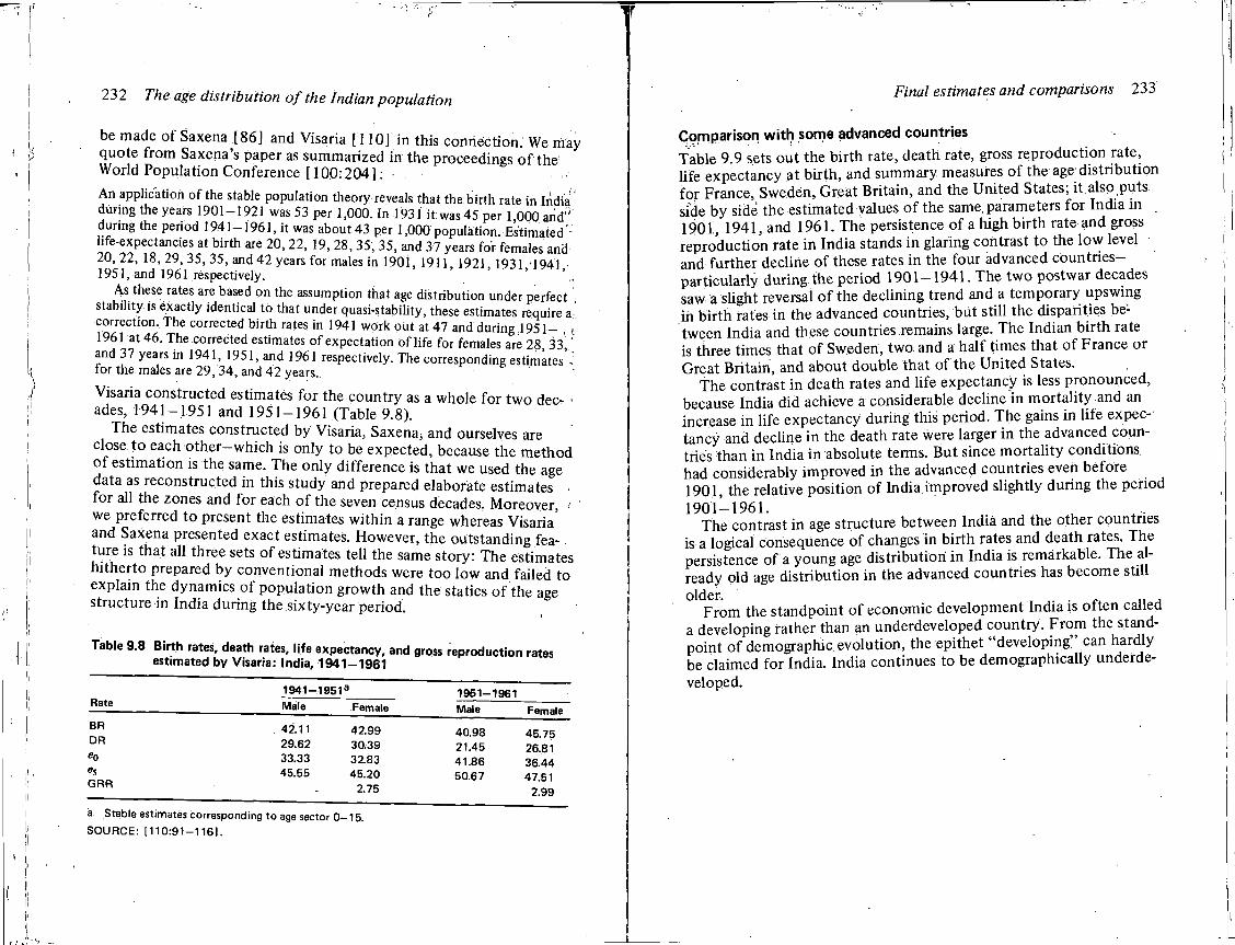
232 The age distribution of the Indian population
be made o f Saxena [86] and Visaria [110] i n this connection.' We may quote f rom Saxena's paper as summarized in the proceedings o f the World Populat ion Conference [ 100:204] :
An application of the stable population theory reveals that the birth rate in India during the years 1901-1921 was 53 per 1,000. In 1931 it was45 per 1,000 and'' during the period 1941—1961, it was about 43 per 1,000 population. Estimated " life-expectancies at birth are 20,22, 19, 28,35, 35, and 37 years for females and 20,22, 18,29, 35, 35, and 42 years for males in 1901, 1911,1921,1931/1941, 1951, and 1961 respectively.
As these rates are based on the assumption that age distribution under perfect ;
stability is exactly identical to that under quasi-stability, these estimates require a. correction. The corrected birth rates in 1941 work out at 47 and during 1951— , i 1961 at 46. The corrected estimates of expectation of life for females are 28, 33, and 37 years in 1941, 1951, and 1961 respectively. The corresponding estimates -for the males are 29, 34, and 42 years.
Visaria constructed estimates for the country as a whole for two dec- • ades, 1941-1951 and 1951-1961 (Table 9.8).
The estimates constructed by Visaria, Saxena, and ourselves are close to each other—which is only to be expected, because the method o f estimation is the same. The only difference is that we used the age data as reconstructed in this study and prepared elaborate estimates fo r all the zones and for each o f the seven census decades. Moreover, ;
we preferred to present the estimates wi th in a range whereas Visaria and Saxena presented exact estimates. However, the outstanding feature is that all three sets o f estimates tell the same story: The estimates hitherto prepared by conventional methods were too low and failed to explain the dynamics o f populat ion growth and the statics o f the age structure in India during the sixty-year period.
Table 9.8 Birth rates, death rates, life expectancy, and gross reproduction rates estimated by Visaria: India, 1941-1961
Rate 1941-•1951a
1951-1961 Rate Male Female Male Female BR . 42.11 42.99 40.98 45.75 DR 29.62 30.39 21.45 26.81 eo 33.33 32.83 41.86 36.44 eS 45.55 45.20 50.67 47.51 GRR 2.75 2.99
a Stable estimates corresponding to age sector 0—15. SOURCE: [110:91-116].
Final estimates and comparisons 233
Comparison with some advanced countries
Table 9.9 sets out the bir th rate, death rate, gross reproduction rate, l i fe expectancy at bir th, and summary measures o f the age1 distr ibution for France, Sweden, Great Br i ta in , and the Uni ted States; it also puts side by side the estimated values o f the same, parameters for India in 1901.,. 1941, and 1961. The persistence of a high b i r th rate and gross reproduction rate i n India stands i n glaring contrast to the l o w level and further decline o f these rates i n the four advanced countries— particularly during the period 1901 — 1941. The two postwar decades saw a slight reversal o f the declining trend and a temporary upswing in b i r th rates in the advanced countries, but sti l l the disparities between India and these countries remains large. The Indian b i r th rate is three times that o f Sweden, two and a ha l f times that o f France o f Great Br i ta in , and about double that of the Uni ted States.
The contrast in death rates and l i fe expectancy is less pronounced, because India did achieve a considerable decline i n mortal i ty and an increase in l i fe expectancy during this period. The gains in l i fe expectancy and decline i n the death rate were larger i n the advanced countries than i n India i n absolute terms. Bu t since mortal i ty conditions had considerably improved in the advanced countries even before 1901, the relative posit ion o f India improved slightly during the period 1 9 0 1 - 1 9 6 1 .
The contrast in age structure between India and the other countries is a logical consequence of changes in birth rates arid death rates. The persistence of a young age distr ibution i n India is remarkable. The already old age distribution i n the advanced countries has become sti l l older.
F r o m the standpoint o f economic development India is of ten called a developing rather than an underdeveloped country. F r o m the standpoint of demographic evolution, the epithet "developing" can hardly be claimed for India. India continues to be demographically underdeveloped.
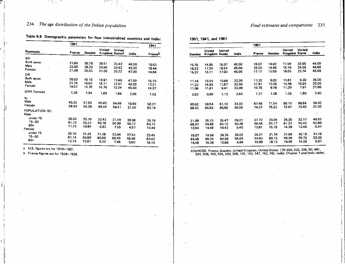
T
234 The age distribution of the Indian population
Table 9.9 Demographic parameters for four industrialized countries and India:
Male under 15 15-60 60+
Female under 15 15-60 60+
a U.S. figures are for 1919-1921.
b France figures are for 1934—1938.
| t 1901 1941
Parameter France Sweden United United Kingdom States3 India France0
BR Both sexes Male Female
DR
21.86 22.65 21.09
26.79 28.20 25.43
28.51 30.05 27.06
23.42 23.62 23.22
48.00 49.00 47.00
15.53 16.49 14.64
Both sexes Male Female
20.63 21.74 19.57
16.19 16.63 15.78
16.91 18.11 15.79
12.49 12.91 12.04
47.00 49.00 45.00
15.73 17.21 14.37
GRR (female) 1.39 1.94 1.69 1.64 2.90 1.02
Male Female
POPULATION (%)
45.02 48.53
51.53 54.26
45.40 49.39
54.49 56.41
19.50 21.00
56.27 62.14
26.55 61.72 11.72
33.79 55.37 10.84
33.43 59.76 6.82
31.49 60.96
7.55
38.66 56.77 4.57
25.79 60.72 13.49
25.70 61.14 13.15
31.24 55.89 12.87
31.38 60.60 8.02
32.04 60.49
7.46
37.42 56.98 5.60
23.45 60.42 16.13
Final estimates and comparisons 235
1901, 1941, and 1961
1961
Sweden United United Kingdom States India France Sweden
United United Kingdom States India
15.76 1R32 15.20
14.95 17.24 13.11
18.07 18.54 17.60
45.00 45.00 45.00
18.07 19.03 17.17
14.02 14.48 13.56
17.58 18.70 16.53
23.65 24.59 22.74
44.00 44.00 45.00
11.14 11.22 11.06
13.54 15.69 11.81
10.64 11.87 9.41
32.00 32.00 33.00
11.32 11.91 10.76
9.82 10.36 9.26
11.81 12.46 11.20
9.39 10.85 7.97
26.00 25.00 27.00
0.93 0.85 1.13 2.90 1.37 1.08 1.35 1.80 2.90
65.62 68.42
58.54 64.63
61.14 65.58
33.00 30.00
67.46 74.23
71.54 75.22
68.10 73.97
66.84 73.40
39.00 37.00
21.09 66.07 12.84
25.13 59.88 14.98
25.47 64.10 10.42
39.27 55.28 5.45
27.72 58.46 13.81
23.04 61.17 15.79
24.28 61.33 14.39
32.17 55.43 12.40
40.93 53.60 5.47
19.97 65.46 14.58
19.58 65.04 15.38
24.76 64.58 10.66
39.02 55.04
5.94
25.21 54.83 19.96
21.74 60.13 18.12
21.66 58.36 19.98
30.19 55.72 14.08
41.16 53.03
5.81
SOURCES: France, Sweden, United Kingdom, United States: [70:324, 332, 326, 90, 491, 501, 506, 103, 525, 530, 536, 107, 142, 147, 152, 74]. India: Chapter 7 and basictables.
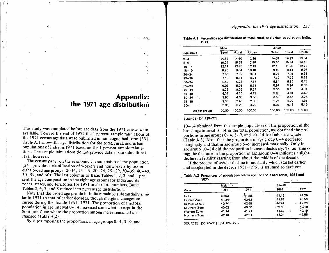
Appendix: the 1971 age distribution
This study was completed before age data f rom the 1971 census were avai lable/Toward the end o f 1972 the 1 percent sample tabulations of the 1971 census age data were published in mimeographed f o r m [ 3 3 ] . Table A . 1 shows the age distribution for the total, rural, and urban populations o f India in 1971 based on the 1 percent sample tabulations. The sample tabulations do not provide data at the subnational level, however.
The census paper on the economic characteristics of the population [34 ] provides a classification o f workers and nonworkers by sex in eight broad age groups: 0 - 1 4 , 1 5 - 1 9 , 2 0 - 2 4 , 2 5 - 2 9 , 3 0 - 3 9 , 4 0 - 4 9 , 5 0 - 5 9 , and 60+. The last columns o f Basic Tables 1,2, 3, and 4 present the age composi t ion in the eight age groups for India and its zones, states, and territories for 1971 in absolute numbers. Basic Tables 5, 6, 7, and 8 reduce it to percentage distribution.
Note that the broad age profile in India remained substantially similar in 1971 to that of earlier decades, though marginal changes occurred during the decade 1 9 6 1 - 1 9 7 1 . The proport ion o f the total population in age interval 0-1'4 increased somewhat, except in the Southern Zone where the proport ion among males remained unchanged (Table A .2 ) .
By superimposing the proportions in age groups 0 - 4 , 5 - 9 , and
Appendix: the 1971 age distribution 237
Table A.1 Percentage age distribution of total, rural, and urban population: India, 1971
Male Female
Age group Total Rural Urban Total Rural Urban
0-4 14.11 14.60 12.26 14.68 14.93 13.64
5-9 15.04 15.58 12.98 15.10 15.34 14.10
10-14 12.71 12.85 12.19 12.10 11.96 12.72
15-19 8.96 8.64 10.18 8.49 8.14 9.96 20^24 7.60 7.02 9.84 8.23 7.93 9.53
25-29 7.10 6.81 8.21 7.82 7.72 8.26 30-34 6.43 6.23 7.17 6.84 6.85 6.78
35-39 6.07 5.95 6.51 5.97 5.94 6.09 40-44 5.33 5.26 5.63 5.05 5.10 4.84
45-49 4.38 4.35 4.49 3.95 4.01 3.69 50-54 3.93 4.00 3.66 3.58 3.65 3.25
55-59 2.38 2.45 2.09 2.21 2.27 1.95
60+ 1 5.96 6.26 4.79 5.98 6.16 5.19
All age groups 100.00 100.00 100.00 100.00 100.00 100.00
SOURCE: [34:125-27].
1 0 - 1 4 obtained f rom the sample population on the proport ion in the broad age interval 0 - 1 4 in the total populat ion, we obtained the proportions in age groups 0 - 4 , 5 - 9 , and 1 0 - 1 4 fo r India as a whole (Table A . 3 ) . Note that the proport ion in age g r o u p ' 0 - 4 decreased marginally and that in age group 5 -9 increased marginally. O n l y in age group 1 0 - 1 4 did the proport ion increase decisively. T o our think-, ing, the decrease in the proport ion of age group 0 - 4 indicates a slight decline in fer t i l i ty starting f rom about the middle o f the decade.
If the process of secular decline in mortali ty which started earlier and accelerated in the decade r 1951-1961 is assumed to have con-
Table A.2 Percentage of population below age 15: India and zones, 1961 and 1971 ,
Zone Male • Female
Zone 1961 1971 1961 1971
India 40.93 41.88 41.16 42.20
Eastern Zone 41.34- 42.62 41.97 43.53
Central Zone 40.74 42.58 • •' 40.44 42.28
Southern Zone 40.02 40.00 i 39.93 - 40.10
Western Zone 41.24 41.71 41.63 42.19 Northern Zone 42.10 42.91 43.24 43.55
SOURCES: [30:20-21]; [34:125-27].
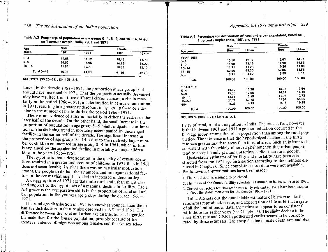
23 8 The age distribution of the Indian population
Table A.3 Percentage of population in age groups 0-4, 5-9, and 10-14, based on 1 percent sample: India, 1961 and 1971
Age group
Male Female Age group 1961 1971 1961 1971-0-4 14.68 14.12 15.47 14.79 5-9 14.63 15.05 14.86 15.22 . 10-14 11.62 12.71 10.83 12.19 ;
Total 0-14 40.93 41.88 41.16 42.20
SOURCES: [30:20-21 j ; [34:125-27].
t inued i n the decade 1961 — 1971, the proport ion i n age group 0—4 should have increased i n 1971. That the propor t ion actually decreased may have resulted f rom three different circumstances: a rise in mor- . tality in the period 1 9 6 6 - 1 9 7 1 ; a deterioration i n census enumeration in 1971, resulting in a greater undercount in age group 0—4; or a decline in the number o f births during the period 1 9 6 6 - 1 9 7 1 .
There is no evidence o f a rise in mortali ty in either the earlier or the later half o f the decade. O n the other hand, the small increase in the proport ion o f population in age group 5—9 might indicate a continuation o f the declining trend in mortal i ty accompanied by unchanged fer t i l i ty in the earlier half o f the decade. The significant increase in the propor t ion o f age group 10—14 is due to the relatively larger number o f children enumerated i n age group 0 - 4 in 1961, which in turn is explained by the accelerated decline i n mortal i ty among children born i n the years 1 9 5 6 - 1 9 6 1 .
The hypothesis that a deterioration i n the quality of census operations resulted in a greater undercount o f chi ldren i n 1971 than i n 1961 does not seem tenable. In 1971 there was no particular motivat ion among the people to deflate their numbers and no organizational factors in the census that might have led to increased undercounting.
A disaggregation o f 1971 age data into rural and urban might also lend support to the hypothesis o f a marginal decline in fert i l i ty. Table A . 4 presents the comparative shifts i n the proport ion o f rural and urban populat ion in the younger age groups during the decade 1961 — 1971.
The rural age distr ibution i n 1971 is somewhat younger than the urban age distribution—a feature also observed in 1951 and 1961. The difference between the rural and urban age distributions is larger for the male than fo r the female population, possibly because o f the greater incidence o f migration among females and the age-sex selec-
Appendix: the 1971 age distribution 239
Table A.4 Percentage age distribution of rural and urban population, based on 1 percent sample: India, 1961 and 1971
Male Female
Rural Urban Rural Urban
YEAR 1961 0—4 15.10 12.87 15.63 14.71
5—9 14.98 13.15 14.90 14.66
10—14 11.71 11.26 10.26 11.66
15- -59 52:50 58:30 52.86 53.86
60+ 5.71 4.42 5.95 5.11
Total 100.00 100.00 100.00 100.00
YEAR 1971 0—4 14.60 12.26 14.93 13.64
5—9 15.58 12.98 14.34 ,14.10
10—14 12.85 12.19 11.96 12.72
15—59 50.71 57.78 51.61 54.35
60+ 6.26 4.79 6.16 5.19
Total 100.00 100.00 100.00 100.00
SOURCES: [30:20-21]; [34:125-27].
t ivi ty o f rural-to-urban migration i n India. The crucial fact, however, is that between 1961 and 1971 a greater reduction occurred in the 0—4 age group among the urban populat ion than among the rural population. The inference is that the hypothesized decline in the bi r th rate was greater in urban areas than in rural areas. Such an inference is consistent wi th the widely observed phenomenon that urban people tend to accept family planning practices earlier than rural people.
Quasi-stable estimates o f fer t i l i ty and mortal i ty have been constructed f r o m the 1971 age distribution according to the methods discussed i n Chapter 6. Since complete census data were not available, the fo l lowing approximations have been made:
1. The population is assumed to be closed. 2. The mean of the female fertility schedule is assumed to be the same as in 1961.
3. Correction factors for changes in mortality relevant to 1961 have been used to correct the stable estimates for the decade 1961-1971.
Table A . 5 sets out the quasi-stable estimates of birth rate, death rate, gross reproduction rate, and expectation of l i fe at bir th . In spite o f all the limitations o f data, the estimates appear to be consistent with those for earlier years (see Chapter 7). The slight decline i n female bir th rate and G R R hypothesized earlier seems to be corroborated by these estimates. The steep decline in male death rate and rise
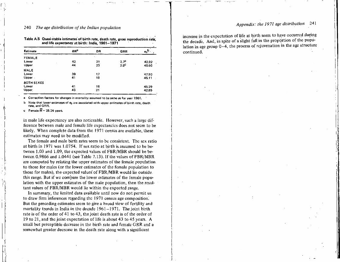
240 The age distribution of the Indian population
Table A.5 Quasi-stable estimates of birth rate, death rate, gross reproduction rate, and life expectancy at birth: India, 1961—1971
j i . Estimate B R a DR GRR e 0
b
:
FEMALE Lower 42 21 2.1C 42.92 Upper 44 23 2.9C 40.50 MALE Lower 39 17 47.50 Upper 41 19 45.11
BOTH SEXES Lower 41 19 45.29 Upper 43 21 42.89
a Correction factors for changes in mortality assumed to be same as'for year 1961. b Note that lower estimates
rate, and GRR.
c Female M = 28.24 years.
b Note that lower estimates of BQ are associated with upper estimates of birth rate, death rate, and GRR.
in male l ife expectancy are also noticeable. However, such a large difference between male and female l ife expectancies does not seem to be l ikely . When complete data f r o m the 1971 census are available, these estimates may need to be modi f ied .
The female and male birth rates seem to be consistent. The sex ratio at bir th i n 1971 was 1.0754. If sex ratio at bir th is assumed to be between 1.03 and 1.09, the expected values of F B R / M B R should be between 0.9866 and 1.0441 (see Table 7.13). If the values o f F B R / M B R are computed by relating the upper estimates o f the female population to those for males (or the lower estimates of the female populat ion to those for males), the expected values' o f F B R / M B R would lie outside this range. But i f we compare the lower estimates of the female populat ion w i t h the upper estimates of the male population, then the resultant values o f F B R / M B R would lie wi th in the expected range.
In summary, the l imited data available unt i l now do not permit us to draw f i r m inferences regarding the 1971 census age composition! But the preceding estimates seem to give a broad view of fert i l i ty and mortal i ty trends in India in the decade 1961 —1971. The joint bir th rate is o f the order of 41 to 43 , the joint death rate is o f the order o f 19 to 21 , and the joint expectation o f l i fe is about 43 to 45 years. A small but perceptible decrease in the birth rate and female G R R and a somewhat greater decrease in the death rate along wi th a significant
Appendix: the 1971 age distribution 241
increase in the expectation o f l i fe at bir th seem to have occurred during the decade. A n d , in spite o f a slight fa l l in the proport ion o f the population in age group 0 - 4 , the process of rejuvenation in the age structure continued.
[R(gfe[rcB[^](C(E,
N o attempt has been made to provide ah extensive bibliography on the subject treated. Only those references have been cited that were sources of data or ideas presented in this study.
1. Agarwal, S.P. Interrelationship between Population and Manpower Problems in the Context of Socio-Economic Development of the E C A F E Region. In Interrelation between Population and Manpower Problems. Bangkok: U.N. Economic Commission for Asia and the Far East, 1972.
2. Agarwala, S.N. Corrected Age Data of the 1931 Indian Census. Delhi: Asia Publishing House, Institute of Economic Growth, 1967.
3. Bower, W.G., and T. Aldrich Finegan. The Economics of Labor Force Participation. Princeton: Princeton University Press, 1969.
4. Brass, W. The Graduation of Fertility Distribution by Polynomial Functions. Population Studies 14(2), 1960.
5. Brass, W., et al. The Demography of Tropical Africa. Princeton: Princeton University Press, 1969.
6. Carrier, Norman, and John Hobcroft. Demographic Estimates for Develop- , ing Societies. London: Population Investigation Committee, London School of Economics, 1971.
244 . The age distribution of the Indian population
7. Census of Bengal, Report on the Census of Bengal, 1872. Calcutta, 1873. .
! 8. Census of Indja, Bibliography of Census Publications in India, Office of the Registrar General, India. New Delhi, 1972.
9. Census of India 18 71 - 72, Memorandum on the Census of British India of .1871-72. Calcutta, 1873.
10. Census of India, 1881, vol. 1.
11. Census of India, 1891, vol. 1.
12. Census of India, 1901, vol. l,pt. 1.
13. Census of India, 1911, vol. l , p L 1. ;
j 14. Census of India, 1921, vol. 1, pt. 1.
•: 15. Census of India, 1931, vol. l .pt. 1,
16. Census of India, 1931, vol. 5, pt. 1.
17. Census of India, 1941, vol. 1 (India report).
18. Census of India, 1941, Paper 1 of 1948 (age tables for West Bengal on Y-sample), foreword.
19. Census of India, 1941, vol. 17 (Baroda).
20. Census of India, Paper 3 of 1954(1951 age tables).
21. Census of India, 1951, vol. 1, pt. 2A.
22. Census of India, 1951, vol. 1, pt. IB.
, ' 23. Census of India, 1951, vol. 6, pt. 1 A.
24. Census of India, Paper 5 of 1953.
25. Census of India, Paper 2 of 1954 (life tables-1951).
26. Census of India, Paper 4 of 1954 (displaced persons).
27. Census of India, Paper 1 of 1957 (general population tables and summary I figures by districts of reorganized states).
' I ' • . , 28. Census of India, 1961, Paper 2 of 1963 (age tables).
[ 29. Census of India, 1961, vol. 1, pt. 2 A(i). i.
i f
>.\ •
\
References 245
30. Census of India, 1961, vol. 1, pt. 2C(i)'.
31. Census of India, 1961; vol. 1, pt. 2C(iii) (migration tables).
32. Census of India, 1971, Series 1, Paper 1 of 1972.
33. Chandrasekhara, A. Census of India, 1971: All-India Census Tables (estimated from 1 percent sample data), Series 1, India, pt. 2, Special. New Delhi, 1972.
34. Chandrasekhara, A. Census of India, 1971: Economic Characteristics of Population (selected tables), Series 1, India, Paper 3 of 1972. New Delhi, 1972.
35. Chandrasekharan, C , and M.G. George. Mechanism Underlying the Differences in Fertility Patterns of Bengalee Women from Three Socio-economic Groups. Milbank Memorial Fund Quarterly40(1), 1962.
36. Clark, Colin. Population Growth and Land Use. New York: Macmillan, 1967.
37. Coale, Ansley J. The Effects of Changes in Mortality and Fertility on Age-Composition. Milbank Memorial Fund Quarterly 34, January 1956.
38. Coale, Ansley J. Estimates of Various Demographic Measures Through the Quasi-Stable Age-Distribution. In Emerging Techniques in Population Research. New York: Milbank Memorial Fund, 1963.
39. Coale, Ansley J. How a Population Ages or Grows Younger. In Population: The Vital Revolution, ed. Ronald Freedman. New York: Doubleday, 1964.
40. Coale, Ansley J. The Growth and Structure of Human Populations: A Mathematical Investigation. Princeton: Princeton University Press, 1972.
'41. Coale, Ansley J. The Determination of Vital Rates in the Absence of Registration Data. Milbank Memorial Fund Quarterly 49(4), pt. 2, October 1971.
42. Coale, Ansley J. , and Paul Demeny. Regional Life Tables and Stable Populations, pt. 2. Princeton: Princeton University Press, 1966.
43. Coale, Ansley J. , and Edgar M. Hoover. Population Growth and Economic Development in Low Income Countries. Princeton: Princeton University Press, 1958.
44. Colecraft, E.A. Social and Economic Aspects of the Problem/In Population Growth and Economic Development in Africa. London: Heinemann, 1972.
45. Commission on Population Growth arid the American Future. Population and the American Future. Washington: U.S. Government Printing Office, 1972.
246 The age distribution of the Indian population
46. Das Gupta, Ajit. An Empirical Approach to the Measurement of Underemployment. Bulletin of the International Statistical Institute, 32nd session, vol. 38, bk. 2. Tokyo, 1960.
47. Davis, Kingsley. The Population of India and Pakistan. Princeton: Princeton University Press, 1951.
48. Davis, Kingsley. Cities and Mortality. In Proceedings of the International Population Conference, vol. 3. Liege, 1973.
49. Demeny, Paul. Estimates of Vital Rates for Populations in the Process of Destabuization. Demography 2, 1965.
50. Demeny, Paul. Investment Allocation and Population Growth. Demography 2, 1965.
51. Durand, John B. Population Growth and Changing Structure of Economic Activity. In Interrelation between Population and Manpower Problems. Bangkok: U.N. Economic Commission for Asia and the Far East, 1972.
52. Easterlin, Richard A. Effects of Population Growth on the Economic Development of Developing Countries. American Academy of Political and Social Science Annals 369, January 1967.
53. Enke, Stephen. The Economic Aspects of Slowing Population Growth. Economic Journal 76(301), March 1966.
54. Gini,, Corrado. Note in Economic Journal, March 1921.
55. Gordon, J .E.; Sohan Singh; and J.B. Wyon. Demographic Characteristics of Deaths in Eleven Punjab Villages. Indian Journal of Medical Research 51(2), March 1963.
56. Gordon, J .E. ; Sohan Singh; and J.B. Wyon. A Field Study of Deaths and Causes of Death in Rural Populations of the Punjab, India. American Journal of Medical Sciences 241(3), March 1961.
57. Government of India, Child Marriage Restraint Act. In India Code, vol. 3, pt. 4. New Delhi, 1929.
58. Government of India Planning Commission. Approach to the Fifth Five Year Plan: 1974- 79. New Delhi, 1973.
59. Hainsworth, G.B. The Lorenz Curve as a General Tool of Economic Analysis. Economic Record 40, 1964.
60. Hainsworth, G.B. Measures of Imbalance in International Trade Payments: Sankhya: The Indian Journal of Statistics 29, series B, pt. 1 and 2. Calcutta, June 1967.
References 247
61. Harbison, Frederick H. , and Charles A. Myers. Education, Manpower and Economic Growth. New York: McGraw-Hill, 1964.
62. Hodge, G. , and J.D. Paris. Population Growth and Regional Development: Implications for Educational Planning. Iri Demography and Educational Planning, ed. Betty McLeod. Toronto: Ontario Institute for Studies in Education, 1970.
63. Hoover, Edgar M. , and Mark Perlman. Measuring the Effects of Population Control on Economic Development. Pakistan Development Review 6(4), 1966.
64. Government of India, Cabinet Secretariat. The National Sample Survey, 14th Round, no. 48, Preliminary Estimates of Birth and Death Rates and of the Rate of Growth of Population. Delhi, 1961.
65. Indian Statistical Institute, National Sample Survey, 14th Round-Rural, July 1958-June 1959 , no. 76, Fertility and Mortality Rates in India. Cabinet Secretariat, Government of India, 1963.
66. Indian Statistical Institute, National Sample Survey, 18th Round, mimeographed report, Preliminary Estimates of Birth and Death Rates and the Rate of Growth of Population. Calcutta, 1965.
67. Jain, S.P. The Indian Programme for Improving Basic Registration. In Papers Contributed by Indian Authors to the World Population Conference, Belgrade, Yugoslavia. New Delhi: Office of the Registrar General, 1965.
68. Karmel, P.H. The Relations between Male and Female Reproduction Rates. Population Studies 1, 1947.
69. Keyfitz, Nathan. Introduction to the Mathematics of Population: Reading, Mass.: Addison-Wesley, 1968.
70. Keyfitz, Nathan, and Wilhelm Flieger. World Population: An Analysis of Vital Data. Chicago: University of Chicago Press, 1968.
71. Kurup, R.S. A Revision of Model Life Tables. In Papers Contributed by Indian Authors to the World Population Conference, Belgrade, Yugoslavia. New Delhi: Office of the Registrar General, 1965.
72. Kuznets, Simon. Population Change and Aggregate Output. In Demographic and Economic Change in Developed Countries. New York: National Bureau of Economic Research, 1960.
73. Lai, Brijesh B. Length of Life in India. Sample Registration Bulletin 8(1). Registrar Genera^ New Delhi, April 1974.
74. Lee, Everett, et al. Population Redistribution and Economic Growth in the
<
248 The age distribution of the Indian population
United States: 1870-1950, pt. 1. Philadelphia: American Philosophical Society i 1967.
75. Lopez, Alvaro. Problems in Stable Population Theory. Princeton: Office of Population Research, Princeton University, 1961.
76. Lorenz, M.C. Methods of Measuring the Concentration of Wealth. Publications of the American Statistical Association, vol. 9, new series, 1905.
77. Lorimer, F. Dynamics of Age-Structure in a Population with Initially High Fertility and Mortality. Population Bulletin of the United Nations, 1951.
78. Lotka, A.J. On the True Rate of Natural Increase (appendix). Journal of the American Statistical Association'20(150), new series, September 1962.
79. Meade, J.E. The Growing Economy. London: Allen & Unwin, 1968.
80. Mitra, S. The Pattern of Age-specific Fertility Rates. Demography 4(2), 1967.
81. Mukherjee, S.B. Inconsistency between Male and Female Reproduction Rates. Bulletin of the Calcutta Statistical Association, Department of Statistics, Calcutta University, 1957.
82. Notestein, F.W. Mortality, Fertility, Size, Age Distribution and the Growth Rate. In Demographic and Economic Change in Developed Countries. New York: National Bureau of Economic Research, 1960.
83. Okazaki, Y. Population Change and Development in Man Power, Labour Force, Employment and Income. In Population Aspects of Social Development: Bangkok: E C A F E , 1972.
84. Ramabhadran, V.K. Experience and Problems iri the Creation of the Sample Registration System in India. Paper presented at the International Symposium on Statistical Problems in Population Research, Honolulu', 1971.
85. Risley, H.H., and E.A. Gait. Census of India, 1901 Report, vol. 1, pt. 1, 1903,
86. Saxena, G.P. Estimates of Fertility and Mortality in India from 1901. to 1961. In Papers Contributed by Indian Authors to the World Population Conference;Belgrade, Yugoslavia. New Delhi: Office of the Registrar General, 1965.
87. Sharma, H.M. Enquiry into Infant Mortality in Poonamallee Health Unit Area. Mimeographed, Madras, 1955.
88. Shryock, Henry S., et al. The Methods and Materials of Demography. Washington: Bureau of the Census, 1971.
References 249
89. United Nations Population Division, Department of Social Affairs. The Causes of the Aging of Populations: Declining Mortali ty or Declining Fertility? Population Bulletin of the United Nations 4, 1954.
90. United Nations Population Division, Department of Social Affairs. Age and Sex Patterns of Mortality: Model Life Tables for Underdeveloped Countries. •New York: United Nations, 1955.
91. United Nations Population Division, Department of Social Affairs. Methods of Appraisal of Quality of Basic Data for Population Studies, no. 23, manual 2. New York: United Nations, 1955.
92. United Nations Population Division, Department of Social Affairs. 77ie • Aging of Populations and Its Economic and Social Implications. Population Studies no. 26. New York: United Nations, 1956.
93. United Nations Population Division, Department of Social Affairs. Recent Trends in Fertility in Industrialized Countries. Population Studies no. 27. New York: United Nations, 1958.
94. United Nations Population Division, Department of Social Affairs. The Aging of Populations and Its Consequences in Industrialized Countries. Population Studies no. 27. New York: United Nations, 1958.
95. United Nations Population Division, Department of Social Affairs. The Mysore Population Studies. Population Studies no. 34, ST/SOA/Series A/34. New York: United Nations, 1961,
96. United Nations Economic Commission for Africa. Principles of Applications of Demographic Data and Analysis to Development Planning in Reference to Africa. E/CN, 14/Pop/3. Addis Ababa: United Nations, 1964.
97. United Nations Economic Commission for Africa. Technical Paper on Non-sampling Errors and Biases in Retrospective Demographic Enquiries. E /CE, 14/CAS, 4/vs/3. Addis Ababa: United Nations, 1964.
98. United Nations Department of Economic and Social Affairs. General Principles for National Programmes of Population Projections as Aids to Development Planning. New York: United Nations, 1965.
99. United-Nations Department of Economic and Social Affairs. Methods of Estimating Basic Demographic Measures from Incomplete Data. New York: United Nations, 1967.
100. United Nations Department of Economic and Social Affairs. Estimates of Birth Rate and Expectation of Life in India on the Basis of Quasi-stability. In Proceedings of the World Population Conference, Belgrade, 1965, vol. 1. New York: United Nations, 1967.
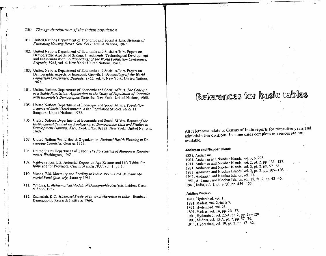
250 The age distribution of the Indian population
101. United Nations Department of Economic and Social Affairs. Methods of Estimating Housing Needs. New York: United Nations, 1967.
102. United Nations Department of Economic and Social Affairs. Papers on Demographic Aspects of Savings, Investments, Technological Development and Industrialization. In Proceedings of the World Population Conference, Belgrade, 1965, vol. 4. New York: United Nations, 1967.
103. United Nations Department of Economic and Social Affairs. Papers on Demographic Aspects of Economic Growth. In Proceedings of the World Population Conference, Belgrade, 1965, vol. 4. New York: United Nations, 1967.
104. United Nations Department of Economic and Social Affairs. The Concept of a Stable Population: Application to the Study of Population of Countries with Incomplete Demographic Statistics. New York: United Nations, 1968.
105. United Nations Department of Economic and Social Affairs. Population Aspects of Social Development. Asian Population Studies, series 11. Bangkok: United Nations, 1972.
106. United Nations Department of Economic and Social Affairs. Report of the Inter-regional Seminar on Application of Demographic Data and Studies to Development Planning, Kiev, 1964. E/Cn, 9/223. New York: United Nations, 1969.
107. United Nations World Health Organization. National Health Planning in Developing Countries. Geneva, 1967.
108. United States Department of Labor. The Forecasting of Manpower Requirements. Washington, 1963.
109. Vaidyanathan, L.S. Actuarial Report on Age Returns and Life Tables for India and for Provinces. Census of India 1931, vol. 1, pt. 1.
110. Visaria, P.M. Mortality and Fertility in India: 19'51-1961. Milbank Memorial Fund Quarterly, January 1961.
111. Yntema, L. Mathematical Models of Demographic A nalysis. Leiden: G reen &Zoon, 1952.
112. Zachariah, K.C. Historical Study of Internal Migration in India. Bombay: Demographic Research Institute, 1960.
|R®fer<Ein)<s@§ fer toffls&c tolbfe
A l l references relate to Census o f India reports for respective years and
administrative divisions. In some cases complete references are not
available.
Andaman and Nicobar Islands
1881, Andamans. 1901, Andaman and Nicobar Islands, vol. 3, p. 298. 1911, Andaman and Nicobar Islands, vol. 2, pt. 2, pp. 131-137.. 1921, Andaman and Nicobar Islands, vol. 2, pt. 2, pp. 57-64. 1931, Andaman and Nicobar Islands,'vol. 2, pt. 2, pp. 105-108. 1941, Andaman and Nicobar Islands, vol. 13. 1951, Andaman and Nicobar Islands, vol. 17, pt. 2, pp. 43-45. 1961, India, vol. 1, pt. 2C(i), pp. 454-455.
Andhra Pradesh
1881, Hyderabad, vol. 1. 1881, Madras, vol. 2, table 7. 1891, Hyderabad, vol. 23. 1891, Madras, vol. 14, pp. 26-57. 1901, Hyderabad, vol. 22-A, pt. 2, pp. 57-128, 1901, Madras, vol. 15-A, pt. 2, pp. 57-76. 1911, Hyderabad, vol. 19, pt. 2, pp. 37-62.
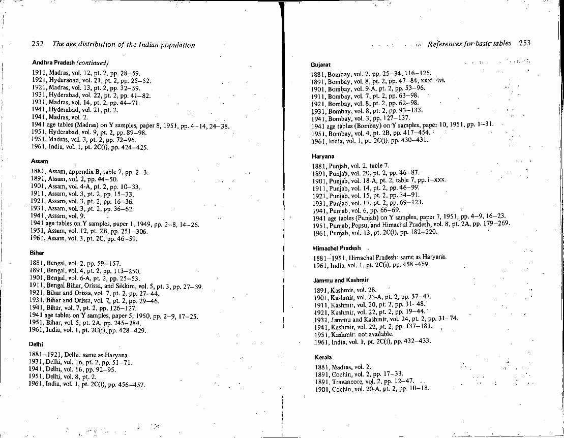
252 The age distribution of the Indian population
Andhra Pradesh (continued)
1911, Madras, vol. 12, pt. 2, pp. 28-59. 1921, Hyderabad, vol. 21, pt. 2, pp. 25-52: 1921, Madras, vol. 13, pt. 2, pp. 32-59. . 1931, Hyderabad, vol. 22, pt. 2, pp. 41-82. 1931, Madras, vol. 14, pt. 2, pp. 44-71. 1941, Hyderabad, vol. 21, pt. 2. 1941, Madras, vol. 2. 1941 age tables (Madras) on Y samples, paper 8, 1951, pp. 4-14, 24-38. 1951, Hyderabad, vol. 9, pt. 2, pp. 89-98. 1951, Madras, vol. 3, pt. 2, pp. 72-96. 1961, India, vol. 1, pt. 2C(i), pp. 424-425.
Assam
1881, Assam, appendix B, table 7, pp. 2-3. 1891, Assam, vol. 2, pp. 44-50. 1901, Assam, vol. 4-A, pt. 2, pp. 10-33. 1911, Assam, vol. 3, pt. 2, pp. 15-33. 1921, Assam, vol. 3, pt. 2, pp. 16-36. 1931, Assam, vol. 3, pt. 2, pp. 36-62. 1941, Assam, vol. 9. 1941 age tables on.Y samples, paper 1, 1949, pp. 2-8, 14-26. 1951, Assam, vol. 12, pt. 2B, pp. 251-306. 1961, Assam, vol. 3, pt. 2C, pp. 46-59.
Bihar
1881, Bengal, vol. 2, pp. 59-157. 1891, Bengal, vol. 4, pt. 2, pp. 113-250. 1901, Bengal, vol. 6-A, pt. 2, pp. 25-53. 1911, Bengal Bihar, Orissa, and Sikkim, vol. 5, pt. 3, pp. 27-39. 1921, Bihar and Orissa, vol. 7, pt. 2, pp. 27-44. 1931, Bihar and Orissa, vol. 7, pt. 2, pp. 29-46. 1941, Bihar, vol. 7, pt. 2, pp. 126-127. 1941 age tables on Y samples, paper 5, 1950, pp. 2-9, 17-25. 1951, Bihar, vol. 5, pt. 2A, pp. 245-284. 1961, India, vol. 1, pt. 2C(i), pp. 428^429.,
Delhi
1881-1921, Delhi: same as Haryana. 1931, Delhi, vol. 16, pt. 2, pp. 51-71. 1941, Delhi, vol. 16, pp. 92-95. 1951, Delhi, vol. 8, pt. 2. 1961, India, vol. 1, pt. 2C(i), pp. 456-457.
!•> References for basic: tables 253
Gujarat 1881, Bombay, vol. 2, pp. 25-34,116-125. 1891, Bombay, vol. 8, pt. 2, pp. 47-84, xxxi-lvi. 1901, Bombay, vol. 9-A, pt. 2, pp. 53-96. 1911, Bombay, vol. 7, pt. 2, pp. 63-98. - ?
1921, Bombay, vol. 8, pt. 2, pp. 62-98. 1931 .Bombay, vol. 8,pt. 2, pp. 93-133. • , • 1941, Bombay, vol. 3, pp. 127-137. 1941 age tables (Bombay) on Y samples, paper 10, 1951, pp. 1 -31 . 1951, Bombay, vol. 4, pt. 2B, pp. 417-454. : >. 1961, India, vol. 1, pt. 2C(i), pp. 430-431.
Haryana 1881, Punjab, vol. 2, table 7. 1891, Punjab, vol. 20, pt. 2, pp. 46-87. 1901, Punjab, vol. 18-A, pt. 2, table 7, pp. i-xxx. 1911, Punjab, vol. 14, pt, 2, pp. 46-99. 1921, Punjab, vol. 15, pt. 2, pp. 34-91. 1931, Punjab, vol. 17, pt. 2, pp. 69-123. 1941, Punjab, vol. 6, pp. 66-69. 1941 age tables (Punjab) on Y samples, paper 7, 1951, pp. 4-9, 16—23. 1951, Punjab, Pepsu, and Himachal Pradesh, vol. 8, pt. 2A, pp. 179-269. 1961, Punjab, vol. 13, pt. 2C(i), pp. 182-220.
Himachal Pradesh
1881-1951, Himachal Pradesh: same as Haryana. 1961, India, vol. 1, pt. 2C(i), pp. 458-459.
Jammu and Kashmir
1891, Kashmir, vol. 28. 1901, Kashmir, vol. 23-A, pt. 2, pp. 37-47. 1911, Kashmir, vol. 20, pt. 2, pp. 31-48. 1921, Kashmir, vol. 22, pt. 2, pp. 19-44. • .1931, Jammu and Kashmir, vol. 24, pt. 2, pp. 31-74. 1941, Kashmir, vol. 22, pt. 2, pp. 137-181. 1951, Kashmir: not available. 1961, India, vol. 1, pt. 2C(i), pp. 432-433.
Kerala
1881, Madras, vol. 2. 1891, Cochin, vol. 2, pp. 17-33. 1891, Travancore, vol. 2, pp. 12-47. . . 1901, Cochin, vol. 20-A, pt. 2, pp. 10-18.
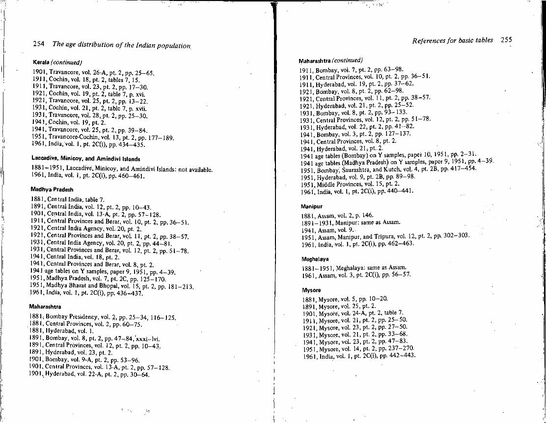
254 The age distribution of the Indian population
Kerala (continued)
1901, Travancore, vol. 26-A, pt. 2, pp. 25-65. 1911, Cochin, vol. 18, pt. 2, tables 7, 15. 1911, Travancore, vol. 23, pt. 2, pp. 17-30. 1921, Cochin, vol. 19, pt. 2, table 7, p. xvi. 1921, Travancore, vol. 25, pt. 2, pp. 13-22. 1931, Cochin, vol. 21, pt. 2, table 7, p. xvii. 1931, Travancore, vol. 28, pt. 2, pp. 25-30. 1941, Cochin, vol. 19, pt. 2. 1941, Travancore, vol. 25, pt. 2, pp. 39-84. 1951, Travancore-Cochin, vol. 13, pt. 2, pp. 177-189. 1961, India, vol. 1, pt. 2C(i), pp. 434-435.
Laccadive, Minicoy, and Amindivi Islands
1881-1951, Laccadive, Minicoy, and Amindivi Islands: not available. 1961, India, vol. 1, pt. 2C(i), pp. 460-461.
Madhya Pradesh
1881, Central India, table 7. 1891, Central India, vol. 12, pt. 2, pp. 10-43. 1901, Central India, vol. 13-A, pt. 2, pp. 57-128. 1911, Central Provinces and Berar, vol. 10, pt. 2, pp. 36-51. 1921, Central India Agency, vol. 20, pt. 2. 1921, Central Provinces and Berar, vol. 11, pt. 2, pp. 38-57. 1931, Central India Agency, vol. 20, pt. 2, pp. 44-81. 1931, Central Provinces and Berar, vol. 12, pt. 2, pp. 51-78. 1941, Central India, vol. 18, pt. 2. 1941, Central Provinces and Berar, vol. 8, pt. 2. 1941 age tables on Y samples, paper 9, 1951, pp. 4-39. 1951, Madhya Pradesh, vol. 7, pt. 2C, pp. 125-170. 1951, Madhya Bharat and Bhppal, vol. 15, pt. 2, pp. 181-213. 1961, India, vol. 1, pt. 2C(i), pp. 436-437.
Maharashtra
1881, Bombay Presidency, vol. 2, pp. 25-34, 116-125. 1881, Central Provinces, vol. 2, pp. 60-75. 1881, Hyderabad, vol. 1. 1891, Bombay, vol. 8, pt. 2, pp. 47-84,'xxxi-lvi. 1891, Central Provinces, vol. 12, pt. 2, pp. 10-43, 1891, Hyderabad, vol. 23, pt. 2. 1901, Bombay, vol. 9-A, pt. 2, pp. 53-96. 1901, Central Provinces, vol. 13-A, pt. 2, pp. 57-128. 1901, Hyderabad, vol. 22-A, pt. 2, pp. 30-64.
References for basic tables 255
Maharashtra (continued)
1911, Bombay, vol. 7, pt. 2, pp. 63-98. 1911, Central Provinces, vol. 10, pt. 2, pp. 36-51. 1911, Hyderabad, vol. 19, pt. 2, pp. 37-62. 1921, Bombay, vol. 8, pt. 2, pp. 62-98. 1921, Central Provinces, vol. 11, pt. 2, pp. 38-57. 1921, Hyderabad, vol. 21, pt. 2, pp. 25-52. 1931, Bombay, vol. 8, pt. 2, pp. 93-133. 1931, Central Provinces, vol. 12, pt. 2, pp. 51-78. 1931, Hyderabad, vol. 22, pt. 2, pp. 41-82. 1941, Bombay, vol. 3, pt. 2, pp. 127-137. 1941, Central Provinces, vol. 8, pt. 2. 1941, Hyderabad, vol. 21, pt. 2. 1941 age tables (Bombay) on Y samples, paper 1.0, 1951, pp. 2-31. 1941 age tables (Madhya Pradesh) on Y samples, paper 9, 1951, pp. 4-39. 1951, Bombay; Saurashtra, and Kutch, vol. 4, pt. 2B, pp. 417-454. 1951, Hyderabad, vol. 9, pt. 2B, pp. 89-98. 1951, Middle Provinces, vol. 15, pt. 2. 1961, India, vol. 1, pt. 2C(i), pp. 440-441.
Manipur
1881, Assam, vol. 2, p. 146. 1891-1931, Manipur: same as Assam. 1941, Assam, vol. 9. 1951, Assam, Manipur, and Tripura, vol. 12, pt. 2, pp. 302-303. 1961, India, vol. 1, pt. 2C(i), pp. 462-463.
Meghalaya 1881-1951, Meghalaya: same as Assam. 1961, Assam, vol. 3, pt. 2C(i), pp. 56-57.
Mysore 1881, Mysore, vol. 5, pp. 10-20. 1891, Mysore, vol. 25, pt. 2. 1901, Mysore, vol. 24-A, pt. 2, table 7. 1911, Mysore, vol. 21, pt. 2, pp. 25-50. 1921, Mysore, vol, 23, pt. 2, pp. 27-50. 1931, Mysore, vol. 21, pt. 2, pp. 33-68. 1941, Mysore, vol. 23, pt. 2, pp. 47-83. 1951, Mysore, vol. 14, pt. 2, pp. 237-270. 1961, India, vol. 1, pt. 2C(i), pp. 442-443.
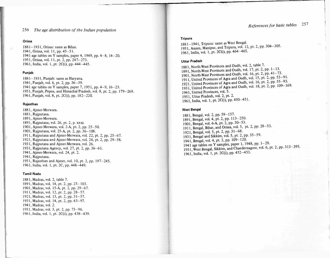
256 The age distribution of the Indian population
Orissa
1881—1931, Orissa: same as Bihar. 1941, Orissa, vol. 11, pp. 45 -5 1. 1941 age tables on Y samples, paper 4, 1949, pp. 4-8, 14-20. 1951, Orissa, vol. 11, pt. 2, pp. 247-273. 1961, India, vol. 1, pt. 2C(i), pp. 444-445.
Punjab
1881—1931, Punjab: same as Haryana. 1941, Punjab, vol. 6, pt. 2, pp. 36-39. 1941 age tables on Y samples, paper 7, 1951, pp. 4—9, 16-23. 1951, Punjab, Pepsu, and Himachal Pradesh, vol. 8, pt. 2, pp. 179-269. 1961, Punjab, vol. 8, pt. 2C(i), pp. 182-220.
Rajasthan
1881, Ajmer-Merwara. 1881, Rajputana. 1891, Ajmer-Merwara. 1891, Rajputana, vol. 26, pt. 2, p. xxxi. 1901, Ajmer-Merwara, vol. 2-A, pt. 2, pp. 25—50. 1901, Rajputana, vol. 25-A, pt. 2, pp. 36-108. 1911, Rajputana and Ajmer-Merwara, vol. 22, pt. 2, pp. 25—67. 1921, Rajputana and Ajmer-Merwara, vol. 24, pt. 2, pp. 29—58. 1931, Rajputana and Ajmer-Merwara, vol. 26. 1931, Rajputana Agency, vol. 27, pt. 2, pp. 36—61. 1941, Ajmer-Merwara, vol. 24, pt. 2. 1941, Rajputana. 1951, Rajasthan and Ajmer, vol. 10, pt. 2, pp. 197-245. 1961, India, vol. 1, pt. 2C, pp. 448-449.
Tamil Nadu
1881, Madras, vol. 2, table 7. 1891, Madras, vol. 14, pt. 2, pp. 25-103. 1901, Madras, vol. 15-A, pt. 2, pp. 29-67. 1911, Madras, vol. 12, pt. 2, pp. 28-57. 1921, Madras, vol. 13, pt. 2, pp. 31-57. 1931, Madras, vol. 14, pt. 2, pp. 43-97. 1941, Madras, vol. 2. 195 1, Madras, vol. 3, pt. 2, pp. 73-96. 1961, India, vol. 1, pt. 2C(i), pp. 438-439.
References for basic tables 257
Tripura 1881-1941, Tripura: same as West Bengal. 1951, Assam, Manipur, and Tripura, vol. 12, pt. 2, pp. 304-305. 1961, India, vol. 1, pt. 2C(i), pp. 464-465.
Uttar Pradesh 1881, North-West Provinces and Oudh, vol. 2, table 7. 1891, North-West Provinces and Oudh, vol. 17, pt. 2, pp. 1-13. 1901, North-West Provinces and Oudh, vol. 16, pt. 2, pp. 41-73. 1911, United Provinces of Agra and Oudh, vol. 15, pt. 2, pp. 53-91. 1921, United Provinces of Agra and Oudh, vol. 16, pt. 2, pp. 55—93. 1931, United Provinces of Agra and Oudh, vol. 18, pt. 2, pp. 109-169. 1941, United Provinces, vol. 5. 1951, Uttar Pradesh, vol. 2, pt. 2. 1961, India, vol. 1, pt. 2C(i), pp. 450-451.
West Bengal 1881, Bengal, vol. 2, pp. 59-157. 1891, Bengal, vol. 4, pt. 2, pp. 113-250. 1901, Bengal, vol. 6-A, pt. 2, pp. 30-53. 1911, Bengal, Bihar, and Orissa, vol. 5, pt. 2, pp. 28-53. 1921, Bengal, vol. 5, pt. 2, pp. 31-68. 1931, Bengal and Sikkim, vol. 5, pt. 2, pp. 35-59. 1941, Bengal, vol. 4, pt. 2, pp. 109-120. 1941 age tables on Y samples, paper 1, 1948, pp. 1-29. 1951, West Bengal, Sikkim, and Chandernagore, vol. 6, pt. 2, pp. 313-395. 1961, India, vol. 1, pt. 2C(i), pp. 452-453.
THE EAST-WEST C E N T E R is a national educational institution established in Hawaii by the United States Congress in 1960. Its purpose is to promote better relations and understanding between the United States and the nations of Asia and the Pacific area through cooperative study, training, and research. Since 1975, the Center has been administered by a public, nonprofit educational corporation, officially known as the "Center for Cultural and Technical Interchange Between East and West, Inc." An international Board of Governors consisting of distinguished scholars, business leaders, and public servants guides Center policies.
Each year more than 1,500 men and women from more than 60 nations and dependencies in the region participate in Center programs that seek cooperative solutions to problems of mutual consequence to East and West Working in research and development projects with the Center's multidisciplinary and multicultural staff, participants include visiting scholars and researchers; leaders, policymakers, and other professionals; and graduate degree students, most of whom are also enrolled at the University of Hawaii. For each Center participant from the United States, two participants are sought from the Asian-Pacific area.
Center programs are conducted by five institutes addressing problems of communication, culture learning, food, population, and technology and development. A limited number of open grants are awarded each year for degree education and innovative research in areas not encompassed by institute programs.
The U.S. Congress provides basic funding for Center programs and a variety of awards to participants. Because of the cooperative nature of Center programs, financial support and cost-sharing are also sought from Asian and Pacific governments, public and private sectors, and individuals. The Center campus is on land adjacent to and provided by the University of Hawaii.
T H E EAST-WEST P O P U L A T I O N INSTITUTE, established as a unit of the East-West Center in 1969 with the assistance of a grant from the Agency for International Development, carries out multidisciplinary research, training, and related activities in the field of population, placing emphasis on economic, social, psychological, and environmental aspects of population problems in Asia, the Pacific, and the United States.
East-West Population Institute East-West Center 1777 East-West Road Honolulu, Hawaii 96822
Director Lee-jay Cho Publications Officer Sandra E. Ward
Editor Elizabeth B. Gould Production Assistant Lois M. Bender
Related Documents