18 October, 2018 ISSN 1991-637X DOI: 10.5897/AJAR www.academicjournals.org OPEN ACCESS African Journal of Agricultural Research

Welcome message from author
This document is posted to help you gain knowledge. Please leave a comment to let me know what you think about it! Share it to your friends and learn new things together.
Transcript

18 October, 2018 ISSN 1991-637X DOI: 10.5897/AJARwww.academicjournals.org
OPEN ACCESS
African Journal of
Agricultural Research
About AJAR
The African Journal of Agricultural Research (AJAR) is a double blind peer reviewed journal. AJAR
publishes articles in all areas of agriculture such as arid soil research and rehabilitation, agricultural
genomics, stored products research, tree fruit production, pesticide science, post-harvest biology and
technology, seed science research, irrigation, agricultural engineering, water resources management,
agronomy, animal science, physiology and morphology, aquaculture, crop science, dairy science,
forestry, freshwater science, horticulture, soil science, weed biology, agricultural economics and
agribusiness.
Indexing
Science Citation Index Expanded (ISI), CAB Abstracts, CABI’s Global Health Database
Chemical Abstracts (CAS Source Index), Dimensions Database, Google Scholar Matrix of Information for The Analysis of Journals (MIAR) Microsoft Academic
ResearchGate, The Essential Electronic Agricultural Library (TEEAL)
Open Access Policy
Open Access is a publication model that enables the dissemination of research articles to the global
community without restriction through the internet. All articles published under open access can be
accessed by anyone with internet connection.
The African Journal of Agricultural Research is an Open Access journal. Abstracts and full texts of all
articles published in this journal are freely accessible to everyone immediately after publication
without any form of restriction.
Article License
All articles published by African Journal of Agricultural Research are licensed under the Creative
Commons Attribution 4.0 International License. This permits anyone to copy, redistribute, remix,
transmit and adapt the work provided the original work and source is appropriately cited. Citation
should include the article DOI. The article license is displayed on the abstract page the following
statement:
This article is published under the terms of the Creative Commons Attribution License 4.0 Please
refer to https://creativecommons.org/licenses/by/4.0/legalcode for details about Creative Commons
Attribution License 4.0

Article Copyright
When an article is published by in the African Journal of Agricultural Research the author(s) of the
article retain the copyright of article. Author(s) may republish the article as part of a book or other
materials. When reusing a published article, author(s) should;
Cite the original source of the publication when reusing the article. i.e. cite that the article was
originally published in the African Journal of Agricultural Research. Include the article DOI
Accept that the article remains published by the African Journal of Agricultural Research (except in
occasion of a retraction of the article)
The article is licensed under the Creative Commons Attribution 4.0 International License.
A copyright statement is stated in the abstract page of each article. The following statement is an
example of a copyright statement on an abstract page.
Copyright ©2016 Author(s) retains the copyright of this article..
Self-Archiving Policy
The African Journal of Agricultural Research is a RoMEO green journal. This permits authors to
archive any version of their article they find most suitable, including the published version on their
institutional repository and any other suitable website.
Please see http://www.sherpa.ac.uk/romeo/search.php?issn=1684-5315
Digital Archiving Policy
The African Journal of Agricultural Research is committed to the long-term preservation of its content.
All articles published by the journal are preserved by Portico. In addition, the journal encourages
authors to archive the published version of their articles on their institutional repositories and as well
as other appropriate websites.
https://www.portico.org/publishers/ajournals/
Metadata Harvesting
The African Journal of Agricultural Research encourages metadata harvesting of all its content. The
journal fully supports and implements the OAI version 2.0, which comes in a standard XML
format. See Harvesting Parameter

Memberships and Standards
Academic Journals strongly supports the Open Access initiative. Abstracts and full texts of all articles
published by Academic Journals are freely accessible to everyone immediately after publication.
All articles published by Academic Journals are licensed under the Creative Commons Attribution 4.0
International License (CC BY 4.0). This permits anyone to copy, redistribute, remix, transmit and
adapt the work provided the original work and source is appropriately cited.
Crossref is an association of scholarly publishers that developed Digital Object Identification (DOI)
system for the unique identification published materials. Academic Journals is a member of Crossref
and uses the DOI system. All articles published by Academic Journals are issued DOI.
Similarity Check powered by iThenticate is an initiative started by CrossRef to help its members
actively engage in efforts to prevent scholarly and professional plagiarism. Academic Journals is a
member of Similarity Check.
CrossRef Cited-by Linking (formerly Forward Linking) is a service that allows you to discover how
your publications are being cited and to incorporate that information into your online publication
platform. Academic Journals is a member of CrossRef Cited-by.
Academic Journals is a member of the International Digital Publishing Forum (IDPF). The
IDPF is the global trade and standards organization dedicated to the development and
promotion of electronic publishing and content consumption.

Contact
Editorial Office: [email protected]
Help Desk: [email protected]
Website: http://www.academicjournals.org/journal/AJAR
Submit manuscript online http://ms.academicjournals.org
Academic Journals
73023 Victoria Island, Lagos, Nigeria
ICEA Building, 17th Floor, Kenyatta Avenue, Nairobi, Kenya
Editors
Prof. N. Adetunji Amusa
Department of Plant Science and Applied Zoology
Olabisi Onabanjo University
Nigeria.
Dr. Mesut YALCIN
Forest Industry Engineering, Duzce
University,
Turkey.
Dr. Vesna Dragicevic
Maize Research Institute
Department for Maize Cropping
Belgrade, Serbia.
Dr. Ibrahim Seker
Department of Zootecny,
Firat university faculty of veterinary medicine,
Türkiye.
Dr. Abhishek Raj
Forestry, Indira Gandhi Krishi Vishwavidyalaya,
Raipur (Chhattisgarh) India.
Dr. Ajit Waman
Division of Horticulture and Forestry, ICAR-
Central Island Agricultural
Research Institute, Port Blair, India.
Dr. Zijian Li
Civil Engineering, Case Western Reserve
University,
USA.
Dr. Mohammad Reza Naghavi
Plant Breeding (Biometrical Genetics) at
PAYAM NOOR University,
Iran.
Dr. Tugay Ayasan
Çukurova Agricultural Research Institute
Adana,
Turkey.

Editorial Board Members
Prof. Hamid Ait-Amar
University of Science and Technology
Algiers,
Algeria.
Prof. Mahmoud Maghraby Iraqi Amer
Animal Production Department
College of Agriculture
Benha University
Egypt.
Dr. Sunil Pareek
Department of Horticulture
Rajasthan College of Agriculture
Maharana Pratap University of Agriculture & Technology
Udaipur,
India.
Prof. Irvin Mpofu
University of Namibia
Faculty of Agriculture
Animal Science Department
Windhoek,
Namibia.
Prof. Osman Tiryaki
Çanakkale Onsekiz Mart University,
Plant Protection Department,
Faculty of Agriculture, Terzioglu Campus,17020, Çanakkale,
Turkey.
Dr. Celin Acharya
Dr. K.S. Krishnan Research Associate (KSKRA)
Molecular Biology Division
Bhabha Atomic Research Centre (BARC)
Trombay,
India.
Prof. Panagiota Florou-Paneri
Laboratory of Nutrition
Aristotle University of Thessaloniki
Greece.
Dr. Daizy R. Batish
Department of Botany
Panjab University
Chandigarh,
India.
Prof. Dr. Abdul Majeed
Department of Botany
University of Gujrat
Pakistan.
Dr. Seyed Mohammad Ali Razavi
University of Ferdowsi
Department of Food Science and Technology
Mashhad,
Iran.

Prof. Suleyman Taban
Department of Soil Science and Plant Nutrition
Faculty of Agriculture
Ankara University
Ankara, Turkey.
Dr. Abhishek Raj
Forestry, Indira Gandhi Krishi Vishwavidyalaya,
Raipur (Chhattisgarh) India.
Dr. Zijian Li
Civil Engineering,
Case Western Reserve University,
USA.
Prof. Ricardo Rodrigues Magalhães
Engineering,
University of Lavras,
Brazil
Dr. Venkata Ramana Rao Puram,
Genetics And Plant Breeding,
Regional Agricultural Research Station, Maruteru, West Godavari District,
Andhra Pradesh,
India.
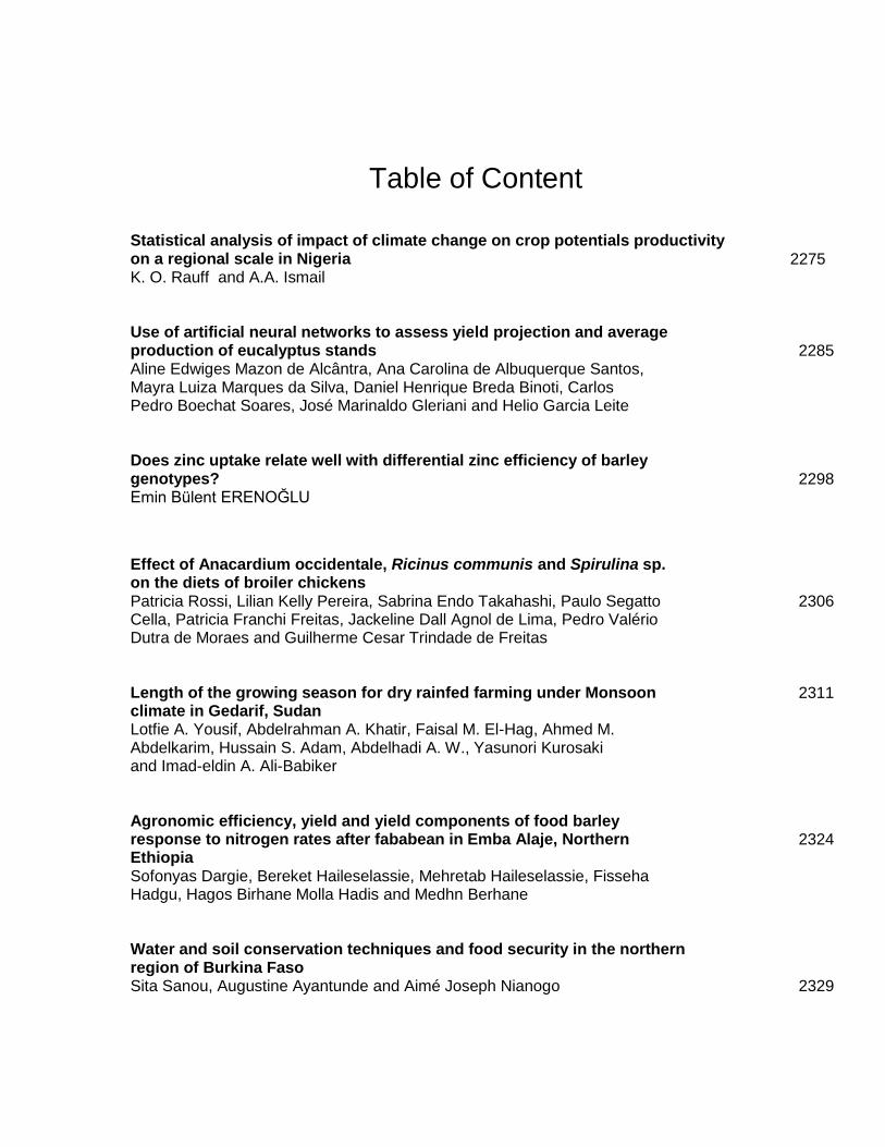
Table of Content Statistical analysis of impact of climate change on crop potentials productivity on a regional scale in Nigeria K. O. Rauff and A.A. Ismail
2275
Use of artificial neural networks to assess yield projection and average production of eucalyptus stands Aline Edwiges Mazon de Alcântra, Ana Carolina de Albuquerque Santos, Mayra Luiza Marques da Silva, Daniel Henrique Breda Binoti, Carlos Pedro Boechat Soares, José Marinaldo Gleriani and Helio Garcia Leite
2285
Does zinc uptake relate well with differential zinc efficiency of barley genotypes? Emin Bülent ERENOĞLU
2298
Effect of Anacardium occidentale, Ricinus communis and Spirulina sp. on the diets of broiler chickens Patricia Rossi, Lilian Kelly Pereira, Sabrina Endo Takahashi, Paulo Segatto Cella, Patricia Franchi Freitas, Jackeline Dall Agnol de Lima, Pedro Valério Dutra de Moraes and Guilherme Cesar Trindade de Freitas
2306
Length of the growing season for dry rainfed farming under Monsoon climate in Gedarif, Sudan Lotfie A. Yousif, Abdelrahman A. Khatir, Faisal M. El-Hag, Ahmed M. Abdelkarim, Hussain S. Adam, Abdelhadi A. W., Yasunori Kurosaki and Imad-eldin A. Ali-Babiker
2311
Agronomic efficiency, yield and yield components of food barley response to nitrogen rates after fababean in Emba Alaje, Northern Ethiopia Sofonyas Dargie, Bereket Haileselassie, Mehretab Haileselassie, Fisseha Hadgu, Hagos Birhane Molla Hadis and Medhn Berhane
2324
Water and soil conservation techniques and food security in the northern region of Burkina Faso Sita Sanou, Augustine Ayantunde and Aimé Joseph Nianogo
2329

Table of Content
Strategic planning of regional oil-and-fat subcomplex of Russia Mikhail O. Sinegovsky and Anastasia A. Malashonok
2343
Evaluation of diazotrophic bacteria from rice varieties (Oryza sativa L.) grown in Rio de Janeiro State, Brazil Esdras da Silva, Mayan Blanc Amaral, Katia Regina dos Santos Teixeira and Vera Lucia Divan Baldani
2351
Agricultural productivity, land use and draught animal power formula derived from mixed crop-livestock systems in Southwestern Ethiopia Asrat Guja Amejo, Yoseph Mekasha Gebere, Habtemariam Kassa and Tamado Tana
2362
Vol. 13(42), pp. 2275-2284, 18 October, 2018
DOI: 10.5897/AJAR2018.13455
Article Number: DE48AF158897
ISSN: 1991-637X
Copyright ©2018
Author(s) retain the copyright of this article
http://www.academicjournals.org/AJAR
African Journal of Agricultural
Research
Full Length Research Paper
Statistical analysis of impact of climate change on crop potentials productivity on a regional scale in Nigeria
K. O. Rauff1* and A.A. Ismail2
1Department of Physics, Faculty of Science, Federal University of Kashere, Gombe State Nigeria.
2School of Physics, Universiti Sains Malaysia, 11800 USM, Penang, Malaysia.
Received 11 August, 2018; Accepted 5 September, 2018
Yield improvement is the main aim of all agricultural activities. Therefore, it is important to have an idea about the yield that can be produced from a piece of land before investing in it. This work is aimed at analysing the impact of climate change on crop yield potential and predicting the crop yield potential in six geo political zones in Nigeria using global solar radiation as the only limiting factor of production. Climatic data were obtained from Nigeria Meteorological Agency (NIMET), Oshodi, Nigeria. Results of impact of climate change on the photosynthetic, light-temperature, and climatic potential productivities of maize and their gap differences are presented using a crop growth dynamics statistical method. The results showed that photosynthetic potential productivity decreased from north to south, with the largest values in two maize-growing zones due to higher average growing season radiation and a longer maize growing season. The light-temperature potential productivity of maize was higher than photosynthetic potential productivity, which varied from 3223.99 to 4425.79 kg ha
−1, with a mean of
3821.402 kg ha−1
; the climatic potential productivity varied from 11279.92 to 29263.75 kg ha−1
, with a similar distribution pattern to light-temperature potential productivity with a mean of 23817.32 kg ha
−1.
The gap between light temperature and climatic potential productivity varied from 6884.07 to 33506.92 kg ha
−1, with the high value areas centered in Southern Nigeria.
Key words: Climate change, crop yield potential, global solar radiation, dynamics statistical method, climatic potential productivity, light-temperature potential productivity.
INTRODUCTION The relation between the atmosphere and the soil cannot be overemphasized. Food production is being influenced by weather and climate variations therefore, studying the impact of climate change is important in order to cater for people as the population of the world is expected to be around 10 billion people by 2100 (Keyzer et al., 2002,
Boogaard et al., 2014)). The key parameter that determines food production is crop potential productivity (Wang et al., 2011). Grassini et al. (2009) reported that when a crop is grown under favorable conditions unlike in 2016 in which the earth’s surface experienced the warmest climate for the past 135 years (NASA GISS,
*Corresponding author. E-mail: [email protected]. Tel: +601114424190.
Author(s) agree that this article remain permanently open access under the terms of the Creative Commons Attribution
License 4.0 International License

2276 Afr. J. Agric. Res. 2015), it is referred to as potential yield. Yang et al. (2010) and Zheng-Hong et al. (2017) defined photosynthetic light-temperature and climatic potential productivity as when there is maximum crop output determined by radiation, light-temperature, and light-temperature-precipitation conditions, respectively. Crop growth models which we use to estimate agriculture potential and to forecast crop yield are important tools of interdisciplinary research (Zunfu et al., 2017). The essential input variable to estimate potential productivity and actual evapotranspiration is global solar radiation (
0H ), but there has been a significant challenge. Despite
the fact that remote sensing technique makes 0H data
available to users, the use of empirical models to
estimate 0H from measured meteorological variables is
still relevant in many applications (Chen et al., 2013). Many formulas were developed so as to choose the best selection method to tackle these challenges and some of these formulas have been incorporated into crop models as part of the software package (Donatelli et al., 2003), so as to facilitate the preparation of the necessary weather data. The concern of the general community is our climate variation and its impact on our food production. There is need to develop a statistical tool that can assist the farmers (Keating et al., 2003) to forecast the production even before going to the farm. Some studies (Chen et al., 2013) have estimated the spatiotemporal changes in crop potential productivity using various approaches. The generally acceptable method (Supit et al., 1994) used to calculate evapotranspiration is the Penman approach. Penman (1948) was the first to describe evapotranspiration in physical mathematical terms. He calculated evaporation from free-water surfaces, wet bare soil and low grass swards for 10-day periods (Foken, 2008). METHODOLOGY Penman Equation 1 consists of two parts: the radiative that calculates the net absorbed radiation and the aerodynamic that calculates the evaporative demand of the atmosphere and the resulting equations are used to calculate the potential evaporation.
an EWWHET 1 (1)
Where, ET = the evapo(transpi)ration (mm d-1); nH = the net
absorbed radiation in equivalent evaporation (mm d-1); W = the
temperature related weighing factor; and aE = the evaporative
demand in equivalent evaporation (mm d-1).
Preparatory calculations The average temperature is equal to the air temperature (T) which
is calculated as.
2minmax TT
T
(2)
Where, maxT = the maximum temperature (°C); minT = the
minimum temperature (o
C); and T = the average daily air temperature (°C).
The difference between maximum and minimum temperature is used to calculate the empiric constant of the wind function in the Penman equation.
minmax TTT (3)
Where, T = the temperature difference (°C)
The wind-speed dependency is incorporated in the evaporative demand as the wind speed measured at a height of two meters, and multiplied by an empirical coefficient which is temperature dependent and it is calculated as.
4
1235.054.0
TBU , CT 012 (4)
54.0BU , CT 012 (5)
Where, BU = the empirical coefficient in the wind function.
Saturated vapor pressure is related to mean daily air temperature (Goudriaan, 1977) and given as,
16.27386.35
2693882.17exp61078.0
T
Tes
(6)
Where, se = the saturated vapor pressure (hPa); and T = the air
temperature (°C).
Terms in the Penman Formula
The temperature related weighing factor W in Equation 1 is defined (Penman, 1948) as,
W (7)
Where, = slope of the saturation vapor pressure curve
1ChPao , = the psychometric constant 1ChPao
.
The evaporative demand of the atmosphere depends on the difference between saturated and actual vapor pressure and on the wind function.
226.0 uBUfeeE casa (8)

Where, aE = the evaporative demand (mm d-1); se = the saturated
vapour pressure (hPa); ae = the actual vapour pressure(hPa); cf =
the empirical constant; BU = the coefficient in wind function; and
u = the mean wind-speed (m s-1).
For crop canopies cf = 1.0 and for a free water surface cf = 0.5
are assumed, Eq. 1 becomes.
an EH
ET (9)
Where: ET = the pan evaporation in 1mmd ; nH = the net
absorbed radiation 1mmd ; : the slope of the saturation
vapor pressure versus air temperature 1ChPao; = the
psychometric constant 49.0 mmof Hg Co/ or
KkPa/667.0 ; and aE = the evaporative demand (mm d-1).
Methods used to estimate global radiation Solar radiation is one of the meteorological factors determining potential productivity (Boisvert et al., 1990). This can be estimated (Ångström, 1924) from other climatic variables; for example from sunshine duration; air temperature range (De Jong and Stewart, 1993), precipitation (De Jong and Stewart, 1993) and cloud-cover (Barker, 1992). We used the equation postulated by Ångström (1924) and modified by Prescott (1940).
N
nba
H
Hh 0
(10)
Where, hH = the monthly average daily global radiation on a
horizontal surface 12 daymMJ ; 0H = the monthly
average daily extraterrestrial radiation on a horizontal surface
12 daymMJ ; n = the monthly average daily number of
hours of bright sunshine; N = the monthly average daily maximum
number of hours of possible sunshine (or day length); and a and
b = the regression constants.
This above named equation is the most widely used empirical equation which estimates global solar radiation from sunshine hour duration.
Daily climate data from sixteen (16) stations of the Nigeria Meteorological Agency (NIMET) Oshodi, Nigeria were obtained. The climate data are of high quality. The data include Sunshine Hours (h), Average Temperature (°C), Maximum Temperature (°C),
Minimum Temperature (°C), Precipitation (mm), Relative Humidity
(%), and Wind Speed (ms−1) over the period of 30 years (1985 to 2014). In estimating crop yield potential, the study areas were divided into three maize-growing districts based on different sowing dates and growth periods. Observed maize phenology from the Institute of Agricultural Research and Training (IAR&T)
Rauff and Ismail 2277 meteorological station was used to calibrate the maize-growing districts. Calculation of maize potential productivity Crop potential productivity is calculated according to the crop growth dynamics statistical method, which divides the potential production into three levels: photosynthetic, light-temperature, and climatic potential productivity (Yuan et al., 2012). The photosynthetic potential productivity (PPP; 103 kg ha−1) is calculated as,
4
1 1
219.0j
dl
ih
i
HCPPP
(11)
Where, 0.219 = the Huang Bingwei coefficient in unit of
1510 kgkJ ; C = the crop economic coefficient, taking the
value of 0.4 (Li et al., 2009); j represents each maize development
stage; i
dl = the length of each crop development stage; hH = the
daily shortwave radiation during the crop growing season in unit of 12 daycmkJ .
The light-temperature potential productivity (LTPP; 103 kg ha−1) is calculated by correcting the Photosynthetic Potential Productivity with the Temperature Stress Coefficient.
4
1 1
219.0i
dl
ih
i
TfHCLTPP
(12)
Where, itf = the temperature stress coefficient that can be
calculated as follows.
MAXTTTTT
TT
TTTTT
TT
TT
TT
Tf
0
0max
max
0min
min,0
min,
min
min0
(13)
Where, T = the daily average temperature in ( CO); minT , maxT ,
and oT = the minimum, maximum, and optimum temperatures (
CO) for each crop development stage, respectively.
The climatic potential productivity (CPP; 103 kg ha−1) is calculated by correcting the light temperature potential productivity with the water stress coefficient.

2278 Afr. J. Agric. Res.
4
1 1
219.0i
dl
ijh
i
wfTfHCLTPP
(14)
Here, jwf = the water stress coefficient is calculated as,
ETP
ETPET
P
wf
j
j
j
j
1
0
(15)
Where, jP = the total precipitation (mm) during each maize
development stage; ET = the total crop water requirement (mm) during each crop development stage, which can be calculated as shown in Equation 1. RESULTS AND DISCUSSION The results of photosynthetic potential productivity (PPP), light-temperature potential productivity (LTPP), climatic potential productivity (CPP) and gap differences for the six geo political zones in Nigeria are presented in Table 1 while the geographical map of the area of study is presented in Figure 1.
The geographical information of photosynthetic potential productivity (PPP); light-temperature potential productivity (LTPP) and climatic potential productivity (CPP) are presented in Figures 2, 4 and 6 while their values are presented in Figures 3, 5 and 7 respectively; Figure 8 shows the trend pattern of their gap difference.
The potential productivity and potential productivity gap evaluation is important in order to understand the effect of temperature, rainfall and light resources on crop production. In this study, we analyzed the variations in climate factors and their impact on crop (maize) potential productivities (photosynthetic, light-temperature, and climatic) in six geo-political zones of Nigeria for 30 years between 1985 and 2014, and then quantified the spatial and temporal variations in the gap between light temperature and climatic potential productivity. The highest values of maize potential productivity occurred in North-Eastern and North-Western states. In general, PPP decreases from North to South, with the largest values in maize-growing zones II and III (Bauchi, Yola, Kaduna and Kano states) due to higher average growing season radiation and a longer maize growing season as shown in Figure 2. The spatial change in maize potential productivity did not follow a decreasing trend with latitude due to the complex topographic conditions in these regions. The distribution of areas with high values of
photosynthetic potential productivity was different from that with high values of light-temperature productivity due to change in altitude. Areas with high values of photosynthetic productivity were mainly located in the North-Eastern and North-Western regions; however, those with low values of light-temperature potential productivity were mainly located in Southern region of Nigeria. Figure 3 depicts the photosynthetic potential productivity (PPP) of maize that varied from 1091.03 kg
to 1505.37 kg ha−1
, with a mean of 1294.78 kg ha−1
and the highest values of PPP occurred both in the northwest and northeast; whereas the lowest values occurred in the south-south and south-east of the six geopolitical zones in Nigeria. It was noticed that both the PPP and LTP productivities followed the same patterns where the lowest values were recorded in both the south east and south-south of Nigeria as presented in Figure 4. Light-temperature potential productivity of maize was noticeably higher than photosynthetic potential productivity, which varied from 3223.99 to 4425.79 kg ha
−1, with a mean of 3821.402 kg ha
−1 as it has been
shown in Figure 5. Figure 6 presents the geographical information of climatic potential productivity (CPP) of the six geopolitical zones of the area of study. Climatic potential productivity varied from 11279.92 to 29263.75 kg ha
−1, with a mean of 23817.32 kg ha
−1. Figure 6
exhibits the climatic potential productivity variations which decrease in the Northeast of Nigeria, whereas it increases in the Southwest of Nigeria. The gap between light- temperature and climatic potential productivity varied from 6884.07 to 33506.92 kg ha
−1, with the high
value areas centered in Southern Nigeria as shown in Table 1 and Figure 8, respectively. The gap between light-temperature and climatic potential productivity varied considerably with location (between 6884.07 to 33506.92 kg ha
−1) from 1985 to 2014 in Nigeria. Climatic potential
productivity was about 10 to 24% of light-temperature potential productivity in these regions, which implies that precipitation is a strong limiting factor for maize potential productivity.
In general, the simulated potential yield decreases generally from north to south due to the latitudinal distribution of solar radiation and growing season temperature which corresponds to the work of Wu et al. (2006). Precipitation during the maize growing season ranges from 412 to 608 mm in different maize-growing districts, which in theory can meet the water requirements of maize. The climatic potential productivity decreases in the northeast of Nigeria, whereas it increases in the southwest of Nigeria. However, a distinct gap between light- temperature and climatic potential productivity exists, varying from 6884.07 to 33506.92 kg ha
−1, with the
high value areas centered in Southern Nigeria, which presents a maize potential productivity loss due to water stress caused by uneven precipitation distribution during the maize growing season. As presented in Table 1, the

Rauff and Ismail 2279
Table 1. The six geo-political zones of Nigeria.
District Geo-political zones PPP (kg ha−1
) LTPP (kg ha−1
) CPP (kg ha−1
) Gap Diff
I North Central States 1400.07 4116.20 18390.89 14274.60
II North-Eastern States 1495.19 4395.85 11279.92 6884.07
III North-Western States 1505.37 4425.79 20986.05 16560.26
IV South-Eastern States 1180.43 3470.48 29263.75 25793.27
V South-Southern States 1096.59 3223.99 36730.91 33506.92
VI South-Western States 1091.03 3296.10 26252.41 22956.31
Figure 1. The map of Nigeria showing the six geopolitical zones of area of study. The six Geo-Political Zones of Nigeria where the data were obtained: North Central States: Kogi, Plateau and Federal Capital Territory; North-Eastern States: Borno, Bauchi and Adamawa; North-Western States: Kaduna and Kano; South-Eastern States: Enugu; South-Southern States: Edo and Rivers; South-Western States: Oyo, Ogun, Lagos, Ondo and Osun.

2280 Afr. J. Agric. Res.
Figure 2. The geographical information of photosynthetic potential productivity (PPP) of the six geopolitical zones of area of study.
NC NE NW SE S/S S/W
0
200
400
600
800
1000
1200
1400
1600
PP
P K
g/H
a
SIX GEO-POLITICAL ZONES IN NIGERIA
Figure 3. The photosynthetic potential productivity in the six geopolitical zones, Nigeria.

Rauff and Ismail 2281
Figure 4. The geographical information of Light Temperature Potential Productivity (LTPP) of the six geopolitical zones of area of study.
NC NE NW SE S/S S/W
0
1000
2000
3000
4000
LT
PP
Kg
/Ha
SIX GEO-POLITICAL ZONES IN NIGERIA
Figure 5. The light-temperature potential productivity in the six geopolitical zones, Nigeria.

2282 Afr. J. Agric. Res.
Figure 6. The geographical information of Climatic Potential Productivity (CPP) of the six geopolitical zones of area of study.
NC NE NW SE S/S S/W
0
5000
10000
15000
20000
25000
30000
35000
CP
P K
g/H
a
SIX GEO-POLITICAL ZONES IN NIGERIA
Figure 7. The climatic potential productivity in the six geopolitical zones, Nigeria.

Rauff and Ismail 2283
NC NE NW SE S/S S/W
0
5000
10000
15000
20000
25000
30000
35000
GA
P D
IFF
ER
EN
CE
SIX GEO-POLITICAL ZONES IN NIGERIA
Figure 8. The gap difference in the six geopolitical zones, Nigeria.
largest yield gap was located in south-south and south-east zones. Conclusion The major advantage of potential productivity gap analysis is that it is used to know crop yield improvement when there is information about the solar radiation, evapotranspiration, photosynthetic potential productivity (PPP), light-temperature potential productivity (LTPP) and climatic potential productivity (CPP) of the area. Generally, it is a known fact that increases in temperature causes a reduction in climatic potential productivity in the high temperature category, whereas it contributes to an increase in climatic potential productivity at stations in the low temperature category. However, in Northeast, a simulated increase in maximum temperature generally caused a reduction in yield potential, while an increase in minimum temperature produced no significant impact on yield potential. It is noticed that potential productivity is not completely consistent with actual yield. In conclusion, we have demonstrated that a distinct gap between light-temperature and climatic potential productivity exists where annual and growing season precipitation is sufficient when analyzing the impact of climate change on the spatial and temporal variations of maize photosynthetic, light-temperature, and climatic potential productivity from 1985 to 2014 in Nigeria. It is also worth concluding that the geographic information helps to gather actionable intelligence from all types of data.
CONFLICT OF INTERESTS
The authors have not declared any conflict of interests. REFERENCES
Ångström A (1924). Solar and atmospheric radiation. Quarterly Journal
of the Royal Meteorological Society 50:121-126. Barker HW (1992). Solar radiative transfer through clouds possessing
isotropic variable extinction coefficient. Quarterly Journal of the Royal Meteorological Society 118(3):1145-1162.
Boisvert JB, Hayhoe HN, Dubé PA (1990). Improving the estimation of global radiation across canada. Agricultural and Forest Meteorology 52(3-4):275-286.
Boogaard HL, De Wit AJW, te Roller JA, Van Diepen CA (2014). Wofost control centre 2.1; User’s guide for the wofost control centre 2.1 and the crop growth simulation model wofost 7.1.7. Wageningen (Netherlands), Alterra, Wageningen University and Research Centre 133 p.
Chen C, Baethgen WE, Robertson A (2013). Contributions of individual variation in temperature, solar radiation and precipitation to crop yield in the north china plain, 1961–2003. Climatic Change 116(3-4):767-788.
De Jong R, Stewart DW (1993). Estimating global radiation from common meteorological variables in Western Canada. Canadian Journal of Plant Science 73(2):509-518.
Donatelli M, Bellochi G, Fontana F (2003). RadEst300: Software to estimate daily radiation data from commonly available meteorological variables. European Journal of Agronomy 18(3-4):363-367.
Foken T (2008). Micrometeorology. Springer-Verlag Berlin Heidelberg 306 p.
Goudriaan J (1977). Crop micrometeorology: a simulation study. simulation monographs. pudoc, wageningen, Netherland 262 p.
Grassini P, Yang H, Cassman KG (2009). Limits to maize productivity in western corn-belt: a simulation analysis for fully irrigated and rainfed conditions. Agricultural and Forest Meteorology 149(8):1254-1265.

2284 Afr. J. Agric. Res. Keating BA, Carberry PS, Hammer GL (2003). An overview of apsim, a
model designed for farming systems simulation. European Journal of Agronomy 18(3-4):267-288.
Keyzer M, Merbis M, Pavel F (2002). Can we feed the animals? origins and implications of rising meat demand. Paper presented at 2002 International Congress, European Association of Agricultural Economists, Zaragoza, Spain, 28–31 Aug.
National Aeronautics and Space Administration, Goddard Institute for Space Studies (NASA, GISS) (2015). NASA, NOAA Finds 2015 Warmest Year in Modern Record. 18 January. http://www.giss. nasa.gov/research/news/20150116/ (accessed 18 January 2017).
Penman HL (1948). Natural evaporation from open water, bare soil and grass. Proceedings Royal Society Series A 193(1032):120-146.
Prescott JA (1940). Evaporation from a water surface in relation to solar radiation. Transactions of the Royal Society of South Australia 64:114-480.
Supit I Hooijer AA, van Diepen CA (1994). System description of the wofost 60 crop simulation model implemented in CGMS. Volume 1 theory and algorithms, Joint Research Centre Commission of the European Communities EUR 15956 EN: Luxembourg 146 p.
Wang T Lu C, Yu B (2011). Production potential and yield gaps of summer maize in the Beijing-Tianjin-Hebei Region. Journal of Geographical Sciences 21(4):677–688.
Yang J, Peter MV, Jian Y, Michael EG (2010). A Commentary on
‘Common SNPs Explain a Large Proportion of the Heritability for Human Height. Twin Research and Human Genetics 13(6):517-524.
Yuan Z, Li J, Zhang L, Gao X, Gao HJ Xu S (2012). Investigation on brca1 snps and its effects on mastitis in chinese commercial cattle. Elsevier 505:190-194.
Zheng-Hong T, Jiye Z, Yong-Jiang Z, Martijn S, Minoru G, Takashi H, Yoshiko K, Humberto RR, Scott RS, Michael LG (2017). Optimum air temperature for tropical forest photosynthesis: mechanisms involved and implications for climate warming 2017. Environmental Research Letters 12:054022
Zunfu L, Xiaojun Liu, Weixing C, Yan Z (2017). A Model-Based Estimate of Regional Wheat Yield Gaps and Water Use Efficiency in Main Winter Wheat Production Regions of China. Scientific Reports 7:6081.

Vol. 13(42), pp. 2285-2297, 18 October, 2018
DOI: 10.5897/AJAR2017.12942
Article Number: 9BAB7FB58899
ISSN: 1991-637X
Copyright ©2018
Author(s) retain the copyright of this article
http://www.academicjournals.org/AJAR
African Journal of Agricultural
Research
Full Length Research Paper
Use of artificial neural networks to assess yield projection and average production of
eucalyptus stands
Aline Edwiges Mazon de Alcântra1, Ana Carolina de Albuquerque Santos1*, Mayra Luiza Marques da Silva2, Daniel Henrique Breda Binoti3, Carlos Pedro Boechat Soares1, José
Marinaldo Gleriani1 and Helio Garcia Leite1
1Department of Forest, Universidade Federal de Viçosa, CEP 36570-000, Viçosa – MG, Brazil.
2Department of Forestry, Alto Universitário, Universidade Federal do Espírito Santo, Guararema, CEP 29500-000,
Alegre/Espirito Santo, Brazil. 3DAP Florestal, R. Papa João XXIII, 9 - CEP 36570-000, Viçosa – Minas Gerais, Brazil.
Received 19 December, 2017; Accepted 11 May, 2018
Eucalyptus stands growth depends on genotype, age, quality of the local soil and silvicultural treatment. Environmental factors, mainly the water availability to plants throughout the years, temperature and solar radiation are relevant to production capacity. The models used in Brazil to stimulate the future production of forestry stands are those that estimate growth and/or production according to age, basal area and local index. One of the possible approaches to do so is the use of procedural models (ecophysiological) such as the 3PG and the artificial neural network. The current study has the aim to construct, validate and apply an artificial neural model to predict the production and growth of eucalyptus stands in Minas Gerais, Brazil. The herein used data resulted from continuous forestall inventory plots conducted in eucalyptus stands in the North, Center and South of the state. The edaphic and climatic information added to the IFC data were used to train neural nets on predicting growth and production in the state. A neural network, lacking inventory variables, was also trained to extrapolate the mean productivity in the entire state of Minas Gerais due to the physiographic, edaphic and climatic conditions. The neural network efficiency was attested by the great accuracy of productivity forecasts. The generated productivity maps are indicated for studies on the expansion of eucalyptus cultivation in the state. The applied methodology is simple and efficiently inapplicable to different forestry cultures in other states or countries. Key words: Eucalyptus, water availability, forestry stands, neural network, productivity.
INTRODUCTION The Forestry Sector is responsible for approximately 3.5% of Brazilian Gross Domestic Product (2007 GDP) and it accounts for 7% of total exportation, thus generating 7 million jobs (Brazilian Forestry Service, 2015). From the 8 million hectares of planted forest, about 5.6 million are Eucalyptus spp. stands basically
located in the states of Minas Gerais (25.2%), São Paulo (17.6%) and Mato Grosso do Sul (14.5%) (IBA, 2015). The eucalyptus stands are composed of many clones (Gonçalves et al., 2008) and spatial arrangements conducted in high stem and coppice systems. The timber is mainly used in cellulose and charcoal production

2286 Afr. J. Agric. Res. (Campos and Leite, 2013). The cutting time in Brazil takes place when the trees are around seven years old and the mean production (38 m
3 ha
-1) varies a lot (IBA,
2014). Production may potentially reach 90 m3 ha
-1 when
the tree is at the age of 6 (Borges, 2012). In 2014, cellulose and charcoal production in Brazil was about 80,873,295 million m³ and 6,219,325 tons (IBGE, 2014). The timber is also used in the construction industry, in sawmills, for electric power generation, and in plates (IBA, 2015). The harvest often occurs approximately five to eight years after the plantation or after the sprouting. Yet, the harvest period depends on the regulation model applied by the company, that is, on the hierarchical planning.
Minas Gerais state has the largest eucalyptus plantation area in Brazil. These plantations are mostly located in regions called Mares de Morros, Tabuleiros Costeiros (Gonçalves et al., 2008), and Brazilian Savanna (Cerrado), wherein the soil fertility is relatively low and the water availability is irregular throughout the years (Lelles et al., 2001). The mean productivity of seven-year-old stands (cutting point) varies according to physiographic, edaphic and climatic conditions. It also changes according to genotype, spacing and spatial arrangements, the productive capacity of the area, cultural practices (Stape et al., 2006, 2010; Oda-Souza et al., 2008), silvicultural management (Gonçalves et al., 2008) and water availability regularity (Ryan et al., 2010 and Stape et al., 2010).
Most of the Brazilian eucalyptus stands belong to more than 6.000 forestry companies in the country and to forestry smallholders supported by promotion programs (IBA, 2015). The study was done in partnership with researchers from 66 current forestry engineering courses placed in the country in 2015 (SNIF, 2016).
Research institutions, universities and engineers from forestry companies have been conducting studies on the growth and production of eucalyptus stands for many years in Brazil, developing large databases of permanent plot and tress cubage samples. These data are mostly used by companies assisted by researchers from public institutions and in partnership with universities to develop growth and yield models (GYM). The most used GYMs in Brazil are the total stands types (Campos and Leite, 2013). Trevizol (1985) published one of the first consistent variable density models for Amazonian eucalyptus stands. Thenceforth, many studies were individually conducted by different companies, most of these studies focused on defining stratification due to cutting process, spatial arrangement, genotype and region or project (Trevizol, 1985; Soares, 2000; Cruz et al, 2008; Nogueira, 2005; Oliveira et al., 2009; Silva,
2010; Borges, 2009; Salles, 2012; Binoti, 2012). Campos and Leite (2013) published a summary of the main models and functional relationships used in Brazilian eucalyptus stands. According to the authors, the most commonly applied models are the sigmoid and Clutter´s (1963). Larger companies have been following the modeling approaches that present the maximum forest stratification and, consequently, the sigmoid prediction models such as the logistic Gompertz (Winsor, 1932) and Richards (Richards, 1959) ones, despite the other variables resulting from the Von Bertalanffy (1938) model. The functional relationships used are the types: V=f(I), V=f(I,S) or V=f(I,S,B), wherein V is the production per hectare, B is the basal area per hectare, S is the local index and I is the age of the stands.
Besides the large range of physiographic, edaphic and climatic feature effects, one of the challenges faced by the production and yield modeling of Brazilian eucalyptus is the large diversity of genotypes (mainly clones) that interact in time and space with different spacing, spatial arrangements and handling types. The constant genotypes often change and the silvicultural practices hamper the modeling. It is common to find 30 to 60% of permanent sample parcels with just one or two calibrations (Oliveira et al., 2009) and results from current technological packages are often quite important for the companies (Oliveira et al., 2009; Campos and Leite, 2013).
The Brazilian eucalyptus is also hard to model due to the old databases that are often discarded because of the new “technological packages” that have been employed lately (Oliveira et al., 2009). A statistician would say: “it is impossible to develop a biologically consistent model only by counting on one or two measurements of permanent parcels”. Nevertheless, the problem is incredibly challenging, since there is a large variety of calibrations applied to permanent parcels, there are handling unities or projects composed of none, one, two, three or more calibrations, there is the use of old places, where the plantation has not been initiated WITH the use of various technological packages (Oliveira et al., 2009). It is necessary to attend to the third handling element in the hierarchal plan of eucalyptus forests (Campos and Leite, 2013); having harvest storage expectation, even for areas where the crop that will possibly contain new genotypes and that will be planted in future years; and also counting on expectations on a whole spectrum of planning that encompasses fifteen to thirty years ahead.
Brazilian researchers are very interested in the influence of climatic changes on the development and production of eucalyptus stands countrywide, in remarkable and sometimes uncertain ways (Baesso et
*Corresponding author. E-mail: [email protected]. Tel: 55 31 992248445 or 55 31 995808939.
Author(s) agree that this article remain permanently open access under the terms of the Creative Commons Attribution
License 4.0 International License

al., 2010). Thereby, predictions are getting harder with time, since the modeling process is often based on past data, due to the assumption that environmental conditions will repeat themselves, but the fact is that the environmental conditions are increasingly uncertain and their inclusion in the models is not trivial (Soares, 2000). New technological packages are implemented in a yearly basis and the cultivated areas are extended to different places that present other physiographic, edaphic and climatic features.
Despite the modeling complexity, it is necessary having accurate production estimations, since the hierarchy planning depends on it. A possibility to improve production estimation accuracy in comparison with the usual production and yield models lies on the computational intelligence methods (CI) such as the artificial neural networks (ANN) (Binoti, 2012). The CI methods used in forestry sciences have been largely employed in the forestry calibration and in pattern classification areas. The Multilayer Perceptron model (MP) is often used for logistical activation (Guan and Gertner, 1991a, b; 1995; Gordon, 1998; Diamantopoulou, 2005; Silva, 2010; Binoti, 2012; Özçelik et al., 2010; Özçelik et al., 2013; Diamantopoulou, 2010a, b; Khoury Junior et al., 2006; Leduc et al., 2001; Silva et al., 2009, Leite et al, 2011; Binoti et al, 2014, b; Gorgens et al., 2009). Most studies employing ANN to predict the Brazilian eucalyptus stands have been using specific data from certain companies or locations (Silva, 2009; Binoti, 2012; Binoti et al., 2012). The ANN allows assessing and/or simulating the climatic, edaphic and silvicultural effects on the productivity of the stands; although it looks superior in many studies when it is compared with current methods, which were described in most of the herein mentioned researches. It also allows estimating the production and productivity in areas that do not have trees or inventory data available (Silva Binoti, 2012).
The production and yield models are employed not only to the forestry handling management of Brazilian eucalyptus, but in certain cases, to ecophysiological models such as the “Physiological Processes Predicting Growth” (3PG) (Sands and Landsberg, 2002; Miehle et al., 2009), which have been already tested and applied in Brazil (Stape, 2002; Almeida et al., 2003, 2004; Stape et al., 2004; Borges, 2009; Stape et al., 2010; Borges, 2012). These models describe the stands growth based on processes linked to physical (soil and climate) and biological features (genetic materials and plant physiology). The aforementioned models are efficient to assess productivity losses caused by root issues and to determinate the potential productivity. However, they demand data from directed trial and stands samples. On the other hand, the ANN may be trained through the employment of parcel data from continuous and temporary forestry inventories, as well as through the use of different climatic, edaphic and physiographic
de Alcântra et al. 2287 calibrations, which are somehow an alternative to the processual models.
It is worth considering the combination of features that express these factors when the MCP is adjusted, since the trees depend on climatic, edaphic and physiographic factors, as well as in genotype, spacing and silvicultural practices to develop. However, the inclusion of categorical variables such as soil, name of the project, genotype, spacing, fertilization level, among other categorical variables, is not trivial and it is often impossible to be done due to lack of representativeness of all the combined variables. It may bring representativeness deficiency to some strata, and it would lead to the need for and to the possibility of using the CI and ecophysiographic models. The possibility of including any continuous or categorical variable and the fact that it is not necessary to observe the statistical preconditions of the regression modeling are some of the advantages of applying the IC model, which does not need a large amount of data from the categorical combinations (Jensen et al., 1999).
The aim of the present study is to develop and validate artificial neural network models in order to identify the production and development of eucalyptus stands in the State of Minas Gerais by taking into account its great potential to produce eucalyptus and its importance to the Brazilian economy. Another aim of the current study is to reduce the investment on these new kinds of plantations in the state by configuring, training, validating, and applying neural networks through the generation of productivity category maps; and to define a methodology to be applied in other states or countries. MATERIALS AND METHODS Data
Data from permanent parcels of continuous forestry inventories (CFI) were used in the current study, which was conducted in eucalyptus stands in Minas Gerais – Brazil (Figures 5 and 6). The studied stands are located in North, Center and South of the state; they result in 10,000 parcels that encompass an area of approximately 500 m² aged 12 to 357 months and account for 317,000 registers in the database. All the recorded information and six hierarchic area division levels were standardized– the smallest unit has a 20 hectares edge. The registration form listed city, plantation date, spacing, genotype, predominant soil and rotation. The IFC data were processed according to the parcel level and they comprised all the variables, such as age (months), mean height of predominant trees (Hd), basal area (B) and trees with commercial bark volume (diameter equals to or greater than 4 cm) (Table 1).
Physiographic, edaphic and climatic information from the climatic stations were added to the database, besides the forestry inventory data (Table 2). The annual mean of physiographic, edaphic and climatic information from 2006 to 2013 were processed. The data from the climatic station where connected according to their geographic coordinates and processed in the database in order to extrapolate the information of each edge using the Thiessen polygons methodology (Thiessen, 1911). The climatic information was obtained through Köppen Geiger classification, which takes

2288 Afr. J. Agric. Res.
Table 1. Amplitude, mean values and standard deviation for age, dominant height (Dh), basal area (B) and volume in parcel level, in the sampled area of the state of Minas Gerais, Brazil.
Variable Minimum Maximum Mean Standard deviation
Age (months) 11.97 357.34 61.17 35.18
Dh (m) 6.00 59.83 24.44 6.59
N (m²/ha) 0.70 58.91 18.37 6.92
Yield (m³/ha) 3.80 1158.42 197.16 118.75z
Table 2. Amplitude and standard deviation of the edaphic and climatic variables used as input variables in train neural networks to estimate eucalyptus development, production and productivity in the state of Minas Gerais, Brazil.
Variable Year Minimum Mean Maximum Standard deviation
Temperature (°C) 14.69 19.85 29.69 3.82
Relative humidity (%) 72.77 77.83 81.83 2.74
Annual precipitation averages (mm)
2007 20.08 69.68 114.91 20.50
2008 19.86 107.23 162.56 30.10
2009 19.98 115.68 160.86 37.62
2010 72.77 77.83 81.83 2.74
2011 18.52 115.73 179.84 38.68
2012 19.78 83.01 109.55 23.10
2013 19.32 122.26 190.50 40.99
Wind speed (m/s) 1.27 2.97 4.30 1.02
Total radiation (MJ/m²/day) 12.88 14.81 17.23 1.53
Temperature (°C) 31.020,50 32.979,50 34.721,94 1.256,72
Relative humidity (%) 8.76 14.92 24.57 5.57
Annual precipitation averages (mm) 4.10 5.98 8.41 1.45
into account the seasonality and the annual and monthly mean temperature and precipitation (Köppen and Geiger, 1928). Developing and applying neural networks Two studies were conducted. The aim of the first (Case 1) was to estimate the mean production at different ages (prediction) and the second (Case 2) was to estimate and extrapolate the mean production in previously set ages (six and seven years old - the usual regulatory rotation age in the Minas Gerais State).
Besides the regional categorical variables, namely: spacing, genotype, cutting cycle and predominant soil in Case 1, the variables in Tables 1 and 2 were also taken into consideration. Production was the output variable (m3 ha-1). Training and validation percentages were: 100(0), 50(50), 40(60), 30(70), 20(80) and 10(90). The numbers in brackets refer to the percentage given to the data in order to validate the neural networks. These variables allow assessing the generalizing capacity of trained networks. The network training was performed in the parcel level because the output variable “volume” presented parcel level variance.
The aim of Case 2 was to assess prediction efficiency by using the climatic and edaphic variables, and to assess the generation of the mean productivity map for the entire state. The applied categorical output variables were the sub-region, spacing, genotype, cutting cycle, predominant soil, altitude; highest, lowest and mean temperatures, and minimum, maximum and the mean precipitation during the sampled period (Table 2). Six and seven-years-old productions (m3 ha-1) were chosen as output variables.
Only the 7 years old parcels (IMA7)- acceptable variation between 78.1 and 90 months, and 6 years old parcels (IMA6)- acceptable variation between 66 and 78 months, were selected in the IFC database, since the used database (Table 2) did not contain parcels from all the cities in the herein studied state. Information on temperature, precipitation and climate (Köppen-Geiger classification), extracted from http://www.ipef.br/geodatabase were also employed, besides the variables in Table 2. The percentage of data for training and validation in case 2 were 100(0), 95(5), 90(10) and 85(15). Training and generalizing artificial neural networks The network training was performed in the parcel level because the output variable “volume”, presented variation in this level in both cases. However, the validation was performed in the block level because the edaphic and climatic variables used in the training network database just presented variation in this level. The Neuroforest was the software used to train and apply the networks. The trained network was the Multilayer Perceptron (MLP), with three layers. The Resilient propagation (RPROP+) (Riedmiller and Braun, 1993) was the employed algorithm, since it adapts its weight of each step according to the local gradient information. Such adaptation is not influenced by the behavior of the gradient.
The amount of neuron in the entrance layer fluctuated according to the number of variables taken into consideration in each study. Twelve neurons were used in the intermediate layer and one, in the
de Alcântra et al. 2289
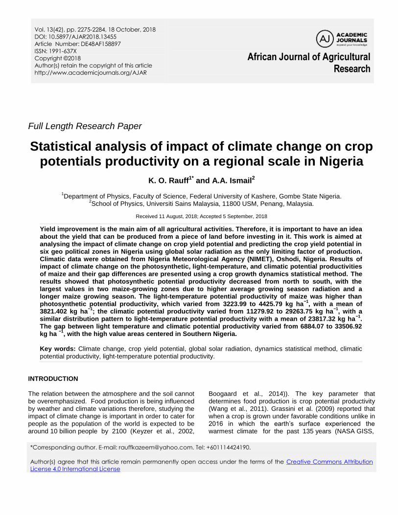
Table 3. Root mean square error (RMSE %) and the correlation between the observed and estimated ( ) volumes of eucalyptus stands in Case 1.
Percentage for training Percentage for validation Status RMSE (%)
100 0 Training 5.15 0.9929
50 50 Training 4.65 0.9941
50 50 Validation 5.13 0.9931
40 60 Training 4.64 0.9943
40 60 Validation 4.97 0.9934
30 70 Training 4.65 0.9943
30 70 Validation 4.77 0.9939
20 80 Training 4.64 0.9943
20 80 Validation 5.65 0.9915
10 90 Training 4.65 0.9943
10 90 Validation 6.17 0.9898
exit layer. The activation function used in the hidden and exit layers was of the sigmoid type (logistics). The stopping criteria were the mean error or the number of cycles, in other words, the network training ended when the first parameter was reached. The stopping limit was 0.0001 for the mean error and 3,000 for the number of cycles. Assessing the artificial neural network forecast The assessment of the artificial neural network forecast in training and the validation stages were done through statistics and graphic analysis. The employed statistics were the mean absolute
differences ( e ), the correlation between estimated and observed
volumes (YYR ˆ ), root mean square error (RMSE) and the relative
percentage error (RE %).
∑ | | √ ∑ ( )
∑ ( )
n
ii
n
imi
n
iimi
YY
YYnYYn
YYYYn
R
1
21
1
21
1
1
ˆ
)()ˆˆ(
))(ˆˆ(,
n
iim YnY
1
1 ˆˆ ,
n
i i
ii
Y
YYnER
1
1ˆ
100%
Wherein: i
Y, i
Y ˆ and Y are the observed value, the model
estimation value and mean observed values, respectively, and “n” is the number of cases. RESULTS
Case 1
Table 3 shows root mean square error (RMSE) estimations and the correlation between observed and
estimated volumes , according to the training and
validation percentage, in Case 1. Figures 1 and 2 show the dispersion graphs of observed and estimated volumes; and the corresponding histograms of residue distribution frequency, which used 100, 50, 40, 30, 20 and 10% of the data kept for network training in Case 1. Case 2 Table 4 presents root mean square error (RMSE %) estimations and the correlation between observed and estimated values , according to the validation and
training percentage. Figures 3 and 4 introduce graphs of estimated and observed volumes and histograms that correspond to the residue distribution frequency, which used 100, 95, 90 and 85% of the data kept for network training. Figures 5 and 6 present the productivity maps for Minas Gerais at the ages of 7 (IMA7) and 6 (IMA6) using the neural network from Case 2, which was trained with 100% of the data. DISCUSSION The link between the observed and the estimated volumes (Tables 3 and 4) indicates the strength and direction between the two variables. The closest to 1 it is, the greater the correlation between the variables. The root mean square error assesses the error between the observed and the estimated volumes; the greater the RMSE is, greater the accuracy (Mehtätalo et al., 2006). When the number of observations (number of parcels and blocks in the present study) is relatively large, the RMSE forecast presented in Tables 3 and 4 may be understood as residual standard error.
The statistics obtained in the validation predictions were lower than 6% in the network training with more than 20% of data available; and equals to 6.17% in the

2290 Afr. J. Agric. Res.
Figure 1. Observed versus estimated volumes and the histograms corresponding to percentage error frequency using 100, 50 and 40% of the data to train artificial neutral networks in Case 1.
training network with 10% of the data availability. The correlation between the observed and the estimated productions was 0.99 in all the cases (Table 3). This accuracy is adequate for prediction in the parcel level. Besides, it is possible to observe that the errors often follow the normal distribution and the relative errors (RE %) float around the mean 0. The graphic analysis of the errors (residues) was also employed to assess the neural network models and it contained histograms presenting the frequency of the cases through relative error category percentage and cross-validation graph (observed volume versus estimated volume). The obtained relative error distributions met the results often obtained in production and yield models used in Brazil.
According to Tables 3 and 4, the RMSE and the correlation between the observed and the estimated
values remained constant in trainings that had used 100 to 10% of the data in this stage. However, in Case 2 in which validation did not include the stands variable “inventory”, the RMSE forecasts were almost 50% of those observed in the network training. Besides, the validation error estimates were satisfactory. The neural network in Case 2 must be trained with 100% of the data available in order to extrapolate the whole state productivity; so that the relative error margin (RE %) is 10.36% with ryy correlation of 0.88.
More than 90% of the errors were close to 7.5%, which is an excellent result for parcel-level data. The range of errors (RE %) is wider although acceptable for the reforestation investment analysis, since Case 2 just employs edaphic and climatic variables. All the cases (Figures 1 to 4) presented normal error distribution, and

de Alcântra et al. 2291
Figure 2. Observed versus estimated volumes and histograms corresponding to the percentage error frequency using 30, 20 and 10% of the data to train artificial neutral networks in Case 1.
Case 1 presented a more leptokurtic shape.
It is still possible to observe relatively high correlations between the observed and the estimated values, over 80% (Table 4), despite the accuracy loss due to the adoption of the edaphic and climatic variables without the IFC data. The error diffusion (Figures 3 and 4) changes in this case, that is, the residual variance may be directly interpreted through the RMSE, due to the large number of observations. Therefore, in this case, it is an excellent
approximation to the residual standard error. The error distribution in Case 2 was normal in several projection ranges; it presented 90% of errors between 25 and -25% variance. Neural networks in Case 2 may be employed to the new investments in the eucalyptus plantation of the states with a good margin of error, given that the residual graphic analysis was performed in the plot level and that the projection took into account different age ranges in the absence of IFC data.

2292 Afr. J. Agric. Res.
Table 4. Root mean square error (RMSE %) and the correlation between the observed and estimated ( )
volumes of eucalyptus stands in Case 2.
Percentage of training data Percentage of validation data Status RMSE (%) ( )
100 0 Training 10.36 0.8830
95 5 Training 12.18 0.8377
Validation 21.83 0.5295
90 10 Training 11.63 0.8555
Validation 22.14 0.5387
85 15 Training 11.21 0.8640
Validation 22.22 0.5355
Figure 3. Observed versus estimated volumes and the histograms corresponding to percentage error frequency using 100% and 95% of the data to train artificial neutral networks in Case 2.
The IMA7 map (Figure 5) presents more productivity classes than the IMA6 map (Figure 6), and it is justified by the different results of growth curves of clones in different regions of the state. The curves were more similar until the age of six, but from this point on, they differ from each other and show different productivity and yield rates. The maps generated in the present study can be employed in studies on the expansion of cultivation areas. However, the overlapping of an updated land use
map is necessary to enable this project’s implementation. Future studies are necessary to map the grazing lands in the state, especially the degraded ones; as well as to assess the potential timber production in the areas cultivated in an agroforestry system layout in the state. Between 30 and 40% of training basis is enough for production modeling and for prediction purposes in IFC databases or for the IFC added to physiographic, edaphic and climatic information. Such percentage presents great
Yield est (m³/ha)
Yield est (m³/ha)
Yield est (m³/ha)
Yie
ld o
bs
(m³/
ha)
Y
ield
ob
s (m
³/h
a)
Y
ield
ob
s (m
³/h
a)
Fre
quen
cy (
%)
Fre
quen
cy (
%)
Fre
quen
cy (
%)
Residue class
Residue class
Residue class
100%
Training
95%
Training
5%
Validation
Figure 1 - Observed versus estimated volumes and the histograms corresponding to percentage error
frequency using 100% and 95% of the data to train artificial neutral networks in Case 2.

de Alcântra et al. 2293
Figure 4. Observed versus estimated volumes and the histograms corresponding to the percentage error frequency using 90 and 85% of the data to train artificial neutral networks in Case 2.
coverage of eucalyptus plantation areas in Minas Gerais State. All the data available must be used to map the productivity classes (Case 2); unless there is too much data for the combinations, and for the categorical and continuous variables. In that case, the neural network itself may be used to decide what variables and data are relevant for the modeling or for the analysis; or the main component analysis may be previously used to reduce the database without causing representative losses to it. Besides, a specific neural network may be developed and applied at the time to decide data which are really important for the modeling and mapping processes.
The productivity simulated by Borges (2012) shows the potential that may be reached if adequate silvicultural practices and genotypes are employed in the area,
without limitations caused by physiographic-nutritional features. The author observed that productivity rises as precipitation increases and maximum temperature diminishes. The mean production varied from 42.3 a 73.4 m
3/ha/year in six years old trees. The author concluded
that precipitation, solar radiation, rain distribution throughout the years, and maximum temperature influence the potential productivity. The writer estimated potential productivities between 40 and 60 m
3ha
-1 ano
-1 at
seven-years-old trees in the state of Minas Gerais; whereas Guimarães et al. (2007) estimated potential productivities that float from 6 to 23 and from 10 to 50 m
3
ha-1
year-1
, for high and medium technological levels, respectively.
Borges (2012) and Guimarães et al. (2007) employed
90%
Training
Yie
ld o
bs
(m³/
ha)
Y
ield
obs
(m³/
ha)
Y
ield
obs
(m³/
ha)
Yie
ld o
bs
(m³/
ha)
Yield est (m³/ha)
Yield est (m³/ha)
Yield est (m³/ha)
Yield est (m³/ha)
Fre
qu
ency
(%
) F
requ
ency
(%
) F
requ
ency
(%
) F
requ
ency
(%
)
Residue class
Residue class
Residue class
Residue class
10%
Validation
85%
Training
15%
Validation

2294 Afr. J. Agric. Res.
Figure 5. Productivity at the age of 7 (IMA7) using an artificial neural network in Case 2.

de Alcântra et al. 2295
Figure 6. Productivity at the age of 7 (IMA6) using an artificial neural network in Case 2.
the procedural model. The present study estimated production of 20 a 50 m
3 ha
-1 year
-1 for the ages of 6 and
7 by applying the RNA using data from forest surveys conducted in the last ten years. Those forecasts reflect
the climatic and silvicultural reality in the stands plantation up to 2014.
The results in the present paper show that the mean production of eucalyptus stands in the state of Minas

2296 Afr. J. Agric. Res. Gerais present volumes between 35 and 40 m
3 ha
-1 for
seven years old trees. The generated maps help defining the reforestation public policies in the state of Minas Gerais. They also help subsiding the expansion plans for the plantation areas in the state. The configuration and topology herein defined are the starting points to the development of artificial neural network models to be used in other Brazilian states and in other countries; and also to the mapping of productivity classes. Differently from the traditional statistical approaches demand of the fulfillment of statistical assumptions, the neural networks do not demand such requirement (Jensen et al., 1999) and they may be employed in modeling by using stands variables and biophysical parameters.
The aim of the present study was not to simulate climate scenario, but to demonstrate the neural network efficiency predictions; and to use them in mapping the productivity classes in the state of Minas Gerais. The used setup may be a starting point for similar studies focused on mapping carbon productivity or storage in aerial or soil biomass. The continuous variables and the categories employed in the present study are enough to estimate the future production in eucalyptus stands.
Besides, RNA may also be employed to predict production improvement and to project forthcoming climate conditions (Ashraf et al., 2015). Thereby, it is possible to estimate upcoming productions in different climate scenarios. Such estimations are important due to climate changes from the last years and to the neural networks efficiency in this type of modeling. CONFLICT OF INTERESTS
The authors have not declared any conflict of interests. REFERENCES Almeida A, Maestri R, Landsberg JJ, Scolforo JR (2003). Linking
process-based and empirical forest models in Eucalyptus plantations in Brazil. Modelling Forest Systems. CABI, Wallingford - UK, pp. 63-74.
Almeida AC, Landsberg JJ, Sands PJ (2004). Parametrisation of 3-PG model for fast-growing Eucalyptus grandis plantations. Forest Ecology and Management 193:179-195.
Ashraf MI, Meng FR, Bourque CPA, MacLean DA (2015). A Novel Modelling Approach for Predicting Forest Growth and Yield under Climate Change. PloS one, San Francisco – US, CA 10(7).
Baesso RCE, Ribeiro A, Silva MP (2010). The impact of climatic changes on Eucalyptus productivity in Northern Espiríto Santo and Southern Bahia. Ciência Florestal, Santa Maria-Brasil, RS 20(2):335-344.
Binoti DHB, Binoti MLMS, Leite HG, Silva A, Santos ACA (2012). Modelagem da distribuição diamétrica em povoamentos de eucalipto submetidos a desbaste utilizando autômatos celulares. Revista Árvore, Viçosa - Brasil, MG 36(5):931-939.
Binoti DHB, Binoti MLMS, Leite HG (2014). Configuration of artificial neural network for estimating the volume of trees. Brazilian Journal of Wood Science, Pelotas - Brasil, RS 5(1):58-67.
Binoti MLMS, Binoti, DHB, Leite, HG, Silva A, Pontes C (2014b). Use of artificial neural network for diameter distribution modeling for even-aged populations. Revista Árvore, Viçosa - Brazil, MG 38(4):747-754.
Borges JS (2009). Parametrização, calibração e validação do modelo 3-
PG para eucalipto na região do cerrado de Minas Gerais. Dissertation (Master in Soil Science and Plant Nutrition) – Universidade Federal de Viçosa, Viçosa -Brasil, MG. P 77.
Borges JS (2012). Modulador edáfico para uso em modelo ecofisiológico e produtividade potencial de povoamentos de eucalipto. Thesis (PhD in Forest Science) - Universidade Federal de Viçosa, Viçosa – Brasil, MG. P 70
Campos JCC, Leite HG (2013). Mensuração florestal: perguntas e respostas. 3. ed. Viçosa - Brasil: Editora UFV. P 548.
Clutter JL (1963). Compatible growth and yield models for loblolly pine. Forest Science 9(3):354-371.
Cruz JP, Leite HG, Soares CPB, Campos JCC, Smit L, Nogueira GS, de Oliveira MLR (2008). Modelos de crescimento e produção para plantios comerciais jovens de Tectona grandis em Tangará da Serra, Mato Grosso. Revista Árvore, Viçosa - Brasil, MG 32(5):821-828.
Diamantopoulou MJ (2005). Artificial Neural Networks as an alternative tool in pine bark volume estimation. Computers and Electronics in Agriculture 10:235-244.
Diamantopoulou MJ (2010a). Filling gaps in diameter measurements on standing tree boles in the urban forest of Thessaloniki, Greece. Environmental Modelling and Software 25(12):1857-1865.
Diamantopoulou MJ, Milios E (2010b). Modelling total volume of dominant pine trees in reforestations via multivariate analysis and artificial neural network models. Biosystems Engineering 105(3):306-315.
Gonçalves JDM, Stape JL, Laclau JP, Bouillet JP, Ranger J (2008). Assessing the effects of early silvicultural management on long-term site productivity of fast-growing eucalypt plantations: The Brazilian experience. Southern Forests: A Journal of Forest Science 70(2):105-118.
Gordon C (1998). Artificial Neural Network Modeling of Forest Tree Growth. Dissertation (Master of Science) – University of the Witwatersrand P 76.
Gorgens EB, Leite HG, Santos H, Gleriani JM (2009). Estimate of tree volume using neural nets. Revista Árvore, Viçosa - Brasil, MG, 33:1141-1147.
Guan BT, Gertner G (1991a). Using a parallel distributed processing system to model individual tree mortality. Forest Science 37(3):871-885.
Guan BT, Gertner G (1991b). Modeling red pine tree survival with an artificial neural network. Forest Science 37(5):1429-1440.
Guan BT, Gertner G (1995). Modeling individual tree survival probability with a random optimization procedure: An artificial neural network approach. Artificial Intelligence Application 9(2):39-52.
Guimarães D, Silva GGC, Sans LMA, Leite FP (2007). Uso do modelo de crescimento 3-PG para o zoneamento do potencial produtivo do eucalipto no estado de Minas Gerais. Revista Brasileira de Agrometeorologia 15(2):192-197.
Indústria Brasileira de Árvores. Relatório IBA (2014). Available from: <http://www.iba.org/pt/ biblioteca-iba/publicacoes>. [Acessed 18 May 2015].
Indústria Brasileira de Árvores. Relatório IBA (2015). Available from: <http://www.iba.org/pt/ biblioteca-iba/publicacoes>. [Acessed 18 May 2015].
Instituto Brasileiro de Geografia e Estatística – IBGE. Produção da Extração Vegetal e da Silvicultura (2014). Available from: < http://www.ibge.gov.br/home/estatistica/economia/pevs/2014/default_xls.shtm>. [Acessed 18 March 2016].
Jensen JR, Qiu F, Minhe JI (1999). Predictive modelling of coniferous forest age using statistical and artificial neural network approachs applied to remote sensig sensor data. International Journal Remote Sensing 20(14):2805-2822.
Köppen W, Geiger R (1928). Klimate der Erde. Gotha: Verlag Justus Perthes. Wall-map 150cmx200cm.
Leduc DJ, Matney TG, Belli KL, Baldwin Jr. VC (2001). Predicting diameter distributions of longleaf pine plantations: a comparison between artificial neural networks and other accepted methodologies. United States Department of Agriculture. Forest Service P. 22.
Leite HG, da Silva MLM, Binoti DHB, Fardin L, Takizawa FH (2011). Estimation of inside-bark diameter and heartwood diameter for Tectona grandis Linn. trees using artificial neural networks. European
Journal of Forest Research 130(2):263-269. Lelles PSS, Reia GG, Reis MGF, Moraes EJ (2001). Growth and
biomass distribution in Eucalyptus camaldulensis and E. pellita under diferente spacing in the savannah region, Brazil. Scientia Forestalis, Piracicaba – Brasil SP 59:77-87.
Mehtätalo L, Maltamo M, Kangas A (2006). The use of quantile trees in the prediction of the diameter distribution of a stand. Silva Fennica 40(3):501-516.
Miehle P, Battaglia M, Sands PJ, Forrester DI, Feikema PM, Livesley SJ, Morris JD, Arndt SK (2009). A comparison of four process-based models and a statistical regression model to predict growth of Eucalyptus globulus plantations. Ecological Modelling 220(5):734-746.
Nogueira GS, Leite HG, Campos JCC, Carvalho AF, Souza AL (2005). Modelo de distribuição diamétrica para povoamentos de Eucalyptus sp. submetidos a desbaste. Revista Árvore, Viçosa - Brasil, MG 29(4):579-589.
Oda-Souza M, Barbin D, Junior PJR, Stape JLR (2008). Aplicação de métodos geoestatísticos para identificação de dependência espacial na análise de dados de um ensaio de espaçamento florestal em delineamento sistemático tipo leque. Revista Árvore, Viçosa - Brasil, MG 32(3):499-509.
Oliveira MLR., Leite HG, Nogueira GS, Carlos J, Campos C (2009). Modelagem e prognose em povoamentos não desbastados de clones de eucalipto. Revista Árvore, Viçosa - Brasil, MG 33(5):841-852.
Özçelik R, Diamantopoulou MJ, Brooks JR, Wiant HV (2010). Estimating tree bole volume using artificial neural network models for four species in Turkey. Journal of Environmental Management 91(3):742-753.
Özçelik R, Diamantopoulou MJ, Crecente-Campo F, Eler U (2013). Estimating Crimean juniper tree height using nonlinear regression and artificial neural network models. Forest Ecology and Management 306:52-60.
Richards FJ (1959). A flexible growth function for empirical use. Journal of experimental Botany 10(2):290-301.
Riedmiller M, Braun H (1993). A direct adaptive method for faster backpropagation learning: the RPROP algorithm. Proceedings of IEEE International Conference on Neural Networks, San Francisco 1:586-591.
Ryan MG, Stape JL, Binkley D, Fonseca S, Loos RA, Takahashi EN, Lima AM (2010). Factors controlling Eucalyptus productivity: how water availability and stand structure alter production and carbon allocation. Forest Ecology and Management 259(9):1695-1703.
Salles TT, Leite HG, Oliveira Neto, SD, Soares, CPB, Paiva HD, Santos FD (2012). Modelo de Clutter na modelagem de crescimento e produção de eucalipto em sistemas de integração lavoura-pecuária-floresta. Pesquisa Agropecuária Brasileira 47(2):253-260.
Sands PJ, Landsberg JJ (2002). Parameterisation of 3-PG for plantation grown Eucalyptus globulus. Forest Ecology and Management 163(1):273-292.
Servico Florestal Brasileiro (2015). Available from: http://www.florestal.gov.br/snif/ producao-florestal/cadeia-produtiva). [Acessed 18 May 2015].
Silva MLMS, Binoti DHB, Gleriani JM (2009). Ajuste do modelo de Schumacher e Hall e aplicação de redes neurais artificiais para estimar volume de árvores de eucalipto. Revista Árvore 33(6):1133-1139.
de Alcântra et al. 2297 Silva MLM (2010). Uso de redes neurais artificiais para prognose da
produção de povoamentos equiâneos. Dissertation (Master in Forest Science) – Universidade Federal de Viçosa, Viçosa – Brasil, MG P 48.
Silva Binoti MLM (2012). Emprego de redes neurais artificiais em mensuração e manejo florestal. Thesis (Phd in Forest Science) – Universidade Federal de Viçosa, Viçosa - Brasil, MG, P. 130.
Sistema Nacional de Engenharia Florestal – SNIF (2016). Available from: <http://www.florestal.gov.br/snif/ensino-e-pesquisa-florestal/graduacao>. [Acessed 19 january 2016].
Soares CPB, Leite HG (2000). Predição da produção de madeira de eucalipto em região com alta variabilidade pluviométrica. Scientia Forestalis, Piracicaba – Brazil, SP 58:41-48.
Stape JL (2002). Production ecology of clonal Eucalyptus plantations in northeastern Brazil. Thesis (Phd in Forest Science) - Colorado State University, Colorado - US. P 233.
Stape JL, Ryan MG, Binkley D (2004). Testing the utility of the 3-PG model for growth of Eucalyptus grandis × urophylla with natural and manipulated supplies of water and nutrients. Forest Ecology and Management 193(1):219-234.
Stape JL, Binkley D, Jacob WS, Takahashi EN (2006). A twin-plot approach to determine nutrient limitation and potential productivity in Eucalyptus plantations at landscape scales in Brazil. Forest Ecology and Management 223(1):358-362.
Stape JL, Binkley D, Ryan MG, Fonseca S, Loos RA, Takahashi EN, Lima AM (2010). The Brazil Eucalyptus Potential Productivity Project: Influence of water, nutrients and stand uniformity on wood production. Forest Ecology and Management 259(9):1684-1694.
Thiessen AH (1911). Precipitation averages for large areas. Monthly Weather Review 39:1082-1089.
Trevizol Júnior TL (1985). Análise de um modelo compatível de crescimento e produção em plantações de Eucalyptus grandis (W.Hil ex-maiden). Dissertation (Master in Forest Science) - Universidade Federal de Viçosa, Viçosa – Brazil, MG. P 74.
Von Bertalanffy L (1938). A quantitative theory of organic growth (inquiries on growth laws. II). Human Biology 10(2):181-213.
Winsor CP (1932). The Gompertz curve as a growth curve. Proceedings of the national academy of sciences 18(1):1-8.

Vol. 13(42), pp. 2298-2305, 18 October, 2018
DOI: 10.5897/AJAR2018. 13478
Article Number: 6BD31A458901
ISSN: 1991-637X
Copyright ©2018
Author(s) retain the copyright of this article
http://www.academicjournals.org/AJAR
African Journal of Agricultural
Research
Full Length Research Paper
Does zinc uptake relate well with differential zinc efficiency of barley genotypes?
Emin Bülent ERENOĞLU
Department of Soil Science and Plant Nutrition, Faculty of Agriculture, Çukurova University, Balcalı, Sarıçam 01330 Adana, Turkey.
Received 21 August, 2018; Accepted 18 September, 2018
To some extent, differential zinc (Zn) efficiency of cereals, particularly differences between species may be attributed to phytosiderophores (PSs) release and inorganic Zn (Zn
2+) uptake; however, the
discrepancies within a given species are still under discussion. Moreover, studies on the explanations of differential Zn efficiencies of barleys are limited. That is why using two barley (Hordeum vulgare L.) cultivars (Zn-efficient, Tarm-92 and -inefficient, Hamidiye-79), two short-term uptake experiments were designed with two forms of Zn, free Zn (Zn
2+) or PS chelated Zn (Zn-PS) labelled with radioactive Zn
(65
Zn) in nutrient solution culture. Similar to earlier studies, the Zn uptake by roots and its translocation to shoots of barley supplied as either free (Zn
2+) or chelated (Zn-PS) was induced under Zn deficiency.
Although according to results of previous works, a close relationship between Zn2+
uptake of roots and Zn efficiencies of the same barley cultivars might have existed, the outcomes of the present research showed the opposite. Neither the uptake of Zn
2+ and Zn-PS from roots nor their translocation to shoot
had any compatible connection with the Zn efficiencies of barley cultivars. So the reason for differential Zn efficiency within a given cereal species remained unclear including barley as well. Key words: Barley, phytosiderophores, uptake, zinc, zinc efficiency.
INTRODUCTION Zinc (Zn) deficiency is one of the well-recognized micronutrient deficiencies all over the world and particularly in calcareous soils of arid and semi-arid regions (Cakmak et al., 1996a). The use of Zn containing fertilizers to eliminate the problem of Zn deficiency is a typical application. However, plant species (Moraghan, 1984) and cultivars within a species, mainly wheat (Cakmak et al., 1996b, 1998; Graham et al., 1992) significantly differ in their ability to take up Zn from soils
or to utilize this absorbed Zn internally. In the light of such genotypical differences, the importance of breeding genotypes with higher efficiency in Zn uptake from soils or utilization of Zn in plants increases. Also, the genotypes of a given species show substantial differences in sensitivity to Zn deficiency. As in wheat and barley, there is a significant genotypic variation in Zn efficiency (Graham et al., 1992). The barley cultivars, Tarm-92 (Zn-efficient) and Hamidiye-79 (Zn-efficient)
E-mail: [email protected]. Tel: + 90 533 301 3213.
Author(s) agree that this article remain permanently open access under the terms of the Creative Commons Attribution
License 4.0 International License
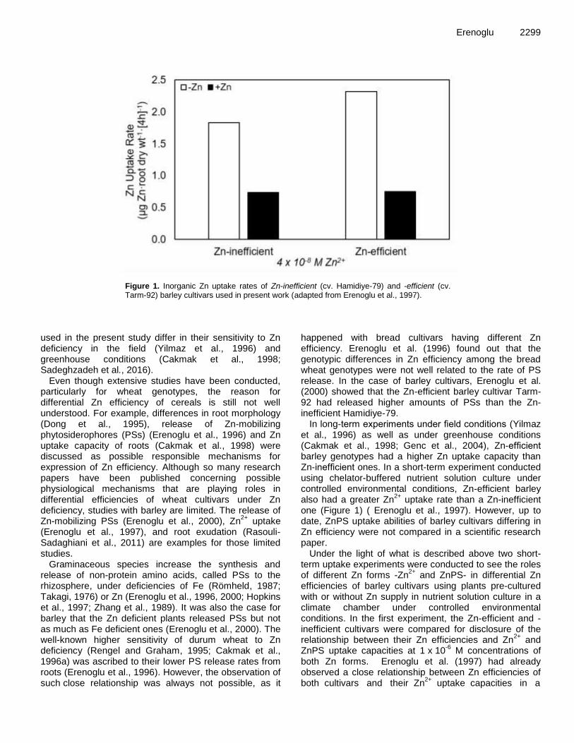
Erenoglu 2299
Figure 1. Inorganic Zn uptake rates of Zn-inefficient (cv. Hamidiye-79) and -efficient (cv. Tarm-92) barley cultivars used in present work (adapted from Erenoglu et al., 1997).
used in the present study differ in their sensitivity to Zn deficiency in the field (Yilmaz et al., 1996) and greenhouse conditions (Cakmak et al., 1998; Sadeghzadeh et al., 2016).
Even though extensive studies have been conducted, particularly for wheat genotypes, the reason for differential Zn efficiency of cereals is still not well understood. For example, differences in root morphology (Dong et al., 1995), release of Zn-mobilizing phytosiderophores (PSs) (Erenoglu et al., 1996) and Zn uptake capacity of roots (Cakmak et al., 1998) were discussed as possible responsible mechanisms for expression of Zn efficiency. Although so many research papers have been published concerning possible physiological mechanisms that are playing roles in differential efficiencies of wheat cultivars under Zn deficiency, studies with barley are limited. The release of Zn-mobilizing PSs (Erenoglu et al., 2000), Zn
2+ uptake
(Erenoglu et al., 1997), and root exudation (Rasouli-Sadaghiani et al., 2011) are examples for those limited studies.
Graminaceous species increase the synthesis and release of non-protein amino acids, called PSs to the rhizosphere, under deficiencies of Fe (Römheld, 1987; Takagi, 1976) or Zn (Erenoglu et al., 1996, 2000; Hopkins et al., 1997; Zhang et al., 1989). It was also the case for barley that the Zn deficient plants released PSs but not as much as Fe deficient ones (Erenoglu et al., 2000). The well-known higher sensitivity of durum wheat to Zn deficiency (Rengel and Graham, 1995; Cakmak et al., 1996a) was ascribed to their lower PS release rates from roots (Erenoglu et al., 1996). However, the observation of such close relationship was always not possible, as it
happened with bread cultivars having different Zn efficiency. Erenoglu et al. (1996) found out that the genotypic differences in Zn efficiency among the bread wheat genotypes were not well related to the rate of PS release. In the case of barley cultivars, Erenoglu et al. (2000) showed that the Zn-efficient barley cultivar Tarm-92 had released higher amounts of PSs than the Zn-inefficient Hamidiye-79.
In long-term experiments under field conditions (Yilmaz et al., 1996) as well as under greenhouse conditions (Cakmak et al., 1998; Genc et al., 2004), Zn-efficient barley genotypes had a higher Zn uptake capacity than Zn-inefficient ones. In a short-term experiment conducted using chelator-buffered nutrient solution culture under controlled environmental conditions, Zn-efficient barley also had a greater Zn
2+ uptake rate than a Zn-inefficient
one (Figure 1) ( Erenoglu et al., 1997). However, up to date, ZnPS uptake abilities of barley cultivars differing in Zn efficiency were not compared in a scientific research paper.
Under the light of what is described above two short-term uptake experiments were conducted to see the roles of different Zn forms -Zn
2+ and ZnPS- in differential Zn
efficiencies of barley cultivars using plants pre-cultured with or without Zn supply in nutrient solution culture in a climate chamber under controlled environmental conditions. In the first experiment, the Zn-efficient and -inefficient cultivars were compared for disclosure of the relationship between their Zn efficiencies and Zn
2+ and
ZnPS uptake capacities at 1 x 10⁻⁶
M concentrations of both Zn forms. Erenoglu et al. (1997) had already observed a close relationship between Zn efficiencies of both cultivars and their Zn
2+ uptake capacities in a

2300 Afr. J. Agric. Res. HEDTA chelator-buffered nutrient solution with 4 x 10
-8 M
free Zn2+
activity. That is why the second experiment was planned only with ZnPS to realize if the ZnPS uptake of both cultivars would differ by their Zn efficiency levels at a lower ZnPS concentration (4 x 10
-8 M).
MATERIALS AND METHODS Plant materials and pre-culture Two barley (Hordeum vulgare L. cvs. Tarm-92 and Hamidiye-92) cultivars were used in two independent nutrient solution experiments under controlled environmental conditions (a light/dark regime of 16/8 h, 24/20°C, 65-75% relative humidity, and a photosynthetic photon flux density of 300 µmol·m-2·s-1 at plant height provided by Sylvania FR 96 T lamps). Both cultivars had different Zn efficiency scores; and according to their performances in a field (Yılmaz et al., 1996) and a greenhouse (Cakmak et al., 1998) experiments, Tarm-92 and Hamidiye-92 were classified as Zn-efficient and -inefficient, respectively.
For both experiments, surface-sterilized seeds of barley cultivars were germinated in quartz sand moistened with saturated CaSO4 solution. After 5 days, seedlings were transferred to 2.8-L plastic pots (20 seedlings per pot) containing continuously aerated nutrient solution prepared as follows: (in mM): 0.88 K2SO4, 2.0 Ca(NO3)2, 0.25 KH2PO4, 1.0 MgSO4, 0.1 KCl, and as μM 100 Fe(III)EDTA, 1 H3BO3, 0.5 MnSO4, 0.2 CuSO4, and 0.02 (NH4)6Mo7O24. The Zn was supplied in the form of ZnSO4 at concentrations of 0 μM (for -Zn plants) and 1 μM (for +Zn plants). For both experiments, plants were pre-cultured in nutrient solution for 11 days; and to have a nutrient-free apoplast during short-term uptake experiment, they were removed into a micronutrient free solution for one day. Zn2+ uptake vs. ZnPS uptake (Experiment I) On day 12, a part of the plants was transferred into 0.5-L containers (each contained 2-bundles with two plants) and supplied with 1 x 10⁻⁶ M ZnSO4 or ZnPSs (hydroxymugineic -acid) + 500% excess of PSs, labeled with 65Zn (46 KBq) for 3 h in freshly prepared micronutrients free nutrient solution. Four replicas were used to represent each treatment. After the uptake period, the roots were washed with 1 mM CaSO4 and 1 mM NaEDTA for 10 min to remove extracellular 65Zn, respectively.
Following the termination of the experiment, each bundle in each pot was collected as one replica, and in total, each treatment had four independent replicates. The roots and shoots were harvested, dried, and ashed at 550°C. After that, the ashed samples were dissolved in HCl and assayed for 65Zn activity by liquid scintillation spectrometry.
For determining Zn nutritional status of plants grown for 12 days with or without Zn supply, the plants were harvested, separated into shoot and roots, oven dried (70°C), ashed at 500°C, dissolved in 1% HCl, and later on, analyzed using AAS (Atomic Absorption Spectroscopy). Four replicas were examined to represent each treatment. Zinc uptake at low ZnPS supply (Experiment II) After 11 days of pre-culture, the plants were transferred to micronutrients free solution and on day 12, a part of them was moved into 5-L containers (each contained 2-bundles with two plants) and supplied with 4 x 10⁻⁸ M ZnPSs (hydroxymugineic acid) + 500% excess of PSs, labeled with 65Zn (185 kBq) for 8 h in
freshly prepared micronutrients free nutrient solution. In this experiment as well, four replicas were used to represent each treatment. Root washing after uptake period; preparation of samples; and measuring the activities in them were also done as explained in Experiment I. Statistics Experiments were designed using four replicas for each treatment, and the results of each trait were analyzed using ANOVA and Duncan’s test at p < 0.05.
RESULTS Experiment I For clarifying the relationships between the Zn efficiencies of two barley cultivars and their Zn uptake capacities, a short-term uptake experiment was set up. Earlier results obtained using both varieties emphasized that there were relations between Zn efficiencies of both cultivars and their phytosiderophore releases (Erenoglu et al., 2000) and Zn
2+ uptake (Erenoglu et al., 1997). In
such a way, that the Zn-efficient cv. Tarm-92 reached up to higher PSs release rates and absorbed higher Zn
2+ in
comparison to the Zn-inefficient cv. Hamidiye-79. After 12 days of preculture with or without Zn
application, some growth parameters such as shoot and root dry weights and roots to shoot ratios (Table 1) and Zn contents per shoot or root dry weights (Table 2) of both cultivars revealed that the Zn-deficient plants of both varieties were suffering from Zn deficiency. Although the root dry weights of both cultivars were not affected by Zn composition of the nutrient solution, the shoot growths were significantly regressed by the non-sufficient supply of Zn. Because of this, roots to shoot ratios of plants grown without Zn were higher than control plants. Following these results, when the plants were supplied with deficient Zn, the Zn concentrations in shoot and roots of both cultivars decreased very drastically (Table 2).
Both barley cultivars pre-cultured without Zn tended to take more Zn
2+ and ZnPS up compared to those pre-
cultured with Zn supply (Figure 2a). However, Zn deficiency induced Zn uptake was much more evident for Zn
2+ than Zn-PS. While the Zn-deficient plants absorbed
up to 5.1-fold (Zn-efficient cv.) more Zn2+
in comparison to Zn-sufficient plants, the increment for Zn-phytosiderophores uptake was only 1.5-fold (Zn-efficient cv.). For neither inorganic Zn nor Zn-PS, there were no distinct differences among the cultivars. In fact, the Zn efficient cultivar, particularly in the case of Zn-PS, showed lower Zn uptake capacity than the Zn inefficient one.
When it comes to transport of absorbed Zn from roots to shoot, Figure 2b shows a similar tendency to that of the root uptake values. Both barley cultivars pre-cultured

Erenoglu 2301
Table 1. Shoot and roots dry weights and roots/shoot ratios of barley cultivars with different Zn efficiency. The plants were pre-cultured with or without Zn application for 11 days after five days germination period; and on day 17, supplied with 1 x 10⁻⁶ M 65Zn2+ (as ZnSO4) or 65Zn-PS (chelated with hydroxymugineic acid) for 3 h.
Parameter
Dry weights (mg plant-1
)
Shoot Roots Roots/Shoot
-Zn +Zn -Zn +Zn -Zn +Zn
1 x 10⁻⁶
M Zn
Zn-inefficient 47d 64
abc 20
c 18
c 0.42
a 0.27
b
Zn-efficient 62bc
74ab
26abc
24abc
0.42a 0.32
b
1 x 10⁻⁶
M ZnPS
Zn-inefficient 47d 60
dc 18
c 17
c 0.39
a 0.29
b
Zn-efficient 60dc
78a 25
ab 25
ab 0.42
a 0.32
b
Values are the means of four independent replicates. For each trait, numbers with different letters are significantly different from each other at p < 0.05 according to ANOVA and Duncan’s test.
Table 2. Zinc concentrations in shoot and roots of barley cultivars with different Zn efficiency. The plants were pre-cultured with or without Zn application for 11 days after five days germination period.
Parameter
Zn concentration (µg g-1
)
Shoot Roots
-Zn +Zn -Zn +Zn
Zn-inefficient 5.7c 56
a 9.3
c 71
b
Zn-efficient 4.3c 49
b 9.0
c 87
a
Values are the means of four independent replicates. For each trait, numbers with different letters are significantly different from each other at p < 0.05 according to ANOVA and Duncan’s test
without Zn tended to translocate more Zn2+
and Zn-PS from roots to shoot in comparison to those pre-cultured with Zn supply (Figure 2b). Moreover, the effect of Zn deficiency on the induction of this translocation was almost twice higher in comparison to the induction of uptake. Opposite to very distinct differences in Zn deficiency induced Zn uptake values for Zn
2+ than Zn-PS,
the distinctions in Zn translocation values for Zn2+
than Zn-PS became less. It is to say that; while the Zn-deficient plants translocated up to 9.6-fold (Zn-efficient cv.) more Zn
2+ in comparison to Zn-sufficient plants, the
increment for Zn-PS uptake was 3.8-fold (Zn-efficient cv.). Among the cultivars, there were no apparent differences for neither inorganic Zn nor Zn-PS translocations. Experiment II As mentioned above, in an earlier study conducted using chelator-buffered nutrient solution, a clear relationship between Zn efficiencies of both cultivars and their Zn
2+
uptake at 4 x 10⁻⁸
M free Zn2+
activity had already been
shown (Erenoglu et al., 1997). That is why another short-term uptake experiment was set up to study the relationships between Zn efficiencies of these two barley cultivars and their Zn uptake from a solution with 4 x 10
-8
M final Zn-PS concentration. After 12 days of pre-culture with or without Zn application, some growth parameters such as shoot and root dry weights and roots to shoot ratios of both cultivars harvested after the experiment revealed that the Zn-deficient plants of both cultivars were in Zn deficiency stress (Table 3). Since the behaviours of both varieties were similar to their performances in Experiment I, these observations are not given here.
Parallel to the results obtained in Experiment I, both barley cultivars pre-cultured without Zn showed a tendency to take more Zn-PS up compared to those pre-cultured with Zn supply (Figure 3a). However, although 25 times lower Zn-PS concentration than Experiment I was applied, similar to Experiment I, no apparent differences in Zn absorption of both cultivars were found. Moreover, the induction of Zn-PS uptake under Zn deficiency for both varieties was in similar range given for Experiment I.
Roots to shoot transport of Zn-PS in both cultivars are presented in Figure 3b. Similar to Experiment I, although there was no apparent genotypical difference, the amounts of Zn-PS translocated from roots to shoot increased in both varieties. DISCUSSION As it is in well-agreement with earlier studies (Erenoglu et al., 1996, 2000), the growth parameters and tissue Zn concentrations in shoot and roots of barley cultivars (Tables 1 and 2) were negatively affected from the deficient supply of Zn. It is to say that the Zn-deficient plants showed declined shoot growth, enhanced roots-to- shoot ratios, and dramatically decreases in Zn

2302 Afr. J. Agric. Res.
Figure 2. Zinc uptake and root-to-shoot translocation rates of barley cultivars with different Zn efficiency. The plants were pre-cultured with or without Zn application for 11 days after five days germination period; and on day 17, supplied with 1 x 10⁻⁶ M 65Zn2+ (as ZnSO4) or 65Zn-PS (chelated with hydroxymugineic acid) for 3 h. Values are the means of four independent replicates. For each trait, numbers with different letters are significantly different from each other at p < 0.05 according to ANOVA and Duncan’s test.
Table 3. Shoot and roots dry weights and roots/shoot ratios of barley cultivars with different Zn efficiency. The plants were pre-cultured with or without Zn application for 11 days after five days germination period; and on day 17, supplied with 4 x 10⁻⁸ M 65Zn-PS (chelated with hydroxymugineic acid) for 8 hours.
Parameter
Dry weights (mg plant-1
) Roots/Shoot
Shoot Roots
-Zn +Zn -Zn +Zn -Zn +Zn
4 x 10⁻⁸
M ZnPS
Zn-inefficient 65b 86
a 45
ab 34
b 0.69
a 0.40
c
Zn-efficient 81a 95
a 49
a 41
a 0.61
b 0.43
c
Values are the means of four independent replicates. For each trait, numbers with different letters are significantly different from each other at p < 0.05 according to ANOVA and Duncan’s test.

Erenoglu 2303
Figure 3. Zinc uptake (A) and root-to-shoot translocation (B) rates of barley cultivars with different Zn efficiency. The plants were pre-cultured with or without Zn application for 11 days after five days germination period; and on day 17, supplied with 4 x 10⁻⁸ M 65Zn-PS (chelated with hydroxymugineic acid) for 8 h. Values are the means of four independent replicates. For each trait, numbers with different letters are significantly different from each other at p < 0.05 according to ANOVA and Duncan’s test.
concentrations of the shoot and root tissues.
As scientifically well proven, plant species (Moraghan, 1984) and cultivars within a species, particularly in wheat (Cakmak et al., 1996b, 1998; Graham et al., 1992) significantly differ in their ability to take Zn up from soils or to utilize it internally. As in wheat, there are also sizeable genotypic differences among the barley cultivars concerning Zn efficiency (Graham et al., 1992; Yilmaz et al., 1996; Cakmak et al., 1998; Sadeghzadeh et al., 2016).
A large number of mechanisms contributing to Zn efficiency have been proposed which might be operative either in the rhizosphere or within plants; for example,
differences in root morphology, mycorrhizal infection, the release of Zn-mobilizing PSs, uptake, translocation, and compartmentation of Zn (Graham and Rengel, 1993). Shortly after this introduction, the reason for differential Zn efficiency of wheat genotypes was extensively studied but is still not well understood. Enhanced root growth (Dong et al., 1995), release of Zn-mobilizing PSs from roots (Cakmak et al., 1998), and an increased Zn uptake capacity of roots (Cakmak et al., 1998) were suggested as possible parameters determining Zn efficiency. For barley, only the release of PSs was investigated in detail among these possible mechanisms in differential Zn efficiencies of a species or cultivars within a species
2304 Afr. J. Agric. Res. (Erenoglu et al., 2000). Besides, the potential role of Zn
2+
uptake in Zn efficiency of the same barley cultivars was evaluated in short-term uptake experiment set up in a chelator-buffered nutrient solution (Erenoglu et al., 1997).
In accordance with an earlier study conducted using barley cultivars in chelator-buffered nutrient solution (Erenoglu et al., 1997), the Zn uptake by roots of barley plants is induced under Zn deficiency in conventional nutrient solution (Figures 2 and 3). Besides, this output is similar to those found in other cereals as well (Cakmak et al., 1998; Rengel and Hawkesford, 1997; Rengel and Wheal, 1997). Possibly, this induction in Zn
2+ uptake is
due to one (or combination) of the six members of ZIP family transporters which were recently found in barley suffering from Zn deficiency (Tiong et al., 2015).
As it was clearly proved, to some extent, differential Zn efficiency of cereals may be attributed to Zn
2+ uptake
capacities of cereals, particularly when compared to bread wheat, higher Zn efficiency of rye and lower efficiency of durum wheat to their higher and lower Zn
2+
uptake abilities, respectively (Cakmak et al. 1998). However, up till now, the reason for a higher Zn uptake rate of rye or lower Zn uptake of durum wheat under deficient supply of Zn is not scientifically clarified yet. Differences in the Zn uptake rates are also known within genotypes of a given cereal species such as sorghum (Ramani and Kannan, 1985), bread wheat (Rengel and Wheal, 1997), and barley (Erenoglu et al., 1997). However, no clear difference could be found between Zn-efficient and Zn-inefficient bread wheat cultivars in either uptake or root-to-shoot translocation rates of Zn (Cakmak et al. 1998). In the present study, the Zn-efficient and -inefficient barley cultivars did not show any consistency between their efficiencies and Zn
2+ uptake (Figure 2a).
This result was surprising since the Zn2+
absorptions of same cultivars had reflected perfect accordance with their Zn efficiencies in a chelator-buffered nutrient solution supplied with 4 x 10
-8 M free Zn in previous work
(Erenoglu et al., 1997). The reason for such discrepancy is not known and may be the result of different experimental conditions (that is, use of a chelate-buffered nutrient solution or 25 times lower free Zn activity than present experiment).
As it is well-known, graminaceous plant species increase capacities for PS release and Fe(III)-PS absorption under iron deficiency (Römheld and Marschner, 1986). In roots of maize high-affinity Fe(III)-phytosiderophore uptake is necessary to produce healthy plants and is strongly dependent on the YS1 gene (von Wiren et al., 1994) and there is the stoichiometric uptake of metal and ligand (von Wiren et al., 1995). Besides Fe, while the putative Fe-PSs transporter in maize (Zea mays L.) roots recognizes Zn-PS (von Wiren et al., 1996), ZmYS1 complements the growth defect of the zinc uptake-defective yeast mutant zap1 and transports PS-bound Zn into oocytes (Schaaf et al., 2004a). In parallel, the results of the present paper indicated that barley
could also take Zn-PS up (Figures 2a and 3a) and translocate it into shoots (Figures 2b and 3b). However, the opposite of Zn
2+ uptake (Figure 2a), the inductive
effect of Zn deficiency on Zn-PS uptake (Figures 2a and 3a) was very low. In agreement with this, in leaves of maize, while Fe deficiency upregulated ZmYS1 transcript levels very strongly, Zn deficiency had a minimal effect on it (Schaaf et al., 2004b). As it is for Zn
2+ uptake
(Figure 2a) and translocation (Figure 2b), no apparent relation exists between Zn efficiencies and Zn-PS uptake (Figures 2a and 3a) or its translocation into shoots (Figures 2b and 3b).
As mentioned above, in a previous study conducted using the same barley cultivars, a positive relationship between Zn efficiencies and Zn
2+ uptake rates had been
observed (Erenoglu et al., 1997); however, in the present study, this relation disappeared (Figure 2a). Besides, lower free Zn activity in chelate-buffered nutrient solution was mentioned as one of the possible reasons for this discordance. Nevertheless, the barley cultivars having differential Zn efficiencies did not show any differences concerning their Zn efficiencies for either ZnPS uptake or translocation (Figures 3a and 3b) even at a lower Zn concentration (4 x 10
-8 M) compared to the mentioned
study (Erenoglu et al. 1997).
Conclusion In line with earlier studies (Cakmak et al., 1998; Erenoglu et al., 1997, 1999; Rengel and Hawkesford, 1997; Rengel and Wheal, 1997), the Zn uptake by roots of barley supplied as either free (Zn
2+) or chelated (Zn-PS) was
induced under Zn deficiency (Figures 2a and 3a). However, the induction was much apparent for Zn
2+ than
Zn-PS. Although according to results of previous works (Erenoglu et al., 1997) that a close relationship between Zn
2+ uptake capacity of roots and Zn efficiencies of the
same barley cultivars might have existed, the outcomes of present research paper showed the opposite. In such a way, that neither the uptake of Zn
2+ and Zn-PS from roots
(Figures 2a and 3a) nor their translocation from roots-to-shoot (Figures 2b and 3b) had no compatible connection to the Zn efficiencies of barley cultivars. So the reason(s) for differential Zn efficiency within a given cereal species remained unclear including barley. Internal utilization efficiency might also be considered as a possible mechanism in differential efficiencies in cultivars of a species. Also, such differences within a species might also be combined results of multiple mechanisms, which are not easily followed experimentally in laboratory conditions.
ACKNOWLEDGEMENTS
The author thank DFG-Deutsche Forschungsgemeinschaft for the financial support and

Prof. Volker Römheld (†) for his guidance during the lab-works. This manuscript was prepared by using a part of the results obtained from the research project funded by DFG-Deutshe Forschungsgemeinschaft (Project No. DFG-RO 796/10). CONFLICT OF INTERESTS The author has not declared any conflict of interests. REFERENCES Cakmak I, Gülüt KY, Marschner H, Graham RD (1994). Effect of zinc
and iron deficiency on phytosiderophore release in wheat genotypes differing in zinc efficiency. Journal of Plant Nutrition 17:1-17.
Cakmak I, Sari N, Marschner H, Kalayci M, Yilmaz A, Eker S, Gülüt KY (1996b). Dry matter production and distribution of zinc in bread wheat and durum wheat genotypes differing in zinc efficiency. Plant and Soil 180:173-181.
Cakmak I, Torun B, Erenoglu B, Oztürk L, Marschner H, Kalayci M, Ekiz H, Yilmaz A. (1998). Morphological and physiological differences in the response of cereals to zinc deficiency. Euphytica 100:349-357.
Cakmak I, Yilmaz A, Kalayci M, Ekiz H, Torun B, Erenoglu B, Braun HJ (1996a). Zinc deficiency as a critical problem in wheat production in Central Anatolia. Plant and Soil 180:165-172.
Dong B, Rengel Z, Graham RD (1995). Root morphology of wheat genotypes differing in zinc efficiency. Journal of Plant Nutrition 18:2761-2773.
Erenoglu B, Cakmak I, Römheld V, Derici R, Rengel Z (1999). Uptake of zinc by rye, bread wheat, and durum wheat cultivars differing in zinc efficiency. Plant and Soil 209:245-252.
Erenoglu B, Cakmak I, Marschner H, Römheld V, Eker S, Daghan H, Kalayci M, Ekiz H (1996). Phytosiderophore release does not relate well with Zn efficiency in different bread wheat genotypes. Journal of Plant Nutrition 19:1569-1580.
Erenoglu B, Eker S, Cakmak I, Derici R, Römheld V (1997). Effect of Zn deficiency on zinc (65Zn) uptake of some barley cultivars (in Turkish). In: I. National Zinc Congress, 12-16 May 1997. Eskisehir, Turkey.
Erenoglu B, Eker S, Cakmak I, Derici R, Römheld V (2000). Effect of iron and zinc deficiency on release of phytosiderophores in barley cultivars differing in zinc efficiency. Journal of Plant Nutrition 23:1645-1656.
Genc Y, McDonald GK, Graham RD (2004). Differential expression of zinc efficiency during the growing season of barley. Plant and Soil 263:273-282.
Graham RD, Aschner JS, Hynes SC (1992). Selecting zinc-efficient cereal genotypes for soils of low zinc status. Plant and Soil 146:241-250.
Graham RD, Rengel Z (1993). Genotypic variation in zinc uptake and utilization by plants. In Zinc in Soils and Plants. Ed. A D Robson. pp. 107-118. Kluwer Academic Publishers, Dordrecht, The Netherlands.
Hopkins BG, Whitney DA, Lamond RE, Jolley VD (1997). Phytosiderophore release by sorghum, wheat, and corn under zinc deficiency. Journal of Plant Nutrition 21:2623-2637.
Moraghan JT (1984). Differential response of five species to phosphorus and zinc fertilizers. Communications in Soil Science and Plant Analysis 15:437-447.
Ramani S, Kannan S (1985). Zinc absorption and transport in young peanut seedlings. Communications in Soil Science and Plant Analysis 9:311-316.
Rasouli-Sadaghiani MH, Sadeghzadeh B, Sepehr E, Rengel Z (2011). Root exudation and zinc uptake by barley genotypes differing in Zn efficiency. Journal of Plant Nutrition 34:1120-1132.
Erenoglu 2305 Rengel Z, Graham RD (1995). Wheat genotypes differ in zinc efficiency
when grown in the chelate-buffered nutrient solution. I. Growth. Plant and Soil 176:307-316.
Rengel Z, Hawkesford MJ (1997). Biosynthesis of a 34-kDa polypeptide in the root-cell plasma membrane of a Zn-efficient wheat genotype increases upon Zn deficiency. Australian Journal of Plant Physiology 24: 307-315.
Rengel Z, Wheal WS (1997). Kinetic parameters of zinc uptake by wheat are affected by the herbicide chlorsulfuron. Journal of Experimental Botany 48:935-941.
Römheld V (1987). Different strategies for iron acquisition in higher plants. Physiologia Plantarum 70:231-234.
Römheld V, Marschner H (1986). Evidence for a specific uptake system for iron phytosiderophore in roots of grasses. Plant Physiology 80:175-180.
Sadeghzadeh B, Sadeghzadeh N, Sepehr E (2016). Barley Genotypes Differing in Zinc Efficiency When Grown in Various Soil Types. International Journal of Plant and Soil Science 12(4):1-13.
Schaaf G, Erenoglu BE, von Wirén N (2004a). Physiological and biochemical characterization of metal-phytosiderophore transport in graminaceous species. Soil Science and Plant Nutrition 50: 989-995.
Schaaf G, Ludewig U, Erenoglu BE, Mori S, Kitahara T, von Wirén N (2004b). ZmYS1 functions as a proton-coupled symporter for phytosiderophore- and nicotianamine-chelated metals. Journal of Biological Chemistry 279:9091-9096.
Takagi S (1976). Naturally occurring iron-chelating compounds in oat and rice-root washings. I. Activity measurements and preliminary characterization. Soil Science and Plant Nutrition 22:423-433.
Tiong J, McDonald G, Genc Y, Shirley N, Langridge P, Huang CY (2015). Increased expression of six ZIP family genes by zinc (Zn) deficiency is associated with enhanced uptake and root-to-shoot translocation of Zn in barley (Hordeum vulgare). New Phytologist 207:1097–1109
Von Wirén N, Marschner H, Römheld V (1995). Uptake kinetics of iron-phytosiderophores in two maize genotypes differing in iron efficiency. Physiologia Plantarum 93:611-616.
Von Wirén N, Marschner H, Römheld V (1996). Roots of ironefficient maize (Zea mays L.) take up also phytosiderophore chelated zinc. Plant Physiology 111:1119-1125.
Von Wirén N, Mori S, Marschner H, Römheld V (1994). Iron inefficiency in maize mutant ysl (Zea mays L. cv Yellow-Stripe) is caused by a defect in uptake of iron phytosiderophores. Plant Physiology 106:71-77.
Yilmaz A, Kalayci M, Ekiz H, Torun B, Oztürk L, Cakmak I (1996). Response of different barley genotypes to zinc fertilization in Central Anatolia (in Turkish). In: III. Malt and Barley Symposium, 5-7 September 1995. Konya, Turkey.
Zhang F, Römheld V, Marschner H (1989). Effect of zinc deficiency in wheat on the release of zinc and iron mobilizing exudates. Journal of Plant Nutrition and Soil Sciences 152:205-210.

Vol. 13(42), pp. 2306-2310, 18 October, 2018
DOI: 10.5897/AJAR2018.13420
Article Number: 4F707B158903
ISSN: 1991-637X
Copyright ©2018
Author(s) retain the copyright of this article
http://www.academicjournals.org/AJAR
African Journal of Agricultural
Research
Full Length Research Paper
Effect of Anacardium occidentale, Ricinus communis and Spirulina sp. on the diets of broiler chickens
Patricia Rossi1*, Lilian Kelly Pereira2, Sabrina Endo Takahashi1, Paulo Segatto Cella1, Patricia Franchi Freitas1, Jackeline Dall Agnol de Lima3, Pedro Valério Dutra de Moraes4 and
Guilherme Cesar Trindade de Freitas1
1Department of Animal Science, Federal Technologic University of Parana, UTFPR, Dois Vizinhos, Paraná, Brazil.
2Posgraduation Program in Animal Science, Federal Technologic University of Parana, UTFPR, Dois Vizinhos,
Paraná, Brazil. 3Depertment of Biology, Federal Technologic University of Parana, UTFPR, Dois Vizinhos, Paraná, Brazil.
4Department of Agronomy, Federal Technologic University of Parana, UTFPR, Dois Vizinhos, Paraná, Brazil.
Received 26 July, 2018; Accepted 19 September, 2018
The use of antibiotics as a growth promoter was banned because of residues that are left in animal products. Alternatives to antibiotics that promote animal growth and health without leaving residues in food are being sought. An experiment was conducted to evaluate the effects of a commercial mixture of functional oils and algae (FOA) on growth and gut morphology in broiler chickens. A total of 224 one day-old Cobb male broilers were randomly divided into 2 dietary treatment groups, with 8 replicate pens per treatment group (14 birds each). The dietary treatments consisted of a control basal diet without FOA, or control diet plus 1.50 kg/ton of FOA. The FOA was a commercial mixture of castor oil plant (Ricinus communis L.), Cashew nut oil (Anacardium occidentale L.) and spirulin (Spirulina sp.). Body weight and viability were not significantly influenced by treatments (P>0.05). Feed intake and feed conversion rate improved significantly upon the use of FOA (P<0.05). Villus height, villus width, crypt depth, or crypt diameter were not influenced by treatments. This therefore suggest that the use of FOA improves performance parameters in broiler chickens and is economically viable. Key words: Anacardium occidentale, body weight gain, feed conversion rate, villus height, Ricinus communis.
INTRODUCTION Feed additives have been used in the poultry industry for several decades. A number of additives, including antibiotics, have been used to manipulate gut function and microbial habitat with the objective of improving growth performance and feed conversion rate. However, growing concerns that antibiotic use could leave residues in animal products and increase resistance of disease-
causing microorganisms in humans led to decisions on their being banned as a feed additive. This also accelerated research on feed additive alternatives in animal production. In addition, consumers are demanding animal products that are free of residues and have minimal impact on the environment.
In the search of alternatives to antibiotics, several
*Corresponding author. E-mail: [email protected].
Author(s) agree that this article remain permanently open access under the terms of the Creative Commons Attribution
License 4.0 International License
natural alternatives such as probiotics, prebiotics, organic acids, enzymes, essential oils, and functional oils have been developed. As one of the alternatives, functional oils are used to improve only growth and reduction of pathogenic bacteria. Unlike essential oils which are obtained from plants oils (herbs) or spices, functional oils are obtained from seeds that have some added benefits and further energy value. (Bess et al., 2012). Their mode of action is similar to that of ionophores, inhibit resistant bacterial and provide antimicrobial, antioxidant, and anti-inflammatory properties.
Castor oil bean (Ricinus communis) and Cashew oil (Anacardium occidentale) are a by-product of the castor and cashew oil extraction industry, respectively. Castor oil is a Euphorbiaceae used primarily in the cosmetic industry. The world’s largest castor oil producers are India, China and Brazil. Castor oil is rich in ricinoleic acid, and chemical reactions involving this acid yield numerous compounds (Oliveira, 2012). The cashew is a tropical plant from north and from northeast Brazil belonging to the Anacardiaceae family. Cashew is rich in vitamin C, calcium, and iron, and is used primarily in some cuisines. Cashew oil (Anacardium occidentale) extracted from cashew fruit is composed of anacardiol acids, cardol and cardanol, which give an antioxidant effect to the oils extracted (Oliveira, 2012)
Recent studies have shown that adding castor and ricinus oils to poultry diet increased the growth performance and related antimicrobial and anti-inflammatory effects (Bess et al., 2012). In addition, castor oils in broiler diets reduce Escherichia coli present in the gut (López et al., 2012). Castor and ricinus oils added to broiler diets improves growth performance, metabolizable energy, and gut morphometry (Murakami et al., 2011). In addition, ricinus meals and oil do not negatively influence the growth performance, nutrient digestibility, or gut morphology of broiler chickens (Sobayo et al., 2012). In broiler chickens affected with coccidiosis, the functional oils improve energy utilization and survival rate and decrease lesions caused by coccidiosis in supplemented birds (Murakami et al., 2014).
Other substances, such as algae, may also contribute to an improvement in the health and performance of animals. Algae have antioxidant properties, and can stimulate the immune system. Also, algae can be utilized as an alternative ingredient to other protein sources because they are rich in amino acids (Becker, 2007), and in some instances, they can work as source of calcium (Souza, 2012), thus reducing feed cost when used as an alternative to other protein sources. The high demand for substitutes to antibiotics in poultry has triggered extensive research in this field. The current study aim to evaluate the effect of commercial mixtures made of functional oils and algae on the growth performance and the commercial mixture’s cost and benefit when applied to rearing of broiler chickens.
Rossi et al. 2307 MATERIALS AND METHODS
This experiment was approved by the Ethics Committee on Animal Use at Federal Technologic University of Parana, UTFPR, Dois Vizinhos, Paraná, Brazil, Protocol number: 2014-006. A total of 224 one day-old male Cobb broiler chickens were obtained from a commercial hatchery - Pluma Agro Avícola, Dois Vizinhos, PR, Brazil. The birds were weighed at a day-old and sorted by body weight into litter-floor pens of identical size (1 m2). The initial average Body Weight (BW) for all pens was 44.8 g. The dietary treatments consisted of control diet, plus a commercial mixture of functional oils with algae (FOA) (1.5 kg/ton), with 8 replicates of 14 birds each. The test product was a mixture of castor oil plant (R. communis L.), Cashew nut oil (A. occidentale L.) and spirulin (Spirulina sp.) from Natupremix LDTA. The feeding program consisted of a pre-starter diet, which was fed until 7 days of age; a starter diet which was fed from day 8 to 21; grower diet, which was fed from day 22 until 39; and finisher diet, which was fed from day 40 until 42 (Table 1). The diets were formulated to meet the requirements recommended by Rostagno et al. (2011) for broiler chickens.
The water and feed were ad libitum, and all diets were fed as mash. The feeder space for 50 old birds was provided as recommended by manufacturer. The light regimen was as follows: day 1 to 7, 23L:1D; day 8 to 21, 20L:4D; day 22 to 28, 14L:10D; day 29 to 35, 18L:6D; and day 36 to 42, 23L:1D (Moraes et al., 2008). The light intensity (lx) was reduced from 20lx from day 1 to 7 to 10-5lx from day 8 to 42 in accordance with standard management practice of Cobb manual. The temperature was reduced gradually from 32°C at beginning of the study to approximately 20°C at the end of the experiment and in accordance with standard management practice of Cobb manual. Data on body weight (BW) and feed consumption were measured on weekly basis and used to calculate the weight gain, feed intake, and feed conversion ratio. Mortality was recorded as it occurred. The economic viability was calculated according to Sogunle et al. (2014). At the end of the feeding trial (day 42), 1 bird per pen (8 birds/diet) was euthanized by cervical dislocation. Intestinal segment samples (approximately 3 cm in length) of duodenum, jejunum, and ileum were excised and flushed with 0.9% saline to remove the contents. For histology, gut segments were fixed in solution containing 85 ml of 80% ethanol, 15 ml of formaldehyde (37-40%), and 5 ml of glacial acetic acid for 16 hours. The segments of intestine collected were first section of the duodenum, a midpoint between the bile duct entry and Meckel’s diverticulum (jejunum), and midway between Meckel’s diverticulum and the ileocecal junction (ileum). Samples were dehydrated, cleared, and paraffin-embedded. Intestinal segments from 8 birds per dietary treatment were sectioned at a 5-μm thickness, placed on glass slides, and processed in Leica’s trichrome stain, the histological sections were stained with hematoxylin and eosin (HE) as described by Gava (2012). The morphometric indices evaluated were villus height, villus width, crypt depth, and crypt diameter, according to Gava (2012). Morphometric investigations were performed on 5 intact villi and 5 crypts from each intestinal segment of broiler chickens per treatment. All parameters were analyzed with an ANOVA, as a completely randomized design using the Statistix® software at P<0.05.
RESULTS AND DISCUSSION
The growth performance parameters are listed in Table 2. No treatment differences (P>0.05) were observed on body weight gain (BWG) and viability overall. However,

2308 Afr. J. Agric. Res. Table 1. Composition of experimental diets.
Ingredient (%) Pre-starter
d 1-7
Starter
d 8-21
Grower
d 22-39
Finisher
d 40-42
Maize 57.5 64.3 67.1 69.4
Soybean meal (48% CP1) 31.8 25.3 22.7 20.5
Soybean oil 0.7 1.1 1.6 2.2
Meat and bone meal (45% CP SPF2) 7.6 6.9 6.2 5.5
Vitamin and mineral premix3
2.4 2.4 2.4 2.4
Calculated chemical composition
AMEn4 (kcal/kg) 2926.25 3028.72 3090.93 3143.72
CP (%) 23.05 20.38 19.10 17.76
Fiber (%) 3.35 3.15 3.06 2.98
Lysine (%) 1.47 1.27 1.17 0.99
Methionine (%) 0.64 0.61 0.58 0.46
Threonine (%) 1.47 1.27 1.17 0.99
Calcium (%) 1.16 1.06 0.998 0.931
Phosphorus (%) 0.524 0.478 0.474 0.471
Sodium (%) 0.233 0.228 0.216 0.204
Linoleic acid (%) 1.78 2.06 2.35 2.69 1CP: crude protein.
2SPF: Specific Pathogen Free.
3Supplied per kilogram of diet, initial: vitamin A, 562.5 KUI; vitamin D3, 156.25 KUI; vitamin E, 1.25
g/kg; vitamin K3, 0.16 g/kg; vitamin B1, 0.13 g/kg; vitamin B2, 0.38 g/kg; vitamin B6, 0.19 g/kg; pantothenic acid,0.75g/kg; folicacid, 0.09% g/kg; vitamin B12, 0.94 mg/kg; iodine, 0.00147%; selenium, 0,00156%; copper, 0.04; manganese, 0.24%; zinc, 0.27%; iron, 0.24%; cupper, 0.04 mg; manganese, 0.24 %.Supplied per kilogramof diet, grower: vitamin A, 431.25 KUI; vitamin D3, 119.79 KUI; vitamin E, 0.96 g/kg; vitamin K3, 0.12 g/kg; vitamin B1, 0.10 g/kg; vitamin B2, 0.29 g/kg; vitamin B6, 0.14 g/kg; pantothenicacid, 0.58 g/kg; folicacid, 0.07 g/kg; vitamin B12, 0.72 mg/kg; iodine, 0.00417 %; selenium, 0.00120 %; copper, 0.04 %; manganese, 0.35 %; zinc, 0.27 %; iron, 0.00417 %.cupper, 0.04 mg; manganese, 0.24 %. Supplied per kilogram of diet, finisher: vitamin A, 300; vitamin D3, 83.33; vitamin E, 0.67; vitamin K3, 0.08; vitamin B1, 0.07; vitamin B2, 0.20; vitamin B6, 0.10; pantothenic acid, 0.40; folic acid, 0.05; vitamin B12, 0.50; iodine, 0.00417 %; selenium, 0.00083 %; copper, 0.04 %; manganese, 0.46 %; zinc, 0.27 %; iron, 0.00417 %; cupper, 0.27 %; manganese, 0.46%.
4AMEn: Apparent Metabolizable Energy corrected for nitrogen.
Table 2. Effect of functional oil and algae on growth performance of broiler chickens.
Variable Control FOA P value
Feed consumption, g
1-7d 177.7 167.6 ns
7-14d 370.7 328.4 ns
14-21d 671.8a
608.5b
0.0396
21-28d 1077.0a
941.2b
0.0002
28-35d 1356.5a
1247.7b
0.0073
35-42d 695.7 668.2 ns
1-42d 4349.2a
3961.5b
0.0019
Body weight gain, g
1-7d 132.1 132.0 ns
7-14d 266.9b
291.2a
0.0006
14-21d 404.7a
292.8b
0.0002
21-28d 694.0 667.6 ns
28-35d 771.5 792.6 ns
35-42d 676.8b
816.4a
<0.0001
1-42d 2946.0 2992.7 ns
Feed conversion, g:g
1-7d 1.34 1.27 ns
7-14d 1.39a
1.13b
0.0092
14-21d 1.67b
2.11a
0.0028

Rossi et al. 2309
Table 2. Contd.
21-28d 1.55a
1.41b
0.0157
28-35d 1.75a
1.58b
0.0491
35-42d 1.02a
0.82b
0.0003
1-42d 1.47a
1.32b
0.0003
Viability, %
1-42d 98.2 93.8 ns
Cost benefit to FOA
Cost of feed intake per bird per day, R$
1.18 1.06 -
Cost of feed intake per weight gain, R$
0.40 0.35 -
a-bValues in the same row with different superscript are significantly different (P<0.05); NS: P>0.05.
Table 3. Villus height, villus width, crypt depth, crypt diameter in duodenum, jejunum and ileum in chickens fed with or without FOA.
Treatments Control FOA P value
Duodenum
Villus height, µm 990.45 985.17 ns
Villus width, µm 187.85 182.07 ns
Crypt depth, µm 251.14 207.53 ns
Crypt diameter, µm 47.36a 38.32
b 0.0179
Jejunum
Villus height, µm 846.7 861.35 ns
Villus width, µm 156.08 167.35 ns
Crypt depth, µm 191.13 227.51 ns
Crypt diameter, µm 39.87 43.08 ns
Ileum
Villus height, µm 693.09 728.9 ns
Villus width, µm 161.58 161.71 ns
Crypt depth, µm 181.39 185.05 ns
Crypt diameter, µm 45.64 42.8 ns
a –b Values in the same row with different superscript are significantly different (P<0.05); NS: P>0.05.
low body weight gain in birds fed with FOA compared to control diets from 14 to 21 days of age was observed. Therefore, part of this reduction in BWG in birds supplemented with FOA could be attributed to dietary energy levels, since the product was added on top and this could reduce feed intake resulting in lower BWG. In addition, spirulin resulted to a reduced feed intake in rats Mitchell et al. (1990) and broilers Kharde et al. (2012), and could negatively affect the BWG results in this study. These results on growth performance are not in agreement with the results obtained by Bess et al. (2012), where birds supplemented with castor oils–CNSL mixture showed improved BWG. The viability results are not in agreement with those of Murakami et al. (2014) who observed that birds challenged with coccidiosis, when supplemented with functional oils improved in viability.
Feed intake and feed conversion rate (FCR) were
significantly affected by the dietary treatments (P<0.05). Birds fed with FOA had lower feed intake and feed conversion ratio compared to control diet (Table 2). This result is in consonance with the findings of Bess et al. (2012) who observed an improvement in feed conversion ratio in birds supplemented with castor oils–CNSL mixture, which showed an improvement in FCR. The reduction of feed consumption was visible on feeders during the experiment and affected the BWG within the 14-21day old chicks. The economic feasibility result (Table 2) showed that it is feasible to use FOA poultry diets, since the cost of feed intake per body weight gain was 0.05 cents lower and the cost of feed intake per bird per day was 0.12 cents lower when birds were fed supplementary FOA compared to control diet.
No differences (P>0.05) were observed in villus height, villus width, crypt depth, or crypt diameter between treatments (Table 3). An exception was a crypt diameter

2310 Afr. J. Agric. Res. in the duodenum (P<0.05), which was lower when birds were fed supplementary FOA than when they were fed the control diet (Table 3). These results are not in agreement with those reported by Murakami et al. (2014) that observed higher villus height in jejunum for birds supplemented with functional oils on 14 days. Since functional oils have antimicrobial properties, these could decrease microbial effects and improve performance parameters. Thus, functional oils may act as growth promoters by eliminating some pathogenic bacteria from the gastrointestinal tract. Conclusion The present study suggests that FOA is a useful feed additive for broiler chickens and it could be included in broiler diets to improve growth performance. The addition of FOA in the diets of broiler chickens till 42 days of age is economically feasible because it reduced the cost of feed intake of 0.12 cents of a bird per day. Further investigations are needed to evaluate better dose of FOA from 14 to 35 days of age, to reduce the negative effect on weight gain and feed intake. CONFLICT OF INTERESTS The authors have not declared any conflict of interests. REFERENCES Becker EW (2007). Micro-algae as a source of protein. Biotechnolology
Advances 25(2):207-210. Bess F, Fávero A, Silveira SL, Torrent J (2012). The effects of
functional oils on broiler diets of varying energy levels. Journal Applied Poultry Research 21:567-578.
Gava MS (2012). Metodologia de morfometria intestinal em frango de corte. [master's thesis]. Porto Alegre: Universidade Federal do Rio Grande do Sul.
Kharde SD, Shribhate RN, Bahiram KB, Nipane SF (2012). Effect of Spirulina supplementation on growth performance of broilers. Indian Journal of Veterinary Research 21:66-69.
López CAA, Lima KRS, Manno MC, Tavares FB, Fernandes Neto DL, Jesus MLC, Viana MAO, Fonseca LAB (2012). Effects of cashew nut shell liquid (CNSL) on the performance of broiler chickens. Arquivo Brasileiro de Medicina Veterinária e Zootecnia 64:1027-1035.
Mitchell GV, Grundel E, Jenkins M, Blakely SR (1990). Effects of graded dietary levels of Spirulina on vitamins A and E in male rats. 1990. The Journal of Nutrition 120:1235-1240.
Moraes DT, Lara, LJC, Baião NC, Cançado SV, Gonzalez ML, Aguilar CAL, Lana AMQ (2008). Efeitos de programas de luz sobre o desempenho, rendimento de carcaça e resposta imunológica em frangos de corte. 2008. Arquivo Brasileiro de Medicina Veterinária e Zootecnia 60:201-208.
Murakami AE, Eyng C, Torrent J (2011). Effects of functional oils on performance, apparent metabolizable energy and intestinal morphometry in broiler chickens. 2011. Proccedings of International Poultry Scientific Forum. Georgia World Congress Center - Atlanta, Georgia.
Murakami AE, Eyng C, Torrent J (2014). Effects of Functional Oils on
Coccidiosis and Apparent Metabolizable Energy in Broiler Chickens. 2014. Asian-Australian. Journal of Animal Science 27:981-989.
Oliveira JP (2012). Avaliação de óleos essenciais, extratos vegetais e óleos funcionais em dietas de frangos de corte. [master's thesis]. Curitiba: Universidade Federal do Paraná.
Rostagno HS, Albino LFT, Donzele JL, Gomes PC, Oliveira RF, Lopes DC, Ferreira AS, Barreto SLT, Euclides RF (2011). Tabelas brasileiras para aves e suínos: composição de alimentos e exigências nutricionais. 2
nd ed. Viçosa, MG: UFV, Departamento de
Zootecnia P 186. Sobayo RA, Oso AO, Adeyemi OA, Fafiolu AO, Jedege AV, Idowu
OMO, Dairo OU, Iyerimah RB, Ayoola OA, Awosanya RA (2012). Changes in growth, digestibility and gut anatomy by broilers fed diets containing ethanol-treated castor oil seed (Ricinus communis L.) meal. Revista Científica UDO Agrícola 12:660-667.
Sogunle OM, Akinosi OK, Adeyemi OA, Sobayo RA, Bello KO, Ekunseitan DA, Olaniyi OA (2014). Performance and carcass yield of sexed broiler chickens reared on two housing types. Bulletin of Animal Health and Production in Africa 62:85-94.
Souza YLS (2012). Use of the alga Lithothamnium calcareum for laying hens. [master's thesis]. Uberlândia: Universidade Federal de Uberlândia.

Vol. 13(42), pp. 2311-2323, 18 October, 2018
DOI: 10.5897/AJAR2018.13449
Article Number: 16D3D0158987
ISSN: 1991-637X
Copyright ©2018
Author(s) retain the copyright of this article
http://www.academicjournals.org/AJAR
African Journal of Agricultural
Research
Full Length Research Paper
Length of the growing season for dry rainfed farming under Monsoon climate in Gedarif, Sudan
Lotfie A. Yousif1, Abdelrahman A. Khatir2, Faisal M. El-Hag3, Ahmed M. Abdelkarim4, Hussain S. Adam5, Abdelhadi A. W.6, Yasunori Kurosaki7 and Imad-eldin A. Ali-Babiker3,7*
1Gedarif Research Station, Agricultural Research Corporation (ARC), Gedarif, Sudan.
2El Obied Research Station, Agricultural Research Corporation (ARC), El Obied, Sudan.
3Dry Lands Research Center (DLRC), Agricultural Research Corporation (ARC), Soba, Khartoum, Sudan.
4Sudan Meteorological Authority (SMA), Khartoum, Sudan.
5Water Management and Irrigation Institute, University of Gezira, Wad-Medani, Sudan.
6College of Graduate Studies, Desert and Arid Zones Sciences Program, Arabian Gulf University, Manama, Bahrain
(ARC Professor), Sudan. 7Arid Land Research Center (ALRC), Tottori University, Tottori, Japan.
Received 9 August, 2018; Accepted 28 September, 2018
Reliable information on the starting and ending of growing season as well as its length will greatly assist in appropriate planning for rainfed agriculture farming practices. The objective of this study is to determine the start, end and length of growing season, based on dependable rainfall during wet (20%), normal (50%) and dry (80%) years, which were retrieved from historical rainfall records analysis of seven stations in Gedarif state for the period 1985 to 2014. The seven studied stations were categorized into two groups according to the total seasonal rainfall. During wet years, Group I had about 900 mm/year and Group II about 700-790 mm/year. In normal years, Group I had about 660-700 mm/year and Group II had 515-570 mm/year. During dry years, Group I had 490-550 mm/year and Group II had 350-425 mm/year. The results showed consistent trend of starting dates of the growing seasons; regardless of the high seasonal variability and variation in amount and distribution of rainfall among the stations and seasons. Similar results were obtained using the MODIS Enhanced Vegetation Index (EVI) for three different years representing different probability levels (2013, dry; 2000, Normal; 2007, wet). Groups I and II in normal and wet years had 70 to 90% of the total annual rainfall during the growing season. In dry years, Group I had 70 to 80% of the total rainfall during the growing season, while Group II had only 50 to 65%. The two groups have indicated different seasonal characteristics (start of growth season, end of growth season and length of growth season) in the dry, normal and wet years. Length of the growth season increases with early start of the season and in wetter years. Key words: Season start, season end, sowing date, dry season, normal season, wet season.
INTRODUCTION Agricultural crops grow in favorable weather conditions for their emergence, vegetative growth, and ripening. For rainfed agriculture in the arid and semi-arid areas, like
Gedarif State in Sudan, water availability is the main constraint that limits the time crops can grow. Irregularities in rainfall reliability and spread have

2312 Afr. J. Agric. Res. contributed significantly to poor yields and high variability in production from year to year (Ogungbenro and Morakinyo, 2014; Araujo et al., 2016). The most important problems associated with rainfall variability as a result of changes in moisture availability are: (a) The highly variable dates of rainy season onset from one station to another; (b) The temporal (monthly and annual) distribution of the rainfall at each station or over a certain area; (c) The cessation and length of the rainy season. Hence, it is necessary to explore the rainfall and its spatial variability over space along with its length of growing period to make crop based decisions (Sathyamoorthy et al., 2017).
To avoid and mitigate the risks that accompanied annual rainfall variability, the concept of dependable rainfall is usually used in agricultural planning. The planner needs to know the amount of rainfall that can be depended upon with a certain degree of probability (Haque, 2005). Adam (2008) defined dependable rainfall as the rainfall which can be expected in a number of years out of a total number of years, expressed as percentage or probability. Accordingly, he described three types of years (seasons), dry, normal and wet, which corresponds to the probability of rainfall exceedance of 80, 50 and 20%, respectively. On the other hand, the availability of sufficient water at appropriate times is the most crucial factor determining the type and productivity of crops (Fox and Rockstrom, 2000). Thus, the rainfall distribution characteristics during the growing seasons affect the schedule of agricultural activities beginning with land preparation; through the crop variety selection and planting, to the time of harvest (Odekunle, 2004). In other words, reliable information of rainfall onset and cessation times, and thus the length of the growing season, will greatly assist on time land preparation, mobilization of inputs and equipment and will also reduce the risk involved in sowing too early or too late (Omotosho et al., 2000). Also, determination of the length of the growing season is a useful guide for fitting crops that are suitable for various agroecological zones (Adam, 2008; Legese et al., 2018).
Growing season can be defined as the period during which rainfall distribution characteristics are appropriate for crop germination, establishment, growth and ripening. Hence, the onset and cessation of rainfall are of special important in rainfed agriculture growing season. The combination of these two determines the length of the growing season. The length of the growing season, under rainfed conditions, is defined as the period from the date of the onset of the rainy season to the date of its cessation (Mhizha et al., 2012).
The length of the growing season can be estimated using different methods. Benoit (1977) and Adam (2008)
used the relation between rainfall and evapotranspiration to determine the onset, cessation and length of the growing season (FAO, 1978); however, other researchers have used rainfall alone (Adejuwon et al., 1992; Ati et al., 2002). Odekunle (2004) identified two approaches in using rainfall data alone: one approach based on certain threshold value and the other one based on certain proportion relative to the total rainfall. Likewise, satellite images were also used to determine the characteristics of growing season's (Vrieling, et al., 2013).
Gedarif State in Eastern Sudan encompasses vast areas, around 3 million hectares, suitable for crop production, which depend totally on rainfall. These areas extend through different climatic zones, with different rainfall amount and onset and cessation dates. The annually cropped areas as well as crop yields fluctuate with the variability in rainfall amount and distribution (Ali Babiker et al., 2015). Therefore, to ensure maximum and sustainable agricultural productivity together with efficient water management, reliable information of dependable annual rainfall, the start and cessation dates of rainfall and the length of the rainy season are important. The objective of this study was to determine the start, end and length of the growing season based on dependable rainfall, expressed as a percent of the descending rank order of annual rainfall (Critchley et al.,1991 and Adam, 2008) as explained in the section below, namely: wet (20%), normal (50%) and dry (80%) years. These are retrieved from historical rainfall records analysis for seven stations in Gedarif State for the period 1985 to 2014.
MATERIALS AND METHODS
Study area and collected data
Gedarif State is in the Eastern part of the Sudan between latitudes 12.67° and 15.75°N and longitudes 33.57° and 37.0°E, covering 71000 km2 (Figure 1). The state stretches from North to South through three climate zones: arid, semi-arid and the dry monsoon zones (Adam, 2008). The soil is heavy cracking clay soils (Vertisols), characterized by shrinking when dry and swelling when wet. The mean daily maximum temperature reaches 33.4°C in May and drops to about 26.3°C in January. The relative humidity varies from 22% in March to 71% in August, as published by Sudan Metrological Authority (SMA, 2010). Rainfall is always in summer and most of rainfall events occur within June to September (JJAS); resulting in a short-single rainfed growing season per year. To achieve the objectives of this study, rainfall data were obtained from the records of Mechanized Farming Corporation (MFC). Monthly data (April to October) for seven stations during 30 years (1985 to 2014) period were used. These stations are scattered in the major rainfed agricultural production areas of Gedarif State. Figure 1 portrays the names and geographical locations of these stations (Umseenat, Samsam, Douka, Alhawaata, Alhoory, Gedarif (MFC office) and Gadambalia). Moreover, monthly potential
*Corresponding author. E-mail: [email protected].
Author(s) agree that this article remain permanently open access under the terms of the Creative Commons Attribution
License 4.0 International License
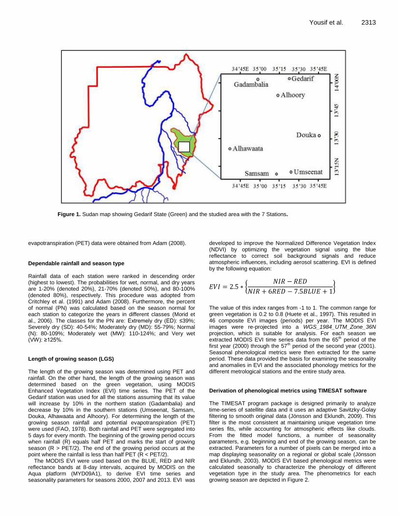
Yousif et al. 2313
Figure 1. Sudan map showing Gedarif State (Green) and the studied area with the 7 Stations.
evapotranspiration (PET) data were obtained from Adam (2008). Dependable rainfall and season type Rainfall data of each station were ranked in descending order (highest to lowest). The probabilities for wet, normal, and dry years are 1-20% (denoted 20%), 21-70% (denoted 50%), and 80-100% (denoted 80%), respectively. This procedure was adopted from Critchley et al. (1991) and Adam (2008). Furthermore, the percent of normal (PN) was calculated based on the season normal for each station to categorize the years in different classes (Morid et al., 2006). The classes for the PN are: Extremely dry (ED): ≤39%; Severely dry (SD): 40-54%; Moderately dry (MD): 55-79%; Normal (N): 80-109%; Moderately wet (MW): 110-124%; and Very wet (VW): ≥125%. Length of growing season (LGS) The length of the growing season was determined using PET and rainfall. On the other hand, the length of the growing season was determined based on the green vegetation, using MODIS Enhanced Vegetation Index (EVI) time series. The PET of the Gedarif station was used for all the stations assuming that its value will increase by 10% in the northern station (Gadambalia) and decrease by 10% in the southern stations (Umseenat, Samsam, Douka, Alhawaata and Alhoory). For determining the length of the growing season rainfall and potential evapotranspiration (PET) were used (FAO, 1978). Both rainfall and PET were segregated into 5 days for every month. The beginning of the growing period occurs when rainfall (R) equals half PET and marks the start of growing season (R > PET/2). The end of the growing period occurs at the point where the rainfall is less than half PET (R < PET/2).
The MODIS EVI were used based on the BLUE, RED and NIR reflectance bands at 8-day intervals, acquired by MODIS on the Aqua platform (MYD09A1), to derive EVI time series and seasonality parameters for seasons 2000, 2007 and 2013. EVI was
developed to improve the Normalized Difference Vegetation Index (NDVI) by optimizing the vegetation signal using the blue reflectance to correct soil background signals and reduce atmospheric influences, including aerosol scattering. EVI is defined by the following equation:
The value of this index ranges from -1 to 1. The common range for green vegetation is 0.2 to 0.8 (Huete et al., 1997). This resulted in 46 composite EVI images (periods) per year. The MODIS EVI images were re-projected into a WGS_1984_UTM_Zone_36N projection, which is suitable for analysis. For each season we extracted MODIS EVI time series data from the 65th period of the first year (2000) through the 57th period of the second year (2001). Seasonal phenological metrics were then extracted for the same period. These data provided the basis for examining the seasonality and anomalies in EVI and the associated phonology metrics for the different metrological stations and the entire study area. Derivation of phenological metrics using TIMESAT software The TIMESAT program package is designed primarily to analyze time-series of satellite data and it uses an adaptive Savitzky-Golay filtering to smooth original data (Jönsson and Eklundh, 2009). This filter is the most consistent at maintaining unique vegetation time series fits, while accounting for atmospheric effects like clouds. From the fitted model functions, a number of seasonality parameters, e.g. beginning and end of the growing season, can be extracted. Parameters for a number of pixels can be merged into a map displaying seasonality on a regional or global scale (Jönsson and Eklundh, 2003). MODIS EVI based phenological metrics were calculated seasonally to characterize the phenology of different vegetation type in the study area. The phenometrics for each growing season are depicted in Figure 2.
𝐸𝑉𝐼 = 2.5 ∗ 𝑁𝐼𝑅 − 𝑅𝐸𝐷
𝑁𝐼𝑅 + 6𝑅𝐸𝐷 − 7.5𝐵𝐿𝑈𝐸 + 1
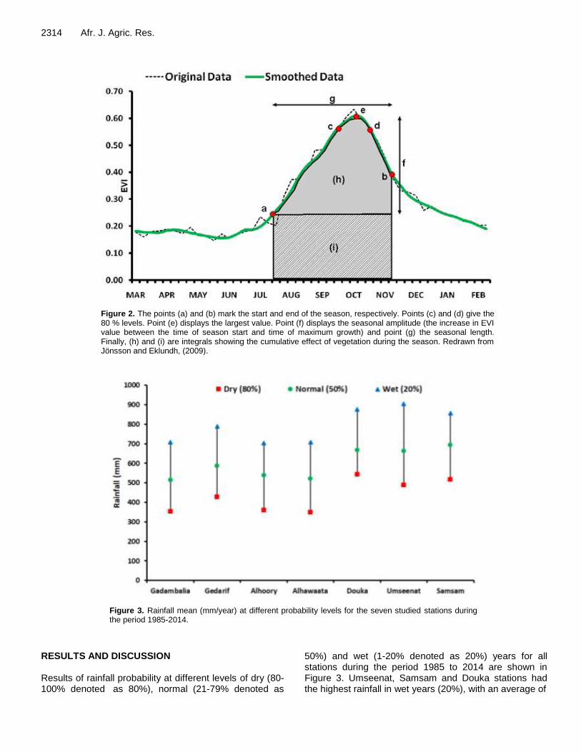
2314 Afr. J. Agric. Res.
Figure 2. The points (a) and (b) mark the start and end of the season, respectively. Points (c) and (d) give the 80 % levels. Point (e) displays the largest value. Point (f) displays the seasonal amplitude (the increase in EVI value between the time of season start and time of maximum growth) and point (g) the seasonal length. Finally, (h) and (i) are integrals showing the cumulative effect of vegetation during the season. Redrawn from Jönsson and Eklundh, (2009).
Figure 3. Rainfall mean (mm/year) at different probability levels for the seven studied stations during the period 1985-2014.
RESULTS AND DISCUSSION Results of rainfall probability at different levels of dry (80-100% denoted as 80%), normal (21-79% denoted as
50%) and wet (1-20% denoted as 20%) years for all stations during the period 1985 to 2014 are shown in Figure 3. Umseenat, Samsam and Douka stations had the highest rainfall in wet years (20%), with an average of

Yousif et al. 2315
Figure 4. The number of years (frequency) for different classes of Percent of Normal (PN) are: Extremely dry (ED): ≤39%; Severely dry (SD): 40-54%; Moderately dry (MD): 55-79%; Normal (N): 80-109%; Moderately wet (MW): 110-124%; and Very wet (VW): ≥125%. the percent of normal (PN) was calculated based on the season normal for each station for the period 1985-2014.
about 900 mm/year. Alhawaata, Alhoory, Gedarif and Gadambalia had the lowest values of rainfall in wet years, which ranged between 700 and 790 mm/year. In normal years (50%) rainfall was high in Samsam, Douka and Umseenat (660 to 700 mm) compared to the other four stations, which ranged between 515 and 570 mm/year. Rainfall in dry years (80%) followed the same trends and was higher in Umseenat, Samsam and Douka stations (490-550 mm/year) than the other four stations (Alhawaata, Alhoory, Gedarif and Gadambalia) in which the range was between 350-425 mm/year. From these results, based on the probability and total amount of rainfall, the stations of Umseenat, Samsam and Douka could be grouped in the same rainfall-zone (Group I: rainfall range from 500 to 900 mm/year). On the other hand, Alhawaata, Alhoory, Gedarif and Gadambalia could be grouped in another rainfall-zone (Group II: rainfall range 350 to 790 mm/year). These results were supported by the earlier classification of the stations into two groups (Yousif et al., 2018). This information on rainfall amount at different probability levels is useful as guidelines for farmers in these sites, because it can facilitate their seasonal planning choices based on the seasonal forecasts delivered to them by the meteorological services.
Figure 4 shows the number of years for different classes of Percent of Normal (PN). In all stations, the years with normal rainfall (80-100%) were the most
frequent. In Group I stations (Samsam, Douka and Umseenat), 50-60% of their years were normal. In Group II ((Alhawaata, Alhoory, Gedarif and Gadambalia), 40-55% of their years were normal. The other classes of the PN did show consistency in their frequency to the two groups of stations. However, the dry year’s classes (Severely dry (SD): 40-54%; Moderately dry (MD): 55-79%) tended to have more frequency in Group II stations. None of Group I stations showed any incidence of severely dry (SD) years (40-54%). All the stations did not show any incidences of extremely dry (ED) years (≤39%). Previous regional studies in eastern Africa showed future drying will have a radical impact on growing season length and agriculture (Cook and Vizy, 2012; Cook and Vizy, 2013). Sayari et al. (2013) reported that higher drought (dry years) frequency associated with global warming and increase in drought frequency would have major implications for natural resource management, water security planning, and water demand management strategies.
Figure 5 displays the start, length, and end of the growing season at the seven stations during the period at dry (80%), normal (50%) and wet (20%) years. There were variations in the start of the growing season in these stations. The growing season in dry years started between 25 and 30 of June in Group I; while it started late between the 1st and 20th of July in Group II. For normal years it started in first half of June in Group I;

2316 Afr. J. Agric. Res.
Figure 5. Growing season start, length and end determined by the Rainfall/Evapotranspiration (R/ET) ratio at different probability levels (Dry, 80%; Normal, 50%; Wet, 20%) for the seven studied stations during the period 1985-2014. Numbers in the centre of the bars indicate the length of the season.
while in Group II, started late between the last week of June and first week of July. In wet years it started earlier in the first 10 days of June in Group I and in the last days of June in Group II. These results revealed a consistent
trend of starting dates of the growing seasons; regardless of the high seasonal variability and variation in amount and distribution of rainfall among the stations and seasons. Similar results were obtained (Figure 6) using
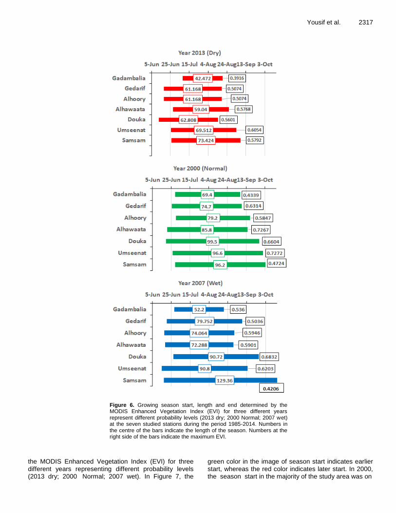
Yousif et al. 2317
Figure 6. Growing season start, length and end determined by the MODIS Enhanced Vegetation Index (EVI) for three different years represent different probability levels (2013 dry; 2000 Normal; 2007 wet) at the seven studied stations during the period 1985-2014. Numbers in the centre of the bars indicate the length of the season. Numbers at the right side of the bars indicate the maximum EVI.
the MODIS Enhanced Vegetation Index (EVI) for three different years representing different probability levels (2013 dry; 2000 Normal; 2007 wet). In Figure 7, the
green color in the image of season start indicates earlier start, whereas the red color indicates later start. In 2000, the season start in the majority of the study area was on

2318 Afr. J. Agric. Res.
Figure 7. Starts of the growing seasons in the study area covering the 7 stations for seasons (a) 2000, (b) 2007, and (c) 2013 as detected by the MODIS Enhanced Vegetation Index (EVI) based on the BLUE, RED and NIR reflectance bands at 8-day intervals, acquired by MODIS on the Aqua platform (MYD09A1).
17 June. There was an earlier start (May) in the area extending between Samsam and Alhawaata, whereas later start (July) was around Gadambalia and east of Gedarif (Figure 7a). In 2007, the season started in almost half of the study area in the period extending from 16 May to the 1
st of June (green-yellow color); whereas, in
the other half (brown-red color) the season started between 25 June to 11 July (Figure 7b). In 2013, the season started in most of the study area as late as July. Smaller areas had earlier starting dates in late May and early June (Figure 7c)
Adam (2008) has studied the growing season in Gedarif during the period 1941- 1970. His results showed systematic trend of growing season commencement, it started early on 27 May and late on 21 July. The starting dates of the growing season denote dates of seeding or germination of crops, inferring that seedbed preparation must be done earlier; that is, before the start of the growing season. However, farmers have a propensity to delay sowing dates due to many reasons; a) they do not do seeding during the beginning of the wet period (22
July to 3rd of August), the period is locally known as “Natra”, because of remarkable insect's activity (Adam, 2015); b) they wait until the soil moisture is sufficient to seal all the soil cracks and adequate to germinate the seeds; and c) after weed germination to control weeds using wide level disc harrow with seeding box in one operation for economic considerations. Generally, it could be avowed that in Southern areas (Group I) the season started as early as mid-June and in Northern areas (Group II) it started around mid-July. For the ending of the season (Figures 5 and 6), the growing season in dry years (80%), ended in the third week of September in areas of Group I, while it ended earlier in first week of September in areas of Group II. In normal years, it ended in the fourth week of September for stations of Group I and second to third weeks of September in stations of Group II. In wet years, it ended in the first week of October in Group I areas and third to fourth weeks of September in Group II areas. It could be stated that in southern areas (Group I) the end of the growing season occurred late September and early October; while in

Central-Northern areas (Group II) it ended in early to mid-September. A pervious study (1941-1970) by Adam (2008) showed that the growing season in Gedarif (Group II area) ended around the first week of October. It seemed that the growing season in this study ended earlier by 7 to 10 days compared to this previous study. An early cessation of the growing season will adversely affect the rainfed agriculture (Amekudzi et al., 2015), these periods are critical to crop maturity, and may also lead to crop failure. This implies that farmers have to grow short maturing varieties for successful production, especially in the dry years that are characterized by early seasonal cessations.
Length of the growing season (LGS) is also depicted in Figure 5. In dry years it varied from 85 to 90 days in areas of Group I, while between 45 to 65 days in areas of Group II. The general trend is that the wetter the years the longer the growing season. In normal years, it ranged between 100 to 110 days and 65 to 85 days for areas of Group I and Group II, respectively. In wet years it ranged between 115 to 120 days for Group I areas and 75 to 105 days for Group II areas. It is clear that areas of Group I have longer growing seasons compared to areas of Group II. This was due to the early start and later end of the growing season. This is in agreement with Mubvuma (2013) who showed that there was a strong correlation between the onset of the rainy season and the LGS. He showed that the LGS increases with the earlier onset of the rainy season. In this study, the LGS increased with the early start of the growing season and late end of it. The LGS was variable among the studied stations, however, it was generally longer in Group I and shorter in Group II. The length of the growing season varies from one station to another due to variation in rainfall (Amekudzi et al., 2015) and also it is possible there is a very high spatial variability between stations, and temporal variability within each station (Ayanlade et al., 2018). However, variability in the length of growing season is dominant in arid and semi-arid areas, and is susceptible to crop failure risk (Vrieling et al., 2013).
The MODIS Enhanced Vegetation Index (EVI) determination of LGS in year 2000 (normal year) revealed that the LGS varied between 85 to 70 days for Group II with no variations for Group I (Figure 6). In year 2007 (wet), much variation was noticed in the length of the season in both groups. In Group II, Gadambalia recorded lower days (52 days) than the other three stations in the range of 72 to 79 days. In Group I, Samsam recorded as high as 129 days, while the other two stations about 90 days. In year 2013 (dry), there was a shorter LGS with fewer variations, which was between 42 days in Gadambalia and 73 days in Samsam. Over all, the LGS based on the R/ET ratio at different probability levels and EVI displayed that in the wet years it was longer and in the dry years was shorter. For the study area as a whole (Figure 8a), the length of the season during the year 2000 (normal) was two months, but in
Yousif et al. 2319 some locations (between Alhawaata and Samsam), the length was three months. Smaller areas recorded one month, while in the areas around water courses the length was four months. In year 2007 (wet), the growing season was very long in more than half of the study areas, especially in the east-south direction, where the season was recorded as four months. When analyzing data in the north-west direction, the length becomes less (three months), and finally it becomes two months in the north-west corner (Figure 8b). The LGS was similar in the years 2000 and 2013 (two months in general), with the exception of areas in the north-west corner (one month) and areas in the east-north corners (three months). In the areas around water courses (Figure 8c), the length of the season was four months.
The maximum EVI value during the growing season indicates maximum vegetative growth (Figure 9). For the three different years representing different probability levels (2013 dry; 2000 Normal; 2007 wet); the maximum value in Gedarif, Umseenat and Alhawaata was recorded in year 2000. In Gadambalia, Alhoory and Douka the maximum production was recorded in year 2007. Samsam is the only station that recorded maximum vegetative growth in year 2013. Regarding the entire study area, it could be noted that years 2000 and 2007 were similar in most areas recording higher values (0.60- 0.95); whereas the recorded lower values (0.15, 0.30) were in very small patches (Figure 10.a and 10.b). In year 2013 values of maximum EVI decreased (Figure 10c), as the majority of study area recorded medium value (0.45- 0.60). There was less area recorded in the north-east corner (0.60-0.75), and lower values of EVI (0.15-0.30) in the north-west corner (Figure 10c).
The average distribution of rainfall received in each station before, during and after the growing season for different rainfall probabilities (20%, 50%, and 80%) seasons is shown in Figure 11. The rainfall amount during the growing season in areas of Group I ranged between 370 - 400 mm; 565 - 610 mm; and 765 - 825 mm, in dry, normal and wet years, respectively. For Group II, rainfall ranged between 170- 265 mm; 360 - 460 mm; and 540 - 660 mm in dry, normal and wet years, respectively. It is clear that for both Group I and Group II in normal and wet years that the growing season received 70 to 90% of the total rainfall during the year. This is in agreement with and confirms, the early start of the growing season during wet and normal years with lower rainfall risks in all the studied areas. However, in dry years, Group I received 70 to 80% of the total rainfall during the growing season, while Group II received only 50 to 65% of total rainfall during the growing season. This shows that the rainfall risks during the dry years is higher for Group II than Group I. Before and after the growing season, fewer rain amounts occurred in areas of Group I compared to areas of Group II. Generally, less than 20 mm rainfall occurred before or after the growing season in areas of Group I; however, in areas of Group II, about

2320 Afr. J. Agric. Res.
Figure 8. Length of the growing seasons in the study area covering the 7 stations for seasons (a) 2000, (b) 2007, and (c) 2013 as detected by the MODIS Enhanced Vegetation Index (EVI).
Figure 9. Maximum EVI values in seven studied stations for three different years represent different probability levels (2013 dry; 2000 Normal; 2007 wet) at the seven studied stations during the period 1985-2014.
EV
I

Yousif et al. 2321
Figure 10. Maximum values of Enhanced Vegetation Index (EVI) values (maximum vegetative growth) in the study area covering the 7 stations for seasons (a) 2000, (b) 2007, and (c) 2013.
25 to 50% of rainfall happened outside the growing season period, especially in the dry years. This information on the amount of rainfall at different probability levels is useful for farmers in the studied areas, which can facilitate the choice of appropriate crop and variety that can be grown most productively. Conclusions The studied stations can be categorized into two groups according to the total seasonal rainfall. The two groups have indicated different seasonal characteristics (start of growth season, end of growth season and length of growth season) in the dry, normal and wet years. Length of the growth season increases with early start of the season and in the wetter years. In general, the results of this study suggest that adaptive, climate-informed practices, such as planting short maturing varieties and employing early sowing dates coupled with water
harvesting techniques, should be used in areas of short growing seasons, (such as group II). In areas of extended growing season (such as group I), suitable crops and varieties with appropriate climate smart crop management practices should be used. Farmers are advised to use suitable adaptation cultural practices to avoid water logging during the seedling stage in areas of Group I, and appropriate strategies to avoid water shortage during flowering and maturity stages in areas of Group II. CONFLICT OF INTERESTS The authors have not declared any conflict of interests ACKNOWLEDGEMENT The authors would like to appreciate the Mechanized Farming Corporation in Gedarif State, Sudan for

2322 Afr. J. Agric. Res.
Figure 11. Seasonal rainfall distribution before, during and after the growing season at different probability levels (Dry, 80%; Normal, 50%; Wet, 20%) for the seven stations during the period 1985-2014.

providing rainfall data of the seven stations in the studied area. REFERENCES Adam HS (2008). Agroclimatology, Crop Water Requirement and Water
Management; Gezira University Printing and Publishing Co. LTD, Wad Medani, Sudan.
Adam HS (2015). Indigenous Knowledge and Irrigation in Sudan. Sudan Academy of Sciences Journal-Special Issue (Climate Change) 11(1):234-235.
Adejuwon JO, Balogun EE, Adejuwon SA (1990). On the Annual and Seasonal Pattern of Rainfall Fluctuations in Sub-Saharan West Africa. International Journal of Climatology 10:810-848.
Ali Babiker IA, El-Hag FAM, Abdelkarim AM, Abdalla AK (2015). Changing Climate and Farming Productivity in the Drylands of Eastern Sudan. Sudan Academy of Sciences Journal-Special Issue (Climate Change) 11(1):56-61.
Amekudzi LK, Yamba EI, Preko K, Asare EO, Aryee J, Baidu M, Codjoe SNA (2015). Variabilities in rainfall onset, cessation and length of rainy season for the various agro-ecological zones of Ghana. Climate 3:416-434.
Araujo JA, Abiodun BJ, Crespo O (2016). Impacts of drought on grape yields in Western Cape, South Africa. Theoretical and Applied Climatology 123:117-130.
Ati OF, Stigter CJ, Oladipupo EO (2002). A comparison of methods to determine the onset of growing season in northern Nigeria. International Journal of Climatology 22:731-742.
Ayanlade A, Radeny M, Mortonc JF, Muchaba T (2018). Rainfall variability and drought characteristics in two agro-climatic zones: An assessment of climate change challenges in Africa. Science of the Total Environment 630:728-737.
Benoit P (1977). The start of the growing season in northern Nigeria. Agricultural Meteorology 18:91-99.
Cook KH, Vizy EK (2012). Impact of climate change on mid-twenty-first century growing seasons in Africa. Climate Dynamics 39:2937-2955.
Cook KH, Vizy EK (2013). Projected changes in East African rainy seasons. Journal of Climate 26:5931-5948.
Critchley W, Siegert K, Chapman C (1991). A Manual for the Design and Construction of Water Harvesting Schemes for Plant Production. FAO (AGL/MISC/17/91). http://www.fao.org/docrep/U3160E/u3160e00.HTM
Food and Agricultural Organization (FAO) (1978). Report on the agroecological zones project Food and Agricultural Organization, Rome, Italy.
Fox P, Rockström J (2000). Water-Harvesting for Supplementary Irrigation of Cereal Crops to Overcome Intra-Seasonal Dry-Spells in the Sahel. Physics and Chemistry of the Earth (B) 25(3):289-296.
Haque AM (2005). Estimating monthly and yearly dependable rainfall for different climatic zones of the world Songklanakarin Journal of Science and Technology 27(3):667-673.
Huete AR, Batchily H, Liu K, van Leeuwen W (1997). A Comparison of Vegetation Indices Over a Global Set of TM Images for EOS-MODIS. Remote Sensing of Environment 59(3):440-451.
Jönsson P, Eklundh L (2003). Seasonality extraction from time-series of satellite sensor data. In Frontiers of Remote Sensing Information Processing, C.H. Chen (Ed.), 487-500.World Scientific Publishing.
Jönsson P, Eklundh L (2009). TIMESAT 3.0, Software Manual. Department of Earth and Ecosystem Sciences, Lund University, S-223 62 Lund, Sweden. Center for Technology Studies, Malmö University, S-205 06 Malmö, Sweden.
Yousif et al. 2323 Legese W, Koricha D, Ture K (2018). Characteristics of seasonal
rainfall and its distribution over Bale Highland, Southeastern Ethiopia. Journal of Earth Science and Climatic Change 9(2):443-449.
Mhizha T, Geerts S, Vanuytrecht E, Makarau A, Raes D (2012). Relative transpiration as a decision tool in crop management: a case for rainfed maize in Zimbabwe. African Crop Science Journal 201:47-57.
Morid S, Smakhtin V, Moghaddasi M (2006). Comparison of Seven Meteorological Indices for Drought Monitoring in Iran. International Journal of Climatology 26:971-985.
Mubvuma MT (2013). Climate Change: Matching growing season length with maize crop varietal life cycles in semi-arid regions of Zimbabwe, Greener Journal of Agricultural Sciences 3(12):809-816.
Odekunle TO (2004). Rainfall and the length of the growing season in Nigeria. International Journal of Climatology 24:467-479.
Ogungbenro SB, Morakinyo TE (2014). Rainfall distribution and change detection across climatic zones in Nigeria. Weather Climate Extremes 5:1-6.
Omotosho JB, Balogun AA, Ogunjobi K (2000). Predicting monthly and seasonal rainfall, onset and cessation of the rainy season in West Africa using only surface data. International Journal of Climatology 20:865-880.
Sathyamoorthy NK, Ramaraj AP, Dheebakaran G, Arthirani B, Senthilraja K, Jagannathan R (2017). Characterization of Rainfall and Length of Growing Period Over North Western Zone of Tamil Nadu. Indian Journal of Ecology 44(2):232-238
Sayari N, Bannayan M, Alizadeh A, Farid A (2013). Using drought indices to assess climate change impacts on drought conditions in the northeast of Iran (case study: Kashafrood basin). Meteorol. Appl. 20:115-127.
Sudan Meteorological Authority (SMA) (2010). Climatological norms for the period from 1981 to 2010. In: Sudan Seasonal Monitor by Sudan Meteorological Authority 5:6.
Vrieling A, Leeuw J, Said MY (2013). Length of growing period over Africa: Variability and trends from 30 Years of NDVI Time Series. Remote Sensing 5:982-1000.
Yousif LA, Khatir AA, El-Hag FM, Abdelkarim AA, Adam H, Abdelhadi AW, Kurosaki Y, Ali-Babiker IA (2018). Rainfall analysis and its implications for Agricultural production in Gedarif State, eastern Sudan. African Journal of Agricultural Research 13(31):1577-1590.

Vol. 13(42), pp. 2324-2328, 18 October, 2018
DOI: 10.5897/AJAR2018.13452
Article Number: 35B91D058989
ISSN: 1991-637X
Copyright ©2018
Author(s) retain the copyright of this article
http://www.academicjournals.org/AJAR
African Journal of Agricultural
Research
Full Length Research Paper
Agronomic efficiency, yield and yield components of food barley response to nitrogen rates after fababean in
Emba Alaje, Northern Ethiopia
Sofonyas Dargie1*, Bereket Haileselassie1, Mehretab Haileselassie1,2, Fisseha Hadgu1, Hagos Birhane1 Molla Hadis1 and Medhn Berhane1
1Tigray Agricultural Research Institute, Mekelle Soil Research Center, P. O. Box 1070, Mekelle, Ethiopia.
2Wageningen University and Research, Soil Biology and Quality, Wageningen, Netherlands.
Received 9 August, 2018; Accepted 19 September, 2018
This study was initiated to investigate the effect of nitrogen fertilizer on agronomic efficiency, yield and yield components of barley after faba bean precursor crop. A field experiment was carried out in 2015 main cropping season at district at Ayba and Tek’a kebeles in Tigray Regional State, Ethiopia. The experiments were arranged in a randomized complete block design with three replications. Treatments were six levels of nitrogen (0, 11.5, 23, 34.5, 46 and 69 kg N ha-1). Soil samples were collected before planting and analyzed for selected physicochemical properties. Pre-planting soil analysis results revealed that total N was low at Tek’a kebelle (0.09%) and medium at Ayba (0.186%). The organic carbon content of experimental fields was medium at Ayba and low at Tek'a. Application of nitrogen had significantly influenced yield and yield components of barley at Tek'a site but not at Ayba after fababean precursor crop. This is consistent with the initial soil nitrogen and contribution of the precursor crop for nitrogen fixation. The highest agronomic efficiency was recorded from the addition of 23 kg N ha-1 (31.52 kg kg-1) and 34.5 kg N ha-1 (31.44 kg kg-1) at Ayba kebelle and Tek’a, respectively. Both biological and partial budget analysis depicted that application of 34.5 kg N ha-1 was found to be economical. Therefore, application of nitrogen after legume crop should consider initial soil result.. Key words: Barley, Fababean, nitrogen, crop rotation, agronomic efficiency.
INTRODUCTION
Barley is one of the most important cereal crops widely grown by small-scale farmers under rain fed conditions in Ethiopia. For millennia it has been supplying the basic necessities of life (food, feed and beverages) for many in the Ethiopian highlands. Barley ranks fourth in worldwide
production of all cereals (FAO, 2004). In Ethiopia, barley is ranked fifth of all cereals, based
on area of production, but fourth based on yield per unit area (CSA, 2014).
The factors constraining the increased production of
*Corresponding author. E-mail: [email protected].
Author(s) agree that this article remain permanently open access under the terms of the Creative Commons Attribution
License 4.0 International License

barley in the different barley production systems are various (Chilot et al., 1998). The most important abiotic stresses include low soil fertility, low soil pH, poor soil drainage, frost and drought. Soil fertility depletion is a key problem of cereal production in Ethiopia. Low soil nitrogen is often the major factor limiting crop production (Andrews et al., 2004). Application of inorganic nitrogen fertilizer, crop rotation and intercropping are some of the important tools used to increase crop yields and grain quality in intensive agricultural system. Crop rotation is necessary and a desirable management option to restore, maintain, enhance soil fertility, and maximise yield (Tolera et al., 2011). Legumes contribute to increased productivity of other crops when incorporated into cropping systems as intercrops and through crop rotation (Giller, 1991).
Rotations with legumes build up the N status of the soil. Patwary et al. (1989) reported that available soil N was increased by about 32 and 40 kg ha
-1 following chickpea
and lentil crop compared with wheat. The grain yield of barley monoculture with an application of 41/20 kg ha
-1
N/P was lower than the yield of barley following linseed or faba bean with an application of 18/20 kg ha
-1 N/P, which
saved 23 kg N ha-1
in the form of urea (Tolera et al., 2011). Farmers in the mid-highlands and highlands of Ethiopia are well aware of the importance of crop rotation to replenish soil fertility and skill fully used this option for nitrogen management (Bereket et al., 2011). Depending on agro-ecology, farmers grow legumes such as chick pea, faba bean, field pea, grass pea and fenugreek as rotation crop with cereals to improve soil fertility of cereals. Farmers usually reduce the N requirement of next cereal crop after legume. For example, farmers in Ude and Hatsebo reduce their N fertilizer rate for teff after leguminous crops, mostly for one year based on their personal judgments (Bereket et al., 2011). However, the N rate required after a specific legume crop for barley is not well studied in Ethiopia specifically in northern Ethiopia. Therefore, a study was conducted to evaluate agronomic efficiency, yield and yield components of barley response to nitrogen rates after faba bean precursor crop. METHODOLOGY
On farm field experiments were conducted at district of Emba-Alaje at Te'ka and Ayba Tabias sites in 2014. The experiment consists of six nitrogen treatments that were 0, 11.5, 23, 34.5, 46 and 69 kg N ha-1. Each treatments were supplied with basal application of phosphorous, potassium and sulfur at rates of 69 kg P2O5 ha-1, 80 kg K2O ha-1 and 30 kg S ha-1. The design was Randomized Complete Block Design treatments with three replications in a plot size of 3 m by 4 m. Nitrogen, phosphorus, potassium and sulfur were applied in the form of urea, Triple Super Phosphate (TSP), potassium chloride and calcium sulfate, respectively. Phosphorus, potassium, sulfur and half of the nitrogen rates were applied at planting. The remaining half of the nitrogen rates were applied during tillering.
The initial experimental soils (0-20 cm) were analyzed for texture,
Dargie et al. 2325 organic carbon, total nitrogen, CEC, available P, pH and EC. The methods used for samples physicochemical analysis were pH (Jackson, 1967), EC (Bower and Wilcox, 1965), organic carbon [modified Walkley and Black method (Jackson, 1967)], texture [hydrometer method procedure of Bouyoucos (Day, 1965)], available phosphorous (Olsen et al., 1954), total nitrogen [Kjeldehal method (Bremner and Mulvaney, 1982)] and CEC [Neutral ammonium acetate method (Black et al., 1965)]. Agronomic efficiency was calculated following Fageria and Baligar (2001).
Na
GUGf)kg(kg efficiency use N Agronomic 1
Where: Gf is the grain yield in the fertilized plot (kg), Gu is the grain yield in the unfertilized plot (kg), Na is the quantity of N applied (kg).
The barley variety used in this experiment was HB1307 and was planted at a rate of 150 kg ha-1 in row planting. Above ground biomass from whole plots were sun-air dried before weighing. The spikes were threshed and cleaned and grain yield was weighed. The straw yield was calculated by subtracting grain yield from the above ground biomass.
Data collection Soil and agronomic data were collected following the standard procedure.
Data analysis The collected data were subjected to analysis of variance (ANOVA) using SAS software program version 9.1.3 (SAS, 2002).Significant difference among treatment means were assessed using the least significant difference (LSD) at 0.05 level of probability (Gomez and Gomez, 1984). RESULTS AND DISCUSSION Soil properties before planting The chemical and physical property of the soils of the experimental sites after the precursor legume crops is indicated in Table 1. Textural class of Te'ka and Ayba sites was sandy clay and clay loam, respectively. According to Tekalign (1991) rating of soil pH, the pH of soils of both Te'ka and Ayba was slightly acidic. The organic carbon content of soils of the experimental sites was low at both sites (Tekalign, 1991). According to Birhanu (1980) total nitrogen content at Te'ka was low and medium at Ayba. Available phosphorous (Olsen P) for fababean- barley was medium at Ayba and high at Te'ka (Olsen, 1954). According to Landon (1991) rating, CEC was very high at both sites.
Growth parameters
Application of different nitrogen rates for barley production after faba bean was significantly influenced the plant height at Tek’a kebelle. The reverse was true for increasing nitrogen rate. Application of nitrogen

2326 Afr. J. Agric. Res.
Table 1. Surface (0-20 cm) soil properties of experimental fields.
Parameter Tek'a Ayba
pHwater (1:2.5) 6.64 6.31
Organic carbon (%) 0.8 1.37
Total N (%) 0.09 0.186
P-Olsen (mg kg-1
) 20.27 9.96
CEC (meq/100 gm soil) 50.2 54.4
Clay (%) 48 48
Silt (%) 9 39
Sand (%) 43 13
Table 2. Effect of nitrogen on growth parameters of barley after faba bean in Tek’a and Ayba.
Treatments PH (cm) SL (cm)
Tek'a Ayba Tek'a Ayba
0 kg N/ha 77.73b 87.87 5.6 5.433
b
11.5 kg N/ha 82ab
88.6 5.9 5.3b
23 kg N/ha 82.2ab
95.8 6.133 5.367b
34.5 kg N/ha 88ab
93.87 5.8 6.433a
46 kg N/ha 87ab
93.2 5.867 5.567ab
69 kg N/ha 93.07a 93.13 5.6 5.767
ab
LSD 13.66 NS NS 0.94
CV (%) 9.03 7.07 7.74 9.44
significantly influenced spike length at Ayba kebelle. This study were in line with the findings of Sofonyas et al. (2016) and Bereket et al. (2016). Effect of nitrogen on barley grain straw yields after fababean There is a significant difference in grain and straw yields of barley due to application of nitrogen after fababean crop rotation at Te'ka (Table 2) but not at Ayba probably due to the initial moderate level of soil total nitrogen. Grain and straw yields of barley increased with an increase of nitrogen application at Te'ka up to 69 kg N/ha though it was not significant with nitrogen rates of 23, 34.5, and 46 kg N/ha. Although it was not statistically significant, grain and straw yield of barley increased with nitrogen application till 34.5 kg N/ha with further decreasing trend at the higher rates. Most of the farmers at Tek’a and Ayba kebelles reduce the amount of nitrogen for barley production after faba bean. This may be similar with the findings of Bereket et al. (2016) reported that half of the recommended nitrogen rate was optimum for wheat production after legume crops at Emba Alaje. Maadi et al. (2012) reported that the
preceding leguminous crop increases the grain yields of wheat significantly. Benefit of legumes insertion in the cropping sequence is the yield advantage associated with extra soil N availability to a cereal crop succeeding a legume; for example, under pea-wheat rotation, approxi-mately 50 kg ha
-1 more N was accumulated compared to
wheat-wheat rotation (Evans et al., 1991) (Table 4).. Agronomic efficiency of nitrogen Agronomic efficiency is the amount of additional yield obtained for each additional kg of nutrient applied (Fageria and Baligar, 2001). The highest agronomic efficiency was recorded from the addition of 23 kg N ha
-1
(31.52 kg kg-1
) and the lowest from 11.5 kg N ha-1
(3.65 kg kg
1), respectively at Ayba kebelle (Table 4). At Tek’a
kebelle the highest and lowest agronomic efficiency were obtained at 34.5 kg N ha
-1 (31.44 kg kg
-1) and 11.5 kg N
ha-1
(8.45 kg ka-1), respectively (Table 4). Partial budget analysis of nitrogen rates At Emba Alaje district Tek’a kebelle the highest marginal
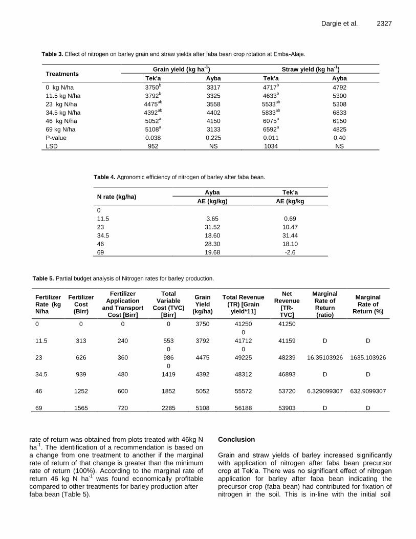
Dargie et al. 2327
Table 3. Effect of nitrogen on barley grain and straw yields after faba bean crop rotation at Emba-Alaje.
Treatments Grain yield (kg ha
-1) Straw yield (kg ha
-1)
Tek'a Ayba Tek'a Ayba
0 kg N/ha 3750b 3317 4717
b 4792
11.5 kg N/ha 3792b 3325 4633
b 5300
23 kg N/ha 4475ab
3558 5533ab
5308
34.5 kg N/ha 4392ab
4402 5833ab
6833
46 kg N/ha 5052a 4150 6075
a 6150
69 kg N/ha 5108a 3133 6592
a 4825
P-value 0.038 0.225 0.011 0.40
LSD 952 NS 1034 NS
Table 4. Agronomic efficiency of nitrogen of barley after faba bean.
N rate (kg/ha) Ayba Tek'a
AE (kg/kg) AE (kg/kg
0
11.5 3.65 0.69
23 31.52 10.47
34.5 18.60 31.44
46 28.30 18.10
69 19.68 -2.6
Table 5. Partial budget analysis of Nitrogen rates for barley production.
Fertilizer Rate (kg N/ha
Fertilizer Cost (Birr)
Fertilizer Application
and Transport Cost [Birr]
Total Variable
Cost (TVC) [Birr]
Grain Yield
(kg/ha)
Total Revenue (TR) [Grain yield*11]
Net Revenue
[TR-TVC]
Marginal Rate of Return (ratio)
Marginal Rate of
Return (%)
0 0 0 0 3750 41250 41250
0
11.5 313 240 553 3792 41712 41159 D D
0 0
23 626 360 986 4475 49225 48239 16.35103926 1635.103926
0
34.5 939 480 1419 4392 48312 46893 D D
46 1252 600 1852 5052 55572 53720 6.329099307 632.9099307
69 1565 720 2285 5108 56188 53903 D D
rate of return was obtained from plots treated with 46kg N ha
-1. The identification of a recommendation is based on
a change from one treatment to another if the marginal rate of return of that change is greater than the minimum rate of return (100%). According to the marginal rate of return 46 kg N ha
-1 was found economically profitable
compared to other treatments for barley production after faba bean (Table 5).
Conclusion Grain and straw yields of barley increased significantly with application of nitrogen after faba bean precursor crop at Tek’a. There was no significant effect of nitrogen application for barley after faba bean indicating the precursor crop (faba bean) had contributed for fixation of nitrogen in the soil. This is in-line with the initial soil

2328 Afr. J. Agric. Res. nitrogen in Ayba kebelle. Partial budget analysis revealed that nitrogen application rate has to be 46 kg N/ha in Tek’a kebelle. But, application of 34 and 46 kg N ha
-1 was
statistically the same, consequently 34.5 kg N ha-1
was optimum rate for barley production after faba bean. CONFLICT OF INTERESTS The authors have not declared any conflict of interests. ACKNOWLEDGEMENT The authors would like to extend their sincere thanks and appreciation to Tigray Agricultural Research Institute (TARI), Ethiopia for sponsoring this study and special thanks to Mekele Soil Research Center staffs. REFERENCES Bereket H, Tjeerd JS, Ellis H (2011.) Tef (Eragrostis tef) production
constraints on Vertisols in Ethiopia: farmers' perceptions and evaluation of low soil zinc as yield- limiting factor. Journal of Soil Science and Plant Nutrition 57(4) 587-596
Bereket H, Sofonyas D, Mehretab H, Fisseha H, Medhn B (2016). Response of Bread Wheat (Tritcum aestivum L.) to Nitrogen after Major Leguminous Crops Rotation in Tigray, Northern Ethiopia. Science, Technology and Arts Research Journal 5(1):9-15
Berhanu D (1980). The physical criteria and their rating proposed for land evaluation in the highland region of Ethiopia. Land Use Planning and Regulatory Department, Ministry of Agriculture, Addis Ababa, Ethiopia.
Black CA, Evans DD, White JL, Ensminger LE, Clark FE (1965). Method of Soil Analysis, Part 2. ASA, Inc. Madison, Wis, USA.
Brady NC, Weil RR (2002). The nature and properties of soils. 13th ed. Pearson Education. Inc. USA.
Bremner JM, Mulvaney CS (1982). Nitrogen - Total, Methods of soil analysis. Part 2- Chemical and microbiological properties. American Society of Agronomy Madison Wis. Agronomy 9(2):595-624.
Chilot Y, Fekadu Al, Woldeyesus S (1998). Barley-livestock production system in Ethiopia: An overview. pp 1-10, in: Chilot Y, Fekadu A, Woldeyesus Sinebo (eds.). Barley-based Farming Systems in the Highlands of Ethiopia. EARO, Addis Ababa, Ethiopia.
Central Statistics Agency (CSA) (2014). The Federal Democratic Republic of Ethiopia Central Statistical Agency. Agricultural sample survey, report on area and production of major crops, Addis Ababa, Ethiopia.
Evans J, Fettell NA, Coventry DR, O’Connor GE, Walsgott DN, Mahoneyand J, Armstrong EL (1991). Wheat response after temperate crop legumes in southeastern Australia. Australian Journal of Agricultural Research 42:31-43.
Fageria NK, Baligar VC (2001). Lowland rice response to nitrogen fertilization. Communication Soil Science and Plant Analysis 32:1405-1429.
Food and Agricultural Organization (FAO) (2004). Fertilizers and Their
Use 4th ed. International Fertilizer Industry Association, FAO, Rome, Italy.
Giller KE (2001). Nitrogen Fixation in Tropical Cropping Systems. CAB International, Wallingford, UK, 423 pp.
Gomez, Gomez H (1984). Statistical analysis for agricultural research. John Willy and Sons Inc. pp.120-155.
Hailu GM, Taner DG, Mengistu H (1991). Wheat research in Ethiopia: A historical perspective. Addis Ababa: IAR/CIMMYT.
Jackson ML (1967). Soil Chemical Analysis. Prentice Hall of India Pvt. Ltd., New Delhi 498p.
Ken EG, Kate JW (1991). Nitrogen fixation in tropical cropping systems. Centre for Agriculture and Bioscience International.
Landon JR (1991). Booker Tropical Soil Manual: A hand book for soil survey and Agricultural Land Evaluation in the Tropics and Subtropics. Longman Scientific and Technical, Essex, New York. 474 p. OR John Wiley & Sons Inc., New York.
Maadi B, Fathi G, Siadat SA, Alami SK, Jafari S (2012). Effects of Preceding Crops and Nitrogen Rates on Grain Yield and Yield Components of Wheat (Triticum aestivum L.). World Applied Sciences Journal 17(10):1331-1336.
Olsen R, Cole S, Watanabe F, Dean L (1954). Estimation of available phosphorus in soils by extraction with sodium bicarbonate. United States Department of Agriculture Circ. 939 p.
SAS (2002). SAS/STAT User’s Guide, Version 9.1.3. SAS institute Inc., Cary, NC.
Sofonyas D, Lemma W, Selamyihun K (2016). Response of Wheat on Uptake, Protein and Nitrogen Use Efficiency to Application of Slow Releasing Nitrogen Fertilizer in Northern Ethiopia. Asian Research Journal of Agriculture 2(1):1-8.
Susan SA, Douglas LK, Cynthia AC (2004). The Soil Management Assessment Framework: A Quantitative Soil Quality Evaluation Method. Soil Science Society of America Journal 68(6):1945-1962.
Tekalign T (1991). Soil, plant, water, fertilizer, animal manure and compost analysis. Working Document No. 13. International Livestock Research Center for Africa, Addis Ababa.
Tolera A, Adamu M, Abraham F, Minale L, Abdo W, Legesse A, Agdew B (2011). Research achievements in barley cultural practices in Ethiopia. In: Mulatu, B. and Grando, S. (eds). Barley Research and Development in Ethiopia. Proceedings of the 2nd National Barley Research and Development Review Workshop. 28-30 November 2006, HARC, Holetta, Ethiopia. ICARDA, PO Box 5466, Aleppo, Syria pp. xiv + 391.
Walkley A, Black IA (1934). An examination of the Degtjareff method for determining soil organic matter and proposed chromic acid titration method. Soil Science 37:29-38.
Vol. 13(42), pp. 2329-2342, 18 October, 2018
DOI: 10.5897/AJAR2018.13454
Article Number: 522B31758991
ISSN: 1991-637X
Copyright ©2018
Author(s) retain the copyright of this article
http://www.academicjournals.org/AJAR
African Journal of Agricultural
Research
Full Length Research Paper
Water and soil conservation techniques and food security in the northern region of Burkina Faso
Sita Sanou1*, Augustine Ayantunde2 and Aimé Joseph Nianogo3
1Institut de l’Environment et de Recherches Agricoles (INERA), Animal Production Department, Ouagadougou,
Burkina Faso. 2International Livestock Research Institute (ILRI), Ouagadougou, Burkina Faso.
3Nazi BONI University (UNB), Institute of Rural Development, Bobo-Dioulasso, Burkina Faso.
Received 10 August, 2018; Accepted 19 September, 2018
Food insecurity is a major challenge facing the rapidly growing population in the sub-Saharan Africa and it is a common feature in the northern region of Burkina Faso. The focus of this study was to investigate the prevalence of food insecurity in the northern region of Burkina Faso after many years of implementation of water and soil conservation techniques. A survey was carried out in six villages in the Northern Region of Burkina Faso involving 300 households to assess water and soil conservation techniques, and to examine the prevalence of food insecurity. The study was conducted between June and July 2015. Data collected was analyzed using logistic regression to identify factors influencing food insecurity in the study areas. The results also showed a high level of food insecurity affecting a large proportion of the population even during the post-harvest period when food was supposed to be available. Results showed that water and soil conservation techniques and household head education level were important factors in determining household food insecurity status. Despite the application of these techniques, food insecurity is still persistent, which raised questions about the efficiency of current agricultural production systems. In addressing food insecurity in the study area, it is necessary to reinforce the practice of combining stone bunds and inter-row ridges techniques along with proper use of fertilizer and manure. Given the persistent problem of water scarcity in Burkina Faso, and the relationship between water and food security, there is need to increase investment in water management infrastructures. Key words: Mixed crop-livestock systems, water and soil conservation techniques, food security, Burkina Faso, Sahel.
INTRODUCTION Water and soil conservation techniques are commonly practiced by farmers in the northern region of Burkina Faso in coping with the problem of land degradation.
After several decades of application of these techniques, studies had proven their effectiveness by enhancing regeneration of the vegetative cover, improvement of
*Corresponding author. E-mail: [email protected]. Tel: +226 70 73 80 33.
Author(s) agree that this article remain permanently open access under the terms of the Creative Commons Attribution
License 4.0 International License

2330 Afr. J. Agric. Res. water infiltration in the soil, and increasing crop yields (Zougmoré et al., 2003; Zougmoré et al., 2004; Kiema, 2008; Zougmore et al., 2002; Liu et al., 2015).
In years of average rainfall, crop yields could increase by 63-74% on farms using stone bunds (Sawadogo, 2011). The increase in crop productivity should normally lead to an improvement in household food security in the region –as higher yields often improve household food security (Sawadogo, 2003; Sinyolo et al., 2014). Most cereal crops (80-85%) were produced for domestic consumption, as cereals account for up to 67% of the calorie content of the Burkinabe’s diet in the rural areas (Sawadogo, 2011). Water and soil conservation measures had been advocated in the past 40 years in Burkina Faso to improve cereal production and consequently food security (Douxchamps et al., 2014). However, there was little or no data on the effect of the application of water and soil conservation techniques on food security in the northern region and on the factors that influence the prevalence of food insecurity. In Burkina Faso, many households experience chronic seasonal and transitory food insecurity (Sawadogo, 2011). A study conducted by the Ministry of Agriculture and Water Resources in 2008 (MAHRH, 2009) showed that 57.7% of the households in northern region were at risk of food insecurity. The availability of information on the determinants of food insecurity can better inform identification of strategies and targeting of interventions to address this challenge. The present study was conducted to partly address the knowledge gap by focusing on the prevalence of food insecurity in households practicing water and soil conservation techniques. MATERIALS AND METHODS
Study site
The study was conducted in the northern region of Burkina Faso (Figure 1). The six villages involved in this study were part of the "climate smart" villages of the CGIAR Climate Change, Agriculture and Food Security (CCAFS) program (Somda et al., 2014). The climate of the region is Sahelo-Soudanian with a long dry season aggravated by a Saharan wind, the harmattan (Roose et al., 1995). Average annual rainfall ranges from 400 to 800 mm. Its spatial and temporal distribution is uneven, with heavy rains at the onset of the season causing soil erosion (Sawadogo, 2011). The soils are in a state of advanced degradation because of the imbalance of nutrients and organic matter caused by the extensive cropping and overgrazing of rangelands (Roose et al., 1993). In addition, these soils are often intensively used with little application of animal manure, resulting in low crop yields (Ouedraogo and Ripama, 2009).
Household survey
This study was conducted in six villages in Northern region of Burkina Faso between June and July 2015. Fifty households were
randomly selected in each village giving a total sample size of 300 households. A semi-structured questionnaire was administered to characterize socio-economic profiles of the households, and water and soil conservation practices. The questions focused mainly on the use of water and soil conservation techniques and the effect on household food security. In addition, a section of the questionnaire included household food security status. Only household heads were interviewed because all important decisions are often taken by them (Abdullah et al., 2017). Measurement of food insecurity The food security status was measured using Household Food Insecurity Access Scale (HFIAS). The method is based on the idea that the experience of food insecurity (access) causes predictable reactions and responses that can be captured and quantified through a survey and summarized in a scale found to be universal across cultures (Tshwene and Oladele, 2016). Household food insecurity access scale was based on measure of severity of food insecurity. For this measurement, the respondents were directly asked about their experience regarding food access during the four past weeks (Table 1). For this study, we used a food insecurity scale based on the work of Coates et al. (2007). This scale of nine indicators provides valid and reliable estimates of the severity of food insecurity for the concerned population, through response to nine questions on access to adequate food. For each answer, a score was assigned (Table 1). From the score of response to the different questions, respondents were classified into different degrees of food insecurity: severe food insecurity, moderate food insecurity, mild food insecurity and food security (Coates et al., 2007). To perform the logistic regression analysis, the groupings were merged into two categories – food secured and non-food secured (MAHRH, 2009). The different levels of food insecurity were obtained by consulting the scores according to Coates et al. (2007) in the following way. (i) Severely food insecure: this class corresponds to people who answered "yes" to the last three questions (7, 8 and 9) or who answered "often" to questions 5 and 6 in Table 1. (ii) Moderately food insecure: this class is for those who answered “rarely” or “sometimes” to questions 5 and 6 or who answered “sometimes” or “often” to questions 3 and 4. (iii) Mildly food insecure: this class refers to those who answered “rarely” for questions 3 and 4 or who answered "sometimes" or "often" for questions 1 and 2. Some authors considered this class as the food security line. (iv) Food secure: people are considered to be food secure when they responded negatively or "rarely" to question 1. Statistical analyses The data was analyzed using the SPSS Statistics software version 22. Frequency analysis was done to describe households and to highlight the most common water and soil conservation techniques used in the study area. Cross tables and Pearson Chi-square tests were conducted to observe the relationships between the prevalence of food insecurity and household socio-demographic and economic characteristics (age of the household head, household size, household formal education level, households domestic asset index, income from sources such as livestock, artisanal gold mining, vegetables growing and money transfers, land areas, household income per capita, off-farm income, livestock and water and soil conservation practice). These variables have been chosen because some studies indicated a relationship between households socio-economic characteristics, agricultural

Sanou et al. 2331
Table 1. Household food insecurity access scale.
Number Questions Response Score
1 In the past four weeks, were you worried that there will not be enough food for the household?
No 0
Rarely 1
Sometimes 2
Often 3
2 In the past four weeks, did you have someone in the household who could not eat the kind of food he / she would like?
No 0
Rarely 1
Sometimes 2
Often 3
3 In the past four weeks, had you had at least one member of the household who had fewer balanced diets because of lack of means?
No 0
Rarely 1
Sometimes 2
Often 3
4 In the past four weeks, did you have at least one member of the household who had to eat food that he did not really want because of lack of means to have others?
No 0
Rarely 1
Sometimes 2
Often 3
5 In the past four weeks, had you had at least one member of the household who had to eat less food than he needed because there was not enough food?
No 0
Rarely 1
Sometimes 2
Often 3
6 In the past four weeks, did you have at least one member in the household who had to eat less food during the day because there was not enough food?
No 0
Rarely 1
Sometimes 2
Often 3
7 In the past four weeks, has there been no food of any type to eat in the household in the household because there was no way to get food?
No 0
Rarely 1
Sometimes 2
Often 3
8 In the past four weeks, was there not someone in the household who slept without eating because there was not enough to eat?
No 0
Rarely 1
Sometimes 2
Often 3
9 In the last four weeks, was there not someone in the household who spent the whole day and the evening without eating something because there was not enough to eat?
No 0
Rarely 1
Sometimes 2
Often 3
Source: Coates et al., 2007.
technology practice and food security (Fengying et al., 2010; Li and Yu, 2010; Sinyolo et al., 2014; Frayne and McCordic, 2015; Abdullah et al., 2017; Nyantakyi-Frimpong et al., 2017).
Household domestic asset index which estimates the total asset owned by the household was calculated with respect to animal asset, domestic asset, transport asset and productive asset. Each

2332 Afr. J. Agric. Res.
Figure 1. Map of study sites location.
of the assets was assigned a weight according the description in Njuki et al. (2011). Household income was measured as the sum of income received from all sources over the last 12 months by a given household (Frayne and McCordic, 2015). Household income was then divided by the size of a given household to have per capita annual income which is commonly used for this kind of studies (Li and Yu, 2010; Mahmoud and Thiele, 2013; Anwar and Cooray, 2015). The total livestock count was obtained by converting livestock number into Tropical Livestock Unit (TLU) using the method of Schwartz et al. (1991) described in Ng'anga'a et al. (2016): 1 TLU = 10 sheep or goats; 1 TLU = 0.7 bovine; 1 TLU = 0.5 donkey.
Based on the results of the Pearson Chi-square tests, we performed binary logistic regressions to establish the relationships between our variable of interest (prevalence of food insecurity) and the others variables. The prevalence of food insecurity had two possible values: 1= food insecurity and 0=food security. First time, we used a model which examined the relationship between household food insecurity and water and soil conservation techniques only. In the second run of the regression analysis, we added other variables to the model.
For the purpose of analyses, the variables were categorized. The age categorization of respondents was based on a report by Diiro et al. (2016). Variables such as household size, livestock capital and cultivated area were categorized by frequency distribution and these categories are in line with the data reported by Amole and Ayantunde (2016) in similar sites in Burkina Faso. Household domestic asset index was categorized by frequency distribution. Household per capita income was categorized in two groups
considering per capita annual average annual per capita expenditure which was estimated at 150 086 FCFA (INSD, 2015).
RESULTS Socio-economic characteristics of respondents The majority of the respondents were not formally educated, only 16.7% had formal education (Table 2). Household size was relatively high in general with 78.7% having more than 5 members of which 16.4% had at least 15 members in their household. Overall, 14.6% of the respondents were young adults aged between 21 and 35, and 16.8% of households were headed by elderly people of over 65 years. The largest age group (45.5%) was made of those between 45 and 65 years of age. The main sources of income identified were crop farming (71.1%), livestock rearing (52%), vegetable production (48.7%), small commerce (33.3%), remittances (33%) and artisanal gold mining (17.1%). The results showed a large disparity between households with respect to household domestic asset index. Values ranged from 2 to 811 with an average value of 103.3 ± 93.3. Households were then grouped into three classes: those with a
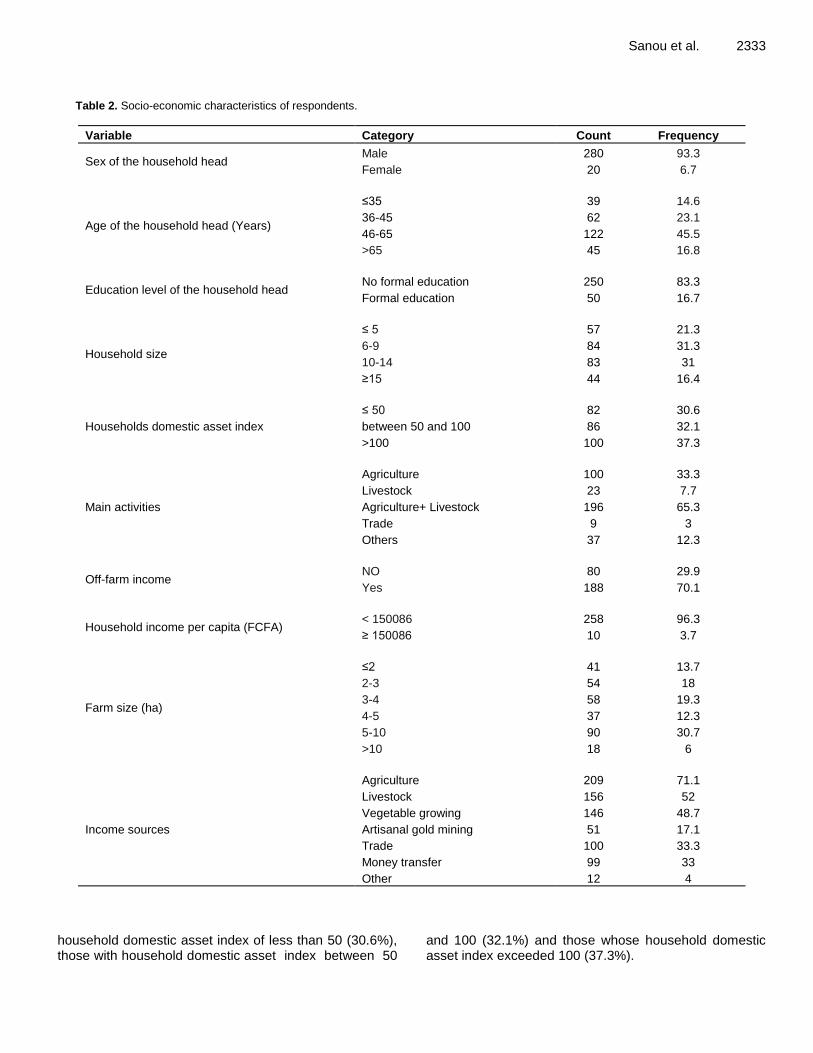
Sanou et al. 2333
Table 2. Socio-economic characteristics of respondents.
Variable Category Count Frequency
Sex of the household head Male 280 93.3
Female 20 6.7
Age of the household head (Years)
≤35 39 14.6
36-45 62 23.1
46-65 122 45.5
>65 45 16.8
Education level of the household head No formal education 250 83.3
Formal education 50 16.7
Household size
≤ 5 57 21.3
6-9 84 31.3
10-14 83 31
≥15 44 16.4
Households domestic asset index
≤ 50 82 30.6
between 50 and 100 86 32.1
>100 100 37.3
Main activities
Agriculture 100 33.3
Livestock 23 7.7
Agriculture+ Livestock 196 65.3
Trade 9 3
Others 37 12.3
Off-farm income NO 80 29.9
Yes 188 70.1
Household income per capita (FCFA) < 150086 258 96.3
≥ 150086 10 3.7
Farm size (ha)
≤2 41 13.7
2-3 54 18
3-4 58 19.3
4-5 37 12.3
5-10 90 30.7
>10 18 6
Income sources
Agriculture 209 71.1
Livestock 156 52
Vegetable growing 146 48.7
Artisanal gold mining 51 17.1
Trade 100 33.3
Money transfer 99 33
Other 12 4
household domestic asset index of less than 50 (30.6%), those with household domestic asset index between 50
and 100 (32.1%) and those whose household domestic asset index exceeded 100 (37.3%).

2334 Afr. J. Agric. Res.
Figure 2. Water harvesting practices in the study sites (n= 300).
Table 3. Prevalence of food insecurity according to the respondents (n=268).
Period of the year Food insecurity Food security
Count Frequency (%) Count Frequency (%)
Favorable period 223 83.7 45 16.8
Bad period 247 92.2 21 7.8
All year 250 93.3 18 6.7
Water and soil conservation techniques
Figure 2 showed that the most commonly used techniques were stone bunds (92% of the respondents), zaï (90.3% of the respondents) and rainwater harvesting (57% of the respondents). Zaï was a traditional technique used in Yatenga (northern Burkina Faso) during drought years between 1982 and 1984 (Bayala et al., 2011). In this method, small pits are dug at a regular spacing on a field, and about two handfuls of organic amendments such as crop residue, manure, or their composted form, are placed in each pit. It is now widespread in the Sudano-Sahelian zone and is used for recovering encrusted soils. The zaï pits are 20-40 cm in diameter and 10-15 cm deep, dug into the degraded, crusted soil. Decomposition of the organic material releases nutrients required for crop growth. Biological activity, and especially the action of termites, favors the development of soil macro-porosity that improves water infiltration (Fatondji et al., 2009). Besides the supply of valuable nutrients for crop growth, the zaï pits promote better infiltration of water locally. Since this water infiltrates deeper than usual, zaï ensures that a sizable fraction of the water percolates to depths where evaporation losses are reduced. The technique combines water harvesting as well as nutrient management practices, which helps to minimize the diversion of water to where it is unproductive, and ensures that its utilization by the crop
is as efficient as possible (Fatondji et al., 2009). The techniques of zaï and stone bunds are presented in Figures 4 and 5. The main combination of options in the area (Figure 3) were practice of stone bunds and zaï (36.3%), stone bunds and inter-row ridges and stone bunds combined with zaï and inter-row ridges (48% of respondents).
Food status and prevalence of food insecurity
According to the agricultural calendar in the study sites, 51.7, 22.3 and 7% of the respondents stated that food was sufficient during post-harvest period, in the late dry season and during the rainy season, respectively. In addition, the average number of daily meals consumed by the surveyed households was 2.72 ± 0.6 (mean ± standard deviation) during the post-harvest period; 2.56 ± 0.6 in the late dry season and 2.52 ± 0.6 during the rainy season. The results of the food insecurity prevalence showed that food insecurity is actually real in our study area. Even during the favorable period, 83.7% of respondents were food-insecure. Across the sites, 93.3% were food-insecure (Table 3).
Determinants of food insecurity
The results of the cross tables and Pearson Chi-square

Sanou et al. 2335
Figure 3. Proportion (%) of respondents by type of association of soil and water conservation techniques.
tests conducted are summarized in Table 4. These results showed that the prevalence of food insecurity was not associated with the sex of the household head, group membership, off farm income, household income, land area cultivated, sources of income from small commerce or sale of agricultural products. Instead, there was significant correlation between prevalence of food insecurity and the age and formal education level of the household head, household size, income sources such as sale of livestock, artisanal gold mining, remittances, vegetable production, livestock asset, the practice of water and soil conservation technique and the household domestic asset index. In our survey, 95% of household heads who were not formally educated were food insecure against 86% of households headed by those who received formal education. Also, 99% of the households who used stone bunds in association with zaï were food insecure as compared to 73% of those who practiced stone bunds in combination with the inter-row ridges. The first model (Table 5), which tested the effect of water and soil conservation techniques on the probability of food insecurity, revealed a very significant difference between households practicing stone bunds in combination with inter-row ridges or by incorporating the zaï technique, and the households that practiced a combination of stone bunds and zaï (reference category). After comparing the practice of water and soil conservation techniques with other independent variables, the logistic regression resulted in a significant model
(Chi-square = 53.90, df = 17; P = 0.000, Nagelkerke R²= 0.47; percentage correct= 93.6%). The model predictors explained 47% of the total variance of the probability of a household to be food insecure. Despite the introduction of other variables, the practice of water and soil conservation techniques remained a significant variable (odd ratio= 0.04, P < 0.05) for likelihood of prevalence of food insecurity in the surveyed households. The second variable which contributed significantly to explain the likelihood to be food insecure in the study area was the formal education level of the household head (odd ratio=0.18, p<0.05). The combination of the stone bunds and the inter-row ridges technique and formal education reduced the probability of household food insecurity (Table 6). DISCUSSION Food security situation in the study sites Food insecurity is common in rural areas of Burkina Faso with the northern region among the most vulnerable regions in the country in terms of food insecurity. Considering the high rainfall variability and the poor soil fertility in the Northern region, the results of this study were not surprising. These results are in line with the observations of Fengying et al. (2010) who argued that food insecurity is common in rural areas where natural

2336 Afr. J. Agric. Res.
Table 4. Food insecurity prevalence according to the household characteristics (n=268).
Variables Categories
Prevalence of food insecurity (%)
Chi-square results
Insecurity Securit
y Values
Sex of the household head Male 93.2 6.8 0.04
Female 94.4 5.6
Education level of the household head
No formal education 94.7 5.3 4.28*
Formal education 86 14
Group membership
1-2 groups 93 7 0.75
3-5 groups 93 7
Plus de 5 groups 100 0
Practice of the water conservation options
Stone bunds + zaï 99.1 0.9 16.61*
Stone bunds + the inter-row ridges 73.3 26.7
Stone bunds + the inter-row ridges +zaï 91 9
Income control
Male 93.8 6.2 3.46
Female 100 0
Jointly 90.8 9.2
Foreign person 100 0
Children 100 0
Income from livestock No 96.8 3.2 4.62*
Yes 90.2 9.8
Income from Agriculture No 89 11 2.64
Yes 94.7 5.3
Income from vegetable growing No 97.7 2.3 8.39*
Yes 88.9 11.1
Income from artisanal gold mining
No 91.9 8.1 4.02*
Yes 100 0
Income from trade No 93 7 0.09
Yes 94 6
Remittance No 95.6 11.5 4.69*
Yes 88.5 4.4
Other sources of income No 93.4 6.6 0.10
Yes 90.9 9.1
Off-farm income No 96.3 3.8 1.60
Yes 92 8
Household income per capita (FCFA)
<150086 93.4 6.6 0.93
≥150086 90 101

Sanou et al. 2337
Table 4. Contd.
Age of the household head (year)
≤ 35 97.4 2.6 8.59
Between 36 and 45 88.7 11.3
Between 46 and 65 96.7 3.3
>65 86.7 13.3
Household size
≤ 5 98.2 1.8 12.55
Between 6 and 9 93.3 4.7
Between 10 and 14 94 6
≥15 81.4 18.6
Farm size (ha)
≤ 3 93.6 6.4 1.14
Between 3 and 5 95.3 4.7
>5 91.4 8.6
Livestock asset (TLU)
≤ 2 97.2 2.8 10.06
Between 2 and 3 97.9 2.1
>3 87.6 12.4
Households domestic asset index (g)
≤ 50 100 0 13.58
Between 50 and 100 94.4 5.6
>100 86.3 13.7
*level of significance p < 0.05.
Table 5. Determinants of food insecurity in the first model.
Variables Categories B OR
Practice of the water conservation techniques
stone bunds technique and the inter-row ridges -3.67* 0.03
Zaï , stone bunds technique and the inter-row ridges -2.68* 0.09
B: coefficient; OR : odds ratio ; *level of significance p < 0.05.
and ecological conditions are fragile because of the soil quality and soil water availability which are limiting factors (Wolka et al., 2018). Considering the improved yields achieved following the adoption of water and soil conservation techniques, the expectation was that a high proportion of surveyed households would be less vulnerable to food insecurity; however the reverse was the case. The plausible reason might be that the increase in crop productivity resulting from the use of water and soil conservation techniques was insufficient to offset food insecurity. The effect of water and soil conservation techniques on improving crop yield to an extent as to achieve food security was found to be dependent on rainfall characteristics, types of crop, slope, and soil type (Sawadogo, 2011; Wolka et al., 2018). Then it is suggested to combine the water and soil conservation techniques with other management activities to enhance crop yields. In our study, the food insecurity might be
attributed to the low crop productivity (Sawadogo, 2011) which is caused by: (i) Low coverage of fields by water and soil conservation techniques; (ii) Low level of the use of improved seeds; (iii) Low level of the use of fertilizers; (iv) Rainfall variability. In fact, farmers are not able to apply water and soil conservation techniques over large areas due to varied reasons according to the respondents. Thirty to sixty-two percent of respondents mentioned lack of equipment as a major constraint that limited the use of water and soil conservation techniques. Lack of fertilizer (manure and chemical fertilizer) and lack of manpower were other constraints mentioned by 24 and 13% of the respondents, respectively. This lack of assets (particularly tools for

2338 Afr. J. Agric. Res. Table 6. Determinants of food insecurity in the second model.
Variables Categories B AOR
Practice of the water conservation techniques
Zaï and stone bunds technique
stone bunds technique and the inter-row ridges -3.22*±1.57 0.04
Zaï , stone bunds technique and the inter-row ridges -1.35±1.26 0.26
Education level of the household head
No formal education
Formal education -1.70*±0.81 0.18
Income from livestock No
Yes -0.64±0.72 0.53
Income from vegetable growing No
Yes -0.58±0.83 0.56
Remittance No
Yes -0.44±700 0.65
Income from artisanal gold mining
No
Yes -18.46±4935.9 1043831.9
Age of the household head (year)
≤ 35
Between 36 and 45 -0.55±1.67 0.58
Between 46 and 65 0.89±1.69 2.42
≥65 -0.86±1.72 0.42
Livestock asset (TLU)
≤ 2
Between 2 and 3 1.64±1.17 5.14
>3 0.10±0.01 1.1
Households domestic asset index
≤ 50
Between 50 and 100 -17.58±3888.30 0.000
>100 -17.48±3888.30 0.000
Household size
≤ 5
Between 6 and 9 -0.47±1.57 0.62
Between 10 and 14 -0.73±1.58 0.48
≥15 -2.08±1.61 0.13
B: coefficient; AOR : adjusted ; * : level of significance p < 0.05.
installation and labor) constrained ability to use water and soil conservation techniques even with external assistance (Bunclark et al., 2018). Socio-economic factors such as financial capital access to credit, and market access, as well as policy environments have been reported as limiting the potential of water and soil conservation techniques in West African Sahel (Koning et al., 2001). The high labor demand of water and soil techniques is another challenge (Koning et al., 2001). Despite these challenges, land management with water and soil conservation techniques could be a promising
solution in addressing food insecurity in Sahelian countries, provided that they cover sufficient areas (GIZ, 2012).
Application of inorganic fertilizer and animal manure is very important in supporting water and soil conservation techniques, especially for zaï technique as it is often applied to degraded land (Zougmoré et al., 2004). So when the manure is not applied in the required quantity, this would limit the benefit of the water and soil conservation techniques. To improve the efficiency of the water and soil conservation techniques it has been

Sanou et al. 2339
Figure 4. Digging Zai pit (Photo credit: Tunde Amole).
suggested to combine these measures with soil fertility management practices (Zougmoré et al., 2002). Applying compost manure to fields laid with stone bunds increased the yields by 77-130%, according to Sawadogo (2011). In our study, the low effectiveness of water and soil conservation techniques could be explained by the low level of the use of improved seeds. Only 8% of the respondents frequently used improved seeds according to the respondents.
Effectiveness of water and soil conservation techniques on crop productivity has been found to vary depending on the amount and distribution of rainfall (Wiyo et al., 2000; Zougmoré et al., 2014). The rainfall variability tends to negatively affects crop yields because these technologies work by retaining surface runoff within the field to ensure rainwater and soil moisture conservation. So the main purpose of these techniques is to harvest the limited
rainwater and store it in crop zone for use during dry spell periods (Wiyo et al., 2000). Past research revealed that tied-ridge is effective in reducing surface runoff and increasing soil water storage (Wiyo et al., 2000). However, in recent years, changes in the climate patterns have led to frequent droughts in many areas (Tietjen et al., 2017). Below 500 mm, rainfall is insufficient to meet crop water requirements with or without tied-ridging (Wiyo et al., 2000) and this water deficit can seriously affect crop production, leading to remarkable reduction in grain yield (Jia et al., 2018). Therefore, it is better to combine water and soil conservation techniques with irrigation in order to provide water for crops at least during the critical period (Jia et al., 2018). The results of Jia et al. (2018) showed that combining ridge-furrow and irrigation at the silking stage provide moisture for crop growth and improve maize grain yield, economic benefit, and water
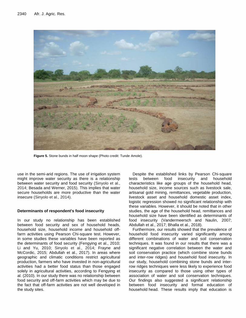
2340 Afr. J. Agric. Res.
Figure 5. Stone bunds in half moon shape (Photo credit: Tunde Amole).
use in the semi-arid regions. The use of irrigation system might improve water security as there is a relationship between water security and food security (Sinyolo et al., 2014; Besada and Werner, 2015). This implies that water secure households are more productive than the water insecure (Sinyolo et al., 2014). Determinants of respondent's food insecurity In our study no relationship has been established between food security and sex of household heads, household size, household income and household off-farm activities using Pearson Chi-square test. However, in some studies these variables have been reported as the determinants of food security (Fengying et al., 2010; Li and Yu, 2010; Sinyolo et al., 2014; Frayne and McCordic, 2015; Abdullah et al., 2017). In areas where geographic and climatic conditions restrict agricultural production, farmers who have invested in non-agricultural activities had a better food status than those engaged solely in agricultural activities, according to Fengying et al. (2010). In our study there was no relationship between food security and off-farm activities which may be due to the fact that off-farm activities are not well developed in the study sites.
Despite the established links by Pearson Chi-square tests between food insecurity and household characteristics like age groups of the household head, household size, income sources such as livestock sale, artisanal gold mining, remittances, vegetable production, livestock asset and household domestic asset index, logistic regression showed no significant relationship with these variables. However, it should be noted that in other studies, the age of the household head, remittances and household size have been identified as determinants of food insecurity (Vandermeersch and Naulin, 2007; Abdullah et al., 2017; Bhalla et al., 2018).
Furthermore, our results showed that the prevalence of household food insecurity varied significantly among different combinations of water and soil conservation techniques. It was found in our results that there was a significant negative correlation between the water and soil conservation practice (which combine stone bunds and inter-row ridges) and household food insecurity. In our study, household combining stone bunds and inter-row ridges techniques were less likely to experience food insecurity as compared to those using other types of association of water and soil conservation techniques. Our findings also suggested a significant relationship between food insecurity and formal education of household head. These results imply that education is

important for improving the food security status of farmers as the educated farmers were less likely to be food insecure (Li and Yu, 2010; Bhalla et al., 2018). Previous studies showed that formally educated respondents had a better food security score than those without formal education (Li and Yu, 2010; Bhalla et al., 2018). In fact, the low level of formal education is strongly associated with the probability of experiencing food insecurity (Maxwell et al., 2014).
Possible explanation for the relationship between household level of formal education and food security could be that households with formal education are more likely to adopt new technologies which could increase their productive capacity and improve their nutritional status (Kelebe et al., 2017). According to Smale et al. (2018), formal education is a significant determinant of technology adoption as the ability to read and write can positively affect access and acceptance of new information and production techniques. The relationship between the improvement of the household food security and the formal education level of the household head could also be explained by the increase in earning capacity (Fengying et al., 2010). Education gives knowledge and awareness and increases the chances of obtaining job and people with higher education were more likely to get higher paying jobs (Abdullah et al., 2017). In Burkina Faso, more than 8 out of 10 poor people live in households whose head did not receive any formal education (INSD, 2015). So, education can be a good political tool to fight poverty.
Conclusion This study aimed at answering the question of whether the practice of water and soil conservation techniques influences the food security situation in the northern region where they are commonly practiced. Our results showed that water and soil conservation techniques help to reduce food insecurity. Prevalence of food insecurity was reduced by stone bunds in combination with the inter-row ridges technique and possession of formal education. Despite the application of these water and soil conservation techniques however, food insecurity is still persistent in the area, which raises questions about the efficiency of current agricultural production systems. Farmers should therefore be encouraged to support water and soil conservation techniques with improved agronomic practices in term of use of improved seeds, fertilizers and irrigation.
RECOMMENDATION
Based on the results of our study, the following recommendations can be drawn:
1. Combining water and soil conservation techniques with
Sanou et al. 2341 inputs such as improved crop varieties and organic manure is necessary for improved food security in the region. 2. Significant increased investment in water management infrastructures is necessary to improve food security situation in Burkina Faso and in other West Africa Sahelian countries. In view of the strong relationship between water scarcity and food insecurity. 3. Improving access to quality education, particularly in rural areas can be a powerful tool to combat food insecurity in the Sahel. CONFLICT OF INTERESTS The authors have not declared any conflict of interests. ACKNOWLEDGEMENTS The authors would like to thank the respondents from the study sites in the Northern Region of Burkina Faso for their participation in the interviews. In addition, we thank Viviane Yameogo for coordinating the data collection and entry. The authors are solely responsible for the opinions expressed in this manuscript. REFERENCES Abdullah, Zhou D, Shah T, Ali S, Ahmad W, Ud Din I, Ilyas A (2017).
Factors affecting household food security in rural northern hinterland of Pakistan. Journal of the Saudi Society of Agricultural Sciences.
Amole A, Ayantunde A (2016). Livestock Water Productivity in Mixed Crop-Livestock Farming Systems in Burkina Faso: Assessment and Strategies for Improvement. Technical report, International Livestock Research Institute, Nairobi, Kenya.
Anwar S, Arusha C (2015). Financial flows and per capita income in developing countries. International Review of Economics and Finance 35:304-314.
Bayala J, Kalinganire A, Tchoundjeu Z, Sinclair F, Garrity D (2011). Conservation agriculture with trees in the West African Sahel–a review. ICRAF occasional paper 14
Besada H, Werne K (2015). An assessment of the effects of Africa’s water crisis on food security and management. International Journal of Water Resources Development 31(1):120-133.
Bhalla G, Handa S, Angeles G, Seidenfeld D (2018). The effect of cash transfers and household vulnerability on food security in Zimbabwe. Food policy 74:81-99.
Bunclark L, Gowing J, Oughton E, Ouattara K, Ouoba S, Benao B (2018). Understanding farmers’ decisions on adaptation to climate change: Exploring adoption of water harvesting technologies in Burkina Faso. Global Environmental Change 48:243-254.
Coates J, Swindale A, Bilinsky P (2007). Household food insecurity access scale (HFIAS) for measurement of food access: indicator guide. Washington, DC: Food and Nutrition Technical Assistance Project, Academy for Educational Development 34.
Diiro G, Petri M, Zemadim B, Sinare B, Dicko M, Traore D, Tabo R, (2016). Gendered analysis of stakeholder perceptions of climate change, and the barriers to its adaptation in Mopti region in Mali (No. 68). Research Report.
Douxchamps S, Ayantunde A, Barron J (2014). Taking stock of forty years of agricultural water management interventions in smallholder systems of Burkina Faso. Water resources and rural development
2342 Afr. J. Agric. Res.
3:1-13. Fatondji D, Martius C, Zougmore R, Vlek PLG, Bielders CL, Koala S
(2009). Decomposition of organic amendment and nutrient release under the zai technique in the Sahel. Nutrient Cycling in Agroecosystems 85(3):225-239.
Fengying N, Jieying B, Xuebiao Z (2010). Study on China’s Food Security Status Agriculture and Agricultural Science Procedia 1:301-310.
Frayne B, McCordic C (2015). Planning for food secure cities: Measuring the influence of infrastructure and income on household food security in Southern African cities. Geoforum 65:1-11.
Deutsche Gesellschaft für Internationale Zusammenarbeit (GIZ) (2012). Bonnes pratiques de conservation des eaux et des sols : contribution à l’adaptation au changement climatique et à la résilience des producteurs au Sahel. Dag-Hammarskjöld-Weg 1-5 65760 Eschborn, Allemagne [email protected] www.giz.de
Institut National de la Statistique et de la Démographie (INSD) (2015). Enquête multisectorielle continue (EMC) 2014: Profil de pauvreté et d’inégalités. Rapport, Novembre 2015, 90 p.
Jia Q, Sun L, Wanga J, Li J, Ali S, Liu T, Zhang P, Lian Y, Ding R, Ren X, Jia Z (2018). Limited irrigation and planting densities for enhanced water productivity and economic returns under the ridge-furrow system in semi-arid regions of China. Field Crops Research 221:
Kelebe HE, Ayimut KM, Berhe GH, Hintsa K (2017). Determinants for adoption decision of small scale biogas technology by rural households in Tigray, Ethiopia. Energy Economics 66:272-278.
Kiema A (2008). Effets des cordons pierreux sur la régénération d’un pâturage naturel de glacis au Sahel. Agricultures 17(3):281-288.
Koning N, Heerink N, Kauffman S (2001). Food insecurity, soil degradation and agricultural markets in West Africa: Why current policy approaches fail. Oxford Development Studies 29(2):189-207.
Li Y, Yu W (2010). Households Food Security in Poverty-Stricken Regions: Evidence from Western Rural China. Agriculture and Agricultural Science 1:386-395.
Liu QJ, An J, Wang LZ, Wu YZ, Zhang HY (2015). Influence of ridge height, row grade, and field slope on soil erosion in contour ridging systems under seepage conditions. Soil and Tillage Research 147:50-59.
Mahmoud TO, Thiele R (2013). Does Prime-Age Mortality Reduce Per-Capita Household Income? Evidence from Rural Zambia. World Development 45:51-62.
Ministère de l’Agriculture, de l’Hydraulique Et des Ressources Halieutiques (MAHRH) (2009). Enquête Nationale sur l’Insécurité Alimentaire et la Malnutrition Rapport Définitif 193 p.
Maxwell D, Vaitla B, Coates J (2014). How do indicators of household food insecurity measureup? An empirical comparison from Ethiopia. Food Policy 47:107-116.
Ng’ang’a SK, Bulte EH, Giller KE, Ndiwa NN, Kifugo SC, McIntire JM, Herrero M, Rufino MC (2016). Livestock wealth and social capital as insurance against climate risk: A case study of Samburu County in Kenya. Agricultural Systems 146:44-54.
Njuki J, Poole J, Johnson N, Baltenweck I, Pali P, Lokman Z, Mburu S (2011). Gender, livestock and livelihood. International Livestock Reasearch Institute 40 p.
Nyantakyi-Frimpong H, Kangmennaang J, Kerr RB, Luginaah I, Dakishoni L, Lupafya E, Shumba L, Katundu M (2017). Agroecology and healthy food systems in semi-humid tropical Africa:Participatory research with vulnerable farming households in Malawi. Acta Tropica 175:42-49.
Ouedraogo M, Ripama T (2009). Recensement général de la population et de l’habitation (RGPH) de 2006, thème 2 : état et structure de la population analyse des résultats définitifs. Institut national de la statistique et de la démographie 181 p.
Roose E, Kabore V, Guenat C (1993). Le zaï: fonctionnement, limites et
amélioration d'une pratique traditionnelle africaine de réhabilitation de la végétation et de la productivité des terres dégradées en région soudano-sahélienne (Burkina Faso). Cahiers ORSTOM. Série Pédologie 28(2):159-173.
Roose E, Kabore V, Guenat C (1995). Le zaï, une technique traditionnelle africaine de réhabilitation des terres dégradées de la région soudano-sahélienne (Burkina Faso). L'Homme peut-il refaire ce qu'il a défait? 249.
Sawadogo H (2003). Impact des aménagements sur les systèmes de production, les rendements et la sécurité alimentaire des exploitations agricoles. Etude Plateau Central. Rapport de travail (2).
Sawadogo H (2011). Using soil and water conservation techniques to rehabilitate degraded lands in northwestern Burkina Faso. International Journal of Agricultural Sustainability 9(1):120-128.
Sinyolo S, Mudhara M, Wale E (2014). Water security and rural household food security: Empirical evidence from the Mzinyathi district in South Africa. Food Security 6(4):483-499.
Smale M, Assima A, Kergna A, Thériault V, Weltzien E (2018). Farm family effects of adopting improved and hybrid sorghum seed in the Sudan Savanna of West Africa. Food Policy 74:162-171.
Somda J, Sawadogo I, Savadogo M, Zougmore R, Bationo BA, Abdoulaye SM, Nakoulma G, Sanou J, Barry S, Sanou AO, Some L (2014). Analyse participative de la vulnérabilité et planification de l’adaptation au changement climatique dans le Yatenga, Burkina Faso.
Tietjen B, Schlaepfer DR, Bradford JB, Lauenroth WK, Hall SA, Duniway MC, Hochstrasser T, Jia G, Munson SM, Pyke DA, Wilson SD (2017). Climate change-induced vegetation shifts lead to more ecological droughts despite projected rainfall increases in many global temperate dry lands. Global Change Biol.ogy 23(7):2743-2754.
Tshwene C, Oladele I (2016). Water use productivity and food security among smallholder homestead food gardening and irrigation crop farmers in North West province, South Africa. Journal of Agriculture and Environment for International Development 110(1):73-86.
Vandermeersch C, Naulin A (2007). Sécurité alimentaire des ménages et stratégies alternatives de diversification des sources de revenus
en milieu rural: le cas de la zone de Niakhar au Sénégal entre 2000-‐2003. communication à la Chaire Quetelet 2007 19 p.
Wiyo KA, Kasomekera ZM, Feyen J (2000). Effect of tied-ridging on soil water status of a maize crop under Malawi conditions. Agricultural Water Management 45(2):101-125.
Wolka K, Mulder J, Biazin B (2018). Effects of soil and water conservation techniques on crop yield, runoff and soil loss in Sub-Saharan Africa: A review. Agricultural Water Management 207:67-79.
Zougmore R, Gnankambary Z, Guillobez S, Stroosnijder L (2002). Effect of stone lines on soil chemical characteristics under continuous sorghum cropping in Semiarid Burkina Faso. Soil and Tillage Research 66(1):47-53.
Zougmoré R, Jalloh A, Tioro A (2014). Climate-smart soil water and nutrient management options in semiarid West Africa: a review of evidence and analysis of stone bunds and zaï techniques. Agriculture andFood Security 3(1):16.
Zougmoré R, Mando A, Ringersma J, Stroosnijder L (2003). Effect of combined water and nutrient management on runoff and sorghum yield in semiarid Burkina Faso. Soil Use and Management 19(3):257-264.
Zougmoré R, Mando A, Stroosnijder L (2004). Effect of soil and water conservation and nutrient management on the soil-plant water balance in semi-arid Burkina Faso. Agricultural Water Management 65(2):103-120.
Vol. 13(42), pp. 2343-2350, 18 October, 2018
DOI: 10.5897/AJAR2018.13459
Article Number: 4F11E2158993
ISSN: 1991-637X
Copyright ©2018
Author(s) retain the copyright of this article
http://www.academicjournals.org/AJAR
African Journal of Agricultural
Research
Full Length Research Paper
Strategic planning of regional oil-and-fat subcomplex
of Russia
Mikhail O. Sinegovsky and Anastasia A. Malashonok*
Economic Research Group, Аll-Russian Scientific Research Institute of Soybean, ZIP Code 675027, 19 Ignatievskoe Highway, Blagoveshchensk, Russian Federation, Russia.
Received 13 August, 2018; Accepted 18 September, 2018
The purpose of the work is to analyze the trends in the development of the oil-and-fat subcomplex as one of the most important components of the agribusiness of the Russian Federation, and state policy in the strategic planning in this sphere. The materials of the United States Department of Agriculture, the State Statistics Service and the Ministry of Agriculture of the Russian Federation served as the information basis for the research. The legislative and regulatory acts of the Russian Federation were used for the analysis of the state policy in the field of strategic planning in the agribusiness. Results of the research showed that the development of the oil-and-fat subcomplex is hampered by a large number of problems, one of which is the absence of the development target program-strategy. The most optimal of the possible options for the development strategy is the formation of a cluster that will allow optimizing the work of all its participants, involved in various spheres of the agribusiness, logistic infrastructure, public authorities, scientific and personnel support, as well as contributes to solving the identified problems. In the study, within the framework of the analysis of the internal and external environment of the oil-and-fat subcomplex, the problems that hamper its development are considered. The advisability of developing a state program for creating a cluster has been revealed and directions for implementing state support for solving technical and technological as well as social and economic problems have been determined. Key words: Development strategy, agro-food sector, soybean, gross yield, crop yield, sown areas.
INTRODUCTION The oil-and-fat subcomplex in its present state is a complex multifunctional system that involves a large number of elements, including various markets of the oil primary products-sunflower seed oil, soybean, rape, cotton, palm seeds, etc. The oil-yielding crops are widely used for food production, serve as raw material in the production of industrial products in such sectors as
leather, textile, paint-and-varnish, medical, etc., and in addition to that, the by-products of the oil primary products processing are used in the production of mixed fodder for livestock (Tiwari, 2017; Ramos et al., 2017).
To fully and sustainably meet the needs of the population of individual countries and regions in the products of the oil-and-fat subcomplex, it is
*Corresponding author. E-mail: [email protected].
Author(s) agree that this article remain permanently open access under the terms of the Creative Commons Attribution
License 4.0 International License

2344 Afr. J. Agric. Res. Table 1. Change in the structure and volume of production of the most important types of oil-yielding crops in the world.
Type of oil-yielding crops 2013 2016 2017 Increase in 2017 in relation to in %
mln, t % mln, t % mln, t % 2013 2016
Arachis Hypogaea 41.9 8.3 42.8 7.5 44.1 7.6 +5.3 +3.0
Copra 5.4 1.1 5.4 0.9 5.5 1.0 +1.8 +1.8
Cotton seeds 45.0 8.9 39.0 6.8 44.6 7.7 -0.9 +14.4
Sunflower seeds 41.5 8.2 47.6 8.3 45.8 7.9 +10.4 -3.8
Rape seeds 71.7 14.2 70.2 12.2 73.1 12.6 +1.9 +4.1
Soya beans 282.7 56.1 351.4 61.2 346.9 60.0 +22.7 -1.3
Palm seeds 15.9 3.2 17.3 3.0 18.6 3.2 +16.9 +7.5
Oil crops, total 504.2 100.0 573.6 100.0 578.6 100.0 +14.8 +1.0
necessary to create for producers, processors and consumers the proper conditions that ensure the production of high-quality products in volumes and in range corresponding to the demand and consumption norms. As the experience of developed countries shows, the solution of these tasks is impossible without the use of strategic planning mechanisms that allow increasing the efficiency of managing elements of the agribusiness. In the conditions of rapidly changing market requirements and growing competition, the main success factor is the ability at the state level to put into practice long-term planning and forecasting, as well as system monitoring and control over the implementation of the strategy in order to identify possible deviations from the adopted line in a timely manner and to correct them (Avadi et al., 2018; Calabro and Vieri, 2015).
The purpose of this study is to analyze current trends in the development of the oil-and-fat subcomplex as one of the most important components of the agribusiness of the Russian Federation, as well as the state policy in the strategic planning in this sphere.
To achieve this goal, the following tasks were set: (i) To analyze the structure and volumes of production of the main types of oil-yielding crops in the world and in the Russian Federation; (ii) To identify the main trends and problems for the development of the regional oil-and-fat subcomplex of the Russian Federation; (iii) To analyze the main documents regulating strategic management in the agribusiness, using the example of the Amur Region as the leading region for soybean production in the Russian Federation. MATERIALS AND METHODS The materials presented in this paper are the result of the research conducted on the basis of the All-Russian Scientific Research Institute of Soybean (Russian Federation). As an initial study, a theoretical analysis of the existing methodological approaches to strategic planning in the economic scientific literature (Abigor et al., 2003; Ah Chee et al., 2011; Kozenko et al., 2016; Manzhosova et
al., 2017; Wegren et al., 2015) was carried out. The analytical review made it possible to get an overview of the development of strategic planning in the Russian Federation and foreign countries, to clarify the research issues and to identify key sources of obtaining the information for further work.
Further, an analysis of the structure and volumes of production of the main types of oil-yielding crops in the world and in the Russian Federation was conducted. The analysis was based on the data from the United States Department of Agriculture for the period from 2013 to 2017. As a result of economic and statistical processing of the selected data, the main trends and problems in the development of the regional oil-and-fat subcomplex of the Russian Federation were revealed. In addition to the data of the bodies of the international and internal state statistics of the Russian Federation, we considered the official documents regulating strategic management in the agribusiness, using the example of the Amur Region as the leading region for soybean production in the Russian Federation.
Then, based on the existing experience of strategic planning in the agribusiness studied at the first stage of the research, the optimal variant of the development strategy for regional agro-industrial subcomplexes was chosen and the directions for implementing state support for solving technical and technological as well as social and economic problems were determined.
RESULTS AND DISCUSSION
In the last 5 years, the volume of world production of the most important oil-yielding crops has a stable tendency to growth (Cattelan and Dall'Agnol, 2018; Kuzmenko et al., 2016; Li et al., 2017). At present, soybean occupies a dominant position in the structure of gross yields of agricultural plants of the oilseed group. In 2017, the share of soybean amounted to 60% of the world production (Table 1). The rape and sunflower (12.6 and 7.9%, respectively) take the second and third positions (USDA Foreign Agricultural Service, 2018).
In the period from 2013 to 2017, the production of soya beans demonstrated the highest growth rates, 122.7%; except for cotton, the rest of the crops also showed positive dynamics. The growing interest in soybeans in the world and, as a result, an increase in production volumes, is caused by a wide range of its application. It is associated with a combination of high protein content,

Sinegovsky and Malashonok 2345
Table 2. Leading oil-yielding crops producing countries as of 2017.
Volume of production, mln t
Soybeans Sunflower seeds Rape seeds
1. USA - 119.5 (34.3) 1. Ukraine - 13.0 (28.4) 1. EU - 22.1 (30.3)
2. Brazil - 110.0 (31.6) 2. Russia - 10.5 (22.9) 2. Canada - 21.5 (29.5)
3. Argentina - 56.0 (16.0) 3. EU - 9.3 (20.3) 3. China - 13.1 (17.9)
4. China - 14.2 (4.1) 4. Argentina - 3.6 (7.8) 4. India - 6.5 (8.9)
5. India - 10.0 (2.8) 5. China - 2.8 (6.1) 5. Australia - 2.9 (3.9)
All types of oil-yielding crops
1. USA -132.2 (22.8)
2. Brazil - 111.3 (19.2)
3. Argentina - 62.3 (10.1)
4. China - 57.5 (9.9)
5. India – 36.61 (6.3)
*Numerals in brackets are the percentage of total world production.
Table 3. Dynamics of the growth rates of production of the main types of oil-yielding crops of the Russian Federation for 2013-2017.
Type of oil-yielding crops Rate of Growth (Trn), %
2014/2013 2015/2014 2016/2015 2017/2016 Average for 2013-2017
Sunflower 85.6 108.9 119.8 87.2 99.3
Soybean 158.7 111.3 115.7 114.9 123.8
Rape 105.1 76.8 99.5 150.5 104.9
Oil crops, total 97.8 106.8 118.1 95.9 104.3
close in quality to the animal protein, and oil, that is rare for plants. At present, soybean is an indispensable component in fodder production, primary products for the food and chemical industries and for the production of building materials, and in recent years also for biofuel.
According to the Food and Agricultural Organization (FAO) estimates, the Russian Federation took the 8th position in the oil crop production in 2017; and its share in the worldwide production was 2.6% (USDA Foreign Agricultural Service, 2018). The situation is largely determined by the production of sunflower seeds, which is the main oil-yielding crop, cultivated in Russia, and according to the level of which the country takes the second position in the world after Ukraine (Table 2). In 2017, the share of sunflower was 61% in the structure of gross yield of the oil-yielding crops. The soybean takes the second position, both in the structure of sown areas and in gross output (Figure 1).
In recent years, the growth rates of the production of soya beans in Russia significantly exceed the growth rates of production of rapeseeds and sunflower seeds (Chetvertakov, 2015). So, for the period from 2013 to 2017, the production of soybean seeds increased at an average by 24% per year, the similar indicator for rape is 5%, while the sunflower is characterized by a decrease at
an average of 0.7% per year (Table 3). Historically, the main production of soybean in Russia
is concentrated in the Far East. This is due to the proximity to the genetic center of the crop origin and the centuries-old traditions of cultivation (Krivoshlykov et al., 2016). The All-Russian leader in soybean production is the Amur Region. In 2017, a record harvest of soybean was collected in the region. It amounted to 1366.8 thousand tonnes (35.6% in the total amount of yields) (Fedstat.ru). For the year, soybean production increased by 40% or by 389.6 thousand tonnes (Table 4).
Over the past decades, soybean production remains the main direction of agriculture in the Amur Region, the efficiency of which affects the financial and economic situation of the agribusiness of the region. Since only soybean, determining the direction for development of all the spheres of the agribusiness of the region as a whole, is grown from all the crops of the oil-and-fat subcomplex in the Amur Region; in this case, we consider it expedient to use the wording "soy subcomplex" instead of "oil-and-fat subcomplex". The system-forming role of the soy subcomplex for the Amur Region requires the most responsible approach to the elaboration of its development strategy, based on a deep analysis of the situation and the identification of existing development

2346 Afr. J. Agric. Res.
Figure 1. Structure of gross yield of the oil-yielding crops in the Russian Federation in 2017, %.
Table 4. Production of soybean in the main Russian regions engaged in soybean cultivation, thousand tonnes (fedstat.ru).
The Russian federation and its entities 2013 2014 2015 2016 2017
The Russian Federation 1636.3 2596.6 2708.2 3342.4 3842.6
Amur region 398.4 1061 1002 977.2 1366.8
Belgorod region 235.2 241.5 323.9 515.3 347.9
Jewish Autonomous region 60.8 125.7 118.4 99.4 162.1
Krasnodar Krai 313.8 281.3 254.9 330.6 352.2
Kursk region 98.2 151.3 170.2 325.0 311.5
Primorsky Krai 168.5 305.1 262 294.3 379.6
Others 529.9 735.8 838.8 800.6 922.5
trends, barriers and potential opportunities in the conditions of challenges and threats to the external environment. Trends in the development of the soy subcomplex of the Amur Region Agriculture in the Amur Region is developing quite dynamically. In 2017, the volume of produced agricultural products amounted to 62225.2 million rubles, 77% of which accounts for the products of plant growing (Table 5). The leading position of the plant-growing sub-sector in the agribusiness of the Amur Region is determined by the production of soybean, as the main crop of the region. So, in 2017, the share of this crop amounted to more than 50% of the value of all the products of the plant-grown and more than 40% of the total agricultural production (Operational Data of the Ministry of Agriculture 2013-2017). According to the estimates of the authors, in 2017, soybeans were produced for a total amount of over 26 billion rubles.
Over the past 5 years, the size of sown areas under
soybean in the Amur Region has grown by more than 40%, from 649.7 thousand hectares in 2013 to 964.7 thousand hectares in 2017 (Operational Data of the Ministry of Agriculture, 2013-2017). The growth of sown areas under soybean in the region is not only caused by plowing of fallow land, but also by the reduction in cultivation of other crops that entails a disorder of crop rotations that leads to an increase in weed infestation of crops, diseases damage of soybean, and, as a result, there is a reduction in the crop yield and profitability of its production (Figure 2) (Sinegovskiy, 2015).
Export is one of the main directions of soybean realization in the Amur Region. China is the largest consumer of the Amur soybean. From 2013 to 2017, the export of the Amur soybean grew 6.7 times in physical terms and 9.2 times in value terms (Table 6) (Customs Statistics of Foreign Trade). The share of soybean in the total volume of exports from the Amur Region has also increased, and if in 2013-2014 it did not exceed 5%, then in 2017 it amounted to 24.8%.
The growing interest in the Russian soybean on the part of China is the main reason for the increase in volume of export. This is due to the advantage of the

Sinegovsky and Malashonok 2347
Figure 2. Dynamics of production, sown areas and soybean yield in the Amur Region, 2013-2017.
Table 5. Agricultural production in the Amur region for 2013-2017.
Indicator 2013 2014 2015 2016 2017
Agricultural products, mln rubles 22260.1 39517.7 46712.7 53258.9 62225.2
Plant-growing 10665.8 26960.4 32711.1 38531.7 47753.0
Livestock farming 11594.3 12557.3 14001.6 14727.2 14472.2
Soybean 5899.9 15985.0 21982.4 23511.4 26162.1
Structure of products, %
Plant-growing 47.9 68.2 70.0 72.3 76.7
Livestock farming 52.1 31.8 30.0 27.7 23.3
Share of soybean in agricultural products, % 26.5 40.5 47.0 44.1 42.0
Share of soybean in plant-growing products, % 55.3 59.3 67.2 61.0 54.8
geographical position of the Amur Region as the main region of the country engaged in soybean cultivation in relation to China with a cheaper ruble, as well as a high gross yield of this crop in the Far East.
The second direction of soybean realization in the region is processing for soy oil, flour, oil-seed meal and other purposes. At present, in the territory of only the Amur Region, there are three oil-extraction plants, which are able to process in total about 500,000 tonnes of soybeans a year, including a plant for deep soybean processing "Amurskiy", which was put into operation in 2017. Totally, the Amur Region is capable of processing 600,000 tonnes of soybean grain. Main problems of the soy subcomplex of the Amur Region The functioning of the soy subcomplex is influenced by a range of problems that hampers its development. The
main barrier is the absence of the integrated strategic program for the development of soybean cultivation because such program must take into account all the main problems that challenge producers and processers of soybean, and also include a complex of measures aimed at their solution (Malashonok and Pashina, 2016; Manzhosova et al., 2017).
A serious obstacle narrowing down the possibilities of the soy subcomplex organizations is a weak development of the service infrastructure: logistical system for transportation of soybean and soy products; warehouse infrastructure; underdevelopment of the system for providing quality seed material, fertilizers, plant protection products, technical equipment; focus of the market on large producers; difficulty in assessing the farms to credit funds, etc.
High tariffs for rail transportation make it difficult to sell soy primary products produced in the Far East in the amount that exceeds the production capacities of the region. For the processing companies in the western part

2348 Afr. J. Agric. Res.
Table 6. Dynamics of export of soya grain from the Amur region in 2013-2017 in physical and in value terms.
Indicator 2013 2014 2015 2016 2017
Weight, thousand tonnes 35.2 21.0 206.0 231.4 236.3
Cost, million dollars 8.33 6.5 72.2 76.9 76.6
Export, total, million dollars 446.3 383.3 398.7 340.2 308.6
Share of Soybean in total exports, % 1.9 1.7 18.1 22.6 24.8
of Russia and other consumers of soya beans, it is easier and cheaper to purchase soybean from foreign suppliers (Brazil, Paraguay, Argentina, and Venezuela), which is mostly genetically modified and does not ensure the ecological safety of its processing. The permission for the Russian producers to purchase genetically modified soybean for processing, but under conditions of prohibition of its cultivation in Russia is quite contradictory in this situation.
A competitor for the Western producers is cheap soybean from the North and South American countries. Favorable climatic conditions, developed logistical infrastructure, and also a permission to grow genetically modified soybean allow these countries to obtain high yields at low cost. Even with such a great competitive advantage as the border with China the main importer of soybean grain, the Russian Federation is much inferior in the level of logistics. This is evidenced by the lack of grain terminals in the Far Eastern ports and the discrepancy of the Russian standards of railway gauge to the international level.
The high level of wear and slow rates of renovation of agricultural machines and equipment used in the economy of the region hinder the technical and technological development. The growth of costs for repair and maintenance of the operable condition of out-of-date equipment leads to an increase in the cost-price of the resulting products and, as a consequence, a decrease in incomes of the agricultural producers.
The problem of disorder of crop rotations and the predominance of soybean in crops is also essential. Many agricultural producers cultivate soybean on soybean annually that will certainly have a detrimental effect on the fertility of the soils and the yield of soybean, which lead to an increase in the contamination of the crops and deterioration of the phytosanitary situation in the near future.
In recent years, the number of agricultural specialists has sharply decreased and the professional characteristics of managers and specialists in the level of education, age, and management experience have worsened. One of the main reasons for the shortage of specialists is the lag in the wages of rural workers from the urban ones’. So, in 2017, the average wage of agricultural workers amounted to 28044.7 rubles, which is 23% lower than the average wage of the urban population – 36534.4 rubles. The second reason why the
graduates of agricultural specialties are much more willing to work in other areas is the lack of prestige of working in rural areas. This problem is aggravated by the weak development of the social and household infrastructure of the countryside. The number of institutions rendering services in the healthcare, education, culture decreases annually. The issue of engineering development of rural areas is especially acute.
The development of the soybean industry is also hampered by the unfavorable external environment, in particular, caused by the monopoly of the iII sphere of the agribusiness, which led to an increase in the price disparity for agricultural products, industrial means of production, reinforced by imperfection of price and tax policies, and inaccessibility to concessional lending. Strategic planning in the agribusiness of the Amur Region The absence in the majority of regions of the Russian Federation of target-oriented programs for the development of food subcomplexes of the agribusiness, which are currently the main efficiently operating program-target instrument for implementing the priority directions for development, hampers the possibilities to find a comprehensive solution of the existing problems. This takes into consideration the documents, on the basis of which a strategic planning is carried out in the agribusiness of the Amur Region, as a leader of the soybean production in Russia, and the most suitable region for the implementation of the pilot project to create the soy cluster.
The priorities and goals for the development of agriculture, including the soy sub-complex, are laid down in the main document that defines the regional policy of the region in the agribusiness, Strategy of Social and Economic Development of the Amur Region until 2025 (Strategy of Social and Economic Development, 2012). According to the document, one of the main principles of the regional policy of the Amur Region is the formation of the growth points, zones of priority development, clusters and special economic zones (Decree of the Government of the Amur Region, 2012). In the subsection "Prospects for the Application of the Modern Development Mechanisms in the Amur Region" of the Strategy, the soy

cluster is also specified in the list of potential clusters, the formation of which in the case of sufficient investment, will allow the region to create steady competitive advantages. As noted in the document, "The project of creating a soy cluster will allow organizing steady production and technological chains from the cultivation of cereals and oil-yielding crops through their processing to the production of fodders as a basis for the livestock farming development of the meat and dairy directions" (Decree of the Government of the Amur Region, 2012).
The tasks that contribute to the development of the soy subcomplex are also set in the State target-oriented program "Development of the Agriculture and Regulation of the Markets of Agricultural Products, Primary Products and Foodstuffs of the Amur Region in 2014-2020 " and are defined concretely in the subprogram "Development of the Sub-Sector of Plant Production, Processing and Realization of Plant-Growing Products" (Decree of the Government of the Amur Region, 2013).
The two aforementioned documents highlight the following main goals and tasks, which, in the opinion of the developers, should contribute to the development of the soy subcomplex:
i) Expansion of sown areas up to 2 million hectares and bringing the production of soybean and cereals to 2 million tonnes; ii) Modernization and construction of granaries, elevators, grain processing capacities; iii) Industrialization of agriculture at the expense of updating the material and technical base with a new high-performance resource-saving equipment; iv) Increase in the yields and productivity due to new innovative technologies of cultivation, production, application of new highly productive varieties and breeds; v) Increase in the level of income of the population engaged in agricultural production, quality of life of the rural population, and development of the social infrastructure of the countryside; vi) Implementation of the target-oriented personnel policy, including training and retraining of personnel, attraction and consolidation of young specialists; vii) Development of integration connections and formation of food and territorial clusters; development of import-substituting subsectors of agriculture (including soybean production). viii) Stimulating the development of seed production and yield increase; ix) Stimulating the development of production and processing of plant-growing products; x) Development of insurance and credit systems for the sub-sector of plant production; xi) Reimbursement of partial expenses of agricultural commodity producers for payment of the insurance premium calculated under the contract of agricultural insurance in the field of plant production. The conducted analysis of the regional policy of
Sinegovsky and Malashonok 2349 regulation of the agribusiness showed that in the agrarian sphere, the policy is distinctly sectoral in nature and the cluster approach is reflected only in the strategy of social and economic development. In fact, the State target-oriented program has not ensured the development of the cluster strategy of the soy subcomplex.
In this context, in our view, the high-priority task of the strategic planning for today is the development of the State-run program "Creation and Development of the Soy Cluster of the Amur Region" aimed at ensuring the integration of enterprises for the production and processing of soybean, serving infrastructure, public authorities, institutes of scientific support, financial and credit support system and other concerned parties within the framework of the united cluster space. The world experience shows that today one of the most effective mechanisms for the solution of the problems existing in agribusiness are cluster structures (Bezrukova et al., 2017; Wardhana et al., 2017; Abrham, 2014).
The considerable financial injections will be required in order to solve the technical and technological, social and economic problems. Because of the low investment attractiveness of the agribusiness, private investors have little interest in investing in its development. Therefore, the role of the organizer and coordinator in technical modernization and solving social problems falls to a greater extent on the state. In particular, financial support should be provided in the following areas: (i) Subsidizing the purchase of seed material; (ii) support in obtaining concessional lending for the modernization and construction of granaries, elevators, grain processing capacities and renewal of the machine and tractor fleet; (iii) Providing state support to agricultural producers in the form of targeted grants and supporting small enterprise; (iv) Reimbursement of partial expenses for loans; (v) granting of tax privileges, including the possibility of partial exemption of agricultural producers from taxes; (vi) Increase in the amount of financial resources aimed at the development of the social and household infrastructure of the rural periphery.
Conclusion
The creation of soy cluster in the region will allow optimizing the work of all its participants involved in various spheres of the agribusiness, logistic infrastructure, public authorities, and scientific and personnel support that will enable achieving the following results: (1) To increase the efficiency and competitiveness of agricultural enterprises producing soybean. (2) To increase the soybean production and to expand the number of directions for its processing due to the

2350 Afr. J. Agric. Res. scientifically grounded approach (since the cluster provides the grounds for direct interaction between production and science). (3) To provide the subsector of livestock farming with fodder base, and to provide the population with soybean processing products, which in conditions of low self-sufficiency with meat products, will allow satisfying the need for protein. (4) To raise the incomes and living standards of the agricultural population. The success of the strategy for the development of the soy subcomplex depends to a large extent on the financial and organizational support of the Ministry of Agriculture, the Ministry of Economic Development and other departments of the Amur Region in increasing investment and financial transfers to the agricultural sector, solving problems of rural population employment, improving the level and quality of life. The government of the region should form a unified strategy for cluster development of the soy subcomplex of the Amur Region, define a list of targets, and carry out annual monitoring of their achievements with adjustment of the developed measures in order to achieve the intended purposes. CONFLICT OF INTERESTS The authors have not declared any conflict of interests. REFERENCES Abigor RD, Marmer WN, Foglia TA, Jones KC, DiCiccio RJ, Ashby R,
Uadia PO (2003). Production of Cocoa Butter-like Fats by the Lipase-Catalyzed Interesterification of Palm Oil and Hydrogenated Soybean Oil. Journal of the American Oil Chemists' Society 80(12):1193-1196.
Abrham J (2014). Clusters in tourism, agriculture and food processing within the visegrad group. Agricultural Economics/Zemedelska Ekonomika 60(5).
Ah Chee A, Wurms KV, George M (2011). Control of powdery mildew (Sphaerotheca pannosa var. rosae) on Rose (Rosa L. sp.) using Anhydrous Milk Fat and Soybean oil Emulsions. New Zealand Plant Protection 64:195-200.
Avadi A, Corson MS, van der Werf HMG (2018). Modelling Environmental Effects of Selected Agricultural Management Strategies with Regional Statistically based Screening LCA. The International Journal of Life Cycle Assessment 23(1):12-25.
Bezrukova TL, Lashkareva OV, Kozhakhmetova GA, Dulatbekova ZA, Mukhiyayeva DM (2017). Creation of innovations-oriented clusters in the sphere of agro-industrial complex as a perspective direction of foreign economic cooperation of Russia and Europe. In overcoming uncertainty of institutional environment as a tool of global crisis management. Springer, Cham. pp. 589-596.
Calabro G, Vieri S (2015). Political actions oriented to territorial development: The multifunctional role of agriculture. Amfiteatru Economic Journal 17(Special No. 9):1346-1358.
Customs statistics of foreign trade. The Federal Customs Service of Russia. Available at: http://stat.customs.ru/apex/
Decree of the Government of the Amur Region of September (2012).
On approval of the state program "development of agriculture and regulation of the markets of agricultural products, primary products and foodstuffs of the Amur Region for 2014-2020. Available at: http://docs.cntd.ru/document/326137734
Kozenko Y, Kozenko Z, Bobicheva A, Kozenko K, Filin M (2016). Perspectives of development of agriculture in crisis by the example of present-day Russia. European Research Studies 19(2):171.
Krivoshlykov KM, Roshchina EYu, Kozlova SA (2016). Analysis of the State and development of soybean production in the world and in Russia. Oil Crops. Scientific and Technical Bulletin of the All-Russian Research Institute of Oil Crops 3(167):64-69.
Kuzmenko S, Perederiy N, Labenko O (2016). Market trends of oil seeds production in Ukraine.
Li Ch, Liu S, Liu W (2017). Analysis of soybean supply fluctuations and its influencing factors-a case study in Jilin Province. Proceedings of the 7th International Conference on Education, Management, Computer and Society (Emcs 2017) 61:275-280.
Malashonok AA, Pashina LL (2016). A Concept of the soy cluster formation in the agribusiness of the Amur Region. Far East Agrarian Bulletin 2(38):122-130. Not Found Online
Manzhosova IB, Putrenok EL, Alekseeva OA, Litvin DB, Tatarinova MN (2017). Justification for perspective directions of fat-and-oil industry development of agricultural regions in the south of Russia. Espacios 38(26):5.
Operational data of the Ministry of Agriculture of the Amur Region (2013-2017). The main indicators of the agribusiness development in the amur region for 2013-2017 (all categories of farms). Official website of the Ministry of Agriculture of the Amur Region. Available at: http://www.agroamur.ru/2/2.html
Ramos LP, Kothe V, Cesar-Oliveira MAF, Muniz-Wypych AS, Nakagaki S, Krieger N, Wypych F, Cordeiro CS (2017). Biodiesel: Primary Products, Production Technologies and Fuel Properties. Revista Virtual De Quimica 9(1):317-369. https://doi.org/10.21577/1984-6835.20170020
Sinegovskiy MO (2015). Current state of soybean production in the amur region. oil crops. scientific and technical bulletin of the all-Russian. research institute of oil crops 3(163):86-90. Not Found Online
Strategy of Social and Economic Development of the Amur Region until (2012). Decree of the Government of the Amur Region of July 13, 2012, No 380 "On Approval of the Strategy of Social and Economic Development of the Amur Region until 2025". Available at: http://mer.amurobl.ru/ckeditor_assets/attachments/355/strat_raz_do_2025.pdf
Tiwari SP (2017). Emerging trends in soybean industry. Soybean Research 15(1):1-17.
USDA Foreign Agricultural Service (2018). World Agricultural Production. Available at: http://apps.fas.usda.gov/psdonline/circulars/production.pdf
Wardhana D, Ihle R, Heijman W (2017). Agro-clusters and Rural Poverty: A Spatial Perspective for West Java. Bulletin of Indonesian Economic Studies 53(2):161-186.
Wegren SK, Nikulin AM, Trotsuk I (2015). Russia's tilt to Asia and implications for agriculture in the Far East. Eurasian Geography and Economics 56(2):127-149.
Vol. 13(42), pp. 2351-2361, 18 October, 2018
DOI: 10.5897/AJAR2018.13256
Article Number: 4B5FBF158995
ISSN: 1991-637X
Copyright ©2018
Author(s) retain the copyright of this article
http://www.academicjournals.org/AJAR
African Journal of Agricultural
Research
Full Length Research Paper
Evaluation of diazotrophic bacteria from rice varieties (Oryza sativa L.) grown in Rio
de Janeiro State, Brazil
Esdras da Silva1*, Mayan Blanc Amaral1, Katia Regina dos Santos Teixeira2
and Vera Lucia Divan Baldani2
1Universidade Federal Rural do Rio de Janeiro, Km 07, BR 465, Seropédica, Rio de Janeiro, 23890-000, Brazil.
2Embrapa Agrobiologia, Km 07, BR 465, Seropédica, Rio de Janeiro, 23890-000, Brazil.
Received 19 May, 2018; Accepted 5 September, 2018
The indiscriminate application of nitrogen fertilizer in order to increase rice crop productivity contributes to environmental degradation. One of the possible alternatives to ease up this problem is the use of sustainable and cost-effective technologies such as biofertilizers to promote plant growth. This work aimed to isolate, characterize and select diazotrophic bacteria associated with rice cultivars EPAGRI-109 and BRS TROPICAL. About 39 bacteria belonging to the genera Azospirillum, Herbaspirillum, Paenibacillus, Ideonella and Pseudomonas were isolated. Based on the best results of acetylene reduction assay (ARA), indolic compounds production and phosphate solubilization, the isolates were selected as potential plant growth promoters which were tested on rice cultivars IR 42, EPAGRI 109 and BRS TROPICAL under axenic condition and the most efficient isolates promoted up to 31% of dry weight of the evaluated rice cultivars. Two promising isolates were selected in this work (Paenibacillus species strain EP3-16N and Nitrospirillum species strain EP4-1L), however, more studies are necessary to confirm this capacity in field conditions. Key words: Plant growth promoters, biological nitrogen fixation, rice cultivars.
INTRODUCTION Rice (Oryza sativa L.) has been playing an important nutritional role for more than half of the world population, and about 486.67 million ton of rice was consumed worldwide in 2016/2017 (United States Department of Agriculture [USDA], 2018). Brazil is the world's 10
th
largest rice producer and it is produced mostly in the wetlands ecosystem of the Southern region under flooded condition (USDA, 2018).
Rice cropping requires considerable amounts of nutrients for development and growth and, nitrogen is particularly important for rice cultivation. Association of this crop with several nitrogen-fixing bacteria might contribute a part of nitrogen required by the plant (Choudhury and Kennedy, 2005).
Nitrogen contribution derived from biological nitrogen fixation (BNF) is a promising alternative to circumvent N
*Corresponding author. E-mail: [email protected]. Tel: (55) 77988099202.
Author(s) agree that this article remain permanently open access under the terms of the Creative Commons Attribution
License 4.0 International License

2352 Afr. J. Agric. Res. losses associated to rice cropping. The BNF occurs in some prokaryotic organisms, such as, bacteria and cyanobacteria which are capable of converting N2 into NH3 (Baca et al., 2000; Baldani and Baldani, 2005; Kraiser et al., 2011).
The enzyme nitrogenase which is present in free-living or symbiotic diazotrophic bacteria is extremely versatile as it transforms N2 into ammonia and catalyzes the reduction of several other substrates such as acetylene. As a consequence, the reduction of acetylene (C2H2) to ethylene (C2H4) became the basis of indirect estimation of nitrogenase activity (Boddey et al., 1990; Stoltzfus et al., 1997; Moreira and Siqueira, 2006; Mus et al., 2016).
Many genera of diazotrophs such as Azospirillum, Herbaspirillum, Burkhoderia and Sphingomonas have been isolated from rice and have shown positive effects on many rice varieties (Baldani et al., 2000; Tran Van et al., 2000; Baldani and Baldani, 2005; Rodrigues et al., 2006; Rodrigues et al., 2008; Pedraza et al., 2009; Araújo et al., 2013).
These microorganisms colonize the interior and exterior of plant organs exerting beneficial functions (in addition to BNF) to diseases either directly or indirectly by antagonizing the pathogenic fungi through siderophores, chitinase and antibiotics production as well as phosphate solubilization, phytohormones production, etc (Downing et al., 2000; Baldani et al., 2002; Lee et al., 2004; Videira et al., 2009; Figueredo et al., 2010).
Indole acetic acid (IAA) is the most abundant phytohormone that regulates various aspects of plant developmental functions (Teale et al., 2006) reflected by the complexity of their biosynthesis, transport and signaling pathways (Santner et al., 2009). Studies have revealed great variability of auxin production among these strains; also, their inoculation promotes plant growth (Asghar et al., 2002; Khalid et al., 2004; Kuss et al., 2007; Richardson et al., 2009).
Solubilization of phosphates is presented by many bacteria and fungi in soil and in association with different plant species altogether. The metabolic processes involved in P solubilization and mineralization include excretion of hydrogen ions, release of organic anions, siderophores and phosphatases (Richardson, 2001). Solubilization of phosphate compounds is very common in vitro, but it has not been reported frequently because of technical difficulties in uncontrolled environment (Khan et al., 2007; Estrada et al., 2013).
Rice cultivars EPAGRI-109 and BRS TROPICAL are recommended for planting in Rio de Janeiro State and their associations with plant growth promoting bacteria have been previously reported (Kuss et al., 2007; Viana et al., 2015); however, no data is available to diazotrophic bacteria associated with these cultivars in Rio de Janeiro State.
According to some authors, native isolates of diazotrophic bacteria may contribute to greater nitrogen gains in Poaceae since it is locally adapted to
environmental conditions (Santos et al., 2015; Viana et al., 2015).
The work aimed to isolate, characterize and select diazotrophic bacteria associated with rice cultivars IR-42, EPAGRI-109 and BRS TROPICAL grown in Rio de Janeiro State. MATERIALS AND METHODS Sampling Two rice cultivars (O. sativa L.), EPAGRI-109 and BRS TROPICAL, and their rhizospheric soils were used for enumeration and isolation of diazotrophic bacteria. Samples from cultivar EPAGRI-109 were obtained at field condition while those of cultivar BRS TROPICAL were derived from seeds cultivated at greenhouse condition because during the isolation none was planted in the field.
EPAGRI–109 plants were collected during January 2013 100 days of growth (DAG) and 120 DAG during the vegetative growth stage in Campo dos Goytacazes, RJ, Brazil field.
Seeds of BRS TROPICAL were inoculated with Sp 245 to evaluate if the inoculation would alter bacteria groups associated with rice plants. The seeds of BRS TROPICAL were sown in a randomized experimental design in the greenhouse using 12 pots each containing 16 seeds and 20 kg un-sterile soil of an Ultisol soil collected from Embrapa Agrobiologia experimental field at Seropédica, RJ. The treatments were inoculated and un-inoculated with Azospirillum brasilense strain Sp 245 with 4 replicates. Isolation of diazotrophic bacteria EPAGRI-109 and BRS TROPICAL plants were individually wrapped in plastic bags and brought to the Laboratory of Grasses at Embrapa Agrobiologia, RJ for the extraction of soil adhered to roots (rhizospheric soil), shoots and roots. Diazotrophic bacteria were isolated using the serial dilution technique. 10 g rhizospheric soil was transferred to flasks containing 90 ml saline solution of K2HPO4 (100 mg L−1), MgSO4 (50 mg L−1), NaCl, (20 mg L−1), CaCl2.2H2O (50 mg L−1), and FeEDTA (16.4 mg L−1). The roots and shoots were washed in tap water and then surface disinfested in chloramine T (1%), chopped into 10-cm pieces and 10 g were transferred to flasks containing 90 ml saline solution. After homogeneization by blending, each sample was diluted up to 10-6 level with saline solution. Thereafter, 0.1 ml of each dilution extract was used to inoculate vials containing 5 ml JNFb (Döbereiner et al., 1995), Nfb (Döbereiner et al., 1995) and LGI (Magalhães et al., 1983) semi-solid media. The diazotrophs population per gram of fresh tissue was enumerated by the Most Probable Number (MPN) technique according to the McCrady's table (Döbereiner et al., 1995). Acetylene reduction activity (ARA)
Isolates from EPAGRI-109 were obtained using JNFb, NFb and LGI nitrogen free semi-solid media and those from BRS TROPICAL were obtained using JNFb and NFb semi-solid media. The positive growth was evaluated after the appearance of a typical diazotrophic bacterial pellicle in the subsurface of the medium after incubation for 7 to 10 days at 30°C. The bacteria were purified on potato agar medium (Döbereiner et al., 1995).
ARA was performed to estimate nitrogenase activity following Boddey et al. (1990). Isolates were cultured in NFb, JNFB or LGI semi-solid (without bromothymol blue) and incubated at 30°C, then evaluated after 24, 48, 72 and 96 h in different flasks. Flasks were

sealed with rubber caps, injected with 10% acetylene (v/v of gas phase) and incubated for 1 h at 30°C. Aliquots of 0.5 ml of gas samples were analysed through a Perkin Elmer F11 model gas chromatograph with Porapak N column (50 cm, 40°C). Diazotrophic bacteria A. brasilense Sp245, Nitrospirillum amazonense CBAmC and Herbaspirillum seropedicae ZAE94 were used as positive control. Total proteins were determined according to Bradford method (Bradford et al., 1976). Absorbance was recorded through a Labsystems iEMS Microplate Reader MF at 595 nm and protein contents were estimated using bovine serum albumin (BSA) calibration curve (7.5 to 150.0 μg ml-1) as external standard. Indolic compounds production Total indolic compounds produced by isolates were quantified in microplates as described by Sarwar and Kremer (1995). For this test, 1 ml of bacterial culture previously cultured for 24 h in DYGS medium (Rodrigues Neto et al., 1986) was inoculated into 5 ml of DYGS medium supplemented with L-tryptophan at the final concentration of 100 μg ml-1. The tubes remained in the dark under agitation of 150 rpm at a temperature of 30°C for 48 h. 1 ml aliquots were removed and centrifuged at 5000 ° g for 15 min.
In microplate 96-well, 150 μl aliquot of the supernatant was mixed with 100 μl of the Salkowski reagent (1 ml of 0.5 M FeCl3 in 49 ml of 35% perchloric acid) previously prepared. The samples remained in the dark for 30 min at room temperature and the absorbance reading was done on a microplate reader (Labsystem IEMS Reader MF, Labsystem) to a wavelength of 540 nm. The quantification of indole compounds was evaluated using a calibration curve prepared with serial dilutions of synthetic IAA standards (5 to 100 μg tryptophan ml-1). Cultures of Gluconacetobacter diazotroficus (PAL5), A. brasilense (Sp245), H. seropedicae (ZAE94) and N. amazonense (CBAmc) were used as positive controls. Concentration was estimated with a standard calibration curve of indole acetic acid (10 to 80 mg ml-1). Values are presented as mg of indolic compounds per mg of proteins, determined by the Bradford method (Bradford et al., 1976). After the determination of ARA, 20 μl of pellicle and culture medium mix was added into 20 μl 1 M NaOH and 60 μl of sterile distilled water and placed in a water bath at 90°C for 5 min to promote cell disruption. Subsequently, 900 μl of the Bradford reagent was added, the tubes were mixed by vortex and incubated for 3 min at room temperature. Phosphate solubilization
Phosphate solubilization was evaluated using NBRIP agar medium containing Ca3 (PO4)2 (Nautiyal, 1999). Cells were grown in DYGS liquid medium at 30°C for 24 h at 150 rpm; thereafter, culture optical density was adjusted to O.D0.9-1.0 at 600 nm. Aliquots (20 μL) of each culture were spotted onto NBRIP solid media, in triplicate. Growth and halo formation (mm) were measured at 48 h intervals during 15 d incubation at 30°C. Molecular characterization
Total DNA extraction was performed using cetyl trimethylammonium bromide (CTAB) protocol as described in Sambrook et al. (1989). The isolates were inoculated in liquid DYGS medium at 30°C for 24 h under constant agitation and the bacterial culture was transfered to 2 ml microtube centrifuged at 4,000 x g for 8 min. The pellet was suspended in 567 μl T₁₀E₁ (10 mM Tris pH 8.0 and 1 mM NA₂EDTA) and homogenized vigorously; further, 30 μl of 10% SDS was added and homogenized by inversion with 3 μl of Proteinase K (20 mg ml-1) and then incubated at 65°C for 20 min.
da Silva et al. 2353
After 100 μl of 5 M sodium chloride was added and homogenized by inversion, an additional 80 μl of CTAB / NaCl (10% CTAB in 0.7 M NaCl) was added and the incubation was carried out at 65°C for 20 min. 700 μl phenol-chloroform-alcohol isoamyl alcohol (25:24:1) was added and left overnight. The material was centrifuged for 10 min at 4°C at 13,000 × g. The supernatant was transferred to a new microtube and 700 μl chloroform-isoamyl alcohol (24:1) was added and centrifuged for 10 min at 4°C at 13,000 × g. The supernatant was thereafter recovered and transferred to a new 1.5 ml microtube to which 0.6 volume of ice-cold isopropanol was added. The material was incubated at 20°C for 30 min. Afterwards, the material was again centrifuged for 10 min at 4°C at 13,000 × g and the supernatant was discarded. The material was further subjected to centrifugation for 10 min at 4°C to 13,000 x g, with 70% ice-cold ethanol. The material was dried at room temperature and then suspended in 100 μl T₁₀E₁ (10 mM Tris pH 8.0 and 1 mM NA₂EDTA).
The DNA quantification and qualification was assessed by electrophoresis on 0.7% agarose gel. 5 μl of sample was used together with 2 μl of sample buffer (0.25% bromophenol blue and 40% sucrose), along with 3 μl of 1 kb Plus DNA ladder standard (invitrogen® Cat. No. 10787-018). The samples were migrated in 80 v for 90 min in 1X TAE buffer (0.04 M Tris acetate and 1 mM EDTA). The gel was stained with an ethidium bromide solution (0.5 μg ml-1) and visualized with ultraviolet light on KODAK® Gel Logic 100 Photodocumentator (KODAK Scientific Imaging Systems, Cat. No. 172.8468) and one computer. Gels were analyzed using the KODAK® 1D Image Analysis (KODAK Molecular Imaging Systems, Cat. Nr. 811.2344).
The 16S rRNA gene was amplified using the universal pair of primers: Amp-1: (5′-GAG AGT TTG ATY CTG GCT CAG-3′) and Amp-R (5′-AAG GAG GTG ATC CAR CCG CA-3′) (Wang et al., 1996).
Amplification was carried out in 50 μl final reaction volume which contained 10% (final volume) 10X PCR buffer; 3 μl MgCl2 (50 mM); 1 μl dNTP (200 mM); 1 μl of Taq DNA polymerase (INVITROGEN®) (1.25U μl -1); 1 μl of native DNA (50 ng μl) and the volume made up to 50 μl with PCR grade water. The PCR schedule was: one denaturation cycle (95ºC for 5 min), followed by 34 intermittent cycles (94°C for 15 s, 60°C for 45 s and 72°C for 2 min), and one final extension cycle (72°C for 30 min), followed by cooling (4°C for 24 h).
For identification and phylogenetic analysis, PCR products of each isolate were purified using Wizard® genomic DNA purification kit (cat. A1120, PROMEGA Corporation, USA) and then sequenced at the Genomic Laboratory of Embrapa Agrobiologia. Sequences were deposited in the GenBank at accession numbers KT619165 - KT619177.
Inoculation experiment
The 12 most promising isolates (TR-I1, TR-N1, EP3-13J, EP4-2J, EP4-1L, EP3-2L, EP3-16N, EP4-8N, EP3-1L, EP3-7L and EP4-5J) based on plant growth promoting tests (Table 3) were selected to be tested in an inoculation experiment for growth promotion of rice in the Laboratory of Grasses, Embrapa Agrobiologia, Seropédica, RJ in a completely randomized factorial design (3×20) with four replicates using three cultivars of irrigated rice (IR 42, EPAGRI-109 and BRS TROPICAL) and were inoculated with 12 diazotrofic bacteria isolates (TR -I1, TR-N1, EP3-1L, EP3-2L, EP3-7L, EP3-13J, EP3-14J, EP3-16N, EP4-1L, EP4-2J, EP4-5J, EP4-7J), two bacterial mixtures comprising of MIX 1 (EP4-2J, EP3-13J and EP3-14J) and MIX 2 (TR-I1, TR-N1, EP4-1L, EP4-5J and EP3-14J), positive controls H. seropedicae Z94 (BR11417), A. brasilense Sp245 (BR11005), N. amazonense CBAMC (BR11145) provided by Diabotrophic Bacteria Collection of Embrapa Agrobiologa - CRB

2354 Afr. J. Agric. Res.
Table 1. MPN of bacteria from shoots, roots and rhizospheric soil of rice cultivar BRS TROPICAL grown at greenhouse condition and MPN of bacteria from shoots, roots and rhizospheric soil of rice cultivar EPAGRI-109 from production area at Campo dos Goytacazes, RJ. Mean values of 3 replicates.
Cultivar
BRS TROPICAL
Shoots Roots Rizospheric soil
NFB JNFB NFB JNFB NFB JNFB
Inoculated 5.65 5.04 6.04 6.04 5.15 5.15
Non inoculated 3.40 4.14 6.15 6.15 4.65 4.04
EPAGRI 109
LGI NFB JNFB LGI NFB JNFB LGI NFB JNFB
Plot 103 4.15 3.65 4.04 6.04 5.15 5.15 6.04 6.04 4.15
Plot 104 5.15 4.65 5.15 6.04 6.15 6.04 4.65 6.04 5.15
Johanna Döbereiner and a commercial inoculant (AZOTOTAL), an uninoculated treatment and a nitrogen treatment with 2.60 mM of nitrogen as ammonium nitrate.
The bacteria were reactivated in 125-ml Erlenmeyer flask containing 50 ml DYGS medium, at 30°C agitation at 150 rpm for 24 h.The experiment was conducted in 120-ml test tubes containing 50 ml Hoagland's agar solution (6 g L-1), without nitrogen. The tubes were covered with autoclaved cottons. After sterilization and prior to the solidification of the agar, each tube was inoculated with 2 ml pre-grown bacterial culture. The uninoculated treatment was inoculated with sterile culture medium. The seeds were disinfested according to Hurek et al. (1994) and pre-germinated on agar plates (1%) for 48 h. A pre-germinated seed was planted in each test tube. The experiment was terminated at 30 DAP, thereafter shoot and root dry weight were analyzed. Statistical analysis The normality (Lilliefors test) and homogeneity of variance (Bartlet's test) of the data were processed with SAEG 8.0 program (Euclydes, 1983). Analysis of variance was performed using the SISVAR 5.0 program (Ferreira, 2003) and a comparison of means by the Scott-Knott test at a 5% probability (Scott and Knott, 1974).
RESULTS AND DISCUSSION Isolation of diazotrophic bacteria The MPN counts of cultivar EPAGRI-109 varied from 10
4
cells g root frw -1
and 106 cells g frw
-1 in rhizospheric soil
while the shoot values were 103 to 10
4 cells g root frw
-1.
Interestingly, root associated bacteria of un-inoculated plants of BRS TROPICAL of the greenhouse were similar to EPAGRI-109 grown under field condition. In addition, number of bacteria in shoots and rhizospheric soil were higher in plants inoculated with A. brasilense Sp245 (Table 1).
The microbial population intimately associated with the rice plants was of 10
6 cells g frw
-1 in cultivar EPAGRI 109
and in un-inoculated BRS TROPICAL plants. When BRS TROPICAL plants were inoculated with A. brasilense Sp245 the MPN values for shoots grossly doubled over in
un-inoculated plants. Pedraza et al. (2009) also observed bacterial MPN increased on phyllosphere of rice cultivars in response to inoculation of Azospirillum strains. The inoculation treatment affected the bacterial counts in shoots and rhizosphere because A. brasilense Sp245 effectively colonized and established at these sites and altered the population of diazotrophs.
We obtained isolates in shoots (10), roots (8) and rhizospheric soil (9) from BRS TROPICAL and only isolates in shoots (9) and roots (3) from cultivar EPAGRI-109 (Table 2).
Hardoim et al. (2011) observed that some rice cultivars have a strong influence on the population composition of bacterial communities in their rhizosphere, selecting similar bacterial communities while other genotypes select divergent bacterial communities. Both bacterial adaptation and plant genotype contribute to the formation of bacterial communities associated with rice roots. This behavior could also be explained by the development stage which influences different exsudates production in roots (Chaparro et al., 2014). Reduction of acetylene activity The isolates were screened for in vitro eficiency of nitrogen fixation in semi-solid media (NFb, JNFb and LGI) (Figure 1A and B). Isolates obtained from cultivar EPAGRI-109, fixed 0.36 to 1462.0 nmol C2H4 mg protein
-
1 (Figure 1A). The isolates EP4-2J and EP4-3J presented
ARA of 1021 and 1462 nmol C2H4 mg protein-1
, respectively. The ARA values were higher than those of positive control, that is, A. brasilense Sp245 (702 nmol C2H4 mg protein
-1), H. seropedicae Z94 (305 nmol C2H4
mg protein-1
) and N. amazonense CBAmC (53 nmol C2H4 mg protein
-1). The EP3-8J, EP4-4J, EP4-6J, EP4-7J,
EP4-9N and EP4-10N isolates could not grow in semi-solid medium and were not evaluated by ARA. Isolates obtained from BRS TROPICAL cultivar showed ARA range of 3.16 to 416 nmol C2H4 mg protein
-1 (Figure 1B).

da Silva et al. 2355
Table 2. Isolates from rice cultivars EPAGRI-109 and BRS TROPICAL according to isolation source and semisolid medium.
Cultivar Isolation source
Semi-solid medium
Isolates
EPAGRI-109
Shoots
LGI EP3-1L, EP3-2L, EP3-3L, EP3-4L, EP3-7L
JNFb EP3-8J, EP3-9J, EP3-10J, EP4-7J
NFb EP4-8N
Roots
LGI EP4-1L
JNFb EP3-11J, EP3-12J, EP3-13J, EP4-2J, EP4-3J
NFb EP4-9N, EP4-10N
Rhizospheric soil
LGI EP3-5L, EP3-6L
JNFb EP3-14J, EP4-4J, EP4-5J, EP4-6J
NFb EP3-15N, EP3-16N, EP3-17N
BRS TROPICAL
Shoots JNFb TR-N3, TR-N4, TR-N5, TR-N6, TR-N7, TR-N8, TR-N9, TR-N10, TR-N11
NFb n.d.
Roots JNFb TR-N1, TR-N2
NFb TR-I1
Rhizospheric soil JNFb n.d.*
NFb n.d.*
*n.d.: not detected.
Table 3. Selected isolates and their main characteristics for potential use as plant growth promoter.
Isolate ARA Indolic compounds Phosphate solubilization 16S rDna Blast analysis
TR-I1 ++ + + Azospirillum spp.
TR-N1 + + + Herbaspirillum spp.
TR-N7 + + + Herbaspirillum spp.
EP3-13J +++ ++ ++ Azospirillum spp.
EP3-14J +++ ++ + Azospirillum spp.
EP3-15N + ++ + Azospirillum spp.
EP3-16N + +++ + Paenibacillus spp.
EP4-1L + + + Nitrospirillum spp.
EP4-2J +++ +++ ++ Azospirillum spp.
EP4-3J +++ ++ + n.d.
EP4-5J ++ ++ ++ n.d.
EP4-8N + + n.d. Pseudomonas spp.
Nitrogenase activity evaluated as nmol C2H4 mg protein-1: (+) < 100; (++) ≥100; (+++) ≥
500. Indolic compounds production
mg protein-1: (+) from 0.3 to 10; (++) from 10 to 20; (+++) > 20 μg. Solubilization halo in mm: (-) not observed; (+) < 2.0; (++)
from 2.0 to 5.0; (+++) >5.0 n.d. = not determined. None of them presented ARA comparable to A. brasilense Sp245 (601 nmol C2H4 mg protein
-1) but TR-I1
presented ARA more than double to that of H. seropedicae Z94 (198 nmol C2H4 mg protein
-1). We
selected 3 strains obtained from BRS TROPICAL (TR-I1, TR-N1 and TR-N7) and 15 from EPAGRI-109 (EP3-1L, EP3-2L, EP3-3L, EP3-4L, EP3-6L, EP3-7L, EP3-13J,
EP3-14J, EP3-15N, EP3-16N, EP4-1L, EP4-2J, EP4-3J, EP4-5J and EP4-8N) based on the best ARA results. These isolates were further evaluated for indolic componds production and phosphate solubilization.
Although, N-free semi solid medium was used for diazotyroph isolation, all isolates from EPAGRI-109 were not able to grow and/or reduce acetylene to ethylene

2356 Afr. J. Agric. Res.
A) B)
A) B)
Figure 1. Estimative of nitrogenase activity measured by Acetylen Reduction Activity (ARA) of diazotrophic bacteria isolates from rice cultivar (A) EPAGRI-109 and (B) BRS-TROPICAL.
under the experimental conditions. Some isolates from EPAGRI-109 showed higher ARA than A. brasilense Sp245 (Figure 1A). In contrast, isolates from BRS TROPICAL showed lower ARA than A. brasilense Sp245, although 16S rDNA homology showed that TR-I1 is closely related to this species (Figure 1A, Table 4). Variations of ARA values among the isolates of the same
species have been reported previously by several authors (Staal et al., 2001; Videira et al., 2012; Estrada et al., 2013). Although an indirect technique, ARA was used for indirect nitrogen fixation ability measurement because it is inexpensive and practical but since several factors (such as pH, carborn source, temperature and dissolved oxygen) can interfere with the performance of the isolates

da Silva et al. 2357
Table 4. Dry weight of shoots and roots (g) of irrigated Rice cultivars at 30 days after inoculation with diazotrophic bacteria in Hoagland’s solution.
Treatment Shoot dry weight (g) Root dry weight(g)
IR42 Tropical Epagri-109 IR42 Tropical Epapri-109
Uninoculated 0.0098Ab
0.0128Aa
0.0133Ba
0.0054Ba
0.0056Aa
0.0065Aa
Sp 245 0.0103Ab
0.0166Aa
0.0141Ba
0.0054Ba
0.0066Aa
0.0050Ba
ZAE 94 0.0077Ab
0.0121Aa
0.0131Ba
0.0055Ba
0.0050Ba
0.0061Aa
CBAMC 0.0088Aa
0.0116Aa
0.0115Ba
0.0051Ba
0.0050Ba
0.0045Ba
AZO TOTAL 0.0084Ab
0.0114Aa
0.0130Ba
0.0069Aa
0.0066Aa
0.0061Aa
TR-I 0.0102Aa
0.0139Aa
0.0126Ba
0.0055Ba
0.0053Ba
0.0041Ba
TR-N1 0.0079Ab
0.0118Aa
0.0138Ba
0.0049Ba
0.0063Aa
0.0057Aa
EP3-1L 0.0072Ab
0.0130Aa
0.0136Ba
0.0041Ba
0.0053Ba
0.0056Aa
EP3-2L 0.0093Aa
0.0109Aa
0.0130Ba
0.0051Ba
0.0043Ba
0.0048Ba
EP3-7L 0.0076Ab
0.0138Aa
0.0125Ba
0.0048Ba
0.0052Ba
0.0045Ba
EP3-13J 0.0057Ab
0.0127Aa
0.0132Ba
0.0040Bb
0.0048Bb
0.0063Aa
EP3-14J 0.0086Aa
0.0108Aa
0.0117Ba
0.0053Ba
0.0051Ba
0.0058Aa
EP3-16N 0.0083Ab
0.0095Ab
0.0173Aa
0.0052Ba
0.0050Ba
0.0054Aa
EP4-1L 0.0097Ab
0.0139Aa
0.0129Ba
0.0071Aa
0.0061Ab
0.0052Bb
EP4-2J 0.0091Ab
0.0119Aa
0.0136Ba
0.0054Bb
0.0056Ab
0.0068Aa
EP4-5J 0.0085Ab
0.0132Aa
0.0150Ba
0.0051Ba
0.0041Ba
0.0055Aa
EP4-8N 0.0079Ab
0.0140Aa
0.0132Ba
0.0050Ba
0.0055Aa
0.0053Ba
MIX 1 0.0088Ab
0.0100Ab
0.0129Ba
0.0057Ba
0.0056Aa
0.0055Aa
MIX 2 0.0055Ab
0.0128Aa
0.0099Ba
0.0045Bb
0.0066Aa
0.0055Ab
Nitrogen 0.0108Ab
0.0134Ab
0.0185Aa
0.0037Ba
0.0036Ba
0.0044Ba
Mean 0.0085 0.0125 0.0135 0.0052 0.0054 0.0055
CV% - 19.91 - - 17.59 -
Mean values of 4 triplicates. Means followed by distinct letters, upper case in column and lower case in row, differ by Scott Knott's test at 5% probability.
it have been used mostly to qualify than quantify their BNF potential. Production of indolic compounds Production of indolic compounds varied among the isolates (EP3-13J, EP3-14J EP3-16N and EP4-8N) and positive control strain (H. seropedicae ZAE94). The H. seropedicae ZAE94 and the isolates EP3-13J, EP3-14J EP3-16N as well as EP4-8N produced indole compounds during the first 24 h, with most of them attaining optimum production at 72 h; however, isolate EP4-8N accumulated indole compounds only after 48 h (Figure 2).
Indolic compound production by isolates TR-N1, TR-N7, EP3-1L, EP3-7L, EP3-15N, EP4-1L, EP4-2J, EP4-3J and EP4-5J could be detected after 24 h, in which their maximum production was observed at 48 h and then decreased up to 72 h. Interestingly, TR-I1 and EP3-7L behaved similarly to A. brasilense Sp245 and accumulated small amounts of indolic compounds after 72 h, that is, EP3-2L after 72 h had minimal production after 72 h but A. amazonense CBAmC and isolates EP3-3L and EP3-4L did not produce indolic compounds (data
not shown). Indolic compounds production by isolates was similar
to those previously reported for rice plants isolates, an average production of 1.8 and 53 µg IAA ml
-1 (Kuss et al.,
2007; Rodrigues et al., 2008; Araújo et al., 2013). After 48 h, amount of indole accumulation was lesser than after 72 h probably due to degradation of indole compounds as reported by Leveau and Gerards (2008). Based on positive control, the organisms could be clustered into: Group 1 - Isolates that produced indole compounds comparable to H. seropedicae (EP3-13J, EP3-16N, EP4-2J and EP4-3J); Group 2 - Isolates that produced lower indoles than H. seropedicae ZAE94 but higher than that of A. brasilense Sp245 (TR-N1, TR-N7, EP3-14J, EP3-15N and EP4-5J); and Group 3 - Isolates that produced indoles comparable to A. brasilense Sp245 (TR-I1, EP3-1L EP3-2L, EP3-6L, EP3-7L, EP4-1L and EP4-8N). Phosphate solubilization 41% of isolates was able to solubilize inorganic phosphates in vitro; the solubilization halo of isolates

2358 Afr. J. Agric. Res.
Figure 2. Indolic compounds production of isolates from irrigated rice cultivars at 24, 48 and 72 h of growth in Dygs medium suplemented with L-tryptofhan.
Figure 3. Solubilization activity of isolates of irrigated Rice cultivars at 4, 8, 12 and 16 days of growth in NBRIP agar medium.
varied from 0.33 to 2.45 mm during the four evaluations (Figure 3). These values are in the same range of those observed for A. brasilense Sp245 and N. amazonense CBAmC used as positive control. Phosphates solubilization was higher for G. diazotrophicus PAL5, Burkhoderia tropica Ppe8 and H. seropedicae ZAE94.
However, no trend of P solubilization by the isolates could be established until 16
th day of evaluation. Some
isolates produced greater solubilization halo on first day and others produced bigger halos of solubilization on the last day of analysis.
Phosphorus (P) is important in several physiological

processes of plants, especially in photosynthesis, carbon metabolism and membrane formation, being a structural component of many coenzymes, phospho-proteins, phospholipids, DNA of all living organisms and responsible for the transfer and storage of energy which is used for growth and reproduction (Anand et al., 2016).
Despite this, about 95 to 99% of the phosphorus present in the soils is unavailable to the plants due to the fixation of P that is adsorbed on the mineral particles of the soil or precipitated by the ions Al
3+ and Fe
3+ in
solution (Wu, 2005; Sharma et al., 2013; Anand et al., 2016).
Soil microorganisms play a key role in the soil P dynamics and subsequent soil P availability. Phosphates solubilizers, especially bacteria, increase the solubilization of insoluble phosphorus compounds through the release of phosphatic and phytase enzymes and enzymes that are present in various soil micro-organisms (Vassileva et al., 2000; Anand et al., 2016). Molecular characterization Amplification of 16S rDNA from all isolates generated fragments in the range of 1500 base pairs. The sequences varied in the range of 1208 to 1479 bp and Blast analysis revealed their phylogenetic relationship, based on similarity to sequences deposited at GenBank (GenBank accession numbers KT619165 - KT619177). The diazotrophic isolates belong to Alfaproteobacteria (Azospirillum and Nitrospirillum species), Betaproteobacteria (Herbaspirillum and Ideonella species) and Gammaproteobacteria (Pseudomonas species) within Proteobacteria. In addition, Firmicutes (Paenibacillus species) within Bacilli was also identified (Table 3).
Some authors found these same genera associated with rice plants and closely related to diazothrofic bacteria (Baldani and Baldani, 2005; Breidenbach et al., 2016).
The most promising isolates (TR-I1, TR-N1, EP3-13J, EP4-2J, EP4-1L, EP3-2L, EP3-16N, EP4-8N, EP3-1L, EP3-7L and EP4-5J) based on plant growth promoting tests (Table 3) were selected to be tested in an inoculation experiment. Inoculation experiment The results of diazotrophic bacteria inoculation under axenic conditions showed significant improvement in dry weight of the inoculated rice cultivars. The shoots of EPAGRI-109 were more responsive to inoculation than BRS TROPICAL and IR42 which did not significantly respond to any treatment (Table 4). The EP3-16N significantly improved shoot wt., that is, about 30% higher than the uninoculated plants and was similar to that of
da Silva et al. 2359 nitrogen supplemented cultivar EPAGRI-109.
Root dry weight of the cultivar IR42 increased more with inoculation of the isolate EP4-1L and commercial inoculant AZOTOTAL recording 27 and 31% improvement, respectively. However, growth of bacterized BRS TROPICAL and EPAGRI-109 were not statistically different from the uninoculated plants, rather cultivars were negatively affected for inoculation of some bacteria (Table 4). The results support that in addition to the intrinsic characteristics of the bacteria, interactions between genotype and genotype-environment would directly interfere in the growth promotion efficiency of host plants also (Oliveira, 1994; Reis et al., 2000; Kennedy, 2004; Hungria et al., 2016).
However, the results conform to several studies which have shown that in axenic conditions diazotrophic bacteria was promising for field conditions. The in vitro evaluation allows selection of a large number of strains with potential plant growth promoting functions (Baldani et al., 2000; Araújo et al., 2013).
Evaluation under axenic conditions enabled Araújo et al. (2013) to select plant growth promoting isolates and host cultivars for testing in greenhouse, and found dstinct increases in biomass, that is, by 48 and 21% of Cana Forte and Cana Roxa varieties due to inoculation of N. amazonense strains AR3122, respectively. In addition, some varieties respond more to inoculation than others. The bacteria that promote yield with lower nitrogen fertilizer are greatly relevant for sustainable agriculture.
Application of inoculant Azototal containing A. brasilense strains Abv5 and Abv6 has been approved by the Ministry of Agriculture Livestock and Food Supply (MAPA) in Brazil for maize, wheat and rice to reduce nitrogen fertilizers by up to 50% which implies in savings of R$ 1.5 billion per year to farmers.
Conclusion
Thirty-nine isolates of diazotrophic bacteria were isolated from rice cultivars EPAGRI-109 and BRS TROPICAL, about 49% of which occurred from shoots, 28% from roots and 23% in rhizospheric soil. Among them, eight isolates belonged to the genus Azospirillum spp. and two isolates were identified as Herbaspirillum spp.
Paenibacillus spp. strain EP3-16N increased in biomass of plants mainly the cultivar EPAGRI-109 and Nitrospirillum spp. strain EP4-1L in roots of cultivar IR-42. However, more studies are necessary to confirm this capacity in field conditions.
The use of molecular tools must be considered in future studies to elucidate the microorganism diversity and interaction in rice plants.
CONFLICT OF INTERESTS The authors have not declared any conflict of interests.
2360 Afr. J. Agric. Res. ACKNOWLEDGEMENTS The authors thank the Coordination for the Improvement of Higher Education Personnel (CAPES) for the fellowships granted and the Brazilian Agricultural Research Corporation (Embrapa) for the financial support received. REFERENCES Anand K, Kumari B, Mallick MA (2016). Phosphate solubilizing
microbes: an effective and alternative approachas biofertilizers. International Journal of Pharmacy and Farmaceutical Sciences 8:37-40.
Araújo AE, Baldani VLD, Galisa OS, Pereira JA, Baldani JI (2013). Response of traditional upland rice varieties to inoculation with selected diazotrophic bacteria isolated from rice cropped at the Northeast region of Brazil. Applied Soil Ecology 64:49-55.
Asghar HN, Zahir ZA, Arshad M, Khaliq A (2002). Relationship between in vitro production of auxins by rhizobacteria and their growth-promoting activities in Brassica juncea L. Biology and Fertility of Soils 35:231-237.
Baca B, Soto L, Pardo M (2000). Fijación biológica de nitrógeno. Elementos 1:39-49.
Baldani JI, Baldani VLD (2005). History on the biological nitrogen fixation research in graminaceous plants: special emphasis on the Brasilian experience. Anais da Academia Brasileira de Ciências, Rio de Janeiro 77(3):549-579.
Baldani JI, Reis VM, Teixeira KRS, Baldani VLD (2002). Potencial biotecnológico de bactérias diazotróficas associativas e endofíticas. In: Serafini, L. A., Barros, N. M., Azevedo, J.L. Biotecnologia: avanços na agricultura e na agroindústria, Caxias do Sul: EDUCS, pp. 195-232.
Baldani VLD, Baldani JI, Döbereiner J (2000). Inoculation of rice plants with the endophytic diazotrophs Herbaspirillum seropedicae and Burkholderia spp. Biology and Fertility of Soils 30:485-491.
Boddey RM, Boddey LH, Urquiaga S (2016). A técnica de redução de acetileno na medição da fixação biológica de nitrogênio. Itaguai: Editora Universidade Rural, 37p. (EMPRAPA-CNPBS. Documentos, 6). (1990). Avaiable in: https://www.infoteca.cnptia.embrapa.br/bitstream/doc/622536/1/doc245.pdf. Access in: 25 jul.
Bradford MM (1976). A rapid and sensitive method for the quantitation of microgram quantities of protein utilizing the principle of protein-dye binding. Analytical Biochemistry 72:248-254.
Breidenbach B, Pump J, Dumont MG (2016). Microbial community structure in the rhizosphere of rice plants. Frontiers in Microbiology 6:1-10.
Chaparro JM, Badri DV, Vivanco, JM (2014). Rhizosphere microbiome assemblage is affected byplant development. The ISME Journal 8:790-803.
Choudhury ATMA, Kennedy IR (2005). Nitrogen Fertilizer Losses from Rice Soils and Control of Environmental Pollution Problems. Communications in Soil Science and Plant Analysis 36:1625-1639.
Döbereiner J, Baldani VLD, Baldani JI (1995). Como isolar e identificar bactérias diazotróficas de plantas não-leguminosas. 60 p. Embrapa-SPI, Brasília.
Downing KJ, Leslie G, Thomson JA (2000). Biocontrol of the sugarcane borer Eldana saccharina by expression of the Bacillus thringiensis cry1Ac7 and Serratina marcescens chiA genes in sugarcane-associated bacteria. Applied and Environmental Microbiology 6(7):2804-2810.
Estrada GA, Baldani VLD, Oliveira DM, Urquiaga S, Baldani JI (2013). Selection of phosphate-solubilizing diazotrophic Herbaspirillum and Burkholderia strains and their effect on rice crop yield and nutrient uptake. Plant and Soil 369:115-129.
Euclydes RF (1983) Manual de utilização do programa SAEG (Sistema de Análise Estatística e Genética). Viçosa, MG: Universidade Federal de Viçosa 59 p.
Ferreira DF (2003). Análises estatísticas por meio do Sisvar para
Windows versão 5.0. 45ª Reunião Anual da Região Brasileira da Sociedade internacional de Biometria. UFSCar, São Carlos, SP pp. 255-258.
Figueredo MVB, Sobral JK, Stamford TLM, Araújo JM (2010). Bactérias promotoras do crescimento de plantas estratégia para uma agricultura Sustentável. In: Biotecnologia aplicada à agricultura: textos de apoio e protocolos experimentais/ editores técnicos, Márcia do Vale Barreto Figueredo, Hélio Almeida Burity, José de Paula Oliveira, Carolina Etienne de Rosália e Silva, Newton Perreira Stamford- Brasília, DF: Embrapa Informação Tecnologica; Recife, PE: Instituto Agronômico de Pernambuco 761 p.
Hardoim PR, Andreote FD, Reinhold-Hurek B, Sessitsch A, Overbeek LSV, Elsas JDV (2011). Rice root-associated bacteria: insights into community structures across 10 cultivars. FEMS Microbiology Ecology, Amsterdam 77:154-164,
Hungria M, Nogueira MA, Araujo RS (2016). Inoculation of Brachiaria spp. with the plant growth-friendly component in the reclamation of degraded pastures in the tropics. Agriculture, Ecosystems and Enviroment 221:125-131.
Hurek T, Reinhold HB, Van MME, Ontagu K, Ellenberger E (1994). Root colonization and systemic spreading of Azoarcus sp systemic strain BH72 in grasses. Journal of Bacteriology 176:1913-1923.
Kennedy IR, Choudhury ATMA, Kecskés ML (2004). Non-symbiotic bacterial diazotrophs in crop-farming systems: can their potential for plant growth promotion be better exploited? Soil Biology and Biochemistry 36:1229-1244.
Khalid A, Arshad M, Zahir ZA (2004). Screening plant growth-promoting rhizobacteria for improving growth and yield of wheat. Journal Applied Microbiology 96(3):473-80.
Khan MS, Zaidi A, Wani PA (2007). Role of Phosphate Solubilizing Microorganisms in Sustainable Agriculture – A Review. Agronomy for Sustainable Development 27:29-43.
Kraiser T, Gras DE, Gutierrez AG, Gonzalez B, Gutierrez R A (2011). A holistic view of nitrogen acquisition in plants, Journal of Experimental Botany 62(4):1455-1466.
Kuss AV, Kuss VV, Lovato T, Flôres ML (2007). Fixação de nitrogênio e produção de ácido indolacético in vitro por bactérias diazotróficas endofíticas. Pesquisa Agropecuária Brasileira 42(10):1459-1465.
Lee S, Flores-Encarnación M, Contreras-Zentella M, Garcia-Flores L, Escamilla JE, Kennedy C (2004). Indole-3-acetic acid biosynthesis is deficient in Gluconactobacter diazotrophicus strains with mutations in cytochrome c biogenesis genes. Journal of Bacteriology 186(16):5384-91.
Leveau JHJ, Gerads S (2008). Discovery of a bacterial gene cluster for catabolism of the plant hormone indole 3-acetic acid. FEMS Microbiology Ecology 65:238-250.
Magalhães FM, Baldani JI, Souto SM, Kuykendall JR, Döbereiner J (1983). A new acid-tolerant Azospirillum species. Anais da Academia Brasileira de Ciências, Rio de Janeiro 55:417-430.
Moreira FMS, Siqueira JO (2006). Microbiologia e bioquímica do solo, 626 p. Lavras: Editora UFLA.
Nautiyal C (1999). An efficient microbiological growth medium for screening phosphate solubilizing microorganisms. FEMS Microbiology Letters 170:265-270.
Oliveira E (1994). Quantificação da fixação biológica de nitrogênio em arroz (Oryza sativa L.) inundado.135 p. Dissertação (Mestrado) - Universidade Federal Rural do Rio de Janeiro, Seropédica, RJ.
Pedraza RO, Bellone CH, Bellone SC, Boa Sorte PMF, Teixeira KRS (2009) Azospirillum inoculation and nitrogen fertilization effect on grain yield and on the diversity of endophytic bacteria in the phyllosphere of rice rainfed crop. European Journal of Soil Biology 45:36-43.
Reis VM, dos Reis FB Jr, Sales JF, Schloter M (2000). Characterisation of different polyclonal antisera to quantify Herbaspirillum spp. in Elephant grass (Pennisetum purpureum Schum). Symbiosis 29:139-150.
Richardson AE (2001). Prospects for using soil microorganisms to improve the acquisition of phosphorus by plants. Australian Journal Plant Physiology 28:897-906.
Richardson AE, Barea JM, Mcneill AM, Prigent-Combaret C (2009). Acquisition of phosphorus and nitrogen in the rhizosphere and plant

growth promotion by microorganisms. Plant Soil 321:305-339. Rodrigues EP, Rodrigues LS, Oliveira ALM, Baldani VLD, Teixeira KRS,
Urquiaga S, Reis VM (2008). Azospirillum amazonense inoculation: effects on growth yield and N2 fixation of rice (Oryza sativa L.). Plant and Soil 302:249-261.
Rodrigues LS, Baldani VLD, Reis VM, Baldani JI (2006). Diversidade de bactérias diazotróficas endofíticas dos gêneros Herbaspirillum e Burkholderia na cultura do arroz inundado. Pesquisa Agropecuária Brasileira 41(2):275-284.
Rodrigues Neto J, Malavolta VA Jr, Victor O (1986). Meio simples para o isolamento e cultivo de Xanthomonas campestris pv. citri tipo B. Sum Phytol 12:16.
Sambrook J, Fritsch EF, Maniatis T (1989). Molecular Cloning: a laboratory manual. 2nd ed. N.Y., Cold Spring Harbor Laboratory Press 1659 p.
Santner A, Calderon-Villalobos LIA, Estelle, M (2009). Plant hormones are versatile chemical regulators of plant growth. Nature Chemical Biology 5:301-307.
Santos JS, Viana TdeO, Jesus CM, Baldani VLD, Ferreira JS (2015). Inoculation and isolation of plant growth-promoting bacteria in maize grown in vitória da conquista, Bahia, Brazil. Revista Brasileira de Ciência do Solo 39:78-85.
Sarwar M, Kremer RJ (1995). Determination of bacterially derived auxins using a microplate method. Letters in Applied Microbiology 20:282-285.
Scott AJ, Kmott MA (1974). A cluster analysis method for grouping means in the analysis of variance. Biometrics, Oxford 30:507-512.
Sharma SB, Riyaz ZS, Mrugesh HT, Thivakaran AG (2013). Phosphate solubilizing microbes: a sustainable approach for managing phosphorus deficiency in agricultural soils. Springer plus. Available: http://www.springerplus.com/content/2/1/587. [Acces in: 03.02.2017].
Staal M, Telitel-Hekkert S, Harren F, Stal L (2001). Nitrogenase activity in cyanobacteria measured by the acetylene reduction assay: a comparison between batch incubation and on-line monitoring. Environmental Microbiology 3(5):343-351.
Stoltzfus JR, So R, Malarvithi PP, Ladha JK, Bruijn FJ (1997). Isolation of endophytic bacteria from rice and assessment of their potential for supplying rice with biologically fixed nitrogen. Plant and Soil 194:25-36.
Teale WD, Paponov IA, Palme K (2006). Auxin in action: signalling, transport and the control of plant growth and development. Nature Reviews Molecular Cell Biology 7:847-859.
Tran Van V, Berge O, Ngô Kê S, Balandreau J, Heulin T (2000). Repeated beneficial effects of rice inoculation with a strain of Burkholderia vietnamiensis on early and late yield components in low fertility sulphate acid soils of Vietnan. Plant Soil 218:273-284.
United States Department of Agriculture (USDA) (2018). Foreign Agricultural Service Available in: https://www.Sciencedirect.com/topics/ne uroscience/oryza-sativa. Access in: May 2018. https://apps.fas.usda.gov/psdonline/circulars/grain-rice.pdf
da Silva et al. 2361 Vassileva M, Azcon R, Barea JM, Vasslev N (2000) Rock phosphate
solubilization by free and encapsulated cells of Yarowia lipolytica. Process Biochemistry 35:693-700.
Viana T de O, Santos JS, Manfredi C, Moreira RVS, Baldani VLD, Ferreira JS (2015). Isolation and inoculation of diazotrophic bacteria in Rice (Oryza sativa L.) grown in Vitoria da Conquista- BA. African Journal of Agricultural Research 10(29):2847-2854.
Videira SS, Araújo JLS, Rodrigues LS, Baldani VLD, Baldani JI (2009). Occurrence and diversityof nitrogen-Fixing Sphingomonas bacteria associated with rice plants grown in Brazil. FEMS Microbiology Letters 293:11-19.
Videira SS, Oliveira DM, Morais RF, Borges WL, Baldani VLD, Baldani JI (2012). Genetic diversity and plant growth promoting traits of diazotrophic bacteria isolated from two Pennisetum purpureum Schum. genotypes grown in the field. Plant and Soil 356:51-66.
Wang RF, Cao WW, Cerniglia CE (1996). Phylogenetic analysis of Fusobacterium prausnitzii based upon 16S rRNA gene sequence and PCR confirmation. International Journal of Systematic Bacteriology 46:341-343.
Wu H (2005). Identification and characterization of a novel biotin synthesis gene in Saccharomyces cerevisiae. Applied and Environmental Microbiology 71:45-55.

Vol. 13(42), pp. 2362-2381, 18 October, 2018
DOI: 10.5897/AJAR2018.13258
Article Number: D39C3F858997
ISSN: 1991-637X
Copyright ©2018
Author(s) retain the copyright of this article
http://www.academicjournals.org/AJAR
African Journal of Agricultural
Research
Full Length Research Paper
Agricultural productivity, land use and draught animal power formula derived from mixed crop-livestock
systems in Southwestern Ethiopia
Asrat Guja Amejo1,2*, Yoseph Mekasha Gebere3, Habtemariam Kassa4 and Tamado Tana5
1Department of Animal Science, College of Agricultural
Science, Arba Minch University, P. O. Box 21; Arba
Minch, Ethiopia. 2School of Animal and Range Sciences, College of Agricultural and Environment
Sciences, Haramaya University, P. O.
Box 138; Dire Dawa, Ethiopia. 3Ethiopian Agricultural Transformation Agency, P. O. Box 708; Addis Ababa, Ethiopia.
4Center for International Forestry Research, CIFOR Addis Ababa Office, 5689, Ethiopia.
5School of Plant Science, College of Agriculture and Environment Sciences, Haramaya University, P. O. Box 138;
Dire Dawa, Ethiopia.
Received 21 May, 2018; Accepted 6 July, 2018
The interaction of agricultural land cover area between land use systems and level of household income was identified. The annual cropland area was significantly higher than the natural pastureland and perennial cropland. The difference in household income earned was not significant between the annual crop and livestock. Such a difference however is not surprising because smallholder land system is a dual asset, and farm components are interrelated to and interdependent upon each other. In one season directly and simultaneously, the diversified forms of agricultural land provide food and feed that reduce the direct allocation of land for grazing. Nonetheless, decisions made in the household on the land use allocation for farm enterprise is neither random nor optional but are through behavioural adaptation of the system in changing condition, emerging opportunity and its ability to maximize choice and utility in the household. The study set up was initiated from the characterization of smallholder mixed crop-livestock systems divided into different agro-ecological zones for land use in South-western Ethiopia. Agricultural productivity in a smallholder system is chiefly an aggregate effect of interaction between elements and component, specialization and diversity in a farming system mainly found in food production biomass base. Several challenges, however, limit various positive significant balance reflected in the food and non-food production biomass base, as well as non-farm activities. Key words: Agricultural productivity performance, agro-ecology, crop-livestock, draught animal power, soil distribution, system interaction.
INTRODUCTION
In collective farming, crop-livestock systems coexist and are managed together in many different production
systems in similar environment, as this combination can provide a useful scheme for the description and analysis
*Corresponding author. E-mail: [email protected]. Tel: +251911071200.
Author(s) agree that this article remain permanently open access under the terms of the Creative Commons Attribution
License 4.0 International License
of development opportunities and constraints in crop and livestock production (Otte and Chilonda, 2002; Ryschawy et al., 2012; Lipper et al., 2014). It could be agreeable ideal to model different future scenarios for these systems. Afterwards, decisions can be made to the smallholder and their natural environment (Notenbaert et al., 2009), for investments in agriculture to have a sustainable impact on food security and poverty reduction.
A rural smallholder agricultural production is mainly traditionally organized in a dual system. The land is the only productive asset base that transfers from family, owned privately by an individual as well as exists in the collective term. The land market is not common and restructuring as too, so as smallholder peasant cannot easily acquire additional land to increase production. The smallholder farm plot provides not only subsistence but income for family, obtained from the land organized in a dual system. Smallholder farmer is, therefore a result of the precarious nature of peasant agricultural production and is modelled by forces, which constrain and strengthen their position within the family. They attempt to increase food production and improve farm efficiency by selecting farm enterprises, flexible in the land use efficiency over seasons and relative turnover in ecology, marketing condition, competence, price, and labour requirement. A means of system interaction, output delivery, and mechanization as well as joint production socially for land, labour, seed, and oxen between the wealth groups have enhanced their ability and capability.
Gliessman (2007) reported that an integrated farm is one in which livestock are incorporated into farm operations to achieve synergies among farm units and not just as a marketable commodity. There are recent evidences on smallholder farms in terms of the world’s agricultural land and potential food production. According to FAO (2015) report, smallholders farm representing the vast majority of the world’s farms are small and medium-sized; about 85% of them are below 2 hectares and almost 95% are below 5 hectares in contrast to the large farms of more than 100 hectares occupying more than 50% of the world’s farmlands. Small and medium-sized farms below 2 hectares are only around 12% and farms below 5 hectares are less than 20% of global share. These smallholder farms support food production systems, livelihoods of rural and urban households, and local and regional economies; however, they have some important similarities and significant variation in the regional and global context (Lowder et al., 2016; Graeub et al., 2016).
The overwhelming story of more small farms, shrinking farm sizes and increased income diversification (Hazell’s, 2013) have occurred in agriculture during the last fifty years in most of the world’s small farms located in Africa and Asia regions (Cervantes-Godoy, 2015). The fundamental properties of complex dynamic systems and their relation with the mechanisms that govern resilience
Amejo et al. 2363 and transformability in African smallholder agriculture emerge from the aggregation of diverse livelihood strategies in response to changes in the agro-ecosystem context, and are characterised by non-linearity, irreversibility, convergence/divergence and hysteresis (Tittonell, 2014).
In low-income countries, farms less than 2 hectares occupy about 40% and less than 5 hectares occupy about 70% of farmland. In Ethiopia, smallholders below 0.5 hectares are around 29% and below 1 hectare is around 55% (CACC, 2003). In 2015/16 production year, smallholder producers’ national share accounted for more than 95% of grain production and more than 98% of livestock production (CSA, 2016). More than 90% of rural households in Ethiopia rely on livestock, crop production or a combination of the two as the main occupation of their household head (Ethiopia et al., 2014).
Instead of smallholders’ resource base, therefore, Cervantes-Godoy (2015) suggests to focus on the degree, which makes resource use, most productive. The degree of integration between system units and intensifying use efficiency is vital significant in economic return both individual household, group of farm society and the country at large. More often smallholder farming systems are dynamic entity, developed by adopting patterns in farming practices based on the conditions of specific location and aims of the farmers. To devise proper measures in agricultural policy, it is necessary to understand the schemes the rural smallholders farming systems are managed.
Tittonell (2014) summarized that desirable shifts in farming systems can only be stimulated by working on both ends simultaneously to deal with the Matryoshka effect or with interactions that are presumably panarchical; the knowledge base for the ecological intensification of smallholder landscapes, policy and market developments can be approached through agroecology stratification; whereas thresholds in specific variables that may point to the existence of possible tipping points are rather elusive and largely site specific in East African agroecosystems.The objectives of this study are therefore: (1) To estimate land use land cover of smallholder enterprise at farm level as well as the level of communal biomass share in the household. (2) To identify major soils and soil property from metadata source at farm level in the household. (3) To asses productivity performance of smallholder farm enterprise in terms of landholdings in the households and (4) To assess the role of system interaction in food production biomass base or from communal base, if available in the households.
Moreover, the study aimed to provide fairly a holistic view on a socio-economic and environmental analysis of

2364 Afr. J. Agric. Res. how different types of production systems contribute to the sustainability of smallholder livelihood in mixed crop-livestock system in southwestern Ethiopia. MATERIALS AND METHODS Description of study area The study was conducted in smallholder mixed crop-livestock systems in South Nations, Nationalities and Peoples’ (SNNP) regional state in Dawuro and Gamo Gofa zones in southwestern Ethiopia. The study area consisted of virtually a complex raged landscape within the altitudinal range of 1214 meter above sea level (m.a.s.l) in dry lowlands to 2723 m.a.s.l in wet highlands. Station data show that the mean annual rainfall of 1240 mm was measured at 2800 m.a.s.l and 850 mm at 1300 m.a.s.l. Rainfall occurs bi-modally, mainly in late dry (March to May) season, and in summer ( July to November) as the main rainy season. However, often community subdivides a year into four different seasons locally: September-November as ‘adile’; December-February as ‘boneya’; March-May as ‘assura’ and June-August as ‘balegua’ with respect to differences in rain and sunny condition, environment and access to and availability for livelihood options in a period of season.
The livelihood system of the community is organized based on the environment and landholdings, the scale of food and feed products available from the plots and socio-cultural means to sustain life across seasons in the year. In tropics, according to Ruthenberg (1971), farm operation and labor productivity are further hindered by the acute seasonality of many climates, in which wide differences exist between the wet and dry seasons and without irrigation water. The production of cereals, pulses, potato, and garlic in terms of crop and mare, sheep with cross-breed dairy in livestock has characterized highland agriculture farming. Enset (Ensete ventricosum), a perennial drought-resistance crop produced from highland to lowland, is a staple food in form of kochoo (carbohydrate-based diet) and the mainstay of food security. Crops such as maize, teff, sorghum, root crops and banana and goats with cattle dominate the lowland system. The midland agricultural system incorporates both lowland and the highland with relative reflectance gradient. Toward the lowland gradient, the area is an abundance of rangelands, shrubs, browses, and grasslands with pasture. Dawuro and Gamo Gofa zones are about 2286 counts of surface water bodies with 930 intermittent and 1356 permanent rivers with Gojeb and Omo rivers among the twelve major river basins in Ethiopia.
The two zones lie between 5° 34′ 16.31′′ N to 7°20′ 58.01′′ N latitude and 36° 22′ 13.04′′ E to 37° 51′ 26.31′′ E longitude. The capitals Arba Minch of Gamo Gofa and Tarcha of Dawuro are found in about 490 and 505 km south of Addis Ababa. The total human population of these zones is about 2.66 million with a total area coverage of about 16,530 km2. The rural population accounts for about 88% in Dawuro and 84% in Gamo Gofa. Fourteen administrative zones constitute the South Nations Nationalities Peoples’ (SNNP) regional state. The study was conducted in two of the zones, namely Gamo Gofa and Dawuro zones.
Study design
The districts were stratified into three agro-ecological zones (AEZs): highland, midland, and lowland with proportions to area in each zone. Then, the districts were randomly selected from AEZ, followed by the peasant administrations (PAs), designated for its production potential based on the selected group at a lower level.
According to the Global Positioning System (GPS) data tracked during a survey at the household level, distinct four AEZs (the wet highland, wet upper lowland to sub-humid, and wet and dry lowland) were further distinguished which were also statistically significant for elevation and slope.
Between February 2014 and December 2016, a survey was conducted in generic integrated crop-livestock systems database (Herrero et al., 2005, 2007) in 13 focus PAs in two administrative zones. The survey included all households, keeping at least one head of ruminant livestock. A total of seven PAs, one at wet highland AEZ in Chencha District at Losha (n=32, n=31), two at wet upper lowland to sub-humid AEZ in Bonke District at Fishto (n=32, n=32) and Gress Zala (n=33, n=33) and four at dry lowland AEZ in Mirab Abaya District at Alga (n=32, n=32), Ancover (n=32, n=32), Furra (n=6, n=6) and Para Gossa (n=19, n=25) in Gamo Gofa (n=186, n=191) zone administration were selected. Where n is respective crop and livestock. A total of six PAs, one at wet highland AEZ in Tocha District at Gmra Qema (n=29, n=29), two at wet upper lowland to sub-humid AEZ in Issara District at Guzza (n=32, n=32) and in Maraka District at Myla (n=32, n=32), and three at wet lowland AEZ in Tocha District at Qcheme Kessi (n=25, n=26), in Mareka District at Tarcha Zuri (n=9, n=10), and Loma District at Yallo Worbati (n=32, n=32) in Dawuro (n=159, n=161) zone administration were selected. A total of 345 crops related entries and 352 livestock related entries were recorded in the two zones.
Qualitative and quantitative information regarding socioeconomic, farm holdings, crops grown, herd structures of cattle, sheep, goats, poultry and the livestock products and honeybee keeping were collected during the households’ interview. The plot size and type of crops, patterns of cropping and seasons of crop growing, the percentage of individual crop cover per plot during intercropping for each crop and yield per plot were gathered. The proportion and amount of fodder, weeds, residues, primary and by-products used for livestock feed and the use of animal manure for crops were recorded. Rangeland biomass in the respective site was the proportion of average farm holdings, population, and total area coverage of the sample. PA was classified according to interviews data, field experience, and other literature for the study zones.
The households were interviewed about their income from sales of crops, tree plantation, livestock products, natural capital, off-farm and other sources (such as labor, and remittance). The weekly local market price assessed during three years (2014-2016) for agricultural commodities was obtained from the zonal agriculture office (Figure 1).
Data calculation
Biomass base monthly feed dry matter supply from food crops and grazing/browsing sources in the classified LULC class was quantified with Moderate-Resolution Imaging Spectroradiometric (MODIS). Normalized Difference Vegetation Index (NDVI) average value for the period 2008 to 2015 (Food and Agriculture Organization of United Nation) was established in the equation given by Quiroz et al. (1999). The NDVI value is processed vegetation greenness for livelihood early assessment and protection for Ethiopia (from LEAP version 2.7; World Food Program/Food and Agriculture Organization, 2012). The superimposed factors for biomass production in land use types such as natural pastureland, cropland/fallow, grassland, bushland, woodland, forest, slope and soil depth as well as specific herd units were adopted from woody biomass project (SNNP, 2001).
Biomass base available and livestock dry matter requirement were computed using the procedure followed by Kassam et al. (1991) for agro-ecological resource assessment, and population and productivity performance requirements of the livestock in specific sample location. Energy allowance was maintenance unit
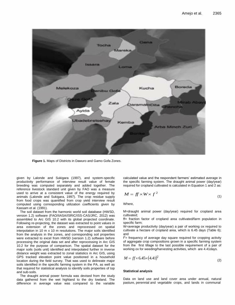
Amejo et al. 2365
Figure 1. Maps of Districts in Dawuro and Gamo Gofa Zones.
given by Lalonde and Sukigara (1997), and system-specific productivity performance of interview result value of female breeding was computed separately and added together. The reference livestock standard unit given by FAO was a measure used to arrive at a consistent value of the energy required by animals (Lalonde and Sukigara, 1997). The crop residue supply from food crops was quantified from crop yield interview result computed using corresponding utilization coefficients given by Kassam et al. (1991).
The soil dataset from the harmonic world soil database (HWSD, version 1.2) software (FAO/IIASA/ISRIC/ISS-CAS/JRC, 2012) was assembled to Arc GIS 10.2 with its global projected coordinate. Following re-projecting, the dataset was extracted to point values in area extension of the zones and reprocessed on spatial interpolation in 10 m x 10 m resolutions. The major soils identified from the analysis in the zones, and corresponding soil properties were extracted to excel from HWSD (version 1.2) software before processing the original data set and after reprocessing in Arc GIS 10.2 for the purpose of comparison. The spatial dataset for the major soils (soils unit) identified and interpolated further in inverse distance weight was extracted to zonal statistics in Arc GIS, using GPS tracked elevation point value positioned in a household location during the field survey. That was used to delineate major soils identified in the specific farming system in the PA, as well as that required for statistical analysis to identify soils properties of top and sub-soils.
The draught animal power formula was devised from the study data gathered from the wet highland to the dry lowland. The difference in average value was compared to the variable
calculated value and the respondent farmers’ estimated average in the specific farming system. The draught animal power (day/year) required for cropland cultivated is calculated in Equation 1 and 2 as:
2fWffM (1)
Where, M=draught animal power (day/year) required for cropland area cultivated; ff= fraction factor of cropland area cultivated/farm population in specific farm; W=average productivity (day/year) a pair of working ox required to cultivate a hectare of cropland area, which is 6.45 days (Table 6); and f2= frequency of average day square required for cropping activity of aggregate crop compositions grown in a specific farming system from the first tillage to the last possible requirement of a pair of working ox for weeding/harvesting activities, which are 4.41days.
241.445.6 ffM (2)
Statistical analysis
Data on land use and land cover area under annual, natural pasture, perennial and vegetable crops, and lands in communal

2366 Afr. J. Agric. Res. biomass base as well as livestock composition were analyzed using descriptive statistics of chi-square frequency and percentages. The area coverage of major crops, yields, gross household income obtained from major livelihood activities, as well as productivity performance of cow and draught animal power formula were quantified and presented in figures and tables. Regression analysis was carried out on soils’ properties of major soils, which were significant and further compared in independent samples multiple test comparison (p<0.05). Statistical analysis was done using IBM SPSS version 20.
RESULTS AND DISCUSSION
Agricultural land use land cover Figure 2 presents land use area (ha) of annual crop in PA. Wheat was the largest annual crop in wet highland agricultural land use system (43%), followed by barley and horse bean (22% and 17% respectively).
Similarly, wheat was the largest annual crop in an area (31%) followed by maize (24%) and teff (14%) in wet upper lowland to the sub-humid AEZ. Whereas in the wet lowland maize, 53% and teff, 25%, and in the dry lowland maize 86% and cotton 11% were the major annual crops occupying the land cover area of the farm household. There was significant difference (χ
2=46.39, p=0.000,
df=13, n=71) between annual crops for land use in PA. Maize, teff, wheat and groundnut/peanut were significantly higher in agricultural land area than the others, but test statistics was not significant (χ
2=6.18,
p=0.10, df=3, n=25) for land use between the major dominant annual crops.
Enset was the largest perennial crop (64%) in the highland of AEZ, followed by bamboo (24%) and apple fruit and eucalyptus/juniper tree species (6%) (Figure 2). The land area share of enset in wet upper lowland to the sub-humid AEZ was 75% and bamboo, the second largest, took 15%. For the perennial crop category, coffee, tree fruit and banana cover 59%, 28%, and 10% respectively of the land area in the wet lowland. Often, banana plantation is the largest single perennial crop in the agricultural land of the dry lowland of AEZ (Figure 3). Among perennial crops in terms of agricultural land cover area, 46% of enset was the largest followed by 28% of banana and 12% of bamboo, which also revealed a significant difference (χ
2=24.53, p=0.000, df=6, n=34)
compared to other perennial crops except coffee and apple fruit across the farming system.
The land cover area of vegetable crops consisted of 42% ethio cabbage, 32% garlic and 18% head cabbage in the highland of PAs (Figure 4). Ethio cabbage was dominantly horticultural crop in the midland with 68% area coverage; whereas pepper was 78% and onion, 22% in the wet lowland. While 100% of the land used for vegetable crop was onion in the dry lowland. Ethio cabbage (46%) and garlic (13%) were the leading vegetable crops in agricultural land use system, which were significant (χ
2=14.58, p=0.01, df=5, n=19) in their
group for land coverage.
The herd head in Tropical Livestock Unit (TLU) of the household is indicated in Figure 5. Cattle were the largest in the land use system of the smallholders with 86% of the overall herd population. The remaining 11% and 3% were taken by small ruminants and equines respectively in the land use system. Equines were significantly lower (χ
2=19.73, p=0.00) than cattle as well
as than the small ruminants (χ2=18.27, p=0.00) in the
land use system. The TLU of livestock was the largest in the wet upper
lowland to the sub-humid PAs, in the Myla and Guzza, and the wet lowland in the Yallo Worbati for each equal 11 %. The herd population was also high in dry lowland AEZ; however relatively low in the wet highland land use system. Whereas, sheep production increased toward the highland gradient and goats toward lowland farming system (Figure 5). The agricultural land area (ha) in smallholder land use system is presented in Figure 6. The LULC area of the annual crop accounted for 56% of the overall agricultural land followed by natural pasture and different types of perennial crop (17% and 15%, respectively). The difference was significant between annual crops and natural pastureland (χ
2=22.85, p=0.02) and between the
perennial cropland (χ2=22.58, p=0.02) for the agricultural
land where no significant difference (χ2=0.23, 0.98) was
observed between the latter two. The agricultural LULC area of the households was relatively high in the upper lowland to the sub-humid and the wet lowland AEZs, but reasonably low in the dry lowland and wet highland households. Similarly, the type of farm enterprises in the land use system varies across the AEZ. In the gradient toward the highland, the area coverage in perennial trees, staple food crops, and the natural pastureland increases; it is similar in the lowland gradient for major grain and root crops (Figure 6). Communal land use and land cover area share potential in farming system Table 1 presents the communal land area shares in the sampled household (ha/household). The communal biomass base area share was negative in the highland households, where the largest in the wet lowland in Qchem Kessi and the dry lowland in Para Gossa accounted for 20.36 ha and 18.12 ha per household (Table 1). The land cover composition in the communal biomass base consisted of a different mixture of grassland, woody grassland, bush/shrubland, woodland, forest, potential area and water body in/around the PA in AEZ (Figure 7). The area coverage of trees/forest increased toward the highland gradient similarly to the woody grassland/grassland biomass in the lowland gradient. The wet lowland biomass base typically reflects the savannah type grassland where the dry lowland is

Amejo et al. 2367
Figure 2. Annual crops in agricultural land area in agro-ecological zone in peasant administration (PA).
encroached with bush/shrub/woodland biomass by 70 and 64%, respectively (Figure 6). Spatial pattern of major soil and its property The spatial distribution of major soil in PA is presented in Figure 8. In the wet upper lowland to the sub-humid region, various mixes of soils were observed. The
diversity in major soils was relatively high in plain areas of the lowland of AEZ. However, most of the soils in the lowlands were expansions of the upland soil (Figure 7). Apart from limited information on soil, a field experiment by Mengiste (2009) demonstrated about four soil types in 182 km
2 of watershed area between Chencha, Boreda,
Mirab Abaya and Arba Minch Zuri districts in Gamo Gofa zone. The soils were cambisol, ferrasol, fluvisol, and regosol.

2368 Afr. J. Agric. Res.
Figure 3. Perennial/plantation crops in agricultural land area in agro-ecological zone in peasant administration (PA).
Regression analysis showed that the sodicity (%) of the topsoil properties was significant (F=6.32, p=0.03) to the other attributes in the PA (Table 2). Similarly, the significant variation (F=7.59, p=0.02) was observed for the salinity (ds/m) of the topsoil of major soils. The non-parametric test statistics showed that the sodicity was found in moderately rated class for the haplic solonchaks and solonetz soils in topsoil properties, which in turn were significant (χ
2=5.92, p=0.02) for the other major soils’
(Figure 7) property in the PA. The topsoil properties of haplic solonchaks and petric gypsisols soils were found in low rated salinity (2-4 dS/m), which were found significant (χ
2=5.08, p=0.02) for the other major soil (Figure 7)
groups. The rest soils identified in the PA were found with
very low salinity (< 2 dS/m). The subsoil organic carbon content (% weight), pH and
base saturation (%) of the major soils identified in the PA have shown a significant difference in regression analysis (Table 3). The soil organic carbon content of subsoil was significantly (χ
2=9.07, p=0.01) different for independent
sample test statistics (Table 4). In group comparison, the humic nitisols, humic alisols and haplic phaeozem soils were significantly higher (χ
2=-10.5, p=0.00) in organic
carbon content (moderate for subsoil and high to very high categories for topsoil properties) than the other groups of haplic solonchaks and petric gypsisols; the former group was significant (χ
2=-5.5, p=0.04) in
solonetz, eutric vertisols, haplic calcisols, chromic

Amejo et al. 2369
Figure 4. Vegetable/Horticultural crops in agricultural land area in agro-ecological zone in peasant administration (PA).
Figure 5. Herd head in Tropical Livestock Unit (TLU) in land use system in peasant administration.

2370 Afr. J. Agric. Res. Table 1. Population and total area and communal land area share of the sampled household in PA.
PA N Average farm size (ha/HH)a Population total b Area total (ha/total HH)c Area total (ha/total HH)a*b Land area change
(ha/PA)c-a*b Communal share area
(ha/HH)
Gmra Qema 29 1.76 327 538.48 575.52 -37.08 0
Losha 32 0.99 407 398.2 401.15 -2.95 0
Myla 32 2.35 710 2599.25 1666.95 932.3 1.31
Guzza 32 1.58 304 1139.57 480.8 658.78 2.17
Fishto 32 1.35 1070 4741.55 1441.16 3300.39 3.08
Gress Zala 33 2.94 672 2001.55 1977.92 23.63 0.035
Qchem Kssi 25 2.67 231 5321.38 617.32 4704.06 20.36
Tarcha Zuri 9 2.83 381 3092.4 1079.5 2012.9 5.28
Yallo Worbti 32 1.29 342 1822.14 440.93 1381.21 4.04
Alga 32 1.23 548 1460.67 675.92 784.75 1.43
Ancover 32 1.13 1352 2015.27 1527.76 487.51 0.36
Furra 6 1.67 343 2485.08 571.67 1913.41 5.58
Para Gossa 19 1.7 244 4836.25 414.16 4422.09 18.12
Total 345 23.49 6987 32427.79 11967.6 50160.2 61.765
Figure 6. Agricultural land area (ha/farm enterprise type) in land use system in peasant administration.

Amejo et al. 2371
Table 2. Regression analysis of topsoil properties of fourteen major soils identified from spatial analysis in peasant administration.
Topsoil property X (SD) DF R R2 Adj R
2 F p<0.05
Soil depth (cm) 93.57 (23.81) 1 0.31 0.1 0.02 1.27 0.28
AWC (mm) 138.57 (35.9) 1 0.3 0.09 0.02 1.21 0.29
Sand fraction (%) 42.79 (11.89) 1 0.22 0.05 -0.03 0.63 0.44
Silt fraction (%) 27.21 (5.5) 1 0.12 0.02 -0.07 0.18 0.68
Clay fraction (%) 30 (11.5) 1 0.29 0.08 0.01 1.1 0.32
Ref bulk density (kg/dm3) 1.36 (0.08) 1 0.26 0.08 0 0.98 0.34
Bulk density (kg/dm3) 1.32 (0.09) 1 0.41 0.17 0.1 2.45 0.14
Gravel content (%) 4.79 (9.77) 1 0.28 0.08 0.003 1.04 0.33
Organic carbon (% wght) 0.97 (0.66) 1 0.46 0.22 0.15 3.29 0.1
pH (H2O) 6.77 (0.92) 1 0.49 0.24 0.18 3.88 0.07
CEC (clay) (cmol/kg) 45.86 (17.97) 1 0.48 0.23 0.17 3.67 0.08
CEC (soil) (cmol/kg) 16.71 (8.81) 1 0.01 0 0.08 0.001 0.98
Base saturation (%) 82.43 (23.12) 1 0.48 0.23 0.16 3.54 0.08
TEB (cmol/kg) 14.09 (9.15) 1 0.27 0.07 0 0.97 0.35
Calcium carbonate (% wt) 1.31 (1.76) 1 0.34 0.12 0.04 1.55 0.24
Gypsum (% weight) 0.66 (1.71) 1 0.45 0.2 0.14 3.03 0.11
Sodicity (ESP) (%) 3.14 (3.59) 1 0.59 0.35 0.29 6.32 0.03*
Salinity (ECe) (dS/m) 0.55 (0.76) 1 0.62 0.39 0.34 7.59 0.02*
*Topsoil properties of major soils in each row are significantly different.
Figure 7. Communal biomass base land use and land cover area (ha/sampled household population) share in peasant administration.
cambisols, chromic luvisols, eutric fluvisols, eutric regosols and haplic ferralsols, found in poor to moderate organic carbon content groups in the PA. Whereas, the comparison between the latter two categories showed no significant difference (χ
2=-5.0, p=0.10) in the PA for
organic carbon content. The pH of subsoil properties was found significant
(χ2=10.18, p=0.01) (Table 4). The subsoil property
indicated a very acidic condition in haplic ferralsols and
humic nitisols soils; it is also significant (χ2=-9.00, p=0.01)
in carbonate rich soil groups of chromic luvisols, eutric regosols, petric gypsisols, haplic solonchaks, eutric vertisols and solonetz. The humic alisols, chromic cambisols, haplic calcisols, eutric fluvisols and haplic phaeozems soils were acid to neutral categories with significant difference (χ
2=-5.50, p=0.02) in carbonate rich
soil category of subsoil properties in the PA. Whereas the test statistics showed no significant difference (χ
2=-3.50,

2372 Afr. J. Agric. Res.
Table 3. Regression analysis of subsoil properties of thirteen major soils identified from spatial analysis in peasant administration.
Subsoil property X (SE) DF R R2 Adj R
2 F p<0.05
Bulk Density (kg/dm3) 1.40 (0.09) 1 0.23 0.53 -0.03 0.61 0.45
Gravel Content (%) 3.54 (9.54) 1 0.06 0 -0.09 0.04 0.84
Organic Carbon (% weight) 0.43 (0.21) 1 0.62 0.39 0.33 7 0.023*
pH (H2O) 6.97 (0.86) 1 0.65 0.43 0.38 8.23 0.015*
CEC (clay) (cmol/kg) 44.77 (18.19) 1 0.49 0.24 0.18 3.58 0.09
CEC (soil) (cmol/kg) 16.31 (9.41) 1 0.04 0 -0.09 0.02 0.9
Base Saturation (%) 81.69 (21.71) 1 0.64 0.41 0.35 7.5 0.019*
TEB (cmol/kg) 13.83 (9.89) 1 0.35 0.12 0.04 1.56 0.24
Calcium Carbonate (% weight) 2.23 (3.28) 1 0.41 0.17 0.09 2.2 0.17
Gypsum (% weight) 1.02 (3.05) 1 0.4 0.16 0.09 2.14 0.17
Sodicity (ESP) (%) 2.46 (3.30) 1 0.46 0.21 0.14 2.93 0.11
Salinity (ECe) (dS/m) 1.56 (3.12) 1 0.52 0.23 0.2 4 0.07
*Subsoil properties for major soils in each row are significantly different.
Table 4. Independent samples test statistics on top and subsoil properties of major soils identified in peasant administration.
Property N χ2 Df p
Topsoil
Sodicity (%) 3 12.68 2 0.02
Salinity (dS/m) 2 5.08 1 0.02
Subsoil
Organic carbon (% weight) 3 9.07 2 0.01
pH in water solution 3 10.18 2 0.01
Base saturation (%) 2 6.82 1 0.01
p=0.28) between very acid and acid to neutral soil categories of the subsoil. The major soil identified in the study area failed in two categories for base saturation properties; haplic ferralsols, humic nitisols, and humic alisols in base saturation corresponding to acid conditions; the rest in saturated conditions sometimes sodic or saline soil also showed a significant difference (χ
2=-6.82, p=0.01) in the sub-region (Table 4).
Agricultural production productivity In the wet highland, households’ wheat and barley share 6.52 and 6.33 ha, and 3.19 and 3.37 ha of the annual cropland area respectively in Losha and Gmra Qema PAs (Figure 1). The household estimated yield of each of these crops was 17 quintals/ha. The pulse crops cover area in Losha and Gmra Qema by 0.65 and 4.53 ha, and
0.57 and 1.4 ha (Figure 1), with production yield of 15 and 14 quintals/ha for horse bean and pea respectively. Irish potato is an important crop with high turnover in land use system; it shares 0.89 ha of the area and 250 quintals/ha with average sales of 75% production yield in the household in Losha PA.
Wheat of 14.47 ha in Myla and 7.56 ha in Guzza, and maize of 19.94 ha in Gress Zala and 9.65 ha in Fishto of the wet upper lowland to the sub-humid in PAs were the largest among the annual croplands area coverage. Wheat and teff in the latter three PAs and pea and teff in Myla have also substantiated holdings of the production area (Figure 1). The production of wheat and barley of 19 quintals/ha, and 16 and 15 quintals/ha of horse bean and pea in this region was the highest yield/ha area than the highland in AEZ. The production yield of taro of 200 quintal/ha in Myla and Guzza and sweet potato of 300 quintals/ha in Gress Zala and Fishto households were

Amejo et al. 2373
Figure 8. Spatial pattern of major soil extracted to point value in GIS 10.2 in peasant administration.
major components of staple food with 15% of the farm products used for commercial purpose in the household. The average sales amount of farm production was 45% of horse bean, 50% of pea, and 70% of each wheat and barley equal in both households of the highland and the midland. However, 80% of teff and 45% of maize (mainly from fresh harvest) were additional sources of household income from annual crop category in the latter AEZ households.
In the wet lowland PA, maize and teff took a prominent place in the agricultural land area with 25.59 and 10.06 ha in Qchem Kessi, 9.53 and 3.49 ha in Tarcha Zuri and 11.81 and 8.92 ha in Yallo Worbati household respectively (Figure 2). Whereas, groundnut of 1.95 ha with 12 quintals/ha production yield was lucrative cash crop with 80% used for commercial purpose in Yallo Worbati household. Maize was as equally important in the dry lowland PAs in the production area where only about 35% of the production yield used for business in a household was lower than that of 55% in the wet lowland. The average yield of maize of 42 quintals/ha in the wet lowland was also better than that of 38 quintals/ha in the dry lowland and 28 quintals/ha in the midland.
The most staple food crop, enset plantation was most typical in Myla, Gmra Qema and Guzza PA households with 12.76, 8.17 and 7.88 ha in land cover area (Figure 2). Banana occupied 15. 07 ha of cropland area, growing toward the area with specialized farming system in Ancover PA in the dry lowland. Although growing steady currently 1.04 ha of apple tree covering area in Losha household has been most promising for both household income, agro-industrial batch and as source of breeding stock for the entire country (Figure 2). Similarly, coffee plantation has been a reasonable allocation of land use system with mid-term level response to household
income in the wet lowland. Although gradual turn over to household income, bamboo, eucalyptus and juniper trees were a substantial contribution to area coverage and household income in upward gradients to the highland (Figure 2).
The cropland cover area of the ethio cabbage was almost uniform from the wet upper lowland to the highland household holdings (Figure 3). However, it varies in its function, which in enset dominant production system was prominently used for household dietary supplement; where households relatively in the right position to consumer market such as Losha, Gress Zala and Fishto different compositions of vegetable growing to provide additional support in the household incomes with better turn over in land use system. Similarly, garlic has been household adapted crop with added value in Gmra Qema and groundnut in Yallo Worbati, in the highland and lowland land use system respectively. In the agricultural land cover area, crops such as maize, teff, wheat, groundnut, Irish potato with other different sorts such as cabbage, garlic, coffee, banana and the apple fruit contributed a significant high amount to household income, compared to crops of similar categories in land use system in any specific farming system (Amejo et al., 2018).
The diversity of livestock and products, chicken, and honey production plays a vital role in the household economy. The livestock sector household earnings consist of 60% cattle and 20% small ruminants (sheep and goats). Livestock product, butter and cottage cheese of 7% and buttermilk of 6% vary between the farming systems accounting for the household income. Butter in wet lowland in Dawuro zone household and buttermilk in the dry lowland household in Gamo Gofa zone are commodities valuable in cash income.

2374 Afr. J. Agric. Res.
Table 5. Productivity performance of cow in peasant administration.
Peasant administration Milk yield, kg/day Milk yield, kg/lactation Lactation Length, day Fertility rate
Gmra Qema 1.83 495 270 0.87
Losha 1.83 467 255 1.00
Myla 1.67 902 540 0.68
Guzza 1.63 731 450 0.81
Fishto 1.55 557 360 1.00
Gress Zala 2.12 509 240 0.76
Qchem Kessi 2.00 776 390 1.00
Tarcha Zuri 2.08 624 300 1
Yallo Worbti 2.51 902 360 0.87
Alga 2.00 597 300 1.00
Ancover 2.02 544 270 1.00
Furra 1.95 585 300 1.00
Para Gossa 2.00 597 300 1.00
Total average 1.94 637.38 333.46 0.92
Table 6. Formula for draught animal power (day/year) for cropland cultivated in peasant administration.
PA N A ff X f W A*f E M=ff*6.45*(4.41)2
Gmra Qema 29 18.78 0.65 12.00 3.50 5.48 65.73 71.00 81
Losha 32 14.02 0.44 8.00 4.00 7.01 56.09 68.00 55
Myla 32 30.76 0.96 24.5 3.89 4.88 119.6 149.00 121
Guzza 32 22.4 0.70 22.00 3.89 3.96 87.11 135.00 88
Fishto 32 26.5 0.83 28.00 3.89 3.68 103.1 107.00 104
Grss Zala 33 64.84 1.96 22.00 3.89 11.46 252.2 182.00 246
Qcheme Kessi 25 47.20 1.89 28.50 4.40 7.29 207.70 159.00 237
Tarcha Zuri 9 16.58 1.84 9.50 5.50 9.60 91.16 126.00 231
Yallo Worbati 32 27.19 0.85 22.50 4.40 5.32 119.60 137.00 107
Alga 32 30.22 0.94 14.50 5.00 10.42 151.10 175.00 118
Ancover 32 17.28 0.54 14.50 5.00 5.96 86.40 43.00 68
Furra 6 8.10 1.35 5.50 5.00 7.36 40.50 101.00 169
Para Gossa 19 21.28 1.12 19.00 5.00 5.60 106.40 125.00 140
Average 26.54 26.55 1.0 17.73 4.41 6.45 114.36 121.38 125
Note: a=total hectare area of cropland requiring draught animal power, f=frequency of average day requiring a pair of working ox for aggregate composition of crops grows, ff=fraction factor of total cropland area, W=average productivity day of a pair of working ox per hectare of cropland, X=a pair of ox available, A*f=variable calculated average days/year for a pair of working oxen, E=framers’ estimate average days/year for a pair of working ox to cultivate cropland, N=sample househ
A cow productivity performance impartially increases in the gradient toward the lowland (Table 5), the dairy and lactation milk yields, as well as the fertility rate higher in lowland AEZ. The productivity performance average of cow milk yields, 1.94 kg/day and 637.38 kg/lactation as well as 92% fertility rate in the wet highland and wet upper to sub-humid households was below the population average of the sample in PAs (Table 5). This probably associates with the resource potential in the AEZ. In the zones, the lowland gradients mainly comprise grassland, shrublands and woody browsing species, which on the other hand entertain extensive grazing and browsing.
Agricultural productivity is regularly calculated by the partial productivity of land (value of agricultural output per hectare of agricultural land) and partial productivity of labor (value of agricultural output per agricultural worker, including self-employed). An aggregate, the partial measures into one index that allows for the entire basket of resources and inputs used in agriculture is total factor productivity. While, both could have a limitation in the area context of present study due to several compounded factors. However, one can describe the agricultural productivity in the current study area as part of the result compositions and specialized forms of agriculture

Amejo et al. 2375
Figure 9. Percentage of annual average and grand gross income obtained between household and on-and off-farm activities in peasant administration.
production systems maintained in the farm household and adapted in the AEZ.
According to Ruthenberg (1971), farming within each system is carried out in holdings, which are more or less distinct managerial units. Thus, it is difficult to measure agricultural productivity straight, and land productivity can vary for its own various different reason in smallholder system. As observed in this study a 0.25 ha area of farm holdings in banana growing area in the dry lowland can sustain the household livelihood with substantial numbers of a family member in case current farm level price of banana continues to increase steadily than the average holdings of 0.99 ha in the highland household. Another experience given was the role of a small farm 0.3 ha supporting livelihood in a non-graze dairy system in Kenya (Prinsley, 1990).
The overall percentage of relative agricultural productivity in gross average income in different LULC, for instance, between households and the livelihood activities in the PAs is presented in Figure 9. A comparison showed that the LULC area in the annual cropland was significantly higher than the other farm enterprises in the study PAs. However, the household annual gross income contributed from livestock sector (40%) was significantly (χ
2=1.38, SE=0.19, p=0.85) as
equal as that of the annual crop production earned (46%).
Therefore, it is not only the farm or land size alone that determines agricultural productivity, particularly in smallholder system. There are also other factors playing a prominent role in smallholder agricultural productivity that could relate to the locally available and accessible resources; also infrastructures with necessary facilities, relative productivity of the land in relation with pre-historic population settlement trend, farm-level prices, AEZ, environment, etc are important determinants. The
differential changes in the relative distribution of land, livestock, natural resources (rangeland biomass, forest flora, rivers, streams, and lakes) in specific farming have to lead to striking differences and changes in the structure of agricultural production.
For over 20 years, for instance, in most of the highland gradient PAs, local dairy production was carried out conjointly with artificial insemination service. However, in the lowland production system local cows yet fundamental in a dairy production also depicted highest average productivity performance of population (Table 5). This fact could supposedly be related to the availability of feed and water resources through extensive grazing. This also supports our assumption that local livestock productivity performance could be improved through improvement of feed and feeding management (Amejo et al., 2018).
There is no debate for increased farm size accompanied by management objective and the determinant factors mentioned above can increase agricultural productivity in smallholder households. An implication of this fact in the current study could be the Losha household in the wet highland PA. In this household of the major livelihood strategies identified off-farm, remittance and labor categories relatively contributed the largest with 28% (main of these were traditional cloth making), followed by annual crop, 26%, livestock, 12% and perennial crop plantation, 10% of the gross annual income. This shows that the household livelihood activities more or less contributed to equal as important as and interactively to the household income. However, the lowest average of 0.99 ha farm size (Table1) severely limited the household income with a grand average of 76% in a range between a minimum of 54% and a maximum of 143% (Figure 9).
The other striking evidence could be the land area of

2376 Afr. J. Agric. Res. Fishto PA, in the midland AEZ, which is the second largest in population and the third in total land area of all the study PAs (Table 1). The land biomass existing in communal biomass base was the largest than the household holdings. This is also in contrast with the adjacent PA, Gress Zala in which the land area evidenced was exclusively in farm holding level (Table 1). The household income gained was the third largest with 131% in the latter PA whereas the former the lowest of all with 54% from a range of a minimum and a maximum as mentioned above. The high slope surface, with the mean rise of 32.9% and confidence interval of 27.90-37.92 has been most likely affected by soil fertility. The soils observed were found to have poor organic carbon content, and others very acidic suffering from aluminum toxicity in case of Fishto PA. That could probably contribute less interaction effect to income from the livelihood activities mainly from farm-based sources in this PA. Proximity to urban area, road and transportation accesses, market stimuli to produce crops with relative better turnover have provided resilience and adaptability capacity in the household with small farm size such as Losha PA. A specialized type of production system with farmer objectives, for example, was observed in crops such as cabbages, garlic, groundnut, apple fruit, and Irish potato between the PAs and AEZs. The household had a specialized type of adaptation in these crops, and the crops also depicted a significant difference in some specific production system than the others.
It appears that to cultivate frequently in a year between seasons increases the land use efficiency, family cash income flow and most of the crops production ‘purely’ for cash or little parts (component) used for consumption. Its specialized adaptation in some production environment is also describable. For instance, the apple fruit introduced earlier has been well adapted in the highlands of Chencha (for example, in Losha PA), with significant cash value. Expansion effort to this crop has been made earlier in Gmra Qema PA (almost in the similar agroecology). In the Losha PA, the production of Irish potato together with the composition of other vegetables intensifying the system has given an opportunity for critical shortages of the farmland. That advanced with relative availability in road accesses and transportation in positions to Arba Minch town, which comprised about over 125,000 populations.
The production practices of Irish potato are overshadowed in Gmra Qema of similar agro-ecology, due to disease related to the crop and the soil moisture stress condition. But garlic in Gmra Qema as the most adopted and flexible crop is farmed twice in March to May and October yearly; it is supplied to either local or reachable consumers and carried by pack of animals or family labor. Its influence also explained a significant difference between the land use systems of the PAs and income values of crops in the similar category. The turnover of the income driven by the crop could be much
more important for the household given that the production system is heavily intensified by crops like enset known to prolong provisions of household food demand. Tree plantation like bamboo, juniper, eucalyptus, etc. might take time to create income and compounded factors like infrastructural facilities. The disease condition and wet stress make less cropping opportunity twice in a year in bimodal rainfall often usual in many parts of Ethiopia. A remarkable result was shown in the number of farmers’ cropping activity in two seasons (main rainy and belg season) in Gmra Qema compared to the other PAs. The positive sign in practices, however, farmers use the cropland for aftermath grazing season to season.
In contrast, in Tanzania, for instance, households cultivating maize on wrong soil or increasing landholding for the purpose of increasing output provided to soil resulted in low yields and therefore, more land is needed for better harvest (Hepelwa, 2010). According to that study, there was no much increase in landholding byhouseholds but the only feasible means to increase agricultural production is via improving technical efficiency.
Constraints like land shortage, disease, market limitation, rising production cost, lack of labor and shortage in improved verities were important factors pronounced by the respondent households in the sub-regions. In addition, soil data analyses from metadata source showed that the major soils identified in the PAs were problem of sodicity and salinity and some others were very acidic and poor organic carbon content except humic nitisols, humic alisol, and petric phaezems. The declining soil fertility conditions in the highland are also related to the long history of human settlement in Ethiopia.
Farm activities, its specific function designated to the household strategy could result in influences of the ecological environment on local knowledge and the economy. The farming system functioning would value remarkably the land efficiency, labor productivity, and supplement income. Its role should be encouraged and transformed into a diversified form. Livelihood strategies are dynamic and are composed of activities that generate the means of household survival (Ellis, 2000). A positive relationship with the landholding and socioeconomic factors such as income, primary education, age, household size, family labor, remittances (Hepelwa, 2010) was indicated. System interaction Livestock production is the primary input source of agricultural production in a smallholder production system, hence the livestock production could be claimed as a by-product of agricultural enterprises in mixed crop-livestock systems. From highland to dry lowland, in the

patchy surface, to the machine, oxen have taken a proper position in the number of thousands hectare of area cultivated in the present study place.
Table 6 presents the formula for draught oxen power (day/year) used in cropland cultivated. The draught power used in the PAs to cultivate annual crop including horticulture was on average 125 days/year. This was the product of average productivity of 6.45 days for a pair of working ox per hectare area of cropland cultivated and the square of average frequency of 4.41 days for various aggregate crops growing required a pair of working ox from first tillage to the last with possible weeding/ harvesting activities yearly from highland to the lowland of AEZs. Similarly, farmers’ interview result for their experience on a pair of working ox used for cropland cultivated was 121.38 days/year and that the variable calculated average was 114.37 days/year from the highland to the lowland AEZs (Table 6). The difference observed was 3.62 days for the farmers’ experience estimation and 10.63 days for the variable calculated average compared to the formula derived from draught animal day.
In another study in Nepal, cultivation in hill zebu for 62 days and swamp buffalo for 130 days per year (Oli, 1985) was estimated. According to Gebresenbet et al. (1997), small-scale farming is the most important sector of agricultural production in most Sub Saharan countries and about 80% use human or animal power in the production of their food and income needs. Animal power used for thousands of years in Ethiopia is unique in Sub-Saharan Africa compared with the rest of Africa where animal traction for cultivation has been introduced within the recent past as one of several technical interventions (Gebresenbet et al., 1997).
The annual crops requiring working oxen in the highland AEZ include wheat, barley, pea, horse bean, lentil and some other oil crops. Crops such as potato, garlic and other vegetable orchid could also engender oxen plough depending on plot size and access. The wet upper lowland to the sub-humid PA households use working oxen to cultivate crops such as teff, maize, root crops, wheat, barley, pulse and some other crops. Teff, maize, sorghum, root crops and groundnut in wet lowland and maize, cotton and bean in either intercropping or single unit require oxen power in the dry lowland. The pattern of crop cultivation in terms of oxen use seems to be more cyclic toward the lowland gradient in Gamo Gofa PA households; however, it seems like more season based cropping activity and crops carried out in Dawuro zone PAs, broadly between the two seasons when cropping activity is done. In the former, the households mostly follow the rainfall patterns and cultivate cropland at the slightest signs of rainfall; the farmers have adaptability capacity to change and varied climate change. While in the latter case, it is supposed to be due to moisture stress and catering to relative rest period in the cropland.
Amejo et al. 2377
The fraction factor of draught power, 1.96 in the Grss Zala, in wet upper lowland to the sub-humid zone and 1.89 in the Qchem Kessi in the wet lowland was the largest that used oxen for cropland ploughing per year. This value was low in wet highland in Losha 0.44 and in dry lowland in Ancover 0.54. The difference reflected in fraction factor between AEZs and PAs could be due to farm and plot sizes available for cultivation. Otherwise draught power requirement for traction could depend on the suitability of cropland for plough, the aggregate compositions of the crops cultivated by oxen in particular farming systems and the frequency farmers use oxen during cropping activities. This means that a pair of working ox is used to cultivate one hectare of cropland area per year from first tillage to growing an aggregate type of annual/temporal crops; weeding and harvest was done in mixed crop-livestock system from highland to lowland AEZ for an average of 125 days. The estimated average number of working hour/day recorded for a pair of working ox during the rice planting season in the hills was eight hours and the area ploughed was 0.25 ha/day; that for swamp buffalo was seven hours and 0.37 ha/day (Oli, 1985).
The formula could, therefore, be used directly or with slight modification in Ethiopia or elsewhere; oxen traction is common for cropland cultivation. Oxen power value estimate in agricultural production is the major difficulty Ethiopia is currently facing. This result, however, provides a remarkable opportunity to the sector. Animal traction provides almost a quarter of the total area under crop production in the level of global estimate (Swanepoel et al., 2010). On the other hand, Oli (1984) estimated that the draught power used for cultivation in Nepal was equivalent to about 1.37 million kilowatts of energy and contribution of those animals was worth about Nepal currency 1,300 million at 1984 prices. In another, during a serious economic crisis for the Cuban society approximately 385,000 oxen were substituted 40,000 tractors (Henriksson and Lindholm, 2000). The fundamental issue raised on monetary valuing of a draught power has been mentioned earlier by IGAD Livestock Policy Initiative paper (Behnke, 2010; Behnke and Metaferia, 2013).
Manure is another livestock output which farmer households much rely on as a means to soil fertility improvement in their production system, and apply to identified crops associated with yield perfection (Amejo et al., 2018). Peasant farmers in the highland due to stressed soil condition, small plot size, and increasing fertilizer debt have the tendencies to carry livestock wastes over distance crop field, allowing tethering by small ruminants in the ploughed plot prior to sowing period. However, the production level of manure dry matter (DM) matches the herd holdings as well as the crop residue DM supply to the annual cropland area in the household (Table 7).
Livestock production, on the other hand, bears the

2378 Afr. J. Agric. Res.
Table 7. Annual cropland area, percent of household cultivated annual cropland area per season and farm output supply dry matter (DM) in peasant administration (PA).
PA Annual cropland
area, ha (%)
Household cropping activity between season Farm level output supply
% household in Belg season
% household in Meher season
Crop residue DM (%)
Manure DM (%)
Gmra Qema 17.26 (34) 0 100 37 (3) 57.58 (7)
Losha 12.56 (40) 53 100 33 (3) 33.89 (4)
Myla 30.01(40) 25 100 77 (6) 83.58 (11)
Guzza 21.85 (43) 19 100 55 (4) 81.93 (11)
Fishto 25.73 (60) 78 56 114 (9) 64.17 (8)
Grss Zala 63.74 (66) 72 75 229 (18) 69.10 (9)
Qcheme Kessi 46.68 (70) 61 39 208 (16) 80.62 (10)
Tarcha Zuri 15.56 (61) 57 43 72 (6) 18.43 (2)
Yallo Worbati 26.89 (65) 57 43 109 (8) 98.39 (13)
Alga 30.22 (76) 100 47 147 (11) 60.87 (8)
Ancover 17.28 (46) 100 47 80 (6) 50.02 (6)
Furra 7.8 (78) 100 33 29 (2) 17.77 (2)
Para Gossa 21.28 (66) 100 32 101 (8) 56.27 (7)
Total 335.75 822 815 1289.81 772.62
burdens of labor, abets risks arisen due to market limitation for crop commodities in far distance households, topographies of the location in the corridors bounded by water logs across each regions and gives compensation for crop miscarry due to climate change. The farm household in the Gmra Qema PA in particular and mostly toward highland gradients in the Dawuro zone, for instance, did not practice belg season cropping activities in the plots of the annual crop (Table 7). The variation in the household cropping activity could probably be stress related to soil condition. Our standardized precipitation index (SPI) analysis also evidenced other causes like wet event extremity in this region in addition to drought event. The respondent households in the Grma Qema PA also disclosed soil related problems in growing some root crops. However, in Gmra Qema (100%), livestock production has provided a positive attribute in the land use system through grazing from season to season (Table 7).
The livestock feed supply from food crop production accounted for 8% of the total annual in the study area. The value indicated was apart from feeds from aftermath grazing of cropland, weeds harvested from different land use types or livestock graze directly on it. Grazing/ browsing base, both food and non-food production biomass systems presented the dominant share of livestock feed supply which accounted for 92% of the total amount quantified in relations to herd population and levels of their physiological feed requirements in the specific farming system. The variability in biomass base availability is high within and between the AEZs and PAs.
In the highland, feed resources and crop residues are wheat, barley, and legumes, tubers, and leftovers of the arched of vegetable, enset, bamboo, and tree leaves.
Maize, teff, sorghum, field bean, root crops, coffee leaves, tree plantations and banana left over after fruit cut in the lowland were all important sources of livestock feed in wet and dry seasons. Whereas, feed resources supply from food crop production in the mid-altitude comprehensively constitute that of the highland and lowlands.
However, households’ use of crop residue as livestock feed was inconsistent and inefficient, despite its limited potentials in nutritive value. On the other hand, enset and bamboo that are grazed results in land shortage during cropping season, filthiness of grazing areas due to heavy rainfall and frequent grazing on the same pasture and dry period are invasive in the highland to sub-humid regions. All the land use systems occupied by various items of crops are an alternative means that could provide significant strategic opportunity in the face of a critical shortage of grazing land particularly in highland household.
The highland livestock feed supply was basically described in land held by private ownership where farm holdings were significantly low as well as natural pasture land; these are strikingly unmatchable to the number of livestock herd head in the system. Other studies expressed similar evidence in northern highland of Ethiopia (Yimer, 2009). However, multifarious mixes of the crops in different forms of land use system, magnitudes of range in inter-seasonal cropping activities in a certain area due to disease and wet stress systematically are arranged. Types and species mixes of the livestock, regime and scheme in a grazing system for the different groups of livestock and farmers’ tendencies to harvest, collect, store and use crop residue and other fodder cut through scarcity, function together influence land shortage. In contrast, in the lowland there is

sufficient stack of rangeland biomass with wide varieties of grasses, shrub and abundant browse species.
Relating livestock and biophysical resources, a study emphasized different categories of land, such as total land, arable land, arable and permanent crops, permanent or non-permanent pastures, and non-arable pastures. The proportion of each land type and its evolution over time in relation to total land is important, especially that of permanent pastures need to be considered (Swanepoel et al., 2010).The farming system is congenital in the area, yet adopted in the AEZs, for instance, sheep, and mare production is typical in the highland and goat system in the lowland. The diversity together with land use allocation in various cropland strikingly maximized the opportunity for livestock production not only in areas with abundant grazing but also in the highland where grazing land is rare. Land and grazing resources availability often determines the type of livestock that can be kept, the way they are managed, and the extent to which livestock production can expand further (Swanepoel et al., 2010).
Conclusions The present study set out to characterise smallholder rural mixed crop-livestock systems subdividing various AEZs into LULC classes in Gamo Gofa and Dawuro zones. The major livelihood strategies identified in the community are farm system (crops and livestock production), collecting (forest product and fishing) and non-farm (such as traditional clothes making, local small trading, remittance, and labor) activities. The assets and activities in these categories are predominately and solely evolving steadily and diversely in natural environment and experiences of farm household. In a way, labor and family health are invariably important for households to derive their livelihood means. Despite fragmented holdings, structures on land use allocation of the farm entity provide particular options on integrity and utilization of the household owned resources in the subregions. In terms of provision of food, income and feed, small plot size holding, scale of production and intra-seasonal based production due to bi-modal rainfall distribution in the area annual crops had the largest agricultural land cover area in the subregions of PAs. The components and elements of crop and livestock type existing within AEZs are similar. The difference resulted in similar AEZ probably due to the existence of a minor level of manipulation on the system, soil and on awareness development of the farmers. This deviation lays an opportunity for developing interventions that can address common features in the area. Whereas, the basic difference associated with the farming system and the household were the difference in agro-ecological conditions, geo-location, and distance to marketing point where a substantial number of consumer market exists to dispose farm households supply and their demand.
The non-food production rbiomass consisted of two-
Amejo et al. 2379
thirds of the total, in which 18% exist in the mid-land AEZ, and annual draught power use for the cultivated area fraction marked the highest despite the high slope surface. Agricultural land use efficiency might be impeded due to high slope surface in wet upper lowland to the sub-humid agro-ecology. The highest non-food production biomass, 82% was found in the wet and dry lowland. While the economic contribution is comparable lower in land productivity in the lowland region due to inefficient use and utilization of this biomass base. The highest average gross income of livestock in this drought-prone area largely capitalizes resilience and responding capability of livestock agriculture to major supply-side difficulties generally in the current study area.
Moreover, livestock production is an important component of current mixed crop-livestock systems; its role is beyond that of the usual provision of milk and meat. Livestock production supplements numerous supply-side difficult factors observed in the current study. Through changes and several deriving force, farmers are aware that their land fertility is less efficient to gain enough yield. They have the desire to use fertilizer as the level of their yield increases. However, production cost (full package soil fertilizer cost) and family demand are limited by plot size and the output per holdings.
Therefore, smallholder farmers estimate the amount of manure they can gain per head of animal they have, plot size to cultivate particular crop and the amount of mineral fertilizer they can afford to blend with animal manure. This experience is emerging particularly in the highland farming system. The high proportion of income obtained from livestock sector shows that livestock can be remarkably intensifying systems without the associated effects of land-based intensification. This also clearly implicates the land-livestock productivity per hectare basis. The high income from crops reveals the sales of high-value cash crops (such as maize, wheat, teff, bean, cabbages, apple, banana, etc).
The range and balance of resource, assets and enterprise
combinations that are reflected in any specific farming system are limited by a number of constraining factors. Several constraining factors increase agricultural productivity from land holdings alone, in smallholder agriculture production. On the other hand, many smallholders’ peasant production insinuates small plot size in developing countries.
The role of the livelihood strategies identified in crop-livestock systems to household economy is crucially important for agricultural development. The efforts towards strengthening infrastructural facilities to link marketing opportunities, undertaking investment in agricultural research for development, improving the linkage between agriculture and natural resources like water, rangelands and disease control promote not only farm household economy from the existing potential but also foster availability and access to food security between smallholder rural producers and consumers. Without a significant approach to development support,

2380 Afr. J. Agric. Res. the future will be very pessimistic to farm household in high-altitude.
Scope for future work
The data of the current study could be useful in crop and livestock modeling and management decision by interlinking each other in several modeling tools. Future study in these lines can explore livestock productivity per land area; compare and evaluate an area where animal manure is commonly used for crops such as enset, root and other horticultural crops, its population density and diversity, production level and yield and trends of change in these attributes over time as well as soil-microbe population and diversity; the level of manure production, proportion used for crops, proportions of cropland fertilized, farmers’ desire and levels of manure supply in a supplement to mineral fertilizer amount in the household; the monitory value of manure and draught animal power in agricultural production; rangeland evaluation for management objective. Also farm animals’ demographic characteristic should be assessed in details for local farm animals in mid-term records of demographic data. An argument was developed from this study: the milk yield of the cow toward lowland gradient was higher than that of the highland. In the latter case artificial insemination service is common from exotic or improved breeds. Therefore, this result implicates that better milk yield in the lowland supposedly is associated with local resource availabilities rather than the imported input. Integrated analysis to ensure the roles, extent and potential demand of the resource base can confer certainty of long-term impact on increased efficiency of food production, and sufficiently high economic return to merit the land capability. The co-existence of traditional mixed crop-livestock systems evolves with soil-plant-animal-atmosphere in combination with the entire systems of genetic material. CONFLICT OF INTERESTS The authors have not declared any conflict of interests. REFERENCES
Amejo AG, Gebere YM, Dickoefer U, Kassa H, Tana T, Lawrence P
(2018). Herd dynamics and productivity performance modeling of livestock in smallholder crop-livestock systems in Southwestern Ethiopia. International Journal of Veterinary Sciences and Animal Husbandry 3(1):17-24.
Behnke RH (2010). The contribution of livestock to the economies of IGAD member states: study findings, application of the methodology in Ethiopia and recommendations for further work. IGAD LPI Working Paper No. 02-10. pp. 1-45.
Behnke RH, Metaferia F (2013). The contribution of livestock to the Ethiopian economy. Nairobi: IGAD Centre for Patoral Areas and Livestock Development. IGAD LPI Working Paper No. 02-11. pp. 1-43.
CACC (2003). Ethiopian Agricultural Sample Enumeration, 2001/02.
Results for Southern Nations, Nationalities and Peoples’ Region. Statistical Report on Livestock and Farm implements. Part IV. Addis Ababa, Ethiopia.
Cervantes-Godoy D (2015). Strategies for addressing smallholder agriculture and facilitating structural transformation.
Central statistical agency (CSA) (2016). Federal democratic republic of Ethiopia. Central statistical agency. Key findings of the 2015/2016 (2008 E.C) agricultural sample surveys, country summary. Addis Ababa, July, 2016 pdf
Ethiopia, WFP, Headquarters, WFP (2014). Comprehensive food security and vulnerability analysis (CFSVA) http://www.wfp.org/food-security.pdf
FAO/IIASA/ISRIC/ISSCAS/JRC. (2012). Harmonized world soil database (version 1.2). FAO, Rome, Italy and IIASA, Laxenburg, Austria.
Food and Agriculture Organization (FAO) (2015). The state of food insecurity in the world 2014: strengthening the enabling environment for food... security and nutrition. FAO, Rome, Italy.
Gebresenbet G, O’Neill D, Mutua J, Oram C (1997). Technological support for rural agricultural transport and development. Keynote paper presentation to Improving Rural Agricultural Transport Systems for Enhanced Production and Marketing in Smallholder Farms of East
Africa. Proceedings published by KENDAT (Kenya Network for Draught Animal Technology), Nairobi.
Gliessman SR (2007). Agroecology: the Ecology of Sustainable Food Systems. 2nd edition. Boca raton, Fl, usa, crc Press, Taylor and Francis group.
Graeub BE, Chappell MJ, Wittman H, Ledermann S, Kerr RB, Gemmill-Herren B (2016). The state of family farms in the world. World Development 87:1-15.
Hazell P (2013). Is Small Farm Led Development Still a Relevant Strategy for Africa and Asia.
Henriksson M, Lindholm EL (2000). The use and role of animal draught power in Cuban Agriculture: a field study in Havana Province. Swedish University of Agricultural Sciences pp. 1-47
Hepelwa A (2010). Environmental and socioeconomic factors influencing crop cultivation. An application of Multivariate Discriminant Analysis (MDA) model in Sigi catchment, Tanzania pp. 1-29.
Herrero M, González-Estrada E, Thornton PK, Hoogenboom G (2005). Impact: Integrated Modelling Platform for Mixed Animal-crop Systems: User's Manual. ILRI (aka ILCA and ILRAD). Retrieved from https://cgspace.cgiar.org/bitstream/handle/10568/1214/Impact.pdf
Herrero M, González-Estrada E, Thornton PK, Quiros C, Waithaka MM, Ruiz R, Hoogenboom G (2007). IMPACT: Generic household-level databases and diagnostics tools for integrated crop-livestock systems analysis. Agricultural Systems 92(1):240-265.
Kassam H, Velthuizen G, Fischer G, Shah M (1991). Resource database and land productivity; Technical Annex 5: Livestock Productivity. Agro-Ecological Land Resources for Agricultural Development Planning. Retrieved from/available from http://www.fao.org/tempref/docrep/fao/009/t0737e.pdf
Lalonde LG, Sukigara T (1997). LDPS2 User's Guide. Food and
Agriculture Organization of the United Nations. Retrieved from http://www. fao. org/ag/aga/lspa/ldps2.pdf
Lipper L, Thornton P, Campbell BM, Baedeker T, Braimoh A, Bwalya M, Caron P, Cattaneo A, Garrity D, Henry K, Hottle R (2014). Climate-smart agriculture for food security. Nature Climate Change 4(12):1068.
Lowder SK, Skoet J, Raney T (2016). The number, size, and distribution of farms, smallholder farms, and family farms worldwide. World Development 87:16-29.
Notenbaert A, Herrero M, Kruska R, You L, Wood S, Thornton P, Omolo A (2009). Classifying livestock production systems for targeting agricultural research and development in a rapidly changing world. ILRI Discussion Paper 19. ILRI (International Livestock Research Institute), Nairobi, Kenya 41 p.
Oli KP (1984). Utilization of draught animal power in the hill agriculture systems of Nepal (a concept paper for contribution)[of mules, yaks, ponies and asses].(Workshop paper). In Workshop on Hill Farming System (livestock). Pokhara (Nepal). 17-19 Jan 1984.

Oli KP (1985). Draught animals in the hill agricultural system. Livestock
in the Hills of Nepal” Edited by Morel, AM; Oli, KP Pakhribas Agricultural Centre, Dhankuta, Nepal.
Otte MJ, Chilonda P (2002). Cattle and small ruminant production systems in sub-Saharan Africa. A systematic review. Livestock Information Sector Analysis and Policy Branch, FAO Agriculture Department.
Prinsley RT (1990). Agroforestry for sustainable production. Economic implications. Commonwealth Science Council (CSC).
Quiroz R, Zorogastúa P, Baigorria G, Barreda C, Valdivia R, Cruz M, Reinoso J (1999). Toward a dynamic definition of agroecological zones using modern information technology tools. CIP Program Report, 2000:361-370.
Ryschawy J, Choisis N, Choisis JP, Joannon A, Gibon A (2012). Mixed crop-livestock systems: an economic and environmental-friendly way of farming?.Animal 6(10):1722-1730.
Ruthenberg H (1971). Farming systems in the tropics. Oxford University Press. 424 p.
Southern Nations, Nationalities and Peoples (SNNP) (2001). A strategic plan for the sustainable development, conservation, and management of the woody biomass resources. The Southern Nations, Nationalities and Peoples Regional State www.eap.gov.et/sites/default/files/SNNPR-grazing.pdf
Amejo et al. 2381 Swanepoel F, Stroebel A, Moyo S (2010). The role of livestock in
developing communities: enhancing multifunctionality. University of the Free State and Technical Centre for Agricultural and Rural Cooperation, Cape Town.
Tittonell P (2014). Livelihood strategies, resilience and transformability in African agroecosystems. Agricultural Systems 126:3-14.
World Food Program/Food and Agriculture Organization (WFP/FAO) (2012). LEAP version 2.61 for Ethiopia. Retrieved from/Available from http://hoefsloot.com/download/leap_install.exe
Yimer AA (2005). Farm management in mixed crop-livestock systems in the Northern Highlands of Ethiopia. PhD thesis Wageningen University, Wageningen, The Netherlands pp. 1-238.

Related Journals:
www.academicjournals.org
O PE N ACCE S S
O PE N ACCE S S
O PE N ACCE S S
O PE N ACCE S S
O PE N ACCE S S
Journal of
Agricultural Extension
and Rural Development
International Journal of
Fisheries and Aquaculture
Journal of
Cereals and Oilseeds
Journal of Agricultural
Biotechnology and
Sustainable Development
International Journal of
Livestock Production
African Journal of
Agricultural Research
O PE N ACCE S S
O PE N ACCE S S O PE N ACCE S S O PE N ACCE S S
Journal of Plant Breeding and Crop Science
Journal of Stored Products and Postharvest Research
Journal of
ent
Soil Science and Environmental Managem
Related Documents