POUR L'OBTENTION DU GRADE DE DOCTEUR ÈS SCIENCES acceptée sur proposition du jury: Prof. H. Shea, président du jury Prof. Ph. Renaud, Dr A. Meister, directeurs de thèse Dr C. Duschl, rapporteur Dr S. Gautsch, rapporteur Prof. D. Mueller, rapporteur AFM Based Single Cell Microinjection: Technological Developements, Biological Experiments and Biophysical Analysis of Probe Indentation THÈSE N O 5489 (2012) ÉCOLE POLYTECHNIQUE FÉDÉRALE DE LAUSANNE PRÉSENTÉE LE 16 NOVEMBRE 2012 À LA FACULTÉ DES SCIENCES ET TECHNIQUES DE L'INGÉNIEUR LABORATOIRE DE MICROSYSTÈMES 4 PROGRAMME DOCTORAL EN MICROSYSTÈMES ET MICROÉLECTRONIQUE Suisse 2012 PAR Joanna Katarzyna BITTERLI

Welcome message from author
This document is posted to help you gain knowledge. Please leave a comment to let me know what you think about it! Share it to your friends and learn new things together.
Transcript
POUR L'OBTENTION DU GRADE DE DOCTEUR ÈS SCIENCES
acceptée sur proposition du jury:
Prof. H. Shea, président du juryProf. Ph. Renaud, Dr A. Meister, directeurs de thèse
Dr C. Duschl, rapporteur Dr S. Gautsch, rapporteur
Prof. D. Mueller, rapporteur
AFM Based Single Cell Microinjection: Technological Developements, Biological Experiments and Biophysical
Analysis of Probe Indentation
THÈSE NO 5489 (2012)
ÉCOLE POLYTECHNIQUE FÉDÉRALE DE LAUSANNE
PRÉSENTÉE LE 16 NOvEMBRE 2012
À LA FACULTÉ DES SCIENCES ET TECHNIQUES DE L'INGÉNIEURLABORATOIRE DE MICROSYSTÈMES 4
PROGRAMME DOCTORAL EN MICROSYSTÈMES ET MICROÉLECTRONIQUE
Suisse2012
PAR
Joanna Katarzyna BITTERLI


To the three women: my mum, my mum-inlaw and my daughter

I have not failed. I’ve just found 10000 ways that won’t work. - Thomas Edison
iv
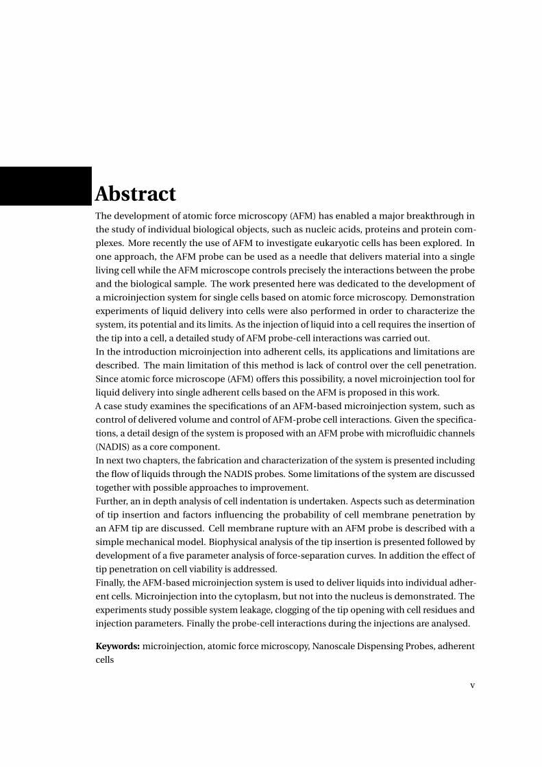
AbstractThe development of atomic force microscopy (AFM) has enabled a major breakthrough in
the study of individual biological objects, such as nucleic acids, proteins and protein com-
plexes. More recently the use of AFM to investigate eukaryotic cells has been explored. In
one approach, the AFM probe can be used as a needle that delivers material into a single
living cell while the AFM microscope controls precisely the interactions between the probe
and the biological sample. The work presented here was dedicated to the development of
a microinjection system for single cells based on atomic force microscopy. Demonstration
experiments of liquid delivery into cells were also performed in order to characterize the
system, its potential and its limits. As the injection of liquid into a cell requires the insertion of
the tip into a cell, a detailed study of AFM probe-cell interactions was carried out.
In the introduction microinjection into adherent cells, its applications and limitations are
described. The main limitation of this method is lack of control over the cell penetration.
Since atomic force microscope (AFM) offers this possibility, a novel microinjection tool for
liquid delivery into single adherent cells based on the AFM is proposed in this work.
A case study examines the specifications of an AFM-based microinjection system, such as
control of delivered volume and control of AFM-probe cell interactions. Given the specifica-
tions, a detail design of the system is proposed with an AFM probe with microfluidic channels
(NADIS) as a core component.
In next two chapters, the fabrication and characterization of the system is presented including
the flow of liquids through the NADIS probes. Some limitations of the system are discussed
together with possible approaches to improvement.
Further, an in depth analysis of cell indentation is undertaken. Aspects such as determination
of tip insertion and factors influencing the probability of cell membrane penetration by
an AFM tip are discussed. Cell membrane rupture with an AFM probe is described with a
simple mechanical model. Biophysical analysis of the tip insertion is presented followed by
development of a five parameter analysis of force-separation curves. In addition the effect of
tip penetration on cell viability is addressed.
Finally, the AFM-based microinjection system is used to deliver liquids into individual adher-
ent cells. Microinjection into the cytoplasm, but not into the nucleus is demonstrated. The
experiments study possible system leakage, clogging of the tip opening with cell residues and
injection parameters. Finally the probe-cell interactions during the injections are analysed.
Keywords: microinjection, atomic force microscopy, Nanoscale Dispensing Probes, adherent
cells
v

RésuméLe développement de la microscopie à force atomique (AFM pour atomic force microscope) a
permis une avancée majeure dans l’étude d’entités biologiques individuelles, telles que les
acides nucléiques ou les protéines et leurs complexes. Plus récemment, des études ont exploré
l’aptitude des techniques AFM à analyser des cellules eucaryotes. Dans une des approches, la
sonde de l’AFM est utilisée comme aiguille permettant de délivrer une substance à l’intérieur
d’une cellule individuelle vivante, l’interaction entre la sonde et la cellule étant contrôlée de
manière précise par l’AFM.
Le travail présenté ici est consacré au développement d’un système de micro-injection pour
des cellules individuelles, basé sur le principe de l’AFM. Des expériences démontrant la
libération de substances à l’intérieur de cellules ont été réalisées dans le but de caractériser
le système, ainsi que son potentiel et ses limites. L’injection intracellulaire nécessitant une
pénétration de la sonde AFM dans la cellule, une étude approfondie de l’interaction sonde-
cellule a été effectuée.
L’introduction décrit la méthode de la microinjection dans des cellules, les applications et les
limites. La limitation principale de cette méthode est l’absence de contrôle sur la pénétration
de la cellule. Puisque la microscopie à force atomique (AFM) offre cette possibilité elle a été
proposée comme alternative. Pour cela un nouvel outil de microinjection pour la libération de
substances à l’intérieur de cellules individuelles basé sur l’AFM est développé dans le cadre de
cette thèse.
Une étude de cas examine les spécifications d’un système de micro-injection basé sur un
AFM, telles que le contrôle du volume délivré et le contrôle de l’interaction sonde-cellule.
Une conception détaillée d’un système tenant compte des spécifications est présentée, dont
la composante principale est une sonde AFM pourvue de canaux microfluidiques (sonde
NADIS). Les deux chapitres suivants décrivent la fabrication et la caractérisation du système, y
compris du flux de liquide passant par la sonde NADIS. Quelques limitations du système sont
discutées conjointement avec les améliorations possibles.
Ensuite, une analyse approfondie de l’indentation cellulaire est entreprise. Des aspects tels
que la détermination de l’insertion de la sonde et des facteurs influençant la probabilité d’une
pénétration de la membrane cellulaire sont discutés. La rupture de la membrane cellulaire par
la sonde AFM est décrite à l’aide d’un modèle mécanique simple. Une analyse biophysique
de l’insertion de la pointe est présentée, ainsi qu’une analyse des courbes force-séparation
à l’aide de cinq paramètres. De plus, l’effet de la pénétration de la sonde sur la viabilité des
cellules est abordé.
vii
Finalement, le système de micro-injection basé sur un AFM est utilisé pour libérer des sub-
stances dans des cellules adhérentes individuelles. La micro-injection dans le cytoplasme,
mais non pas dans le noyau, est démontrée. Les expériences analysent les fuites possibles
dans le système, l’obstruction de l’ouverture située à la pointe de la sonde par des résidus
cellulaires et les paramètres de micro-injection. Finalement, les interactions sonde-cellule
durant la micro-injection sont analysées.
Mots-clés : microinjection, microscopie à force atomique, Nanoscale Dispensing Probes, celles
adhérentes
viii
Contents
Abstract v
Résumé vii
List of figures xiii
List of tables xvi
Introduction 1
1 Introduction 1
1.1 Microinjection into single adherent cells . . . . . . . . . . . . . . . . . . . . . . . 1
1.2 Components of a microinjection system . . . . . . . . . . . . . . . . . . . . . . . 1
1.3 Applications . . . . . . . . . . . . . . . . . . . . . . . . . . . . . . . . . . . . . . . 3
1.4 Limitations of the microinjection systems for adherent cells . . . . . . . . . . . 3
1.5 AFM-based delivery systems into single adherent cells . . . . . . . . . . . . . . 4
1.6 Delivery of biomolecules with AFM probes . . . . . . . . . . . . . . . . . . . . . 6
1.7 AFM probes with microfluidic systems . . . . . . . . . . . . . . . . . . . . . . . . 7
1.8 Thesis objectives . . . . . . . . . . . . . . . . . . . . . . . . . . . . . . . . . . . . . 9
2 Materials and methods 11
2.1 Fabrication of the apertures . . . . . . . . . . . . . . . . . . . . . . . . . . . . . . 11
2.1.1 Interaction of the ion beam with the matter (specifications) . . . . . . 12
2.2 Development of parylene C mask for KOH etching . . . . . . . . . . . . . . . . . 13
2.2.1 Substrates . . . . . . . . . . . . . . . . . . . . . . . . . . . . . . . . . . . . 13
2.2.2 Substrate cleaning . . . . . . . . . . . . . . . . . . . . . . . . . . . . . . . 13
2.2.3 Chemical adhesion promotion . . . . . . . . . . . . . . . . . . . . . . . . 13
2.2.4 Parylene deposition . . . . . . . . . . . . . . . . . . . . . . . . . . . . . . 14
2.3 Thermal treatment . . . . . . . . . . . . . . . . . . . . . . . . . . . . . . . . . . . 14
2.3.1 Potassium Hydroxide (KOH) Exposure . . . . . . . . . . . . . . . . . . . 14
2.3.2 Scratch test . . . . . . . . . . . . . . . . . . . . . . . . . . . . . . . . . . . 14
2.3.3 XRD measurements . . . . . . . . . . . . . . . . . . . . . . . . . . . . . . 15
2.3.4 The AFM imaging . . . . . . . . . . . . . . . . . . . . . . . . . . . . . . . . 15
2.4 Instrumentation . . . . . . . . . . . . . . . . . . . . . . . . . . . . . . . . . . . . . 15
2.4.1 Atomic force microscope (AFM) . . . . . . . . . . . . . . . . . . . . . . . 15
ix
Contents
2.4.2 Pressure generator . . . . . . . . . . . . . . . . . . . . . . . . . . . . . . . 15
2.4.3 Flow measurements system . . . . . . . . . . . . . . . . . . . . . . . . . . 16
2.5 Substrates for biological experiments . . . . . . . . . . . . . . . . . . . . . . . . 17
2.6 Cell culture . . . . . . . . . . . . . . . . . . . . . . . . . . . . . . . . . . . . . . . . 18
2.6.1 Cell seeding on Petri dish substrates . . . . . . . . . . . . . . . . . . . . . 18
2.6.2 Cell seeding on CYTOOchip™ . . . . . . . . . . . . . . . . . . . . . . . . 18
2.6.3 Cell staining . . . . . . . . . . . . . . . . . . . . . . . . . . . . . . . . . . . 18
2.6.4 Confocal analysis . . . . . . . . . . . . . . . . . . . . . . . . . . . . . . . . 18
2.6.5 Cell death analysis . . . . . . . . . . . . . . . . . . . . . . . . . . . . . . . 19
2.6.6 Cell fixation . . . . . . . . . . . . . . . . . . . . . . . . . . . . . . . . . . . 19
2.7 AFM probes . . . . . . . . . . . . . . . . . . . . . . . . . . . . . . . . . . . . . . . . 19
2.8 Data processing and statistical analysis . . . . . . . . . . . . . . . . . . . . . . . 20
2.8.1 Analysis of force-distance curves . . . . . . . . . . . . . . . . . . . . . . 20
2.8.2 Statistical analysis . . . . . . . . . . . . . . . . . . . . . . . . . . . . . . . 20
3 Concept study 21
3.1 Introduction: Delivery of liquids into a living body . . . . . . . . . . . . . . . . . 21
3.2 Design of a liquid delivery system into single mammalian cells . . . . . . . . . 22
3.2.1 Amount of liquid delivered into a single cell . . . . . . . . . . . . . . . . 23
3.2.2 Control of liquid delivery . . . . . . . . . . . . . . . . . . . . . . . . . . . 24
3.3 Detailed design of the AFM – based microinjection system . . . . . . . . . . . 25
3.4 Specifications of the system . . . . . . . . . . . . . . . . . . . . . . . . . . . . . . 27
3.4.1 Characteristics of the AFM probe . . . . . . . . . . . . . . . . . . . . . . 27
3.4.2 Characteristics of the pressure driven flow in the system . . . . . . . . . 29
3.4.3 Control of volume injected to single cell . . . . . . . . . . . . . . . . . . 32
3.5 Summary . . . . . . . . . . . . . . . . . . . . . . . . . . . . . . . . . . . . . . . . . 32
4 Design and fabrication of the NADIS probes for a microinjection system 35
4.1 Introduction . . . . . . . . . . . . . . . . . . . . . . . . . . . . . . . . . . . . . . . 35
4.1.1 Closed NADIS probes . . . . . . . . . . . . . . . . . . . . . . . . . . . . . 35
4.1.2 Fabrication Process . . . . . . . . . . . . . . . . . . . . . . . . . . . . . . 36
4.1.3 Design of the NADIS probes . . . . . . . . . . . . . . . . . . . . . . . . . 38
4.1.3.1 Design of the AFM probe and fluidic channels . . . . . . . . . 39
4.1.4 Fabrication Results . . . . . . . . . . . . . . . . . . . . . . . . . . . . . . . 40
4.1.5 Metallization of the AFM probes . . . . . . . . . . . . . . . . . . . . . . . 41
4.1.6 Fabrication of the tip aperture . . . . . . . . . . . . . . . . . . . . . . . . 41
4.1.7 Summary . . . . . . . . . . . . . . . . . . . . . . . . . . . . . . . . . . . . 42
4.2 Design and fabrication of NADIS probes for the cell microinjection system . . 42
4.2.1 Design of the AFM chip . . . . . . . . . . . . . . . . . . . . . . . . . . . . 43
4.2.2 Modification of the process flow . . . . . . . . . . . . . . . . . . . . . . . 45
4.2.3 3D parylene mask for KOH etching of NADIS probes . . . . . . . . . . . 46
4.2.3.1 Parylene adhesion study . . . . . . . . . . . . . . . . . . . . . 47
4.2.3.2 Testing of the 3D mask . . . . . . . . . . . . . . . . . . . . . . . 52
x
Contents
4.2.4 Microfabrication results . . . . . . . . . . . . . . . . . . . . . . . . . . . . 54
4.2.5 Metallization of the AFM probes . . . . . . . . . . . . . . . . . . . . . . . 55
4.2.6 Fabrication of the tip aperture . . . . . . . . . . . . . . . . . . . . . . . . 56
4.2.6.1 Milling the apertures . . . . . . . . . . . . . . . . . . . . . . . . 57
4.2.6.2 Results . . . . . . . . . . . . . . . . . . . . . . . . . . . . . . . . 58
4.2.7 Discussion . . . . . . . . . . . . . . . . . . . . . . . . . . . . . . . . . . . 59
4.3 Summary . . . . . . . . . . . . . . . . . . . . . . . . . . . . . . . . . . . . . . . . . 61
5 AFM – based microinjection system: assembly and characterization 63
5.1 Assembling of the system components . . . . . . . . . . . . . . . . . . . . . . . . 63
5.2 Characterization of the system . . . . . . . . . . . . . . . . . . . . . . . . . . . . 64
5.2.1 Calibration of the spring constant of the NADIS cantilevers . . . . . . . 65
5.2.2 Filling of the system with liquid . . . . . . . . . . . . . . . . . . . . . . . 66
5.2.3 Characterization of the fluid flow through the system . . . . . . . . . . 68
5.2.3.1 Flow measurments of gas . . . . . . . . . . . . . . . . . . . . . 70
5.2.3.2 Flow measurements of liquid . . . . . . . . . . . . . . . . . . . 75
5.3 Control of ejected liquid volume . . . . . . . . . . . . . . . . . . . . . . . . . . . 78
5.4 Discussion . . . . . . . . . . . . . . . . . . . . . . . . . . . . . . . . . . . . . . . . 80
5.5 Conclusions . . . . . . . . . . . . . . . . . . . . . . . . . . . . . . . . . . . . . . . 83
6 AFM-based microinjection system: biophysical analysis of probe indentation 85
6.1 Introduction: Mechanical penetration of a cell membrane . . . . . . . . . . . . 85
6.2 How to determine cell membrane penetration . . . . . . . . . . . . . . . . . . . 87
6.2.1 Analysis of tip insertion . . . . . . . . . . . . . . . . . . . . . . . . . . . . 88
6.2.2 Proposed specifications of tip insertion . . . . . . . . . . . . . . . . . . . 91
6.3 Probability of cell membrane penetration . . . . . . . . . . . . . . . . . . . . . . 91
6.3.1 Influence of tip sharpness . . . . . . . . . . . . . . . . . . . . . . . . . . 92
6.3.1.1 Force distance–curves with multiple force drops . . . . . . . 92
6.3.2 Influence of cell–surface interactions . . . . . . . . . . . . . . . . . . . . 94
6.3.3 The influence of ethylenediaminetetraacetic acid (EDTA) . . . . . . . . 95
6.4 Analysis of probe indentation: 5A method . . . . . . . . . . . . . . . . . . . . . 96
6.4.1 Description of the 5A method . . . . . . . . . . . . . . . . . . . . . . . . 96
6.4.1.1 Macroparameters . . . . . . . . . . . . . . . . . . . . . . . . . . 97
6.4.1.2 Microparameters . . . . . . . . . . . . . . . . . . . . . . . . . . 97
6.4.2 5A analysis of probe indentation . . . . . . . . . . . . . . . . . . . . . . . 101
6.5 5A analysis of actin cytoskeleton modifications . . . . . . . . . . . . . . . . . . 106
6.5.1 Comparative analysis between cells spread on fibronectin and pat-
terned fibronectin . . . . . . . . . . . . . . . . . . . . . . . . . . . . . . . 108
6.5.2 Comparative analysis between cells spread on fibronectin, with and
without EDTA . . . . . . . . . . . . . . . . . . . . . . . . . . . . . . . . . . 111
6.5.3 Comparative analysis between cells spread on patterned fibronectin,
with and without EDTA . . . . . . . . . . . . . . . . . . . . . . . . . . . . 114
6.5.4 Discussion . . . . . . . . . . . . . . . . . . . . . . . . . . . . . . . . . . . . 117
xi
Contents
6.6 General discussion . . . . . . . . . . . . . . . . . . . . . . . . . . . . . . . . . . . 119
6.6.1 Determination of tip insertion . . . . . . . . . . . . . . . . . . . . . . . . 119
6.6.2 Force-separation curves with multiple force drops . . . . . . . . . . . . 121
6.6.3 5A method . . . . . . . . . . . . . . . . . . . . . . . . . . . . . . . . . . . 121
6.7 Conclusions . . . . . . . . . . . . . . . . . . . . . . . . . . . . . . . . . . . . . . . 122
7 Quantification of single cell damage 125
7.1 Method 1: Cell damage quantification using Petri dish . . . . . . . . . . . . . . 126
7.1.1 Cell damage analysis after cell membrane penetration . . . . . . . . . . 128
7.2 Method 2: Cell damage quantification using patterned fibronectin . . . . . . . 130
7.2.1 Cell damage analysis after cell membrane penetration . . . . . . . . . . 132
7.2.2 Cell damage analysis after penetration of the entire cell . . . . . . . . . 135
7.3 Discussion . . . . . . . . . . . . . . . . . . . . . . . . . . . . . . . . . . . . . . . . 138
7.4 Conclusions . . . . . . . . . . . . . . . . . . . . . . . . . . . . . . . . . . . . . . . 140
8 Microinjection using the AFM–based system 141
8.1 Experimental design . . . . . . . . . . . . . . . . . . . . . . . . . . . . . . . . . . 141
8.2 Preliminary experiments . . . . . . . . . . . . . . . . . . . . . . . . . . . . . . . . 143
8.2.1 Mechanical stability of probe/probe holder seal . . . . . . . . . . . . . . 144
8.2.2 Origin of increasing resistance to liquid injection . . . . . . . . . . . . . 148
8.2.3 Discussion . . . . . . . . . . . . . . . . . . . . . . . . . . . . . . . . . . . . 149
8.3 Intracellular injection of sodium fluorescein . . . . . . . . . . . . . . . . . . . . 150
8.3.1 Discussion . . . . . . . . . . . . . . . . . . . . . . . . . . . . . . . . . . . . 154
8.4 Intranuclear injection . . . . . . . . . . . . . . . . . . . . . . . . . . . . . . . . . . 154
8.5 General Discussion . . . . . . . . . . . . . . . . . . . . . . . . . . . . . . . . . . . 158
8.6 Conclusions . . . . . . . . . . . . . . . . . . . . . . . . . . . . . . . . . . . . . . . 160
9 Conclusion & Outlook 161
Bibliography 171
Acknowledgements 173
List of publications 175
Curriculum Vitae 177
xii

List of Figures
1.1 Microinjection . . . . . . . . . . . . . . . . . . . . . . . . . . . . . . . . . . . . . 1
1.2 Different needles . . . . . . . . . . . . . . . . . . . . . . . . . . . . . . . . . . . . 2
1.3 MANiPEN . . . . . . . . . . . . . . . . . . . . . . . . . . . . . . . . . . . . . . . . 3
1.4 A microinjection system for injection into adherent cells . . . . . . . . . . . . 4
1.5 Schematic of a typical AFM set up for cell biology. . . . . . . . . . . . . . . . . 5
1.6 Optical images of a) a micropipette needle penetrating primary neuronal cells
2; and b) a standard AFM probe penetrating HEK293 cell. . . . . . . . . . . . 5
1.7 Nanoneedle . . . . . . . . . . . . . . . . . . . . . . . . . . . . . . . . . . . . . . . 6
1.8 NanoFountain Probe . . . . . . . . . . . . . . . . . . . . . . . . . . . . . . . . . 7
1.9 NADIS cantilever . . . . . . . . . . . . . . . . . . . . . . . . . . . . . . . . . . . 8
1.10 Schematic of the probe design and its fabrication process . . . . . . . . . . . 8
2.1 Configuration of the system and the sample . . . . . . . . . . . . . . . . . . . 12
2.2 Pictures of the AFM setup . . . . . . . . . . . . . . . . . . . . . . . . . . . . . . 16
2.3 Optical images of a tube filled with liquid . . . . . . . . . . . . . . . . . . . . . 17
3.1 Schematic of liquid delivery into a living organism. . . . . . . . . . . . . . . . 21
3.2 Diversity of cell types. . . . . . . . . . . . . . . . . . . . . . . . . . . . . . . . . . 22
3.3 Schematic of an AFM based system for liquid delivery into adherent cell. . . 23
3.4 Schematic of an AFM–based microinjection system. . . . . . . . . . . . . . . . 26
3.5 Schematic of rectangular cross–sectional view. . . . . . . . . . . . . . . . . . . 27
3.6 Spring constant dependency on the length of a cantilever with defined width
and wall thickness . . . . . . . . . . . . . . . . . . . . . . . . . . . . . . . . . . . 28
3.7 Spring constant dependency on the length for a cantilever with defined width
and height . . . . . . . . . . . . . . . . . . . . . . . . . . . . . . . . . . . . . . . 29
3.8 Schematics of a simplified fluidic system of the AFM–based microinjection
system . . . . . . . . . . . . . . . . . . . . . . . . . . . . . . . . . . . . . . . . . . 30
4.1 Schematic of the NADIS probe . . . . . . . . . . . . . . . . . . . . . . . . . . . 36
4.2 Schematic of Type I and Type II design . . . . . . . . . . . . . . . . . . . . . . . 36
4.3 Flow–chart of the principle process steps . . . . . . . . . . . . . . . . . . . . . 37
4.4 Schematic of Type A and Type B . . . . . . . . . . . . . . . . . . . . . . . . . . . 38
4.5 Schematic of a different cantilevers. . . . . . . . . . . . . . . . . . . . . . . . . 39
4.6 Optical micrographs of different cantilevers . . . . . . . . . . . . . . . . . . . . 40
4.7 Optical micrograph of double beam cantilever . . . . . . . . . . . . . . . . . . 41
xiii
List of Figures
4.8 Schematic drawing of the NADIS probe with aperture . . . . . . . . . . . . . . 42
4.9 Schematic of the FIB holder . . . . . . . . . . . . . . . . . . . . . . . . . . . . . 42
4.10 Schematic drawings of the NADIS chip with their geometrical parameters. . 44
4.11 Schematic of different cantilevers . . . . . . . . . . . . . . . . . . . . . . . . . . 45
4.12 Flow–chart of the principle process steps . . . . . . . . . . . . . . . . . . . . . 46
4.13 Diffraction patterns of Parylene films on a silicon nitride substrate . . . . . . 49
4.14 Optical and AFM micrographs before and after thermal treatment . . . . . . 50
4.15 Graphs showing the rupture load for samples . . . . . . . . . . . . . . . . . . . 51
4.16 Images of the position of the rupture load . . . . . . . . . . . . . . . . . . . . . 52
4.18 Images showing residues after first attempt to remove the Parylene mask . . 53
4.19 Optical micrograph of different cantilevers . . . . . . . . . . . . . . . . . . . . 54
4.20 SEM micrographs . . . . . . . . . . . . . . . . . . . . . . . . . . . . . . . . . . . 55
4.21 SEM micrograph of an AFM tip coated with a) 45 nm of gold and b) 47 nm of
platinum layer. . . . . . . . . . . . . . . . . . . . . . . . . . . . . . . . . . . . . . 56
4.22 Schematic drawings of NADIS tips . . . . . . . . . . . . . . . . . . . . . . . . . 57
4.23 Schematic drawings of the new FIB holder . . . . . . . . . . . . . . . . . . . . 58
4.24 Schematics of the tip–ion beam configuration. . . . . . . . . . . . . . . . . . . 60
4.25 SEM micrographs . . . . . . . . . . . . . . . . . . . . . . . . . . . . . . . . . . . 61
4.26 SEM micrograph of a tip . . . . . . . . . . . . . . . . . . . . . . . . . . . . . . . 61
5.1 AFM system . . . . . . . . . . . . . . . . . . . . . . . . . . . . . . . . . . . . . . . 64
5.2 AFM holder with two fluidic channels . . . . . . . . . . . . . . . . . . . . . . . 65
5.3 AFM holder with double–side tape . . . . . . . . . . . . . . . . . . . . . . . . . 66
5.4 Measurement of the resonance frequency . . . . . . . . . . . . . . . . . . . . . 68
5.5 Schematic of the experimental apparatus. . . . . . . . . . . . . . . . . . . . . . 69
5.6 Schematic drawing . . . . . . . . . . . . . . . . . . . . . . . . . . . . . . . . . . 70
5.7 Theoretical and measured flow value . . . . . . . . . . . . . . . . . . . . . . . . 71
5.8 Theoretical and measured flow values for NADIS probe . . . . . . . . . . . . . 72
5.9 Theoretical and measured flow values for NADIS probe . . . . . . . . . . . . . 73
5.10 Theoretical and measured flow values for NADIS probe . . . . . . . . . . . . . 74
5.11 Theoretical and measured flow values for 3 NADIS probe without the tip . . 75
5.12 Theoretical and measured flow values for 3 NADIS probe without the tip . . 77
5.13 Theoretical values of the steady state flow of water through needle like open-
ing type in the NADIS probe. . . . . . . . . . . . . . . . . . . . . . . . . . . . . 79
5.14 SEM micrograph . . . . . . . . . . . . . . . . . . . . . . . . . . . . . . . . . . . . 82
6.1 Force-distance curves . . . . . . . . . . . . . . . . . . . . . . . . . . . . . . . . . 85
6.2 Schematic of an animal cell and its components [63]. . . . . . . . . . . . . . . 86
6.3 Drawing of three-dimensional view of a cell membrane [63]. . . . . . . . . . 87
6.4 Force-separation curves . . . . . . . . . . . . . . . . . . . . . . . . . . . . . . . 89
6.5 Different types of force-separation curves . . . . . . . . . . . . . . . . . . . . . 89
6.6 Force-distance distribution chart . . . . . . . . . . . . . . . . . . . . . . . . . . 90
xiv
List of Figures
6.7 SEM micrograph of two NADIS tips before and after cell indentation experi-
ments . . . . . . . . . . . . . . . . . . . . . . . . . . . . . . . . . . . . . . . . . . 91
6.8 SEM images . . . . . . . . . . . . . . . . . . . . . . . . . . . . . . . . . . . . . . 93
6.9 Example of force–separation curves . . . . . . . . . . . . . . . . . . . . . . . . 94
6.10 Cells viewed via phase contrast microscopy . . . . . . . . . . . . . . . . . . . . 94
6.11 Schematic representation of the macroparameters . . . . . . . . . . . . . . . 97
6.12 Schematic representation of an AFM tip indenting the cell . . . . . . . . . . . 99
6.13 Force–distance curve . . . . . . . . . . . . . . . . . . . . . . . . . . . . . . . . . 100
6.14 Schematic representation of the microparameters on a force–separation curve. 100
6.15 Comparison of indentation depth . . . . . . . . . . . . . . . . . . . . . . . . . . 102
6.16 Comparison of a) penetration depth (D1) and b) penetration force (F1) . . . 103
6.17 Schematic of cell membrane rupture . . . . . . . . . . . . . . . . . . . . . . . . 103
6.18 Comparison of the Force drop . . . . . . . . . . . . . . . . . . . . . . . . . . . . 104
6.19 Comparison of the membrane slip parameter d (*p < 0.05). . . . . . . . . . . 105
6.20 Graphical representation of the Fd /F1 and d/D1 ratios . . . . . . . . . . . . . 106
6.21 Schematic of actin cytoskeleton structures located in a single adherent cell . 107
6.22 Schematic of an AFM tip inserted through a cell membrane with actin mesh
undercoat . . . . . . . . . . . . . . . . . . . . . . . . . . . . . . . . . . . . . . . . 107
6.23 Cells viewed via confocal microscopy . . . . . . . . . . . . . . . . . . . . . . . 109
6.24 Comparison of cell height, nucleus height and membrane–nucleus distance 110
6.25 Schematic drawing of cell spread on the glass . . . . . . . . . . . . . . . . . . . 110
6.26 Schematic of cell membrane rupture . . . . . . . . . . . . . . . . . . . . . . . . 112
6.27 Cells spread on the glass coated with fibronectin . . . . . . . . . . . . . . . . . 113
6.28 Comparison of cell height, nucleus height and membrane-nucleus distance 113
6.29 Schematic representation of actin cytoskeleton . . . . . . . . . . . . . . . . . 114
6.30 Schematic of cell membrane rupture . . . . . . . . . . . . . . . . . . . . . . . . 115
6.31 Cells spread on the glass coated with fibronectin spots . . . . . . . . . . . . . 116
6.32 Comparison of cell height, nucleus height and membrane–nucleus distance 116
6.33 Schematic representation of actin cytoskeleton . . . . . . . . . . . . . . . . . 117
6.34 Schematic of cell membrane rupture . . . . . . . . . . . . . . . . . . . . . . . . 118
7.1 Schematic drawing of an AFM tip positioned above the nucleus and penetrating126
7.2 Mapping of a Petri dish with a grid with squares. . . . . . . . . . . . . . . . . . 126
7.3 Force–separation curves. . . . . . . . . . . . . . . . . . . . . . . . . . . . . . . . 127
7.4 Confocal and DIC microscopy images . . . . . . . . . . . . . . . . . . . . . . . 128
7.5 Overlapped phase contrast image before tip indentation experiment with
confocal images of cells after the experiment . . . . . . . . . . . . . . . . . . . 130
7.6 Overlapped phase contrast image before tip indentation experiment with
confocal images of cells after the experiment . . . . . . . . . . . . . . . . . . . 131
7.7 Phase contrast image of a section with 81 fibronectin spots. . . . . . . . . . . 132
7.8 Confocal images of cells after indentation experiment . . . . . . . . . . . . . 134
7.9 Confocal images of cells after indentation experiment . . . . . . . . . . . . . 136
xv

7.10 Overlapped confocal images of control sample . . . . . . . . . . . . . . . . . . 137
8.1 Diagram showing the planning of the experiment. . . . . . . . . . . . . . . . . 142
8.2 Injection of excess of water into a cell . . . . . . . . . . . . . . . . . . . . . . . 143
8.3 Force–time curves . . . . . . . . . . . . . . . . . . . . . . . . . . . . . . . . . . . 145
8.4 Schematic drawing of the NADIS probe . . . . . . . . . . . . . . . . . . . . . . 146
8.5 Force increase measurements . . . . . . . . . . . . . . . . . . . . . . . . . . . . 146
8.6 Apparent force increase . . . . . . . . . . . . . . . . . . . . . . . . . . . . . . . . 147
8.7 SEM images of a NADIS tip . . . . . . . . . . . . . . . . . . . . . . . . . . . . . . 148
8.8 SOverlapped confocal and phase contrast images . . . . . . . . . . . . . . . . 151
8.9 Examples presenting 4 types of force distance curves found after the injection
experiment. . . . . . . . . . . . . . . . . . . . . . . . . . . . . . . . . . . . . . . . 153
8.10 Confocal images of SaOS-2 cells after the injection of the sodium fluorescein
and propidium iodide mixture. . . . . . . . . . . . . . . . . . . . . . . . . . . . 155
8.11 Force-separation curves measured for 50 nN applied force. . . . . . . . . . . 156
8.12 Force-separation curves measured for a) - b) 80 nN applied force, and c)-d)
100 nN applied force. . . . . . . . . . . . . . . . . . . . . . . . . . . . . . . . . . 157
8.13 Schematic drawin . . . . . . . . . . . . . . . . . . . . . . . . . . . . . . . . . . . 159
List of Tables
3.1 Calculations of liquid amount that can be delivered into a single cell . . . . . . 24
3.2 Size description of the fluidic components. . . . . . . . . . . . . . . . . . . . . . 31
3.3 Calculated range of values of the hydraulic resistance . . . . . . . . . . . . . . . 31
3.4 Values of the pressure pulses applied to the fluidic system for cell injection. . . 32
4.1 Values of the free length of the cantilevers. . . . . . . . . . . . . . . . . . . . . . 39
4.2 The widths and heights of channels and beam depending on the design . . . . 43
4.3 Detailed summary of the free length for different cantilever design . . . . . . . 45
4.4 Parylene C adhesion study: summary of tested conditions. . . . . . . . . . . . . 48
4.5 A comparison of two metallization processes. . . . . . . . . . . . . . . . . . . . . 56
4.6 A comparison of two metallization processes. . . . . . . . . . . . . . . . . . . . . 59
5.1 Measured values of the spring constant for a single and double beam type
cantilevers. . . . . . . . . . . . . . . . . . . . . . . . . . . . . . . . . . . . . . . . . 65
5.2 Resonance frequency measurements of the NADIS probe before and after being
filled with liquid. The average decrease in resonance frequency is (26±9) kHz 67
xvi
List of Tables
5.3 Comparison of theoretical and measured values of hydraulic resistance for the
NADIS probe without the tip. . . . . . . . . . . . . . . . . . . . . . . . . . . . . . 71
5.4 Comparison of theoretical and measured values of hydraulic resistance for the
NADIS probe with 6µm×6µm tip opening. . . . . . . . . . . . . . . . . . . . . . 72
5.5 Comparison of theoretical and measured values of hydraulic resistance for the
NADIS probe with 1.78µm diameter tip opening. . . . . . . . . . . . . . . . . . 73
5.6 Comparison of theoretical and measured values of hydraulic resistance for the
NADIS probe with 0.2µm diameter tip opening. . . . . . . . . . . . . . . . . . . 74
5.7 Comparison of theoretical and experimental hydraulic resistance values for the
3 NADIS probes without the tip. . . . . . . . . . . . . . . . . . . . . . . . . . . . . 76
5.8 ] . . . . . . . . . . . . . . . . . . . . . . . . . . . . . . . . . . . . . . . . . . . . . . . 76
5.9 Comparison of theoretical and measured values of hydraulic resistance . . . . 76
5.10 Summary of the measured values . . . . . . . . . . . . . . . . . . . . . . . . . . . 77
5.11 Values of the applied pressure and calculated length of the pressure pulses
required to inject the minimum and the maximum liquid volumes. . . . . . . 79
6.1 Tip–cell membrane interaction determined by the Force drop and the change
in elastic modulus. . . . . . . . . . . . . . . . . . . . . . . . . . . . . . . . . . . . . 92
6.2 Tip–cell membrane interaction determined by the Force drop and the change
in elastic modulus. . . . . . . . . . . . . . . . . . . . . . . . . . . . . . . . . . . . . 93
6.3 Probability of cell membrane penetration for cells seeded on 3 types of substrates. 95
6.4 Probability of cell membrane penetration for cells treated and without EDTA
treatment.Percentage of penetration events of SaOs-2 cells with 10 nm sharp
tip and applied force of 5 nN . . . . . . . . . . . . . . . . . . . . . . . . . . . . . . 96
6.5 Macroparameters and its definitions . . . . . . . . . . . . . . . . . . . . . . . . . 98
6.6 Probability of cell membrane penetration (taken from Section 6.3.1.1) . . . . . 108
6.7 Comparison of penetration probability and the 5A parameters . . . . . . . . . 111
6.8 Comparison of penetration probability and the 5A parameters . . . . . . . . . 114
6.9 Comparison of penetration probability and the 5A parameters . . . . . . . . . 117
7.1 Results of the force-separation curves analysis . . . . . . . . . . . . . . . . . . . 138
7.2 Summary of the cell death analysis . . . . . . . . . . . . . . . . . . . . . . . . . . 138
8.1 Comparison of the parameters values assumed in the experiment designed
with the values used during the experiment. . . . . . . . . . . . . . . . . . . . . 150
8.2 Comparison of the parameters values assumed in the experiment designed
with the values used during the experiment. . . . . . . . . . . . . . . . . . . . . 150
8.3 Analysis of the force–distance curves after the delivery of biomolecules to SaOs-
2 cells. . . . . . . . . . . . . . . . . . . . . . . . . . . . . . . . . . . . . . . . . . . . 152
8.4 Tip–cell membrane interaction determined by the force drop Fd and change in
elastic modulus E . . . . . . . . . . . . . . . . . . . . . . . . . . . . . . . . . . . . . 154
8.5 Summary of the parameters values used during the injection of sodium fluores-
cein molecules. . . . . . . . . . . . . . . . . . . . . . . . . . . . . . . . . . . . . . . 155
xvii

List of Tables
8.6 Comparison of the force-separation curve analysis with the cell analysis (green
fluorescent emission, death, or no fluorescence). . . . . . . . . . . . . . . . . . 156
xviii
1 Introduction
1.1 Microinjection into single adherent cells
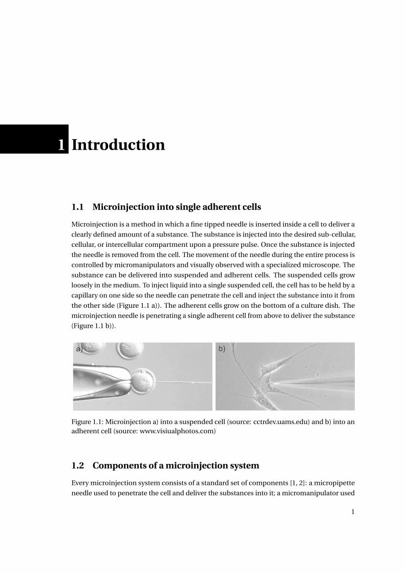
Microinjection is a method in which a fine tipped needle is inserted inside a cell to deliver a
clearly defined amount of a substance. The substance is injected into the desired sub-cellular,
cellular, or intercellular compartment upon a pressure pulse. Once the substance is injected
the needle is removed from the cell. The movement of the needle during the entire process is
controlled by micromanipulators and visually observed with a specialized microscope. The
substance can be delivered into suspended and adherent cells. The suspended cells grow
loosely in the medium. To inject liquid into a single suspended cell, the cell has to be held by a
capillary on one side so the needle can penetrate the cell and inject the substance into it from
the other side (Figure 1.1 a)). The adherent cells grow on the bottom of a culture dish. The
microinjection needle is penetrating a single adherent cell from above to deliver the substance
(Figure 1.1 b)).
Figure 1.1: Microinjection a) into a suspended cell (source: cctrdev.uams.edu) and b) into anadherent cell (source: www.visiualphotos.com)
1.2 Components of a microinjection system
Every microinjection system consists of a standard set of components [1, 2]: a micropipette
needle used to penetrate the cell and deliver the substances into it; a micromanipulator used
1
Chapter 1. Introduction
for precise positioning of the micropipette needle; an inverted microscope equipped with
phase-contrast for visualization of target cells and coordination of positioning and a vibration
isolation tabletop to decrease vibrations of the fine tipped needle. The micropipette needles
are fabricated from glass capillary tubing with micropipette pullers. The most common
material of glass capillary tubing is borosilicate glass due its excellent strength1. A fabricated
micropipette needle consists of four parts: the tip, the shank, the shoulder, and the shaft. The
shape of the needle and size of its opening depends on the pulling parameters. Standard inner
diameter of a needle opening varies from 0.2µm to 0.5µm. It is more common for a standard
user to fabricate its own needles than to buy it. Therefore on the market numerous types of
micropipette pullers are available, for example David Kopf Instruments, MicroData Instrument
or Energy Beam Sciences. There are also direct producers of micropipette needles, for example
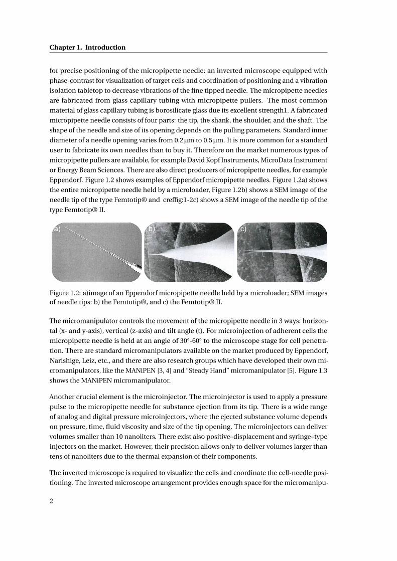
Eppendorf. Figure 1.2 shows examples of Eppendorf micropipette needles. Figure 1.2a) shows
the entire micropipette needle held by a microloader, Figure 1.2b) shows a SEM image of the
needle tip of the type Femtotip® and creffig:1-2c) shows a SEM image of the needle tip of the
type Femtotip® II.
Figure 1.2: a)image of an Eppendorf micropipette needle held by a microloader; SEM imagesof needle tips: b) the Femtotip®, and c) the Femtotip® II.
The micromanipulator controls the movement of the micropipette needle in 3 ways: horizon-
tal (x- and y-axis), vertical (z-axis) and tilt angle (t). For microinjection of adherent cells the
micropipette needle is held at an angle of 30°-60° to the microscope stage for cell penetra-
tion. There are standard micromanipulators available on the market produced by Eppendorf,
Narishige, Leiz, etc., and there are also research groups which have developed their own mi-
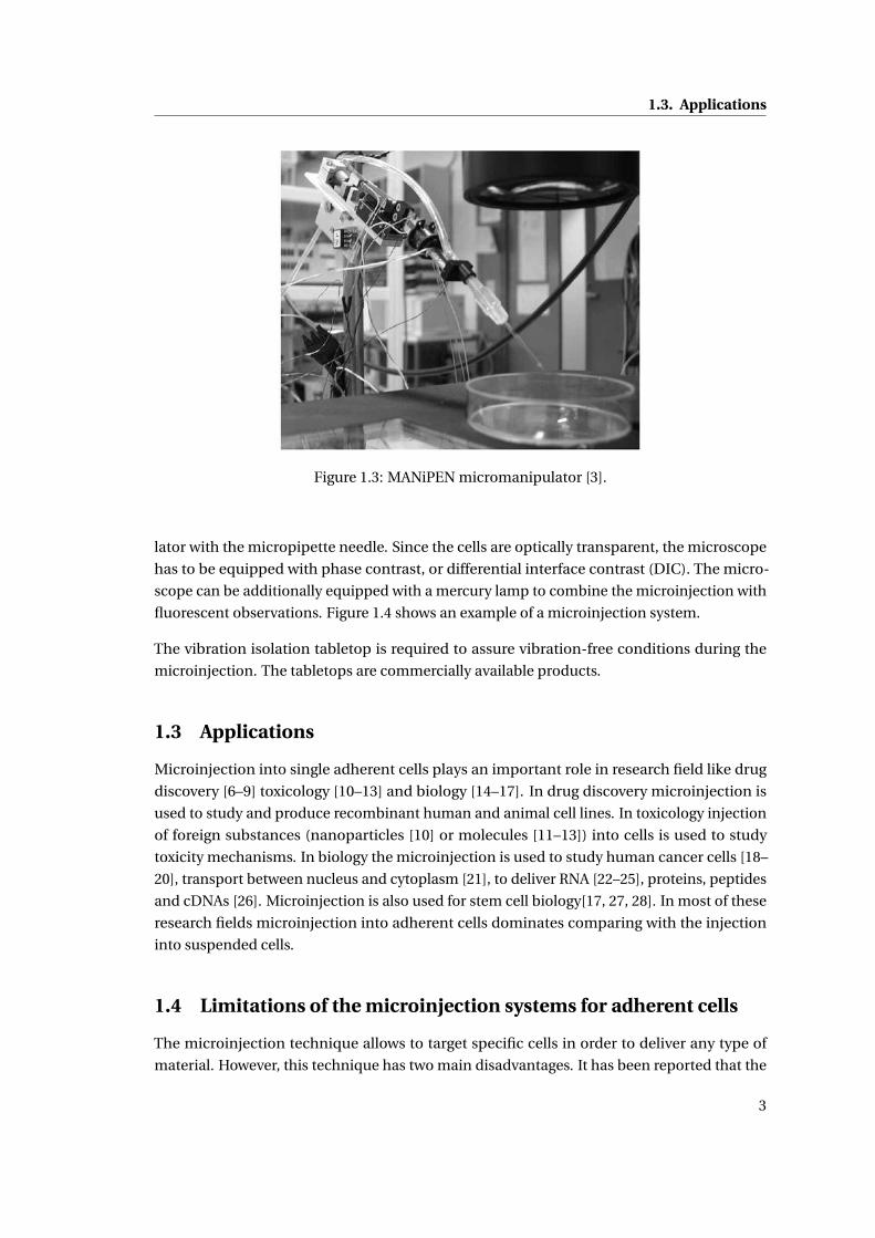
cromanipulators, like the MANiPEN [3, 4] and “Steady Hand” micromanipulator [5]. Figure 1.3
shows the MANiPEN micromanipulator.
Another crucial element is the microinjector. The microinjector is used to apply a pressure
pulse to the micropipette needle for substance ejection from its tip. There is a wide range
of analog and digital pressure microinjectors, where the ejected substance volume depends
on pressure, time, fluid viscosity and size of the tip opening. The microinjectors can deliver
volumes smaller than 10 nanoliters. There exist also positive–displacement and syringe–type
injectors on the market. However, their precision allows only to deliver volumes larger than
tens of nanoliters due to the thermal expansion of their components.
The inverted microscope is required to visualize the cells and coordinate the cell-needle posi-
tioning. The inverted microscope arrangement provides enough space for the micromanipu-
2
1.3. Applications
Figure 1.3: MANiPEN micromanipulator [3].
lator with the micropipette needle. Since the cells are optically transparent, the microscope
has to be equipped with phase contrast, or differential interface contrast (DIC). The micro-
scope can be additionally equipped with a mercury lamp to combine the microinjection with
fluorescent observations. Figure 1.4 shows an example of a microinjection system.
The vibration isolation tabletop is required to assure vibration-free conditions during the
microinjection. The tabletops are commercially available products.
1.3 Applications
Microinjection into single adherent cells plays an important role in research field like drug
discovery [6–9] toxicology [10–13] and biology [14–17]. In drug discovery microinjection is
used to study and produce recombinant human and animal cell lines. In toxicology injection
of foreign substances (nanoparticles [10] or molecules [11–13]) into cells is used to study
toxicity mechanisms. In biology the microinjection is used to study human cancer cells [18–
20], transport between nucleus and cytoplasm [21], to deliver RNA [22–25], proteins, peptides
and cDNAs [26]. Microinjection is also used for stem cell biology[17, 27, 28]. In most of these
research fields microinjection into adherent cells dominates comparing with the injection
into suspended cells.
1.4 Limitations of the microinjection systems for adherent cells
The microinjection technique allows to target specific cells in order to deliver any type of
material. However, this technique has two main disadvantages. It has been reported that the
3
Chapter 1. Introduction
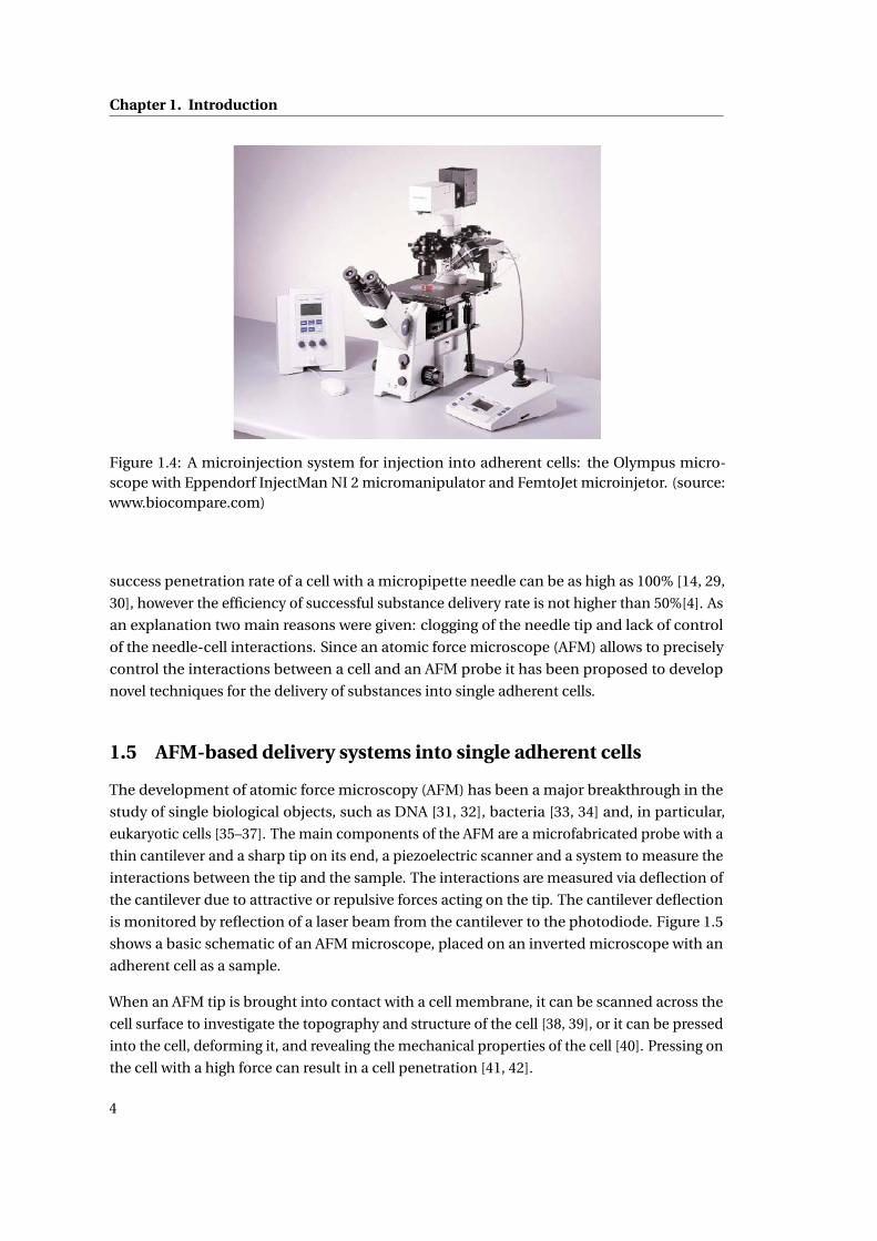
Figure 1.4: A microinjection system for injection into adherent cells: the Olympus micro-scope with Eppendorf InjectMan NI 2 micromanipulator and FemtoJet microinjetor. (source:www.biocompare.com)
success penetration rate of a cell with a micropipette needle can be as high as 100% [14, 29,
30], however the efficiency of successful substance delivery rate is not higher than 50%[4]. As
an explanation two main reasons were given: clogging of the needle tip and lack of control
of the needle-cell interactions. Since an atomic force microscope (AFM) allows to precisely
control the interactions between a cell and an AFM probe it has been proposed to develop
novel techniques for the delivery of substances into single adherent cells.
1.5 AFM-based delivery systems into single adherent cells
The development of atomic force microscopy (AFM) has been a major breakthrough in the
study of single biological objects, such as DNA [31, 32], bacteria [33, 34] and, in particular,
eukaryotic cells [35–37]. The main components of the AFM are a microfabricated probe with a
thin cantilever and a sharp tip on its end, a piezoelectric scanner and a system to measure the
interactions between the tip and the sample. The interactions are measured via deflection of
the cantilever due to attractive or repulsive forces acting on the tip. The cantilever deflection
is monitored by reflection of a laser beam from the cantilever to the photodiode. Figure 1.5
shows a basic schematic of an AFM microscope, placed on an inverted microscope with an
adherent cell as a sample.
When an AFM tip is brought into contact with a cell membrane, it can be scanned across the
cell surface to investigate the topography and structure of the cell [38, 39], or it can be pressed
into the cell, deforming it, and revealing the mechanical properties of the cell [40]. Pressing on
the cell with a high force can result in a cell penetration [41, 42].
4
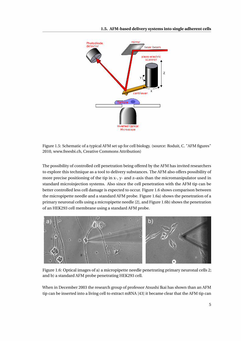
1.5. AFM-based delivery systems into single adherent cells
Figure 1.5: Schematic of a typical AFM set up for cell biology. (source: Roduit, C. "AFM figures"2010, www.freesbi.ch, Creative Commons Attribution)
The possibility of controlled cell penetration being offered by the AFM has invited researchers
to explore this technique as a tool to delivery substances. The AFM also offers possibility of
more precise positioning of the tip in x-, y- and z–axis than the micromanipulator used in
standard microinjection systems. Also since the cell penetration with the AFM tip can be
better controlled less cell damage is expected to occur. Figure 1.6 shows comparison between
the micropipette needle and a standard AFM probe. Figure 1.6a) shows the penetration of a
primary neuronal cells using a micropipette needle [2], and Figure 1.6b) shows the penetration
of an HEK293 cell membrane using a standard AFM probe.
Figure 1.6: Optical images of a) a micropipette needle penetrating primary neuronal cells 2;and b) a standard AFM probe penetrating HEK293 cell.
When in December 2003 the research group of professor Atsushi Ikai has shown than an AFM
tip can be inserted into a living cell to extract mRNA [43] it became clear that the AFM tip can
5
Chapter 1. Introduction
be used as a tool for operations on single living adherent cells. One year later the group of
professor Jun Miyake has demonstrated first molecular delivery system using an AFM [44].
From then, many research groups have shown successful delivery of molecules into single
living cell [38, 45–49].
1.6 Delivery of biomolecules with AFM probes
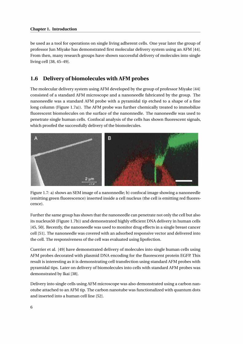
The molecular delivery system using AFM developed by the group of professor Miyake [44]
consisted of a standard AFM microscope and a nanoneedle fabricated by the group. The
nanoneedle was a standard AFM probe with a pyramidal tip etched to a shape of a fine
long column (Figure 1.7a)). The AFM probe was further chemically treated to immobilize
fluorescent biomolecules on the surface of the nanonnedle. The nanoneedle was used to
penetrate single human cells. Confocal analysis of the cells has shown fluorescent signals,
which proofed the successfully delivery of the biomolecules.
Figure 1.7: a) shows an SEM image of a nanonnedle; b) confocal image showing a nanoneedle(emitting green fluorescence) inserted inside a cell nucleus (the cell is emitting red fluores-cence).
Further the same group has shown that the nanoneedle can penetrate not only the cell but also
its nucleus50 (Figure 1.7b)) and demonstrated highly efficient DNA delivery in human cells
[45, 50]. Recently, the nanoneedle was used to monitor drug effects in a single breast cancer
cell [51]. The nanoneedle was covered with an adsorbed responsive vector and delivered into
the cell. The responsiveness of the cell was evaluated using lipofection.
Cuerrier et al. [49] have demonstrated delivery of molecules into single human cells using
AFM probes decorated with plasmid DNA encoding for the fluorescent protein EGFP. This
result is interesting as it is demonstrating cell transfection using standard AFM probes with
pyramidal tips. Later on delivery of biomolecules into cells with standard AFM probes was
demonstrated by Ikai [38].
Delivery into single cells using AFM microscope was also demonstrated using a carbon nan-
otube attached to an AFM tip. The carbon nanotube was functionalized with quantum dots
and inserted into a human cell line [52].
6
1.7. AFM probes with microfluidic systems
Several groups began to work on AFM systems allowing to deliver not only molecules, but also
liquids inside the cells [46, 47, 53]. Delivery of liquids into single cells is technologically more
challenging than delivery of ‘dry’ molecules that are attached to the AFM tip chemically or by
adhesion forces. Liquids, however, cannot be attach to the tip and require more sophisticated
carriers. In order to deliver liquids into cells AFM probes with integrated microfluidic systems
are being developed.
1.7 AFM probes with microfluidic systems
To deliver liquids inside single living cells attached to a culture dish and filled with culture
cell medium AFM probes have to have embedded microfluidic system. Such a system has to
have a built in reservoir and channels connected to the tip. In the literature, probes have been
already demonstrated: NanoFountain Probe [48, 53], NADIS Probe [47, 54, 55], and Bioprobe
[46].
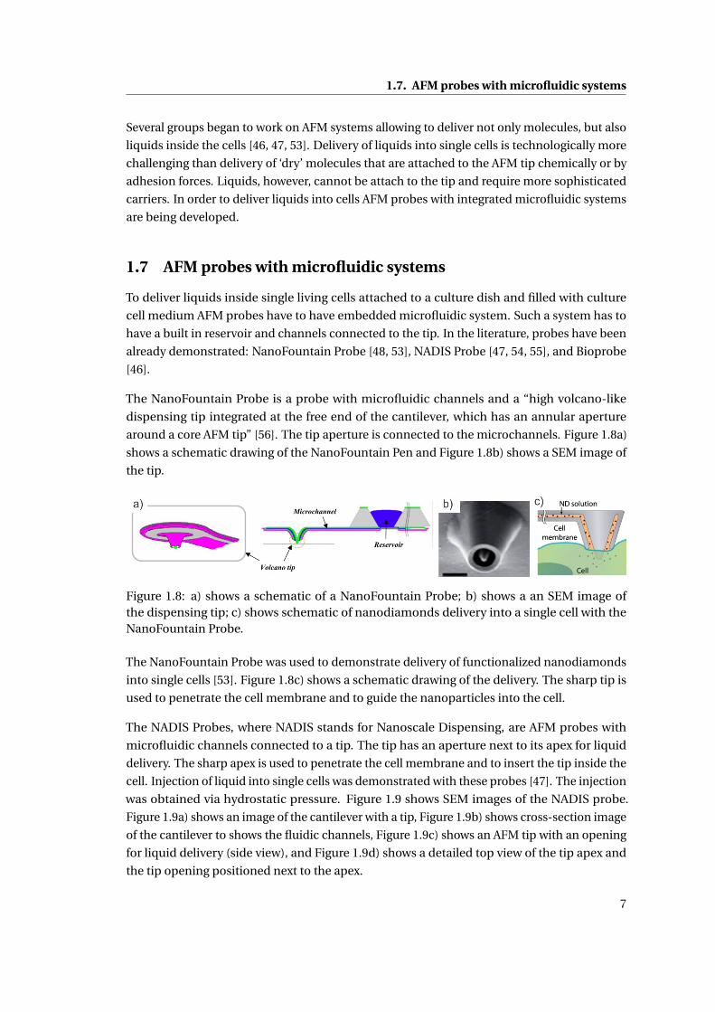
The NanoFountain Probe is a probe with microfluidic channels and a “high volcano-like
dispensing tip integrated at the free end of the cantilever, which has an annular aperture
around a core AFM tip” [56]. The tip aperture is connected to the microchannels. Figure 1.8a)
shows a schematic drawing of the NanoFountain Pen and Figure 1.8b) shows a SEM image of
the tip.
Figure 1.8: a) shows a schematic of a NanoFountain Probe; b) shows a an SEM image ofthe dispensing tip; c) shows schematic of nanodiamonds delivery into a single cell with theNanoFountain Probe.
The NanoFountain Probe was used to demonstrate delivery of functionalized nanodiamonds
into single cells [53]. Figure 1.8c) shows a schematic drawing of the delivery. The sharp tip is
used to penetrate the cell membrane and to guide the nanoparticles into the cell.
The NADIS Probes, where NADIS stands for Nanoscale Dispensing, are AFM probes with
microfluidic channels connected to a tip. The tip has an aperture next to its apex for liquid
delivery. The sharp apex is used to penetrate the cell membrane and to insert the tip inside the
cell. Injection of liquid into single cells was demonstrated with these probes [47]. The injection
was obtained via hydrostatic pressure. Figure 1.9 shows SEM images of the NADIS probe.
Figure 1.9a) shows an image of the cantilever with a tip, Figure 1.9b) shows cross-section image
of the cantilever to shows the fluidic channels, Figure 1.9c) shows an AFM tip with an opening
for liquid delivery (side view), and Figure 1.9d) shows a detailed top view of the tip apex and
the tip opening positioned next to the apex.
7
Chapter 1. Introduction
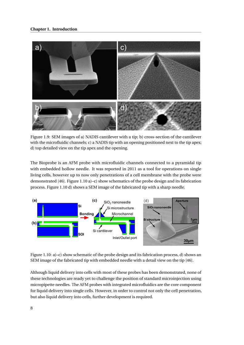
Figure 1.9: SEM images of a) NADIS cantilever with a tip; b) cross-section of the cantileverwith the microfluidic channels; c) a NADIS tip with an opening positioned next to the tip apex;d) top detailed view on the tip apex and the opening.
The Bioprobe is an AFM probe with microfluidic channels connected to a pyramidal tip
with embedded hollow needle. It was reported in 2011 as a tool for operations on single
living cells, however up to now only penetrations of a cell membrane with the probe were
demonstrated [46]. Figure 1.10 a)–c) show schematics of the probe design and its fabrication
process. Figure 1.10 d) shows a SEM image of the fabricated tip with a sharp needle.
Figure 1.10: a)–c) show schematic of the probe design and its fabrication process, d) shows anSEM image of the fabricated tip with embedded needle with a detail view on the tip [46].
Although liquid delivery into cells with most of these probes has been demonstrated, none of
these technologies are ready yet to challenge the position of standard microinjection using
micropipette needles. The AFM probes with integrated microfluidics are the core component
for liquid delivery into single cells. However, in order to control not only the cell penetration,
but also liquid delivery into cells, further development is required.
8
1.8. Thesis objectives
1.8 Thesis objectives
The main objective of this thesis is to develop an AFM-based microinjection system for liquid
delivery into single adherent cells. The development will be based on the NADIS probe with
integrated microfluidic channels and a hollow tip.
In order to deliver liquid into a cell via the AFM tip, it is crucial to understand the complex
tip–cell interactions. These interactions will be studied via ‘force spectroscopy’.
Also the invasiveness of the tip insertion will be studied to verify possible cell damage. Finally,
the AFM–based microinjection system will be used to demonstrate intracellular injection.
9

2 Materials and methods
In this chapter materials and experimental methods are detailed.
2.1 Fabrication of the apertures
Fabrication of the tip apertures in NADIS probes was performed using focused ion beam
milling (FIB).
FIB was used in a wide range of applications such as imaging [57] and deposition [58] but
its main application is localized milling of material with high precision [59, 60]. To create
apertures in the AFM tips, precise control of the volume of the material being removed at
precise location was required; hence the FIB milling was the method of choice.
The FIB milling was carried out with an FEI Nova 600 NanoLab - DualBeam system. The
DualBeam system consists of electron and gallium ion beams. The electron beam plays the
role of the SEM and allows image sampling with ultra-high resolution. The DualBeam system
allows one to operate the two beams at the same time. When the sample is being milled with
the ion beam, the process can be observed in real time with the SEM. The process takes place
in a high-vacuum environment. The critical point of making the system work correctly is to
set the sample to the eucentric point. The eucentric point is where the coincidence of the
beams with the stage tilt axis occurs. At this point, the place of interest on the sample remains
in focus and very little image displacement occurs, independently of how the sample is tilted
or rotated. To position the place of interest at the eucentric point, the working distance of
the electron beam (the eucentric height) has to be found. The milling process is the most
efficient when the ion beam is perpendicular to the place of interest-the angle of the incidence
θ = 0r (the angle of the incidence is the angle between the surface normal of the AFM chip and
the ion beam). In this configuration the system with the sample is ready to work. Figure 2.1
illustrates the configuration for the NADIS chip inside the FIB system. The tip apex was placed
in the eucentric point. Figure 2.1 b) shows a micrograph of the tip seen with the ion beam and
Figure 2.1 c) shows a micrograph of the tip seen at the same time with the electron beam.
11
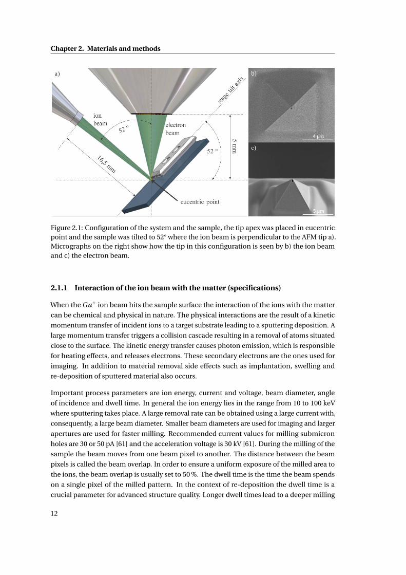
Chapter 2. Materials and methods
Figure 2.1: Configuration of the system and the sample, the tip apex was placed in eucentricpoint and the sample was tilted to 52° where the ion beam is perpendicular to the AFM tip a).Micrographs on the right show how the tip in this configuration is seen by b) the ion beamand c) the electron beam.
2.1.1 Interaction of the ion beam with the matter (specifications)
When the Ga+ ion beam hits the sample surface the interaction of the ions with the matter
can be chemical and physical in nature. The physical interactions are the result of a kinetic
momentum transfer of incident ions to a target substrate leading to a sputtering deposition. A
large momentum transfer triggers a collision cascade resulting in a removal of atoms situated
close to the surface. The kinetic energy transfer causes photon emission, which is responsible
for heating effects, and releases electrons. These secondary electrons are the ones used for
imaging. In addition to material removal side effects such as implantation, swelling and
re-deposition of sputtered material also occurs.
Important process parameters are ion energy, current and voltage, beam diameter, angle
of incidence and dwell time. In general the ion energy lies in the range from 10 to 100 keV
where sputtering takes place. A large removal rate can be obtained using a large current with,
consequently, a large beam diameter. Smaller beam diameters are used for imaging and larger
apertures are used for faster milling. Recommended current values for milling submicron
holes are 30 or 50 pA [61] and the acceleration voltage is 30 kV [61]. During the milling of the
sample the beam moves from one beam pixel to another. The distance between the beam
pixels is called the beam overlap. In order to ensure a uniform exposure of the milled area to
the ions, the beam overlap is usually set to 50 %. The dwell time is the time the beam spends
on a single pixel of the milled pattern. In the context of re-deposition the dwell time is a
crucial parameter for advanced structure quality. Longer dwell times lead to a deeper milling
12
2.2. Development of parylene C mask for KOH etching
but at the same time cause larger re-deposition, thus its value depends on the compromise
between these two effects. A dwell time of 500 ns has been chosen to mill the tip apertures,
since shorter dwell time does not improve the quality and the FIB system becomes unstable at
dwell times shorter than approximately 200 ns. The angle of the incidence (θ) has an influence
on a sputtering yield of the ion beam and roughly increases with 1/cos(θ) [62]. Milling of the
tip apertures occurred always at 0°.
2.2 Development of parylene C mask for KOH etching
2.2.1 Substrates
To study adhesion properties of parylene C, the following substrates were used: 4 inch silicon
wafers (Silitronix France), silicon wafers with 250 nm thermally grown silicon dioxide and
silicon wafers coated with silicon dioxide and additional LPCVD deposited 100 nm nitride.
After the cleaning process 1 wafer per substrate type was diced to 1 cm×1 cm samples.
For testing parylene C mask on 3D structures Pyrex wafers with microfluidic channels were an-
odically bonded to structured silicon wafers with inlets. The microfluidic channels were 10µm
and 20µm wide and 1.2µm high. The length of the channels varied from 1.1µm to 1.6µm. The
inlets were etched through the entire thickness of the silicon wafer by KOH etching.
2.2.2 Substrate cleaning 1
The wafers were immersed 10 minutes in a solution of H2SO4 (96 %, 120 ◦C) followed by 1
minute in a BHF solution (1:7, 23 ◦C) and 10 minutes in a H NO3 solution 70 %, 116 ◦C). Finally
the samples were rinsed in DI water and dried in spin rinse dryer (SRD).
2.2.3 Chemical adhesion promotion
To promote adhesion of parylene C to the substrates -methacryl-oxy-propyl-trimethoxy-silane,
also known as the Silquest A-174® silane (ABCR GmbH&Co, Germany) was used. Silane
deposition was studied in liquid and gas phase. The samples silanized in the liquid phase
were left for 5 min in a solution of silane A-174 and water (ratio 1:10 ml). For the gas phase
silanization, the samples were placed in a custom made parallel plate vacuum chamber and
pumped down to a base pressure of 8×10⁻³ mbar . The surface activation was done using air
plasma (0.3 mbar, 50 watts during 15 minutes). The chamber was then returned to the base
pressure before closing the pump valve and introducing the silane A-174 up to a pressure of
2×10⁻² mbar. Finally, the silane was left to condense on the samples for 60 minutes. Static
and dynamic contact angle measurements were used to optimize the deposition parameters.
The contact angle of water was measured at (100±8)° for the gas silanization and (115±6)°
1The substrate cleaning was done by group of Dr Philippe Niedermann at CSEM SA (Switzerland)
13
Chapter 2. Materials and methods
for the liquid phase silanization on all substrates. The cleaning procedure consisting of a
sonication for 10 min in hexane and rinsing with Milli®–Q water had no effect on the contact
angle.
2.2.4 Parylene deposition 2
The Parylene deposition took place in a COMELEC model 1010 deposition chamber using
the conventional LPCVD process. 10 grams of dichloro[2.2]-paracyclophane dimer (Galxyl
C purchased from Galentis Srl, Italy) yielded layers of 5 microns (±10%) of Parylene C on the
samples. It was verified and confirmed on dummy samples using a Dektak profilometer.
2.3 Thermal treatment
Samples dedicated to test influence of thermal treatment on parylene adhesion were placed
in an oven, under a nitrogen atmosphere at atmospheric pressure. The oven was heated
10 ◦C min−1 from room temperature up to 350 ◦C. This temperature was kept for 2h before
cooling down the oven at a rate of 5 ◦C min−1 down to room temperature.
2.3.1 Potassium Hydroxide (KOH) Exposure 3
The samples were immersed in a 40 % solution of KOH (Potassium hydroxide) at 60 ◦C for 5 or
25 hours. The etching rate was approximately 16µm h−1 on a 110 orientated Si wafer.
2.3.2 Scratch test
The adhesion of the Parylene layers was assessed using a scratch test equipment REVETEST®
from CSM Instruments S.A (Switzerland), controlled by the proprietary Scratch software. The
measurement principle consists in a stylus with a diamond tip of spherical shape and diameter
of 200µm that is put in contact with a surface. An increasing load is applied on the stylus as
it is dragged across the sample. The instrument measures the acoustic signal made by the
stylus scratching the layer. A layer breaking is characterized by a large noise that indicates
the rupture load. A visual inspection kit enables to check the accuracy of the information
recorded by the acoustic signal and it enables to visualize the shape of the imprint left by the
stylus. Even though this kind of instrument is normally used to characterize the adhesion of
hard thin films on a softer substrate, it enabled to compare the adhesion of the treated and
non-treated Parylene layer on our samples. Prior to the measurements, the samples were fixed
with in a substrate holder with acrylate glue. The measurement length was set to 5 mm with
a load of 30 N cm−1. The measurements were recorded using the proprietary software and 3
2The parylene deposition, thermal treatment and scratch test were done by group of Prof. Herber Keppner atHE-ARC (Switzerland)
3The KOH exposure was done by Dr Fabio Jutzi and Dr Dara Bayat from EPFL (Switzerland)
14
2.4. Instrumentation
pictures (start of the imprint, rapture point and end point) were taken for each sample.
2.3.3 XRD measurements 4
The XRD measurements were used to understand the influence of carried different treatment
conditions on crystalline properties of the parylene. The X-Ray Diffraction data were measured
in reflection mode on a X’pert pro PAN’alytical diffractometer (MRD) using CuKα radiation.
The data was collected first in the ω/2θ mode and secondly in the range 2θ(ω= 1° range of 5°
to 40° (step size 0.02°, 1s/step). The crystallite size were calculated using the Scherrer equation
and the contribution of the peak width from the instrument was taken into account (Si sample
was used).
2.3.4 The AFM imaging
The AFM measurements were performed in tapping mode on a 3100 Dimension microscope
(Digital Instruments, Santa Barbara, CA). Silicon tips (Tap 150-AL-G from Budget Sensors, USA)
with a radius less than 10 nm, spring constant of 5 N m−1 and resonance frequency of 150 kHz
were used. The samples were cleaned with N2 nitrogen gun directly before the measurements.
2.4 Instrumentation
2.4.1 Atomic force microscope (AFM)
The AFM based microinjection system was built based on a Nanowizard® II BioAFM (JPK
Instruments, Germany) mounted on an Axiovert 200 inverted optical microscope (Carl Zeiss,
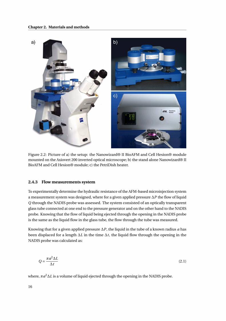
Germany). Figure 2.2 shows pictures of the setup. Additionally a CellHesion® module (JPK
Instruments, Germany) was used to expend the travel range of the AFM microscope in the z-
axis to 100µm. The module has a precise sample lift mechanism integrated into the AFM stage.
To the setup a fully compatible Petri dish heater was used (PetriDish Heater, JPK Instruments,
Germany) to maintain the cells at the temperature of 37 ◦C.
2.4.2 Pressure generator
To apply pressure pulses into the NADIS probes PM 8000 Programable 8-Channel Pressure
Injector (MicroData Instrument, Inc., USA) was used. It is a standard device used in microin-
jection.
4The XRD measurements were done by group of Dr Antonia Neels, CSEM SA (Switzerland)
15
Chapter 2. Materials and methods
Figure 2.2: Picture of a) the setup: the Nanowizard® II BioAFM and Cell Hesion® modulemounted on the Axiovert 200 inverted optical microscope; b) the stand alone Nanowizard® IIBioAFM and Cell Hesion® module; c) the PetriDish heater.
2.4.3 Flow measurements system
To experimentally determine the hydraulic resistance of the AFM-based microinjection system
a measurement system was designed, where for a given applied pressure ∆P the flow of liquid
Q through the NADIS probe was assessed. The system consisted of an optically transparent
glass tube connected at one end to the pressure generator and on the other hand to the NADIS
probe. Knowing that the flow of liquid being ejected through the opening in the NADIS probe
is the same as the liquid flow in the glass tube, the flow through the tube was measured.
Knowing that for a given applied pressure ∆P , the liquid in the tube of a known radius a has
been displaced for a length ∆L in the time ∆t , the liquid flow through the opening in the
NADIS probe was calculated as:
Q = πa2∆L
∆t(2.1)
where, πa2∆L is a volume of liquid ejected through the opening in the NADIS probe.
16
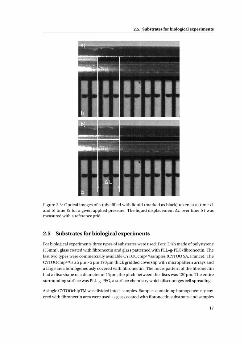
2.5. Substrates for biological experiments
Figure 2.3: Optical images of a tube filled with liquid (marked as black) taken at a) time t1and b) time t2 for a given applied pressure. The liquid displacement ∆L over time ∆t wasmeasured with a reference grid.
2.5 Substrates for biological experiments
For biological experiments three types of substrates were used: Petri Dish made of polystyrene
(35mm), glass coated with fibronectin and glass patterned with PLL–g-PEG/fibronectin. The
last two types were commercially available CYTOOchip™samples (CYTOO SA, France). The
CYTOOchip™is a 2µm×2µm 170µm thick gridded coverslip with micropattern arrays and
a large area homogeneously covered with fibronectin. The micropattern of the fibronectin
had a disc shape of a diameter of 45µm; the pitch between the discs was 130µm. The entire
surrounding surface was PLL-g-PEG, a surface chemistry which discourages cell spreading.
A single CYTOOchipTM was divided into 4 samples. Samples containing homogeneously cov-
ered with fibronectin area were used as glass coated with fibronectin substrates and samples
17
Chapter 2. Materials and methods
containing the micropattern arrays were used as glass patterned with PLL–g-PEG/fibronectin
substrates.
2.6 Cell culture 5
The human osteosarcoma cell line (SaOs-2) was obtained from American Type Culture Collec-
tion (Manassas, VA, USA) and maintained in culture in McCoy’s 5A medium supplemented
with 10% heat-inactivated standardized foetal bovine serum (Biochrom AG, Germany)), 1%
L-glutamine and 50 mL−1 of penicillin, 50µg mL−1 of streptomycin at 37 ◦C in humidified 5%
CO2 atmosphere.
2.6.1 Cell seeding on Petri dish substrates
A cell suspension of 105 SaOs-2 cells was seeded on Petri dishes and cultured for 24 hours
on complete medium. Experiments with the samples were performed in regular medium
supplemented with 25 mmol HEPES.
2.6.2 Cell seeding on CYTOOchip™
The CYTOOchip™was attached the to the bottom of the petri dish. 120,000 cells were added
to the top of the CYTOOchip™and left to settle under the laminar flow hood for 10 minutes
before transferring to a 37 ◦C incubator for 40 minutes. The CYTOOchip™was then rinsed
with PBS three times to remove any unattached cells and then left in the incubator for 3 hours
before using.
A 25mM EDTA in cell culture media solution was used for experiments with EDTA.
2.6.3 Cell staining
Cells have been fixed with 4% formaldehyde after 3 hours of culture. Then incubated in PBS-
glycine 0.1 M to permeabilize the cell membrane, and in blocking buffer to block nonspecific
sites. Alexa Fluor 488 Phalloidin (Molecular probes) was used to label F-actin while DAPI
(4’,6-diamidino-2-phenylindole) was used to label the cell nuclei.
2.6.4 Confocal analysis
All confocal measurements were done with Leica Confocal Microscope (Leica Microsystems,
Germany). Measurements of cell height, nucleus height and nucleus–membrane distances
were done as follows: from the top of the cell we take a stack of images in z–direction, step
5The cell culture was prepared by Ms. Marta Giazzon, Ms. Nadège Matthey and Mr. Sher Ahmed from CSEMSA (Switzerland)
18
2.7. AFM probes
500 nm. The entire cell thickness has been calculated on the basis of the number of sections
necessary to image completely the cell. The distance sub-membrane nucleus has been calcu-
lated by analysing the number of sections with actin before to have the nucleus appearing.
The nucleus height was calculated making the sum of the sections where DAPI signal was
present.
2.6.5 Cell death analysis
To measure cell survival rate a LIVE/DEAD kit (Sigma Alrdrich) was used. The LIVE/DEAD kit
contained two components. The first component is Calcein-AM. This is a highly lipophilic and
cell membrane permeable. Although CAM is not a fluorescent molecule, when it enters viable
cells it emits a strong green fluorescent signal. The second component is propidium iodide.
This is a nuclear stain which cannot pass through viable cell membranes. It passed through
the dead cell’s membranes and intercalates with the DNA in the nucleus to emit a strong red
fluorescence. After applying the kit to the cells, the cells were viewed by confocal microscopy.
2.6.6 Cell fixation
Cell fixation was used to investigate cells spread on substrates coated with Parylene. Samples
were rinsed with PBS. The cell fixation was done in a solution of 2.5% glutaraldehyde in 0.2
M cacodylate buffer, pH 7.4, overnight. Afterwards, the cells were dehydrated in a series of
ethanol/water mixtures: 20%, 30%, 40%, 50%, 60%, 70%, 80%, 90%, 100%, ethanol (5 min
each), followed by air drying. Once the samples were ready, the substrates were coated with
20 nm Au layer and investigated with a XL-30 ESEM (Royal Philips, Netherlands) scanning
electron microscope.
2.7 AFM probes
For the force spectroscopy experiments two types of AFM probes were used. The first type was
commercially available silicon probes (Tap150–G, Budget Sensors, Bulgaria) with a pyramidal
tip shape and tip radius of approximately 10 nm. The probes were 125µm long with a nominal
spring constant of 5 N m−1. Before every experiment each cantilever was calibrated using
cantilever–on–cantilever method. The final working spring constant of cantilevers was in the
range of 3 N m−1 to 7 N m−1.
The second type of probe was fabricated and developed at CSEM SA, Switzerland Nanoscale
Dispensing (NADIS) probes. The NADIS probes contain a microfluidic system and are a core
component of the AFM-based microinjection system. Chapter 4 is dedicated to its design and
microfabrication process and Chapter 5 describes its characterization.
19
Chapter 2. Materials and methods
2.8 Data processing and statistical analysis
2.8.1 Analysis of force-distance curves
Data analysis was carried out using Image Processing software (JPK Instruments, Germany).
For every single cell 1 force distance–curve was obtained. The force–distance curves were
first transformed into force vs. tip–sample separation curves and analysed in terms of the
indentation depth (D), the penetration depth (D1), the penetration force (F 1), the force drop
(F d) and the membrane slip (d). The mean of these values together with the sample standard
deviation was then taken to be characteristic of each condition.
2.8.2 Statistical analysis
The obtained data was analysed with the Microsoft Excel with Data Analysis Tool. Two types of
statistical analysis were used: ANOVA and T–test. The ANOVA (Single Factor) test was used to
compare four population means (populations of cells spread on glass coated with fibronectin
and cells spread on glass patterned with PLL-g-PEG/fibronectin, with and without EDTA). The
Sheffé test was further used to find which of the samples means are different. For any other
statistical analysis two–sample T-test was used.
For all statistical tests, a p < 0.05 was considered significant.
20
3 Concept study
3.1 Introduction: Delivery of liquids into a living body
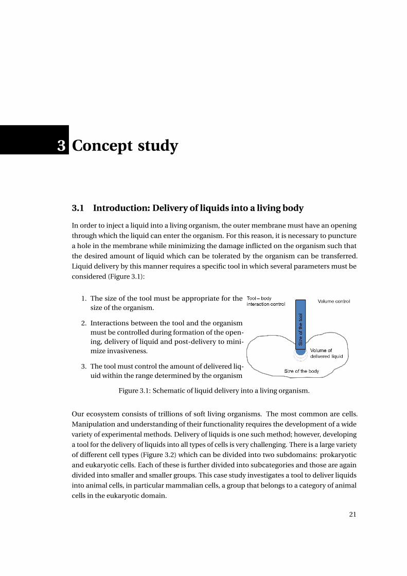
In order to inject a liquid into a living organism, the outer membrane must have an opening
through which the liquid can enter the organism. For this reason, it is necessary to puncture
a hole in the membrane while minimizing the damage inflicted on the organism such that
the desired amount of liquid which can be tolerated by the organism can be transferred.
Liquid delivery by this manner requires a specific tool in which several parameters must be
considered (Figure 3.1):
1. The size of the tool must be appropriate for thesize of the organism.
2. Interactions between the tool and the organismmust be controlled during formation of the open-ing, delivery of liquid and post-delivery to mini-mize invasiveness.
3. The tool must control the amount of delivered liq-uid within the range determined by the organism
Figure 3.1: Schematic of liquid delivery into a living organism.
Our ecosystem consists of trillions of soft living organisms. The most common are cells.
Manipulation and understanding of their functionality requires the development of a wide
variety of experimental methods. Delivery of liquids is one such method; however, developing
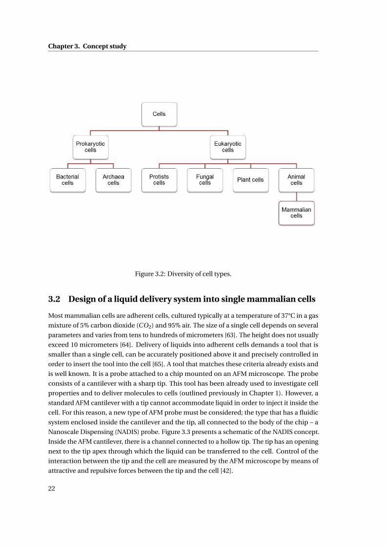
a tool for the delivery of liquids into all types of cells is very challenging. There is a large variety
of different cell types (Figure 3.2) which can be divided into two subdomains: prokaryotic
and eukaryotic cells. Each of these is further divided into subcategories and those are again
divided into smaller and smaller groups. This case study investigates a tool to deliver liquids
into animal cells, in particular mammalian cells, a group that belongs to a category of animal
cells in the eukaryotic domain.
21
Chapter 3. Concept study
Figure 3.2: Diversity of cell types.
3.2 Design of a liquid delivery system into single mammalian cells
Most mammalian cells are adherent cells, cultured typically at a temperature of 37°C in a gas
mixture of 5% carbon dioxide (CO2) and 95% air. The size of a single cell depends on several
parameters and varies from tens to hundreds of micrometers [63]. The height does not usually
exceed 10 micrometers [64]. Delivery of liquids into adherent cells demands a tool that is
smaller than a single cell, can be accurately positioned above it and precisely controlled in
order to insert the tool into the cell [65]. A tool that matches these criteria already exists and
is well known. It is a probe attached to a chip mounted on an AFM microscope. The probe
consists of a cantilever with a sharp tip. This tool has been already used to investigate cell
properties and to deliver molecules to cells (outlined previously in Chapter 1). However, a
standard AFM cantilever with a tip cannot accommodate liquid in order to inject it inside the
cell. For this reason, a new type of AFM probe must be considered; the type that has a fluidic
system enclosed inside the cantilever and the tip, all connected to the body of the chip – a
Nanoscale Dispensing (NADIS) probe. Figure 3.3 presents a schematic of the NADIS concept.
Inside the AFM cantilever, there is a channel connected to a hollow tip. The tip has an opening
next to the tip apex through which the liquid can be transferred to the cell. Control of the
interaction between the tip and the cell are measured by the AFM microscope by means of
attractive and repulsive forces between the tip and the cell [42].
22
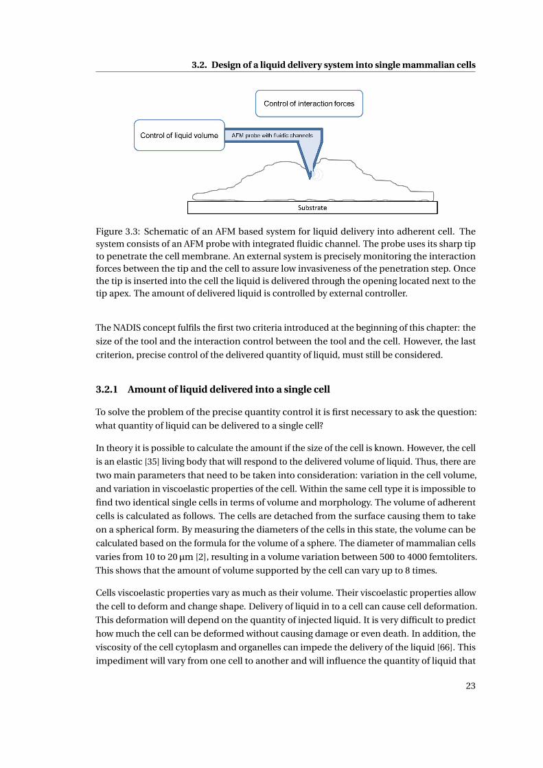
3.2. Design of a liquid delivery system into single mammalian cells
Figure 3.3: Schematic of an AFM based system for liquid delivery into adherent cell. Thesystem consists of an AFM probe with integrated fluidic channel. The probe uses its sharp tipto penetrate the cell membrane. An external system is precisely monitoring the interactionforces between the tip and the cell to assure low invasiveness of the penetration step. Oncethe tip is inserted into the cell the liquid is delivered through the opening located next to thetip apex. The amount of delivered liquid is controlled by external controller.
The NADIS concept fulfils the first two criteria introduced at the beginning of this chapter: the
size of the tool and the interaction control between the tool and the cell. However, the last
criterion, precise control of the delivered quantity of liquid, must still be considered.
3.2.1 Amount of liquid delivered into a single cell
To solve the problem of the precise quantity control it is first necessary to ask the question:
what quantity of liquid can be delivered to a single cell?
In theory it is possible to calculate the amount if the size of the cell is known. However, the cell
is an elastic [35] living body that will respond to the delivered volume of liquid. Thus, there are
two main parameters that need to be taken into consideration: variation in the cell volume,
and variation in viscoelastic properties of the cell. Within the same cell type it is impossible to
find two identical single cells in terms of volume and morphology. The volume of adherent
cells is calculated as follows. The cells are detached from the surface causing them to take
on a spherical form. By measuring the diameters of the cells in this state, the volume can be
calculated based on the formula for the volume of a sphere. The diameter of mammalian cells
varies from 10 to 20 µm [2], resulting in a volume variation between 500 to 4000 femtoliters.
This shows that the amount of volume supported by the cell can vary up to 8 times.
Cells viscoelastic properties vary as much as their volume. Their viscoelastic properties allow
the cell to deform and change shape. Delivery of liquid in to a cell can cause cell deformation.
This deformation will depend on the quantity of injected liquid. It is very difficult to predict
how much the cell can be deformed without causing damage or even death. In addition, the
viscosity of the cell cytoplasm and organelles can impede the delivery of the liquid [66]. This
impediment will vary from one cell to another and will influence the quantity of liquid that
23
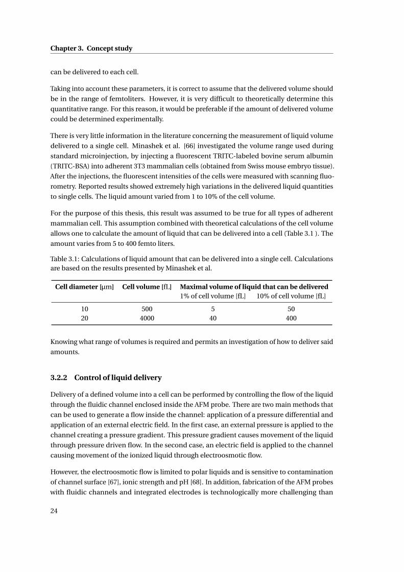
Chapter 3. Concept study
can be delivered to each cell.
Taking into account these parameters, it is correct to assume that the delivered volume should
be in the range of femtoliters. However, it is very difficult to theoretically determine this
quantitative range. For this reason, it would be preferable if the amount of delivered volume
could be determined experimentally.
There is very little information in the literature concerning the measurement of liquid volume
delivered to a single cell. Minashek et al. [66] investigated the volume range used during
standard microinjection, by injecting a fluorescent TRITC-labeled bovine serum albumin
(TRITC-BSA) into adherent 3T3 mammalian cells (obtained from Swiss mouse embryo tissue).
After the injections, the fluorescent intensities of the cells were measured with scanning fluo-
rometry. Reported results showed extremely high variations in the delivered liquid quantities
to single cells. The liquid amount varied from 1 to 10% of the cell volume.
For the purpose of this thesis, this result was assumed to be true for all types of adherent
mammalian cell. This assumption combined with theoretical calculations of the cell volume
allows one to calculate the amount of liquid that can be delivered into a cell (Table 3.1 ). The
amount varies from 5 to 400 femto liters.
Table 3.1: Calculations of liquid amount that can be delivered into a single cell. Calculationsare based on the results presented by Minashek et al.
Cell diameter [µm] Cell volume [fL] Maximal volume of liquid that can be delivered1% of cell volume [fL] 10% of cell volume [fL]
10 500 5 5020 4000 40 400
Knowing what range of volumes is required and permits an investigation of how to deliver said
amounts.
3.2.2 Control of liquid delivery
Delivery of a defined volume into a cell can be performed by controlling the flow of the liquid
through the fluidic channel enclosed inside the AFM probe. There are two main methods that
can be used to generate a flow inside the channel: application of a pressure differential and
application of an external electric field. In the first case, an external pressure is applied to the
channel creating a pressure gradient. This pressure gradient causes movement of the liquid
through pressure driven flow. In the second case, an electric field is applied to the channel
causing movement of the ionized liquid through electroosmotic flow.
However, the electroosmotic flow is limited to polar liquids and is sensitive to contamination
of channel surface [67], ionic strength and pH [68]. In addition, fabrication of the AFM probes
with fluidic channels and integrated electrodes is technologically more challenging than
24
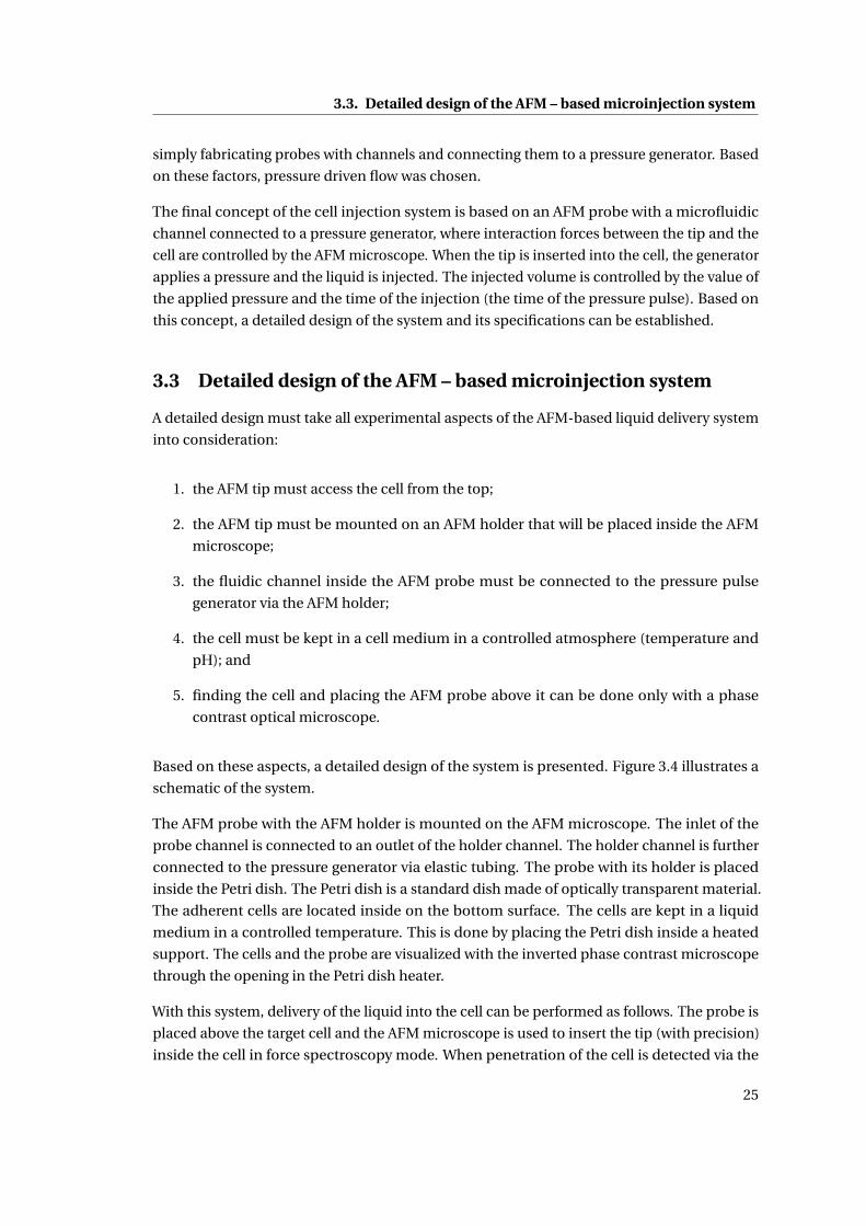
3.3. Detailed design of the AFM – based microinjection system
simply fabricating probes with channels and connecting them to a pressure generator. Based
on these factors, pressure driven flow was chosen.
The final concept of the cell injection system is based on an AFM probe with a microfluidic
channel connected to a pressure generator, where interaction forces between the tip and the
cell are controlled by the AFM microscope. When the tip is inserted into the cell, the generator
applies a pressure and the liquid is injected. The injected volume is controlled by the value of
the applied pressure and the time of the injection (the time of the pressure pulse). Based on
this concept, a detailed design of the system and its specifications can be established.
3.3 Detailed design of the AFM – based microinjection system
A detailed design must take all experimental aspects of the AFM-based liquid delivery system
into consideration:
1. the AFM tip must access the cell from the top;
2. the AFM tip must be mounted on an AFM holder that will be placed inside the AFM
microscope;
3. the fluidic channel inside the AFM probe must be connected to the pressure pulse
generator via the AFM holder;
4. the cell must be kept in a cell medium in a controlled atmosphere (temperature and
pH); and
5. finding the cell and placing the AFM probe above it can be done only with a phase
contrast optical microscope.
Based on these aspects, a detailed design of the system is presented. Figure 3.4 illustrates a
schematic of the system.
The AFM probe with the AFM holder is mounted on the AFM microscope. The inlet of the
probe channel is connected to an outlet of the holder channel. The holder channel is further
connected to the pressure generator via elastic tubing. The probe with its holder is placed
inside the Petri dish. The Petri dish is a standard dish made of optically transparent material.
The adherent cells are located inside on the bottom surface. The cells are kept in a liquid
medium in a controlled temperature. This is done by placing the Petri dish inside a heated
support. The cells and the probe are visualized with the inverted phase contrast microscope
through the opening in the Petri dish heater.
With this system, delivery of the liquid into the cell can be performed as follows. The probe is
placed above the target cell and the AFM microscope is used to insert the tip (with precision)
inside the cell in force spectroscopy mode. When penetration of the cell is detected via the
25
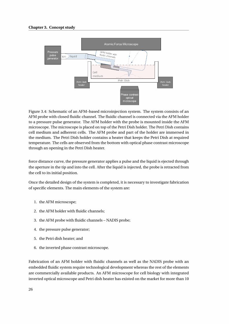
Chapter 3. Concept study
Figure 3.4: Schematic of an AFM–based microinjection system. The system consists of anAFM probe with closed fluidic channel. The fluidic channel is connected via the AFM holderto a pressure pulse generator. The AFM holder with the probe is mounted inside the AFMmicroscope. The microscope is placed on top of the Petri Dish holder. The Petri Dish containscell medium and adherent cells. The AFM probe and part of the holder are immersed inthe medium. The Petri Dish holder contains a heater that keeps the Petri Dish at requiredtemperature. The cells are observed from the bottom with optical phase contrast microscopethrough an opening in the Petri Dish heater.
force distance curve, the pressure generator applies a pulse and the liquid is ejected through
the aperture in the tip and into the cell. After the liquid is injected, the probe is retracted from
the cell to its initial position.
Once the detailed design of the system is completed, it is necessary to investigate fabrication
of specific elements. The main elements of the system are:
1. the AFM microscope;
2. the AFM holder with fluidic channels;
3. the AFM probe with fluidic channels – NADIS probe;
4. the pressure pulse generator;
5. the Petri dish heater; and
6. the inverted phase contrast microscope.
Fabrication of an AFM holder with fluidic channels as well as the NADIS probe with an
embedded fluidic system require technological development whereas the rest of the elements
are commercially available products. An AFM microscope for cell biology with integrated
inverted optical microscope and Petri dish heater has existed on the market for more than 10
26
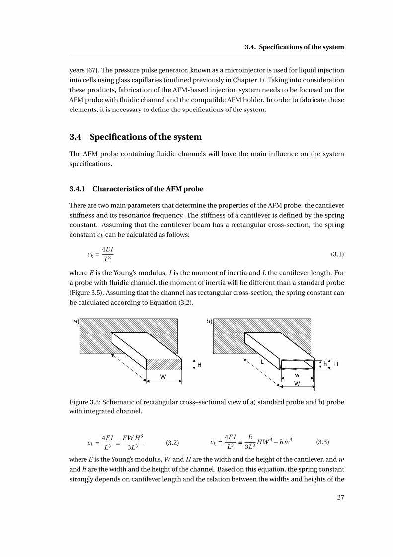
3.4. Specifications of the system
years [67]. The pressure pulse generator, known as a microinjector is used for liquid injection
into cells using glass capillaries (outlined previously in Chapter 1). Taking into consideration
these products, fabrication of the AFM-based injection system needs to be focused on the
AFM probe with fluidic channel and the compatible AFM holder. In order to fabricate these
elements, it is necessary to define the specifications of the system.
3.4 Specifications of the system
The AFM probe containing fluidic channels will have the main influence on the system
specifications.
3.4.1 Characteristics of the AFM probe
There are two main parameters that determine the properties of the AFM probe: the cantilever
stiffness and its resonance frequency. The stiffness of a cantilever is defined by the spring
constant. Assuming that the cantilever beam has a rectangular cross-section, the spring
constant ck can be calculated as follows:
ck = 4E I
L3 (3.1)
where E is the Young’s modulus, I is the moment of inertia and L the cantilever length. For
a probe with fluidic channel, the moment of inertia will be different than a standard probe
(Figure 3.5). Assuming that the channel has rectangular cross-section, the spring constant can
be calculated according to Equation (3.2).
Figure 3.5: Schematic of rectangular cross–sectional view of a) standard probe and b) probewith integrated channel.
ck = 4E I
L3 ≡ EW H 3
3L3 (3.2) ck = 4E I
L3 ≡ E
3L3 HW 3 −hw3 (3.3)
where E is the Young’s modulus, W and H are the width and the height of the cantilever, and w
and h are the width and the height of the channel. Based on this equation, the spring constant
strongly depends on cantilever length and the relation between the widths and heights of the
27
Chapter 3. Concept study
cantilever and the channel.
It has been shown that cell indentations with an AFM probe should be performed with a
very flexible cantilever (preferably in the range of 10−2 N m−1). Thus, geometrical parameters
of a cantilever should be adapted to fulfill this requirement. Standard flexible cantilevers
have a length in the range of several hundreds of micrometers, the width varies from 10 to 40
micrometers and the height can be as small as 600 nm. The same range of values for length and
width can be adopted when designing cantilevers containing fluidic channels. The cantilever
height, however, has to be larger due to the presence of the channel. The cantilever height will
depend on the channel height and thickness of the cantilever wall. As the height of the channel
will have the most influence on the flow of liquid through the cantilever, it is preferable to
keep it relatively large. Thus, the channel height and the cantilever height must be adjusted
to provide a compromise between cantilever stiffness and liquid flow through the channel.
Figure 3.6 shows an example of the spring constant dependency on cantilever length L when
the width W and wall thickness ∆/2 are constant and the cantilever height H is changing.
Figure 3.6: Spring constant dependency on the length of a cantilever with defined width andwall thickness ∆/2 for three cantilever heights (and three channel heights consequently).
It can be seen that for the same cantilever length the cantilever stiffness increases when the
cantilever height increases (the height of the channel increases).
Once the geometrical values of the cantilever are chosen, it is necessary to determine the in-
fluence of the size of the channel embedded in the cantilever on its spring constant. Figure 3.7
shows dependency of the cantilever spring constant on its wall thickness.
In order to obtain soft cantilevers with rectangular channels, the following requirements
28
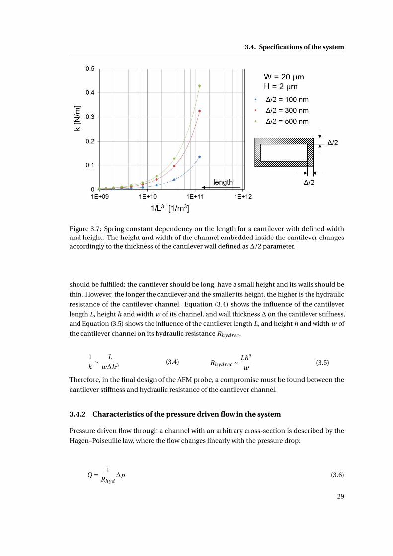
3.4. Specifications of the system
Figure 3.7: Spring constant dependency on the length for a cantilever with defined widthand height. The height and width of the channel embedded inside the cantilever changesaccordingly to the thickness of the cantilever wall defined as ∆/2 parameter.
should be fulfilled: the cantilever should be long, have a small height and its walls should be
thin. However, the longer the cantilever and the smaller its height, the higher is the hydraulic
resistance of the cantilever channel. Equation (3.4) shows the influence of the cantilever
length L, height h and width w of its channel, and wall thickness ∆ on the cantilever stiffness,
and Equation (3.5) shows the influence of the cantilever length L, and height h and width w of
the cantilever channel on its hydraulic resistance Rhydr ec .
1
k∼ L
w∆h3 (3.4) Rhydr ec ∼Lh3
w(3.5)
Therefore, in the final design of the AFM probe, a compromise must be found between the
cantilever stiffness and hydraulic resistance of the cantilever channel.
3.4.2 Characteristics of the pressure driven flow in the system
Pressure driven flow through a channel with an arbitrary cross-section is described by the
Hagen–Poiseuille law, where the flow changes linearly with the pressure drop:
Q = 1
Rhyd∆p (3.6)
29
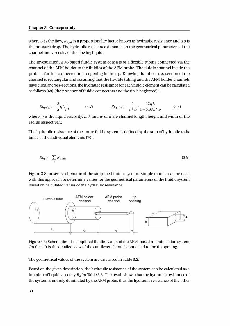
Chapter 3. Concept study
where Q is the flow, Rhyd is a proportionality factor known as hydraulic resistance and ∆p is
the pressure drop. The hydraulic resistance depends on the geometrical parameters of the
channel and viscosity of the flowing liquid.
The investigated AFM-based fluidic system consists of a flexible tubing connected via the
channel of the AFM holder to the fluidics of the AFM probe. The fluidic channel inside the
probe is further connected to an opening in the tip. Knowing that the cross-section of the
channel is rectangular and assuming that the flexible tubing and the AFM holder channels
have circular cross-sections, the hydraulic resistance for each fluidic element can be calculated
as follows [69] (the presence of fluidic connectors and the tip is neglected):
Rhydci r =8
πηL
1
a4 (3.7) Rhydr ec =1
h3w· 12ηL
1−0.63h/w(3.8)
where, η is the liquid viscosity, L, h and w or a are channel length, height and width or the
radius respectively.
The hydraulic resistance of the entire fluidic system is defined by the sum of hydraulic resis-
tance of the individual elements [70]:
Rhyd =∑i
Rhydi (3.9)
Figure 3.8 presents schematic of the simplified fluidic system. Simple models can be used
with this approach to determine values for the geometrical parameters of the fluidic system
based on calculated values of the hydraulic resistance.
Figure 3.8: Schematics of a simplified fluidic system of the AFM–based microinjection system.On the left is the detailed view of the cantilever channel connected to the tip opening.
The geometrical values of the system are discussed in Table 3.2.
Based on the given description, the hydraulic resistance of the system can be calculated as a
function of liquid viscosity Rh(η) Table 3.3. The result shows that the hydraulic resistance of
the system is entirely dominated by the AFM probe, thus the hydraulic resistance of the other
30
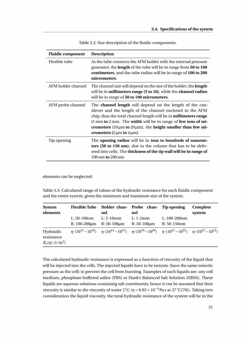
3.4. Specifications of the system
Table 3.2: Size description of the fluidic components.
Fluidic component Description
Flexible tube As the tube connects the AFM holder with the external pressuregenerator, the length of the tube will be in range from 50 to 100centimeters, and the tube radius will be in range of 100 to 200micrometers.
AFM holder channel The channel size will depend on the size of the holder; the lengthwill be in millimeters range (5 to 10), while the channel radiuswill be in range of 50 to 100 micrometers.
AFM probe channel The channel length will depend on the length of the can-tilever and the length of the channel enclosed in the AFMchip, thus the total channel length will be in millimeters range(1 mm to 2 mm. The width will be in range of few tens of mi-crometers (10µm to 20µm), the height smaller than few mi-crometers (2µm to 4µm).
Tip opening The opening radius will be in tens to hundreds of nanome-ters (50 to 150 nm), due to the volume that has to be deliv-ered into cells. The thickness of the tip wall will be in range of100 nm to 200 nm.
elements can be neglected.
Table 3.3: Calculated range of values of the hydraulic resistance for each fluidic componentand the entire system, given the minimum and maximum size of the system.
Systemelements
Flexible Tube Holder chan-nel
Probe chan-nel
Tip opening Completesystem
L: 50-100cm L: 5-10mm L: 1-2mm L: 100-200nmR: 100-200µm R: 50-100µm R: 50-100µm R: 50-150nm
HydraulicresistanceRs(η) [1/m3]
η·(1015−1016) η·(1014−1015) η·(1019−1020) η·(1021−1022) η·(1021−1022)
The calculated hydraulic resistance is expressed as a function of viscosity of the liquid that
will be injected into the cells. The injected liquids have to be isotonic (have the same osmotic
pressure as the cell) to prevent the cell from bursting. Examples of such liquids are: any cell
medium, phosphate buffered saline (PBS) or Hank’s Balanced Salt Solution (HBSS). These
liquids are aqueous solutions containing salt constituents, hence it can be assumed that their
viscosity is similar to the viscosity of water [71] (η= 6.92×10⁻⁴ Pa s at 37 ◦C[70]). Taking into
consideration the liquid viscosity, the total hydraulic resistance of the system will be in the
31
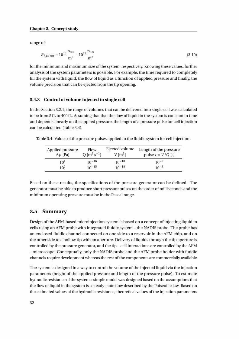
Chapter 3. Concept study
range of:
Rhyd tot ∼ 1018 Pa s
m3 −1019 Pa s
m3 (3.10)
for the minimum and maximum size of the system, respectively. Knowing these values, further
analysis of the system parameters is possible. For example, the time required to completely
fill the system with liquid, the flow of liquid as a function of applied pressure and finally, the
volume precision that can be ejected from the tip opening.
3.4.3 Control of volume injected to single cell
In the Section 3.2.1, the range of volumes that can be delivered into single cell was calculated
to be from 5 fL to 400 fL. Assuming that that the flow of liquid in the system is constant in time
and depends linearly on the applied pressure, the length of a pressure pulse for cell injection
can be calculated (Table 3.4).
Table 3.4: Values of the pressure pulses applied to the fluidic system for cell injection.
Applied pressure∆p [Pa]
FlowQ [m3 s−1]
Ejected volume
V [m3]Length of the pressure
pulse t =V /Q [s]
101 10−16 10−18 10−2
102 10−15 10−18 10−3
Based on these results, the specifications of the pressure generator can be defined. The
generator must be able to produce short pressure pulses on the order of milliseconds and the
minimum operating pressure must be in the Pascal range.
3.5 Summary
Design of the AFM-based microinjection system is based on a concept of injecting liquid to
cells using an AFM probe with integrated fluidic system – the NADIS probe. The probe has
an enclosed fluidic channel connected on one side to a reservoir in the AFM chip, and on
the other side to a hollow tip with an aperture. Delivery of liquids through the tip aperture is
controlled by the pressure generator, and the tip – cell interactions are controlled by the AFM
– microscope. Conceptually, only the NADIS probe and the AFM probe holder with fluidic
channels require development whereas the rest of the components are commercially available.
The system is designed in a way to control the volume of the injected liquid via the injection
parameters (height of the applied pressure and length of the pressure pulse). To estimate
hydraulic resistance of the system a simple model was designed based on the assumptions that
the flow of liquid in the system is a steady-state flow described by the Poiseuille law. Based on
the estimated values of the hydraulic resistance, theoretical values of the injection parameters
32

3.5. Summary
were proposed.
The conceptual description of the AFM based microinjection system presented here is an
introduction to a detailed design and fabrication of the NADIS probe and the AFM probe
holder and is used as a guide when choosing elements that are commercially available.
33

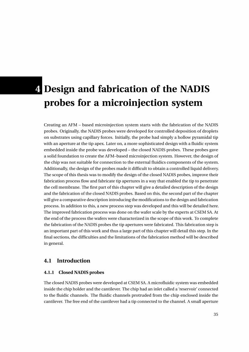
4 Design and fabrication of the NADISprobes for a microinjection system
Creating an AFM – based microinjection system starts with the fabrication of the NADIS
probes. Originally, the NADIS probes were developed for controlled deposition of droplets
on substrates using capillary forces. Initially, the probe had simply a hollow pyramidal tip
with an aperture at the tip apex. Later on, a more sophisticated design with a fluidic system
embedded inside the probe was developed – the closed NADIS probes. These probes gave
a solid foundation to create the AFM–based microinjection system. However, the design of
the chip was not suitable for connection to the external fluidics components of the system.
Additionally, the design of the probes made it difficult to obtain a controlled liquid delivery.
The scope of this thesis was to modify the design of the closed NADIS probes, improve their
fabrication process flow and fabricate tip apertures in a way that enabled the tip to penetrate
the cell membrane. The first part of this chapter will give a detailed description of the design
and the fabrication of the closed NADIS probes. Based on this, the second part of the chapter
will give a comparative description introducing the modifications to the design and fabrication
process. In addition to this, a new process step was developed and this will be detailed here.
The improved fabrication process was done on the wafer scale by the experts at CSEM SA. At
the end of the process the wafers were characterized in the scope of this work. To complete
the fabrication of the NADIS probes the tip apertures were fabricated. This fabrication step is
an important part of this work and thus a large part of this chapter will detail this step. In the
final sections, the difficulties and the limitations of the fabrication method will be described
in general.
4.1 Introduction
4.1.1 Closed NADIS probes
The closed NADIS probes were developed at CSEM SA. A microfluidic system was embedded
inside the chip holder and the cantilever. The chip had an inlet called a ‘reservoir’ connected
to the fluidic channels. The fluidic channels protruded from the chip enclosed inside the
cantilever. The free end of the cantilever had a tip connected to the channel. A small aperture
35
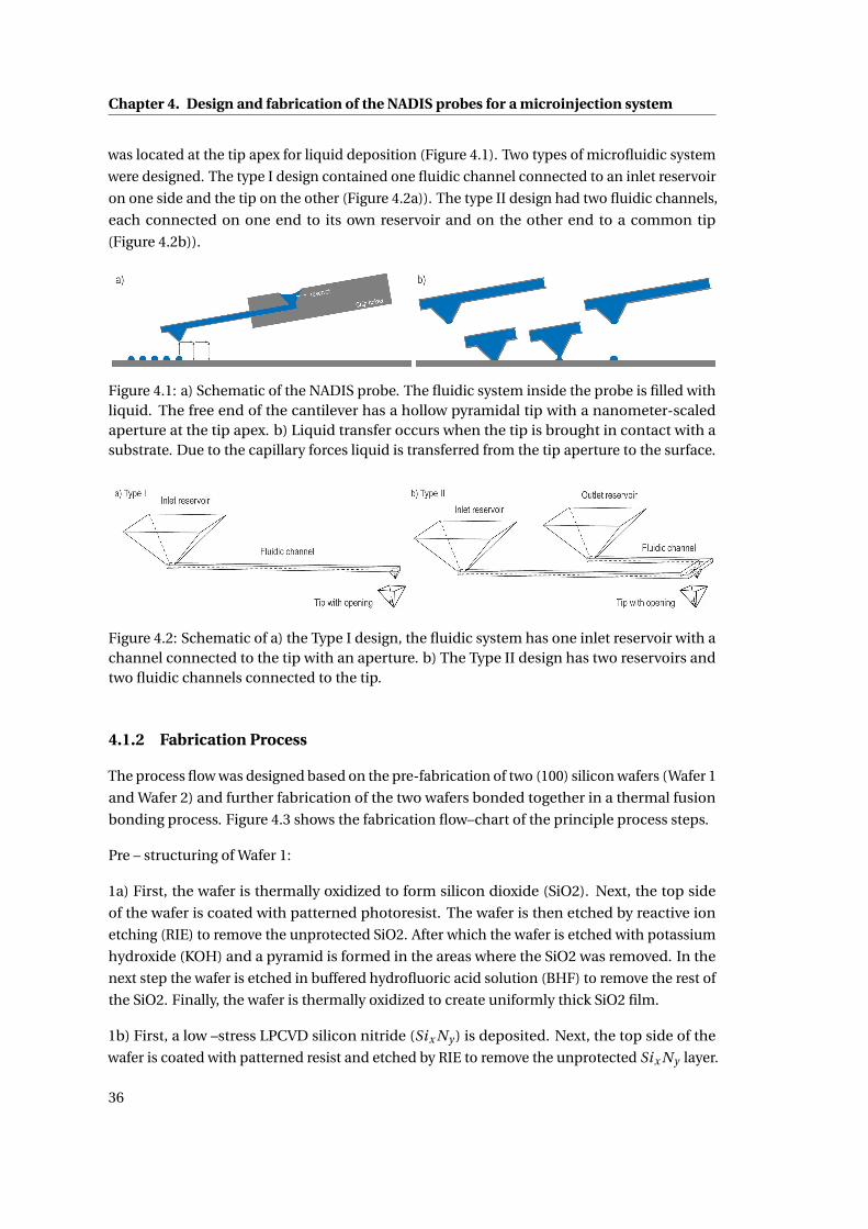
Chapter 4. Design and fabrication of the NADIS probes for a microinjection system
was located at the tip apex for liquid deposition (Figure 4.1). Two types of microfluidic system
were designed. The type I design contained one fluidic channel connected to an inlet reservoir
on one side and the tip on the other (Figure 4.2a)). The type II design had two fluidic channels,
each connected on one end to its own reservoir and on the other end to a common tip
(Figure 4.2b)).
Figure 4.1: a) Schematic of the NADIS probe. The fluidic system inside the probe is filled withliquid. The free end of the cantilever has a hollow pyramidal tip with a nanometer-scaledaperture at the tip apex. b) Liquid transfer occurs when the tip is brought in contact with asubstrate. Due to the capillary forces liquid is transferred from the tip aperture to the surface.
Figure 4.2: Schematic of a) the Type I design, the fluidic system has one inlet reservoir with achannel connected to the tip with an aperture. b) The Type II design has two reservoirs andtwo fluidic channels connected to the tip.
4.1.2 Fabrication Process
The process flow was designed based on the pre-fabrication of two (100) silicon wafers (Wafer 1
and Wafer 2) and further fabrication of the two wafers bonded together in a thermal fusion
bonding process. Figure 4.3 shows the fabrication flow–chart of the principle process steps.
Pre – structuring of Wafer 1:
1a) First, the wafer is thermally oxidized to form silicon dioxide (SiO2). Next, the top side
of the wafer is coated with patterned photoresist. The wafer is then etched by reactive ion
etching (RIE) to remove the unprotected SiO2. After which the wafer is etched with potassium
hydroxide (KOH) and a pyramid is formed in the areas where the SiO2 was removed. In the
next step the wafer is etched in buffered hydrofluoric acid solution (BHF) to remove the rest of
the SiO2. Finally, the wafer is thermally oxidized to create uniformly thick SiO2 film.
1b) First, a low –stress LPCVD silicon nitride (Six Ny ) is deposited. Next, the top side of the
wafer is coated with patterned resist and etched by RIE to remove the unprotected Six Ny layer.
36
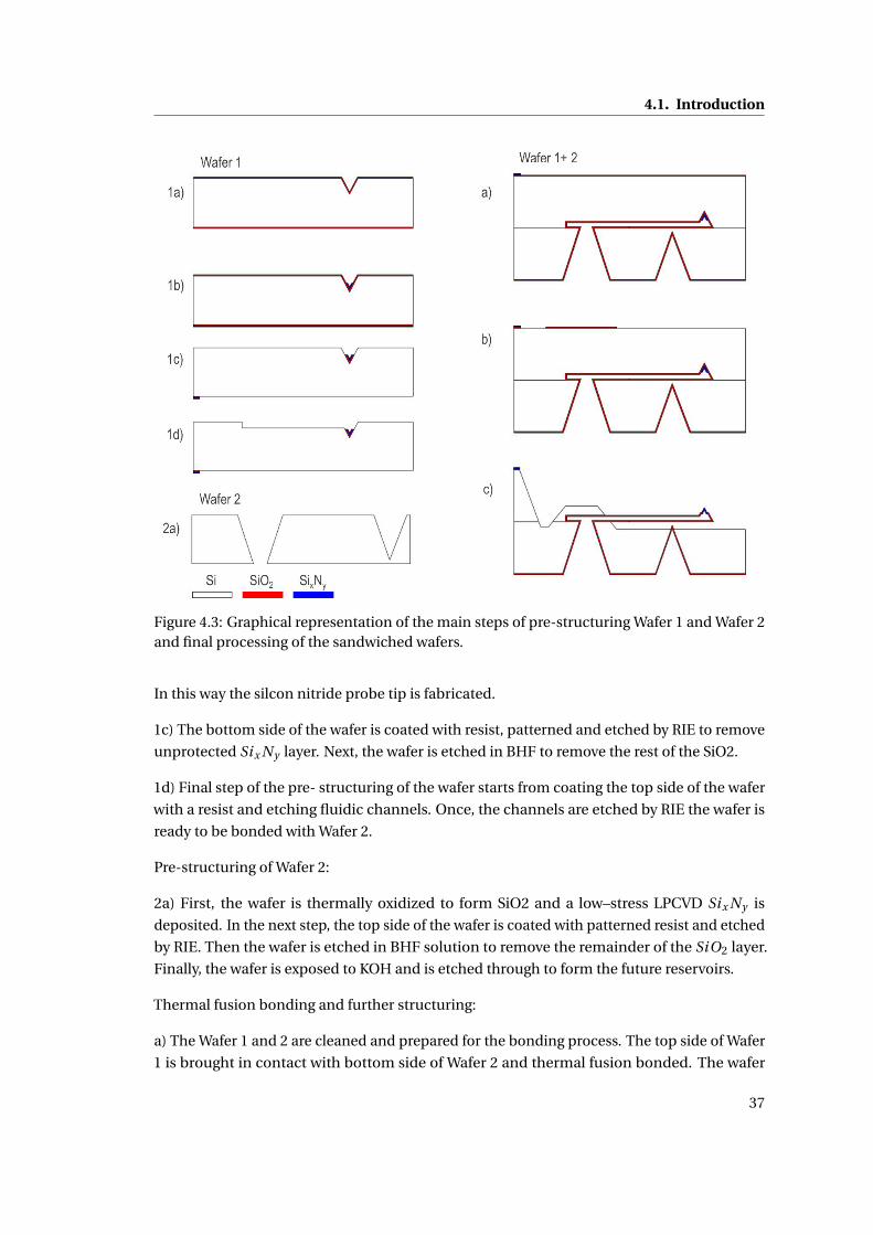
4.1. Introduction
Figure 4.3: Graphical representation of the main steps of pre-structuring Wafer 1 and Wafer 2and final processing of the sandwiched wafers.
In this way the silcon nitride probe tip is fabricated.
1c) The bottom side of the wafer is coated with resist, patterned and etched by RIE to remove
unprotected Six Ny layer. Next, the wafer is etched in BHF to remove the rest of the SiO2.
1d) Final step of the pre- structuring of the wafer starts from coating the top side of the wafer
with a resist and etching fluidic channels. Once, the channels are etched by RIE the wafer is
ready to be bonded with Wafer 2.
Pre-structuring of Wafer 2:
2a) First, the wafer is thermally oxidized to form SiO2 and a low–stress LPCVD Six Ny is
deposited. In the next step, the top side of the wafer is coated with patterned resist and etched
by RIE. Then the wafer is etched in BHF solution to remove the remainder of the SiO2 layer.
Finally, the wafer is exposed to KOH and is etched through to form the future reservoirs.
Thermal fusion bonding and further structuring:
a) The Wafer 1 and 2 are cleaned and prepared for the bonding process. The top side of Wafer
1 is brought in contact with bottom side of Wafer 2 and thermal fusion bonded. The wafer
37
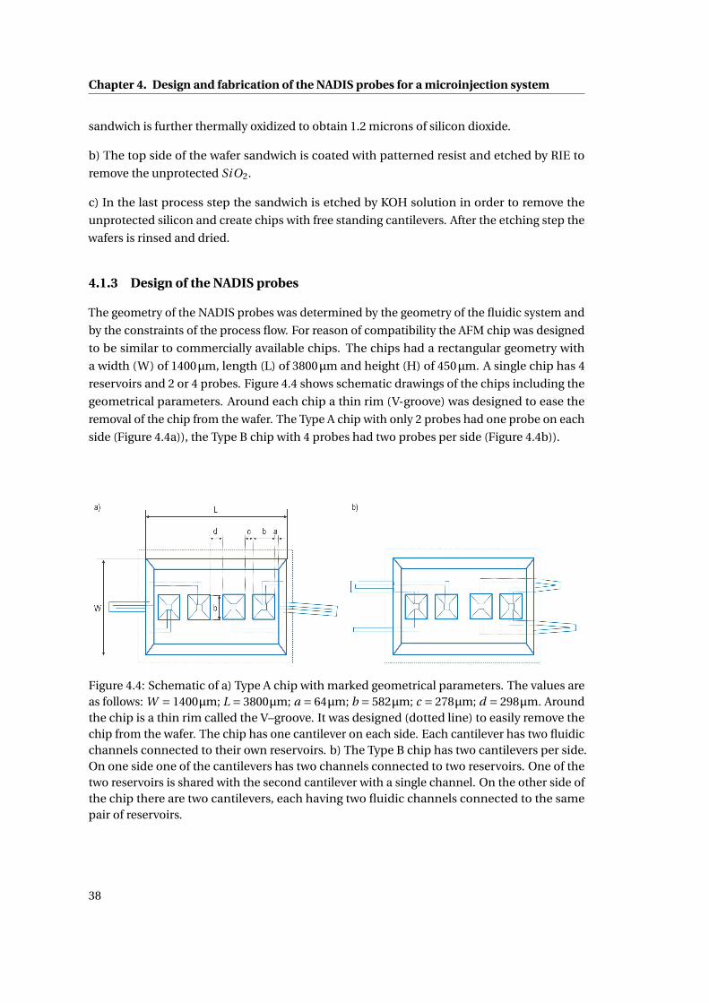
Chapter 4. Design and fabrication of the NADIS probes for a microinjection system
sandwich is further thermally oxidized to obtain 1.2 microns of silicon dioxide.
b) The top side of the wafer sandwich is coated with patterned resist and etched by RIE to
remove the unprotected SiO2.
c) In the last process step the sandwich is etched by KOH solution in order to remove the
unprotected silicon and create chips with free standing cantilevers. After the etching step the
wafers is rinsed and dried.
4.1.3 Design of the NADIS probes
The geometry of the NADIS probes was determined by the geometry of the fluidic system and
by the constraints of the process flow. For reason of compatibility the AFM chip was designed
to be similar to commercially available chips. The chips had a rectangular geometry with
a width (W) of 1400µm, length (L) of 3800µm and height (H) of 450µm. A single chip has 4
reservoirs and 2 or 4 probes. Figure 4.4 shows schematic drawings of the chips including the
geometrical parameters. Around each chip a thin rim (V-groove) was designed to ease the
removal of the chip from the wafer. The Type A chip with only 2 probes had one probe on each
side (Figure 4.4a)), the Type B chip with 4 probes had two probes per side (Figure 4.4b)).
Figure 4.4: Schematic of a) Type A chip with marked geometrical parameters. The values areas follows: W = 1400µm; L = 3800µm; a = 64µm; b = 582µm; c = 278µm; d = 298µm. Aroundthe chip is a thin rim called the V–groove. It was designed (dotted line) to easily remove thechip from the wafer. The chip has one cantilever on each side. Each cantilever has two fluidicchannels connected to their own reservoirs. b) The Type B chip has two cantilevers per side.On one side one of the cantilevers has two channels connected to two reservoirs. One of thetwo reservoirs is shared with the second cantilever with a single channel. On the other side ofthe chip there are two cantilevers, each having two fluidic channels connected to the samepair of reservoirs.
38
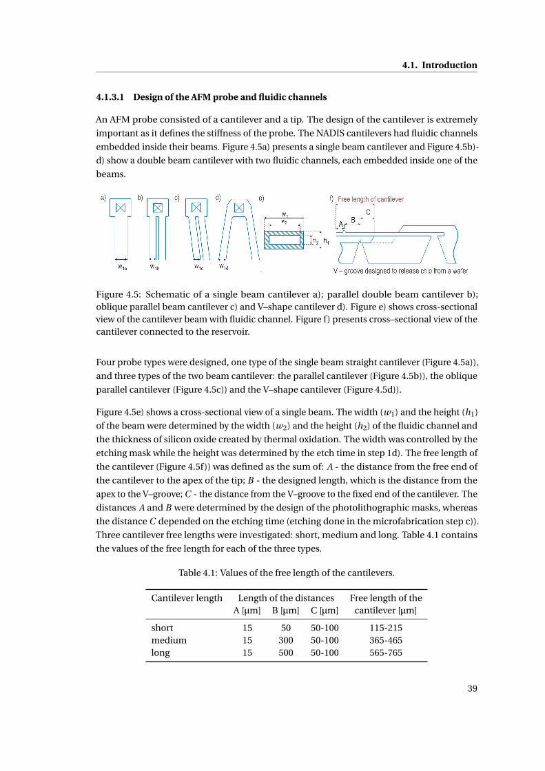
4.1. Introduction
4.1.3.1 Design of the AFM probe and fluidic channels
An AFM probe consisted of a cantilever and a tip. The design of the cantilever is extremely
important as it defines the stiffness of the probe. The NADIS cantilevers had fluidic channels
embedded inside their beams. Figure 4.5a) presents a single beam cantilever and Figure 4.5b)-
d) show a double beam cantilever with two fluidic channels, each embedded inside one of the
beams.
Figure 4.5: Schematic of a single beam cantilever a); parallel double beam cantilever b);oblique parallel beam cantilever c) and V–shape cantilever d). Figure e) shows cross-sectionalview of the cantilever beam with fluidic channel. Figure f) presents cross–sectional view of thecantilever connected to the reservoir.
Four probe types were designed, one type of the single beam straight cantilever (Figure 4.5a)),
and three types of the two beam cantilever: the parallel cantilever (Figure 4.5b)), the oblique
parallel cantilever (Figure 4.5c)) and the V–shape cantilever (Figure 4.5d)).
Figure 4.5e) shows a cross-sectional view of a single beam. The width (w1) and the height (h1)
of the beam were determined by the width (w2) and the height (h2) of the fluidic channel and
the thickness of silicon oxide created by thermal oxidation. The width was controlled by the
etching mask while the height was determined by the etch time in step 1d). The free length of
the cantilever (Figure 4.5f)) was defined as the sum of: A - the distance from the free end of
the cantilever to the apex of the tip; B - the designed length, which is the distance from the
apex to the V–groove; C - the distance from the V–groove to the fixed end of the cantilever. The
distances A and B were determined by the design of the photolithographic masks, whereas
the distance C depended on the etching time (etching done in the microfabrication step c)).
Three cantilever free lengths were investigated: short, medium and long. Table 4.1 contains
the values of the free length for each of the three types.
Table 4.1: Values of the free length of the cantilevers.
Cantilever length Length of the distances Free length of theA [µm] B [µm] C [µm] cantilever [µm]
short 15 50 50-100 115-215medium 15 300 50-100 365-465long 15 500 50-100 565-765
39
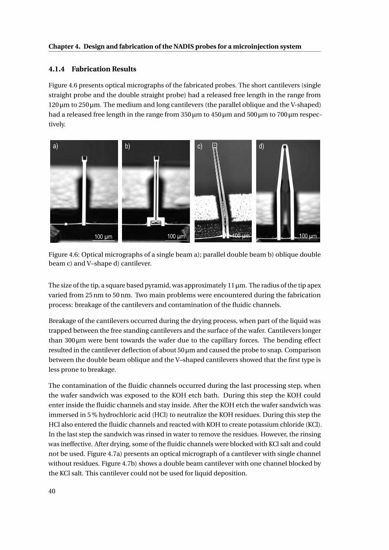
Chapter 4. Design and fabrication of the NADIS probes for a microinjection system
4.1.4 Fabrication Results
Figure 4.6 presents optical micrographs of the fabricated probes. The short cantilevers (single
straight probe and the double straight probe) had a released free length in the range from
120µm to 250µm. The medium and long cantilevers (the parallel oblique and the V-shaped)
had a released free length in the range from 350µm to 450µm and 500µm to 700µm respec-
tively.
Figure 4.6: Optical micrographs of a single beam a); parallel double beam b) oblique doublebeam c) and V–shape d) cantilever.
The size of the tip, a square based pyramid, was approximately 11µm. The radius of the tip apex
varied from 25 nm to 50 nm. Two main problems were encountered during the fabrication
process: breakage of the cantilevers and contamination of the fluidic channels.
Breakage of the cantilevers occurred during the drying process, when part of the liquid was
trapped between the free standing cantilevers and the surface of the wafer. Cantilevers longer
than 300µm were bent towards the wafer due to the capillary forces. The bending effect
resulted in the cantilever deflection of about 50µm and caused the probe to snap. Comparison
between the double beam oblique and the V–shaped cantilevers showed that the first type is
less prone to breakage.
The contamination of the fluidic channels occurred during the last processing step, when
the wafer sandwich was exposed to the KOH etch bath. During this step the KOH could
enter inside the fluidic channels and stay inside. After the KOH etch the wafer sandwich was
immersed in 5 % hydrochloric acid (HCl) to neutralize the KOH residues. During this step the
HCl also entered the fluidic channels and reacted with KOH to create potassium chloride (KCl).
In the last step the sandwich was rinsed in water to remove the residues. However, the rinsing
was ineffective. After drying, some of the fluidic channels were blocked with KCl salt and could
not be used. Figure 4.7a) presents an optical micrograph of a cantilever with single channel
without residues. Figure 4.7b) shows a double beam cantilever with one channel blocked by
the KCl salt. This cantilever could not be used for liquid deposition.
40
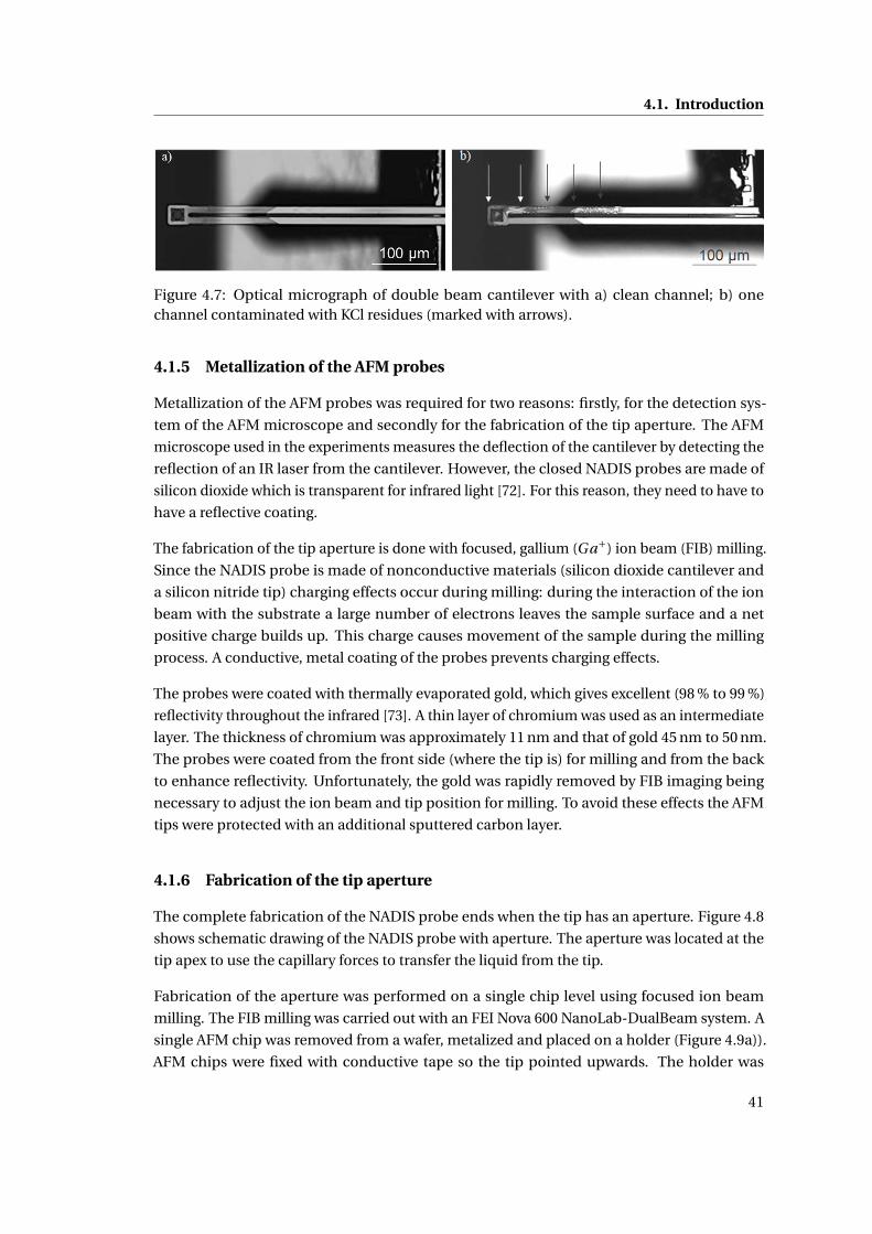
4.1. Introduction
Figure 4.7: Optical micrograph of double beam cantilever with a) clean channel; b) onechannel contaminated with KCl residues (marked with arrows).
4.1.5 Metallization of the AFM probes
Metallization of the AFM probes was required for two reasons: firstly, for the detection sys-
tem of the AFM microscope and secondly for the fabrication of the tip aperture. The AFM
microscope used in the experiments measures the deflection of the cantilever by detecting the
reflection of an IR laser from the cantilever. However, the closed NADIS probes are made of
silicon dioxide which is transparent for infrared light [72]. For this reason, they need to have to
have a reflective coating.
The fabrication of the tip aperture is done with focused, gallium (Ga+) ion beam (FIB) milling.
Since the NADIS probe is made of nonconductive materials (silicon dioxide cantilever and
a silicon nitride tip) charging effects occur during milling: during the interaction of the ion
beam with the substrate a large number of electrons leaves the sample surface and a net
positive charge builds up. This charge causes movement of the sample during the milling
process. A conductive, metal coating of the probes prevents charging effects.
The probes were coated with thermally evaporated gold, which gives excellent (98 % to 99 %)
reflectivity throughout the infrared [73]. A thin layer of chromium was used as an intermediate
layer. The thickness of chromium was approximately 11 nm and that of gold 45 nm to 50 nm.
The probes were coated from the front side (where the tip is) for milling and from the back
to enhance reflectivity. Unfortunately, the gold was rapidly removed by FIB imaging being
necessary to adjust the ion beam and tip position for milling. To avoid these effects the AFM
tips were protected with an additional sputtered carbon layer.
4.1.6 Fabrication of the tip aperture
The complete fabrication of the NADIS probe ends when the tip has an aperture. Figure 4.8
shows schematic drawing of the NADIS probe with aperture. The aperture was located at the
tip apex to use the capillary forces to transfer the liquid from the tip.
Fabrication of the aperture was performed on a single chip level using focused ion beam
milling. The FIB milling was carried out with an FEI Nova 600 NanoLab-DualBeam system. A
single AFM chip was removed from a wafer, metalized and placed on a holder (Figure 4.9a)).
AFM chips were fixed with conductive tape so the tip pointed upwards. The holder was
41
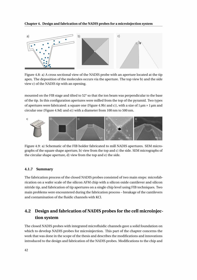
Chapter 4. Design and fabrication of the NADIS probes for a microinjection system
Figure 4.8: a) A cross sectional view of the NADIS probe with an aperture located at the tipapex. The deposition of the molecules occurs via the aperture. The top view b) and the sideview c) of the NADIS tip with an opening.
mounted on the FIB stage and tilted to 52° so that the ion beam was perpendicular to the base
of the tip. In this configuration apertures were milled from the top of the pyramid. Two types
of apertures were fabricated: a square one (Figure 4.9b) and c)), with a size of 1µm×1µm and
circular one (Figure 4.9d) and e)) with a diameter from 100 nm to 500 nm.
Figure 4.9: a) Schematic of the FIB holder fabricated to mill NADIS apertures. SEM micro-graphs of the square shape aperture, b) view from the top and c) the side. SEM micrographs ofthe circular shape aperture, d) view from the top and e) the side.
4.1.7 Summary
The fabrication process of the closed NADIS probes consisted of two main steps: microfab-
rication on a wafer scale of the silicon AFM chip with a silicon oxide cantilever and silicon
nitride tip, and fabrication of tip apertures on a single chip level using FIB techniques. Two
main problems were encountered during the fabrication process – breakage of the cantilevers
and contamination of the fluidic channels with KCl.
4.2 Design and fabrication of NADIS probes for the cell microinjec-
tion system
The closed NADIS probes with integrated microfluidic channels gave a solid foundation on
which to develop NADIS probes for microinjection. This part of the chapter concerns the
work that was done in the scope of the thesis and describes the modifications and innovations
introduced to the design and fabrication of the NADIS probes. Modifications to the chip and
42
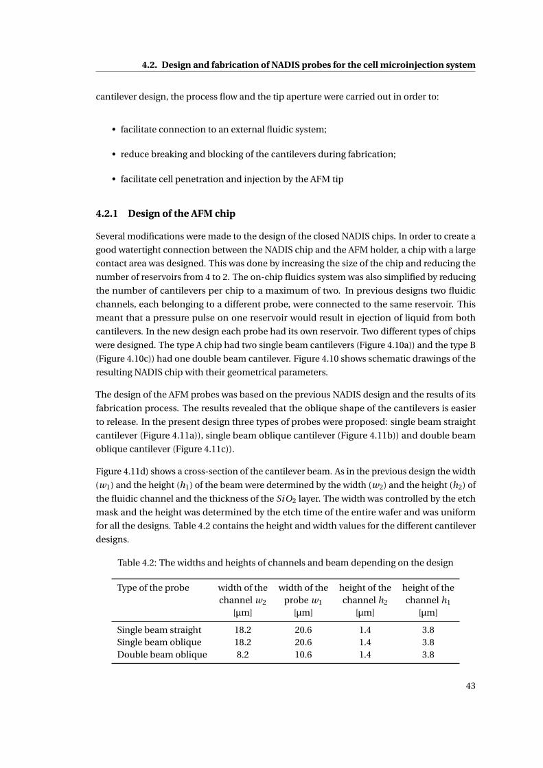
4.2. Design and fabrication of NADIS probes for the cell microinjection system
cantilever design, the process flow and the tip aperture were carried out in order to:
• facilitate connection to an external fluidic system;
• reduce breaking and blocking of the cantilevers during fabrication;
• facilitate cell penetration and injection by the AFM tip
4.2.1 Design of the AFM chip
Several modifications were made to the design of the closed NADIS chips. In order to create a
good watertight connection between the NADIS chip and the AFM holder, a chip with a large
contact area was designed. This was done by increasing the size of the chip and reducing the
number of reservoirs from 4 to 2. The on-chip fluidics system was also simplified by reducing
the number of cantilevers per chip to a maximum of two. In previous designs two fluidic
channels, each belonging to a different probe, were connected to the same reservoir. This
meant that a pressure pulse on one reservoir would result in ejection of liquid from both
cantilevers. In the new design each probe had its own reservoir. Two different types of chips
were designed. The type A chip had two single beam cantilevers (Figure 4.10a)) and the type B
(Figure 4.10c)) had one double beam cantilever. Figure 4.10 shows schematic drawings of the
resulting NADIS chip with their geometrical parameters.
The design of the AFM probes was based on the previous NADIS design and the results of its
fabrication process. The results revealed that the oblique shape of the cantilevers is easier
to release. In the present design three types of probes were proposed: single beam straight
cantilever (Figure 4.11a)), single beam oblique cantilever (Figure 4.11b)) and double beam
oblique cantilever (Figure 4.11c)).
Figure 4.11d) shows a cross-section of the cantilever beam. As in the previous design the width
(w1) and the height (h1) of the beam were determined by the width (w2) and the height (h2) of
the fluidic channel and the thickness of the SiO2 layer. The width was controlled by the etch
mask and the height was determined by the etch time of the entire wafer and was uniform
for all the designs. Table 4.2 contains the height and width values for the different cantilever
designs.
Table 4.2: The widths and heights of channels and beam depending on the design
Type of the probe width of the width of the height of the height of thechannel w2 probe w1 channel h2 channel h1
[µm] [µm] [µm] [µm]
Single beam straight 18.2 20.6 1.4 3.8Single beam oblique 18.2 20.6 1.4 3.8Double beam oblique 8.2 10.6 1.4 3.8
43
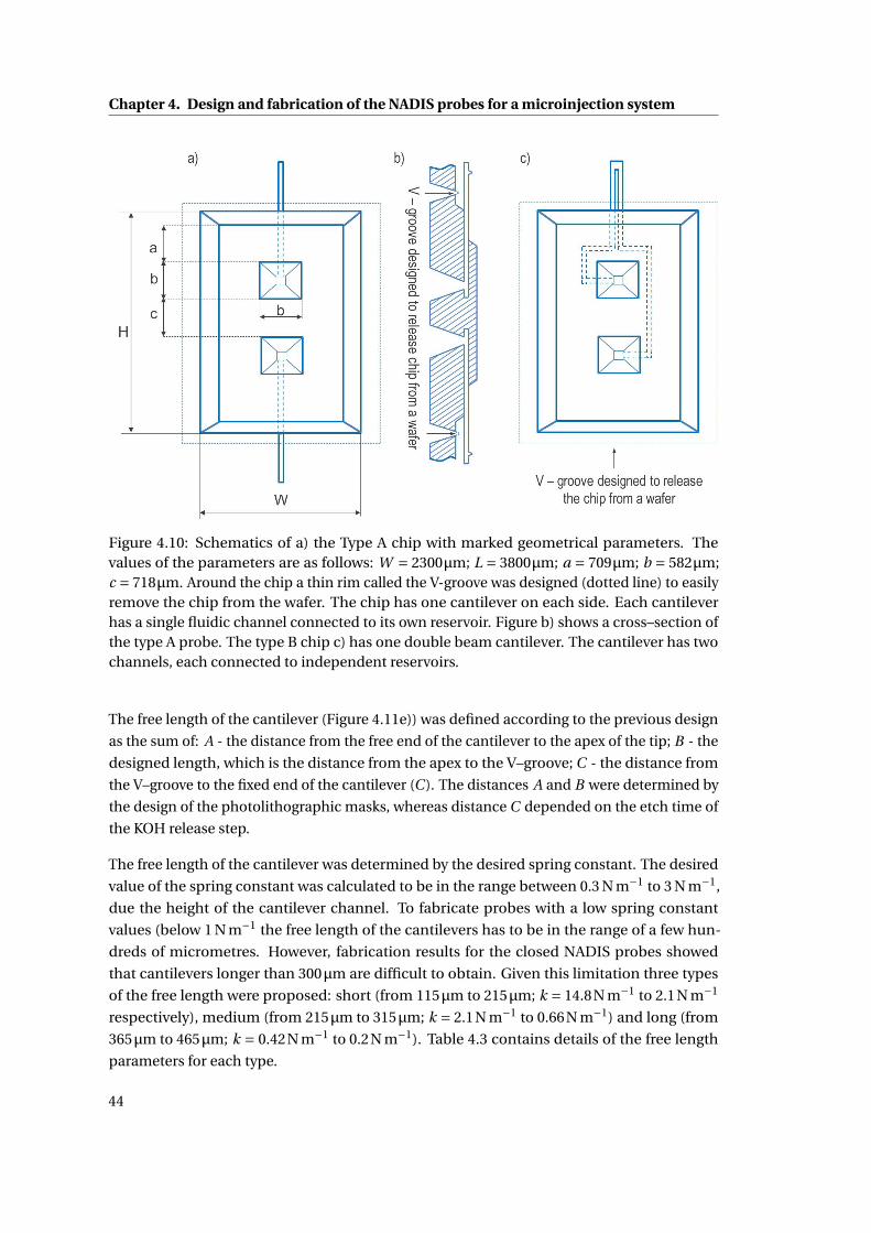
Chapter 4. Design and fabrication of the NADIS probes for a microinjection system
Figure 4.10: Schematics of a) the Type A chip with marked geometrical parameters. Thevalues of the parameters are as follows: W = 2300µm; L = 3800µm; a = 709µm; b = 582µm;c = 718µm. Around the chip a thin rim called the V-groove was designed (dotted line) to easilyremove the chip from the wafer. The chip has one cantilever on each side. Each cantileverhas a single fluidic channel connected to its own reservoir. Figure b) shows a cross–section ofthe type A probe. The type B chip c) has one double beam cantilever. The cantilever has twochannels, each connected to independent reservoirs.
The free length of the cantilever (Figure 4.11e)) was defined according to the previous design
as the sum of: A - the distance from the free end of the cantilever to the apex of the tip; B - the
designed length, which is the distance from the apex to the V–groove; C - the distance from
the V–groove to the fixed end of the cantilever (C ). The distances A and B were determined by
the design of the photolithographic masks, whereas distance C depended on the etch time of
the KOH release step.
The free length of the cantilever was determined by the desired spring constant. The desired
value of the spring constant was calculated to be in the range between 0.3 N m−1 to 3 N m−1,
due the height of the cantilever channel. To fabricate probes with a low spring constant
values (below 1 N m−1 the free length of the cantilevers has to be in the range of a few hun-
dreds of micrometres. However, fabrication results for the closed NADIS probes showed
that cantilevers longer than 300µm are difficult to obtain. Given this limitation three types
of the free length were proposed: short (from 115µm to 215µm; k = 14.8N m−1 to 2.1N m−1
respectively), medium (from 215µm to 315µm; k = 2.1N m−1 to 0.66N m−1) and long (from
365µm to 465µm; k = 0.42N m−1 to 0.2N m−1). Table 4.3 contains details of the free length
parameters for each type.
44
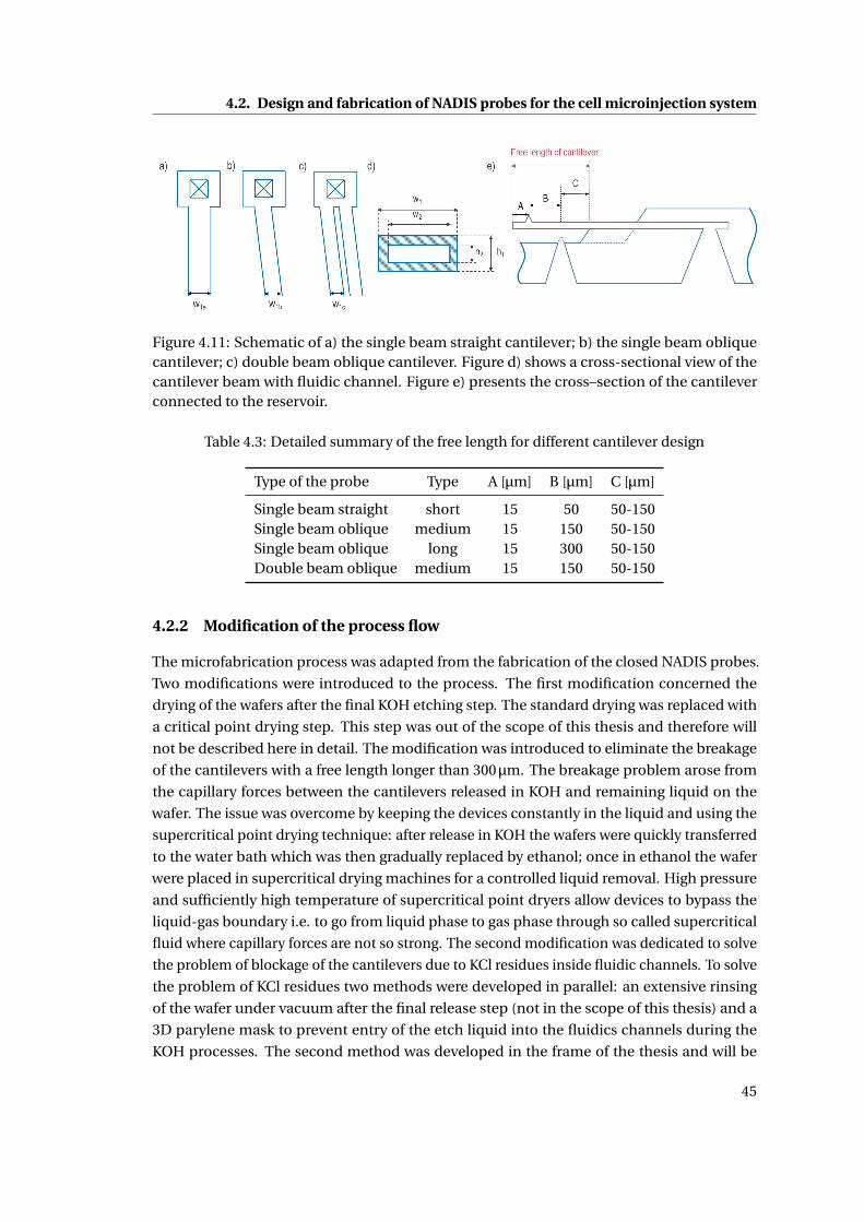
4.2. Design and fabrication of NADIS probes for the cell microinjection system
Figure 4.11: Schematic of a) the single beam straight cantilever; b) the single beam obliquecantilever; c) double beam oblique cantilever. Figure d) shows a cross-sectional view of thecantilever beam with fluidic channel. Figure e) presents the cross–section of the cantileverconnected to the reservoir.
Table 4.3: Detailed summary of the free length for different cantilever design
Type of the probe Type A [µm] B [µm] C [µm]
Single beam straight short 15 50 50-150Single beam oblique medium 15 150 50-150Single beam oblique long 15 300 50-150Double beam oblique medium 15 150 50-150
4.2.2 Modification of the process flow
The microfabrication process was adapted from the fabrication of the closed NADIS probes.
Two modifications were introduced to the process. The first modification concerned the
drying of the wafers after the final KOH etching step. The standard drying was replaced with
a critical point drying step. This step was out of the scope of this thesis and therefore will
not be described here in detail. The modification was introduced to eliminate the breakage
of the cantilevers with a free length longer than 300µm. The breakage problem arose from
the capillary forces between the cantilevers released in KOH and remaining liquid on the
wafer. The issue was overcome by keeping the devices constantly in the liquid and using the
supercritical point drying technique: after release in KOH the wafers were quickly transferred
to the water bath which was then gradually replaced by ethanol; once in ethanol the wafer
were placed in supercritical drying machines for a controlled liquid removal. High pressure
and sufficiently high temperature of supercritical point dryers allow devices to bypass the
liquid-gas boundary i.e. to go from liquid phase to gas phase through so called supercritical
fluid where capillary forces are not so strong. The second modification was dedicated to solve
the problem of blockage of the cantilevers due to KCl residues inside fluidic channels. To solve
the problem of KCl residues two methods were developed in parallel: an extensive rinsing
of the wafer under vacuum after the final release step (not in the scope of this thesis) and a
3D parylene mask to prevent entry of the etch liquid into the fluidics channels during the
KOH processes. The second method was developed in the frame of the thesis and will be
45
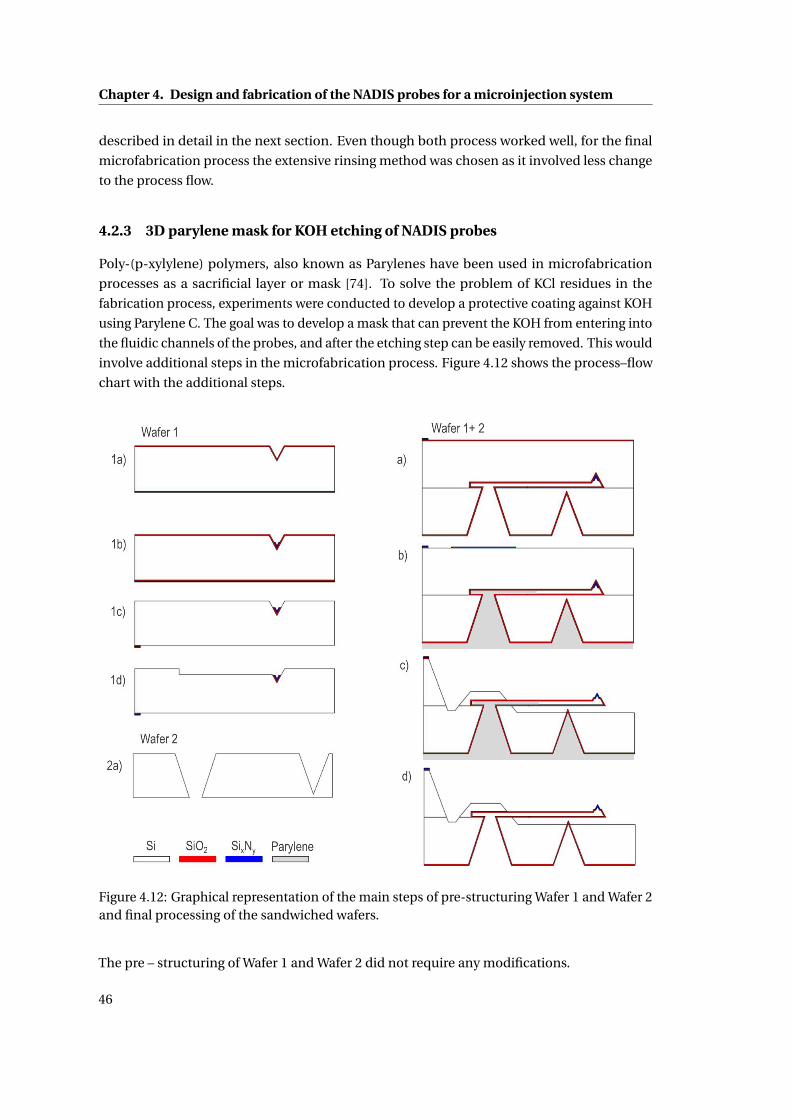
Chapter 4. Design and fabrication of the NADIS probes for a microinjection system
described in detail in the next section. Even though both process worked well, for the final
microfabrication process the extensive rinsing method was chosen as it involved less change
to the process flow.
4.2.3 3D parylene mask for KOH etching of NADIS probes
Poly-(p-xylylene) polymers, also known as Parylenes have been used in microfabrication
processes as a sacrificial layer or mask [74]. To solve the problem of KCl residues in the
fabrication process, experiments were conducted to develop a protective coating against KOH
using Parylene C. The goal was to develop a mask that can prevent the KOH from entering into
the fluidic channels of the probes, and after the etching step can be easily removed. This would
involve additional steps in the microfabrication process. Figure 4.12 shows the process–flow
chart with the additional steps.
Figure 4.12: Graphical representation of the main steps of pre-structuring Wafer 1 and Wafer 2and final processing of the sandwiched wafers.
The pre – structuring of Wafer 1 and Wafer 2 did not require any modifications.
46
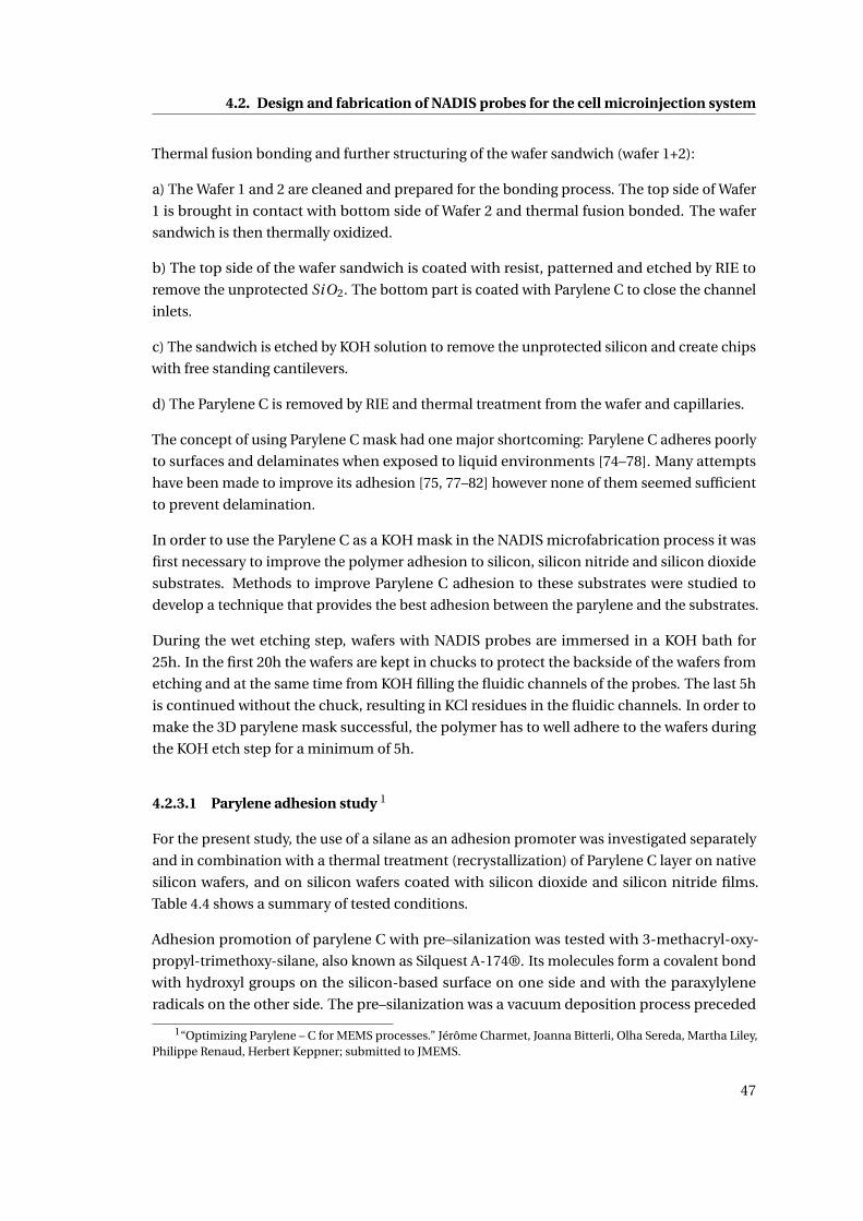
4.2. Design and fabrication of NADIS probes for the cell microinjection system
Thermal fusion bonding and further structuring of the wafer sandwich (wafer 1+2):
a) The Wafer 1 and 2 are cleaned and prepared for the bonding process. The top side of Wafer
1 is brought in contact with bottom side of Wafer 2 and thermal fusion bonded. The wafer
sandwich is then thermally oxidized.
b) The top side of the wafer sandwich is coated with resist, patterned and etched by RIE to
remove the unprotected SiO2. The bottom part is coated with Parylene C to close the channel
inlets.
c) The sandwich is etched by KOH solution to remove the unprotected silicon and create chips
with free standing cantilevers.
d) The Parylene C is removed by RIE and thermal treatment from the wafer and capillaries.
The concept of using Parylene C mask had one major shortcoming: Parylene C adheres poorly
to surfaces and delaminates when exposed to liquid environments [74–78]. Many attempts
have been made to improve its adhesion [75, 77–82] however none of them seemed sufficient
to prevent delamination.
In order to use the Parylene C as a KOH mask in the NADIS microfabrication process it was
first necessary to improve the polymer adhesion to silicon, silicon nitride and silicon dioxide
substrates. Methods to improve Parylene C adhesion to these substrates were studied to
develop a technique that provides the best adhesion between the parylene and the substrates.
During the wet etching step, wafers with NADIS probes are immersed in a KOH bath for
25h. In the first 20h the wafers are kept in chucks to protect the backside of the wafers from
etching and at the same time from KOH filling the fluidic channels of the probes. The last 5h
is continued without the chuck, resulting in KCl residues in the fluidic channels. In order to
make the 3D parylene mask successful, the polymer has to well adhere to the wafers during
the KOH etch step for a minimum of 5h.
4.2.3.1 Parylene adhesion study 1
For the present study, the use of a silane as an adhesion promoter was investigated separately
and in combination with a thermal treatment (recrystallization) of Parylene C layer on native
silicon wafers, and on silicon wafers coated with silicon dioxide and silicon nitride films.
Table 4.4 shows a summary of tested conditions.
Adhesion promotion of parylene C with pre–silanization was tested with 3-methacryl-oxy-
propyl-trimethoxy-silane, also known as Silquest A-174®. Its molecules form a covalent bond
with hydroxyl groups on the silicon-based surface on one side and with the paraxylylene
radicals on the other side. The pre–silanization was a vacuum deposition process preceded
1“Optimizing Parylene – C for MEMS processes.” Jérôme Charmet, Joanna Bitterli, Olha Sereda, Martha Liley,Philippe Renaud, Herbert Keppner; submitted to JMEMS.
47
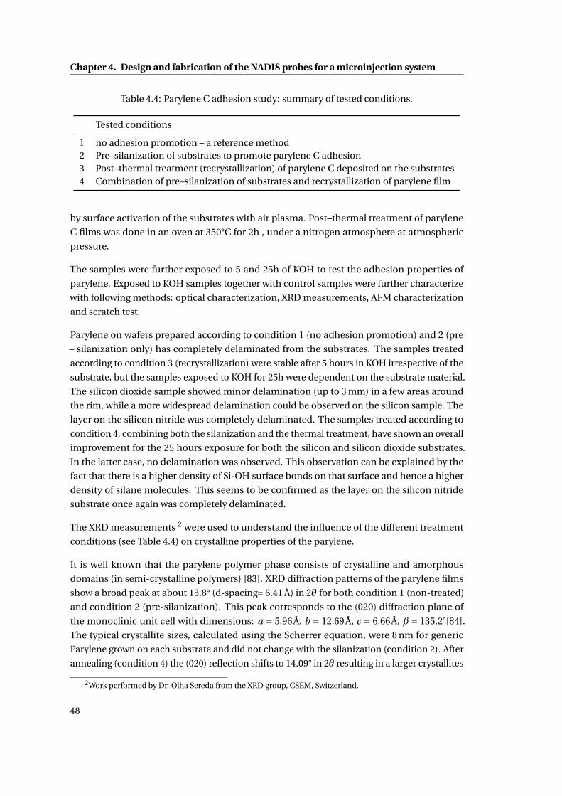
Chapter 4. Design and fabrication of the NADIS probes for a microinjection system
Table 4.4: Parylene C adhesion study: summary of tested conditions.
Tested conditions
1 no adhesion promotion – a reference method2 Pre–silanization of substrates to promote parylene C adhesion3 Post–thermal treatment (recrystallization) of parylene C deposited on the substrates4 Combination of pre–silanization of substrates and recrystallization of parylene film
by surface activation of the substrates with air plasma. Post–thermal treatment of parylene
C films was done in an oven at 350°C for 2h , under a nitrogen atmosphere at atmospheric
pressure.
The samples were further exposed to 5 and 25h of KOH to test the adhesion properties of
parylene. Exposed to KOH samples together with control samples were further characterize
with following methods: optical characterization, XRD measurements, AFM characterization
and scratch test.
Parylene on wafers prepared according to condition 1 (no adhesion promotion) and 2 (pre
– silanization only) has completely delaminated from the substrates. The samples treated
according to condition 3 (recrystallization) were stable after 5 hours in KOH irrespective of the
substrate, but the samples exposed to KOH for 25h were dependent on the substrate material.
The silicon dioxide sample showed minor delamination (up to 3 mm) in a few areas around
the rim, while a more widespread delamination could be observed on the silicon sample. The
layer on the silicon nitride was completely delaminated. The samples treated according to
condition 4, combining both the silanization and the thermal treatment, have shown an overall
improvement for the 25 hours exposure for both the silicon and silicon dioxide substrates.
In the latter case, no delamination was observed. This observation can be explained by the
fact that there is a higher density of Si-OH surface bonds on that surface and hence a higher
density of silane molecules. This seems to be confirmed as the layer on the silicon nitride
substrate once again was completely delaminated.
The XRD measurements 2 were used to understand the influence of the different treatment
conditions (see Table 4.4) on crystalline properties of the parylene.
It is well known that the parylene polymer phase consists of crystalline and amorphous
domains (in semi-crystalline polymers) [83]. XRD diffraction patterns of the parylene films
show a broad peak at about 13.8° (d-spacing= 6.41 Å) in 2θ for both condition 1 (non-treated)
and condition 2 (pre-silanization). This peak corresponds to the (020) diffraction plane of
the monoclinic unit cell with dimensions: a = 5.96Å, b = 12.69Å, c = 6.66Å, β = 135.2°[84].
The typical crystallite sizes, calculated using the Scherrer equation, were 8 nm for generic
Parylene grown on each substrate and did not change with the silanization (condition 2). After
annealing (condition 4) the (020) reflection shifts to 14.09° in 2θ resulting in a larger crystallites
2Work performed by Dr. Olha Sereda from the XRD group, CSEM, Switzerland.
48
4.2. Design and fabrication of NADIS probes for the cell microinjection system
with smaller inter-planar d-spacing (6.28 Å) yielding a smaller full width half max (FWHM). The
crystallite size increased to 40 nm, 47 nm and 45 nm for the silicon, silicon oxide and silicon
nitride substrates respectively. The thermal treatment outcomes with more pronounced
amorphous part (Figure 4.13) as expected when heating Parylene C above its melting point,
regardless of the cooling rate [83]. The samples treated according to condition 4 and immersed
in KOH for 5 hours, show a neat diffractogramm with the complete disappearance of the
amorphous part. It is indeed known that a solvent can swell the Parylene layer and increase
the mobility of polymer chains which, as a consequence, can lead to a higher cristallinity of
the Parylene.
Figure 4.13: Diffraction patterns (under 2ω/θ geometry) of Parylene films on a silicon nitridesubstrate for condition 1 (black curve), condition 2 (red curve), condition 4 (green curve) andcondition 4 after 5 hours in KOH (blue curve).
The above evidences show that KOH swells the recrystallized Parylene layer and changes its
morphology. One expects such swelling to be even more pronounced on a non-recrystallized,
less dense, Parylene layer. This swelling could induce additional stress at the interface which
probably plays a role in the delamination of the layer. The recrystallization evidences pointed
by the XRD were also investigated with optical and AFM microscopes. Figure 4.14 shows
optical and AFM micrographs of Parylene layer before and after thermal treatment. The
non-treated Parylene film has a smooth surface with a roughness of approximately 10nm
(measured on a 10µm×10µm area). The recrystallization induces changes in morphology of
the Parylene. The treated polymer films consist of large domains that can be easily detected
with optical microscope. Size of a domain varies from 20µm to 500µm. Detailed imaging
of a single domain with an AFM shows fiber like structures. The length of the fibers varies
from 200 to more than 1000nm. The diameter of the fibers varies from 30 nm to 40 nm. AFM
49
Chapter 4. Design and fabrication of the NADIS probes for a microinjection system
measurements of the Parylene films after exposure to 5h KOH showed no change in the
morphology of the Parylene surface. However exposure to the 25h KOH had influence on
the thickness of the fibers. The fiber diameter decreases to less than 30 nm. Those results
corroborate the XRD measurements.
Figure 4.14: Images showing non treated (condition 1) and recrystallized (condition 3) Parylenelayers on the left (images a, c and e) and right column (images b, d and f) respectively. Imagesa) and b) show an optical image. Images c) and d) are AFM images on a 100µm×100µm scanarea and images e) and f) are AFM images on a 1µm×1µm scan area. The images reveal thatthe recrystallization changes the morphology of the polymer. The AFM images reveal a fiberlike structure that cluster into domains whose size vary between 20µm to 500µm (AFM andoptical microscopy).
The scratch tests3 were used to compare the adhesion of our layers. Figure 4.15 shows the
average rupture load values for each sample. The rupture load corresponds to the load at the
time of the film rupture (when the acoustic signal reaches an abrupt peak). The scratch tests
were used to compare the adhesion of our layers. As mentioned in Section 2.3.2, those values
should not be regarded as absolute as the scratch test method is designed for measuring the
adhesion of a hard coating on a softer substrate. They give however comparative information
between the different samples and conditions. The rupture load values are comparable
on each substrate for identical conditions. However, one can clearly see that the thermal
3Work was done by group of Prof Herbert Keppner, HE–ARC, Switzerland
50
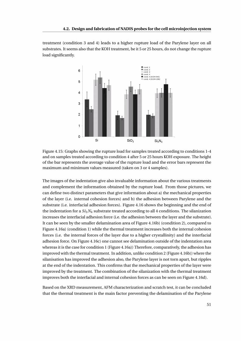
4.2. Design and fabrication of NADIS probes for the cell microinjection system
treatment (condition 3 and 4) leads to a higher rupture load of the Parylene layer on all
substrates. It seems also that the KOH treatment, be it 5 or 25 hours, do not change the rupture
load significantly.
Figure 4.15: Graphs showing the rupture load for samples treated according to conditions 1-4and on samples treated according to condition 4 after 5 or 25 hours KOH exposure. The heightof the bar represents the average value of the rupture load and the error bars represent themaximum and minimum values measured (taken on 3 or 4 samples).
The images of the indentation give also invaluable information about the various treatments
and complement the information obtained by the rupture load. From those pictures, we
can define two distinct parameters that give information about a) the mechanical properties
of the layer (i.e. internal cohesion forces) and b) the adhesion between Parylene and the
substrate (i.e. interfacial adhesion forces). Figure 4.16 shows the beginning and the end of
the indentation for a Si3N4 substrate treated according to all 4 conditions. The silanization
increases the interfacial adhesion force (i.e. the adhesion between the layer and the substrate).
It can be seen by the smaller delamination area of Figure 4.16b) (condition 2), compared to
Figure 4.16a) (condition 1) while the thermal treatment increases both the internal cohesion
forces (i.e. the internal forces of the layer due to a higher crystallinity) and the interfacial
adhesion force. On Figure 4.16c) one cannot see delamination outside of the indentation area
whereas it is the case for condition 1 (Figure 4.16a)) Therefore, comparatively, the adhesion has
improved with the thermal treatment. In addition, unlike condition 2 (Figure 4.16b)) where the
silanisation has improved the adhesion also, the Parylene layer is not torn apart, but ripples
at the end of the indentation. This confirms that the mechanical properties of the layer were
improved by the treatment. The combination of the silanization with the thermal treatment
improves both the interfacial and internal cohesion forces as can be seen on Figure 4.16d).
Based on the XRD measurement, AFM characterization and scratch test, it can be concluded
that the thermal treatment is the main factor preventing the delamination of the Parylene
51
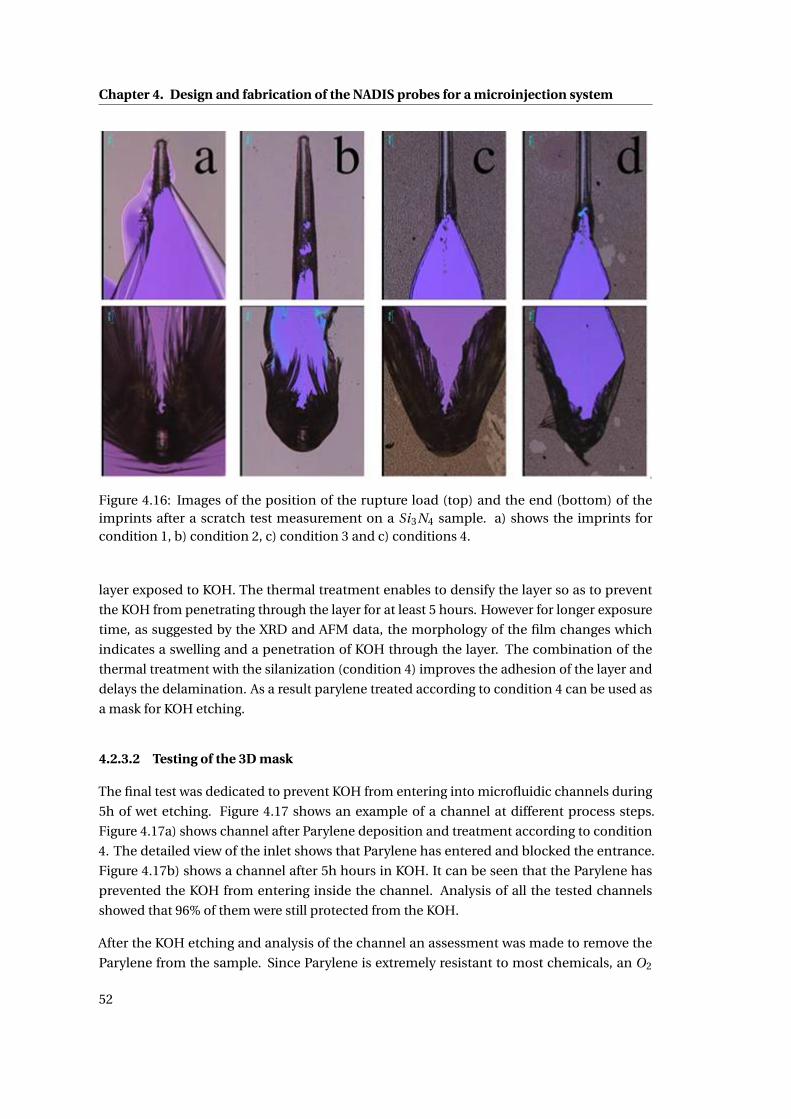
Chapter 4. Design and fabrication of the NADIS probes for a microinjection system
Figure 4.16: Images of the position of the rupture load (top) and the end (bottom) of theimprints after a scratch test measurement on a Si3N4 sample. a) shows the imprints forcondition 1, b) condition 2, c) condition 3 and c) conditions 4.
layer exposed to KOH. The thermal treatment enables to densify the layer so as to prevent
the KOH from penetrating through the layer for at least 5 hours. However for longer exposure
time, as suggested by the XRD and AFM data, the morphology of the film changes which
indicates a swelling and a penetration of KOH through the layer. The combination of the
thermal treatment with the silanization (condition 4) improves the adhesion of the layer and
delays the delamination. As a result parylene treated according to condition 4 can be used as
a mask for KOH etching.
4.2.3.2 Testing of the 3D mask
The final test was dedicated to prevent KOH from entering into microfluidic channels during
5h of wet etching. Figure 4.17 shows an example of a channel at different process steps.
Figure 4.17a) shows channel after Parylene deposition and treatment according to condition
4. The detailed view of the inlet shows that Parylene has entered and blocked the entrance.
Figure 4.17b) shows a channel after 5h hours in KOH. It can be seen that the Parylene has
prevented the KOH from entering inside the channel. Analysis of all the tested channels
showed that 96% of them were still protected from the KOH.
After the KOH etching and analysis of the channel an assessment was made to remove the
Parylene from the sample. Since Parylene is extremely resistant to most chemicals, an O2
52
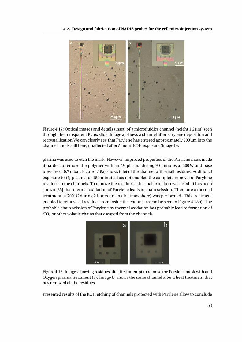
4.2. Design and fabrication of NADIS probes for the cell microinjection system
Figure 4.17: Optical images and details (inset) of a microfluidics channel (height 1.2µm) seenthrough the transparent Pyrex slide. Image a) shows a channel after Parylene deposition andrecrystallization We can clearly see that Parylene has entered approximately 200µm into thechannel and is still here, unaffected after 5 hours KOH exposure (image b).
plasma was used to etch the mask. However, improved properties of the Parylene mask made
it harder to remove the polymer with an O2 plasma during 90 minutes at 500 W and base
pressure of 0.7 mbar. Figure 4.18a) shows inlet of the channel with small residues. Additional
exposure to O2 plasma for 150 minutes has not enabled the complete removal of Parylene
residues in the channels. To remove the residues a thermal oxidation was used. It has been
shown [85] that thermal oxidation of Parylene leads to chain scission. Therefore a thermal
treatment at 700 ◦C during 2 hours (in an air atmosphere) was performed. This treatment
enabled to remove all residues from inside the channel as can be seen in Figure 4.18b). The
probable chain scission of Parylene by thermal oxidation has probably lead to formation of
CO2 or other volatile chains that escaped from the channels.
Figure 4.18: Images showing residues after first attempt to remove the Parylene mask with andOxygen plasma treatment (a). Image b) shows the same channel after a heat treatment thathas removed all the residues.
Presented results of the KOH etching of channels protected with Parylene allow to conclude
53
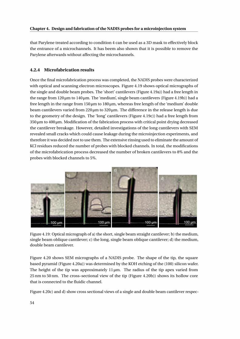
Chapter 4. Design and fabrication of the NADIS probes for a microinjection system
that Parylene treated according to condition 4 can be used as a 3D mask to effectively block
the entrance of a microchannels. It has beem also shown that it is possible to remove the
Parylene afterwards without affecting the microchannels.
4.2.4 Microfabrication results
Once the final microfabrication process was completed, the NADIS probes were characterized
with optical and scanning electron microscopes. Figure 4.19 shows optical micrographs of
the single and double beam probes. The ‘short’ cantilevers (Figure 4.19a)) had a free length in
the range from 120µm to 140µm. The ‘medium’, single beam cantilevers (Figure 4.19b)) had a
free length in the range from 150µm to 180µm, whereas free length of the ‘medium’ double
beam cantilevers varied from 220µm to 320µm. The difference in the release length is due
to the geometry of the design. The ‘long’ cantilevers (Figure 4.19c)) had a free length from
350µm to 400µm. Modification of the fabrication process with critical point drying decreased
the cantilever breakage. However, detailed investigations of the long cantilevers with SEM
revealed small cracks which could cause leakage during the microinjection experiments, and
therefore it was decided not to use them. The extensive rinsing used to eliminate the amount of
KCl residues reduced the number of probes with blocked channels. In total, the modifications
of the microfabrication process decreased the number of broken cantilevers to 8% and the
probes with blocked channels to 5%.
Figure 4.19: Optical micrograph of a) the short, single beam straight cantilever; b) the medium,single beam oblique cantilever; c) the long, single beam oblique cantilever; d) the medium,double beam cantilever.
Figure 4.20 shows SEM micrographs of a NADIS probe. The shape of the tip, the square
based pyramid (Figure 4.20a)) was determined by the KOH etching of the (100) silicon wafer.
The height of the tip was approximately 11µm. The radius of the tip apex varied from
25 nm to 50 nm. The cross–sectional view of the tip (Figure 4.20b)) shows its hollow core
that is connected to the fluidic channel.
Figure 4.20c) and d) show cross sectional views of a single and double beam cantilever respec-
54
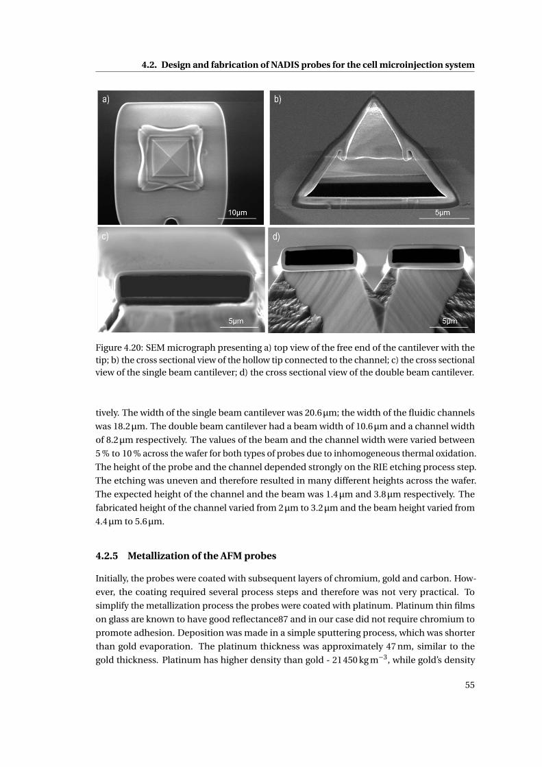
4.2. Design and fabrication of NADIS probes for the cell microinjection system
Figure 4.20: SEM micrograph presenting a) top view of the free end of the cantilever with thetip; b) the cross sectional view of the hollow tip connected to the channel; c) the cross sectionalview of the single beam cantilever; d) the cross sectional view of the double beam cantilever.
tively. The width of the single beam cantilever was 20.6µm; the width of the fluidic channels
was 18.2µm. The double beam cantilever had a beam width of 10.6µm and a channel width
of 8.2µm respectively. The values of the beam and the channel width were varied between
5 % to 10 % across the wafer for both types of probes due to inhomogeneous thermal oxidation.
The height of the probe and the channel depended strongly on the RIE etching process step.
The etching was uneven and therefore resulted in many different heights across the wafer.
The expected height of the channel and the beam was 1.4µm and 3.8µm respectively. The
fabricated height of the channel varied from 2µm to 3.2µm and the beam height varied from
4.4µm to 5.6µm.
4.2.5 Metallization of the AFM probes
Initially, the probes were coated with subsequent layers of chromium, gold and carbon. How-
ever, the coating required several process steps and therefore was not very practical. To
simplify the metallization process the probes were coated with platinum. Platinum thin films
on glass are known to have good reflectance87 and in our case did not require chromium to
promote adhesion. Deposition was made in a simple sputtering process, which was shorter
than gold evaporation. The platinum thickness was approximately 47 nm, similar to the
gold thickness. Platinum has higher density than gold - 21450 kg m−3, while gold’s density
55
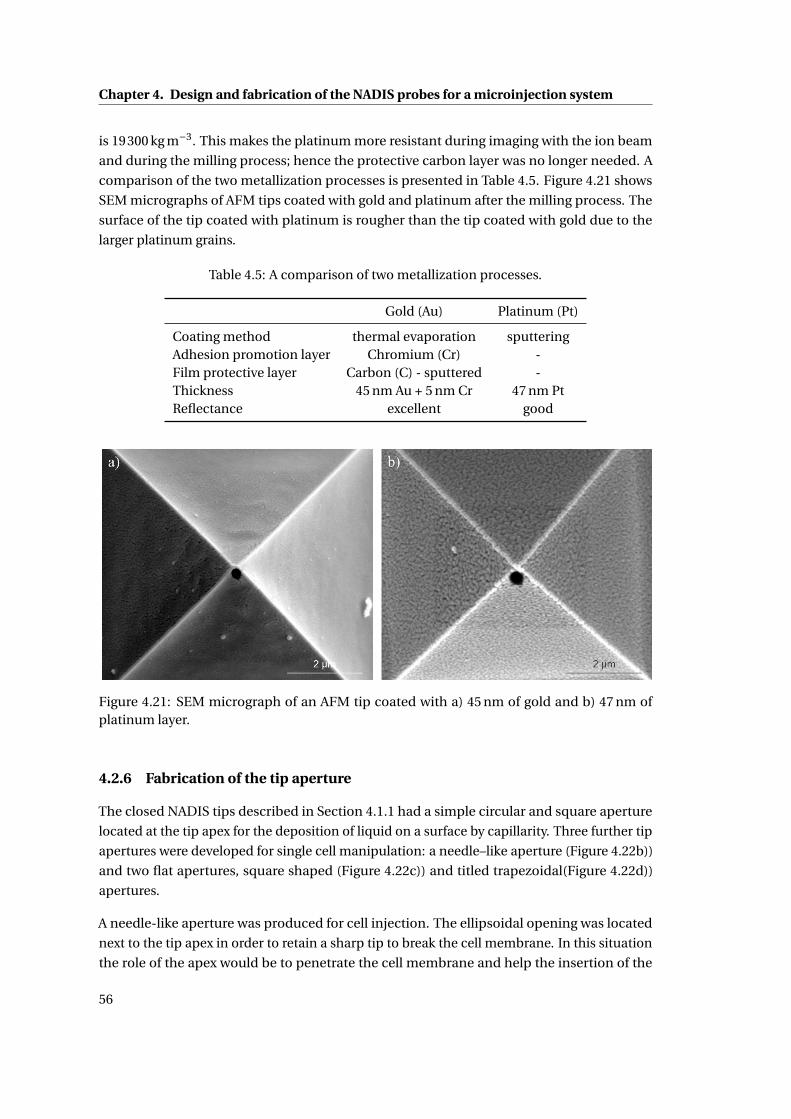
Chapter 4. Design and fabrication of the NADIS probes for a microinjection system
is 19300 kg m−3. This makes the platinum more resistant during imaging with the ion beam
and during the milling process; hence the protective carbon layer was no longer needed. A
comparison of the two metallization processes is presented in Table 4.5. Figure 4.21 shows
SEM micrographs of AFM tips coated with gold and platinum after the milling process. The
surface of the tip coated with platinum is rougher than the tip coated with gold due to the
larger platinum grains.
Table 4.5: A comparison of two metallization processes.
Gold (Au) Platinum (Pt)
Coating method thermal evaporation sputteringAdhesion promotion layer Chromium (Cr) -Film protective layer Carbon (C) - sputtered -Thickness 45 nm Au + 5 nm Cr 47 nm PtReflectance excellent good
Figure 4.21: SEM micrograph of an AFM tip coated with a) 45 nm of gold and b) 47 nm ofplatinum layer.
4.2.6 Fabrication of the tip aperture
The closed NADIS tips described in Section 4.1.1 had a simple circular and square aperture
located at the tip apex for the deposition of liquid on a surface by capillarity. Three further tip
apertures were developed for single cell manipulation: a needle–like aperture (Figure 4.22b))
and two flat apertures, square shaped (Figure 4.22c)) and titled trapezoidal(Figure 4.22d))
apertures.
A needle-like aperture was produced for cell injection. The ellipsoidal opening was located
next to the tip apex in order to retain a sharp tip to break the cell membrane. In this situation
the role of the apex would be to penetrate the cell membrane and help the insertion of the
56
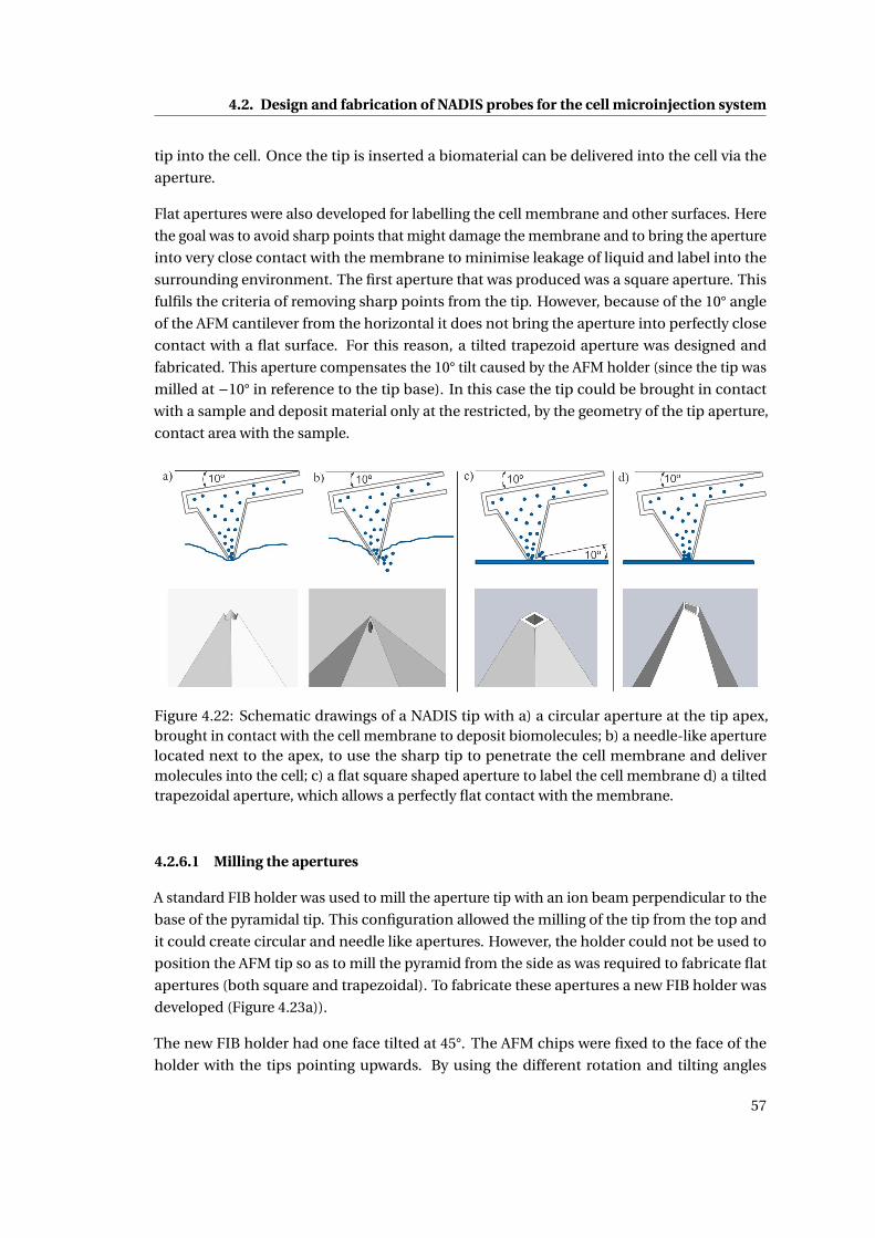
4.2. Design and fabrication of NADIS probes for the cell microinjection system
tip into the cell. Once the tip is inserted a biomaterial can be delivered into the cell via the
aperture.
Flat apertures were also developed for labelling the cell membrane and other surfaces. Here
the goal was to avoid sharp points that might damage the membrane and to bring the aperture
into very close contact with the membrane to minimise leakage of liquid and label into the
surrounding environment. The first aperture that was produced was a square aperture. This
fulfils the criteria of removing sharp points from the tip. However, because of the 10° angle
of the AFM cantilever from the horizontal it does not bring the aperture into perfectly close
contact with a flat surface. For this reason, a tilted trapezoid aperture was designed and
fabricated. This aperture compensates the 10° tilt caused by the AFM holder (since the tip was
milled at −10° in reference to the tip base). In this case the tip could be brought in contact
with a sample and deposit material only at the restricted, by the geometry of the tip aperture,
contact area with the sample.
Figure 4.22: Schematic drawings of a NADIS tip with a) a circular aperture at the tip apex,brought in contact with the cell membrane to deposit biomolecules; b) a needle-like aperturelocated next to the apex, to use the sharp tip to penetrate the cell membrane and delivermolecules into the cell; c) a flat square shaped aperture to label the cell membrane d) a tiltedtrapezoidal aperture, which allows a perfectly flat contact with the membrane.
4.2.6.1 Milling the apertures
A standard FIB holder was used to mill the aperture tip with an ion beam perpendicular to the
base of the pyramidal tip. This configuration allowed the milling of the tip from the top and
it could create circular and needle like apertures. However, the holder could not be used to
position the AFM tip so as to mill the pyramid from the side as was required to fabricate flat
apertures (both square and trapezoidal). To fabricate these apertures a new FIB holder was
developed (Figure 4.23a)).
The new FIB holder had one face tilted at 45°. The AFM chips were fixed to the face of the
holder with the tips pointing upwards. By using the different rotation and tilting angles
57
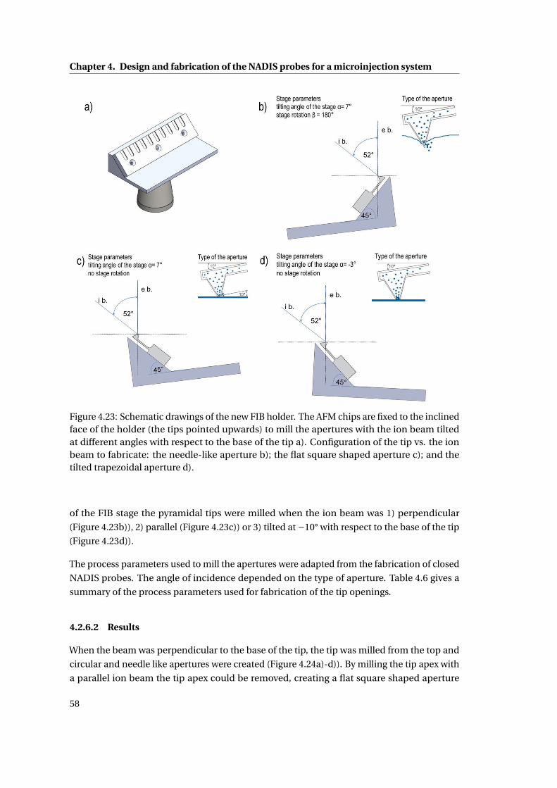
Chapter 4. Design and fabrication of the NADIS probes for a microinjection system
Figure 4.23: Schematic drawings of the new FIB holder. The AFM chips are fixed to the inclinedface of the holder (the tips pointed upwards) to mill the apertures with the ion beam tiltedat different angles with respect to the base of the tip a). Configuration of the tip vs. the ionbeam to fabricate: the needle-like aperture b); the flat square shaped aperture c); and thetilted trapezoidal aperture d).
of the FIB stage the pyramidal tips were milled when the ion beam was 1) perpendicular
(Figure 4.23b)), 2) parallel (Figure 4.23c)) or 3) tilted at −10° with respect to the base of the tip
(Figure 4.23d)).
The process parameters used to mill the apertures were adapted from the fabrication of closed
NADIS probes. The angle of incidence depended on the type of aperture. Table 4.6 gives a
summary of the process parameters used for fabrication of the tip openings.
4.2.6.2 Results
When the beam was perpendicular to the base of the tip, the tip was milled from the top and
circular and needle like apertures were created (Figure 4.24a)-d)). By milling the tip apex with
a parallel ion beam the tip apex could be removed, creating a flat square shaped aperture
58
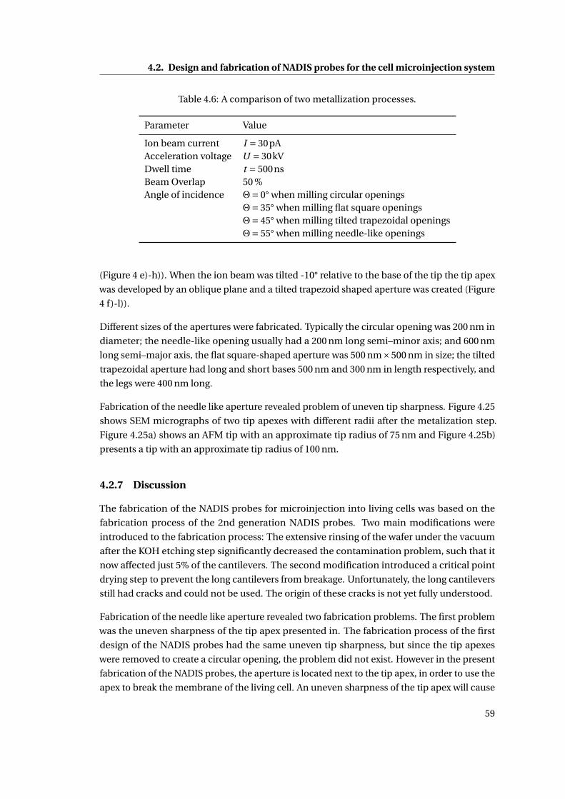
4.2. Design and fabrication of NADIS probes for the cell microinjection system
Table 4.6: A comparison of two metallization processes.
Parameter Value
Ion beam current I = 30pAAcceleration voltage U = 30kVDwell time t = 500nsBeam Overlap 50 %Angle of incidence Θ= 0° when milling circular openings
Θ= 35° when milling flat square openingsΘ= 45° when milling tilted trapezoidal openingsΘ= 55° when milling needle-like openings
(Figure 4 e)-h)). When the ion beam was tilted -10° relative to the base of the tip the tip apex
was developed by an oblique plane and a tilted trapezoid shaped aperture was created (Figure
4 f)-l)).
Different sizes of the apertures were fabricated. Typically the circular opening was 200 nm in
diameter; the needle-like opening usually had a 200 nm long semi–minor axis; and 600 nm
long semi–major axis, the flat square-shaped aperture was 500 nm×500 nm in size; the tilted
trapezoidal aperture had long and short bases 500 nm and 300 nm in length respectively, and
the legs were 400 nm long.
Fabrication of the needle like aperture revealed problem of uneven tip sharpness. Figure 4.25
shows SEM micrographs of two tip apexes with different radii after the metalization step.
Figure 4.25a) shows an AFM tip with an approximate tip radius of 75 nm and Figure 4.25b)
presents a tip with an approximate tip radius of 100 nm.
4.2.7 Discussion
The fabrication of the NADIS probes for microinjection into living cells was based on the
fabrication process of the 2nd generation NADIS probes. Two main modifications were
introduced to the fabrication process: The extensive rinsing of the wafer under the vacuum
after the KOH etching step significantly decreased the contamination problem, such that it
now affected just 5% of the cantilevers. The second modification introduced a critical point
drying step to prevent the long cantilevers from breakage. Unfortunately, the long cantilevers
still had cracks and could not be used. The origin of these cracks is not yet fully understood.
Fabrication of the needle like aperture revealed two fabrication problems. The first problem
was the uneven sharpness of the tip apex presented in. The fabrication process of the first
design of the NADIS probes had the same uneven tip sharpness, but since the tip apexes
were removed to create a circular opening, the problem did not exist. However in the present
fabrication of the NADIS probes, the aperture is located next to the tip apex, in order to use the
apex to break the membrane of the living cell. An uneven sharpness of the tip apex will cause
59
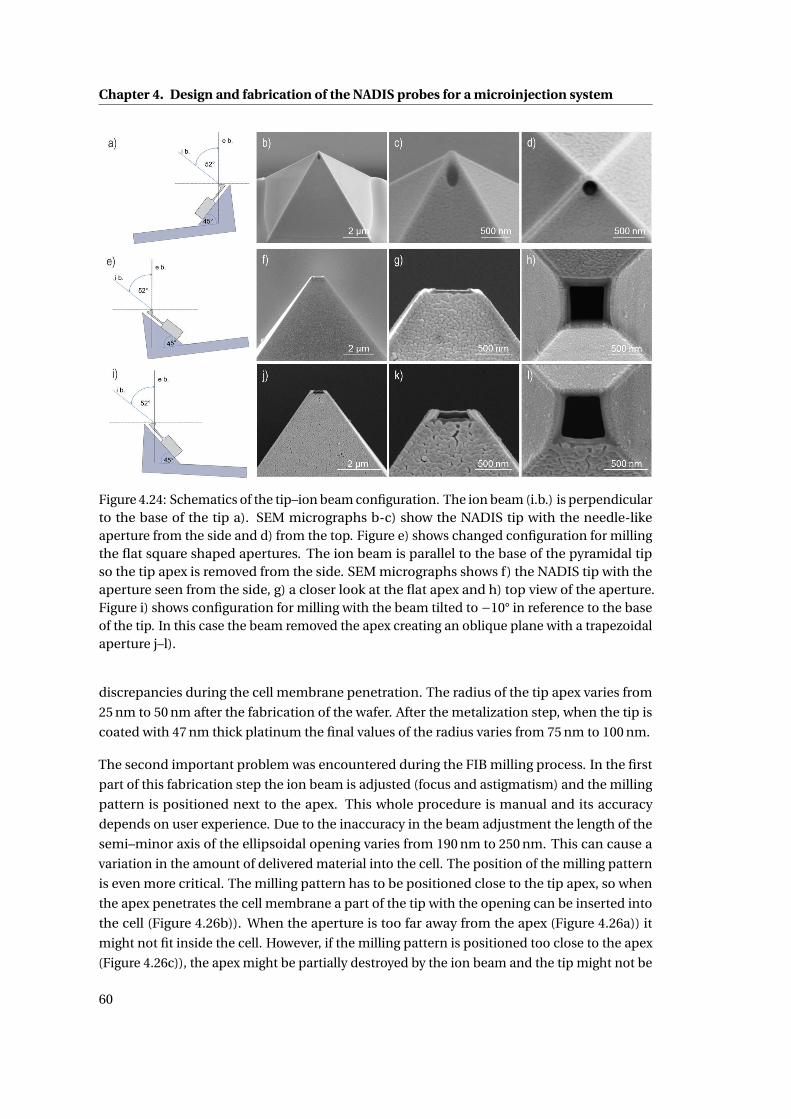
Chapter 4. Design and fabrication of the NADIS probes for a microinjection system
Figure 4.24: Schematics of the tip–ion beam configuration. The ion beam (i.b.) is perpendicularto the base of the tip a). SEM micrographs b-c) show the NADIS tip with the needle-likeaperture from the side and d) from the top. Figure e) shows changed configuration for millingthe flat square shaped apertures. The ion beam is parallel to the base of the pyramidal tipso the tip apex is removed from the side. SEM micrographs shows f) the NADIS tip with theaperture seen from the side, g) a closer look at the flat apex and h) top view of the aperture.Figure i) shows configuration for milling with the beam tilted to −10° in reference to the baseof the tip. In this case the beam removed the apex creating an oblique plane with a trapezoidalaperture j–l).
discrepancies during the cell membrane penetration. The radius of the tip apex varies from
25 nm to 50 nm after the fabrication of the wafer. After the metalization step, when the tip is
coated with 47 nm thick platinum the final values of the radius varies from 75 nm to 100 nm.
The second important problem was encountered during the FIB milling process. In the first
part of this fabrication step the ion beam is adjusted (focus and astigmatism) and the milling
pattern is positioned next to the apex. This whole procedure is manual and its accuracy
depends on user experience. Due to the inaccuracy in the beam adjustment the length of the
semi–minor axis of the ellipsoidal opening varies from 190 nm to 250 nm. This can cause a
variation in the amount of delivered material into the cell. The position of the milling pattern
is even more critical. The milling pattern has to be positioned close to the tip apex, so when
the apex penetrates the cell membrane a part of the tip with the opening can be inserted into
the cell (Figure 4.26b)). When the aperture is too far away from the apex (Figure 4.26a)) it
might not fit inside the cell. However, if the milling pattern is positioned too close to the apex
(Figure 4.26c)), the apex might be partially destroyed by the ion beam and the tip might not be
60
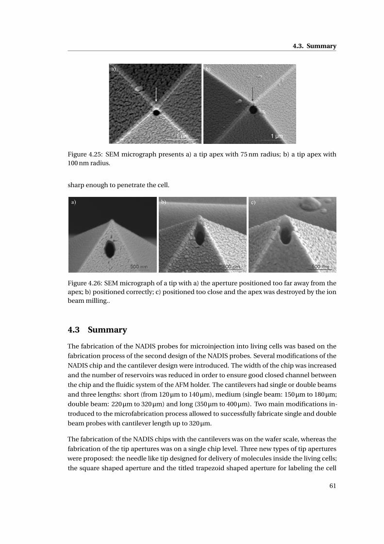
4.3. Summary
Figure 4.25: SEM micrograph presents a) a tip apex with 75 nm radius; b) a tip apex with100 nm radius.
sharp enough to penetrate the cell.
Figure 4.26: SEM micrograph of a tip with a) the aperture positioned too far away from theapex; b) positioned correctly; c) positioned too close and the apex was destroyed by the ionbeam milling..
4.3 Summary
The fabrication of the NADIS probes for microinjection into living cells was based on the
fabrication process of the second design of the NADIS probes. Several modifications of the
NADIS chip and the cantilever design were introduced. The width of the chip was increased
and the number of reservoirs was reduced in order to ensure good closed channel between
the chip and the fluidic system of the AFM holder. The cantilevers had single or double beams
and three lengths: short (from 120µm to 140µm), medium (single beam: 150µm to 180µm;
double beam: 220µm to 320µm) and long (350µm to 400µm). Two main modifications in-
troduced to the microfabrication process allowed to successfully fabricate single and double
beam probes with cantilever length up to 320µm.
The fabrication of the NADIS chips with the cantilevers was on the wafer scale, whereas the
fabrication of the tip apertures was on a single chip level. Three new types of tip apertures
were proposed: the needle like tip designed for delivery of molecules inside the living cells;
the square shaped aperture and the titled trapezoid shaped aperture for labeling the cell
61

Chapter 4. Design and fabrication of the NADIS probes for a microinjection system
membrane and other surfaces. The fabrication of the last two apertures was possible due to
the design and fabrication of a new FIB probe holder, which allows milling of the tips from
different sides.
62
5 AFM – based microinjection system:assembly and characterization
This chapter discusses the assembly of the system, the spring constant of the NADIS probes,
filling of the system with liquid, liquid expulsion and flow of fluids through the system. The
system specifications are extensively discussed. Finally, based on the specifications, injection
parameters are determined.
5.1 Assembling of the system components
The AFM–based microinjection system was built based on the NADIS probe, AFM probe holder
with fluidic channels and four commercially available components: the NanoWizard® AFM
microscope, the inverted microscope Axiovert 200, the JPK PetriDishHeater and the pressure
pulse generator – PM8000 Injector (details of these products are outlined in the Section 2.4.1).
Figure 5.1 presents the complete system. The NADIS probe is first placed on the AFM probe
holder and mounted on the AFM microscope. The microscope is then placed on the top of the
inverted phase contrast microscope such that the NADIS probe is located inside a Petri dish
held by the Petri dish heater. The Petri dish heater has an opening in the middle which is used
for optical access by the inverted microscope to visualize the cells and control the position of
the NADIS probe inside the Petri dish.
The development and fabrication of the NADIS probe was extensively described in the previous
chapter. To mount the probe on the AFM microscope and connect its fluidic channels to the
microinjector, an AFM holder with fluidic channels was developed. The geometry of the holder
is based on the geometry of a standard AFM holder used for the given AFM microscope. Since
the NADIS probe consists of single or double channels, the AFM probe holder was designed
to incorporate two fluidic channels. The outlets of the channels are on the top of the holder,
where the NADIS probe is to be placed, and the inlets are positioned at the side of holder.
Connectors were mounted to the inlets so that flexible tubes could be connected to the holder
channels (Figure 5.2).
For the NADIS probe with a single channel, only one channel of the AFM holder is used. To
63
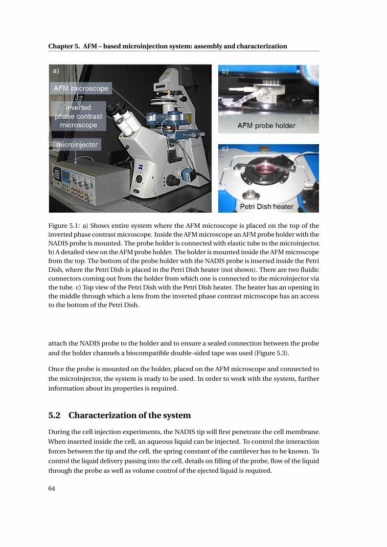
Chapter 5. AFM – based microinjection system: assembly and characterization
Figure 5.1: a) Shows entire system where the AFM microscope is placed on the top of theinverted phase contrast microscope. Inside the AFM microscope an AFM probe holder with theNADIS probe is mounted. The probe holder is connected with elastic tube to the microinjector.b) A detailed view on the AFM probe holder. The holder is mounted inside the AFM microscopefrom the top. The bottom of the probe holder with the NADIS probe is inserted inside the PetriDish, where the Petri Dish is placed in the Petri Dish heater (not shown). There are two fluidicconnectors coming out from the holder from which one is connected to the microinjector viathe tube. c) Top view of the Petri Dish with the Petri Dish heater. The heater has an opening inthe middle through which a lens from the inverted phase contrast microscope has an accessto the bottom of the Petri Dish.
attach the NADIS probe to the holder and to ensure a sealed connection between the probe
and the holder channels a biocompatible double-sided tape was used (Figure 5.3).
Once the probe is mounted on the holder, placed on the AFM microscope and connected to
the microinjector, the system is ready to be used. In order to work with the system, further
information about its properties is required.
5.2 Characterization of the system
During the cell injection experiments, the NADIS tip will first penetrate the cell membrane.
When inserted inside the cell, an aqueous liquid can be injected. To control the interaction
forces between the tip and the cell, the spring constant of the cantilever has to be known. To
control the liquid delivery passing into the cell, details on filling of the probe, flow of the liquid
through the probe as well as volume control of the ejected liquid is required.
64
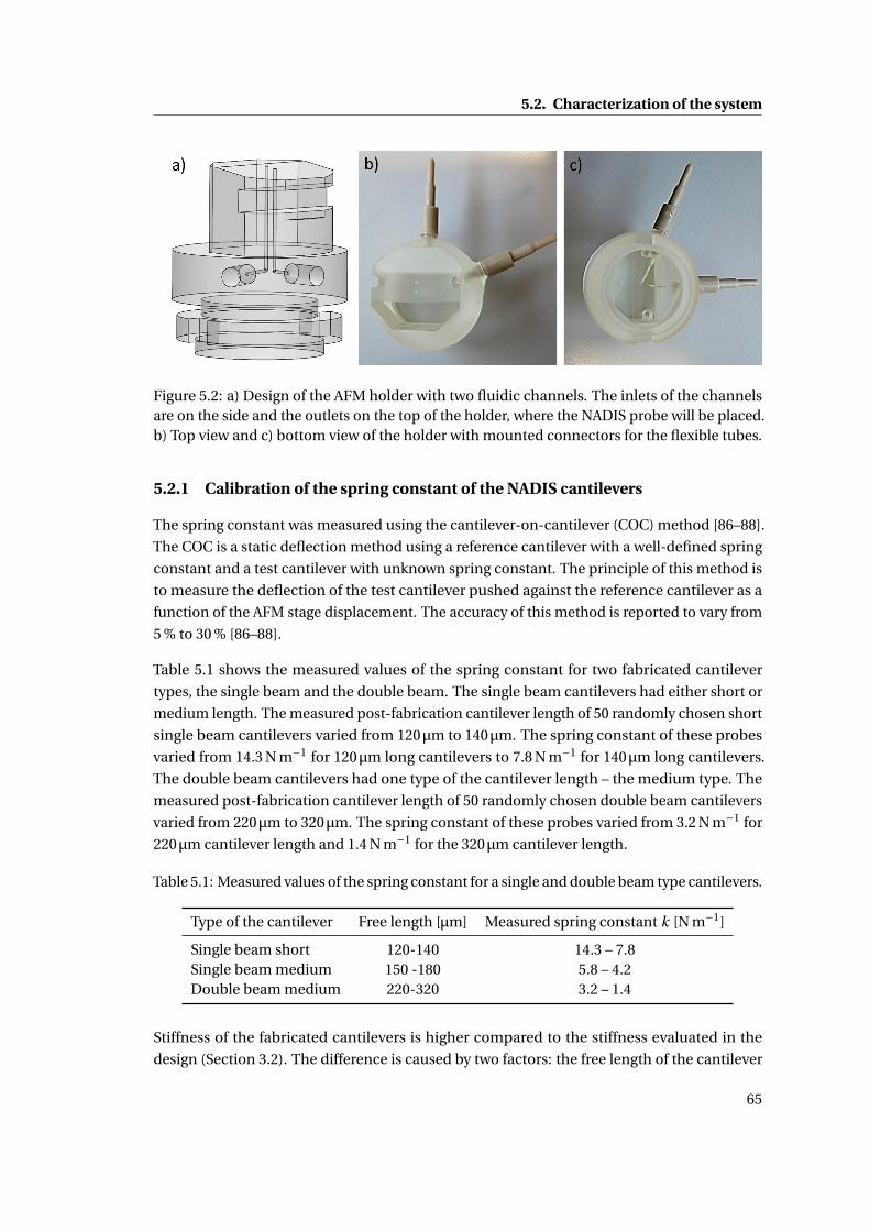
5.2. Characterization of the system
Figure 5.2: a) Design of the AFM holder with two fluidic channels. The inlets of the channelsare on the side and the outlets on the top of the holder, where the NADIS probe will be placed.b) Top view and c) bottom view of the holder with mounted connectors for the flexible tubes.
5.2.1 Calibration of the spring constant of the NADIS cantilevers
The spring constant was measured using the cantilever-on-cantilever (COC) method [86–88].
The COC is a static deflection method using a reference cantilever with a well-defined spring
constant and a test cantilever with unknown spring constant. The principle of this method is
to measure the deflection of the test cantilever pushed against the reference cantilever as a
function of the AFM stage displacement. The accuracy of this method is reported to vary from
5 % to 30 % [86–88].
Table 5.1 shows the measured values of the spring constant for two fabricated cantilever
types, the single beam and the double beam. The single beam cantilevers had either short or
medium length. The measured post-fabrication cantilever length of 50 randomly chosen short
single beam cantilevers varied from 120µm to 140µm. The spring constant of these probes
varied from 14.3 N m−1 for 120µm long cantilevers to 7.8 N m−1 for 140µm long cantilevers.
The double beam cantilevers had one type of the cantilever length – the medium type. The
measured post-fabrication cantilever length of 50 randomly chosen double beam cantilevers
varied from 220µm to 320µm. The spring constant of these probes varied from 3.2 N m−1 for
220µm cantilever length and 1.4 N m−1 for the 320µm cantilever length.
Table 5.1: Measured values of the spring constant for a single and double beam type cantilevers.
Type of the cantilever Free length [µm] Measured spring constant k [N m−1]
Single beam short 120-140 14.3 – 7.8Single beam medium 150 -180 5.8 – 4.2Double beam medium 220-320 3.2 – 1.4
Stiffness of the fabricated cantilevers is higher compared to the stiffness evaluated in the
design (Section 3.2). The difference is caused by two factors: the free length of the cantilever
65
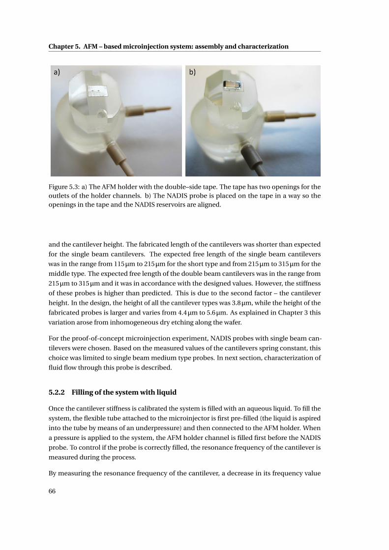
Chapter 5. AFM – based microinjection system: assembly and characterization
Figure 5.3: a) The AFM holder with the double–side tape. The tape has two openings for theoutlets of the holder channels. b) The NADIS probe is placed on the tape in a way so theopenings in the tape and the NADIS reservoirs are aligned.
and the cantilever height. The fabricated length of the cantilevers was shorter than expected
for the single beam cantilevers. The expected free length of the single beam cantilevers
was in the range from 115µm to 215µm for the short type and from 215µm to 315µm for the
middle type. The expected free length of the double beam cantilevers was in the range from
215µm to 315µm and it was in accordance with the designed values. However, the stiffness
of these probes is higher than predicted. This is due to the second factor – the cantilever
height. In the design, the height of all the cantilever types was 3.8µm, while the height of the
fabricated probes is larger and varies from 4.4µm to 5.6µm. As explained in Chapter 3 this
variation arose from inhomogeneous dry etching along the wafer.
For the proof-of-concept microinjection experiment, NADIS probes with single beam can-
tilevers were chosen. Based on the measured values of the cantilevers spring constant, this
choice was limited to single beam medium type probes. In next section, characterization of
fluid flow through this probe is described.
5.2.2 Filling of the system with liquid
Once the cantilever stiffness is calibrated the system is filled with an aqueous liquid. To fill the
system, the flexible tube attached to the microinjector is first pre-filled (the liquid is aspired
into the tube by means of an underpressure) and then connected to the AFM holder. When
a pressure is applied to the system, the AFM holder channel is filled first before the NADIS
probe. To control if the probe is correctly filled, the resonance frequency of the cantilever is
measured during the process.
By measuring the resonance frequency of the cantilever, a decrease in its frequency value
66
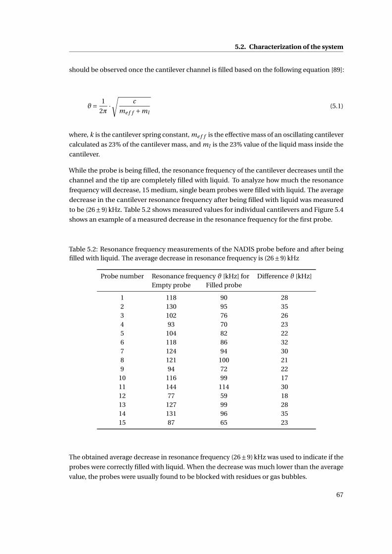
5.2. Characterization of the system
should be observed once the cantilever channel is filled based on the following equation [89]:
ϑ= 1
2π·√
c
me f f +ml(5.1)
where, k is the cantilever spring constant, me f f is the effective mass of an oscillating cantilever
calculated as 23% of the cantilever mass, and ml is the 23% value of the liquid mass inside the
cantilever.
While the probe is being filled, the resonance frequency of the cantilever decreases until the
channel and the tip are completely filled with liquid. To analyze how much the resonance
frequency will decrease, 15 medium, single beam probes were filled with liquid. The average
decrease in the cantilever resonance frequency after being filled with liquid was measured
to be (26±9) kHz. Table 5.2 shows measured values for individual cantilevers and Figure 5.4
shows an example of a measured decrease in the resonance frequency for the first probe.
Table 5.2: Resonance frequency measurements of the NADIS probe before and after beingfilled with liquid. The average decrease in resonance frequency is (26±9) kHz
Probe number Resonance frequency ϑ [kHz] for Difference ϑ [kHz]Empty probe Filled probe
1 118 90 282 130 95 353 102 76 264 93 70 235 104 82 226 118 86 327 124 94 308 121 100 219 94 72 22
10 116 99 1711 144 114 3012 77 59 1813 127 99 2814 131 96 3515 87 65 23
The obtained average decrease in resonance frequency (26±9) kHz was used to indicate if the
probes were correctly filled with liquid. When the decrease was much lower than the average
value, the probes were usually found to be blocked with residues or gas bubbles.
67
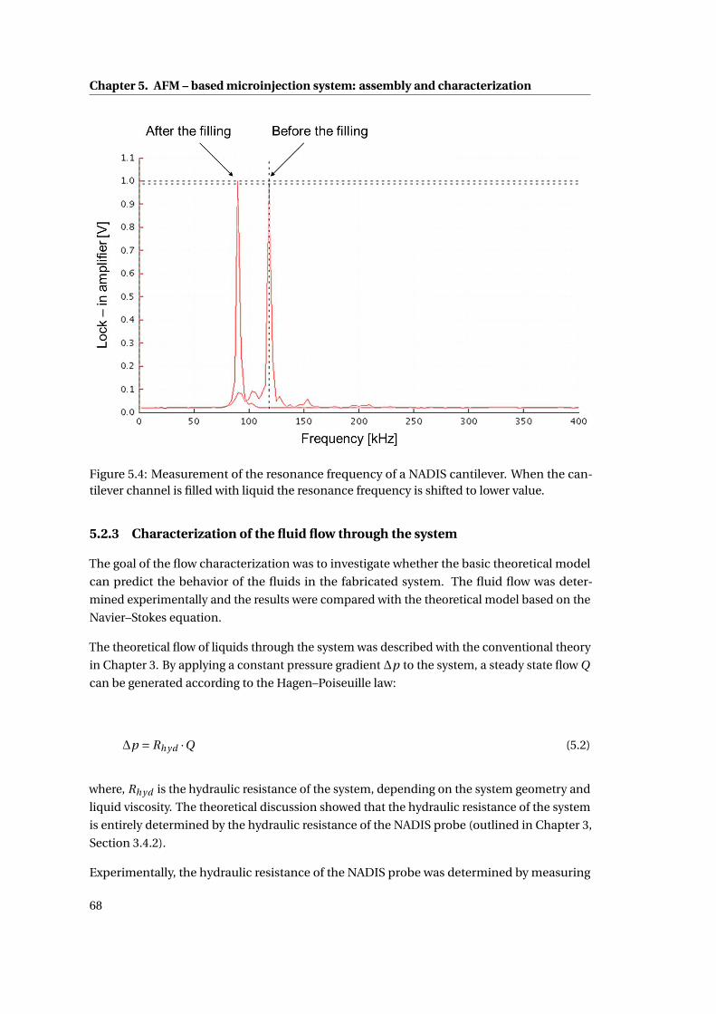
Chapter 5. AFM – based microinjection system: assembly and characterization
Figure 5.4: Measurement of the resonance frequency of a NADIS cantilever. When the can-tilever channel is filled with liquid the resonance frequency is shifted to lower value.
5.2.3 Characterization of the fluid flow through the system
The goal of the flow characterization was to investigate whether the basic theoretical model
can predict the behavior of the fluids in the fabricated system. The fluid flow was deter-
mined experimentally and the results were compared with the theoretical model based on the
Navier–Stokes equation.
The theoretical flow of liquids through the system was described with the conventional theory
in Chapter 3. By applying a constant pressure gradient ∆p to the system, a steady state flow Q
can be generated according to the Hagen–Poiseuille law:
∆p = Rhyd ·Q (5.2)
where, Rhyd is the hydraulic resistance of the system, depending on the system geometry and
liquid viscosity. The theoretical discussion showed that the hydraulic resistance of the system
is entirely determined by the hydraulic resistance of the NADIS probe (outlined in Chapter 3,
Section 3.4.2).
Experimentally, the hydraulic resistance of the NADIS probe was determined by measuring
68
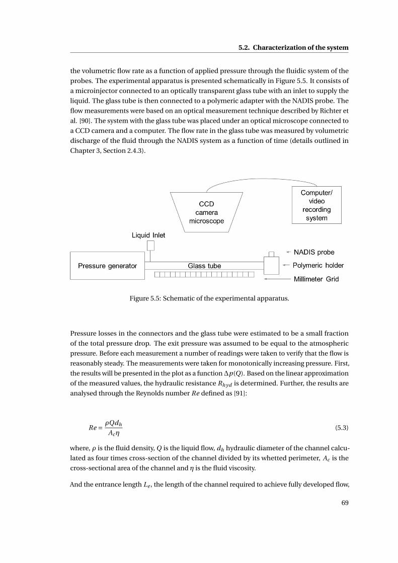
5.2. Characterization of the system
the volumetric flow rate as a function of applied pressure through the fluidic system of the
probes. The experimental apparatus is presented schematically in Figure 5.5. It consists of
a microinjector connected to an optically transparent glass tube with an inlet to supply the
liquid. The glass tube is then connected to a polymeric adapter with the NADIS probe. The
flow measurements were based on an optical measurement technique described by Richter et
al. [90]. The system with the glass tube was placed under an optical microscope connected to
a CCD camera and a computer. The flow rate in the glass tube was measured by volumetric
discharge of the fluid through the NADIS system as a function of time (details outlined in
Chapter 3, Section 2.4.3).
Figure 5.5: Schematic of the experimental apparatus.
Pressure losses in the connectors and the glass tube were estimated to be a small fraction
of the total pressure drop. The exit pressure was assumed to be equal to the atmospheric
pressure. Before each measurement a number of readings were taken to verify that the flow is
reasonably steady. The measurements were taken for monotonically increasing pressure. First,
the results will be presented in the plot as a function∆p(Q). Based on the linear approximation
of the measured values, the hydraulic resistance Rhyd is determined. Further, the results are
analysed through the Reynolds number Re defined as [91]:
Re = ρQdh
Acη(5.3)
where, ρ is the fluid density, Q is the liquid flow, dh hydraulic diameter of the channel calcu-
lated as four times cross-section of the channel divided by its whetted perimeter, Ac is the
cross-sectional area of the channel and η is the fluid viscosity.
And the entrance length Le , the length of the channel required to achieve fully developed flow,
69
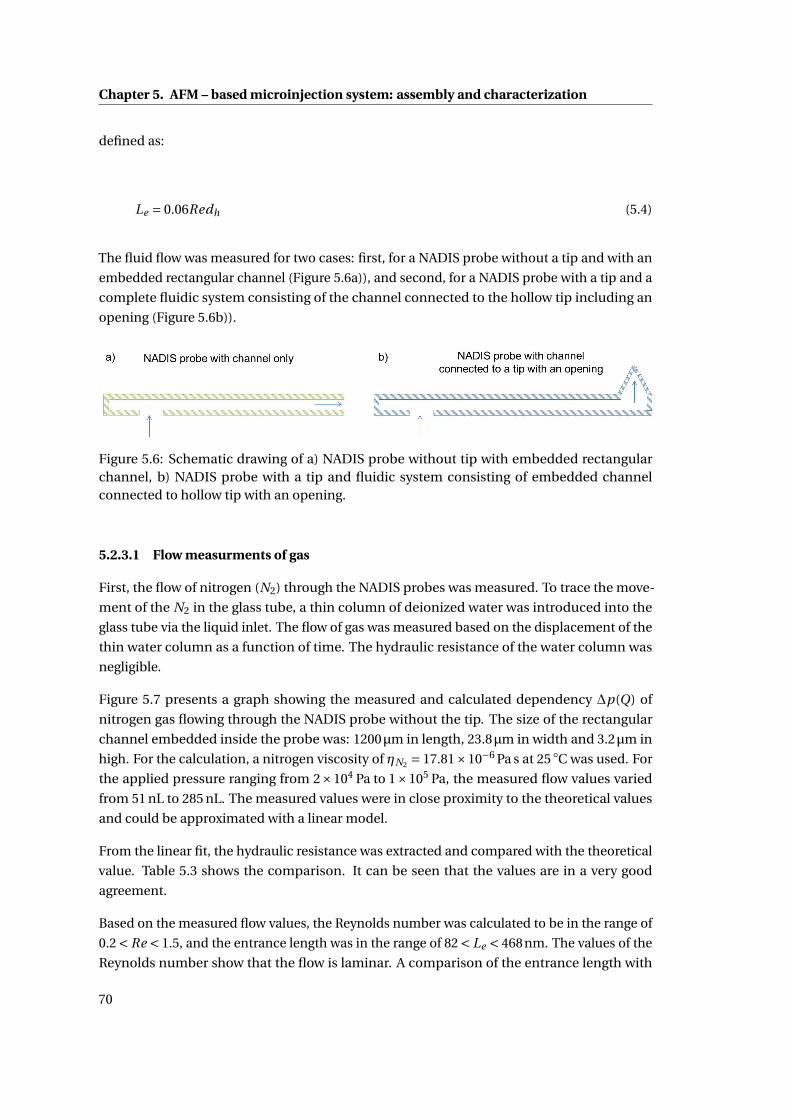
Chapter 5. AFM – based microinjection system: assembly and characterization
defined as:
Le = 0.06Redh (5.4)
The fluid flow was measured for two cases: first, for a NADIS probe without a tip and with an
embedded rectangular channel (Figure 5.6a)), and second, for a NADIS probe with a tip and a
complete fluidic system consisting of the channel connected to the hollow tip including an
opening (Figure 5.6b)).
Figure 5.6: Schematic drawing of a) NADIS probe without tip with embedded rectangularchannel, b) NADIS probe with a tip and fluidic system consisting of embedded channelconnected to hollow tip with an opening.
5.2.3.1 Flow measurments of gas
First, the flow of nitrogen (N2) through the NADIS probes was measured. To trace the move-
ment of the N2 in the glass tube, a thin column of deionized water was introduced into the
glass tube via the liquid inlet. The flow of gas was measured based on the displacement of the
thin water column as a function of time. The hydraulic resistance of the water column was
negligible.
Figure 5.7 presents a graph showing the measured and calculated dependency ∆p(Q) of
nitrogen gas flowing through the NADIS probe without the tip. The size of the rectangular
channel embedded inside the probe was: 1200µm in length, 23.8µm in width and 3.2µm in
high. For the calculation, a nitrogen viscosity of ηN2 = 17.81×10⁻⁶ Pa s at 25 ◦C was used. For
the applied pressure ranging from 2×10⁴ Pa to 1×10⁵ Pa, the measured flow values varied
from 51 nL to 285 nL. The measured values were in close proximity to the theoretical values
and could be approximated with a linear model.
From the linear fit, the hydraulic resistance was extracted and compared with the theoretical
value. Table 5.3 shows the comparison. It can be seen that the values are in a very good
agreement.
Based on the measured flow values, the Reynolds number was calculated to be in the range of
0.2 < Re < 1.5, and the entrance length was in the range of 82 < Le < 468nm. The values of the
Reynolds number show that the flow is laminar. A comparison of the entrance length with
70
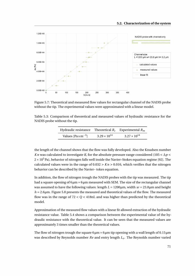
5.2. Characterization of the system
Figure 5.7: Theoretical and measured flow values for rectangular channel of the NADIS probewithout the tip. The experimental values were approximated with a linear model.
Table 5.3: Comparison of theoretical and measured values of hydraulic resistance for theNADIS probe without the tip.
Hydraulic resistance Theoretical Rc Experimental Rm
Values [Pa s m−3] 3.29×10¹⁴ 3.27×10¹⁴
the length of the channel shows that the flow was fully developed. Also the Knudsen number
K n was calculated to investigate if, for the absolute pressure range considered (105 <∆p <2×10⁵ Pa), behavior of nitrogen falls well inside the Navier–Stokes equation regime [92]. The
calculated values were in the range of 0.032 > K n > 0.016, which verifies that the nitrogen
behavior can be described by the Navier– tokes equation.
In addition, the flow of nitrogen trough the NADIS probes with the tip was measured. The tip
had a square opening of 6µm×6µm measured with SEM. The size of the rectangular channel
was assumed to have the following values: length L = 1200µm, width w = 23.8µm and height
h = 2.6µm. Figure 5.8 presents the measured and theoretical values of the flow. The measured
flow was in the range of 72 < Q < 418nL and was higher than predicted by the theoretical
model.
Approximation of the measured flow values with a linear fit allowed extraction of the hydraulic
resistance value. Table 5.4 shows a comparison between the experimental value of the hy-
draulic resistance with the theoretical value. It can be seen that the measured values are
approximately 3 times smaller than the theoretical values.
The flow of nitrogen trough the square 6µm×6µm tip opening with a wall length of 0.15µm
was described by Reynolds number Re and entry length Le . The Reynolds number varied
71
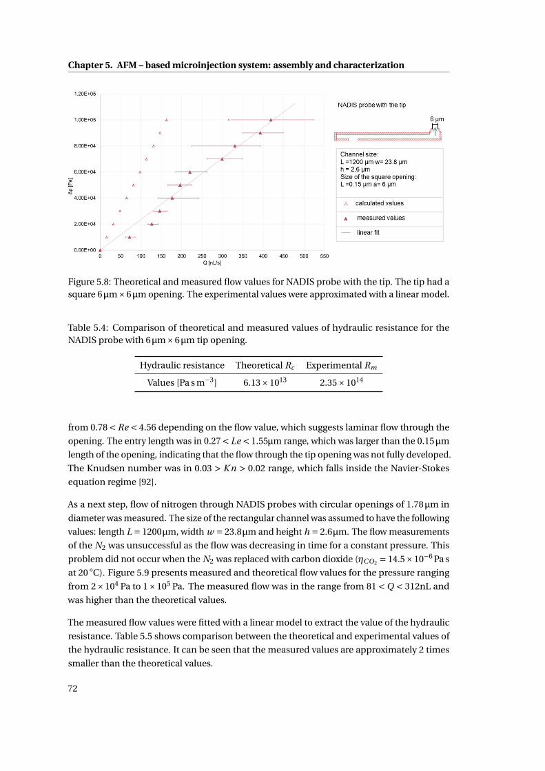
Chapter 5. AFM – based microinjection system: assembly and characterization
Figure 5.8: Theoretical and measured flow values for NADIS probe with the tip. The tip had asquare 6µm×6µm opening. The experimental values were approximated with a linear model.
Table 5.4: Comparison of theoretical and measured values of hydraulic resistance for theNADIS probe with 6µm×6µm tip opening.
Hydraulic resistance Theoretical Rc Experimental Rm
Values [Pa s m−3] 6.13×10¹³ 2.35×10¹⁴
from 0.78 < Re < 4.56 depending on the flow value, which suggests laminar flow through the
opening. The entry length was in 0.27 < Le < 1.55µm range, which was larger than the 0.15µm
length of the opening, indicating that the flow through the tip opening was not fully developed.
The Knudsen number was in 0.03 > K n > 0.02 range, which falls inside the Navier-Stokes
equation regime [92].
As a next step, flow of nitrogen through NADIS probes with circular openings of 1.78µm in
diameter was measured. The size of the rectangular channel was assumed to have the following
values: length L = 1200µm, width w = 23.8µm and height h = 2.6µm. The flow measurements
of the N2 was unsuccessful as the flow was decreasing in time for a constant pressure. This
problem did not occur when the N2 was replaced with carbon dioxide (ηCO2 = 14.5×10⁻⁶ Pa s
at 20 ◦C). Figure 5.9 presents measured and theoretical flow values for the pressure ranging
from 2×10⁴ Pa to 1×10⁵ Pa. The measured flow was in the range from 81 < Q < 312nL and
was higher than the theoretical values.
The measured flow values were fitted with a linear model to extract the value of the hydraulic
resistance. Table 5.5 shows comparison between the theoretical and experimental values of
the hydraulic resistance. It can be seen that the measured values are approximately 2 times
smaller than the theoretical values.
72
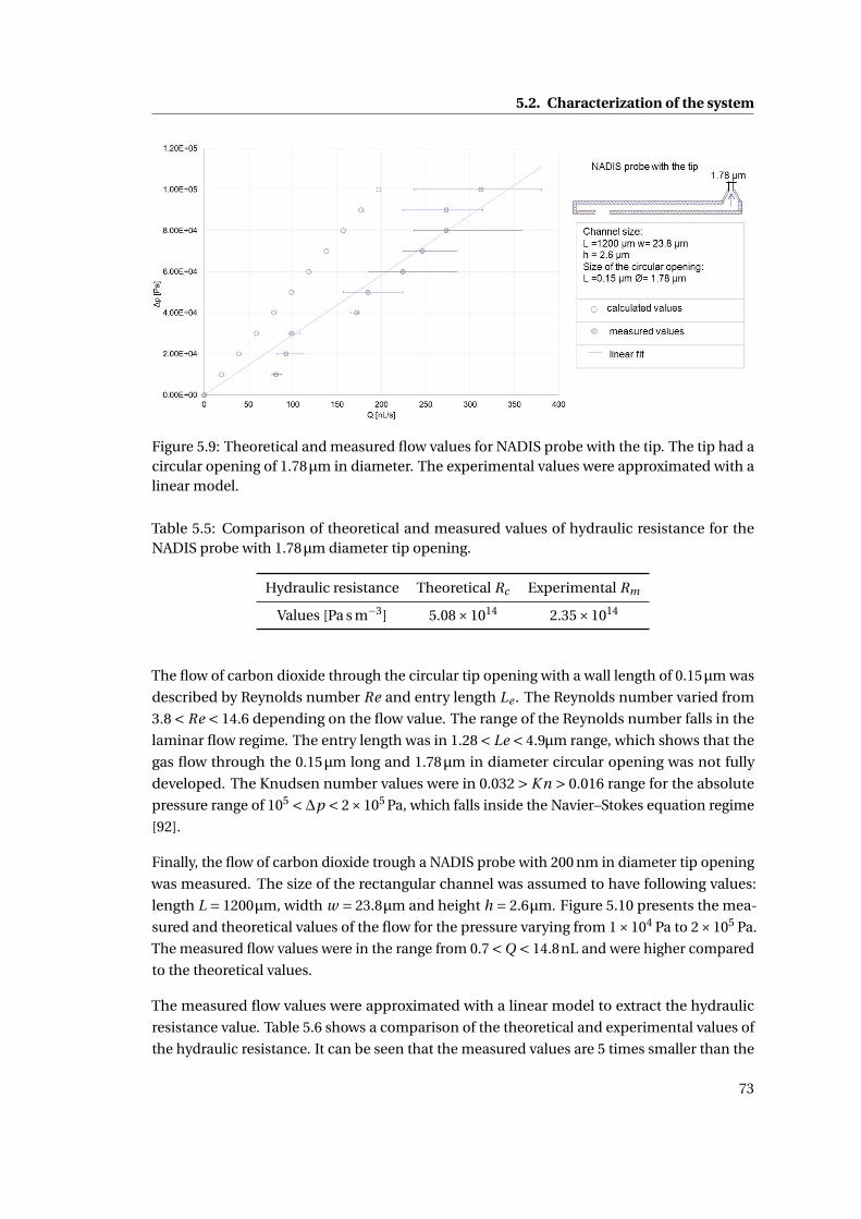
5.2. Characterization of the system
Figure 5.9: Theoretical and measured flow values for NADIS probe with the tip. The tip had acircular opening of 1.78µm in diameter. The experimental values were approximated with alinear model.
Table 5.5: Comparison of theoretical and measured values of hydraulic resistance for theNADIS probe with 1.78µm diameter tip opening.
Hydraulic resistance Theoretical Rc Experimental Rm
Values [Pa s m−3] 5.08×10¹⁴ 2.35×10¹⁴
The flow of carbon dioxide through the circular tip opening with a wall length of 0.15µm was
described by Reynolds number Re and entry length Le . The Reynolds number varied from
3.8 < Re < 14.6 depending on the flow value. The range of the Reynolds number falls in the
laminar flow regime. The entry length was in 1.28 < Le < 4.9µm range, which shows that the
gas flow through the 0.15µm long and 1.78µm in diameter circular opening was not fully
developed. The Knudsen number values were in 0.032 > K n > 0.016 range for the absolute
pressure range of 105 <∆p < 2×10⁵ Pa, which falls inside the Navier–Stokes equation regime
[92].
Finally, the flow of carbon dioxide trough a NADIS probe with 200 nm in diameter tip opening
was measured. The size of the rectangular channel was assumed to have following values:
length L = 1200µm, width w = 23.8µm and height h = 2.6µm. Figure 5.10 presents the mea-
sured and theoretical values of the flow for the pressure varying from 1×10⁴ Pa to 2×10⁵ Pa.
The measured flow values were in the range from 0.7 <Q < 14.8nL and were higher compared
to the theoretical values.
The measured flow values were approximated with a linear model to extract the hydraulic
resistance value. Table 5.6 shows a comparison of the theoretical and experimental values of
the hydraulic resistance. It can be seen that the measured values are 5 times smaller than the
73
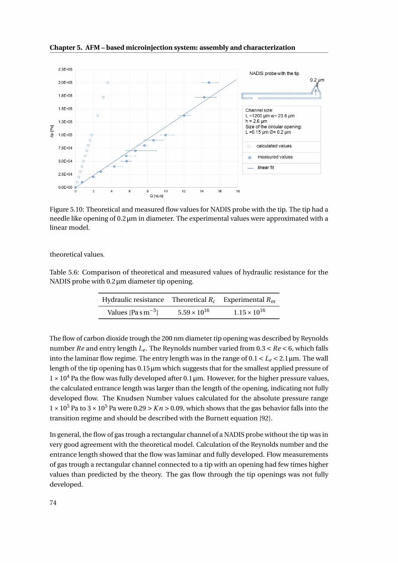
Chapter 5. AFM – based microinjection system: assembly and characterization
Figure 5.10: Theoretical and measured flow values for NADIS probe with the tip. The tip had aneedle like opening of 0.2µm in diameter. The experimental values were approximated with alinear model.
theoretical values.
Table 5.6: Comparison of theoretical and measured values of hydraulic resistance for theNADIS probe with 0.2µm diameter tip opening.
Hydraulic resistance Theoretical Rc Experimental Rm
Values [Pa s m−3] 5.59×10¹⁶ 1.15×10¹⁶
The flow of carbon dioxide trough the 200 nm diameter tip opening was described by Reynolds
number Re and entry length Le . The Reynolds number varied from 0.3 < Re < 6, which falls
into the laminar flow regime. The entry length was in the range of 0.1 < Le < 2.1µm. The wall
length of the tip opening has 0.15µm which suggests that for the smallest applied pressure of
1×10⁴ Pa the flow was fully developed after 0.1µm. However, for the higher pressure values,
the calculated entrance length was larger than the length of the opening, indicating not fully
developed flow. The Knudsen Number values calculated for the absolute pressure range
1×10⁵ Pa to 3×10⁵ Pa were 0.29 > K n > 0.09, which shows that the gas behavior falls into the
transition regime and should be described with the Burnett equation [92].
In general, the flow of gas trough a rectangular channel of a NADIS probe without the tip was in
very good agreement with the theoretical model. Calculation of the Reynolds number and the
entrance length showed that the flow was laminar and fully developed. Flow measurements
of gas trough a rectangular channel connected to a tip with an opening had few times higher
values than predicted by the theory. The gas flow through the tip openings was not fully
developed.
74
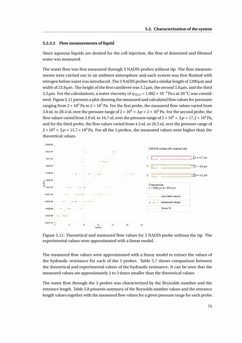
5.2. Characterization of the system
5.2.3.2 Flow measurements of liquid
Since aqueous liquids are desired for the cell injection, the flow of deionized and filtrated
water was measured.
The water flow was first measured through 3 NADIS probes without tip. The flow measure-
ments were carried out in an ambient atmosphere and each system was first flushed with
nitrogen before water was introduced. The 3 NADIS probes had a similar length of 1200µm and
width of 23.8µm. The height of the first cantilever was 3.2µm, the second 3.0µm, and the third
3.2µm. For the calculations, a water viscosity of ηH2O = 1.002×10⁻³ Pa s at 20 ◦C was consid-
ered. Figure 5.11 presents a plot showing the measured and calculated flow values for pressures
ranging from 2×10⁴ Pa to 2×10⁵ Pa. For the first probe, the measured flow values varied from
3.6 nL to 20.4 nL over the pressure range of 2×10⁴ <∆p < 2×10⁵ Pa. For the second probe, the
flow values varied from 3.0 nL to 16.7 nL over the pressure range of 2×10⁴ <∆p < 17.2×10⁴ Pa,
and for the third probe, the flow values varied from 4.5 nL to 26.5 nL over the pressure range of
2×10⁴ <∆p < 13.7×10⁴ Pa. For all the 3 probes, the measured values were higher than the
theoretical values.
Figure 5.11: Theoretical and measured flow values for 3 NADIS probe without the tip. Theexperimental values were approximated with a linear model.
The measured flow values were approximated with a linear model to extract the values of
the hydraulic resistance for each of the 3 probes. Table 5.7 shows comparison between
the theoretical and experimental values of the hydraulic resistance. It can be seen that the
measured values are approximately 2 to 3 times smaller than the theoretical values.
The water flow through the 3 probes was characterized by the Reynolds number and the
entrance length. Table 5.8 presents summary of the Reynolds number values and the entrance
length values together with the measured flow values for a given pressure range for each probe.
75
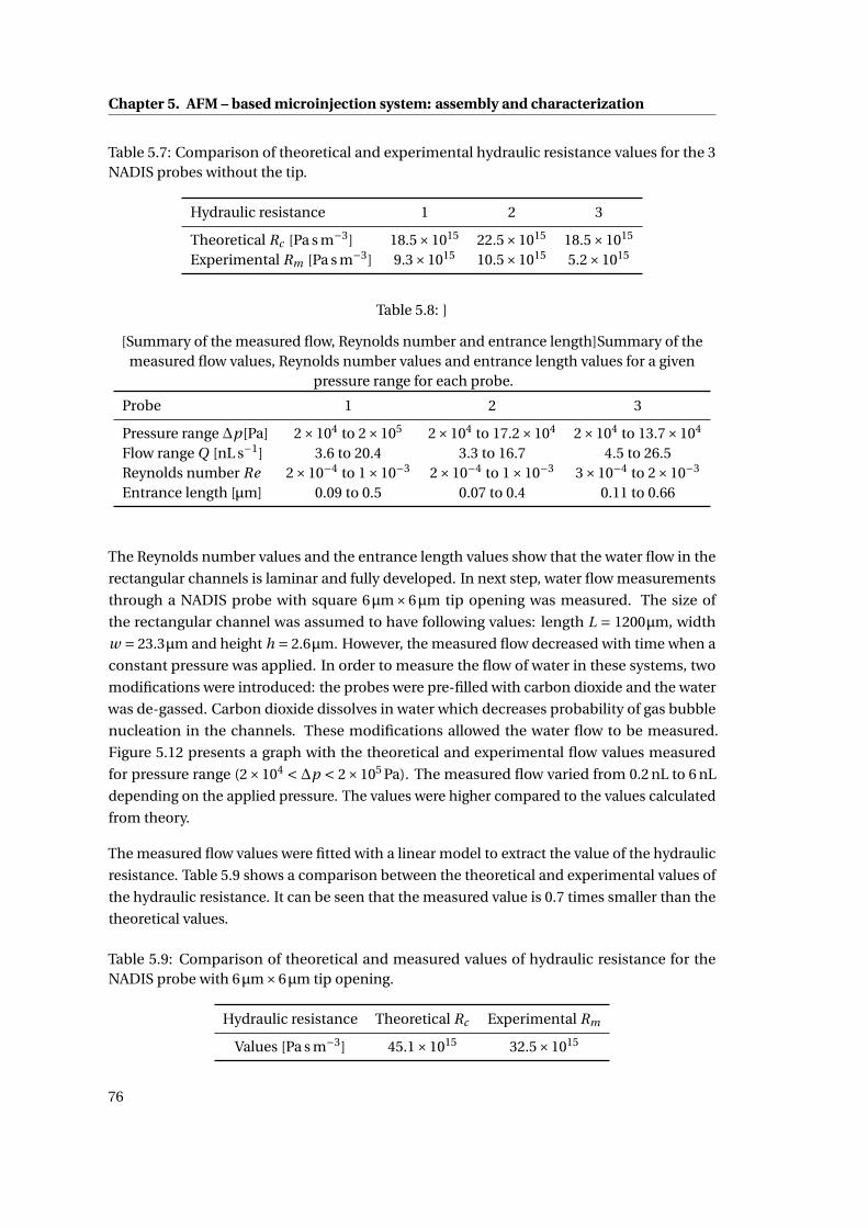
Chapter 5. AFM – based microinjection system: assembly and characterization
Table 5.7: Comparison of theoretical and experimental hydraulic resistance values for the 3NADIS probes without the tip.
Hydraulic resistance 1 2 3
Theoretical Rc [Pa s m−3] 18.5×10¹⁵ 22.5×10¹⁵ 18.5×10¹⁵
Experimental Rm [Pa s m−3] 9.3×10¹⁵ 10.5×10¹⁵ 5.2×10¹⁵
Table 5.8: ]
[Summary of the measured flow, Reynolds number and entrance length]Summary of themeasured flow values, Reynolds number values and entrance length values for a given
pressure range for each probe.
Probe 1 2 3
Pressure range ∆p[Pa] 2×10⁴ to 2×10⁵ 2×10⁴ to 17.2×10⁴ 2×10⁴ to 13.7×10⁴
Flow range Q [nL s−1] 3.6 to 20.4 3.3 to 16.7 4.5 to 26.5Reynolds number Re 2×10⁻⁴ to 1×10⁻³ 2×10⁻⁴ to 1×10⁻³ 3×10⁻⁴ to 2×10⁻³
Entrance length [µm] 0.09 to 0.5 0.07 to 0.4 0.11 to 0.66
The Reynolds number values and the entrance length values show that the water flow in the
rectangular channels is laminar and fully developed. In next step, water flow measurements
through a NADIS probe with square 6µm×6µm tip opening was measured. The size of
the rectangular channel was assumed to have following values: length L = 1200µm, width
w = 23.3µm and height h = 2.6µm. However, the measured flow decreased with time when a
constant pressure was applied. In order to measure the flow of water in these systems, two
modifications were introduced: the probes were pre-filled with carbon dioxide and the water
was de-gassed. Carbon dioxide dissolves in water which decreases probability of gas bubble
nucleation in the channels. These modifications allowed the water flow to be measured.
Figure 5.12 presents a graph with the theoretical and experimental flow values measured
for pressure range (2×10⁴ <∆p < 2×10⁵ Pa). The measured flow varied from 0.2 nL to 6 nL
depending on the applied pressure. The values were higher compared to the values calculated
from theory.
The measured flow values were fitted with a linear model to extract the value of the hydraulic
resistance. Table 5.9 shows a comparison between the theoretical and experimental values of
the hydraulic resistance. It can be seen that the measured value is 0.7 times smaller than the
theoretical values.
Table 5.9: Comparison of theoretical and measured values of hydraulic resistance for theNADIS probe with 6µm×6µm tip opening.
Hydraulic resistance Theoretical Rc Experimental Rm
Values [Pa s m−3] 45.1×10¹⁵ 32.5×10¹⁵
76
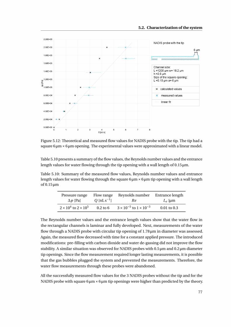
5.2. Characterization of the system
Figure 5.12: Theoretical and measured flow values for NADIS probe with the tip. The tip had asquare 6µm×6µm opening. The experimental values were approximated with a linear model.
Table 5.10 presents a summary of the flow values, the Reynolds number values and the entrance
length values for water flowing through the tip opening with a wall length of 0.15µm.
Table 5.10: Summary of the measured flow values, Reynolds number values and entrancelength values for water flowing through the square 6µm×6µm tip opening with a wall lengthof 0.15µm
Pressure range Flow range Reynolds number Entrance length∆p [Pa] Q [nL s−1] Re Le [µm
2×10⁴ to 2×10⁵ 0.2 to 6 3×10⁻⁵ to 1×10⁻³ 0.01 to 0.3
The Reynolds number values and the entrance length values show that the water flow in
the rectangular channels is laminar and fully developed. Next, measurements of the water
flow through a NADIS probe with circular tip opening of 1.78µm in diameter was assessed.
Again, the measured flow decreased with time for a constant applied pressure. The introduced
modifications: pre-filling with carbon dioxide and water de-gassing did not improve the flow
stability. A similar situation was observed for NADIS probes with 0.5µm and 0.2µm diameter
tip openings. Since the flow measurement required longer lasting measurements, it is possible
that the gas bubbles plugged the system and prevented the measurements. Therefore, the
water flow measurements through these probes were abandoned.
All the successfully measured flow values for the 3 NADIS probes without the tip and for the
NADIS probe with square 6µm×6µm tip openings were higher than predicted by the theory.
77
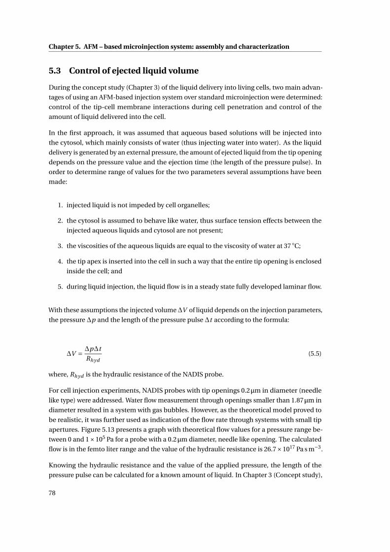
Chapter 5. AFM – based microinjection system: assembly and characterization
5.3 Control of ejected liquid volume
During the concept study (Chapter 3) of the liquid delivery into living cells, two main advan-
tages of using an AFM-based injection system over standard microinjection were determined:
control of the tip-cell membrane interactions during cell penetration and control of the
amount of liquid delivered into the cell.
In the first approach, it was assumed that aqueous based solutions will be injected into
the cytosol, which mainly consists of water (thus injecting water into water). As the liquid
delivery is generated by an external pressure, the amount of ejected liquid from the tip opening
depends on the pressure value and the ejection time (the length of the pressure pulse). In
order to determine range of values for the two parameters several assumptions have been
made:
1. injected liquid is not impeded by cell organelles;
2. the cytosol is assumed to behave like water, thus surface tension effects between the
injected aqueous liquids and cytosol are not present;
3. the viscosities of the aqueous liquids are equal to the viscosity of water at 37 ◦C;
4. the tip apex is inserted into the cell in such a way that the entire tip opening is enclosed
inside the cell; and
5. during liquid injection, the liquid flow is in a steady state fully developed laminar flow.
With these assumptions the injected volume∆V of liquid depends on the injection parameters,
the pressure ∆p and the length of the pressure pulse ∆t according to the formula:
∆V = ∆p∆t
Rhyd(5.5)
where, Rhyd is the hydraulic resistance of the NADIS probe.
For cell injection experiments, NADIS probes with tip openings 0.2µm in diameter (needle
like type) were addressed. Water flow measurement through openings smaller than 1.87µm in
diameter resulted in a system with gas bubbles. However, as the theoretical model proved to
be realistic, it was further used as indication of the flow rate through systems with small tip
apertures. Figure 5.13 presents a graph with theoretical flow values for a pressure range be-
tween 0 and 1×10⁵ Pa for a probe with a 0.2µm diameter, needle like opening. The calculated
flow is in the femto liter range and the value of the hydraulic resistance is 26.7×10¹⁷ Pa s m−3.
Knowing the hydraulic resistance and the value of the applied pressure, the length of the
pressure pulse can be calculated for a known amount of liquid. In Chapter 3 (Concept study),
78
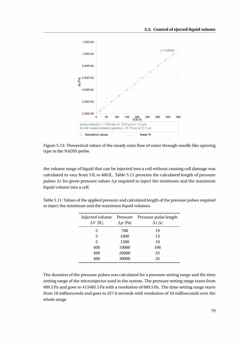
5.3. Control of ejected liquid volume
Figure 5.13: Theoretical values of the steady state flow of water through needle like openingtype in the NADIS probe.
the volume range of liquid that can be injected into a cell without causing cell damage was
calculated to vary from 5 fL to 400 fL. Table 5.11 presents the calculated length of pressure
pulses ∆t for given pressure values ∆p required to inject the minimum and the maximum
liquid volume into a cell.
Table 5.11: Values of the applied pressure and calculated length of the pressure pulses requiredto inject the minimum and the maximum liquid volumes.
Injected volume Pressure Pressure pulse length∆V [fL] ∆p [Pa] ∆t [s]
5 700 195 1000 135 1300 10
400 10000 106400 20000 53400 30000 35
The duration of the pressure pulses was calculated for a pressure setting range and the time
setting range of the microinjector used in the system. The pressure setting range starts from
689.5 Pa and goes to 413685.5 Pa with a resolution of 689.5 Pa. The time setting range starts
from 10 milliseconds and goes to 327.6 seconds with resolution of 10 milliseconds over the
whole range.
79
Chapter 5. AFM – based microinjection system: assembly and characterization
5.4 Discussion
Characterization of the AFM-based microinjection system focused on three main aspects:
cantilever spring constants, specifications of properly filled probes (with water) and fluid flow
measurements through the probes.
First, the stiffness of the cantilevers was measured. It was found that the probes are stiffer
than expected. The single beam probes assigned to the proof-of-concept microinjection
experiments had spring constants varying from 8 N m−1 to 15 N m−1 for the short length type
and 4 N m−1 to 6 N m−1 for the medium length type. Since cell indentation experiments with
AFM probes should be performed with flexible cantilevers, it was decided to use only the
single beam probes with the ‘medium’ length type.
In the next step, filling of the probes was controlled by measuring the resonance frequency
of the vibrating cantilever. Due to the cantilever filling with water, its resonance frequency
decreased. It was determined that the average decrease is 26 kHz. This value will be used in
future experiments as an indication of a correctly filled system.
Finally, the volumetric flow rate Q of fluids through NADIS probes was measured. Two types of
probes were used: one where the fluidic system consisted only of a rectangular channel, and a
second where the channel was connected to a hollow tip with an aperture. The measured flow
values were used to find the value of the hydraulic resistance for each probe. The measured
hydraulic resistance was further compared with the theoretical value.
The flow of nitrogen through the rectangular channel, with known geometry and without a
tip was in an excellent agreement with the theoretical model. In the theoretical model, the
nitrogen is treated as a continuous medium. For the absolute pressure range (105 < ∆p <2×10⁵ Pa), Knudsen numbers K n were in the range between 0.032 to 0.016, which falls well
inside the Navier–Stokes equation regime [92]. The calculated Reynolds numbers Re and
entrance length Le based on the measured flow were from 0.2 to 1.4 and 82 nm to 468 nm,
respectively, indicating fully developed laminar flow.
The value range of the Knudsen number indicates, according to Roy et. al [92], a slip flow
regime. However, the experimental data fit well with the ones reported by Harley et al.[93] and
Pfahler et al. [94], where no slip flow of nitrogen was reported.
Measurements of the nitrogen flow through NADIS channels connected to a hollow tip with
a square 6µm×6µm tip opening were 3 times higher than predicted by theory. Based on
the values of the Knudsen number, nitrogen flowing through the tip opening behaves as
a continuous medium. The entrance length however shows that the flow cannot be fully
developed due to the small length of the tip opening. This could explain the difference
between the measured and theoretical values, since the theoretical model assumed a fully
developed laminar flow.
An attempt to measure the flow of nitrogen through probes with tip openings smaller than
80
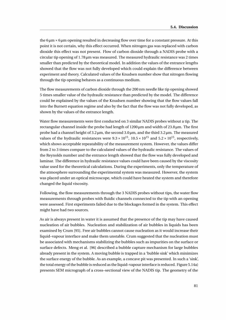
5.4. Discussion
the 6µm×6µm opening resulted in decreasing flow over time for a constant pressure. At this
point it is not certain, why this effect occurred. When nitrogen gas was replaced with carbon
dioxide this effect was not present. Flow of carbon dioxide through a NADIS probe with a
circular tip opening of 1.78µm was measured. The measured hydraulic resistance was 2 times
smaller than predicted by the theoretical model. In addition the values of the entrance lengths
showed that the flow was not fully developed which could explain the difference between
experiment and theory. Calculated values of the Knudsen number show that nitrogen flowing
through the tip opening behaves as a continuous medium.
The flow measurements of carbon dioxide through the 200 nm needle like tip opening showed
5 times smaller value of the hydraulic resistance than predicted by the model. The difference
could be explained by the values of the Knudsen number showing that the flow values fall
into the Burnett equation regime and also by the fact that the flow was not fully developed, as
shown by the values of the entrance length.
Water flow measurements were first conducted on 3 similar NADIS probes without a tip. The
rectangular channel inside the probe had length of 1200µm and width of 23.8µm. The first
probe had a channel height of 3.2µm, the second 3.0µm, and the third 3.2µm. The measured
values of the hydraulic resistances were 9.3×10¹⁵, 10.5×10¹⁵ and 5.2×10¹⁵, respectively,
which shows acceptable repeatability of the measurement system. However, the values differ
from 2 to 3 times compare to the calculated values of the hydraulic resistance. The values of
the Reynolds number and the entrance length showed that the flow was fully developed and
laminar. The difference in hydraulic resistance values could have been caused by the viscosity
value used for the theoretical calculations. During the experiments, only the temperature of
the atmosphere surrounding the experimental system was measured. However, the system
was placed under an optical microscope, which could have heated the system and therefore
changed the liquid viscosity.
Following, the flow measurements through the 3 NADIS probes without tips, the water flow
measurements through probes with fluidic channels connected to the tip with an opening
were assessed. First experiments failed due to the blockages formed in the system. This effect
might have had two sources.
As air is always present in water it is assumed that the presence of the tip may have caused
nucleation of air bubbles. Nucleation and stabilization of air bubbles in liquids has been
examined by Crum [95]. Free air bubbles cannot cause nucleation as it would increase their
liquid–vapour interface and make them unstable. Crum suggested that the nucleation must
be associated with mechanisms stabilizing the bubbles such as impurities on the surface or
surface defects. Meng et al. [96] described a bubble capture mechanism for large bubbles
already present in the system. A moving bubble is trapped in a ‘bubble sink’ which minimizes
the surface energy of the bubble. As an example, a concave pit was presented. In such a ‘sink’,
the total energy of the bubble is reduced as the liquid–vapour interface is reduced. Figure 5.14a)
presents SEM micrograph of a cross–sectional view of the NADIS tip. The geometry of the
81
Chapter 5. AFM – based microinjection system: assembly and characterization
hollow tip fulfills the requirements of a ‘bubble sink’. In addition, inside the tip, as a result
of the fabrication process, two smaller concave pits are present, enhancing nucleation and
capturing of the gas bubbles.
Figure 5.14: SEM micrograph presenting cross–sectional view of the hollow tip a) and it’sschematic drawing with marked positions of the ‘bubble sinks’.
The bubble nucleation and/or capturing occurred in the system due to the tip geometry. In
order to diminish these effects, the water was either degassed with nitrogen gas, boiled or both
before each experiment. However, these methods did not eliminate the problem.
In addition to the presence of the air bubbles it is possible that the nitrogen gas was also
trapped in the system causing blockages. Before each experiment the fluidic system was
flushed with nitrogen gas. When the system was being filled with water part of the nitrogen gas
could have been captured by the ‘bubble sinks’ in the tip. To diminish this effect the nitrogen
was replaced with carbon dioxide due to its high solubility in water.
Combination of the water degassing and pre-filling of the system with carbon dioxide allowed
the flow of water to be measured through a tip with a square 6µm×6µm opening.
Obtained values of the hydraulic resistance were 0.7 times smaller than theoretical values. The
values of Reynold number and entrance length suggest fully developed laminar flow. At this
point, it is rather uncertain whether the differences in the hydraulic resistance were caused by
the heating of the system as for the water flow measured through the 3 NADIS probes without
the tip or if it was due to an effect connected with presence of the tip.
The water flow measurement through smaller tip apertures required longer lasting measure-
ments. Large time periods required to obtain repeatable flow read-outs through openings
smaller than 1.78µm in diameter were held responsible for allowing the gas bubbles to plug
the system and prevent the measurements. It is suspected that the geometry of the tip is
enhancing the plugging effect.
The fluid flow measurements through the NADIS probes were designed to determine if the
theoretical model created in Chapter 3 adequately predicts fluid behavior. The theoretical
82
5.5. Conclusions
model was based on a few assumptions:
1. the flow is a fully developed laminar flow;
2. the Knudsen number is in the range of 0.001 to 0.1;
3. there is no slip flow effects;
4. the fluids behave like incompressible Newtonian fluids;
5. the walls of the channels are smooth and straight; and
6. the heat transfer and energy dissipation is negligible.
These assumptions permitted a very simple analytical solution to be found. However, their
presence caused quite significant deviation of the model when the flow of gases was measured.
Nevertheless, for the water flow measurements, the theoretical model proved to be realistic
and it could be used as an indication of the flow rate through systems with small tip apertures.
Based on the above conclusion, values of the pressure pulses required to inject a specific
amount of liquid into a cell were calculated theoretically. It is clear that due to the large
spectrum of assumptions used in the calculations, the parameters found contain a rather large
uncertainty. However, it should be noted that the prediction from chapter 3 of the volume of
liquid that can be injected into a single cell without causing damage varies from 5 fL to 400 fL
resulting in a large variation of volume allowed to be injected. Thus, although knowledge on
the amount of liquid ejected from the tip opening is theoretical, it is assumed to fall within the
required volume range.
5.5 Conclusions
The AFM-based microinjection system was assembled and characterized. First, the spring
constant of the NADIS probes was experimentally determined. The cantilever stiffness was
higher compared to the values assigned in the design. The difference was caused by two
factors: the free length of the cantilever and the cantilever height. Based on the measured
spring constant values, it was decided to use single beam NADIS probes with spring constants
lower than 7 N m−1 for the cell injection experiments.
Filling the system with liquid was tested through measurements of the cantilever resonance
frequency. It was found that due to the water presence in the cantilever, a decrease in the
resonance frequency of 26 kHz in average can be measured. This method was critical in
determining whether the probes were correctly filled with liquid, or blocked due to residues or
gas bubbles.
83

Chapter 5. AFM – based microinjection system: assembly and characterization
Water flow measurement through NADIS probes with tip openings smaller than 1.78µm in
diameter resulted in system blockages; therefore, the theoretical model was used as indication
of the flow rate through systems with small tip apertures.
84
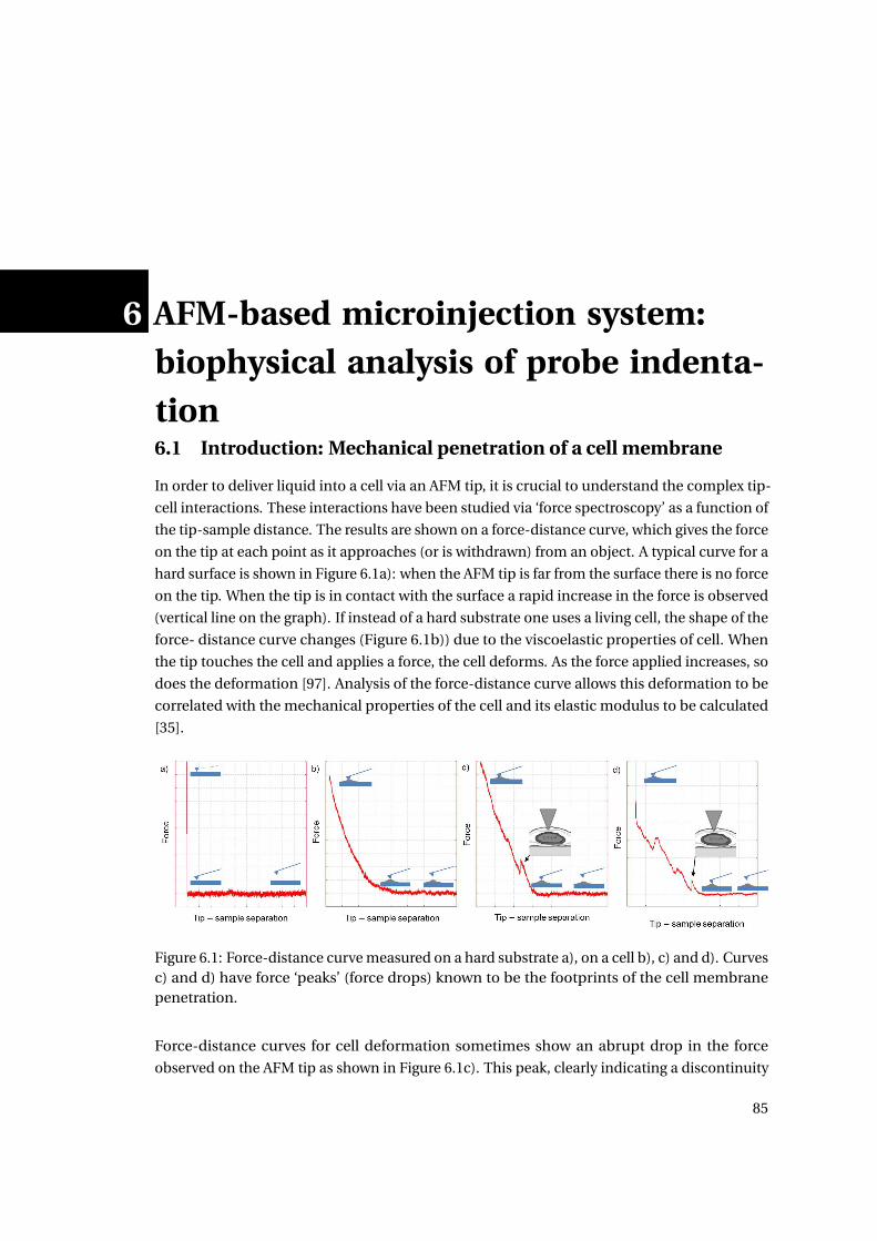
6 AFM-based microinjection system:biophysical analysis of probe indenta-tion6.1 Introduction: Mechanical penetration of a cell membrane
In order to deliver liquid into a cell via an AFM tip, it is crucial to understand the complex tip-
cell interactions. These interactions have been studied via ‘force spectroscopy’ as a function of
the tip-sample distance. The results are shown on a force-distance curve, which gives the force
on the tip at each point as it approaches (or is withdrawn) from an object. A typical curve for a
hard surface is shown in Figure 6.1a): when the AFM tip is far from the surface there is no force
on the tip. When the tip is in contact with the surface a rapid increase in the force is observed
(vertical line on the graph). If instead of a hard substrate one uses a living cell, the shape of the
force- distance curve changes (Figure 6.1b)) due to the viscoelastic properties of cell. When
the tip touches the cell and applies a force, the cell deforms. As the force applied increases, so
does the deformation [97]. Analysis of the force-distance curve allows this deformation to be
correlated with the mechanical properties of the cell and its elastic modulus to be calculated
[35].
Figure 6.1: Force-distance curve measured on a hard substrate a), on a cell b), c) and d). Curvesc) and d) have force ‘peaks’ (force drops) known to be the footprints of the cell membranepenetration.
Force-distance curves for cell deformation sometimes show an abrupt drop in the force
observed on the AFM tip as shown in Figure 6.1c). This peak, clearly indicating a discontinuity
85
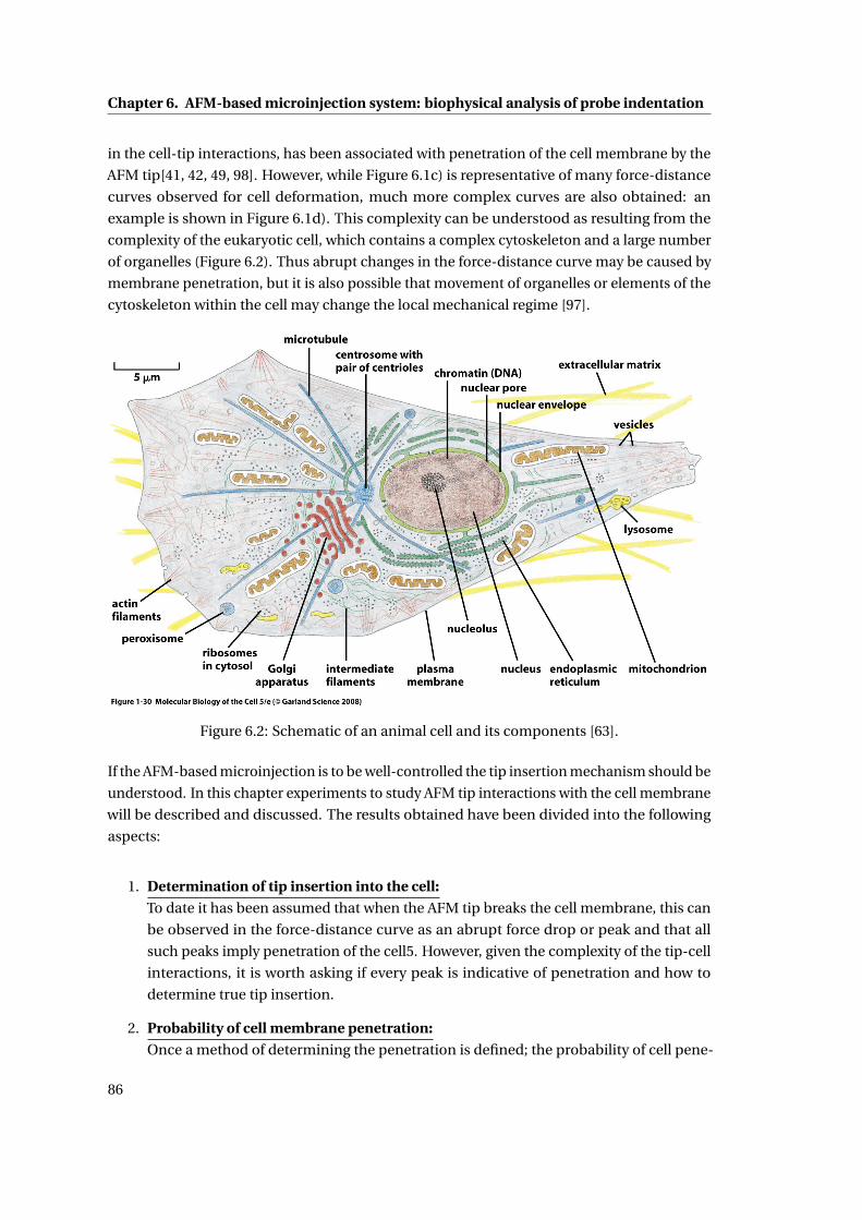
Chapter 6. AFM-based microinjection system: biophysical analysis of probe indentation
in the cell-tip interactions, has been associated with penetration of the cell membrane by the
AFM tip[41, 42, 49, 98]. However, while Figure 6.1c) is representative of many force-distance
curves observed for cell deformation, much more complex curves are also obtained: an
example is shown in Figure 6.1d). This complexity can be understood as resulting from the
complexity of the eukaryotic cell, which contains a complex cytoskeleton and a large number
of organelles (Figure 6.2). Thus abrupt changes in the force-distance curve may be caused by
membrane penetration, but it is also possible that movement of organelles or elements of the
cytoskeleton within the cell may change the local mechanical regime [97].
Figure 6.2: Schematic of an animal cell and its components [63].
If the AFM-based microinjection is to be well-controlled the tip insertion mechanism should be
understood. In this chapter experiments to study AFM tip interactions with the cell membrane
will be described and discussed. The results obtained have been divided into the following
aspects:
1. Determination of tip insertion into the cell:
To date it has been assumed that when the AFM tip breaks the cell membrane, this can
be observed in the force-distance curve as an abrupt force drop or peak and that all
such peaks imply penetration of the cell5. However, given the complexity of the tip-cell
interactions, it is worth asking if every peak is indicative of penetration and how to
determine true tip insertion.
2. Probability of cell membrane penetration:
Once a method of determining the penetration is defined; the probability of cell pene-
86
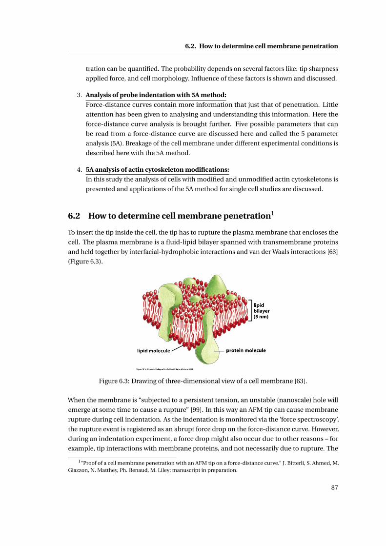
6.2. How to determine cell membrane penetration
tration can be quantified. The probability depends on several factors like: tip sharpness
applied force, and cell morphology. Influence of these factors is shown and discussed.
3. Analysis of probe indentation with 5A method:
Force-distance curves contain more information that just that of penetration. Little
attention has been given to analysing and understanding this information. Here the
force-distance curve analysis is brought further. Five possible parameters that can
be read from a force-distance curve are discussed here and called the 5 parameter
analysis (5A). Breakage of the cell membrane under different experimental conditions is
described here with the 5A method.
4. 5A analysis of actin cytoskeleton modifications:
In this study the analysis of cells with modified and unmodified actin cytoskeletons is
presented and applications of the 5A method for single cell studies are discussed.
6.2 How to determine cell membrane penetration1
To insert the tip inside the cell, the tip has to rupture the plasma membrane that encloses the
cell. The plasma membrane is a fluid-lipid bilayer spanned with transmembrane proteins
and held together by interfacial-hydrophobic interactions and van der Waals interactions [63]
(Figure 6.3).
Figure 6.3: Drawing of three-dimensional view of a cell membrane [63].
When the membrane is “subjected to a persistent tension, an unstable (nanoscale) hole will
emerge at some time to cause a rupture” [99]. In this way an AFM tip can cause membrane
rupture during cell indentation. As the indentation is monitored via the ‘force spectroscopy’,
the rupture event is registered as an abrupt force drop on the force-distance curve. However,
during an indentation experiment, a force drop might also occur due to other reasons – for
example, tip interactions with membrane proteins, and not necessarily due to rupture. The
1“Proof of a cell membrane penetration with an AFM tip on a force-distance curve.” J. Bitterli, S. Ahmed, M.Giazzon, N. Matthey, Ph. Renaud, M. Liley; manuscript in preparation.
87
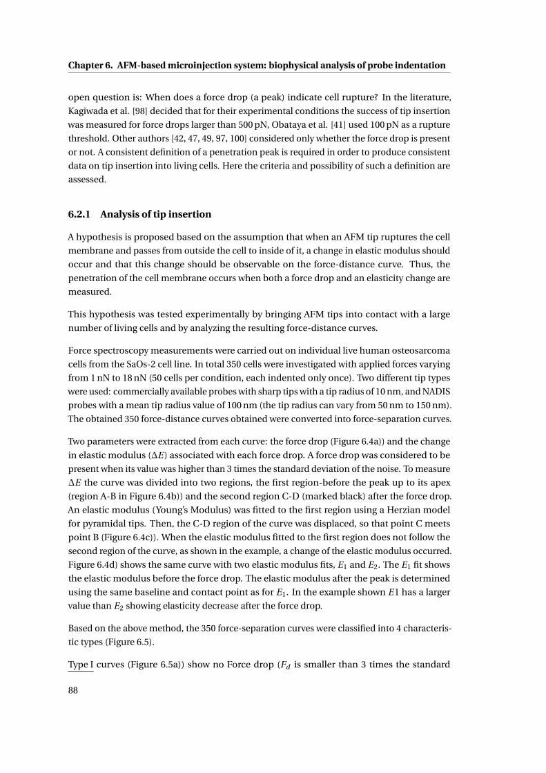
Chapter 6. AFM-based microinjection system: biophysical analysis of probe indentation
open question is: When does a force drop (a peak) indicate cell rupture? In the literature,
Kagiwada et al. [98] decided that for their experimental conditions the success of tip insertion
was measured for force drops larger than 500 pN, Obataya et al. [41] used 100 pN as a rupture
threshold. Other authors [42, 47, 49, 97, 100] considered only whether the force drop is present
or not. A consistent definition of a penetration peak is required in order to produce consistent
data on tip insertion into living cells. Here the criteria and possibility of such a definition are
assessed.
6.2.1 Analysis of tip insertion
A hypothesis is proposed based on the assumption that when an AFM tip ruptures the cell
membrane and passes from outside the cell to inside of it, a change in elastic modulus should
occur and that this change should be observable on the force-distance curve. Thus, the
penetration of the cell membrane occurs when both a force drop and an elasticity change are
measured.
This hypothesis was tested experimentally by bringing AFM tips into contact with a large
number of living cells and by analyzing the resulting force-distance curves.
Force spectroscopy measurements were carried out on individual live human osteosarcoma
cells from the SaOs-2 cell line. In total 350 cells were investigated with applied forces varying
from 1 nN to 18 nN (50 cells per condition, each indented only once). Two different tip types
were used: commercially available probes with sharp tips with a tip radius of 10 nm, and NADIS
probes with a mean tip radius value of 100 nm (the tip radius can vary from 50 nm to 150 nm).
The obtained 350 force-distance curves obtained were converted into force-separation curves.
Two parameters were extracted from each curve: the force drop (Figure 6.4a)) and the change
in elastic modulus (∆E) associated with each force drop. A force drop was considered to be
present when its value was higher than 3 times the standard deviation of the noise. To measure
∆E the curve was divided into two regions, the first region-before the peak up to its apex
(region A-B in Figure 6.4b)) and the second region C-D (marked black) after the force drop.
An elastic modulus (Young’s Modulus) was fitted to the first region using a Herzian model
for pyramidal tips. Then, the C-D region of the curve was displaced, so that point C meets
point B (Figure 6.4c)). When the elastic modulus fitted to the first region does not follow the
second region of the curve, as shown in the example, a change of the elastic modulus occurred.
Figure 6.4d) shows the same curve with two elastic modulus fits, E1 and E2. The E1 fit shows
the elastic modulus before the force drop. The elastic modulus after the peak is determined
using the same baseline and contact point as for E1. In the example shown E1 has a larger
value than E2 showing elasticity decrease after the force drop.
Based on the above method, the 350 force-separation curves were classified into 4 characteris-
tic types (Figure 6.5).
Type I curves (Figure 6.5a)) show no Force drop (Fd is smaller than 3 times the standard
88
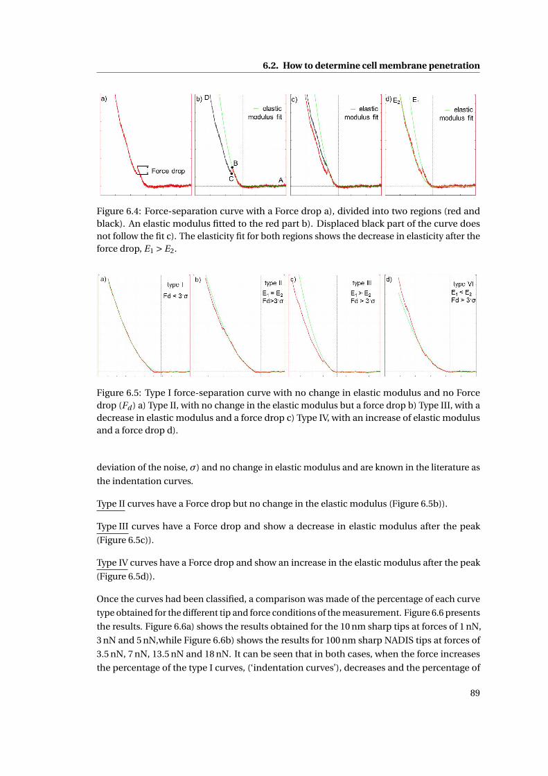
6.2. How to determine cell membrane penetration
Figure 6.4: Force-separation curve with a Force drop a), divided into two regions (red andblack). An elastic modulus fitted to the red part b). Displaced black part of the curve doesnot follow the fit c). The elasticity fit for both regions shows the decrease in elasticity after theforce drop, E1 > E2.
Figure 6.5: Type I force-separation curve with no change in elastic modulus and no Forcedrop (Fd ) a) Type II, with no change in the elastic modulus but a force drop b) Type III, with adecrease in elastic modulus and a force drop c) Type IV, with an increase of elastic modulusand a force drop d).
deviation of the noise, σ) and no change in elastic modulus and are known in the literature as
the indentation curves.
Type II curves have a Force drop but no change in the elastic modulus (Figure 6.5b)).
Type III curves have a Force drop and show a decrease in elastic modulus after the peak
(Figure 6.5c)).
Type IV curves have a Force drop and show an increase in the elastic modulus after the peak
(Figure 6.5d)).
Once the curves had been classified, a comparison was made of the percentage of each curve
type obtained for the different tip and force conditions of the measurement. Figure 6.6 presents
the results. Figure 6.6a) shows the results obtained for the 10 nm sharp tips at forces of 1 nN,
3 nN and 5 nN,while Figure 6.6b) shows the results for 100 nm sharp NADIS tips at forces of
3.5 nN, 7 nN, 13.5 nN and 18 nN. It can be seen that in both cases, when the force increases
the percentage of the type I curves, (‘indentation curves’), decreases and the percentage of
89
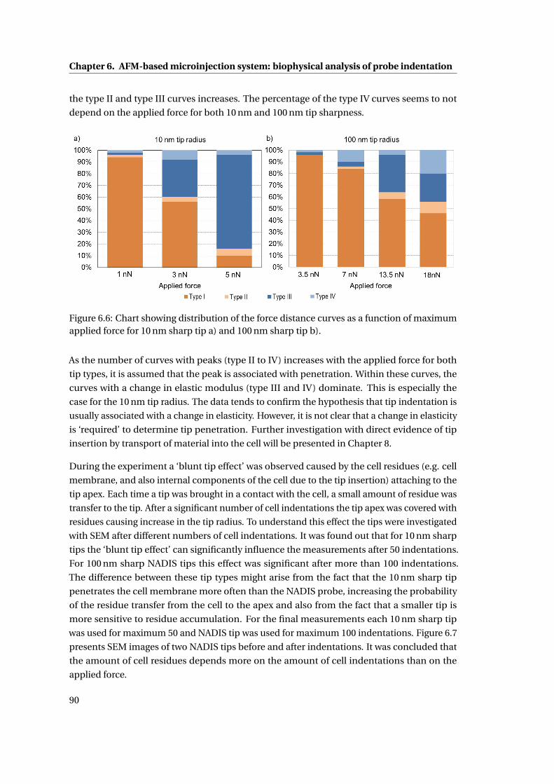
Chapter 6. AFM-based microinjection system: biophysical analysis of probe indentation
the type II and type III curves increases. The percentage of the type IV curves seems to not
depend on the applied force for both 10 nm and 100 nm tip sharpness.
Figure 6.6: Chart showing distribution of the force distance curves as a function of maximumapplied force for 10 nm sharp tip a) and 100 nm sharp tip b).
As the number of curves with peaks (type II to IV) increases with the applied force for both
tip types, it is assumed that the peak is associated with penetration. Within these curves, the
curves with a change in elastic modulus (type III and IV) dominate. This is especially the
case for the 10 nm tip radius. The data tends to confirm the hypothesis that tip indentation is
usually associated with a change in elasticity. However, it is not clear that a change in elasticity
is ‘required’ to determine tip penetration. Further investigation with direct evidence of tip
insertion by transport of material into the cell will be presented in Chapter 8.
During the experiment a ‘blunt tip effect’ was observed caused by the cell residues (e.g. cell
membrane, and also internal components of the cell due to the tip insertion) attaching to the
tip apex. Each time a tip was brought in a contact with the cell, a small amount of residue was
transfer to the tip. After a significant number of cell indentations the tip apex was covered with
residues causing increase in the tip radius. To understand this effect the tips were investigated
with SEM after different numbers of cell indentations. It was found out that for 10 nm sharp
tips the ‘blunt tip effect’ can significantly influence the measurements after 50 indentations.
For 100 nm sharp NADIS tips this effect was significant after more than 100 indentations.
The difference between these tip types might arise from the fact that the 10 nm sharp tip
penetrates the cell membrane more often than the NADIS probe, increasing the probability
of the residue transfer from the cell to the apex and also from the fact that a smaller tip is
more sensitive to residue accumulation. For the final measurements each 10 nm sharp tip
was used for maximum 50 and NADIS tip was used for maximum 100 indentations. Figure 6.7
presents SEM images of two NADIS tips before and after indentations. It was concluded that
the amount of cell residues depends more on the amount of cell indentations than on the
applied force.
90
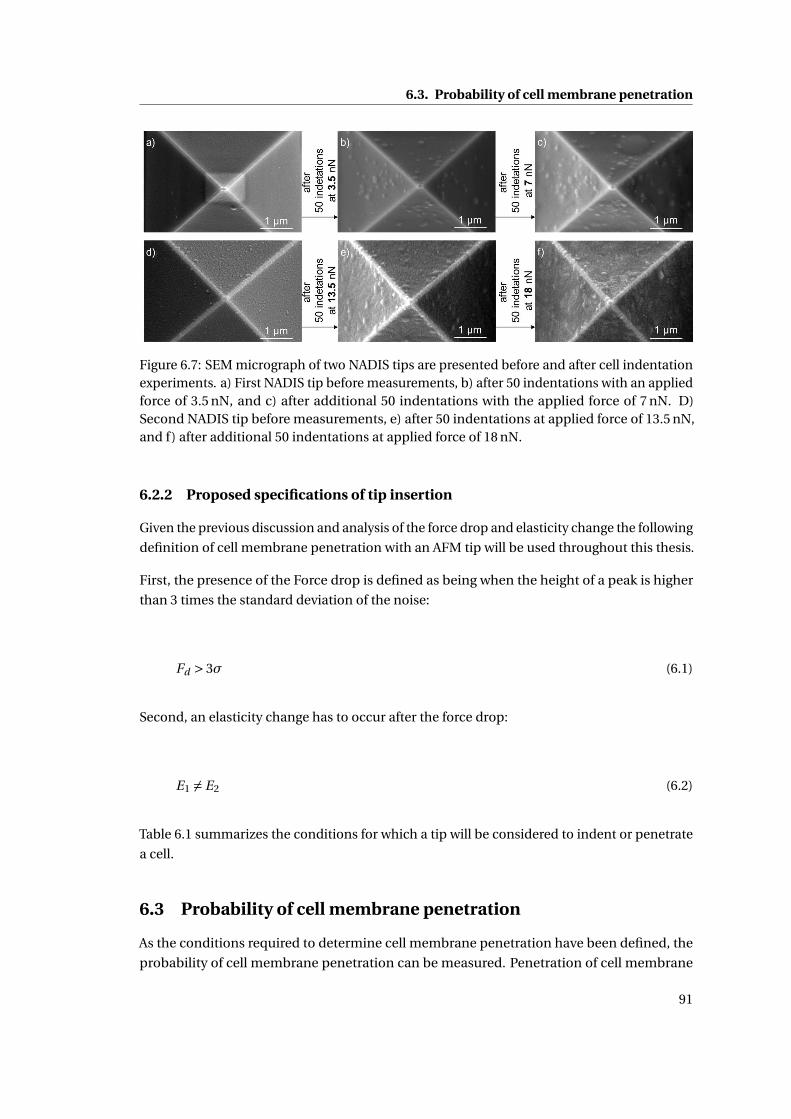
6.3. Probability of cell membrane penetration
Figure 6.7: SEM micrograph of two NADIS tips are presented before and after cell indentationexperiments. a) First NADIS tip before measurements, b) after 50 indentations with an appliedforce of 3.5 nN, and c) after additional 50 indentations with the applied force of 7 nN. D)Second NADIS tip before measurements, e) after 50 indentations at applied force of 13.5 nN,and f) after additional 50 indentations at applied force of 18 nN.
6.2.2 Proposed specifications of tip insertion
Given the previous discussion and analysis of the force drop and elasticity change the following
definition of cell membrane penetration with an AFM tip will be used throughout this thesis.
First, the presence of the Force drop is defined as being when the height of a peak is higher
than 3 times the standard deviation of the noise:
Fd > 3σ (6.1)
Second, an elasticity change has to occur after the force drop:
E1 6= E2 (6.2)
Table 6.1 summarizes the conditions for which a tip will be considered to indent or penetrate
a cell.
6.3 Probability of cell membrane penetration
As the conditions required to determine cell membrane penetration have been defined, the
probability of cell membrane penetration can be measured. Penetration of cell membrane
91
Chapter 6. AFM-based microinjection system: biophysical analysis of probe indentation
Table 6.1: Tip–cell membrane interaction determined by the Force drop and the change inelastic modulus.
Cell indentation Cell penetration
Type I Type II Type III Type IVFd < 3σ Fd > 3σ Fd > 3σ Fd < 3σE1 = E2 E1 = E2 E1 > E2 E1 < E2
can be expected to depend on many parameters such as: the tip sharpness [41], the applied
force [100], the position (above nucleus or cytoplasm) [42, 97], and cell morphology [42, 98].
6.3.1 Influence of tip sharpness
In this study the force spectroscopy measurements used to analyze tip insertion in Section 6.2.1
were used to demonstrate influence of the tip sharpness. In total 350 force-separation curves
were obtained with two tip types: 10 nm sharp tips and 100 nm sharp NADIS tips, for applied
forces varying from 1 nN to 18 nN, and SaOs-2 cells seeded on a Petri dish. For both probes,
the total travel distance of the cantilever was the same – 10µm (approach and retract mo-
tion) and the speed was 2µm s−1. The tip position was always above the nucleus. The data
were completed with additional 50 force-distance curves measured with 10 nm sharp tip and
applied force of 15 nN.
The results are presented in the form of a graph (Figure 6.8e)). The result for the 10 nm sharp
tips at forces of 1 nN, 3 nN, 5 nN and 15 nN are marked with blue dots while the results for
100 nm sharp NADIS tips at forces of 3.5 nN, 7 nN, 13.5 nN and 18 nN are marked with red
dots. Probability of cell membrane penetration with 10 nm sharp tip for the maximum applied
force of 15 nN is more than 90 %. When the 100 nm sharp NADIS probe is used at maximum
applied force of 18 nN the probability is found to be less than 50 %.
The result confirm the expectation that the sharper the tip apex the higher the probability of
the cell membrane penetration.
6.3.1.1 Force distance–curves with multiple force drops
Within the experimental results force-distance curves with multiple force drops were found
(Figure 6.9).
The experimental data were analyzed in terms of the number of force drops and their depen-
dency on the applied force. Table 6.2 shows the results. It was observed that the number of
force drops (Fd ) depends on both the applied force and the tip sharpness. The higher the
applied force and the sharper the tip, the larger the number of force-distance curves with
multiple force drops.
92
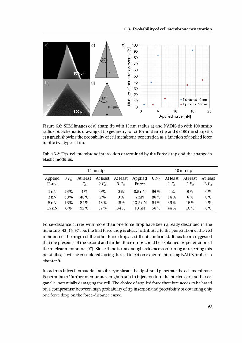
6.3. Probability of cell membrane penetration
Figure 6.8: SEM images of a) sharp tip with 10 nm radius a) and NADIS tip with 100 nmtipradius b). Schematic drawing of tip geometry for c) 10 nm sharp tip and d) 100 nm sharp tip.e) a graph showing the probability of cell membrane penetration as a function of applied forcefor the two types of tip.
Table 6.2: Tip–cell membrane interaction determined by the Force drop and the change inelastic modulus.
10 nm tip 10 nm tip
Applied 0 Fd At least At least At least Applied 0 Fd At least At least At leastForce Fd 2 Fd 3 Fd Force 1 Fd 2 Fd 3 Fd
1 nN 96 % 4 % 0 % 0 % 3.5 nN 96 % 4 % 0 % 0 %3 nN 60 % 40 % 2 % 0 % 7 nN 86 % 14 % 6 % 0 %5 nN 16 % 84 % 48 % 28 % 13.5 nN 64 % 36 % 16 % 2 %
15 nN 8 % 92 % 52 % 34 % 18 nN 56 % 44 % 16 % 6 %
Force–distance curves with more than one force drop have been already described in the
literature [42, 45, 97]. As the first force drop is always attributed to the penetration of the cell
membrane, the origin of the other force drops is still not confirmed. It has been suggested
that the presence of the second and further force drops could be explained by penetration of
the nuclear membrane [97]. Since there is not enough evidence confirming or rejecting this
possibility, it will be considered during the cell injection experiments using NADIS probes in
chapter 8.
In order to inject biomaterial into the cytoplasm, the tip should penetrate the cell membrane.
Penetration of further membranes might result in injection into the nucleus or another or-
ganelle, potentially damaging the cell. The choice of applied force therefore needs to be based
on a compromise between high probability of tip insertion and probability of obtaining only
one force drop on the force-distance curve.
93
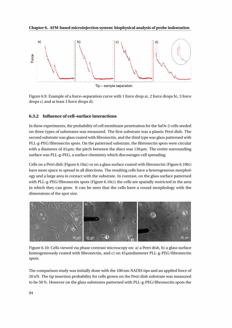
Chapter 6. AFM-based microinjection system: biophysical analysis of probe indentation
Figure 6.9: Example of a force–separation curve with 1 force drop a), 2 force drops b), 3 forcedrops c) and at least 3 force drops d).
6.3.2 Influence of cell–surface interactions
In these experiments, the probability of cell membrane penetration for the SaOs-2 cells seeded
on three types of substrates was measured. The first substrate was a plastic Petri dish. The
second substrate was glass coated with fibronectin, and the third type was glass patterned with
PLL-g-PEG/fibronectin spots. On the patterned substrate, the fibronectin spots were circular
with a diameter of 45µm; the pitch between the discs was 130µm. The entire surrounding
surface was PLL-g-PEG, a surface chemistry which discourages cell spreading.
Cells on a Petri dish (Figure 6.10a)) or on a glass surface coated with fibronectin (Figure 6.10b))
have more space to spread in all directions. The resulting cells have a heterogeneous morphol-
ogy and a large area in contact with the substrate. In contrast, on the glass surface patterned
with PLL-g-PEG/fibronectin spots (Figure 6.10c)) the cells are spatially restricted in the area
in which they can grow. It can be seen that the cells have a round morphology with the
dimensions of the spot size.
Figure 6.10: Cells viewed via phase contrast microscopy on: a) a Petri dish, b) a glass surfacehomogeneously coated with fibronectin, and c) on 45µmdiameter PLL-g-PEG/fibronectinspots.
The comparison study was initially done with the 100 nm NADIS tips and an applied force of
20 nN. The tip insertion probability for cells grown on the Petri dish substrate was measured
to be 50 %. However on the glass substrates patterned with PLL-g-PEG/fibronectin spots the
94
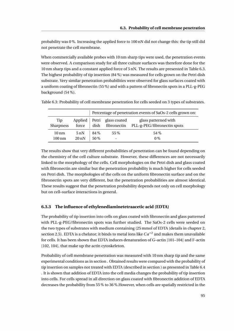
6.3. Probability of cell membrane penetration
probability was 0 %. Increasing the applied force to 100 nN did not change this: the tip still did
not penetrate the cell membrane.
When commercially available probes with 10 nm sharp tips were used, the penetration events
were observed. A comparison study for all three culture surfaces was therefore done for the
10 nm sharp tips and a constant applied force of 5 nN. The results are presented in Table 6.3.
The highest probability of tip insertion (84 %) was measured for cells grown on the Petri dish
substrate. Very similar penetration probabilities were observed for glass surfaces coated with
a uniform coating of fibronectin (55 %) and with a pattern of fibronectin spots in a PLL-g-PEG
background (54 %).
Table 6.3: Probability of cell membrane penetration for cells seeded on 3 types of substrates.
Percentage of penetration events of SaOs-2 cells grown on:
Tip Applied Petri glass coated glass patterned withSharpness force dish fibronectin PLL-g-PEG/fibronectin spots
10 nm 5 nN 84 % 55 % 54 %100 nm 20 nN 50 % - 0 %
The results show that very different probabilities of penetration can be found depending on
the chemistry of the cell culture substrate. However, these differences are not necessarily
linked to the morphology of the cells. Cell morphologies on the Petri dish and glass coated
with fibronectin are similar but the penetration probability is much higher for cells seeded
on Petri dish. The morphologies of the cells on the uniform fibronectin surface and on the
fibronectin spots are very different, but the penetration probabilities are almost identical.
These results suggest that the penetration probability depends not only on cell morphology
but on cell–surface interactions in general.
6.3.3 The influence of ethylenediaminetetraacetic acid (EDTA)
The probability of tip insertion into cells on glass coated with fibronectin and glass patterned
with PLL-g-PEG/fibronectin spots was further studied. The SaOs-2 cells were seeded on
the two types of substrates with medium containing (25 mmol of EDTA (details in chapter 2,
section 2.5). EDTA is a chelator; it binds to metal ions like C a+2 and makes them unavailable
for cells. It has been shown that EDTA induces denaturation of G–actin [101–104] and F-actin
[102, 104], that make up the actin cytoskeleton.
Probability of cell membrane penetration was measured with 10 nm sharp tip and the same
experimental conditions as in section . Obtained results were compared with the probability of
tip insertion on samples not treated with EDTA (described in section ) as presented in Table 6.4
. It is shown that addition of EDTA into the cell media changes the probability of tip insertion
into cells. For cells spread in all direction on glass coated with fibronectin addition of EDTA
decreases the probability from 55 % to 36 %.However, when cells are spatially restricted in the
95
Chapter 6. AFM-based microinjection system: biophysical analysis of probe indentation
area on the PLL-g-PEG/fibronectin spots the probability increases from 54 % to 75 % after the
addition of EDTA.
Table 6.4: Probability of cell membrane penetration for cells treated and without EDTA treat-ment.Percentage of penetration events of SaOs-2 cells with 10 nm sharp tip and applied forceof 5 nN
Treatment glass coated with fibronectin glass patterned withPLL-g-PEG/fibronectin spots
No EDTA 55 % 54 %With EDTA 36 % 75 %
Kagiwada et al.[98] showed that the cell actin cytoskeleton of plays a significant role in proba-
bility of tip insertion. The actin skeleton consists of actin mesh and stress fibres. It has been
shown that actin mesh, localized under the cell membrane, has a direct influence on the cell
membrane penetration and the stress fibres might facilitate the insertion by giving the cell a
mechanical stability.
It is known that EDTA influences G- and F–actin. However its effect on the actin cytoskeleton
of the SaOs-2 cells in general is not yet understood. Taking into consideration results presented
by Kagiwada et al. [98] it is possible that EDTA has modified the actin cytoskeleton of the
SaOs-2 cells which influenced the penetration probability.
6.4 Analysis of probe indentation: 5A method 2
Force-distance curves contain more information that just that of tip insertion. When an
AFM tip penetrates a cell, additional information can be extracted from the force-distance
curve. Yokokawa et al. [97] extracted a ‘penetration force’ parameter from the force-separation
curves and showed its analysis. Kim et al. [42] discussed a ‘penetration distance’ parameter.
Kagiwada et al.[98] and Obataya et al.[41] discussed a ‘force drop’ parameter. In this section
five parameters that can be read from a force-separation curve are described. The parameters
are further used in a simple biophysical analysis of the cell membrane penetration for different
experimental conditions. As the analysis is based on the 5 parameters therefore the name is: 5
parameter analysis (5A).
6.4.1 Description of the 5A method
The five parameters were divided into two groups, macro and microparameters.
2“Analysis of approach curve after cell membrane penetration with a 5A method.” J. Bitterli, A. Meister, S.Ahmed, M. Giazzon, N. Matthey, Ph. Renaud, M. Liley; manuscript in preparation.
96
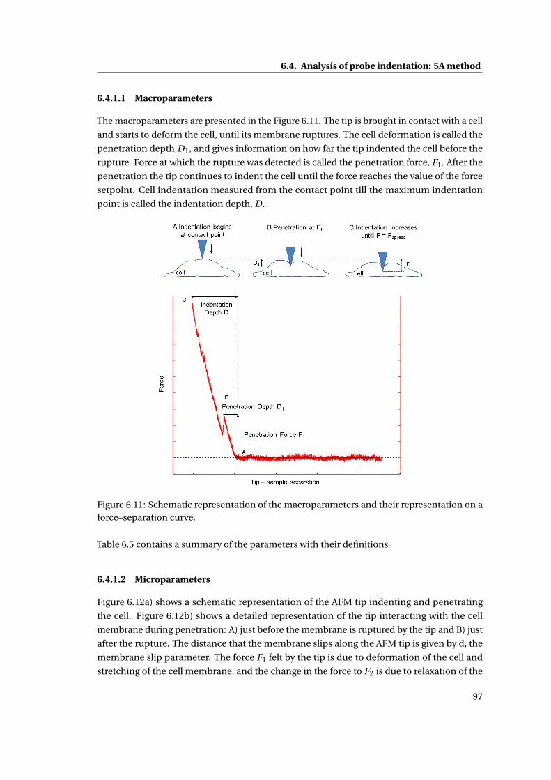
6.4. Analysis of probe indentation: 5A method
6.4.1.1 Macroparameters
The macroparameters are presented in the Figure 6.11. The tip is brought in contact with a cell
and starts to deform the cell, until its membrane ruptures. The cell deformation is called the
penetration depth,D1, and gives information on how far the tip indented the cell before the
rupture. Force at which the rupture was detected is called the penetration force, F1. After the
penetration the tip continues to indent the cell until the force reaches the value of the force
setpoint. Cell indentation measured from the contact point till the maximum indentation
point is called the indentation depth, D .
Figure 6.11: Schematic representation of the macroparameters and their representation on aforce–separation curve.
Table 6.5 contains a summary of the parameters with their definitions
6.4.1.2 Microparameters
Figure 6.12a) shows a schematic representation of the AFM tip indenting and penetrating
the cell. Figure 6.12b) shows a detailed representation of the tip interacting with the cell
membrane during penetration: A) just before the membrane is ruptured by the tip and B) just
after the rupture. The distance that the membrane slips along the AFM tip is given by d, the
membrane slip parameter. The force F1 felt by the tip is due to deformation of the cell and
stretching of the cell membrane, and the change in the force to F2 is due to relaxation of the
97
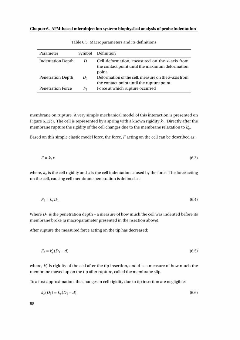
Chapter 6. AFM-based microinjection system: biophysical analysis of probe indentation
Table 6.5: Macroparameters and its definitions
Parameter Symbol Definition
Indentation Depth D Cell deformation, measured on the z–axis fromthe contact point until the maximum deformationpoint.
Penetration Depth D1 Deformation of the cell, measure on the z–axis fromthe contact point until the rupture point.
Penetration Force F1 Force at which rupture occurred
membrane on rupture. A very simple mechanical model of this interaction is presented on
Figure 6.12c). The cell is represented by a spring with a known rigidity kc . Directly after the
membrane rupture the rigidity of the cell changes due to the membrane relaxation to k ′c .
Based on this simple elastic model force, the force, F acting on the cell can be described as:
F = kc x (6.3)
where, kc is the cell rigidity and x is the cell indentation caused by the force. The force acting
on the cell, causing cell membrane penetration is defined as:
F1 = kc D1 (6.4)
Where D1 is the penetration depth – a measure of how much the cell was indented before its
membrane broke (a macroparameter presented in the nsection above).
After rupture the measured force acting on the tip has decreased:
F2 = k ′c (D1 −d) (6.5)
where, k ′c is rigidity of the cell after the tip insertion, and d is a measure of how much the
membrane moved up on the tip after rupture, called the membrane slip.
To a first approximation, the changes in cell rigidity due to tip insertion are negligible:
k ′c (D1) = kc (D1 −d) (6.6)
98
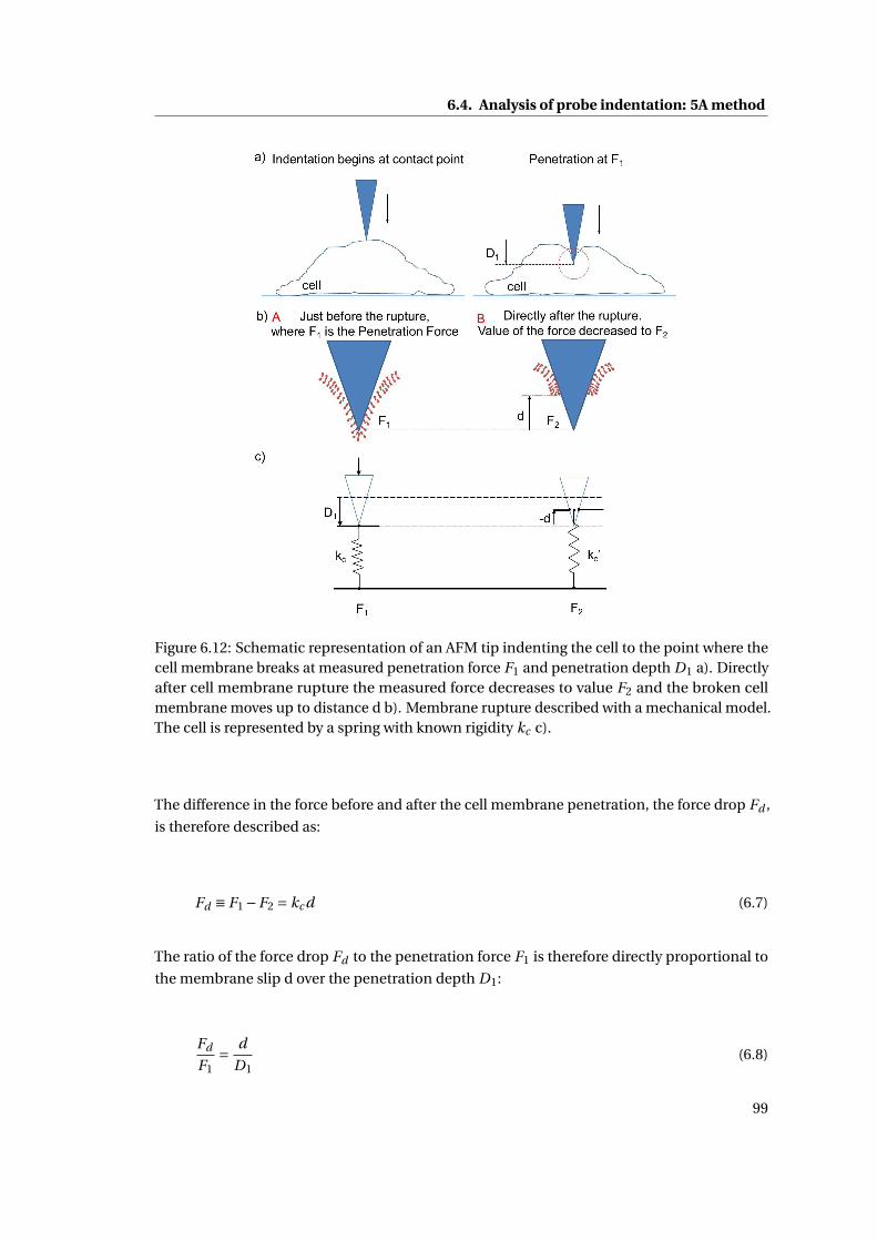
6.4. Analysis of probe indentation: 5A method
Figure 6.12: Schematic representation of an AFM tip indenting the cell to the point where thecell membrane breaks at measured penetration force F1 and penetration depth D1 a). Directlyafter cell membrane rupture the measured force decreases to value F2 and the broken cellmembrane moves up to distance d b). Membrane rupture described with a mechanical model.The cell is represented by a spring with known rigidity kc c).
The difference in the force before and after the cell membrane penetration, the force drop Fd ,
is therefore described as:
Fd ≡ F1 −F2 = kc d (6.7)
The ratio of the force drop Fd to the penetration force F1 is therefore directly proportional to
the membrane slip d over the penetration depth D1:
Fd
F1= d
D1(6.8)
99
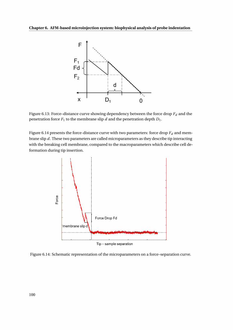
Chapter 6. AFM-based microinjection system: biophysical analysis of probe indentation
Figure 6.13: Force–distance curve showing dependency between the force drop Fd and thepenetration force F1 to the membrane slip d and the penetration depth D1.
Figure 6.14 presents the force-distance curve with two parameters: force drop Fd and mem-
brane slip d . These two parameters are called microparameters as they describe tip interacting
with the breaking cell membrane, compared to the macroparameters which describe cell de-
formation during tip insertion.
Figure 6.14: Schematic representation of the microparameters on a force–separation curve.
100
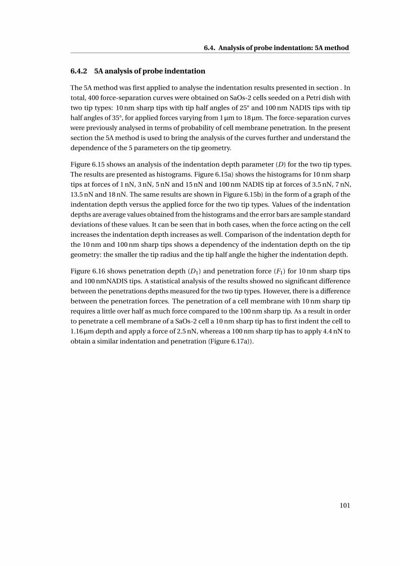
6.4. Analysis of probe indentation: 5A method
6.4.2 5A analysis of probe indentation
The 5A method was first applied to analyse the indentation results presented in section . In
total, 400 force-separation curves were obtained on SaOs-2 cells seeded on a Petri dish with
two tip types: 10 nm sharp tips with tip half angles of 25° and 100 nm NADIS tips with tip
half angles of 35°, for applied forces varying from 1µm to 18µm. The force-separation curves
were previously analysed in terms of probability of cell membrane penetration. In the present
section the 5A method is used to bring the analysis of the curves further and understand the
dependence of the 5 parameters on the tip geometry.
Figure 6.15 shows an analysis of the indentation depth parameter (D) for the two tip types.
The results are presented as histograms. Figure 6.15a) shows the histograms for 10 nm sharp
tips at forces of 1 nN, 3 nN, 5 nN and 15 nN and 100 nm NADIS tip at forces of 3.5 nN, 7 nN,
13.5 nN and 18 nN. The same results are shown in Figure 6.15b) in the form of a graph of the
indentation depth versus the applied force for the two tip types. Values of the indentation
depths are average values obtained from the histograms and the error bars are sample standard
deviations of these values. It can be seen that in both cases, when the force acting on the cell
increases the indentation depth increases as well. Comparison of the indentation depth for
the 10 nm and 100 nm sharp tips shows a dependency of the indentation depth on the tip
geometry: the smaller the tip radius and the tip half angle the higher the indentation depth.
Figure 6.16 shows penetration depth (D1) and penetration force (F1) for 10 nm sharp tips
and 100 nmNADIS tips. A statistical analysis of the results showed no significant difference
between the penetrations depths measured for the two tip types. However, there is a difference
between the penetration forces. The penetration of a cell membrane with 10 nm sharp tip
requires a little over half as much force compared to the 100 nm sharp tip. As a result in order
to penetrate a cell membrane of a SaOs-2 cell a 10 nm sharp tip has to first indent the cell to
1.16µm depth and apply a force of 2.5 nN, whereas a 100 nm sharp tip has to apply 4.4 nN to
obtain a similar indentation and penetration (Figure 6.17a)).
101
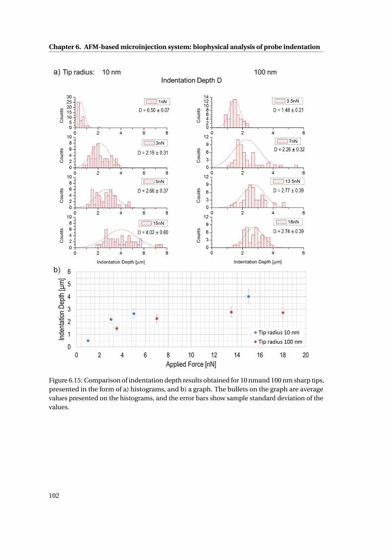
Chapter 6. AFM-based microinjection system: biophysical analysis of probe indentation
Figure 6.15: Comparison of indentation depth results obtained for 10 nmand 100 nm sharp tips,presented in the form of a) histograms, and b) a graph. The bullets on the graph are averagevalues presented on the histograms, and the error bars show sample standard deviation of thevalues.
102
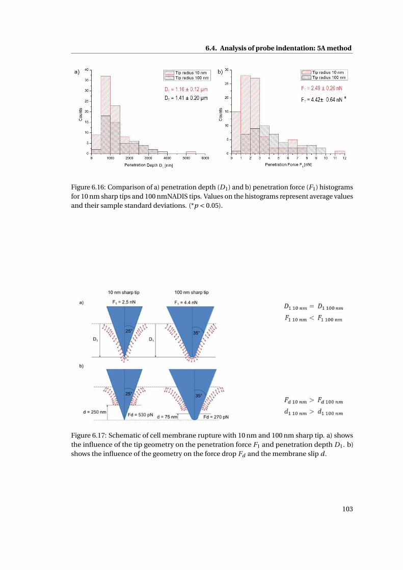
6.4. Analysis of probe indentation: 5A method
Figure 6.16: Comparison of a) penetration depth (D1) and b) penetration force (F1) histogramsfor 10 nm sharp tips and 100 nmNADIS tips. Values on the histograms represent average valuesand their sample standard deviations. (*p < 0.05).
Figure 6.17: Schematic of cell membrane rupture with 10 nm and 100 nm sharp tip. a) showsthe influence of the tip geometry on the penetration force F1 and penetration depth D1. b)shows the influence of the geometry on the force drop Fd and the membrane slip d .
103
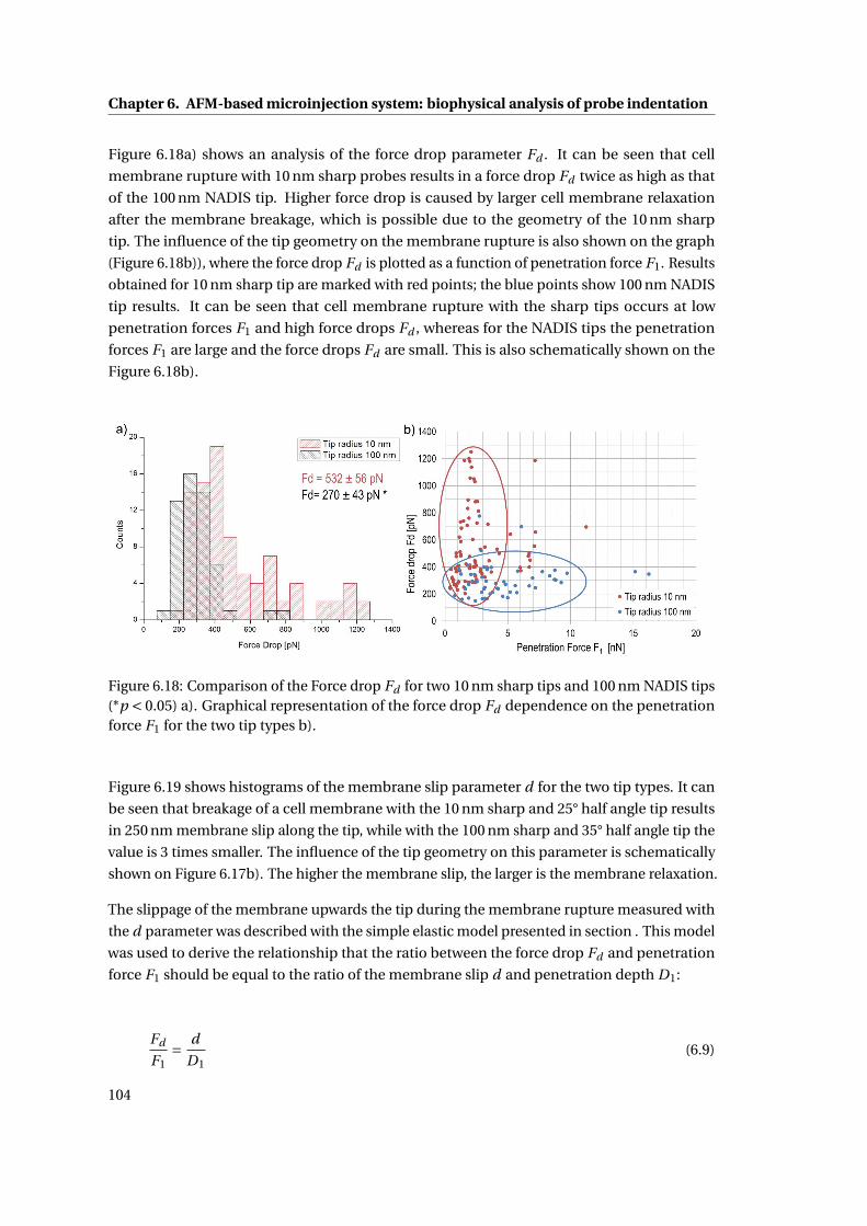
Chapter 6. AFM-based microinjection system: biophysical analysis of probe indentation
Figure 6.18a) shows an analysis of the force drop parameter Fd . It can be seen that cell
membrane rupture with 10 nm sharp probes results in a force drop Fd twice as high as that
of the 100 nm NADIS tip. Higher force drop is caused by larger cell membrane relaxation
after the membrane breakage, which is possible due to the geometry of the 10 nm sharp
tip. The influence of the tip geometry on the membrane rupture is also shown on the graph
(Figure 6.18b)), where the force drop Fd is plotted as a function of penetration force F1. Results
obtained for 10 nm sharp tip are marked with red points; the blue points show 100 nm NADIS
tip results. It can be seen that cell membrane rupture with the sharp tips occurs at low
penetration forces F1 and high force drops Fd , whereas for the NADIS tips the penetration
forces F1 are large and the force drops Fd are small. This is also schematically shown on the
Figure 6.18b).
Figure 6.18: Comparison of the Force drop Fd for two 10 nm sharp tips and 100 nm NADIS tips(*p < 0.05) a). Graphical representation of the force drop Fd dependence on the penetrationforce F1 for the two tip types b).
Figure 6.19 shows histograms of the membrane slip parameter d for the two tip types. It can
be seen that breakage of a cell membrane with the 10 nm sharp and 25° half angle tip results
in 250 nm membrane slip along the tip, while with the 100 nm sharp and 35° half angle tip the
value is 3 times smaller. The influence of the tip geometry on this parameter is schematically
shown on Figure 6.17b). The higher the membrane slip, the larger is the membrane relaxation.
The slippage of the membrane upwards the tip during the membrane rupture measured with
the d parameter was described with the simple elastic model presented in section . This model
was used to derive the relationship that the ratio between the force drop Fd and penetration
force F1 should be equal to the ratio of the membrane slip d and penetration depth D1:
Fd
F1= d
D1(6.9)
104
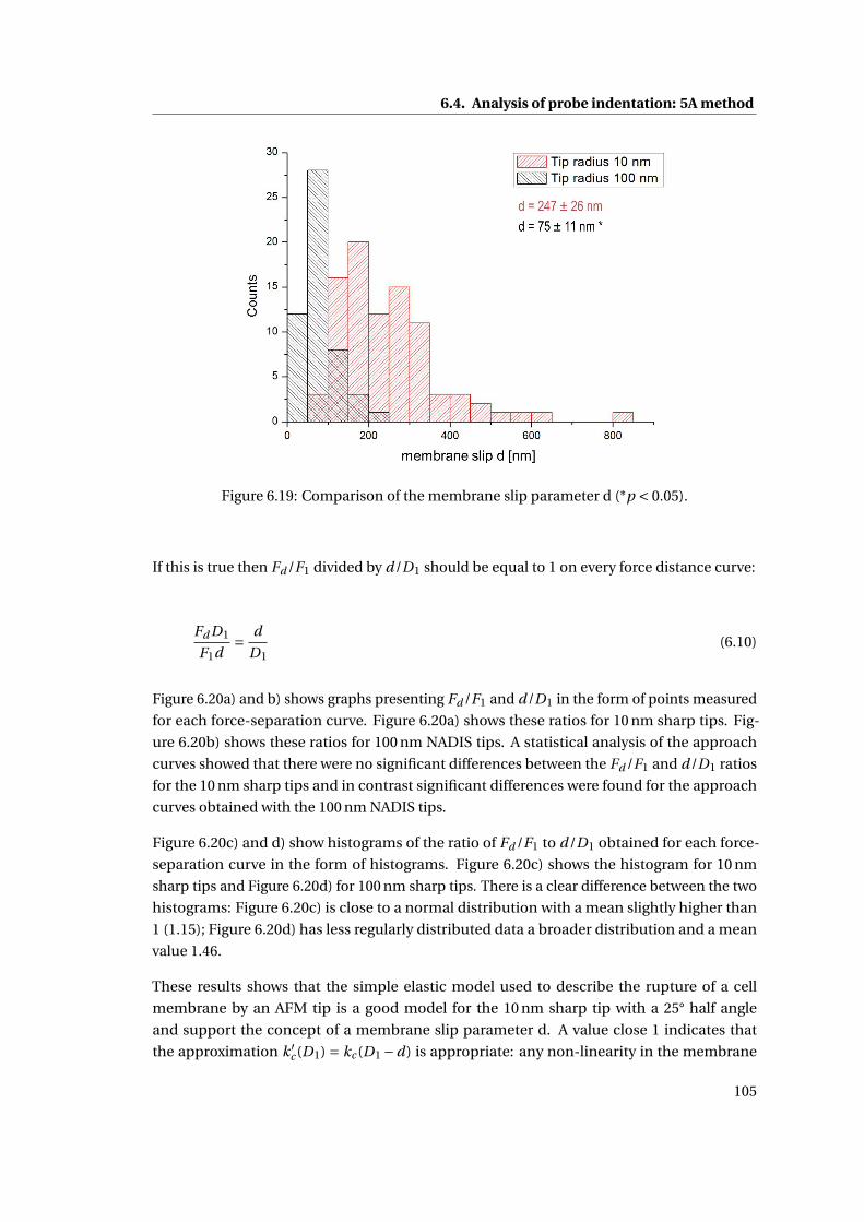
6.4. Analysis of probe indentation: 5A method
Figure 6.19: Comparison of the membrane slip parameter d (*p < 0.05).
If this is true then Fd /F1 divided by d/D1 should be equal to 1 on every force distance curve:
Fd D1
F1d= d
D1(6.10)
Figure 6.20a) and b) shows graphs presenting Fd /F1 and d/D1 in the form of points measured
for each force-separation curve. Figure 6.20a) shows these ratios for 10 nm sharp tips. Fig-
ure 6.20b) shows these ratios for 100 nm NADIS tips. A statistical analysis of the approach
curves showed that there were no significant differences between the Fd /F1 and d/D1 ratios
for the 10 nm sharp tips and in contrast significant differences were found for the approach
curves obtained with the 100 nm NADIS tips.
Figure 6.20c) and d) show histograms of the ratio of Fd /F1 to d/D1 obtained for each force-
separation curve in the form of histograms. Figure 6.20c) shows the histogram for 10 nm
sharp tips and Figure 6.20d) for 100 nm sharp tips. There is a clear difference between the two
histograms: Figure 6.20c) is close to a normal distribution with a mean slightly higher than
1 (1.15); Figure 6.20d) has less regularly distributed data a broader distribution and a mean
value 1.46.
These results shows that the simple elastic model used to describe the rupture of a cell
membrane by an AFM tip is a good model for the 10 nm sharp tip with a 25° half angle
and support the concept of a membrane slip parameter d. A value close 1 indicates that
the approximation k ′c (D1) = kc (D1 −d) is appropriate: any non-linearity in the membrane
105
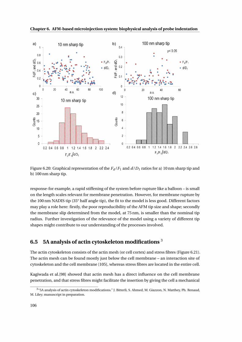
Chapter 6. AFM-based microinjection system: biophysical analysis of probe indentation
Figure 6.20: Graphical representation of the Fd /F1 and d/D1 ratios for a) 10 nm sharp tip andb) 100 nm sharp tip.
response-for example, a rapid stiffening of the system before rupture like a balloon – is small
on the length scales relevant for membrane penetration. However, for membrane rupture by
the 100 nm NADIS tip (35° half angle tip), the fit to the model is less good. Different factors
may play a role here: firstly, the poor reproducibility of the AFM tip size and shape; secondly
the membrane slip determined from the model, at 75 nm, is smaller than the nominal tip
radius. Further investigation of the relevance of the model using a variety of different tip
shapes might contribute to our understanding of the processes involved.
6.5 5A analysis of actin cytoskeleton modifications 3
The actin cytoskeleton consists of the actin mesh (or cell cortex) and stress fibres (Figure 6.21).
The actin mesh can be found mostly just below the cell membrane – an interaction site of
cytoskeleton and the cell membrane [105], whereas stress fibres are located in the entire cell.
Kagiwada et al.[98] showed that actin mesh has a direct influence on the cell membrane
penetration, and that stress fibres might facilitate the insertion by giving the cell a mechanical
3“5A analysis of actin cytoskeleton modifications.” J. Bitterli, S. Ahmed, M. Giazzon, N. Matthey, Ph. Renaud,M. Liley; manuscript in preparation.
106
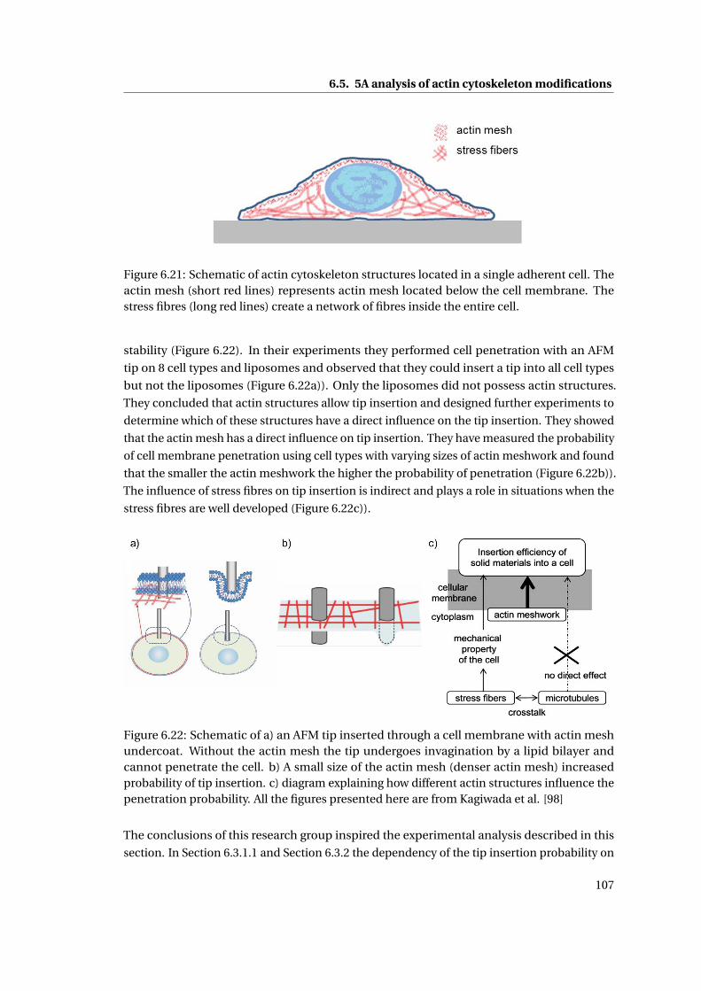
6.5. 5A analysis of actin cytoskeleton modifications
Figure 6.21: Schematic of actin cytoskeleton structures located in a single adherent cell. Theactin mesh (short red lines) represents actin mesh located below the cell membrane. Thestress fibres (long red lines) create a network of fibres inside the entire cell.
stability (Figure 6.22). In their experiments they performed cell penetration with an AFM
tip on 8 cell types and liposomes and observed that they could insert a tip into all cell types
but not the liposomes (Figure 6.22a)). Only the liposomes did not possess actin structures.
They concluded that actin structures allow tip insertion and designed further experiments to
determine which of these structures have a direct influence on the tip insertion. They showed
that the actin mesh has a direct influence on tip insertion. They have measured the probability
of cell membrane penetration using cell types with varying sizes of actin meshwork and found
that the smaller the actin meshwork the higher the probability of penetration (Figure 6.22b)).
The influence of stress fibres on tip insertion is indirect and plays a role in situations when the
stress fibres are well developed (Figure 6.22c)).
Figure 6.22: Schematic of a) an AFM tip inserted through a cell membrane with actin meshundercoat. Without the actin mesh the tip undergoes invagination by a lipid bilayer andcannot penetrate the cell. b) A small size of the actin mesh (denser actin mesh) increasedprobability of tip insertion. c) diagram explaining how different actin structures influence thepenetration probability. All the figures presented here are from Kagiwada et al. [98]
The conclusions of this research group inspired the experimental analysis described in this
section. In Section 6.3.1.1 and Section 6.3.2 the dependency of the tip insertion probability on
107
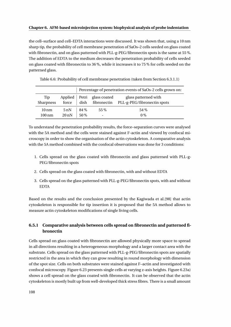
Chapter 6. AFM-based microinjection system: biophysical analysis of probe indentation
the cell–surface and cell–EDTA interactions were discussed. It was shown that, using a 10 nm
sharp tip, the probability of cell membrane penetration of SaOs–2 cells seeded on glass coated
with fibronectin, and on glass patterned with PLL-g-PEG/fibronectin spots is the same at 55 %.
The addition of EDTA to the medium decreases the penetration probability of cells seeded
on glass coated with fibronectin to 36 %, while it increases it to 75 % for cells seeded on the
patterned glass.
Table 6.6: Probability of cell membrane penetration (taken from Section 6.3.1.1)
Percentage of penetration events of SaOs-2 cells grown on:
Tip Applied Petri glass coated glass patterned withSharpness force dish fibronectin PLL-g-PEG/fibronectin spots
10 nm 5 nN 84 % 55 % 54 %100 nm 20 nN 50 % - 0 %
To understand the penetration probability results, the force–separation curves were analysed
with the 5A method and the cells were stained against F-actin and viewed by confocal mi-
croscopy in order to show the organisation of the actin cytoskeleton. A comparative analysis
with the 5A method combined with the confocal observations was done for 3 conditions:
1. Cells spread on the glass coated with fibronectin and glass patterned with PLL-g-
PEG/fibronectin spots
2. Cells spread on the glass coated with fibronectin, with and without EDTA
3. Cells spread on the glass patterned with PLL-g-PEG/fibronectin spots, with and without
EDTA
Based on the results and the conclusion presented by the Kagiwada et al.[98] that actin
cytoskeleton is responsible for tip insertion it is proposed that the 5A method allows to
measure actin cytoskeleton modifications of single living cells.
6.5.1 Comparative analysis between cells spread on fibronectin and patterned fi-bronectin
Cells spread on glass coated with fibronectin are allowed physically more space to spread
in all directions resulting in a heterogeneous morphology and a larger contact area with the
substrate. Cells spread on the glass patterned with PLL-g-PEG/fibronectin spots are spatially
restricted in the area in which they can grow resulting in round morphology with dimension
of the spot size. Cells on both substrates were stained against F–actin and investigated with
confocal microscopy. Figure 6.23 presents single cells at varying z-axis heights. Figure 6.23a)
shows a cell spread on the glass coated with fibronectin. It can be observed that the actin
cytoskeleton is mostly built up from well-developed thick stress fibres. There is a small amount
108
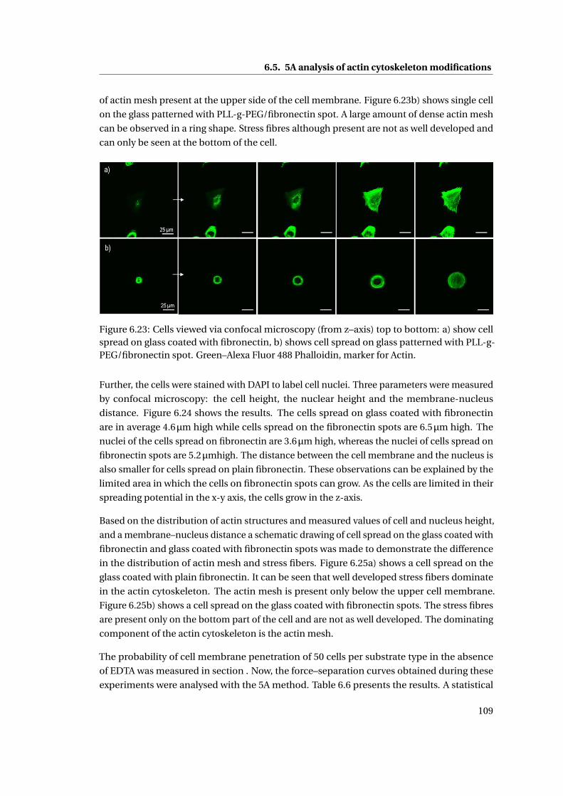
6.5. 5A analysis of actin cytoskeleton modifications
of actin mesh present at the upper side of the cell membrane. Figure 6.23b) shows single cell
on the glass patterned with PLL-g-PEG/fibronectin spot. A large amount of dense actin mesh
can be observed in a ring shape. Stress fibres although present are not as well developed and
can only be seen at the bottom of the cell.
Figure 6.23: Cells viewed via confocal microscopy (from z–axis) top to bottom: a) show cellspread on glass coated with fibronectin, b) shows cell spread on glass patterned with PLL-g-PEG/fibronectin spot. Green–Alexa Fluor 488 Phalloidin, marker for Actin.
Further, the cells were stained with DAPI to label cell nuclei. Three parameters were measured
by confocal microscopy: the cell height, the nuclear height and the membrane-nucleus
distance. Figure 6.24 shows the results. The cells spread on glass coated with fibronectin
are in average 4.6µm high while cells spread on the fibronectin spots are 6.5µm high. The
nuclei of the cells spread on fibronectin are 3.6µm high, whereas the nuclei of cells spread on
fibronectin spots are 5.2µmhigh. The distance between the cell membrane and the nucleus is
also smaller for cells spread on plain fibronectin. These observations can be explained by the
limited area in which the cells on fibronectin spots can grow. As the cells are limited in their
spreading potential in the x-y axis, the cells grow in the z-axis.
Based on the distribution of actin structures and measured values of cell and nucleus height,
and a membrane–nucleus distance a schematic drawing of cell spread on the glass coated with
fibronectin and glass coated with fibronectin spots was made to demonstrate the difference
in the distribution of actin mesh and stress fibers. Figure 6.25a) shows a cell spread on the
glass coated with plain fibronectin. It can be seen that well developed stress fibers dominate
in the actin cytoskeleton. The actin mesh is present only below the upper cell membrane.
Figure 6.25b) shows a cell spread on the glass coated with fibronectin spots. The stress fibres
are present only on the bottom part of the cell and are not as well developed. The dominating
component of the actin cytoskeleton is the actin mesh.
The probability of cell membrane penetration of 50 cells per substrate type in the absence
of EDTA was measured in section . Now, the force–separation curves obtained during these
experiments were analysed with the 5A method. Table 6.6 presents the results. A statistical
109
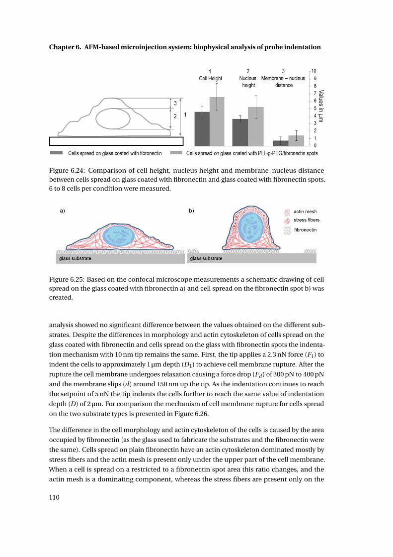
Chapter 6. AFM-based microinjection system: biophysical analysis of probe indentation
Figure 6.24: Comparison of cell height, nucleus height and membrane–nucleus distancebetween cells spread on glass coated with fibronectin and glass coated with fibronectin spots.6 to 8 cells per condition were measured.
Figure 6.25: Based on the confocal microscope measurements a schematic drawing of cellspread on the glass coated with fibronectin a) and cell spread on the fibronectin spot b) wascreated.
analysis showed no significant difference between the values obtained on the different sub-
strates. Despite the differences in morphology and actin cytoskeleton of cells spread on the
glass coated with fibronectin and cells spread on the glass with fibronectin spots the indenta-
tion mechanism with 10 nm tip remains the same. First, the tip applies a 2.3 nN force (F1) to
indent the cells to approximately 1µm depth (D1) to achieve cell membrane rupture. After the
rupture the cell membrane undergoes relaxation causing a force drop (Fd ) of 300 pN to 400 pN
and the membrane slips (d) around 150 nm up the tip. As the indentation continues to reach
the setpoint of 5 nN the tip indents the cells further to reach the same value of indentation
depth (D) of 2µm. For comparison the mechanism of cell membrane rupture for cells spread
on the two substrate types is presented in Figure 6.26.
The difference in the cell morphology and actin cytoskeleton of the cells is caused by the area
occupied by fibronectin (as the glass used to fabricate the substrates and the fibronectin were
the same). Cells spread on plain fibronectin have an actin cytoskeleton dominated mostly by
stress fibers and the actin mesh is present only under the upper part of the cell membrane.
When a cell is spread on a restricted to a fibronectin spot area this ratio changes, and the
actin mesh is a dominating component, whereas the stress fibers are present only on the
110
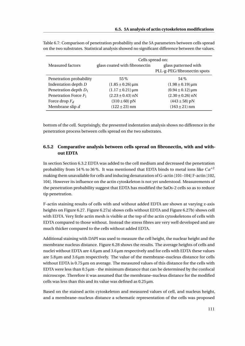
6.5. 5A analysis of actin cytoskeleton modifications
Table 6.7: Comparison of penetration probability and the 5A parameters between cells spreadon the two substrates. Statistical analysis showed no significant difference between the values.
Cells spread on:Measured factors glass coated with fibronectin glass patterned with
PLL-g-PEG/fibronectin spots
Penetration probability 55 % 54 %Indentation depth D (1.85±0.26)µm (1.98±0.19)µmPenetration depth D1 (1.17±0.21)µm (0.94±0.12)µmPenetration Force F1 (2.23±0.43) nN (2.30±0.26) nNForce drop Fd (310±60) pN (443±58) pNMembrane slip d (122±23) nm (163±21) nm
bottom of the cell. Surprisingly, the presented indentation analysis shows no difference in the
penetration process between cells spread on the two substrates.
6.5.2 Comparative analysis between cells spread on fibronectin, with and with-out EDTA
In section Section 6.3.2 EDTA was added to the cell medium and decreased the penetration
probability from 54 % to 36 %. It was mentioned that EDTA binds to metal ions like C a+2
making them unavailable for cells and inducing denaturation of G–actin [101–104] F-actin [102,
104]. However its influence on the actin cytoskeleton is not yet understood. Measurements of
the penetration probability suggest that EDTA has modified the SaOs-2 cells so as to reduce
tip penetration.
F-actin staining results of cells with and without added EDTA are shown at varying z-axis
heights on Figure 6.27. Figure 6.27a) shows cells without EDTA and Figure 6.27b) shows cell
with EDTA. Very little actin mesh is visible at the top of the actin cytoskeletons of cells with
EDTA compared to those without. Instead the stress fibres are very well developed and are
much thicker compared to the cells without added EDTA.
Additional staining with DAPI was used to measure the cell height, the nuclear height and the
membrane nucleus distance. Figure 6.28 shows the results. The average heights of cells and
nuclei without EDTA are 4.6µm and 3.6µm respectively and for cells with EDTA these values
are 5.8µm and 3.6µm respectively. The value of the membrane–nucleus distance for cells
without EDTA is 0.75µm on average. The measured values of this distance for the cells with
EDTA were less than 0.5µm - the minimum distance that can be determined by the confocal
microscope. Therefore it was assumed that the membrane–nucleus distance for the modified
cells was less than this and its value was defined as 0.25µm.
Based on the stained actin cytoskeleton and measured values of cell, and nucleus height,
and a membrane–nucleus distance a schematic representation of the cells was proposed
111
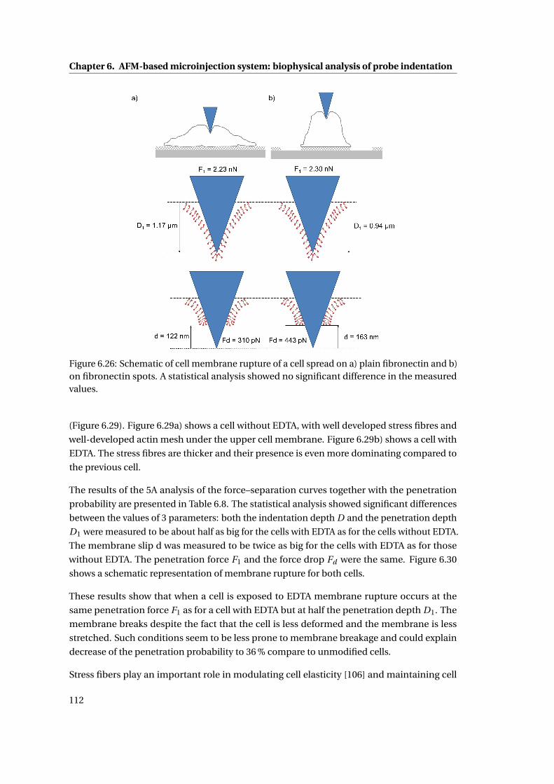
Chapter 6. AFM-based microinjection system: biophysical analysis of probe indentation
Figure 6.26: Schematic of cell membrane rupture of a cell spread on a) plain fibronectin and b)on fibronectin spots. A statistical analysis showed no significant difference in the measuredvalues.
(Figure 6.29). Figure 6.29a) shows a cell without EDTA, with well developed stress fibres and
well-developed actin mesh under the upper cell membrane. Figure 6.29b) shows a cell with
EDTA. The stress fibres are thicker and their presence is even more dominating compared to
the previous cell.
The results of the 5A analysis of the force–separation curves together with the penetration
probability are presented in Table 6.8. The statistical analysis showed significant differences
between the values of 3 parameters: both the indentation depth D and the penetration depth
D1 were measured to be about half as big for the cells with EDTA as for the cells without EDTA.
The membrane slip d was measured to be twice as big for the cells with EDTA as for those
without EDTA. The penetration force F1 and the force drop Fd were the same. Figure 6.30
shows a schematic representation of membrane rupture for both cells.
These results show that when a cell is exposed to EDTA membrane rupture occurs at the
same penetration force F1 as for a cell with EDTA but at half the penetration depth D1. The
membrane breaks despite the fact that the cell is less deformed and the membrane is less
stretched. Such conditions seem to be less prone to membrane breakage and could explain
decrease of the penetration probability to 36 % compare to unmodified cells.
Stress fibers play an important role in modulating cell elasticity [106] and maintaining cell
112
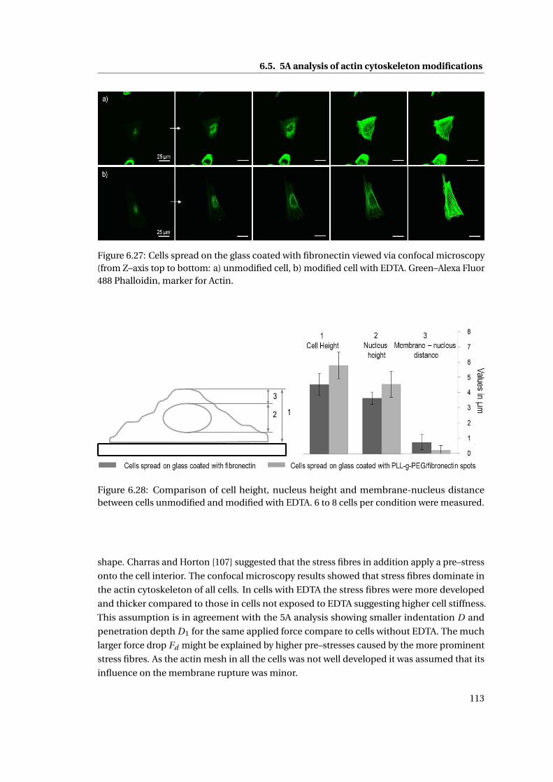
6.5. 5A analysis of actin cytoskeleton modifications
Figure 6.27: Cells spread on the glass coated with fibronectin viewed via confocal microscopy(from Z–axis top to bottom: a) unmodified cell, b) modified cell with EDTA. Green–Alexa Fluor488 Phalloidin, marker for Actin.
Figure 6.28: Comparison of cell height, nucleus height and membrane-nucleus distancebetween cells unmodified and modified with EDTA. 6 to 8 cells per condition were measured.
shape. Charras and Horton [107] suggested that the stress fibres in addition apply a pre–stress
onto the cell interior. The confocal microscopy results showed that stress fibres dominate in
the actin cytoskeleton of all cells. In cells with EDTA the stress fibres were more developed
and thicker compared to those in cells not exposed to EDTA suggesting higher cell stiffness.
This assumption is in agreement with the 5A analysis showing smaller indentation D and
penetration depth D1 for the same applied force compare to cells without EDTA. The much
larger force drop Fd might be explained by higher pre–stresses caused by the more prominent
stress fibres. As the actin mesh in all the cells was not well developed it was assumed that its
influence on the membrane rupture was minor.
113
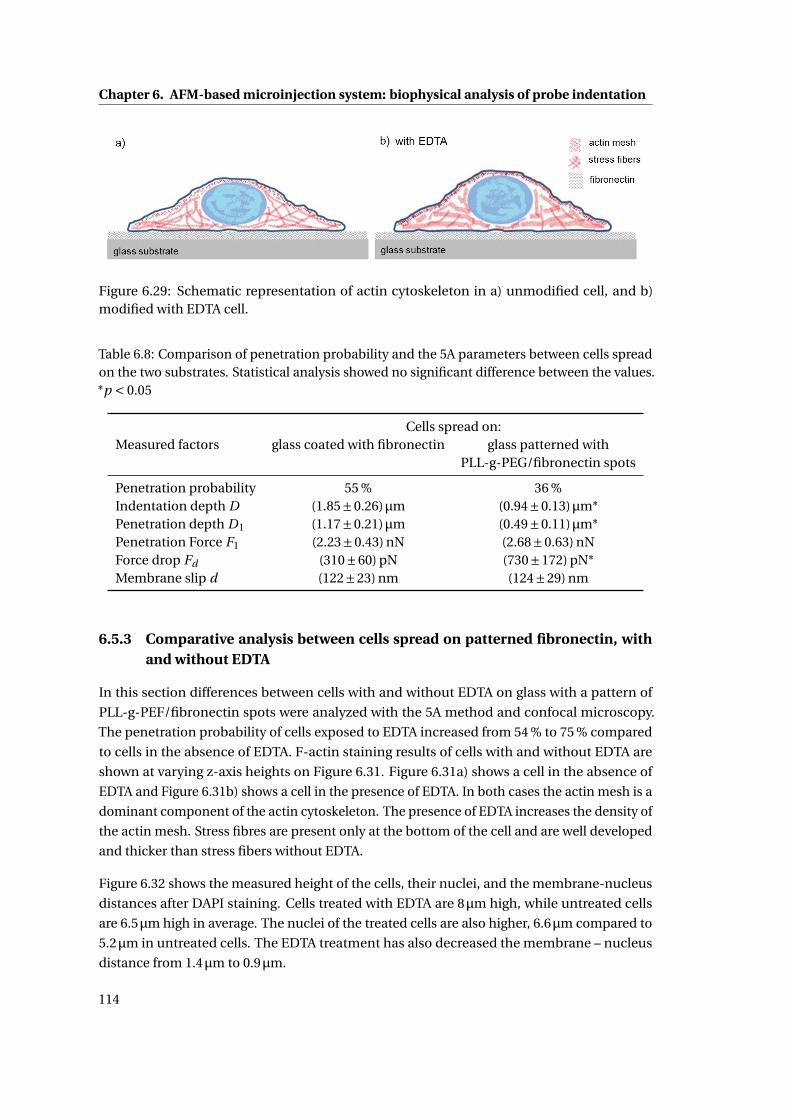
Chapter 6. AFM-based microinjection system: biophysical analysis of probe indentation
Figure 6.29: Schematic representation of actin cytoskeleton in a) unmodified cell, and b)modified with EDTA cell.
Table 6.8: Comparison of penetration probability and the 5A parameters between cells spreadon the two substrates. Statistical analysis showed no significant difference between the values.*p < 0.05
Cells spread on:Measured factors glass coated with fibronectin glass patterned with
PLL-g-PEG/fibronectin spots
Penetration probability 55 % 36 %Indentation depth D (1.85±0.26)µm (0.94±0.13)µm*Penetration depth D1 (1.17±0.21)µm (0.49±0.11)µm*Penetration Force F1 (2.23±0.43) nN (2.68±0.63) nNForce drop Fd (310±60) pN (730±172) pN*Membrane slip d (122±23) nm (124±29) nm
6.5.3 Comparative analysis between cells spread on patterned fibronectin, withand without EDTA
In this section differences between cells with and without EDTA on glass with a pattern of
PLL-g-PEF/fibronectin spots were analyzed with the 5A method and confocal microscopy.
The penetration probability of cells exposed to EDTA increased from 54 % to 75 % compared
to cells in the absence of EDTA. F-actin staining results of cells with and without EDTA are
shown at varying z-axis heights on Figure 6.31. Figure 6.31a) shows a cell in the absence of
EDTA and Figure 6.31b) shows a cell in the presence of EDTA. In both cases the actin mesh is a
dominant component of the actin cytoskeleton. The presence of EDTA increases the density of
the actin mesh. Stress fibres are present only at the bottom of the cell and are well developed
and thicker than stress fibers without EDTA.
Figure 6.32 shows the measured height of the cells, their nuclei, and the membrane-nucleus
distances after DAPI staining. Cells treated with EDTA are 8µm high, while untreated cells
are 6.5µm high in average. The nuclei of the treated cells are also higher, 6.6µm compared to
5.2µm in untreated cells. The EDTA treatment has also decreased the membrane – nucleus
distance from 1.4µm to 0.9µm.
114
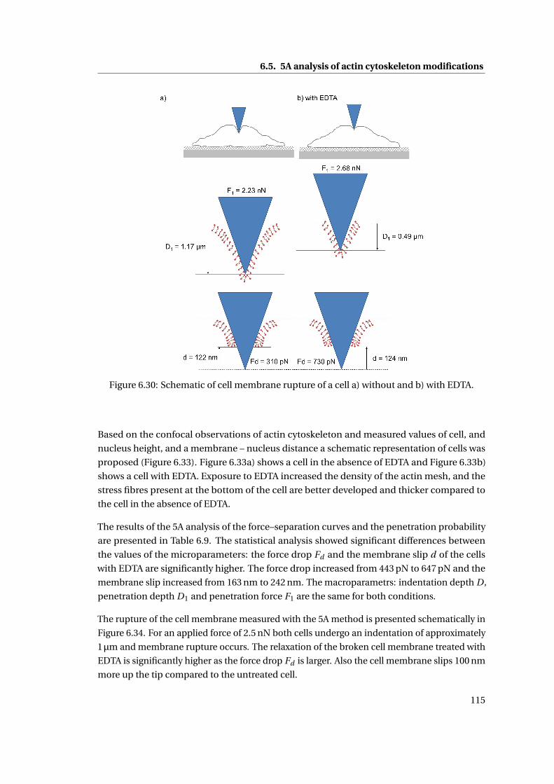
6.5. 5A analysis of actin cytoskeleton modifications
Figure 6.30: Schematic of cell membrane rupture of a cell a) without and b) with EDTA.
Based on the confocal observations of actin cytoskeleton and measured values of cell, and
nucleus height, and a membrane – nucleus distance a schematic representation of cells was
proposed (Figure 6.33). Figure 6.33a) shows a cell in the absence of EDTA and Figure 6.33b)
shows a cell with EDTA. Exposure to EDTA increased the density of the actin mesh, and the
stress fibres present at the bottom of the cell are better developed and thicker compared to
the cell in the absence of EDTA.
The results of the 5A analysis of the force–separation curves and the penetration probability
are presented in Table 6.9. The statistical analysis showed significant differences between
the values of the microparameters: the force drop Fd and the membrane slip d of the cells
with EDTA are significantly higher. The force drop increased from 443 pN to 647 pN and the
membrane slip increased from 163 nm to 242 nm. The macroparametrs: indentation depth D ,
penetration depth D1 and penetration force F1 are the same for both conditions.
The rupture of the cell membrane measured with the 5A method is presented schematically in
Figure 6.34. For an applied force of 2.5 nN both cells undergo an indentation of approximately
1µm and membrane rupture occurs. The relaxation of the broken cell membrane treated with
EDTA is significantly higher as the force drop Fd is larger. Also the cell membrane slips 100 nm
more up the tip compared to the untreated cell.
115
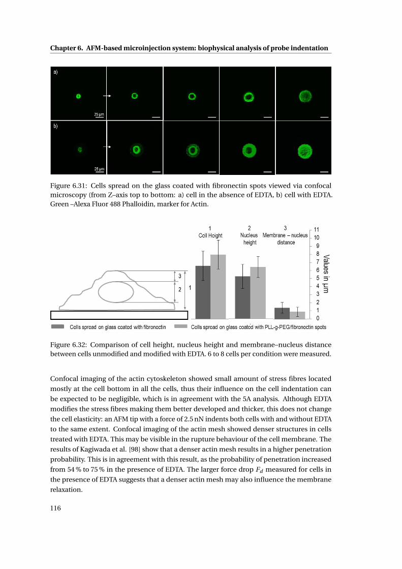
Chapter 6. AFM-based microinjection system: biophysical analysis of probe indentation
Figure 6.31: Cells spread on the glass coated with fibronectin spots viewed via confocalmicroscopy (from Z–axis top to bottom: a) cell in the absence of EDTA, b) cell with EDTA.Green –Alexa Fluor 488 Phalloidin, marker for Actin.
Figure 6.32: Comparison of cell height, nucleus height and membrane–nucleus distancebetween cells unmodified and modified with EDTA. 6 to 8 cells per condition were measured.
Confocal imaging of the actin cytoskeleton showed small amount of stress fibres located
mostly at the cell bottom in all the cells, thus their influence on the cell indentation can
be expected to be negligible, which is in agreement with the 5A analysis. Although EDTA
modifies the stress fibres making them better developed and thicker, this does not change
the cell elasticity: an AFM tip with a force of 2.5 nN indents both cells with and without EDTA
to the same extent. Confocal imaging of the actin mesh showed denser structures in cells
treated with EDTA. This may be visible in the rupture behaviour of the cell membrane. The
results of Kagiwada et al. [98] show that a denser actin mesh results in a higher penetration
probability. This is in agreement with this result, as the probability of penetration increased
from 54 % to 75 % in the presence of EDTA. The larger force drop Fd measured for cells in
the presence of EDTA suggests that a denser actin mesh may also influence the membrane
relaxation.
116
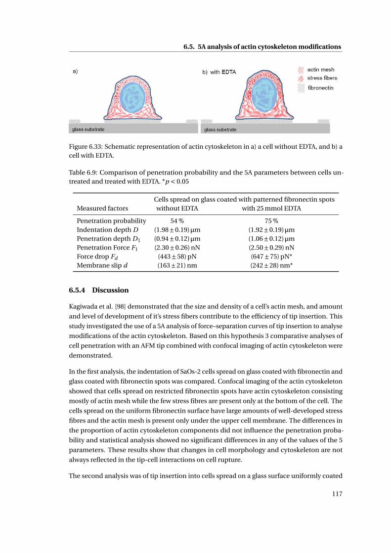
6.5. 5A analysis of actin cytoskeleton modifications
Figure 6.33: Schematic representation of actin cytoskeleton in a) a cell without EDTA, and b) acell with EDTA.
Table 6.9: Comparison of penetration probability and the 5A parameters between cells un-treated and treated with EDTA. *p < 0.05
Cells spread on glass coated with patterned fibronectin spotsMeasured factors without EDTA with 25 mmol EDTA
Penetration probability 54 % 75 %Indentation depth D (1.98±0.19)µm (1.92±0.19)µmPenetration depth D1 (0.94±0.12)µm (1.06±0.12)µmPenetration Force F1 (2.30±0.26) nN (2.50±0.29) nNForce drop Fd (443±58) pN (647±75) pN*Membrane slip d (163±21) nm (242±28) nm*
6.5.4 Discussion
Kagiwada et al. [98] demonstrated that the size and density of a cell’s actin mesh, and amount
and level of development of it’s stress fibers contribute to the efficiency of tip insertion. This
study investigated the use of a 5A analysis of force–separation curves of tip insertion to analyse
modifications of the actin cytoskeleton. Based on this hypothesis 3 comparative analyses of
cell penetration with an AFM tip combined with confocal imaging of actin cytoskeleton were
demonstrated.
In the first analysis, the indentation of SaOs-2 cells spread on glass coated with fibronectin and
glass coated with fibronectin spots was compared. Confocal imaging of the actin cytoskeleton
showed that cells spread on restricted fibronectin spots have actin cytoskeleton consisting
mostly of actin mesh while the few stress fibres are present only at the bottom of the cell. The
cells spread on the uniform fibronectin surface have large amounts of well-developed stress
fibres and the actin mesh is present only under the upper cell membrane. The differences in
the proportion of actin cytoskeleton components did not influence the penetration proba-
bility and statistical analysis showed no significant differences in any of the values of the 5
parameters. These results show that changes in cell morphology and cytoskeleton are not
always reflected in the tip-cell interactions on cell rupture.
The second analysis was of tip insertion into cells spread on a glass surface uniformly coated
117
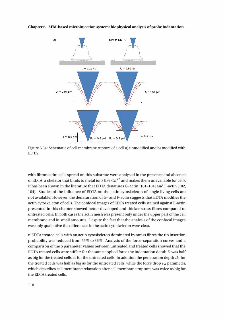
Chapter 6. AFM-based microinjection system: biophysical analysis of probe indentation
Figure 6.34: Schematic of cell membrane rupture of a cell a) unmodified and b) modified withEDTA.
with fibronectin: cells spread on this substrate were analysed in the presence and absence
of EDTA, a chelator that binds to metal ions like C a+2 and makes them unavailable for cells.
It has been shown in the literature that EDTA denatures G–actin [101–104] and F-actin [102,
104]. Studies of the influence of EDTA on the actin cytoskeleton of single living cells are
not available. However, the denaturation of G– and F-actin suggests that EDTA modifies the
actin cytoskeleton of cells. The confocal images of EDTA treated cells stained against F-actin
presented in this chapter showed better developed and thicker stress fibres compared to
untreated cells. In both cases the actin mesh was present only under the upper part of the cell
membrane and in small amounts. Despite the fact that the analysis of the confocal images
was only qualitative the differences in the actin cytoskeleton were clear.
n EDTA treated cells with an actin cytoskeleton dominated by stress fibres the tip insertion
probability was reduced from 55 % to 36 %. Analysis of the force–separation curves and a
comparison of the 5 parameter values between untreated and treated cells showed that the
EDTA treated cells were stiffer: for the same applied force the indentation depth D was half
as big for the treated cells as for the untreated cells. In addition the penetration depth D1 for
the treated cells was half as big as for the untreated cells, while the force drop Fd parameter,
which describes cell membrane relaxation after cell membrane rupture, was twice as big for
the EDTA treated cells.
118
6.6. General discussion
It has been shown that the presence of F-actin in cells influences cell elasticity [106, 107] and
causes a pre-stress onto the cell interior [107, 108]. It is thus easy to conceive that the increase
in the presence of stress fibres could lead to the observed increase in cell stiffness. The reduced
penetration depth D1 can also be associated with the increased cell stiffness and the fact that
the penetration force F1 remains unchanged. Any explanation of the higher value of the force
drop Fd , and the reduced probability of penetration is, however, more speculative.
The third analysis concerned tip insertion on cells spread on fibronectin spots on a glass
surface: cells in the presence and absence of EDTA were compared. Confocal imaging of the
actin cytoskeleton of cells spread on fibronectin spots showed that in such conditions stress
fibres are present only on the bottom of the cells and that the actin mesh is the dominant
component. EDTA treated cells had denser actin mesh compared to untreated cells.
Analysis of the force–separation curves and comparison of the 5 parameters showed no
significant difference between the macroparameters: indentation depth D , penetration depth
D1 and penetration force F1. However, a statistical analysis showed significant differences
between microparameters: the force drop Fd and the membrane slip d . Both parameters had
higher values for EDTA treated cells, indicating larger membrane relaxation and membrane
slippage after rupture. The differences in the microparameters was attributed to the EDTA
modifications of the actin mesh: a denser actin mesh facilitated tip insertion (in agreement
with Kagiwada et al. [98]), membrane slip up the tip and membrane relaxation.
The 5A method presented here can be used to obtain more information about the mechanical
characteristics of the tip insertion process. The data presented here suggest the potential of
this approach while underlining the complexity of all aspects of the living cell. They are an
open invitation to the interested scientist to take this approach further.
One interesting extension of this work would be the investigation of healthy and unhealthy
cells using cell penetration experiments and the 5A analysis. In particular, a number of specific
diseases have been linked to actin cytoskeleton defects [109]. For example, dystrophic muscle
cells, “due to the defects in dystrophin’s ability to link the actin to cell surface” cause muscular
dystrophy diseases.
6.6 General discussion
6.6.1 Determination of tip insertion
A hypothesis was proposed for determining when an AFM tip has penetrated a cell membrane
based on the assumption that penetration of the cell membrane occurs when a force drop and
an elasticity change occur at the same time on a force-separation (f-s) curve. To support this
hypothesis cell indentation experiments were performed with 10 nm and 100 nm sharp tips
and forces were applied on cells ranging from 1 nN to 18 nN. After analysis of the f-s curves,
the curves were classified into 4 types:
119
Chapter 6. AFM-based microinjection system: biophysical analysis of probe indentation
1. Type I: F-s curves without a force drop, known in literature as indentation curves
2. Type II: F-s curves with a force drop and no change in elasticity
3. Type III: F-s curves with a force drop and a decrease in elastic modulus after the force
drop
4. Type IV: F-s curves with a force drop and an increase in elastic modulus after the force
drop
For both tip sharpness the number of f-s curves with a force drop increases when the maximum
force applied on a cell increases. Since, intuitively, it is expected that the harder the tip presses
on a cell membrane the more probable is the cell penetration, it can be assumed that the force
drop can be related to membrane rupture (Figure 6.6).
It can be also expected that when a tip passes through a stiff cell membrane into a softer
cell cytoplasm an elasticity change should occur as well. Analysis of the elasticity change
on the f-s curves with force drop showed that an elasticity change occurred on most of the
curves. For the 10 nm sharp tip and the highest force setpoint of 5 nN, 90 % of the f-s curves
had characteristic force drops from which only 6.6 % of the curves showed no elasticity change.
For the 100 nm NADIS tip and the highest force setpoint of 18 nN, 54 % of the f-s curves had
force drops from which 18.5 % showed no elasticity change. The presence of a force drop with
no elasticity change might for example be due to interactions of a tip with proteins associated
with the cell membrane.
Within the f-s curves with a force drop and a change in elasticity, two types of elasticity change
were observed, first, when the elasticity decreases after the tip penetrates the cell (type III
f-s curves), and second, when the elasticity increases once the tip is inside the cell (type IV
f-s curves). A decrease in the elasticity could be explained by AFM tip breaking a stiff cell
membrane and entering in contact with a softer cytoplasm. The f-s curves analysis show that
the number of type III f-s curves have tendency to increase with increasing force setpoint for
both tip sharpness.
An increase in elasticity (type IV f-s curves) suggests that after the membrane breakage the tip
has encountered a stiffer component of the cell. Such a component might be, for example,
the nucleus or another organelle. It has been shown [110] that the nucleus can be stiffer than
a cell. Thus, it could be possible that when an AFM tip ruptures a cell membrane, it comes
directly into contact with a stiff organelle. The percentage of type IV f-s curves is higher for the
100 nm NADIS tip (out of all the f-s curves with a force drop and a change in elasticity, 37 % of
the curves were type IV curves, compared to 10 nm sharp tip, where in total only 11 % of the
curves were classified as type IV), suggesting an influence of the tip sharpness on probability
of encountering a stiffer component of the cells after the penetration.
The analysis of the f-s curves for 10 nm and 100 nm sharp tips in terms of force drop and
elasticity change support the presented hypothesis. However they provide only indirect
120
6.6. General discussion
evidence. Further confirmation would be required, for example by injection of a fluorescent
dye into living cells using the NADIS probes. Comparison of the force-distance curves obtained
on successful injection into the cell with those obtained where no injection occurred would
show if the penetration was always associated with an elasticity change in the f-s curve.
6.6.2 Force-separation curves with multiple force drops
Within the f-s curves analysis, curves with multiple force drops were found. It was shown that
the number of force drop increases with the maximum applied force (Table 6.2). F-s curves
with multiple force drops have been already described in the literature [42, 45, 97]. The first
force drop is associated with membrane rupture; however origin of the other force drop is
not certain at the moment. Yokokawa et al. [97] suggested that presence of the second and
more force drops could be explained by penetration of the nuclear membrane. To confirm this
assumption a nuclear injection experiment could be carried out using for example the NADIS
probes. The injection into a cell of a fluorescent dye that stains the nucleus and an f-s curve
analysis of the successfully injected dye might show if the presence of the first and second
force drops is due to penetration of the cell membrane followed by the nuclear envelope.
Another possible explanation for the multiple force drops is slippage of the tip inside the cell.
It is possible that after penetration of the AFM tip into the cell, further indentation results in
enlarging of the opening of the membrane which could result in additional force drops on the
f-s curve as the membrane slips up the tip. This hypothesis might be tested using for example,
an AFM tip with different surface chemistries e.g. an antifouling layer to penetrate the cell
membrane and investigate the presence and characteristics of multiple force drops.
6.6.3 5A method
5 parameters were defined from a force–separation curve with a penetration peak. Four of
these parameters have already been mentioned in the literature: the indentation depth (D)
[97], the penetration depth (D1)[42] the penetration force (F1)[42], and the force drop (Fd )[41,
98]. The fifth parameter, the ‘membrane slip’ (d) has not yet been discussed in publications
on AFM/cell interactions.
A simple mechanical model was presented, based on the assumption that d represents the
movement of the cell membrane up the AFM tip during rupture of the membrane. In this
model the forces of the membrane on the tip are represented by a linear spring where it was
assumed that cell spring constant just before the cell penetration is the same as the cell spring
constant directly after the penetration (Figure 6.12).
Further, the 5 parameters were tested on f-s curves obtained on SaOSs-2 cells with 10 nm and
100 nm sharp tips. It was shown that the penetration force (F1) depends on the size of the tip
radius. The larger the radius the higher the force required to rupture a cell membrane. The
penetration depth (D1) does not depend on the tip size. It was measured that breakage of a
121
Chapter 6. AFM-based microinjection system: biophysical analysis of probe indentation
SaOs-2 cell membrane occurs at penetration depth D1 of approximately 1µm, and penetration
force F1 of 2.5 nN for 10 nm sharp tip and 4.4 nN for 100 nm sharp tip. The indentation depth
D , the penetration depth D1 and the penetration force F1 were here called macroparameters,
as they describe the behaviour of the entire cell upon a contact with the tip. The force drop Fd
and the membrane slip d were called microparameters, as they describe breakage of the cell
membrane.
It was shown that the force drop Fd and the membrane slip d depend on the geometry of the
tip. When the tip radius and the half tip angle are small (the 10 nm sharp tip had half angle tip
of (25°, the 100 nm sharp tip half angle tip of (35°) the values of the microparameters are high.
According to the simple mechanical model describing cell membrane rupture, the ratio of
Fd /F1 (force drop over penetration force) divided by ratio of d/D1 (membrane slip over
penetration depth) should be equal to 1. An analysis of this dependency for every f-s curve is
presented in Figure 6.20. This shows that the mechanical model is in very good agreement
with the results obtained with the 10 nmsharp tip, but that the agreement is less good for the
100 nm NADIS tip. This can be clearly seen from the histograms, where for the 10 nm sharp
tip most of the F d/F 1÷d/D1 values are close to 1, whereas for 100 nm sharp tip the values
are range from 1 to 1.6. The results suggest that the simple elastic model perfectly describes
rupture of a cell membrane with a sharp and narrow AFM tip. To confirm this assumption
further experiment would be required with tip radii of for example 20 nm, 50 nm and 80 nm
sharp tip. Another interesting point is the influence of the half angle tip on the membrane
rupture. In experiments presented here two tip sharpness with two different half tip angles
were used. More experiments would be required to investigate how variation of the half angle,
while keeping the same tip sharpness, is influencing the cell membrane penetration and if the
presented here model can be used to describe the penetration.
6.7 Conclusions
Three main aspects of mechanical cell membrane penetration were presented here: determi-
nation of tip insertion into a cell; dependence of the probability of penetration on tip geometry,
cell-substrate interactions and the presence of EDTA; biophysical analysis of the penetration.
To determine tip insertion the hypothesis was proposed that when an AFM tip breaks the
cell membrane and passes from outside the cell to inside of it a change in elastic modulus
should occur and that this change in elastic modulus should be observable in the force
separation curve. Indirect evidence of this hypothesis was provided through analysis of 350
force-separation curves obtained for 10 nm and 100 nm sharp tips with applied forces varying
from 1 nN to 18 nN. For most of the force-separation curves the peak was associated with
change in elastic modulus (in total, for 10 nm sharp tip 91.5 % f-s curves, and 77.8 % for 100 nm
sharp tip. Based on the hypothesis a specification of cell penetration with an AFM tip was
proposed: a force drop is considered to be present when its value is higher than 3 standard
deviation of the noise, and an elasticity change has to occur.
122
6.7. Conclusions
Based on this proposed specification, the probability of penetration of SaOs-2 cells was
measured for 10 nm and 100 nm sharp tips and three different substrates: a Petri dish, glass
uniformly coated with fibronectin and glass coated with patterned PLL-g-PEG/fibronectin.
For 10 nm sharp tips and an applied force of 5 nN the penetration probability of cells spread
on a Petri dish was 84 % and 55 % and 54 % when cells on the uniform fibronectin and on the
patterned PLL-g-PEG/fibronectin respectively. For 100 nm NADIS tips and an applied force of
20 nN the penetration probability of cells spread on a Petri dish was 50 % and on patterned
PLL-g-PEG/fibronectin was 0 %.
A biophysical analysis of cell membrane penetration was shown here using 5 parameters
obtained from a force-separation curve. Four parameters are known from the literature, the
fifth parameter-the membrane slip, was proposed based on a simple mechanical model. The
influence of the tip geometry on the different parameters was investigated with 10 nm and
100 nmsharp tips. It was shown that indentation depth, penetration force, force drop and
membrane slip depend on the tip sharpness and the penetration depth is independent of the
sharpness. An analysis of the Fd /F1 ÷d/D1 values, for 10 nm and 100 nm sharp tips, supports
the association of the fifth parameter with the slip of the membrane up the AFM tip during
rupture.
In conclusion, the success of cell penetration strongly depends on the tip geometry and the
surface on which the cell is spread. The biophysical analysis of the penetration gives insight
into the mechanical tip-cell interactions. This analysis will be of great use during microinjec-
tion experiments and will help to distinguish effects that due to the tip–cell interaction from
the effects caused by liquid delivery.
123

7 Quantification of single cell damage 1
Since AFM allows the interaction between the tip and the sample to be controlled precisely,
very little or no damage is expected to be done to the cell by the tip during penetration. To
confirm this assumption invasiveness of an AFM tip was investigated and will be described in
this chapter. Very few studies have been dedicated to investigating cell necrosis and apoptosis
due to breakage of the cell membrane with an AFM tip. Han et al.[50] showed that no cell
damage can be expected for a tip diameter smaller than 200 nm. This demonstration was
based on a single melanocyte cell. To form a better view on the possible tip invasiveness,
more studies with a significant number of cells is required. However experiments using larger
number of single cells are challenging, as every individual cell has to be first indented with an
AFM tip and a force-separation curve has to be recorded and analyzed in order to know if the
cell was penetrated or not. After the indentation of each cell, the sample with the cells has to be
checked for possible cell damage. If a cell is damaged, analysis of the force–separation curve
attributed to this cell will show whether the damage could be triggered by the tip penetration.
To study tip invasiveness on a large number of cells two methods were proposed:
1. When the cells are spread on a Petri dish
2. When the cells are spread on glass patterned fibronectin
With these methods invasiveness of tip insertion was investigated for two situations:
1. when the tip penetrates only the upper part of the cell (Figure 7.1a))
2. when the tip penetrates the cell entirely (Figure 7.1b))
amples with cells were investigated for possible damage either directly after the last cell was
indented with a tip, or 20 hours after the last indentation. By investigating cell damage directly
1„Quantification of cell damage.“ J. Bitterli, S. Ahmed, M. Giazzon, N. Matthey, Ph. Renaud, M. Liley;manuscript in preparation.
125
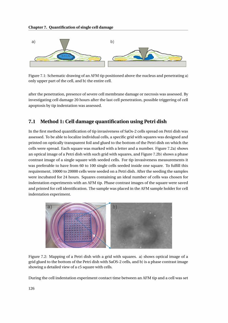
Chapter 7. Quantification of single cell damage
Figure 7.1: Schematic drawing of an AFM tip positioned above the nucleus and penetrating a)only upper part of the cell, and b) the entire cell.
after the penetration, presence of severe cell membrane damage or necrosis was assessed. By
investigating cell damage 20 hours after the last cell penetration, possible triggering of cell
apoptosis by tip indentation was assessed.
7.1 Method 1: Cell damage quantification using Petri dish
In the first method quantification of tip invasiveness of SaOs-2 cells spread on Petri dish was
assessed. To be able to localize individual cells, a specific grid with squares was designed and
printed on optically transparent foil and glued to the bottom of the Petri dish on which the
cells were spread. Each square was marked with a letter and a number. Figure 7.2a) shows
an optical image of a Petri dish with such grid with squares, and Figure 7.2b) shows a phase
contrast image of a single square with seeded cells. For tip invasiveness measurements it
was preferable to have from 60 to 100 single cells seeded inside one square. To fulfill this
requirement, 10000 to 20000 cells were seeded on a Petri dish. After the seeding the samples
were incubated for 24 hours. Squares containing an ideal number of cells was chosen for
indentation experiments with an AFM tip. Phase contrast images of the square were saved
and printed for cell identification. The sample was placed in the AFM sample holder for cell
indentation experiment.
Figure 7.2: Mapping of a Petri dish with a grid with squares. a) shows optical image of agrid glued to the bottom of the Petri dish with SaOS-2 cells, and b) is a phase contrast imageshowing a detailed view of a c5 square with cells.
During the cell indentation experiment contact time between an AFM tip and a cell was set
126
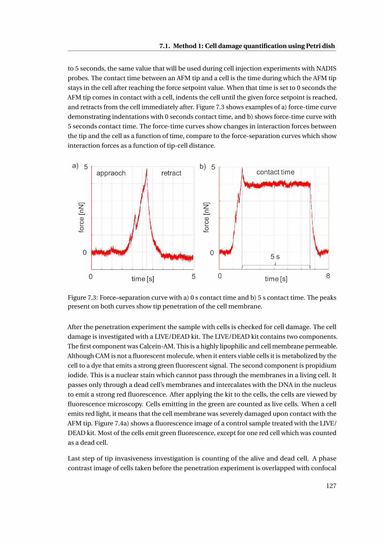
7.1. Method 1: Cell damage quantification using Petri dish
to 5 seconds, the same value that will be used during cell injection experiments with NADIS
probes. The contact time between an AFM tip and a cell is the time during which the AFM tip
stays in the cell after reaching the force setpoint value. When that time is set to 0 seconds the
AFM tip comes in contact with a cell, indents the cell until the given force setpoint is reached,
and retracts from the cell immediately after. Figure 7.3 shows examples of a) force-time curve
demonstrating indentations with 0 seconds contact time, and b) shows force-time curve with
5 seconds contact time. The force-time curves show changes in interaction forces between
the tip and the cell as a function of time, compare to the force-separation curves which show
interaction forces as a function of tip-cell distance.
Figure 7.3: Force–separation curve with a) 0 s contact time and b) 5 s contact time. The peakspresent on both curves show tip penetration of the cell membrane.
After the penetration experiment the sample with cells is checked for cell damage. The cell
damage is investigated with a LIVE/DEAD kit. The LIVE/DEAD kit contains two components.
The first component was Calcein-AM. This is a highly lipophilic and cell membrane permeable.
Although CAM is not a fluorescent molecule, when it enters viable cells it is metabolized by the
cell to a dye that emits a strong green fluorescent signal. The second component is propidium
iodide. This is a nuclear stain which cannot pass through the membranes in a living cell. It
passes only through a dead cell’s membranes and intercalates with the DNA in the nucleus
to emit a strong red fluorescence. After applying the kit to the cells, the cells are viewed by
fluorescence microscopy. Cells emitting in the green are counted as live cells. When a cell
emits red light, it means that the cell membrane was severely damaged upon contact with the
AFM tip. Figure 7.4a) shows a fluorescence image of a control sample treated with the LIVE/
DEAD kit. Most of the cells emit green fluorescence, except for one red cell which was counted
as a dead cell.
Last step of tip invasiveness investigation is counting of the alive and dead cell. A phase
contrast image of cells taken before the penetration experiment is overlapped with confocal
127
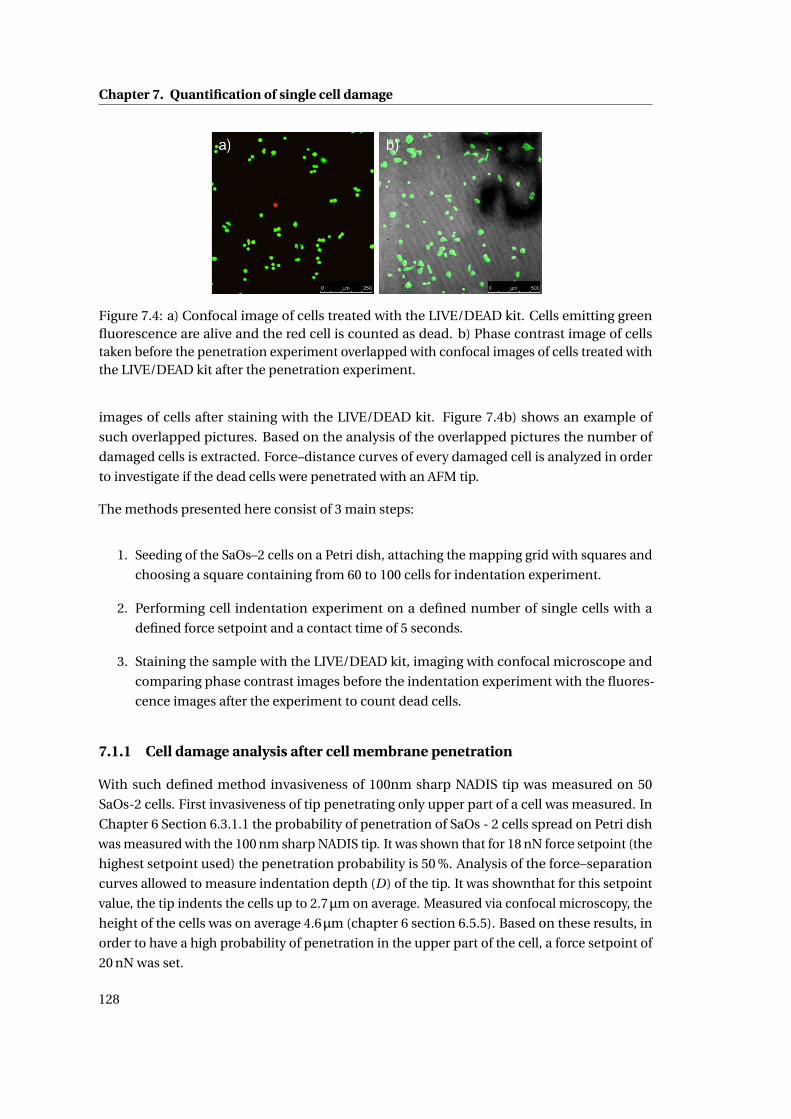
Chapter 7. Quantification of single cell damage
Figure 7.4: a) Confocal image of cells treated with the LIVE/DEAD kit. Cells emitting greenfluorescence are alive and the red cell is counted as dead. b) Phase contrast image of cellstaken before the penetration experiment overlapped with confocal images of cells treated withthe LIVE/DEAD kit after the penetration experiment.
images of cells after staining with the LIVE/DEAD kit. Figure 7.4b) shows an example of
such overlapped pictures. Based on the analysis of the overlapped pictures the number of
damaged cells is extracted. Force–distance curves of every damaged cell is analyzed in order
to investigate if the dead cells were penetrated with an AFM tip.
The methods presented here consist of 3 main steps:
1. Seeding of the SaOs–2 cells on a Petri dish, attaching the mapping grid with squares and
choosing a square containing from 60 to 100 cells for indentation experiment.
2. Performing cell indentation experiment on a defined number of single cells with a
defined force setpoint and a contact time of 5 seconds.
3. Staining the sample with the LIVE/DEAD kit, imaging with confocal microscope and
comparing phase contrast images before the indentation experiment with the fluores-
cence images after the experiment to count dead cells.
7.1.1 Cell damage analysis after cell membrane penetration
With such defined method invasiveness of 100nm sharp NADIS tip was measured on 50
SaOs-2 cells. First invasiveness of tip penetrating only upper part of a cell was measured. In
Chapter 6 Section 6.3.1.1 the probability of penetration of SaOs - 2 cells spread on Petri dish
was measured with the 100 nm sharp NADIS tip. It was shown that for 18 nN force setpoint (the
highest setpoint used) the penetration probability is 50 %. Analysis of the force–separation
curves allowed to measure indentation depth (D) of the tip. It was shownthat for this setpoint
value, the tip indents the cells up to 2.7µm on average. Measured via confocal microscopy, the
height of the cells was on average 4.6µm (chapter 6 section 6.5.5). Based on these results, in
order to have a high probability of penetration in the upper part of the cell, a force setpoint of
20 nN was set.
128

7.1. Method 1: Cell damage quantification using Petri dish
In order to investigate cell damage, each sample was treated with the LIVE/DEAD kit immedi-
ately preceding the last cell indentation. Total time needed to indent 50 cells is 3 hours, which
means that the first indented cell was stained 3 hours after, and the last cell, was stained 5
minutes after the indentation.
Preparation of the sample took place in sterile conditions, whereas cell indentation experiment
with an AFM and treatment with the kit were done in non-sterile conditions.
Figure 7.5 shows the results. A phase contrast image of cells before the indentation experiment
is overlapped with confocal images of cells treated after the experiment. Only cells emitting
green fluorescence are present. On the image 8 individual cells are highlighted and their
force-separation curves are demonstrated. 5 cells are shown as tip insertion examples, with
penetration peak marked with black arrow on each force-separation curve, and 3 cells are
shown as indentation examples. Two cells on the image marked with red circles do not emit
fluorescence signal. These cells were not indented during the experiment. Their absence was
probably caused by the sample treatment with the LIVE/DEAD kit, which required washing
steps.
Analysis of the force-separation curves showed that 28 cells were penetrated, from which 12
cells had more than one peak present.
Based on the overlapped images all the cell indented with an AFM tip survived, and managed
to repair their cell membranes before treatment with the LIVE/DEAD kit. Lack of cells emitting
red fluorescence is a proof that during the sample treatment cell membrane of the penetrated
cells was impermeable for propidium iodide.
To study cell death another sample with cells was prepared. After indentation of 50 cells with
the 100 nm sharp NADIS tip, the sample was placed in the incubator for 20 hours and then
treated with the LIVE/DEAD kit. Figure 7.6 shows the results. It can be seen that after 20
hours the number of cells increased and the cells changed their position which made the
cell identification very difficult. Cells marked with red circles were present before treatment
with the LIVE/DEAD kit. Their absence on the fluorescence images can be explained by
many factors: they were washed from the samples during treatments, or they died due to tip
indentation.
Obtained results showed that this method cannot be used to investigate tip invasiveness 20
hours after the indentation experiments. In order to perform such experiments a new method
was proposed.
129
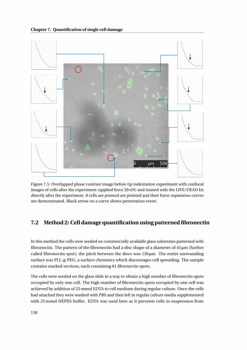
Chapter 7. Quantification of single cell damage
Figure 7.5: Overlapped phase contrast image before tip indentation experiment with confocalimages of cells after the experiment (applied force 20 nN) and treated with the LIVE/DEAD kitdirectly after the experiment. 8 cells are pointed are pointed and their force-separation curvesare demonstrated. Black arrow on a curve shows penetration event.
7.2 Method 2: Cell damage quantification using patterned fibronectin
In this method the cells were seeded on commercially available glass substrates patterned with
fibronectin. The pattern of the fibronectin had a disc shape of a diameter of 45µm (further
called fibronectin spot); the pitch between the discs was 130µm. The entire surrounding
surface was PLL-g-PEG, a surface chemistry which discourages cell spreading. The sample
contains marked sections, each containing 81 fibronectin spots.
The cells were seeded on the glass slide in a way to obtain a high number of fibronectin spots
occupied by only one cell. The high number of fibronectin spots occupied by one cell was
achieved by addition of 25 mmol EDTA to cell medium during regular culture. Once the cells
had attached they were washed with PBS and then left in regular culture media supplemented
with 25 mmol HEPES buffer. EDTA was used here as it prevents cells in suspension from
130
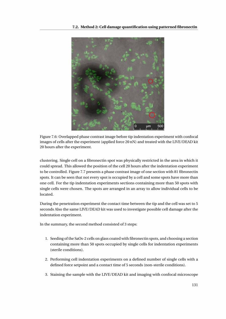
7.2. Method 2: Cell damage quantification using patterned fibronectin
Figure 7.6: Overlapped phase contrast image before tip indentation experiment with confocalimages of cells after the experiment (applied force 20 nN) and treated with the LIVE/DEAD kit20 hours after the experiment.
clustering. Single cell on a fibronectin spot was physically restricted in the area in which it
could spread. This allowed the position of the cell 20 hours after the indentation experiment
to be controlled. Figure 7.7 presents a phase contrast image of one section with 81 fibronectin
spots. It can be seen that not every spot is occupied by a cell and some spots have more than
one cell. For the tip indentation experiments sections containing more than 50 spots with
single cells were chosen. The spots are arranged in an array to allow individual cells to be
located.
During the penetration experiment the contact time between the tip and the cell was set to 5
seconds Also the same LIVE/DEAD kit was used to investigate possible cell damage after the
indentation experiment.
In the summary, the second method consisted of 3 steps:
1. Seeding of the SaOs-2 cells on glass coated with fibronectin spots, and choosing a section
containing more than 50 spots occupied by single cells for indentation experiments
(sterile conditions).
2. Performing cell indentation experiments on a defined number of single cells with a
defined force setpoint and a contact time of 5 seconds (non-sterile conditions).
3. Staining the sample with the LIVE/DEAD kit and imaging with confocal microscope
131
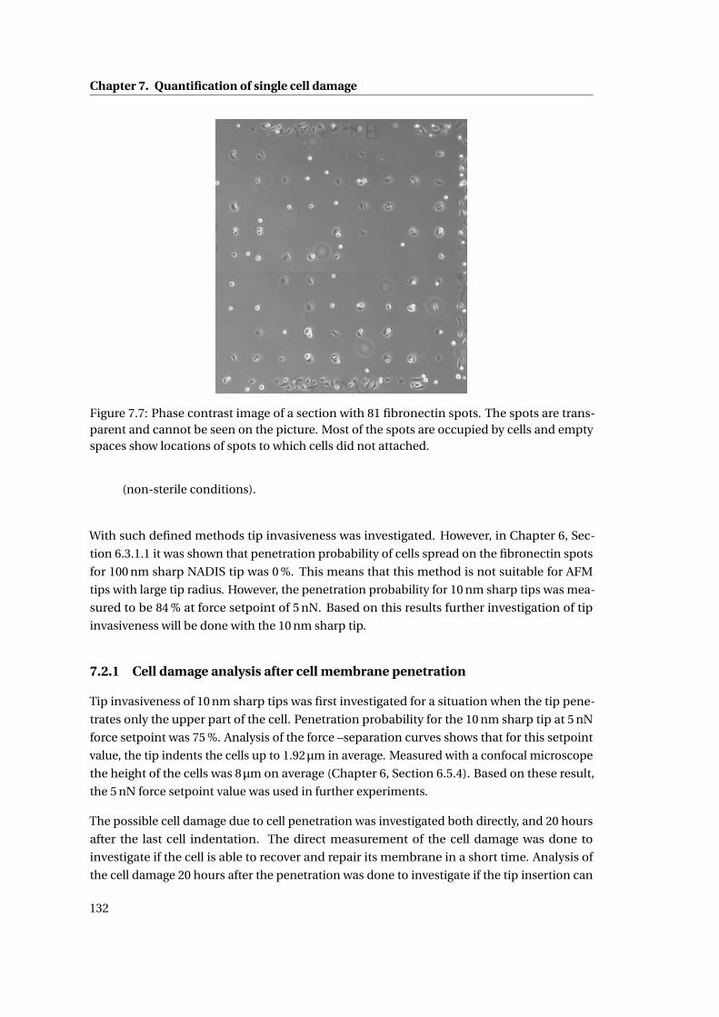
Chapter 7. Quantification of single cell damage
Figure 7.7: Phase contrast image of a section with 81 fibronectin spots. The spots are trans-parent and cannot be seen on the picture. Most of the spots are occupied by cells and emptyspaces show locations of spots to which cells did not attached.
(non-sterile conditions).
With such defined methods tip invasiveness was investigated. However, in Chapter 6, Sec-
tion 6.3.1.1 it was shown that penetration probability of cells spread on the fibronectin spots
for 100 nm sharp NADIS tip was 0 %. This means that this method is not suitable for AFM
tips with large tip radius. However, the penetration probability for 10 nm sharp tips was mea-
sured to be 84 % at force setpoint of 5 nN. Based on this results further investigation of tip
invasiveness will be done with the 10 nm sharp tip.
7.2.1 Cell damage analysis after cell membrane penetration
Tip invasiveness of 10 nm sharp tips was first investigated for a situation when the tip pene-
trates only the upper part of the cell. Penetration probability for the 10 nm sharp tip at 5 nN
force setpoint was 75 %. Analysis of the force –separation curves shows that for this setpoint
value, the tip indents the cells up to 1.92µm in average. Measured with a confocal microscope
the height of the cells was 8µm on average (Chapter 6, Section 6.5.4). Based on these result,
the 5 nN force setpoint value was used in further experiments.
The possible cell damage due to cell penetration was investigated both directly, and 20 hours
after the last cell indentation. The direct measurement of the cell damage was done to
investigate if the cell is able to recover and repair its membrane in a short time. Analysis of
the cell damage 20 hours after the penetration was done to investigate if the tip insertion can
132
7.2. Method 2: Cell damage quantification using patterned fibronectin
induce cell apoptosis.
Figure 7.8a) shows tip invasiveness measured directly after the indentation experiment. It can
be seen that all cells emit green fluorescence. Analysis of the force-separation curves showed
that 35 cells were penetrated with the tip. 4 examples of cell emitting the green fluorescence
are presented with their force-separation curves. Each curve has a penetration peak. Lack of
cell stained red on the picture shows that cells managed to repair their membranes before the
treatment with the LIVE/DEAD kit.
Figure 7.8b) shows the results measured 20 hours after the indentation experiment. 43 cells
were emitting green signal, 7 cells were either emitting red signal or missing. Any cells which
were missing were assumed to be dead as the SaOs-2 cell line is an adherent cell line. Analysis
of the force-separation curves showed that 40 cells were penetrated with the tip. Not all
of the dead cells were penetrated. As an example cell 1c and its force-separation curve is
presented. It can bee seen that the tip only indented the cell. Another example, cell 8i was
also only indented and 20 hours after the indentation two cells were found there, suggesting
that the cell went through mitosis. Two additional examples are shown as well: cell 6h with its
force- separation curve showing penetration peak, and cell 8g with its force-separation curve
showing multiple penetration peaks.
In summary, no cell damage was observed on the first sample treated with the LIVE/DEAD
kit directly after the indentation experiment. 7 cells were missing on the second sample, first
incubated for 20 hours and after treatment with the kit. The cells that detached from the
sample are assumed dead.
133
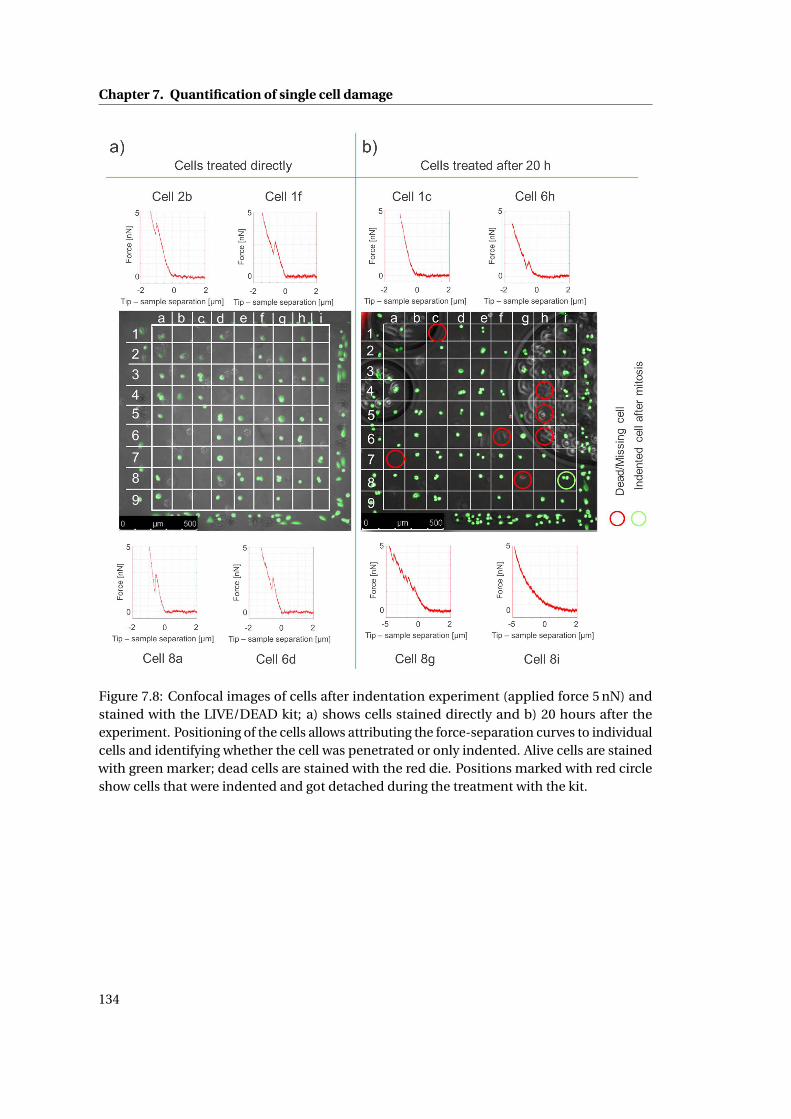
Chapter 7. Quantification of single cell damage
Figure 7.8: Confocal images of cells after indentation experiment (applied force 5 nN) andstained with the LIVE/DEAD kit; a) shows cells stained directly and b) 20 hours after theexperiment. Positioning of the cells allows attributing the force-separation curves to individualcells and identifying whether the cell was penetrated or only indented. Alive cells are stainedwith green marker; dead cells are stained with the red die. Positions marked with red circleshow cells that were indented and got detached during the treatment with the kit.
134
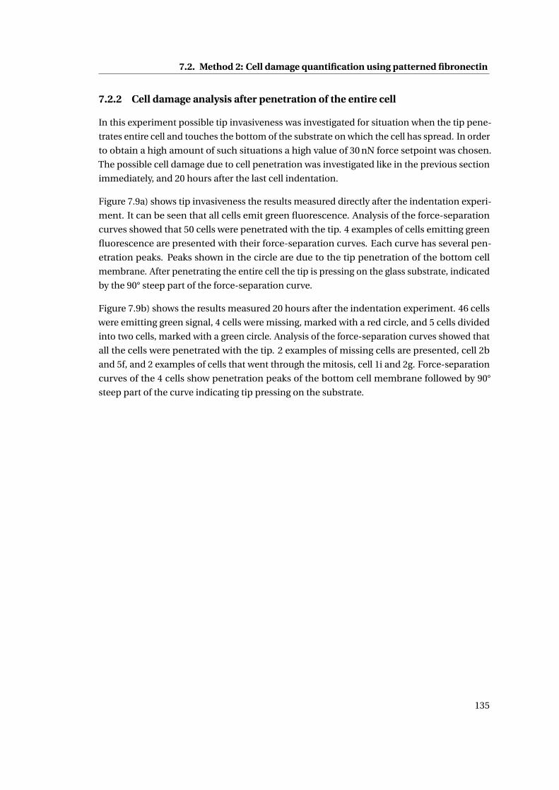
7.2. Method 2: Cell damage quantification using patterned fibronectin
7.2.2 Cell damage analysis after penetration of the entire cell
In this experiment possible tip invasiveness was investigated for situation when the tip pene-
trates entire cell and touches the bottom of the substrate on which the cell has spread. In order
to obtain a high amount of such situations a high value of 30 nN force setpoint was chosen.
The possible cell damage due to cell penetration was investigated like in the previous section
immediately, and 20 hours after the last cell indentation.
Figure 7.9a) shows tip invasiveness the results measured directly after the indentation experi-
ment. It can be seen that all cells emit green fluorescence. Analysis of the force-separation
curves showed that 50 cells were penetrated with the tip. 4 examples of cells emitting green
fluorescence are presented with their force-separation curves. Each curve has several pen-
etration peaks. Peaks shown in the circle are due to the tip penetration of the bottom cell
membrane. After penetrating the entire cell the tip is pressing on the glass substrate, indicated
by the 90° steep part of the force-separation curve.
Figure 7.9b) shows the results measured 20 hours after the indentation experiment. 46 cells
were emitting green signal, 4 cells were missing, marked with a red circle, and 5 cells divided
into two cells, marked with a green circle. Analysis of the force-separation curves showed that
all the cells were penetrated with the tip. 2 examples of missing cells are presented, cell 2b
and 5f, and 2 examples of cells that went through the mitosis, cell 1i and 2g. Force-separation
curves of the 4 cells show penetration peaks of the bottom cell membrane followed by 90°
steep part of the curve indicating tip pressing on the substrate.
135
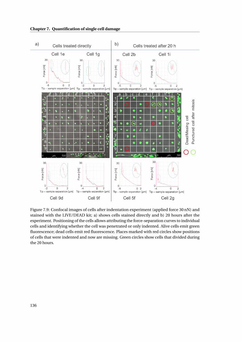
Chapter 7. Quantification of single cell damage
Figure 7.9: Confocal images of cells after indentation experiment (applied force 30 nN) andstained with the LIVE/DEAD kit; a) shows cells stained directly and b) 20 hours after theexperiment. Positioning of the cells allows attributing the force-separation curves to individualcells and identifying whether the cell was penetrated or only indented. Alive cells emit greenfluorescence; dead cells emit red fluorescence. Places marked with red circles show positionsof cells that were indented and now are missing. Green circles show cells that divided duringthe 20 hours.
136
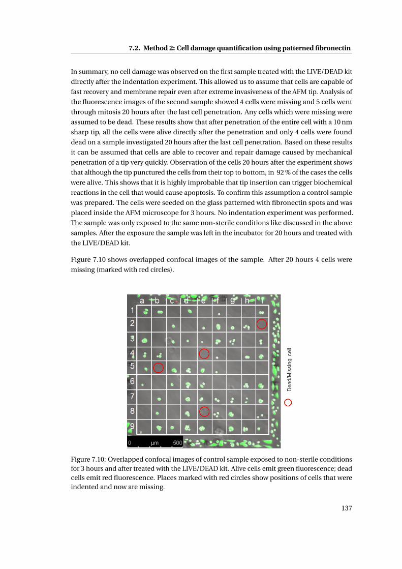
7.2. Method 2: Cell damage quantification using patterned fibronectin
In summary, no cell damage was observed on the first sample treated with the LIVE/DEAD kit
directly after the indentation experiment. This allowed us to assume that cells are capable of
fast recovery and membrane repair even after extreme invasiveness of the AFM tip. Analysis of
the fluorescence images of the second sample showed 4 cells were missing and 5 cells went
through mitosis 20 hours after the last cell penetration. Any cells which were missing were
assumed to be dead. These results show that after penetration of the entire cell with a 10 nm
sharp tip, all the cells were alive directly after the penetration and only 4 cells were found
dead on a sample investigated 20 hours after the last cell penetration. Based on these results
it can be assumed that cells are able to recover and repair damage caused by mechanical
penetration of a tip very quickly. Observation of the cells 20 hours after the experiment shows
that although the tip punctured the cells from their top to bottom, in 92 % of the cases the cells
were alive. This shows that it is highly improbable that tip insertion can trigger biochemical
reactions in the cell that would cause apoptosis. To confirm this assumption a control sample
was prepared. The cells were seeded on the glass patterned with fibronectin spots and was
placed inside the AFM microscope for 3 hours. No indentation experiment was performed.
The sample was only exposed to the same non-sterile conditions like discussed in the above
samples. After the exposure the sample was left in the incubator for 20 hours and treated with
the LIVE/DEAD kit.
Figure 7.10 shows overlapped confocal images of the sample. After 20 hours 4 cells were
missing (marked with red circles).
Figure 7.10: Overlapped confocal images of control sample exposed to non-sterile conditionsfor 3 hours and after treated with the LIVE/DEAD kit. Alive cells emit green fluorescence; deadcells emit red fluorescence. Places marked with red circles show positions of cells that wereindented and now are missing.
137
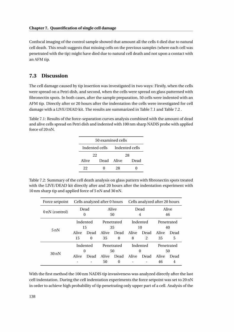
Chapter 7. Quantification of single cell damage
Confocal imaging of the control sample showed that amount all the cells 4 died due to natural
cell death. This result suggests that missing cells on the previous samples (where each cell was
penetrated with the tip) might have died due to natural cell death and not upon a contact with
an AFM tip.
7.3 Discussion
The cell damage caused by tip insertion was investigated in two ways: Firstly, when the cells
were spread on a Petri dish, and second, when the cells were spread on glass patterned with
fibronectin spots. In both cases, after the sample preparation, 50 cells were indented with an
AFM tip. Directly after or 20 hours after the indentation the cells were investigated for cell
damage with a LIVE/DEAD kit. The results are summarized in Table 7.1 and Table 7.2 .
Table 7.1: Results of the force-separation curves analysis combined with the amount of deadand alive cells spread on Petri dish and indented with 100 nm sharp NADIS probe with appliedforce of 20 nN.
50 examined cells
Indented cells Indented cells
22 28Alive Dead Alive Dead
22 0 28 0
Table 7.2: Summary of the cell death analysis on glass pattern with fibronectin spots treatedwith the LIVE/DEAD kit directly after and 20 hours after the indentation experiment with10 nm sharp tip and applied force of 5 nN and 30 nN.
Force setpoint Cells analyzed after 0 hours Cells analyzed after 20 hours
0 nN (control)Dead Alive Dead Alive
0 50 4 46
5 nN
Indented Penetrated Indented Penetrated15 35 10 40
Alive Dead Alive Dead Alive Dead Alive Dead15 0 35 0 8 2 35 5
30 nN
Indented Penetrated Indented Penetrated0 50 0 50
Alive Dead Alive Dead Alive Dead Alive Dead- - 50 0 - - 46 4
With the first method the 100 nm NADIS tip invasiveness was analyzed directly after the last
cell indentation. During the cell indentation experiments the force setpoint was set to 20 nN
in order to achieve high probability of tip penetrating only upper part of a cell. Analysis of the
138
7.3. Discussion
force-separation curves showed that 22 cells out of 50 were penetrated with the tip. Confocal
imaging of the sample showed that all the 50 cells were alive after the experiment. All the
penetrated cells repaired their ruptured membranes as no red fluorescence was emitted during
confocal imaging of the cells. The results obtained show that cell membrane penetration with
a 100 nm sharp tip does not create any immediate damage to cells.
It was not possible to assess cell damage 20 hours after indentation due to cell division
preventing identification of the individual cells.
In the second method cells were spread on fibronectin spots. Single cells on fibronectin spots
are physically restricted in the area in which they can spread. This allows the position of
the cell to be controlled 20 hours after an indentation experiment. Since the penetration
probability of 100 nm NADIS tip is 0 % when cells are spread on the fibronectin spots cell
damage was investigated with 10 nm sharp tip. The indentation experiments were performed
with 5 nN and 30 nN force setpoint value. 50 cells were indented for each condition. In each
case cell damage was investigated directly after, or 20 hours after the indentation experiment.
When a 10 nm sharp tip penetrates a cell with 5 nN force setpoint, the tip penetrates only the
upper part of the cell. Analysis of the force-separation curves showed that 35 out of 50 cells
were penetrated with the tip. Treatment with the DEAD/LIVE kit directly after indentation
followed by imaging of the sample showed that all 50 cells were alive. In a second sample the
force-separation curves showed that 40 out of 50 cells were penetrated with the tip. Analysis
20 hours after the penetration/indentation and fluorescence imaging of the sample showed
that 43 cells were alive and 7 cells were missing. Since the SaOs-2 cells are adherent cells,
the 7 missing cells were counted as dead cells. When a 30 nN force setpoint was used, the
tip penetrated the entire cell and hit the bottom of the substrate. Fluorescence imaging of
cells treated with the LIVE/DEAD kit directly after the penetration showed that all cells were
alive and managed to repair their ruptured membranes. Imaging of cells treated 20 hours after
penetration showed 46 live cells emitting green fluorescence and 4 cells missing.
Analysis of the control sample 20 hours after exposure to non-sterile conditions reveled 4
cell missing. This result shows that even under conditions where cells are not exposed to
mechanical stress and cell membrane penetration, around 8 percent of the cell population
can be expected to die. This value can be compared with the values obtained after indentation:
with a 5 nN force setpoint 14 % of cells were dead after 20 hours with a 30 nN force setpoint 8 %
of cells were dead. This comparison suggests that cell penetration (even most drastic, when
an AFM tip penetrates entire cell) with a 10 nm sharp tip does not triggering cell death.
These results show that SaOs-2 cell are surprisingly resistant to AFM tip penetration, clearly
possessing suitable mechanisms that allow to repair their ruptured membranes and recovers
rapidly after tip insertion. SaOs-2 cells – an osteosarcoma cell line – are robust adherent
eukaryotic cells. It is possible, perhaps likely, that other cell types are more sensitive to AFM
tip penetration. Therefore, extension of this work to other cell lines and primary cells could
give a more general overview on the invasiveness of the AFM tips.
139
Chapter 7. Quantification of single cell damage
Different tip shapes (cylindrical or conical) could be used to test the limits of cell robustness.
In this study the tip was inserted in the cell for 5 seconds and left static. It would be interesting
to see how the cell would react to the tip being inserted in the cell for a longer period of time
and how if moving the tip whilst inside the cell would influence cell damage.
A limiting factor in using SaOs-2 cells for long term studies is their capacity to divide very
quickly and make identification of individual cells that have been penetrated impossible.
Using a cell type that divides more slowly, such as nerve cells, would allow the long term effects
of cell penetration to be studied.
7.4 Conclusions
Two methods on how to measure possible single cell damage were demonstrated.
The first method allows cell damage to be measure a few hours after tip insertion into cells
which are spread on a petri dish. The second method allows cell damage to be measured on
cells grown on glass patterned with PLL-g-PEG/fibronectin spots, 24 hours after tip insertion.
Measurement of tip invasiveness directly after the cell penetration showed no cell damage,
even when the tip was penetrating the cell entirely and touching the substrate. Measurement
of tip invasiveness 20 hours after the cell penetration showed maximum 14 % of cell death.
This is similar the rate of natural cell death measured on the control sample.
Results obtained here show that cell penetration with an AFM tip does not cause severe
damage to cells. This result will be further utilised in the analysis of microinjection of liquids
into cells with the NADIS probe.
140
8 Microinjection using the AFM–basedsystem
Once the AFM-based microinjection system had been fabricated and characterized (Chapters 4
and 5), and AFM tip insertion into single living cells had been studied (Chapters 6 and 7), the
system was used to inject liquids into cells. These experiments were used to test the feasibility
of the system and investigate which technological aspects require further development. Two
types of experiments were designed, first to investigate feasibility of intracellular injection,
and second, to inject liquid directly into a cell nucleus.
8.1 Experimental design
The intracellular injection experiments were designed to investigate different aspects con-
cerning successful liquid delivery after tip insertion into a single cell. In previous chapters
theoretical values of the volume of liquid that can be delivered into a single cell were discussed;
experimental values of the injection parameters: the pressure and the length of the pressure
pulse were proposed; the probability of cell membrane penetration was measured to find
optimal conditions for tip insertion; and finally possible cell death due to tip insertion was
investigated in order to understand the effect of tip invasiveness into cells. All these results
presented in Chapters 4 to 7 were used to design the intracellular injection experiments.
Figure 8.1 presents schematically the experimental design. The experiment consists of 6
steps. The first step is the preparation of a sample with cells and liquids used for injection. In
Chapter 6, Section 6.3.1.1 it was shown that the highest probability of cell penetration with
NADIS tips was measured for cells seeded on a Petri dish. Based on this result it was decided to
use cells seeded on this substrate. Two liquids were used: sterile water and fluorescent sodium
salt dissolved in PBS at a concentration of 0.1 mg mL−1. The water injection experiment was
designed to check for possible leakage of the fluidic connectors, clogging of the tip opening
due to cell membrane residues, and to study tip interactions with the cells during liquid
injection via force-time curves. Injection of the fluorescent solution was dedicated to study
the most suitable values of the injection parameters (pressure and length of the pressure
pulse).
141
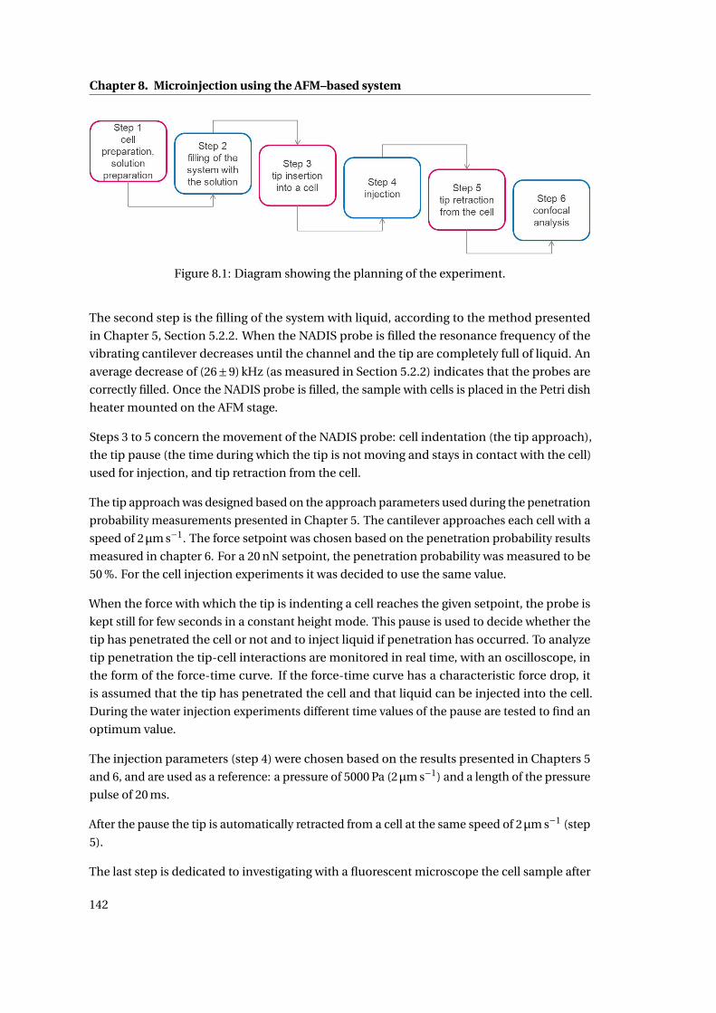
Chapter 8. Microinjection using the AFM–based system
Figure 8.1: Diagram showing the planning of the experiment.
The second step is the filling of the system with liquid, according to the method presented
in Chapter 5, Section 5.2.2. When the NADIS probe is filled the resonance frequency of the
vibrating cantilever decreases until the channel and the tip are completely full of liquid. An
average decrease of (26±9) kHz (as measured in Section 5.2.2) indicates that the probes are
correctly filled. Once the NADIS probe is filled, the sample with cells is placed in the Petri dish
heater mounted on the AFM stage.
Steps 3 to 5 concern the movement of the NADIS probe: cell indentation (the tip approach),
the tip pause (the time during which the tip is not moving and stays in contact with the cell)
used for injection, and tip retraction from the cell.
The tip approach was designed based on the approach parameters used during the penetration
probability measurements presented in Chapter 5. The cantilever approaches each cell with a
speed of 2µm s−1. The force setpoint was chosen based on the penetration probability results
measured in chapter 6. For a 20 nN setpoint, the penetration probability was measured to be
50 %. For the cell injection experiments it was decided to use the same value.
When the force with which the tip is indenting a cell reaches the given setpoint, the probe is
kept still for few seconds in a constant height mode. This pause is used to decide whether the
tip has penetrated the cell or not and to inject liquid if penetration has occurred. To analyze
tip penetration the tip-cell interactions are monitored in real time, with an oscilloscope, in
the form of the force-time curve. If the force-time curve has a characteristic force drop, it
is assumed that the tip has penetrated the cell and that liquid can be injected into the cell.
During the water injection experiments different time values of the pause are tested to find an
optimum value.
The injection parameters (step 4) were chosen based on the results presented in Chapters 5
and 6, and are used as a reference: a pressure of 5000 Pa (2µm s−1) and a length of the pressure
pulse of 20 ms.
After the pause the tip is automatically retracted from a cell at the same speed of 2µm s−1 (step
5).
The last step is dedicated to investigating with a fluorescent microscope the cell sample after
142
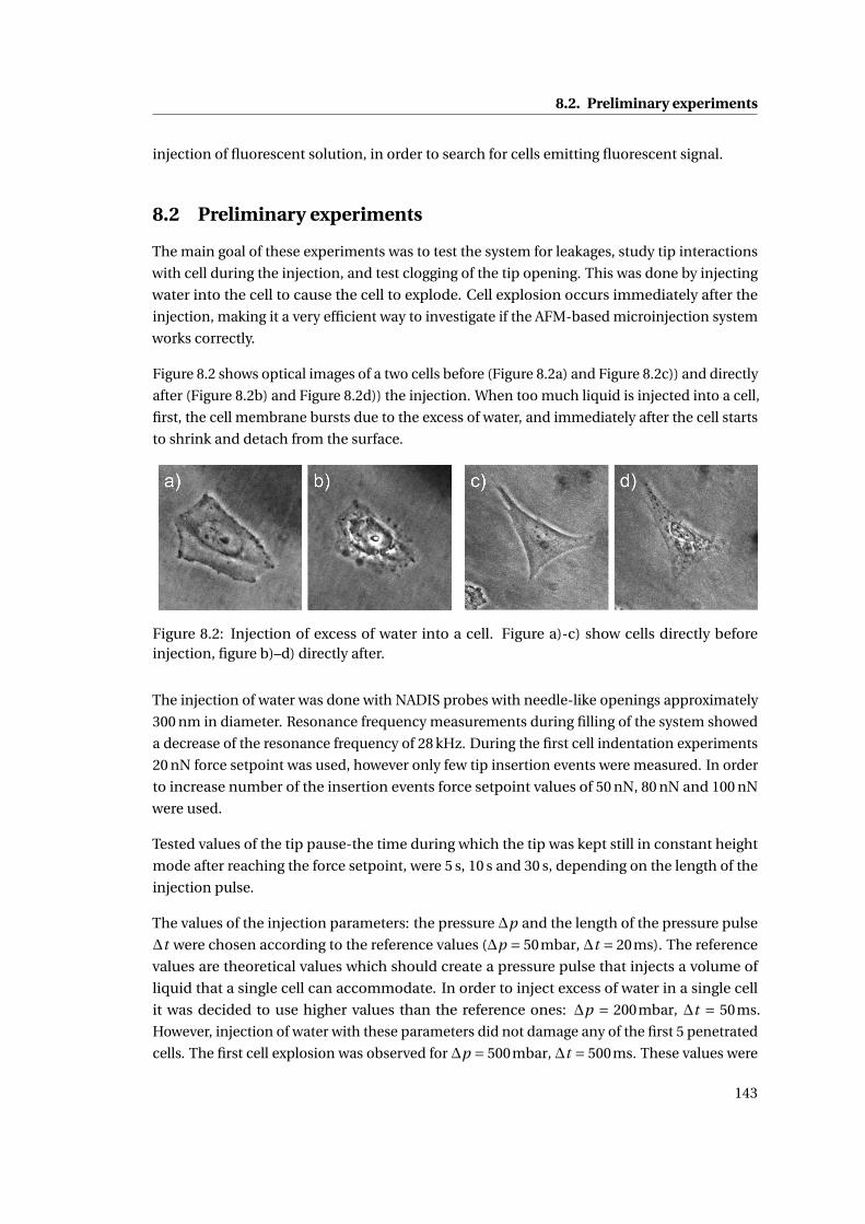
8.2. Preliminary experiments
injection of fluorescent solution, in order to search for cells emitting fluorescent signal.
8.2 Preliminary experiments
The main goal of these experiments was to test the system for leakages, study tip interactions
with cell during the injection, and test clogging of the tip opening. This was done by injecting
water into the cell to cause the cell to explode. Cell explosion occurs immediately after the
injection, making it a very efficient way to investigate if the AFM-based microinjection system
works correctly.
Figure 8.2 shows optical images of a two cells before (Figure 8.2a) and Figure 8.2c)) and directly
after (Figure 8.2b) and Figure 8.2d)) the injection. When too much liquid is injected into a cell,
first, the cell membrane bursts due to the excess of water, and immediately after the cell starts
to shrink and detach from the surface.
Figure 8.2: Injection of excess of water into a cell. Figure a)-c) show cells directly beforeinjection, figure b)–d) directly after.
The injection of water was done with NADIS probes with needle-like openings approximately
300 nm in diameter. Resonance frequency measurements during filling of the system showed
a decrease of the resonance frequency of 28 kHz. During the first cell indentation experiments
20 nN force setpoint was used, however only few tip insertion events were measured. In order
to increase number of the insertion events force setpoint values of 50 nN, 80 nN and 100 nN
were used.
Tested values of the tip pause-the time during which the tip was kept still in constant height
mode after reaching the force setpoint, were 5 s, 10 s and 30 s, depending on the length of the
injection pulse.
The values of the injection parameters: the pressure ∆p and the length of the pressure pulse
∆t were chosen according to the reference values (∆p = 50mbar, ∆t = 20ms). The reference
values are theoretical values which should create a pressure pulse that injects a volume of
liquid that a single cell can accommodate. In order to inject excess of water in a single cell
it was decided to use higher values than the reference ones: ∆p = 200mbar, ∆t = 50ms.
However, injection of water with these parameters did not damage any of the first 5 penetrated
cells. The first cell explosion was observed for ∆p = 500mbar, ∆t = 500ms. These values were
143
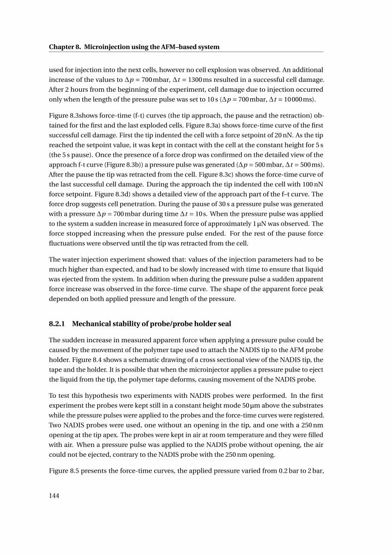
Chapter 8. Microinjection using the AFM–based system
used for injection into the next cells, however no cell explosion was observed. An additional
increase of the values to ∆p = 700mbar, ∆t = 1300ms resulted in a successful cell damage.
After 2 hours from the beginning of the experiment, cell damage due to injection occurred
only when the length of the pressure pulse was set to 10 s (∆p = 700mbar, ∆t = 10000ms).
Figure 8.3shows force-time (f-t) curves (the tip approach, the pause and the retraction) ob-
tained for the first and the last exploded cells. Figure 8.3a) shows force-time curve of the first
successful cell damage. First the tip indented the cell with a force setpoint of 20 nN. As the tip
reached the setpoint value, it was kept in contact with the cell at the constant height for 5 s
(the 5 s pause). Once the presence of a force drop was confirmed on the detailed view of the
approach f-t curve (Figure 8.3b)) a pressure pulse was generated (∆p = 500mbar,∆t = 500ms).
After the pause the tip was retracted from the cell. Figure 8.3c) shows the force-time curve of
the last successful cell damage. During the approach the tip indented the cell with 100 nN
force setpoint. Figure 8.3d) shows a detailed view of the approach part of the f–t curve. The
force drop suggests cell penetration. During the pause of 30 s a pressure pulse was generated
with a pressure ∆p = 700mbar during time ∆t = 10s. When the pressure pulse was applied
to the system a sudden increase in measured force of approximately 1µN was observed. The
force stopped increasing when the pressure pulse ended. For the rest of the pause force
fluctuations were observed until the tip was retracted from the cell.
The water injection experiment showed that: values of the injection parameters had to be
much higher than expected, and had to be slowly increased with time to ensure that liquid
was ejected from the system. In addition when during the pressure pulse a sudden apparent
force increase was observed in the force-time curve. The shape of the apparent force peak
depended on both applied pressure and length of the pressure.
8.2.1 Mechanical stability of probe/probe holder seal
The sudden increase in measured apparent force when applying a pressure pulse could be
caused by the movement of the polymer tape used to attach the NADIS tip to the AFM probe
holder. Figure 8.4 shows a schematic drawing of a cross sectional view of the NADIS tip, the
tape and the holder. It is possible that when the microinjector applies a pressure pulse to eject
the liquid from the tip, the polymer tape deforms, causing movement of the NADIS probe.
To test this hypothesis two experiments with NADIS probes were performed. In the first
experiment the probes were kept still in a constant height mode 50µm above the substrates
while the pressure pulses were applied to the probes and the force-time curves were registered.
Two NADIS probes were used, one without an opening in the tip, and one with a 250 nm
opening at the tip apex. The probes were kept in air at room temperature and they were filled
with air. When a pressure pulse was applied to the NADIS probe without opening, the air
could not be ejected, contrary to the NADIS probe with the 250 nm opening.
Figure 8.5 presents the force-time curves, the applied pressure varied from 0.2 bar to 2 bar,
144
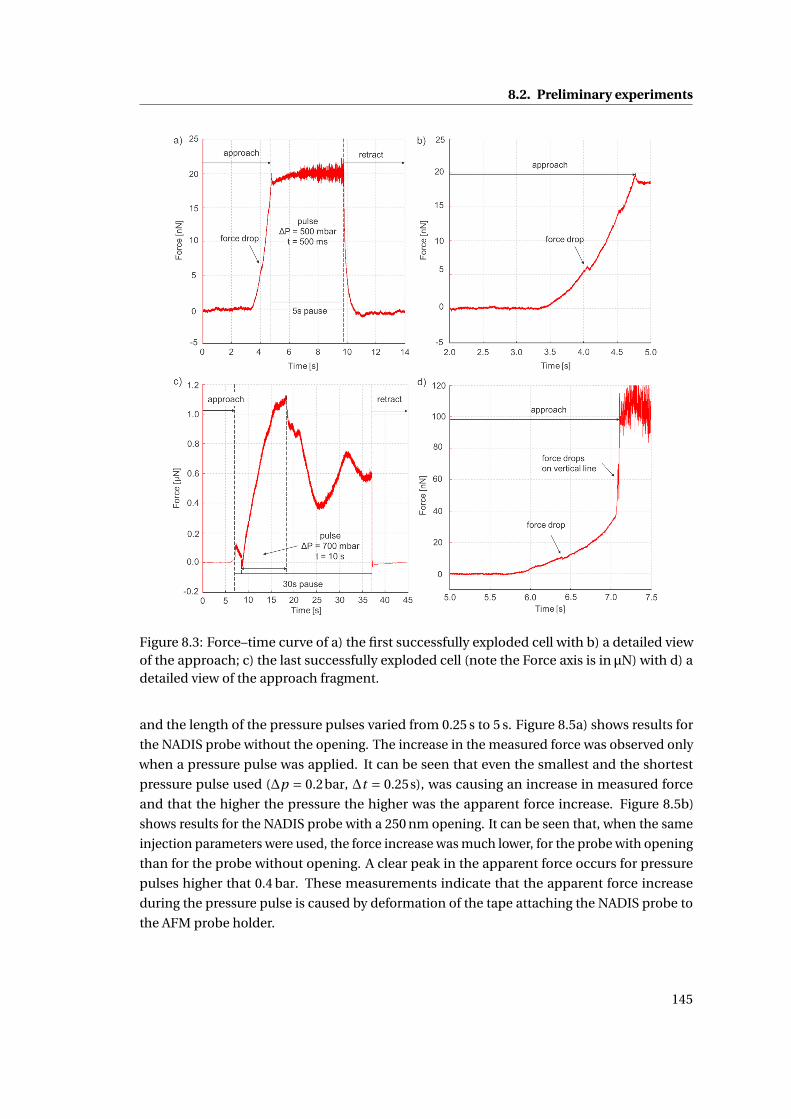
8.2. Preliminary experiments
Figure 8.3: Force–time curve of a) the first successfully exploded cell with b) a detailed viewof the approach; c) the last successfully exploded cell (note the Force axis is in µN) with d) adetailed view of the approach fragment.
and the length of the pressure pulses varied from 0.25 s to 5 s. Figure 8.5a) shows results for
the NADIS probe without the opening. The increase in the measured force was observed only
when a pressure pulse was applied. It can be seen that even the smallest and the shortest
pressure pulse used (∆p = 0.2bar, ∆t = 0.25s), was causing an increase in measured force
and that the higher the pressure the higher was the apparent force increase. Figure 8.5b)
shows results for the NADIS probe with a 250 nm opening. It can be seen that, when the same
injection parameters were used, the force increase was much lower, for the probe with opening
than for the probe without opening. A clear peak in the apparent force occurs for pressure
pulses higher that 0.4 bar. These measurements indicate that the apparent force increase
during the pressure pulse is caused by deformation of the tape attaching the NADIS probe to
the AFM probe holder.
145
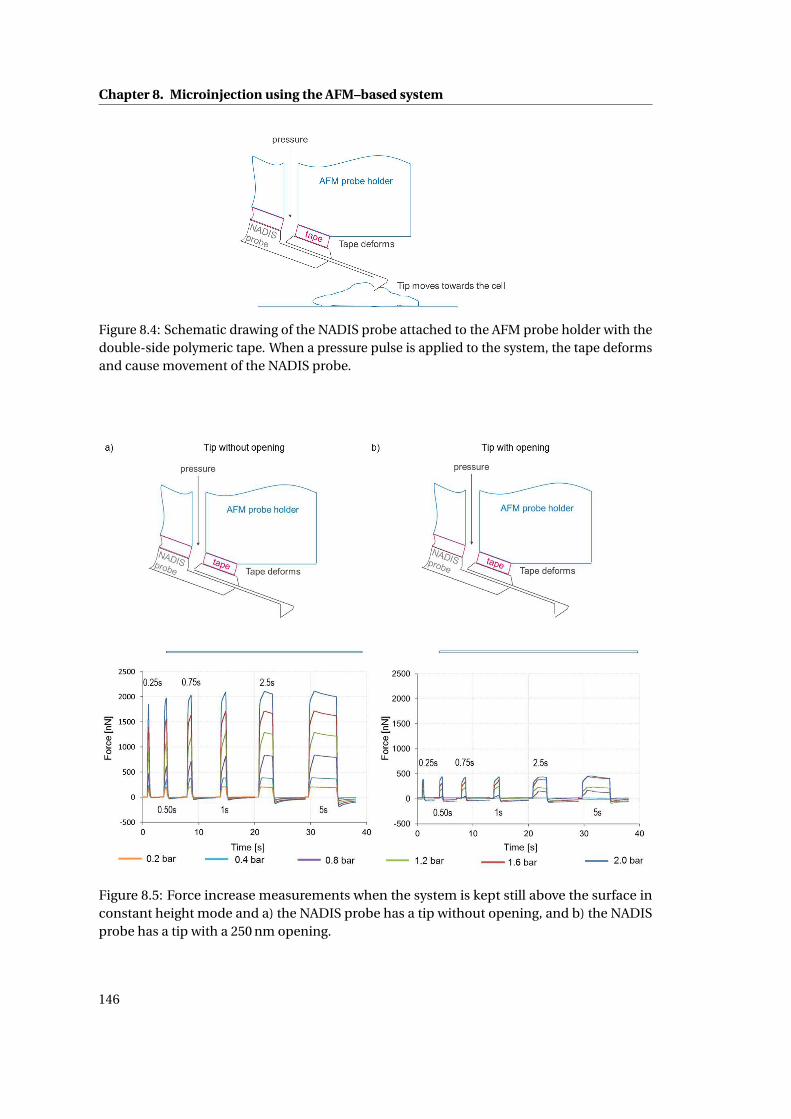
Chapter 8. Microinjection using the AFM–based system
Figure 8.4: Schematic drawing of the NADIS probe attached to the AFM probe holder with thedouble-side polymeric tape. When a pressure pulse is applied to the system, the tape deformsand cause movement of the NADIS probe.
Figure 8.5: Force increase measurements when the system is kept still above the surface inconstant height mode and a) the NADIS probe has a tip without opening, and b) the NADISprobe has a tip with a 250 nm opening.
146
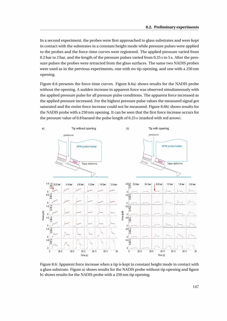
8.2. Preliminary experiments
In a second experiment, the probes were first approached to glass substrates and were kept
in contact with the substrates in a constant height mode while pressure pulses were applied
to the probes and the force-time curves were registered. The applied pressure varied from
0.2 bar to 2 bar, and the length of the pressure pulses varied from 0.25 s to 5 s. After the pres-
sure pulses the probes were retracted from the glass surfaces. The same two NADIS probes
were used as in the previous experiments, one with no tip opening, and one with a 250 nm
opening.
Figure 8.6 presents the force-time curves. Figure 8.6a) shows results for the NADIS probe
without the opening. A sudden increase in apparent force was observed simultaneously with
the applied pressure pulse for all pressure pulse conditions. The apparent force increased as
the applied pressure increased. For the highest pressure pulse values the measured signal got
saturated and the entire force increase could not be measured. Figure 8.6b) shows results for
the NADIS probe with a 250 nm opening. It can be seen that the first force increase occurs for
the pressure value of 0.8 barand the pulse length of 0.25 s (marked with red arrow).
Figure 8.6: Apparent force increase when a tip is kept in constant height mode in contact witha glass substrate. Figure a) shows results for the NADIS probe without tip opening and figureb) shows results for the NADIS probe with a 250 nm tip opening.
147
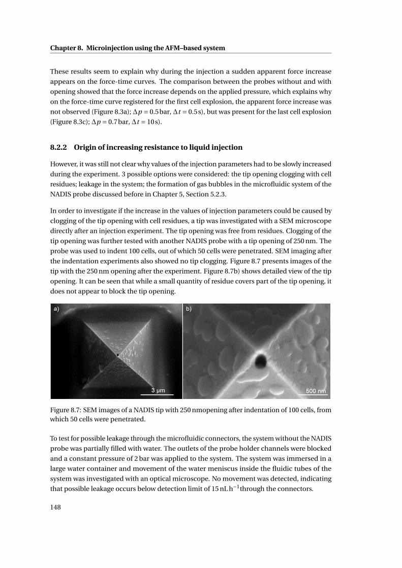
Chapter 8. Microinjection using the AFM–based system
These results seem to explain why during the injection a sudden apparent force increase
appears on the force-time curves. The comparison between the probes without and with
opening showed that the force increase depends on the applied pressure, which explains why
on the force-time curve registered for the first cell explosion, the apparent force increase was
not observed (Figure 8.3a); ∆p = 0.5bar, ∆t = 0.5s), but was present for the last cell explosion
(Figure 8.3c); ∆p = 0.7bar, ∆t = 10s).
8.2.2 Origin of increasing resistance to liquid injection
However, it was still not clear why values of the injection parameters had to be slowly increased
during the experiment. 3 possible options were considered: the tip opening clogging with cell
residues; leakage in the system; the formation of gas bubbles in the microfluidic system of the
NADIS probe discussed before in Chapter 5, Section 5.2.3.
In order to investigate if the increase in the values of injection parameters could be caused by
clogging of the tip opening with cell residues, a tip was investigated with a SEM microscope
directly after an injection experiment. The tip opening was free from residues. Clogging of the
tip opening was further tested with another NADIS probe with a tip opening of 250 nm. The
probe was used to indent 100 cells, out of which 50 cells were penetrated. SEM imaging after
the indentation experiments also showed no tip clogging. Figure 8.7 presents images of the
tip with the 250 nm opening after the experiment. Figure 8.7b) shows detailed view of the tip
opening. It can be seen that while a small quantity of residue covers part of the tip opening, it
does not appear to block the tip opening.
Figure 8.7: SEM images of a NADIS tip with 250 nmopening after indentation of 100 cells, fromwhich 50 cells were penetrated.
To test for possible leakage through the microfluidic connectors, the system without the NADIS
probe was partially filled with water. The outlets of the probe holder channels were blocked
and a constant pressure of 2 bar was applied to the system. The system was immersed in a
large water container and movement of the water meniscus inside the fluidic tubes of the
system was investigated with an optical microscope. No movement was detected, indicating
that possible leakage occurs below detection limit of 15 nL h−1through the connectors.
148
8.2. Preliminary experiments
To test for possible leakage through the tape sealing the NADIS tip to the AFM holder, the
system with the NADIS probe of 200 nm opening was filled with air. As the AFM holder and
the tape are optically transparent, the tape-NADIS probe behaviour was observed with an
optical microscope. When the seal is tight, no air bubbles can be seen trapped between the
NADIS probe and the tape and no nucleation of new air bubbles is observed. When a constant
pressure of 2 bar was generated for 5 min no air bubbles were observed, suggesting that the
seal remained tight. When the pressure was increased to 4 bar, after 5 min air bubbles begin
to occur between the tape and the NADIS, which could be the origin of a leak. Since during
the water injection experiments, the pressure was not higher than 2 bar it was assumed than
no leakage occurred during the experiment.
Based on the SEM imaging of the tip apexes and the leakage tests it was concluded that
most probably the constant increase in the values of the injection parameters is caused by
nucleation of gas bubbles inside the hollow AFM tip.
8.2.3 Discussion
A water injection experiment was used to test the AFM-based microinjection system. The
system was used to inject excess of water into cells to cause cell damage. The experimental
results showed that the system can be used as a microinjection tool.
The water injection experiments also revealed that the 20 nN force setpoint value was not
enough to achieve a 50 % penetration probability. During the injection experiment forces up
to 100 nN were used. It is not clear why this higher setpoint is necessary. It might be due to
the differences in radii of the NADIS tips. In the chapter 4 (Microfabrication of the NADIS
probes) it was outlined that the tip radius can vary from 50 nm to 150 nm, which could cause
a difference in penetration probability between the NADIS probes.
Several tip pause times used to confirm penetration events and inject the liquid were tested,
ranging from 5 s to 30 s. It was verified that a 5 s pause was enough to check if the approach
force-time curve had a force drop, and immediately after apply a pressure pulse. It was also
found that the values of the injection parameters had to be slowly increased in order to inject
an excess of water and cause cell damage. Leakage tests showed that the system is watertight.
The SEM imaging of the tip openings suggest that it is improbable that the tip opening is
blocked with cell residues. In the absence of a visible cause, the effect was attributed to
possible nucleation of gas bubbles inside the tip. Table 8 compares values of the force setpoint
and injection parameters proposed to be used at the beginning of the experiment with the
values that were required to be used during the experiment.
Based on these results, values of the force setpoint, tip pause and the injection parameters
were adapted for the injection of the sodium fluorescein experiment.
149
Chapter 8. Microinjection using the AFM–based system
Table 8.1: Comparison of the parameters values assumed in the experiment designed with thevalues used during the experiment.
Force setpoint Tip pause Pressure ∆p Pulse length ∆t
Assumed in the design 20 nN 5 s 0.2 bar 0.02 sUsed in practice 20 nN to 100 nN 5 s to 30 s 0.5 bar to 2 bar 5 s to 10 s
8.3 Intracellular injection of sodium fluorescein
The main goal of this experiment was to test values of the injection parameters allowing liquid
delivery without causing cell damage. It was decided to deliver a fluorescent solution into
individual cells, and use the fluorescent signal emitted by the cells as evidence of successful
injection.
Before the experiment several NADIS probes were investigated with SEM in order to find a
probe with a small tip radius. The injection of the sodium fluorescein was done with a NADIS
probe with a tip radius of 75 nm and a needle-like opening approximately 200 nm in diameter.
Cantilever resonance frequency measurement during the probe filling showed decrease of
21 kHz.
Table 8.2 presents values of the force setpoint, tip pause and injection parameters used in the
experiment.
Table 8.2: Comparison of the parameters values assumed in the experiment designed with thevalues used during the experiment.
Force setpoint Tip pause Pressure ∆p Pulse length ∆t
Used in experiment 50 nN or 80 nN 5 s 0.8 bar 0.5 s
Figure 8.8 shows an example of overlapped phase contrast and fluorescence images taken after
the experiment. In total 23 SaOs-2 cells were targeted. The number of cells was limited in order
to reduce the time of the experiment and thus the possibility of gas bubble formation inside
the tip. During the water injection experiment, which lasted 2 hours, the values of injection
parameters had to slowly increase to cause cell explosion, which was attributed to the effect of
the gas bubbles nucleation. In order to diminish this effect it was decided to shorten the time
of the experiment to 0.5 h, which should allow to use constant injection parameters. In order
to achieve high penetration probability 50 nN and 80 nN force setpoint values were used.
Two control measurements were carried out at the start of the experiment. The first measure-
ment was to determine whether fluorescent solution could be ejected from the NADIS tip.
The first cell was targeted (marked with the * on the Figure 8.8a), detail on the Figure 8.8b))
and the tip brought into contact with the cell. The system was paused for 5 s at the setpoint
for the applied force. Since a force drop was observed on the force-time curve a pressure
150
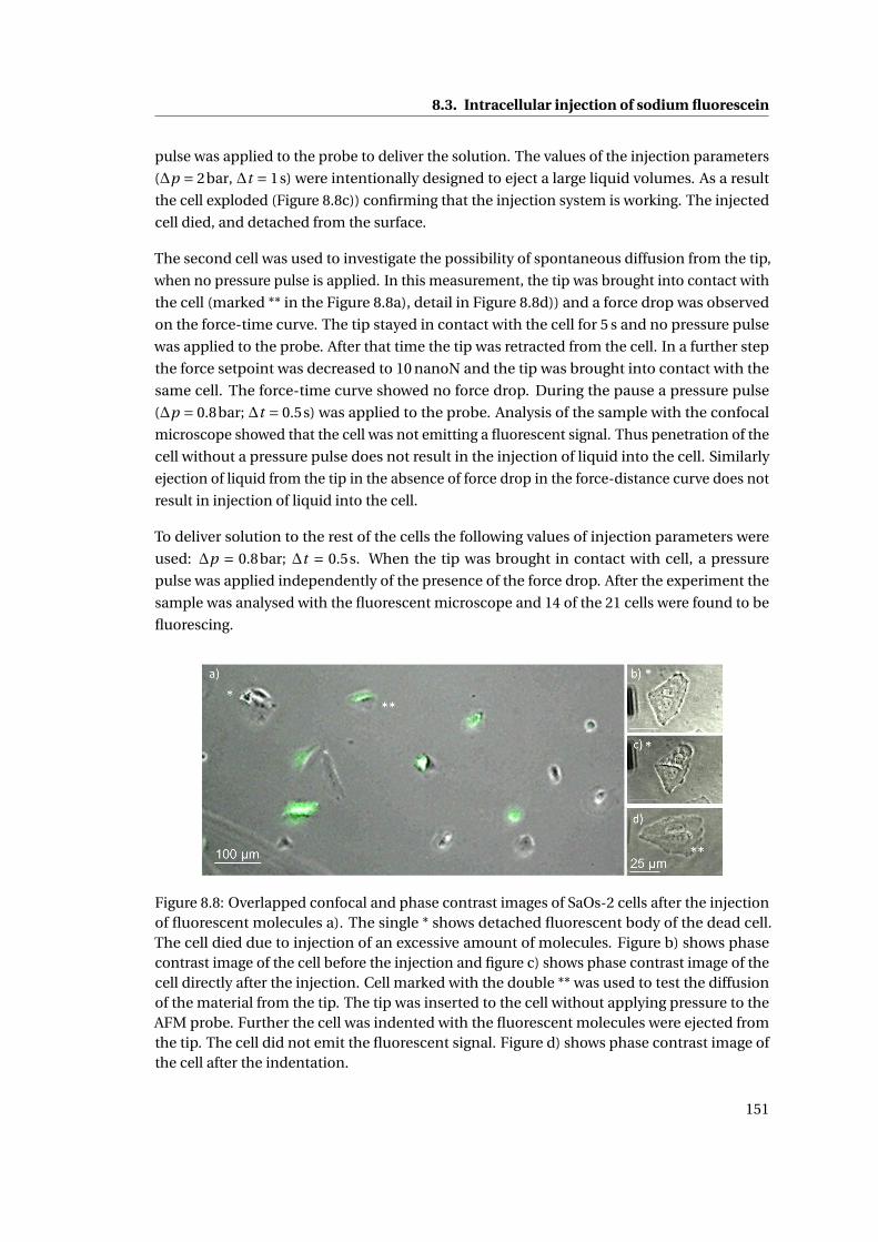
8.3. Intracellular injection of sodium fluorescein
pulse was applied to the probe to deliver the solution. The values of the injection parameters
(∆p = 2bar, ∆t = 1s) were intentionally designed to eject a large liquid volumes. As a result
the cell exploded (Figure 8.8c)) confirming that the injection system is working. The injected
cell died, and detached from the surface.
The second cell was used to investigate the possibility of spontaneous diffusion from the tip,
when no pressure pulse is applied. In this measurement, the tip was brought into contact with
the cell (marked ** in the Figure 8.8a), detail in Figure 8.8d)) and a force drop was observed
on the force-time curve. The tip stayed in contact with the cell for 5 s and no pressure pulse
was applied to the probe. After that time the tip was retracted from the cell. In a further step
the force setpoint was decreased to 10 nanoN and the tip was brought into contact with the
same cell. The force-time curve showed no force drop. During the pause a pressure pulse
(∆p = 0.8bar; ∆t = 0.5s) was applied to the probe. Analysis of the sample with the confocal
microscope showed that the cell was not emitting a fluorescent signal. Thus penetration of the
cell without a pressure pulse does not result in the injection of liquid into the cell. Similarly
ejection of liquid from the tip in the absence of force drop in the force-distance curve does not
result in injection of liquid into the cell.
To deliver solution to the rest of the cells the following values of injection parameters were
used: ∆p = 0.8bar; ∆t = 0.5s. When the tip was brought in contact with cell, a pressure
pulse was applied independently of the presence of the force drop. After the experiment the
sample was analysed with the fluorescent microscope and 14 of the 21 cells were found to be
fluorescing.
Figure 8.8: Overlapped confocal and phase contrast images of SaOs-2 cells after the injectionof fluorescent molecules a). The single * shows detached fluorescent body of the dead cell.The cell died due to injection of an excessive amount of molecules. Figure b) shows phasecontrast image of the cell before the injection and figure c) shows phase contrast image of thecell directly after the injection. Cell marked with the double ** was used to test the diffusionof the material from the tip. The tip was inserted to the cell without applying pressure to theAFM probe. Further the cell was indented with the fluorescent molecules were ejected fromthe tip. The cell did not emit the fluorescent signal. Figure d) shows phase contrast image ofthe cell after the indentation.
151
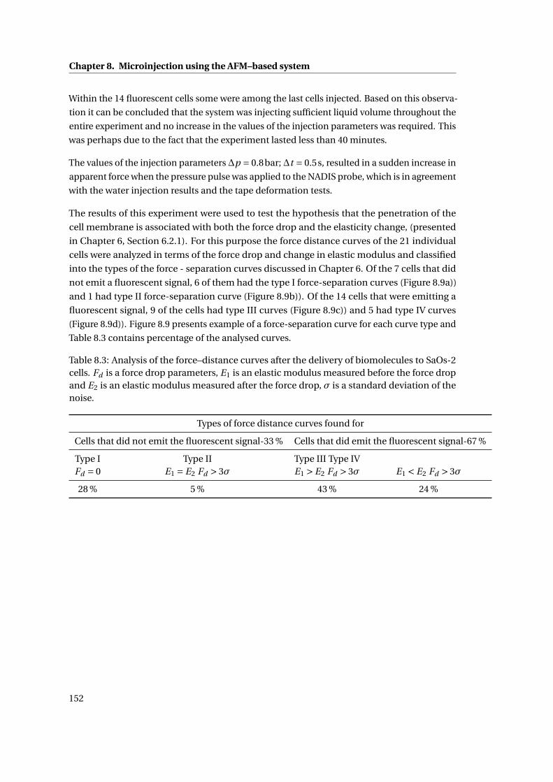
Chapter 8. Microinjection using the AFM–based system
Within the 14 fluorescent cells some were among the last cells injected. Based on this observa-
tion it can be concluded that the system was injecting sufficient liquid volume throughout the
entire experiment and no increase in the values of the injection parameters was required. This
was perhaps due to the fact that the experiment lasted less than 40 minutes.
The values of the injection parameters∆p = 0.8bar;∆t = 0.5s, resulted in a sudden increase in
apparent force when the pressure pulse was applied to the NADIS probe, which is in agreement
with the water injection results and the tape deformation tests.
The results of this experiment were used to test the hypothesis that the penetration of the
cell membrane is associated with both the force drop and the elasticity change, (presented
in Chapter 6, Section 6.2.1). For this purpose the force distance curves of the 21 individual
cells were analyzed in terms of the force drop and change in elastic modulus and classified
into the types of the force - separation curves discussed in Chapter 6. Of the 7 cells that did
not emit a fluorescent signal, 6 of them had the type I force-separation curves (Figure 8.9a))
and 1 had type II force-separation curve (Figure 8.9b)). Of the 14 cells that were emitting a
fluorescent signal, 9 of the cells had type III curves (Figure 8.9c)) and 5 had type IV curves
(Figure 8.9d)). Figure 8.9 presents example of a force-separation curve for each curve type and
Table 8.3 contains percentage of the analysed curves.
Table 8.3: Analysis of the force–distance curves after the delivery of biomolecules to SaOs-2cells. Fd is a force drop parameters, E1 is an elastic modulus measured before the force dropand E2 is an elastic modulus measured after the force drop, σ is a standard deviation of thenoise.
Types of force distance curves found for
Cells that did not emit the fluorescent signal-33 % Cells that did emit the fluorescent signal-67 %
Type I Type II Type III Type IVFd = 0 E1 = E2 Fd > 3σ E1 > E2 Fd > 3σ E1 < E2 Fd > 3σ
28 % 5 % 43 % 24 %
152
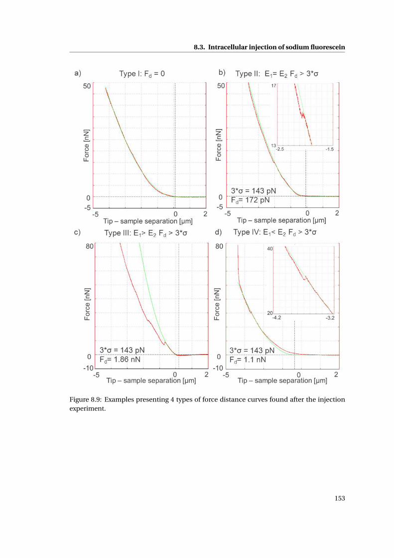
8.3. Intracellular injection of sodium fluorescein
Figure 8.9: Examples presenting 4 types of force distance curves found after the injectionexperiment.
153
Chapter 8. Microinjection using the AFM–based system
8.3.1 Discussion
The injection of sodium fluorescein molecules into cells was used to investigate if the system
can deliver liquid volumes into cells that do not cause cell death. The values of the injection
parameters for this experiment were chosen based on the results of the water injection experi-
ment. As a result out of 21 cells, 14 cells were emitting a fluorescent signal and none of the
cells exploded during the experiment. All were apparently alive a few hours after the injection
(the time during which the fluorescence analysis was done).
The experimental results were also used to test the hypothesis that the cell membrane penetra-
tion occurs when both a force drop and an elasticity change are present on a force-separation
curve (discussed in Chapter 6, Section 6.2.1). The force-separation curves from the 21 cells
used in the injection experiments were analysed in terms of the force drop Fd and change in
elasticity E , and classified according to the four curve types. The force-separation curves from
cells emitting fluorescent signal were falling into type III or type IV curves, indicating that the
cell penetration is associated with the force drop and also with the change in elasticity. Out of
the 7 cells that were not emitting the fluorescent signal, 6 cells had force-separation curves
falling into type I curves, representing only cell indentation. One cell had a force-separation
curve with a force drop value of 172 pN and no elasticity change was observed (shown on
Figure 8.9b)). This example suggests that the type II curves show no tip penetration and
support the proposed hypothesis. However, given the very small number of cells tested in this
experiment, further experiments are required. Table 8.4 contains a summary of the conditions
for which a tip is indenting or penetrating the cell membrane.
Table 8.4: Tip–cell membrane interaction determined by the force drop Fd and change inelastic modulus E .
Cell indentation Cell penetration
Type I Type II Type III Type IVFd = 0 E1 = E2 Fd > 3σ E1 > E2 Fd > 3σ E1 < E2 Fd > 3σ
8.4 Intranuclear injection
The goal of this experiment was to test if the microinjection system with 200 nNtip opening
can deliver liquid directly into cell nuclei.
To test this, a solution of both sodium fluorescein and propidium iodide was used. Propidium
iodide intercalates with the DNA to emit a strong red fluorescence but cannot pass sponta-
neously through the nuclear envelope of a living cell. By injecting a solution of both sodium
fluorescein and propidium iodide into a cell it was possible to test whether the tip had pen-
etrated the cell membrane (the cell fluoresces in the green) and whether it also entered the
cell nucleus (the nucleus fluoresces in the red). The concentration of propidium iodide in the
mixture was very high (1 mg mL−1) to ensure a strong fluorescent signal. Table 8.5 presents
154
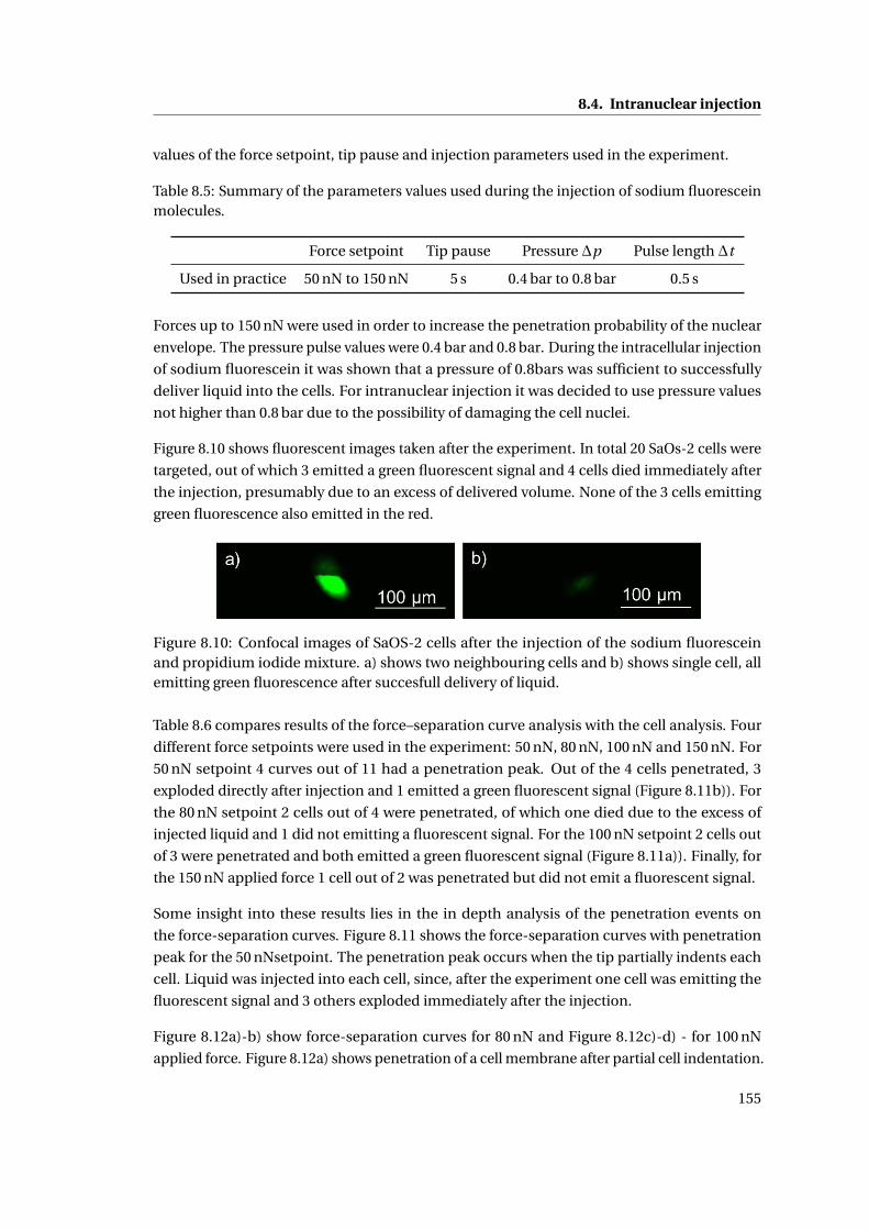
8.4. Intranuclear injection
values of the force setpoint, tip pause and injection parameters used in the experiment.
Table 8.5: Summary of the parameters values used during the injection of sodium fluoresceinmolecules.
Force setpoint Tip pause Pressure ∆p Pulse length ∆t
Used in practice 50 nN to 150 nN 5 s 0.4 bar to 0.8 bar 0.5 s
Forces up to 150 nN were used in order to increase the penetration probability of the nuclear
envelope. The pressure pulse values were 0.4 bar and 0.8 bar. During the intracellular injection
of sodium fluorescein it was shown that a pressure of 0.8bars was sufficient to successfully
deliver liquid into the cells. For intranuclear injection it was decided to use pressure values
not higher than 0.8 bar due to the possibility of damaging the cell nuclei.
Figure 8.10 shows fluorescent images taken after the experiment. In total 20 SaOs-2 cells were
targeted, out of which 3 emitted a green fluorescent signal and 4 cells died immediately after
the injection, presumably due to an excess of delivered volume. None of the 3 cells emitting
green fluorescence also emitted in the red.
Figure 8.10: Confocal images of SaOS-2 cells after the injection of the sodium fluoresceinand propidium iodide mixture. a) shows two neighbouring cells and b) shows single cell, allemitting green fluorescence after succesfull delivery of liquid.
Table 8.6 compares results of the force–separation curve analysis with the cell analysis. Four
different force setpoints were used in the experiment: 50 nN, 80 nN, 100 nN and 150 nN. For
50 nN setpoint 4 curves out of 11 had a penetration peak. Out of the 4 cells penetrated, 3
exploded directly after injection and 1 emitted a green fluorescent signal (Figure 8.11b)). For
the 80 nN setpoint 2 cells out of 4 were penetrated, of which one died due to the excess of
injected liquid and 1 did not emitting a fluorescent signal. For the 100 nN setpoint 2 cells out
of 3 were penetrated and both emitted a green fluorescent signal (Figure 8.11a)). Finally, for
the 150 nN applied force 1 cell out of 2 was penetrated but did not emit a fluorescent signal.
Some insight into these results lies in the in depth analysis of the penetration events on
the force-separation curves. Figure 8.11 shows the force-separation curves with penetration
peak for the 50 nNsetpoint. The penetration peak occurs when the tip partially indents each
cell. Liquid was injected into each cell, since, after the experiment one cell was emitting the
fluorescent signal and 3 others exploded immediately after the injection.
Figure 8.12a)-b) show force-separation curves for 80 nN and Figure 8.12c)-d) - for 100 nN
applied force. Figure 8.12a) shows penetration of a cell membrane after partial cell indentation.
155
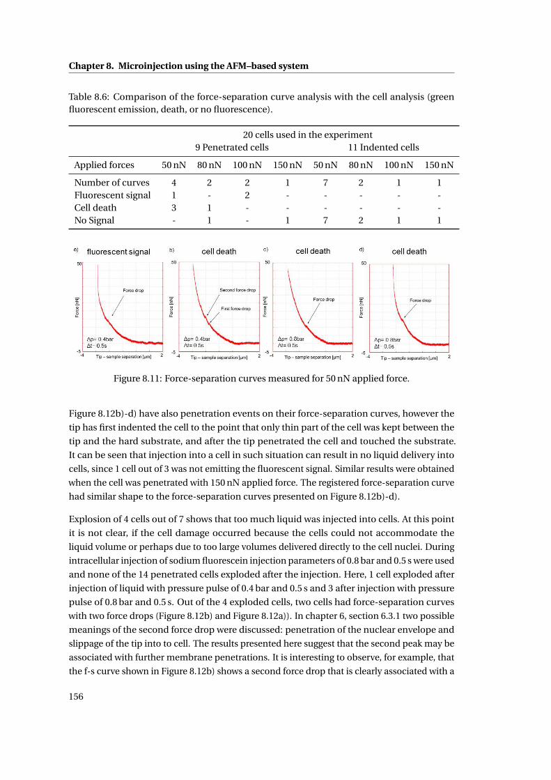
Chapter 8. Microinjection using the AFM–based system
Table 8.6: Comparison of the force-separation curve analysis with the cell analysis (greenfluorescent emission, death, or no fluorescence).
20 cells used in the experiment9 Penetrated cells 11 Indented cells
Applied forces 50 nN 80 nN 100 nN 150 nN 50 nN 80 nN 100 nN 150 nN
Number of curves 4 2 2 1 7 2 1 1Fluorescent signal 1 - 2 - - - - -Cell death 3 1 - - - - - -No Signal - 1 - 1 7 2 1 1
Figure 8.11: Force-separation curves measured for 50 nN applied force.
Figure 8.12b)-d) have also penetration events on their force-separation curves, however the
tip has first indented the cell to the point that only thin part of the cell was kept between the
tip and the hard substrate, and after the tip penetrated the cell and touched the substrate.
It can be seen that injection into a cell in such situation can result in no liquid delivery into
cells, since 1 cell out of 3 was not emitting the fluorescent signal. Similar results were obtained
when the cell was penetrated with 150 nN applied force. The registered force-separation curve
had similar shape to the force-separation curves presented on Figure 8.12b)-d).
Explosion of 4 cells out of 7 shows that too much liquid was injected into cells. At this point
it is not clear, if the cell damage occurred because the cells could not accommodate the
liquid volume or perhaps due to too large volumes delivered directly to the cell nuclei. During
intracellular injection of sodium fluorescein injection parameters of 0.8 bar and 0.5 s were used
and none of the 14 penetrated cells exploded after the injection. Here, 1 cell exploded after
injection of liquid with pressure pulse of 0.4 bar and 0.5 s and 3 after injection with pressure
pulse of 0.8 bar and 0.5 s. Out of the 4 exploded cells, two cells had force-separation curves
with two force drops (Figure 8.12b) and Figure 8.12a)). In chapter 6, section 6.3.1 two possible
meanings of the second force drop were discussed: penetration of the nuclear envelope and
slippage of the tip into to cell. The results presented here suggest that the second peak may be
associated with further membrane penetrations. It is interesting to observe, for example, that
the f-s curve shown in Figure 8.12b) shows a second force drop that is clearly associated with a
156
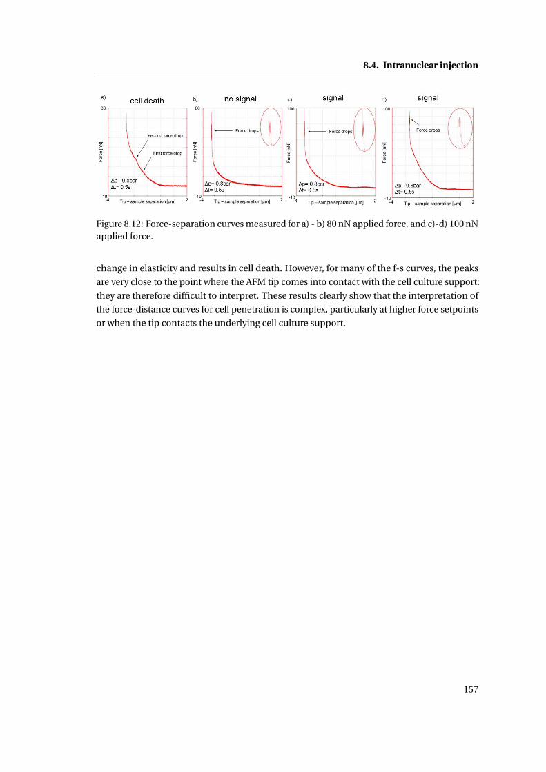
8.4. Intranuclear injection
Figure 8.12: Force-separation curves measured for a) - b) 80 nN applied force, and c)-d) 100 nNapplied force.
change in elasticity and results in cell death. However, for many of the f-s curves, the peaks
are very close to the point where the AFM tip comes into contact with the cell culture support:
they are therefore difficult to interpret. These results clearly show that the interpretation of
the force-distance curves for cell penetration is complex, particularly at higher force setpoints
or when the tip contacts the underlying cell culture support.
157

Chapter 8. Microinjection using the AFM–based system
8.5 General Discussion
The three injection tests (water injection, sodium fluorescein injection, and mixture injec-
tion of sodium fluorescein with propidium iodide) were used to perform proof of concept
experiments of the AFM-based microinjection system. The tests have shown that the AFM
probe could penetrate the cell membrane and that liquid could be delivered into the cells.
The liquid volume depended, as expected on the values of the injection parameters (pressure
and time). It was shown that cell injection of water with 300 nm tip opening and high values
of the injection parameters ∆p > 0.5bar and ∆t = 0.5s caused immediate cell death. Since
in Chapter 6 it was shown that tip insertion does not cause cell death, it was concluded that
during the injection experiment, the cells died due to excess injected liquid.
During the experiment design reference values of the injection parameters were proposed
based on the predicted values of cell volume (Chapter 3, Section 3.2.1) and liquid flow through
NADIS probes discusses in Chapter 5, Section 5.3. It was assumed that in order to successfully
deliver liquid to cells with 200nm opening, values of the injection parameters should be
∆p = 0.05bar, 16 times smaller compare to used ∆p = 0.8bar, and ∆t = 0.02s, which was 25
times smaller than used in the experiment. There are a number of possible explanations
of the large differences in the injection values needed. One possible explanation relates to
the position of the tip apex and its opening during tip insertion. The theoretical values of
the injection parameters were calculated assuming that the entire tip opening is inside the
cell during injection (Figure 8.13a)). However, the membrane slip parameter calculated in
Chapter 6, Section 6.4.1, is 75 nm while the diameter of the tip opening is 200 nm. With a
tip half angle of 35°, even a perfectly positioned opening and a perfectly sharp tip would
require the cell membrane to be displaced by more than 200 nm times cos(35°) or 164 nm
(Figure 8.13b)) for the tip opening to be entirely inside the cell. This suggests that the tip
opening is not entirely enclosed in the cell during the injection (Figure 8.13c)) resulting in
partial injection of liquid outside the cell. Thus, in order to deliver a given liquid volume into a
cell, higher values of injection parameters are required compare to the theoretical situation.
To test the hypothesis that the experimental values of the injection parameters are higher than
the theoretical ones due to the partial insertion of tip opening, an injection experiments could
be performed with tip opening centrally located at the tip apex. Positioning the tip opening at
the apex would decrease the penetration probability, however, once the tip was inserted, the
probability that the entire tip opening was enclosed inside the cell would be much higher.
Another explanation for the difference between calculated and experimental injection pa-
rameters was proposed by Minaschek et al. [66]. The suggestion is that the delivered liquid
might leak out from the cell during the injection. The leakage may be due tothe cytoplasmic
viscosity that is counteracting the injection, or due to weak adhesion or lack of it between the
ruptured membrane and the tip. However, in presented here experiments cells explosion and
their rapid recovery after the injection suggest otherwise. If the leakage had occurred it would
have been difficult to cause cell explosion, since most of the liquid would escape. Also due to
158
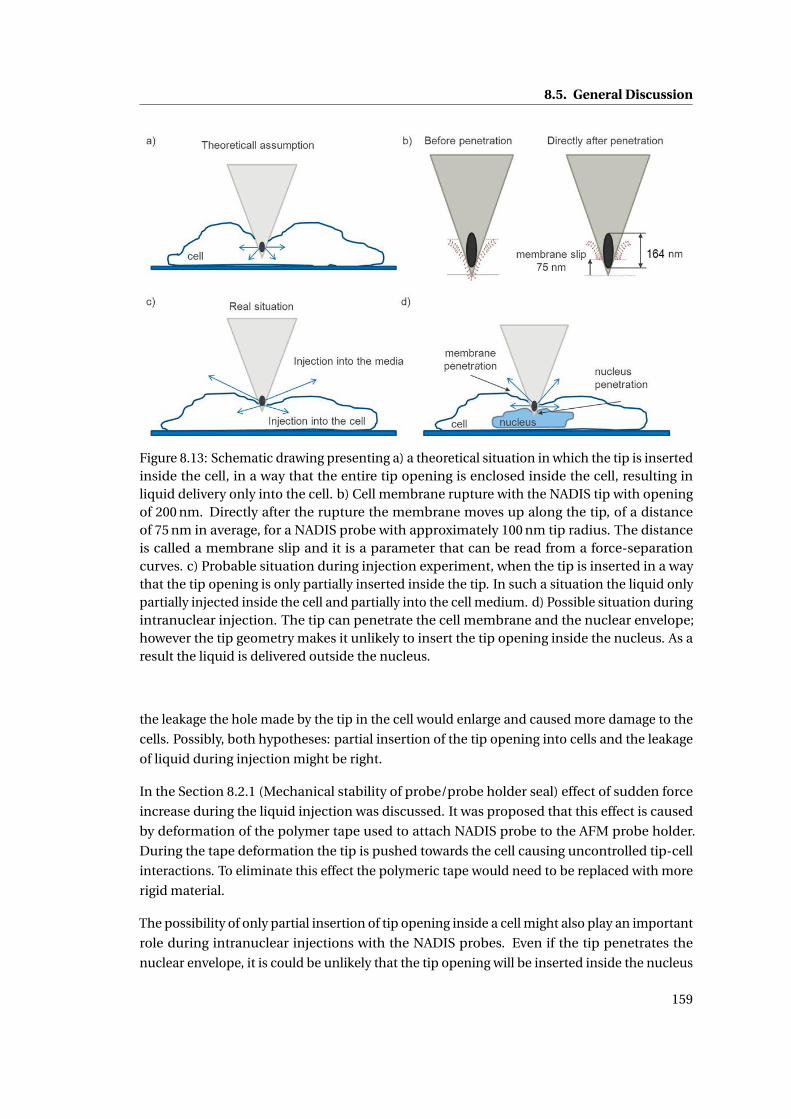
8.5. General Discussion
Figure 8.13: Schematic drawing presenting a) a theoretical situation in which the tip is insertedinside the cell, in a way that the entire tip opening is enclosed inside the cell, resulting inliquid delivery only into the cell. b) Cell membrane rupture with the NADIS tip with openingof 200 nm. Directly after the rupture the membrane moves up along the tip, of a distanceof 75 nm in average, for a NADIS probe with approximately 100 nm tip radius. The distanceis called a membrane slip and it is a parameter that can be read from a force-separationcurves. c) Probable situation during injection experiment, when the tip is inserted in a waythat the tip opening is only partially inserted inside the tip. In such a situation the liquid onlypartially injected inside the cell and partially into the cell medium. d) Possible situation duringintranuclear injection. The tip can penetrate the cell membrane and the nuclear envelope;however the tip geometry makes it unlikely to insert the tip opening inside the nucleus. As aresult the liquid is delivered outside the nucleus.
the leakage the hole made by the tip in the cell would enlarge and caused more damage to the
cells. Possibly, both hypotheses: partial insertion of the tip opening into cells and the leakage
of liquid during injection might be right.
In the Section 8.2.1 (Mechanical stability of probe/probe holder seal) effect of sudden force
increase during the liquid injection was discussed. It was proposed that this effect is caused
by deformation of the polymer tape used to attach NADIS probe to the AFM probe holder.
During the tape deformation the tip is pushed towards the cell causing uncontrolled tip-cell
interactions. To eliminate this effect the polymeric tape would need to be replaced with more
rigid material.
The possibility of only partial insertion of tip opening inside a cell might also play an important
role during intranuclear injections with the NADIS probes. Even if the tip penetrates the
nuclear envelope, it is could be unlikely that the tip opening will be inserted inside the nucleus
159
Chapter 8. Microinjection using the AFM–based system
(Figure 8.13d)) resulting in liquid delivery only into the cell cytoplasm.
8.6 Conclusions
The proof of concept injection results clearly demonstrate that the AFM-based microinjection
system can be used as a tool to deliver liquid into single living cells. During the preliminary
injections of water, an excess of liquid was delivered to cells and caused cell explosion giving
an instantaneous confirmation of successful injection. This approach allowed to successfully
test system limitations, such as leakage and clogging of the tip aperture. It was shown that the
system is tight for pressures up to 2 bar and no clogging was observed. The water injection
results showed that during the pressure pulse an apparent force increase occurs. The results
of the mechanical stability tests showed that this effect is caused due to the deformation of
the polymer tape used to attach the NADIS probe to the probe holder. Further development of
the seal between the probe and probe holder would be required to eliminate this effect.
The intracellular injection experiment demonstrated injection into cells without cell damage
and was used to test the hypothesis presented in Chapter 6 on the determination of tip
insertion. As a result out of 21 cells, 14 cells were emitting a fluorescent signal and none of
the cells exploded during the experiment. Analysis of the force-separation curves showed
that all force-separation curves of the cells emitting fluorescent signal showed a change in
elasticity after a force drop. Among the 7 cells that did emit a fluorescent signal, one cell had a
force-separation curve with a force drop but no elasticity change. These results are exactly
as predicted by the hypothesis. However, given the very small number of cells tested in this
experiment, further experiments would be needed to confirm the hypothesis.
Direct injection into cell nucleus was also attempted. It was shown that during the injection
the tip could penetrate the cell membrane and deliver the liquid into the cell, but labelling of
the nuclear DNA was not shown. It is, however, suggestive, that in these experiments-in which
no damage to the cells was expected - cell death was observed 4 times. These experiments
clearly demonstrated the difficulty of interpreting complex (and sometimes, simple) force
separation curves where cell penetration is involved.
160
9 Conclusion & Outlook
The main objective of this thesis was to develop a micro injection system for single adher-
ent cells based on AFM probes with a micro fluidic system. Additional objectives were the
demonstration of injections into cells and a better understanding of the involved AFM/cell
interactions.
The realized microinjection system was based on the Nanoscale Dispensing (NADIS) probes,
an earlier development at CSEM. The existing micro fabrication process of the NADIS probes
was adapted to improve the poor fabrication yield. A KOH etch mask made of parylene C
was developed to address the KCl contamination of the etched fluidic channels of the probes.
Extensive investigations of adhesion promotion methods such as thermal treatment and
recrystallization of the parylene C mask proved its suitability as a polymer KOH etch mask that
can be easily stripped, even from narrow structures such as the microchannels by thermal
treatment at 700 ◦C for several hours.
Three tip apertures were developed for single cell manipulation: a needle like aperture for cell
injection, where an ellipsoidal opening was located next to the tip apex in order to retain a
sharp tip to break the cell membrane, and two flat apertures for labeling the cell membrane
and other surfaces. The openings with a diameter between 200 nm and 500 nm were milled
with a focused ion beam.
An attempt was made to characterize the fluidics properties of the system. Pressure dependent
flows of gases and degassed water were measured through the NADIS probes with tip apertures
up to 200 nm in diameter. The results for larger tip openings were successfully fitted with a
linear model and can be approximated by simple theoretical model based on Hagen-Poiseuille
law. The water flow measurement through tip apertures smaller than 2µm resulted in tip
clogging due to gas bubbles. Therefore the theoretical model was used as indication of the flow
rate through systems with small tip apertures which allowed to determine reference values of
the injection parameters for the proof of concept injection experiments.
A more in-depth analysis of force-separation curves was developed allowing the biophysical
161
Chapter 9. Conclusion & Outlook
analysis and interpretation of penetration phenomena. 5 parameters were defined from
a force-separation curve with a penetration peak. Four of these parameters have already
been mentioned in the literature, whereas the fifth parameter, the membrane slip has been
proposed in this work. A simple mechanical model was presented, based on the assumption
that the membrane slip parameter represents the movement of the cell membrane up the
AFM tip during rupture of the membrane. The analysis of the force-separation curves with
this model has shown that the mechanical model is in very good agreement with the results
obtained with the 10 nm sharp tip, but that the agreement is less good for the 100 nm NADIS
tip.
A study was made of the invasiveness of the different AFM tips, as well as possible cell death
caused by tip penetration. The obtained results allow to claim that the cell penetration with
an AFM tip does not cause a severe damage to cells. Directly after the cell penetration there is
no cell damage and 20 hours after a maximum of 14 % of cell apoptosis was observed, a value
similar to the natural cell death measured on the control sample.
The proof of concept liquid delivery into individual cells was studied. Intentional injection
of a large water volume resulted in cell explosion which was used as confirmation that the
injection system is working. No system leakage for pressure values up to 2 bar and no clogging
of the tip opening with cell residues were observed. The sodium fluorescein injection was
used to test values of the injection parameters. The values of the injection parameters were
chosen based on the results of the water injection experiment. None of the cells exploded
during the sodium fluorescein injection experiment and all were apparently alive a few hours
after the injection. Direct injection into cell nucleus was also attempted. It was shown that
during the injection the tip could penetrate the cell membrane and deliver the liquid into the
cell, but labelling of the nuclear DNA was not achieved.
Combined technical development of the AFM based microinjection system with the study of
cell membrane penetration allowed to propose for the first time a definition of a cell membrane
penetration, discover the membrane slip parameter and define the 5A method for biophysical
analysis of probe indentations.
The proposed AFM-based microinjection system could be a powerful tool for direct injection
of molecules into nuclei of single cells. However, to achieve this goal further development
of the NADIS probes is required. First of all, the geometry of the tip has to be re-considered
to assure penetration of the nuclear envelope and complete insertion of the tip opening.
Secondly, geometry of the microfluidic channels inside the NADIS probe has to be re-designed
in order to gain control over the ejected from the tip liquid.
162

Bibliography
[1] Yulia Komarova, John Peloquin, and Gary Borisy. “Components of a microinjection
system.” In: Cold Spring Harbor protocols 2011.8 (Aug. 2011), pp. 935–9. ISSN: 1559-6095.
DOI: 10.1101/pdb.ip27.
[2] J. Kuncova and P. Kallio. “Challenges in capillary pressure microinjection”. In: The
26th Annual International Conference of the IEEE Engineering in Medicine and Biology
Society 4 (2004), pp. 4998–5001. DOI: 10.1109/IEMBS.2004.1404381.
[3] Pasi Kallio and Johana Kuncová. “Manipulation of Living Biological Cells : Challenges in
Automation”. In: Workshop on Microrobotics for Biomanipulation at IROS Conference.
2003.
[4] Katrin Viigipuu and Pasi Kallio. “Microinjection of living adherent cells by using a
semi-automatic microinjection system.” In: Alternatives to laboratory animals : ATLA
32.4 (Oct. 2004), pp. 417–23. ISSN: 0261-1929.
[5] Ankur Kapoor, Rajesh Kumar, and Russell H Taylor. “Simple Biomanipulation Tasks
with “ Steady Hand ” Cooperative Manipulator”. In: MICCAI(1). 2003, pp. 141–148.
[6] Mario R. Capecchi. “High efficiency transformation by direct microinjection of DNA
into cultured mammalian cells”. In: Cell 22.2 (Nov. 1980), pp. 479–488. ISSN: 00928674.
[7] Madiha Derouazi et al. “Generation of recombinant Chinese hamster ovary cell lines by
microinjection.” In: Biotechnology letters 28.6 (Mar. 2006), pp. 373–82. ISSN: 0141-5492.
[8] Sebastien Chenuet et al. “DNA delivery by microinjection for the generation of recom-
binant mammalian cell lines.” In: Methods in molecular biology (Clifton, N.J.) 518 (Jan.
2009), pp. 99–112. ISSN: 1064-3745.
[9] Philip Washbourne and A.Kimberley McAllister. “Techniques for gene transfer into
neurons”. In: Current Opinion in Neurobiology 12.5 (Oct. 2002), pp. 566–573. ISSN:
09594388.
[10] Morton Ehrenberg and James L McGrath. “Binding between particles and proteins in
extracts: implications for microrheology and toxicity.” In: Acta biomaterialia 1.3 (May
2005), pp. 305–15. ISSN: 1742-7061.
163
Bibliography
[11] Yan Zhang et al. “Estrogen and androgen protection of human neurons against in-
tracellular amyloid beta1-42 toxicity through heat shock protein 70.” In: The Journal
of neuroscience : the official journal of the Society for Neuroscience 24.23 (June 2004),
pp. 5315–21. ISSN: 1529-2401.
[12] Yan Zhang, Cynthia Goodyer, and Andrea LeBlanc. “Selective and Protracted Apoptosis
in Human Primary Neurons Microinjected with Active Caspase-3, -6, -7, and -8”. In: J.
Neurosci. 20.22 (Nov. 2000), pp. 8384–8389.
[13] Yan Zhang et al. “p75 neurotrophin receptor protects primary cultures of human
neurons against extracellular amyloid beta peptide cytotoxicity.” en. In: The Journal
of neuroscience : the official journal of the Society for Neuroscience 23.19 (Aug. 2003),
pp. 7385–94. ISSN: 1529-2401.
[14] Han-a Park et al. “Current Technologies in Single-Cell Microinjection and Application
to Study Signal Transduction”. In: Methods in Redox Signaling (2010).
[15] Yan Zhang and Long-Chuan Yu. “Microinjection as a tool of mechanical delivery.” In:
Current opinion in biotechnology 19.5 (Oct. 2008), pp. 506–10. ISSN: 0958-1669. DOI:
10.1016/j.copbio.2008.07.005.
[16] Yan Zhang and Long-Chuan Yu. “Single-cell microinjection technology in cell biology.”
In: BioEssays : news and reviews in molecular, cellular and developmental biology 30.6
(June 2008), pp. 606–10. ISSN: 1521-1878. DOI: 10.1002/bies.20759.
[17] Brian R Davis et al. “Glass needle – mediated microinjection of macromolecules and
transgenes into primary human blood stem / progenitor cells”. In: blood 95 (2009),
pp. 437–444.
[18] Myung-Ju Oh et al. “BCAR3 regulates EGF-induced DNA synthesis in normal human
breast MCF-12A cells.” In: Biochemical and biophysical research communications 375.3
(Oct. 2008), pp. 430–4. ISSN: 1090-2104.
[19] Douglas K Frank et al. “Single-cell microinjection of cytochrome c can result in gap
junction-mediated apoptotic cell death of bystander cells in head and neck cancer.”
In: Head & neck 27.9 (Sept. 2005), pp. 794–800. ISSN: 1043-3074.
[20] K Imaizumi et al. “Bystander tumoricidal effect and gap junctional communication in
lung cancer cell lines.” In: American journal of respiratory cell and molecular biology
18.2 (Feb. 1998), pp. 205–12. ISSN: 1044-1549.
[21] Andreas Marg et al. “Microinjected antibodies interfere with protein nucleocytoplas-
mic shuttling by distinct molecular mechanisms.” In: Cytometry. Part A : the journal of
the International Society for Analytical Cytology 73A.12 (Dec. 2008), pp. 1128–40. ISSN:
1552-4930.
[22] Robert King. “Gene delivery to mammalian cells by microinjection.” In: Methods in
molecular biology (Clifton, N.J.) 245 (Jan. 2004), pp. 167–74. ISSN: 1064-3745.
164
Bibliography
[23] J. P. Leonetti et al. “Intracellular distribution of microinjected antisense oligonu-
cleotides.” In: Proceedings of the National Academy of Sciences 88.7 (Apr. 1991), pp. 2702–
2706. ISSN: 0027-8424.
[24] Savita Khanna et al. “Regulation of c-Src activity in glutamate-induced neurodegenera-
tion.” In: The Journal of biological chemistry 282.32 (Aug. 2007), pp. 23482–90. ISSN:
0021-9258.
[25] Anne Järve et al. “Surveillance of siRNA integrity by FRET imaging.” In: Nucleic acids
research 35.18 (Jan. 2007), e124. ISSN: 1362-4962. DOI: 10.1093/nar/gkm694.
[26] Corinna Lappe-Siefke, Christoph Maas, and Matthias Kneussel. “Microinjection into
cultured hippocampal neurons: a straightforward approach for controlled cellular
delivery of nucleic acids, peptides and antibodies.” In: Journal of neuroscience methods
175.1 (Oct. 2008), pp. 88–95. ISSN: 0165-0270.
[27] T Saunders et al. “Generation of Pluripotent Stem Cells from Adult Mouse Liver and
Stomach Cells”. In: Science 321.August (2008), pp. 699–702.
[28] Elena Taverna et al. “A new approach to manipulate the fate of single neural stem cells
in tissue.” en. In: Nature neuroscience 15.2 (Feb. 2012), pp. 329–37. ISSN: 1546-1726.
[29] D J Stephens and R Pepperkok. “The many ways to cross the plasma membrane.” In:
Proceedings of the National Academy of Sciences of the United States of America 98.8
(Apr. 2001), pp. 4295–8. ISSN: 0027-8424. DOI: 10.1073/pnas.081065198.
[30] D Luo and W M Saltzman. “Synthetic DNA delivery systems.” In: Nature biotechnology
18.1 (Jan. 2000), pp. 33–7. ISSN: 1087-0156.
[31] H Clausen-Schaumann et al. “Mechanical stability of single DNA molecules.” In: Bio-
physical journal 78.4 (Apr. 2000), pp. 1997–2007. ISSN: 0006-3495. DOI: 10.1016/S0006-
3495(00)76747-6.
[32] Matthias Rief, Hauke Clausen-schaumann, and Hermann E Gaub. “letters mechanics
of single DNA molecules”. In: America 6.4 (1999), pp. 4–7.
[33] Yea-Ling Ong et al. “Adhesion Forces between E. c oli Bacteria and Biomaterial Sur-
faces”. In: Langmuir 15.8 (Apr. 1999), pp. 2719–2725. ISSN: 0743-7463. DOI: 10.1021/
la981104e.
[34] Herbert H.P Fang, Kwong-Yu Chan, and Li-Chong Xu. “Quantification of bacterial
adhesion forces using atomic force microscopy (AFM)”. In: Journal of Microbiological
Methods 40.1 (Mar. 2000), pp. 89–97. ISSN: 01677012. DOI: 10.1016/S0167-7012(99)
00137-2.
[35] L Sirghi et al. “Probing elasticity and adhesion of live cells by atomic force microscopy
indentation.” In: European biophysics journal : EBJ 37.6 (July 2008), pp. 935–45. ISSN:
0175-7571. DOI: 10.1007/s00249-008-0311-2.
[36] Gilles Weder et al. “Measuring cell adhesion forces during the cell cycle by force
spectroscopy.” In: Biointerphases 4.2 (June 2009), pp. 27–34. ISSN: 1559-4106. DOI:
10.1116/1.3139962.
165
Bibliography
[37] Gilles Weder et al. “Use of force spectroscopy to investigate the adhesion of living
adherent cells.” In: Langmuir : the ACS journal of surfaces and colloids 26.11 (June
2010), pp. 8180–6. ISSN: 1520-5827. DOI: 10.1021/la904526u.
[38] Rehana Afrin et al. “Atomic force microscopy for cellular level manipulation: imaging
intracellular structures and DNA delivery through a membrane hole.” In: Journal of
molecular recognition : JMR 22.5 (2009), pp. 363–72. ISSN: 1099-1352. DOI: 10.1002/jmr.
971.
[39] Yasuhiro Hirano et al. “Nuclear architecture and chromatin dynamics revealed by
atomic force microscopy in combination with biochemistry and cell biology.” In:
Pflügers Archiv : European journal of physiology 456.1 (Apr. 2008), pp. 139–53. ISSN:
0031-6768. DOI: 10.1007/s00424-007-0431-z.
[40] Q S Li et al. “AFM indentation study of breast cancer cells.” In: Biochemical and
biophysical research communications 374.4 (Oct. 2008), pp. 609–13. ISSN: 1090-2104.
DOI: 10.1016/j.bbrc.2008.07.078.
[41] Ikuo Obataya et al. “Mechanical sensing of the penetration of various nanoneedles
into a living cell using atomic force microscopy.” In: Biosensors & bioelectronics 20.8
(Feb. 2005), pp. 1652–5. ISSN: 0956-5663. DOI: 10.1016/j.bios.2004.07.020.
[42] Eun-Young Kwon, Young-Tae Kim, and Dae-Eun Kim. “Investigation of penetration
force of living cell using an atomic force microscope”. In: Journal of Mechanical Science
and Technology 23.7 (July 2009), pp. 1932–1938. ISSN: 1738-494X. DOI: 10.1007/s12206-
009-0508-z.
[43] Toshiya Osada et al. “mRNA analysis of single living cells.” In: Journal of nanobiotech-
nology 1.1 (Feb. 2003), p. 2. ISSN: 1477-3155.
[44] Sung Woong Han et al. “A molecular delivery system by using AFM and nanoneedle.”
In: Biosensors & bioelectronics 20.10 (Apr. 2005), pp. 2120–5. ISSN: 0956-5663.
[45] Sung-Woong Han et al. “High-efficiency DNA injection into a single human mesenchy-
mal stem cell using a nanoneedle and atomic force microscopy.” In: Nanomedicine :
nanotechnology, biology, and medicine 4.3 (Sept. 2008), pp. 215–25. ISSN: 1549-9642.
DOI: 10.1016/j.nano.2008.03.005.
[46] T Shibata et al. “Fabrication Of Bioprobe Integrated With Hollow Nanoneedle For
Cellular Function Analysis”. In: Water (2011), pp. 861–864.
[47] André Meister et al. “FluidFM: combining atomic force microscopy and nanofluidics
in a universal liquid delivery system for single cell applications and beyond.” In: Nano
letters 9.6 (June 2009), pp. 2501–7. ISSN: 1530-6992. DOI: 10.1021/nl901384x.
[48] B.M. Bogle. “Nanofountain Probes for Single-Cell Transfection : A Comparative Study
Assessing Invasiveness”. In: Nanoscape 7.1 (2010), pp. 33–37.
[49] Charles M Cuerrier, Réjean Lebel, and Michel Grandbois. “Single cell transfection using
plasmid decorated AFM probes.” In: Biochemical and biophysical research communi-
cations 355.3 (Apr. 2007), pp. 632–6. ISSN: 0006-291X. DOI: 10.1016/j.bbrc.2007.01.190.
166
Bibliography
[50] SungWoong Han et al. “Gene expression using an ultrathin needle enabling accurate
displacement and low invasiveness.” In: Biochemical and biophysical research commu-
nications 332.3 (July 2005), pp. 633–9. ISSN: 0006-291X. DOI: 10.1016/j.bbrc.2005.04.059.
[51] Sung-Woong Han et al. “Monitoring of hormonal drug effect in a single breast cancer
cell using an estrogen responsive GFP reporter vector delivered by a nanoneedle.”
In: Biosensors & bioelectronics 24.5 (Jan. 2009), pp. 1219–22. ISSN: 1873-4235. DOI:
10.1016/j.bios.2008.07.017.
[52] Xing Chen et al. “A cell nanoinjector based on carbon nanotubes.” In: Proceedings of
the National Academy of Sciences of the United States of America 104.20 (May 2007),
pp. 8218–22. ISSN: 0027-8424. DOI: 10.1073/pnas.0700567104.
[53] Owen Loh et al. “Nanofountain-probe-based high-resolution patterning and single-cell
injection of functionalized nanodiamonds.” In: Small (Weinheim an der Bergstrasse,
Germany) 5.14 (July 2009), pp. 1667–74. ISSN: 1613-6829. DOI: 10.1002/smll.200900361.
[54] André Meister et al. “Nanoscale dispensing in liquid environment of streptavidin on
a biotin-functionalized surface using hollow atomic force microscopy probes”. In:
Microelectronic Engineering 86.4-6 (Apr. 2009), pp. 1481–1484. ISSN: 01679317. DOI:
10.1016/j.mee.2008.10.025.
[55] Peter Ellmark et al. “Attovial-based antibody nanoarrays.” In: Proteomics 9.24 (Dec.
2009), pp. 5406–13. ISSN: 1615-9861. DOI: 10.1002/pmic.200800962.
[56] Kim Keun-Ho et al. “A Novel AFM Chip for Fountain Pen Nanolithography - Design
and Microfabrication”. In: Materials Research Society Symposium proceedings. Vol. 782.
2004, pp. 1–6.
[57] X Chen et al. “Foreign object damage in a thermal barrier system: mechanisms and
simulations”. In: Materials Science and Engineering: A 352.1-2 (July 2003), pp. 221–231.
ISSN: 09215093. DOI: 10.1016/S0921-5093(02)00905-X.
[58] Shinji Matsui et al. “Three-dimensional nanostructure fabrication by focused-ion-
beam chemical vapor deposition”. en. In: Journal of Vacuum Science & Technology B:
Microelectronics and Nanometer Structures 18.6 (Nov. 2000), p. 3181. ISSN: 0734211X.
DOI: 10.1116/1.1319689.
[59] Ch Santschi et al. “Interdigitated 50 nm Ti electrode arrays fabricated using XeF 2
enhanced focused ion beam etching”. In: Nanotechnology 17.11 (June 2006), pp. 2722–
2729. ISSN: 0957-4484. DOI: 10.1088/0957-4484/17/11/002.
[60] Jürgen H Daniel, David F Moore, and John F Walker. “Focused ion beams and silicon-
on-insulator - a novel approach to MEMS”. In: Smart Materials and Structures 9.3 (June
2000), pp. 284–290. ISSN: 0964-1726. DOI: 10.1088/0964-1726/9/3/306.
[61] Mike Hayles and Martin Dufek. xT Nova NanoLab User’s Manual. 5th Editio. FEI Com-
pany, 2006.
[62] Steve Reyntjens and Robert Puers. “A review of focused ion beam applications in
microsystem technology”. In: Work 287 (2001).
167
Bibliography
[63] Bruce Alberts et al. Molecular Biology of the Cell. en. 2008.
[64] Shuichi Takayama et al. “Selective Chemical Treatment of Cellular Microdomains Using
Multiple Laminar Streams”. In: Chemistry & Biology 10.2 (Feb. 2003), pp. 123–130. ISSN:
10745521. DOI: 10.1016/S1074-5521(03)00019-X.
[65] Pasi Kallio and Johana Kuncová. “Manipulation of Living Biological Cells: Challenges in
Automation”. In: Workshop on Microrobotics for Biomanipulation at IROS Conference.
2003.
[66] G. Minaschek, J. Bereiter-Hahn, and G. Bertholdt. “Quantitation of the volume of liquid
injected into cells by means of pressure”. In: Experimental Cell Research 183.2 (Aug.
1989), pp. 434–442. ISSN: 00144827. DOI: 10.1016/0014-4827(89)90402-3.
[67] Tuba Bayraktar and Srikanth B. Pidugu. “Characterization of liquid flows in microflu-
idic systems”. In: International Journal of Heat and Mass Transfer 49.5-6 (Mar. 2006),
pp. 815–824. ISSN: 00179310. DOI: 10.1016/j.ijheatmasstransfer.2005.11.007.
[68] Patrizia Santi and Richard H Guy. “controlled release Reverse iontophoresis - Parame-
ters determining electroosmotic flow : I . pH and ionic strength”. In: 38 (1996), pp. 159–
165.
[69] Henrik Bruus. Theoretical Microfluidics. Oxford Univeristy Press, 2008. ISBN: 978-0-19-
923508-7.
[70] F J Millero et al. “Viscosity of Water at Various Temperatures”. In: 90.23 (1968), pp. 34–
39.
[71] Milica Radisic et al. “Mathematical model of oxygen distribution in engineered cardiac
tissue with parallel channel array perfused with culture medium containing oxygen
carriers.” In: American journal of physiology. Heart and circulatory physiology 288.3
(Mar. 2005), H1278–89. ISSN: 0363-6135. DOI: 10.1152/ajpheart.00787.2004.
[72] I. H. MALITSON. “Interspecimen Comparison of the Refractive Index of Fused Silica * t”.
In: Journal of the Optical Society of America 55.10 (1965). DOI: 10.1364/JOSA.55.001205.
[73] Jean M. Bennett and E. J. Ashley. “Infrared Reflectance and Emittance of Silver and
Gold Evaporated in Ultrahigh Vacuum”. In: Applied Optics 4.2 (Feb. 1965), p. 221. ISSN:
0003-6935. DOI: 10.1364/AO.4.000221.
[74] Hsi-wen Lo et al. “Recrystallized parylene as a mask for silicon chemical etching”.
In: 2008 3rd IEEE International Conference on Nano/Micro Engineered and Molecular
Systems. IEEE, 2008, pp. 881–884.
[75] Christina Hassler et al. “Characterization of parylene C as an encapsulation material
for implanted neural prostheses.” In: Journal of biomedical materials research. Part B,
Applied biomaterials 93.1 (Apr. 2010), pp. 266–74. ISSN: 1552-4981.
[76] Matthew Moorman et al. “A novel, micro-contact potential difference probe”. In:
Sensors and Actuators B: Chemical 94.1 (Aug. 2003), pp. 13–26. ISSN: 09254005.
168
Bibliography
[77] Frederick G. Yamagishi. “Investigations of plasma-polymerized films as primers for
Parylene-C coatings on neural prosthesis materials”. In: Thin Solid Films 202.1 (July
1991), pp. 39–50. ISSN: 00406090.
[78] Monika Cieslik et al. “Silane–parylene coating for improving corrosion resistance of
stainless steel 316L implant material”. In: Corrosion Science 53.1 (Jan. 2011), pp. 296–
301. ISSN: 0010938X.
[79] J.W. Seong et al. “Effects of ion bombardment with reactive gas environment on adhe-
sion of Au films to Parylene C film”. In: Thin Solid Films 476.2 (Apr. 2005), pp. 386–390.
ISSN: 00406090.
[80] R. Huang and Y.C. Tai. “Parylene to silicon adhesion enhancement”. In: TRANSDUCERS
2009 - 2009 International Solid-State Sensors, Actuators and Microsystems Conference.
IEEE, June 2009, pp. 1027–1030.
[81] Jay Han-Chieh Chang, Bo Lu, and Yu-Chong Tai. “Adhesion-enhancing surface treat-
ments for parylene deposition”. In: 2011 16th International Solid-State Sensors, Actua-
tors and Microsystems Conference. IEEE, June 2011, pp. 390–393.
[82] J Bienkiewicz. “Plasma-enhanced parylene coating for medical device applications.”
In: Medical device technology 17.1 (), pp. 10–1. ISSN: 1048-6690.
[83] Jay J Senkevich and Seshu B Desu. “Morphology of poly(chloro-p-xylylene) CVD thin
films”. In: Polymer 40.21 (Oct. 1999), pp. 5751–5759. ISSN: 00323861.
[84] S. Ichida et al. “Crystal Structure of Poyle (2 - chloro p-xylylene)”. In: Bulletin of the
Institutue for Chemical Research, Kytoto University 61.3 (1983), pp. 222–228.
[85] M. Bera et al. “Photooxidation of poly(para-xylylene)”. In: European Polymer Journal
36.9 (Sept. 2000), pp. 1753–1764. ISSN: 00143057.
[86] Akihiro Torii, Minoru Sasaki, and Kazuhiro Hane. “A method for determining the
spring constant of cantilevers for atomic force microscopy”. In: Measurment Scinece
and Technology 7 (1996), pp. 179–184.
[87] Charles a Clifford and Martin P Seah. “Improved methods and uncertainty analysis in
the calibration of the spring constant of an atomic force microscope cantilever using
static experimental methods”. In: Measurement Science and Technology 20.12 (Dec.
2009), p. 125501. ISSN: 0957-0233. DOI: 10.1088/0957-0233/20/12/125501.
[88] Min-Seok Kim et al. “Accurate determination of spring constant of atomic force micro-
scope cantilevers and comparison with other methods”. In: Measurement 43.4 (May
2010), pp. 520–526. ISSN: 02632241. DOI: 10.1016/j.measurement.2009.12.020.
[89] J. P. Cleveland et al. “A nondestructive method for determining the spring constant of
cantilevers for scanning force microscopy”. In: Review of Scientific Instruments 64.2
(1993), p. 403. ISSN: 00346748. DOI: 10.1063/1.1144209.
[90] M Richter, P Weiss, and D Weig. “measurement”. In: 62 (1997), pp. 480–483.
169
Bibliography
[91] Qu Weilin, Gh Mohiuddin Mala, and Li Dongqing. “Pressure-driven water flows in
trapezoidal silicon microchannels”. In: International Journal of Heat and Mass Transfer
43 (2000).
[92] Subrata Roy et al. “Modeling gas flow through microchannels and nanopores”. In:
Journal of Applied Physics 93.8 (2003), p. 4870. ISSN: 00218979. DOI: 10.1063/1.1559936.
[93] John C Harley and Jay N Zemel. “Gas Flow in Micro-Channels”. In: Journal of Fluid
Mechanics 284 (1994), pp. 257–274.
[94] J Pfahler et al. “Liquid Transport in Micron and Submicron Channels”. In: Sensors and
Actuators A: Physical 23 (1990), pp. 431–434.
[95] Lawrence A Crum. “Nucleation and stabilization of microbubbles in liquids”. In: Ap-
plied Scientific Research 38 (1982), pp. 101–115.
[96] Dennis Desheng Meng, Joonwon Kim, and Chang-Jin Kim. “A degassing plate with
hydrophobic bubble capture and distributed venting for microfluidic devices”. In:
Journal of Micromechanics and Microengineering 16.2 (Feb. 2006), pp. 419–424. ISSN:
0960-1317. DOI: 10.1088/0960-1317/16/2/028.
[97] M Yokokawa, K Takeyasu, and S H Yoshimura. “Mechanical properties of plasma
membrane and nuclear envelope”. In: Journal of Microscopy 232.August 2007 (2008),
pp. 82–90.
[98] Harumi Kagiwada et al. “The mechanical properties of a cell, as determined by its actin
cytoskeleton, are important for nanoneedle insertion into a living cell.” In: Cytoskeleton
(Hoboken, N.J.) 67.8 (Aug. 2010), pp. 496–503. ISSN: 1949-3592. DOI: 10.1002/cm.20460.
[99] Evan Evans and Benjamin a Smith. “Kinetics of Hole Nucleation in Biomembrane
Rupture.” In: New journal of physics 13 (Sept. 2011). ISSN: 1367-2630. DOI: 10.1088/1367-
2630/13/9/095010.
[100] Rehana Afrin et al. “Extraction of membrane proteins from a living cell surface using
the atomic force microscope and covalent crosslinkers.” In: Cell biochemistry and
biophysics 39.2 (Jan. 2003), pp. 101–17. ISSN: 1085-9195. DOI: 10.1385/CBB:39:2:101.
[101] S. M. Hayden et al. “Analysis of the interactions of actin depolymerizing factor with G-
and F-actin”. In: Biochemistry 32.38 (Sept. 1993), pp. 9994–10004. ISSN: 0006-2960. DOI:
10.1021/bi00089a015.
[102] Sherwin S. Lehrer and Grace Kerwar. “Intrinsic fluorescence of actin”. In: Biochemistry
11.7 (Mar. 1972), pp. 1211–1217. ISSN: 0006-2960. DOI: 10.1021/bi00757a015.
[103] M Miki. “Detection of conformational changes in actin by fluorescence resonance
energy transfer between tyrosine-69 and cysteine-374.” In: Biochemistry 30.45 (Nov.
1991), pp. 10878–84. ISSN: 0006-2960.
[104] Sho Asakura, Mieko Taniguchi, and Fumio Oosawa. “Mechano-chemical behaviour
of F-actin”. In: Journal of Molecular Biology 7.1 (July 1963), pp. 55–69. ISSN: 00222836.
DOI: 10.1016/S0022-2836(63)80018-2.
170
Bibliography
[105] H Ishikawa. “Plasmalemmal undercoat: the cytoskeleton supporting the plasmalemma.”
In: Archives of histology and cytology 51.2 (May 1988), pp. 127–45. ISSN: 0914-9465.
[106] C Rotsch and M Radmacher. “Drug-induced changes of cytoskeletal structure and
mechanics in fibroblasts: an atomic force microscopy study.” In: Biophysical journal
78.1 (Jan. 2000), pp. 520–35. ISSN: 0006-3495. DOI: 10.1016/S0006-3495(00)76614-8.
[107] Guillaume T Charras and Mike a Horton. “Single cell mechanotransduction and its
modulation analyzed by atomic force microscope indentation.” In: Biophysical journal
82.6 (June 2002), pp. 2970–81. ISSN: 0006-3495. DOI: 10.1016/S0006-3495(02)75638-5.
[108] Sanjay Kumar et al. “Viscoelastic retraction of single living stress fibers and its impact
on cell shape, cytoskeletal organization, and extracellular matrix mechanics.” In: Bio-
physical journal 90.10 (May 2006), pp. 3762–73. ISSN: 0006-3495. DOI: 10.1529/biophysj.
105.071506.
[109] P a Janmey and C Chaponnier. “Medical aspects of the actin cytoskeleton.” In: Current
opinion in cell biology 7.1 (Feb. 1995), pp. 111–7. ISSN: 0955-0674.
[110] Jan Lammerding et al. “Nuclear mechanics and methods.” In: Methods in cell biology
83.07 (Jan. 2007), pp. 269–94. ISSN: 0091-679X. DOI: 10.1016/S0091-679X(07)83011-1.
171


Acknowledgements
During all the years of my doctoral studies I have received an endless support from my
colleagues, friends and family. I would like to use this part of my thesis to express my endless
gratitude for their presence in my work and my life.
I am sincerely grateful to my sector – head Dr. Martha Liley, whose expertise directed me
during me research, and her patience and understanding kept me going through all the years
of my studies. I appreciated her great assistance in writing publications and this thesis, but
first of all I appreciated her kindness and friendship I could always count on. Thank you
Martha for all our precious discussions, your trust, and the time you always found for me
despite your tight schedule.
Very special thanks go to my thesis supervisor Prof Philippe Renaud from EPFL. I appreciated
his vast knowledge in microfluidics, physics and microfabrication. Thank you Philippe for
you helping me shaping my fields of research (liquid flow, cell indentations, development of
parylene mask), which gave a solid foundation for this thesis.
I would like also acknowledge Dr. André Meister, my thesis co–supervisor, for his technical
assistance throughout the first three years of my studies. It was a great pleasure to works with
a person who has unlimited sources of ideas, patience and kindness.
Many thanks go to the biologist I had the pleasure to work with: Martha Giazzon, Nadège
Matthey and Sher Ahmed (the three musketeers) for introducing me into the world of cell
biology, for their support, hard work and many great ideas which allowed me to succeed in my
work.
I am grateful to Prof Herbert Keppner and his group in La Chaux-de - Fonds for the fruitful
collaboration on parylene mask development. Special thanks go to fellow PhD student Jérome
Charmet, for his energy, enthusiasm and determination and most of all for his friendship.
I would like also to acknowledge Dr. Christian Santschi for introducing me to the focused ion
beam technique and sharing with me his knowledge and experience in this field. Thank you
Christian for your optimism and readiness to help each time I needed it.
Many sincere thanks to Dr. Emmanuel Scolan for his enormous support in the chemistry field
173

Acknowledgements
and Dr. Philippe Niedermann for introduction to the microfabrication techniques.
I am also very grateful to all my colleagues and friends from SAMLAB and LMTS group from
EPFL for their never – ending support in my research: Dr. Dara Bayat, Dr. Fabio Jutzi and Dr.
Robert Lockhart for support in the microfabrication, Blaise Guélat for his precious advices on
microfluidics, Luc Maffli for electronics, Dr. Çaglar Ataman for his ideas, and last but not least
Dr. Peter Van der Wall for allowing me to work in his laboratory to develop my microfluidic
system and his expertise.
Special thanks go to Patrick Othenin–Girard and Laurent Beynon from the mechanical work-
shop for their enormous support and hard work on technical development. But most of all for
supporting my crazy ideas.
I would like also to express my gratitude towards my colleagues from CSEM for all the fruitful
discussions we had together, specially: Silvia Angeloni, Branislav Timotijevic, Andrea Dunbar,
Rolf Eckert, Bastien Shyrr, Massoud Dadras and Mireille Leboeuf.
Many thanks go to Patricia Bingeli for helping me going through Swiss administration and
French classes during the first two years of my studies.
As the last one I would like to express my gratitude to my family and friends and without whom
I would not have accomplished my work.
First of all I would like to thank my mum Irena Przybylska and my mum-in-law Katrin Bitterli,
to whom I have dedicated this thesis, for their sacrifice which gave me time to finish my thesis.
Mamo dziekuje Ci za to ze zawsze byłas i za twoja wiare we mnie. Mutti, thank you for all your
love and affection to my daughter.
Many thanks go to my brother-in-law Sebastian and his wife Mariflore for all the help they
have offered me during my studies. Most of all thank you for all the weekend during the last
two months, it was priceless.
I would like to express my enormous gratitude toward the family Baborowski: Jacek, Rachel,
Arno and Emma–Klara for their friendship and rescue every time I was in troubles. Many
thanks to family Sereda: Olya, Andriey, Weronika and Alex and family Weber: Tordis, Stefan
and Olivia for their affection and support no matter what.
Many thanks to all my friends who never forgot, even when I didn’t remembered: Ksenija
Delgado, Olaf Schleusing and his wife Shamla, Sara Talaei, Rahel Strässle, Samin Akbari,
Budhaditya Banerjee, Philip Wägli and Olga Kubova.
Finally, many thanks to my husband Roland for keeping me going, no matter the cause.
P.S In case I have forgotten somebody, I would like to send him/her my thanks as well!
Neuchâtel, October 14th 2012 J. B.
174
List of publications
Publications related to the thesis
J. Bitterli, S. Ahmed, M. Giazzon, N. Matthey, Ph. Renaud, M. Liley, “Proof of a cell membrane
penetration with an AFM tip on a force-distance curve.”; manuscript in preparation.
J. Bitterli, S. Ahmed, M. Giazzon, N. Matthey, Ph. Renaud, M. Liley, “Analysis of approach curve
after cell membrane penetration with a 5A method.”; manuscript in preparation.
J. Bitterli, S. Ahmed, M. Giazzon, N. Matthey, Ph. Renaud, M. Liley, “5A analysis of actin
cytoskeleton modifications.”; manuscript in preparation.
J. Bitterli, S. Ahmed, M. Giazzon, N. Matthey, Ph. Renaud, M. Liley, „Quantification of cell
damage. “; manuscript in preparation.
Jérôme Charmet, Joanna Bitterli, Olha Sereda, Martha Liley, Philippe Renaud, Herbert Keppner,
“Optimizing Parylene-C for MEMS processes.”; submitted to JMEMS
H. Heinzelmann, A. Meister, P. Niedermann, J. Polesel-Maris, J. Bitterli, M. Liley, M. Gabi, , P.
Behr, P. Studer, J. Vörös, T. Zambelli, "NADIS: A Novel AFM-based Tool for Dispensing Fluids
into Single Cells"
A. Meister, M. Gabi, J. Polesel-Maris, P. Behr, P. Studer, J. Vörös, P. Niedermann, J. Przybylska,
M. Liley, H. Heinzelmann, T. Zambelli, "FluidFM: combining atomic force microscopy and
nanofluidics in a universal liquid delivery system for single cell applications and beyond",
A. Meister, J. Polesel-Maris, P. Niedermann, J. Przybylska, P. Studer, M. Gabi, P. Behr, T. Zam-
belli, M. Liley, J. Vörös, H. Heinzelmann, "Nanoscale dispensing in liquid environment of
streptavidin on a biotin-functionalized surface using hollow atomic force microscopy probes,"
Ch. Santschi, J. Przybylska, M. Guillaumée, O. Vazquez - Mena, J. Brugger, O. J. F. Martin,
"Focused Ion Beam: A Versatile Technique for the Fabrication of Nano-Devices,"
175


Curriculum VitaeJoanna Katarzyna Bitterli (-Przybylska), MSc.Chemin de Belleroche 3/122000 Neuchâtel Technical Physics EngineerBorn 15 May 1983Married, Polish, 1 daughter Education:09/2007 – 2012 Ecole Polytechnique Fédérale de Lausanne, Lausanne, CHStudies towards PhD degree, Doctoral Program Microsystem and Microelectronics, Research held at CSEM SA at the Life Sciences & Nanotechnology Department. Provisory Thesis entitled ‘AFM based single cell microinjection: technological developments, biological experiments and biophysical analysis of probe indentation.’10/2002 – 06/2007 Poznan University of Technology, Poznan, PLStudies towards Master of Science degree at Faculty of Technical PhysicsSpecialization in Material Physics and Nanotechnologies. Master’s Thesis entitled ‘The Application of a Model for Energy Transfer between Monomolecular Centers to Describe Electroluminescence Kinetics of Copper in Polymer Structures’04/2006 – 07/2006 Brandenburgische Technische Universität Cottbus, Cottbus, DESocrates – Erasmus Student Exchange Programme. Studies at the Faculty of Mathematics, Natural Science and Computer Science. Research: Project on Scanning Probe Based Electrical Characterization of Semiconductors Prizes:Doctoral Studies: Oral Presentation Prize AFM BioMed Conference Award 2011
Talk title: AFM microinjection systems for operations on single living cells
Master Studies: J. A. Gorecki Scholarship for excellent scientific achievements, attributed for five best students of University (obtained for three consecutive semesters)
Scholarship for outstanding records of studies and scientific results at Poznan University of Technology, obtained for four consecutive years
Socrates - Erasmus ScholarshipIndividual Curriculum - a privilege to study according to the individual curriculum path
177
Related Documents