AES/PE/10-10 Friction Coefficient Measurements for Casing ...

AES/PE/10-10 Friction Coefficient Measurements for Casing While Drilling with Steel and Composite Tubulars

12 July 2010 Steven Leijnse

Title : Friction Coefficient Measurements for Casing While

Drilling with Steel and Composite Tubulars Author(s) : Steven Leijnse Date : 12 July 2010 Professor(s) : J.D. Jansen Supervisor(s) : T. Bakker, WEP G.L.J. de Blok, CiTG TA Report number : AES/PE/10-10 Postal Address : Section for Petroleum Engineering Department of Applied Earth Sciences Delft University of Technology P.O. Box 5028 The Netherlands Telephone : (31) 15 2781328 (secretary) Telefax : (31) 15 2781189 Copyright ©2010 Section for Petroleum Engineering All rights reserved. No parts of this publication may be reproduced, Stored in a retrieval system, or transmitted, In any form or by any means, electronic, Mechanical, photocopying, recording, or otherwise, Without the prior written permission of the Section for Petroleum Engineering

Page 3 of 23

1. Abstract For the calculation of drilling loads knowledge of the Coulomb friction coefficients for friction

between drilling tubulars and casing or drilling tubulars and open hole is essential. To reduce

drilling costs for geothermal wells the casing while drilling, CwD technique is considered. CwD

reduces drilling time by eliminating round trips, because the well is drilled and cased

simultaneously, thus improving efficiency. Drilling loads are the result of friction in the borehole,

the weight of the string, and the borehole and drillstring geometries. Drilling costs will be

reduced even more if the drilling loads can be reduced. In the Coulomb friction model the ratio

between the friction force and the normal force is constant. Thus, if the normal force is reduced,

the friction reduces. This can be achieved by replacing the regular heavy steel casing by lighter

composite tubulars. Dynamic drilling loads like torsional vibrations can be triggered by the

difference in static and dynamic Coulomb friction coefficients. A large difference increases the

chance on the occurrence of such friction-induced vibrations. The objective of this study was to

compare the Coulomb friction coefficients for steel and composite tubulars, under both static and

dynamic conditions, through experiments with the different samples in sand and steel 'boreholes'.

If the friction factors for composite casing are known, the dynamic drilling loads for CwD with

composite casing can be predicted more accurately. Unfortunately, with the set-up used to

measure the dynamic friction coefficients no conclusive results have been obtained. The Coulomb

friction coefficients for steel on steel and for steel on „rock‟ were constant for all applied loads,

but the coefficients for composite on steel and for composite on „rock‟ behaved unexpectedly. In

particular, decreasing the normal force seemed to increase the friction coefficients to

unrealistically high values. Also the static friction coefficient measurements of the composite

casing showed some inconsistencies, which can be contributed to the irregular surface caused by

the production process.

Page 4 of 23

2. Contents 1. Abstract ................................................................................................................................... 3 2. Contents .................................................................................................................................. 4 3. Introduction............................................................................................................................. 4 4. Casing While Drilling ............................................................................................................. 5 5. Composite casing .................................................................................................................... 5 6. Friction coefficient .................................................................................................................. 6

6.1. Definition ......................................................................................................................... 6 6.2. Static friction ................................................................................................................... 7

6.2.1. Test set up ................................................................................................................ 7 6.2.2. Test results ............................................................................................................... 8 6.2.3. Conclusions ............................................................................................................. 9

6.3. Dynamic friction .............................................................................................................. 9 6.3.1. Test set up .............................................................................................................. 10 6.3.2. Test results ............................................................................................................. 11 6.3.3. Conclusions ........................................................................................................... 13

7. Final conclusions .................................................................................................................. 15 8. Recommendations ................................................................................................................. 16 9. Acknowledgements ............................................................................................................... 17 10. List of References ................................................................................................................. 17 11. List of figures ........................................................................................................................ 18 12. List of tables ......................................................................................................................... 18 13. List of symbols ..................................................................................................................... 18 14. List of abbreviations ............................................................................................................. 19 Appendix A - The test description ................................................................................................. 19 Appendix B - The static test .......................................................................................................... 20 Appendix C - The dynamic test ..................................................................................................... 22

3. Introduction This thesis is concerned with drilling of geothermal wells using the Casing While Drilling

technology as envisaged to be used in the Delft Aardwarmte Project (DAP) (Leijnse 2008).

Drilling of geothermal wells is an expensive undertaking. It is therefore imperative to seek

opportunities to reduce costs, e.g. by applying novel drilling and casing techniques. It has been

suggested that one such technique, reducing time and thus overall costs, would be the

simultaneous drilling and casing of a well with Casing While Drilling or the Casing Drilling

technique. A large part of the cost of the wells will be influenced by the anticipated drilling loads.

These loads determine the size of the drilling rig and the resultant surface footprint. The

maximum static drilling loads are the result of the cumulative torque and drag generated by the

drillstring and bottom hole assembly (BHA) along the curved trajectory in the well, and are

caused by gravity, friction and hole geometry. These maximum drilling loads usually manifest

themselves when drilling the last and final section of the well. Loads could also reach their

maximum when running a heavy steel casing string at intermediate or final depth. In addition,

dynamic drilling loads may occur, resulting from drillstring vibrations in the form of axial, lateral

or torsional oscillations.

Static drilling loads can be calculated using torque and drag analysis software, for example, the

proprietary Torque and Drag application, TanD, developed by Well Engineering Partners. This

application uses the „soft string‟ theory as described by Johancsik et al. (2008), in which the

drillstring in the bore hole is mathematically described as a string without bending stiffness pulled

along the borehole wall. The well and drillstring geometry as well as friction coefficients are

Page 5 of 23

input parameters. To reduce the drilling loads significantly one would have to replace the

conventional steel casing with composite material. The density of composite material is only one

quarter of the density of steel.

Drilling a well with the Casing Drilling technology has been done before. The use of composite

casing instead of regular steel casing is however new and research has to be done to determine if

the composite material is fit for drilling purposes. Questions to be asked and answered are “Is the

drillstring sensitive to vibrations”, “Is the friction coefficient favourable for drilling?”, “Is the

material strong enough?”

The objective of this thesis is to compare the friction coefficients of steel on steel, composite on

steel, steel on sand and composite on sand. While drilling, a well always consists of a cased top

part and an open-hole bottom part. If the relationship between the friction coefficients of steel and

composite can be determined, it would facilitate the prediction of the drilling loads if composites,

or a combination of steel and composites, would be used. When actual torque and drag data of

similar projects is available the actual friction coefficients can be back-calculated. Making use of

newly derived friction factors using composites, or a combination of steel and composites, would

make it possible to arrive at a better estimate of the maximum anticipated.

4. Casing While Drilling The Casing While Drilling technology has been developed to reduce drilling time. The rotary

drillpipe is replaced by the casing and the bottom hole assembly is attached to the bottom of the

casing string. Two essentially different techniques are possible. The first is to use a drillable bit.

In that case, a section of the well is drilled with the bit connected to the bottom of the casing.

When the planned section depth is reached the casing is cemented in place through the bit. The

next section is drilled through the drillable bit of the previous section. PDC cutters are inserted in

a light metal body. The disadvantages of this technique are that directional control is not possible

and the bit can only be replaced when the casing is tripped.

Another option is to use a retrievable BHA. The bit passes through the casing and a hole opener is

ran behind the bit to under ream the hole to the correct size. The BHA is latched in the bottom

part of the casing and can be retrieved by wire line or drillpipe through the casing. When the well

is highly deviated, the BHA can be pumped down (Leijnse 2008). For directional control a

regular BHA with a mud motor or rotary steerable system, (RSS) can be installed, like in a

conventional drilling process. There is no restriction in hole inclination (Warren et al. 2005).

When the section depth is reached the casing is cemented in place, saving roundtrip time. The

BHA is retrieved and replaced by a float collar and subsequently a regular plug cementation can

be performed.

5. Composite casing Current drilling of deeper and longer (extended) reach wells place a heavy demand on

conventional steel drillstrings. In some cases, when the capabilities of steel has reached its limit,

the only solution was to make the drillstring larger (in OD and ID) and manufactured with a

higher steel grade. As a consequence, the size and power requirements (e.g. for hoisting)

increased to exceptional proportions, necessitating larger rigs and bigger footprints. Two of the

non-steel alternatives, namely aluminium and titanium, have been considered for long, and

although they would provide favourable strength-to-weight ratios, they would still need to be

fitted with steel joints and can only be made cost-effective in operations with a very high day rate.

Page 6 of 23

Another alternative to a steel drillstring is the use of a composite drillstring. Composites are much

lighter than steel, but can be manufactured to have a strength, that would satisfy requirements for

the vast majority of wells we drill in a conventional manner. The reduction in weight also reduces

the torque and drag in the hole, because, according to the Coulomb friction model they are

depending on the normal forces between the drillstring and the borehole, which in turn depend on

the weight of the string. A second advantage is that the composite material is not susceptible to

corrosion. For the future, geothermal wells might be candidates for CO2 sequestration.

Geothermal heat production is combined with the injection of CO2. The CO2 dissolves in the cold

injection water and decreases the pH of the water. Steel tubing s susceptible to corrosion in an

environment of water and CO2. Having non-corrosive casing strings in the well would make the

wells suitable for injection of „sour‟ (i.e. CO2 saturated) water. Use of composite pipes may have

long term benefits for the project.

Composite casing is made of glass fibre fabric and resin. The fabric is laminated in different

directions on a stem with the pipe inner diameter. The resin is sprayed on the fabric. Several

dozens of layers are placed on the stem and drenched in resin. The wiring of the fabric determines

the mechanical strength and stiffness properties (van der Poll 2010). The production process

causes the inside of the pipe to be smooth and the outside irregular, because of the sprayed resin.

The pipe is then hardened in an oven. Composites have been used in the oil field applications for

many years, primarily as tubing in water injection wells. The resistance to corrosion and the low

weight make the application very attractive. For regular composite tubulars the collars of the

casing are made of the same material. These connections are not strong enough for the process of

the casing drilling and the collar outside diameter (OD) is two inches more than the casing OD.

This would require an oversized hole inner diameter (ID) of 2-1/2 to 3” larger than the casing

body OD. The composite collars are also vulnerable to cracking of the casing tongs during the

connection make-up. To overcome this the connections of the composite casing to be used for

DAP were redesigned. Steel connections will be glued to the body at the pin and the box. This

reduces the OD and gives a slip setting area and a tong gripping area of sufficient strength. The

connection had to be specially engineered, because the steel and the composite have different

elastic properties, causing peak stresses in tension, unless sufficiently tapered.

6. Friction coefficient

6.1. Definition In the Coulomb friction model, the friction coefficient for an object on a surface is defined as

the ratio of the friction force F between the object and the surface and the normal force N of the

object on the surface. The situation is called static, if a force acts on a body, until the maximum

friction force is reached. At this moment in time the body starts moving.

Figure 6.1; Forces acting on a mass.

The Coulomb friction model with the aid of figure 6.1 can be expressed as

F N 6.1

Page 7 of 23

where is the Coulomb friction coefficient. In equation 6.1 the inequality sign is valid as long

as the body is stationary (static friction), while the equality holds once the body starts moving

(dynamic friction). The friction coefficient is a property of the two surfaces in contact with each

other. During the drilling process the drillstring is in contact with the bore hole wall. In the torque

and drag modelling approach, the friction force and the weight of a drillstring element contribute

to the total load of the drillstring. A high value of means the material needs to overcome a

large resistance to start motion. Once there is motion, the friction force reduces, and acceleration

takes place. At this threshold of motion, the static friction coefficient, static , changes to the

dynamic friction coefficient, dynamic . This

dynamic is lower than the static friction coefficient.

This difference in static and dynamic may cause vibrations. This phenomenon is well documented

and is for instance responsible for vibrations in the drilling process but also for the sound of string

instruments. For instance, if the bow is moved over the strings of a violin they start to vibrate.

There is no motion between the hairs of the bow and the string as the movement starts. Because

of this movement the friction force increases. At a certain point the threshold value is reached and

the string starts to move. The friction coefficient switches to the lower dynamic value and the

friction force decreases. Soon after the motion between the bow and the string stops and the

friction force increases again. This changing mode between the static and the dynamic friction

causes the string to vibrate and make a sound. The same process happens when chalk is used on a

blackboard and used at a high angle. The squeaking sound that occasionally occurs is also caused

by the difference in friction factor.

In the drilling process this phenomenon can cause a vibration in the drillstring called „stick-slip‟.

As the drillstring rotates there is friction between the bit and the formation and between the

formation. When the bit is encountering too much friction, it will remain stationary on bottom

and will not rotate. Subsequently, the friction force increases as the drillstring torques up. When

the friction force reaches a threshold value the bit starts to accelerate and exceed the drillstring

neutral position. In effect, the drillstring acts like a giant dampened spring and the bit angular

velocity will decrease till the motion stops. The drillstring exceeds the bit rotating speed again

and starts to wind up until it reaches the threshold value once more.

Stick-slip vibrations can be violent, generating large accelerations in the BHA. The electronics in

the BHA in particular the MWD/LWD tools, may suffer severely from these accelerations. This

has historically been a frequent cause of BHA failures and if this happens tripping is necessary to

replace the damaged tools, resulting in non productive time (NPT) and thus higher costs.

6.2. Static friction

The static can be calculated when the friction force and the normal force are known. When the

normal force remains constant and a slowly increasing force is applied in opposite direction of the

friction force, the object will start to move when the friction coefficient is reached (Kartika

Surjosantoso 2010).

6.2.1. Test set up

The test samples are pieces of oilfield pipe. For the cased hole a piece of 9-5/8” casing was used,

cut longitudinally in half. The other half was used as a mould, to make an artificial sandstone as

used in the laboratory experiments on the wear of rock cutters (Deketh 1988). A sand/

cement/water mixture was poured into a mould, containing the steel casing half, increasing the

Page 8 of 23

size of the bore hole with only the thickness of the casing. After hardening and removal of the

steel casing half this resulted in a sandstone section for the use of the experiments. The

intermediate section of the DAP wells will be drilled with a similar casing size.

The maximum value of static is determined by increasing the torque on a sample of casing, until

movement starts. The axis of the pipe is fixed to prevent it from climbing against the wall of the

formation, this will introduce a horizontal weight component. As the samples rolls along in the

borehole, the tangential weight component will be in the same direction as the friction force and

will make the determination of the friction coefficient difficult. In this test set-up, the weight of

the sample is the only contribution to the normal force. The required torque is produced with the

aid of a lever, loaded by a bucket at the end. The friction coefficient can now be determined at the

moment when movement of the sample pipe is observed, because the weight is known and the

only contribution to the friction force is the lever and the bucket. The weight of the bucket can be

measured. The tests are repeated until sufficient data is gathered to determine static with a

sufficient level of confidence, here set at 90% (van Soest 1988).

6.2.2. Test results

The data is summarized in the table 1. The distribution found for the tests is a distribution that

resembles a normal distribution. At first the spread for the composite casing sample was

unexpected. The distribution appeared to have two peaks. The production process of composites

causes irregularities to appear on the surface, because the resin is sprayed onto its surface. In the

bore hole the resin irregularities don‟t play a significant role, because the normal forces are of a

different magnitude than just the normal forces caused by the gravity in the test set up. It is

believed that the lower value might be caused by the irregularities, because in the test set up the

contact surface is reduced, therefore causing the friction force to reduce. The sample is supported

by the smaller surface of the irregularities. This might explain the inconsistent behaviour and the

spread of the results. After adding some weight to the sample only one peak remained. Result of

the measurement is shown in the histograms in figure 6.2.

Figure 6.2; The distribution of the static friction coefficients.

0

0,1

0,2

0,3

0,4

0,5

0,28 0,33 0,38 0,43 0,48 0,53 0,58 Meer

Rela

tive f

req

uen

cy

Static friction coefficient

steel in sand

composite in sand

steel in steel

composite in steel

Page 9 of 23

Static friction coefficient

Composite in steel 0.30

Composite in sand 0.33

Steel in steel 0.47

Steel in sand 0.55 Table 1; Static Coulomb friction coefficients found in the tests.

6.2.3. Conclusions

The Coulomb Friction Model is a simplified model. The loads are a combination of the weight of

the string and the cumulative drag in the hole caused by the friction force between the string and

bore hole. The static friction coefficient measured in dry circumstances of the simulated bore hole

and the casing is around 50% higher with steel than with composites. This results in a lower

friction when a stationary composite pipe is moved. This vastly reduces the drilling loads when

composite is moved across a steel casing or formation.

6.3. Dynamic friction There are several ways to measure the dynamic friction coefficient. In a horizontal test set-up, the

dynamic friction force causes the test pipe to roll up against the wall of the bore hole. This makes

the line of contact between the pipe and the bore hole go up. It can be easily derived with the

definition of the Coulomb friction coefficient and a horizontal and vertical force balance that the

friction coefficient equals the tangent of the line through the contact point and the hole centre and

the vertical, see figure 6.2. This line has an angle with the horizontal.

F N 6.2

Vertical force balance:

cos 0N W 6.3

cosN W 6.4

Horizontal force balance:

sin 0F W 6.5

sinF W 6.6

Eliminating the weight and fill in equation 6.4 and 6.6 in 6.2 gives

F

N 6.7

sin

cos

W

W

6.8

tan 6.9

Page 10 of 23

However, in the set up used the difference in diameter is small. The point of contact between the

test pipe and the bore hole is difficult to observe because of the dimensions used in the test, see

appendix C. That makes the spread in the observed friction coefficient very large. The position of

the sample is also not stationary. The test results can however be used as a means to check the

results obtained with other measurements.

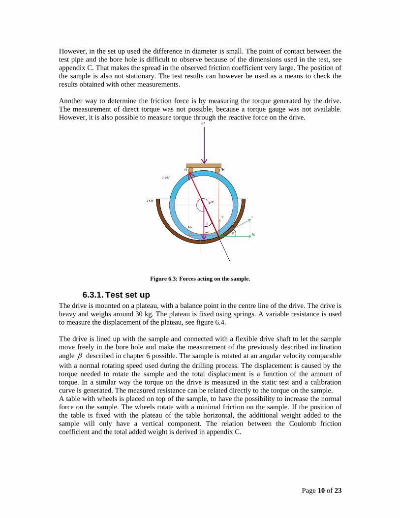
Another way to determine the friction force is by measuring the torque generated by the drive.

The measurement of direct torque was not possible, because a torque gauge was not available.

However, it is also possible to measure torque through the reactive force on the drive.

Figure 6.3; Forces acting on the sample.

6.3.1. Test set up

The drive is mounted on a plateau, with a balance point in the centre line of the drive. The drive is

heavy and weighs around 30 kg. The plateau is fixed using springs. A variable resistance is used

to measure the displacement of the plateau, see figure 6.4.

The drive is lined up with the sample and connected with a flexible drive shaft to let the sample

move freely in the bore hole and make the measurement of the previously described inclination

angle described in chapter 6 possible. The sample is rotated at an angular velocity comparable

with a normal rotating speed used during the drilling process. The displacement is caused by the

torque needed to rotate the sample and the total displacement is a function of the amount of

torque. In a similar way the torque on the drive is measured in the static test and a calibration

curve is generated. The measured resistance can be related directly to the torque on the sample.

A table with wheels is placed on top of the sample, to have the possibility to increase the normal

force on the sample. The wheels rotate with a minimal friction on the sample. If the position of

the table is fixed with the plateau of the table horizontal, the additional weight added to the

sample will only have a vertical component. The relation between the Coulomb friction

coefficient and the total added weight is derived in appendix C.

Page 11 of 23

Figure 6.4; The test schematic with the forces on the drive.

1. The „borehole‟

2. The casing sample

3. Flexible connection

4. Measuring resistance

5. Balance point

6. Drive

7. Gearbox

8. Yoke

9. Counterweight

The total weight added to the pipe is chosen such that the pipe doesn‟t deform, which would

increase the contact area and therefore increase the friction force. This would make the friction

relations of steel and composite difficult to compare to each other. Another limiting factor in the

test was the connection between the drive and the sample. Because of the flexibility of the drive

the maximum amount of torque was limited. Even though the expected normal forces for the

composite pipe are much smaller the tests were performed with the same additional loads.

With a data hub connected to the resistance and the computer it is possible to record the results of

the test. To compare the reading of the resistance a calibration curve was created at static

conditions. With the calibration curve the torque can be calculated.

6.3.2. Test results

The expected result based on the Coulomb friction model was that the friction coefficient would

be independent of the applied extra weight. For the steel that was indeed the case. The friction

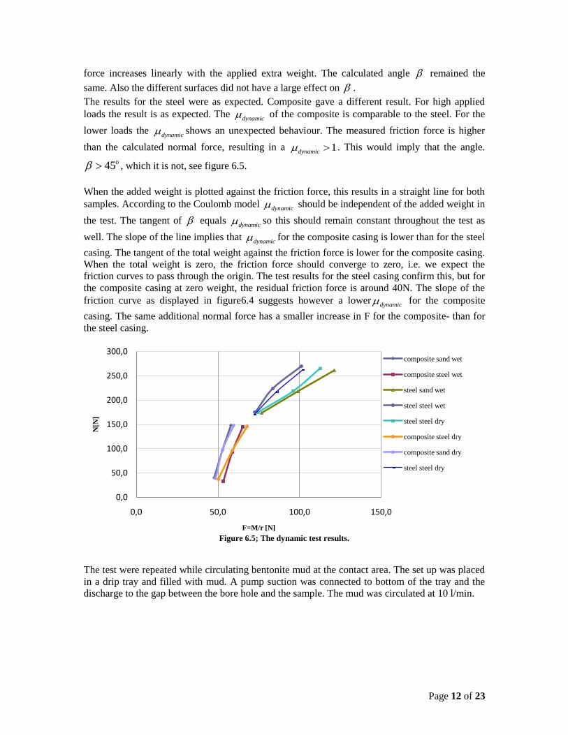
Page 12 of 23

force increases linearly with the applied extra weight. The calculated angle remained the

same. Also the different surfaces did not have a large effect on .

The results for the steel were as expected. Composite gave a different result. For high applied

loads the result is as expected. The dynamic of the composite is comparable to the steel. For the

lower loads the dynamic shows an unexpected behaviour. The measured friction force is higher

than the calculated normal force, resulting in a 1dynamic . This would imply that the angle.

45o , which it is not, see figure 6.5.

When the added weight is plotted against the friction force, this results in a straight line for both

samples. According to the Coulomb model dynamic should be independent of the added weight in

the test. The tangent of equals dynamic so this should remain constant throughout the test as

well. The slope of the line implies that dynamic for the composite casing is lower than for the steel

casing. The tangent of the total weight against the friction force is lower for the composite casing.

When the total weight is zero, the friction force should converge to zero, i.e. we expect the

friction curves to pass through the origin. The test results for the steel casing confirm this, but for

the composite casing at zero weight, the residual friction force is around 40N. The slope of the

friction curve as displayed in figure6.4 suggests however a lowerdynamic for the composite

casing. The same additional normal force has a smaller increase in F for the composite- than for

the steel casing.

Figure 6.5; The dynamic test results.

The test were repeated while circulating bentonite mud at the contact area. The set up was placed

in a drip tray and filled with mud. A pump suction was connected to bottom of the tray and the

discharge to the gap between the bore hole and the sample. The mud was circulated at 10 l/min.

0,0

50,0

100,0

150,0

200,0

250,0

300,0

0,0 50,0 100,0 150,0

N[N

]

F=M/r [N]

composite sand wet

composite steel wet

steel sand wet

steel steel wet

steel steel dry

composite steel dry

composite sand dry

steel steel dry

Page 13 of 23

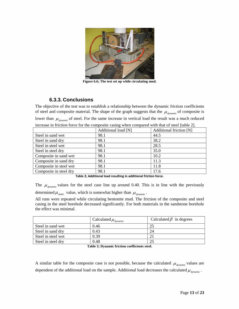
Figure 6.6; The test set up while circulating mud.

6.3.3. Conclusions

The objective of the test was to establish a relationship between the dynamic friction coefficients

of steel and composite material. The shape of the graph suggests that the dynamic of composite is

lower than dynamic of steel. For the same increase in vertical load the result was a much reduced

increase in friction force for the composite casing when compared with that of steel [table 2].

Additional load [N] Additional friction [N]

Steel in sand wet 98.1 44.5

Steel in sand dry 98.1 38.2

Steel in steel wet 98.1 28.5

Steel in steel dry 98.1 35.0

Composite in sand wet 98.1 10.2

Composite in sand dry 98.1 11.3

Composite in steel wet 98.1 11.8

Composite in steel dry 98.1 17.6 Table 2; Additional load resulting in additional friction force.

The dynamic values for the steel case line up around 0.40. This is in line with the previously

determined static value, which is somewhat higher than dynamic .

All runs were repeated while circulating bentonite mud. The friction of the composite and steel

casing in the steel borehole decreased significantly. For both materials in the sandstone borehole

the effect was minimal.

Calculateddynamic Calculated

in degrees

Steel in sand wet 0.46 25

Steel in sand dry 0.43 24

Steel in steel wet 0.39 21

Steel in steel dry 0.48 25 Table 3; Dynamic friction coefficients steel.

A similar table for the composite case is not possible, because the calculated dynamic values are

dependent of the additional load on the sample. Additional load decreases the calculateddynamic .

Page 14 of 23

Calculateddynamic Calculated

Composite in sand wet 0.37-1.14 20-49

Composite in sand dry 0.39-1.17 21-50

Composite in steel wet 0.43-1.59 23-58

Composite in steel dry 0.43-1.31 23-53 Table 4; Dynamic friction coefficients composite.

This is however not in line with the evaluation of the pictures. The test results can be confirmed

by evaluating the position of the sample. Videos were recorded of the tests. Evaluation of the

pictures is difficult, because the difference in diameter of the sample and the bore hole is very

small. This is the situation when drilling with casing. To increase the accuracy of determination

of the angle a ruler was fixed to the bore hole, to measure the position of the axis of the sample in

relation to the axis of the bore hole. With the relative position of the sample axis to the bore hole

axis and the radii of the sample and the bore hole the angle can be derived, see figure 6.7.

Figure 6.7; The dynamic test schematic.

The difference in radius between the „borehole‟ and the casing sample is R-R’. The horizontal

distance between the axis of the „borehole‟ and the casing sample is A-A’.

With the definition of the sine we can derive

'sin

'

A A

R R

6.10

'arcsin

'

A A

R R

6.11

Analysis of the angle does not confirm the unexpected behaviour of the calculated dynamic for

the composite. The observed angle indicates a friction coefficient similar to dynamic for the steel.

For the steel the angle confirms the calculations.

The resistance of the table was measured separately to eliminate extra torque by the table. Only

5% of the minimum torque measured could be contributed to the resistance of the table. To keep

the table in position four studs were installed to prevent the table to get out of position. This

makes the table rest on three points, making the construction statically undetermined. It is not

possible to calculate the weight taken by the stud. At the design of the test this was not considered

a problem. In a worst case the pin would take half of the applied weight and the middle wheel

would carry no weight at all. Unfortunately, recalculating the results for this worst case did not

improve the end results.

Page 15 of 23

7. Final conclusions The objective of the project was to compare the friction coefficients for steel and composite

casing in contact with different surfaces. Knowledge of the coefficient is useful to calculate

drilling loads like torque and drag which are a function of the static and dynamic friction

coefficients and hole geometry. Moreover, the difference between static and dynamic friction

may cause torsional vibrations. The higher difference between the static and dynamic friction

coefficients, the more the drillstring is susceptible to vibrations. Based on static and dynamic

friction measurements we conclude the following:

For steel the friction increases linearly with the additional load. The friction coefficient remains

the same within the tested range. The friction force plotted against the normal force is a line

through the origin of the graph. The friction coefficients are in the range expected before starting

the test. For the composite case the Coulomb friction model seems not to apply. The additional

friction force from an additional normal force is constant, resulting in a linear relationship,

however, the line crosses the x-axis around 40N.

This unexpected result may be an artefact, caused by the method of testing. Applying the

additional weight on top of the sample with the aid of a small wheel-supported plateau, see Fig.

6.3, made it unstable, because the position of the centre of gravity is above the casing sample. To

keep the plateau in place additional supports were used, which created a statically undetermined

situation, making it impossible to calculate the exact weight on the sample. In a revised set-up,

the position of the centre of gravity should be located below the casing sample, keeping the added

weight in place by gravity. However, this was not the case for the present set-up. Assuming the

worst case scenario, in the present set-up only half of the added weight would be applied to the

sample. Unfortunately recalculating all the values using this worst case assumption didn‟t

improve the result. The friction coefficients were found in a range between 0.16 for the additional

weight of 100 N in the wet composite-on-steel test and 1.70 for the wet composite-on-sand test

without an additional weight. Taking the worst case, with only half the added weight transmitted

to the sample did not increase the results. The spread of the results increased. It is therefore

unlikely that the weight is not transmitted to the sample as it is designed. The wide range in

friction coefficients is not supported by the video footage shot during the tests: the video images

did not reveal a correspondingly wide range in angular contact point positions.

The range of the additional load during the test is not in the range of normal loads expected

during the drilling of the DAP wells. With the equipment used in the experiments and the budget

available for the tests it was not possible to achieve the values expected in the worst case during

drilling which are much higher that what could be tested. According to the previously described

TanD sheet the anticipated static normal force in the well is in the order of 1000 N. The net

normal force is the vector sum of the tensile forces and the weight, see figure 7.1, and depends on

the hole radius of curvature, see figure 7.1.

For steel the normal force is around four times higher, because the density of steel is about four

times the density of composite.

The results of these experiments did not provide a satisfactory comparison between the dynamic

friction coefficients of steel and composite casing. Also the static friction coefficient

measurements of the composite casing showed some inconsistencies, which can be contributed to

the irregular surface caused by the production process.

Page 16 of 23

Figure 7.1; The force balance on a drillstring element from Johancsik et al. (1984).

8. Recommendations In order to find a relationship the tests can be repeated in a different set up. The behaviour of the

composite at small normal forces appears to be not linear. For downhole conditions this might not

be a problem. My suggestion is to repeat the measurements at downhole conditions. A more exact

measurement can be obtained by using a torque gauge between the drive and the sample. This

ensures a direct torque measurement instead of the indirect reactive force on the drive. The torque

gauge is expensive however and was not available for the test.

If the sample is mounted in bearings and rotates in the air, the weight of the sample is carried by

the bearings and eliminated from the set up. Normal force can be applied by pushing the borehole

material against the rotating sample by an air operated piston. From the air pressure reading the

normal force can be derived. With this set up the measurements are more controlled. If the drive

is strong enough higher normal forces can be applied. The only friction created by the system is

the friction of the bearings, which can be measured separately.

In figure 1 the recommended set-up is shown. If the weight of the sample, position 1, is carried by

the bearings in position 3. The borehole is pushed against the sample with a air piston at position

2, or with a jack and a scale. In this way, the force applied on the borehole is the normal force.

The measurements can be done in the actual range of the normal forces the pipe is exposed to in

downhole conditions (or at least with a higher normal force). According to the TanD application,

the normal force of in the composite case is at its maximum at 700 m at 10000N, when the dog

leg severity is at its maximum. For the steel case the normal force is maximal near the BHA,

when the weight of the pipe is maximal at maximum inclination, at 12000N. Perhaps the

behaviour of the composite sample is according the Coulomb model at higher normal force.

According to the Coulomb model, the friction coefficient is independent of the rotary speed,

however it might be worthwhile to repeat the test at several velocities.

Page 17 of 23

Figure 8.2; Recommended set-up for future testing

1 The sample

2 The „borehole‟

3 Support with bearings

4 Sample axis

9. Acknowledgements My special thanks go out to several people. First and most important I want to thank my wife

Carina, who has never stopped supporting me, even though it meant all family managing tasks

became her responsibility. This gave me the opportunity to fully focus on my second Delft career,

without worrying about the family management. An occasional tutoring for the kids and a hockey

training were my only responsibility. Off course Gerard Sigon for convincing me to do the MSc

immediately after finishing the BSc program. Without Gerard I would never have considered

starting the MSc program in the first place. Alexander Nagelhout, for getting me involved in the

project. Mr Tom Bakker, for facilitating and funding my project, having faith and bringing up

numerous ideas all the time to get the project going. Professor Jansen, for guiding me through the

project, bringing in new ideas all the time. Never getting tired of re-deriving all formulas and

adding to the science level of my project. Encouraging to make decisions, when things took too

long. Mr Gerard de Blok, for redirecting my writing to make it a decent English report and giving

ample input for the report. My father, taking the time to listen to the progress in the project.

Taking the time to use his knowledge of writing readable reports. Wim Verwaal for his contacts

in the faculty, providing me with the place to do the tests, giving me access to the workshop and

the lab. Creating the „borehole‟ and showing me where to cut the casing samples. Bringing me in

contact with Cees van Beek, who made the set up work with his brilliant measuring resistance,

connected to a TU Delft measuring program, called mp3. Without this missing link the

measurements would be very difficult, when not impossible.

10. List of References Johancsik, C.A., Friesen, D.B., Rapier Dawson, 1984. Torque and Drag in Directional Wells -

Prediction and Measurement, J Pet Technol 36 (6): 987-992. SPE-11380-PA. doi:

10.2118/11380-PA.

Leijnse, S. 2008. Drilling hazards for the DAP geothermal wells. BSc thesis, Delft University of

Technology.

Page 18 of 23

Jansen, J.D. 1993. Nonlinear Dynamics of Oilwell Drillstrings. PhD dissertation, Delft University

of Technology.

Aadnoy, B.S., Cooper, I., Miska, S.Z., Mitchell, R.F., Payne, M.L. 2009. Advanced Drilling and

Well Technology. Textbook series, SPE, Richardson, Texas.

Bourgoyne Jr, A.T., Chenevert, M.E., Millheim, K.K., Young Jr., F.S. 1991. Applied Drilling

Engineering. Textbook Series, Vol 2, SPE Richardson, Texas.

Deketh, H.J.R. 1995., Wear of Rock Cutting Tools, Laboratory Experiments on the Experiments

on the Abrasivity of Rocks. PhD dissertation, Delft University of Technology.

Kartika Surjosantoso, M. 2010. Experiment: Comparing the Static Friction Coefficient for Steel

and Composite Pipe. BSc thesis, Delft University of Technology.

Van Soest, J. 1988. Elementary Statistics (Elementaire Statistiek), sixth edition. Delft University

Press.

Warren, T., Houtchens, B., Madell, G. 2005. Directional Drilling With Casing. Paper SPE 79914

presented at the SPE/IADC Drilling Conference, Amsterdam, Netherlands, 19-21 February.

doi: 10.2118/79914-MS

Strickler, R. , Mushovic, T. , Warren, T., Lesso, B. 2005. Casing Directional Drilling Using a

Rotary Steerable System. Paper SPE 92195 presented at the SPE/IADC Drilling Conference,

Amsterdam, Netherlands, 23-25 February. doi:10.2118/92195-MS.

Van der Poll, J.W., 2010. An investigation of the stress-strain behavior of a GRE cylindrical

structure used for a drilling with casing application and its influence on torsional vibrations.

MSc thesis, Delft University of Technology.

11. List of figures

Figure 6.1; Forces acting on a mass. ............................................................................................... 6 Figure 6.2; The distribution of the static friction coefficients. ........................................................ 8 Figure 6.3; Forces acting on the sample. ....................................................................................... 10 Figure 6.4; The test schematic with the forces on the drive. ......................................................... 11 Figure 6.5; The dynamic test results. ............................................................................................. 12 Figure 6.6; The test set up while circulating mud. ........................................................................ 13 Figure 6.7; The dynamic test schematic. ....................................................................................... 14 Figure 7.1; The force balance on a drillstring element from Johancsik et al. (1984). ................... 16 Figure 8.1; Recommended set-up for future testing ...................................................................... 17 Figure A-1; Forces on an element of drillstring from Johancsik et al. (1984). ............................. 19 Figure B-1; Mass on an inclined surface. ...................................................................................... 20 Figure B-2; Schematic for the static force equilibrium. ................................................................ 21

12. List of tables Table 1; Static Coulomb friction coefficients found in the tests. .................................................... 9 Table 2; Additional load resulting in additional friction force. ..................................................... 13 Table 3; Dynamic friction coefficients steel.................................................................................. 13 Table 4; Dynamic friction coefficients composite. ....................................................................... 14

13. List of symbols Friction coefficient [-]

fricF Friction force [N]

Page 19 of 23

N Normal force [N]

g acceleration of gravity [m/s2]

static static friction coefficient

dynamic dynamic friction coefficient

14. List of abbreviations DAP Delft Aardwarmte Project, the Delft Geothermal Project

CwD Casing While Drilling

BHA Bottom Hole Assembly, drilling equipment at the end of the drillstring

RSS Rotary Steerable System

TanD Torque and Drag application developed by Well Engineering Partners

OD Outer diameter

ID Inner diameter

NPT Non Productive Time

MWD Measurements While Drilling

LWD Logging While Drilling

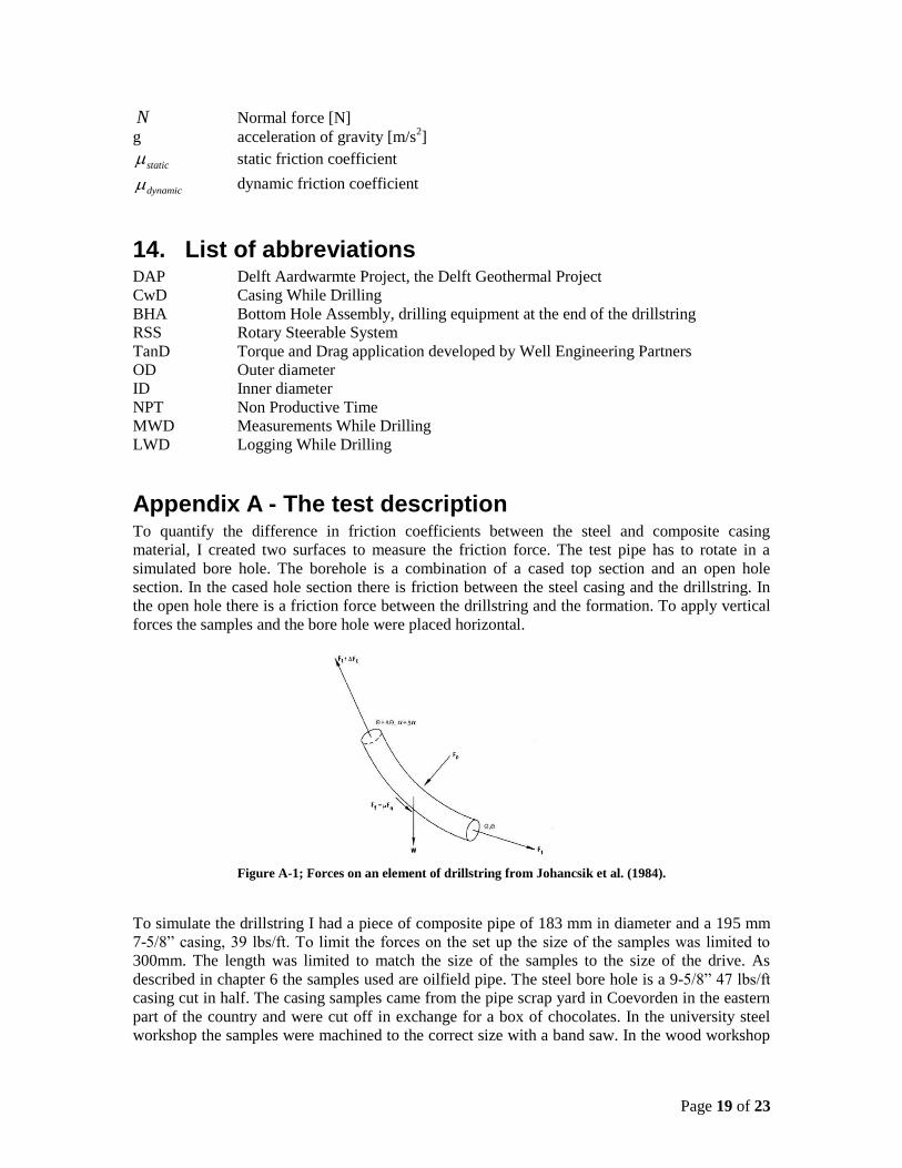
Appendix A - The test description To quantify the difference in friction coefficients between the steel and composite casing

material, I created two surfaces to measure the friction force. The test pipe has to rotate in a

simulated bore hole. The borehole is a combination of a cased top section and an open hole

section. In the cased hole section there is friction between the steel casing and the drillstring. In

the open hole there is a friction force between the drillstring and the formation. To apply vertical

forces the samples and the bore hole were placed horizontal.

Figure A-1; Forces on an element of drillstring from Johancsik et al. (1984).

To simulate the drillstring I had a piece of composite pipe of 183 mm in diameter and a 195 mm

7-5/8” casing, 39 lbs/ft. To limit the forces on the set up the size of the samples was limited to

300mm. The length was limited to match the size of the samples to the size of the drive. As

described in chapter 6 the samples used are oilfield pipe. The steel bore hole is a 9-5/8” 47 lbs/ft

casing cut in half. The casing samples came from the pipe scrap yard in Coevorden in the eastern

part of the country and were cut off in exchange for a box of chocolates. In the university steel

workshop the samples were machined to the correct size with a band saw. In the wood workshop

Page 20 of 23

the mould for the sandstone was made. The sand borehole was mixed and poured in the concrete

workshop. The ID of the sandstone is therefore the OD of the 9-5/8” casing.

To get the torque to the sample two wooden caps are tightened with a M12 stud bolt through the

sample.

For the dynamic test the torque was transmitted to the sample with a 1” air hose, for flexibility

and filled with sand to prevent the hose from winding up. The hose was clamped to the drive and

the sample with exhaust clamps.

Appendix B - The static test To measure the static friction coefficient there are more tests possible. One possibility is to see

when the pipe starts sliding when the inclination of the bore hole increases. By increasing the

inclination the normal force decreases because the gravity component perpendicular to the surface

decreases. At a certain inclination the gravity component parallel to the inclined surface equals

the friction force. As the weight of the sample is known and the angle of inclination can be

measured, the friction force at the moment of

sliding is known. With the friction factor and the inclination known, static can be calculated, see

figure 16.1

Vertical equilibrium states that

cosN W B-1

The horizontal equilibrium

sinF W B-2

Combining equation 16.1 with 16.2 and the Coulomb friction coefficient of the friction

coefficient

sintan

cos

F W

N W

B-3

Figure B-1; Mass on an inclined surface.

Since dynamic > static , the static friction force is larger than the dynamic friction force. Once the

pipe starts moving, it keeps on sliding.

A second way to determine the friction factor is more controlled. With the axis of the pipe fixed,

a force needs to be generated to overcome friction force. The friction force exerts a torque at the

Page 21 of 23

axis of the friction force times the radius of the pipe. On the axis we mounted a lever with a

bucket. The bucket is slowly filled with sand and when the torque applied by the lever, the bucket

and the sand equals the torque from the friction force, the pipe starts to rotate.

Figure B-2; Schematic for the static force equilibrium.

The equations can derived using the statics on the schematic. To determine the friction coefficient

we have to increase the mass at the end if the lever, m1 in this case. A simple force balance can be

used to derive the formulas to calculate the friction force.

For equilibrium in x direction, H is the horizontal force in the hinge.

0xF B-4

0F H B-5

Force equilibrium in the vertical direction:

0yF B-6

1 2 3 4( ) 0N g m m m m B-7

1 2 3 4N w w w w B-8

Also the torque equilibrium around the axis of the sample should hold:

0axisM B-9

1 2 0

2

RFr m gR m g

B-10

21( )

2

wFr R w

B-11

21( )

2

R wF w

r

B-12

Combining equation 16.10 with 16.6 and the Coulomb definition for the friction coefficient gives

Page 22 of 23

:

Ndef

F

B-13

21

1 2 3 4

( )2

( )

wR w

r w w w w

B-14

Appendix C - The dynamic test To measure the friction force on a rotating sample can be calculated directly if the torque on the

sample is known. A direct torque measurement between the sample and the drive is possible, but

not available for the test. These gauges transmit the signal through a radio signal to a measuring

device. These gauges are expensive, but give a direct measurement.

Another way to determine the friction force is by measuring the torque generated by the drive. An

indirect measurement of the torque is the amount of current through the drive is

P T C-1

and

P VI C-2

Where P is the power, T is the torque, ω is the angular velocity, I is the current and V is the

voltage.

Combining both equations gives

VIT

C-3

The angular velocity can be determined by counting the revolutions in a minute and converting to

rad/s. 1rpm = 2π/60=0,105 rad/s.

The drive for the rotation of the sample is a AC drive with a variable gear box from 20-100RPM

and a 400W rating. The drive belongs to the medium size shear box test and was borrowed from

Engineering Geology by mr W. Verwaal.

The drive for the experiments is a large motor with a gearbox. The plate attached to the electric

drive indicates that it is a 400Watt motor, originally driven by 480Volt AC. The input is

converted to 230Volt AC. The direction of rotation can be reversed by turning the power switch

in opposite direction. Because the input voltage is fixed at the main supply at 230Volt, the current

flowing through the drive is a direct measure of the torque when the rotation speed is known.

For the torque measurement the Volts are fixed and the ω can be counted. If the current can be

measured the torque is known. A gauge to measure the current rated for the anticipated power

was not available. However, in convenient stores measuring devices called Energy Saving Timers

are available to help households saving on energy consumption. These devices indicate the

energy usage of a household appliance in KWh or even in Euros. The purchased device has the

possibility to display the current in Amperes. The accuracy of the device according to the manual

is around 3%.

Page 23 of 23

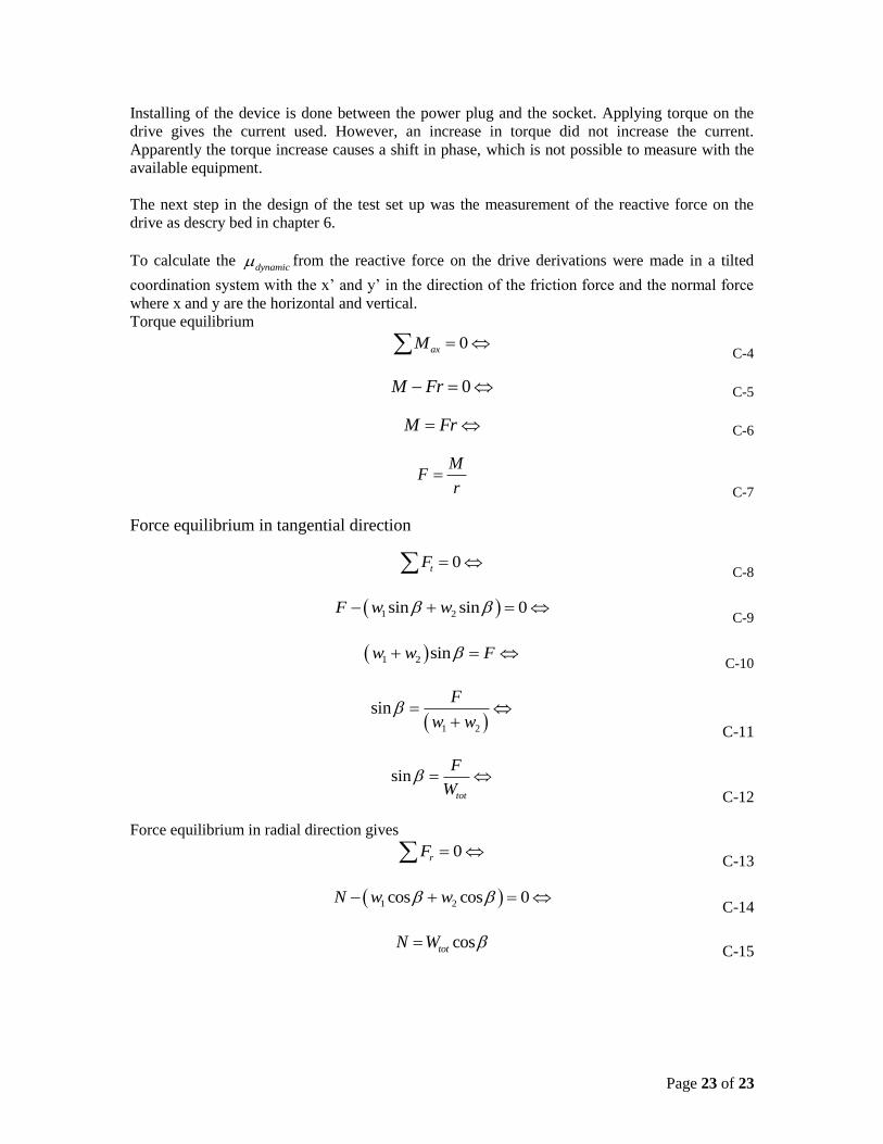
Installing of the device is done between the power plug and the socket. Applying torque on the

drive gives the current used. However, an increase in torque did not increase the current.

Apparently the torque increase causes a shift in phase, which is not possible to measure with the

available equipment.

The next step in the design of the test set up was the measurement of the reactive force on the

drive as descry bed in chapter 6.

To calculate the dynamic from the reactive force on the drive derivations were made in a tilted

coordination system with the x‟ and y‟ in the direction of the friction force and the normal force

where x and y are the horizontal and vertical.

Torque equilibrium

0axM C-4

0M Fr C-5

M Fr C-6

MF

r

C-7

Force equilibrium in tangential direction

0tF C-8

1 2sin sin 0F w w

C-9

1 2 sinw w F

C-10

1 2

sinF

w w

C-11

sintot

F

W

C-12

Force equilibrium in radial direction gives

0rF C-13

1 2cos cos 0N w w

C-14

costotN W

C-15