Aerospace Modeling Tutorial Lecture 2 – Basic Aerodynamics Greg and Mario February 2, 2015

Aerospace Modeling Tutorial Lecture 2 – Basic Aerodynamics Greg and Mario February 2, 2015.
Jan 03, 2016
Welcome message from author
This document is posted to help you gain knowledge. Please leave a comment to let me know what you think about it! Share it to your friends and learn new things together.
Transcript
Aerospace Modeling Tutorial
Lecture 2 – Basic Aerodynamics
Greg and MarioFebruary 2, 2015

˙⃑𝑣𝑏=�⃗�𝑏
𝑚−�⃑�× �⃑�𝑏
˙⃑𝑝𝑛=𝑅Τ𝑣𝑏
�́� ∙ ˙⃑𝜔=�⃑�× ( �́� ∙ �⃑�)+𝑇 𝑏
( �̇�11 �̇�12 �̇�13�̇� 21 �̇�22 �̇� 23�̇� 31 �̇�32 �̇� 33
)=( 0 𝜔𝑧 −𝜔𝑦
−𝜔𝑧 0 𝜔𝑥
𝜔𝑦 −𝜔𝑥 0 )(𝑟11 𝑟12 𝑟13𝑟21 𝑟 22 𝑟 23𝑟31 𝑟 32 𝑟 33
)
Our system dynamics:
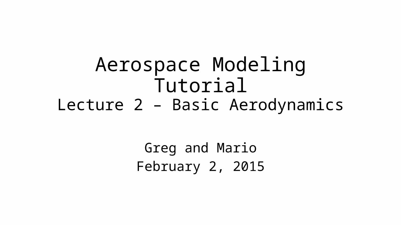
Our model

Navier Stokes Equations

Solving Navier Stokes - CFD
• Computationally demanding• Not suitable for real
time simulation• Not suitable for
dynamic optimization

How to simplify things?
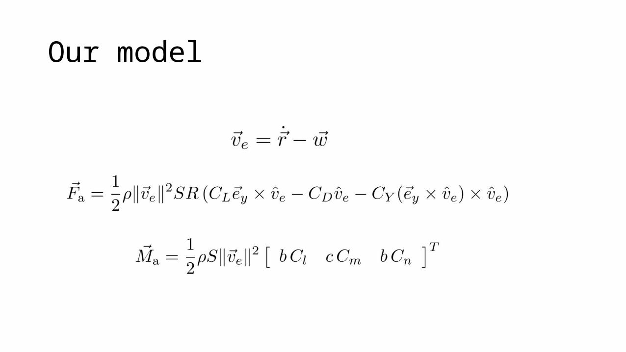
Thin airfoil theory
Assumptions:• 2-dimensional flow• Inviscid flow• Incompressible flow
Solve simplified NS (just Laplace’s equation) with flow tangency condition
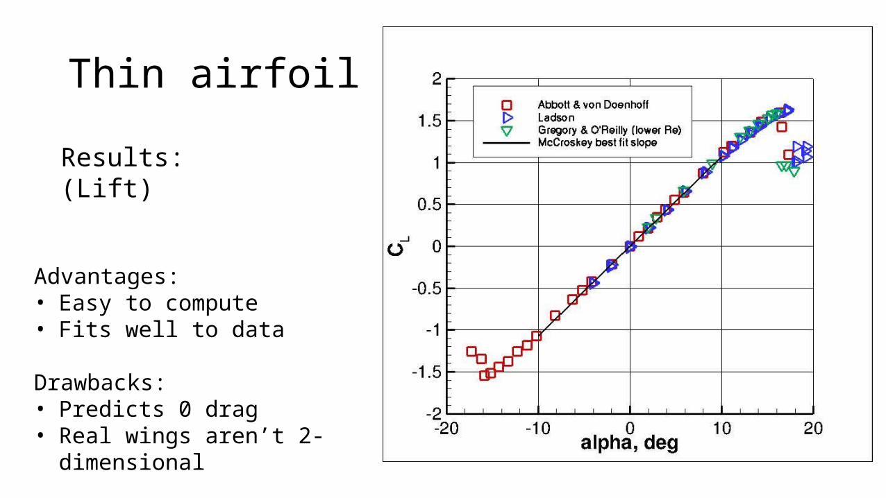
Thin airfoil theory
Results: (Lift)
Advantages:• Easy to compute• Fits well to data
Drawbacks:• Predicts 0 drag• Real wings aren’t 2-dimensional

xfoil
• viscous solution in the boundary layer• Inviscid outside• gives parasitic drag• still 2d

Prandtl lifting line theory• Still inviscid, incompressible• Model flow field as a sum of
horseshoe vortices• Solve for circulation of each 2-d
section
• Still need to account for wing-tail interaction• Ignores spanwise viscous flow
𝐶𝐷𝑖=𝐶𝐿2
𝜋 𝐴𝑅𝑒𝐶𝐿=𝐶𝑙
𝐴𝑅𝐴𝑅+2

Vortex lattice
• Model the wing as a panel of ring vortices
• Can handle arbitrary shapes
Disadvantage: intrinsically computational, no handy formulas

• popular code, includes parasitic drag• Inputs: geometry, alpha/beta/airspeed• Outputs: force/moment vectors + derivatives w.r.t. omega• Strategy: sweep alpha/beta, fit curves for all coefficients
AVL – Athena Vortex Lattice (Mark Drela)

Our model
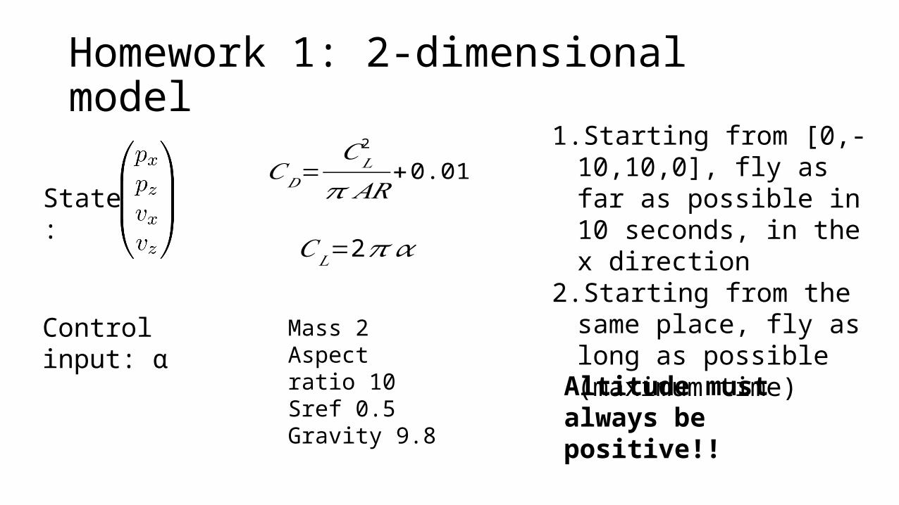
Homework 1: 2-dimensional model
𝐶𝐷=𝐶𝐿2
𝜋 𝐴𝑅+0.01
𝐶𝐿=2𝜋 𝛼
Mass 2Aspect ratio 10Sref 0.5Gravity 9.8
State:
Control input: α
1. Starting from [0,-10,10,0], fly as far as possible in 10 seconds, in the x direction
2. Starting from the same place, fly as long as possible (maximum time)
Altitude must always be positive!!
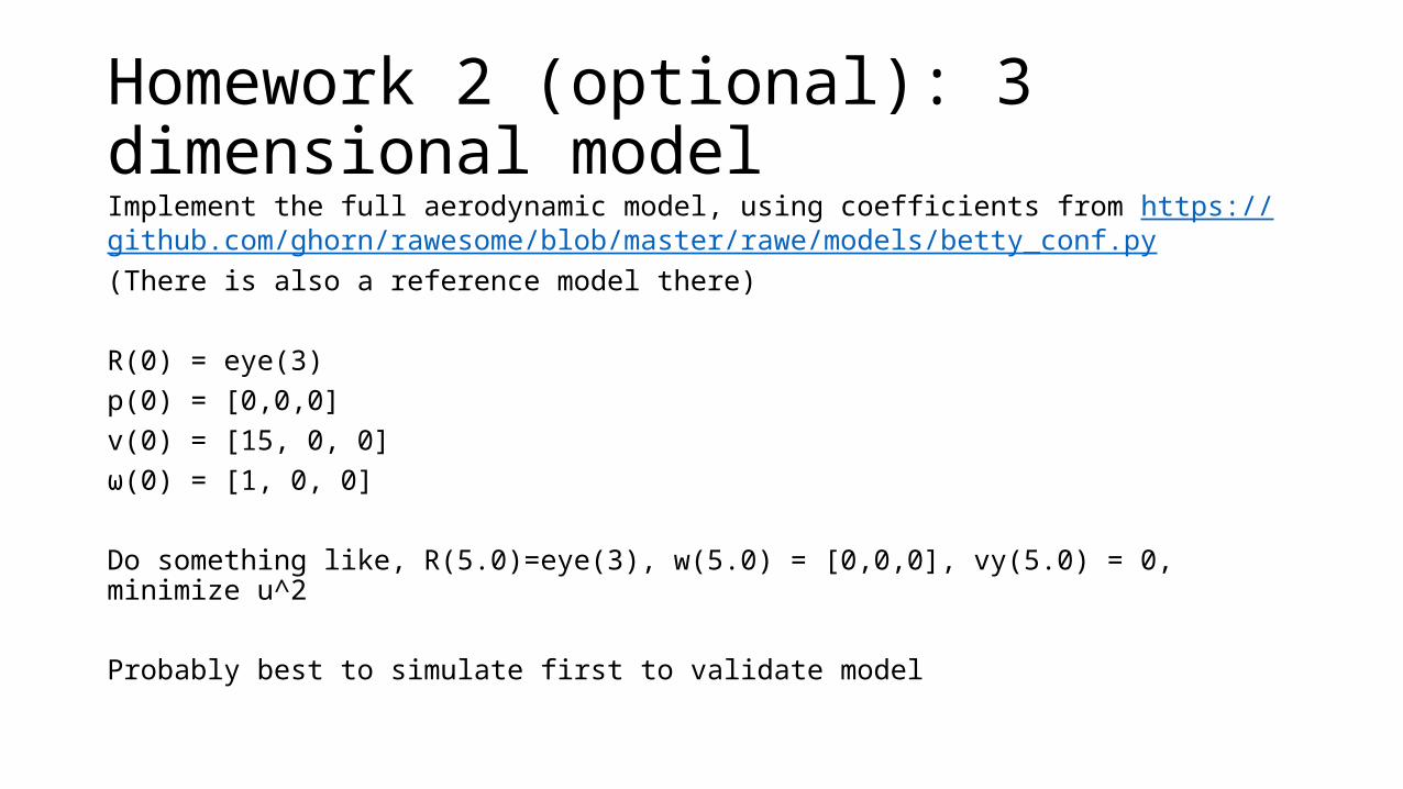
Homework 2 (optional): 3 dimensional modelImplement the full aerodynamic model, using coefficients from https://github.com/ghorn/rawesome/blob/master/rawe/models/betty_conf.py(There is also a reference model there)
R(0) = eye(3)p(0) = [0,0,0]v(0) = [15, 0, 0]ω(0) = [1, 0, 0]
Do something like, R(5.0)=eye(3), w(5.0) = [0,0,0], vy(5.0) = 0, minimize u^2
Probably best to simulate first to validate model
Related Documents