Aerosol remote sensing in polar regions

AEROSOL REMOTE SENSING IN POLAR REGIONS

Tomasi, C., Kokhanovsky, A. A., Lupi, A., Ritter, C., Smirnov, A., O'Neill, N. T., Stone, R. S., Holben, B. N., Nyeki, S., Wehrli, C., Stohl, A., Mazzola, M.,

Lanconelli, C., Vitale, V., Stebel, K., Aaltonen, V., de Leeuw, G., Rodriguez, E., Herber, A. B., Radionov, V. F., Zielinski, T., Petelski, T., Sakerin, S. M.,

Kabanov, D. M., Xue, Y., Mei, L., Istomina, L., Wagener, R., McArthur, B., Sobolewski, P. S., Kivi, R., Courcoux, Y., Larouche, P., Broccardo, S., and

Piketh, S. J.

November 2014

Accepted for publication in Earth-Science Reviews

(140, 108-157, doi:10.1016/j.earscirev.2014.11.001, 2015)

Biological, Environmental & Climate Sciences Dept.

Brookhaven National Laboratory P.O. Box 5000

Upton, NY 11973-5000 www.bnl.gov

Notice: This manuscript has been authored by employees of Brookhaven Science Associates, LLC under Contract No. DE-AC02-98CH10886 with the U.S. Department of Energy. The publisher by accepting the manuscript for publication acknowledges that the United States Government retains a non-exclusive, paid-up, irrevocable, world-wide license to publish or reproduce the published form of this manuscript, or allow others to do so, for United States Government purposes.

DISCLAIMER

This report was prepared as an account of work sponsored by an agency of the United States Government. Neither the United States Government nor any agency thereof, nor any of their employees, nor any of their contractors, subcontractors, or their employees, makes any warranty, express or implied, or assumes any legal liability or responsibility for the accuracy, completeness, or any third party’s use or the results of such use of any information, apparatus, product, or process disclosed, or represents that its use would not infringe privately owned rights. Reference herein to any specific commercial product, process, or service by trade name, trademark, manufacturer, or otherwise, does not necessarily constitute or imply its endorsement, recommendation, or favoring by the United States Government or any agency thereof or its contractors or subcontractors. The views and opinions of authors expressed herein do not necessarily state or reflect those of the United States Government or any agency thereof.

1

Revised version submitted to Earth Science Reviews on August 26, 2014

Aerosol remote sensing in polar regions

by

Claudio Tomasi (1), Alexander A. Kokhanovsky (2, 3), Angelo Lupi (1), Christoph Ritter (4),

Alexander Smirnov (5, 6), Norman T. O’Neill (7), Robert S. Stone (8, 9), Brent N. Holben (6),

Stephan Nyeki (10), Christoph Wehrli (10), Andreas Stohl (11), Mauro Mazzola (1),

Christian Lanconelli (1), Vito Vitale (1), Kerstin Stebel (11), Veijo Aaltonen (12),

Gerrit de Leeuw (12, 13), Edith Rodriguez (12), Andreas B. Herber (14), Vladimir F. Radionov (15),

Tymon Zielinski (16), Tomasz Petelski (16), Sergey M. Sakerin (17), Dmitry M. Kabanov (17),

Yong Xue (18, 19), Linlu Mei (19), Larysa Istomina (2), Richard Wagener (20), Bruce McArthur (21),

Piotr S. Sobolewski (22), Rigel Kivi (23), Yann Courcoux (24), Pierre Larouche (25),

Stephen Broccardo (26) and Stuart J. Piketh (27)

(1) Climate Change Division, Institute of Atmospheric Sciences and Climate (ISAC), Italian

National Research Council (CNR), Bologna, Italy. (2) Institute of Environmental Physics (IUP), University of Bremen, Bremen, Germany. (3) EUMETSAT, Eumetsat Allee 1, D-64295 Darmstadt, Germany. (4) Climate System Division, Alfred Wegener Institute for Polar and Marine Research, Potsdam,

Germany. (5) Sigma Space Corporation, Lantham, Maryland, USA. (6) Biospheric Sciences Branch, NASA/Goddard Space Flight Center (GSFC), Greenbelt, Maryland,

USA. (7) Canadian Network for the Detection of Atmospheric Change (CANDAC) and CARTEL, Dept. of

Applied Geomatics, University of Sherbrooke, Sherbrooke, Québec, Canada. (8) Global Monitoring Division (GMD), National Oceanic and Atmospheric Administration

(NOAA), Boulder, Colorado, USA.

2

(9) Cooperative Institute for Research in Environmental Sciences (CIRES), University of Colorado,

Boulder, Colorado, USA. (10) Physikalisch-Meteorologisches Observatorium (PMOD)/World Radiation Centre (WRC),

Davos, Switzerland. (11) Norwegian Institute for Air Research (NILU), Kjeller, Norway. (12) Climate and Global Change Division, Finnish Meteorological Institute (FMI), Helsinki, Finland. (13) Department of Physics, University of Helsinki, Finland. (14) Climate System Division, Alfred Wegener Institute for Polar and Marine Research,

Bremerhaven, Germany. (15) Arctic and Antarctic Research Institute (AARI), St. Petersburg, Russia. (16) Institute of Oceanology (IO), Polish Academy of Sciences (PAS), Sopot, Poland. (17) V. E. Zuev Institute of Atmospheric Optics (IAO), Siberian Branch (SB), Russian Academy of

Sciences (RAS), Tomsk, Russia. (18) Faculty of Life Sciences and Computing, London Metropolitan University, London, United

Kingdom. (19) Key Laboratory of Digital Earth Science, Institute of Remote Sensing and Digital Earth, Chinese

Academy of Sciences, Beijing, 100094, China (20) Brookhaven National Laboratory, Environmental and Climate Sciences Dept., Upton, NY, USA. (21) Environment Canada, Downsview, North York, Ontario, Canada; now with Agriculture and

Agri-food Canada. (22) Institute of Geophysics, Polish Academy of Sciences (PAS), Warsaw, Poland. (23) Arctic Research Center, Finnish Meteorological Institute (FMI), Sodankylä, Finland. (24) Institute de l'Atmosphère de la Réunion (OPAR), Univ. de la Réunion - CNRS, Saint Denis de la

Réunion, France. (25) Institut Maurice-Lamontagne, Mont-Joli, Quebec, Canada. (26) Geography, Archeology and Environmental Science, University of the Witwatersrand,

Johannesburg, South Africa. (27) Climatology Research Group, Unit for Environmental Sciences and Management, North-West

University, Potchefstroom, South Africa.

Corresponding author: Claudio Tomasi Phone: + 39 051 639 9594 Fax: + 39 051 639 9652 E-mail:[email protected]

3

Abstract

Multi-year sets of ground-based sun-photometer measurements conducted at 12 Arctic sites and 9

Antarctic sites were examined to determine daily mean values of aerosol optical thickness τ(λ) at

visible and near-infrared wavelengths, from which best-fit values of Ångström’s exponent α were

calculated. Analysing these data, the monthly mean values of τ(0.50 µm) and α and the relative

frequency histograms of the daily mean values of both parameters were determined for winter-

spring and summer-autumn in the Arctic and for austral summer in Antarctica. The Arctic and

Antarctic covariance plots of the seasonal median values of α versus τ(0.50 µm) showed: (i) a

considerable increase in τ(0.50 µm) for the Arctic aerosol from summer to winter-spring, without

marked changes in α; and (ii) a marked increase in τ(0.50 µm) passing from the Antarctic Plateau to

coastal sites, whereas α decreased considerably due to the larger fraction of sea-salt aerosol. Good

agreement was found when comparing ground-based sun-photometer measurements of τ(λ) and α

at Arctic and Antarctic coastal sites with Microtops measurements conducted during numerous

AERONET/MAN cruises from 2006 to 2013 in three Arctic Ocean sectors and in coastal and off-

shore regions of the Southern Atlantic, Pacific, and Indian Oceans, and the Antarctic Peninsula.

Lidar measurements were also examined to characterise vertical profiles of the aerosol

backscattering coefficient measured throughout the year at Ny-Ålesund. Satellite-based MODIS,

MISR, and AATSR retrievals of τ(λ) over large parts of the oceanic polar regions during spring and

summer were in close agreement with ship-borne and coastal ground-based sun-photometer

measurements. An overview of the chemical composition of fine and accumulation/coarse mode

particles is also presented, based on in-situ measurements at Arctic and Antarctic sites. Fourteen

log-normal aerosol number size-distributions were defined to represent the average features of fine

and accumulation/coarse mode particles for Arctic haze, summer background aerosol, Asian dust

and boreal forest fire smoke, and for various background austral summer aerosol types at coastal

4

and high-altitude Antarctic sites. The main columnar aerosol optical characteristics were determined

for all 14 particle modes, based on in-situ measurements of the scattering and absorption

coefficients. Diurnally averaged direct aerosol-induced radiative forcing and efficiency were

calculated for a set of multimodal aerosol extinction models, using various Bidirectional

Reflectance Distribution Function models over vegetation-covered, oceanic and snow-covered

surfaces. These gave a reliable measure of the pronounced effects of aerosols on the radiation

balance of the surface-atmosphere system over polar regions.

Key words:

Sun-photometer measurements

Aerosol optical thickness

Polar aerosol optical characteristics

Lidar backscattering coefficient profiles

Satellite aerosol remote sensing

Multimodal aerosol extinction models

5

1. Introduction.

Aerosols are one of the greatest sources of uncertainty in climate modeling, since their

concentrations and microphysical, chemical and optical characteristics vary in time and in space. In

addition, they can alter cloud microphysics, which could strongly impact cloud optical features and

climate. The aim of this paper is to present an overview of the optical characteristics of atmospheric

aerosol observed in polar regions during the past two decades, including recent measurements

conducted with ground-based and ship-borne sun-photometers, or retrieved from remote sensing

data recorded with visible and infrared sensors mounted onboard various satellite platforms. Optical

instruments (e.g., lidars, sun-photometers) measure the characteristics of the atmospheric light field

(internal, reflected, or transmitted). Specific procedures therefore need to be applied to convert

optical signals to aerosol characteristics, such as particle size and shape distributions, or chemical

composition. Similar procedures are also needed to derive the vertical concentration distribution

from columnar measurements. They are based on the solution of the inverse problem of radiative

transfer theory accounting for multiple light scattering, molecular and aerosol scattering and

absorption, and surface reflectance effects.

The presence of a visibility-reducing haze in the Arctic was already noted by early explorers in the

19th century (see Garrett and Verzella, 2008, for a historical overview). The explorers also

documented that haze particles were deposited on snow in remote parts of the Arctic (e.g.,

Nordenskiöld, 1883) and haze layers were also observed later by pilots in the 1950s (Mitchell,

1957). The source of the haze was debated for almost a century but poorly understood until the

1970s when it was suggested that this “Arctic Haze” originated from emissions in northern mid-

latitudes and was transported into the Arctic over thousands of kilometers (Rahn et al., 1977, Barrie

et al., 1981). The seasonality of the haze which peaks in winter and early spring, was explained by

the fact that removal processes are inefficient in the Arctic during that time of the year (Shaw,

1995).

6

Polar aerosols originate from both natural and anthropogenic sources (Shaw, 1988, 1995). In the

Arctic regions, natural aerosols have been found to contain an oceanic sea-salt mass fraction that

frequently exceeds 50% on summer days, and a mass fraction of 30-35% due to mineral dust, with

lower percentages of non-sea-salt (nss) sulphate, methane sulphonic acid (MSA), and biomass

burning combustion products. In contrast, anthropogenic particles have higher concentrations of

sulphates, organic matter (OM) and black carbon (BC) with respect to natural aerosol (Quinn et al.,

2002, 2007; Sharma et al., 2006). In fact, boreal forest fire (hereinafter referred to as BFF) smoke

transported from North America and Siberia often contributes to enhance soot concentration in

summer (Damoah et al., 2004; Stohl et al., 2006). Rather high aerosol mass concentrations of

anthropogenic origin are frequently transported from North America and especially Eurasia in the

winter and spring months, leading to intense Arctic haze episodes (Shaw, 1995). For instance,

Polissar et al. (2001) conducted studies on the BC source regions in Alaska from 1991 to 1999

finding that predominant contributions have been given by large-scale mining and industrial

activities in South and Eastern Siberia. In the North-European sector of the Arctic, the dominant

sources of sulphates and nitrates (and to a lesser extent of water-soluble OM and BC) are located in

Europe and Siberia, due to both urban pollution and industrial activities (Hirdman et al., 2010).

Episodes of Asian dust transport have also been observed over the past years in the North-American

sector of the Arctic, especially in spring (Stone et al., 2007), together with local transport of soil

particles mobilized by strong winds, which provisionally enhance the mass concentrations of

elemental components, such as Al, Si, Mg and Ca (Polissar et al., 1998). The Arctic atmosphere’s

stratification is highly stable, with frequent and strong inversions near the surface, which limit

turbulence and reduce the dry deposition of aerosols to the surface (Strunin et al., 1997). They also

decouple the sea ice inversion layer from the Arctic free troposphere, leading to very different

chemical and physical properties of aerosols in the sea ice inversion layer where aerosols are

depleted, and higher up where a sulphate-rich background aerosol typically of anthropogenic origin

is often found (Brock et al., 2011).

7

The Arctic atmosphere’s stratification is highly stable, with frequent and strong inversions near the

surface, which limit turbulence and reduce the dry deposition of aerosols to the surface (Strunin et

al., 1997). They also decouple the sea ice inversion layer from the Arctic free troposphere, leading

to very different chemical and physical properties of aerosols in the sea ice inversion layer where

aerosols are depleted, and higher up where a sulphate-rich background aerosol typically of

anthropogenic origin is often found (Brock et al., 2011). In addition, organic-rich biomass burning

layers occur in the free troposphere but rarely reach the surface (Brock et al., 2011; Warneke et al.,

2010). The low-altitude high-latitude atmosphere in the southern hemisphere is similarly stably

stratified as the Arctic’s but also influenced strongly by katabatic winds bringing down air from the

high altitudes of interior Antarctica (Stohl and Sodemann, 2010).

On larger scales, the stable Arctic stratification leads to the so-called polar dome, where isentropes

form shells above the Arctic. As atmospheric transport tends to follow the isentropes, direct

transport of air masses from mid-latitude pollution source regions into the Arctic lower troposphere

is very inefficient. According to Stohl (2006), polluted air masses from lower latitudes typically

follow one of five major transport pathways (see Fig. 1): (1) lifting at the Arctic front, where wet

scavenging is efficient; (2) lifting already at lower latitudes (at the polar front or convection), where

wet scavenging is even more efficient; (3) and most importantly for Arctic surface aerosol

concentrations, low-level transport over land in winter where strong radiative cooling allows air

masses to enter the polar dome; (4) slow descent by radiative cooling of upper-tropospheric air

masses into the polar dome; (5) slow mixing across the lateral boundaries of the dome. Forest or

agricultural fires are important, as they produce strong aerosol plumes in the mid- to high-latitude

free troposphere, which can subsequently enter the Arctic by one of the previously mentioned

processes.

In addition to long-range pollution transport, local emission sources can be important. For instance,

emissions from cruise ships, can lead to measurable enhancements of BC and other aerosols in the

Svalbard archipelago (Eckhardt et al., 2013). Diesel generators can also locally pollute the

8

environment (Hagler et al., 2008). Aircraft emissions north of the Arctic circle are primarily

injected into the stratosphere where removal is inefficient and these emissions can slowly descend

(Whitt et al., 2011). All these local sources can also enhance the Arctic aerosol background;

however, quantification of their contribution relative to long-range transport of pollution from

sources outside the Arctic remains uncertain. In addition, sulphate and volcanic ash from high-

latitude eruptions can occasionally influence the Arctic troposphere (e.g., Hoffmann et al., 2010).

The stratospheric background aerosol in the Arctic as elsewhere can be perturbed by explosive

volcanic eruptions (especially in the tropics) for several years. Some volcanic aerosol emission

episodes have been observed by Bourassa et al. (2010) and O’Neill et al. (2012) over the last years,

involving the low stratosphere over short periods of a few months.

Transport processes in the high-latitude southern hemisphere are similar to those sketched for the

Arctic in Fig. 1. As in the northern hemisphere, polluted air masses from the lower-latitude

continents are quasi-isentropically lifted to higher altitudes and, furthermore, there is no low-

altitude transport pathway over land in winter (i.e., the analogue to transport pathway number 3 in

Fig. 1 is missing in the southern hemisphere). Consequently, as in the Arctic, the lowermost

troposphere in the Antarctic is very isolated and, thus, contains little anthropogenic pollution

transported from lower-latitude continents (Stohl and Sodemann, 2010). A major difference to the

Arctic, however, is the high topography of the Antarctic continent. This means that the most

isolated air masses (as measured by the time since last exposure to pollution sources at lower-

latitude continents) are not found close to the pole, as in the Arctic, but in the coastal areas

surrounding Antarctica (Stohl and Sodemann, 2010). Descent over the Antarctic continent is

stronger than over the Arctic and can also bring down air from the stratosphere, and air from the

Antarctic interior is transported down to coastal areas by strong katabatic winds.

In Antarctica, aerosols sampled at coastal sites originate almost totally from natural processes, with

a prevailing oceanic sea-salt mass content of 55-60%, and lower percentages of nss sulphate (20-

30%) and mineral dust (10-20%) (Tomasi et al., 2012). Only very low mass fractions of nitrates,

9

water-soluble OM and BC have been monitored in Antarctica, mainly associated with transport

from remote anthropogenic sources (Wolff and Cachier, 1998) or biomass burning (Fiebig et al.,

2009) in mid-latitude areas. More than 60-80% of particulate matter suspended over the Antarctic

Plateau has been estimated to consist of nss sulphates formed from biogenic sulphur compounds

and/or MSA, due to long-range transport in the free troposphere and subsequent subsidence

processes. Therefore, aerosols sampled at these high-altitude sites contain only moderate mass

fractions of nitrates, and minor or totally negligible mass percentages of mineral dust, water-soluble

OM and BC (Tomasi et al., 2007, 2012).

The paper is organized as follows. In the next section the ground-based remote sensing

measurements of atmospheric aerosol are reviewed (sun-photometers, lidars). Section 3 gives a

description of ship-borne aerosol remote sensing instruments. Section 4 discusses aerosol

backscattering coefficient profiles from lidar measurements, while Section 5 is dedicated to

airborne and satellite observations of polar aerosols. The last section presents the most important

optical characteristics and size-distribution features of polar aerosols, which are appropriate for

calculations of direct radiative forcing effects induced by aerosols on the climate system.

2. Ground-based remote sensing measurements

2.1. Spectral measurements of aerosol optical thickness

Ground-based remote sensing of the optical characteristics of aerosols in the atmospheric column is

usually conducted with multi-wavelength sun-photometers. A sun-photometer is oriented towards

the Sun to detect the solar radiation attenuated along the slant path from the top-of-atmosphere

(TOA) to the ground. The atmospheric aerosol load leads to a decrease in the solar radiation

transmitted through the atmosphere. This decrease depends on the aerosol optical thickness

(hereinafter referred to as AOT and/or using symbol τ(λ)), which is given by the integral of the

volume aerosol extinction coefficient along the vertical path of the atmosphere.

10

The networks, sites and sun-photometers whose data were employed in this paper are defined and

characterized in Tables 1 and 2 for the Arctic and Antarctic regions, respectively. The largest

networks of sun-photometers in the world are AERONET and SKYNET. Spectral measurements of

τ(λ) are performed with AERONET sun-photometers (Holben et al., 1998) at 8 wavelengths

ranging from 0.340 to 1.600 µm, and with SKYNET instruments (Nakajima et al., 2007) at 10

wavelengths from 0.315 to 2.200 µm. The Cimel CE-318 sun-photometers of the AERONET

network are currently used at several Arctic sites: Barrow (since March 2002), Thule (since March

2007), Hornsund (since April 2005), Sodankylä (since February 2007), Tiksi (since June 2010),

Resolute Bay (since July 2004), Eureka-0PAL (since April 2007) and Eureka-PEARL (since May

2007). The last three sites, located in the Nunavut region of Canada, are part of the

AEROCAN/AERONET network. In addition, an AERONET sun-photometer has been

intermittently used since 2002 by the Atmospheric Optics Group (GOA) (University of Valladolid,

Spain) at the Arctic Lidar Observatory for Middle Atmosphere Research (ALOMAR), located on

the Andøya Rocket Range, near Andenes (Northern Norway) (Toledano et al., 2012). AERONET

sun-photometers have been used to obtain Level 2.0 τ(λ) measurements at the South Pole (since

November 2007), and occasionally at Dome Concordia (in January and December 2003) in

Antarctica. AERONET Level 1.5 measurements of τ(λ) are available for McMurdo on the Ross Sea

(from February to December 1997, in the austral summer 2001/2002, and in January-February

2011), at Marambio (Antarctic Peninsula) since October 2007, at Vechernaya Hill (Thala Hills,

Enderby Land) since December 2008, and at Utsteinen (Dronning Maud Land) since February

2009. However, because these data were not promoted to Level 2.0, they were not considered in the

present study. A PREDE POM-01L sun/sky radiometer was used in Antarctica during the 2001-

2002 austral summer by Di Carmine et al., (2005) at the Mario Zucchelli station. PREDE

instruments have been used since 2001 in Antarctica at Syowa (East Ongul Island, Lützow-Holm

Bay) by the National Institute of Polar Research (NIPR, Tokyo, Japan) since 2001, at Rothera by

the British Antarctic Survey (BAS) since January 2008, and at Halley by BAS since February 2009.

11

In addition, Precision Filter Radiometer (PFR) sun-photometers (Wehrli, 2000; Nyeki et al., 2012)

from the Global Atmosphere Watch (GAW) PFR network are currently used in the Arctic at

Summit by PMOD/WRC (Switzerland), at Ny-Ålesund by NILU (Norway), and at Sodankylä by

FMI (Finland), and in Antarctica at Marambio by FMI and at Troll by NILU. The instrumental and

geometrical characteristics of the PFR sun-photometer are described by Wehrli (2000).

The monochromatic total optical thickness τTOT(λ) of the atmosphere is commonly calculated in

terms of the well known Lambert-Beer law for a certain sun-photometer output voltage J(λ) taken

within a spectral channel centred at wavelength λ and for a certain apparent solar zenith angle θ0.

The monochromatic value of τTOT(λ) is given by (Shaw, 1976):

τTOT(λ) = (1/m) ln [R J0(λ)/J(λ)] , (1)

where:

(i) m is the relative optical air mass calculated as a function of θ0 using a realistic model of the

atmosphere, in which wet-air refraction and Earth/atmosphere curvature effects on the direct solar

radiation passing through the atmosphere are properly taken into account (Thomason et al., 1983;

Tomasi and Petkov, 2014); (ii) J(λ) is the output signal (proportional to solar irradiance) measured

by the ground-based solar pointing sun-photometer; (iii) J0(λ) is the output signal that would be

measured by the sun-photometer outside the terrestrial atmosphere, at the mean Earth-Sun distance;

and (iv) R accounts for J0(λ) variations as a function of the daily Earth-Sun distance (Iqbal, 1983).

The solar radiation reaching the surface for cloud-free sky conditions is attenuated not only by

aerosol extinction but also by Rayleigh outscattering as well as absorption by minor gases (mainly

water vapour (H2O), ozone (O3), nitrogen dioxide (NO2) and its dimer (N2O4), and oxygen dimer

(O4)). The spectral values of τ(λ) within the main windows of the atmospheric transmission

spectrum are accordingly calculated by subtracting the Rayleigh scattering and absorption optical

thicknesses from τTOT(λ).

12

AOT is usually a smooth function of wavelength λ (measured in µm), which can be approximated

by the following simple formula:

( ) ( )0 0( / ) ατ λ τ λ λ λ −= , (2)

where α is the so-called Ångström (1964) wavelength exponent, and λ0 is usually assumed to be

equal to 1 µm. In reality, the analytical form defined in Eq. (2) can be convex or concave depending

on the relative contents of fine and coarse particles in the atmospheric column. O’Neill et al.

(2001a) demonstrated that the variation in τ(λ) and its first and second spectral derivatives (named

here α and α’, respectively) can be realistically described in terms of the spectral interaction

between the individual optical components of a bimodal size-distribution. O’Neill et al. (2001a)

then showed that one can exploit the spectral curvature information in the measured τ(λ) to permit a

direct estimate of a fine-mode Ångström exponent (αf) as well as the optical fraction of fine-mode

particles. However, an analysis of α and α’ determined in real cases and taking into account that

both α(0.44-0.87 µm) and α’ are closely related to the spectral features of τ(λ) showed that

propagation of errors leads to an error ∆α/α ∼ 2 ∆τ(λ)/τ(λ) and an error ∆α’/α’ ∼ 5 ∆τ(λ)/τ(λ),

respectively (Gobbi et al., 2007). These estimates yield values of ∆α/α and ∆α’/α’ that are > ∼ 20%

and > ∼ 50%, respectively, for τ(λ) ≤ 0.10 and a typical sunphotometry error equal to ∼ 0.01. To

avoid relative errors > ∼ 30% in ∆α’/α’, Gobbi et al. (2007) suggested using only observations of

τ(λ) > 0.15. We applied the same criterion as a threshold for accepting outputs from the Spectral

Deconvolution Algorithm (SDA) of O’Neill et al. (2003) (notably the fine-mode Ångström

exponent, which offers an alternative refinement to the calculation of α): our logic being that α and

α’ are input parameters to SDA and we did not want to introduce unacceptable processing errors to

the extraction of a spectral exponent indicator. These limitations to the use of spectral values of α

and α’ were also applied by Yoon et al. (2012), who only considered observations with τ(0.44 µm)

> 0.15 in order to avoid relative errors > 30% in α’. Tomasi et al. (2007) showed that for the period

13

1977-2006, τ(0.50 µm) did not exceed 0.15 for background summer aerosol conditions at Barrow,

Alert, Summit, Ny-Ålesund, Hornsund, Sodankylä and Andenes/ALOMAR in the Arctic, and was

greater than 0.15 only during very strong episodes of Arctic haze in late winter and spring, and BFF

smoke transport in summer. Similarly, Tomasi et al. (2012) found that (i) the measurements of

τ(0.50 µm) recorded from 2000 to 2012 at Ny-Ålesund were estimated to exceed 0.15 in summer

(June to September) in only a few cases of strong transport of BFF smoke from lower latitudes;

even in winter (December to March), they were higher than 0.15 only for 10% of the cases,

typically associated with Arctic haze transport episodes; (ii) measurements of τ(0.50 µm) > 0.15

recorded at Barrow over the same period were observed only in a few percent of cases, as a result of

Arctic haze; and (iii) daily mean background summer values of τ(0.50 µm) measured at Tiksi in

Siberia were always lower than 0.08 during the summer 2010. With regard to Antarctic aerosol,

Tomasi et al. (2007) estimated that the daily mean values of τ(0.50 µm) were lower than 0.10 during

the austral summer months at Marambio, Neumayer, Aboa, Mirny, Molodezhnaya, Syowa, Mario

Zucchelli, Kohnen, Dome Concordia and South Pole. In particular, examining the sun-photometer

measurements carried out from 2005 to 2010, Tomasi et al. (2012) reported that the austral summer

values of τ(0.50 µm) measured at Neumayer and Mirny were < 0.10 during the whole season, while

those measured at South Pole never exceeded 0.06.

Therefore, since the values of τ(0.44 µm) determined from the sun-photometer measurements

conducted in polar regions are mostly lower than 0.15 and thus below the value recommended by

Gobbi et al. (2007), we have decided not to determine the exponent αf using the O’Neill et al.

(2001b) algorithm, but to calculate the best-fit value of the Ångström exponent α over the spectral

range 0.40 ≤ λ ≤ 0.87 µm using Eq. (2). In real cases, the exponent α provides by itself a first rough

estimate of the optical influence of the fine particle component on τ(λ), since it gradually decreases

on average from cases where fine particle extinction predominates to cases where coarse particles

are optically predominant.

14

In all cases with relatively high values of τ(0.50 µm), the AERONET and SKYNET sun/sky

radiometers can also be used to provide regular measurements of sky-brightness along the solar

almucantar (an azimuthal circle around the local normal whose zenith angle equals the solar zenith

angle θ0) and also in the principal plane containing the direction to the Sun and the local normal.

The analysis of these measurements enables better constraints for solving the inverse problem

(while accounting for multiple scattering and surface reflectance effects) and allowing the following

parameters to be derived: (i) the aerosol single scattering albedo ω(λ), (ii) the phase function P(Θ),

(iii) the particle number density size distribution N(r) = dN(r)/d(ln r)) given as a function of particle

radius r, and (iv) the complex refractive index n(λ) - i k(λ) (King and Dubovik, 2013).

The data analysis performed in this paper was subject to certain data processing constraints across

networks of instruments. In the first instance, all network protocols differ in many (typically) minor

details such as the means of estimating molecular optical thicknesses and solar air masses, the

nominal time interval between measurements and calibration protocols. In general, all data sets

were cloud-screened using temporal-based criteria that were developed and rigorously tested by

each network group. Only Level 2.0 AERONET data were used: this corresponds to temporal-based

cloud-screened data (Smirnov et al., 2000) that has undergone a final quality assurance step. The

GMD/NOAA data acquired at Barrow and Alert were further cloud-screened using a spectral

criterion wherein τ(λ) spectra were eliminated for α < 0.38. This added cloud-screening feature was

found to be necessary in order to eliminate the influence of homogeneous, thin cirrus clouds that

has escaped the temporal cloud-screening step. Finally we note that the specific spectral ranges of

the α computations, while being nominally limited to 0.40 ≤ λ ≤ 0.87 µm are given in Tables 1 and

2 for each type of instrument (the α regression was carried out for all wavelength channels between

and including the wavelength extremes given in the “Spectral interval” column).

Before presenting the evaluations of the seasonal variations in parameters τ(0.50 µm) and α

measured at the various Arctic and Antarctic sites, it seems useful for the reader to give a measure

15

of the experimental errors and variability features associated with the aerosol optical characteristics

varying as a function of aerosol origin and their chemical composition evolutionary patterns:

(i) the mean experimental error of AOT measured with the most sophisticated sun-photometers

leads to an uncertainty of ~0.01 in the visible and near-IR, mainly due to calibration errors (Eck et

al., 1999);

(ii) the relative errors of exponent α determined in terms of Ångström’s (1964) formula is about

twice the relative error of AOT (Gobbi et al., 2007), therefore leading to obtain at polar sites

relative errors close to 30% and, hence, absolute errors of ~0.50 (Mazzola et al., 2012); and

(iii) the spread of α arising from the natural variability of Arctic and Antarctic aerosol types has

been estimated by Stone (2002), Tomasi et al. (2007) and Treffeisen et al. (2007) to yield average

uncertainties of ± 0.4 for Arctic summer background aerosols, ± 0.6 for Arctic aerosols including

particular cases (like Asian dust and boreal smoke particles), and ± 0.5 for austral summer

background aerosol observed at Antarctic sites.

2.1.1. Measurements in the Arctic

In order to define the seasonal variations in polar aerosol optical characteristics, sun-photometer

measurements of τ(λ) conducted at various visible and near-infrared wavelengths can be

conveniently examined to evaluate the exponent α in terms of Eq. (2). Such measurements have

been carried out at various Arctic and Antarctic sites during the past decades, providing useful

information on polar aerosol optical and microphysical features. In fact, τ(λ) gives a measure of the

overall aerosol extinction along the vertical atmospheric path, while α depends on the combination

of the different extinction effects produced by fine and accumulation/coarse mode particles. Values

of α higher than 1.3 are usually observed in air masses where Aitken nuclei and very fine particles

(having radii r < ∼0.12 µm) optically predominate, while relatively low values of α < 1.0 are

observed when accumulation (over the 0.12 ≤ r ≤ 1.25 µm range) and coarse (over the r > 1.25 µm

16

range) mode particles produce stronger extinction effects. The vertical profile of the aerosol volume

backscattering coefficient can be determined by means of lidar measurements, allowing the

classification of aerosol layers in the troposphere and lower stratosphere.

Direct solar radiation measurements have been regularly conducted for cloud-free sky conditions at

numerous polar sites over the past decades, using multi-spectral sun-photometers of different

design. Tables 1 and 2 list the 12 Arctic sites and 9 Antarctic sites, whose data were employed in

this study together with their geographical coordinates, measurement periods, the peak-wavelengths

of the spectral channels used to measure AOT and determine the best-fit value of α, and the main

references where the technical characteristics of the instruments are detailed. The geographical

location of these sites are separately indicated in Fig. 2 for Arctic and Antarctic regions.

The individual measurements of the spectral values of τ(λ) and of the exponent α obtained from the

analysis of the field data recorded for cloud-free sky conditions were then averaged to yield daily

means. Since the present analysis is devoted to tropospheric aerosols, the sun-photometer

measurements conducted in the presence of stratospheric layers of volcanic particles were removed

for the following sites and intervals at: (a) the Arctic sites, in May 2006 (Soufrière Hills eruption),

October 2006 (Tavurvur eruption) (Stone et al., 2014), from mid-August to late September 2008

(Kasatochi eruption) (Hoffmann et al., 2010), from early July to early October 2009 (Sarychev

eruption) (O’Neill et al., 2012), and in April 2010 (Eyjafjallajokull eruption), as well as the sun-

photometer data collected at Barrow during the periods that followed both the Okmok eruption in

July 2008, and the Mt. Redoubt eruption in March 2009 (Tomasi et al., 2012); and (b) the Antarctic

sites, for all data affected by volcanic features comparable to those of Mt. Pinatubo observed from

late spring 1992 to late autumn 1994 (Stone et al., 1993; Stone, 2002). Actually, the Stratospheric

Aerosol and Gas Experiment (SAGE II) observations made since 2000 over Antarctica did not

provide evidence of appreciable extinction features produced by volcanic particle layers at

stratospheric altitudes (Thomason and Peter, 2006; Thomason et al., 2008), as also confirmed by the

17

analysis of sun-photometer measurements conducted at Mirny, Neumayer, Mario Zucchelli and

South Pole from 2000 to 2010 (Tomasi et al., 2012).

The remaining daily mean “tropospheric” data collected at each site were then subdivided into

multi-year monthly sub-sets for which multi-year monthly mean values of τ(0.50 µm) and α were

determined. Relative frequency histograms (hereinafter referred to as RFHs) were defined

separately using the daily mean values of τ(0.50 µm) and α collected at Arctic sites during the

following seasons: (i) winter-spring, from December to May, when Arctic haze events were most

frequent, and (ii) summer-autumn, from June to October, to characterise background aerosols in

summer. For the Antarctic sites, RFHs were determined for austral summer (from late November to

February), to define the mean optical characteristics of background aerosols.

The remaining daily mean “tropospheric” data collected at each site were then subdivided into

monthly sub-sets consisting of data measured in different years, for which the multi-year monthly

mean values of τ(0.50 µm) and α were determined. Relative frequency histograms (hereinafter

referred to as RFHs) were defined separately using the daily mean values of τ(0.50 µm) and α

collected at Arctic sites during the following seasons: (i) winter-spring, from December to May,

when Arctic haze events were most frequent, and (ii) the summer-autumn, from June to October, to

characterize background aerosols in summer. For the Antarctic sites, RFHs were determined for

austral summer (from late November to February), to define the mean optical characteristics of

background aerosols.

2.1.1.1. Measurements in Northern Alaska

Two multi-year sets of sun-photometer measurements from Barrow, located on the Arctic Ocean

coast, were analysed in the present study: (a) the first series, acquired with the Carter Scott sun-

photometer, was conducted from March 2000 to September 2012 by GMD/NOAA (see Table 1)

and consisted of spectral τ(λ) measurements, taken every minute on apparently cloud-free days and

then cloud-screened by applying the GMD/NOAA selection procedure (for α(0.412 µm/0.675 µm)

18

< 0.38); and (b) the second series was AERONET data collected from March 2002 to September

2013 (see Table 1). The results are shown in Fig. 3 for the GMD/NOAA and AERONET

measurements, where the data coverage is 94% and 78% of the overall 14-year period (March 2000

to September 2013), respectively. The GMD/NOAA monthly mean values of τ(0.50 µm) increase

from about 0.07 in February to more than 0.12 in April and May, and then gradually decrease to

less than 0.10 in June and July, and to around 0.05 in October, with (grey toned) standard deviations

στ > 0.05 from April to July, and < ∼ 0.03 in the other months. Similar results were obtained for the

AERONET measurements, which exhibited monthly mean values of τ(0.50 µm) that increased from

about 0.12 in March to more than 0.16 in April, and then decreased to 0.10 in June and August and

0.05 in September and October, with στ > 0.05 from April to August, and < ∼ 0.03 for the other

months. The monthly mean values of α determined from the GMD/NOAA and AERONET

measurements were rather stable from February to April, varying from 1.10 to 1.20, with a standard

deviation σα = 0.3 on average, followed by a convex cap from April to August, with values close to

1.50 from May to July, and increasing values from 1.30 to ∼ 1.50 in August-October. Figure 3 also

shows the RFHs of the daily mean values of τ(0.50 µm) and α measured during the winter-spring

and summer-autumn seasonal periods. The analytical curves drawn to represent the RFHs are

normal curves and are normalized to yield unit (100%) integration over the measured sampling

intervals of τ(0.50 µm) and α shown in Fig. 3. The RFHs for both instruments were very similar,

although showing appreciable discrepancies between the means and percentiles, which are in

general lower than the corresponding standard deviations. The seasonal mean values of τ(0.50 µm)

were equal to 0.12 and 0.13 in winter-spring, for the GMD/NOAA and AERONET data,

respectively, and close to 0.08 in summer-autumn for both data-sets. The RFHs also have long-tails

towards high values for winter-spring data, and larger kurtosis in summer-autumn. The long-tail

features could in part be ascribed to larger τ(0.50 µm) values in April and May (ranging from 0.12

to 0.16) attributable to the frequent Arctic haze cases observed in spring but would also be, in part,

19

due to the (asymmetrical) log-normal distribution that is arguably a better fit to the AOT RFHs in

general (c.f. O'Neill et al., 2000).

The small discrepancies found between the time-patterns of the monthly mean values of τ(0.50 µm)

and α defined for both data-sets as well as those between the RFHs of both parameters might well

be attributable to slight differences in the total observation periods of both sun-photometers and/or

differences in GMD/NOAA and AERONET cloud-screening. The different seasonal features of

τ(0.50 µm) and α shown in Fig. 3 arise mainly from the origins of the aerosol load, associated with

the transport of continental polluted air masses mainly from North America and Asia, in winter-

spring (Hirdman et al., 2010). It can also be seen in Fig. 3 that the left-hand wings of the RFHs for

α contain some values < 0.75: these are probably due to an optical predominance of coarse mode

sea-salt aerosols and/or local blown dust. Similarly, a fraction of values with α < 1.20 are

presumably related to Asian dust transport episodes (Di Pierro et al., 2011) that are most frequently

observed in March and April, and which are generally characterised by persistent extinction features

typical of coarse mineral dust particles (Stone et al., 2007).

2.1.1.2. Measurements in Northern Canada (Nunavut)

The results derived from the AERONET/AEROCAN measurements conducted at Resolute Bay and

Eureka-0PAL, and those carried out by GMD/NOAA at Alert (Canada) (see Table 1) over the past

decade are shown in Fig. 4, as obtained for air masses containing aerosols mainly transported from

the North American and Arctic Ocean areas (Hirdman et al., 2010) over these three Canadian sites.

The monthly mean values of τ(0.50 µm) exhibit: (i) rather high values related to Arctic haze in

March-April, varying between 0.10 and 0.15, and (ii) relatively low values in the subsequent

months, decreasing to around 0.05 in September at all the three sites. The month-to-month

differences, varying on average from 0.05 at Resolute Bay and Alert in March-June to 0.01 at Alert

in September, are similar to or smaller than the monthly mean values of στ. The winter-spring RFHs

20

exhibit higher mean values of τ(0.50 µm), ranging from 0.09 to 0.12, and broader right-hand wings

compared to the summer-autumn period, where the RFHs are narrower, giving seasonal mean

values varying from 0.06 to no more than 0.08.

Relatively small differences were found between the monthly mean values of α in winter-spring

and summer-autumn, with: (i) stable values close to 1.50 in March-June at Resolute Bay, gradually

decreasing to 1.0 in July-September; and (ii) values increasing from 1.0 to 1.5 in March-June at

Eureka and Alert, and remaining close to 1.50 from July to September (with σα < ∼ 0.3). The

monthly mean values of α determined at Resolute Bay and Eureka-0PAL are appreciably higher

than those measured at Barrow, presumably as a result of the weaker extinction produced by coarse

sea-salt particles and/or local dust, and weaker contributions of Asian dust in the spring months.

Figure 4 shows that the seasonal RFHs of daily mean α values do not exhibit symmetrical shapes:

(i) the winter-spring RFHs are rather wide, showing long-tailed left-hand wings and mean values

varying from 1.29 (at Alert) to 1.52 (at Resolute Bay), and (ii) the summer-autumn RFHs are

characterised by mean values varying from 1.46 (Alert) to 1.64 (Eureka). Only moderate, relative

increases in the coarse particle content occurred at Resolute Bay from winter-spring to summer,

while greater winter-spring to summer-autumn variations were measured at Eureka and Alert

presumably due to fine particle smoke transported from North American boreal forest fires (Stohl et

al., 2006). Finally, it is worth noting that a few cases were found with α < 0.40 at Alert, despite the

α < 0.38 cloud-screening rejection criterion. They were presumably associated with prevailing

extinction by coarse mode sea-salt aerosols transported from the Arctic Ocean, especially in the

spring months.

2.1.1.3. Measurements in Greenland

Figure 5 shows the results derived from the multi-year sets of sun-photometer measurements

conducted at: (i) the Thule AERONET site, in the north-western corner of Greenland; (ii) the

21

Summit PMOD/WRC site, located in the middle of the Central Greenland ice sheet; and (iii)

Ittoqqortoormiit AERONET site, on the eastern coast of Greenland (see Table 1 for details on these

sites).

The monthly mean τ(0.50 µm) values at Thule decreased slowly from about 0.10 in April-May to

around 0.05 in June-September, with στ ∼ 0.03, while α was rather stable with monthly mean values

ranging from 1.40 to 1.50 from March to September, with σα ∼ 0.3. The winter-spring τ(0.50 µm)

RFH is characterized by a mean value of 0.093 and an asymmetric shape whose long-tailed, right-

hand wing is influenced by the frequent occurrences of Arctic haze episodes. The summer-autumn

RFH for τ(0.50 µm) was more symmetric, with mean and median values equal to 0.058 and 0.049,

respectively, and values of the 25th and 75th percentiles relatively close to the median value, as can

be seen in Fig. 5. Very similar shapes of both seasonal RFHs for α were obtained, with mean values

of 1.38 in winter-spring and 1.41 in summer-autumn, and similar values of the main percentiles

from winter-spring to summer-autumn, indicating no relevant seasonal changes in the aerosol size-

distribution.

Rather stable monthly mean values of τ(0.50 µm) were obtained at the high-altitude Summit station,

equal to 0.05 ± 0.03 from March to August, and about 0.03 ± 0.01 in September and October. Both

seasonal RFHs of the daily mean τ(0.50 µm) values assumed very similar shapes, with mean values

close to 0.05, and values of the main percentiles differing by no more than 0.01 from season to the

other. Greater differences were determined between the two seasonal RFHs of α, with mean values

equal to 1.27 in winter-spring and 1.52 in summer-autumn, and the main percentiles differing by no

more than 0.3. These aerosol optical characteristics indicate that Summit is representative of the

Arctic free troposphere, influenced mainly by particulate transport from North America and Europe,

and only weakly by Siberian aerosols (Hirdman et al., 2010).

The monthly mean values of τ(0.50 µm) at Ittoqqortoormiit showed similar seasonal variations to

those at Thule, gradually decreasing from ∼ 0.08 in March to less than 0.04 in September-October,

22

with στ = 0.05 in spring, gradually decreasing in summer until reaching values of ∼ 0.01 in autumn.

The monthly mean α values increase from ∼ 1.00 in March to ∼ 1.50 in summer, and slowly

decrease in September and October, varying around 1.40, with σα = 0.2 in March and close to 0.3 in

the other months. The RFHs for τ(0.50 µm) did not vary largely from winter-spring to summer-

autumn. The seasonal mean values were equal to 0.068 in winter-spring and 0.052 in summer-

autumn, which were not considerably different from the median values in both seasons. They give a

measure of the appreciable decrease in τ(0.50 µm) observed from winter-spring to summer-autumn.

The seasonal RFHs for α are more similar to those obtained at Summit than those of Thule. In fact,

the winter-spring mean value of α was equal to 1.28, and the summer-autumn value equal to 1.45.

These results suggest that the atmospheric content of fine mode particles increases considerably

from winter to summer at Ittoqqortoormiit. Such variations are probably associated with the marked

extinction effects produced by maritime accumulation/coarse mode particles in winter-spring and

the predominant aerosol extinction effects produced by background continental particles mainly

transported in summer-autumn from Europe and North America and containing in general

significant loads of both anthropogenic and BFF particles.

The seasonal changes shown in Fig. 5 at the three Greenland sites can be mainly attributed to the

variations in aerosol transport processes from anthropogenic/polluted regions or remote oceanic

mid-latitude areas, and only rarely to Asian dust. Actually, the transport processes of anthropogenic

soot aerosols are known to appreciably enhance τ(λ), yielding rather high values of α in general

(Tomasi et al., 2007; Stone et al., 2008). This may also occur in free-tropospheric layers, as

observed during airborne measurements conducted at mid-altitudes over the Arctic Ocean (Stone et

al., 2010).

2.1.1.4. Measurements in Spitsbergen (Svalbard)

23

The results obtained at Ny-Ålesund, Barentsburg and Hornsund (Svalbard, Norway) from four

different series of measurements are shown in Fig. 6, as conducted by AWI (Bremerhaven,

Germany) and NILU (Kjeller, Norway) at Ny-Ålesund, IAO-SB-RAS (Tomsk, Russia) at

Barentsburg, and the Institute of Geophysics (Warsaw University, PAS, Poland) in cooperation with

NASA/GSFC (USA) at Hornsund (see Table 1).

The AWI monthly mean values of τ(0.50 µm) varied from 0.07 to 0.09 in winter-spring, and

considerably decreased in summer-autumn from about 0.05 in June to 0.02 in October, with στ =

0.03 on average. The NILU monthly mean values of τ(0.50 µm) were equal to ∼ 0.10 from March to

May, and varied from 0.06 in June-July to less than 0.05 in August-September, with στ equal to

0.04 in spring and 0.03 in summer and autumn. The comparison between the AWI and NILU results

shows good agreement, although the NILU values were occasionally higher than those for AWI by

no more than 10% on average in spring, such discrepancies probably arising from the slightly

dissimilar measurement periods of 14 and 8 years, respectively. The AWI monthly mean values of

α increased from less than 1.30 in March to 1.50 in May, and slowly decreased in summer-autumn

until reaching a value < 1.20 in September and becoming nearly equal to 1.50 in October, with σα =

0.30 on average, while the NILU values increased slowly from 1.20 in March to 1.50 in June, and

slowly decreased to ∼ 1.30 in September, with σα = 0.20 in all months. These discrepancies of no

more than 15% are in general smaller than the monthly values of σα. Therefore, it is not surprising

that the RFHs found for the daily mean τ(0.50 µm) values derived from the AWI and NILU data-

sets differ considerably from one season to another: (i) the AWI and NILU winter-spring mean

values were equal to 0.082 and 0.089, respectively, with the main percentiles differing by no more

than 0.007; and (ii) the AWI and NILU summer-autumn mean values of τ(0.50 µm) were equal to

0.052 and 0.059, respectively, with στ = 0.04 on average, and having differences between the main

percentiles no greater than 0.02. The AWI seasonal RFHs of α yielded mean values of 1.32 in

winter-spring and 1.28 in summer-autumn, while NILU RFHs gave mean values of 1.35 in winter-

24

spring and 1.38 in summer-autumn. Comparable values of the three main percentiles of the AWI

and NILU RFHs were also obtained, differing by less than 0.1 in winter-spring and less than 0.2 in

summer-autumn. Therefore, the analysis of the AWI and NILU RFHs of α showed: (i) more

dispersed features of α in winter-spring, presumably due to the larger variability of fine and coarse

particle concentrations during the frequent Arctic haze episodes, and (ii) values of α mainly varying

from 1.00 to 1.60 in summer-autumn, due to the large variability of the fine particle mode

atmospheric content (mainly related to BFFs smoke particle transport) with respect to that of

accumulation/coarse mode particles (mainly of oceanic origin).

The data-sets of τ(0.50 µm) and α derived from the Barentsburg IAO measurements consisted of a

number of daily measurements smaller than 10% of that given by the AWI and NILU Ny-Ålesund

measurements. The monthly mean τ(0.50 µm) values varied from 0.07 to 0.10, with στ = 0.02 on

average, and those of α increased from ∼ 0.90 to 1.40 during summer, with σα = 0.2. Therefore,

these measurements differ only slightly from those measured at Ny-Ålesund over longer multi-year

periods. The RFHs of the daily mean values of τ(0.50 µm) and α were prepared only for the

summer-autumn period, and were found to have a seasonal mean value of τ(0.50 µm) = 0.078, with

the main percentiles differing by less than 0.02 from the mean. These values are appreciably higher

than those determined at Ny-Ålesund from the AWI and NILU data-sets. A summer-autumn mean

value of α = 1.29 was obtained, with only slightly differing values of the main percentiles, and a

considerably narrower RFH curve than those from the AWI and NILU data-sets measured at Ny-

Ålesund.

The Ny-Ålesund results can also be compared in Fig. 6 with the AERONET measurements

recorded at Hornsund. The Hornsund results are in close agreement with those of Ny-Ålesund, since

the Hornsund monthly mean values of τ(0.50 µm) varied from 0.10 to no more than 0.12 in winter-

spring, with στ = 0.04 on average, and from 0.06 to 0.08 in summer autumn, with στ < 0.03. The

monthly mean values of α were rather stable at Hornsund, mainly ranging from 1.20 to 1.50, and

25

showing small differences with respect to the AWI and NILU results. The Hornsund RFHs of

τ(0.50 µm) show that the winter-spring daily mean values were on average higher than those

obtained in summer-autumn, by more than 0.03, with differences between the main seasonal

percentiles no higher than 0.04. Small variations in α < 0.07 were observed from one season to the

other between the seasonal mean values and the main percentiles. The long-tailed left-hand wings

of the RFHs of α determined during both seasons suggest that important extinction effects were

presumably produced by the sea-salt accumulation/coarse mode particles during both seasons.

The seasonal variations in τ(0.50 µm) shown in Fig. 6 are mainly due to the different aerosol

extinction features produced over the Svalbard region by Arctic haze, especially in spring, and by

background aerosol in summer. They are in part associated with the significant seasonal mean

decrease in the mean concentration of sulphate particles measured within the atmospheric ground-

layer. For instance, on the basis of long-range routine measurements of particulate chemical

composition conducted at the Zeppelin station (78° 58’ N, 11° 53’ E, 474 m a.m.s.l.), near Ny-

Ålesund (Svalbard), Ström et al. (2003) estimated that the mean mass concentration of nss sulphate

ions decreases on average with season, changing from about 3 × 10-1 µg m-3 in March-April (for

frequent Arctic haze episodes) to around 5 × 10-2 µg m-3 in late summer (for background aerosol

conditions). These features arise from the fact that the frequent Arctic haze episodes observed in

winter and spring over the Svalbard region are mainly due to aerosol transport from the Eurasian

area, rather than from North America or East Asia (Hirdman et al., 2010). The region north of 70

°N is isolated in summer from the mid-latitude aerosol sources, as demonstrated by Stohl et al.

(2006), who analysed aerosol transport patterns into the Arctic. BFF smoke particles are

episodically transported over the Svalbard region in summer, from the Siberian region and

sometimes from North America (Tomasi et al., 2007; Stone et al., 2008). For instance, huge

emissions from BFFs in North America reached Svalbard (Stohl et al., 2006) in July 2004, while

26

agricultural fires in Eastern Europe caused very strong pollution levels in the Arctic during spring

2006 (Stohl et al., 2007; Lund Myhre et al., 2007).

2.1.1.5. Measurements in Scandinavian and Siberian regions

Figure 7 shows the time-patterns of the monthly mean values of τ(0.50 µm) and α and the winter-

spring and summer-autumn RFHs of both parameters, derived from the sets of FMI/PFR and

AERONET sun-photometer measurements carried out at Sodankylä (Northern Finland), and the set

of AERONET measurements conducted at Tiksi in Northern-Central Siberia (Russia) (see Table 1).

The FMI/PFR monthly mean values of τ(0.50 µm) slowly increased from ∼ 0.05 in February to 0.08

in May, remained quite stable from June to August, then slowly decreased to 0.05 in September-

October, with comparable values of στ ranging mainly from 0.04 to ± 0.06, without showing clear

variations from winter-spring to summer-autumn. The monthly mean values of α increased from

about 1.10 in February to over 1.50 in July, and then gradually decreased to 0.75 in November.

Different time-patterns of the monthly mean values of τ(0.50 µm) and α were obtained from the

AERONET measurements conducted at Sodankylä over a shorter 7-year period, including only

about a third of the daily PFR observations, and giving monthly mean values of τ(0.50 µm) varying

from 0.05 to 0.09 in winter-spring, and from 0.06 to 0.11 in summer, which then decreased to less

than 0.04 in September-October. The monthly mean values of α varied from 1.20 to 1.40 in winter-

spring, increasing to more than 1.70 in July and decreasing to nearly 1.00 in October.

To provide a more complete picture of the atmospheric turbidity features over Northern

Scandinavia, the time-patterns of the PFR and AERONET monthly mean values of τ(0.50 µm) and

α obtained at Sodankylä are compared in Fig. 7 with those determined by Toledano et al. (2012)

analysing the τ(0.50 µm) and α data-sets collected at: (i) Kiruna (67° 51' N, 20° 13' E, 580 m

a.m.s.l.) in Northern Sweden (270 km WNW from Sodankylä) using the GAW-PFR sun-

photometer of the Swedish Meteorological and Hydrological Institute (SMHI) from 2007 to 2010

27

by, and (ii) Andenes/ALOMAR (69° 18' N, 16° 01' E, 380 m a.m.s.l.) in Northern Norway, using

the AERONET/RIMA Cimel CE-318 sun-photometer from 2002 to 2007. The Kiruna PFR results

are compared in Fig. 7 with those recorded at Sodankylä. The Kiruna monthly mean values of

τ(0.50 µm) were rather stable over the whole measurement period, with στ varying from 0.01 to

0.04, while the monthly mean values of α increased from 1.10 in February to nearly 1.60 in July,

and then decreased gradually to ∼ 1.00 in August and 1.20 in October, with values of σα varying

from 0.10 to 0.25. Thus, the Kiruna monthly mean values of τ(0.50 µm) closely agree with those

measured at Sodankylä and only exhibit small differences between the August-October monthly

mean values of α.

A similar comparison is also made in Fig. 7 between the AERONET/FMI results obtained at

Sodankylä and the ALOMAR results derived from the AERONET/RIMA Cimel CE-318 sun-

photometer measurements at Andenes, from 2002 to 2007. The ALOMAR monthly mean values of

τ(0.50 µm) increased from about 0.04 in February to 0.13 in May, and then slowly decreased to

around 0.11 in September-October, having values of στ mainly varying from 0.04 to 0.06.

Therefore, the ALOMAR evaluations of τ(0.50 µm) were in general considerably higher than those

measured at Sodankylä, with differences comparable to the standard deviations. The ALOMAR

monthly mean values of α varied at Andenes from about 0.85 to 1.05 in February-May, increased in

the following months to ∼ 1.30, and subsequently decreased in late summer and autumn to reach a

value close to 1.00 in October, with σα varying mainly from 0.20 in winter-spring to 0.40 in

summer-autumn. These findings indicate that the ALOMAR monthly mean values of α were

considerably higher than the AERONET evaluations obtained at Sodankylä, by about 15% on

average, presumably because of the more pronounced extinction effects by maritime particles.

The time-patterns of the monthly mean values of τ(0.50 µm) and α shown in Fig. 7, as obtained by

us at Sodankylä, and at Kiruna and Andenes by Toledano et al. (2012) differ appreciably from those

typically observed at the other Arctic sites located at higher latitudes and shown in Figs. 3-6. The

28

reason for such differences is that the air masses reaching Northern Scandinavia during the year

originate from the Eurasian continent and mid-latitude Atlantic Ocean in 56% of cases, and from

the Arctic Basin and Northern Atlantic Ocean in the remaining 44% (Aaltonen et al., 2006). Due to

the alternation of polluted air masses from Eurasia with sea-salt particles from ocean areas, the

monthly mean values of τ(λ) were rather stable over the entire year, while the monthly mean values

of α were higher in early summer, when the Arctic Basin was the principal aerosol source. Because

of the efficient transport processes taking place during the year from continental polluted or ocean

areas, the FMI/PFR and AERONET Sodankylä RFHs of τ(0.50 µm) did not exhibit significant

differences between the seasonal mean values and the main percentiles defined in winter-spring and

summer-autumn. These had monthly mean values of around 0.08 and 0.07 in winter-spring,

respectively, with the main percentiles differing by no more than 0.01, and summer-autumn

monthly mean values close to 0.07 on average, with differences of about 0.01 between the main

percentiles. The FMI/PFR and AERONET Sodankylä monthly mean values of α decreased by 0.10-

0.20 on average, from winter-spring to summer-autumn. Clearer discrepancies over both seasonal

periods were found, with FMI mean values of about 1.32 and 1.52 in winter-spring and summer-

autumn, respectively, and AERONET mean values equal to 1.23 and 1.44 in the same two seasons,

providing similar values of the main seasonal percentiles.

A comparison between the winter-spring and summer-autumn estimates of τ(0.50 µm) and α was

not made at Tiksi, since AERONET sun-photometer measurements have been routinely conducted

at this remote Siberian site only over the May-October period. The monthly mean values of τ(0.50

µm) exhibit a clear increase from ∼ 0.13 in May to 0.16 in July, with large average values of στ =

0.14, followed by a marked decrease in the subsequent months to about 0.05 ± 0.03 in October.

Such large variations in τ(0.50 µm) were associated with a slow decrease in the monthly mean

values of α from 1.9 in May to ∼ 1.5 in September, for which σα ≤ 0.2. The rather high values of

τ(0.50 µm) and α determined in summer were probably due to the frequent BFF smoke transport

29

episodes from the inner regions of Siberia. In fact, the summer-autumn RFH of τ(0.50 µm) exhibits

a mean value close to 0.09 and a value of the 75th percentile equal to 0.12, which are both

appreciably higher than those measured at Sodankylä in summer. The RFH of α yields a mean

value of 1.57, and shows a long-tailed left-hand wing with 25th percentile of 1.39, and a long-tailed

right-hand wing with 75th percentile of 1.74. This rather high value is probably associated with

small fine particles generated by combustion processes, which dominate extinction effects.

In summary, the Arctic results provide evidence of the seasonality of τ(0.50 µm) and α. A scatter

plot of the median values of α versus those of τ(0.50 µm) is shown in Fig. 8a, separately for the

winter-spring and summer-autumn seasonal periods. Figure 8a shows that the median values of α

vary from 1.10 to 1.70 over the whole year, with: (i) winter-spring median values of τ(0.50 µm)

ranging from 1.20 to 1.50 over the 0.04-0.12 range, and (ii) summer-autumn median τ(0.50 µm)

values all smaller than 0.08 and mainly ranging from 1.30 to 1.70. These features suggest that

appreciable differences characterize aerosol extinction in: (a) winter-spring, when the median

values of τ(0.50 µm) vary greatly from one Arctic site to another. This results from their

dependency on the importance of particulate transport from the most densely populated mid-latitude

regions toward the Arctic, which is particularly strong in late winter and early spring; and (b)

summer, when the background aerosol composition varies from one site to another, as a result of

different extinction characteristics of fine and coarse mode particles transported from remote

regions.

2.1.2. Measurements in Antarctica

Ground-based sun-photometer measurements of aerosol optical parameters have been conducted in

Antarctica during the short austral summer period. In the present study, nine multi-year sets of

measurements made since 2000 have been analysed (see Table 2), collected at six coastal sites

30

(Marambio, Neumayer, Novolazarevskaya, Mirny, Syowa, and Mario Zucchelli), a mid-altitude

station (Troll) and two high-altitude sites (Dome Concordia and South Pole).

2.1.2.1. Measurements at coastal and mid-altitude sites

The results obtained from the sun-photometer measurements carried out at Marambio, Neumayer

and Troll are presented in Fig. 9. The Marambio measurements were conducted from September to

April, and provided monthly mean values of τ(0.50 µm) varying from ∼ 0.03 in January to 0.06 in

March (with στ varying from 0.02 to 0.04) and α ranging from 0.50 in March to 1.50 in November-

January (with σα = 0.50 on average). The austral summer RFHs exhibit regular features with mean

values of τ(0.50 µm) = 0.038 and α = 1.20, probably due to sea-salt particles, which dominate

extinction. The Neumayer measurements were conducted over the September-April period, showing

rather stable time-patterns of the monthly mean values of τ(0.50 µm), ranging from 0.04 to 0.06

(with στ = 0.03 on average) and associated with very stable values of α varying from 0.50 to 1.00

(with σα = 0.3 on average), which indicate that aerosols are mostly of oceanic origin. The RFHs of

both optical parameters are similar to those determined at Marambio, showing mean values of

τ(0.50 µm) = 0.041 and α = 0.82, confirming that these stable extinction features are mainly

produced by sea-salt particles. The time-patterns of the monthly mean values of τ(0.50 µm) and α

measured at Troll, about 235 km from the Atlantic Ocean coast in the Queen Maud Land, were also

quite stable from September to April, yielding values of τ(0.50 µm) varying from ∼ 0.02 to 0.03

(with στ < 0.005), and values of α slowly increasing from 1.25 in September to ∼ 1.50 in January,

and then decreasing to 1.00 in April. The RFH of τ(0.50 µm) exhibits nearly symmetrical features

with little dispersion, with a mean value of 0.023, and 25th and 75th percentiles equal to 0.019 and

0.026, respectively, while the RFH of α was also quite symmetrical over the 0.60-2.10 range, with a

mean value of 1.42 and 25th and 75th percentiles differing by less than 0.4 one from the other. These

estimates of τ(0.50 µm) and α differ appreciably from those obtained at Marambio and Neumayer,

31

showing that the aerosol extinction features are only in part produced by maritime aerosols at this

mid-altitude site, and in part by fine mode particles, such as nss sulphate aerosols.

Figure 10 shows the results obtained from the measurements conducted at Novolazarevskaya

(Queen Maud Land) and Mirny (on the Davis Sea coast), using various sun-photometer models

during different years, as reported in Table 2. The monthly mean values of τ(0.50 µm) obtained at

Novolazarevskaya were very close to 0.02 ± 0.01 over the whole period, while α varied from about

0.80 in November to 1.10 in January, with σα equal to 0.10 in the first two months and 0.50 in

January and February. The RFH of τ(0.50 µm) exhibited a leptokurtic curve, with mean value close

to 0.02, while a more dispersed distribution curve was shown by the RFH of α, with the mean value

close to unity, and 25th and 75th percentiles differing by less than 0.20 from it. The monthly mean

values of τ(0.50 µm) determined at Mirny varied from 0.02 to 0.03 (with στ = 0.01), and those of α

from 1.50 to 2.00 in September-January, which then slowly decreased to ∼ 1.20 in April. The RFH

of τ(0.50 µm) exhibited features which had a nearly symmetrical peak, with a mean value of 0.025,

only slightly differing from that obtained at Novolazarevskaya, while the RFH of α was found to be

dispersed and platykurtic, having a mean value of 1.60, and 25th and 75th percentiles differing by

more than 0.40 from the mean value. Therefore, it can be concluded that the aerosol extinction

features shown in Fig. 10 are predominantly produced by sea-salt particles generated by winds over

the ocean, yielding values of α mainly ranging from 0.50 to 1.30.

The results derived from the measurements conducted at Syowa and Mario Zucchelli are shown in

Fig. 11, as obtained using various sun-photometer models over the different periods reported in

Table 2. The monthly mean values of τ(0.50 µm) varied from less than 0.02 to ∼ 0.04 over the

September-April period (with στ < 0.03), while the monthly mean values of α were also very stable,

and described a large maximum of around 1.30 in December, with minima of ∼ 1.00 in September

and ∼ 0.90 in April. The RFH of τ(0.50 µm) assumed a mesokurtic shape, skewed to the right, with

the mean value close to 0.02, while the RFH of α exhibited mesokurtic and symmetrical features,

32

arising from sea-salt particles, which caused the predominant extinction. The ISAC-CNR

measurements conducted at Mario Zucchelli provided the time-patterns of the monthly mean values

of τ(0.50 µm) shown in Fig. 11, which were close to 0.02 in November and December (with στ =

0.01) and then increased to ∼ 0.04 in January and February (with στ = 0.02), while the monthly

mean values of α were stable and very close to 1.00 from November to January, and equal to ∼ 0.80

in February (with σα not exceeding 0.30). The RFHs of τ(0.50 µm) and α were found to exhibit

more dispersed features than those determined at Syowa and both Russian stations, giving mean

values equal to 0.04 and 0.96, respectively. However, they clearly indicate that aerosol extinction is

mainly due to sea-salt particles at this coastal site, yielding values of α ranging in general from 0.50

to 1.30.

2.1.2.2. Measurements at the high-altitude sites on the Antarctic Plateau

The results obtained analysing the sun-photometer measurements conducted since 2000 at the

Dome Concordia and South Pole high-altitude sites are shown in Fig. 12. The measurements were

conducted by five groups using different instruments over distinct periods, as reported in Table 2.

Due to the background transport of aerosols from very remote sources and the predominant role of

subsidence processes on the aerosol load, the time-patterns of the monthly mean values of τ(0.50

µm) determined at Dome Concordia with different sun-photometers were found to be very stable,

mainly ranging from 0.02 to 0.04 (with στ evaluated to be ≤ 0.01) in September-April. The

corresponding monthly mean values of α mainly varied from 1.00 to 2.00, with σα = 0.20 on

average. The RFH of τ(0.50 µm) exhibited a well-marked leptokurtic shape, with a mean value

close to 0.02, while the RFH of α showed dispersed features over the 0.5-2.2 range, with a mean

value close to 1.40, and 25th and 75th percentiles equal to about 1.0 and 1.80, respectively.

The South Pole multi-year measurements conducted by GMD/NOAA at the Amundsen-Scott base

were found to provide very stable time-patterns of the monthly mean values of τ(0.50 µm), mainly

33

ranging from September to March from ∼ 0.02 and 0.04 (with στ = 0.01 on average), and monthly

mean values of α varying from 1.00 to 2.00, with the highest values in October and November

(with σα = 0.10 on average). The AERONET monthly mean values of τ(0.50 µm) were found to

increase from about 0.01 to 0.02 over the November-February period, with στ = 0.01 on average,

the uncertainty of these measurements being primarily due to both calibration (estimated by Eck et

al. (1999) to be of ∼ 0.01 in the visible), and forward scattered light entering the instrument (Sinyuk

et al., 2012). Very stable monthly mean values of α ∼ 1.00 were correspondingly found, with σα =

0.50 on average. Both RFHs of τ(0.50 µm) derived from the GMD/NOAA and AERONET

measurements assumed very narrow and “peaked” curves, with mean values of around 0.02, which

appeared to be slightly skewed to the right. The corresponding RFHs of α presented dispersed

features over the 0.50-2.00 range, with mean values of 1.54 and 1.06. Although such clearly

dispersed results suggest the presence of an important fraction of large-size particles, it is important

to take into account that a predominant particulate mass fraction of around 66% was estimated to

consist of nss sulphates at South Pole, with lower concentrations of nitrates and sea-salt particles

(Arimoto et al., 2004; Tomasi et al.2012), mainly associated with the background transport of

aerosols from very remote sources and the strong effects exerted by subsidence processes. A few

cases showing values of α < 0.50 were probably caused by consistent loads of diamond dust ice-

crystals within the lower planetary boundary layer (hereinafter referred to as PBL), due to wind

mobilization.

The covariance of the median values of τ(0.50 µm) and α obtained at the nine Antarctic sun-

photometer stations is shown in Fig. 13a. There are two clusters: (i) the first at coastal sites, where

the median values of τ(0.50 µm) were in general considerably higher (at least by a factor two) than

those found at the high-altitude Antarctic sites, and the median values of α are in general smaller

than 1.20, and (ii) the second cluster, with lower median values of τ(0.50 µm) and median values of

α > 1.40, for which aerosol extinction is predominantly due to sea-salt coarse particles. It is

34

interesting to note that lower median values of τ(0.50 µm) associated with higher values of α were

observed at the coastal sites of Mirny and Marambio, probably because of aeolian fine particles,

which dominated extinction effects when compared to sea-salt particles. The median values of

τ(0.50 µm) and α determined at the Troll mid-altitude station indicate that the extinction effects

exhibit intermediate features at this non-coastal site. This can probably be attributed in part to sea-

salt aerosol and in part to background nss sulphate aerosol transported over large distances, which

themselves contribute toward an appreciable enhancement in α. As can be seen in Fig. 13a, the

weak median values of τ(0.50 µm) and relatively strong median values of α at Dome Concordia and

South Pole (the latter being partially obscured by the DMC-OPAR symbol) show that atmospheric

aerosol extinction is rather weak above the Antarctic Plateau and mainly produced by fine particles

consisting of nss sulphates. The lower extremes of the α error bars and the low α value of the

AERONET South Pole point are likely due to near-surface diamond dust layers that are observed on

windy, cloud-free days at these sites.

3. Ship-borne measurements.

A large number of ship-borne measurements of the main columnar aerosol radiative parameters τ(λ)

and α were made over the Arctic and Antarctic oceanic regions during the past 10 years. The

cruises were conducted by research groups and institutions from different countries, using hand-

held Microtops II sun-photometers calibrated at the NASA/GSFC calibration facility. As can be

seen in Fig. 2, large areas of the polar oceans were studied during these cruises, yielding an

exhaustive picture of aerosol optical characteristics in these high-latitude remote regions. These

ship-borne sun-photometer measurements were conducted as a part of the activities promoted and

developed in the framework of the Maritime Aerosol Network (MAN), which is a component of the

AERONET network (see http://aeronet.gsfc.nasa.gov/new_web/maritime_aerosol_network.html).

The measurements of τ(λ) were carried out at visible and near-infrared wavelengths. Arctic Ocean

35

cruises are listed in Table 3, while those taken in the oceanic regions around Antarctica are listed in

Table 4. The hand-held Microtops II sun-photometers are equipped with five narrow-band

interference filters with peak-wavelengths of 0.340 (or 0.380), 0.440, 0.675, 0.870 and 0.936 µm for

most cruises, or 0.440, 0.500, 0.675, 0.870 and 0.936 µm in other cruises, as reported in Tables 3

and 4. The first four filters of each spectral set were used to measure the spectral values of τ(λ) and

determine the best-fit value of exponent α over the wavelength range from 0.440 to 0.870 µm,

while the measurements taken at 0.936 µm were combined with those made within the nearby

channel centred at 0.870 µm to evaluate precipitable water (Smirnov et al., 2009). Among the data-

sets available at the MAN website, we only selected measurements conducted since 2006 at

latitudes higher than 67° N in the Arctic and within ocean areas far by no more than 1000 km from

the Antarctic coasts. In addition, the measurement sets obtained by Tomasi et al. (2007) during the

RV Oceania cruises made in the summer months of 2003 and 2006 were included in the present

analysis.

3.1. Aerosol measurements in the Arctic Ocean.

Fourteen Arctic Ocean cruises were selected for this study, as summarized in Table 3. The data-set

collected during the cruise of RV Polarstern (Alfred Wegener Institute (AWI), Bremerhaven,

Germany) in August-September 2009 was not examined to evaluate the background tropospheric

aerosol extinction features, because these measurements were found to be strongly affected by the

extinction of stratospheric volcanic aerosols generated by the Sarychev eruption in July-October

2009. No evidence of Sarychev volcanic particle extinction at stratospheric levels was found in

CALIPSO (Cloud-Aerosol Lidar and Infrared Pathfinder Satellite Observations) data recorded over

the Beaufort Sea (O’Neill et al., 2012) during the CCGS Amundsen cruise of August 2009.

Therefore, this set of measurements was used to calculate the extinction effects associated in

August 2009 with the BFF smoke particles transported from the North-American forests over the

Arctic Ocean. In order to study the aerosol extinction features of the Arctic Ocean, the 14 Microtops

36

sun-photometer data-sets collected during the above-selected MAN cruises were subdivided into

three sub-sets pertaining to the following large-scale oceanic sectors: (a) Northern Greenland Sea

and Norwegian Sea (hereinafter referred to as GNS sector), between 20° W and 30° E longitudes;

(b) Barents Sea and West Siberian Sea (BWS sector), between 30° E and 130° E longitudes; and (c)

the North American Arctic Ocean (NAA sector), including the East Chukchi Sea, the Bering Strait,

the Beaufort Sea and the Amundsen Gulf, between 170° W and 110° W longitudes. No MAN

cruises were carried out in the East Siberian Sea and West Chukchi Sea sectors, at latitudes higher

than 67 °N and longitudes ranging from 130° E to 170 °W, as well as in the Canadian sector from

110 °W to 20° W longitudes, including the Baffin Bay, the Davis Straits and the Northern Atlantic

Ocean.

The same criteria as used for the ground-based stationary sun-photometer measurements taken at

the various Arctic sites were also adopted to examine the ship-borne measurements, including the

selection of data made to reject all the measurements affected by stratospheric volcanic particle

extinction. The daily mean values of τ(0.50 µm) and α obtained from the data-sets collected within

each of the three oceanic sectors were subdivided into monthly sub-sets to determine the monthly

mean values of both parameters, and define their RFHs separately for the winter-spring (Arctic

haze) and summer-autumn (background aerosol) periods. The main purpose of the analysis was to

provide evidence of the seasonal characteristics of aerosol optical parameters in the Arctic Ocean

areas far from anthropogenic aerosol sources.

3.1.1. Northern Greenland Sea and Norwegian Sea.

Monthly mean values of τ(0.50 µm) and α derived from the Microtops measurements performed

during nine cruises made in the Norwegian Sea, west of Spitsbergen, and one cruise in the northern

Greenland Sea and Norwegian Sea are shown in Fig. 14a. Values of τ(0.50 µm) gradually decreased

from less than 0.10 in April to nearly 0.05 in August, with values of στ < 0.03 over the entire

period. The monthly mean values of α were rather stable from April to August, ranging from 1.20

37

to 1.30, with values of σα equal to 0.10 in spring and 0.40 in summer. These features suggest that

the columnar aerosol content was mixed in spring, consisting of anthropogenic (Arctic haze) and

natural sea-salt aerosols, and contained sea-salt aerosol mixed with BFF smoke particles in summer.

In fact, the aerosol extinction parameters measured in spring and summer with the Microtops sun-

photometers turn out to be very similar to those determined at Ittoqqortoormiit and Hornsund from

the AERONET sun-photometer measurements, during spring (when polluted air masses are mainly

transported from Europe) and summer (when polar air masses are transported from the Arctic land

and oceanic regions toward the Svalbard Archipelago) (Rozwadowska et al., 2010; Rozwadowska

and Sobolewski, 2010). These variable features can be more clearly seen by considering the

seasonal RFHs of τ(0.50 µm) and α shown in Fig. 14b, derived from the measurements taken on 77

measurement days in the Greenland Sea and Norwegian Sea (GNS) sector. The RFH of τ(0.50 µm)

exhibits a large peak over the 0.02-0.20 range, with a mean value equal to 0.075, and 25th and 75th

percentiles equal to 0.054 and 0.094, respectively, indicating significant variations even in the

remote Arctic Ocean. The corresponding RFH of α is also rather wide, showing a mean value of

1.23, and 25th and 75th percentiles equal to 1.02 and 1.47, respectively, as a result of the

combination of natural maritime and anthropogenic/continental aerosol loads. It is worth noticing

that the GNS average values of τ(0.50 µm) and α agree fairly well with those determined at

Ittoqqortoormiit (Fig. 5) and Hornsund (Fig. 6) and exhibit similar relationships between α and

τ(0.50 µm) to those of the above-mentioned AERONET stations (compare Fig. 8a with those of Fig.

8b).

3.1.2. Barents Sea and West Siberian Sea

Only the RV Polarstern 2012 cruise crossed the Barents Sea and West Siberian Sea (BWS) sector,

in August 2012, at latitudes varying from 80° N to 84° N and longitudes ranging from 28° E to 120°

E (see Fig. 2). Thus, the monthly mean values of τ(0.50 µm) and α were only calculated for three

38

measurement days, giving statistically poor values of τ(0.50 µm) = 0.054 ± 0.010 and α = 1.42 ±

0.33. As noted in Fig. 14a, the above value of τ(0.50 µm) closely agrees with that measured within

the GNS sector on the same month, and α is slightly higher than that measured in August within the

same sector. Such results are typical of an oceanic area during relatively calm wind periods.

3.1.3. North American Arctic Ocean

Within the North American Arctic (NAA) oceanic sector, including the East Chukchi Sea, Bering

Strait, Beaufort Sea and Amundsen Gulf, only four cruises were considered among those reported in

Table 3. The time-patterns of the monthly mean values of τ(0.50 µm) and α calculated over the

March-September period are shown in Fig. 14a. Monthly mean value of τ(0.50 µm) were about 0.10

in March, peaked in April and May at 0.17 and 0.20, respectively, and decreased in the summer

months to 0.10 in June and 0.05 in September. No pronounced variations in α were obtained, with

values from 0.90 to 1.20 from March to September, and σα varying from 0.20 (in April) to 0.50 (in

July). An overall number of 58 measurement days was collected in this oceanic sector over the 7-

month period from March to September, for which calculations of the RFHs were made, illustrating

a statistically robust data-set. The RFH of τ(0.50 µm) showed a more dispersed distribution curve

over the 0.02-0.25 range than that determined for the GNS sector, with a mean value of 0.16, which

was considerably higher than that measured in the GNS sector, and also had wider right-hand

wings. The RFH of α exhibits a similar shape to that determined in the GNS sector, with a mean

value close to 1.10.

The median values and the 25th and 75th percentiles of parameters τ(0.50 µm) and α were calculated

for the sets of daily mean values derived from the Microtops sun-photometer measurements

conducted over the GNS, BWS and NAA sectors. The results are shown in Fig. 8b for an easier

comparison with those derived from the ground-based sun-photometer measurements conducted at

Arctic sites. The ship-borne measurements provided median values of τ(0.50 µm) ranging from 0.04

39

to about 0.13, which are therefore comparable with the mean background extinction parameter

measured in summer at the ground-based stations. The ship-borne median values of α varied mainly

from 1.10 to 1.50, and were appreciably lower than those measured in summer-autumn at the land

stations: the scatter plot shown in Fig. 8b provides clear evidence of the prevailing oceanic origins

of these aerosol loads.

3.2. Aerosol measurements in the Antarctic Ocean.

Eighteen AERONET/MAN cruises were conducted from 2006 to early 2013 over the Antarctic

Oceans. They are listed in Table 4, together with the geographical areas covered by the various

cruises, the number of measurements days (see also Fig. 2), the measurement periods and the

spectral characteristics of the portable Microtops sun-photometers onboard the vessels. To analyze

the aerosol optical parameters more homogeneously, the sun-photometer data-sets recorded during

the 18 cruises were subdivided into the following four sub-sets: (1) the Southern Indian Ocean

(IND) sector, between 20° E and 150° E longitudes; (2) the Southern Pacific Ocean (PAC) sector,

between 150° E and 75° W longitudes; (3) the Southern Atlantic Ocean (ATL) sector, between 50°

W and 20° E longitudes; and (4) the oceanic region around the Antarctic Peninsula (APE), between

75° and 50° W longitudes. The daily mean values of τ(0.50 µm) and α measured with the portable

Microtops sun-photometers calibrated at NASA/GSFC facility (Smirnov et al., 2009, 2011) were

analysed separately for coastal data (for distances smaller than 300 km from the Antarctic coast)

and off-shore data (for distances of 300 to 1000 km from the coast), according to the criteria used

by Wilson et al. (2010) to distinguish the data related to a significant landmass from those of pure

oceanic origin (i.e., given for the large part by maritime aerosols generated by wind-related

sources). The overall set of Microtops data was then examined following the same criteria adopted

to analyse the Arctic ship-borne measurements, separately for the above-mentioned four oceanic

sectors:

40

3.2.1. Southern Indian Ocean

As can be seen in Table 4, eleven cruises were conducted in the Southern Indian Ocean, during

periods from December to March in the years from 2005/2006 to 2011/2012, collecting an overall

set of 226 coastal measurement days, and only nine off-shore measurement days (see Fig. 2). The

time-patterns of the monthly mean values of τ(0.50 µm) and α are shown in Fig. 15a for coastal and

off-shore data. AOT values of τ(0.50 µm) were rather stable from December to April over the

coastal areas, varying from 0.010 to 0.025, with στ = ± 0.01 on average, and were appreciably

greater over the off-shore area, being close to ∼ 0.06 in January, 0.04 in November and December,

and 0.02 in February. The coastal values of α varied from 1.20 to 1.40 in the December-April

period, while the off-shore values decreased from 1.20 to less than 0.60 from November to

December, and then slowly increased to around 0.90 in February. These findings give a measure of

the increase in τ(λ) and the variations in α, which are observed passing from coastal to off-shore

areas as a result of the stronger production of sea-salt coarse particles. The daily mean values of

τ(0.50 µm) and α were derived over the Southern Indian Ocean on 226 measurement days near the

Antarctic coasts, and on only nine days in off-shore areas. Therefore, only the RFHs of the coastal

daily mean values of τ(0.50 µm) and α have been analysed: the RFH of τ(0.50 µm) shown in Fig.

15b presents a very narrow curve, with a mean value of 0.024, and 25th and 75th percentiles very

close to the mean, while the RFH of α exhibits a broad curve, with a mean value of 1.20 and 25th

and 75th percentiles equal to 0.84 and 1.51. These findings clearly indicate that a large variability

characterizes the sea-salt accumulation and coarse mode particle concentrations in coastal areas.

3.2.2. Southern Pacific Ocean

As reported in Table 4, only three AERONET/MAN cruises were conducted in the Southern Pacific

Ocean over the December-January periods of 2007/2008 to 2009/2010, over the area defined in Fig.

2, giving an overall number of 20 coastal and 5 off-shore measurement days. The monthly mean

41

values of τ(0.50 µm) and α varied from 0.03 to 0.04 near the coasts, and from 0.04 to 0.05 in the

off-shore areas, while the coastal monthly mean values of α decreased from ∼ 1.45 in December to

∼ 1.00 in January, and the off-shore values from 1.40 to 0.70. The values of τ(0.50 µm) and α result

to closely agree with those measured at Neumayer, Novolazarevskaya, Mirny, Syowa, and Mario

Zucchelli, shown in Figs. 9-12. A coastal median value of τ(0.50 µm) equal to ∼ 0.04 was obtained,

with the main percentiles differing by less than 0.02, while the median value of α was equal to 1.20,

with the main percentiles differing by about 0.50. The off-shore data-set provided a similar value of

τ(0.50 µm) and more distant main percentiles, with a median value of α = 1.15, and main

percentiles differing by more than 0.40.

3.2.3. Southern Atlantic Ocean

A large set of AERONET/MAN sun-photometer measurements was collected in the Southern

Atlantic Ocean during five cruises conducted in 2007/2008, 2011/2012 and 2012/2013, as reported

in Table 4, giving 63 coastal and only 8 off-shore measurement days. The monthly mean values of

τ(0.50 µm) varied from 0.03 in December to less than 0.02 in April, with στ = 0.01 on average,

while those of α increased from ∼ 1.10 in December to 1.50 in February, and then decreased to 1.30

in April. The RFH of the coastal τ(0.50 µm) values was found to exhibit similar features to those

determined in the coastal area of the Antarctic Indian Ocean, with a leptokurtic shape having a

mean value of 0.025 and the 25th and 75th percentiles differing by less than 0.01, while the RFH of

α showed a rather broad shape over the 0.5-2.4 range, with a mean value of 1.39 and the 25th and

75th percentiles differing by about 0.30, thus being similar to that determined for the Pacific Ocean

coastal data-set.

3.2.4. Around the Antarctic Peninsula

42

Numerous aerosol optical data were collected in coastal areas surrounding the Antarctic Peninsula

during the seven AERONET/MAN cruises conducted from 2007/2008 to 2012/2013, as reported in

Table 4, collecting an overall number of 49 measurement days, not far from the coasts. The time-

patterns of monthly mean values of τ(0.50 µm) and α obtained from these measurements are shown

in Fig. 15b. A very high value of τ(0.50 µm) close to 0.12 was obtained in October, followed by

decreasing monthly mean values equal to 0.08 in November and lower than 0.06 in December, and

then varying from 0.04 to 0.06 over the January-March period, with στ = 0.02 on average. The

monthly mean values of α were all rather low, varying from 0.50 to 1.00 over the October-February

period, with σα = 0.20 on average. The exceptionally high monthly mean values of τ(0.50 µm) were

determined in October and November for measurement days giving values of α varying from 0.24

to 0.69, and presenting prevailing transport of air masses from the off-shore areas of the Drake

Passage. Similar aerosol optical characteristics were observed by Posyniak and Markowicz (2009)

for flows from the North-Eastern quadrant, accompanied by low visibility conditions because of the

transport of large amounts of sea-salt particles from the Drake Passage, with wind speed > 10 m/s.

Relatively low daily mean values of α were measured on these days, ranging from 0.43 to 0.73, due

to maritime aerosols generated by the strong winds, which dominated extinction. For southerly

wind circulation, considerably lower values of τ(0.50 µm) were measured in this coastal area.

Therefore, because of the large variability of wind directions, the RFH of τ(0.50 µm) determined

over the October-March period exhibited rather dispersed features, with a mean value of ∼ 0.05 and

the 25th and 75th percentiles differing by less than 0.02. These evaluations are higher by about a

factor 2 than those obtained over the coastal areas of the Indian and Atlantic Oceans, because of the

more significant contribution of sea-salt accumulation and coarse mode particles generated by

stronger winds. The RFH of α shows a rather broad shape over the range α < 1.5, with a mean

value close to 0.70, which is about half of that measured over the Indian and Atlantic Ocean coastal

43

areas, and the 25th and 75th percentiles differing by no more than 0.30, due to the predominant

extinction by maritime particles.

The above results obtained from the coastal and off-shore data recorded over the four sectors of the

Southern Antarctic Ocean are characterized by features of τ(0.50 µm) and α typical of sea-salt

maritime particles, as can be clearly seen in Fig. 13b, in which the median values of α are plotted

versus the median values of τ(0.50 µm), separately for the coastal and off-shore data. The

comparison between these results and the scatter plot shown in Fig. 13a shows that they are very

similar to those derived from the sun-photometer measurements conducted at the coastal Antarctic

stations, since the cluster derived from the AERONET/MAN measurements of α and τ(0.50 µm)

essentially covers the same domain of the ground-based measurements recorded at Marambio,

Novolazarevskaya, Syowa, Neumayer, and Mario Zucchelli, although exhibiting slightly lower

values of α.

4. Aerosol backscattering coefficient profiles from lidar measurements

Lidar sends a light pulse through the atmosphere and the telescope collects the backscattered lidar

return signal. As the speed of light is known, one can easily calculate the exact atmospheric

position, from which the lidar signal has originated. Therefore, the determination of aerosol vertical

structure is possible, at least over the altitude range in which the image of the laser is completely

within the field-of-view of the recording telescope. Lidar pulses can be generated at several

wavelengths and polarization elements can also be used at the point of light entrance to the

telescope. This enables a determination of the shape of scatterers because spherical particles do not

depolarize light, while non-spherical particles normally do.

Overcoming the considerable operational and logistic difficulties, various lidar systems have been

deployed in the polar regions to measure: (i) the vertical profiles of backscatter and extinction

coefficients of the various aerosols, cloud droplets and ice crystals, as well as their microphysical

and radiative characteristics; (ii) the vertical distribution of temperature and water vapour mixing

44

ratio; and (iii) the ozone concentration at stratospheric levels, to more thoroughly investigate the

role of Polar Stratospheric Clouds in destroying ozone molecules at polar latitudes. Actually, most

of these measurements were conducted to study the dynamic features of the ozone hole in

Antarctica and ozone depletion in the Arctic region associated with the polar vortex occurrences,

and the physical characteristics of tropospheric clouds, while relatively few measurement

campaigns were specifically conducted with lidar techniques to investigate the optical

characteristics of tropospheric aerosols at polar latitudes. An exhaustive description of the lidar

measurements conducted in polar regions over the past few decades was recently made (Nott and

Duck, 2011). Lidar activities were conducted in the Arctic at the following sites:

(i) Barrow (Northern Alaska), where long-term lidar measurements were recorded and a micropulse

lidar is currently used to carry out cloud climatology studies that have evaluated average seasonal

cloud occurrences of 65% in winter, 68% in spring, 83% in summer, and 89% in autumn, with an

annual mean decrease of -4.8% per year over the past 10 years (Dong et al., 2010).

(ii) Eureka (Nunavut, Canada)), where an elastic lidar was used from 1993 to 1997 to carry out

winter-time aerosol measurements for studying the occurrences of clouds and Arctic haze.

Backscatter peaks due to haze particle layers were frequently observed at altitudes lower than 3 km,

and more occasionally at altitudes of 3-5 km, for relative humidity < 60% over ice, while clouds

dominate at > 80% over ice. Spectral measurements of the aerosol backscatter coefficient βbs(λ) and

depolarization ratio δV(λ) were regularly conducted from 2005 to 2010, over the height range from

70 m up to approximately 15 km, using a High Spectral Resolution Lidar (HSRL) of the University

of Wisconsin (USA), at the wavelengths 0.532 and 1.064 µm, for the aerosol backscatter coefficient

βbs(λ), and 0.532 µm only for δV(λ) and βext(λ). This lidar system was used together with a

millimeter cloud radar to classify the various cloud particle types. Since 2008, a troposphere ozone-

DIAL (Differential Absorption Lidar) and a Raman lidar have been operated simultaneously,

equipped with aerosol channels in the visible and ultraviolet light and water vapour and rotational

Raman temperature channels.

45

(iii) Alert (Nunavut, Canada), where an elastic lidar was operated in 1984-1986 to measure the

vertical profiles of aerosol backscatter coefficient.

(iv) Summit (Central Greenland), where a depolarization lidar and a micropulse lidar were used

since 2010, to characterize the aerosol types suspended over the Greenland ice-sheet.

(v) Ny-Ålesund (Spitsbergen, Svalbard), where various lidar models were used, such as: (a) a

stratospheric lidar since 1988; (b) the KARL (Koldewey-Aerosol-Raman-Lidar) since 1999, this

system being equipped with aerosol channels, depolarization and ultraviolet and visible water

vapour channels, and subsequently rebuilt in 2008 with enhanced multi-wavelength aerosol

channels to cover the 0.45-30 km altitude range; and (c) an automated micropulse lidar (Hoffmann

et al., 2009) since 2003, as a part of the MPLNET and NDACC networks, which provided cloud

and aerosol measurements in March and April 2007, useful to characterise air masses as a function

of depolarization and backscatter ratios.

(vi) Hornsund (Spitsbergen, Svalbard), where an automated lidar has been operated since 2009, to

measure the vertical profiles of volume extinction coefficient βext(0.532 µm) produced by aerosols

during transport episodes of unpolluted air masses from the Greenland Sea and Norwegian Sea

areas; and

(vi) Andøya Rocket Range (Arctic Lidar Observatory for Middle Atmosphere Research,

ALOMAR), near Andenes (Northern Norway), where a tropospheric lidar was installed in 2005 and

a polarization-sensitive bistatic lidar system has been used since 2006 to study the vertical

distribution features of polar aerosols and their optical characteristics.

The above-mentioned field measurements provided vertical profiles of the most significant aerosol

scattering parameters, illustrating that the Arctic haze particles are in general present below the 3

km level during severe haze events, and occasionally at 3-5 km altitudes, as shown by the

measurements conducted at Eureka (Nott and Duck, 2011). During the dense haze episode observed

with the KARL lidar at Ny-Ålesund on May 2, 2006, strong extinction features were recorded from

the ground up to 2.5 km altitude, which showed multi-layered profiles of the aerosol backscattering

46

coefficient βbs(0.532 µm) decreasing on average from 3.5 km-1 near the ground to below 0.5 km-1 at

2.5 km altitude. Conversely, for unpolluted air conditions, the scale height of βbs(0.532 µm) was

often found to vary from 1.0 to 1.3 km at Ny-Ålesund, as estimated for instance by Hoffmann et al.

(2012) who examined the backscatter ratio measurements conducted with the KARL lidar over the

whole of 2007.

However, so far our knowledge of Arctic haze from a lidar point of view is still incomplete, because

the majority of published results are based on case studies. Therefore, the yearly cycle of aerosols

has been studied in this paper on the basis of the lidar measurements conducted at Ny-Ålesund over

the period from 1 November, 2012, to 31 October, 2013, examining the overall set of KARL lidar

measurements taken without cloud interferences and with resolutions of 60 m in height and 10

minutes in time, according to Ansmann (1992). To guarantee a homogeneous data set, only lidar

profiles with identical technical settings have been considered. Moreover, cloud screening was

conducted and the lowest 800 m were removed from the analysis due to overlap (Weitkamp, 2005).

Finally, the data derived from the Vaisala RS-92 radiosonde data collected at the site have been

used to subtract the Rayleigh backscatter coefficient from the lidar data. The fact that the time of the

lidar observation does not coincide with the launch of the radiosonde should cause errors no higher

than 5% in evaluating the aerosol backscatter coefficient. This is probably even an upper bound,

since Rogers et al. (2011) only estimated a 3% bias for the CALIOP (Cloud-Aerosol Lidar with

Orthogonal Polarization) lidar on board the CALIPSO satellite. Figure 16 shows the monthly

averaged profiles of the aerosol volumetric backscatter coefficient βbs(0.532 µm) from January to

May and the three bi-monthly averaged profiles from June to December, providing evidence of

significant variations in this optical parameter throughout the year. A clear annual cycle of the

aerosol backscatter coefficient can be seen, which increased in February mainly in the low

troposphere and reached its maximum values during March and April in the whole troposphere,

subsequently decreasing appreciably in May. The months June to January were relatively clear,

always showing appreciably lower values at all altitudes. Another view of the same data is shown in

47

Fig. 17, where the monthly averaged values of βbs(0.532 µm) were integrated over five partial

height-intervals and the total range from 0.8 to 7.0 km. The results show that the Arctic haze layer

starts to form at low altitudes early in the season and lasts until May not only in the low troposphere

but also at high altitudes. In fact, the maximum values below 2.5 km altitude have been found in

March, while the largest values of βbs(0.532 µm) occur in April at 1.5-2.5 km altitudes. It can be

also noted in Fig. 17 that the haze season starts more rapidly than it disappears, since the increase in

backscatter observed between January and March is steeper, whereas the decline lasts from April

till August.

The annual cycle of the lidar ratio Sa(0.532 µm) between the aerosol extinction coefficient

βext(0.532 µm) and the aerosol backscatter coefficient βbs(0.532 µm) is presented in Fig. 18,

separately calculated over the altitude sub-ranges z < 3.5 km and z > 3.5 km and over the whole

altitude range, for the KARL lidar measurements conducted from early November 2012 to late

October 2013. It shows that Sa(0.532 µm) takes the highest values in June-July and generally

increases with altitude. However, its annual cycle is not very pronounced below 3.5 km altitude,

where most of the aerosol is located, presenting values varying from 30 to 35 sr. This is typical of

clean continental aerosol (Winker et al., 2009). Conversely, the monthly mean values of Sa(0.532

µm) calculated above 3.5 km were estimated to vary from 30 to 40 sr in winter, i.e. assuming values

typical of clean continental aerosol and dust, and to increase until reaching surprisingly high values

of 60 - 70 sr in summer, which are normally typical of BFF smoke and polluted continental aerosol.

However, one has to keep in mind that the lidar ratio depends not only on the chemical composition

but also on the shape and size-distribution of aerosols. It also agrees well with the evaluations of

Sa(0.532 µm) made by Ackermann (1998) for different aerosol types suspended in air for relative

humidity conditions ranging from 40% to 50%, estimated to be of 27 sr for maritime aerosols and

around 55 sr for continental aerosol suspended in relatively dry air masses, like those frequently

observed in the polar atmosphere over land (which probably indicate a decrease in the influence of

48

marine air masses with altitude). Due to the contributions of both low and high tropospheric

regions, the overall values of Sa(0.532 µm) were estimated to range mainly from 30 to 50 sr.

To quantify the direct radiative forcing of Arctic haze, it is very important to know the

morphological and optical features of atmospheric aerosols, as well as the multimodal size-

distribution, the refractive index and the particle shape. The ratio of the perpendicular to parallel

polarized backscatter returns from aerosols at a certain wavelength λ gives the volume

depolarization ratio δV(λ), which provides an effective range-resolved method of determining

whether the laser pulse has been backscattered by spherical or non-spherical aerosols (Winker et al.,

2009). Bearing in mind that spherical particles do not depolarize the incoming solar radiation, the

scatter plot of the monthly (from January to May) and bi-monthly (from June to December)

averaged values of depolarisation ratio percentage are shown in Fig. 19 versus the aerosol

backscatter coefficient βbs(0.532 µm), as obtained from the KARL lidar measurements conducted

from early November 2012 to late October 2013. Generally quite low values of aerosol

depolarization ratio δV(0.532 µm) have been found (appreciably lower for instance than those of

desert dust), with the lowest values in January, and values ranging from 2.0% to 2.6% in October-

December, over the range of βbs(0.532 µm) < 4.5 × 10-4 km-1 sr-1. Remarkably higher depolarisation

values, greater than 2.6%, have been found during the maximum of the haze season, in March and

April, for values of βbs(0.532 µm) ranging from 4.0 × 10-4 to 5.5 × 10-4 km-1 sr-1. This means that

Mie theory, while being a fair assumption to model the forcing of Arctic aerosol during most of the

year, is less accurate during spring time.

Lidar measurements were taken at the coastal Antarctic stations of Syowa, Mario Zucchelli,

McMurdo and Dumont d’Urville (66° 40’ S, 140° 01’ E), and at the Antarctic Plateau sites of Dome

Concordia and South Pole over the past decades (see the Antarctic map in Fig. 2), to monitor the

microphysical parameters of clouds at various altitudes (for cloud climatology studies), and only

occasionally to measure the vertical profile of the tropospheric aerosol scattering coefficient

49

βext(0.532 µm). It was found in general that the cloud-free vertical profile of aerosol scattering does

not exhibit particularly dense layers near the surface, but shows that βext(0.532 µm) decreases

rapidly with height, to reach the free troposphere “background aerosol” conditions immediately

above the marine PBL. The first lidar measurements were conducted during the 1974/1975 austral

summer at South Pole, where regular measurements have also been carried out with a micro-pulse

system since 1999, mainly to study the microphysical characteristics of diamond dust and blowing

snow events. Ground-based lidar measurements have also been regularly conducted at Dome

Concordia since 2007, by using the elastic-backscatter and depolarization lidar system of the IFAC-

CNR Institute (Florence, Italy). Analysis of these data revealed that “diamond dust” ice-crystals are

often present during windy conditions at this remote site, within the boundary-layer of 100-200 m

depth, while aerosols contribute to yield slowly decreasing values of βsca(0.532 µm) with height,

until rapidly reaching the background conditions of the free troposphere.

Diamond dust episodes were also frequently observed over the Arctic Ocean. Ground-based lidar

and radar were used for this purpose during the Surface Heat Budget of the Arctic Ocean (SHEBA)

programme, determining the physical characteristics of diamond dust ice-crystals and assessing the

surface radiative effects induced by such particles under cloud-free sky conditions. Examining a set

of 188 diamond dust or ice crystals episodes over the western Arctic Ocean between November

1997 and May 1998, Intrieri and Shupe (2004) found that diamond dust episodes covered about

13% of the time between November and mid-May over the Arctic Ocean and were never observed

from mid-May to October. Lidar measurements highlighted that the diamond dust vertical depth

varied from 100 m to 1000 m on the various cloud-free sky days, although it was most frequently

observed to involve the lower 250 m of the troposphere on average, thus contributing to induce only

small radiative effects on the sea ice surface.

Airborne lidar measurements of vertical profiles of aerosol extinction and backscatter coefficients

were conducted in the Arctic, over the Svalbard area in spring 2000, 2004 and 2007, during the

ASTAR (Arctic Study of Aerosol Clouds and Radiation) campaigns, together with complementary

50

ground-based lidar measurements at Ny-Ålesund (Spitsbergen). The ASTAR 2000 campaign ran

from 12 March until 25 April 2000 with extensive flight operations over the Svalbard region using

the AWI aircraft POLAR 4. Simultaneous ground-based measurements were conducted at Ny-

Ålesund (at both German Koldewey and Japanese Rabben stations as well as at the Zeppelin

station). Vertical profiles of various aerosol parameters were measured during the campaign and

provided evidence of the strong temporal variability of the Arctic spring aerosol with height. A

strong haze event occurred between 21 and 25 March, in which AOT measured from ground-based

observation was 0.18, i.e. largely greater than the aerosol background value measured in summer.

The airborne measurements made on 23 March showed a high aerosol layer with an extinction

coefficient of 0.03 km−1 or more up to 3 km. The chemical analyses of airborne measurements

showed that such an aerosol transported from anthropogenic sources mainly consisted of sulphate,

soot and sea-salt particles (Yamanouchi et al., 2005). Lidar measurements of 532/355 nm colour

ratio were obtained by Lampert et al. (2009) during the ASTAR 2007 experiment, indicating the

presence of particles with an effective diameter < 5 µm. However, Lampert et al. (2010) found

rather low Arctic haze levels in spring 2007, examining lidar measurements of cloud and aerosol

layers. As pointed out by Hoffmann et al. (2009), the Arctic haze optical thickness τ(0.50 µm)

measured during such a seasonal period was evaluated to vary mainly from 0.05 to 0.08, compared

to a 14-year average value of 0.10. The PBL extended up to 2.5 km altitude and predominantly

contained well-hydrated particles, such as local sea-spray derived sulphates.

Various airborne lidar measurements were conducted as part of the POLARCAT programme during

the 2007-2008 International Polar Year, to define the aerosol radiative characteristics. In particular,

analysing the backscatter measurements provided by the LEANDRE multi-channel lidar mounted

on the ATR-42 aircraft, cases of aerosol transport from Europe and Eastern Asia were monitored in

April 2008 by de Villiers et al. (2010). These studies showed that anthropogenic aerosols

originating in Europe exhibited in general smaller sizes than Asian particles within the PBL below a

height of 0.8 km and within layers at heights ranging from 2.8 to 4.5 km, consisting mainly of

51

biomass burning substances and urban/industrial particulate matter, with aerosol backscatter

coefficient βbs(0.532 µm) ranging from 1.2 × 10-3 to 2.2 × 10-3 km-1 sr-1, and depolarization ratio

varying from 1.6% to 2.1% (with standard deviations of 0.3% on average). Conversely, the Asian

dust plume observed in April 2008 was estimated to contain larger particles, presenting some well-

defined aerosol layers at altitudes from 1.7 to 5.6 km, with βbs(0.532 µm) varying from 1.6 × 10-3 to

3.9 × 10-3 km-1 sr-1, and depolarization ratio values equal to 2.0% (smoke particles), 3.0 - 5.0%

(clean continental aerosol), 8.0% (dust), and 4.0 - 10.0% (polluted dust).

The above results were obtained using also the Level 2.0 products given by the CALIOP lidar

mounted on the CALIPSO satellite, which was launched in April 2006 (Winker et al., 2009, 2010)

as a part of the A-train constellation of satellites, and has an orbit inclination of 98.2°, thus

providing coverage to 82° latitude. This wide coverage has proven immensely important in polar

regions, where ground-based installations are few and far between. The CALIOP lidar operates at

wavelengths of 0.532 and 1.064 µm, with a depolarization ratio measured at 0.532 µm, and was

used to characterize the various aerosol types by assuming in such an approach a set of values of

lidar ratios Sa(0.532 µm) and Sa(1.064 µm) equal to 20 and 45 sr for clean marine aerosol, 35 and 30

sr for clean continental aerosol, 40 and 30 sr for dust, 65 and 30 sr for polluted dust, 70 and 30 sr

for polluted continental aerosol, and 70 and 40 sr for combustion smoke particles, respectively

(Winker et al., 2009).

A first airborne campaign referred to as the Polar Airborne Measurements and Arctic Regional

Climate Model Simulation Project (PAMARCMiP) took place during April 2009 in the Arctic,

using a pair of downward-looking lidars, a depolarization aerosol lidar and a tropospheric ozone

DIAL mounted onboard the Polar 5 research aircraft of the Alfred Wegener Institute (AWI) for

Polar and Marine Research (Germany). On the basis of the evaluations made by Rogers et al.

(2011), it can be assumed that a relative 3% bias of aerosol backscatter coefficient βbs(0.532 µm)

was made on average, due to a wrong assumption of the Rayleigh backscatter coefficient used to

52

correct the overall lidar backscatter coefficient. A series of flights was conducted from

Longyearbyen (Svalbard) across the western Arctic to Barrow (Alaska), reaching Station Nord

(Greenland), Alert, NP-36 (at 88° 40’ N latitude), Eureka, Resolute Bay, Sachs Harbor, Inuvik, and

Fairbanks, while complementary ground-based lidar measurements were regularly conducted at Ny-

Ålesund, Eureka and Barrow (Stone et al., 2010). Significant aerosol backscatter and extinction

effects were measured over the entire region, mainly caused by haze particles with diameters

ranging from 0.13 to 0.20 µm. The PAMARCMiP lidar measurements showed that the aerosol

extinction coefficient decreased in general with height from the surface to the top-level of the

thermal inversion layer, found to be on average equal to 4 km, and often presented a secondary peak

above. A second PAMARCMiP airborne campaign was conducted with the Polar 5 aircraft during

April 2011, following the route from Longyearbyen to Barrow, flying over Station Nord, Alert,

Eureka, Resolute Bay and Inuvik (Herber et al., 2012). During both campaigns, black carbon was

observed at all altitudes sampled but at relatively low concentrations compared with historical

values.

A climatological study of Arctic aerosols was made by Devasthale et al. (2011) examining the

CALIOP measurements recorded from June 2006 to May 2010. The study showed that the bulk of

the aerosol particles are confined within the first 1000 m of the troposphere, from about 65% of

cases in winter to 45% in summer, while the rest is mainly suspended within the middle

troposphere, at altitudes ranging from 3 to 5 km, especially in spring. The relative occurrences of

aerosol types in the vertical profiles show that clean continental aerosol is the largest contributor in

all seasons except in summer, while polluted continental aerosols are the second largest contributor

to the total number of observed aerosol layers in winter and spring, and clean marine aerosol is the

second largest contributor in summer and autumn. The average vertical profile of aerosol extinction

coefficient was found to exhibit a pronounced peak at heights of about 0.4-0.7 km. Associated with

the intrusions from mid-latitudes, polluted continental and smoke aerosols presented much broader

53

distributions of optical and geometrical thicknesses, appearing to be more often optically thicker

and higher up in the troposphere.

5. Airborne and satellite measurements

5.1. Basic remarks

Airborne sun-photometry employs ground-based techniques adapted to the special requirements

(notably solar tracking) of an aircraft environment. Relatively frequent measurements can be made

during ascending or descending profiles to achieve vertically stratified AOT measurements, which

are sensitive to the aerosol vertical structure and can be converted to volume extinction coefficient

profiles, which are analogous to the aerosol backscatter coefficient profiles derived from lidar

measurements and shown in Fig. 16 (see Section 4). It is also possible to carry out measurements

onboard airplanes flying above and below pollution plumes. These aircraft measurements offer the

possibility of surveying large areas in relatively short time-periods, which is not possible, e.g., for

ship-borne measurements. In particular, airborne measurements of this kind were made during the

PAMARCMiP airborne campaign of April 2009 (Stone et al., 2010), in which various airborne lidar

systems and a multi-wavelength sun-photometer were mounted onboard the AWI Polar 5 research

aircraft to perform numerous measurements of volume aerosol scattering and extinction coefficients

were conducted over the wide area from Svalbard across the western Arctic to Barrow, from the

European to the Alaskan Arctic, and from sub-Arctic latitudes to near the Pole. The sun-photometer

measurements were performed using a 8-channel sun-photometer system manufactured by

NOAA/GMD (Boulder, Colorado, USA) in cooperation with ISAC-CNR (Bologna, Italy), and

equipped with narrow-band visible and near-IR channels centred at wavelengths ranging from 0.355

to 1.064 µm, while the lidar measurements were conducted using a pair of downward-looking

lidars, a depolarization aerosol lidar and a tropospheric ozone DIAL. Additional independent in-situ

measurements of particle size-distribution were also made onboard the AWI Polar 5 aircraft, and

54

light extinction data were derived from the airborne lidar measurements to investigate the spectral

effects produced by haze particles.

The measurements revealed that the spatial variations in τ(λ) observed during the most turbid

period of the 2009 haze season were closely related to the atmospheric circulation patterns regulated

by a dominant airflow from Eurasian anthropogenic sources. In addition, lidar observations showed

the presence of elevated aerosol layers, as shown at Ny-Ålesund by Treffeisen et al. (2007) in early

May 2006 during a transport event of biomass burning aerosols from agricultural fires in eastern

Europe, and by Stock et al. (2012) in March 2008 during a BFF smoke pollution event over the

European Arctic region.

Background values of τ(0.50 µm) not exceeding 0.06 were determined in the most remote areas,

while haze values of τ(0.50 µm) varying from 0.12 to around 0.35 were measured, with the highest

values found in the Beaufort Sea region toward the end of April. Such values of τ(λ) were

anomalously high compared with those measured in the previous three years, because of the

transport of haze particles from the industrial regions in Europe and Northern Asia. Arctic haze

particles were frequently found to be concentrated within and just above the surface-based

temperature inversion layer, showing in general bimodal size-distribution features, consisting of an

accumulation mode of moderately small (water-soluble) particles and an additional mode mainly

composed of insoluble coarse particles. In addition, the in-situ sampling and optical measurements

revealed a marked decrease in the mean particle size with increasing altitude from the surface to 4

km, yielding values of the Ångström exponent α(0.412-0.675 µm) varying from 1.40 to 1.70. The

airborne measurements showed that black carbon (BC) was highest near the North Pole, suggesting

long-range transport from combustion sources. However, the BC concentration measurements

performed near the surface were nearly an order of magnitude lower than those reported from

similar campaigns in the 1980s. Enhanced opacity at higher altitudes during the campaign was

attributed to an accumulation of industrial pollutants in the upper troposphere, consisting of residual

aged aerosol and soot particles originating from coal burning in China, in combination with

55

volcanic aerosol resulting from the March-April 2009 eruptions of Mount Redoubt in Alaska and

perhaps minor contributions from aircraft emissions. The Arctic haze particles observed during

April 2009 were estimated to have reduced the net short-wave irradiance by -2 to -5 W m-2,

resulting in a slight cooling of the surface. Examining the data recorded during the second

PAMARCMiP airborne campaign in April 2011, and some aerosol measurements coordinated with

satellite flyovers of NASA’s CALIPSO mission, Herber et al. (2012) found that such satellite-borne

data can be useful to validate aerosol retrievals from the lidar and sun-photometer measurements

made onboard the Polar 5 aircraft.

Even larger areas than those covered by airborne sun-photometer campaigns can be monitored by

means of satellite observations. The retrieval of aerosol properties from satellite-based

measurements is an ill-posed problem. The satellite retrieved aerosol optical thickness over bright

surfaces such as snow and ice is often biased and leads to errors when estimating aerosol-radiation

interactions (IPCC, 2013). Polar-orbit satellite-mounted sensors like MODIS (Moderate Resolution

Imaging Spectroradiometer) and MERIS (Medium Resolution Imaging Spectrometer) utilize multi-

spectral information to characterize surface properties. The NASA/MODIS “dark-target” (DT)

approach developed for the retrieval of aerosol properties uses the 2.1 µm band to estimate the

reflectance in visible bands (Kaufman et al., 1997). The empirical relationships between the surface

reflectance of visible channels and 2.1 µm channel were improved by considering the effect of

geometry and surface types (Levy et al., 2007), while information on global aerosol properties was

determined as a function of location and season by performing cluster analysis of in-situ

measurements (Levy et al., 2010). The major limitation of the MODIS DT algorithm is that no

retrievals are performed when the surface reflectance of the 2.1 µm channel is higher than 0.25

(Levy et al., 2007). For the retrieval over bright surfaces, such as desert and urban regions, Hsu et al

(2004) developed the Deep Blue (DB) algorithm utilizing the fact that the surface is much darker in

the short blue spectral channels compared with longer wavelengths. The second generation of DB

algorithm, the so-called Enhanced Deep Blue algorithm, improved estimates of the surface

56

reflectance, aerosol model selection and cloud screening schemes (Sayer et al., 2012; Hsu et al.,

2013). The current MODIS collection 6.0 AOT product is created from three separate retrieval

algorithms for different surface types (Levy et al., 2013): they are two DT algorithms for dark ocean

surface as well as the vegetated/dark-soiled land and a DB algorithm over desert/arid land. MODIS

C6 also provides a 3 km AOT product compared to C5 (Remer et al., 2013). The Bremen AErosol

Retrieval (BAER) algorithm for MERIS (von Hoyningen-Huene et al., 2003, 2011) utilizes the

Normalized Difference Vegetation Index (NDVI). Polar-orbit satellites with multi-view

observations such as AATSR (Advanced Along Track Scanning Radiometer) (Curier et al., 2009)

and MISR (Multi-angle Imaging Spectroradiometer) (Diner et al., 2005) make use of the

Bidirectional Reflectance Distribution Function (hereinafter referred to as BRDF) surface properties

to constrain the ill-posed inverse problem. A time series method is the most popular aerosol

retrieval method for geostationary satellite based on the assumption that the surface reflectance does

not change significantly during a short period of time (Knapp et al. 2002; Mei et al., 2012). The

retrievals based on POLDER (Polarization and Directionality of the Earth's Reflectances) (Deuze, et

al., 2001; Dubovik et al., 2011) intensity and degree of polarization measurements provide more

accurate AOT products with the advantage that the contribution of land surfaces to the degree of

polarization at the TOA is generally smaller in the visible as compared to the contribution of the

underlying surface to the light intensity as measured on a satellite.

Among the various satellite-based observations, those provided by MODIS (Justice et al., 1998)

mounted on the Terra and Aqua platforms are particularly useful for evaluating the AOT features in

the polar regions, over the ocean and ice-free land surfaces, and studying aerosol climatology

associated with the sources, transport and sinks of specific aerosol types (e.g., sulphates and

biomass-burning smoke particles). The twin MODIS sensors have been flying on the Terra platform

since 2000 and on the Aqua platform since 2002, giving a large data-set of aerosol products using a

number of algorithms over the past decades to retrieve columnar aerosol parameters over sea and

land (Tanré et al., 1997; Kaufman et al., 1997; Hsu et al., 2004; Remer et al., 2005; Levy et al.,

57

2013; Xue et al., 2014). To define the average seasonal maps of AOT τ(0.55 µm), we downloaded

data-sets of MODIS/Terra and MODIS/Aqua monthly Level-3 data (Atmosphere Monthly Global 1

× 1 Degrees Products MOD08_M3.051 and MYD08_M3.051, for the Terra and Aqua platforms,

respectively) from the Giovanni website (http://disc.sci.gsfc.nasa.gov/giovanni). These had been

collected for cloud-free atmospheric conditions over the eight years from January 2005 to

December 2012, at Arctic latitudes ≥ 67 °N and Antarctic latitudes ≥ 62 °S. The cloud-screened

Arctic AOT data-set was divided into seasonal sub-sets of τ(0.55 µm) for spring (March to May)

and summer (June to August), separately for Terra and Aqua observations. The seasonal average

maps of Level-3 AOT τ(0.55 µm) derived from MODIS/Aqua and MODIS/Terra are separately

shown in Fig. 20, for 1° × 1° pixels over oceans and land areas not covered by snow and ice. The

values of τ(0.55 µm) in the summer months are mainly lower than 0.15, with some areas

characterized by average values ranging from 0.15 to 0.30 over the Central and Western Siberian

Sea, and the Chukchi Sea, as well as over the Beaufort Sea, presumably due to the transport of BFF

aerosol from Siberia and North America, respectively. The spring average values of τ(0.55 µm)

range mainly from 0.10 to 0.25, with peaks of more than 0.30 in the Siberian, North American and

North European sectors, associated with dense Arctic haze transported from the anthropogenic mid-

latitude sources. These findings closely agree with the results obtained from the ground-based sun-

photometer measurements conducted at coastal sites (Fig. 8a) and from the ship-borne

AERONET/MAN measurements (Fig. 8b). Figure 20 also shows that AOT cannot be retrieved from

the MODIS data using the operational MODIS algorithm over Greenland and the North Pole in both

spring and summer, and over large regions of Northern America and Siberia in spring, because of

the high reflectance of the surfaces covered by sea ice and snow and also because of generally small

values of AOT in these areas.

Reliable maps of exponent α cannot be retrieved from MODIS data over both land and ocean

surfaces because of the low values of AOT in the polar regions and the relevant uncertainties

58

affecting the MODIS aerosol products (Mishchenko et al., 2010; Kahn et al., 2011). In particular,

Levy ey al. (2013) determined the Collection 6 MODIS aerosol products to retrieve AOT and

aerosol size-parameters from MODIS-observed spectral reflectance data and found that the

Ångström exponent product over land cannot be reliably used. These findings were confirmed by

Mielonen at al. (2011) who stated that MODIS data do not provide quantitative information about

aerosol size and parameter α over land. Similarly, as a result of a validation study of Collection 5

MODIS Level-2 Aqua and Terra AOT and α products over ocean, Schutgens et al. (2013) found

that these products exhibit significant biases due to wind speed and cloudiness of the observed

scene, being significantly affected by AOT and α random errors due to cloud fraction contributions.

On the basis of these results, we have decided to examine here only the MODIS AOT data and

exclude from the present analysis the MODIS α products obtained over snow- and ice-free land and

ocean regions, since they were presumably affected by considerable uncertainties arising from: (i)

the presence of cloud-fractions within the 1° × 1° pixels that cannot be correctly evaluated, and (ii)

the variability of AOT at visible and near-infrared wavelengths, due to cloud extinction effects,

which may efficiently contribute to lower exponent α. On the basis of the AERONET/MAN

measurements, this parameter was evaluated to range from less than 1.00 to around 1.75 over the

Arctic ocean sectors in spring and summer, and from less than 0.50 to about 2.00 in Antarctica, with

in general lower values over the off-shore areas far from the Antarctic coasts.

The Antarctic aerosol data-set downloaded from the Giovanni website over the latitude range ≥ 62°

S covers not only the land region of the Antarctic continent but also the off-shore ocean areas no

further than 1000 km from the coasts. Only the MODIS/Aqua and MODIS/Terra data collected

from December to February were separately examined to determine the maps of average τ(0.55

µm), limited in practice to the oceanic areas only (Fig. 21). The results indicate that such seasonal

average values of τ(0.55 µm) are lower than 0.10 over all ocean areas close to the Antarctic coasts

and sometimes can exceed 0.10 over the off-shore areas, in close agreement with the values derived

59

from ground-based sun-photometer measurements at coastal Antarctic sites (Fig. 13a) and from

AERONET/MAN measurements (Fig. 13b).

Figure 21 also shows that no useful information is available from MODIS observations over the

interior of Antarctica when using the traditional retrieval procedures. The retrieval of τ(λ) over a

bright surface is indeed a very difficult task, because it is hard to separate the radiance contributions

by the reflecting surface and atmospheric aerosol back-scattering to the overall radiance observed

by a satellite-borne sensor at the TOA-level, especially for the very large solar zenith angles typical

of polar latitudes. Mei et al. (2013a) overcame the above difficulties by following a synergetic

approach based on the use of both MODIS/Terra and MODIS/Aqua data, together with: (i) the a-

priori assumption of aerosol optical parameters retrieved over snow made with the Aerosol

Properties Retrieval over Snow (APRS) algorithm, and (ii) an appropriate model of the BRDF

reflectance representing snow-covered surfaces. The APRS algorithm was based on the operational

bi-angle approach proposed by Xue and Cracknell (1995) to retrieve non-absorbing aerosol

extinction parameters over land surfaces (Tang et al., 2005; Wang et al., 2012), in which particulate

absorption was considered, and a two-stream approximation was adopted. This new algorithm was

found reliable by Mei et al. (2013a) by means of an extended comparison between the values of

τ(0.55 µm) retrieved from MODIS data and simultaneous AERONET measurements made at six

high-latitude Arctic stations (Andenes, Barrow, Ittoqqortoormiit, 0PAL, Thule, and PEARL) in

April 2010 and April 2011 (i.e., during periods in which Arctic haze frequently occurs). A

regression line with slope coefficient equal to +0.764 was found by applying the least squares

method to a set of 70 MODIS retrieved values of τ(0.55 µm) obtained with a 10 km × 10 km

resolution plotted versus the corresponding AERONET measurements, with a regression coefficient

equal to +0.81 and a root mean square error RMSE = 0.079. In particular, comparing the MODIS

retrieved values of τ(0.55 µm) with the AERONET measured values at the above stations, Mei et al.

(2013a) found relative discrepancies between them ranging from a few percent to more than 30% in

cases with τ(0.55 µm) > 0.20, presumably associated with strong Arctic haze extinction.

60

These results demonstrate the considerable potential of the APRS algorithm to retrieve τ(λ) at

visible wavelengths over the Arctic, for highly reflective snow/ice surfaces and large solar zenith

angles, as can be seen in the maps of τ(0.55 µm) derived from the MODIS/Aqua observations made

on 29 March and 3 May in 2006 (Fig. 22), using the method of Mei et al. (2013a).

5.2. Aerosol optical thickness retrievals over snow and ice using backscattered solar light

Of particular relevance for remote sensing applications in polar regions, are the multiple-view

(MISR) and double-view (AATSR) sensors. The measurements made with these instruments allow

the contribution from underlying bright surfaces (e.g., snow and ice) to be removed, assuming that

the atmosphere is the same for observations made at different angles, in all cases where the

atmosphere is not filled with broken clouds. MISR is a sensor built by the Jet Propulsion Laboratory

(JPL) and hosted on the NASA Terra platform, which was launched on 18 December 1999, and

became operational in February 2000. It was designed to measure the intensity of solar radiation

reflected by the surface-atmosphere system in various directions and spectral bands, with the main

mission of measuring the intensity of solar radiation reflected and absorbed by the Earth. The

device is composed of nine separate digital cameras, each with four spectral bands (blue, green, red,

and near-infrared), that view the Earth at nine different angles (Diner et al., 1998). The algorithm

for AOT retrieval from the MISR observations performed over land was defined by Diner et al.

(2005), while the algorithm by Kahn et al. (2005) was adopted for oceanic surfaces, these studies

being based on the first results achieved by Martonchik et al. (1998a, 1998b) and further assessed

by Kahn et al. (2010). Examining the MISR monthly Level-3 data (Monthly Global 0.5° x 0.5°

Aerosol Product, MIL3MAE.004) recorded during the 2005-2012 period, the regional maps of

monthly average AOT were determined in the present study, over the Arctic region for latitudes ≥

67 °N, and the Antarctic region for latitudes ≥ 62 °S. The monthly average values of τ(0.55 µm)

collected over the Arctic region under cloudless sky conditions were separated into a pair of

seasonal sub-sets for spring (March-April-May) and summer (June-July-August), from which the

61

seasonal average maps of τ(0.55 µm) shown in Fig. 23 were obtained. It can be seen that these

results are very similar to those retrieved from the MODIS data in Fig. 20, with spring average

values of τ(0.55 µm) varying mainly from 0.10 to 0.25, and being higher than 0.20 (and sometimes

exceeding 0.30) over large areas of Central and Eastern Siberia as in the North American sector,

presumably associated with dense Arctic haze transport episodes. The average summer values of

τ(0.55 µm) were found to mainly range from 0.05 to 0.15, showing similar features to those

detected by MODIS observations. With regard to this, it is worth mentioning that Campbell et al

(2012) examined (i) MODIS and MISR observations made over the Arctic regions in 2007,

obtaining estimates of τ(0.55 µm) all lower than 0.10, and (ii) a CALIOP data-set collected in 2007,

determining mean day-time and night-time values of τ(0.532 µm) all lower than 0.15. In addition,

examining the CALIOP data recorded over the Arctic in 2008, Winker et al. (2013) obtained mean

cloud-free day-time values of τ(0.532 µm) mainly lower than 0.05 and mean cloud-free night-time

values of τ(0.532 µm) not exceeding 0.10 in March-May and September-February. In particular,

they determined average values of τ(0.532 µm) from the CALIOP observations made from 2007 to

2011 that were lower than: (i) 0.02 over inner Greenland, (ii) 0.08 over the GNS sector surrounding

the Svalbard region, (iii) 0.12 over the Scandinavian area, (iv) 0.12 over the Western Siberian Sea

sector, (v) 0.05 over the Eastern Siberian Sea sector, and (vi) 0.06 over the North-American sector

of the Arctic Ocean. These data are in good agreement with ground-based sun-photometer

measurements (Figs. 3-8) and AERONET/MAN ship-borne measurements (Figs. 8b and 14), which

showed that τ(0.50 µm) mainly varies from 0.08 to 0.16 in spring and from 0.04 to 0.10 in summer.

The same procedure was also followed in the analysis of MISR data recorded over Antarctica

during the austral summer from 2005 to 2012 (Fig. 23), which indicates that the seasonal average

values of τ(0.55 µm) are lower than 0.10 over the greater part of the coastal ocean areas around

Antarctica and vary mainly from 0.10 to 0.25 over the off-shore areas very far from the coasts, due

to effective sea-salt production by strong winds. These features are very similar to those obtained

62

from MODIS observations (Fig. 21) and those derived from the AERONET/MAN measurements

carried out in the coastal and off-shore ocean areas surrounding the Antarctic continent (Fig. 13b).

The AATSR sensor is a dual-view (nadir and 55o forward) radiometer on board the European Space

Agency (ESA) Environmental Satellite (ENVISAT), which was launched in March 2002 and is one

of the satellite instruments designed for providing a well-calibrated long-term global data-set of

satellite data for climate research (Grey and North, 2009). ENVISAT was on a sun-synchronous

orbit with an equator passing time of about 10 am. AATSR has a ground pixel resolution which is

equal to 1 x 1 km2 at nadir and a swath width of 500 km, thus taking about six days to achieve full

global coverage (three days at mid-latitudes). Observations in both views are made at seven

wavelengths: 0.55 µm, 0.66 µm, 0.87 µm, 1.6 µm, 3.7 µm, 11 µm and 12 µm, the spectral

resolution of visible channels is approximately 20 nm, which avoids atmospheric water vapour

absorption regions in the electromagnetic spectrum. Contact was lost with ENVISAT on April 2012

after 10 years of service. The follow-up SLSTR mission as currently foreseen on Sentinel-3 will

ensure the continuity of the multi-view-angle method into the future.

The reflectance at the TOA-level can be described as follows (Kaufman et al., 1997):

1 0 20 0

( ) ( , ) ( , )( , , , ) ( , , , )

1 ( ) ( )sfc

TOA atm

sfc

A λ T λ T λρ = ρ λ +

A λ s λ

µ µλ µ µ ϕ µ µ ϕ

⋅

− ⋅ , (2)

where µ = cos θ, µ0 = cos θ0, θ and 0θ are the satellite zenith angle and solar zenith angle

respectively, φ is the relative azimuth angle, λ is the central wavelength of the spectral channel,

ρTOA(λ, µ0, µ, φ) is the contribution of the Earth’s surface to the TOA reflectance, ρatm(λ, µ0, µ, φ) is

the contribution of the atmospheric reflectance to the TOA reflectance, ( )sfc

A λ is the surface spectral

albedo, 1 0( , )T λ µ is transmission of light propagating downward, 2 ( , )T λ µ is the transmission of light

propagating from the surface to the TOA-level, and ( )s λ is the atmospheric hemispherical albedo.

With the use of AATSR dual-view observations, we can obtain the ratio of two direction

observations (forward and nadir) as follows (Istomina et al., 2010; Mei et al., 2013b):

63

0 0 0

0 0 0

A ( , , , ) ( , , , ) ( , , , ) ( , )A ( , , , ) ( , , , ) ( , , , ) ( , )

f f f nsfc TOA atm

n n n f

sfc TOA atm

T

T

λ µ µ φ ρ λ µ µ φ ρ λ µ µ φ λ µ

λ µ µ φ ρ λ µ µ φ ρ λ µ µ φ λ µ

−= ×

− . (3)

Here 1 2( , )= ( , ) ( , )T T Tλ µ λ µ λ µ× is the total atmospheric transmittance from the surface to a receiver

and superscripts f and n stand for forward and nadir observation respectively. For pure snow,

Istomina et al. (2009) used an analytical snow BRDF model for the estimation of the left term of

Eq. (3) with the correction of TOA reflectance and this approach was affected by the “shape” of the

BRDF, not the “magnitude” of BRDF (Vermote et al., 1997a):

0 , 0 , 0 0

0 . 0 , 0 0

A ( , , , ) ( , , , ) ( , , , ) ( , , , )

A ( , , , ) ( , , , ) ( , , , ) ( , , , )

f f n nsfc sfc sim TOA sim TOA

n n f f

sfc sfc sim TOA sim TOA

A

A

λ µ µ φ λ µ µ φ ρ λ µ µ φ ρ λ µ µ φ

λ µ µ φ λ µ µ φ ρ λ µ µ φ ρ λ µ µ φ= × ×

. (4)

Here sim stands for simulated.

Mei and Xue (2013) used an equivalent snow and ice mixture pixel for the spectral surface

reflectance: it is made using a linear mixing model of “snow” and “ice” spectra tuned by the

Normalized Difference Snow Index (NDSI) as an indicator of snow cover. Before calculating

NDSI, cloud and free water were masked.

0 , , 0 , , 0

0 , , 0 , , 0

A ( , , , ) ( , , , ) (1 ) ( , , , )

A ( , , , ) ( , , , ) (1 ) ( , , , )

f f f f f

sfc sfc sim snow sfc sim ice

n n n n n

sfc sfc sim snow sfc sim ice

NDSI A NDSI A

NDSI A NDSI A

λ µ µ φ λ µ µ φ λ µ µ φ

λ µ µ φ λ µ µ φ λ µ µ φ

× + −=

× + − (5)

The Look-Up-Table method was used to obtain τ(λ).

Preliminary attempts based on the above concepts were tried by Istomina et al. (2010) to

individualise cloud-free snow-covered areas using the AATSR measurements, and discriminate

clear snow fields for the retrieval of AOT. In addition to the aerosol retrieval method at the above-

mentioned visible and near-infrared wavelengths (Istomina et al., 2009), the AATSR measurements

in the 3.7 µm channel were also utilized for retrieving AOT (Istomina et al., 2011). Radiative

transfer simulations for the accumulation and coarse particle modes of four main aerosol

components were conducted in order to represent the retrieved τ(λ) in the visible region of the

spectrum. The advantage of this algorithm is that it can be used over any blackbody-like surface

(open ocean, sea ice, snow-covered land). An example of its usage is shown in Fig. 24.

64

Improved results were obtained by Mei et al. (2013b) using the Dual-View Multi-Spectral (DVMS)

approach, in which the dual view is used to separately evaluate the contributions made by

atmospheric aerosol and underlying surface to the reflectance measured by this satellite sensor at

the TOA-level. The algorithm uses an analytical snow BRDF model to estimate the ratio of snow

reflectances in the nadir and forward views, and the atmospheric contribution to the TOA-level

reflectance, obtained using the dark pixel method over the adjacent ocean surface, by assuming that

this value applies over nearby land surfaces in the absence of significant sources across the

coastline. An iteration involving all four AATSR spectral channels in the visible and near-infrared

is used to retrieve the most relevant τ(0.55 µm) information. The method was illustrated for AATSR

overpasses over Greenland in April 2009, with cloud-free sky conditions.

Some examples of the results achieved by Mei et al. (2013b) in Fig. 25 show the daily maps of

τ(0.55 µm) retrieved from AATSR data recorded on four days of April 2009 with 1 km × 1 km

resolution over the western part of Greenland, under cloud-free sky conditions. It can be seen that

τ(0.55 µm) had very low values smaller than 0.10, with very little spatial variations, for moderate

contributions of sea spray aerosol associated with the very low wind speeds at the surface, as

observed on the chosen days.

A comparison test between the values of τ(0.55 µm) retrieved using the DVMS approach for high-

quality AATSR observations and the corresponding AERONET values measured at Thule (North-

western Greenland) during April 2009 exhibited a good correlation, with a regression coefficient

equal to + 0.76 (Mei et al., 2013b). However, it should be mentioned that such good results were

obtained for a selected set of measurements, containing a high number of cases with τ(0.55 µm) >

0.12, due to the frequent occurrence of Arctic haze episodes in April. A synergetic approach to

retrieve aerosol optical characteristics over the Arctic, using data from the MODIS sensor mounted

onboard the Terra and Aqua platforms and prior knowledge of aerosol optical parameters retrieved

over snow (as assumed in the APRS procedure), was presented by Mei et al. (2012). Bearing in

mind that cloud contamination can cause abnormally high retrieved values of AOT, the analysis of

65

MODIS data was limited to only clear-sky pixels selected through MODIS cloud products and

visual inspection. In applying the APRS procedure, it was realistically assumed that the aerosol

optical parameters do not change during the time between the overpasses of Terra and Aqua

platforms. A comparison was also made between the values of τ(0.55 µm) retrieved over Greenland

from MODIS observations following the APRS procedure and those derived from AATSR data

with the DVMS method. This comparison showed that the APRS values of τ(0.55 µm) ranged from

0.07 to 0.09 over the monitored areas, while the DVMS ones were mainly ∼0.09, and exhibited a

maximum value just 0.6% lower than that derived from MODIS data.

It has to be mentioned that the global application of the above-mentioned AOT retrieval algorithms

for both MODIS and AATSR is still very much limited due to several challenges which are listed

below. For instance, one of the major issues is the cloud masking over snow and ice. It is known

that e.g. the operational cloud mask provided with the level 1b AATSR reflectance product is of

questionable performance over snow and ice and additionally developed thresholds are often

manually checked for a selected number of scenes (Istomina et al., 2010). The task of cloud

screening over snow for an AOT retrieval is a challenging problem: clouds have to be distinguished

from snow and ice surface even when the two have very similar optical properties. At the same

time, aerosol loads need not be confused for clouds. Regarding the absolute and not relative cloud

masking thresholds there is a risk of screening out aerosol load instead of cloud or misclassifying

snow for clouds. For instance, the MODIS test BT11 - BT12, used to detect cirrus over many

surface types also covered by snow and ice, contains absolute thresholds (Ackerman et al., 2010),

which may lead to misclassification due to snow emissivity being sensitive to grain size at these

wavelengths and creating the difference between the brightness temperatures BTs recorded within

the 11 and 12 µm channels (Hori et al., 2006). The use of MODIS test BT11 - BT3.9 (Ackerman et

al., 2010) for cloud detection may also lead to screening out heavy aerosol loads as this threshold is

sensitive to any reflecting atmospheric constituents. Relaxing this threshold will inevitably lead to

greater amount of unscreened thin clouds, which drastically affects the retrieved temporal and

66

spatial pattern of AOT. This problem is also valid for the open ocean and not only for snow covered

areas. Therefore, the challenge applying a cloud mask over snow is present even for radiometers

equipped with IR and NIR bands. Another challenge of any AOT retrieval over snow is the

variability of snow and sea ice types in the field, the effect of surface melt or ageing, pollution, and

in case of sea ice the effect of varying sea ice concentrations. All these effects make it difficult to

reliably account for the surface signal contribution to AOT for retrievals over snow surfaces even

when double-viewing observational techniques (e.g. AATSR or simultaneous MODIS Terra and

Aqua usage) are used. At the same time, as the AOT in the Arctic is rather low (background values

∼ 0.05, up to 0.1-0.3 during haze events with occasionally higher peaks), the surface signal is

responsible for the greatest part of the TOA signal measured by satellite. Multispectral AOT

retrievals are in addition challenged by a high variability in ice and snow surface types, depending

on grain size, pollution, density, etc (Warren and Wiscombe, 1980; Negi et al., 2010). The

variability of the aerosol types, which includes a varying scattering phase function shape, spectral

behaviour and particle size distribution, makes it even more challenging to reliably retrieve the

AOT, especially when spectral information on both surface and atmosphere is used simultaneously.

The sensitivity to complex polar atmospheric conditions and temperature inversions (especially for

IR channels used for the retrieval or the cloud mask) are currently not taken into account and also

need to be investigated. The above-mentioned satellite-retrieval algorithms can only be used for

initial evaluation of the atmospheric aerosol load in a qualitative way and only for selected,

apparently cloud-free scenes. They are able to give a correct impression of spatial and temporal

AOT distributions on a regional scale under the assumption that the surface and aerosol properties

do not change, but need to be further improved with more flexibility regarding surface types, their

extensive validation and specifically developed cloud masking being the first priorities. Due to the

above listed issues and challenges, application on a global basis is currently not possible.

6. Optical characteristics of Arctic and Antarctic aerosols

67

To obtain a realistic representation of the optical properties of atmospheric aerosol derived from

ground-based and ship-borne sun-photometer measurements, a set of aerosol extinction models has

been defined here by taking into account the evaluations of aerosol radiative parameters determined

from sun-photometric and in-situ optical measurements made at various Arctic and Antarctic sites.

The main results obtained for the fine, accumulation and coarse mode particles are presented in the

following two sub-sections for four Arctic and four Antarctic aerosol types.

6.1 Arctic aerosol particle size-distributions and optical characteristics

Multi-year measurements of aerosol chemical composition and light scattering and absorption

coefficients were conducted at Barrow by Quinn et al. (2002), separately for the sub-micron and

super-micron particle modes, showing that: (i) extinction effects are dominated by sulphate fine

particles during the spring-time Arctic haze episodes, and by sea-salt accumulation mode particles

formed from wind-driven sea spray in winter, and (ii) sub-micron sulphate and sea-salt particles

efficiently contribute during summer to attenuate the incoming solar radiation. Both sulphate and

sea-salt particle concentrations followed well-defined annual cycles at Barrow, Alert and Arctic

EMEP sites (Quinn et al., 2007). Bimodal features of the aerosol size-distribution were reported at

Barrow by Delene and Ogren (2002), who found that the overall visible light scattering and

absorption at the ground-level is given over the entire year by two particle modes: (i) an

accumulation mode (with mode diameter Dc < 1 µm) yielding annual mean values of volume

scattering coefficient βsca = 6.17 ± 3.61 Mm-1, volume absorption coefficient βabs = 0.36 ± 0.38 Mm-

1, ground-level Ångström exponent αo = 1.67 ± 0.36, and ground-level single-scattering albedo ωo =

0.954 ± 0.028; and (ii) a coarse mode (with Dc < 10 µm), giving annual mean values of βsca = 9.76

± 5.20 Mm-1, βabs = 0.39 ± 0.41 Mm-1, αo = 1.11 ± 0.39, and ωo = 0.965 ± 0.023.

Multimodal features of the fine particle size-distribution were also reported by Ström et al. (2003)

on examining particulate matter sampled at the Zeppelin station (near Ny-Ålesund) with a

Differential Mobility Particle Sizer (DMPS) over the D < 1 µm diameter range. For such

68

multimodal characteristics of the sub-micron aerosols and considering that α varies throughout the

year from more than 1.8 (for prevailing extinction by fine particles) to less than 1 (for predominant

attenuation by coarse particles), a set of particulate extinction models is proposed here, each given

by a linear combination of a fine particle mode with an accumulation or coarse particle mode, to

represent the optical properties of airborne aerosols. In this approach, the overall size distribution

can be defined for a certain value of α by varying the percentage number density concentrations of

both modes until the measured value of α is fitted.

Each aerosol unimodal size-distribution curve was represented by a log-normal curve having the

analytical form,

−−==

2

21

exp)()10(ln2

)(/)()(σσπ Log

rLogrLog

Log

NrLogdrdNrN co , (6)

where No is the total particle number concentration (measured in cm-3), ln 10 is a constant

approximately equal to 2.3026, Log is the decadal logarithm (with base = 10), σ is the geometric

standard deviation, and rc is the mode radius (measured in µm). Thus, the following size-

distribution curves were defined to represent four different Arctic aerosol types:

(1) The size-distribution curve of winter-spring Arctic haze particles, consisting of: (i) a fine

particle mode of dry-air Arctic water-soluble aerosol, and (ii) an accumulation particle mode of

sea-salt particles, according to the Hess et al. (1998) OPAC models.

(2) The average size distribution of summer background aerosols, consisting of: (i) a fine particle

mode predominantly composed of mineral dust nuclei and water-soluble substances, and (ii) a

coarse particle mode of sea-salt particles, as defined by Hess et al. (1998).

(3) The average size distribution curve of Asian dust, consisting of: (i) a mineral dust nuclei mode,

and (ii) a mineral coarse particle mode, having features similar to those represented by Hess et al.

(1998) in the mineral dust OPAC models, and chosen to simulate an episode of Asian dust transport

over a ground-layer of unpolluted aerosol observed by Stone et al. (2007) at Barrow.

69

(4) The overall size-distribution curve of a summer background aerosol model containing BFF

smoke, assumed to consist of: (i) a fine combustion particle mode, and (ii) an accumulation particle

mode. Both modes were assumed to consist of a mixture of combustion dust and soot particles

giving a ratio of 12.86 between the scattering and absorption coefficients, leading to a single-

scattering albedo value ω = 0.928, as indicated by the in-situ measurements conducted by Mielonen

et al. (2013) for Russian wildfire particles.

Each of the above eight modes was represented in terms of Eq. (6) for the values of shape-

parameters rc and σ given in Table 5, while the unimodal optical/chemical characteristics were

represented assuming the mass percentages of the 6S dry-air components defined by Vermote et al.

(1997a) and provided in Table 5 for each pair of modes, according to the chemical composition

estimates made by Quinn et al. (2007) and Tomasi et al. (2012).

The spectral values of the real n(λ) and imaginary k(λ) parts of the particle refractive index obtained

for the Arctic aerosol models given in Table 5 were found to decrease very slowly with wavelength

over the 0.40-1.0 µm spectral range. They are reported in Table 5 for λ = 0.55 µm, together with

values of the single-scattering albedo ω(0.55 µm), asymmetry factor g(0.55 µm), volume extinction

coefficient βext(0.55 µm), and exponent α. It can be seen in Table 5 that the single-scattering albedo

ω(0.55 µm) of the fine Arctic haze particle mode is equal to 0.86 and that of the accumulation mode

is equal to 0.937. Therefore, using the present bimodal model, ω(0.55 µm) is made to vary over the

0.86-0.94 range as a function of the mass fractions of the fine and accumulation particles. The

assumptions made for this optical parameter agree very well with ground-level measurements of

ωo(0.55 µm) obtained from in-situ nephelometer and aethalometer (*) measurements carried out by:

(i) Bodhaine (1995), who estimated a monthly mean value of 0.928 in March at Barrow, (ii)

Sharma et al. (2006), who determined an average value of 0.94 from February to May at Barrow,

(*) for detailed technical characteristics of the two instruments, see Bodhaine (1995), and Anderson

and Ogren (1998).

70

and (iii) Ström et al. (2003), who estimated a monthly mean value ωo(0.55 µm) = 0.94 in spring at

Zeppelin, and monthly mean values varying from 0.84 to 0.91 in late autumn and winter.

The calculations presented in Table 5 provide a single-scattering albedo value ω(0.55 µm) = 0.93

for the Arctic summer background fine particle mode, and 0.81 for the corresponding coarse

particle mode, suggesting that ω(0.55 µm) varies mainly over the 0.81-0.93 range during the Arctic

summer. The results do not differ considerably from those of: (i) Ström et al. (2003), who found

that ωo(0.55 µm) assumes values varying mainly from 0.94 to 0.98 in spring and summer at

Zeppelin, and (ii) Tomasi et al. (2012), who obtained monthly mean values of ωo(0.55 µm) equal to

0.93 ± 0.04 in June, 0.86 ± 0.09 in July, 0.91 ± 0.08 in August, and 0.89 ± 0.09 in September,

yielding a seasonal average value of 0.90 ± 0.07 at Ny-Ålesund during summer 2010. The values of

ω(0.55 µm) assumed in Table 5 for the Asian dust are close to 0.96 for the fine particle mode and

0.67 for the coarse particle mode, indicating that this parameter is presumably subject to decrease

gradually as α assumes lower values as a result of the increase in the relative super-micron dust

content. The fine and coarse particle components of the BFF smoke were both found to yield values

of ω(0.55 µm) close to 0.90, according to Mielonen et al. (2013).

The angular distribution curves of phase function P(Θ) determined for the eight unimodal size-

distribution curves defined in Table 5 to represent the four Arctic aerosol types are shown on the

left-hand side of Fig. 26. The calculations clearly show that the most pronounced forward scattering

lobe is produced by the Asian dust coarse mode and, to a lesser extent, by the coarse mode of Arctic

summer background aerosol, which yields the lowest lateral scattering (at Θ = 90°) and the

strongest backward scattering (at Θ = 180°).

The linear combinations of fine and accumulation/coarse particle modes considered in Table 5 for

the four Arctic aerosol types were made to vary until best-fit values of α were obtained from field

sun-photometer measurements, which provide the unimodal column particle number concentrations

for each field-measured value of τ(0.50 µm). The following four cases were examined: (a) the

71

winter-spring aerosol case recorded at Eureka during the Arctic haze periods of 2007 and 2008,

with average values of τ(0.50 µm) = 0.12 and α = 1.48, (b) the summer background aerosol case

determined at Tiksi, giving mean values of τ(0.50 µm) = 0.08 and α = 1.60, (c) the Asian dust

transport episode observed at Barrow on 16 April, 2002, yielding average daily values of τ(0.50

µm) = 0.22 and α = 0.26, and (d) the BFF smoke case observed by Stock et al. (2012) at Ny-

Ålesund on 23 March, 2008, giving average daily values of τ(0.50 µm) = 0.22 and α = 1.50. The

best-fit bimodal size-distribution curves determined for the four cases are presented on the left-hand

side of Fig. 27, together with the corresponding column particle number concentration of the fine

mode (Nf) and accumulation/coarse mode (Na/c). The bimodal size-distribution curves obtained for

the winter-spring case (a) and the BFF smoke case (d) exhibit in practice a nearly unimodal shape,

since Na/c is lower than Nf by about 7 orders of magnitude in case (a) and by more than 4 orders of

magnitude in case (d). Conversely, the bimodal size-distribution curves obtained in cases (b) and

(c), each using one of the coarse particle modes defined in Table 5, exhibit rapidly decreasing right-

hand wings of the columnar number content over the whole super-micron radius range, associated

with sea-salt and dust particle loads.

6.2. Antarctic aerosol particle size-distributions and optical properties

Multimodal characteristics of the aerosol size-distribution curves were also reported at Antarctic

coastal and high-altitude sites. Analyzing a set of size-segregated particle samples collected at

Mario Zucchelli (Terra Nova Bay) in austral summer 1995, over the 0.035-16 µm aerodynamic

diameter range, Hillamo et al. (1998) found that the particle size distribution usually consists of four

modes: (i) a mode of Aitken nuclei and fine particles, with mode diameter Dc = 0.07 µm, which

contributes ∼ 1% to the total particulate mass content, (ii) an accumulation particle mode with Dc ≈

0.30 µm, contributing 14%, (iii) a large particle mode with Dc ∼ 2 µm (22%), and (iv) a coarse

particle mode with Dc ≈ 6.5 µm (63%). Similar results were obtained by Weller and Lampert (2008)

72

at Neumayer, revealing a seasonal cycle characterized by nss sulphate particles in austral summer,

which dominated optical effects, and prevailing extinction by sea-salt aerosol in the other seasons.

They found an average aerosol mass concentration at ground-level close to 1.1 µg m-3 in austral

winter and 1.3 µg m-3 in austral summer. The average chemical composition of particulate mass

consisted of: (i) 48% sea-salt, 33% nss sulphate, 12% MSA, and ∼ 7% nitrates mixed with mineral

dust and ammonium during the austral summer, and (ii) 93% sea-salt particles, with a few percent

of nss sulphate, nitrate, MSA, ammonium and mineral dust in the austral winter. Minikin et al.

(1998) found that the nss sulphate and MSA concentrations measured in the austral summer at the

coastal stations of Neumayer, Halley and Dumont d’Urville are closely correlated, showing a

regular sequence of pronounced peaks of both such biogenic sulphur aerosol components, mainly

formed from dimethyl sulfide (DMS).

The aerosol chemical composition was investigated at the Finnish station of Aboa, about 150 km

from the Atlantic Ocean coast in Queen Maud Land, by Kerminen et al. (2000), Teinilä et al. (2000)

and Koponen et al. (2003), who analysed sets of regular aerosol sampling measurements conducted

from December 1997 to February 1998. The sea-salt particle concentration was estimated to be

considerably lower than those measured at Mario Zucchelli and Neumayer. Multimodal features of

the particle size distribution curve were detected in most cases over the 0.045 ≤ D ≤ 15 µm range,

with five principal modes: (i) a first mode of fine particles, over the 0.03-0.10 µm range, consisting

of 63% nss sulphate, 29% ammonium, and 8% MSA mass percentages, (ii) two accumulation

particle modes, with average values of Dc close to 0.30 and 0.65 µm, both consisting on average of

61% nss sulphate, 22% MSA, and ∼ 14% ammonium, besides a few percents of sea-salt particles,

(iii) a large particle mode, with Dc varying from 1.4 to 1.9 µm, and consisting of 52% sea-salt, 27%

nss sulphate, 12% MSA, and minor percentages of nitrates and ammonium ions, and (iv) a coarse

particle mode, with daily mean values of Dc varying from 2 to 5 µm, and containing on average

63% sea-salt, 16% nitrate, 14% nss sulphate, 5% MSA and 2% ammonium. These compositional

73

characteristics indicate that biogenic sulphur compounds constitute on average more than 90% of

the aerosol mass concentration of sub-micron particles, ∼ 50% of the accumulation mode particle

mass, and ∼ 30% of the coarse mode particle mass. Correspondingly, sea-salt particles were found

to mainly contribute to the super-micron aerosol mode by more than 60% on average. The above

results were substantively confirmed by Virkkula et al. (2006), who analysed a large set of

particulate samples collected in January 2000 using a 12-stage low-pressure impactor, and observed

a pair of sea-salt particle modes centred at Dc ≈ 0.8 µm and Dc ≈ 3 µm, respectively, and a pair of

nitrate particle modes centred at diameters Dc of ∼ 1.2 µm and ∼ 3 µm.

The Antarctic Plateau aerosol size-distribution were found to consist of a fine particle mode mainly

composed of nss sulphate and MSA substances at South Pole during the austral summer (Hara et

al., 2004), when aerosols are predominantly due to strong subsidence effects from the free

troposphere. However, sea-salt accumulation and coarse particles can be often transported over the

Antarctic Plateau in air masses with relatively high mass concentrations on days characterised by

intense advection of oceanic air masses over the interior of Antarctic continent, associated with

large storm systems (Shaw, 1988). Therefore, in the particular cases yielding values of α

appreciably lower than 1.8, the overall particle size-distribution was represented using a bimodal

size-distribution model consisting of a fine particle mode mainly containing nss sulphates and a sea-

salt coarse particle mode.

On the basis of the above measurements, the following size-distribution curves were considered:

(a) The average size distribution of Antarctic austral summer coastal aerosol was assumed to be

bimodal, since the extinction effects produced by the Aitken nuclei and very fine particle modes

reported by Hillamo et al. (1998) were neglected. It was represented by the linear combination of:

(i) a first particle mode consisting of fine nss sulphate and sea-salt accumulation mode aerosols,

with low contents of mineral nuclei and soot particles, and (ii) a coarse mode mainly composed of

sea-salt particles. The composition of both modes was defined using the 6S (Vermote et al., 1997b)

mass percentages reported in Table 5, according to the composition data calculated by Tomasi et al.

74

(2012) at Mario Zucchelli and Neumayer. In both particle modes, the soot mass concentration was

assumed taking into account the low values of BC mass concentration measured by Wolff and

Cachier (1998) at Halley during the austral summer, ranging in general from 1.0 to 2.0 ng m-3.

(b) The average size distribution of austral summer background aerosol over the Antarctic Plateau

was represented by: (i) a fine particle mode mainly containing nss sulphates and minor percentages

of sea-salt and dust particles, with a soot content equal to 40% of that estimated by Wolff and

Cachier (1998) at a coastal site. and (ii) a coarse particle mode composed mainly of sea-salt

particles, and containing lower mass percentages of water-soluble and dust-like 6S (Vermote et al.,

1997b) components, as given in Table 5.

(c) The average size-distribution of Antarctic austral winter aerosol at coastal sites was not based on

sun-photometer measurements, as such measurements have neither been conducted during the

austral winter at coastal sites (for 66° - 75° S latitudes) nor at Antarctic Plateau stations. In order to

achieve reliable evaluations of complex refractive index n(λ) - i k(λ) and the other radiative

parameters during the austral winter, the chemical composition data determined by Minikin et al.

(1998) at Neumayer and other Antarctic coastal sites over the 14-year period from 1983 to 1996

were taken into account. These in-situ measurements showed a regular sequence of pronounced

mass concentration minima of biogenic sulphur aerosol components originating from DMS in

austral winter and some marked peaks in summer. In particular, they found that: (i) the nss sulphate

mass concentration decreased on average from 50 to 4 ng m-3 (i.e. by 92%) from austral summer to

winter, and (ii) MSA mass concentration decreased from 17 to 2 ng m-3 (i.e. by more than 88%),

because of a strong reduction in biogenic sources of both chemical species during the local winter.

Conversely, the sea-salt particle mass concentration was estimated by Weller and Lampert (2008) to

increase at Neumayer by more than 40%, passing from an average summer value of 597 ± 830 ng

m-3 to an average winter value of 844 ± 1100 ng m-3. Despite the plausible strong decrease in sea-

salt particle concentration caused by the ice coverage of the ocean areas near the Antarctic

continent, the observed austral winter increase in the sea-salt concentration was probably due to the

75

more intense transport of maritime particles from the lower latitude oceanic ice-free areas

characterised by higher wind speed conditions at the sea-surface.

On the basis of these remarks, it was decided to use a bimodal model to represent the austral winter

aerosol at coastal sites, consisting of: (i) a fine water-soluble particle mode, and (ii) an

accumulation particle mode composed mainly of sea-salt particles transported from remote ocean

areas. Each mode of the three Antarctic bimodal size-distribution curves was assumed to have an

analytical form given by Eq. (6) for the values of shape-parameters rc and σ reported in Table 5,

and to consist of the mass percentages defined in Table 5 for the four 6S (Vermote et al., 1997b)

basic components.

Because of the predominant mass fractions of nss sulphate in the fine particle mode and of sea-salt

in the accumulation/coarse mode, the three bimodal size-distributions of Antarctic particles

considered above provided the unimodal average values of refractive index parts n(0.55 µm) and

k(0.55 µm) given in Table 5. For these aerosol extinction models, values of ω(0.55 µm) ranging

from ∼ 0.80 (for the coarse mode of coastal aerosols) to 0.99 (for the accumulation mode of austral

winter aerosol) were obtained (see Table 5). These estimates of ω(0.55 µm) agree very well with the

in-situ evaluations made by: (i) Virkkula et al. (2006a, 2006b) at Aboa, who obtained values of

ωo(0.55 µm) > 0.95 for about 93% of in-situ measurements, and < 0.90 for only 3.5% of cases, (ii)

Weller and Lampert (2008) at Neumayer, who estimated that ωo(0.55 µm) varied from 0.97 to 1.00

in more than 95% of samples, and (iii) Tomasi et al. (2012), who found values of ωo(0.55 µm)

mainly ranging from 0.95 to 0.98 for the particulate chemical composition measurements made by

Hillamo et al. (1998) and Fattori et al. (2005) at Mario Zucchelli, and those conducted by Weller

and Wagenbach (2007), Weller et al. (2008), and Weller and Lampert (2008) at Neumayer. These

findings are in good agreement with the in-situ evaluations made by: (i) Bodhaine (1995), who

obtained monthly mean values of ωo(0.55 µm) at South Pole, varying from 0.942 to 0.972 during

the austral summer, and an annual mean value of ωo(0.55 µm)= 0.97, (ii) Heintzenberg et al. (1997),

76

who determined an annual average value of ωo = 0.965 in the visible at South Pole; and (iii) Tuncel

et al. (1989) and Arimoto et al. (2004) at South Pole, and Piel et al. (2006) at Kohnen, who obtained

values of ωo(0.55 µm) ranging from 0.95 to 0.98.

The daily mean values of τ(0.55 µm) retrieved by Campbell et al. (2012) from the 2007 MODIS and

MISR satellite observations recorded over Antarctica were all lower than 0.10 throughout the whole

year. Reliable measurements of AOT were not retrieved by Winker et al. (2010) from the CALIOP

lidar observations during the Antarctic “polar night”, since they were lower than the lidar detection

limit. This was confirmed by Winker et al. (2013), who showed that the CALIPSO mean cloud-free

day-time and night-time values of τ(0.532 µm) were all lower than 0.05 over the Antarctic continent

and the peri-Antarctic regions during the long austral winter, from March to November. Therefore,

the AOT contribution exhibited by fine particles is in general < 0.01 in the austral winter months,

while that of sea-salt accumulation mode particles increases appreciably yielding daily values of

τ(0.50 µm) varying from 0.02 to 0.05 during the coldest season, and values of α mainly ranging

from 0.50 to 0.70 over the peri-Antarctic regions (Winker et al., 2013).

The angular diagrams of phase function P(Θ) obtained for the unimodal size-distribution curves

defined in Table 5 for the three Antarctic aerosol types are presented on the right-hand side of Fig.

26 as a function of scattering angle Θ. The most pronounced forward scattering lobe is given by the

coarse particle mode of the austral summer coastal aerosol, while the austral summer coarse particle

mode of the Antarctic Plateau size-distribution yields a slightly lower forward scattering lobe and

the most marked backward and lateral (at Θ = 90°) scattering intensities. As a result, four case

studies of Antarctic aerosol were analysed to determine the corresponding best-fit linear

combinations of fine and accumulation/coarse particle modes, for the following sets of τ(0.50 µm)

and α: (i) the austral summer coastal aerosol case (e) obtained at Mario Zucchelli for the mean

values of τ(0.50 µm) = 0.030 and α = 0.90, (ii) the austral summer coastal aerosol case (f)

determined at Neumayer for the mean values of τ(0.50 µm) = 0.043 and α = 0.68, (iii) the austral

77

summer Antarctic Plateau aerosol case (g) defined at South Pole for the mean values of τ(0.50 µm)

= 0.018 and α = 1.49, and (iv) the austral winter aerosol case (h) defined on the basis of in-situ

aerosol measurements conducted during the austral winter months at Neumayer and evaluated to

give the average seasonal values of τ(0.50 µm) = 0.035 ± 0.015 and α = 0.65 ± 0.10. The bimodal

size-distribution curves obtained by applying the best-fit procedure for the four values of α given

above are shown on the right-hand side of Fig. 27, where the columnar number contents Nf and Na/c

are also given. The size-distribution curves obtained in cases (e), (f) and (g) by assuming the

presence of a coarse mode are characterized by robust right-hand wings over the super-micron

radius range. In fact, in the two coastal cases (e) and (f), the columnar number content Na/c is lower

than Nf by more than 6 and 5 orders of magnitude, respectively. Figure 27 also shows that the

relative contribution of sea-salt coarse mode particles is appreciably higher at Neumayer than at

Mario Zucchelli, according to the results shown in Figs. 9 and 11, respectively. Considerably

different values of Nf and Na/c by at least nine orders of magnitude were found in case (g) for the

Antarctic Plateau aerosol, giving a measure of the large differences characterizing the atmospheric

concentrations of nss sulphate fine mode and sea-salt coarse mode particles. By contrast, the

accumulation mode used in case (h) to represent the sea-salt particles during the austral winter

seems to contribute more weakly (by only 4 orders of magnitude) to enhance Na/c, with respect to

Nf.

6.3. Evaluations of direct aerosol-induced radiative forcing effects in polar regions

Atmospheric aerosols are known to affect the radiation balance of the surface-atmosphere system (i)

directly through interaction with solar (short-wave) radiation (Haywood and Boucher, 2000) and

terrestrial (long-wave) radiation (Lubin et al., 2002), and (ii) indirectly, by acting as cloud

condensation nuclei and modifying cloud albedo characteristics (Schwartz and Andreae, 1996).

They can considerably modify the horizontal and vertical distribution of radiant energy passing

through the atmosphere (Stone et al., 2008), generally causing more intense changes in the outgoing

78

flux of solar radiation at TOA-level than those affecting the long-wave radiation, as clearly

indicated by Mie (1908) theory. For this reason, the direct aerosol-induced radiative forcing

(hereinafter referred to as DARF) is commonly evaluated by only considering variations induced by

airborne aerosols on the short-wave radiation flux and by neglecting those affecting long-wave

radiation. Instantaneous DARF effects can vary on a diurnal basis as a function of solar zenith angle

θ0, and closely depend on: (a) aerosol scattering and absorption characteristics (represented in terms

of parameters τ(λ), α, n(λ), k(λ), P(Θ), g(λ), and ω(λ) at solar wavelengths), and (b) the spectral

and geometrical features of surface reflectance. Three different instantaneous DARF terms are

usually considered in these calculations: (i) at the TOA-level, as the difference ∆FTOA(t) estimated

at a certain time t between the upward solar radiation fluxes emerging from the real atmosphere

with aerosols and from the pristine atmosphere without aerosols (Hänel et al., 1999), (ii) at the

bottom-of-atmosphere (BOA) level (i.e. at the surface), as the difference ∆FBOA(t) estimated at a

certain time t between the net short-wave fluxes determined at surface-level in the atmosphere with

aerosols and in the same atmosphere assumed without aerosols (Satheesh and Ramanathan, 2000),

and (iii) within the atmosphere, as the difference ∆FATM(t) between terms ∆FTOA(t) and ∆FBOA(t)

(Ramanathan et al., 2001). To give an average measure of the daily DARF effects, the instantaneous

terms ∆FTOA(t), ∆FBOA(t) and ∆FATM(t) are generally evaluated at pre-fixed hours of the day, and

then integrated over the entire period from sunrise to sunset, and divided by the 24-hour period. The

corresponding diurnally averaged DARF terms ∆FTOA, ∆FBOA and ∆FATM were calculated by

following such a procedure, based on the Bush and Valero (2003) criteria. Negative values of ∆FTOA

indicate that aerosols cause an increase in the radiation budget of the surface-atmosphere system at

TOA-level, producing direct cooling effects on the climate system, while positive values of ∆FTOA

indicate the occurrence of a warming effect during the day. Term ∆FBOA at the surface gives a

measure of the perturbation induced by airborne aerosols in the net flux reaching the surface, which

may be positive (warming) or negative (cooling), while term ∆FATM = ∆FTOA - ∆FBOA defines the

79

radiation surplus (or deficit) induced by aerosols within the atmosphere. In practice, ∆FATM is the

amount of latent heat released in the atmosphere by aerosols and internally redistributed with the

effects of modifying both temperature gradients and atmospheric circulation.

Calculations of ∆FTOA, ∆FBOA and ∆FATM have been made by Tomasi et al. (2014) using the

radiative transfer 6S code of Vermote et al. (1997a) for the aerosol loads and composition, and

optical characteristics defined in Table 6, pertaining to 11 Arctic aerosol types and 4 Antarctic

background austral summer aerosol types. The calculation procedure consisted of the following

seven steps:

(i) Determination of the columnar aerosol extinction parameters τ(λ) and α from the field sun-

photometer measurements collected at Barrow, Ny-Ålesund, Summit, Sodankylä, Tiksi, Mario

Zucchelli, Neumayer, Dome Concordia and South Pole, from which the average values of τ(0.50

µm) and α(0.40-0.87 µm) given in Table 6 were obtained.

(ii) Calculation of the spectral values of parameters n(λ) and k(λ) for the chemical composition data

based on the OPAC mass percentages of fine and accumulation/coarse particles defined by Hess et

al. (1998) for the six OPAC basic components reported in Table 6 at 50% relative humidity of air.

(iii) Definition of the multimodal linear combinations of the size-distribution curves for the 15

aerosol types considered in Table 6 to fit the values of α(0.40-0.87 µm) given in Table 6.

(iv) Calculation of the aerosol single scattering albedo ω(0.55 µm) reported in Table 6 for the 15

multimodal size-distribution curves defined at the previous step.

(v) Selection of the BRDF surface reflectance models of Tomasi et al. (2013) to represent the

surface reflectance characteristics of the land surfaces described in terms of MODIS Level 3.0

MCD43C3 products around the principal sun-photometer stations, and those of Arctic and Antarctic

oceanic surfaces. The analysis of such observational data suggested that the following models were

suitable in the present calculations: (a) the BRDF ocean surface reflectance model OS1, defined for

surface wind velocity Vw = 2 m s-1 and giving a value of broadband albedo Ab(θ0=60°) = 0.193, (b)

80

the BRDF surface reflectance model VS1, yielding a value of Ab(θ0=60°) = 0.155, and used to

represent a land area covered by tundra and conifer forests in the surroundings of Barrow,

Sodankylä and Tiksi, (c) the BRDF land surface reflectance model PS1 for land surfaces covered by

snow-fields and glaciers, giving a value of Ab(θ0=60°) = 0.854, and used to represent the surface

reflectance characteristics observed around Summit in the Arctic and Neumayer, Dome Concordia

and South Pole in Antarctica for fresh snow conditions, (d) the BRDF surface albedo model PS2,

yielding a value of Ab(θ0=60°) = 0.775, which was adopted to represent the surface reflectance

characteristics for land areas covered by slightly polluted snow (at Sodankylä) and not entirely

snow-covered areas (Mario Zucchelli, Neumayer, and other coastal sites), (e) the BRDF model PS3,

giving Ab(θ0=60°) = 0.564, which was chosen to represent the surface albedo characteristics

observed over Spitsbergen in late winter and early spring, and (f) the BRDF model PS4, yielding

Ab(θ0=60°) = 0.329, which realistically represents the mixed ice-covered and ice-free land areas

around Ny-Ålesund in late spring and summer.

(vi) Calculations of the daily time-patterns of instantaneous and diurnally averaged DARFs were

made using the 6S (Vermote et al., 1997a) radiative transfer code for: (a) the values of τ(0.50 µm)

and α(0.40-0.87 µm) defined in Table 6 for the various aerosol types and assumed to be stable from

sunrise to sunset, (b) the values of angle θ0 calculated at the various hours of the day, for the above

stations and seasonal periods, (c) the multimodal size-distribution curves determined at step (iii),

(d) the spectral values of ω(λ) for each of the multimodal size-distribution curves determined at step

(iv), and (e) the surface albedo models chosen at step (v) for the various Arctic and Antarctic sites.

The time-patterns of ∆FTOA(t), ∆FBOA(t) and ∆FATM(t) were then integrated to calculate the daily

values of ∆FTOA, ∆FBOA and ∆FATM given in Table 6 for the various aerosol types and BRDF surface

albedo models.

Examining the results given in Table 6, it can be seen that ∆FTOA varies appreciably at Barrow as

one passes from the OS1 to VS1 model in the Asian dust (AD) case, and from the OS1 to PS2

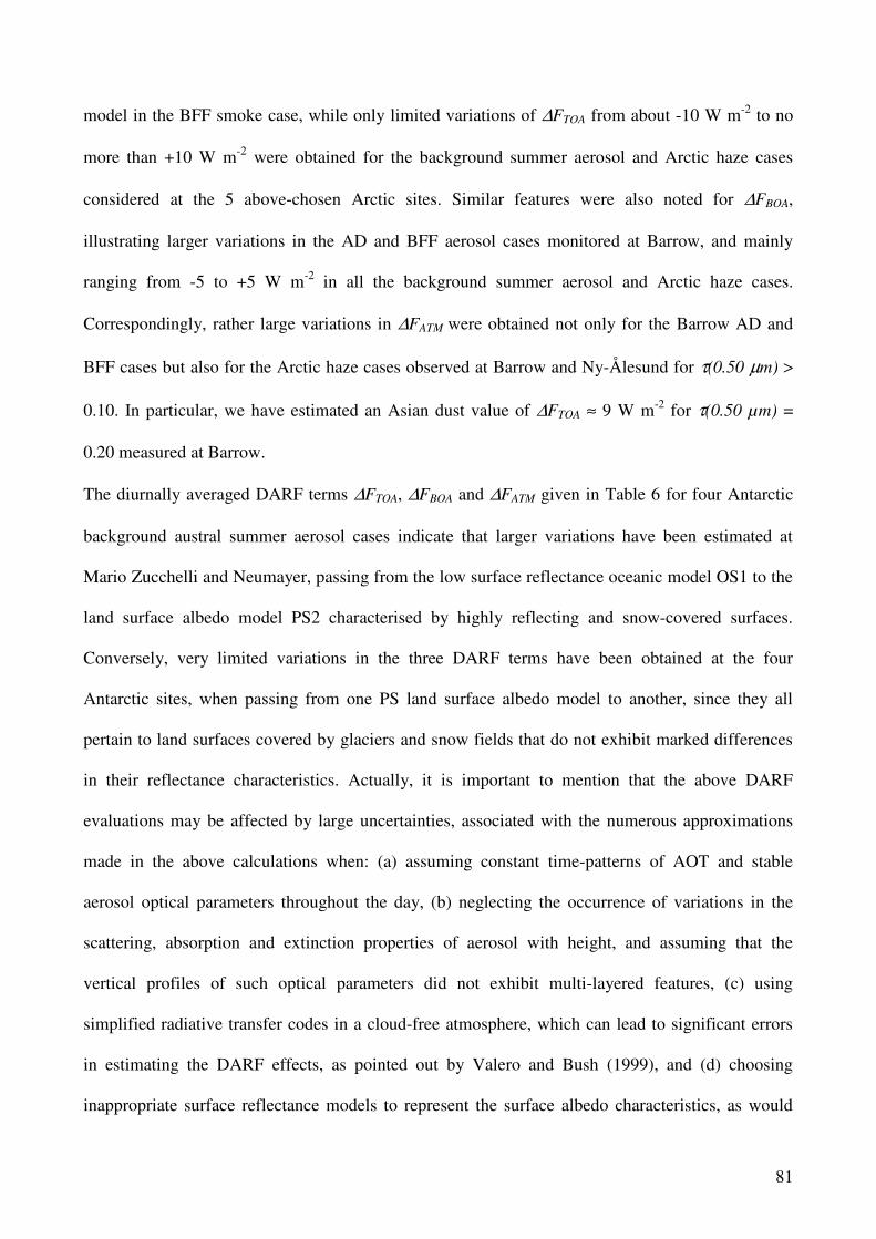
81

model in the BFF smoke case, while only limited variations of ∆FTOA from about -10 W m-2 to no

more than +10 W m-2 were obtained for the background summer aerosol and Arctic haze cases

considered at the 5 above-chosen Arctic sites. Similar features were also noted for ∆FBOA,

illustrating larger variations in the AD and BFF aerosol cases monitored at Barrow, and mainly

ranging from -5 to +5 W m-2 in all the background summer aerosol and Arctic haze cases.

Correspondingly, rather large variations in ∆FATM were obtained not only for the Barrow AD and

BFF cases but also for the Arctic haze cases observed at Barrow and Ny-Ålesund for τ(0.50 µm) >

0.10. In particular, we have estimated an Asian dust value of ∆FTOA ≈ 9 W m-2 for τ(0.50 µm) =

0.20 measured at Barrow.

The diurnally averaged DARF terms ∆FTOA, ∆FBOA and ∆FATM given in Table 6 for four Antarctic

background austral summer aerosol cases indicate that larger variations have been estimated at

Mario Zucchelli and Neumayer, passing from the low surface reflectance oceanic model OS1 to the

land surface albedo model PS2 characterised by highly reflecting and snow-covered surfaces.

Conversely, very limited variations in the three DARF terms have been obtained at the four

Antarctic sites, when passing from one PS land surface albedo model to another, since they all

pertain to land surfaces covered by glaciers and snow fields that do not exhibit marked differences

in their reflectance characteristics. Actually, it is important to mention that the above DARF

evaluations may be affected by large uncertainties, associated with the numerous approximations

made in the above calculations when: (a) assuming constant time-patterns of AOT and stable

aerosol optical parameters throughout the day, (b) neglecting the occurrence of variations in the

scattering, absorption and extinction properties of aerosol with height, and assuming that the

vertical profiles of such optical parameters did not exhibit multi-layered features, (c) using

simplified radiative transfer codes in a cloud-free atmosphere, which can lead to significant errors

in estimating the DARF effects, as pointed out by Valero and Bush (1999), and (d) choosing

inappropriate surface reflectance models to represent the surface albedo characteristics, as would

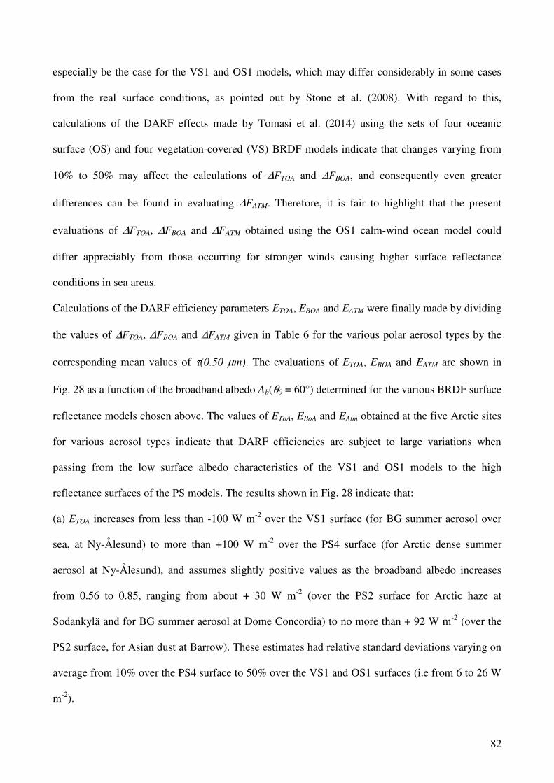
82

especially be the case for the VS1 and OS1 models, which may differ considerably in some cases

from the real surface conditions, as pointed out by Stone et al. (2008). With regard to this,

calculations of the DARF effects made by Tomasi et al. (2014) using the sets of four oceanic

surface (OS) and four vegetation-covered (VS) BRDF models indicate that changes varying from

10% to 50% may affect the calculations of ∆FTOA and ∆FBOA, and consequently even greater

differences can be found in evaluating ∆FATM. Therefore, it is fair to highlight that the present

evaluations of ∆FTOA, ∆FBOA and ∆FATM obtained using the OS1 calm-wind ocean model could

differ appreciably from those occurring for stronger winds causing higher surface reflectance

conditions in sea areas.

Calculations of the DARF efficiency parameters ETOA, EBOA and EATM were finally made by dividing

the values of ∆FTOA, ∆FBOA and ∆FATM given in Table 6 for the various polar aerosol types by the

corresponding mean values of τ(0.50 µm). The evaluations of ETOA, EBOA and EATM are shown in

Fig. 28 as a function of the broadband albedo Ab(θ0 = 60°) determined for the various BRDF surface

reflectance models chosen above. The values of EToA, EBoA and EAtm obtained at the five Arctic sites

for various aerosol types indicate that DARF efficiencies are subject to large variations when

passing from the low surface albedo characteristics of the VS1 and OS1 models to the high

reflectance surfaces of the PS models. The results shown in Fig. 28 indicate that:

(a) ETOA increases from less than -100 W m-2 over the VS1 surface (for BG summer aerosol over

sea, at Ny-Ålesund) to more than +100 W m-2 over the PS4 surface (for Arctic dense summer

aerosol at Ny-Ålesund), and assumes slightly positive values as the broadband albedo increases

from 0.56 to 0.85, ranging from about + 30 W m-2 (over the PS2 surface for Arctic haze at

Sodankylä and for BG summer aerosol at Dome Concordia) to no more than + 92 W m-2 (over the

PS2 surface, for Asian dust at Barrow). These estimates had relative standard deviations varying on

average from 10% over the PS4 surface to 50% over the VS1 and OS1 surfaces (i.e from 6 to 26 W

m-2).

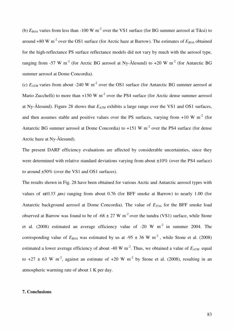
83

(b) EBOA varies from less than -100 W m-2 over the VS1 surface (for BG summer aerosol at Tiksi) to

around +80 W m-2 over the OS1 surface (for Arctic haze at Barrow). The estimates of EBOA obtained

for the high-reflectance PS surface reflectance models did not vary by much with the aerosol type,

ranging from -57 W m-2 (for Arctic BG aerosol at Ny-Ålesund) to +20 W m-2 (for Antarctic BG

summer aerosol at Dome Concordia).

(c) EATM varies from about -240 W m-2 over the OS1 surface (for Antarctic BG summer aerosol at

Mario Zucchelli) to more than +150 W m-2 over the PS4 surface (for Arctic dense summer aerosol

at Ny-Ålesund). Figure 28 shows that EATM exhibits a large range over the VS1 and OS1 surfaces,

and then assumes stable and positive values over the PS surfaces, varying from +10 W m-2 (for

Antarctic BG summer aerosol at Dome Concordia) to +151 W m-2 over the PS4 surface (for dense

Arctic haze at Ny-Ålesund).

The present DARF efficiency evaluations are affected by considerable uncertainties, since they

were determined with relative standard deviations varying from about ±10% (over the PS4 surface)

to around ±50% (over the VS1 and OS1 surfaces).

The results shown in Fig. 28 have been obtained for various Arctic and Antarctic aerosol types with

values of ω(0.55 µm) ranging from about 0.76 (for BFF smoke at Barrow) to nearly 1.00 (for

Antarctic background aerosol at Dome Concordia). The value of ETOA for the BFF smoke load

observed at Barrow was found to be of -68 ± 27 W m-2 over the tundra (VS1) surface, while Stone

et al. (2008) estimated an average efficiency value of -20 W m-2 in summer 2004. The

corresponding value of EBOA was estimated by us at -95 ± 36 W m-2 , while Stone et al. (2008)

estimated a lower average efficiency of about -40 W m-2. Thus, we obtained a value of EATM equal

to +27 ± 63 W m-2, against an estimate of +20 W m-2 by Stone et al. (2008), resulting in an

atmospheric warming rate of about 1 K per day.

7. Conclusions

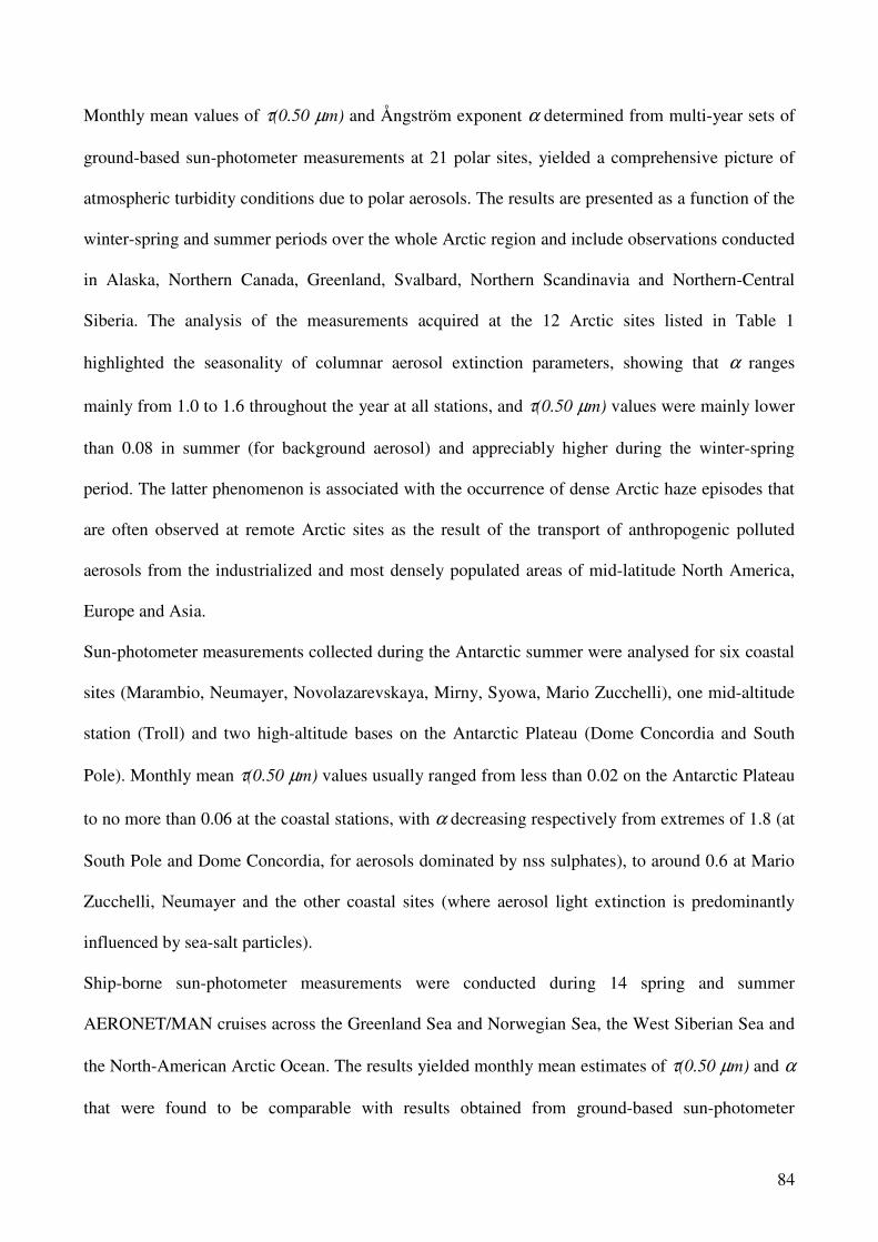
84

Monthly mean values of τ(0.50 µm) and Ångström exponent α determined from multi-year sets of

ground-based sun-photometer measurements at 21 polar sites, yielded a comprehensive picture of

atmospheric turbidity conditions due to polar aerosols. The results are presented as a function of the

winter-spring and summer periods over the whole Arctic region and include observations conducted

in Alaska, Northern Canada, Greenland, Svalbard, Northern Scandinavia and Northern-Central

Siberia. The analysis of the measurements acquired at the 12 Arctic sites listed in Table 1

highlighted the seasonality of columnar aerosol extinction parameters, showing that α ranges

mainly from 1.0 to 1.6 throughout the year at all stations, and τ(0.50 µm) values were mainly lower

than 0.08 in summer (for background aerosol) and appreciably higher during the winter-spring

period. The latter phenomenon is associated with the occurrence of dense Arctic haze episodes that

are often observed at remote Arctic sites as the result of the transport of anthropogenic polluted

aerosols from the industrialized and most densely populated areas of mid-latitude North America,

Europe and Asia.

Sun-photometer measurements collected during the Antarctic summer were analysed for six coastal

sites (Marambio, Neumayer, Novolazarevskaya, Mirny, Syowa, Mario Zucchelli), one mid-altitude

station (Troll) and two high-altitude bases on the Antarctic Plateau (Dome Concordia and South

Pole). Monthly mean τ(0.50 µm) values usually ranged from less than 0.02 on the Antarctic Plateau

to no more than 0.06 at the coastal stations, with α decreasing respectively from extremes of 1.8 (at

South Pole and Dome Concordia, for aerosols dominated by nss sulphates), to around 0.6 at Mario

Zucchelli, Neumayer and the other coastal sites (where aerosol light extinction is predominantly

influenced by sea-salt particles).

Ship-borne sun-photometer measurements were conducted during 14 spring and summer

AERONET/MAN cruises across the Greenland Sea and Norwegian Sea, the West Siberian Sea and

the North-American Arctic Ocean. The results yielded monthly mean estimates of τ(0.50 µm) and α

that were found to be comparable with results obtained from ground-based sun-photometer

85

measurements taken at the stations located on the coasts of the same oceanic sectors during the

March to September period, thus confirming the covariance features of τ(0.50 µm) and α

determined at the ground-based sun-photometer sites. The analysis of ship-borne sun-photometer

measurements performed during the 18 AERONET/MAN cruises conducted in the coastal and off-

shore Antarctic areas of the Indian, Pacific and Atlantic Oceans and along the Antarctic Peninsula

coasts showed that the monthly mean values of τ(0.50 µm) varied between the extremes of 0.02 and

0.06 from December to April, while decreasing from 0.12 in October to 0.07 in November for

measurements acquired around the Antarctic Peninsula. The large magnitude AOTs in the latter

case were likely the result of stronger winds from the northern and western quadrants producing

more sea-salt particles, which are transported toward the continent, while the rapidly decreasing

trend results from a rapid decrease in the amplitude of these winds (a contention that is further

supported by the corresponding increase in α values, between October and January, while τ(0.50

µm) systematically decreases). In more general terms we would argue that scattergrams of α versus

τ(0.50 µm) for the ensemble of both land-based and ship-borne based sun-photometry showed a

roughly inverse relationship of high α, small τ(0.50 µm) to low α, high τ(0.50 µm) that was

representative of a progressive transformation from fine mode dominated nss sulphates above the

Antarctic Plateau to sea-salt dominated aerosols for coastal sites.

The vertical distribution of the aerosol extinction coefficient was investigated with ground-based

lidars at Arctic and Antarctic sites. In particular, the monthly mean vertical profiles of backscatter

coefficient, along with lidar ratio trends and depolarisation ratio covariance with backscattering

coefficient were illustrated for tropospheric altitudes using data acquired at Ny-Ålesund by the AWI

KARL lidar from 1 November, 2012, to 31 October, 2013. As part of this investigation, we

illustrated the seasonal variations of integrated backscatter coefficient and lidar ratio, as influenced

by Arctic haze episodes in late winter and spring, and the background aerosol in summer.

86

Evaluations of AOT in the visible have been obtained through retrieval procedures applied to

MODIS, MISR and AATSR satellite observations, which were found to substantially agree with the

values of AOT obtained using ground-based and ship-borne sun-photometer measurements

conducted in the Arctic and Antarctic regions. Qualitative evaluations of τ(0.55 µm) have been

retrieved from the AATSR measurements recorded over the Arctic oceanic and land regions

covered by ice and snow using observations taken within different spectral channels (Istomina et al.,

2011), and using the DVMS method (Mei et al., 2013b). These retrievals allow the aerosol spatial

distribution (e.g., pollution events) to be analyzed on short term scales, but may contain an AOT

offset due to many challenges connected to virtually unknown surface type and aerosol optical

properties. The global application of these procedures is at present a challenging problem because

of the very high sensitivity of the retrievals to unscreened thin clouds. In fact, these data are already

affected by large uncertainties and need to be further validated, to overcome the errors that may

arise from cloud pollution and the complex picture of polar conditions (low values of AOT, various

cloud types, variable features of snow- and ice-covered surface reflectance,….).

The main characteristics of multimodal particle size-distribution curves have been defined by: (i)

taking into account the in-situ aerosol sampling measurements conducted at various Arctic sites

(Barrow, Ny-Ålesund, Sodankylä) and Antarctic sites (Mario Zucchelli, Neumayer, Aboa, South

Pole, Dome Concordia), and (ii) assuming that the overall size-distribution curves determined at the

various sites consist in general of a fine particle mode and an accumulation or coarse particle mode,

linearly combined to give a bimodal aerosol columnar load for each value of α obtained from the

field measurements. Eight log-normal curves were defined for the Arctic stations on the basis of in-

situ particle samples collected for Arctic haze, summer background aerosol, Asian dust and BFF

smoke. They can be used for each spectral set of sun-photometer τ(λ) measurements to fit the

derived value of α. The radiative parameters of the eight unimodal curves were defined by taking

into account the complex refractive index and single scattering albedo derived from in-situ

measurements conducted with nephelometers and aethalometers and/or using the simulations of the

87

aerosol optical properties made with the aerosol extinction models given by the 6S code. Six log-

normal curves were defined to represent the unimodal size-distribution curves of Antarctic fine,

accumulation and coarse particles, using field data obtained from the aerosol collected at coastal

and high-altitude sites. The optical properties of particulate matter were defined according to the

data provided by the in-situ active remote sensing measurements, and used to determine the optical

characteristics of six Antarctic log-normal size-distribution curves shown in Table 5.

Assumptions about the aerosol optical properties are totally based on the particulate chemical

composition measured at the ground and, therefore, may differ appreciably from airborne particles

suspended within the upper layers of the atmosphere in all cases of aerosol transport from remote

areas (like Arctic haze, Asian dust, and BFF smoke), as shown for instance by the PAMARCMiP

airborne measurements conducted in April 2009 (Stone et al., 2010). However, the best-fit

procedure to combine the fine particle mode with the accumulation/coarse particle mode to fit the

value of α will have probably allowed us to evaluate the average spectral features of the column

loading consisting of larger particles.

The bimodal size-distribution curves of Arctic and Antarctic aerosol obtained as linear

combinations of the fine particle and accumulation/coarse particle modes have been defined by

varying their columnar number contents until a best-fit value of α was obtained for each spectral

series of τ(λ). All these bimodal models were assumed to exhibit the well-defined optical properties

given in Table 5 and to represent the most relevant optical characteristics of Arctic and Antarctic

columnar aerosol. Additional realistic multimodal extinction models of fine, accumulation and

coarse particles have been defined as linear combinations of the OPAC components proposed by

Hess et al. (1998), which fit the mean values of α determined for different columnar aerosol types.

Using these multimodal aerosol extinction models, instantaneous and diurnally averaged DARF

effects induced by atmospheric aerosol at the TOA- and BOA-levels, and within the atmosphere

have been calculated over sea and land surfaces by using the sets of BRDF surface reflectance

models determined by Tomasi et al. (2013) for vegetation-covered, oceanic, and polar snow-

88

covered surfaces. The results indicate that the diurnally averaged DARF terms vary strongly as a

function of τ(0.50 µm), aerosol single scattering albedo and surface albedo. The corresponding

efficiency at the TOA-level was found to increase appreciably as surface albedo over sea and land

increases until higher and more stable values over the snow- and ice-covered surfaces are attained.

Less variable values and a more limited dependence of the BOA-level DARF efficiency on surface

albedo were found, so that the atmospheric DARF efficiency resulted in: (1) a stronger increase

when passing from vegetation-covered and oceanic surfaces to surfaces covered only in part by

snow, and (2) more stable positive values over the polar surfaces covered by fresh snow and clean

glaciers in the Arctic and Antarctic regions.

Acknowledgments.

The present study was developed as a part of the CLIMSLIP (Climate Impacts of Short-Lived

Pollutants in the Polar Regions) joint project, approved by the European Polar Consortium and

coordinated by A. Stohl at NILU (Kjeller, Norway), and supported by the Italian Research

Programme in Antarctica (PNRA). The authors gratefully acknowledge the Office of Antarctic

Observation of the Japan Meteorological Agency (Tokyo, Japan), for supplying the data-set of EKO

sun-photometer measurements carried out at Syowa (Antarctica) from 2000 to 2011. In general we

acknowledge the support provided by the AERONET network in the Arctic and Antarctica and the

AEROCAN / AERONET sub-network in the Canadian Arctic. The Cimel sun-photometer data at

Barrow (Alaska) were collected by the U.S. Department of Energy as part of the Atmospheric

Radiation Measurement Program Climate Research Facility (ARM) and processed by AERONET.

James H. Butler (Global Monitoring Division, Earth System Research Laboratory (ERL), National

Oceanic and Atmospheric Administration (NOAA), Boulder, Colorado, USA) is acknowledged for

his effort in establishing and maintaining the activities at the AERONET South Pole Amundsen-

Scott base. The colleagues D. G. Chernov, Yu. S. Turchinovich and Victor V. Polkin, (V. E. Zuev

Institute of Atmospheric Optics (IAO), Siberian Branch, Russian Academy of Sciences, Tomsk,

89

Russia) are also acknowledged for their participation to field measurements conducted at

Barentsburg and in Antarctica. Author’s acknowledgements are also due to the managerial and

operational support given by M. Fily (LGGE, CNRS, Grenoble, France) at the AERONET

Antarctic Dome Concordia station, and to the P.I.s of the AERONET/MAN cruises conducted in

the Arctic and Antarctic Oceans, during which Microtops measurements of aerosol optical thickness

were performed and examined in the present analysis: Patricia K. Quinn (NOAA Pacific Marine

Environmental Laboratory, Seattle, Washington, USA), Andrey Proshutinsky (Woods Hole

Oceanographic Institution, Woods Hole, Massachusetts, USA), Carlos Duarte (Instituto

Mediterráneo de Estudios Avanzados, Esporles, Mallorca, Spain), Simon Bélanger (Université du

Québec, Rimouski, Québec, Canada), Elizabeth A. Reid (Naval Research Laboratory, Monterey,

California, USA), Gennadi Milinevsky (Space Physics Laboratory, Taras Shevchenko National

University of Kyiv, Kyiv, Ukraine), and Heitor Evangelista (Rio de Janeiro State University,

Brazil). The analyses and visualizations used in this paper to obtain the sets of MODIS and MISR

daily aerosol optical thickness Level-3 data over the Arctic and Antarctic regions were produced

with the Giovanni online data system, developed and maintained by the NASA GES DISC.

90

References

Aaltonen, V., Lihavainen, H., Kerminen, V.-M., Komppula, M., Hatakka, J., Eneroth, K., Kulmala,

M., Viisanen, Y., 2006. Measurements of optical properties of atmospheric aerosols in

Northern Finland. Atmospheric Chemistry and Physics 6, 1155-1164, doi:10.5194/acp-6-

1155-2006.

Ackermann, J., 1998. The extinction-to-backscatter ratio of tropospheric aerosol: A numerical

study. Journal of Atmospheric and Oceanic Technology 15, 4, 1043-1050, doi:10.1175/1520-

0426(1998)015<1043:TETBRO>2.0.CO;2.

Ackerman, S. A., Frey, R., Strabala, K., Liu, Y., Gumley, L., Baum, B., Menzel, P., 2010.

Discriminating Clear-Sky from Cloud with MODIS - Algorithm Theoretical Basis Document.

Products: MOD35. ATBD Reference Number: ATBD-MOD-06 (http://modis-

atmos.gsfc.nasa.gov/MOD35_L2/atbd.html).

Ångström, A., 1964. The parameters of atmospheric turbidity. Tellus 16, 64-75, doi:10.1111/j.2153-

3490.1964.tb00144.x.

Anderson, T. L., Ogren, J. A., 1998. Determining aerosol radiative properties using the TSI 3563

Integrating Nephelometer. Aerosol Science and Technology 29, 57-69,

doi:10.1080/02786829808965551.

Ansmann, A., Wandinger, U., Riebesell, M., Weitkamp, C., Michaelis, W., 1992. Independent

measurement of extinction and backscatter profiles in cirrus clouds by using a combined

Raman elastic-backscatter lidar. Applied Optics 31, 33, 7113-7131,

doi:10.1364/AO.31.007113.

Arimoto, R., Hogan, A., Grube, P., Davis, D., Webb, J., Schloesslin, C., Sage, S., Raccah, F., 2004.

Major ions and radionuclides in aerosol particles from the South Pole during ISCAT-2000.

Atmospheric Environment 38, 5473-5484, doi:10.1016/j.atmosenv.2004.01.049.

91

Barrie, L. A., Hoff, R. M., Daggupaty, S. M., 1981. The influence of mid-latitudinal pollution

sources on haze in the Canadian Arctic. Atmospheric Environment 15, 8, 1407-1419,

doi:i:10.1016/0004-6981(81)90347-4.

Bodhaine, B. A., 1995. Aerosol absorption measurements at Barrow, Mauna Loa and South Pole.

Journal of Geophysical Research 100, 8967-8975, doi:10.1029/95JD00513.

Bourassa, A. E., Degenstein, D. A., Elash, B. J., Llewellyn, E. J., 2010. Evolution of the

stratospheric aerosol enhancement following the eruptions of Okmok and Kasatochi: Odin-

OSIRIS measurements. Journal of Geophysical Research 115, D2, D00L03.

doi:10.1029/2009JD013274.

Brock, C. A., Cozic, J., Bahreini, R., Froyd, K. D., Middlebrook, A. M., McComiskey, A., Brioude,

J., Cooper, O. R., Stohl, A., Aikin, K. C., de Gouw, J. A., Fahey, D. W., Ferrare, R. A., Gao,

R.-S., Gore, W., Holloway, J. S., Huebler, G., Jefferson, A., Lack, D. A., Lance, S., Moore, R.

H., Murphy, D. M., Nenes, A., Novelli, P. C., Nowak, J. B., Ogren, J. A., Peischl, J., Pierce,

R. B., Pilewskie, P., Quinn, P. K., Ryerson, T. B., Schmidt, K. S., Schwarz, J. P., Sodemann,

H., Spackman, J. R., Stark, H., Thomson, D. S., Thornberry, T., Veres, P., Watts, L. A.,

Warneke, C., Wollny, A. G., 2011. Characteristics, sources, and transport of aerosols

measured in spring 2008 during the Aerosol, Radiation, and Cloud Processes Affecting Arctic

Climate (ARCPAC) project. Atmospheric Chemistry and Physics 11, 6, 2423-2453,

doi:10.5194/acp-11-2423-2011.

Bush, B. C., Valero, F. P. J., 2003. Surface aerosol radiative forcing at Gosan during the ACE-Asia

campaign. Journal of Geophysical Research 108, D23, 8660, doi: 10.1029/2002JD003233.

Campbell, J. R., Tackett, J. L., Reid, J. S., Zhang, J., Curtis, C. A., Hyer, E. J., Sessions, W. R.,

Westphal, D. L., Prospero, J. M., Welton, E. J., Omar, A. H., Vaughan, M. A., Winker, D. M.,

2012. Evaluating nighttime CALIOP 0.532 µm aerosol optical depth and extinction coefficient

retrievals. Atmospheric Measurement Techniques 5, 9, 2143-2160, doi:10.5194/amt-5-2143-

2012.

92

Curier, L., de Leeuw, G., Kolmonen, P., Sundstrom, A.-M., Sogacheva, L., Bennouna, Y., 2009.

Aerosol retrieval over land using the (A)ATSR dual-view algorithm. In “Satellite Aerosol

Remote Sensing over Land” (A. A. Kokhanovsky and G. de Leeuw, eds.), Chichester (UK),

Praxis Publishing, pp. 135-160.

Damoah, R., Spichtinger, N., Forster, C., James, P., Mattis, I., Wandinger, U., Beirle, S., Wagner,

T., Stohl, A., 2004. Around the world in 17 days - hemispheric-scale transport of forest fire

smoke from Russia in May 2003. Atmospheric Chemistry and Physics 4, 1311-1321,

doi:10.5194/acp-4-1311-2004.

Delene, D. J., Ogren, J. A., 2002. Variability of aerosol optical properties at four North American

surface monitoring sites. Journal of the Atmospheric Sciences 59, 1135-1150,

doi:10.1175/1520-0469(2002)059<1135:VOAOPA>2.0.CO;2.

Deuzé, J. L., Bréon, F. M., Devaux, C., Goloub, P., Herman, M., Lafrance, B., Maignan, F.,

Marchand, A., Nadal, F., Perry, G., Tanré, D., 2001. Remote sensing of aerosol over land

surfaces from POLDER-ADEOS-1 polarized measurements. Journal of Geophysical Research

106, D5, 4913-4926, doi:10.1029/2000JD900364.

Devasthale, A., Tjernströ, M., Omar, A. H., 2011. The vertical distribution of thin features over the

Arctic analysed from CALIPSO observations. Part II: Aerosols. Tellus 63B, 1, 86-95,

doi:10.1111/j.1600-0889.2010.00517.x.

de Villiers, R. A., Ancellet, G., Pelon, J., Quennehen, B., Schwarzenboeck, A., Gayet, J. F., Law, K.

S., 2010. Airborne measurements of aerosol optical properties related to early spring transport

of mid-latitude sources into the Arctic. Atmospheric Chemistry and Physics 10, 11, 5011-

5030, doi:10.5194/acp-10-5011-2010.

Di Carmine, C., Campanelli, M., Nakajima, T., Tomasi, C., Vitale, V., 2005. Retrievals of Antarctic

aerosol characteristics using a Sun-sky radiometer during the 2001-2002 austral summer

campaign. Journal of Geophysical Research 110, D13202, doi:10.1029/2004JD005280.

93

Diner, D. J., Beckert, J. C., Reilly, T. H., Bruegge, C. J., Conel, J. E., Kahn, R. A., Martonchik, J.

V., Ackerman, T. P., Davies, R., Gerstl, S. A.W., Gordon, H. R., Muller, J.-P., Myneni, R. B.,

Sellers, P. J., Pinty, B., Verstraete, M. M., 1998. Multi-angle Imaging SpectroRadiometer

(MISR) instrument description and experiment overview. IEEE Transactions on Geoscience

and Remote Sensing 36, 4, 1072-1087, doi: 10.1109/36.700992.

Diner, D. J., Martonchik, J. V., Kahn, R. A., Pinty, B., Gobron, N., Nelson, D. L., Holben, B. N.,

2005. Using angular and spectral shape similarity constraints to improve MISR aerosol and

surface retrievals over land. Remote Sensing of Environment, 94, 2, 155-171,

doi:10.1016j.rse.2004.09.009.

Di Pierro, M., Jaeglé, L., Anderson, T. L., 2011). Satellite observations of aerosol transport from

East Asia to the Arctic: three case studies. Atmospheric Chemistry and Physics, 11, 2225-

2243, doi:10.5194/acp-11-2225-2011.

Dong, X., Xi, B., Crosby, K., Long, C. N., Stone, R. S., Shupe, M. D., 2010. A 10 year climatology

of Arctic cloud fraction and radiative forcing at Barrow, Alaska. Journal of Geophysical

Research 115, D17212, doi:10.1029/2009JD013489.

Dubovik, O., Herman, M., Holdak, A., Lapyonok, T., Tanré, D., Deuzé, J. L., Ducos, F., Sinyuk,

A., and Lopatin, A., 2011. Statistically optimized inversion algorithm for enhanced retrieval

of aerosol properties from spectral multi-angle polarimetric satellite observations.

Atmospheric Measurement Techniques, 4, 975-1018, doi:10.5194/amt-4-975-2011.

Eck, T. F., Holben, B. N., Reid, J. S., Dubovik, O., Smirnov, A., O’Neill, N. T., Slutsker, I., Kinne,

S., 1999. Wavelength dependence of the optical depth of biomass burning, urban, and desert

dust aerosols, Journal of Geophysical Research 104, D24, 31333-31349,

doi:10.1029/1999JD900923.

Eckhardt, S., Hermansen, O., Grythe, H., Fiebig, M., Stebel, K., Cassiani, M., Baecklund, A., Stohl,

A., 2013. The influence of cruise ship emissions on air pollution in Svalbard - a harbinger of a

94

more polluted Arctic?, Atmospheric Chemistry and Physics 13, 8401-8409, doi:10.5194/acp-

13-8401-2013.

Fattori, I., Becagli, S., Bellandi, S., Castellano, E., Innocenti, M., Mannini, A., Severi, M., Vitale,

V., Udisti, R., 2005. Chemical composition and physical features of summer aerosol at Terra

Nova Bay and Dome C, Antarctica. Journal of Environmental Monitoring 7, 1265-1274.

Fiebig, M., Lunder, C. R., Stohl, A., 2009. Tracing biomass burning aerosol from South America to

Troll Research Station, Antarctica. Geophysical Research Letters 36, L14815,

doi:10.1029/2009GL038531.

Garrett, T. J., Verzella, L.L., 2008. Looking back: An evolving history of Arctic aerosols. Bullettin

of the American Meteorological Society 89, 299-302, doi: 10.1175/BAMS-89-3-299.

Gobbi, G. P., Kaufman, Y. J., Koren, I., Eck, T. F., 2007. Classification of aerosol properties

derived from AERONET direct sun data. Atmospheric Chemistry and Physics 7, 2, 453-458,

doi:10.5194/acp-7-453-2007.

Grey, W. M. F., North, P. R. J., 2009. Aerosol optical depth from dual-view (A)ATSR satellite

observations. In Satellite Aerosol Remote Sensing Over Land (Kokhanovsky, A.A., and G. de

Leeuw, eds.), Springer-Praxis (Berlin), 2009, ISBN 978-3-540-69396-3, 388 pp.

Hagler, G. S. W., Bergin, M. H., Smith, E. A., Town, M., Dibb, J. E., 2008. Local anthropogenic

impact on particulate elemental carbon concentrations at Summit, Greenland. Atmospheric

Chemistry and Physics 8, 2485-2491, doi:10.5194/acp-8-2485-2008.

Hänel, G., Adam, W., Bundke, U., Komguem, L., Leiterer, U., 1999. Optical properties of boundary

layer particles, columnar absorption and direct radiative forcing by particles in the solar

spectral region. Journal of Aerosol Science 30, Suppl. 1, S171-S172.

Hara, K., Osada, K., Kido, M., Hayashi, M., Matsunaga, K., Iwasaka, Y., Yamanouchi, T., Hashida,

G., Fukatsu, T., 2004. Chemistry of sea-salt particles and inorganic halogen species in

Antarctic regions: Compositional differences between coastal and inland stations. Journal of

Geophysical Research 109, D20208, doi:10.1029/2004JD004713.

95

Haywood, J., Boucher, O., 2000. Estimates of the direct and indirect radiative forcing due to

tropospheric aerosols: A review. Reviews of Geophysics 38, 4, 513-543, doi:

10.1029/1999RG000078.

Heintzenberg, J., Charlson, R. J., Clarke, A. D., Liousse, C., Ramaswamy, V., Shine, K. P.,

Wendisch, M., Helas, G., 1997. Measurements and modelling of aerosol single scattering

albedo: progress, problems and prospects. Contribution to Atmospheric Physics 70, 249-263.

Herber, A., Thomason, L. W., Gernandt, H., Leiterer, U., Nagel, D., Schulz, K., Kaptur, J.,

Albrecht, T., Notholt, J., 2002. Continuous day and night aerosol optical depth observations in

the Arctic between 1991 and 1999. Journal of Geophysical Research 107, D10, 4097,

doi:10.1029/2001JD000536.

Herber, A. B., Haas, C., Stone, R. S., Bottenheim, J. W., Liu, P., Li, S.-M., Staebler, R. M., Strapp,

J. W., Dethloff, K., 2012. Regular airborne surveys of Arctic sea ice and atmosphere. EOS 93,

4, 41-48, doi:10.1029/2012EO040001.

Hess, M., Koepke, P., Schult, I., 1998. Optical properties of aerosols and clouds: The software

package OPAC. Bulletin of the American Meteorological Society 79, 5, 831-844, doi:

10.1175/1520-0477(1998)079<0831:OPOAAC>2.0.CO;2.

Hillamo, R., Allegrini, I., Sparapani, R., Kerminen, V.-M., 1998. Mass size distributions and

precursors gas concentrations of major inorganic ions in Antarctic aerosol. International

Journal of Environmental Analytical Chemistry 71, 353-372,

doi:10.1080/03067319808032638.

Hirdman, D., Sodemann, H., Eckhardt, S., Burkhart, J. F., Jefferson, A., Mefford, T., Quinn, P. K.,

Sharma, S., Ström, J., Stohl, A., 2010, Source identification of short-lived air pollutants in the

Arctic using statistical analysis of measurement data and particle dispersion model output.

Atmospheric Chemistry and Physics 10, 669-693, doi:10.5194/acp-10-669-2010.

96

Hoffmann, A., Ritter, C., Stock, M., Shiobara, M., Lampert, A., Maturilli, M., Orgis, T., Neuber, R.,

Herber, A., 2009. Ground-based lidar measurements from Ny-Ålesund during ASTAR 2007.

Atmospheric Chemistry and Physics 9, 22, 9059-9081, doi:10.5194/acp-9-9059-2009.

Hoffmann, A., Ritter, C., Stock, M., Maturilli, M., Eckhardt, S., Herber, A., Neuber, R., 2010. Lidar

measurements of the Kasatochi aerosol plume in August and September 2008 in Ny-Ålesund,

Spitsbergen. Journal of Geophysical Research 115, D00L12, doi:10.1029/2009JD013039.

Hoffmann, A., Osterloh, L., Stone, R., Lampert, A., Ritter, C., Stock, M., Tunved, P., Hennig, T.,

Bockmann, C., Li, S.-M., Eleftheriadis, K., Maturilli, M., Orgis, T., Herber, A., Neuber, R.,

Dethloff, K., 2012. Remote sensing and in-situ measurements of tropospheric aerosol, a

PAMARCMiP case study. Atmospheric Environment 52C, 56-66,

doi:10.1016/j.atmosenv.2011.11.027.

Holben, B. N., Eck, T. F., Slutsker, I., Tanré, D., Buis, J. P., Setzer, A., Vermote, E., Reagan, J. A.,

Kaufman, Y. J., Nakajima, T., Lavenu, F., Jankowiak, I., Smirnov, A., 1998. AERONET - A

federated instrument network and data archive for aerosol characterization. Remote Sensing of

Environment 66, 1, 1-16, doi: S0034-4257(98)00031-5.

Hori, M., Aoki, T., Tanikawa, T., Motoyoshi, H., Hachikubo, A., Sugiura, K., Yasunari, T. J., Eide,

H., Storvold, R., Nakajima, Y., Takahashi, F., 2006. In-situ measured spectral directional

emissivity of snow and ice in the 8-14 µm atmospheric window. Remote Sensing of

Environment 100, 4, 486-502, doi:10.1016/j.rse.2005.11.001.

Hsu, N. C., Tsay, S. C., King, M. D., Herman, J. R., 2004. Aerosol properties over bright reflecting

source regions. IEEE Transactions on Geoscience and Remote Sensing, 42, 3, 557-569, doi:

10.1117/12.975846.

Hsu, N. C., Jeong, M.-J., Bettenhausen, C., Sayer, A. M., Hansell, R., Seftor, C. S., Huang, J., Tsay,

S.-C., 2013. Enhanced Deep Blue aerosol retrieval algorithm: The second generation. Journal

of Geophysical Research (Atmospheres) 118, 16, 9296–9315, doi:10.1002/jgrd.50712.

97

Intrieri, J. M., Shupe, M. D., 2004. Characteristics and radiative effects of diamond dust over the

Western Arctic ocean region. Journal of Climate 17, 15, 2953-2960, doi:10.1175/1520-

0442(2004)017<2953:CAREOD>2.0.CO;2.

IPCC, 2013. Climate Change 2013: The Physical Science Basis, Fifth Assessment Report of the

United Nations “Intergovernmental Panel on Climate Change (IPCC), Chapter 7, Clouds and

Aerosols, Cambridge University Press, Cambridge (UK)

(http://www.climatechange2013.org/images/report/WG1AR5_Chapter07_FINAL.pdf).

Iqbal, M. (1983), An Introduction to Solar Radiation, Academic Press, Toronto, 390 pp (see Table

1.2.1 at pages 4-5).

Istomina, L.G., von Hoyningen-Huene, W., Kokhanovsky, A. A., Burrows, J. P., 2009. Retrieval of

aerosol optical thickness in Arctic region using dual-view AATSR observations, Proceedings

of ESA Atmospheric Science Conference, ESA SP-676, Barcelona (Spain), 7-11 September

2009.

Istomina, L. G., von Hoyningen-Huene, W., Kokhanovsky, A. A., Burrows, J. P., 2010. The

detection of cloud-free snow-covered areas using AATSR measurements. Atmospheric

Measurement Techniques 3, 1005-1017, doi:10.5194/amt-3-1005-2010.

Istomina, L. G., von Hoyningen-Huene, W., Kokhanovsky, A. A., Schultz, E., Burrows, J. P., 2011.

Remote sensing of aerosols over snow using infrared AATSR observations, Atmospheric

Measurement Techniques 4, 1133-1145, doi:10.5194/amt-4-1133-2011.

Justice, C. O., Vermote, E., Townshend, J. R. G., Defries, R., Roy, D. P., Hall, D. K., Salomonson,

V. V., Privette, J. L., Riggs, G., Strahler, A., Lucht, W., Myneni, R. P., Knyazikhin, Y.,

Running, S. W., Nemani, R. R., Wan, Z., Huete, A. R., van Leeuwen, W., Wolfe, R. E.,

Giglio, L., Muller, J.-P., Lewis, P., Barnsley, M. J., 1998. The Moderate Resolution Imaging

Spectroradiometer (MODIS): Land Remote Sensing for Global Change Research. IEEE

Transactions on Geoscience and Remote Sensing 36, 4, 1228-1249, doi:10.1109/36.701075.

98

Kahn, R. A., Li, W.-H., Martonchik, J. V., Bruegge, C. J., Diner, D. J., Gaitley, B. J., Abdou, W.,

Dubovik, O., Holben, B., Smirnov, A., Jin, Z., Clark, D., 2005. MISR calibration and

implications for low-light-level aerosol retrieval over dark water. Journal of the Atmospheric

Sciences 62, 4, 1032-1052, doi:10.1175/JAS3390.1.

Kahn, R. A., Gaitley, B. J., Garay, M. J., Diner, D. J., Eck, T. F., Smirnov, A., Holben, B. N., 2010.

Multiangle Imaging SpectroRadiometer global aerosol product assessment by comparison

with the Aerosol Robotic Network. Journal of Geophysical Research 115, D23209,

doi:10.1029/2010JD014601.

Kahn, R. A., Garay, M. J., Nelson, D. L., Levy, R. C., Bull, M. A., Diner, D. J., Martonchik, J. V.,

Hansen, E. G., Remer, L. A., Tanré, D., 2011. Response to ‘‘Toward unified satellite

climatology of aerosol properties. 3. MODIS versus MISR versus AERONET’’. Journal of

Quantitative Spectroscopy and Radiative Transfer 112, 5, 901-909,

doi:10.1016/j.jqsrt.2009.11.003.

Kaufman, Y. J., Tanré, D., Remer, L., Vermote, E. F., Chu, A., Holben, B. N., 1997. Operational

remote sensing of tropospheric aerosol over the land from EOS-MODIS. Journal of

Geophysical Research 102, D14, 17051-17067, doi:10.1029/96JD03988.

Kerminen, V.-M., Teinilä, K., Hillamo, R., 2000. Chemistry of sea-salt particles in the summer

Antarctic atmosphere. Atmospheric Environment 34, 2817-2825, doi:10.1016/S1352-

2310(00)00089-3.

King, M. D., Dubovik, O., 2013. Determination of aerosol optical properties from inverse methods.

In Aerosol Remote Sensing (J. Lenoble, L. Remer, and D. Tanré, Eds.), Springer-Verlag, pp.

101-136.

Koponen, I. K., Virkkula, A., Hillamo, R., Kerminen, V.-M. , Kulmala, M., 2003. Number size

distributions and concentrations of the continental summer aerosols in Queen Maud Land,

Antarctica. Journal of Geophysical Research 108, D18, 4587, doi:10.1029/2003JD003614.

99

Knapp, K. R., Vonder Haar, T. H., Kaufman, Y. J., 2002. Aerosol optical depth retrieval from

GOES-8: Uncertainty study and retrieval validation over South America, Journal of

Geophysical Research (Atmospheres) 107, D7, AAC 2-1 – AAC 2-12,

doi:10.1029/2001JD000505.

Lambert, A., Ehrlich, A., Dörnbrack, A., Jourdan, O., Gayet, J.-F., Mioche, G., Shcherbakov, V.,

Ritter, C., Wendisch, M., 2009. Microphysical and radiative characterization of a subvisible

midlevel Arctic ice cloud by airborne observations a case study. Atmospheric Chemistry and

Physics 9, 8, 2647-2661, doi:10.5194/acp-9-2647-2009.

Lambert, A., Ritter, C., Hoffmann, A., Gayet, J.-F., Mioche, G., Ehrlich, A., Doernbrack, A.,

Wendisch, M., Shiobara, M., 2010. Lidar characterization of the Arctic atmosphere during

ASTAR 2007: four cases studies of boundary layer, mixed-phase and multi-layer clouds.

Atmospheric Chemistry and Physics 10, 6, 2847-2866, doi: doi:10.5194/acp-10-2847-2010.

Law, K. S., Stohl, A., Quinn, P. K., Brock, C., Burkhart, J., Paris, J.-D., Ancellet, G., Singh, H. B.,

Roiger, A., Schlager, H., Dibb, J., Jacob, D. J., Arnold, S. R., Pelon, J., Thomas, J. L., 2014.

Arctic air pollution: 1 New insights from POLARCAT-IPY. Bulletin of the American

Meteorological Society, doi:10.1175/BAMS-D-13-00017.1. In press.

Levy, R. C., Remer, L. A., Mattoo, S., Vermote, E. F., Kaufman, Y. J., 2007. Second-generation

operational algorithm: Retrieval of aerosol properties over land from inversion of Moderate

Resolution Imaging Spectroradiometer spectral reflectance. Journal of Geophysical Research

112, D13211, doi:10.1029/2006JD007811.

Levy, R. C., Remer, L. A., Kleidman, R. G., Mattoo, S., Ichoku, C., Kahn, R., Eck, T. F., 2010.

Global evaluation of the Collection 5 MODIS dark-target aerosol products over land.

Atmospheric Chemistry and Physics 10, 10399-10420, doi:10.5194/acp-10-10399-2010.

Levy, R. C., Mattoo, S., Munchak, L. A., Remer, L. A., Sayer, A. M., Patadia, F., Hsu, N. C., 2013.

The Collection 6 MODIS aerosol products over land and ocean. Atmospheric Measurement

Techniques 6, 2989-3034, doi:10.5194/amt-6-2989-2013.

100

Lubin, D., Satheesh, S., McFarquar, G., Heymsfield, A., 2002. Longwave radiative forcing of

Indian Ocean tropospheric aerosol. Journal of Geophysical Research 107, D19, 8004,

doi:10.1029/2001JD001183.

Martonchik, J. V., Diner, D. J., Kahn, R. A., Ackerman, T. P., Verstraete, M. M., Pinty, B., Gordon,

H. R., 1998a. Techniques fot the retrieval of aerosol properties over land and ocean using

multi-angle imagery. IEEE Transactions on Geoscience and Remote Sensing 36, 4, 1212-

1227, doi:10.1109/36.701027.

Martonchik, J. V., Diner, D. J., Pinty, B., Verstraete, M. M., Myneni, R. B., Knyazikhin, Y.,

Gordon, H. R., 1998b. Determination of land and ocean reflective, radiative, and biophysical

properties using multiangle imaging. IEEE Transactions on Geoscience and Remote Sensing

36, IEEE Trans. Geosci. Remote Sens. 36, 4, 1266-1281, doi:10.1109/36.701077.

Mazzola, M., Stone, R. S., Herber, A., Tomasi, C., Lupi, A., Vitale, V., Lanconelli, C., Toledano,

C., Cachorro, V. E., O’Neill, N.T., Shiobara, M., Aaltonen, V., Stebel, K., Zielinski, T.,

Petelski, T., Ortiz de Galisteo, J. P., Torres, B., Berjon, A., Goloub, P., Li, Z., Blarel, L.,

Abboud, I., Cuevas, E., Stock, M., Schulz, K.-H., Virkkula, A., 2012. Evaluation of sun

photometer capabilities for retrievals of aerosol optical depth at high latitudes: The POLAR-

AOD intercomparison campaigns, Atmospheric Environment 52C, 1-14,

doi:10.1016/j.atmosenv.2011.07.042.

Mei, L., Xue, Y., 2013. Aerosol optical thickness retrieval over snow-covered surface using

AATSR data, The 2013 IEEE International Geoscience and Remote Sensing Symposium

(IGARSS), Melbourne, Australia, 21-26 July 2013.

Mei, L., Xue, Y., de Leeuw, G., Holzer-Popp, T., Guang, J., Li, Y., Yang, L., Xu, H., Xu, X., Li, C.,

Wang, Y., Wu, C., Hou, T., He, X., Liu, J., Dong, J., Chen, Z., 2012. Retrieval of aerosol

optical depth over land based on a time series technique using MSG/SEVIRI data.

Atmospheric Chemistry and Physics 12, 9167-9185, doi:10.5194/acp-12-9167-2012.

101

Mei, L., Xue, Y., de Leeuw, G., von Hoyningen-Huene, W., Kokhanovsky, A. A., Istomina, L.,

Guang, J., Burrows, J. P., 2013a. Aerosol optical depth retrieval in the Arctic region using

MODIS over snow. Remote Sensing of Environment 128, 234-245,

doi:10.1016/j.rse.2012.10.009.

Mei, L., Xue, Y., Kokhanovsky, A. A., von Hoyningen-Huene, W., Istomina, L., de Leeuw, G.,

Burrows, J. P., Guang, J., Jing, Y., 2013b. Aerosol optical depth retrieval over snow using

AATSR data, International Journal of Remote Sensing 34, 14, 5030-5041,

doi:10.1080/01431161.2013.786197.

Mei, L., Xue, Y., Kokhanovsky, A. A., von Hoyningen-Huene, W., de Leeuw, G., Burrows, J. P.,

2014. Retrieval of aerosol optical depth over land surfaces from AVHRR data, Atmospheric

Measurement Techniques, in press.

Mie, G., 1908. Beiträge zur Optik trüber Medien, speziell kolloidaler Metallösungen. Annalen der

Physik, Vierte Folge, 25, 3, 377-445.

Mielonen, T., Levy, R. C., Aaltonen, Komppula, M., de Leeuw, G., Huttunen, J., Lihavainen, H.,

Kolmonen, P., Lehtinen, K. E. J., Arola, A., 2011. Evaluating the assumptions of surface

reflectance and aerosol type selection within the MODIS aerosol retrieval over land: the

problem of dust type selection. Atmospheric Measurement Techniques 4, 201-214,

doi:10.5194/amt-4-201-2011.

Mielonen, T., Aaltonen, V., Lihavainen, H., Hyvärinen, A.-P., Arola, A., Komppula, M., Kivi, R.,

2013. Biomass burning aerosols observed in Northern Finland during the 2010 wildfires in

Russia. Atmosphere 4, 17-34, doi:10.3390/atmos4010017.

Minikin, A., Legrand, M., Hall, J., Wagenbach, D., Kleefeld, C., Wolff, E., Pasteur, E. C., Ducroz,

F., 1998. Sulfur-containing species (sulfate and MSA) in coastal Antarctic aerosol and

precipitation. Journal of Geophysical Research 103, D9, 10975-10990,

doi:10.1029/98JD00249.

102

Mishchenko, M. I., Liu, L., Geogdzhayev, I. V., Travis, L. D., Cairns, B., Lacis, A. A., 2010.

Toward unified satellite climatology of aerosol properties. 3. MODIS versus MISR versus

AERONET. Journal of Quantitative Spectroscopy and Radiative Transfer 111, 4, 540-552,

doi:10.1016/j.jqsrt.2009.11.003.

Mitchell, J. M., 1957. Visual range in the polar regions with particular reference to the Alaskan

Arctic. Journal of Atmospheric and Terrestrial Physics, Special Supplement, 195-211.

Nakajima, T., Yoon, S. C., Ramanathan, V., Shi, G. Y., Takemura, T., Higurashi, A., Takamura, T.,

Aoki, K., Sohn, B. J., Kim, S. W., Tsuruta, H., Sugimoto, N., Shimizu, A., Tanimoto, H.,

Sawa, Y., Lin, N. H., Lee, C. T., Goto, D., Schutgens, N., 2007. Overview of the Atmospheric

Brown Cloud East Asian Regional Experiment 2005 and a study of the aerosol direct radiative

forcing in east Asia. Journal of Geophysical Research 112, D24S91,

doi:10.1029/2007JD009009.

Negi, H. S., Singh, S. K., Kulkarni, A. V., Semwal, B. S., 2010. Field-based spectral reflectance

measurements of seasonal snow cover in the Indian Himalaya. International Journal of

Remote Sensing 31, 9, 2393-2417, doi:10.1080/01431160903002417.

Nordenskiöld, A. E., 1883. Nordenskiöld on the inland ice of Greenland. Science 2, 732-739.

Nott, G. J., Duck, T. J., 2011. Lidar studies of the polar troposphere. Meteorological Applications

18, 3, 383–405, doi:10.1002/met.289.

Nyeki, S., Halios, C. H., Baum, W., Eleftheriadis, K., Flentje, H., Gröbner, J., Vuilleumier, L.,

Wehrli, C., 2012. Ground-based aerosol optical depth trends at three high-altitude sites in

Switzerland and southern Germany from 1995 to 2010. Journal of Geophysical Research 117,

D18202, doi:10.1029/2012JD017493.

Ohno, T., 2005. Aerosol routine observation operated by the Japan Meteorological Agency. In

”WMO/GAW Experts Workshop on a Global Surface Based Network for Long Term

Observations of Column Aerosol Optical Properties”, GAW Rep. 162, WMO TD 1287, pp.

70-71, World Meteorological Organization, Geneva, Switzerland.

103

O'Neill, N. T., Ignatov, A., Holben, B. N., Eck, T. F., 2000. The lognormal distribution as a

reference for reporting aerosol optical depth statistics; Empirical tests using multi-year, multi-

site AERONET Sunphotometer data. Geophysical Research Letters 27, 20, 3333-3336,

doi:10.1029/2000GL011581.

O’Neill, N. T., Dubovik, O., Eck, T. F., 2001a. Modified Ångström exponent for the

characterization of submicrometer aerosol. Applied Optics 40, 15, 2368-2375,

doi:10.1364/AO.40.002368.

O’Neill, N. T., Eck, T. F., Holben, B. N., Smirnov, A., Dubovik, O., Royer, A., 2001b. Bimodal

size distribution influences on the variation of Ångström derivatives in spectral and optical

depth space. Journal of Geophysical Research 106, D9, 9787-9806,

doi:10.1029/2000JD900245.

O’Neill, N. T., Eck, T. F., Smirnov, A., Holben, B. N., Thulasiraman, S., 2003. Spectral

discrimination of coarse and fine mode optical depth. Journal of Geophysical Research 108,

D17, 4559, doi:10.1029/2002JD002975.

O’Neill, N. T., Perro, C., Saha, A., Lesins, G., Duck, T. J., Eloranta, E. W., Nott, G. J., Hoffmann,

A., Karumudi, M. L., Ritter, C., Bourassa, A., Abboud, I., Carn, S. A., Savastiouk, V., 2012.

Properties of Sarychev sulphate aerosols over the Arctic. Journal of Geophysical Research

117, D04203, doi:10.1029/2011JD016838.

Piel, C., Weller, R., Huke, M., Wagenbach, D., 2006. Atmospheric methane sulfonate and non-sea-

salt sulfate records at the European Project for Ice Coring in Antarctica (EPICA) deep-drilling

site in Dronning Maud Land, Antarctica. Journal of Geophysical Research 111, D03304,

doi:10.1029/2005JD006213.

Polissar, A. V., Hopke, P. K., Paatero, P., Malm, W. C., Sisler, J. F., 1998. Atmospheric aerosol

over Alaska. 2. Elemental composition and sources. Journal of Geophysical Research 103,

D15, 19045-19057, doi:10.1029/98JD01212.

104

Polissar, A.V., Hopke, P. K., Harris, J. M., 2001. Source regions for atmospheric aerosol measured

at Barrow, Alaska. Environmental Science Technology 35, 4214-4226,

doi:10.1021/es0107529.

Posyniak, M., Markowicz, K., 2009. Measurement of aerosol optical thickness over the Atlantic

Ocean and in West Antarctica, 2006-2007. Acta Geophysica 57, 2, 494-508,

doi:10.2478/s11600-009-0002-0.

Quinn, P. K., Miller, T. L., Bates, T. S., Ogren, J. A., Andrews, E., Shaw, G. E., 2002. A 3-year

record of simultaneously measured aerosol chemical and optical properties at Barrow, Alaska.

Journal of Geophysical Research 107, D11, AAC8-1−AAC8-15, doi:10.1029/2001JD001248.

Quinn, P., Shaw, G., Andrews, E., Dutton, E. G., Ruoho-Airola, T., Gong, S. L., 2007. Arctic haze:

current trends and knowledge gaps. Tellus 59B, 1, 99-114, doi: 10.1111/j.1600-

0889.2006.00238.x.

Radionov, V. F., 2005. Temporal variability of the aerosol optical characteristics of the atmosphere

in the Russian Arctic (Historical review). In WMO/GAW Experts Workshop on a Global

Surface Based Network for Long Term Observations of Column Aerosol Optical Properties,

GAW Rep. 162, WMO TD 1287, pp. 82-85, World Meteorological Organization, Geneva,

Switzerland.

Radionov, V. F., Lamakin, M. V., Herber, A., 2002. Changes in the aerosol optical depth of the

Antarctic atmosphere. Izvestia, Atmospheric and Oceanic Physics 38, 179-183.

Rahn, K.A., Borys, R. D., Shaw, G. E., 1977. Asian source of Arctic haze bands. Nature 268, 713-

715, doi: 10.1038/268713a0.

Ramanathan, V., Crutzen, P. J., Kiehl, J. T., Rosenfeld, D., 2001. Aerosols, climate and the

hydrological cycle. , Science 294, 2119-2124, doi: 10.1126/science.1064034.

Remer, L. A., Kaufman, Y. J., Tanré, D., Mattoo, S., Chu, D. A., Martins, J. V., Li, R.-R., Ichoku,

C., Levy, R. C., Kleidman, R. G., Eck T. F., Vermote, E., Holben, B. N., 2005. The MODIS

105

aerosol algorithm, products, and validation. Journal of the Atmospheric Sciences, 62, 4, 947-

973, doi: 10.1175/JAS3385.1.

Remer, L. A., Mattoo, S., Levy, R. C., Munchak, L. A., 2013. MODIS 3 km aerosol product:

algorithm and global perspective. Atmospheric Measurement Techniques 6, 1829-1844,

doi:10.5194/amt-6-1829-2013.

Rogers, R. R., Hostetler, C. A., Hair, J. W., Ferrare, R. A., Liu, Z., Obland, M. D., Harper, D. B.,

Cook, A. L., Powell, K. A., Vaughan, M. A., Winker, D. M., 2011. Assessment of the

CALIPSO Lidar 532 nm attenuated backscatter calibration using the NASA LaRC airborne

High Spectral Resolution Lidar. Atmospheric Chemistry and Physics 11, 1295-1311,

doi:10.5194/acp-11-1295-2011.

Rozwadowska, A., Zielinski, T., Petelski, T., Sobolewski, P., 2010. Cluster analysis of the impact

of air back-traiectories on aerosol optical properties at Hornsund, Spitsbergen. Atmospheric

Chemistry and Physics 10, 3, 877-893, doi:10.5194/acp-10-877-2010.

Rozwadowska, A., Sobolewski, P., 2010. Variability in aerosol optical properties at Hornsund,

Spitsbergen. Oceanologia 52, 4, 599-620, doi:10.5697/oc.52-4.599.

Sakerin, S. M., Kabanov, D. M., Rostov, A. P., Turchinovich, S. A., 2009. Portative Solar

Photometer. Pribory i Tekhnika Eksperimenta (Instruments and Experimental Techniques) 2,

181-182 (in Russian).

Sakerin, S. M., Chernov, D. G., Kabanov, D. M., Kozlov, V. S., Panchenko, M. V., Polkin, V. V.,

Radionov, V. F., 2012. Preliminary results of studying the aerosol characteristics of the

atmosphere in the region of Barentsburg, Spitsbergen. Problems of the Arctic and Antarctica

1, 91, 20-31 (in Russian).

Sakerin, S. M., Andreev, S. Yu., Kabanov, D. M., Nikolashkin, S. V., Prakhov, A. N., Radionov, V.

F., Turchinovich, Ju. S., Chernov, D. G., Holben, B. N., Smirnov, A., Sorokin, M. G., 2014.

On results of studies of atmospheric aerosol optical depth in Arctic regions. Atmospheric and

Oceanic Optics 27, No. 5. 413-423 (in Russian).

106

Satheesh, S. K., Ramanathan, V., 2000. Large differences in tropical aerosol forcing at the top of

the atmosphere and Earth’s surface. Nature 405, 60-63, doi: 10.1038/35011039.

Sayer, A. M., Hsu, N. C., Bettenhausen, C., Jeong, M.-J., Holben, B. N., Zhang, J., 2012. Global

and regional evaluation of over-land spectral aerosol optical depth retrievals from SeaWiFS,

Atmospheric Measurement Techniques 5, 1761-1778, doi:10.5194/amt-5-1761-2012.

Schutgens, N. A. J., Nakata, M., Nakajima, T., 2013. Validation and empirical correction of

MODIS AOT and AE over ocean. Atmospheric Measurement Techniques 6, 2455-2475,

doi:10.5194/amt-6-2455-2013.

Schwartz, S. E., Andreae, M. O., 1996. Uncertainty in climate change caused by aerosols. Science

272, 5265, 1121-1122, doi:10.126/science.272.5265.1121.

Sharma, S., Andrews, E., Barrie, L. A., Ogren, J. A., Lavoué, D., 2006. Variations and sources of

equivalent black carbon in the high Arctic revealed by long-term observations at Alert and

Barrow: 1989-2003. Journal of Geophysical Research 111, D14208,

doi:10.1029/2005JD006581.

Shaw, G. E., 1976. Error analysis of multi-wavelength sun photometry 114, 1, 1-14,

doi:10.1007/BF00875487.

Shaw, G. E., 1988. Antarctic aerosols: A review. Reviews of Geophysics 26, 1, 89-112, doi:

10.1029/RG026i001p00089.

Shaw, G. E., 1995. The arctic haze phenomenon. Bulletin of the American Meteorological Society

76, 12, 2403-2413, doi: 10.1175/1520-0477(1995)076<2403:TAHP>2.0.CO;2.

Sinyuk, A., Holben, B. N., Smirnov, A., Eck, T. F., Slutsker, I., Schafer, J. S., Giles, D. M.,

Sorokin, M., 2012. Assessment of error in aerosol optical depth measured by AERONET due

to aerosol forward scattering. Geophysical Research Letters 39, L23806,

doi:10.1029/2012GL053894.

107

Six, D., Fily, M., Blarel, L., Goloub, P., 2005. First aerosol optical thickness measurements at

Dome C (East Antarctica), summer season 2003–2004. Atmospheric Environment 39, 28,

5041-5050, doi:10.1016/j.atmosenv.2005.05.010.

Smirnov, A., Holben, B. N., Eck, T. F., Dubovik, O., Slutsker, I., 2000. Cloud-screening and quality

control algorithms for the AERONET database. Remote Sensing of Environment 73, 3, 337-

349, doi:10.1016/S0034-4257(00)00109-7.

Smirnov, A., Holben, B. N., Slutsker, I., Giles, D. M., McClain, C. R., Eck, T. F., Sakerin, S. M.,

Macke, A., Croot, P., Zibordi, G., Quinn, P. K., Sciare, J., Kinne, S., Harvey, M., Smyth, T. J.,

Piketh, S., Zielinski, T., Proshutinsky, A., Goes, J. I., Nelson, N. B., Larouche, P., Radionov,

V. F., Goloub, P., Moorthy, K. K., Matarrese, R., Robertson, E. J., Jourdin, F, 2009. Maritime

Aerosol Network as a component of Aerosol Robotic Network. Journal of Geophysical

Research, 114, D06204, doi:10.1029/2008JD011257.

Smirnov, A., Holben, B. N. , Giles, D. M., Slutsker, I., O’Neill, N. T., Eck, F., Macke, A., Croot, P.,

Courcoux, Y. , Sakerin, S. M., Smyth, T. J., Zielinski, T., Zibordi, G., Goes, J. I., Harvey, M.

J., Quinn, P. K., Nelson, N. B., Radionov, V. F., Duarte, C. M., Losno, R., Sciare, J., Voss, K.

J., Kinne, S., Nalli, N. R., Joseph, E., Krishna Moorthy, K., Covert, D. S., Gulev, S. K.,

Milinevsky, G., Larouche, P., Belanger, S., Horne, E., Chin, M., Remer, L. A., Kahn, R. A.,

Reid, J. S., Schulz, M., Heald, C. L., Zhang, J., Lapina, K., Kleidman, R. G., Griesfeller, J.,

Gaitley, B. J., Tan, Q., Diehl, T. L., 2011. Maritime aerosol network as a component of

AERONET - first results and comparison with global aerosol models and satellite retrievals.

Atmospheric Measurement Techniques, 4, 583–597, doi:10.5194/amt-4-583-2011.

Stock, M., Ritter, C., Herber, A., von Hoyningen-Huene, W., Baibakov, K., Gräser, J., Orgis, T.,

Treffeisen, R., Zinoviev, N., Makshtas, A., Dethloff, K., 2012. Springtime Arctic aerosol:

Smoke versus haze, a case study for March 2008. Atmospheric Environment 52C, 48-55,

doi:10.1016/j.atmosenv.2011.06.051.

108

Stohl, A., 2006. Characteristics of atmospheric transport into the Arctic troposphere. Journal of

Geophysical Research 111, D11306, doi:10.1029/2005JD006888.

Stohl, A., Andrews, E., Burkhart, J. F., Forster, C., Herber, A., Hoch, S. W., Kowal, D., Lunder, C.,

Mefford, T., Ogren, J. A., Sharma, S., Spichtinger, N., Stebel, K., Stone, R., Ström, J.,

Tørseth, K., Wehrli, C., Yttri, K.E., 2006. Pan-Arctic enhancements of light absorbing aerosol

concentrations due to North American boreal forest fires during summer 2004. Journal of

Geophysical Research 111, D22214, doi:10.1029/2006JD007216.

Stohl, A., Sodemann, H., 2010. Characteristics of atmospheric transport into the Antarctic

troposphere. Journal of Geophysical Research 115, D02305, doi:10.1029/2009JD012536.

Stone, R. S., 2002. Monitoring aerosol optical depth at Barrow, Alaska, and South Pole; historical

overview, recent results and future goals. SIF Conference Proceedings 80, 123-144.

Stone, R. S., Key, J. R., Dutton, E. G., 1993. Properties and decay of stratospheric aerosols in the

Arctic following the 1991 eruptions of Mount Pinatubo. Geophysical Research Letters 20, 21,

2359-2362, doi:10.1029/93GL02684.

Stone, R. S., Anderson, G. P., Andrews, E., Dutton, E. G., Shettle, E. P., Berk, A., 2007. Incursions

and radiative impact of Asian dust in northern Alaska. Geophysical Research Letters 34,

L14815. doi:10.1029/2007GL029878.

Stone, R. S., Anderson, G. P., Shettle, E. P., Andrews, E., Loukachine, K., Dutton, E. G., Schaaf,

C., Roman III, M. O., 2008. Radiative impact of boreal smoke in the Arctic: Observed and

modeled. Journal of Geophysical Research 113, D14S16, doi:10.1029/2007JD009657.

Stone, R. S., Herber, A., Vitale, V., Mazzola, M., Lupi, A., Schnell, R. C., Dutton, E. G., Liu, P. S.

K., Li, S.-M., Dethloff, K., Lampert, A., Ritter, C., Stock, M., Neuber, R., Maturilli, M., 2010.

A three-dimensional characterization of Arctic aerosols from airborne Sun photometer

observations: PAM-ARCMIP, April 2009. Journal of Geophysical Research 115, D13203,

doi:10.1029/2009JD013605.

109

Stone, R. S., Sharma, S., Herber, A., Eleftheriadis, K., Nelson, D. W., 2014. A characterization of

Arctic aerosols on the basis of aerosol optical depth and black carbon measurements.

Elementa: Science of Anthropocene 2, 22 pp, doi:10.12952/journal.elementa.000027.

Ström, J., Umegård, J., Tørseth, K., Tunved, P., Hansson, H.-C., Holmén, K., Wismann, V., Herber,

A., König-Langlo, G., 2003. One year of particle size distribution and aerosol chemical

composition measurements at the Zeppelin station, Svalbard, March 2000-March 2001.

Physics and Chemistry of the Earth 28, 1181-1190, doi:10.1016/j.pce.2003.08.058.

Strunin, M. A., Postnov, A. A., Mezrin, M. Y., 1997. Meteorological potential for contamination of

Arctic troposphere: Boundary layer structure and turbulent diffusion characteristics.

Atmospheric Research, 44, 37-51, doi:10.1016/S0169-8095(97)00008-2.

Teinilä, K., Kerminen, V.-M., Hillamo, R., 2000. A study of size-segregated aerosol chemistry in

the Antarctic atmosphere. Journal of Geophysical Research 105, D3, 3893-3904,

doi:10.1029/1999JD901033.

Tang, J., Xue, Y., Yu, T., Guan, Y., 2005. Aerosol optical thickness determination by exploiting the

synergy of TERRA and AQUA MODIS. Remote Sensing of Environment, 94, 3, 327-334,

doi:10.1016/j.rse.2004.09.013.

Tanré, D., Kaufman, Y. J., Herman, M., Mattoo, S., 1997. Remote sensing of aerosol properties

over oceans using the MODIS/EOS spectral radiances. Journal of Geophysical Research 102.

D14, 16971-16988, doi:10.1029/96JD03437.

Thomason, L. W., Herman, B. M., Reagan, J. A., 1983. The effect of atmospheric attenuators with

structured vertical distributions on air mass determinations and Langley plot analyses. Journal

of the Atmospheric Sciences 40, 7, 1851-1854, doi:10.1175/1520-

0469(1983)040<1851:TEOAAW>2.0.CO;2.

Thomason, L. W., Peter, T. (eds.), 2006. Assessment of stratospheric aerosol properties (ASAP).

SPARC Report N°4 (Stratospheric Aerosol Properties and their Role in Climate), WCRP-124,

WMO/TD-No. 1295.

110

Thomason, L.W., Burton, S. P., Luo, B.-P., Peter, T., 2008. SAGE II measurements of stratospheric

aerosol properties at non-volcanic levels. Atmospheric Chemistry and Physics 8, 4, 983-995,

doi:10.5194/acp-8-983-2008.

Toledano, C., Cachorro, V. E., Gausa, M., Stebel, K., Aaltonen, V., Berjón, A., Ortiz de Galisteo, J.

P., De Frutos, A. M., Bennouna, Y., Blindheim, S., Myhre, C. L., Zibordi, G., Wehrli, C.,

Kratzer, S., Hakansson, B., Carlund, T., de Leeuw, G., Herber, A., Torres, B., 2012. Overview

of sun photometer measurements of aerosol properties in Scandinavia and Svalbard.

Atmospheric Environment 52C, 18-28, doi:10.1016/j.atmosenv.2011.10.022.

Tomasi, C., Vitale, V., Lupi, A., Di Carmine, C., Campanelli, M., Herber, A., Treffeisen, R., Stone,

R. S., Andrews, E., Sharma, S., Radionov, V., von Hoyningen-Huene, W., Stebel, K., Hansen,

G. H., Myhre, C.L., Wehrli, C., Aaltonen, V., Lihavainen, H., Virkkula, A., Hillamo, R.,

Ström, J., Toledano, C., Cachorro, V. E., Ortiz, P., de Frutos, A. M., Blindheim, S., Frioud,

M., Gausa, M., Zielinski, T., Petelski, T., Yamanouchi, T., 2007. Aerosols in polar regions: a

historical overview based on optical depth and in situ observations. Journal of Geophysical

Research 112, D16205, doi:10.1029/2007JD008432.

Tomasi, C., Petkov, B. H., Stone, R. S., Benedetti, E., Vitale, V., Lupi, A., Mazzola, M.,

Lanconelli, C., Herber, A., von Hoyningen-Huene, W., 2010. Characterizing polar

atmospheres and their effect on Rayleigh-scattering optical depth. Journal of Geophysical

Research 115, D02205, doi:10.1029/2009JD012852.

Tomasi, C., Lupi, A., Mazzola, M., Stone, R. S., Dutton, E. G., Herber, A., Radionov, V. F.,

Holben, B. N., Sorokin, M. G., Sakerin, S. M., Terpugova, S. A., Sobolewski, P. S.,

Lanconelli, C., Petkov, B. H., Busetto, M., Vitale, V., 2012. An update on polar aerosol

optical properties using POLAR-AOD and other measurements performed during the

International Polar Year. Atmospheric Environment 52C, 29-47,

doi:10.1016/j.atmosenv.2012.02.055.

111

Tomasi, C., Lanconelli, C., Lupi, A., Mazzola, M., 2013. Dependence of direct aerosol radiative

forcing on the optical properties of atmospheric aerosol and underlying surface. Light

Scattering Reviews 8 (Kokhanovsky, A. A., ed.), Chapter 11, 505-626, Springer-Praxis Books

in Environmental Sciences, Heidelberg, Germany.

Tomasi, C., Petkov, B. H., 2014. Calculations of relative optical air masses for various aerosol types

and minor gases in Arctic and Antarctic atmospheres. Journal of Geophysical Research:

Atmospheres 119, 3, 1363-1385, doi:10.1002/2013JD020600.

Tomasi, C., Lanconelli, C., Lupi, A., Mazzola, M., 2014. Diurnally averaged direct aerosol-induced

radiative forcing from cloud-free field measurements performed during seven regional

experiments. Light Scattering Reviews 9, (Kokhanovsky, A. A., ed.), Chapter 8, 297-425,

Springer-Praxis Books in Environmental Sciences, Heidelberg, Germany, November 2014, in

press.

Treffeisen, R., Tunved, P., Ström, J., Herber, A., Bareiss, J., Helbig, A., Stone, R. S., von

Hoyningen-Huene, W., Krejci, R., Stohl, A., Neuber, R., 2007. Arctic smoke - aerosol

characteristics during a record smoke event in the European Arctic and its radiative impact.

Atmospheric Chemistry and Physics, 7, 3035-3053, doi:10.5194/acp-7-3035-2007.

Tuncel, G., Aras, N. K., Zoller, W. H., 1989. Temporal variations and sources of elements in the

South Pole atmosphere. 1. Non enriched and moderately enriched elements. Journal of

Geophysical Research 94, D10, 13025-13038, doi:10.1029/JD094iD10p13025.

Vermote, E. F., Tanré, D., Deuzé, J. L., Herman, M., Morcrette, J.-J., 1997a. Second simulation of

the satellite signal in the solar spectrum (6S): An overview. IEEE Transactions on Geoscience and

Remote Sensing 35, 3, 675-686, doi: 10.1109/36.581987.

Vermote, E., Tanré, D., Deuzé, J. L., Herman, M., Morcrette, J. J., 1997b. Second Simulation of the

Satellite Signal in the Solar Spectrum (6S), 6S User Guide Version 2, July 1997. Universitè de

Lille, France, 218 pp.

112

Virkkula, A., Teinilä, K., Hillamo, R., Kerminen, V.-M., Saarikoski, S., Aurela, M. , Koponen, I.

K., Kulmala, M., 2006a. Chemical size distributions of boundary layer aerosol over the

Atlantic Ocean and at an Antarctic site. Journal of Geophysical Research 111, D05306,

doi:10.1029/2004JD004958.

Virkkula, A., Koponen, I. K., Teinilä, K., Hillamo, R., Kerminen, V.-M., Kulmala, M., 2006b.

Effective real refractive index of dry aerosols in the Antarctic boundary layer. Geophysical

Research Letters 33, L06805, doi:10.1029/2005GL024602.

von Hoyningen-Huene, W., Freitag, M., Burrows, J. P., 2003. Retrieval of aerosol optical thickness

over land surface from top-of-atmosphere radiance, Journal of Geophysical Research 108, D9,

doi:10.1029/2001JD002018.

von Hoyningen-Huene, W., Yoon, J., Vountas, M., Istomina, L. G., Rohen, G., Dinter, T.,

Kokhanovsky, A. A., Burrows, J. P., 2011. Retrieval of spectral aerosol optical thickness over

land using ocean color sensors MERIS and SeaWiFS. Atmospheric Measurement Techniques

4, 151-171, doi:10.5194/amt-4-151-2011.

Wang, Y., Xue, Y., Li, Y., Guang, J., Mei, L., Xu, H.,Ai, J., 2012. Prior knowledge-supported

aerosol optical depth retrieval over land surface at 500 m spatial resolution with MODIS data.

International Journal of Remote Sensing, 33, 3, 674-691, doi:10.1080/01431161.2011.577832.

Warneke, C., Froyd, K. D., Brioude, J., Bahreini, R., Brock, C. A., Cozic, J., de Gouw, J. A., Fahey,

D. W., Ferrare, R., Holloway, J. S., Middlebrook, A. M., Miller, L., Montzka, S., Schwarz, J.

P., Sodemann, H., Spackman, J. R., Stohl, A., 2010. An important contribution to springtime

Arctic aerosol from biomass burning in Russia. Geophysical Research Letters 37, L01801,

doi:10.1029/2009GL041816.

Warren, S. G., Wiscombe, W. J., 1980. A model for the spectral albedo of snow. II: Snow

containing atmospheric aerosols. Journal of the Atmospheric Sciences 37, 12, 2734-2745,

doi:10.1175/1520-0469(1980)037<2734:AMFTSA>2.0.CO;2.

113

Wehrli, C., 2000. Calibrations of filter radiometers for determination of atmospheric optical depths.

Metrologia, 37, 419-422.

Weitkamp, C. (Ed.), 2005. Lidar: Range-Resolved Optical Remote Sensing of the Atmosphere.

Springer Series in Optical Sciences, Vol. 102, ISBN 978-0-387-40075-4, 455 pp.

Weller, R., Wagenbach, D., 2007. Year-round chemical aerosol records in continental Antarctica

obtained by automatic samplings. Tellus 59C, 755-765, doi:10.1111/j.1600-

0889.2007.00293.x.

Weller, R., Lampert, A., 2008. Optical properties and sulfate scattering efficiency of boundary layer

aerosol at coastal Neumayer Station, Antarctica. Journal of Geophysical Research 113,

D16208, doi:10.1029/2008JD009962.

Weller, R., Wöltjen, J., Piel, C., Resenberg, R., Wagenbach, D., König-Langlo, G., Kriews, M.,

2008. Seasonal variability of crustal and marine trace elements in the aerosol at Neumayer

Station, Antarctica. Tellus 60B, 742-752, doi:10.1111/j.1600-0889.2008.00372.x.

Whitt, D. B., Jacobson, M. Z., Wilerson, J. T., Naiman, A. D., Lele, S. K., 2011. Vertical mixing of

commercial aviation emissions from cruise altitude to the surface. Journal of Geophysical

Research 116, D14109, doi:10.1029/2010JD015532.

Wilson, D. I., Piketh, S. J., Smirnov, A., Holben, B. N., Kuyper, B., 2010. Aerosol optical

properties over the South Atlantic and Southern Ocean during the 140th cruise of the M/V S.A.

Agulhas. Atmospheric Research 98, 2 – 4, 285-296, doi:10.1016/j.atmosres.2010.07.007.

Winker, D. M., Vaughan, M. A., Omar, A., Hu, Y., Powell, K. A, 2009. Overview of the CALIPSO

mission and CALIOP data processing algorithms. Journal of Atmospheric and Oceanic

Technology 26, 11, 2310-23231, doi:10.1175/2009JTECHA1281.1.

Winker, D. M., Pelon, J., Coakley, J. A. Jr., Ackerman, S. A., Charlson, R. J., Colarco, P. R.,

Flamant, P., Fu, Q., Hoff, R. M., Kittaka, C., Kubar, T. L., Le Treut, H., McCormick, M. P.,

Mégie, G., Poole, L., Powell, K., Trepte, C., Vaughan, M. A., Wielicki, B. A., 2010. The

114

CALIPSO mission: A global 3D view of aerosols and clouds. Bulletin of the American

Meteorological Society 91, 9, 1211-1229, doi:10.1175/2010BAMS3009.1.

Winker, D. M., Tackett, J. L., Getzewich, B. J., Liu, Z., Vaughan, M. A., Rogers, R. R., 2013. The

global 3-D distribution of tropospheric aerosols as characterized by CALIOP. Atmospheric

Chemistry and Physics 13, 9, 3345-3361, doi:10.5194/acp-13-3345-2013.

Wolff, E. W., Cachier, H., 1998. Concentrations and seasonal cycle of black carbon in aerosol at a

coastal Antarctic station. Journal of Geophysical Research 103, D9, 11033-11041,

doi:10.1029/97JD01363.

Xue, Y., Cracknell, A. P., 1995. Operational bi-angle approach to retrieve the Earth surface albedo

from AVHRR data in the visible band. International Journal of Remote Sensing 16, 3, 417-

429, doi:10.1080/01431169508954410.

Xue, Y., He, X., Xu, H., Guang, J., Guo, J., Mei, L., 2014. China Collection 2.0: The aerosol optical

depth dataset from the synergetic retrieval of aerosol properties algorithm. Atmospheric

Environment 95, 45-58, doi:10.1016/j.atmosenv.2014.06.019.

Yamanouchi, T., Treffeisen, R. , Herber, A., Shiobara, M., Yamagata, S., Hara, K., Sato, K.,

Yabuki, M., Tomikawa, Y., Rinke, A., Neuber, R., Schumachter, R., Kriews, M., Ström, J.,

Schrems, O., Gernandt, H., 2005. Arctic Study of Tropospheric Aerosol and Radiation

(ASTAR) 2000: Arctic haze case study. Tellus B 57, 2, 141-152, doi:10.1111/j.1600-

0889.2005.00140.x.

Yoon, J., von Hoyningen-Huene, W., Kokhanovsky, A. A., Vountas, M., Burrows, J. P., 2012.

Trend analysis of aerosol optical thickness and Ångström exponent derived from the global

AERONET spectral observations. Atmospheric Measurement Techniques 5, 6, 1271-1299,

doi:10.5194/amt-5-1271-2012.

115

Figure legends

Figure 1. Schematic of the main transport pathways of aerosols into the Arctic, as described by Law

et al. (2014) [used with permission of the American Meteorological Society].

Figure 2. Part (a): Map of the Arctic with the geographical positions of the ground-based sun-

photometer stations (solid stars), labelled with the following numbered circles: (1) Barrow, (2)

Resolute Bay, (3) Eureka-0PAL, (4) Alert, (5) Thule, (6) Summit, (7) Ittoqqortoormiit, (8) Ny-

Ålesund, (9) Barentsburg, (10) Hornsund, (11) Sodankylä, (12) Tiksi, (13) Andenes/ALOMAR, and

(14) Kiruna. Grey symbols indicate the geographical positions of ship-borne sun-photometer

measurements made on clear-sky days during the AERONET/MAN cruises in three different

sectors: (i) Northern Greenland-Norwegian Sea (GNS), between 20° W and 30° E (squares), (ii)

Barents Sea and West Siberian Sea (BWS), between 30° E and 130° E (diamonds), and (iii) Eastern

Chuckci Sea, Beaufort Sea and Amundsen Gulf (NAA), between 170° W and 110° W (triangles).

Part (b): as in the upper part, for the Antarctic ground-based sun-photometer and/or lidar stations

(crosses), labelled with the following numbered circles: (1) Marambio, (2) Neumayer, (3) Troll, (4)

Novolazarevskaya, (5) Mirny, (6) Syowa, (7) Mario Zucchelli, (8) Dome Concordia, (9) South Pole,

(10) McMurdo, and (11) Dumont d’Urville. Grey symbols indicate the geographical positions of the

ship-borne sun-photometer measurement days during the AERONET/MAN cruises, subdivided into

the four following oceanic sectors: (i) Southern Indian Ocean (IND), between 20° E and 150° E

(squares), (ii) Southern Pacific Ocean (PAC), between 150° E and 75° W (upward triangles), (iii)

Southern Atlantic Ocean (ATL), between 50° W and 20° E (diamonds), and (iv) Antarctic

Peninsula (APE), between 75° and 50° W (downward triangles).

116

Figure 3.- Left-hand side: Time-patterns of the monthly mean values and standard deviations

(defined by the grey shaded areas) of aerosol optical thickness τ(0.50 µm) (open squares) and

Ångström wavelength exponent α (solid circles) obtained from both series of multi-year sun-

photometer measurements conducted at Barrow (Alaska) by (a) GMD/NOAA (Boulder, Colorado,

USA) over the period from March 2000 to September 2012, using the Carter Scott sun-photometers

listed in Table 1, and (b) NASA/GSFC (USA) (in cooperation with the Brookhaven National

Laboratory (Upton, NY, USA)) over the period from March 2002 to September 2013, using the

AERONET Cimel CE-318 sun-photometer having the spectral characteristics given in Table 1.

Right-hand side: Relative frequency histograms of τ(0.50 µm) and exponent α obtained separately

for the winter-spring (Arctic haze) period from December to May (black colour) and the summer-

autumn (background aerosol) period from June to October (grey colour). The seasonal mean values

and 25th, 50th, and 75th percentiles of τ(0.50 µm) and α are reported in the boxes inserted into the

graphs, as obtained by examining the daily mean values of both optical parameters measured at this

coastal site of the Arctic Ocean in the winter-spring (black italics) and summer-autumn (grey

italics) periods.

Figure 4.- As in Figure 3, for the multi-year sun-photometer measurements of aerosol optical

thickness τ(0.50 µm) and exponent α conducted at: (a) Resolute Bay by Environment Canada

(Ontario, Canada) over the period from July 2004 to October 2012, using the

AERONET/AEROCAN Cimel CE-318 sun-photometer having the spectral characteristics given in

Table 1; (b) Eureka-0PAL by CARTEL (Sherbrooke University, Canada) from April 2007 to

September 2011, using the AERONET/AEROCAN Cimel CE-318 sun-photometer having the

spectral characteristics given in Table 1; and (c) Alert by GMD/NOAA (Boulder, Colorado, USA)

from August 2004 to September 2012, using the Carter Scott SP02 sun-photometer, with the

characteristics given in Table 1.

117

Figure 5.- As in Figure 3, for the for the multi-year sun-photometer measurements of aerosol optical

thickness τ(0.50 µm) and exponent α conducted at: (a) Thule (North-western Greenland) by

NASA/GSFC (USA) over the period from March 2007 to September 2012, using an AERONET

Cimel CE-318 sun-photometer having the spectral characteristics reported in Table 1; (b) Summit

(Central Greenland) by PMOD/WRC (Switzerland) from January 2001 to October 2011, using a

PFR (No. N34) sun-photometer of the GAW-PFR network, having the spectral characteristics given

in Table 1; and (c) Ittoqqortoormiit (Eastern Greenland) by NASA/GSFC (USA) over the period

from May 2010 to October 2013, using an AERONET Cimel CE-318 sun-photometer having the

spectral characteristics reported in Table 1.

Figure 6.- As in Figure 3, for the sun-photometer measurements of aerosol optical thickness τ(0.50

µm) and exponent α conducted on Spitsbergen Island (Svalbard, Norway) at: (a) Ny-Ålesund by

AWI (Bremerhaven, Germany) from April 2000 to September 2013, using the sun- and star-

photometers listed in Table 1; (b) Ny-Ålesund by NILU (Kjeller, Norway) from April 2002 to

September 2004 and from March 2006 to September 2013, using a PFR (No. N18) sun-photometer

of the GAW network; (c) Barentsburg by IAO-SB-RAS (Tomsk, Russia) in the April-August

months of 2011 and 2012, using the SPM portable sun-photometer having the characteristics

reported in Table 1, and (d) Hornsund by NASA/GSFC (USA) in cooperation with the Warsaw

University (PAS, Poland from April 2005 to August 2013, using an AERONET Cimel CE-318 sun-

photometer having the characteristics reported in Table 1.

Figure 7.- As in Figure 3, for the sun-photometer measurements of aerosol optical thickness τ(0.50

µm) and exponent α conducted at: (a) Sodankylä (Northern Finland) by FMI (Helsinki, Finland) in

the winter-spring and summer-autumn periods from late May 2004 to March 2013, using a PFR

(No. N32) sun-photometer having the characteristics reported in Table 1, (b) Sodankylä by

NASA/GSFC (USA) in cooperation with FMI (Helsinki, Finland) from February 2007 to November

118

2013, using an AERONET Cimel CE-318 sun-photometer having the characteristics reported in

Table 1; and (c) Tiksi (North-central Siberia, Russia) by NASA/GSFC (USA) in the summer-

autumn months (June-October) of 2010, 2011 and 2012, using an AERONET Cimel CE-318 sun-

photometer having the characteristics given in Table 1. In the first graphs, the time-patterns of the

monthly mean values of τ(0.50 µm) and α (solid and open diamonds, respectively) estimated by

Toledano et al. (2012) at Kiruna from PFR measurements conducted over the 2007-2010 period are

shown with their standard deviations (vertical bars) for comparison with the FMI results found at

Sodankylä. The time-patterns of the monthly mean values of τ(0.50 µm) and α (solid and open

triangles, respectively) estimated by Toledano et al. (2012) at Kiruna from the Cimel CE-318

measurements conducted from 2002 to 2007 are shown in the seconda graph for comparison with

those derived from the AERONET measurements carried out at Sodankylä.

Figure 8.- Upper part (a): Scatter plot of the seasonal median values of the Ångström exponent α

versus the corresponding seasonal median values of aerosol optical thickness τ(0.50 µm)

determined from the sun-photometer measurements listed in Table 1. Acronym key: Barrow (BRW-

NOAA for the GMD/NOAA measurements, and BRW-AER for the NASA/GSFC AERONET

measurements), Resolute Bay (RES), Eureka-0PAL (E0P), Alert (ALE) Thule (THU), Summit

(SUM), Ittoqqortoormiit (ITT), Ny-Ålesund (NYA-AWI and NYA-NILU, for the AWI and NILU

measurements, respectively), Barentsburg (BAR), Hornsund (HOR), Sodankylä (SOD-PFR and

SOD-AER, for the PFR and AERONET measurements, respectively) and Tiksi (TIK). The median

values are represented using grey-solid and grey-and-white open symbols to represent the summer-

autumn results (as shown in the legend) and solid or black-and-white open symbols to represent the

winter-spring results, showing the background aerosol and Arctic haze optical characteristics,

respectively. The 25th and 75th percentiles are used to define the limits of the vertical and horizontal

dashed bars. Part (b), as in the upper part (a), for the winter-spring (grey symbols) and summer-

autumn (open symbols) median values of α plotted versus the corresponding median values of

119

τ(0.50 µm), as obtained from the seasonal sets of ship-borne sun-photometer measurements

collected over the Arctic Ocean sectors: (i) GNS (Greenland Sea and Norwegian Sea) (diamonds),

(ii) BWS (Barents Sea and West Siberian Sea) (circles), and (iii) NAA (North-American Arctic

ocean, including the East Chukchi Sea, the Bering Strait, the Beaufort Sea and the Amundsen Gulf)

(squares).

Figure 9.- As in Figure 3, for sun-photometer measurements of aerosol optical thickness τ(0.50 µm)

and exponent α conducted during the September-April period at: (a) Marambio in the Seymour-

Marambio Island (Antarctic Peninsula) by FMI (Helsinki, Finland), using a PFR (No. N29) sun-

photometer from August 2011 to March 2013; (b) Neumayer on the Akta Bay (Weddel Sea coast)

by AWI (Bremerhaven, Germany), using the sun-photometers SP1A and SP2H, and the star-

photometer STAR01 listed in Table 2 from September 2000 to April 2007; and (c) Troll located at

Jutulsessen (in the Queen Maud Land, 235 km from the coast, at 1309 m a.m.s.l.) by NILU (Kjeller,

Norway), alternately using two PFR (Nos. N40 and N42) sun-photometers from January 2007 to

April 2013

Figure 10.- As in Figure 3, for sun-photometer measurements of aerosol optical thickness τ(0.50

µm) and exponent α conducted at the Antarctic sites of: (a) Novolazarevskaya in the Schirmaker

Oasis (Quenn Maud Land), 75 km from the coast, by AARI (St. Petersburg, Russia), using a hand-

held Microtops calibrated at GSFC (USA) over the periods from December 2008 to February 2009

and from November 2009 to February 2010, and obtaining Level 1.5 cloud-screened data; and (b)

Mirny on the Davis Sea coast by AARI (St. Petersburg, Russia), using the AARI, SPM and

Microtops sun-photometers, having the spectral characteristics given in Table 2, over the period

from March 2000 to October 2013.

120

Figure 11. As in Figure 3, for sun-photometer measurements of aerosol optical thickness τ(0.50 µm)

and exponent α conducted at the Antarctic sites of: (a) Syowa (East Ongul Island, Lützow-Holm

Bay) over the period from January 2000 to December 2011 by the Office of Antarctic Observation

(Japan Meteorological Agency, Tokyo, Japan), using the EKO MS-110 sun-photometer, having the

spectral characteristics given in Table 2; and (b) Mario Zucchelli on the Terra Nova Bay (Ross Sea,

Victoria Land) during the austral summer periods of 2001/2002 and 2005/2006 by ISAC-CNR

(Bologna, Italy), using the PREDE POM-01L and the ASP-15WL sun-photometers, having the

spectral characteristics given in Table 2.

Figure 12. Upper part: as in Figure 3, for sun-photometer measurements of aerosol optical thickness

τ(0.50 µm) and exponent α conducted at: (a) the high-altitude site of Dome Concordia (DomeC), on

the Eastern Antarctic Plateau, over the period from September to April, by (i) GMD/NOAA

(Boulder, Colorado, USA) from January to November 2010, using a Carter Scott SP02 sun-

photometer (squares); (ii) NASA/GSFC (USA) in cooperation with LGGE/CNRS (Grenoble,

France) in January and December of 2003, and in January 2004, using an AERONET Cimel CE-

318 sun-photometer having the spectral characteristics reported in Table 2 (circles); and (iii) OPAR

Institute (University of Réunion, St. Denis, France) in January of 2010, 2011 and 2012, using an

hand-held Microtops II sun-photometer calibrated at GSFC (USA), obtaining Level 1.5 cloud-

screened data (triangles). Lower part: as in Figure 3, for sun-photometer measurements of aerosol

optical thickness τ(0.50 µm) and exponent α conducted at the high-altitude site of South Pole (SPO)

by (i) GMD/NOAA (Boulder, Colorado, USA), using a Carter Scott SP02 sun-photometer in the

September-March period from November 2001 to March 2012; and (ii) NASA/GSFC (USA) in

cooperation with GMD/NOAA (Boulder, Colorado, USA) using an AERONET Cimel CE-318 sun-

photometer having the spectral characteristics reported in Table 2 in the November-February period

from November 2007 to December 2012.

121

Figure 13.- Part (a): as in Figure 8, but for the sun-photometer measurements listed in Table 2.

Acronym key: Marambio (MAR), Neumayer (NEU), Troll (TRO), Novolazarevskaya (NOV),

Mirny (MIR), Syowa (SYO), Mario Zucchelli (MZS), Dome Concordia (DMC-NOAA, DMC-

AER, and DMC-OPAR, for the measurement sets collected by GMD/NOAA, AERONET and

OPAR groups, respectively (see Table 4)) and South Pole (SPO-NOAA and SPO-AER, for the

measurement sets collected by GMD/NOAA and AERONET groups, respectively). Part (b): as in

part (a), for the Microtops sun-photometer measurements performed in Antarctic coastal (open

symbols) and off-shore areas (solid symbols) during the cruises conducted in the four following

oceanic sectors: (i) IND (Southern Indian Ocean, squares), (ii) PAC (Southern Pacific Ocean,

upward triangles), (iii) ATL (Southern Atlantic Ocean, diamonds), and (iv) APE (Antarctic

Peninsula, downward triangles).

Figure 14. Part (a): as in Figure 3, for Microtops sun-photometer measurements of aerosol optical

thickness τ(0.50 µm) and exponent α performed during the cruises conducted from 2003 to 2012 in

the GNS (Greenland Sea and Norwegian Sea) sector (solid circles), from 2006 to 2012 in the BWS

(Barents Sea and West Siberian Sea) sector (solid squares), and from 2008 to 2011 in the NAA

(Eastern Chuckci Sea, Beaufort Sea and Amundsen Gulf) sector (open triangles) (see also Table 3).

Part (b): relative frequency histograms of the daily mean values of aerosol optical thickness τ(0.50

µm) and exponent α determined from the Microtops measurements conducted from March to

September over the GNS (Greenland Sea and Norwegian Sea) sector, and the NAA (North

American Arctic Ocean) sector, including the Eastern Chuckci Sea, Beaufort Sea and Amundsen

Gulf.

Figure 15. Part (a): as in Figure 3, for Microtops sun-photometer measurements of τ(0.50 µm) and

α performed during the cruises conducted from late 2005 to spring 2013 in the frame of the

Maritime Aerosol Network (MAN) activities listed in Table 4. The data refer to coastal (open

122

symbols) and off-shore (solid symbols) measurements, carried out in the IND sector (Southern

Indian Ocean, circles), PAC sector (Southern Pacific Ocean, upward triangles), ATL sector

(Southern Atlantic Ocean, squares), and APE sector (Antarctic Peninsula, downward triangles). Part

(b): Relative frequency histograms of τ(0.50 µm) and α obtained for the coastal data-sets collected

(i) on 226 measurement days from November to February over the Southern Indian Ocean (IND)

sector; (ii) 63 measurement days from December to April over the Southern Atlantic Ocean (ATL)

sector; and (iii) on 49 measurement days from October to April over the coastal area surrounding

the Antarctic Peninsula (APE sector).

Figure 16. Monthly and bi-monthly averaged vertical profiles of aerosol volume backscatter

coefficient βbs(0.532 µm) obtained from the KARL lidar measurements conducted at Ny-Ålesund

(AWIPEV station) from 1 November, 2012, to 31 October, 2013.

Figure 17. Time-patterns of the monthly average values of the aerosol volume backscatter

coefficient βbs(0.532 µm) integrated over the different altitude ranges reported in the legend, as

obtained from the KARL lidar measurements performed at Ny-Ålesund (AWIPEV station) from 1

November, 2012, to 31 October, 2013.

Figure 18. Time-patterns of the monthly average values of the lidar ratio Sa(0,532 µm) = βext(0.532

µm)/βbs(0.532 µm) calculated over the whole altitude range (triangles) and the altitude sub-ranges z

< 3.5 km (squares) and z > 3.5 km (+), as obtained from the KARL lidar measurements conducted

at Ny-Ålesund (AWIPEV station) from 1 November, 2012, to 31 October, 2013.

Figure 19. Scatter plots of the monthly and bi-monthly averaged values of the depolarisation ratio

(%) versus the aerosol backscatter coefficient βbs(0.532 µm), as obtained from the KARL lidar

123

measurements conducted at Ny-Ålesund (AWIPEV station) from 1 November, 2012, to 31 October,

2013.

Figure 20. Arctic maps of the seasonal average Level-3 aerosol optical thickness τ(0.55 µm) derived

from MODIS/Aqua (upper part) and MODIS/Terra (lower part) satellite data recorded from 2005 to

2012 during the spring (left-hand side) and summer (right-hand side) 3-month periods.

Figure 21. Antarctic maps of the austral summer Level-3 aerosol optical thickness τ(0.55 µm)

derived from the MODIS/Terra (left-hand side) and MODIS/Aqua (right-hand side) satellite data

recorded over the 2005-2012 period.

Figure 22. Maps of aerosol optical thickness τ(0.55 µm) derived over the Arctic region from the

MODIS/Aqua observations made on 29 March, 2006 (left-hand side) and 3 May, 2006 (right-hand

side) using the method of Mei et al. (2013a).

Figure 23. Upper part: Arctic maps of the seasonal average Level-3 aerosol optical thickness τ(0.55

µm) derived from the MISR satellite data recorded from 2005 to 2012 during the spring (left-hand

side) and summer (right-hand side) 3-month periods. Lower part: As in the upper part, for the

austral summer average Level-3 aerosol optical thickness τ(0.55 µm) derived from MISR satellite

data recorded from 2005 to 2012 over oceans and land areas not covered by snow and ice.

Figure 24. Time sequence of aerosol optical thickness τ(0.55 µm) retrieved using AATSR data over

sea-ice and snow-covered land surfaces with the algorithm described by Istomina et al. (2011). Left

panel refers to orbit No. 31673 on 21 March, 2008; middle panel to orbit No. 31687 on 22 March,

124

2008; and right panel to orbit No. 31773 on 28 March, 2008. The increase in τ(0.55 µm) might be

connected to ozone depletion/bromine explosions observed during March 2008 in the region.

Figure 25. Maps of aerosol optical thickness τ(0.55 µm) retrieved from AATSR data taken with 1

km × 1 km resolution on 9, 15, 18, and 21 April, 2009, over snow-covered surfaces in west

Greenland using the method of Mei et al. (2013b).

Figure 26. Angular distribution curves of phase function P(Θ) as a function of the scattering angle

Θ for the 8 unimodal Arctic aerosol extinction models (left) and the 6 unimodal Antarctic aerosol

extinction models defined in Table 5.

Figure 27. Left-hand side: examples of bimodal particle size-distribution curves obtained as best-fit

linear combinations of aerosol unimodal models for fine and accumulation/coarse particles defined

in Table 3 in the following four case studies: (a) the average winter-spring aerosol case determined

at Eureka (Nunavut, Northern Canada) for the mean values τ(0.50 µm) = 0.12 and α = 1.48; (b) the

summer background aerosol case determined at Tiksi (Russia) in North-central Siberia for the mean

values τ(0.50 µm) = 0.08 and α = 1.60; (c) the Asian dust episode observed at Barrow on 16 April,

2002, giving the mean daily values τ(0.50 µm) = 0.22 and α = 0.26; and (d) the BFF smoke episode

observed by Stock et al. (2012) at Ny-Ålesund on 23 March, 2008, for the daily mean values τ(0.50

µm) = 0.22 and α = 1.50. Right-hand side: as on the left, for the following four case studies: (e) the

austral summer coastal aerosol case determined at Mario Zucchelli (MZS) for the mean values

τ(0.50 µm) = 0.03 and α = 0.90; (f) the austral summer coastal aerosol case determined at

Neumayer (NEU) for the mean values of τ(0.50 µm) = 0.045 and α = 0.78; (g) the austral summer

Antarctic Plateau aerosol case determined at South Pole for the mean values τ(0.50 µm) = 0.018 and

125

α = 1.49; and (h) the austral winter aerosol case assumed at Neumayer for the seasonal average

values τ(0.50 µm) = 0.035 and α = 0.65.

Figure 28. Scatter plots of the daily mean values of DARF efficiencies ETOA at the TOA-level

(upper part), EBOA at the BOA-level (middle part), and EATM in the atmosphere (lower part) shown

versus the broadband albedo calculated by Tomasi et al. (2014) at solar zenith angle θo = 60°, for

the BRDF oceanic surface (OS1), vegetation-covered surface (VS1) and snow-covered polar

surface (PS1, PS2, PS3 and PS4) models, and for the 15 polar aerosol types defined in Table 6 and

represented using different symbols.

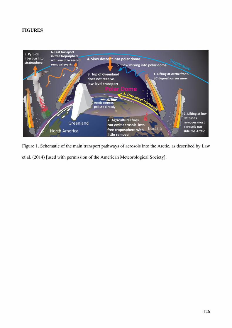
126

FIGURES

Figure 1. Schematic of the main transport pathways of aerosols into the Arctic, as described by Law

et al. (2014) [used with permission of the American Meteorological Society].

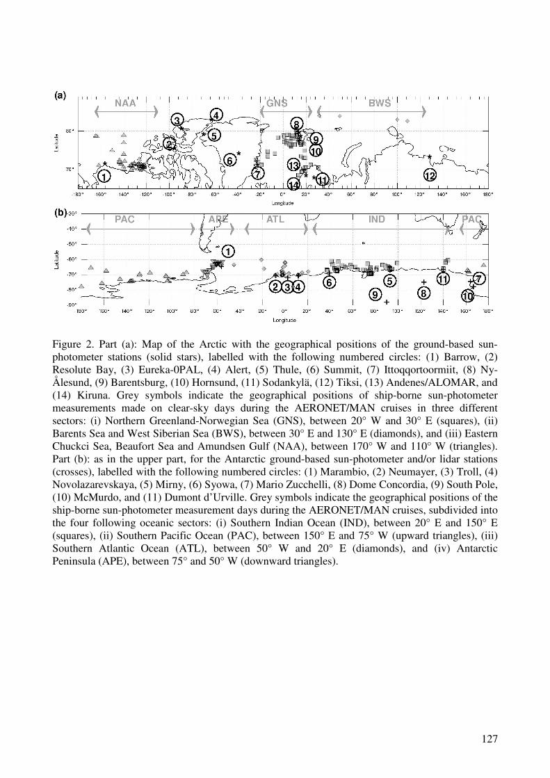
127

Figure 2. Part (a): Map of the Arctic with the geographical positions of the ground-based sun-photometer stations (solid stars), labelled with the following numbered circles: (1) Barrow, (2) Resolute Bay, (3) Eureka-0PAL, (4) Alert, (5) Thule, (6) Summit, (7) Ittoqqortoormiit, (8) Ny-Ålesund, (9) Barentsburg, (10) Hornsund, (11) Sodankylä, (12) Tiksi, (13) Andenes/ALOMAR, and (14) Kiruna. Grey symbols indicate the geographical positions of ship-borne sun-photometer measurements made on clear-sky days during the AERONET/MAN cruises in three different sectors: (i) Northern Greenland-Norwegian Sea (GNS), between 20° W and 30° E (squares), (ii) Barents Sea and West Siberian Sea (BWS), between 30° E and 130° E (diamonds), and (iii) Eastern Chuckci Sea, Beaufort Sea and Amundsen Gulf (NAA), between 170° W and 110° W (triangles). Part (b): as in the upper part, for the Antarctic ground-based sun-photometer and/or lidar stations (crosses), labelled with the following numbered circles: (1) Marambio, (2) Neumayer, (3) Troll, (4) Novolazarevskaya, (5) Mirny, (6) Syowa, (7) Mario Zucchelli, (8) Dome Concordia, (9) South Pole, (10) McMurdo, and (11) Dumont d’Urville. Grey symbols indicate the geographical positions of the ship-borne sun-photometer measurement days during the AERONET/MAN cruises, subdivided into the four following oceanic sectors: (i) Southern Indian Ocean (IND), between 20° E and 150° E (squares), (ii) Southern Pacific Ocean (PAC), between 150° E and 75° W (upward triangles), (iii) Southern Atlantic Ocean (ATL), between 50° W and 20° E (diamonds), and (iv) Antarctic Peninsula (APE), between 75° and 50° W (downward triangles).

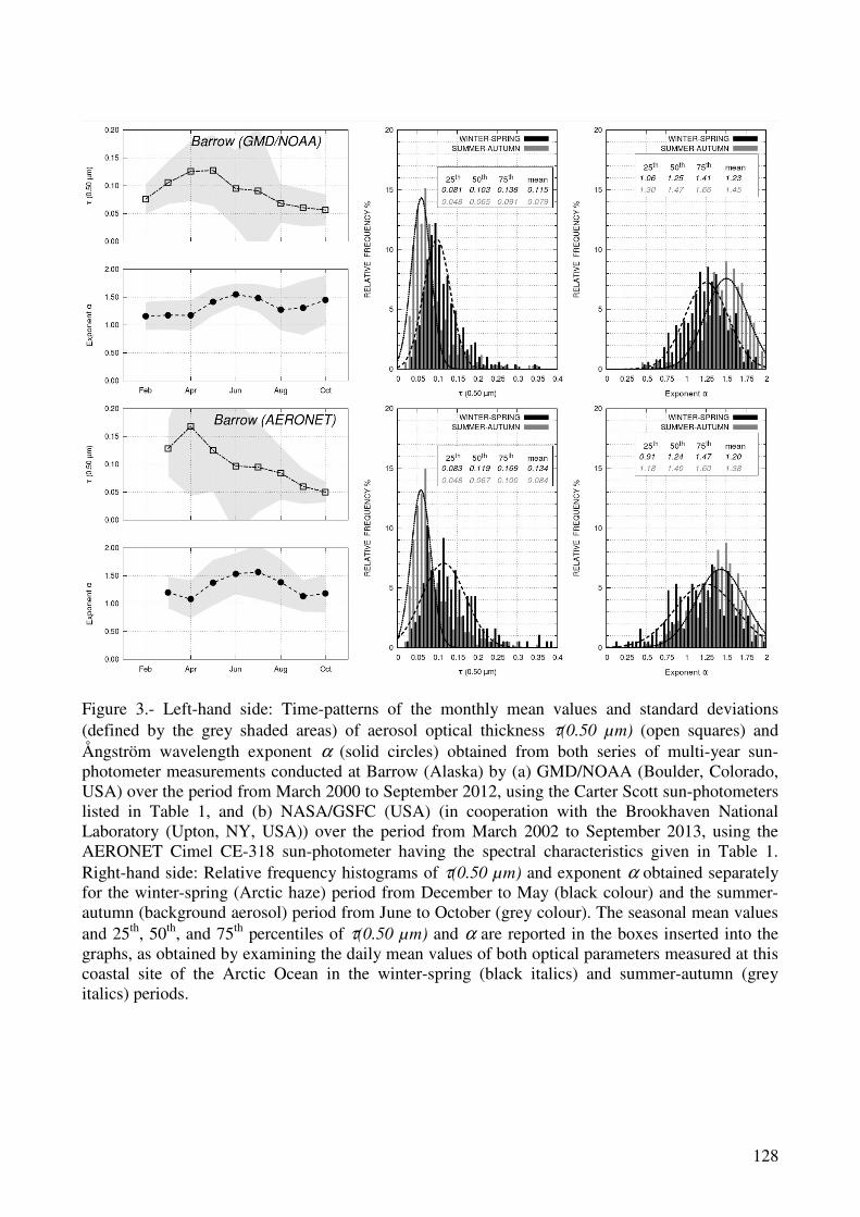
128

Figure 3.- Left-hand side: Time-patterns of the monthly mean values and standard deviations (defined by the grey shaded areas) of aerosol optical thickness τ(0.50 µm) (open squares) and Ångström wavelength exponent α (solid circles) obtained from both series of multi-year sun-photometer measurements conducted at Barrow (Alaska) by (a) GMD/NOAA (Boulder, Colorado, USA) over the period from March 2000 to September 2012, using the Carter Scott sun-photometers listed in Table 1, and (b) NASA/GSFC (USA) (in cooperation with the Brookhaven National Laboratory (Upton, NY, USA)) over the period from March 2002 to September 2013, using the AERONET Cimel CE-318 sun-photometer having the spectral characteristics given in Table 1. Right-hand side: Relative frequency histograms of τ(0.50 µm) and exponent α obtained separately for the winter-spring (Arctic haze) period from December to May (black colour) and the summer-autumn (background aerosol) period from June to October (grey colour). The seasonal mean values and 25th, 50th, and 75th percentiles of τ(0.50 µm) and α are reported in the boxes inserted into the graphs, as obtained by examining the daily mean values of both optical parameters measured at this coastal site of the Arctic Ocean in the winter-spring (black italics) and summer-autumn (grey italics) periods.

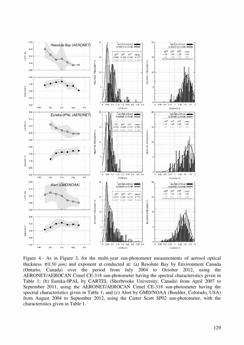
129

Figure 4.- As in Figure 3, for the multi-year sun-photometer measurements of aerosol optical thickness τ(0.50 µm) and exponent α conducted at: (a) Resolute Bay by Environment Canada (Ontario, Canada) over the period from July 2004 to October 2012, using the AERONET/AEROCAN Cimel CE-318 sun-photometer having the spectral characteristics given in Table 1; (b) Eureka-0PAL by CARTEL (Sherbrooke University, Canada) from April 2007 to September 2011, using the AERONET/AEROCAN Cimel CE-318 sun-photometer having the spectral characteristics given in Table 1; and (c) Alert by GMD/NOAA (Boulder, Colorado, USA) from August 2004 to September 2012, using the Carter Scott SP02 sun-photometer, with the characteristics given in Table 1.

130

Figure 5.- As in Figure 3, for the for the multi-year sun-photometer measurements of aerosol optical thickness τ(0.50 µm) and exponent α conducted at: (a) Thule (North-western Greenland) by NASA/GSFC (USA) over the period from March 2007 to September 2012, using an AERONET Cimel CE-318 sun-photometer having the spectral characteristics reported in Table 1; (b) Summit (Central Greenland) by PMOD/WRC (Switzerland) from January 2001 to October 2011, using a PFR (No. N34) sun-photometer of the GAW-PFR network, having the spectral characteristics given in Table 1; and (c) Ittoqqortoormiit (Eastern Greenland) by NASA/GSFC (USA) over the period from May 2010 to October 2013, using an AERONET Cimel CE-318 sun-photometer having the spectral characteristics reported in Table 1.

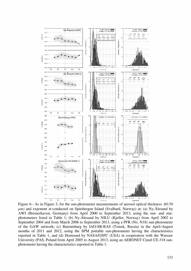
131

Figure 6.- As in Figure 3, for the sun-photometer measurements of aerosol optical thickness τ(0.50

µm) and exponent α conducted on Spitsbergen Island (Svalbard, Norway) at: (a) Ny-Ålesund by AWI (Bremerhaven, Germany) from April 2000 to September 2013, using the sun- and star-photometers listed in Table 1; (b) Ny-Ålesund by NILU (Kjeller, Norway) from April 2002 to September 2004 and from March 2006 to September 2013, using a PFR (No. N18) sun-photometer of the GAW network; (c) Barentsburg by IAO-SB-RAS (Tomsk, Russia) in the April-August months of 2011 and 2012, using the SPM portable sun-photometer having the characteristics reported in Table 1, and (d) Hornsund by NASA/GSFC (USA) in cooperation with the Warsaw University (PAS, Poland from April 2005 to August 2013, using an AERONET Cimel CE-318 sun-photometer having the characteristics reported in Table 1.

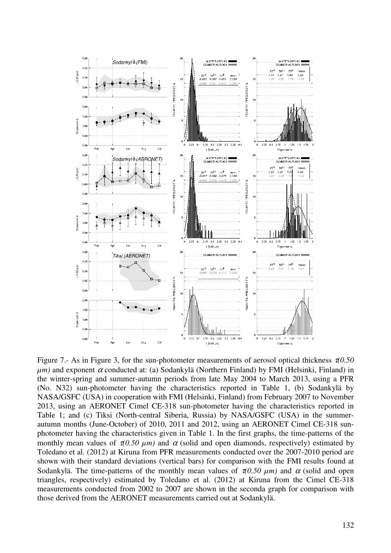
132

Figure 7.- As in Figure 3, for the sun-photometer measurements of aerosol optical thickness τ(0.50

µm) and exponent α conducted at: (a) Sodankylä (Northern Finland) by FMI (Helsinki, Finland) in the winter-spring and summer-autumn periods from late May 2004 to March 2013, using a PFR (No. N32) sun-photometer having the characteristics reported in Table 1, (b) Sodankylä by NASA/GSFC (USA) in cooperation with FMI (Helsinki, Finland) from February 2007 to November 2013, using an AERONET Cimel CE-318 sun-photometer having the characteristics reported in Table 1; and (c) Tiksi (North-central Siberia, Russia) by NASA/GSFC (USA) in the summer-autumn months (June-October) of 2010, 2011 and 2012, using an AERONET Cimel CE-318 sun-photometer having the characteristics given in Table 1. In the first graphs, the time-patterns of the monthly mean values of τ(0.50 µm) and α (solid and open diamonds, respectively) estimated by Toledano et al. (2012) at Kiruna from PFR measurements conducted over the 2007-2010 period are shown with their standard deviations (vertical bars) for comparison with the FMI results found at Sodankylä. The time-patterns of the monthly mean values of τ(0.50 µm) and α (solid and open triangles, respectively) estimated by Toledano et al. (2012) at Kiruna from the Cimel CE-318 measurements conducted from 2002 to 2007 are shown in the seconda graph for comparison with those derived from the AERONET measurements carried out at Sodankylä.

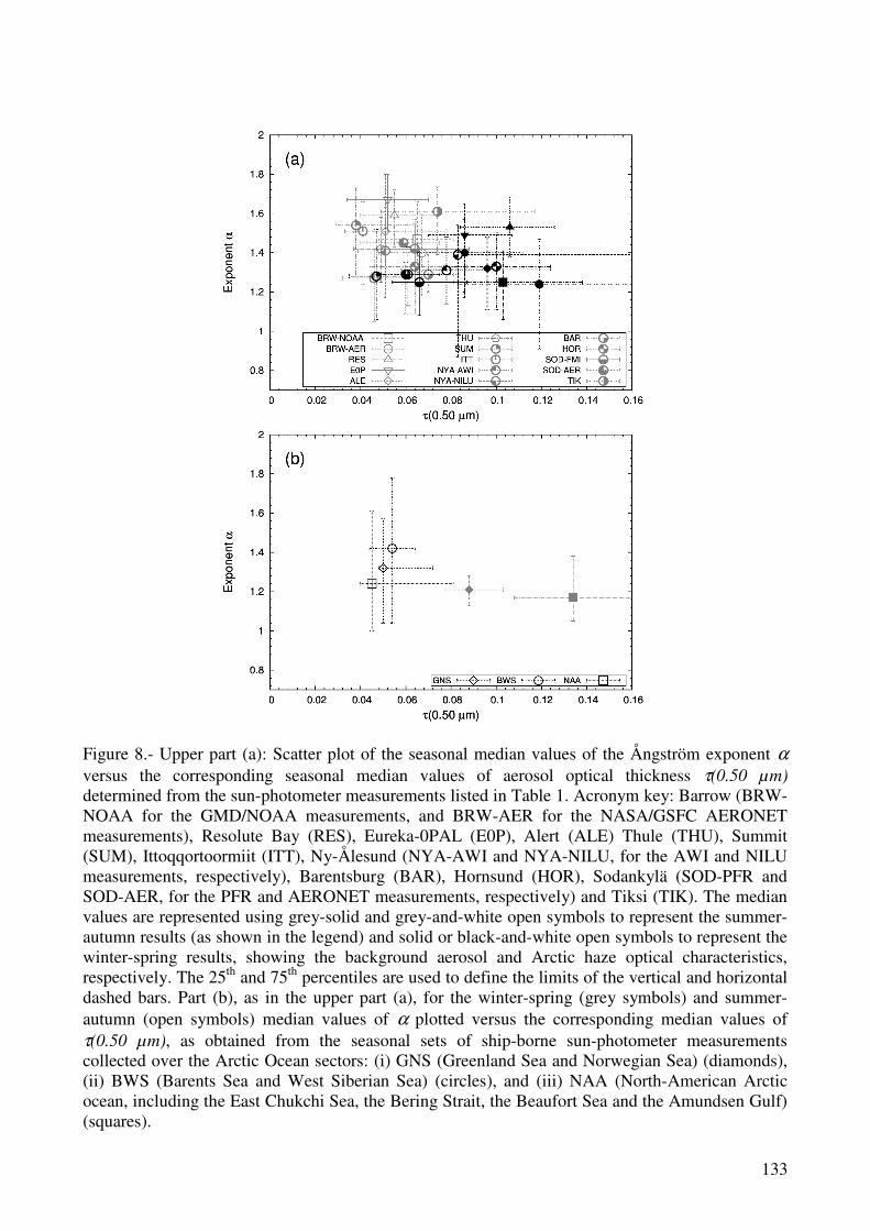
133

Figure 8.- Upper part (a): Scatter plot of the seasonal median values of the Ångström exponent α versus the corresponding seasonal median values of aerosol optical thickness τ(0.50 µm) determined from the sun-photometer measurements listed in Table 1. Acronym key: Barrow (BRW-NOAA for the GMD/NOAA measurements, and BRW-AER for the NASA/GSFC AERONET measurements), Resolute Bay (RES), Eureka-0PAL (E0P), Alert (ALE) Thule (THU), Summit (SUM), Ittoqqortoormiit (ITT), Ny-Ålesund (NYA-AWI and NYA-NILU, for the AWI and NILU measurements, respectively), Barentsburg (BAR), Hornsund (HOR), Sodankylä (SOD-PFR and SOD-AER, for the PFR and AERONET measurements, respectively) and Tiksi (TIK). The median values are represented using grey-solid and grey-and-white open symbols to represent the summer-autumn results (as shown in the legend) and solid or black-and-white open symbols to represent the winter-spring results, showing the background aerosol and Arctic haze optical characteristics, respectively. The 25th and 75th percentiles are used to define the limits of the vertical and horizontal dashed bars. Part (b), as in the upper part (a), for the winter-spring (grey symbols) and summer-autumn (open symbols) median values of α plotted versus the corresponding median values of τ(0.50 µm), as obtained from the seasonal sets of ship-borne sun-photometer measurements collected over the Arctic Ocean sectors: (i) GNS (Greenland Sea and Norwegian Sea) (diamonds), (ii) BWS (Barents Sea and West Siberian Sea) (circles), and (iii) NAA (North-American Arctic ocean, including the East Chukchi Sea, the Bering Strait, the Beaufort Sea and the Amundsen Gulf) (squares).

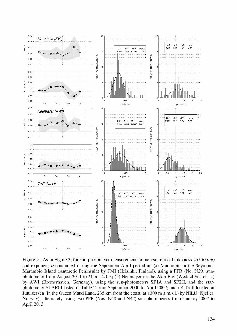
134

Figure 9.- As in Figure 3, for sun-photometer measurements of aerosol optical thickness τ(0.50 µm) and exponent α conducted during the September-April period at: (a) Marambio in the Seymour-Marambio Island (Antarctic Peninsula) by FMI (Helsinki, Finland), using a PFR (No. N29) sun-photometer from August 2011 to March 2013; (b) Neumayer on the Akta Bay (Weddel Sea coast) by AWI (Bremerhaven, Germany), using the sun-photometers SP1A and SP2H, and the star-photometer STAR01 listed in Table 2 from September 2000 to April 2007; and (c) Troll located at Jutulsessen (in the Queen Maud Land, 235 km from the coast, at 1309 m a.m.s.l.) by NILU (Kjeller, Norway), alternately using two PFR (Nos. N40 and N42) sun-photometers from January 2007 to April 2013

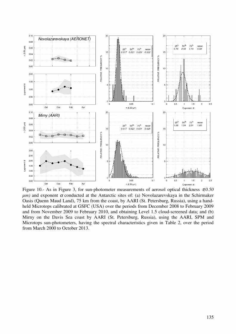
135

Figure 10.- As in Figure 3, for sun-photometer measurements of aerosol optical thickness τ(0.50

µm) and exponent α conducted at the Antarctic sites of: (a) Novolazarevskaya in the Schirmaker Oasis (Quenn Maud Land), 75 km from the coast, by AARI (St. Petersburg, Russia), using a hand-held Microtops calibrated at GSFC (USA) over the periods from December 2008 to February 2009 and from November 2009 to February 2010, and obtaining Level 1.5 cloud-screened data; and (b) Mirny on the Davis Sea coast by AARI (St. Petersburg, Russia), using the AARI, SPM and Microtops sun-photometers, having the spectral characteristics given in Table 2, over the period from March 2000 to October 2013.

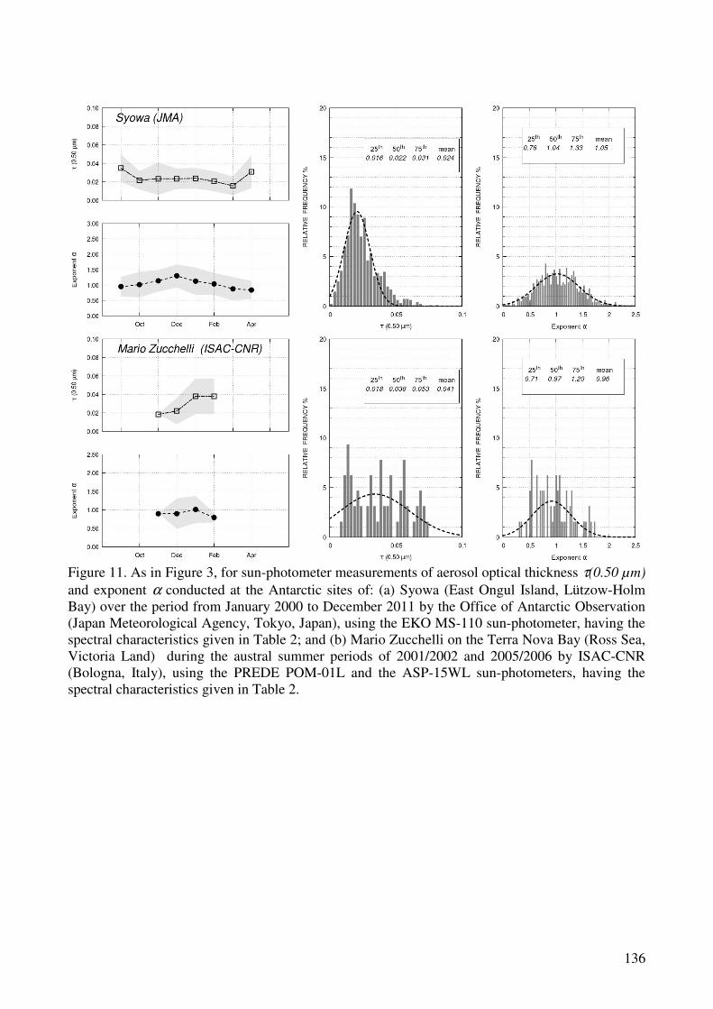
136

Figure 11. As in Figure 3, for sun-photometer measurements of aerosol optical thickness τ(0.50 µm) and exponent α conducted at the Antarctic sites of: (a) Syowa (East Ongul Island, Lützow-Holm Bay) over the period from January 2000 to December 2011 by the Office of Antarctic Observation (Japan Meteorological Agency, Tokyo, Japan), using the EKO MS-110 sun-photometer, having the spectral characteristics given in Table 2; and (b) Mario Zucchelli on the Terra Nova Bay (Ross Sea, Victoria Land) during the austral summer periods of 2001/2002 and 2005/2006 by ISAC-CNR (Bologna, Italy), using the PREDE POM-01L and the ASP-15WL sun-photometers, having the spectral characteristics given in Table 2.

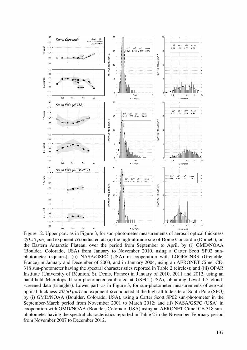
137

Figure 12. Upper part: as in Figure 3, for sun-photometer measurements of aerosol optical thickness τ(0.50 µm) and exponent α conducted at: (a) the high-altitude site of Dome Concordia (DomeC), on the Eastern Antarctic Plateau, over the period from September to April, by (i) GMD/NOAA (Boulder, Colorado, USA) from January to November 2010, using a Carter Scott SP02 sun-photometer (squares); (ii) NASA/GSFC (USA) in cooperation with LGGE/CNRS (Grenoble, France) in January and December of 2003, and in January 2004, using an AERONET Cimel CE-318 sun-photometer having the spectral characteristics reported in Table 2 (circles); and (iii) OPAR Institute (University of Réunion, St. Denis, France) in January of 2010, 2011 and 2012, using an hand-held Microtops II sun-photometer calibrated at GSFC (USA), obtaining Level 1.5 cloud-screened data (triangles). Lower part: as in Figure 3, for sun-photometer measurements of aerosol optical thickness τ(0.50 µm) and exponent α conducted at the high-altitude site of South Pole (SPO) by (i) GMD/NOAA (Boulder, Colorado, USA), using a Carter Scott SP02 sun-photometer in the September-March period from November 2001 to March 2012; and (ii) NASA/GSFC (USA) in cooperation with GMD/NOAA (Boulder, Colorado, USA) using an AERONET Cimel CE-318 sun-photometer having the spectral characteristics reported in Table 2 in the November-February period from November 2007 to December 2012.

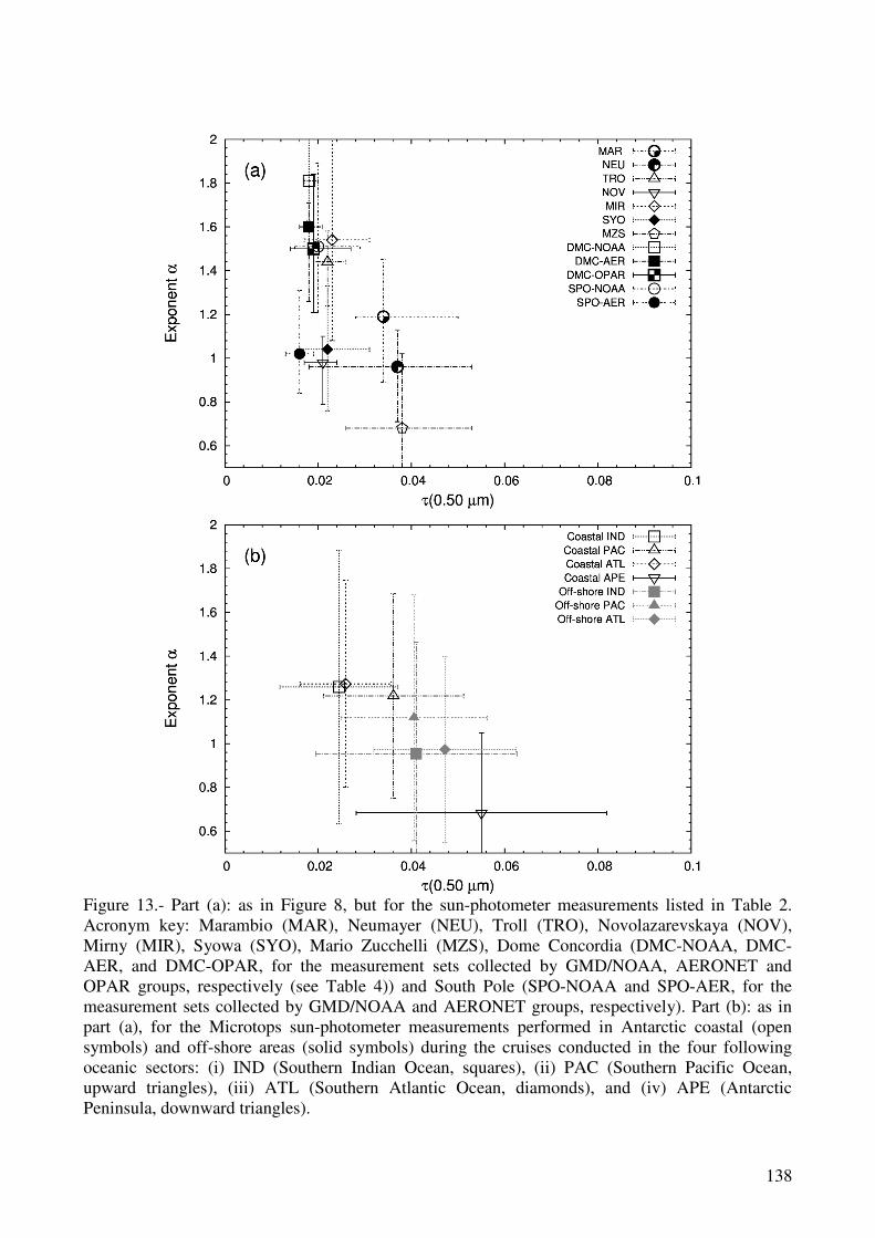
138

Figure 13.- Part (a): as in Figure 8, but for the sun-photometer measurements listed in Table 2. Acronym key: Marambio (MAR), Neumayer (NEU), Troll (TRO), Novolazarevskaya (NOV), Mirny (MIR), Syowa (SYO), Mario Zucchelli (MZS), Dome Concordia (DMC-NOAA, DMC-AER, and DMC-OPAR, for the measurement sets collected by GMD/NOAA, AERONET and OPAR groups, respectively (see Table 4)) and South Pole (SPO-NOAA and SPO-AER, for the measurement sets collected by GMD/NOAA and AERONET groups, respectively). Part (b): as in part (a), for the Microtops sun-photometer measurements performed in Antarctic coastal (open symbols) and off-shore areas (solid symbols) during the cruises conducted in the four following oceanic sectors: (i) IND (Southern Indian Ocean, squares), (ii) PAC (Southern Pacific Ocean, upward triangles), (iii) ATL (Southern Atlantic Ocean, diamonds), and (iv) APE (Antarctic Peninsula, downward triangles).

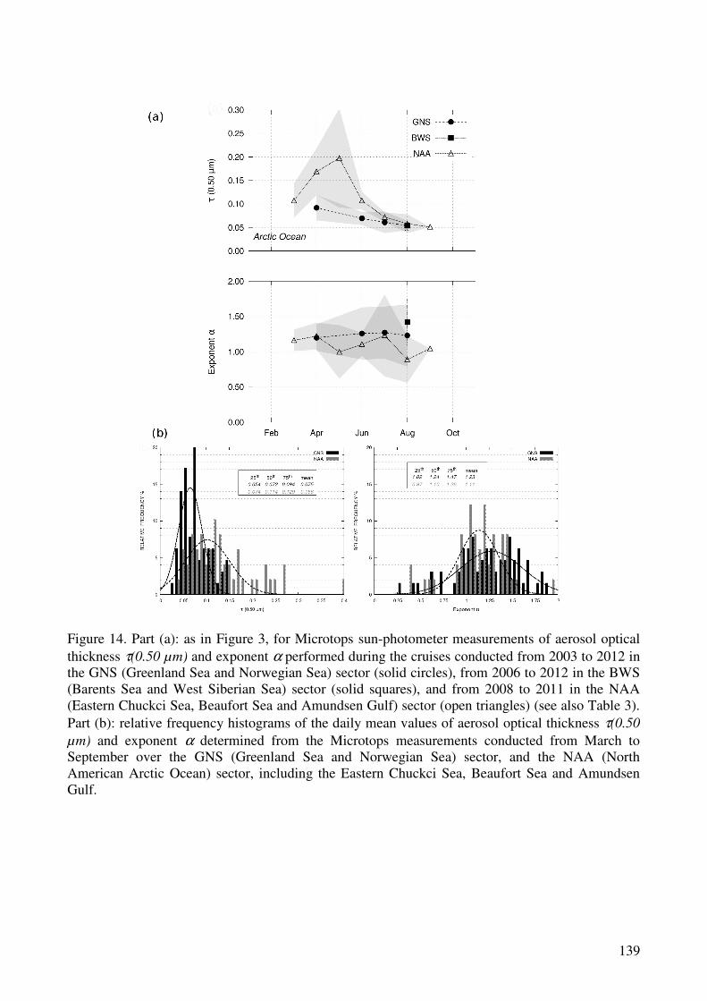
139

Figure 14. Part (a): as in Figure 3, for Microtops sun-photometer measurements of aerosol optical thickness τ(0.50 µm) and exponent α performed during the cruises conducted from 2003 to 2012 in the GNS (Greenland Sea and Norwegian Sea) sector (solid circles), from 2006 to 2012 in the BWS (Barents Sea and West Siberian Sea) sector (solid squares), and from 2008 to 2011 in the NAA (Eastern Chuckci Sea, Beaufort Sea and Amundsen Gulf) sector (open triangles) (see also Table 3). Part (b): relative frequency histograms of the daily mean values of aerosol optical thickness τ(0.50

µm) and exponent α determined from the Microtops measurements conducted from March to September over the GNS (Greenland Sea and Norwegian Sea) sector, and the NAA (North American Arctic Ocean) sector, including the Eastern Chuckci Sea, Beaufort Sea and Amundsen Gulf.

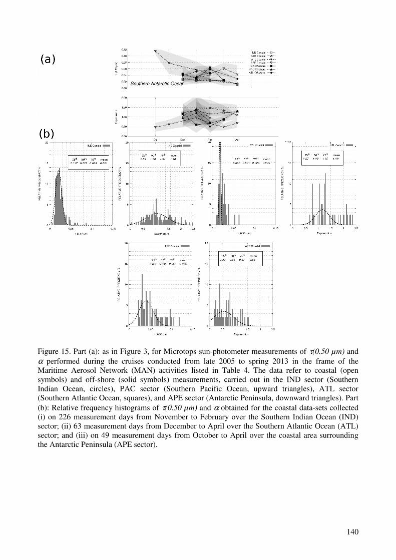
140

Figure 15. Part (a): as in Figure 3, for Microtops sun-photometer measurements of τ(0.50 µm) and α performed during the cruises conducted from late 2005 to spring 2013 in the frame of the Maritime Aerosol Network (MAN) activities listed in Table 4. The data refer to coastal (open symbols) and off-shore (solid symbols) measurements, carried out in the IND sector (Southern Indian Ocean, circles), PAC sector (Southern Pacific Ocean, upward triangles), ATL sector (Southern Atlantic Ocean, squares), and APE sector (Antarctic Peninsula, downward triangles). Part (b): Relative frequency histograms of τ(0.50 µm) and α obtained for the coastal data-sets collected (i) on 226 measurement days from November to February over the Southern Indian Ocean (IND) sector; (ii) 63 measurement days from December to April over the Southern Atlantic Ocean (ATL) sector; and (iii) on 49 measurement days from October to April over the coastal area surrounding the Antarctic Peninsula (APE sector).

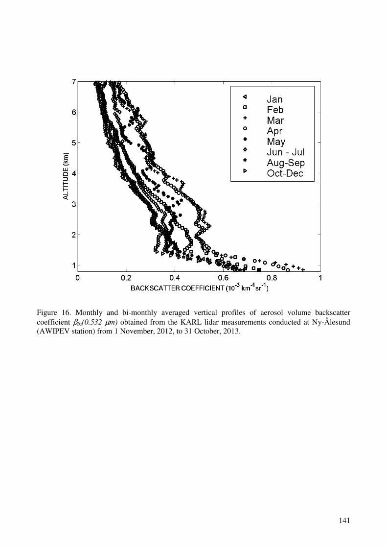
141

Figure 16. Monthly and bi-monthly averaged vertical profiles of aerosol volume backscatter coefficient βbs(0.532 µm) obtained from the KARL lidar measurements conducted at Ny-Ålesund (AWIPEV station) from 1 November, 2012, to 31 October, 2013.

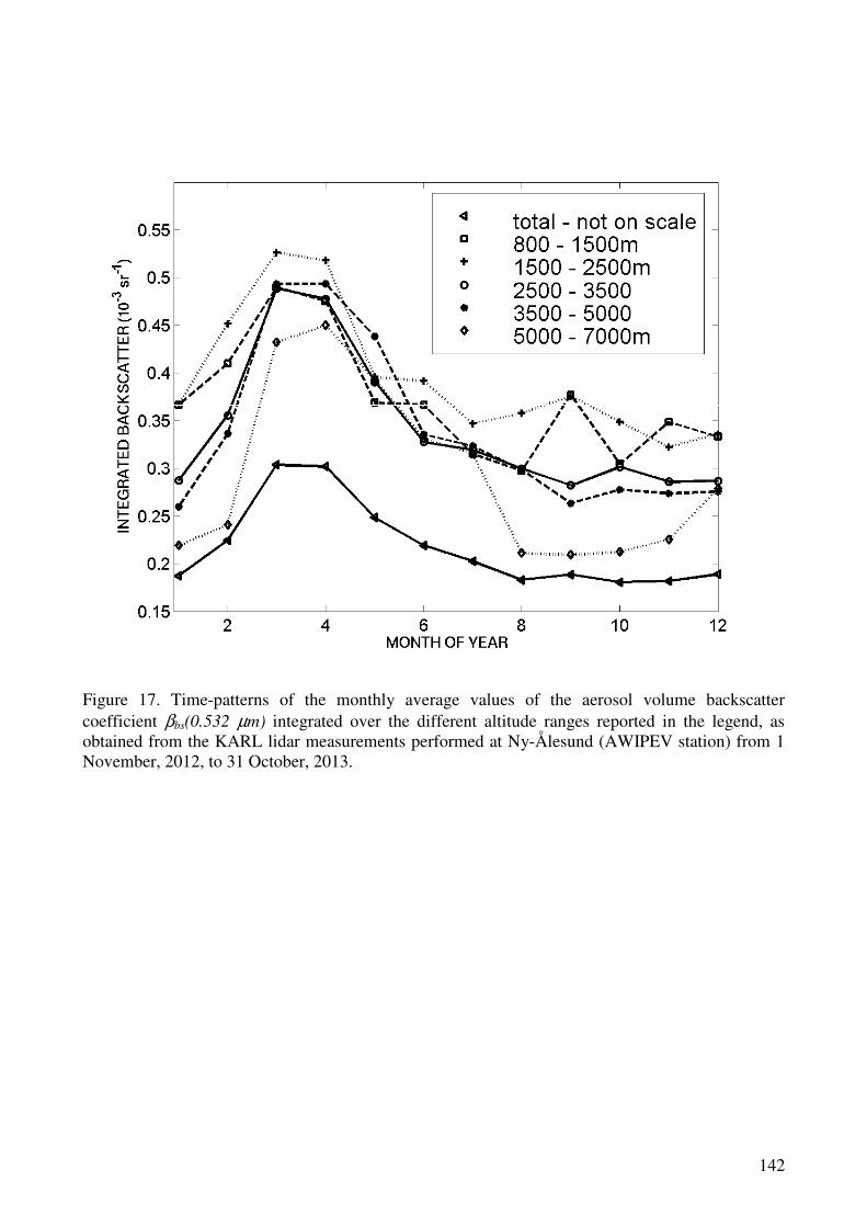
142

Figure 17. Time-patterns of the monthly average values of the aerosol volume backscatter coefficient βbs(0.532 µm) integrated over the different altitude ranges reported in the legend, as obtained from the KARL lidar measurements performed at Ny-Ålesund (AWIPEV station) from 1 November, 2012, to 31 October, 2013.

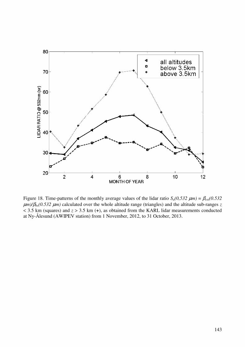
143

Figure 18. Time-patterns of the monthly average values of the lidar ratio Sa(0,532 µm) = βext(0.532

µm)/βbs(0.532 µm) calculated over the whole altitude range (triangles) and the altitude sub-ranges z < 3.5 km (squares) and z > 3.5 km (+), as obtained from the KARL lidar measurements conducted at Ny-Ålesund (AWIPEV station) from 1 November, 2012, to 31 October, 2013.

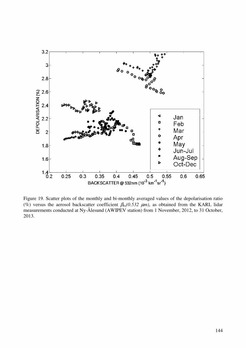
144

Figure 19. Scatter plots of the monthly and bi-monthly averaged values of the depolarisation ratio (%) versus the aerosol backscatter coefficient βbs(0.532 µm), as obtained from the KARL lidar measurements conducted at Ny-Ålesund (AWIPEV station) from 1 November, 2012, to 31 October, 2013.

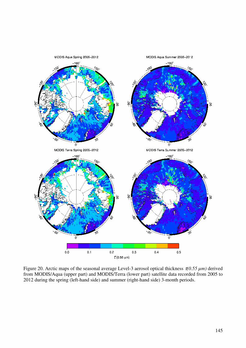
145

Figure 20. Arctic maps of the seasonal average Level-3 aerosol optical thickness τ(0.55 µm) derived from MODIS/Aqua (upper part) and MODIS/Terra (lower part) satellite data recorded from 2005 to 2012 during the spring (left-hand side) and summer (right-hand side) 3-month periods.

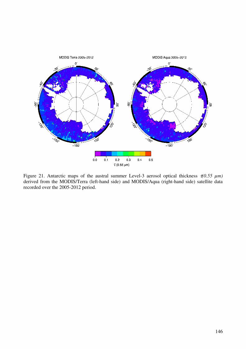
146

Figure 21. Antarctic maps of the austral summer Level-3 aerosol optical thickness τ(0.55 µm) derived from the MODIS/Terra (left-hand side) and MODIS/Aqua (right-hand side) satellite data recorded over the 2005-2012 period.

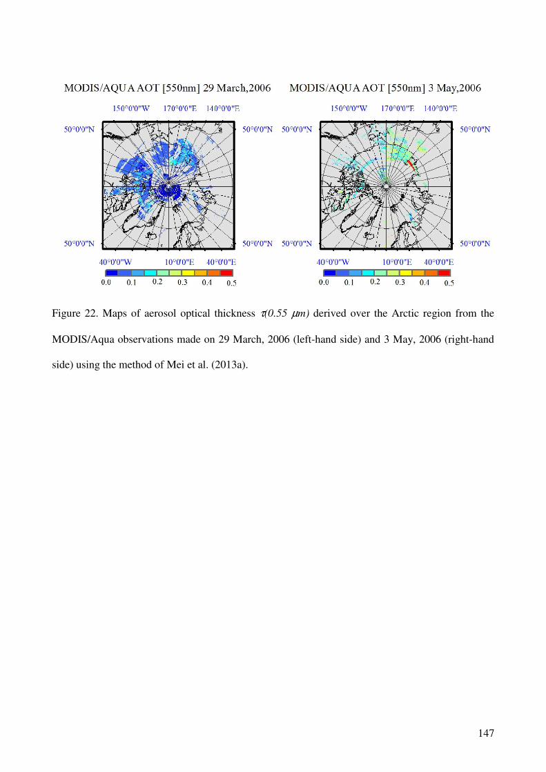
147

Figure 22. Maps of aerosol optical thickness τ(0.55 µm) derived over the Arctic region from the

MODIS/Aqua observations made on 29 March, 2006 (left-hand side) and 3 May, 2006 (right-hand

side) using the method of Mei et al. (2013a).

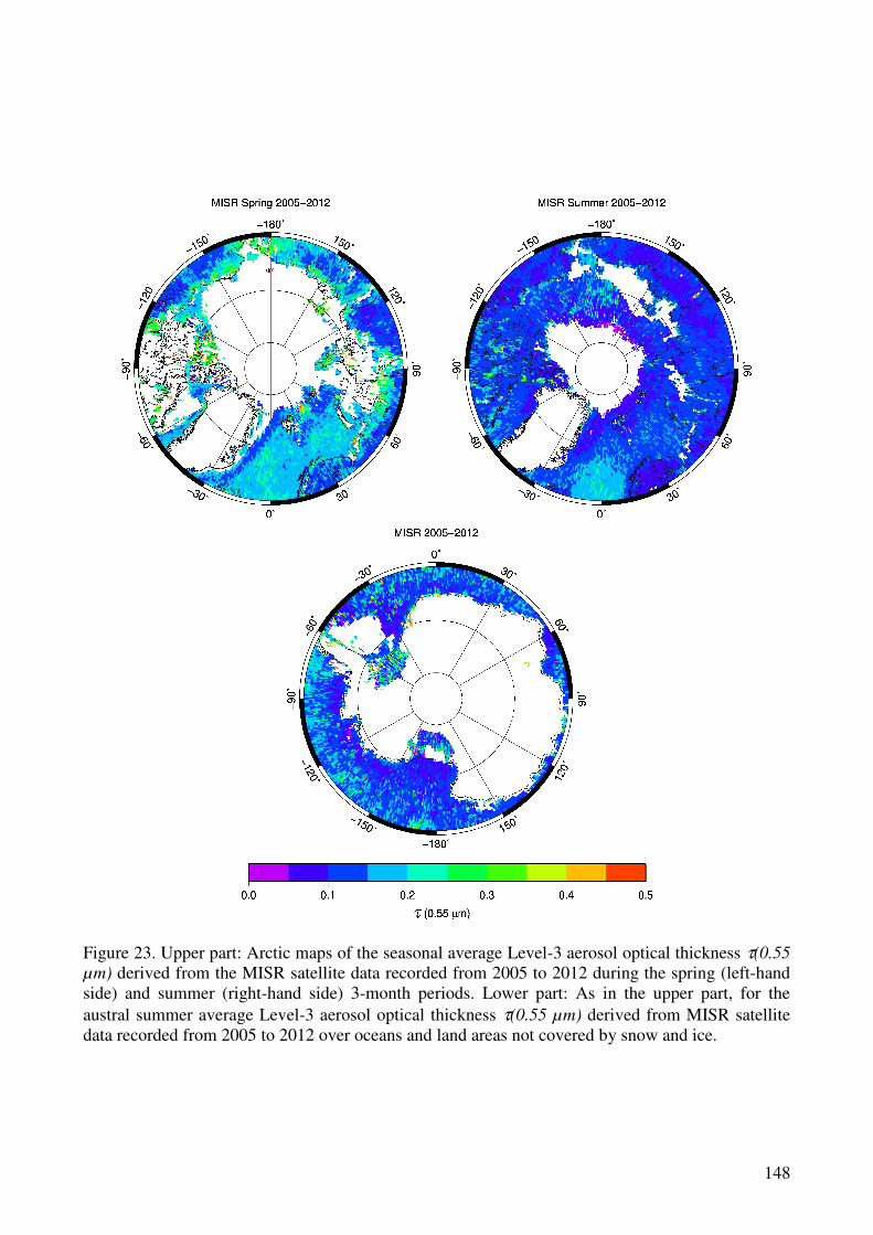
148

Figure 23. Upper part: Arctic maps of the seasonal average Level-3 aerosol optical thickness τ(0.55

µm) derived from the MISR satellite data recorded from 2005 to 2012 during the spring (left-hand side) and summer (right-hand side) 3-month periods. Lower part: As in the upper part, for the austral summer average Level-3 aerosol optical thickness τ(0.55 µm) derived from MISR satellite data recorded from 2005 to 2012 over oceans and land areas not covered by snow and ice.

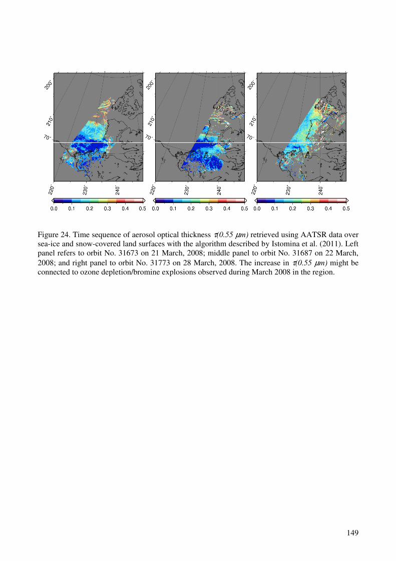
149

Figure 24. Time sequence of aerosol optical thickness τ(0.55 µm) retrieved using AATSR data over sea-ice and snow-covered land surfaces with the algorithm described by Istomina et al. (2011). Left panel refers to orbit No. 31673 on 21 March, 2008; middle panel to orbit No. 31687 on 22 March, 2008; and right panel to orbit No. 31773 on 28 March, 2008. The increase in τ(0.55 µm) might be connected to ozone depletion/bromine explosions observed during March 2008 in the region.

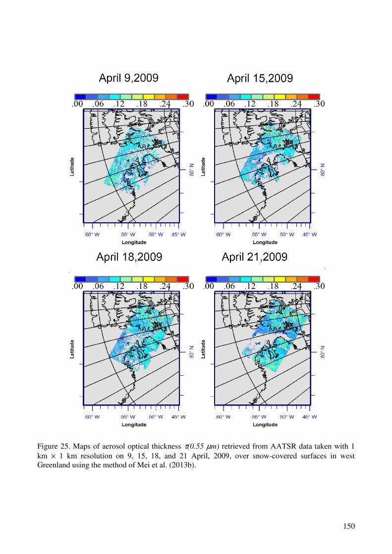
150

Figure 25. Maps of aerosol optical thickness τ(0.55 µm) retrieved from AATSR data taken with 1 km × 1 km resolution on 9, 15, 18, and 21 April, 2009, over snow-covered surfaces in west Greenland using the method of Mei et al. (2013b).

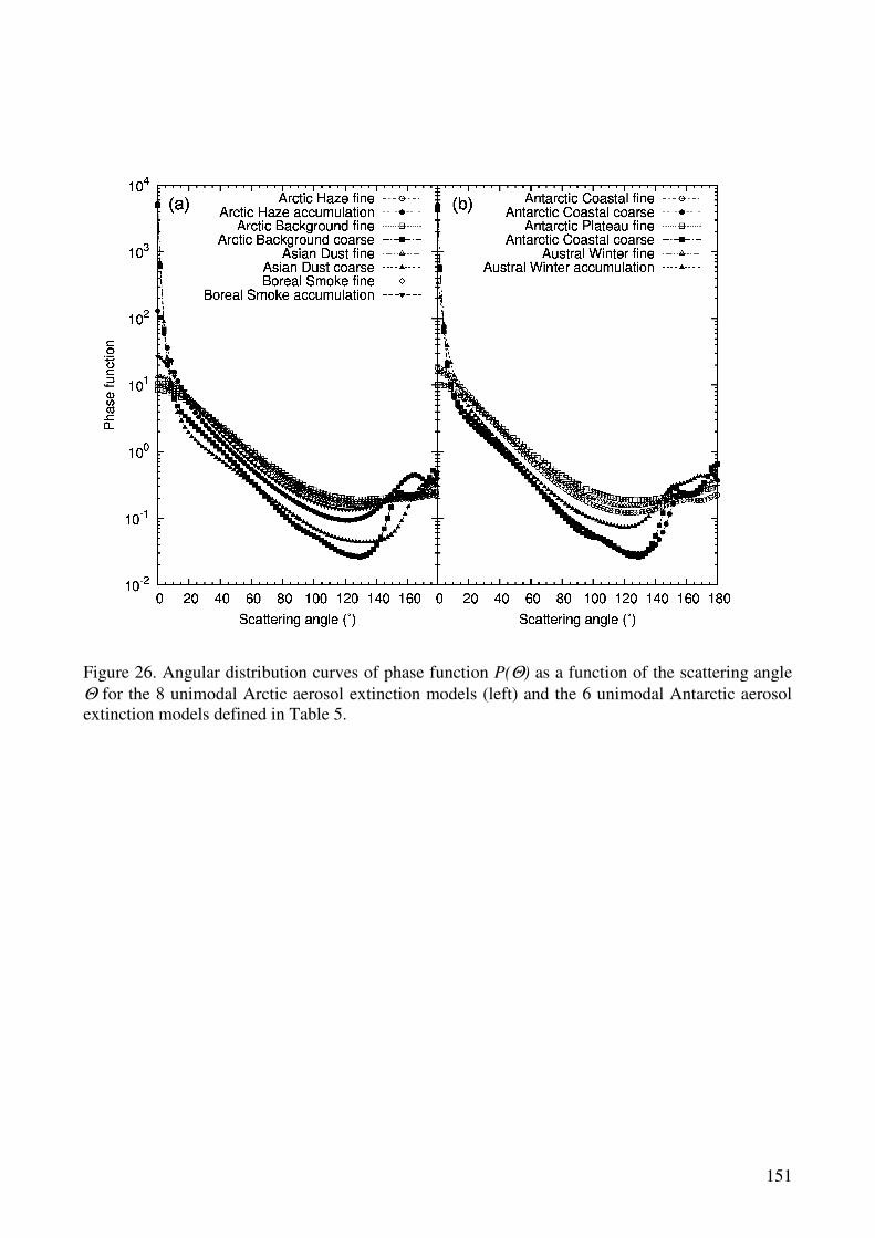
151

Figure 26. Angular distribution curves of phase function P(Θ) as a function of the scattering angle Θ for the 8 unimodal Arctic aerosol extinction models (left) and the 6 unimodal Antarctic aerosol extinction models defined in Table 5.

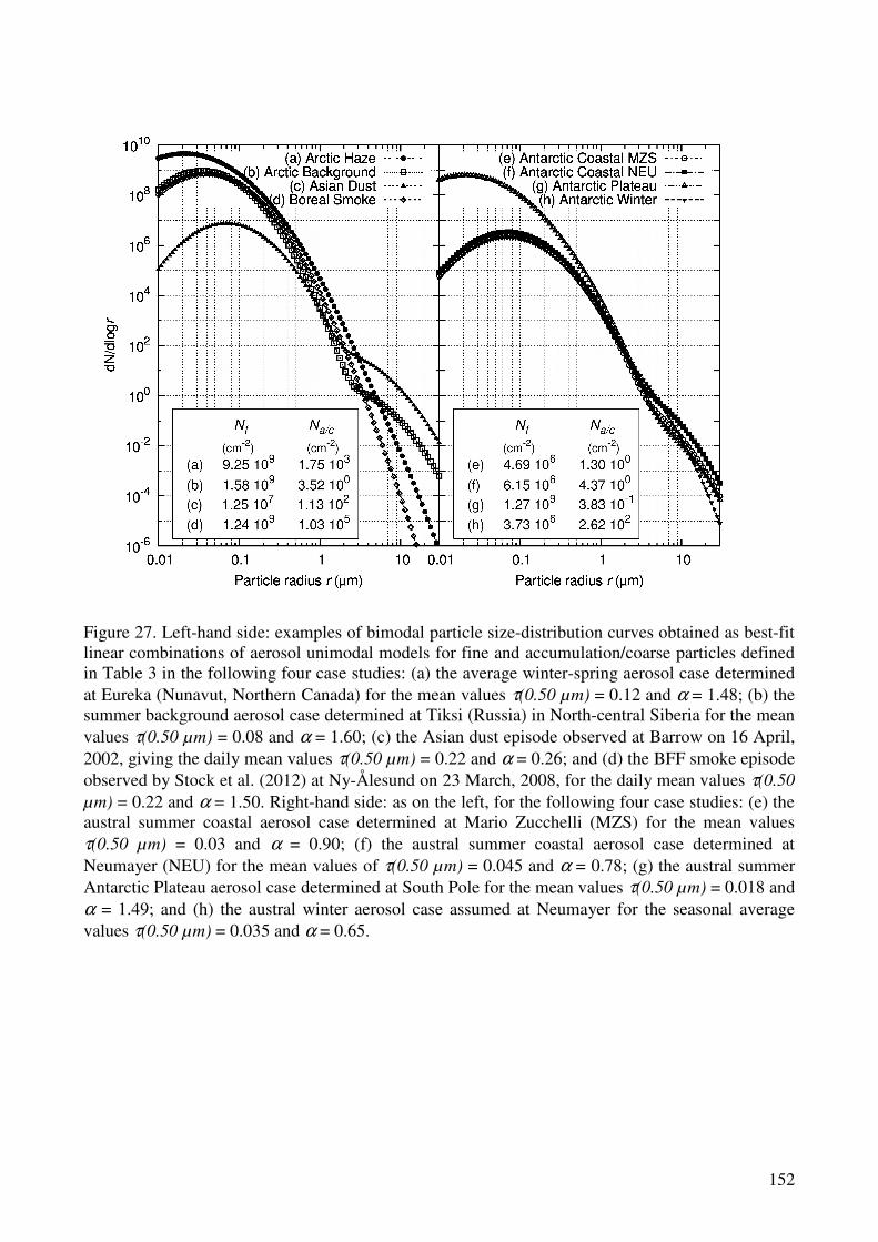
152

Figure 27. Left-hand side: examples of bimodal particle size-distribution curves obtained as best-fit linear combinations of aerosol unimodal models for fine and accumulation/coarse particles defined in Table 3 in the following four case studies: (a) the average winter-spring aerosol case determined at Eureka (Nunavut, Northern Canada) for the mean values τ(0.50 µm) = 0.12 and α = 1.48; (b) the summer background aerosol case determined at Tiksi (Russia) in North-central Siberia for the mean values τ(0.50 µm) = 0.08 and α = 1.60; (c) the Asian dust episode observed at Barrow on 16 April, 2002, giving the daily mean values τ(0.50 µm) = 0.22 and α = 0.26; and (d) the BFF smoke episode observed by Stock et al. (2012) at Ny-Ålesund on 23 March, 2008, for the daily mean values τ(0.50

µm) = 0.22 and α = 1.50. Right-hand side: as on the left, for the following four case studies: (e) the austral summer coastal aerosol case determined at Mario Zucchelli (MZS) for the mean values τ(0.50 µm) = 0.03 and α = 0.90; (f) the austral summer coastal aerosol case determined at Neumayer (NEU) for the mean values of τ(0.50 µm) = 0.045 and α = 0.78; (g) the austral summer Antarctic Plateau aerosol case determined at South Pole for the mean values τ(0.50 µm) = 0.018 and α = 1.49; and (h) the austral winter aerosol case assumed at Neumayer for the seasonal average values τ(0.50 µm) = 0.035 and α = 0.65.

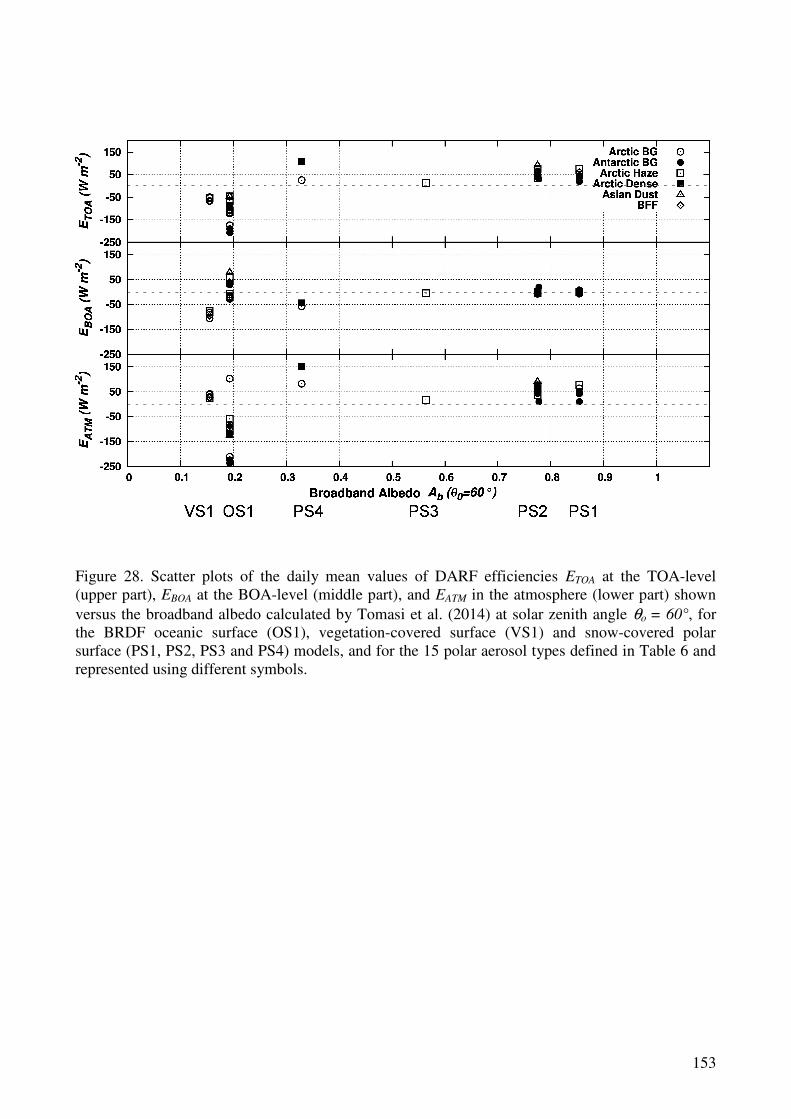
153

Figure 28. Scatter plots of the daily mean values of DARF efficiencies ETOA at the TOA-level (upper part), EBOA at the BOA-level (middle part), and EATM in the atmosphere (lower part) shown versus the broadband albedo calculated by Tomasi et al. (2014) at solar zenith angle θo = 60°, for the BRDF oceanic surface (OS1), vegetation-covered surface (VS1) and snow-covered polar surface (PS1, PS2, PS3 and PS4) models, and for the 15 polar aerosol types defined in Table 6 and represented using different symbols.

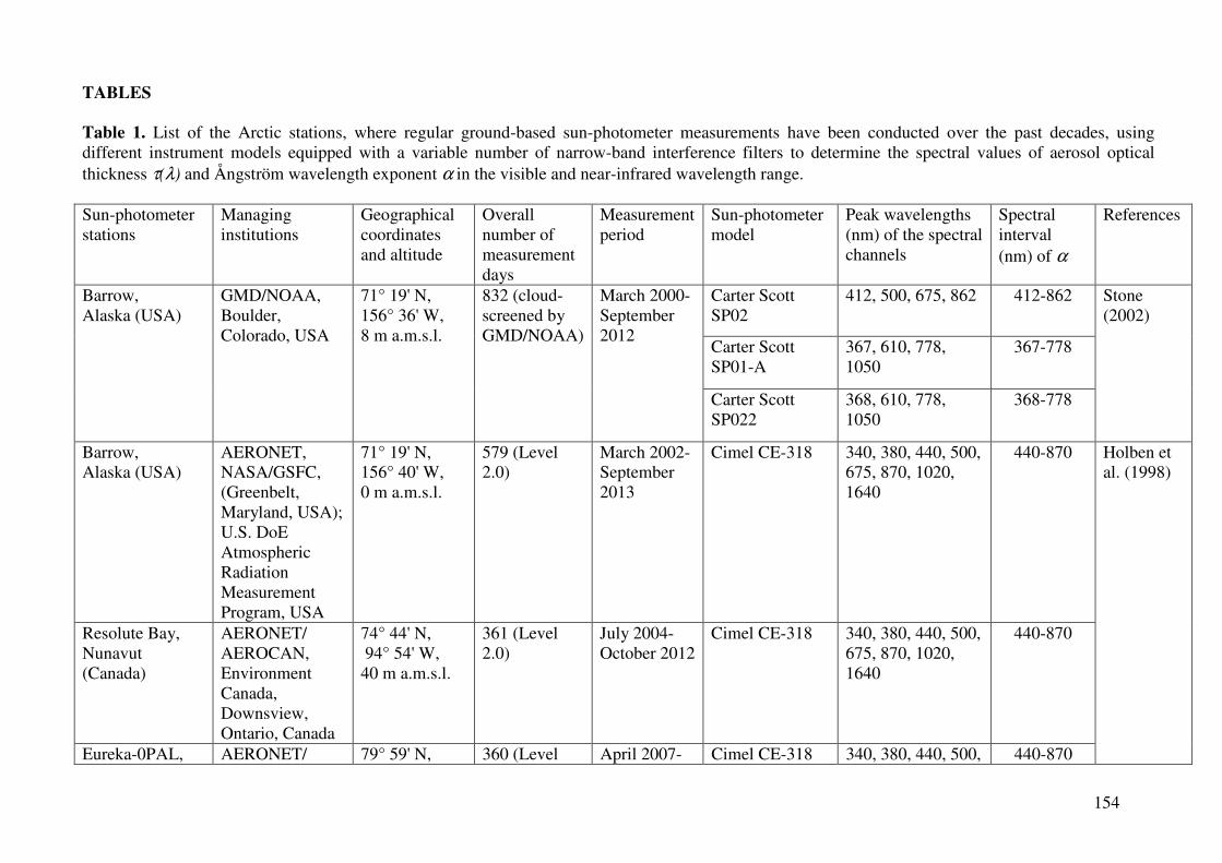
154

TABLES

Table 1. List of the Arctic stations, where regular ground-based sun-photometer measurements have been conducted over the past decades, using different instrument models equipped with a variable number of narrow-band interference filters to determine the spectral values of aerosol optical thickness τ(λ) and Ångström wavelength exponent α in the visible and near-infrared wavelength range. Sun-photometer stations

Managing institutions

Geographical coordinates and altitude

Overall number of measurement days

Measurement period

Sun-photometer model

Peak wavelengths (nm) of the spectral channels

Spectral interval (nm) of α

References

Carter Scott SP02

412, 500, 675, 862 412-862

Carter Scott SP01-A

367, 610, 778, 1050

367-778

Barrow, Alaska (USA)

GMD/NOAA, Boulder, Colorado, USA

71° 19' N, 156° 36' W, 8 m a.m.s.l.

832 (cloud-screened by GMD/NOAA)

March 2000-September 2012

Carter Scott SP022

368, 610, 778, 1050

368-778

Stone (2002)

Barrow, Alaska (USA)

AERONET, NASA/GSFC, (Greenbelt, Maryland, USA); U.S. DoE Atmospheric Radiation Measurement Program, USA

71° 19' N, 156° 40' W, 0 m a.m.s.l.

579 (Level 2.0)

March 2002- September 2013

Cimel CE-318 340, 380, 440, 500, 675, 870, 1020, 1640

440-870

Resolute Bay, Nunavut (Canada)

AERONET/ AEROCAN, Environment Canada, Downsview, Ontario, Canada

74° 44' N, 94° 54' W, 40 m a.m.s.l.

361 (Level 2.0)

July 2004-October 2012

Cimel CE-318 340, 380, 440, 500, 675, 870, 1020, 1640

440-870

Eureka-0PAL, AERONET/ 79° 59' N, 360 (Level April 2007- Cimel CE-318 340, 380, 440, 500, 440-870

Holben et al. (1998)

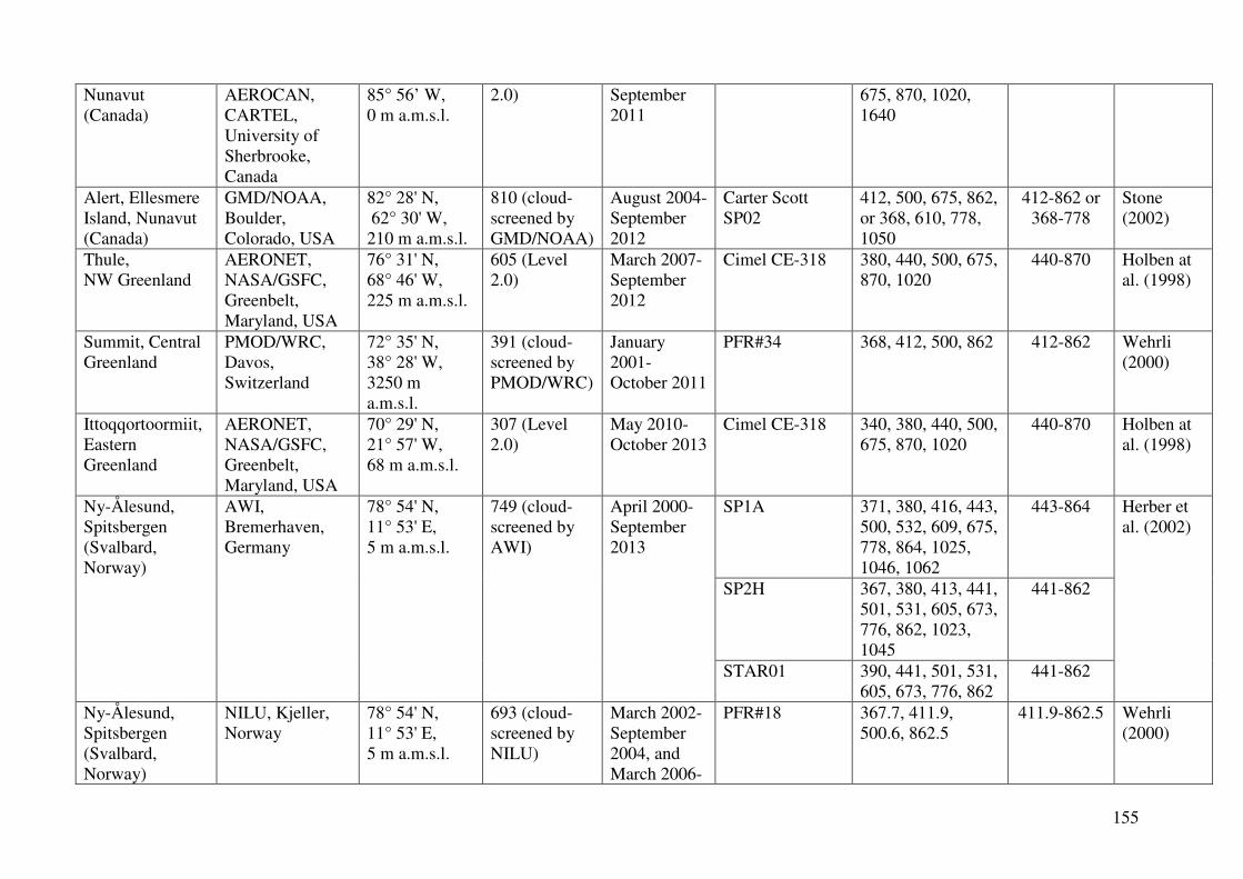
155

Nunavut (Canada)

AEROCAN, CARTEL, University of Sherbrooke, Canada

85° 56’ W, 0 m a.m.s.l.

2.0) September 2011

675, 870, 1020, 1640

Alert, Ellesmere Island, Nunavut (Canada)

GMD/NOAA, Boulder, Colorado, USA

82° 28' N, 62° 30' W, 210 m a.m.s.l.

810 (cloud-screened by GMD/NOAA)

August 2004-September 2012

Carter Scott SP02

412, 500, 675, 862, or 368, 610, 778, 1050

412-862 or 368-778

Stone (2002)

Thule, NW Greenland

AERONET, NASA/GSFC, Greenbelt, Maryland, USA

76° 31' N, 68° 46' W, 225 m a.m.s.l.

605 (Level 2.0)

March 2007-September 2012

Cimel CE-318 380, 440, 500, 675, 870, 1020

440-870 Holben at al. (1998)

Summit, Central Greenland

PMOD/WRC, Davos, Switzerland

72° 35' N, 38° 28' W, 3250 m a.m.s.l.

391 (cloud-screened by PMOD/WRC)

January 2001-October 2011

PFR#34 368, 412, 500, 862 412-862 Wehrli (2000)

Ittoqqortoormiit, Eastern Greenland

AERONET, NASA/GSFC, Greenbelt, Maryland, USA

70° 29' N, 21° 57' W, 68 m a.m.s.l.

307 (Level 2.0)

May 2010-October 2013

Cimel CE-318 340, 380, 440, 500, 675, 870, 1020

440-870 Holben at al. (1998)

SP1A 371, 380, 416, 443, 500, 532, 609, 675, 778, 864, 1025, 1046, 1062

443-864

SP2H 367, 380, 413, 441, 501, 531, 605, 673, 776, 862, 1023, 1045

441-862

Ny-Ålesund, Spitsbergen (Svalbard, Norway)

AWI, Bremerhaven, Germany

78° 54' N, 11° 53' E, 5 m a.m.s.l.

749 (cloud-screened by AWI)

April 2000-September 2013

STAR01 390, 441, 501, 531, 605, 673, 776, 862

441-862

Herber et al. (2002)

Ny-Ålesund, Spitsbergen (Svalbard, Norway)

NILU, Kjeller, Norway

78° 54' N, 11° 53' E, 5 m a.m.s.l.

693 (cloud-screened by NILU)

March 2002-September 2004, and March 2006-

PFR#18 367.7, 411.9, 500.6, 862.5

411.9-862.5 Wehrli (2000)

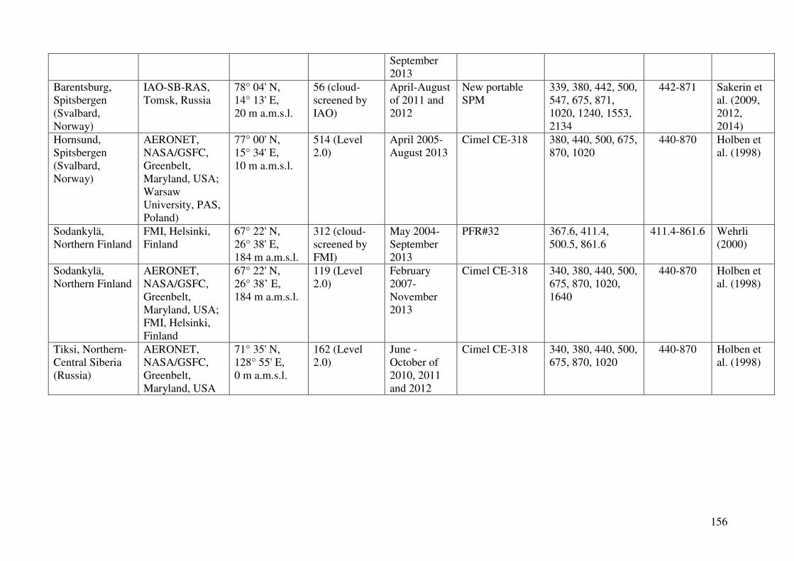
156

September 2013

Barentsburg, Spitsbergen (Svalbard, Norway)

IAO-SB-RAS, Tomsk, Russia

78° 04' N, 14° 13' E, 20 m a.m.s.l.

56 (cloud-screened by IAO)

April-August of 2011 and 2012

New portable SPM

339, 380, 442, 500, 547, 675, 871, 1020, 1240, 1553, 2134

442-871 Sakerin et al. (2009, 2012, 2014)

Hornsund, Spitsbergen (Svalbard, Norway)

AERONET, NASA/GSFC, Greenbelt, Maryland, USA; Warsaw University, PAS, Poland)

77° 00' N, 15° 34' E, 10 m a.m.s.l.

514 (Level 2.0)

April 2005-August 2013

Cimel CE-318 380, 440, 500, 675, 870, 1020

440-870 Holben et al. (1998)

Sodankylä, Northern Finland

FMI, Helsinki, Finland

67° 22' N, 26° 38' E, 184 m a.m.s.l.

312 (cloud-screened by FMI)

May 2004-September 2013

PFR#32 367.6, 411.4, 500.5, 861.6

411.4-861.6 Wehrli (2000)

Sodankylä, Northern Finland

AERONET, NASA/GSFC, Greenbelt, Maryland, USA; FMI, Helsinki, Finland

67° 22' N, 26° 38’ E, 184 m a.m.s.l.

119 (Level 2.0)

February 2007-November 2013

Cimel CE-318 340, 380, 440, 500, 675, 870, 1020, 1640

440-870 Holben et al. (1998)

Tiksi, Northern-Central Siberia (Russia)

AERONET, NASA/GSFC, Greenbelt, Maryland, USA

71° 35' N, 128° 55' E, 0 m a.m.s.l.

162 (Level 2.0)

June - October of 2010, 2011 and 2012

Cimel CE-318 340, 380, 440, 500, 675, 870, 1020

440-870 Holben et al. (1998)

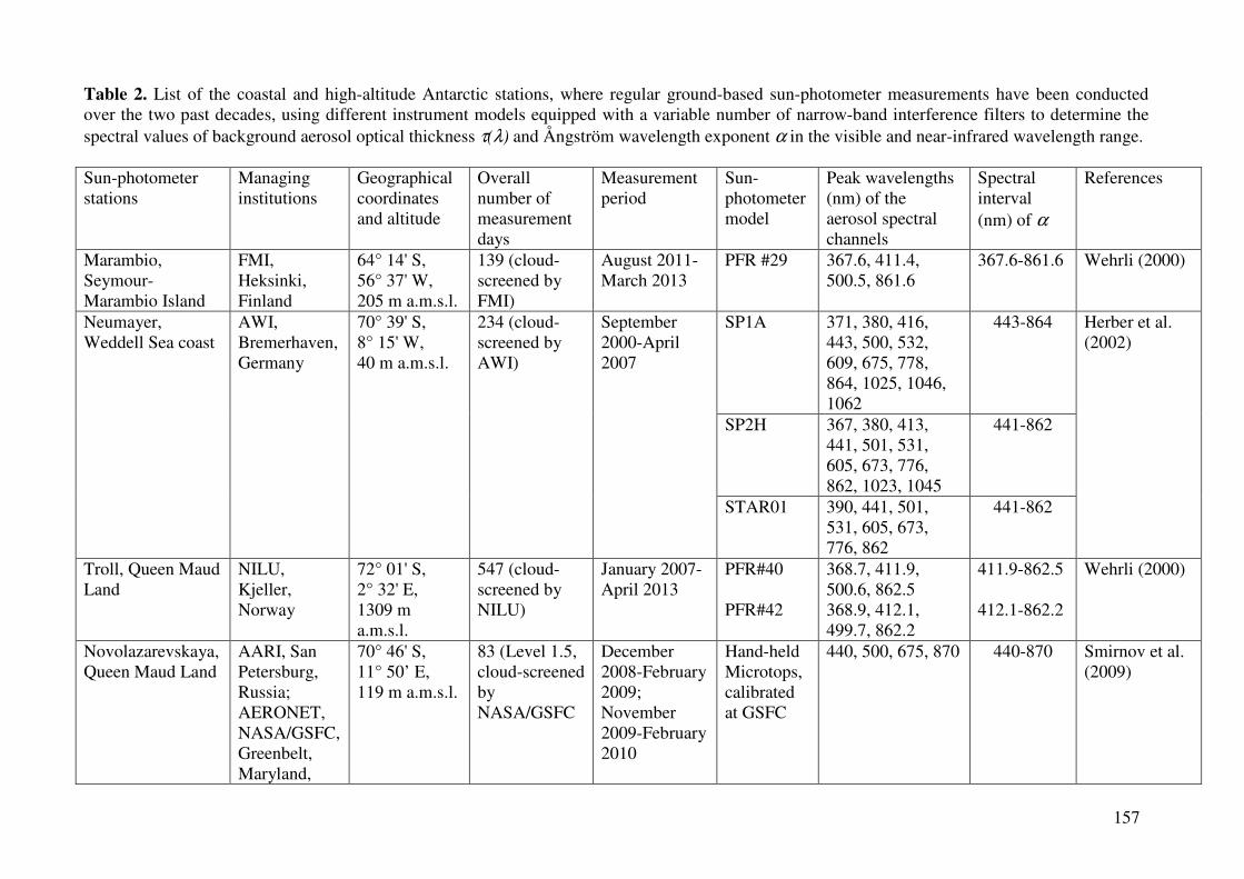
157

Table 2. List of the coastal and high-altitude Antarctic stations, where regular ground-based sun-photometer measurements have been conducted over the two past decades, using different instrument models equipped with a variable number of narrow-band interference filters to determine the spectral values of background aerosol optical thickness τ(λ) and Ångström wavelength exponent α in the visible and near-infrared wavelength range. Sun-photometer stations

Managing institutions

Geographical coordinates and altitude

Overall number of measurement days

Measurement period

Sun-photometer model

Peak wavelengths (nm) of the aerosol spectral channels

Spectral interval (nm) of α

References

Marambio, Seymour-Marambio Island

FMI, Heksinki, Finland

64° 14' S, 56° 37' W, 205 m a.m.s.l.

139 (cloud-screened by FMI)

August 2011-March 2013

PFR #29 367.6, 411.4, 500.5, 861.6

367.6-861.6 Wehrli (2000)

SP1A 371, 380, 416, 443, 500, 532, 609, 675, 778, 864, 1025, 1046, 1062

443-864

SP2H 367, 380, 413, 441, 501, 531, 605, 673, 776, 862, 1023, 1045

441-862

Neumayer, Weddell Sea coast

AWI, Bremerhaven, Germany

70° 39' S, 8° 15' W, 40 m a.m.s.l.

234 (cloud-screened by AWI)

September 2000-April 2007

STAR01 390, 441, 501, 531, 605, 673, 776, 862

441-862

Herber et al. (2002)

Troll, Queen Maud Land

NILU, Kjeller, Norway

72° 01' S, 2° 32' E, 1309 m a.m.s.l.

547 (cloud-screened by NILU)

January 2007-April 2013

PFR#40 PFR#42

368.7, 411.9, 500.6, 862.5 368.9, 412.1, 499.7, 862.2

411.9-862.5 412.1-862.2

Wehrli (2000)

Novolazarevskaya, Queen Maud Land

AARI, San Petersburg, Russia; AERONET, NASA/GSFC, Greenbelt, Maryland,

70° 46' S, 11° 50’ E, 119 m a.m.s.l.

83 (Level 1.5, cloud-screened by NASA/GSFC

December 2008-February 2009; November 2009-February 2010

Hand-held Microtops, calibrated at GSFC

440, 500, 675, 870 440-870 Smirnov et al. (2009)

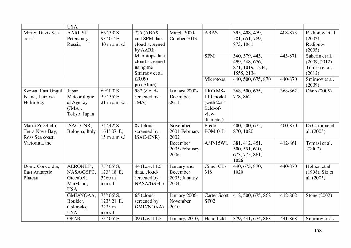
158

USA. ABAS 395, 408, 479,

581, 651, 789, 873, 1041

408-873 Radionov et al. (2002), Radionov (2005)

SPM 340, 379, 443, 499, 548, 676, 871, 1019, 1244, 1555, 2134

443-871 Sakerin et al. (2009, 2012) Tomasi et al. (2012)

Mirny, Davis Sea coast

AARI, St. Petersburg, Russia

66° 33' S, 93° 01' E, 40 m a.m.s.l.

725 (ABAS and SPM data cloud-screened by AARI; Microtops data cloud-screened using the Smirnov et al. (2009) procedure)

March 2000-October 2013

Microtops 440, 500, 675, 870 440-870 Smirnov et al. (2009)

Syowa, East Ongul Island, Lützow-Holm Bay

Japan Meteorological Agency (JMA), Tokyo, Japan

69° 00' S, 39° 35' E, 21 m a.m.s.l.

987 (cloud-screened by JMA)

January 2000-December 2011

EKO MS-110 model (with 2.5° field-of-view diameter)

368, 500, 675, 778, 862

368-862 Ohno (2005)

November 2001-February 2002

Prede POM-01L

400, 500, 675, 870, 1020

400-870 Di Carmine et al. (2005)

Mario Zucchelli, Terra Nova Bay, Ross Sea coast, Victoria Land

ISAC-CNR, Bologna, Italy

74° 42' S, 164° 07' E, 15 m a.m.s.l.

87 (cloud-screened by ISAC-CNR)

December 2005-February 2006

ASP-15WL 381, 412, 451, 500, 551, 610, 673, 775, 861, 1026

412-861 Tomasi et al, (2007)

AERONET , NASA/GSFC, Greenbelt, Maryland, USA

75° 05' S, 123° 18' E, 3260 m a.m.s.l.

44 (Level 1.5 data, cloud-screened by NASA/GSFC)

January and December 2003; January 2004

Cimel CE-318

440, 675, 870, 1020

440-870 Holben et al. (1998), Six et al. (2005)

GMD/NOAA, Boulder, Colorado, USA

75° 06' S, 123° 21' E, 3233 m a.m.s.l.

65 (cloud-screened by GMD/NOAA)

January 2006-November 2010

Carter Scott SP02

412, 500, 675, 862 412-862 Stone (2002)

Dome Concordia, East Antarctic Plateau

OPAR 75° 05' E, 39 (Level 1.5 January, 2010, Hand-held 379, 441, 674, 868 441-868 Smirnov et al.

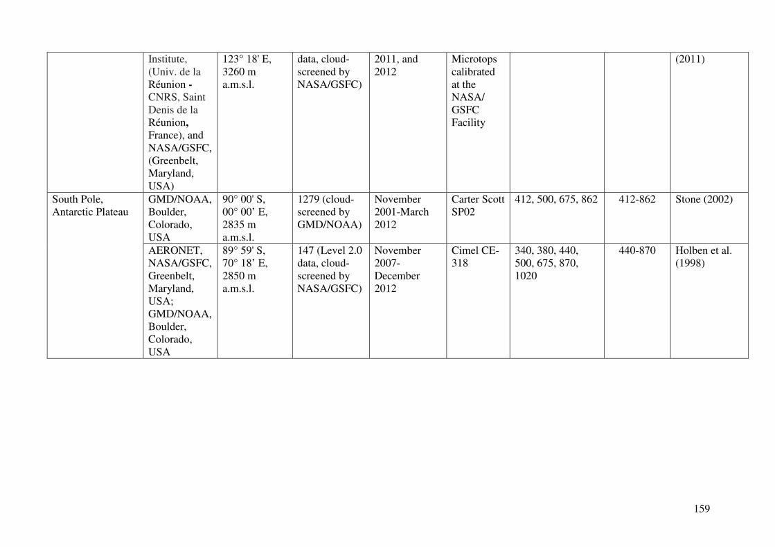
159

Institute, (Univ. de la Réunion - CNRS, Saint Denis de la Réunion,

France), and NASA/GSFC, (Greenbelt, Maryland, USA)

123° 18' E, 3260 m a.m.s.l.

data, cloud-screened by NASA/GSFC)

2011, and 2012

Microtops calibrated at the NASA/ GSFC Facility

(2011)

GMD/NOAA, Boulder, Colorado, USA

90° 00' S, 00° 00’ E, 2835 m a.m.s.l.

1279 (cloud-screened by GMD/NOAA)

November 2001-March 2012

Carter Scott SP02

412, 500, 675, 862 412-862 Stone (2002) South Pole, Antarctic Plateau

AERONET, NASA/GSFC, Greenbelt, Maryland, USA; GMD/NOAA, Boulder, Colorado, USA

89° 59' S, 70° 18’ E, 2850 m a.m.s.l.

147 (Level 2.0 data, cloud-screened by NASA/GSFC)

November 2007-December 2012

Cimel CE-318

340, 380, 440, 500, 675, 870, 1020

440-870 Holben et al. (1998)

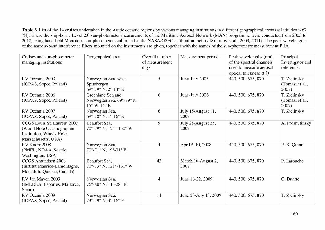
160

Table 3. List of the 14 cruises undertaken in the Arctic oceanic regions by various managing institutions in different geographical areas (at latitudes > 67 °N), where the ship-borne Level 2.0 sun-photometer measurements of the Maritime Aerosol Network (MAN) programme were conducted from 2003 to 2012, using hand-held Microtops sun-photometers calibrated at the NASA/GSFC calibration facility (Smirnov et al., 2009, 2011). The peak-wavelengths of the narrow-band interference filters mounted on the instruments are given, together with the names of the sun-photometer measurement P.I.s. Cruises and sun-photometer managing institutions

Geographical area Overall number of measurement days

Measurement period Peak wavelengths (nm) of the spectral channels used to measure aerosol optical thickness τ(λ)

Principal Investigator and references

RV Oceania 2003 (IOPAS, Sopot, Poland)

Norwegian Sea, west Spitsbergen 69°-79° N, 2°-14° E

5 June-July 2003 440, 500, 675, 870 T. Zielinsky (Tomasi et al., 2007)

RV Oceania 2006 (IOPAS, Sopot, Poland)

Greenland Sea and Norwegian Sea, 69°-79° N, 15° W-14° E

6 June-July 2006 440, 500, 675, 870 T. Zielinsky (Tomasi et al., 2007)

RV Oceania 2007 (IOPAS, Sopot, Poland)

Norwegian Sea, 69°-78° N, 1°-16° E

6 July 15-August 11, 2007

440, 500, 675, 870 T. Zielinsky

CCGS Louis St. Laurent 2007 (Wood Hole Oceanographic Institution, Woods Hole, Massachusetts, USA)

Beaufort Sea, 70°-79° N, 125°-150° W

9 July 28-August 25, 2007

440, 500, 675, 870 A. Proshutinsky

RV Knorr 2008 (PMEL, NOAA, Seattle, Washington, USA)

Norwegian Sea, 70°-71° N, 19°-31° E

4 April 6-10, 2008 440, 500, 675, 870 P. K. Quinn

CCGS Amundsen 2008 (Institut Maurice-Lamontagne, Mont-Joli, Quebec, Canada)

Beaufort Sea, 70°-73° N, 121°-131° W

43 March 16-August 2, 2008

440, 500, 675, 870 P. Larouche

RV Jan Mayen 2009 (IMEDEA, Esporles, Mallorca, Spain)

Norwegian Sea, 76°-80° N, 11°-28° E

4 June 18-22, 2009 440, 500, 675, 870 C. Duarte

RV Oceania 2009 (IOPAS, Sopot, Poland)

Norwegian Sea, 73°-79° N, 3°-16° E

11 June 23-July 13, 2009 440, 500, 675, 870 T. Zielinsky

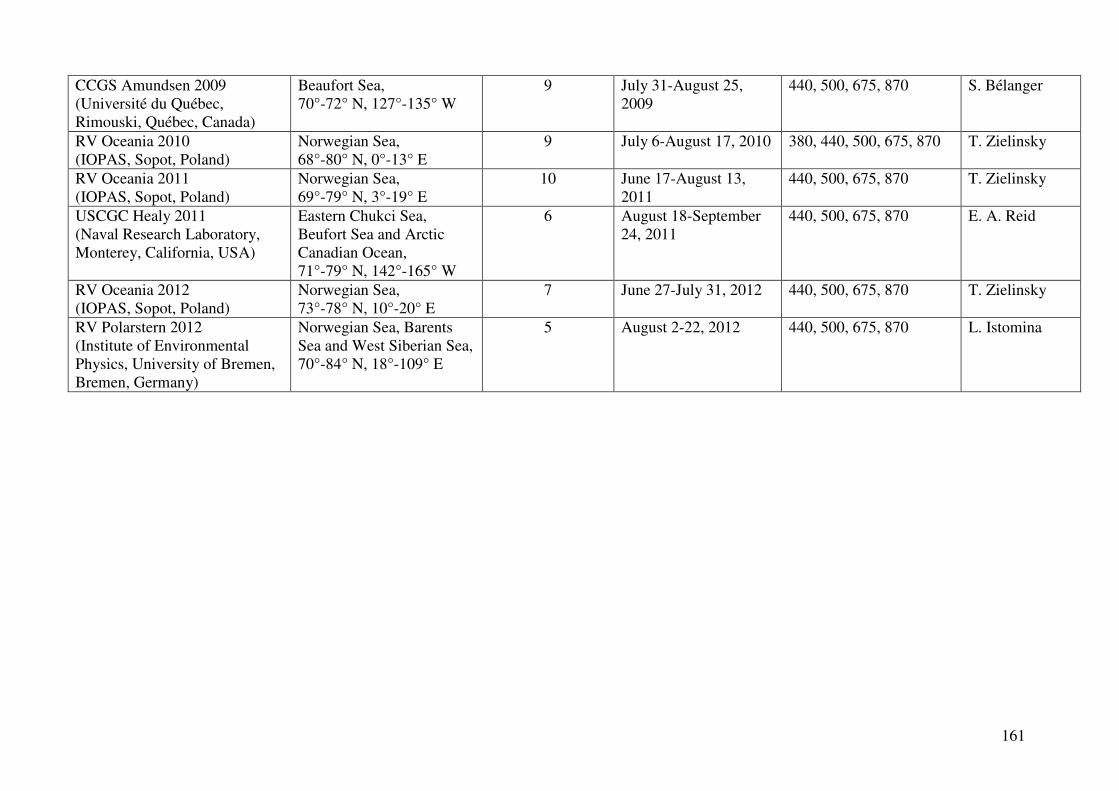
161

CCGS Amundsen 2009 (Université du Québec, Rimouski, Québec, Canada)

Beaufort Sea, 70°-72° N, 127°-135° W

9 July 31-August 25, 2009

440, 500, 675, 870 S. Bélanger

RV Oceania 2010 (IOPAS, Sopot, Poland)

Norwegian Sea, 68°-80° N, 0°-13° E

9 July 6-August 17, 2010 380, 440, 500, 675, 870 T. Zielinsky

RV Oceania 2011 (IOPAS, Sopot, Poland)

Norwegian Sea, 69°-79° N, 3°-19° E

10 June 17-August 13, 2011

440, 500, 675, 870 T. Zielinsky

USCGC Healy 2011 (Naval Research Laboratory, Monterey, California, USA)

Eastern Chukci Sea, Beufort Sea and Arctic Canadian Ocean, 71°-79° N, 142°-165° W

6 August 18-September 24, 2011

440, 500, 675, 870 E. A. Reid

RV Oceania 2012 (IOPAS, Sopot, Poland)

Norwegian Sea, 73°-78° N, 10°-20° E

7 June 27-July 31, 2012 440, 500, 675, 870 T. Zielinsky

RV Polarstern 2012 (Institute of Environmental Physics, University of Bremen, Bremen, Germany)

Norwegian Sea, Barents Sea and West Siberian Sea, 70°-84° N, 18°-109° E

5 August 2-22, 2012 440, 500, 675, 870 L. Istomina

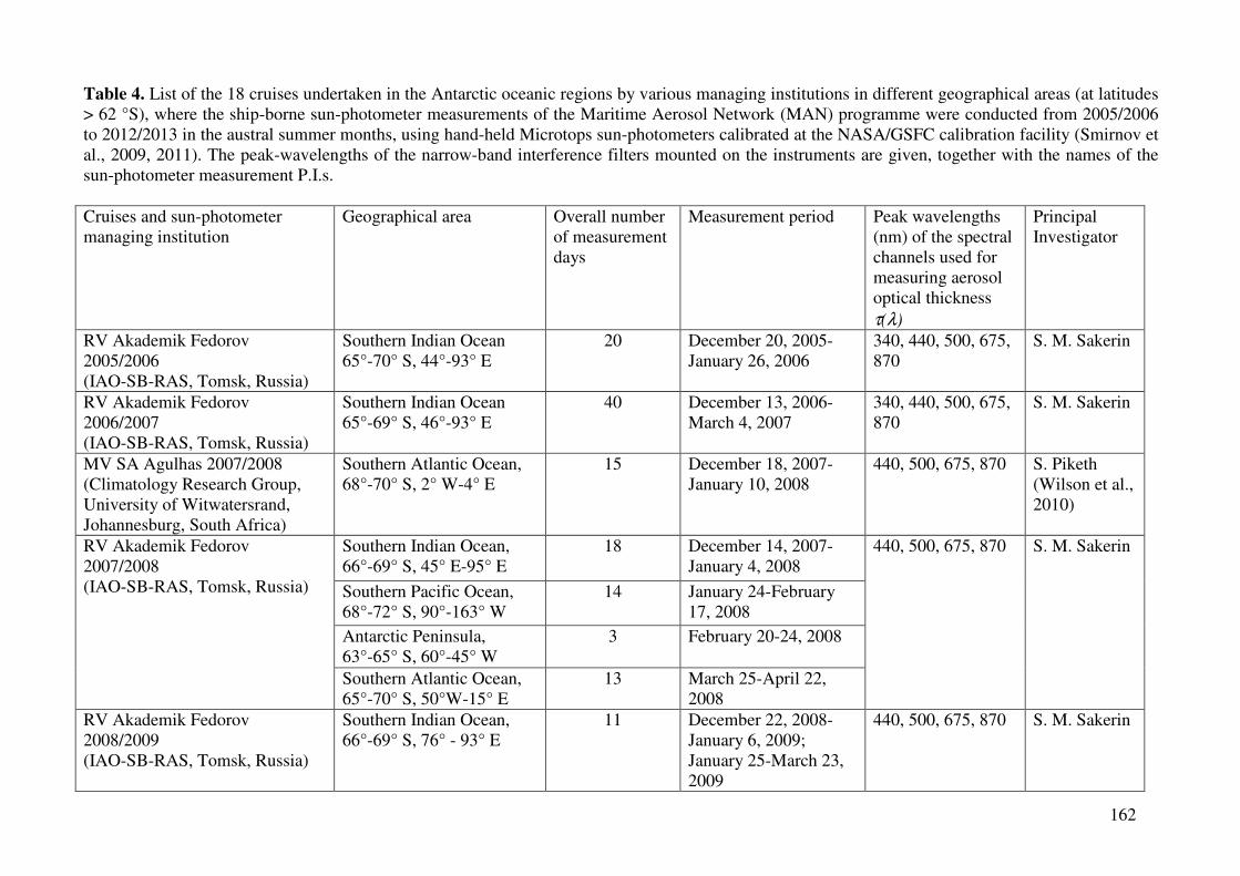
162

Table 4. List of the 18 cruises undertaken in the Antarctic oceanic regions by various managing institutions in different geographical areas (at latitudes > 62 °S), where the ship-borne sun-photometer measurements of the Maritime Aerosol Network (MAN) programme were conducted from 2005/2006 to 2012/2013 in the austral summer months, using hand-held Microtops sun-photometers calibrated at the NASA/GSFC calibration facility (Smirnov et al., 2009, 2011). The peak-wavelengths of the narrow-band interference filters mounted on the instruments are given, together with the names of the sun-photometer measurement P.I.s. Cruises and sun-photometer managing institution

Geographical area Overall number of measurement days

Measurement period Peak wavelengths (nm) of the spectral channels used for measuring aerosol optical thickness τ(λ)

Principal Investigator

RV Akademik Fedorov 2005/2006 (IAO-SB-RAS, Tomsk, Russia)

Southern Indian Ocean 65°-70° S, 44°-93° E

20 December 20, 2005-January 26, 2006

340, 440, 500, 675, 870

S. M. Sakerin

RV Akademik Fedorov 2006/2007 (IAO-SB-RAS, Tomsk, Russia)

Southern Indian Ocean 65°-69° S, 46°-93° E

40 December 13, 2006-March 4, 2007

340, 440, 500, 675, 870

S. M. Sakerin

MV SA Agulhas 2007/2008 (Climatology Research Group, University of Witwatersrand, Johannesburg, South Africa)

Southern Atlantic Ocean, 68°-70° S, 2° W-4° E

15 December 18, 2007-January 10, 2008

440, 500, 675, 870 S. Piketh (Wilson et al., 2010)

Southern Indian Ocean, 66°-69° S, 45° E-95° E

18 December 14, 2007-January 4, 2008

Southern Pacific Ocean, 68°-72° S, 90°-163° W

14 January 24-February 17, 2008

Antarctic Peninsula, 63°-65° S, 60°-45° W

3 February 20-24, 2008

RV Akademik Fedorov 2007/2008 (IAO-SB-RAS, Tomsk, Russia)

Southern Atlantic Ocean, 65°-70° S, 50°W-15° E

13 March 25-April 22, 2008

440, 500, 675, 870 S. M. Sakerin

RV Akademik Fedorov 2008/2009 (IAO-SB-RAS, Tomsk, Russia)

Southern Indian Ocean, 66°-69° S, 76° - 93° E

11 December 22, 2008-January 6, 2009; January 25-March 23, 2009

440, 500, 675, 870 S. M. Sakerin

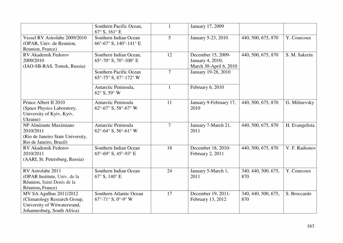
163

Southern Pacific Ocean, 67° S, 161° E

1 January 17, 2009

Vessel RV Astrolabe 2009/2010 (OPAR, Univ. de Reunion, Reunion, France)

Southern Indian Ocean 66°-67° S, 140°-141° E

5 January 5-23, 2010 440, 500, 675, 870 Y. Courcoux

Southern Indian Ocean, 65°-70° S, 70°-100° E

12 December 15, 2009-January 4, 2010; March 30-April 6, 2010

Southern Pacific Ocean 65°-75° S, 87°-172° W

7 January 19-28, 2010

RV Akademik Fedorov 2009/2010 (IAO-SB-RAS, Tomsk, Russia)

Antarctic Peninsula, 62° S, 59° W

1 February 6, 2010

440, 500, 675, 870 S. M. Sakerin

Prince Albert II 2010 (Space Physics Laboratory, University of Kyiv, Kyiv, Ukraine)

Antarctic Peninsula 62°-67° S, 58°-67° W

11 January 9-February 17, 2010

440, 500, 675, 870 G. Milinevsky

NP Almirante Maximiano 2010/2011 (Rio de Janeiro State University, Rio de Janeiro, Brazil)

Antarctic Peninsula 62°-64° S, 56°-61° W

7 January 7-March 21, 2011

440, 500, 675, 870 H. Evangelista

RV Akademik Fedorov 2010/2011 (AARI, St. Petersburg, Russia)

Southern Indian Ocean 65°-69° S, 45°-93° E

18 December 18, 2010-February 2, 2011

440, 500, 675, 870 V. F. Radionov

RV Astrolabe 2011 (OPAR Institute, Univ. de la Réunion, Saint Denis de la Réunion, France)

Southern Indian Ocean 67° S, 140° E

24 January 5-March 1, 2011

340, 440, 500, 675, 870

Y. Courcoux

MV SA Agulhas 2011/2012 (Climatology Research Group, University of Witwatersrand, Johannesburg, South Africa)

Southern Atlantic Ocean 67°-71° S, 0°-9° W

17 December 19, 2011-February 13, 2012

340, 440, 500, 675, 870

S. Broccardo

164

NP Almirante Maximiano 2011/2012 (Rio de Janeiro State University, Rio de Janeiro, Brazil)

Antarctic Peninsula, 61°-62° S, 55°-59° W

6 October 24, 2011-November 14, 2011

440, 500, 675, 870 H. Evangelista

Southern Indian Ocean 66°-69° S, 37°-93° E

19 December 12, 2011-March 21, 2012

Southern Atlantic Ocean 62°-70° S, 18° W-20° E

8 March 22-April 7, 2012

RV Akademik Fedorov 2011/2012 (AARI, St. Petersburg, Russia)

Antarctic Peninsula 62.2° S, 58.9° W

2 April 21 and 22, 2012

440, 500, 675, 870 V. F. Radionov

RV Astrolabe 2012 (OPAR Institute, Univ. de la Réunion, Saint Denis de la Réunion, France)

Southern Indian Ocean 66° 40’ S, 140° E

14 February 20-March 2, 2012

380, 440, 500, 675, 870

Y. Courcoux

RV SA Agulhas II 2012/2013 (Climatology Research Group, University of Witwatersrand, Johannesburg, South Africa)

Southern Atlantic Ocean 70° - 71° S, 1°-8° W

11 December 19, 2012-February 5, 2013

380, 440, 500, 675, 870

S. Broccardo

Southern Indian Ocean 66°-70° S, 46°-93° E

24 December 13, 2012-March 15, 2013

RV Akademik Fedorov 2012/2013 (AARI, St. Petersburg, Russia) Southern Atlantic Ocean

67°-70° S, 10°-12° E 3 March 22-24, 2013

440, 500, 675, 870 V. F. Radionov

RV Akademik Treshnikov 2012/2013 (AARI, St. Petersburg, Russia)

Antarctic Peninsula, 64°-70° S, 57°-72° W

13 February 11-March 5, 2013

440, 500, 675, 870 V. F. Radionov

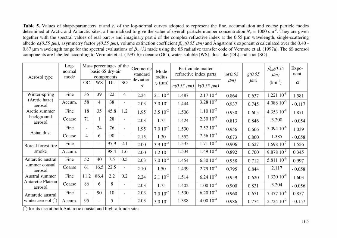
165

Table 5. Values of shape-parameters σ and rc of the log-normal curves adopted to represent the fine, accumulation and coarse particle modes determined at Arctic and Antarctic sites, all normalized to give the value of overall particle number concentration No = 1000 cm-3. They are given together with the spectral values of real part n and imaginary part k of the complex refractive index at the 0.55 µm wavelength, single-scattering albedo ω(0.55 µm), asymmetry factor g(0.55 µm), volume extinction coefficient βext(0.55 µm) and Ångström’s exponent α calculated over the 0.40 - 0.87 µm wavelength range for the spectral evaluations of βext(λ) made using the 6S radiative transfer code of Vermote et al. (1997a). The 6S aerosol components are labelled according to Vermote et al. (1997 b): oceanic (OC), water-soluble (WS), dust-like (DL) and soot (SO).

Mass percentages of the basic 6S dry-air

components

Particulate matter refractive index parts

Aerosol type

Log-normal mode

OC WS DL SO

Geometric standard deviation

σ

Mode radius rc (µm)

n(0.55 µm) k(0.55 µm)

ω(0.55

µm) g(0.55

µm)

βext(0.55

µm)

(km-1)

Expo-nent

α

Fine 35 39 22 4 2.24 2.1 10-2 1.487 2.17 10-2 0.864 0.637 1.221 10-8 1.581 Winter-spring (Arctic haze)

aerosol Accum. 58 4 38 - 2.03 3.0 10-1 1.444 3.28 10-3

0.937 0.745 4.088 10-3 - 0.117

Fine 18 35 45.8 1.2 1.95 3.5 10-2 1.506 1.10 10-2 0.930 0.605 4.353 10-8

1.871 Arctic summer background

aerosol Coarse 71 1 28 - 2.03 1.75 1.424 2.30 10-3

0.813 0.846 3.200 - 0.054

Fine - 24 76 - 1.95 7.0 10-2 1.530 7.52 10-3 0.956 0.666 5.094 10-6 1.039 Asian dust

Coarse 4 6 90 - 2.15 1.30 1.552 7.56 10-3 0.673 0.860 1.385 - 0.058 Fine - - 97.9 2.1 2.00 3.9 10-2 1.535 1.71 10-2 0.906 0.627 1.698 10-7 1.556 Boreal forest fire

smoke Accum. - - 98.4 1.6 2.00 1.2 10-1 1.534 1.49 10-2 0.892 0.700 9.878 10-5 0.345

Fine 52 40 7.5 0.5 2.03 7.0 10-2 1.454 6.30 10-3 0.958 0.712 5.811 10-6 0.997 Antarctic austral

summer coastal aerosol

Coarse 61 16.5 22.5 - 2.10 1.50 1.439 2.79 10-3 0.795 0.844 2.117 - 0.058

Fine 11.2 86.4 2.2 0.2 2.24 2.1 10-2 1.514 6.24 10-3 0.959 0.620 1.320 10-8 1.603 Austral summer

Antarctic Plateau aerosol

Coarse 86 6 8 - 2.03 1.75 1.402 1.00 10-3 0.900 0.831 3.204 - 0.056

Fine - 90 10 - 2.03 7.0 10-2 1.530 6.20 10-3 0.960 0.671 7.477 10-6 0.857 Antarctic austral winter aerosol (*) Accum. 95 - 5 - 2.03 5.0 10-1 1.388 4.00 10-4 0.986 0.774 2.724 10-2 - 0.157

(*) for its use at both Antarctic coastal and high-altitude sites.

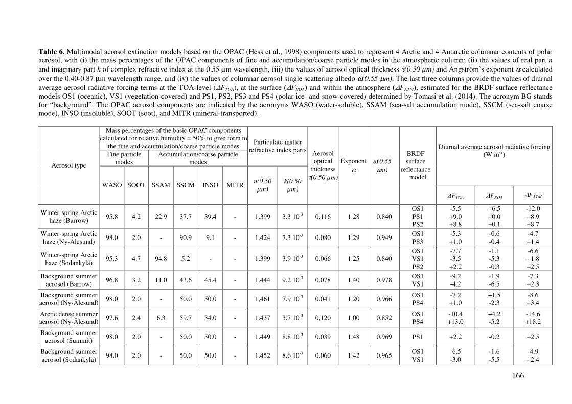
166

Table 6. Multimodal aerosol extinction models based on the OPAC (Hess et al., 1998) components used to represent 4 Arctic and 4 Antarctic columnar contents of polar aerosol, with (i) the mass percentages of the OPAC components of fine and accumulation/coarse particle modes in the atmospheric column; (ii) the values of real part n and imaginary part k of complex refractive index at the 0.55 µm wavelength, (iii) the values of aerosol optical thickness τ(0.50 µm) and Ångström’s exponent α calculated over the 0.40-0.87 µm wavelength range, and (iv) the values of columnar aerosol single scattering albedo ω(0.55 µm). The last three columns provide the values of diurnal average aerosol radiative forcing terms at the TOA-level (∆FTOA), at the surface (∆FBOA) and within the atmosphere (∆FATM), estimated for the BRDF surface reflectance models OS1 (oceanic), VS1 (vegetation-covered) and PS1, PS2, PS3 and PS4 (polar ice- and snow-covered) determined by Tomasi et al. (2014). The acronym BG stands for “background”. The OPAC aerosol components are indicated by the acronyms WASO (water-soluble), SSAM (sea-salt accumulation mode), SSCM (sea-salt coarse mode), INSO (insoluble), SOOT (soot), and MITR (mineral-transported).

Mass percentages of the basic OPAC components calculated for relative humidity = 50% to give form to

the fine and accumulation/coarse particle modes Fine particle

modes Accumulation/coarse particle

modes

Particulate matter refractive index parts Diurnal average aerosol radiative forcing

(W m-2)

Aerosol type

WASO SOOT SSAM SSCM INSO MITR n(0.50

µm)

k(0.50

µm)

Aerosol optical

thickness τ(0.50 µm)

Exponent α

ω(0.55

µm)

BRDF surface

reflectance model

∆FTOA ∆FBOA ∆FATM

Winter-spring Arctic haze (Barrow) 95.8 4.2 22.9 37.7 39.4 - 1.399 3.3 10-3 0.116 1.28 0.840

OS1 PS1 PS2

-5.5 +9.0 +8.8

+6.5 +0.0 +0.1

-12.0 +8.9 +8.7

Winter-spring Arctic haze (Ny-Ålesund)

98.0 2.0 - 90.9 9.1 - 1.424 7.3 10-3 0.080 1.29 0.949 OS1 PS3

-5.3 +1.0

-0.6 -0.4

-4.7 +1.4

Winter-spring Arctic haze (Sodankylä)

95.3 4.7 94.8 5.2 - - 1.399 3.9 10-3 0.066 1.25 0.840 OS1 VS1 PS2

-7.7 -3.5 +2.2

-1.1 -5.3 -0.3

-6.6 +1.8 +2.5

Background summer aerosol (Barrow)

96.8 3.2 11.0 43.6 45.4 - 1.444 9.2 10-3 0.078 1.40 0.978 OS1 VS1

-9.2 -4.2

-1.9 -6.5

-7.3 +2.3

Background summer aerosol (Ny-Ålesund)

98.0 2.0 - 50.0 50.0 - 1,461 7.9 10-3 0.041 1.20 0.966 OS1 PS4

-7.2 +1.0

+1.5 -2.3

-8.6 +3.4

Arctic dense summer aerosol (Ny-Ålesund)

97.6 2.4 6.3 59.7 34.0 - 1.437 3.7 10-3 0,120 1.00 0.852 OS1 PS4

-10.4 +13.0

+4.2 -5.2

-14.6 +18.2

Background summer aerosol (Summit) 98.0 2.0 - 50.0 50.0 - 1.449 8.8 10-3 0.039 1.48 0.969 PS1 +2.2 -0.2 +2.5

Background summer aerosol (Sodankylä)

98.0 2.0 - 50.0 50.0 - 1.452 8.6 10-3 0.060 1.42 0.965 OS1 VS1

-6.5 -3.0

-1.6 -5.5

-4.9 +2.4

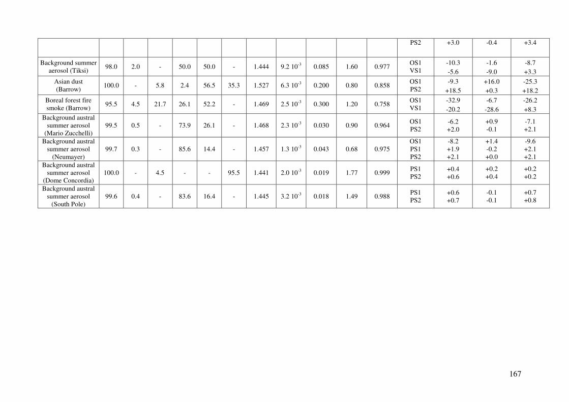
167

PS2 +3.0 -0.4 +3.4

Background summer aerosol (Tiksi)

98.0 2.0 - 50.0 50.0 - 1.444 9.2 10-3 0.085 1.60 0.977 OS1 VS1

-10.3 -5.6

-1.6 -9.0

-8.7 +3.3

Asian dust (Barrow)

100.0 - 5.8 2.4 56.5 35.3 1.527 6.3 10-3 0.200 0.80 0.858 OS1 PS2

-9.3 +18.5

+16.0 +0.3

-25.3 +18.2

Boreal forest fire smoke (Barrow)

95.5 4.5 21.7 26.1 52.2 - 1.469 2.5 10-3 0.300 1.20 0.758 OS1 VS1

-32.9 -20.2

-6.7 -28.6

-26.2 +8.3

Background austral summer aerosol

(Mario Zucchelli) 99.5 0.5 - 73.9 26.1 - 1.468 2.3 10-3 0.030 0.90 0.964

OS1 PS2

-6.2 +2.0

+0.9 -0.1

-7.1 +2.1

Background austral summer aerosol

(Neumayer) 99.7 0.3 - 85.6 14.4 - 1.457 1.3 10-3 0.043 0.68 0.975

OS1 PS1 PS2

-8.2 +1.9 +2.1

+1.4 -0.2 +0.0

-9.6 +2.1 +2.1

Background austral summer aerosol

(Dome Concordia) 100.0 - 4.5 - - 95.5 1.441 2.0 10-3 0.019 1.77 0.999

PS1 PS2

+0.4 +0.6

+0.2 +0.4

+0.2 +0.2

Background austral summer aerosol

(South Pole) 99.6 0.4 - 83.6 16.4 - 1.445 3.2 10-3 0.018 1.49 0.988

PS1 PS2

+0.6 +0.7

-0.1 -0.1

+0.7 +0.8

168

1